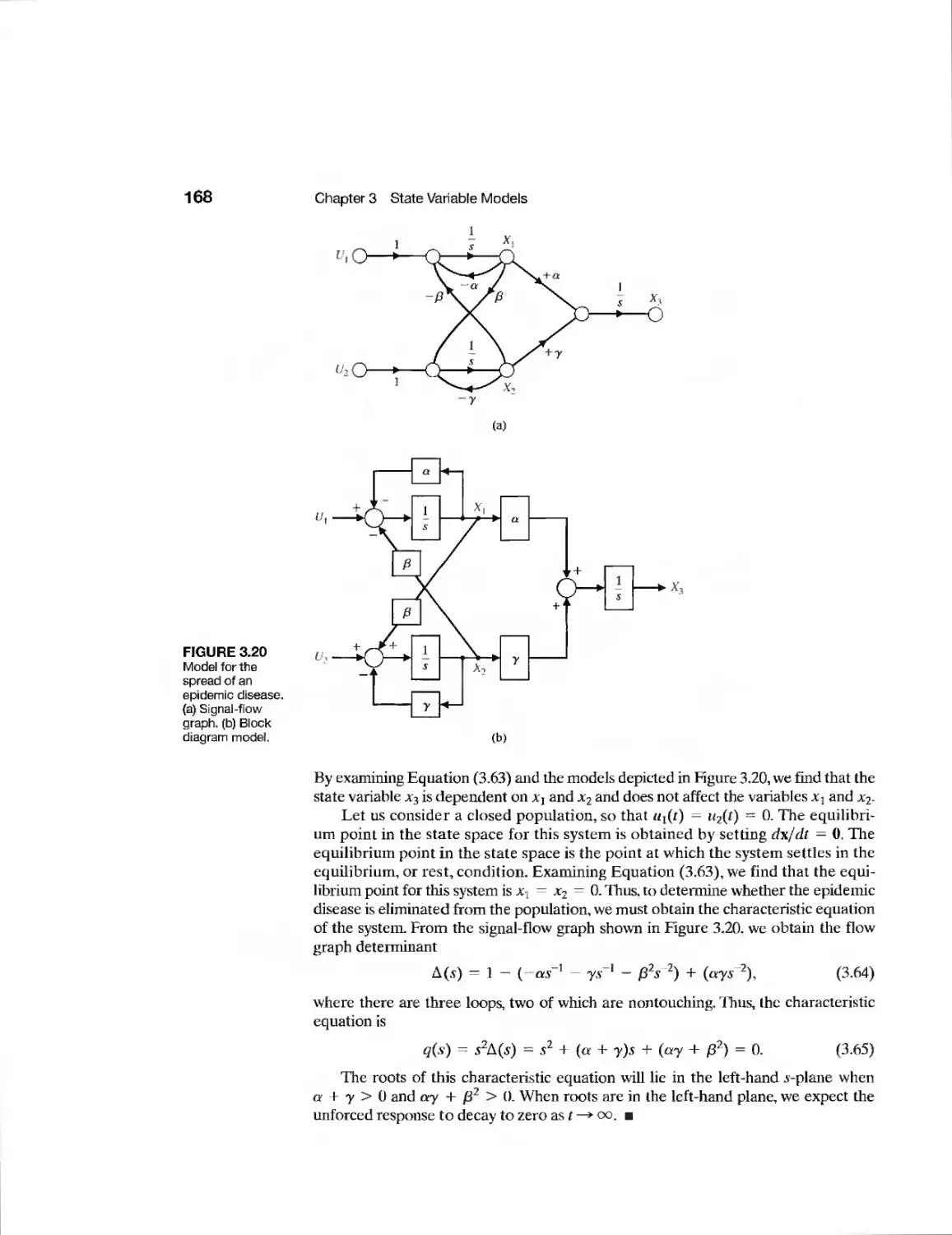
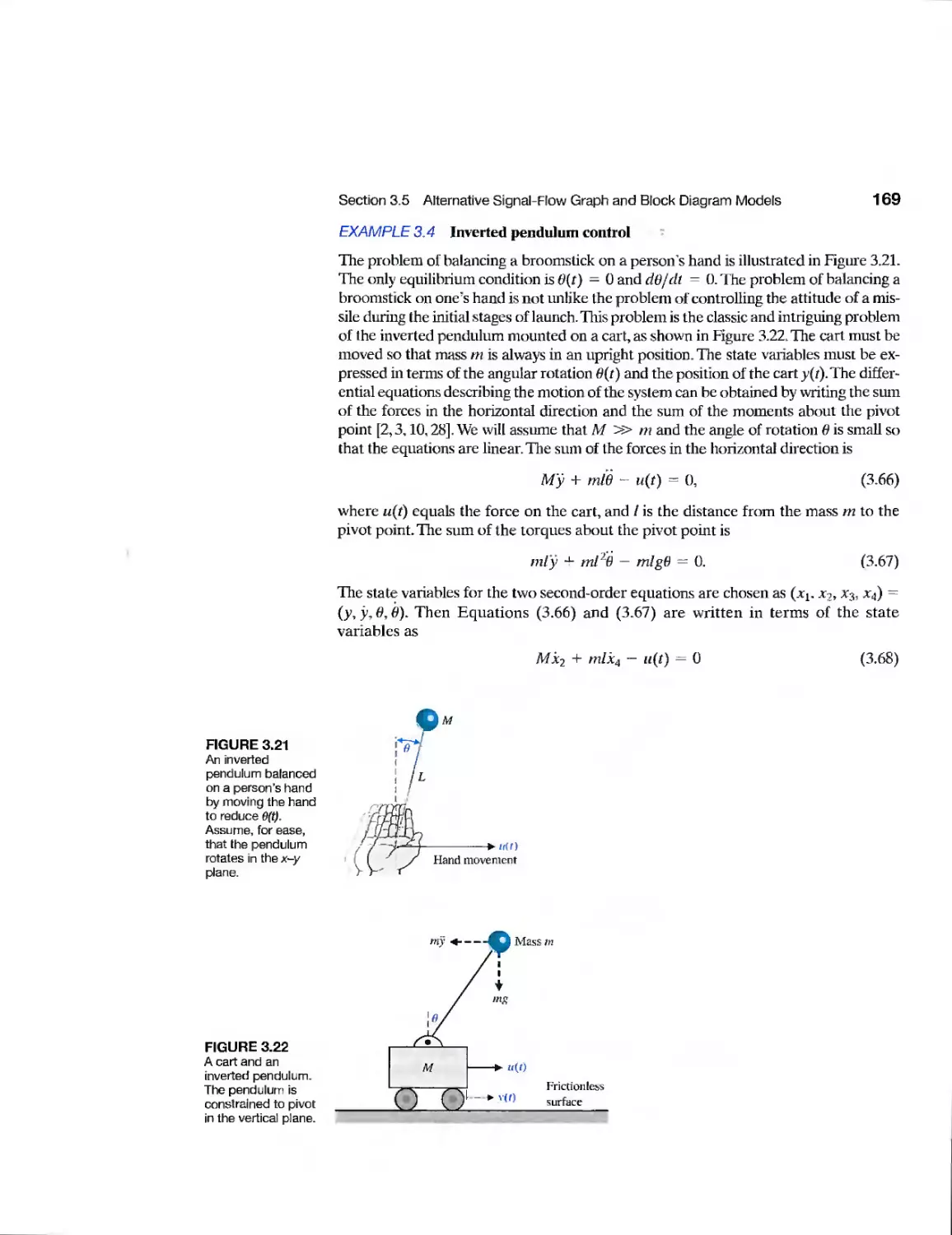
/


Текст
I .
r i ■r . ii ii ii
ELEVEN EHTION
*
% •
Oi-m - ntrol y$te' s^_\
•
Richard C. »• ■•bert H. Bishop
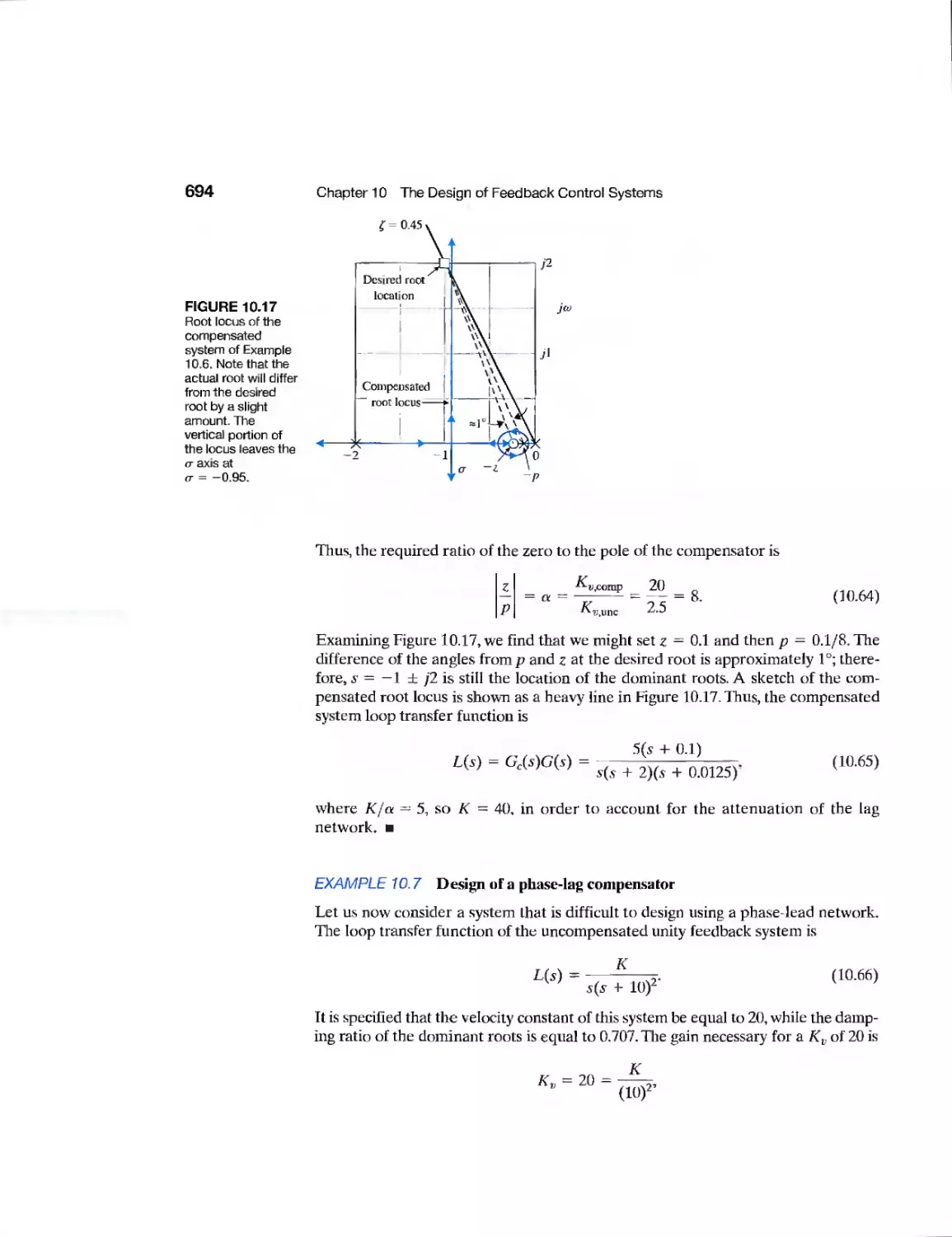
Design Examples and Design Problems (DP)
CHAPTER 1 PAGE
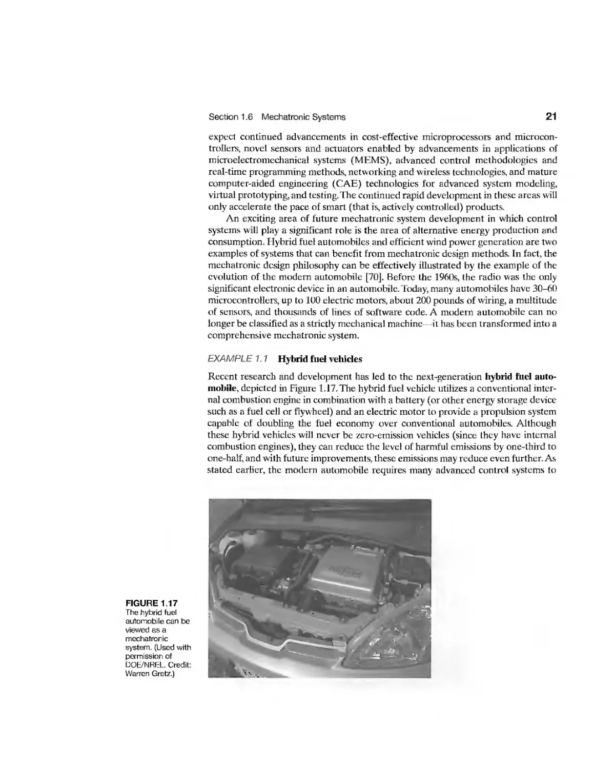
Example Hybrid Fuel Vehicles 21
Example Wind Power 22
Example Embedded Computers 23
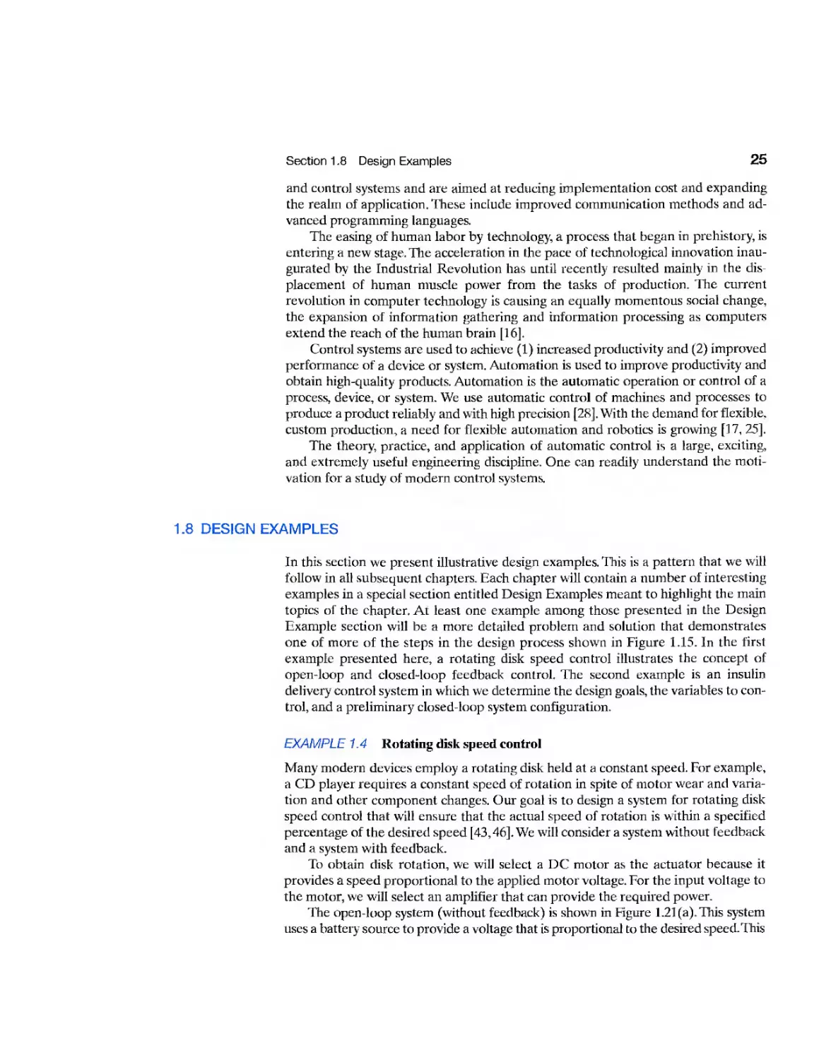
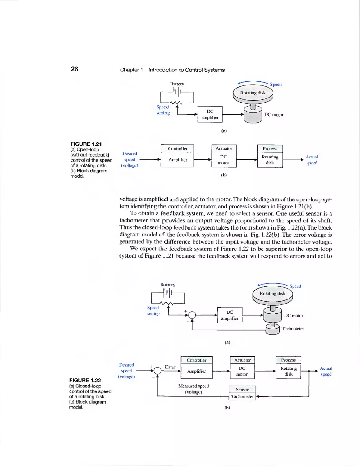
Example Rotating Disk Speed Control 25
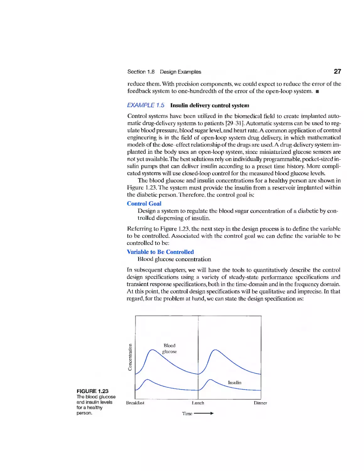
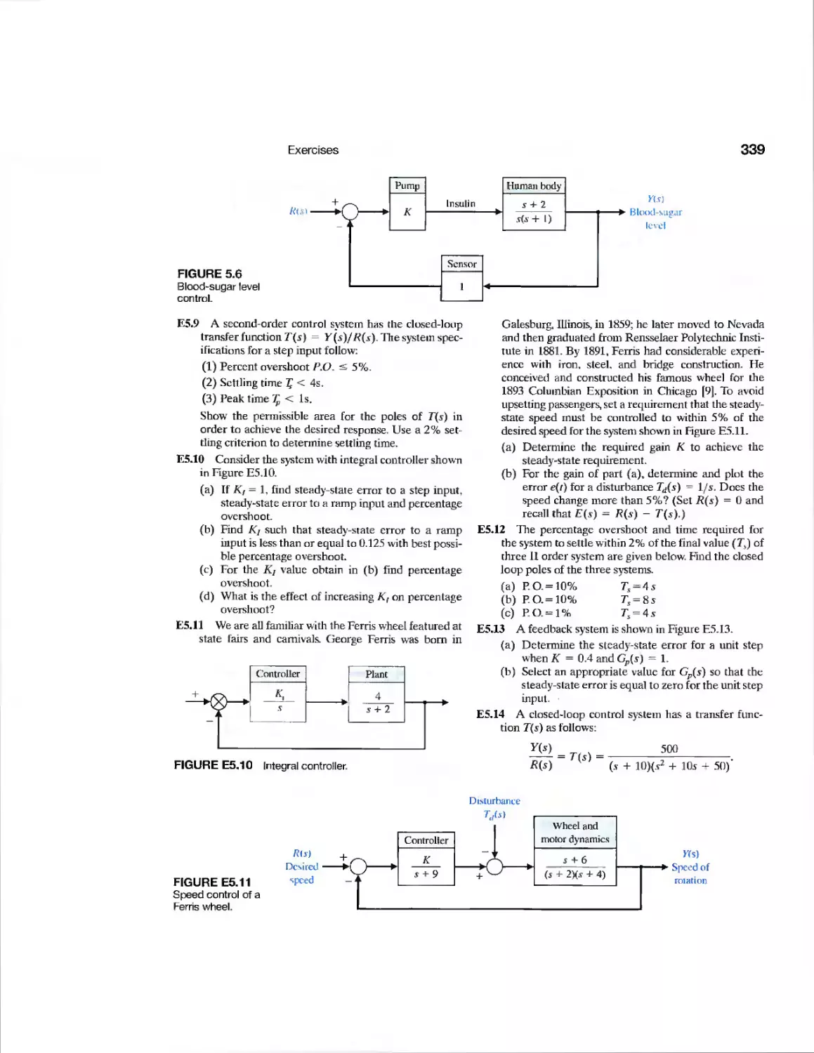
Example Insulin Delivery Control System 27
Example Disk Drive Read System 28
CDP1.1 Traction Drive Motor Control 38
DP1.1 Automobile Noise Control 38
DPI.2 Automobile Cruise Control 38
DPI.3 Dairy Farm Automation 38
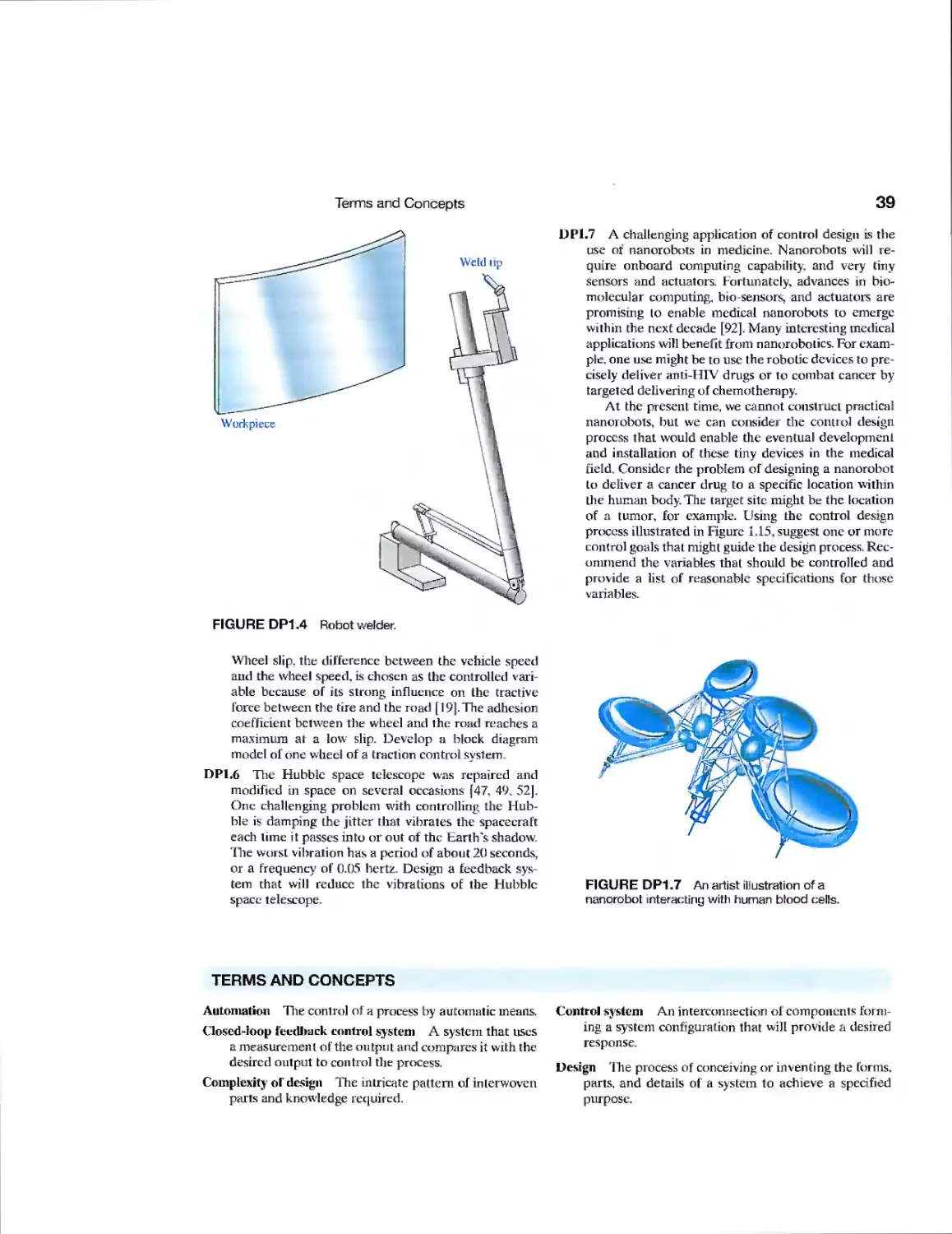
DPI.4 Welder Control 38
DPI .5 Automobile Traction Control 38
DP1.6 Hubble Telescope Vibration 39
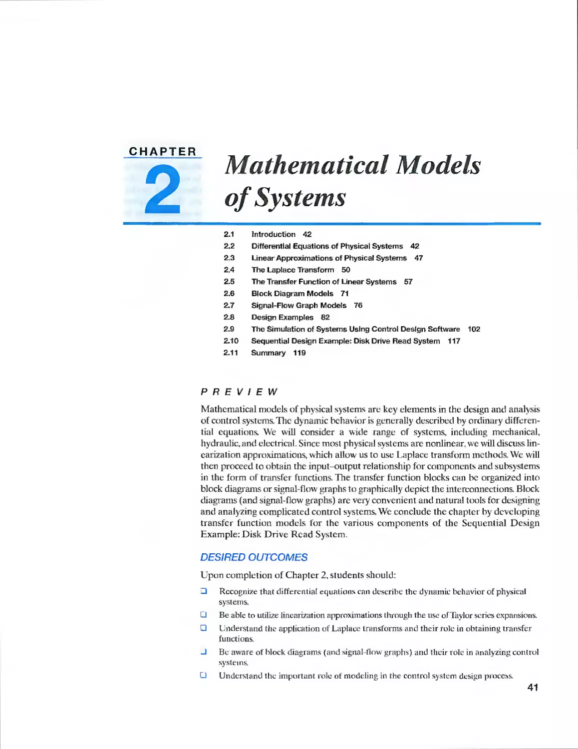
DPI.7 Nanorobotics in Medicine 39
CHAPTER 2
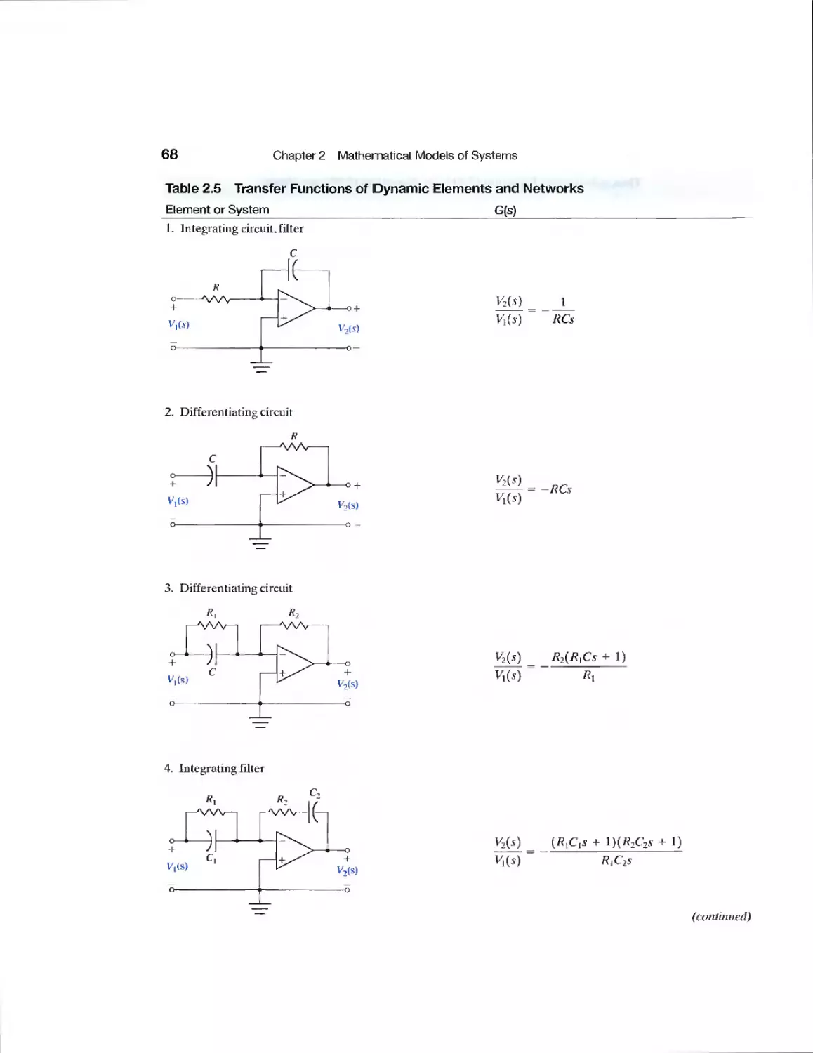
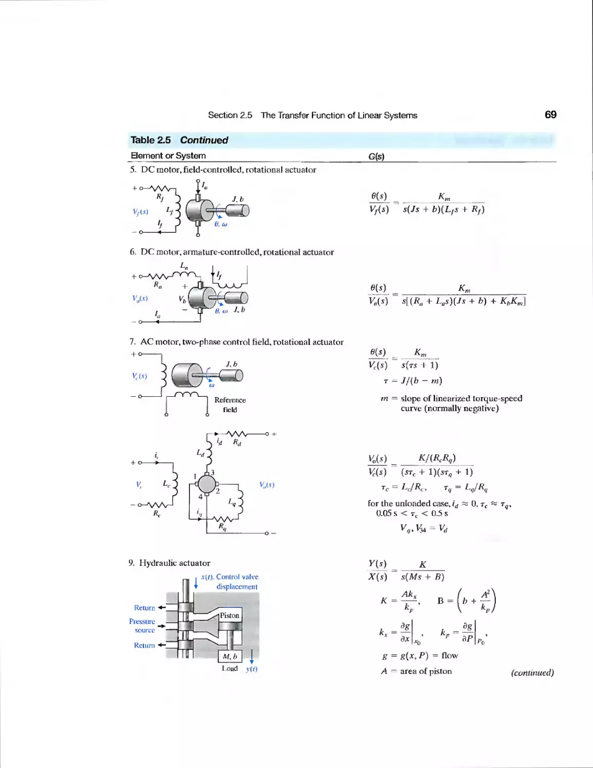
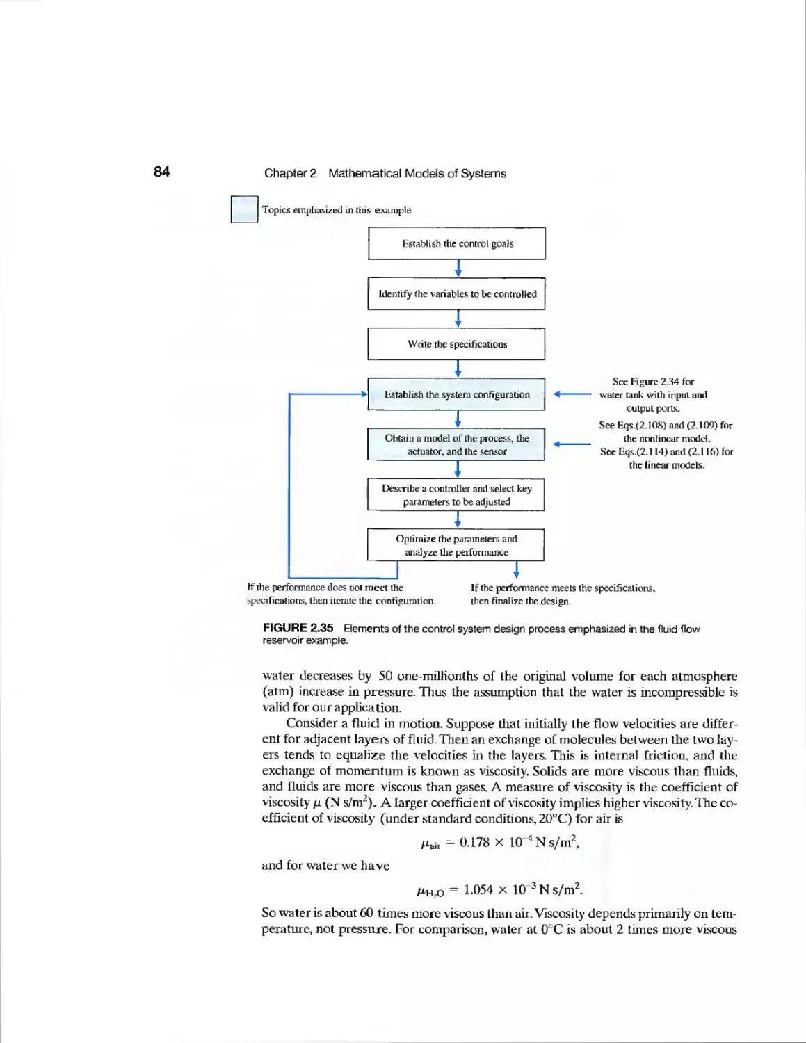
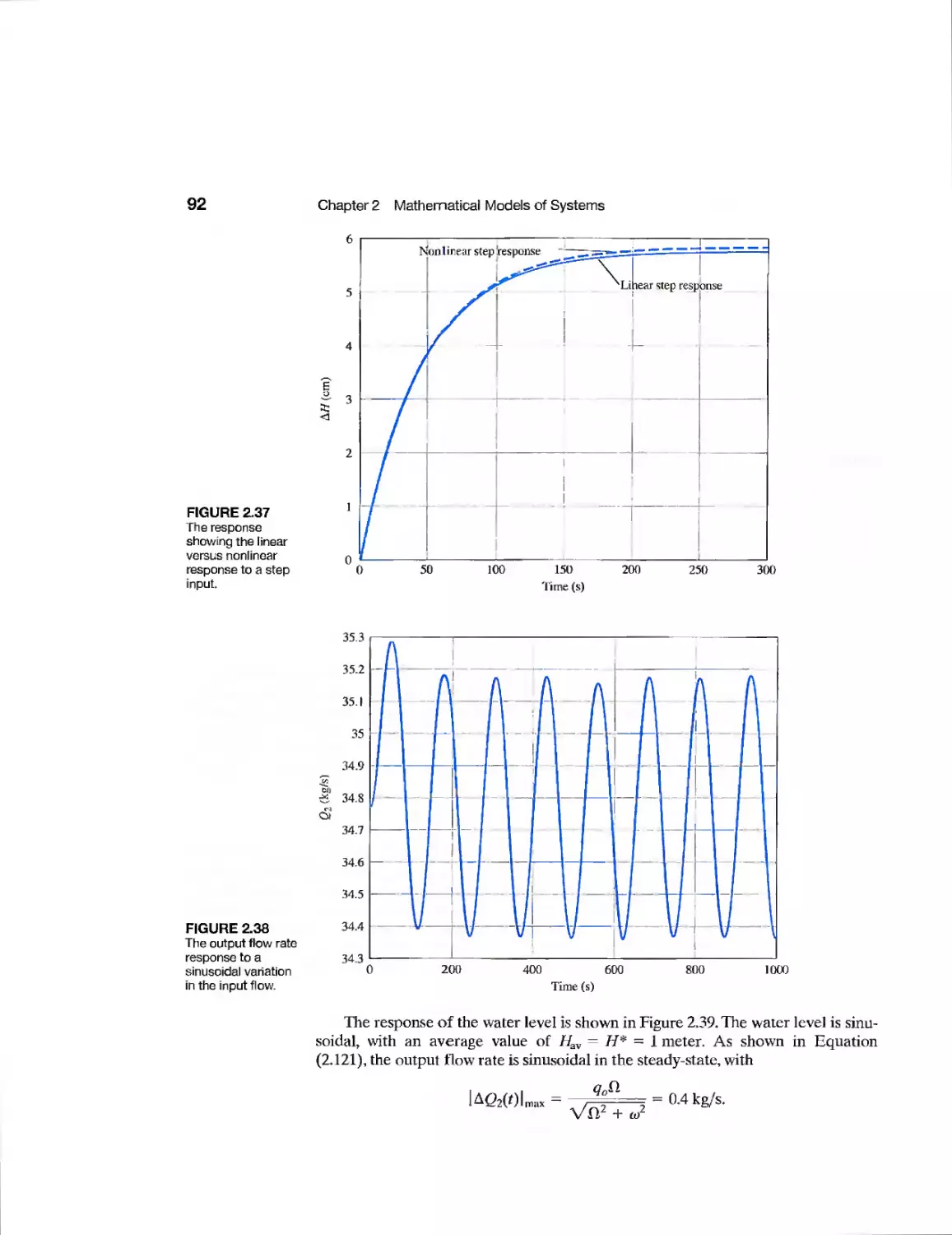
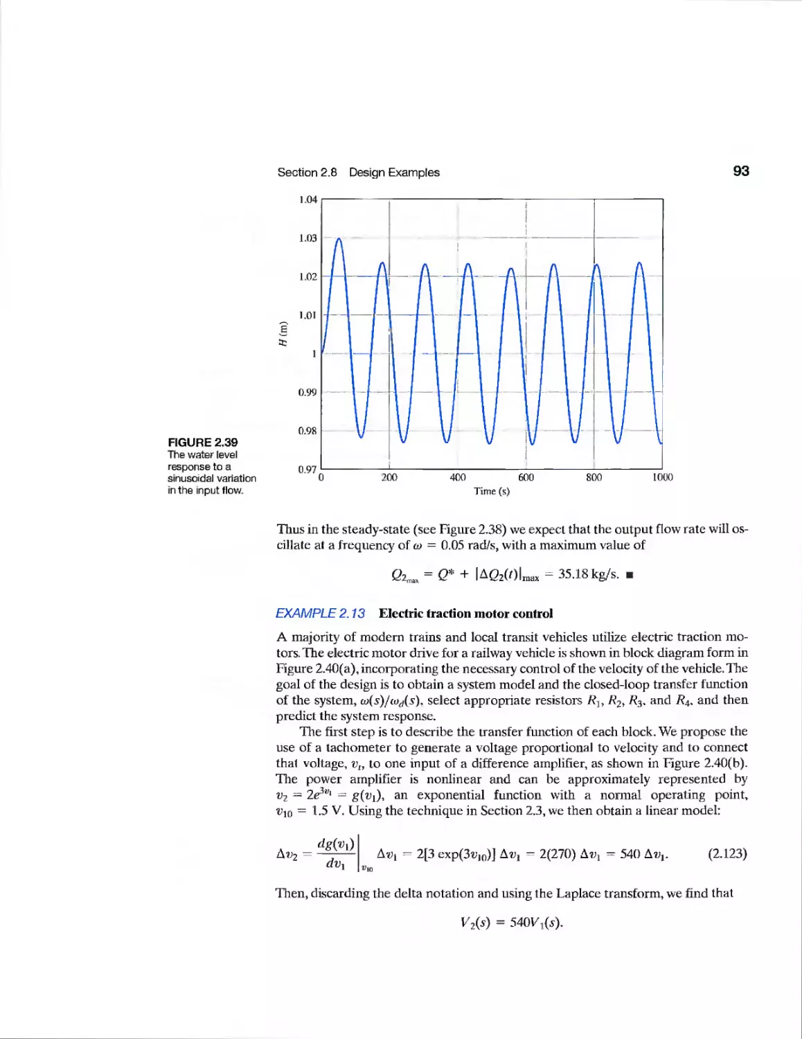
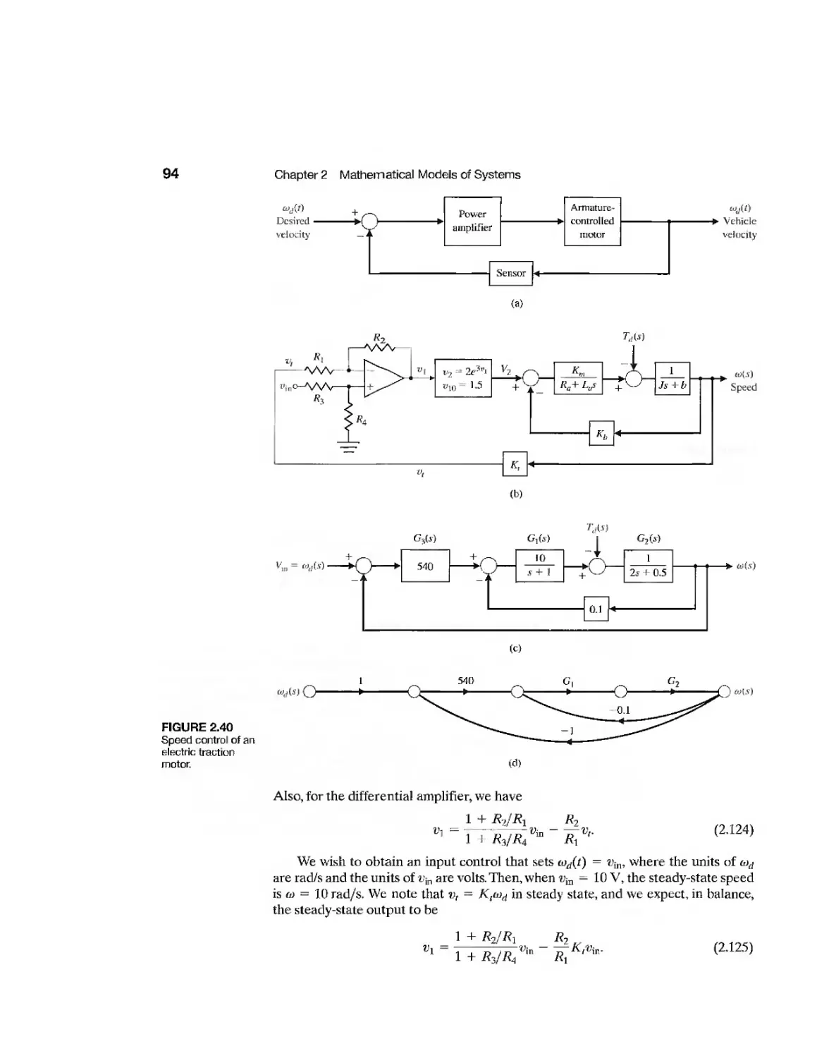
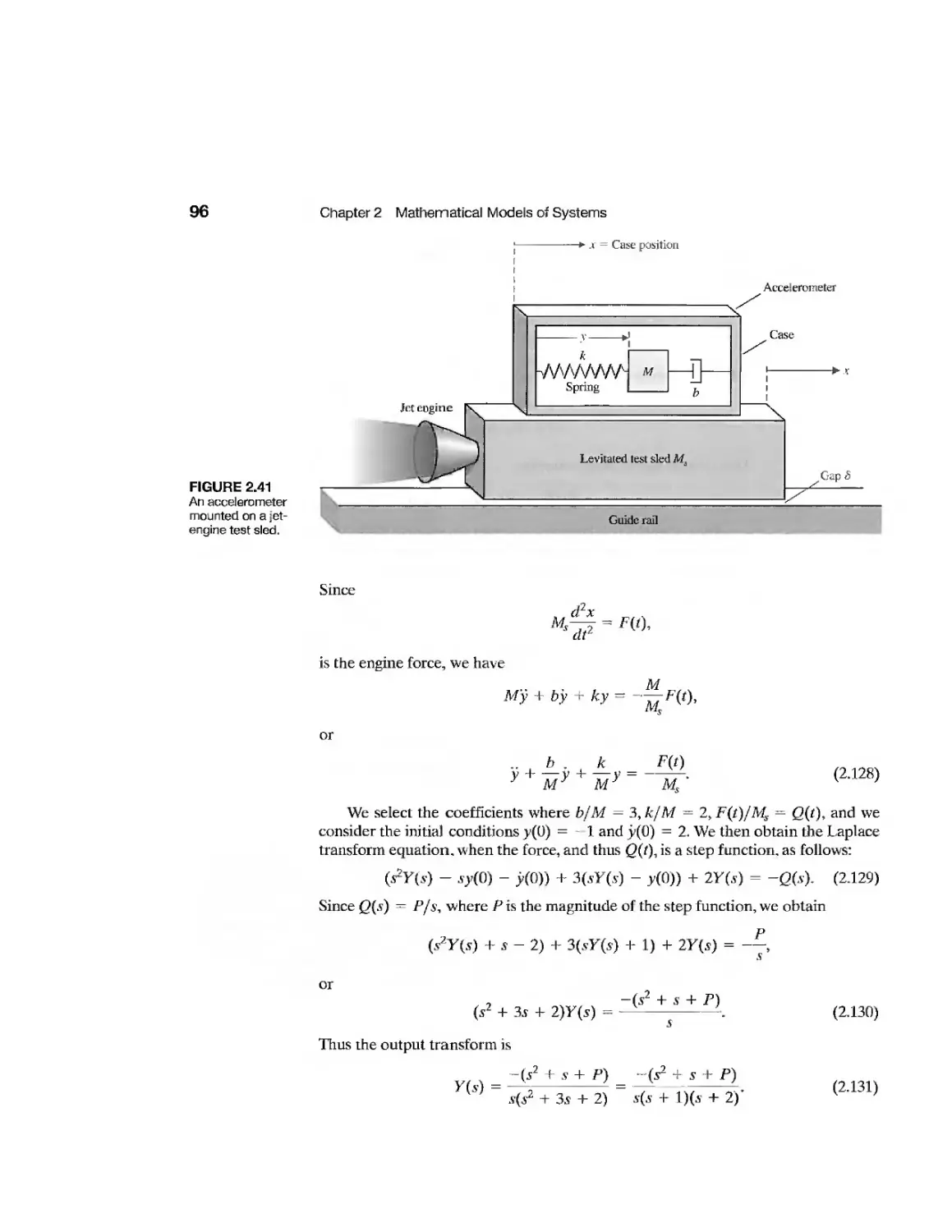
Example Fluid Flow Modeling 83
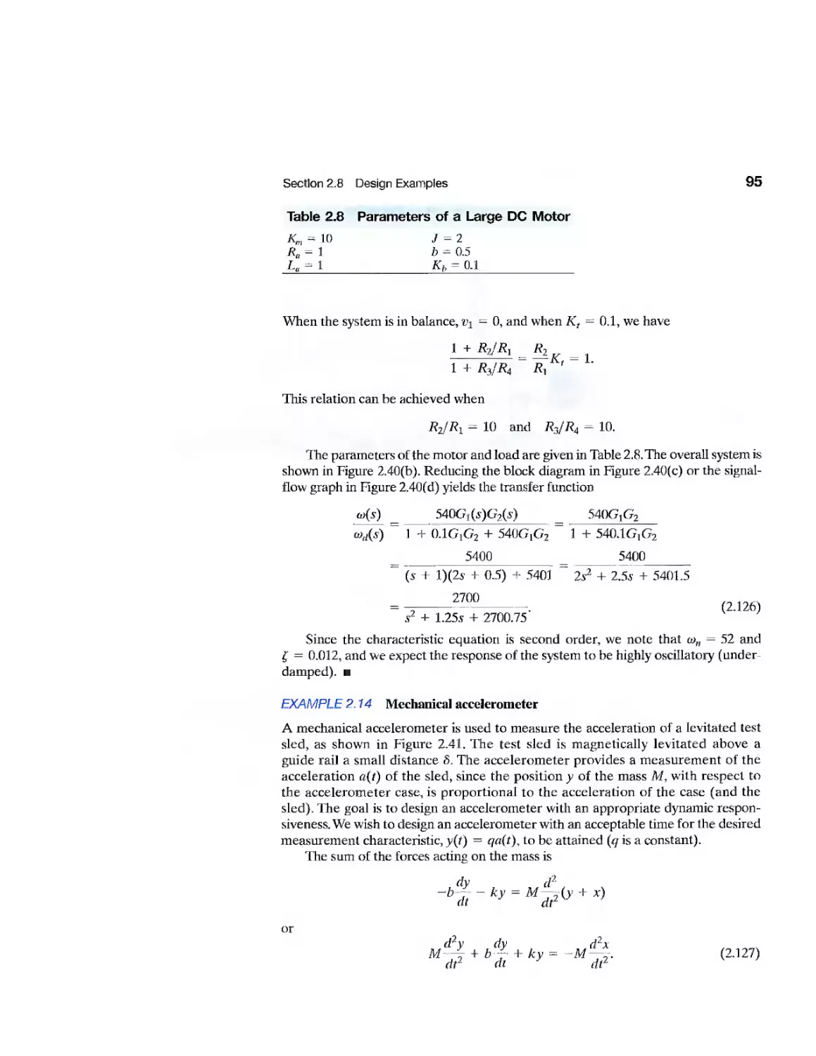
Example Electric Traction Motor Control 93
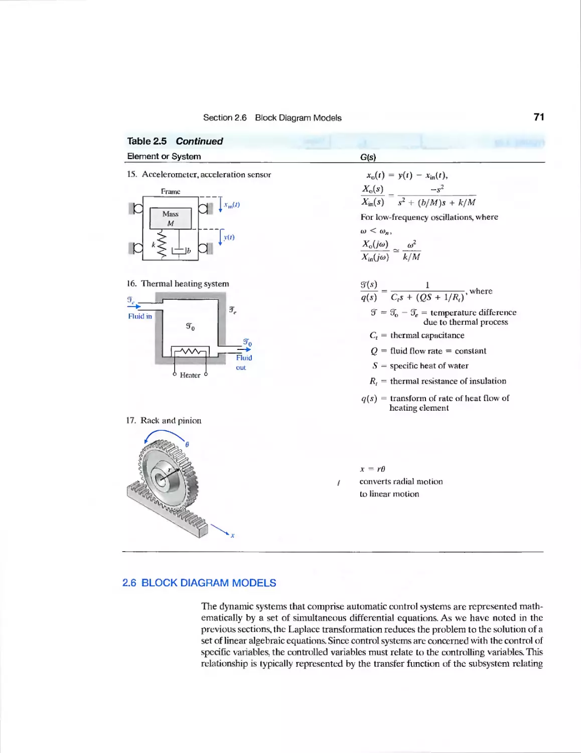
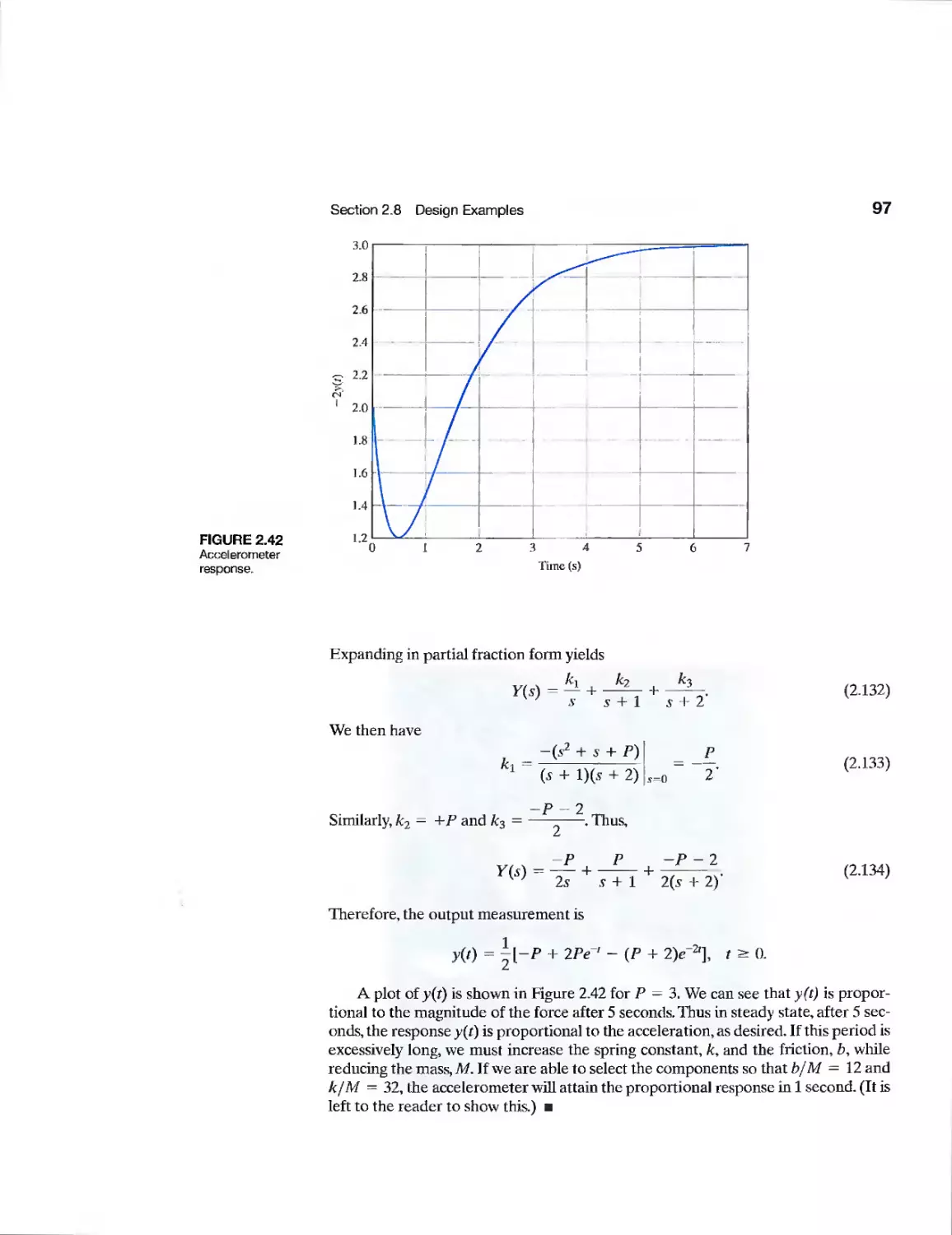
Example Mechanical Accelerometer 95
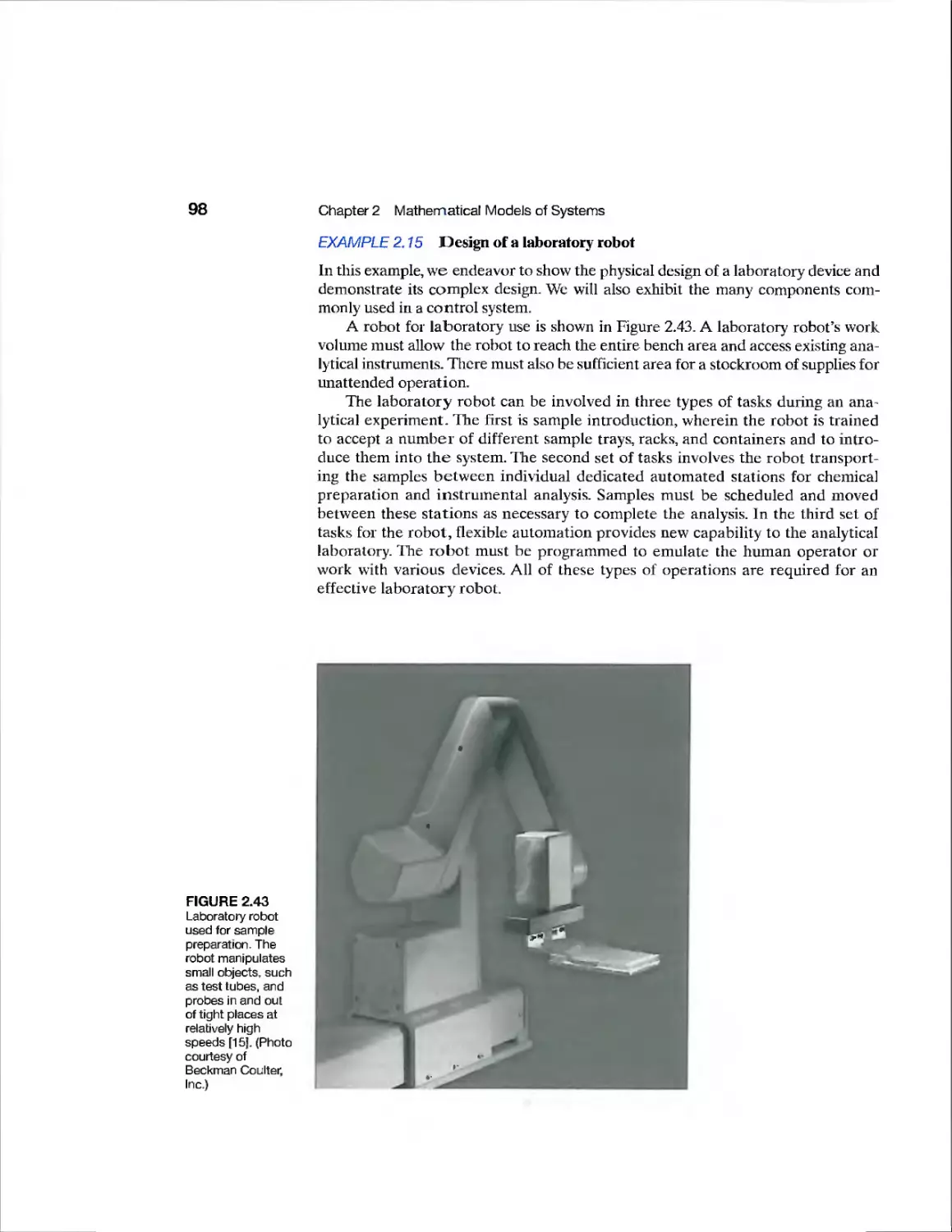
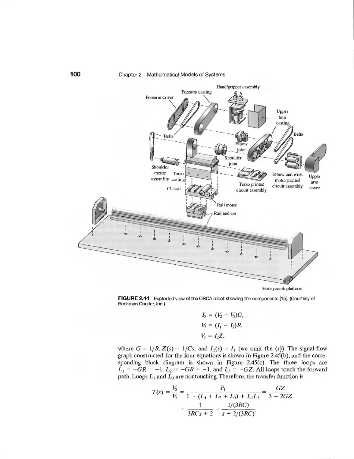
Example Laboratory Robot 98
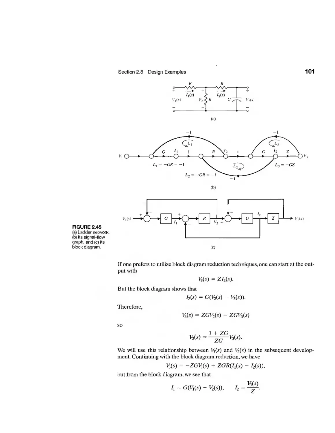
Example Low-Pass Filter 99
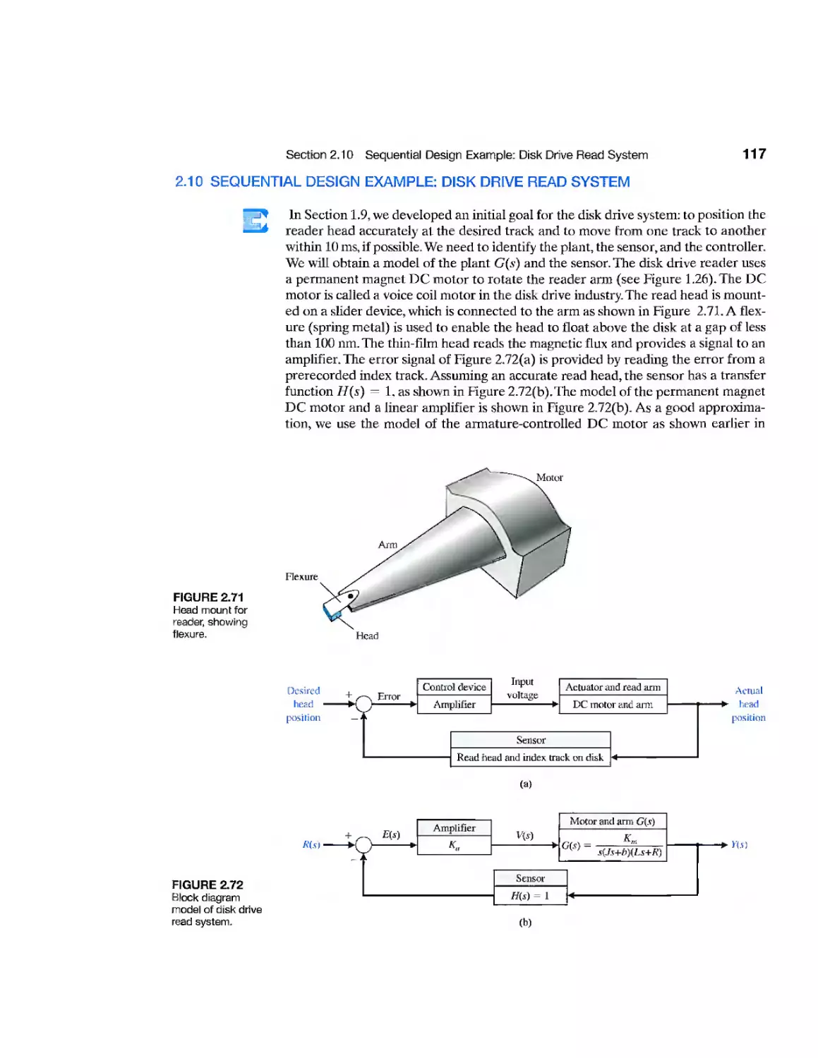
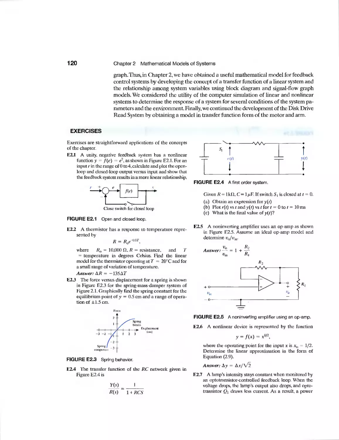
Example Disk Drive Read System 117
CDP2.1 Traction Drive Motor Control 139
DP2.1 Selection of Transfer Functions 139
DP2.2 Television Beam Circuit 139
DP2.3 Transfer Function Determination 139
DP2.4 Op Amp Differentiating Circuit 139
CHAPTER 3
Example Modeling the Orientation of a
Space Station 176
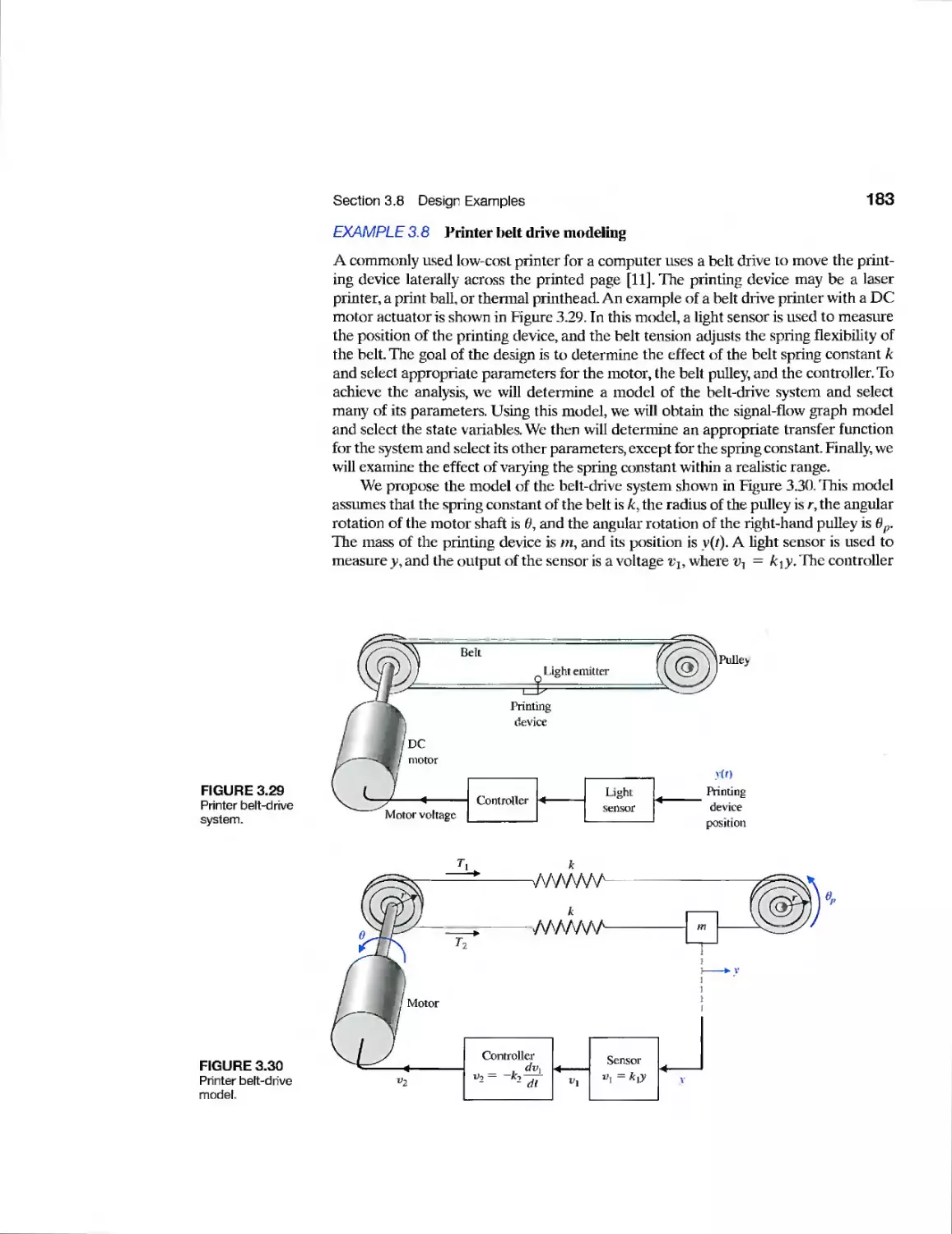
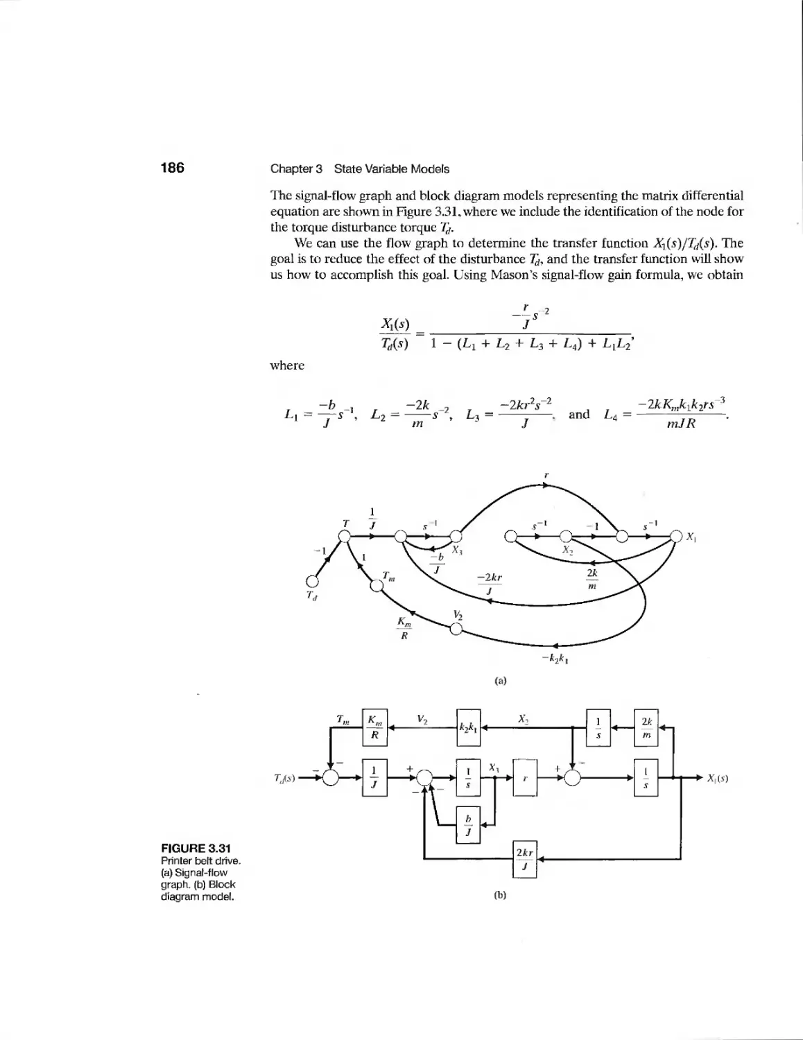
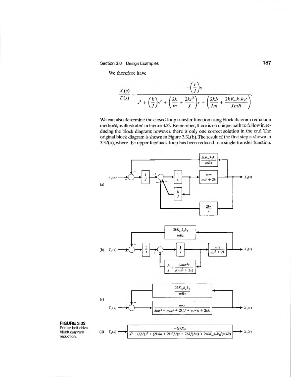
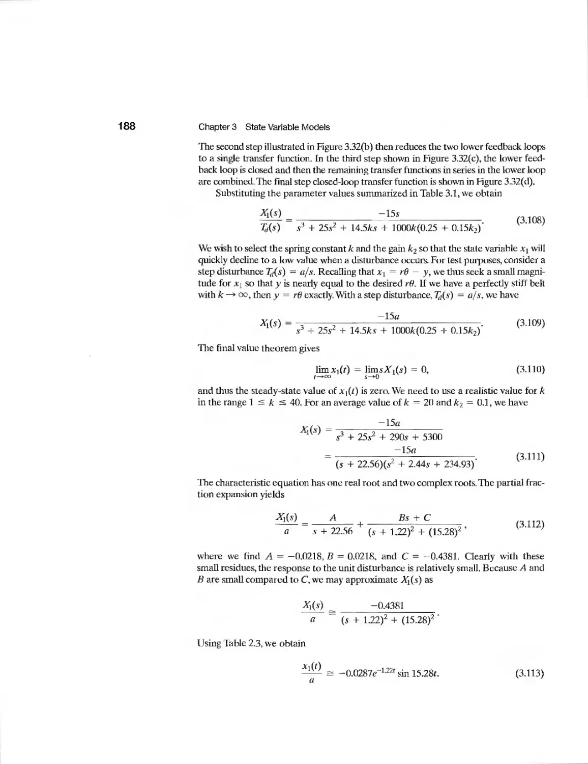
Example Printer Belt Drive 183
Example Disk Drive Read System 192
CDP3.1 Traction Drive Motor Control 208
DP3.I Shock Absorber for Motorcycle 208
DP3.2 Diagonal Matrix Differential
Equation 209
DP3.3 Aircraft Arresting Gear 209
DP3.4 Bungi Jumping System 209
DP3.5 State Variable Feedback 209
CHAPTER 4
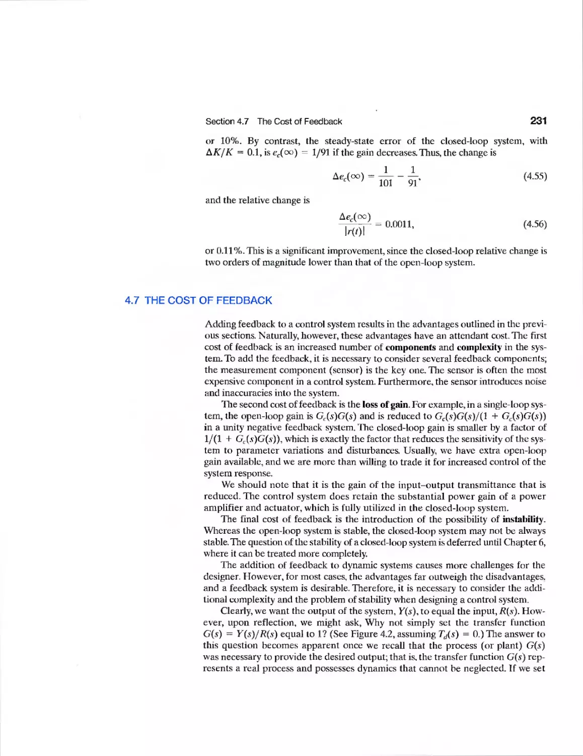
Example English Channel Boring
Machines 232
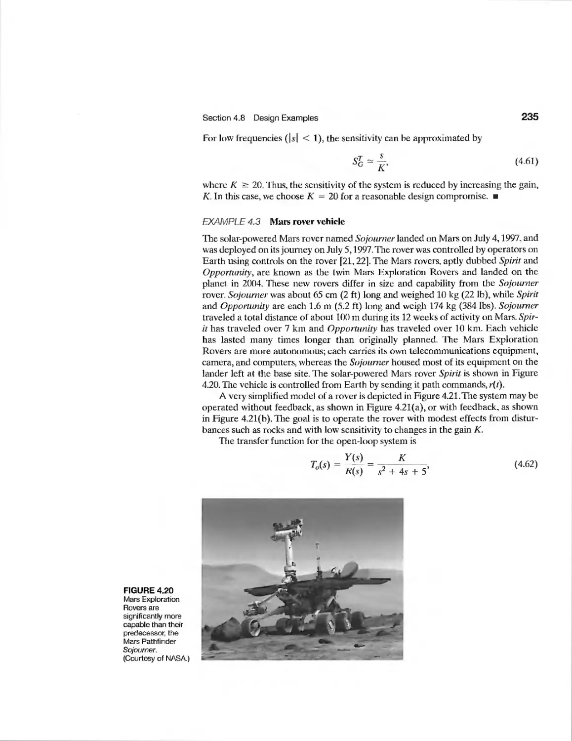
Example Mars Rover Vehicle 235
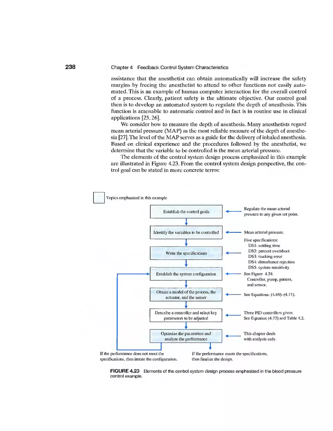
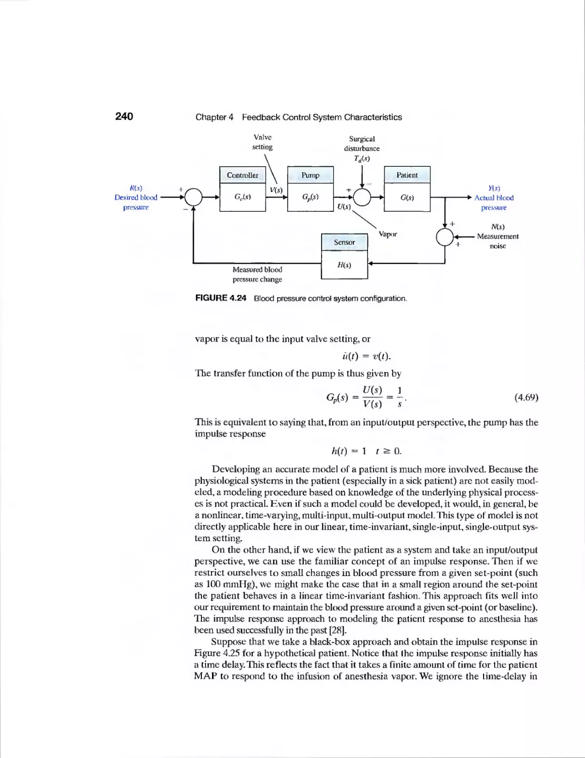
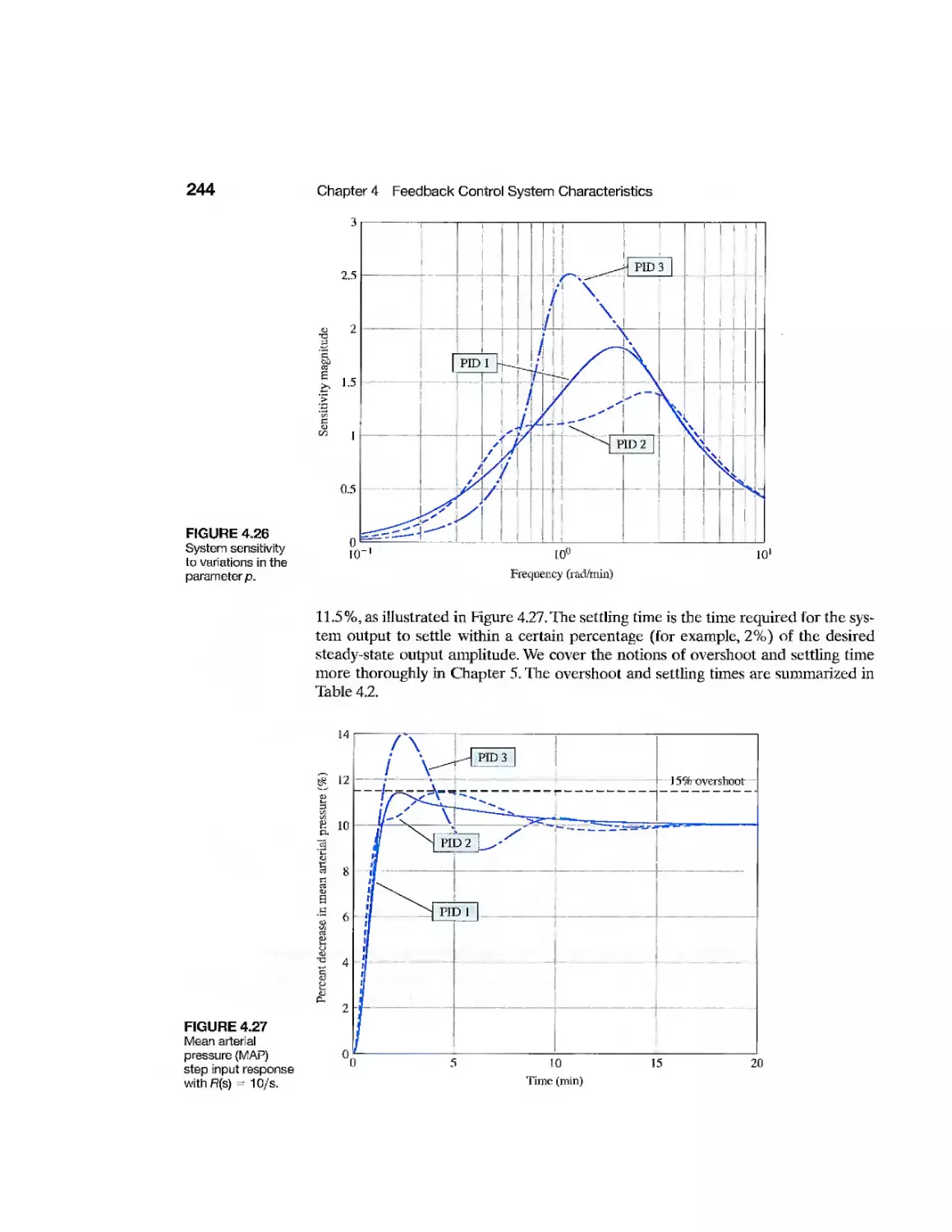
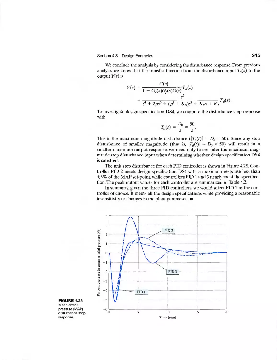
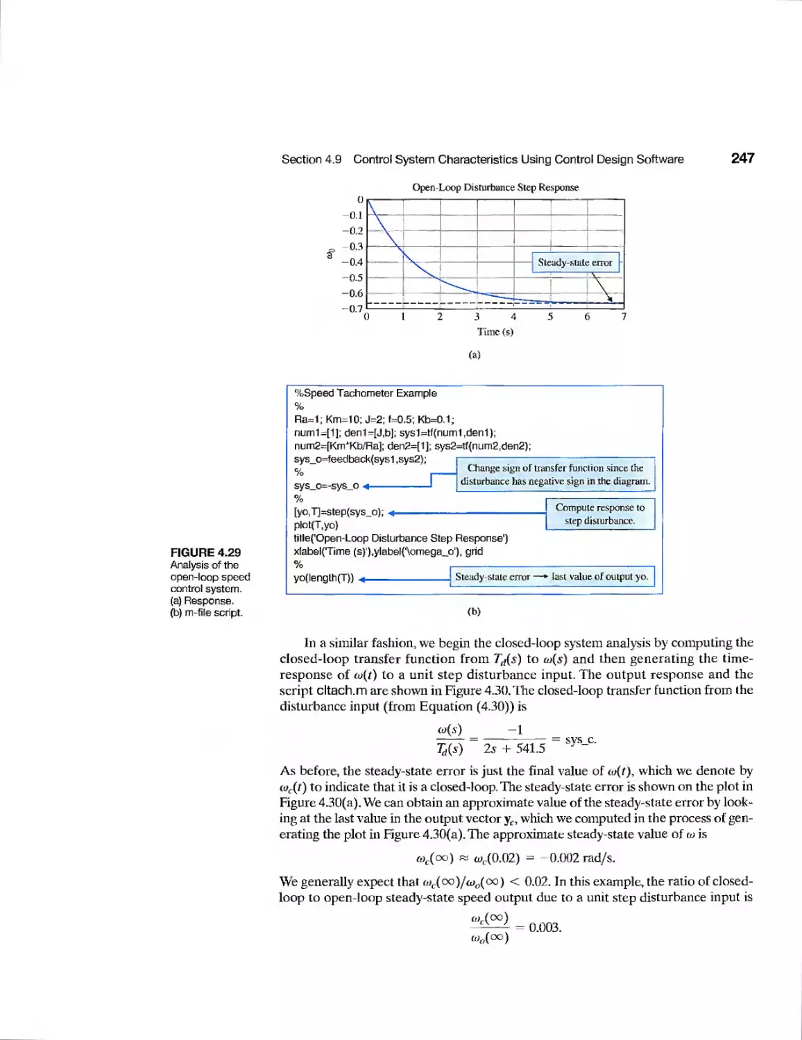
Example Blood Pressure Control 237
Example Disk Drive Read System 251
CDP4.1 Traction Drive Motor Control 270
DP4.1 Speed Control System 270
DP4.2 Airplane Roll Angle Control 271
DP4.3 Velocity Control System 271
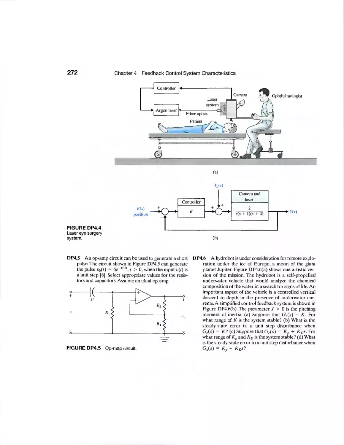
DP4.4 Laser Eye Surgery 271
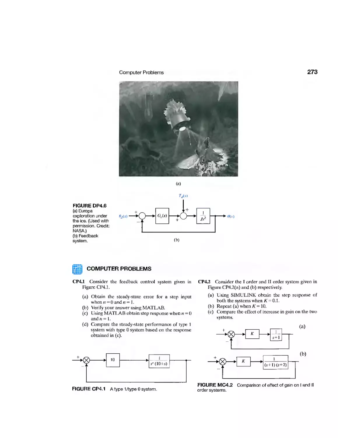
DP4.5 Pulse Generating Op Amp 272
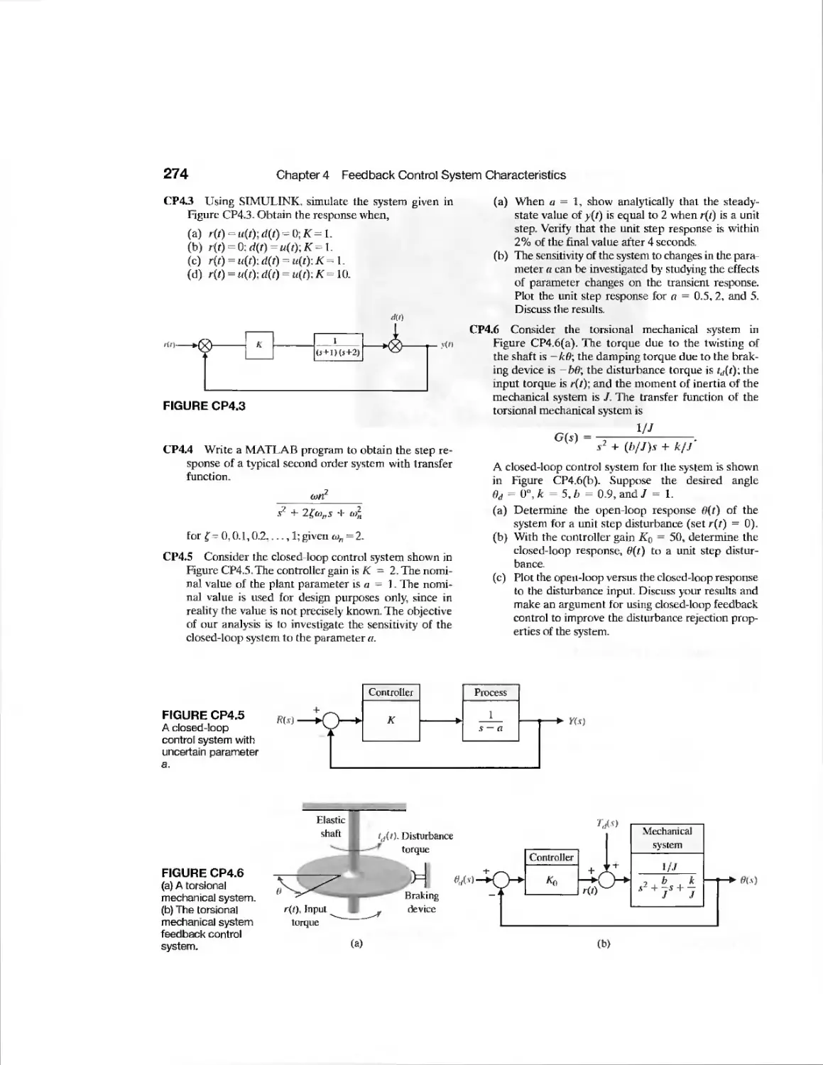
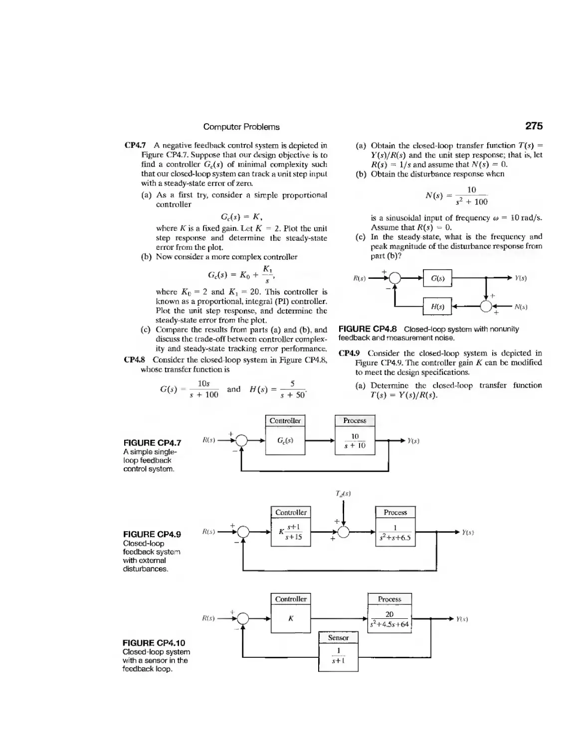
DP4.6 Hydrobot 272
CHAPTER 5
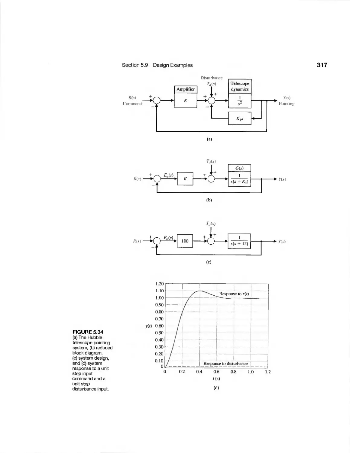
Example Hubble Telescope Pointing 316
Example Attitude Control of an Airplane 319
Example Disk Drive Read System 333
CDP5.1 Traction Drive Motor Control 349
DP5.1 Jet Fighter Roll Angle Control 349
DP5.2 Welding Arm Position Control 349
DP5.3 Automobile Active Suspension 349
DP5.4 Satellite Orientation Control 350
DP5.5 Deburring Robot for Machined
Parts 350
DP5.6 DC Motor Position Control 351
CHAPTER 6
Example Tracked Vehicle Turning 373
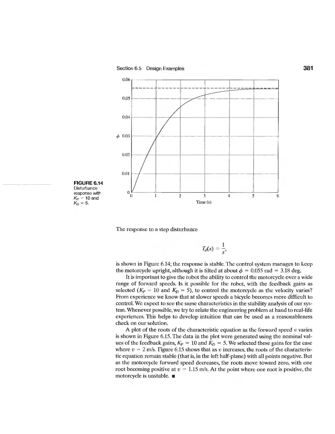
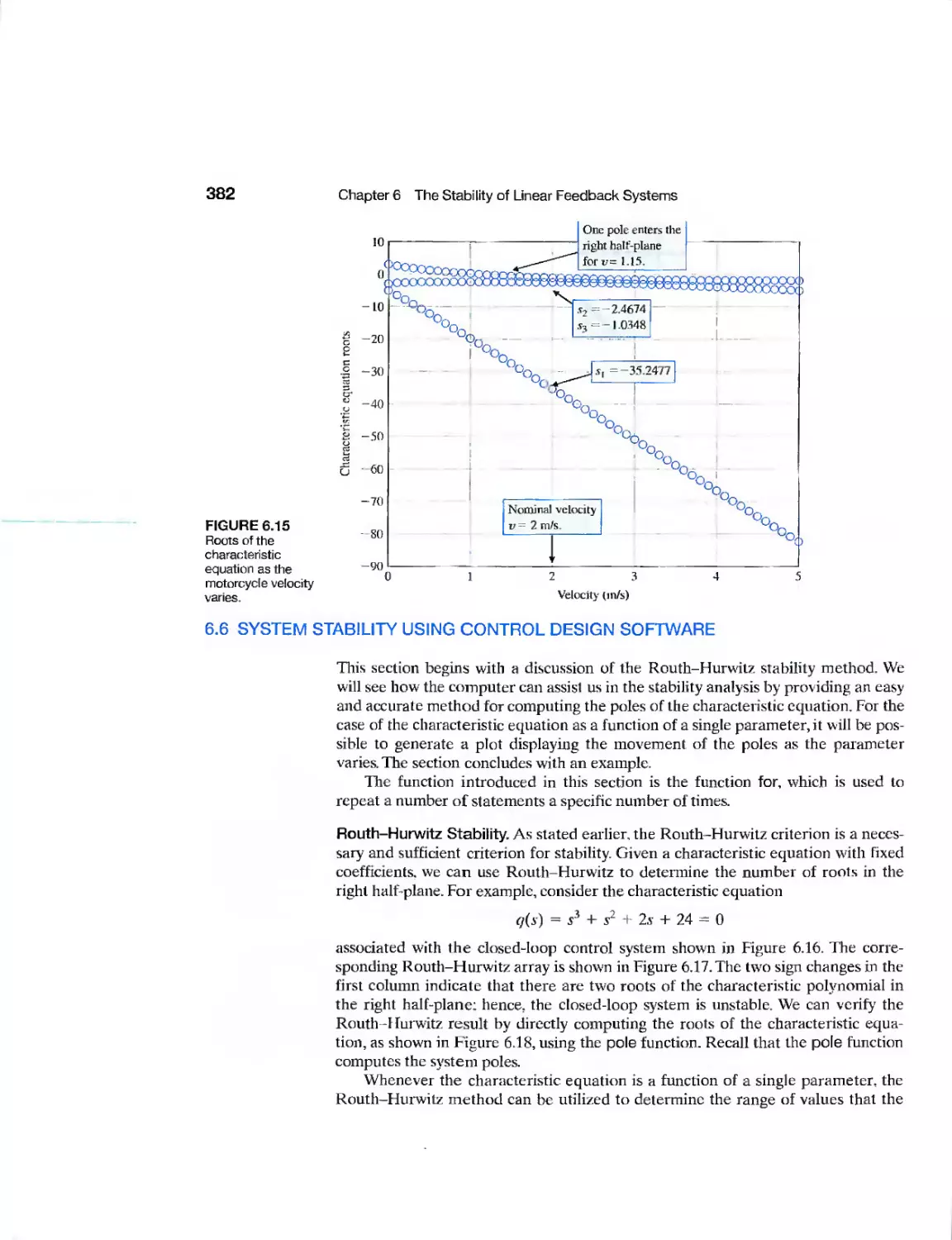
Example Robot-Controlled Motorcycle 375
Example Disk Drive Read System 390
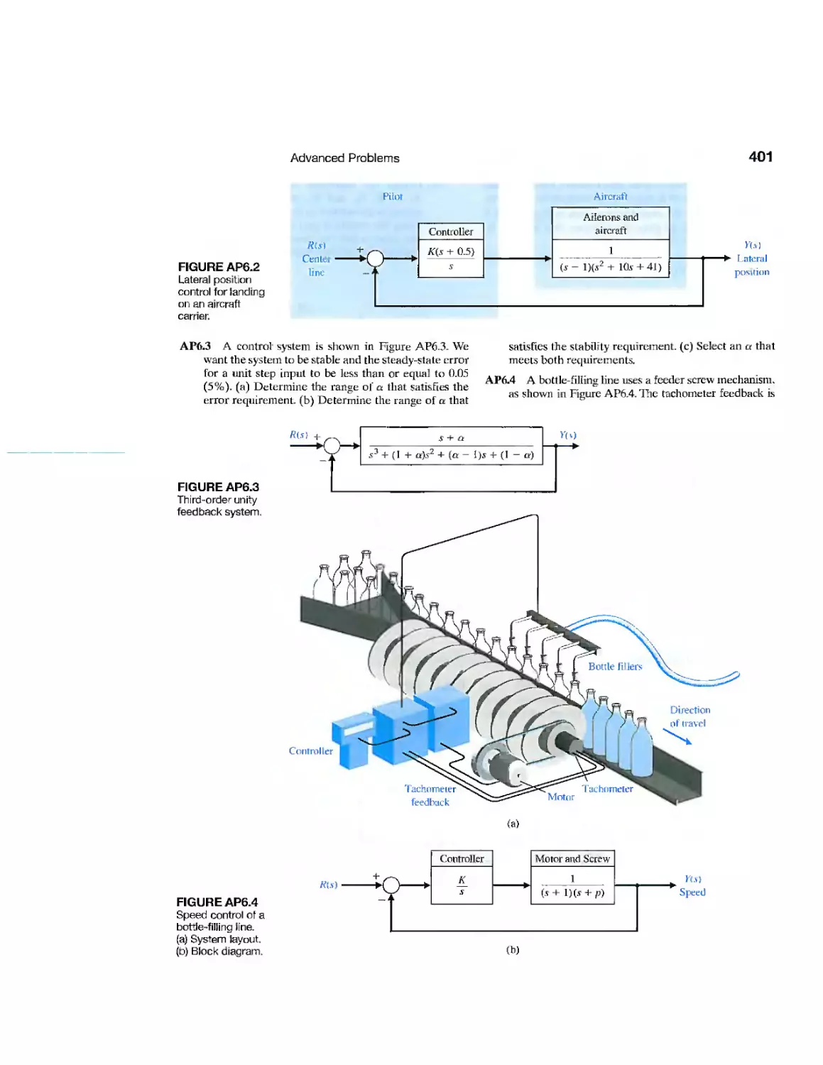
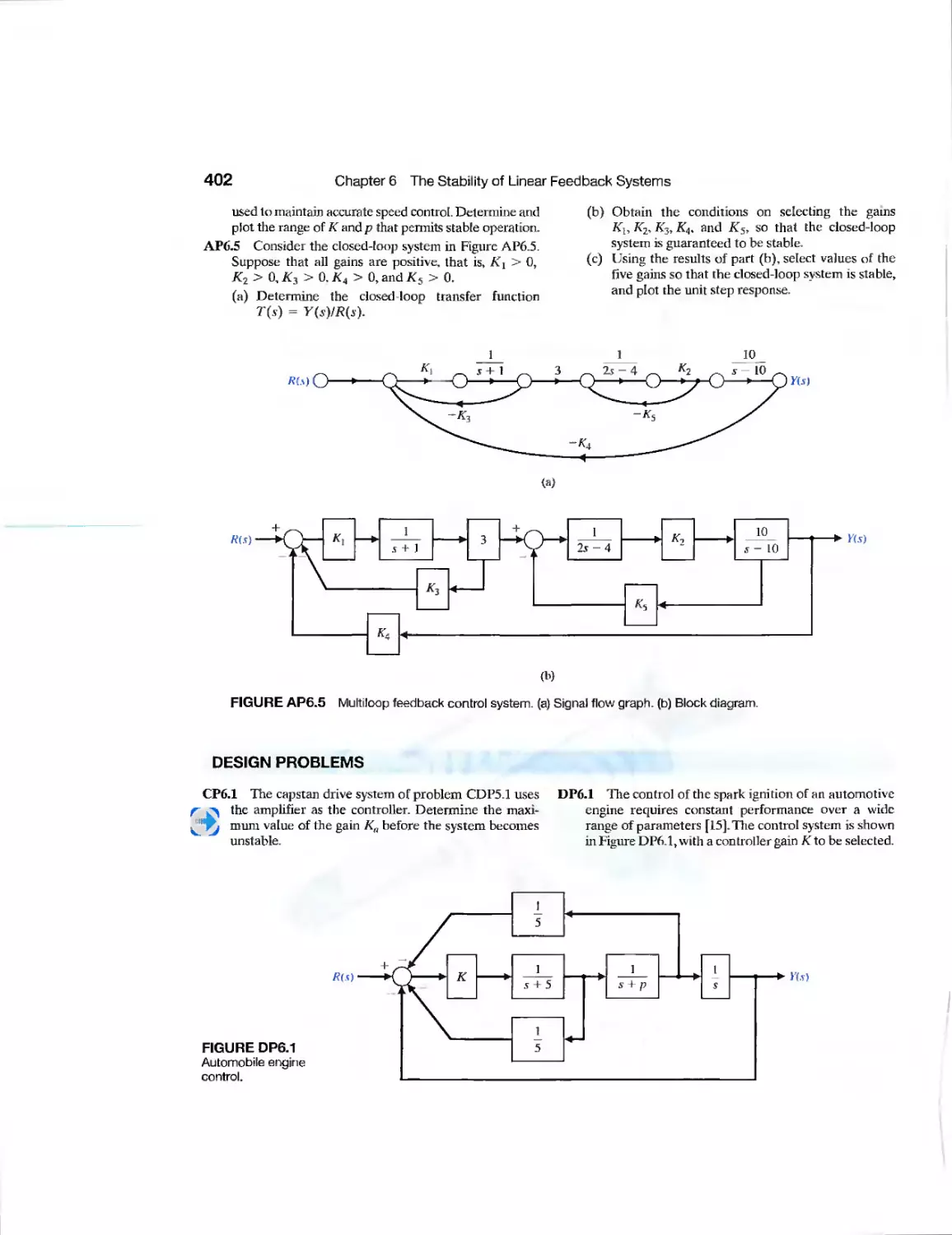
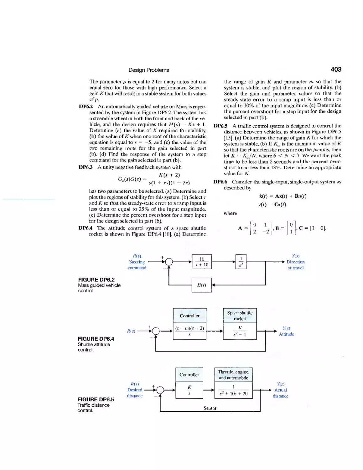
CDP6.1 Traction Drive Motor Control 402
DP6.1 Automobile Ignition Control 402
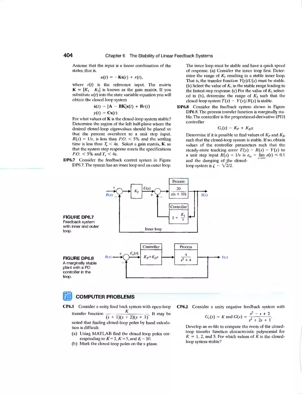
DP6.2 Mars Guided Vehicle Control 403
DP6.3 Parameter Selection 403
DP6.4 Space Shuttle Rocket 403
DP6.5 Traffic Control System 403
DP6.6 State Variable Feedback 403
DP6.7 Inner and Outer Loop Control 404
DP6.8 PD Controller Design 404
CHAPTER 7
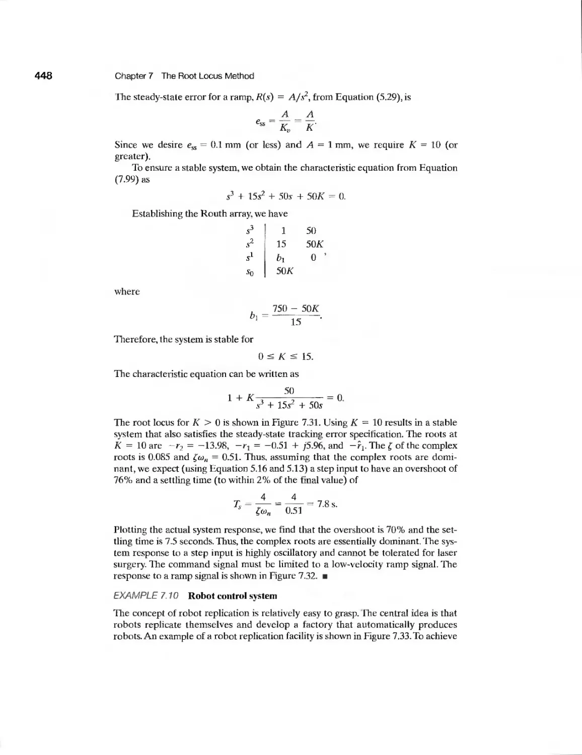
Example Laser Manipulator Control 447
Example Robot Control System 448
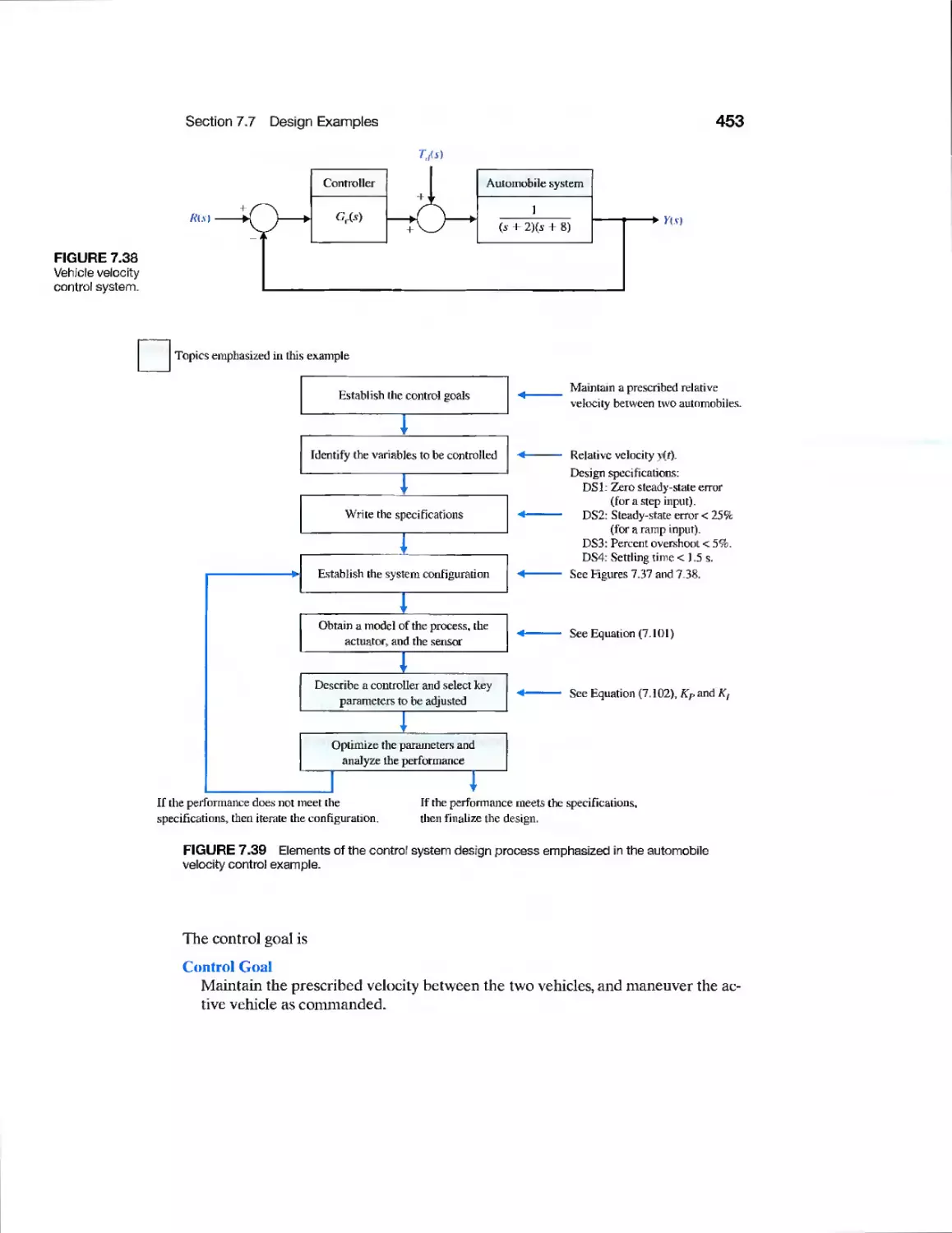
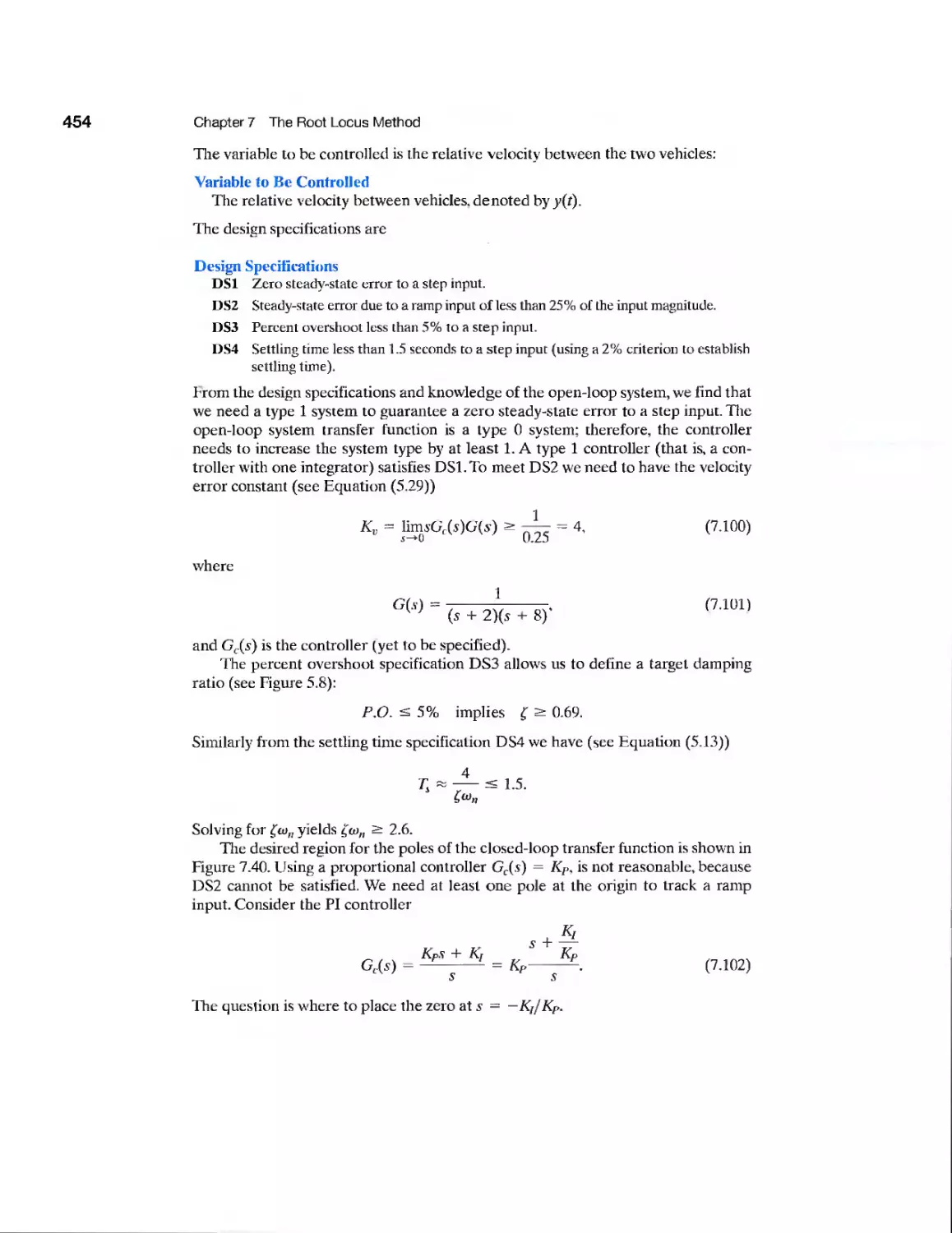
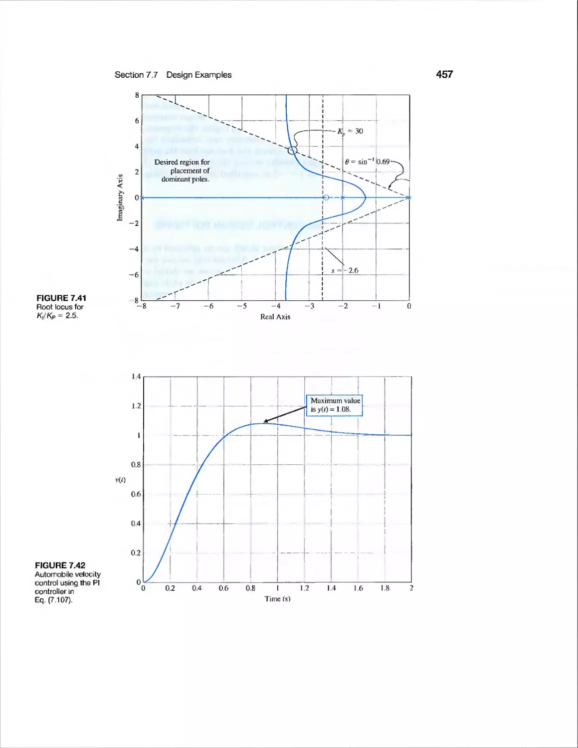
Example Automobile Velocity Control 452
Example Disk Drive Read System 463
CDP7.1 Traction Drive Motor Control 485
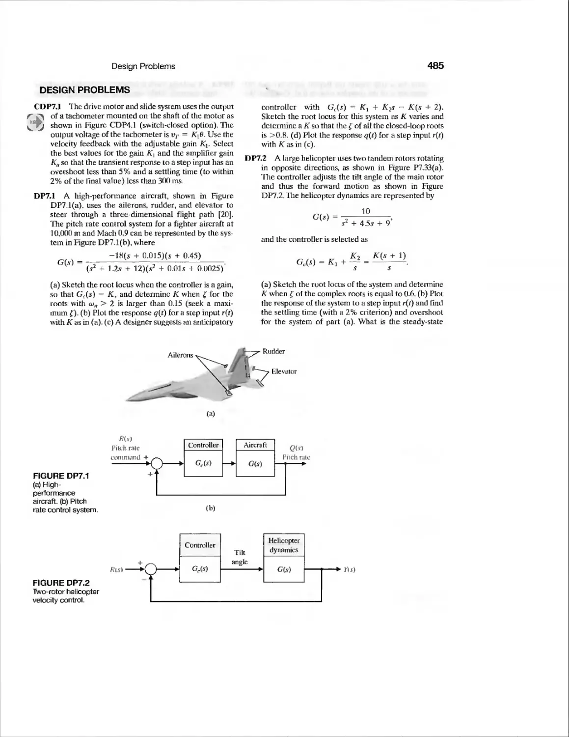
DP7.1 Pitch Rate Aircraft Control 485
DP7.2 Helicopter Velocity Control 485
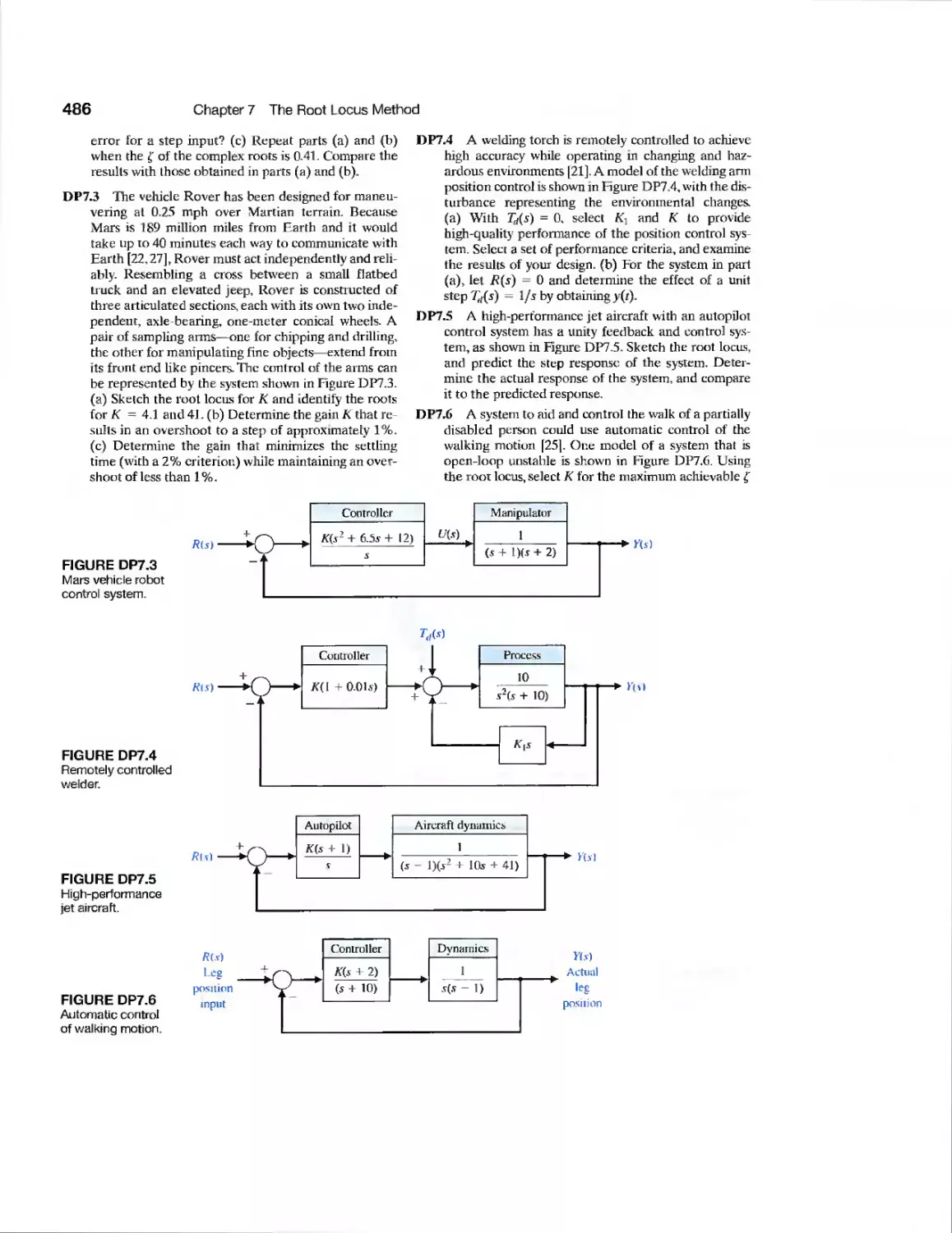
DP7.3 Mars Rover 486
DP7.4 Remotely Controlled Welder 486
DP7.5 • High-Performance Jet Aircraft 486
DP7.6 Control of Walking Motion 486
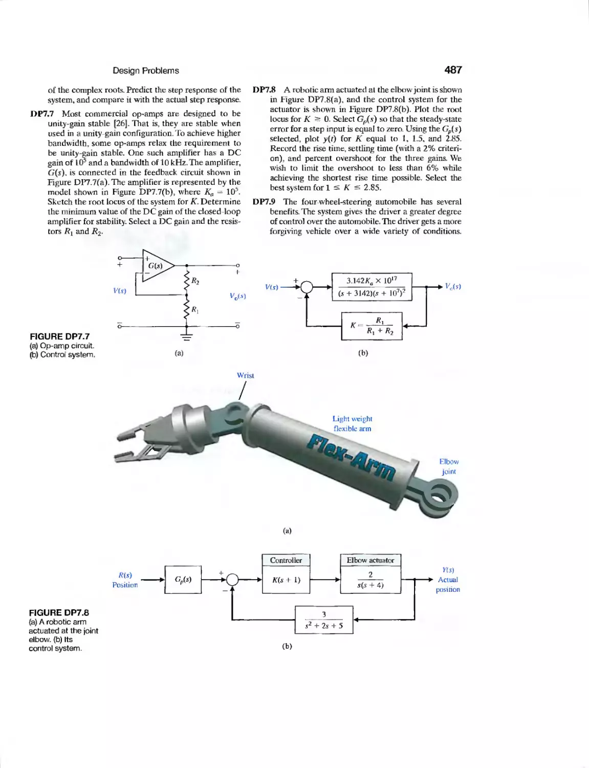
DP7.7 OP Amp Control System 487
DP7.8 Robot Arm Elbow Joint
Actuator 487
DP7.9 Four-Wheel-Steered Automobile 487
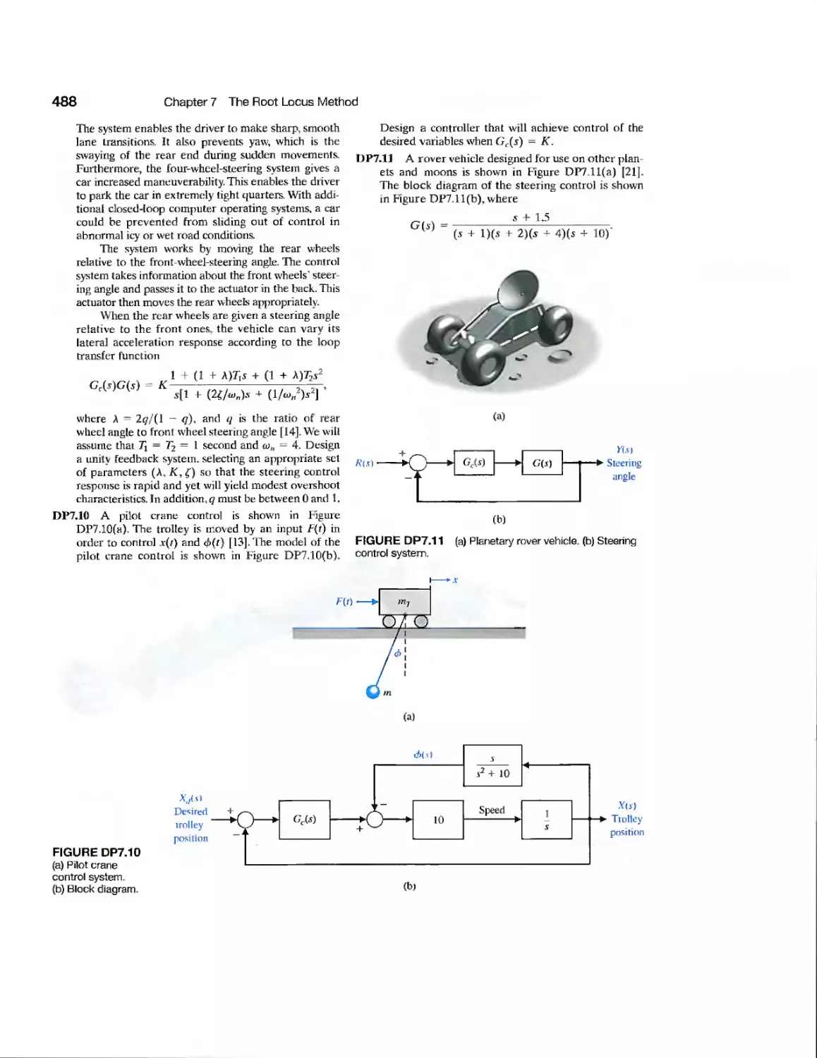
DP7.10 Pilot Crane Control 488
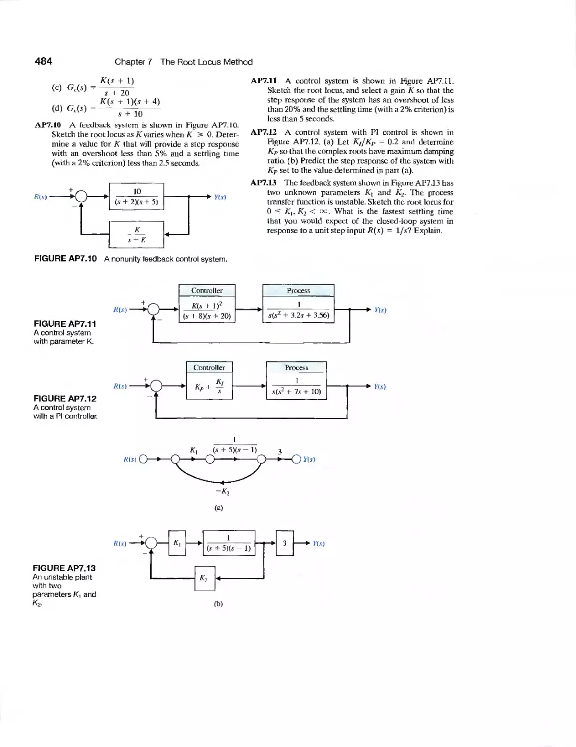
DP7.11 Planetary Rover Vehicle 488
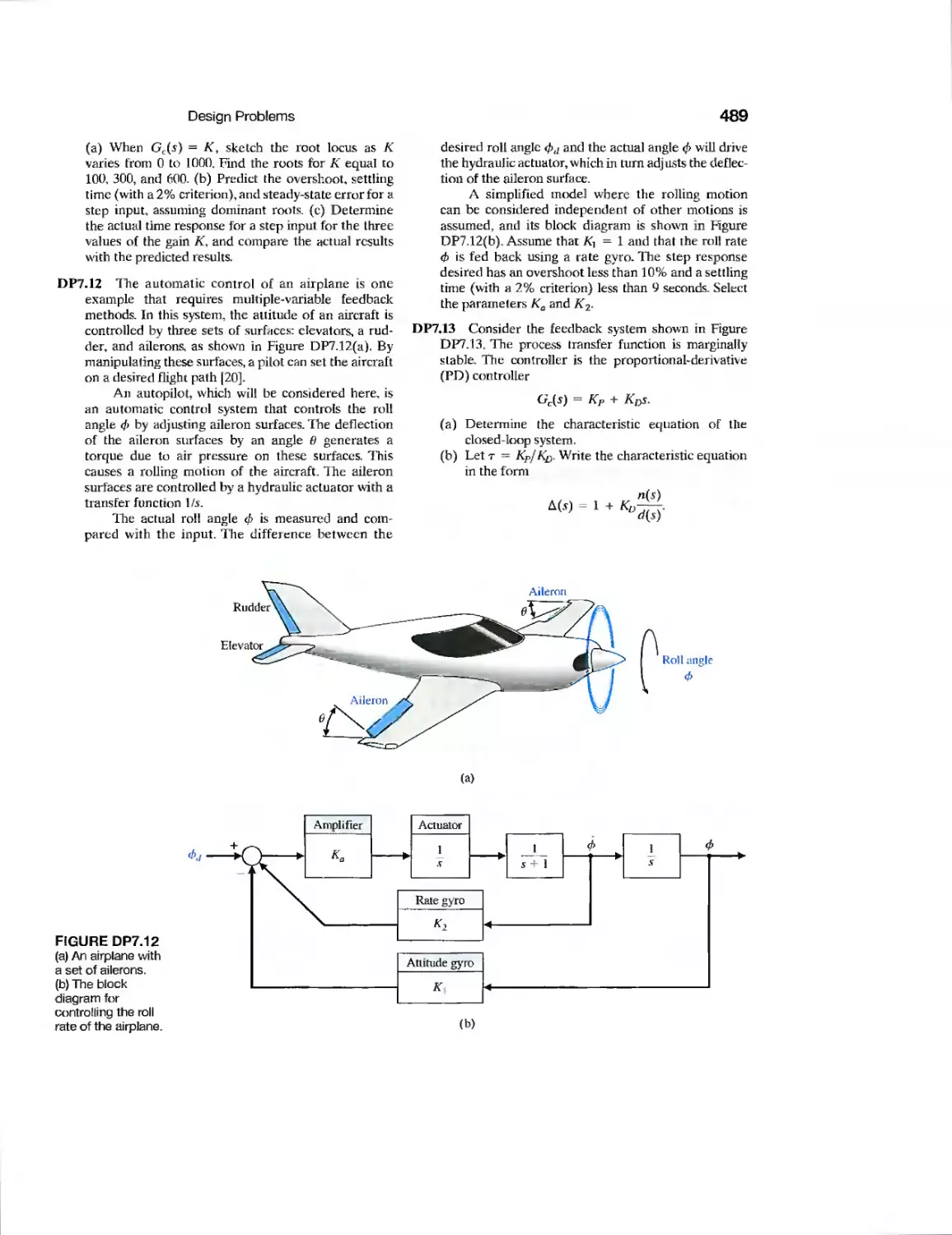
DP7.12 Roll Angle Aircraft Autopilot 489
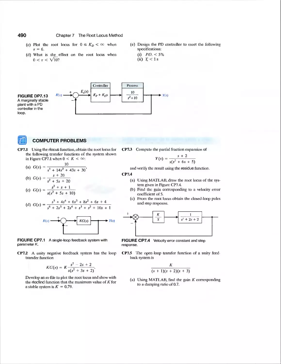
DP7.13 PD Control of a Marginally
Stable Process 489
CHAPTER 8
Example
Example
Example
CDP8.1
DP8.1
DP8.2
DP8.3
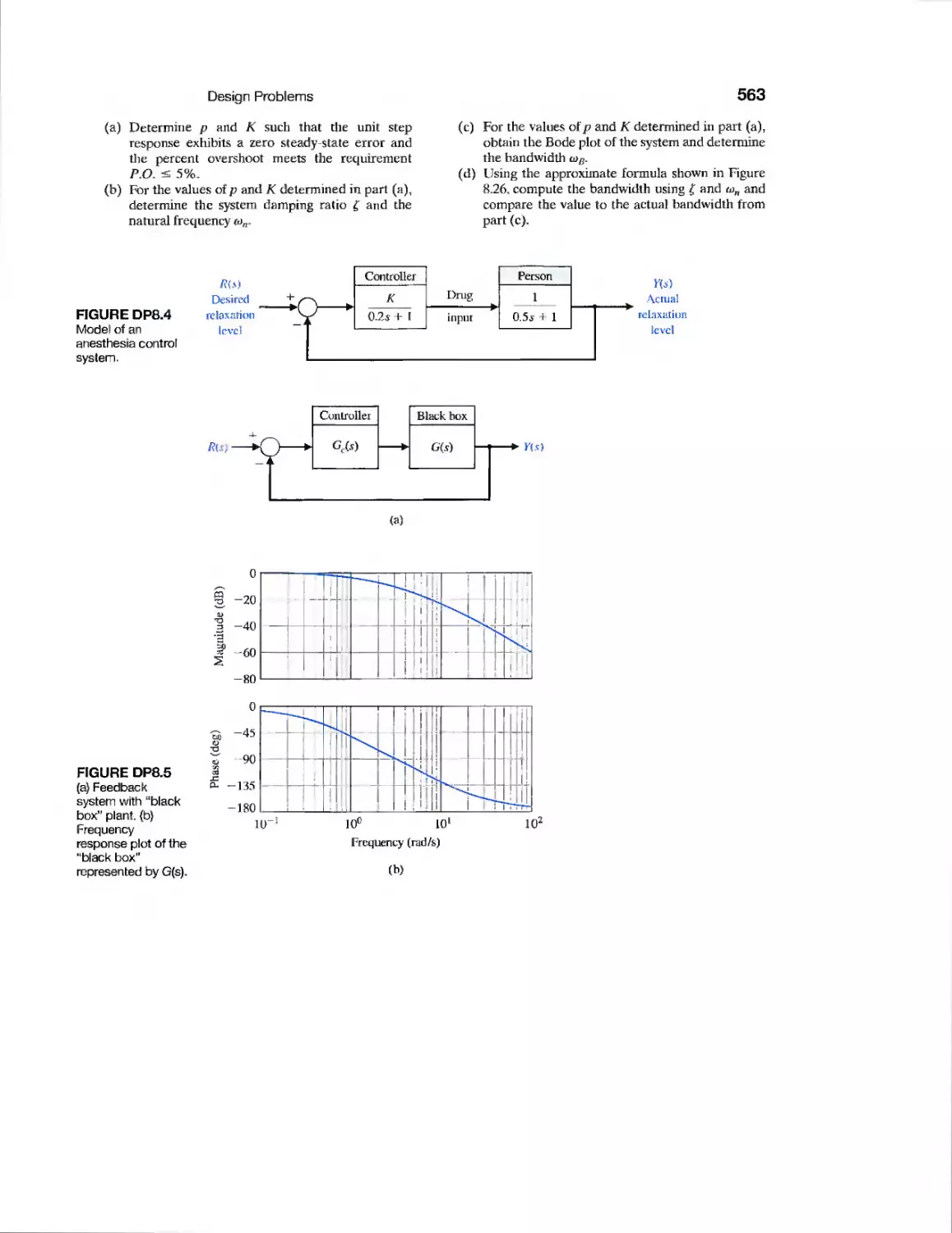
DP8.4
DP8.5
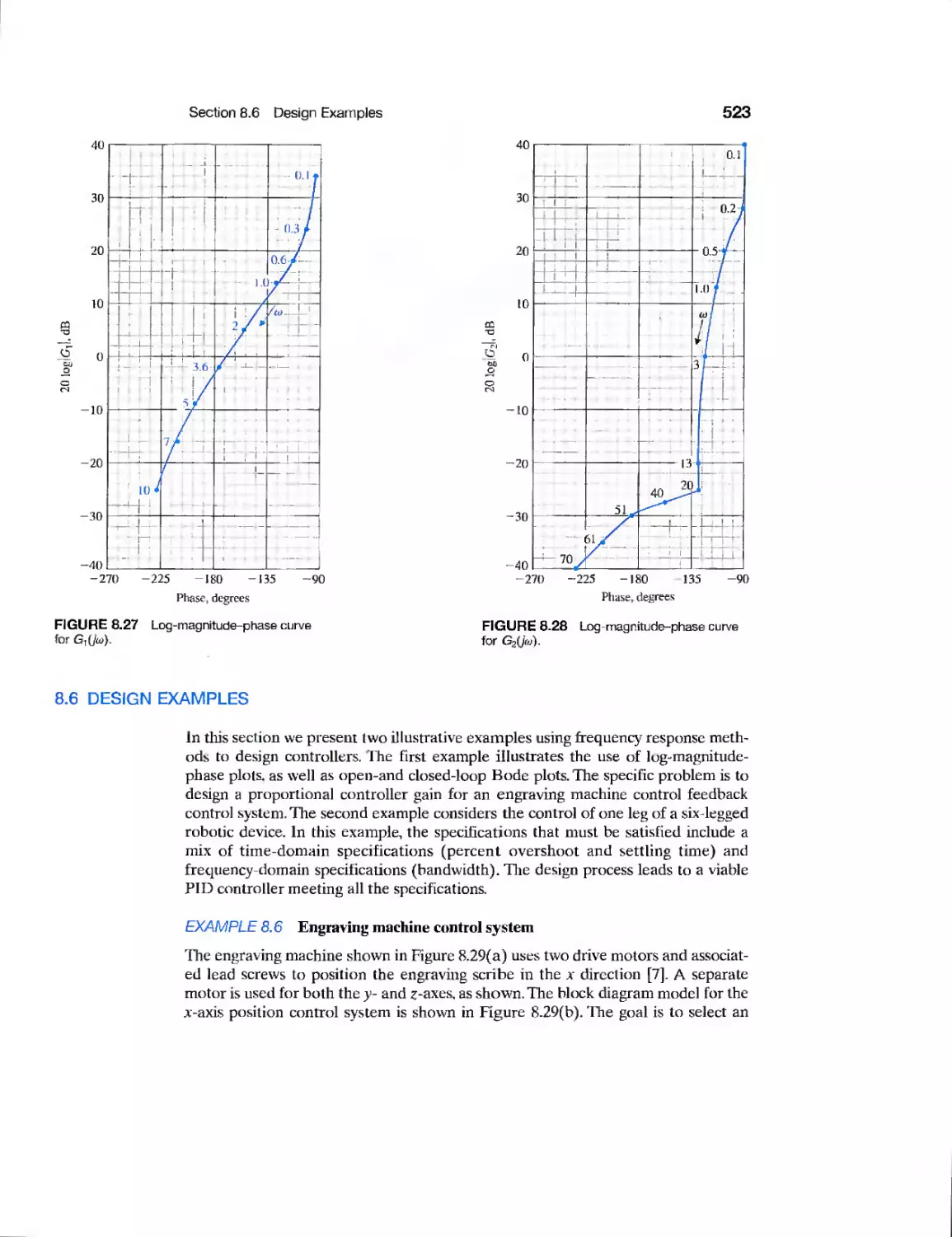
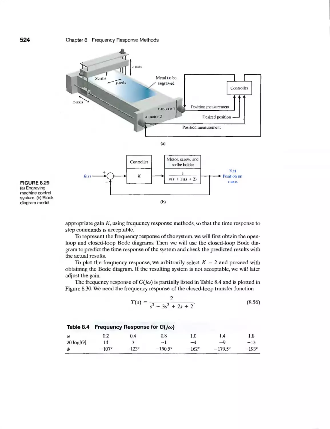
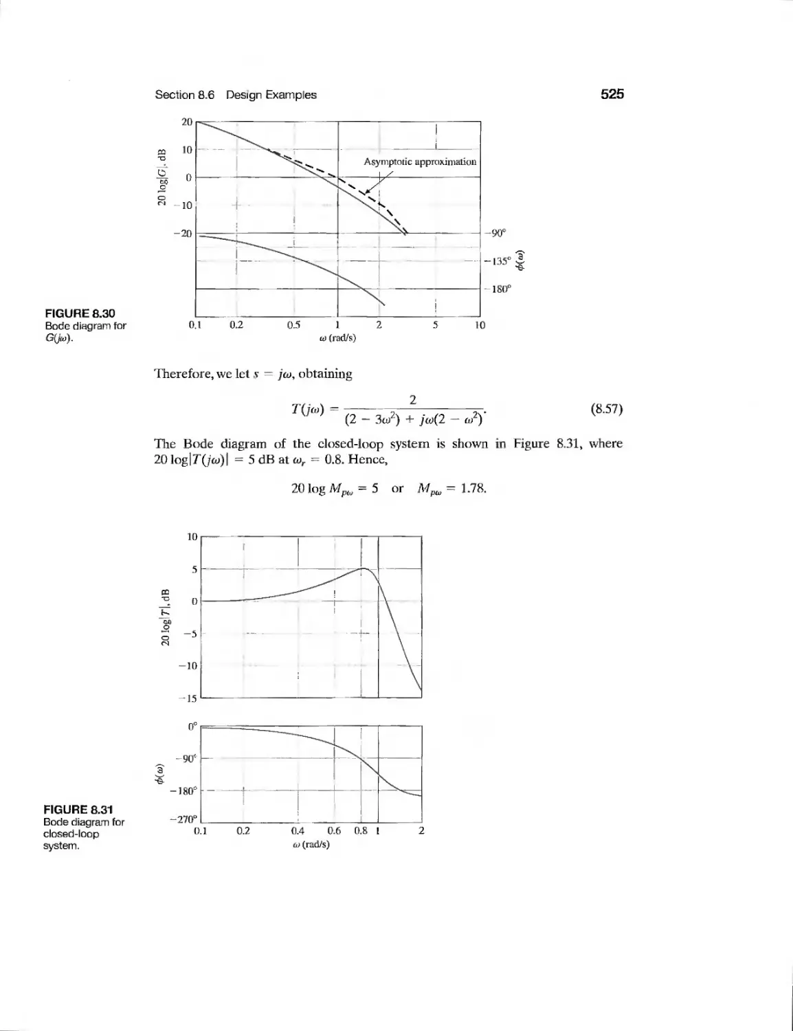
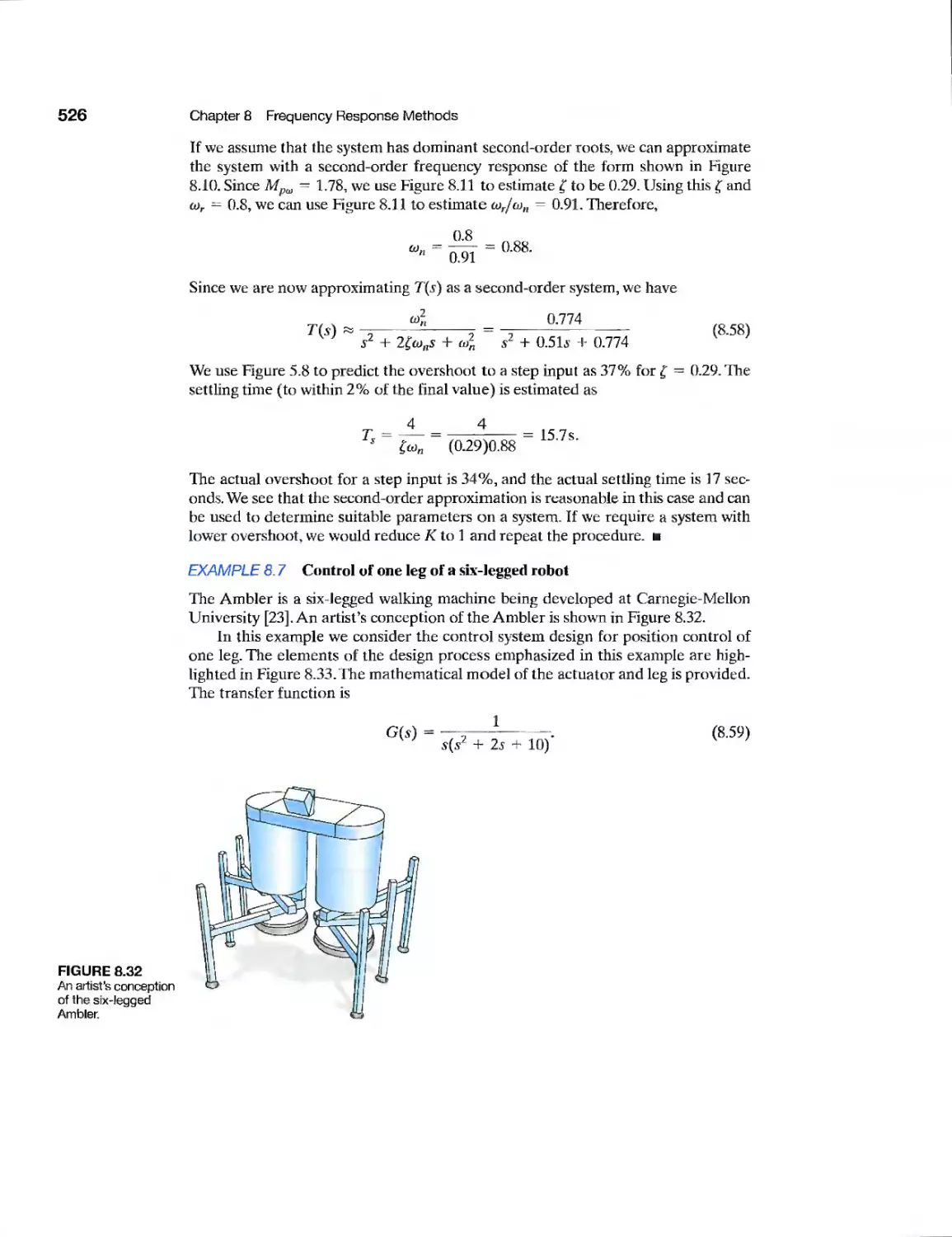
DP8.6
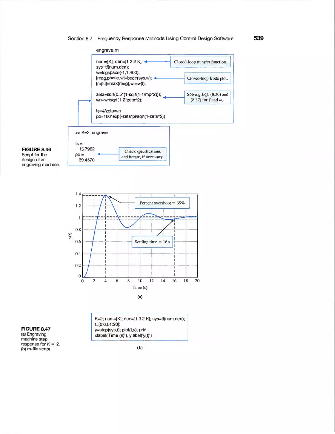
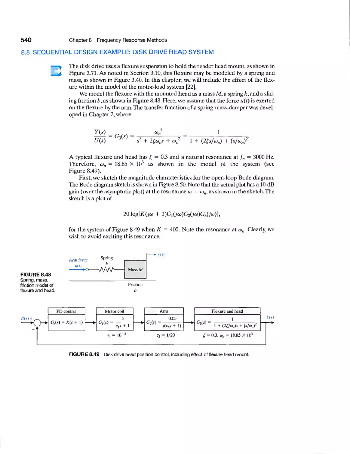
Engraving Machine Control
Control of a Six-Legged Robot
Disk Drive Read System
Traction Drive Motor Control
Automobile Steering System
Autonomous Planetary
Explorer-Ambler
Vial Position Control Under a
Dispenser
Automatic Anesthesia Control
Black Box Control
State Variable System Design
523
526
540
561
561
561
561
561
563
563
CHAPTER 9
Example
Example
Example
CDP9.1
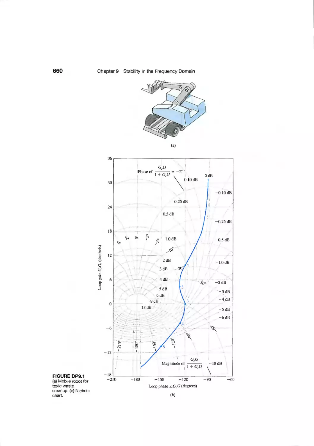
DP9.1
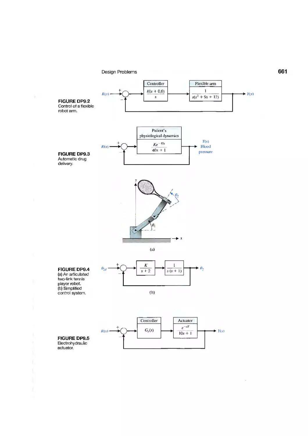
DP9.2
DP9.3
DP9.4
DP9.5
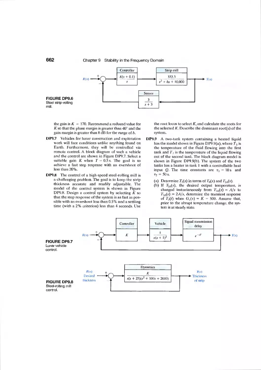
DP9.6
DP9.7
DP9.8
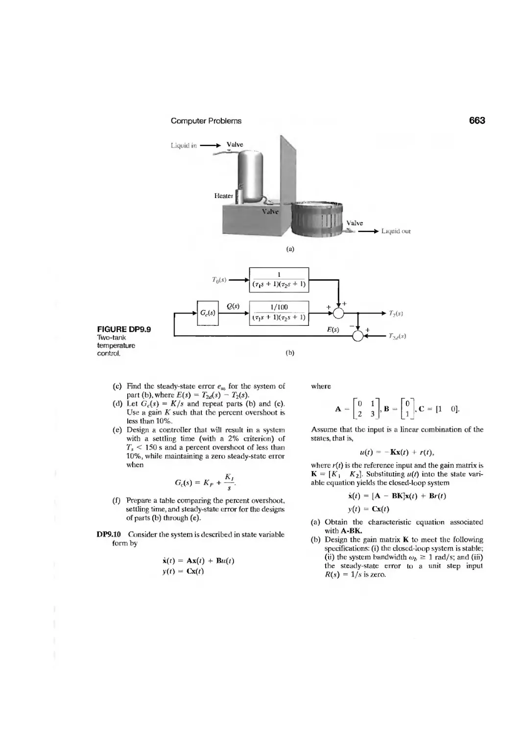
DP9.9
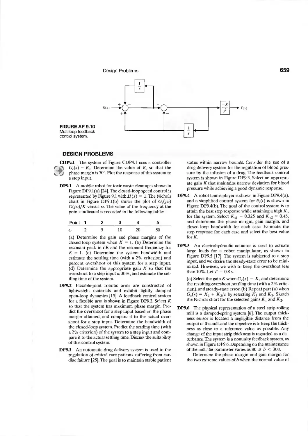
DP9.10
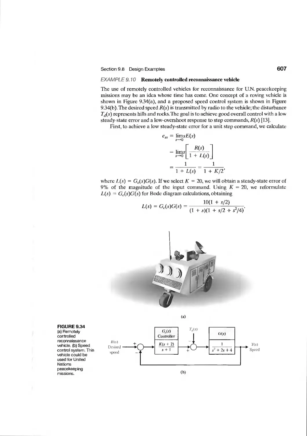
Remotely Controlled
Reconnaissance Vehicle
Hot Ingot Robot Control
Disk Drive Read System
Traction Drive Motor Control
Mobile Robot for Toxic Waste
Cleanup
Control of a Flexible Arm
Blood Pressure Regulator
Robot Tennis Player
Electrohydraulic Actuator
Steel Strip-Rolling Mill
Lunar Vehicle Control
High-Speed Steel-Rolling Mill
Two-Tank Temperature Control
State Variable Feedback Control
607
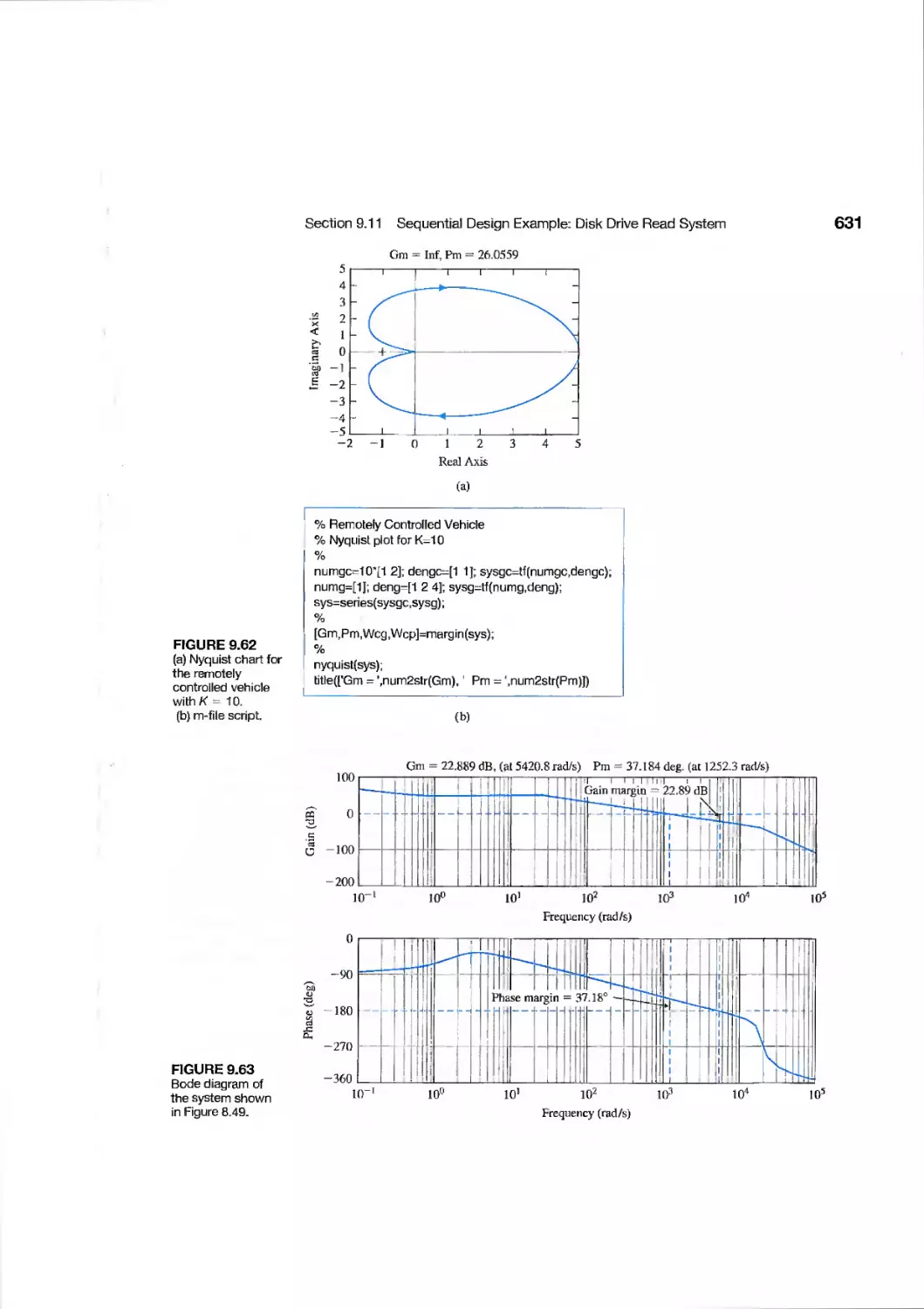
610
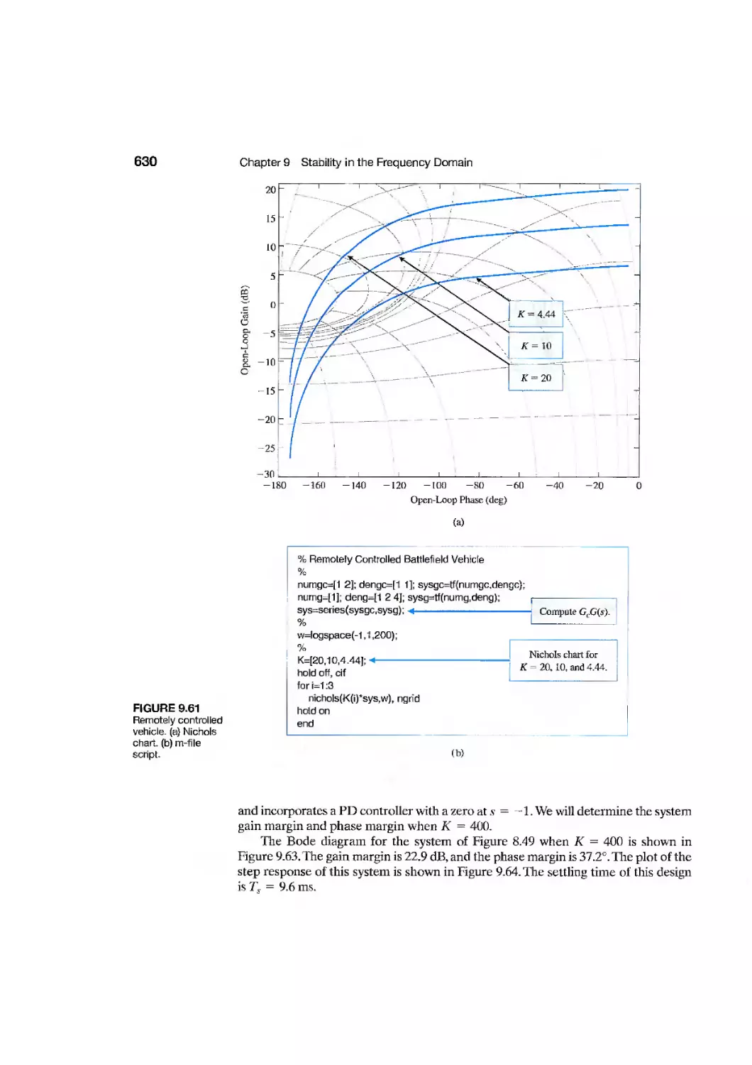
629
659
659
659
659
659
659
659
662
662
663
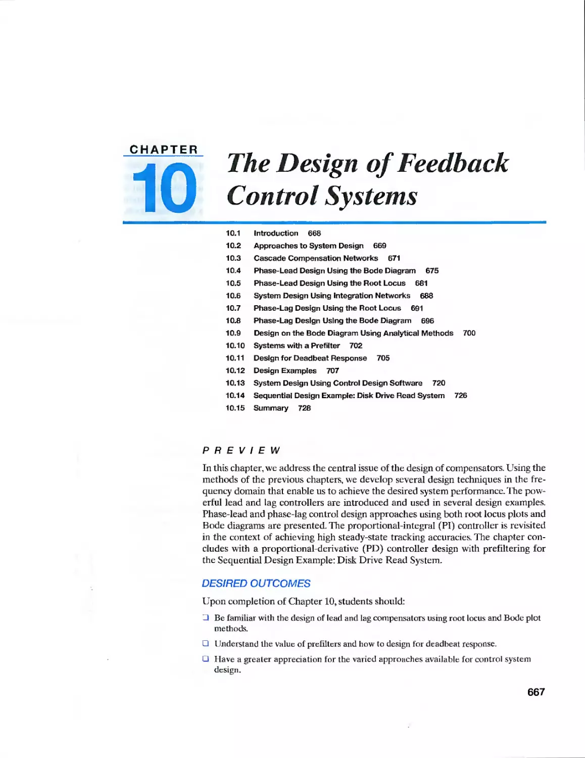
CHAPTER 10
Example
Example
Example
Example
CDP10.1
DP10.1
DP10.2
DP10.3
DP10.4
DP10.5
DP10.6
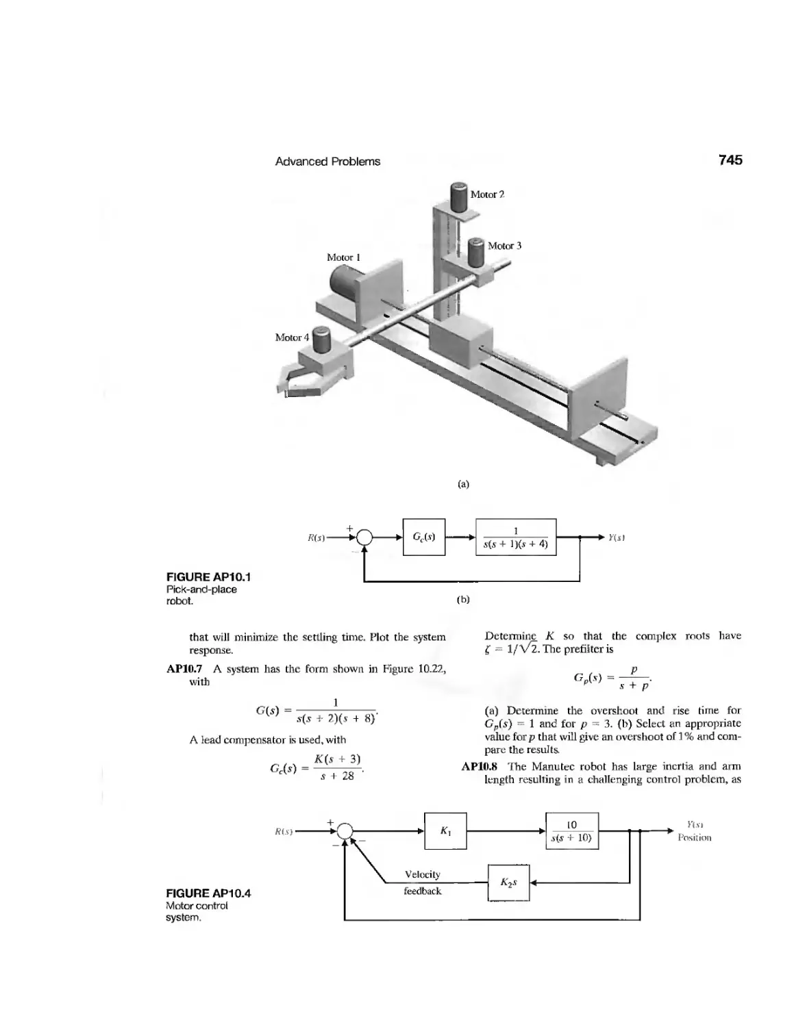
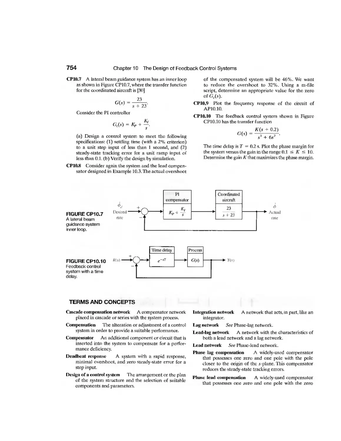
DP10.7
DP10.8
DP10.9
Rotor Winder Control System
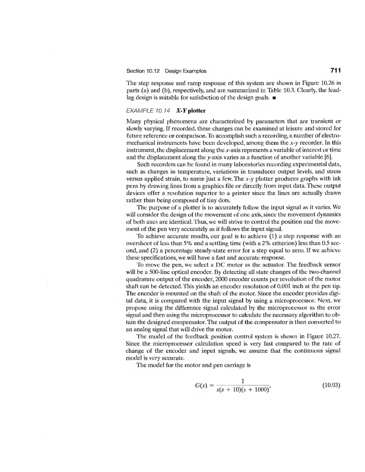
The X-Y Plotter
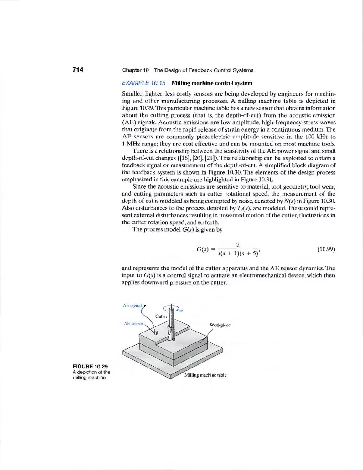
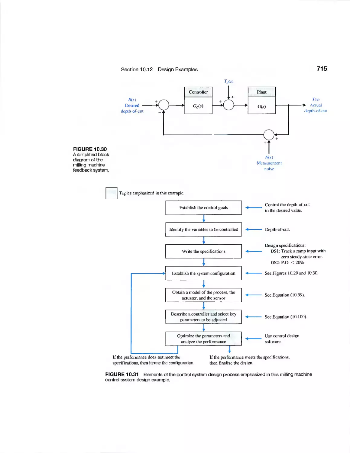
Milling Machine Control System
Disk Drive Read System
Traction Drive Motor Control
Two Cooperating Robots
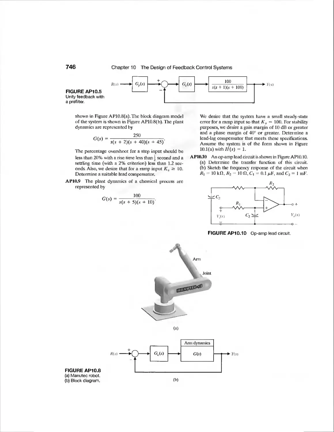
Heading Control of a Bi-Wing
Aircraft
Mast Flight System
Robot Control Using Vision
High-Speed Train Tilt Control
Large Antenna Control
Tape Transport Speed Control
Automobile Engine Control
Aircraft Roll Angle Control
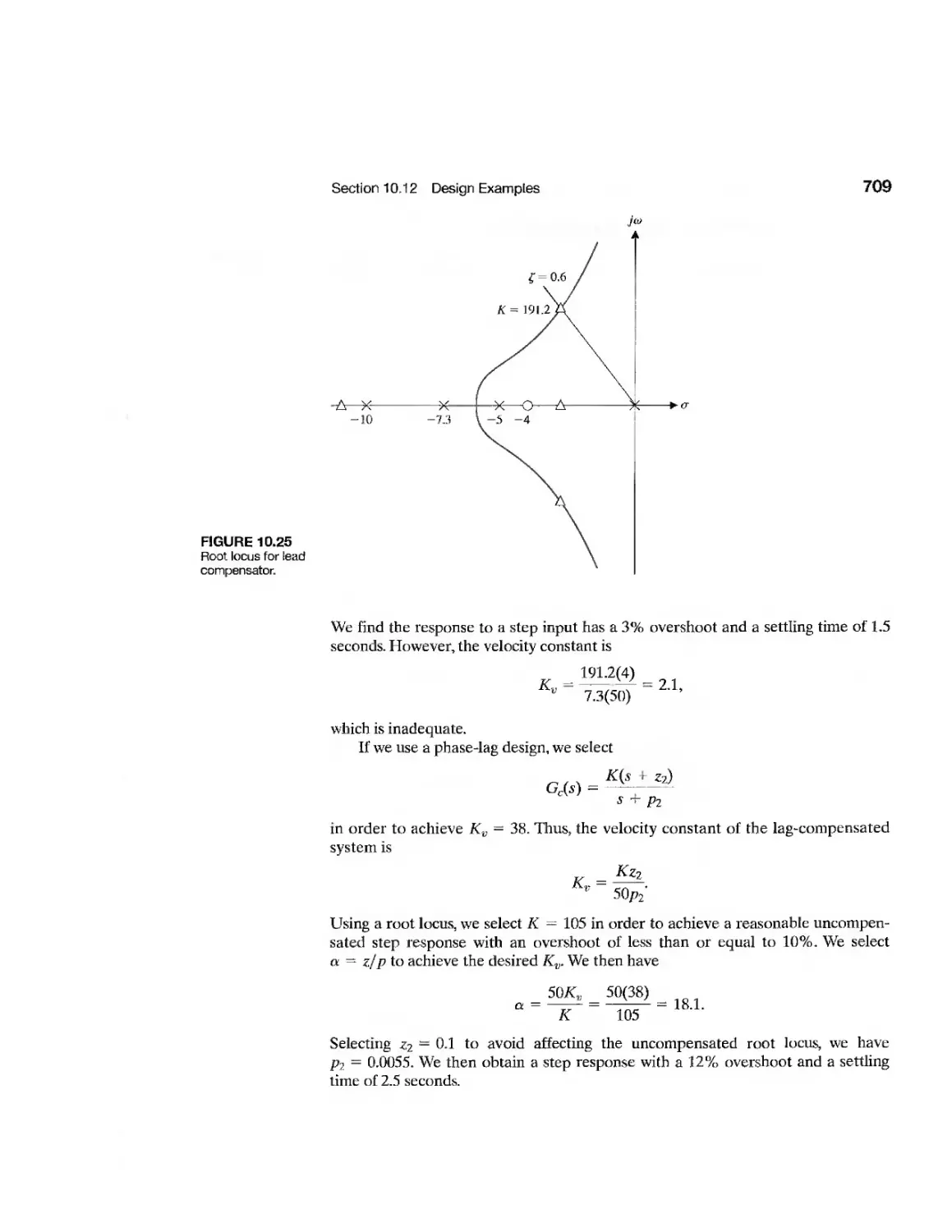
707
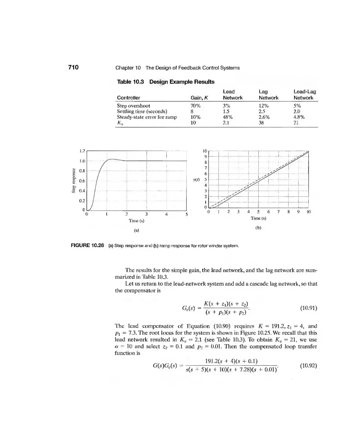
711
714
726
747
747
747
747
749
749
749
750
750
751
DP10.10 Windmill Radiometer 751
DP10.I1 Control with Time Delay 752
DP10.12 Loop Shaping 752
CHAPTER 11
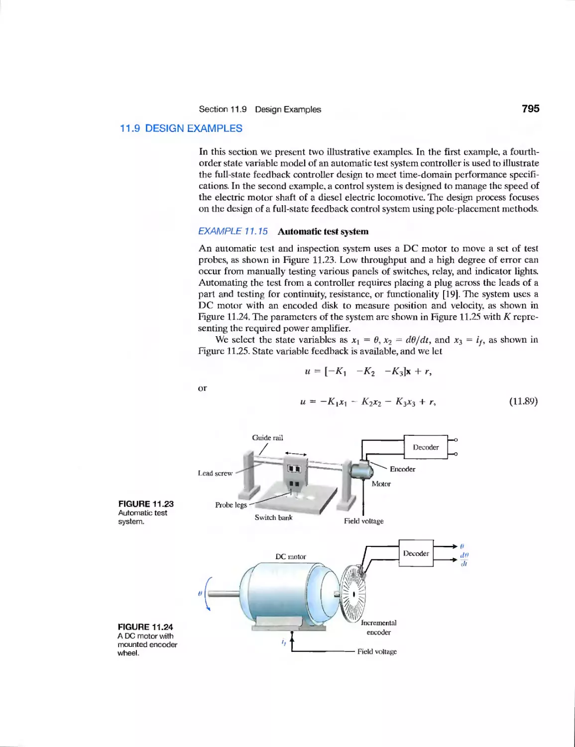
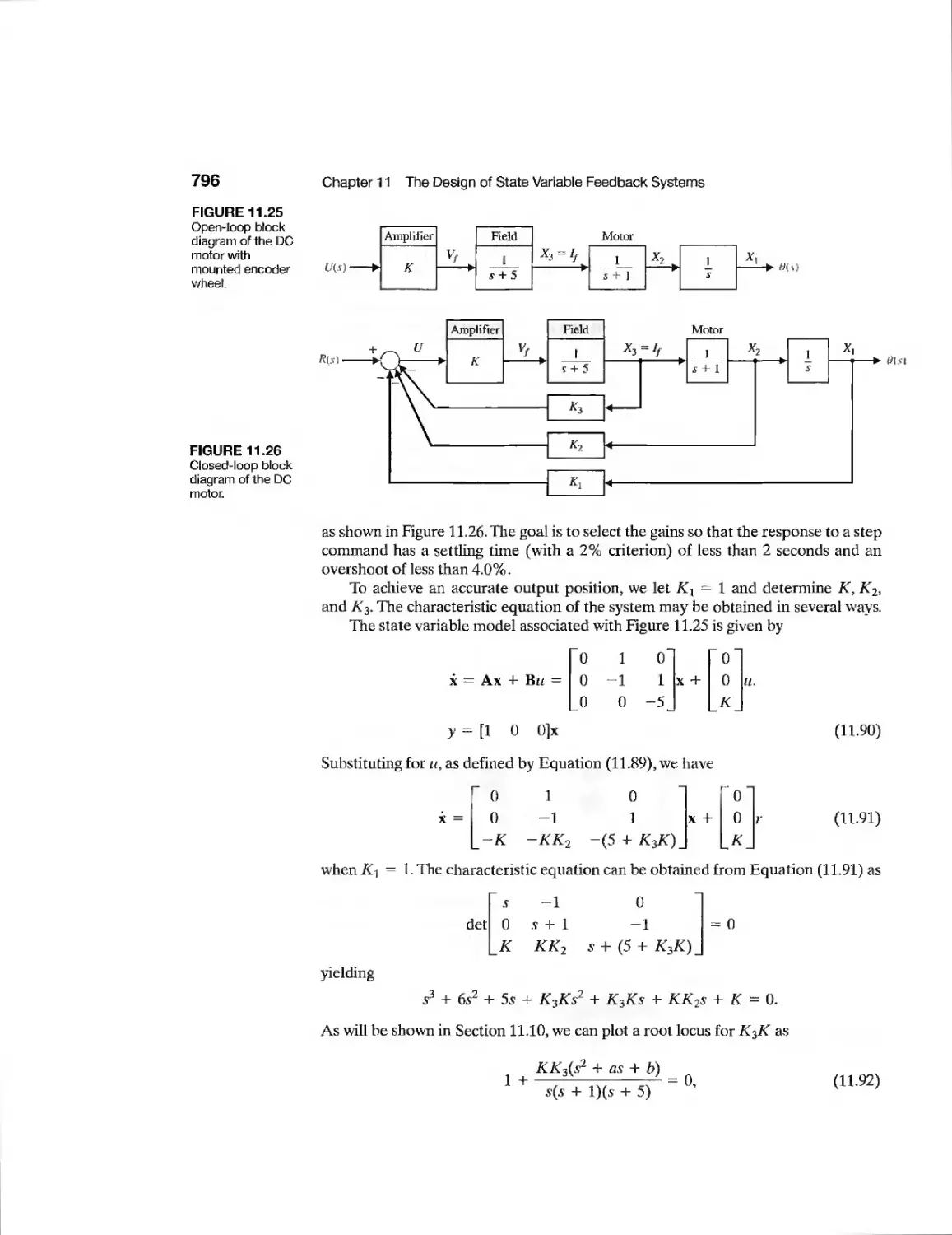
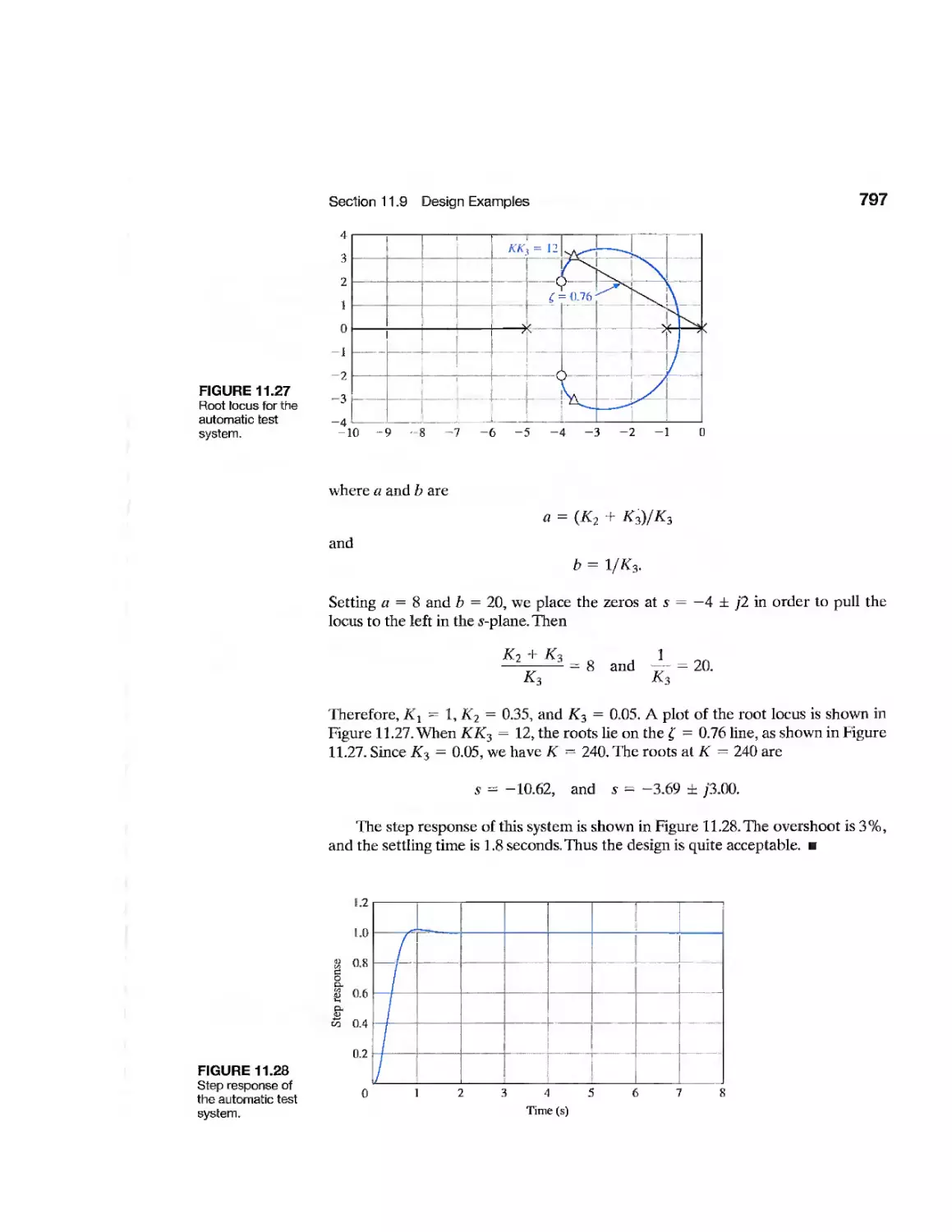
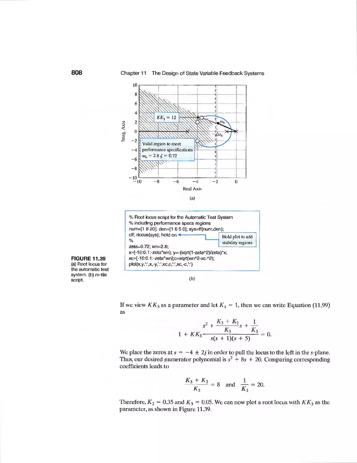
Example Automatic Test System 795
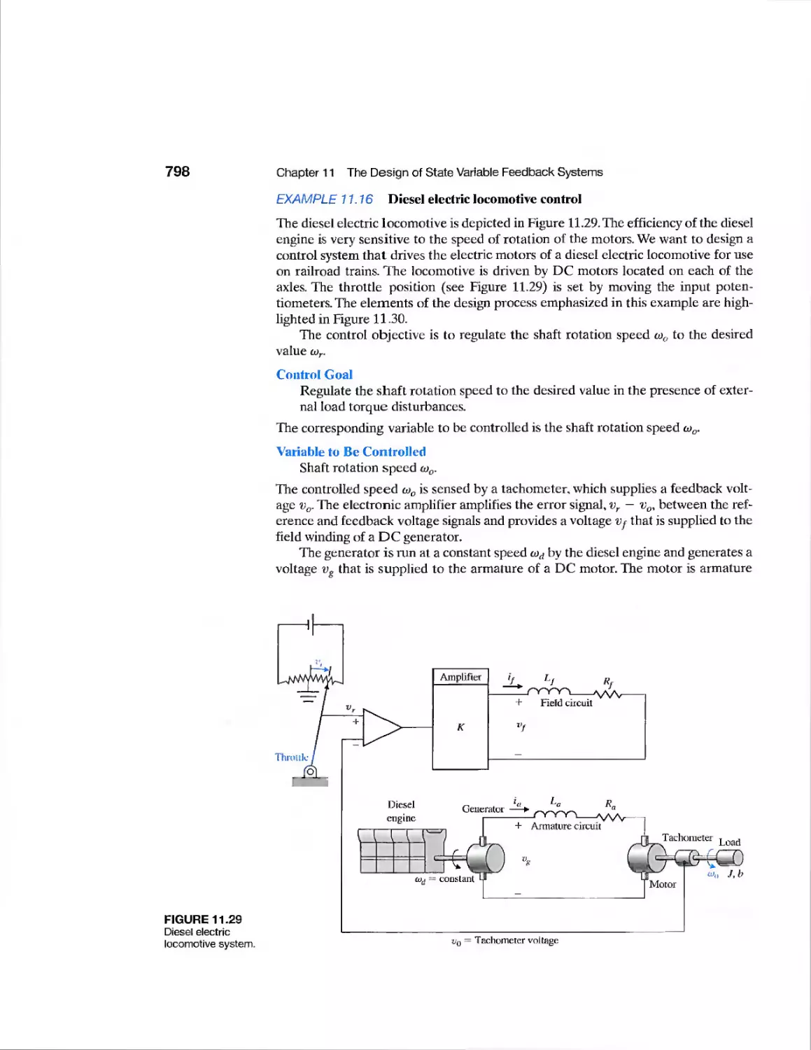
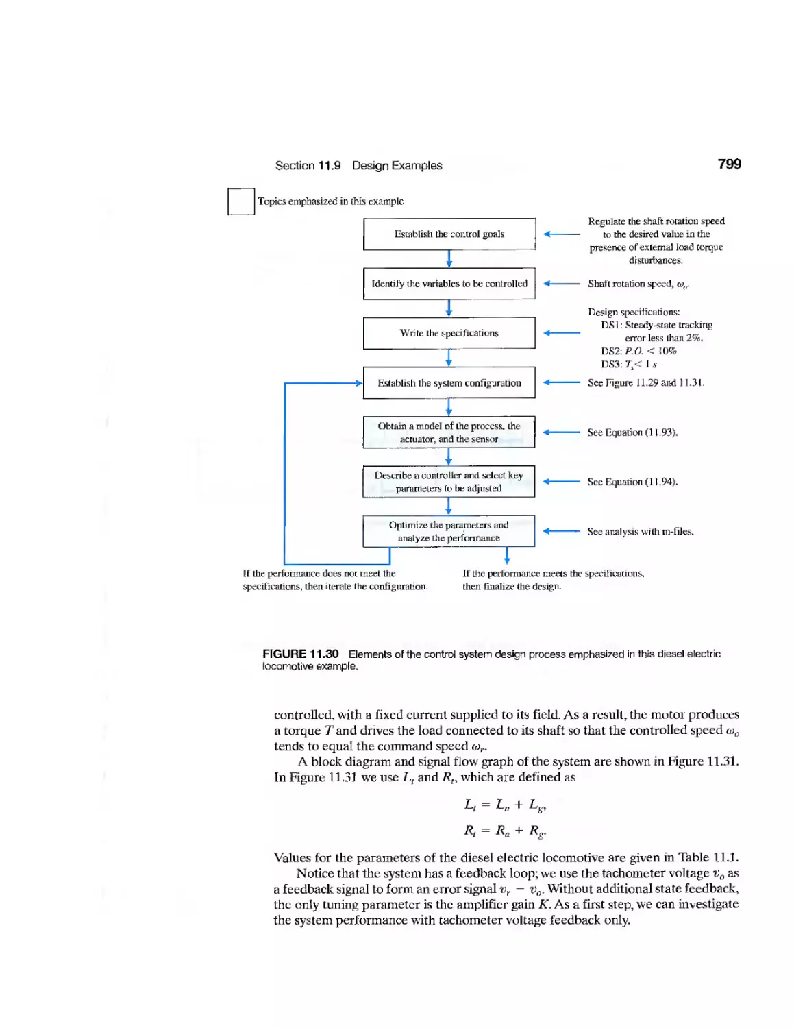
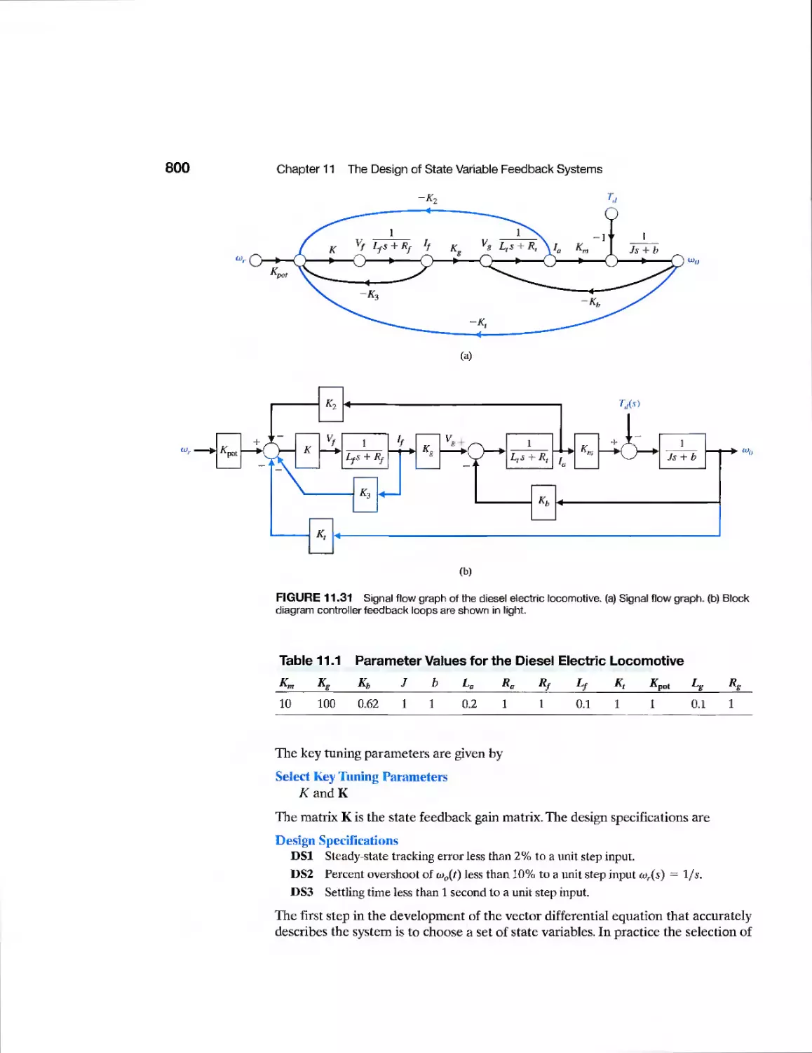
Example Diesel Electric Locomotive 798
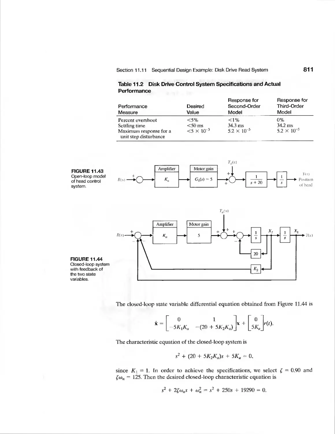
Example Disk Drive Read System 810
CDP11.1 Traction Drive Motor Control 821
DP11.1 LevitationofaSteelBall 821
DPI 1.2 Automobile Carburetor 821
DP11.3 State Variable Compensation 821
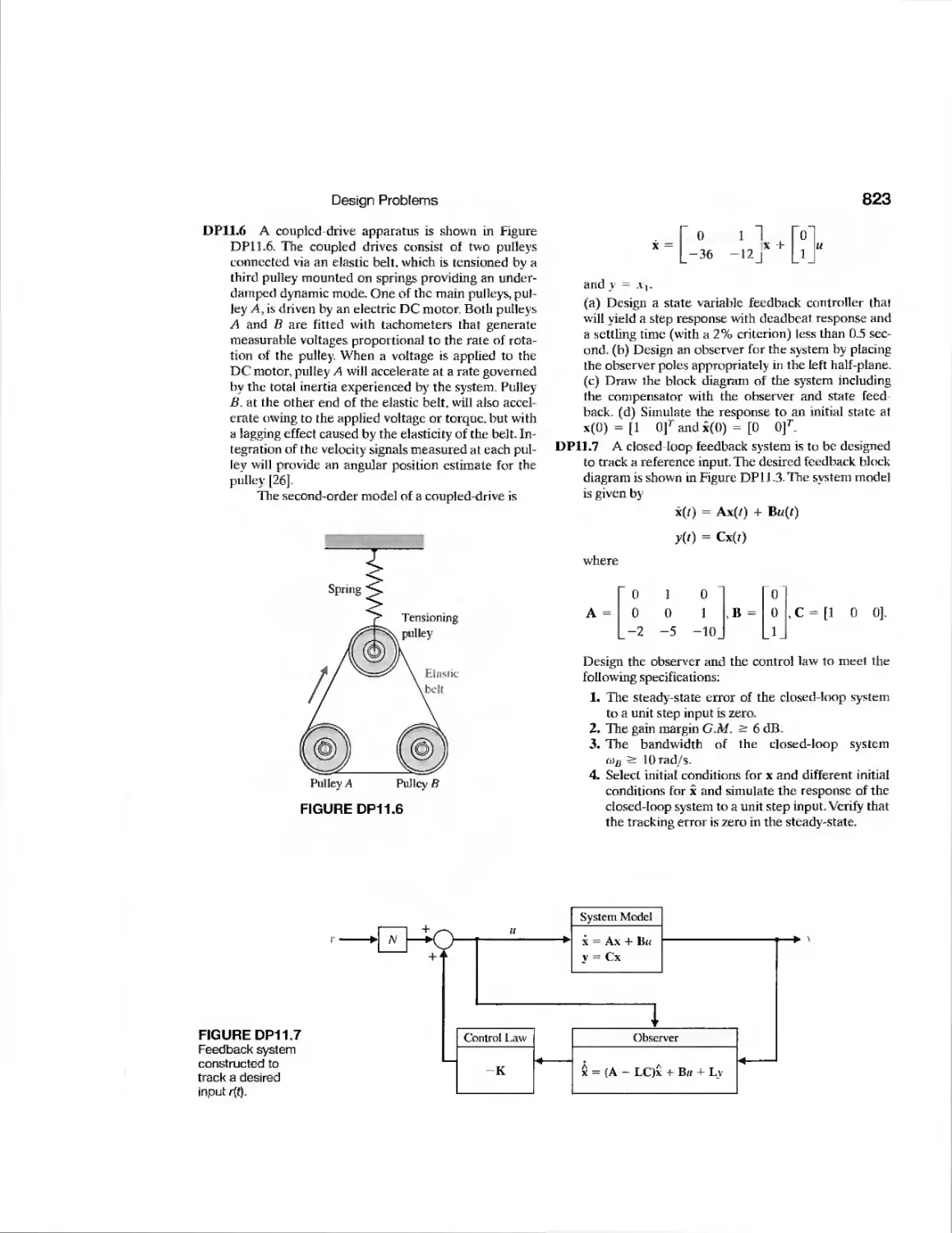
DP11.4 Helicopter Control 822
DPI 1.5 Manufacturing of Paper 822
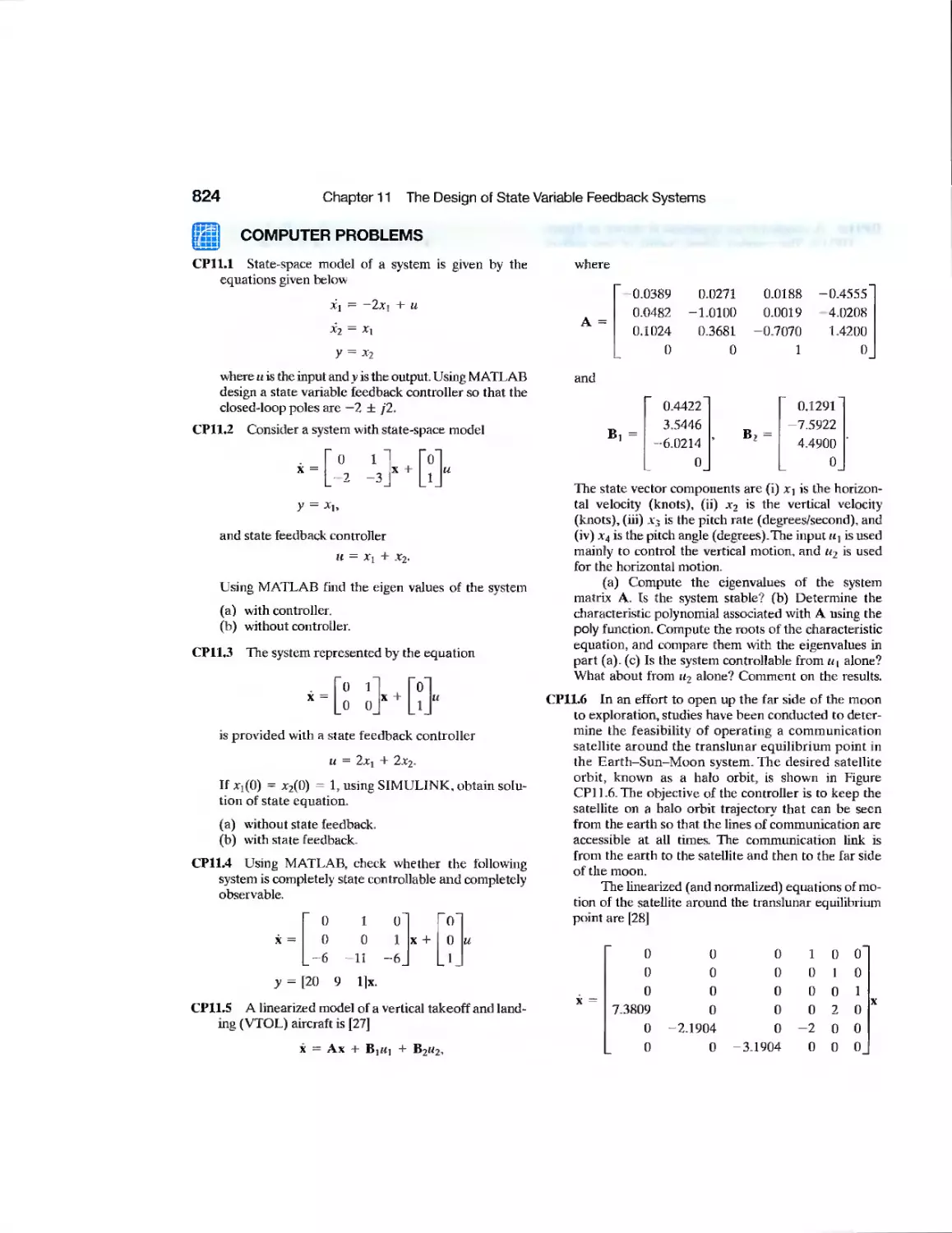
DPI 1.6 Coupled-Drive Control 823
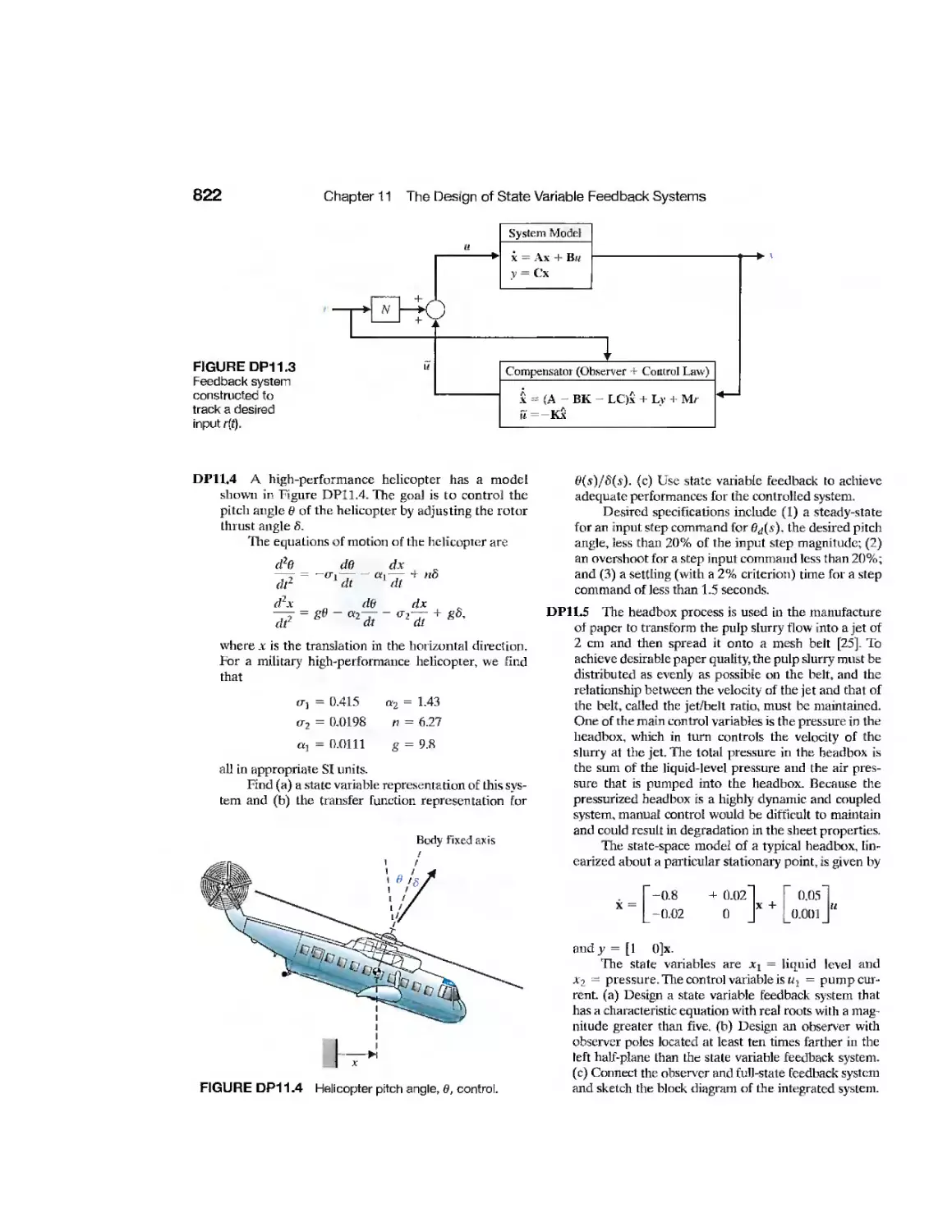
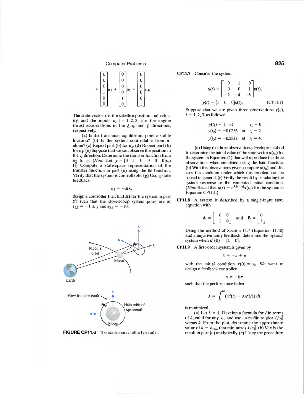
DPI 1.7 Tracking a Reference Input 823
CHAPTER 12
Example
Example
Example
Example
Example
Example
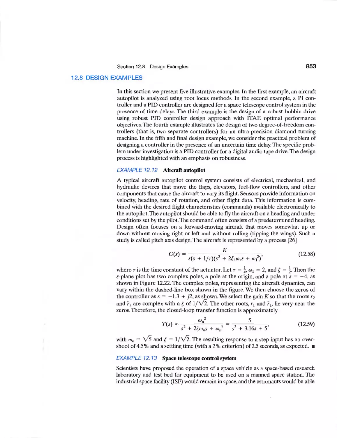
Aircraft Autopilot
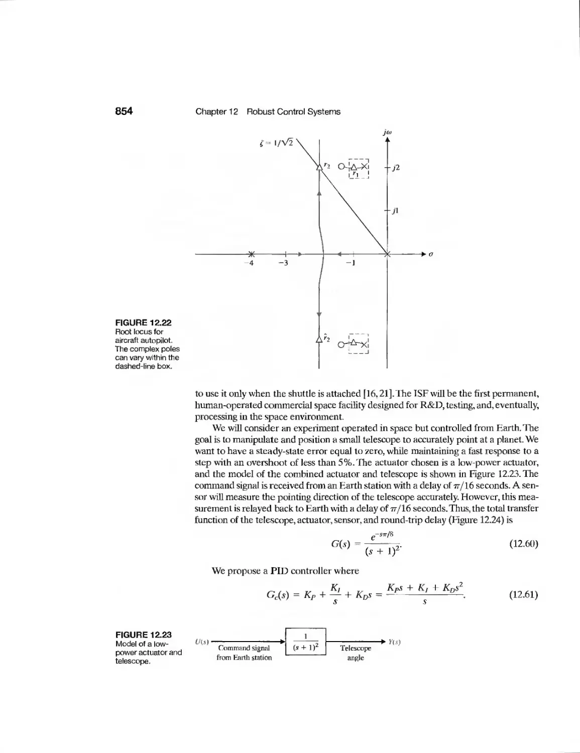
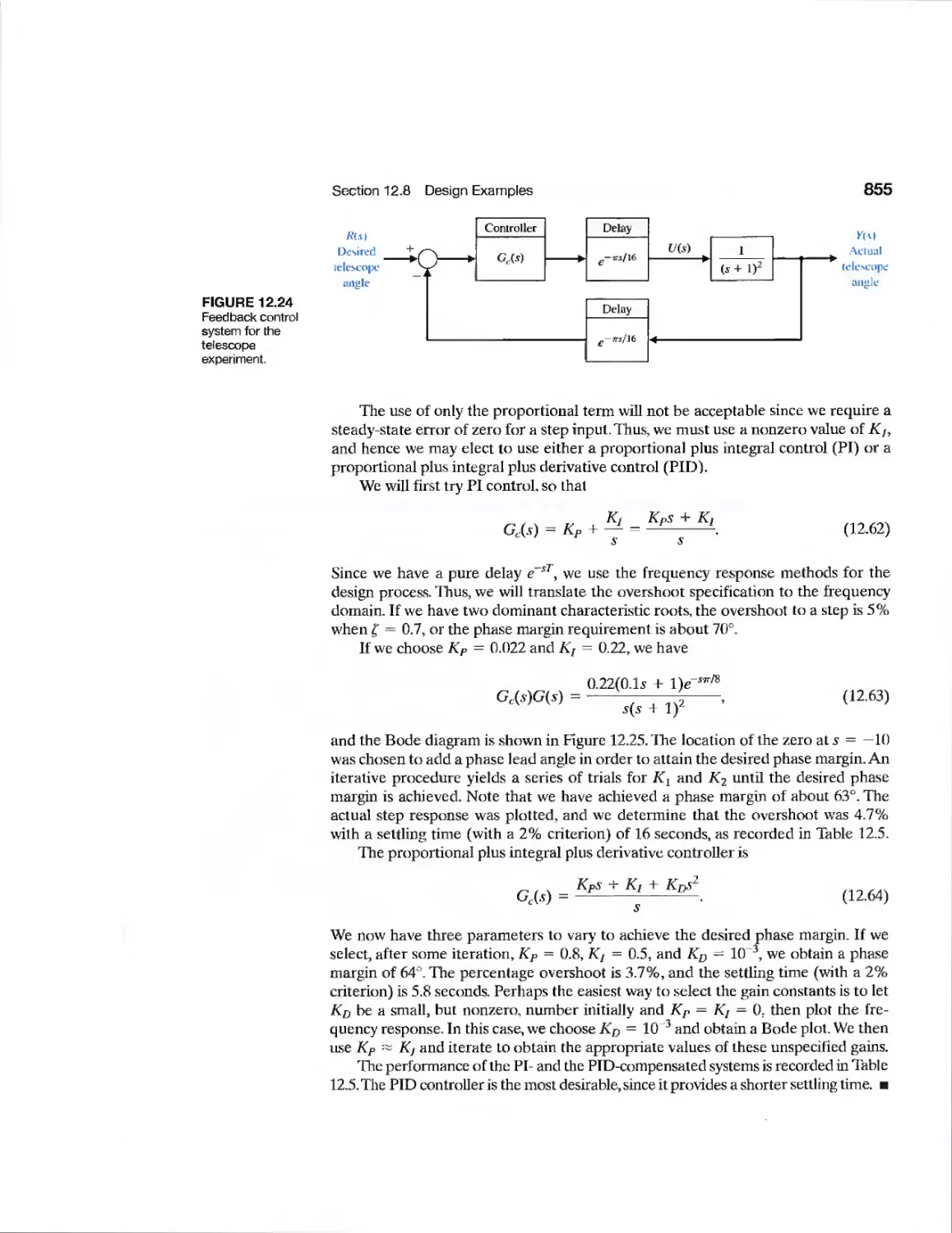
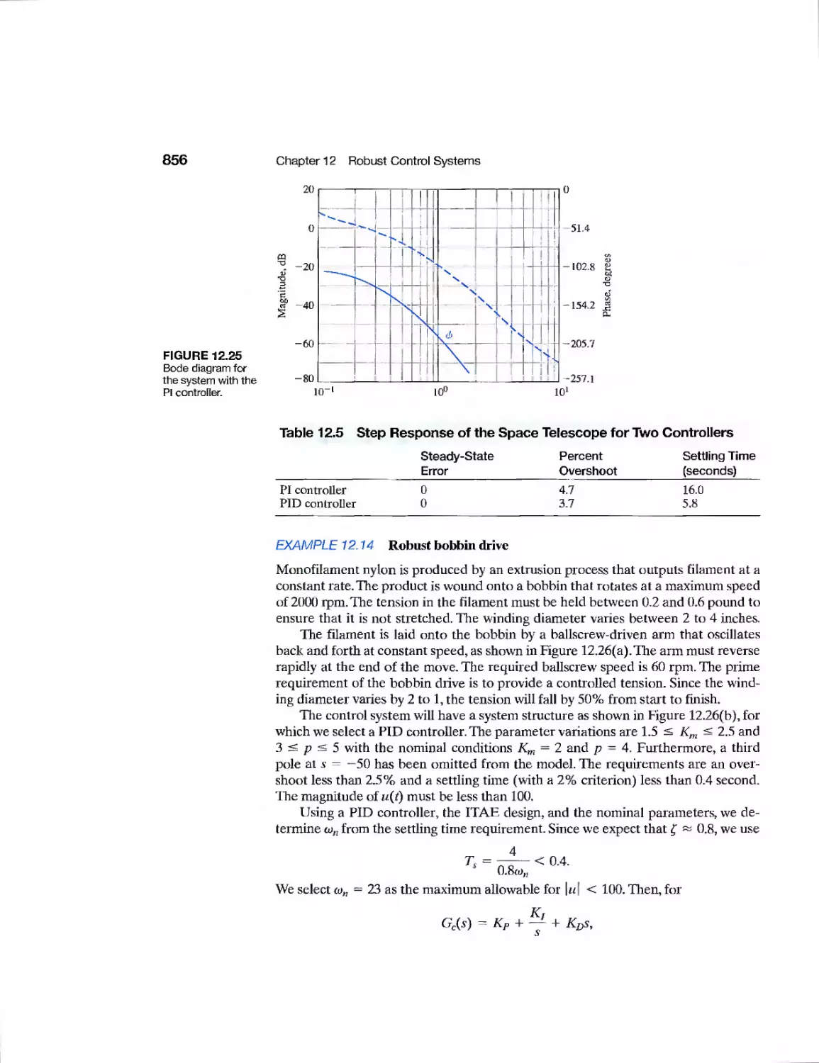
Space Telescope Control
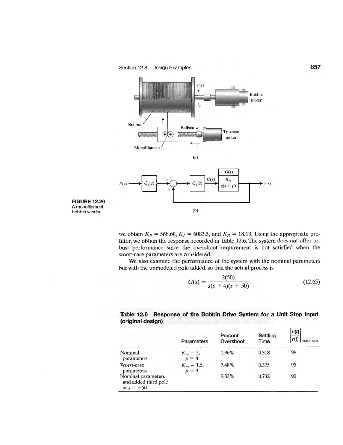
Robust Bobbin Drive
Ultra-Precision Diamond
Turning Machine
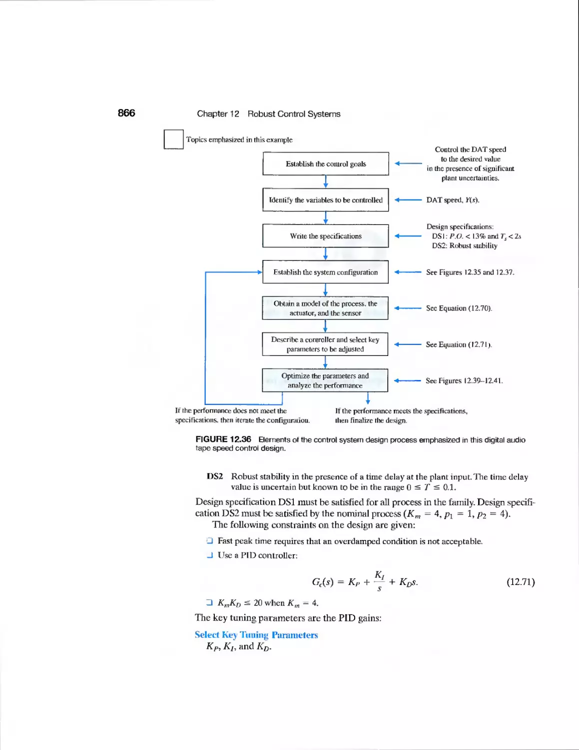
Digital Audio Tape Controller
Disk Drive Read System
CDP12.1 Traction Drive Motor Control
DP12.1
DP12.2
DP12.3
DP12.4
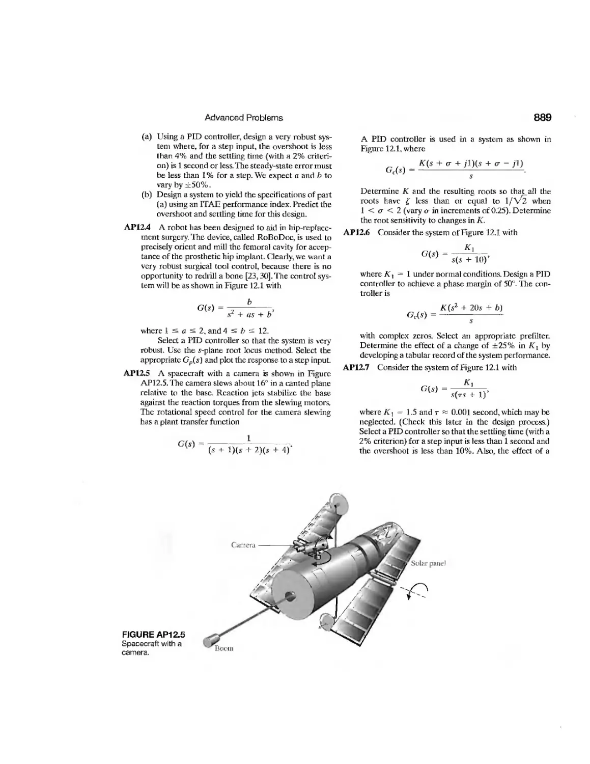
DP12.5
DP12.6
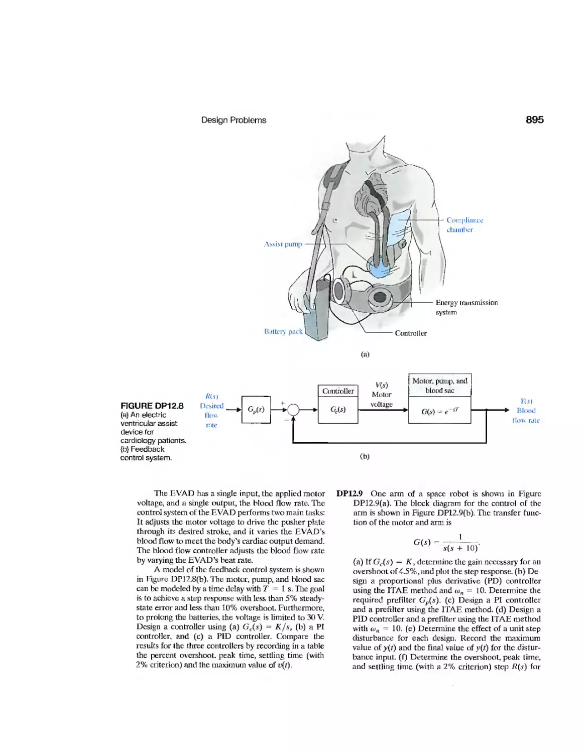
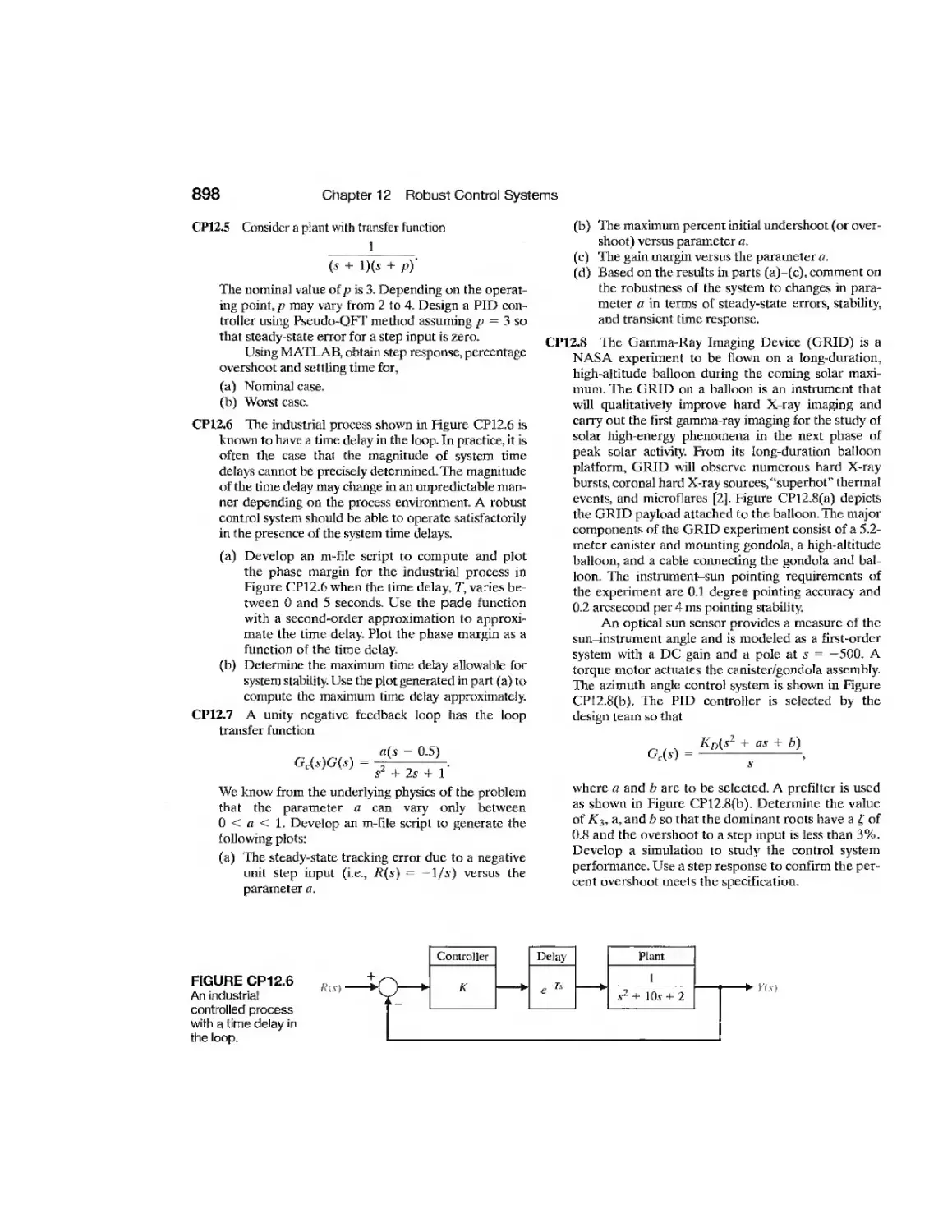
DPI 2.7
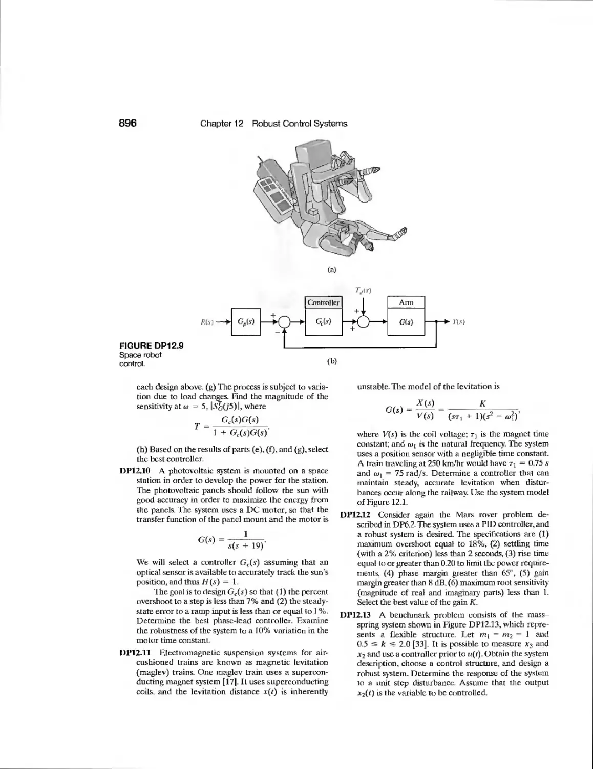
DP12.8
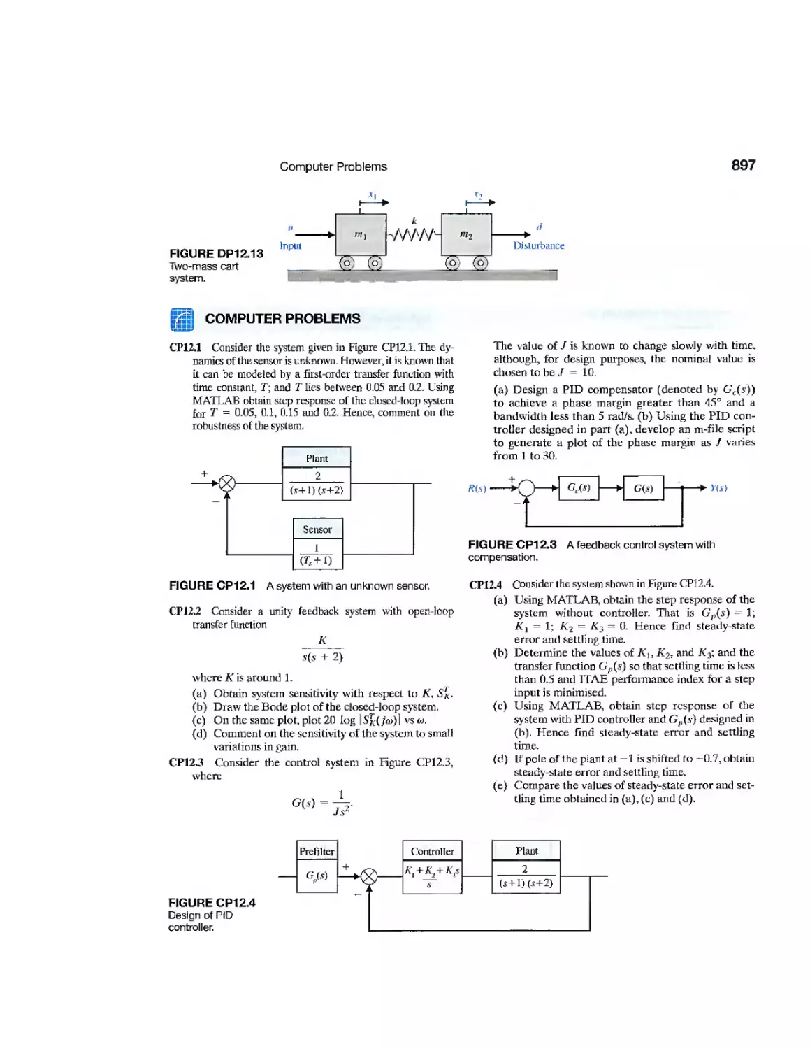
DP12.9
DP12.10
DP12.11
DP12.12
DP12.13
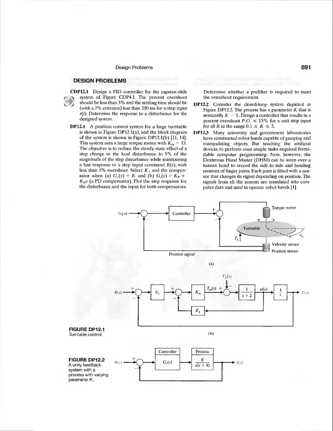
Turntable Position Control
Robust Parameter Design
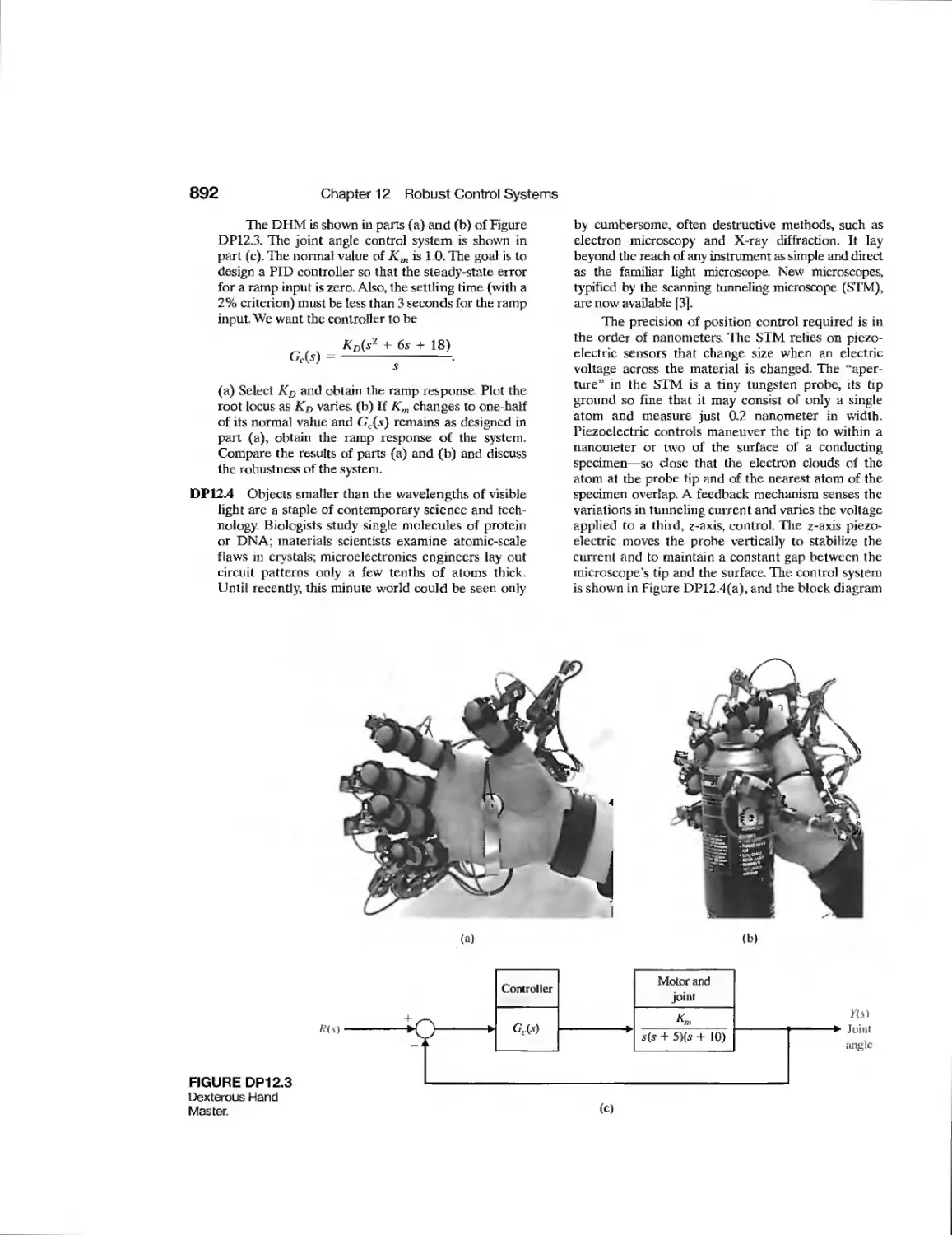
Dexterous Hand Master
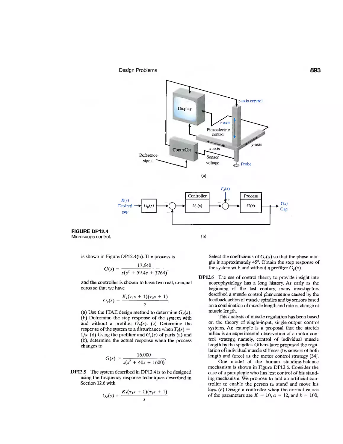
Microscope Control
Microscope Control
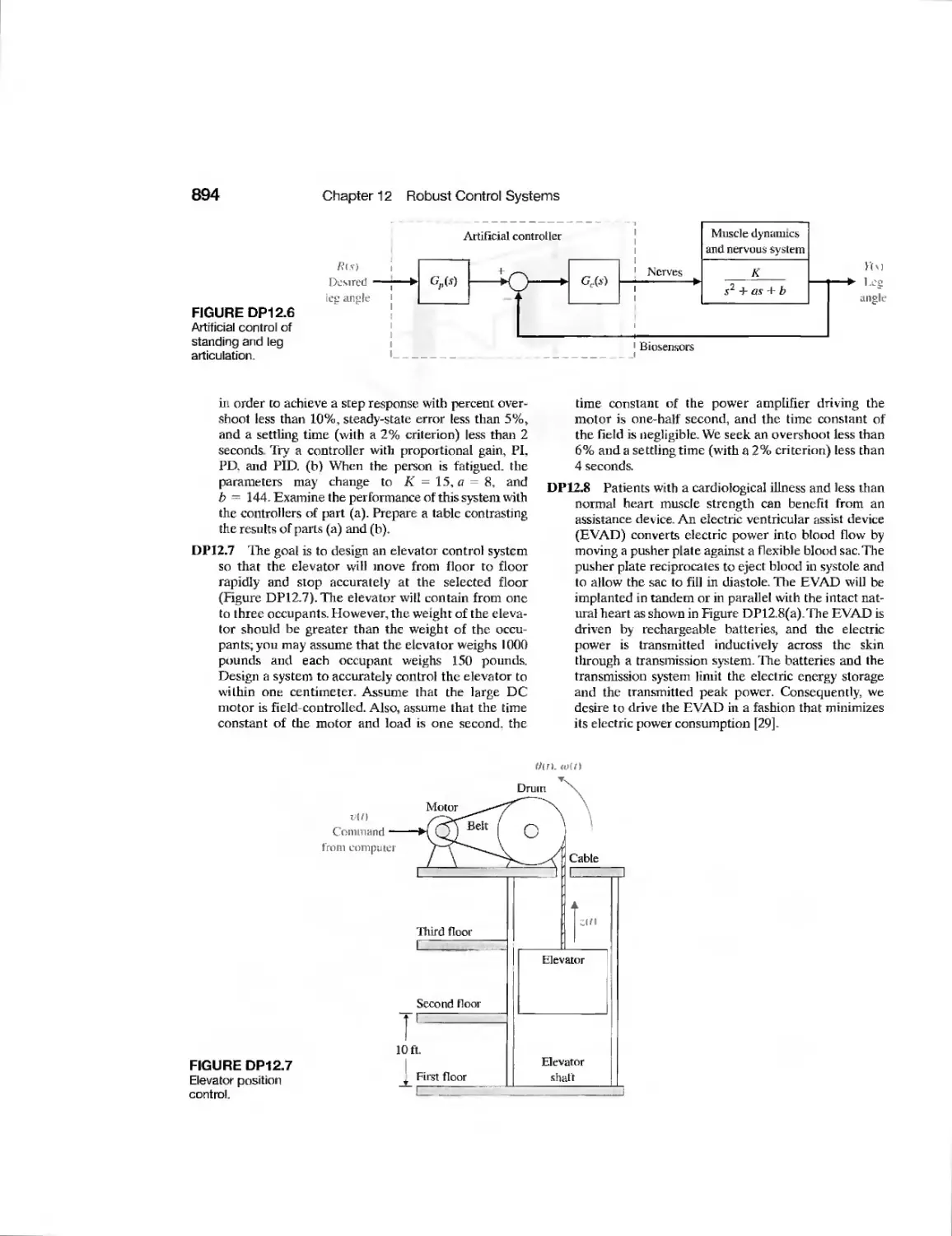
Artificial Control of Leg
Articulation
Elevator Position Control
Electric Ventricular Assist
Device
Space Robot Control
Solar Panel Pointing Control
Magnetically Levitated Train
Mars Guided Vehicle Control
Benchmark Mass-Spring
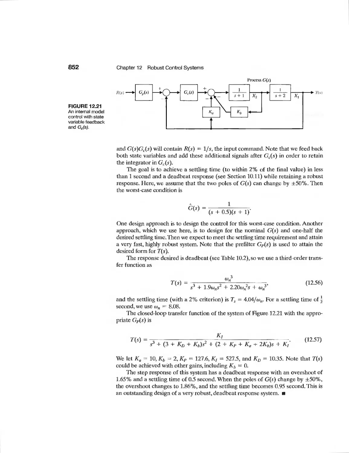
853
853
856
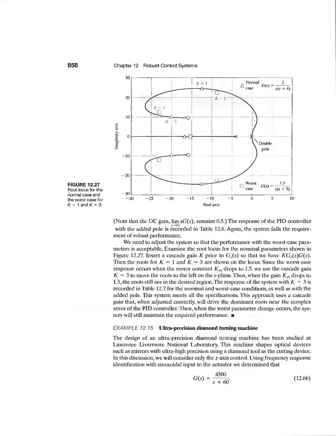
858
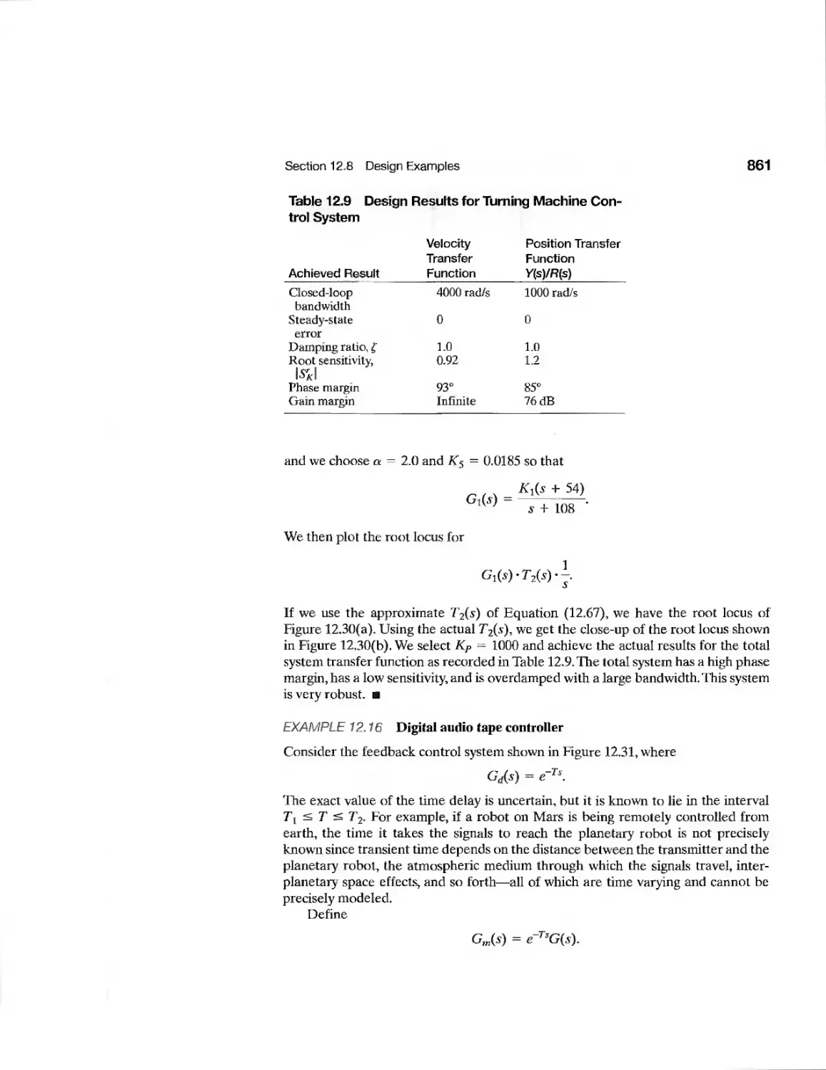
861
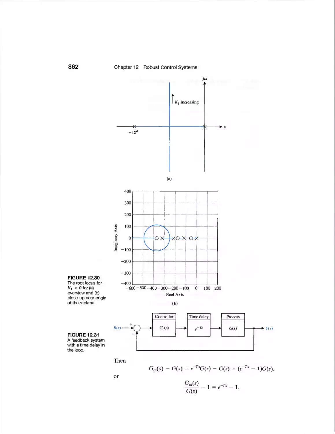
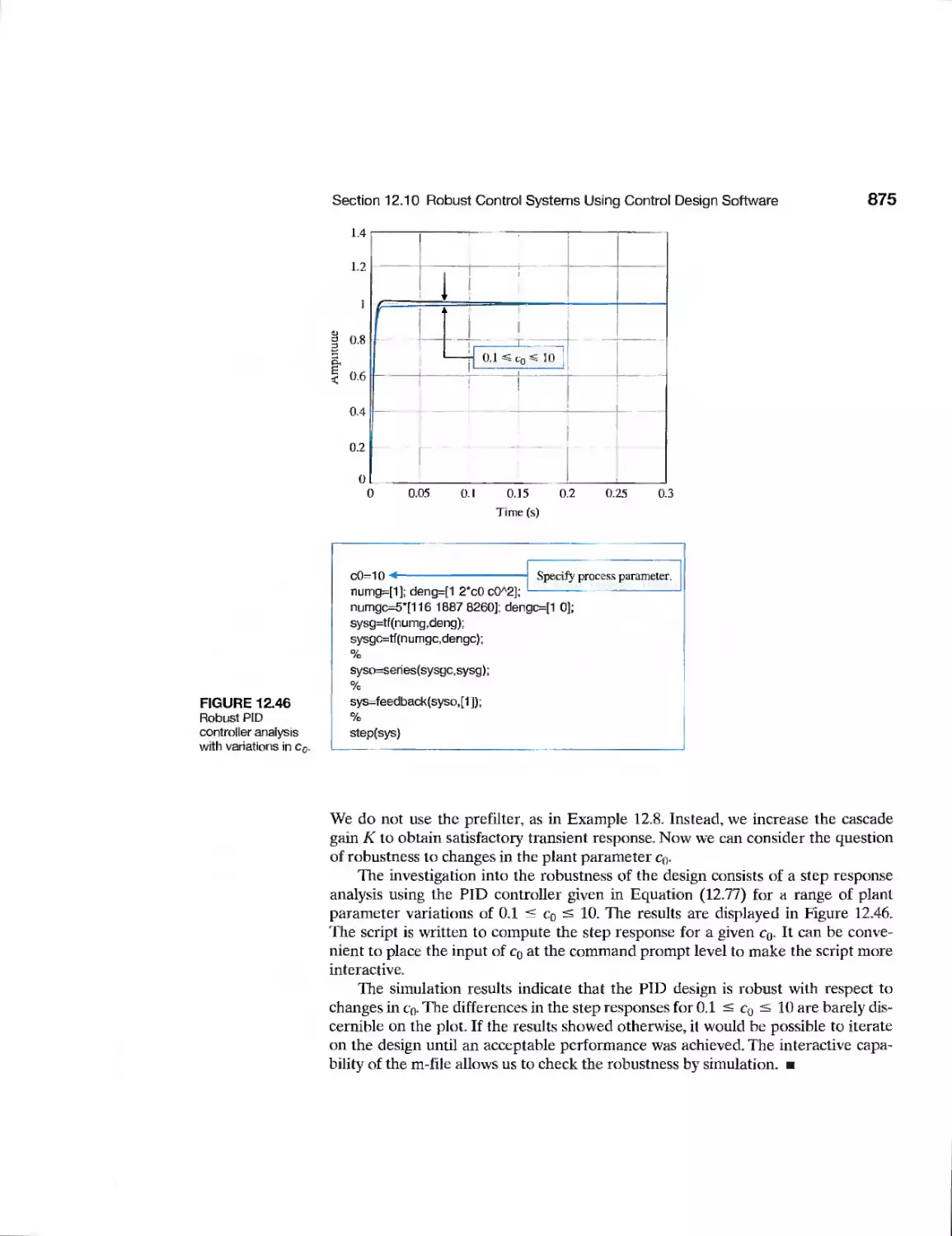
876
891
891
891
891
892
893
893
894
894
895
896
896
896
896
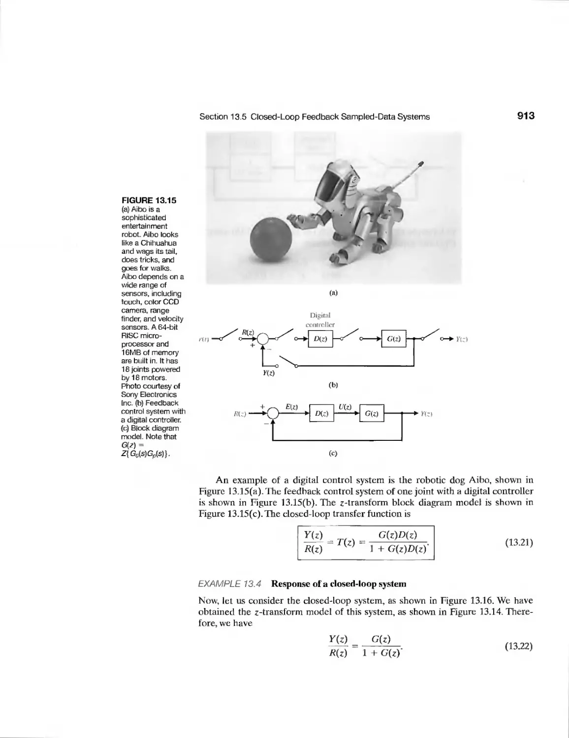
CHAPTER 13
Example
Example
Example
CDP13.1
DP13.1
DP13.2
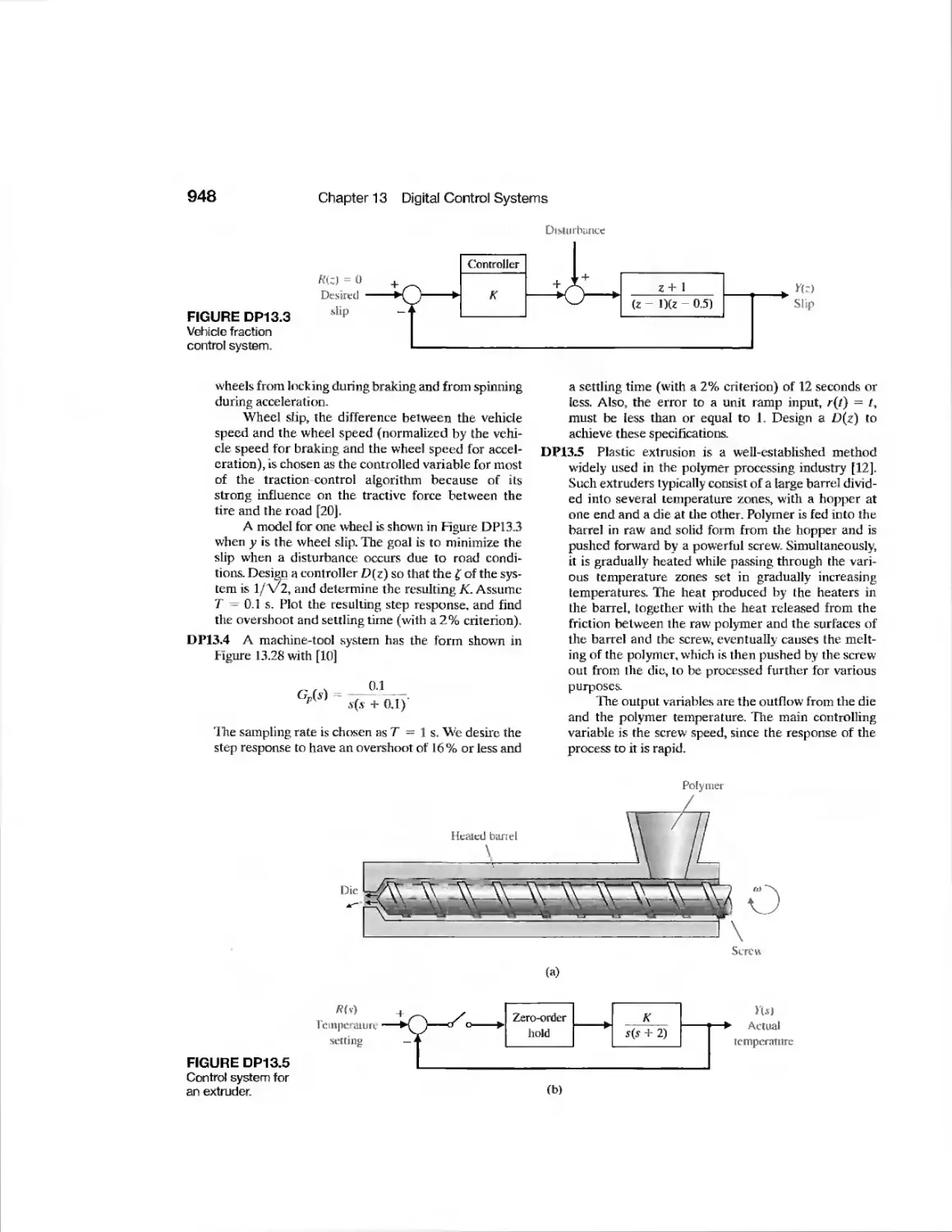
DP13.3
DP13.4
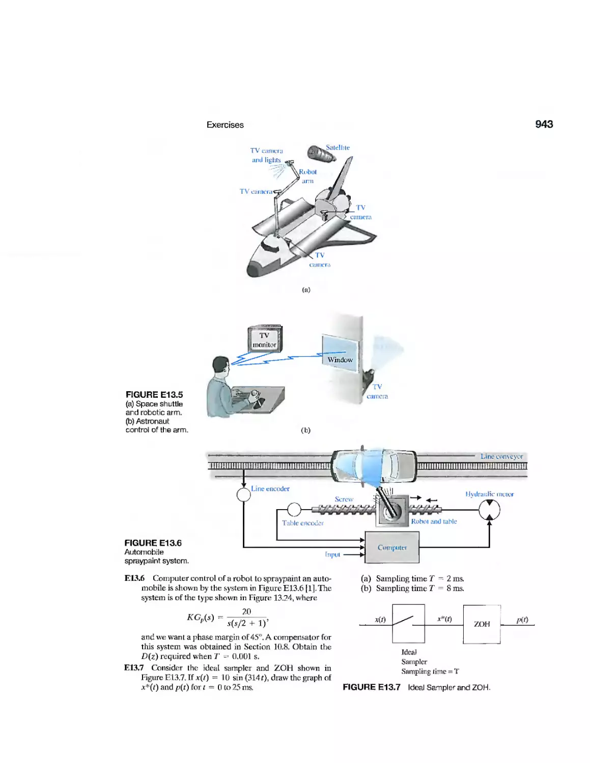
DP13.5
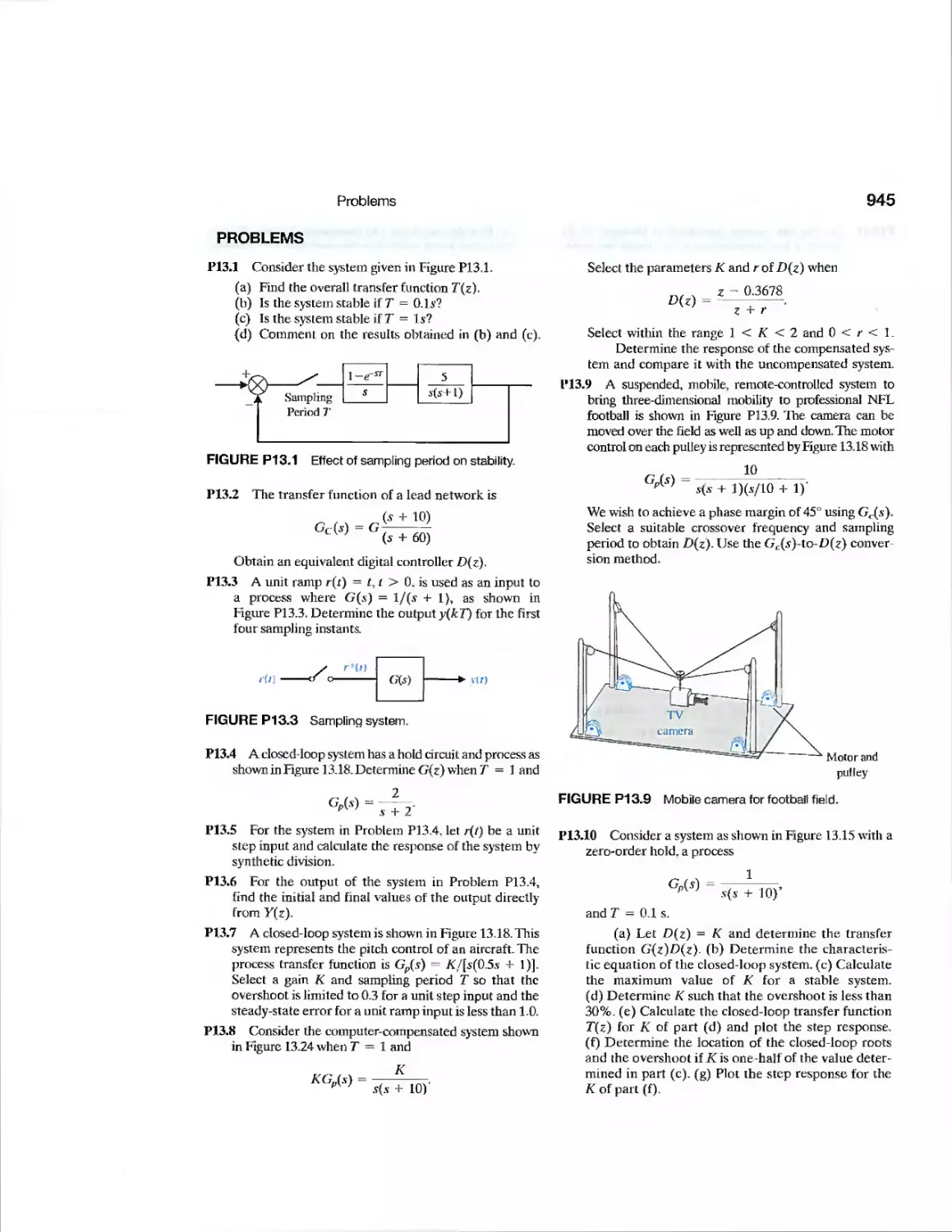
DP13.6
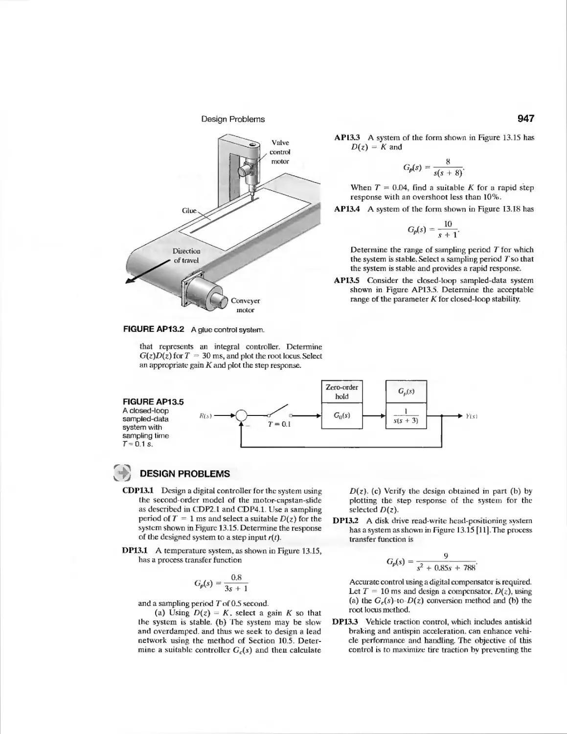
Worktable Motion Control
Fly-by-wire Aircraft Control
Disk Drive Read System
Traction Drive Motor Control
Temperature Control System
Disk Drive Read-Write Head-
Positioning System
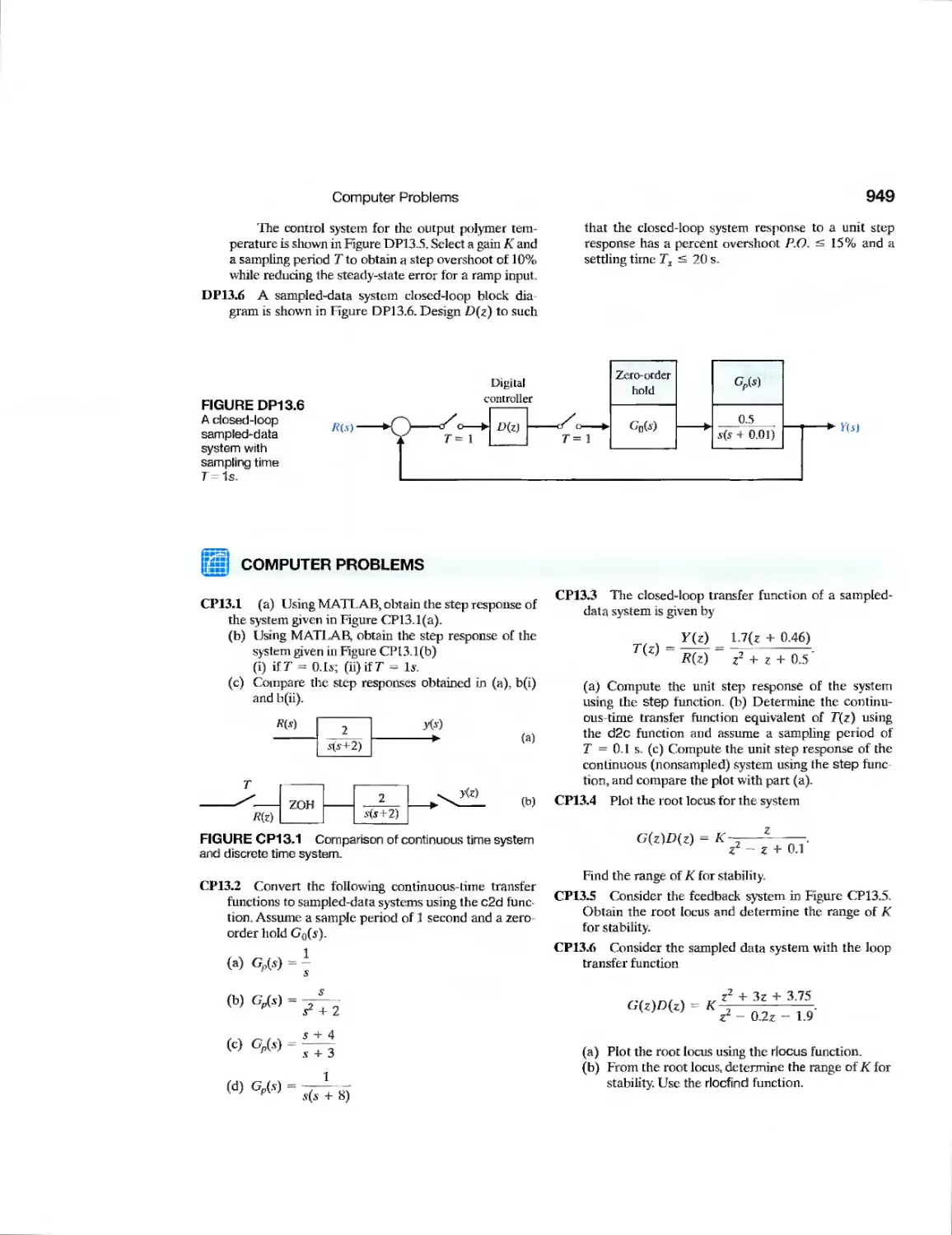
Vehicle Traction Control
Machine-Tool System
Polymer Extruder Control
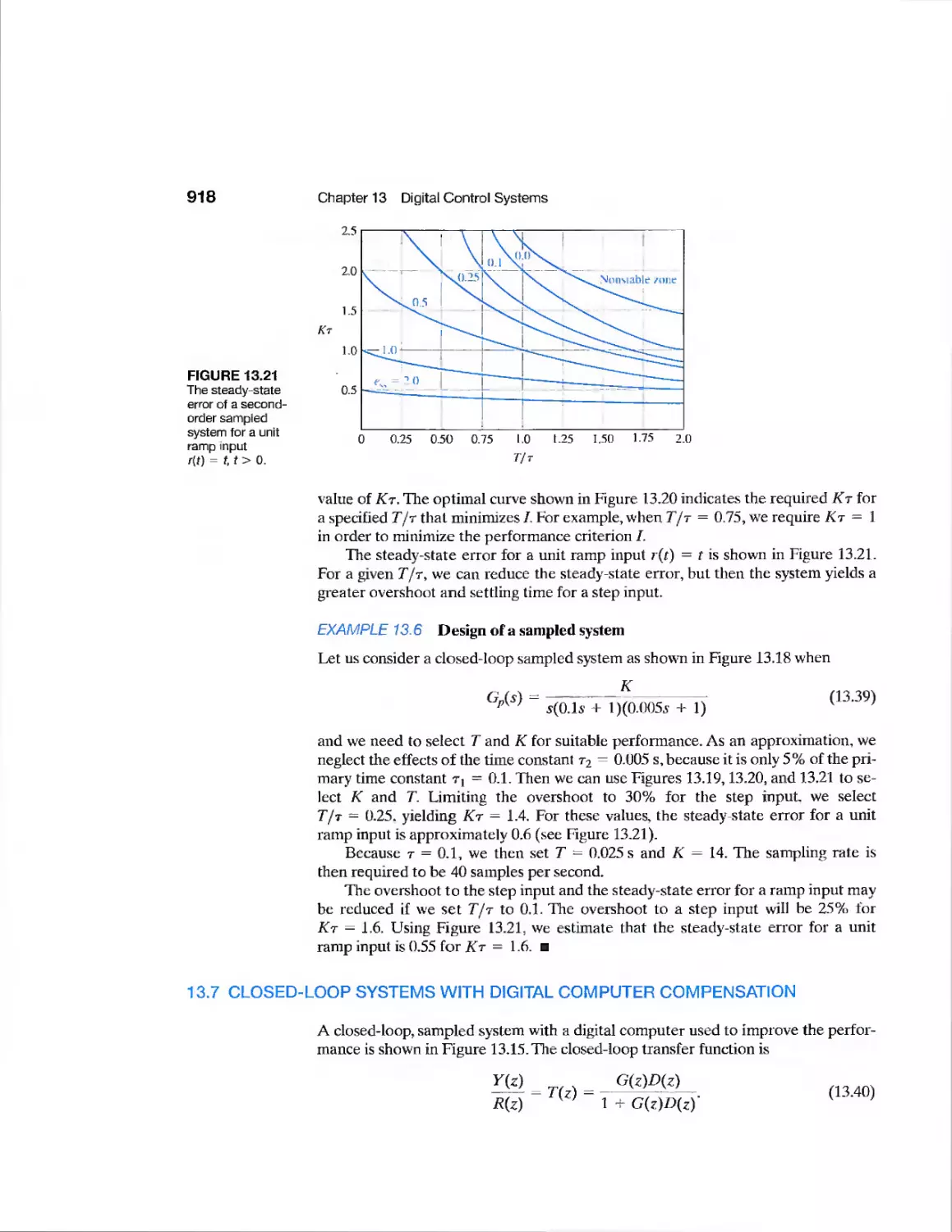
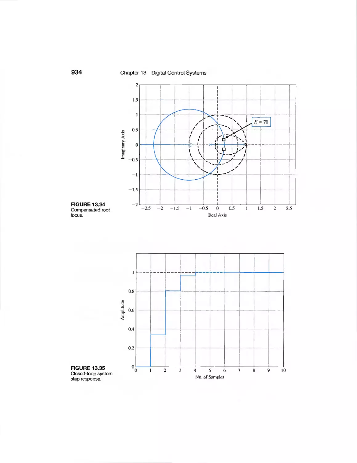
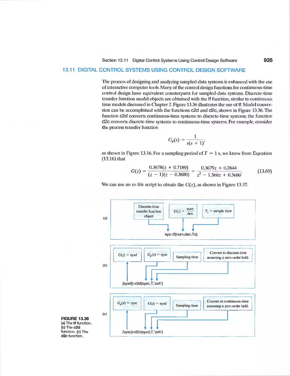
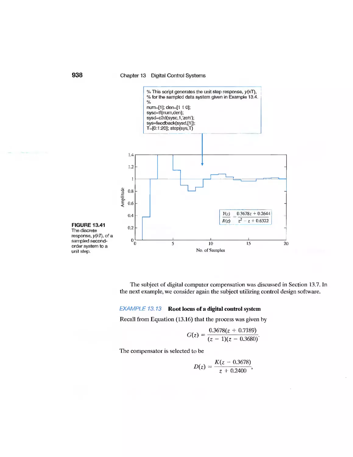
Sampled-Data System
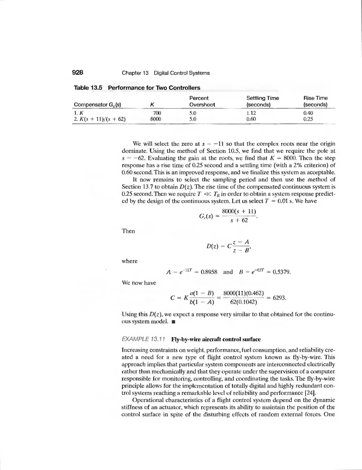
926
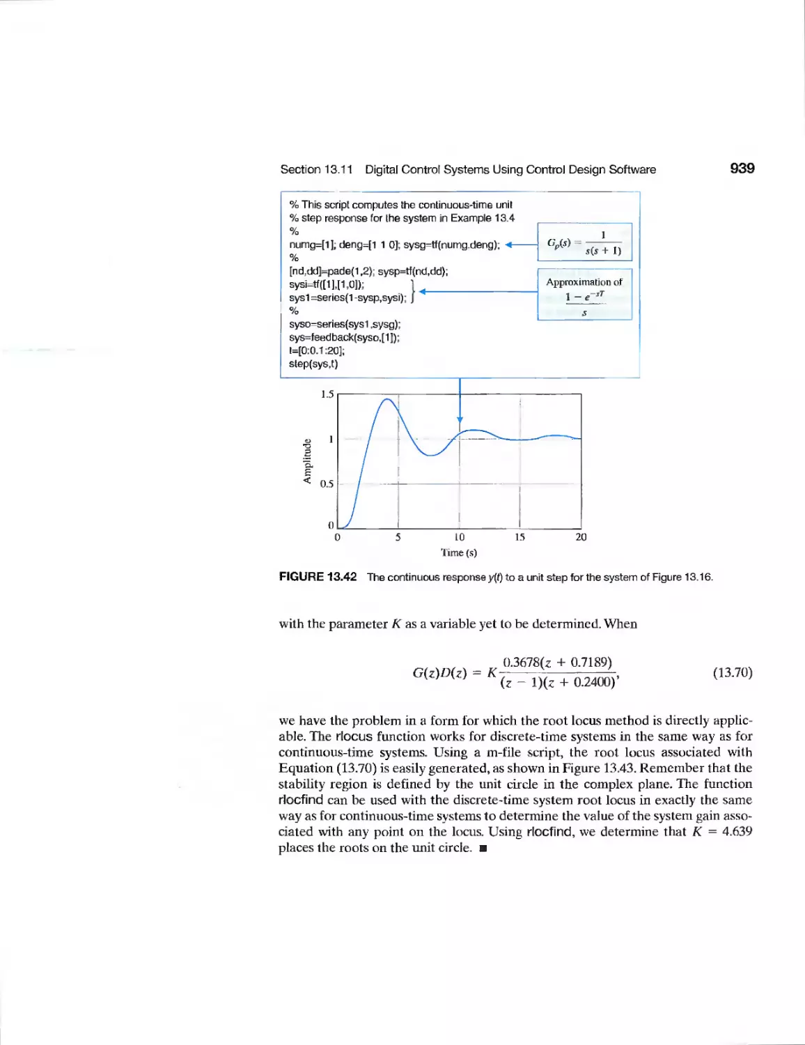
928
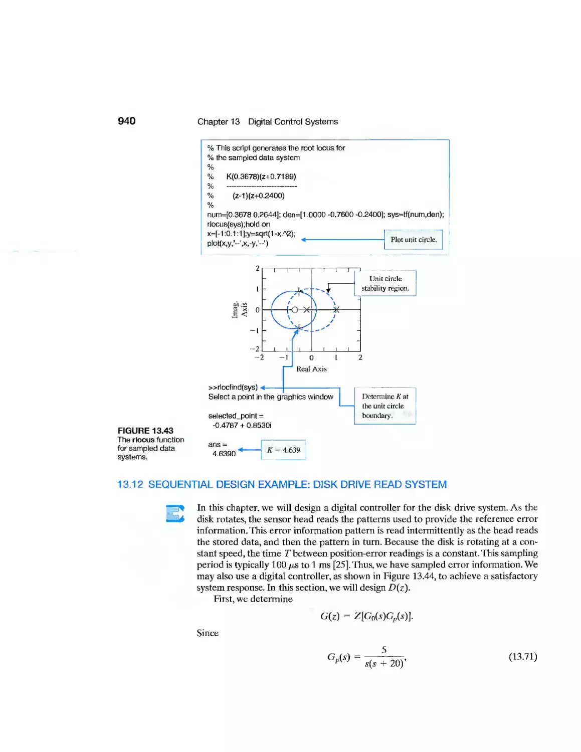
940
947
947
947
947
948
948
948
Modern
Control
ELEVENTH EDITION
Richard C. Dorf
University of California, Davis
Robert H. Bishop
The University of Texas at Austin
PEARSON
Prentice
Hall
Pearson Education International
Systems
If you purchased this book within the United States or Canada you should be aware that it has been wrongfully
imported without the approval of the Publisher or the Author.
Vice President and Editorial Director, ECS: Marcia J. Horton
Acquistions Editor: Michael McDonald
Senior Managing Editor: Scott Disanno
Senior Production Editor: Irwin Zucker
Art Editor: Greg Dulles
Manufacturing Manager: Alexis Heydt-Long
Manufacturing Buyer: Lisa McDowell
Senior Marketing Manager: Tim Galligan
© 2008 Pearson Education, Inc.
Pearson Prentice Hall
Pearson Education, Inc.
Upper Saddle River, NJ 07458
All rights reserved. No part of this book may be reproduced, in any form or by any means, without permission in
writing from the publisher.
Pearson Prentice Hall® is a trademark of Pearson Education, Inc.
Matlab is a registered trademark of The Math Works, Inc., 24 Prime Park Way, Natick, MA 01760-1520
The author and publisher of this book have used their best efforts in preparing this book. These efforts include the
development, research, and testing of the theories and programs to determine their effectiveness. The author and
publisher make no warranty of any kind, expressed or implied, with regard to these programs or the
documentation contained in this book. The author and publisher shall not be liable in any event for incidental or
consequential damages in connection with, or arising out of, the furnishing, performance, or use of these programs.
Printed in Singapore
10 987654321
ISBN 0-13-e0b?lD-2
tnA-D-13-2Qb710-E
Pearson Education Ltd., London
Pearson Education Australia Pty. Ltd., Sydney
Pearson Education Singapore, Pte. Ltd.
Pearson Education North Asia Ltd., Hong Kong
Pearson Education Canada, Inc., Toronto
Pearson Education de Mexico, S.A. de C.V.
Pearson Education—Japan, Tokyo
Pearson Education Malaysia, Pte. Ltd.
Pearson Education, Inc., Upper Saddle River, New Jersey
PEARSON
Prentice
Hal!
Of the greater teachers-
when they are gone,
their students will say:
we did it ourselves.
Dedicated to
Lynda Ferrera Bishop
and
Joy MacDonald Dorf
In grateful appreciation
Contents
Preface xiii
About the Authors xxv
chapter 1 Introduction to Control Systems 1
1.1 Introduction 2
1.2 Brief History of Automatic Control 4
1.3 Examples of Control Systems 8
1.4 Engineering Design 16
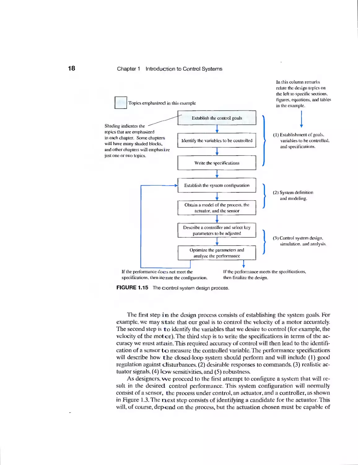
1.5 Control System Design 17
1.6 Mechatronic Systems 20
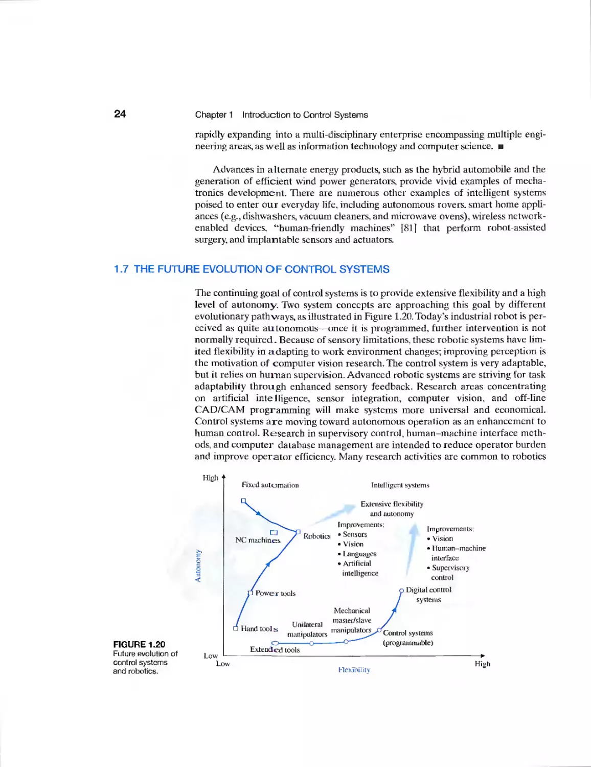
1.7 The Future Evolution of Control Systems 24
1.8 Design Examples 25
1.9 Sequential Design Example: Disk Drive Read System 28
1.10 Summary 30
Exercises 30
Problems 31
Advanced Problems 36
Design Problems 38
Terms and Concepts 39
chapter 2 Mathematical Models of Systems 41
2.1 Introduction 42
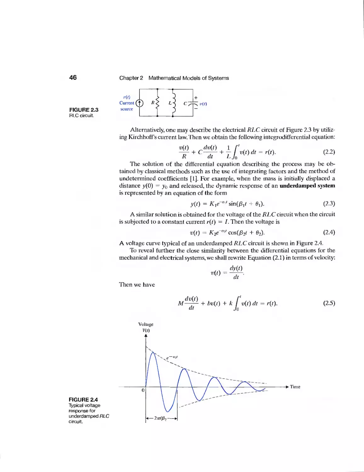
2.2 Differential Equations of Physical Systems 42
2.3 Linear Approximations of Physical Systems 47
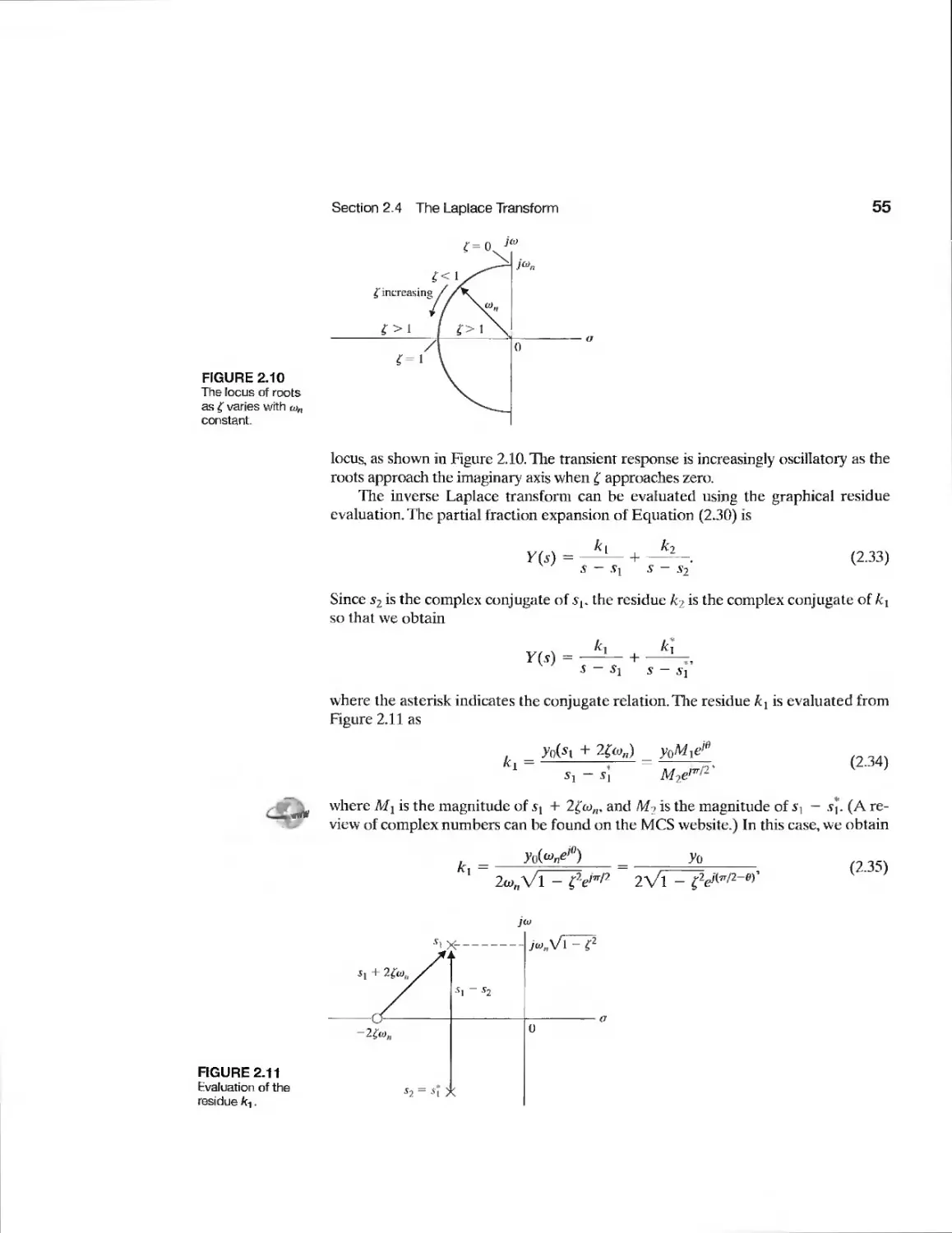
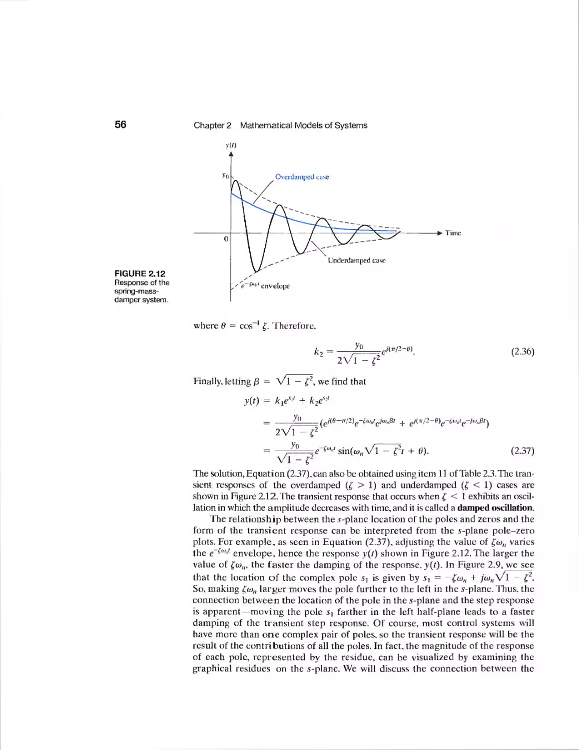
2.4 The Laplace Transform 50
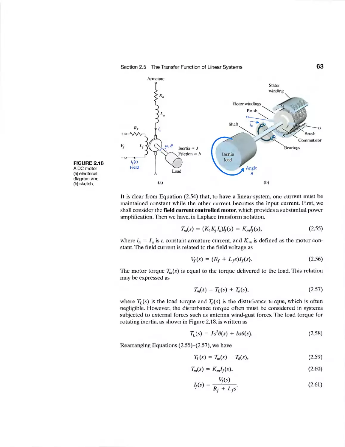
2.5 The Transfer Function of Linear Systems 57
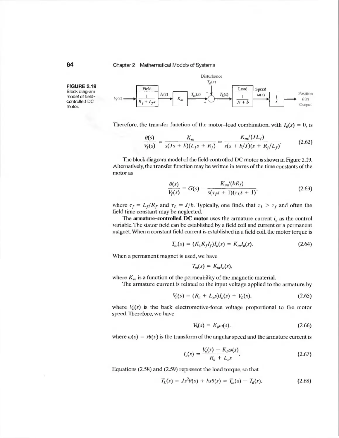
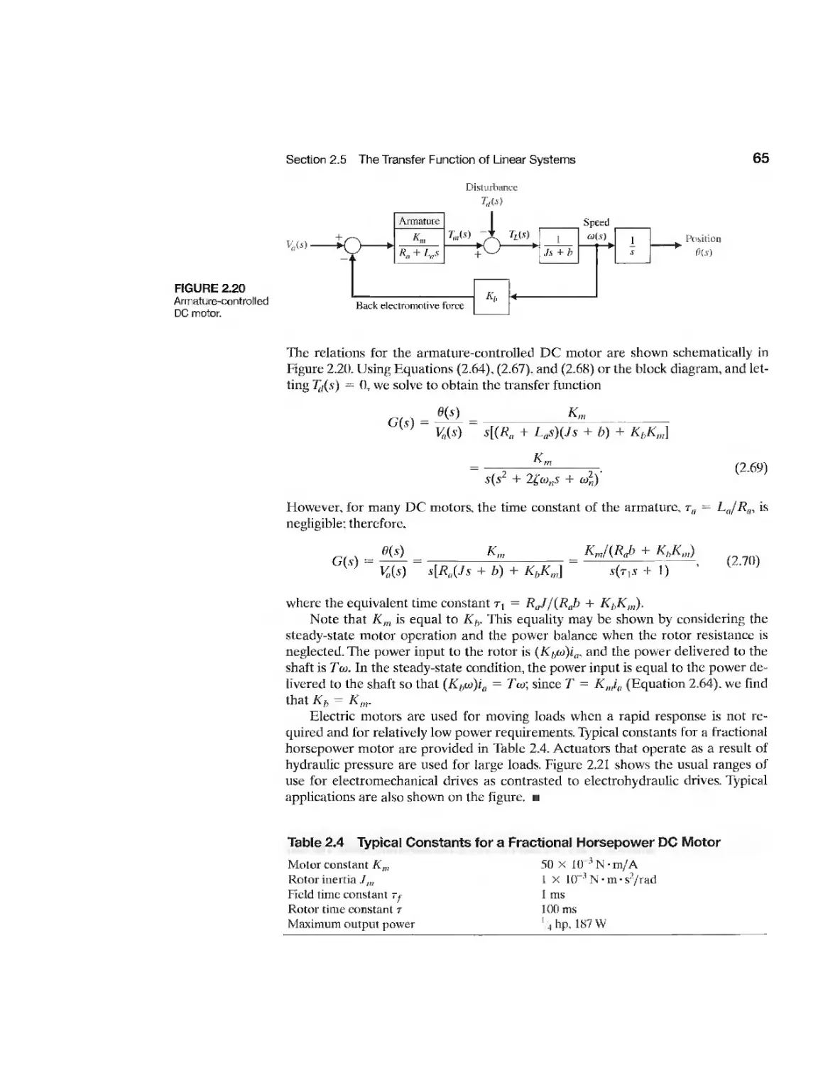
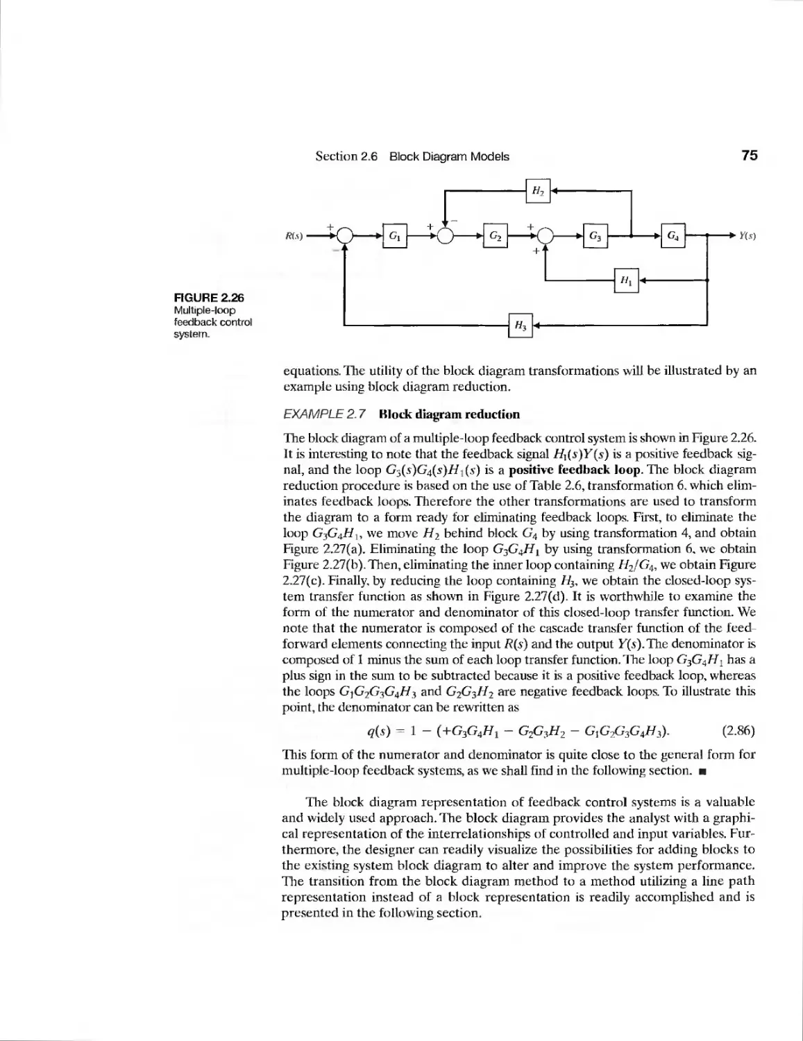
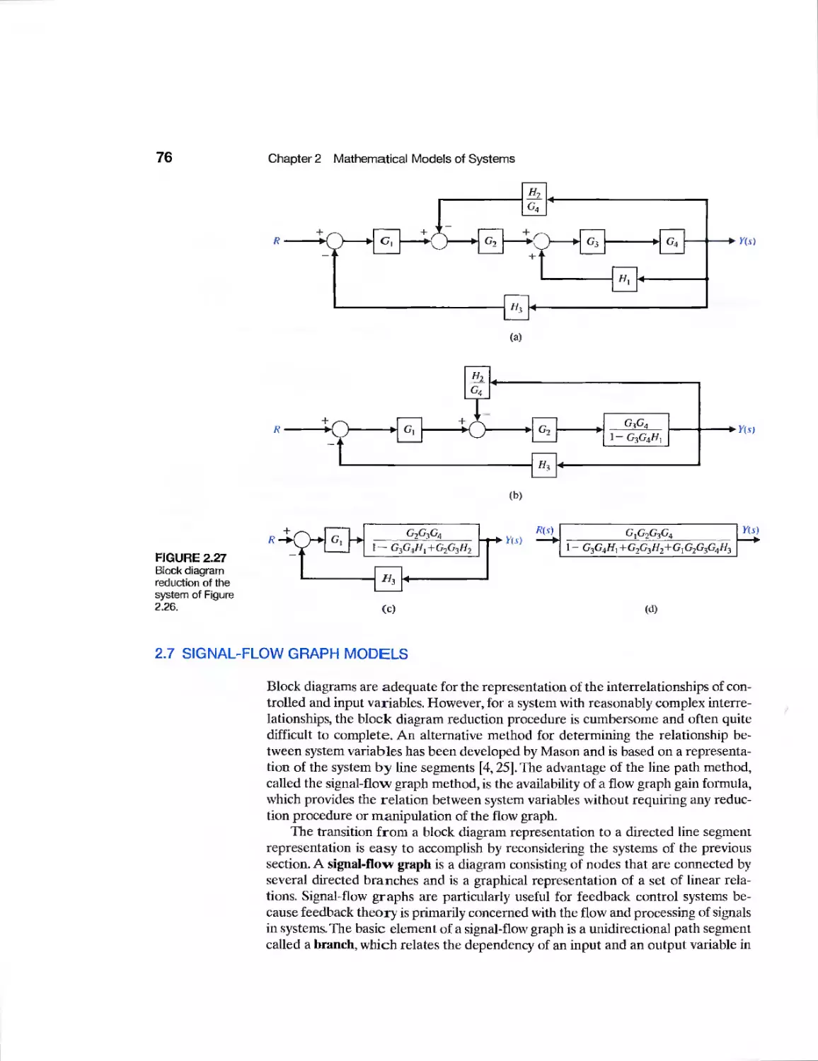
2.6 Block Diagram Models 71
2.7 Signal-Flow Graph Models 76
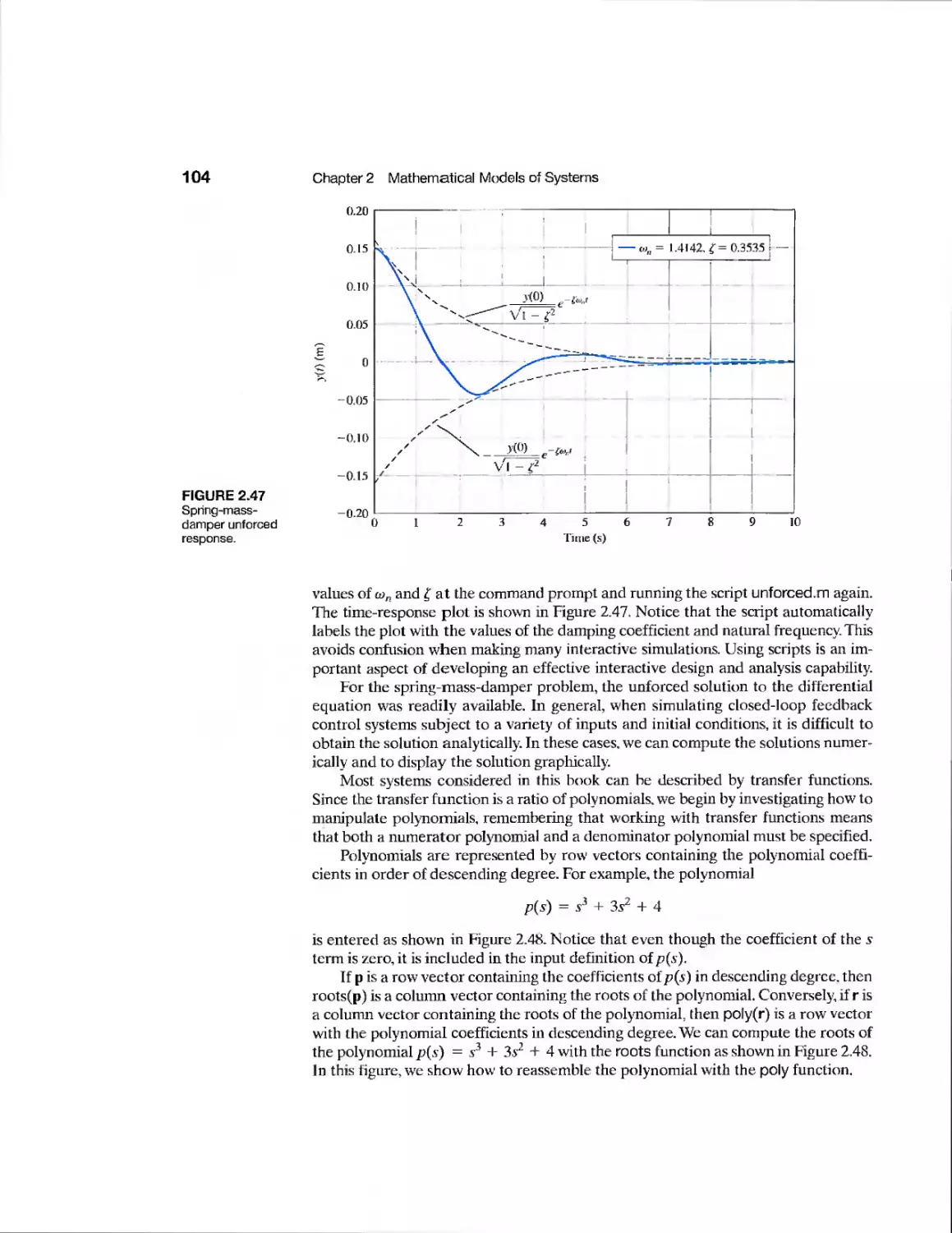
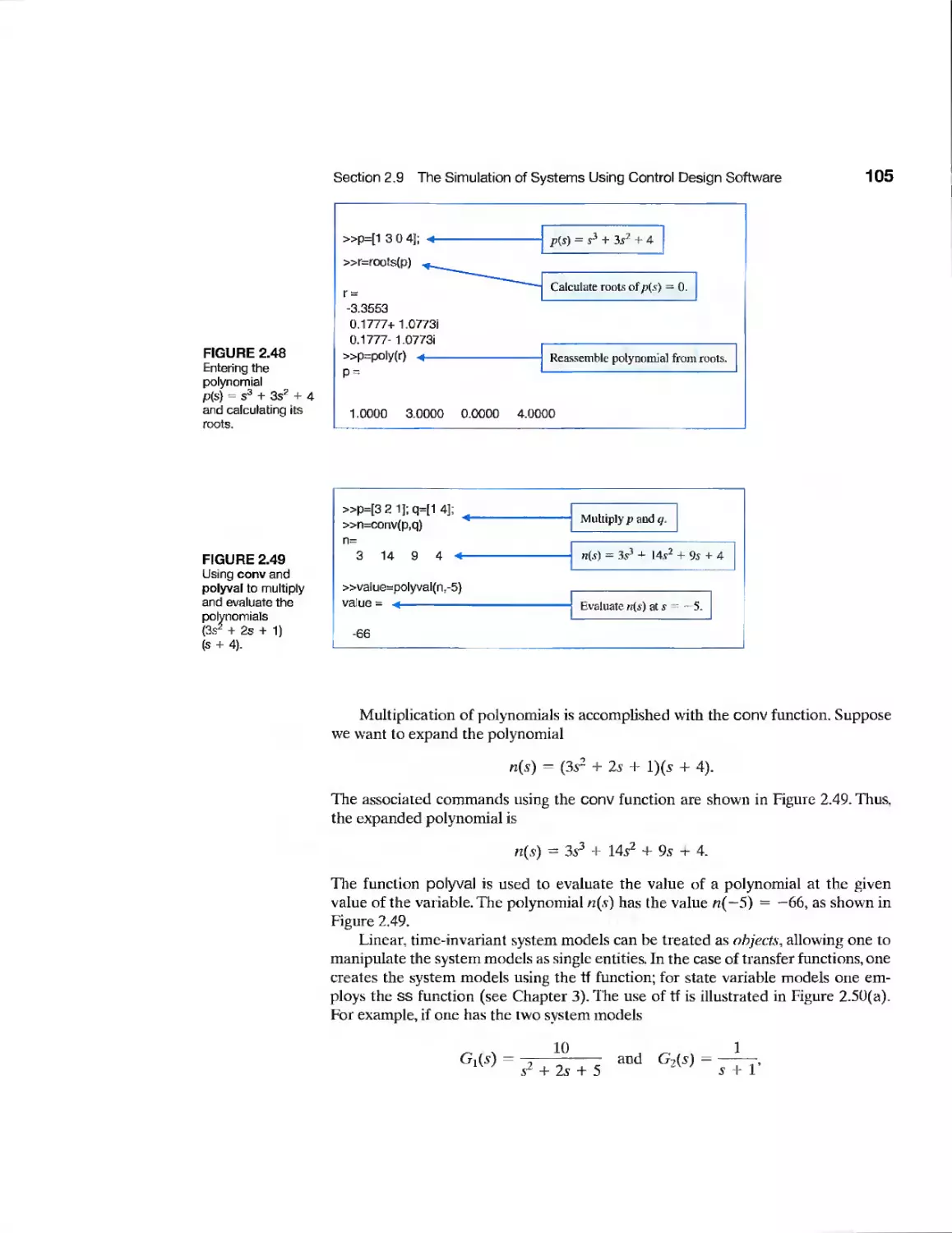
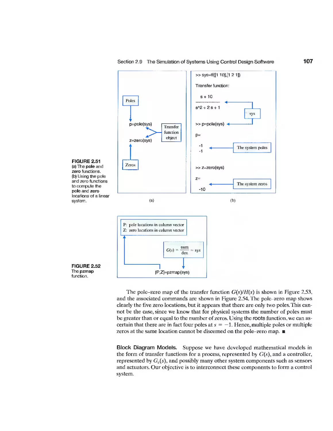
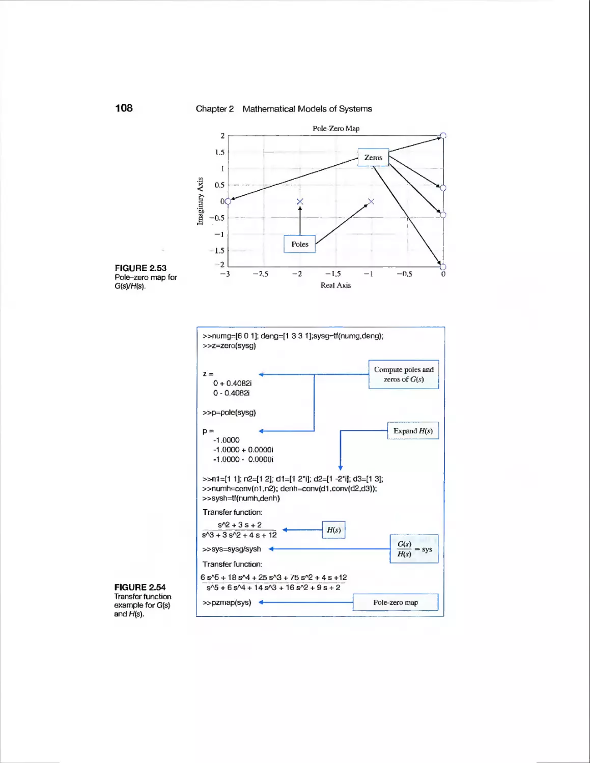
2.8 Design Examples 82
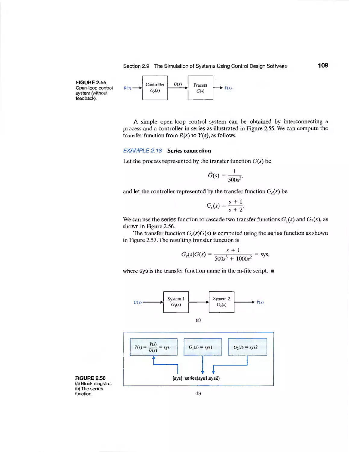
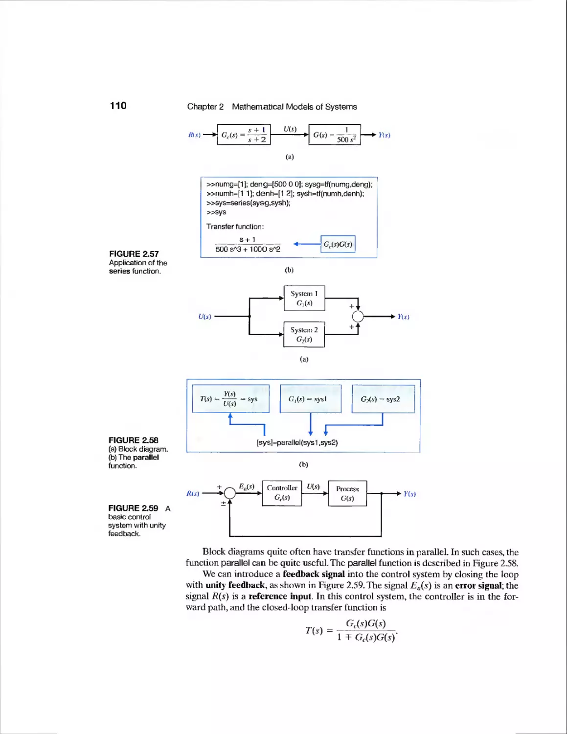
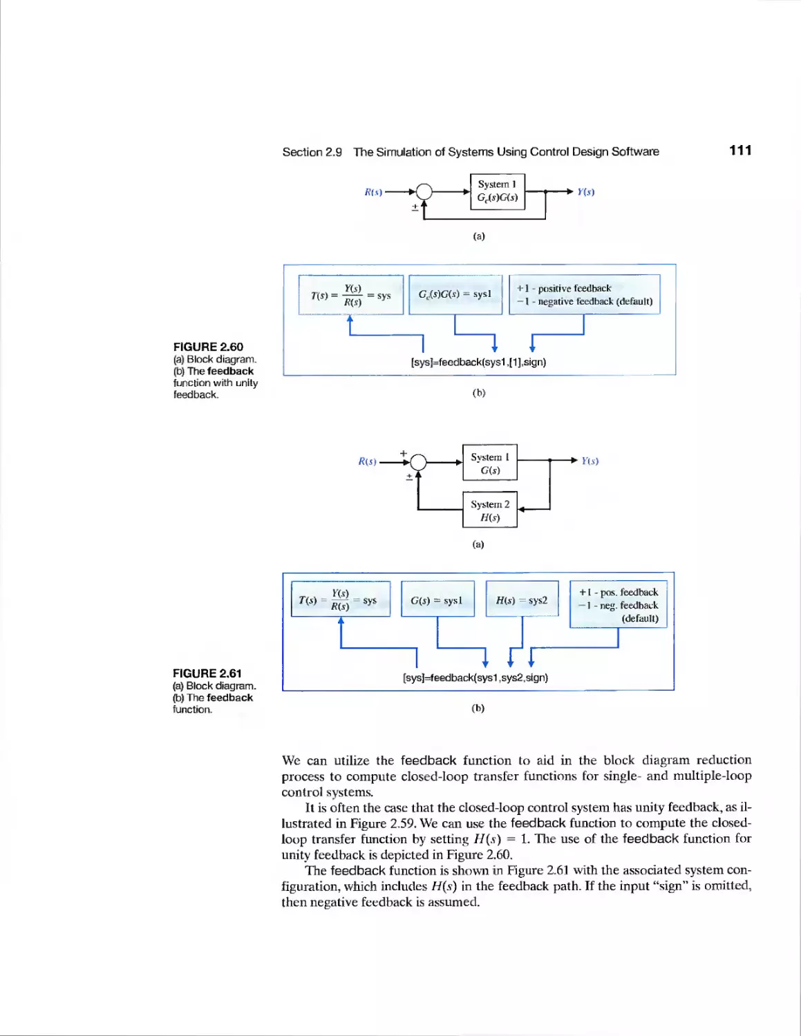
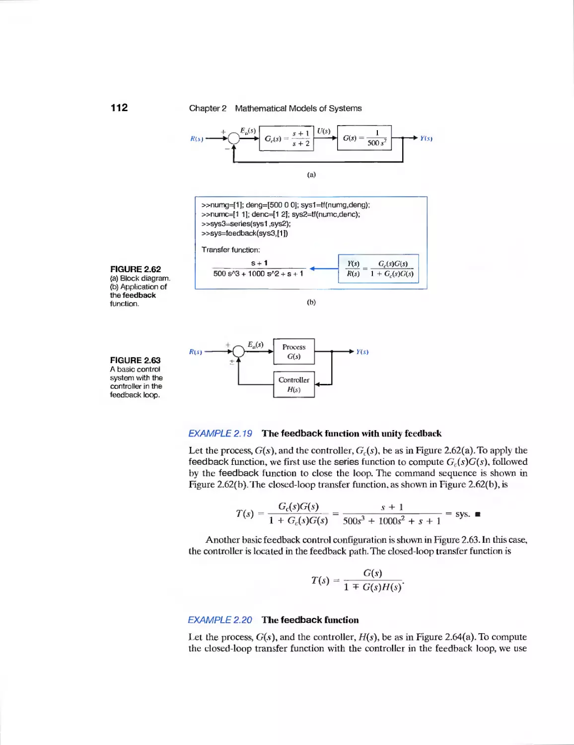
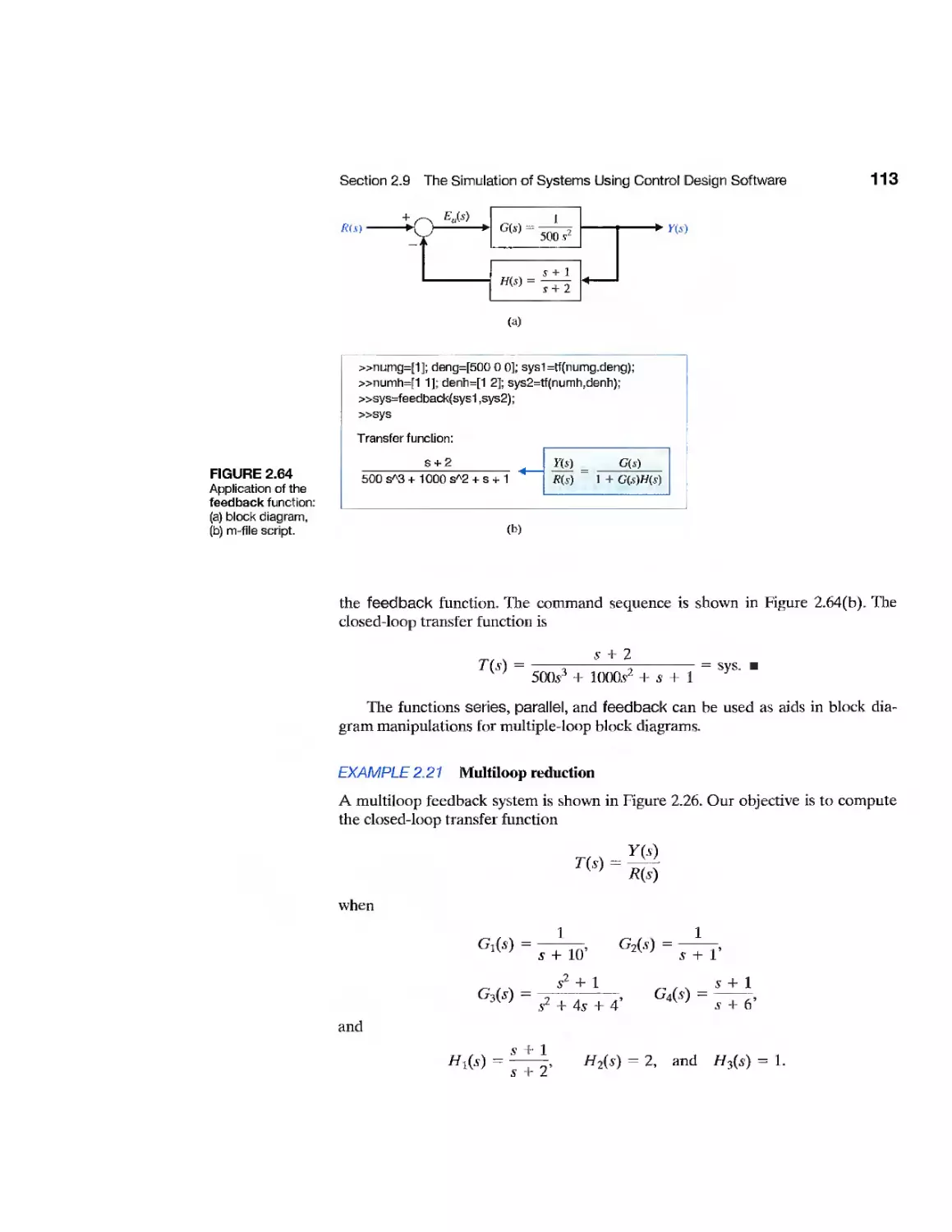
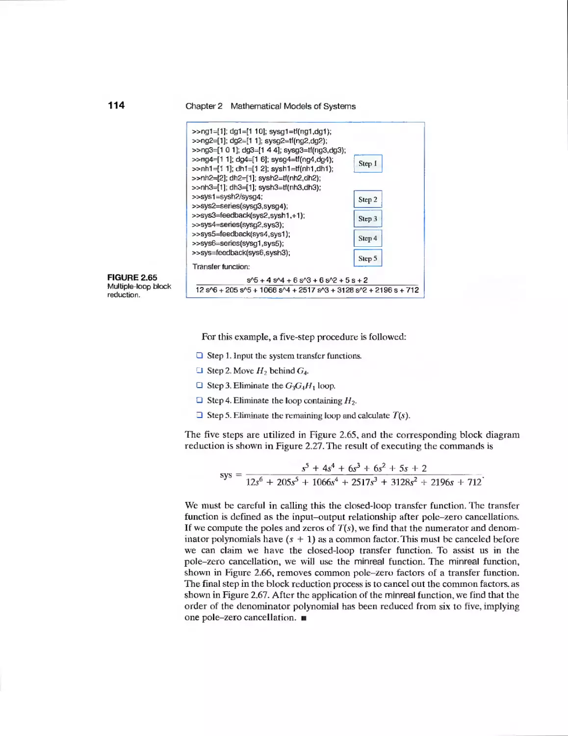
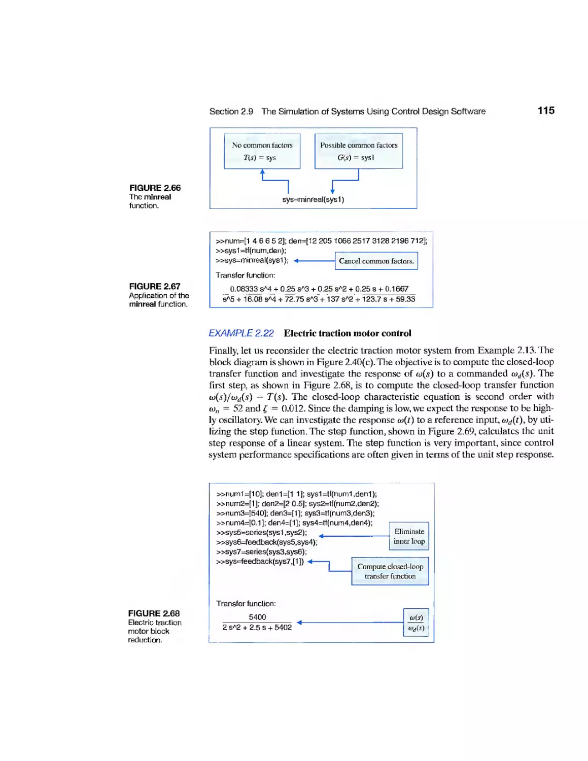
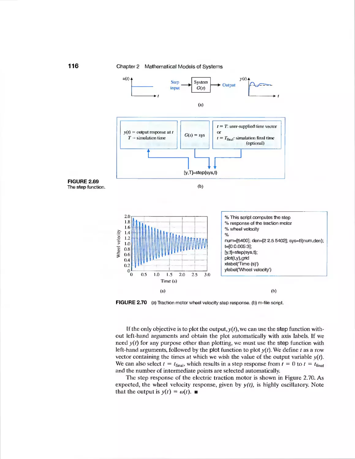
2.9 The Simulation of Systems Using Control Design Software 102
2.10 Sequential Design Example: Disk Drive Read System 117
2.11 Summary 119
Exercises 120
Problems 126
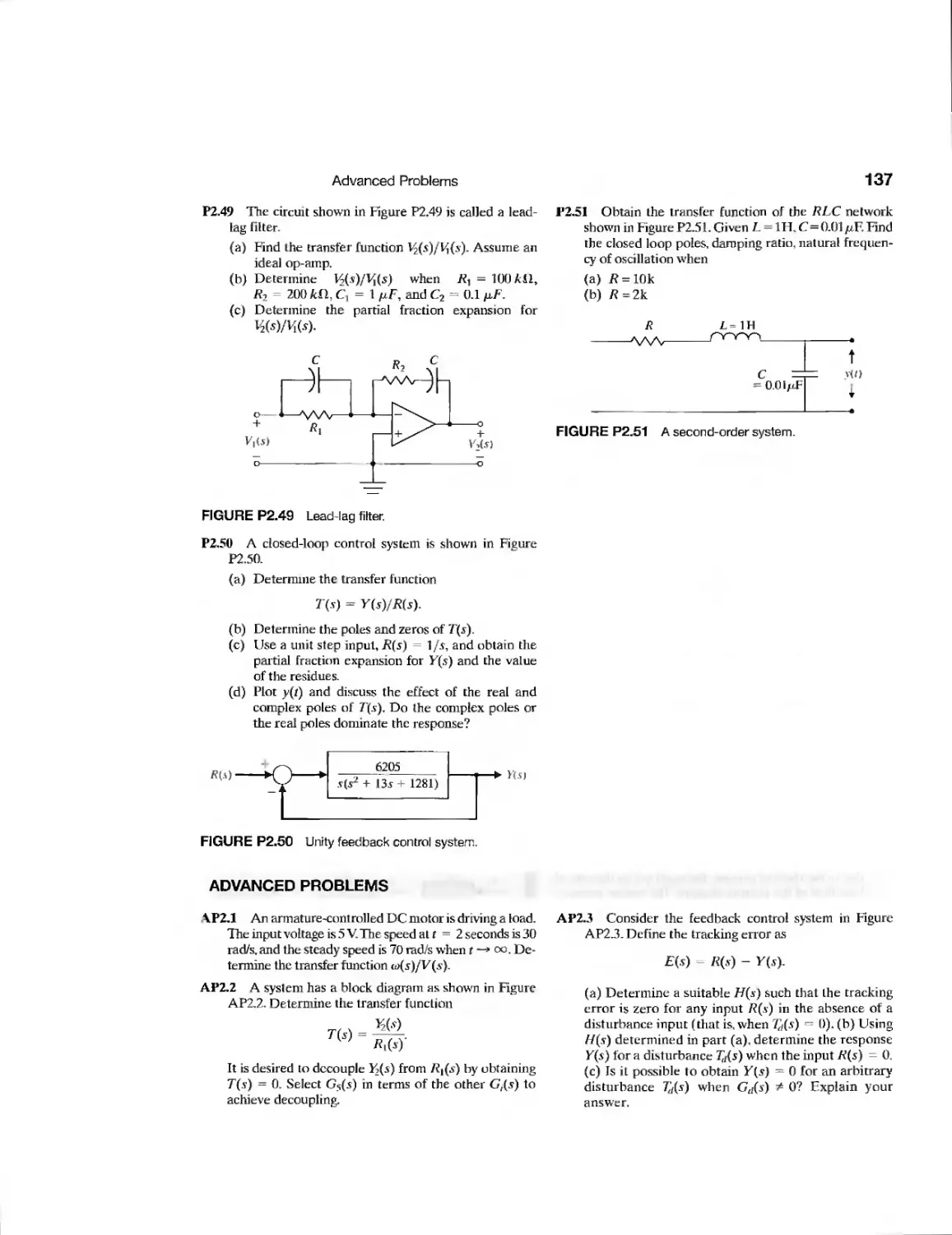
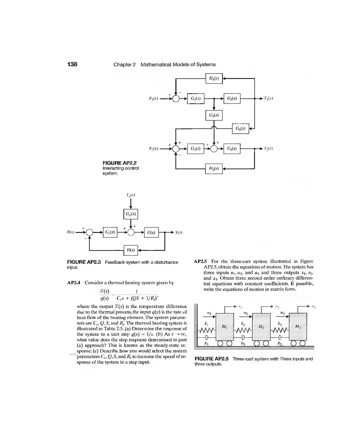
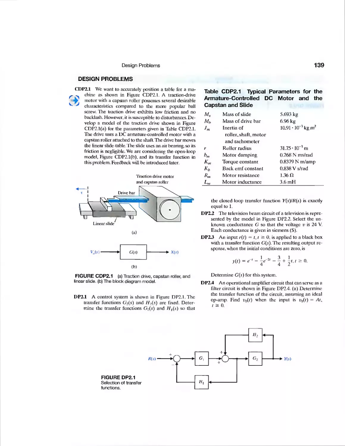
Advanced Problems 137
Design Problems 139
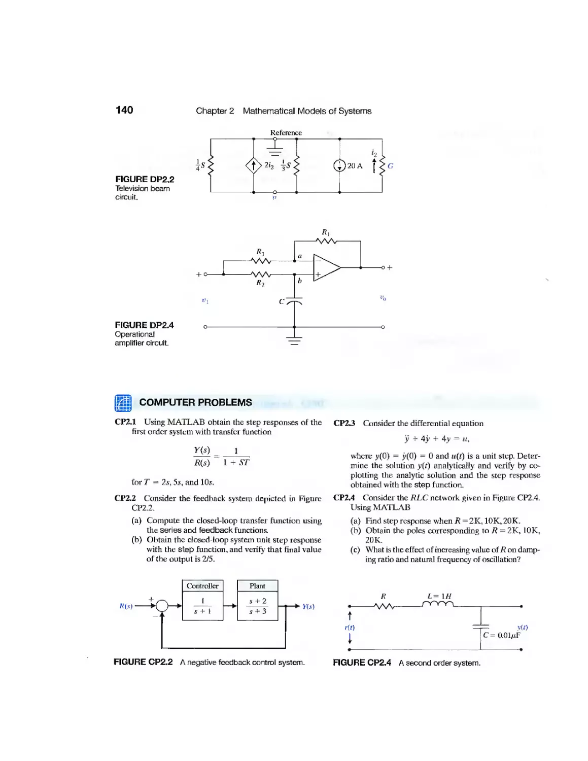
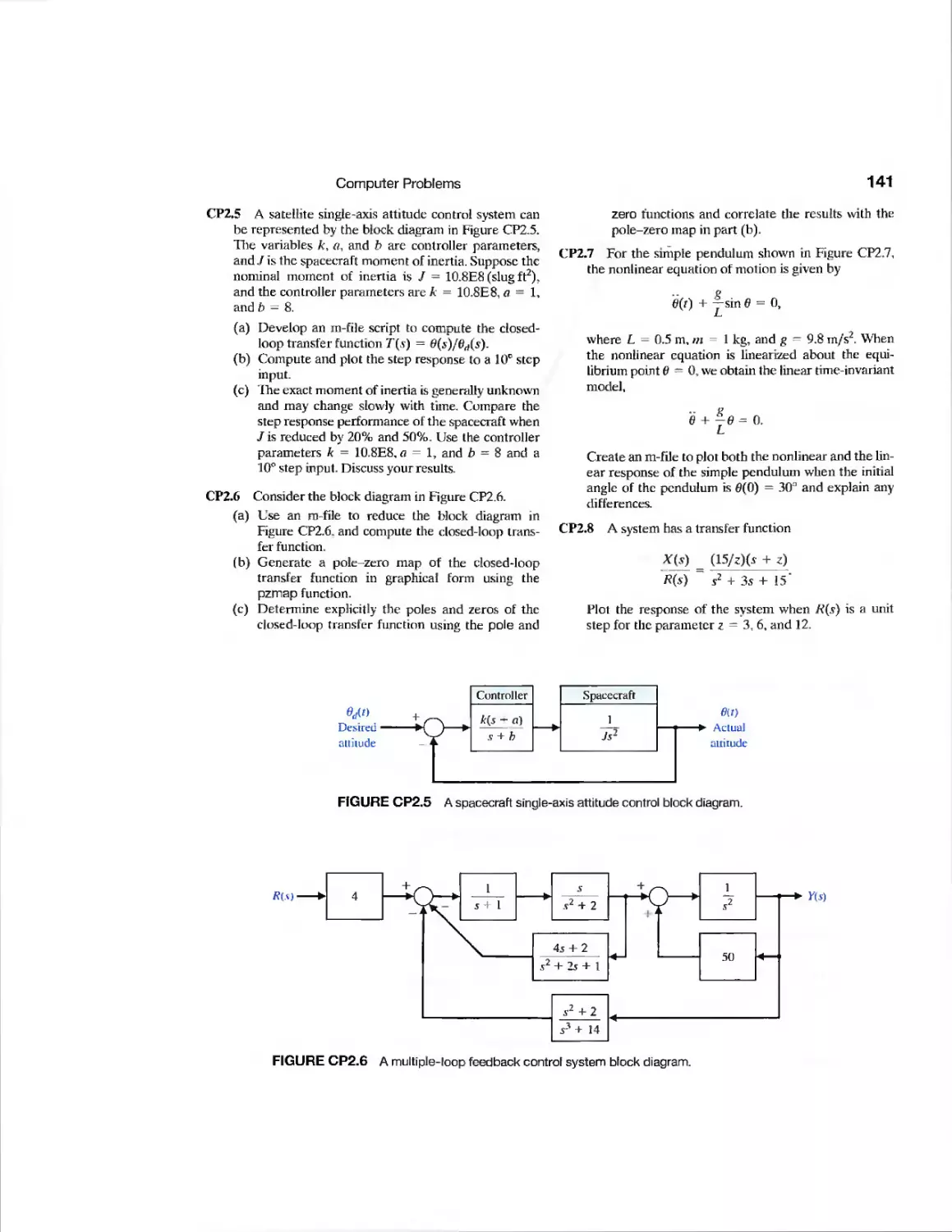
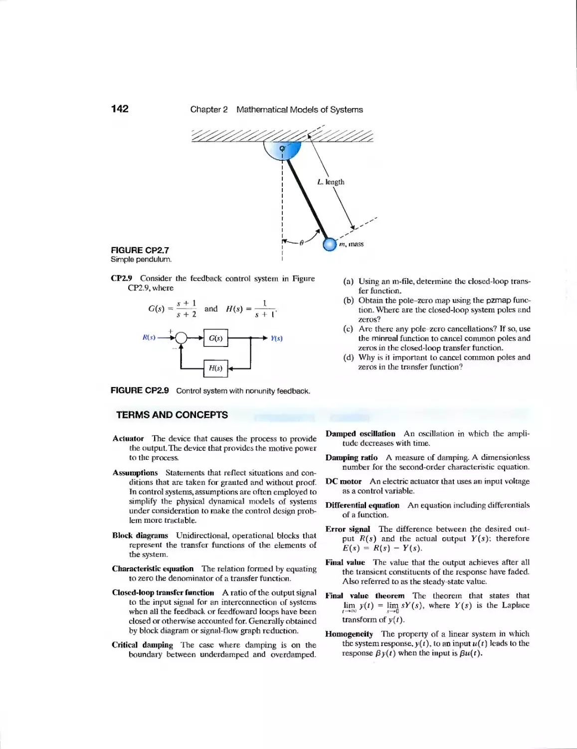
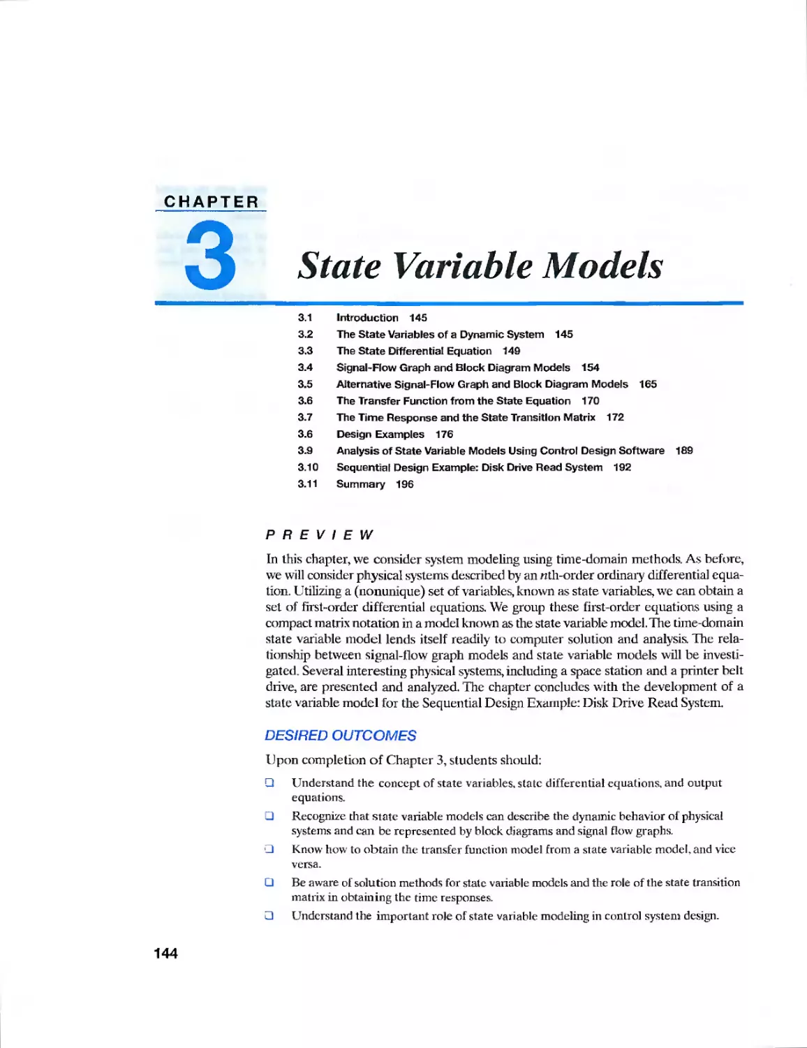
Computer Problems 140
Terms and Concepts 142
v
VI
Contents
CHAPTER
State Variable Models 144
3.1 Introduction 145
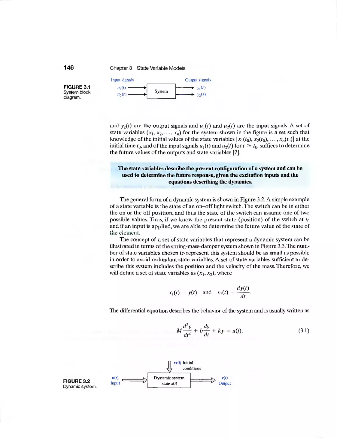
3.2 The State Variables of a Dynamic System 145
3.3 The State Differential Equation 149
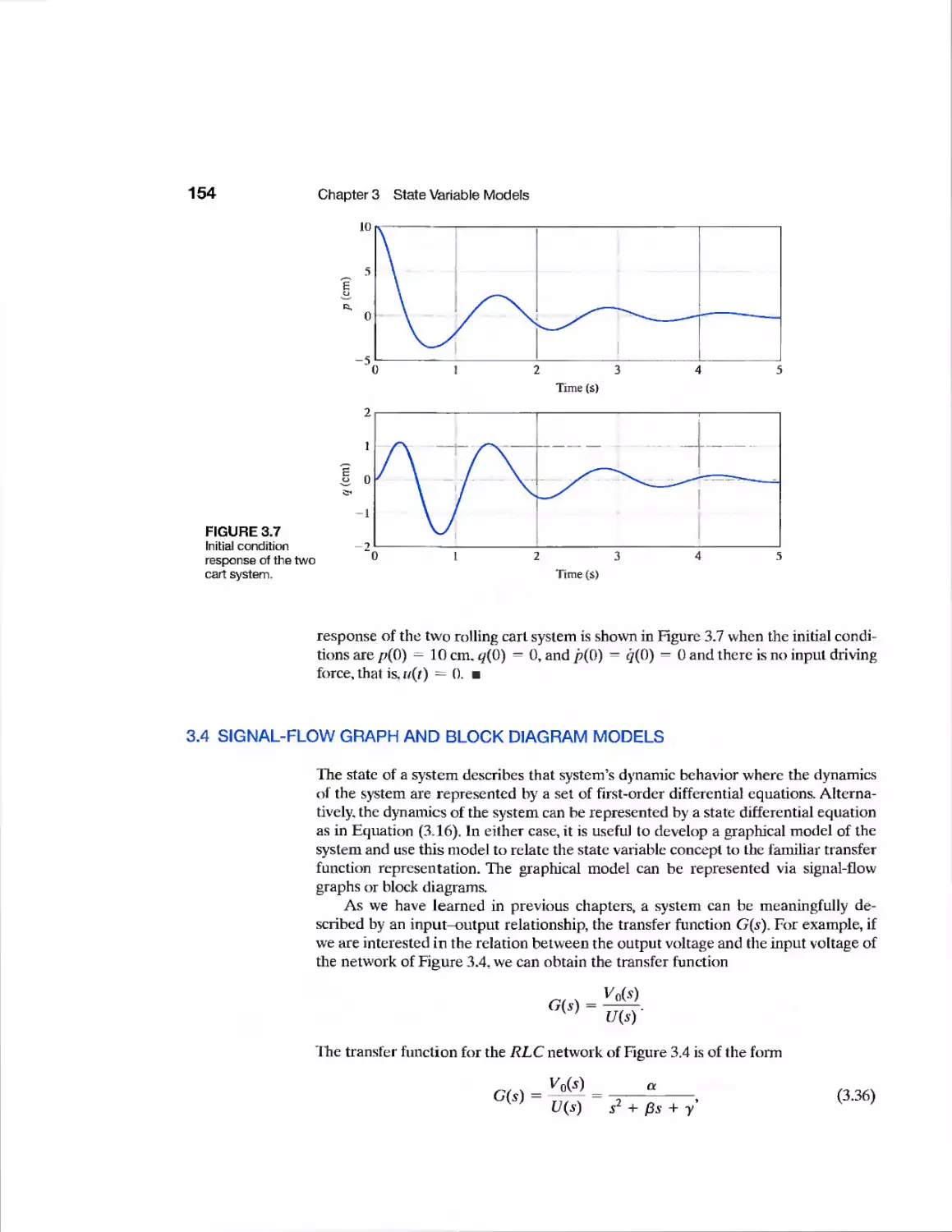
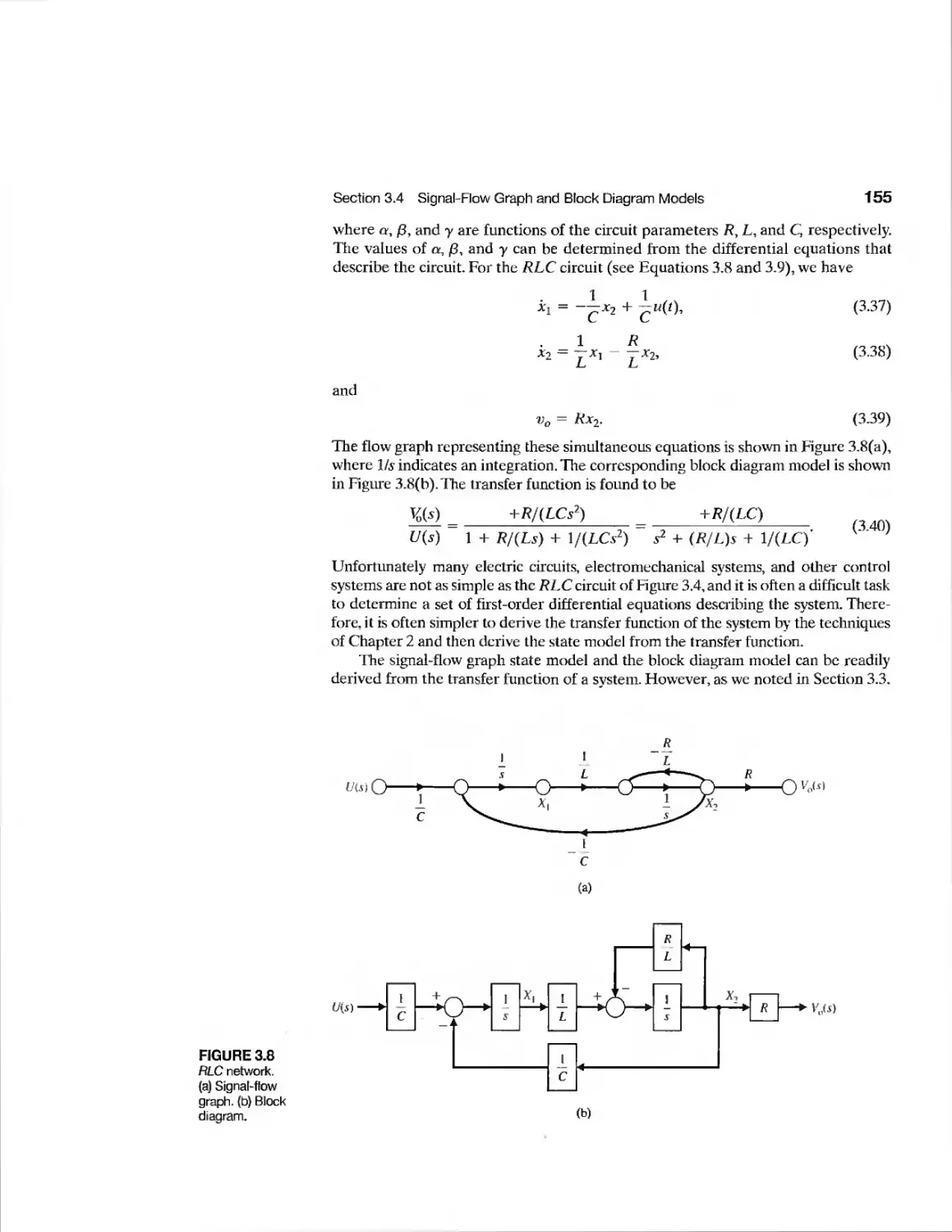
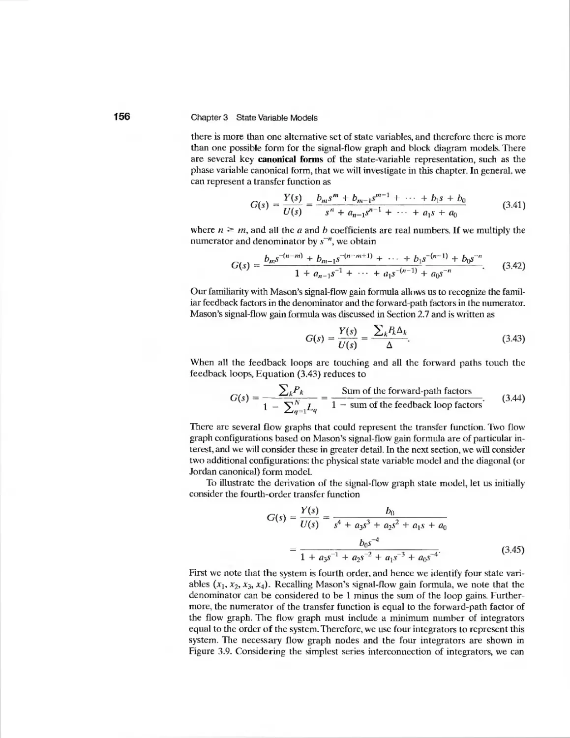
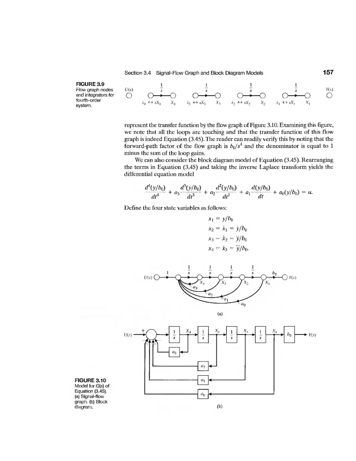
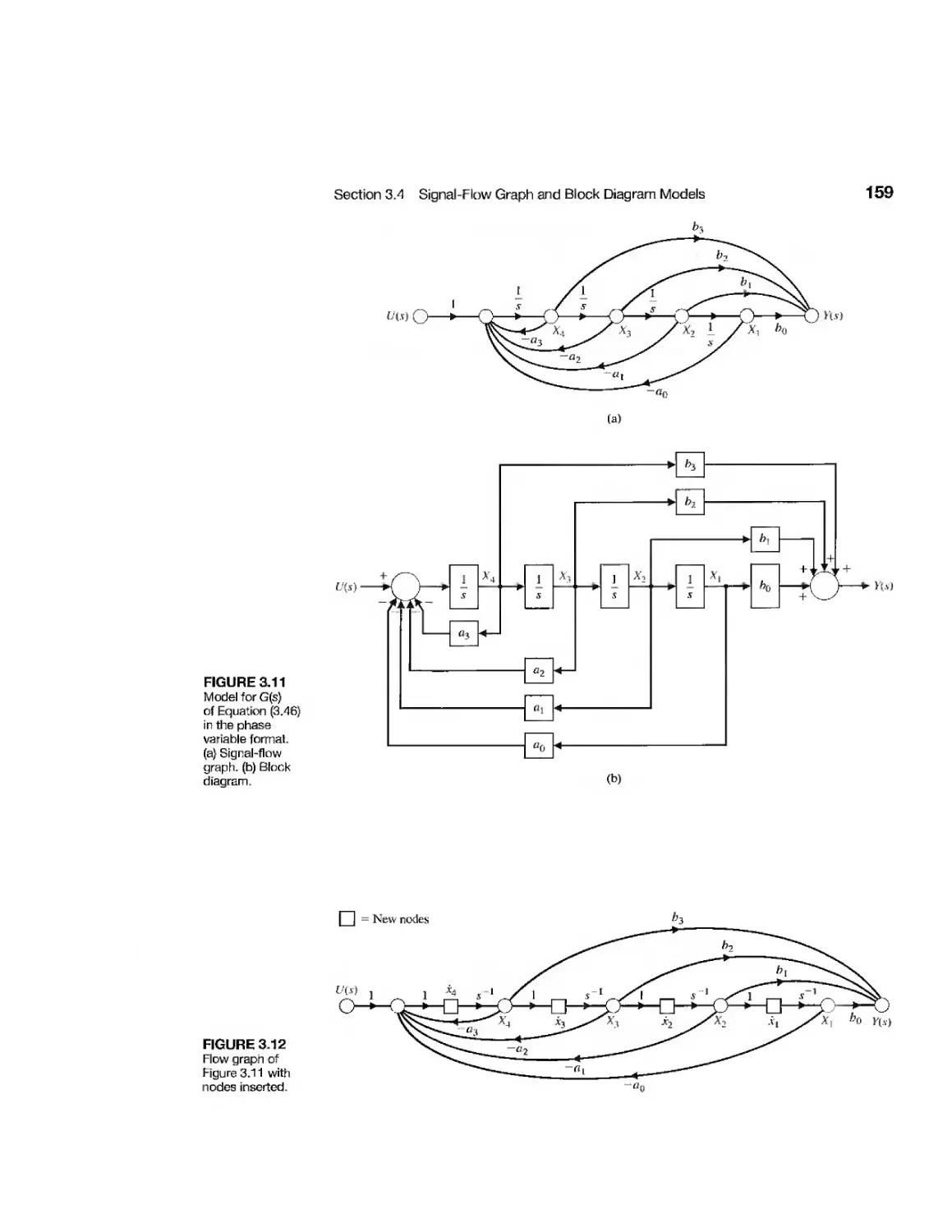
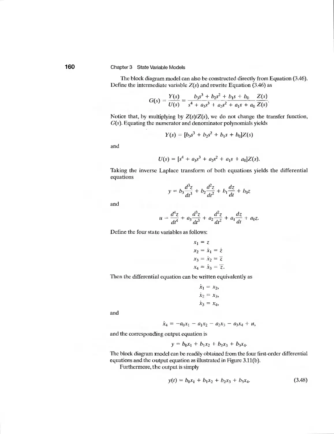
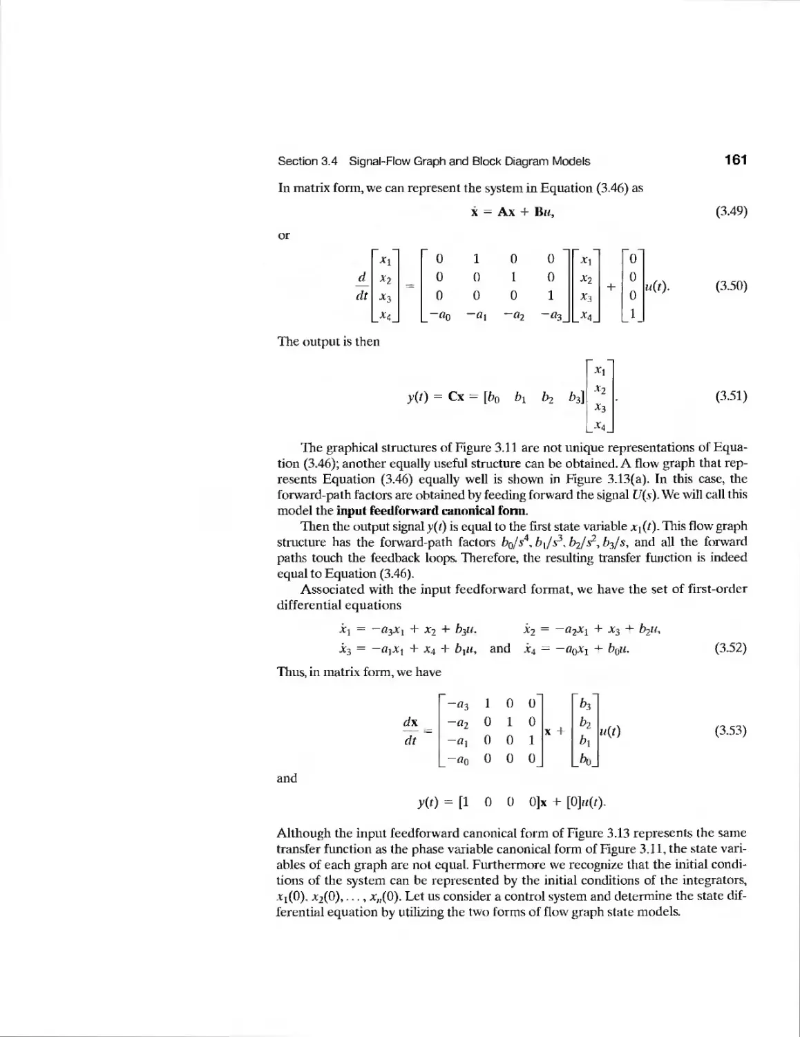
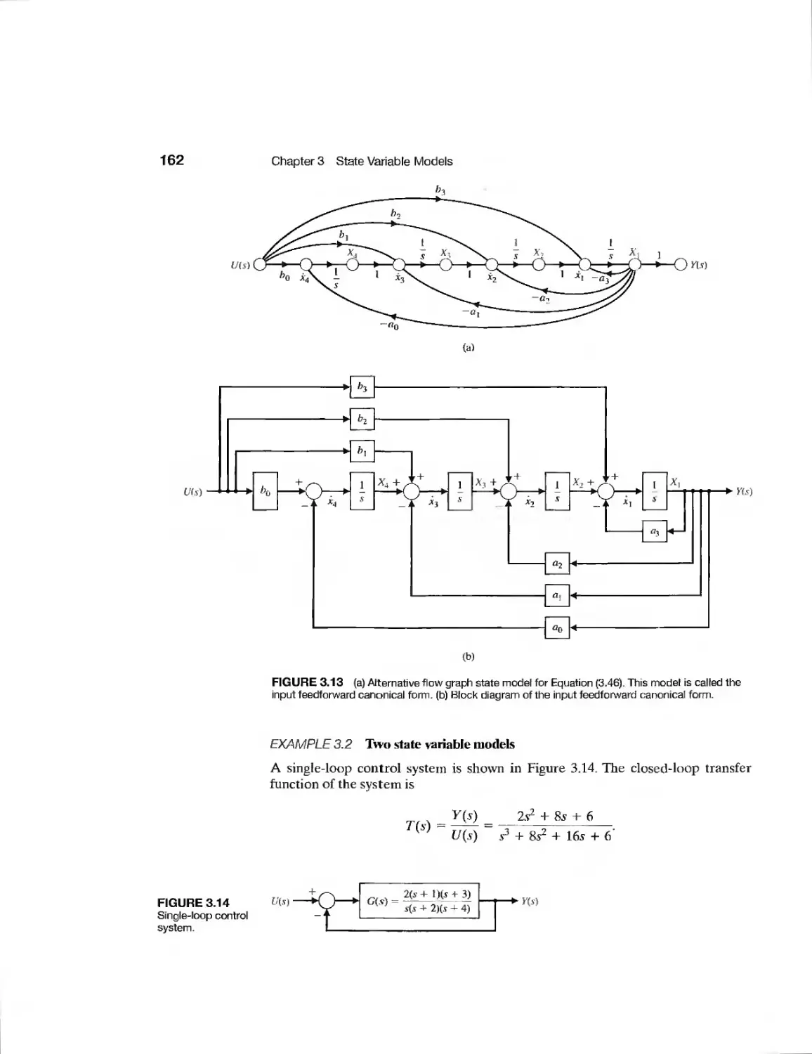
3.4 Signal-Flow Graph and Block Diagram Models 154
3.5 Alternative Signal-Flow Graph and Block Diagram Models 165
3.6 The Transfer Function from the State Equation 170
3.7 The Time Response and the State Transition Matrix 172
3.8 Design Examples 176
3.9 Analysis of State Variable Models Using Control Design Software 189
3.10 Sequential Design Example: Disk Drive Read System 192
3.11 Summary 196
Exercises 197
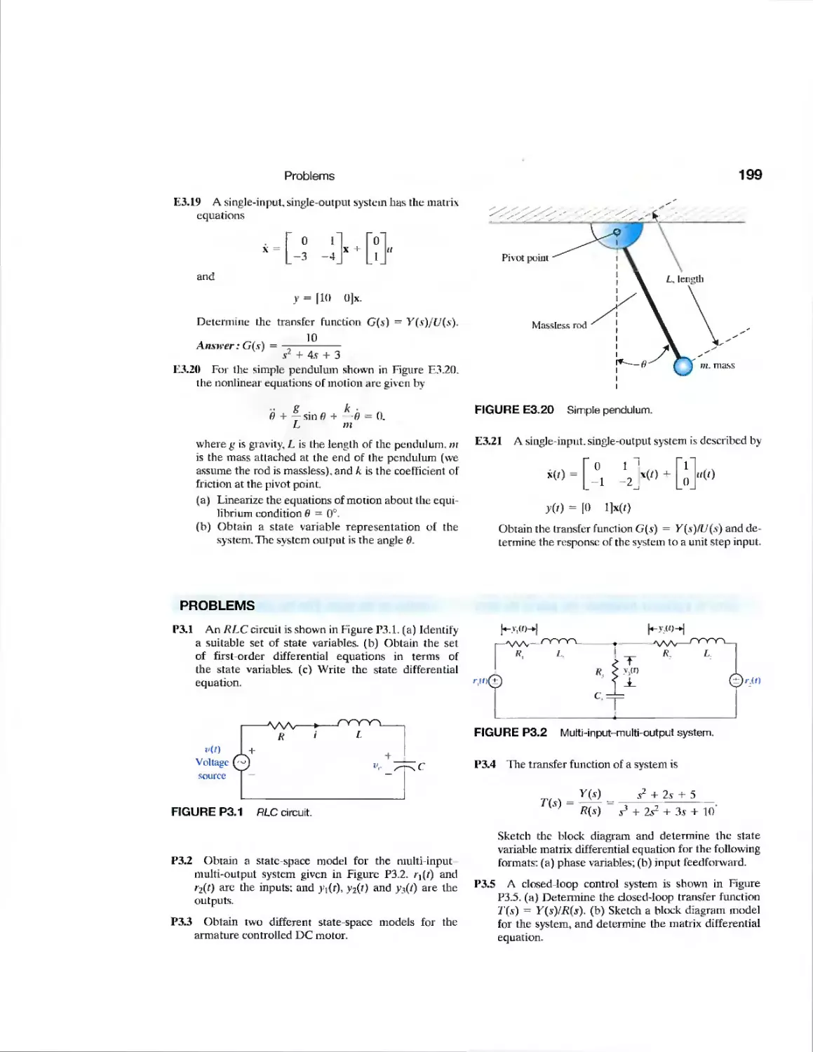
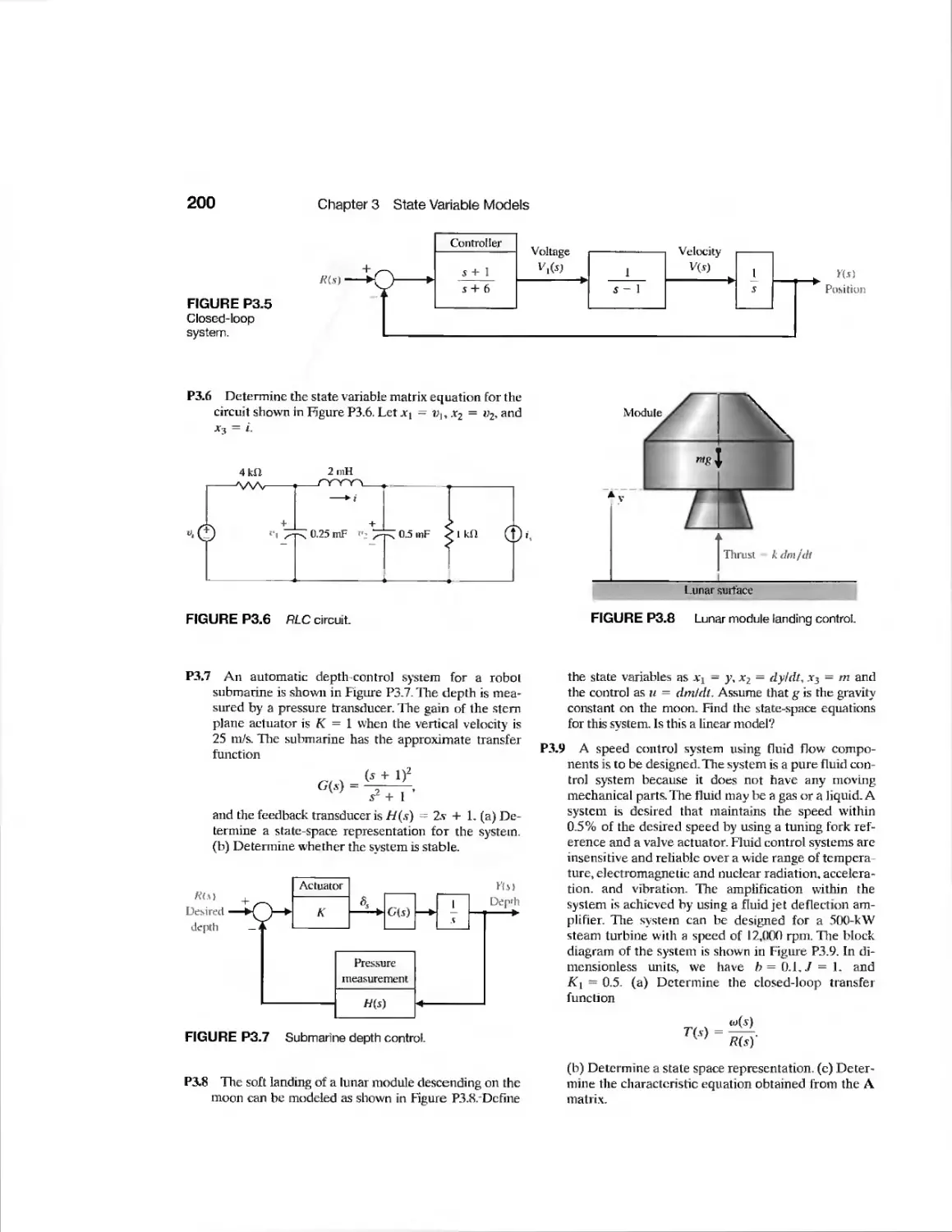
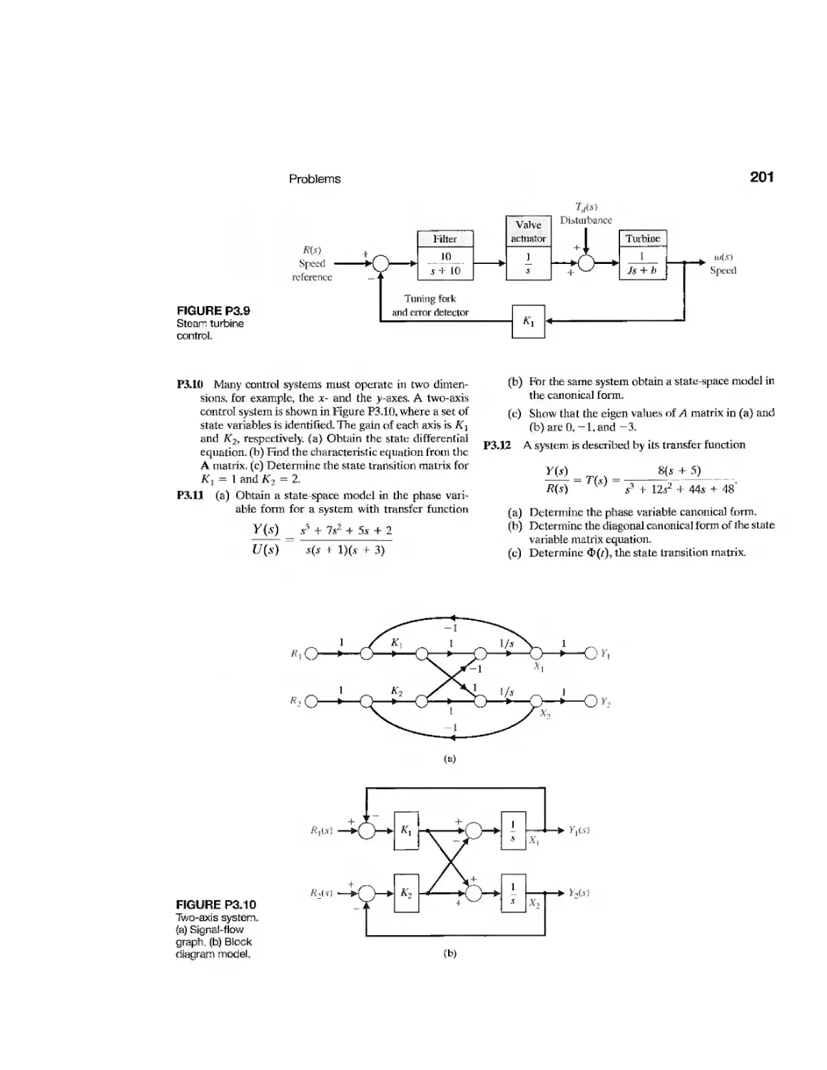
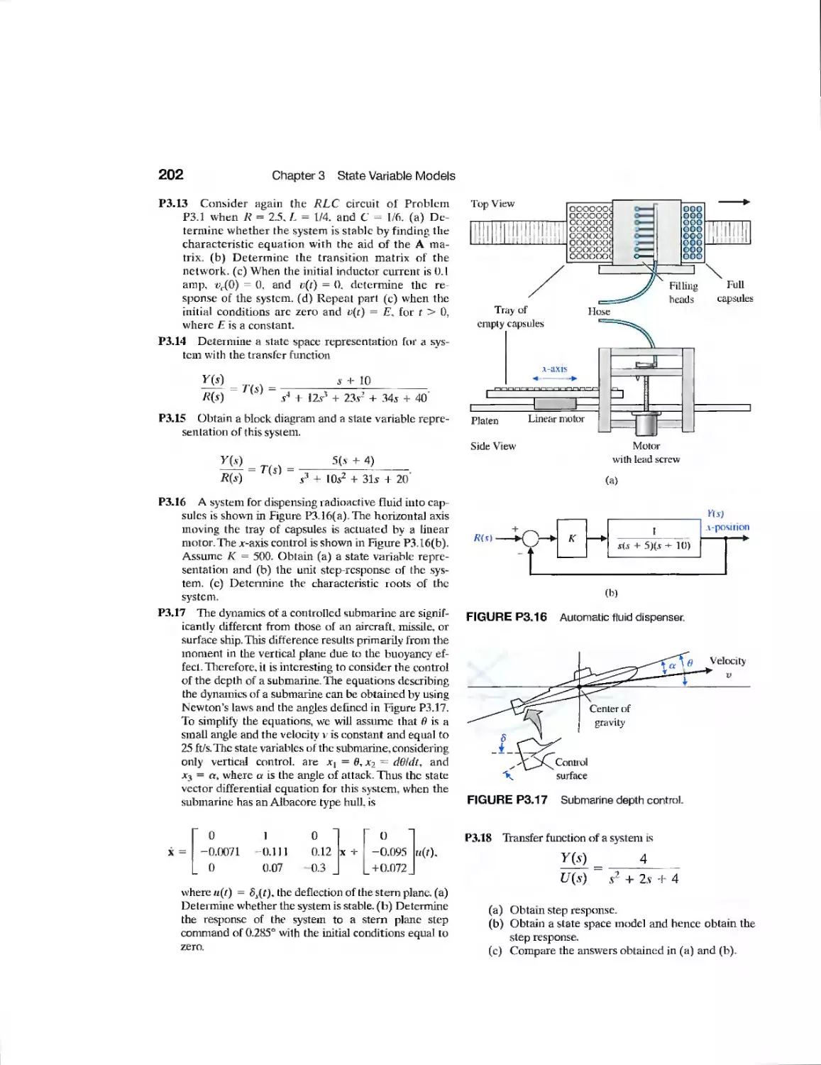
Problems 199
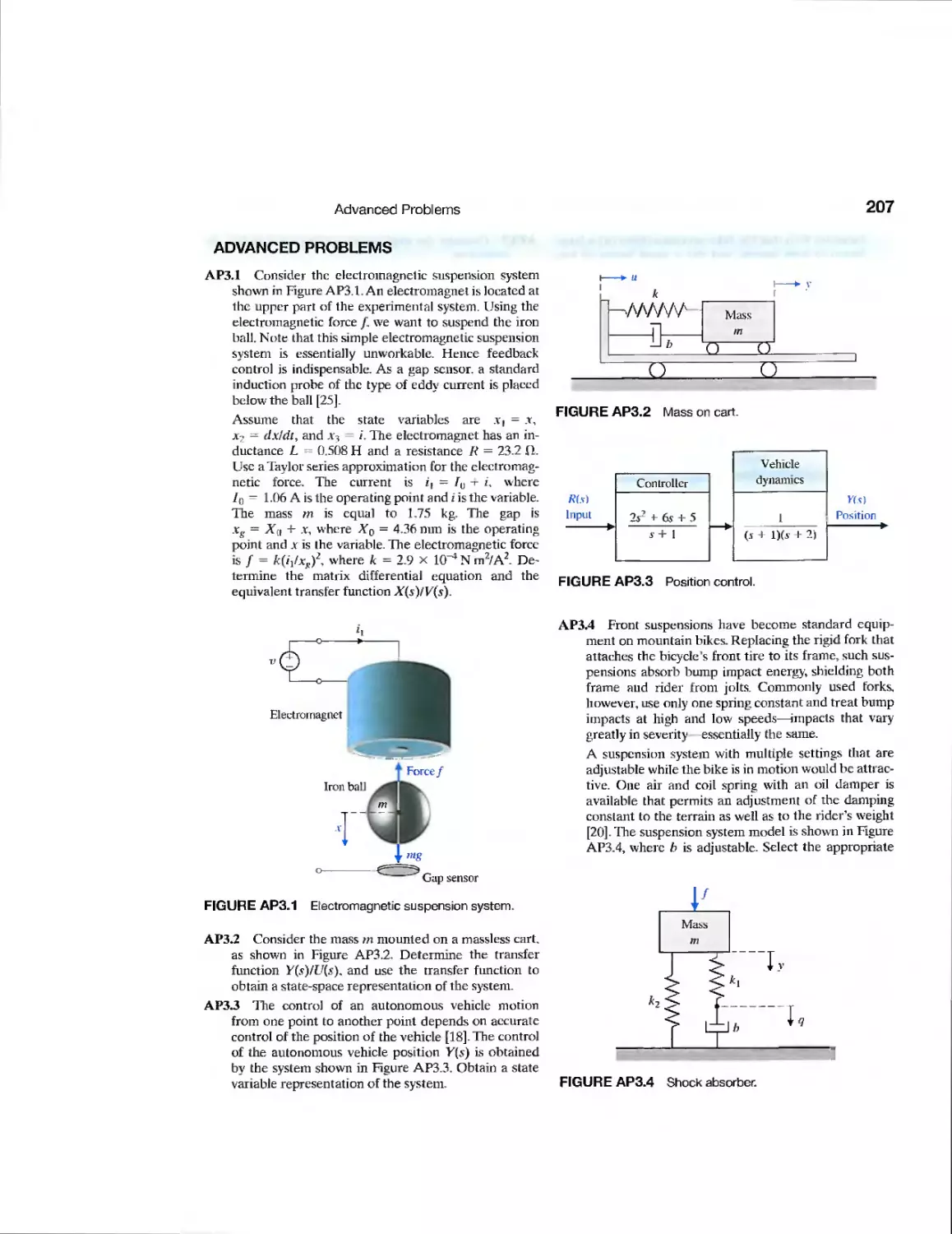
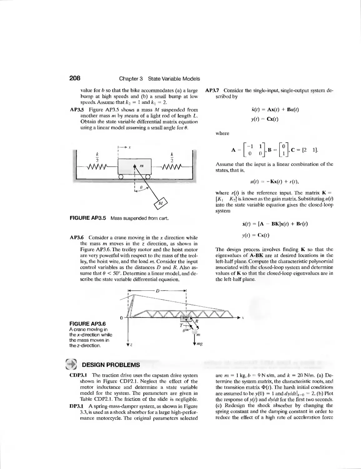
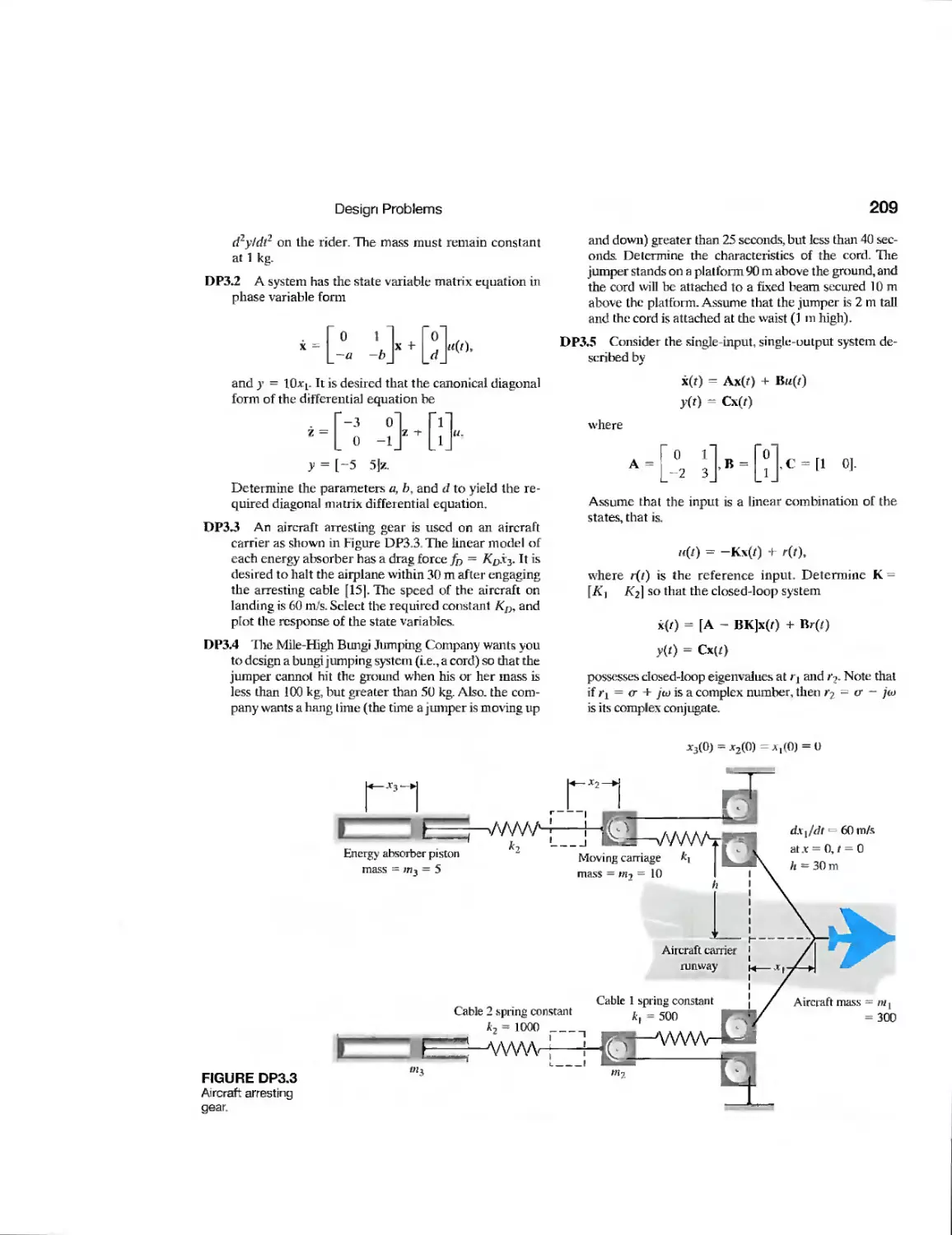
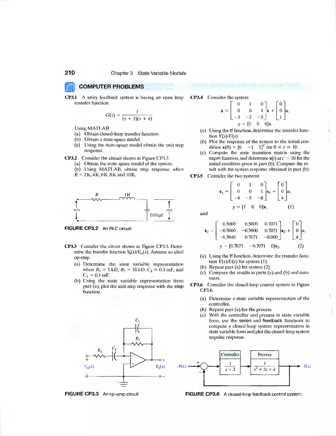
Advanced Problems 207
Design Problems 208
Computer Problems 210
Terms and Concepts 211
chapter 4 Feedback Control System Characteristics 212
4.1 Introduction 213
4.2 Error Signal Analysis 215
4.3 Sensitivity of Control Systems to Parameter Variations 217
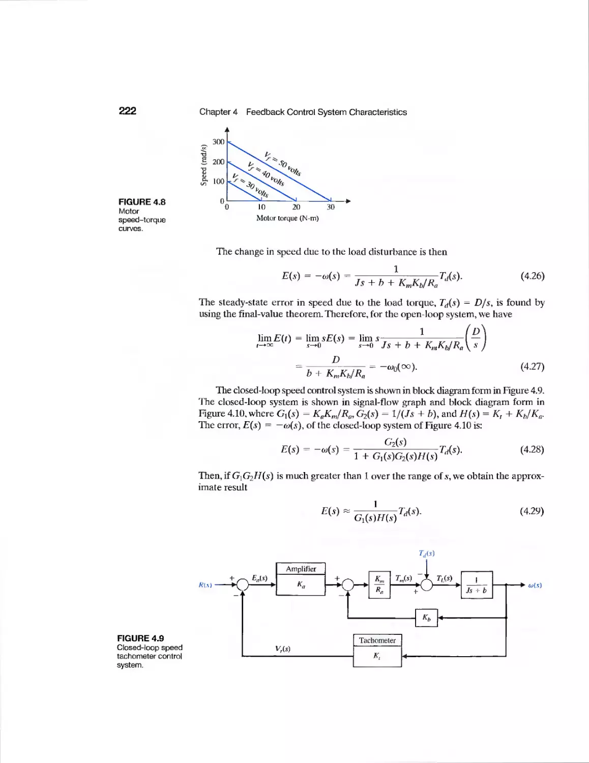
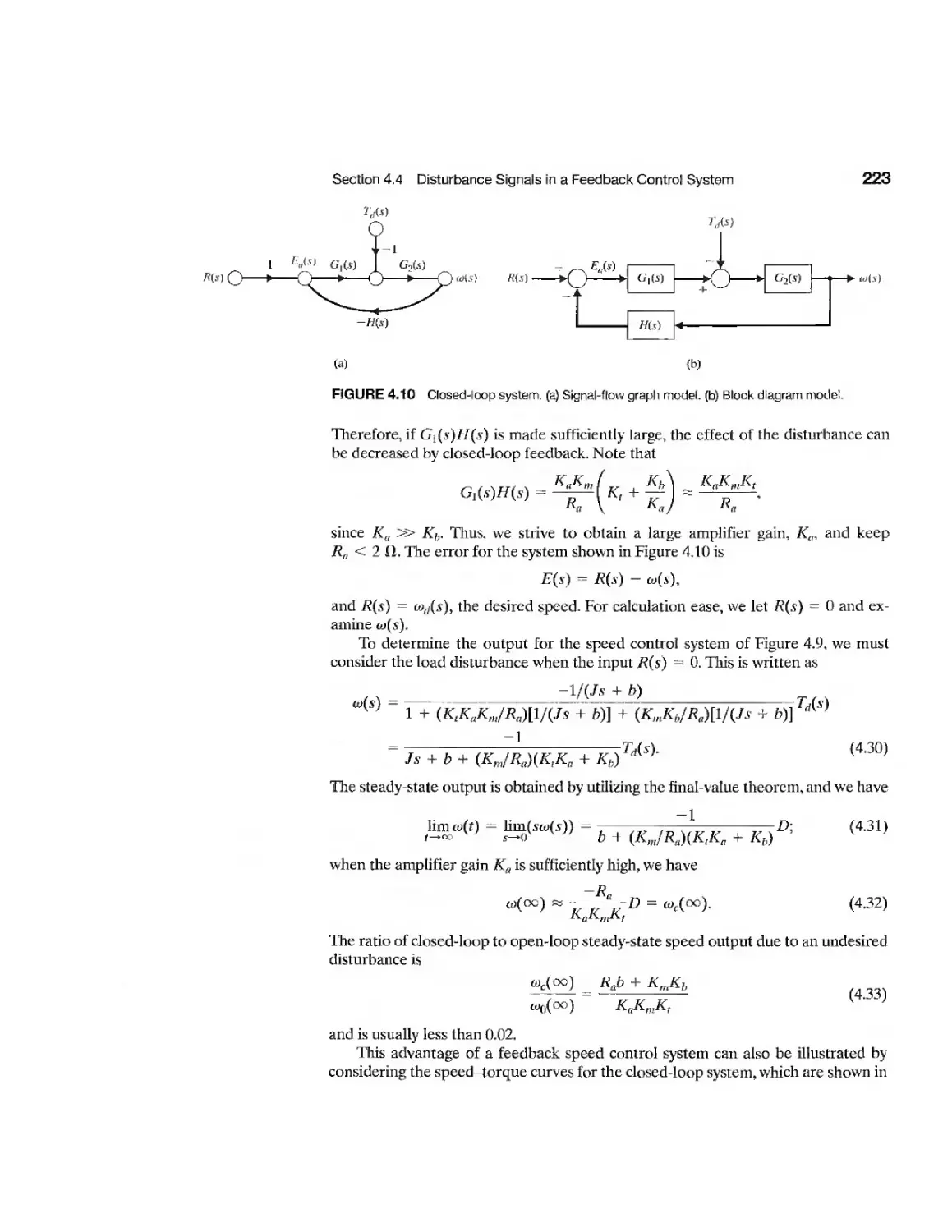
4.4 Disturbance Signals in a Feedback Control System 220
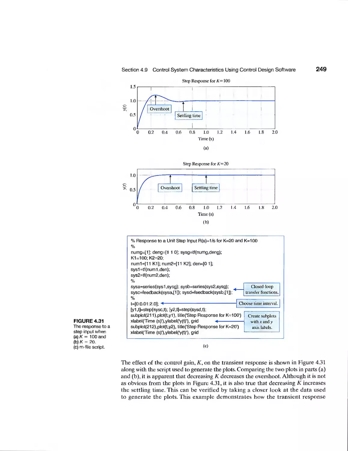
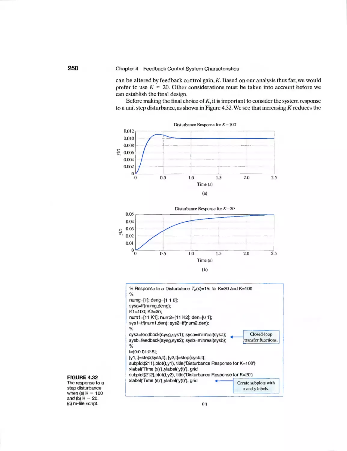
4.5 Control of the Transient Response 225
4.6 Steady-State Error 228
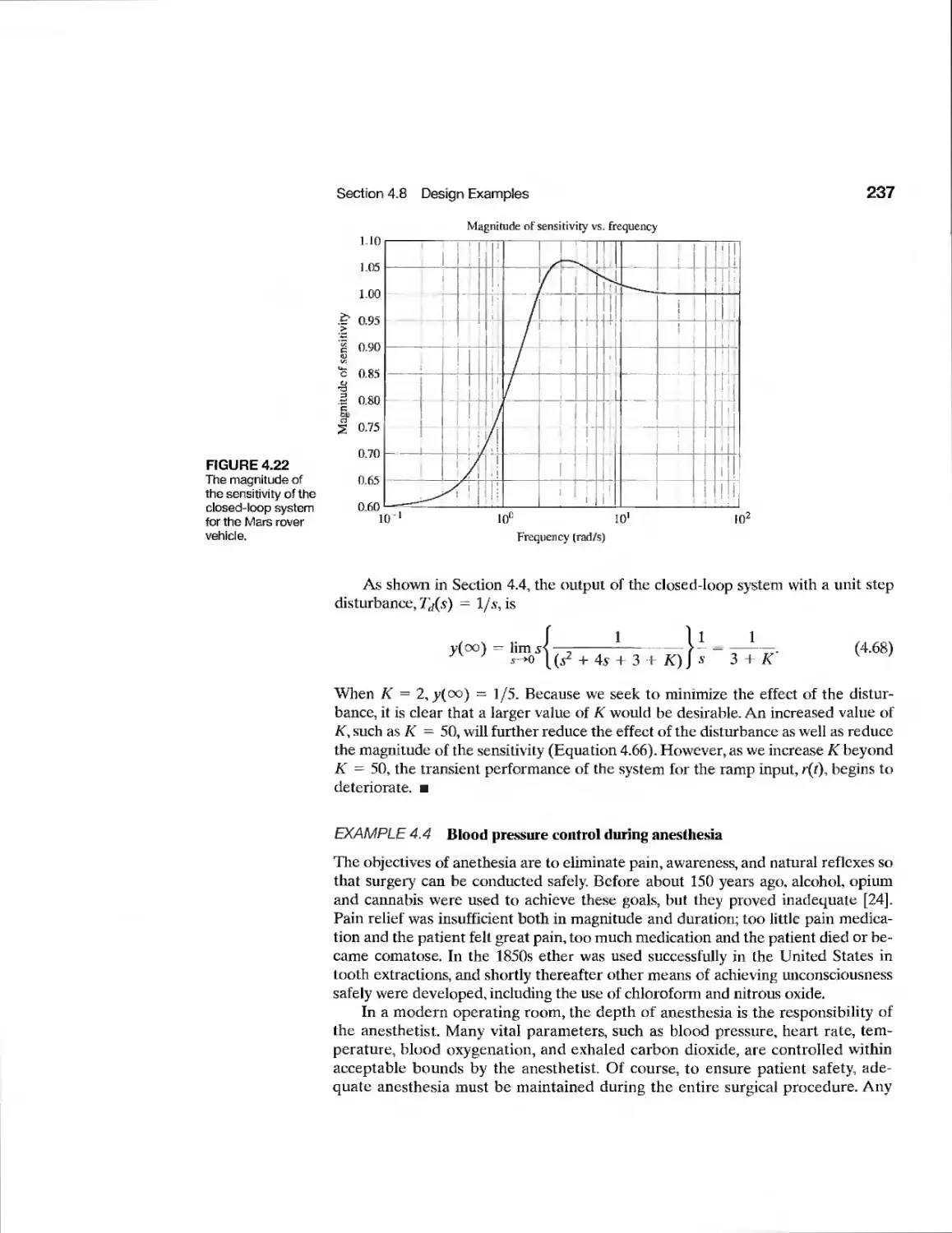
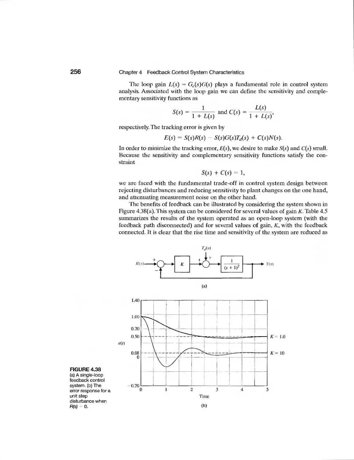
4.7 The Cost of Feedback 231
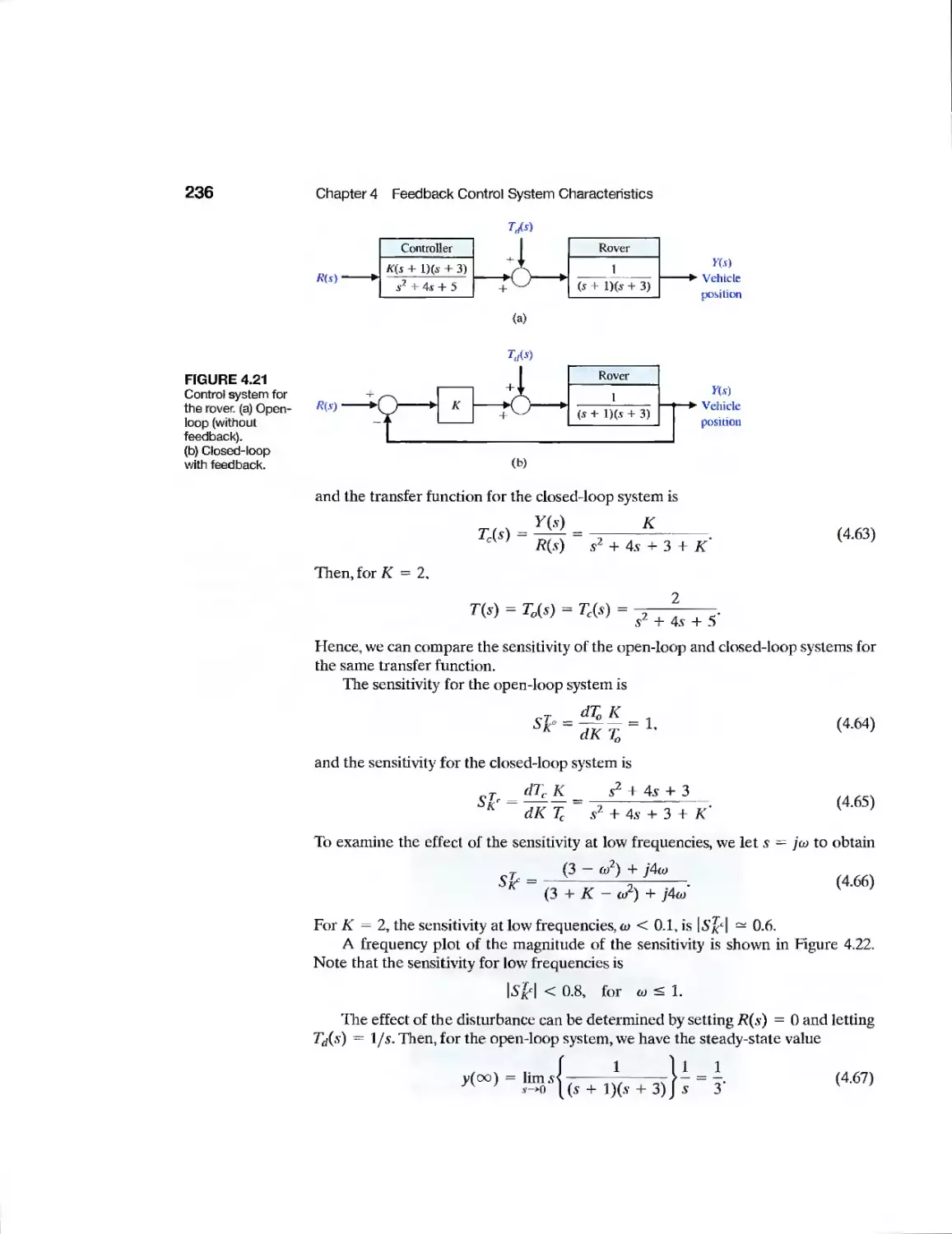
4.8 Design Examples 232
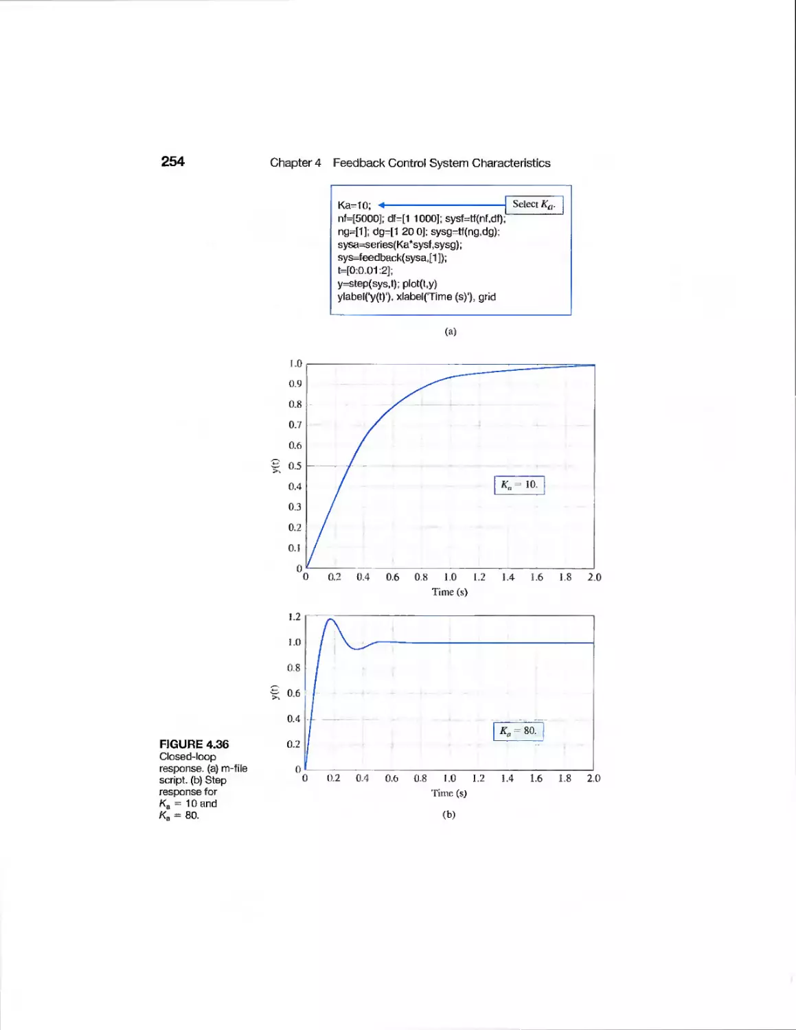
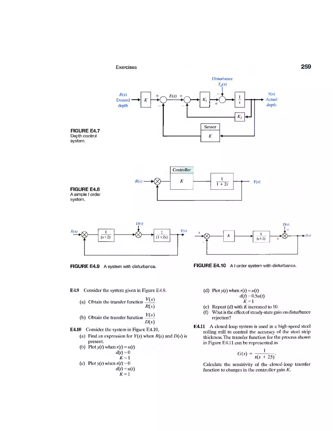
4.9 Control System Characteristics Using Control Design Software
4.10 Sequential Design Example: Disk Drive Read System 251
4.11 Summary 255
Exercises 257
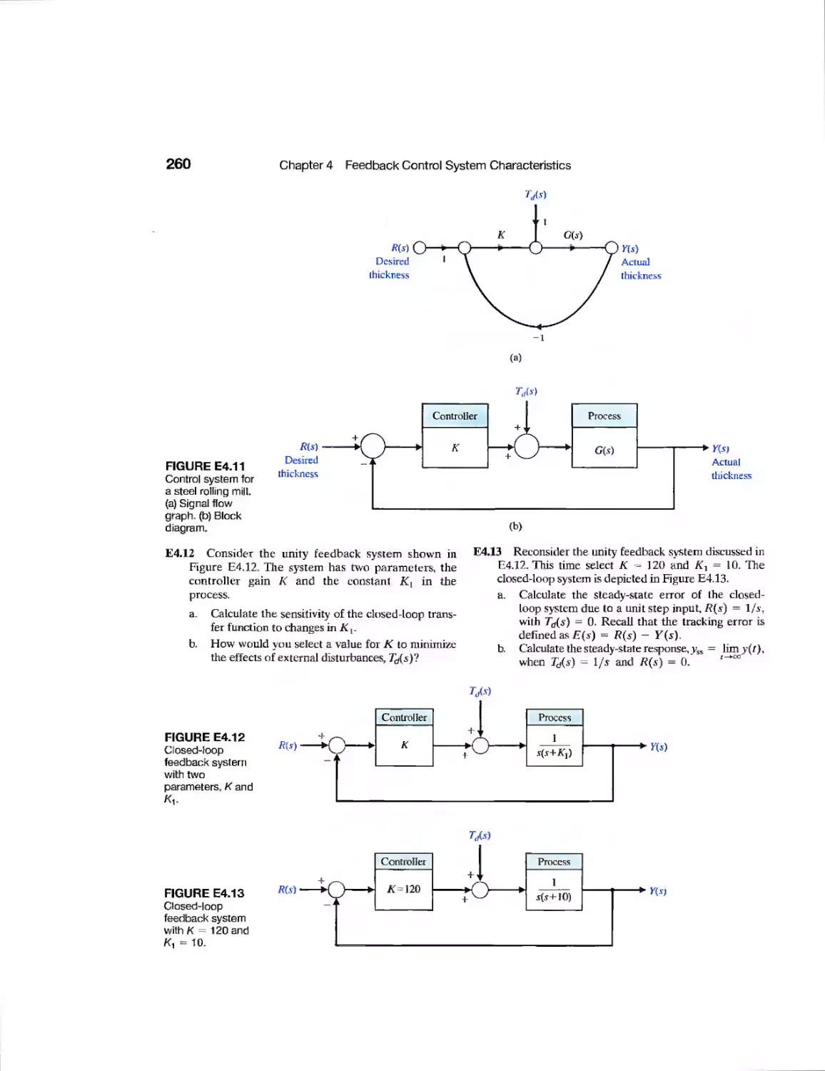
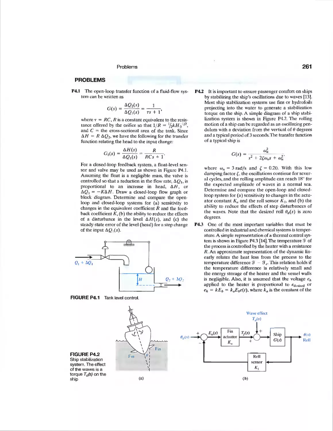
Problems 261
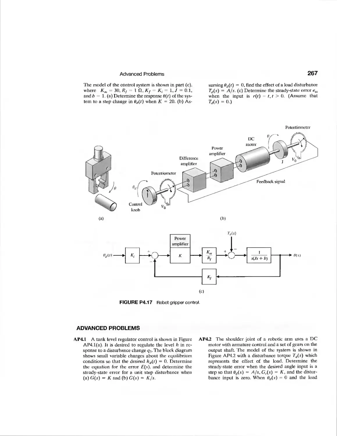
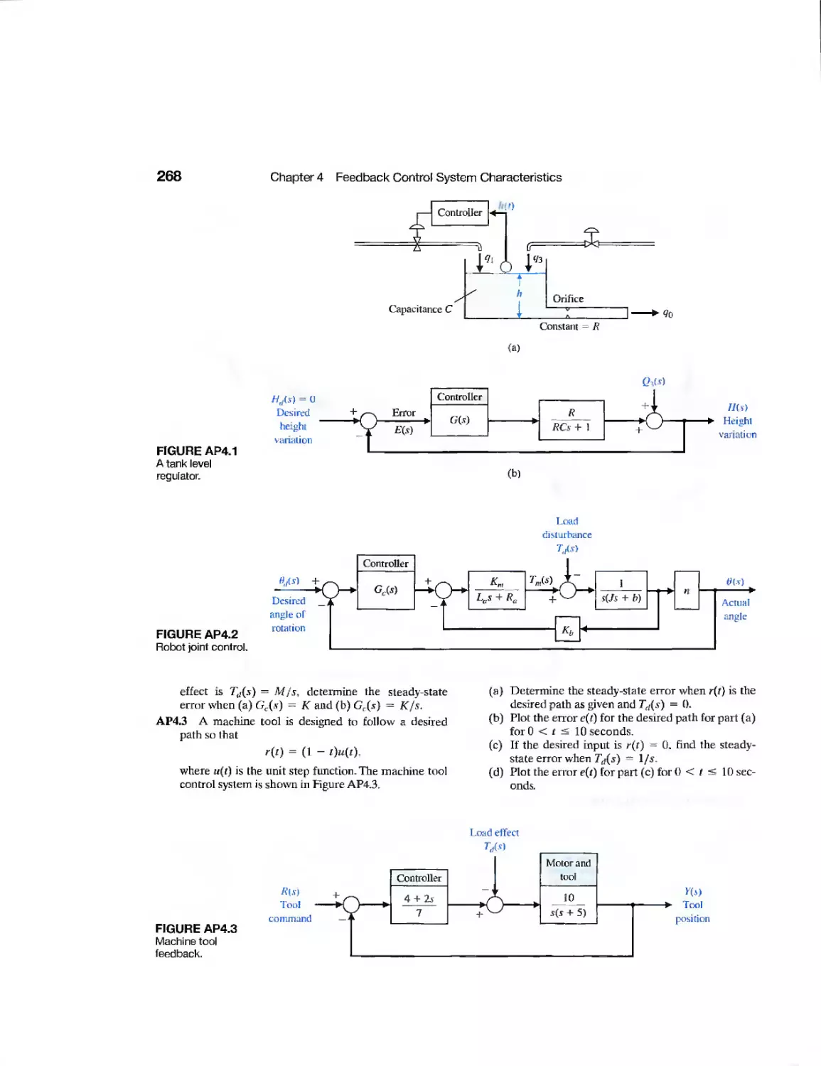
Advanced Problems 267
Design Problems 270
Computer Problems 273
Terms and Concepts 276
246
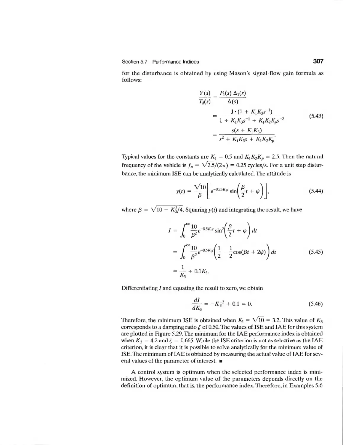
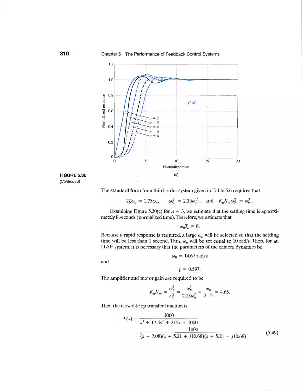
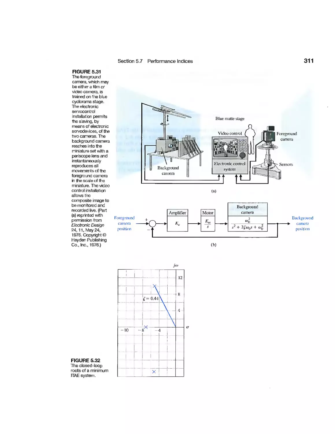
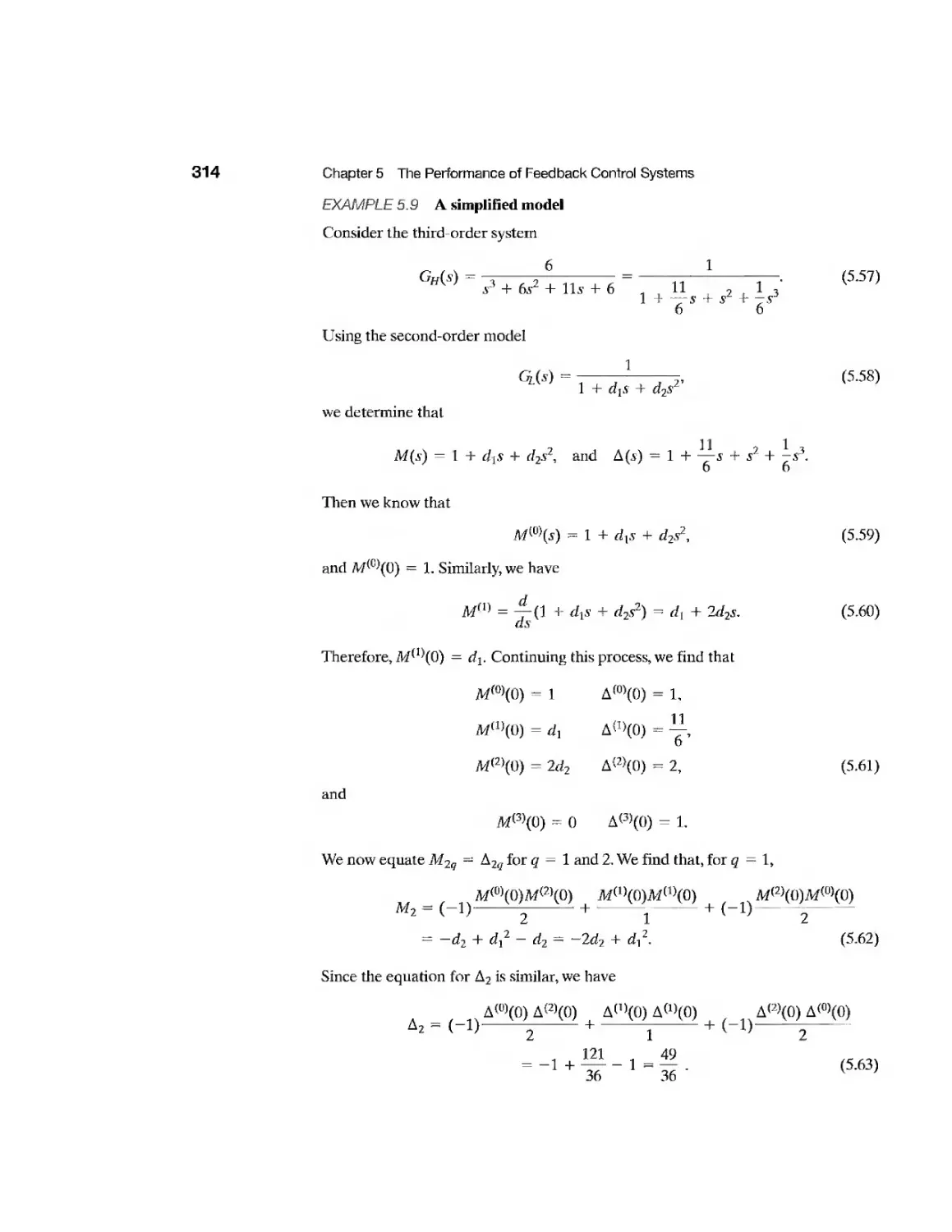
chapter 5 The Performance of Feedback Con trol Systems 2 77
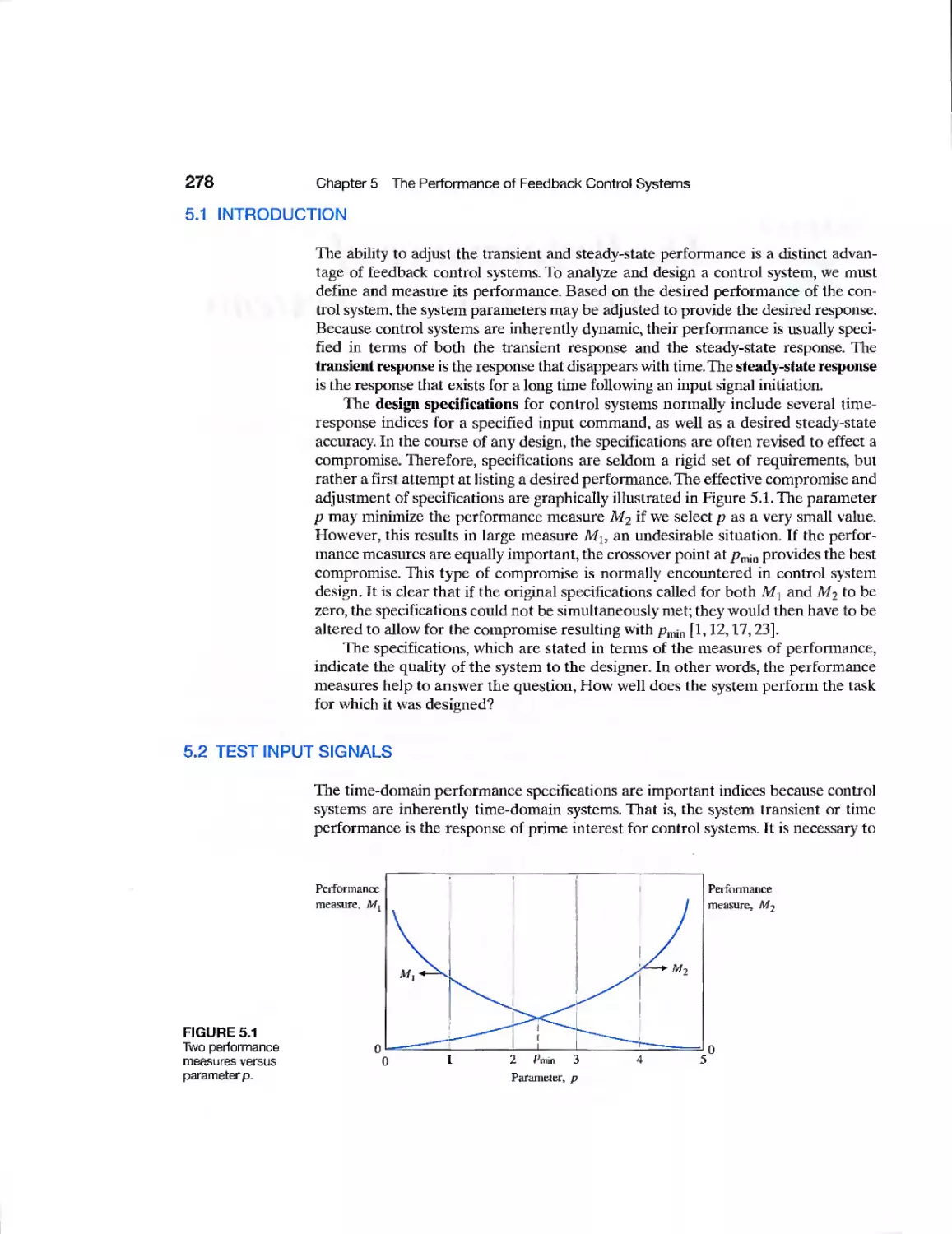
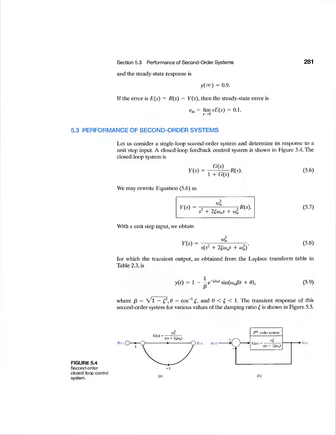
5.1 Introduction 278
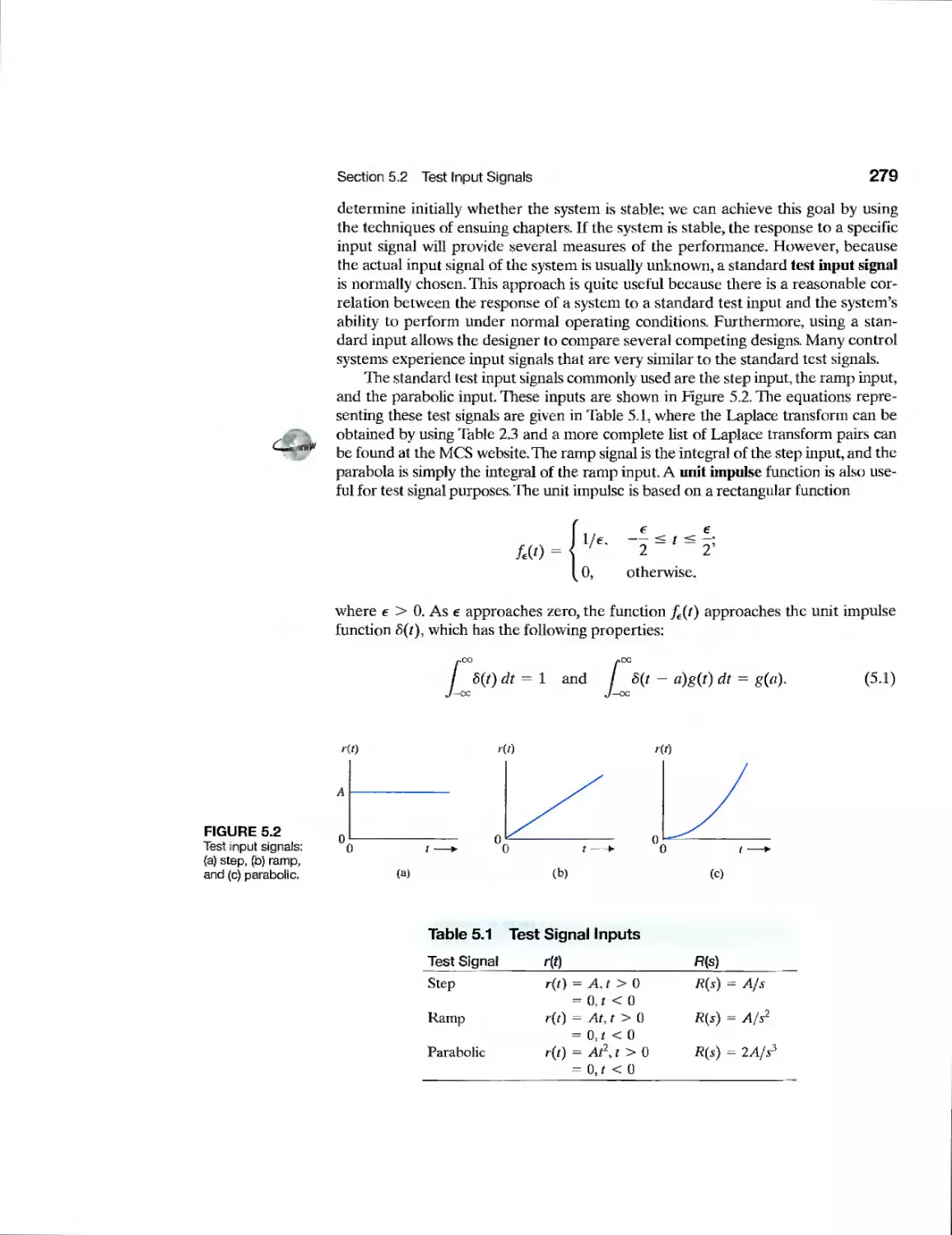
5.2 Test Input Signals 278
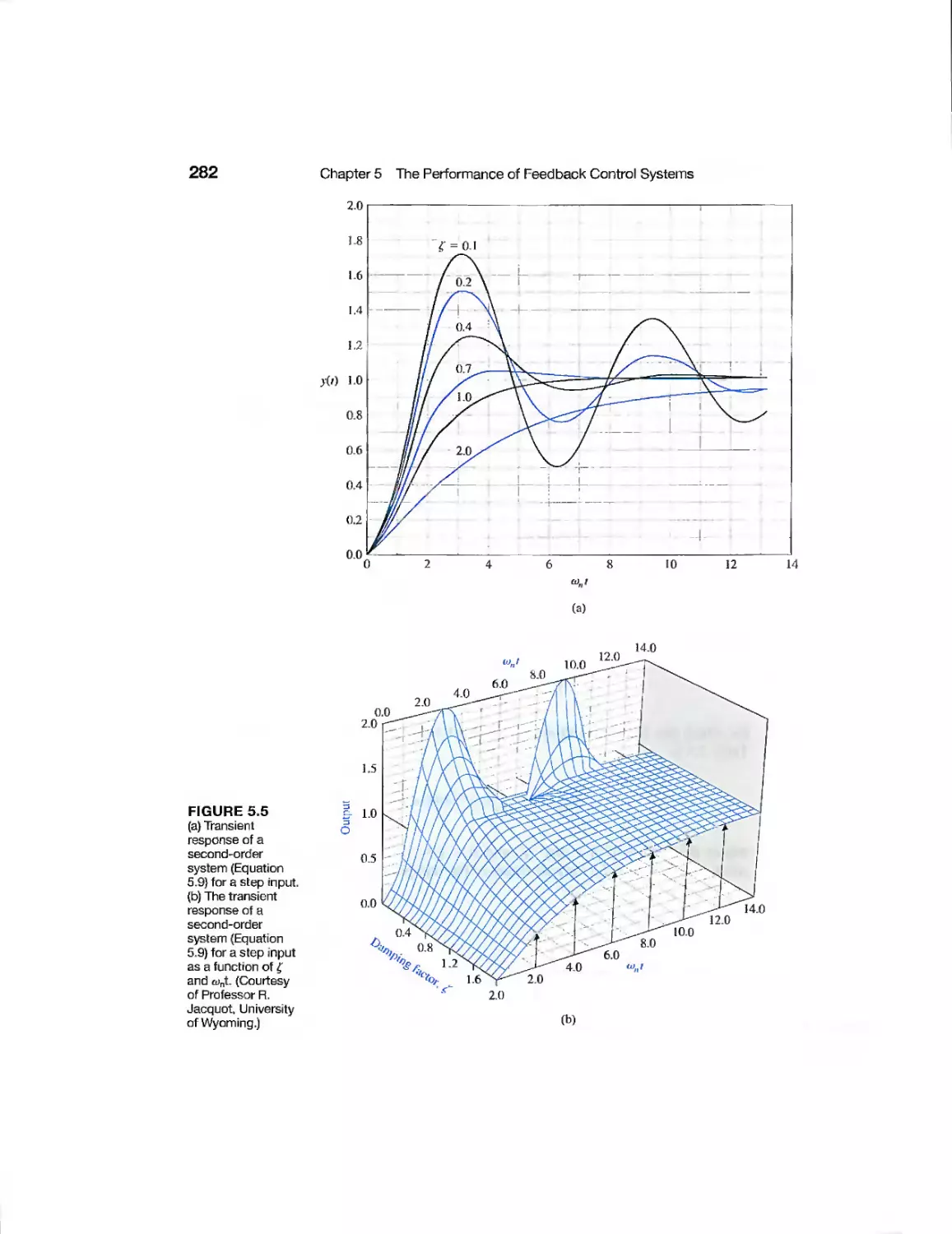
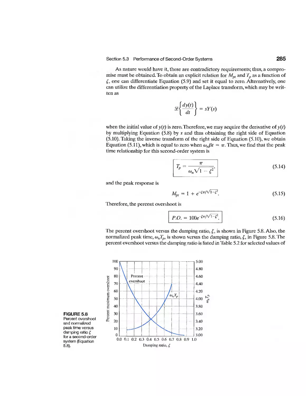
5.3 Performance of Second-Order Systems
281
Contents
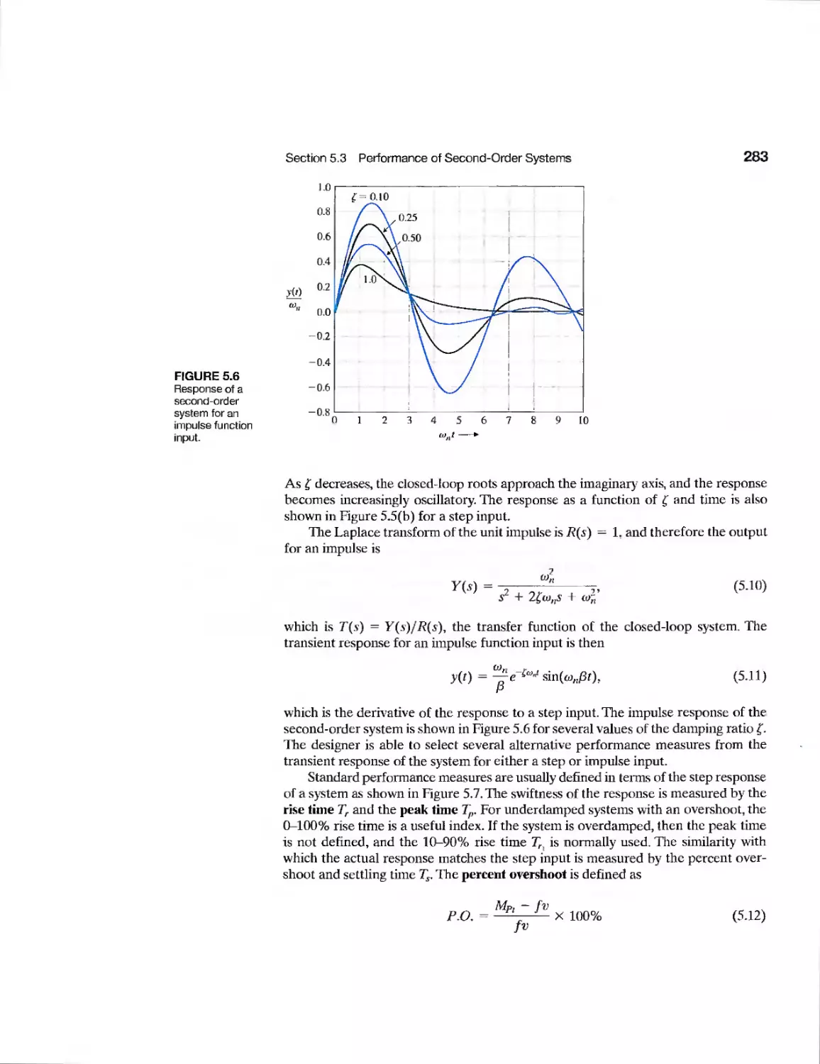
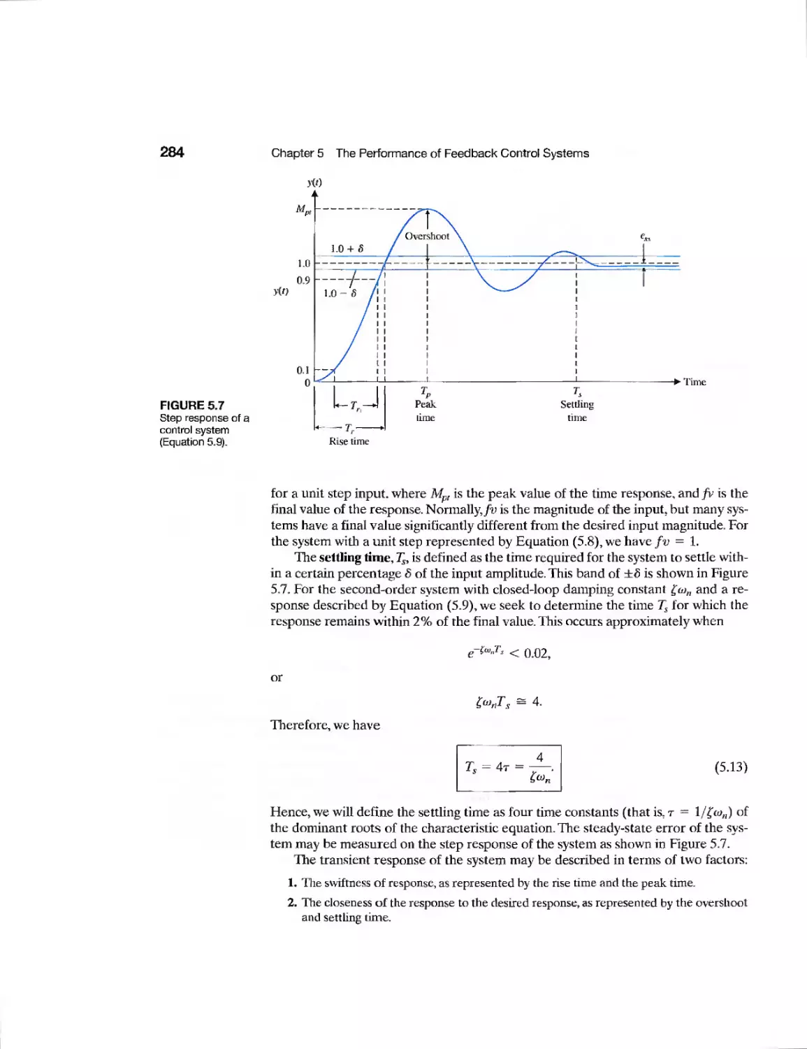
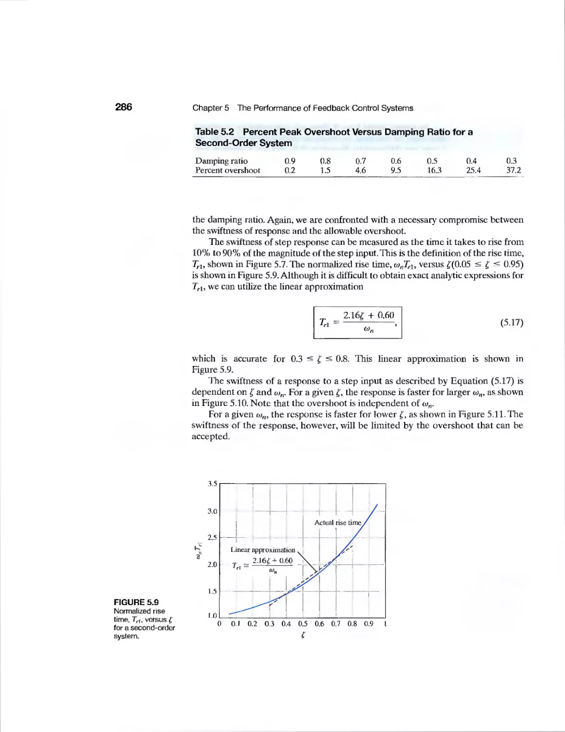
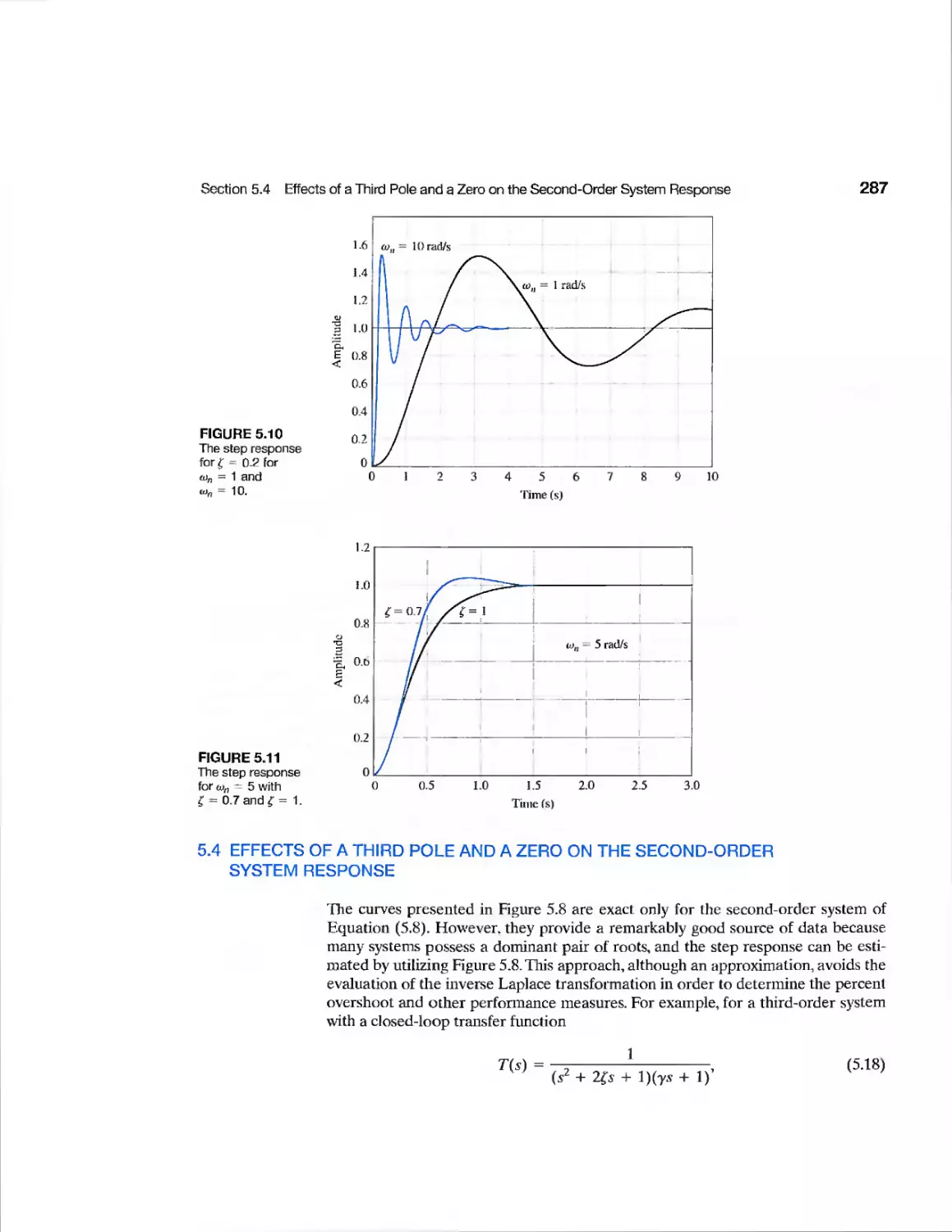
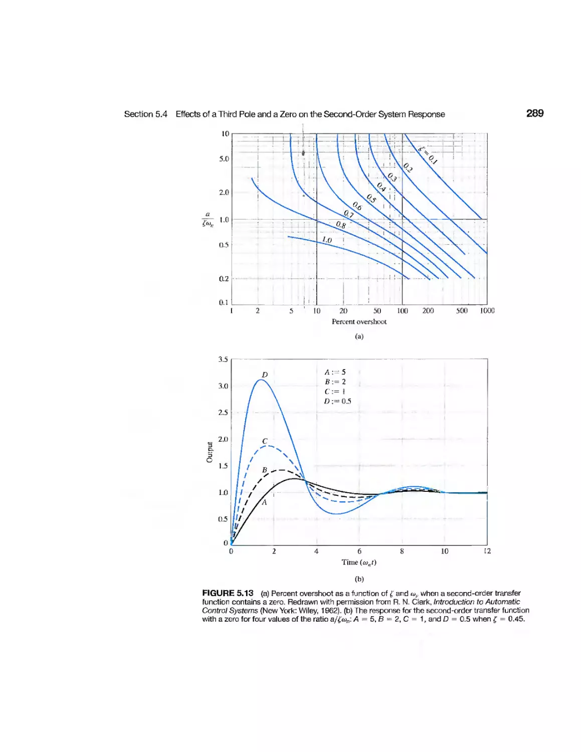
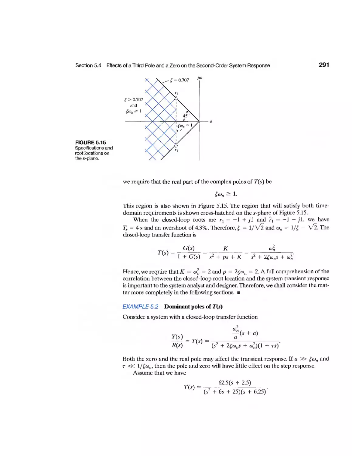
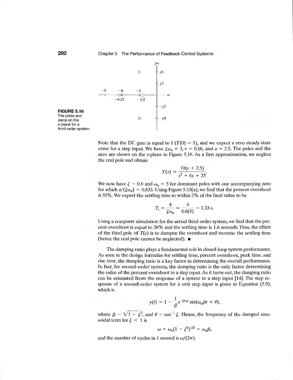
5.4 Effects of a Third Pole and a Zero on the Second-Order System
Response 287
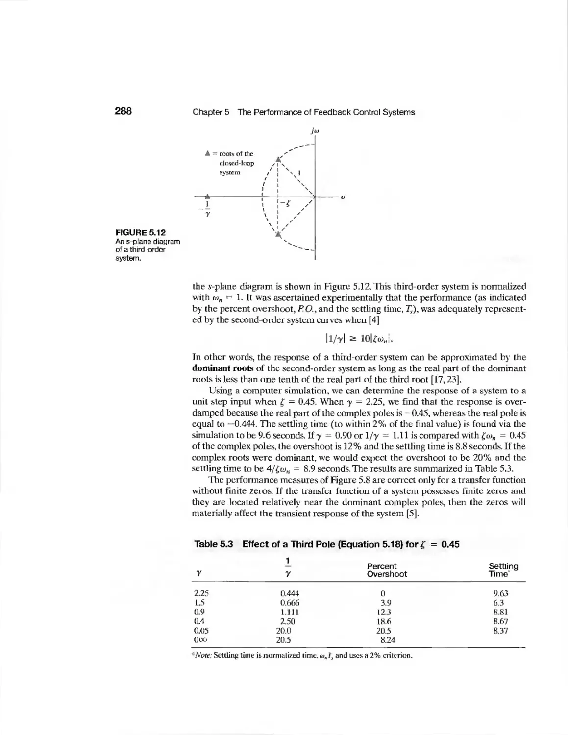
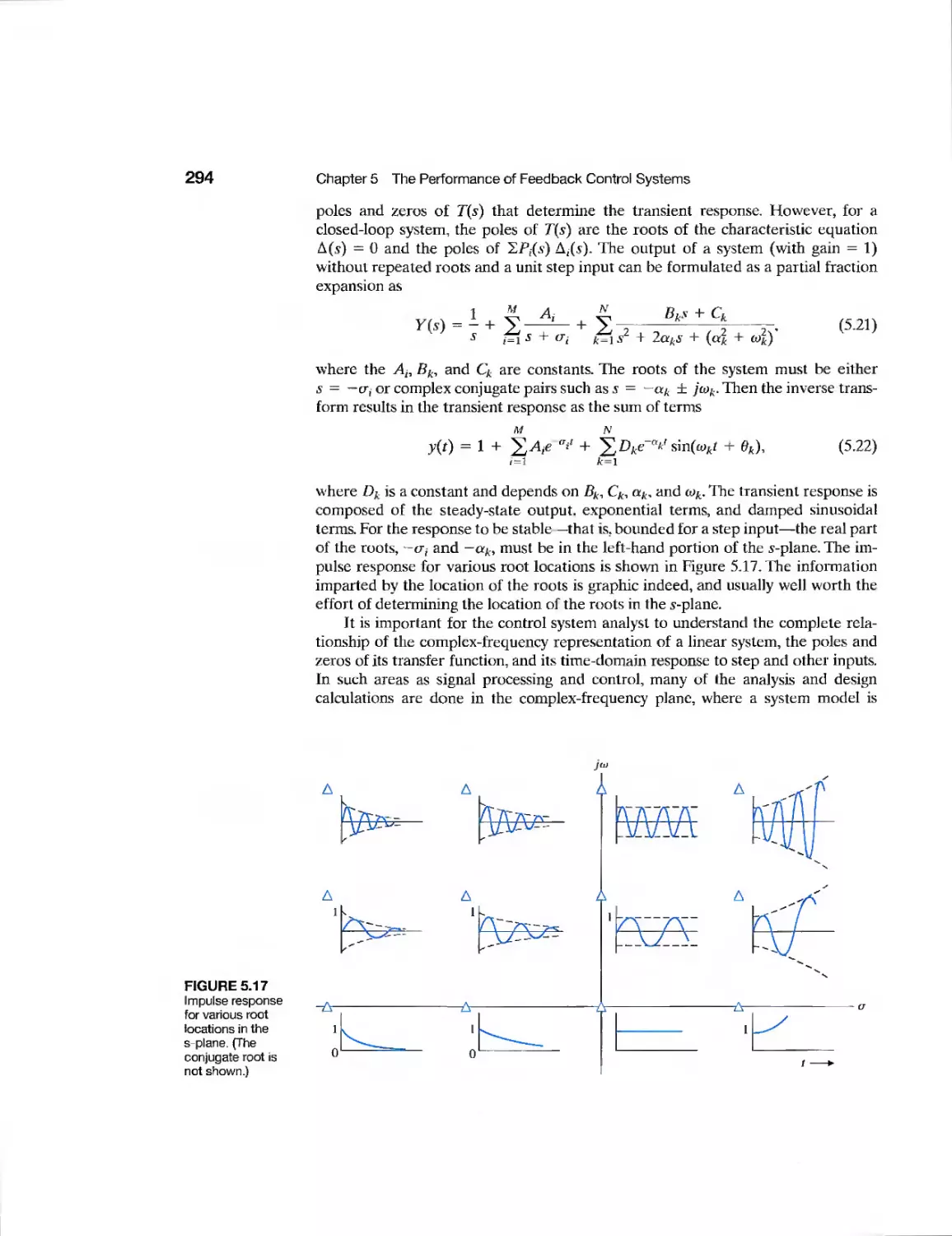
5.5 The 5-Plane Root Location and the Transient Response 293
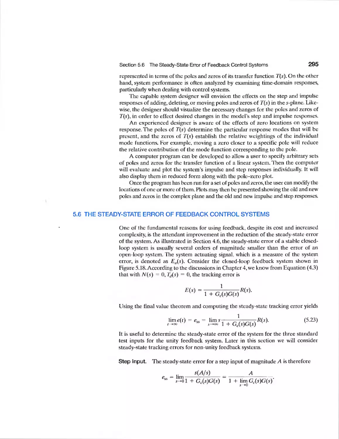
5.6 The Steady-State Error of Feedback Control Systems 295
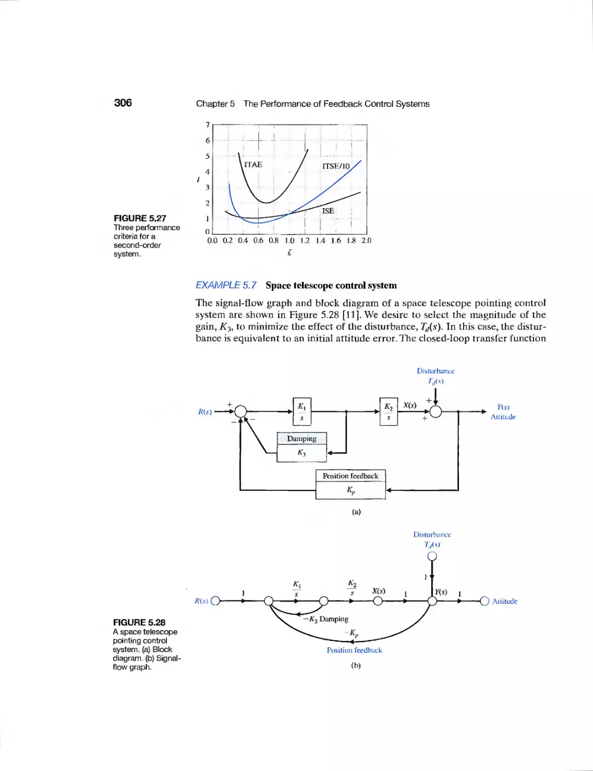
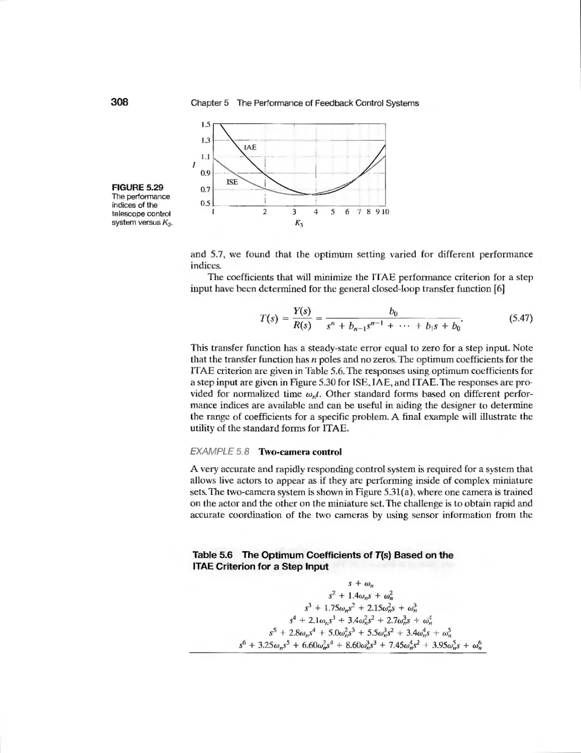
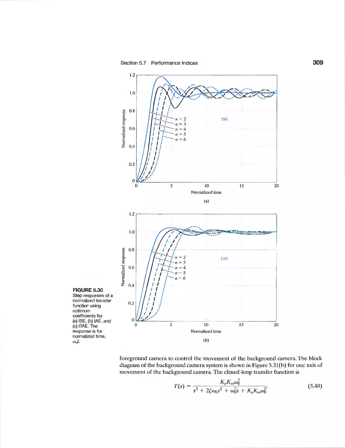
5t7 Performance Indices 303
5.8 The Simplification of Linear Systems 312
5.9 Design Examples 315
5.10 System Performance Using Control Design Software 329
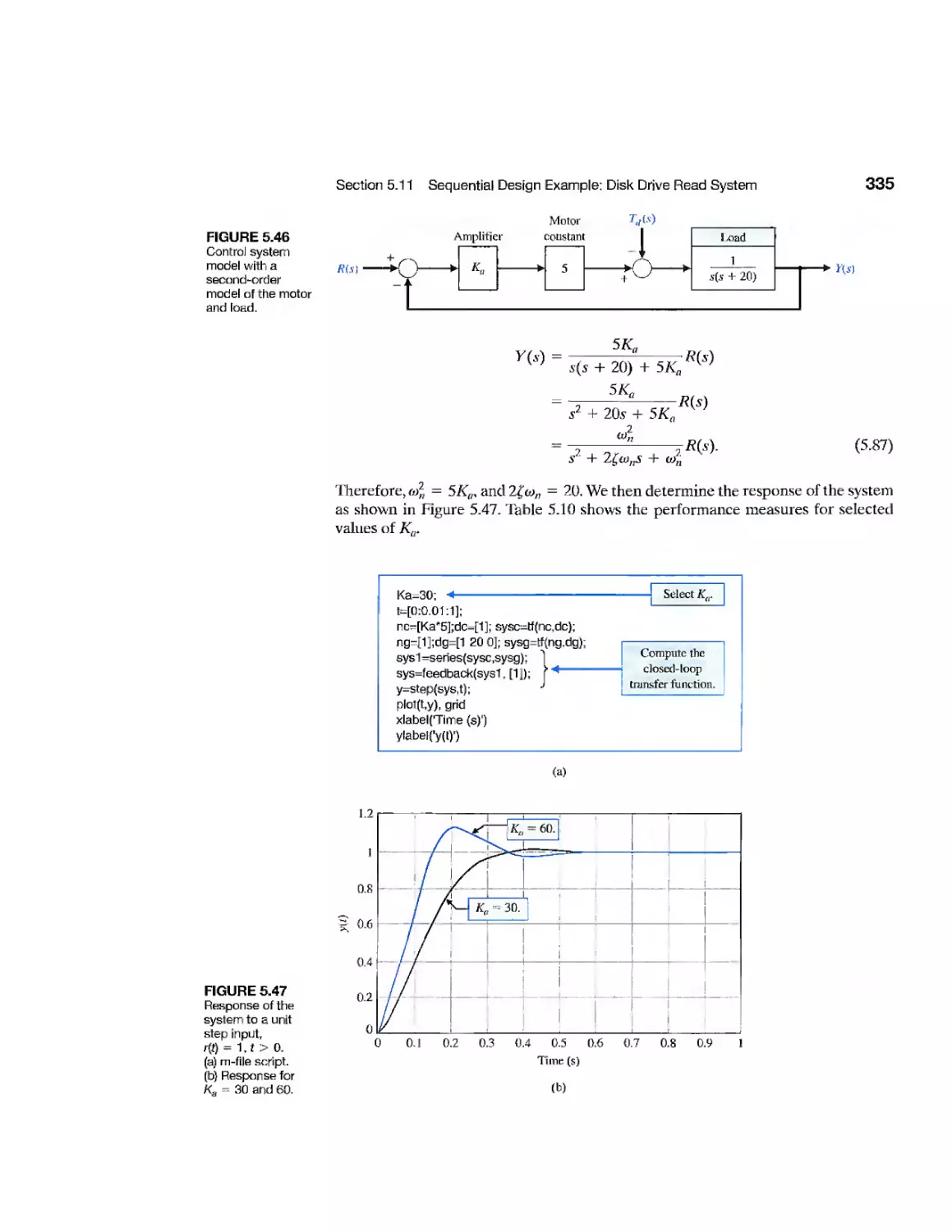
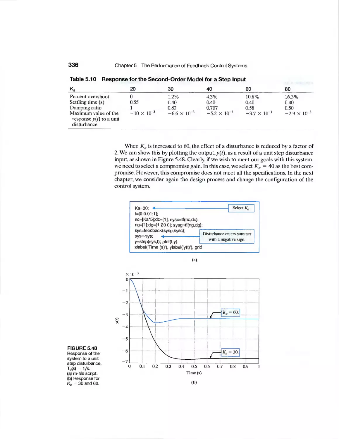
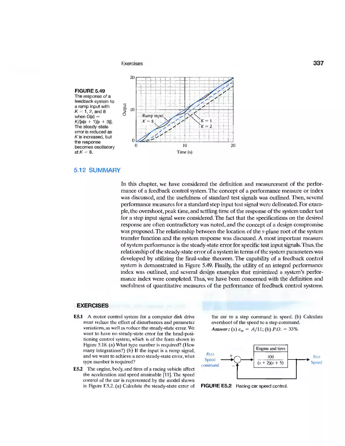
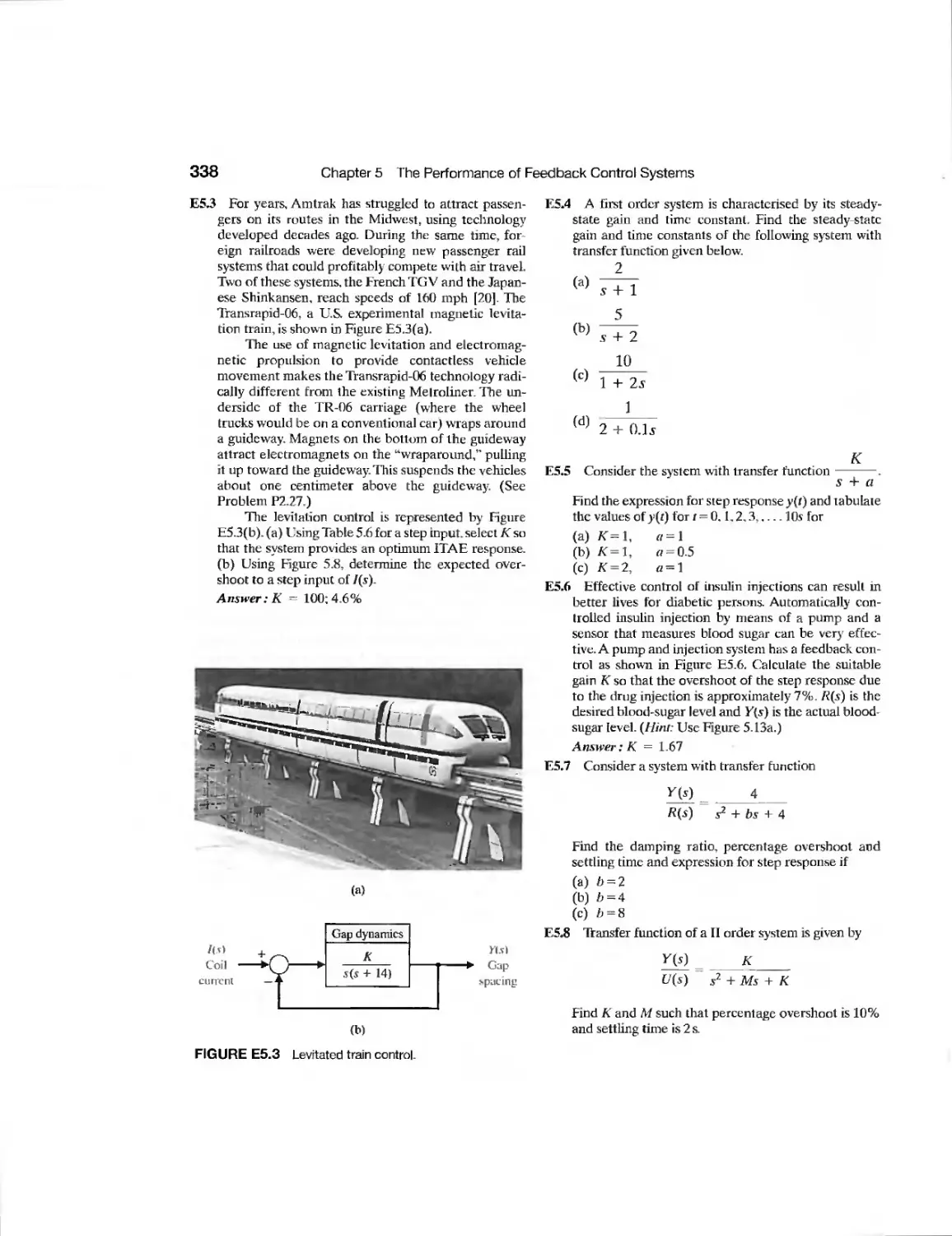
5.11 Sequential Design Example: Disk Drive Read System 333
5.12 Summary 337
Exercises 337
Problems 341
Advanced Problems 346
Design Problems 348
Computer Problems 350
Terms and Concepts 353
chapter 6 The Stability of Linear Feedback Systems 355
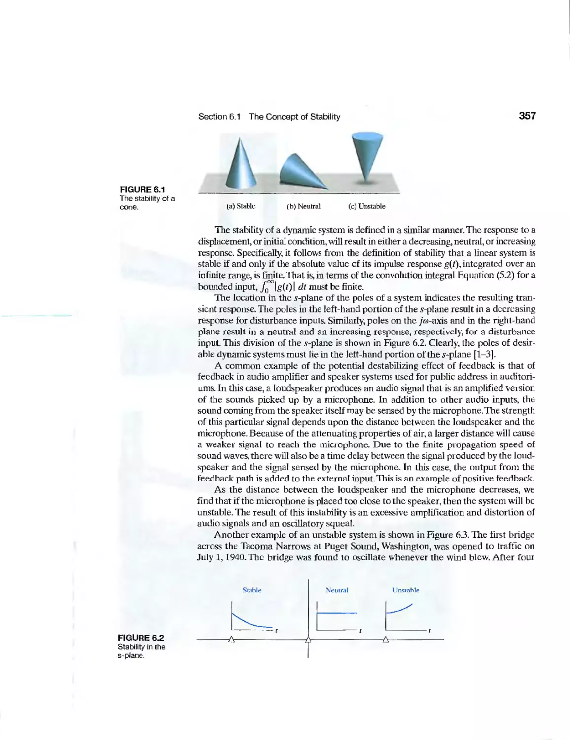
6.1 The Concept of Stability 356
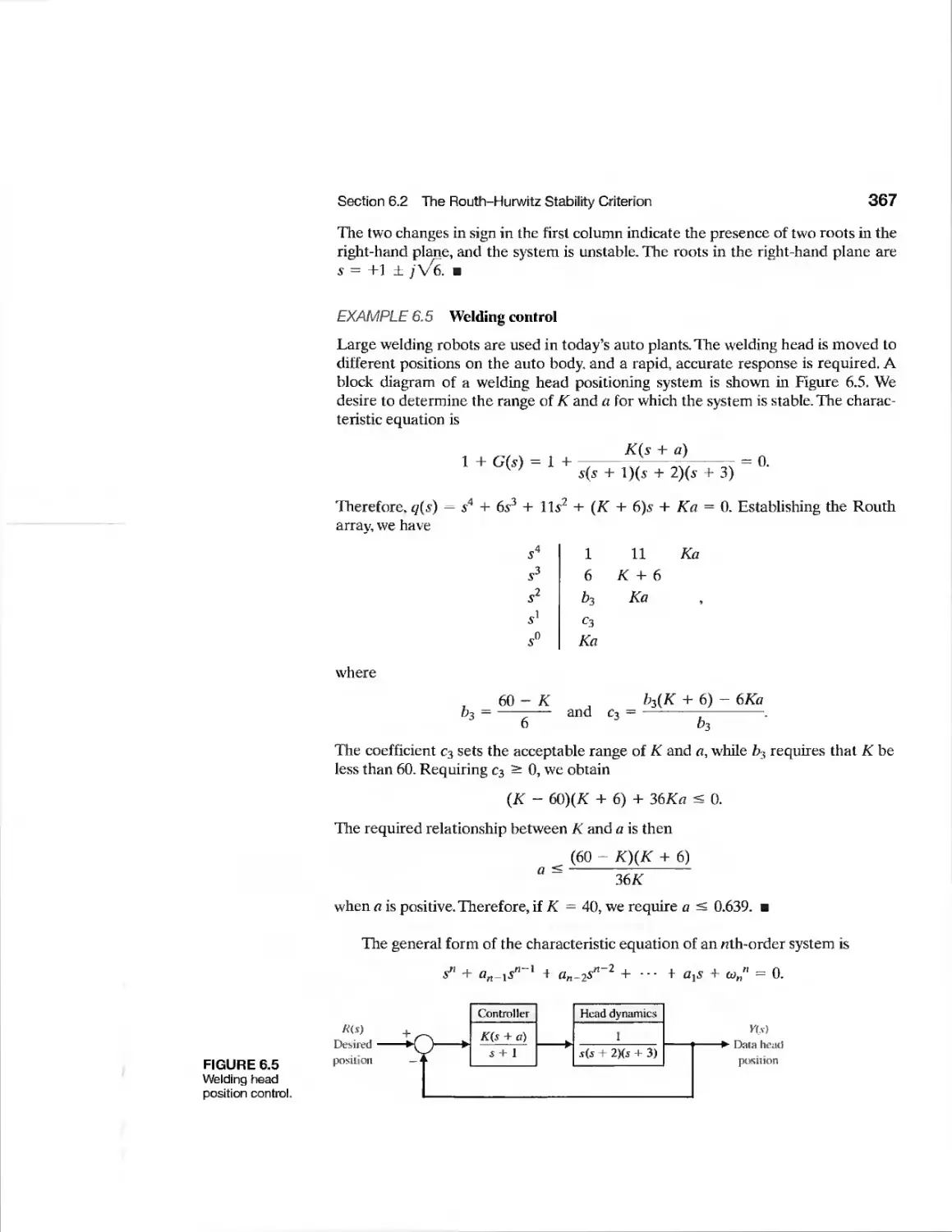
6.2 The Routh-Hurwitz Stability Criterion 360
6.3 The Relative Stability of Feedback Control Systems 368
6.4 The Stability of State Variable Systems 370
6J5 Design Examples 373
6.6 System Stability Using Control Design Software 382
6.7 Sequential Design Example: Disk Drive Read System 390
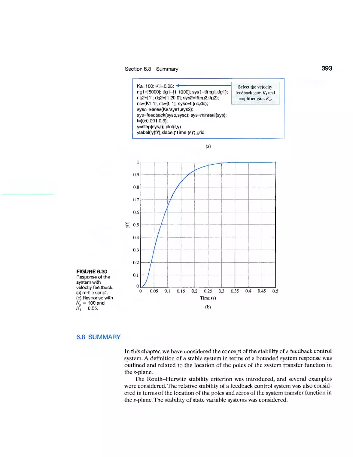
6.8 Summary 393
Exercises 394
Problems 396
Advanced Problems 400
Design Problems 402
Computer Problems 404
Terms and Concepts 406
VII
CHAPTER
The Root Locus Method 407
7.1 Introduction 408
7.2 The Root Locus Concept 408
7.3 The Root Locus Procedure 413
7.4 Parameter Design by the Root Locus Method 431
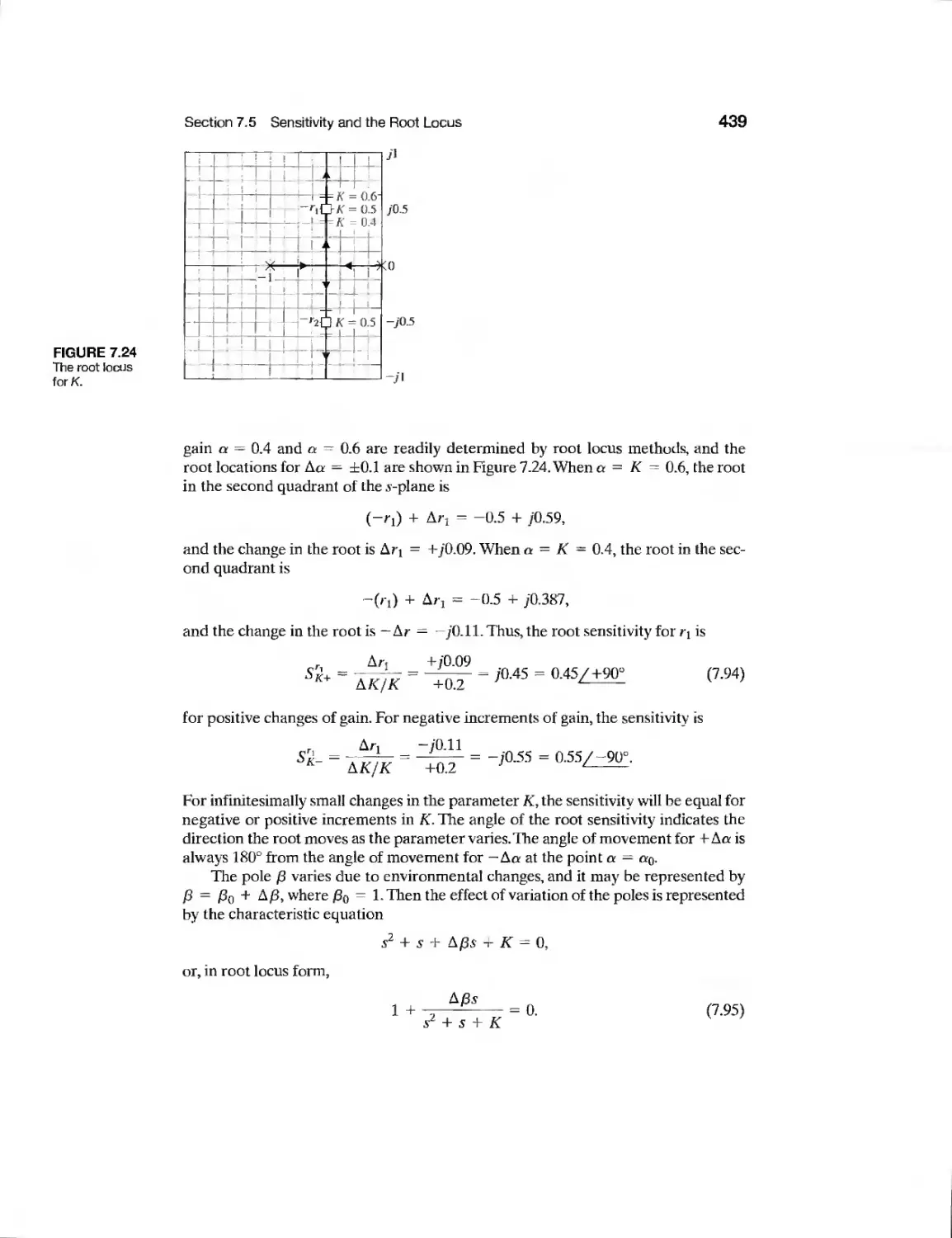
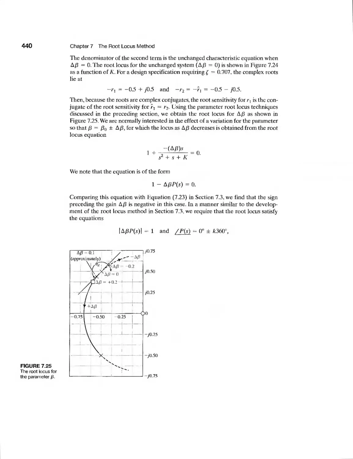
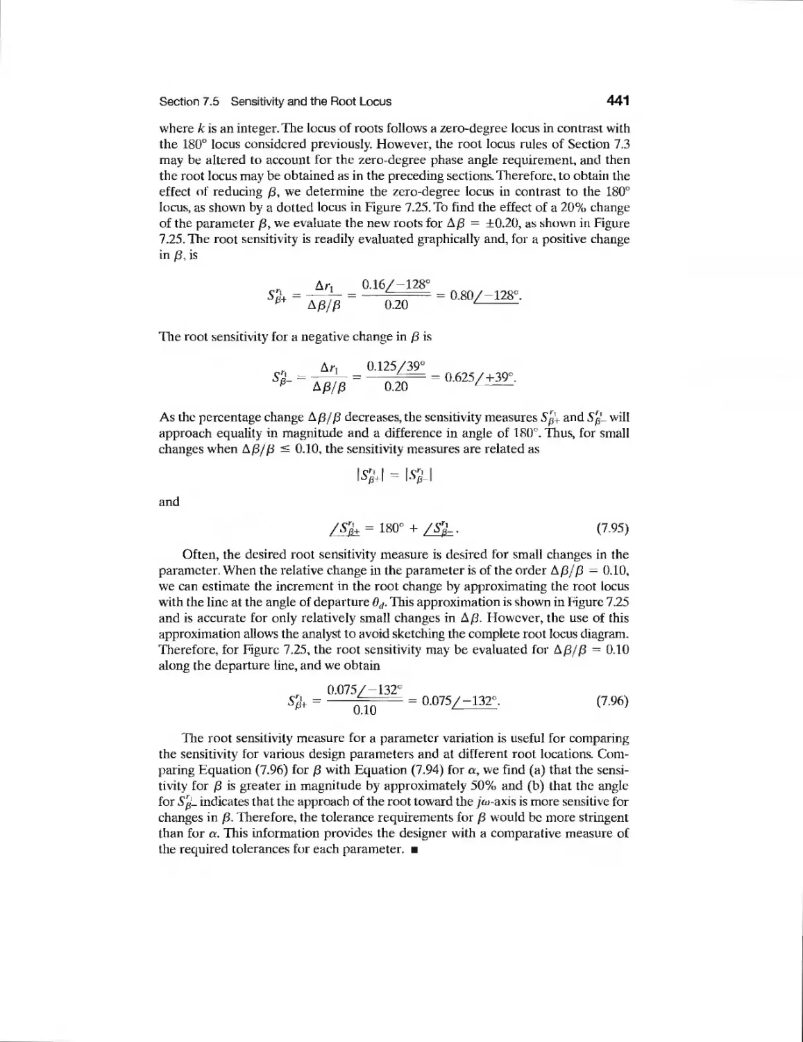
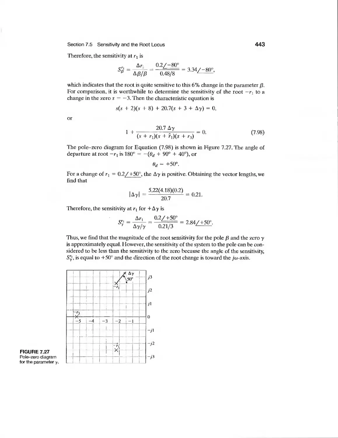
7.5 Sensitivity and the Root Locus 437
7.6 Three-Term (PID) Controllers 444
7.7 Design Examples 447
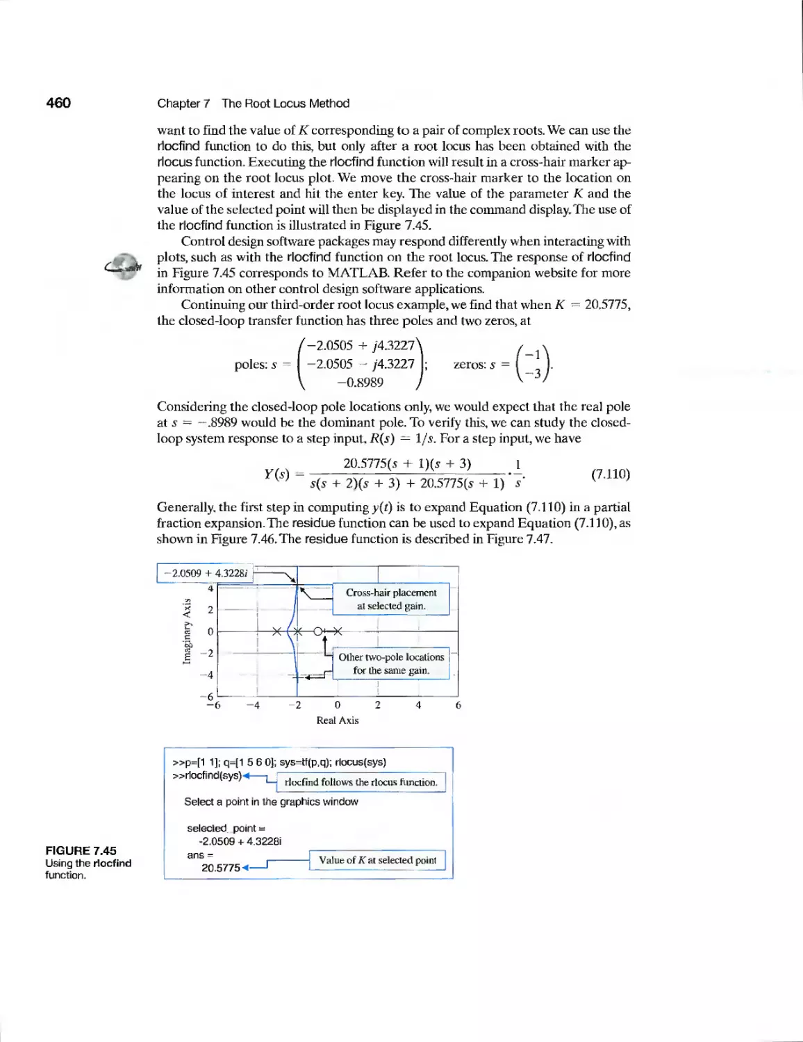
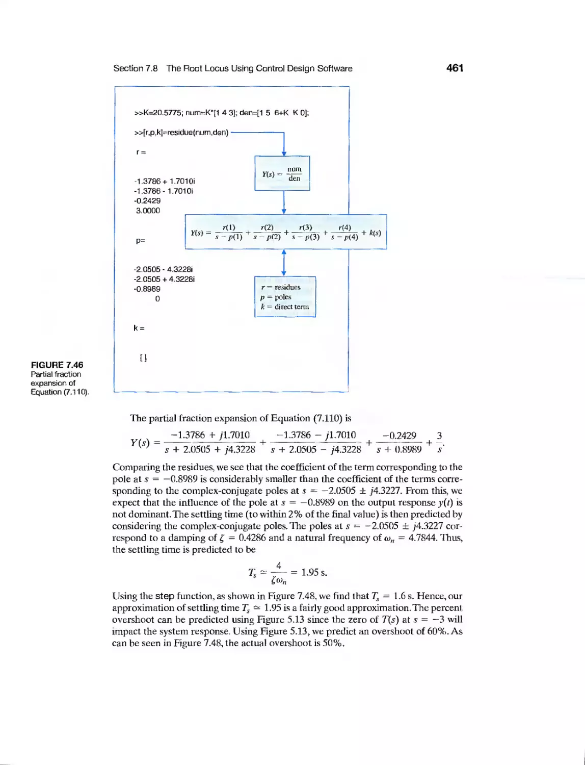
7.8 The Root Locus Using Control Design Software 458
7.9 Sequential Design Example: Disk Drive Read System 463
viii
Contents
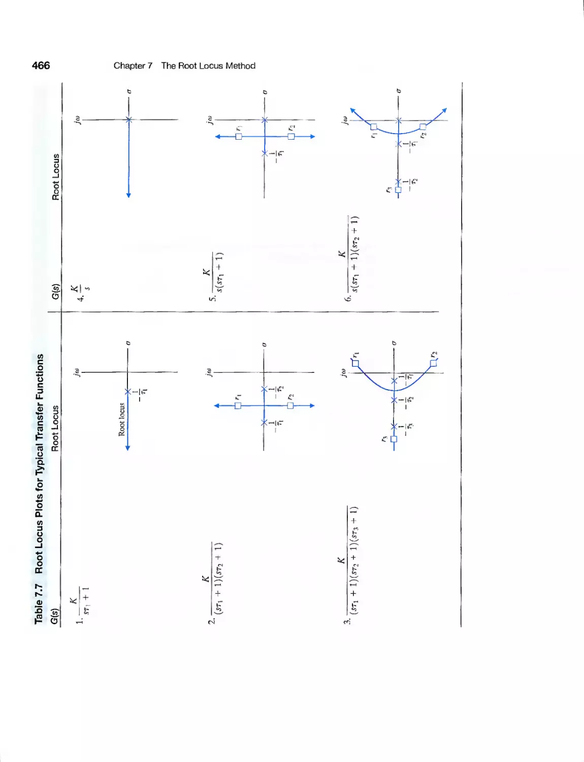
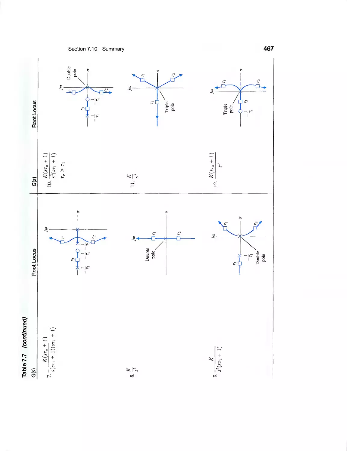
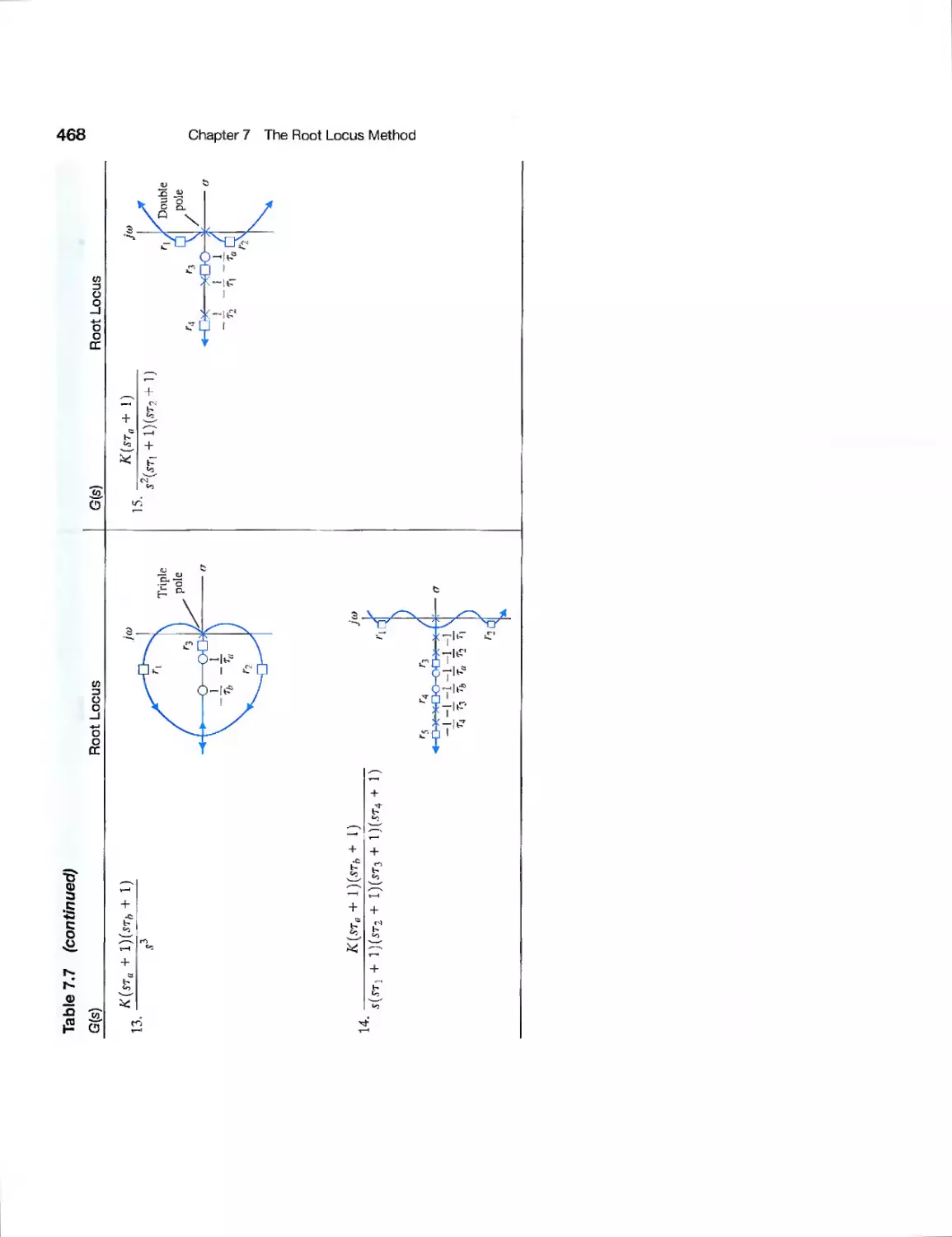
7.10 Summary 465
Exercises 469
Problems 472
Advanced Problems 482
Design Problems 485
Computer Problems 490
Terms and Concepts 492
chapter 8 Frequency Response Methods 493
8.1 Introduction 494
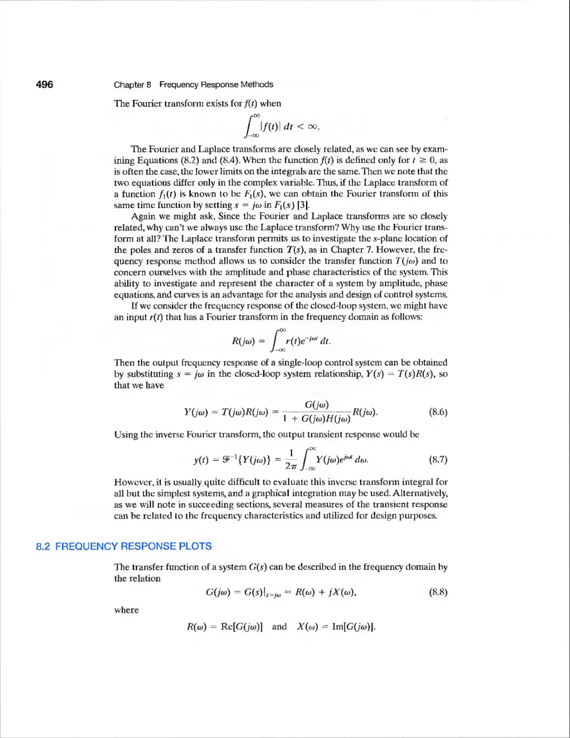
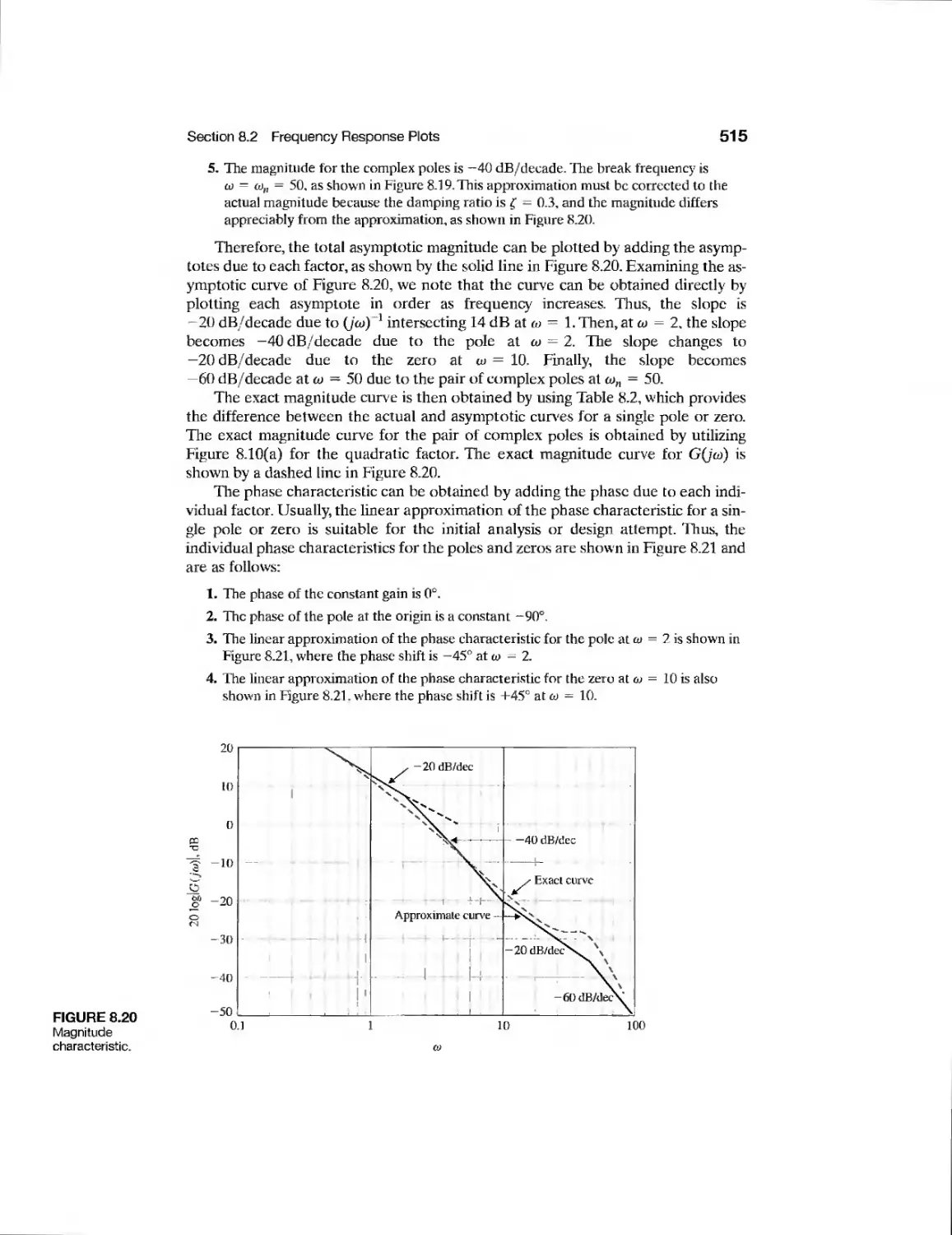
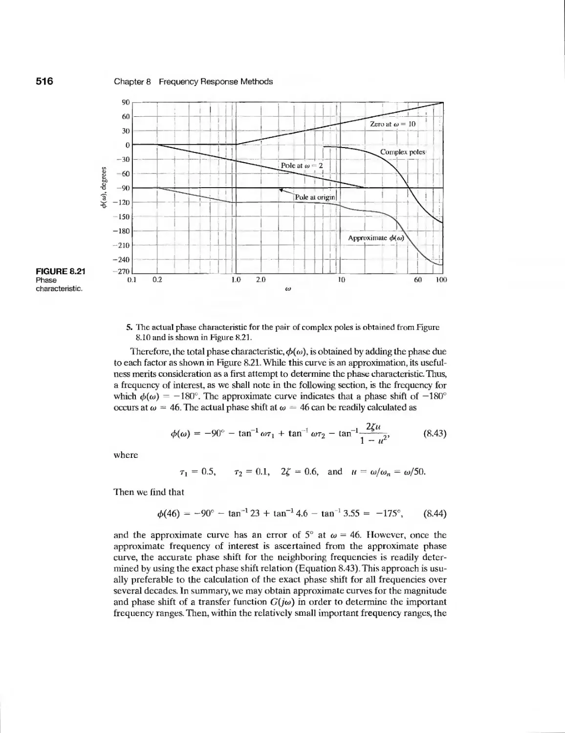
8.2 Frequency Response Plots 496
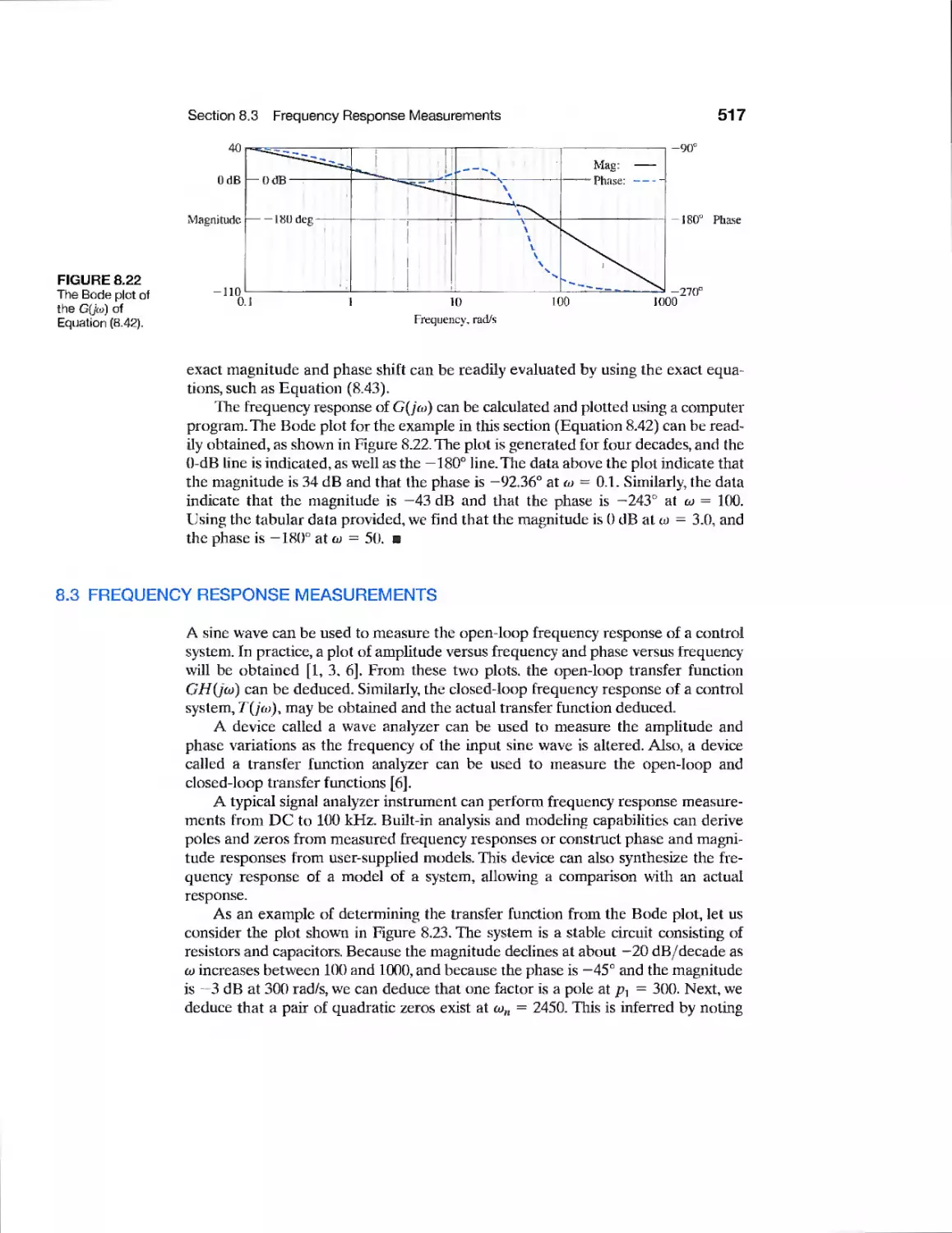
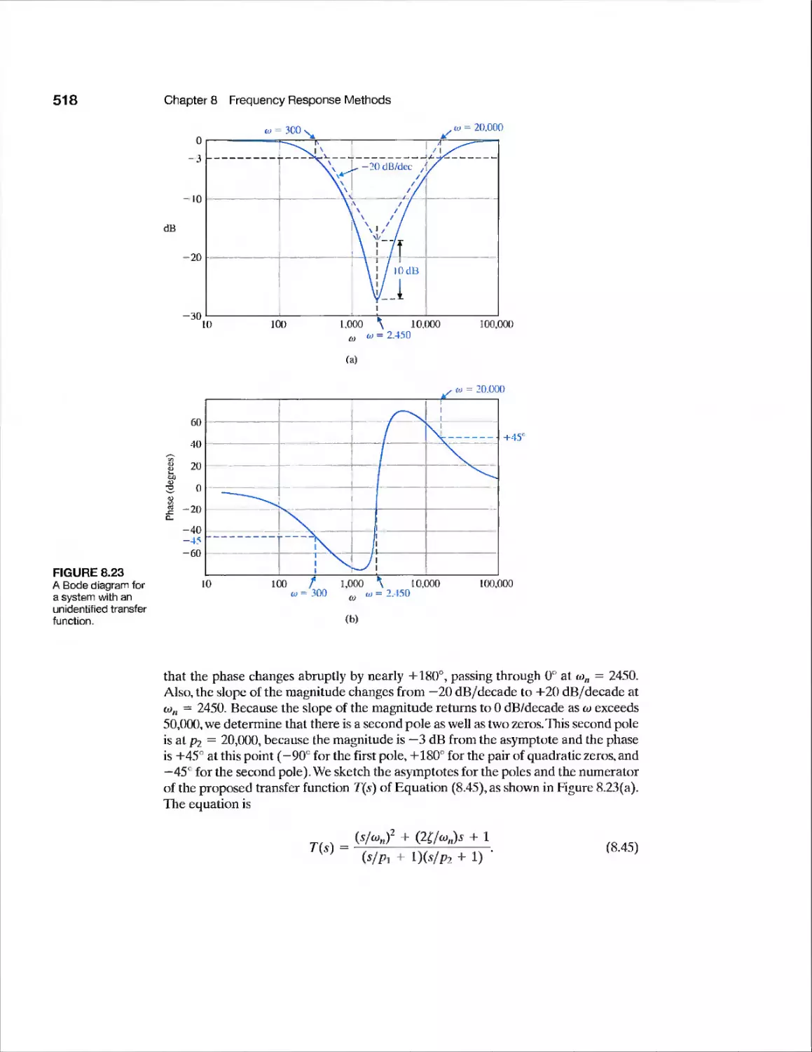
8.3 Frequency Response Measurements 517
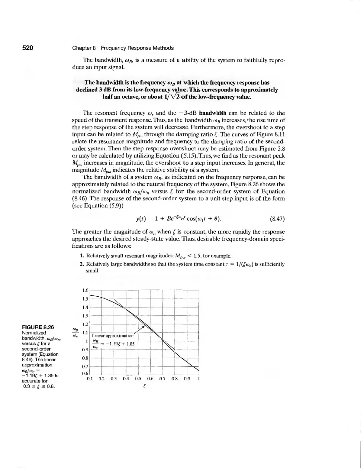
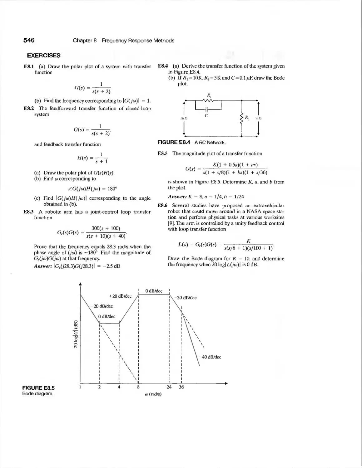
8.4 Performance Specifications in the Frequency Domain 519
8.5 Log Magnitude and Phase Diagrams 522
8.6 Design Examples 523
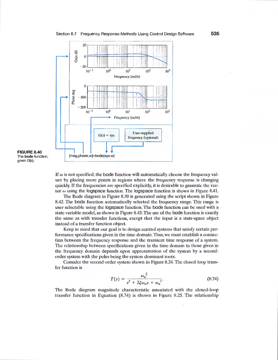
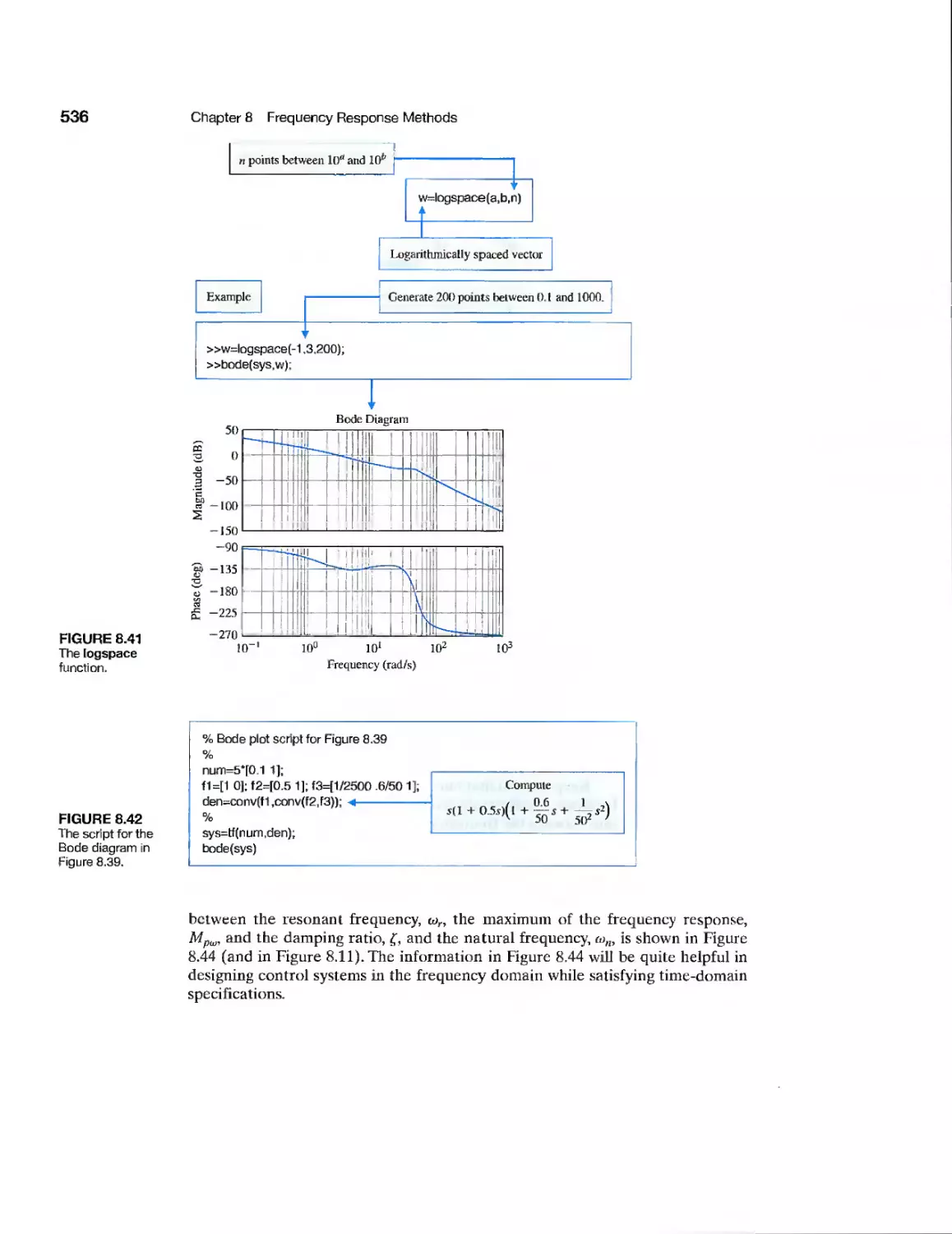
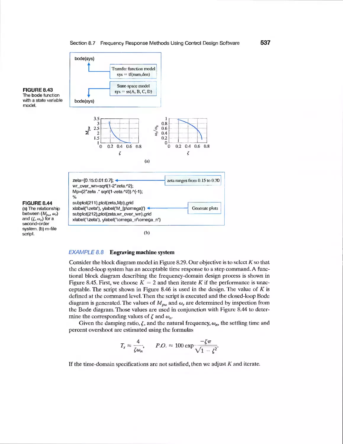
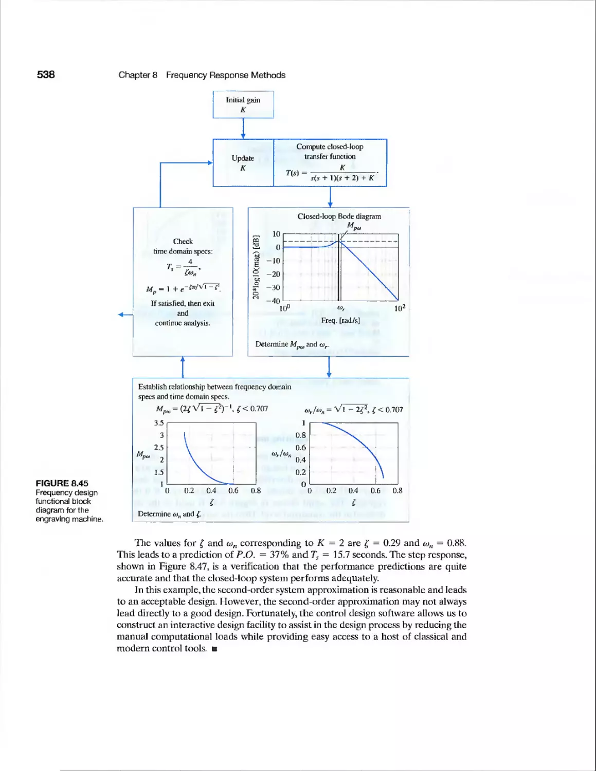
8.7 Frequency Response Methods Using Control Design Software 534
8.8 Sequential Design Example: Disk Drive Read System 540
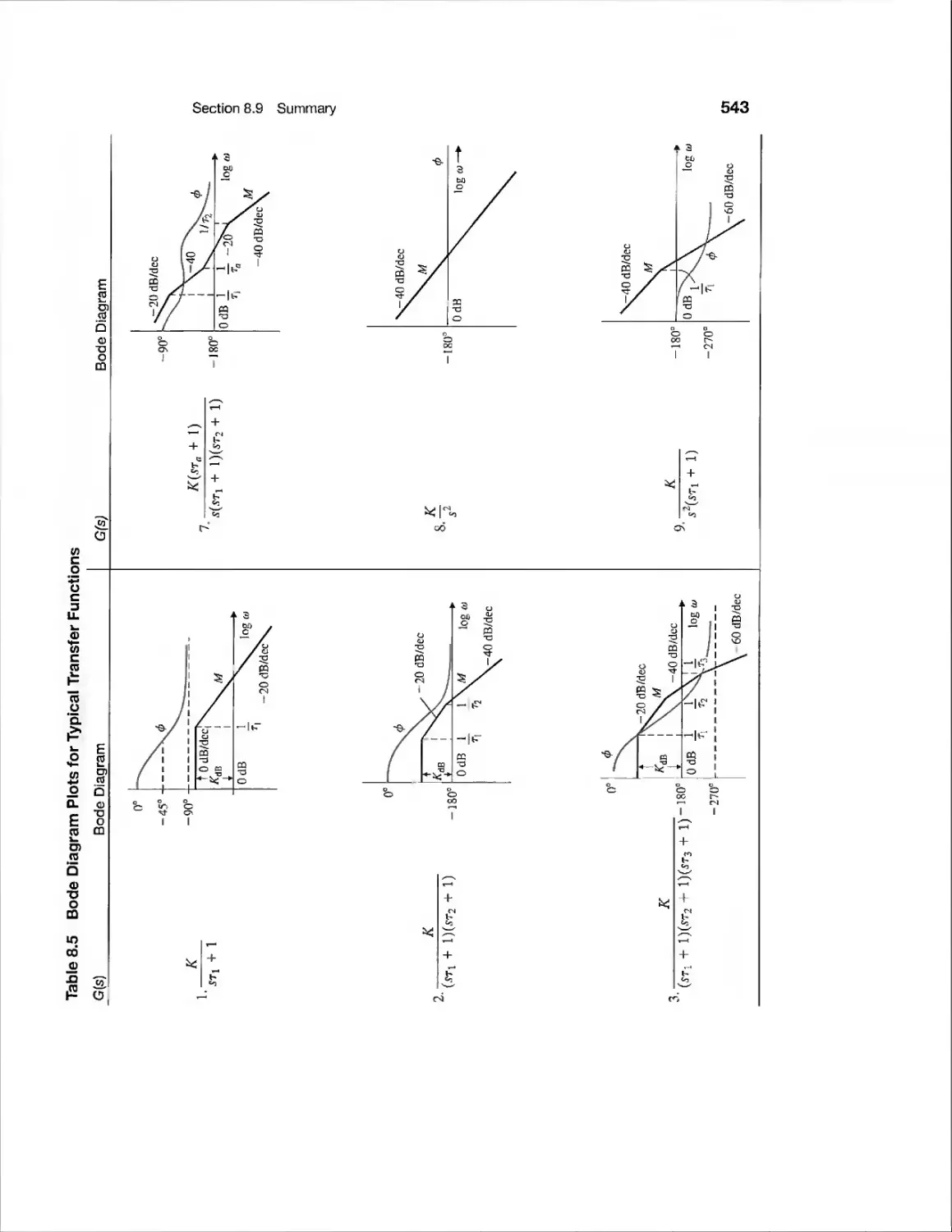
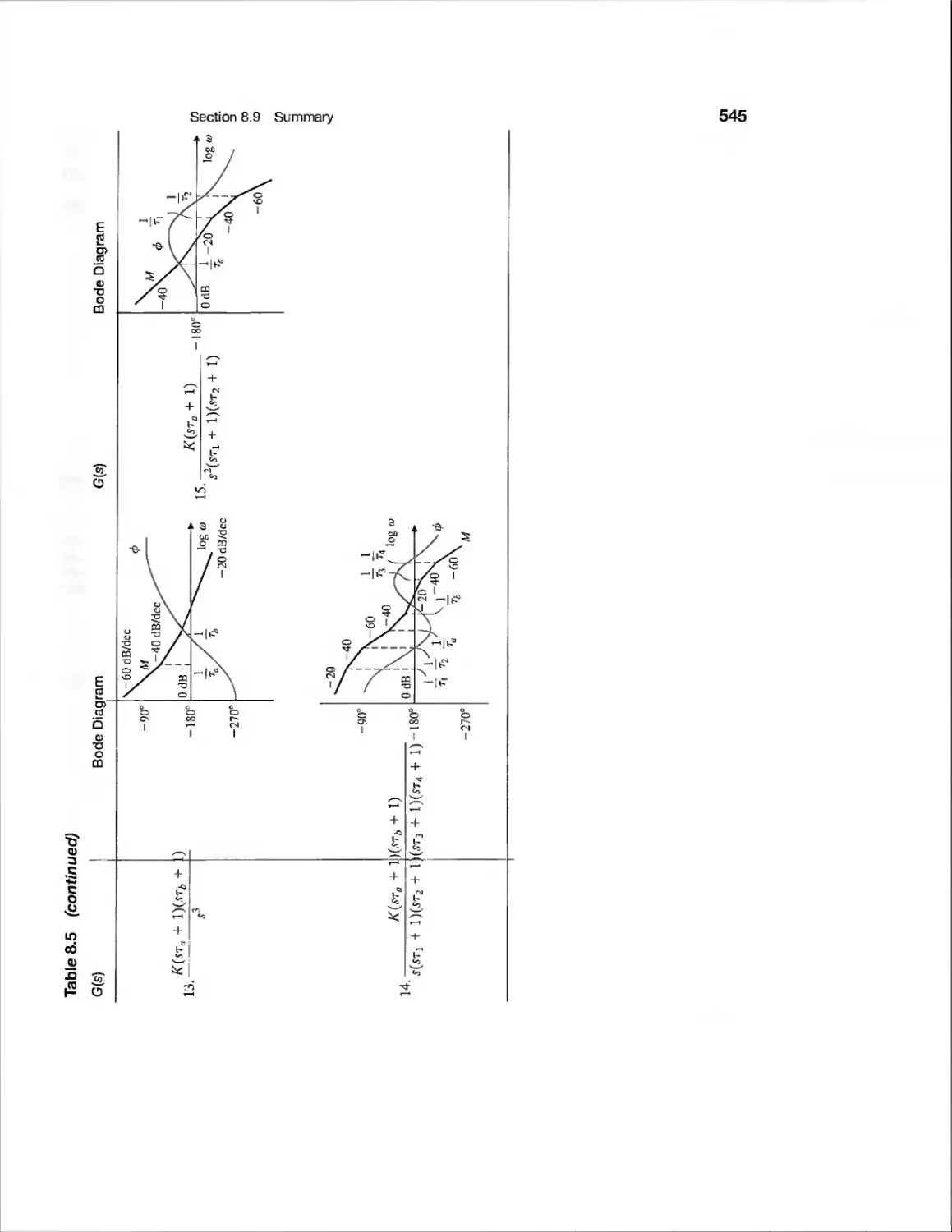
8.9 Summary 541
Exercises 546
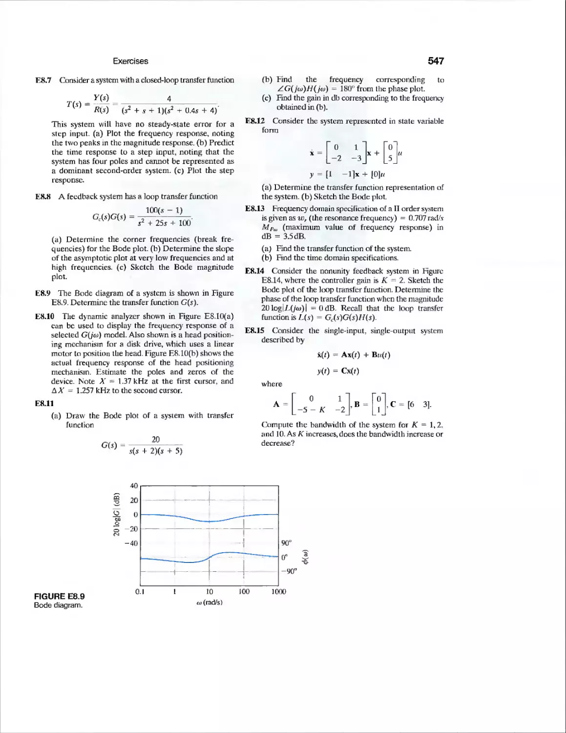
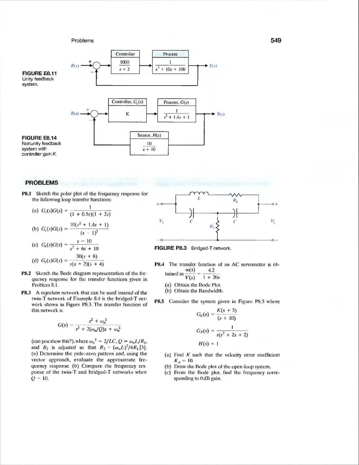
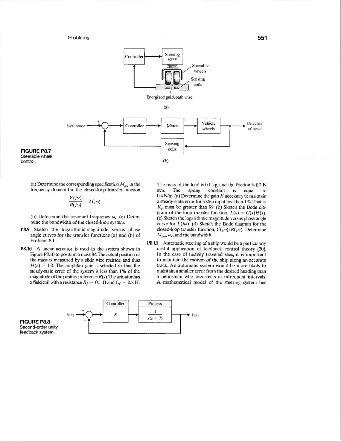
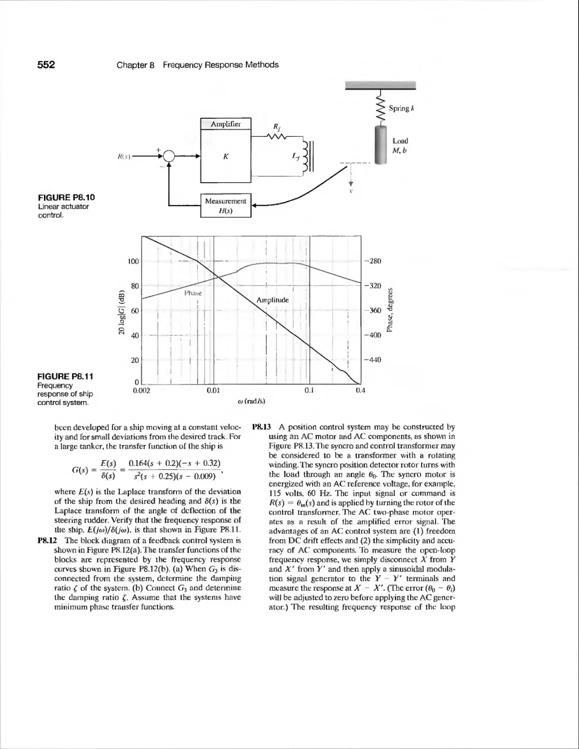
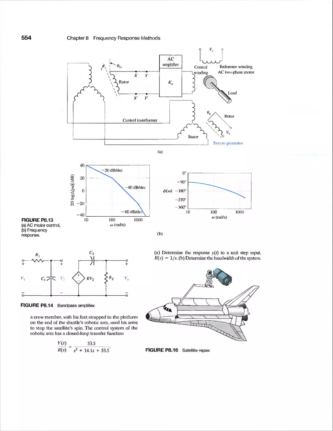
Problems 549
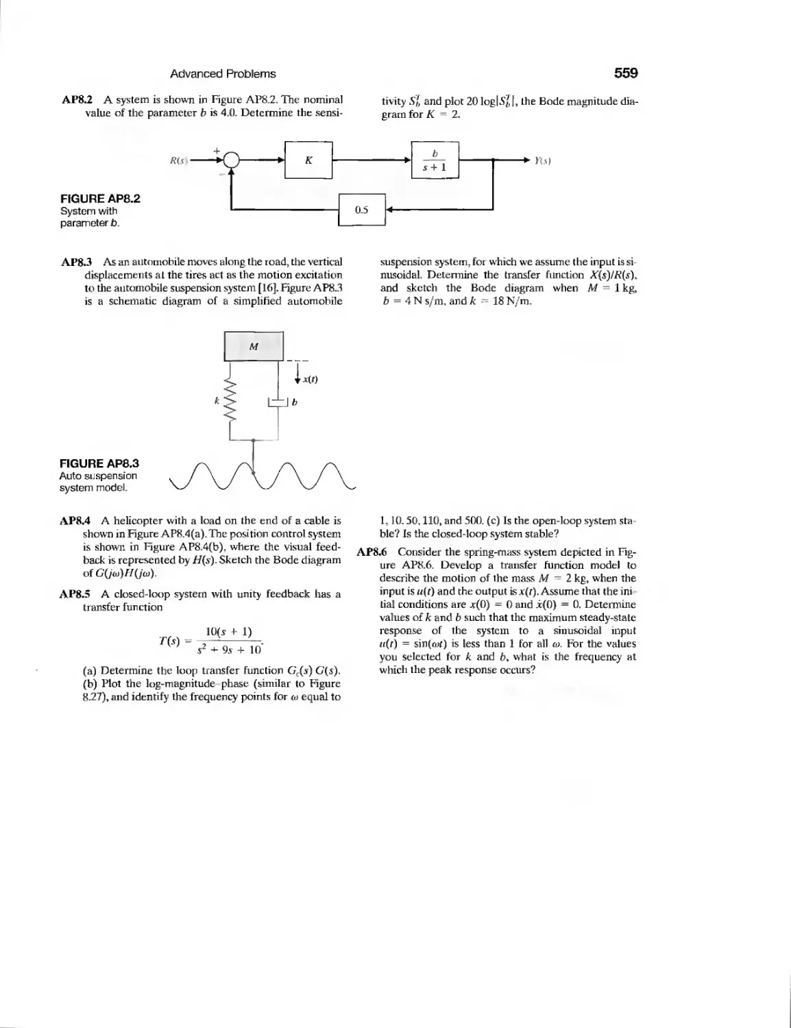
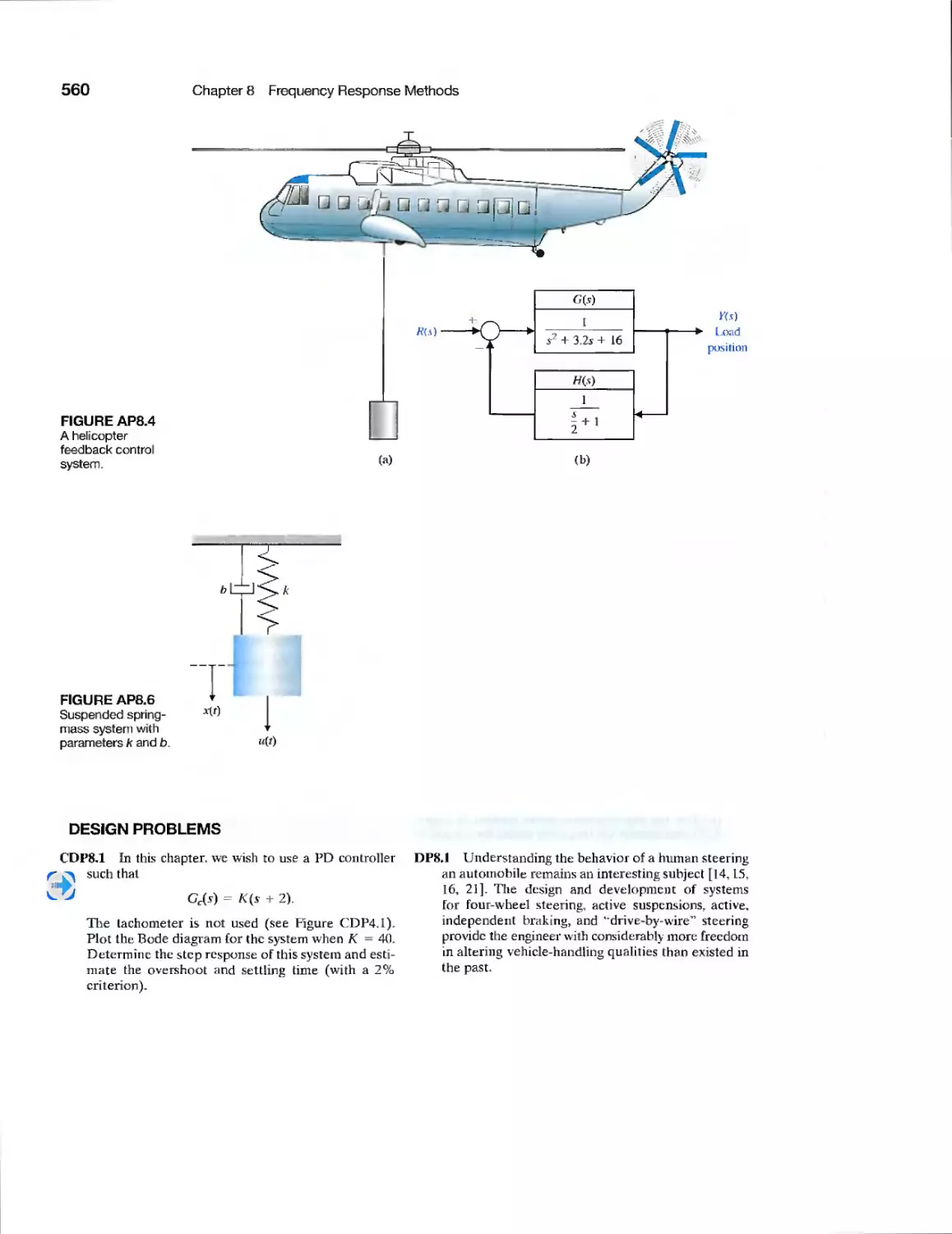
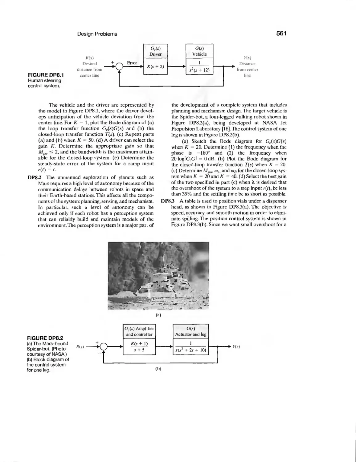
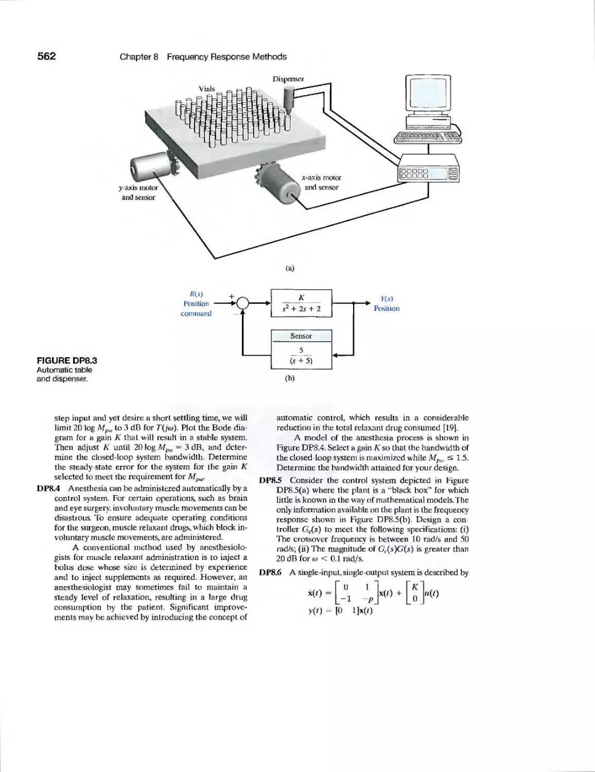
Advanced Problems 558
Design Problems 560
Computer Problems 564
Terms and Concepts 566
chapter 9 Stability in the Frequency Domain 567
9.1 Introduction 568
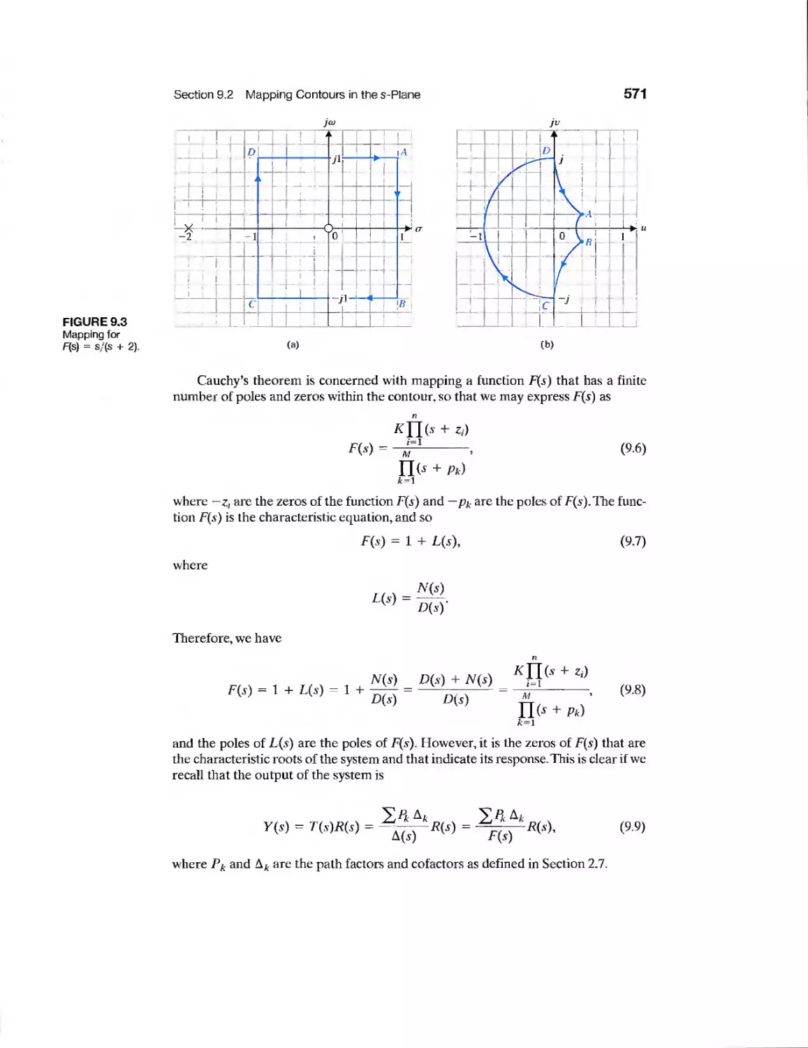
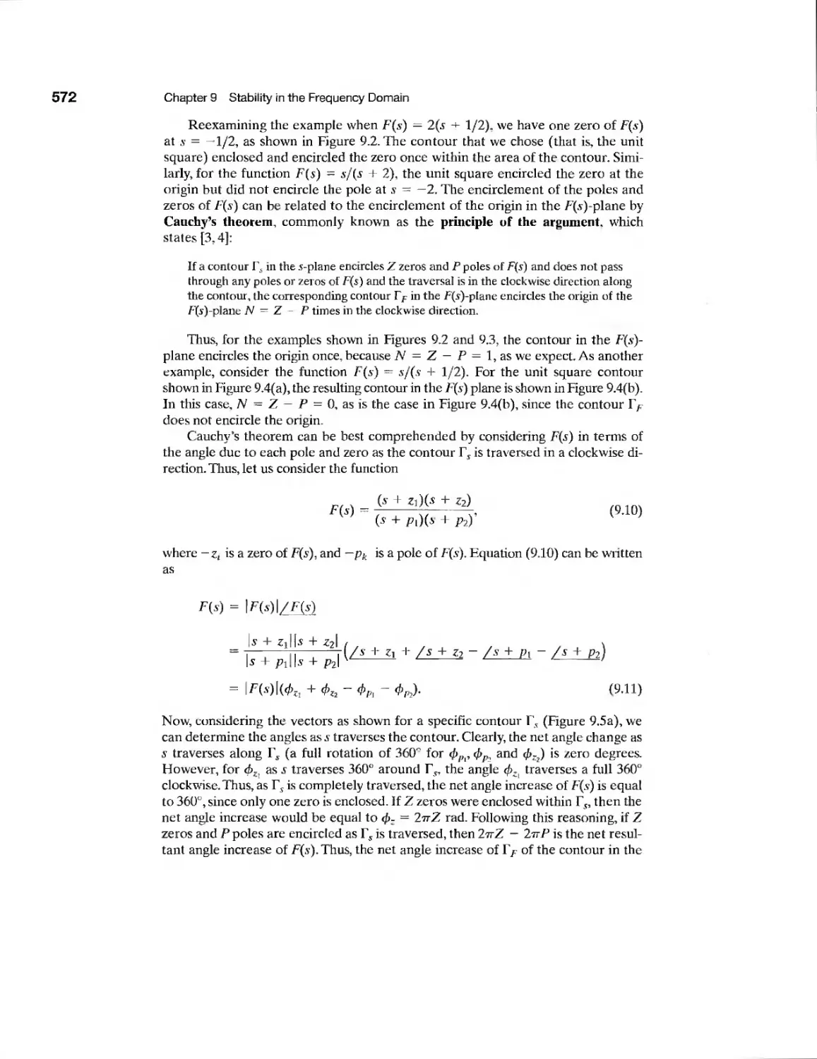
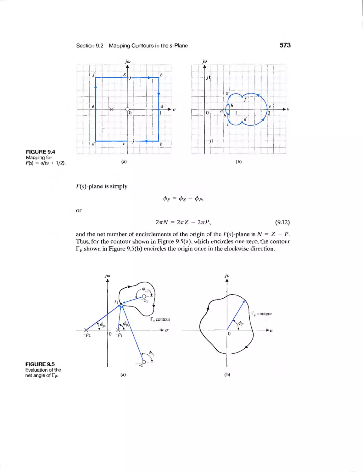
9.2 Mapping Contours in the s-Plane 569
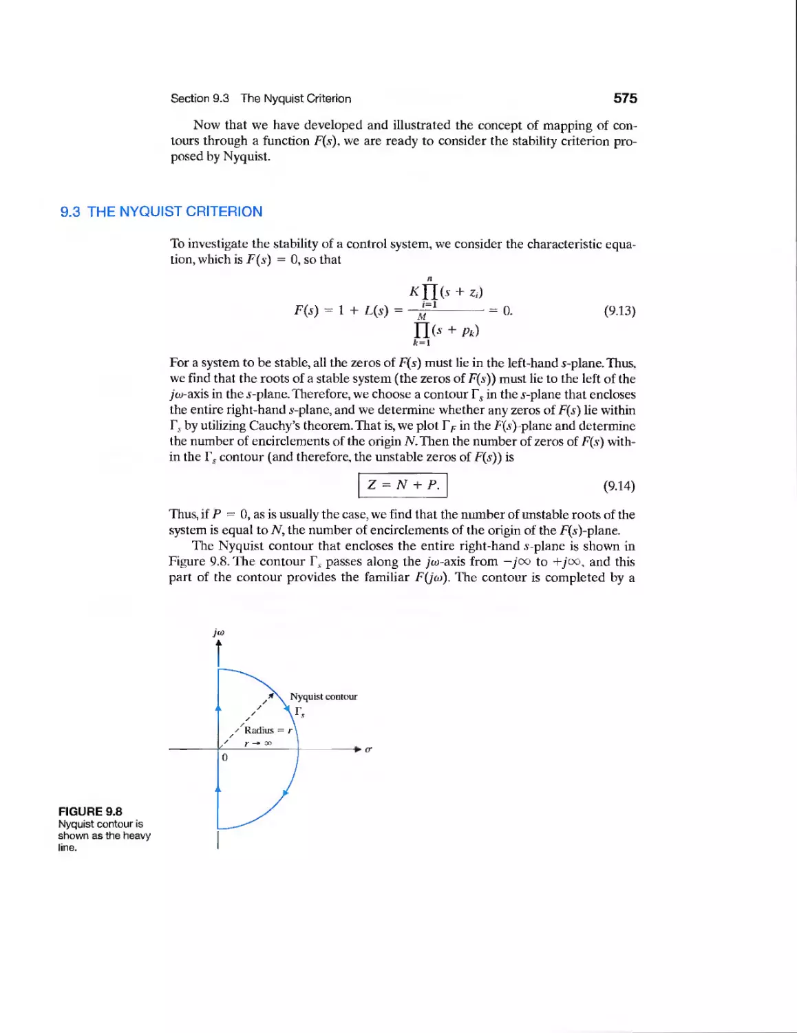
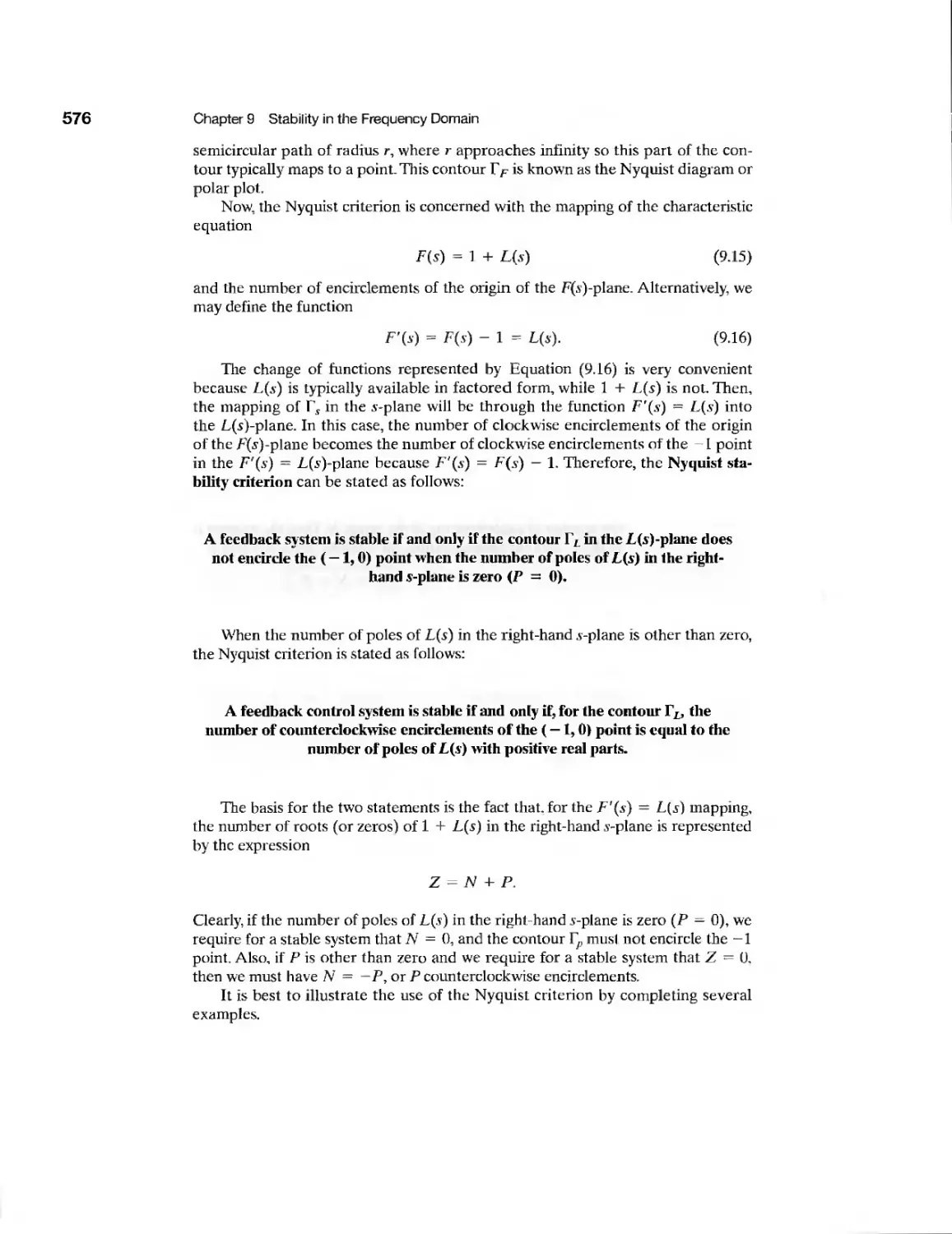
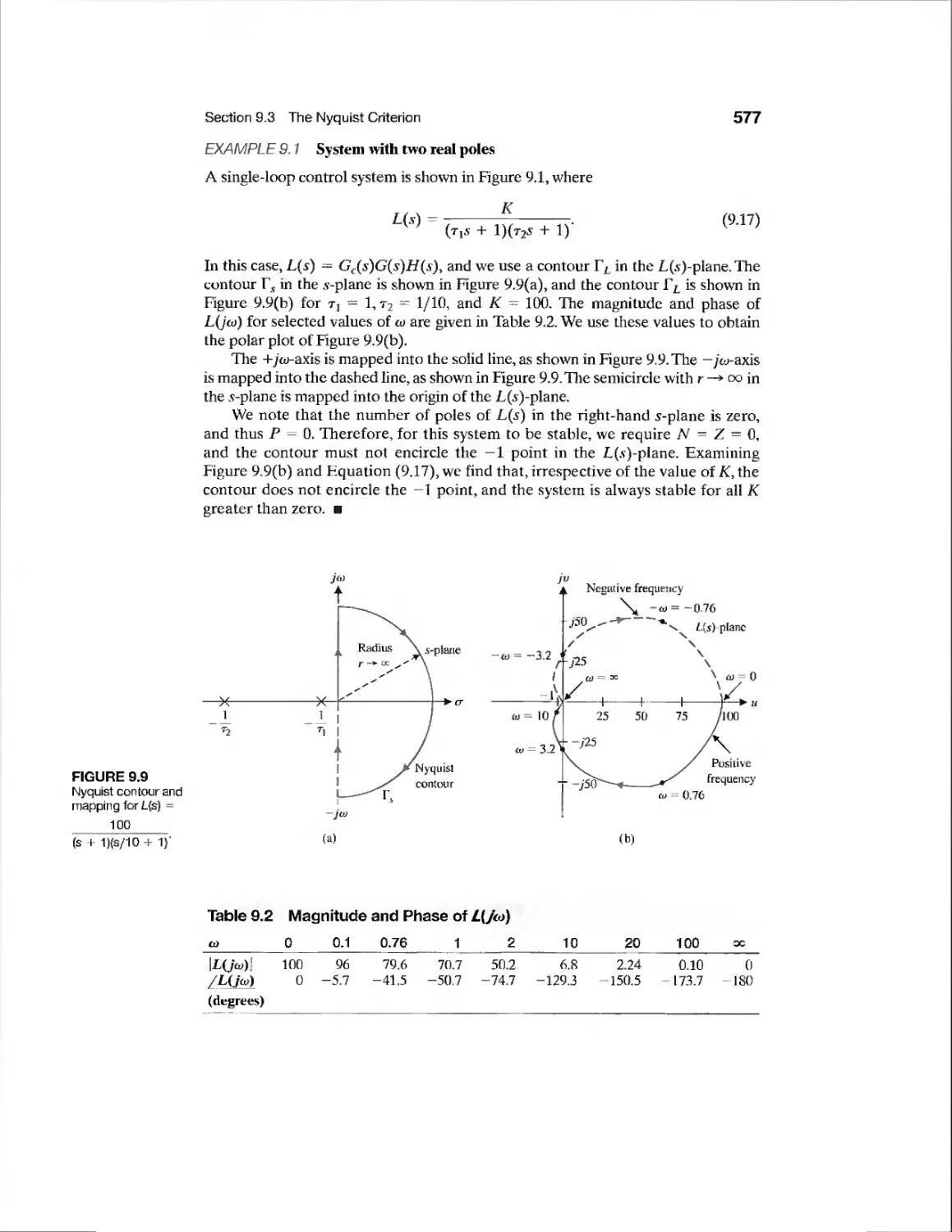
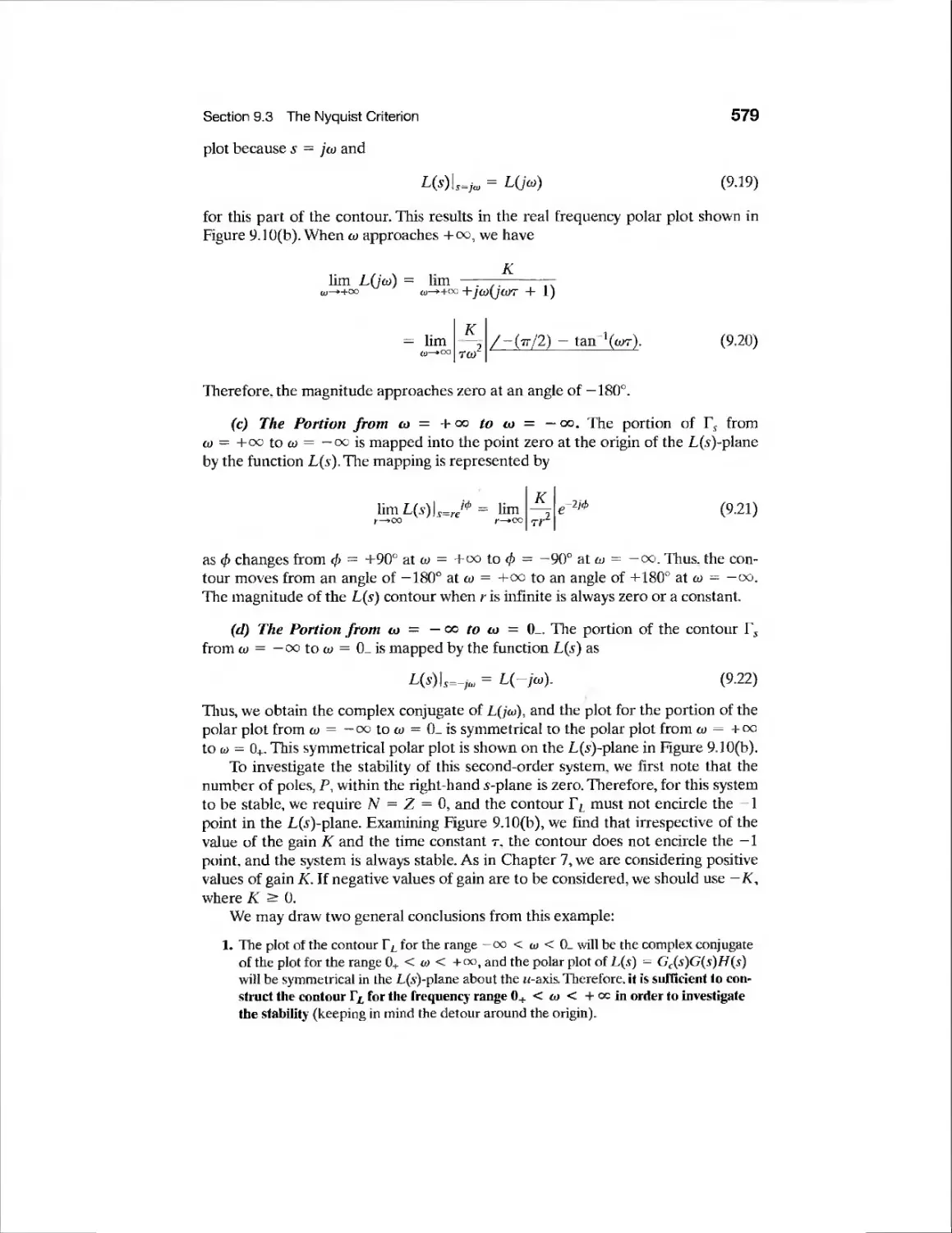
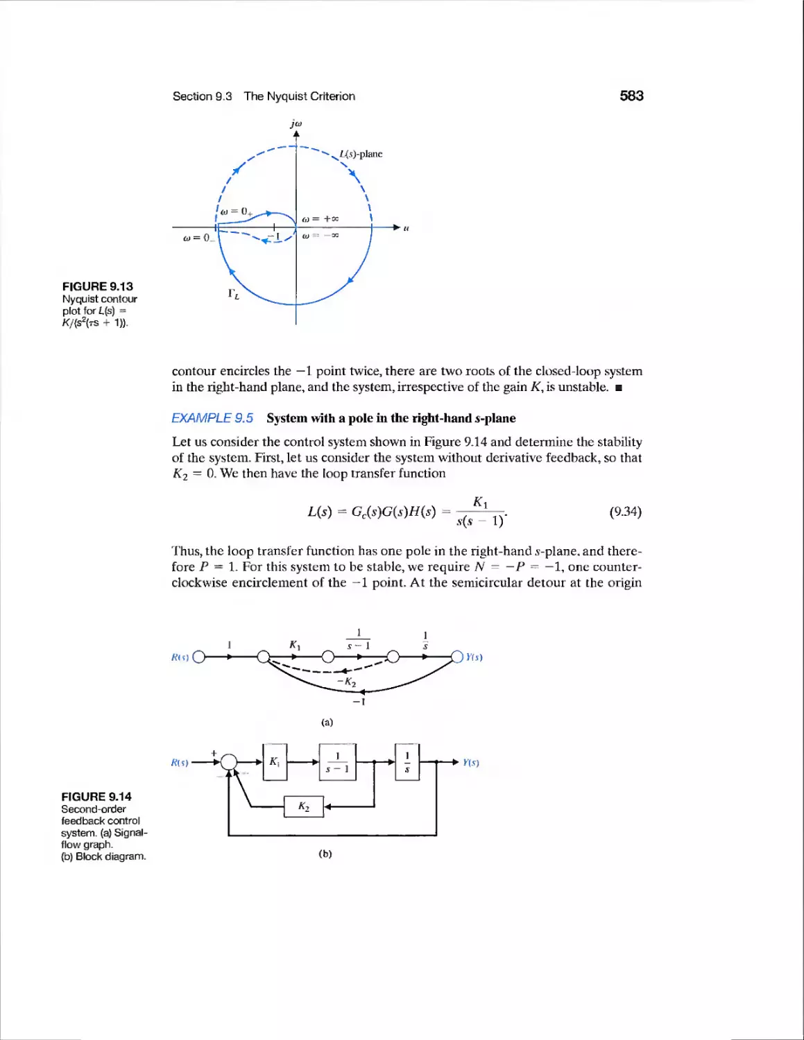
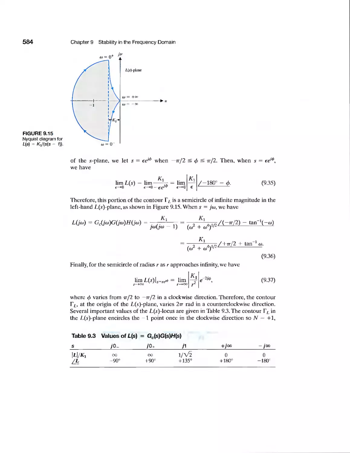
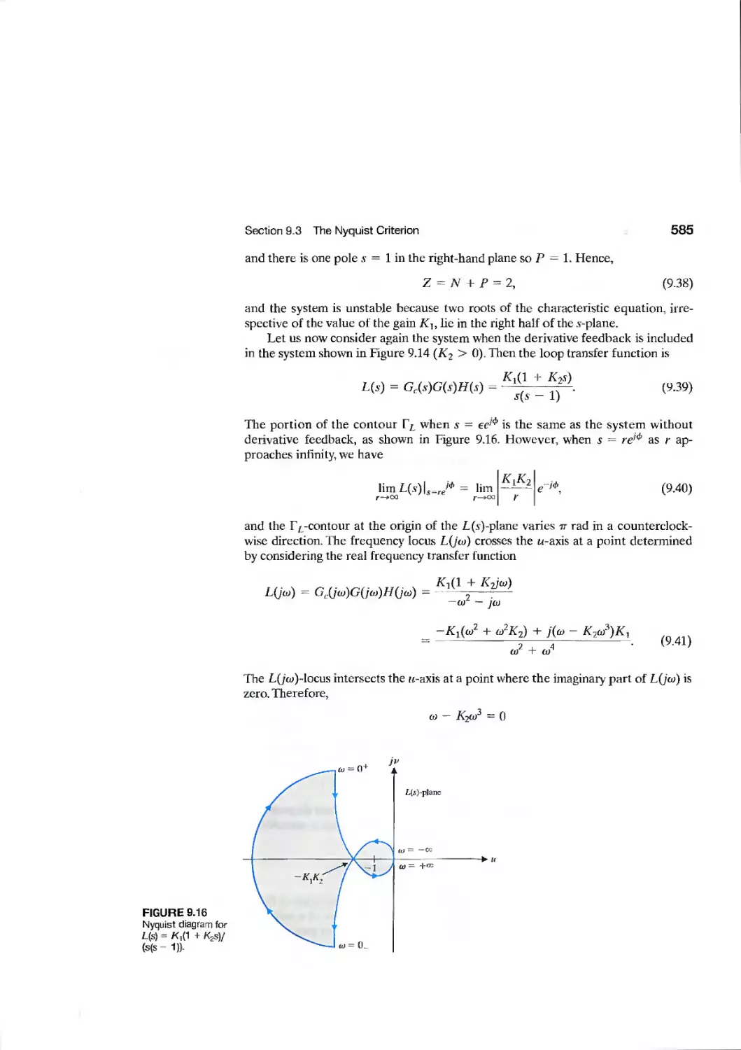
9.3 The Nyquist Criterion 575
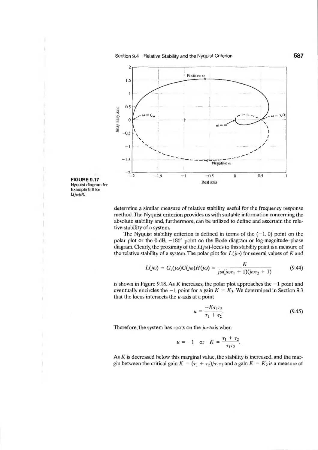
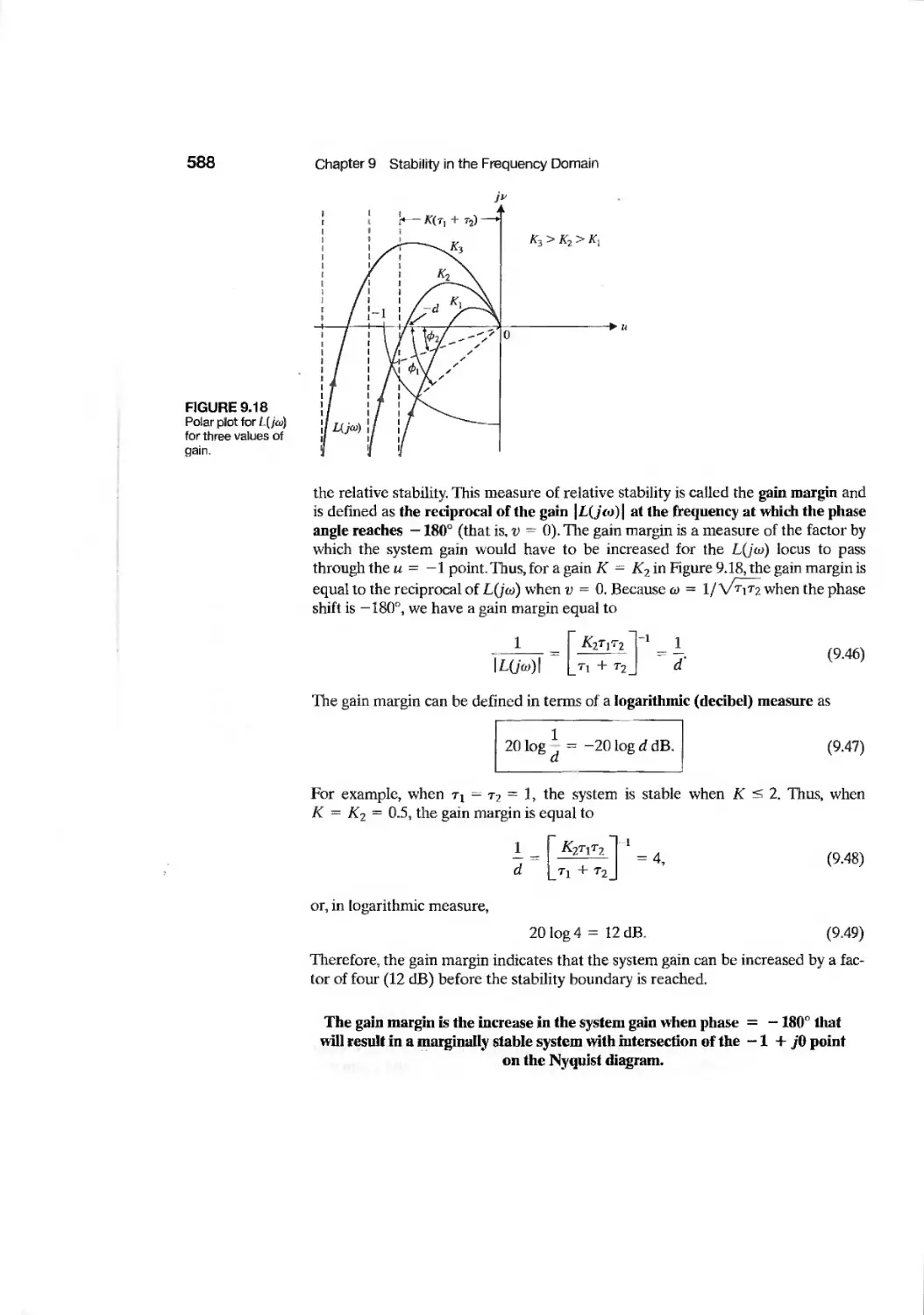
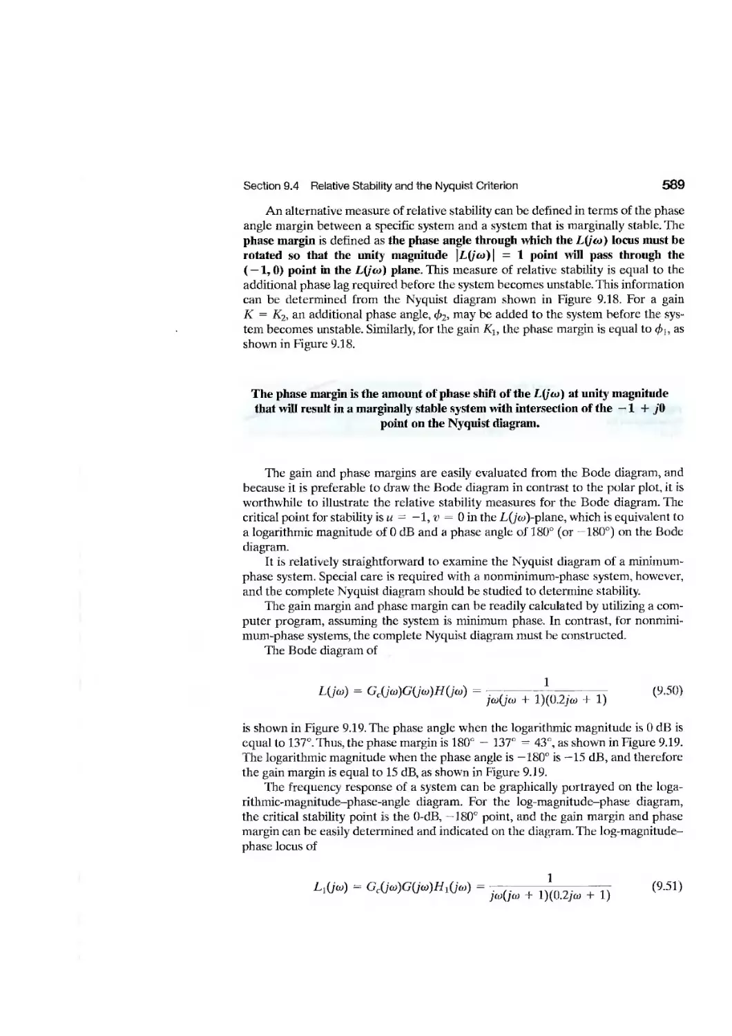
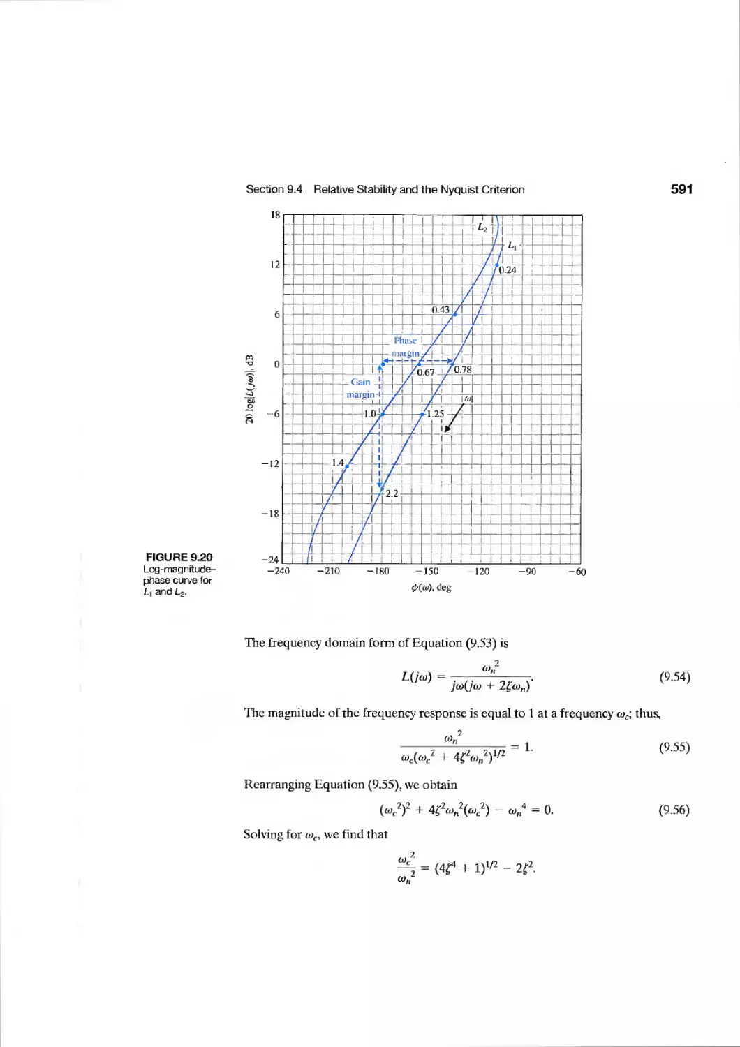
9.4 Relative Stability and the Nyquist Criterion 586
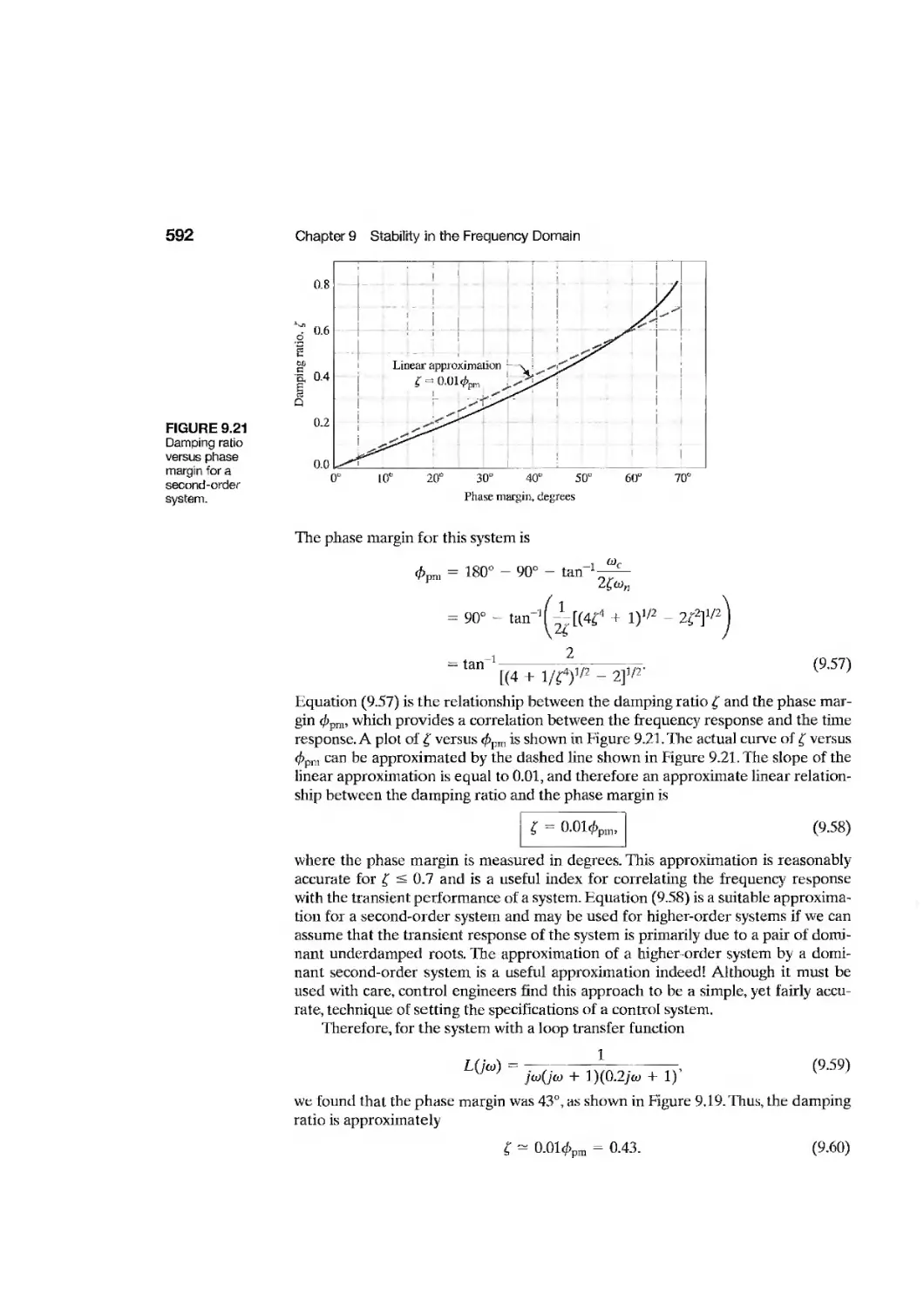
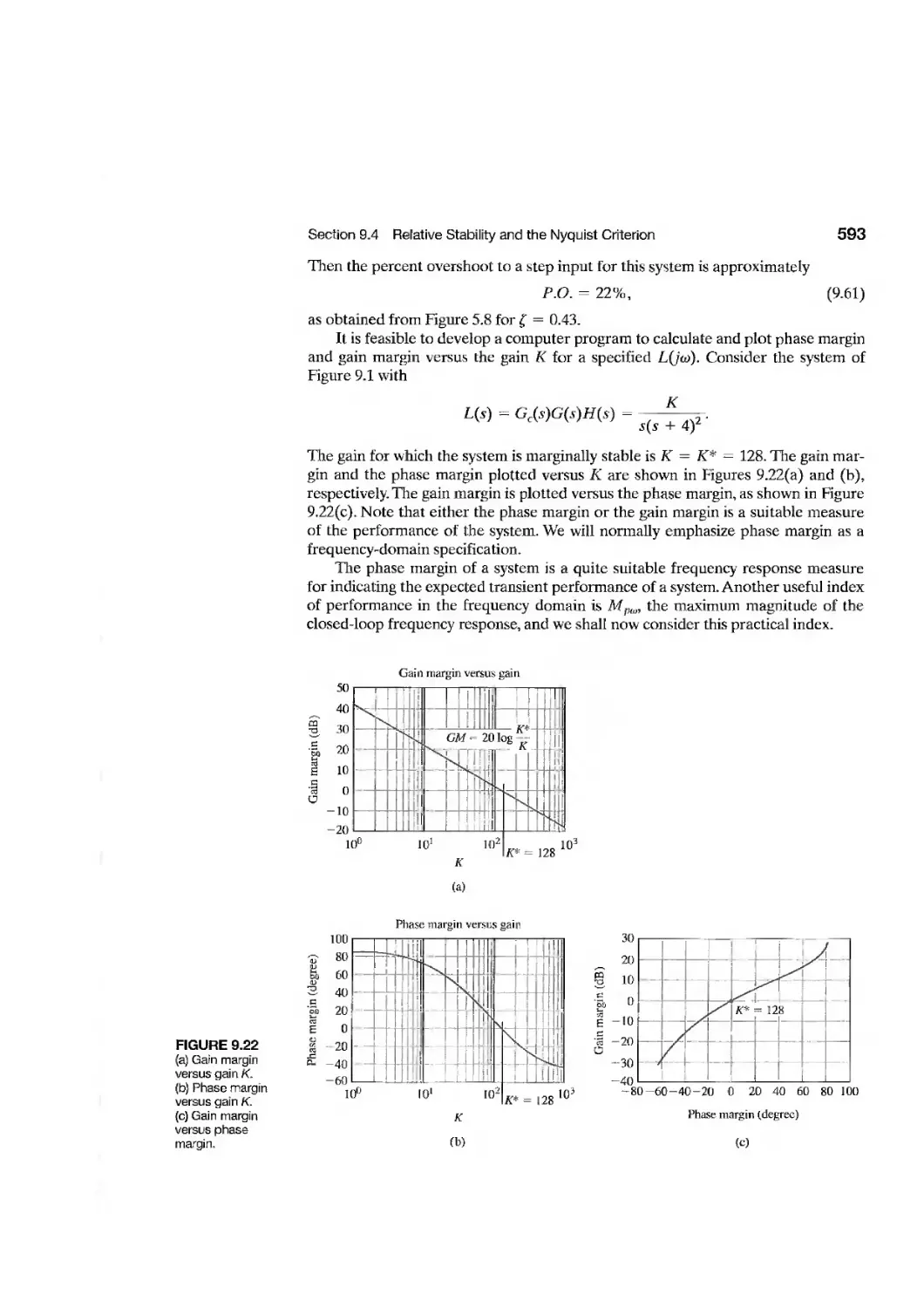
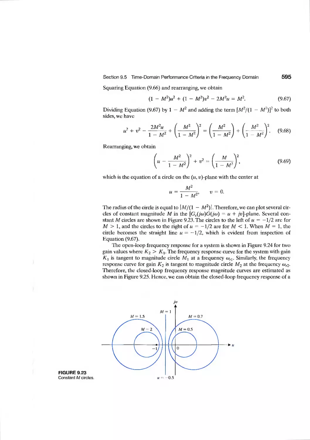
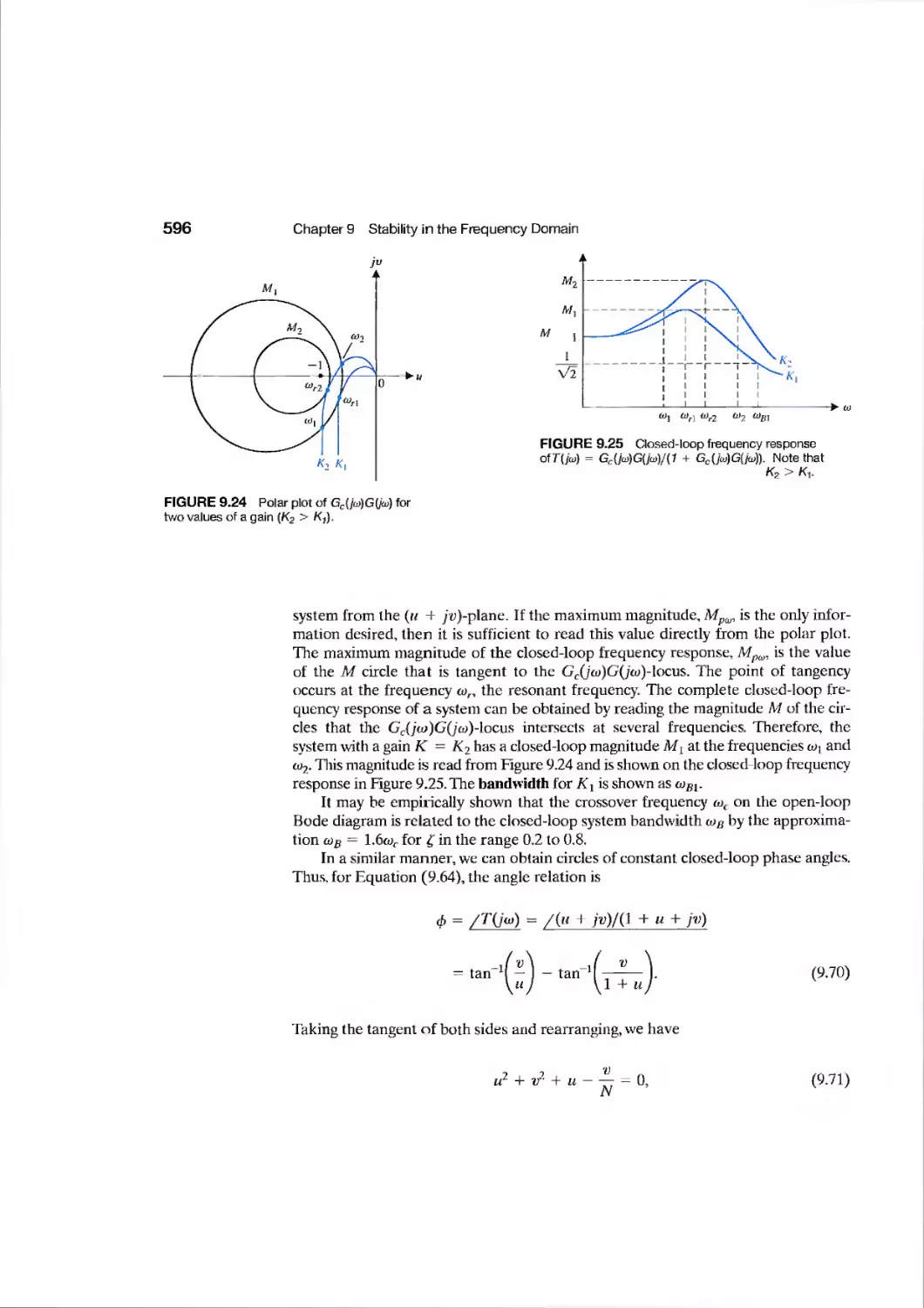
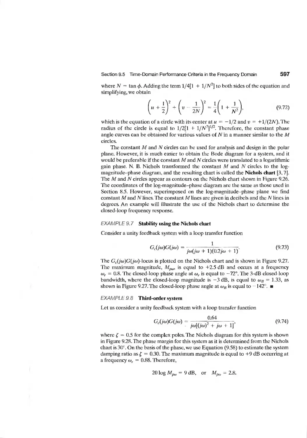
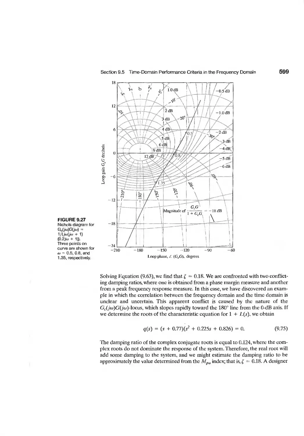
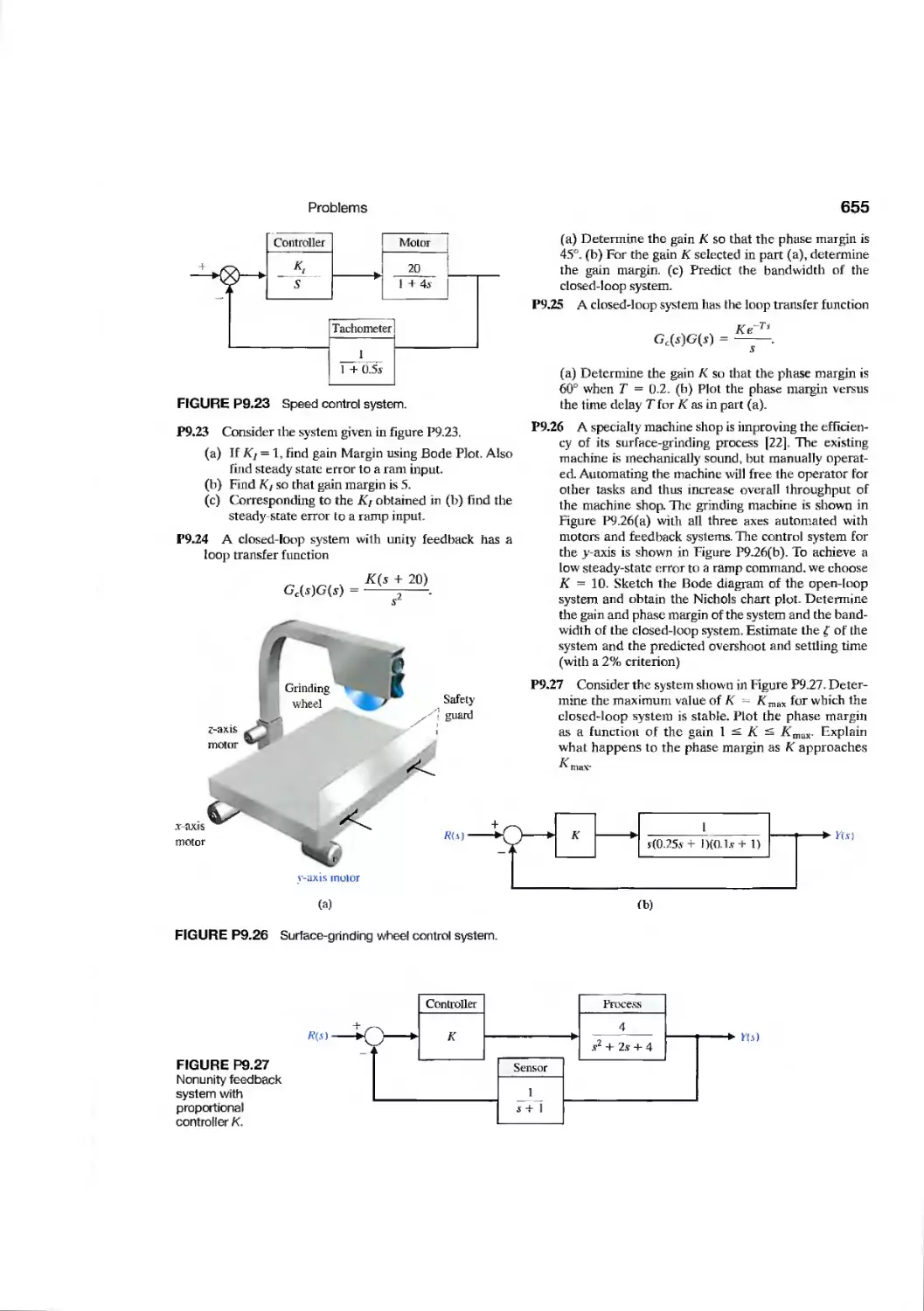
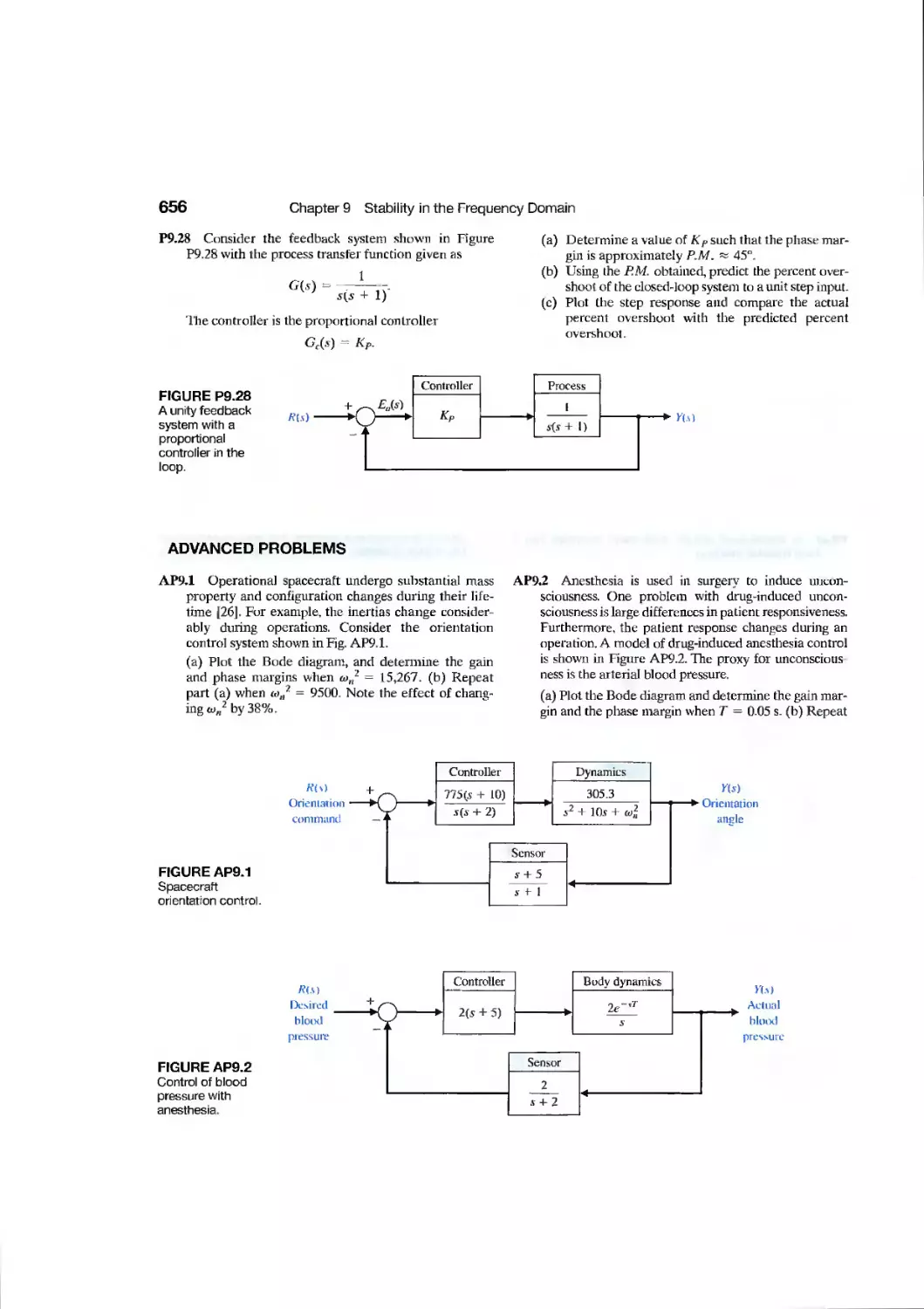
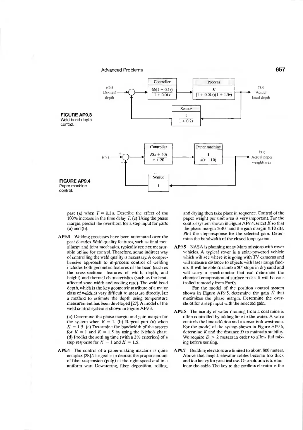
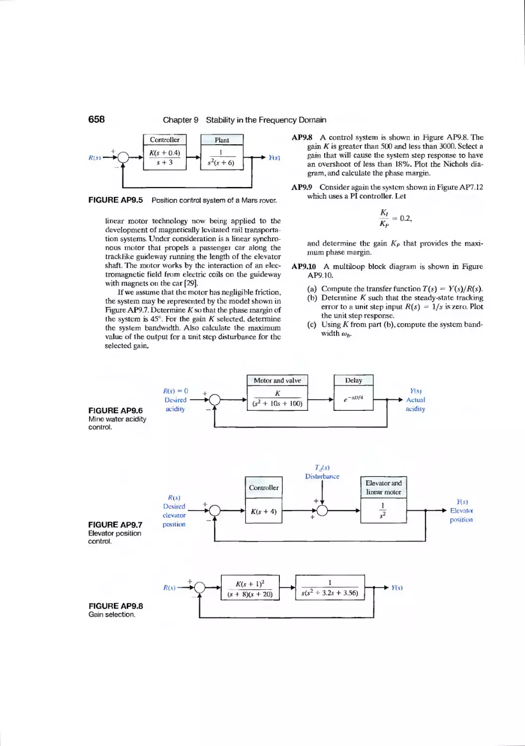
9.5 Time-Domain Performance Criteria in the Frequency Domain 594
9.6 System Bandwidth 601
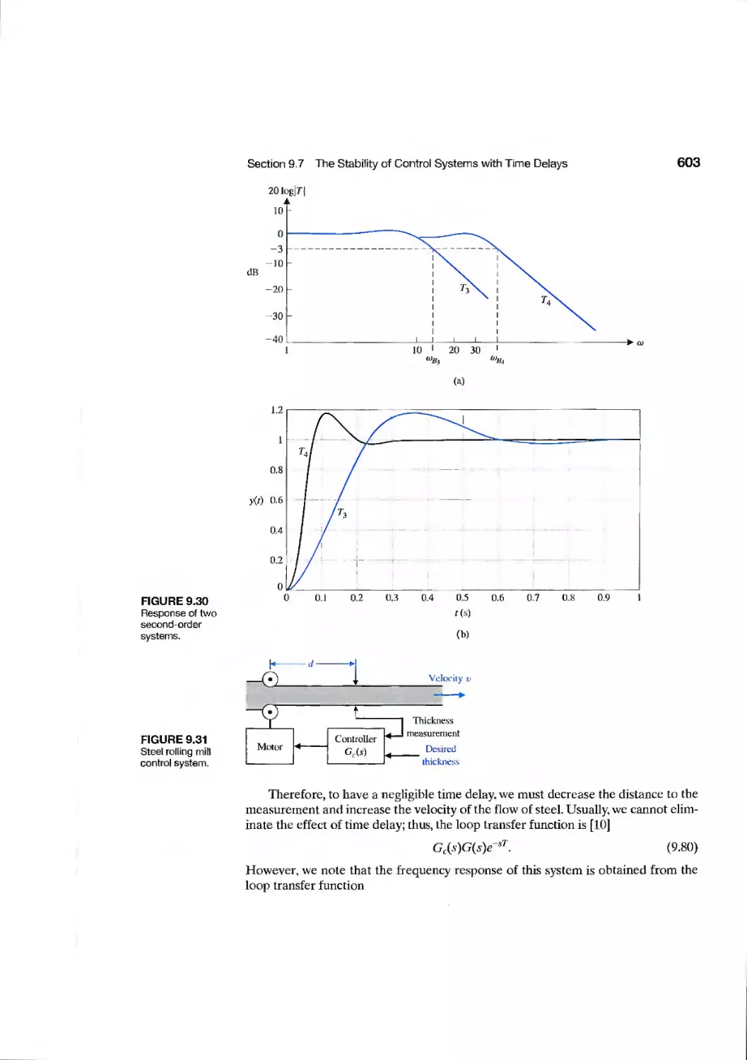
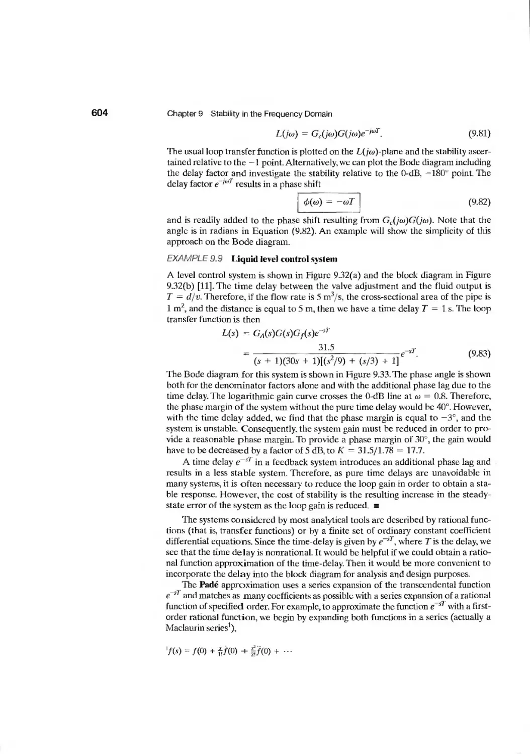
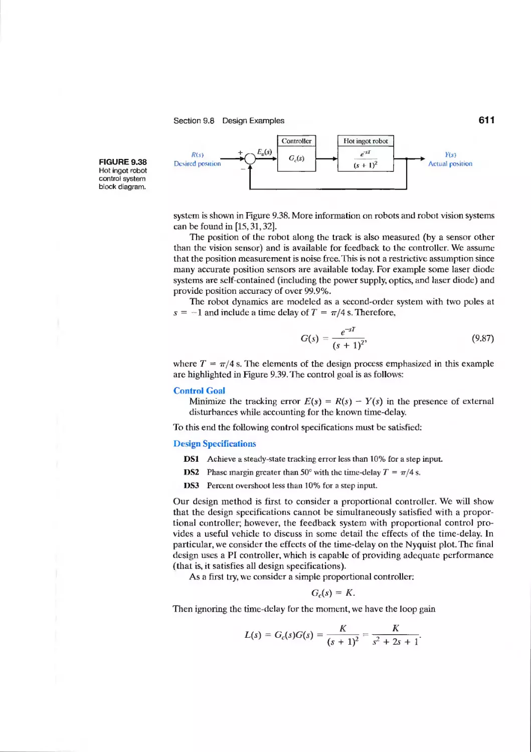
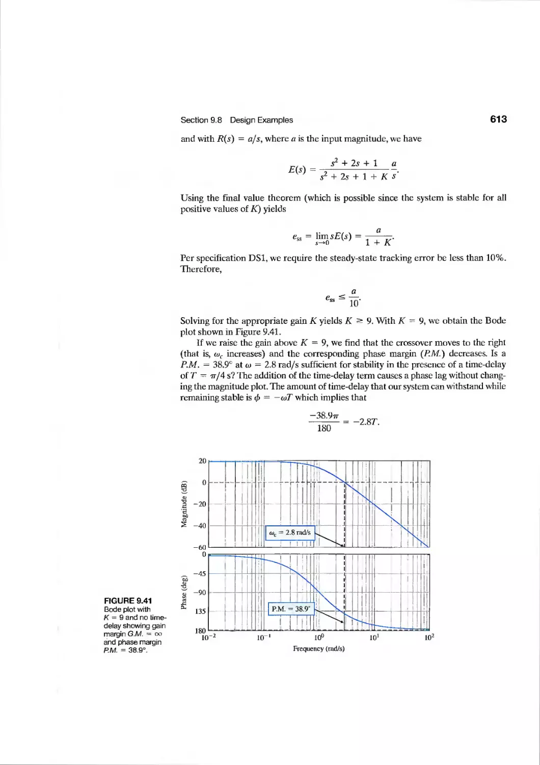
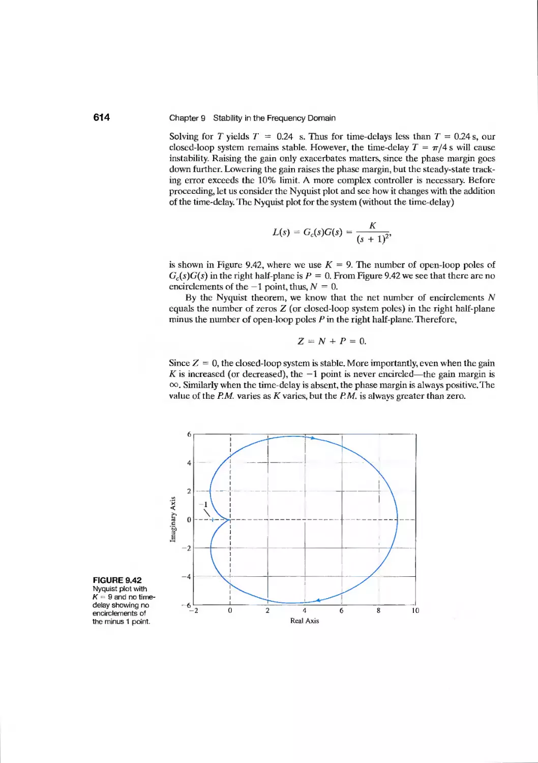
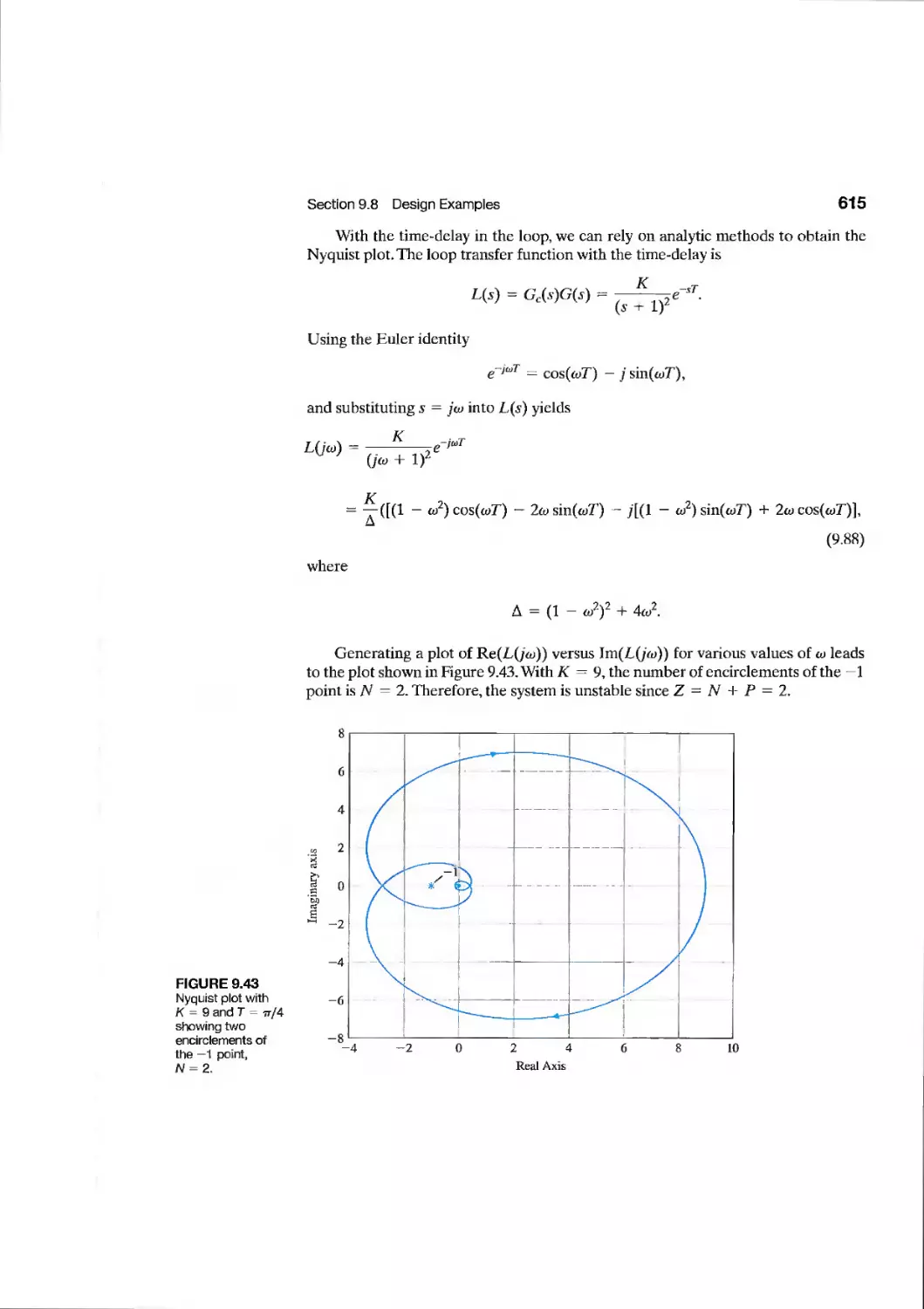
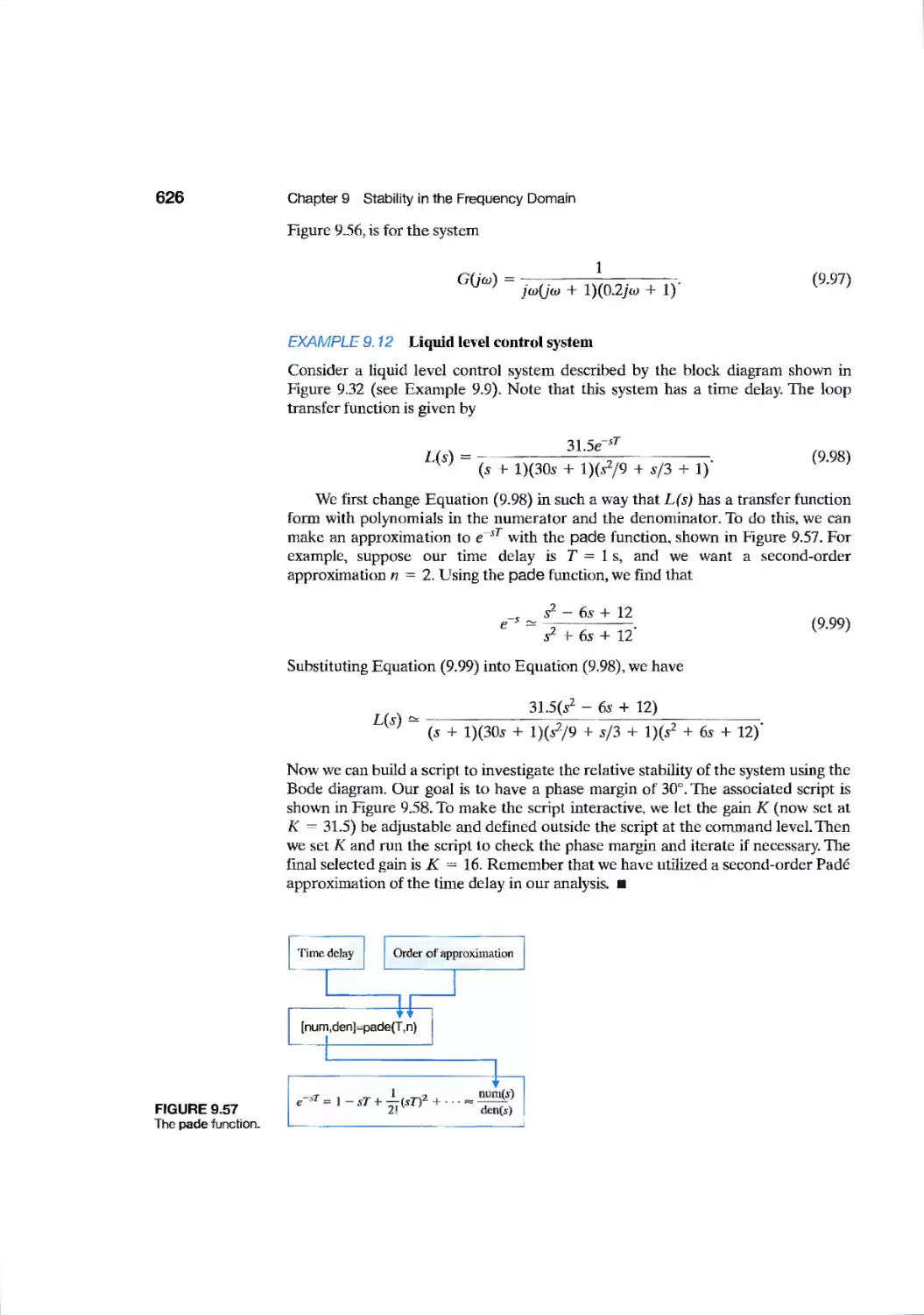
9.7 The Stability of Control Systems with Time Delays 601
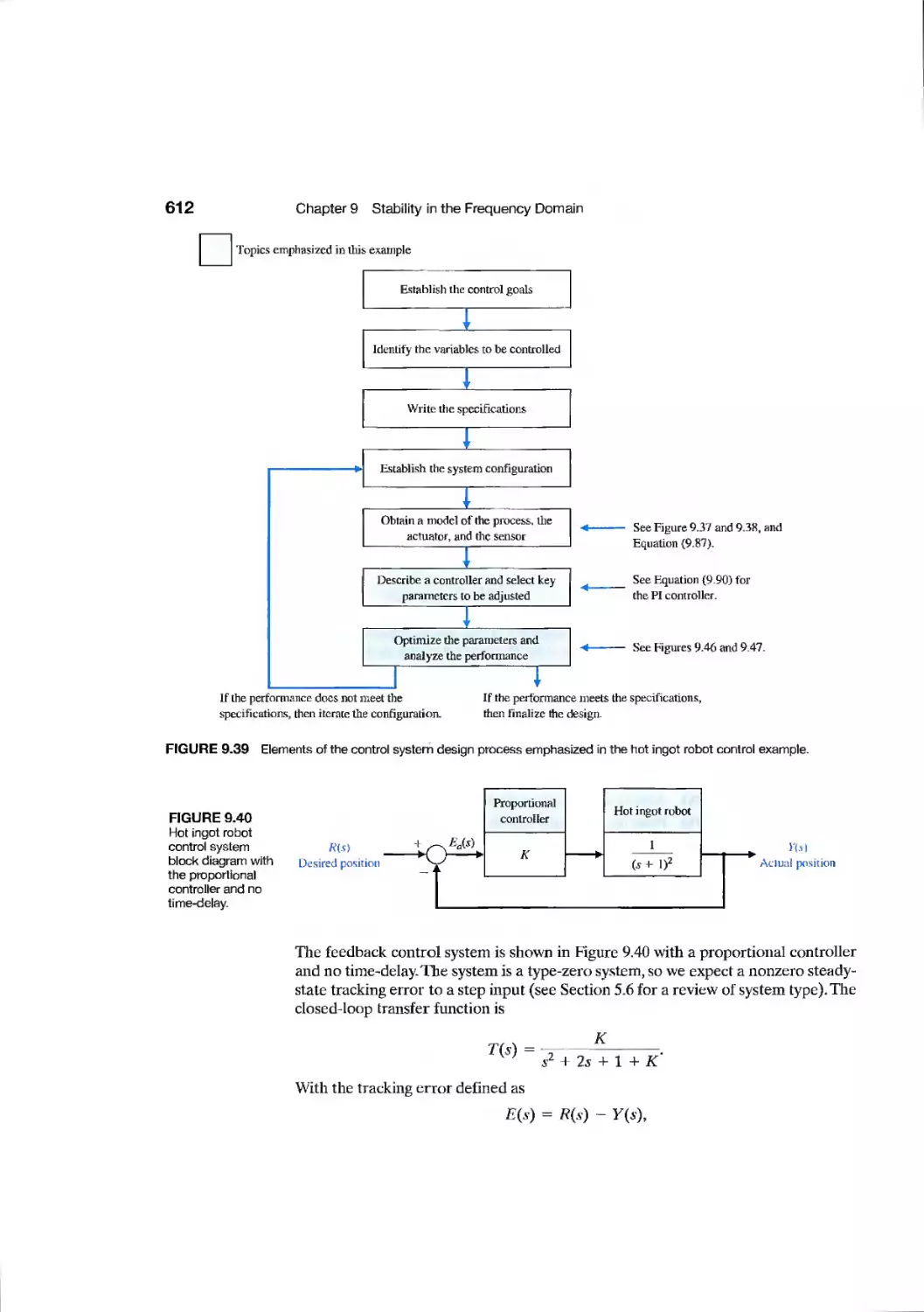
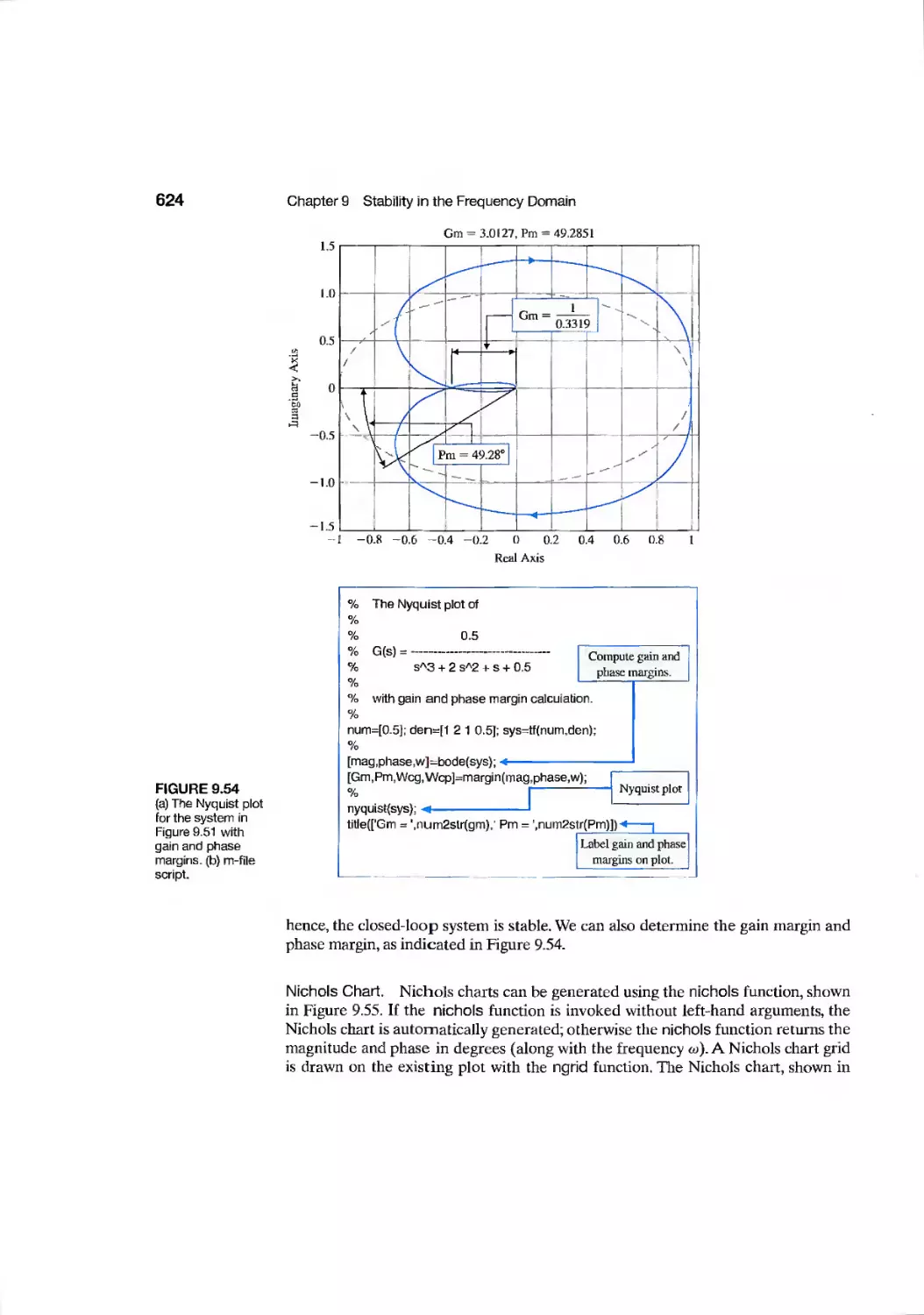
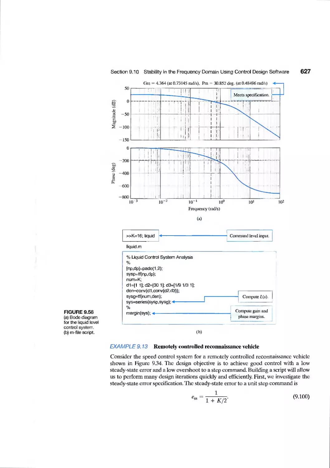
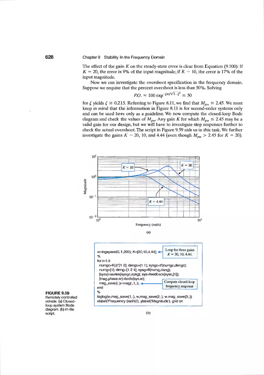
9.8 Design Examples 606
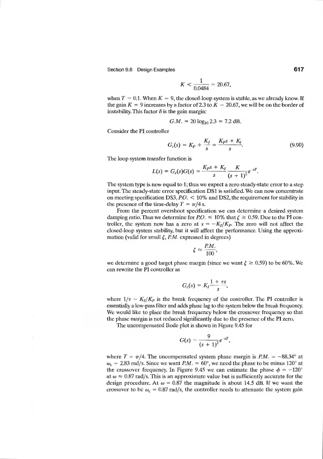
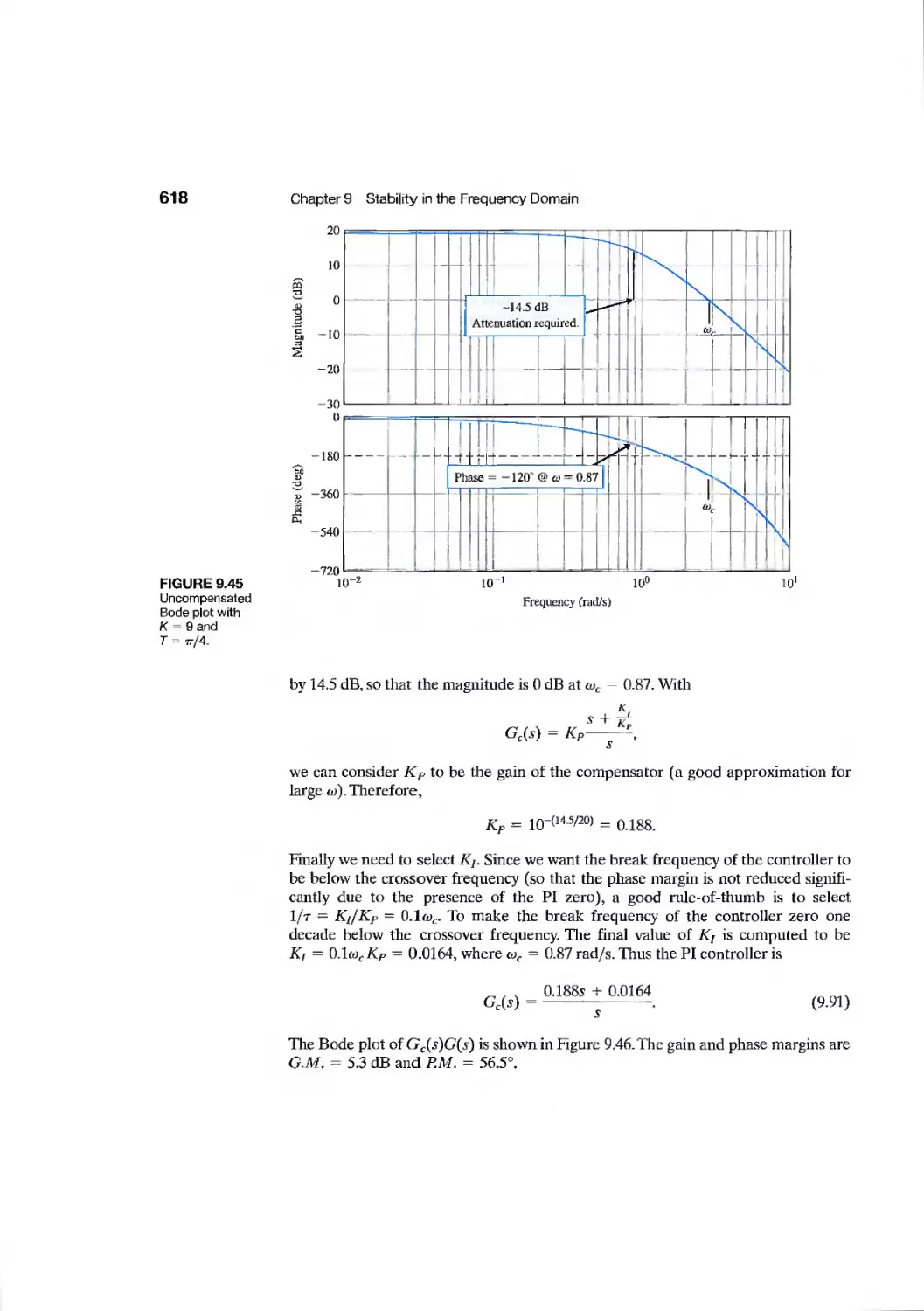
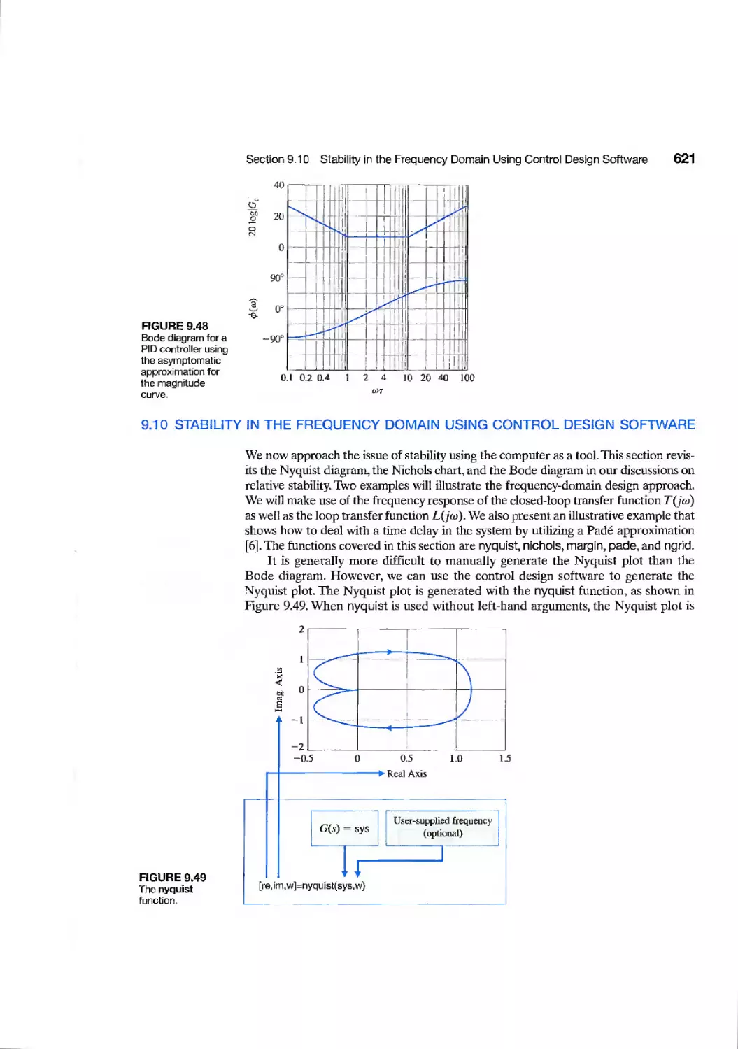
9.9 PID Controllers in the Frequency Domain 620
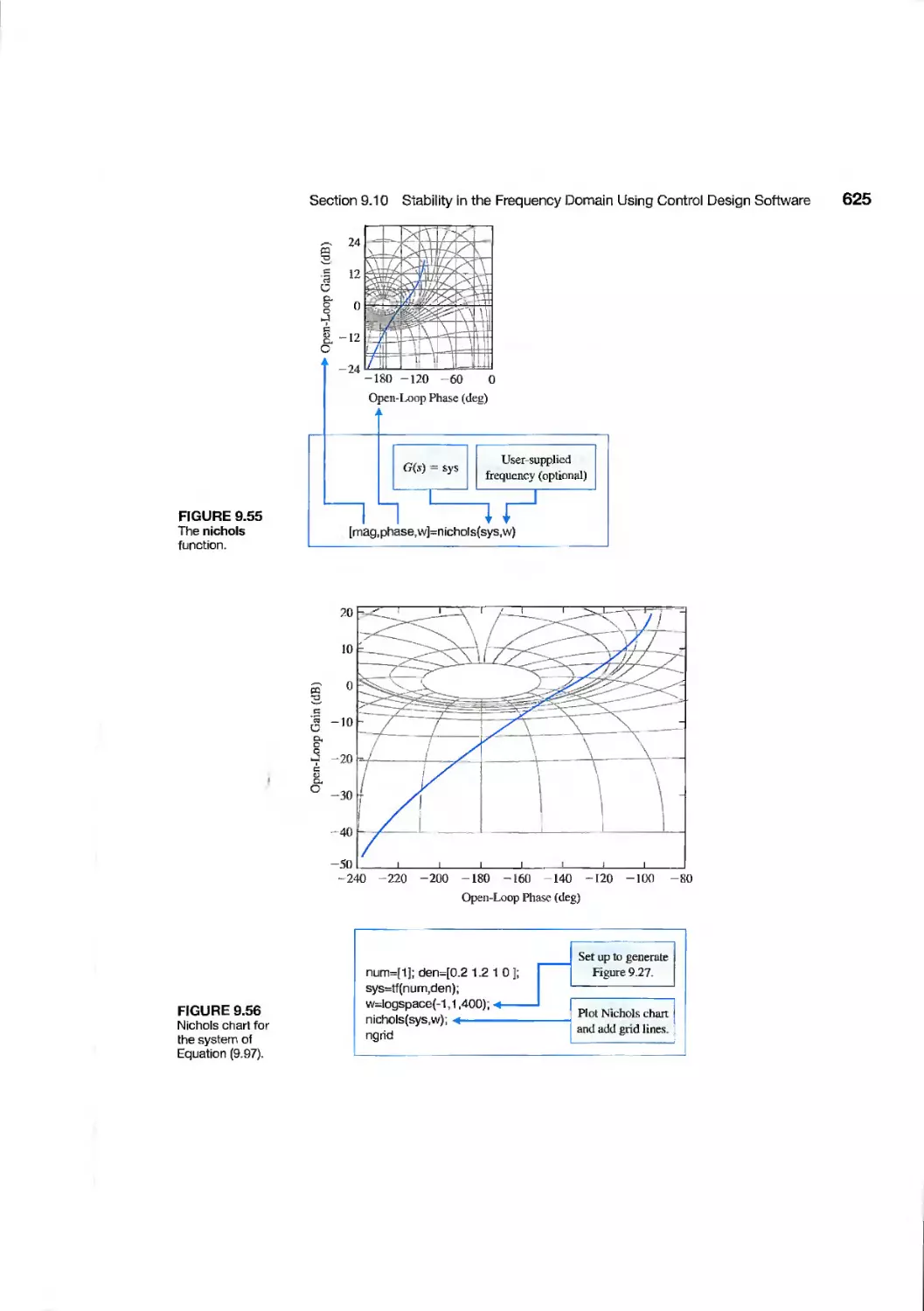
9.10 Stability in the Frequency Domain Using Control Design Software 621
9.11 Sequential Design Example: Disk Drive Read System 629
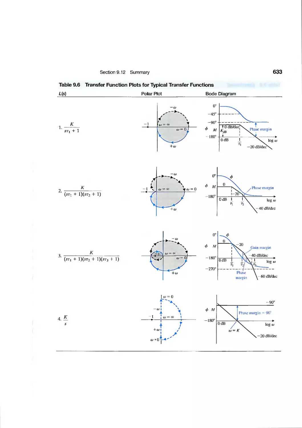
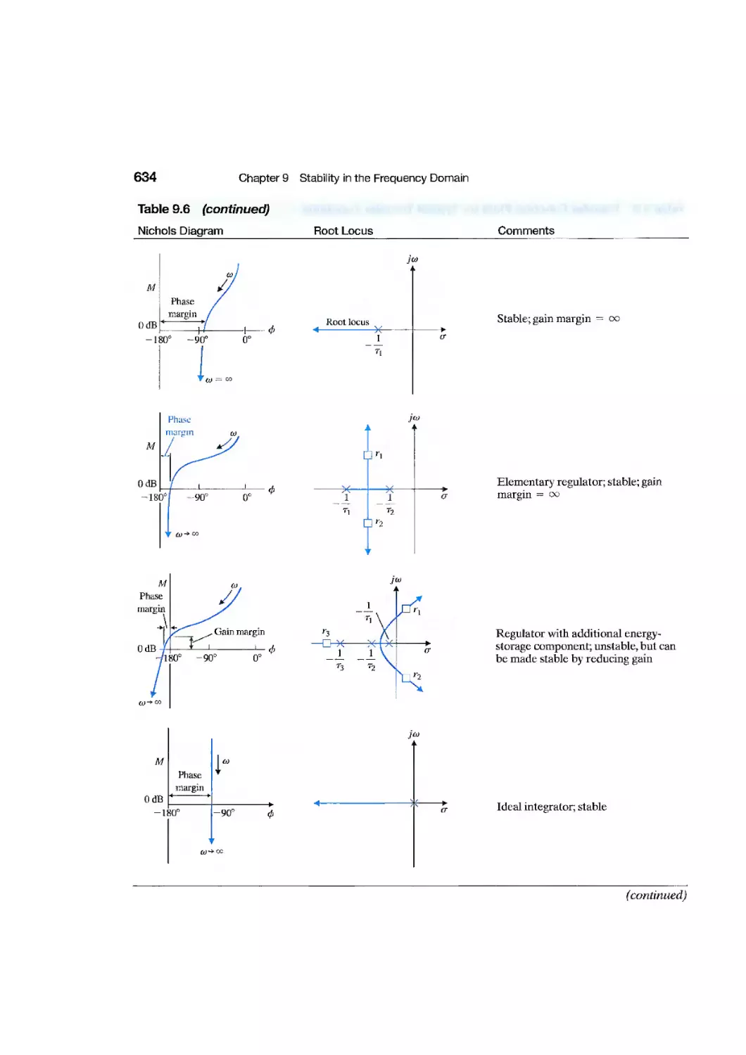
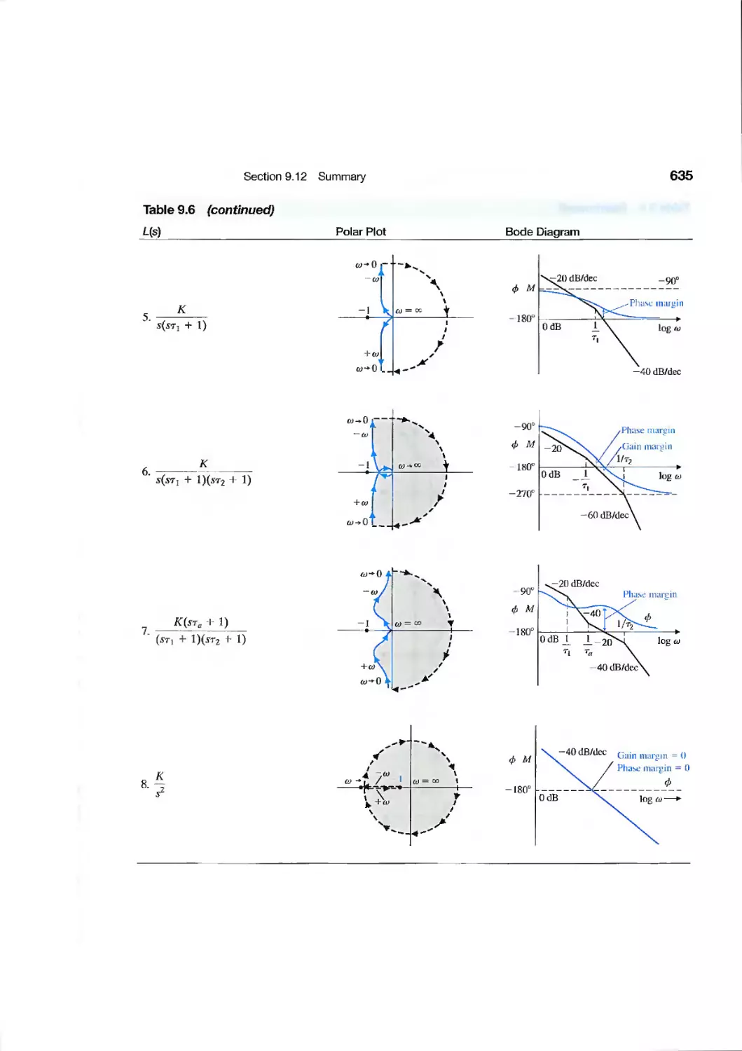
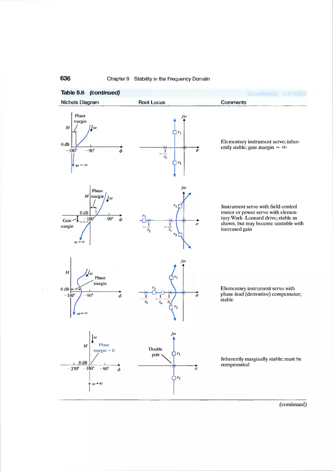
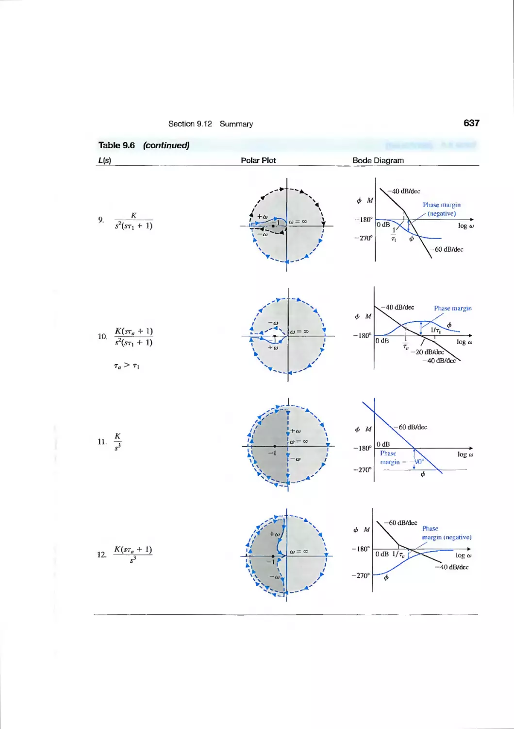
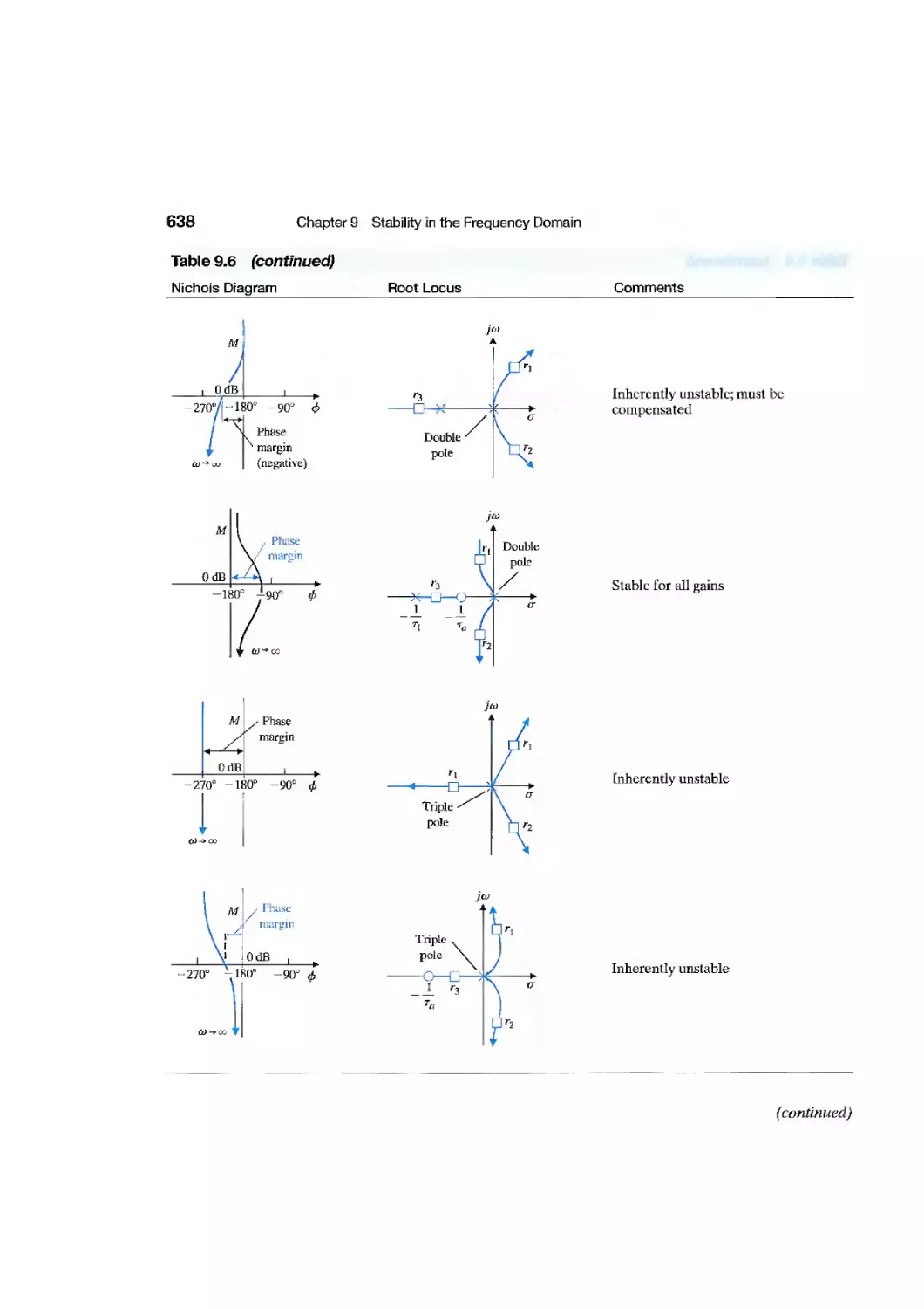
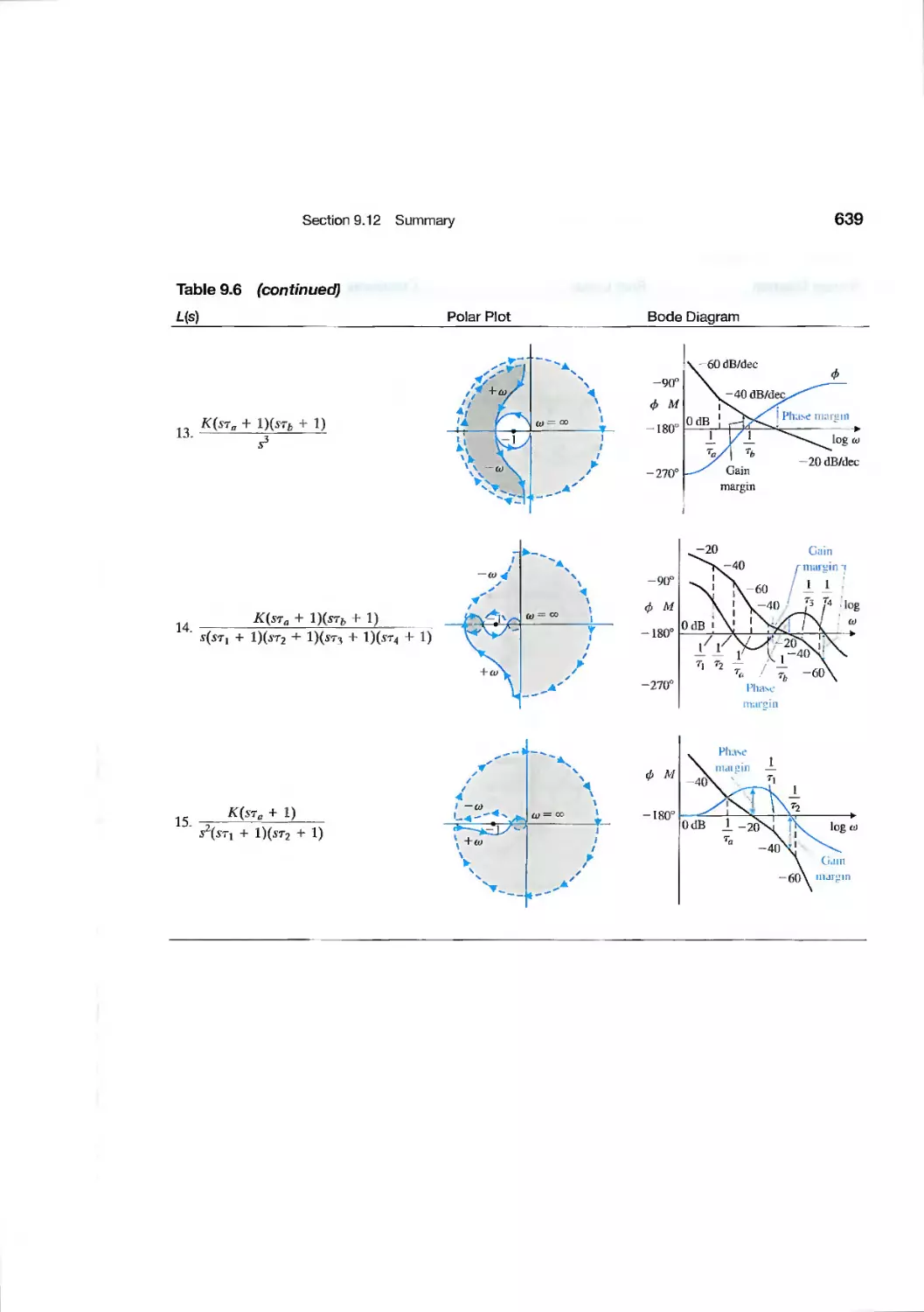
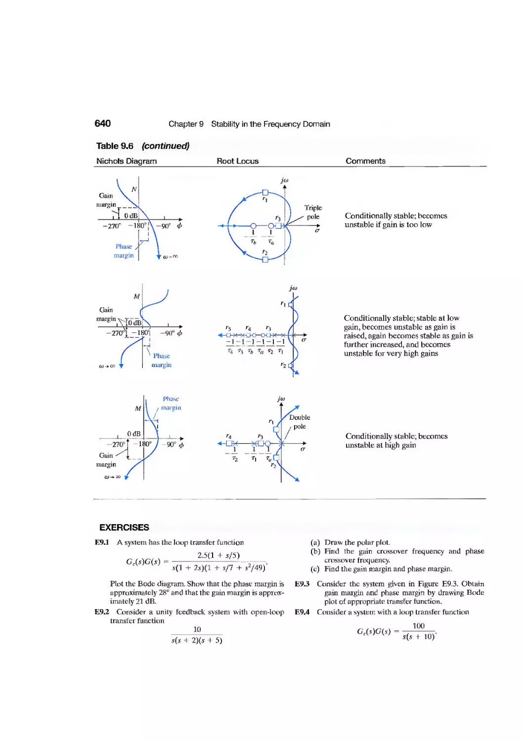
9.12 Summary 632
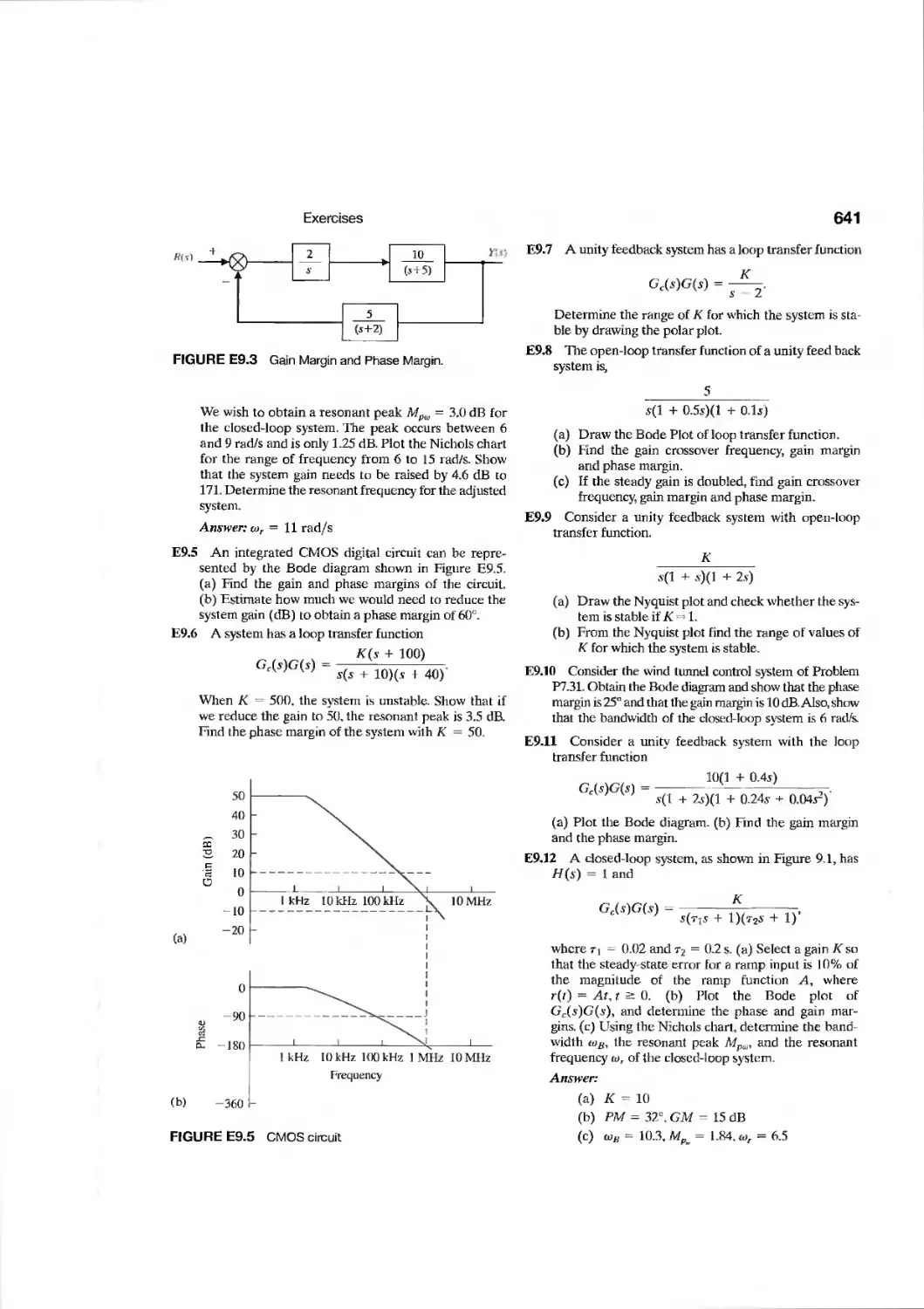
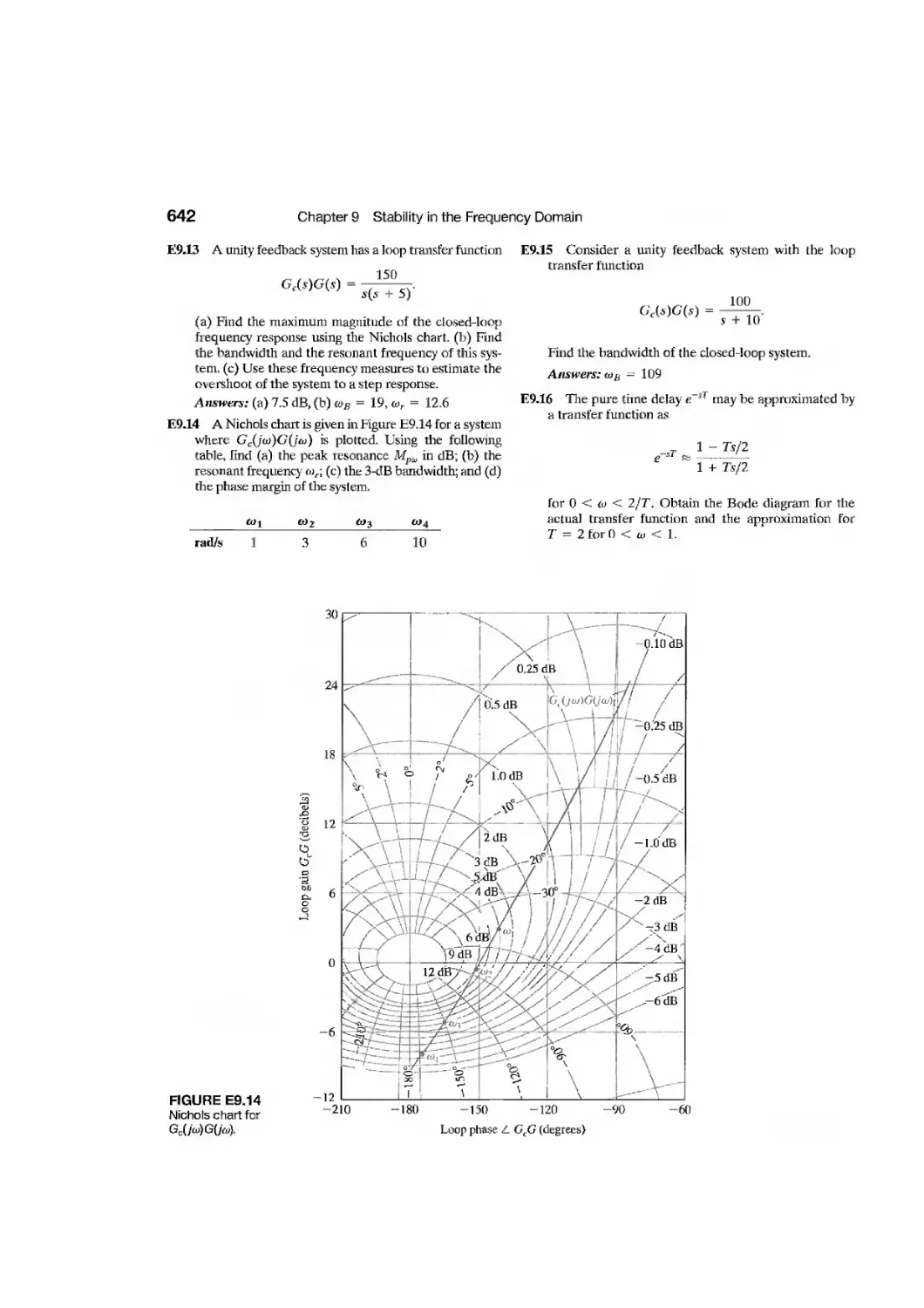
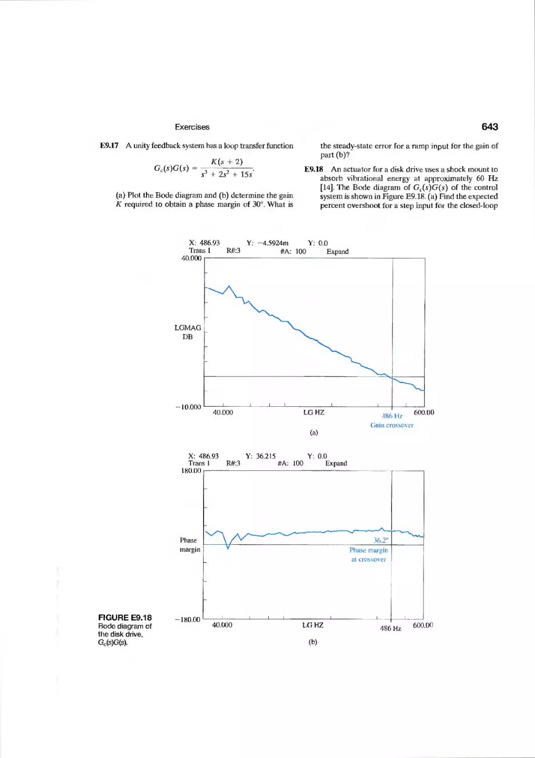
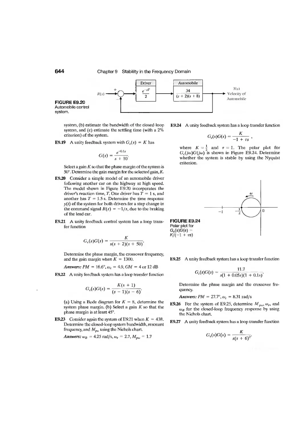
Exercises 640
Problems 646
Advanced Problems 656
Design Problems 659
Computer Problems 664
Terms and Concepts 665
Contents ix
chapter 10 The Design of Feedback Control Systems 667
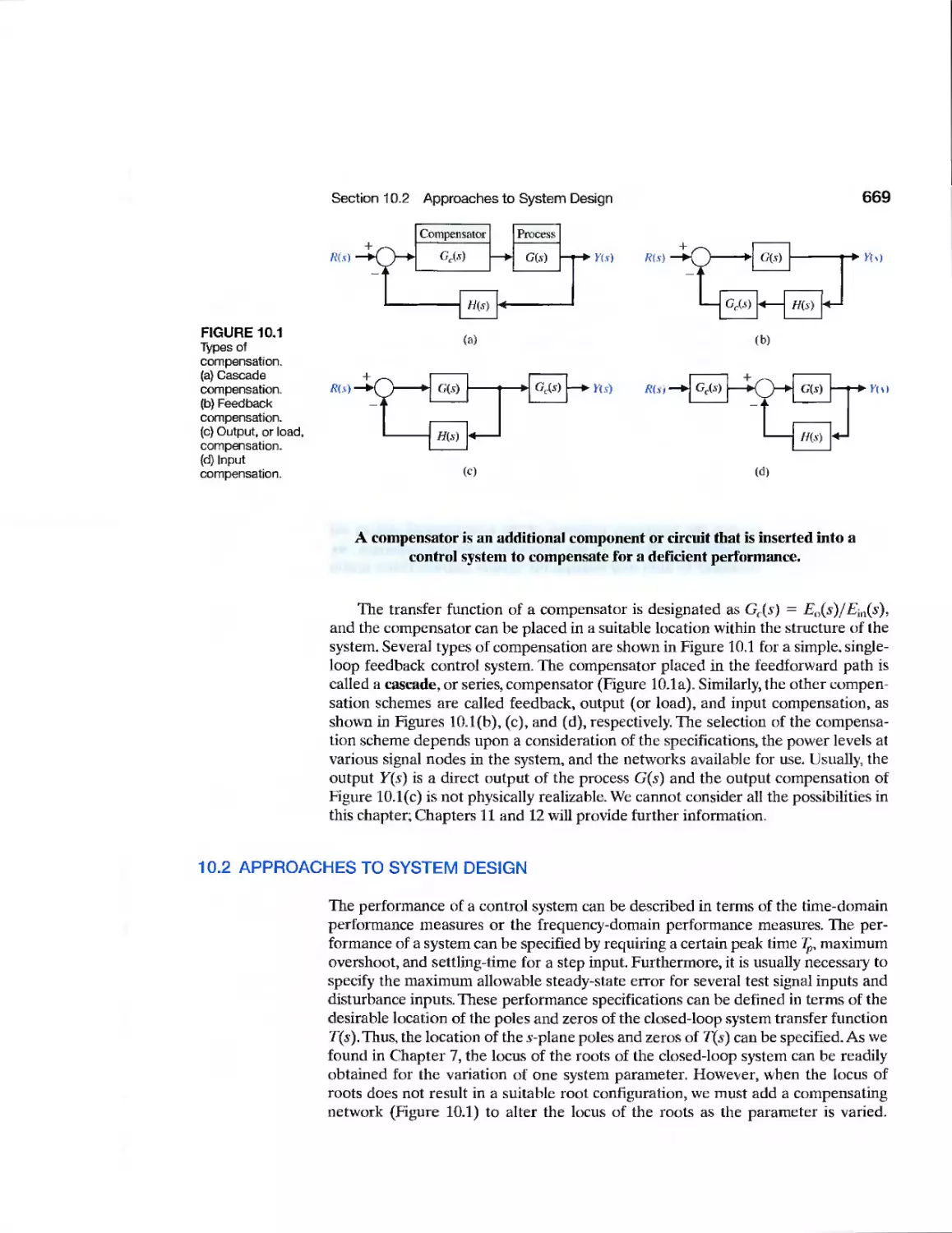
10.1 Introduction 668
10.2 Approaches to System Design 669
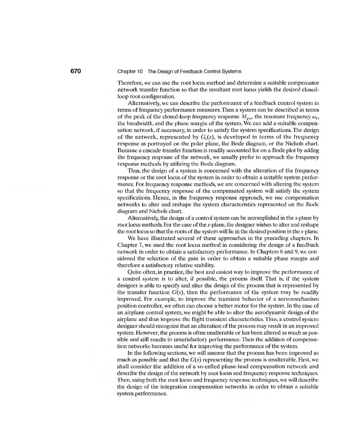
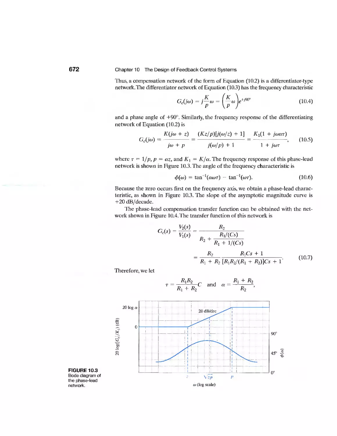
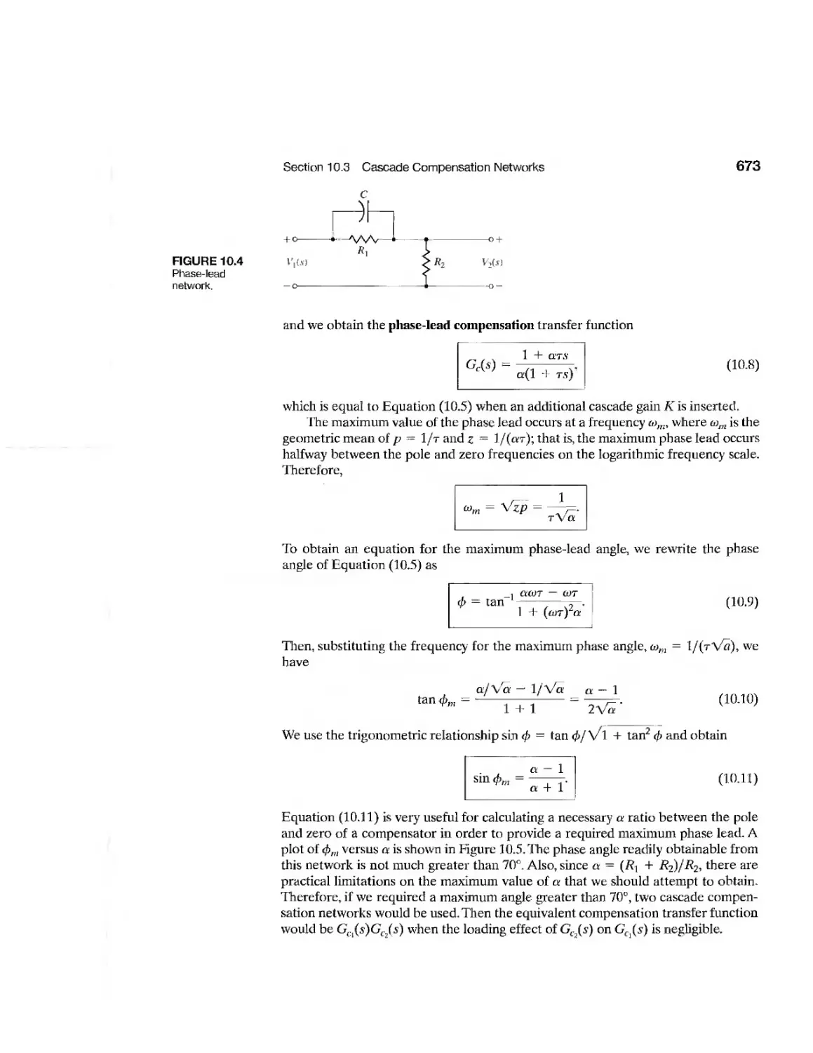
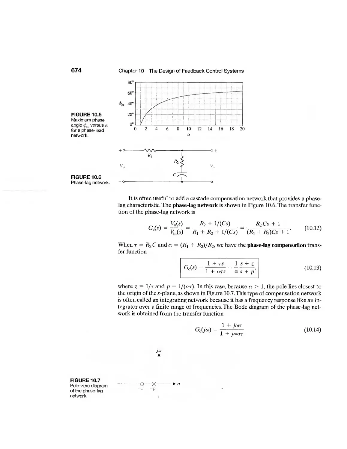
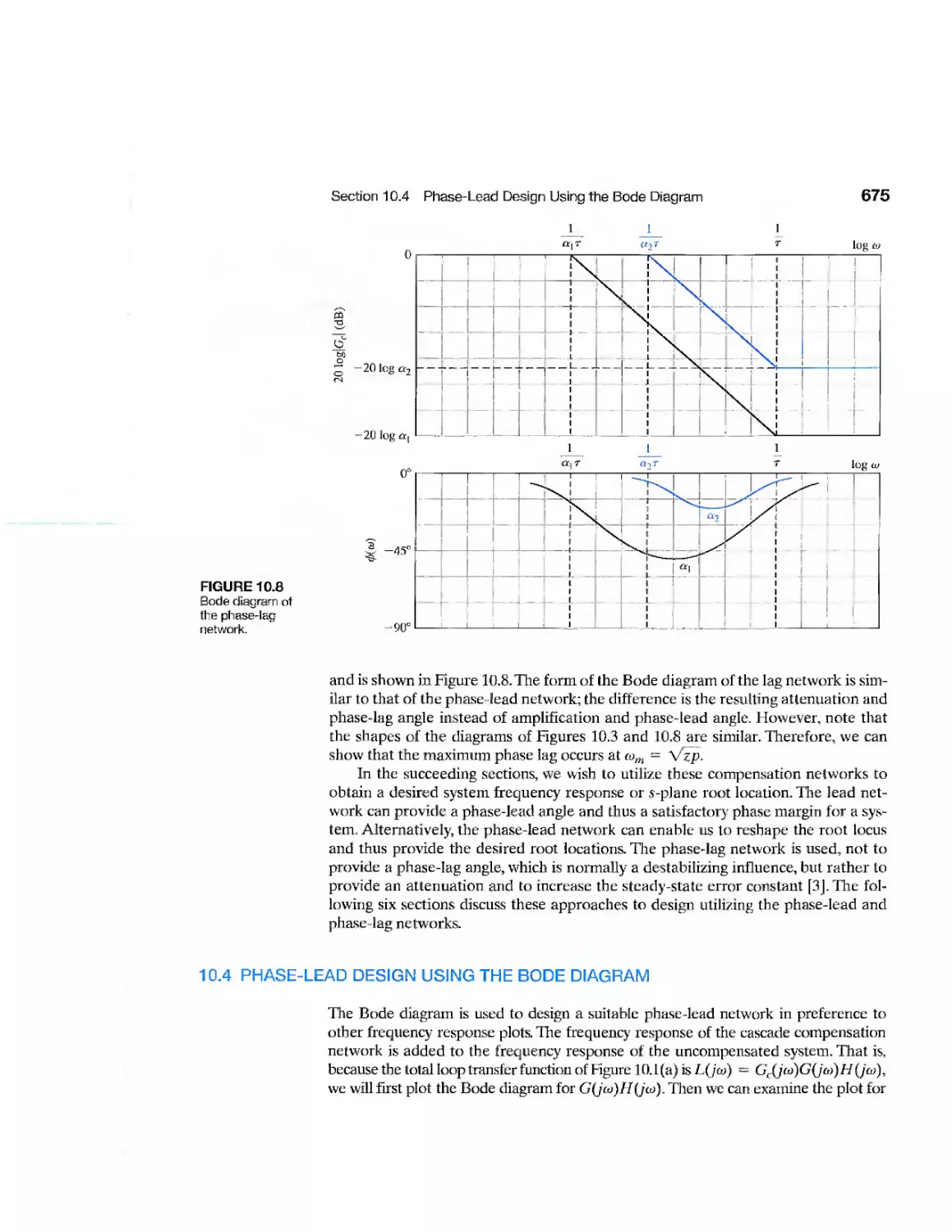
10.3 Cascade Compensation Networks 671
10.4 Phase-Lead Design Using the Bode Diagram 675
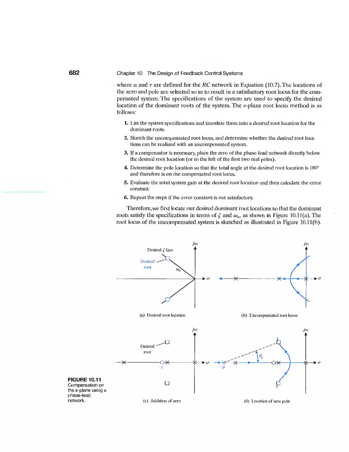
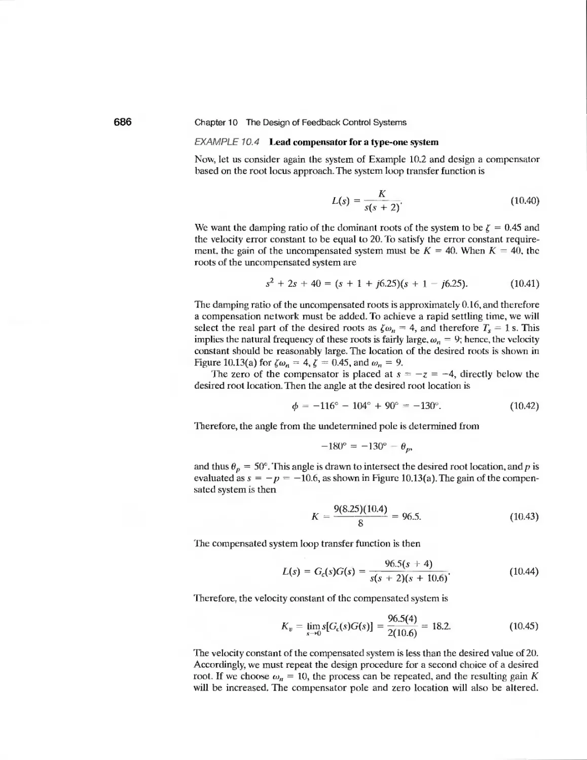
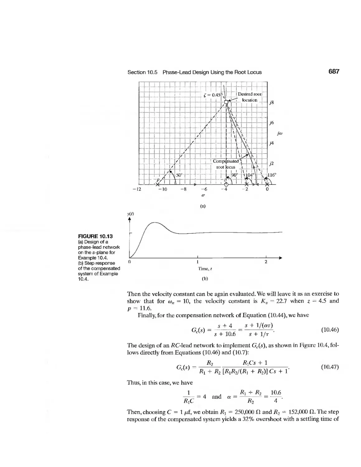
10.5 Phase-Lead Design Using the Root Locus 681
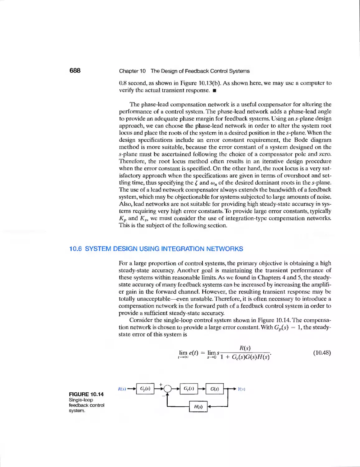
10.6 System Design Using Integration Networks 688
10.7 Phase-Lag Design Using the Root Locus 691
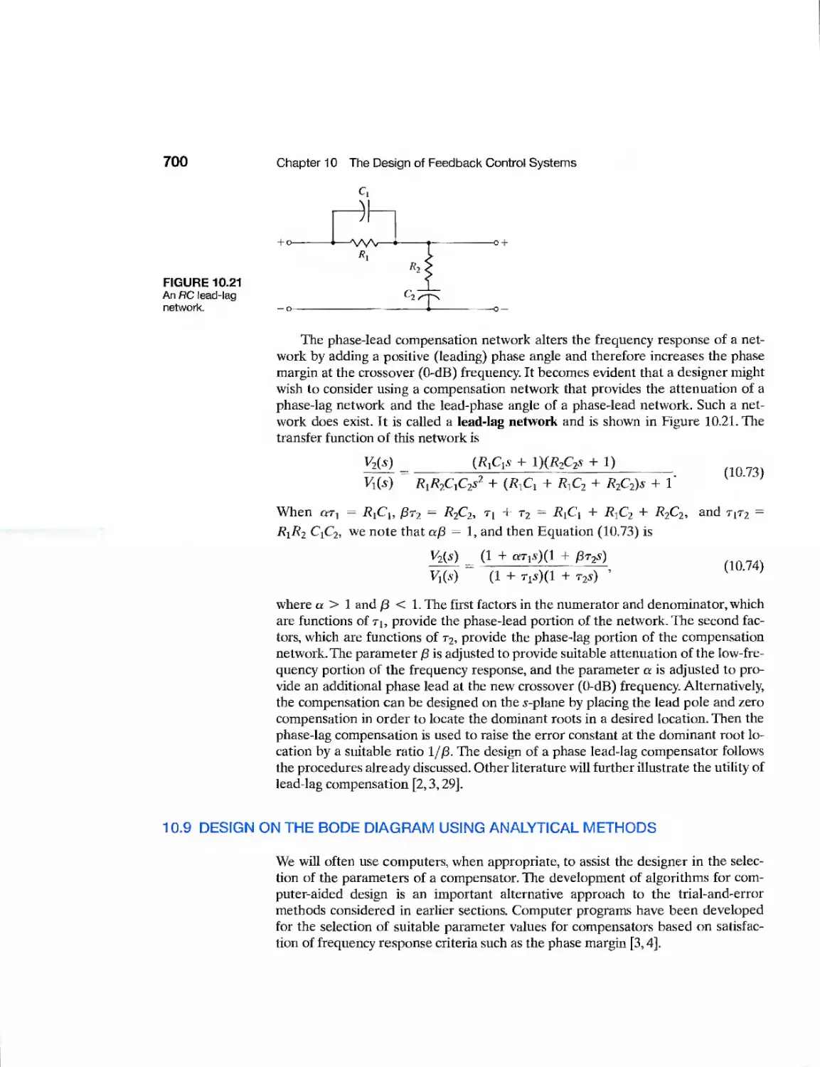
10.8 Phase-Lag Design Using the Bode Diagram 696
10.9 Design on the Bode Diagram Using Analytical Methods 700
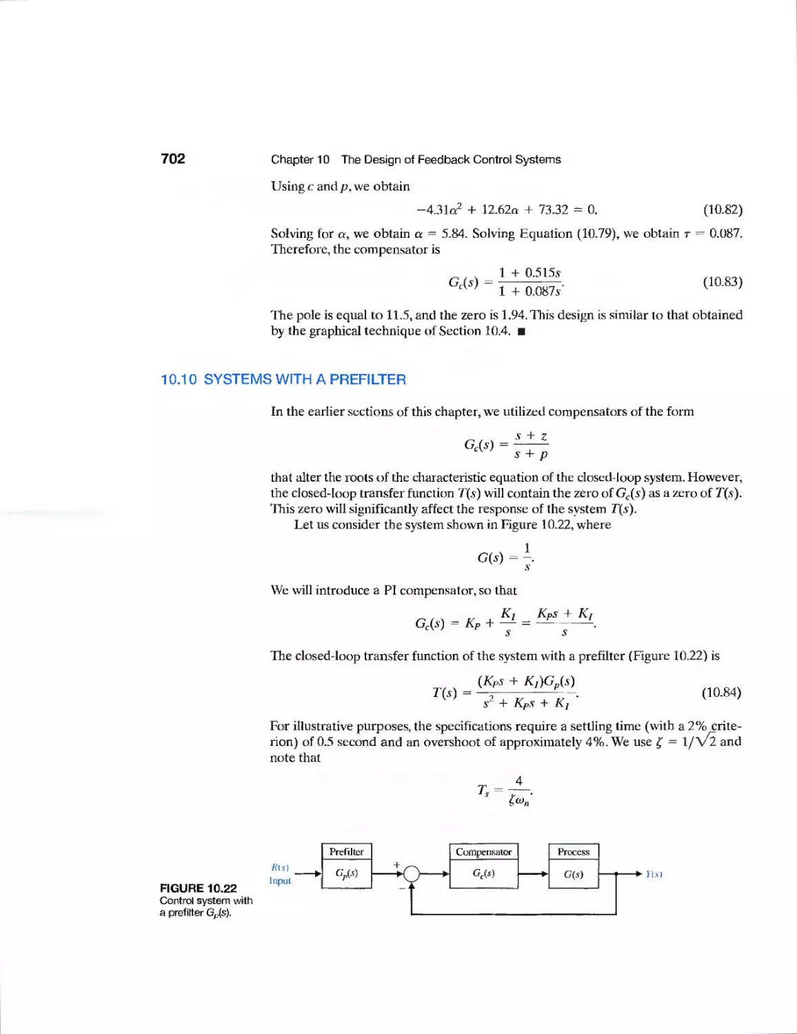
10.10 Systems with a Prefilter 702
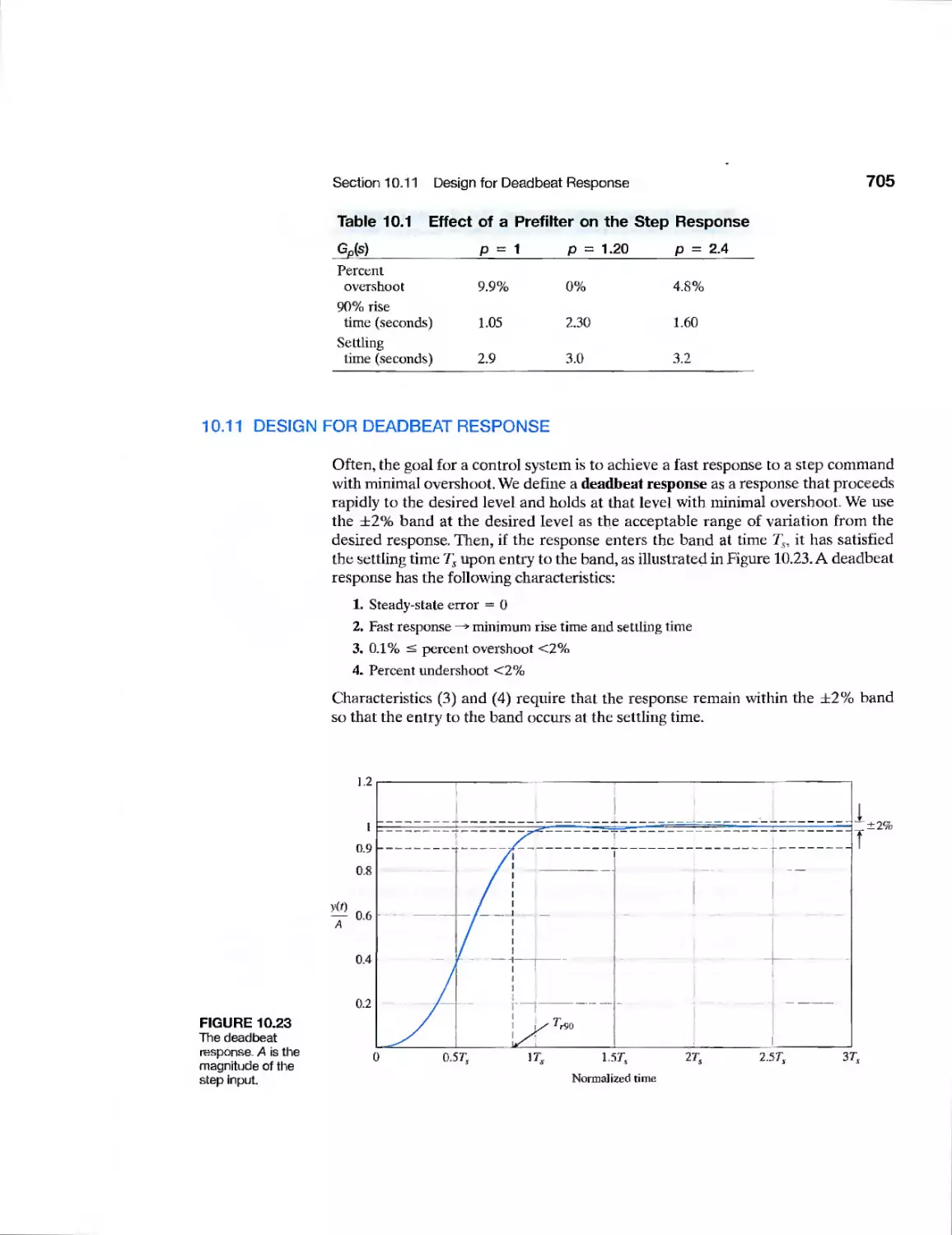
10.11 Design for Deadbeat Response 705
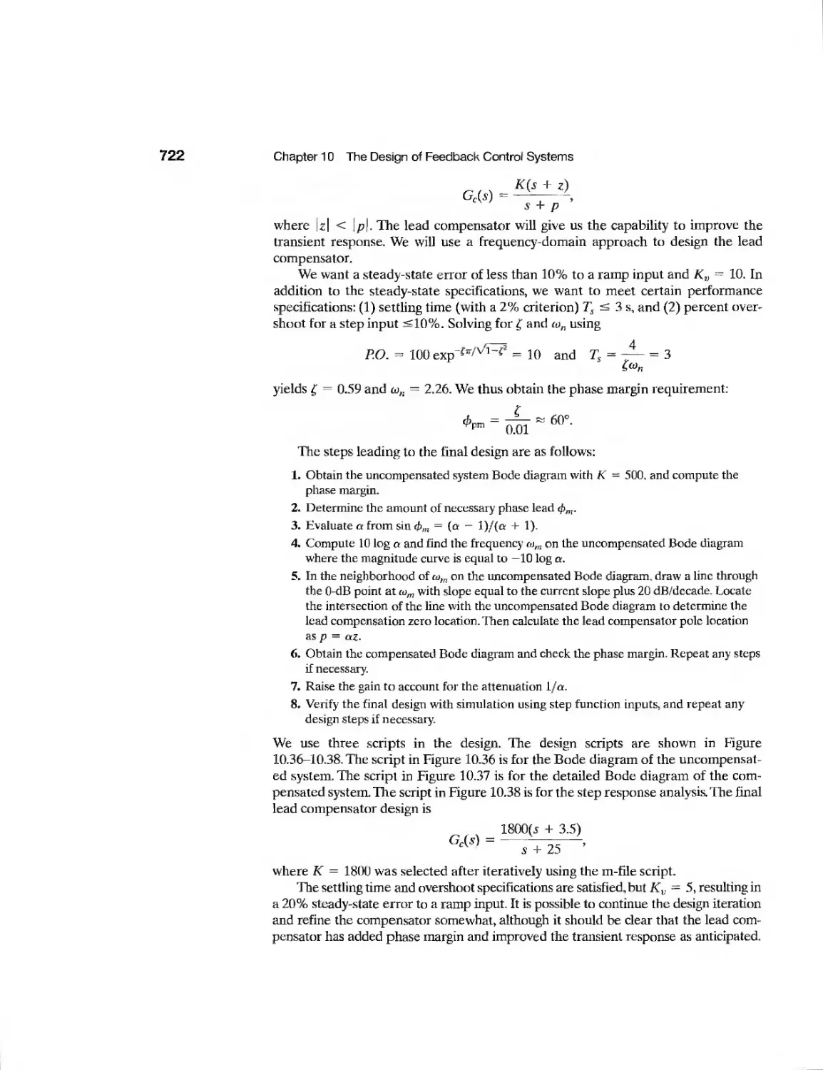
10.12 Design Examples 707
10.13 System Design Using Control Design Software 720
10.14 Sequential Design Example: Disk Drive Read System 726
10.15 Summary 728
Exercises 730
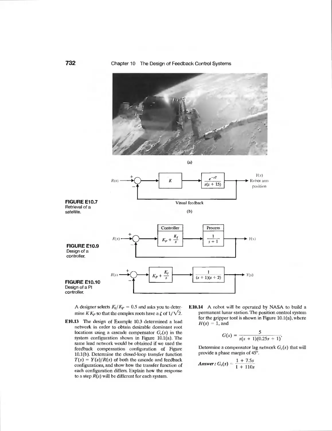
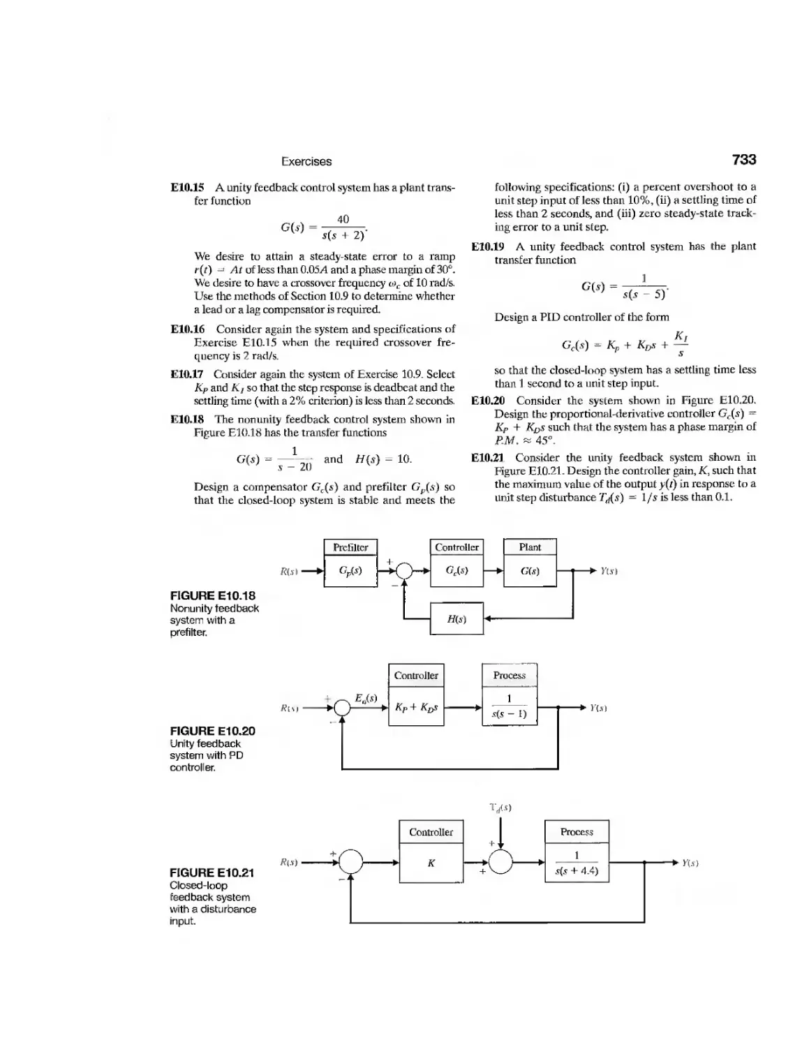
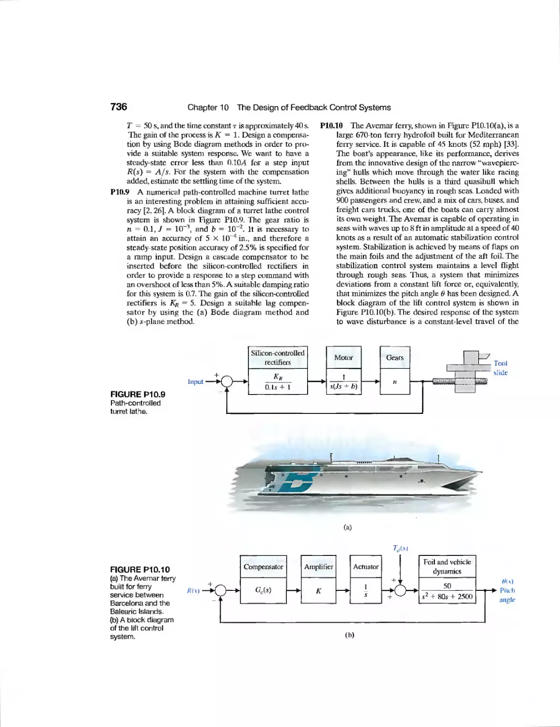
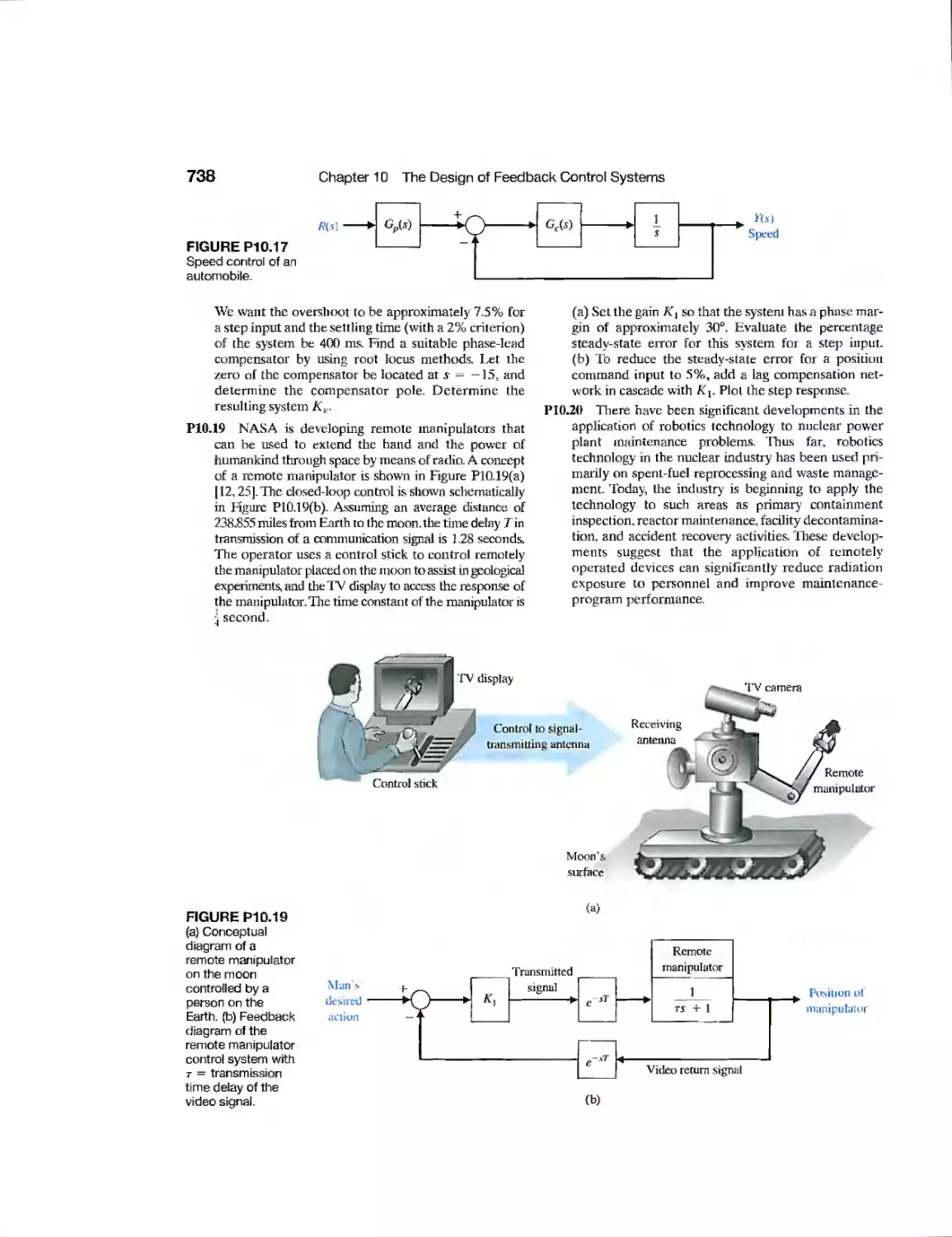
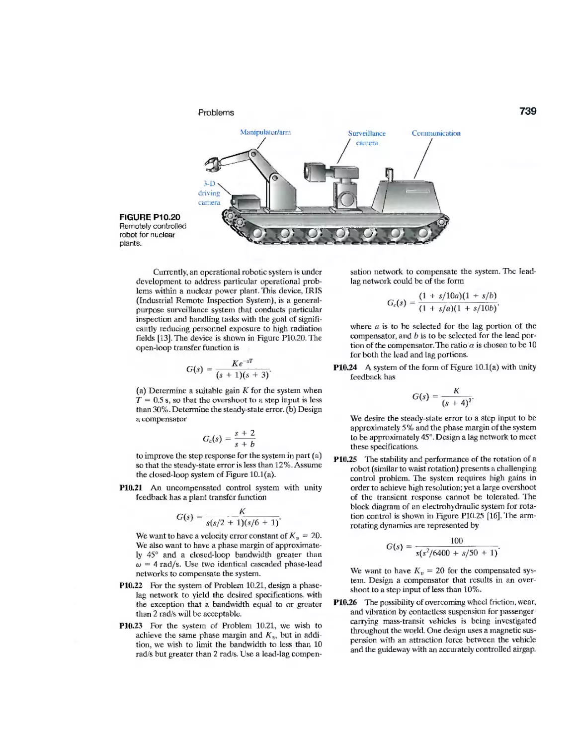
Problems 734
Advanced Problems 744
Design Problems 747
Computer Problems 752
Terms and Concepts 754
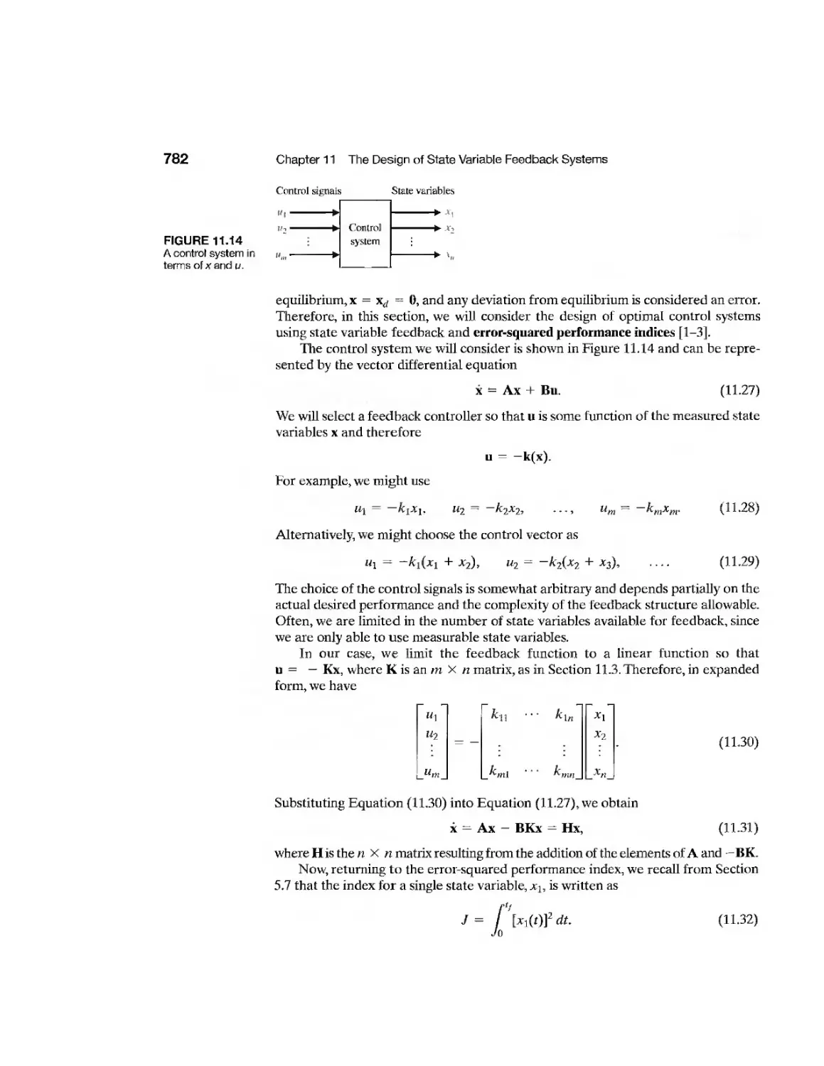
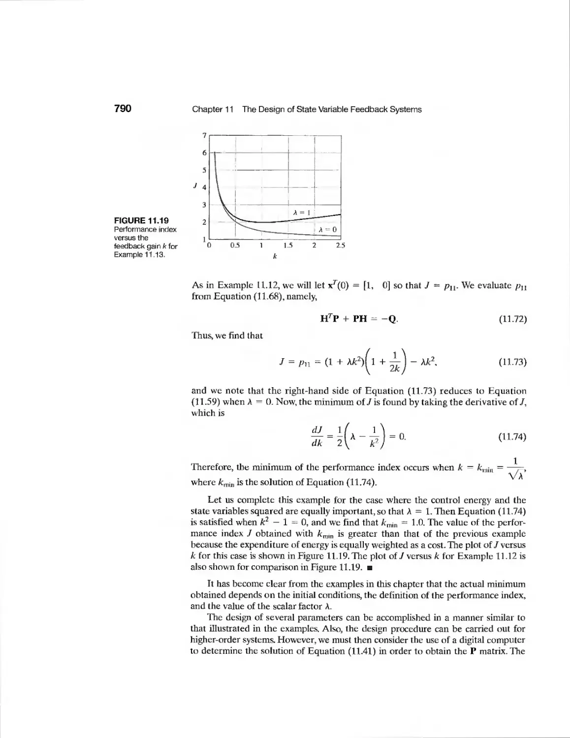
chapter 11 The Design of State Variable Feedback
Systems 756
11.1 Introduction 757
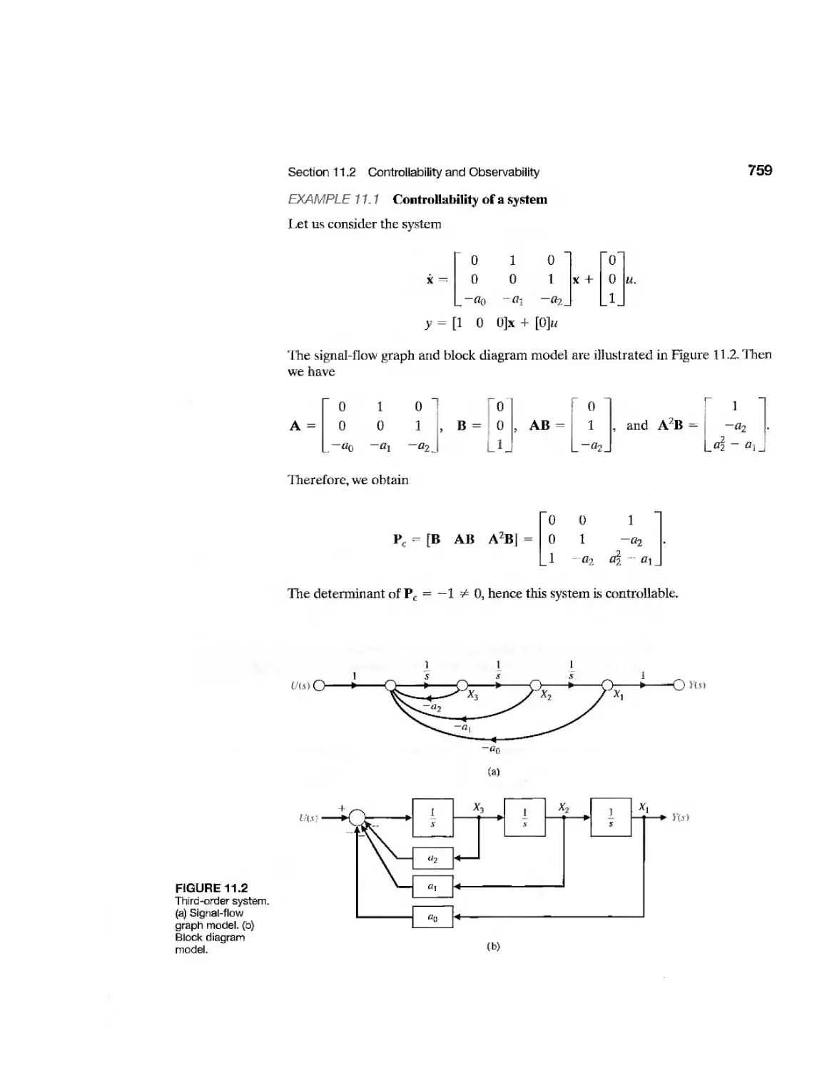
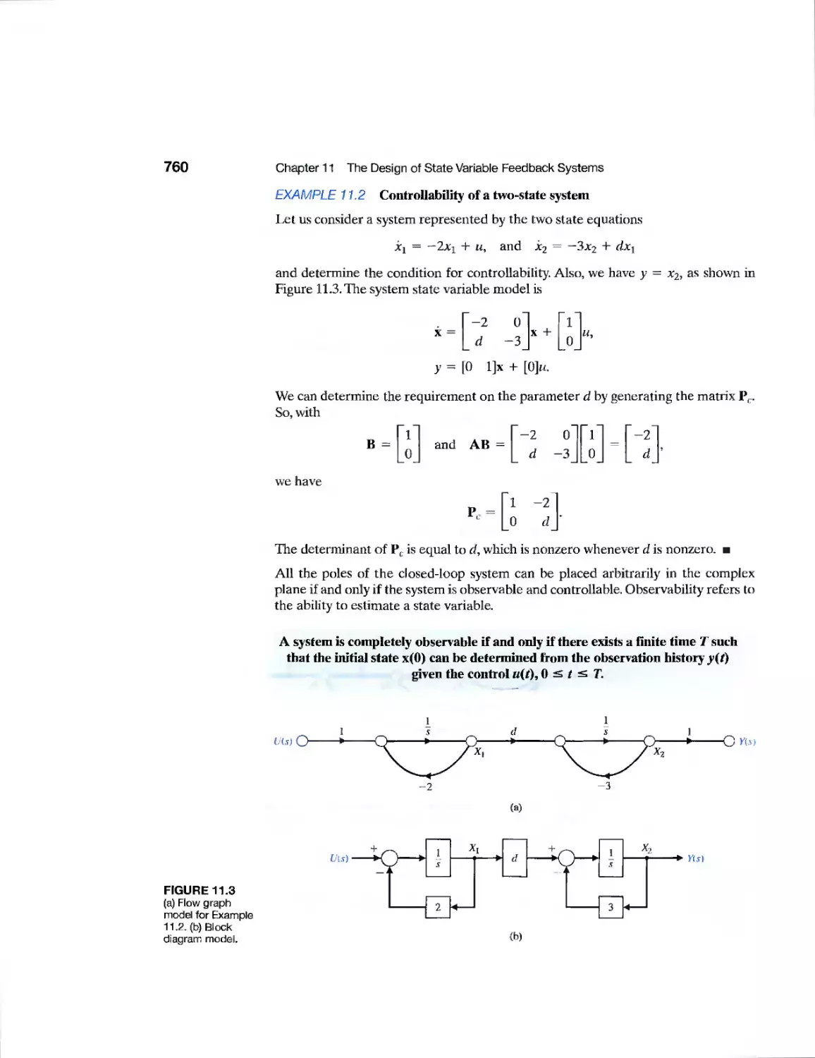
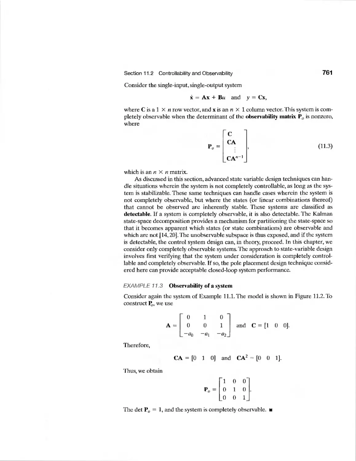
11.2 Controllability and Observability 757
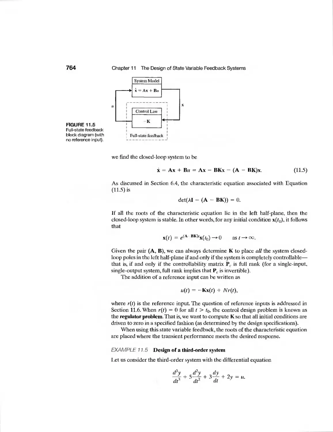
11.3 Full-State Feedback Control Design 763
11.4 Observer Design 769
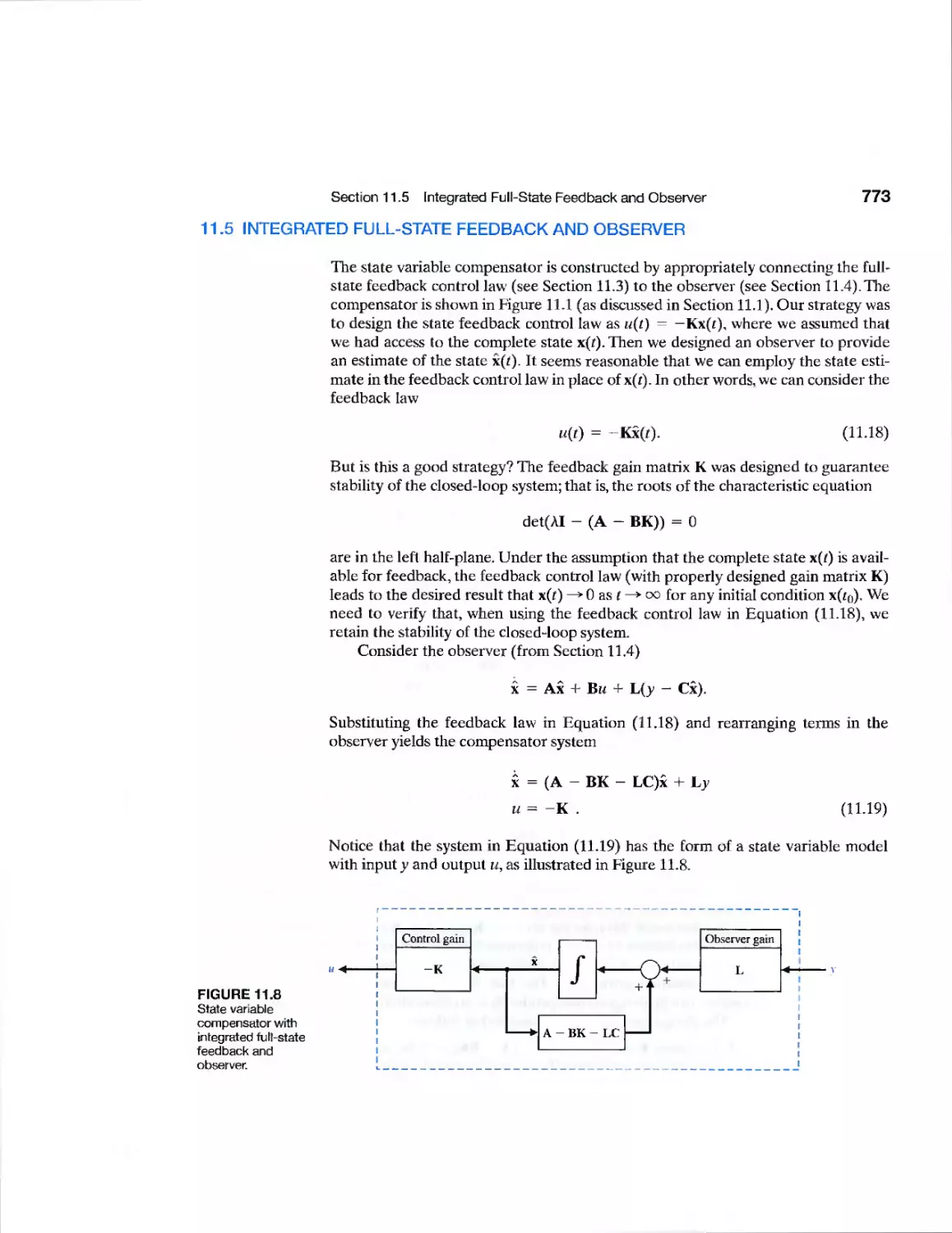
11.5 Integrated Full-State Feedback and Observer 773
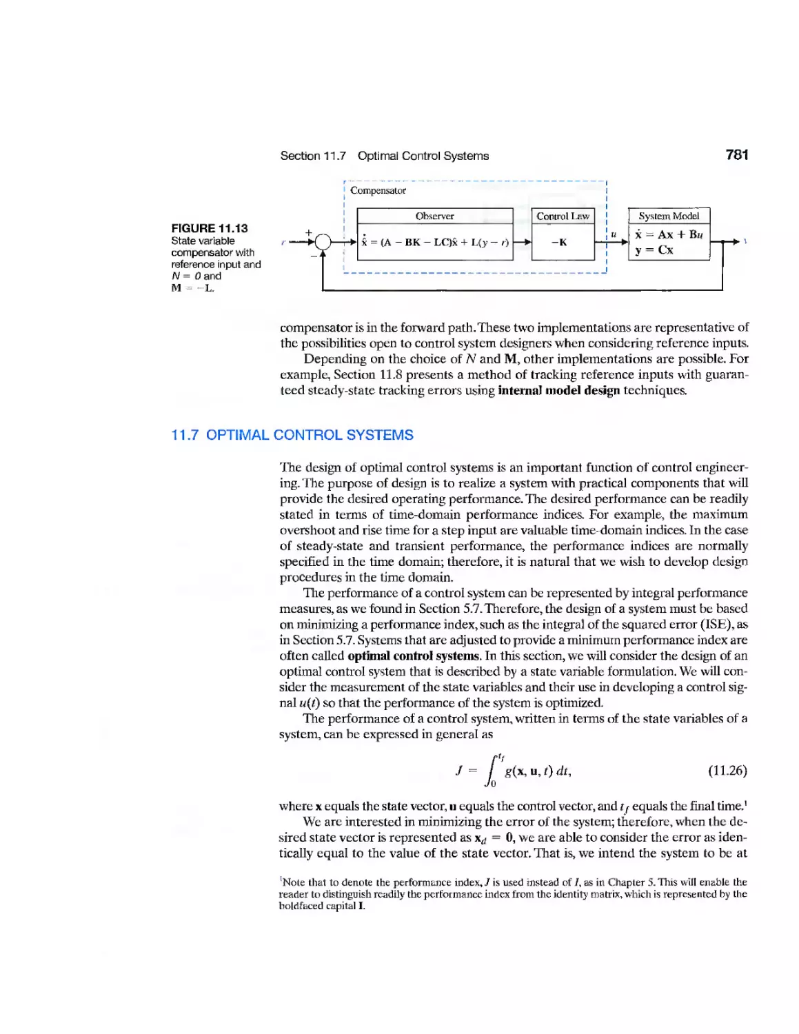
11.6 Reference Inputs 779
11.7 Optimal Control Systems 781
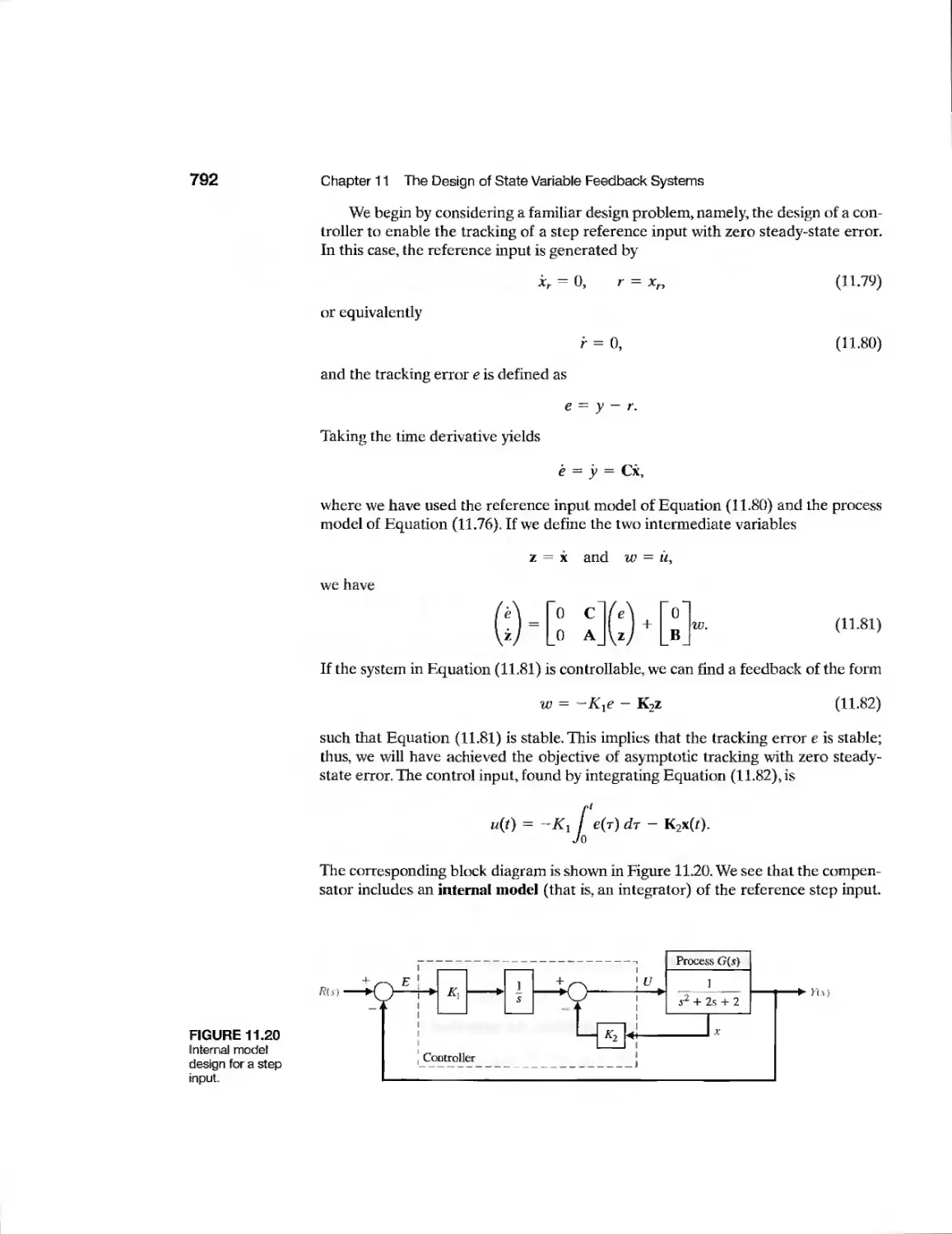
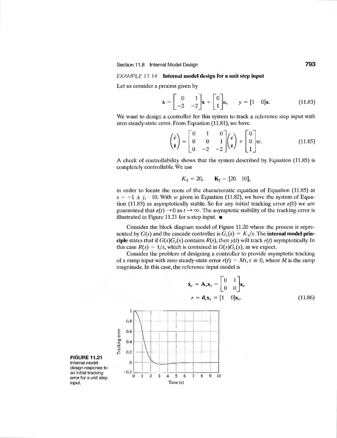
11.8 Internal Model Design 791
11.9 Design Examples 795
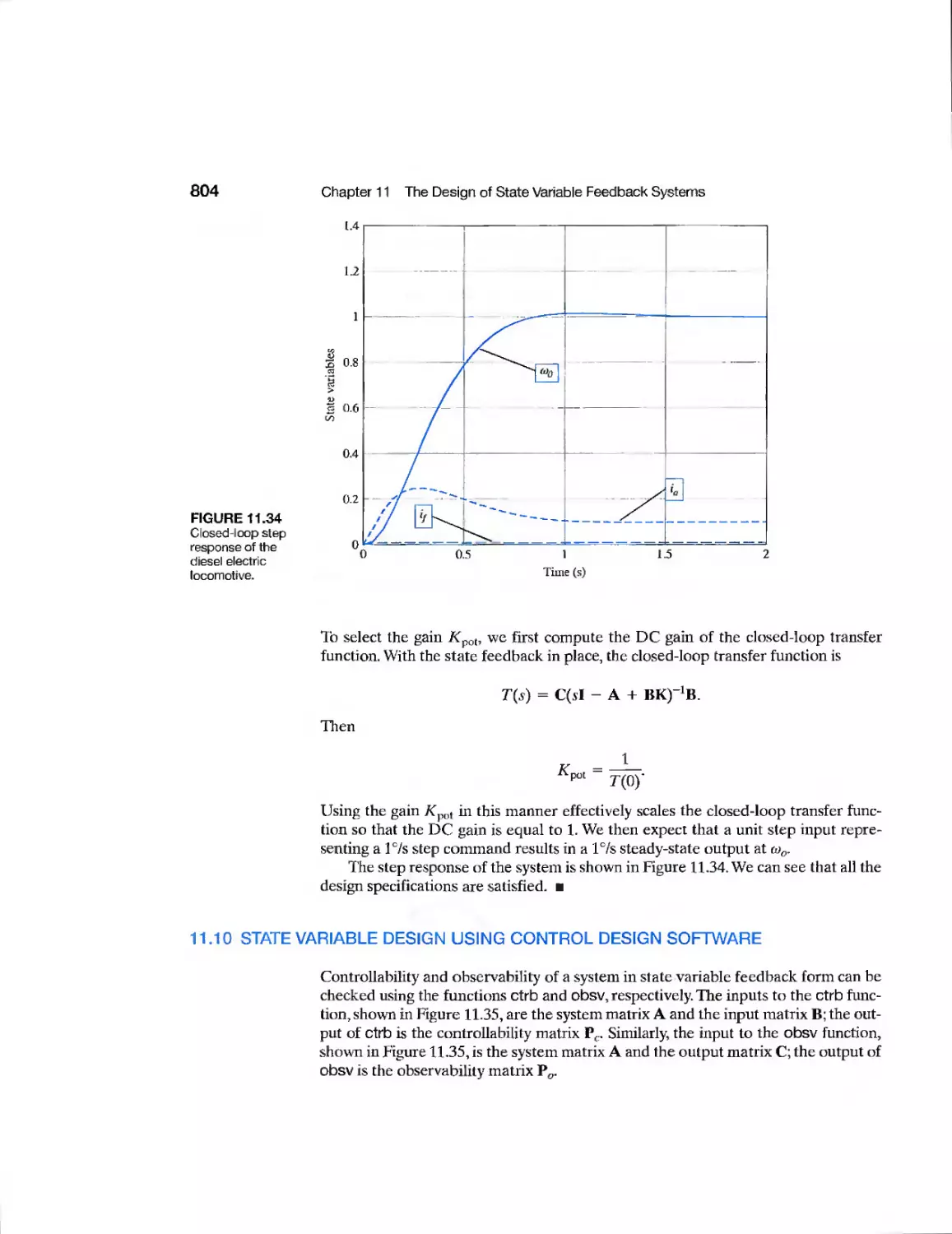
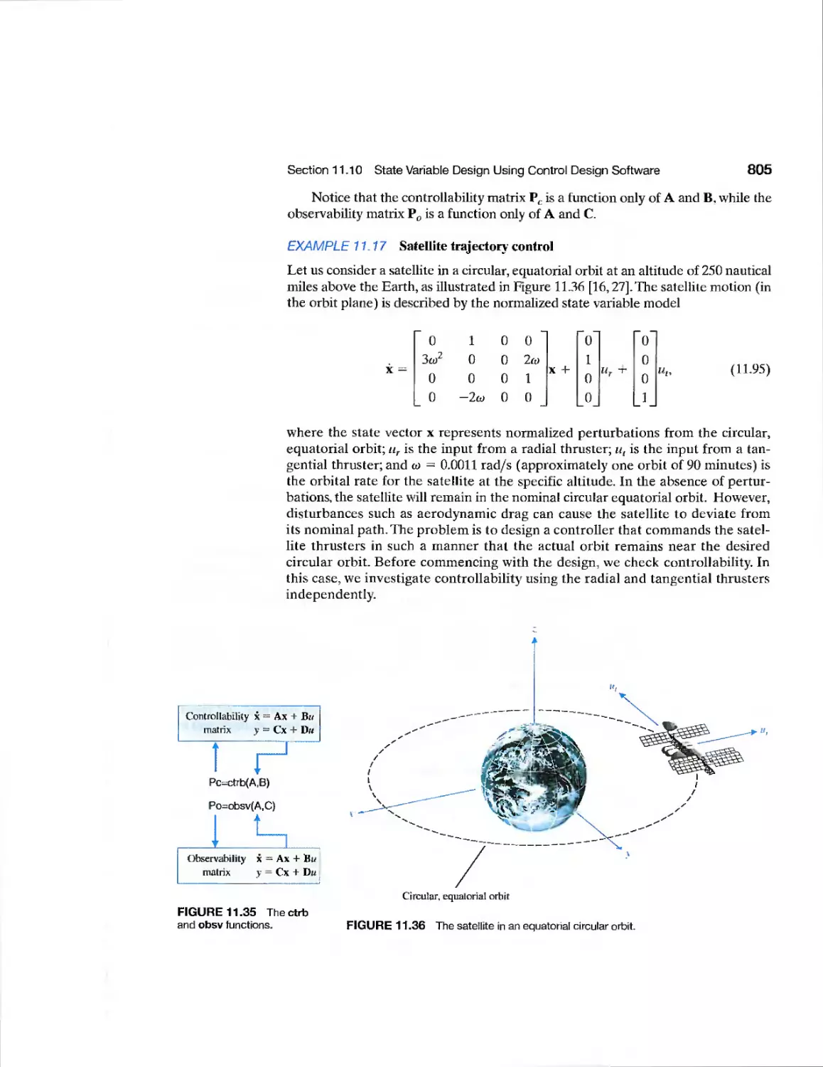
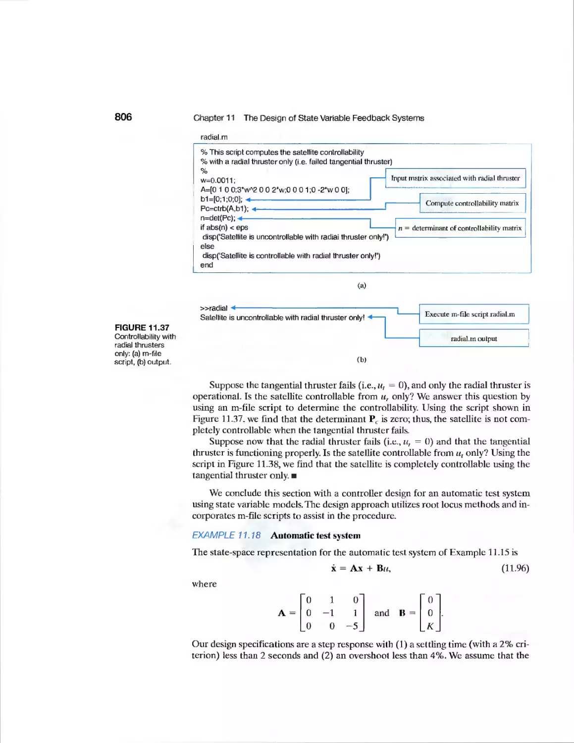
11.10 State Variable Design Using Control Design Software 804
11.11 Sequential Design Example: Disk Drive Read System 810
11.12 Summary 812
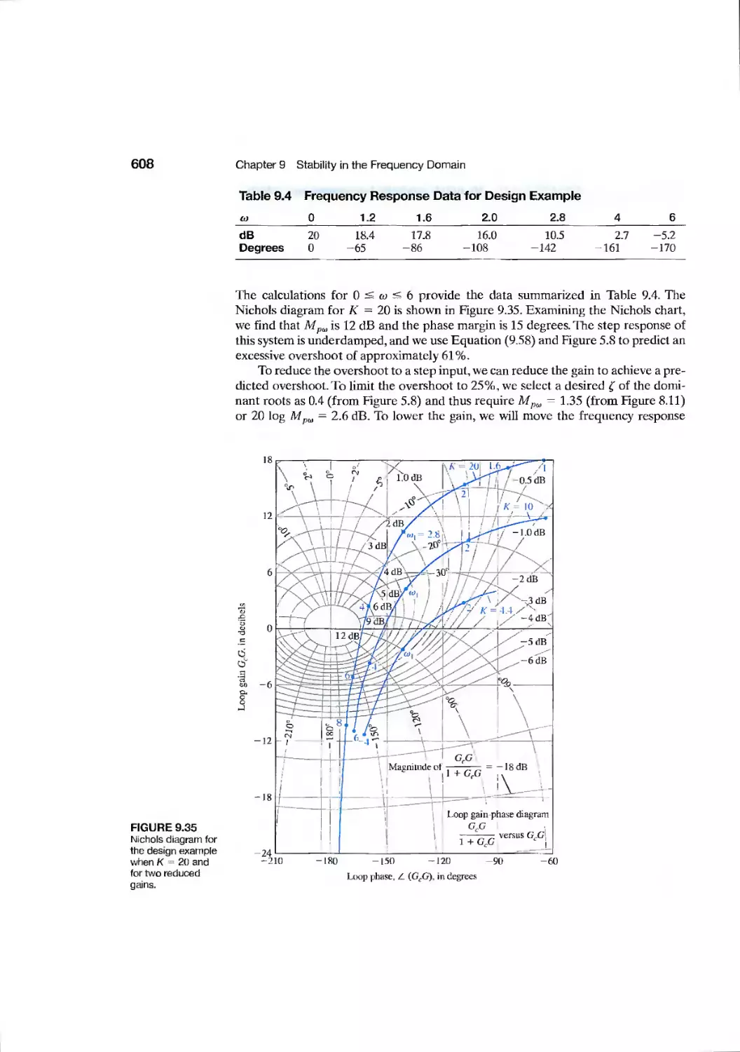
Exercises 812
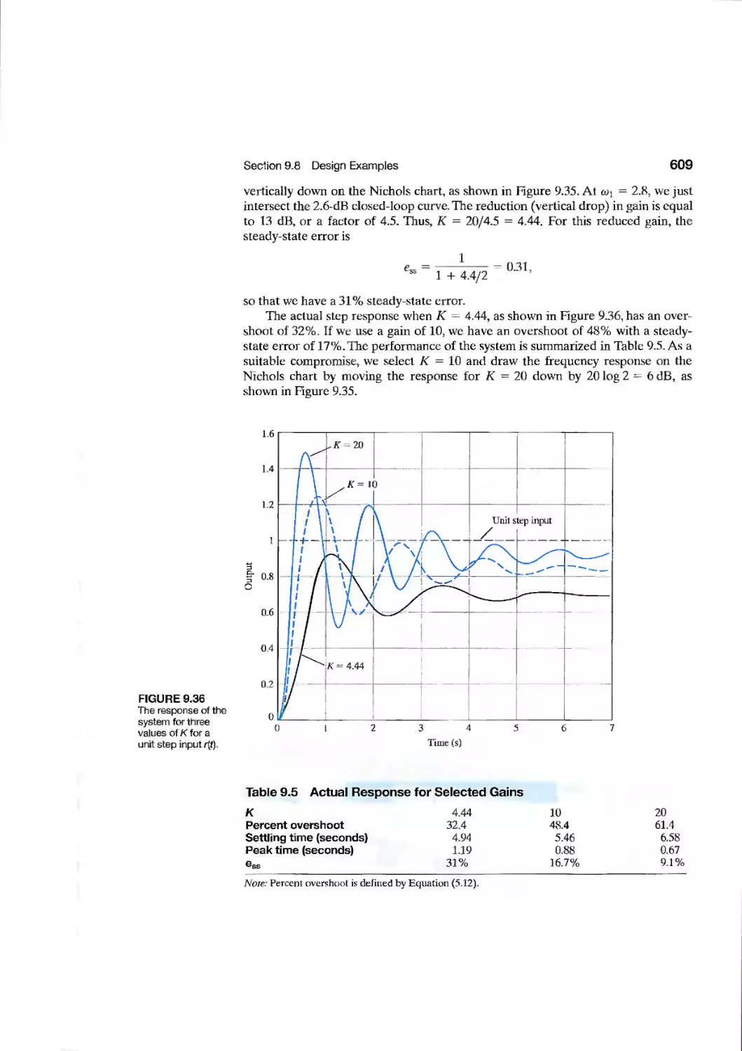
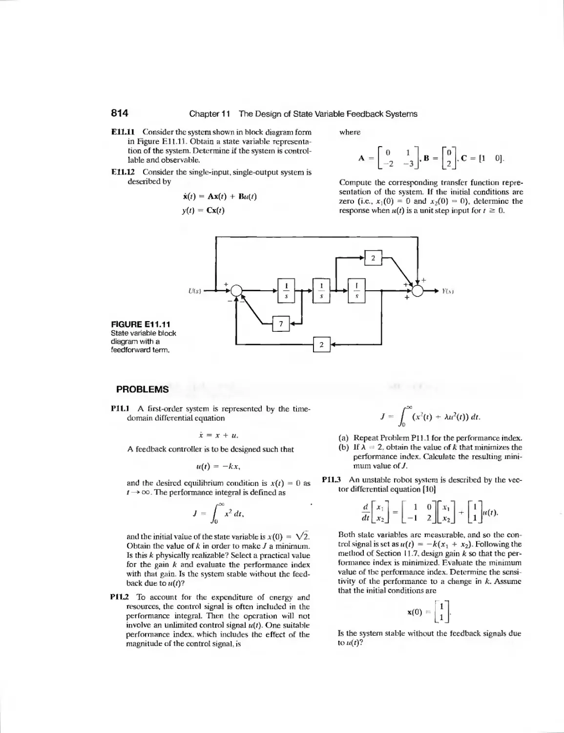
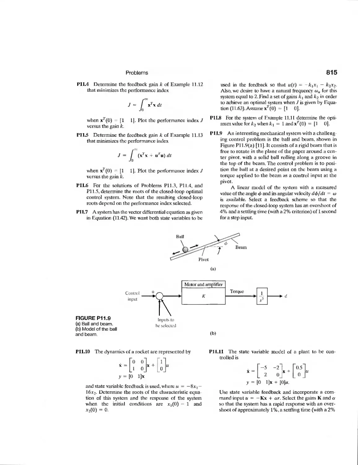
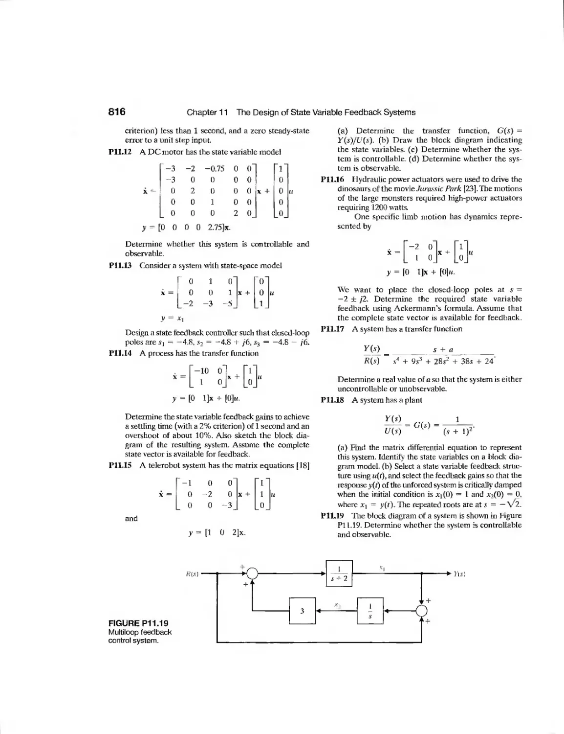
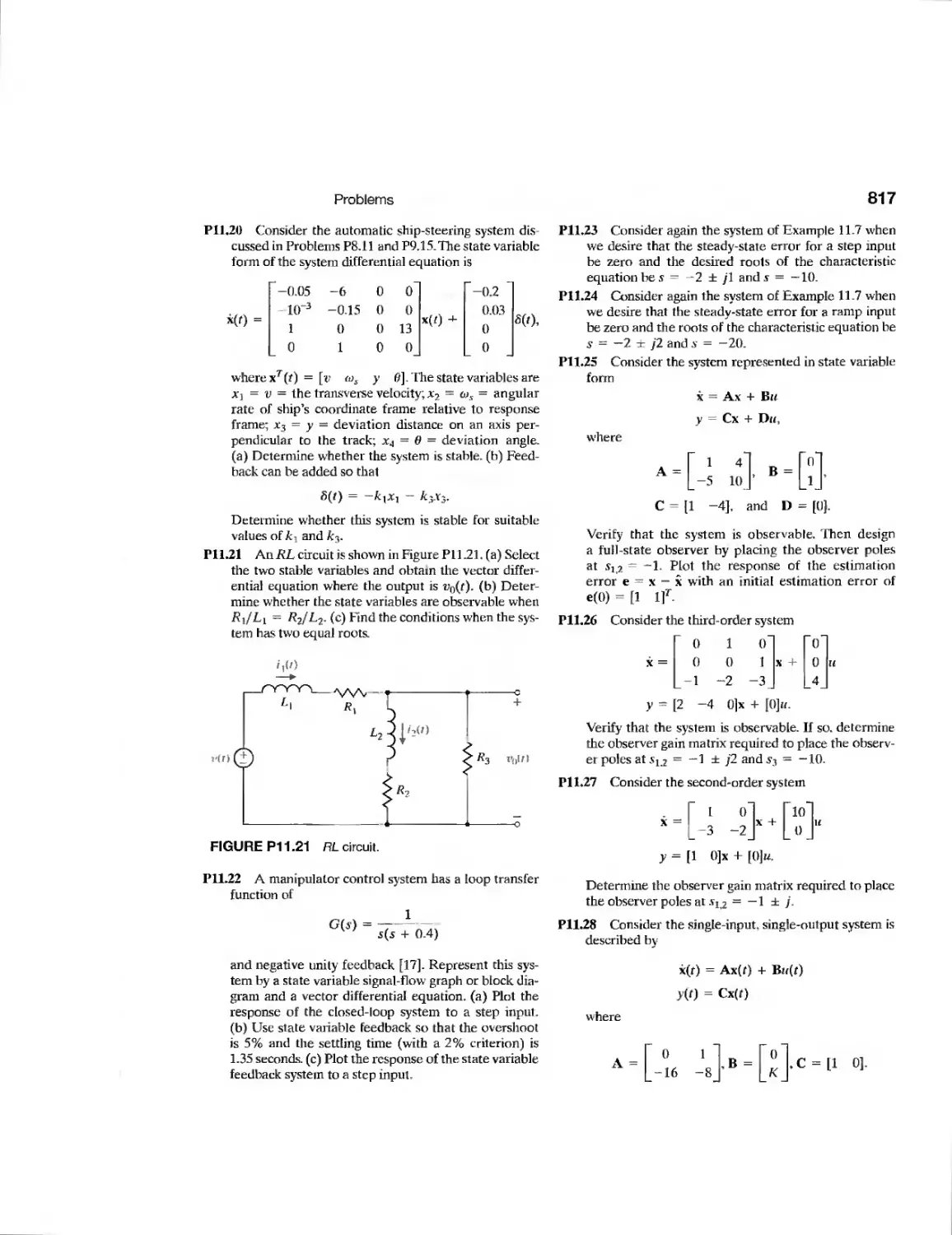
Problems 814
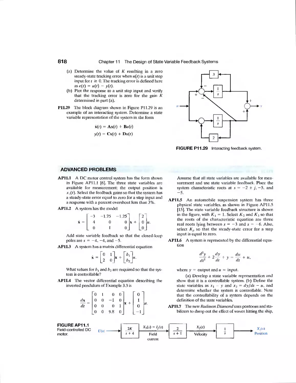
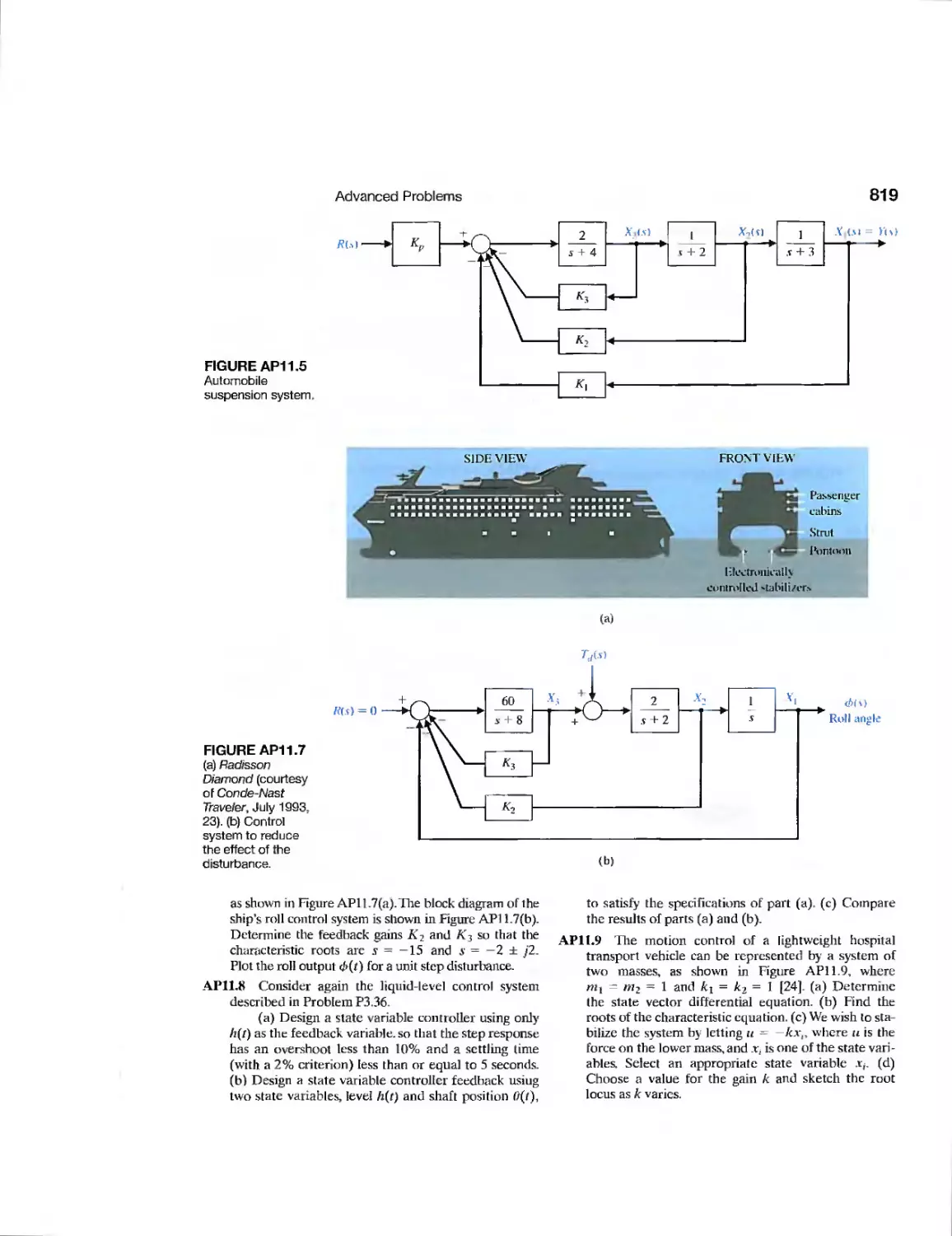
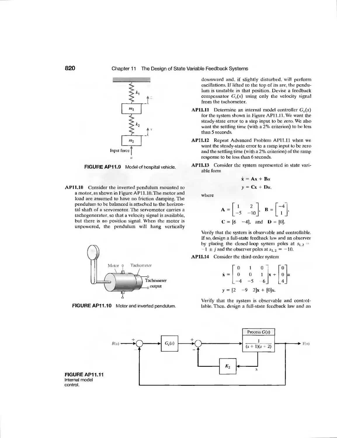
Advanced Problems 818
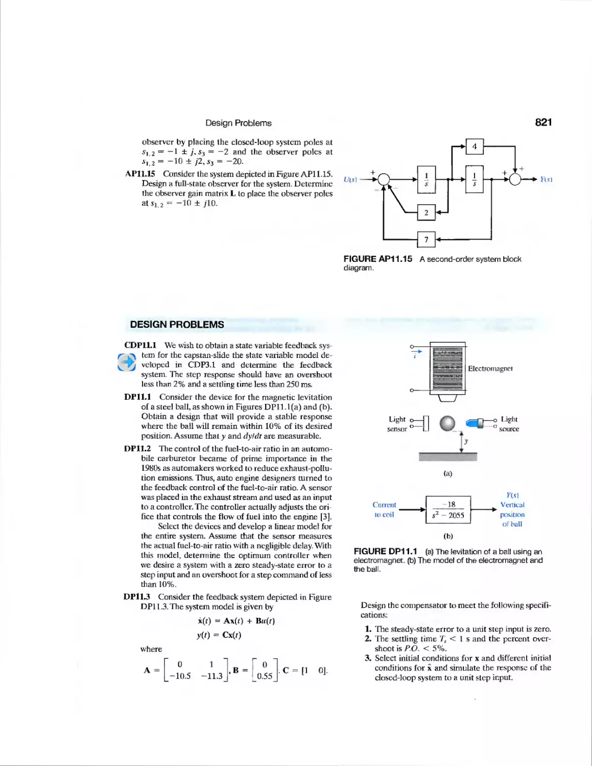
Design Problems 821
Computer Problems 824
Terms and Concepts 826
X Contents
chapter 12 Robust Control Systems 828
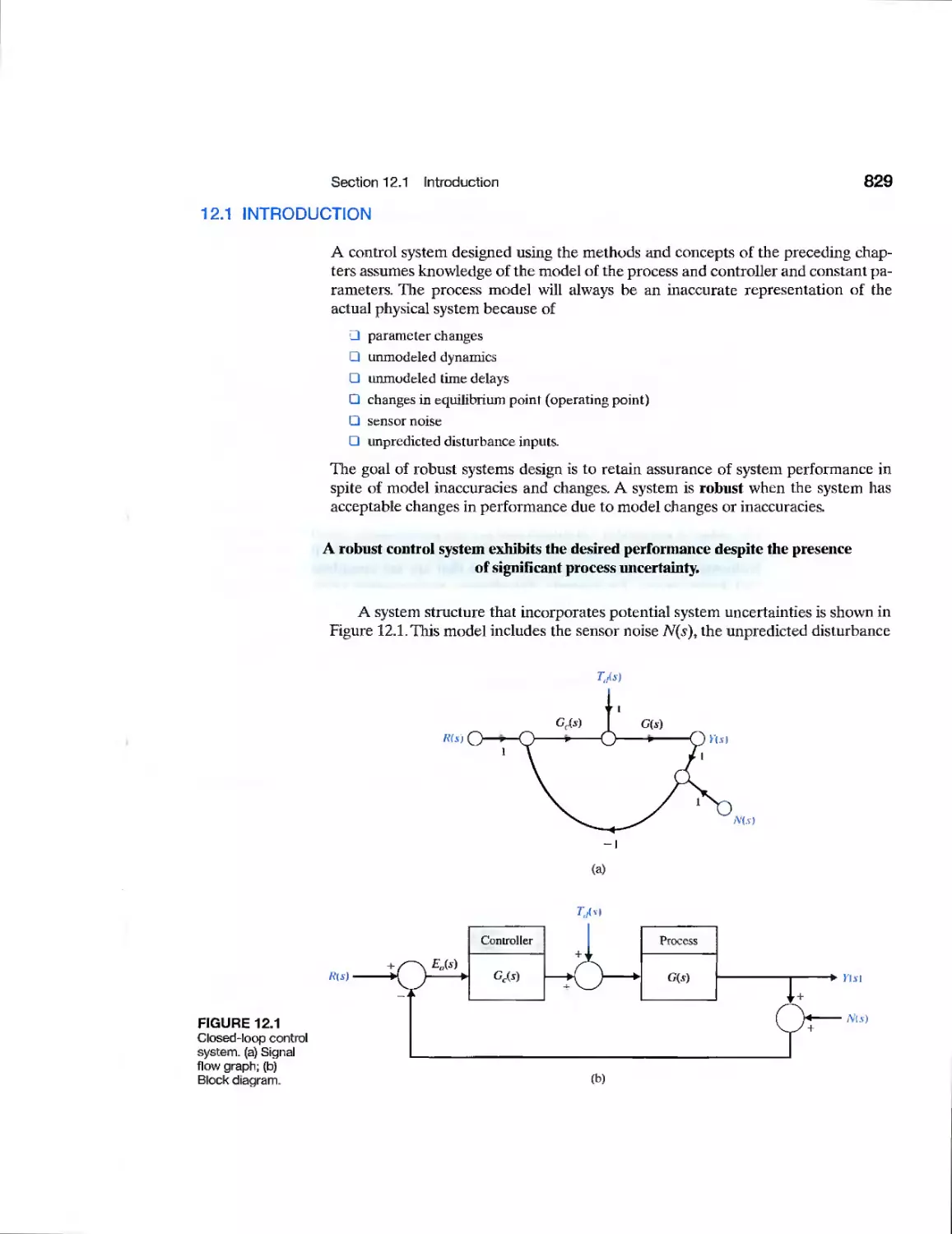
12.1 Introduction 829
12.2 Robust Control Systems and System Sensitivity 830
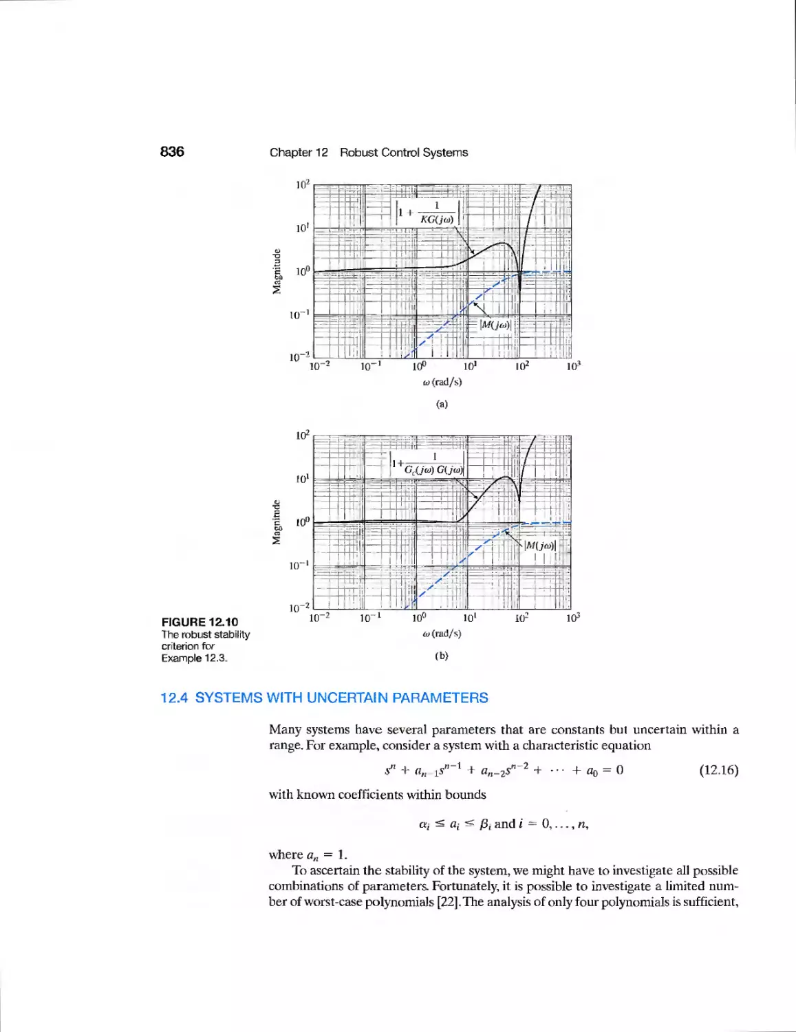
12.3 Analysis of Robustness 834
12.4 Systems with Uncertain Parameters 836
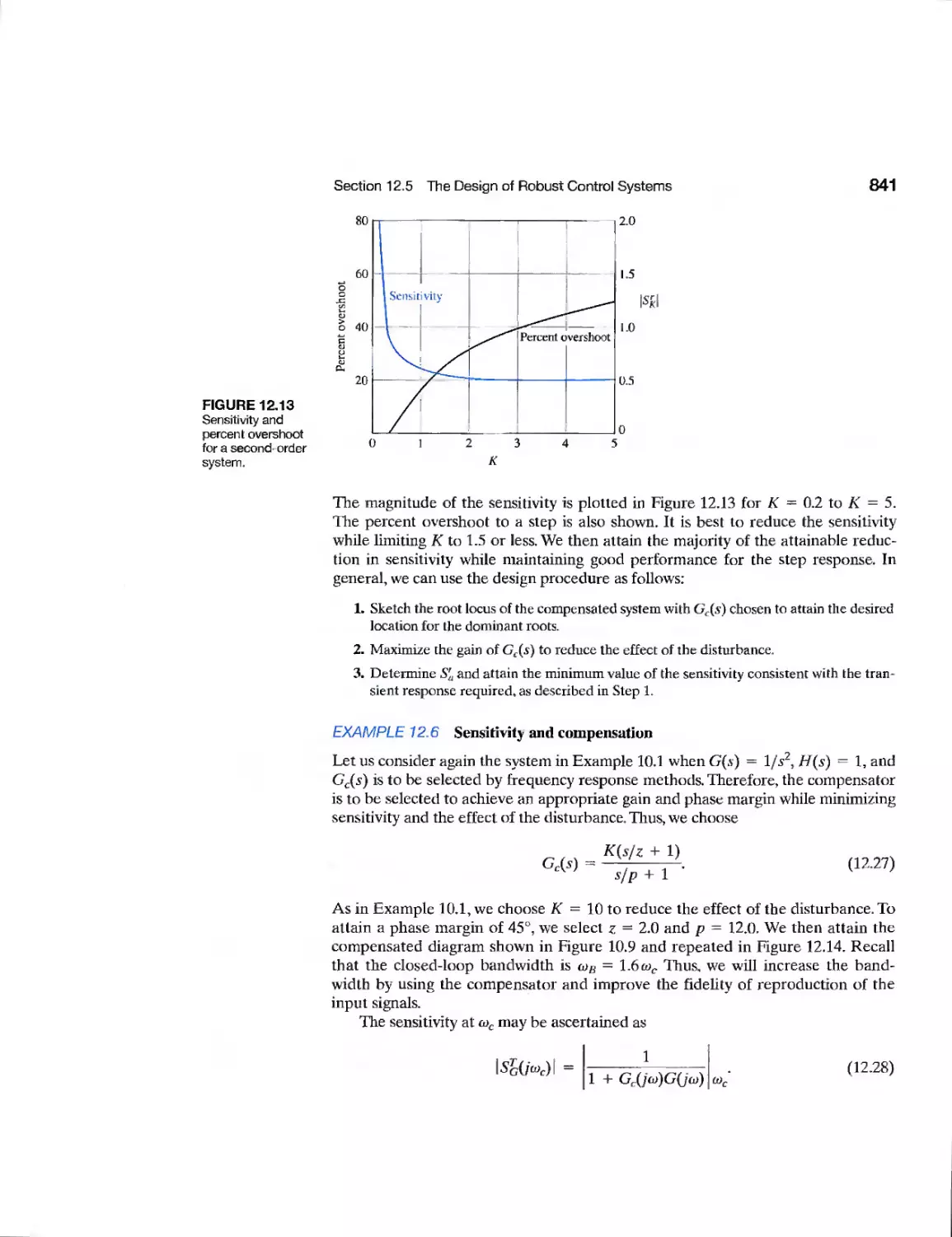
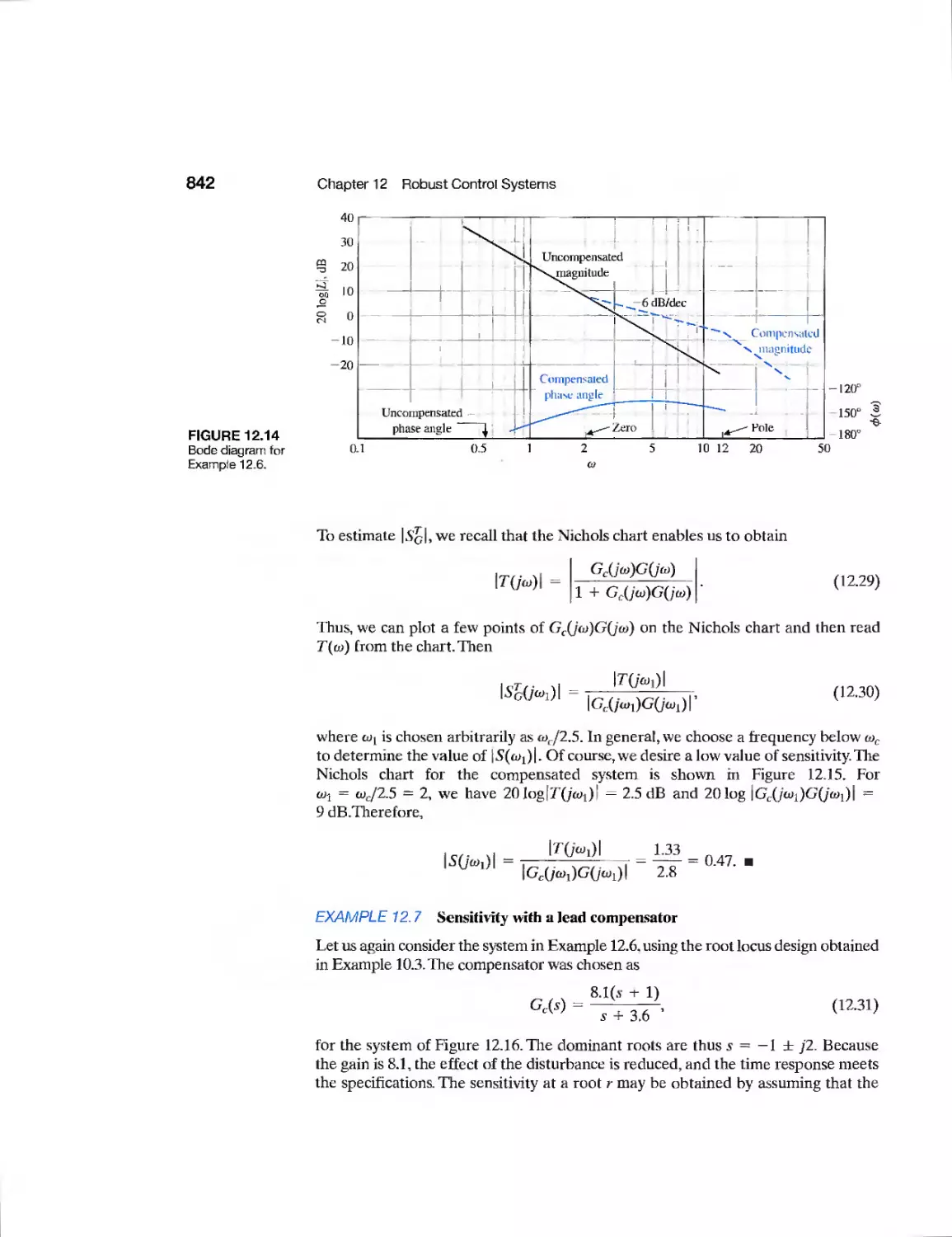
12.5 The Design of Robust Control Systems 838
12.6 The Design of Robust PID-Controlled Systems 844
12.7 The Robust Internal Model Control System 850
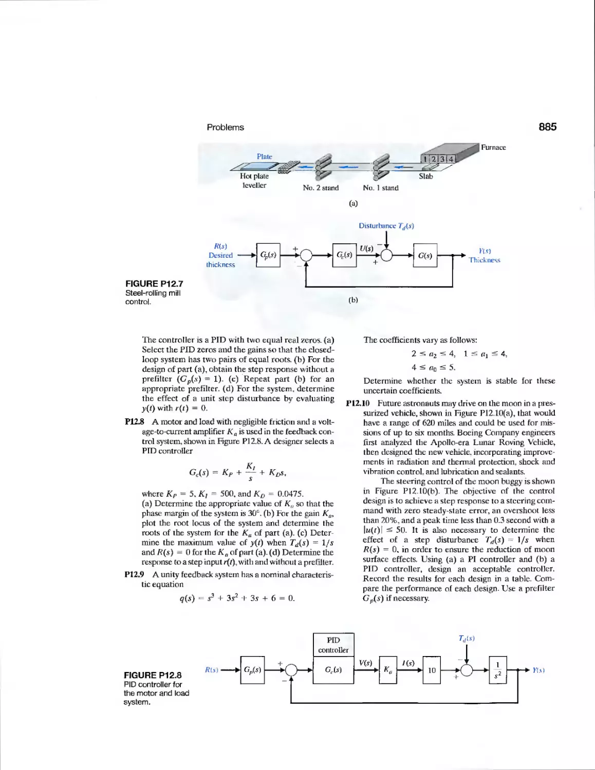
12.8 Design Examples 853
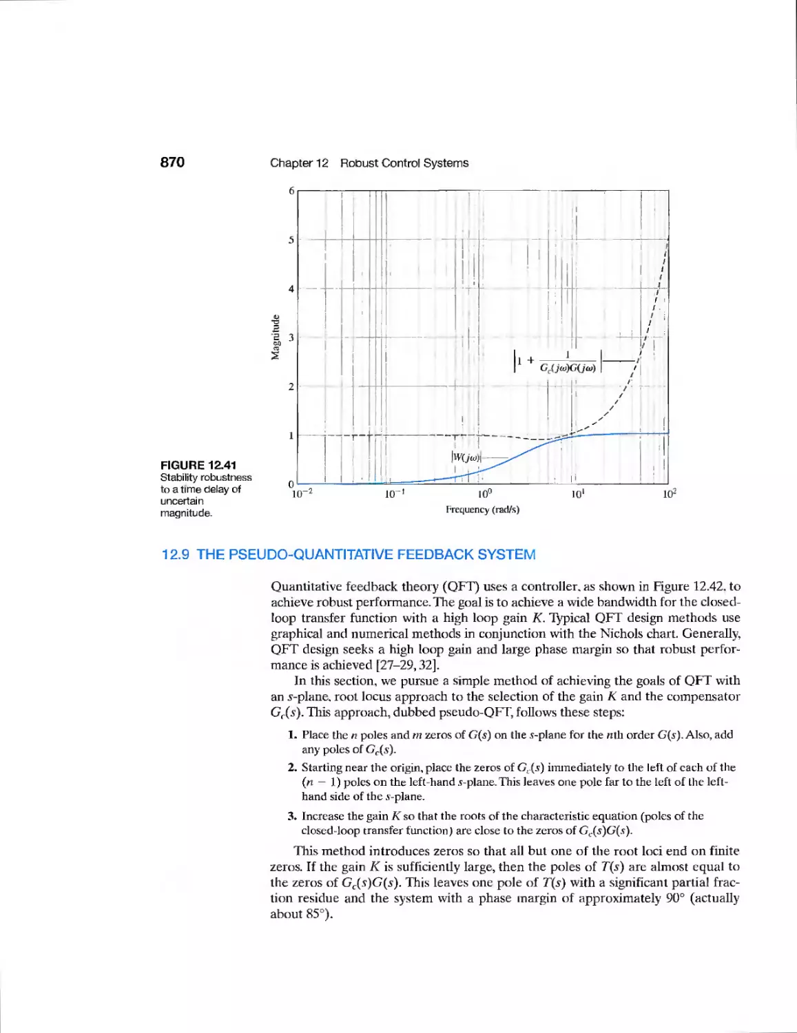
12.9 The Pseudo-Quantitative Feedback System 870
12.10 Robust Control Systems Using Control Design Software 871
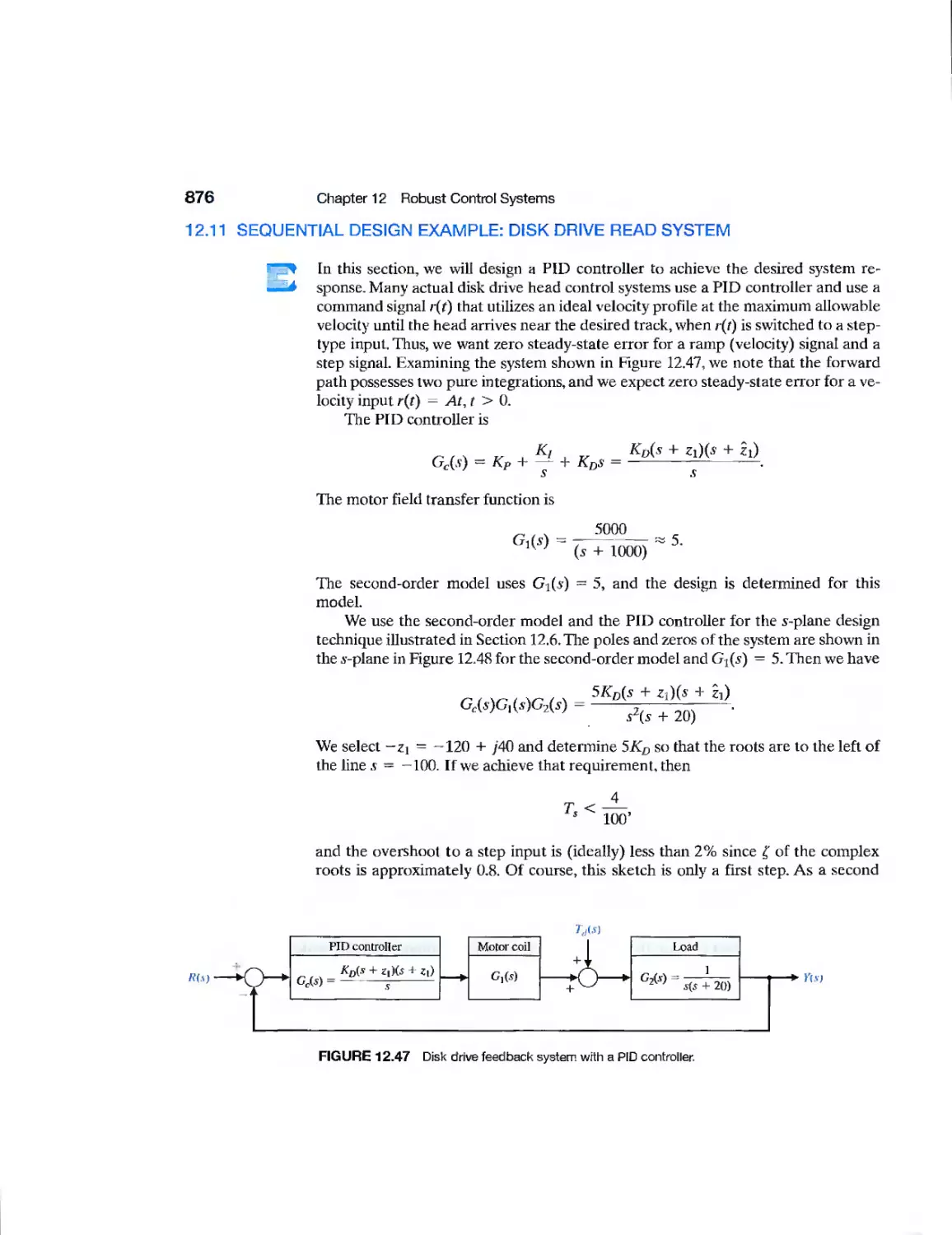
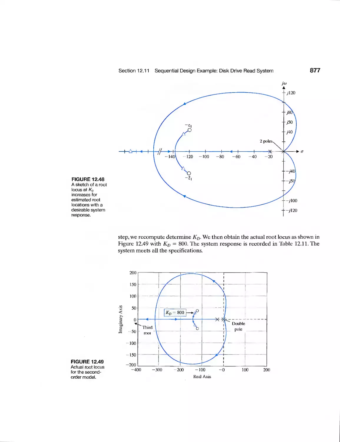
12.11 Sequential Design Example: Disk Drive Read System 876
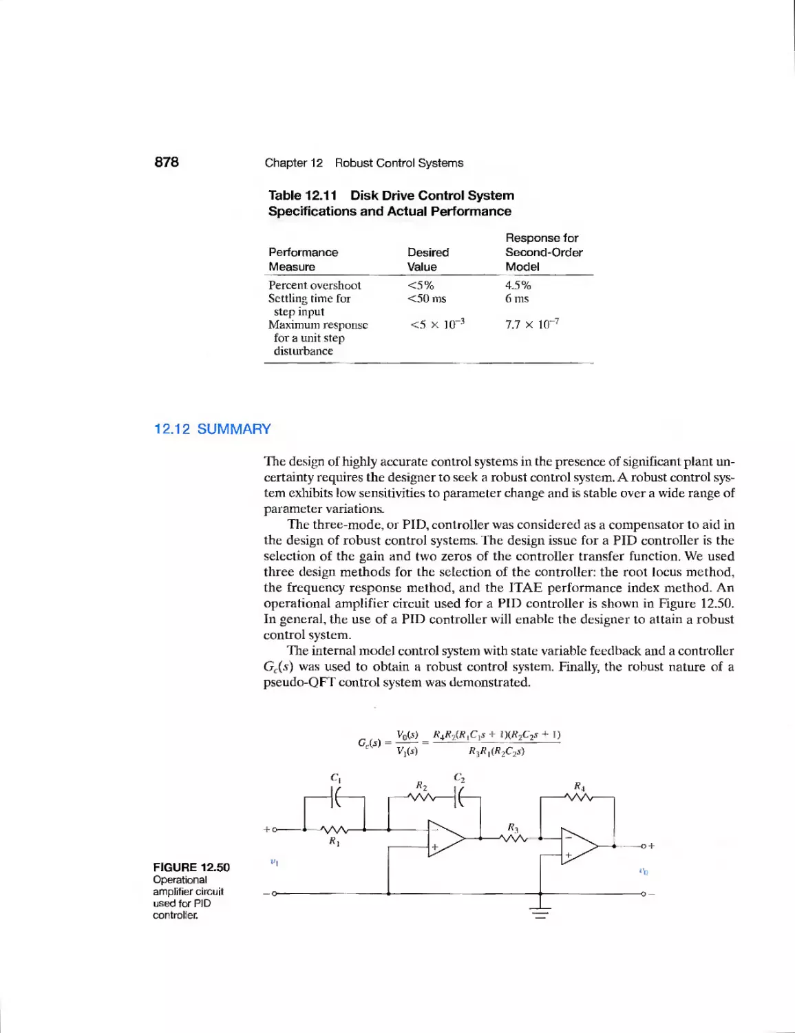
12.12 Summary 878
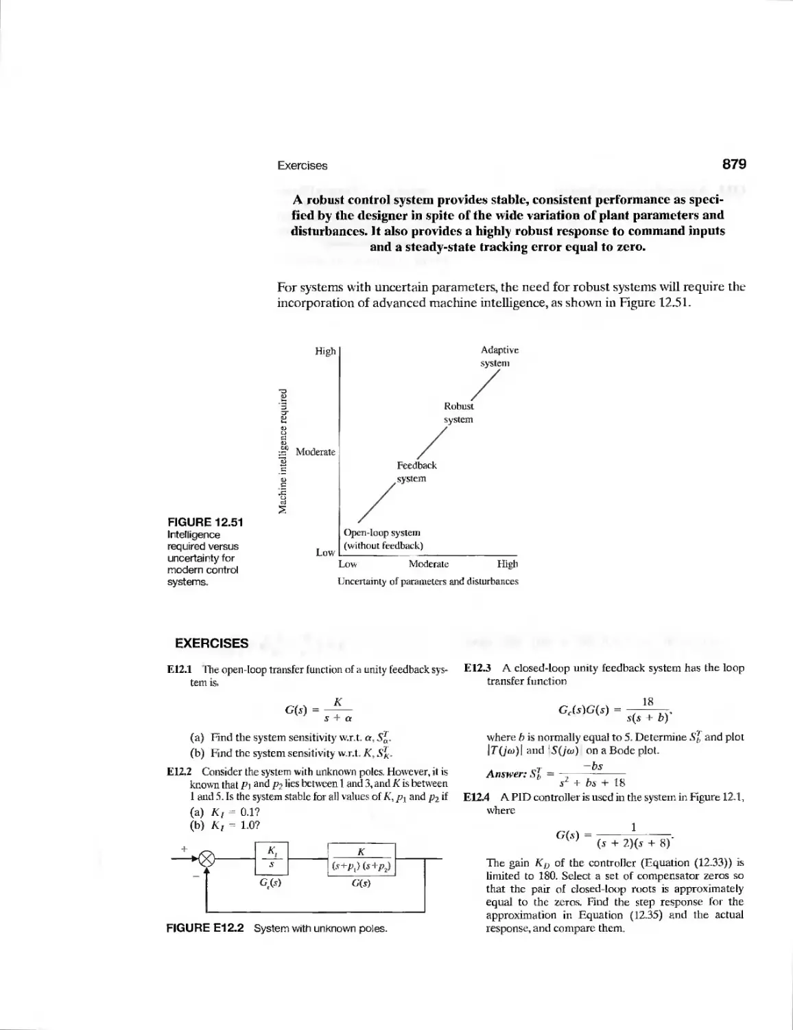
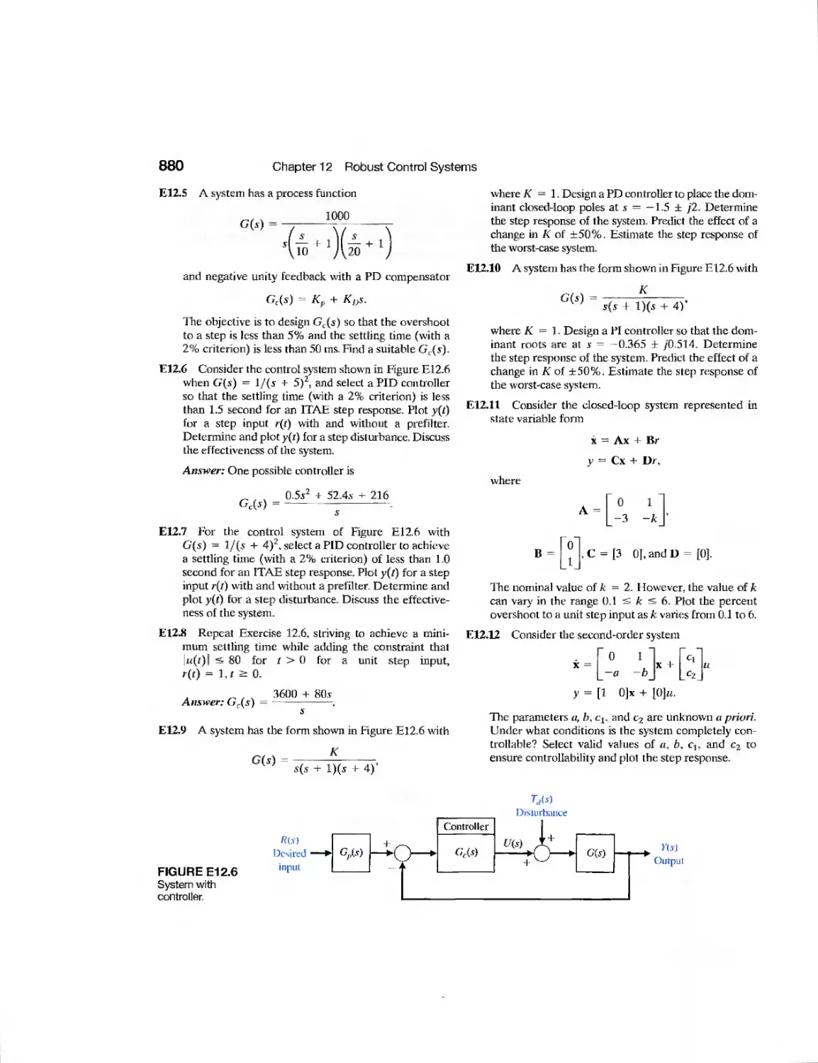
Exercises 879
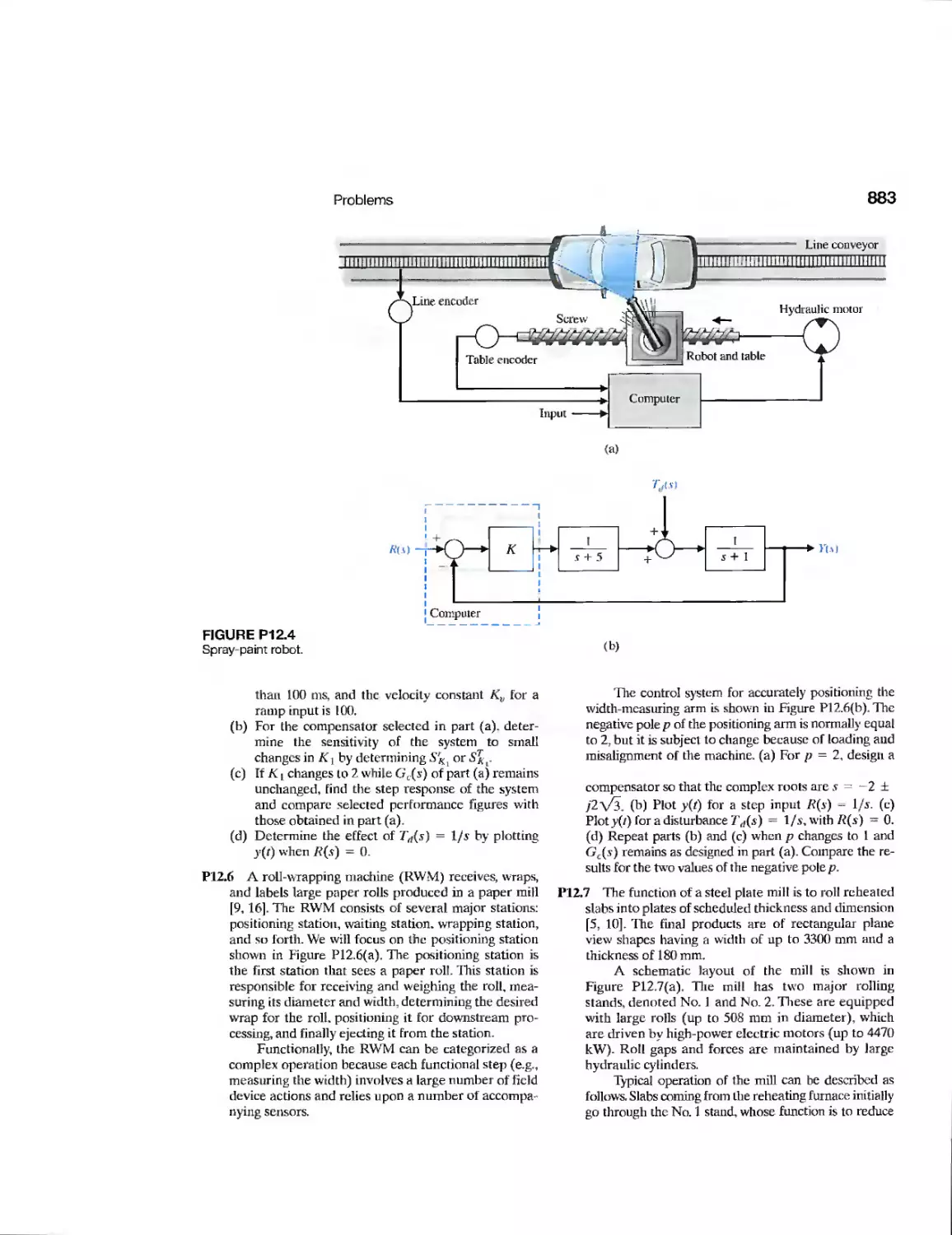
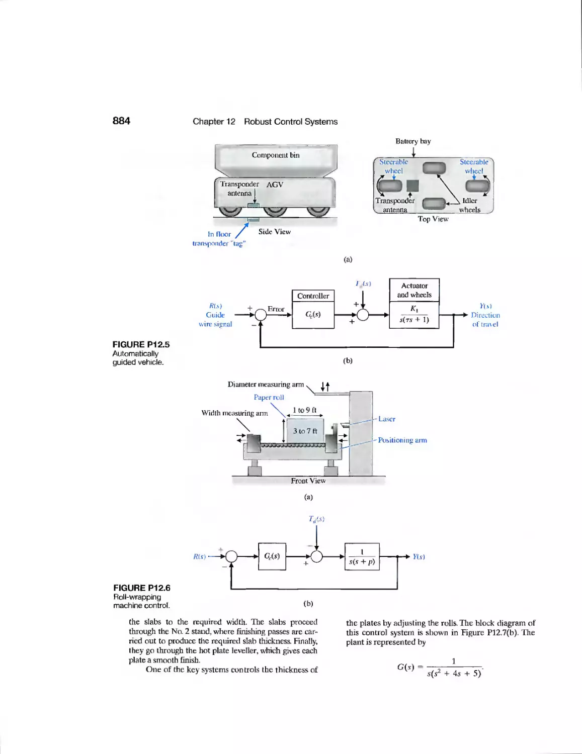
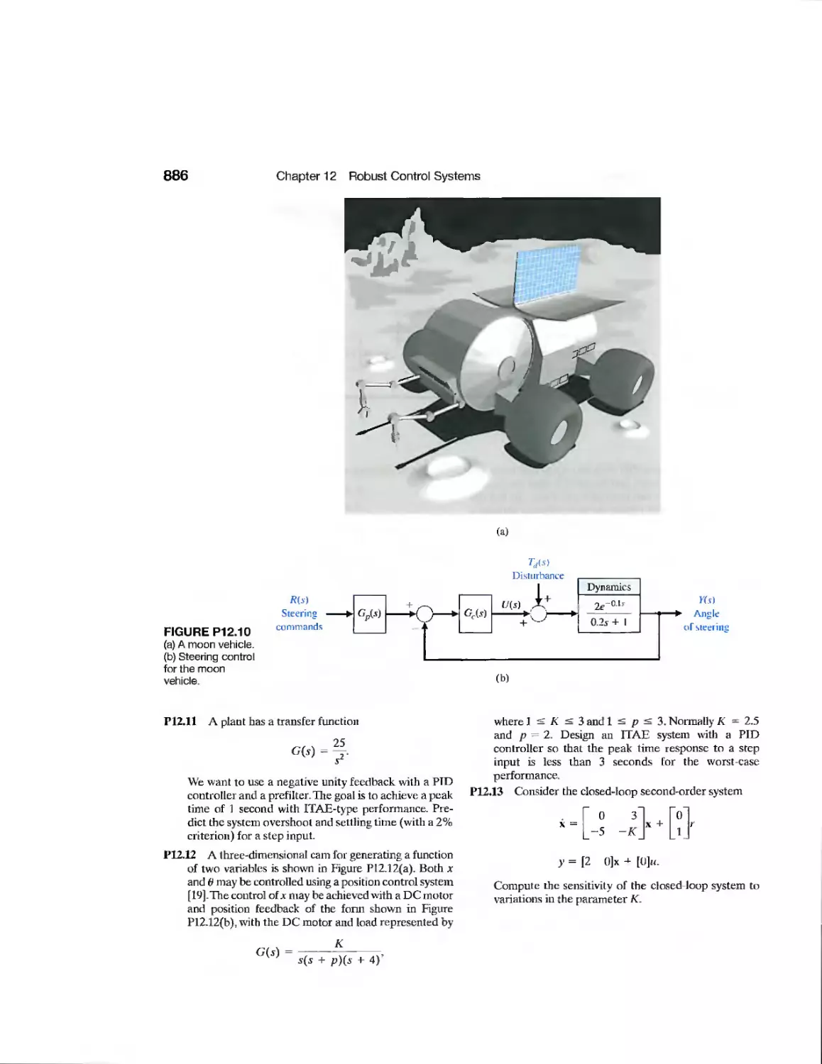
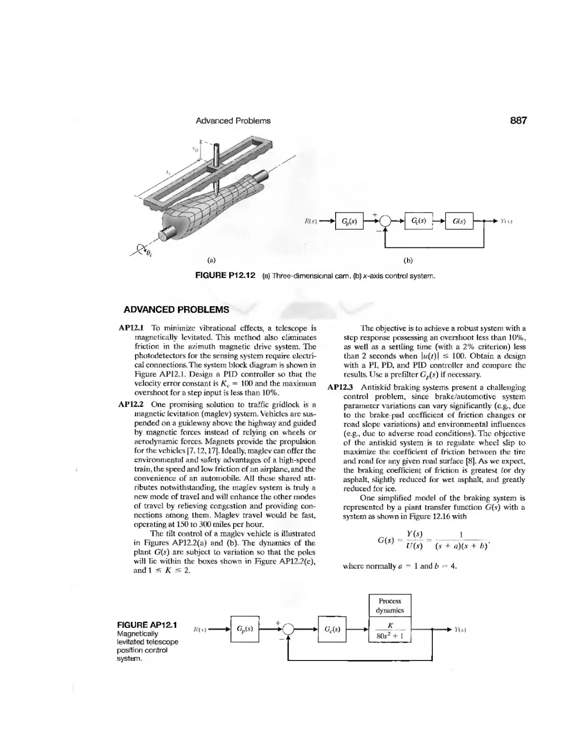
Problems 881
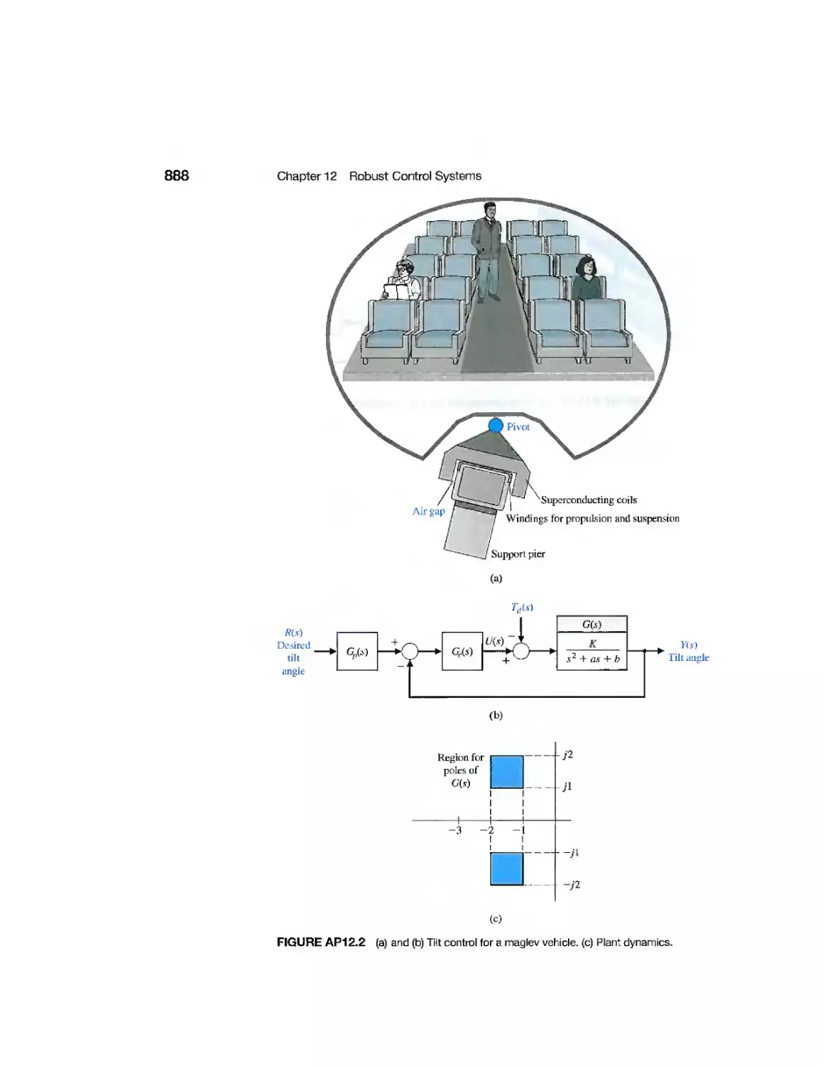
Advanced Problems 887
Design Problems 891
Computer Problems 897
Terms and Concepts 899
chapter 13 Digital Control Systems 901
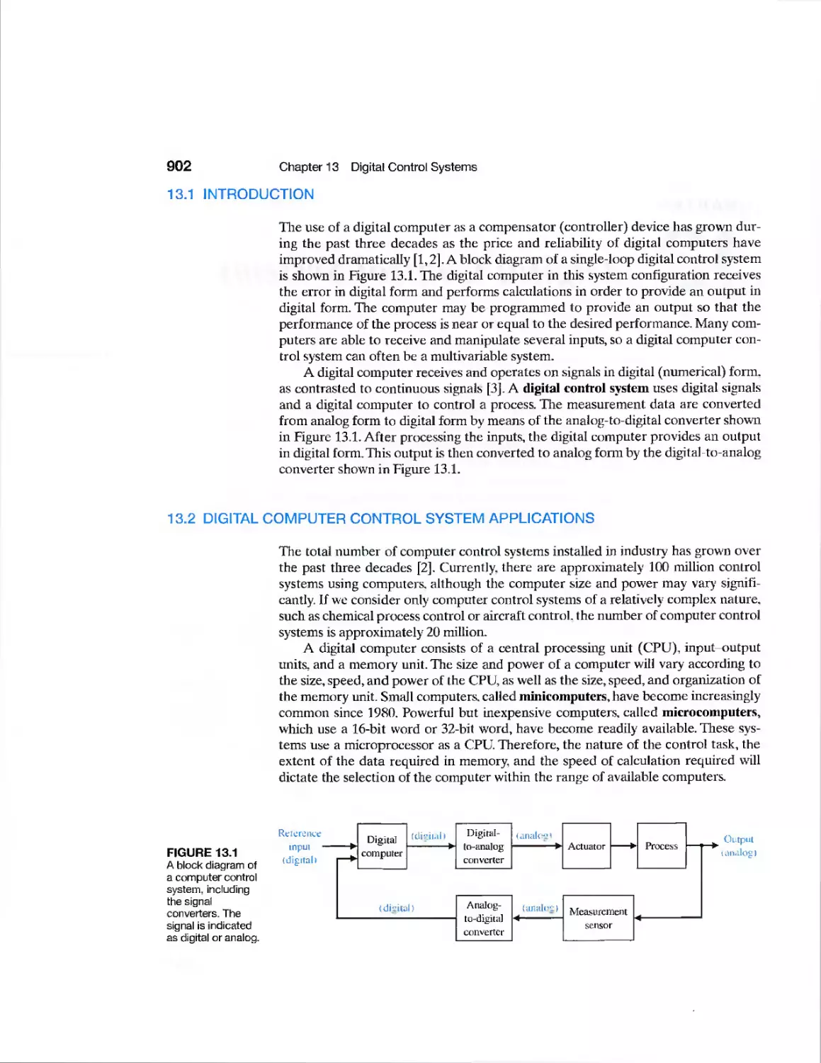
13.1 Introduction 902
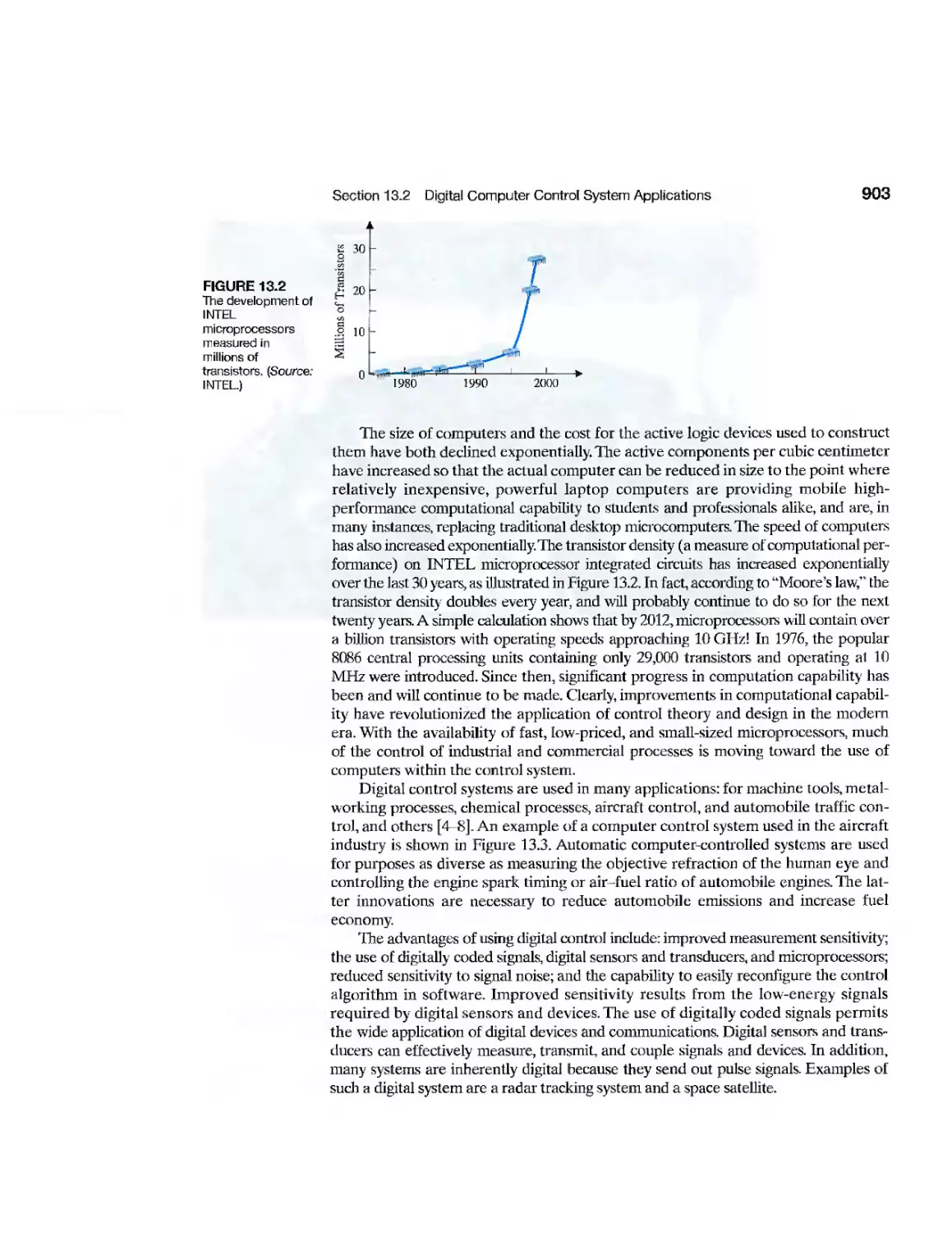
13.2 Digital Computer Control System Applications 902
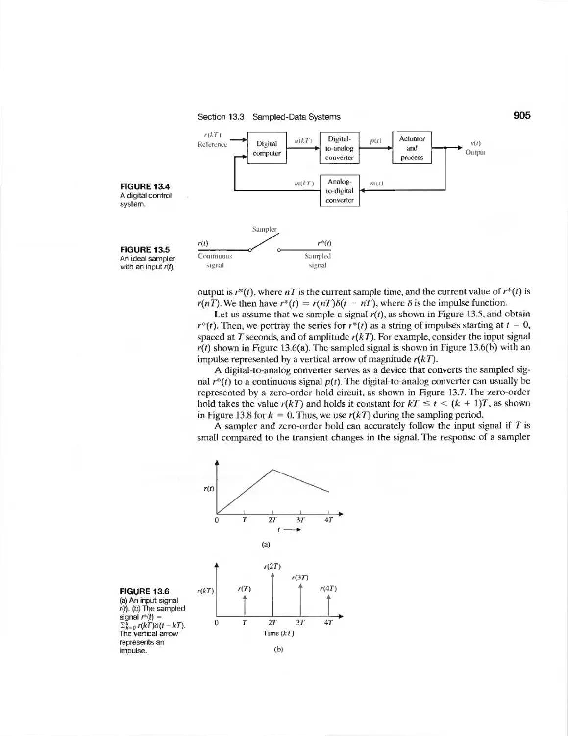
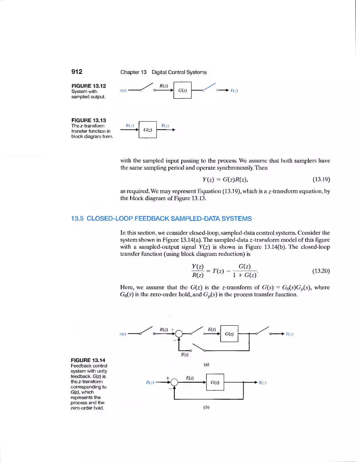
13.3 Sampled-Data Systems 904
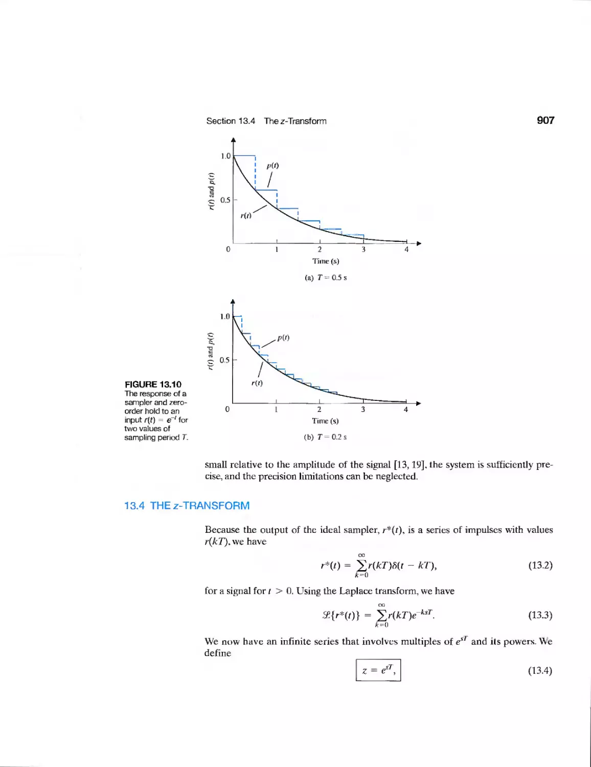
13.4 The z-Transf orm 907
13.5 Closed-Loop Feedback Sampled-Data Systems 912
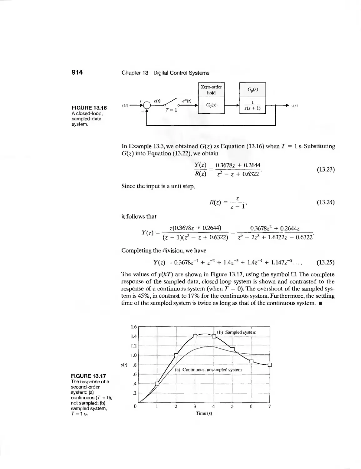
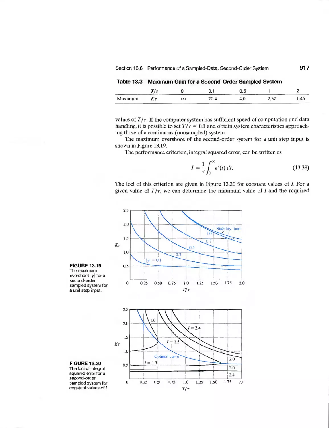
13.6 Performance of a Sampled-Data, Second-Order System 916
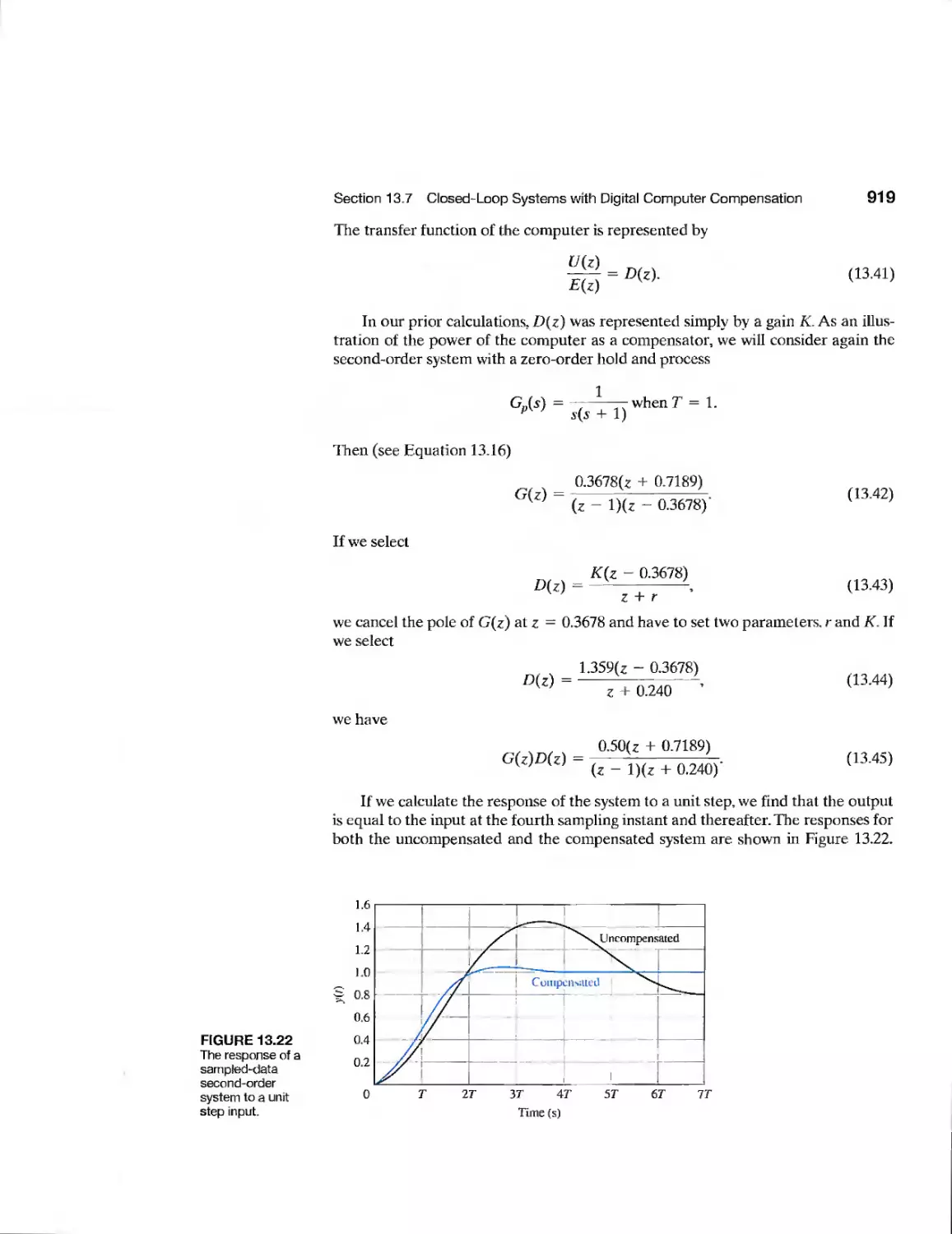
13.7 Closed-Loop Systems with Digital Computer Compensation 918
13.8 The Root Locus of Digital Control Systems 921
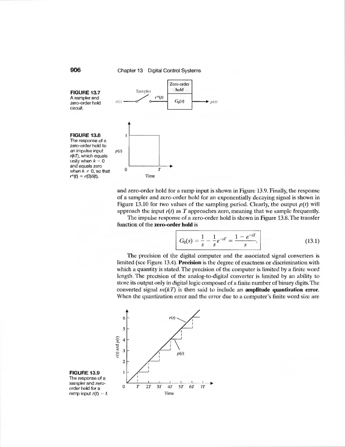
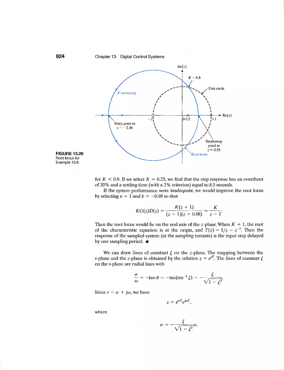
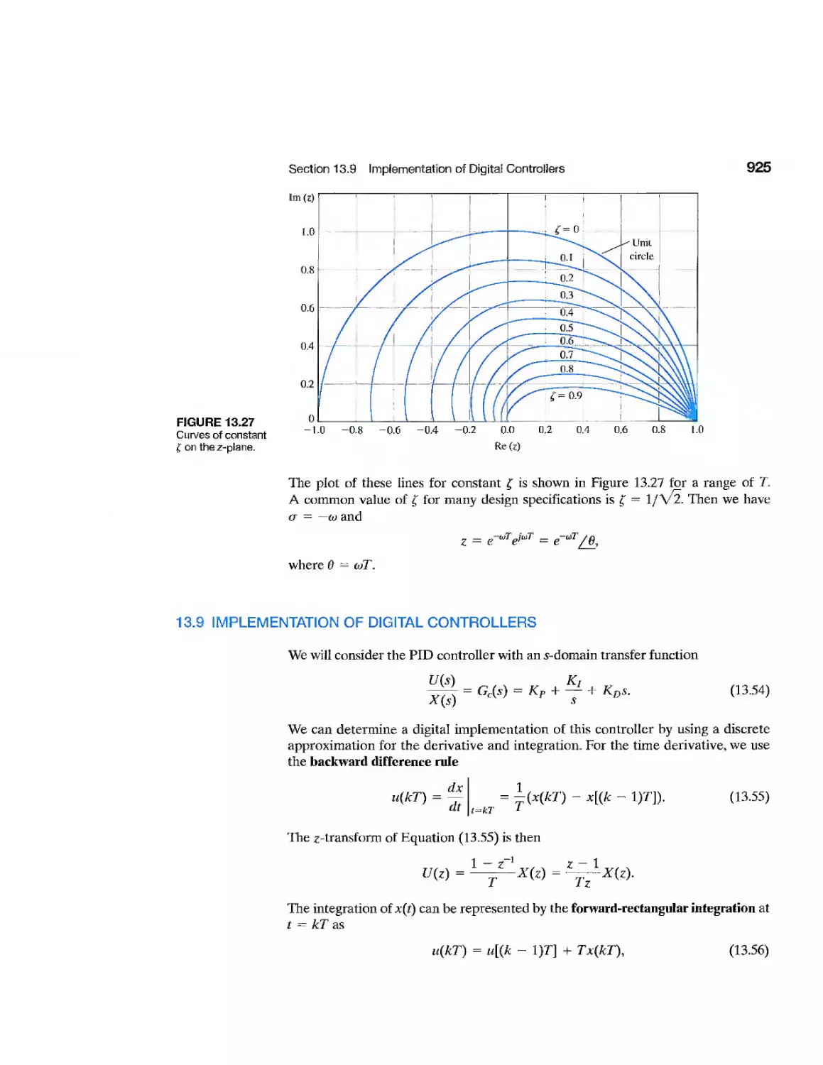
13.9 Implementation of Digital Controllers 925
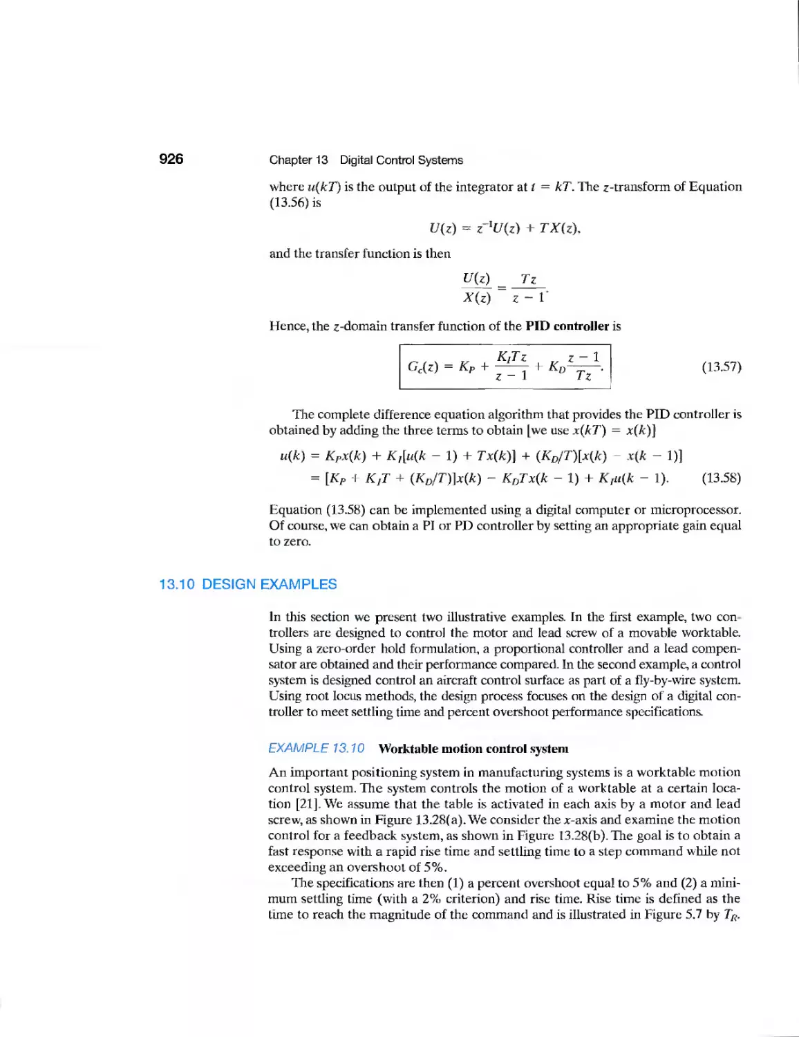
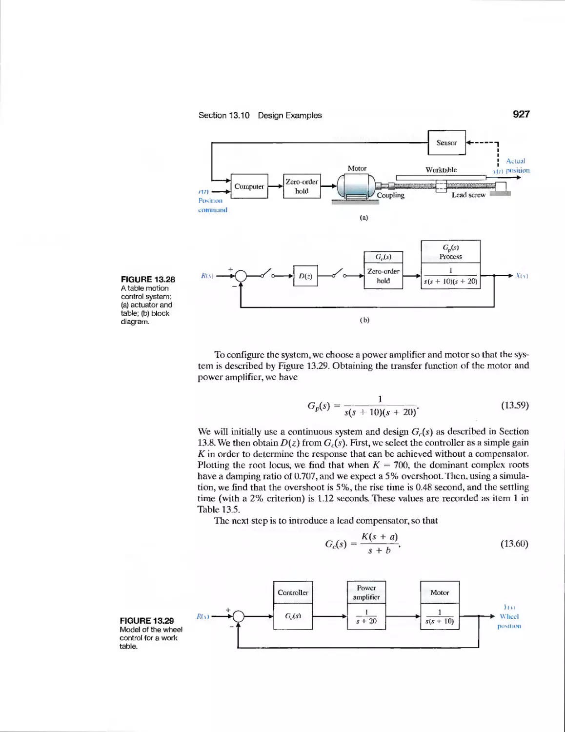
13.10 Design Examples 926
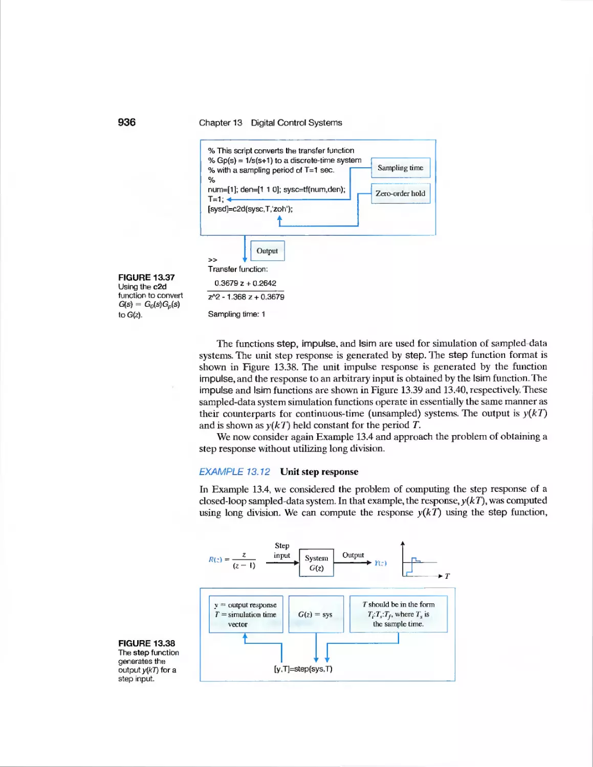
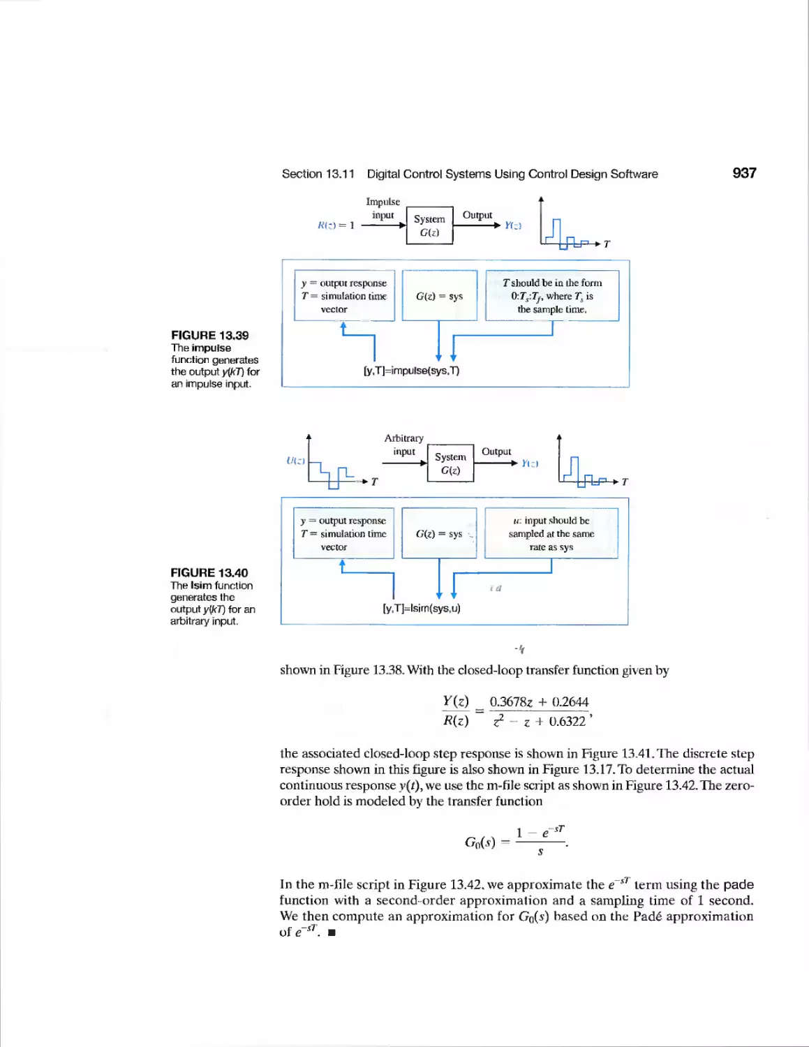
13.11 Digital Control Systems Using Control Design Software 935
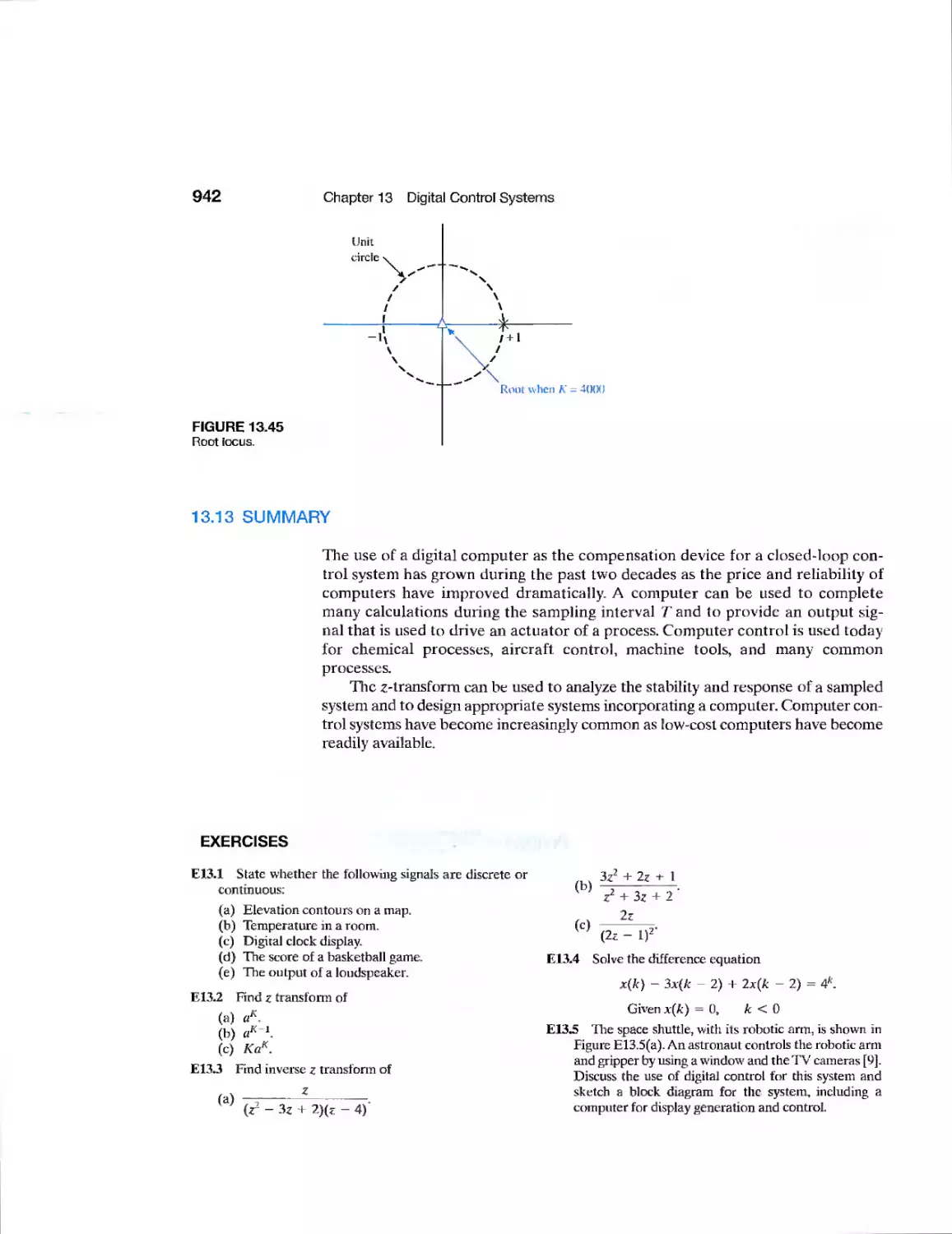
13.12 Sequential Design Example: Disk Drive Read System 940
13.13 Summary 942
Exercises 942
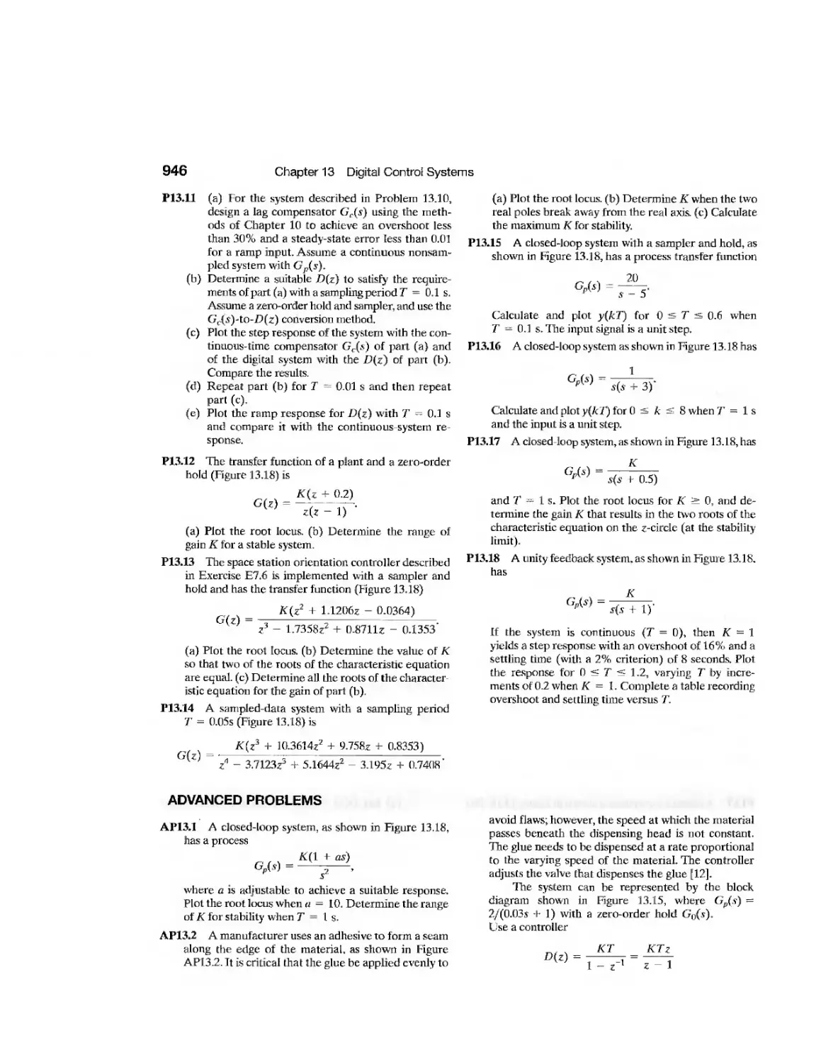
Problems 945
Advanced Problems 946
Design Problems 947
Computer Problems 949
Terms and Concepts 950
Contents
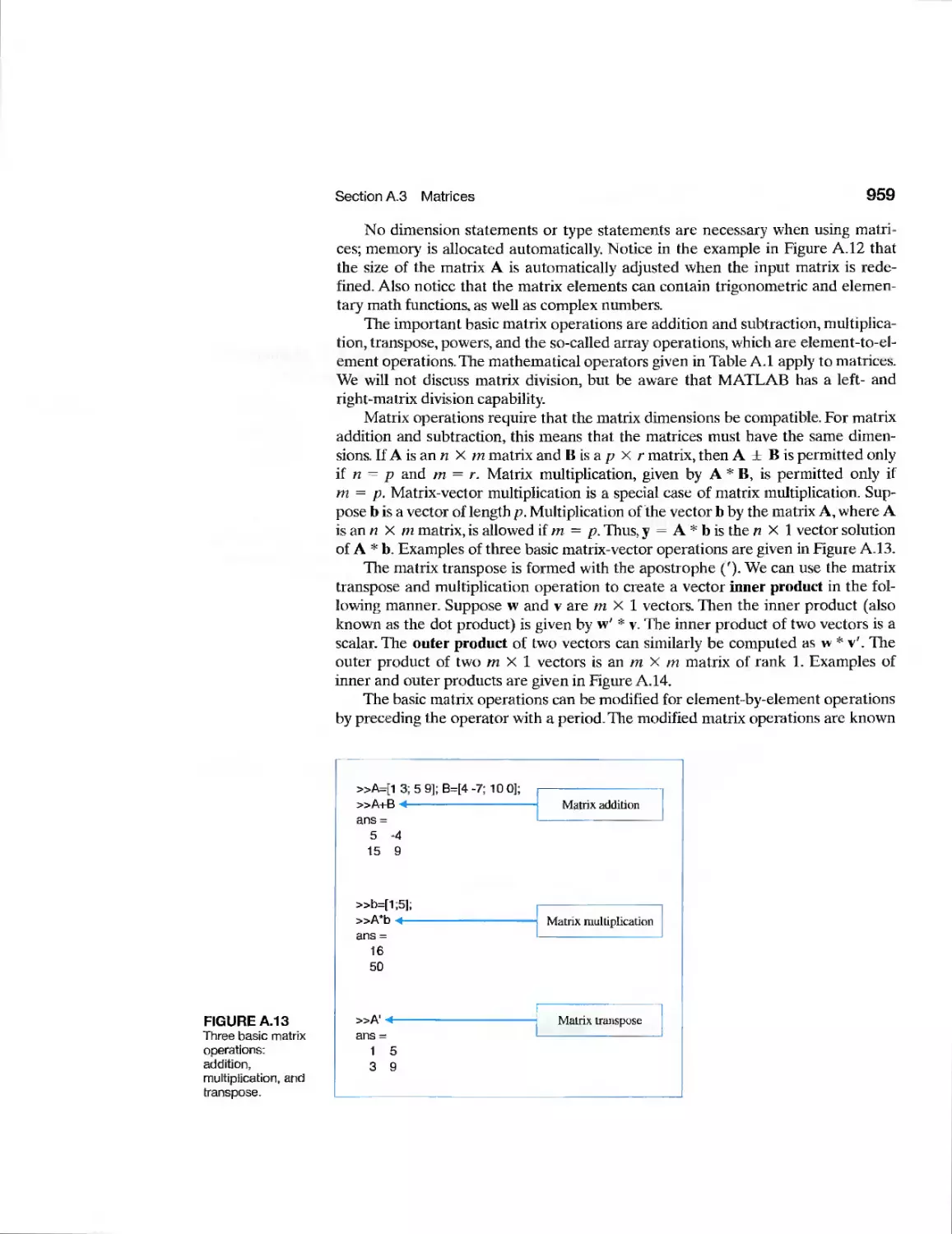
appendix A MATLAB Basics 953
appendix B MathScript Basics 971
XI
d& WEB RESOURCES
Symbols, Units, and Conversion Factors
Laplace Transform Pairs
An Introduction to Matrix Algebra
Decibel Conversion
Complex Numbers
z-Transform Pairs Preface
Discrete-Time Evaluation of the Time Response
References 993
Index 1007
APPENDIX C
APPENDIX D
APPENDIX E
APPENDIX F
APPENDIX G
APPENDIX H
APPENDIX I
Preface
MODERN CONTROL SYSTEMS—THE BOOK
The Mars Exploration Rover (MER-A), also known as Spirit, was launched on a
Delta II rocket, in June 2003 to Mars, the Red Planet. Spirit entered the Martian
atmosphere seven months later in January, 2004. When the spacecraft entered the
Martian atmosphere it was traveling 19,300 kilometers per hour. For about four
minutes in the upper atmosphere, the spacecraft aeroshell decelerated the vehicle to
a velocity of 1,600 kilometers per hour. Then a parachute was deployed to slow the
spacecraft to about 300 kilometers per hour. At an altitude of about 100 meters,
retrorockets slowed the descent and airbags were inflated to cushion the shock of
landing. The Spirit struck the Martian ground at around 50 km/hr and bounced and
rolled until it stopped near the target point in the Gusev Crater. The target landing
site was chosen because it looks like a crater lakebed. The Spirit mobile rover has
reached interesting places in the Gusev Crater to perform in-situ tests to help
scientists answer many of the lingering questions about the history of our neighbor planet.
In fact, Spirit discovered evidence of an ancient volcanic explosion near the landing
site in Gusev Crater. The successful entry, descent, and landing of Spirit is an
astonishing illustration of the power of control systems. Given the large distances to Mars,
it is not possible for a spacecraft to fly through the atmosphere while under ground
control—the entry, descent, and landing must be controlled autonomously on-board
the spacecraft. Designing systems capable of performing planetary entry is one of
the great challenges facing control system engineers.
The precursor NASA Mare mission, known as the Mars Pathfinder, also
journeyed to the Red Planet and landed on July 4,1997. The Pathfinder mission, one of
the first of the NASA Discovery-class missions, was the first mission to land on Mars
since the successful Viking spacecraft in the 1970s. Pathfinder deployed the first-
ever autonomous rover vehicle, known as the Sojourner, to explore the landing site
area. The mobile Sojourner had a mass of 10.5 kilograms and traveled a total of 100
meters (never straying more than 12 meters or so from the lander) in its 30-day
mission. By comparison, the Spirit rover has a mass of 180 kilograms and is designed to
roam about 40 meters per day. Spirit has spent four years exploring Mars and has
driven over 7 kilometers. The fast pace of development of more capable planetary
rovers is evident. Plans for the Mars Science Laboratory planetary rover (scheduled
for launch in 2009) call for a 1000-kilogram rover with a mission duration of 500
days and the capability to traverse 30 kilometers over the mission lifetime.
Control engineers play a critical role in the success of the planetary exploration
program. The role of autonomous vehicle spacecraft control systems will continue to
increase as flight computer hardware and operating systems improve. Pathfinder
used a commercially produced, multitasking computer operating system hosted in a
32-bit radiation-hardened workstation with 1-gigabyte storage, programmable in C.
XIII
Preface
This was quite an advancement over the Apollo computers, which had a fixed
(readonly) memory of 36,864 words (one word was 16 bits) together with an erasable
memory of 2,048 words. The Apollo "programming language" was a pseudocode
notation encoded and stored as a list of data words "interpreted" and translated into a
sequence of subroutine links.'The MER computer in the Spirit rover utilizes a 32-
bit Rad 6000 microprocessor operating at a speed of 20 million instructions per
second. This is a radiation-hardened version of the PowerPC chip used in many
Macintosh computers. The on-board memory includes 128 megabytes of random
access memory, 256 megabytes of flash memory, and smaller amounts of other
nonvolatile memory to protect against power-off cycles so that data will not be
unintentionally erased. The total memory and power of the MER computers is
approximately the equivalent memory of a typical powerful laptop. As with all space
mission computers, the Spirit computer contains special memory to tolerate the
extreme radiation environment from space. Interesting real-world problems, such as
planetary mobile rovers like Spirit and Sojourner, are used as illustrative examples
throughout the book. For example, a mobile rover design problem is discussed in
the Design Example in Section 4.8.
Control engineering is an exeiting and a challenging field. By its very nature,
control engineering is a multidisciplinary subject, and it has taken its place as a
core course in the engineering curriculum. It is reasonable to expect different
approaches to mastering and practicing the art of control engineering. Since the
subject has a strong mathematical foundation, we might approach it from a strictly
theoretical point of view, emphasizing theorems and proofs. On the other hand,
since the ultimate objective is to implement controllers in real systems, we might
take an ad hoc approach relying only on intuition and hands-on experience when
designing feedback control systems. Our approach is to present a control
engineering methodology that, while based on mathematical fundamentals, stresses
physical system modeling and practical control system designs with realistic system
specifications.
We believe that the most important and productive approach to learning is for
each of us to rediscover and re-create anew the answers and methods of the past.
Thus, the ideal is to present the studenl with a series of problems and questions and
point to some of the answers that have been obtained over the past decades. The
traditional method—to confront the student not with the problem but with the finished
solution—is to deprive the student of all excitement, to shut off the creative
impulse, to reduce the adventure of humankind to a dusty heap of theorems. The
issue, then, is to present some of the unanswered and important problems that we
continue to confront, for it may be asserted that what we have truly learned and
understood, we discovered ourselves.
The purpose of this book is to present the structure of feedback control theory
and to provide a sequence of exciting discoveries as we proceed through the text
and problems. If this book is able to assist the student in discovering feedback
control system theory and practice, it will have succeeded.
xFor further reading on the Apollo guidance, navigation, and control system, see R. H. Battin. An
Introduction to the Mathematics and Methods of Astrodynamics, AIAA Education Series, J. S. Pzemieniecki/Series
Editor-in-Chief. 1987.
Preface
XV
THE AUDIENCE
This text is designed for an introductory undergraduate course in control systems for
engineering students. There is very little demarcation between aerospace, chemical,
electrical, industrial, and mechanical engineering in control system practice;
therefore, this text is written without any conscious bias toward one discipline. Thus, it is
hoped that this book will be equally useful for all engineering disciplines and,
perhaps, will assist in illustrating the utility of control engineering. The numerous
problems and examples represent all fields, and the examples of the sociological,
biological, ecological, and economic control systems are intended to provide the
reader with an awareness of the general applicability of control theory to many
facets of life. We believe that exposing students of one discipline to examples and
problems from other disciplines will provide them with the ability to see beyond
their own field of study. Many students pursue careers in engineering fields other
than their own. For example, many electrical and mechanical engineers find
themselves in the aerospace industry working alongside aerospace engineers. We hope this
introduction to control engineering will give students a broader understanding of
control system design and analysis.
In its first ten editions, Modern Control Systems has been used in senior-level
courses for engineering students at more than 400 colleges and universities. It also
has been used in courses for engineering graduate students with no previous
background in control engineering.
THE ELEVENTH EDITION
A companion website is available to students and faculty using the eleventh edition.
The website contains practice exercises, all the m-files in the book, Laplace and
z-transform tables, written materials on matrix algebra, complex numbers, and sym-
( "vlw* k°'s' umts>anc' conversion factors. An icon will appear in the book margin whenever
there is additional related material on the website. Also, since the website provides
a mechanism for continuously updating and adding control-related materials of
interest to students and professors, it is advisable to visit the website regularly
during the semester or quarter when taking the course. The MCS website address is
http://www.prenhalI.com/dorf.
With the eleventh edition, we continue to evolve the design emphasis that
historically has characterized Modem Control Systems. Using the real-world engineering
problems associated with designing a controller for a disk drive read system, we pre-
^ sent the Sequential Design Example (identified by an arrow icon in the text), which is
***"* considered sequentially in each chapter using the methods and concepts in that
chapter. Disk drives are used in computers of all sizes and they represent an important
application of control engineering. Various aspects of the design of controllers for the disk
drive read system are considered in each chapter. For example, in Chapter 1 we identify
the control goals, identify the variables to be controlled, write the control specifications,
and establish the preliminary system configuration for the disk drive.Then, in Chapter 2,
we obtain models of the process, sensors, and actuators. In the remaining chapters, we
continue the design process, stressing the main points of the chapters.
XVJ Preface
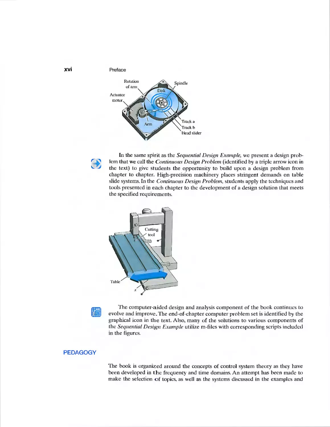
In the same spirit as the Sequential Design Example, we present a design
problem that we call the Continuous Design Problem (identified by a triple arrow icon in
the text) to give students the opportunity to build upon a design problem from
chapter to chapter. High-precision machinery places stringent demands on table
slide systems. In the Continuous Design Problem, students apply the techniques and
tools presented in each chapter to the development of a design solution that meets
the specified requirements.
The computer-aided design and analysis component of the book continues to
evolve and improve. The end-of-chapter computer problem set is identified by the
graphical icon in the text. Also, many of the solutions to various components of
the Sequential Design Example utilize m-files with corresponding scripts included
in the figures.
PEDAGOGY
The book is organized around the concepts of control system theory as they have
been developed in the frequency and time domains. An attempt has been made to
make the selection of topics, as well as the systems discussed in the examples and
Preface
XVII
problems, modern in the best sense. Therefore, this book includes discussions on
robust control systems and system sensitivity, state variable models, controllability
and observability, computer control systems, internal model control, robust PID
controllers, and computer-aided design and analysis, to name a few. However, the
classical topics of control theory that have proved to be so very useful in practice have
been retained and expanded.
Building Basic Principles: From Classical to Modern. Our goal is to present a clear
exposition of the basic principles of frequency- and time-domain design techniques.
The classical methods of control engineering are thoroughly covered: Laplace
transforms and transfer functions; root locus design; Routh-Hurwitz stability analysis;
frequency response methods, including Bode, Nyquist, and Nichols; steady-state
error for standard test signals; second-order system approximations; and phase and
gain margin and bandwidth. In addition, coverage of the state variable method is
significant. Fundamental notions of controllability and observability for state
variable models are discussed. Full state feedback design with Ackermann's formula for
pole placement is presented, along with a discussion on the limitations of state
variable feedback. Observers are introduced as a means to provide state estimates when
the complete state is not measured.
Upon this strong foundation of basic principles, the book provides many
opportunities to explore topics beyond the traditional. Advances in robust control theory
are introduced in Chapter 12. The implementation of digital computer control
systems is discussed in Chapter 13. Each chapter (but the first) introduces the student
to the notion of computer-aided design and analysis. The book concludes with an
extensive references section, divided by chapter, to guide the student to further
sources of information on control engineering.
Progressive Development of Problem-Solving Skills. Reading the chapters, attending
lectures and taking notes, and working through the illustrated examples are all part of
the learning process. But the real test comes at the end of the chapter with the
problems. The book takes the issue of problem solving seriously. In each chapter, there are
five problem types:
_l Exercises
J Problems
^1 Advanced Problems
3 Design Problems
-J Computer Problems
For example, the problem set for The Root Locus Method, Chapter 7 (see page
407) includes 27 exercises, 39 problems, 13 advanced problems, 13 design problems,
and 9 computer-based problems. The exercises permit the students to readily utilize
the concepts and methods introduced in each chapter by solving relatively
straightforward exercises before attempting the more complex problems. Answers to one-
third of the exercises are provided. The problems require an extension of the
concepts of the chapter to new situations. The advanced problems represent
problems of increasing complexity. The design problems emphasize the design task; the
xviii
Preface
computer-based problems give the student practice with problem solving using
computers. In total, the book contains more than 800 problems. Also, the MCS
website contains practice exercises that are instantly graded, so they provide quick
feedback for students. The abundance of problems of increasing complexity gives
students confidence in their problem-solving ability as they work their way from the
exercises to the design and computer-based problems. A complete instructor manual,
available for all adopters of the text for course use, contains complete solutions to
all end-of-chapter problems.
A set of m-files, the Modern Control Systems Toolbox, has been developed by
the authors to supplement the text. The m-files contain the scripts from each
computer-based example in the text. You may retrieve the m-files from Prentice Hall at
http://www.prenhall.com/dorf.
Design Emphasis without Compromising Basic Principles. The all-important topic
of design of real-world, complex control systems is a major theme throughout the
text. Emphasis on design for real-world applications addresses interest in design by
ABET and industry.
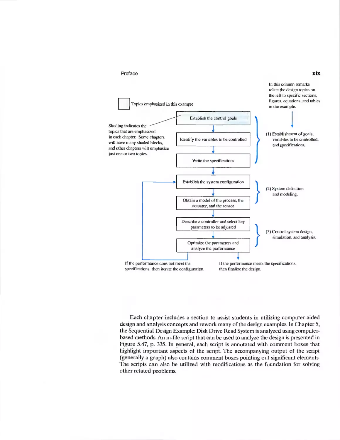
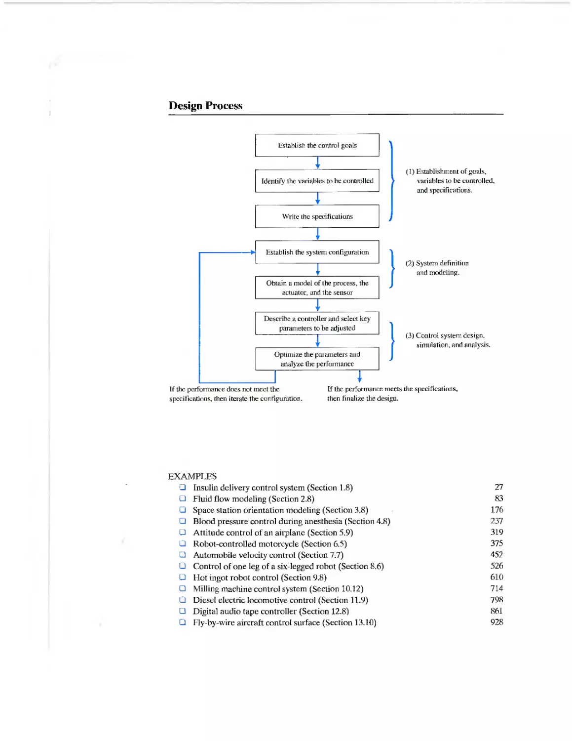
The design process consists of seven main building blocks which we arrange
into three groups:
1. Establishment of goals and variables to be controlled, and definition of
specifications (metrics) against which to measure performance
2. System definition and modeling
3. Control system design and integrated system simulation and analysis
In each chapter of this book, we highlight the connection between the design
process and the main topics of that chapter. The objective is to demonstrate
different aspects of the design process through illustrative examples. Various aspects of
the control system design process are illustrated in detail in the following examples:
G insulin delivery control system (Section 1.8, page 27)
G fluid flow modeling (Section 2.8, page 83)
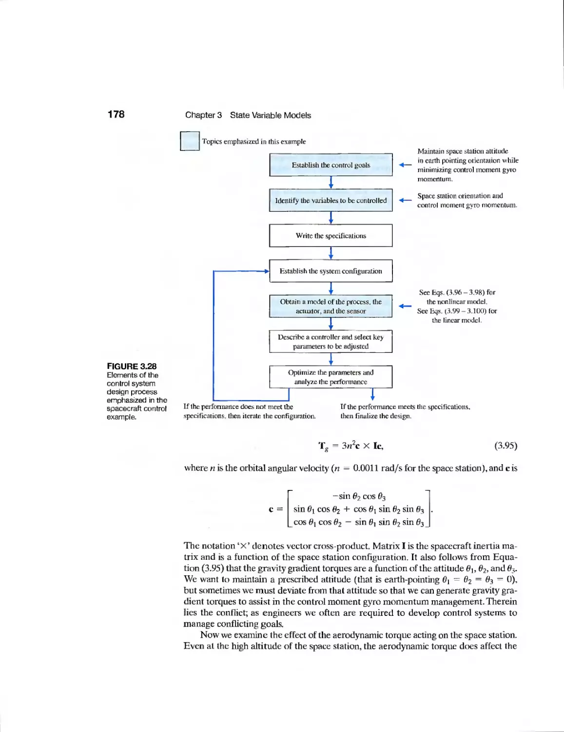
J space station orientation modeling (Section 3.8, page 176)
G blood pressure control during anesthesia (Section 4.8, page 237)
G attitude control of an airplane (Section 5.9,page 319)
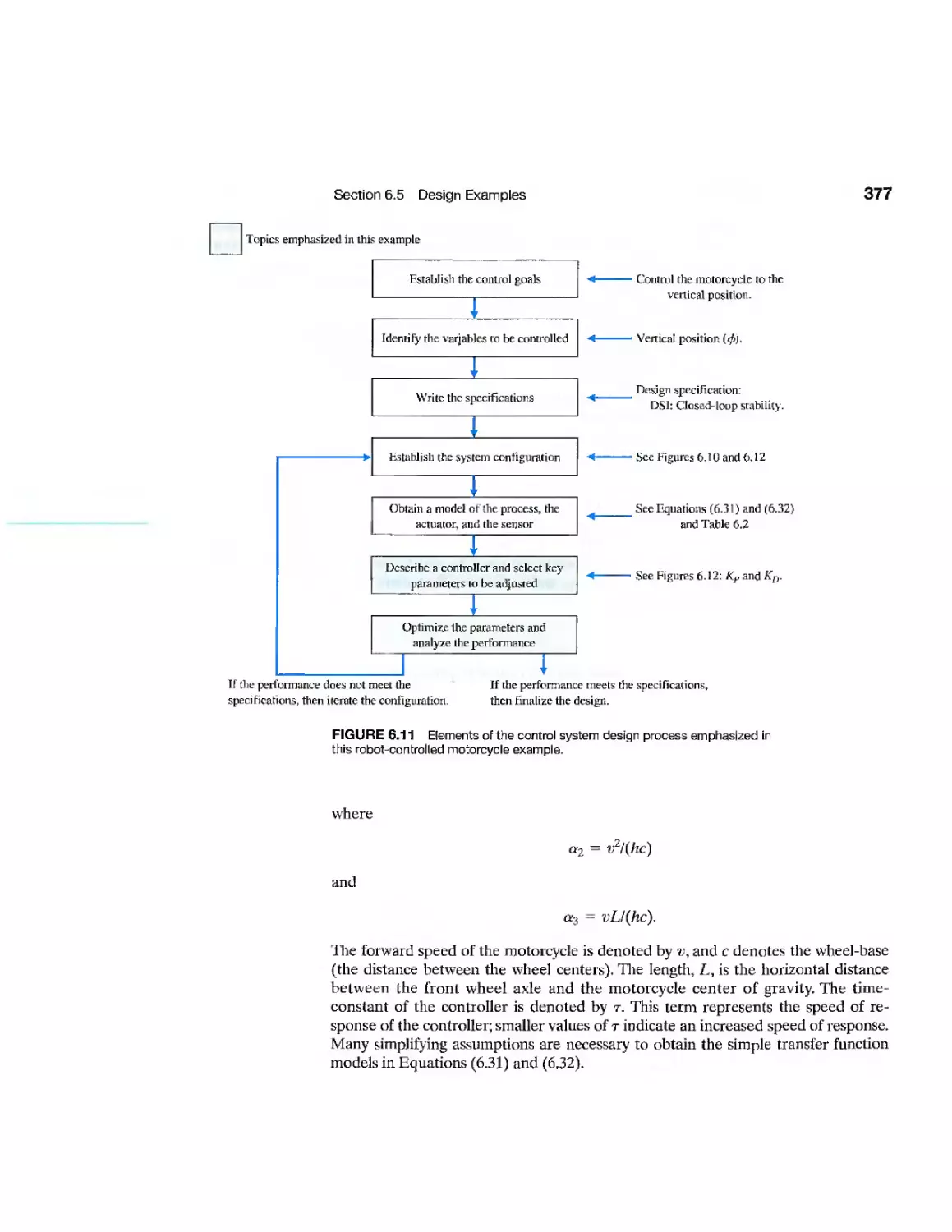
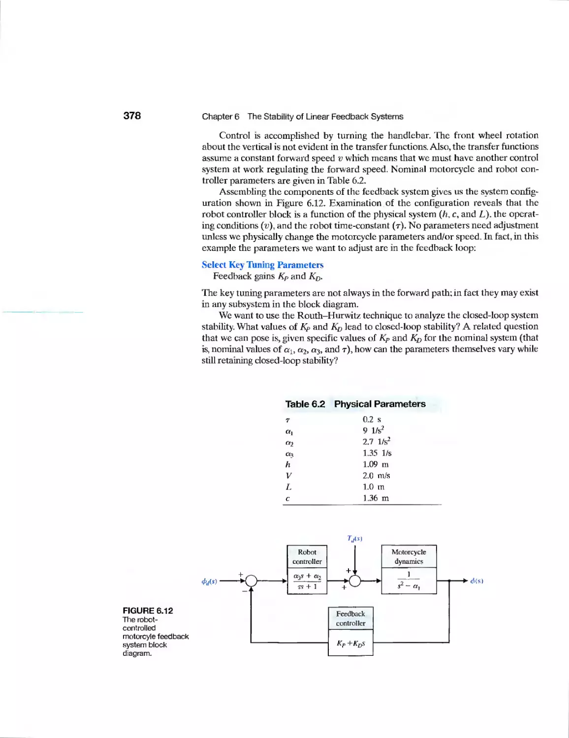
G robot-controlled motorcycle (Section 6.5, page 375)
G automobile velocity control (Section 7.7, page 452)
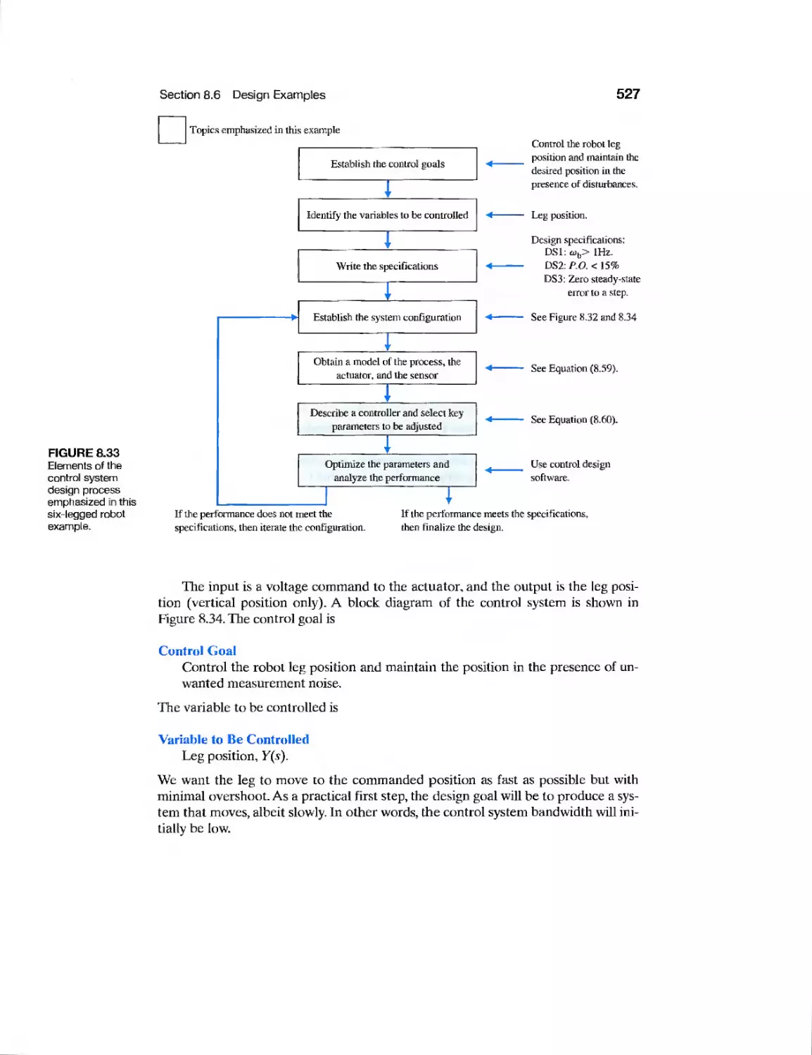
G control of one leg of a six-legged robot (Section 8.6, page 526)
G hot ingot robot control (Section 9.8,page 610)
G milling machine control system (Section 10.12, page 714)
G diesel electric locomotive control (Section 11.9, page 798)
U digital audio tape controller (Section 12.8. page 861)
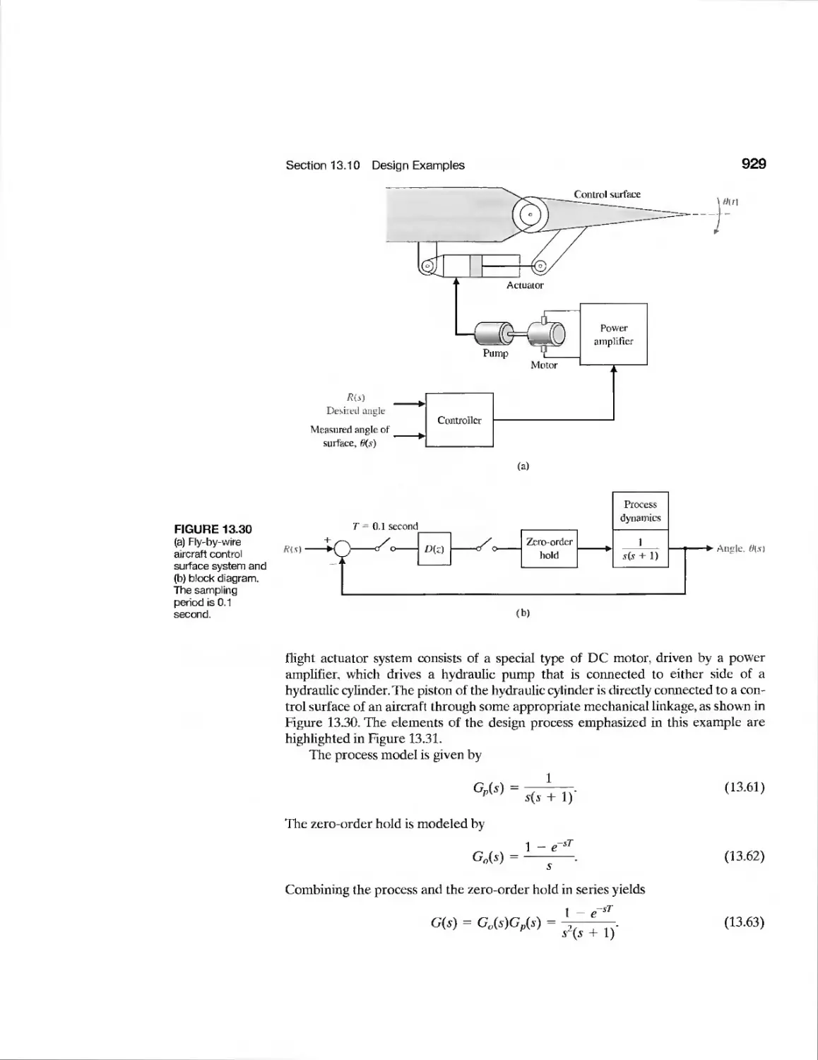
U fly-by-wire aircraft control surface (Section 13.10, page 928)
Preface
XIX
Topics emphasized in this example
Shading indicates the
topics that are emphasized
in each chapter. Some chapters
will have many shaded blocks,
and other chapters will emphasize
just one or two topics.
Establish the control goals
Identify the variables to be controlled
Write the specifications
In this column remarks
relate the design topics on
the left to specific sections,
figures, equations, and tables
in the example.
(1) Establishment oF goals,
variables to be controlled,
and specifications.
1
Obtain a model of the process, the
actuator, and the sensor
1
Describe a controller and select key
parameters to be adjusted
"
Optimize the parameters and
analyze the performance
i
}
}
(2) System definition
and modeling.
(3) Control system design,
simulation, and analysis.
If the performance does not meet the
specifications, then iterate the configuration.
[f the performance meets the specifications,
then finalize the design.
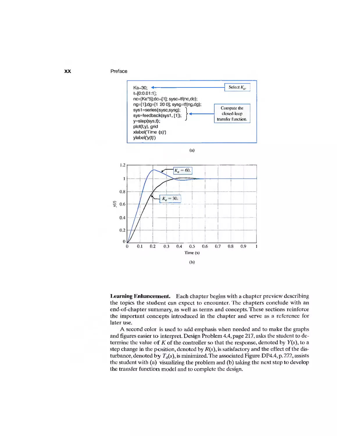
Each chapter includes a section to assist students in utilizing computer-aided
design and analysis concepts and rework many of the design examples. In Chapter 5,
the Sequential Design Example: Disk Drive Read System is analyzed using computer-
based methods. An m-file script that can be used to analyze the design is presented in
Figure 5.47, p. 335. In general, each script is annotated with comment boxes that
highlight important aspects of the script. The accompanying output of the script
(generally a graph) also contains comment boxes pointing out significant elements.
The scripts can also be utilized with modifications as the foundation for solving
other related problems.
XX
Preface
Ka=30; *
H0:0.01:1];
nc=[Ka*5];dc=[1]; sysc=tf(nc,dc);
ng=[1];dg=[1 20 0]; sysg=tf(ng,dg);
sysl =series(sysc,sysg);
sys=feed bac k(sysi, [1 ]);
y=slep(sys,t);
plot(t,y), grid
xlabel(Time (s)')
ylabel('y(tr)
Select K„.
Compute ihe
closed-loop
transfer function.
(a)
1
0.8
S 0.6
0.4
0.2
0
i /
^■^Cj
iS,
Ka = 60.
1
XT- i
// t
77 ■
H
i
K„ = 30.
i I
!
1 , i
I "' , "" ! " i"
I ; ; '
!
i
1 ' ' '
1
0 0.1 0.2 0.3 0.4 0.5 0.6 0.7 0.8 0.9 1
Time (s)
(b)
Learning Enhancement. Each chapter begins with a chapter preview describing
the topics the student can expect to encounter. The chapters conclude with an
end-of-chapter summary, as well as terms and concepts. These sections reinforce
the important concepts introduced in the chapter and serve as a reference for
later use.
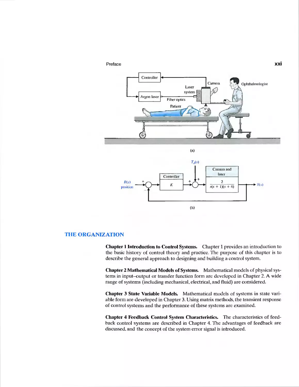
A second color is used to add emphasis when needed and to make the graphs
and figures easier to interpret. Design Problem 4.4, page 217, asks the student to
determine the value of K of the controller so that the response, denoted by Y{s), to a
step change in the position, denoted by R(s), is satisfactory and the effect of the
disturbance, denoted by Td(s), is minimized. The associated Figure DP4.4, p. 272, assists
the student with (a) visualizing the problem and (b) taking the next step to develop
the transfer function model and to complete the design.
Preface
xxi
Ophthalmologist
R(i)
position
*■ n.\)
(b)
THE ORGANIZATION
Chapter 1 Introduction to Control Systems. Chapter 1 provides an introduction to
the basic history of control theory and practice. The puipose of this chapter is to
describe the general approach to designing and building a control system.
Chapter 2 Mathematical Models of Systems. Mathematical models of physical
systems in input-output or transfer function form are developed in Chapter 2. A wide
range of systems (including mechanical, electrical, and fluid) are considered.
Chapter 3 State Variable Models. Mathematical models of systems in state
variable form are developed in Chapter 3. Using matrix methods, the transient response
of control systems and the performance of these systems are examined.
Chapter 4 Feedback Control System Characteristics. The characteristics of
feedback control systems are described in Chapter 4. The advantages of feedback are
discussed, and the concept of the system error signal is introduced.
Preface
Chapter 5 The Performance of Feedback Control Systems. In Chapter 5, the
performance of control systems is examined. The performance of a control system is
correlated with the s-plane location of the poles and zeros of the transfer function of
the system.
Chapter 6 The Stability of Linear Feedback Systems. The stability of feedback
systems is investigated in Chapter 6. The relationship of system stability to the
characteristic equation of the system transfer function is studied. The Routh-Hurwitz
stability criterion is introduced.
Chapter 7 The Root Locus Method. Chapter 7 deals with the motion of the
roots of the characteristic equation in the s-plane as one or two parameters are
varied. The locus of roots in the s-plane is determined by a graphical method. We also
introduce the popular PID controller.
Chapter 8 Frequency Response Methods. In Chapter 8. a steady-state sinusoid
input signal is utilized to examine the steady-state response of the system as the
frequency of the sinusoid is varied. The development of the frequency response plot,
called the Bode plot, is considered.
Chapter 9 Stability in the Frequency Domain. System stability utilizing frequency
response methods is investigated in Chapter 9. Relative stability and the Nyquist
criterion are discussed.
Chapter 10 The Design of Feedback Control Systems. Several approaches to
designing and compensating a control system are described and developed in Chapter
10. Various candidates for service as compensators are presented and it is shown
how they help to achieve improved performance.
Chapter 11 The Design of State Variable Feedback Systems. The main topic of
Chapter 11 is the design of control systems using state variable models. Full-state
feedback design and observer design methods based on pole placement are
discussed. Tests for controllability and observability are presented, and the concept of
an internal model design is discussed.
Chapter 12 Robust Control Systems. Chapter 12 deals with the design of highly
accurate control systems in the presence of significant uncertainty. Five methods for
robust design are discussed, including root locus, frequency response, ITAE
methods for robust PID controllers, internal models, and pseudo-quantitative feedback.
Chapter 13 Digital Control Systems. Methods for describing and analyzing the
performance of computer control systems are described in Chapter 13. The stability
and performance of sampled-data systems are discussed.
Appendixes. The appendixes are as follows:
A MATLAB Basics
B MathScript Basics
Preface xxiii
ACKNOWLEDGMENTS
We wish to express our sincere appreciation to the following individuals who have
assisted us with the development of this eleventh edition, as well as all previous
editions: Mahinoud A. Abdallah, Central Sate University (OH); John N. Chiasson,
University of Pittsburgh; Samy El-Sawah, California State Polytechnic University,
Pomona; Peter J. Gorder, Kansas State University; Duane Hanselman, University of
Maine; Ashok Iyer, University of Nevada, Las Vegas; Leslie R. Koval, University of
Missouri-Rolla; L. G. Kraft, University of New Hampshire; Thomas Kurfess,
Georgia Institute of Technology; Julio C. Mandojana, Mankato State University; Jure
Medanic, University of Illinois at Urbana-Champaign; Eduardo A. Misawa,
Oklahoma State University; Medhat M. Morcos, Kansas State University; Mark Nagurka,
Marquette University; Carla Schwartz, The MathWorks, Inc.; D. Subbaram Naidu,
Idaho State University; Ron Perez, University of Wisconsin-Milwaukee; Murat
Tanyel, Dordt College; Hal Tharp, University of Arizona; John Valasek,Texas A & M
University; Paul P. Wang, Duke University; and Ravi Warrier, GMI Engineering and
Management Institute.
OPEN LINES OF COMMUNICATION
The authors would like to establish a line of communication with the users of
Modern Control Systems. We encourage all readers to send comments and
suggestions for this and future editions. By doing this, we can keep you informed of any
general-interest news regarding the textbook and pass along interesting comments
of other users.
Keep in touch!
Richard C. Dorf
Robert H. Bishop
dorf@ece.ucdavis.edu
rhbishop@mail.utexas.edu
About the Authors
Richard C. Dorf is a Professor of Electrical and Computer Engineering at the
University of California, Davis. Known as an instructor who is highly concerned with
the discipline of electrical engineering and its application to social and economic
needs, Professor Dorf has written and edited several successful engineering
textbooks and handbooks, including the best selling Engineering Handbook, second
edition and the third edition of the Electrical Engineering Handbook. Professor
Dorf is also co-author of Technology Ventures, a leading textbook on technology
entrepreneurship. Professor Dorf is a Fellow of the IEEE and a Fellow of the
ASEE. He is active in the fields of control system design and robotics. Dr. Dorf
holds a patent for the PIDA controller.
Robert H. Bishop is the Chairman of the Department of Aerospace Engineering
and Engineering Mechanics at The University of Texas at Austin. He holds the Joe J.
King Professorship and in 2002 was inducted into the UT Academy of
Distinguished Teachers. A talented educator, Professor Bishop has been recognized for his
contributions in the classroom with the coveted Lockheed Martin Tactical Aircraft
Systems Award for Excellence in Engineering Teaching. He received the John Leland
Atwood Award from the American Society of Engineering Educators and the
American Institute of Aeronautics and Astronautics, which is periodically given to
"a leader who has made lasting and significant contributions to aerospace
engineering education." Professor Bishop is a Fellow of AIAA and is active in the IEEE and
ASEE. He is a distinguished researcher with an interest in guidance, navigation, and
control of aerospace vehicles.
XXV
CHAPTER
Introduction to Control
1
Systems
1.1
1.2
1.3
1.4
1.5
1.6
1.7
1.8
1.9
1.10
Introduction 2
Brief History of Automatic Control 4
Examples of Control Systems 8
Engineering Design 16
Control System Design 17
Mechatronic Systems 20
The Future Evolution of Controi Systems 24
Design Examples 25
Sequential Design Example: Disk Drive Read System 28
Summary 30
PREVIEW
In this chapter, we discuss open- and closed-loop feedback control systems. A
control system consists of interconnected components to achieve a desired purpose. We
examine examples of control systems through the course of history. These early
systems incorporated many of the same ideas of feedback that are employed in modem
manufacturing processes, alternative energy, complex hybrid automobiles, and
sophisticated robots. A design process is presented that encompasses the
establishment of goals and variables to be controlled, definition of specifications, system
definition, modeling, and analysis. The iterative nature of design allows us to handle
the design gap effectively while accomplishing necessary trade-offs in complexity,
performance, and cost. Finally, we introduce the Sequential Design Example: Disk
Drive Read System. This example will be considered sequentially in each chapter of
this book. It represents a very important and practical control system design problem
while simultaneously serving as a useful learning tool.
DESIRED OUTCOMES
Upon completion of Chapter 1, students should:
□ Possess a basic understanding of control system engineering and be able to offer
some illustrative examples and their relationship to key contemporary issues.
11 Be able to recount a brief history of control systems and their role in society.
Q Be capable of discussing the future of controls in the context of their
evolutionary pathways.
3 Recognize the elements of control system design and possess an appreciation of
controls in the context of engineering design.
1
2 Chapter 1 Introduction to Control Systems
1.1 INTRODUCTION
Engineering is concerned with understanding and controlling the materials and
forces of nature foT the benefit of humankind. Control system engineers are
concerned with understanding and controlling segments of their environment, often
called systems, to provide useful economic products for society. The twin goals of
understanding and controlling are complementary because effective systems
control requires that the systems be understood and modeled. Furthermore, control
engineering must often consider the control of poorly understood systems such as
chemical process systems. The present challenge to control engineers is the
modeling and control of modern, complex, interrelated systems such as traffic control
systems, chemical processes, and robotic systems. Simultaneously, the fortunate
engineer has the opportunity to control many useful and interesting industrial
automation systems. Perhaps the most characteristic quality of control engineering is
the opportunity to control machines and industrial and economic processes for the
benefit of society.
Control engineering is based on the foundations of feedback theory and linear
system analysis, and it integrates the concepts of network theory and
communication theory. Therefore control engineering is not limited to any engineering
discipline but is equally applicable to aeronautical, chemical, mechanical, environmental,
civil, and electrical engineering. For example, a control system often includes
electrical, mechanical, and chemical components. Furthermore, as the understanding of
the dynamics of business, social, and political systems increases, the ability to control
these systems will also increase.
A control system is an interconnection of components forming a system
configuration that will provide a desired system response. The basis for analysis of a system
is the foundation provided by linear system theory, which assumes a cause-effect
relationship for the components of a system. Therefore a component or process to be
controlled can be represented by a block, as shown in Figure 1.1. The input-output
relationship represents the cause-and-effect relationship of the process, which in turn
represents a processing of the input signal to provide an output signal variable, often
with a power amplification. An open-loop control system uses a controller and an
actuator to obtain the desired response, as shown in Figure 1.2. An open-loop system is
a system without feedback.
An open-loop control system utilizes an actuating device to control the process
directly without using feedback.
FIGURE 1.1
Process to be
controlled.
Input■
Process
-+• Output
FIGURE 1.2
Open-loop control
system (without
feedback).
Desired output
response
Controller
Actuator
Process
Output
Section 1.1 Introduction
3
FIGURE 1.3
Closed-loop
feedback control
system (with
feedback).
Desired output
response
-<
-^ Error
i _
Controller
Measurement output
Actuator
Sensor
Process
Feedback
Actual
output
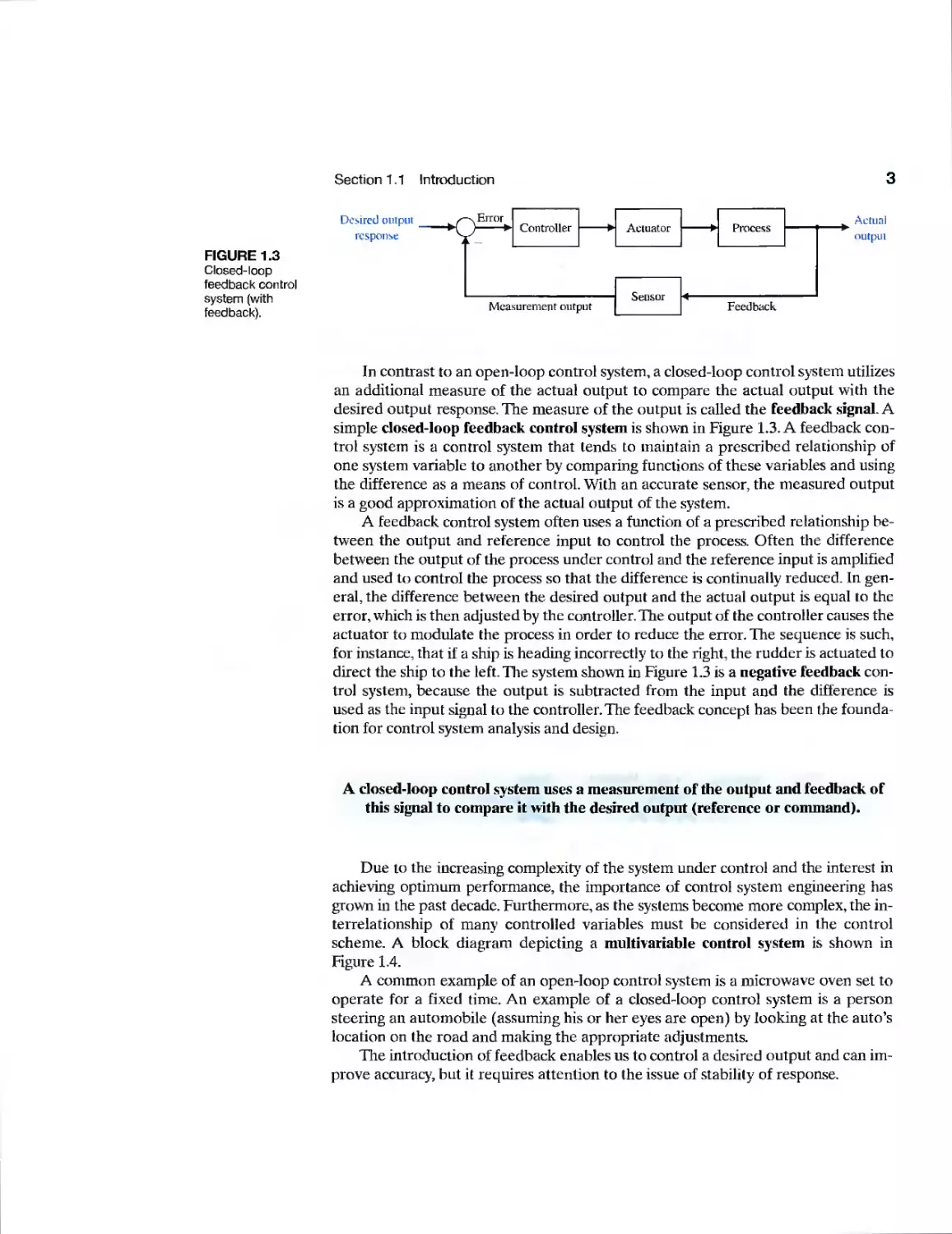
In contrast to an open-loop control system, a closed-loop control system utilizes
an additional measure of the actual output to compare the actual output with the
desired output response. The measure of the output is called the feedback signal. A
simple closed-loop feedback control system is shown in Figure 1.3. A feedback
control system is a control system that tends to maintain a prescribed relationship of
one system variable to another by comparing functions of these variables and using
the difference as a means of control. With an accurate sensor, the measured output
is a good approximation of the actual output of the system.
A feedback control system often uses a function of a prescribed relationship
between the output and reference input to control the process. Often the difference
between the output of the process under control and the reference input is amplified
and used to control the process so that the difference is continually reduced. In
general, the difference between the desired output and the actual output is equal to the
error, which is then adjusted by the controller. The output of the controller causes the
actuator to modulate the process in order to reduce the error. The sequence is such,
for instance, that if a ship is heading incorrectly to the right, the rudder is actuated to
direct the ship to the left. The system shown in Figure 1.3 is a negative feedback
control system, because the output is subtracted from the input and the difference is
used as the input signal to the controller.The feedback concept has been the
foundation for control system analysis and design.
A closed-loop control system uses a measurement of the output and feedback of
this signal to compare it with the desired output (reference or command).
Due to the increasing complexity of the system under control and the interest in
achieving optimum performance, the importance of control system engineering has
grown in the past decade. Furthermore, as the systems become more complex, the
interrelationship of many controlled variables must be considered in the control
scheme. A block diagram depicting a multivariable control system is shown in
Figure 1.4.
A common example of an open-loop control system is a microwave oven set to
operate for a fixed time. An example of a closed-loop control system is a person
steering an automobile (assuming his or her eyes are open) by looking at the auto's
location on the road and making the appropriate adjustments.
The introduction of feedback enables us to control a desired output and can
improve accuracy, but it requires attention to the issue of stability of response.
4
Chapter 1 Introduction to Control Systems
Uesired *
respond ^
Comparison
. . M .
.
Error
Controller
Measurement output
Actuator
Sensor
Process
Feedback
Actual
output
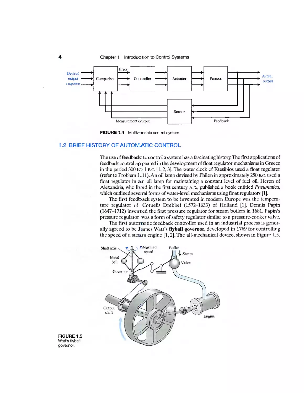
FIGURE 1.4 Multivariable control system.
1.2 BRIEF HISTORY OF AUTOMATIC CONTROL
The use of feedback to control a system has a fascinating history. The first applications of
feedback control appeared in the development of float regulator mechanisms in Greece
in the period 300 to 1 b.c. [1,2,3], The water clock of Ktesibios used a float regulator
(refer to Problem 1.11). An oil lamp devised by Philon in approximately 250 B.c. used a
float regulator in an oil lamp for maintaining a constant level of fuel oil. Heron of
Alexandria, who lived in the first century a.d., published a book entitled Pneumatica,
which outlined several forms of water-level mechanisms using float regulators [1].
The first feedback system to be invented in modern Europe was the
temperature regulator of Cornelis Drebbel (1572 1633) of Holland [1]. Dennis Papin
(1647-1712) invented the first pressure regulator for steam boilers in 1681. Papin's
pressure regulator was a form of safety regulator similar to a pressure-cooker valve.
The first automatic feedback controller used in an industrial process is
generally agreed to be James Watt's flyball governor, developed in 1769 for controlling
the speed of a steam engine [1,2]. The all-mechanical device, shown in Figure 1.5,
FIGURE 1.5
Watt's flyball
governor.
Shaft axis
Metal
ball
Measured
Boiler
Output
shaft
Engine
FIGURE 1.6
Water-level float
regulator.
Section 1.2 Brief History of Automatic Control
Water
Float
Valve
measured the speed of the output shaft and utilized the movement of the flyball to
control the steam valve and therefore the amounl of steam entering the engine. As
depicted in Figure 1.5, the governor shaft axis is connected via mechanical
linkages and beveled gears to the output shaft of the steam engine. As the steam
engine output shaft speed increases, the ball weights rise and move away from the
shaft axis and through mechanical linkages the steam valve closes and the engine
slows down.
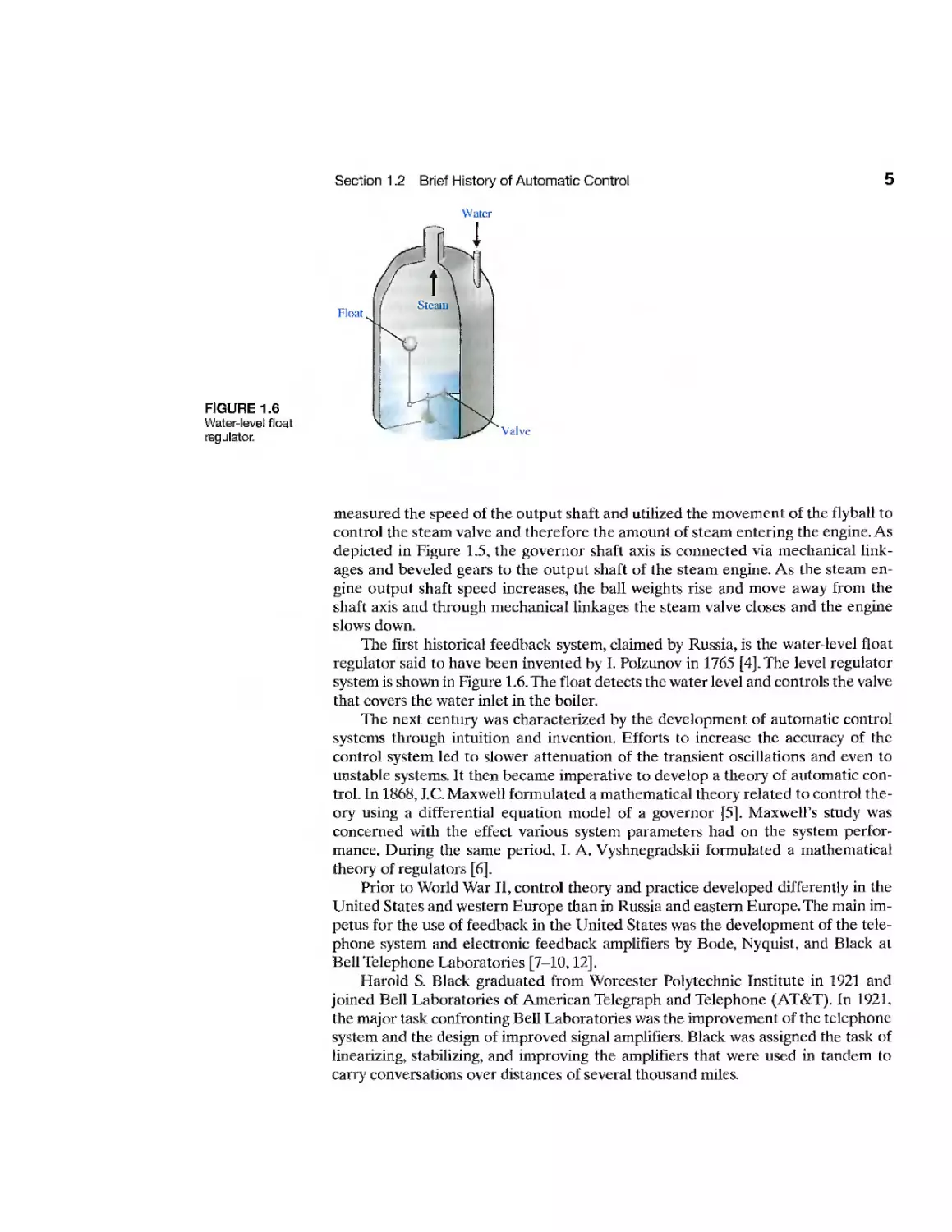
The first historical feedback system, claimed by Russia, is the water-level float
regulator said to have been invented by I. Polzunov in 1765 [4]. The level regulator
system is shown in Figure 1.6. The float detects the water level and controls the valve
that covers the water inlet in the boiler.
The next century was characterized by the development of automatic control
systems through intuition and invention. Efforts to increase the accuracy of the
control system led to slower attenuation of the transient oscillations and even to
unstable systems. It then became imperative to develop a theory of automatic
control. In 1868, J.C. Maxwell formulated a mathematical theory related to control
theory using a differential equation model of a governor [5]. Maxwell's study was
concerned with the effect various system parameters had on the system
performance. During the same period, I. A. Vyshnegradskii formulated a mathematical
theory of regulators [6].
Prior to World War II, control theory and practice developed differently in the
United States and western Europe than in Russia and eastern Europe. The main
impetus for the use of feedback in the United States was the development of the
telephone system and electronic feedback amplifiers by Bode, Nyquist, and Black at
Bell Telephone Laboratories [7-10,12].
Harold S. Black graduated from Worcester Polytechnic Institute in 1921 and
joined Bell Laboratories of American Telegraph and Telephone (AT&T). In 1921,
the major task confronting Bell Laboratories was the improvement of the telephone
system and the design of improved signal amplifiers. Black was assigned the task of
linearizing, stabilizing, and improving the amplifiers that were used in tandem to
carry conversations over distances of several thousand miles.
6
Chapter 1 Introduction to Control Systems
Black reports [8]:
Then came the morning or Tuesday, August 2,1927, when the concept of the negative
feedback amplifier came to me in a flash while J was crossing the Hudsun River on the
Lackawanna Ferry, on my way to work. For more than 50 years I have pondered how
and why the idea came, and I can't say any more today than I could that morning. All I
know is that after several years of hard work on the problem. I suddenly realized that if
I fed the amplifier output back to the input, in reverse phase, and kept the device from
oscillating (singing, as we called it then), I would have exactly what I wanted: a means
of canceling out the distortion in the output. I opened my morning newspaper and on a
page of The New York Times I sketched a simple canonical diagram of a negative
feedback amplifier plus the equations for the amplification with feedback-1 signed the
sketch, and 20 mi nutes later, when I reached the laboratory at 463 West Street, it was
witnessed, understood, and signed by the late Earl C. Blessing.
I envisioned this circuit as leading to extremely linear amplifiers (40 to 50 dB of
negative feedback), but an important question is: How did I know I could avoid self-
oscillations over very wide frequency bands when many people doubted such circuits
would be stable? My confidence stemmed from work that I had done two years earlier
on certain novel oscillator circuits and three years earlier in designing the terminal
circuits, including the filters, and developing the mathematics for a carrier telephone system
for short toll circuits.
The frequency domain was used primarily to describe the operation of the
feedback amplifiers in terms of bandwidth and other frequency variables. In contrast,
the eminent mathematicians and applied mechanicians in the former Soviet Union
inspired and dominated the field of control theory. Therefore, the Russian theory
tended to utilize a time-domain formulation using differential equations.
The control of an industrial process (manufacturing, production, and so on) by
automatic rather than manual means is often called automation. Automation is
prevalent in the chemical, electric power, paper, automobile, and steel industries,
among others. The concept of automation is central to our industrial society.
Automatic machines are used to increase the production of a plant per worker in order to
offset rising wages and inflationary costs. Thus industries are concerned with the
productivity per worker of their plants. Productivity is defined as the ratio of
physical output to physical input [26]. In this case, we are referring to labor productivity,
which is real output per hour of work.
The transformation of the U.S. labor force in the country's brief history follows
the progressive mechanization of work that attended the evolution of the agrarian
republic into an ind ustrial world power. In 1820, more than 70 percent of the labor
force worked on the farm. By 1900, less than 40 percent were engaged in agriculture.
Today, less than 5 percent works in agriculture [15].
In 1925, some 588.000 people—about 1.3 percent of the nation's labor force—
were needed to mine 520 million tons of bituminous coal and lignite, almost all of it
from underground. By 1980, production was up to 774 million tons, but the work
force had been reduced to 208.000. Furthermore, only 136.000 of that number were
employed in underground mining operations. The highly mechanized and highly
productive surface mines, with just 72,000 workers, produced 482 million tons, or 62
percent of the total [27].
A large impetus to the theory and practice of automatic control occurred during
World War II when it became necessary to design and construct automatic airplane
Section 1.2 Brief History of Automatic Control
7
piloting, gun-positioning systems, radar antenna control systems, and other military
systems based on the feedback control approach. The complexity and expected
performance of these military systems necessitated an extension of the available
control techniques and fostered interest in control systems and the development of new
insights and methods. Prior to 1940, for most cases, the design of control systems was
an art involving a trial-and-error approach. During the 1940s, mathematical and an
alytical methods increased in number and utility, and control engineering became an
engineering discipline in its own right [10-12].
Another example of the discovery of an engineering solution to a control system
problem was the creation of a gun director by David B. Parkinson of Bell Telephone
Laboratories. In the spring of 1940, Parkinson was a 29-year-old engineer intent on
improving the automatic level recorder, an instrument that used strip-chart paper to
plot the record of a voltage. A critical component was a small potentiometer used to
control the pen of the recorder through an actuator.
Parkinson had a dream about an antiaircraft gun that was successfully felling
airplanes. Parkinson described the situation [13]:
After three or four shots one of the men in the crew smiled at me and beckoned me to
come closer to the gun. When I drew near he pointed to the exposed end of the left
trunnion. Mounted there was the control potentiometer of my level recorder!
The next morning Parkinson realized the significance of his dream:
If my potentiometer couLd control the pen on the recorder, something similar could,
with suitable engineering, control an antiaircraft gun.
After considerable effort, an engineering model was delivered for testing to the
U.S. Army on December 1, 1941. Production models were available by early 1943,
and eventually 3000 gun controllers were delivered. Input to the controller was
provided by radar, and the gun was aimed by taking the data of the airplane's present
position and calculating the target's future position.
Frequency-domain techniques continued to dominate the field of control
following World War II with the increased use of the Laplace transform and the complex
frequency plane. During the 1950s, the emphasis in control engineering theory was on the
development and use of the s-plane methods and, particularly, the root locus
approach. Furthermore, during the 1980s, the use of digital computers for control
components became routine. The technology of these new control elements to perform
accurate and rapid calculations was formerly unavailable to control engineers. There
are now over 400,000 digital process control computers installed in the United States
[14, 27]. These computers are employed especially for process control systems in
which many variables are measured and controlled simultaneously by the computer.
With the advent of Sputnik and the space age, another new impetus was
imparted to control engineering. It became necessary to design complex, highly accurate
control systems for missiles and space probes. Furthermore, the necessity to
minimize the weight of satellites and to control them very accurately has spawned the
important field of optimal control. Due to these requirements, the time-domain
methods developed by Liapunov,Minorsky, and others have been met with great
interest in the last two decades. Recent theories of optimal control developed by L. S.
Pontryagin in the former Soviet Union and R. Bellman in the United States, as well
Chapter 1 Introduction to Control Systems
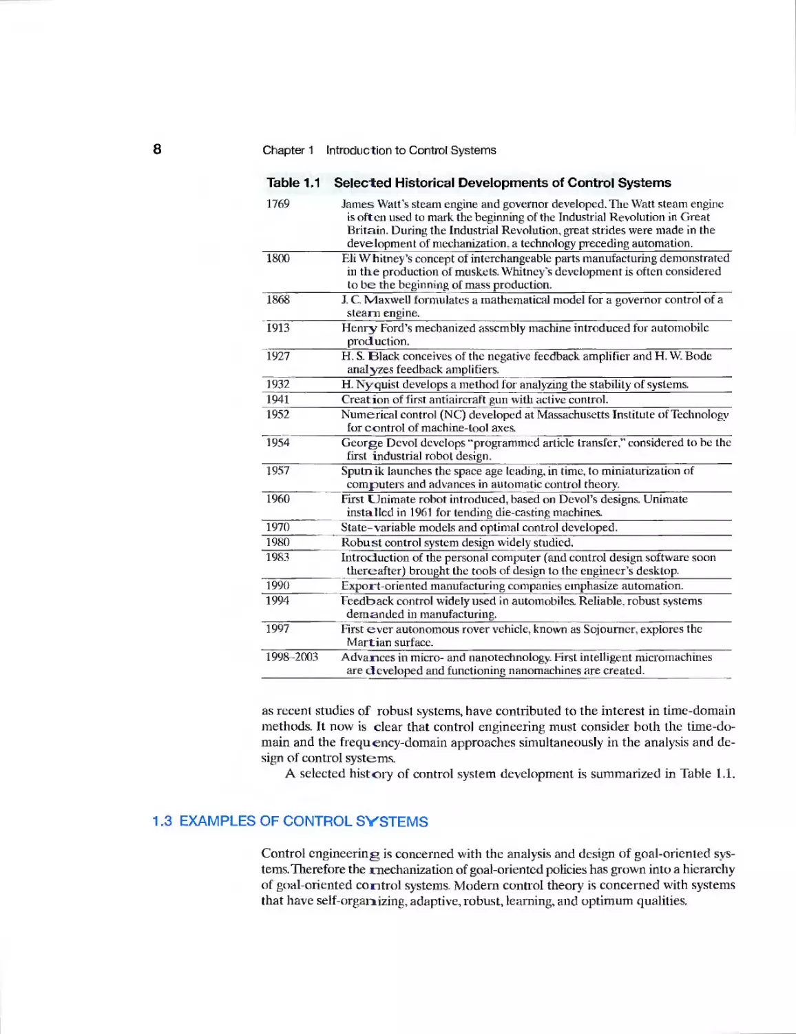
Table 1.1 Selected Historical Developments of Control Systems
1769 James Watt's steam engine and governor developed. The Watt steam engine
is often used to mark the beginning of the Industrial Revolution in Great
Britain. During the Industrial Revolution, great strides were made in the
development of mechanization, a technology preceding automation.
1800 Eli Whitney's concept of interchangeable parts manufacturing demonstrated
in the production of muskets. Whitney's development is often considered
to be the beginning of mass production.
1868 IC. Maxwell formulates a mathematical model for a governor control of a
steam engine.
1913 Henry Ford's mechanized assembly machine introduced for automobile
production.
1927 H. S. Black conceives of the negative feedback amplifier and H. W. Bode
analyzes feedback amplifiers.
1932 H. Nyquist develops a method for analyzing the stability of systems.
1941 Creation of first antiaircraft gun with active control.
1952 Numerical control (NC) developed at Massachusetts Institute of Technology
for control of machine-tool axes.
1954 George Devol develops "programmed article transfer," considered to be the
first industrial robot design.
1957 Sputnik launches the space age leading, in time, to miniaturization of
computers and advances in automatic control theory.
1960 First Unimate robot introduced, based on Devol's designs. Unimate
installed in 1961 for tending die-casting machines.
1970 State-variable models and optimal control developed.
1980 Robust control system design widely studied.
1983 Introduction of the personal computer (and control design software soon
thereafter) brought the tools of design to the engineer's desktop.
1990 Export-oriented manufacturing companies emphasize automation.
1994 Feedback control widely used in automobiles. Reliable, robust systems
demanded in manufacturing.
1997 First ever autonomous rover vehicle, known as Sojourner, explores the
Martian surface.
1998-2003 Advances in micro- and nanotechnology. First intelligent micromachines
are developed and functioning nanomachines are created.
as recent studies of robust systems, have contributed to the interest in time-domain
methods. It now is clear that control engineering must consider both the
time-domain and the frequency-domain approaches simultaneously in the analysis and
design of control systems.
A selected history of control system development is summarized in Table 1.1.
1.3 EXAMPLES OF CONTROL SYSTEMS
Control engineering is concerned with the analysis and design of goal-oriented
systems. Therefore the mechanization of goal-oriented policies has grown into a hierarchy
of goal-oriented control systems. Modern control theory is concerned with systems
that have self-organizing, adaptive, robust, learning, and optimum qualities.
Section 1.3 Examples of Control Systems
9
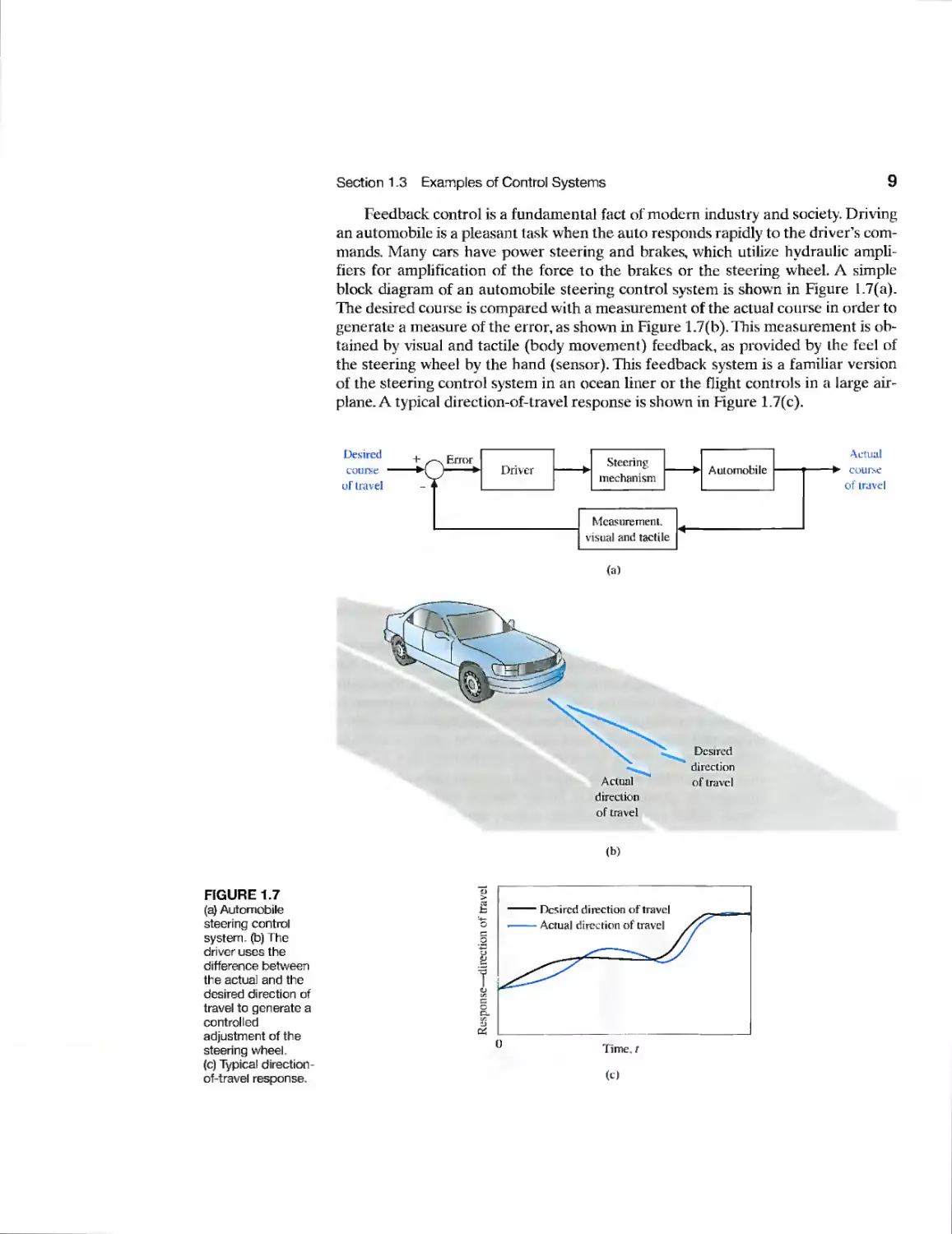
Feedback control is a fundamental fact of modern industry and society. Driving
an automobile is a pleasant task when the auto responds rapidly to the driver's
commands. Many cars have power steering and brakes, which utilize hydraulic
amplifiers for amplification of the force to the brakes or the steering wheel. A simple
block diagram of an automobile steering control system is shown in Figure 1.7(a).
The desired course is compared with a measurement of the actual course in order to
generate a measure of the error, as shown in Figure 1.7(b).This measurement is
obtained by visual and tactile (body movement) feedback, as provided by the feel of
the steering wheel by the hand (sensor). This feedback system is a familiar version
of the steering control system in an ocean liner or the flight controls in a large
airplane. A typical direction-of-travel response is shown in Figure 1.7(c).
-^ Error
i
Driver
Steering
mechanism
Measurement.
visual and tactile
Automobile
Actual
>- course
of travel
(a)
Actual
direction
of travel
Desired
direction
of travel
(b)
FIGURE 1.7
(a) Automobile
steering control
system, (b) The
driver uses the
difference between
the actual and the
desired direction of
travel to generate a
controlled
adjustment of the
steering wheel,
(c) Typical direction-
of-travel response.
■ Desired direction of travel
- Actual direction of travel
Time, t
(O
10 Chapter 1 Introduction to Control Systems
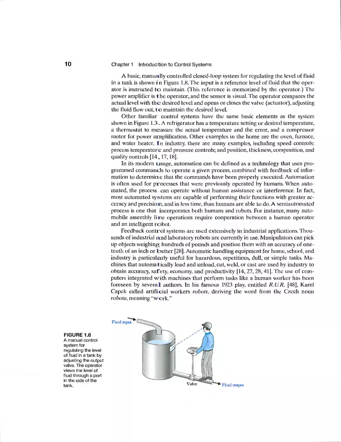
A basic, manually controlled closed-loop system for regulating the level of fluid
in a tank is shown in Figure 1.8. The input is a reference level of fluid that the
operator is instructed to maintain. (This reference is memorized by the operator.) The
power amplifier is the operator, and the sensor is visual. The operator compares the
actual level with the desired level and opens or closes the valve (actuator), adjusting
the fluid flow out, to maintain the desired level.
Other familiar control systems have the same basic elements as the system
shown in Figure 1.3. A refrigerator has a temperature setting or desired temperature,
a thermostat to measure the actual temperature and the error, and a compressor
motor for power amplification. Other examples in the home are the oven, furnace,
and water heater. In industry, there are many examples, including speed controls:
process temperature and pressure controls; and position, thickness, composition, and
quality controls [14,17,18].
In its modem usage, automation can be defined as a technology that uses
programmed commands to operate a given process, combined with feedback of
information to determine that the commands have been properly executed. Automation
is often used for processes that were previously operated by humans. When
automated, the process can operate without human assistance or interference. In fact,
most automated systems are capable of performing their functions with greater
accuracy and precision, and in less time, than humans are able to do. A semiautomatcd
process is one that incorporates both humans and robots. For instance, many
automobile assembly line operations require cooperation between a human operator
and an intelligent robot.
Feedback control systems are used extensively in industrial applications.
Thousands of industrial and laboratory robots are currently in use. Manipulators can pick
up objects weighing hundreds of pounds and position them with an accuracy of one-
tenth of an inch or better [28]. Automatic handling equipment for home, school, and
industry is particularly useful for hazardous, repetitious, dull, or simple tasks.
Machines that automatically load and unload, cut, weld, or cast are used by industry to
obtain accuracy, safety, economy, and productivity [14,27,28,41]. The use of
computers integrated with machines that perform tasks like a human worker has been
foreseen by several authors. In his famous 1923 play, entitled R. U.R. [48], Karel
Capek called artificial workers robots, deriving the word from the Czech noun
robota, meaning "w^ork."
Flu ill input
FIGURE 1.8
A manual control
system for
regulating the level
of fluid in a tank by
adjusting the output
valve. The operator
views the level of
fluid through a port
in the side of the
tank.
Section 1.3 Examples of Control Systems
11
r
i
FIGURE 1.9
The Honda P3
humanoid robot. P3
walks, ciimbs stairs,
and turns corners.
Photo courtesy of
American Honda
Motor, Inc.
A robot is a computer-controlled machine and involves technology closely
associated with automation. Industrial robotics can be defined as a particular field of
automation in which the automated machine (that is, the robot) is designed to substitute
for human labor [18, 27, 33]. Thus robots possess certain humanlike characteristics.
Today, the most common humanlike characteristic is a mechanical manipulator that is
patterned somewhat after the human arm and wrist. Some devices even have
anthropomorphic mechanisms, including what we might recognize as mechanical arms,
wrists, and hands [14.27,28J. An example of an anthropomorphic robot is shown in
Rgure 1.9. We recognize that the automatic machine is well suited to some tasks, as
noted in Table 1.2, and that other tasks are best carried out by humans.
Another very important application of control technology is in the control of the
modern automobile [19, 20]. Control systems for suspension, steering, and engine
Table 1.2 Task Difficulty: Human Versus Automatic Machine
Tasks Difficult for a Machine Tasks Difficult for a Human
Inspect seedlings in a nursery.
Drive a vehicle through rugged terrain.
Identify the most expensive jewels on
a tray of jewels.
Inspect a system in a hot, toxic
environment.
Repetitively assemble a clock.
Land an airliner at night, in bad weather.
Chapter 1 Introduction to Control Systems
control have been introduced. Many new autos have a four-wheel-steering system, as
well as an antiskid control system.
A three-axis control system for inspecting individual semiconductor wafers is
shown in Figure 1.] 0. This system uses a specific motor to drive each axis to the
desired position in the x-y-z-axis, respectively. The goal is to achieve smooth, accurate
movement in each axis. This control system is an important one for the semiconductor
manufacturing industry.
There has been considerable discussion recently concerning the gap between
practice and theory in control engineering. However, it is natural that theory
precedes the applications in many fields of control engineering. Nonetheless, it is
interesting to note that in the electric power industry, the largest industry in the
United States, the gap is relatively insignificant. The electric power industry is
primarily interested in energy conversion, control, and distribution. It is critical that
computer control be increasingly applied to the power industry in order to improve
the efficient use of energy resources. Also, the control of power plants for minimum
waste emission has become increasingly important. The modern, large-capacity
plants, which exceed several hundred megawatts, require automatic control
systems that account for the interrelationship of the process variables and optimum
power production. It is common to have 90 or more manipulated variables under
v-a\is motor
FIGURE 1.10 A three-axis control system for inspecting individual semiconductor wafers with a
highly sensitive camera.
Section 1.3 Examples of Control Systems
13
coordinated control. A simplified model showing several of the important control
variables of a large boiler generator system is shown in Figure 1.11. This is an
example of the importance of measuring many variables, such as pressure and
oxygen, to provide information to the computer for control calculations.
The electric power industry has used the modern aspects of control engineering
for significant and interesting applications. It appears that in the process industry,
the factor that maintains the applications gap is the lack of instrumentation to
measure all the important process variables, including the quality and composition of
the product. As these instruments become available, the applications of modern
control theory to industrial systems should increase measurably.
Another important industry, the metallurgical industry, has had considerable
success in automatically controlling its processes. In fact, in many cases, the control
theory is being fully implemented. For example, a hot-strip steel mill, which involves
a $100-million investment, is controlled for temperature, strip width, thickness, and
quality.
Rapidly rising energy costs coupled with threats of energy curtailment are
resulting in new efforts for efficient automatic energy management. Computer
controls are used to control energy use in industry and to stabilize and connect loads
evenly to gain fuel economy.
There has been considerable interest recently in applying the feedback control
concepts to automatic warehousing and inventory control. Furthermore, automatic
control of agricultural systems (farms) is receiving increased interest. Automatically
controlled silos and tractors have been developed and tested. Automatic control of
FIGURE 1.11
Coordinated control
system for a
boiler-generator.
Feed
water
Fuel ■
Valve
•age
Air'
Valve
Valve
Boiler
Turbine
<K
Oxygen
measurement
r*"~L
Computer
ffW
Desired temperature,
pressure. 02. generation
Shaft
Temperature
measurement
Generator
Actual
generation
Speed
governor
Pressure
measurement
14
Chapter 1 Introduction to Control Systems
wind turbine generators, solar heating and cooling, and automobile engine
performance are important modern examples [20.21].
Also, there have been many applications of control system theory to biomedical
experimentation, diagnosis, prosthetics, and biological control systems [22,23, 51].
The control systems under consideration range from the cellular level to the central
nervous system and include temperature regulation and neurological, respiratory,
and cardiovascular control. Most physiological control systems are closed-loop
systems. However, we find not one controller but rather control loop within control
loop, forming a hierarchy of systems. The modeling of the structure of biological
processes confronts the analyst with a high-order model and a complex structure.
Prosthetic devices that aid the 46 million handicapped individuals in the United
States are designed to provide automatically controlled aids to the disabled [22,27,42].
The robotic hand shown in Figure 1.12 belongs to Obrero, a humanoid robot
developed at MIT that is capable of sensitive manipulation. The Obrero robot is
responsive to the properties of the object it holds and does not rely on vision as the main
sensor. The hand has position and force control of the fingers employing very
sensitive tactile sensors and series elastic actuators in its joints.
Finally, it has become interesting and valuable to attempt to model the feedback
processes prevalent in the social, economic, and political spheres. This approach is
undeveloped at present but appears to have a reasonable future. Society, of course,
is composed of many feedback systems and regulatory bodies, such as the Federal
Reserve Board, whrich are controllers exerting the forces on society necessary to
maintain a desired output. A simple lumped model of the national income feedback
control system is shown in Figure 1.13. This type of model helps the analyst to
understand the effects of government control—granted its existence—and the dynamic
effects of government spending. Of course, many other loops not shown also exist, since,
theoretically, government spending cannot exceed the tax collected without
generating a deficit, which is itself a control loop containing the Internal Revenue Service and
the Congress. In a socialist country, the loop due to consumers is de-emphasized and
* •
(a) Computer-aided drawing (Courtesy of Eduardo Torres-Jam). (b) The Obrero robotic hand (Photo by luliu Vasilescu).
FIGURE 1.12 The Obrero robot is responsive to the properties of the object it holds and does not
rely on vision as the main sensor but as a complement. Obrero is part of the Humanoid Robotics
Group at the MIT Computer Science and Artificial Intelligence Laboratory.
Section 1.3 Examples of Control Systems
15
FIGURE 1.13
A feedback control
system model of
the national income.
Private business
investment
Naiicnal
income
FIGURE 1.14
An unmanned aerial
vehicle. (Used with
permission. Credit:
DARPA.)
government control is emphasized. Tn that case, the measurement block must be
accurate and must respond rapidly; both are very difficult characteristics to realize
from a bureaucratic system. This type of political or social feedback model, while
usually nonrigorous, does impart information and understanding.
The ongoing area of research and development of unmanned aerial vehicles
(UAVs) is full of potential for the application of control systems. An example of a
UAV is shown in Figure 1.14. UAVs are unmanned but are usually controlled by
ground operators. Typically they do not operate autonomously and their inability to
provide the level of safety of a manned plane keeps them from flying freely in the
commercial airspace. One significant challenge is to develop control systems that
will avoid in-air collisions. Ultimately, the goal is to employ the UAV autonomously
in such applications as aerial photography to assist in disaster mitigation, survey
work to assist in construction projects, crop monitoring, and continuous weather
monitoring. In a military setting. UAVs can perform intelligence, surveillance, and
reconnaissance missions [83]. Smart unmanned aircraft will require significant
deployment of advanced control systems throughout the airframe.
i*22>
\SC»'v
16 Chapterl Introduction to Control Systems
1.4 ENGINEERING DESIGN
Engineering design is the central task of the engineer. It is a complex process in
which both creativity and analysis play major roles.
Design is the process of conceiving or inventing the forms, parts, and details of a
system to achieve a specified purpose.
Design activity can be thought of as planning for the emergence of a
particular product or system. Design is an innovative act whereby the engineer creatively
uses knowledge and materials to specify the shape, function, and material content
of a system. The design steps are (1) to determine a need arising from the values
of various groups, covering the spectrum from public policy makers to the
consumer; (2) to specify in detail what the solution to that need must be and to
embody these values; (3) to develop and evaluate various alternative solutions to
meet these specifications; and (4) to decide which one is to be designed in detail
and fabricated.
An important factor in realistic design is the limitation of time. Design takes
place under imposed schedules, and we eventually settle for a design that may be less
than ideal but considered "good enough." In many cases, time is the only competitive
advantage.
A major challenge for the designer is writing the specifications for the technical
product. Specifications are statements that explicitly state what the device or
product is to be and do. The design of technical systems aims to provide appropriate
design specifications and rests on four characteristics: complexity, trade-offs, design
gaps, and risk.
Complexity of design results from the wide range of tools, issues, and knowledge
to be used in the process. The large number of factors to be considered illustrates the
complexity of the design specification activity, not only in assigning these factors
their relative importance in a particular design, but also in giving them substance
either in numerical or written form, or both.
The concept of trade-off involves the need to resolve conflicting design goals, all
of which are desirable. The design process requires an efficient compromise between
desirable but conflicting criteria.
In making a technical device, we generally find that the final product does not
appear as originally visualized. For example, our image of the problem we are
solving does not appear in written description and ultimately in the specifications. Such
design gaps are intrinsic in the progression from an abstract idea to its realization.
This inability to be absolutely sure about predictions of the performance of a
technological object leads to major uncertainties about the actual effects of the
designed devices and products. These uncertainties are embodied in the idea of
unintended consequences or risk. The result is that designing a system is a risk-taking
activity.
Complexity, trade-off. gaps, and risk are inherent in designing new systems and
devices. Although they can be minimized by considering all the effects of a given
design, they are always present in the design process.
Section 1.5 Control System Design
17
Within engineering design, there is a fundamental difference between the two
major types of thinking that must take place: engineering analysis and synthesis.
Attention is focused on models of the physical systems that are analyzed to provide
insight and that indicate directions for improvement. On the other hand, synthesis is
the process by which these new physical configurations are created.
Design is a process that may proceed in many directions before the desired
one is found. It is a deliberate process by which a designer creates something new
in response to a recognized need while recognizing realistic constraints. The
design process is inherently iterative— we must start somewhere! Successful
engineers learn to simplify complex systems appropriately for design and analysis
purposes. A gap between the complex physical system and the design model is
inevitable. Design gaps arc intrinsic in the progression from the initial concept to
the final product. We know intuitively that it is easier to improve an initial
concept incrementally than to try to create a final design at the start. In other words,
engineering design is not a linear process. It is an iterative, nonlinear, creative
process.
The main approach to the most effective engineering design is parameter
analysis and optimization. Parameter analysis is based on (1) identification of the key
parameters, (2) generation of the system configuration, and (3) evaluation of how well
the configuration meets the needs. These three steps form an iterative loop. Once
the key parameters are identified and the configuration synthesized, the designer
can optimize the parameters. Typically, the designer strives to identify a limited set
of parameters to be adjusted.
1.5 CONTROL SYSTEM DESIGN
The design of control systems is a specific example of engineering design. The goal
of control engineering design is to obtain the configuration, specifications, and
identification of the key parameters of a proposed system to meet an actual need.
The control system design process is illustrated in Figure 1.15. The design
process consists of seven main building blocks, which we arrange into three groups:
1. Establishment of goals and variables to be controlled, and definition of specifications
(metrics) against which to measure performance
2. System definition and modeling
3. Control system design and integrated system simulation and analysis
In each chapter of this book, we will highlight the connection between the
design process illustrated in Figure 1.15 and the main topics of that chapter. The
objective is to demonstrate different aspects of the design process through illustrative
examples. We have established the following connections between the chapters in
this book and the design process block diagram:
1. Establishment of goals, control variables, and specifications: Chapters 1.3,4, and 13.
2. System definition and modeling: Chapters 2-4, and 11-13.
3. Control system design, simulation, and analysis: Chapters 4-13.
18
Chapter 1 Introduction to Control Systems
□
Topics emphasized in this example
Shading indicates ihe
topics (hat are emphasized
in each chapter. Some chapters
will have many shaded blocks,
and other chapters will emphasize
just one or two topics.
Establish ihe control goals
1
Identify the variables to be controlled
I
Write the specifications
1'
Establish the system configuration
i'
Obtain a model of the process, the
actuator, and ihe sensor
1
Describe a controller and select key
parameters lo be adjusted
''
Optimize the parameters and
analyze the performance
1
)
In this column remarks
relate the design topics on
the left to specific sections,
figures, equations, and tables
in the example.
(1) Establishment of goals,
variables to he controlled,
and specificaiions.
(2) System definition
and modeling.
(3) Control system design,
simulation, and analysis
If the performance does not meet the
specifications, then iterate the configuration.
If the performance meets the specifications,
then finalize the design.
FIGURE 1.15 The control system design process.
The first step in the design process consists of establishing the system goals. For
example, we may state that our goal is to control the velocity of a motor accurately.
The second step is to identify the variables that we desire to control (for example, the
velocity of the motor). The third step is to write the specifications in terms of the
accuracy we must attain. This required accuracy of control will then lead to the
identification of a sensor to measure the controlled variable. The performance specifications
will describe how the closed-loop system should perform and will include (I) good
regulation against disturbances. (2) desirable responses to commands. (3) realistic
actuator signals, (4) low sensitivities, and (5) robustness.
As designers, we proceed to the first attempt to configure a system that will
result in the desired control performance. This system configuration will normally
consist of a sensor, the process under control, an actuator, and a controller, as shown
in Figure 1.3. The next step consists of identifying a candidate for the actuator. This
will, of course, depend on the process, but the actuation chosen must be capable of
Section 1.5 Control System Design
19
effectively adjusting the performance of the process. For example, if we wish to
control the speed of a rotating flywheel, we will select a motor as the actuator. The
sensor, in this case, must be capable of accurately measuring the speed. We then obtain
a model for each of these elements.
Students studying controls are often given the models, frequently represented
in transfer function or state variable form, with the understanding that they
represent the underlying physical systems, but without further explanation. An obvious
question is, where did the transfer function or state variable model come from?
Within the context of a course in control systems, there is a need to address key
questions surrounding modeling. To that end, in the early chapters, we will provide
insight into key modeling concerns and answer fundamental questions: How is the
transfer function obtained? What basic assumptions are implied in the model
development? How general are the transfer functions? However, mathematical modeling
of physical systems is a subject in and of itself. We cannot hope to cover the
mathematical modeling in its entirety, but interested students are encouraged to seek
outside references (see for example [85-89]).
The next step is the selection of a controller, which often consists of a summing
amplifier that will compare the desired response and the actual response and then
forward this error-measurement signal to an amplifier.
The final step in the design process is the adjustment of the parameters of the
system to achieve the desired performance. If we can achieve the desired
performance by adjusting the parameters, we will finalize the design and proceed to
document the results. If not, we will need to establish an improved system configuration
and perhaps select an enhanced actuator and sensor. Then we will repeat the design
steps until we are able to meet the specifications, or until we decide the
specifications are too demanding and should be relaxed.
The design process has been dramatically affected by the advent of powerful
and inexpensive computers and effective control design and analysis software. For
example, the Boeing 777, which incorporates the most advanced flight avionics of
any U.S. commercial aircraft, was almost entirely computer-designed [62,63].
Verification of final designs in high-fidelity computer simulations is essential. In many
applications, the certification of the control system in realistic simulations represents a
significant cost in terms of money and time. The Boeing 777 test pilots flew about
2400 flights in high-fidelity simulations before the first aircraft was even built.
Another notable example of computer-aided design and analysis is the
McDonnell Douglas Delta Clipper experimental vehicle DC-X. which was designed, built,
and flown in 24 months. Computer-aided design tools and automated code-generation
contributed to an estimated 80 percent cost savings and 30 percent time savings [64].
In summary, the controller design problem is as follows: Given a model of the
system to be controlled (including its sensors and actuators) and a set of design
goals, find a suitable controller, or determine that none exists. As with most of
engineering design, the design of a feedback control system is an iterative and nonlinear
process. A successful designer must consider the underlying physics of the plant under
control, the control design strategy, the controller design architecture (that is, what
type of controller will be employed), and effective controller tuning strategies. In
addition, once the design is completed, the controller is often implemented in hardware,
and hence issues of interfacing with hardware can appear. When taken together, these
20
Chapter 1 Introduction to Control Systems
different phases of control system design make the task of designing and
implementing a control system quite challenging [82].
1.6 MECHATRONIC SYSTEMS
A natural stage in the evolutionary process of modern engineering design is
encompassed in the area known as mechatronics [70]. The term mechatronics was
coined in Japan in the 1970s [71-73]. Mechatronics is the synergistic integration of
mechanical, electrical, and computer systems and has evolved over the past 30
years, leading to a new breed of intelligent products. Feedback control is an integral
aspect of modern mechatronic systems. One can understand the extent that
mechatronics reaches into various disciplines by considering the components that make
up mechatronics [74—77]. The key elements of mechatronics are (1) physical
systems modeling, (2) sensors and actuators, (3) signals and systems, (4) computers
and logic systems, and (5) software and data acquisition. Feedback control
encompasses aspects of all five key elements of mechatronics. but is associated primarily
with the element of signals and systems, as illustrated in Figure 1.16.
Advances in computer hardware and software technology coupled with the
desire to increase the performance-to-cost ratio has revolutionized engineering
design. New products are being developed at the intersection of traditional
disciplines of engineering, computer science, and the natural sciences. Advancements in
traditional disciplines are fueling the growth of mechatronics systems by providing
"enabling technologies." A critical enabling technology was the microprocessor
which has had a profound effect on the design of consumer products. We should
Physical System \
Modeling /
V / Control Systems
Sensors and \ / Signals and
Actuators I \ Systems
FIGURE 1.16
The key elements of
mechatronics [70].
Section 1.6 Mechatronic Systems
21
expect continued advancements in cost-effective microprocessors and
microcontrollers, novel sensors and actuators enabled by advancements in applications of
microelectromechanical systems (MEMS), advanced control methodologies and
real-time programming methods, networking and wireless technologies, and mature
computer-aided engineering (CAE) technologies for advanced system modeling,
virtual prototyping, and testing. The continued rapid development in these areas will
only accelerate the pace of smart (that is, actively controlled) products.
An exciting area of future mechatronic system development in which control
systems will play a significant role is the area of alternative energy production and
consumption. Hybrid fuel automobiles and efficient wind power generation are two
examples of systems that can benefit from mechatronic design methods. In fact, the
mechatronic design philosophy can be effectively illustrated by the example of the
evolution of the modern automobile [70], Before the 1960s, the radio was the only
significant electronic device in an automobile. Today, many automobiles have 30-60
microcontrollers, up to 100 electric motors, about 200 pounds of wiring, a multitude
of sensors, and thousands of lines of software code. A modern automobile can no
longer be classified as a strictly mechanical machine—it has been transformed into a
comprehensive mechatronic system.
EXAMPLE 1.1 Hybrid fuel vehicles
Recent research and development has led to the next-generation hybrid fuel
automobile, depicted in Figure 1.17. The hybrid fuel vehicle utilizes a conventional
internal combustion engine in combination with a battery (or other energy storage device
such as a fuel cell or flywheel) and an electric motor to provide a propulsion system
capable of doubling the fuel economy over conventional automobiles. Although
these hybrid vehicles will never be zero-emission vehicles (since they have internal
combustion engines), they can reduce the level of harmful emissions by one-third to
one-half, and with future improvements, these emissions may reduce even further. As
stated earlier, the modern automobile requires many advanced control systems to
FIGURE 1.17
The hybrid fuel
automobile can be
viewed as a
mechatronic
system. (Used with
permission of
DOE/NREL. Credit:
Warren Gretz.)
V.
Chapter 1 Introduction to Control Systems
operate. The control systems must regulate the performance of the engine, including
fuel-air mixtures, valve timing, transmissions, wheel traction control, antilock brakes,
and electronically controlled suspensions, among many other functions. On the
hybrid fuel vehicle, there are additional control functions that must be satisfied.
Especially necessary is the control of power between the internal combustion engine and
the electric motor, determining power storage needs and implementing the battery
charging, and preparing the vehicle for low-emission start-ups. The overall
effectiveness of the hybrid fuel vehicle depends on the combination of power units that are
selected (e.g., battery versus fuel cell for power storage). Ultimately, however, the
control strategy that integrates the various electrical and mechanical components
into a viable transportation system strongly influences the acceptability of the hybrid
fuel vehicle concept in the marketplace. ■
The second example of a mechatronic system is the advanced wind power
generation system.
EXAMPLE 1.2 Wind power
Many nations in the world today are faced with unstable energy supplies, often
leading to rising fuel prices and energy shortages. Additionally, the negative effects of
fossil fuel utilization on the quality of our air are well documented. Many nations
have an imbalance in the supply and demand of energy, consuming more than they
produce. To address this imbalance, many engineers are considering developing
advanced systems to access other sources of energy, such as wind energy. In fact, wind
energy is one of the fastest-growing forms of energy generation in the United States
and in other locations around the world. A wind farm now in use in western Texas is
illustrated in Figure 1.18.
In 2006, the installed global wind energy capacity was over 59,000 MW. In the
United States, there was enough energy derived from wind to power over 2.5 million
homes, according to the American Wind Energy Association. For the past 35 years,
researchers have concentrated on developing technologies that work well in high
wind areas (defined to be areas with a wind speed of at least 6.7 m/s at a height of 10 m).
r ^ )
■A.
Section 1.6 Mechatronic Systems
23
Most of the easily accessible high wind sites in the United States are now utilized,
and improved technology must be developed to make lower wind areas more cost
effective. New developments are required in materials and aerodynamics so that
longer turbine rotors can operate efficiently in the lower winds, and in a related
problem, the towers that support the turbine must be made taller without increasing
the overall costs. In addition, advanced controls will be required to achieve the level
of efficiency required in the wind generation drive train. ■
EXAMPLE 1.3 Embedded computers
Many contemporary control systems are embedded control systems [90]. Embedded
control systems employ on-board special-purpose digital computers as integral
components of the feedback loop. Fig. 1.19 illustrates a student-built rover
constructed around the Compact RIO by National Instruments, Inc. that serves as the
on-board embedded computer. In the rover design, the sensors include an optical
encoder for measuring engine speed, a rate gyro and accelerometer to measure
turns, and a Global Positioning System (GPS) unit to obtain position and velocity
estimates of the vehicle. The actuators include two linear actuators to turn the front
wheels and to brake and accelerate. The communications device permits the rover
to stay in contact with the ground station.
Advances in sensors, actuators, and communication devices are leading to a new
class of embedded control systems that are networked using wireless technology,
thereby enabling spatially-distributed control. Embedded control system designers
must be able to understand and work with various network protocols, diverse
operating systems and programming languages. While the theory of systems and controls
serves as the foundation for the modern control system design, the design process is
Embedded
computer
Compact RIO
Sensor
\
GPS antenna
and receiver
Actuator
1
Servo
amplifiers
Battery Communications
antenna
W
• Powerplant
_ Optical
encoder
Sensor
Linear
actuator
\
Actuator
Housing for accelerometer
rate gyro, and radio ' Sensors
FIGURE 1,19 A rover using an embedded computer in the feedback loop. (Photo by R.H. Bishop.)
' \. V
24
Chapter 1 Introduction to Control Systems
rapidly expanding into a multi-disciplinary enterprise encompassing multiple
engineering areas, as well as information technology and computer science. ■
Advances in alternate energy products, such as the hybrid automobile and the
generation of efficient wind power generators, provide vivid examples of mecha-
tronics development. There are numerous other examples of intelligent systems
poised to enter our everyday life, including autonomous rovers, smart home
appliances (e.g., dishwashers, vacuum cleaners, and microwave ovens), wireless network-
enabled devices, "human-friendly machines'' [81] that perform robot-assisted
surgery, and implantable sensors and actuators.
1.7 THE FUTURE EVOLUTION OF CONTROL SYSTEMS
The continuing goal of control systems is to provide extensive flexibility and a high
level of autonomy. Two system concepts are approaching this goal by different
evolutionary pathways, as illustrated in Figure 1.20. Today's industrial robot is
perceived as quite autonomous—once it is programmed, further intervention is not
normally required. Because of sensory limitations, these robotic systems have
limited flexibility in adapting to work environment changes; improving perception is
the motivation of computer vision research. The control system is very adaptable,
but it relies on human supervision. Advanced robotic systems are striving for task
adaptability through enhanced sensory feedback. Research areas concentrating
on artificial intelligence, sensor integration, computer vision, and off-line
CAD/CAM programming will make systems more universal and economical.
Control systems are moving toward autonomous operation as an enhancement to
human control. Research in supervisory control, human-machine interface
methods, and computer database management are intended to reduce operator burden
and improve operator efficiency. Many research activities are common to robotics
Hieh
FIGURE 1.20
Future evolution of
control systems
and robotics.
Low
Fixed automation
Robotics
Intelligent systems
Extensive flexibility
and autonomy
Improvements:
• Sensors
Power tools
■ Vision
• Languages
• Artificial
intelligence
Improvements:
• Vision
• Human—machine
interface
• Supervisory
control
Digital control
systems
Hand tool s
Unilateral
manipulators
Mechanical
master/slave
manipulators
Extended tools
Control systems
(programmable)
Low
Flexibility
High
Section 1.8 Design Examples
25
and control systems and are aimed at reducing implementation cost and expanding
the realm of application. These include improved communication methods and
advanced programming languages.
The easing of human labor by technology, a process that began in prehistory, is
entering a new stage. The acceleration in the pace of technological innovation
inaugurated by the Industrial Revolution has until recently resulted mainly in the dis
placement of human muscle power from the tasks of production. The current
revolution in computer technology is causing an equally momentous social change,
the expansion of information gathering and information processing as computers
extend the reach of the human brain [16].
Control systems are used to achieve (1) increased productivity and (2) improved
performance of a device or system. Automation is used to improve productivity and
obtain high-quality products. Automation is the automatic operation or control of a
process, device, or system. We use automatic control of machines and processes to
produce a product reliably and with high precision [28]. With the demand for flexible,
custom production, a need for flexible automation and robotics is growing [17, 25].
The theory, practice, and application of automatic control is a large, exciting,
and extremely useful engineering discipline. One can readily understand the
motivation for a study of modern control systems.
1.8 DESIGN EXAMPLES
In this section we present illustrative design examples. This is a pattern that we will
follow in all subsequent chapters. Each chapter will contain a number of interesting
examples in a special section entitled Design Examples meant to highlight the main
topics of the chapter. At least one example among those presented in the Design
Example section will be a more detailed problem and solution that demonstrates
one of more of the steps in the design process shown in Figure 1.15. In the first
example presented here, a rotating disk speed control illustrates the concept of
open-loop and closed-loop feedback control. The second example is an insulin
delivery control system in which we determine the design goals, the variables to
control, and a preliminary closed-loop system configuration.
EXAMPLE 1.4 Rotating disk speed control
Many modern devices employ a rotating disk held at a constant speed. For example,
a CD player requires a constant speed of rotation in spite of motor wear and
variation and other component changes. Our goal is to design a system for rotating disk
speed control that will ensure that the actual speed of rotation is within a specified
percentage of the desired speed [43,46]. We will consider a system without feedback
and a system with feedback.
To obtain disk rotation, we will select a DC motor as the actuator because it
provides a speed proportional to the applied motor voltage. For the input voltage to
the motor, we will select an amplifier that can provide the required power.
The open-loop system (without feedback) is shown in Figure 1.21 (a). This system
uses a battery source to provide a voltage that is proportional to the desired speed.This
26
Chapter 1 Introduction to Control Systems
Speed
DC motor
(a)
FIGURE 1.21
(a) Open-loop
(without feedback)
control of the speed
of a rotating disk.
(b) Block diagram
model.
Desired
speed
(voliage)
Controller
Amplifier
Actuator
DC
motor
Process
Rotating
disk
(b)
Actual
speed
voltage is amplified and applied to the motor. The block diagram of the open-loop
system identifying the controller, actuator, and process is shown in Figure 1.21 (b).
To obtain a feedback system, we need to select a sensor. One useful sensor is a
tachometer that provides an output voltage proportional to the speed of its shaft.
Thus the closed-loop feedback system takes the form shown in Fig. 1.22(a).The block
diagram model of the feedback system is shown in Fig. 1.22(b). The error voltage is
generated by the difference between the input voltage and the tachometer voltage.
We expect the feedback system of Figure 1.22 to be superior to the open-loop
system of Figure 1.21 because the feedback system will respond to errors and act to
Speed
DC moior
Tachometer
(a)
FIGURE 1.22
(a) Closed-loop
controi of the speed
of a rotating disk.
(b) Block diagram
modei.
Desired
speed ■
(voltage)
-^TBttov
Controller
Amplifier
(voltage)
Actuator
DC
molor
Sensor
Tachometei
Process
Rotating
disk
Actual
speed
(b)
Section 1.8 Design Examples
27
reduce them. With precision components, we could expect to reduce the error of the
feedback system to one-hundredth of the error of the open-loop system. ■
EXAMPLE 1.5 Insulin delivery control system
Control systems have been utilized in the biomedical field to create implanted
automatic drug-delivery systems to patients [29-31]. Automatic systems can be used to
regulate blood pressure, blood sugar level, and heart rate. A common application of control
engineering is in the field of open-loop system drug delivery, in which mathematical
models of the dose-effect relationship of the drugs are used. A drug-delivery system
implanted in the body uses an open-loop system, since miniaturized glucose sensors are
not yet available. The best solutions rely on individually programmable, pocket-sized
insulin pumps that can deliver insulin according to a preset time history. More
complicated systems will use closed-loop control for the measured blood glucose levels.
The blood glucose and insulin concentrations for a healthy person are shown in
Figure 1,23. The system must provide the insulin from a reservoir implanted within
the diabetic person. Therefore, the control goal is:
Control Goal
Design a system to regulate the blood sugar concentration of a diabetic by
controlled dispensing of insulin.
Referring to Figure 1.23, the next step in the design process is to define the variable
to be controlled. Associated with the control goal we can define the variable to be
controlled to be:
Variable to Be Controlled
Blood glucose concentration
In subsequent chapters, we will have the tools to quantitatively describe the control
design specifications using a variety of steady-state performance specifications and
transient response specifications, both in the time-domain and in the frequency domain.
At this point, the control design specifications will be qualitative and imprecise. In that
regard, for the problem at hand, wc can state the design specification as:
FIGURE 1.23
The blood glucose
and insulin levels
for a healthy
person.
Breakfast
Dinner
28
Chapter 1 Introduction to Control Systems
Programmed
signal generator
t'(f)
Motor
voltage
Motor,
pump.
ami
valve
(a)
/(')
Insulin
■*- delivery
rate
FIGURE 1.24
(a) Open-loop
(without feedback)
control and
(b) closed-loop
control of biood
glucose.
+ t
Desired glucose level
Measured glucose level
Insulin
delivery
rate
Human
body,
blood, and
pancreas
Actual
-*■ glucose
level
(b)
Control Design Specifications
Provide a blood glucose level for the diabetic that closely approximates
(tracks) the glucose level of a healthy person.
Given the design goals, variables to be controlled, and control design specifications,
we can now propose a preliminary system configuration. An open-loop system
would use a preprogrammed signal generator and miniature motor pump to
regulate the insulin delivery rate as shown in Figure 1.24(a). The feedback control
system would use a sensor to measure the actual glucose level and compare that level
with the desired level, thus turning the motor pump on when it is required, as shown
in Figure 1.24(b). ■
1.9 SEQUENTIAL DESIGN EXAMPLE: DISK DRIVE READ SYSTEM
This design example, identified by the arrow icon, will be considered sequentially in
each chapter. We will use the design process of Figure 1.15 in each chapter to
identify the steps that we are accomplishing. For example, in Chapter 1 we (1) identify the
control goal, (2) identify the variables to control, (3) write the initial specifications
for the variables, and (4) establish the preliminary system configuration.
Information can be readily and efficiently stored on magnetic disks. Disk drives
are used in notebook computers and larger computers of all sizes and are essentially
all standardized as defined by ANSI standards [54.69]. Worldwide sales of disk drives
are greater than 250 million units [55,68]. In the past, disk drive designers have
concentrated on increasing data density and dala access times. Beginning in the early
1990s, disk drive densities increased at rates of over 60 percent per year and very
recently, these rates exceed 100 percent per year. Figure 1.25 shows the disk drive
density trends. Designers are now considering employing disk drives to perform tasks
historically delegated to central processing units (CPUs), thereby leading to improvements
in the computing environment [69]. Three areas of "intelligence" under investigation
FIGURE 1.25
Disk drive data
density trends
{Source: IBM).
Section 1.9 Sequential Design Example: Disk Drive Read System
105
29
1980
1985
1990 1995
Production (Year)
2000
2005
include off-line error recovery, disk drive failure warnings, and storing data across
multiple disk drives. Consider the basic diagram of a disk drive shown in Fig. 1.26. The
goal of the disk drive reader device is to position the reader head to read the data
stored on a track on the disk. The variable to accurately control is the position of the
reader head (mounted on a slider device). The disk rotates at a speed between 1800
and 7200 rpm, and the head "flies" above the disk at a distance of less than 100 nm.
The initial specification for the position accuracy is 1 ju,m. Furthermore, we plan to be
able to move the head from track a to track b within 50 ms, if possible. Thus, we
establish an initial system configuration as shown in Figure 1.27. This proposed closed-
loop system uses a motor to actuate (move) the arm to the desired location on the
disk. We will consider the design of the disk drive further in Chapter 2.
FIGURE 1.26
(a) A disk drive
© 1999 Quantum
Corporation. All
rights reserved.
(b) Diagram of a
disk drive.
Rotation
of arm
Spmdlc
Actuator
motor.
Track a
Track b
Head slider
ta)
lb)
30
Chapter 1 Introduction to Control Systems
FIGURE 1.27
Closed-loop control
system for disk
drive.
Desired
-^ Error
position - -'
Control
device
Sensor
Actuator motor
and read arm
Actual
position
1.10 SUMMARY
In this chapter, we discussed open- and closed-loop feedback control systems.
Examples of control systems through the course of history were presented to motivate and
connect the subject to the past. In terms of contemporary issues, key areas of
application were discussed, including humanoid robots, unmanned aerial vehicles, wind
energy, hybrid automobiles, and embedded control. The central role of controls in
mechatronics was discussed. Mechatronics is the synergistic integration of
mechanical, electrical, and computer systems. Finally, the design process was presented in a
structured form and included the following steps: the establishment of goals and
variables to be controlled, definition of specifications, system definition, modeling,
and analysis. The iterative nature of design allows us to handle the design gap
effectively while accomplishing necessary trade-offs in complexity, performance, and cost.
EXERCISES
Exercises are straightforward applications of the concepts
of the chapter.
The following systems can be described by a block diagram
showing the cause-effect relationship and the feedback (if
present). Identify the function of each block and the
desired input variable, output variable, and measured
variable. Use Figure 1.3 as a model where appropriate.
El.l A precise optical signal source can control the
output power level to within 1 percent [32]. A laser is
controlled by an input current to yield the power
output. A microprocessor controls the input current
to the laser. The microprocessor compares the
desired power level with a measured signal proportional
to the laser power output obtained from a sensor.
Complete the block diagram representing this closed-
loop control system shown in Figure El.l, identifying
the output, input, and measured variables and the
control device.
E1.2 Draw the block diagram of a general feedback
control system and identify the plant, controller, desired
output, actual output and measurement device.
E1.3 All of us know that an automatic iron box set at
••silk1" will get heated upto a particular value, and if it
is set at "wool" iron box will get heated upto a higher
value. Draw a block diagram representing the control
system. Identify the measuring device and controller.
E1.4 Consider a semi-automatic washing machine.
(a) Is it an open loop system or closed loop system?
(b) Give reasons.
(c) What is the desired output of a washing machine?
Input ■
-so
Error
Device
Current
Measured
variable
Sensor
Laser
■*- Output
FIGURE E1.1 Partial block diagram of an optical source.
Problems
31
E1.5 Because a sailboat can't sail directly into the wind,
and traveling straight downwind is usually slow, the
shortest sailing distance is rarely a straight line. Thus
sailboats tack upwind—the familiar zigzag course—and
jibe downwind. A tactician's decision of when to tack
and where to go can determine the outcome of a race.
Describe the process of tacking a sailboat as the
wind shifts direction. Sketch a block diagram depicting
this process.
E1.6 Modern automated highways are being implemented
around the world. Consider two highway lanes
merging into a single lane. Describe a feedback control system
carried on the automobile trailing the lead automobile
that ensures that the vehicles merge with a prescribed
gap between the two vehicles.
E1.7 You might have studied series regulator in you:
electronic circuits laboratory. Draw a block diagram
and identify the desired output, actual output and the
feedback element.
E1.8 A samovar is a common sight in village lea shops. It
is a metal urn used for heating water for making tea.
Whenever boiling water is taken out, cold water may
be poured into the samovar. This will decrease the
temperature of the outlet value. To compensate this
more charcoal may be added. The teamaker. some
how, "usually" gets boiling water whenever he wants.
Discuss the working of samovar in the perspective of
control systems.
E1.9 Future advanced commercial aircraft will be E-en-
abled.This will allow the aircraft to take advantage of
continuing improvements in computer power and
network growth. Aircraft can continuously
communicate their location, speed, and critical health
parameters to ground controllers, and gather and traiismil
local meteorological data. Sketch a block diagram
showing how the meteorological data from multiple
aircraft can be transmitted to the ground, combined
using ground-based powerful networked computers to
'\
r\
Optical encoder to
measure angle ^~-^ 'N.J", torque
FIGURE E1.11 Inverted pendulum control.
S&,
create an accurate weather situational awareness,
and then transmitted back to the aircraft for optimal
routing.
El.lO Unmanned aerial vehicles (UAVs) are being
developed to operate in the air autonomously for long
periods of time (see Section 1.3). By autonomous, we
mean that there is no interaction with human ground
controllers. Sketch a block diagram of an autonomous
UAV that is tasked for crop monitoring using aerial
photography. The UAV must photograph and transmit
the entire land area by flying a pre-specified trajectory
as accurately as possible.
El.ll Consider the inverted pendulum shown in Figure
El.I 1. Sketch the block diagram of a feedback control
system using Figure 1.3 as the model. Identify the
process, sensor, actuator, and controller. Tile objective
is keep the pendulum in the upright position, that is to
keep 6 = 0, in the presence of disturbances.
E1.12 Describe the block diagram of a person playing a
video game. Suppose that the input device is a joystick
and the game is being played on a desktop computer.
Use Figure 1.3 as a model of the block diagram.
PROBLEMS
Problems require extending the concepts of this chapter to
new situations.
The following systems may be described by a block
diagram showing the cause-effect relationship and the
feedback (if present). Each block should describe its
function. Use Figure 1.3 as a model where appropriate.
Pl.l Many luxury automobiles have thermostatically
controlled air-conditioning systems for the comfort
of the passengers. Sketch a block diagram of an air-
conditioning system where the driver sets the desired
interior temperature on a dashboard panel. Identify
the function of each element of the thermostatically
controlled cooling system.
P1.2 Consider a steel vessel filled 10% of its capacity
with water placed on a gas stove. The gas stove
is switched on and a mercury thermometer is used
to measure the temperature of the water in the
vessel.
(a) If the gas stove is switched off when the
temperature reached 75°C, will the temperature of the
water increase further?
(b) If no why?
(c) If yes. explain the difficulty of heating the water
to a specified value.
32
Chapter 1 Introduction to Control Systems
Additive
Main
stream
Measurement of
composition
FIGURE P1.3 Chemical composition control.
I A Sample
\\\ tube
■+■ Output
P1.3 In a chemical process control system, it is valuable
to control the chemical composition of the product.
To do so, a measurement of the composition can be
obtained by using an infrared stream analyzer, as
shown in Figure P1.3. The valve on the additive
stream may be controlled. Complete the control
feedback loop, and sketch a block diagram describing the
operation of the control loop.
P1.4 The overflow of water from overhead tanks is a
common sight in houses in towns and villages. If you
know the current level of water in the tank, volume of
water in the tank and flow of water into the tank,
suggest an open loop control system to control the motor
which drives the pump used to fill the tank.
P1.5 A light-seeking control system, used to track the
sun, is shown in Figure PI .5. The output shaft, driven
by the motor through a worm reduction gear, has a
bracket attached on which are mounted two photocells.
Complete the closed-loop system so that the system
follows the light source.
Photocell
tubes
Gears
Light
source
FIGURE P1.5 A photocell is mounted in each tube. The light reaching
each cell is the same in both only when the light source is exactly in the
middle as shown.
P1.6 Feedback systems do not always involve negative
feedback. Economic inflation, which is evidenced by
continually rising prices, is a positive feedback
system. A positive feedback control system, as shown in
Figure PI.6. adds the feedback signal to the input
signal, and the resulting signal is used as the input to the
process. A simple model of the price-wage
inflationary spiral is shown in Figure PI.6. Add additional
feedback loops, such as legislative control or control
of the tax rate, to stabilize the system. It is assumed
that an increase in workers' salaries, after some time
delay, results in an increase in prices. Under what
conditions could prices be stabilized by falsifying or
delaying the availability of cost-of-living data? How
would a national wage and price economic guideline
program affect the feedback system?
Initial
wascs +
o
Actual
wages
Process
Industry
Prices
Wage
increase
Automatic-
cost of living
increase
Cost of
living
FIGURE P1.6 Positive feedback.
Problems
33
P1.7 The story is told about the sergeant who stopped at
the jewelry store every morning at nine o'clock and
compared and reset his watch with the chronometer in
the window. Finally, one day the sergeant went into
the store and complimented the owner on the accuracy
of the chronometer.
"Is it set according to time signals from Arlington?"
asked the sergeant.
"No," said the owner,"! set it by the five o'clock
cannon fired from the fort each afternoon.Tell me,Sergeant,
why do you stop every day and check your watch?"
The sergeant replied, "I'm the gunner at the fort!"
Is the feedback prevalent in this case positive or
negative? The jeweler's chronometer loses two minutes
each 24-hour period and the sergeant's watch loses
three minutes during each eight hours. What is the net
time error of the cannon at the fort after 12 days?
P1.8 The student-teacher learning process is inherently a
feedback process intended to reduce the system error
Pl.lO The role of air traffic control systems is increasing as
airplane traffic increases at busy airports. Engineers are
developing air traffic control systems and collision
avoidance systems using the Global Positioning System
(GPS) navigation satellites [34, 61]. GPS allows each
aircraft to know its position in the airspace landing
corridor very precisely. Sketch a block diagram depicting
how an air traffic controller might use GPS for aircraft
collision avoidance.
Pl.ll Automatic control of water level using a float level
was used in the Middle East for a water clock [1, II].
The water clock (Figure Pl.ll) was used from
sometime before Christ until the 17th century. Discuss the
operation of the water clock, and establish how the
float provides a feedback control that maintains the
accuracy of the clock. Sketch a block diagram of the
feedback svstem.
Stretch
u
lungs
Lung
slretch
receptors
frequency
V
Nerve
frequency
Medulla,
brain
Pressure
receptors
Nerve
frequency
w
y
Pressure
Heart
Vascular
system
j
<—
Heart
rate
FIGURE P1.9 Heart-rate control.
to a minimum. With the aid of Figure 1.3, construct a
feedback model of the learning process and identify
each block of the system.
P1.9 Models of physiological control systems are
valuable aids to the medical profession. A model of the
heart-rate control system is shown in Figure PI.9
(23,24,51 ]. This model includes the processing of the
nerve signals by the brain. The heart-rate control
system is, in fact, a multivariable system, and the
variables x, y. iv. v. z, and u are vector variables. In
other words, the variable x represents many heart
variables ,vl7x2,...,x„. Examine the model of the
heart-rate control system and add or delete blocks, if
necessary. Determine a control system model of one
of the following physiological control systems:
1. Respiratory control system
2. Adrenaline control system
3. Human arm control system
4. Eye control system
5. Pancreas and the blood-sugar-level control
system
6. Circulatory system
FIGURE P1.11 Water clock. (From Newton, Gould, and
Kaiser, Analytical Design of Linear Feedback Controls. Wiley,
New York, 1957, with permission.)
34
Chapter 1 Introduction to Control Systems
P1.12 An automatic turning gear for windmills was
invented by Meikle in about 1750 [1, 11].The fantail
gear shown in Figure PI. 12 automatically turns the
windmill into the wind. The fantail windmill at right
angle to the mainsail is used to turn the turret. The
gear ratio is of the order of 3000 to 1. Discuss the
operation of the windmill, and establish the
feedback operation thai maintains the main sails into
the wind.
FIGURE P1.12 Automatic turning gear for windmills.
(From Newton, Gould, and Kaiser, Analytical Design of
Linear Feedback Controls. Wiley, New York, 1S57, with
permission.)
P1.13 A common example of a two-input control system
is a home shower with separate valves for hot and cold
water. The objective is to obtain (1) a desired
temperature of the shower water and (2) a desired flow of
water. Sketch a block diagram of the closed-loop control
system.
P1.14 Adam Smith (1723-1790) discussed the issue of
free competition between the participants of an
economy in his book Wealth of Nations. It may be said that
Smith employed social feedback mechanisms to
explain his theories [44]. Smith suggests that (1) the
available workers as a whole compare the various
possible employments and enter that one offering the
greatesl rewards, and (2) in any employment the
rewards diminish as the number of competing workers
rises. Let r = total of rewards averaged over all
trades, c = total of rewards in a particular trade, and
q = influx of workers into the specific trade. Sketch a
feedback system to represent this system.
P1.15
(a) In the context of the solution of problem P1.4,
what are the draw back of open loop system?
(b) Suggest a manual closed loop system for the same
problem.
P1.16 All humans have experienced a fever associated
with an illness. A fever is related to the changing
of the control input in the body's thermostat. This
thermostat, within the brain, normally regulates
temperature near 98°F in spite of external
temperatures ranging from 0° to 100°F or more. For a fever,
the input, or desired, temperature is increased. Even
to many scientists, it often comes as a surprise to
learn that fever does not indicate something wrong
with body temperature control but rather
well-contrived regulation at an elevated level of desired
input. Sketch a block diagram of the temperature
control system and explain how aspirin will lower a
fever.
P1.17 Consider an electric furnace whose temperature
can increase from 30°C to 630°C in one hour. If
the thermometer used in the control system takes
one minute to reach the steady value, will the closed
loop system work satisfactorily. Explain your
answer.
P1.18 A cutaway view of a commonly used pressure
regulator is shown in Figure PI.18. The desired
pressure is set by turning a calibrated screw. This
compresses the spring and sets up a force that
FIGURE P1.18 Pressure regulator.
Problems
35
opposes the upward motion of the diaphragm. The
bottom side of the diaphragm is exposed to the
water pressure that is to be controlled. Thus the
motion of the diaphragm is an indication of the
pressure difference between the desired and the actual
pressures. It acts like a comparator. The valve is
connected to the diaphragm and moves according to the
pressure difference until it reaches a position in
which the difference is zero. Sketch a block diagram
showing the control system with the output pressure
as the regulated variable.
P1.19 In a car, to control speed, there is accelerator and
break. Suppose break is not there, will you be able to
decrease the speed when desired. Explain the need for
two control signals (accelerator and break).
P1.20 A high-performance race car with an adjustable
wing (airfoil) is shown in Figure P1.20. Develop a
block diagram describing the ability of the airfoil to
keep a constant road adhesion between the car's tires
and the race track surface. Why is it important to
maintain good road adhesion?
Adjustable wing
Helicopter 1
FIGURE P1.20 A high-performance race car with an
adjustable wing.
P1.21 The potential of employing two or more
helicopters for transporting payloads that are too heavy
for a single helicopter is a well-addressed issue in
the civil and military rotorcraft design arenas [38].
Overall requirements can be satisfied more
efficiently with a smaller aircraft by using multilift for
Attachment
point
Helicopter 2
Tether
IL
Load
FIGURE P1.21 Two helicopters used to lift and move a
large load.
infrequent peak demands. Hence the principal
motivation for using multilift can be attributed to the
promise of obtaining increased productivity without
having to manufacture larger and more expensive
helicopters. A specific case of a multilift
arrangement where two helicopters jointly transport pay-
loads has been named twin lift. Figure PI .21 shows a
typical "two-point pendant" twin lift configuration in
the lateral/vertical plane.
Develop the block diagram describing the pilots'
action, the position of each helicopter, and the position
of the load.
P1.22. Engineers want to design a control system that will
allow a building or other structure to react to the force
of an earthquake much as a human would.The
structure would yield to the force, but only so much, before
developing strength to push back [50]. Develop a
block diagram of a control system to reduce the effect
of an earthquake force.
PL23 Engineers at the Science University of Tokyo are
developing a robot with a humanlike face [56]. The
robot can display facial expressions, so that it can
work cooperatively with human workers. Sketch a
block diagram for a facial expression control system
of your own design.
P1.24 An innovation for an intermittent automohile
windshield wiper is the concept of adjusting its wiping
cycle according to the intensity of the rain [60]. Sketch
a block diagram of the wiper control system.
P1.25 In the past 40 years, over 20.000 metric tons of
hardware have been placed in Earth's orbit. During
the same time span, over 15.000 metric tons of
hardware returned to Earth. The objects remaining in
36
Chapter 1 Introduction to Control Systems
Earth's orbit range in size from large operational
spacecraft to tiny flecks of paint. There arc about
15(J,UU0 objects in Earth's orbit 1 cm or larger in size.
About 10,000 of the space objects are currently
tracked from groundstations on the Earth. Space
traffic control [67] is becoming an important issue,
especially for commercial satellite companies that
plan to "fly" their satellites through orbit altitudes
where other satellites are operating, and through
areas where high concentrations of space debris may
exist. Sketch a block diagram of a space traffic
control system that commercial companies might use to
keep their satellites safe from collisions while
operating in space.
P1.26 NASA is developing a compact rover designed to
transmit data from the surface of an asteroid back to
Earth, as illustrated in Figure PI.26.The rover will use
a camera to take panoramic shots of the asteroid
surface. The rover can position itself so that the camera
can be pointed straight down at the surface or straight
up at the sky. Sketch a block diagram illustrating how
the microrover can be positioned to point the camera
in the desired direction. Assume that the pointing
commands are relayed from the Earth to the micro-
rover and that the position of the camera is measured
and relayed back to Earth.
P1.27 A direct methanol fuel cell is an electrochemical
device that converts a methanol water solution to
electricity [84]. Like rechargeable batteries, fuel cells
directly convert chemicals to energy: they are very
ADVANCED PROBLEMS
Advanced problems represent problems of increasing
complexity.
APl.l The development of robotic microsurgery devices
will have major implications on delicate eye and
brain surgical procedures. The microsurgery devices
employ feedback control to reduce the effects of the
surgeon's muscle tremors. Precision movements by an
articulated robotic arm can greatly help a surgeon by
providing a carefully controlled hand. One such
device is shown in Figure APl.l. The microsurgical
devices have been evaluated in clinical procedures and
are now being commercialized. Sketch a block
diagram of the surgical process with a microsurgical
device in the loop being operated by a surgeon. Assume
that the position of the end-effector on the
microsurgical device can be measured and is available for
feedback.
•
FIGURE P1.26 Microrover designed to explore an
asteroid. (Photo courtesy of NASA.)
often compared to batteries, specifically rechargeable
batteries. However, one significant difference between
rechargeable batteries and direct methanol fuel cells
is that, by adding more methanol water solution, the
fuel cells recharge instantly. Sketch a block diagram of
the direct methanol fuel cell recharging system that
uses feedback (refer to Figure 1.3) to continuously
monitor and recharge the fuel cell.
AP1.2 Advanced wind energy systems are being instaUed
in many locations throughout the world as a way for
nations to deal with rising fuel prices and energy
shortages, and to reduce the negative effects of fossil fuel
utilization on the quality of the air (refer to Example
1.2 in Section 1.6). The modern windmill can be viewed
as a mechatronic system. Consider Figure 1.16. which
illustrates the key elements of mechatronic systems.
Using Figure 1.16 as a guide, think about how an
advanced wind energy system would be designed as a
mechatronic system. List the various components of
the wind energy system and associate each component
with one of the five elements of a mechatronic system:
physical system modeling, signals and systems,
computers and logic systems, software and data acquisition,
and sensors and actuators.
Advanced Problems
37
V
FIGURE AP1.1 Microsurgery robotic manipulator. (Photo
courtesy of NASA.)
APL3 Many modern luxury automobiles have an au-
topark option. This feature will parallel park an
automobile without driver intervention. Figure AP1.3
illustrates the parallel parking scenario. Using Figure
1.3 as a model, sketch a block diagram of the
automated parallel parking feedback control system. In your
own words, describe the control problem and the
challenges facing the designers of the control system.
AP1.4 Adaptive optics has applications to a wide variety of
key control problems, including imaging of the human
retina and large-scale, ground-based astronomical
observations [91]. In both cases, the approach is to use a
wavefront sensor to measure distortions in the incoming
light and to actively control and compensate to the
errors induced by the distortions. Consider the case of an
extremely large ground-based optical telescope,
possibly an optical telescope up to 100 meters in diameter.
The telescope components include deformable mirrors
actuated by micro-electro-mechanical (MEMS) devices
and sensors to measure the distortion of the incoming
light as it passes through the turbulent and uncertain
atmosphere of Earth.
There is at least one major technological barrier to
constructing a 100-m optical telescope. The numerical
computations associated with the control and
compensation of the extremely large optical telescope can
be on the order of 10lD calculations each 1.5 ms. To
date, this computational power is unachievable. If we
assume that the computational capability will
ultimately be available, then one can consider the design
of a feedback control system that uses the available
computational power. We can consider many control
issues associated vvith the large-scale optical
telescope. Some of the controls problems that might be
considered include controlling the pointing of the
main dish, controlling the individual deformable
mirrors, and attenuating the deformation of the dish due
to changes in outside temperature.
Employing Figure 1.3 as a model for the block
diagram, describe a closed-loop feedback control system
to control one of the deformable mirrors to
compensate for the distortions in the incoming light. Figure
AP1.4 shows a diagram of the telescope with a single
deformable mirror. Suppose that the mirror has an
associated MEMS actuator that can be used to vary
the orientation. Also, assume that the wavefront
sensor and associated algorithms provide the desired
configuration of the deformable mirror to the
feedback control svstem.
Immobile parked
automobiles
Desired parking path
,i
Radar measurements
FIGURE AP1.3 Automated parallel parking of an automobile.
38
Chapter 1 Introduction to Control Systems
x \
Light from
celestiul object
MEMS actuator
(not to scale)
Wavefront sensor
and algorithms
^^^
Controller
FIGURE AP1.4 Extremely large optical telescope with deformable mirrors
for atmosphere compensation.
DESIGN PROBLEMS
Design problems emphasize the design task. Continuous
design problems (CDP) build upon a design problem from
chapter to chapter.
CDPl.l Increasingly stringent requirements of modern,
f ?\ high-precision machinery are placing increasing de-
/"Xi mands on slide systems [57]. The typical goal is to
accurately control the desired path of the table shown
in Figure CDPl.l. Sketch a block diagram model of a
Table
FIGURE CDP1.1 Machine tool with table.
feedback system to achieve the desired goal. The table
can move in the x direction as shown.
DP1.1 The road and vehicle noise that invade an
automobile's cabin hastens occupant fatigue [66]. Design
the block diagram of an "antinoise" feedback system
that will reduce the effect of unwanted noises. Indicate
the device within each block.
DP1.2 Many cars are fitted with cruise control that, at the
press of a button, automatically maintains a set speed.
In this way, the driver can cruise at a speed limit or
economic speed without continually checking the
speedometer. Design a feedback-control in block
diagram form for a cruise control system.
DP1.3 As part of the automation of a dairy farm, the
automation of cow milking is under study [37]. Design a
milking machine that can milk cows four or five times
a day at the cow's demand. Sketch a block diagram
and indicate the devices in each block.
DP1.4 A large, braced robot arm for welding large
structures is shown in Figure DPI .4. Sketch the block
diagram of a closed-loop feedback control system for
accurately controlling the location of the weld tip.
DP1.5 Vehicle traction control, which includes antiskid
braking and antispin acceleration, can enhance
vehicle performance and handling. The objective of this
control is to maximize tire traction by preventing locked
brakes as well as tire spinning during acceleration.
Terms and Concepts
39
FIGURE DP1.4 Robot welder.
Wheel slip, the difference between the vehicle speed
and the wheel speed, is chosen as the controlled
variable because of its strong influence on the tractive
force between the tire and the road [19]. The adhesion
coefficient between the wheel and the road reaches a
maximum at a low slip. Develop a block diagram
model of one wheel of a traction control system.
DP1.6 The Hubble space telescope was repaired and
modified in space on several occasions [47, 49, 52).
One challenging problem with controlling the
Hubble is damping the jitter that vibrates the spacecraft
each time it passes into or out of the Earth's shadow.
The worst vibration has a period of about 20 seconds,
or a frequency of 0.05 hertz. Design a feedback
system that will reduce the vibrations of the Hubble
space telescope.
TERMS AND CONCEPTS
Automation The control of a process by automatic means.
Closed-loop feedback control system A system that uses
a measurement of the output and compares it with the
desired output to control the process.
Complexity or design The intricate pattern of interwoven
parts and knowledge required.
DP1.7 A challenging application of control design is the
use of nanorobots in medicine. Nanorobots will
require onboard computing capability, and very tiny
sensors and actuators. Fortunately, advances in bio-
molecular computing, bio-sensors, and actuators are
promising to enable medical nanorobots to emerge
within the next decade [92]. Many interesting medical
applications will benefit from nanorobotics. For
example, one use might be to use the robotic devices to
precisely deliver anti-HIV drugs or to combat cancer by
targeted delivering of chemotherapy.
At the present time, we cannot construct practical
nanorobots, but we can consider the control design
process that would enable the eventual development
and installation of these tiny devices in the medical
field. Consider the problem of designing a nanorobot
to deliver a cancer drug to a specific location within
the human body. The target site might be the location
of a tumor, for example. Using the control design
process illustrated in Figure 1.15, suggest one or more
control goals that might guide the design process.
Recommend the variables that should be controlled and
provide a list of reasonable specifications for those
variables.
FIGURE DP1.7 An artist illustration of a
nanorobot interacting with human blood cells.
Control system An interconnection of components
forming a system configuration that will provide a desired
response.
Design The process of conceiving or inventing the forms,
parts, and details of a system to achieve a specified
purpose.
40
Chapter 1 Introduction to Control Systems
Design gap A gap between the complex physical system
and the design model intrinsic to the progression from
the initial concept to the final product.
Engineering design The process of designing a technical
System.
Feedback signal A measure of the output of the system
used for feedback to control the system.
Flyball governor A mechanical device for controlling the
speed of a steam engine.
Hybrid fuel automobile An automobile that uses a
conventional internal coinhustion engine in combination
with an energy storage device to provide a propulsion
system.
Mechatronics The synergistic integration of mechanical,
electrical, and compuler systems.
Multivariable control system A system with more than
one input variable or more than one output variable.
Negative feedback An output signal fed back so that it
subtracts from the input signal.
Open-loop control system A system that uses a device to
control the process without using feedback. Thus the
output has no effect upon the signal to the process.
Optimization The adjustment of the parameters to achieve
the most favorable or advantageous design.
Plant See Process.
Positive feedback An output signal fed back so that it
adds to the input signal.
Process The device, plant, or system under control.
Productivity The ratio of physical output to physical input
of an industrial process.
Risk Uncertainties embodied in the unintended
consequences of a design.
Robot Programmable computers integrated with a
manipulator. A reprogrammable, multifunctional
manipulator used for a variety of tasks.
Specifications Statements that explicitly state what the
device or product is to be and to do. A set of prescribed
performance criteria.
Synthesis The process by which new physical coiifigura
tions are created. The combining of separate elements
or devices to form a coherent whole.
System An interconnection of elements and devices for a
desired purpose.
Trade-off The result of making a judgment about how to
compromise between conflicting criteria.
Mathematical Models
2
of Systems
2.1 Introduction 42
2.2 Differential Equations of Physical Systems 42
2.3 Linear Approximations of Physical Systems 47
2.4 The Laplace Transform 50
2.5 The Transfer Function of Linear Systems 57
2.6 Block Diagram Models 71
2.7 Signal-Flow Graph Models 76
2.8 Design Examples 82
2.9 The Simulation of Systems Using Control Design Software 102
2.10 Sequential Design Example: Disk Drive Read System 117
2.11 Summary 119
PREVIEW
Mathematical models of physical systems are key elements in the design and analysis
of control systems. The dynamic behavior is generally described by ordinary
differential equations. We will consider a wide range of systems, including mechanical,
hydraulic, and electrical. Since most physical systems are nonlinear, we will discuss
linearization approximations, which allow us to use Laplace transform methods. VVc will
then proceed to obtain the input-output relationship for components and subsystems
in the form of transfer functions. The transfer function blocks can be organized into
block diagiams or signal-flow graphs to graphically depict the interconnections. Block
diagrams (and signal-flow graphs) are very convenient and natural tools for designing
and analyzing complicated control systems. We conclude the chapter by developing
transfer function models for the various components of the Sequential Design
Example: Disk Drive Read System.
DESIRED OUTCOMES
Upon completion of Chapter 2, students should:
D Recognize that differential equations can describe the dynamic behavior of physical
systems.
□ Be able to utilize linearization approximations through the use of Taylor series expansions.
□ Understand the application of Laplace transforms and their role in obtaining transfer
functions.
_l Be aware of block diagiams (and signal-flow graphs) and their role in analyzing control
systems.
U Understand the important role of modeling in the control system design process.
41
42
Chapter 2 Mathematical Models of Systems
2.1 INTRODUCTION
To understand and control complex systems, one must obtain quantitative
mathematical models of these systems. It is necessary therefore to analyze the
relationships between the system variables and to obtain a mathematical model.
Because the systems under consideration are dynamic in nature, the descriptive
equations are usually differentia] equations. Furthermore, if these equations can be
linearized, then the Laplace transform can be used to simplify the method of
solution. In practice, the complexity of systems and our ignorance of all the relevant
factors necessitate the introduction of assumptions concerning the system
operation. Therefore we will often find it useful to consider the physical system, express
any necessary assumptions, and linearize the system. Then, by using the physical
laws describing the linear equivalent system, we can obtain a set of linear
differential equations. Finally, using mathematical tools, such as the Laplace transform, we
obtain a solution describing the operation of the system. In summary, the approach
to dynamic system modeling can be listed as follows:
1. Define the system and its components.
2. Formulate [he mathematical model and fundamenta! necessary assumptions based on
basic principles.
3. Obtain the differential equations representing the mathematical model.
4. Solve the equations for the desired output variables.
5. Examine the solutions and the assumptions.
6. If necessary,reanalyze or redesign the system.
2.2 DIFFERENTIAL EQUATIONS OF PHYSICAL SYSTEMS
The differential equations describing the dynamic performance of a physical system
are obtained by utilizing the physical laws of the process [1-3].This approach applies
equally well to mechanical [1], electrical [3], fluid, and thermodynamic systems [4].
Consider the torsional spring-mass system in Figure 2.1 with applied torque Ta(t).
Assume the torsional spring element is massless. Suppose we want to measure the
torque Ts(t) transmitted to the mass m. Since the spring is massless, the sum of the
torques acting on the spring itself must be zero, or
Ut) - Ts(t) ~- 0,
which implies that Ts(t) = Ta(t). We see immediately that the external torque Ta{t)
applied at the end of the spring is transmitted through the torsional spring. Because
of this, we refer to the torque as a through-variable. In a similar manner, the angular
rate difference associated with the torsional spring element is
<y(f) = ws(f) - wa{i).
Section 2.2 Differential Equations of Physical Systems
43
FIGURE 2.1
(a) Torsional
spring-mass
system, (b) Spring
element.
(a)
C_-rttf
Thus, the angular rate difference is measured across the torsional spring element and is
referred to as an across-variable. These same types of arguments can be made for most
common physical variables (such as force, current, volume, flow rate, etc.). A more
complete discussion on through- and across-variables can be found in [30,33]. A
summary of the through- and across-variables of dynamic systems is given in Table 2.1 [5].
Information concerning the International System (SI) of units associated with the
various variables discussed in this section can be found at the MCS website.* For example,
variables that measure temperature are degrees Kelvin in SJ units, and variables that
measure length are meters. Important conversions between SI and English units arc
also given at the MCS website. A summary of the describing equations for lumped.
Table 2.1 Summary of Through- and Across-Variables for Physical Systems
System
Electrical
Mechanical
translations!
Mechanical
rotational
Fluid
Thermal
Variable
Through
Element
Current, /
Force, F
Torque, T
Fluid
volumetric rate
of flow. Q
Heat flow
rate,q
Integrated
Through-
Variable
Charge, q
Translational
momentum. P
Angular
momentum, h
Volume, V
Heat energy.
H
Variable
Across
Element
Voltage
difference, v2i
Velocity
difference. v2\
Angular velocity
difference. <u2I
Pressure
difference. P2t
Temperature
difference, 9"2i
Integrated
Across-
Variable
Flux linkage. A21
Displacement
difference, y2i
Angular
displacement
difference, 021
Pressure
momentum, y21
The companion website is found at www.prcnhall.com/dorf.
44
Chapter 2 Mathematical Models of Systems
linear, dynamic elements is given in Table 2.2 [5], The equations in Table 2,2 are
idealized descriptions and only approximate the actual conditions (for example, when a
linear, lumped approximation is used for a distributed element).
Table 2.2 Summary of Governing Differential Equations for Ideal Elements
Type of
Element
Physical
Element
Governing
Equation
Energy E or
Power 9
Symbol
Inductive storage <
( Electrical inductance
Translational spring
Rotational spring
, Fluid inertia
' Electrical capacitance
Translational mass
Capacitive storage \ Rotational mass
Fluid capacitance
( Electrical resistance
Energy dissipators ^ Rotational damper
Fluid resistance
^ rhermal resistance
vn — L
di
V2l
">2I
Pn = I
i = C
dt
^dF_
k dt
)_dT_
k dt
dO
dt
dvn
~~dt~
dv->
F = M-r
dt
T = J-
dti>2
~d7
Q = ci—r
' dt
d$->
< Thermal capacitance q = C,
dt
1 = F»
Translational damper F = bv2i
T = bu>
21
0 = rA
« = R^
E = -Li2
2
E =
E =
IE
2 k
III
2 k
E = \l&
E = -jCvzc
E = -Mv-,2
2
E = -JtlJn1
E = ~CfP2l2
E = C$2
9 = fa
S> = bv2l2
<3> = bojn2
— i-r*'
R,'
o,
-o»i
M
constaut
■ in.
constant
Q-
3t
Kf Q
"< <I
.3",
Section 2.2 Differential Equations of Physical Systems
45
Nomenclature
3 Through-variable: F = force. T — torque, i = current, Q — fluid volumetric flow
rate, q = heat flow rate.
3 Across-variable: v = translational velocity, w = angular velocity, v = voltage.
P — pressure. JT = temperature.
□ Inductive storage: L = inductance, \jk = reciprocal translational or rotational
stiffness, I = fluid inertance.
3 Capacitive storage: C = capacitance, M = mass, J = moment of inertia. Cf = fluid
capacitance. C, = thermal capacitance.
3 Energy dissipators: R = resistance, b = viscous friction. Rf = fluid resistance,
7?, = thermal resistance.
The symbol v is used for both voltage in electrical circuits and velocity in
translational mechanical systems and is distinguished within the context of each
differential equation. For mechanical systems, one uses Newton's laws: for electrical systems,
Kirchhoff's voltage laws. For example, the simple spring-mass-damper mechanical
system shown in Figure 2.2(a) is described by Newton's second law of motion. (This
system could represent, for example, an automobile shock absorber.) The free-body
diagram of the mass M is shown in Figure 2.2(b). In this spring-mass-damper
example, we model the wall friction as a viscous damper, that is, the friction force is
linearly proportional to the velocity of the mass. In reality the friction force may
behave in a more complicated fashion. For example, the wall friction may behave as a
Coulomb damper. Coulomb friction, also known as dry friction, is a nonlinear
function of the mass velocity and possesses a discontinuity around zero velocity. For a
well-lubricated, sliding surface, the viscous friction is appropriate and will be used
here and in subsequent spring-mass-damper examples. Summing the forces acting
on M and utilizing Newton's second law yields
d2y(t) dy(t)
M^r1 + b^- + ky(t) = r{t),
dtL
dt
(2.1)
where k is the spring constant of the ideal spring and b is the friction constant.
Equation (2.1) is a second-order linear constant-coefficient differential equation.
FIGURE 2.2
(a) Spring-mass-
damper system.
(b) Free-body
diagram.
Wall
friclion. b
\
4
r
Mass
M
1
Force
(a)
1
1-
fcv kv
1 1
M
I
ril)
(b)
'
46
Chapter 2 Mathematical Models of Systems
FIGURE 2.3
BLC circuit.
Alternatively, one may describe the electrical RLC circuit of Figure 2.3 by
utilizing Kirchhoff s current law. Then we obtain the following integrodifferential equation:
«(0
R
+ C
dv(t)
+
ii^
>(t) dt = r(t).
(2.2)
dt ' L,
The solution of the differential equation describing the process may be
obtained by classical methods such as the use of integrating factors and the method of
undetermined coefficients [1]. For example, vvhen the mass is initially displaced a
distance y(0) = y0 and released, the dynamic response of an underdamped system
is represented by an equation of the form
y(/) = Kxe^' sinGS,* + 0,). (2.3)
A similar solution is obtained for the voltage of the RLC circuit when the circuit
is subjected to a constant current r(t) = /. Then the voltage is
v(t) = K2e~a* cos(p2t + flj). (2.4)
A voltage curve typical of an underdamped RLC circuit is shown in Figure 2.4.
To reveal further the close similarity between the differential equations for the
mechanical and electrical systems, we shall rewrite Equation (2.1) in terms of velocity:
v{i) =
dt
Then we have
dv(t)
M—f1 + bv{t) + k
dt
/v\
it) dt = lit).
(2.5)
2.4
Typical voltage
response for
underdamped PLC
circuit.
► Time
Section 2.3 Linear Approximations of Physical Systems
47
One immediately notes the equivalence of Equations (2.5) and (2.2) where
velocity v(t) and voltage v{t) are equivalent variables, usually called analogous variables,
and the systems are analogous systems.Therefore the solution for velocity is similar to
Equation (2.4), and the response for an underdamped system is shown in Figure 2.4.
The concept of analogous systems is a very useful and powerful technique for system
modeling. The voltage-velocity analogy, often called the force-current analogy, is a
natural one because it relates the analogous through- and across-variables of the
electrical and mechanical systems. Another analogy that relates the velocity and current
variables is often used and is called the force-voltage analogy [22.24].
Analogous systems with similar solutions exist for electrical, mechanical,
thermal, and fluid systems. The existence of analogous systems and solutions provides
the analyst with the ability to extend the solution of one system to all analogous
systems with the same describing differentia] equations. Tlierefore what one learns
about the analysis and design of electrical systems is immediately extended to an
understanding of fluid, thermal, and mechanical systems.
2.3 LINEAR APPROXIMATIONS OF PHYSICAL SYSTEMS
A great majority of physical systems are linear within some range of the variables.
In general, systems ultimately become nonlinear as the variables are increased
without limit. For example, the spring-mass-damper system of Figure 2.2 is linear and
described by Equation (2.1) as long as the mass is subjected to small deflections y(t).
However, if y(t) were continually increased, eventually the spring would be
overextended and break. Therefore the question of linearity and the range of applicability
must be considered for each system.
A system is defined as linear in terms of the system excitation and response.
In the case of the electrical network, the excitation is the input current r(t) and the
response is the voltage v(t). In general, a necessary condition for a linear system
can be determined in terms of an excitation x(t) and a response y(t). When the
system at rest is subjected to an excitation xt(t), it provides a response yi(r).
Furthermore, when the system is subjected to an excitation x2(t), it provides a
corresponding response y2(0- F°r a linear system, it is necessary that the excitation
x^t) + x2(t) result in a response y^f) +- >'2(0- This is usually called the principle
of superposition.
Furthermore, the magnitude scale factor must be preserved in a linear system.
Again, consider a system with an input x(t) that results in an output y(f). Then the
response of a linear system to a constant multiple jS of an input x must be equal to
the response to the input multiplied by the same constant so that the output is equal
to (3y. This is called the property of homogeneity
A linear system satisfies the properties of superposition and homogeneity,
A system characterized by the relation v — x2 is not linear, because the
superposition property is not satisfied. A system represented by the relation y = mx + b
is not linear, because it does not satisfy the homogeneity property. However, this
48
Chapter 2 Mathematical Models of Systems
second system may be considered linear about an operating point x0, y() for small
changes Ax and Ay. When x = .rn + Ax and y = y() + Ay, we have
v = mx + b
or
y0 + Ay = mx() + in Ax + b.
Therefore, Ay = in Ax, which satisfies the necessary conditions.
The linearity of many mechanical and electrical elements can be assumed over a
reasonably large range of the variables [7], This is not usually the case for thermal and
fluid elements, which are more frequently nonlinear in character. Fortunately, however,
one can often linearize nonlinear elements assuming small-signal conditions. This is the
normal approach used to obtain a linear equivalent circuit for electronic circuits and
transistors. Consider a general element with an excitation (through-) variable x(t) and
a response (across-) variable y{i). Several examples of dynamic system variables arc
given in Table 2.1 .The relationship of the two variables is written as
y(t) = g(x(t)), (2.6)
where g(x(t)) indicates y(f) is a function of x(t).Thc normal operating point is
designated by .Vf). Because the curve (function) is continuous over the range of interest, a
Taylor series expansion about the operating point may be utilized [7], Then we have
y = s(x) = g(*o) +
dx
-V=.T„
(* ~ *!)) j tfg
1! dx2
(-v - -vc)2
A'=Jt(j
2!
(2.7)
The slope at the operating point,
dx
is a good approximation to the curve over a small range of (x — x0), the deviation from
the operating point. Then, as a reasonable approximation. Equation (2.7) becomes
(x - a-„) = y„ + m(x - x0),
(2.8)
where m is the slope at the operating point. Finally, Equation (2.8) can be rewritten
as the linear equation
(y - yo) = '"(.v - x())
or
Ay = m Ax. (2.9)
Consider the case of a mass, M. sitting on a nonlinear spring, as shown in Figure 2.5(a).
The normal operating point is tlie equilibrium position that occurs when the spring force
balances tlie gravitational force Mg, where g is the gravitational constant. Thus, we obtain
/o = Mg, as shown. For the nonlinear spring with / = y2, the equilibrium position is
y0 = (Mg)1/2. The linear model for small deviation is
A/ = m Ay,
Section 2.3 Linear Approximations of Physical Systems
/
49
Mass
M
~^T
FIGURE 2.5
(a) A mass sitting
on a nonlinear
spring, (b) The
spring force
versus y.
Nonlinear [>
spring <.
<.
(a)
► y
where
m =
4f
dy
>"u
as shown in Figure 2.5(b). Thus, m = 2yn. A linear approximation is as accurate as
the assumption of small signals is applicable to the specific problem.
If the dependent variable y depends upon several excitation variables,
jfi, x2,..., xn, then the functional relationship is written as
y = g(xi, x2, - - -, x„).
(2.10)
The Taylor series expansion about the operating point xla, x2 x„0 is useful for a
linear approximation to the nonlinear function. When the higher-order terms are
neglected, the linear approximation is written as
v = gK),.v-2ii,...,.v,J +
, . 38
3g
dx„
dXi
(x„ - x„J
(Vl ~~ X*> + ^7
(xi-xij (2.11)
_Y=.V„
Y = J0
where xQ is the operating point. Example 2.1 will clearly illustrate the utility of this
method.
EXAMPLE 2.1 Pendulum oscillator model
Consider the pendulum oscillator shown in Figure 2.6(a). The torque on the mass is
T=MgLsine, (2.12)
where g is the gravity constant. The equilibrium condition for the mass is 6t) = 0°.
Tlie nonlinear relation between Tand 8 is shown graphically in Figure 2.6(b).Tlie
first derivative evaluated at equilibrium provides the linear approximation,
which is
T -Tn
MgL
3 sin0
«=e„
(ft ~ Go).
50
Chapter 2 Mathematical Models of Systems
FIGURE 2.6
Pendulum
oscillator.
Mass M
(a)
(b)
where 7n = 0. Then, we have
T = MgL(co& O°)(0 - 0°)
= MgL6. (2.13)
This approximation is reasonably accurate for -tt/4 < 8 =£ tt/4. For example, the
response of the linear model for the swing through ±30° is within 5% of the actual
nonlinear pendulum response. ■
2.4 THE LAPLACE TRANSFORM
The ability to obtain linear approximations of physical systems allows the analyst to
consider the use of the Laplace transformation. The Laplace transform method
substitutes relatively easily solved algebraic equations for the more difficult differential
equations [1,3].The time-response solution is obtained by the following operations:
1. Obtain the linearized differential equations.
2. Obtain the Laplace transformation of the differential equations.
3. Solve the resulting algebraic equation for the transform of the variable of interest.
The Laplace transform exists for linear differential equations for which the
transformation integral converges. Therefore, for/(f) to be transformable, it is sufficient that
7(|-
l/COie^'df < oo,
for some real, positive rrj [lj. The 0" indicates that the integral should include any
discontinuity, such as a delta function at f = 0. If the magnitude of f(t) is
\f{t) | < Meat for all positive t, the integral will converge for rrx > a. The region of
convergence is therefore given by oo > o-L > a, and a\ is known as the abscissa of
absolute convergence. Signals that are physically realizable always have a Laplace
transform. The Laplace transformation for a function of time,/(/), is
F(s)
F
Jo
f(t)e-s>dt = X{f(t)}.
The inverse Laplace transform is written as
1 /•(r+jee
(2.14)
(2.15)
Section 2.4 The Laplace Transform
51
C
The transformation integrals have been employed to derive tables of Laplace
transforms that are used for the great majority of problems. A table of important Laplace
transform pairs is given in Table 2.3, and a more complete list of Laplace transform
pairs can be found at the MCS website.
Table 2.3 Important Laplace Transform Pairs
m
F(s)
Step function, u(t)
sin bit
s + a
w
7To7
cos oA
t"
/ mat
J CO
Impulse function S(t)
e~'" sin at
e~ai cos o>t
1
2-.1/2
o)
[(a - a)2 + or] 'V*sin(orf + <£),
<£ = tan
a — a
—=2==e-frJ sin «,Vl - t\ £ < 1
Vl-£2
e~"' sin(cot - <fr).
a2 + w2 wVa2 + oi
$ = tan '-
—a
1 , e~flV sin(a,„Vl - f2f + d>),
VI - £2
<£ = cos"Y, f < 1
a 1
+ —
(a - a)2 +
? i 2
a + of
1/2
e^" sin(wf + <£).
$ = tan
tan
a — a —a
s2 + or
skF(s) - sklf{0 ) - sk-2f'(0~)
-...-/<*-'>((r)
F(s) l /•"
1
(*
('
s
4-
s
+
A
sj
(0
af +
+ a
a)2 +
+ a
o>2
7
(J -4- fl)2 +
52 + 2^a,„5 + &)2
1
s[(s + a)2 + or]
S(S2 + 2(oj„S + OJ1,)
5 + a
s[(.v + a)2 + w2]
Chapter 2 Mathematical Models of Systems
Alternatively, the Laplace variable .9 can be considered to be the differential
operator so that
s - i (2-16)
Then we also have the integral operator
(2.17)
The inverse Laplace transformation is usually obtained by using the Heaviside
partial fraction expansion. This approach is particularly useful for systems analysis
and design because the effect of each characteristic root or eigenvalue can be
clearly observed.
To illustrate the usefulness of the Laplace transformation and the steps involved
in the system analysis, reconsider the spring-mass-damper system described by
Equation (2.1), which is
d2y dy
df at
We wish to obtain the response, v, as a function of time. The Laplace transform of
Equation (2.18) is
MU2Y(s) - sy(Qr) - y(0")J + b(sY{s) - y(0 )) + kY(s) = R(s). (2.19)
When
we have
r(t) = 0, and y(0 ) = y{h and —
- 0,
1=0"
Ms?Y(s) - Mav'o + bsY(s) - by() + kY(s) = 0. (2.20)
Solving for lK(s),we obtain
(Ms + b)v(j p(s)
Y{s) = ^-7 }-^- = ^f. (2.21)
v Ms2 + bs + k q(s) v '
The denominator polynomial q(s), when set equal to zero, is called the characteristic
equation because the roots of this equation determine the character of the time
response.The roots of this characteristic equation are also called the poles of the
system. The roots of the numerator polynomial /;(.v) are called the zeros of the system;
for example, s = —b/M is a zero of Equation (2.21). Poles and zeros are critical
frequencies. At the poles, the function Y(s) becomes infinite, whereas at the zeros, the
function becomes zero. The complex frequency A-plane plot of the poles and zeros
graphically portrays the character of the natural transient response of the system.
For a specific case, consider the system when kjM = 2 and b/M = 3. Then
Equation (2.21) becomes
(s + 3)Vn
Section 2.4 The Laplace Transform
FIGURE 2.7
An s-plane pole and
zero plot.
-O-
-3
X = pole
O = zero
ja>
-Xr
—x-
-1
The poles and zeros of Y(s) are shown on the s-plane in Figure 2.7.
Expanding Equation (2.22) in a partial fraction expansion, we obtain
Y(s) =
+ ,
s + 1 s + 2
(2.23)
where k\ and k2 are the coefficients of the expansion. The coefficients k, are called
residues and are evaluated by multiplying through by the denominator factor of
Equation (2.22) corresponding to kt and setting s equal to the root. Evaluating kx
when y0 = 1, we have
*i =
(s ~ s{)p(s)
Q(s)
(2-24)
(.v + \){s + 3)
(s + l)(.v + 2)
and k2 = — 1. Alternatively, the residues of Y(s) at the respective poles may be
evaluated graphically on the s-plane plot, since Equation (2.24) may be written as
*t =
s + 3
s + 2
(2.25)
s=.r,=-l
S, + 3
si + 2
2.
The graphical representation of Equation (2.25) is shown in Figure 2.8. The
graphical method of evaluating the residues is particularly valuable when the order of the
characteristic equation is high and several poles are complex conjugate pairs.
FIGURE 2.8
Graphical
evaluation of the
residues.
-O
■v, + 3
-2
—?^—
i = -'
—►
2)
./">
54
FIGURE 2.9
An s-plane plot of
the poles and zeros
of Y(s).
Chapter 2 Mathematical Models of Systems
The inverse Laplace transform of Equation (2.22) is then
y(t) = X
= cp-l
S + 1
+ 3T1
-1
s + 2
(2.26)
Using Table 2.3, we find that
y(t) = 2e~' - If-2' (2.27)
Finally, it is usually desired to determine the steady-state or final value of the
response of y(f). For example, the final or steady-state rest position of the spring-mass-
damper system may be calculated. The final value theorem states that
lim y{t) = lim sY(s),
l—>OQ .5—»0
(2.28)
Y(s)
(2.30)
where a simple pole of Y(s) at the origin is permitted, but poles on the imaginary
axis and in the right half-plane and repeated poles at the origin are excluded.
Therefore, for the specific case of the spring-mass-damper, we find that
lim v(r) = lim sY(s) = 0. (2.29)
Hence the final position for the mass is the normal equilibrium position y — 0.
To illustrate clearly the salient points of the Laplace transform method, let us
reconsider the spring-mass-damper system for the underdamped case. The equation
for Y(s) may be written as
(s + b/M)yl} (s + 2£a>„)y0
s2 + (b/M)s + k/M s2 + 2£w„s + a£
where f is the dimensionless damping ratio, and w„ is the natural frequency of the
system. The roots of the characteristic equation are
*1.*2 = ~Wn ± «nV^2 - 1, (2.31)
where, in this case, w„ — vk/M and f = b/{2\/kM). When £ > 1, the roots are
real; when t, < 1, the roots are complex and conjugates. When £ = 1, the roots are
repeated and real, and the condition is called critical damping.
When £ < 1, the response is underdamped, and
si2 = -£to„ ± M,Vl - f2. (2.32)
The s-plane plot of the poles and zeros of Y(s) is shown in Figure 2.9, where
0 = cos^11,. As t, varies with u>n constant, the complex conjugate roots follow a circular
J™
s\>fr
8 = cas-l£^\
' \fc>„
—O-
2^„
j [ :
i
i
i
sX—
J™,
vVT
->„Vi - (2
Section 2.4 The Laplace Transform
55
FIGURE 2.10
The locus of roots
as £ varies with a>„
constant.
**w
locus, as shown in Figure 2.10. The transient response is increasingly oscillatoi'y as the
roots approach the imaginary axis when £ approaches zero.
The inverse Laplace transform can be evaluated using the graphical residue
evaluation. The partial fraction expansion of Equation (2.30) is
k\ k2
Y{s) = — + —.
s - s1 s - s2
(2.33)
Since s2 is the complex conjugate of $,. the residue k2 is the complex conjugate of ki
so that we obtain
Y(.v) =
*,
s — Si
S\
where the asterisk indicates the conjugate relation.The residue kx is evaluated from
Figure 2.11 as
ydist + 2£co„) ypM^o
ki = ; = „ „„• (2-34)
S\ ~ -?1
M2e
W2-
where M\ is the magnitude of sx + 2£w„, and M2 is the magnitude of S\ — s^. (A
review of complex numbers can be found on the MCS website.) In this case, we obtain
*i =
yoKe'")
vo
2&>„Vl - ?e>'w/2 2Vl - fVW2-*)'
(2.35)
FIGURE 2.11
Evaluation of the
residue k-,.
i, + 2fr>„
56
Chapter 2 Mathematical Models of Systems
FIGURE 2.12
Response of the
spring-mass-
damper system.
^ Time
Underdamped case
where 6 = cos ' £. Therefore.
k-,=
2 V1 - C
Finally, letting )3 = Vl - f2, we find that
Jlvp-o)
(2.36)
y{t) = k^' -•- k2e"-!
>'(>
2Vl - (■
■ {J^—ir/2)e-C^eJw,fit + e){-nl2-B)e-t,w,fe-iw,fii^
>0
=<Tf'""' sin(fc>„Vl - £2r + 0).
VI - £2
The solution, Equation (2.37). can also be obtained using item 11 of Table 2.3. The
transient responses of the overdamped (f > 1) and underdamped (f < 1) cases are
shown in Figure 2.12. The transient response that occurs when f < 1 exhibits an
oscillation in which the amplitude decreases with time, and it is called a damped oscillation.
The relationship between the .v-planc location of the poles and zeros and the
form of the transient response can be interpreted from the s-plane pole-zero
plots. For example, as seen in Equation (2.37), adjusting the value of fw„ varies
the e~ioi,f envelope, hence the response v(/) shown in Figure 2.12. The larger the
value of £&>„, the faster the damping of the response. \{t). In Figure 2.9, we see
that the location of the complex pole Sj is given by s, = - £w„ + jwH
So. making fw„ larger moves the pole further to the left in the s-plane. Thus, the
connection between the location of the pole in the s-plane and the step response
is apparent - moving the pole S\ farther in the left half-plane leads to a faster
damping of the transient step response. Of course, most control systems will
have more than one complex pair of poles, so the transient response will be the
result of the contributions of all the poles. In fact, the magnitude of the response
of each pole, represented by the residue, can be visualized by examining the
graphical residues on the s-planc. We will discuss the connection between the
Section 2.5 The Transfer Function of Linear Systems
57
pole and zero locations and the transient and steady state response more in
subsequent chapters. We will find that the Laplace transformation and the s-plane
approach are very useful techniques for system analysis and design where
emphasis is placed on the transient and steady-state performance. In fact, because
the study of control systems is concerned primarily with the transient and
steady-state performance of dynamic systems, we have real cause to appreciate
the value of the Laplace transform techniques.
2.5 THE TRANSFER FUNCTION OF LINEAR SYSTEMS
The transfer function of a linear system is defined as the ratio of the Laplace transform
of the output variable to the Laplace transform of the input variable, with all initial
conditions assumed to be zero. The transfer function of a system (or element)
represents the relationship describing the dynamics of the system under consideration.
A transfer function may be defined only for a linear, stationary (constant
parameter) system. A nonstationary system, often called a time-varying system, has one
or more time-varying parameters, and the Laplace transformation may not be
utilized. Furthermore, a transfer function is an inpu^output description of the
behavior of a system. Thus, the transfer function description does not include any
information concerning the internal structure of the system and its behavior.
The transfer function of the spring-mass-damper system is obtained from the
original Equation (2.19), rewritten with zero initial conditions as follows:
Ms2Y(s) + bsY(s) + kY(s) = R(s). (2.38)
Then the transfer function is
Output = = Y(s) = 1
Input {S) R(s) Ms2 + bs + k
The transfer function of the RC network shown in Figure 2.13 is obtained by
writing the Kirchhoff voltage equation, yielding
Vi(s) = (r + ^ W), (2.40)
expressed in terms of transform variables. We shall frequently refer to variables and
their transforms interchangeably. The transform variable will be distinguishable by
the use of an uppercase letter or the argument (s).
The output voltage is
V2(s) = m[jr\ (2-41)
R
+ ° =r VW
FIGURE 2.13
An RC network.
-o +
Chapter 2 Mathematical Models of Systems
Therefore, solving Equation (2.40) for I(s) and substituting in Equation (2.41), we have
(l/C.v)H(s)
V2(S) = R + 1/Cs •
Then the transfer function is obtained as the ratio V£(j')/H(s), which is
_ V2(s) 1 1 1/t
G(S) ~ Ws) ~ RCs + 1 ~ ts+ 1 ~ * + 1/t' (2-42)
where t = RC, the time constant of the network. The single pole of G(s) is
s = -1/t. Equation (2.42) could be immediately obtained if one observes that the
circuit is a voltage divider, where
V2(s) Z2{s)
_^lZ = i±-L (2 431
KM z,(5) + z2(sY ( ■ '
and Zx(s) = R,Z2 = \/Cs.
A multiloop electrical circuit or an analogous multiple-mass mechanical
system results in a set of simultaneous equations in the Laplace variable. It is usually
more convenient to solve the simultaneous equations by using matrices and
determinants [1, 3,16]. An introduction to matrices and determinants can be found on
the MCS website.
Let us consider the long-term behavior of a system and determine the response
to certain inputs that remain after the transients fade away. Consider the dynamic
system represented by the differential equation
d"y d" ly d" lr d"-2r , _
-& + q"-1^Zr + '" + %,y = P-l~d^ + P-21^ + ""' + ^ {2M)
where y(r) is the response, and r(t) is the input or forcing function. If the initial
conditions are all zero, then the transfer function is the coefficient of R(s) in
q(s) (S) s" + qn _1s""1 + ■■• + q0
Y(s) = G(s)R(s) = ~^R(s) = „ , . „_! , r—^Ris). (2.45)
The output response consists of a natural response (determined by the initial
conditions) plus a forced response determined by the input. We now have
m(s) p(s)
q(s) q(s)
where q(s) = 0 is the characteristic equation. If the input has the rational form
n{s)
then
m(s) p(s) n(s)
y«>" W> + W) M " Y,fs> + **>+ *»• {2M>
Section 2.5 The Transfer Function of Linear Systems
59
where Y^s) is the partial fraction expansion of the natural response, Y2(s) is the
partial fraction expansion of the terms involving factors of q(s), and Ys(s) is the partial
fraction expansion of terms involving factors of d(s).
Taking the inverse Laplace transform yields
y(t) = ydt) + y2(/) h y3(f).
The transient response consists of yt(t) + y2(/), and the steady-state response is y3(f).
EXAMPLE 2.2 Solution of a differential equation
Consider a system represented by the differential equation
d2y dy
"77 + 4 ,; + 3y = 2r(r),
dt
dt
dv
where the initial conditions are y(0) = 1, -f-(0) = 0, and r(t) = 1, t > 0.
dt
The Laplace transform yields
[s2Y(s) - sy(0)] + 4[sY(s) y(0)] + 3Y(s) = 2R(s).
Since R(s) = 1/s and y(0) = 1, we obtain
s + 4 2
Y(s) = -7 + —z -,
s2 + 4s + 3 s(s2 + 4s + 3)
where q(s) = s2 + 4s + 3 = (s + l)(s + 3) = 0 is the characteristic equation, and
d(s) = s. Then the partial fraction expansion yields
Y(s) =
3/2 -1/2
+
s + 1 * + 3
Hence, the response is
and the steady-state response is
-1 1/3
s + \ s + 3
+ ^- = Y^s) + Y2(s) -r Y3(s).
3 -, 1 -3t
-e - —e
2 2
+
-le'' + ^<T3'
2
+ 3'
Urn y(0 = -.
i—►oo 3
EXAMPLE 2.3 Transfer function of an op-amp circuit
The operational amplifier (op-amp) belongs to an important class of analog
integrated circuits commonly used as building blocks in the implementation of control
systems and in many other important applications. Op-amps are active elements
(that is. they have external power sources) with a high gain when operating in their
linear regions. A model of an ideal op-amp is shown in Figure 2.14.
60
FIGURE 2.14
The ideal op-amp.
Chapter 2 Mathematical Models of Systems
'■ = 0
Inverting
input node + Noninvening
j'i input node _|_
i,-0
'a
-o Output node
The operating conditions for the ideal op-amp are (1) ij = 0 and i2 = 0, thus
implying that the input impedance is infinite, and (2) v2 - vr = 0 (or v\ - u2)-The
input-output relationship for an ideal op-amp is
v0 = K(v2 - v^ = - K(vx - v2),
where the gain K approaches infinity. In our analysis, we will assume that the linear
op-amps arc operating with high gain and under idealized conditions.
Consider the inverting amplifier shown in Figure 2.15. Under ideal conditions,
we have ix = 0, so that writing the node equation at vx yields
«i - vin vx
«D
*1
R?
0.
Since v2 = vt (under ideal conditions) and v2 = 0 (see Figure 2.15 and compare it
with Figure 2.14). it follows that vx = 0. Therefore,
and rearranging terms, we obtain
~R,
V;„
va_
= 0.
Rl
R^
We see that when R2 — R\* the ideal op-amp circuit inverts the sign of the input,
that is, v0 = —vm when R2 = Rx. m
EXAMPLE 2.4 Transfer function of a system
Consider the mechanical system shown in Figure 2.16 and its electrical circuit analog
shown in Figure 2.17. The electrical circuit analog is a force-current analog as
outlined in Table 2.1.The velocities vx(t) and v2(t) of the mechanical system are directly
FIGURE 2.15
An inverting amplifier
operating with ideal
conditions.
o—VW-
+
R2
-a/vv-
"1
Section 2.5 The Transfer Function of Linear Systems
61
FIGURE 2.16
Two-mass
mechanical system.
l-ncuon b-)
Z
M-,
Friction /;,
M,
Force r(t) I
£
Velocity
Velocity
FIGURE 2.17
Two-node electric
circuit analog
C, = M,, C2 = M2,
L = A/k, fi, = ^|bu
R2 = ^jbz.
Current
lit)
©c,
Rn<
analogous to the node voltages Vy(t) and v2(t) of the electrical circuit. The
simultaneous equations, assuming that the initial conditions are zero, are
and
MysVy(s) + (by + fcz)H(s) - biYt{s) = R(s),
M2sV2(s) + by(V2(s) - M(s)) + k^^- = 0,
(2.47)
(2.48)
Tliese equations are obtained using the force equations for the mechanical system
of Figure 2.16. Rearranging Equations (2.47) and (2.48), we obtain
(MlS + (by + b2))Vy(s) + {-byMs) = R(S).
(-bi)Vi(s) + \ M2s + by+- )V2(s) = 0,
or, in matrix form,
'MyS + by + foj
-by
M2S + by +
k
s
rvy{s)i
V2(s)
=
[«(*)]
0
(2.49)
62 Chapter 2 Mathematical Models of Systems
Assuming that the velocity of Mi is the output variable, we solve for VJ(.v) by matrix
inversion or Cramer's rule to obtain [1,3]
(M2s + bi + k/s)R(s)
(M,i- + bx + b2)(M2s + bj + k/s) - b{2
HW = ,„ , , , , w„ . , , ,,,——v (2-5°)
Then the transfer function of the mechanical (or electrical) system is
Vi(s) (M2s + bi + k/s)
G(.v) =
R(s) (Mhs + hi + b2)(M2s + 6, + k/s) - b?
(M2s2 + b^ + k)
(M,s + bi ->- b2)(M2s2 + his + k) - ft,2s
If the transfer function in terms of the position -Y](/) is desired, then we have
Xi(s) Vi(s) G(s)
(2.51)
R(s) sR(s)
(2.52)
As an example, let us obtain the transfer function of an important electrical
control component, the DC motor [8]. A DC motor is used to move loads and is
called an actuator.
An actuator is a device that provides the motive power to the process.
EXAMPLE 2.5 Transfer function of the DC motor
The DC motor is a power actuator device that delivers energy to a load, as shown in
Figure 2.18(a); a sketch of a DC motor is shown in Figure 2.18(b). The DC motor
converts direct current (DC) electrical energy into rotational mechanical energy. A
major fraction of the torque generated in the rotor (armature) of the motor is
available to drive an external load. Because of features such as high torque, speed
controllability over a wide range, portability, well-behaved speed-torque
characteristics, and adaptability to various types of control methods, DC motors are widely
used in numerous control applications, including robotic manipulators, tape
transport mechanisms, disk drives, machine tools, and servovalve actuators.
The transfer function of the DC motor will be developed for a linear
approximation to an actual motor, and second-order effects, such as hysteresis and the
voltage drop across the brushes, will be neglected. The input voltage may be applied to
the field or armature terminals. The air-gap flux <f) of the motor is proportional to
the field current, provided the field is unsaturated, so that
4> = Kfif. (2.53)
The torque developed by the motor is assumed to be related linearly to 4> and the
armature current as follows:
Tm = Ki<t>ia{t) = KiKfif(t)iu(l)- (2-54)
Section 2.5 The Transfer Function of Linear Systems
63
Armature
FIGURE 2.18
A DC motor
(a) electrical
diagram and
(b) sketch.
Inertia = J
friction = b
if(t)
Field
(a)
(b)
It is clear from Equation (2.54) that, to have a linear system, one current must be
maintained constant while the other current becomes the input current. First, we
shall consider the field current controlled motor, which provides a substantial power
amplification. Then we have, in Laplace transform notation,
TM{s) = {K,KfTa)If{s) = K„Jf{s),
(2.55)
where ia = Ia is a constant armature current, and K,„ is defined as the motor
constant. The field current is related to the field voltage as
Vf(s) = (Rf + Lrflfis).
(2.56)
The motor torque Tm(s) is equal to the torque delivered to the load. This relation
may be expressed as
TJs) = TL(s) + Us),
(2.57)
where TL(s) is the load torque and Us) is the disturbance torque, which is often
negligible. However, the disturbance torque often must be considered in systems
subjected to external forces such as antenna wind-gust forces. The load torque for
rotating inertia, as shown in Figure 2.18, is written as
TL(s) = Js26{s) + bs0(s).
Rearranging Equations (2.55)-(2.57), we have
TL(s) = Tm(s) - Td(s),
Tm{s) = K„Jf(s),
Vf(s)
m
Rf + Lfs
(2.58)
(2.59)
(2.60)
(2.61)
64
Chapter 2 Mathematical Models of Systems
FIGURE 2.19
Block diagram
model of field-
controlled DC
motor.
Disturbance
j;,(.v)
Vfis) ■
Field
I
R,+ Ljx
IjU)
*,„
T„As)
+
Tip)
Load
I
Js + b
Speed
w(s)
I
.?
Position
Output
Therefore, the transfer function of the motor-load combination, with 7^(s) = 0, is
K„
KJ(JLf)
m_ = ___ =
Vf(s) s(Js + b)(Lfs + Rf) v(.t + b/J){s + Rf/Lf)'
(2.62)
The block diagram model of the field-controlled DC motor is shown in Figure 2.19.
Alternatively, the transfer function may be written in terms of the time constants of the
motor as
Vfc) ^ *TfS + l)(TLS + 1)'
(2.63)
where tj- = LfjRf and tl = Jjb. Typically, one finds that tl > 7y and often the
field time constant may be neglected.
The armature-controlled DC motor uses the armature current /„ as the control
variable. The stator field can be established by a field coil and current or a permanent
magnet. When a constant field current is established in a field coil, the motor torque is
Tm(s) = (K^flfMs) = K,Ja(s). (2.64)
When a permanent magnet is used, we have
Tm(s) = K„,Ia(s).
where K,„ is a function of the permeability of the magnetic material.
The armature current is related to the input voltage applied to the armature by
%(s) = (R„ + L„s)la(s) + V,,(s),
(2.65)
where Vh(s) is the back electromotive-force voltage proportional to the motor
speed. Therefore, we have
Vh(s) = Kb(o(s). (2.66)
where w(s) = s6(s) is the transform of the angular speed and the armature current is
Va(s) - *Xs)
Rtt + L„.v
Equations (2.58) and (2.59) represent the load torque, so that
TL(s) = Js20(s) + hsi){s) = Tm(s) ~ Us).
(2.67)
(2.68)
Section 2.5 The Transfer Function of Linear Systems
65
FIGURE 2.20
Arm ature-controll ed
DC motor.
w -
— t
~\ t,
Armature
Ra + L„s
Disturbance
1
TJs) ^ TL{s)
*+u *
Back electromotive force
K„
1
Js +b
Speed
o>ls)
1
.5
Position
(5(.v)
The relations for the armature-controlled DC motor are shown schematically in
Figure 2.20. Using Equations (2.64), (2.67). and (2.68) or the block diagram, and
letting Te!(s) = 0, we solve to obtain the transfer function
G(s)
K„
m =
Va(s) s[(Ra + Las)(Js + b) + KhKm]
_ ^_m
s(s2 + 2£wns 4- w2n)
(2.69)
However, for many DC motors, the time constant of the armature, tb = La/Rg, is
negligible: therefore.
G(s) =
K„
Hs)
Va{s) s[Ra(Js + b) + KhKm]
KjjRJb + KhK,„)
s(t!S +1)
(2.70)
where the equivalent time constant tx = RaJ/(Rab + KbK,„).
Note that Km is equal to Kh. This equality may be shown by considering the
steady-state motor operation and the power balance when the rotor resistance is
neglected. The power input to the rotor is {Kbtx))ia, and the power delivered to the
shaft is Tw. In the steady-state condition, the power input is equal to the power
delivered to the shaft so that (Kbw)iB = Tw; since T = Kmit, (Equation 2.64). we find
that Kb = Km.
Electric motors are used for moving loads when a rapid response is not
required and for relatively low power requirements. Typical constants for a fractional
horsepower motor are provided in Table 2.4. Actuators that operate as a result of
hydraulic pressure are used for large loads. Figure 2.21 shows the usual ranges of
use for electromechanical drives as contrasted to electrohydraulic drives. Typical
applications are also shown on the figure, ■
Table 2.4 Typical Constants for a Fractional Horsepower DC Motor
Motor constant K„,
Rotor inertia .[,„
Field time constant -f
Rotor time constant t
Maximum output power
50 X 10 3N-m/A
1 X 10~-:|N-m-s2/rad
1 ms
100 ms
'.,hp, 187 W
66
Chapter 2 Mathematical Models ot Systems
FIGURE 2.21
Range of control
response time and
power to load for
electromechanical
and electrohy-
draulic devices.
-3
500
400
300
200
100
70
50
40
30
20
10
7
5
4
3
1
0.7
0.5
0.4
0.3
0.2
Maybe
hydrostatic
drives
I
I
Steel '
mills
Beyond present
state of the art
Cranes and
hoists
Antennas
I
| Range of ,
conventional
eleclrohydraulic
control
i
Machine tools
Robots
Usually electromechanical ■
actuation
Auto j
engine control
Level control
J
10 20 30 40 50 70 100 200 300 400500 700 1000
Reciprocal of response time (1 As)
EXAMPLE 2.6 Transfer function of a hydraulic actuator
A useful actuator for the linear positioning of a mass is the hydraulic actuator
shown in Table 2.5, item 9 [9, 10]. The hydraulic actuator is capable of providing a
large power amplification. It will be assumed that the hydraulic fluid is available
from a constant pressure source and that the compressibility of the fluid is
negligible. A downward input displacement x moves the control valve; thus, fluid passes
into the upper part of the cylinder, and the piston is forced downward. A small, low-
power displacement of x(t) causes a larger, high-power displacement, y(t). The
volumetric fluid flow rate Q is related to the input displacement x(t) and the differential
pressure across the piston as Q = g(x, P). Using the Taylor series linearization as in
Equation (2.11), we have
*~ \Bx
x +
•V(|, P„
-% P0
P = kxx — kpP,
(2.71)
where g = g(x, P) and (.v0, P$) is the operating point. The force developed by the
actuator piston is equal to the area of the piston, A, multiplied by the pressure, P.
This force is applied to the mass, so we have
d~y dy
AP = M~ + b—.
dt2 dt
(2.72)
Section 2.5 The Transfer Function of Linear Systems
67
Thus, substituting Equation (2.71) into Equation (2,72), we obtain
A <fy dv
— {kxx - Q) = M-f + A-f.
kP dr dt
— (kxx - Q) = M-+ + b±. (2.73)
Furthermore, the volumetric fluid flow is related to the piston movement as
Ay
Q = A-f. (2.7'4)
at
Then, substituting Equation (2.74) into Equation (2.73) and rearranging, we have
Akx d2\> ( A2\dy m ..
(2.76)
kP dt2 \ kpj dt
Therefore, using the Laplace transformation, we have the transfer function
Y{s) K
X(s) s(Ms H BY
where
Akr A2
K = —— and B = b + —.
kp kP
Note that the transfer function of the hydraulic actuator is similar to that of the
electric motor. For an actuator operating at high pressure levels and requiring a rapid
response of the load, we must account for the effect of the compressibility of the
fluid [4,5].
Symbols, units, and conversion factors associated with many of the variables in
Table 2.5 are located at the MCS website.The symbols and units for each variable can be
found in tables with corresponding conversions between SI and English units. ■
The transfer function concept and approach is very important because it
provides the analyst and designer with a useful mathematical model of the system
elements. We shall find the transfer function to be a continually valuable aid in the
attempt to model dynamic systems. The approach is particularly useful because the
5-plane poles and zeros of the transfer function represent the transient response of
the system. The transfer functions of several dynamic elements are given in Table 2.5.
In many situations in engineering, the transmission of rotary motion from one
shaft to another is a fundamental requirement. For example, the output power of an
automobile engine is transferred to the driving wheels by means of the gearbox and
differential. The gearbox allows the driver to select different gear ratios depending
on the traffic situation, whereas the differential has a fixed ratio. The speed of the
engine in this case is not constant, since it is under the control of the driver.
Another example is a set of gears that transfer the power at the shaft of an electric motor
to the shaft of a rotating antenna. Examples of mechanical converters are gears,
chain drives, and belt drives. A commonly used electric converter is the electric
transformer. An example of a device that converts rotational motion to linear
motion is the rack-and-pinion gear shown in Table 2.5, item 17.
68
Chapter 2 Mathematical Models of Systems
Table 2.5 Transfer Functions of Dynamic Elements and Networks
Element or System G(s)
1. Integrating circuit, filter
C
H(-
+
R
AA/V
V2is)
V2(s)
I
RCs
2. Differentiating circuit
+^h
V,(s)
V,(s)
Vds)
= -RCs
3. Differentiating circuit
R, R-,
■)h
V,(s)
Vi(s)
V2{s) R2(RiCs + 1)
4. Integrating filter
K, R
V((S)
#
-^wv—|h-
+
V2(s)
Vz(*) _ («iC,a- + l)(fi2C2i' + 1)
HW " R&s
(continued)
Section 2.5 The Transfer Function of Linear Systems
69
Table 2.5 Continued
Element or System
G(s)
5. DC motor, field-controlled, rotational actuator
6. DC motor, armature-controlled, rotational actuator
+ <
VM) Vby
yR m J, b
g(*) = Km
Vf(s) s(Js + b){L,s + Rf)
e{s) Kg
Va(s) s[{Ra + LBs)(Js + b) + KbK,t!]
7. AC motor, two-phase control field, rotational actuator
+ o-
J,b
GBt»
Reference
field
e(s) = Km
Vc(s) s(ts + 1)
r = J/(b - m)
m = slope of linearized torque-speed
curve (normally negative)
>—*VV\ o +
V„fs)
yo(s) _ K/(RcRq)
Vc(s) (stc + !)(«-, + 1)
LJRC,
LJR,
ql'^q
for the unloaded case, id = 0, tc ~ rq
0.05 s < tc. < 0.5 s
9. Hydraulic actuator
.\(r). Control valve
displacement
_ ULU
Return ■*-_
Pressure
source
Y(s)
K
Return
Load y(r)
X(s)
K
kx
8
A
s(Ms +
Akx
V
dx
>
= g{x, P)
= are
B)
B = f b +
k -*
kp SP
= flow
a of piston
(continued)
70
Chapter 2 Mathematical Models of Systems
Table 2.5 Continued
Element or System
Gfe)
10. Gear train, rotational transformer
Gear 1
Gear 2
11. Potentiometer, voltage control
*2
V,M R<* ° +
r2 v2{s) I rv,(s)j
I O — ^^— \/ tr\ —"^
v,« -
12. Potentiometer, error detector bridge
T
13. Tachometer, velocity sensor
o +
Shaft
L
=^W)*«
6(5). W(S)
14. DC amplifier
Gearratio = n =
M
N;
N2eL = /v,e„„ eL = «e„
V2(s)
i?2
tfj + R2
v2{s) = ^(e,^)-e2(5))
V2(S) = Mcrro,W
*,=
K
Bailery
V^j) = A>(s) = Kts6(s)
K, = constant
V2(S) k.
Vv(s) st + 1
Ra = output resistance
C0 = output capacitance
T = R0C0, T « IS
and is often negligible for
controller amplifier
(continued)
Section 2.6 Block Diagram Models
Table 2.5 Continued
Element or System
G(s)
15. Accelerometer, acceleration sensor
Frame
' I xmil)
yd)
*o(0 = y(t) - xin{t),
Xin(s) s2 + (b/M)s + k/M
For low-frequency oscillations, where
w < o>„,
XoU") 0>2
XtaU°>) k/M
16. Thermal heating system
g-,. i
Fluid in
9n
rAA^n
0 Heater °
17. Rack and pinion
9n
Fluid
out
${s) 1 .
= where
q(s) C,s + (QS + 1/R,Y
9" = % — % = temperature difference
due to thermal process
C, = thermal capacitance
Q = fluid flow rate = constant
S — specific heat of water
Rt = thermal resistance of insulation
q{s) = transform of rate of heat flow of
heating element
x = r6
converts radial motion
to linear motion
2.6 BLOCK DIAGRAM MODELS
The dynamic systems that comprise automatic control systems are represented
mathematically by a set of simultaneous differential equations. As we have noted in the
previous sections, the Laplace transformation reduces the problem to the solution of a
set of linear algebraic equations. Since control systems are concerned with the control of
specific variables, the controlled variables must relate to the controlling variables. This
relationship is typically represented by the transfer function of the subsystem relating
72
Chapter 2 Mathematical Models of Systems
FIGURE 2.22
Block diagram of a
DC motor.
VA.i) ■
G{s) =
s{Js + b)(Lfs + Rf)
Output
► 0W
FIGURE 2.23
General block
representation of
two-input, two-
output system.
FIGURE 2.24
Block diagram of
interconnected
the input and output variables. Therefore, one can correctly assume that the transfer
function is an important relation for control engineering.
The importance of this cause-and-effcct relationship is evidenced by the facility
to represent the relationship of system variables by diagrammatic means. The block
diagram representation of the system relationships is prevalent in control system
engineering. Block diagrams consist of unidirectional, operational blocks that represent
the transfer function of the variables of interest. A block diagram of a
field-controlled DC motor and load is shown in Figure 2.22. The relationship between the
displacement 6(s) and the input voltage Vj{s) is clearly portrayed by the block diagram.
To represent a system with several variables under control, an interconnection
of blocks is utilized. For example, the system shown in Figure 2.23 has two input
variables and two output variables [6]. Using transfer function relations, we can
write the simultaneous equations for the output variables as
TO = CTO/?,(s) + Gl2(s)R2(s). (2.77)
and
TO = G»i(*)*TO + G22(s)R2(s), (2.78)
where G,y(s) is the transfer function relating the iXh output variable to the/th input
variable. The block diagram representing this set of equations is shown in Figure 2.24. In
general, for / inputs and / outputs, we write the simultaneous equation in matrix form as
or simply
TO
TO
_TO_
G,,(i)
=
Gn(s) ■■■ Gu(s)
G2,(.v) ••• G2/(»
_Gn(s) ■■■ G„(s)_
Y = GR.
KJ ► Y,tt)
/?,(*)
R2(s)
_*/(*)
(2.79)
(2.80)
Section 2.6 Block Diagram Models
73
Here the Y and R matrices are column matrices containing the / output and the J input
variables, respectively, and G is an / by / transfer function matrix. The matrix
representation of the interrelationship of many variables is particularly valuable for complex multi-
Ciiwtffc variable control systems. An introduction to matrix algebra is provided on the MCS
website for those unfamiliar with matrix algebra or who would find a review helpful [22].
The block diagram representation of a given system often can be reduced to a
simplified block diagram with fewer blocks than the original diagram. Since the
transfer functions represent linear systems, the multiplication is commutative. Thus,
in Table 2.6, item 1, we have
X3(s) - G2{s)Xz(S) = G1(s)G2{s)X1(s).
Table 2.6 Block Diagram Transformations
Transformation Original Diagram
Equivalent Diagram
1. Combining blocks in cascade x.
G,W
G2{s)
Gfi7
or
*i
GnGi
*3
2. Moving a summing point
behind a block
X, +
+ ^s X,
-¥•>
3. Moving a pickoff point
ahead of a block
X-,
X-,
x\ I—
1 *■ G
X-, I 1
<4 G < '
X,
4. Moving a pickoff point
behind a block
r~* G
■4 —i
X-,
5. Moving a summing point
ahead of a block
X, +
6. Eliminating a feedback loop x, +•
x.
H
G
\ + GH
X-
74
Chapter 2 Mathematical Models of Systems
FIGURE 2.25
Negative feedback
control system.
/?U-)
o
EM
Conlroller
Cr(s)
Z(s)
Actuator
G«W
J7(s)
Process
G(5)
B(s)
Sensor
H{s)
■+■ )'(5)
When two blocks are connected in cascade, as in Table 2.6, item 1, we assume that
holds true. This assumes that when the first block is connected to the second block,
the effect of loading of the first block is negligible. Loading and interaction between
interconnected components or systems may occur. If the loading of interconnected
devices does occur, the engineer must account for this change in the transfer
function and use the corrected transfer function in subsequent calculations.
Block diagram transformations and reduction techniques are derived by
considering the algebra of the diagram variables. For example, consider the block diagram
shown in Figure 2.25. This negative feedback control system is described by the
equation for the actuating signal, which is
Ea(s) = R(5) - B(s) = R(s) - H{s)Y(s).
Because the output is related to the actuating signal by G(s), we have
Y(s) = G(s)U(s) = G(s)Ga(s)Z(s) = G(S)Ga(s)Gc(s)Ea(s);
thus,
Y(s) = G(s)Ga(s)Gc{s)[R(s) ~ H(s)Y(s)].
Combining the Y(s~) terms, we obtain
y(j)[l + G(s)Ga(s)Gc(s)H(s)] = G{s)Ga(s)Gc(s)R(s).
Therefore, the transfer function relating the output Y(s) to the input R(s) is
Y{s) = G{s)Ga(S)Gc(s)
R{s) 1 + G(s)Ga(s)Gc{s)H(s)'
(2.81)
(2.82)
(2.83)
(2.84)
(2.85)
This closed-loop transfer function is particularly important because it represents
many of the existing practical control systems.
The reduction of the block diagram shown in Figure 2.25 to a single block
representation is one example of several useful techniques. These diagram
transformations are given in Table 2.6. All the transformations in Table 2.6 can be derived by
simple algebraic manipulation of the equations representing the blocks. System
analysis by the method of block diagram reduction affords a better understanding of
the contribution of each component element than possible by the manipulation of
Section 2.6 Block Diagram Models
75
FIGURE 2.26
Multiple-loop
feedback control
system.
H-,
M.s) ►{") ► G, ►(_) ► G, hQ ►
H, ■*
H3 -4
->Y(s)
equations. The utility of the block diagram transformations will be illustrated by an
example using block diagram reduction.
EXAMPLE 2.7 Block diagram reduction
The block diagram of a multiple-loop feedback control system is shown in Figure 2.26.
It is interesting to note that the feedback signal H^(s)Y(s) is a positive feedback
signal, and the loop G3(s)G4(s)H1 (s) is a positive feedback loop. The block diagram
reduction procedure is based on the use of Table 2.6, transformation 6. which
eliminates feedback loops. Therefore the other transformations are used to transform
the diagram to a form ready for eliminating feedback loops. First, to eliminate the
loop G3GiHu we move H2 behind block G4 by using transformation 4, and obtain
Figure 2.27(a). Eliminating the loop GiGiHy by using transformation 6. we obtain
Figure 2.27(b). Then, eliminating the inner loop containing //2/G4, we obtain Figure
2.27(c). Finally, by reducing the loop containing H3, we obtain the closed-loop
system transfer function as shown in Figure 2.27(d). It is worthwhile to examine the
form of the numerator and denominator of this closed-loop transfer function. We
note that the numerator is composed of the cascade transfer function of the feed
forward elements connecting the input R(s) and the output Y(s). The denominator is
composed of 1 minus the sum of each loop transfer function. The loop G3G^Hi has a
plus sign in the sum to be subtracted because it is a positive feedback loop, whereas
the loops G^G2G3G4H3 and G2G3H2 aTe negative feedback loops. To illustrate this
point, the denominator can be rewritten as
q(s) = 1 - i+GiGiHi - G2G3H2 - G^G2G3GAH3).
(2.86)
This form of the numerator and denominator is quite close to the general form for
multiple-loop feedback systems, as we shall find in the following section. ■
The block diagram representation of feedback control systems is a valuable
and widely used approach. The block diagram provides the analyst with a
graphical representation of the interrelationships of controlled and input variables.
Furthermore, the designer can readily visualize the possibilities for adding blocks to
the existing system block diagram to alter and improve the system performance.
The transition from the block diagram method to a method utilizing a line path
representation instead of a block representation is readily accomplished and is
presented in the following section.
76
Chapter 2 Mathematical Models of Systems
* YU)
(a)
"^ ,
c,
Hi
G4
1
"in
*yj *
C2
»3
, Gfr
1-G3G4W,
*-yw
(b)
FIGURE 2.27
Block diagram
reduction of the
system of Figure
2.26.
Y{s)
«(*)
C 1G2G3G4
1- G3G4H]+G2G3,H2+G1G2G3G^H3
Yis)
(c)
(d)
2.7 SIGNAL-FLOW GRAPH MODELS
Block diagrams are adequate for the representation of the interrelationships of
controlled and input variables. However, for a system with reasonably complex
interrelationships, the block diagram reduction procedure is cumbersome and often quite
difficult to complete. An alternative method for determining the relationship
between system variables has been developed by Mason and is based on a
representation of the system by line segments [4,25]. The advantage of the line path method,
called the signal-flow graph method, is the availability of a flow graph gain formula,
which provides the relation between system variables without requiring any
reduction procedure or manipulation of the flow graph.
The transition from a block diagram representation to a directed line segment
representation is easy to accomplish by reconsidering the systems of the previous
section. A signal-flow graph is a diagram consisting of nodes that are connected by
several directed branches and is a graphical representation of a set of linear
relations. Signal-flow graphs are particularly useful for feedback control systems
because feedback theory is primarily concerned with the flow and processing of signals
in systems. The basic element of a signal-flow graph is a unidirectional path segment
called a branch, which relates the dependency of an input and an output variable in
Section 2.7 Signal-Flow Graph Models
77
FIGURE 2.28
Signal-flow graph
of the DC motor.
FIGURE 2.29
Signal-flow graph
of interconnected
system.
VrU) Q-
Ri(i)
R^is)
G(.0
—>—
CnO)
-O «■')
f,(i)
J'-.(.v)
a manner equivalent to a block of a block diagram. Therefore, the branch relating
the output 6(s) of a DC motor to the field voltage V^(s) is similar to the block
diagram of Figure 2.22 and is shown in Figure 2.28. The input and output points or
junctions are called nodes. Similarly, the signal-flow graph representing Equations (2.77)
and (2.78), as well as Figure 2.24, is shown in Figure 2.29. The relation between each
variable is written next to the directional arrow. All branches leaving a node will
pass the nodal signal to the output node of each branch (unidirectionally).The
summation of all signals entering a node is equal to the node variable. A path is a branch
or a continuous sequence of branches that can be traversed from one signal (node)
to another signal (node). A loop is a closed path that originates and terminates on
the same node, with no node being met twice along the path. Two loops are said to
be nontouching if they do not have a common node. Two touching loops share one
or more common nodes. Therefore, considering Figure 2.29 again, we obtain
Yx(s) = Guises) + Gu(s)R2(s), (2.87)
and
Y2(s) = G21(s)Rl(s) + G22{s)R2(s).
(2.88)
The flow graph is simply a pictorial method of writing a system of algebraic
equations that indicates the interdependencies of the variables. As another example,
consider the following set of simultaneous algebraic equations:
anxi + al2x2 + ri = Xi (2.89)
«21*1 + fl22*2 + r2 = x2- (2-9°)
The two input variables are r-^ and r2, and the output variables are X\ and x2. A
signal-flow graph representing Equations (2.89) and (2,90) is shown in Figure 2.30.
Equations (2.89) and (2.90) may be rewritten as
*i(l ~ «n) + x2(-a12) = rh (2.91)
and
*i(-«2i) + *2(1 - a22) = r2. (2.92)
The simultaneous solution of Equations (2.91) and (2.92) using Cramer's rule
results in the solutions
xi
(1 - a^r-j + al2r2
(1 - an)(l - a22) - a12a21
—„ + Tr2, (2.93)
78
Chapter 2 Mathematical Models of Systems
FIGURE 2.30
Signal-flow graph
of two algebraic
equations.
*iO-
K20-
a-,, + 1c
and
*2
(1 - an)r2 + aziTj
(1 - an)(l - «2l) - «12«21
^2 + f„. (2.94,
The denominator of the solution is the determinant A of the set of equations
and is rewritten as
A = (1 - «n)(l ~ au) - ana2i = 1 - fin - «22 + «n022 ~~ «i2G2i-
(2.95)
In this case, the denominator is equal to 1 minus each self-loop an, a22, and ai2a2i,
plus the product of the two nontouching loops «u and a22. The loops a22 and a2lal2
are touching, as are an and «2tfli2-
The numerator for Aj with the input r\ is 1 times 1 — a21, which is the value of A
excluding terms thai touch the path 1 from r\ to xv Therefore the numerator from r2
to a'i is simply ax2 because the path through al2 touches all the loops. The numerator
for x2 is symmetrical to that of X\.
In general, the linear dependence Tri between the independent variable xt
(often called the input variable) and a dependent variable xj is given by Mason's
signal-flow gain formula [11,12],
Tli =
(2.96)
Pjjic = gain of /:th path from variable x, to variable xy,
A = determinant of the graph,
Ajjk - cofactor of the path Pijk,
and the summation is taken over all possible k paths from a,- to Xj. The path gain or
transmittance P^k is defined as the product of the gains of the branches of the path,
traversed in the direction of the arrows with no node encountered more than once.
The cofactor A^ is the determinant with the loops touching the A:th path removed.
The determinant A is
N
a = 1 - 2^- + X
^n^m
n=\
^n^m'-'p '
(2.97)
11. m, p
nontouching
nonlouching
where Lq equals the value of the qth loop transmittance. Therefore the rule for
evaluating A in terms of loops Lh L2, L3,..., LN is
Section 2.7 Signal-Flow Graph Models
79
A = 1 — (sum of all different loop gains)
+ (sum of the gain products of all combinations of two nontouching loops)
— (sum of the gain products of all combinations of three nontouching loops)
+ •■•.
The gain formula is often used to relate the output variable Y(s) to the input
variable R(s) and is given in somewhat simplified form as
T =
2^Afc
(2.98)
where T(s) = Y{s)/R(s).
Several examples will illustrate the utility and ease of this method. Although the
gain Equation (2.96) appears to be formidable, one must remember that it
represents a summation process, not a complicated solution process.
EXAMPLE 2.8 Transfer function of an interacting system
A two-path signal-flow graph is shown in Figure 2.31(a) and the corresponding block
diagram is shown in Figure 2.31(b). An example of a contiol system with multiple signal
paths is a multilegged robot. The paths connecting the input R(s) and output Y(s) are
Pi = GtG&3Ga (path 1) and P2 = GsG^Gs (path 2).
Rts)
(a)
FIGURE 2.31
Two-patti
interacting system.
(a) Signal-flow
graph, (b) Block
diagram.
fiU)
C,W
G5fe)
1
"Y
C2(5)
H2{s)
Gt(s)
H6(0
+.r-\ .
+y
t^ .
"W
+ '
(b)
C3(s)
H3(s)
G7(s)
H-As)
CA(s)
G8W
A
c
+ '
80
Chapter 2 Mathematical Models of Systems
There are four self-loops:
Li = G2HZ, L2 = 7/3G3, L3 = G6H6, and L4 = G7H7.
Loops L] and L2 do not touch L3 and L4. Therefore, the determinant is
A = 1 - (Lx + L2 + L3 + L4) + (L,L3 + LtL4 + L2L3 + L2L4). (2.99)
The cofactor of the determinant along path 1 is evaluated by removing the loops
that touch path 1 from A. Hence, we have
LL = L2 = 0 and A, = 1 - (L3 + L4).
Similarly, the cofactor for path 2 is
A2 = 1 - (L, + L2).
Therefore, the transfer function of the svstem is
R(s)
= T(s)
PA, + P2&2
G1G2G3G4(l -Li~ U) + G5G<,G7Ga(l - L, - L2)
(2.100)
1 — Lj - L2 - L3 - LA ->- LiL3 + LtLA + L2L3 + L2Li
A similar analysis can be accomplished using block diagram reduction techniques.
The block diagram shown in Figure 2.31(b) has four inner feedback loops within the
overall block diagram. The block diagram reduction is simplified by first reducing
the four inner feedback loops and then placing the resulting systems in series. Along
the top path, the transfer function is
Yi(s) = G^s)
G2{s)
1 - G2(s)H2(s)
G3(s)
1 - G3(s)H3(s)
G<{s)R{s)
b
G,(5)G2(5)G3(.v)G4(5)
(1 - G2(s)H2(sW - G3(s)H3(s))
Similarly across the bottom path, the transfer function is
R(s).
y2(s) = r?5(s)
G6(s)
1 - G6(s)IUs)
G7(s)
1 - G7(s)//7(s).
G8(s)R(s)
G5(s)G6(s)G7{s)Gs(s)
(1 - G6(s)He(s))(l - G7(s)//7(s))
The total transfer function is then given by
Gt(s)G2(s)G3(s)G,(s)
R(s).
Y(s) = y,(5) t- Y2(s) =
(1 - G2(s)H2(s)Xl - G3(s)H3(s))
G5(s)G6(s)G7(s)Gz(s)
(1 - Gds)H6(s))(\ - G7(s)H7(s))
R(s).
Section 2.7 Signal-Flow Graph Models
81
EXAMPLE 2.9 Armature-controlled motor
The block diagram of the armature-controlled DC motor is shown in Figure 2.20.
This diagram was obtained from Equations (2.64)-(2.68). The signal-flow diagram
can be obtained either from Equations (2.64)-(2.68) or from the block diagram and
is shown in Figure 2.32. Using Mason's signal-flow gain formula, let us obtain the
transfer function for 8(s)/Va(s) with Td(s) = 0. The forward path is Pi(s), which
touches the one loop, L^s), where
^,0) = Ig1(s)G2(s) and L^s) = -i^AM^s).
Therefore, the transfer function is
T(s)
KK
1 - Lx(s) 1 + KbGl{s)G2{s) -s[(Ra + LaS)(Js + b) + KbKmV
which is exactly the same as that derived earlier (Equation 2.69). ■
The signal-flow graph gain formula provides a reasonably straightforward
approach for the evaluation of complicated systems. To compare the method with
block diagram reduction, which is really not much more difficult, let us reconsider
the complex system of Example 2.7.
EXAMPLE 2.10 Transfer function of a multiple-loop system
A multiple-loop feedback system is shown in Figure 2.26 in block diagram form.
There is no need to redraw the diagram in signal-flow graph form, and so we shall
proceed as usual by using Mason's signal-flow gain formula. Equation (2.98). There
is one forward path Pt = G1G2G3G4. The feedback loops are
Lv = -G2G3H2, L2 = G3G4HU and L3 = -G^G^H^ (2.101)
All the loops have common nodes and therefore are all touching. Furthermore, the
path P, touches all the loops, so A, = 1. Thus, the closed-loop transfer function is
Y{s) PXA,
T{s) =
R(s) 1 - L, - L2 - L3
G1G2G3G<i
1 + G2G3//2 — G3G4//1 + G1G2G3G4//3
(2.102)
FIGURE 2.32
The signal-flow
graph of the
armature-controlled
DC motor.
VUM O
~Kh
O8^
82
Chapter 2 Mathematical Models of Systems
FIGURE 2.33
Multiple-loop
system.
R(s) O
EXAMPLE 2.11 Transfer function of a complex system
Finally, we shall consider a reasonably complex system that would be difficult to
reduce by block diagram techniques. A system with several feedback loops and
feedforward paths is shown in Figure 2.33. The forward paths are
Pi = GlG2G2GAG5G6, P2 - GiG2G7G6, and P3 = GiGzG3GAGs.
The feedback loops are
L\ = -G2G3GliG5H2, L2 = -G5G6Hi,
L$ = —G^Hq L,^ = —G^GiG^G^G^GfjHy
L8 = -GlG2G3G4GsH3.
Loop L5 does not touch loop L4 or loop L7, and loop L3 does not touch loop L4; but
all other loops touch. Therefore, the determinant is
A = 1 - (Lj + L2 + L3 + L4 + L5 -i- L6 + L7 + L8) + (L5L7 + LSLA + L3U).
(2.103)
L3 - -GgHx, LA — —G1H2G2
L7 = —G^GiG-jG^Hi-, and
The cofactors are
Ax = A3 = 1 and
Finally, the transfer function is
Y(s)
T(s)
A2 = 1 - L5 = 1 + GAH4.
Pt + P2A2 + P3
R(s)
(2.104)
Signal-flow graphs and Mason's signal-flow gain formula may be used
profitably for the analysis of feedback control systems, electronic amplifier circuits,
statistical systems, and mechanical systems, among many other examples.
2.8 DESIGN EXAMPLES
In this section we present five illustrative design examples. In the first example, we present
a detailed look at modeling of the fluid level in a reservoir. The modeling is presented in a
very detailed manner to emphasize the effort required to obtain a linear model in the form
of a transfer function. The design process depicted in Figure 1.15 is highlighted in this
Section 2.8 Design Examples
83
example. The remaining four examples include an electric traction motor model
development, a look at a mechanical accelerometer aboard a rocket sled, an overview of a
laboratory robot and the associated hardware specifications, and the design of a low-pass filter.
EXAMPLE 2.12 Fluid flow modeling
A fluid flow system is shown in Figure 2.34. The reservoir (or tank) contains water
that evacuates through an output port. Water is fed to the reservoir through a pipe
controlled by an input valve. The variables of interest are the fluid velocity V (m/s),
fluid height in the reservoir H (m), and pressure p (N/m2). The pressure is defined
as the force per unit area exerted by the fluid on a surface immersed (and at rest
with respect to) the fluid. Fluid pressure acts normal to the surface. For further
reading on fluid flow modeling, see [34-36].
The elements of the control system design process emphasized in this example
are shown in Figure 2.35. The strategy is to establish the system configuration and
then obtain the appropriate mathematical models describing the fluid flow reservoir
from an input-output perspective.
The general equations of motion and energy describing fluid flow are quite
complicated. The governing equations are coupled nonlinear partial differential
equations. We must make some selective assumptions that reduce the complexity of
the mathematical model. Although the control engineer is not required to be a fluid
dynamicist, and a deep understanding of fluid dynamics is not necessarily acquired
during the control system design process, it makes good engineering sense to gain at
least a rudimentary understanding of the important simplifying assumptions. For a
more complete discussion of fluid motion, see [37 39],
To obtain a realistic, yet tractable, mathematical model for the fluid flow
reservoir, we first make several key assumptions. We assume that the water in the tank is
incompressible and that the flow is inviscid, irrotational and steady. An incompressible
fluid has a constant density p (kg/m3). In fact, all fluids are compressible to some
extent. The compressibility factor, k, is a measure of the compressibility of a fluid. A
smaller value of k indicates less compressibility. Air (which is a compressible fluid) has
a compressibility factor of kair = 0.98 m2/N, while water has a compressibility factor
of ^H2o = 4.9 X 10 10m2/N = 50 X 1CT6 aim"1. In other words, a given volume of
FIGURE 2.34
The fluid flow
reservoir
configuration.
G2+AG2
Chapter 2 Mathematical Models of Systems
Topics emphasized in this example
Establish the control goals
I ~
Identify the variables to be controlled
I
Write the specifications
See Figure 2.34 for
< water tank with input and
output ports.
See Eqs.(2.108) and (2.109) for
the nonlinear model.
See Eqs.(2.114) and (2.116) for
the linear models.
Describe a controller and select key
parameters to be adjusted
"" I "~
Optimize the parameters and
analyze the performance
If the performance does not meet the If the performance meets the specifications,
specifications, then iterate the configuration. then finalize the design.
FIGURE 2.35 Elements of the control system design process emphasized in the fluid flow
reservoir example.
water decreases by 50 one-millionths of the original volume for each atmosphere
(atm) increase in pressure. Thus the assumption that the water is incompressible is
valid for our application.
Consider a fluid in motion. Suppose that initially the flow velocities are
different for adjacent layers of fluid. Then an exchange of molecules between the two
layers tends to equalize the velocities in the layers. This is internal friction, and the
exchange of momentum is known as viscosity. Solids are more viscous than fluids,
and fluids are more viscous than gases. A measure of viscosity is the coefficient of
viscosity ju (N s/m2). A larger coefficient of viscosity implies higher viscosity. The
coefficient of viscosity (under standard conditions, 20°C) for air is
Mair = 0.178 X 10⁻⁴ N s/m2,
and for water we have
Mh,o = 1-054 X 10_3Ns/m2.
So water is about 60 times more viscous than air. Viscosity depends primarily on
temperature, not pressure. For comparison, water at 0°C is about 2 times more viscous
T
Establish the system configuration
1
Obtain a model of the process, the
actuator, and the sensor
1
Section 2.8 Design Examples
85
than water at 20°C. With fluids of low viscosity, such as air and water, the effects of
friction are important only in the boundary layer, a thin layer adjacent to the wall of
the reservoir and output pipe. We can neglect viscosity in our model development.
We say our fluid is inviscid.
If each fluid element at each point in the flow has no net angular velocity about
that point, the flow is termed irrotational. Imagine a small paddle wheel immersed
in the fluid (say in the output port). If the paddle wheel translates without rotating,
the flow is irrotational. We will assume the water in the tank is irrotational. For an
inviscid fluid, an initially irrotational flow remains irrotational.
The water flow in the tank and output port can be either steady or unsteady. The
flow is steady if the velocity at each point is constant in time. This does not
necessarily imply that the velocity is the same at every point but rather that at any given
point the velocity does not change with time. Steady-state conditions can be
achieved at low fluid speeds. We will assume steady flow conditions. If the output
port area is too large, then the flow through the reservoir may not be slow enough to
establish the steady-state condition that we are assuming exists and our model will
not accurately predict the fluid flow motion.
To obtain a mathematical model of the flow within the reservoir, we employ
basic principles of science and engineering, such as the principle of conservation of
mass. The mass of water in the tank at any given time is
m = pAJi, (2.105)
where A^ is the area of the tank, p is the water density, and H is the height of the
water in the reservoir. The constants for the reservoir system are given in Table 2.7.
In the following formulas, a subscript 1 denotes quantities at the input, and a
subscript 2 refers to quantities at the output. Taking the time derivative of m in
Equation (2.105) yields
m — pA^H,
where we have used the fact that our fluid is incompressible (that is, p = 0) and that
the area of the tank, Ai, does not change with time. The change in mass in the
reservoir is equal to the mass that enters the tank minus the mass that leaves the tank, or
m = pAxH = QX- pA2v2, (2.106)
where Q{ is the steady-state input mass flow rate, v2 is the exit velocity, and A2 is the
output port area. The exit velocity, v2, is a function of the water height. From
Bernoulli's equation [39] we have
-Pv?+ Py + pgH = -pv22+ P2,
Table 2.7 Water Tank Physical Constants
p g A1 As H* Q*
(kg/m3) (m/s2) (mf) {nf} (m) (kg/s)
1000 9.8 7r/4 77/400 1 34.77
Chapter 2 Mathematical Models of Systems
where V\ is the water velocity at the mouth of the reservoir, and Pl and P2 are the
atmospheric pressures at the input and output, respectively. But P] and P2 are equal to
atmospheric pressure, and A2 is sufficiently small {A2 = AJ100). so the water flows
out slowly and the velocity v1 is negligible. Thus Bernoulli's equation reduces to
v2 = V2gH. (2.107)
Substituting Equation (2.107) into Equation (2.106) and solving for H yields
H = -
A
2g
VH + 4-01- (2.108)
pAx
Tjsing Equation (2.107), we obtain the exit mass flow rate
Qi = pA2v2 = (PV2^A2)Vh. (2.109)
To keep the equations manageable, define
A2Vlg
kl'-~ A, '
1
Then, it follows that
k3:=pV^A2.
H = k{VH + k2Qu
Q2 = k5VH. (2.110)
Equation (2.110) represents our model of the water tank system, where the input is
Qi and the output is Q2. Equation (2.110) is a nonlinear, first-order, ordinary
differential equation model. The nonlinearity comes from the H1?2 term. The model in
Equation (2.110) has the functional form
H = W, Gi),
Qi = h(H, e,),
where
f(H, ft) = fci VH + k& and h{H, ft) = £3V77.
A set of linearized equations describing the height of the water in the reservoir
is obtained using Taylor series expansions about an equilibrium flow condition.
When the tank system is in equilibrium, we have H = 0. We can define Q* and H*
as the equilibrium input mass flow rate and water level, respectively. The
relationship between Q* and H* is given by
Q* = -- 1V/H* = pV2gA2VH*. (2.111)
k2
This condition occurs when just enough water enters the tank in A{ to make up for the
amount leaving through A2. We can write the water level and input mass flow rate as
// = //* + AH, (2.112)
Gi = e* + agi,
Section 2.8 Design Examples
87
where AH and A0t are small deviations from the equilibrium (steady-state) values.
The Taylor series expansion about the equilibrium conditions is given by
df
H = /(//,ei) = /(H*,e*) +
dH
II W
Qi-Q1
(H - H*)
(2.113)
1L
dQi
II-II-
(01-0*)+ ---,
where
and
11
dH
dikiVH i- k2Qx)
H-H-
dH
e,-e*
1 h
2
1L
a(fc,Vff + k2Qx)
dQ,
H-H*
01-G*
= A:7
Using Equation (2.111), we have
0*
'H* = —
p\/2gA2
so that
dH
H-H'
A? gP
It follows from Equation (2.112) that
H = AH,
since H* is constant. Also, the term /(//*, 6*) is identically zero, by definition of
the equilibrium condition. Neglecting the higher order terms in the Taylor series
expansion yields
AH =
M gP
AH +
M Q* PA,
AGi-
(2.114)
Equation (2.114) is a linear model describing the deviation in water level AH from
the steady-state due to a deviation from the nominal input mass flow rate AQV
Similarly, for the output variable Q2 we have
02 = 02+ AQ2 = h{HiQi)
MH*, 0*) +
^ v J 8H
AH + i?-
0,-G*
A0lf
where AQ2 is a small deviation in the output mass flow rate and
~dH
H^H'
gp2A2
(2.115)
88
Chapter 2 Mathematical Models of Systems
and
eh
3Qi
= 0.
H = H'
Therefore, the linearized equation for the output variable Q2 is
AQ2 = ^TAH- (2-116)
For control system design and analysis, it is convenient to obtain the input-output
relationship in the form of a transfer function. The tool to accomplish this is the
Laplace transform, discussed in Section 2.4. Taking the time-derivative of Equation
(2.116) and substituting into Equation (2.114) yields the input-output relationship
2 „„ a 2,
If we define
then we have
aa . Ai sp kr, M%p A „
U:=^g, (2.117)
AQ2 + D,AQ2 = SIAQV (2.118)
Taking the Laplace transform (with zero initial conditions) yields the transfer
function
AQ2(s)/AQ,(s) = —^ -. (2.119)
Equation (2.119) describes the relationship between the change in the output mass
flow rate AQ2(s) due to a change in the input mass flow rate AQ^s). We can also
obtain a transfer function relationship between the change in the input mass flow
rate and the change in the water level in the tank, AH(s). Taking the Laplace
transform (with zero initial conditions) of Eq. (2.114) yields
AH(s)/AQx(s) - j^. (2.120)
Given the linear time-invariant model of the water tank system in Equation (2.118),
we can obtain solutions for step and sinusoidal inputs. Remember that our input
AQy(s) is actually a change in the input mass flow rate from the steady-state value Q*.
Consider the step input
AQi(s) = qjs,
where q0 is the magnitude of the step input, and the initial condition is AQ2(0) = 0.
Then we can use the transfer function form given in Eq. (2.119) to obtain
Section 2.8 Design Examples
89
The partial fraction expansion yields
AQ2is) = TTrT + V
Taking the inverse Laplace transform yields
AGz(0 = -q0e~nt + do-
Note that il > 0 (see Equation (2.117), so the term e~n' approaches zero as t
approaches oo. Therefore, the steady-state output due to the step input of magnitude q0 is
We see that in the steady state, the deviation of the output mass flow rate from the
equilibrium value is equal to the deviation of the input mass flow rate from the
equilibrium value. By examining the variable D. in Equation (2.117), we find that the
larger the output port opening A2, the faster the system reaches steady state. In
other words, as D. gets larger, the exponential term e_n' vanishes more quickly, and
steady state is reached faster.
Similarly for the water level we have
A TJf \ ~Cio^ ( 1 1
kH(s) =
Taking the inverse Laplace transform yields
Aff(0 = -fl-fr-* - D-
The steady-state change in water level due to the step input of magnitude q0 is
A H = ^£-A
A"s> n ■
Consider the sinusoidal input
AQi(f) = q0 sin tot,
which has Laplace transform
AGi(5) = 2 ^ 2-
s + to
Suppose the system has zero initial conditions, that is, A<22(0) = 0- Then from
Equation (2.119) we have
A&w = (, + n)(^ + <J)
Expanding in a partial fraction expansion and taking the inverse Laplace
transform yields
( e_n' sin(w/ - <j>)
AGz(0 = o>n J „2 , 2 +
ft2 + W2 L0(tt2 + I02)l'2f
90
Chapter 2 Mathematical Models of Systems
where <f> = tan (<w/fl). So, as t—» oo, we have
A02(0 ^ -~==sin(flrf-0).
Vf>
2 + w2
The maximum change in output flow rate is
|A02(Olmax = , ^ -■ (2.121)
Vfi2 + w2
The above analytic analysis of the linear system model to step and sinusoidal
inputs is a valuable way to gain insight into the system response to test signals.
Analytic analysis is limited, however, in the sense that a more complete
representation can be obtained with carefully constructed numerical investigations using
computer simulations of both the linear and nonlinear mathematical models. A
computer simulation uses a model and the actual conditions of the system being
modeled, as well as actual input commands to which the system will be subjected.
Various levels of simulation fidelity (that is. accuracy) are available to the
control engineer. In the early stages of the design process, highly interactive design
software packages are effective. At this stage, computer speed is not as important as the
time it takes to obtain an initial valid solution and to iterate and fine tune that
solution. Good graphics output capability is crucial. The analysis simulations are
generally low fidelity in the sense that many of the simplifications (such as linearization)
made in the design process are retained in the simulation.
As the design matures usually it is necessary to conduct numerical experiments
in a more realistic simulation environment. At this point in the design process, the
computer processing speed becomes more important, since long simulation times
necessarily reduce the number of computer experiments that can be obtained and
correspondingly raise costs. Usually these high-fidelity simulations are programmed
in FORTRAN, C, C++, Matlab, Lab VIEW or similar languages.
Assuming that a model and the simulation are reliably accurate, computer
simulation has the following advantages [14]:
1. System performance can be observed under all conceivable conditions.
2. Results of field-system performance can be extrapolated with a simulation model for
prediction purposes.
3. Decisions concerning future systems presently in a conceptual stage can be examined.
4. Trials of systems under test can be accomplished in a much-reduced period of time.
5. Simulation results can be obtained at lower cost than real experimentation.
6. Study of hypothetical situations can be achieved even when the hypothetical situation
would be unrealizable at present.
7. Computer modeling and simulation is often the only feasible or safe technique to
analyze and evaluate a system.
The nonlinear model describing the water level flow rate is as follows (using the
constants given in Table 2.7):
H = -Q.0443Vh + 1.2732 X 10"3 Qi, (2.122)
Q2 = 34.77V//.
FIGURE 2.36
The tank water level
time history
obtained by
integrating the nonlinear
equations of motion
in Equation (2.122)
with tf(0) = 0.5 m
and QJt) =
Q* = 34.77 kg/s.
Section 2.8 Design Examples
l
0.95
0.9
0.85
0.8
•S 0.75
a:
0.7
0.65
0.6
0.55
0.5
91
o
/ i I
/ -1-
/ i
/ — 1 1-
50
100
150
Time (s)
200
250
300
With H(0) = 0.5 m and Qi(t) = 34.77 kg/s, we can numerically integrate the
nonlinear model given by Equation (2.122) to obtain the time history of H{t) and Q2(t).
The response of the system is shown in Figure 2.36. As expected from Equation
(2.111), the system steady-state water level is H* = 1 m when Q* = 34.77 kg/m3.
It takes about 250 seconds to reach steady-state. Suppose that the system is at
steady state and we want to evaluate the response to a step change in the input mass
flow rate. Consider
AQi(0 = 1 kg/s.
Then we can use the transfer function model to obtain the unit step response. The
step response is shown in Figure 2.37 for both the linear and nonlinear models.
Using the linear model, we find that the steady-state change in water level is
AH = 5.75 cm. Using the nonlinear model, we find that the steady-state change in
water level is AH = 5.835 cm. So we see a small difference in the results obtained
from the linear model and the more accurate nonlinear model.
As the final step, we consider the system response to a sinusoidal change in the
input flow rate. Let
AGi(s) =
q0<»
j2 W
where w = 0.05 rad/s and q0 = 1. The total water input flow rate is
GiM = e* + Ae,(f),
where Q* = 34.77 kg/s. The output flow rate is shown in Figure 2.38.
92
Chapter 2 Mathematical Models of Systems
FIGURE 2.37
The response
showing the linear
versus nonlinear
response to a step
input.
a;
50
100
.
/ --L !
i
i
xLihear step response
1
[
150
Time (s)
200
250
300
FIGURE 2.38
The output flow rate
response to a
sinusoidal variation
in the input flow.
400 600
Time (s)
1000
The response of the water level is shown in Figure 2.39. The water level is
sinusoidal, with an average value of Hav = H* = 1 meter. As shown in Equation
(2.121), the output flow rate is sinusoidal in the steady-state, with
|Ae2(0lmax =
q0D.
\fa2
+ w£
= 0.4 kg/s.
Section 2.8 Design Examples
93
FIGURE 2.39
The water level
response to a
sinusoidal variation
in the input flow.
1.04
1.03
1.02
1.01
0.99
0.98
0.97
A ! '
I I f\ A i f\ /\ AAA
71 ni / \ TV ft /1 1 II
I 1 I 1 I I" I 1 ~ I l ' I 1 —¥ "I T ■
I I I I ~l — I 1 I l'l \ I 111
I l
200
400 600
Time (s)
800
1000
Thus in the steady-state (see Figure 2.38) we expect that the output flow rate will
oscillate at a frequency of <w = 0.05 rad/s, with a maximum value of
62mai = Q* + toOU = 35.18 kg/s. .
EXAMPLE 2.13 Electric fraction motor control
A majority of modern trains and local transit vehicles utilize electric traction
motors. The electric motor drive for a railway vehicle is shown in block diagram form in
Figure 2.40(a), incorporating the necessary control of the velocity of the vehicle. The
goal of the design is to obtain a system model and the closed-loop transfer function
of the system, (a(s)/wd(s). select appropriate resistors Rt, R2, R3, and R4, and then
predict the system response.
The first step is to describe the transfer function of each block. We propose the
use of a tachometer to generate a voltage proportional to velocity and to connect
thai voltage, vt, to one input of a difference amplifier, as shown in Figure 2.40(b).
The power amplifier is nonlinear and can be approximately represented by
v2 — 2e3i'1 = g(vi), an exponential function with a normal operating point,
Vio = 1.5 V. Using the technique in Section 2.3, we then obtain a linear model:
Av2
dg(Vi)
dvx
hvi = 2[3 exp(3*JJ0)] Aw, = 2(270) Aw, = 540 Aw,. (2.123)
»i(i
Then, discarding the delta notation and using the Laplace transform, we find that
V2(s) = 5401^0).
Chapter 2 Mathematical Models of Systems
Wj{t)
velocity
^ »
Power
amplifier
<;„„o„.
"
Armature-
controlled
motor
(0,1(1)
velocity
(a)
7»
Vm = itijis)
(b)
G3(i-)
Tlt(s)
G,(s) I C2(s)
2s + 0.5
(c)
Speed
-+• wis)
FIGURE 2.40
Speed control of an
electric traction
motor.
iod(s) O
(d)
W{.1)
Also, for the differential amplifier, we have
1 + R2JRl
R-,
ui =",
"U,n -
(2.124)
1 + R2/RA m Ri
We wish to obtain an input control that sets tod(t) = v-m, where the units of wd
are rad/s and the units of vm are volts. Then, when v-m = 10 V, the steady-state speed
is w = 10 rad/s. We note that vt = KtuiA in steady state, and we expect, in balance,
the steady-state output to be
1 + R2/R1 R2^
v* = YTr-/r-4v- - T^
(2.125)
Section 2.8 Design Examples
Table 2.8 Parameters of a Large DC Motor
Kn = 10 J = 2
J?0 = 1 Z> = 0.5
I»=l ^ = 0-1
When the system is in balance, v1 = 0, and when Kt — 0.1, we have
1 + Rt/Ri = Ri =
1 + R3/R4 Rx ' ■
This relation can be achieved when
R2/R1 = 10 and R3/R4 = 10.
The parameters of the motor and load are given in Table 2.8. The overall system is
shown in Figure 2.40(b). Reducing the block diagram in Figure 2.40(c) or the signal-
flow graph in Figure 2.40(d) yields the transfer function
io(s)
wd(s)
540G1(s)Gz(s)
1 + 0AGiG2 + 540GiG2
5400
(s + \)(2s + 0.5) + 5401
2700
540GiG2
1 + 540.1G,G2
5400
2sr + 2.5s + 5401.5
s2 + 1.25s + 2700.75
(2.126)
Since the characteristic equation is second order, we note that <w„ = 52 and
f = 0.012, and we expect the response of the system to be highly oscillatory (under
damped). ■
EXAMPLE 2.14 Mechanical accelerometer
A mechanical accelerometer is used to measure the acceleration of a levitated test
sled, as shown in Figure 2.41. The test sled is magnetically levitated above a
guide rail a small distance S. The accelerometer provides a measurement of the
acceleration a(t) of the sled, since the position y of the mass M, with respect to
the accelerometer case, is proportional to the acceleration of the case (and the
sled). The goal is to design an accelerometer with an appropriate dynamic
responsiveness. We wish to design an accelerometer with an acceptable time for the desired
measurement characteristic, y{t) = qa(t), to be attained {g is a constant).
The sum of the forces acting on the mass is
dy , a, d2
i - — ky = M—n
(It J dt2
-b -t - ky = M—2{y + x)
or
d2y dy d2x
dt2 dt y dt
M'17> + b X + ky = ~M^- {2M1)
96
FIGURE 2.41
An accelerometer
mounted on a jet-
engine test sled.
Chapter 2 Mathematical Models of Systems
► .i = Case position
Accelerometer
Guide rail
Since
is the engine force, we have
M
d x
or
M
My + by + ky = ~^F(t),
.. b . k F{t)
y My AT M
(2.128)
We select the coefficients where b/M = 3, k/M = 2, F(t)/Ms = Q(t), and we
consider the initial conditions y(Q) = - 1 and y(0) = 2. We then obtain the Laplace
transform equation, when the force, and thus Q(t), is a step function, as follows:
(s2Y(s) - Sy(0) - y(0)) + 3(sY(s) - y(0)) + 2Y(s) = -Q(s). (2.129)
Since Q(s) = Pfs, where P is the magnitude of the step function, we obtain
(s2Y{s) + s - 2) + 3(sY(s) + 1) + 2Y{s) = ,
or
(s2 + 3s + 2)Y(s) =
-(s2 + s + P)
Thus the output transform is
Y(s) =
~(s2 + s + P) _ ~(<r + s + P)
s(s2 + 3s + 2) ~ s(s + l)(s + 2)'
(2.130)
(2.131)
Section 2.8 Design Examples
97
FIGURE 2.42
Accelerometer
response.
3.0
2.8
2.6
2.4
2.2
2.0
1.8
1.6
1.4
1.2
3 4
Time (s)
Expanding in partial fraction form yields
We then have
Similarly, k2 =
k, k?
Y(s) = — + —2—
w s s + 1
-(s2 + s + P)
Ll (s + l){s + 2)
j + 2
F
j?=o 2
-P - 2
+P and k-t = . Thus,
J 2
-P P
Y(s) = — + ^—
-P -2
+ — ,
2s s + 1 2(5 + 2)
(2.132)
(2.133)
(2.134)
Therefore, the output measurement is
X0 = \[~p + 2pe~' ~ (P + 2)c~2'], t > 0.
A plot of y(r) is shown in Figure 2.42 for P — 3. We can see that y(t) is
proportional to the magnitude of the force after 5 seconds. Thus in steady state, after 5
seconds, the response y(i) is proportional to the acceleration, as desired. If this period is
excessively long, we must increase the spring constant, k, and the friction, b, while
reducing the mass, M. If we are able to select the components so that b/M = 12 and
k/M = 32, the accelerometer will attain the proportional response in 1 second. (It is
left to the reader to show this.) ■
98
Chapter 2 Mathematical Models of Systems
EXAMPLE 2.15 Design of a laboratory robot
In this example, we endeavor to show the physical design of a laboratory device and
demonstrate its complex design. Wc will also exhibit the many components
commonly used in a control system.
A robot for laboratory use is shown in Figure 2.43. A laboratory robot's work
volume must allow the robot to reach the entire bench area and access existing
analytical instruments. There must also be sufficient area for a stockroom of supplies for
unattended operation.
The laboratory robot can be involved in three types of tasks during an
analytical experiment. The first is sample introduction, wherein the robot is trained
to accept a number of different sample trays, racks, and containers and to
introduce them into the system. The second set of tasks involves the robot
transporting the samples between individual dedicated automated stations for chemical
preparation and instrumental analysis. Samples must be scheduled and moved
between these stations as necessary to complete the analysis. In the third set of
tasks for the robot, flexible automation provides new capability to the analytical
laboratory. The robot must be programmed to emulate the human operator or
work with various devices. All of these types of operations are required for an
effective laboratory robot.
FIGURE 2.43
Laboratory robot
used for sample
preparation. The
robot manipulates
small objects, such
as test tubes, and
probes in and out
of tight places at
relatively high
speeds [15J. (Photo
courtesy of
Beckman Coulter,
Inc.)
Section 2.8 Design Examples
99
Table 2.9 ORCA Robot Arm Hardware Specifications
Arm
Degrees of
freedom
Reach
Height
Rail
Weight
Precision
Finger travel
(gripper)
Gripper rotation
Articulated,
Rail-Mounted
6
±54 cm
78 cm
1 and 2 m
8.0 kg
±0.25 mm
40 mm
±77 revolutions
Teach Pendant
Cycle time
Maximum speed
Dwell time
Payload
Vertical deflection
Cross-sectional
work envelope
Joy Stick with
Emergency Stop
4 s (move 1 inch up, 12 inch
across, 1 inch down, and back)
75 cm/s
50 ms typical (for moves
within a motion)
0.5 kg continuous, 2.5 kg
transient (with restrictions)
<1.5 mm at continuous payload
lm2
The ORCA laboratory robot is an anthropomorphic arm, mounted on a rail,
designed as the optimum configuration for the analytical laboratory [15]. The rail can
be located al the front or back of a workbench, or placed in the middle of a table
when access to both sides of the rail is required. Simple software commands permit
moving the arm from one side of the rail to the other while maintaining the wrist
position (to transfer open containers) or locking the wrist angle (to transfer objects in
virtually any orientation). The rectilinear geometry, in contrast to the cylindrical
geometry used by many robots, permits more accessories to be placed within the
robot workspace and provides an excellent match to the laboratory bench.
Movement of all joints is coordinated through software, which simplifies the use of the
robot by representing the robot positions and movements in the more familiar
Cartesian coordinate space.
The physical and performance specifications of the ORCA system are shown in
Table 2.9. The design for the ORCA laboratory robot progressed to the selection of
the component parts required to obtain the total system. The exploded view of the
robot is shown in Figure 2.44. This device uses six DC motors, gears, belt drives, and
a rail and carriage. The specifications are challenging and require the designer to
model the system components and their interconnections accurately. ■
EXAMPLE 2.16 Design of a low-pass filter
Our goal is to design a first-order low-pass filter that passes signals at a frequency
below 106.1 Hz and attenuates signals with a frequency above 106.1 Hz. In addition,
the DC gain should be y2.
A ladder network with one energy storage element, as shown in Figure 2.45(a),
will act as a first-order low-pass network. Note that the DC gain will be equal to %
(open-circuit the capacitor). The current and voltage equations are
100
Chapter 2 Mathematical Models of Systems
Forearm casting
Hand/gripper assembly
Forearm cover
Belts
Shoulder
motor Torso ____
assembly castingi J
I
Chassis 1
Elbow and wrist
motor printed
Torso printed circlnt assembIy
circuit assembly
^
Upper
arm
cover
J Rail motor
Rail and car
Honeycomb platform
FIGURE 2.44 Exploded view of the ORCA robot showing the components [15]. (Courtesy of
Beckman Coulter, Inc.)
h = (V2 - V3)G,
v2 = (A - i2)R,
v3 = hz,
where G = l/R,Z(s) = \/Cs, and Ii(s) = /] (we omit the (s)). The signal-flow
graph constructed for the four equations is shown in Figure 2.45(b), and the
corresponding block diagram is shown in Figure 2.45(c). The three loops are
LY = ~GR = -1, L2 = -GR = -1, and L3 = -GZ. All loops touch the forward
path. Loops Li and L3 are nontouching. Therefore, the transfer function is
T^ ~ ^ ~ 1 - (L, + L2 + £3) + LxLt,
1
GZ
3 + 1GZ
1/(3/0?)
3RCs + 2 ~ s + 2/(3RCy
Section 2.8 Design Examples
101
v,0—»-
o \A/V- ,
+ —► +
IM
V,(s)
V,<fR
-A/W
/2«
+
V,(.0
(a)
(b)
FIGURE 2.45
(a) Ladder network,
(b) its signal-flow
graph, and (c) its
block diagram.
V.U) ■
o—
(cj
-*■ V-,(.\)
If one prefers to utilize block diagram reduction techniques, one can start at the
output with
V3(s) = ZI2(s).
But the block diagram shows that
I2(s) = G(V2(s) - V3(s)).
Therefore,
V3(s) = ZGV2(s) - ZGV3(s)
so
We will use this relationship between Vj(s) and V2(s) in the subsequent
development. Continuing with the block diagram reduction, we have
V3(s) = -ZGV3{s) + ZGR{h{s) - I2(s)),
but from the block diagram, we see that
h = G{V,{s) - V2{s)\ I2 = -^A
102 Chapter 2 Mathematical Models of Systems
Therefore,
V,(s) = -ZGV^s) + ZC2Rm(s) ~ V2(s)) - GRV3(s).
Substituting for l^(^) yields
V( ^ = (Gfl)(GZ)
3{i> 1 + 2GR + GZ + {GR)(GZ) lW
But we know that GR = 1; hence, we obtain
Note that the DC gain is lJ2, as expected. The pole is desired at p = 27r(106.1) =
666.7 = 2000/3. Therefore, we require RC - 0.001. Select R = 1 kfi and
C = 1 /iF. Hence, we achieve the filter
333.3
(s + 666.7)"
2.9 THE SIMULATION OF SYSTEMS USING CONTROL DESIGN SOFTWARE
Application of the many classical and modern control system design and analysis
tools is based on mathematical models. Most popular control design software
packages can be used with systems given in the form of transfer function
descriptions. In this book, we will focus on m-file scripts containing commands and
functions to analyze and design control systems. Various commercial control system
packages are available for student use. The m-files described here are compatible
with the MATLABf Control System Toolbox and the LabVIEW MathScript.-
We begin this section by analyzing a typical spring-mass-damper mathematical
model of a mechanical system. Using an m-file script, we will develop an
interactive analysis capability to analyze the effects of natural frequency and damping
on the unforced response of the mass displacement. This analysis will use the fact
that we have an analytic solution that describes the unforced time response of the
mass displacement.
Later, we will discuss transfer functions and block diagrams. In particular, we
are interested in manipulating polynomials, computing poles and zeros of transfer
functions, computing closed-loop transfer functions, computing block diagram
reductions, and computing the response of a system to a unit step input. The section
concludes with the electric traction motor control design of Example 2.13.
'See Appendix A for an introduction to MATLAB.
*See Appendix B for an introduction to LabVIEW MathScipt.
Section 2.9 The Simulation of Systems Using Control Design Software
103
The functions covered in this section are roots, poly, conv, polyval, tf, pzmap,
pole, zero, series, parallel, feedback, minreal, and step.
Spring-Mass-Damper System. A spring-mass-damper mechanical system is
shown in Figure 2.2.The motion of the mass, denoted by y(t), is described by the
differential equation
My(t) + by(t) + ky(t) = /-(f).
The unforced dynamic response y(t) of the spring-mass-damper mechanical
system is
y{t)~-
v(C\\
= -^e-wSm{^\/r
VI - f v
- ft + e),
where con — \k/M, f = b/(2'vkM), and 8 = cos-11,. The initial displacement is
y(0).The transient system response is underdamped when f < 1, overdamped when
I > 1, and critically damped when t, = 1. We can visualize the unforced time
response of the mass displacement following an initial displacement of y{0). Consider
the underdamped case:
□ y(0) = 0.15 m, w„
sec
2V2
k^
M
2,
M
1
The commands to generate the plot of the unforced response are shown in Figure 2.46.
In the setup, the variables _y(0), wn, t, and I are input at the command level. Then the
script unforced.m is executed to generate the desired plots. This creates an
interactive analysis capability to analyze the effects of natural frequency and damping on
the unforced response of the mass displacement. One can investigate the effects of
the natural frequency and the damping on the time response by simply entering new
FIGURE 2.46
Script to analyze
the spring-mass-
damper.
»y0=0.15;
»wn=sqrt(2); -*
»zeta=l/(2*sqrt(2));
»t=[0:0.1:10J;
»unforced
unforced.m
%Compute Unforced Response to an Initiai Condition
%
c=(y0/sqrt(1-zeta^2)); <
y=c*exp(-zeta*wn*t).*sin{wn*sqrt(1-zetaA2)*t+acos(zela));
%
bii=c*exp(-zeta*wn"t);bl=-bu; <
%
plot(t,y,t,bu,,-\t,bl,1-'), grid
xlabeI(Time (s)'), yiabel('y(t) (m)')
legend(E'\omega_n=',num2str(wn),' \zeta=',num2str(zeta)])
y(0)/VT
e-l<aJ envelope
104
Chapter 2 Mathematical Models of Systems
FIGURE 2.47
Spring-mass-
damper unforced
response.
0.20
0.15
0.10
0.05
0
-0.05
-0.10
-0.15
-0.20
! i
^
X j
Y . ! i
1
— w„= 1.4142, £=0.3535
■- -
\ ~:^~
V^^'""
s
i 1 '
—
4 5 6
Time (s)
10
values of <w„ and f at the command prompt and running the script unforced.m again.
The time-response plot is shown in Figure 2.47. Notice that the script automatically
labels the plot with the values of the damping coefficient and natural frequency. This
avoids confusion when making many interactive simulations. Using scripts is an
important aspect of developing an effective interactive design and analysis capability.
For the spring-mass-damper problem, the unforced solution to the differential
equation was readily available. In general, when simulating closed-loop feedback
control systems subject to a variety of inputs and initial conditions, it is difficult to
obtain the solution analytically. In these cases, we can compute the solutions
numerically and to display the solution graphically.
Most systems considered in this book can be described by transfer functions.
Since the transfer function is a ratio of polynomials, we begin by investigating how to
manipulate polynomials, remembering that working with transfer functions means
that both a numerator polynomial and a denominator polynomial must be specified.
Polynomials are represented by row vectors containing the polynomial
coefficients in order of descending degree. For example, the polynomial
p(s) = s3 + 3s2
+ 4
is entered as shown in Figure 2.48. Notice that even though the coefficient of the s
term is zero, it is included in the input definition of p(s).
If p is a row vector containing the coefficients oip(s) in descending degree, then
roots(p) is a column vector containing the roots of the polynomial. Conversely, if r is
a column vector containing the roots of the polynomial, then poly(r) is a row vector
with the polynomial coefficients in descending degree. We can compute the roots of
the polynomial p(s) = s3 + 3sz + 4 with the roots function as shown in Figure 2.48.
In this figure, we show how to reassemble the polynomial with the poly function.
Section 2.9 The Simulation of Systems Using Control Design Software
105
FIGURE 2.48
Entering the
polynomial
p(s) = s3 + 3s2 + 4
and calculating its
roots.
»p=[1 3 0 4]; •*-
»r=roots(p)
r =
-3.3553
0.1777+ 1.0773i
0.1777-1.0773i
»p=poly(r) 4
P =
p{s) = j3 + 3j2 + 4
Calculate roots of p(s) = 0.
Reassemble polynomial from roots.
1.0000 3.0000 0.0000 4.0000
FIGURE 2.49
Using conv and
polyval to multiply
and evaluate the
polynomials
(3s^ + 2s + 1)
(s + 4).
»p=[3 2 1];q=[14];
»n=conv(p,q)
n=
»val ue=polyval(n ,-5)
-66
Multiply p and q.
n(s) = 3s* ->- 14.t2 + 9s + 4
Evaluate n(s) at s = - 5.
Multiplication of polynomials is accomplished with the conv function. Suppose
we want to expand the polynomial
n(s) = (3s2 + 2s + 1)0 + 4).
The associated commands using the conv function are shown in Figure 2.49. Thus,
the expanded polynomial is
n(s) = 3s3 + 14s2 + 9s -r 4.
The function polyval is used to evaluate the value of a polynomial at the given
value of the variable. The polynomial «(.v) has the value n{—5) = —66, as shown in
Figure 2.49.
Linear, time-invariant system models can be treated as objects, allowing one to
manipulate the system models as single entities. In the case of transfer functions, one
creates the system models using the tf function; for state variable models one
employs the ss function (see Chapter 3). The use of tf is illustrated in Figure 2.50(a).
For example, if one has the two system models
G,(s)
10
s2 + 2s + 5
and G2(s)
1
5 + 1'
106
Chapter 2 Mathematical Models of Systems
FIGURE 2.50
(a) The tf function.
(b) Using the tf
function to create
transfer function
objects and adding
them using the "+"
operator.
Transfer function
object
™ . num
I I
sys = tf(num,den)
» num1=[10];den1=E1 2 5];
» sys1=tf{num1,den1)
Transfer function:
10
sA2 + 2 s + 5
» num2=[ll;den2=[1 1];
» sys2=tf{num2,den2)
Transfer function:
1
G,(s)
s +1
»sys=sysi+sys2
Transfer function:
sA2 + 12 s + 15
sA3 + 3 sA2 + 7 s + 5
G2(s)
G,(s) + G2Cs)
(a)
(b)
one can add them using the "+" operator to obtain
s2 + 12s + 15
GO) = G^s) + G2(s) =
s3 + 3s2 + Is + 5
The corresponding commands are shown in Figure 2.50(b) where sysl represents
Gi(s) and sys2 represents G2{s). Computing the poles and zeros associated with a
transfer function is accomplished by operating on the system model object with the
pole and zero functions, respectively, as illustrated in Figure 2.51.
Tn the next example, we will obtain a plot of the pole-zero locations in the
complex plane. This will be accomplished using the pzmap function, shown in Figure 2.52.
On the pole-zero map,zeros are denoted by an "o" and poles are denoted by an "X",
If the pzmap function is invoked without left-hand arguments, the plot is generated
automatically.
EXAMPLE 2.17 Transfer functions
Consider the transfer functions
6s2 + 1
G(s) =
+ 3sz + 3s + 1
and H(s) =
0 + 1)0 + 2)
(s + 2i)(s - 2i)(s + 3)'
Using an m-file script, we can compute the poles and zeros of G(s), the
characteristic equation of H(s), and divide G(s) by H(s). We can also obtain a plot of the
pole-zero map of G(s)/H(s) in the complex plane.
Section 2.9 The Simulation of
Systems Using Control Design Software 107
FIGURE 2.51
(a) The pole and
zero functions.
(b) Using the pole
and zero functions
to compute the
pole and zero
locations of a linear
system.
Poles
p=pole(sys)
z=2ero(sys)
Transfer
function
object
Zeros
(a)
»sys=tf([1 10],[1 2 1])
Transfer function:
s + 10
4
sA2 •+ 2 s + 1
P=
~1 .
-1
The
I
sys
I
system poles
» z=zero(sys)
-10
The system zeros
(b)
FIGURE 2.52
The pzmap
function.
P: pole locations in column vector
Z: zero locations in column vector
i
L
1
[P,2
num
G(i) = leTT = SyS
1
1
=pzmap(sy
3)
The pole-zero map of the transfer function G(s)/H(s) is shown in Figure 2,53,
and the associated commands are shown in Figure 2.54. The pole-zero map shows
clearly the five zero locations, but it appears that there are only two poles. This
cannot be the case, since we know that for physical systems the number of poles must
be greater than or equal to the number of zeros. Using the roots function, we can
ascertain that there are in fact four poles at s = —1. Hence, multiple poles or multiple
zeros at the same location cannot be discerned on the pole-zero map. ■
Block Diagram Models. Suppose we have developed mathematical models in
the form of transfer functions for a process, represented by G(s), and a controller,
represented by Gc(s), and possibly many other system components such as sensors
and actuators. Our objective is to interconnect these components to form a control
system.
FIGURE 2.53
Pole-zero map for
G(s)/H(s).
Chapter 2 Mathematical Models of Systems
Pole-Zero Map
FIGURE 2.54
Transfer function
example for G(s)
and H{s).
»numg=[6 0 1]; deng=[1 3 3 1];sysg=tf(numg,deng);
»z=zero(sysg)
0 + Q.4082i
0 - Q.4082i
»p=pole(sysg)
p= * 1
Compute poles and
zeros of C{s)
Expand H(s)
-1.0000
-1.0000 + O.OOOOi
-1.0000- O.OOOOi
»n1=[1 1]: n2=[1 21; d1=[1 2*il; d2=[1 -2*i]; d3=[1 31;
»numh=conv(n1 ,n2); denh=conv(d1 ,conv(d2,d3));
»sysh=tf(numh,denh)
Transfer function:
sA2 + 3 s + 2
sA3 + 3 sA2 + 4 s + 12
»sys=sysg/sysh -4—
Transfer function:
H(s)
■ sys
6s^5 +jI8j>M +_25 sA3 + 75 sA2 + 4 s+12
sA5 + 6 sM + 14 sA3 + 16 sA2 + 9 s + 2 "
»pzmap(sys) *
Pole-zero map
Section 2.9 The Simulation of Systems Using Control Design Software 109
FIGURE 2.55
Open-loop control R(s) -
system (withou!
feedback).
Controller
Gc(s)
U(s)
Process
G(s)
>'W
A simple open-loop control system can be obtained by interconnecting a
process and a controller in series as illustrated in Figure 2.55. We can compute the
transfer function from R(s) to Y(s), as follows.
EXAMPLE 2.18 Series connection
Let the process represented by the transfer function G(s) be
1
G(s) =
500s2'
and let the controller represented by the transfer function Gc(s) be
5 + 1
Cc(s) =
5 + 2'
We can use the series function to cascade two transfer functions Gx(s) and G2(s), as
shown in Figure 2.56.
The transfer function Gc(s)G(s) is computed using the series function as shown
in Figure 2.57. The resulting transfer function is
Gc(s)G(s) = -
s + 1
sys,
500s3 + 1000s2
where sys is the transfer function name in the m-file script
Mo
(a)
*• n-o
FIGURE 2.56
(a) Block diagram.
(b) The series
function.
TV , ^>
[Si
1
/s]=
G,(i) = sysl
series(sy
G2(s) = sys2
I 1
s1 ,sys2)
(b)
110
Chapter 2 Mathematical Models of Systems
ffl.o ■
ce(s) =
s+ 1
i + 2
U(s)
G(s) =
500.1
YU)
(a)
FIGURE 2.57
Application of the
series function.
»numg=[1]; deng=[500 0 0J; sysg=tf(numg,deng);
»numh=[1 1]; denh=[1 2]; sysh=tf(numh,denh);
»sys=series(sysg,sysh);
»sys
Transfer function:
s + 1
— -+-
500sA3 + 100OsA2
Gcis)C(s)
(b)
UM
System I
Ci(.t)
(a)
System 2
C2(s)
■*■ ¥{s)
FIGURE 2.58
(a) Block diagram.
(b) The parallel
function.
m =
■ sys
G,(s) = sysl
T7
G2(i) = sys2
[sys]=parallel(sys1 ,sys2)
(b)
RlS) ■
FIGURE 2.59 A
basic control
system with unity
feedback.
^O
Ea(s)
Controller
GCU)
UU)
Process
G(5)
■> YU)
Block diagrams quite often have transfer functions in parallel. In such cases, the
function parallel can be quite useful. The parallel function is described in Figure 2.58.
We can introduce a feedback signal into the control system by closing the loop
with unity feedback, as shown in Figure 2.59. The signal Ea(s) is an error signal; the
signal R(s) is a reference input. In this control system, the controller is in the
forward path, and the closed-loop transfer function is
Us)
Gc(s)G(s)
1 =F Gc(s)G(s)'
Section 2.9 The Simulation of Systems Using Control Design Software
111
ma) —hQ ►
System ]
G(.(i-)G(i)
(a)
-*■ ris)
FIGURE 2.60
(a) Block diagram.
(b) The feedback
function with unity
feedback.
Y(s)
Gc(j)G(.f) = sysl
t
+1 - positive feedback
— 1 - negative feedback (default)
I 1 1
[sys]=feedback(sys1 ,[1],sign)
(b)
~>
J *
System I
System 2
+ Yis)
(a)
FIGURE 2.61
(a) Block diagram.
(b) The feedback
function.
^SH5*
i
>.
G(s) = sysl
i \
[sys]=feedback(sy
H(i) = sys2
. 1
s1 ,sys2
+1 - pos. feedback
— 1 - neg. feedback
(default)
,sign)
(b)
We can utilize the feedback function to aid in the block diagram reduction
process to compute closed-loop transfer functions for single- and multiple-loop
control systems.
It is often the case that the closed-loop control system has unity feedback, as
illustrated in Figure 2.59. We can use the feedback function to compute the closed-
loop transfer function by setting H(s) = 1. The use of the feedback function for
unity feedback is depicted in Figure 2.60.
The feedback function is shown in Figure 2.61 with the associated system
configuration, which includes H(s) in the feedback path. If the input "sign" is omitted,
then negative feedback is assumed.
Chapter 2 Mathematical Models of Systems
K(M
C,(i) =
s+ 1
+ 2
U(s)
G(s)
500 j
(a)
■+• Yis>
FIGURE 2.62
(a) Block diagram.
(b) Application of
the feedback
function.
»numg=[1]; deng=[500 0 0]; sys1=tf(numg,deng);
»numc=[1 1l;denc=[1 2]; sys2=tf(niimc,denc);
»sys3=series(syst ,sys2);
»sys=feedback(sys3,[1 ])
Transfer function:
s + 1
500 SA3 +1000 sA2 + s+1 *
¥(:) Gt{*)G{s)
R(s) 1 + Gc{s)G(s)
(b)
FIGURE 2.63
A basic control
system with the
controller in the
feedback loop.
/?(.() ■
o
£„00
Process
G(s)
Gontroller
His)
-*-Y(s)
EXAMPLE 2.19 The feedback function with unity feedback
Let the process, G(s), and the controller, Gc(s), be as in Figure 2.62(a). To apply the
feedback function, we first use the series function to compute Gc(s)G(s), followed
by the feedback function to close the loop. The command sequence is shown in
Figure 2.62(b).The closed-loop transfer function, as shown in Figure 2.62(b), is
T(s)
s + 1
Gc(s)G(s) =
1 + Gc(s)G(s) 500s3 + 1000s2 + s + 1
sys.
Another basic feedback control configuration is shown in Figure 2.63. In this case,
the controller is located in the feedback path. The closed-loop transfer function is
T(s) =
G(s)
1 ^ G(s)H(Sy
EXAMPLE 2.20 The feedback function
Let the process, G(s), and the controller, H(s), be as in Figure 2.64(a). To compute
the closed-loop transfer function with the controller in the feedback loop, we use
Section 2.9 The Simulation of Systems Using Control Design Software
113
R(s) ■
o
Ev{s)
G(J) ■-
500^
H(s) =
s + 1
s + 2
(a)
■+Y(s)
FIGURE 2.64
Application of the
feedback function:
(a) block diagram,
(b) m-file script.
»numg=[1]; deng=[500 0 0]; sys1=tf(numg,deng);
»numh=[1 1];denri=[1 2]; sys2=tf(numh,denri);
»sys=feedback(sys1 ,sys2);
»sys
Transfer funclion:
s + 2
500 sA3 + 1000 sA2 + s + 1
G(s)
1 + G(s)H(s)
(b)
the feedback function. The command sequence is shown in Figure 2.64(b). The
closed-loop transfer function is
T(s) =
s + 2
500s3 + 1000s2 + s + 1
= sys.
The functions series, parallel, and feedback can be used as aids in block
diagram manipulations for multiple-loop block diagrams.
EXAMPLE 2.21 Multiloop reduction
A multiloop feedback system is shown in Figure 2.26. Our objective is to compute
the closed-loop transfer function
when
and
T(s)
Y(s)
R(s)
GM =
G3(s) =
1
s + 10'
s2 + l
s2 + 4s + 4*
G2(s) =
s + V
s + 1
G4(s) =
s + 6'
H^ = ^ri- H&)= 2> and H3(5) = i.
s + 2
114
Chapter 2 Mathematical Models of Systems
FIGURE 2.65
Multiple-loop block
reduction.
»ng1=[1J; dg1=[1 10]; sysg1=tf(ng1,dg1);
»ng2=[1]; dg2=[1 1]; sysg2=tf(ng2,dg2);
»ng3=[1 0 1]; dg3=[1 4 4]; sysg3=tf(ng3,dg3);
»ng4=[1 1I;dg4=[1 6]; sysg4=tf(ng4,dg4);
»nh1=[1 1];dh1=[1 2]; sysh1=tf(nh1,dh1);
»nri2=[2]; dh2=[1]; sysh2=tf(nh2,dh2);
»nh3=[1]; dh3=[1]; sysh3=tf(nh3,dh3);
»sys 1 =sysh2/sysg4;
»sys2=series(sysg3,sysg4);
»sys3=feedback(sys2,sysri1 ,+1);
»sys4=series(sysg2,sys3);
»sys5=feedback(sys4,sys1);
»sys6=series(sysg1 ,sys5);
»sys=feedback(sys6,sysh3);
Transfer funclion:
3*5 + 4 sM + 6 sA3 + 6 s*2 + 5 s + 2
12 s*6 + 205 sA5 + 1066 sM + 2517 sA3 + 3128 sA2 + 2196 s + 712
Step 1
Step 2
Step 3
Step 4
Step 5
For this example, a five-step procedure is followed:
Q Step 1. Input the system transfer functions.
□ Step 2. Move H2 behind GA.
□ Step 3. Eliminate the G3G4//1 loop.
Q Step 4. Eliminate the loop containing H2.
D Step 5. Eliminate the remaining loop and calculate T(s).
The five steps are utilized in Figure 2.65, and the corresponding block diagram
reduction is shown in Figure 2.27. The result of executing the commands is
sys
s5 + 4/ + 6s3 + 6r + 5s + 2
Us6 + 205s5 + 1066s4 + 2517s3 + 3128s2 + 2196s + 712'
We must be careful in calling this the closed-loop transfer function. The transfer
function is defined as the input-output relationship after pole-zero cancellations.
If we compute the poles and zeros of T(s), we find that the numerator and
denominator polynomials have (s + 1) as a common factor. This must be canceled before
we can claim we have the closed-loop transfer function. To assist us in the
pole-zero cancellation, we will use the minreal function. The minreal function,
shown in Figure 2.66, removes common pole-zero factors of a transfer function.
The final step in the block reduction process is to cancel out the common factors, as
shown in Figure 2.67. After the application of the minreal function, we find that the
order of the denominator polynomial has been reduced from six to five, implying
one pole-zero cancellation. ■
Section 2.9 The Simulation of Systems Using Control Design Software
115
FIGURE 2.66
The minreal
function.
No common factors
T(s) = sys
j.
I
sys=r
ninrf
Possible common factors
G(i-) = sysl
?al(sys1)
FIGURE 2.67
Application of the
minreal function.
Cancel common factors.
»num=[1 4 6 6 5 2]; den=[12 205 1066 2517 3128 2196 712];
»sys1=tf(num,der0;
»sys=minreal(sysl); -«
Transfer function:
0.08333 sM + 0.25 sA3 + 0.25 sA2 + 0.25 s + 0.1667
sA5 + 16.08 sM + 72.75 sA3 + 137 sA2 + 123.7 s + 59.33
EXAMPLE 2.22 Electric traction motor control
Finally, let us reconsider the electric traction motor system from Example 2.13. The
block diagram is shown in Figure 2.40(c).The objective is to compute the closed-loop
transfer function and investigate the response of <y(s) to a commanded <w,/(s). The
first step, as shown in Figure 2.68, is to compute the closed-loop transfer function
(o(s)/(ad(s) = T(s). The closed-loop characteristic equation is second order with
to„ = 52 and f = 0.012. Since the damping is low, we expect the response to be
highly oscillatory. We can investigate the response <w(/) to a reference input, wrf(r), by
utilizing the step function. The step function, shown in Figure 2.69, calculates the unit
step response of a linear system. The step function is very important, since control
system performance specifications are often given in terms of the unit step response.
FIGURE 2.68
Electric traction
motor block
reduction.
»numl=[l0]; den1=[1 1J; sysl=tf(numl,dent);
»num2=[1]; den2=[2 0.5]; sys2=tf(num2.den2);
»num3=I540]; den3=[1]; sys3=tf(num3,den3);
»num4=]0.1]; den4-[1]; sys4-(f(num4,den4);
»svs5=series(svs1,svs2j: ^
»sys6=f eedback(sys5,sys4);
»sys7=series{sys3,sys6);
Transfer function:
Eliminate
inner loop
Compute closed-loop
transfer function
5400
2 8*2 + 2.5 8 + 5402 '
III
116
Chapter 2 Mathematical Models of Systems
u(f) +
Step
input
System
(a)
y(t)+
Output
FIGURE 2.69
The step function.
y(t) = output response at /
F = simulation time
G(i) = sys
/ = 7': user-supplied time vector
or
' = Tfinai- simulation final time
(optional)
ir
[y,T]=step(sys,t)
(b)
I |P1 j^+f
0.5
1.0 1.5 2.0
Time (s)
(a)
2.5 3.0
% This script computes the step
% response of the traction motor
% wheel velocity
%
num=[5400]; den=[2 2.5 5402]; sys=tf(num,den);
l=[0:0.005:3];
[y,t]=step(sys,t);
plot(t,y),grid
xlabel(Time (s)')
ylabel('Wheel velocity")
(b)
FIGURE 2.70 (a) Traction motor wheel velocity step response, (b) m-file script.
If the only objective is to plot the output,_y(/), we can use the step function
without left-hand arguments and obtain the plot automatically with axis labels. If we
need y(t) for any purpose other than plotting, we must use the step function with
left-hand arguments, followed by the plot function to plot y(t). We define t as a row
vector containing the times at which we wish the value of the output variable y{t).
We can also select t = (fillal. which results in a step response from t = f) to ( = ffina,
and the number of intermediate points are selected automatically.
The step response of the electric traction motor is shown in Figure 2.70. As
expected, the wheel velocity response, given by y(t), is highly oscillatory. Note
that the output is y(t) = w(r). ■
Section 2.10 Sequential Design Example: Disk Drive Read System
117
2.10 SEQUENTIAL DESIGN EXAMPLE: DISK DRIVE READ SYSTEM
^
In Section 1.9, we developed an initial goal for the disk drive system: to position the
reader head accurately at the desired track and to move from one track to another
within 10 ms, if possible. We need to identify the plant, the sensor, and the controller.
We will obtain a model of the plant C(s) and the sensor. The disk drive reader uses
a permanent magnet DC motor to rotate the reader arm (see Figure 1.26). The DC
motor is called a voice coil motor in the disk drive industry. The read head is
mounted on a slider device, which is connected to the arm as shown in Figure 2.71. A
flexure (spring metal) is used to enable the head to float above the disk at a gap of less
than 100 nm. The thin-film head reads the magnetic flux and provides a signal to an
amplifier. The error signal of Figure 2.72(a) is provided by reading the error from a
prerecorded index track. Assuming an accurate read head, the sensor has a transfer
function H(s) — 1. as shown in Figure 2.72(b). The model of the permanent magnet
DC motor and a linear amplifier is shown in Figure 2.72(b). As a good
approximation, we use the model of the armature-controlled DC motor as shown earlier in
FIGURE 2.71
Head mount for
reader, showing
flexure.
Motor
Flexure
Head
FIGURE 2.72
Block diagram
model of disk drive
read system.
Desired + ,-
head >f
position —'
-\ error
*
R(s) +{"
i
^ »
J *
i
Control device
Amplifier
Input
voltage
Actuator and read arm
DC motor and arm
Sensor
Read head and index track on disk
(a)
Amplifier
K.
VU)
Actual
i i
Motor and arm G{s)
C
Yrt m
K" ' sUx4-h\U x+m
Sensor
H{S) 1
position
(b)
118
Chapter 2 Mathematical Models of Systems
Table 2.10 Typical Parameters for Disk Drive Reader
Parameter Symbol Typical Value
Inertia of arm and
read head
Friction
Amplifier
Armature resistance
Motor constant
Armature inductance
/
b
Ka
R
Km
L
1N m sz/rad
20 N m s/rad
10-1000
in
SNnvA
lmH
Figure 2.20 with Kh = 0. The model shown in Figure 2.72(b) assumes that the
flexure is entirely rigid and does not significantly flex. In Chapter 4, we will consider the
model when the flexure cannot be assumed to be completely rigid.
Typical parameters for the disk drive system are given in Table 2.10. Thus, we have
U(s) =
K„
We can also write
G(s) = -
s(Js + b){Ls -J- R)
5000
s(s + 20)(s + 1000)"
KJ(bR)
s(tls + l)(w + 1)'
(2.135)
(2.136)
where rL = Jjb = 50 ms and t = L/R = 1 ms. Since t <K tl, we often neglect r.
Then, we would have
G{s)
0.25
Km/(bR)
s(tls -j- 1) s(0.05-r + 1)'
or
G(s)
s(s + 20)'
The block diagram of the closed-loop system is shown in Figure 2.73. Using the
block diagram transformation of Table 2.6, we have
Y(s) KaG(s)
R(s) 1 + Kfiis)'
(2.137)
FIGURE 2.73
Block diagram of
closed-loop
system.
m.<) ■
o
GU)
■+• ru)
FIGURE 2.74
The system
response of the
system shown in
Figure 2.73 for
Section 2.11 Summary
0.12
0.1
0.08
£ 0.06
0.04
0.02
0
0 0.1 0.2 0.3 0.4 0.5 0.6 0.7
Time (s)
119
\f j
/ j
_/_| I | _
j-^-m—p—
/ L I I
Using the approximate second-order model for G(s), we obtain
Y(s) 5Ka
R(s) s2 + 20s + 5Ka'
When Kq = 40, we have
Y(s)
200
sz + 20s + 200
R(s).
0.1
We obtain the step response for R(s) = — rad, as shown in Figure 2.74.
2.11 SUMMARY
In this chapter, we have been concerned with quantitative mathematical models of
control components and systems. The differential equations describing the dynamic
performance of physical systems were utilized to construct a mathematical model. The
physical systems under consideration included mechanical, electrical, fluid, and
thermodynamic systems. A linear approximation using a Taylor series expansion about the
operating point was utilized to obtain a small-signal linear approximation for nonlinear
control components. Then, with the approximation of a linear system, one may utilize
the Laplace transformation and its related input-output relationship given by the
transfer function. The transfer function approach to linear systems allows the analyst to
determine the response of the system to various input signals in terms of the location
of the poles and zeros of the transfer function. Using transfer function notations, block
diagram models of systems of interconnected components were developed. The block
relationships were obtained. Additionally, an alternative use of transfer function models
in signal-flow graph form was investigated. Mason's signal-flow gain formula was
investigated and was found to be useful for obtaining the relationship between system variables
in a complex feedback system. The advantage of the signal-flow graph method was the
availability of Mason's signal-flow gain formula, which provides the relationship
between system variables without requiring any reduction or manipulation of the flow
120
Chapter 2 Mathematical Models of Systems
graph. Thus, in Chapter 2, we have obtained a useful mathematical model for feedback
control systems by developing the concept of a transfer function of a linear system and
the relationship among system variables using block diagram and signal-flow graph
models. We considered the utility of the computer simulation of linear and nonlinear
systems to determine the response of a system for several conditions of the system
parameters and the environment. Finally, we continued the development of the Disk Drive
Read System by obtaining a model in transfer function form of the motor and arm.
EXERCISES
Exercises are straightforward applications of the concepts
of the chapter.
E2.1 A unity, negative feedback system has a nonlinear
function y = f{e) => e2, as shown in Figure E2.1. For an
input r in the range of 0 to 4, calculate and plot the open-
loop and closed-loop output versus input and show that
the feedback system results in a more linear relationship.
r
r
f(e)
—o~>>—
-
Close switch for closed loop
FIGURE E2.1 Open and closed loop.
E2.2 A thermistor has a response to temperature
represented by
R = RQe-01T.
where R„ = 10.000 fi. R = resistance. and T
= temperature in degrees Celsius. Find the linear
model for the thermistor operating at T = 20CC and for
a small range of variation of temperature.
Answer: AR = -135AT
E2J The force versus displacement for a spring is shown
in Figure E2.3 for the spring-mass-damper system of
Figure 2.1. Graphically find the spring constant for the
equilibrium point of y = 0.5 cm and a range of
operation of ±1.5 cm.
FIGURE E2.4 A first order system.
Given R = lkfi, C = 1 /xF. If switch 5] is closed at I = 0.
(a) Obtain an expression for y(r)
(b) Plot r(f) vs r and y(t) vs l for t = 0 to t = 10 ms
(c) What is the final value of y(l)l
E2.5 A noninverting amplifier uses an op-amp as shown
in Figure E2.5. Assume an ideal op-amp model and
determine v0/via.
Answer:
'♦£
-AAAr-
—o
+
zr
FIGURE E2.3 Spring behavior.
E2.4 The transfer function of the RC network given in
Figure E2.4 is
_YC0
J
1 + RCS
FIGURE E2.5 A noninverting amplifier using an op-amp.
E2.6 A nonlinear device is represented by the function
y = f{x) = *i/2,
where the operating point for the input x is xu = 1/2.
Determine the linear approximation in the form of
Equation (2.9).
Answer: Ay = A.r/V2
E2.7 A lamp's intensity stays constant when monitored by
an optotransistor-controlled feedback loop. When the
voltage drops, the lamp's output also drops, and opto-
transistor f?i draws less current. As a result, a power
Exercises
121
transistor conducts more heavily and charges a
capacitor more rapidly [25]. The capacitor voltage controls
the lamp voltage directly. A block diagram of the
system is shown in Figure E2.7.Find the closed-loop
transfer function, f(s)/R(s) where I(s) is the lamp intensity,
and R(s) is the command or desired level of light.
RW ■
+ f~*\
_ 1
I
Giis)
-
HU)
G2{s)
Us)
(a)
Filter
&^
\
Opaque tube
(b)
FIGURE E2.7 Lamp controller.
E2.8 A control engineer, N. Minorsky, designed an
innovative ship steering system in the 1930s for the U.S.
Navy. The system is represented by the block diagram
shown in Figure E2.8, where Y(s) is the ship's course,
R(s) is the desired course, and A(s) is the rudder angle
[17]. Find the transfer function Y(s)IR(s).
Y{s)
Answer:
R(s)
KG«s)GAs)/s
E2.9 A four-wheel antilock automobile braking system
uses electronic feedback to control automatically the
brake force on each wheel [16]. A block diagram
model of a brake control system is shown in Figure E2.9,
where Ff(s) and FR(s) are the braking force of the
front and rear wheels, respectively, and R(s) is the
desired automobile response on an icv road. Find
Ff(s)/R(s).
/?(.()
G,W
-+Ff(s)
C3(5)
■*■ FR(s)
1 +G,(*)//3(*) + GrfjjGtfspf.M + Wz(j)I + KG,(s)G2(s)/s
FIGURE E2.9 Brake control system.
E2.10 One of the most potentially beneficial
applications of an automotive control system is the active
control of the suspension system. One feedback
control system uses a shock absorber consisting of a
cylinder filled with a compressible fluid that provides
both spring and damping forces [18]. The cylinder has
a plunger activated by a gear motor, a displacement-
measuring sensor, and a piston. Spring force is
generated by piston displacement, which compresses the
fluid. During piston displacement, the pressure
imbalance across the piston is used to control damping. The
plunger varies the internal volume of the cylinder.
This feedback system is shown in Figure E2.10.
Develop a linear model for this device using a block
diagram model.
/?(v) •
"A +A\
L i
1
H2(s)
G,(.v)
H}(s)
WiW
AU)
G20?)
*~
-►
1
s
H-()
FIGURE E2.8 Ship steering system.
122
Chapter 2 Mathematical Models of Systems
Plunger
\y
Damping
orifice
Piston rod'
Gear motor
Control output
, Cylinder
Piston
Controller
, Liquid
Sensor output
Piston travel
FIGURE E2.10 Shock absorber.
E2.ll A spring exhibits a force-versus-displacement
characteristic as shown in Figure E2.ll. For small
deviations from the operating point xc, find the spring
constant when xQ is (a) —1.4; (b) 0; (c) 3.5.
i
i y
S4U
g 30
f 20
ba
i. io
« 0
i A
\/~
1
/
1
S"
•--
L—
~T
t 1
1
!
0 12 3 4
x, deflection (cm)
-20
-30
-4
0
-2 -1 0
FIGURE E2.11 Spring characteristic.
W(s)
Us)
for the system
E2.12 Off-road vehicles experience many disturbance
inputs as they traverse over rough roads. An active
suspension system can be controlled by a sensor that looks
"ahead" at the road conditions. An example of a simple
suspension system that can accommodate the bumps is
shown in Figure E2.12. Find the appropriate gain it] so
that the vehicle does not bounce when the desired
deflection is R(s) = 0 and the disturbance is Ta(s).
Answer: KiK2 = 1
E2.13 Find the transfer function
shown in Figure E2.13.
E2.14 Obtain the transfer functions
Uj/Ls)
(0 ™
E>,(s)
for the system given in Figure E2.14.
E2.15 The position control system for a spacecraft
platform is governed by the following equations:
(a)
(b)
and
d2p dp
+ 2-^- + 4p
ditto
6
u, = r - p
^ = 0.6.2
dt 2
v2 = 7nj.
The variables involved are as follows:
r(t) = desired platform position
p(t) = actual platform position
vT(i) = amplifier input voltage
Bump disturbance
Preview of disturbance
Desired
deflection
FIGURE E2.12 Active suspension system.
Exercises
123
f,„= v,,(.v)
*-V(i)
FIGURE E2.13 Electric traction motor control.
'«—v,(fl-
FIGURE E2.14 Multi-input-multi-output system.
«,(')
w2(') = amplifier output voltage
(9(() = motor shaft position
Sketch a signal-flow diagram or a block diagram of
the system, identifying the component parts and their
transmittances; then determine the system transfer
function P(s)/R(s).
E2.16 A spring used in an auto shock absorber develops a
force/represented by the relation
/ = kx\
where x is the displacement of the spring. Determine a
linear model for the spring when xc = 1.
E2.17 The output y and input* of a device are related by
y = x 4- 1,4-t3.
(a) Find the values of the output for steady-state
operation at the two operating points xa = 1 and xu - 2.
(b) Obtain a linearized model for both operating
points and compare them.
E2.18 The transfer function of a system is
Y{s) _ 10(s + 2)
R(s) ~ s2 + 85 + 15'
Determine y(t) when r(t) is a unit step input.
Answer: y{t) = 1.33 + 1.67e-3' - 3<T5', / s 0
E2.19 Determine the transfer function V0(s]jV{s) of the q>
erational amplifier circuit shown in Figure E2.19. Assume
an ideal operational amplifier. Determine the transfer
function when Rt = R2= 100 kfi, Cv = 10 ^F, and
C2 = 5 fiF.
-It
-©
■fc
R->
-o +
FIGURE E2.19 Op-amp circuit.
E2.20 A high-precision positioning slide is shown in Figure
E2.20. Determine the transfer function AJ,(s)/AJ,,(.s)
Sliding
friction, b.
FIGURE E2.20 Precision slide.
124
Chapter 2 Mathematical Models of Systems
when the drive shaft friction is bd = 0.7, the drive shaft
spring constant is kA = 2. mc = 1. and Ihe sliding
friction is bs = 0.8.
E2.21 The rotational velocity la of the satellite shown in
Figure E2.21 is adjusted by changing the length of the
beam L. The transfer function between oj(s) and the
incremental change in beam length AL(s) is
w(s)
2.5(s + 2)
AL(i) (S + 5)(s + If
The beam length change is AL(s) = 1/(4*).
Determine the response of the velocity co(t).
Answer: a*) = \ + ±e* - ^e~' - |,e<
Rotation
FIGURE E2.21 Satellite with adjustable rotational velocity.
E2.22 Determine the closed-loop transfer function T(s) -
Y(s)/R(s) for the system of Figure E2.22.
*wO
FIGURE E2.22 Control system with three feedback loops.
E2.23 The block diagram of a system is shown in
Figure E2.23. Determine the transfer function
T(s) = Y(s)/R(s).
E2.24 An amplifier may have a region of deadband as
shown in Figure E2.24. Use an approximation that uses
a cubic equation y = c.v3 in the approximately linear
region. Select a and determine a linear approximation
for the amplifier when the operating point is x = 0.6.
«(.»)
*• Hv)
FIGURE E2.23 Multiloop feedback system.
I
-I.2
-0+8
i >
2.0-
l.fi-
1.2-
0.8-
0.4-
'^Ko.4-
/ 0.8-
1.2-
1.6-
-2.0-
0.4
0.8
1.2
FIGURE E2.24 An amplifier with a deadband region.
E2.25 Determine the transfer function X2(s)/F(s) for the
system shown in Figure E2.25. Both masses slide on a
frictionless surface, and k = I N/m.
X&) 1
Answer:
FU) ■
F(s) *V + 2)
VWW^
FIGURE E2.25 Two connected masses on a frictionless
surface.
E2.26 Find the transfer function V(s)/7,</(s) for the
system shown in Figure E2.26.
Answer:
G2(s)
Td(s) 1 + G^C^His)
Exercises
flti)—*Q—► Gt(s)
G2{s)
H(s)
■ Y(s)
FIGURE E2.26 System with disturbance.
E2.27 Determine the transfer function %(s)/V(s) for the
op-amp circuit shown in Figure E2.27 [1]. Let R^ —
167 kil, R2 = 240 kfi, J?3 = 1 kfl, K4 = 100 kfi, and
C = 1 /tF. Assume an ideal op-amp.
125
E2.29 A system is shown in Figure E2.29.
(a) Find the closed-loop transfer function y(s)AR(s)
when G(s) = -r- — —.
sz + 2s + 10
(b) Determine Y(s) when the input R(s) is a unit step.
(c) Compute y(t).
E2.30 Determine the partial Fraction expansion for V(s)
and compute the inverse Laplace transform. The
transfer function V(s) is given by:
V(s) =
400
s2 + Ss + 400'
Ki
+
V
FIGURE E2.27
Op-amp circuit.
*3
^-WV-v—^
-o +
E2.28 A system is shown in Fig. E2.28(a).
(a) Determine G(s) and H(s) of the block diagram
shown in Figure E2.28(b) that are equivalent to
those of the block diagram of Figure E2.28(a).
(b) Determine Y(s)/R(s) for Figure E2.28(b).
(a)
RU) KT) ► GW
HW
■> n.o
(b)
/f(.v)
FIGURE E2.29 Unity feedback control system.
*■ l'(.v>
FIGURE E2.28 Block diagram equivalence.
126
Chapter 2 Mathematical Models of Systems
PROBLEMS
Problems require an extension of the concepts of the
chapter to new situations.
P2.1 An electric circuit is shown in Figure P2.1. Obtain a
set of simultaneous integrodifferential equations
representing the network.
*)©
FIGURE P2.1 Electric circuit.
P2.2 A dynamic vibration absorber is shown in Figure
P2.2. This system is representative of many situations
involving the vibration of machines containing
unbalanced components. The parameters M2 and kn may
be chosen so that the main mass Ml does not vibrate
in the steady state when F(t) = a sin(a>Bt). Obtain the
differential equations describing the system.
Force
Fir)
M,
I
"JViM
1
■*12
M,
Xv*"
FIGURE P2.2 Vibration absorber.
P2.3 A coupled spring-mass system is shown in Figure
P2.3. The masses and springs are assumed to be equal.
Obtain the differential equations describing the system.
Force
F{t)
h
WWW
k
M
TTTT
—»-i'l(f>
—► A,(f)
WWW
k
I'll/)
I
I
I »■ \A0
l
l
M
ft
P2.4 A nonlinear amplifier can be described by Ihe
following characteristic:
vo(t) =
-{-
The amplifier will be operated over a range of ±0.5
volts around the operating point for vin. Describe
the amplifier by a linear approximation (a) when
the operating point is win = 0 and (b) when the
operating point is vm = 1 volt. Obtain a sketch of the
nonlinear function and the approximation for each
case.
P2.5 Fluid flowing through an orifice can be represented
by the nonlinear equation
Q = *(*>, - P2),/2,
where the variables are shown in Figure P2.5 and K is
a constant [2]. (a) Determine a linear approximation
for the fluid-flow equation, (b) What happens to the
approximation obtained in part (a) if the operating
point is P, - P2 = 0?
FIGURE P2.5 Flow through an orifice.
P2.6 Obtain the transfer function
for the two-mass system given in Figure P2.6.
v,(0
v,m
FIGURE P2.6 Two-mass system.
FIGURE P2.3 Two-mass system.
Problems
127
P2.7 Obtain the transfer function of the differentiating
circuit shown in Figure P2.7.
c
-}
V,(J>
rb
4-
-±r
V0(s) _ 1 + IR-fis + RiR2C2s2
Kn(s) 1 + (ZR, + R2)Ci' + R\R2Chr
Sketch the pole-zero diagram when ft; = 0.5, R2 = 1.
and C = 0.5.
P2.9 Determine the transfer function Xi(s)/F(s) for the
coupled spring-mass system of Problem 2.3. Sketch
the s-plane pole-zero diagram for low damping when
M = l.b/k = l,and
FIGURE P2.7 A differentiating circuit.
P2.8 A bridged-T network is often used in AC control
systems as a filter network [8]. The circuit of one
bridged-T network is shown in Figure P2.8. Show that
the transfer function of the network is
R2
--VW-
C =
= 0.1.
+
■M-
+
v..
P2.10 Determine the transfer function yj(s)/F(s) for the
vibration absorber system of Problem 2.2. Determine
the necessary parameters Mi and kl2 so that the mass
Mi does not vibrate in the steady state when
F(t) = a sin(w0 r).
P2.ll For electromechanical systems that require large
power amplification, rotary amplifiers are often used
[8,19]. An amplidyne is a power amplifying rotary
amplifier. An amplidyne and a servomotor are shown in
Figure P2.ll. Obtain the transfer function 6{s)/Vc(s),
and draw the block diagram of the system. Assume
vj = k2iq and vq = kxic.
FIGURE P2.8 Bridged-T network.
Control
field
Motor! ( i ; [ £J)
Load J. b
FIGURE P2.11 Amplidyne and armature-controlled motor.
P2.12 For the open-loop control system described by the
block diagram shown in Figure P2.12. determine the
value of K such that y(i) —» 10 as t —* oo when r(t) is a
unit step input. Assume zero initial conditions.
Controller
K
Process
1
i-HO
R(s)-
FIGURE P2.12 Open-loop control system.
■ Yti)
P2.13 An electromechanical open-loop control system is
shown in Figure P2.13.The generator, driven at a
constant speed, provides the field voltage for the motor.The
motor has an inertia J„, and bearing friction bm. Obtain
the transfer function 0L(s)fVj{s) and draw a block
diagram of the system. The generator voltage ns can be
assumed to be proportional to the field current if.
P2.14 A rotating load is connected to a field-controlled
DC electric motor through a gear system. The motor is
assumed to be linear. A test results in the output load
reaching a speed of 1 rad/s within 0.5 s when a constant
128
Chapter 2 Mathematical Models of Systems
Generator
FIGURE P2.13 Motor and generator.
Motor
dear ratio n = —
N-,
\ Load
T
. k, spring constant
FIGURE P2.15 Suspended spring-mass system.
80 V is applied to the motor terminals. The output
steady-state speed is 2.4 rad/s. Determine the transfer
function 6(s)/Vf(s) of the motor, in rad/V. The
inductance of the field may be assumed to be negligible (see
Figure 2.18). Also, note that the application of 80 V to
the motor terminals is a step input of 80 V in magnitude.
P2.15 Consider the spring-mass system depicted in Figure
P2.15, Determine a differential equation to describe
the motion of the mass m. Obtain the system response
x(t) with the initial conditions x(0) = x0 and x(0) = 0.
P2.16 Obtain a signal-flow graph to represent the
following set of algebraic equations where .Vj and x2 are to
be considered the dependenl variables and 6 and 1]
are the inputs:
+ 1.5x->
2xx + 4x2 =11.
Determine the value of each dependent variable by
using the gain formula. After solving for jc, by Mason's
signal-flow gain formula, verify the solution by using
Cramer's rule.
P2.17 A mechanical system is shown in Figure P2.17,
which is subjected to a known displacement X}(t) with
respect to the reference, (a) Determine the two
independent equations of motion, (b) Obtain the equations
of motion in terms of the Laplace transform, assuming
that the initial conditions are zero, (c) Sketch a signal-
flow graph representing the system of equations.
(d) Obtain the relationship Tu(s) between X^s) and
X3(s) by using Mason's signal-flow gain formula.
Compare the work necessary to obtain Tti(s) by matrix
methods to that using Mason's signal-flow gain formula.
a, |
xii
v3|
M,
M-,
i:
Friction
T
I
<:
FIGURE P2.17 Mechanical system.
P2.18 An LC ladder network is shown in Figure P2.18.
One may write the equations describing the network
as follows:
h = N - va)Yu va = (h - QZ2,
la = (Va - IQYy, V2 = /„£,.
Construct a flow graph from the equations and
determine the transfer function ^(s)/V[(-s)-
_ OTYY\_ _ "
V',(.v)
V':(.s)
FIGURE P2.18 LC ladder network.
Problems
129
P2.19 A voltage follower (buffer amplifier) is shown in
Figure P2.19. Show that T — V(,/vm = 1. Assume an
ideal op-amp.
+ °-
-° +
—o —
FIGURE P2.19 A buffer amplifier.
P2.20 The source follower amplifier provides lower
output impedance and essentially unity gain. The circuit
diagram is shown in Figure P2.20(a), and the
small-signal model is shown in Figure P2.20(b).This circuit uses
an FET and provides a gain of approximately unity.
Assume that R^ y> Ri for biasing purposes and that
o +
(a)
G *U
©SW^
"in (~)
(b)
FIGURE P2.20 The source follower or common drain
amplifier using an FET.
Rg :» R2. (a) Solve for the amplifier gain, (b) Solve
for the gain when gm = 2000 pfl and Rs = 10 kfl
where R^ = R^ + R2. (c) Sketch a block diagram that
represents the circuit equations.
P2.21 A hydraulic servomechanism with mechanical
feedback is shown in Figure P2.21 [19]. The power
piston has an area equal to A. When the valve is moved a
small amount Az, the oil will flow through to the
cylinder at a rate p • Az, where p is the port coefficient. The
input oil pressure is assumed to be constant. From the
geometry, we find that Az
,h-h,
k ; (X
y)
h
y-
h "" J' h
(a) Determine the closed-Joop signal-flow graph or
block diagram for this mechanical system, (b) Obtain
the closed-loop transfer function Y{s)IX(s).
Power
cylinder
Jnput
pressure
k(x - y)
Output, t
FIGURE P2.21 Hydraulic servomechanism.
P2.22 Figure P2.22 shows two pendulums suspended
from frictionless pivots and connected at their
midpoints by a spring [1]. Assume that each pendulum can
be represented by a mass M at the end of a massless
bar of length L. Also assume that the displacement is
small and linear approximations can be used for sin 6
and cos 8. The spring located in the middle of the bars
is unstretched when 61 = fl2. The input force is
represented by f(t), which influences the left-hand bar only,
(a) Obtain the equations of motion, and sketch a
hlock diagram for them, (b) Determine the transfer
function T(s) = 6t(s)/F(s). (c) Sketch the location of
the poles and zeros of T(s) on the s-plane.
130
Chapter 2 Mathematical Models of Systems
0-,
^-w
WWM
k
FIGURE P2.22 The bars are each of length L and the
spring is located at L12.
P2.23 The small-signal circuit equivalent to a common-
emitter transistor amplifier is shown in Figure P2.23,
■AAV
i—VW—o—►
JL JL JL
"■„Q v»c hrevce<Pj (T)/J,
—*—i>
The transistor amplifier includes a feedback resistor
Rf. Determine the input-output ratio vce/vm.
P2.24 A two-transistor series voltage feedback amplifier
is shown in Figure P2.24(a).This AC equivalent circuit
neglects the bias resistors and the shunt capacitors. A
block diagram representing the circuit is shown in
Figure P2.24(b).This block diagram neglects the effect
of /)„,, which is usually an accurate approximation, and
assumes that R2 + RL » R\. (a) Determine the
voltage gain Vo/v-m- (b) Determine the current gain iC2 A/,i.
(c) Determine the input impedance vicJibl.
P2.2S H. S. Black is noted for developing a negative
feedback amplifier in 1927. Often overlooked is the fact
that three years earlier he had invented a circuit
design technique known as feedforward correction [20].
Recent experiments have shown that this technique
offers the potential for yielding excellent amplifier
stabilization. Black's amplifier is shown in Figure
P2.25(a) in the form recorded in 1924. The block
diagram is shown in Figure P2.25(b). Determine the
transfer function between the output Y(s) and the
input R(s) and between the output and the
disturbance Td(s). G(s) is used to denote the amplifier rep-
1 resented by /x in Figure P2.25(a).
FIGURE P2.23 CE amplifier.
>cl
fHt
&>«
'.f
*2
«/.<"o
(a)
(b)
FIGURE P2.24 Feedback amplifier.
FIGURE P2.25 H. S.
Black's amplifier.
Tis)
RU) —f-K
m^
Y(s)
(a)
(b)
Problems
131
P2.26 A robot includes significant flexibility in the arm
members with a heavy load in the gripper [6, 21]. A
two-mass model of the robot is shown in Figure. P2.26.
Find the transfer function Y(s)/F(s).
nn-
k
FIGURE P2.26 The spring-mass-damper model of a
robot arm.
P2.27 Magnetic levitation trains provide a high-speed, very
low friction alternative to steel wheels on steel rails. The
train floats on an air gap as shown in Figure P2.27 [27].
The levitation force FL is controlled by the coil current i
in the levitation coils and may be approximated hy
where z is the air gap. This force is opposed by the
downward force F = mg. Determine the linearized
relationship between the air gap z and the controlling
current near the equilibrium condition.
Lev nation
cuil
FIGURE P2.27 Cutaway view of train.
P2.28 A multiple-loop model of an urban ecological system
might include the following variables: number of people
iu the city (P), modernization (M). migration into the
city (C), sanitation facilities (5), number of diseases (D),
bacteria/area (B), and amount of garbage/area (C).
where the symbol for the variable is given in
parentheses. The following causal loops are hypothesized:
1. P^G^B^D^P
2. P^-M^C^P
3. P->M->S->D->P
Sketch a signal-flow graph for these causal
relationships, using appropriate gain symbols. Indicate whether
you believe each gain transmission is positive or
negative. For example, the causal link S to B is negative
because improved sanitation facilities lead to reduced
bacteria/area. Which of the four loops are positive
feedback loops and which are negative feedback loops?
P2.29 We desire to balance a rolling ball on a tilting beam
as shown in Figure P2.29. We will assume the motor
input current / controls the torque with negligible
friction. Assume the beam may be balanced near the
horizontal (4> — 0): therefore, we have a small deviation
of 4>. Find the transfer function X(s)//(*), and draw a
block diagram illustrating the transfer function
showing <f>{s), AX*), and I(s).
Torque moior
FIGURE P2.29 Tilting beam and ball.
P2.30 The measurement or sensor element in a feedback
system is important to the accuracy of the system [6].
The dynamic response of the sensor is important.
VIost sensor elements possess a transfer function
H(s) =
TS + 1
Suppose thai a position-sensing photo detector has
t = 4/jls and 0.999 < k < 1.001. Obtain the step re
sponse of the system, and find the k resulting in the
fastest response—that is. the fastest time to reach 98%
of the final value.
P2.31 Consider the cable reel control system given in Figure
P2.31. Find the value of K such that for a desired velocity
of 50 m/s. the percent overshoot is less than 9%.
P2.32 Obtain the overall transfer function of the system
given in Figure P2.32.
—Mg>-
c,b)
G,i.o
C,(j)
H(H
-I G,(i) I Mg)
4. P-^M-
•B^D
FIGURE P2.32
132
Chapter 2 Mathematical Models of Systems
iHs)-
Desired
velocity +
^ b
Amplifier
K
Measured
velocity
Motor
500
s+ ]
Tachometer
1
0.5s + 1
Torque
Reel
dynamics
1
s + 10
Actual cable
velocity
V(.>)
FIGURE P2.31 Cable reel control system.
R,(s)
Ri(s)
FIGURE P2.32 Interacting System.
P2.33 A system consists of two electric motors that are
coupled by a continuous flexible belt. The belt also
passes over a swinging arm that is instrumented to
allow measurement of the belt speed and tension. The
basic control problem is to regulate the belt speed and
tension by varying the motor torques.
An example of a practical system similar to that
shown occurs in textile fiber manufacturing processes
when yarn is wound from one spool to another at high
speed. Between the two spools, the yarn is processed
in a way that may require the yarn speed and tension
to be controlled within defined limits. A model of the
system is shown in Figure P2.33. Find Y>(s)/R1($).
Determine a relationship for the system that will make K
independent of R{.
P2.34 Find the transfer function for Y(s)tR(s) for the idle-
speed control system for a fuel-injected engine as
shown in Figure P2.34.
FIGURE P2.33
A model of the
coupled motor
drives.
Tension
Problems
133
FIGURE P2.34 Idle speed control system.
P2.35 The suspension system for one wheel of an old-
fashioned pickup truck is illustrated in Figure P2.35.
The mass of the vehicle is mt and the mass of the wheel
is m2. The suspension spring has a spring constant kx and
the tire has a spring constant k2. The damping
constant of the shock absorber is b. Obtain the transfer
function Yl(s)/X(s), which represents the vehicle
response to bumps in the road.
s+ 1
' r
*2
I
S
no
"i.
Shock
absorber
FIGURE P2.36 Multiloop feedback system.
P2.37
'1
Spring
Profile
of road
FIGURE P2.35 Pickup truck suspension.
P2.36 A feedback control system has the structure shown
in Figure P2.36. Determine the closed-loop transfer
function Y(s)/R(s) (a) by block diagram manipulation
and (b) by using a signal-flow graph and Mason's
signal-flow gain formula, (c) Select the gains ifT and K2
so that the closed-loop response to a step input is
critically damped with two equal roots at s — —10. (d)
Plot the critically damped response for a unit step
input. What is the time required for the step response
to reach 90% of its final value?
"t/^
► (X)
I
K
Amplifier
0.1
(*+l) (s+2)
Plant
«((!
FIGURE P2.37 A simple feedback control system.
Y(s)
(a) Obtain the overall transfer function ot the
system given in Figure P2.37.
(b) Obtain the closed-loop poles, open-loop poles and
expression for step response when K = \.
(c) Repeat (b) for K= 10.
P2.38
(a) Draw the signal flow graph corresponding to the
system shown in Figure P2.38.
134 Chapter 2 Mathematical Models of Systems
(b) Find the overall transfer function
using Masons Gain Formula.
Ki
V|(.v)
fi2
ft
:C2
C3 V'2(.v)
FIGURE P2.38 A Udder Network.
P2.39 A winding oscillator consists of two steel spheres
on each end of a long slender rod, as shown in
Figure P2.39. The rod is hung on a thin wire that
can be twisted many revolutions without breaking.
The device will be wound up 4000 degrees. How
long will it take until the motion decays to a swing
of only 10 degrees? Assume that the thin wire has a
rotational spring constant of 2 x 10"4 N m/rad and
that the viscous friction coefficient for the sphere
in air is 2 x 10⁻⁴ N m s/rad. The sphere has a mass of
lkg.
P2.40 For the circuit of Figure P2.40, determine the
transform of the output voltage Jfi(s). Assume that the
circuit is in steady state when t < 0. Assume that
the switch moves instantaneously from contact 1 to
contact 2 at t = 0.
o
-0.5 m-
F1GURE P2.39 Winding oscillator.
Shaft /
O
. Outer wheel
. Inner wheel
h- e2
Fluid, b
FIGURE P2.41 Cutaway view of damping device.
P2.41 A damping device is used to reduce the undesired
vibrations of machines. A viscous fluid, such as a
heavy oil, is placed between the wheels, as shown in
Figure P2.41. When vibration becomes excessive, the
relative motion of the two wheels creates damping.
When the device is rotating without vibration, there is
no relative motion and no damping occurs. Find 6\{s)
and 02(s). Assume that the shaft has a spring constant
K and that b is the damping constant of the fluid. The
load torque is T.
P2.42 The lateral control of a rocket with a gimbaled
engine is shown in Figure P2.42. The lateral deviation
from the desired trajectory is h and the forward
rocket speed is V. The control torque of the engine is Tc
and the disturbance torque is Td. Derive the
describing equations of a linear model of the system, and
draw the block diagram with the appropriate transfer
functions.
-L°^7^
2H
/YYYV
>v©
FIGURE P2.40
Model of an
electronic circuit.
' + H(V"2'V
1 F
He-
*>« ? 2 fl <±> D.5i>
•4fl
10 fl > v„
Problems
135
Desired
trajectory
Actual
trajectory
+--- ft--;
Engine
FIGURE P2.42 Rocket with gimbaled engine.
P2.43 In many applications, such as reading product
codes in supermarkets and in printing and
manufacturing, an optical scanner is utilized to read codes, as
shown in Figure P2.43. As the mirror rotates, a friction
force is developed that is proportional to its angular
speed. The friction constant is equal to 0.06 N s/rad,
and the moment of inertia is equal to 0.1 kg m2. The
output variable is the velocity w(t). (a) Obtain the
differential equation for the motor, (b) Find the response
of the system when the input motor torque is a unit
step and the initial velocity at / = 0 is equal to 0.7.
Mirror
Bar code
Reflected light
Microcomputer
FIGURE P2.43 Optical scanner.
P2.44 An ideal set of gears is shown in Table 2.5, item 10.
Neglect the inertia and friction of the gears and
assume that the work done by one gear is equal to that
of the other. Derive the relationships given in item 10
of Table 2.5. Also, determine the relationship between
the torques Tm and TL.
P2.45 An ideal set of gears is connected to a solid
cylinder load as shown in Figure P2.45. The inertia of the
motor shaft and gear G2 is J,„. Determine (a) the
inertia of the load JL and (b) the torque T at the motor
shaft. Assume the friction at the load is bL and the
friction at the motor shaft is bm. Also assume the density
of the load disk is p and the gear ratio is n. Hint: The
torque at the motorshaft is given by T = Tj + Tm.
FIGURE P2.45 Motor, gears, and load.
P2.46 To exploit the strength advantage of robot
manipulators and the intellectual advantage of humans, a class
of manipulators called extenders has been examined
[23]. The extender is defined as an active manipulator
worn by a human to augment the human's strength.
The human provides an input U(s), as shown in Figure
P2.46.The endpoint of the extender is P(s). Determine
the output P(s) for both U(s) and F(s) in the form
P(s) = r,(j)C/(j) + T2(s)F(s).
P2.47 A load added to a truck results in a force Fon the
support spring, and the tire flexes as shown in Figure
FIGURE P2.46 Model of extender.
136
Chapter 2 Mathematical Models of Systems
Tire
FIGURE P2.47
Truck support
model.
4
<
Force of material
placed in truck bed
Track vehicle mass
► Shock absorber
(a)
h2 \-r-i 5; k2 Tire
<
(b)
P2.47(a). The model for the tire movement is shown in
Figure P2.47(b). Determine the transfer function
X,{s)IF{s).
P2.48 The water level h(t) in a tank is controlled by an
open-loop system, as shown in Figure P2.48. A DC
motor controlled by an armature current („ turns a
shaft, opening a valve. The inductance of the DC
motor is negligible, that is, La = 0. Also, the
rotational friction of the motor shaft and valve is
negligible, that is, b = 0. The height of the water in the
tank is
h{i) = Al .60(0 - h{t)]dt,
the motor constant is Km = 10, and the inertia of the
motor shaft and valve is / = 6 X 1CT3 kg in2.
Determine (a) the differential equation for hit) and v{t) and
(b) the transfer function H{s)IV{s).
Amplifier
+
I'
0
*fl = 50
+
v„
ion
Motor
0(0
o>(t)
=C*3=
Valve
FIGURE P2.48
Open-loop control
system for the
water level of a
tank.
h
Advanced Problems
137
P2.49 The circuit shown in Figure P2.49 is called a lead- P2.51 Obtain the transfer function of the RLC network
lag filter.
(a) Find the transfer function V2(s)/V,(s). Assume an
ideal op-amp.
(b) Determine K(s)/V{(s) when J?, = 100*11,
R2 = 200 *fi, Q = 1 ixF, and C2 = 0.1 pF.
(c) Determine the partial fraction expansion for
V2(s)/li(s).
Ry
3H r-Mh
V,(5)
+
shown in Figure P2.51. Given L = 1H. C=0.01 /iF Find
the closed loop poles, damping ratio, natural
frequency of oscillation when
(a) i? = 10k
(b) /?=2k
R
-AAV-
L=1H
C =
= O.OlfiF
t
yV)
FIGURE P2.51 A second-order system.
FIGURE P2.49 Lead-lag filter.
P2.50 A closed-loop control system is shown in Figure
P2.50.
(a) Determine the transfer function
7(5) = Y(s)/R(s).
(b) Determine the poles and zeros of T(s).
(c) Use a unit step input, R(s) = 1/s, and obtain the
partial fraction expansion for Y(s) and the value
of the residues.
(d) Plot y(l) and discuss the effect of the real and
complex poles of T(s). Do the complex poles or
the real poles dominate the response?
«(a) •
~> »
J *
6205
s[s2 + Y3s + 1281)
*• Vlsi
FIGURE P2.50 Unity feedback control system.
ADVANCED PROBLEMS
\P2.1 An armature-controlled DC motor is driving a load.
The input voltage is 5 V. The speed at t = 2 seconds is 30
rad/s, and the steady speed is 70 rad/s when f —> oo.
Determine the transfer function co{s)/V{s).
AP2.2 A system has a block diagram as shown in Figure
AP2.2. Determine the transfer function
ns) =
y2(-y)
It is desired to decouple K(s) from Ri(s) by obtaining
T(s) = 0. Select G5(s) in terms of the other C,(^) to
achieve decoupling.
AP2.3 Consider the feedback control system in Figure
AP2.3. Define the tracking error as
E(s) = R(S) - Y(s).
(a) Determine a suitable H(s) such that the tracking
error is zero for any input R(s) in the absence of a
disturbance input (that is, when T^s) ■= 0). (b) Using
H(s) determined in part (a), determine the response
Y(s) for a disturbance T(l(s) when the input R(s) — 0.
(c) Is it possible to obtain Y(s) = 0 for an arbitrary
disturbance Td{s) when G,i(s) * 0? Explain your
answer.
138
Chapter 2 Mathematical Models of Systems
/?,(*-)
R2(.v)
FIGURE AP2.2
Interacting control
system.
*■ ytU)
*- Y4s)
FIGURE AP2.3
input.
*- y\s)
Feedback system with a disturbance
AP2.4 Consider a thermal heating system given by
9X0 1
~q(s) C,s + (QS + l/R,Y
where the output 3"(s) is the temperature difference
due to the thermal process, the input q(s) is the rate of
heat flow of the heating element. The system
parameters are C„ Q,S, and R,. The thermal heating system is
illustrated in Table 2.5. (a) Determine the response of
the system to a unit step q(s) = \/s. (b) As t—> oo,
what value does the step response determined in part
(a) approach? This is known as the steady-state re-
__ sponse. (c) Describe how you would select the system
parameters C,, Q,S, and Rr to increase the speed of
response of the system to a step input.
AP2.5 For the three-cart system illustrated in Figure
AP2.5, obtain the equations of motion. The system has
three inputs uuU2, and «3 and three outputs xt,x2,
and jc3. Obtain three second-order ordinary
differential equations with constant coefficients. If possible,
write the equations of motion in matrix form.
►
h
*i
M,
00
*• rl
►
h
b2
M%
00
* x2
——►
*3
VvW-
h
M3
OO
*-*!
FIGURE AP2.5 Three-cart system with Three inputs and
three outputs.
Design Problems
139
DESIGN PROBLEMS
v7j
CDP2.1 Wc want to accurately position a table for a ma-
f- ,_ chine as shown in Figure CDP2.1. A traction-drive
motor with a capstan roller possesses several desirable
characteristics compared to the more popular ball
screw. The traction drive exhibits low friction and no
backlash. However, it is susceptible to disturbances.
Develop a model of the traction drive shown in Figure
CDP2.1(a) for the parameters given in Table CDP2.1.
The drive uses a DC armature-controlled motor with a
capstan roller attached to the shaft.The drive bar moves
the linear slide-table. The slide uses an air bearing, so its
friction is negligible. We are considering the open-loop
model. Figure CDP2.1(b), and its transfer function in
this problem. Feedback will be introduced later.
Traction drive motor
and capstan roller
Linear slide
(a)
VJf'-
C(s)
■*■ X[s)
(b)
FIGURE CDP2.1 (a) Traction drive, capstan roller, and
linear slide, (b) The block diagram model.
DP2.1 A control system is shown in Figure DP2.1. The
transfer functions G3(s) and //2(*) are fixed.
Determine the transfer functions Gi(s) and Hj(i) so that
Table CDP2.1 Typical Parameters for the
Armature-Controlled DC Motor and the
Capstan and Slide
Ms
Mh
■*/«
r
K,
K,„
Kh
R,n
'-'m
Mass of slide
Mass of drive bar
Inertia of
roller, shaft, motor
and tachometer
Roller radius
Motor damping
Torque constant
Back emf constant
Motor resistance
Motor inductance
5.693 kg
6.96 kg
10.91-lO-3 kg m2
31.75-lOr^m
0.268 N ms/rad
0.8379 N m/amp
0.838 V s/rad
1.36 ft
3.6 mH
the closed-loop transfer function Y(s)!R(s) is exactly
equal to 1.
DP2.2 The television beam circuit of a television is
represented by the model in Figure DP2.2. Select the un
known conductance G so that the voltage v is 24 V.
Each conductance is given in Siemens (S).
DP2.3 An input r(t) = /, ( a 0. is applied to a black box
with a transfer function G(s). The resulting output
response, when the initial conditions are zero, is
y{t)
-, 1-2, 3 1
e ' e2' + -r, / =2 0.
4 4 2
Determine G(s) for this system.
DP2.4 An operational amplifier circuit that can serve as a
filter circuit is shown in Figure DP2.4. (a) Determine
the transfer function of the circuit, assuming an ideal
op-amp. Find va(t) when the input is iij(r) = At,
i a 0.
«(s) ■
►O
FIGURE DP2.1
Selection of transfer
functions.
tf,
TO
-+YU)
140
Chapter 2 Mathematical Models of Systems
Reference
FIGURE DP2.2
Television beam
circuit.
FIGURE DP2.4
Operational
amplifier circuit.
+ 0 i
fil
—"vW^
«7
-o +
■;■■ COMPUTER PROBLEMS
(JUKI
CP2.1 Using MATLAB obtain the step responses of the
first order system with transfer function
Y(s) _ 1
R(s) 1 + ST
for T = 2s, 5s, and 10s.
CP2.2 Consider the feedback system depicted in Figure
CP2.2.
(a) Compute the closed-loop transfer function using
the series and feedback functions.
(b) Obtain the closed-loop system unit step response
with the step function, and verify that final value
of the output is 2/5.
CP2.3 Consider the differential equation
y + 4y + Ay — u,
where v(0) = y(0) = 0 and u(t) is a unit step.
Determine the solution y(t) analytically and verify by co-
plotting the analytic solution and the step response
obtained with the step function.
CP2.4 Consider the RLC network given in Figure CP2.4.
Using MATLAB
(a) Find step response when R = 2K, 10K, 20K.
(b) Obtain the poles corresponding to R = 2K, 10K,
20 K.
(c) What is the effect of increasing value of R on
damping ratio and natural frequency of oscillation?
R(.v)'
a-
Controller
s+ 1
—►
Plant
s + 2
s + 3
Hi)
rit)
R
C=0.01;uF
FIGURE CP2.2 A negative feedback control system.
FIGURE CP2.4 A second order system.
Computer Problems
141
CP2.5 A satellite single-axis attitude control system can
be represented by the block diagram in Figure CP2.5.
Tile variables k, a, and b are controller parameters,
and J is the spacecraft moment of inertia. Suppose the
nominal moment of inertia is / = 10.8E8(slugft2),
and the controller parameters are k = 10.8E8, a = 1,
and 6 = 8.
(a) Develop an m-file script to compute the closed-
loop transfer function T(s) = 6(s)/6ri(s).
(b) Compute and plot the step response to a 10c step
input.
(c) The exact moment of inertia is generally unknown
and may change slowly with time. Compare the
step response performance of the spacecraft when
/ is reduced by 20% and 50%. Use the controller
parameters k = 10.8E8, a = 1, and b = 8 and a
10° step input. Discuss your results.
CP2.6 Consider the block diagram in Figure CP2.6.
(a) Use an m-file to reduce the block diagram in
Figure CP2.6. and compute the closed-loop
transfer function.
(b) Generate a pole-zero map of the closed-loop
transfer function in graphical form using the
pzmap function.
(c) Determine explicitly the poles and zeros of the
closed-loop transfer function using the pole and
zero functions and correlate the results with the
pole-zero map in part (b).
CP2.7 For the simple pendulum shown in Figure CP2.7,
the nonlinear equation of motion is given by
e(r) + —sin 6
0,
where L = 0.5 m, m = 1 kg, and g = 9.8 m/s2. When
the nonlinear equation is linearized about the
equilibrium point 0 = 0, we obtain the linear time-invariant
model,
6 + j8 = 0.
Create an m-file to plot both the nonlinear and the
linear response of the simple pendulum when the initial
angle of the pendulum is 6(0) = 30° and explain any
differences.
CP2.8 A system has a transfer function
~R(s)
(15/z)(j + z)
s2 + 3s + 15'
Plot the response of the system when K(s) is a unit
step for the parameter z = 3, 6, and 12.
6jt)
Desired ■
attitude
"^ »
Controller
k(s - a)
s + h
—►
Spacecraft
1
Js2
6{l)
¥■ Actual
auiiude
FIGURE CP2.5 A spacecraft single-axis attitude control block diagram.
«(.<)-
*• YU)
FIGURE CP2.6 A multiple-loop feedback control system block diagram.
142
Chapter 2 Mathematical Models of Systems
'&&&&&&ZZ^&&&^
L. length
FIGURE CP2.7
Simple pendulum.
CP2.9 Consider the feedback control system in Figure
CP2.9, where
G^) = 1T^ and W<s>=—TT
.S + 2 i + I
KW ■
ms)
-> no
FIGURE CP2.9 Control system with nonunity feedback.
TERMS AND CONCEPTS
(a) Using an m-file, determine die closed-loop
transfer function.
(b) Obtain the pole-zero map using the pzmap
function. Where are the closed-loop system poles and
zeros?
(c) Are there any pole zero cancellations? If so, use
the minreal function to cancel common poles and
zeros in the closed-loop transfer function.
(d) Why is i1 important to cancel common poles and
zeros in the transfer function?
Actuator The device that causes the process to provide
the output. The device that provides the motive power
to the process.
Assumptions Statements that reflect situations and
conditions that are taken for granted and without proof.
In control systems, assumptions are often employed to
simplify the physical dynamical models of systems
under consideration to make the control design
problem more tractable.
Block diagrams Unidirectional, operational blocks that
represent the transfer functions of the elements of
the system.
Characteristic equation The relation formed by equating
to zero the denominator of a transfer function.
Closed-loop transfer function A ratio of the output signal
to the input signal for an interconnection of systems
when all the feedback or feedfoward loops have been
closed or otherwise accounted for. Generally obtained
by block diagram or signal-flow graph reduction.
Crilical damping The case where damping is on the
boundary between underdamped and overdamped.
Damped oscillation An oscillation in which the
amplitude decreases with time.
Damping ratio A measure of damping. A dimensionless
number for the second-order characteristic equation.
DC motor An electric actuator that uses an input voltage
as a control variable.
Differential equation An equation including differentials
of a function.
Error signal The difference between the desired
output R(s) and the actual output Y(s): therefore
E(s) = R(s) - Y(s).
Final value The value that the output achieves after all
the transient constituents of the response have faded.
Also referred to as the steady-state value.
Final value theorem The theorem that states that
lim >(/) = lhn sY(s), where Y(s) is the Laplace
transform of y{t).
Homogeneity The property of a linear system in which
the system response, y(t), to an input u(t) leads to the
response /3>(f) when die input is &u(t).
Terms and Concepts
143
Laplace transform A transformation of a function /(()
from the time domain into the complex frequency
domain yielding F(s).
Linear approximation An approximate model that
results in a linear relationship between the output and
the input of the device.
Linear system A system that satisfies the properties of
superposition and homogeneity.
Linearized Made linear or placed in a linear form. Taylor
series approximations are commonly employed to
obtain linear models of physical systems.
Mason loop rule A rule that enables the user to obtain a
transfer function by tracing paths and loops within
a system.
Mathematical models Descriptions of the behavior of a
system using mathematics.
Natural frequency The frequency of natural oscillation
that would occur for two complex poles if the
damping were equal to zero.
Necessary condition A condition or statement that must
be satisfied to achieve a desired effect or result. For
example, for a linear system it is necessary that the input
iii(t) + u2(l) results in the response yj(t) + yi^t),
where the input «i(0 results in the response yi[t) and
the input u2(t) results in the response j/j(i).
Over damped The case where the damping ratio is f > 1.
Poles The roots of the denominator polynomial (i.e..
the roots of the characteristic equation) of the
transfer function.
Principle of superposition The law that states that if two
inputs are scaled and summed and routed through a
linear, time-invariant system, then the output will be
identical to the sum of outputs due to the individual
scaled inputs when routed through the same system.
Reference input The input to a control system often
representing the desired output, denoted by R(s).
Residues The constants k; associated with the partial
fraction expansion of the output Y{s). when the
output is written in a residue-pole format
Signal-flow graph A diagram that consists of nodes
connected by several directed branches and that
is a graphical representation of a set of linear
relations.
Simulation A model of a system that is used to investigate
the behavior of a system by utilizing actual input
signals.
Steady state The value that the output achieves after all
the transient constituents of the response have faded.
Also referred to as the final value.
s-plane The complex plane where, given the complex
number s = s + jw, the Jt-axis (or horizontal axis) is
the s-axis, and the y-axis (or vertical axis) is thejw-axis.
Taylor series A power series defined by g(x) =
00 g(m)(x0)
2 (x — Xf,)'". Form < do, the series is an
wTm) ml
approximation which is used to linearize functions
and system models.
Time constant The time interval necessary for a system to
change from one state to another by a specified
percentage. For a first order system, the time constant is
the time it takes the output to manifest a 63.2%
change due to a step input.
Transfer function The ratio of the Laplace transform of
the output variable to the Laplace transform of the
input variable.
Underdamped The case where the damping ratio is f < 1.
Unity feedback A feedback control system wherein the
gain of the feedback loop is one.
Zeros The roots of the numerator polynomial of the
transfer function.
CHAPTER
State Variable Models
3.1 Introduction 145
3.2 The State Variables of a Dynamic System 145
3.3 The State Differential Equation 149
3.4 Signal-Flow Graph and Block Diagram Models 154
3.5 Alternative Signal-Flow Graph and Block Diagram Models 165
3.6 The Transfer Function from the State Equation 170
3.7 The Time Response and the State Transition Matrix 172
3.6 Design Examples 176
3.9 Analysis of State Variable Models Using Control Design Software 189
3.10 Sequential Design Example: Disk Drive Read System 192
3.11 Summary 196
PREVIEW
In this chapter, we consider system modeling using time-domain methods. As before,
we will consider physical systems described by an nth-order ordinary differential
equation. Utilizing a (nonunique) set of variables, known as state variables, we can obtain a
set of first-order differential equations. We group these first-order equations using a
compact matrix notation in a model known as the state variable model. The time-domain
state variable model lends itself readily to computer solution and analysis. The
relationship between signal-flow graph models and state variable models will be
investigated. Several interesting physical systems, including a space station and a printer belt
drive, are presented and analyzed. The chapter concludes with the development of a
state variable model for the Sequential Design Example: Disk Drive Read System.
DESIRED OUTCOMES
Upon completion of Chapter 3, students should:
Q Understand the concept of state variables, state differential equations, and output
equations.
□ Recognize that state variable models can describe the dynamic behavior of physical
systems and can be represented by block diagrams and signal flow graphs.
□ Know how to obtain the transfer function model from a state variable model, and vice
versa.
□ Be aware of solution methods for state variable models and the role of the state transition
matrix in obtaining the time responses.
□ Understand the important role of state variable modeling in control system design.
3
Section 3.2 The State Variables of a Dynamic System 145
3.1 INTRODUCTION
In the preceding chapter, we developed and studied several useful approaches to
the analysis and design of feedback systems. The Laplace transform was used to
transform the differential equations representing the system to an algebraic
equation expressed in terms of the complex variable s. Using this algebraic
equation, we were able to obtain a transfer function representation of the input-output
relationship.
The ready availability of digital computers makes it practical to consider the time-
domain formulation of the equations representing control systems. The time-domain
techniques can be used for nonlinear, time-varying, and multivariable systems.
A time-varying control system is a system in which one or more of the
parameters of the system may vary as a function of time.
For example, the mass of a missile varies as a function of time as the fuel is
expended during flight. A multivariable system, as discussed in Section 2.6, is a system
with several input and output signals.
The solution of a time-domain formulation of a control system problem is
facilitated by the availability and ease of use of digital computers. Therefore we are
interested in reconsidering the time-domain description of dynamic systems as they
are represented by the system differential equation. The time domain is the
mathematical domain that incorporates the response and description of a system in terms
of time, t.
The time-domain representation of control systems is an essential basis for modern
control theory and system optimization. In Chapter 11, we will have an opportunity
to design an optimum control system by utilizing time-domain methods. In this
chapter, we develop the time-domain representation of control systems and
illustrate several methods for the solution of the system time response.
3.2 THE STATE VARIABLES OF A DYNAMIC SYSTEM
The time-domain analysis and design of control systems uses the concept of the
state of a system [1-3,5].
The state of a system is a set of variables whose values, together with the input
signals and the equations describing the dynamics, will provide the future state
and output of the system.
For a dynamic system, the state of a system is described in terms of a set of state
variables [xr(t),x2(t),...,x„(t)]. The state variables are those variables that
determine the future behavior of a system when the present state of the system and the
excitation signals are known. Consider the system shown in Figure 3.1, where y^t)
146
Chapter 3 State Variable Models
FIGURE 3.1
System block
diagram.
Input signals
"2(0
^
System
Output signals
v,(l)
v,(/)
and y2(t) are the output signals and u^t) and u2(t) are the input signals. A set of
state variables (.tj, x2,..., x„) for the system shown in the figure is a set such that
knowledge of the initial values of the state variables [a'i(*0), x2(to), - ■ • > xn(to)] at tne
initial time t0, and of the input signals U\(t) and u2{t) for t s t0, suffices to determine
the future values of the outputs and state variables [2].
The state variables describe the present configuration of a system and can be
used to determine the future response, given the excitation inputs and the
equations describing the dynamics.
The general form of a dynamic system is shown in Figure 3.2. A simple example
of a state variable is the state of an on-off light switch. The switch can be in either
the on or the off position, and thus the state of the switch can assume one of two
possible values. Thus, if we know the present state (position) of the switch at /0
and if an input is applied, we are able to determine the future value of the state of
the element.
The concept of a set of state variables that represent a dynamic system can be
illustrated in terms of the spring-mass-damper system shown in Figure 3.3. The
number of state variables chosen to represent this system should be as small as possible
in order to avoid redundant state variables. A set of state variables sufficient to
describe this system includes the position and the velocity of the mass. Therefore, we
will define a set of state variables as (x\, x2), where
*i(0 = At) and *2<f) =
dt
The differential equation describes the behavior of the system and is usually written as
d2y dy
M
, + b— + fcv = u(t).
dr A*
dt
(3.1)
FIGURE 3.2
Dynamic system.
Input
^>
I
.t(0) Initial
conditions
Dynamic system
siate x{t)
~^ Output
Section 3.2 The State Variables of a Dynamic System
147
FIGURE 3.3
A spring-mass-
damper system.
To write Equation (3.1) in terms of the state variables, we substitute the state variables
as already defined and obtain
dx2
M— + bx2 + kx\ = u(t).
(3.2)
Therefore, we can write the equations that describe the behavior of the spring-mass-
damper system as the set of two first-order differential equations
dx-i
*2
and
1
dx2 _ — b k
~di"~MX2~ ~MXl + MU-
(3.3)
(3-4)
This set of differential equations describes the behavior of the state of the system in
terms of the rate of change of each state variable.
As another example of the state variable characterization of a system, consider
the RLC circuit shown in Figure 3.4. The state of this system can be described by a set
of state variables (xu x2), where jq is the capacitor voltage vc(t) and x2 is the
inductor current ii(t). This choice of state variables is intuitively satisfactory because the
stored energy of the network can be described in terms of these variables as
1
.Li,
1
Cvr2.
(3.5)
Therefore JCjfro) and x2(t0) provide the total initial energy of the network and the
state of the system at t = t0. For a passive RLC network, the number of state
variables required is equal to the number of independent energy-storage elements.
Utilizing Kirchhoffs current law at the junction, we obtain a first-order differential
equation by describing the rate of change of capacitor voltage as
dvc
ic = c_ = +u(0
tL-
(3.6)
Kirchhoffs voltage law for the right-hand loop provides the equation describing the
rate of change of inductor current as
L
diL
dt
-Rir
(3.7)
The output of this system is represented by the linear algebraic equation
v0 = RidO-
FIGURE 3.4
An RLC circuit.
rv-Y-Y-Y.
148
Chapter 3 State Variable Models
We can rewrite Equations (3.6) and (3.7) as a set of two first-order differential
equations in terms of the state variables jcj and x2 as follows:
f - ~h+ b^ (3-8)
and
The output signal is then
£-4*-^
>'i(0 = vjf) = Rx2. (3.10)
Utilizing Equations (3.8) and (3.9) and the initial conditions of the network represented
by [xi('o)' -^(fo)]*we can determine the system's future behavior and its output.
The state variables that describe a system are not a unique set, and several
alternative sets of state variables can be chosen. For example, for a second-order system,
such as the spring-mass-damper or RLC circuit, the state variables may be any two
independent linear combinations of xx{t) and x2(t). For the RLC circuit, we might
choose the set of state variables as the two voltages, vc(t) and vL(t), where vL is the
voltage drop across the inductor. Then the new state variables, x* and x2, are related
to the old state variables, xl and x2, as
x\ = vc = xh (3.11)
and
x2 = vl = vc ~ Rh = X\ - Rx2. (3-12)
Equation (3.12) represents the relation between the inductor voltage and the former
state variables vc and iL. In a typical system, there are several choices of a set of slate
variables that specify the energy stored in a system and therefore adequately
describe the dynamics of the system. It is usual to choose a set of state variables that can
be readily measured.
An alternative approach to developing a model of a device is the use of the bond
graph. Bond graphs can be used for electrical, mechanical, hydraulic, and thermal
devices or systems as well as for combinations of various types of elements. Bond
graphs produce a set of equations in the state variable form [7J.
The state variables of a system characterize the dynamic behavior of a
system. The engineer's interest is primarily in physical systems, where the variables
are voltages, currents, velocities, positions, pressures, temperatures, and similar
physical variables. However, the concept of system state is not limited to the
analysis of physical systems and is particularly useful in analyzing biological,
social, and economic systems. For these systems, the concept of state is extended
beyond the concept of the current configuration of a physical system to the broader
viewpoint of variables that will be capable of describing the future behavior of
the svstem.
Section 3.3 The State Differential Equation
3.3 THE STATE DIFFERENTIAL EQUATION
149
The response of a system is described by the set of first-order differential equations
written in terms of the state variables (x^ ,x2,..., x„) and the inputs (tti, u2,..-, «,„).
These first-order differential equations can be written in general form as
*1 = fillet + «12-*2 + " • • + fll,,*,, + &U«1 + • ■ • + blmUm,
x2 = fl2i-*i + «22^2 + • • • + a2nx„ + b2\U\ + • • • + b2mum,
anlxY + an2x2 -!-■•■+ annx„ + bniux + ••• + b,unu„
(3.13)
where x = dx/dt. Thus, this set of simultaneous differential equations can be written
in matrix form as follows [2,5]:
d_
dt
*\
x2
=
fill fil2"
«21 ^22'
a,a an2 ■
fill,
«2n
«,,«_
X]
*2
_-V«_
+
^11 "■^Im
b,i\ •■blim
"l
(3.14)
The column matrix consisting of the state variables is called the state vector and is
written as
-*2
(3.15)
where the boldface indicates a vector. The vector of input signals is defined as u.
Then the system can be represented by the compact notation of the state differential
equation as
x = Ax + Bu.
(3.16)
The differential equation (3.16) is also commonly called the state equation.
The matrix A is an n X n square matrix, and B is an n X m matrix^ The state
differential equation relates the rate of change of the state of the system to the state
of the system and the input signals. In general, the outputs of a linear system can be
related to the state variables and the input signals by the output equation
y = Cx + Du,
(3.17)
Boldfaced lowercase letters denote vector quantities and boldfaced uppercase letters denote
matrices. For an introduction to matrices and elementary matrix operations, refer to the MCS website and
references [1] and [2].
150
Chapter 3 State Variable Models
where y is the set of output signals expressed in column vector form. The state-space
representation (or state-variable representation) comprises the state differential
equation and the output equation.
We use Equations (3.8) and (3.9) to obtain the state variable differential equation
for the RLC of Figure 3.4 as
0
1
L
-1
C
-R
L
•x +
i
C
r\
Lu J
«(0
and the output as
y = [0 R]x.
When R = 3, L = 1, and C = 1/2, we have
(3.18)
(3.19)
0
l_l
-2
-3 J
x +
2
|_oJ
and
j/ = [0 3]x.
The solution of the state differential equation (Equation 3.16) can be obtained
in a manner similar to the method for solving a first-order differential equation.
Consider the first-order differential equation
x = ax + bu.
(3.20)
where x(t) and u(t) are scalar functions of time. We expect an exponential solution of
the form e°'. Taking the Laplace transform of Equation (3.20), we have
therefore,
sX(s) - x(0) = aX(s) + bU(s);
x(0) .
X(s)
-Ms).
s — a s — a
The inverse Laplace transform of Equation (3.21) can be shown to be
x(t) = ea'jc(0) + / e+a«-T)bu(T) dr.
Jo
(3.21)
(3.22)
We expect the solution of the general state differential equation to be similar to
Equation (3.22) and to be of exponential form. The matrix exponential function is
defined as
eA( = exp(Ar) = I + At +
Att2
AW
k\
+ -•
(3.23)
Section 3.3 The State Differential Equation
151
which converges for all finite t and any A [2j. Then the solution of the state differential
equation is found to be
x(r) = exp(Af)x(0)
/'
Jo
exp[A(f - t)]Bu(t) dr.
(3.24)
Equation (3.24) may be verified by taking the Laplace transform of Equation (3.16)
and rearranging to obtain
X(s) = [sl - A]_1x(0) + [sl - A]~'BU(5),
(3.25)
where we note that [sl - A]-1 = <3>(s) is the Laplace transform of 3>(f) = exp(Ar).
Taking the inverse Laplace transform of Equation (3.25) and noting that the second
term on the right-hand side involves the product <J>(s)BU(s), we obtain Equation
(3.24). The matrix exponential function describes the unforced response of the
system and is called the fundamental or state transition matrix $(0- Thus, Equation
(3.24) can be written as
Jo
x(f) = <D(f)x(0) + / <D(r - t)Bd(t) dr.
(3.26)
The solution to the unforced system (that is, when u = 0) is simply
x„{t)
<M0
<h»(t)
*2ii(0
*™(0_
~*i(0)"
x2(0)
M°)-
(3.27)
We note therefore that to determine the state transition matrix, all initial conditions
are set to 0 except for one state variable, and the output of each state variable is
evaluated. That is, the term #,y-(f) is the response of the ith state variable due to an initial
condition on the y'th state variable when there are zero initial conditions on all the
other variables. We shall use this relationship between the initial conditions and the
state variables to evaluate the coefficients of the transition matrix in a later section.
However, first we shall develop several suitable signal-flow state models of systems
and investigate the stability of the systems by utilizing these flow graphs.
EXAMPLE 3.1 Two rolling carts
Consider the system shown in Figure 3.5. The variables of interest are noted on the
figure and defined as: Mx, M2 = mass of carts, p, q = position of carts, h = external
force acting on system, kx, k2 = spring constants, and /?,, b2 = damping coefficients.
The free-body diagram of mass M\ is shown in Figure 3.6(b), where p,q = velocity
of Mi and M2, respectively. We assume that the cars have negligible rolling friction.
We consider any existing rolling friction to be lumped into the damping coefficients,
fc] and b2.
152
Chapter 3 State Variable Models
FIGURE 3.5
Two rolling carts
attached with
springs and
dampers.
I k2
|a/vV
-*■ i
-*■ p
Cart 2 AAA^ Cart 1
M2 J\Iv M,
Now, given the free-body diagram with forces and directions appropriately
applied, we use Newton's second law (sum of the forces equals mass of the object
multiplied by its acceleration) to obtain the equations of motion—one equation for
each mass. For mass M1 we have
or
Mi'p = u + fs + fd = u - k)(p - q) - biip - q),
Mx'p + bip + k\p — u + ktf + biq,
(3.28)
where
p,q = acceleration of Mj and M2, respectively.
Similarly, for mass M7 we have
M2q' = kx(p - q) + b^p - q) - k2q - b2q,
or
M2q + (fcx + k2)q + (bY + b2)q = kxp + btp. (3.29)
We now have a model given by the two second-order ordinary differential equations in
Equations (3.28) and (3.29). We can start developing a state-space model by defining
X\ = P,
x2 = q-
We could have alternatively defined x\ = q and x2 = p. The state-space model is
not unique. Denoting the derivatives of jtj and x2 as x3 and x$, respectively, it
follows that
X3 = X-i = p,
xA= x2 = q.
Taking the derivative of x3 and x4 yields, respectively,
1 *,
x4
M,P Af,
k\ + k2 b\ + b2
k3 = p = -jt/ ~ wxp + m7 + m, *" w*
M2
ki bx .
M2 q + W2P + W2P'
(3.30)
(3.31)
(3.32)
(3.33)
Section 3.3 The State Differential Equation
153
where we use the relationship for p given in Equation (3.28) and the relationship
for q given in Equation (3.29). But p = jt3 and q = x4, so Equation (3.32) can be
written as
Ail , h h bx 1
x3 = ~~rrxi + ~rrx2 ~ tt*3 + ~,tx4 + \rli
Mi Mx Mx Mi Mi
and Equation (3.33) as
ki kr + k2
XA = TTxi '
bi
M-,
M7 Mn
bi + b2
Mn
x4.
(3.34)
(3.35)
In matrix form, Equations (3.30), (3.31), (3.34), and (3.35) can be written as
x = Ax + B»
where
M M
x2
X3
\xj \qj
A =
0
0
*,
Af,
*>
M2
0
0
ft,
~M~,
ft, *
M2
K
1
0
h
Mi
b,
M2
0
1
''1
AT,
fcl + b2
M2 J
and B =
0
0
Mi
0
and u is the external force acting on the system (see Figure 3.6). If we choose p as the
output, then
y = [1 0 0 0]x - Cx.
Suppose that the two rolling carts have the following parameter values: A^ = 150 N/m;
k2 = 700 N/m; bv = 15 N s/m; b2 = 30 N s/m; ML = 5 kg; and M2 = 20 kg. The
hi -*-
btf*-
-*-<!
-+•/>
M-,
■ b,(q p) bfy~> ij) ■*-
M,
(a) (b)
FIGURE 3.6 Free-body diagrams of the two rolling carts, (a) Cart 2; (b) Cart 1.
-+■ «
154
Chapter 3 State Variable Models
10
FIGURE 3.7
Initial condition
response of the two
cart system.
response of the two rolling cart system is shown in Figure 3.7 when the initial
conditions are p(0) = 10 cm. q(0) = 0, and p(0) = q(0) = 0 and there is no input driving
force, that is. u(t) = 0. ■
3.4 SIGNAL-FLOW GRAPH AND BLOCK DIAGRAM MODELS
The state of a system describes that system's dynamic behavior where the dynamics
of the system are represented by a set of first-order differential equations.
Alternatively, the dynamics of the system can be represented by a state differential equation
as in Equation (3.16). In either case, it is useful to develop a graphical model of the
system and use this model to relate the state variable concept to the familiar transfer
function representation. The graphical model can be represented via signal-flow
graphs or block diagrams.
As we have learned in previous chapters, a system can be meaningfully
described by an input-output relationship, the transfer function G(s). For example, if
we are interested in the relation between the output voltage and the input voltage of
the network of Figure 3.4. we can obtain the transfer function
G(s) =
U(s)-
The transfer function for the RLC network of Figure 3.4 is of the form
VoCO
G(s)
U(s) s2 + (3s + y
(3.36)
Section 3.4 Signal-Flow Graph and Block Diagram Models
155
where a, /3, and y are functions of the circuit parameters R, L, and C, respectively.
The values of a, /3, and y can be determined from the differential equations that
describe the circuit. For the RLC circuit (see Equations 3.8 and 3.9), we have
1 1 ,x
xi = — ~FX2 + 7^W(0'
and
C
*2 = £*,
v0 = Rx2.
R
L
*2,
(3.37)
(3.38)
(3.39)
The flow graph representing these simultaneous equations is shown in Figure 3.8(a),
where l/s indicates an integration. The corresponding block diagram model is shown
in Figure 3.8(b). The transfer function is found to be
+R/(LCs2)
+R/(LQ
TO =
U(s) 1 + R/(Ls) + \/{LCs2) s2 + (R/L)s + V(LC)'
(3.40)
Unfortunately many electric circuits, electromechanical systems, and other control
systems are not as simple as the RLC circuit of Figure 3.4, and it is often a difficult task
to determine a set of first-order differential equations describing the system.
Therefore, it is often simpler to derive the transfer function of the system by the techniques
of Chapter 2 and then derive the state model from the transfer function.
The signal-flow graph state model and the block diagram model can be readily
derived from the transfer function of a system. However, as we noted in Section 3.3.
U(s) O
o v»
FIGURE 3.8
RLC network,
(a) Signal-flow
graph, (b) Block
diagram.
U(s)-
1
s
\
I
L
1
C
+ A.
R
L
]
*2
R
(b)
VJs)
156 Chapter 3 State Variable Models
there is more than one alternative set of state variables, and therefore there is more
than one possible form for the signal-flow graph and block diagram models. There
are several key canonical forms of the state-variable representation, such as the
phase variable canonical form, that we will investigate in this chapter. In general, we
can represent a transfer function as
Y(s) _ bmsm + fr,,,-^"'"1 + ■■■ + blS + b0
U(s) s" + fl,,-^""1 + -•• + ats + a0
G(s) = 7777T = „ . . --i ■ . . _ . . (3-41)
where n ^ m, and all the a and b coefficients are real numbers. If we multiply the
numerator and denominator by s~", we obtain
bms~{" m) + fcm_I5"(" ",+ I) + ••• + bis-1"-1* + fa-"
G(s) = — *-±-. r—~ —. (3.42)
1 + fl„_]5_1 + ••• + a^'-V + atf-"
Our familiarity with Mason's signal-flow gain formula allows us to recognize the
familiar feedback factors in the denominator and the forward-path factors in the numerator.
Mason's signal-flow gain formula was discussed in Section 2.7 and is written as
G^=W)=-V-- (3-43)
When all the feedback loops are touching and all the forward paths touch the
feedback loops, Equation (3.43) reduces to
zlii.Pk Sum of the forward-path factors
G(s) = = -— (3-44)
1 _ yN £ 1 - sum of the feedback loop factors'
There are several flow graphs that could represent the transfer function. Two flow
graph configurations based on Mason's signal-flow gain formula are of particular
interest, and we will consider these in greater detail. In the next section, we will consider
two additional configurations: the physical state variable model and the diagonal (or
Jordan canonical) form model.
To illustrate the derivation of the signal-flow graph state model, let us initially
consider the fourth-order transfer function
Y(s) bn
G(s) =
u(i) s' -i- 035" -1- aos- -1- a^s + a0
(3.45)
First we note that the system is fourth order, and hence we identify four state
variables (A], x2, a:3) xa). Recalling Mason's signal-flow gain formula, we note that the
denominator can be considered to be 1 minus the sum of the loop gains.
Furthermore, the numerator of the transfer function is equal to the forward-path factor of
the flow graph. The flow graph must include a minimum number of integrators
equal to the order of the system. Therefore, we use four integrators to represent this
system. The necessary flow graph nodes and the four integrators are shown in
Figure 3.9. Considering the simplest series interconnection of integrators, we can
Section 3.4 Signal-Flow Graph and Block Diagram Models
157
FIGURE 3.9
Flow graph nodes
and integrators for
fourth-order
system.
0(s)
O
O
-o
O
-o
O
*-» sX.
v3 «-> sX,
x-, <-» sX-,
-o
x,
O-
-o
o
represent the transfer function by the flow graph of Figure 3.10. Examining this figure,
we note that all the loops are touching and that the transfer function of this flow
graph is indeed Equation (3.45). The reader can readily verify this by noting that the
forward-path factor of the flow graph is b0/sA and the denominator is equal to 1
minus the sum of the loop gains.
We can also consider the block diagram model of Equation (3.45). Rearranging
the terms in Equation (3.45) and taking the inverse Laplace transform yields the
differential equation model
d\y/b0) d\yjb0) d2(y/b0) djy/bo)
+ a3 -^— + a2-—7^— + flt——— + aa(y/b0) -
dt
df
dt1
dt
Define the four state variables as follows:
xi = y/bo
*2 = *i = y/bo
X3 = x2 = ylh
x4 = x3 = 'y/bo.
U(s) O
ft) ^
*—O iw
(a)
FIGURE 3.10
Model for G(s) of
Equation (3.45).
(a) Signal-flow
graph, (b) Block
diagram.
U(s)
n.o
(b)
158
Chapter 3 State Variable Models
Then it follows that the fourth-order differential equation can be written equivalently
as four first-order differential equations, namely,
x2 = x3t
X$ = A4,
and
X4 = ~UqX\ — Cl\X2 — OqX^ ~ a3xA + u\
and the corresponding output equation is
y = Mi-
The block diagram model can be readily obtained from the four first-order differential
equations as illustrated in Figure 3.10(b).
Now consider the fourth-order transfer function when the numerator is a
polynomial in s, so that we have
b3s3 + b2s2 + V + b0
(j(s) — —\ ; j
s + a3s + a2s + a^s + flo
biS~l + b2s'2 + blS~3 + bps'4
= v^.—=rr—^~7—~±—h- (3-46)
] + a3s + a2s + a^s + 0(,s
The numerator terms represent forward-path factors in Mason's signal-flow gain
formula. The forward paths will touch all the loops, and a suitable signal-flow graph
realization of Equation (3.46) is shown in Figure 3.11(a). The forward-path factors are
63/s, b2/s2, bjs3, and b0/s4 as required to provide the numerator of the transfer
function. Recall that Mason's signal-flow gain formula indicates that the numerator of the
transfer function is simply the sum of the forward-path factors. This general form of a
signal-flow graph can represent the general transfer function of Equation (3.46) by
utilizing n feedback loops involving the a„ coefficients and m forward-path factors
involving the bm coefficients. The general form of the flow graph state model and the
block diagram model shown in Figure 3.11 is called the phase variable canonical form.
The state variables are identified in Figure 3.11 as the output of each energy
storage element, that is, the output of each integrator. To obtain the set of first-order
differential equations representing the state model of Equation (3.46), we will introduce a
new set of flow graph nodes immediately preceding each integrator of Figure 3.11(a)
[5, 6]. The nodes are placed before each integrator, and therefore they represent the
derivative of the output of each integrator. The signal-flow graph, including the added
nodes, is shown in Figure 3.12. Using the flow graph of this figure, we are able to obtain
the following set of first-order differential equations describing the state of the model:
.*! = X2, X2 = X3, X$ = X4,
x4 — -a0xt - aix2 - a2x3 - a3xA + u. (3-47)
In this equation, X\ ,x2,... xn are the n phase variables.
Section 3.4 Signal-Flow Graph and Block Diagram Models
(/(.i) O *~
159
(a)
FIGURE 3.11
Model for G(s)
of Equation (3.46)
in the phase
variable format.
(a) Signal-flow
graph, (b) Block
diagram.
+ S~\
U(S) W
n
t\
1
s
o3
*4
-<—
1
s
x:.
]
s
*2
(b)
»
>>3
[*1
1
s
X,
l>o
+
r +
■Xj '
no
| | = New nodes
FIGURE 3.12
Flow graph of
Figure 3.11 with
nodes inserted.
160 Chapter 3 State Variable Models
The block diagram model can also be constructed directly from Equation (3.46).
Define the intermediate variable Z(s) and rewrite Equation (3.46) as
= *%*) = fc5^ + b2s2 + blS + b0 Z{s)
U(s) s4 + a3s3 + cijs1 + ajs + a0 Z(s)
Notice that, by multiplying by Z(s)IZ(s), we do not change the transfer function,
G{s). Equating the numerator and denominator polynomials yields
Y(s) = [fcjs3 + b2s2 + blS + b0]Z(s)
and
U(s) = [sA + a3s3 + a2s2 + axs + a0]Z(s).
Taking the inverse
equations
and
Define the four state
Then the differentia
and
Laplace
y-
dh
U = —7
dtA
transform of both
b-i—^ + b2—j + bx
dr dr
d\ d2z
3dt* 1dtl
, variables as follows:
equatioi
x^ = ~
*1 = Z
x2 = xl = z
x3 = x2 = z
xA = x3 = 'z.
equations yields the differential
d-'
dz
n can be written equivalently as
*i = -*2>
x2 = x3,
X% Xqt
%*! - aix2 - a2x3
- a3xA + u,
and the corresponding output equation is
y = fc0.V] + bxx2 +- b2x3 + 63X4.
The block diagram model can be readily obtained from the four first-order differential
equations and the output equation as illustrated in Figure 3.11(b).
Furthermore, the output is simply
y(t) = b0xi + b\x2 + b2x3 + b3x4. (3.48)
Section 3.4 Signal-Flow Graph and Block Diagram Models
161
In matrix form, we can represent the system in Equation (3.46) as
x = Ax + Bk,
or
d
dt
*1
x2
x$
—
0
0
0
-a0
1
0
0
-fll
0
1
0
-a2
0
0
1
"fl3_
-*1
x2
x3
x^
+
0
0
0
_1_
u(t).
(3.49)
(3.50)
The output is then
y(t) = Cx = [bo bx b2 bs]
xx
x3
XA
(3.51)
The graphical structures of Figure 3.11 are not unique representations of
Equation (3.46); another equally useful structure can be obtained. A flow graph that
represents Equation (3.46) equally well is shown in Figure 3.13(a). In this case, the
forward-path factors are obtained by feeding forward the signal U(s). We will call this
model the input feedforward canonical form.
Then the output signal y(t) is equal to the first state variable xi(t). This flow graph
structure has the forward-path factors b0/s4, bjs3, b2/si, b3/s, and all the forward
paths touch the feedback loops. Therefore, the resulting transfer function is indeed
equal to Equation (3.46).
Associated with the input feedforward format, we have the set of first-order
differential equations
ij = — %*! + x2 + b3u. x2 = — ajXi + x3 ■*■ biit,
x3 = —ajjtt + x4 + biii, and i4 = — a0x1 ->- b0u.
Thus, in matrix form, we have
(3.52)
dx
~dt
«3
«2
«1
«0
1
0
0
0
0
1
0
0
0
0
1
0_
X +
bi
bz
bi
Lvl
u{t)
(3.53)
and
y(t) = [1 0 0 0]x + [0]h(0-
Although the input feedforward canonical form of Figure 3.13 represents the same
transfer function as the phase variable canonical form of Figure 3.11, the state
variables of each graph are not equal. Furthermore we recognize that the initial
conditions of the system can be represented by the initial conditions of the integrators,
-*i(0), x2(0),..., *„(0). Let us consider a control system and determine the state
differential equation by utilizing the two forms of flow graph state models.
162
Chapter 3 State Variable Models
b
Ms)
(a)
*- ¥(s)
(b)
FIGURE 3.13 (a) Alternative flow graph state model for Equation (3.46). This model is called the
input feedforward canonical form, (b) Block diagram of the input feedforward canonical form.
EXAMPLE 3.2 Two state variable models
A single-loop control system is shown in Figure 3.14. The closed-loop transfer
function of the system is
T(s)
Y(s) 2s1 + 85 + 6
U(s) s3 + 8s2 + 16^ + 6'
FIGURE 3.14 &'W
Single-loop control
system.
G(s) =
Us + 1)Q + 3)
s(s + 2)(s + 4)
■*■ Y(s)
Section 3.4 Signal-Flow Graph and Block Diagram Models
163
Multiplying the numerator and denominator by s 3. we have
Y(s) 2s'1 + 8s~2 + 6s-3
T(s) =
U(s)
1 + 8.T1 + 16^ + 6s"
(3.54)
The first model is the phase variable state model using the feedforward of the
state variables to provide the output signal. The signal-flow graph and block diagram
are shown in Figures 3.15(a) and (b), respectively. The state differential equation is
and the output is
x =
0
0
6
1
0
-16
0
1
-8
x +
0
0
1
«(0.
>-(0 = [6 8 2]
.X3.
(3.55)
(3.56)
U{s) O
(a)
FIGURE 3.15
(a) Phase variable
flow graph state
model for T(s).
(b) Block diagram
for the phase
variable canonical
form.
Mi) -
_.
r~^
**-
^
i
*.
._
i
s
8
16
6
*i
1
5
x2
(
1
s
*■ .
b)
2
8
6
■i
-fL-
164
Chapter 3 State Variable Models
U(s)
(a)
-+—O h>>
FIGURE 3.16
(a) Alternative flow
graph state model
for 7"(s) using the
input feedforward
canonical form.
(b) Block diagram
model.
n.u
(b)
The second model uses the feedforward of the input variable, as shown in
Figure 3.16. The vector differential equation for the input feedforward model is
-8 1 0
-16 0 1
6 0 0_
x +
~2~
8
_6_
«(r).
(3.57)
and the output is y(t) = x^(t). m
We note that it was not necessary to factor the numerator or denominator
polynomial to obtain the state differential equations for the phase variable model or the input
feedforward model. Avoiding the factoring of polynomials permits us to avoid the
tedious effort involved- Both models require three integrators because the system is
third order. However, it is important to emphasize that the state variables of the state
model of Figure 3.15 are not identical to the state variables of the state model of Figure
3.16. Of course, one set of state variables is related to the other set of state variables by
an appropriate linear transformation of variables. A linear matrix transformation is
represented by z = Mx, which transforms the x-vector into the z-vector by means of
the M matrix (see Appendix E on the MCS website). Finally, we note that the transfer
function of Equation (3.41) represents a single-output linear constant coefficient
system; thus, the transfer function can represent an Hth-order differential equation
Section 3.5 Alternative Signal-Flow Graph and Block Diagram Models
165
dt"
J«-l.
a«-i
dt
,«-i
+ ••• + a0y(t) = — + 6m_,
jra-1,
dr'
/n—1
+ ■ • • + fc0H(f)- (3.58)
Accordingly, we can obtain the n first-order equations for the «th-order differential
equation by utilizing the phase variable model or the input feedforward model of this
section.
3.5 ALTERNATIVE SIGNAL-FLOW GRAPH AND BLOCK DIAGRAM MODELS
Often the control system designer studies an actual control system block diagram that
represents physical devices and variables. An example of a model of a DC motor with
shaft velocity as the output is shown in Rgure 3.17 [9]. Wc wish to select the physical
variables as the state variables. Thus, we select: Xi = y(t), the velocity output; x2 = i(t),
the field current; and the third state variable, x3, is selected to be x3 = \r(t) — ^"(r),
where u(t) is the field voltage. We may draw the models for these physical variables, as
shown in Figure 3.18. Note that the stale variables xh x2, and Xj are identified on the
models. We will denote this format as the physical state variable model. This model is
particularly useful when we can measure the physical state variables. Note that the
model of each block is separately determined. For example, note that the transfer
FIGURE 3.17
A block diagram
model of an open-
loop DC motor
control with velocity
as the output.
RU) ■
Controller
rn 50? + 1)
Field
vollage
U(s)
1
.5 + 2
Motor and load
hieta
current
m
6
s + 3
Velocity
R(-0 O—»-
(a)
O m
Kfc) +0
► 5
► - I > 5
- 5 ■*-
~\ ,
J *
L
s
2
Us)
<—
*2
6
L
1
3
*i
-►- Y\s)
(b)
FIGURE 3.18 (a) The physical state variable signal-flow graph for the block diagram of Figure 3.17.
(b) Physical state block diagram.
166
Chapter 3 State Variable Models
function for the controller is
R(s)
= Gc(s) =
5Q + 1) _ 5 + 5s"1
s + 5 ~ l + 5s~r
and the flow graph between R(s) and U(s) represents Gc(s).
The state variable differential equation is directly obtained from Figure 3.18 as
x =
-3
0
0
6
-2
0
°1
-20 x +
-5J
r(t)
and
y = [1 0 0]x.
(3.59)
(3.60)
A second form of the model we need to consider is the decoupled response
modes. The overall input-output transfer function of the block diagram system
shown in Figure 3.17 is
Y(s)
R(s)
= T(s)
30(5 + 1)
?(')
(s + 5)(s + 2)(s + 3) (s - si)(s - s2)(s - s3)'
and the transient response has three modes dictated by S\, s2, and 53. These modes
are indicated by the partial fraction expansion as
Y(s)
R(s)
m
*i
+
+
s + 5 s + 2 5 + 3
(3.61)
Using the procedure described in Chapter 2, we find that kv = —20, k2 = -10,
and k3 = 30. fhe decoupled state variable model representing Equation (3.61) is
shown in Figure 3.19.The state variable matrix differential equation is
-5
0
0
0
-2
0
0
0
-3
x +
1
1
1
r(t)
and
V(f) = [-20 -10 30]x.
(3.62)
Note that we chose jcj as the state variable associated with Si = —5, x2 associated
with s2 = -2, and x3 associated with s3 = -3, as indicated in Figure 3.19.This choice
of state variables is arbitrary; for example, X\ could be chosen as associated with the
factor s + 2.
The decoupled form of the state differential matrix equation displays the
distinct model poles — sh —s2,..., s„, and this format is often called the diagonal
canonical form. A system can always be written in diagonal form if it possesses
distinct poles; otherwise, it can only be written in a block diagonal form, known as
the Jordan canonical form [29].
Section 3.5 Alternative Signal-Flow Graph and Block Diagram Models 167
m «(*■) ■
L
1
s
5
A
i
20
ir>^
_,
i
2
A
■«—
7
10
•yd i
(a)
(b)
FIGURE 3.19 (a) The decoupled state variable flow graph model for the system shown in block
diagram form in Figure 3.17. (b) The decoupled state variable block diagram model.
EXAMPLE 3.3 Spread of an epidemic disease
The spread of an epidemic disease can be described by a set of differential
equations. The population under study is made up of three groups, x-[tx2, and x3, such
that the group xr is susceptible to the epidemic disease, group x2 is infected with the
disease, and group x3 has been removed from the initial population. The removal of
x3 will be due to immunization, death, or isolation from jt|. The feedback system can
be represented by the following equations:
dxi
dt
dxj
dt
Px2 + «i(fX
= (3xi - yx2 + u2(t).
dx3
— = ax{ + yx2.
The rate at which new susceptibles are added to the population is equal to ut(t),
and the rate at which new infectives are added to the population is equal to u2(t). For a
closed population, we have «j(f) = w2(0 = 0. It is interesting to note that these
equations could equally well represent the spread of information or a new idea through a
population.
The physical state variables for this system are X\, x2, and x3. The model that
represents this set of differential equations is shown in Figure 3.20. The vector
differential equation is equal to
d
dt
Xl
Xl
a
P
a
-P
-y
y
0
0
0
■*!
x2
_*3_
+
1
0
0
0
1
0
«i(0
«2(0
(3.63)
168
Chapter 3
State Variable Models
-y
(a)
FIGURE 3.20
Model for the
spread of an
epidemic disease.
(a) Signal-flow
graph, (b) Block
diagram model.
(/,-
U2-
_jj
' ~
V
P
P
A
1
5
1
y
•4—
*i
a.
A,
Y
(b)
c
^+
i
A',
By examining Equation (3.63) and the models depicted in Figure 3.20, we find that the
state variable x3 is dependent on jtj and x2 and does not affect the variables x-[ and x2.
Let us consider a closed population, so that tii(t) = u2(t) = 0. The
equilibrium point in the state space for this system is obtained by setting dx/dt = 0. The
equilibrium point in the state space is the point at which the system settles in the
equilibrium, or rest, condition. Examining Equation (3.63), we find that the
equilibrium point for this system is xx — x2 — 0. Thus, to determine whether the epidemic
disease is eliminated from the population, we must obtain the characteristic equation
of the system. From the signal-flow graph shown in Figure 3.20. we obtain the flow
graph determinant
A(s) = 1 - (-
as
j2„-2
ys~l - ps-1) + (ays"'),
(3.64)
where there are three loops, two of which are nontouching. Thus, the characteristic
equation is
g(s) = s2A(s) = s2 + (a + y)s + (ay + /32) = 0. (3.65)
The roots of this characteristic equation will lie in the left-hand i-plane when
a + y > 0 and ay + (B2 > 0. When roots are in the left-hand plane, we expect the
unforced response to decay to zero as t —* oo. ■
Section 3.5 Alternative Signal-Flow Graph and Block Diagram Models 169
EXAMPLE 3.4 Inverted pendulum control
The problem of balancing a broomstick on a person's hand is illustrated in Figure 3.21.
The only equilibrium condition is 0(t) = 0 and dQjdt = 0. The problem of balancing a
broomstick on one's hand is not unlike the problem of controlling the attitude of a
missile during the initial stages of launch. This problem is the classic and intriguing problem
of the inverted pendulum mounted on a cart, as shown in Figure 3.22. The cart must be
moved so that mass m is always in an upright position. The state variables must be
expressed in terms of the angular rotation 6(t) and the position of the cart y{i). The
differential equations describing the motion of the system can be obtained by writing the sum
of the forces in the horizontal direction and the sum of the moments about the pivot
point [2,3,10,28]. We will assume that M » m and the angle of rotation 6 is small so
that the equations are linear. The sum of the forces in the horizontal direction is
My + mie - u(t) = 0,
(3.66)
where u(t) equals the force on the cart, and / is the distance from the mass m to the
pivot point. The sum of the torques about the pivot point is
mly -*- ml26 - rnlgB = 0.
(3.67)
The state variables for the two second-order equations are chosen as (jq. x2, x$, x$) =
(_y, y, 6,6). Then Equations (3.66) and (3.67) are written in terms of the state
variables as
Mx2 + mlxA — u(t) = 0
(3.68)
FIGURE 3.21
An inverted
pendulum balanced
on a person's hand
by moving the hand
to reduce Oft).
Assume, for ease,
that the pendulum
rotates in the x-y
plane.
> mi)
Hand movement
FIGURE 3.22
A cart and an
inverted pendulum.
The pendulum is
constrained to pivot
in the vertical plane.
Mass in
no-
Frictionless
1"' surface
170
Chapter 3 State Variable Models
and
x2 ■+■ /i4 - gx3 = 0.
(3.69)
To obtain the necessary first-order differential equations, we solve for lx4 in
Equation (3.69) and substitute into Equation (3.68) to obtain
Mx2 + mgx3 = u(t), (3.70)
since M ~» m. Substituting x2 from Equation (3.68) into Equation (3.69), we have
M/i4 - Mgxj, t u(t) = 0.
Therefore, the four first-order differential equations can be written as
A"i — xz*
x2 =
mg 1
"F*3 + MH(r)'
8
i3 = A'4, and x^ ~ ~x^
Ml
u(t).
Thus, the system matrices are
0
0
0
0
1
0
0
0
0
—mg/M
0
8/1
0
0
1
0_
, B =
0
l/M
0
_-l/(M/)
(3.71)
(3.72)
(3.73)
3.6 THE TRANSFER FUNCTION FROM THE STATE EQUATION
Given a transfer function G(s), we can obtain the state variable equations using the
signal-flow graph model. Now we turn to the matter of determining the transfer
function G($) of a single-input, single-output (SISO) system. Recalling Equations
(3.16) and (3.17), we have
i = Ax + Bk (3.74)
and
y = Cx + Du
(3.75)
where y is the single output and u is the single input. The Laplace transforms of
Equations (3.74) and (3.75) are
and
sX(s) = AX(j) + BU(s)
Y(s) = CX(s) + DU(s)
(3.76)
(3.77)
where B is an n X 1 matrix, since u is a single input. Note that we do not include
initial conditions, since we seek the transfer function. Rearranging Equation (3.76), we
obtain
(si - A)X(s) = VU(s).
Section 3.6 The Transfer Function from the State Equation
Since [si — A]_1 = &(s), we have
X(s) = ®(s)BU(s).
Substituting X(j) into Equation (3.77), we obtain
Y(s) = [C<5(s)B + D](7(s).
Therefore, the transfer function G(s) = Y(s)/U(s) is
171
G(s) = C*(s)B + D
(3.78)
(3.79)
EXAMPLE 3.5 Transfer function of an RLC circuit
Let us determine the transfer function G(s) = Y(s)/U(s) for the RLC circuit of
Figure 3.4 as described by the differential equations (see Equations 3.18 and 3.19):
x =
0
1
L
-l"
C
-R
L
\ +
1
(,
n
L " J
>' = [0 R]x.
Then we have
[si - A] =
1
s c
-1 R
— s + - -
L L
Therefore, we obtain
*(s) = [si - A] ' =
where
Then the transfer function is
A(s)
R
'(•♦f) 2
&(s) = s1 + —s +
1_
L
LC
G(s) = [0 R]
R
S + L -1
A(i) CA(s)
1 s
LA(s) A(s)
C
0
Chapter 3 State Variable Models
R/jLC) _ R/(LC)
~ A(s) ~ R P
which agrees with the result Equation (3.40) obtained from the flow graph model
using Mason's signal-flow gain formula. ■
3.7 THE TIME RESPONSE AND THE STATE TRANSITION MATRIX
It is often desirable to obtain the time response of the state variables of a control
system and thus examine the performance of the system. The transient response of a
system can be readily obtained by evaluating the solution to the state vector
differential equation. In Section 3.3, we found that the solution for the state differential
equation (3.26) was
x(r) = *(f)x(0) 4 / (p(t - t)Bu(t) dr. (3.80)
Jo
Clearly, if the initial conditions x(0), the input u(t), and the state transition
matrix <&(f) are known, the time response of x(/) can be numerically evaluated.Thus
the problem focuses on the evaluation of ^(O, the state transition matrix that
represents the response of the system. Fortunately, the state transition matrix can
be readily evaluated by using the signal-flow graph techniques with which we are
already familiar.
Before proceeding to the evaluation of the state transition matrix using signal-
flow graphs, we should note that several other methods exist for evaluating the
transition matrix, such as the evaluation of the exponential series
°° a¥
*(0 = exp(Af) =2-7,- (3-81)
in a truncated form [2,8]. Several efficient methods exist for the evaluation of <fr(t)
by means of a computer algorithm [21].
In Equation (3.25), we found that <J>(s) = [si — A]-1. Therefore, if 0(s) is
obtained by completing the matrix inversion, we can obtain <&(£) by noting that
<£(r) = 2T1 {<£(.?)}. The matrix inversion process is generally unwieldy for higher-
order systems.
The usefulness of the signal-flow graph state model for obtaining the state
transition matrix becomes clear upon consideration of the Laplace transformation
version of Equation (3.80) when the input is zero. Taking the Laplace
transformation of Equation (3.80) when u(t) = 0, we have
X(s) = <J>(s)x(0). (3.82)
Therefore, we can evaluate the Laplace transform of the transition matrix from the
signal-flow graph by determining the relation between a state variable -Xj-(s) and the
state initial conditions [xi(0),x2(Q),...,x„(0)]. Then the state transition matrix is
Section 3.7 The Time Response and the State Transition Matrix
173
simply the inverse transform of <J>(s); that is,
$(f) = ST^fcC*)}.
(3.83)
The relationship between a state variable X,(s) and the initial conditions x(0) is
obtained by using Mason's signal-flow gain formula. Thus, for a second-order system,
we would have
Ai(s) = <M*)*i(0) + *,2(*)*2(0),
X2(S) = <hl(s)Xi{0) + 022(^2(0),
(3.84)
and the relation between X2{s) as an output and jt](0) as an input can be evaluated
by Mason's signal-flow gain formula. All the elements of the state transition matrix,
4>ij(s), can be obtained by evaluating the individual relationships between Xj(s) and
Xj(0) from the state model flow graph. An example will illustrate this approach to
determining the transition matrix.
EXAMPLE 3.6 Evaluation of the state transition matrix
We will consider the RLC network of Figure 3.4. We seek to evaluate <J>(s) by (1)
determining the matrix inversion $>(s) = [si - A]-1 and (2) using the signal-flow
diagram and Mason's signal-flow gain formula.
First, we determine <J>(a) by evaluating <J>(s) = [si - A]~l. We note from
Equation (3.18) that
A =
0 -2
1 -3
Then
The inverse matrix is
[si - A] =
*(s) = [si - A]"1
5 2
-1 *• + 3
1
A(s)
s + 2
1
S -2
(3.85)
(3.86)
where A(s) = s(s + 3) + 2 = s2 + 3s -r 2 = (s + l)(s + 2).
The signal-flow graph state model of the RLC network of Figure 3.4 is shown in
Figure 3.8. This RLC network, which was discussed in Sections 3.3 and 3.4, can be
represented by the state variables .V] = vc and x2 = //.- The initial conditions, a"i(0)
and x2(P), represent the initial capacitor voltage and inductor current, respectively.
The flow graph, including the initial conditions of each state variable, is shown in
Figure 3.23. The initial conditions appear as the initial value of the state variable at
the output of each integrator.
To obtain $>(s), we set U(s) = 0. When R = 3,L = \, and C = 1/2, we obtain
the signal-flow graph shown in Figure 3.24, where the output and input nodes are
deleted because they are not involved in the evaluation of <P(s). Then, using Mason's
174
Chapter 3 State Variable Models
FIGURE 3.23
Flow graph of the
RLC network.
FIGURE 3.24
Flow graph of the
RLC network with
U{s) = 0.
0\s) O
.Y2(0)
R ^
*—O VCU)
J=i(0>
-v2(0),
X7is)
signal-flow gain formula, we obtain Xi(s) in terms of *i(0) as
l-AxW-^O)/*]
*i(s) =
A(s)
(3.87)
where A(s) is the graph determinant, and A 1(5) is the path cofactor. The graph
determinant is
A(s) = 1 + 3.T1 + 2s~2.
The path cofactor is A] = 1 + 3s_I because the path between a::(0) and X^(s) does
not touch the loop with the factor —3s""1. Therefore, the first element of the transition
matrix is
4>n0)
s + 3
(1 + 3^)(1A) =
1 + 3s""1 + 2s"2 s2 + 3s + 2
(3.88)
The element 4>n(s) is obtained by evaluating the relationship between Xx(s) and
jc2(0) as
X,(s)
Therefore, we obtain
Similarly, for $2i(s) we nave
<£21(s) =
(-2s-')(x2(0)/s)
1 + 3s_1 + 2s-2'
-2
s + 3s + 2
(s^Xl/s)
1 + 3s l + 2s"2 sl + 3s + 2
(3.89)
(3.90)
Finally, for 4>22{s), we obtain
Section 3.7 The Time Response and the State Transition Matrix
175
<fo(*) =
1(1/0
1 + 3s ' + 2s~2 s2 + 3s + 2
Therefore, the state transition matrix in Laplace transformation form is
9(s)
\s + 3)/{s2 + 3s + 2) -2/(s2 + 35 + 2)
l/(jr + 3^ + 2) s/($2 + 3* + 2)
(3.91)
(3.92)
The factors of the characteristic equation are (s + 1) and (s + 2), so that
(s + l)(s + 2) = s2 + 3s + 2.
Then the state transition matrix is
*(0 = sr^*^)}
\2e~-' - e~2') (-2e~' + 2e2i)
(«f - e'24) (-e'1 + 2e-2')
(3.93)
The evaluation of the time response of the RLC network to various initial
conditions and input signals can now be evaluated by using Equation (3.80). For example,
when xx(0) = x2(0) = 1 and u(t) = 0, we have
(3.94)
The response of the system for these initial conditions is shown in Figure 3.25. The
trajectory of the state vector [x^t), x2(t)] on the (x\, Jt2)-plane is shown in Figure 3.26.
The evaluation of the time response is facilitated by the determination of the state
transition matrix. Although this approach is limited to linear systems, it is a powerful
method and utilizes the familiar signal-flow graph to evaluate the transition matrix. ■
*i(0
M0_
= *(0
1
_1_
=
V2'-
y2t_
v,(f)
FIGURE 3.25
Time response
of the state
variables of the
RLC network for
x,(0)=jf2(0) = 1.
0.25 0.50 0.75 1.00
*-t
*2(o
I
1
0
I
1
0.25
i
0.50
i
0.75
i
1.00
FIGURE 3.26
Trajectory of the
state vector in the
(*i. *2)-plane.
(jc,(0),jc,(0))
*-jr,(0
176
Chapter 3 State Variable Models
3.8 DESIGN EXAMPLES
In this section we present two illustrative design examples. In the first example, we
present a detailed look at modeling a large space vehicle (such as a space station) using a
state variable model. The state variable model is then used to take a look at the stability
of the orientation of the spacecraft in a low earth orbit. The design process depicted in
Figure 1.15 is highlighted in this example. The second example is a printer belt drive
modeling exercise. The relationship between the state variable model and the block
diagram discussed in Chapter 2 is illustrated and, using block diagram reduction methods,
the transfer function equivalent of the state variable model is obtained.
EXAMPLE 3.7 Modeling the orientation of a space station
The International Space Station, shown in Figure 3.27, is a good example of a
multipurpose spacecraft that can operate in many different configurations. An important
step in the control system design process is to develop a mathematical model of the
spacecraft motion. In general, this model describes the translation and attitude motion
of the spacecraft under the influence of external forces and torques, and controller and
actuator forces and torques. The resulting spacecraft dynamic model is a set of highly
coupled, nonlinear ordinary differential equations. Our objective is to simplify the
model while retaining important system characteristics. This is not a trivial task, but an
important, and often neglected component of control engineering. In this example, the
rotational motion is considered. The translational motion, while critically important to
orbit maintenance, can be decoupled from the rotational motion.
Many spacecraft (such as the International Space Station) will maintain an
earth-pointing attitude. This means that cameras and other scientific instruments
pointing down will be able to sense the earth, as depicted in Figure 3.27. Conversely,
FIGURE 3.27
An artist's
conception of the
International Space
Station. (Courtesy
of NASA.)
\
•H-n^
■«- K- '"
Section 3.8 Design Examples
177
scientific instruments pointing up will see deep space, as desired. To achieve earth-
pointing attitude, the spacecraft needs an attitude hold control system capable of
applying the necessary torques. The torques are the inputs to the system, in this case,
the space station. The attitude is the output of the system. The International Space
Station employs control moment gyros and reaction control jets as actuators to
control the attitude. The control moment gyros are momentum exchangers and are
preferable to reaction control jets because they do not expend fuel. They are
actuators that consist of a constant-rate flywheel mounted on a set of gimbals. The
flywheel orientation is varied by rotating the gimbals, resulting in a change in direction
of the flywheel angular momentum. In accord with the basic principle of
conservation of angular momentum, changes in control moment gyro momentum must be
transferred to the space station, thereby producing a reaction torque. The reaction
torque can be employed to control the space station attitude. However, there is a
maximum limit of control that can be provided by the control moment gyro. When
that maximum is attained, the device is said to have reached saturation. So, while
control moment gyros do not expend fuel, they can provide only a limited amount
of control. In practice, it is possible to control the attitude of the space station while
simultaneously desaturating the control moment gyros.
Several methods for desaturating the control moment gyros are available, but
using existing natural environmental torques is the preferred method because it
minimizes the use of the reaction control jets. A clever idea is to use gravity gradient
torques (which occur naturally and come free of charge) to continuously desaturate
the momentum exchange devices. Due to the variation of the earth's gravitational
field over the International Space Station, the total moment generated by the
gravitational forces about the spacecraft's center of mass is nonzero. This nonzero moment is
called the gravity gradient torque. A change in attitude changes the gravity gradient
torque acting on the vehicle. Thus, combining attitude control and momentum
management becomes a matter of compromise.
The elements of the design process emphasized in this example are illustrated in
Figure 3.28. We can begin the modeling process by defining the attitude of the space
station using the three angles, 62 (the pitch angle), 83 (the yaw angle), and fy (the roll
angle). These three angles represent the attitude of the space station relative to the
desired earth-pointing attitude. When 6^ = 82 = #3 = 0, the space station is oriented
in the desired direction. The goal is to keep the space station oriented in the desired
attitude while minimizing the amount of momentum exchange required by the
control momentum gyros (keeping in mind that we want to avoid saturation). The
control goal can be stated as
Control Goal
Minimize the roll, yaw, and pitch angles in the presence of persistent external
disturbances while simultaneously minimizing the control moment gyro momentum.
The time rate of change of the angular momentum of a body about its center of
mass is equal to the sum of the external torques acting on that body. Thus the
attitude dynamics of a spacecraft are driven by externally acting torques. The main
external torque acting on the space station is due to gravity. Since we treat the
earth as a point mass, the gravity gradient torque [30] acting on the spacecraft is
given by
Chapter 3 State Variable Models
FIGURE 3.28
Elements of the
control system
design process
emphasized in the
spacecraft control
example.
□
Topics emphasized in this example
Establish the control goals
I
Identify the variables to be controlled
1
Write the specifications
I
Maintain space station attitude
in earth pointing orientation while
minimizing control moment gyro
momentum.
Space station orientation and
control moment gvro momentum.
Establish the system configuration
I
Obtain a mode) of the process, the
aciualor, and the sensor
1
Describe a controller and select key
parameters to be adjusted
1
Optimize the parameters and
analyze the performance
I
See Eqs. (3.96 - 3.98) for
the nonlinear model.
See Eqs. (3.99 - 3.100) for
the linear model.
If the performance does not meet the
specifications, then iterate the configuration.
If the performance meets the specifications,
then finalize the design.
Tg = 3«2c X Ic,
(3.95)
where n is the orbital angular velocity (n = 0.0011 rad/s for the space station), and c is
c =
—sin 02 cos f?3
sin 0i cos 82 + cos 6i sin 82 sin 03
cos 6\ cos 82 — sin 8-, sin 82 sin 63
The notation 'X' denotes vector cross-product. Matrix I is the spacecraft inertia
matrix and is a function of the space station configuration. It also follows from
Equation (3.95) that the gravity gradient torques are a function of the attitude 6\, 62, and 03.
We want to maintain a prescribed attitude (that is earth-pointing 6\ — 82 = 83 = 0),
but sometimes we must deviate from that attitude so that we can generate gravity
gradient torques to assist in the control moment gyro momentum management. Therein
lies the conflict; as engineers we often are required to develop control systems to
manage conflicting goals.
Now we examine the effect of the aerodynamic torque acting on the space station.
Even at the high altitude of the space station, the aerodynamic torque does affect the
Section 3.8 Design Examples
179
attitude motion. The aerodynamic torque acting on the space station is generated by
the atmospheric drag force that acts through the center of pressure. In general, the
center of pressure and the center of mass do not coincide, so aerodynamic torques develop.
In low earth orbit, the aerodynamic torque is a sinusoidal function that tends to
oscillate around a small bias. The oscillation in the torque is primarily a result of the earth's
diurnal atmospheric bulge. Due to heating, the atmosphere closest to the sun extends
further into space than the atmosphere on the side of the earth away from the sun. As
the space station travels around the earth (once every 90 minutes or so), it moves
through varying air densities, thus causing a cyclic aerodynamic torque. Also, the space
station solar panels rotate as they track the sun. This results in another cyclic
component of aerodynamic torque. The aerodynamic torque is generally much smaller than
the gravity gradient torque. Therefore, for design purposes we can ignore the
atmospheric drag torque and view it as a disturbance torque. We would like the controller to
inininuze the effects of the aerodynamic disturbance on the spacecraft attitude.
Torques caused by the gravitation of other planetary bodies, magnetic fields,
solar radiation and wind, and other less significant phenomena are much smaller
than the earth's gravity-induced torque and aerodynamic torque. We ignore these
torques in the dynamic model and view them as disturbances.
Finally, we need to discuss the control moment gyros themselves. First, we will
lump all the control moment gyros together and view them as a single source of torque.
We represent the total control moment gyro momentum with the variable h. We need
to know and understand the dynamics in the design phase to manage the angular
momentum. But since the time constants associated with these dynamics are much shorter
than for attitude dynamics, we can ignore the dynamics and assume that the control
moment gyros can produce precisely and without a time delay the torque demanded by
the control system.
Based on the above discussion, a simplified nonlinear model that we can use as
the basis for the control design is
© = RO + n, (3.96)
Ifl = -fl X Ifl + 3n2c X k - u, (3.97)
h = -n X h + u, (3.98)
where
cos 63 —cos 6\ sin 03 sin 8X sin 03
0 cos 8i —sin 8^
0 sin 8i cos 83 cos 6^ cos 03
0
n
_0_
, n =
*>I
<x>2
J03_
, © =
01
02
L0.J
, u =
«i
u2
_w3_
where u is the control moment gyro input torque, ft in the angular velocity, I is the
moment of inertia matrix, and n is the orbital angular velocity. Two good references
that describe the fundamentals of spacecraft dynamic modeling are [31] and [32].
There have been many papers dealing with space station control and momentum
180
Chapter 3 State Variable Models
management. One of the first to present the nonlinear model in Equations
(3.96-3.98) is Wie et al. [33]. Other related information about the model and the
control problem in general appears in [34-38], Articles related to advanced control
topics on the space station can be found in [39^45]. Researchers are developing
nonlinear control laws based on the nonlinear model in Equations (3.96)-(3.98).
Several good articles on this topic appear in [46-55].
Equation (3.96) represents the kinematics the relationship between the Euler
angles, denoted by 0, and the angular velocity vector, 11. Equation (3.97) represents
the space station attitude dynamics. The terms on the right side represent the sum of
the external torques acting on the spacecraft. The first torque is due to inertia cross-
coupling. The second term represents the gravity gradient torque, and the last term is
the torque applied to the spacecraft from the actuators. The disturbance torques (due
to such factors as the atmosphere) are not included in the model used in the design.
Equation (3.98) represents the control moment gyro total momentum.
The conventional approach to spacecraft momentum management design is to
develop a hnear model, representing the spacecraft attitude and control moment gyro
momentum by linearizing the nonlinear model. This linearization is accomplished by a
standard Taylor series approximation. Linear control design methods can then be readily
applied. For linearization purposes we assume that the spacecraft has zero products of
inertia (that is, the inertia matrix is diagonal) and the aerodynamic disturbances are
negligible. The equilibrium state that we linearize about is
6 = 0,
ft
0
—n
0
h = 0,
and where we assume that
II
0
0
0
h
0
0
0
Is
In reality, the inertia matrix, I, is not a diagonal matrix. Neglecting the off-diagonal
terms is consistent with the linearization approximations and is a common assumption.
Applying the Taylor series approximations yields the linear model, which as it turns
out decouples the pitch axis from the roll/yaw axis.
The linearized equations for the pitch axis are
02
0>2
h2\
=
0
3h2A2
0
1 0
0 0
0 0_
02
fc>2
KJ
+
0
1
A
1
u2,
(3.99)
where
A,:=
/3-/1
Section 3.8 Design Examples
181
The subscript 2 refers to the pitch axis terms, the subscript 1 is for the roll axis terms,
and 3 is for the yaw axis terms. The linearized equations for the roll/yaw axes are
where
A,:=-
and A,—
h-h
h
03
wx
<"3
ih
Jh_
0
—n
-3n2hx
0
0
0
+
0
0
l
h
0
1
0
n
0
0
0
0
0
o"
0
0
l
h
0
1
1
0
0
—nA3
0
0
»1
_"3_
•}
0
1
-nAi
0
0
0
0
()
0
0
0
—n
0
u
0
0
n
0_
6i
03
fc>i
0>3
/«!
_*3
(3.100)
Consider the analysis of the pitch axis. Define the state-vector as
(o2(ty
x(t) := w2(f)
and the output as
y(O = 02(r) = [i o o]x(/).
Here we are considering the spacecraft attitude, 62{t), as the output of interest. We
can just as easily consider both the angular velocity, o)2, and the control moment gyro
momentum, h2, as outputs. The state variable model is
i = Ax + B«, (3.101)
y = Cx + Du,
where
0
1 0
3n2 A2 0 0
0 0 0
C = [1 0 0], D =
B
0
1
h
[0],
and where u is the control moment gyro torque in the pitch axis. The solution to the
state differential equation, given in Equation (3.101), is
x(/) = *(r)x(0) +
/ <&(t - t)Bu
Jo
(t) dr,
182
Chapter 3 State Variable Models
where
<D(r) = exp(Af) - £_1{(5l - A)-1}
I^V3?A2r + ^V3n?A2(j
V3n2A
2(eV3»rA2r _ e-V3«'A;r
>\/
/3KzAnr _ -V3n2A2r. 0
r(ev3«^2r _ e-VJ« ^
2V3nz A,
0
20
We can see that if A2 > 0, then some elements of the state transition matrix will have
terms of the form e"', where a > 0. As we shall see (in Chapter 6) this indicates that
our system is unstable. Also, if we are interested in the output, y(t) = 82(t), we have
y(t) = Cx(0-
With \(t) given by
it follows that
Jo
x(t) = G>0)x(0) + / $(? - T)Bii(r)dT
Jo
y{t) = C*(f)x(0) + / C<J>(r - t)Bu(t)Jt.
Jo
The transfer function relating the output Y(s) to the input U(s) is
Y(s) -,. 1
G(5) =
U(s)
C(sl - A)_1B
I2(s2 - 3n2A2)
The characteristic equation is
s2 - 3n2A2 = [s + y/in^is - \/3n2A2) = 0.
If A2 > 0 (that is, if I3 > /i), then we have two real poles—one in the left half-plane
and the other in the right half-plane. For spacecraft with I3 > lu we can say that an
earth-pointing attitude is an unstable orientation. This means that active control is
necessary.
Conversely, when A2 < 0 (that is, when Ix > /3), the characteristic equation has
two imaginary roots at
s = ±jV3nr\A2~\.
This type of spacecraft is marginally stable. In the absence of any control moment
gyro torques, the spacecraft will oscillate around the earth-pointing orientation for
any small initial deviation from the desired attitude. ■
Section 3.8 Design Examples
183
EXAMPLE 3.8 Printer belt drive modeling
A commonly used low-cost printer for a computer uses a belt drive to move the
printing device laterally across the printed page [11]. The printing device may be a laser
printer, a print ball, or thermal printhead. An example of a belt drive printer with a DC
motor actuator is shown in Figure 3.29. In this model, a light sensor is used to measure
the position of the printing device, and the belt tension adjusts the spring flexibility of
the belt. The goal of the design is to determine the effect of the belt spring constant k
and select appropriate parameters for the motor, the belt pulley, and the controller. To
achieve the analysis, we will determine a model of the belt-drive system and select
many of its parameters. Using this model, we will obtain the signal-flow graph model
and select the state variables. We then will determine an appropriate transfer function
for the system and select its other parameters, except for the spring constant. Finally, we
will examine the effect of varying the spring constant within a realistic range.
We propose the model of the belt-drive system shown in Figure 3.30. This model
assumes that the spring constant of the belt is k, the radius of the pulley is r, the angular
rotation of the motor shaft is 6, and the angular rotation of the right-hand pulley is 8p.
The mass of the printing device is in, and its position is v(r). A light sensor is used to
measure y, and the output of the sensor is a voltage Vj, where v-, = k\y. The controller
FIGURE 3.29
Printer belt-drive
system.
Belt
=&
Light emitter
Printing
device
Motor voltage
Controller ■+
Pulle>
Light
sensor
y(r)
Printing
device
position
FIGURE 3.30
Printer belt-drive
model.
-VWMAA
MAMAA
m j Motor
"2
Controller
dvi
"1
Sensor
a, = kty
i
V
184
Chapter 3 State Variable Models
provides an output voltage v2, where v2 is a function of Vy. The voltage v2 is connected
to the field of the motor. Let us assume that we can use the linear relationship
v2
dvi
k2— + Mi
and elect to use k2 = 0.1 andA:3 = 0 (velocity feedback).
Tlie inertia of the motor and pulley is/ = /motor + Jpuiiey We plan to use a moderate-
DC motor. Selecting a typical 1/8-hp DC motor, we find that J = 0.01 kg m2, the field
inductance is negligible, the field resistance is R = 2 fl, the motor constant is
Km = 2 Nm/A, and the motor and pulley friction is b = 0.25 Nms/rad. The radius of
the pulley is r = 0.15 m. The system parameters are summarized in Table 3.1.
We now proceed to write the equations of the motion for the system; note that
y = r8p. Then the tension from equilibrium 7J is
7i = k[rB - r6p) = k(r8 - y).
The tension from equilibrium T2 is
T2 = k{y- rd).
Tlie net tension at the mass m is
d2y
i
dt2
Tx-T2 = m~^ (3-102)
and
7J - T2 = k(r6 - y) - k(y - r6) = 2k(rV - y) = 2kxu (3.103)
where the first state variable is xt = rd - y. Let the second state variable be
x2 = dy/dt. and use Equations (3.102) and (3.103) to obtain
(3.104)
The first derivative of jtj is
dxi
~d~t
dx2
~~dT
de
2k
= —*i
m
dy _
dt
rx3 - x2 (3.105)
Table 3.1 Parameters of Printing Device
Mass
Light sensor
Radius
Inductance
Friction
Resistance
Constant
Inertia
m = 0.2 kg
A:, = 1 V/m
r = 0.15 m
b = 0.25 Nms/rad
R = 211
Km = 2 Nm/A
■* ■'motor "*" ■'pulley **
= 0.01 kg m2
Section 3.8 Design Examples
185
when we select the third state variable as x-$ = dBjdt. We now require a differential
equation describing the motor rotation. When L = 0, we have the field current
i = VtJR and the motor torque Tj„ = Kmi. Therefore,
Tm = —tfc
and the motor torque provides the torque to drive the belts plus the disturbance or
undesired load torque, so that
Tm = T + Td.
The torque T drives the shaft to the pulley, so that
r id2e + hdf} + (T t\
T = J^ + bTt+,iT'~Tl)-
Therefore,
dx3 d26
dt ~ dt2'
Hence,
dxj, = Tm - Td b
dt J
2kr
~ J*, - -j-xlt
where
K™
dy
-Vi, and v2 = ~k\k2~^t = ~*iM2
Thus, we obtain
dx3 —Kmk\k2 b 2kr Td
x2 7X3 7~x\ 7-
dt
JR
J
(3.106)
Equations (3.104)-(3.106) are the three first-order differential equations required to
describe this system. The matrix differential equation is
0
Ik
in
-2kr
J
-1
0
- K,Hk\k2
JR
r
0
-b
J
x +
0
0
J
~J
(3.107)
186
Chapter 3 State Variable Models
The signal-flow graph and block diagram models representing the matrix differential
equation are shown in Rgure 3.31, where we include the identification of the node for
the torque disturbance torque Td.
We can use the flow graph to determine the transfer function Xi(s)/Td(s). The
goal is to reduce the effect of the disturbance Td, and the transfer function will show
us how to accomplish this goal. Using Mason's signal-flow gain formula, we obtain
~r
Td(s) 1 - (Li + L2 + L3 + L4) + LyL2'
where
L, = -j-s-\
L,=
-2k
m
L, =
-2kius
,-2.-2
-. and L4
-IkKmkfars
mJR
k'jkt
(a)
FIGURE 3.31
Printer belt drive,
(a) Signal-flow
graph, (b) Block
diagram model.
W ■
T
' —
*»
R
f
V
2
-^CH
_ j
r
L
¥i
i
b
J
Xl
*i
r
+J
*Ly
i
•4
Ik
tn
1
2kr
J
■+ X,(5)
(b)
Section 3.8 Design Examples
187
We therefore have
Us)
s3 +
(!)-
2k_
m
Ikr
s +
Ikb UcKJcfar
Jm JmR
We can also determine the closed-loop transfer function using block diagram reduction
methods, as illustrated in Figure 3.32. Remember, there is no unique path to follow in
reducing the block diagram; however, there is only one correct solution in the end. The
original block diagram is shown in Figure 3.31(b). The result of the first step is shown in
3.32(a), where the upper feedback loop has been reduced to a single transfer function.
Ta(s)
(a)
*■ Xt(s)
(b) rdu)
' —
1 J
^S-
2*K-A*i L
mRs
1
f> 2kmrs k<_
J + J(.ms2 + 2k) |
mrs
ins2 + 2k
-► X ,(.<:)
(c)
2kK,nk2k,
mRs
7» +0
Jmsl + mbs2 + 2kU + mi2)* + 2bk
-*■ Xftt)
FIGURE 3.32
Printer belt drive
block diagram
reduction.
(d) Us) ■
-(r/J)s
s3 + (b/J)s2+ (2k/tn + 2kr2/J)s + 2bk/(Jni) + 2rkKmk2kl/{mJR)
X,(.s)
188
Chapter 3 State Variable Models
The second step illustrated in Figure 3.32(b) then reduces the two lower feedback loops
to a single transfer function. In the third step shown in Figure 3.32(c), the lower
feedback loop is closed and then the remaining transfer functions in series in the lower loop
are combined. The final step closed-loop transfer function is shown in Figure 3.32(d).
Substituting the parameter values summarized in Table 3.1, we obtain
*%—, 2 =^ (3-108)
Td(s) s3 + 25s2 + U.5ks + 1000^(0.25 + 0.15k2)
We wish to select the spring constant k and the gain k2 so that the state variable x\ will
quickly decline to a low value when a disturbance occurs. For test purposes, consider a
step disturbance Td(s) = ajs. Recalling that x\ = r8 — y, we thus seek a small
magnitude for x1 so that y is nearly equal to the desired r6. If we have a perfectly stiff belt
with k —» oo, then y = r6 exactly. With a step disturbance, Td(s) = ajs, we have
Xfc) = = -^ . (3.109)
s" + 25s2 + U.5ks + 1000A(0.25 + GA5k2) '
The final value theorem gives
limjdd) = lumA^s) = 0, (3.110)
and thus the steady-state value of Xy(t) is zero. We need to use a realistic value for k
in the range 1 < k £ 40. For an average value of k = 20 and k2 = 0.1, we have
Ms) ~l5a
s3 + 25s2 + 290s + 5300
-\5a
(s + 22.56)(s2 + 2.445 + 234.93)"
(3.111)
The characteristic equation has one real root and two complex roots. The partial
fraction expansion yields
™= A + *L±£ (3112)
a s + 22.56 (s + 1.22)2 + (15.28)2 '
where we find A = -0.0218, B = 0.0218, and C = - 0.4381. Clearly with these
small residues, the response to the unit disturbance is relatively small. Because A and
B are small compared to C, we may approximate Xy{s) as
Xfa) -0.4381
a (jh 1.22)2 + (15.28)
Using Table 2.3, we obtain
*i(0
s -0.0287e-1-22'sin 15.28r. (3.113)
Section 3.9 Analysis of State Variable Models Using Control Design Software 189
The actual response of X\ is shown in Figure 3.33.This system will reduce the
effect of the unwanted disturbance to a relatively small magnitude. Thus we have
achieved our design objective. ■
3.9 ANALYSIS OF STATE VARIABLE MODELS USING CONTROL DESIGN SOFTWARE
The time-domain method utilizes a state-space representation of the system model,
given by
x = Ax + Bu and y = Cx ^ Du. (3.114)
The vector x is the state of the system, A is the constant n X n system matrix, B is the
constant n X m input matrix, C is the constant p X n output matrix, and D is a constant
p X m matrix. The number of inputs, m, and the number of outputs,/?, are taken to be
one, since we are considering only single-input, single-output (SISO) problems.
Therefore y and u are not bold (matrix) variables.
The main elements of the state-space representation in Equation (3.114) are
the state vector x and the constant matrices (A, B, C, D). Two new functions
covered in this section are ss and Isim. We also consider the use of the expm function
to calculate the state transition matrix.
Given a transfer function, we can obtain an equivalent state-space representation
and vice versa. The function tf can be used to convert a state-space representation to a
transfer function representation; the function ss can be used to convert a transfer
function representation to a state-space representation. These functions are shown in
Figure 3.34, where sys_tf represents a transfer function model and sys_ss is a state-
space representation.
For instance, consider the third-order system
m =
Y(s) 2s2 + Ss + 6
R(s) ~ s3 + 8s2 + 16s + 6"
(3.115)
FIGURE 3.33
Response of *,(/)
to a step
disturbance: peak
value = -0.0325.
*iW
0.03
0.02
0.01
0
-0.01
-0.02
-0.03
-0.04
A '
1
A-
f i
11
11
.j
/ \
/ \ /
_
A /
r
i
1
1
L
_
0.5 1
1.5 2 2.5 3
Time (s)
3.5 4 4.5
190
Chapter 3 State Variable Models
We can obtain a state-space representation using the ss function, as shown in
Figure 3.35. A state-space representation of Equation (3.115) is given by Equation
(3.114), where
[1
8
4
0
1
-4
0
1
0.75
-1.5
0
0_
, B =
1, and D = [01
2
0
_0
FIGURE 3.34
(a) The ss function.
(b) Linear system
model conversion.
State-space object
,
1
Si
/s=ss
[A,
x = Ax + Bii
y = Cx + Dh
B,
CD)
i = Ax + Bn
y = Cx + Dh
Y(s) = G(s)U(.s)
sys_ss=ss(sys_Jf)
sys_tf=tf(sys_ss)
ir
Y(s) = G(s)UU)
i L
x = Ax + B«
y = Cx + Dn
(a)
(b)
convert.m
% Convert G(S) = (2sA2+8s+6)/(sA3+8sA2+16s+6)
% to a state-space representation
%
num=[2 8 6]; den=[1 8 16 6]; sys_tf=tf(num,den);
sys„ss=ss(sys_tf);
»convert
a =
x1
x2
x3
b =
x1
X2
x3
c =
yi
d =
yi
x1
-8
4
0
U1
2
0
0
x1
1
U1
0
x2
-4
0
1
x2
1
x3
-1.5
0
0
x3
0.75
(a)
(b)
FIGURE 3.35 Conversion of Equation (3.115) to a state-space representation, (a) m-fiie script,
(b) Output printout.
Section 3.9 Analysis of State Variable Models Using Control Design Software 191
The state-space representation of the transfer function in Equation (3.115) is depicted
in Figure 3.36.
The state variable representation is not unique. For example, another equally
valid state variable representation is given by
A =
-8
8
0
-2
0
1
-0.75
0
0
,B =
0.125
0
0
, C = [16 8 6], D = [0].
It is possible that when using the ss function, the state variable representation
provided by your control design software will be different from the above two examples
depending on the specific software and version.
The time response of the system in Equation (3.114) is given by the solution to
the vector integral equation
/
Jo
x(f) = exp(A?)x(0) + / exp[A(r - t)]Bm(t) dr.
(3.116)
The matrix exponential function in Equation (3.116) is the state transition matrix.
<I>(r), where (Equation 3.23)
<£(0 = exp(Ar).
We can use the function expm to compute the transition matrix for a given time, as
illustrated in Figure 3.37. The expm(A) function computes the matrix exponential. In
contrast, the exp(A) function calculates e"» for each of the elements a^ E A.
For example, let us consider the RLC network of Figure 3.4 described by the
state-space representation of Equation (3.18) with
0 -2
1 -3
C = [1 0], and D = 0.
R(s)
)t
L
s
-4
f|
—*■
4
—*
1
s
x2
•«
1.5
■*—
—*
1
—*■
—►
1
1
1
s
c1
—*
0.75
J
FIGURE 3.36 Block diagram with x-i defined as the leftmost state variable.
192
Chapter 3 State Variable Models
FIGURE 3.37
Computing the
state transition
matrix for a given
time, At = eft.
»A=[0 -2; 1 -3]; dt=0.2; Phi=expm(A*dt)
Phi-
0.1484 0.5219
State transition matrix
for a Af of 0.2 second
Trie initial conditions are jct(0) = Jt2(0) = 1 and the input u{t) = 0. At t = 0.2, the
state transition matrix is as given in Figure 3.37. The state at t — 0.2 is predicted by
the state transition methods to be
*1
*2
(=0.2
0.9671
0.1484
-0.2968
0.5219
*i
*2
r=0
0.6703
0.6703
The time response of the system of Equation (3.115) can also be obtained by
using the Isim function. The Isim function can accept as input nonzero initial
conditions as well as an input function, as shown in Figure 3.38. Using the Isim function, we
can calculate the response for the RLC network as shown in Figure 3.39.
The state at t = 0.2 is predicted with the Isim function to be *i(0.2) = x2(0.2) =
0.6703. If we can compare the results obtained by the Isim function and by multiplying
the initial condition state vector by the state transition matrix, we find identical results.
3.10 SEQUENTIAL DESIGN EXAMPLE: DISK DRIVE READ SYSTEM
Advanced disks have as many as 5000 tracks per cm. These tracks are typically
1 fim wide. Thus, there are stringent requirements on the accuracy of the reader
head position and of the movement from one track to another. In this chapter, we
u(t)
Arbitral}
input
X
y
System
= Ax + Bh
= Cx + Dm
y{t)
■ Output
(a)
FIGURE 3.38
The Isim function
for calculating the
output and state
response.
y(t) = output response at t
T: time vector
jc(rt = state response at /
r = limes at which
response is
computed
u = input
i ur
[y ,T,x]=lsim (sy s, u,t, xO)
(b)
Initial
conditions
(optional)
Section 3.10 Sequential Design Example: Disk Drive Read System
193
0 0.1 0.2 0.3 0.4 0.5 0.6 0.7 0.8 0.9 1.0
Time (s)
1.0
0.8
0.6
0.4
0.2
0
\
\
■N
—
IV
1
1
0 0.1 0.2 0.3 0.4 0.5 0.6 0.7 0.8 0.9 1.0
Time (s)
FIGURE 3.39
Computing the time
response for
nonzero initial
conditions and zero
input using Isim.
A=[0 -2;1 -3]; B=[2;0]; C=[1 0]; D=[0];
sys=ss(A,B,C,D); -4
X0=[1 1]; m
t=[0:0.01:lj;
u=0*t: •*
Initial conditions
State-space model
Zero input
[y,T,x]=!sim(sys,u,t,xO);
subplot(121), plot(T,x(:,1))
xlabe[('Time (s)'), ylabel('x _1")
subplot(122), plot(T,x(:,2))
xlabel('Time (s)')f ylabel('x_2')
will develop a state variable model of the disk drive system that will include the
effect of the flexure mount.
Consider again the head mount shown in Figure 2.71. Since we want a
lightweight arm and flexure for rapid movement, we must consider the effect of the
flexure, which is a very thin mount made of spring steel. Again, we wish to accurately
control the position of the head y{t) as shown in Figure 3.40(a). We will attempt to
derive a model for the system shown in Figure 3.40(a). Here we identify the motor
mass as Mx and the head mount mass as M2. The flexure spring is represented by the
spring constant A.The force u(t) to drive the mass My is generated by the DC motor. If
the spring is absolutely rigid (nonspringy), then we obtain the simplified model shown
in Figure 3.40(b). Typical parameters for the two-mass system are given in Table 3.2.
Let us obtain the transfer function model of the simplified system of Figure 3.40(b).
Note that M = My + M2 = 20.5 g = 0.0205 kg. Then we have
d2y dy
(3.117)
Therefore, the transfer function model is
Y(s)
1
U(s) s(Ms + b{)'
194
Chapter 3 State Variable Models
Table 3.2 Typical Parameters of the Two-Mass Model
Parameter
Symbol
Value
FIGURE 3.40
(a) Model of the
two-mass system
with a spring
flexure.
(b) Simplified model
with a rigid spring.
Motor mass M[
Flexure spring k
Head mounting mass M2
Head position x2(t)
Friction at mass 1 b]
Field resistance jR
Field inductance L
Motor constant Km
Friction at mass 2
Force
Motor
mass
M,
t>i
b2
Flexure spring
-WvVW-
k
(a)
Head
mass
Mi
b2
20 g = 0.02 kg
10 < i < oo
0.5 g = 0.0005 kg
variable in mm
410 X 10"3N/(m/s)
1 il
ImH
0.1025 N m/A
4.1 x 10"3 N/(m/s)
Head
position
\-f\it)
1
1 u(l) ►
M--
= M1+ M2
*i
(b)
l—►
y(r)
For the parameters of Table 3,2, we obtain
Y{s) 1 48.78
U(s) ~ s(0.0205s + 0.410) ~ s(s + 20)'
The transfer function model of the head reader, including the effect of the motor coil,
is shown in Figure 3.41. When R = 1 £1, L = 1 mH, and K„, - 0.1025, we obtain
G(s)
Y(s) _ 5000
V(s) ~ s(s + 20)(s + 1000)'
(3.118)
which is exactly the same model we obtained in Chapter 2.
Now let us obtain the state variable model of the two-mass system shown in
Figure 3.40(a). Write the differential equations as
d2q
dq
Mass Mt: M,—- + ft,— + k(q - y) = u{t)
dt
dt
FIGURE 3.41
Transfer function
model of head
reader device with
a rigid spring.
V(s) ■
Motor
coil
Ls + R
U(s)
Force
Mass
1
s(Ms + £>[)
Y[s)
Section 3.10 Sequential Design Example: Disk Drive Read System
195
Mass M2: M2 ^ + b2 £ + k(y - q) = 0.
To develop the state variable model, we choose the state variables as xx =
x2 = y. Then we have
dq dy
x$ = -, and X4 = —.
at at
Then, in matrix form,
q and
and we have
x — Ax + Bw,
x =
B =
Q
y
h
i
0
0
1/Mj '
0
and
0
0
-kjMx
kjM2
0
0
k/Mx
-k/M2
1
0
-br/M,
0
0
1
0
-b2jM2
(3.119)
Note that the output is y(f) = x4. Also, for L = 0 or negligible inductance, then
u(t) = Kmv(t). For the typical parameters and for k = 10, we have
and
0
0
-500
+20000
B =
0
0
50
0_
0
0
+500
-20
000
1
0
-20.5
0
0
1
0
-8.2
The response of y for u{t) = 1, r > 0 is shown in Figure 3.42. This response is quite
oscillatory, and it is clear that we want a very rigid flexure with k > 100.
196
Chapter 3 State Variable Models
Units
k: kg/m
b: kg/m/s
m:kg
% Model Parameters
k=10;
M1=0.02; M2=0.0005;
b1 =41 Oe-03; b2=4.1 e-03; ■*
t=[0:0.001:1.5];
% State Space Model
A=[0 0 1 0;0 0 0 1;-k/M1 k/M1 -b1/M1 0; k/M2 -k/M2 0 -b2/M2];
B=[0;0;1/M1;0]; C=[0 0 0 1]; D=[0]; sys=ss(A,B,C,D);
% Simulated Step Response
y=step(sys,l); plot(t.y); grid
xlabel('Time (s)'), ylabel('y dot (m/s)')
FIGURE 3.42
Response of y for a
step input for the
two-mass model
withfr= 10.
3
2.5
_ 2
E
r 1.5
-3
1
0.5
A7TA
-
Mass 2
position rate
_
i
0.5 1
Time (s)
1.5
3.11 SUMMARY
In this chapter, we have considered the description and analysis of systems in the time
domain. The concept of the state of a system and the definition of the state variables of
a system were discussed. The selection of a set of state variables of a system was
examined, and the nonuniqueness of the state variables was noted. The state differential
equation and the solution for \(t) were discussed. Alternative signal-flow graph and
block diagram model structures were considered for representing the transfer function
(or differential equation) of a system. Using Mason's signal-flow gain formula, we
noted the ease of obtaining the flow graph model. The state differential equation
representing the flow graph and block diagram models was also examined. The time
response of a linear system and its associated transition matrix was discussed, and the
utility of Mason's signal-flow gain formula for obtaining the transition matrix was
illustrated. A detailed analysis of a space station model development was presented for a
realistic scenario where the attitude control is accomplished in conjunction with
minimizing the actuator control. The relationship between modeling with state variable
forms and control system design was established. The use of control design software to
convert a transfer function to state variable form and calculate the state transition
matrix was discussed and illustrated. The chapter concluded with the development nf a
state variable model for the Sequential Design Example: Disk Drive Read System.
Exercises
197
EXERCISES
E3.1 For the circuit shown in Figure E3.1 identify a set of
state variables.
V-,
FIGURE E3.1 RLC circuit.
E3.2 A robot-arm drive system for one joint can be
represented by the differential equation [8]
dv{t)
dt
-*,«(() ~ k2y{t) + fc3i(f),
where v(t) - velocity, y(() = position, and i(t) is the
control-motor current. Put the equations in state
variable form and set up the matrix form for kt = k2 — 1.
E3.3 A system can be represented by the state vector
differential equation of Equation (3.16), where
A =
0 I
-1 -1
Find the characteristic roots of the system.
Answer: s - -1/2 ± /V3/2
E3.4 Obtain a state variable matrix for a system with a
differential equation
d3y d2y dy
—7 + 4^- + 6-f + Sy = 20u(f).
dp dt2 dt
E3.5 A system is represented by a block diagram as
shown in Figure E3.5. Write the state equations in the
form of Equations (3.16) and (3.17).
E3.6 A system is represented by Equation (3.16), where
0 1
0 0
(a) Find the matrix 3>(r). (b) For the initial conditions
*i(0) = x2<0) = l.ftndxff).
Answer: (b) xt = 1 + t, jc2 = l,r a 0
E3.7 Consider the spring and mass shown in Figure 3.3
where M = I kg,k = 100 N/m, and b = 20 Ns/m.
(a) Find the state vector differential equation, (b) Find
the roots of the characteristic equation for this system.
0
100
3
-20
x +
0
1
Answer: (a) x =
(b)s = -10,-10
E3.S The manual, low-altitude hovering task above a
moving landing deck of a small ship is very
demanding, particularly in adverse weather and sea
conditions. The hovering condition is represented by the
matrix
0 1 0
0 0 1
0 -5 -2
Find the roots of the characteristic equation.
E3.9 A multi-loop block diagram is shown in Figure E3.9.
The state variables are denoted by x-i and jc2. (a)
Determine a state variable representation of the closed-
loop system where the output is denoted by y(t) and
the input is r(t). (b) Determine the characteristic
equation.
*i
U(s) ■
R-ro-nr
RU) KI)
k •«-
«*>
o
-*► Yls)
FIGURE E3.5 Block diagram.
FIGURE E3.9 Multi-loop feedback control system.
198
Chapter 3 State Variable Models
E3.10 A hovering vehicle control system is represented
by two state variables, and [15]
A
(a) Find the roots of the characteristic equation.
(b) Find the state transition matrix 4>(t).
Answer: (a) s = —3, —2
r +q
*l
"Ijding fricrira coi s - b
FIGURE E3.15 Two-mass system.
(b) *(/) =
3<T2' - 2e~
-SC* + 6e"2f
3e-* - 2e"2'
E3.ll Obtain two different state-space model for the
system with transfer function
1
Y(s) =
U(s) s* + 6s2 + Us + 6
E3.12 Obtain a state-space model in the Jordan-
canonical form for a system with transfer function.
Y(s) _ 4
U(s) ~ (S + 1)2(, + 2)
E3.13 A system is described by the two differential
equations
dy
— + v — 2h + aw — 0,
at
and
dw
— b y + Au = 0,
dt
where w and y are functions of time, and u is an
input u(t). (a) Select a set of state variables, (b) Write
the matrix differential equation and specify the
elements of the matrices, (c) Find the characteristic
roots of the system in terms of the parameters a
andfr.
Answer, (c) s = -1/2 ± Vl - Aabjl
E3.14 Develop the state space representation of
a radioactive material of mass M to which
additional radioactive material is added at the rate
r(t) = Ku(t), where K is a constant. Identify the state
variables.
E3.15 Consider the case of the two masses connected as
shown in Figure E3.15. The sliding friction of each
mass has the constant b. Determine a state variable
matrix differential equation.
E3.16 Two cars with negligible rolling friction are
connected as shown in Figure E3.16, An input force is
u(t). The output is the position of cart 2, that is,
y(t) = q(t). Determine a state space representation
of the system.
!" *4
»(r)
Input ■
force
ITU
Q,
m2
■ rm
Hi
FIGURE E3.16 Two cars with negligible rolling friction.
E3.17 Obtain the transfer function corresponding to a
system with state-space model:
J -S}+[!}'
y = P -3]x
E3.18 Consider a system represented by the following
differential equations:
Ri
+ LX
din
dt
dt
+
+
V
V =
= vb
,dv
h + h ~ C
dt
where R, Lj, L2 and C are given constants, and va
and vh are inputs. Let the state variables be defined
as X\ = i"i, x2 = ii, and _v3 = v. Obtain a state variable
representation of the system where the output
is x3.
Problems
199
E3.19 A single-input, single-output system has the matrix
equations
0
3
1
-4
x +
V
[_lj
and
y = [10 0]x.
Determine the transfer function C(s)
Answer: &(s)
Y(s)/U(s).
s2 + 4s + 3
E3.20 For the simple pendulum shown in Figure E3.20.
the nonlinear equations of motion are given by
.. e k ■
0 + — sin (9+ (9 = 0.
L m
where g is gravity, L is the length of the pendulum, m
is the mass attached at the end of the pendulum (we
assume the rod is massless), and k is the coefficient of
friction at the pivot point.
(a) Linearize the equations of motion about the
equilibrium condition 8 = 0°.
(b) Obtain a state variable representation of the
system.The system output is the angle 8.
L, length
Massless rod
FIGURE E3.20 Simple pendulum.
E3.21 A single-input, single-output system is described by
1
*(0
o l
-1 -2
<t)
«(0
>•(/) = [0 l]x(0
Obtain the transfer function G(s) = Y(s)IU(s) and
determine the response of the system to a unit step input.
PROBLEMS
P3.1 An RLC circuit is shown in Figure P3.1. (a) Identify
a suitable set of state variables, (b) Obtain the set
of first-order differential equations in terms of
the state variables, (c) Write the state differential
equation.
v{t)
+
Voltage (^A
source
-AAA^-
R
—►—
L
+
FIGURE P3.1 RLC circuit.
P3.2 Obtain a state-space model for the multi-input
multi-output system given in Figure P3.2. ^(r) and
r2{t) are the inputs; and y\(t), y2(r) and xi(0 are the
outputs.
P3.3 Obtain two different state-space models for the
armature controlled DC motor.
h->.('H
FIGURE P3.2 Multi-input-multi-output system.
P3.4 The transfer function of a system is
T(s) =
Y(s) _ s2 + 2s + 5
R{s) ~ P + Is2 + 3s+ 10'
Sketch the block diagram and determine the state
variable matrix differential equation for the following
formats: (a) phase variables; (b) input feedforward.
P3.5 A closed-loop control system is shown in Figure
P3.5. (a) Determine the closed-loop transfer function
T(s) = Y(s)/R(s). (b) Sketch a block diagram model
for the system, and determine the matrix differential
equation.
200
Chapter 3 State Variable Models
Rto —KT)
FIGURE P3.5
Closed-loop
system.
Position
P3.6 Determine the state variable matrix equation for the
circuit shown in Figure P3.6. Let jf! = Di,.t2 = v2, and
jc3 = i.
Module
2mH
FIGURE P3.6 RLC circuit.
™8\
Thrust = k dm /di
Lunar surface
FIGURE P3.8 Lunar module landing control.
P3.7 An automatic depth-control system for a robot
submarine is shown in Figure P3.7. The depth is
measured by a pressure transducer. The gain of the stem
plane actuator is K = 1 when the vertical velocity is
25 m/s. The submarine has the approximate transfer
function
(s + l)2
and the feedback transducer is //(.?) = 2s + 1. (a)
Determine a state-space representation for the system,
(b) Determine whether the system is stable.
Actuator
K
*»
C(5)
Pressure
measurement
ijij
-
1
s
K(i)
Dep'h
FIGURE P3.7 Submarine depth control.
P3.8 The soft landing of a lunar module descending on the
moon can be modeled as shown in Figure P3.8.-Dcfine
the state variables as X\ = y. x2 = dyldt, .r3 = m and
the control as u = dmldt. Assume that g is the gravity
constant on the moon. Find the state-space equations
for this system. Is this a linear model?
P3.9 A speed control system using fluid flow
components is to be designed. The system is a pure fluid
control system because it does not have any moving
mechanical parts. The fluid may be a gas or a liquid. A
system is desired that maintains the speed within
0.5% of the desired speed by using a tuning fork
reference and a valve actuator. Fluid control systems are
insensitive and reliable over a wide range of
temperature, electromagnetic and nuclear radiation,
acceleration, and vibration. The amplification within the
system is achieved by using a fluid jet deflection
amplifier. The system can be designed for a 500-kW
steam turbine with a speed of 12,000 rpm. The block
diagram of the system is shown in Figure P3.9. In di-
mensionless units, we have h = 0.1,7 = 1. and
K\ = 0.5. (a) Determine the closed-loop transfer
function
T{s)
R(sY
(b) Determine a state space representation, (e)
Determine the characteristic equation obtained from the A
matrix.
Problems
201
FIGURE P3.9
Steam turbine
control.
R(s)
\r
'S
^
Filter
10
5+ 10
Tuning fork
and error detector
Valve
actuator
]
s
- Jf, -
T,,U)
Disturbance
-to—
Turbine
1
Js + b
_ <u(s)
Speed
P3.10 Many control systems must operate in two
dimensions, for example, the x- and the y-axes. A two-axis
control system is shown in Figure P3.10, where a set of
state variables is identified. The gain of each axis is Ki
and K2, respectively, (a) Obtain the state differential
equation, (b) Find the characteristic equation from the
A matrix, (c) Determine the state transition matrix for
Kt = 1 and K2 = 2.
P3.ll (a) Obtain a state-space model in the phase
variable form for a system with transfer function
Y(s) _ s3 + 7sz + 5s + 2
U(s) s(s + l)(s + 3)
(b) For the same system obtain a state-space model in
the canonical form.
(c) Show that the eigen values of A matrix in (a) and
(b) are 0, — 1, and —3.
P3.12 A system is described by its transfer function
Y(s)
T(s)
8{s + 5)
s3 + 12^ + 44s + 48
(a) Determme the phase variable canonical form.
(b) Determine the diagonal canonical form of the state
variable matrix equation.
(c) Determine $(/), the state transition matrix.
*,o—►-
K20—►■
-»—O*'.
->—Or2
(a)
FIGURE P3.10
Two-axis system,
(a) Signal-flow
graph, (b) Block
diagram model.
K|(.V)
«■-(?)
*■ Yds)
*■ Y-.U)
(b)
202
Chapter 3 State Variable Models
P3.13 Consider again the RLC circuit of Problem
P3.1 when R = 2.5. L = 1/4. and C = 1/6. (a)
Determine whether the system is stable by finding the
characteristic equation with the aid of the A
matrix, (b) Determine the transition matrix of the
network, (c) When the initial inductor current is 0.1
amp, vc(Q) = 0, and v(t) = 0, determine the
response of the system, (d) Repeat part (c) when the
initial conditions arc zero and v(c) = E, for f > 0,
where £ is a constant.
P3.14 Determine a state space representation for a
system with the transfer function
R(s)
= T^ = ,4 . ,,„,
s + 10
sA + Ms" + 23s1 + 34s + 40
P3.15 Obtain a block diagram and a state variable
representation of this system.
T(s) =
5(i + 4)
10s2 + 31s + 20
P3.16 A system for dispensing radioactive fluid into
capsules is shown in Figure P3.16(a).The horizontal axis
moving the tray of capsules is actuated by a linear
motor. The jt-axis control is shown in Figure P3.16(b).
Assume K = 500. Obtain (a) a state variable
representation and (b) Ihe unit step-response of the
system, (e) Determine the characteristic roots of the
system.
P3.17 The dynamics of a controlled submarine are
significantly different from those of an aircraft, missile, or
surface ship.This difference results primarily from the
moment in the vertical plane due to the buoyancy
effect. Therefore, it is interesting to consider the control
of the depth of a submarine. The equations describing
the dynamics of a submarine can be obtained by using
Newton's laws and the angles defined in Figure P3.17.
To simplify the equations, we will assume that f) is a
small angle and the velocity v is constant and equal to
25 ft/s.The state variables of the submarine, considering
only vertical control, are xx = 6, jc2 = dOldt, and
jr3 = a, where a is the angle of attack. Thus the state
vector differential equation for this system, when the
submarine has an Albacore type hull, is
Top View
nlr
oooooo<
ooooooc
ooooooc
oooooot
ooooooc
ooooooc
ooooooc
ooooooc
3
oooooooo
oooooooo
oooooooo
Ml:
Tray of
empty capsules
\
Filling Full
heads capsules
Hose
__A
i-ir-ii-ii-T—n—i-ir-i-^r-lnnni-1—
Platen Linear motor
Side View
Motor
with lead screw
(a)
tf(0 ►Q~
i
sis + 5){s ■+■ 10)
y\s)
A-posiiion
(b)
FIGURE P3.16 Automatic fluid dispenser.
g Velocity
v
Center of
gravity
1
^■\S>^ Control
"K surface
FIGURE P3.17 Submarine depth control.
0
0.0071
0
1
0.111
0.07
0
0.12
0.3
x +
0
-0.095
+0.072
"(0-
where «(/) = 8JJ). the deflection of the stern plane, (a)
Determine whether the system is stable, (b) Determine
the response of the system to a stern plane step
command of 0.285° wilh the initial conditions equal to
zero.
P3.18 Transfer function of a system is
Y(s) 4
U(s) s1 + 2.v + 4
(a) Obtain step response.
(b) Obtain a state space model and hence obtain the
step response.
(c) Compare the answers obtained in (a) and (b).
Problems
203
P3.19 Consider the control of the robot shown in Figure
P3.19.The motor turning at the elbow moves the wrist
through the forearm, which has some flexibility as
shown [16].The spring has a spring constant k and
friction-damping constant b. Let the state variables be
X\ = <f>i — <}>2 and x-i = tuj/oiy, where
suddenly shut down. At shutdown, the density X
of xenon 135 and the density / of iodine 135 arc
7 x 10¹⁶ and 3 X 10¹⁵ atoms per unit volume,
respectively. The half-lives of Ij35 and Xel35 nucleides are 6.7
and 9.2 hours, respectively. The decay equations
are [17.23]
2 fc(/, + J2)
Write the state variable equation in matrix form when
P3.20 Consider the system described by
m =
HO,
where x(t) = [jcj(/) x2(t)]T. (a) Compute the state
transition matrix G>(/, 0). (b) Using the state transition
matrix from (a) and for the initial conditions .^(O) = 1
and *2(0) = — 1, find the solution \(t) for/ > 0.
P3.21 A nuclear reactor that has been operating in
equilibrium at a high thermal-neutron flux level is
Elbow
<!><
<h
Hi)
Current
Motor
4=
Wrist
"V
y,
FIGURE P3.19 An industrial robot. (Courtesy of GCA
Corporation.)
/ =
0.693
' 6.7
i,
X =
0.693
9.2
X 1.
Determine the concentrations of I135 and Xe,-^ as
functions of time following shutdown by determining
(a) the transition matrix and the system response, (b)
Verify that the response of the system is that shown in
Figure P3.21.
P3.22 Two equivalent block diagram models for a fourth-
order equation (Equation (3.46)) are shown in Figures
3.11 and 3.13. Another alternative structure is shown in
Figure P3.22. In this case, the system is second order
and the input-output transfer function is
G{s)
(a) Verify that the block diagram model of Figure P3.22
is in fact a model of G(s). (b) Show that the vector
differential equation representing the block diagram
model of Figure P3.22 is
0
-no
;H:;>*'
where h1 = fel7 and h0 = bu — b\a\.
FIGURE P3.21
Nuclear reactor
response.
X. I 7
2 -
-1
\ x
\io'6
X = Xenon 135
/ = Iodine 135
1
10
15 20 25
Time (/) in hours
30
35
40
204
Chapter 3 State Variable Models
£/<*)■
h
^(V
:\
s
«0
1
+ ^^
i
s
"■ MJJ
Inpul
signal
Motor and
valve
=
1 Valve
=**=* «*>
"^ G2(
s)
Cw
Output
flow
; *■
FIGURE P3.22 Model of second-order system.
(a)
P3.23 Detennine the state variable matrix differential
equation for the circuit shown in Figure P3.23. The
state variables are je-j = i, x2 = vt. and x3 = v2. The
output variable is v0(t).
"Q "i:
Output
C2 <^R3 t0 voltage
FIGURE P3.23 RLC circuit.
P3.24 The two-tank system shown in Figure P3.24(a) is
controlled by a motor adjusting the input valve and
ultimately varying the output flow rate. The system has
the transfer function
T(s)
1
jt3 + IDs2 + 31s + 30
for the block diagram shown in Figure P3.24(b). Obtain
a block diagram model and the matrix differential
equation for the following models: (a) phase variables,
(b) input feedforward, (c) physical state variables, and
(d) decoupled state variables.
P3.25 It is desirable to use well-designed controllers to
maintain building temperature with solar collector
space-heating systems. One solar heating system can
be described by [10]
d-Vi
—— = 3x, + M, + U2»
dt
and
dx-i
—r- = 2x2 + Ui + d,
di
Inpul
signal
1
s + 5
Q,(s)
1
j + 2
e2w
i
.s + 3
QJs)
Output
flow
(b)
FIGURE P3.24 A two-tank system with the motor
current controlling the output flow rate, (a) Physical diagram,
(b) Block diagram.
where xt = temperature deviation from desired
equilibrium, and .v2 = temperature of the storage
material (such as a water tank). Also, it] and u2 are
the respective flow rates of conventional and solar
heat, where the transport medium is forced air. A
solar disturbance on the storage temperature (such
as overcast skies) is represented by d. Write the
matrix equations and solve for the system response
when iii = 0.h2 = 1, and d = 1, with zero initial
conditions.
P3.26 A system has the following differential equation:
'(f).
Determine <&(/) and its transform Q>(s) for the system.
P3.27 A system has a block diagram as shown in Figure
P3.27. Determine the state variable differential
equation and the state transition matrix <!>(*).
K(.v)
25
—►
1
s + 3
3
25
1
s
Yis)
FIGURE P3.27 Feedback system.
Problems
205
P3.28 A gyroscope with a single degree of freedom is
shown in Figure P3.28. Gyroscopes sense the angular
motion of a system and are used in automatic flighl
control systems. The gimbal moves about the output
axis OB. The input is measured around the input axis
OA. The equation of motion about the output axis is
obtained by equating the rate of change of angular
momentum to the sum of torques. Obtain a state-
space representation of the gyro system.
Spinning
wheel
Gimbal
B
Output axis
FIGURE P3.28 Gyroscope.
P3.29 A two-mass system is shown in Figure P3.29.
The rolling friction constant is b. Determine the
matrix differential equation when the output variable
is v2(0-
II
Foice
i
ra,
O O
VWWA
k
l
l
'"2
o o
Rolling friction constant = b
FIGURE 3.29 Two-mass system.
P330 There has been considerable engineering effort
directed at finding ways to perform manipulative
operations in space—for example, assembling a
space station and acquiring target satellites. To
perform such tasks, space shuttles carry a remote
manipulator system (RMS) in the cargo bay [4, 12, 26].
The RMS has proven its effectiveness on recent
shuttle missions, but now a new design approach is
being considered—a manipulator with inflatable arm
segments. Such a design might reduce manipulator
Space
structure
\JJ>->/ Manipulator
Load mass
Drive
motor
1i
12
(b)
FIGURE P3.30 Remote manipulator system.
weight by a factor of four while producing a
manipulator that, prior to inflation, occupies only one-
eighth as much space in the shuttle's cargo bay as the
present RMS.
The use of an RMS for constructing a space
structure in the shuttle bay is shown in Figure P3.30(a).
and a model of the flexible RMS arm is shown in
Figure P3.30(b), where J is the inertia of the drive
motor and L is the distance to the center of gravity of
the load component. Derive the state equations for
this system.
P3.31 Obtain the state equations for the two-input and
one-output circuit shown in Figure P3.31, where the
output is i2.
»>(*) '4
'W f WN
R2 \ R3
©«>
FIGURE P3.31 Two-input RLC circuit.
P3.32 Extenders are roboi manipulators that extend
(that is, increase) the strength of the human arm in
206
Chapter 3 State Variable Models
Extender
Gripper
FIGURE P3.32 Extender for increasing the strength of
the human arm in load maneuvering tasks.
load-maneuvering tasks (Figure P3.32) [23, 27]. The
system is represented by the transfer function
= G(s) =
30
s2 + 4,v + 3
where U(s) is the force of the human hand applied to
the robot manipulator, aud Y(s) is the force of the
robot manipulator applied to the load. Determine a
state variable model and the state transition matrix
for the system.
P3.33 A drug taken orally is ingested at a rate r. The mass
of the drug in the gastrointestinal tract is denoted by
rrii and in the bloodstream by /m2- The rate of change
of the mass of the drug in the gastrointestinal tract is
equal to the rate at which the drug is ingested minus
the rate at which the drug enters the bloodstream, a
rate that is taken to be proportional to the mass
present. The rate of change of the mass in the
bloodstream is proportional to the amount coming from the
gastrointestinal tract minus the rate at which mass is
lost by metabolism, which is proportional to the mass
present in the blood. Develop a state space
representation of this system.
For the special case where the coefficients of A are
equal to 1 (with the appropriate sign), determine
the response when Wi(0) = 1 and rri2(G) = 0. Plot
the state variables versus time and on the .Vj — x2
state plane.
P3.34 The dynamics of a rocket arc represented by
Y(s)
C(s) =
1
and state variable feedback is used where jct = >■(/)-
*2 = >'(')' and " = ~x2 ~ 0.5.V,. Determine the roots
of the characteristic equation of this system and the
response of the system when the initial conditions are
A"](0) = 0 and x2{0) = 1. The input U(s) is the applied
torques, and Y(s) is the rocket attitude.
P3.35 Solve
x1=~2xl
x2— 3jt2
i3 = -4x3
l..v2(0)=jt,(0) = 2.
given. .v^O)
P3.36 Determine a state-space representation for the
system shown in Figure P3.36.The motor inductance
is negligible, the motor constant is Km = 10, the
back electromagnetic force constanl is
Kh = 0.0706, the motor friction is negligible. The
motor and valve inertia is J = 0.006, aud the area
of the tank is 50 m2. Note that the motor is
controlled by the armature current /„. Let
xx = h, x2 = 8, and .v3 = ddldt. Assume that
q, = 800, where 6 is the shaft angle. The output
flow is qv = 50h(t).
Amplifier
+
»a
_
R -^
ioV +J
•s
"1
FIGURE P3.36
One-tank system.
Reservoir
Advanced Problems
207
ADVANCED PROBLEMS
AP3.1 Consider the ciectroinagnelic suspension system
shown in Figure AP3.1. An electromagnet is located at
the upper part of the experimental system. Using the
electromagnetic force /. we want to suspend the iron
ball. Note that this simple electromagnetic suspension
system is essentially unworkable. Hence feedback
control is indispensable. As a gap sensor, a standard
induction probe of the type of eddy current is placed
below the ball [25].
Assume that the state variables are x, = x,
x2 = dxldt, and ,v3 = /. The electromagnet has an
inductance L = 0.508 H and a resistance R = 23.2 O.
Use a Taylor series approximation for the
electromagnetic force. The current is i, = Fu-r i, where
/o = 1.06 A is the operating point and i is the variable.
The mass m is equal to 1.75 kg. The gap is
xg = Xa + x, where X0 = 4.36 mm is the operating
point and x is the variable. The electromagnetic force
is / = kiij/xgf, where k = 2.9 x lO^N m2/A3.
Determine the matrix differential equation and the
equivalent transfer function X(s)IV(s).
-MAW
-Di-
Mass
in
d:
iq
H
U
FIGURE AP3.2 Mass on cart.
W.V)
Input
Controller
2i2 +■ 6s + 5
s+ 1
—►
Vehicle
dynamics
1
(.? + 1)0 + 2)
Position
FIGURE AP3.3 Position control.
Electromagnet
Force/
Iron ball
I
nig
Gap sensor
FIGURE AP3.1 Electromagnetic suspension system.
AP3.2 Consider the mass m mounted on a massless cart.
as shown in Figure AP3.2. Determine the transfer
function Y(s)/U(s). and use the transfer function to
obtain a state-space representation of the system.
AP3.3 The control of an autonomous vehicle motion
from one point to another point depends on accurate
control of the position of the vehicle [18]. The control
of the autonomous vehicle position Y{s) is obtained
by the system shown in Figure AP3.3. Obtain a state
variable representation of the system.
AP3.4 Front suspensions have become standard
equipment on mountain bikes. Replacing the rigid fork that
attaches the bicycle's front tire to its frame, such
suspensions absorb bump impact energy, shielding both
frame and rider from jolts. Commonly used forks,
however, use only one spring constant and treat bump
impacts at high and low speeds—impacts that vary
greatly in severity essentially the same.
A suspension system with multiple settings that are
adjustable while the bike is in motion would be
attractive. One air and coil spring with an oil damper is
available that permits an adjustment of the damping
constant to the terrain as well as to the rider's weight
[20]. The suspension system model is shown in Figure
AP3.4, where b is adjustable- Select the appropriate
Mass
m
FIGURE AP3.4 Shock absorber.
208
Chapter 3 State Variable Models
value for b so that the bike accommodates (a) a large
bump at high speeds and (b) a small bump at low
speeds. Assume that k2 — 1 and k\ = 2.
AP3.5 Figure AP3.5 shows a mass M suspended from
another mass m by means of a light rod of length L.
Obtain the state variable differential matrix equation
using a linear model assuming a small angle for 8.
AP3.7 Consider the single-input, single-output system
described by
where
x(f) = Ax(0
y(t) = Cx(o
B«(/)
~-l
Lu
r
u J
,B =
o"
|_lj
FIGURE AP3.5 Mass suspended from cart.
AP3.6 Consider a crane moving in the x direction while
the mass m moves in the z direction, as shown in
Figure AP3.6. The trolley motor and the hoist motor
are very powerful with respect to the mass of the
trolley, the hoist wire, and the load m. Consider the input
control variables as the distances D and R. Also
assume that 8 < 50°. Determine a linear model, and
describe the state variable differential equation.
[2 1].
Assume that the input is a linear combination of the
states, that is,
u(t) = -Kx(/) + r(t),
where r(t) is the reference input. The matrix K =
[K i Ko] is known as the gain matrix. Substituting u(t)
into the state variable equation gives the closed-loop
system
x(f) = [A - BK]x(/) + Br(f)
y(0 = Cx(0
The design process involves finding K so that the
eigenvalues of A-BK are at desired locations in the
left-half plane. Compute the characteristic polynomial
associated with the closed-loop system and determine
values of K so that the closed-loop eigenvalues are in
the left-half plane.
FIGURE AP3.6
A crane moving in
the x-direction while
the mass moves in
thez-direction.
*-»
DESIGN PROBLEMS
CDP3.1 The traction drive uses the capstan drive system
shown in Figure CDP2.1. Neglect the effect of the
motor inductance and determine a state variable
model for the system. The parameters are given in
Table CDP2.1. The friction of the slide is negligible.
DP3.1 A spring-mass-darnper system, as shown in Figure
3.3, is used as a shock absorber for a large
high-performance motorcycle. The original parameters selected
are m = 1 kg, b = 9 N s/m, and k = 20 N/m. (a)
Determine the system matrix, the characteristic roots, and
the transition matrix 4>(f). The harsh initial conditions
are assumed to be v(0) = 1 and dyldt\i=o ~ 2. (b) Plot
the response of y{t) and dyldt for the first two seconds,
(e) Redesign the shock absorber by changing the
spring constant and the damping constant in order to
reduce the effect of a high rate of acceleration force
Design Problems
209
d2yldt2 on the rider. The mass must remain constant
at 1 kg.
DP3.2 A system has the state variable matrix equation in
phase variable form
«(0.
and y = 10jq. It is desired that the canonical diagonal
form of the differential equation be
0
—a
1
-b\
x +■
"o
\_d]
-3
Lu
o"
-ij
Z f
V
[_lj
y = [-5 5]z.
Determine the parameters a, b, and d to yield the
required diagonal matrix differential equation.
DP3J An aircraft arresting gear is used on an aircraft
carrier as shown in Figure DP3.3. The linear model of
each energy absorber has a drag force fD = KD.ij. It is
desired to halt the airplane within 30 m after engaging
the arresting cable [15]. The speed of the aircraft on
landing is 60 m/s. Select the required constant KD, and
plot the response of the state variables.
DP3.4 The Mile-High Bungi Jumping Company wants you
to design a bungi jumping system (i.e., a cord) so that the
jumper cannol hit the ground when his or her mass is
less than 100 kg, but greater than 50 kg. Also, the
company wants a hang time (the time a jumper is moving up
and down) greater than 25 seconds, but less than 40
seconds. Determine the characteristics of the cord. The
jumper stands on a platform 90 m above the ground, and
the cord will be attached to a fixed beam secured 10 m
above the platform. Assume that the jumper is 2 m tall
and the cord is attached at the waist (1 m high).
DP3.5 Consider the single-input, single-output system
described by
x(r) = Ax(f) + Bu(t)
y(t) = Cx(r)
where
A =
" 0
-2
r
3
,B =
V
1
C = [l 0].
Assume that the input is a linear combination of the
states, that is.
«(/) = -Kx(/) + r(t),
where r(j) is the reference input. Determine K =
[Kj K2] so that the closed-loop system
x{/) = [A - BK]x(r) + Rr(/)
y(t) = Cxtf)
possesses closed-loop eigenvalues at /j and r2. Note that
\frl = <r + jio is a complex number, then r2 - a - y'oi
is its complex conjugate.
jc-3(OJ = jc2(0)=J[1(0) = 0
n
t
Energy absorber piston
mass = m3 = 5
-VvWA
k-,
PI
r?
.__J ItrrWVWW
Moving carriage ^i
h
mass = m-, = 10
Cable 2 spring constant
k-, = 1000
-A/VWV
FIGURE DP3.3
Aircraft arresting
gear.
Aircraft carrier
runway
Cable 1 spring constant
k, = 500 W }/
"! r^—WAV-La
rf.v,/rfr=60m/s
at.x = 0,f = 0
h = 30 m
■►
Aircraft mass = nt i
= 300
m2
h.
210
Chapter 3 State Variable Models
COMPUTER PROBLEMS
CP3.1 A unity feedback system is having an open loop
transfer function
CP3.4 Consider the system
0 1
G(s)
1
(s + 3)(s + 4)
Using MATLAB
(a) Obtain closed-loop transfer function.
(b) Obtain a state-space model.
(c) Using the state-space model obtain the unit step
response.
CP3.2 Consider the circuit shown in Figure CP3.2.
(a) Obtain the state-space model of the system.
(b) Using MATLAB, obtain step response when
R = 2K,4K,6K.8Kand 10K.
°1
0 0 I * +
-3 -2 -5 J
y = [1 0 0]x.
(a) Using the tf function, determine the transfer
function Y(s)IU(s).
(b) Plot the response of the system to the initial
condition x(0) = [0 -1 l]7' for 0 =£ / < 10.
(c) Compute the state transition matrix using the
expm function, and determine x(f) at f = 10 for the
initial condition given in part (b). Compare the
result with the system response obtained in part (b).
CP3.5 Consider the two systems
t
R
-JVW-
1H
1
0.01 uF '
0
0
4
1
0
-5
0
1
-8
x, +
0
0
4
y = [l 0 0]x,
0)
and
FIGURE CP3.2 An RLC circuit.
CP3.3 Consider the circuit shown in Figure CP3.3,
Determine the transfer function V0(s)iyn(s). Assume an ideal
op-amp.
(a) Determine the state variable representation
when /?, = 1 kfi, fl- = 10 kfl, Q = 0.5 mF, and
C2 = 0.1 mF.
(b) Using the state variable representation from
part (a), plot the unit step response with the step
function.
0.5000
0.5000
6.3640
0.5000
-0.5000
0.7071
0.7071
0.7071
-8.000
x2 +
0
0
4
y = [0.7071 -0.7071 01x2.
(2)
(a)
Using the tf function, determine the transfer
function Y[s)IU(s) for system (1).
Repeat part (a) for system (2).
Compare the results in parts (a) and (b) and
comment.
CP3.6 Consider the closed-loop control system in Figure
CP3.6.
(b)
(c)
(a)
(b)
(c)
o—WV-
+
v,„(«
~ L
Mr
Determine a state variable representation of the
controller.
Repeat part (a) for the process.
With the controller and process in state variable
form, use the series and feedback functions to
compute a closed-loop system representation in
state variable form and plot the closed-loop system
impulse response.
"W*>
-> fc
Controller
1
j + 2
Process
1
s1 + 2s + 4
*- n.v)
FIGURE CP3.3 An op-amp circuit. FIGURE CP3.6 A closed-loop feedback control system.
Terms and Concepts
CP3.7 Consider the following system:
o r
-2 -3
X +
0
1_
y=[l 0]x
TERMS AND CONCEPTS
Canonical form A fundamental or basic form of the state
variable model representation, including phase variable
canonical form, input feedforward canonical form,
diagonal canonical form, and Jordan canonical form.
Diagonal canonical form A decoupled canonical form
displaying the n distinct system poles on the diagonal
of the state variable representation A matrix.
Discrete-time approximation An approximation used
to obtain the time response of a system based on the
division of the time into small increments At.
Euler's method A first-order explicit integration method
utilized to obtain numerical solutions of differential
equations.
Fundamental matrix See Transition matrix.
Input feedforward canonical form A canonical form
described by n feedback loops involving the a„
coefficients of the ttth order denominator polynomial of
the transfer function and feedforward loops obtained
by feeding forward the input signal.
Jordan canonical form A block diagonal canonical form
for systems that do not possess distinct system poles.
Matrix exponential function An important matrix
function, defined as e^ = I + At + (At )2/2! + - ■ • +
(At)k/k[ + - ■ •, that plays a role in the solution of
linear constant coefficient differential equations.
Output equation The algebraic equation that relates the
state vector x and the inputs u to the outputs y
through the relationship y = Cx 4- Du.
Phase variable canonical form A canonical form described
by n feedback loops involving the a„ coefficients of the
211
with
*(0) = (J).
Using the Isim function obtain and plot the system
response (for jt^r) and x2(t)) when u(t) = 0.
«th order denominator polynomial of the transfer
function and m feedforward loops involving the b„,
coefficients of the mth order numerator polynomial of the
transfer function.
Phase variables The state variables associated with the
phase variable canonical form.
Physical variables The state variables representing the
physical variables of the system.
State differential equation Tire differential equation for
the state vector: x = Ax + Bu.
State of a system A set of numbers such that the
knowledge of these numbers and the input function will,
with the equations describing the dynamics, provide
the future state of the system.
State-space representation A time-domain model
comprising the state differential equation x = Ax + Bu
and the output equation, y = Cx + Du.
Stale variable feedback The use of a control signal formed
as a direct function of all the state variables.
State variables The set of variables that describe the system.
State vector The vector containing all n state variables,
Xi,Xi,. . -, X„.
Time domain The mathematical domain that
incorporates the time response and the description of a
system in terms of time /.
Time-varying system A system for which one or more
parameters may vary with time.
Transition matrix <£(/) The matrix exponential function
that describes the unforced response of the system.
CHAPTER
4
Feedback Control System
Characteristics
4.1 Introduction 213
4.2 Error Signal Analysis 215
4.3 Sensitivity of Control Systems to Parameter Variations 217
4.4 Disturbance Signals in a Feedback Control System 220
4.5 Control of the Transient Response 225
4.6 Steady-State Error 228
4.7 The Cost of Feedback 231
4.8 Design Examples 232
4.9 Control System Characteristics Using Control Design Software 246
4.10 Sequential Design Example: Disk Drive Read System 251
4.11 Summary 255
PREVIEW
In this chapter, we explore the role of error signals to characterize feedback control
system performance. The areas of interest include the reduction of sensitivity to
model uncertainties, disturbance rejection, measurement noise attenuation, steady-
state errors and transient response characteristics. The error signal is used to control
the process by negative feedback. Generally speaking, the goal is to minimize the
error signal. We discuss the sensitivity of a system to parameter changes, since it is
desirable to minimize the effects of parameter variations and uncertainties. We also
wish to diminish the effect of unwanted disturbances and measurement noise on the
ability of the system to track a desired input. We then describe the transient and
steady-state performance of a feedback system and show how this performance can
be readily improved with feedback. Of course, the benefits of a control system come
with an attendant cost. The chapter concludes with a system performance analysis of
the Sequential Design Example: Disk Drive Read System.
DESIRED OUTCOMES
Upon completion of Chapter 4, students should:
Q Be aware of the central role of error signals in analysis of control systems.
□ Recognize the improvements afforded by feedback control in reducing system sensitivity
to parameter changes, disturbance rejection, and measurement noise attenuation.
_1 Understand the differences between controlling the transient response and the steady-
state response of a system.
3 Have a sense of the benefits and costs of feedback in the control design process.
212
Section 4.1 Introduction
213
4.1 INTRODUCTION
A control system is defined as an interconnection of components forming a system
that will provide a desired system response. Because the desired system response
is known, a signal proportional to the error between the desired and the actual
response is generated. The use of this signal to control the process results in a
closed-loop sequence of operations that is called a feedback system. This closed-
loop sequence of operations is shown in Figure 4.1. The introduction of feedback to
improve the control system is often necessary. It is interesting that this is also the
case for systems in nature, such as biological and physiological systems; feedback is
inherent in these systems. For example, the human heartrate control system is a
feedback control system.
To illustrate the characteristics and advantages of introducing feedback, we will
consider a single-loop feedback system. Although many control systems are
multiloop, a single-loop system is illustrative. A thorough comprehension of the benefits
of feedback can best be obtained from the single-loop system and then extended to
multiloop systems.
A system without feedback, often called an open-loop system, is shown in
Figure 4.2. The disturbance. Td(s), directly influences the output, Y(s). In the
absence of feedback, the control system is highly sensitive to disturbances and to
changes is parameters in G(s).
Controller
Process
Output
FIGURE 4.1
A closed-loop
system.
Comparison
Measurement
FIGURE 4.2
An open-loop
system with a
disturbance input,
T„(s). (a) Signal-flow
graph, (b) Block
diagram.
Ris) (
O
TM
—*-—O *'<-v>
fi(.v)
*• y\s)
(a)
(b)
214
Chapter 4 Feedback Control System Characteristics
An open-loop (direct) system operates without feedback and directly generates
the output in response to an input signal.
By contrast, a closed-loop, negative feedback control system is shown in Figure 4.3.
A closed-loop system uses a measurement of the output signal and a
comparison with the desired output to generate an error signal that is used
by the controller to adjust the actuator.
The two forms of control systems are shown in both block diagram and signal-flow
graph form. Despite the cost and increased system complexity, closed-loop feedback
control has the following advantages:
□ Decreased sensitivity of the system to variations in the parameters of the process.
□ Improved rejection of the disturbances.
□ Improved measurement noise attenuation.
D Improved reduction of the steady-state error of the system.
D Easy control and adjustment of the transient response of the system.
FIGURE 4.3
A closed-loop
control system,
(a) Signal-flow
graph, (b) Block
diagram.
rt(.v)
Rfs) ■
o
)E"{S\
1 *
Controller
Gt/s)
I
Sensor
H(s)
(b)
N{s)
Process
G(s)
O
Section 4.2 Error Signal Analysis
215
In this chapter, we examine how the application of feedback can result in the
benefits listed above. Using the notion of a tracking error signal, it will be readily
apparent that it is possible to utilize feedback with a controller in the loop to improve
system performance.
4.2 ERROR SIGNAL ANALYSIS
The closed-loop feedback control system shown in Figure 4.3 has three inputs—
R(s). Td(s), and N(s)—and one output. Y(s). The signals T^s) and N(s) are the
disturbance and measurement noise signals, respectively. Define the tracking
error as
E{s) = R(s) - Y(s). (4.1)
For ease of discussion, we will consider a unity feedback system, that is, H(s) = 1, in
Figure 4.3. In Section 5.5 of the following chapter, the influence of a nonunity
feedback element in the loop is considered.
After some block diagram manipulation, we find that the output is given by
Gc(s)G(s) Gfr) Gc(s)G(s)
Y^ = ixrnrn R(-s^ + 1 u. r / \r( J^ ~ TZ FTr^TT W- (4-2)
1 + &c{s)Cj(s) 1 + Gc(s)G(s) 1 + Gc(s)G(s)
Therefore, with E(s) = R{s) — Y(s), we have
1 G(s) Gc(s)G(s)
E^ = TTFT^FnR^ ~ rXWw^O) + 1 +rt\A\NW- (43)
1 + G,.{s)G(s) 1 + Gc{s)G(s) 1 + Gc(s)G(s)
Define the function
L(s) = Gc(s)G(s).
The function, L(s), is known as the loop gain and plays a fundamental role in control
system analysis [12]. In terms of L(s) the tracking error is given by
1 G(s) L(s)
We can define the function [41]
F(s) = 1 + L(s).
216
Chapter 4 Feedback Control System Characteristics
Then, in terms of F(s), we define the sensitivity function as
s^ = W)°TTm' (45>
Similarly, in terms of the loop gain, we define the complementary sensitivity Function as
L(.v)
c(!) - rrzw- (46)
In terms of the functions S(s) and C(s), we can write the tracking error as
E(s) = S(s)R(s) - S(s)G(s)Td(s) + C(s)N(s). (4.7)
Examining Equation (4.7), we see that (for a given G(s)), if we want to minimize the
tracking error, we want both S(s) and C(s) to be small. Remember that S(s) and C(s)
are both functions of the controller, Gc(s), which the control design engineer must
select. However, the following special relationship between 5(s) and C(s) holds
S(s) + C(s) = 1. (4.8)
We cannot simultaneously make S(s) and C(s) small. Obviously, design
compromises must be made.
To analyze the tracking error equation, we need to understand what it means for
a transfer function to be "large" or to be "small." The discussion of magnitude of a
transfer function is the subject of Chapters 8 and 9 on frequency response methods.
However, for our purposes here, we describe the magnitude of the loop gain L(s) by
considering the magnitude \L(jw) | over the range of frequencies, w, of interest.
Considering the tracking error in Equation (4.4), it is evident that, for a given
G(s), to reduce the influence of the disturbance, Td{s), on the tracking error, E(s).
we desire L(s) to be large over the range of frequencies that characterize the
disturbances. That way, the transfer function G(s)/(1 + L(s)) will be small, thereby
reducing the influence of Td(s). Since L(s) = G(.(.s-)G(s). this implies that we need to
design the controller Gc(s) to have a large magnitude. Conversely, to attenuate the
measurement noise, N(s), and reduce the influence on the tracking error, we desire
L(s) to be small over the range of frequencies that characterize the measurement
noise. The transfer function L(s)/(1 + L(s)) will be small, thereby reducing the
influence of N(s). Again, since L(s) = Gc(s) G(s), that implies that we need to design
the controller Gc(s) to have a small magnitude. Fortunately, the apparent conflict
between wanting to make Gc(s) large to reject disturbances and the wanting to
make Gc(s) small to attenuate measurement noise can be addressed in the design
phase by making the loop gain, L(s), large at low frequencies (generally associated
with the frequency range of disturbances), and making L(s) small at high
frequencies (generally associated with measurement noise).
More discussion on disturbance rejection and measurement noise attenuation
follows in the subsequent sections. Next, we discuss how we can use feedback to
reduce the sensitivity of the system to variations and uncertainty in parameters in the
process, G(s).This is accomplished by analyzing the tracking error in Equation (4.2)
when 7"d(s) = N(s) = 0.
Section 4.3 Sensitivity of Control Systems to Parameter Variations
217
4.3 SENSITIVITY OF CONTROL SYSTEMS TO PARAMETER VARIATIONS
A process, represented by the transfer function G(s), whatever its nature, is subject
to a changing environment, aging, ignorance of the exact values of the process
parameters, and other natural factors that affect a control process. In the open-loop
system, all these errors and changes result in a changing and inaccurate output.
However, a closed-loop system senses the change in the output due to the process
changes and attempts to correct the output. The sensitivity of a control system to
parameter variations is of prime importance. A primary advantage of a closed-loop
feedback control system is its ability to reduce the system's sensitivity [1-4,18].
For the closed-loop case, if Gc(s)G(s) » 1 for all complex frequencies of
interest, we can use Equation (4,2) to obtain (letting Td(s) — 0 and N(s) — 0)
Y(s) = R(S).
The output is approximately equal to the input. However, the condition Gc(s)G(s) » 1
may cause the system response to be highly oscillatory and even unstable. But the fact
that increasing the magnitude of the loop gain reduces the effect of G(s) on the output
is an exceedingly useful result. Therefore, the first advantage of a feedback system is
that the effect of the variation of the parameters of the process, G(s), is reduced.
Suppose the process (or plant) G(s) undergoes a change such that the true plant
model is G(s) + AG(s). The change in the plant may be due to a changing external
environment or natural aging, or it may just represent the uncertainty in certain
plant parameters. We consider the effect on the tracking error E(s) due to AG(s).
Relying on the principle of superposition, we can let Td(s) — N(s) = 0 and
consider only the reference input R(s). From Equation (4.3), it follows that
£(S) + 4£(!) " l + G^GM + AGM)^
Then the change in the tracking error is
A , . = -Gc(s) AG(s)
{S) (1 + Gc(s)G(s) + Gc(s) AG(s))(l + Gc(s)G(s)) {S)'
Since we usually find that Gc(s)G(s) » Gc(s) AG(s), we have
-Gc(s) AG(s)
(1 + L(s))2
We see that the change in the tracking error is reduced by the factor 1 +- L(s),
which is generally greater than 1 over the range of frequencies of interest.
For large L(s), we have 1 + L(s) w L(s), and we can approximate the change
in the tracking error by
1 AG(s) , v
L(s) G(s)
Larger magnitude L(s) translates into smaller changes in the tracking error (that is,
reduced sensitivity to changes in AG(s) in the process). Also, larger L(s) implies
218
Chapter 4 Feedback Control System Characteristics
smaller sensitivity, S(s). The question arises, how do we define sensitivity? Since our
goal is to reduce system sensitivity, it makes sense to formally define the term.
The system sensitivity is defined as the ratio of the percentage change in the
system transfer function to the percentage change of the process transfer function. The
system transfer function is
T(.v) =
R(sY
and therefore the sensitivity is defined as
Ans)/T(s)
AG(s)/G(sy
In the limit, for small incremental changes. Equation (4.11) becomes
(4.10)
(4.11)
(4.12)
System sensitivity is the ratio of the change in the system transfer function
to the change of a process transfer function (or parameter) for a small
incremental change.
The sensitivity of the open-loop system to changes in the plant G(s) is equal to 1.
The sensitivity of the closed-loop is readily obtained by using Equation (4.12). The
system transfer function of the closed-loop system is
m =
Gc(s)G(s)
1 + Gc(s)G(s)'
Therefore, the sensitivity of the feedback system is
dT G Gc
ST
dG
or
T (1 + GCG)2 GGc/(l + GCG)
1
"u 1 + Gc(s)G(i)'
(4.13)
We find that the sensitivity of the system may be reduced below that of the open-
loop system by increasing L(s) = Gc(s)G(s) over the frequency range of interest.
Note that Sq in Equation (4.12) is exactly the same as the sensitive function 5(s)
given in Equation (4.5). In fact, these functions are one and the same.
Often, we seek to determine 5^, where a is a parameter within the transfer
function of a block G. Using the chain rule, we find that
rT _ oTr.G
(4.14)
Section 4.3 Sensitivity of Control Systems to Parameter Variations 219
Very often, the transfer function of the system T(s) is a fraction of the form [1]
N(s, a)
T{s, a)
D(s.a)'
(4.15)
where a is a parameter that may be subject to variation due to the environment.
Then we may obtain the sensitivity to a by rewriting Equation (4.11) as
Sl =
d In T a In N
din a rl In i
aln£>
d In i
— cA' _ c"
(4.16)
where a0 is the nominal value of the parameter.
An important advantage of feedback control systems is the ability to reduce the effect
of the variation of parameters of a control system by adding a feedback loop. To obtain
highly accurate open-loop systems, the components of the open-loop, G(s), must be
selected carefully in order to meet the exact specifications. However, a closed-loop
system allows G(s) to be less accurately specified, because the sensitivity to changes or
errors in G(s) is reduced by the loop gain L(s). This benefit of closed-loop systems is a
profound advantage for the electronic amplifiers of the communication industry. A
simple example will illustrate the value of feedback for reducing sensitivity.
EXAMPLE 4.1 Feedback amplifier
An amplifier used in many applications has a gain — Ka, as shown in Figure 4.4(a).
The output voltage is
vo = -A>i,
(4.17)
We often add feedback using a potentiometer Rpt as shown in Figure 4.4(b). The
transfer function of the amplifier without feedback is
T = ~ Ka,
and the sensitivity to changes in the amplifier gain is
Si = 1.
(4.18)
(4.19)
The block diagram model of the amplifier with feedback is shown in Figure 4.5,
where
R2
(4.20)
FIGURE 4.4
(a) Open-loop
amplifier.
(b) Amplifier with
feedback.
+t>
''inO—f
(a)
(b)
220
vjm
Chapter 4 Feedback Control System Characteristics
l'n(*»
^in(')
* v;,w
(a) (b)
FIGURE 4.5 Block diagram model of feedback amplifier assuming Rp » R0 of the amplifier.
and
The closed-loop transfer function of the feedback amplifier is
1 + Kap
The sensitivity of the closed-loop feedback amplifier is
If Ka is large, the sensitivity
and
we have
&.
= sbsi
1 4- K
is low. For example, if
Ka =
)S-
qT -
-- 10"
0.1,
1
tP
(4.21)
(4.22)
(4.23)
1 + 103'
(4.24)
(4.25)
or the magnitude is one-thousandth of the magnitude of the open-loop amplifier.
Wc shall return to the concept of sensitivity in subsequent chapters. These
chapters will emphasize the importance of sensitivity in [he design and analysis of
control systems. ■
4.4 DISTURBANCE SIGNALS IN A FEEDBACK CONTROL SYSTEM
An important effect of feedback in a control system is the control and partial
elimination of the effect of disturbance signals. A disturbance signal is an unwanted input
signal that affects the output signal. Many control systems are subject to extraneous
disturbance signals that cause the system to provide an inaccurate output. Electronic
amplifiers have inherent noise generated within the integrated circuits or transistors;
Section 4.4 Disturbance Signals in a Feedback Control System
221
radar antennas are subjected to wind gusts; and many systems generate unwanted
distortion signals due to nonlinear elements. The benefit of feedback systems is that
the effect of distortion, noise, and unwanted disturbances can be effectively reduced.
Disturbance Rejection
When R(s) = N(s) = 0. it follows from Equation (4.4) that
G(s)
E(s) = -S(s)G(s)Us) =
1 + L(s)
Us).
For a fixed G(s) and a given Td(s), as the loop gain L(s) increases, the effect of Td(s)
on the tracking error decreases. In other words, the sensitivity function S(s) is small
when the loop gain is large. We say that large loop gain leads to good disturbance
rejection. More precisely, for good disturbance rejection, we require a large loop gain
over the frequencies of interest associated with the expected disturbance signals.
In practice, the disturbance signals are often low frequency. When that is the
case, we say that we want the loop gain to be large at low frequencies. This is
equivalent to stating that we want to design the controller Gc(s) so that the sensitivity
function S(s) is small at low frequencies.
As a specific example of a system with an unwanted disturbance, let us consider
again the speed control system for a steel rolling mill. The rolls, which process steel,
are subjected to large load changes or disturbances. As a steel bar approaches the
rolls (see Figure 4.6), the rolls are empty. However, when the bar engages in the rolls,
the load on the rolls increases immediately to a large value. This loading effect can be
approximated by a step change of disturbance torque. Alternatively, the response can
be seen from the speed-torque curves of a typical motor, as shown in Figure 4.8.
The transfer function model of an armature-controlled DC motor with a load
torque disturbance was determined in Example 2.3 and is shown in Figure 4.7,
where it is assumed that Lu is negligible. Let R(s) = 0 and examine E(s) = — w(s),
for a disturbance 7j(s).
FIGURE 4.6
Steel rolling mill.
Steel bar ►■
o o o o o o o
Conveyor
Roll;,
©
©
Disturbance
7»
FIGURE 4.7
Open-loop speed
control system
(without tachometer
feedback).
K,W ■
/„(*)
rj»)
TL(.s)
l
Js + b
Motor back electromotive force
to(s)
Speed
222
Chapter 4 Feedback Control System Characteristics
FIGURE 4.8
Motor
speed-torque
curves.
300
!
£ 200
100
^^^■* „
%. ^ \. ■%>
>^n>
^5J W
10 20 30
Motor torque (N-m)
The change in speed due to the load disturbance is then
1
E(s) = — oj(s)
Js + b + KmKb/Ra
Us).
(4.26)
The steady-state error in speed due to the load torque, Td(s) = D/s, is found by
using the final-value theorem. Therefore, for the open-loop system, we have
1 ID
lim£(r) = IimsfY.?) = lim s , ,, .„ \ —
,-*x w 5_K) w s^0 Js + b + KmKb/Ra \ s
D
b + K„,Kh/Ra
= -wqC00)-
(4.27)
The closed-loop speed control system is shown in block diagram form in Figure 4.9.
The closed-loop system is shown in signal-flow graph and block diagram form in
Figure 4.10, where G,(<f) = K„Km/Ra, G2(s) = l/(Js + b), and H(s) = K, + K„/Ka.
The error, E(s) = —o>(s), of the elosed-loop system of Figure 4.10 is:
E(s) = -oj(s) =
G2(s)
1 + G^G^)//^)
Us)-
(4.28)
Then, if G^H^s) is much greater than 1 over the range of s, we obtain the
approximate result
E(s)
1
G^sWis)
Us)-
(4.29)
FIGURE 4.9
Closed-loop speed
tachometer control
system.
Kl.v) '
-to
i»
I *
Amplifier
K„
V,(s)
7-,,(.v)
*• ad)
Section 4.4 Disturbance Signals in a Feedback Control System
223
W
1 £..(v' Gt(s)
His) O *——C) ►
C,(.v)
U)(S)
1»- fc)l.v)
-//(!■)
(a) <b)
FIGURE 4.10 Closed-loop system, (a) Signal-flow graph model, (b) Block diagram model.
Therefore, if Gl(s)H(s) is made sufficiently large, the effect of the disturbance can
be decreased by closed-loop feedback. Note that
K,,Km I Kh \ KnK,,,Kt
since Ka :s> Kh. Thus, we strive to obtain a large amplifier gain, Ka, and keep
Ra < 2 II. The error for the system shown in Figure 4.10 is
E(s) = R(s) - co(s),
and R(s) = wrf(^), the desired speed. For calculation ease, we let R(s) = 0 and
examine oj(s).
To determine the output for the speed control system of Figure 4.9, we must
consider the load disturbance when the input R(s) = 0. This is written as
w(s) =
-l/(/s + b)
1 + {KtKaKm/Ra){l/(Js + b)\ + (KmKh/Rn)[l/(Js + b)]
-1
Us)
Ms).
(4.30)
Js + b+(KJRa){KtKn + Kh)
The steady-state output is obtained by utilizing the final-value theorem, and we have
-1
limtoft) = lim(sw(s)) = ,„,„.,„„
when the amplifier gain K„ is sufficiently high, we have
D;
io(oo)
D = wc(oo).
(4.31)
(4.32)
KaKmK,
The ratio of closed-loop to open-loop steady-state speed output due to an undesired
disturbance is
ojc(oo) Rab + KmKb
w0(oo) KaKmKt
(4.33)
and is usually less than 0.02.
This advantage of a feedback speed control system can also be illustrated by
considering the speed-torque curves for the closed-loop system, which are shown in
224
Chapter 4 Feedback Control System Characteristics
FIGURE 4.11
The speed-torque
curves for the
closed-loop
system.
300
S 200
I" 100
0
Vf = 50 volts
■ Vf = 40 volts
Vf = 30 volis
_l_
_l_
_l_
0 10 20 30
Motor torque iN-m)
Figure 4.11. The improvement of the feedback system is evidenced by the almost
horizontal curves, which indicate that the speed is almost independent of the load
torque.
Measurement Noise Attenuation
When R(s)
Td(s) = 0, it follows from Equation (4.4) that
L(s)
E{s) = C(s)N(s) =
-N(s).
1 + L(s)
As the loop gain L(s) decreases, the effect of N(s) on the tracking error decreases. In
other words, the complementary sensitivity function C(s) is small when the loop gain
L(s) is small. If we design Gc(s) such that L(s) oc 1, then the noise is attenuated
because
C(s) * L(5).
We say that small loop gain leads to good noise attenuation. More precisely, for
effective measurement noise attenuation, we need a small loop gain over the
frequencies associated with the expected noise signals.
In practice, measurement noise signals are often high frequency. Thus we want
the loop gain to be low at high frequencies. This is equivalent to a small
complementary sensitivity function at high frequencies. The separation of disturbances (at
low frequencies) and measurement noise (at high frequencies) is very fortunate
because it gives the control system designer a way to approach the design process: the
controller should be high gain at low frequencies and low gain at high frequencies.
Remember that by low and high we mean that the loop gain magnitude is low/high
at the various high/low frequencies. It is not always the case that the disturbances
are low frequency or that the measurement noise is high frequency. For example, an
astronaut running on a treadmill on a space station may impart disturbances to the
spacecraft at high frequencies. If the frequency separation does not exist, the design
process usually becomes more involved (for example, we may have to use notch
filters to reject disturbances at known high frequencies). A noise signal that is
prevalent in many systems is the noise generated by the measurement sensor. This noise,
N(s), can be represented as shown in Figure 4.3. The effect of the noise on the
output is
-Gc(s)G(s)
Section 4.5 Control of the Transient Response
225
which is approximately
Y(s) - -N(s), (4.35)
for large loop gain L(s) = Gc(s)G(s). This is consistent with the earlier discussion
that smaller loop gain leads to measurement noise attentuation. Clearly, the
designer must shape the loop gain appropriately.
The equivalency of sensitivity, Sq, and the response of the closed-loop system
tracking error to a reference input can be illustrated by considering Figure 4.3. The
sensitivity of the system to G(s) is
S° ~ 1 + Gc(s)G(s) ~ 1 + L(s)' (4-36)
The effect of the reference on the tracking error (with 7^,(s) = 0 and N(s) = 0) is
E(s) 1 1
R(s) 1 + Gc(s)G(s) 1 + L(s)'
(4.37)
In both cases, we find that the undesired effects can be alleviated by increasing the
loop gain. Feedback in control systems primarily reduces the sensitivity of the system
to parameter variations and the effect of disturbance inputs. Note that the measures
taken to reduce the effects of parameter variations or disturbances are equivalent,
and fortunately, they reduce simultaneously. As a final illustration, consider the
effect of the noise on the tracking error:
E(s) = Vc(s)G(s) = L{s)
Td(s) 1 + Gc(s)G(S) 1 + L(sY
We find that the undesired effects of measurement noise can be alleviated by
decreasing the loop gain. Keeping in mind the relationship
S{s) + C(s) = 1,
the trade-off in the design process is evident.
4.5 CONTROL OF THE TRANSIENT RESPONSE
One of the most important characteristics of control systems is their transient
response. The transient response is the response of a system as a function of time.
Because the purpose of control systems is to provide a desired response, the transient
response of control systems often must be adjusted until it is satisfactory. If an open-
loop control system does not provide a satisfactory response, then the process, G(s),
must be replaced with a more suitable process. By contrast, a closed-loop system can
often be adjusted to yield the desired response by adjusting the feedback loop
parameters. It is often possible to alter the response of an open-loop system by inserting a
suitable cascade controller, Gc(s), preceding the process, G(s), as shown in Figure 4.12.
Then it is necessary to design the cascade transfer function, Gc(s)G(s), so that the
resulting transfer function provides the desired transient response.
226
Chapter 4 Feedback Control System Characteristics
FIGURE 4.12
Cascade controller
system (without
feedback).
(a) Signal-flow graph.
(b) Block diagram
Kf.v) O
Gr(s)
Controller
■o
Process
-O Y<**
R(s) ■
Controller
Ct(.vj
PlOCCSS
G(s)
Y(s)
(a)
(b)
To make this concept more comprehensible, consider a specific control system,
which may be operated in an open- or closed-loop manner. A speed control system,
as shown in Figure 4.13, is often used in industrial processes to move materials and
products. Several important speed control systems are used in steel mills for rolling
the steel sheets and moving the steel through the mill [19]. The transfer function of
the open-loop system (without feedback) was obtained in Equation (2.70). For
«(s)/V;,(s), we have
Va(s)
= G(s)
Ki
t^s + r
(4.39)
where
K, =
K„
R„b + KbK„
and tj =
RJ
RJ> + KbK„
In the case of a steel mill, the inertia of the rolls is quite large, and a large armature-
controlled motor is required. If the steel rolls are subjected to a step command for a
speed change of
Ve(s) = ^-,
(4.40)
the output response is
a>{s) = G(s)Va(s).
The transient speed change is then
oj(t) = K{{k2E){\ - e-"^).
(4.41)
(4.42)
If this transient response is too slow, we must choose another motor with a
different time constant ti, if possible. However, because ti is dominated by the load
inertia,/, it may not be possible to achieve much alteration of the transient response.
FIGURE 4.13
Open-loop speed
control system
(without feedback).
E~^=
if = Constant field current
CD
J.b
Load
Section 4.5 Control of the Transient Response
227
Rls)'
k-,E
r—K>
"> »
J *
L
Amplifier
Tachometer
Kin .
Motor
CM
Speed
(a)
FIGURE 4.14
(a) Closed-loop
speed control
system.
(b) Transistorized
closed-loop speed
control system.
(b)
A closed-loop speed control system is easily obtained by using a tachometer
to generate a voltage proportional to the speed, as shown in Figure 4.14(a). This
voltage is subtracted from the potentiometer voltage and amplified as shown in
Figure 4.14(a). A practical transistor amplifier circuit for accomplishing this
feedback in low-power applications is shown in Figure 4.14(b) [1,5,7], The closed-loop
transfer function is
w(s)
R(s)
KaG(s)
1 + KaK,G(s)
KaK^ =
T,<f + 1 + K„KtKi s + (1 + K„KtKi)lTi'
KaKr/-
'i
(4.43)
The amplifier gain, /Cc, may be adjusted to meet the required transient response
specifications. Also, the tachometer gain constant, K„ may be varied, if necessary.
The transient response to a step change in the input command is then
KaKt
<t) =
1 + KnKtKx
{k2E)(l - e-P),
(4.44)
where p = (1 + KaK,K\)/Ti. Because the load inertia is assumed to be very large,
we alter the response by increasing Ka. Thus, we have the approximate response
«(')
(k2E)
1 - exp
-{K&KJtY
(4.45)
For a typical application, the open-loop pole might be 1/ti = 0.10, whereas the
closed-loop pole could be at least {KaKtK{)/T\ = 10, a factor of one hundred in
the improvement of the speed of response. To attain the gain KnKtKh the
amplifier gain K„ must be reasonably large, and the armature voltage signal to the
228
Chapter 4 Feedback Control System Characteristics
FIGURE 4.15
The response of the
open-loop and
closed-loop speed
control system
when t = 10 and
K,KaK, = 100. The
time to reach 98%
of the final value for
the open-loop and
closed-loop system
is 40 seconds and
0.4 second,
respectively.
1.0
0.9
0.8
0.7
0.6
0.5
0.4
0.3
0.2
0.1
[ :
f
Closed-loop
"■/
r
■
i
i i
i Open-loop.
(without feedback)
l......,.; .
/ ' ! ! ' ! ' !
0 12 3 4 5
6 7 8 9
Time (s)
10 11 12 13 14 is
motor and its associated torque signal must be larger for the closed-loop than for
the open-loop operation. Therefore, a higher-power motor will be required to
avoid saturation of the motor. The responses of the closed-loop system and the
open-loop system are shown in Figure 4,15. Note the rapid response of the
closed-loop system.
While we are considering this speed control system, it will be worthwhile to
determine the sensitivity of the open- and closed-loop systems. As before, the sensitivity
of the open-loop system to a variation in the motor constant or the potentiometer
constant k2 is unity. The sensitivity of the closed-loop system to a variation in Km is
[S + (1/T,)]
s + (KJCfa + 1)/t,"
Using the typical values given in the previous paragraph, we have
(s + 0.10)
Si
s + 10
We find that the sensitivity is a function of s and must be evaluated for various values of
frequency. This type of frequency analysis is straightforward but will be deferred until a
later chapter. However, it is clearly seen that at a specific low frequency—for example,
s = jw = /l—the magnitude of the sensitivity is approximately |S^ | = 0.1.
4.6 STEADY-STATE ERROR
A feedback control system is valuable because it provides the engineer with the
ability to adjust the transient response. In addition, as we have seen, the sensitivity
of the system and the effect of disturbances can be reduced significantly. However,
as a further requirement, we must examine and compare the final steady-state error
Section 4.6 Steady-State Error
229
for an open-loop and a closed-loop system. The steady-state error is the error after
the transient response has decayed, leaving only the continuous response.
The error of the open-loop system shown in Figure 4.2 is
£0(s) = R(s) - Y(s) = (1 - G(s))R(s), (4.46)
when Td(s) = 0. Figure 4.3 shows the closed-loop system. When Td(s) = 0 and
N(s) = 0, and we let H(s) = 1, the tracking error is given by (Equation 4.3)
1 + Crc(j)Cr(s)
To calculate the steady-state error, we use the final-value theorem
lime(0 = hmsE(s). (4.48)
(-*oo s-»0
Therefore, using a unit step input as a comparable input, we obtain for the open-
loop system
c0(oo) = lims(l - G(s))(-) = lim(l - G(s)) = 1 - G(0). (4.49)
For the closed-loop system we have
e<(00) = !s{i + g^cm)(*)= tt-g^gWy (4-50)
The value of G(s) when s = 0 is often called the DC gain and is normally greater
than one. Therefore, the open-loop system will usually have a steady-state error of
significant magnitude. By contrast, the closed-loop system with a reasonably large
DC loop gain L(0) = Gc(0)G(0) will have a small steady-state error. In Chapter 5,
we discuss steady-state error in much greater detail.
Upon examination of Equation (4.49), we note that the open-loop control
system can possess a zero steady-state error by simply adjusting and calibrating the
system's DC gain, G(0), so that G(0) = 1. Therefore, we may logically ask, What is
the advantage of the closed-loop system in this case? To answer this question, we
return to the concept of the sensitivity of the system to parameter changes. In the
open-loop system, we may calibrate the system so that G(0) = 1, but during the
operation of the system, it is inevitable that the parameters of G(s) will change
due to environmental changes and that the DC gain of the system will no longer
be equal to 1. Because it is an open-loop system, the steady-state error will not
equal zero until the system is maintained and recalibrated. By contrast, the closed-
loop feedback system continually monitors the steady-state error and provides an
actuating signal to reduce the steady-state error. Because systems are susceptible
to parameter drift, environmental effects, and calibration errors, negative
feedback provides benefits. An example of an ingenious feedback control system is
shown in Figure 4.16.
The advantage of the closed-loop system is that it reduces the steady-state error
resulting from parameter changes and calibration errors. This may be illustrated by
230
Chapter 4 Feedback Control System Characteristics
/
^
FIGURE 4.16 Trie DLR German Aerospace
Center is developing an advanced robotic hand. The
final goal—fully autonomous operation—has not yet
been acheived. Currently, the control is ajj" ^ j
accomplished via a telemanipulation system Jt. ;_ P
consisting of a lightweight robot with a four-fingered
articulated hand mounted on a mobile platform. The
hand operator receives stereo video feedback and ® _.,'
force feedback. This information is employed in ^ J
conjunction with a data glove equipped with force
feedback and an input device to control the robot.
(Used with permission. Credit: DLR Institute of " 0
Robotics and Mechatronics.)
%■■- - "/*
J
an example. Consider a unity feedback system with a process transfer function
G(s) = —^—, (4.51)
TS + 1
which could represent a thermal control process, a voltage regulator, or a water-
level control process. For a specific setting of the desired input variable, which may
be represented by the normalized unit step input function, we have R(s) = \js.
Then the steady-state error of the open-loop system is, as in Equation (4.49),
e0(oo) = 1 - G(0) = 1 - K (4.52)
when a consistent set of dimensional units is utilized for R(s) and K. The error for
the closed-loop system is
Ec(s) = R(s) ~ ns)R(s)
where T{s) = Gc(s)G(s)/(l + Gc(s)G(s)). The steady-state error is
ec(oo) ^ nms{l - T(s)}- = I - T(0).
s—>0 A
When Gc(s) = l/(ris + 1), we obtain Gc(0) = 1 and G(0) = K. Then we have
For the open-loop system, we would calibrate the system so that K = 1 and the
steady-state error is zero. For the closed-loop system, we would set a large gain K. If
K = 100, the closed-loop system steady-state error is ec(oo) = 1/101.
If the calibration of the gain setting drifts or changes by AK/K = 0.1 (a 10%
change), the open-loop steady-state error is Ae0(oo) = 0.1. Then the percent
change from the calibrated setting is
T&r = 5r- <454>
\r(t)\ 1
Section 4.7 The Cost of Feedback 231
or 10%. By contrast, the steady-state error of the closed-loop system, with
AK/K = 0.1, is ec(oo) = 1/91 if the gain decreases. Thus, the change is
Aec(oo) = — -, (4.55)
cV ' 101 91 V '
and the relative change is
AeJca)
^^ = 0.0011, (4.56)
or 0.11%.This is a significant improvement, since the closed-loop relative change is
two orders of magnitude lower than that of the open-loop system.
4.7 THE COST OF FEEDBACK
Adding feedback to a control system results in the advantages outlined in the
previous sections. Naturally, however, these advantages have an attendant cost. The first
cost of feedback is an increased number of components and complexity in the
system. To add the feedback, it is necessary to consider several feedback components;
the measurement component (sensor) is the key one. The sensor is often the most
expensive component in a control system. Furthermore, the sensor introduces noise
and inaccuracies into the system.
The second cost of feedback is the loss of gain. For example, in a single-loop
system, the open-loop gain is Gc(s)G(s) and is reduced to Gc(s)G(s)/(l + Gc(s)G(s))
in a unity negative feedback system. The closed-loop gain is smaller by a factor of
1/(1 + Gt.(s)G(s)), which is exactly the factor that reduces the sensitivity of the
system to parameter variations and disturbances. Usually, we have extra open-loop
gain available, and we are more than willing to trade it for increased control of the
system response.
We should note that it is the gain of the input-output transmittance that is
reduced. The control system does retain the substantial power gain of a power
amplifier and actuator, which is fully utilized in the closed-loop system.
The final cost of feedback is the introduction of the possibility of instability.
Whereas the open-loop system is stable, the closed-loop system may not be always
stable. The question of the stability of a closed-loop system is deferred until Chapter 6,
where it can be treated more completely.
The addition of feedback to dynamic systems causes more challenges for the
designer. However, for most cases, the advantages far outweigh the disadvantages,
and a feedback system is desirable. Therefore, it is necessary to consider the
additional complexity and the problem of stability when designing a control system.
Clearly, we want the output of the system, Y(s), to equal the input, R(s).
However, upon reflection, we might ask, Why not simply set the transfer function
G(s) = Y(s)/R(s) equal to 1? (See Figure 4.2, assuming Td(s) = 0.) The answer to
this question becomes apparent once we recall that the process (or plant) G(s)
was necessary to provide the desired output; that is, the transfer function G(s)
represents a real process and possesses dynamics that cannot be neglected. If we set
232
Chapter 4 Feedback Control System Characteristics
G(s) equal to 1, we imply that the output is directly connected to the input. We must
recall that a specific output (such as temperature, shaft rotation, or engine speed), is
desired, whereas the input can be a potentiometer setting or a voltage. The process
G(s) is necessary to provide the physical process between R(s) and Y(s). Therefore,
a transfer function G(s) — 1 is unrealizable, and we must settle for a practical
transfer function.
4.8 DESIGN EXAMPLES
In this section we present three illustrative examples: the English Channel boring
machine, the Mars rover, and a blood pressure control problem during anesthesia.
The English Channel boring machine example focuses on the closed-loop system
response to disturbances. The Mars rover example highlights the advantages of
closed-loop feedback control in decreasing system sensitivity to plant changes. The
final example on blood pressure control is a more in-depth look at the control
design problem. Since patient models in the form of transfer functions are
difficult to obtain from basic biological and physical principles, a different approach
using measured data is discussed. The positive impact of closed-loop feedback control
is illustrated in the context of design.
EXAMPLE 4.2 English Channel boring machines
The construction of the tunnel under the English Channel from France to Great
Britain began in December 1987. The first connection of the boring tunnels from
each country was achieved in November 1990. The tunnel is 23.5 miles long and is
bored 200 feet below sea level. The tunnel, completed in 1992 at a total cost of $14
billion, accommodates 50 train trips daily. This construction is a critical link between
Europe and Great Britain, making it possible for a train to travel from London to
Paris in three hours.
The machines, operating from both ends of the channel, bored toward the
middle. To link up accurately in the middle of the channel, a laser guidance system kept
the machines precisely aligned. A model of the boring machine control is shown in
Figure 4.17, where Y{s) is the actual angle of direction of travel of the boring machine
and R(s) is the desired angle. The effect of load on the machine is represented by the
disturbance, Td(s).
The design objective is to select the gain K so that the response to input angle
changes is desirable while we maintain minimal error due to the disturbance. The
FIGURE 4.17
A block diagram
model of a boring
machine control
system.
Rls)
Desirec ■
anele
*>
£„W
GAs)
Controller
K + I l.i
W
0->
G(s)
Boring machine
1
s(s + 1)
Y(s)
Ansle
Section 4.8 Design Examples
233
output due to the two inputs is
y(„ . / + "■'
v s1 + 12s + K
R(s) +
e2 + 12s + K
TM-
(4.57)
Thus, to reduce the effect of the disturbance, we wish to set the gain greater than 10.
When we select K = 100 and let the disturbance be zero, we have the step response for
a unit step input r(t), as shown in Figure 4.18(a). When the input r(t) = 0 and we
determine the response to the unit step disturbance, we obtain y(t) as shown in Figure 4.18(b).
The effect of the disturbance is quite small. If we set the gain K equal to 20, we
obtain the responses of y(t) due to a unit step input r{t) and disturbance Td(t) displayed
1.4
1.2
l
I 0.8
X 0.6
0.4
0.2
0
0 0.5 1 1.5 2
Time (s)
(a)
2.5
FIGURE 4.18
The response y[f) to
(a) a unit input step
rtf) and (b) a unit
disturbance step
input with
Us) = 1/s for
K = 100.
0.01
0.008
S 0.006
0.004
0.002
0
-
0.5 1 1.5 2
Time (s)
(b)
2.5
234
FIGURE 4.19
The response y[t)
for a unit step input
(solid line) and for a
unit step
disturbance
(dashed line) for
K = 20.
Chapter 4 Feedback Control System Characteristics
1.2
l
0.8
S 0.6
0.4
0.2
0.5
1.5
Time (s)
2.5
together in Figure 4.19. Since the overshoot of the response is small (less than 4%)
and the steady state is attained in 2 seconds, we would prefer that K — 20. The
results are summarized in Table 4.1.
The steady-state error of the system to a unit step input R(s) = 1/s is
lim e(t) = lim s-
1 +
K + Us 1
s(s + 1) V s
0.
(4.58)
The steady-state value of y(t) when the disturbance is a unit step, Td(s) = 1/s,
and the desired value is r(t) = 0 is
lim v(t) = lim
1
s(s + 12) + K
K'
(4.59)
Thus, the steady-state value is 0.01 and 0.05 for K = 100 and 20, respectively.
Finally, we examine the sensitivity of the system to a change in the process G(s)
using Equation (4.12). Then
s(s + 1)
STn
s(s + 12) + K'
(4.60)
Table 4.1 Response of the Boring System for Two Gains
Overshoot of
Gain response to
K r(t) - step
Time for
response to
r(t) = step
to reach
steady state
(2% criterion)
Steady-state
response
y(f) for unit
step disturbance
with r(t) = 0
Steady-state error
of response to
r(f) = step with
zero disturbance
100 22% 0.7s 0.01 0
20 4% 1.0j 0.05 0
Section 4.8 Design Examples
235
FIGURE 4.20
Mars Exploration
Rovers are
significantly more
capable than their
predecessor, the
Mars Pathfinder
Sojourner.
(Courtesy of NASA.)
For low frequencies (|s| < 1), the sensitivity can be approximated by
#-
K"
(4.61)
where K > 20. Thus, the sensitivity of the system is reduced by increasing the gain,
K. In this case, we choose K = 20 for a reasonable design compromise. ■
EXAMPLE 4.3 Mars rover vehicle
The solar-powered Mars rover named Sojourner landed on Mars on July 4,1997, and
was deployed on its journey on July 5,1997. The rover was controlled by operators on
Earth using controls on the rover [21,22]. The Mars rovers, aptly dubbed Spirit and
Opportunity, are known as the twin Mars Exploration Rovers and landed on the
planel in 2004. These new rovers differ in size and capability from the Sojourner
rover. Sojourner was about 65 cm (2 ft) long and weighed 10 kg (22 lb), while Spirit
and Opportunity are each 1.6 m (5.2 ft) long and weigh 174 kg (384 lbs). Sojourner
traveled a total distance of about 100 m during its 12 weeks of activity on Mars.
Spirit has traveled over 7 km and Opportunity has traveled over 10 km. Each vehicle
has lasted many times longer than originally planned. The Mars Exploration
Rovers are more autonomous; each carries its own telecommunications equipment,
camera, and computers, whereas the Sojourner housed most of its equipment on the
lander left at the base site. The solar-powered Mars rover Spirit is shown in Figure
4.20.The vehicle is controlled from Earth by sending it path commands, r(t),
A very simplified model of a rover is depicted in Figure 4.21. The system may be
operated without feedback, as shown in Figure 4.21(a), or with feedback, as shown
in Figure 4.21(b). The goal is to operate the rover with modest effects from
disturbances such as rocks and with low sensitivity to changes in the gain K.
The transfer function for the open-loop system is
_ y(s) _ K
T°^S) ~lR{s)~ s2 + 4s + 5'
(4.62)
236
Chapter 4 Feedback Control System Characteristics
W
FIGURE 4.21
Control system for
the rover, (a) Open-
loop (without
feedback).
(b) Closed-loop
with feedback.
R{s) M
Controller
K(s + l)(s + 3)
i-2 +4i + 5
^ fc
y
T
K
i -
(a)
*u »
(b)
Rover
1
(J + l)(s + 3)
Rover
1
(s + l)(s + 3)
■ Vehicle
position
Vehicle
position
and the transfer function for the closed-loop system is
Y(s) K
Tc(s) =
R(s) s2 + 4s + 3 + K
(4.63)
Then, for K = 2,
r(i) = r^s) = rc(s) =
r + As + 5
Hence, we can compare the sensitivity of the open-loop and closed-loop systems for
the same transfer function.
The sensitivity for the open-loop system is
and the sensitivity for the closed-loop system is
s2 + 4s + 3
T dTc K
dKTc s2 + 4s + 3 + K
(4.64)
(4.65)
To examine the effect of the sensitivity at low frequencies, we let s — jco to obtain
s£ =
(3 - co2) + J4o
(4.66)
(3 + K - «/) + j4w
For K = 2, the sensitivity at low frequencies, co < 0.1, is [Sxc\ — 0.6.
A frequency plot of the magnitude of the sensitivity is shown in Figure 4.22.
Note that the sensitivity for low frequencies is
\Sfr\ < 0.8, for co < 1.
The effect of the disturbance can be determined by setting R(s) = 0 and letting
Td(s) — \/s. Then, for the open-loop system, we have the steady-state value
^°°> = i^o5{(5 + ix, + 3)/7= i-
(4.67)
Section 4.8 Design Examples
237
Magnitude of sensitivity vs. frequency
FIGURE 4.22
The magnitude of
the sensitivity of the
closed-loop system
for the Mars rover
vehicle.
1.10
1.05
1.00
.£■ 0.95
>
| 0.90
V.
c 0.85
o
-d
M 0.80
c
i 0.75
0.70
0.65
0.60
1
1
-
—
1
It
'
II
'
T"
i
i
"i
::/!
/
_^^'
|;
7
!
/ j
i
1
/ i
/
i
1
J,
X
i
t
i
1
■ i
1
. Jj.
i
i
i
- — ■
,
■ !
1 ;
i
! i
! . !!
i
i
i
T
[
i
1
10 '
10°
10'
I02
Frequency (rad/s)
As shown in Section 4.4, the output of the closed-loop system with a unit step
disturbance, T^s) = 1/s, is
y{oo) = lim A —7 !■ - - ^r-~- (4-68)
7 *-*o \(s2 + 45 + 3 + K)\ s 3 + K
When K = 2, y(oo) = 1/5. Because we seek to minimize the effect of the
disturbance, it is clear that a larger value of K would be desirable. An increased value of
K, such as K = 50, will further reduce the effect of the disturbance as well as reduce
the magnitude of the sensitivity (Equation 4.66). However, as we increase K beyond
K = 50, the transient performance of the system for the ramp input, r(f), begins to
deteriorate. ■
EXAMPLE 4.4 Blood pressure control during anesthesia
The objectives of anethesia are to eliminate pain, awareness, and natural reflexes so
that surgery can be conducted safely. Before about 150 years ago. alcohol, opium
and cannabis were used to achieve these goals, but they proved inadequate [24].
Pain relief was insufficient both in magnitude and duration; too little pain
medication and the patient felt great pain, too much medication and the patient died or
became comatose. In the 1850s ether was used successfully in the United States in
tooth extractions, and shortly thereafter other means of achieving unconsciousness
safely were developed, including the use of chloroform and nitrous oxide.
In a modern operating room, the depth of anesthesia is the responsibility of
the anesthetist. Many vital parameters, such as blood pressure, heart rate,
temperature, blood oxygenation, and exhaled carbon dioxide, are controlled within
acceptable bounds by the anesthetist. Of course, to ensure patient safety,
adequate anesthesia must be maintained during the entire surgical procedure. Any
238
Chapter 4 Feedback Control System Characteristics
assistance that the anesthetist can obtain automatically will increase the safety
margins by freeing the anesthetist to attend to other functions not easily
automated. This is an example of human computer interaction for the overall control
of a process. Clearly, patient safety is the ultimate objective. Our control goal
then is to develop an automated system to regulate the depth of anesthesia. This
function is amenable to automatic control and in fact is in routine use in clinical
applications [25.26].
We consider how to measure the depth of anesthesia. Many anesthetists regard
mean arterial pressure (MAP) as the most reliable measure of the depth of
anesthesia [27].The level of the MAP serves as a guide for the delivery of inhaled anesthesia.
Based on clinical experience and the procedures followed by the anesthetist, we
determine that the variable to be controlled is the mean arterial pressure.
The elements of the control system design process emphasized in this example
are illustrated in Figure 4.23. From the eontrol system design perspective, the
control goal can be stated in more concrete terms:
□
Topics emphasized in this example
1
Identify the variables to be controlled
i
Write the specifications
I
Establish the system configuration
I
Obtain a model of the process, the
actuator, and the sensor
I
Describe a controller and select key
parameters to be adjusted
I
Optimize the parameters and
analyze the performance
I
Regulate the mean arterial
pressure to any given set point.
Mean arterial pressure.
Five specifications:
DS1: settling time
DS2: percent overshoot
DS3: tracking error
DS4: disturbance rejection
DS5: system sensitivity
See Figure 4.24.
Controller, pump, patient,
and sensor.
See Equations: (4.6y)-(4.71).
Three P1D controllers given.
See Equation (4.72) and Table 4.2.
This chapter deals
with analysis only.
If the performance does not meet the
specifications, then iterate the configuration.
If the performance meets the specifications,
then finalize the design.
FIGURE 4.23 Elements of the control system design process emphasized in the blood pressure
control example.
Section 4.8 Design Examples
239
Control Goal
Regulate the mean arterial pressure to any desired set-point and maintain the
prescribed set-point in the presence of unwanted disturbances.
Associated with the stated control goal, we identify the variable to be controlled:
Variable to Be Controlled
Mean arterial pressure (MAP).
Because it is our desire to develop a system that will be used in clinical
applications, it is essential to establish realistic design specifications. In general terms
the control system should have minimal complexity while satisfying the control
specifications. Minimal complexity translates into increased system reliability and
decreased cost.
The closed-loop system should respond rapidly and smoothly to changes in the
MAP set-point (made by the anesthetist) without excessive overshoot. The closed-
loop system should minimize the effects of unwanted disturbances. There are two
important categories of disturbances: surgical disturbances, such as skin incisions
and measurement errors, such as calibration errors and random stochastic noise. For
example, a skin incision can increase the MAP rapidly by 10 mmHg [27]. Finally,
since we want to apply the same control system to many different patients and we
cannot (for practical reasons) have a separate model for each patient, we must have
a closed-loop system that is insensitive to changes in the process parameters (that is,
it meets the specifications for many different people).
Based on clinical experience [25], we can explicitly state the control
specifications as follows:
Control Design Specifications
DS1 Settling time less than 20 minutes for a 10% step change from the MAP set-point.
DS2 Percent overshoot less than 15% for a 10% step change from the MAP set-point.
DS3 Zero steady-state tracking error to a step change from the MAP set-point.
DS4 Zero steady-state error to a step surgical disturbance input (of magnitude
|rf(f)| £ 50) with a maximum response less than ±5% of the MAP set-point.
DS5 Minimum sensitivity to process parameter changes.
We cover the notion of percent overshoot (DS1) and settling time (DS2) more
thoroughly in Chapter 5. They fall more naturally in the category of system
performance. The remaining three design specifications, DS3-DS5, covering steady-state
tracking errors (DS3), disturbance rejection (DS4), and system sensitivity to
parameter changes (DS5) are the main topics of this chapter. The last specification, DS5,
is somewhat vague; however, this is a characteristic of many real-world
specifications. In the system configuration, Figure 4.24, we identify the major system
elements as the controller, anesthesia pump/vaporizer, sensor, and patient.
The system input R(s) is the desired mean arterial pressure change, and the
output Y(s) is the actual pressure change. The difference between the desired and the
measured blood pressure change forms a signal used by the controller to determine
value settings to the pump/vaporizer that delivers anesthesia vapor to the patient.
The model of the pump/vaporizer depends directly on the mechanical design.
We will assume a simple pump/vaporizer, where the rate of change of the output
240
Chapter 4 Feedback Control System Characteristics
Desired blood ■
pressure
Valve
setting
K>
Surgical
disturbance
Controller
GCU)
\
V(s)
Pump
Gp(s)
Sensor
Measured blood
pressure change
FIGURE 4.24 Blood pressure control system configuration.
Yls)
*■ Actual blood
pressure
Nis)
Measurement
vapor is equal to the input valve setting, or
u(t) = v(t).
The transfer function of the pump is thus given by
U(s) = 1
V(s) s
Gp(s)
(4.69)
This is equivalent to saying that, from an input/output perspective, the pump has the
impulse response
h(t) = 1 (>0.
Developing an accurate model of a patient is much more involved. Because the
physiological systems in the patient (especially in a sick patient) are not easily
modeled, a modeling procedure based on knowledge of the underlying physical
processes is not practical. Even if such a model could be developed, it would, in general, be
a nonlinear, time-varying, multi-input, multi-output model. This type of model is not
directly applicable here in our linear, time-invariant, single-input, single-output
system setting.
On the other hand, if we view the patient as a system and take an input/output
perspective, we can use the familiar concept of an impulse response. Then if we
restrict ourselves to small changes in blood pressure from a given set-point (such
as 100 mmHg), we might make the case that in a small region around the set-point
the patient behaves in a linear time-invariant fashion. This approach fits well into
our requirement to maintain the blood pressure around a given set-point (or baseline).
The impulse response approach to modeling the patient response to anesthesia has
been used successfully in the past [28].
Suppose that we take a black-box approach and obtain the impulse response in
Figure 4.25 for a hypothetical patient. Notice that the impulse response initially has
a time delay. This reflects the fact that it takes a finite amount of time for the patient
MAP to respond to the infusion of anesthesia vapor. "We ignore the time-delay in
FIGURE 4.25
Mean arterial
pressure (MAP)
impulse response
for a hypothetical
patient.
Section 4.8 Design Examples
0.2
241
Curve fit
-0.05
Time delay
I 2 3
Time (min)
our design and analysis, but we do so with caution. In subsequent chapters we will
learn to handle time delays. We keep in mind that the delay does exist and should be
considered in the analysis at some point.
A reasonable fit of the data shown in Figure 4.25 is given by
v(f) = te~p'
0.
where p = 2 and time (r) is measured in minutes. Different patients are associated
with different values of the parameter p. The corresponding transfer function is
G(s) =
(4.70)
(s + pf
For the sensor we assume a perfect noise-free measurement and
H(s) = 1. (4.71)
Therefore, we have a unity feedback system.
A good controller for this application is a proportional-integral-derivative
(PID) controller:
Gc(s) = Kp + sKD H = ,
(4.72)
where KP, KD, and Kj are the controller gains to be determined to satisfy all design
specifications. The selected key parameters are as follows:
Select Key Tuning Parameters
Controller gains KP, KDl and Kj.
We begin the analysis by considering the steady-state errors. The tracking error
(shown in Figure 4.24 with Td(s) = 0 and N(s) — 0) is
242 Chapter 4 Feedback Control System Characteristics
E(s) = R{s) - Y(s) = —_J___i?(s),
1 +■ Gc(s)Gp(s)G{s)
or
s4 + 2ns3 +- p2s2
E(s) = -. = ^- -. R(s).
s4 + 2ps* + (p2 + KD)s2 + KPs + K,
Using the final-value theorem, we determine that the steady-state tracking
error is
r p/ a r i?0(*4 + 2psi + p2s2)
hm sE(s) — hm—; — 0,
*-o s^os4 + 2ps3 + (p1 + KD)s2 + KPs + K[
where R(s) = R0/s is a step input of magnitude R0. Therefore,
lime(f) = 0.
With a PID controller, we expect a zero steady-state tracking error (to a step input)
for any nonzero values of KP, KD, and Kt. As we will see in Chapter 5, the integral
term, Kj/s, in the PID controller is the reason that the steady-state error to a unit
step is zero. Thus design Specification DS3 is satisfied.
When considering the effect of a step disturbance input, we let R(s) = 0 and
N(s) — 0. We want the steady-state output Y(s) to be zero for a step disturbance.
The transfer function from the disturbance Td(s) to the output Y(s) is
G(s)
Y(s) = Td(s)
1 + Gc(s)Gp(s)G(s)
-s2
When
we find that
s4 + 2ps3 + {p2 + KD)s2 + KPs + Ki
A)
TM-
lim sY(s) = lim-
-Dqs2
5-0 s^os4 + 2ps3 + (p2 + KD)s2 + Kps + K,
Therefore,
Thus a step disturbance of magnitude D0 will produce no output in the steady-state,
as desired.
The sensitivity of the closed-loop transfer function to changes in p is given by
cT cT cC
Section 4.8 Design Examples
243
We compute S^ as follows:
SG = dG(s) P = ~2P
p dp ' G(s) s + p
and
Therefore,
,T = 1 = s\s + Pf
c 1 + Gc(s)Gp(s)G(s) s4 + 2ps3 + (p2 + KD)s2 + KPs + K,'
STp = STcSGp = - 4 , „ , , 7r.'S7? .„..„■ (4-73)
2p(5 + p)s2
sq + Ips* + {p2 + KD)s2 + KPs + Ki
We must evaluate the sensitivity function STp, at various values of frequency. For low
frequencies we can approximate the system sensitivity STp by
'P
So at low frequencies and for a given p we can reduce the system sensitivity to
variations in p by increasing the PID gain, Kj. Suppose that three PID gain sets have been
proposed, as shown in Table 4.2. With p = 2 and the PID gains given as the cases 1-3 in
Table 4.2, we can plot the magnitude of the sensitivity S£ as a function of frequency for
each PID controller.The result is shown in Figure 4.26. We see that by using the PID 3
controller with the gains KP = 6, KD = 4. and Kt — 4, we have the smallest system
sensitivity (at low frequencies) to changes in the process parameter, p. PID 3 is the
controller with the largest gain K/. As the frequency increases we see in Figure 4.26
that the sensitivity increases, and that PID 3 has the highest peak sensitivity.
Now we consider the transient response. Suppose we want to reduce the MAP
by a 10% step change. The associated input is
s s
The step response for each PID controller is shown in Figure 4.27. PID 1 and PID 2
meet the settling time and overshoot specifications; however PID 3 has excessive
overshoot. The overshoot is the amount the system output exceeds the desired
steady-state response. In this case the desired steady-state response is a 10% decrease
in the baseline MAP. When a 15% overshoot is realized, the MAP is decreased by
Table 4.2 PID Controller Gains and System Performance Results
Input response Settling Disturbance response
PID KP KD K, overshoot (%) time (min) overshoot (%)
16 4 1 14.0 10.9 5.25
2 5 7 2 14.2 8.7 4.39
3 6 4 4 39.7 11.1 5.16
244
Chapter 4 Feedback Control System Characteristics
FIGURE 4.26
System sensitivity
to variations in the
parameter p.
10°
Frequency (rad/min)
10'
11.5 %, as illustrated in Figure 4.27. The settling time is the time required for the
system output to settle within a certain percentage (for example, 2%) of the desired
steady-state output amplitude. We cover the notions of overshoot and settling time
more thoroughly in Chapter 5. The overshoot and settling times are summarized in
Table 4.2.
FIGURE 4.27
Mean arterial
pressure (MAP)
step input response
withR(s) = 10/s.
^ 12
t
10
Time (min)
Section 4.8 Design Examples
245
We conclude the analysis by considering the disturbance response. From previous
analysis we know that the transfer function from the disturbance input Td(s) to the
output Y{s) is
Y(s) =
-G(s)
1 + Gc{s)GJs)G(s)
TM
—s
5* + 2/>s3 + (p2 + KD)s2 + KPs + K,
TAs).
To investigate design specification DS4, we compute the disturbance step response
with
w = T = T"
This is the maximum magnitude disturbance (17d(£)I = D0 = 50). Since any step
disturbance of smaller magnitude (that is, \Td(t)\ = D0 < 50) will result in a
smaller maximum output response, we need only to consider the maximum
magnitude step disturbance input when determining whether design specification DS4
is satisfied.
The unit step disturbance for each PID controller is shown in Figure 4.28.
Controller PID 2 meets design specification DS4 with a maximum response less than
±5% of the MAP set-point, while controllers PID 1 and 3 nearly meet the
specification. The peak output values for each controller are summarized in Table 4.2.
In summary, given the three PID controllers, we would select PID 2 as the
controller of choice. It meets all the design specifications while providing a reasonable
insensitivity to changes in the plant parameter. ■
FIGURE 4.28
Mean arterial
pressure (MAP)
disturbance step
response.
5 10
Time (inin)
20
246 Chapter 4 Feedback Control System Characteristics
4.9 CONTROL SYSTEM CHARACTERISTICS USING CONTROL DESIGN SOFTWARE
In this section, the advantages of feedback will be illustrated with two examples. In
the first example, we wilt introduce feedback control to a speed tachometer system
in an effort to reject disturbances. The tachometer speed control system example
can be found in Section 4.5. The reduction in system sensitivity to process variations,
adjustment of the transient response, and reduction in steady-state error will be
demonstrated using the English Channel boring machine example of Section 4.8.
EXAMPLE 4.5 Speed control system
The open-loop block diagram description of the armature-controlled DC motor
with a load torque disturbance Td(s) is shown in Figure 4.7. The values for the
various parameters (taken from Figure 4.7) are given in Table 4.3. We have two inputs to
our system, VB(s) and Td(s). Relying on the principle of superposition, which applies
to our linear system, we consider each input separately. To investigate the effects of
disturbances on the system, we let Va(s) = 0 and consider only the disturbance
Td(s). Conversely, to investigate the response of the system to a reference input, we
let Td(s) = 0 and consider only the input Va(s).
The closed-loop speed tachometer control system block diagram is shown in
Figure 4.9. The values for Ka and K, are given in Table 43.
If our system displays good disturbance rejection, then we expect the
disturbance Td(s) to have a small effect on the output w(s). Consider the open-loop
system in Figure 4.11 first. We can compute the transfer function from Tt/(s) to w(s) and
evaluate the output response to a unit step disturbance (that is, Td(s) = l/s). The
time response to a unit step disturbance is shown in Figure 4.29(a).The script shown
in Figure 4.29(b) is used to analyze the open-loop speed tachometer system.
The open-loop transfer function (from Equation (4.26)) is
(o(s) -1
Td(s) 2s + 1.5
where sys_p represents the open-loop transfer function in the script. Since our desired
value of a>(t) is zero (remember that Va(s) = 0), the steady-state error is just the final
value of oj(t), which we denote by wD(r) to indicate open-loop. The steady-state error,
shown on the plot in Figure 4.29(a), is approximately the value of the speed when
r = 7 seconds. We can obtain an approximate value of the steady-state error by
looking at the last value in the output vector y„, which we computed in the process of
generating the plot in Figure 4.29(a). The approximate steady-state value of w0 is
wp(oo) s= Wo(7) = -0.66 rad/s.
The plot verifies that we have reached steady state.
Table 4.3 Tachometer Control System Parameters
fia ^m J b Kb Kg Kt
in lONm/A 2kgm2 0.5 Nms 0.1 Vs 54 lVs
Section 4.9 Control System Characteristics Using Control Design Software 247
Open-Loop Disturbance Step Response
-0.1
-0.2
0.3
-0.4
-0.5
-0.6
-0.7
\
\
V
7^-^_
I
Sleady-state error -
\
^ \
0
3 4
Time (s)
(a)
FIGURE 4.29
Analysis of the
open-loop speed
control system.
(a) Response.
(b) m-file script.
%Speed Tachometer Example
%
Ra=1; Km=10; J=2; f=0.5; Kb=0.1;
num1=[1]; den1=[J,b]; sys1=tf(num1,den1);
num2=[Km*Kb/Ra]; den2=[1]; sys2=tf{num2,den2)
sys_o=feedback(sys1 ,sys2);
%
sys_o=-sys_o •«
%
[yo,T]=step(sys_o); -4
plotfT.yo)
title('Open-Loop Disturbance Step Response')
xlabel(Time (s)'),ylabel{'\omega_o'), grid
%
yo(length(T)) *
Change sign of transfer function since the
disturbance has negative sign in the diagram.
I Compute response to
step disturbance.
Steady-stale error —► last value of output yo.
(b)
In a similar fashion, we begin the closed-loop system analysis by computing the
closed-loop transfer function from Td(s) to w(s) and then generating the time-
response of (v(t) to a unit step disturbance input. The output response and the
script cltach.m are shown in Figure 4.30.The closed-loop transfer function from the
disturbance input (from Equation (4.30)) is
-1
Td(s) 2s + 541.5
= sys_c.
As before, the steady-state error is just the final value of (o{t), which we denote by
(oc(t) to indicate that it is a closed-loop. The steady-state error is shown on the plot in
Figure 4.30(a). We can obtain an approximate value of the steady-state error by
looking at the last value in the output vector yc, which we computed in the process of
generating the plot in Figure 4.30(a). The approximate steady-state value of w is
wc(oo) ^ wc(0.02) = 0.002 rad/s.
We generally expect that wc(oo)/w0(co) < 0.02. In this example, the ratio of closed-
loop to open-loop steady-state speed output due to a unit step disturbance input is
wc(oo)
"0(°°)
U.003.
248
Chapter 4 Feedback Control System Characteristics
Closed Loop Disturbance Step Response
SJH^
-0.2
-0.4
-0.6
I -0.8
S -1.0
^ - 1.2
-1.4
-1.6
-1.8
-2.0
V -
\ ' .
Note the scale
|
^ ' 1
^ 1
!
i
i
— -
Steady-state error -
i
""*T^^_J
r ■ i
\
IV
1 \
0
0.004
0.008 0.012
Time (s)
(a)
0.016
0.020
FIGURE 4.30
Analysis of the
closed-loop speed
control system.
(a) Response.
(b) m-file script.
%Speed Tachometer Example
%
Ra=1; Km=10; J=2; b=0.5; Kb=0.1; Ka=54; Kt=
num1=[1]; den1=[J,b]; sys1=tf(num1,den1);
num2=[Ka*KfJ; den2=[1]; sys2=tf(num2,den2);
num3=[Kb]; den3=[1]; sys3=tf(num3,den3);
num4=[Km/Ra]; den4=[1]; sys4=tf(num4,den4)
sysa=parallel(sys2.sys3);
sysb=series(sysa,sys4);
sys_c=feedback(sys1 ,sysb);
%
sys_c=-sys_c -4
%
[yc,T]=slep(sys_c); -4
plot(T.yc)
litle('Closed-Loop Disturbance Step Response')
xlabelfTime (s)'), ylabel('\omega_c (rad/s)'), grid
%
yc(lengthfT)) 4
Block diagram reduction
Change sign of transfer function since the
disturbance has negative sign in the diagram.
Compute response to
step disturbance.
Steady-state error —► last value of output yc.
(b)
We have achieved a remarkable improvement in disturbance rejection. It is clear
that the addition of the negative feedback loop reduced the effect of the disturbance
on the output. This demonstrates the disturbance rejection property of closed-loop
feedback systems. ■
EXAMPLE 4.6 English Channel boring machines
The block diagram description of the English Channel boring machines is shown
in Figure 4.17. The transfer function of the output due to the two inputs is
(Equation (4.57))
Y(s) =
K + lis
-t- 12s + K
R(s) +
s2 + Us + K
Us).
Section 4.9 Control System Characteristics Using Control Design Software
Step Response for K= 100
1.5
1.0 -
249
0.5
0
1
Overshoot
1
,
i
Settling lime
1
1
0 0.2 0.4 O.fi 0.8 1.0 1.2 1.4 1.6 1.8 2.0
Time (s)
(a)
Step Response for K=20
1.0
0.5
0
/^
1
1
■
.
Overshoot
t__,
Settling time 1
0 0.2 0.4 0.6 0.8 1.0 1,2 1.4 1.6 t.8 2.0
Time (s)
(b)
FIGURE 4.31
The response to a
step input when
(a)K = 100 and
(b) K = 20.
(c) m-file script.
% Response to a Unit Step Input R(s)=1/s for K=20 and K=100
%
numg=[1]; deng=[1 1 0]; sysg=tf(numg,deng);
K1=100; K2=20;
num1=[11 K1]; num2=[11 K2]; den=[0 1];
sys1=tf(num1,den);
sys2=lf(num2,den);
%
sysa=series(sys1 ,sysg); sysb=series{sys2,sysg);
sysc=feedback(sysa,[1 ]); sysd=feedback(sysb,[1 ]);
%
t=[0:0.01:2.0]; -«
Closed-loop
transfer functions.
Choose time interval.
[y1 ,t]=step(sysc,t); [y2,t]=step(sysd,t);
subplot(211),plot(t,y1), titlefStep Response for K=100')
xlabel('Time (s)'),ylabel(V(t)'), 9"^ ■* 1
subplot(212),plot(t,y2), title('Step Response Tor K=20')
xlabel('Time (s)'),ylabel('y(t)'), grid
Create subplots
with x and y
axis labels.
(c)
The effect of the control gain, K, on the transient response is shown in Figure 4.31
along with the script used to generate the plots. Comparing the two plots in parts (a)
and (b), it is apparent that decreasing K decreases the overshoot. Although it is not
as obvious from the plots in Figure 4.31, it is also true that decreasing K increases
the settling time. This can be verified by taking a closer look at the data used
to generate the plots. This example demonstrates how the transient response
250
Chapter 4 Feedback Control System Characteristics
can be altered by feedback control gain, K. Based on our analysis thus far, we would
prefer to use K — 20. Other considerations must be taken into account before we
can establish the final design.
Before making the final choice of K, it is important to consider the system response
to a unit step disturbance, as shown in Figure 4.32. We see that increasing K reduces the
Disturbance Response for K= 100
].0 1.5
Time (s)
(a)
2.0
2.5
0.05
0.04
0.03
0.02
0.01
0.
0
—
Disturbance Response for K=20
^"^ i. .
0.5
1.0 1.5
Time (s)
(b)
2.0
2.5
FIGURE 4.32
The response to a
step disturbance
when (a) K = 100
and (b) K = 20.
(c) m-file script.
% Response to a Disturbance Tcf(s)=1/s for K=20 and K=
%
numg=[1]; deng=[1 1 0];
sysg=tf(numg,deng);
K1=100;K2=20;
num1=[11 K1]; num2=[11 K2]; den=[0 1];
sysl=tf(num1 ,den); sys2=tf(num2,den);
%
svsa=feedback(svsq.svs1); svsa=minreal(svsa);
sysb=feedback(sysg,sys2); sysb=minreal(sysb);
%
H0:0.01:2.5J;
[y1 ,t]=step(sysa,t); [y2,t]=step(sysb,t);
subplot(211),plot(t,y1), title('Disturbance Response
xlabelfTime (s)'),ylabel('y(t)% grid
subplot(212),plot(t,y2), title('Disturbance Response
forK
forK
=100
Closed-loop
transfer functions
=100')
=20')
Create subplots with
x and y labels.
(c)
Section 4.10 Sequential Design Example: Disk Drive Read System 251
Table 4.4 Response of the Boring Machine Control System
forIC = 20 and K = 100
K = 20 K = 100
Step Response
Overshoot 4% 22%
7; 1.0 s 0.7 s
Disturbance Response
e„ 5% 1%
steady-state response of y(t) to the step disturbance. The steady-state value of y(t)
is 0.05 and 0.01 for K = 20 and 100, respectively. The steady-state errors, percent
overshoot, and settling times (2% criteria) are summarized in Table 4.4. The
steady-state values are predicted from the final-value theorem for a unit
disturbance input as follows:
lim y(r) = lim s{ — — — ? - = —.
(-*/v ' y-»o \s{s + 12) + K) s K
If our only design consideration is disturbance rejection, we would prefer to use
K = 100.
We have just experienced a very common trade-off situation in control system
design. In this particular example, increasing K leads to better disturbance rejection,
whereas decreasing K leads to better performance (that is, less overshoot). The final
decision on how to choose K rests with the designer. Although control design
software can certainly assist in the control system design, it cannot replace the
engineer's decision-making capability and intuition.
The final step in the analysis is to look at the system sensitivity (o changes in the
process. The system sensitivity is given by (Equation 4.60),
s(s + 1)
G s(s + 12) + K'
We can compute the values of Sjj(s) for different values of s and generate a plot of the
system sensitivity. For low frequencies, we can approximate the system sensitivity by
Increasing the gain K reduces the system sensitivity. The system sensitivity plots
when s = jto are shown in Figure 4.33 for K = 20. ■
4.10 SEQUENTIAL DESIGN EXAMPLE: DISK DRIVE READ SYSTEM
_j*
The design of a disk drive system is an exercise in compromise and optimization. The
disk drive must accurately position the head reader while being able to reduce the
effects of parameter changes and external shocks and vibrations. The mechanical arm
and flexure will resonate at frequencies that may be caused by excitations such as a
shock to a notebook computer. Disturbances to the operation of the disk drive include
252
Chapter 4 Feedback Control System Characteristics
System Sensitivity to Plant Variations
0.6
g 0.4
re
M 0.2
0
J.
-0.2 C
in7
"- 10°
w 1U
3 10"2
10 4
1
i
) 0.2 0.4
Real (S)
o-'
- S(s) = y
1
_\.
0.6 0.8 1.0
x^---
^~~"^^"~
10°
10'
hi (rad/s)
\
102
SW-4-2+12,+ K
103
(a)
FIGURE 4.33
(a) System
sensitivity to plant
variations (s = jw).
(b) m-file script.
% System Sensitivity Hot
K=20; num=[1 1 0]; den=[1 12 K]; [
w=logspace(-1,3,200); s=w*i; -* '
Set up vector of s =jin
to evaluate the sensitivity.
n2= s; d2=K; S2=n2./d2;
of ** i ,^t
subplot(2l 1), plot(real(S),imag(S))
title('System Sensitivity to Plant Variations')
xlabel('Real(S)'), ylabelClmag(S)'), grid
subplol(2l 2), loglog(w,abs(S),w,abs(S2))
xlabel('\omega(rad/s)'), ylabel('Abs(S)'), grid
" App
System sensitivity.
roximate sensitivity.
(b)
physical shocks, wear or wobble in the spindle bearings, and parameter changes due to
component changes. In this section, we will examine the performance of the disk drive
system in response to disturbances and changes in system parameters. In addition, we
examine the steady-state error of the system for a step command and the transient
response as the amplifier gain Ka is adjusted. Thus, in this section, we are carrying out
the last two steps of the design process shown in Figure 1.15.
Let us consider the system shown in Figure 4.34. This closed-loop system uses an
amplifier with a variable gain as the controller. Using the parameters specified in
Table 2.10, we obtain the transfer functions as shown in Figure 4.35. First, we will
determine the steady states for a unit step input, R(s) = 1/s, when Td(s) = 0.
When H(s) = 1, we obtain
E(s) = R(s) - Y(s) =
1 + KaG,(s)G2(s)
R(s).
Section 4.10 Sequential Design Example: Disk Drive Read System
253
FIGURE 4.34
Control system for
disk drive head
reader.
fits)
Desired "■"
head
position
-k>
Disturbance
r,,(.v)
■^
1
Amplifier
Ka
V(s)
Coil
Km
R + Ls
Sensor
H(s) = 1
-^
Load
1
s(Js + b)
Actual
position
FIGURE 4,35
Disk drive head
control system with
the typical
parameters of
Table 2.10.
*a
Coil
r 5000
c,(l) ,+ iooo
Disturbance
Load
G2M =
1
s{s + 20)
■+YU)
Therefore,
lime(<) = lims
f-»oo i-»0
1 + K&tfGiis)
(4.74)
Then the steady-state error is e(oo) -= 0 for a step input. This performance is
obtained in spite of changes in the system parameters.
Now let us determine the transient performance of the system as Ka is adjusted.
The closed-loop transfer function (with Td(s) = 0) is
T(s)
Y(s) K&WGAs)
R(s) 1 + iCQG1(s)G2(5)
5000 Ka
s3 + 1020.S2 + 20000* + 5000K,
(4.75)
Using the script shown in Figure 4.36(a), we obtain the response of the system
for Ka — 10 and Ka = 80, shown in Figure 4.36(b). Clearly, the system is faster in
responding to the command input when Ka — 80, but the response is unacceptably
oscillatory.
Now let us determine the effect of the disturbance Td(s) = 1/s when R(s) = 0.
We wish to decrease the effect of the disturbance to an insignificant level. Using
the system of Figure 4.35, we obtain the response Y(s) for the input Td(s) when
K„ = 80 as
Y(s) -
G2(s)
1 + K&WGAs)
TO-
(4.76)
Using the script shown in Figure 4.37(a), we obtain the response of the system when
Ka = 80 and Td(s) = 1/s, as shown in Figure 4.37(b). In order to further reduce the
254
Chapter 4 Feedback Control System Characteristics
Ka=10; •<
nf=[5000]; df=[1 1000J; sysf=tf(nf.df)f
ng=[1]; dg=[1 20 0]; sysg=-tf(ng,dg);
sysa=series(Ka*sysf,sysg);
sys=feedback(sysa,[1 ]);
t=[0:0.01:2J;
y=step(sys,t); plot(t.y)
ylabel('y(t)'). xlabel('Time (s)'), grid
Select Ka.
(a)
FIGURE 4.36
Closed-loop
response, (a) m-file
script, (b) Step
response for
Ka= 10 and
K„ = 80.
1.0
0.9
0.8
0.7
0.6
£ 0.5
0.4
0.3
0.2
0.1
0
1.2
1.0
0.8
£ 0.6
0.4
0.2
J<
K„ = 10.
0
0 0.2 0.4 0.6 0.8 1.0 1.2
Time (s)
1.4 1.6 1.8 2.0
f\
1 ~
1
i
Ka = &0.
0 0.2 0.4 0.6 0.8 1,0 1.2 1.4 1.6
Time (s)
(b)
1.8 2.0
Section 4.11 Summary
255
Ka=80; -«
nf=[5000]; df=[1 1000]; sysf=tf(nf,df);
ng=[1l; dg=[1 20 0]; sysg=tf(ng,dg);
sys=feedback(sysg,Ka*sysf);
sys=-sys; •<
H0:0.01:2];
y=step(sys,t);
ploi(t,y), grid
ylabel('y(t)'). xlabel('Time (s)'), grid
Select K„.
Disturbance enters
summer with a
negative sign.
(a)
X 10"
FIGURE 4.37
Disturbance step
response, (a) m-file
script.
(b) Disturbance
response for
Ka = 80.
-0.5
-1
-1.5
-2.5
\_
1
1 1
r
J
Ka = 80.
0.2 0.4 0.6
0.8 1.0 1.2
Time (s)
1.4 L.6 1.8 2.0
effect of the disturbance, we would need to raise Ka above 80. However, the response
to a step command r(t) = 1, f > 0 is unacceptably oscillatory. In the next chapter,
we attempt to determine the best value for Ka, given our requirement for a quick,
yet nonoscillatory response.
4.11 SUMMARY
The fundamental reasons for using feedback, despite its cost and additional
complexity, are as follows:
1. Decrease in the sensitivity of the system to variations in the parameters of the process.
2. Improvement in the rejection of the disturbances.
3. Improvement in the attenuation of measurement noise.
4. Improvement in the reduction of the steady-state error of the system.
5. Ease of control and adjustment of the transient response of the system.
256
Chapter 4 Feedback Control System Characteristics
The loop gain L(s) = Gc(s)G(s) plays a fundamental role in control system
analysis. Associated with the loop gain we can define the sensitivity and
complementary sensitivity functions as
1 Hs)
m = T^W) andC(s) = TTlw*
respectively. The tracking error is given by
E(s) = S(s)R(s) - S(s)G(s)Td(s) + C(s)N(s).
In order to minimize the tracking error, E(s), we desire to make S(s) and C(s) small.
Because the sensitivity and complementary sensitivity functions satisfy the
constraint
S(s) + C(s) = 1,
we are faced with the fundamental trade-off in control system design between
rejecting disturbances and reducing sensitivity to plant changes on the one hand,
and attenuating measurement noise on the other hand.
The benefits of feedback can be illustrated by considering the system shown in
Figure 4.38(a). This system can be considered for several values of gain K. Table 4.5
summarizes the results of the system operated as an open-loop system (with the
feedback path disconnected) and for several values of gain, K, with the feedback
connected. It is clear that the rise time and sensitivity of the system are reduced as
fid)
K
1.
to—
l
(s + I)2
-*• Y(s)
(a)
FIGURE 4.38
(a) A single-loop
feedback control
system, (b) The
error response for a
unit step
disturbance when
R(s) = 0.
e{t)
1.40
1.00
0.70
0.50
0.08
0
0.70
^""****si
-V—
l\
i \
1
N*^
1 l
i
-h -i—
i—
—
hf^ H^-
—
K= 1.0
K= 10
Time
(b)
Exercises
257
Table 4.5 System Response of the System Shown in Figure 4.38(a)
Open Loop*
K = 1
Rise time (s) (10% to 90% of final value)
Percent overshoot (%)
Final value of y(t) due to a disturbance, JQ(s) = l/s
Percent steady-state error for unit step input
Percent change in steady-state error due to 10%
decrease in K
3.35
0
1.0
0
10%
K = 1
1.52
4.31
0.50
50%
5.3%
Closed Loop
K = 8
0.45
33
0.11
11%
1.2%
K = 10
0.38
40
0.09
9%
0.9%
*Response only when K = 1 exactly.
the gain is increased. Also, the feedback system demonstrates excellent reduction of
the steady-state error as the gain is increased. Finally, Figure 4.38(b) shows the
response for a unit step disturbance (when R(s) = 0) and shows how a larger gain will
reduce the effect of the disturbance.
Feedback control systems possess many beneficial characteristics. Thus, it is not
surprising that there is a multitude of feedback control systems in industry,
government, and nature.
EXERCISES
E4.1 A closed-loop system is used to track the sun to obtain
maximum power from a photovoltaic array. The
tracking system may be represented by Figure 4.3 with
H(s) = 1 and
where r = 3 seconds nominally, (a) Calculate the
sensitivity of this system for a small change in t. (b)
Calculate the time constant of the closed-loop system
response.
Answers: S — —3s/(3s + 101); tc = 3/101 seconds
E4.2 A digital audio system is designed to minimize the
effect of disturbances and noise as shown in Figure
E4.2. As an approximation, we may represent
G(s) = K2. (a) Calculate the sensitivity of the system
due to K2. (b) Calculate the effect of the disturbance
noise Td(s) on VD. (c) What value would you select for
Kx to minimize the effect of the disturbance?
E4.3 A robotic arm and camera could be used to pick
fruit, as shown in Figure E4.3(a). The camera is used
to close the feedback loop to a microcomputer, which
controls the arm [8, 9]. The transfer function for the
process is
G(s)
K
(s + 4)2
(a) Calculate the expected steady-state error of the grip-
per for a step command A as a function of K. (b) Name
a possible disturbance signal for this system.
A
Answers: (a) es.
1 + K/16
FIGURE E4.2
Digital audio
system.
V,„W
*> V0(s)
258
Chapter 4 Feedback Control System Characteristics
>G ripper
Desired
position
(a)
Desired
gripper
position
+ r~\
^
i
Process
G(s)
VU)
Gripper
position
(b)
FIGURE E4.3 Robot fruit picker.
E4.4 A magnetic disk drive requires a motor to position a
read/write head over tracks of data on a spinning disk,
as shown in Figure E4.4. The motor and head may be
represented by the transfer function
C{s)
10
s(ts + 1)'
where t = 0.001 second. The controller takes the
difference of the actual and desired positions and
generates an error. This error is multiplied by an amplifier
K. (a) What is the steady-state position error for a
step change in the desired input? (b) Calculate the
required K in order to yield a steady-state error of
0.1 mm for a ramp input of 10 cm/s.
Answers: ess = 0; K = 100
E4.5 Most people have experienced an out-of-focus slide
projector. A projector with an automatic focus adjusts
for variations in slide position and temperature
disturbances [11]. Draw the block diagram of an autofocus
system, and describe how the system works. An
unfocused slide projection is a visual example of steady-
state error.
E4.6 Four-wheel drive automobiles are popular in
regions where winter road conditions are often
slippery due to snow and ice. A four-wheel drive vehicle
Magnetic disk Read/write
head
Motor
FIGURE E4.4 Disk drive control.
with antilock brakes uses a sensor to keep each
wheel rotating to maintain traction. One system is
shown in Figure E4.6. Find the closed-loop response
of this system as it attempts to maintain a constant
speed of the wheel. Determine the response when
R(s) = A/s.
-k-
^ „
J *
%* + 2)
s(s + 10)
„ Y(S)
Wheel speed
/?(.?)
FIGURE E4.6 Four-wheel drive auto.
E4,7 Submersibles with clear plastic hulls have the
potential to revolutionize underwater leisure. One small
submersible vehicle has a depth-control system as
illustrated in Figure E4.7.
(a) Determine the closed-loop transfer function
T(s) = Y(s)/R(s).
(b) Determine the sensitivity 5^ and S£.
(c) Determine the steady-state error due to a
disturbance Td{s) = 1/s.
(d) Calculate the response v(r) for a step input
R(s) = 1/tfwhentf = ni = 1 andl < K, < 10.
Select Kj for the fastest response.
E4.8 Consider the simple closed-loop system shown in
Figure E4.8. Obtain the time constant and steady state
error for a step input for K = 2,5,10. Hence, explain the
effect of gain on time constant and steady-state error
on a type 0 first order system.
Exercises
259
Rl.s)
Desired *
depth
+ ^, m +
*-^O^Q-^
FIGURE E4.7
Depth control
system.
Disturbance
ftU) ■
FIGURE E4.8
A simple I order
system.
Controller
K
1
1 +2s
Y(s)
flI>
i
(J+2)
D(s)
*v9 *
1
Y(s)
-1*®-
(.v+2)
J5(.0
FIGURE E4.9 A system with disturbance.
FIGURE E4.10 A I order system with disturbance.
E4.9 Consider the system given in Figure E4.9.
Y(s)
(a) Obtain the transfer function
Y(s)
(b) Obtain the transfer function —^
D{S)
E4.10 Consider the system in Figure E4.10,
(a) Find an expression for Y(s) when R(s) and D(s) is
present.
(b) Plot y(t) when r(t) = u{t)
d(0=0
K = l
(c) Plot y(f) when f(f) = 0
d(t) - u{t)
K = \
(d) Plot y{i) when r(t) = u{t)
d{f) = 0.5a<0
(e) Repeat (d) with K increased to TO.
(f) What is the effect of steady-state gain on disturbance
rejection?
E4.11 A closed-loop system is used in a high-speed steel
rolling mill to control the accuracy of the steel strip
thickness. The transfer function for the process shown
in Figure E4.ll can be represented as
C(s) = ^TTTs)-
Calculate the sensitivity of the closed-loop transfer
function to changes in the controller gain K.
260
Chapter 4 Feedback Control System Characteristics
W
Desired
thickness
Y(s)
Actual
thickness
(a)
W
R(s)-
Desired
thickness
FIGURE E4.11
Control system for
a steel rolling mill,
(a) Signal flow
graph, (b) Block
diagram.
E4.12 Consider the unity feedback system shown in
Figure E4.12, The system has two parameters, the
controller gain K and the constant Kv in the
process.
a. Calculate the sensitivity of the closed-loop
transfer function to changes in Kv.
b. How would you select a value for K to minimize
the effects of external disturbances, 7^(s)?
^ ,
Controller
K
+ x '
Process
GOO
Actual
thickness
(b)
E4.13 Reconsider the unity feedback system discussed in
E4.12. This time select K = 120 and Kt = 10. The
closed-loop system is depicted in Figure E4.13.
a. Calculate the steady-state error of the closed-
loop system due to a unit step input, R(s) — lis,
with Td(s) = 0. Recall that the tracking error is
defined as E(s) = R(s) - Y(s).
b. Calculate the steady-state response, vss = limj(/),
when Td(s) = 1/s and R(s) = 0. t_*
FIGURE E4.12
Closed-loop
feedback system
with two
parameters, K and
K,.
Td(s)
Controller
K
+
^
o
Process
1
*(*+*,)
-*• na)
FIGURE E4.13
Closed-loop
feedback system
withK = 120 and
K-, = 10.
R(s)-
ky^
Controller
A>120
4
rO
Process
1
sCr+10)
Y(.st
Problems
261
PROBLEMS
P4.1 The open-loop transfer function of a fluid-flow
system can be written as
G(s) =
AC2(*)
1
AGi(s) « + l'
where t = RC, R'isa constant equivalent to the
resistance offered by the orifice so that 1/7? = ^kH^^2,
and C = the cross-sectional area of the tank. Since
A/f = R A(22, we have the following for the transfer
function relating the head to the input change:
AH(s)
Gi{s) =
R
AQ^s) RCs + 1'
For a closed-loop feedback system, a float-level
sensor and valve may be used as shown in Figure P4.1.
Assuming the float is a negligible mass, the valve is
controlled so that a reduction in the flow rate, A(2i, is
proportional to an increase in head, AH, or
AQi = —KAH. Draw a closed-loop flow graph or
block diagram. Determine and compare the open-
loop and closed-loop systems for (a) sensitivity to
changes in the equivalent coefficient R and the
feedback coefficient K, (b) the ability to reduce the effects
of a disturbance in the level A//(j), and (c) the
steady-state error of the level (head) for a step change
of the input AJ2i(*)-
-fSfr-
0, + A0,
^
I
6
►
P4.2 It is important to ensure passenger comfort on ships
by stabilizing the ship's oscillations due to waves [13].
Most ship stabilization systems use fins or hydrofoils
projecting into the water to generate a stabilization
torque on the ship. A simple diagram of a ship
stabilization system is shown in Figure P4.2. The rolling
motion of a ship can be regarded as an oscillating
pendulum with a deviation from the vertical of 6 degrees
and a typical period of 3 seconds.The transfer function
of a typical ship is
,.?
G(*) =
s 4- 2((o„s + (o^
where wn = 3 rad/s and £ = 0.20. With this low
damping factor £, the oscillations continue for
several cycles, and the rolling amplitude can reach 18° for
the expected amplitude of waves in a normal sea.
Determine and compare the open-loop and closed-
loop system for (a) sensitivity to changes in the
actuator constant Ku and the roll sensor Kt, and (b) the
ability to reduce the effects of step disturbances of
the waves. Note that the desired roll 6d(s) is zero
degrees.
P4.3 One of the most important variables that must be
controlled in industrial and chemical systems is
temperature. A simple representation of a thermal control
system is shown in Figure P4.3 [14]. The temperature 3~ of
the process is controlled by the heater with a resistance
R. An approximate representation of the dynamic
linearly relates the heat loss from the process to the
temperature difference 9^ - S~e. This relation holds if
the temperature difference is relatively small and
the energy storage of the heater and the vessel walls
is negligible. Also, it is assumed that the voltage eh
applied to the heater is proportional to ensued or
eh = kEb = kaEtfe{i), where ka is the constant of the
FIGURE P4.1 Tank level control.
FIGURE P4.2
Ship stabilization
system. The effect
of the waves is a
torque Tdfs) on the
ship
^O
Wave effect
TJs)
ft.v)
Roll
(a)
(b)
262
Chapter 4 Feedback Control System Characteristics
r
't
kE„
eh
Acluator
n Heater
< Process
\e(.()
FIGURE P4.3
Temperature control
system.
Environment
Thermocouple
I ^desired
actuator. Then the linearized open-loop response of
the system is
k-i_kaEb , &c(s)
ts + 1
7S +■ 1'
where
r = MC/{pA),
M = mass in tank,
A = surface area of tank,
p = heat transfer constant,
C = specific heat constant,
k1 = a dimensionality constant, and
ef/l = output voltage of thermocouple.
Determine and compare the open-loop and closed-
loop systems for (a) sensitivity to changes in the
constant K = k^kaEb; (b) the ability to reduce the
effects of a step disturbance in the environmental
temperature A9",,(s); and (c) the steady-state error of
the temperature controller for a step change in the
input, Cdesired-
P4.4 Consider the feedback amplifier given in Figure P4.4.
(a) Find the overall gain if K„ = 1000.
(b) Find the sensitivity of the amplifier to changes in KB.
(c) Find the overall gain if KB decreases to 900.
(d) Find the overall gain if Ka is increased to 2000.
(e) Compare answers obtained in (a), (c) and (d).
P4.5 Large microwave antennas have become
increasingly important for radio astronomy and satellite
tracking. A large antenna with a diameter of 60 ft, for
example, is subject to large wind-gust torques. A
proposed antenna is required to have an error of less
than 0.10° in a 35 mph wind. Experiments show that
this wind force exerts a maximum disturbance at the
antenna of 200,000 ft lb at 35 mph, or the equivalent
to 10 volts at the input Td[s) to the amplidyne. One
problem of driving large antennas is the form of the
system transfer function that possesses a structural
resonance. The antenna servosystem is shown in
Figure P4.5. The transfer function of the antenna,
drive motor, and amplidyne is approximated by
"--^
FIGURE P4.4 A
Feedback amplifier.
-K
0.2
FIGURE P4.5
Antenna control
system.
Td(s)
~\ >
i
Power
amplifier
*(
^
K ,
J *
Sensor
*.= >
Antenna, drive motor,
and amplidyne G(.r)
0(.v>
(radians)
Probiems
263
G(s) =
s(s* + 2geo„s + 6%)'
where t, =• 0.707 and o>„ = 15. The transfer function
of the power amplifier is approximately
Gl(5) = —\t,
TS + 1
where r = 0.15 second, (a) Determine the sensitivity
of the system to a change of the parameter ka. (b) The
system is subjected to a disturbance T^s) = 10/s.
Determine the required magnitude of ka in order to
maintain the steady-state error of the system less than
0.10° when the input R(s) is zero, (c) Determine the
error of the system when subjected to a disturbance
Td{s) = 10/.v when it is operating as an open-loop
system (ks = 0) with R(s) = 0.
P4.6 An automatic speed control system will be
necessary for passenger cars traveling on the automatic
highways of the future. A model of a feedback speed
control system for a standard vehicle is shown in
Figure P4.6. The load disturbance due to a percent
grade &T,j(s) is also shown. The engine gain Ke
varies within the range of 10 to 1000 for various
models of automobiles. The engine time constant re is 20
seconds, (a) Determine the sensitivity of the system
to changes in the engine gain Ke. (b) Determine the
effect of the load torque on the speed, (c) Determine
the constant percent grade ATd(s) = Ad/s for which
the vehicle stalls (velocity V(s) = 0) in terms of the
gain factors. Note that since the grade is constant, the
steady-state solution is sufficient. Assume that
R(s) = 30/s km/hr and that it,,*:, » 1. When
Kg/K1 = 2, what percent grade Ad would cause the
automobile to stall?
P4.7 A robot uses feedback to control the orientation
of each joint axis. The load effect varies due to vary
ing load objects and the extended position of the
arm.The system will be deflected by the load carried
in the gripper. Thus, the system may be represented
by Figure P4.7, where the load torque is
T^s) = D/s. Assume R(s) = 0 at the index
position, (a) What is the effect of T^s) on F(,v)? (b)
Determine the sensitivity of the closed loop to k2. (c)
What is the steady-state error when R(s) = l/s and
rrf« = o?
P4.8 Consider the feedback control system given in Figure
P4.8. Find the value of gain K such that the step
response reaches 99% of the final value in 15. Also find
steady-state error to a unit step input.
P4.9 A useful unidirectional sensing device is the pho-
toemitter sensor [15]. A light source is sensitive to the
emitter current flowing and alters the resistance of the
photosensor. Both the light source and the photocon-
ductor are packaged in a single four-terminal device.
This device provides a targe gain and total isolation.
A feedback circuit utilizing this device is shown in
Figure P4.9(a), and the nonlinear resistance-current
Load torque
AW
Speed ►(^J ► G^s)
setting
FIGURE P4.6
Automobile speed
control.
r,s + 1
Throttle controller Throttle
Tachometer
K=\
Engine and vehicle
GO):
T„S + I
Speed
Load disturbance
Desired
joint
angle
-k>
Controller
*i
J(ra + 1)
n.v)
Actual
joint
anple
FIGURE P4.7
Robot control
system.
k3 + k4s
264
Chapter 4 Feedback Control System Characteristics
RU)
FIGURE P4.8
A feed back control
system.
characteristic is shown in Figure P4.9(b) for the
Raytheon CK1116.The resistance curve can be
represented by the equation
logio R =
0.175
(i - 0.005)1/2'
where i is the lamp current. The normal operating
point is obtained when vQ = 35 V, and vin = 2.0 V.
(a) Determine the closed-loop transfer function of the
system, (b) Determine the sensitivity of the system to
changes in the gain, K.
P4.10 For a paper processing plant, it is important to
maintain a constant tension on the continuous sheet
of paper between the wind-off and wind-up rolls. The
tension varies as the widths of the rolls change, and an
adjustment in the take-up motor speed is necessary, as
shown in Figure P4.10. ff the wind-up motor speed is
uncontrolled, as the paper transfers from the wind-off
roll to the wind-up roll, the velocity vn decreases and
the tension of the paper drops [10, 14]. The three-
roller and spring combination provides a measure of
the tension of the paper. The spring force is equal to
k^y, and the linear differential transformer, rectifier,
and amplifier may be represented by e0 = —k->y.
Therefore, the measure of the tension is described by
the relation 2T(s) = kty, where y is the deviation
from the equilibrium condition, and T{s) is the vertical
component of the deviation in tension from the
equilibrium condition. The time constant of the motor is
r = LJRa, and the linear velocity of the wind-up roll
FIGURE P4.9
Photosensor
system.
/~a\ Constant current
*- ^ source = 7
(a)
0123456789 10
Lamp current (mA)
(b)
FIGURE P4.10
Paper tension
control.
Wind-off
i'il/)
Motor
"n")
Linear
differentia]
transformer
Rectifier
Amplifier
Wind-up
roll
XT\ w„m
Motor
Problems
265
Water
_J
Pulp
mixing
Valve
Desired cnnsistencv = ft(s)
t/(.v)
Controller
W(0
Consistency
measurement
To papei
making
(a)
Ms) ■
o-
FIGURE P4.11
Paper-making
control.
Gc(s)
U(s)
GW
1 ► }'(.v)
M(s)
H(s)
(b)
is twice the angular velocity of the motor, that is,
V(j(t) = 2a>0(t). The equation of the motor is then
1
E0(s) = —[Tseonis) + wn(s)] + k^AT^s),
where AT = a tension disturbance, (a) Draw the
closed-loop block diagram for the system, including
the disturbance AT[s). (b) Add the effect of a
disturbance in the wind-off roll velocity A V](s-) to the block
diagram, (c) Determine the sensitivity of the system to
the motor constant K,„. (d) Determine the steady-
state error in the tension when a step disturbance in
the input velocity. AVi{$) = A/s, occurs.
P4.ll One important objective of the paper-making
process is to maintain uniform consistency of the
stock output as it progresses to drying and rolling. A
diagram of the thick stock consistency dilution
control system is shown in Figure P4.tl(a). The amount
of water added determines the consistency. The block
diagram of the system is shown in Figure P4.11(b).
Let H(s) = 1 and
G£(s) =
K
l&s + f
G(s)
1
2* + r
Determine (a) the closed-loop transfer function
T(s) = Y(s)/R(s), (b) the sensitivity 5£, and (c) the
steady-state error for a step change in the desired
consistency R(s) = A/s. (d) Calculate the value of K
required for an allowable steady-state error of 2%.
P4.12
Y(s)
(a) Compute the overall transfer function ' v"/- for
the system given in Figure P4.12. ^Hs)
Y(s)
(b) Compute the transfer function ——
system.
for the same
(c) Ohtain an expression for Y{s) when there is both
reference input and disturbance.
P4.13 One form of a closed-loop transfer function is
_ G,(s) + kG2(s)
(S> G3(s) + kG4(s)'
(a) Use Equation (4.16) to show that [1]
k(G2G3 - Gfin)
<G3 + /cG4)(G1 + kG2)
IX11
,^
y\
9
(s+l)
0+2)
-1
i(Vl
+ >[29
1
(i+4)
1
(1 + 3)
vm
FIGURE P4.12 A feedback control system with
disturbance input.
266
Chapter 4 Feedback Control System Characteristics
FIGURE P4.13
Closed-loop
system.
FIGURE P4.14
Hypersonic airplane
speed control.
*■ H.0
(b) Detennine the sensitivity of the system shown
in Figure P4.13, using the equation verified in
part (a).
P4.14 A proposed hypersonic plane would climh to
100,000 feet, fly 3800 miles per hour, and cross the
Pacific in 2 hours, Control of the aircraft speed could be
represented by the model in Figure P4.14. Find the
sensitivity of the closed-loop transfer function T(s) to
a small change in the parameter a.
P4.15 The steering control of a modern ship may be
represented by the system shown in Figure P4.15 [16,20].
Find the steady-state effect of a constant wind force
represented by Td(s) = 1/s for K = 5 and K = 25.
(a) Assume that the rudder input R(s) is zero, without
any disturbance, and has not been adjusted, (b) Show
that the rudder can then be used to bring the ship
deviation back to zero.
P4.16 Figure P4.16 shows the model of a two-tank
system containing a heated liquid, where 7"0 is the
temperature of the fluid flowing into the first tank and T2
is the temperature of the liquid flowing out of the
second tank. The system of two tanks has a heater in the
first tank with a controllable heat input Q.The, time
constants are T[ = 10 s and t2 = 50 s. (a) Determine
Ti(s) in terms of T0(s) and T2li(s). (b) If T2li(s), the
desired output temperature, is changed
instantaneously from T2li{s) = A/s to T2l}{s) = 2A/s, where
T0(s) = A/s, determine the transient response of
T2(t) when Cc(s) = K = 500. (c) Find the steady-
state error eJS for the system of part (b), where
E(s) = T2d(s) - T2(s).
P4.17 A robot gripper, shown in part (a) of Figure P4.17,
is to be controlled so that it closes to an angle 6 by
using a DC motor control system, as shown in part (b).
FIGURE P4.15
Ship steering
control.
FIGURE P4.16
Two-tank
temperature
control.
Rudder ►(
input —'
Tn(s)
G^s)
>
)
Ql.s)
K
Wind disturbance
1
-tt ■
+»u »
1
(t,*H
hl)(r2s + 1)
1/100
(T,SH
h 1)(t-25 + 1)
s
100
2 + 10s + 100
+ -
'
+ ^
E
w ;
-► / ll.t
r i
Y{s)
Ship
from
prescrihed
course
)
Advanced Problems
267
The model of the control svstem is shown in part (c).
where K„, = 30, Rf = I h. Kf = K,■= 1, J = 0.1,
and b = 1. (a) Determine the response 6(t) of the
system to a step change in Bd(t) when K = 20. (b)
Assuming 0d(t) = 0, find the effect of a load disturbance
Td(s) = A/s. (c) Determine the steady-state error ess
when the input is r(t) = t, t > 0. (Assume that
Td(S) = 0.)
Potentiometer
Difference
amplifier
Power
amplifier
Control
knob
Feedback signal
(a)
(b)
0,,UI -
o
Power
amplifier
K
Km
TAs)
.1
(c)
FIGURE P4.17 Robot gripper control.
ADVANCED PROBLEMS
r ,r~r~
n s(Js + b)
-*■ WD
AP4.1 A tank level regulator control is shown in Figure
AP4.1(a). It is desired to regulate the level h in
response to a disturbance change q3. The block diagram
shows small variable changes about the equilibrium
conditions so that the desired hlt(t) = 0. Determine
the equation for the error E(s). and determine the
steady-state error for a unit step disturbance when
(a) G(s) = K and (b) G(s) = K/s.
AP4.2 The shoulder joint of a robotic arm uses a DC
motor with armature control and a set of gears on the
output shaft. The model of the system is shown in
Figure AP4.2 with a disturbance torque Tti(s) which
represents the effect of the load. Determine the
steady-state error when the desired angle input is a
step so that e,,(s) = A/s, GL.(s) = K, and the
disturbance input is zero. When fld($) = 0 and the load
268
Chapter 4 Feedback Control System Characteristics
Controller
Capacitance C
ilAjt
(a)
Orifice
%
Constant = R
0i(0
FIGURE AP4.1
A tank level
regulator.
Hjs) = 0
Desired
height
variation
o
v Error
£(.?)
Controller
G(s)
R
RCs+ 1
,f
+ C
//(y)
■+• Height
variation
(b)
FIGURE AP4.2
Robot joint control.
W +0 -
Desired _ t
angle of
rotation
i
Controller
Cc(j)
-to—
Load
disturbance
T/s)
TJ.S) IT
**
1
s(/s + b)
n
0<-v)
Actual
angle
effect is Td(s) = jW/j, determine the steady-state
error when (a) Gc(s) = K and (b) Gc{s) = K/s.
AP4.3 A machine tool is designed to follow a desired
path so that
r(0 = (1 - £)«(£).
where u(t) is the unit step function. The machine tool
control system is shown in Figure AP4.3.
(a) Determine the steady-state error when r{t) is the
desired path as given and Td(s) = 0.
(b) Plot the error e(t) for the desired path for part (a)
for 0 < t < 10 seconds.
(c) If the desired input is r(t) = 0. find the steady-
state error when Td(s) — 1/s.
(d) Plot the error e(r) for part (c) for 0 < ( :£ 10
seconds.
FIGURE AP4.3
Machine tool
feedback.
Tool
command
Load effect
X
Controller
4 + 2*
7
+>o -
Motor and
tool
10
s(s + 5)
no
Tool
position
Advanced Problems
269
V(.f)
Control ►(")
voltage
FIGURE AP4.4
DC motor with
feedback.
Error
) *
Integrator
1
s
—►■
Power
Amplifier
K
Tachometer
7>>
K.= \
mis)
Speed
FIGURE AP4.5
Blood pressure
control.
ft(.v)
Desired
blood
pressure
o-
Surgical
disturbance
K
Valve
setting
1
Vapor
+
o-
Patient
1
(*■ + 2)2
Actual
blood
pressure
AP4.4 An armature-controlled DC motor with
tachometer feedback is shown in Figure AP4.4. Assume that
Km = 10, / = l.andi? = 1.
(a) Determine the required gain. K, to restrict the
steady-state error to a ramp input (v(t) = t for
t > 0) to 0.1 (assume that Tri(s) = 0).
(b) For the gain selected in part (a), determine and
plot the error, e(r), due to a ramp disturbance for
0 ^ t ^ 5 seconds.
AP4.5 A system that controls the mean arterial pressure
during anesthesia has been designed and tested [12].
The level of arterial pressure is postulated to be a
proxy for depth of anesthesia during surgery. A block
diagram of the system is shown in Figure AP4.5, where
the impact of surgery is represented by the
disturbance Ta(s).
(a) Determine the steady-state error due to a
disturbance Trf(s) = 1/j (let R(s) = 0).
(b) Determine the steady-state error for a ramp input
r(t) = t, t> 0 (let Td(s) = 0).
(c) Select a suitable value of K less than or equal to
10, and plot the response v(r) for a unit step
disturbance input (assume r{t) = 0).
AP4.6 A useful circuit, called a lead network, which we
discuss in Chapter 10, is shown in Figure AP4.6.
(a) Determine the transfer function G(s) =VG(s)/
V(s).
(b) Determine the sensitivity of G(s) with respect to
the capacitance C.
+
v
R
FIGURE AP4.6 A lead network.
(c) Determine and plot the transient response v0(t)
for a step input V(s) = \/s.
AP4.7 A feedback control system with sensor noise and a
disturbance input is shown in Figure AP4.7.The goal is
to reduce the effects of the noise and the disturbance.
Let R{s) = 0.
(a) Determine the effect of the disturbance on Y(s).
(b) Determine the effect of the noise on Y(s).
(c) Select the best value for A" when 1 < K < 100 so
that the effect of steady-state error due to the
disturbance and the noise is minimized. Assume
T,i(s) = A/s, and N(s) = B/s.
AP4.8 The block diagram of a machine-tool control
system is shown in Figure AP4.8.
(a) Determine the transfer function T(s) =Y(s)/R(s).
(b) Determine the sensitivity Sf.
(c) Select K when 1 s K s 50 so that the effects of
the disturbance and i'f are minimized
270
Chapter 4 Feedback Control System Characteristics
Disturbance
Rti) *Q p
Controller
/if
s
FIGURE AP4.7
Feedback system
with noise.
Sensor noise
Dynamics
s + 2
Sensor
if, = 1
-+■ K(.»)
?»
R(a) ►(") ►
FIGURE AP4.8
Machine-tool
control.
*-YM
Laser sensor
DESIGN PROBLEMS
<7j
CDP4.1 A capstan drive for a table slide is described in
f ^ CDP2.1.The position of the slide x is measured with a
capacitance gauge, as shown in Figure CDP4.1, which
is very linear and accurate. Sketch the model of the
feedback system and determine the response of the
system when the controller is an amplifier and
H{s) = 1. Determine the step response for several
selected values of the amplifier gain Cc(s) = Ka.
DP4.I A closed-loop speed control system is subjected to
a disturbance due to a load, as shown in Figure DP4.1.
The desired speed is cod(t) = 100 rad/s, and the load
disturbance is a unit step input Td(s) = l/s. Assume
that the speed has attained the no-load speed of 100
rad/s and is in steady state, (a) Determine the steady-
state effect of the load disturbance, and (b) plot o>(r)
for the step disturbance for selected values of gain so
FIGURE CDP4.1
The model of the
feedback system
with a capacitance
measurement
sensor. The
tachometer may be
mounted on the
motor (optional),
and the switch will
normally be open.
fi(.v)
Controller
Gr(A)
W
Motor and slide
G,0)
Switch
normally
open
Tachometer
*i
Capacitance sensor
H{s) = 1
■+()
Design Problems
271
FIGURE DP4.1
Speed control
system.
Desired
speed
Load
disturbance
7»
that 10 < K ^ 25.
the gain K.
Determine a suitable value for
DP4.2 The control of the roll angle of an airplane is
achieved by using the torque developed by the ailerons.
A linear model of the roll control system for a small
experimental aircraft is shown in Figure DP4.2, where
q{f) is the flow of fluid into a hydraulic cylinder and
G{s) = .
s2 + 4s + 9
The goal is to maintain a small roll angle 6 due to
disturbances. Select an appropriate gain KK\ that will
reduce the effect of the disturbance while attaining a
desirable transient response to a step disturbance, with
0<<(O ~ 0- To obtain a desirable transient response, let
KKj < 35.
DV43 The speed control system of Figure DP4.1 is altered
so that G(s) = l/(s + 5) and the feedback is Klt as
shown in Figure DP4.3.
(a) Determine the range of K1 allowable so that the
steady state is eES < 1 %.
(b) Determine a suitable value for Ki and K so that
the magnitude of the steady-state error to a wind
disturbance Td(t) = 2f mrad/s, 0 <, t < 5 s, is
less than 0.1 mrad.
DP4.4 Lasers have been used in eye surgery for more
than 25 years. They can cut tissue or aid in coagulation
[17]. The laser allows the ophthalmologist to apply
heat to a location in the eye in a controlled manner.
Many procedures use the retina as a laser target. The
retina is the thin sensory tissue that rests on the inner
surface of the back of the eye and is the actual
transducer of the eye, converting light energy into electrical
pulses. On occasion, this layer will detach from the
wall, resulting in death of the detached area from lack
of blood and leading to partial or total blindness in
that eye. A laser can be used to "weld" the retina into
its proper place on the inner wall.
Automated control of position enables the
ophthalmologist to indicate to the controller where lesions
should be inserted. The controller then monitors the
retina and controls the laser's position so that each
lesion is placed at the proper location. A wide-angle
video-camera system is required to monitor the
movement of the retina, as shown in Figure DP4.4(a).
If the eye moves during the irradiation, the laser
must be either redirected or turned off. The position-
control system is shown in Figure DP4.4(b). Select an
appropriate gain for the controller so that the
transient response to a step change in r(t) is satisfactory
and the effect of the disturbance due to noise in the
system is minimized. Also, ensure that the steady-state
error for a step input command is zero. To ensure
acceptable transient response, require that K < 10.
T,,t.s)
FIGURE DP4.2
Control of the roll
angle of an
airplane.
H,i(s)
fl(.v)
Rull angle
o>,,(s)
FIGURE DP4.3
Speed control
system.
/;,(.v)
<u(s)
Speed
Tachometer
272
Chapter 4 Feedback Control System Characteristics
Controller •*
Argon laser »
Ophthalmologist
(a)
poiilion
FIGURE DP4.4
Laser eye surgery
system.
Camera and
laser
s{s + l)(s + 41
■+■ Y(s)
(b)
DP4.5 An op-amp circuit can be used to generate a short
pulse. The circuit shown in Figure DP4.5 can generate
the pulse un(i) = 5e I0C", t > 0, when the input v(t) is
a unit step [6]. Select appropriate values for the
resistors and capacitors. Assume an ideal op-amp.
K
*3.
FIGURE DP4.5 Op-map circuit.
DP4.6 A hydrobot is under consideration for remote
exploration under the ice of Europa, a moon of the giani
planet Jupiter. Figure DP4.6(a) shows one artistic
version of the mission. The hydrobot is a self-propelled
underwater vehicle that would analyze the chemical
composition of the water in a search for signs of life. An
important aspect of the vehicle is a controlled vertical
descent to depth in the presence of underwater
currents. A simplified control feedback system is shown in
Figure DP4.6(b). The parameter / > 0 is the pitching
moment of inertia, (a) Suppose that Gr(s) = K. For
what range of K is the system stable? (b) What is the
steady-state error to a unit step disturbance when
Gc(s) = Kl (c) Suppose that Gc(s) = Kp + KDs. For
what range of Kp and K0 is the system stable? (d) What
is the steady-state error to a unit step disturbance when
Gc(s) = K„ + Kofi
Computer Problems
273
FIGURE DP4.6
(a) Europa
exploration under
the ice. (Used with
permission. Credit:
NASA.)
(b) Feedback
system.
"V
GJs)
t _ *■
(a)
7>>
4-
(h)
k
1
Js2
*■<>(*)
COMPUTER PROBLEMS
CP4.1 Consider the feedback control system given in
Figure CP4.1.
(a) Obtain the steady-state error for a step input
when n=0 and « = 1.
(b) Verify your answer using MATLAB.
(c) Using MATLAB obtain step response when n = 0
and n = 1.
(d) Compare the steady-state performance of type 1
system with type 0 system based on the response
obtained in (c).
^+®
^ »
10
1
s"(10+i)
CP4.2 Consider the I order and II order system given in
Figure CP4,2(a) and (b) respectively.
(a) Using SIMULINK obtain the step response of
both the systems when K - 0.1.
(b) Repeat (a) when K= 10.
(c) Compare the effect of increase in gain on the two
systems,
(a)
(b)
l
fc+l)(j+2)
FIGURE CP4.1 A type 1/type 0 system.
FIGURE MC4.2 Comparison of effect of gain on I and II
order systems.
274
Chapter 4 Feedback Control System Characteristics
CP4.3 Using STMULINK. simulate the system given in
Figure CP4.3. Obtain the response when,
(a) r(/) = u(/);rf(0 = 0;*:=l.
(b) r{t) = 0:d(f)=u(t);K=l.
(c) r(t) = u(t):d(t) = t<(r):iC=l.
(d) r(() = «(();d(f) = u(i):K = 10.
d(t)
rf')—►&
i
(j+I)(s+2)
«■(')
FIGURE CP4.3
CP4.4 Write a MATLAB program to obtain the step
response of a typical second order system with transfer
function.
s2 +■ 2£to„s + to},
for f = 0,0.1,0.2 1; given a>„ = 2.
CP4.S Consider the closed-loop control system shown in
Figure CP4.5.The controller gain is K = 2. The
nominal value of the plant parameter is a = 1. The
nominal value is used for design purposes only, since in
reality the value is not precisely known. The objective
of our analysis is to investigate the sensitivity of the
closed-loop system to the parameter a.
(a) When a = 1, show analytically that the steady-
state value of y(t) is equal to 2 when r(t) is a unit
step. Verify that the unit step response is within
2% of the final value after 4 seconds.
(b) The sensitivity of the system to changes in the
parameter a can be investigated by studying the effects
of parameter changes on the transient response.
Plot the unit step response for a = 0.5, 2, and 5.
Discuss the results,
CP4.6 Consider the torsional mechanical system in
Figure CP4.6(a). The torque due to the twisting of
the shaft is — k6; the damping torque due to the
braking device is -b6; the disturbance torque is td(t); the
input torque is /■(/); and the moment of inertia of the
mechanical system is J. The transfer function of the
torsional mechanical system is
1/J
s2 + (b/J)s + k/J
A closed-loop control system for the system is shown
in Figure CP4.6(b). Suppose the desired angle
ed = 0°, k = 5, b = 0.9, and J = \.
(a) Determine the open-loop response 6(t) of the
system for a unit step disturbance (set r(t) = 0).
(b) With the controller gain K0 = 50, determine the
closed-loop response, 6(t) to a unit step
disturbance.
(c) Plot the open-loop versus the closed-loop response
to the disturbance input. Discuss your results and
make an argument for using closed-loop feedback
control to improve the disturbance rejection
properties of the system.
FIGURE CP4.5
A closed-loop
control system with
uncertain parameter
L
Controller
K
Process
1
s — a
*■ Yd)
FIGURE CP4.6
(a) A torsional
mechanical system.
(b) The torsional
mechanical system
feedback control
system.
Elastic
shaft
r(t). Input
torque
ld(i). Disturbance
torque
7"dW
(a)
Braking
device
H «w-o-+Q-»-
Controller
Mechanical
svstem
I//
b k
-*• 0(a)
(b)
Computer Problems
275
CP4.7 A negative feedback control system is depicted in
Figure CP4.7. Suppose thai our design objective is to
find a controller Gc(s) of minimal complexity such
that our closed-loop system can track a unit step input
with a steady-state error of zero.
(a) As a first try, consider a simple proportional
controller
Gc<» = K,
where K is a fixed gain. Let K = 2. Plot the unit
step response and determine the steady-state
error from the plot,
(b) Now consider a more complex controller
Gc(i) = K0 + —,
s
where Kv = 2 and Kx = 20. This controller is
known as a proportional, integral (PI) controller.
Plot the unit step response, and determine the
steady-state error from the plot.
(c) Compare the results from parts (a) and (b), and
discuss the trade-off between controller
complexity and steady-state tracking error performance.
CP4.8 Consider the closed-loop system in Figure CP4.8,
whose transfer function is
GO) = 10^ and H(s) = —.
w 5 + 100 v ' s + 50
(a) Obtain the closed-loop transfer function T(s) =
Y(s)/R(s) and the unit step response; that is, let
R(s) = 1/s and assume that N(s) = 0.
(b) Obtain the disturbance response when
N(s)
10
s2 + 100
is a sinusoidal input of frequency a> = 10 rad/s.
Assume that R(s) = 0.
(c) In the steady-state, what is the frequency and
peak magnitude of the disturbance response from
part(b)?
*• Y(s)
ftU)
FIGURE CP4.8 Closed-loop system with nonunity
feedback and measurement noise.
CP4.9 Consider the closed-loop system is depicted in
Figure CP4.9. The controller gain K can be modified
to meet the design specifications.
(a) Determine the closed-loop transfer function
T(s) = Y(s)/R{s).
FIGURE CP4.7
A simple single-
loop feedback
control system.
fid)
Controller
Gc(s)
Process
■*• n.v)
FIGURE CP4.9
Closed-loop
feedback system
with external
disturbances.
R(s) ■
Controller
lj+15
Tjs)
to
Process
1
sz+s+6.5
-*► n.v)
FIGURE CP4.10
Closed-loop system
with a sensor in the
feedback loop.
fi(.r) ■
t
Controller
K
Sensor
1
s+l
Process
20
s2+4.5s+64
*■ m->
276
Chapter 4 Feedback Control System Characteristics
(b) Plot the response of the closed-loop system for
K = 5,10, and 50.
(c) When the controller gain is K = 10, determine
the steady-state value of y(t) when the
disturbance is a unit step, that is. when Td(s) = 1/s and
R(s) = 0.
CP4.10 Consider the non-unity feedback system is depicted
in Figure CP4.10.
TERMS AND CONCEPTS
Closed-loop system A system with a measurement of the
output signal and a comparison with the desired
output to generate an error signal that is applied to the
actuator.
Complexity A measure of the structure, intricateness.
or behavior of a system that characterizes the
relationships and interactions between various
components.
Components The parts, subsystems, or subassemblies
that comprise a total system.
Direct system See Open-loop system.
Disturbance signal An unwanted input signal that affects
the system's output signal.
Error signal The difference between the desired output
R(s) and the actual output Y(s). Therefore.
E{s) = R(s) - Y(s).
(a) Determine the closed-loop transfer function
T(s) = Y(s)/R{s).
(b) For K = 10,12, and lS.plot the unit step responses.
Determine the steady-state error errors and the
settling times from the plots.
For parts (a) and (b), develop an m-file that computes
the closed-loop transfer function and generates the
plots for varying K.
Instability An attribute of a system that describes a ten
dency of the system to depart from the equilibrium
condition when initially displaced.
Loss of gain A reduction in the amplitude of the ratio of
the output signal to the input signal through a system,
usually measured in decibels.
Open-loop system A system without feedback that directly
generates the output in response to an input signal.
Steady-state error The error when the time period is
large and the transient response has decayed, leaving
the continuous response.
System sensitivity The ratio of the change in the system
transfer function to the change of a process transfer
function (or parameter) for a small incremental change.
Transient response The response of a system as a
function of time.
CHAPTER
5
The Performance of
Feedback Control Systems
5.1 Introduction 278
5.2 Test Input Signals 278
5.3 Performance of Second-Order Systems 281
5.4 Effects of a Third Pole and a Zero on the Second-Order System Response 287
5.5 The s-Plane Root Location and the Transient Response 293
5.6 The Steady-State Error of Feedback Control Systems 295
5.7 Performance Indices 303
5.8 The Simplification of Linear Systems 312
5.9 Design Examples 315
5.10 System Performance Using Control Design Software 329
5.11 Sequential Design Example: Disk Drive Read System 333
5.12 Summary 337
PREVIEW
The ability to adjust the transient and steady-state response of a control system is a
beneficial outcome of the design of control systems. In this chapter, we introduce
the time-domain performance specifications and we use key input signals to test the
response of the control system. The correlation between the system performance
and the location of the transfer function poles and zeros is discussed. We will develop
relationships between the performance specifications and the natural frequency and
damping ratio for second-order systems. Relying on the notion of dominant poles,
we can extrapolate the ideas associated with second-order systems to those of higher
order. The concept of a performance index will be considered. We will present a set
of popular quantitative performance indices that adequately represent the
performance of the control system. The chapter concludes with a performance analysis of
the Sequential Design Example: Disk Drive Read System.
DESIRED OUTCOMES
Upon completion of Chapter 5, students should:
□ Be aware of key test signals used in controls and of the resulting transient response
characteristics of second-order systems to test signal inputs.
3 Recognize the direct relationship between the pole locations of second-order systems
and the transient response.
3 Be familiar with the design formulas that relate the second-order pole locations to
percent overshoot, settling time, rise time, and time to peak.
3 Be aware of the impact of a zero and a third pole on the second-order system response.
^t Gain a sense of optimal control as measured with performance indices.
277
278 Chapter 5 The Performance of Feedback Control Systems
5.1 INTRODUCTION
The ability to adjust the transient and steady-state performance is a distinct
advantage of feedback control systems. To analyze and design a control system, we must
define and measure its performance. Based on the desired performance of the
control system, the system parameters may be adjusted to provide the desired response.
Because control systems are inherently dynamic, their performance is usually
specified in terms of both the transient response and the steady-state response. The
transient response is the response that disappears with time. The steady-state response
is the response that exists for a long time following an input signal initiation.
The design specifications for control systems normally include several time-
response indices for a specified input command, as well as a desired steady-state
accuracy. In the course of any design, the specifications are often revised to effect a
compromise. Therefore, specifications are seldom a rigid set of requirements, but
rather a first attempt at listing a desired performance. The effective compromise and
adjustment of specifications are graphically illustrated in Figure 5.1. The parameter
p may minimize the performance measure M2 if we select p as a very small value.
However, this results in large measure Ml5 an undesirable situation. If the
performance measures are equally important, the crossover point at pmia provides the best
compromise. This type of compromise is normally encountered in control system
design. It is clear that if the original specifications called for both M1 and M2 to be
zero, the specifications could not be simultaneously met; they would then have to be
altered to allow for the compromise resulting with pmin [1,12,17,23].
The specifications, which are stated in terms of the measures of performance,
indicate the quality of the system to the designer. In other words, the performance
measures help to answer the question, How well does the system perform the task
for which it was designed?
5.2 TEST INPUT SIGNALS
The time-domain performance specifications are important indices because control
systems are inherently time-domain systems. That is, the system transient or time
performance is the response of prime interest for control systems. It is necessary to
FIGURE 5.1
Two performance
measures versus
parameter p.
Performance
measure, Ml
.W,*^v
1
■■—■ '^^
—^1 !
2 Pxm, 3
Parameter, p
Performance
measure, M2
Section 5.2 Test Input Signals
279
C^.aW
determine initially whether the system is stable: we can achieve this goal by using
the techniques of ensuing chapters. If the system is stable, the response to a specific
input signal will provide several measures of the performance. However, because
the actual input signal of the system is usually unknown, a standard test input signal
is normally chosen. This approach is quite useful because there is a reasonable
correlation between the response of a system to a standard test input and the system's
ability to perform under normal operating conditions. Furthermore, using a
standard input allows the designer to compare several competing designs. Many control
systems experience input signals that are very similar to the standard test signals.
The standard test input signals commonly used are the step input, the ramp input,
and the parabolic input. These inputs are shown in Figure 5.2. The equations
representing these test signals are given in Table 5.1, where the Laplace transform can be
obtained by using Table 2.3 and a more complete list of Laplace transform pairs can
be found at the MCS website. The ramp signal is the integral of the step input, and the
parabola is simply the integral of the ramp input, A unit impulse function is also
useful for test signal purposes. The unit impulse is based on a rectangular function
m = {
l/e. -
10,
t :£ —
2 2'
otherwise.
where e > 0. As e approaches zero, the function f6(t) approaches the unit impulse
function 5(r), which has the following properties:
J-a
5(f) dt = 1 and
J-o
S(t - a)g(t) dt = g(a).
(5.1)
FIGURE 5.2
Test input signals:
(a) step, (b) ramp,
and (c) parabolic.
r(t)
(a)
(b)
(c)
Table 5.1
Test Signal
Step
Ramp
Parabolic
Test Signal Inputs
r(t)
r(t) = A. t > 0
= 0, / < 0
r(t) = At, r > 0
= 0,1 < 0
r(0 = At2, t > 0
= 0, t < 0
R{s)
*(*) =
R{s) =
R(s) =
= A/s
= A/s2
= 2A/s3
280
Chapter 5 The Performance of Feedback Control Systems
FIGURE 5.3
Open-loop control
system.
G(s)
Ris) 0HpO—*—O ™
(a)
/?(.«) '
GM
-* n.v)
(b)
The impulse input is useful when we consider the convolution integral for the
output y(t) in terms of an input r(£), which is written as
y(0 = I git- r)r(r) clr = <Tl{G(s)R(s)}. (5.2)
J-oc
This relationship is shown in block diagram form in Figure 5.3. If the input is a unit
impulse function, we have
(5.3)
>'(0 = / g{t~ t)S(t) dr.
J-oo
The integral has a value only at r = 0; therefore,
y(0 = g(t),
the impulse response of the system G(j).The impulse response test signal can often
be used for a dynamic system by subjecting the system to a large-amplitude, narrow-
width pulse of area A.
The standard test signals are of the general form
>it) = t",
and the Laplace transform is
R(s)
nl
(5.4)
(5.5)
Hence, the response to one test signal may be related to the response of another test
signal of the form of Equation (5.4). The step input signal is the easiest to generate
and evaluate and is usually chosen for performance tests.
Consider the response of the system shown in Figure 5.3 for a unit step input when
Then the output is
G(s) =
Y(s) =
5 + 10
9
s(s + 10)'
the response during the transient period is
y(t) = 0.9(1 - <T10f),
Section 5.3 Performance of Second-Order Systems
and the steady-state response is
y(oo) = 0.9.
If the error is E(s) = R(s) — Y(s), then the steady-state error is
ess = lim sE(s) = 0.1.
281
5.3 PERFORMANCE OF SECOND-ORDER SYSTEMS
Let us consider a single-loop second-order system and determine its response to a
unit step input. A closed-loop feedback control system is shown in Figure 5.4. The
closed-loop system is
Y(s)
We may rewrite Equation (5.6) as
1 + G(s)
R(s).
(5.6)
Y(s) =
s2 + 2£wns + w„
R(s).
(5.7)
With a unit step input, we obtain
Y(S)
s(s2 + 2£a)ns + a>%)
(5.8)
for which the transient output, as obtained from the Laplace transform table in
Table 2.3, is
y(t) = 1 - y-^"' Sm(wnpt + 6),
(5.9)
where /3 = VI — £2,6 = cos 1 £. and 0 < f < 1. The transient response of this
second-order system for various values of the damping ratio £ is shown in Figure 5.5.
sin
FIGURE 5.4
Second-order
closed-loop control
system.
Hi) fi(M
o-
2"d-order svsiem
C(j) =
sis + 2fw„)
■+■ Mu
(a)
(b)
282
Chapter 5 The Performance of Feedback Control Systems
2.0
1.8
1.6
1.4
1.2
>(') 1.0
0.8
0.6
0.4
0.2
0.0
0
— i
<r = o.i
/ °-2 \
/ / '
// °-4
/// z1^
If/ 2.0/
i
i i ■ ■
V _i_ _ -
\ /^^
^^ f//<-^
^B^
i-V-f~
_.j L ,_
A __
i
1
--I-
._,. !
6 8
(a)
10
12
14
FIGURE 5.5
(a) Transient
response of a
second-order
system (Equation
5.9) for a step input.
(b) The transient
response of a
second-order
system (Equation
5.9) for a step input
as a function of \
and ttint. (Courtesy
of Professor R.
Jacquot, University
of Wyoming.)
*"»' 10.0
8.0
12.0
14.0
%/■ . 1.6 "V" 2.0
2.0
•g-
(b)
Section 5.3 Performance of Second-Order Systems
283
FIGURE 5.6
Response of a
second-order
system for an
impulse function
input.
1.0
0.8
0.6
0.4
0.2
0.0
-0.2
-0.4
-0.6
-0.8
£=0.10
¥ ^\
,0.25
10.50
:Wv i"
1 U^-—
T
1
l ,
/ ' \
/
I'"
1
0
10
As f decreases, the closed-loop roots approach the imaginary axis, and the response
becomes increasingly oscillatory. The response as a function of f and time is also
shown in Figure 5.5(b) for a step input.
The Laplace transform of the unit impulse is R(s) = 1. and therefore the output
for an impulse is
Y(s) =
s2 + 2£wns +
(5.10)
which is T(s) = Y(s)/R(s), the transfer function of the closed-loop system. The
transient response for an impulse function input is then
)<0 = ^-^sin(G,J3f),
P
(5.11)
which is the derivative of the response to a step input. The impulse response of the
second-order system is shown in Figure 5.6 for several values of the damping ratio t,.
The designer is able to select several alternative performance measures from the
transient response of the system for either a step or impulse input.
Standard performance measures are usually defined in terms of the step response
of a system as shown in Figure 5.7. The swiftness of the response is measured by the
rise time Tr and the peak time Tp. For underdamped systems with an overshoot, the
0-100% rise time is a useful index. If the system is overdamped, then the peak time
is not defined, and the 10-90% rise time Tri is normally used. The similarity with
which the actual response matches the step input is measured by the percent
overshoot and settling time Ts, The percent overshoot is defined as
P.O.
MP, - fv
fv
X 100%
(5-12)
284
Chapter 5 The Performance of Feedback Control Systems
FIGURE 5.7
Step response of a
control system
(Equation 5.9).
>-Time
Settling
time
Rise time
for a unit step input, where Mpr is the peak value of the time response, and fv is the
final value of the response. Normally, fv is the magnitude of the input, but many
systems have a final value significantly different from the desired input magnitude. For
the system with a unit step represented by Equation (5.8), we have fv = 1.
The settling time, 7^, is defined as the time required for the system to settle
within a certain percentage S of the input amplitude. This band of ±8 is shown in Figure
5.7. For the second-order system with closed-loop damping constant f w„ and a
response described by Equation (5.9), we seek to determine the time Ts for which the
response remains within 2% of the final value. This occurs approximately when
e-(w„Ts < om,
or
Z,(d„Ts = 4.
Therefore, we have
At =
w
(5.13)
Hence, we will define the settling time as four time constants (that is, t = l/£to„) of
the dominant roots of the characteristic equation. The steady-state error of the
system may be measured on the step response of the system as shown in Figure 5.7.
The transient response of the system may be described in terms of two factors:
1. The swiftness of response, as represented by the rise time and the peak time.
2. The closeness of the response to the desired response, as represented by the overshoot
and settling time.
Section 5.3 Performance of Second-Order Systems
285
As nature would have it, these are contradictory requirements; thus, a
compromise must be obtained. To obtain an explicit relation for Mpt and Tp as a function of
t,, one can differentiate Equation (5.9) and set it equal to zero. Alternatively, one
can utilize the differentiation property of the Laplace transform, which may be
written as
5£
dy(t)\
-dTj = sY(s)
when the initial value of y(t) is zero. Therefore, we may acquire the derivative of y(i)
by multiplying Equation (5.8) by s and thus obtaining the right side of Equation
(5.10). Taking the inverse transform of the right side of Equation (5.10), we obtain
Equation (5.11), which is equal to zero when w„/3r = it. Thus, we find that the peak
time relationship for this second-order system is
and the peak response is
Therefore, the percent overshoot is
Mpt = 1 + e-^Ni-i\
P.O. = 100c-f™'/v^=?.
(5.14)
(5.15)
(5.16)
The percent overshoot versus the damping ratio, t,, is shown in Figure 5.8. Also, the
normalized peak time, o>„7J„ is shown versus the damping ratio, t,, in Figure 5.8. The
percent overshoot versus the damping ratio is listed in Table 5.2 for selected values of
FIGURE 5.8
Percent overshoot
and normalized
peak time versus
damping ratio f
for a second-order
system (Equation
5.8).
100
90
80
70
60
50
40
30
20
10
0
„'
I
\ overshoot j
- -
] .
\
\ i ,
- -
N s\
--
-- -
—
/ujp
I V
-
-
-
i i . ■— t
5.00
4.80
4.60
4.40
4.20
4.00 *"'
3
3.80
3.60
3.40
3.20
3.00
0.0 0.1 0.2 0.3 0.4 0.5 0.6 0.7 0.8 0.9 1.0
Damping ratio, f
286
Chapter 5 The Performance of Feedback Control Systems
Table 5.2 Percent Peak Overshoot Versus Damping Ratio for a
Second-Order System
Damping ratio 0.9 0.8 0.7 0.6 0.5 0.4 0.3
Percent overshoot 0.2 1.5 4.6 9.5 16.3 25.4 37.2
the damping ratio. Again, we are confronted with a necessary compromise between
the swiftness of response and the allowable overshoot.
The swiftness of step response can be measured as the time it takes to rise from
10% to 90% of the magnitude of the step input. This is the definition of the rise time,
Tn, shown in Figure 5.7. The normalized rise time, b>nTn> versus f(0.05 < f < 0.95)
is shown in Figure 5.9. Although it is difficult to obtain exact analytic expressions for
Trl, we can utilize the linear approximation
Ta =
2.16f + 0.60
w„
(5.17)
which is accurate for 0.3 s f < 0.8. This linear approximation is shown in
Figure 5.9.
The swiftness of a response to a step input as described by Equation (5.17) is
dependent on t, and mn. For a given f, the response is faster for larger w„, as shown
in Figure 5.10. Note that the overshoot is independent of w„.
For a given wm the response is faster for lower f, as shown in Figure 5.11. The
swiftness of the response, however, will be limited by the overshoot that can be
accepted.
FIGURE 5.9
Normalized rise
time, Tr1, versus (
for a second-order
system.
3.5
3.0
2.5
2.0
1.5
1.0
1
1
1
1
1
1
Linear appro
. T 2.16f
filiation
-•-0.60
T"- "„
A
\
>
r
ctual
7
rise time/
As
1 ,
/-
1 l
1 1
0 0.1 0.2 0.3 0.4 0.5 0.6 0.7 0.8 0.9 t
Section 5.4 Effects of a Third Pole and a Zero on the Second-Order System Response
287
FIGURE 5.10
The slep response
for f = 0.2 for
ftj„ = 1 and
&)„ = 10.
1.6
1.4
1.2
0.8
0.6
0.4
0.2
nl
<".. =
10 rad/s
\ ton = 1 rad/s
4 5 6 7 8 9 10
Time (s)
FIGURE 5.11
The step response
for o)n — 5 with
£ = 0.7 and (= 1.
1.0
0.8
O.b
0.4
0.2
0
1
£=0.7/
/t=y
\
\
|
1
i ">n =
1
1
1
1
1
i
1 1
1
5 rad/s
1
1
0 0.5 1.0 1.5 2.0
Time fs)
2.5
3.0
5.4 EFFECTS OF A THIRD POLE AND A ZERO ON THE SECOND-ORDER
SYSTEM RESPONSE
The curves presented in Figure 5.8 are exact only for the second-order system of
Equation (5.8). However, they provide a remarkably good source of data because
many systems possess a dominant pair of roots, and the step response can be
estimated by utilizing Figure 5.8. This approach, although an approximation, avoids the
evaluation of the inverse Laplace transformation in order to determine the percent
overshoot and other performance measures. For example, for a third-order system
with a closed-loop transfer function
T(s) =
1
(s2 + 2£s + l)(ys + 1)'
(5.18)
288
Chapter 5 The Performance of Feedback Control Systems
JW
FIGURE 5.12
An s-plane diagram
of a third-order
system.
A = roots of the
1
7
closefl-loo
system
/
/
i
I
I
i
i
i
X
\
\
V
\
\
-( /
/
/
/
the s-plane diagram is shown in Figure 5.12. This third-order system is normalized
with h>„ — 1. It was ascertained experimentally that the performance (as indicated
by the percent overshoot, P.O., and the settling time, T,), was adequately
represented by the second-order system curves when [4]
|l/y| > 10|f<C
In other words, the response of a third-order system can be approximated by the
dominant roots of the second-order system as long as the real part of the dominant
roots is less than one tenth of the real part of the third root [17,23],
Using a computer simulation, we can determine the response of a system to a
unit step input when f = 0.45. When y = 2.25, we find that the response is over-
damped because the real part of the complex poles is 0.45, whereas the real pole is
equal to —0.444. The settling time (to within 2% of the final value) is found via the
simulation to be 9.6 seconds. If y = 0.90 or \/y = 1.11 is compared with fw„ = 0.45
of the complex poles, the overshoot is 12% and the settling time is 8.8 seconds. If the
complex roots were dominant, we would expect the overshoot to be 20% and the
settling time to be 4/£w„ = 8.9 seconds. The results are summarized in Table 5.3.
The performance measures of Figure 5.8 are correct only for a transfer function
without finite zeros. If the transfer function of a system possesses finite zeros and
they are located relatively near the dominant complex poles, then the zeros will
materially affect the transient response of the system [5].
Table 5.3 Effect of a Third Pole (Equation 5.18) for £ = 0.45
1_
r r
Percent
Overshoot
Settling
Time"
2.25
1.5
0.9
0.4
0.05
0oo
0.444
0.666
1.111
2.50
20.0
20.5
0
3.9
12.3
18.6
20.5
8.24
9.63
6.3
8.81
8.67
8.37
Note: Settling time is normalized time, a>„Ts and uses a 2% criterion.
Section 5.4 Effects of a Third Pole and a Zero on the Second-Order System Response
10
289
f%
10 20 50 100
Percent overshoot
(a)
500 1000
Time (o)nt)
(b)
FIGURE 5.13 (a) Percent overshoot as a function of f and a>v when a second-order transfer
function contains a zero. Redrawn with permission from R. N. Clark, Introduction to Automatic
Control Systems (New York: Wiley, 1962). (b) The response for the second-order transfer function
with a zero for four values of the ratio a/(ion: A=5,B = 2,C='\, and D = 0.5 when f = 0.45.
290
Chapter 5 The Performance of Feedback Control Systems
Table 5.4 The Response of a Second-Order
System with a Zero and £ = 0.45
a/£«n
5
2
1
0.5
Percent
Overshoot
23.1
39.7
89.9
210.0
Settling
Time
8.0
7.6
10.1
10.3
Peak
Time
3.0
2.2
1.8
1.5
Note: Time is normalized as oi„t, and settling time is based on a 2%
criterion.
The transient response of a system with one zero and two poles may be affected
by the location of the zero [5]. The percent overshoot for a step input as a function
of «/fw„, when f < 1, is given in Figure 5.13(a) for the system transfer function
Ti?)~
{a>l/a){,s + a)
s2 + 2£h>ns + w;
The actual transient response for a step input is shown in Figure 5.13(b) for selected
values of a/fw,,. The actual response for these selected values is summarized in
Table 5.4 when f = 0.45.
The correlation of the time-domain response of a system with the s-plane
location of the poles of the closed-loop transfer function is very useful for selecting the
specifications of a system. To illustrate clearly the utility of the s-plane, let us
consider a simple example.
EXAMPLE 5.1 Parameter selection
A single-loop feedback control system is shown in Figure 5.14. We select the gain K
and the parameter p so that the time-domain specifications will be satisfied. The
transient response to a step should be as fast as is attainable while retaining an
overshoot of less than 5 %. Furthermore, the settling time to within 2% of the final value
should be less than 4 seconds. The damping ratio, f, for an overshoot of 4.3% is
0.707. This damping ratio is shown graphically as a line in Figure 5.15. Because the
settling time is
Ts = -^- =£ 4 s,
FIGURE 5.14
Single-loop
feedback control
system.
R(v)-
o-
s{s + p)
Yis)
Section 5.4 Effects of a Third Pole and a Zero on the Second-Order System Response
291
FIGURE 5.15
Specifications and
root locations on
the s-plane.
we require that the real part of the complex poles of T(s) be
fan a I-
This region is also shown in Figure 5.15. The region that will satisfy both time-
domain requirements is shown cross-hatched on the s-plane of Figure 5.15.
When the closed-loop roots are rx = — 1 + ]\ and rT = —1 — ;'l, we have
Ts = 4 s and an overshoot of 4.3%. Therefore, f = 1/V5 and w„ = 1/f = V2. The
closed-loop transfer function is
T(s) = 7
G(s)
K
1 + G(s) s2 + ps + K s2 + 2£wns + wl'
Hence, we require that K = to2, = 2 and p = 2f«„ = 2. A full comprehension of the
correlation between the closed-loop root location and the system transient response
is important to the system analyst and designer. Therefore, we shall consider the
matter more completely in the following sections. ■
EXAMPLE 5.2 Dominant poles of T(s)
Consider a system with a closed-loop transfer function
—[s + a)
R(s)
= T(s)
02 + 2£a>ns -r o?n){\ + ts)
Both the zero and the real pole may affect the transient response. If a >£> fw„ and
t <K 1/f a>m then the pole and zero will have little effect on the step response.
Assume that we have
T(s) =
62.50 + 2.5)
(s2 + 6s + 25)(s + 6.25)
292
Chapter 5 The Performance of Feedback Control Systems
X
J°>
■jA,
FIGURE 5.16
The poles and
zeros on the
s-plane for a
third-order system.
-6
—M-
-6.25
-3
■+o-
2.5
-ft
-J4
Note that the DC gain is equal to 1 (7X0) = 1), and we expect a zero steady-state
error for a step input. We have f w„ = 3, t = 0.16, and a = 2.5. The poles and the
zero are shown on the s-plane in Figure 5,16. As a first approximation, we neglect
the real pole and obtain
10(s + 2.5)
T(s)
s2 + 6s + 25
We now have f = 0.6 and mn = 5 for dominant poles with one accompanying zero
for which «/(£ w„) = 0.833. Using Figure 5.13(a), we find that the percent overshoot
is 55%. We expect the settling time to within 2% of the final value to be
= 1.33 s.
Using a computer simulation for the actual third-order system, we find that the
percent overshoot is equal to 38% and the settling time is 1.6 seconds. Thus, the effect
of the third pole of T(s) is to dampen the overshoot and increase the settling time
(hence the real pole cannot be neglected). ■
The damping ratio plays a fundamental role in closed-loop system performance.
As seen in the design formulas for settling time, percent overshoot, peak time, and
rise time, the damping ratio is a key factor in determining the overall performance.
In fact, for second-order systems, the damping ratio is the only factor determining
the value of the percent overshoot to a step input. As it turns out, the damping ratio
can be estimated from the response of a system to a step input [14]. The step
response of a second-order system for a unit step input is given in Equation (5.9),
which is
y(t) = 1 - -e-*" sm(a„pt + 0),
where /3 = £, , and 6 = cos £. Hence, the frequency of the damped
sinusoidal term for f < 1 is
a = wn(l - C-fl2 = wn[S,
and the number of cycles in 1 second is o)/(2tt).
Section 5.5 The s-Plane Root Location and the Transient Response 293
The time constant for the exponential decay is t — l/(fci)„) in seconds. The
number of cycles of the damped sinusoid during one time constant is
/ i /♦• \ v, w w"@ &
(cycles/time) X t — — —
2irt>oin 2ir£w„ 2itt,
Assuming that the response decays in n visible time constants, we have
cycles visible = . (5.19)
2irf
For the second-order system, the response remains within 2% of the steady-state
value after four time constants (4t). Hence, n = 4. and
, .... 4/3 4(1 - £2)1/2 ., 0-55
cycles visible = —— = —— ~ —— (5.20)
2tt£ 2tt£ £
for 0.2 == I == 0.6.
As an example, examine the response shown in Figure 5.5(a) for £ = 0.4. Use
y(t) = 0 as the first minimum point and count 1.4 cycles visible (until the response
settles with 2% of the final value). Then we estimate
^055
cycles 1.4
We can use this approximation for systems with dominant complex poles so that
s2 + 2^oj„s + o?n
Then we are able to estimate the damping ratio t, from the actual system response of
a physical system.
An alternative method of estimating £ is to determine the percent overshoot for
the step response and use Figure 5.8 to estimate t,. For example, we determine an
overshoot of 25% for t, = 0.4 from the response of Figure 5.5(a). Using Figure 5.8,
we estimate that f = 0.4. as expected.
5.5 THE s-PLANE ROOT LOCATION AND THE TRANSIENT RESPONSE
The transient response of a closed-loop feedback control system can be described in
terms of the location of the poles of the transfer function. The closed-loop transfer
function is written in general as
T(._Y(s)_^Pi(s)Ai(s)
ns) m ' aw '
where A(s) - 0 is the characteristic equation of the system. For the single-loop
system of Figure 5.4, the characteristic equation reduces to 1 + G(s) = 0. It is the
294
Chapter 5 The Performance of Feedback Control Systems
poles and zeros of T(s) that determine the transient response. However, for a
closed-loop system, the poles of T(s) are the roots of the characteristic equation
A(s) =0 and the poles of 1,Pi(s) A,(s). The output of a system (with gain = 1)
without repeated roots and a unit step input can be formulated as a partial fraction
expansion as
Y(s) = \ +
2
A
Bks + Ck
i s + o-i *=i / + 2aks + (ak + cok)
^T s
(5.21)
where the Ah Bk, and Ck are constants. The roots of the system must be either
s = — cr, or complex conjugate pairs such as s = ~ak ± jiok. Then the inverse
transform results in the transient response as the sum of terms
M N
y(t) = 1 + ^Afi "V + 2ZV-V sin(w,f + Bk\
(5.22)
(=i
k=\
where Dk is a constant and depends on Bk, Ck, ak, and wk. The transient response is
composed of the steady-state output, exponential terms, and damped sinusoidal
terms. For the response to be stable —that is, bounded for a step input—the real part
of the roots, -a, and — ak, must be in the left-hand portion of the s-plane. The
impulse response for various root locations is shown in Figure 5.17. The information
imparted by the location of the roots is graphic indeed, and usually well worth the
effort of determining the location of the roots in the s-plane.
It is important for the control system analyst to understand the complete
relationship of the complex-frequency representation of a linear system, the poles and
zeros of its transfer function, and its time-domain response to step and other inputs.
In such areas as signal processing and control, many of the analysis and design
calculations are done in the complex-frequency plane, where a system model is
FIGURE 5.17
Impulse response
for various root
locations in the
s-plane. (The
conjugate root is
not shown.)
^fe^ 2gS£s
"^Ssk
Ik
JW
A
A
i -,
-zV-
Section 5.6 The Steady-State Error of Feedback Control Systems
295
represented in terms of the poles and zeros of its transfer function T(s). On the other
hand, system performance is often analyzed by examining time-domain responses,
particularly when dealing with control systems.
The capable system designer will envision the effects on the step and impulse
responses of adding, deleting, or moving poles and zeros of T(s) in the s-plane.
Likewise, the designer should visualize the necessary changes for the poles and zeros of
T(s), in order to effect desired changes in the model's step and impulse responses.
An experienced designer is aware of the effects of zero locations on system
response. The poles of T(s) determine the particular response modes that will be
present, and the zeros of T(s) establish the relative weightings of the individual
mode functions. For example, moving a zero closer to a specific pole will reduce
the relative contribution of the mode function corresponding to the pole.
A computer program can be developed to allow a user to specify arbitrary sets
of poles and zeros for the transfer function of a linear system. Then the computer
will evaluate and plot the system's impulse and step responses individually. It will
also display them in reduced form along with the pole-zero plot.
Once the program has been run for a set of poles and zeros, the user can modify the
locations of one or more of them. Plots may then be presented showing the old and new
poles and zeros in the complex plane and the old and new impulse and step responses.
5.6 THE STEADY-STATE ERROR OF FEEDBACK CONTROL SYSTEMS
One of the fundamental reasons for using feedback, despite its cost and increased
complexity, is the attendant improvement in the reduction of the steady-state error
of the system. As illustrated in Section 4.6, the steady-state error of a stable closed-
loop system is usually several orders of magnitude smaller than the error of an
open-loop system. The system actuating signal, which is a measure of the system
error, is denoted as Ea(s). Consider the closed-loop feedback system shown in
Figure 5.18. According to the discussions in Chapter 4, we know from Equation (4.3)
that with N(s) = 0, Td(s) = 0, the tracking error is
1 + Gc(s)G(s)
Using the final value theorem and computing the steady-state tracking error yields
1
lime(f) = <?M = Urns R(s). (5.23)
/-»=° j-»°° 1 + GL\S)G(S)
It is useful to determine the steady-state error of the system for the three standard
test inputs for the unity feedback system. Later in this section we will consider
steady-state tracking errors for non-unity feedback systems.
Step Input. The steady-state error for a step input of magnitude A is therefore
p = lim =
ss 5^ol + Gc(s)G(s) 1 + lim Gc(s)G(s)'
296
Chapter 5 The Performance of Feedback Control Systems
ra„0
Gc{s) G{s)
O
(a)
Hi)
FIGURE 5.18
Closed-loop control
system with unity
feedback.
Wi).
-^eM
Controller
o»
Process
G{s)
(b)
*- )'(%)
It is the form of the loop transfer function Gc(s)G(s) that determines the steady-
state error. The loop transfer function is written in general form as
M
Gc(s)G(s) = —^ ,
(5.24)
where Y[ denotes the product of the factors and z{ ¥= 0, pk # 0 for any 1 ^ i < M
and i: ^ /z < G\ Therefore, the loop transfer function as s approaches zero depends
on the number of integrations, TV. Tf TV is greater than zero, then lim Gc(s)G(s)
approaches infinity, and the steady-state error approaches zero.The number of
integrations is often indicated by labeling a system with a type number that simply is
equal to N.
Consequently, for a type-zero system, N = 0. the steady-state error is
1 + CC(0)G(0) ™ Q ■
i + K\yziiy{pk
i=l k=l
(5.25)
The constant Gc(0)G(0) is denoted by Kp, the position error constant, and is given by
Kp = lim Gc(s)G(s).
s-+Q
Section 5.6 The Steady-State Error of Feedback Control Systems 297
The steady-state tracking error for a step input of magnitude A is thus given by
A
e^ -
1 + K„
(5.26)
Hence, the steady-state error for a unit step input with one integration or more,
N S: 1, is zero because
ess = lim
,-oi + KUzif^UPk)
lim-
As
,N
0.
(5.27)
. •o/' + KY[Zi/TlPk
Ramp Input. The steady-state error for a ramp (velocity) input with a slope A is
A ..A
s(A/sz)
e« = lim „ „ .„. . = lim
= lim-
■—. (5.28)
5-01 + Gc(s)G(s) s->os + sGc(s)G(s) s-*o sGc{s)G(s)
Again, the steady-state error depends upon the number of integrations, N. For a
type-zero system, N = 0, the steady-state error is infinite. For a type-one system,
N = 1, the error is
e„ = lim
s-o^Tj(s + *()/[*!!(*+ Pk)Y
or
(5.29)
where Kr is designated the velocity error constant. The velocity error constant is
computed as
K„ = lim sGc(s)G(s).
s—»0
When the transfer function possesses two or more integrations, N ^ 2, we obtain a
steady-state error of zero. When N = 1, a steady-state error exists. However, the
steady-state velocity of the output is equal to the velocity of input, as we shall see
shortly.
Acceleration Input. When the system input is r(t) = At1/!, the steady-stale error is
siA/s*)
A
*ss ]™l + Gt(y>G(Y> i™52G,(s)G(s)"
(5.30)
298
Chapter 5 The Performance of Feedback Control Systems
Table 5.5 Summary of Steady-State Errors
Number of
Integrations
in Gc(s)G(s), Type
Number
0
1
2
Step, r(t) = A,
R(s) = A/s
A
tss 1 + Kp
ess = 0
<?S5 = o
Input
Ramp, At,
A/s2
Infinite
A
0
Parabola,
Af/2, A/s3
Infinite
Infinite
A
Ka
The steady-state error is infinite for one integration. For two integrations, N — 2,
and we obtain
(5.31)
where Ka is designated the acceleration error constant. The acceleration error
constant is
Ka = lim s2Gc(s)G(s).
j-»0
When the number of integrations equals or exceeds three, then the steady-state
error of the system is zero.
Control systems are often described in terms of their type number and the error
constants, Kp, Km and Ka. Definitions for the error constants and the steady-state
error for the three inputs are summarized in Table 5.5. The usefulness of the error
constants can be illustrated by considering a simple example.
FIGURE 5.19
Block diagram of
steering control
system for a mobile
robot.
EXAMPLE 5.3 Mobile robot steering control
A mobile robot may be designed as an assisting device or servant for a severely
disabled person [8].The steering control system for such a robot can be represented by
the block diagram shown in Figure 5.19.The steering controller is
Ris)
heading ande
Hn *
1
Gc(s) =
Controller
Cc(s)
■- Kt + K2/s.
Vehicle dynamics
rs + 1
(5.32
>'(.v)
heading angle
Section 5.6 The Steady-State Error of Feedback Control Systems
299
Therefore, the steady-state error of the system for a step input when K2
Gc{s) = A, is
Oand
e* 1 + KJ
(5.33)
where Kp = KK^ When K2 is greater than zero, we have a type-1 system,
Gc(s)
KlS + K2
and the steady-state error is zero for a step input.
If the steering command is a ramp input, the steady-state error is
A,,
(5.34)
where
Kv = lim sGc(s)G(s)
s—>0
K7K.
The transient response of the vehicle to a triangular wave input when
<jc(a") = (Kis + K2)/s is shown in Figure 5.20. The transient response clearly shows
the effect of the steady-state error, which may not be objectionable if Kv is
sufficiently large. Note that the output attains the desired velocity as required by the
input, but it exhibits a steady-state error. ■
The control system's error constants, Kp, Kv, and Ka, describe the ability of a
system to reduce or eliminate the steady-state error. Therefore, they are utilized as
numerical measures of the steady-state performance. The designer determines the
error constants for a given system and attempts to determine methods of increasing
the error constants while maintaining an acceptable transient response. In the case
of the steering control system, we want to increase the gain factor KK2 in order to
increase Kv and reduce the steady-state error. However, an increase in KK2 results
300
Chapter 5 The Performance of Feedback Control Systems
FIGURE 5.21
A nonunity
feedback system.
J?(s) -
+ ^ £0M
« -K>
Controller
Gc(.5)
Sensor
H(s)
Process
Cls)
-*• Yls)
in an attendant decrease in the system's damping ratio £ and therefore a more
oscillatory response to a step input. Thus, we want a compromise that provides the
largest Kv based on the smallest £ allowable.
In the preceding discussions, we assumed that we had a unity feedback system
where H{s) = 1. Now we consider nonunity feedback systems. A general feedback
system with nonunity feedback is shown in Figure 5.21. For a system in which the
feedback is not unity, the units of the output Y(s) are usually different from the
output of the sensor. For example, a speed control system is shown in Figure 5.22,
where H(s) = K2. The constants Ki and K2 account for the conversion of one set
of units to another set of units (here we convert rad/s to volts). We can select Kt,
and thus we set K1 = K2 and move the block for K\ and K2 past the summing
node. Then we obtain the equivalent block diagram shown in Figure 5.23. Thus, we
obtain a unity feedback system as desired.
Let us return to the system of Figure 5.21 with H(s). In this case, suppose
H(s) =
which has a DC gain of
TS + 1
limff(s) = K2.
s—»0
The factor K2 is a conversion-of-units factor. If we set K2 = Ku then the system is
transformed to that of Figure 5.23 for the steady-state calculation. To see this,
consider error of the system E(s), where
E(s) = R(s) - Y(s) = [1 - T{s)]R(s),
(5.35)
FIGURE 5.22
A speed control
system.
Desired
speed
[ rad/s)
Volts + r~^ Volts
_ i
J
Controller
Gc{s)
Volts
Sensor
K-,
Process
G(s)
*■ Speed
<rad/s)
FIGURE 5.23
The speed control
system of
Figure 5.22 with
/?(s),
(rad/s)
o
EJf)
Volts
Gc(s)GU)
no
(rad/s)
Section 5.6 The Steady-State Error of Feedback Control Systems 301
since Y(s) = T(s)R(s). Note that
= K&WGjs) = {rs + l)KiGAs)G{s)
^ 1 + H(s)Gc(s)G(s) rs + 1 + K^^G^Y
and therefore,
1 + rs(l - JfrG^Gfr))
^ rs + 1 + K.G^Gis) (S)-
Then the steady-state error for a unit step input is
ess = lim j E(s) = ;—n—„ , ^„, ,. (5.36)
ss s-o w 1 + Kx lim Gc(s)G(s)
i—»0
We assume here that
lim sGc(s)G(s) = 0.
EXAMPLE 5.4 Steady-state error
Let us determine the appropriate value of Kt and calculate the steady-state error
for a unit step input for the system shown in Figure 5.21 when
Gc(s) = 40 and G(s) =
' s + 5
and
We can rewrite H(s) as
Selecting K1 = K2 = 2, we can use Equation (5.36) to determine
= 1 1 1
Css 1 + Kt lim Gc.(s)G(s) ~ 1 + 2(40)(l/5) 17'
j-»0
or 5.9% of the magnitude of the step input. ■
EXAMPLE 5.5 Feedback system
Let us consider the system of Figure 5.24, where we assume we cannot insert a gain
Ki following R(s) as we did for the system of Figure 5.21. Then the actual error is
given by Equation (5.35), which is
302
Chapter 5 The Performance of Feedback Control Systems
FIGURE 5.24
A system with a
feedback H{s).
His} ■
-v W
I
Controller
K
Sensor
2
4+4
Process
1
.9 + 2
•*- n.v)
E(s) = [1 - T(s)]R(s).
Let us determine an appropriate gain K so that the steady-state error to a step input
is minimized. The steady-state error is
ess = lims[l - T(s)]-,
s—»0 S
where
T(s)
Gc{s)G{s)
K(s + 4)
1 + Gc(s)G(s)H(s) {s ■>- 2)(s + 4) + IK'
Then we have
r(0) =
AK
8 + 2K
The steady-state error for a unit step input is
ea = l- r(0).
Tlius, to achieve a zero steady-state error, we require that
AK
7X0)
= 1,
8 + 2K
or 8 + 2K = AK. Thus, K = 4 will yield a zero steady-state error. ■
The determination of the steady-state error is simpler for unity feedback systems.
However, it is possible to extend the notion of error constants to nonunity feedback
systems by first appropriately rearranging the block diagram to obtain an equivalent unity
feedback system. Remember that the underlying system must be stable, otherwise our
use of the final value theorem will be compromised. Consider the nonunity feedback
system in Figure 5.21 and assume that Ki = 1. The closed-loop transfer function is
R(s)
T(s)
Gc{s)G(s)
1 + H(s)Gc(s)G(s)'
By manipulating the block diagram appropriately we can obtain the equivalent
unity feedback system with
R(s)
T(s)
Z(s)
1 + Z(s)
where Z(s) =
Gc(s)G(s)
1 + Gc(s)G(s){H(s) - I)'
Section 5.7 Performance Indices 303
The loop transfer function of the equivalent unity feedback system is Z(s). It follows
that the error constants for nonunity feedback systems are given as:
K„ = limZ(s), Kv = lim sZ(s), and Ka = lim s2Z(s).
s^O jf-»0 5-»0
Note that when H(s) — l.thenZfa) = Gc(s)G(s) and we maintain the unity feedback
error constants. For example, when H(s) = 1, then Kp = lim Z(s) = lim Gc(s)G(s),
as expected.
5.7 PERFORMANCE INDICES
Increasing emphasis on the mathematical formulation and measurement of control
system performance can be found in the recent literature on automatic control.
Modern control theory assumes that the systems engineer can specify quantitatively
the required system performance. Then a performance index can be calculated or
measured and used to evaluate the system's performance. A quantitative measure of
the performance of a system is necessary for the operation of modern adaptive
control systems, for automatic parameter optimization of a control system, and for the
design of optimum systems.
Whether the aim is to improve the design of a system or to design a control
system, a performance index must be chosen and measured.
A performance index is a quantitative measure of the performance
of a system and is chosen so that emphasis is given
to the important system specifications.
A system is considered an optimum control system when the system parameters
are adjusted so that the index reaches an extremum, commonly a minimum value.
To be useful, a performance index must be a number that is always positive or zero.
Then the best system is defined as the system that minimizes this index.
A suitable performance index is the integral of the square of the error, ISE,
which is defined as
ISE - / e2(t) dt. (5.37)
Jo
The upper limit T is a finite time chosen somewhat arbitrarily so that the integral
approaches a steady-state value. It is usually convenient to choose T as the settling
time 7^. The step response for a specific feedback control system is shown in Figure
5.25(b), and the error in Figure 5.25(c). The error squared is shown in Figure 5.25(d),
and the integral of the error squared in Figure 5.25(e). This criterion will discriminate
between excessively overdamped and excessively underdamped systems. The
minimum value of the integral occurs for a compromise value of the damping. The
performance index of Equation (5.37) is easily adapted for practical measurements because a
squaring circuit is readily obtained. Furthermore, the squared error is mathematically
convenient for analytical and computational purposes.
304
Chapter 5 The Performance of Feedback Control Systems
(a) lit)
(b)
(c)
(d)
FIGURE 5.25 (e) fe2(t)dl
The calculation of
the integral squared
error. 0
e^t)
Another readily instrumented performance criterion is the integral of the
absolute magnitude of the error, TAE, which is written as
IAE
T
I Ht)\ dt.
Jo
(5.38)
This index is particularly useful for computer simulation studies.
To reduce the contribution of the large initial error to the value of the
performance integral, as well as to emphasize errors occurring later in the response, the
following index has been proposed [6]:
ITAE
/ Mt)\
Jo
dt.
(5.39)
This performance index is designated the integral of time multiplied by absolute error,
ITAE. Another similar index is the integral of time multiplied by the squared error, or
ITSE
JO
(0*.
(5.40)
Section 5.7 Performance Indices
305
The performance index ITAE provides the best selectivity of the performance
indices; that is, the minimum value of the integral is readily discernible as the system
parameters are varied. The general form of the performance integral is
JO
f(e(t), r(t), y{t), t) dt.
(5.41)
where /is a function of the error, input, output, and time. We can obtain numerous
indices based on various combinations of the system variables and time. Note that
the minimization of IAE or ISE is often of practical significance. For example, the
minimization of a performance index can be directly related to the minimization of
fuel consumption for aircraft and space vehicles.
Performance indices are useful for the analysis and design of control systems.
Two examples will illustrate the utility of this approach.
EXAMPLE 5.6 Performance criteria
A single-loop feedback control system is shown in Figure 5.26, where the natural
frequency is the normalized value, w„ = 1. The closed-loop transfer function is then
T(s)
s1 + 2£s + 1'
(5.42)
Three performance indices—ISE, ITAE, and ITSE—calculated for various values
of the damping ratio £ and for a step input are shown in Figure 5.27. These curves
show the selectivity of the ITAE index in comparison with the ISE index. The value
of the damping ratio f selected on the basis of ITAE is 0.7. For a second-order
system, this results in a swift response to a step with a 4.6% overshoot. ■
«u>0 *-
(a)
FIGURE 5.26
Single-loop
feedback control
system, (a) Signal-
flow graph,
(b) Block diagram
model.
tfi
1 to
V
k
1
s + 2£
—► I
s
(b)
*-Y{s)
306
Chapter 5 The Performance of Feedback Control Systems
FIGURE 5.27
Three performance
criteria for a
second-order
system.
0.0 0.2 0.4 0.6 0.8 1.0 1.2 1.4 1.6 1.8 2.0
EXAMPLE 5.7 Space telescope control system
The signal-flow graph and block diagram of a space telescope pointing control
system are shown in Figure 5.28 [11]. We desire to select the magnitude of the
gain, A3, to minimize the effect of the disturbance, Td(s). In this case, the
disturbance is equivalent to an initial attitude error. The closed-loop transfer function
Disturbance
RW-
*-
^1
Damping
f.
"3
s
X(s) +
+ (
Position feedback
K,
A
Yls)
Attitude
(a)
FIGURE 5.28
A space telescope
pointing control
system, (a) Block
diagram, (b) Signal-
flow graph.
RU) O
Position feedback
(b)
O Altitude
Section 5.7 Performance Indices
307
for the disturbance is obtained by using Mason's signal-flow gain formula as
follows:
Y(s) P^s) \(s)
Td(s) A(s)
1 • (1 + KlK^'1)
1 + KiK^s'1 + KiK2KpS-2
s(s + KXK3)
s2 + K^KiS + K^K2K'
(5.43)
Typical values for the constants are K\ = 0.5 and K}K2Kp = 2.5. Then the natural
frequency of the vehicle is /„ = v2.5/(2tt) = 0.25 cycles/s. For a unit step
disturbance, the minimum ISE can be analytically calculated. The attitude is
,. VTo
e~°-25K*sm[?t + ili
(5.44)
where f5 = V10 — K\/4. Squaring y(t) and integrating the result, we have
Jo P2
c-oskJI _ Icos(y3/ + 2lj/) j dt (5 45)
= i- + 0,K,
Differentiating / and equating the result to zero, we obtain
j~- = -K? + 0.1 = 0. (5.46)
Therefore, the minimum ISL is obtained when K3 = v 10 = 3.2. This value of K3
corresponds to a damping ratio £ of 0.50. The values of ISE and IAE for this system
are plotted in Figure 5.29. The minimum for the IAE performance index is obtained
when K3 = 4.2 and £ = 0.665. While the ISE criterion is not as selective as the IAE
criterion, it is clear that it is possible to solve analytically for the minimum value of
ISE. The minimum of IAE is obtained by measuring the actual value of IAE for
several values of the parameter of interest. ■
A control system is optimum when the selected performance index is
minimized. However, the optimum value of the parameters depends directly on the
definition of optimum, that is, the performance index. Therefore, in Examples 5.6
308
Chapter 5 The Performance of Feedback Control Systems
FIGURE 5.29
The performance
indices of the
telescope control
system versus K3.
1.5
1.3
I.l
/
0.9
0.7
0.5
ISE
IAE
i
1 JT
1 S
5 6 7 8 910
K,
and 5.7, we found that the optimum setting varied for different performance
indices.
The coefficients that will minimize the ITAE performance criterion for a step
input have been determined for the general closed-loop transfer function [6]
Hs)
Y(s) foo
R(s) sn + b^s"'1 + • • • + V + b{
(5.47)
This transfer function has a steady-state error equal to zero for a step input. Note
that the transfer function has n poles and no zeros. The optimum coefficients for the
ITAE criterion are given in Table 5.6. The responses using optimum coefficients for
a step input are given in Figure 5.30 for ISE. IAE, and ITAE. The responses are
provided for normalized time wnt. Other standard forms based on different
performance indices are available and can be useful in aiding the designer to determine
the range of coefficients for a specific problem. A final example will illustrate the
utility of the standard forms for ITAE.
EXAMPLE 5.8 Two-camera control
A very accurate and rapidly responding control system is required for a system that
allows live actors to appear as if they are performing inside of complex miniature
sets.The two-camera system is shown in Figure 5.31(a), where one camera is trained
on the actor and the other on the miniature set. The challenge is to obtain rapid and
accurate coordination of the two cameras by using sensor information from the
Table 5.6 The Optimum Coefficients of 7"(s) Based on the
ITAE Criterion for a Step Input
S + 0)„
S2 + 1.4a)„j + wl
s3 + 1.75a»„A'2 + 2.15coj,s + a%
s4 + 2.1&)„53 + 3.4(o2ns2 + 2.1 cols + a>\
ss + 2.8cons4 + 5.0a&3 + 5.5<4j2 + 3.4co4,s + cosn
s6 + 3.25&V5 + 6.60w^ + 8.6O0&3 + 7A5coy + 3.95^ + wf,
Section 5.7 Performance Indices
1.2
309
Normalized time
(a)
FIGURE 5.30
Step responses of a
normalized transfer
function using
optimum
coefficients for
(a) ISE, (b) IAE, and
(c) 1TAE. The
response is for
normalized time,
o
Z
1.2
1.0
0.8
0.6
0.4
0.2
/// //
// ' ' f
/ ' '
J' f
}j~~-i-~l'
// / /Czr"=4
// / / l-"~5
III ;^« = 6
// ' ' :'
//' '
hi :
ii :
ii :
//' ' /
h / /
p ss
J*e-'
^==55^*
__J-r_ tT_irr~»
""■"""
-
IAE
10
Normalized time
(b)
15
20
foreground camera to control the movement of the backgi'ound camera. The block
diagram of the background camera system is shown in Figure 5.31(b) for one axis of
movement of the background camera. The closed-loop transfer function is
T(s) =
KaK,
2
,w0
s3 +
2^(t)QS + wjjs + KaK,
,wfj
(5.48)
310
Chapter 5 The Performance of Feedback Control Systems
FIGURE 5.30
(Continued)
1.2
1.0
ffi 0.8
"5 0.6
£ 0.4
0.2
// ' I
/ /"Tf-5^r~~~-« = 2
/ 1 /—^^-^ " =
/ ' /^T" = 5
/ / /
/ //''
ITAE
-
10 15 20
Normalised time
(c)
The standard form for a third-order system given in Table 5.6 requires that
2£7yo = 1.75w„, wq = 2.15w„ , and KaKmit^ — &>;, .
Examining Figure 5.30(c) for n = 3, we estimate that the settling time is
approximately 8 seconds (normalized time). Therefore, we estimate that
o>,Js — 8.
Because a rapid response is required, a large w„ will be selected so that the settling
time will be less than 1 second. Thus, &>„ will be set equal to 10 rad/s. Then, for an
ITAE system, it is necessary that the parameters of the camera dynamics be
to0 = 14.67 rad/s
and
f = 0.597.
The amplifier and motor gain are required to be
KaK,„
w,
tog 2.15w„ 2.15
Then the closed-loop transfer function is
1000
-. = 4.65.
T(s) =
s3 + 17.5s2 + 215* + 1000
1000
(j + 7.08)(s + 5.21 + /10.68)(s + 5.21 - /10.68)'
(5.49)
Section 5.7 Performance Indices
311
FIGURE 5.31
The foreground
camera, which may
be either a film or
video camera, is
trained on the blue
cyciorama stage.
The electronic
servocontrol
installation permits
the slaving, by
means of electronic
servodevices, of the
two cameras. The
background camera
reaches into the
miniature set with a
periscope lens and
instantaneously
reproduces all
movements of the
foreground camera
in the scale of the
miniature. The video
control installation
allows the
composite image to
be monitored and
recorded live. (Part
(a) reprinted with
permission from
Electronic Design
24,11, May 24,
1976. Copyright©
Hayden Publishing
Co., Inc., 1976.)
Foreground
position
-^
U)
Foreground
camera
Sensors
Amplifier
Ka
Motor
Km
s
Background
camera
$"■ + 2£o>qs + <u0
Background
-+■ camera
position
(b)
jo>
FIGURE 5.32
The closed-loop
roots of a minimum
ITAE system.
' I
i \
f=0.44
1
-10
1 i
3'( -
1
- _ ,
X
'
-
—\ -
1 .
1— J- --
i
i
i
i
12
■8
4
■ —
312 Chapter 5 The Performance of Feedback Control Systems
Table 5.7 The Optimum Coefficients of T[s) Based
on the ITAE Criterion for a Ramp Input
s2 + 3-2cd„s + o?n
si + 1.75a),/ + 3.25a>2„s + toi
s4 + 2.41w„i'3 + 4.93cois2 + 5.14&& + aAn
s5 + 2.19^,/ + 6.50wls3 + 6.3G(ols2 + 5.24afns + m5n
The locations of the closed-loop roots dictated by the ITAE system are shown
in Figure 5.32. The damping ratio of the complex roots is f = 0.44. However, the
complex roots do not dominate. The actual response to a step input using a
computer simulation showed the overshoot to be only 2% and the settling time (to within
2% of the final value) to be equal to 0.75 second.
For a ramp input, the coefficients have been determined that minimize the
ITAE criterion for the general closed-loop transfer function [6]
T(s) = ; . (5.50)
This transfer function has a steady-state error equal to zero for a ramp input. The
optimum coefficients for this transfer function are given in Table 5.7. The transfer
function, Equation (5.50), implies that the process G(s) has two or more pure
integrations, as required to provide zero steady-state error. ■
5.8 THE SIMPLIFICATION OF LINEAR SYSTEMS
It is quite useful to study complex systems with high-order transfer functions by
using lower-order approximate models. For example, a fourth-order system could be
approximated by a second-order system leading to a use of the performance indices
in Figure 5.8. Several methods are available for reducing the order of a systems
transfer function.
One relatively simple way to delete a certain insignificant pole of a transfer
function is to note a pole that has a negative real part that is much more negative
than the other poles. Thus, that pole is expected to affect the transient response
insignificantly.
For example, if we have a system with transfer function
<Ks) K
s(s + 2)(s + 30)'
we can safely neglect the impact of the pole at s ~ —30. However, we must retain
the steady-state response of the system, so we reduce the system to
G(s) =
s(s + 2)'
Section 5.8 The Simplification of Linear Systems
313
A more sophisticated approach attempts to match the frequency response of
the reduced-order transfer function with the original transfer function frequency
response as closely as possible. Although frequency response methods are covered
in Chapter 8, the associated approximation method strictly relies on algebraic
manipulation and is presented here. We will let the high-order system be described by
the transfer function
b„sn + bn-}s" ' + -■- + biS + 1
r- i \ v"»'J "m-lJ ' i mij ■ -i ,„n
GH(s) = K t n t_ -^-t , , , , , (5.51)
in which the poles are in the left-hand i-plane and m ^ n. The lower-order
approximate transfer function is
cBsp + ■■■ + c,s + 1
G^ = K1~T^ .w -ui' (5"52)
dgsk + - - • + d^s + 1
where p ^ g < n. Notice that the gain constant, K, is the same for the original
and approximate system; this ensures the same steady-state response. The method
outlined in Example 5.9 is based on selecting q and d-, in such a way that G/(s) has
a frequency response (see Chapter 8) very close to that of G//(s). This is
equivalent to stating that Gff(jco)/GL(jw) is required to deviate the least amount from
unity for various frequencies. The c and d coefficients are obtained by using the
equations
M*\s) = ^M(.) (5.53)
and
Af*>(5) = ^rA(s), (5.54)
OS
where M(s) and A(s) are the numerator and denominator polynomials of
Gff(s)/GL(s), respectively. We also define
*? (-l)l'+<W(*)(0)M(2«-')(0)
M* = g0 M(2,-t)1 • «'°-h2- (555)
and an analogous equation for A2(?. The solutions for the c and d coefficients are
obtained by equating
M2q = &2q (5.56)
for q = 1,2,.,, up to the number required to solve for the unknown coefficients,.
Let us consider an example to clarify the use of these equations.
314 Chapter 5 The Performance of Feedback Control Systems
EXAMPLE 5.9 A simplified model
Consider the third order system
G»^ = a + ^ln -4.fi = —rH—r~- (5-57)
S + 6s + IIS + 6 , ,11 , o , 1 i
1 + -—s + s + -s
Using the second-order model
1 + «!« + d2S
we determine that
11 ili
Mf» = 1 + rfjs + rf2-s , and Af» = 1 + — j + s2 + -s3.
6 6
Then we know that
M<-°\s) = 1 + dxs + d2s2, (5.59)
and M<°>(0) = 1. Similarly, we have
M") = 4-(l + d> + d2s2) = rfi + M2j. (5.60)
as
Therefore, M(1^(0) = dj. Continuing this process, we find that
Mf0)(0) = 1 A(0)(0) = 1,
M(1)(0) = di A<1>(0) = —
M<2)(0) - 2d2 A<2>(0) = 2, (5.61)
and
Af(3)(0) = 0 A<3>(0) = 1.
We now equate M2g = A2e for q = 1 and 2. We find that, for q = 1,
M(0)(0)M(2)(0) M^^M^tO) M(2)(0)M(0)(0)
= -d2 + dx2 - rf2 = ~2d2 + d,2. (5.62)
Since the equation for A2 is similar, we have
A<°)(0) A<2)(0) A(,)(0) A(1>(0) A(2>(0) A<0)(0)
121 49
= -i+-x-lmx- (5'63)
Section 5.9 Design Examples
315
Equation (5.56) with q — 1 requires that M2 = A2; therefore,
-2d2 + 4 =^. (5.64)
j6
Completing the process for M4 = A4, we obtain
a\ = ^. (5.65)
Solving Equations (5.64) and (5.65) yields rfx = 1.615 and d2 = 0.624. (The other
sets of solutions are rejected because they lead to unstable poles.) The lower-order
system transfer function is
GL(s) = r = -5 : . (5.66)
w 1 + 1.615s + 0.624s2 s7 + 2.590s +1.60
It is interesting to see that the poles of H(s) are s = — 1, —2, —3, whereas the poles
of GL(s) are s = —1.024 and —1.565. Because the lower-order model has two poles,
we estimate that we would obtain a slightly overdamped step response with a
settling time to within 2% of the final value in approximately 3 seconds. ■
It is sometimes desirable to retain the dominant poles of the original system,
GH(s), in the low-order model. This can be accomplished by specifying the
denominator of GL(s) to be the dominant poles of GH(s) and allowing the numerator of
GL(s) to be subject to approximation.
Another novel and useful method for reducing the order is the Routh
approximation method based on the idea of truncating the Routh table used to determine
stability. The Routh approximants can be computed by a finite recursive algorithm
that is suited for programming on a digital computer [22].
A robot named Domo was developed to investigate robot manipulation in
unstructured environments [25-26]. The robot shown in Figure 5.33 has 29 degrees of freedom,
making it a very complex system. Domo employs two six-degree-of-freedom arms and
hands with compliant and force-sensitive actuators coupled with a behavior-based
system architecture to achieve robotic manipulation tasks in human environments.
Designing a controller to control the motion of the arm and hands would require significant
model reduction and approximation before the methods of design discussed in the
subsequent chapters (e.g., root locus design methods) could be successfully applied.
5.9 DESIGN EXAMPLES
In this section we present two illustrative examples. The first example is a simplified
view of the Hubble space telescope pointing control problem. The Hubble space
telescope problem highlights the process of computing controller gains to achieve
desired percent overshoot specifications, as well as meeting steady-state error
specifications. The second example considers the control of the bank angle of an
airplane. The airplane attitude motion control example represents a more in-depth look
at the control design problem. Here we consider a complex fourth-order model of
316
Chapter 5 The Performance of Feedback Control Systems
FIGURE 5.33
An upper-torso
humanoid robot
named Domo helps
researchers
investigate robot
manipulation in
unstructured
environments.
(Photo courtesy of
Aaron Edsinger, MIT
Humanoid Robotics
Group.)
'■%'"
* '•
4 -
, f*m-
* ^ ■*
t
»■**
/*
ll
• L
' 1
K ' 1
?
.;n
■■ ^
>■ -
, -*>i v .
x ■ ■■ .
* —
:- j ■ " -i i
■ : '-, *
«: ' !
• l
th
- ; -^ J
fS'
■*■
the lateral dynamics of the aircraft motion that is approximated by a second-order
model using the approximation methods of Section 5.8.The simplified model can be
used to gain insight into the controller design and the impact of key controller
parameters on the transient performance.
EXAMPLE 5.10 Hubble space telescope control
The orbiting Hubble space telescope is the most complex and expensive scientific
instrument that has ever been built. Launched to 380 miles above the earth on April 24,
1990, the telescope has pushed technology to new limits. The telescope's 2.4 meter
(94.5-inch) mirror has the smoothest surface of any mirror made, and its pointing
system can center it on a dime 400 miles away [21]. The telescope had a spherical
aberration that was largely corrected during space missions in 1993 and 1997 [24].
Consider the model of the telescope-pointing system shown in Figure 5.34.
Section 5.9 Design Examples
317
L onimanc ^—'
~\ t
I
Amplifier
K
Disturbance
4 ■
Telescope
dynamics
1
s2
KlS
/f(.v>
EgW.
K
100
(a)
r,(.vi
(b)
-k>
1'l.v)
Pointing
C(i)
s(i + AT])
■*■ Y(.\)
1
.*(.V + 12)
■+• Yls)
(c)
FIGURE 5.34
(a) The Hubble
telescope pointing
system, (b) reduced
block diagram,
(c) system design,
and (d) system
response to a unit
step input
command and a
unit step
disturbance input.
1.20
1.10
1.00
0.90
0.80
0.70
y(/) 0.60
0.50
0.40
0.30
0.20
0.10
0
1
/
/
/ ~"
Respoi
Response to r(i)
1
1
se to disturbance '
0
0.2
0.4
0.6
Ms)
(d)
0.8
i.O
1.2
318
Chapter 5 The Performance of Feedback Control Systems
The goal of the design is to choose K^ and K so that (1) the percent overshoot
of the output to a step command, r{t), is less than or equal to 10%, (2) the steady-
state error to a ramp command is minimized, and (3) the effect of a step disturbance
is reduced. Since the system has an inner loop, block diagram reduction can be used
to obtain the simplified system of Figure 5.34(b).
The output due to the two inputs of the system of Figure 5.34(b) is given by
where
The error is
Y(s) = T(s)R(s) + [T{s)/K)Us), (5.67)
KG(s) L(s)
T(s) =
1 + KG(s) 1 + L(s)'
First, let us select K and Ky to meet the percent overshoot requirement for a step
input, R(s) = A/s. Setting Td(s) = 0, we have
KG(s)
K :f4)-TT^^lT|. C^>
s(s + Kj) + K \ s j s2 + KlS + K\ s
To set the overshoot less than 10%, we select I = 0.6 by examining Figure 5.8 or
using Equation (5.16) to determine that the overshoot will be 9.5% for t, — 0.6.
We next examine the steady-state error for a ramp, r{i) = Bt,t 5= 0, using
(Equation 5.28):
The steady-state error due to a unit step disturbance is equal to —l/K. (The
student should show this.) The transient response of the error due to the step
disturbance input can be reduced by increasing K (see Equation 5.68). In summary,
we seek a large K and a large value of K/K\ to obtain a low steady-state error for
the ramp input (see Equation 5.70). However, we also require £ — 0.6 to limit the
overshoot.
For our design, we need to select K. With £ = 0.6, the characteristic equation of
the system is
s2 + 2£a>ns + wl = s2 + 2(0.6)&v + K.
(5.71)
Section 5.9 Design Examples
319
Therefore, w„ = Vk, and the second term of the denominator of Equation (5.69)
requires K\ = 2(0.6)w„. Then K^ — l.lvK, so the ratio KfK\ becomes
K_
K
1.2 VK
1.2 '
Selecting K = 25, we have KY — 6 and KjK\ = 4.17. If we select K = 100, we have
Ki = 12 and KjKY = S.33. Realistically, we must limit K so that the system's
operation remains linear. Using K = 100. we obtain the system shown in Figure 5.34(c).
The responses of the system to a unit step input command and a unit step
disturbance input are shown in Figure 5.34(d). Note how the effect of the disturbance is
relatively insignificant.
Finally, we note that the steady-state error for a ramp input (see Equation 5.70) is
B
8.33
= 0.12B.
This design, using K = 100. is an excellent system. ■
EXAMPLE 5.11 Attitude control of an airplane
Each time we fly on a commercial airliner, we experience first-hand the benefits of
automatic control systems. These systems assist pilots by improving the handling
qualities of the aircraft over a wide range of flight conditions and by providing pilot
relief (for such emergencies as going to the restroom) during extended flights. The
special relationship between flight and controls began in the early work of the
Wright brothers. Using wind tunnels, the Wright brothers applied systematic
design techniques to make their dream of powered flight a reality. This systematic
approach to design contributed to their success.
Another significant aspect of their approach was their emphasis on flight
controls; the brothers insisted that their aircraft be pilot-controlled. Observing
birds control their rolling motion by twisting their wings, the Wright brothers
built aircraft with mechanical mechanisms that twisted their airplane wings.
Today we no longer use wing warping as a mechanism for performing a roll
maneuver; instead we control rolling motion by using ailerons, as shown in Figure
5.35. The Wright brothers also used elevators (located forward) for longitudinal
Bank angle, <)>,
FIGURE 5.35
Control of the bank
angle of an airplane
using differential
deflections of the
ailerons.
Plane of symmetry
I
Bank angle, d>
320
Chapter 5 The Performance of Feedback Control Systems
control (pitch motion) and rudders for lateral control (yaw motion). Today's
aircraft still use both elevators and rudders, although the elevators are generally
located on the tail (rearward).
The first controlled, powered, unassisted take-off flight occurred in 1903 with
the Wright Flyer I (a.k.a. Kitty Hawk). The first practical airplane, the Flyer III,
could fly figure eights and stay aloft for half an hour. Three-axis flight control was a
major (and often overlooked) contribution of the Wright brothers. A concise
historical perspective is presented in Stevens and Lewis [27]. The continuing desire to
fly faster, lighter, and longer fostered further developments in automatic flight
control. Today's challenge is to develop a single-stage-to-orbit aircraft/spacecraft that
can take off and land on a standard runway.
The main topic of this chapter is control of the automatic rolling motion of an
airplane. The elements of the design process emphasized in this chapter are
illustrated in Figure 5,36.
Topics emphasized in this example
Establish the control goals
Regulate the bank angle
to zero degrees.
Identify the variables to be controlled
Airpiane bank angle
Write (he specifications
'
'
Obtain a mode] of the process, the
actuator, and the sensor
I
Describe a controller and select key
parameters to be adjusted
I
Optimize the parameters and
analyze the performance
I
Design specifications:
DSl:P.O. <20%
DS2: Fast response time
See Figure 5.37
Controller, aileron,
aircraft and gyro.
See Eqs. (5.73)-(5.75)
Proportional controller with
gain K.
Use control design
software
If the performance does not meet the
specifications, then iterate the configuration.
If the performance meets the specifications,
then finalize the design.
FIGURE 5.36 Elements of the control system design process emphasized in the airplane attitude
control example.
Section 5.9 Design Examples
321
We begin by considering the model of the lateral dynamics of an airplane moving
along a steady, wings-level flight path. By lateral dynamics, we mean the attitude motion
of the aircraft about the forward velocity. An accurate mathematical model describing
the motion (translational and rotational) of an aircraft is a complicated set of highly
nonlinear, time-varying, coupled differential equations. A good description of the
process of developing such a mathematical model appears in Etkin and Reid [28].
For our purposes a simplified dynamic model is required for the autopilot
design process. A simplified model might consist of a transfer function describing the
input/output relationship between the aileron deflection and the aircraft bank
angle. Obtaining such a transfer function would require many prudent
simplifications to the original high-fidelity, nonlinear mathematical model.
Suppose we have a rigid aircraft with a plane of symmetry. The airplane is
assumed to be cruising at subsonic or low supersonic (Mach < 3) speeds. This allows
us to make a flat-earth approximation. We ignore any rotor gyroscopic effects due to
spinning masses on the aircraft (such as propellors or turbines). These assumptions
allow us to decouple the longitudinal rotational (pitching) motion from the lateral
rotational (rolling and yawing) motion.
Of course, we also need to consider a linearization of the nonlinear equations of
motion. To accomplish this, we consider only steady-state flight conditions such as
D Steady, wings-level flight
Z) Steady, level turning flight
□ Steady, symmetric pull-up
□ Steady roll.
For this example we assume that the airplane is flying at low speed in a steady,
wings-level attitude, and we want to design an autopilot to control the rolling
motion. We can state the control goal as follows:
Control Goal
Regulate the airplane bank angle to zero degrees (steady, wings level) and
maintain the wings-level orientation in the presence of unpredictable external
disturbances.
We identify the variable to be controlled as
Variable to Be Controlled
Airplane bank angle (denoted by <£).
Defining system specifications for aircraft control is complicated, so wc do not
attempt it here. It is a subject in and of itself, and many engineers have spent
significant efforts developing good, practical design specifications. The goal is to design a
control system such that the dominant closed-loop system poles have satisfactory
natural frequency and damping [27]. We must define satisfactory and choose test
input signals on which to base our analysis.
The Cooper-Harper pilot opinion ratings provide a way to correlate the feel of
the airplane with control design specifications [29]. These ratings address the
handling qualities issues. Many flying qualities requirements are specified by
government agencies, such as the United States Air Force [30]. The USAF MIL-F-8785C is
a source of time-domain control system design specifications.
322 Chapter 5 The Performance of Feedback Control Systems
For example we might design an autopilot control system for an aircraft in
steady, wings-level flight to achieve a 20% overshoot to a step input with minimal
oscillatory motion and rapid response time (that is, a short time-to-peak).
Subsequently we implement the controller in the aircraft control system and conduct flight
tests or high-fidelity computer simulations, after which the pilots tell us whether they
liked the performance of the aircraft. If the overall performance was not satisfactory,
we change the time-domain specification (in this case a percent overshoot
specification) and redesign until we achieve a feel and performance that pilots (and ultimately
passengers) will accept. Despite the simplicity of this approach and many years of
research, precise-control system design specifications that provide acceptable
airplane flying characteristics in all cases are still not available [27].
The control design specifications given in this example may seem somewhat
contrived. In reality the specifications would be much more involved and, in many
ways, less precisely known. But recall in Chapter 1 we discussed the fact that we
must begin the design process somewhere. With that approach in mind, we select
simple design specifications and begin the iterative design process. The design
specifications are
Control Design Specifications
DS1 Percent overshoot less than 20% for a unit step input.
DS2 Fast response time as measured by time-to-peak.
By making the simplifying assumptions discussed above and linearizing about
the steady, wings-level flight condition, we can obtain a transfer function model
describing the bank angle output, $(s), to the aileron deflection input, Sa(s). The
transfer function has the form
Hs) = Ks ~ co)(j2 + V + fco) (5 72)
Sa(s) s(s + d0)(s + e0)(s2 + /,s + /„)"
The lateral (roll/yaw) motion has three main modes: Dutch roll mode, spiral
mode, and roll subsidence mode. The Dutch roll mode, which gets its name from its
similarities to the motion of an ice speed skater, is characterized by a rolling and
yawing motion. The airplane center of mass follows nearly a straightline path, and a
rudder impulse can excite this mode. The spiral mode is characterized by a mainly
yawing motion with some roll motion. This is a weak mode, but it can cause an
airplane to enter a steep spiral dive. The roll subsidence motion is almost a pure roll
motion. This is the motion we are concerned with for our autopilot design. The
denominator of the transfer function in Equation (5.72) shows two first-order
modes (spiral and roll subsidence modes) and a second-order mode (Dutch roll mode).
In general the coefficients c0, ba, b\, do, eD, /0, /] and the gain k are complicated
functions of stability derivatives. The stability derivatives are functions of the flight
conditions and the aircraft configuration; they differ for different aircraft types. The
coupling between the roll and yaw is included in Equation (5.72).
In the transfer function in Equation (5.72), the pole at s = —d0 is associated
with the spiral mode. The pole at j = —e0 is associated with the roll subsidence
mode. Generally, e0 » dG. For an F-16 flying at 500 ft/s in steady, wings-level flight,
Section 5.9 Design Examples
323
we have e0 = 3.57 and d0 = 0.0128 [27]. The complex conjugate poles given by the
term s2 + fas + f0 represent the Dutch roll motion.
For low angles of attack (such as with steady, wings-level flight), the Dutch roll
mode generally cancels out of the transfer function with the s2 + bts + bn term. This
is an approximation, but it is consistent with our other simplifying assumptions. Also,
we can ignore the spiral mode since it is essentially a yaw motion only weakly
coupled to the roll motion. The zero at s = c0 represents a gravity effect that causes the
aircraft to sideslip as it rolls. We assume that this effect is negligible, since it is most
pronounced in a slow roll maneuver in which the sideslip is allowed to build up, and
we assume thai the aircraft sideslip is small or zero. Therefore we can simplify the
transfer function in Eq. (5.72) to obtain a single-degree-of-freedom approximation:
In-rr-v <"3>
8n(s) s{s + en)
For our aircraft we select e0 = 1.4 and A: = 11.4. The associated time-constant of the
roll subsidence is t = l/e0 = 0.7 s. These values represent a fairly fast rolling
motion response.
For the aileron actuator model, we typically use a simple first-order system
model,
&a(s) P
-TV = ——. (5.74)
e(s) s + p
where e(s) = 4>lt(s) — <j>(s). In this case we select p = 10. This corresponds to a time
constant of r = l/p = 0.1 s. This is a typical value consistent with a fast response. Wc
need to have an actuator with a fast response so that the dynamics of the actively
controlled airplane will be the dominant component of the system response. A slow actuator
is akin to a time delay that can cause performance and stability problems.
For a high-fidelity simulation, we would need to develop an accurate model of the
gyro dynamics. The gyro, typically an integrating gyro, is usually characterized by a very
fast response. To remain consistent with our other simplifying assumptions, we ignore
the gyro dynamics in the design process. This means we assume that the sensor
measures the bank angle precisely. The gyro model is given by a unity transfer function,
Kg = \. (5.75)
Thus our physical system model is given by Equations (5.73), (5.74), and (5.75).
The controller we select for this design is a proportional controller,
Gc(s) = K.
The system configuration is shown in Figure 5.37.The select key parameter is as follows:
Select Key Tuning Parameter
Controller gain K.
The closed-loop transfer function is
Tls) = . , „ = — n ■ (5.76)
• <t>d(.s) s> + 11.4s2 + 14s + \UK
324
Chapter 5 The Performance of Feedback Control Systems
FIGURE 5.37
Bank angle control
autopilot.
Desired ■
bank angle
"> b
J *
1
Gain
K
Aileron
actuator
10
s+ 10
Gyro
K^l
Aircraft
dynamics
11.4
4s + 1.4)
Bank angle
We want to determine analytically the values of K that will give us the desired
response, namely, a percent overshoot less than 20% and a fast time-to-peak.
The analytic analysis would be simpler if our closed-loop system were a second-
order system (since we have valuable relationships between settling time, percent
overshoot, natural frequency and damping ratio); however we have a third-order
system, given by T(s) in Equation (5.76), We could consider approximating the
third-order transfer function by a second-order transfer function—this is sometimes
a very good engineering approach to analysis. There are many methods available to
obtain approximate transfer functions. Here we use the algebraic method described
in Section 5.8 that attempts to match the frequency response of the approximate
system as closely as possible to the actual system.
Our transfer function can be rewritten as
T(s) =
1
1 + mns +
U4KA T 114Ka
by factoring the constant term out of the numerator and denominator. Suppose our
approximate transfer function is given by the second-order system
GL(s) =
1 r- dtS + (i2S
2"
The objective is to find appropriate values of d\ and d2- As in Section 5.8, we define
M(s) and A(s) as the numerator and denominator of T(s)/GL(s). We also define
and
M (-l)k+*Mlk\0)M&i-k)(0)
M^I *KWV ' * = 1'2'"-
q *=o k\{2q - k)\
Then, forming the set of algebraic equations
M2q = A^, q= 1,2,.
(5.77)
(5.78)
(5.79)
Section 5.9 Design Examples
325
we can solve for the unknown parameters of the approximate function. The index q
is incremented until sufficient equations are obtained to solve for the unknown
coefficients of the approximate function. In this case, q = 1,2 since we have two
parameters dY and d2 to compute.
We have
M(s) = 1 + diS + d2s2
Ml%) = ^ = d, + 2d2s
ds
M*Ks) ~ = 2d2
M(3\s) = M\s) = ■ ■ • =0.
Thus evaluating at s = 0 yields
M(1)(U) = d,
M(2)(0) = 2d2
M(3\0) = M(4)(0) = • • ■ =0.
Similarly,
K ' ds UAK IUK IUK
A ™, , rf2A 22.8 6
A( ){S) = -& = liiX + i^S
W ds3 114K
A<4>(s) = As(a) = ■ ■ • =0.
Evaluating at s = 0, it follows that
14
A(1>(0) =
A(2)(0) =
A(3)(0) =
K J IUK
A(4)(0) = A<5>(0)= ••• =0.
114K'
22.8
IUK'
6
326
Chapter 5 The Performance of Feedback Control Systems
Using Equation (5.77) for q = 1 and q = 2 yields
M(0)M(2>(0) M<n(0)M<n(0) M(2)(0)M(0) _
M2 = 1 = -2d2 + di,
and
_ M(0)M<4)(0) M(1,(0)AfP>(0) M(2)(0)M(2>(0)
M* ~ 0!4! 113! + 2!2J
M(3>(0)M(1)(0) M'4'(O)Jlf(0) _ 2
m\ + 47o! " df-
Similarly using Equation (5.78), we find that
-22.8 196 J , 101.96
A7 = 1 r and A,. = r.
2 1UK (IUK)2 A (114K)2
Thus forming the set of algebraic equations in Equation (5.79),
M2 = A2 and MA = A4,
we obtain
-22.8 196 . . , 101.96
—2d2 + dt2 = „ """ H , and rf22 -j
114K (114K")' (114/Q2
Solving for dy and d2 yields
Vl96 - 296.96K
rfi- n4X . (5-80)
10.097
d2 = UAK- (5'81)
where we always choose the positive values of d± and rf2 so that Gf(s) has poles in the
left half-plane. Thus (after some manipulation) the approximate transfer function is
GL{s) = . U29K . (5.82)
s2 + VI.92 - 2.91 Ks + U.29K
We require that K < 0.65 so that the coefficient of the s term remains a real
number (we do not want to have a transfer function with complex valued parameters).
Our desired second-order transfer function can be written as
2
Ql(s) = , J^ 2 (5.83)
<r + 2t,a)„s + w%
Section 5,9 Design Examples
327
Comparing coefficients in Equations (5.82) and (5.83) yields
w,} =11.29* and £2 = ^ - 0.065. (5.84)
K
The design specification that the percent overshoot P.O. is to be less than 20%
implies that we want t, 2: 0.45. This follows from solving Equation (5.16)
P.O. = 100e_,rf/ViZ?
for t,. Setting t, = 0.45 in Equation (5.84) and solving for K yields
K = 0.16.
With K — 0.16 we compute
wn =- V\129K = 1.34.
Then we can estimate the time-to-peak Tp from Equation (5.14) to be
Tp = . = 2.62s.
We might be tempted at this point to select £ > 0.45 so that we reduce the percent
overshoot even further than 20%. What happens if we decide to try this approach?
From Equation (5.84) we see that K decreases as C increases. Then, since
w„ = Vll.29*,
as K decreases, then w„ also decreases. But the time-to-peak, given by
_ it
p ~ WjIVi - f
increases as on decreases. Since our goal is to meet the specification of percent
overshoot less than 20% while minimizing the time-to-peak, we use the initial selection
of £ = 0.45 so that we do not increase Tp unnecessarily.
The second-order system approximation has allowed us to gain insight into the
relationship between the parameter K and the system response, as measured by
percent overshoot and time-to-peak. Of course, the gain K = 0.16 is only a starting
point in the design because we in fact have a third-order system and must consider
the effect of the third pole (which we have ignored so far).
A comparison of the third-order aircraft model in Equation (5.76) with the
second-order approximation in Equation (5.82) for a unit step input is shown in
Figure 5.38. The step response of the second-order system is a good approximation
of the original system step response, so we would expect that the analytic analysis
using the simpler second-order system to provide accurate indications of the
relationship between K and the percent overshoot and time to-peak.
With the second-order approximation, we estimate that with K = 0.16 the
percent overshoot P.O. ==20% and the time-to-peak Tp = 2.62 seconds. As shown in
328
Chapter 5 The Performance of Feedback Control Systems
FIGURE 5.38
Step response
comparison of
third-order aircraft
model versus
second-order
approximation.
Figure 5.39 the percent overshoot of the original third-order system is P.O. = 20.5%
and the time-to-peak Tp = 2.73 s. Thus, we see that that analytic analysis using the
approximate system is an excellent predictor of the actual response. For comparison
purposes, we select two variations in the gain and observe the response. For K = 0.1, the
percent overshoot is 9.5% and the time-to-peak Tp = 3.74 s. For K = 0.2, the percent
overshoot is 26.5% and the time-to-peak Tp = 2.38 s. So as predicted, as K decreases
the damping ratio increases, leading to a reduction in the percent overshoot. Also as
FIGURE 5.39
Step response of
the 3rd-order aircraft
model with
K = 0.10, 0.16, and
0. 20 showing that,
as predicted, as K
decreases percent
overshoot
decreases while the
time-to-peak
increases.
1.4
1.2
0.8
0.6
0.4
0.2
K=0
.20^
i
L ' -*
^=0.16^
J/\^-
" //" " 7
if /
it
'/ r
i'
r
li.
- -_
i
= o.io|
J' '
-
. ._
|
5
Time
9 10
(s)
Section 5.10 System Performance Using Control Design Software
329
Table 5.8 Performance Comparison for K = 0.10,
0.16, and 0.20.
K
P.O. (%)
T-p(s)
0.10
0,16
0.20
9.5
20.5
26.5
3.74
2.73
2.38
predicted, as the percenl overshoot decreases the time-to-peak increases. The results
are summarized in Table 5.8. ■
5.10 SYSTEM PERFORMANCE USING CONTROL DESIGN SOFTWARE
In this section, we will investigate time-domain performance specifications given in
terms of transient response to a given input signal and the resulting steady-state
tracking errors. We conclude with a discussion of the simplification of linear systems. The
function introduced in this section is impulse. We will revisit the Isim function
(introduced in Chapter 3) and see how these functions are used to simulate a linear system.
Time-Domain Specifications. Time-domain performance specifications are
generally given in terms of the transient response of a system to a given input signal.
Because the actual input signals are generally unknown, a standard test input signal is
used. Consider the second-order system shown in Figure 5.4.The closed-loop output is
Y(s) =
;R(s).
(5.87)
We have already discussed the use of the step function to compute the step
response of a system. Now we address another important test signal: the impulse.
The impulse response is the time derivative of the step response. We compute the
impulse response with the impulse function shown in Figure 5.40.
«{/)
yd)
Impulse
input
System
Ouipui
FIGURE 5.40
The impulse
function.
y(t) = output response at /
T — simulation time
G(s) = sys
t = T: user-supplied
time vector
or
t — 7fjnaI: simulation
final time (optional)
ir
[y,T]=impulse(sys,t)
330
Chapter 5 The Performance of Feedback Control Systems
i= 0.1,0.2,0.4,0.7,1.0,2.0
1.8
1.6
1.4
1.2
_ 1-0
0.8
0.6
0.4
0.2
0
// '— --A
#'''-W- -
II S •' \\ -rt
III - \ \ ---"X7
If/"
1
r ^
0
6
(a)
10
12
FIGURE 5,41
(a) Response of a
second-order
system to a step
input, (b) m-file
script.
%Compute step response for a second-order system
%Duplicate Figure 5.5 (a)
%
t=[0:0.1:12];num=[1];
zeta1=0.1;den1=[1 2*zeia1 1]; sys1=tf(num,den1);
zeta2=0.2; den2=[1 2*zeta2 1]; sys2=tf(num,den2);
zeta3=0.4; den3=[1 2*zeta3 1]; sys3=tf(num,den3);
zeta4=0.7; den4=[1 2*zeta4 1]; sys4=tf(num,den4);
zeta5=1.0; den5=[1 2*zeta5 1]: sys5=tf(num,den5);
zeta6=2.0; den6=[1 2*zeta6 1]; sys6=tf(num,den6);
%
[y1,T1]=step(sys1,t);[y2,T2]=step(sys2,t);
[y3,T3]=step(sys3.t);[y4,T4]=step(sys4,t);
[y5,T5]=step(sys5.t);ly6,T61=step(sys6,t);
%
plot(T1 ,y1 ,T2,y2,T3,y3.T4,y4,T5,y5,T6.y6)
xlabel('\omega_n t'), yiabel('y{t)')
title(Veta = 0.1, 0.2, 0.4. 0.7, 1.0, 2.0'), grid
•4
Compute
response.
Generate plot
and labels.
(b)
We can obtain a plot similar to that of Figure 5.5(a) with the step function, as
shown in Figure 5.41. Using the impulse function, we can obtain a plot similar to
that of Figure 5.6. The response of a second-order system for an impulse function
input is shown in Figure 5.42. In the script, we set w„ = 1, which is equivalent to
computing the step response versus a>j. This gives us a more general plot valid for
any w„ > 0.
In many cases, it may be necessary to simulate the system response to an
arbitrary but known input. In these cases, we use the Isim function. The Isim function is
Section 5.10 System Performance Using Control Design Software
<r=o.i.o.Z,i,o.5.1.0
331
«>J
(a)
FIGURE 5.42
(a) Response of a
second-order
system to an
impulse function
input, (b) m-file
script.
%Compute impulse response for a second-order system
%Duplicate Figure 5.6
%
t=[0:0.1;10];num=[1];
zeta1=0.1; den1=[1 2*zeta1 1]; sys1=tf(num,den1);
zeta2=0.25; den2=[1 2*zeta2 1]; sys2=tf(num,den2);
zeta3=0.5; den3=[1 2*zeta3 1]; sys3=tf(num,den3);
zeta4=1.0; den4=[1 2*zeta4 1]; sys4=tf(num,den4);
%
[y1 ,T1 ]=impulse(sys1 ,t);
ry2.T21=impulse(sys2.t): 4
[y3,T3]-impUlse(sys3,t);
[y4,T4]=impulse(sys4.t);
%
xlabel(' \omega _nt'), ylabel('y(l)Ao
litlef\zeta = 0.1, 0.25, 0.5, 1.0'), grit
neg
1
Compute impulse response.
Generate plot and labels.
a_n')
(b)
shown in Figure 5.43. Wc studied the Isim function in Chapter 3 for use with state-
variable models; however, now we consider the use of Isim with transfer function
models. An example of the use of Isim is given in Example 5.12.
EXAMPLE 5.12 Mobile robot steering control
The block diagram for a steering control system for a mobile robot is shown in
Figure 5.19. Suppose the transfer function of the steering controller is
332
Chapter 5 The Performance of Feedback Control Systems
Kit) J'W
Arbitrary
input
System
C(5)
• Output
FIGURE 5.43
The Isim function.
y(t) = output response at t
T = simulation time
vector
j.
C(s) = sys.
m = input '
/ = times at which
response to u is
computed
1 HI
[y,T]=lsim(sys,u,t)
When the input is a ramp, the steady-state error is
where
e* k;
K„ = K7K.
(5.86)
The effect of the controller constant, K2, on the steady-state error is evident from
Equation (5.86). Whenever K2 is large, the steady-state error is small.
We can simulate the closed-loop system response to a ramp input using the
Isim function. The controller gains, Ky and K2, and the system gain K can be
represented symbolically in the script so that various values can be selected and
simulated. The results are shown in Figure 5.44 for Kx = K = 1, K2 = 2, and
T = 1/10. ■
Simplification of Linear Systems. It may be possible to develop a lower-order
approximate model that closely matches the input-output response of a high-order
model. A procedure for approximating transfer functions is given in Section 5.8. We
can use computer simulation to compare the approximate model to the actual
model, as illustrated in the following example.
EXAMPLE 5.13 A simplified model
Consider the third-order system
"y ' s3 + 6s2 + lis + 6
Section 5.11 Sequential Design Example: Disk Drive Read System
333
2.0
1.5
1.0
0.5
0
-0.5
-1.0
1.5
-2.0
p
\-<—
, / y^4 l|_
| T~A XT
'•■' A i v\
/ y i—l_
'/ |_!L
i
■
V
1
Input
J
1
:
v\+ 1 Output
\
\
v \
\ \
s\
l\\
i
ss
\
|
^ /
i
/ /
/ /
/
i
0123456789
Time (s)
(a)
FIGURE 5.44
(a) Transient
response of the
mobile robot
steering control
system to a ramp
input, (b) m-file
script.
%Compute Ihe response of the Mobile Robot Control
%System to a triangular wave input
%
numg=[10 20]; deng=[1 10 0]; sysg=tf(numg,deng); -*■
[sys]=feedback(sysg, [1 ]);
t=[0:0.1:8.2]';
vl^OiO.I^'iva^-O.li-g'ivS^O.IiOl'; •«-
u=[v1 ;v2;v3];
[y,T]=lsim(sys,u,t); <
plot(T.y,t,u,'-'),
xlabel('Time (s)'), ylabel('\lheta (rad)'), grid
4(Kn)Gc(s)
Compute triangular
wave input.
Linear simulation.
fb)
A second-order approximation (see Example 5.9) is
1.60
GL{s) =
sz + 2.590s + 1.60
A comparison of their respective step responses is given in Figure 5.45.
5.11 SEQUENTIAL DESIGN EXAMPLE: DISK DRIVE READ SYSTEM
—""^ In Section 4.10, we considered the response of the closed-loop reader head control
■* system. Let us further consider the system shown in Figure 4.35. In this section, we
further consider the design process. We will specify the desired performance for the
system. Then we will attempt to adjust the amplifier gain Ka in order to obtain the
best performance possible.
Chapter 5 The Performance of Feedback Control Systems
FIGURE 5.45
(a) Step response
comparison for an
approximate
transfer function
versus the actual
transfer function.
(b) m-file script.
1.0
0.9
0.8
0.7
o
I 0.6
| 0.5
J!" 0.4
0.3
0.2
0.1
Second-order
approximation
/
i'/
^-
' / /
~ —t
i
■r~f
'7
1/
.^>
'* i
Third-order
system
1
1
1
1 1
1
1
1
'
4
Tijne (s)
(a)
% Compare step response for second-order approximation
%
num1=[6]; den1=[1 6 116]; sys1=lf(num1,den1); ^
num2=[1.6]: den2=[1 2.594 1.6]; sys2=(tf(num2,den2);
t=[0:0.1:8];
[y1,T1]=step(sys1.t);
[y2,T2]=step(sys2,t);
plot(T1,y1,T2,y2,,-,)I grid
xlabel(Time (s)'). ylabel('Step Response')
(b)
Table 5.9 Specifications for the Transient Response
Performance Measure Desired Value
Percent overshoot
Settling time
Maximum value of response
to a unit step disturbance
Less than 5%
Less than 250 ms
Less than 5 x lfT3
Our goal is to achieve the fastest response to a step input r{t) while (1) limiting
the overshoot and oscillatory nature of the response and (2) reducing the effect of a
disturbance on the output position of the read head. The specifications are
summarized in Table 5.9.
Let us consider the second-order model of the motor and arm, which neglects
the effect of the coil inductance. We then have the closed-loop system shown in
Figure 5.46. Then the output when TJs) = 0 is
Section 5.11 Sequential Design Example: Disk Drive Read System
335
FIGURE 5.46
Control system
model with a
second-order
model of the motor
and load.
Amplifier
Motor
constant
w
K(s)
Load
1
s{s + 20)
-*Y(s)
Y(s) =
5K„
s(s + 20) + 5KB
R(s)
5K„
s2 + 20s + 5K,
s + 2£w„s + <!)„
■R{s)
R(s).
(5.87)
Therefore,^, = 5KB, and2£w„ = 20. We then determine the response of the system
as shown in Figure 5.47. Table 5.10 shows the performance measures for selected
values of K„.
Ka=30; A
K0:0.01:1];
nc=[Ka*5];dc=[1]; sysc=tf(nc,dc);
ng=[1];dg=[1 20 0]; sysg=tf(ng.dg);
sysl =series(sysc,sysg);
sys=feedback(sys1, [1]);
y=step(sys,t);
plot(t,y), grid
xlabel('Time (s)')
ylabelfy(t)')
(a)
Select K„.
Compute the
closed-loop
transfer function.
FIGURE 5.47
Response of the
system to a unit
step input,
r{t) = 1,t > 0.
(a) m-file script.
(b) Response for
= 30 and fin
1.2
1
0.8
3 0.6
0,4
0.2
0
/ **c
/ 1
/ A
Kc
1 / i
/ '/ '
—^ = 60.
■Vj^J
1
= 30.
■ i
1
i ;
j ■
| i
1 i i
'
i
i
0 0.1 0.2 0.3 0.4 0.5 0.6 0.7 0.8 0.9 1
Time (s)
(b)
336
Chapter 5 The Performance of Feedback Control Systems
Table 5.10 Response for the Second-Order Model for a Step Input
Ka
20
30
40
60
80
Percent overshoot
Settling time (s)
Damping ratio
Maximum value of the
response y(t) to a unit
disturbance
0
0.55
1
-io x io'3
1.2%
0.40
0.82
-6.6 x 10"3
4.3%
0.40
0.707
-5.2 x 10"-'
10.8%
0.40
0.58
-3.7 X 10"3
16.3%
0.40
0.50
-2.9 X 10~3
When Ka is increased to 60, the effect of a disturbance is reduced by a factor of
2. We can show this by plotting the output, y(r), as a result of a unit step disturbance
input, as shown in Figure 5.48. Clearly, if we wish to meet our goals with this system,
we need to select a compromise gain. In this case, we select K„ = 40 as the best
compromise. However, this compromise does not meet all the specifications. In the next
chapter, we consider again the design process and change the configuration of the
control system.
Ka=30; ■*
t=[0:0.01:1];
nc=[Ka*5];dc=[1 ]; sysc=tf(nc,dc);
ng=[1];dg=[1 20 0]; sysg=tf(ng,dg):
sys=feedback(sysg,sysc);
sys=-sys; -<
Select K„.
y=step(sys,t); plot(l.y)
xlabel('Time (s)'), ylabel('y(t)'), grid
Disturbance enters summer
with a negative sign.
(a)
X lfr3
0
FIGURE 5.48
Response of the
system to a unit
step disturbance,
Td(s) = 1/s.
(a) m-file script.
(b) Response for
K, = 30 and 60.
-3
-4
5
-6
-7
I
I
!
I
V '
\\ I
\t— ^
\
' V '
1
/ j*„ = 60.
/ 1 1 ■
/ f &a = M-
0 0.1 0.2 0.3 0.4 0.5 0.6 0.7 0.8 0.9
Time (s)
(b)
Exercises
337
20
FIGURE 5.49
The response of a
feedback system to
a ramp input with
K= 1,2, and 8
when Gfc) =
K/[s(s i- 1)(s + 3)].
The steady-state
error is reduced as
K is increased, but
the response
becomes oscillatory
at K = 8. Time (s)
5.12 SUMMARY
In this chapter, we have considered the definition and measurement of the
performance of a feedback control system. The concept of a performance measure or index
was discussed, and the usefulness of standard test signals was outlined. Then, several
performance measures for a standard step input test signal were delineated. For
example, the overshoot, peak time, and settling time of the response of the system under test
for a step input signal were considered. The fact that the specifications on the desired
response are often contradictory was noted, and the concept of a design compromise
was proposed. The relationship between the location of the s-plane root of the system
transfer function and the system response was discussed. A most important measure
of system performance is the steady-state error for specific test input signals. Thus, the
relationship of the steady-state error of a system in terms of the system parameters was
developed by utilizing the final-value theorem. The capability of a feedback control
system is demonstrated in Figure 5.49. Finally, the utility of an integral performance
index was outlined, and several design examples that minimized a system's
performance index were completed. Thus, we have been concerned with the definition and
usefulness of quantitative measures of the performance of feedback control systems.
EXERCISES
E5.1 A motor control system for a computer disk drive
must reduce the effect of disturbances and parameter
variations, as well as reduce the steady-state error. We
want to have no steady-state error for the
head-positioning control system, which is of the form shown in
Figure 5.18. (a) What type number is required? (How
many integrations?) (b) If the input is a ramp signal,
and we want to achieve a zero steady-state error, what
type number is required?
E5.2 The engine, body, and tires of a racing vehicle affect
the acceleration and speed attainable [11]. The speed
control of the car is represented by the model shown
in Figure E5.2. (a) Calculate the steady-state error of
the car to a step command in speed, (b) Calculate
overshoot of the speed to a step command.
Answer: (a) e%% = ,4/11; (b) P.O. = 33%
Speed
command
Engine and tires
100
(s + 2)(s + 5)
r'(v)
Speed
FIGURE E5.2 Racing car speed control.
338
Chapter 5 The Performance of Feedback Control Systems
E5.3 For years, Amtrak has struggled to attract
passengers on its routes in the Midwest, using technology
developed decades ago. During the same time,
foreign railroads were developing new passenger rail
systems that could profitably compete with air travel.
Two of these systems, the French TG V and the
Japanese Shinkansen, reach speeds of 160 mph [20]. The
Transrapid-06, a U.S. experimental magnetic levita-
tion train, is shown in Figure E5.3(a).
The use of magnetic levitation and
electromagnetic propulsion to provide contactless vehicle
movement makes the Transrapid-06 technology
radically different from the existing Melroliner. The
underside of the TR-06 carriage (where the wheel
trucks would be on a conventional car) wraps around
a guideway. Magnets on the bottom of the guideway
attract electromagnets on the "wraparound," pulling
it up toward the guideway.This suspends the vehicles
about one centimeter above the guideway. (See
Problem P2.27.)
The levitation control is represented by Figure
E5.3(b). (a) Using Table 5.6 for a step input, select K so
that the system provides an optimum ITAE response,
(b) Using Figure 5.8, determine the expected
overshoot to a step input of I(s).
Answer: K = 100:4.6%
_\=i
J
V
(a)
Gap dynamics
s(s + 14)
ri.v)
-► Gap
spacing
E5.4 A first order system is characterised by its steady-
state gain and time constant. Find the steady-state
gain and time constants of the following system with
transfer function given below.
2
(a)
(b)
(c)
(d)
s + 1
5
s + 2
10
1 + 2s
1
2 + 0.1s
ES.5 Consider the system with transfer function
K
s + a
Find the expression for step response y{t) and tabulate
the values of >>(f) for t = 0.1.2.3,.... 10s for
(a) K=\, a = \
(b) K=\, a = 0.5
(c) K = 2, o = l
E5.6 Effective control of insulin injections can result in
better lives for diabetic persons. Automatically
controlled insulin injection by means of a pump and a
sensor that measures blood sugar can be very
effective. A pump and injection system has a feedback
control as shown in Figure E5.6. Calculate the suitable
gain K so that the overshoot of the step response due
to the drug injection is approximately 7%. R(s) is the
desired blood-sugar level and Y(s) is the actual blood-
sugar level. (Hint: Use Figure 5.13a.)
Answer: K = 1.67
E5.7 Consider a system with transfer function
Y(s) _ 4
R(s) s2 + bs + 4
Find the damping ratio, percentage overshoot and
settling time and expression for step response if
(a) b = 2
(b) 6 = 4
(c) 6 = 8
ES.8 Transfer function of a II order system is given by
K
(b)
Y(s)
V(s) s1 + Ms + K
Find K and M such that percentage overshoot is 10%
and settling time is 2 s.
FIGURE E5.3 Levitated train control.
Exercises
339
«(.'! ■
FIGURE 5.6
Blood-sugar level
control.
E5.9 A second-order control system has the closed-loup
transfer function T( s) = Y(s)/R(s).T\ie system
specifications for a step input follow:
(1) Percent overshoot P.O. £ 5%.
(2) Settling time £ < 4s.
(3) Peak time Tp < Is.
Show the permissible area for the poles of T(s) in
order to achieve the desired response. Use a 2%
settling criterion to determine settling time.
E5.10 Consider the system with integral controller shown
in Figure E5.10.
(a) If Ki = 1, find steady-state error to a step input,
steady-state error to a ramp input and percentage
overshoot.
(b) Find Kj such that steady-state error to a ramp
input is less than or equal to 0.125 with best
possible percentage overshoot.
(c) For the Kj value obtain in (b) find percentage
overshoot.
(d) What is the effect of increasing K, on percentage
overshoot?
E5.ll We are all familiar with the Ferris wheel featured at
state fairs and carnivals. George Ferris was born in
.
Pump
K
Insulin
Sensor
1
Human body
s + 2
s(s + 1)
Vis)
level
"^ k
r
Controller
Ki
°
Plant
4
s + 2
Galesburg, Illinois, in 1859; he later moved to Nevada
and then graduated from Rensselaer Polytechnic
Institute in 1881. By 1891, Ferris had considerable
experience with iron, steel, and bridge construction. He
conceived and constructed his famous wheel for the
1893 Columbian Exposition in Chicago [9]. To avoid
upsetting passengers, set a requirement that the steady-
state speed must be controlled to within 5% of the
desired speed for the system shown in Figure E5.ll.
(a) Determine the required gain K to achieve the
steady-state requirement.
(b) For the gain of part (a), determine and plot the
error e(t) for a disturbance Td(s) = l/s. Does the
speed change more than 5%? (Set R(s) = 0 and
recall that E(s) = R(s) - T(s).)
E5.12 The percentage overshoot and time required for
the system to settle within 2% of the final value (7"J of
three 11 order system are given below. Find the closed
loop poles of the three systems.
(a) P.O. = 10% T,=4s
(b) P.O. = 10% Ts = 8s
(c) P.O.= l% Ts = 4s
E5.13 A feedback system is shown in Figure E5.13.
(a) Determine the steady-state error for a unit step
when K = 0.4 and Gp(s) - 1.
(b) Select an appropriate value for Cp(s) so that the
steady-state error is equal to zero for the unit step
input. •
E5.14 A closed-loop control system has a transfer
function T(s) as follows:
FIGURE E5.10 Integral controller.
Y(£)
R(s)
T{s)
500
(i- + 10)(.*2 + 10s + 50)'
FIGURE E5.11
Speed control of a
Ferris wheel.
Disturbance
TJs)
Ws)
*■ Speed of
rotation
340 Chapter 5 The Performance of Feedback Control Systems
m.i)—►
G„(s)
+ _.
—4
K
s(s + 2)
.9+3
(j + 0.1)
FIGURE E5.13 Feedback system.
I'm
Ploty(f) for a step input R(s) when (a) the actual T(s)
is used, and (b) using the relatively dominant complex
poles. Compare the results.
E5.15 A second-order system is
R(s)
T(s)
(10/z)(s + Z)
(s + l)(s + 8)'
Consider the case where 1 < z < 8. Obtain the
partial fraction expansion, and plot y(t) for a step input
r{t) for z = 2,4, and 6.
ES.16 A closed-loop control system transfer function T(s)
has two dominant complex conjugate poles. Sketch the
region in the left-hand j-plane where the complex poles
should be located to meet the given specifications.
(a) 0.6 < f < 0.8, oj„ £ 10
(b) 0.5 < f < 0.707, to„ > 10
(c) £ > 0.5, 5 £ («„ £ 10
(d) £ < 0.707, 5 ^ i»n £ 10
(e) £ a 0.6, w„ £ 6
E5.17 A system is shown in Figure E5.17(a). The response
to a unit step, when K = 1, is shown in Figure
E5.17(b). Determine the value of K so that the steady-
state error is equal to zero.
Answer :K = 1.25.
E5.18 A second-order system has the closed-loop
transfer function
r(*) =
Y(s) *?„ 7
R(s) s2 + 2£wns + w2 s2 + 3.175* + 7'
(a) Determine the percent overshoot P.O., the time
to peak Tp, and the settling time Ts of the unit step
response, R(s) = l/s. To compute the settling
time, use a 2% criterion.
(b) Obtain the system response to a unit step and
verify the results in part (a).
Ris)
G(s)
-+• Y{\)
(a)
> (
(b)
FIGURE 5.17 Feedback system with prefilter.
E5.19 Consider the closed-loop system in Figure E5.19,
where
Gc(s)G(S) = / + * andf/(s) = K„.
s + 03s
(a) Determine the closed-loop transfer function
T(s) = Y(s)/R(s).
(b) Determine the steady-state error of the closed-loop
system response to a unit ramp input, R(s) = l/s2.
(c) Select a value for K^, so that the steady-state error
of the system response to a unit step input,
R(s) = l/s, is zero.
Ris}-
o
s+ 1
s2 + 3s
K„
-*■ "(.v)
FIGURE E5.19 Nonunity closed-loop feedback control
system with parameter Ks.
Problems
341
PROBLEMS
P5.1 An important problem for television systems is
the jumping or wobbling of the picture due to the
movement of the camera. This effect occurs when
the camera is mounted in a moving truck or
airplane. The Dynalens system has been designed to
reduce the effect of rapid scanning motion; see
Camera
(a)
Rate gyro
K..
srg+\
J *
Amplifier
*«
Motor
Km
Wm+1
Tachometer
"i
Bellows
speed
(b)
FIGURE P5.1 Camera wobble control.
Figure P5.1. A maximum scanning motion of 25°/s is
expected. Let Kg - K, - 1 and assume that rg is
negligible, (a) Determine the error of the system
E(s). (b) Determine the necessary loop gain
KaKmKl when a l°/s steady-state error is allowable,
(c) The motor time constant is 0.40 s. Determine the
necessary loop gain so that the settling time (to
within 2% of the final value of vh) is less than or
equal to 0.03 s.
P5.2 A specific closed-loop control system is to be
designed for an underdamped response to a step
input. The specifications for the system are as
follows:
10% < percent overshoot < 20%,
Settling time < 0.6 s.
(a) Identify the desired area for the dominant roots
of the system, (b) Determine the smallest value of a
third root r3 if the complex conjugate roots are to
represent the dominant response, (c) The closed-
loop system transfer function T(s) is third-order, and
the feedback has a unity gain. Determine the
forward transfer function G(s) = Y(s)/E(s) when the
settling time to within 2% of the final value is 0.6 s
and the percent overshoot is 20%.
P5.3 A laser beam can be used to weld, drill, etch, cut, and
mark metals, as shown in Figure P5.3(a) [16]. Assume
we have a work requirement for an accurate laser to
mark a parabolic path with a closed-loop control
system, as shown in Figure P5.3(b). Calculate the
necessary gain to result in a steady-state error of 5 mm for
r(t) = t2 cm.
P5.4 The final value of step response of a II order system
is unity and percentage overshoot is 9%. If the step
response settled in 2 j, find the transfer function of
the system. Also Find the poles of the system.
P5.5 A space telescope is to be launched to carry out
astronomical experiments [9]. The pointing control
system is desired to achieve 0,01 minute of arc and
track solar objects with apparent motion up to 0.21
arc minute per second. The system is illustrated in
Figure P5.5(a). The control system is shown in
Figure P5.5(b). Assume that rt = 1 second and
Laser
caviiy
.Mirror
Focusing lens
Nozzle assembly
Beam
Workpiece
(aj
Km-
■K>
■*■ >'(v)
(b)
FIGURE P5.3 Laser beam control.
342
Chapter 5 The Performance of Feedback Control Systems
Starlight .
)
C T.ciS.
&*ff dalii rela)
I s;i >llil> -
£
(Ground , -
station ^^r
(a)
FIGURE P5.5
(a) The space
telescope, (b) The
space telescope
pointing control
system.
fits)
Input
\r
_ i
-\ t
Controller
K2(T,S + 1)
r2s + 1
Process
t
Yis)
ansle
(b)
t2 = 0 (an approximation), (a) Determine the gain
K = K)K2 required so that the response to a step
command is as rapid as reasonable with an
overshoot of less than 5%. (b) Determine the steady-
stale error of the system for a step and a ramp
input, (c) Determine the value of KiK2 for an ITAE
optimal system for (1) a step input and (2) a ramp
input.
P5.6 A robot is programmed to have a tool or welding
torch follow a prescribed path [8, 13]. Consider a
robot tool that is to follow a sawtooth path, as
shown in Figure P5.6(a). The transfer function of
the plant is
G(s) =
75(5 + 1)
s(s + 5)(s + 20)
for the closed-loop system shown in Figure 5.6(b).
Calculate the steady-state error.
20 JO
Time (s)
(a)
wis) ►Q—*■
G(s)
■+■ Path
lrajectoi>
(b)
FIGURE P5.6 Robot path control.
Problems
343
P5.7 Astronaut Bruce McCandless IT took the first unteth-
ered walk in space on February 7,1984, using the gas-jei
propulsion device illustrated in Figure P5.7(a). The
controller can be represented by a gain Ki, as shown in
Figure P5.7(b).The moment ofinertia of the equipment
and man is 25 kg m2. (a) Determine the necessary gain
K3 to maintain a steady-state error equal to 1 cm when
the input is a ramp r(() = / (meters), (b) With this gain
K-„ determine the necessary gain K,K2 in order to
restrict the percent overshoot to 10%. (c) Determine
analytically the gain KtK2 in order to minimize the 1SE
performance index for a step input.
P5.8 Photovoltaic arrays (solar cells) generate a DC
voltage that can be used to drive DC motors or that can be
converted to AC power and added to the distribution
network. It is desirable to maintain the power out of
the array at its maximum available as the solar
incidence changes during the day. One such closed-loop
system is shown in Figure P5.8. The transfer function
for the process is
G(s) =
K
s + 10'
where K = 20. Find (a) the time constant of the
closed-loop system and (b) the settling time to within
2% of the final value of the system when disturbances
such as clouds occur.
P5.9 The antenna that receives and transmits signals to
the Telstar communication satellite is the largest horn
antenna ever built. The microwave antenna is 177 ft
long, weighs 340 tons, and rolls on a circular track. A
photo of the antenna is shown in Figure P5.9. The
Telstar satellite is 34 inches in diameter and moves
about 16,000 mph at an altitude of 2500 miles. The
antenna must be positioned accurately to 1/10 of a
degree, because the microwave beam is 0.2° wide and
highly attenuated by the large distance. If the antenna
is following the moving satellite, determine the Kr
necessary for the system.
P5.10 A speed control system of an armature-controlled
DC motor uses the back emf voltage of the motor as a
feedback signal, (a) Draw the block diagram of this
system (see Equation (2.69)). (b) Calculate the steady-state
error of this system to a step input command setting the
speed to a new level. Assume that Ra = La = J =
b = 1, the motor constant is Km — 1, and Kb = 1. (c)
^r
FIGURE P5.7
Astronaut Bruce
McCandless II is
shown a few meters
away from the
earth-orbiting
space shuttle. He
used a nitrogen-
propelled hand-
controlled device
called the manned
maneuvering unit.
(Courtesy of
National
Aeronautics and
Space
Administration.)
(b) Block diagram of
controller.
(a)
A
«(.v) H
Desired
position
tstronaul
f \
A',
*>
Gas jet
controller
Kl
Force
1
Is
Velocity
1
s
Position
(meters)
(b)
344
Chapter 5 The Performance of Feedback Control Systems
Slope of
power curve __t/^~\
ai maximum ^-^^
power
FIGURE P5.8
Solar cell control.
Integrator
1
dt
Disiurhance
Tjis)
G(s)
Differentiator
H[s)
-+■ Power
output
FIGURE 5.9 A model of the antenna for the Telstar
System at Andover, Maine. (Photo courtesy of Bell
Telephone Laboratories, Inc.)
Select a feedback gain for the back emf signal to yield a
step response with an overshoot of 15%.
P5.ll A simple unity feedback control system has a
process transfer function
Y^ „, x K
= G(s) = -.
E(s)
The system input is a step function with an amplitude
A. The initial condition of the system at time (0 is
y{to) = Q-, where y(t) is the output of the system. The
performance index is defined as
P5.12 Train travel between cities will increase as trains are
developed that travel at high speeds, making the travel
time from city center to city center equivalent to airline
travel time. The Japanese National Railway has a train
called the Bullet Express that travels between Tokyo
and Osaka on theTokaido line.This train travels the 320
miles in 3 hours and 10 minutes, an average speed of 101
mph [20]. This speed will be increased as new systems
are used, such as magnetically levitated systems to float
vehicles above an aluminum guideway. To maintain a
desired speed, a speed control system is proposed that
yields a zero steady-state error to a ramp input. A third-
order system is sufficient. Determine the optimum
system transfer function T(s) for an ITAE performance
criterion. Estimate the settling time (with a 2%
criterion) and overshoot for a step input when to,, = 10.
P5.13 We want to approximate a fourth-order system by
a lower-order model.The transfer function of the
original system is
i-3 + 7s2 + 24s + 24
H(s) =
sA + 10s3 + 35s2 + 50s + 24
_ s3 + Is2 + 24s + 24
~ (s + l)(s + 2)(s + 3)(s + 4)'
Show thai if we obtain a second-order model by the
method of Section 5.8. and we do not specify the poles
and the zero of L(s), we have
L(s)
0.2917s + 1
(a) Show that / = (A - Q)2/(2K). (b) Determine
the gain K that will minimize the performance index I.
Is this gain a practical value? (c) Select a practical
value of gain and determine the resulting value of the
performance index.
0.399 s2 + 1.375s + 1
0.731(s + 3.428)
~~ (s + 1.043)(s + 2.4)'
P5.14 For the original system of Problem P5.13, we want
to find the lower-order model when the poles of the
second-order model are specified as —1 and -2 and
the model has one unspecified zero. Show that this
low-order model is
L(s) =
0.986s + 2 0.986(s + 2.028)
s2 + 3s + 2 (s + l)(s + 2)
Problems
345
P5.15 A magnetic amplifier with a low-output impedance
is shown in Figure P5.15 in cascade with a low-pass
filter and a preamplifier. The amplifier has a high-input
impedance and a gain of 1 and is used for adding the
signals as shown. Select a value for the capacitance C
so that the transfer function ^o(s)/Viri(s) has a
damping ratio of 1/V2. The time constant of the magnetic
amplifier is equal to 1 second, and the gain is K = 10.
Calculate the settling time (with a 2% criterion) of the
resulting system.
P5.16 Electronic pacemakers for human hearts regulate
the speed of the heart puinp. A proposed closed-loop
system that includes a pacemaker and the
measurement of the heart rate is shown in Figure P5.16 [2,3].
The transfer function of the heart pump and the
pacemaker is found to be
C(*) =
K
s(sfl2 + 1)"
Design the amplifier gain to yield a system with a
settling time to a step disturbance of less than 1 second.
The overshoot to a step in desired heart rate should be
less than 10%. (a) Find a suitable range of K. (b) If the
nominal value of K is K = 10, find the sensitivity of
the system to small changes in K. (c) Evaluate the
sensitivity of part (b) at DC (set s = 0). (d) Evaluate the
magnitude of the sensitivity at the normal heart rate
of 60 beats/minute.
P5.17 Consider the original third-order system given in
Example 5.9. Determine a first-order model with one
pole unspecified and no zeros that will represent the
third-order system.
P5.18 A closed-loop control system with negative unity
feedback has a plant with a transfer function
G(s) =
8
s(s2 + 6s + 12)
(a) Determine the closed-loop transfer function T(s).
(b) Determine a second-order approximation for T(s)
using the method of Section 5.10. (c) Plot the response
of T(s) and the second-order approximation to a unit
step input and compare the results.
P5.19 A system is shown in Figure P5.19.
(a) Determine the steady-state error for a unit step
input in terms of K and K{, where E(s) =
R(s) - Y(s).
(b) Select K1 so that the steady-state error is zero.
P5.20 Consider the closed-loop system in Figure P5.20.
Determine values of the parameters k and « so that
the following specifications are satisfied:
(a) The steady-state error to a unit step input is zero.
(b) The closed-loop system has a percent overshoot
of less than 5%.
VJ.s) >
FIGURE P5.15
Feedback amplifier.
t-^
^
Amplifier
Magnetic
amplifier
K
TS + 1
if = 50 i I
-nC
-° vy*>
7»
FIGURE P5.16
Heart pacemaker.
Desired
heart rate
+ ~.
_ a
i
Pacemaker
K
f2,+ 1
-^
Rate measurement
sensor
Km=l
Heart
I
s
heart rate
346
Chapter 5 The Performance of Feedback Control Systems
R(s)-
FIGURE P5.19 System with pregain, /<-,.
*■ Y(s)
(a) If t = 2.43, determine the value of K such that
the steady-state error of the closed-loop system
response to a unit step input, R(s) = 1/s. is zero.
(b) Determine the percent overshoot P.O. and the
time to peak Tp of the unit step response when K
is as in part (a).
/?(.(> ■
-s ,
i
1
s + 2k
1
S + a
«(5l-
*-Y{s)
+.n
j
i
2
s + Q.2K
2
2.S+ T
-+-K1.M
FIGURE P5.20 Closed-loop system with
parameters k and a.
P5.21 Consider the closed-loop system in Figure P5.21,
where
FIGURE P5.21 Nonunity closed-loop feedback control
system.
G£(s)G(s) =
s + Q.2K
and //(s) =
2s + t"
ADVANCED PROBLEMS
AP5.1 A closed-loop transfer function is
T(s) =
96(s + 3)
yw
tf(s) (s + 8)(.r2 + 8s + 36)"
(a) Determine the steady-state error for a unit step
input R(s) = l/s.
(b) Assume that the complex poles dominate, and
determine the overshoot and settling time to
within 2% of the final value.
(c) Plot the actual system response, and compare it
with the estimates of part (b).
\P5.2 A closed-loop system is shown in Figure AP5.2.
Plot the response to a unit step input for the system
for r. = 0, 0.05,0.1, and 0.5. Record the percent
overshoot, rise time, and settling time (with a 2% criterion)
as Tj varies. Describe the effect of varying tz.
Compare the location of the zero — 1/t, with the location
of the closed-loop poles.
RU) ■
5440(tj I- I)
s{s2 + 28s + 432)
■*• n.v>
FIGURE AP5.2 System with a variable zero.
AP5.3 A closed-loop system is shown in Figure AP5.3.
Plot the response to a unit step input for the system
with rp = 0, 0.5, 2, and 5. Record the percent
overshoot, rise time, and settling time (with a 2% criterion)
as t„ varies. Describe the effect of varying Tp.
Compare the location of the open-loop pole
the location of the closed-loop poles.
-1/tp with
s(s + 2)[Tps + I)
■+YM
FIGURE AP5.3 System with a variable pole in the process.
Advanced Problems
347
AP5.4 The speed control of a high-speed train is
represented by the system shown in Figure AP5.4 [20].
Determine the equation for steady-state error for K
for a unit step input r(t). Consider the three values for
K equal to 1,10, and 100.
(a) Determine the steady-state error.
(b) Determine and plot the response v(r) for (i) a unit
step input R(s) = 1/s and (ii) a unit step
disturbance input Tjis) = 1/s.
(c) Create a table showing overshoot, settling lime
(with a 2% criterion), ess for r(t), and ly/irf|max for
the three values of if. Select the best compromise
value.
fit.-- ■
Disturbance
FIGURE AP5.4
Speed control.
vu\
J *
K
/,,(.v)
Train
dynamics
15
U + 5)(s + 7)
Yls)
Speed
AP5.5 A system with a controller is shown in Figure
AP5.5. The zero of the controller may be varied. Let
a = 0.10,100.
(a) Determine the steady-state error for a step input
r{t) for a = 0 and a * 0.
(b) Plot the response of the system to a step input
disturbance for the three values of a. Compare the
results and select the best value of the three
values of a.
Disturbance
K(.v)
FIGURE AP5.5
System with control
parameter a.
Plant
50(i + 2)
(j + 3)(j + 4)
-►ns)
AP5.6 The block diagram model of an armature-current-
controlled DC motor is shown in Figure AP5.6.
(a) Determine the steady-state tracking error to a
ramp input r(t) = t,t Sl 0, in terms of K, Kb, and
K,„.
(b) Let K„, = 10 and Kh = 0.05. and select K so that
steady-state tracking error is equal to 1.
(c) Plot the response to a unit step input and a unit
ramp input for 20 seconds. Are the responses
acceptable?
Kis) ■
FIGURE AP5.6
DC motor control.
K
O-
DC motor
s + 0.01
Kb *
-*■ Y(s)
348
Chapter 5 The Performance of Feedback Control Systems
AP5.7 Consider the closed-loop system in Figure AP5.7
with transfer functions
Gc(s)
where
MM-
100 ^ r-, n K
—0- and G(S) = ^7T5^,
1000 < K £ 5000.
L
Controller
Cc{s)
—►
Process
C(.v)
»• 1"(M
FIGURE AP5.7 Closed-loop system with unity feedback.
(a) Assume that the complex poles dominate and
estimate the settling time and percent overshoot
to a unit step input for K = 1000, 2000, 3000,
4000, and 5000.
(b) Determine the actual settling time and percent
overshoot to a unit step for the values of K in part
(a).
(c) Co-plot the results of (a) and (b) and comment.
AP5.8 A unity negative feedback system (as shown in
Figure E5.10) has the open-loop transfer function
G(s) =
K(<? + 1205 + 110)
s2 + Ss + 6
Determine the gain K that minimizes the damping
ratio £ of the closed-loop system poles. What is the
minimum damping ratio?
DESIGN PROBLEMS
wo
CDP5.1 The capstan drive system of the previous problems
(see CDP1.1-CDP4.1) has a disturbance due to changes
in the part that is being machined as material is removed.
The controller is an amplifier Gc(s) = Ka. Evaluate the
effect of a unit step disturbance, and determine the best
value of the amplifier gain so that the overshoot to a step
command r(t) = A,t > 0 is less than 5%, while
reducing the effect of the disturbance as much as possible.
DP5.1 The roll control autopilot of a jet fighter is shown in
Figure DPS. 1. The goal is to select a suitable K so that
the response to a unit step command 4>,i(t) = j4,i a 0.
will provide a response <j>(t) that is a fast response and
has an overshoot of less than 20%. (a) Determine the
closed-loop transfer function <#>(s)/«£rf(*). (b)
Determine the roots of the characteristic equation for
K = 0.7, 3, and 6. (c) Using the concept of dominant
roots, find the expected overshoot and peak time for
the approximate second-order system, (d) Plot the
actual response and compare with the approximate
results of part (c). (e) Select the gain K so that the
percentage overshoot is equal to 16%. What is the
resulting peak time?
FIGURE DP5.1
Roll angle control.
_ A
>
Aileron actuator
K
s + 1
>
Aircraft dynamics
j
Gyro
K — 1
Ki
12.2
{s + 2.2)
<1'U)
Roll angle
DP5.2 The design of the control for a welding arm with a
long reach requires the careful selection of the para
meters [13]. The system is shown in Figure DP5.2.
where £ = 0.2, and the gain K and the natural
frequency w„ can be selected, (a) Determine K and <d„ so
that the response to a unit step input achieves a peak
time for the first overshoot (above the desired level of
1) that is less than or equal to 1 second and the
overshoot is less than 5%. {Hint:1ry 0.1 < K/o>„ < 0.3.)
(b) Plot the response of the system designed in part
(a) to a step input.
Design Problems
349
K{i
+ ~
-t
Actuator and
amplifier
K
s
Arm
dynamics
»l
s1 +- 2(wns + <o},
FIGURE DP5.2
Welding tip position
control.
DPS.3 Active suspension systems for modern
automobiles provide a comfortable firm ride. The design of an
active suspension system adjusts the valves of the
shock absorber so that the ride fits the conditions. A
small electric motor, as shown in Figure DP5.3,
changes the valve settings [15]. Select a design value
Welding tip
position
for K and the parameter q in order to satisfy the 1TAE
perforinance for a step command R{s) and a settling
time (with a 2% criterion) for the step response of less
than or equal to 0.5 second. Upon completion of your
design, predict the resulting overshoot for a step
input.
FIGURE DP5.3
Active suspension
system.
Commiind
\r
3—
L
Amplifier
K
Electric
motor
1
s(s + q)
position
DP5.4 The space satellite shown in Figure DP5.4(a) uses (b)
a control system to readjust its orientation, as shown
in Figure DP5.4(b).
(a) Determine a second-order model for the closed- (c)
loop system.
Using the second-order model, select a gain K so
that the percent overshoot is less than 15% and
the steady-state error to a step is less than 12%.
Verify your design by determining die actual
performance of the third-order system.
(a)
FIGURE DP5.4
Control of a space
satellite.
fi(0-
tn -
i.
GC.U)
K
4 + 70
(b
GU)
10
{s + 3)(* + 7)
)
)'U)
orie niuiion
350
Chapter 5 The Performance of Feedback Control Systems
DP5.5 A deburring robot can be used to smooth off
machined parts by following a preplanned path (input
command signal). In practice, errors occur due to
robot inaccuracy, machining errors, large tolerances,
and tool wear. These errors can be eliminated using
force feedback to modify the path online [9,13].
While force control has been able to address the
problem of accuracy, it has been more difficult to solve
the contact stability problem. In fact, by closing the
force loop and introducing a compliant wrist force
sensor (the most common type of force control), one
can add to the stability problem.
A model of a robot deburring system is shown in
Figure DP5.5. Determine the region of stability for the
system for AT, and K2. Assume both adjustable gains
are greater than zero.
X"{i) A
Position >( J-
inpul
FIGURE DP5.5
Deburring robot.
O^
1
s(s + 1)
s + 2
Force sensor
XU)
■*- Actual
position
Fit)
Actual
force
DP5.6 The model for a position control system using a
DC motor is shown in Figure DP5.6. The goal is to
select Ky and K: so that the peak time is 0.2 second
and the overshoot P.O. for a step input is negligible
(1% < P.O. < 4%).
KU) ■
*o—>
K,
s(s + 1)
1 + K,s
■+• no
FIGURE DP5.6 Position control robot.
COMPUTER PROBLEMS
CP5.1 In a power system, if the power demand Pq
increases suddenly, the speed of turbine driving the
alternator will decrease and hence frequency of power
supply also will decrease. Hence, a speed governor is
usually employed at the input of the turbine. The
speed governor will increase the fuel input when the
frequency decreases and vice-versa. A block diagram
of a linearised model of an isolated power system is
shown in Figure CP5.1. Simulate the system using
SIMULINK and obtain the response for 20 s when,
(a) R = 2.5 APc = 0 APD = 0.1u(/).
(b) R = 1.5 APc = 0 AP„ = 0.1u(/).
(c) R = 2.5 ±PL. = 0.1u(t) APo = 0.1u(i).
Note: u(t) denotes unit step function.
Computer Problems
351
^
FIGURE CP5.1
Power System
Control.
AP„
^ »
k
GOVERNOR
1
1 -t- 0.8j-
TURBINE
1
+ 0.5i
1
R
>(Ov
*£
POWER SYSTEM
120
1 + 20.5
A/
CP5.2 A unity negative feedback system has the open-
loop transfer function
G(s)
s + 7
s2(s +10)'
Using Isim, obtain the response of the closed-loop
system to a unit ramp input,
R(s) = l/s1,
Consider the time interval 0 ^
steady-state error?
25. What is the
CP5.3 (a) Obtain the step response of the system given
in Figure CP5.3(a) using MATLAB.
(b) Obtain the step response of the system with an
additional pole given in Figure CP5.3(b) if p = 2.
(c) Repeat (b) if p = 20.
(d) Compare (a) and (b).
(e) Compare (a) and (c).
s" + 2s + 4
p
J+p
4
s2 + 2s + 4
(a)
(b)
FIGURE CP5.3
(a) A second-order system.
(b) A second-order system with additional pole.
CP5.4 Consider the control system shown in Figure
CP5.4.
(a) Show analytically that the expected percent
overshoot of the closed-loop system response to a unit
step input is about 50%.
(b) Develop an m-file to plot the unit step response
of the closed-loop system and estimate the
percent overshoot from the plot. Compare the result
with part (a).
CP5.S A unity feedback system is having an open-loop
9
transfer function . Using MATLAB find,
s(s + 3)
(a) Impulse response.
(b) Step response.
(c) Ram response.
CP5.6 An autopilot designed to hold an aircraft in
straight and level flight is shown in Figure CP5.6.
(a) Suppose the controller is a constant gain
controller given by Gc(s) = 2. Using the Isim
function, compute and plot the ramp response for
6d{t) = at, where a = 0.5°/s. Determine the
attitude error after 10 seconds.
(b) If we increase the complexity of the controller, we
can reduce the steady-state tracking error. With
this objective in mind, suppose we replace the
constant gain controller with the more
sophisticated controller
K2 1
GAs) = X, + — = 2 + -.
s s
Rix) ■
FIGURE CP5.4
A negative feedback
control system.
Controller
21
Process
s + 1
-> H.v)
352
Chapter 5 The Performance of Feedback Control Systems
This type of controller is known as a proportional,
integral (PI) controller. Repeat the simulation of part
(a) with the PI controller, and compare the steady-
state tracking errors of the constant gain controller
versus the PI controller.
CPS.7 The block diagram of a rate loop for a missile
autopilot is shown in Figure CP5.7. Using the analytic formu
las for second-order systems, predict Mp„ Tp, and 7^
for the closed-loop system due to a unit step input.
Compare the predicted results with the actual unit
step response obtained with the step function. Explain
any differences.
CP5.8 Develop an m-file that can be used to analyze
the closed-loop system in Figure CP5.8. Drive the
system with a step input and display the output on a
graph. What is the settling time and the percent
overshoot?
CPS.9 Develop an m-file to simulate the response of the
system in Figure CP5.9 to a ramp input R(s) = 1/s2.
What is the steady-state error? Display the output on
an x-y graph.
CP5.10 Consider the closed-loop system in Figure
CP5.10. Develop an m-file to accomplish the following
tasks:
(a) Determine the closed-loop transfer function
T{S) = Y{s)/R{s).
(b) Plot the closed-loop system response to an
impulse input R{s) — 1, a unit step input R(s) =
1/s, and a unit ramp input R(s) = 1/s2.
Use the subplot function to display the three
system responses.
FIGURE CP5.6
An aircraft autopilot
block diagram.
Desired ■
altitude
Controller
Gc(s)
Elevator servo
-10
.?+ 10
Aircraft model
-fc + 5)
s(s2 + 3.5s + 6)
Hit)
*■ Actual
altitude
FIGURE CP5.7
A missile rate loop
autopilot.
Desired ■
L
Controller
5
0.1 + -
s
Missile dynamics
100(s + 1)
(s2 + 2s + 100)
(til)
*■ Actual
i ate
It Is) ►
o
10
s+ 10
0.5
10s + 0.5
■+■ ym
FIGURE CP5.8 Nonunity feedback system.
/?(0-
.
10
s(s + 15)<s + 5)
-+ns>
FIGURE CP5.9 Closed-loop system for Simulink
simulation.
Terms and Concepts
353
RM
(a)
FIGURE CP5.10
A single loop unity
feedback system,
(a) Signal flow
graph, (b) Block
diagram.
Ris) —
+
.. . >pi t
*
Controller
0.5 + 4
(b)
Process
1
s(s + 2)
■*■ n.v)
CP5.11 A closed-loop transfer function is given by
Y(s) 77(5 + 2)
T(s) =
R(s) {s + 7)(s2 + 4s + 22)'
(a) Obtain the response of the closed-loop transfer
function T(s) = Y(s)/R(s) to a unit step input.
What is the settling time Ts (use a 2% criterion)
and percent overshoot P.O.I
(b) Neglecting the real pole at s = —7, determine the
settling time 7^ and percent overshoot P.O..
Compare the results with the actual system response in
part (a). What conclusions can be made regarding
neglecting the pole?
TERMS AND CONCEPTS
Acceleration error constant, K„ The constant evaluated
as JiSJl^ G'(.(s)G(s)]- The steady-state error for a
parabolic input, r(t) - At2/2, is equal to AjKa.
Design specifications A set of prescribed performance
criteria.
Dominant roots The roots of the characteristic equation
that cause the dominant transient response of the
system.
Optimum control system A system whose parameters
are adjusted so that the performance index reaches
an extremum value.
Peak time The time for a system to respond to a step
input and rise to a peak response.
Percent overshoot The amount by which the system
output response proceeds beyond the desired response.
Performance index A quantitative measure of the
performance of a system.
354
Chapter 5 The Performance of Feedback Control Systems
Position error constant, K„ rhe constant evaluated as
;!2j)Gt.(s)G(s). The steady-state error for a step input
(of magnitude A) is equal to Aj{\ + Kp).
Rise time The time for a system to respond to a step input
and attain a response equal to a percentage of the
magnitude of the input. ITie 0-100% rise time. Tn
measures the time to 100% of the magnitude of the
input. Alternatively, 7"r| measures the time from 10%
to 90% of the response to the step input.
Settling time The time required for the system output
to settle within a certain percentage of the input
amplitude.
Steady-state response The constituent of the system
response that exists a long time following any signal
initiation.
Test input signal An input signal used as a standard test
of a system's ability to respond adequately.
Transient response The constituent of the system response
that disappears with time.
Type number The number N of poles of the transfer
function, Gc{s)G(s), at the origin. Gc{s)G(s) is the loop
transfer function.
Unit impulse A test input consisting of an impulse of
infinite amplitude and zero width, and having an area of
unity.The unit impulse is used to determine the impulse
response.
Velocity error constant, KB The constant evaluated as
lim
j^o[:r<-^<;(s)G(.?)J- The steady-state error for a ramp
input (of slope A) for a system is equal to A/Kv.
CHAPTER
6
The Stability of Linear
Feedback Systems
6.1 The Concept of Stability 356
6.2 The Routh-Hurwltz Stability Criterion 360
6.3 The Relative Stability of Feedback Control Systems 368
6.4 The Stability of State Variable Systems 370
6.5 Design Examples 373
6.6 System Stability Using Control Design Software 382
6.7 Sequential Design Example: Disk Drive Read System 390
6.8 Summary 393
PREVIEW
Stability of closed-loop feedback systems is central to control system design. A stable
system should exhibit a bounded output if the corresponding input is bounded. This
is known as bounded-input-bounded-output stability and is one of the main topics of
this chapter. The stability of a feedback system is directly related to the location of
the roots of the characteristic equation of the system transfer function and to the
location of the eigenvalues of the system matrix for a system in state variable format.
The Routh- Hurwitz method is introduced as a useful tool for assessing system
stability. The technique allows us to compute the number of roots of the characteristic
equation in the right half plane without actually computing the values of the roots.
This gives us a design method for determining values of certain system parameters
that will lead to closed-loop stability. For stable systems, we will introduce the notion
of relative stability, which allows us to characterize the degree of stability. The
chapter concludes with a stabilizing controller design based on the Routh-Hurwitz
method for the Sequential Design Example: Disk Drive Read System.
DESIRED OUTCOMES
Upon completion of Chapter 6, students should:
3 Understand the concept of stability of dynamic systems.
3 Be aware of the key concepts of absolute and relative stability.
G Be familiar with the notion of bounded-input, bounded-output stability.
Q Understand the relationship of the .v-plane pole locations (for transfer function models)
and of the eigenvalue locations (for state variable models) to system stability.
3 Know how to construct a Routh array and be able to employ the Routh-Hurwitz
stability criterion to determine stability.
355
356
Chapter 6 The Stability of Linear Feedback Systems
6.1 THE CONCEPT OF STABILITY
When considering the design and analysis of feedback control systems, stability is of
the utmost importance. From a practical point of view, a closed-loop feedback system
that is unstable is of little value. As with all such general statements, there are
exceptions; but for our purposes, we will declare that all our control designs must result in
a closed-loop stable system. Many physical systems are inherently open-loop
unstable, and some systems are even designed to be open-loop unstable. Most modern
fighter aircraft are open-loop unstable by design, and without active feedback control
assisting the pilot, they cannot fly. Active control is introduced by engineers to
stabilize the unstable system—that is, the aircraft—so that other considerations, such as
transient performance, can be addressed. Using feedback, we can stabilize unstable
systems and then with a judicious selection of controller parameters, we can adjust
the transient performance. For open-loop stable systems, we still use feedback to
adjust the closed-loop performance to meet the design specifications. These
specifications take the form of steady-state tracking errors, percent overshoot, settling time,
time to peak, and the other indices discussed in Chapters 4 and 5.
We can say that a closed-loop feedback system is either stable or it is not stable.
This type of stable/not stable characterization is referred to as absolute stability. A
system possessing absolute stability is called a stable system—the label of absolute is
dropped. Given that a closed-loop system is stable, we can further characterize the
degree of stability. This is referred to as relative stability. The pioneers of aircraft design
were familiar with the notion of relative stability - the more stable an aircraft was, the
more difficult it was to maneuver (that is, to turn). One outcome of the relative
instability of modern fighter aircraft is high maneuverability. A fighter aircraft is less stable
than a commercial transport, hence it can maneuver more quickly. In fact, the motions
of a fighter aircraft can be quite violent to the "passengers." As we will discuss later in
this section, we can determine that a system is stable (in the absolute sense) by
determining that all transfer function poles lie in the left-half s-plane, or equivalently, that all
the eigenvalues of the system matrix A lie in the left-half .s-plane. Given that all the
poles (or eigenvalues) are in the left-half s-plane, we investigate relative-stability by
examining the relative locations of the poles (or eigenvalues).
A stable system is defined as a system with a bounded (limited) system response.
That is, if the system is subjected to a bounded input or disturbance and the response
is bounded in magnitude, the system is said to be stable.
A stable system is a dynamic system with a bounded response
to a bounded input.
The concept of stability can be illustrated by considering a right circular cone
placed on a plane horizontal surface. If the cone is resting on its base and is tipped
slightly, it returns to its original equilibrium position. This position and response are
said to be stable. If the cone rests on its side and is displaced slightly, it rolls with no
tendency to leave the position on its side. This position is designated as the neutral
stability. On the other hand, if the cone is placed on its tip and released, it falls onto its side.
This position is said to be unstable. These three positions are illustrated in Figure 6.1.
Section 6.1 The Concept of Stability
357
FIGURE 6.1
The stability of a
cone.
(a) Stable
(b) Neutral
(c) Unstable
The stability of a dynamic system is defined in a similar manner. The response to a
displacement, or initial condition, will result in either a decreasing, neutral, or increasing
response. Specifically, it follows from the definition of stability that a linear system is
stable if and only if the absolute value of its impulse response g(/), integrated over an
infinite range, is finite. That is, in terms of the convolution integral Equation (5.2) for a
bounded input, /0 \g(t) \ dt must be finite.
The location in the s-plane of the poles of a system indicates the resulting
transient response. The poles in the left-hand portion of the s-plane result in a decreasing
response for disturbance inputs. Similarly, poles on the yw-axis and in the right-hand
plane result in a neutral and an increasing response, respectively, for a disturbance
input. This division of the s-plane is shown in Figure 6.2. Clearly, the poles of
desirable dynamic systems must lie in the left-hand portion of the j-plane [1-3].
A common example of the potential destabilizing effect of feedback is that of
feedback in audio amplifier and speaker systems used for public address in
auditoriums. In this case, a loudspeaker produces an audio signal that is an amplified version
of the sounds picked up by a microphone. In addition to other audio inputs, the
sound coming from the speaker itself may be sensed by the microphone.The strength
of this particular signal depends upon the distance between the loudspeaker and the
microphone. Because of the attenuating properties of air, a larger distance will cause
a weaker signal to reach the microphone. Due to the finite propagation speed of
sound waves, there will also be a time delay between the signal produced by the
loudspeaker and the signal sensed by the microphone. In this case, the output from the
feedback path is added to the external input. This is an example of positive feedback.
As the distance between the loudspeaker and the microphone decreases, we
find that if the microphone is placed too close to the speaker, then the system will be
unstable. The result of this instability is an excessive amplification and distortion of
audio signals and an oscillatory squeal.
Another example of an unstable system is shown in Figure 6.3. The first bridge
across the Tacoma Narrows at Puget Sound, Washington, was opened to traffic on
July 1,1940. The bridge was found to oscillate whenever the wind blew. After four
FIGURE 6.2
Stability in the
s-plane.
Stable
Neutral
Unstable
7
358
Chapter 6 The Stability of Linear Feedback Systems
'■■!: I
, , i IB)
it
i 'i
(a)
s
< Tf
»«*
FIGURE 6.3
Tacoma Narrows
Bridge (a) as
oscillation begins
(b) at catastrophic
failure.
ft
-->
^«<W(** r~
r- >■
>
.1
•'V
' "J
(b)
Section 6.1 The Concept of Stability
359
months, on November 7, 1940, a wind produced an oscillation that grew in
amplitude until the bridge broke apart. Figure 6.3(a) shows the condition at the beginning
of oscillation; Figure 6.3(b) shows the catastrophic failure [5].
In terms of linear systems, we recognize that the stability requirement may be
defined in terms of the location of the poles of the closed-loop transfer function. The
closed-loop system transfer function is written as
T(s) = —- = — , (6.1)
^nc* + "*> n [*2 + 2an>s + (a2m + <>&)]
k=l m=l
where q(s) = A(s) = 0 is the characteristic equation whose roots are the poles of
the closed-loop system. The output response for an impulse function input (when
N = 0) is then
Q R ( i \
At) = 2***""" + 5X 7T )e ""'sin(w-f + e'»)' (62)
where Ak and Bm are constants that depend on ak, Zj, a„„ K, and a>m. To obtain a
bounded response, the poles of the closed-loop system must be in the left-hand
portion of the s-plane. Thus, a necessary and sufficient condition for a feedback system
to be stable is that all the poles of the system transfer function have negative real
parts. A system is stable if all the poles of the transfer function are in the left-hand
s-plane. A system is not stable if not all the roots are in the left-hand plane. If the
characteristic equation has simple roots on the imaginary axis (yw-axis) with all
other roots in the left half-plane, the steady-state output will be sustained oscillations
for a bounded input, unless the input is a sinusoid (which is bounded) whose frequency
is equal to the magnitude of the /w-axis roots. For this case, the output becomes
unbounded. Such a system is called marginally stable, since only certain bounded inputs
(sinusoids of the frequency of the poles) will cause the output to become unbounded.
For an unstable system, the characteristic equation has at least one root in the right half
of the 5-plane or repeated jco roots; for this case, the output will become unbounded
for any input.
For example, if the characteristic equation of a closed-loop system is
(s + 10)(s2 + 16) = 0,
then the system is said to be marginally stable. If this system is excited by a sinusoid
of frequency to = 4, the output becomes unbounded.
To ascertain the stability of a feedback control system, we could determine the
roots of the characteristic polynomial q(s). However, we are first interested in
determining the answer to the question, Is the system stable? If we calculate the roots of the
characteristic equation in order to answer this question, we have determined much
more information than is necessary. Therefore, several methods have been developed
that provide the required yes or no answer to the stability question. The three
approaches to the question of stability are (1) the 5-plane approach, (2) the frequency
plane (jw) approach, and (3) the time-domain approach. The real frequency (ja)
approach is outlined in Chapter 9, and the discussion of the time-domain approach is
considered in Section 6.4.
360
Chapter 6 The Stability of Linear Feedback Systems
■Ul«'" *)
il k'fc:
FIGURE 6.4
The 1V12 robot is
more energy-
efficient but less
stable than many
other designs that
are well-balanced
but consume much
more power.
(Courtesy of
Professor Gill Pratt,
Olin College.)
.•
" i
' \
J
'M
)
*Uf
A
WW
There are about one million robots in service throughout the world [10]. As the
capability of robots increases, it is reasonable to assume that the numbers in service
will continue to rise. Especially interesting are robots with human characteristics,
particularly those that can walk upright. A class of robots that utilize series-elastic
actuators as mechanical muscles emerged in the late 1990s. The M2 robot depicted in
Figure 6.4 is more energy-efficient but less stable than many other designs that are
well-balanced but consume much more power [22]. Examining the M2 robot in
Figure 6.4, one can imagine that it is not inherently stable and that active control is
required to keep it upright during the walking motion. In the next sections we
present the Routh-Hurwitz stability criterion to investigate system stability by analyzing
the characteristic equation without direct computation of the roots.
6.2 THE ROUTH-HURWITZ STABILITY CRITERION
The discussion and determination of stability has occupied the interest of many
engineers. Maxwell and Vyshnegradskii first considered the question of stability of
dynamic systems. In the late 1800s, A. Hurwitz and E. J. Routh independently
Section 6.2 The Routh-Hurwitz Stability Criterion
361
published a method of investigating the stability of a linear system [6, 7]. The
Routh-Hurwitz stability method provides an answer to the question of stability by
considering the characteristic equation of the system. The characteristic equation in
the Laplace variable is written as
A(s) = q(s) = ans" + an^sn~l + ■■■ + a^ + aD = 0. (6.3)
To ascertain the stability of the system, it is necessary to determine whether any one
of the roots of q(s) lies in the right half of the .v-plane. If Equation (6.3) is written in
factored form, we have
alt(s - r{)(s - r2) ■ ■ ■ (s r„) = 0, (6.4)
where rt = rth root of the characteristic equation. Multiplying the factors together,
we find that
q(s) = an^ - a„(r! + r2 + ■•• + rjs"-1
+ an(rir2 + r2r3 + r^ + ■■■ )s"~2
- a„(/V-2r3 + r{r2r4 ■ ■ ■ )s"~3 + - • •
+ fl„(-l)l,/W3--Tn = 0. (6.5)
In other words, for an nth-degree equation, we obtain
q(s) — ans" — an (sum of all the roots) s"_1
+ an (sum of the products of the roots taken 2 at a time) s"2
— an (sum of the products of the roots taken 3 at a time) s"~3
+ ■ • • + a„(-l)" (product of all n roots) = 0. (6.6)
Examining Equation (6.5), we note that all the coefficients of the polynomial
must have the same sign if all the roots are in the left-hand plane. Also, it is
necessary that all the coefficients for a stable system be nonzero. These requirements are
necessary but not sufficient. That is, we immediately know the system is unstable if
they are not satisfied; yet if they are satisfied, we must proceed further to ascertain
the stability of the system. For example, when the characteristic equation is
q(s) = (s + 2)(s2 - s + 4) = (s3 + s2 + 2s + 8), (6.7)
the system is unstable, and yet the polynomial possesses all positive coefficients.
The Routh-Hurwitz criterion is a necessary and sufficient criterion for the
stability of linear systems. The method was originally developed in terms of
determinants, but we shall use the more convenient array formulation.
The Routh-Hurwitz criterion is based on ordering the coefficients of the
characteristic equation
ansn + a„_]s"_1 + an-2s" 2 + ■■• + ats + a0 = 0 (6.8)
into an array or schedule as follows [4]:
s
an an-2 an-4'
air-l an-3 an-5'
362
Chapter 6 The Stability of Linear Feedback Systems
Further rows of the schedule are then completed as
y«-i
„n-3
an an-2 fln-4
an-\ fln-3 an-5
bn-\ bn-3 fc„_5
cn-l cn-3 nn-5
where
->n-\
K-
an-\an-2 anan-3
*n-l
•n-1
a«-2
fln-3
bn-7. = —
'n-1
an-i
-1
b«-
«n-l
&„-1
fl„-
4
fl„_5
fl/i-3
fc«-3
7
and so on. The algorithm for calculating the entries in the array can be followed on
a determinant basis or by using the form of the equation for £>„_i.
The Routb-Hurwitz criterion states that the number of roots of q(s) with
positive real parts is equal to the number of changes in sign of the first column of the
Kourh array. This criterion requires that there be no changes in sign in the first
column for a stable system. This requirement is both necessary and sufficient.
Four distinct cases or configurations of the first column array must be
considered, and each must be treated separately and requires suitable modifications of
the array calculation procedure: (1) No element in the first column is zero; (2) there
is a zero in the first column, but some other elements of the row containing the zero
in the first column are nonzero; (3) there is a zero in the first column, and the other
elements of the row containing the zero are also zero; and (4) as in the third case,
but with repeated roots on the yoj-axis.
To illustrate this method clearly, several examples will be presented for each case..
Case 1. No element in the first column is zero.
EXAMPLE 6.1 Second-order system
The characteristic polynomial of a second-order system is
q{s) = a2s2 + flj.T + flo-
The Routh array is written as
«2 oo
fli 0,
bi 0
Section 6.2 The Routh-Hurwitz Stability Criterion
363
where
by =
"1^0 - (0)O2 "I
fl2
«0
0
a0.
Therefore, the requirement for a stable second-order system is simply that all the
coefficients be positive or all the coefficients be negative. ■
EXAMPLE 6.2 Third-order system
The characteristic polynomial of a third-order system is
q(s) = fl3.93 + fas1 + a^s 4- Ay.
The Routh array is
«3
a2
lh
c-i
fl.
«o
0
0
where
b, =
«2
and C\
b\ag
bx
««•
For the third-order system to be stable, it is necessary and sufficient that the
coefficients be positive and aid] > a^3. The condition when a2nl = o0fl3 results in a
marginal stability case, and one pair of roots lies on the imaginary axis in the s-plane.
This marginal case is recognized as Case 3 because there is a zero in the first column
when a2al — «0fl3. It will be discussed under Case 3.
As a final example of characteristic equations that result in no zero elements in
the first row, let us consider the polynomial
q(s) = (s - 1 + jVl){s - 1 - jV7)(s + 3) = i-3 + s2 + 2s + 24. (6.9)
The polynomial satisfies all the necessary conditions because all the coefficients
exist and are positive. Therefore, utilizing the Routh array, we have
.1*
.V
sl
s°
1
1
-22
24
2
24
0
0
Because two changes in sign appear in the first column, we find that two roots of
q(s) lie in the right-hand plane, and our prior knowledge is confirmed. ■
Case 2. There is a zero in the iirst column, but some other elements of the row
containing the zero in the iirst column are nonzero. If only one element in the
array is zero, it may be replaced with a small positive number, e, that is allowed to
364 Chapter 6 The Stability of Linear Feedback Systems
approach zero after completing the array. For example, consider the following
characteristic polynomial:
q(s) = s5 + 2.94 + 2s3 + 4s2 + lis + 10. (6.10)
The Routh array is then
s5
s4
s3
s2
sl
s°
1
2
e
Cl
rfi
10
2
4
6
10
0
0
11
10
0
0'
0
0
where
4e - 12 -12 J J 6q - lOe ,
ci = = and rfi = > 6.
€ 6 Cj
There are two sign changes due to the large negative number in the first column,
cx = — 12/e. Therefore, the system is unstable, and two roots lie in the right half of
the plane.
EXAMPLE 6.3 Unstable system
As a final example of the type of Case 2, consider the characteristic polynomial
q{s) = s4 + s3 + s2 + s + K, (6.11)
where we desire to determine the gain K that results in marginal stability. The Routh
array is then
s4
s3
s2
s1
s°
1
1
e
Cl
K
1
1
K
0
0
K
0
0,
0
0
where
e - K -K
e e
Therefore, for any value of K greater than zero, the system is unstable. Also, because
the last term in the first column is equal to K, a negative value of K will result in an
unstable system. Consequently, the system is unstable for all values of gain K. m
Case 3. There is a zero in the first column, and the other elements of the row
containing the zero are also zero. Case 3 occurs when all the elements in one row are
zero or when the row consists of a single element that is zero. This condition occurs
when the polynomial contains singularities that are symmetrically located about the
origin of the s-plane. Therefore, Case 3 occurs when factors such as (s + a)(s — cr)
Section 6.2 The Routh-Hurwitz Stability Criterion
365
or (s + jco)(s — jw) occur. This problem is circumvented by utilizing the auxiliary
polynomial, U(s), which immediately precedes the zero entry in the Routh array.
The order of the auxiliary polynomial is always even and indicates the number of
symmetrical root pairs.
To illustrate this approach, let us consider a third-order system with the
characteristic polynomial
q(s) = s3 + 2s2 -t- 4s + if, (6.12)
where K is an adjustable loop gain. The Routh array is then
s3
s2
sl
s°
1
2
8-K
2
K
4
K
0
0
For a stable system, we require that
0 < K < 8.
When K = 8, we have two roots on the jeo-axis and a marginal stability case. Note
that we obtain a row of zeros (Case 3) when K = 8. The auxiliary polynomial, U(s),
is the equation of the row preceding the row of zeros. The equation of the row
preceding the row of zeros is, in this case, obtained from the s2-row. We recall that this
row contains the coefficients of the even powers of s, and therefore we have
U(s) = 2s2 + Ks° = 2s2 + 8 = 2(s2 + 4) = 2(s + j2)(s - ]2). (6.13)
To show that the auxiliary polynomial, U(s), is indeed a factor of the characteristic
polynomial, we divide q(s) by U(s) to obtain
2.v2
+
±s + 1
Sis3 + 2s2
s3
2i2
2*2
+ 4v
+ 4s
+ 8
+ 8
+ 8
When K = 8, the factors of the characteristic polynomial are
q(s) = {s + 2)(s + J2)(s ~ P). (6.14)
The marginal case response is an unacceptable oscillation.
Case 4. Repeated roots of the characteristic equation on the jto-axis. If the
/w-axis roots of the characteristic equation are simple, the system is neither stable
nor unstable; it is instead called marginally stable, since it has an undamped
sinusoidal mode. If the /w-axis roots are repeated, the system response will be unstable
with a form t sm(wt + 4>)- The Routh-Hurwitz criteria will not reveal this form of
instability [21].
366
Chapter 6 The Stability of Linear Feedback Systems
Consider the system with a characteristic polynomial
q(s) = (s + l)(s + j)(s - j)(s + j)(s - j) = s5 + s4 + 2s3 + 2s2 + s + 1.
The Routh array is
2 1
2 1
6 0
1 '
0
where e —» 0. Note the absence of sign changes, a condition that falsely indicates
that the system is marginally stable. The impulse response of the system increases
with time as / sin(f + <£). The auxiliary polynomial at the s2 line is s2 + 1, and the
auxiliary polynomial at the s4 line is s4 + 2s" + \ = (s2 + l)2, indicating the
repeated roots on the /w-axis.
EXAMPLE 6.4 Fifth-order system with roots on the jw-axis
Consider the characteristic polynomial
q(s) = s5 + s4 + 4s3 + 24s2 + 3s + 63. (6.15)
The Routh array is
1
1
20
21
0
4
24
-60
63
0
3
63
0.
0
0
Therefore, the auxiliary polynomial is
U(s) = 21s2 + 63 = 21(s2 + 3) = 2l(s + y'V5)(j - /V5), (6.16)
which indicates that two roots are on the imaginary axis. To examine the remaining
roots, we divide by the auxiliary polynomial to obtain
g(*) 3 . 2 , ,n,
-: = S + S + S + 21.
s2 +■ 3
Establishing a Routh array for this equation, we have
s3 1 1
s2 1 21
sl -20 0'
s° 21 0
s5
s4
si
s2
sl
s°
1
1
€
1
e
1
55
S*
S3
s2
ss
Section 6.2 The Routh-Hurwitz Stability Criterion
367
The two changes in sign in the first column indicate the presence of two roots in the
right-hand plane, and the system is unstable. The roots in the right-hand plane are
s = +1 ± jVe. u
EXAMPLE 6.5 Welding control
Large welding robots are used in today's auto plants. The welding head is moved to
different positions on the auto body, and a rapid, accurate response is required. A
block diagram of a welding head positioning system is shown in Figure 6.5. We
desire to determine the range of K and a for which the system is stable. The
characteristic equation is
1 + G{s) = 1 +
K{s + a)
s(s + \)(s + 2)0 + 3)
= 0.
Therefore. q{s) = / + 6s3 + Us2 + (K + 6)s + Ka = 0. Establishing the Routh
arrav, we have
1
6
b3
c3
Ka
11
K + 6
Ka
Ka
where
b^ =
60- K
and c3 =
b3(K + 6) - 6Ka
The coefficient Cj, sets the acceptable range of K and a, while b3 requires that K be
less than 60. Requiring c$ ^ 0, we obtain
(K - G0)(K + 6) + 36Ka < 0.
The required relationship between K and a is then
(60 - K)(K + 6)
0=5 3^
when a is positive. Therefore, if K = 40, we require a < 0.639. ■
The general form of the characteristic equation of an Hth-order system is
s" + flrt-15""1 -t an-2s"~2 + ■■■ + ars + w„" = 0.
FIGURE 6.5
Welding head
position control.
Desired *\)
posiiion
"^ »
J *
Controller
K(s + a)
s+ 1
Head dynamics
1
s(s + 2)fc + 3)
»%v>
>• Data head
posiiion
2
3
4
5
6
s1 + bs + I =0
s2 ■+■ fcy2 + cs 4 1 = 0
s4 + fo3 + cs2 + ds + 1 = 0
s5 + bs4 4 cs3 4 ds2 + es 4 1 = 0
/' + bss 4 cs4 4 ds3 + es2 + fs f 1 = 0
368 Chapter 6 The Stability of Linear Feedback Systems
Table 6.1 The Routh-Hurwitz Stability Criterion
n Characteristic Equation Criterion
b>0
be - 1 > 0
bed - d2 - b~ > 0
bed + b- d1 - b2e > 0
(bed 4 bf-d2- b2e)e 4 b2c -bd- bc2f - f 4 bfe 4 cdf > 0
Note:The equations are normalized by (wn)".
We divide through by co„" and use s = s/w„ to obtain the normalized form of the
characteristic equation:
P> 4 bs"''1 + cP<~2 4 • • • 4 1 = 0.
For example, we normalize
s3 4 5a'2 4 2s 4 « =• 0
by dividing through by 8 = w„J, obtaining
s3 5 s2 2 s „ „
—* ^^ + T— + 1=0.
w„3 2 w,r2 4 w„
or
P 4 2.5S2 4 0.5s 4 1=0,
where s = s/co„. In this case, b = 2.5 and c = 0.5. Using this normalized form of the
characteristic equation, we summarize the stability criterion for up to a sixth-order
characteristic equation, as provided in Table 6.1. Note that be = 1.25 and the system
is stable.
6.3 THE RELATIVE STABILITY OF FEEDBACK CONTROL SYSTEMS
The verification of stability using the Routh Hurwitz criterion provides only a
partial answer to the question of stability. The Routh-Hurwitz criterion ascertains the
absolute stability of a system by determining whether any of the roots of the
characteristic equation lie in the right half of the s-plane. However, if the system
satisfies the Routh-Hurwitz criterion and is absolutely stable, it is desirable to
determine the relative stability; that is, it is necessary to investigate the relative
damping of each root of the characteristic equation. The relative stability of a
system can be defined as the property that is measured by the relative real part of
each root or pair of roots.Thus, root r2 is relatively more stable than the roots /-j, fx,
as shown in Figure 6.6. The relative stability of a system can also be defined in
terms of the relative damping coefficients f of each complex root pair and,
therefore, in terms of the speed of response and overshoot instead of settling time.
Hence, the investigation of the relative stability of each root is clearly
necessary because, as we found in Chapter 5, the location of the closed-loop poles in the
s-plane determines the performance of the system. Thus, it is imperative that we
Section 6.3 The Relative Stability of Feedback Control Systems
369
A
]W
A
FIGURE 6.6
Root locations in
the s-plane.
A
i
A
reexamine the characteristic polynomial q(s) and consider several methods for the
determination of relative stability.
Because the relative stability of a system is dictated by the location of the roots
of the characteristic equation, a first approach using an .s-plane formulation is to
extend the Routh-Hurwitz criterion to ascertain relative stability. This can be simply
accomplished by utilizing a change of variable, which shifts the s-plane axis in order
to utilize the Routh-Hurwitz criterion. Examining Figure 6.6, we notice that a shift of
the vertical axis in the s-plane to -al will result in the roots r\, r\ appearing on the
shifted axis. The correct magnitude to shift the vertical axis must be obtained on a
trial-and-error basis. Then, without solving the fifth-order polynomial q(s), we may
determine the real part of the dominant roots rt, r-\.
EXAMPLE 6.6 Axis shift
Consider the simple third-order characteristic equation
q(s) = si + 4s2 + 6s + 4.
(6.17)
As a first try, let sn = s + 2 and note that we obtain a Routh array without a zero
occurring in the first column. However, upon setting the shifted variable s„ equal to
s + 1, we obtain
(sn - l)3 + 4(5„ - l)2 + 6(sn - 1) + 4 = sn3 + s„2 + sn + 1. (6.18)
Then the Routh array is established as
1 1
1 1
0 0'
1 0
There are roots on the shifted imaginary axis that can be obtained from the
auxiliary polynomial
U(sn) = sn2 + 1 = (s„ + j)(sn -j) = (s+l+ j)(s + 1 - /).
(6.19)
The shifting of the j-plane axis to ascertain the relative stability of a system is a
very useful approach, particularly for higher-order systems with several pairs of
closed-loop complex conjugate roots.
370
Chapter 6 The Stability of Linear Feedback Systems
6.4 THE STABILITY OF STATE VARIABLE SYSTEMS
The stability of a system modeled by a state variable flow graph model can be
readily ascertained. The stability of a system with an input-output transfer function T(s)
can be determined by examining the denominator polynomial of T(s). Therefore, if
the transfer function is written as
TV N P^
T(S) = **)'
where p(s) and q(s) are polynomials in s, then the stability of the system is
represented by the roots of q(s).The polynomial q(s), when set equal to zero, is called the
characteristic equation. The roots of the characteristic equation must lie in the left-
hand s-plane for the system to exhibit a stable time response. Therefore, to ascertain
the stability of a system represented by a transfer function, we investigate the
characteristic equation and utilize the Routh-Hurwitz criterion. If the system we
are investigating is represented by a signal-flow graph state model, we obtain the
characteristic equation by evaluating the flow graph determinant. If the system is
represented by a block diagram model we obtain the characteristic equation using
the block diagram reduction methods. As an illustration of these methods, let us
investigate the stability of the system of Example 3.2.
EXAMPLE 6.7 Stability of a system
The transfer function T(s) examined in Example 3.2 is
2s2 + 8s + 6
T(s) = -j ; . (6.20)
W s3 + 8s2 + 16s + 6
The characteristic polynomial for this system is
q(s) = a-3 + 8s2 + 16s + 6. (6.21)
This characteristic polynomial is also readily obtained from either the flow graph
model or block diagram model shown in Figure 3.11 or the ones shown in Figure 3.13.
Using the Routh-Hurwitz criterion, we find that the system is stable and that all the
roots of q(s) lie in the left-hand s-plane. ■
We often determine the flow graph or block diagram model directly from a set
of state differential equations. We can use the flow graph directly to determine the
stability of the system by obtaining the characteristic equation from the flow graph
determinant A(s). Similarly, we can use block diagram reduction to define the
characteristic equation. An illustration of these approaches will aid in comprehending
these methods.
EXAMPLE 6.8 Stability of a second-order system
A second-order system is described by the two first-order differential equations
ii = -3*1 + x2 and x2 = + lx2 — Kxi + Ku,
Section 6.4 The Stability of State Variable Systems
371
Uls) O *~
(a)
X.ls)
FIGURE 6.7
(a) Flow graph
model for state
variable equations
of Example 6.8.
(b) Block diagram
model.
Uis)
G,(s)
1
s- 1
I
G2(s)
1
.s + 3
(b)
-+-*.(.*)
where the dot notation implies the first derivative and u{i) is the input. The flow
graph model of this set of differential equations is shown in Figure 6.7(a) and the
block diagram model is shown in Figure 6.7(b).
Using Mason's signal-flow gain formula, we note three loops:
Li = s~l, L2 = -3s"1, and L3 = ~Ks~2,
where L] and L2 do not share a common node. Therefore, the determinant is
A = 1 - (Lt + L2 + L3) + Z4L2 = 1 (s~l 3s_1 - Ks~2) + (-3s~~2).
We multiply by s2 to obtain the characteristic equation
s2 + 2s + (K - 3) = 0.
Since all coefficients must be positive, we require K > 3 for stability. A similar
analysis can be undertaken using the block diagram. Closing the two feedback loops
yields the two transfer functions
Gi(s)
1 1
r and G2(s) = ——,
S ~ l 5 + 3
as illustrated in Figure 6.7(b). The closed loop transfer function is thus
_ KG1{S)G2{s)
{S) 1 + KGt(s)G2(Sy
Therefore, the characteristic equation is
A(s) - 1 + KG1(s)G2(s) = 0,
372
Chapter 6 The Stability of Linear Feedback Systems
or
A(s) = (s - l)(s + 3) + K = s2 + 2s + (K - 3) = 0.
This confirms the results obtained using signal-flow graph techniques. ■
A method of obtaining the characteristic equation directly from the vector
differential equation is based on the fact that the solution to the unforced system is an
exponential function. The vector differential equation without input signals is
x = Ax, (6.22)
where x is the state vector. The solution is of exponential form, and we can define a
constant A such that the solution of the system for one state can be of the form
Xj(t) — kiek''. The Af are called the characteristic roots or eigenvalues of the system,
which are simply the roots of the characteristic equation. If we let x = keM and
substitute into Equation (6.22), we have
AkeAr = Ak<?
M
(6.23)
or
Ax = Ax. (6.24)
Equation (6.24) can be rewritten as
(AI - A)x = 0, (6.25)
where I equals the identity matrix and 0 equals the null matrix. This set of
simultaneous equations has a nontrivial solution if and only if the determinant vanishes—
that is. only if
det(AI - A) = 0. (6.26)
The nth-order equation in A resulting from the evaluation of this determinant is the
characteristic equation, and the stability of the system can be readily ascertained.
Let us consider again the third-order system described in Example 3.3 to illustrate
this approach.
EXAMPLE 6.9 Closed epidemic system
The vector differential equation of the epidemic system is given in Equation (3.63)
and repeated here as
ds.
~dt
-a -p
j8 -y
a y
The characteristic equation is then
"A
det(AI - A) = det^ 0
0
o~
0
o_
X +
1 0
0 1
1- -1
«1
_"2_
0
A
0
0
0
A_
-
—a
P
a
~P
-J
y
0
0
0
det
A + a
~P
—a
P
A + y
-y
Section 6.5 Design Examples
373
= A[(A + «)(A + y) + (32]
= A[A2 + (a + y)A + (ay + 01)] = 0.
Thus, we obtain the characteristic equation of the system, and it is similar to that
obtained in Equation (3.65) by flow graph methods. The additional root A = 0
results from the definition of x3 as the integral of axi + yx2, and jc3 does not affect
the other state variables. Thus, the root A = 0 indicates the integration connected
with ,r3. The characteristic equation indicates that the system is marginally stable
when a + y > 0 and ay + ft1 > 0. ■
As another example, consider again the inverted pendulum described in
Example 3.4. The system matrix is
A =
1
0
0
0
f)
-mglM
0
gll
0
0
1
0
The characteristic equation can be obtained from the determinant of (Al - A) as
follows:
det
A
0
0
0
-1
A
0
0
0
mglM
A
-gll
0
0
-1
A
= A
A A2 - =-
= A2 \l - v
The characteristic equation indicates that there are two roots at A = 0: a root at
A — + Vgll and a root at A = —wgtl. Hence, the system is unstable, because there is
a root in the right-hand plane at A = + wgll. The two roots at A = 0 will also result in
an unbounded response.
6.5 DESIGN EXAMPLES
In this section we present two illustrative examples. The first example is a tracked
vehicle control problem. In this first example, stability issues are addressed
employing the Routh-Hurwitz stability criterion and the outcome is the selection of two
key system parameters. The second example illustrates the stability problem robot-
controlled motorcycle and how Routh-Hurwitz can be used in the selection of
controller gains during the design process. The robot-controlled motorcycle example
highlights the design process with special attention to the impact of key controller
parameters on stability.
EXAMPLE 6.10 Tracked vehicle turning control
The design of a turning control for a tracked vehicle involves the selection of two
parameters [8]. In Figure 6.8, the system shown in part (a) has the model shown in
part (b).The two tracks are operated at different speeds in order to turn the vehicle.
374
Chapter 6 The Stability of Linear Feedback Systems
Throttle .
Steering •
Power train
and controller
Track torque
Right
Left
Vehicle
Difference in track speed
(a)
■+■ Direction
of travel
FIGURE 6.8
(a) Turning control
system for a two-
track vehicle.
(b) Block diagram.
R(s)
Desired +
direction
of turning
k
Controller
s + a
Power train and
vehicle G(s)
lb)
*- Yis)
We must select K and a so that the system is stable and the steady-state error for a
ramp command is less than or equal to 24% of the magnitude of the command.
The characteristic equation of the feedback system is
1 + GcG(s) = 0.
K(s + a)
or
1 +
s(s + 1)0 + 2)(j + 5)
0.
(6.27)
Therefore, we have
s(s + l)(s + 2)(s + 5) + K(s + a) = 0,
or
s4 + 8s3 + 17s2 + (K + W)s + Ka = 0.
To determine the stable region for K and a, we establish the Routh array as
(6.28)
1
8
b3
c3
Ka
17
K + 10
Ka
Ka
0
where
b,=
126 - K
and c3
WK + 10) - 8Ka
For the elements of the first column to be positive, we require that Ka, b^. and C3 be
positive. Therefore, we require that
Section 6.5 Design Examples
375
FIGURE 6.9
The stable region.
1
3.0
2.0
1.0
0.6
0
L
Stable
region
i
s
!
1
1
1
s Selected Jf and a
i \i i
—►
50 70 100 126 150
K
K < 126,
Ka > 0, and
(K + 10)(126 ~ K)~ 64Ka > 0.
(6.29)
The region of stability for K > 0 is shown in Figure 6.9. The steady-state error to a
ramp input r(t) = At, t > 0 is
ess = A/Kv,
where
Therefore, we have
Kv = lim sGeG = Ka/10.
s >0
_ 10A_
(6.30)
When ess is equal to 23.8% of A, we require that Ka = 42. This can be satisfied by
the selected point in the stable region when jftT = 70 and a — 0.6, as shown in Figure
6.9. Another acceptable design would be attained when K — 50 and a = 0.84. We
can calculate a series of possible combinations of K and a that can satisfy Ka = 42
and that lie within the stable region, and all will be acceptable design solutions.
However, not all selected values of K and a will lie within the stable region. Note
that K cannot exceed 126. ■
EXAMPLE 6.11 Robot-controlled motorcycle
Consider the robot-controlled motorcycle shown in Figure 6.10. The motorcycle will
move in a straight line at constant forward speed v. Let <£ denote the angle between
the plane of symmetry of the motorcycle and the vertical. The desired angle <pd is
equal to zero:
Ms) = o.
376
Chapter 6 The Stability of Linear Feedback Systems
FIGURE 6.10
The robot-
controlled
motorcycle.
Robot
e.g. = Center of gravity
The design elements highlighted in this example are illustrated in Figure 6.11. Using
the Routh -Hurwitz stability criterion will allow us to get to the heart of the matter,
that is, to develop a strategy for computing the controller gains while ensuring
closed-loop stability.
The control goal is
Control Goal
Control the motorcycle in the vertical position, and maintain the prescribed
position in the presence of disturbances.
The variable to be controlled is
Variable to Be Controlled
The motorcycle position from vertical (<£).
Since our focus here is on stability rather than transient response characteristics, the
control specifications will be related to stability only; transient performance is an
issue that we need to address once we have investigated all the stability issues. The
control design specification is
Design Specification
DS1 The closed-loop system must be stable.
The main components of the robot-controlled motorcycle are the motorcycle and
robot, the controller, and the feedback measurements. The main subject of the
chapter is not modeling, so we do not concentrate on developing the motorcycle
dynamics model. We rely instead on the work of others (see [25]). The motorcycle
model is given by
G(s) = -2 ,
s - a.x
(6.31)
where ax = g/h, g = 9.806 m/s2, and h is the height of the motorcycle center of
gravity above the ground (see Figure 6.10). The motorcycle is unstable with poles at
s — ± Vof|. The controller is given by
Gc[s)
a2 + ajS
ts + 1 '
(6.32)
Section 6.5 Design Examples
377
Topics emphasized in this example
Establish the control goals
I
Identify the varjables to be controlled
Write the specifications
F_
Establish the system configuration
1
Obtain a model of the process, the
actuator, and the sensor
1
Describe a controller and select key
parameters to be adjusted
i
Optimize the parameters and
analyze [he performance
i
■ Control the motorcycle to the
vertical position.
■ Vertical position (<j>).
Design specification:
DS1: Closed-loop stability.
■ See Figures 6.10 and 6.12
See Equations (6.31) and (6,32)
and Table 6.2
■ See Figures 6.12: KF and KD.
If the performance does not meet the If the performance meets the specifications,
specifications, then iterate the configuration. then finalize the design.
FIGURE 6.11 Elements of the control system design process emphasized in
this robot-controlled motorcycle example.
where
and
a2 = v2/(hc)
a3 = vLI{hc).
The forward speed of the motorcycle is denoted by v, and c denotes the wheel-base
(the distance between the wheel centers). The length, L, is the horizontal distance
between the front wheel axle and the motorcycle center of gravity. The time-
constant of the controller is denoted by t. This term represents the speed of
response of the controller; smaller values of r indicate an increased speed of response.
Many simplifying assumptions are necessary to obtain the simple transfer function
models in Equations (6.31) and (6.32).
378
Chapter 6 The Stability of Linear Feedback Systems
Control is accomplished by turning the handlebar. The front wheel rotation
about the vertical is not evident in the transfer functions. Also, the transfer functions
assume a constant forward speed v which means that we must have another control
system at work regulating the forward speed. Nominal motorcycle and robot
controller parameters are given in Table 6.2.
Assembling the components of the feedback system gives us the system
configuration shown in Figure 6.12. Examination of the configuration reveals that the
robot controller block is a function of the physical system (/i, c, and L). the
operating conditions (v), and the robot time-constant (t). No parameters need adjustment
unless we physically change the motorcycle parameters and/or speed. In fact, in this
example the parameters we want to adjust are in the feedback loop:
Select Key Tuning Parameters
Feedback gains KP and KD.
The key tuning parameters are not always in the forward path: in fact they may exist
in any subsystem in the block diagram.
We want to use the Routh-Hurwitz technique to analyze the closed-loop system
stability. What values of Kp and KD lead to closed-loop stability? A related question
that we can pose is, given specific values of KP and KD for the nominal system (that
is, nominal values of a\, a2, a3, and t), how can the parameters themselves vary while
still retaining closed-loop stability?
Table 6.2
7
<*1
"2
a%
h
V
L
c
Physical Parameters
0.2 s
9 1/s2
2.7 1/s2
1.35 1/s
1.09 m
2.0 m/s
1.0 m
1.36 m
FIGURE 6.12
The robot-
controlled
motorcyle feedback
system block
diagram.
*/*) ■
■*o
Robot
controller
<*3S + «2
7S+ 1
T,,[s)
-ro
Feedback
controller
Motorcycle
dynamics
■+• <Ks)
Section 6.5 Design Examples
379
The closed-loop transfer function from <brf(s) to d>(s) is
a2 + 0:3s
T{S) = -AW~'
where
A(s) = ts3 + (1 + KDa3)s2 + (KDa2 + ^p«3 — ra{)s + KPa2 - a^.
The characteristic equation is
A(s) = 0.
The question that we need to answer is for what values of KP and KD does the
characteristic equation A(s) = 0 have all roots in the left half-plane?
We can set up the following Routh array:
-3
S
sz
s
1
1 + Kpaj KPa2 — a^
a
KPa2 ~ «i
where
(1 + KDa3)(KDa2 + KPa3 - rax) - r(a2KP - at)
a ; Ts •
1 ->- KDa3
By inspecting column 1, we determine that for stability we require
t > 0, Kp > —1/0:3, Kp > a-Ja2, and a > 0.
Choosing KD > 0 satisfies the second inequality (note that a3 > 0). In the event
t = 0, we would reformulate the characteristic equation and rework the Routh array.
The computational difficulty arises in determining the conditions on KP and KD
such that a > 0. We find that a > 0 implies that the following relationship must be
satisfied:
/ = a2a3Ki^ + (a2 — raya^ + a32KP)KD + (a3 - ra2)Kp > 0. (6.33)
Using the nominal values of the parameters «j, a2, a3, and r (see Table 6.2), the
stability region is shown in Figure 6,13, For all KD > 0 and KP > 3.33, the function
/ > 0, hence a > 0. Taking into account all the inequalities, a valid region for
selecting the gains is KD > 0 and KP > a1/a2 — 3.33.
Selecting any point (Kp, KD) in the stability region yields a valid (that is, stable)
set of gains for the feedback loop. For example, selecting
KP = 10 and KD = 5
yields a stable closed-loop system. The closed-loop poles are
si = -35.2477, s2 = -2.4674, and s3 = -1.0348.
Since all the poles have negative real parts, we know the system response to any
bounded input will be bounded.
380
Chapter 6 The Stability of Linear Feedback Systems
FIGURE 6.13
Region of valid
gains (KD, KP) for
which the inequality
in Equation. (6.33)
is satisfied.
Valid gains for which
/ > 0. See Equation. (6.33).
K,
For this robot-controlled motorcycle, we do not expect to have to respond to
nonzero command inputs (that is, 4>rf # 0) since we want the motorcyle to remain
upright, and we certainly want to remain upright in the presence of external
disturbances,. The transfer function for the disturbance T,t(s) to the output <b(s)
without feedback is
4>(s)
s — ai
-Td{s).
The characteristic equation is
q(s) = s — «i = 0.
The system poles are
Si = — Ve^and.^ = +Vaj.
Thus we see that the motorcycle is unstable; it possesses a pole in the right half-
plane. Without feedback control, any external disturbance will result in the
motorcycle falling over. Clearly the need for a control system (usually provided by the
human rider) is necessary. With the feedback and robot controller in the loop, the
closed-loop transfer function from the disturbance to the output is
<Ks)
TS + 1
Td(s) ts3 + (1 + Kjya^s2 + (/^d^ + KPa3 - rat)s + Kpa2 - a{
FIGURE 6.14
Disturbance
response with
KP = 10 and
KD = 5.
Section 6.5 Design Examples
0.06
0.05
381
0.04
$ 0.03
0.02 -
0.01
Time (s)
The response to a step disturbance
TO = ~,
is shown in Figure 6.14; the response is stable. The control system manages to keep
the motorcycle upright, although it is tilted at about <f> = 0.055 rad = 3.18 deg.
It is important to give the robot the ability to control the motorcycle over a wide
range of forward speeds. Is it possible for the robot, with the feedback gains as
selected (Kp = 10 and KD = 5), to control the motorcycle as the velocity varies?
From experience we know that at slower speeds a bicycle becomes more difficult to
control. We expect to see the same characteristics in the stability analysis of our
system. Whenever possible, we try to relate the engineering problem at hand to real-life
experiences. This helps to develop intuition that can be used as a reasonableness
check on our solution.
A plot of the roots of the characteristic equation as the forward speed v varies
is shown in Figure 6.15. The data in the plot were generated using the nominal
values of the feedback gains, KP = 10 and KD = 5. We selected these gains for the case
where v = 2 m/s. Figure 6.15 shows that as v increases, the roots of the
characteristic equation remain stable (that is, in the left half-plane) with all points negative. But
as the motorcycle forward speed decreases, the roots move toward zero, with one
root becoming positive at v = 1.15 m/s. At the point where one root is positive, the
motorcycle is unstable. ■
382
Chapter 6 The Stability of Linear Feedback Systems
FIGURE 6.15
Roots of the
characteristic
equation as the
motorcycle velocity
varies.
10
0
-10
% -20
E
I -30
.£ "40
S -50
S ■ 60
-70
- 80
-90
One pole enters the
right half-plane
foru= 1.15.
^:-
Jor
^Or
■ty
•Or
-'Or.
Jo,
U
s2 =-2.4674
s3 =-1.0348
l
■
s, =-35.2477
Nominal velocity
v = 2 m/s.
■ *
0
2 3
Velocity (m/s)
6.6 SYSTEM STABILITY USING CONTROL DESIGN SOFTWARE
This section begins with a discussion of the Routh-Hurwitz stability method. We
will see how the computer can assisl us in the stability analysis by providing an easy
and accurate method for computing the poles of the characteristic equation. For the
case of the characteristic equation as a function of a single parameter, it will be
possible to generate a plot displaying the movement of the poles as the parameter
varies. The section concludes with an example.
The function introduced in this section is the function for, which is used to
repeat a number of statements a specific number of times.
Routh-Hurwitz Stability. As stated earlier, the Routh-Hurwitz criterion is a
necessary and sufficient criterion for stability. Given a characteristic equation with fixed
coefficients, we can use Routh-Hurwitz to determine the number of roots in the
right half-plane. For example, consider the characteristic equation
q(s) = s3 + s2
+ 2s + 24 = 0
associated with the closed-loop control system shown in Figure 6.16. The
corresponding Routh-Hurwitz array is shown in Figure 6.17. The two sign changes in the
first column indicate that there are two roots of the characteristic polynomial in
the right half-plane: hence, the closed-loop system is unstable. We can verify the
Routh-Hurwitz result by directly computing the roots of the characteristic
equation, as shown in Figure 6.18, using the pole function. Recall that the pole function
computes the system poles.
Whenever the characteristic equation is a function of a single parameter, the
Routh-Hurwitz method can be utilized to determine the range of values that the
Section 6.6 System Stability Using Control Design Software
383
FIGURE 6.16
Closed-loop control
system with T(s) =
Y(s)/H{s) = 1/(s3 +
s2 + 2s + 24).
fits)
*- Yis)
FIGURE 6.17
Routh array for the
closed-loop control
system with T(s) =
Y(s)/F(s) = 1/(s8 +
s2 + 2s + 24).
2nd sign change
1 -*-
■+--22 -«-
■> 24
24
1st sign change
parameter may take while maintaining stability. Consider the closed-loop feedback
system in Figure 6.19. The characteristic equation is
<?(*)
= s3 + 2s2 + 4s + K = 0.
Using a Routh-Hurwitz approach, we find that we require 0 < K < 8 for stability
(see Equation 6.12). We can verify this result graphically. As shown in Figure
6.20(a), we establish a vector of values for K at which we wish to compute the roots
of the characteristic equation. Then using the roots function, we calculate and plot
the roots of the characteristic equation, as shown in Figure 6.20(b). It can be seen
that as K increases, the roots of the characteristic equation move toward the right
half-plane as the gain tends toward K = 8, and eventually into the right half-plane
when K > 8.
FIGURE 6.18
Using the pole
function to
compute the
closed-loop control
system poles of the
system shown in
Figure 6.16.
»numg=[1]; deng=[1 1 2 23]; sysg=tf(numg,deng);
»sys=feedback(sysg,[1 ]);
»pole{sys)
ans =
-3.0000
1.0000+ 2.6458il
1.0000-2.64581 J
Unstable poles
FIGURE 6.19
Closed-loop control
system with 1\s) =
y[s)/fl(s) = K/(s3 +
2s2 + 4s + K).
Ris) ■
K
I
s3 + Is1 + As
-*■ mi
384
Chapter 6 The Stability of Linear Feedback Systems
FIGURE 6.20
(a) Plot of root
locations of q(s) =
s3 + 2s2 + 4s + K
for 0 £ K £ 20.
(b) m-file script.
% This script computes the roots of the characterislic
% equation q(s) = sA3 + 2 sA2 + 4 s + K for 0<K<20
%
K=[0:0.5:20];
fori=1:length(K)1
q=[1 2 4 K(i)]; I „
p(:,i)=roots(q);
end J
plot(real(p),imag(p),'x'), grid
xlabel('Real axis'), ylabel('Imaginary axis')
Loop for roois as
a function of K
lb)
The script in Figure 6.20 contains the for function. This function provides a
mechanism for repeatedly executing a series of statements a given number of times.
The for function connected to an end statement sets up a repeating calculation loop.
Figure 6.21 describes the for function format and provides an illustrative example of
its usefulness. The example sets up a loop that repeats ten times. During the /th
iteration, where 1 < / < 10, the /th element of the vector a is set equal to 20, and the
scalar b is recomputed.
The Routh-Hurwitz method allows us to make definitive statements regarding
absolute stability of a linear system. The method does not address the issue of
relative stability, which is directly related to the location of the roots of the
characteristic equation. Routh-Hurwitz tells us how many poles lie in the right half-plane, but
not the specific location of the poles. With control design software, we can easily
calculate the poles explicitly, thus allowing us to comment on the relative stability.
EXAMPLE 6.12 Tracked vehicle control
The block diagram of the control system for the two-track vehicle is shown in Figure 6.8.
The design objective is to find a and K such that the system is stable and the steady-state
error for a ramp input is less than or equal to 24% of the command.
Section 6.6 System Stability Using Control Design Software
General format
385
Loop
+• for variable=expression
statement
statement
-► end
FIGURE 6.21
The for function
and an illustrative
example.
The end statement
must be included to
indicate the end of
[he loop.
Example
fori=1:10-«—
a(i)=20; •*-
b=a(i)+2*i;
♦■endt
Counter i
a is a vector
with 10 elements
bis a scalar that
changes as i increments.
We can use the Routh-Hurwitz method to aid in the search for appropriate values
of a and K. The closed-loop characteristic equation is
q(s) = 5* + 8s3 + lis2 + {K + VS)s -t- aK = 0.
Using the Routh array, we find that, for stability, we require that
K < 126,
126 - K
8
(K + 10) - 8aK > 0, and aK > 0.
For positive K, it follows that we can restrict our search to 0 < K < 126 and a > 0.
Our approach will be to use the computer to help find a parameterized a versus K
region in which stability is assured. Then we can find a set of {a, K) belonging to the
stable region such that the steady-state error specification is met. This procedure,
shown in Figure 6.22, involves selecting a range of values for a and K and computing
the roots of the characteristic polynomial for specific values of a and K. For each
value of K, we find the first value of a that results in at least one root of the
characteristic equation in the right half-plane. The process is repeated until the entire
selected range of a and K is exhausted. The plot of the (a, K) pairs defines the
separation between the stable and unstable regions. The region to the left of the plot of a
versus K in Figure 6.22 is the stable region.
If we assume that r(/) = At, t > 0, then the steady-state error is
s(s + l)(s + 2)(s + 5)
= Jim.y ■ —
5-0 s(s + l)(s + 2)(* + 5) + K(s + a) s2
10A
aK"
where we have used the fact that
1
E(s) =
1 + GcG(s)
R(s)
s(s + l)(s + 2)(s + 5)
s(s + l)(s + 2)(s + 5) + K(s + a)
R(s).
386
Chapter 6 The Stability of Linear Feedback Systems
2.5
2.0
1.5
1.0
0.5
0
V
\^ 1
"\^
Stable region
"- 1
i
',
i
(a = 0.6, K = 70)
-t
1
zr-^^.
20
40
60
80
100
120
K
(a)
FIGURE 6.22
(a) Stability region
for a and K for two-
track vehicle turning
control, (b) m-file
script.
% The a-K stability region for the two track vehicle
% control problem .
% I
a=[0.1:0.01:3.0]; K=[20:1:120];
x=0*K;y=0*K; -4
Range of a and K.
n=length(K); m=length(a);
for i=1:n
for j=1 :m
q=[1, 8, 17, K(i)+10, K{i)*aG)];-«
p=roots(q);
if max(real(p)) > 0, x(i)=K(i); y(i)=aG-1); break; end
end ♦
Initialize plot vectors as zero
vectors of appropriate lengths.
Characteristic
polynomial.
end
plot(x.y). grid, xlabel('K'), ylabel('a')
For a given value of K, determine
first value of a for instability.
(b)
Given the steady-state specification, e^ < 0.24A, we find that the specification is
satisfied when
10.4
aK
< 0.24A
or
aK > 41.67.
(6.34)
Any values of a and K that lie in the stable region in Figure 6.22 and satisfy
Equation (6.34) will lead to an acceptable design. For example, K = 70 and a = 0.6 will
satisfy all the design requirements. The closed-loop transfer function (with a = 0.6
and K = 70) is
T{s) =
70s + 42
/ + 8s3 + 17s2 + 80s + 42'
The associated closed-loop poles are
s = -7.0767,
5 = -0.5781,
s = -0.1726 + 3.1995i, and
s = -0.1726 - 3.1995f.
Section 6.6 System Stability Using Control Design Software
387
0 2 4
(a)
FIGURE 6.23
(a) Ramp response
for a = 0.6 and
K = 70 for two-
track vehicle
turning control.
(b) nvfile script.
% Two-track vehicle turning control ramp response
% with a=0.6 and K=70
%
t=[0:0.01:16];u=t; -4
numgc=[1 0.6]; dengc=[1 1]; sysgc=tf(numgc,dengc);
numg=[70]; deng=[1 710 0]; sysg=tf(numg,deng);
sysa=se ries(sy sgc,sysg);
sys=feedback(sysa,[1 ]);
y=lsim(sys,u,t); -<
plot(t,y,t,u,'--'), grid
xlabel{Time (s)'), ylabel{'y(t)')
u = unit ramp input
Linear simulation
a = 0.6 and K = 70
(b)
The corresponding unit ramp input response is shown in Figure 6.23. The steady-
state error is less than 0.24, as desired. ■
The Stability of State Variable Systems. Now let us turn to determining the
stability of systems described in state variable form. Suppose we have a system in state-
space form as in Equation (6.22). The stability of the system can be evaluated with
the characteristic equation associated with the system matrix A. The characteristic
equation is
det(d - A) = 0. (6.35)
The left-hand side of the characteristic equation is a polynomial in s. if all of the
roots of the characteristic equation have negative real parts (i.e., Re(.v,) < 0), then
the system is stable.
When the system model is given in state variable form, we must calculate the
characteristic polynomial associated with the A matrix. In this regard, we have
several options. We can calculate the characteristic equation directly from Equation
(6.35) by manually computing the determinant of si - A. Then, we can compute
the roots using the roots function to check for stability, or alternatively, we can use
388
Chapter 6 The Stability of Linear Feedback Systems
FIGURE 6.24
Computing the
characteristic
polynomial of A
with the poly
function.
Coefficients of characteristic
polynomial in descending order.
n X n matrix
S
p=poly(A)
»A=[-8-16-6;1 0 0;01 0];
»p=poly(A)
1
Characteristic polynomial
1.0000 8.0000 16.0000 6.0000
»roots(p)
ans =
-5.0861
-2.4280 ■*—
-0.4859
Stable
8
1
0
-16
0
1
-6
U
0
the Routh-Hurwitz method to detect any unstable roots. Unfortunately, the manual
computations can become lengthy, especially if the dimension of A is large. We
would like to avoid this manual computation if possible. As it turns out, the
computer can assist in this endeavor.
The poly function described in Section 2.9 can be used to compute the
characteristic equation associated with A. Recall that poly is used to form a polynomial
from a vector of roots. It can also be used to compute the characteristic equation of
A, as illustrated in Figure 6.24. The input matrix A is
A =
and the associated characteristic polynomial is
s3 + 8s2 + 16s + 6 = 0.
If A is an n X n matrix, poly(A) is an n + 1 element row vector whose
elements are the coefficients of the characteristic equation det(5,I — A) — 0.
EXAMPLE 6.13 Stability region for an unstable process
A jump-jet aircraft has a control system as shown in Figure 6.25 [17]. Assume that
z > 0 and p > 0. The system is open-loop unstable (without feedback), since the
characteristic equation of the process and controller is
s(s - 1)0 + p) = s[s2 + {p - l)s - p] = 0.
FIGURE 6.25
Control system for
jump-jet aircraft.
Assume that z > 0
and p > 0.
Aircraft
desired
orienlation
t
~\ fc
J *
Controller
K{s + z)
s + p
Aircraft
I
s{s - 1)
Y{s)
orienlation
Section 6.6 System Stability Using Control Design Software 389
Note that since one term within the bracket has a negative coefficient, the
characteristic equation has al least one root in the right-hand s-plane. The characteristic
equation of the closed-loop system is
s2 + O - l)s2 + (K - p)s + Kz = 0.
The goal is to determine the region of stability for K, p, and z. The Routh
array is
1
p-1
b2
Kz
K~p
Kz
where
ih =
{p - \){K -p)-Kz
p-1
From the Routh-Hurwitz criterion, we find that we require Kz > 0 and p > 1.
Setting b2 > 0, we have
(p - D(K - p) - Kz = K[(p - 1) - z] - p{P - 1) > 0.
Consider two cases:
1. z ^ p — 1: there is no 0 < K < oo that leads to stability.
2. z < p — 1: any 0 < K < oo satisfying the stability condition for a given p and z will
result in stability:
K >
P{P ~ 1)
(P ~ 1) - Z
(6.36)
The stability conditions can be depicted graphically. The m-file script used to
generate a three-dimensional stability surface is shown in Figure 6.26. This script
uses mesh to create the three-dimensional surface and meshgrid to generate arrays
for use with the mesh surface.
The three-dimensional plot of the stability region for K, p, and z is shown in
Figure 6.27. One acceptable stability point is z = 1, p = 10, and J^ = 15. ■
FIGURE 6.26
m-file script for
stability region.
% Jump-jet control system 3-D stability region.
%
[p,z]=meshgrid(1.2:0.2:1u,0.t:.2:10); -4
k=p.*(P-1)./{p-l-z); „
mesh(k) 4
Transform domains for
p and z for mesh plot.
Stability surface
Generate 3D plot
390
Chapter 6 The Stability of Linear Feedback Systems
FIGURE 6.27
The three-
dimensional region
of stability lies
above the surface
shown.
Stability region exists
above the stability surface.
Stability surface
6.7 SEQUENTIAL DESIGN EXAMPLE: DISK DRIVE READ SYSTEM
_: In Section 5.11. we examined the design of the head reader system with an adjustable
-J/ gain Ka. In this section, we will examine the stability of the system as Ka is adjusted
and then reconfigure the system.
Let us consider the system as shown in Figure 6.28. This is the same system with
a model of the motor and load as considered in Chapter 5, except that the velocity
T,,(s)
FIGURE 6.28
The closed-loop
disk drive head
system with an
optional velocity
feedback.
RM~*Q—*
\
Amplifier
*.
\
\
Motor coil
G,(.t)
Velocity sensor
Ki
Position sensor
His) = 1
-.&-
1
Velocity
i
Yis)
Position
Section 6.7 Sequential Design Example: Disk Drive Read System 391
feedback sensor was added, as shown in Figure 6.28. Initially, we consider the case
where the switch is open. Then the closed-loop transfer function is
Y(s) KBGl(s)G2(s)
(6.37)
R(s) 1 + K.G^G^s)'
where
5000
Gl(s) = 7TTM
and
The characteristic equation is
s(s + 20){s + 1000) + 5000#fl = 0, (6.38)
or
s3 + 1020s2 + 20000s + 5000^ = 0.
We use the Routh array
s3
s2
s1
s°
1 20000
1020 5000A:o
5000K,
where
_ (20000)1020 - 5000/Q,
6| ~ 1020 ■
The case bx = 0 results in marginal stability when Ka — 4080. Using the auxiliary
equation, we have
1020s2 + 5000(4080) = 0.
or the roots of the /w-axis are s = ±/'141.4. In order for the system to be stable,
Ka < 4080.
Now let us add the velocity feedback by closing the switch in the system of
Figure 6.28. The closed-loop transfer function for the system is then
Y(s) KaG1(s)G2(s)
R(s) 1 1 [K/hisyGzisJM. + Kis)'
since the feedback factor is equal to 1 + Kxs, as shown in Figure 6.29.
392
Chapter 6 The Stability of Linear Feedback Systems
Tdts>
FIGURE 6.29
Equivalent system
with the velocity
feedback switch
closed.
>■ )'(.m
The characteristic equation is then
1 + [KaG,(s)G2{s)](l + KlS) = 0,
or
s(s + 20)(s + 1000) + 5QO0KJH ■+ Kxs) = 0.
Therefore, we have
s3 + I020i2 + [20000 + SOOOKaKfis + 5000Ka = 0.
Then the Routh array is
1 20000 + SOOOKaKt
1020 5000#„
by
50ooa:„
where
bx =
1020 (20000 + 5000/C„/<:i) - SOOOXo
1020 '
To guarantee stability, it is necessary to select the pair (itrt, K^ such that bx > 0.
where Ka> 0. When Ki = 0.05 and Ka = 100, we can determine the system
response using the script shown in Figure 6.30. The settling time (with a 2% criterion)
is approximately 260 ms, and the percent overshoot is zero. The system performance
is summarized in Table 6.3. The performance specifications are nearly satisfied, and
some iteration of K\ is necessary to obtain the desired 250 ms settling time.
Table 6.3 Performance of the Disk Drive System Compared to the
Specifications
Performance Measure
Percent overshoot
Settling time
Maximum response
to a unit disturbance
Desired Value
Less than 5%
Less than 250 ms
Less than 5 x 10"3
Actual Response
0%
260 ms
2 x 10"3
Section 6.8 Summary
393
Ka=100; K1=0.05; +
ng1=[5000]; dg1=[1 1000]; sysl=tf(ng1.dg1);
ng2=[1]; dg2=[1 20 0]; sys2=tf(ng2,dg2);
nc=IK1 1]; dc=[0 1]; sysc=tf(nc,dc);
syso=series(Ka*sys1 ,sys2);
sys=feedback(syso,sysc); sys=minreal(sys);
t=[0:0.OO1:O.5];
y=step(sys,t); plot(t.y)
ylabel{'y(t)'),xtabel{Time{s)'),grid
Select the velocity
feedback gain K, and
amplifier gain K„.
(a)
FIGURE 6.30
Response of the
system with
velocity feedback.
(a) m-file script.
(b) Response with
KB = 100 and
KT = 0.05.
1
0.9
0.8
0.7
0.6
0.5
0.4
0.3
0.2
0.1
0
X T
\f
0 0.05 0.1 0.15 0.2 0.25 0.3 0.35 0.4 0.45 0.5
Time (s)
6.8 SUMMARY
In this chapter, we have considered the concept of the stability of a feedback control
system. A definition of a stable system in terms of a bounded system response was
outlined and related to the location of the poles of the system transfer function in
the s-planc.
The Routh-Hurwitz stability criterion was introduced, and several examples
were considered. The relative stability of a feedback control system was also
considered in terms of the location of the poles and zeros of the system transfer function in
the s-plane.The stability of state variable systems was considered.
394
Chapter 6 The Stability of Linear Feedback Systems
EXERCISES
E6.1 Mark the poles of the following system on the
s-plane. Comment on the stability of the system.
(a)
(b)
(c)
s2
(*
-4
+ DC
1
t2 +
10
2s + 4)
s(s -r l)(s2 - 2s + 1)
E6.2 Consider a unity feed system with open loop transfer
K
function —. Find the range of value of K for
(s - 1)
which the system is stable.
E6.3 Find the roots of the characteristic equation
s* + 9.5s3 + 30.5s2 + 31s + 12 = 0.
E6.4 Consider the closed loop system given in Figure E6.4.
(a) Mark the open-loop poles on the s-plane.
(b) Find the closed-loop poles when K l,K = 5, and
K=10.
(c) Find the range of values of K for which the system
is stable.
E6.5 A unity feed back system is having an open-loop
1
transfer function
check whe-
(s + 3)(s + 4)(.t + 5)
ther the system is stable.
E6.6 For the feedback system of Exercise E6.5, find the
value of K when two roots lie on the imaginary axis.
Determine the value of the three roots.
Answer: s = —10, ±/5.2
E6.7 A negative feedback system has a loop transfer
function
Hs) =
K(s + 2)
+ >6^ »
>
FIGURE E
i
:e.4
Controller
K
Dpen-loop c
p.
joles and
Plant
1
5 + 2
closed-loot
} pole
s(s - 1)
(a) Find the value of the gain when the f of the closed-
loop roots is equal to 0.707. (b) Find the value of the
gain when the closed-loop system has two roots on the
imaginary axis.
E6.8 Designers have developed small, fast, vertical-take-
off fighter aircraft that are invisible to radar (stealth
aircraft). This aircraft concept uses quickly turning jet
nozzles to steer the airplane [22]. The control
system for the heading or direction control is shown
in Figure E6.8. Determine the maximum gain of the
system for stable operation.
E6.9 A system has a characteristic equation
s3 + 2s2 + (K + 1)5 + 6 = 0.
Find the range of K for a stable system.
Answer: K > 2
E6.10 We all use our eyejs and ears to achieve balance.
Our orientation system allows us to sit or stand in a de
sired position even while in motion. This orientation
system is primarily run by the information received in
the inner ear, where the semicircular canals sense
angular acceleration and the otoliths measure linear
acceleration. But these acceleration measurements
need to be supplemented by visual signals. Try the
following experiment: (a) Stand with one foot in front of
another, with your hands resting on your hips and your
elbows bowed outward, (b) Close your eyes. Did you
experience a low-frequency oscillation that grew until
you lost balance? Is this orientation position stable
with and without the use of your eyes?
E6.ll A system with a transfer function Y(s)/R(s) is
R(s)
24(s + 1)
s4 + 6s3 + 2s2 + s + 3
RU) ►O
Determine the steady-state error to a unit step input.
Is the system stable?
E6.12 By using magnetic bearings, a rotor is supported
contactless. The technique of contactless support for
HO
FIGURE E6.8
Aircraft heading
control.
"> k
Controller
K
Aircraft dynamics
(s + 20)
sis + 10)2
Heading
Exercises
395
rotors becomes more important in light and heavy
industrial applications [14]. The matrix differential
equation for a magnetic bearing system is
0 1 0'
-3 -1 0
-2 -1 -2
where x7 = [y, dyldt. i], y = bearing gap, and / is
the electromagnetic current. Determine whether the
system is stable.
Answer: 'Hie system is stable.
E6.13 A system lias a characteristic equation
q(s) = s6 + 9s5 + 31.25s4 + 61.25s3
+ 67.75s2 + 14.75s +15 = 0.
(a) Determine whether the system is stable, using the
Routh-Hurwitz criterion, (b) Determine the roots of
the characteristic equation.
Answer: (a) The system is marginally stable.
(b) s = -3, -4. -1 ±~2/. ±0.5/
E6.14 Consider the system given in Figure E6.14. Find
the range of values of K for which the system is stable.
±+®-+
Controller
K
Plant
Sensor
1
s + 1
1
i(s + 2)
FIGURE E6.14 A closed-loop system.
E6.15 The characteristic equation of a system is given below.
/ + 2s5 + 8s4 + I2s3 + 20s2 + 16s + 16 = 0.
Check whether the system is stable.
E6.16 A system has a characteristic equation
q(s) = s3 + 20s2 + 5s + 100 = 0.
(a) Determine whether the system is stable, using the
Routh-Hurwitz criterion, (b) Determine the roots of
the characteristic equation.
E6.17 Determine whether the systems with the following
characteristic equations are stable or unstable:
(a) ss - 4s2 + 6s- + 100 = 0,
(b) s4 - 6s3 - s2 - 17s - 6 = 0. and
(c) s2 + 6s + 3 = 0.
E6.18 Find the roots of the following polynomials:
(a) s3 + 5s2 + 8s + 4 = 0 and
(b) s3 + 9s2 + 27s + 27 = 0.
E6.19 A system has the characteristic equation
q{s) = s3 + 10s2 + 29s + K = 0.
Shift the vertical axis to the right by 2 by using
s = s„ — 2, and determine the value of gain K so thai
the complex roots are x = — 2 ± j.
E6.20 A system has a transfer function Y{s)/R(s) =
T(s) = 1/s. (a) Is this system stable? (b) If r(t) is a unit
step input, determine the response y(t).
E6.21 A system is represented by Equation (6.22) where
0
0
6
1
0
-k
0
1
-3
Find the range of k where the system is stable.
E6.22 Consider the system represented in state variable
form
where
X = A.V -r Bu
y = Cx + Ou.
0 1 0~
0 0 1
-k -k -k
,B =
~0
0
1
C = [1 0 0]. D = [0].
(a) What is the system transfer function? (b) For what
values of k is the system stable?
E6.23 A closed-loop feedback system is shown in
Figure E6.23. For what range of values of the
parameters K and p is the system stable?
E6.24 Consider the closed-loop system in Figure E6.24,
where
G(s) =
10
10
and
Gc(s) =
I
2s + K
(a) Determine the characteristic equation associated
with the closed-loop system.
(b) Determine the values of K for which the closed-
loop system is stable.
R(s> ■
o—
Ks+ 1
1
s\s + p)
■> l'(.s)
FIGURE E6.23 Closed-loop system with parameters K
and p.
396
Chapter 6 The Stability of Linear Feedback Systems
R(5)Q
M.v)
(a)
K(4) ■
O
FIGURE E6.24
Closed-loop
feedback control
system with
parameter K.
)W\
} '
Controller
GrW
W
*■ !'(»
N{s)
PROBLEMS
P6.1 Consider the system given in Figure P6.1. Find the
range of value of K for which the closed-loop poles
are to the left of 5 = -1 line.
P6.2 An antenna control system was analyzed in Problem
4.5, and it was determined that, to reduce the effect of
wind disturbances, the gain of the magnetic amplifier,
ka, should be as large as possible, (a) Determine the
limiting value of gain for maintaining a stable system,
(b) We want to have a system settling time equal to 1.5
seconds. Using a shifted axis and the Routh-Hurwitz
criterion, determine the value of the gain that satisfies
this requirement. Assume that the complex roots of the
—*g>
7)
9
1
K
2
(j+3) (j+4)
I
(s+5)
closed-loop system dominate the transient response. (Is
this a valid approximation in this case?)
P6.3 Arc welding is one of the most important areas of
application for industrial robots [11]. In most
manufacturing welding situations, uncertainties in dimensions
of the part, geometry of the joint, and the welding
process itself require the use of sensors for maintaining
weld quality. Several systems use a vision system to
measure the geometry of the puddle of melted metal.
as shown in Figure P6.3. This system uses a constant
rate of feeding the wire to be melted, (a) Calculate the
maximum value for K for the system that will result in
a stable system, (b) For half of the maximum value of
K found in part (a), determine the roots of the charac
teristic equation, (c) Estimate the overshoot of the
system of part (b) when it is subjected to a step input.
P6.4 A feedback control system is shown in Figure P6.4.
The controller and process transfer functions are
given by
FIGURE P6.1 Relative stability.
Gc(s) = K and G(s)
s + 40
s(s + 10)
Problems
397
FIGURE P6.3
Welder control.
Desired
diameter
-iO
-^ Error
Controller
K
s + 2
Measured
diameter
Arc
current
Wire-melting process
(
Vision system
1
0.fX)5j + 1
1
0.5j + t)(j + 1)
Puddle
diameter
and the feedback transfer function is H{s) =l/(s + 20).
(a) Determine the limiting value of gain K for a stable
system, (b) For the gain that results in marginal stability,
determine the magnitude of the imaginary roots, (c)
Reduce the gain to half the magnitude of the marginal
value and determine the relative stability of the system
(1) by shifting the axis and using the Routh-Hurwitz
criterion and (2) by determining the root locations.
Show the roots are between -1 and —2.
P6.5 Determine the relative stability of the systems with
the following characteristic equations (1) by shifting
the axis in the .v-plane and using the Routh-Hurwitz
criterion, and (2) by determining the location of the
complex roots in the s-plane:
(a)
+ 3s2 + 4s + 2 = 0.
0.
(b) s* + 9s3 + 30s2 + 42s + 20
(c) s3 + 19s2 + 110s + 200 = 0.
P6.6 A unity-feedback control system is shown in
Figure P6.6. Determine the relative stability of the
system with the following transfer functions by-
locating the complex roots in the s-plane:
(a) Gc(s)G(s) = -^ + 2
!T(S + 1)
(b) Gc(s)G(s) =
24
s(s3 + 10s2 + 35s + 50)
(c) Gc(s)G{s)
(s + 2)(s + 3)
s(s + 4)(s + 6)
P6.7 The linear model of a phase detector (phase-lock loop)
can be represented by Figure P6.7 [9]. The phase-lock
systems are designed to maintain zero difference in phase
between the input carrier signal and a local voltage-
controlled oscillator. Phase-lock loops find application in
color television, missile tracking, and space telemetry.The
filter for a particular application is chosen as
F{S)
10(s + 10)
(s + l)(s + 100)'
We want to minimize the steady-state error of the
system for a ramp change in the phase information
signal, (a) Determine the limiting value of the gain
KttK = K„ in order to maintain a stable system, (b) A
steady-state error equal to 1° is acceptable for a
ramp signal of 100 rad/s. For that value of gain Kv,
determine the location of the roots of the system.
P6.8 A very interesting and useful velocity control system
has been designed for a wheelchair control system. We
want to enable people paralyzed from the neck down
to drive themselves in motorized wheelchairs. A
proposed system utilizing velocity sensors mounted in a
headgear is shown in Figure P6.8.The headgear sensor
provides an output proportional to the magnitude of
FIGURE P6.4
Nonunity feedback
system.
R(s)
+ 0£0(^
i
i
Controller
G(.(s)
Sensor
H(s)
Process
G(s)
*■ YU)
FIGURE P6.6
Unity feedback
system.
fi(s) ■
+ _ £»
Controller
Cc(s)
Process
C(s)
-+* Yls)
398
Chapter 6 The Stability of Linear Feedback Systems
FIGURE P6.7
Phase-lock loop
system.
~> „
J *
L
Amplifier
K.
—►
Filter
F(s)
►
Voltage-control led
oscillator
K
s
the head movement. There is a sensor mounted at 90'
intervals so that forward, left, right, or reverse can be
commanded. Typical values for the time constants are
T[ = 0.5s, t3 = Is, and ta = ^s.
(a) Determine Ihe limiting gain K = KiK2Ks for a
stable system.
(b) When the gain K is set equal to one-third of the
limiting value, determine whether the settling
time (to within 2% of the final value of the
system) is less than 4 s.
(c) Determine the value of gain that results in a
system with a settling time of 4 s. Also, obtain the
value of the roots of the characteristic equation
when the settling time is equal to 4 s.
P6.9 A cassette tape storage device has been designed for
mass-storage [l].It is necessary to control the velocity of
the tape accurately. The speed control of the tape drive
is represented by the system shown in Figure P6.9.
(a) Determine the limiting gain for a stable system.
(b) Determine a suitable gain so that the overshoot
to a step command is approximately 5%.
P6.10 Robots can be used in manufacturing and assembly
operations that require accurate, fast, and versatile
manipulation [10,11].The open-loop transfer function
of a direct-drive arm may be approximated by
K(s t- 10)
G(s)H{s) = —— ~ .
s(s + 3 (s2 + 4s + 8)
(a) Determine the value of gain K when the system
oscillates, (b) Calculate the roots of the closed-loop
system for the K determined in part (a).
P6.ll A feedback control system has a characteristic
equation
s3 + (1 + K)s2 + 10s + (5 + 1SK) = 0.
The parameter K must be positive. What is the
maximum value K can assume before the system becomes
unstable? When K is equal to the maximum value,
the system oscillates. Determine the frequency of
oscillation.
P6.12 Consider the system described by the following
differential equations.
*i = —2x\ + 3h
x2 = —4x2 + 2m
JC3 = —.t3 + U
y = 1x\ + 3*2 + x 3
where u is the input and y is the output. Is the system
stable.
P6.13 The stability of a motorcycle and rider is an
important area for study because many motorcycle
designs result in vehicles that are difficult to control
[12,13]. The handling characteristics of a motorcycle
must include a model of the rider as well as one of
the vehicle. The dynamics of one motorcycle and
FIGURE P6.8
Wheelchair control
system.
Desired
velocity
Head
-\ nod
.
Sensor
in hai
K,
T,S + 1
Amplifier
K2
Wheelchair
dynamics
*3
(^+1)^ + 1)
*■ Velocirs
FIGURE P6.9
Tape drive control.
«(.«) ■
"in »
-V
Power
amplifier
K
s+ 100
Motor and
drive mechanism
10
(s + 20)2
n.v)
Speed
Problems
399
rider can be represented by an open-loop transfer
function (Figure P6.4)
K(s2 + 30s + 1125)
GH(s) = r-^ r— .
s{s + 20) (s2 + 105 + I25){s2 + 60s + 3400)
(a) As an approximation, calculate the acceptable
range of K for a stable system when the numerator
polynomial (zeros) and the denominator polynomial
(s2 + 60s + 3400) are neglected, (b) Calculate the
actual range of acceptable K, account for all zeros and
poles.
P6.14 A system has a transfer function
T(s) = ^ ^ .
s3 + 5s2 + 20s + 6
(a) Determine whether the system is stable, (b)
Determine the roots of the characteristic equation, (c) Plot
the response of the system to a unit step input.
P6.15 On July 16,1993, the elevator in Yokohama's 70-story
Landmark Tower, operating at a peak speed of 45 km/hr
(2# mph), was inaugurated as the fastest super-fast
elevator. To reach such a speed without inducing
discomfort in passengers, the elevator accelerates for longer
periods, rather than more precipitously. Going up, it
reaches full speed only at the 27th floor: it begins
decelerating 15 floors later. The result is a peak acceleration
similar to that of other skyscraper elevators—a bit less
than a tenth of the force of gravity. Admirable ingenuity
has gone into making this safe and comfortable.
Special ceramic brakes had to be developed; iron ones
would melt. Computer-controlled systems damp out
vibrations. The lift has been streamlined to reduce the
wind noise as it speeds up and down [20]. One
proposed control system for the elevator's vertical
position is shown in Figure P6.15. Determine the range of
K for a stable system.
P6.16 Consider the case of rabbits and foxes in Australia.
The number of rabbits is X\ and, if left alone, it would
grow indefinitely (until the food supply was
exhausted) so that
Xi = kx-y.
However, with foxes present on the continent, we
have
X\ = KX\ CIX2,
where x2 is the number of foxes. Now, if the foxes must
have rabbits to exist, we have
x2 = —hx2 + bX].
Determine whether this system is stable and thus
decays to the condition Xi{t) = x2(t) = 0 at / = 00.
What are the requirements on a,b,h,&nd k for a stable
system? What is the result when k is greater than hi
P6.17 The goal of vertical takeoff and landing (VTOL)
aircraft is to achieve operation from relatively small
airports and yet operate as a normal aircraft in level
flight [17]. An aircraft taking off in a form similar to a
missile (on end) is inherently unstable (see Example
3.4 for a discussion of the inverted pendulum). A
control system using adjustable jets can control the
vehicle, as shown in Figure P6.17. (a) Determine the range
of gain for which the system is stable, (b) Determine
the gain K for which the system is marginally stable
and the roots of the characteristic equation for this
value of K.
P6.18 A vertical-liftoff vehicle is shown in Figure P6.18{a).
The four engines swivel for iiftoff. The control
system for aircraft altitude is shown in Figure P6.18(b).
(a) For K = 1, determine whether the system is
stable, (b) Determine a range of stability, if any, for
K > 0.
P6.19 Consider the system described in state variable
form by
x(/) = Ax(/) + B«(0
y(t) = Cx(0
FIGURE P6.15
Elevator control
system.
Desired
vertical
position
~> fc
J *
Controller
K+ 1
Elevator dynamics
1
s{s2 + 3s + 3)
Vertical
position
FIGURE P6.17
Control of a jump-
jet aircraft.
Desired
vertical
path
Controller
K(s + 2)
s+ 10
Aircraft dynamics
1
s{s - I)
Actual
vertical
path
400
Chapter 6 The Stability of Linear Feedback Systems
(a)
FIGURE P6.18
(a) Vertical-takeoff
aircraft. {Courtesy
of Moller
International.)
(b) Control system.
R{s)-
O^
K(4s- + 2.9+1)
(b)
*v+*-
4)
■*• Y(s)
where
r o 11 To
A^U -*J-B"k
and where kt ^ k2 and both k\ and k2 are real
numbers.
, andC = [1 -1],
(a) Compute the state transition matrix <J>(f, 0).
(b) Compute the eigenvalues of the system matrix A.
(c) Compute the roots of the characteristic
polynomial, (d) Discuss the results of parts (a)-(c) in terms of
stability of the system.
ADVANCED PROBLEMS
AP6.1 A teleoperated control system incorporates both a
person (operator) and a remote machine. The normal
teleoperation system is based on a one-way link to the
machine and limited feedback to the operator.
However, two-way coupling using bilateral information
exchange enables better operation [19]. In the case of
remote control of a robot, force feedback plus
position feedback is useful. The characteristic equation for
a teleoperated system, as shown in Figure AP6.1, is
s4 + 20s3 + Kts2 + 4.? + K2 = 0,
where /f, and K2 are feedback gain factors. Determine
and plot the region of stability for this system for Kt
and K2.
APG.2 Consider the case of a navy pilot landing an
aircraft on an aircraft carrier. The pilot has three basic
tasks. The first task is guiding the aircraft's approach
to the ship along the extended centerline of the
runway. The second task is maintaining the aircraft on the
correct glidcslope. The third task is maintaining the
correct speed. A model of a lateral position control
system is shown in Figure AP6.2. Determine the range
of stability for ff > 0.
Human
operator
Operalor
commands
Feedback
Remote
machine
FIGURE AP6.1 Model of a teleoperated machine.
Advanced Problems
401
FIGURE AP6.2
Lateral position
control for landing
on an aircraft
carrier.
Pilot
«(!■)
Genu., +0~
line
Aircraft
"^ *
J "
Controller
K(s + 0.5)
Ailerons and
aircraft
1
(s- l)(s2+ 10i+41)
n.o
position
AP6.3 A control1 system is shown in Figure AP6.3. We
want the system to be stable and the steady-state error
for a unit step input to be less than or equal to 0.05
(5%). (a) Determine the range of a that satisfies the
error requirement, (b) Determine the range of a that
satisfies the stability requirement, (c) Select an a that
meets both requirements.
AP6.4 A bottle-filling line uses a feeder screw mechanism,
as shown in Figure AP6.4. The tachometer feedback is
FIGURE AP6.3
Third-order unity
feedback system.
fl(.?> +^-.
_J
I
s + a
s3 + (1 + a)s2 + {a- l)s + (1 - a)
>'(0
Controller
Tachomeier
feedback
Motor
Tachometer
(a)
FIGURE AP6.4
Speed control of a
bottle-filling line.
(a) System layout.
(b) Block diagram.
W.v) ■
"A .
J *
Controller
K
s
Motor and Screw
1
0+l)(j + p)
Speed
(b)
402
Chapter 6 The Stability of Linear Feedback Systems
used to maintain accurate speed control. Determine and (b)
plot the range of K andp that permits stable operation.
AP6.5 Consider the closed-loop system in Figure AP6.5.
Suppose that all gains are positive, that is, Kl > 0, (c)
K2 >0,K3> 0.K4 > 0,andX5 > 0.
(a) Determine the closed-loop transfer function
T(s) = Y(s)IR(S).
Obtain the conditions on selecting the gams
Ki, K2, K3, Kn, and Ks, so that the closed-loop
system is guaranteed to be stable.
Using the results of part (b), select values of the
five gains so that the closed-loop system is stable,
and plot the unit step response.
K(M O
(a)
K(.t)
*■
\
1
s +
K
i
-*■ Y(s)
<b)
FIGURE AP6.5 Multiloop feedback control system, (a) Signal flow graph, (b) Block diagram.
DESIGN PROBLEMS
CP6.1 The capstan drive system of problem CDP5.1 uses
f~ £\ 'he amplifier as the controller. Determine the maxi-
/"Irj mum value of the gain Ka before the system becomes
unstable.
DP6.1 The control of the spark ignition of an automotive
engine requires constant performance over a wide
range of parameters [15]. The control system is shown
in Figure DP6.1,\vith a controller gain /Cto be selected.
FIGURE DP6.1
Automobile engine
control.
R(.0 -
/
+.c* ■
*L
iX
t
K
i
I
5
1
5 + 5
1
5
1
s + p
I
s
-*■ m>
Design Problems
403
The parameter p is equal to 2 for many autos but can
equal zero for those with high performance. Select a
gain K that will result in a stable system for both values
ofp.
DP6.2 An automatically guided vehicle on Mars is
represented by the system in Figure DP6.2.The system has
a steerable wheel in both the front and back of the
vehicle, and the design requires that H(ji) = Ks + 1.
Determine (a) the value of K required for stability,
(b) the value of K when one root of the characteristic
equation is equal to s = —5, and (c) the value of the
two remaining roots for the gam selected in part
(b). (d) Find the response of the system to a step
command for the gain selected in part (b).
DP6.3 A unity negative feedback system with
K (s + 2)
has two parameters to be selected, (a) Determine and
plot the regions of stability for this system, (b) Select r
and K so that the steady-state error to a ramp input is
less than or equal to 25% of the input magnitude.
(c) Determine the percent overshoot for a step input
for the design selected in part (b).
DP6.4 The attitude control system of a space shuttle
rocket is shown in Figure DP6.4 [18]. (a) Determine
the range of gain K and parameter m so that the
system is stable, and plot the region of stability, (b)
Select the gain and parameter values so that the
steady-state error to a ramp input is less than or
equal to 10% of the input magnitude, (c) Determine
the percent overshoot for a step input for the design
selected in part (b).
DP6.5 A traffic control system is designed to control the
distance between vehicles, as shown in Figure DP6.5
[15]. (a) Determine the range of gain K for which the
system is stable, (b) If Km is the maximum value of K
so that the characteristic roots are on the y'co-axis, then
let K - KJN, where 6 < N < 7. We want the peak
time to be less than 2 seconds and the percent
overshoot to be less than 18%. Determine an appropriate
value for N.
DP6.6 Consider the single-input, single-output system as
described by
x(r) = Ax(r) + Bu{t)
y(t) = Cx(f)
where
A =
0
[_2
1
-2j
,B =
0
|_lj
, C = [1 0].
Jt(s)
Sicering ■
command
FIGURE DP6.2
Mars guided vehicle
control.
"^ „
10
s+ 10
H(s)
J
n
Y(s)
Direction
of travel
KM-
FIGURE DP6.4
Shuttle attitude
control.
in ►
i
Controller
(j + m)(j + 2)
Space shuttle
rocket
K
s2-l
Y(s)
Altitude
FIGURE DP6.5
Traffic distance
control.
K(.s)
Desired
distance
+ r~\
_j
.
Controller
K
s
Senso
Throttle, engine,
and automobile
1
s2 + 10i + 20
r
Y(s)
Actual
distance
404
Chapter 6 The Stability of Linear Feedback Systems
Assume that the input is a linear combination of the
states, that is.
u{t) = Kx(r) + r(r).
where r(f) is the reference input. The matrix
K = [rv, AS] is known as the gain matrix. If you
substitute «(r) into the state variable equation you will
obtain the closed-loop system
x(f) = [A - BK]x(/) + Br(f)
y(t) = Cx(r)
For what values of K is the closed-loop system stable?
Determine the region of the left half-plane where the
desired closed-loop eigenvalues should be placed so
that the percent overshoot to a unit step input.
R(s) = lis, is less than P.O. < 5% and the settling
time is less than T> < 4s. Select a gain matrix, K. so
that the system step response meets the specifications
P.O. < 5% and Ts < 4s.
DP6.7 Consider the feedback control system in Figure
DP6.7.The system has an inner loop and an outer loop.
The inner loop must be stable and have a quick speed
of response, (a) Consider the inner loop first.
Determine the range of K-\ resulting in a stable inner loop.
That is, the transfer function Y{s)IV{s) must be stable,
(b) Select the value of A] in the stable range leading to
the fastest step response, (c) For the value of At
selected in (b), determine the range of K2 such that the
closed-loop system T(s) = Y(s)/R(s) is stable.
DP6.8 Consider the feedback system shown in Figure
DP6.8.The process transfer function is marginally
stable. The controller is the proportional-derivative (PD)
controller
Gl:(s) = KP + KqS.
Determine if it is possible to find values of KP and KD
such that the closed-loop system is stable. If so, obtain
values of the controller parameters such that the
steady-state tracking error E(s) - R(s) — Y(s) to
a unit step input R(s) = lis is ess = lim e(t) s 0.1
7—*CO
and the damping of the closed-
loop system is ( = V2/2.
FIGURE DP6.7
Feedback system
with inner and outer
loop.
R(s)
o-*
r~
V(s) ,
o->
Process
20
s(s + 10)
Inner loop
Controller
i+ -r
«*)
FIGURE DP6.8
A marginally stable
plant with a PD
controller in the
loop.
K(.v) ■
-.£»
L
Controller
Kp+Kps
Process
4
s2 + A
*■ K(v)
COMPUTER PROBLEMS
CP6.1 Consider a unity feed back system with open-loop
is
transfer function It may be
(s + 1)0 + 2)(j + 3)'
noted that finding closed-loop poles by hand
calculation is difficult.
(a) Using MATLAB find the closed-loop poles
corresponding to K= 1, K = 5, and A' = 10.
(b) Mark the closed-loop poles on the s-plane.
CP6.2
Consider a unity negative feedback system with
s2 - s + 2
G^s) = K and G(s)
s2 + 2s + 1
Develop an m-file to compute the roots of the closed-
loop transfer function characteristic polynomial for
K = 1. 2. and 5. For which values of K is the closed-
loop system stable?
Computer Problems
405
CP6.3 Consider the system.
x =
0 10
0 0 1
j-6 -11 -6__
y = [1 0 0]x
x +
0
0
I
Using MATLAB
(a) Find the eigen values of the system matrix.
Find the transfer function model of the system.
Obtain the closed-loop poles.
Is the system stable?
CP6.4 Consider the ciosed-loop transfer function
<b)
(c)
(d)
T(5)
1
2s3 + 4s2 + s + 2
(a) Using the Routh-Hurwitz method, determine
whether the system is stable. If it is not stable, how
many poles are in the right half-plane? (b)
Compute the poles of T(s) and verify the result in part (a),
(c) Plot the unit step response, and discuss the results.
CP6.5 A. "paper-pilot" model is sometimes utilized in
aircraft control design and analysis to represent the pilot
in the loop. A block diagram of an aircraft with a pilot
"in the loop" is shown in Figure CP6.5. The variable r
represents the pilot's time delay. We can represent a
slower pilot with i = 0.5 and a faster pilot with
t = 0.25. The remaining variables in the pilot model are
assumed to be K = 1, tj = 2, and r2 = 0.5. Develop
an m-file to compute the closed-loop system poles for
the fast and slow pilots. Comment on the results. What is
the maximum pilot time delay allowable for stability?
CP6.6 Consider the feedback control system in Figure
CP6.6. Using the for function, develop an m-file script
to compute the closed-loop transfer function poles for
0<KS5 and plot the results denoting the poles
with the "X" symbol. Determine the maximum range
of K for stability with the Routh-Hurwit? method.
Compute the roots of the characteristic equation
when K is the minimum value allowed for stability.
CP6.7 Consider a system in state variable form:
u.
y = [1 1 0]x.
(a) Compute the characteristic equation using the poly
function, (b) Compute the roots of the characteristic
equation, and determine whether the system is stable,
(c) Obtain the response plot of y(f) when u{t) is a unit
step and when the system has zero initial conditions.
CP6.8 Consider the feedback control system in Figure
CP6.R (a) Using the Routh Hurwitz method,
determine the range of K L resulting in closed-loop stability.
(b) Develop an m-file to plot the pole locations as a
function of 0 < K, < 30 and comment on the results.
0
0
10
1
0
-15
0
1
-10
x -4-
0
0
10
FIGURE CP6.5
An aircraft with a
pilot in the loop.
o-
Pilot
model
-K(Tts + l)(ra - 2)
(r2s+ l)(ra + 2)
Elevator
servo
-10
s+ 10
Aircraft
model
-<* + 5)
,v(.v2 + 3.5.? + 6)
-*■(?
FIGURE CP6.6
A single-loop
feedback control
system with
parameter K.
ft(.v)
I
.v3 + 5s7 + (K-3)s + K
-*■ YW
FIGURE CP6.8
Nonunity feedback
system with
parameter IC).
K(.v) ■
o
Process
s{s + 10)
Controller
2 + -
-»- Y[s)
406
Chapter 6 The Stability of Linear Feedback Systems
CP6.9 Consider a system represented in state variable form
x — Ax + Bn
y = Cx + Dm,
where
A =
1
0
-k -3
C= [1 2
0
1
-2
0],D
B =
-1
0
1
[0].
(a) For what values of k is the system stable?
(b) Develop an m-file to plot the pole locations as a
function of 0 < k < 10 and comment on the
results.
TERMS AND CONCEPTS
Absolute stability A system description that reveals
whether a system is stable or not stable without
consideration of other system attributes such as degree of
stability.
Auxiliary polynomial The equation that immediately
precedes the zero entry in the Routh array.
Marginally stable A system is marginally stable if and
only if the zero input response remains bounded as
t —* oo.
Relative stability The property that is measured by the
relative real part of each root or pair of roots of the
characteristic equation.
Routh-Hurwitz criterion A criterion for determining the
stability of a system by examining the characteristic
equation of the transfer function. The criterion states
that the number of roots of the characteristic equation
with positive real parts is equal to the number of
changes of sign of the coefficients in the first column
of the Routh array.
Stability A performance measure of a system. A system
is stable if all the poles of the transfer function have
negative real parts.
Stable system A dynamic system with a bounded system
response to a bounded input.
CHAPTER
The Root Locus Method
7.1 Introduction 408
7.2 The Root Locus Concept 408
7.3 The Root Locus Procedure 413
7.4 Parameter Design by the Root Locus Method 431
7.5 Sensitivity and the Root Locus 437
7.6 Three-Term (PID) Controllers 444
7.7 Design Examples 447
7.8 The Root Locus Using Control Design Software 458
7.9 Sequential Design Example: Disk Drive Read System 463
7.10 Summary 465
PREVIEW
The performance of a feedback system can be described in terms of the location of the
roots of the characteristic equation in the s-plane. A graph showing how the roots of
the characteristic equation move around the s-plane as a single parameter varies is
known as a root locus plot. The root locus is a powerful tool for designing and
analyzing feedback control systems. We will discuss practical techniques for obtaining a
sketch of a root locus plot by hand. We also consider computer-generated root locus
plots and illustrate their effectiveness in the design process. We will show that it is
possible to use root locus methods for controller design when more than one parameter
varies. This is important because we know that the response of a closed-loop feedback
system can be adjusted to achieve the desired performance by judicious selection of
one or more controller parameters. The popular PID controller is introduced as a
practical controller structure with three adjustable parameters. We will also define
a measure of sensitivity of a specified root to a small incremental change in a system
parameter. The chapter concludes with a controller design based on root locus
methods for the Sequential Design Example: Disk Drive Read System.
DESIRED OUTCOMES
Upon completion of Chapter 7, students should:
□ Understand the powerful concept of the root locus and its role in control system design.
□ Know how to sketch a root locus and also how to obtain a computer-generated root
locus plot.
3 Be familiar with the PID controller as a key element of many feedback systems in use
today.
3 Recognize the role of root locus plots in parameter design and system sensitivity analysis.
3 Be capable of designing a controller to meet desired specifications using root locus
methods.
407
7
408 Chapter 7 The Root Locus Method
7.1 INTRODUCTION
The relative stability and the transient performance of a closed-loop control system
are directly related to the location of the closed-loop roots of the characteristic
equation in the .v-plane. It is frequently necessary to adjust one or more system
parameters in order to obtain suitable root locations. Therefore, it is worthwhile to
determine how the roots of the characteristic equation of a given system migrate
about the A-plane as the parameters are varied; that is, it is useful to determine the
locus of roots in the .v-plane as a parameter is varied. The root locus method was
introduced by Evans in 1948 and has been developed and utilized extensively in
control engineering practice [1-3]. The root locus technique is a graphical method for
sketching the locus of roots in the .v-plane as a parameter is varied. In fact, the root
locus method provides the engineer with a measure of the sensitivity of the roots of
the system to a variation in the parameter being considered. The root locus technique
may be used to great advantage in conjunction with the Routh-Hurwitz criterion.
The root locus method provides graphical information, and therefore an
approximate sketch can be used to obtain qualitative information concerning the stability
and performance of the system. Furthermore, the locus of roots of the characteristic
equation of a multiloop system may be investigated as readily as for a single-loop
system. If the root locations are not satisfactory, the necessary parameter
adjustments often can be readily ascertained from the root locus [4].
7.2 THE ROOT LOCUS CONCEPT
The dynamic performance of a closed-loop control system is described by the
closed-loop transfer function
T(s) =
R(s) q(s)'
(7.1)
where p(s) and q(s) are polynomials in .v. The roots of the characteristic equation
q(s) determine the modes of response of the system. In the case of the simple single-
loop system shown in Figure 7.1, we have the characteristic equation
1 + KG(s) = 0,
(7.2)
where K is a variable parameter. The characteristic roots of the system must satisfy
Equation (7.2), where the roots lie in the s-plane. Because s is a complex variable,
Equation (7.2) may be rewritten in polar form as
\KG(s)\/KG{s) = -1 + JO,
(7.3)
FIGURE 7.1
Closed-loop
control system with
a variable
parameter K.
+ YU)
Section 7.2 The Root Locus Concept
and therefore it is necessary that
409
\KG(s)\ = 1
and
/KG(s) = 180° + £360°.
(7.4)
where k = 0, ±1, ±2, ±3,....
The root locus is the path of the roots of the characteristic equation traced out
in the s-plane as a system parameter is changed.
The simple second-order system considered in the previous chapters is shown in
Figure 7.2. The characteristic equation representing this system is
A(s) = 1 + KG(s) = 1 +
= 0,
s(s + 2)
or, alternatively,
A(s) = .v2 + 2s + K = s1 + 2£w„s + w2 = 0,
The locus of the roots as the gain K is varied is found by requiring that
A'
\KG(s)\ =
s(s + 2)
= 1
and
(7.5)
(7.6)
/KG(s) = ±180°, ±540°,.... (7.7)
The gain K may be varied from zero to an infinitely large positive value. For a
second-order system, the roots are
«i. *2 = - £«>„ ± ™„V£2 - 1, (7.8)
and for t, < 1, we know that 0 = cos J f. Graphically, for two open-loop poles as
shown in Figure 7.3, the locus of roots is a vertical line for f < 1 in order to satisfy
the angle requirement, Equation (7.7). For example, as shown in Figure 7.4, at a root
Si, the angles are
K
s(s + 2)
si - /{si + 2) = - [(180° -8)+ 6]
-180°.
(7.9)
s=s,
FIGURE 7.2
Unity feedback
control system. The
gain K is a variable
parameter.
R(.v) •
L
K
i
s(s + 2)
410
Chapter 7 The Root Locus Method
FIGURE 7.3
Root locus for a
second-order
system when
Ke < /C, < Ks. The
locus is shown as
heavy lines, with
arrows indicating
the direction of
increasing K. Note
that roots of the
characteristic
equation are
denoted by "D"' on
the root locus.
I
,14^ , i
inc
J
J''*
1 -2
[ ■ inc
I i
K
eas
-y
*■
A
^
K
reasing
□ = roots or the
1 closed-lo
"'■ system
op
Vm
i orien-looD
system
--[
1
La,
' "V 1
>x
-I - -£wH
n ,
i
*i
r
H i
^ ' i
k 1
jf>
1
This angle requirement is satisfied at any point on the vertical line that is a
perpendicular bisector of the line 0 to -2. Furthermore, the gain K at the particular points
is found by using Equation (7.6) as
K
s(s + 2)
K
S=^1
UilUi + 2|
1,
(7.10)
and thus
FIGURE 7.4
Evaluation of the
angle and gain at s1
for gain K = Ki.
K = IsjHsj +2|,
(7.11)
where \s\\ is the magnitude of the vector from the origin to sh and Jsj + 2| is the
magnitude of the vector from — 2 to s-[.
For a multiloop closed-loop system, we found in Section 2.7 that by using
Mason's signal-flow gain formula, we had
A(S)=l-^L„+ 2 LnL,«- 2 LaLaLp+-, (7.12)
«=i
n.m
nontouching
n. m, p
nontouching
Section 7.2 The Root Locus Concept
411
where Ln equals the value of the Hth self-loop transmittance. Hence, we have a
characteristic equation, which may be written as
q(s) = &(s) = 1 + F(s).
(7.13)
To find the roots of the characteristic equation, we set Equation (7.13) equal to zero
and obtain
1 + F(s) = 0.
Equation (7.14) may be rewritten as
F(s) = -1 + A
and the roots of the characteristic equation must also satisfy this relation.
In general, the function F(s) may be written as
= K(s + Zi)(s + z2){s + z3) - ■ • (s + zM)
(s + Pi)(s + p2)U + P3) ■ ■ ■ (s + pn) '
Then the magnitude and angle requirement for the root locus are
K\s + zJU + z2\--
(7.14)
(7.15)
\F(s)\ =
\s + p^s + p2\
= 1
(7.16)
and
/F(s) = /s + zx + /s + z2 + •-•
- (/s + P\ + /s + Pi +
■) = 180° + A;360r, (7.17)
where k is an integer. The magnitude requirement, Equation (7.16), enables us to
determine the value of K for a given root location Sj. A test point in the s-plane, sr,
is verified as a root location when Equation (7.17) is satisfied. All angles are
measured in a counterclockwise direction from a horizontal line.
To further illustrate the root locus procedure, let us consider again the
second-order system of Figure 7.5(a). The effect of varying the parameter a can
FIGURE 7.5
(a) Single-loop
system, (b) Root
locus as a function
of the parameter a,
where a > 0.
R(s) ■
L
K
G(s)
]
s(s +- a)
*■ n.v)
(a)
(b)
412
Chapter 7 The Root Locus Method
(7.19)
be effectively portrayed by rewriting the characteristic equation for the root
locus form with a as the multiplying factor in the numerator. Then the
characteristic equation is
1 + KG(s) = 1 + — = 0,
v s(s + a)
or, alternatively,
s2 + as + K = 0.
Dividing by the factor s2 + K, we obtain
{IS
1 + -2 = 0. (7.18)
Then the magnitude criterion is satisfied when
U, + K\
at the root s\. The angle criterion is
/si - (A, + jVJC + /s^ - jVk) = ±180°, ±540°
In principle, we could construct the root locus by determining the points in the
5-plane that satisfy the angle criterion. In the next section, we will develop a multi-
step procedure to sketch the root locus. The root locus for the characteristic
equation in Equation (7.18) is shown in Figure 7.5(b). Specifically at the root s,, the
magnitude of the parameter a is found from Equation (7.19) as
ki - jVk\\si + jVk\
a = :—j . (7.20)
The roots of the system merge on the real axis at the point s? and provide a critically
damped response to a step input. The parameter a has a magnitude at the critically
damped roots, s2 = tr2, equal to
^J^-yv^lk.yV^I^ ^ (7.2i)
a-2 cr2
where cr2 is evaluated from the s-plane vector lengths as a2 = Vk. As a increases
beyond the critical value, the roots are both real and distinct; one root is larger than
cr2, and one is smaller.
In general, we desire an orderly process for locating the locus of roots as a
parameter varies. In the next section, we will develop such an orderly approach to
sketching a root locus diagram.
Section 7.3 The Root Locus Procedure 413
7.3 THE ROOT LOCUS PROCEDURE
The roots of the characteristic equation of a system provide a valuable insight
concerning the response of the system. To locate the roots of the characteristic equation
in a graphical manner on the s-plane, we will develop an orderly procedure of seven
steps that facilitates the rapid sketching of the locus.
Step 1: Prepare the root locus sketch. Begin by writing the characteristic
equation as
1 + F(s) = 0. (7.22)
Rearrange the equation, if necessary, so that the parameter of interest, K, appears as
the multiplying factor in the form,
1 + KP(s) = 0. (7.23)
We are usually interested in determining the locus of roots as K varies as
0 < K < oo.
Factor P(s), and write the polynomial in the form of poles and zeros as follows:
M
1 + K-~± = 0. (7.24)
7 = 1
Locate the poles — pt and zeros — z,- on the j-plane with selected symbols. By
convention, we use 'x' to denote poles and 'o' to denote zeros.
Rewriting Equation (7.24), we have
n M
Y[(s + Pi) + KJJis + n) = 0. (7.25)
/=i i=i
Note that Equation (7.25) is another way to write the characteristic equation. When
K = 0, the roots of the characteristic equation are the poles of P(s).To see this,
consider Equation (7.25) with K = 0. Then, we have
f[(s + pf) = 0.
7=1
When solved, this yields the values of s that coincide with the poles of P(s).
Conversely, as K —» oo, the roots of the characteristic equation are the zeros of P(s).To
see this, first divide Equation (7.25) by /f.Then, we have
in M
414
Chapter 7 The Root Locus Method
which, as K —» oo, reduces to
M
IK* + *;) = 0.
When solved, this yields the values of 5 that coincide with the zeros of P(s).
Therefore, we note that the locus of the roots of the characteristic equation
1 + KP(s) = 0 begins at the poles of P(s) aud ends at the zeros of P(s) as K
increases from zero to infinity. For most functions P(s) that we will encounter,
several of the zeros of P(.v) lie at infinity in the s-plane. This is because most of our
functions have more poles than zeros. With n poles and M zeros and n > M, we have
n — M branches of the root locus approaching the n — M zeros at infinity.
Step 2: Locate the segments of the real axis that are root loci. The root locus on
the real axis always lies in a section of the real axis to the left of an odd number of poles
and zeros. This fact is ascertained by examining the angle criterion of Equation (7.17).
These two useful steps in plotting a root locus will be illustrated by a suitable example.
EXAMPLE 7.1 Second-order system
A single-loop feedback control system possesses the characteristic equation
K[ks + l)
1 + GH(s) = 1 + -^ = 0.
W + *
(7.26)
Step 1: The characteristic equation can be written as
2(s + 2)
1 + K-\ - 0,
where
s~ + 4s
2{s + 2)
sr + 4s
The transfer function, P(s), is rewritten in terms of poles and zeros as
2(5 + 2)
1 + K , IT = 0,
s(s + 4)
(7.27)
and the multiplicative gain parameter is K.To determine the locus of roots for the gain
0 ^ K ^ 00, we locate the poles and zeros on the real axis as shown in Figure 7.6(a).
FIGURE 7.6
(a) The zero and
poles of a second-
order system,
(b) the root locus
segments, and
(c) the magnitude of
each vector at s,.
Zero
-K-
-n x—s.e—i
-O
-2
Poles'
(a)
/
/
A
y~
Root locus
.segments.
-2
(b)
l*i+2k /Kl
Roots
o—b—&
-5fe— -n *—
■»2 -4 -2 -'1 0
l«- |j, + 4| -4
(c)
Section 7.3 The Root Locus Procedure
415
Step 2: The angle criterion is satisfied on the real axis between the points 0 and —2,
because the angle from pole p\ at the origin is 180°, and the angle from the zero and
pole p2 at s = -4 is zero degrees. The locus begins at the pole and ends at the zeros,
and therefore the locus of roots appears as shown in Figure 7.6(b), where the
direction of the locus as K is increasing (K]) is shown by an arrow. We note that because
the system has two real poles and one real zero, the second locus segment ends at a
zero at negative infinity. To evaluate the gain K at a specific root location on the
locus, we use the magnitude criterion, Equation (7.16). For example, the gain K at
the root s = sl = —1 is found from (7.16) as
(2/QK + 2|
klk + 4|
or
JC-hlltliil.? (7.28,
2|-1 + 2| 2 v '
This magnitude can also be evaluated graphically, as shown in Figure 7.6(c). For the
gain of K = j, one other root exists, located on the locus to the left of the pole at
—4. The location of the second root is found graphically to be located at s = -6, as
shown in Figure 7.6(c).
Now, we determine the number of separate loci, SL. Because the loci begin at
the poles and end at the zeros, the number of separate loci is equal to the number of
poles since the number of poles is greater than or equal to the number of zeros.
Therefore, as we found in Figure 7-6, the number of separate loci is equal to two
because there are two poles and one zero.
Note that the root loci must be symmetrical with respect to the horizontal real
axis because the complex roots musl appear as pairs of complex conjugate roots. ■
We now return to developing a general list of root locus steps.
Step 3: The loci proceed to the zeros at infinity along asymptotes centered at uA
and with angles <f>A. When the number of finite zeros of P(s), M, is less than the
number of poles n by the number N = n — M, then TV sections of loci must end at zeros
at infinity. These sections of loci proceed to the zeros at infinity along asymptotes as
K approaches infinity. These linear asymptotes are centered at a point on the real
axis given by
M
oa =
£ poles of/>(V) - £ zeros of/>(*•) _ pfi P^ f^ ^
n — M n - M
(7.29)
The angle of the asymptotes with respect to the real axis is
k= 0,1,2,...,(«- M - 1), (7.30)
*--^sw-
416
Chapter 7 The Root Locus Method
where k is an integer index [3]. The usefulness of this rule is obvious for sketching
the approximate form of a root locus. Equation (7.30) can be readily derived by
considering a point on a root locus segment at a remote distance from the finite poles
and zeros in the s-plane. The net phase angle at this remote point is 180°, because it
is a point on a rool locus segment. The finite poles and zeros of P(s) are a great
distance from the remote point, and so the angles from each pole and zero, <£, are
essentially equal, and therefore the net angle is simply (n — M)([>, where n and M
are the number of finite poles and zeros, respectively. Thus, we have
(n - M)4> = 180°,
or, alternatively,
180°
* ~ n - M'
Accounting for all possible root locus segments at remote locations in the s-plane,
we obtain Equation (7.30).
The center of the linear asymptotes, often called the asymptote centroid, is
determined by considering the characteristic equation in Equation (7.24). For large
values of s, only the higher-order terras need be considered, so that the characteristic
equation reduces to
Ks'yi n
1 + —ir = o.
However, this relation, which is an approximation, indicates that the centroid of
n — M asymptotes is at the origin, s = 0. A better approximation is obtained if we
consider a characteristic equation of the form
1- ^7 = 0
with a centroid at aA.
The centroid is determined by considering the first two terms of Equation
(7.24), which may be found from the relation
1 + —'-* = 1 + K — : ~.
From Chapter 6. especially Equation (6.5), we note that
M n
bM-l = 2'' and an-\ = 2P/-
i=l j=l
Considering only the first two terms of this expansion, we have
K
n-A-7 I / _ l \ n-M-\
Section 7.3 The Root Locus Procedure
417
The first two terms of
1+ ^7 = 0
(? ~ VAT'"
are
K
1 +
s"~M - («. - Afjcfts"-""1
Equating the term for i'"~'w_1, we obtain
c«-i - fr.M-i = -(" - M)aA.
or
« m
E(-a) - 2,{-zi)
i=l i=l
°^ = Z, Ta
which is Equation (7.29).
For example, reexamine the system shown in Figure 7.2 and discussed in
Section 7.2. The characteristic equation is written as
1 + -7-^7 = 0-
s(s + 2)
Because n — M — 2, we expect two loci to end at zeros at infinity. The asymptotes
of the loci are located at a center
-2
"a = — = "I
and at angles of
4>A = 90° (for k = 0) and <}>A = 270° (for k = 1).
The root locus is readily sketched, and the locus shown in Figure 7.3 is obtained. An
example will further illustrate the process of using the asymptotes.
EXAMPLE 7.2 Fourth-order system
A single-loop feedback control system has a characteristic equation as follows:
K(s + 1)
1 + GH(s) = 1 + —r. (7.31)
*■ s(s + 2)(s + 4)2 '
We wish to sketch the root locus in order to determine the effect of the gain K. The
poles and zeros are located in the s-plane, as shown in Figure 7.7(a). The root loci on
the real axis must be located to the left of an odd number of poles and zeros; they
are shown as heavy lines in Figure 7.7(a). The intersection of the asymptotes is
(-2) + 2(-4)-(-l) -9_
°* = TH = T ~ ~3- (7-32)
418
Chapter 7 The Root Locus Method
FIGURE 7.7
A fourth-order
system with (a) a
zero and (b) root
locus.
Root loci sections
T
~l
-Mr
/-A
—x—o
-2 -1
Double pole
(a)
Asymptote
(b)
+ -jb
The angles of the asymptotes are
4>A = +60" [k = 0),
tf^ = 18U° (k = 1), and
tfu = 300° (* = 2),
where there are three asymptotes, since n — M = 3. Also, we note that the root loci
must begin at the poles; therefore, two loci must leave the double pole at s = —4.
Then with the asymptotes sketched in Figure 7.7(b), we may sketch the form of the
root locus as shown in Figure 7.7(b), The actual shape of the locus in the area near
aA would be graphically evaluated, if necessary. ■
We now proceed to develop more steps for the process of determining the root loci.
Step 4: Determine where the locus crosses the imaginary axis (if it does so),
using the Routh-Hurwitz criterion. The actual point at which the root locus crosses
the imaginary axis is readily evaluated by using the criterion.
Step 5: Determine the breakaway point on the real axis (if any). The root
locus in Example 7.2 left the real axis at a breakaway point. The locus breakaway
from the real axis occurs where the net change in angle caused by a small
displacement is zero. The locus leaves the real axis where there is a multiplicity of
roots (typically, two). The breakaway point for a simple second-order system is
shown in Figure 7.8(a) and, for a special case of a fourth-order system, is shown in
Figure 7.8(b). In general, due to the phase criterion, the tangents to the loci at the
breakaway point are equally spaced over 360°. Therefore, in Figure 7.8(a), we find
that the two loci at the breakaway point are spaced 180° apart, whereas in Figure
7.8(b), the four loci are spaced 90° apart.
The breakaway point on the real axis can be evaluated graphically or
analytically. The most straightforward method of evaluating the breakaway point involves
Section 7.3 The Root Locus Procedure
419
FIGURE 7.8
Illustration of the
breakaway point
(a) for a simple
second-order
system and (b) for a
fourth-order
system.
-X-
Breakaway
poini
(a)
the rearranging of the characteristic equation to isolate the multiplying factor K.
Then the characteristic equation is written as
P(S) = K.
(7.33)
For example, consider a unity feedback closed-loop system with an open-loop
transfer function
G(s)
K
(s + 2)(s + 4)'
which has the characteristic equation
1 + G(s) = 1 +
K
(s + 2)(s + 4)
Alternatively, the equation may be written as
K = p(s) = -(s + 2)(s + 4).
= 0.
(7.34)
(7.35)
The root loci for this system are shown in Figure 7.8(a). We expect the breakaway
point to be near s = a — —3 and plot p(s)\s=(r near that point, as shown in Figure 7.9.
In this case,p(i) equals zero at the poles 5 = -2 and s = —4. The plot of p(s) versus
s - tr is symmetrical, and the maximum point occurs at s = a = —3, the breakaway
point.
FIGURE 7.9
A graphical
evaluation of the
breakaway point.
-4 -3 -2
420 Chapter 7 The Root Locus Method
Analytically, the very same result may be obtained by determining the
maximum of K = p(s). To find the maximum analytically, we differentiate, set the
differentiated polynomial equal to zero, and determine the roots of the polynomial.
Therefore, we may evaluate
dK dp(s)
in order to find the breakaway point. Equation (7.36) is an analytical expression of
the graphical procedure outlined in Figure 7.9 and will result in an equation of only
one degree less than the total number of poles and zeros n + M — 1.
The proof of Equation (7.36) is obtained from a consideration of the
characteristic equation
KY(s)
which may be written as
X(s) -r KY(s) = 0. (7.37)
For a small increment in K, we have
X(s) + (K + AK)Y(s) = 0.
Dividing by X(s) + KY(s) yields
AKY(s)
Because the denominator is the original characteristic equation, a multiplicity m of
roots exists at a breakaway point, and
Y(s) C, Q
Then we may write
or, alternatively,
X(s)
Equatior
+ KY(s)
i (7.38) as
1 +
AK
(s-
AKCj
(As)"1
-(As)
sy
0.
171 —1
(A*)"
As Q
Therefore, as we let As approach zero, we obtain
(7.39)
(7.40)
(7-41)
ds
at the breakaway points.
* 0 (7.42)
Section 7.3 The Root Locus Procedure
Now, considering again the specific case where
we obtain
421
K
(s + 2)(s + 4)"
p(s) = K = ~{s + 2)(s + 4) = -(s1 + 6s + 8).
Then, when we differentiate, we have
dp(s)
ds
-(2.s + 6) = 0,
(7.43)
(7.44)
or the breakaway point occurs at s = —3. A more complicated example will
illustrate the approach and demonstrate the use of the graphical technique to determine
the breakaway point.
EXAMPLE 7.3 Third-order system
A feedback control system is shown in Figure 7.10. The characteristic equation is
K(s + 1)
i + g(s)h(s) = i + -7- "; = 0.
s(s + 2)(s + 3)
(7.45)
Tlie number of poles n minus the number of zeros M is equal to 2, and so we have
two asymptotes at ±90° with a center at aA = —2. Tlie asymptotes and the
sections of loci on the real axis are shown in Figure 7.11(a). A breakaway point occurs
between s = —2 and s = —3. To evaluate the breakaway point, we rewrite the
characteristic equation so that K is separated; thus,
s(s + 2)(s + 3) + K(s + 1) = 0,
or
-s{s + 2)(s + 3)
P(s) = — = K.
(7.46)
Then, evaluating p(s) at various values of s between s = —2 and s = —3, we obtain
the results of Table 7.1, as shown in Figure 7.11(b). Alternatively, we differentiate
FIGURE 7.10
Closed-loop
system.
+ „
.
G(s)
K{s + l)
s{s + 21
H(s)
1
5 + 3
■+■ Y(s)
422
Chapter 7 The Root Locus Method
Table 7.1
P(s)
s
0
-2.00
0.411
-2.40
0.419
-2.46
0.417
-2.50
+ 0.390
-2.60
0
-3.0
Equation (7.46) and set it equal to zero to obtain
ds
s(s + 2)(s + 3)\ (s3 + 5s2 + 6s) - (s +• \)(3s2 + 10s + 6)
f> + 1)
0 + D2
2s3 + 8s2 + 10s + 6 = 0.
= 0
(7.47)
Now to locate the maximum of p(s), we locate the roots of Equation (7.47) to obtain
s = —2.46, -0.77 ± 0.79/. The only value of s on the real axis in the interval s = — 2
to s = —3 is s = -2.46; hence this must be the breakaway point. It is evident from
this one example thai the numerical evaluation of p(s) near the expected breakaway
point provides an effective method of evaluating the breakaway point. ■
Step 6: Determine the angle of departure of the locus from a pole and the angle
of arrival of the locus at a zero, using the phase angle criterion. The angle of locus
departure from a pole is the difference between the net angle due to all other poles
and zeros and the criterion angle of -tl80° {2k + 1), and similarly for the locus
angle of arrival at a zero. The angle of departure (or arrival) is particularly of
interest for complex poles (and zeros) because the information is helpful in completing
the root locus. For example, consider the third-order open-loop transfer function
F(s) = G(S)H{S)
K
(s + p3)(s2 + 2£w„s + a>l)
(7.48)
The pole locations and the vector angles at one complex pole —pt are shown in
Figure 7.12(a). The angles at a test point sr, an infinitesimal distance from -pr, must
FIGURE 7.11
Evaluation of the
(a) asymptotes and
(b) breakaway
point.
-X-
Asymptote
—o
-1
(a)
<bj
PU)
-3
/ '\
( ' >
i
i
i
-2.46
Maximum
—
-2
0.50
0.419
0.25
0
Section 7.3 The Root Locus Procedure
423
FIGURE 7.12
Illustration of the
angle of departure.
(a) Test point
infinitesimal
distance from -p,.
(b) Actual departure
vector at-pv
A point at small
distance from — />|V )
(a)
Pi
'P\
Departure
vector
~Pl
(b)
meet the angle criterion. Therefore, since 02 = 90°, we have
6"i + 62 + 03 = 0, -^ 90° + 03 = +180°,
or the angle of departure at pole pi is
6i = 90° - 03,
as shown in Figure 7.12(b).The departure at pole — p2 is the negative of that at -p,,
because —p\ and — p2 are complex conjugates. Another example of a departure
angle is shown in Figure 7.13. In this case, the departure angle is found from
62 - (0! + 03 + 90°) = 180° + k3bQa.
Since 82 — 03 — y in the diagram, we find that the departure angle is 9± = 90° + y.
Step 7: The final step in the root locus sketching procedure is to complete the
sketch. This entails sketching in all sections of the locus not covered in the previous
Departure Y,
FIGURE 7.13
Evaluation of the
angle of departure.
424
Chapter 7 The Root Locus Method
six steps. If a more detailed root locus is required, we recommend using a computer-
aided tool. (See Section 7.8.)
In some situation, we may want to determine a root location sv and the value of
the parameter Kx at that root location. Determine the root locations that satisfy the
phase criterion at the root sx,x — 1,2,.... n, using the phase criterion. The phase
criterion, given in Equation (17.17), is
/P(s) = 180° ■*■ fc36U°. and k = 0, ±1, ±2,....
To determine the parameter value Kx at a specific root sx, we use the magnitude
requirement (Equation 7.16). The magnitude requirement at sx is
ri>
/=!
M
Pi\
Kx
It is worthwhile at this point to summarize the seven steps utilized in the root
locus method (Table 7.2) and then illustrate their use in a complete example.
Table 7.2 Seven Steps for Sketching a Root Locus
Step
Related Equation or Rule
1. Prepare the root locus sketch.
(a) Write the characteristic equation so that the
parameter of interest, K, appears as a multiplier.
(b) Factor P(s) in terms of n poles and M zeros.
(c) Locate the open-loop poles and zeros of P(s)
in the s-plane with selected symbols.
(d) Determine the number of separate loci. SL.
(e) The root loci are symmetrical with respect to the
horizontal real axis.
2. Locate the segments of the real axis that are root loci.
3. The loci proceed to the zeros at infinity along
asymptotes centered at &a and with angles <£,,.
4. Determine the points at which the locus crosses the
imaginary axis (if it does so).
5. Determine the breakaway point on the real axis (if any).
6. Determine the angle of locus departure from complex
poles and the angle of locus arrival at complex zeros,
using the phase criterion.
7. Complete the root locus sketch.
1 + KP{s) = 0.
1 + K
i=i
fft* + pa
>=i
= 0.
x = poles, O = zeros
Locus begins at a pole and ends at a zero.
SL — n when n & M; n — number of finite poles.
M — number of finite zeros.
Locus lies to the left of an odd number of poles and
zeros.
4>A
n-M
2k + 1
180°,* = 0,1.2,...(n- M - 1).
n-M
Use Routh-Hurwitz criterion (see Section 6.2).
a) Set K = p(s).
b) Determine roots of dp(s)/ds = 0 or use
graphical method to find maximum of p(s).
/P(s) = 180° + £360° at s = - ps or -z,.
Section 7.3 The Root Locus Procedure
425
EXAMPLE 7.4 Fourth-order system
1. (a). We desire to plot the root locus for the characteristic equation of a system as K
varies for K > 0 when
FIGURE 7.14
The root locus for
Example 7.4.
Locating (a) the
poles and (b) the
1 +
K
s* + 12j3 + 64s2 + 1285
(b) Determining the poles, we have
K
= 0.
1 +
s(s + 4)(s + 4 + j4)(s + 4 - ;4)
= 0
(7.49)
as K varies from zero to infinity. This system has no finite zeros.
(c) The poles are located on the s-plane as shown in Figure 7.14(a).
(d) Because the number of poles n is equal to 4, we have four separate loci.
(e) The root loci are symmetrical with respect to the real axis.
2. A segment of the root locus exists on the real axis between s = 0 and 5 = -4.
3. The angles of the asymptotes are
(2k + 1)
4>A = -—1—^80°> A: = 0,1.2,3;
4>a = +45°, 135°, 225°, 315°.
The center of the asymptotes is
-4-4-4
<rA = -A = " 3-
Then the asymptotes are drawn as shown in Figure 7.14(a).
",-^v
&
Crossover
point \
+jw
s
~jl
-j
-x—^ P4—i ^e
vr
•^
Breakaway
^ point
^v Departure
>^ vector
e.
f-j2
+ -J4
(a)
(b)
426
Chapter 7 The Root Locus Method
4. The characteristic equation is rewritten as
s(s + 4)(s2 + 8s + 32) + K = s" + 12s3 + 64s2 + 128s + K = 0.
Therefore, the Routh arrav is
(7.50)
1
12
&i
Cl
K
64
128
K
/<:
i
where
12(64) - 128
12
53.33 and Cj
53.33(128) - UK
5131 '
Hence, the limiting value of gain for stability is K = 568.89, and the roots of the
auxiliary equation are
53.33s2 -+- 568.89 = 53.33(s2 + 10.67) = 53.33(j- + /3.266)(s - ;"3.266). (7.51)
The points where the locus crosses the imaginary axis are shown in Figure 7.14(a).
Therefore, when K = 568.89, the root locus crosses the /oj-axis at s = ±;"3.266.
5. The breakaway point is estimated by evaluating
K = p(s) = -s(s -*- 4)(s + 4 + ;4)(s + 4 - ;4)
between s = — 4 and s = 0. We expect the breakaway point to lie between s = — 3 and
s — —1, so we search for a maximum value of p(s) in that region. The resulting values
of p(s) for several values of s are given in Table 7.3. The maximum of p(s) is found to lie
at approximately s = —1.577, as indicated in the table. A more accurate estimate of the
breakaway point is normally not necessary. The breakaway point is then indicated on
Figure 7.14(a).
6. The angle of departure at the complex pole px can be estimated by utilizing the angle
criterion as follows:
0! + 90° + 90° + 6-i = 180° +• A-3600.
Here, 03 is the angle subtended by the vector from pole p3. The angles from the pole at
5 = -4 and s — — 4 - ;4 are each equal to 90". Since 63 = 135°. we find that
0! = -135° = +225°.
as shown in Figure 7.14(a).
7. Complete the sketch as shown in Figure 7.14(b).
Table 7.3
p{s) 0
-4.0
51.0
-3.0
68.44
-2.5
80.0
-2.0
83.57
-1.577
75.0
-1.0
Section 7.3 The Root Locus Procedure
427
Using the information derived from the seven steps of the root locus method,
the complete root locus sketch is obtained by filling in the sketch as well as possible
by visual inspection. The root locus for this system is shown in Figure 7.14(b). When
the complex roots near the origin have a damping ratio of f = 0.707, the gain K can
be determined graphically as shown in Figure 7.14(b). The vector lengths to the root
location sy from the open-loop poles are evaluated and result in a gain at Sy of
K = \Sl\\sx + A\\sy - Pl\\Sl - p,| = (1.9)(2.9)(3.8)(6.0) = 126. (7.52)
The remaining pair of complex roots occurs at s2 and s2, when K = 126. The effect
of the complex roots at s2 and s2 on the transient response will be negligible
compared to the roots Sy and s\. This fact can be ascertained by considering the damping
of the response due to each pair of roots. The damping due to Sy and sr is
and the damping factor due to s2 and s2 is
where a2 is approximately five times as large as try. Therefore, the transient response
term due to s2 will decay much more rapidly than the transient response term due to
sy. Thus, the response to a unit step input may be written as
y(t) = 1 + cye~ai' sin(wif + 6y) + c2e~<T21 sin(w2f + 62)
« 1 + qe^V sinfwjf + 8:). (7.53)
The complex conjugate roots near the origin of the s-plane relative to the other roots
of the closed-loop system are labeled the dominant roots of the system because they
represent or dominate the transient response. The relative dominance of the complex
roots, in a third-order system with a pair of complex conjugate roots, is determined
by the ratio of the real root to the real part of the complex roots and will result in
approximate dominance for ratios exceeding 5.
The dominance of the second term of Equation (7.53) also depends upon the
relative magnitudes of the coefficients Cy and c2. These coefficients, which are the
residues evaluated at the complex roots, in turn depend upon the location of the
zeros in the s-plane. Therefore, the concept of dominant roots is useful for estimating
the response of a system, but must be used with caution and with a comprehension of
the underlying assumptions. ■
EXAMPLE 7.5 Automatic self-balancing scale
The analysis and design of a control system can be accomplished by using the
Laplace transform, a signal-flow diagram or block diagram, the s-plane, and the root
locus method. At this point, it will be worthwhile to examine a control system and
select suitable parameter values based on the root locus method.
Figure 7.15 shows an automatic self-balancing scale in which the weighing
operation is controlled by the physical balance function through an electrical feedback
loop [5].The balance is shown in the equilibrium condition, and x is the travel of the
counterweight Wc from an unloaded equilibrium condition. The weight W to be
428
Chapter 7 The Root Locus Method
FIGURE 7.15
An automatic self-
balancing scale.
(Reprinted with
permission from
J. H. Goldberg,
Automatic Controls,
Allyn and Bacon,
Boston, 1964.)
Viscous
damper
measured is applied 5 cm from the pivot, and the length /,- of the beam to the viscous
damper is 20 cm. We desire to accomplish the following:
1. Select the parameters and the specifications of the feedback system.
2. Obtain a model representing the system.
3. Select the gain K based on a root locus diagram.
4. Determine the dominant mode of response.
An inertia of the beam equal to 0.05 kg m2 will be chosen. We must select a battery
voltage that is large enough to provide a reasonable position sensor gain, so we will
choose Eb = 24 volts. We will use a lead screw of 20 turns/cm and a potentiometer
for x equal to 6 cm in length. Accurate balances are required; therefore, an input
potentiometer 0.5 cm in length for y will be chosen. A reasonable viscous damper will
be chosen with a damping constant b = 10V3 N/(m/s). Finally, a counterweight Wc
is chosen so that the expected range of weights W can be balanced. The parameters
of the system are selected as listed in Table 7.4.
Specifications. A rapid and accurate response resulting in a small steady-state
weight measurement error is desired. Therefore, we will require that the system be
at least a type one so that a zero measurement error is obtained. An underdamped
response to a step change in the measured weight W is satisfactory, so a dominant
response with f = 0.5 will be specified. We want the settling time to be less than 2
Table 7.4 Self-Balancing Scale Parameters
Wc — 2 N Lead screw gain Ks =
1
-m/rad.
/ = 0.05 kg m2
/„, = 5 cm
/,• = 20 cm
b = 10V3Nm/s
4000tt
Input potentiometer gain K, = 4800 V/m.
Feedback potentiometer gain Kf = 400 V/m.
Section 7.3 The Root Locus Procedure
429
Table 7.5 Specifications
Steady-state error
Underdamped response
Settling time (2% criterion)
Kp = oo, ess = (J for a step input
f = 0.5
Less than 2 seconds
seconds in order to provide a rapid weight-measuring device. The settling time must
be within 2% of the final value of the balance following the introduction of a weight
to be measured. The specifications are summarized in Table 7.5.
The derivation of a model of the electromechanical system may be
accomplished by obtaining the equations of motion of the balance. For small deviations
from balance, the deviation angle is
e
I
(7.54)
The motion of the beam about the pivot is represented by the torque equation
d26
dtl
^ torques.
Therefore, in terms of the deviation angle, the motion is represented by
.SB
dt2
I— = iwW - xWc - l,2b
'dt'
The input voltage to the motor is
Kfx.
The lead screw motion and transfer function of the motor are described by
X(s) = Ks6m(s) and
Vm(s) s(ts + 1)'
(7.55)
(7.56)
(7.57)
where t will be negligible with respect to the time constants of the overall system,
and 6,„ is the output shaft rotation. A signal-flow graph and block diagram
representing Equations (7.54) through (7.57) is shown in Figure 7.16. Examining the
forward path from W to X(s). we find that the system is a type one due to the
integration preceding Y(s). Therefore, the steady-state error of the system is zero.
The closed-loop transfer function of the system is obtained by utilizing Mason's
signal-flow gain formula and is found to be
W{s)
lJiKtKmKJU^)
1 + It2b/(Is) + (KmKxKf/s) + liKiKmKsWJ(I^) + ll2bKmKsKf/(Isiy
(7.58)
where the numerator is the path factor from W to X, the second term in the
denominator is the loop Ly, the third term is the loop factor L2, the fourth term is the loop
430
Chapter 7 The Root Locus Method
-lib
WW ;„,
Applied Q ►-
weight
Input
sY{s) potentiometer
*—o—►
Motor Lead
K,„Js m screw
Measurement
(a)
FIGURE 7.16
Model of the
automatic self-
balancing scale.
(a) Signal-flow
graph, (b) Block
diagram.
Applied
weight
'»■
- '
^KJ^
lib
I,
Fs
-4-1
1
Y{s)
Wr
Input
potentiometer
K,
+ „K„(s)
(b)
S
f
—►■
Lead
screw
K,
XM
Mes ureme it
L3, and the fifth term is the two nontouching loops LiL2. Therefore, the closed-loop
transfer function is
X(s)
liJiKiK,„Ks
W(s) s(Is + lfb)(s + KmKsKf) + WcK^Kik
The steady-state gain of the system is then
x(t) X(s) lw
lim -.—r = lim —r—- = —- = 2.5 cm/kg
/-.«|W| i-oW(j) Wc ' &
(7.59)
(7.60)
when W(s) = \ W\/s. To obtain the root locus as a function of the motor constant
Km, we substitute the selected parameters into the characteristic equation, which is
the denominator of Equation (7.59). Therefore, we obtain the following
characteristic equation:
K*\ 96K„
s(s + 8V5)(S + £) +
IOtt
0.
(7.61)
Rewriting the characteristic equation in root locus form, we first isolate Km as
follows:
sHs + 8 Vs) + sis + 8 V3) ^ + ^ = 0.
v J v 'lChr 10?r
(7.62)
Section 7.4 Parameter Design by the Root Locus Method
431
FIGURE 7.17
Root locus as Km
varies (only upper
halfplane shown).
One locus leaves
the two poles at the
origin and goes to
the two complex
zeros as K
increases. The
other locus is to the
left of the pole at
s = -14.
Then, rewriting Equation (7.62) in root locus form, we have
KJ(10tt)[s(s + 8V3) + 96]
1 + KP(s) = 1 +
s2(s + 8V3)
= 0
, , Km/Q.0ir)(s + 6.93 + ;6.93)Q + 6.93 - /6.93)
= 1 H : 1=- . (7.63)
s2(s + 8V5) K '
The root locus as Km varies is shown in Figure 7.17. The dominant roots can be
placed at f = 0.5 when K = 25.3 — Km/l(kT. To achieve this gain.
Kn = 795
rad/s
volt
7600
rpm
wit'
(7.64)
an amplifier would be required to provide a portion of the required gain. The real
part of the dominant roots is less than -4; therefore, the settling time,4/o\ is less than
1 second, and the settling time requirement is satisfied. The third root of the
characteristic equation is a real root at s = —30.2, and the underdamped roots clearly
dominate the response. Therefore, the system has been analyzed by the root locus method
and a suitable design for the parameter K,n has been achieved. The efficiency of the
5-plane and root locus methods is clearly demonstrated by this example. ■
7.4 PARAMETER DESIGN BY THE ROOT LOCUS METHOD
Originally, the root locus method was developed to determine the locus of roots of
the characteristic equation as the system gain, K, is varied from zero to infinity.
However, as we have seen, the effect of other system parameters may be readily
432
Chapter 7 The Root Locus Method
investigated by using the root locus method. Fundamentally, the root locus method
is concerned with a characteristic equation (Equation 7.22), which may be written as
1 + F(s) = 0. (7.65)
Then the standard root locus method we have studied may be applied. The question
arises: How do we investigate the effect of two parameters, a and (31 It appears that
the root locus method is a single-parameter method; fortunately, it can be readily
extended to the investigation of two or more parameters. This method of parameter
design uses the root locus approach to select the values of the parameters.
The characteristic equation of a dynamic system may be written as
ans" + a„^sn~l + -■ - -*- ftx5 + c0 = 0- (7.66)
Hence, the effect of the coefficient a^ may be ascertained from the root locus equation
1 1- =rJ 5 = 0. (7.67)
aHs" -f a„-isn + - - ■ + a2s- + a0
If the parameter of interest, a. does not appear solely as a coefficient, the parameter
may be isolated as
ans" + fl„-is"_1 + •-• + (fl„_9 - (x)s"~q + as"-9 + --• + a,s + a0 = 0. (7.68)
For example, a third-order equation of interest might be
s3+(3f a)s2 + 3s + 6 = 0. (7.69)
To ascertain the effect of the parameter a, we isolate the parameter and rewrite the
equation in root locus form, as shown in the following steps:
s3 + 3s2 + as2 + 3s + 6 = 0; (7.70)
2
as
1 + -, 5 = 0. (7.71)
53 + 3s2 + 3s + 6 K '
Then, to determine the effect of two parameters, we must repeat the root locus
approach twice. Thus, for a characteristic equation with two variable parameters, a
and /3, we have
a„s" + a,,-!*"-1 +•-■-*- (an-g - a)s" " +■ as"-" + ■■■
+ (fl„_,. - [3)s"-r + ps"-r + ■■■ + fljs + aa = 0. (7.72)
The two variable parameters have been isolated, and the effect of a will be
determined. Then, the effect of /3 will be determined. For example, for a certain third-
order characteristic equation with a and (3 as parameters, we obtain
s3 -t- s2 + j3s + a = 0. (7.73)
In this particular case, the parameters appear as the coefficients of the characteristic
equation. The effect of varying (3 from zero to infinity is determined from the root
Section 7.4 Parameter Design by the Root Locus Method
433
locus equation
1 +
13s
s3 + s2 + a
= 0.
(7.74)
We note that the denominator of Equation (7.74) is the characteristic equation of
the system with (3 = 0. Therefore, we must first evaluate the effect of varying a from
zero to infinity by using the equation
sD + .v2 + a = 0,
rewritten as
1 +
s2(s + 1)
= 0,
(7.75)
where /3 has been set equal to zero in Equation (7.73). Then, upon evaluating the
effect of a, a value of a is selected and used with Equation (7.74) to evaluate the effect
of fi. This two-step method of evaluating the effect of a and then (3 may be carried
out as two root locus procedures. First, we obtain a locus of roots as a varies, and we
select a suitable value of a; the results are satisfactory root locations. Then, we obtain
the root locus for /3 by noting that the poles of Equation (7.74) are the roots
evaluated by the root locus of Equation (7.75). A limitation of this approach is that we
will not always be able to obtain a characteristic equation that is linear in the
parameter under consideration (for example, a).
To illustrate this approach effectively, let us obtain the root locus for a and then
(3 for Equation (7.73). A sketch of the root locus as a varies for Equation (7.75) is
shown in Figure 7.18(a), where the roots for two values of gain a are shown. If the
gain a is selected as at, then the resultant roots of Equation (7.75) become the poles
of Equation (7.74). The root locus of Equation (7.74) as (3 varies is shown in Figure
7.18(b), and a suitable /3 can be selected on the basis of the desired root locations.
Using the root locus method, we will further illustrate this parameter design
approach by a specific design example.
FIGURE 7.18
Root loci as a
function of a and j8.
(a) Loci as a varies.
(b) Loci as p varies
for one value of
a == »].
-*-
(a)
(b)
434
Chapter 7 The Root Locus Method
EXAMPLE 7.6 Welding head control
A welding head for an auto body requires an accurate control system for positioning
the welding head [4]. The feedback control system is to be designed to satisfy the
following specifications:
1. Steady-state error for a ramp input =£35% of input slope
2. Damping ratio of dominant roots £0.707
3. Settling time to within 2% of the final value £3 seconds
The structure of the feedback control system is shown in Figure 7.19, where the
amplifier gain K\ and the derivative feedback gain K2 are to be selected. The steady-
state error specification can be written as
s(\R\/s2)
ess = Iime(f) = limj£(s) = Iim- ,_, , ^,
(7.76)
where G2(s) = G(s)/(1 + G(s)Hi(s)). Therefore, the steady-state error
requirement is
2 + KtK2
\R\
^ 0.35.
(7.77)
Thus, we will select a small value of K2 to achieve a low value of steady-state
error. The damping ratio specification requires that the roots of the closed-loop
system be below the line at 45° in the left-hand s-plane. The settling time specification
can be rewritten in terms of the real part of the dominant roots as
T = - < 3 s.
s a
(7.78)
Therefore, it is necessary that a & 73; this area in the left-hand s-plane is indicated
along with the ^-requirement in Figure 7.20- Note that tr > 4/3 implies that we want
the dominant roots to lie to the left of the line defined by a = — 73. To satisfy the
specifications, all the roots must lie within the shaded area of the left-hand plane.
The parameters to be selected are a = Ki and /3 = K2K^ The characteristic
equation is
1 + GH (s) = s2 + 2s + (is + a = 0. (7.79)
FIGURE 7.19
Block diagram of
welding head
control system.
Ris)
+ r
t
~\ +A~A
. _ 1
L
G(s)
K,
s{s + 2)
H,(x)
K2x
*■ tt-9)
Section 7.4 Parameter Design by the Root Locus Method
435
FIGURE 7.20
A region in the
s-plane for desired
root location.
The locus of roots as a — Ky varies (set /3 = 0) is determined from the equation
a
1 +
s(s + 2)
0,
(7.80)
as shown in Figure 7.21 (a). For a gain of Kx = a = 20, the roots are indicated on the
locus. Then the effect of varying (3 = 20K2 is determined from the locus equation
1 +
i8»
s1 + 2s + a
= 0,
(7.81)
where the poles of this root locus are the roots of the locus of Figure 7.21(a).The root
locus for Equation (7.81) is shown in Figure 7.21(b), and roots with f = 0.707 are
obtained when ji = 4.3 = 20K2 or when K2 — 0.215. The real part of these roots is
FIGURE 721
Root loci as a
function of (a) a
—
-
-6
-4
I
i
■i
a'
-2
L
1
[.-
r
t
~
74.36
"J2
V+
(a)
(b)
436
Chapter 7 The Root Locus Method
cr = —3.15; therefore, the time to settle (to within 2% of the final value) is equal to
1.27 seconds, which is considerably less than the specification of 3 seconds. ■
We can extend the root locus method to more than two parameters by
extending the number of steps in the method outlined in this section. Furthermore, a
family of root loci can be generated for two parameters in order to determine the total
effect of varying two parameters. For example, let us determine the effect of varying
a and /3 of the following characteristic equation:
s3 + 3s2 + 2s + /3s + a = 0.
The root locus equation as a function of a is (set /3 = 0)
(7.82)
1 +
s(s + l)(s + 2)
The root locus as a function of jS is
13s
= 0.
1 +
s3 + 3s2 + 2s + a
0.
(7.83)
(7.84)
The root locus for Equation (7.83) as a function of a is shown in Figure 7.22
(unbroken lines). The roots of this locus, indicated by slashes, become the poles for the locus
of Equation (7.84). Then the locus of Equation (7.84) is continued on Figure 7.22
(dotted lines), where the locus for /3 is shown for several selected values of a. This
family of loci, often called root contours, illustrates the effect of a and [} on the roots
of the characteristic equation of a system [3].
FIGURE 7.22
Two-parameter root
locus. The loci for a
varying are solid:
the loci for p
varying are dashed.
Section 7.5 Sensitivity and the Root Locus
437
7.5 SENSITIVITY AND THE ROOT LOCUS
One of the prime reasons for the use of negative feedback in control systems is the
reduction of the effect of parameter variations. The effect of parameter variations, as we
found in Section 4.3, can be described by a measure of the seasitivity of the system
performance to specific parameter changes. In Section 4.3, we defined the logarithmic
sensitivity originally suggested by Bode as
Sk~ dlnK ~ BKIK* (?-85)
where the system transfer function is T(s) and the parameter of interest is K.
In recent years, there has been an increased use of the pole-zero (s-plane)
approach. Therefore, it has become useful to define a sensitivity measure in terms of
the positions of the roots of the characteristic equation [7-9]. Because these roots
represent the dominant modes of transient response, the effect of parameter
variations on the position of the roots is an important and useful measure of the
sensitivity. The root sensitivity of a system T(s) can be defined as
d In K dK/K'
(7.86)
where r,- equals the ith root of the system, so that
M
KiII(* + */)
T(s) = —^ (7.87)
(=i
and K is a parameter affecting the roots. The root sensitivity relates the changes in
the location of the root in the s-plane to the change in the parameter. The root
sensitivity is related to the logarithmic sensitivity by the relation
T dlnK, " d^ 1
d In K /tj d In K s + r,
when the zeros of T(s) are independent of the parameter K, so that
dZj
dlnK~ °"
This logarithmic sensitivity can be readily obtained by determining the derivative of
T(s), Equation (7.87), with respect to K. For this particular case, when the gain of the
system is independent of the parameter K. we have
s£ = -M—J-, am
and the two sensitivity measures are directly related.
438
Chapter 7 The Root Locus Method
The evaluation of the root sensitivity for a control system can be readily
accomplished by utilizing the root locus methods of the preceding section. The root
sensitivity S£ may be evaluated at root ~rf by examining the root contours for the parameter
K. We can change K by a small finite amount AK and determine the modified root
—(i-,- + Ar() at K + AK. Then, using Equation (7.86), we have
5* ~ ~m- (7-9,))
Equation (7.90) is an approximation that approaches the actual value of the
sensitivity as A K —» 0. An example will illustrate the process of evaluating the root sensitivity.
EXAMPLE 7.7 Root sensitivity of a control system
The characteristic equation of the feedback control system shown in Figure 7.23 is
s(s + JS)
or, alternatively,
s2 + /3s + K = 0. (7.91)
The gain K will be considered to be the parameter a. Then the effect of a change in
each parameter can be determined by utilizing the relations
a = «0 ± Aa and /3 = /30 ± A/3,
where a0 and /30 are the nominal or desired values for the parameters a and /3,
respectively. We shall consider the case when the nominal pole value is /30 = 1 and
the desired gain is a0 = K = 0.5. Then the root locus can be obtained as a function
of a — K by utilizing the root locus equation
1 + , K n N = 1 + , K .,, = 0, (7.92)
s(s + /30) s(s + 1)
as shown in Figure 7.24, The nominal value of gain K = «0 = 0.5 results in two
complex roots, -r1 = —0.5 + y'0.5 and — r2 = —r\. as shown in Figure 7.24. To evaluate
the effect of unavoidable changes in the gain, the characteristic equation with
a = oq ± Aa becomes
s2 + s + a0 ± Aa - s2 + s + 0.5 ± Aa. (7.93)
Therefore, the effect of changes in the gain can be evaluated from the root locus of
Figure 7.24. For a 20% change in a, we have Aa = ±0.1. The root locations for a
kw—tQ ► CW = ^TS —I—*ni)
FIGURE 7.23
A feedback control
system.
s(s + p)
FIGURE 7.24
The root locus
forK.
Section 7.5 Sensitivity and the Root Locus
439
i L
r
T*-
1
-t—t Hfif = 0.6-
~riQK = 0.5
-j-i ==A' = 0.4
4-
<7-r>'-o
rlO K = 0.5
;'0.5
-J05
"/I
gain a = 0.4 and a = 0.6 are readily determined by root locus methods, and the
root locations for Aa = ±0.1 are shown in Figure 7.24. When a = K = 0.6, the root
in the second quadrant of the s-plane is
(-r{) + A/-! = -0.5 + /0.59,
and the change in the root is Ari = +/0.09. When a - K = 0.4, the root in the
second quadrant is
-(/-!> + Arj = -0.5 + /0.387,
and the change in the root is — Ar = —j'0.11. Thus, the root sensitivity for ri is
A/-j +/0.09
K+
= /0.45 = 0.45/+90°
AK/K +0.2
for positive changes of gain. For negative increments of gain, the sensitivity is
Aii -/0.11
(7.94)
■JK-
AK/K
+0.2
= -;0.55 = 0.55/-90°.
For infinitesimally small changes in the parameter K, the sensitivity will be equal for
negative or positive increments in K. The angle of the root sensitivity indicates the
direction the root moves as the parameter varies. The angle of movement for + Aa is
always 180° from the angle of movement for — Aa at the point a = a<}.
The pole (3 varies due to environmental changes, and it may be represented by
f} = /30 + A/3, where/3o = 1. Then the effect of variation of the poles is represented
by the characteristic equation
s2 + s + A/3s -r K = 0,
or, in root locus form,
1 +
A/3s
s* + s + K
= 0.
(7.95)
440
Chapter 7 The Root Locus Method
The denominator of the second term is the unchanged characteristic equation when
A/3 = 0. The root locus for the unchanged system (A/3 = 0) is shown in Figure 7.24
as a function of K. For a design specification requiring f = 0.707. the complex roots
lie at
-/•j = -0.5 + y"0.5 and -r2 = -r1 = -0.5 - y0.5.
Then, because the roots are complex conjugates, the root sensitivity for rt is the
conjugate of the root sensitivity for rr = r2. Using the parameter root locus techniques
discussed in the preceding section, we obtain the root locus for A/3 as shown in
Figure 7.25. We are normally interested in the effect of a variation for the parameter
so that /3 = /30 ± A/3, for which the locus as A/3 decreases is obtained from the root
locus equation
1 + . v = 0.
i-2 + s + K
We note that the equation is of the form
1 - A/3P(s) = 0.
Comparing this equation with Equation (7.23) in Section 7.3. we find that the sign
preceding the gain A/3 is negative in this case. In a manner similar to the
development of the root locus method in Section 7.3, we require that the root locus satisfy
the equations
|A/3P(s)| = 1 and /P(s) = 0° ± *360°,
FIGURE 7.25
The root locus for
the parameter jB.
A/? = 0.1
(approximately)
47
-0.75 -0.50 -0.25
jO.75
J0.50
J0.25
-70.25
-;0.50
-;0.75
Section 7.5 Sensitivity and the Root Locus
441
where k is an integer.The locus of roots follows a zero-degree locus in contrast with
the 180° locus considered previously. However, the root locus rules of Section 7.3
may be altered to account for the zero-degree phase angle requirement, and then
the root locus may be obtained as in the preceding sections. Therefore, to obtain the
effect of reducing (3, we determine the zero-degree locus in contrast to the 180°
locus, as shown by a dotted locus in Figure 7.25. To find the effect of a 20% change
of the parameter fi, we evaluate the new roots for A/3 = ±0.20, as shown in Figure
7.25. The root sensitivity is readily evaluated graphically and, for a positive change
in (3, is
Ar, 0.16/128°
52+ = — = - ' = 0.80/128°.
p+ A/3//3 0.20 L
The root sensitivity for a negative change in /3 is
Ar, 0.125/39°
S£- = 1—7- = —„±— = 0.625/+39c.
p A/3/j8 0.20 l
As the percentage change A/3//3 decreases, the sensitivity measures Sp\ and 5p!_ will
approach equality in magnitude and a difference in angle of 180°. Thus, for small
changes when A/3//3 ^ 0.10, the sensitivity measures are related as
and
/5g'+ = 180° + /Sg_. (7.95)
Often, the desired root sensitivity measure is desired for small changes in the
parameter. When the relative change in the parameter is of the order A/3//3 = 0.10,
we can estimate the increment in the root change by approximating the root locus
with the line at the angle of departure 6d. This approximation is shown in Figure 7.25
and is accurate for only relatively small changes in A/3. However, the use of this
approximation allows the analyst to avoid sketching the complete root locus diagram.
Therefore, for Figure 7.25, the root sensitivity may be evaluated for A/3//3 = 0.10
along the departure line, and we obtain
0.075/-132C
se+ = —oio— = °-075/~132°- (7-%>
The root sensitivity measure for a parameter variation is useful for comparing
the sensitivity for various design parameters and at different root locations.
Comparing Equation (7.96) for /3 with Equation (7.94) for a, we find (a) that the
sensitivity for /3 is greater in magnitude by approximately 50% and (b) that the angle
for Sp- indicates that the approach of the root toward the jio-axis is more sensitive for
changes in fi. Therefore, the tolerance requirements for fi would be more stringent
than for a. This information provides the designer with a comparative measure of
the required tolerances for each parameter. ■
442
Chapter 7 The Root Locus Method
EXAMPLE 7.8 Root sensitivity to a parameter
A unity feedback control system has a forward transfer function
20.7(s + 3)
G(5) ~ s(s + 2)(s + p)'
where /3 = /30 ■*■ A/3 and /30 = 8. The characteristic equation, as a function of A/3, is
s(s + 2)(s + 8 + Aj8) + 20.7(s + 3) = 0,
or
s(s + 2)(s + 8) + A/3s(s + 2) + 2Q.7(s + 3) = 0.
When A/3 = 0, the roots are
-r, = -2.36 + /'2.48, -r2 = r,, and -r3 = -5.27.
The root locus for A/3 is determined by using the root locus equation
A/3s(s + 2)
1 +
(s + n)(s + rx)(s + r3)
0.
(7.97)
The roots and zeros of Equation (7.97) are shown in Figure 7.26. The angle of
departure at rl is evaluated from the angles as follows:
180 = -(od + 90° + ePi) + (etl + <y
= -(6d + 90° + 40°) + (133° + 98°).
Therefore, 0d = -80° and the locus is approximated near ~rl by the line at an angle
of 6d. For a change of Arj = 0.2/—80° along the departure line, the + A/3 is
evaluated by determining the vector lengths from the poles and zeros. Then we have
4.8(3.75)(0.2)
+A/3 = --„ ' ' = 0.48.
H (3.25)(2.3)
FIGURE 7.26
Pole and zero
diagram for the
parameter /J.
-
~r3
--
_
i
i
4
1.
5
' *-#»,
'V j i j
iip — I
. — r
i
i
1 1
-4 1
i
I
_-i_
4A
W
r
-
P » tJjJ
-2
X
-1 ^
1
1
-
fl
J2
Jl
)0
"/I
-J2
-J"3
Section 7.5 Sensitivity and the Root Locus
443
Therefore, the sensitivity at r1 is
Ar- 0.2/-80°
■Jfl
p
Aj3/j8 0.48/8
3.34/-80°,
which indicates that the root is quite sensitive to this 6% change in the parameter j3.
For comparison, it is worthwhile to determine the sensitivity of the root —r\ to a
change in the zero s — —3. Then the characteristic equation is
s(s + 2)(s + 8) + 20.7(5 + 3 + Ay) = 0,
or
1 +
20.7 A-y
(.v + nX* + f,)(s + r3)
= 0.
(7.98)
The pole-zero diagram for Equation (7.98) is shown in Figure 7.27. The angle of
departure at root -rx is 180° = ~(6d + 90° + 40°), or
BA = +50°.
For a change of rx = 0.2/ +50°, the Ay is positive. Obtaining the vector lengths, we
find that
, , 5.22(4.18)(0.2)
lAyl = \0/ - 0.21.
Therefore, the sensitivity at rt for + Ay is
Ar, 0.2/+50°
Sy[ = -r-7- = —^TJ^ = 2.84/+50°.
7 Ay/y 0.21/3 L
Thus, we find that the magnitude of the root sensitivity for the pole (i and the zero y
is approximately equal. However, the sensitivity of the system to the pole can be
considered to be less than the sensitivity to the zero because the angle of the sensitivity,
Sy\ is equal to +50° and the direction of the root change is toward the /w-axis.
FIGURE 7.27
Pole-zero diagram
for the parameter y.
-
-
1
i
1
i
~r3
-5
1
1
_
;
-4 | -3
v^
1 I !
1 "
i
i
r
\J&r
~ri i
i i
,
' i
.
—
4-
-2 i -1
i
. 1 .
J3
P
0
-yi
-J2
-J*
444 Chapter 7 The Root Locus Method
Evaluating the root sensitivity in the manner of the preceding paragraphs, we
find that the sensitivity for the pole s = —SQ - —2 is
ijL = 2.1/+27°.
Thus, for the parameter 8. the magnitude of the sensitivity is less than for the other
parameters, but the direction of the change of the root is more important than for /3
and y. ■
To utilize the root sensitivity measure for the analysis and design of control
systems, a series of calculations must be performed; they will determine the various
selections of possible root configurations and the zeros and poles of the open-loop
transfer function. Therefore, the root sensitivity measure as a design technique is
somewhat limited by two things: the relatively large number of calculations required
and the lack of an obvious direction for adjusting the parameters in order to provide
a minimized or reduced sensitivity. However, the root sensitivity measure can be
utilized as an analysis measure, which permits the designer to compare the sensitivity
for several system designs based on a suitable method of design. The root sensitivity
measure is a useful index of the system's sensitivity to parameter variations expressed
in the s-plane.The weakness of the sensitivity measure is that it relies on the ability
of the root locations to represent the performance of the system. As we have seen in
the preceding chapters, the root locations represent the performance quite adequately
for many systems, but due consideration must be given to the location of the zeros of
the closed-loop transfer function and the dominancy of the pertinent roots. The root
sensitivity measure is a suitable measure of system performance sensitivity and can
be used reliably for system analysis and design.
7.6 THREE-TERM (PID) CONTROLLERS
One form of controller widely used in industrial process control is called a three-
term, or PID controller. This controller has a transfer function
Gc(s) = Kp + ^-+ Kos.
The controller provides a proportional term, an integration term, and a derivative
term [4.10]. The equation for the output in the time domain is
K,jt
. de(t)
u(t) = Kpe{t) + K, J e(t) dt + KD-^-.
The three-mode controller is also called a PID controller because it contains a
proportional, an integral, and a derivative term. The transfer function of the derivative
term is actually
Kos
GM
TdS + 1'
but rrf is usually much smaller than the time constants of the process itself, so it may
be neglected.
Section 7.6 Three-Term (PID) Controllers 445
If we set K[} = 0, then we have the proportional plus integral (PI) controller
K,
Gc(s) = Kp + ~.
When K/ = 0, we have
Gc(s) = Kp + KDs,
which is called a proportional plus derivative (PD) controller.
Many industrial processes are controlled using proportional-integral-derivative
(PID) controllers. The popularity of PID controllers can be attributed partly to their
good pei formance in a wide range of operating conditions and partly to their
functional simplicity, which allows engineers to operate them in a simple, straightforward
manner. To implement such a controller, three parameters must be determined for
the given process: proportional gain, integral gain, and derivative gain [10].
The PID controller can also be viewed as a cascade of the PI and the PD
controllers. Consider the PI controller
GPI(s) = KP +
Kj
and the PD controller
GPD(s) = KP+ Kos,
where KP and Ks are the PI controller gains and Kp and KD are the PD controller
gains. Cascading the two controllers (that is, placing them in series) yields
Gc(s) = GPI(s)GPD(s)
KP +
(KP + Kps)
- _ K,K
I^D
= (KpKP + K[KD) + KPKpS +
= KP + Kr,s +• —-,
s
where we have the following relationships between the PI and PD controller gains
and the PID controller gains
Ap = l\pKp ~r r\.jK[)
KD = KpKp
K, = KfKD.
Consider the PID controller
Gc(s)
K, Kps2 + KPs + Kj
KP H 1- KDs
5 s
KD(s2 + as + b) KD{s + z,)(s + z2)
446
Chapter 7 The Root Locus Method
FIGURE 7.28
Closed-loop system
with a controller.
R(
Controller
Gc(s)
Process
G(i-)
-*■ Yls)
where a = KP/KD and b = K[/KD. Therefore, a PID controller introduces a transfer
function with one pole at the origin and two zeros that can be located anywhere in
the left-hand s-plane.
Recall that a root locus begins at the poles and ends at the zeros. If we have a
system, as shown in Figure 7.28, with
G(s) =
(s + 2)(5 + 3)'
and we use a PID controller with complex zeros — Zj and ~zo, where — z\ = —3 + j\
and -z2 = ~~Z\, we can plot the root locus as shown in Figure 7.29. As the gain, KD, of
the controller is increased, the complex roots approach the zeros. The closed-loop
transfer function is
T(s) =
G(s)Gc(s)
1 + G(s)Gc(s)
KD(s + zi)(s + zi)
(s + r2)(s + n)(s r rj)'
The response of this system will be attractive.The percent overshoot to a step will be
less than 2%, and the steady-state error for a step input will be zero. The settling
FIGURE 7.29
Root locus for plant
with a PID
controller with
complex zeros.
Section 7.7 Design Examples
447
time will be approximately 1 second. If a shorter settling time is desired, then we
select zi and z2 to lie further left in the left-hand s-plane and set KD to drive the
roots near the complex zeros.
We will use the PD controller later in this chapter to control the hard disk drive
sequential design problem (see Section 7.9).
7.7 DESIGN EXAMPLES
In this section we present three illustrative examples. The first example is a laser
manipulator control system. Here the root locus method is used to show how the
closed-loop system poles move in the s-plane as the proportional controller
amplifier gain varies. The second example considers a simplified robotic replication facility.
In the example, the system is represented by a fifth-order transfer function model.
The feedback control strategy employs a velocity feedback coupled with a
controller in the forward loop. Root locus design methods are used to select the two
feedback controller gains. In the final example, the automatic control of the velocity
of an automobile is considered. In this example, the root locus method is extended
from one parameter to three parameters as the three gains of a PID controller are
determined. The design process is emphasized, including considering the control
goals and associated variables to be controlled, the design specifications, and the
PID controller design using root locus methods.
EXAMPLE 7.9 Laser manipulator control system
Lasers can be used to drill the hip socket for the appropriate insertion of an artificial
hip joint. The use of lasers for surgery requires high accuracy for position and
velocity response. Let us consider the system shown in Figure 7.30, which uses a DC
motor manipulator for the laser. The amplifier gain K must be adjusted so that the
steady-state error for a ramp input, r(i) = At (where A = 1 mm/s), is less than or
equal to 0.1 mm, while a stable response is maintained.
To obtain the steady-state error required and a good response, we select a
motor with a field time constant Ti = 0.1 s and a motor-plus-load time constant
t? = 0.2 s. We then have
T(s)
KG(s)
K
1 + KG(s) s(tiS + 1)(t2s + 1) + K
K 5QK
0.02s3 + 0.3s2 + s + K s3 + 15s2 + 50s + 50K
(7.99)
FIGURE 7.30
Laser manipulator
control system.
fil.V]
.
Amplifier
K
—►
Motor and manipulator
1
s(r,s + IXtjS + 1)
*■ Y(s)
448
Chapter 7 The Root Locus Method
fhe steady-state error for a ramp, R(s) = A/s1, from Equation (5.29), is
-A -A
€ss ~ Kv K-
Since we desire e5S = 0.1 mm (or less) and A = 1 mm, we require K = 10 (or
greater).
To ensure a stable system, we obtain the characteristic equation from Equation
(7.99) as
s3 4 15s2 + 50s + 5QK = 0.
Establishing the Routh array, we have
s3
s2
s1
so
1 50
15 50K
&! 0 '
50tf
where
750 - 50K
b'- 15 "
Therefore, the system is stable for
0
< K ^ 15.
The characteristic equation can be written as
50
1 + K-, ^ = 0.
s3 + 15r + 50s
The root locus for K > 0 is shown in Figure 7.31. Using K — 10 results in a stable
system that also satisfies the steady-state tracking error specification. The roots at
K = 10 are ~r2 = -13.98, -rt = -0.51 + /"5.96, and -rv The £ of the complex
roots is 0.085 and £w„ = 0.51. Thus, assuming that the complex roots are
dominant, we expect (using Equation 5.16 and 5.13) a step input to have an overshoot of
76% and a settling time (to within 2% of the final value) of
4 4
^^To^7-8*-
Plotting the actual system response, we find that the overshoot is 70% and the
settling time is 7.5 seconds. Thus, the complex roots are essentially dominant. The
system response to a step input is highly oscillatory and cannot be tolerated for laser
surgery. The command signal must be limited to a low-velocity ramp signal. The
response to a ramp signal is shown in Figure 7.32. ■
EXAMPLE 7.10 Robot control system
The concept of robot replication is relatively easy to grasp, fne central idea is that
robots replicate themselves and develop a factory that automatically produces
robots. An example of a robot replication facility is shown in Figure 7.33. To achieve
Section 7.7 Design Examples
449
FIGURE 7.31
Root locus for a
laser control
system.
-13.98
-10
FIGURE 7.32
The response to a
ramp input for a
laser control
system.
the rapid and accurate control of a robot, it is important to keep the robotic arm stiff
and yet lightweight [6].
The specifications for controlling the motion of the arm are (1) a settling time to
within 2% of the final value of less than 2 seconds, (2) a percent overshoot of less
than 10% for a step input, and (3) a steady-state error of zero for a step input.
The block diagram of the proposed system with a controller is shown in
Figure 7.34. The configuration proposes the use of velocity feedback as well as
450
Chapter 7 The Root Locus Method
J
-or ..|
II
FIGURE 7.33
A robot replication
facility.
FIGURE 7.34
Proposed
configuration for
control of the
lightweight robotic
arm.
Desired
position
"> 1
r\
\
\_
Gcis)
V(s)
G(s)
K2
t
1
Velocity
Posiiion
the use of a controller Gc(s). The transfer function of the arm is
Y(s) 1
W)= ? (s)
(s2 + 4s + 10004)(s2 + 12s + 90036)
where
G(s) =
(s + 10)(s2 + 2s + 2501 )(s2 + 6s + 22509)"
The complex zeros are located at
5 = -2 ± /100 and s = -6 ± y"300.
The complex poles are located at
s = -1 ± /50 and s = -3 ± /150.
A sketch of the root locus when K2 = 0 and the controller is an adjustable gain,
Gc(s) = Kltis shown in Figure 7.35. The system is unstable since two roots of the
characteristic equation appear in the right-hand s-plane for Kx > 0.
It is clear that we need to introduce the use of velocity feedback by setting K2 to
a positive magnitude. Then we have H(s) = 1 + K2s; therefore, the loop transfer
function is
1
Gc(s)G(s)H(s) =
K\K2\ s + — ](s2 + 4s + 10004)(s2 + 12s + 90036)
s2(s + W)(s2 + 2s + 2501)(s2 + 6s + 22509J
Section 7.7 Design Examples
451
t;300
FIGURE 7.35
Root locus of the
system if
K2 = 0, K, is varied
from K-i = 0 to
K, = oo, and
Gc(s) = K,.
where /£, is the gain of Gc(s). We now have available two parameters, Kx and K2,
that we may adjust. We select 5 < K2 < 10 in order to place the adjustable zero
near the origin.
When K2 = 5 and 2^ is varied, we obtain the root locus sketched in Figure 7.36.
When Kt = 0.8 and K2 = 5, we obtain a step response with a percent overshoot of
12% and a settling time of 1.8 seconds. This is the optimum achievable response. If
we try K2 = 7 or K2 = 4, the overshoot will be larger than desired. Therefore, we
have achieved the best performance with this system. If we desired to continue the
design process, we would use a controller Gc(s) with a pole and zero in addition to
retaining the velocity feedback with K2 = 5.
One possible selection of a controller is
Get*) =
K,{s + z)
s + p
FIGURE 7.36
Root locus for the
robot controller with
a zero inserted at
s = -0.2 with
Gc(s) = K,.
-10
^
-4
--y300
7200
-./100
-i—«—I »-Oc.
\
Two
poles
452
Chapter 7 The Root Locus Method
If we select z = 1 and p — 5, then, when Kf = 5, we obtain a step response
with an overshoot of 8% and a settling time of 1.6 seconds. ■
EXAMPLE 7.11 Automobile velocity control
The automotive electronics market is expected to reach $52 billion by 2010. It is
predicted that there will be growth of about 5% up to the year 2010 in electronic
braking, steering, and driver information in North America alone [32]. Much of
the additional computing power will be used for new technology for smart cars
and smart roads, such as IVHS (intelligent vehicle/highway systems) [14,33]. New
systems on-board the automobile will support semi-autonomous automobiles,
safety enhancements, emission reduction, and other features including intelligent
cruise control, and brake by wire systems eliminating the hydraulics [34].
The term IVHS refers to a varied assortment of electronics that provides
realtime information on accidents, congestion, and roadside services to drivers and
traffic controllers. IVHS also encompasses devices that make vehicles more
autonomous: collision-avoidance systems and lane-tracking technology that alert
drivers to impending disasters and allow a car to drive itself.
An example of an automated highway system is shown in Figure 7.37. A velocity
control system for maintaining the velocity between vehicles is shown in Figure
7.38. The output Y(s) is the relative velocity of the two automobiles; the input R(s)
is the desired relative velocity between the two vehicles. Our design goal is to develop
a controller that can maintain the prescribed velocity between the vehicles and
maneuver the active vehicle (in this case the rearward automobile) as commanded.
The elements of the design process emphasized in this example are depicted in
Figure 7,39.
FIGURE 7.37
Automated
highway system.
Lateral system information
Intervehicle communications
Vehicle with
built-in equipment
Sector
controller
Communications
Passive benchmarks
for longitudinal control
Communications
Network
controller
Cooperative
guideway
structure
Section 7.7 Design Examples
453
FIGURE 7.38
Vehicle velocity
control system.
«(.v| ■
o
Controller
G,.(s)
T/s)
+ ,r
Automobile system
1
(a- + 2)<s + 8)
■> n.v)
Topics emphasized in this example
Establish the control goals
Maintain a prescribed relative
velocity between two automobiles.
Identify the variables to be controlled
I
Write the specifications
I
1
Obtain a model of the process, the
actuator, and the sensor
i
Describe a controller and select key
parameters to be adjusted
1
Optimize the parameters and
analyze the performance
1
Relative velocity y(f).
Design specifications:
DS1: Zero steady-state error
(for a step input).
DS2: Steady-state error < 25%
(for a ramp input).
DS3: Percent overshoot < 5%.
DS4: Settling lime < 1.5 s.
See Figures 7.37 and 7.38.
See Equation (7.101)
See Equation (7.102), KP and K,
If the performance does not meet the
specifications, then iterate the configuration.
If the performance meets the specifications,
then finalize the design.
FIGURE 7.39 Elements of the control system design process emphasized in the automobile
velocity control example.
The control goal is
Control Goal
Maintain the prescribed velocity between the two vehicles, and maneuver the
active vehicle as commanded.
454
Chapter 7 The Root Locus Method
The variable to be controlled is the relative velocity between the two vehicles:
Variable to Be Controlled
The relative velocity between vehicles, denoted by y(t).
The design specifications are
Design Specifications
DS1 Zero steady-state error to a step input.
DS2 Steady-state error due to a ramp input of less than 25% of the input magnitude.
DS3 Percent overshoot less than 5% to a step input.
DS4 Settling time less than 1.5 seconds to a step input (using a 2% criterion to establish
settling time).
rrom the design specifications and knowledge of the open-loop system, we find that
we need a type 1 system to guarantee a zero steady-state error to a step input. The
open-loop system transfer function is a type 0 system; therefore, the controller
needs to increase the system type by at least 1. A type 1 controller (that is, a
controller with one integrator) satisfies DSl.To meet DS2 we need to have the velocity
error constant (see Equation (5.29))
Kv = limsGc(s)G{s) > -^- = 4, (7.100)
s-*o 0.25
where
G(s) = -, -, r, (7.101)
W (s + 2)(s + 8)
and Gc(s) is the controller (yet to be specified).
The percent overshoot specification DS3 allows us to define a target damping
ratio (see Figure 5.8):
P.O. s 5% implies f > 0.69.
Similarly from the settling time specification DS4 we have (see Equation (5.13))
4
T, ~ == 1.5.
Solving for fa>„ yields £w„ S: 2.6.
The desired region for the poles of the closed-loop transfer function is shown in
Figure 7.40. Using a proportional controller Gc(s) = KP. is not reasonable, because
DS2 cannot be satisfied. We need at least one pole at the origin to track a ramp
input. Consider the PI controller
+ R
KPs + K, S KP
GUs) = — = KP -. (7.102)
s s
The question is where to place the zero at s = —KjfKp.
Section 7.7 Design Examples
455
FIGURE 7.40
Desired region in
the complex plane
for locating the
dominant system
poles.
-2.6
Desired region for \
placement of v ""
dominant poles. N^
■F
-0=sin_I 0.69
We ask for what values of KP and Kt is the system stable.The closed-loop
transfer function is
m =
Kps + K,
s3 + 10s2 + (16 + Kp)s + Kf'
The corresponding Routh array is
s
s
1
1
10
10(KP + 16) - K,
io
16 + KP
K,
The first requirement for stability (from column one, row four) is
K,>0.
From the first column, third row, we have the inequality
KP> — - 16.
p 10
It follows from DS2 that
KP\ s +
Kr
(7.103)
(7.104)
, kpJ 1
Kv = lim sGc(s)G(s) = lims —-
" s^o cV ' w s-o s (s + 2)(s + 8) 16
Therefore, the integral gain must satisfy
Kf > 64.
= — >4.
(7.105)
456
Chapter 7 The Root Locus Method
If we select K} > 64, then the inequality in Equation (7.103) is satisfied. The valid
region for KP is then given by Equation (7.104), where K; > 64.
We need to consider DS4. Here we want to have the dominant poles to the left
of the s = —2.6 line. We know from our experience sketching the root locus that
since we have three poles (at s = 0, —2, and —8) and one zero (at x = -Kj/KP), we
expect two branches of the loci to go to infinity along two asymptotes at
4> = -90°and +90° centered at
E( a) - Ee*)
where np = 3 and nz = 1. In our case
np
K,
, Kp) _ _,_ 1 K,
(XA = = — 5 -i .
A 2 2 KP
We want to have a < —2.6 so that the two branches will bend into the desired regions.
Therefore,
1 Kj
-5 + '- < -2.6,
2 KP
or
IS
-T < 4.7. (7.106)
KP
So as a first design, we can select KP and Kt such that
K K
Kj >64.KP> ' - 16, and —- < 4.7.
P 10 KP
Suppose we choose Kt/KP = 2.5. Then the closed-loop characteristic equation is
1 + Kfs(s + 2)(s + 8) = °'
The root locus is shown in Figure 7.41. To meet the f = 0.69 (which evolved
from DS3), we need to select Kp < 30. We selected the value at the boundary of the
performance region (see Figure 7.41) as carefully as possible.
Selecting KP = 26, we have KjjKp = 2.5 which implies K} = 65. This satisfies
the steady-state tracking error specification (DS2) since Kj = 65 > 64.
The resulting PI controller is
Gc(s) = 26 + —. (7.107)
The step response is shown in Figure 7.42.
Section 7.7 Design Examples
457
FIGURE 7.41
Root locus for
K,/KP = 2.5.
x
<
S 0
-2
-4
-6
^4
•**
""■-
1
-^ l ^—
1 K
NTV 1
Desired regi on for \ ^ ^ *-
placement of ^*"**-*J~ - ~
dominant poles. ]""""-^
, = 30
0=siiT'!o.69-~N
^
"*-^.
" J
^ f-
/ *■**"
,-''
+*
i
i
i\
! s ~
y
-2.6
^**'
-8
-7
-6
-5
-4
Real Axis
-3
-2
-1
FIGURE 7.42
Automobile velocity
control using the PI
controller in
Eq. (7.107).
1.4
1.2
0.8
v(0
0.6
0.4
0.2
1
I \
/ 1
/ 1
1
-
- —
-
1 1
Maximum value
isy(0 = 108.
1
i
L_ 1
1
I
1
1
0.2 0.4 0.6 0.8 1 1.2
Time (s)
1.4 1.6
1.8
458 Chapter 7 The Root Locus Method
The percent overshoot is P.O. = 8%, and the settling time is 7^ = 1.45 s. The
percent overshoot specification is not precisely satisfied, but the controller in Equation
(7.107) represents a very good first design. We can iteratively refine it. Even though the
closed-loop poles lie in the desired region, the response does not exactly meet the
specifications because the controller zero influences the response. The closed-loop
system is a third-order system and does not have the performance of a second-order
system. We might consider moving the zero to s - — 2 (by choosing K//KP = 2) so
that the pole at s = — 2 is cancelled and the resulting system is a second-order
svstem. ■
7.8 THE ROOT LOCUS USING CONTROL DESIGN SOFTWARE
An approximate root locus sketch can be obtained by applying the orderly
procedure summarized in Table 7-2. Alternatively, we can use control design software to
obtain an accurate root locus plot. However, we should not be tempted to rely solely
on the computer for obtaining root locus plots while neglecting the manual steps in
developing an approximate root locus. The fundamental concepts behind the root
locus method are embedded in the manual steps, and it is essential to understand
their application fully.
The section begins with a discussion on obtaining a computer-generated root
locus plot. This is followed by a discussion of the connections between the partial
fraction expansion, dominant poles, and the closed-loop system response. Root
sensitivity is covered in the final paragraphs.
The functions covered in this section are riocus, rlocfind, and residue. The
functions riocus and rlocfind are used to obtain root locus plots, and the residue function
is utilized for partial fraction expansions of rational functions.
Obtaining a Root Locus Plot. Consider the closed-loop control system in
Figure 7.10. The closed-loop transfer function is
Y(s) K(s + l)(s + 3)
T(s) =
R(s) s(s + 2)(.? + 3) + K(s + 1)"
The characteristic equation can be written as
1 + K-—^~y — = 0. (7.108)
s(s + 2)0? + 3) ^ '
The form of the characteristic equation in Equation (7.108) is necessary to use the
riocus function for generating root locus plots. The general form of the
characteristic equation necessary for application of the riocus function is
1 + KG(s) = 1 + K~i = 0. (7.109)
Section 7.8 The Root Locus Using Control Design Software
459
FIGURE 7.43
The riocus
function.
r = complex root locations
K = gain vector
h
1 + KGU) = 0
[r,K]=rlocus(sys)
where K is the parameter of interest to be varied from 0 < K < oo. The riocus
function is shown in Figure 7.43, where we define the transfer function object
sys = G(s). The steps to obtaining the root locus plot associated with Equation (7.108),
along with the associated root locus plot, are shown in Figure 7.44. Invoking the
riocus function without left-hand arguments results in an automatic generation of
the root locus plot. When invoked with left-hand arguments, the riocus function
returns a matrix of root locations and the associated gain vector.
The steps to obtain a computer-generated root locus plot are as follows:
1. Obtain the characteristic equation in the form given in Equation (7.109), where K is
the parameter of interest.
2. Use the riocus function to generate the plots.
Referring to Figure 7.44, we can see that as K increases, two branches of the
root locus break away from the real axis. This means that, for some values of K, the
closed-loop system characteristic equation will have two complex roots. Suppose we
c
Zero at s =
Poles at s = 0, -2,-3
-2
0
Real Axis
»p=[1 1]; q=[1 5 6 0]; sys=tf(p,q); rlocus(sys)
Generating a root locus plot.
FIGURE 7.44
The root locus for
the characteristic
equation.
Equation (7.108).
»p=[1 1]; q=[1 5 6 0]; sys=tf(p,q); [r,K]=rlocus(sys);
Obtaining root locations r associaied
with various values of the gain K.
460
Chapter 7 The Root Locus Method
C-**iM
want to find the value of K corresponding to a pair of complex roots. We can use the
rlocfind function to do this, but only after a root locus has been obtained with the
rlocus function. Executing the rlocfind function will result in a cross-hair marker
appearing on the root locus plot. We move the cross-hair marker to the location on
the locus of interest and hit the enter key. The value of the parameter K and the
value of the selected point will then be displayed in the command display. The use of
the rlocfind function is illustrated in Figure 7.45.
Control design software packages may respond differently when interacting with
plots, such as with the rlocfind function on the root locus. The response of rlocfind
in Figure 7.45 corresponds to MATLAB. Refer to the companion website for more
information on other control design software applications.
Continuing our third-order root locus example, we find that when K — 20.5775,
the closed-loop transfer function has three poles and two zeros, at
-2.0505 + y"4.3227\
poles: s = | -2.0505 - /4.3227 ;
-0.8989 /
zeros: s
Considering the closed-loop pole locations only, we would expect that the real pole
at s = —.8989 would be the dominant pole. To verify this, we can study the closed-
loop system response to a step input, R(s) — 1/s. For a step input, we have
Y(s)
20.5775(5 + l)(s + 3) 1
s(s + 2)(s + 3) + 20.5775(s + 1)'?
(7.110)
Generally, the first step in computing y{i) is to expand Equation (7.110) in a partial
fraction expansion.The residue function can be used to expand Equation (7.110), as
shown in Figure 7.46. The residue function is described in Figure 7.47.
-2.0509+4.3228/
__ ^
2
0
-2
-4
-6
-6
-4
Cross-hair placement
at selected gain.
x (y c>-x-
^ Other two-pole locations
for the same gain.
-2
0
Real Axis
FIGURE 7.45
Using the rlocfind
function.
»p=[1 1]; q=[i 5 6 0J; sys=tt(p,q); rlocus(sys)
»rIocfind(sys)"*-
'—i rlocfind follows the rlocus function.
Select a point in the graphics window
selected point =
-2.0509 + 4.3228i
ans =
20.5775 •< 1
Value of K at selected point
Section 7.8 The Root Locus Using Control Design Software
461
FIGURE 7.46
Partial fraction
expansion of
Equation (7.110).
»K=20.5775; num=K*[1 4 3]; den=[1 5 6+K K 0];
»[r,p,k]=residue(num,den)
r =
-1.3786+1.701 Oi
-1.3786- 1.7010i
-0.2429
3.0000
Y(s)<
den
K*) =
s - p(l) T s - p(2) T s - p(3) ^ i - p(4)
-2.0505 - 4.3228i
-2.0505 + 4.3228i
-0.8989
0
k =
r = residues
p = poles
k = direct term
[1
The partial fraction expansion of Equation (7.110) is
Y(s) =
-1.3786 + /1.7010
-1.3786 - /T.7010
s + 2.0505 + ;4.3228 s + 2.0505 - ;'4.3228
-0.2429 3
s + 0.8989 s'
Comparing the residues, we see that the coefficient of the term corresponding to the
pole at s = —0.8989 is considerably smaller than the coefficient of the terms
corresponding to the complex-conjugate poles at * = —2.0505 ± ;"4.3227. From this, we
expect that the influence of the pole at s = —0.8989 on the outpuL response y(t) is
not dominant.The settling time (to within 2% of the final value) is then predicted by
considering the complex-conjugate poles. The poles at s — —2.0505 ± /4.3227
correspond to a damping of t, = 0.4286 and a natural frequency of a>„ = 4.7844. Thus,
the settling time is predicted to be
4
Z^
Coin
1.95 s.
Using the step function, as shown in Figure 7.48, we find that 7^ = 1.6 s. Hence, our
approximation of settling time 7^ =* 1.95 is a fairly good approximation. The percenl
overshoot can be predicted using Figure 5.13 since the zero of T(s) at s = -3 will
impact the system response. Using Figure 5.13, we predict an overshoot of 60%. As
can be seen in Figure 7.48, the actual overshoot is 50%.
462
Chapter 7 The Root Locus Method
FIGURE 7.47
The residue
function.
r = residues
p = pole locations
k - direct term
K(.«) = T(s)U(s) ■■
den
[r,p,k]=residue(num,den)
Y(S)
nn
'(2)
j-p(l) s-p(2)
-p(n)
+ k(s)
When using the step function, we can right-click on the figure to access the
pulldown menu, which allows us to determine the step response settling time and peak
response, as illustrated in Figure 7.48. On the pull-down menu select
"Characteristics" and select "SettlingTime." A dot will appear on the figure at the settling point.
Place the cursor over the dot to determine the settling time.
In this example, the role of the system zeros on the transient response is illustrated.
The proximity of the zero at s = —1 to the pole at <r = 0.8989 reduces the impact of
that pole on the transient response. The main contributors to the transient response
are the complex-conjugate poles at s = -2.O505 ± /4.3228 and the zero at s = —3.
There is one final point regarding the residue function: We can convert the
partial fraction expansion back to the polynomials num/den, given the residues r, the
pole locations p, and the direct terms k, with the command shown in Figure 7.49.
FIGURE 7.48
Step response for
the closed-loop
system in
Figure 7.10 with
K = 20.5775.
- Injun-*n 1
Ffc Cdt "to* Inert TooM wn£« tfcto
D c^BS h A. * / & £> ■
£fld
Zoom
Propew..
Setting Turn
5tM&5Uta
-} rutin* ftn I
ffe Edt Mm Iraat Two Wrdwt rtfc
Right click on figure to
open putt-down menu
Select peak, response
and settling time.
»K=20.5775:num=k*[1 4 3]; den=[1 5 6+K K]; sys=tf(num,den);
»step(sys)
Section 7.9 Sequential Design Example: Disk Drive Read System
463
FIGURE 7.49
Converting a partial
fraction expansion
back to a rational
function.
iw = 7Ts)i/M = ^r
r = residues
p = pole locations
k = direct term
[num,den]=residue(r,p,k)
Sensitivity and the Root Locus. The roots of the characteristic equation play an
important role in defining the closed-loop system transient response. The effect of
parameter variations on the roots of the characteristic equation is a useful measure
of sensitivity. The root sensitivity is defined to be
dK/K'
(7.111)
We can use Equation (7.111) to investigate the sensitivity of the roots of the
characteristic equation to variations in the parameter K. If we change K by a small finite
amount AK, and evaluate the modified root rt + Art, it follows that
si
AK/K'
(7.112)
The quantity Sg is a complex number. Referring back to the third-order example of
Figure 7.10 (Equation 7.108), if we change K by a factor of 5%, we find that the
dominant complex-conjugate pole at s = —2.0505 ■+• ;'4.3228 changes by
A/- = -0.0025 - y0.1168
when K changes from K = 20.5775 to K = 21.6064. From Equation (7.112), it
follows that
S'k
-0.0025 - /0.1168
1.0289/20.5775
0.0494 - ;2.3355.
The sensitivity S/£ can also be written in the form
Sr£ = 2.34/268.79°.
The magnitude and direction of S£ provides a measure of the root sensitivity. The
script used to perform these sensitivity calculations is shown in Figure 7.50.
The root sensitivity measure may be useful for comparing the sensitivity for
various system parameters at different root locations.
7.9 SEQUENTIAL DESIGN EXAMPLE: DISK DRIVE READ SYSTEM
In Chapter 6, we introduced a new configuration for the control system using veloci-
'. ty feedback (see Section 6.7). In this chapter, we will use the PID controller to obtain
a desirable response. We will proceed with our model and then select a controller.
Finally, we will optimize the parameters and analyze the performance. In this
chapter, we will use the root locus method in the selection of the controller parameters.
464
Chapter 7 The Root Locus Method
FIGURE 7.50
Sensitivity
calculations for the
root locus for a 5%
change in
K = 20.5775.
% Compute the system sensitivity to a parameter
% variation
%
K=20.5775, den=[1 5 6+K K]; r1=roots(den);
%
dK=1.0289; -*
/o
Km=K+dK; denm=[1 5 6+Km Km]; r2=roots(denm);
dr=r1-r2; •*
%
S=dr/(dK/K); ■*
5% change in K
Ar
Sensitivity formula
We use the root locus to select the controller gains. The PID controller
introduced in this chapter is
Gc(s) = KP + -± + Kds.
Since the process model Gi(s) already possesses an integration, we set Kt = 0. Then
we have the PD controller
Gc(s) = KP + Kds,
and our goal is to select Kp and Kq in order to meet the specifications. The system is
shown in Figure 7.51. The closed-loop transfer function of the system is
R(s)
= T(s) =
1 + Gc(s)G1(s)G2(s)H(Sy
where H(s) — 1.
In order to obtain the root locus as a function of a parameter, we write
Gc{s)G1(s)G2{s)H(s) as
5000(KP + KDs) 5000KD(s + z)
Gjddms) =
s(s + 20)(s + 1000) s(s + 20)(s + 1000)'
where z — KP/KD. We use KP to select the location of the zero z. and then sketch the
locus as a function of KD. Based on the insight developed in Section 6.7, we select
z = 1 so that
5000i^0 + 1)
G.G&His)
s(s H 20)1* + 1000)'
FIGURE 7.51
Disk drive control
system with a PD
controller.
Disturbance
R(s) ■
PD controller
G>) = KP + KDs
Motor coil
C,W =
5000
s + 1000
4~
Load
G*s)- s(s + 20)
Yis)
Head
position
FIGURE 7.52
Sketch of the root
locus.
Section 7.10 Summary
Asymptote
-509.52 + 464.68/
-H //—
-IOO0
aA = -509.5
Hh
-*-
-20
465
= -0.96
-1
roots Up hen
Table 7.6 Disk Drive Control System Specifications and
Actual Design Performance
Performance
Measure
Desired Value
Actual
Response
Percent overshoot
Settling time
Maximum response
to a unit disturbance
Less than 5% 0%
Less than 250 ms 20 ms
Less than 5 X 10~3 2x10"
The number of poles minus the number of zeros is 2. and we expect asymptotes at
4>A = ±90° with a centroid
-1020 +1 m r
<rA = = -509.5,
as shown in Figure 7.52. We can quickly sketch the root locus, as shown in Figure 7.52.
We use the computer-generated root locus to determine the root values for various
values of KD. When KD = 91.3, we obtain the roots shown in Figure 7.52. Then,
obtaining the system response, we achieve the actual response measures as listed in
Table 7.6. As designed, the system meets all the specifications. It takes the system a
settling time of 20 ms to "practically" reach the final value. In reality, the system drifts
very slowly toward the final value after quickly achieving 97% of the final value.
7.10 SUMMARY
The relative stability and the transient response performance of a closed-loop
control system are directly related to the location of the closed-loop roots of the
characteristic equation. Therefore, we have investigated the movement of the characteristic
roots on the .v-plane as the system parameters are varied by using the root locus
method. The root locus method, a graphical technique, can be used to obtain an
approximate sketch in order to analyze the initial design of a system and determine
suitable alterations of the system structure and the parameter values. A computer is
commonly used to calculate several accurate roots at important points on the locus.
A summary of fifteen typical root locus diagrams is shown in Table 7.7.
Table 7.7 Root Locus Plots for Typical Transfer Functions
G{s) Root Locus
1.-
K
ST, + 1
J<»
Root locus
K
(JT, + l)(ffT2 H 1)
J'"
0r>
-X-
J,
1
u^
K
(jti + 1)(st2 + l)(sr3 + 1)
—D-* X-f-Xr
G(s)
Root Locus
O
4.*
5
;a>
$i <T
O
:r
n>
H
:t
CD
30
O
O
5.
K
s(STy + 1)
-x-
ja>
I
0ri
-¥-
1
o
a
a:
S(ST, -«-l)(ST2+l)
l« -ff
Section 7.10 Summary
467
10
O
o
I
CD
+ „
^ A
"> 1-
^
I
o
c
EC
-3«-
-O-
-D-
3
C
o
■S S
+
Table 7.7 (continued)
G(s)
Root Locus
13.
K(sTtt + l)(srb + 1)
14.
K(sre + l){srh + 1)
J(ffi + 1)(ST2+ 1)(5T3+ 1)(.!T4+ 1)
4
4 r3 /
X>-0O*-X ()S (7
-±-i-!-!\
*4 T3 Tb T„ T2 T,
'3[
G(S)
Root Locus
O
03
15.
*(»■„ + 1)
sVl+l)(^2+l)
o
CD
■D
CD
O
O
o
o
c
w
o
Exercises
469
EXERCISES
Furthermore, we extended the root locus method for the design of several
parameters for a closed-loop control system. Then the sensitivity of the characteristic
roots was investigated for undesired parameter variations by defining a root
sensitivity measure. It is clear that the root locus method is a powerful and useful approach
for the analysis and design of modern control systems and will continue to be one of
the most important procedures of control engineering.
E7.1 Let us consider a device that consists of a ball rolling
on the inside rim of a hoop [11]. This model is similar
to the problem of liquid fuel sloshing in a rocket. The
hoop is free to rotate about its horizontal principal
axis as shown in Figure E7.1.The angular position of
the hoop may be controlled via the torque T applied
to the hoop from a torque motor attached to the hoop
drive shaft. If negative feedback is used, the system
characteristic equation is
1 +
Ks{s + 4)
0.
(a) Sketch the root locus, (b) Find the gain when the
roots are both equal, (c) Find these two equal roots,
(d) Find the settling time of the system when the roots
are equal.
Torque
Hoop
FIGURE E7.1 Hoop rotated by motor.
E7.2 The open-loop transfer function of a unity feedback
system is -. Find the closed-loop poles when K =
1,2,3,..., 10, and mark it on the s-plane.
E7.3 A control system for an automobile suspension
tester has negative unity feedback and a process [12]
K(s2 + 4s + 8)
GJs)C(s) = t. .
W s\s + 4)
We desire the dominant roots to have a £ equal to 0.5.
Using the root locus, show that K - 7.35 is required
and the dominant roots are s = —1.3 ± j'2.2.
E7.4 Consider the closed-loop system in Figure E7.4. Find
the closed-loop poles when K = 0. 2,4. 6, 8,10. Mark
the same on the s-plane.
E7-5 A unity feedback system with open-loop transfer
1
function is controlled by an integral controller
(* + 4)
of gain Kt.
(a) Find the closed-loop poles when K = 0,2,4,6,8,10.
Is the system stable for these values of Ktl
(b) Find the range of values of Kt for which the
system is stable.
(c) Find the range of values of Kt for which system is
underdamped.
E7.6 One version of a space station is shown in Figure E7.6
[30]. It is critical to keep this station in the proper
orientation toward the sun and the Earth for
generating power and communications. The orientation
controller may be represented by a unity feedback system
with an actuator and controller, such as
Gc(s)G(s) =
20K
s()? + 20s + 100)
Sketch the root locus of the system as K increases.
Find the value of K that results in an unstable system.
Answers: K = 100
E7.7 Consider a unity feedback system with open-loop
K
transfer function
s(i + 2)(s + 4)
f/(5)
(i+7)
FIGURE E7.4
470
Chapter 7 The Root Locus Method
Solar power panels
\
Radar antenna
Rockets
I
Adjuster
rockets
FIGURE E7.6
United Slitu
Space shuitle
Space station.
(a) Draw the root locus of the system.
(b) Find the range of value of K for which the system
is stable.
(c) Find the range of values of K for which all the
closed-loop poles are real.
E7.8 Sketch the root locus for a unity feedback system with
K(s + 1)
Gc(s)G(j) = , ■
x (s + 9)
(a) Find the gain when all three roots are real and
equal, (b) Find the roots when all the roots are equal
as in part (a).
Answers: K — 27; s = — 3
E7.9 Consider the closed-loop system given in Figure E7.9.
(a) Find the characteristic equation.
(b) Draw the locus of the roots of the characteristic
equation.
(c) Find the value of K for which damping ratio is 0.2.
(d) Find the corresponding dominant closed-loop poles.
E7.10 A unity feedback system has the loop transfei"
function
KG(s)
K(s + 2)
s(s + 1) "
(a) Find the breakaway and entry points on the real
axis.
-^
R^
5~
1
~i
(i+l)(5+2)
1
(0.2i+l)
(b) Find the gain and the roots when the real pari of
the complex roots is located at -2. (c) Sketch the
locus.
Answers: (a) -0.59, -3.41; (b) K = 3,s = -2 ± jV2
E7.ll A robot force control system with unity feedback
has a loop transfer function [6]
A'G(s)
K (s + 2.5)
(s2 + 2s + 2)(i-2 + 4.9 + 5)
(a) Find the gain K that results in dominant roots with
a damping ratio of 0.707. Sketch the root locus.
(b) Find the actual percent overshoot and peak time
for the gain K of part (a).
E7.12 A unity feedback system has a loop transfer function
K{s + 1)
KG(s) =
s(s2 + 6s + 18)'
(a) Sketch the root locus for K > 0. (b) Find the
roots when K = 10 and 20. (c) Compute the 0-100%
rise time, percent overshoot, and settling time (with a
2% criterion) of the system for a unit step input when
K = 10 and 20.
E7.13 A unity feedback system has a loop transfer function
4(5 + z)
Cc(s)Gli) =
s(s + \)(s + 3)'
(a) Draw the root locus as z varies from 0 to 100.
(b) Using the root locus, estimate the percent overshoot
and settling time (with a 2% criterion) of the system at
4 = 0.6, 2, and 4 for a step input, (c) Determine the
actual overshoot and settling time at z = 0.6, 2, and 4.
E7.14 A unity feedback system has the loop transfer
function
Cc(s)G(s) =
K(s + 10)
s(s + 5) '
(a) Determine the breakaway and entry points of the
root locus and sketch the root locus for K > 0.
(b) Determine the gain K when the two characteristic
roots have a C, of 1/V2. (c) Calculate the roots.
E7.15 (a) Plot the root locus for a unity feedback system
with loop transfer function
K{s + 1Q)(, + 2)
Gc{s)G(s) = j .
s
(b) Calculate the range of K for which the system is
stable, (c) Predict the steady-state error of the system
for a ramp input.
Answers: (a) K > 1.67; (b) e„ = 0
FIGURE E7.9 A fourth-order system.
Exercises
471
E7.16 A negative unity feedback system has a loop
transfer function
Gc(.s)G(s) =
Ke
sT
S + \
where T = 0.1 s. Show that an approximation for the
time delay is
Using
T
20 - s
20 + s'
obtain the root locus for the system for K > 0.
Determine the range of K for which the system is stable.
E7.17 A control system, as shown in Figure E7.17, has a
process
1
G(s)
s(s - I)'
(a) When Gc(s) = K, show that the system is always
unstable by sketching the root locus, (b) When
Gc(s) =
K{s + 2)
s + 20 '
sketch the root locus and determine the range of K for
which the system is stable. Determine the value of K
and the complex roots when two roots lie on the
yw-axis.
*► Y(s)
GCU)
►
G(s)
FIGURE E7.17 Feedback system.
E7.18 A closed-loop negative unity feedback system is
used to control the yaw of the A-6 Intruder attack jet.
When the loop transfer function is
Gf(s)G(j)
K
s(s + 3)(s2 + 2s + 2)
determine (a) the root locus breakaway point and
(b) the value of the roots on the jiv-axis and the gain
required for those roots. Sketch the root locus.
Answers: (a) Breakaway: s = —2.29 (b) y'fti-axis:
s = ±y"1.09, K = 8
E7.19 A unity feedback system has a loop transfer function
is
Gc(s)G{s) = .
s(s + 3)(52 + 6s + 64)
(a) Determine the angle of departure of the root
locus at the complex poles, (b) Sketch the root locus,
(c) Determine the gain K when the roots are on the
yw-axis and determine the location of these roots.
E7.20 A unity feedback system has a loop transfer
function
K{s + 1)
GMG{S) - ,(.-!)(,+ 4)-
(a) Determine the range of K for stability, (b) Sketch
the root locus, (c) Determine the maximum £ of the
stable complex roots.
Answers: (a) K > 6: (b) £ = 0.2
E7.21 A uni ty feedback system has a loop transfer function
GAs)G(s) = — .
W K s3 + 5s2 + 10
Sketch the root locus. Determine the gain K when the
complex roots of the characteristic equation have a £
approximately equal to 0.66.
E7.22 A high-performance missile-for launching a
satellite has a unity feedback system with a loop transfer
function
Gc(s)G(j) =
Kis2 + 20)(s + 1)
(r- - 2)(s + 10)
Sketch the root locus as K varies from 0 < K < oo.
E7.23 A unity feedback system has a loop transfer function
4(.r + 1)
C^)G(s) = ———-.
s(s + a)
Sketch the root locus for 0 s a < oo.
E7.24 Consider the system represented in state variable
form
x = Ax + Bu
Cx + Du,
where
A =
0
-2
1 "
-k
,B =
o"
_lj
C = [1 0], and D = [0].
Determine the characteristic equation and then
sketch the root locus as 0 < k < oo.
E7.25 A closed-loop feedback system is shown in
Figure E7.25. For what range of values of the
parameters K is the system stable? Sketch the root locus
asO < K < oo.
472
Chapter 7 The Root Locus Method
FIGURE 7.25
Nonunity feedback
system with
parameter K.
K(a-)
-\E«{S\
L
Controller
K
Sensor
1
Process
10
.9 + 25
>• >"<*)
E7.26 Consider the signle-input, single-output system is
described by
x(r) = Ax(r) + Bu(r)
y(t) = Cx(r)
where
A =
n l
3 - K -2 - K
,B =
.C = [l -1].
Compute the characteristic polynomial and plot the
roollocus as 0 s K < oo.For what values of Kis the
system stable?
E7.27 Consider the unity feedback system in Figure
E7.27. Sketch the root locus as 0 £ p < oo.
FIGURE 7.27
Unity feedback
system with
parameter p.
R(s) ■
-\E°(S\
L
Controller
s+ 10
s
Process
4
s + p
*■ >'<0
PROBLEMS
P7.1 Sketch the root locus for the following loop transfer
functions of the system shown in Figure P7.1 when
0 < K < do:
(a) Gc(s)C(s) =
K
s(s + 10)0 + S)
K
(b) Gc{s)G(s) = —z—
W V ; J (s2 + 2s + 2)0 + 1)
(c) Gc(s)C(s) =
(d) Gc(s)G(s) =
K{s + 5)
s(s + 2)0 + 7)
K{s2 + 4s + 8)
*20 + 7)
P7.2 The linear model of a phase detector was presented in
Problem 6.7. Sketch the root locus as a function of the
gain K„ = KaK. Determine the value of K„ attained
if the complex roots have a damping ratio equal to
0.60 [13].
FIGURE P7.1
Ea(s)
J *
Controller
Gt.(s)
Process
G(s)
P7.3 Consider a unity feedback system with open-loop
is
transfer function
(s +a)(s-rb)'
When the closed-loop system is subjected to a step
input, the output has an overshool of 16.3% but
ultimately attains the final value of 1. The response to a
ramp input has a steady-state error of 0.0625.
(a) Find the value of K, a and b.
(b) Mark the closed-loop poles.
(c) If the gain is doubled, find the closed-loop poles
and mark it on the s-plane.
(d) Find percentage overshoot corresponding to the
gain obtained in (c).
P7.4 The analysis of a large antenna was presented in
Problem 4.5. Sketch the root locus of the system as
0 < ka < oo. Determine the maximum allowable
gain of the amplifier for a stable system.
* Mi-)
Problems
473
Ri
..-to-
FIGURE P7.5
Helicopter control.
Pilot
^1
sl+ \ls+ I
Conirol
stick
Disiurbarce
Switch
Helicopter dynamics
C(s)
Automatic stabilization
K2(s + 1)
a+ 9
-> Pitch
altitude
P7,5 Automatic control of helicopters is necessary
because, unlike fixed-wing aircraft which possess a fair
degree of inherent stability, the helicopter is quite
unstable. A helicopter control system that utilizes an
automatic control loop plus a pilot stick control is
shown in Figure P7.5. When the pilot is not using the
control stick, the switch may be considered to be
open. The dynamics of the helicopter are represented
by the transfer function
G(s) =
25(5 + 0.03)
{s + 0.4)(s2 - 0.36a- + 0.16)
(a) With the pilot control loop open (hands-off
control), sketch the root locus for the automatic
stabilization loop. Determine the gain K2 that results in a
damping for the complex roots equal- to f = 0.707.
(b) For the gain K2 obtained in part (a), determine the
steady-state error due to a wind gust Td(s) = l/s.
(c) With the pilot loop added, draw the root locus as
A'| varies from zero to co when K2 is set at the value
calculated in part (a), (d) Recalculate the steady-state
error of part (b) when Ki is equal to a suitable value
based on the root locus.
P7.6 An attitude control system for a satellite vehicle
within the earth's atmosphere is shown in Figure P7.6,
The transfer functions of the system are
C(s) =
K(s + 0.20)
and
Gc(s) =
(s + 0.90)(s - 0.60)(i- - 0.10)
(s + 2 + jl.5)(s + 2 - /1.5)
s + 4.0
FIGURE P7.6
Satellitte attitude
control.
Desired ■
attitude
(a) Draw the root locus of the system as K varies from
0 to oo. (b) Determine the gain K that results in a
system with a settling time (with a 2% criterion) less than
12 seconds and a damping ratio for the complex roots
greater than 0.50.
P7.7 The speed control system for an isolated power
system is shown in Figure P7.7. The valve controls the
steam flow input to the turbine in order to account for
load changes AL(s) within the power distribution
network. The equilibrium speed desired results in a
generator frequency equal to 60 cps. The effective rotary
inertia J is equal to 4000 and the friction constant b is
Attitude
k
Controller
Gc(s)
Satellite
dynamics
G(S)
Reference +
speed
FIGURE P7.7
Power system
control.
*■ Speed
deviation
474
Chapter 7 The Root Locus Method
equal to 0.75. The steady-state speed regulation factor
R is represented hy the equation R ~ (wo — tor)/AL,
where o>r equals the speed at rated load and a>0 equals
the speed at no load. We want to obtain a very small
R, usually less than 0.10. (a) Using root locus
techniques, determine the regulation R attainable when
the damping ratio of the roots of the system must be
greater than 0.60. (b) Verify that the steady-state speed
deviation for a load torque change AL(s) = AL/s is,
in fact, approximately equal to i?AL when R < 0.1.
P7.8 Consider again the power control system of
Problem P7.7 when the steam turbine is replaced by a
hydroturbine. For hydroturbines, the large inertia of
the water used as a source of energy causes a
considerably larger time constant. The transfer function of a
hydroturbine may be approximated by
C,(s)
-TS + 1
(r/2)s + 1'
where t = 1 second. With the rest of the system
remaining as given in Problem P7.7, repeat parts (a)
and (b) of Problem P7.7.
P7.9 The achievement of safe, efficient control of the
spacing of automatically controlled guided vehicles is
an important part of the future use of the vehicles in a
manufacturing plant [14,15]. It is important that the
system eliminate the effects of disturbances (such as
oil on the floor) as well as maintain accurate spacing
between vehicles on a guideway. The system can be
represented by the block diagram of Figure P7.9. The
vehicle dynamics can be represented by
G(s) =
(s f 0.1)02 + 2s 4 289)
s(s - 0A)(s + 0.8)(s2 + 1.45s + 361)"
(a) Sketch the root locus of the system, (b) Determine
all the roots when the loop gain K = /l]/^ is equal to
4000.
FIGURE P7.9
Guided vehicle
control.
JM. tr>
spacing —'
i
Controller
K^s + 0.5)
(i + 30)
Engine throttle
K2
s + 30
Sensor
1
Vehicle
G(s)
Y(s)
*• Spacing between
vehicle1.
P7.10 New concepts in passenger airliner design will have
the range to cross the Pacific in a single flight and the
efficiency to make it economical [16, 31]. These new
designs will require the use of temperature-resistant,
lightweight materials and advanced control systems.
Noise control is an important issue in modern aircraft
designs since most airports have strict noise level
requirements. One interesting concept is the Boeing
Sonic Cruiser depicted in Figure P7.10(a). It would
seat 200 to 250 passengers and cruise at just below the
speed of sound.
The flight control system must provide good
handling characteristics and comfortable flying
conditions. An automatic control system can be designed
for the next generation passenger aircraft.
The desired characteristics of the dominant roots
of the control system shown in Figure P7.10(b) have a
£ = 0.707. The characteristics of the aircraft are
b>„ = 2.5, f = 0.30, and r = 0.1. The gain factor Ku
however, will vary over the range 0.02 at medium-
weight cruise conditions to 0.20 at lightweight descent
conditions, (a) Sketch the root locus as a function of
the loop gain K1K2. (b) Determine the gain K2
necessary to yield roots with f = 0.707 when the aircraft is
in the medium-cruise condition, (c) With the gain K2
as found in part (b), determine the £ of the roots when
the gain Ki results from the condition of light descent.
P7.ll A computer system requires a high-performance
magnetic tape transport system [17]. The
environmental conditions imposed on the system result in a severe
test of control engineering design. A direct-drive DC
motor system for the magnetic tape reel system is
shown in Figure P7.11, where r equals the reel radius,
and J equals the reel and rotor inertia. A complete
reversal of the tape reel direction is required in 6 ms,
and the tape reel must follow a step command in 3 ms
or less. The tape is normally operating at a speed of
100 inte. The motor and components selected for this
system possess the following characteristics:
Kb = 0.40 r - 0.2
Kp= I K{ = 2.0
Tj = tu = 1 ms K2 is adjustable.
KT/(LJ) = 2.0
The inertia of the reel and motor rotor is 2.5 X 10~3
when the reel is empty, and 5.0 X 10~3 when the reel
is full. A series of photocells is used as an error-
sensing device. The time constant of the motor is
L/R = 0.5 ms. (a) Sketch the root locus for the system
when K2 = 10 and J = 5.0 X 10"3, 0 < Ka < oo.
(b) Determine the gain KB that results in a well-damped
system so that the £ of all the roots is greater than or
equal to 0.60. (c) With the Ka determined from part
(b), sketch a root locus for 0 < K2 < oo.
Problems
475
(a)
FIGURE P7.10
(a) A passenger jet
aircraft of the
future. (™ and ©
Boeing. Used under
license.) (b) Control
system.
K(.v) —
+>n -
!
Controller
(i + TrK-,
(.v + 10)(i- + 100)
Actuator
10
s+ 10
Rate gyro
1
(b)
►
Aircraft dynamics
A-,(r.v + 1)
s2 + 2(w„s + <x>l
V't-v)
raie
P7.12 A precision speed control system (Figure P7.12) is
required for a platform used in gyroscope and inertial
system testing where a variety of closely controlled
speeds is necessary. A direct-drive DC torque motor
system was utilized to provide (1) a speed range of
0.017s to 6007s, and (2) 0.1% steady-state error
maximum for a step input. The direct-drive DC torque
motor avoids the use of a gear train with its attendant
backlash and friction. Also, the direct-drive motor has
a high-torque capability, high efficiency, and low motor
time constants. The motor gain constant is nominally
Km = 1.8. but is subject to variations up to 50%. The
amplifier gain Ku is normally greater than 10 and
subject to a variation of 10%. (a) Determine the minimum
loop gain necessary to satisfy the steady-state error
requirement, (b) Determine the limiting value of gain
for stability, (c) Sketch the root locus as Ka varies from
0 to oo. (d) Determine the roots when K„ = 40, and
estimate the response to a step input.
P7.13 A unity feedback system has the loop transfer
function
Gc(s)G(s) = r^ .
s(s + 3)(s2 + 4s + 7.84)
(a) Find the breakaway point on the real axis and the
gain for this point, (b) Find the gain to provide two
complex roots nearest the y'ftj-axis with a damping
ratio of 0.707. (c) Are the two roots of part (b)
dominant? (d) Determine the settling time (with a 2%
criterion) of the system when the gain of part (b) is used.
P7.14 The loop transfer function of a single-loop negative
feedback system is
Gc(s)G(s) =
K(s + 2)(y + 3)
i2(s + l)(s +- W)(s + 50)'
This system is called conditionally stable because it is
stable only for a range of the gain K such that
ki < K < k2. Using the Routh-Hurwitz criteria and
the root locus method, determine the range of the gain
for which the system is stable. Sketch the root locus
forO < K < oo.
P7.15 Let us again consider the stability and ride of a
rider and high performance motorcycle as outlined
in Problem 6.13. The dynamics of the motorcycle
and rider can be represented by the loop transfer
function
476
Chapter 7 The Root Locus Method
(,, /
Tape reels
and motors "X
Capstans
/
I
FIGURE P7.11
(a) Tape control
system, (b) Block
diagram.
R{s) +
position '
Phoiocell
transducer
0.5 AT,
TjS+ 1
t^ ■
i
J
nr
1 "!•
Amplifier
Ku
V + l
Tachometer
K2
i L
Motor
Kr/L
s + R/L
Kh
Reel
-*■
1
Js
Motor
_ hack emf
-►
,
■
Tape
nosiiion
(b)
Disturbance
Rls) +
Refereno
FIGURE P7.12
Speed control.
Speed
Cc(s)C(S) =
K(s2 + 30s + 625)
s{s + 20)O2 + 20s + 200)(s2 + 60s + 3400)
Sketch the root locus for the system. Determine the £
of the dominant roots when K = 3 X 10⁴.
P7.16 Control systems for maintaining constant tension
on strip steel in a hot strip finishing mill are called
'ioopers.'" A typical system is shown in Figure P7.16.
The looper is an arm 2 to 3 feet long with a roller on the
end; it is raised and pressed against the strip by a motor
[18]. The typical speed of the strip passing the looper is
2000 ft/min. A voltage proportional to the looper
position is compared with a reference voltage and
integrated where it is assumed that a change in looper position
is proportional to a change in the steel strip tension.
The time constant r of the filter is negligible relative to
the other time constants in the system, (a) Sketch the
Problems
477
Steel
Rolls
Amplidyne
and generator
(a)
Motor
FIGURE P7.16
Steel mill control
system.
K(.v) -►("
Hi
Filter
2j+ 1
TS+ 1
Amplidyne
Generator
1
(s + n
(b)
-to
I
Motor
0.25
(.?+ 1)
Rolls
1
Hi)
root locus of the control system for 0 < Ka < oo.
(b) Determine the gain Ka that results in a system
whose roots have a damping ratio of ( = 0.707 or
greater, (c) Determine the effect of r as t increases
from a negligible quantity.
P7.17 Consider again the vibration absorber discussed in
Problems 2.2 and 2.10 as a design problem. Using the
root locus method, determine the effect of the
parameters Mi and fc]2. Determine the specific values of
the parameters M2 and ku so that the mass Mr does
not vibrate when F(t) = a sin(o)r/)- Assume that
M, = i,ki = 1, and 6 = 1. Also assume that
kn < 1 and that the term fc122 may be neglected.
P7.18 A feedback control system is shown in Figure
P7.18. The filter Gc(s) is often called a compensator,
and the design problem involves selecting the
parameters a and p. Using the root locus method, determine
the effect of varying the parameters. Select a suitable
filter so that the time to settle (to within 2% of the
final value) is less than 4 seconds and the damping
ratio of the dominant roots is greater than 0.60.
k
Filter
as + 1
Ps+ 1
Process
4
s(s + 2)
Ris)
FIGURE P7.18 Filter design.
*■ Yin)
P7.19 In recent years, many automatic control systems
for guided vehicles in factories have been installed.
One system uses a guidance cable embedded in the
floor to guide the vehicle along the desired lane [10,
15]. An error detector, composed of two coils
mounted on the front of the cart, senses a magnetic field
produced by the current in the guidance cable. An
example of a guided vehicle in a factory is shown in
Figure P7.19(a). We have
Gf» =
s1 + 3.6s + 81
s(s + l)(s + 5)
and Ka is the amplifier gain, (a) Sketch a root locus
and determine a suitable gain K„ so that the damping
ratio of the complex roots is 0.707. (b) Determine the
root sensitivity of the system for the complex root r,
as a function of (1) KB and (2) the pole of G(s) at
s = -1.
P7.20 Determine the root sensitivity for the dominant
roots of the design for Problem 7.18 for the gain
A' = 4a/p and the pole s = -2.
P7.21 Determine the root sensitivity of the dominant
roots of the power system of Problem P7.7. Evaluate
the sensitivity for variations of (a) the poles at
5 = -4, and (b) the feedback gain, 1/fi.
P7.22 Determine the root sensitivity of the dominant
roots of Problem P7.1(a) when K is set so that the
damping ratio of the unperturbed roots is 0.707.
Evaluate and compare the sensitivity as a function of the
poles and zeros of Gc(s)G(s).
478
Chapter 7 The Root Locus Method
"- F 4
I — *
" A." " '
i «! '■ Sf'"
1 ,i f~ J j
!|'J Vr \
1
(a)
FIGURE P7.19
(a) An automatically
guided vehicle.
(Photo courtesy of
Control Engineering
Corporation.)
(b) Block diagram.
K(.v)
Direction ■
reference
-£»
i
Controller
K„
Acmator and
vehicle
CM
>'(.v>
of travel
(b)
P7.23 Repeat Problem P7.22 for the loop transfer func
tion Gc{s)G(s) of Problem P7.1(c).
P7.24 For systems of relatively high degree, the form of
the root locus can often assume an unexpected pattern.
The root loci of four different feedback systems of
third order or higher are shown in Figure P7.24. The
open-loop poles and zeros of KG(s) are shown, and the
form of the root loci as K varies from zero to infinity is
presented. Verify the diagrams of Figure P7.24 by
constructing the root loci.
P7.25 Solid-state integrated electronic circuits are
composed of distributed R and C elements. Therefore,
feedback electronic circuits in integrated circuit form
must be investigated by obtaining the transfer
function of the distributed RC networks. It has been shown
that the slope of the attenuation curve of a distributed
RC network is Wn dB/decadc, where n is the order of
the RC filter [13]. This attenuation is in contrast with
the normal 20« dB/decade for the lumped parameter
circuits. (The concept of the slope of an attenuation
curve is considered in Chapter 8. If it is unfamiliar,
reexamine this problem after studying Chapter 8.) An
interesting case arises when the distributed RC
network occurs in a series-to-shunt feedback path of a
transistor amplifier. Then the loop transfer function
may be written as
Gc(s)C(s) =
K(s - l)(s + 3)'/2
(s + l)(i- + 2)"2 '
(a) Using the root locus method, determine the locus
of roots as K varies from zero to infinity, (b) Calculate
the gain at borderline stability and the frequency of
oscillation for this gain.
P7.26 A single-loop negative feedback system has a loop
transfer function
Gc(s)G(s) =
K(s + 2)2
s{s2 + l)(s + 8)'
(a) Sketch the root locus for 0 < K £ oo to indicate
the significant features of the locus, (b) Determine the
range of the gain K for which the system is stable,
(c) For what value of K in the range KaOdo purely
imaginary roots exist? What are the values of these
roots? (d) Would the use of the dominant roots
approximation for an estimate of settling time be justified hi
this case for a large magnitude of gain (K > 50)?
Problems
479
-f
-5.5
\ i^ ;
l *
[
1
1.5
y
v/
\
-l
yi
o
K= 10101
-15
(a)
K= 1010
-9.34 /-A-~ -6.4
V ~8 A/
11.6
-1.125
*—x > * «>e
a:= ioio
(b)
FIGURE P7.24
Root loci of four
systems.
/^\ ]"*
/ -4.5' >
V 1 f >
-1.5
Vv o"
^Kt
-2
6
»4'
-1
7"
ko
(c)
P7.27
transfer
A unity negative feedback system has a loop
function
K(s2 + 0.105625)
s{s^ +1)
_ /?(s + j0.325)(s - y0.325)
s(j2 + 1)
Sketch the root locus as a function of K. Carefully
calculate where the segments of the locus enter and leave
the real axis.
P7.28 To meet current U.S. emissions standards for
automobiles, hydrocarbon (HC) and carbon monoxide
(CO) emissions are usually controlled by a catalytic
converter in the automobile exhaust. Federal standards
(d)
for nitrogen oxides (NO,) emissions are met mainly by
exhaust-gas recirculation (EGR) techniques. However,
as NOx emissions standards were tightened from the
current limit of 2.0 grams per mile to 1.0 gram per mile,
these techniques alone were no longer sufficient.
Although many schemes are under investigation
for meeting the emissions standards for all three
emissions, one of the most promising employs a three-way
catalyst—for HC, CO, and NOx emissions—in
conjunction with a closed-loop engine-control system.
The approach is to use a closed-loop engine control, as
shown in Figure P7.28 [19,23]. The exhaust-gas sensor
gives an indication of a rich or lean exhaust and
compares it to a reference. The difference signal is
processed by the controller, and the output of the
controller modulates the vacuum level in the carburetor
480
Chapter 7 The Root Locus Method
FIGURE P7.28
Auto engine control.
Reference
+ r~~\
Si
Controller
Carburetor
Sensor
Engine
Uxygen
Three-way
catalytic
converter
Exhaust
to achieve the best air-fuel ratio for proper operation
of the catalytic converter. The loop transfer function is
represented by
L(s) =
Ks2 + 12s + 20
s3 + 10s2 + 25.?'
Calculate the root locus as a function of K. Carefully
calculate where the segments of the locus enter and
leave the real axis. Determine the roots when K = 2.
Predict the step response of the system when K = 2.
P7.29 A unity feedback control system has a transfer
function
Gc(s)G(s)
K(s2 ■+- Ss + 25)
s7(s + 4)
We desire the dominant roots to have a damping
ratio equal to 0.707. Find the gain K when this
condition is satisfied. Show that the complex roots are
s = — 4 ± ;4 at this gain.
P7.30 An RLC network is shown in Figure P7.30. The
nominal values (normalized) of the network elements
are L - C = 1 and R •= 2.5. Show that the root
sensitivity of the two roots of the input impedance Z(s) to
a change in R is different by a factor of 4.
-AA/V-
Zu)
FIGURE P7.30 RLC network.
P7.31 The development of high-speed aircraft and missiles
requires information about aerodynamic parameters
prevailing at very high speeds. Wind tunnels are used to
test these parameters. These wind tunnels are
constructed by compressing air to very high pressures and
releasing it through a valve to create a wind. Since the
air pressure drops as the air escapes, it is necessary to
open the valve wider to maintain a constant wind
speed. Thus, a control system is needed to adjust the
valve to maintain a constant wind speed. The loop
transfer function for a unity feedback system is
Gc(s)C(s) =
K(s + 4)
s(s + 0.16)(s + p)(s - pY
where p = 7.3 + 9.7831/. Sketch the root locus and
show the location of the roots for K = 326 and
K = 1350.
P7.32 A mobile robot suitable for nighttime guard duty is
available. This guard never sleeps and can tirelessly
patrol large warehouses and outdoor yards. The
steering control system for the mobile robot has a unity
feedback with the loop transfer function
Gc(s)G(s)
K(s + l)(s + 5)
s(s + 1.5)(s + 2)'
(a) Find K for all breakaway and entry points on the
real axis, (b) Find K when the damping ratio of the
complex roots is 0.707. (c) Find the minimum value of
the damping ratio for the complex roots and the
associated gain K. (d) Find the overshoot and the time to
settle (to within 2% of the final value) for a unit step
input for the gain, K, determined in parts (b) and (c).
P7.33 The Bell-Boeing V-22 Osprey Tiltrotor is both an
airplane and a helicopter. Its advantage is the ability to
rotate its engines to 90° from a vertical position for
takeoffs and landings as shown in Figure P7.33(a). and
then to switch the engines to a horizontal position for
cruising as an airplane [20]. The altitude control system
in the helicopter mode is shown in Figure P7.33(b).
(a) Determine the root locus as K varies and
determine the range of K for a stable system, (b) For
K = 280, find the actual y{i) for a unit step input r{t)
and the percentage overshoot and settling time (with a
2% criterion), (c) When K = 280 and r(t) = 0. find
y(t) for a unit step disturbance, Td(s) - \/s. (d) Add a
prefilter between R(s) and the summing node so that
G„{5) =
0.5
s2 + 1.5.5 + 0.5
and repeat part (b).
P7.34 The fuel control for an automobile uses a diescl
pump that is subject to parameter variations. A unity
negative feedback has a loop transfer function
K(s + 2)
Gc(s)G(s) =
(s + l)(s + 2.5)(s + 4)(s + 10)'
(a) Sketch the root locus as K varies from 0 to 2000.
(b) Find the roots for K equal to 400, 500. and 600.
(c) Predict how the percent overshoot to a step will
vary for the gain .K, assuming dominant roots, (d) Fmd
Problems
481
r\
^§r~
r^
(a)
T/s)
R(.s) ■
FIGURE P7.33
(a) Osprey Tiltrotor
aircraft, (b) Its
control system.
+ /~\
t
Controller
K(s2+ 1.5i + 0 J)
-k
k.
Dynamics
1
(20s + 1)(105 + 1)(D.5j + 1)
n.s)
Altimde
(b)
the actual time response for a step input for all three
gains and compare the actual overshoot with the
predicted overshoot.
P7.35 A powerful electrohydraulic forklift can be used to
lift pallets weighing several tons on top of 35-foot
scaffolds at a construction site. The negative unity
feedback system has a loop transfer function
Gc(s)G(s) =
K(s + l)2
s(s2 + 1) '
(a) Sketch the root locus for K > 0. (b) Find the gain
K when two complex roots have a f of 0.707, and
calculate all three roots, (c) Find the entry point of the
root locus at the real axis, (d) Estimate the expected
overshoot to a step input, and compare it with the
actual overshoot determined from a computer program.
P7.36 A microrobot with a high-performance manipu
lator has been designed for testing very small parti
cles, such as simple living cells [6]. The single-loop
unity negative feedback system has a loop transfer
function
GAs)G(s) =
K(s + 1)Q + 2)(g + 3)
s\s - I)
(a) Sketch the root locus for K > 0. (b) Find the gain
and roots when the characteristic equation has two
imaginary roots, (c) Determine the characteristic
roots when K = 20 and K = 100. (d) For K = 20.
estimate the percent overshoot to a step input, and
compare the estimate to the actual overshoot
determined from a computer program.
P7.37 (a) Draw the root locus of the system given in
Figure P7.37.
(b) Find the gain of the controller so that percent
age overshoot is 10%.
(c) Find the velocity error coefficient
corresponding to this value.
+ fcM -
►(X
J
>>
Integral
Controller
5
Plant
1 + 0.25s
l
1 + 0.5s
FIGURE P7.37 Gain of integral controller.
P7.38 A unity feedback system has the loop transfer
function
Gc(s)G(s) =
K{s + 1)
s(s - 3)"
This system is open-loop unstable, (a) Determine the
range of K so that the closed-loop system is stable,
(b) Sketch the root locus, (c) Determine the roots for
K = 10. (d) For K = 10, predict the percent
overshoot for a step input using Figure 5.13. (e) Determine
the actual overshoot by plotting the response.
P7.39 High-speed trains for U.S. railroad tracks must
traverse twists and turns. In conventional trains, the axles
are fixed in steel frames called trucks. The trucks pivot
482
Chapter 7 The Root Locus Method
as the train goes into a curve, but the fixed axles stay
parallel to each other, even though the front axle tends
to go in a different direction from the rear axle [24]. If
the train is going fast, it may jump the tracks. One
solution uses axles that pivot independently. To
counterbalance the strong centrifugal forces in a curve, the
train also has a computerized hydraulic system that
tilts each car as it rounds a turn. On-board sensors
calculate the train's speed and the sharpness of the curve
and feed this information to hydraulic pumps under
the floor of each car.The pumps tilt the car up to eight
degrees, causing it to lean into the curve like a race car
on a banked track.
The tilt control system is shown in Figure P7.39.
Sketch the root locus, and determine the value of K
when the complex roots have maximum damping.
Predict the response of this svstem to a step input
FIGURE P7.39
Tilt control for a
high-speed train.
RU)
tilt
+>n
- ;
J
L
Controller
K
s+ 1
fc
Dynamics
22
s2 + &$ + 22
V(i>
tilt
ADVANCED PROBLEMS
AP7.1 The top view of a high-performance jet aircraft is
shown in Figure AP7.1(a) [20]. Sketch the root locus
and determine the gain K so that the f of the complex
poles near the y<u-axis is the maximum achievable.
Evaluate the roots at this K and predict the response
to a step input. Determine the actual response and
compare it to the predicted response.
AP7-2 A magnetically levitated high-speed train "flies"
on an air gap above its rail system [24]. The air gap
control system has a unity feedback system with a
loop transfer function
K(s + 1)0 + 3)
GAS)G{S) = s(s - 1)(, + 4)(S + 8)"
The goal is to select K so that the response for a unit
step input is reasonably damped and the settling
time is less than 3 seconds. Sketch the root locus, and
select K so that all of the complex roots have a f
greater than 0.6. Determine the actual response for
the selected K and the percent overshoot.
Aileron
Elevator
Rudder
(a)
K(s + 6)
s(s + 4)(i2 + 4s + 8)
Yd)
Pitch
FIGURE AP7.1
(a) High-performance aircraft, (b) Pitch control system.
Advanced Problems
483
AP7.3 A compact disc player for portable use requires a
good rejection of disturbances and an accurate position
of the optical reader sensor. The position control
system uses unity feedback and a loop transfer function
Gc(s)G(S) =
10
s(s + l)(.v + p)
The parameter p can be chosen by selecting the
appropriate DC motor. Sketch the root locus as a
function of p. Select p so that the f of the complex roots of
the characteristic equation is approximately 1/V2.
AP7.4 A remote manipulator control system has unity
feedback and a loop transfer function
Gc(s)G(s)
(s + a)
s3 + (1 + a)s7 + (a - l)s + I - a
We want the steady-state position error for a step input
to be less than or equal to 10% of the magnitude of the
input. Sketch the root locus as a function of the
parameter a. Determine the range of a required for the desired
steady-state error. Locate the roots for the allowable
value of a to achieve the required steady-state error,
and estimate the step response of the system.
AP7.5 A unity feedback system has a loop transfer
function
K
Gc(5)G(j) = —
si + 10iz + Is - 18
(a) Sketch the root locus and determine K for a stable
system with complex roots with f equal to 1/V2.
(b) Determine the root sensitivity of the complex
roots of part (a).
(c) Determine the peicent change in K (increase or
decrease) so that the roots lie on the /m-axis.
AP7.6 A unity feedback system has a loop transfer function
K(s2 + ls + 5)
Ge{s)G{s)
si + 2s7 + 2s + 1
Sketch the root locus for K > 0, and select a value for
K that will provide a closed step response with settling
time less than 2 second.
AP7.7 A feedback system with positive feedback is
shown in Figure AP7.7. The root locus for K > 0
must meet the condition
KG(s) = l/±fc360°
for* = 0,1.2,....
Sketch the root locus for 0 < K < t».
K
G(s)
1
(.v + 4)(s + 8)
FIGURE AP7.7
feedback.
A closed-loop system with positive
AP7.8 A position control system for a DC motor is shown
in Figure AP7.8. Oblain the root locus for the velocity
feedback constant K, and select K so that all the roots
of the characteristic equation are real (two are equal
and real). Estimate the step response of the system for
the K selected. Compare the estimate with the actual
response.
AP7.9 A control system is shown in Figure AP7.9. Sketch
the root loci for the following transfer functions Gc(s):
(a) Gc{s) = K
(b) Gc(s) = K(s + 3)
FIGURE AP7.8
A position control
system with
velocity feedback.
K(.s) '
~>
K
120
(j + 2)(j+ 17)
K
1
s
Position
FIGURE AP7.9
A unity feedback
control system.
KM ■
~> »
J *
1
Controller
Oc(s)
Process
1
s(s + 2)(s + 5)
*- YU)
484
Chapter 7 The Root Locus Method
(c) GM =
(d) Gc(s) =
K(s + 1)
s + 20
K(s + l)(s + 4)
s + 10
AP7.10 A feedback system is shown in Figure AP7.10.
Sketch the root locus as K varies when K s= 0.
Determine a value for K that will provide a step response
with an overshoot less than 5% and a settling time
(with a 2% criterion) less than 2.5 seconds.
RU)-
+ r
1
1
10
(s + 2)(s + 5)
K
-*■ Y(s)
AP7.11 A control system is shown in Figure AP7.11.
Sketch the root locus, and select a gain K so that the
step response of the system has an overshoot of less
than 20% and the settling time (with a 2% criterion) is
less than 5 seconds.
AP7.12 A control system with PI control is shown in
Figure AP7.12, (a) Let Kf/KP = 0.2 and determine
Kp so that the complex roots have maximum damping
ratio, (b) Predict the step response of the system with
KP set to the value determined in part (a).
AP7.13 The feedback system shown in Figure AP7.13 has
two unknown parameters Kt and K2. The process
transfer function is unstable. Sketch the root locus for
0 < Kj. K2 < oc. What is the fastest settling time
that you would expect of the closed-loop system in
response to a unit step input R(s) = 1/s? Explain.
FIGURE AP7.10 A nonunity feedback control system.
FIGURE AP7.11
A control system
with parameter K.
Rls)
Controller
(s + 8)(.r + 20)
Process
s(sz + 3.2s + 3.56)
■*• i\s)
FIGURE AP7.12
A control system
with a PI controller.
Rls)-
"^ „
1
Controller
KP+ -!-
Process
I
s(ir + 7s+ 10)
*-Y(s)
R[s)Q—*-
K, (s + 5)(s - 1) ^
■+—o—*—o—*—on*>
FIGURE AP7.13
An unstable plant
with two
parameters K-\ and
Rts) ■
l
*i
L
(j + 5)(j-1)
K
i
3
Y(s)
fb)
Design Problems
485
DESIGN PROBLEMS
CDP7.1 The drive motor and slide system uses the output
f_^ of a tachometer mounted on the shaft of the motor as
y|H^ shown in Figure CDP4.1 (switch-closed option). The
output voltage of the tachometer is vr = K\8. Use the
velocity feedback with the adjustable gain Kt. Select
the best values for the gain Kj and the amplifier gain
KB so that the transient response to a step input has an
overshoot less than 5% and a settling time (to within
2% of the final value) less than 300 ms.
DP7.1 A high-performance aircraft, shown in Figure
DP7.1(a), uses the ailerons, rudder, and elevator to
steer through a three-dimensional flight path [20].
The pitch rate control system for a fighter aircraft at
10,000 in and Mach 0.9 can be represented by the
system in Figure DP7.1(b), where
G(s) =
-18(y + 0.0l5)(s + 0.45)
(s2 + 1.2s + 12)(s7 + 0.01s + 0.0025)
(a) Sketch the root locus when the controller is a gain,
so that Gc(s) = K, and determine K when f for the
roots with a>„ > 2 is larger than 0.15 (seek a
maximum f). (b) Plot the response g(t) for a step input r(t)
with K as in (a), (c) A designer suggests an anticipatory
controller with Gc(s) = /f, + K2s = K(s + 2).
Sketch the root locus for this system as K varies and
determine a K so that the f of all the closed-loop roots
is >0.8. (d) Plot the response q{t) for a step input r{t)
with K as in (c).
DP7.2 A large helicopter uses two tandem rotors rotating
in opposite directions, as shown in Figure P7.33(a).
The controller adjusts the tilt angle of the main rotor
and thus the forward motion as shown in Figure
DP7.2. Hie helicopter dynamics are represented by
G(s) =
10
s1 + 4.5s + 9
and the controller is selected as
K2 K{s + 1)
Gc(s) = K,+^= s '.
(a) Sketch the root locus of the system and determine
K when f of the complex roots is equal to 0.6. (b) Plot
the response of the system to a step input r(f) and find
the settling time (with a 2% criterion) and overshoot
for the system of part (a). What is the steady-state
Ailerons
VMV
Rudder
Elevator
(a)
FIGURE DP7.1
(a) High-
performance
aircraft, (b) Pitch
rate control system.
Pitch rate
comnund. + ^~s
J
Controller
Gc(s)
(b)
Aircraft
G(.v)
Q{s)
Puch r-ite
Km —*0
FIGURE DP7.2
Two-rotor helicopter
velocity control.
"^ „
1
Controller
Gc(s)
Tilt
angle
Helicopter
dynamics
CM
*-m>
486
Chapter 7 The Root Locus Method
error for a step input? (c) Repeat parts (a) and (b)
when the f of the complex roots is 0.41. Compare the
results with those obtained in parts (a) and (b).
DP7.3 The vehicle Rover has been designed for
maneuvering at 0.25 mph over Martian terrain. Because
Mars is 189 million miles from Earth and it would
take up to 40 minutes each way to communicate with
Earth [22,27], Rover must act independently and
reliably. Resembling a cross between a small flatbed
truck and an elevated jeep, Rover is constructed of
three articulated sections, each with its own two
independent, axle-bearing, one-meter conical wheels. A
pair of sampling arms—one for chipping and drilling,
the other for manipulating fine objects—extend from
its front end like pincers. The control of the arms can
be represented by the system shown in Figure DP7.3.
(a) Sketch the root locus for K and identify the roots
for K = 4.1 and 41. (b) Determine the gain K that
results in an overshoot to a step of approximately 1%.
(c) Determine the gain that minimizes the settling
time (with a 2% criterion) while maintaining an
overshoot of less than 1 %.
DP7.4 A welding torch is remotely controlled to achieve
high accuracy while operating in changing and
hazardous environments [21]. A model of the welding arm
position control is shown in Figure DP7.4, with the
disturbance representing the environmental changes,
(a) With Td{s) = 0, select K: and K to provide
high-quality performance of the position control
system. Select a set of performance criteria, and examine
the results of your design, (b) For the system in part
(a), let B(s) = 0 and determine the effect of a unit
step Td(s) — l/s by obtaining y(t).
DP7.5 A high-performance jet aircraft with an autopilot
control system has a unity feedback and control
system, as shown in Figure DP7.5. Sketch the root locus,
and predict the step response of the system.
Determine the actual response of the system, and compare
it to the predicted response.
DP7.6 A system to aid and control the walk of a partially
disabled person could use automatic control of the
walking motion [25]. One model of a system that is
open-loop unstahle is shown in Figure DP7.6. Using
the root locus, select K for the maximum achievable f
FIGURE DP7.3
Mars vehicle robot
control system.
/JUt-
Con trailer
K(s2 + 6.5s + 12)
UU)
Manipulator
1
(s+ 1)(.t + 2)
■*■ n.i)
FIGURE DP7.4
Remotely controlled
welder.
Ris) ■
Controller
K(l + 0.01s)
kf
-^
Process
10
s2(s + 10)
K.s
-*■ >'(»>
FIGURE DP7.5
High-performance
jet aircraft.
/?(v) ■
k
Autopilot
K(s + 1)
Aircraft dynamics,
1
(s - l)(.s2 + 10s + 41)
*■ >'(.v)
FIGURE DP7.6
Automatic control
of walking motion.
fi(.v)
Leg
position
input
-L
j
L
Controller
K(s + 2)
(s + 10)
Dynamics
1
j(.v - 1)
n.v)
Actual
leg
position
Design Problems
487
of the complex roots. Predict the step response of the
system, and compare it with the actual step response.
DP7.7 Most commercial op-amps are designed to be
unity-gain stable [26]. That is, they are stable when
used in a unity-gain configuration. To achieve higher
bandwidth, some op-amps relax the requirement to
be unity-gain stable. One such amplifier has a DC
gain of LO5 and a bandwidth of 10 kHz. The amplifier,
G(s), is connected in the feedback circuit shown in
Figure DP7.7(a). The amplifier is represented by the
model shown in Figure DP7.7(b), where Ka = 10s.
Sketch the root locus of the system for K. Determine
the minimum value of the DC gain of the closed-loop
amplifier for stability. Select a DC gain and the
resistors R1 and R2.
DP7.8 A robotic arm actuated al the elbow joint is shown
in Figure DP7.8(a), and the control system for the
actuator is shown in Figure DP7.8(b). Plot the root
locus for X>0. Select Gp(s) so that the steady-state
error for a step input is equal to zero. Using the Gp(s)
selected, plot y(t) for K equal to 1, 1.5, and 2.85.
Record the rise time, settling time (with a 2%
criterion), and percent overshoot for the three gains. We
wish to limit the overshoot to less than 6% while
achieving the shortest rise time possible. Select the
best system for 1 < K & 2.85.
DP7.9 The four wheel-steering automobile has several
benefits. The system gives the driver a greater degree
of control over the automobile. The driver gets a more
forgiving vehicle over a wide variety of conditions.
FIGURE DP7.7
(a) Op-amp circuit.
(b) Control system.
VDM
(a)
V(s)
*• l>>
(b)
Wrisi
/
Light weight
flexible arm
//-
Elbow
joint
(a)
FIGURE DP7.8
(a) A robotic arm
actuated at the joint
elbow, (b) Its
control system.
Position
Gp(s)
\n -
_.
J
Controller
K(s + 1)
(b)
j
3
' + 2s + .
Elbow actuator
2
s(s + 4)
Y(s)
position
488
Chapter 7 The Root Locus Method
The system enables the driver to make sharp, smooth
lane transitions. It also prevents yaw, which is the
swaying of the rear end during sudden movements.
Furthermore, the four-wheel-steering system gives a
car increased maneuverability. This enables the driver
to park the car in extremely tight quarters. With
additional closed-loop computer operating systems, a car
could be prevented from sliding out of control in
abnormal icy or wet road conditions.
The system works by moving the rear wheels
relative to the front-wheel-steering angle. The control
system takes information about the front wheels'
steering angle and passes it to the actuator in the back. This
actuator then moves the rear wheels appropriately.
When the rear wheels are given a steering angle
relative to the front ones, the vehicle can vary its
lateral acceleration response according to the loop
transfer function
Gc(s)G(s) = K
1 + (1 + A)7is + (1 + \)T2s2
s[l + (2*/«„)s + (l/c„2)^]
where A = 20/(1 — q), and q is the ratio of rear
wheel angle to front wheel steering angle [14]. We will
assume thai 7J = T2 — 1 second and a>„ = 4. Design
a unity feedback system, selecting an appropriate set
of parameters (A, K, () so that the steering control
response is rapid and yet will yield modest overshoot
characteristics. In addition, q must be between 0 and 1.
DP7.10 A pilot crane control is shown in Figure
DP7.10(a). The trolley is moved by an input F(t) in
order to control x(t) and <$>(t) [13]. The model of the
pilot crane control is shown in Figure DP7.10(b).
Design a controller that will achieve control of the
desired variables when Gc(s) = K.
DP7.1J A rover vehicle designed for use on other
planets and moons is shown in Figure DP7.11(a) [21].
The block diagram of the steering control is shown
in Figure DP7.11(b), where
G(5) =
s + 1.5
(s + l)(s + 2)(s + 4)(s + 10)"
(a)
to ►
V
1
Gr«
C(s)
n.st
angle
«{.v)
(b)
FIGURE DP7.11 (a) Planetary rover vehicle, (b) Steering
control system.
(a)
FIGURE DP7.10
(a) Pilot crane
control system.
(b) Block diagram.
A',,!.*)
Desired + >->,
irolley v
position —
.
ccw
+ *-
<A<0
>->
(b
10
)
s
P+ 10
Speed
1
s
-V(i-)
position
Design Problems
489
(a) When Cc(s) = K, sketch the root locus as K
varies from 0 to 1000. Find the roots for K equal to
100, 300, and 600. (b) Predict the overshoot, settling
time (with a 2% criterion), and steady-state error for a
step input, assuming dominant roots, (c) Determine
the actual time response for a step input for the three
values of the gain K, and compare the actual results
with the predicted results.
DP7.12 The automatic control of an airplane is one
example that requires multiple-variable feedback
methods. In this system, the attitude of an aircraft is
controlled by three sets of surfaces: elevators, a
rudder, and ailerons, as shown in Figure DP7.12(a). By
manipulating these surfaces, a pilot can set the aircraft
on a desired flight path [20].
An autopilot, which will be considered here, is
an automatic control system that controls the roll
angle 4' by adjusting aileron surfaces. The deflection
of the aileron surfaces by an angle 6 generates a
torque due to air pressure on these surfaces. This
causes a rolling motion of the aircraft. The aileron
surfaces are controlled by a hydraulic actuator with a
transfer function \ls.
The actual roll angle <f> is measured and coin-
pared with the input. The difference between the
desired roll angle <f>d and the actual angle 4> will drive
the hydraulic actuator, which in turn adjusts the
deflection of the aileron surface.
A simplified model where the rolling motion
can be considered independent of other motions is
assumed, and its block diagram is shown in Figure
DP7.12(b). Assume that K, = 1 and that the roll rate
<6 is fed back using a rate gyro. The step response
desired has an overshoot less than 10% and a settling
time (with a 2% criterion) less than 9 seconds. Select
the parameters Ka and K2-
DP7.13 Consider the feedback system shown in Figure
DP7.13. The process transfer function is marginally
stable. The controller is the proportional-derivative
(PD) controller
Gc(s) = KP + Krf.
(a) Determine the characteristic equation of the
closed-loop system.
(b) Let t = KpJKq. Write the characteristic equation
in the form
A(.v) = 1 + KD
n(s)
Aileron
Roll angle
(a)
FIGURE DP7.12
(a) An airplane with
(b) The block
diagram for
controlling the roll
rate of the airplane.
_ j
L ^.
Amplifier
Ka
Actuator
1
X
Rate gyro
«2
Attitude gyro
K
(b
)
1
s+ 1
d>
1
s
</>
490
Chapter 7 The Root Locus Method
(c) Plot the root locus for 0 s KD < co when
t = 6.
(d) What is the effect on the root locus when
0 < t < VlO?
(e) Design the PD controller to meet the following
specifications:
(i) P.O. < 5%
(ii) X < 1 s
FIGURE DP7.13
A marginally stable
plant with a PD
controller in the
loop.
. E&
Controller
KP + K&
Process
10
s2+10
*• no
COMPUTER PROBLEMS
CP7.1 Using the rlocus function, obtain the root locus for
the following transfer functions of the system shown
in Figure CP7.1 when 0 < K < co:
(a) G(s) = 10
(b) C(s) =
CP7.3 Compute the partial fraction expansion of
s + 2
Y(s) =
s(s2 + 6« + 5)
(c) G(s) =
(d) G(s) =
V3
s2
+
A-
+
s2
Us2 + 43s
+ 20
5s + 20
+ s + 1
+
30'
s(s2 + 5s + 10)
5s + 4s* + 6s3 + 8s2 + 6s + 4
i6 + 2s5 + 2s4 + s5 + s2 + 10s + 1
*•«*)
and verify the result using the residue function.
CP7.4
(a) Using MATLAB, draw the root locus of the
system given in Figure CP7.4.
(b) Find the gain corresponding to a velocity error
coefficient of 5.
(c) From the root locus obtain the closed-loop poles
and step response.
^Xg>
7\
K
S
1
s2 + 2s + 2
KU)
FIGURE CP7.1 A single-loop feedback system with FIGURE CP7.4 Velocity error constant and step
parameter K. response.
CP7.2 A unity negative feedback system has the loop CP7.5 The open-loop transfer function of a unity feed-
transfer function back system is
KG(s} = Kf~2S + 2 K
s(sl + 3s + 2)
(s + l)(s + 2)(s + 3)
Develop an m-file to plot the root locus and show with , * TT . n,.^, .„ ,- , , . ,, ..
., , ,. j c Tl . .u • i r ts r (a) Using MATLAB, find the earn K corresponding
the rlocfmd function that the maximum value of K for v ' ? .. ,„-, 6 F &
^ ., . . ,. „ nt. to a damping ratio of 0.7.
a stable system is K = 0.79. p &
Terms and Concepts
491
FIGURE CP7.6
A single-loop
feedback control
system with
controller Gcpj.
"-\ t
i -
Controller
Cc(s)
Process
1
i-2 + 5s + 6
+ y<.s)
FIGURE CP7.7
A spacecraft
attitude control
system with a
proportional-
derivative controller.
'.!
Desired ■
altitude
i
PD controller
Kp + Kns
Spacecraft
model
1
Actual
;iiti[ude
(b) Obtain the steady-state error due to a step input.
(c) What should be the gain if the steady-state
error has to be reduced to 50% of the original
value?
(d) Obtain the step responses corresponding to the
gain obtained in (a) and (c).
CP7.6 The open-loop transfer function of a unity
feedback system is,
K(s + l)(s + 2)
s(s + 4)
(a) Find the characteristic equation of the system.
(b) Using the MATLAB function "roots", find the roots
of the characteristic equation for K — 0,1,2,..., 10.
(c) Plot the roots of the characteristic equation
obtained in (b) on a graph sheet.
(d) Draw the root locus of the system using the
MATLAB funtion rlocus.
(e) Compare (c) and (d).
CP7.7 Consider the spacecraft single-axis attitude control
system shown in Figure CPU. The controller is known
as a proportional-derivative (PD) cnntroller. Suppose
that we require the ratio of KJKD = 5. Then, develop
an m-file using root locus methods find the values of
KD/J and KpjJ so that the settling time 7j is less than or
equal to 4 seconds, and the peak overshoot P.O. is less
than or equal to 10% for a unit step input. Use a 2%
criterion in determining the settling time.
CP7.8 Consider the feedback control system in Figure
CP7.8. Develop an m-file to plot the root locus for
0 < K < oo. Find the value ofK resulting in a
damping ratio of the closed-loop poles equal to 0.707.
CP7.9 Consider the system represented in state variable
form
where
" 0
0
_-l
x = Ax + Bu
y = Cx + Dh,
1 0
0 1
-5 -2 - k
,B =
"l
0
_4
A =
C = [I -9 12], and D = [0].
(a) Determine the characteristic equation, (b) Using
the Routh-Hurwitz criterion, determine the values of
k for which the system is stable, (c) Develop an m-file
to plot the root locus and compare the results to those
obtained in (b).
FIGURE CP7.8
Unity feedback
system with
parameter K.
Ms)
*• Yis)
492
Chapter 7 The Root Locus Method
TERMS AND CONCEPTS
Angle of departure The angle at which a locus leaves a
complex pole in the s-plane.
Angle of the asymptotes The angle 4>a that the
asymptote makes with respect to the real axis.
Asymptote The path the root locus follows as the
parameter hecomes very large and approaches infinity. The
number of asymptotes is equal to the number of poles
minus the number of zeros.
Asymptote centroid The center crA of the linear
asymptotes.
Breakaway point The point on the real axis where the
locus departs from the real axis of the a-plane.
Dominant roots The roots of the characteristic equation
that represent or dominate the closed-loop transient
response.
Locus A path or trajectory that is traced out as a
parameter is changed.
Logarithmic sensitivity A measure of the sensitivity of
the system performance to specific parameter changes.
ST(s)/T(s)
given by SK(s) = — —, where T(s) is the system
oK IK
transfer function and K is the parameter of interest.
Number of separate loci Equal to the number of poles of
the transfer function, assuming that the number of
poles is greater than or equal to the number of zeros
of the transfer function.
Parameter design A method of selecting one or two
parameters using the root locus method.
PID controller A widely used controller used in industry
K,
of the form Gc(s) = Kp H + KDs, where Kp is
the proportional gain, Kj is the integral gain, and KD
is the derivative gain.
Proportional plus deriviative (PD) controller A two-
term controller of the form Cc(s) = Kp + KDs,
where Kp is the proportional gain and KD is the
derivative gain.
Proportional plus integral (PI) controller A two-term
controller of the form Oc{s) = Kp + —, where Kp
is the proportional gain and Kt is the integral gain.
Root contours The family of loci that depict the effect of
varying two parameters on the roots of the
characteristic equation.
Root locus The locus or path of the roots traced out on
the i-plane as a parameter is changed.
Root locus method The method for determining the locus
of roots of the characteristic equation 1 + KP(s) = 0
as K varies from 0 to infinity.
Root locus segments on the real axis The root locus lying
in a section of the real axis to the left of an odd
number of poles and zeros.
Root sensitivity The sensitivity of the roots as a
parameter changes from its normal value. The root sensitivity
is given by S'K = -——, the incremental change in the
root divided by the proportional change of the
parameter.
CHAPTER
8
Frequency Response
Methods
8.1 Introduction 494
8.2 Frequency Response Plots 496
8.3 Frequency Response Measurements 517
8.4 Performance Specifications in the Frequency Domain 519
8.5 Log Magnitude and Phase Diagrams 522
8.6 Design Examples 523
8.7 Frequency Response Methods Using Control Design Software 534
8.8 Sequential Design Example: Disk Drive Read System 540
8.9 Summary 541
PREVIEW
In previous chapters, we examined the use of test signals such as a step and a ramp
signal. In this chapter, we consider the steady-state response of a system to a
sinusoidal input test signal. We will see that the response of a linear constant coefficient
system to a sinusoidal input signal is an output sinusoidal signal at the same
frequency as the input. However, the magnitude and phase of the output signal differ
from those of the input sinusoidal signal, and the amount of difference is a function
of the input frequency. Thus, we will be investigating the steady-state response of the
system to a sinusoidal input as the frequency varies.
We will examine the transfer function G(s) when s = jco and develop methods
for graphically displaying the complex number Gfjeo) as a> varies. The Bode plot is
one of the most powerful graphical tools for analyzing and designing control
systems, and we will cover that subject in this chapter. We will also consider polar plots
and log magnitude and phase diagrams. We will develop several time-domain
performance measures in terms of the frequency response of the system, as well as
introduce the concept of system bandwidth. The chapter concludes with a frequency
response analysis of the Sequential Design Example: Disk Drive Read System.
DESIRED OUTCOMES
Upon completion of Chapter 8, students should:
Q Understand the powerful concept of frequency response and its role in control system
design.
J Know how to sketch a Bode plot and also how to obtain a computer-generated Bode plot.
Q Be familiar with log magnitude and phase diagrams.
□ Understand performance specifications in the frequency domain and relative stability
based on gain and phase margins.
3 Be capable of designing a controller to meet desired specifications using frequency
response methods. AQ1^
494 Chapter 8 Frequency Response Methods
8.1 INTRODUCTION
In preceding chapters, the response and performance of a system have been described
in terms of the complex frequency variable s and the location of the poles and zeros
on the s-plane. A very practical and important alternative approach to the analysis
and design of a system is the frequency response method.
The frequency response of a system is defined as the steady-state response of
the system to a sinusoidal input signal. The sinusoid is a unique input signal,
and the resulting output signal for a linear system, as well as signals
throughout the system, is sinusoidal in the steady state; it differs
from the input waveform only in amplitude and phase angle.
For example, consider the system Y(s) = T(s)R(s) with r(t) = A sin tot. We have
Aw
sL + or
and
T(s)
m(s) m(s)
IK*-*-a)
;=i
where pt are assumed to be distinct poles. Then, in partial fraction form, we have
k\ k„ as + B
Y(s) = — + ■■■ + — + -= %
s + pi s + p„ sl + or
Taking the inverse Laplace transform yields
, I as + B
y{t) = kie-Pi' + ■■■ + kne-Pn< + $tH^ ^
where a and B are constants which are problem dependent. If the system is stable,
then all p. have positive real parts and
Jas + B
lim y(t) = 1im<TH-= ^
,-.«]•'v ' ,^oo [s2 + hf
since each exponential term kje~p>' decays to zero as f —> oo.
In the limit for y(t), it can be shown, for t —» oo (the steady state),
y{t) = tf
i-i
as + B
7+V
AtaT(ju>)
sin(wr 4- <f>)
= A\T(joj)\ sin(W + $),
(8.1)
where $ = /T{jw).
Section 8.1 Introduction
495
Thus, the steady-state output signal depends only on the magnitude and phase
of T(jw) at a specific frequency to. Notice that the steady-state response, as
described in Equation (8.1), is true only for stable systems, T(s).
One advantage of the frequency response method is the ready availability of
sinusoid test signals for various ranges of frequencies and amplitudes. Thus, the
experimental determination of the system's frequency response is easily
accomplished; it is the most reliable and uncomphcated method for the experimental
analysis of a system. Often, as we shall find in Section 8.4, the unknown transfer
function of a system can be deduced from the experimentally determined frequency
response of a system [1, 2]. Furthermore, the design of a system in the frequency
domain provides the designer with control of the bandwidth of a system, as well as
some measure of the response of the system to undesired noise and disturbances.
A second advantage of the frequency response method is that the transfer
function describing the sinusoidal steady-state behavior of a system can be obtained by
replacing s with ju> in the system transfer function r^J.The transfer function
representing the sinusoidal steady-state behavior of a system is then a function of the
complex variable ja> and is itself a complex function T(j(o) that possesses a
magnitude and phase angle. The magnitude and phase angle of T{jw) are readily
represented by graphical plots that provide significant insight into the analysis and design
of control systems.
The basic disadvantage of the frequency response method for analysis and
design is the indirect link between the frequency and the time domain. Direct
correlations between the frequency response and the corresponding transient response
characteristics are somewhat tenuous, and in practice the frequency response
characteristic is adjusted by using various design criteria that will normally result in a
satisfactory transient response.
The Laplace transform pair was given in Section 2.4: it is written as
F(s) = <£{/«)} = / f(t)e-«dt
Jo
and
1 rv+joa
/(/) = <rl{F(s)} = — / F{s)e»
ds.
(8.2)
(8.3)
where the complex variable s = <r + ja>. Similarly, the Fourier transform pair is
written as
F(co) = S{/(0> = / me-^dt
f
J-a
(8.4)
and
/(/) = &~l{F(w)} = — / Fiw^dw.
t-TT J-oo
(8.5)
496 Chapter 8 Frequency Response Methods
The Fourier transform exists for f(t) when
|/(0l dt < oo.
/
J-a
The Fourier and Laplace transforms are closely related, as we can see by
examining Equations (8.2) and (8.4), When the function f(t) is defined only for t > 0, as
is often the case, the lower limits on the integrals are the same. Then we note that the
two equations differ only in the complex variable. Thus, if the Laplace transform of
a function f\(t) is known to be F±{s), we can obtain the Fourier transform of this
same time function by setting s = jco in F^s) [3].
Again we might ask, Since the Fourier and Laplace transforms are so closely-
related, why can't we always use the Laplace transform? Why use the Fourier
transform at all? The Laplace transform permits us to investigate the s-plane location of
the poles and zeros of a transfer function T(s), as in Chapter 7. However, the
frequency response method allows us to consider the transfer function T(j(o) and to
concern ourselves with the amplitude and phase characteristics of the system. This
ability to investigate and represent the character of a system by amplitude, phase
equations, and curves is an advantage for the analysis and design of control systems.
If we consider the frequency response of the closed-loop system, we might have
an input r(t) that has a Fourier transform in the frequency domain as follows:
-/
R(jw)= / r(t)e-"«dt.
J—oo
Then the output frequency response of a single-loop control system can be obtained
by substituting s = ju> in the closed-loop system relationship, Y(s) = T(s)R(s), so
that we have
y</«) = tw*CM - rT^—SUa). (8.6)
Using the inverse Fourier transform, the output transient response would be
i r
y{t) = 9-x{YUu>)} = — J J(ju>)j" dco. (8.7)
However, it is usually quite difficult to evaluate this inverse transform integral for
all but the simplest systems, and a graphical integration may be used. Alternatively,
as we will note in succeeding sections, several measures of the transient response
can be related to the frequency characteristics and utilized for design purposes.
8.2 FREQUENCY RESPONSE PLOTS
The transfer function of a system G(s) can be described in the frequency domain by
the relation
G(jco) = G(s)U;w - R(w) + jX(w), (8.8)
where
R(u>) = Re[G(»l and X(m) = Im[G(/<a)].
FIGURE 8.1
The polar plane.
Section 8.2 Frequency Response Plots
Im(C) = X(co)
497
Re{C) = K{a>)
C—*l#
See the MCS website for a review of complex numbers.
Alternatively, the transfer function can be represented by a magnitude |G(yw)|
and a phase 4>(jo)) as
G(» = \G{jc)\em^ = \C(]w)\/4>(co), (8.9)
where
4>(u) = tarT1^- and \G{jo>)\2 = [R(a>)f + [X{o>)\2.
Tlie graphical representation of the frequency response of the system G(ju>) can
utilize either Equation (8.8) or Equation (8.9).The polar plot representation of the
frequency response is obtained by using Equation (8.8). The coordinates of the polar
plot are the real and imaginary parts of Gfjto), as shown in Figure 8.1. An example
of a polar plot will illustrate this approach.
EXAMPLE 8.1 Frequency response of an RC filter
A simple RC filter is shown in Figure 8.2. Tlie transfer function of this filter is
V2(s) 1
G(S) V^s) RCs + 1'
and the sinusoidal steady-state transfer function is
GUto) =
1
jco(RC) + 1 /(w/wO + 1'
(8.10)
(8.11)
where
W) =
RC'
FIGURE 8.2
An RC filter.
+o-
V,(.s)
-AA/V
\Us)
498
Chapter 8 Frequency Response Methods
FIGURE 8.3
Polar plot for RC
filter.
w
to =
X(
= —=c
y
o>)
s
/
/
/
1
%
Positive 1
Negative o>
\
>
h>— CO,
to
'.I
K
u> = 0
fi(w)
Then the polar plot is obtained from the relation
G(ju>) = R(w) + jX(io)
(^M)2 + 1
1
/OM)
\2"
(8.12)
1 + (to/an)2 1 + (w/w!^
The first step is to determine R{io) and X((o) at the two frequencies, &> = 0 and
to = oo. At <u — 0, we have /?(w) = 1 and X{ta) = 0. At a> — oo, we have R(co) = 0
and X(a)) = 0. These two points are shown in Figure 8.3. The locus of the real and
imaginary parts is also shown in Figure 8.3 and is easily shown to be a circle with the
center at U, OJ.Wheno) = &>], the real and imaginary parts are equal in magnitude, and the
angle <£(w) = —45°. The polar plot can also be readily obtained from Equation (8.9) as
G(jco) = \G(ju>)\/4>(co),
(8.13)
where
\G(Jw)\ =
[1 + (co/cotf)1'2
and 4>(to) = —tan l(a)/a)i).
Hence, when a — wx, the magnitude is lG(ywi)l = 1/V2 and the phase 4>{(o^) =
—45°. Also, when to approaches +oo,wehave |G(/"&>)| —»0and</>(w) = 90°. Similarly,
when to = 0, we have |G(/w)l = 1 and </>(&;) = 0. ■
EXAMPLE 8.2 Polar plot of a transfer function
The polar plot of a transfer function is useful for investigating system stability and
will be utilized in Chapter 9. Therefore, it is worthwhile to complete another
example at this point. Consider a transfer function
G(s)\s^ = G(jco) = : ,:K_ l ^ = , K 2 ■ (8.14)
j(x)(jarr + 1) /&>
(X) T
Section 8.2 Frequency Response Plots
Table 8.1
499
to
I GO) I
0
oo
-90°
1/2t
AKt/VI
-117°
1/T
Kr/Vl
-135°
oo
0
-180°
ImfC]
FIGURE 8.4
Polar plot for G(/(l>) =
K/(/fc>{/wT + 1)). Note
that to = oc at the
origin.
Re[G]
Tlien the magnitude and phase angle are written as
K
\G(jco)\ =
and $(w) = -tan J-
-(t)T
(to2 + WV)"2
The phase angle and the magnitude are readily calculated at the frequencies
co = 0,co = l/r,andw = +oo.The values of |G(w)| and $(&>) are given in Table 8.1,
and the polar plot of G(jto) is shown in Figure 8.4.
An alternative solution uses the real and imaginary parts of G(jco) as
G(jco) = r = ' = R(co) + jX(co), (8.15)
jo) ~ co t co + co -r
where R(co) = - Kco2t/M(co) and X(co) = —coK/M(co), and where M(co) =
co2 + co4t2. Then when co = oo, we have R(io) = 0andX(to) = O.Whenw = 0, we have
R(io) = -Kt and X(to) = -oo. When to = 1/t, we have R(co) = -Kt/2 and
X(co) = —Kt/2, as shown in Figure 8.4.
Another method of obtaining the polar plot is to evaluate the vector G(jto)
graphically at specific frequencies, co, along the s = jco axis on the j-plane. We consider
K/t
with the two poles shown on the s-plane in Figure 8.5.
500
Chapter 8 Frequency Response Methods
FIGURE 8.5
Two vectors on the
s-plane to evaluate
GO*,).
When s = ja, we have
G(/*>) = 7
K/i
}o)(Jco + pY
where p = 1/t. The magnitude and phase of G(/&>) can be evaluated at a specific
frequency, wb on the /'w-axis, as shown in Figure 8.5. The magnitude and the phase are,
respectively,
|G(/"i)l =
K/t
|/WiIIM -r p\
and
4>(w) = -/(M) - /(Ml ±Pl= -9n° - tan-^wj/p).
There are several possibilities for coordinates of a graph portraying the
frequency response of a system. As we have seen, we may use a polar plot to represent
the frequency response (Equation 8.8) of a system. However, the limitations of
polar plots are readily apparent. The addition of poles or zeros to an existing system
requires the recalculation of the frequency response, as outlined in Examples 8.1
and 8.2. (See Table 8.1.) Furthermore, calculating the frequency response in this
manner is tedious and does not indicate the effect of the individual poles or zeros.
The introduction of logarithmic plots, often called Bode plots, simplifies the
determination of the graphical portrayal of the frequency response. The
logarithmic plots are called Bode plots in honor of H. W. Bode, who used them extensively
in his studies of feedback amplifiers [4, 5]. The transfer function in the frequency
domain is
G(/o)
\G{jo>)W
M«>)
(8.16)
The logarithm of the magnitude is normally expressed in terms of the logarithm to
the base 10, so we use
Logarithmic gain = 20 log10|G(y&>)l,
(8.17)
Section 8.2 Frequency Response Plots
501
o
-5
-10
-15
-20
X
l_
1
1
1 1
1
-
i
i '
1
i
i ;
i
•\ '■!■
1 ^s. 1
(a)
FIGURE 8.6
Bode diagram for
G(ju) = 1/(/W + 1):
(a) magnitude plot
and (b) phase plot.
C-
3
■©-
-50°
-100°
- —
1
4+
—
~~
i
i
i
PJ. I jo
T T 7
to. rad/s
(b)
where the units are decibels (dB). A decibel conversion table is given on the MCS
website.The logarithmic gain in dB and the angle c/>(w) can De plotted versus the
frequency to by utilizing several different arrangements. For a Bode diagram, the plot
of logarithmic gain in dB versus w is normally plotted on one set of axes, and the
phase 4>(<») versus w on another set of axes, as shown in Figure 8.6. For example, the
Bode diagram of the transfer function of Example 8.1 can be readily obtained, as we
will find in the following example.
EXAMPLE 8.3 Bode diagram of an RC filter
The transfer function of Example 8.1 is
GO) =
1
ja)(RC) + 1 jar ■+- 1'
where
t = RC,
the time constant of the network. The logarithmic gain is
1 \V2
(8.18)
20log|G(/w)| = 20 log
J + ((or)2
For small frequencies—that is, w <c 1/t—the logarithmic gain is
20 log|G(»| - -10 log(l) = 0 dB, to « 1/t
= -10 log(l + (corY). (8.19)
(8.20)
502
Chapter 8 Frequency Response Methods
For large frequencies—that is, o> >E> 1/t—the logarithmic gain is
20 logGO'w) = -20 log(wT) w » 1/t, (8.21)
and at w = 1/t, we have
201og|Gt»| = -10 log 2 = -3.01 dB.
The magnitude plot for this network is shown in Figure 8.6(a). The phase angle of
the network is
4>(h)) = —tan '(wt).
(8.22)
The phase plot is shown in Figure 8.6(b). The frequency a> = 1/t is often called the
break frequency or corner frequency. ■
A linear scale of frequency is not the most convenient or judicious choice, and we
consider the use of a logarithmic scale of frequency. The convenience of a logarithmic
scale of frequency can be seen by considering Equation (8.21) for large frequencies
o) » 1/t, as follows:
201og|G(/w)l = -201og(wT) = -20 log t - 20 log w.
(8.23)
Then, on a set of axes where the horizontal axis is log w, the asymptotic curve for
to >£> 1/t is a straight line, as shown in Figure 8.7. The slope of the straight line can
be ascertained from Equation (8.21). An interval of two frequencies with a ratio
equal to 10 is called a decade, so that the range of frequencies from a>i to o}2, where
w2 = lOfc)!, is called a decade. The difference between the logarithmic gains, for
to » 1/t, over a decade of frequency is
201og|G(/wi)l - 201og|G(>2)| =
-201og(Wlr)-(-201og(W2T))
COlT
-20 log —
-20 log ^ = +20 dB;
(8,24)
that is, the slope of the asymptotic line for this first-order transfer function is
—20 dB/decade, and the slope is shown for this transfer function in Figure 8.7. Instead
of using a horizontal axis of log a and linear rectangular coordinates, it is easier to use
semilog paper with a linear rectangular coordinate for dB and a logarithmic coordinate
for o). Alternatively, we could use a logarithmic coordinate for the magnitude as well as
for frequency and avoid the necessity of calculating the logarithm of the magnitude.
FIGURE 8.7
Asymptotic curve
for (jb>T + 1)"1.
Section 8.2 Frequency Response Plots 503
The frequency interval w2 = 2u>\ is often used and is called an octave of
frequencies. The difference between the logarithmic gains for u> » 1/t, for an octave, is
201og|G(/V«>i)l - 201og|G0"«2)l = -20log —
U>2T
1
= -20 log - = 6.02 dB. (8.25)
Therefore, the slope of the asymptotic line is —6 dB/octave.
The primary advantage of the logarithmic plot is the conversion of multiplicative
factors, such as (J cot + 1), into additive factors, 20 \og{Jwr + 1), by virtue of the
definition of logarithmic gain. This can be readily ascertained by considering the
generalized transfer function
Q
KbYl{\ + jwrd
G(ju>) = -j, f^ . (8.26)
0)'vn(i + JTJlllQ + (2&to*)/*> + 0W^)2)]
This transfer function includes Q zeros, N poles at the origin, M poles on the real axis,
and R pairs of complex conjugate poles. Obtaining the polar plot of such a function
would be a formidable task indeed. However, the logarithmic magnitude of G(ja>) is
Q
201og|GO)| = 20 log Kb + 20]£l°g1l + Mil
M
-201ogi(/o>)w| - 20 ^ log11 + MJ
m=l
-20 X log
t=i
% . / fa ^2
1 -I ](o + I
(8.27)
and the Bode diagram can be obtained by adding the plot due to each individual
factor. Furthermore, the separate phase angle plot is obtained as
4>{w) = +2tan-'(«Ti) - N(90°) - ^tair1^™)
i=l m=]
*=i of* - ">A
which is simply the summation of the phase angles due to each individual factor of
the transfer function.
Therefore, the four different kinds of factors that may occur in a transfer
function are as follows:
1. Constant gain Kb
2. Poles (or zeros) at the origin (Ja>)
3. Poles (or zeros) on the real axis (jcor + 1)
4. Complex conjugate poles (or zeros) [1 + (2£/ion)ja> + (j(i)/o>ny]
504
Chapter 8 Frequency Response Methods
We can determine the logarithmic magnitude plot and phase angle for these four
factors and then use them to obtain a Bode diagram for any general form of a transfer
function. Typically, the curves for each factor are obtained and then added together
graphically to obtain the curves for the complete transfer function. Furthermore, this
procedure can be simplified by using the asymptotic approximations to these curves
and obtaining the actual curves only at specific important frequencies.
Constant Gain Kb. The logarithmic gain for the constant Kh is
20 log Kb = constant in dB,
and the phase angle is
<£(&>) = 0.
The gain curve is a horizontal line on the Bode diagram.
If the gain is a negative value, —Kb, the logarithmic gain remains 20 log Kh. The
negative sign is accounted for by the phase angle, —180°.
Poles (or Zeros) at the Origin, (jot). A pole at the origin has a logarithmic
magnitude
20 log
1
= -201ogwdB
(8.29)
and a phase angle
4>(to) = -90°.
The slope of the magnitude curve is —20 dB/decade for a pole. Similarly, for a
multiple pole at the origin, we have
20 log
or
-20iV log w,
(8.30)
and the phase is
</>(w) = -90°/V.
In this case, the slope due to the multiple pole is —20/V dB/decade. For a zero at the
origin, we have a logarithmic magnitude
201og|jw| = +20 log w,
(8.31)
where the slope is +20 dB/decade and the phase angle is
4>(o) = +90°.
The Bode diagram of the magnitude and phase angle of (Jcd)±n is shown in Figure 8.8
for N = 1 and N = 2.
Poles or Zeros on the Real Axis. The pole factor (1 + j(or)~l has been
considered previously, and we found that, for a pole on the real axis,
Section 8.2 Frequency Response Plots
505
FIGURE 8.8
Bode diagram for
(M±w-
dB 0
-40
3
■©-
180
90
-90
-180
100 0.
10
or1
or
100
20 log
1
1 + jurr
-101og(l + orV).
(8.32)
The asymptotic curve for w <*; 1/t is 20 log 1 =0 dB, and the asymptotic curve for
to >£> 1/t is —20 log(fc)T), which has a slope of —20 dB/decade. The intersection of
the two asymptotes occurs when
20 log 1 = 0 dB = -20 log(wr),
or when &> = 1/t, the break frequency. The actual logarithmic gain when id = 1/t is
—3 dB for this factor. The phase angle is <£(«) = —tan_1(fc)r) for the denominator
factor. The Bode diagram of a pole factor (l + jan) J is shown in Figure 8.9.
10
m
•a
10
,-20 -
-30 -
-40
(a)
1
Exact
curve
1 1 1
.
curvp
\,
—
-
i
i
i
1
>4J
FIGURE 8.9
Bode diagram for
(1 +jan)1.
a - 45
-90
I— ,
~\^
I [I
Exact .
Linear ^5;
approximation
—
^TK
--^^
0.01
T
0.1
T
Frequency (rad/s)
(b)
T
100
506
Chapter 8 Frequency Response Methods
The Bode diagram of a zero factor 1 +- jar is obtained in the same manner as
that of the pole. However, the slope is positive at +20 dB/decade, and the phase
angle is <j>(w) = +tan_1(wr).
A piecewise linear approximation to the phase angle curve can be obtained as
shown in Figure 8.9. This linear approximation, which passes through the correct
phase at the break frequency, is within 6° of the actual phase curve for all
frequencies. This approximation will provide a useful means for readily determining the
form of the phase angle curves of a transfer function G(s). However, often the
accurate phase angle curves are required, and the actual phase curve for the first-order
factor must be obtained via a computer program. The exact values of the frequency
response for the pole (1 + /ow)-1, as well as the values obtained by using the
approximation for comparison, are given in Table 8.2.
Complex Conjugate Poles or Zeros [1 +■ (2f/w„)jw + (jw/w„)2]. The quadratic
factor for a pair of complex conjugate poles can be written in normalized form as
[1 + j2£u - u2Y\ (8.33)
where u = w/wn. Then the logarithmic magnitude for a pair of complex conjugate
poles is
(8.34)
201og|G(/w)| = -101og((l - u2)2 + 4«r2«2),
and the phase angle is
<£(w) = -tan '- r.
1 - u
(8.35)
When u <*; 1, the magnitude is
201og|G(/'«)| = -10 log 1 = OdB,
and the phase angle approaches 0°. When a » 1, the logarithmic magnitude
approaches
201og|G(/w)l = -lOlogu4 = -40 log u,
which results in a curve with a slope of —40 dB/decade. The phase angle, when
u » 1, approaches —180°. The magnitude asymptotes meet at the 0 dB line when
it = (o/w„ = 1. However, the difference between the actual magnitude curve and
the asymptotic approximation is a function of the damping ratio and must be
accounted for when t, < 0.707. The Bode diagram of a quadratic factor due to a
Table 8.2
felT
201og|(l +/Wr1|,dB
Asymptotic
approximation. dB
<b(w), degrees
Linear approximation,
degrees
0.10
-0.04
0
-5.7
0
0.50
-1.0
0
-26.6
-31.50
0.76
-2.0
0
-37.4
-39.5
1
-3.0
0
-45.0
-45.0
1.31
-4.3
-2.3
-52.7
-50.3
2
-7.0
-6.0
-63.4
-58.5
5
-14.2
- 14.0
-78.7
-76.5
10
-20.04
-20.0
-84.3
-90.0
Section 8.2 Frequency Response Plots
507
pair of complex conjugate poles is shown in Figure 8.10. The maximum value Alpo>
of the frequency response occurs at the resonant frequency (or. When the damping
ratio approaches zero, then a>r approaches &>,„ the natural frequency. The resonant
frequency is determined by taking the derivative of the magnitude of Equation
(8.33) with respect to the normalized frequency, k, and setting it equal to zero. The
resonant frequency is given by the relation
o, = wnVT - 2£\
£ < 0.707,
(8.36)
-20
0.1 0.2 0.3 0.4 0.5 0.6 0.8 1.0 2
« = «/&>„ = Frequency ralio
8 10
(a)
FIGURE 8.10
Bode diagram for
Gt/.a) = I1+(2fMJ
jw + Uco/con)z] \
0.3 0.4 0.5 0.6 0.8 I.O 2
h = o>Iu>tl = Frequency ratio
(b)
8 10
508
Chapter 8 Frequency Response Methods
and the maximum value of the magnitude |G(/w)| is
Mpa = |G(/a>f)| = (2^Vl - £2)~\
t, < 0.707,
(8.37)
for a pair of complex poles. The maximum value of the frequency response, Mpa,
and the resonant frequency cor are shown as a function of the damping ratio f for a
pair of complex poles in Figure 8.11. Assuming the dominance of a pair of complex
conjugate closed-loop poles, we find that these curves are useful for estimating the
damping ratio of a system from an experimentally determined frequency response.
The frequency response curves can be evaluated on the j-plane by determining
the vector lengths and angles at various frequencies co along the (s = +y'w)-axis. For
example, considering the second-order factor with complex conjugate poles, we have
G(s)
1
(s/o)ny + 2£s/u>n -1-1 s + 2C<o„s + urn
(8.38)
FIGURE 8.11
The maximum Mp^
of the frequency
response and the
resonant frequency
wf versus ( for a
pair of complex
conjugate poles.
3.25
3.0
2.75
2.5
2.25
2.0
1.75
1.5
1.25
1.0
i i : |
1 '
^S-'
i r*\ 1
. ^
! 1 1 ^ 1 i ' '1
III \ ' 1 ' ill
■ 1 i\ ' i1 i
__ -J-J^/a,,,^ _J_ .
i 1 i 1 1 \l i
II ' i \1
1 . l\ 1
l\ II
\i ■ 1 1 j 1 \ i '
V 1 ' \ '
\ ' ' \-
\ ' ' ^
l\ ' 'V
i \ 1 i . \
1 \ \
1 i\ i ' i i \
J 'V ' Jin
' \ i 1 1
1
! 1 \ I
\ , ' i i
i \i i [ !
1 1 ' \ • 1
1 \ ' ' !
I N*^ i ■ i
1 ^ 1
I \
1 1 ^
. i \ 1
'■ 1 . ] . \. t , .
1 l*^ 1
1 ; | ^>^ I
_L 1 J ' ' U>^-
. ! . ■ . i -
i
i '
. ' J-
1
i 1
1 ' 1
nil
i
i i
! i
= 1
1
i
,
1 .
\ i
i\i
|Aj_.
■\1"
1 \l
\l
~~*f \
'l
1.0
0.90
0.80
0.70
0.60
«vM,
0.50
0.40
0.30
0.20
0.10
0.20 0.30 0.40 0.50 0.60 0.70
Section 8.2 Frequency Response Plots
509
The poles for varying f lie on a circle of radius to,, and are shown for a particular f in
Figure 8.12(a).The transfer function evaluated for real frequency s = ju> is written as
GO)
(s - sjis - s{)
S-JIO
(jto - S^iJO) - 5t)*
(8.39)
where S, and s{ are the complex conjugate poles. The vectors jto — S\ and jto — Si
are the vectors from the poles to the frequency jto, as shown in Figure 8.12(a). Then
the magnitude and phase may be evaluated for various specific frequencies. The
magnitude is
I GO") I =
(o„
(8.40)
1/w - s^ljto - s1\'
and the phase is
4>(<») = -/(]*> ~ Ji) ~ /(/fa) ~ Ji)-
The magnitude and phase may be evaluated for three specific frequencies, namely,
to = 0, to = wr, and to = w^,
as shown in Figure 8.12 in parts (b), (c), and (d), respectively. The magnitude and
phase corresponding to these frequencies are shown in Figure 8.13.
1
JW - S, ><
1 <-» - /
ia>- .v, /
■
1 ! /
!___/ L_
— ij X ■ -
1
i jlil 1
0
i
'
:
sl
1 1 ' 1
~"1
J
T
,„,,
/^
—
1
!
■
01
_i_
Jo
(a)
(b)
FIGURE 8.12
Vector evaluation of
the frequency
response for
selected values of o>.
I
I ' !
1 !
1
~~~' M\f
.
■ j,X —
■-M
■ ■&>,
0
(c)
(d)
510
Chapter 8 Frequency Response Methods
FIGURE 8.13
Bode diagram for
complex conjugate
poles.
Id
1.5
1.0
0.5
0.0
-1
1 :
1 i\
4-| ^
O
sAfw)
1
1
' \ i (
1 N.
1 -—
90°
0°
0M
-90°
-180°
EXAMPLE 8.4 Bode diagram of a twin-T network
As an example of the determination of the frequency response using the pole-zero
diagram and the vectors to jw, consider the twin-T network shown in Figure 8.14 [6].
The transfer function of this network is
G{s) =
Vjs)
(ST)2 + 1
(8.41)
Kn(s) (ST)2 + 4ST + 1'
where t = RC. The zeros are at ±/l, and the poles are at -2 ± V3 in the .s-r-plane,
as shown in Figure 8.15(a). At w = 0, we have |G(yw)| = 1 and 4>(oj) = 0°. At
w = 1/t, |G(/w)| = 0 and the phase angle of the vector from the zero at st = j]
passes through a transition of 180°. When w approaches oo, |G(/tu)| = 1 and
4>(w) = 0 again. Evaluating several intermediate frequencies, we can readily obtain
the frequency response, as shown in Figure 8.15(b). ■
A summary of the asymptotic curves for basic terms of a transfer function is
provided in Table 8.3.
In the previous examples, the poles and zeros of G(s) have been restricted to
the left-hand plane. However, a system may have zeros located in the right-hand .?-
plane and may still be stable. Transfer functions with zeros in the right hand j-plane
are classified as nonminimum phase transfer functions. If the zeros of a transfer
function are all reflected about the y'w-axis, there is no change in the magnitude of
the transfer function, and the only difference is in the phase-shift characteristics. If
the phase characteristics of the two system functions are compared, it can be readily
FIGURE 8.14
Twin-T network.
R
^
2C.
R/2<
R
—wv-
^
Section 8.2 Frequency Response Plots
511
FIGURE 8.15
Twin-T network.
(a) Pole-zero pattern.
(b) Frequency
response.
-X 1-
st - plane
+
jiar
Q;'1
-2-V3 -2
H X—
-2+V3
G|
9~fl
90°
4>(to) 0°
-90°
(a)
i
l/r
' ' ! , i^, ' 1
-J— ■-- J-r-4-r^^
V | . ! 1 ]
1
--J-
I
(b)
shown that the net phase shift over the frequency range from zero to infinity is less
for the system with all its zeros in the left-hand s-plane. Thus, the transfer function
GiCO, with all its zeros in the left-hand s-plane, is called a minimum phase transfer
function. The transfer function G2(s), with |G2G"gj)| = iGjfjw)! and all the zeros of
Gi(s) reflected about the /w-axis into the right-hand s-plane, is called a nonmini-
mum phase transfer function. Reflection of any zero or pair of zeros into the right
half-plane results in a nonminimum phase transfer function.
A transfer function is called a minimum phase transfer function if all its
zeros lie in the left-band s-plane. It is called a nonminimum phase
transfer Function if it has zeros in the right-hand s-plane.
The two pole zero patterns shown in Figures 8.16(a) and (b) have the same
amplitude characteristics as can be deduced from the vector lengths. However, the
phase characteristics are different for Figures 8.16(a) and (b). The minimum phase
characteristic of Figure 8.16(a) and the nonminimum phase characteristic of Figure
8.16(b) are shown in Figure 8.17. Clearly, the phase shift of
Gi(s) =
s + z
s + p
ranges over less than 80°, whereas the phase shift of
G2(s)
s + p
ranges over 180°.The meaning of the term minimum phase is illustrated by Figure 8.17.
The range of phase shift of a minimum phase transfer function is the least possible
or minimum corresponding to a given amplitude curve, whereas the range of the
nonminimum phase curve is the greatest possible for the given amplitude curve.
512
Chapter 8 Frequency Response Methods
Table 8.3 Asymptotic Curves for Basic Terms of a Transfer Function
Term Magnitude 20 log|G| Phase <f>{co)
1. Gain,
GO)
K
2. Zero,
GO") =
1 + ju/coi
40
20
20 log K
dB 0
-20
-40
40
20
dB 0
-20
-40
O.lti'i <U{ 10o)|
to
3. Pole,
GO) =
(1 + jw/w,)-'
4. Pole at the origin, 40
20
dB 0
-20
-40
0.01
0.1
1
10
100
5. Two complex poles, 40
O.I<?< l,G(jw) =
(1 + }2£u - it2)' ' 2°
" = w/w« dB 0
-20
-40
0.01
—
1 \
yo°
45°
<£(&>) 0°
-45°
-90°
O.lo),
O.lo,
90°
45°
<K&j) 0°
-45°
-90°
0.01
0.1
- 180'
lOoj,
10tj,
10
100
0.1
10
100
100
Section 8.2 Frequency Response Plots
513
FIGURE 8.16
Pole-zero patterns
giving the same
amplitude response
and different phase
characteristics.
- -
"
""C
l^
G2ls)
l>i
\l
0 +
(a)
(b)
FIGURE 8.17
The phase
characteristics for
the minimum phase
and nonminimum
phase transfer
function.
180°
90°
A particularly interesting nonminimum phase network is the all-pass network,
which can be realized with a symmetrical lattice network [8]. A symmetrical pattern
of poles and zeros is obtained as shown in Figure 8.18(a). Again, the magnitude
|G(y'w)| remains constant; in this case, it is equal to unity. However, the angle varies
FIGURE 8.18
The all-pass
network (a)
pole-zero pattern,
(b) frequency
response, and (c) a
lattice network.
(a)
R
■VvV
~7*x?
(c)
Id
i ___
0(w) -180'
-360'
(b)
514
Chapter 8 Frequency Response Methods
fromO° to -360°. Because 62 = 180° - 6X and B*2 = 180° - 0,, the phase is given by
$((o) = —2(6i + 6\). The magnitude and phase characteristic of the all-pass
network is shown in Figure 8.18(b). A nonminimum phase lattice network is shown in
Figure 8.18(c).
EXAMPLE 8.5 Sketching a bode plot
The Bode diagram of a transfer function G(s), which contains several zeros and
poles, is obtained by adding the plot due to each individual pole and zero. The
simplicity of this method will be illustrated by considering a transfer function that
possesses all the factors considered in the preceding section. The transfer function of
interest is
G(/a>) =
5(1 + j0.1w)
yw(l + ;0.5w)(l + ;0.6(w/50) + (j(o/50)2)
(8.42)
The factors, in order of their occurrence as frequency increases, are as follows:
1. A constant gain K = 5
2. A pole at the origin
3. A pole at a> = 2
4. A zero at m = 10
5. A pair of complex poles at to = a>n = 50
First, we plot the magnitude characteristic for each individual pole and zero
factor and the constant gain:
1. The constant gain is 20 log 5 = 14 dB, as shown in Figure 8.19.
2. The magnitude of the pole at the origin extends from zero frequency to infinite
frequencies and has a slope of —20 dB/decade intersecting the 0-dB line at w = 1, as
shown in Figure 8.19.
3. The asymptotic approximation of the magnitude of the pole at w = 2 has a slope of
—20 dB/decade beyond the break frequency at <x> — 2. The asymptotic magnitude
below the break frequency is 0 dB, as shown in Figure 8.19.
4. The asymptotic magnitude for the zero at w = +10 has a slope of +20 dB/decade
beyond the break frequency at m = 10, as shown in Figure 8.19.
FIGURE 8.19
Magnitude
asymptotes of
poles and zeros
used in the
example.
20
14
10
-rk 0
-10
-20
0.1
0.2
10
i
r-^K J \
l©^<
■ 1 ■ tl
I
I
I
i;
CD,
i
"
I ' '
i I
: ! I
(D ' ' '
^
>< i;
I \^;
>^ I
^S^
'©
I
I
iv
<D\
h-
1
1
50
100
Section 8.2 Frequency Response Plots
515
5. Trie magnitude for the complex poles is —40 dB/decade. The break frequency is
co = co„ = 50, as shown in Figure 8.19. This approximation must be corrected to the
actual magnitude because the damping ratio is C, — 0.3, and the magnitude differs
appreciably from the approximation, as shown in Figure 8.20.
Therefore, the total asymptotic magnitude can be plotted by adding the
asymptotes due to each factor, as shown by the solid line in Figure 8.20. Examining the
asymptotic curve of Figure 8.20, we note that the curve can be obtained directly by
plotting each asymptote in order as frequency increases. Thus, the slope is
—20 dB/decade due to (jio) l intersecting 14 dB at to = 1. Then, at co = 2, the slope
becomes -40 dB/decade due to the pole at co = 2. The slope changes to
—20 dB/decade due to the zero at co = 10. Finally, the slope becomes
60 dB/decade at w = 50 due to the pair of complex poles at co„ = 50.
The exact magnitude curve is then obtained by using Table 8.2, which provides
the difference between the actual and asymptotic curves for a single pole or zero.
The exact magnitude curve for the pair of complex poles is obtained by utilizing
Figure 8.10(a) for the quadratic factor. The exact magnitude curve for G(Jto) is
shown by a dashed line in Figure 8.20.
The phase characteristic can be obtained by adding the phase due to each
individual factor. Usually, the linear approximation of the phase characteristic for a
single pole or zero is suitable for the initial analysis or design attempt. Thus, the
individual phase characteristics for the poles and zeros are shown in Figure 8.21 and
are as follows:
1. The phase of the constant gain is 0°.
2. The phase of the pole at the origin is a constant -90°.
3. The linear approximation of the phase characteristic for the pole at co - 2 is shown in
Figure 8.21, where the phase shift is -45° at co = 2.
4. The linear approximation of the phase characteristic for the zero at co = 10 is also
shown in Figure 8.21. where the phase shift is +45° at co = 10.
FIGURE 8.20
Magnitude
characteristic.
i
I
0.1
zu
10
0
10
20
30
40
50
V
1
r
— -1
|
]-
!'
. , -
, -20 dB/dec
*S*^
^S.* . .
^— .
\js
N.*
i +-t- >
Approximate curve —
I
- _ 1 U
1
1 ■
/in rlBWo/-
1
\
s Exaci curve
-20dB/dec\\
-60dB/decS:
10
100
516
Chapter 8 Frequency Response Methods
FIGURE 8.21
Phase
characteristic.
90
60
30
0
-30
60
-90
-120
-150
-180
-210
-240
-270
0.
1
1
1 1
i |
1 1 i
p
1 i
I
i
r
1
1
-U!
j
L J.. .
1 ;
i ■ '
l ■—■—
1
i
1
i
i
1
■
j i
1
^ "
i
-^^iPoJe at to =
1
-—~^*T
l ■
r
= 2
i_
T^Ht
[PoJe at origin |
i
'l
j |
1
■~ Zero at to =
i
• i
10 '
1
■ '-
■~"->vCompIex poles1
|
1
i -»^
Appr
,
J
- —
—+ \ '
\ ' i
wimate $(aj)\
i
\i.
1 0.2
1.0 2.0
10
60 100
5. The actual phase characteristic for the pair of complex poles is obtained from Figure
8.10 and is shown in Figure 8.21.
Therefore, the total phase characteristic, <£(w). is obtained by adding the phase due
to each factor as shown in Figure 8.21. While this curve is an approximation, its
usefulness merits consideration as a first attempt to determine the phase characteristic. Thus,
a frequency of interest, as we shall note in the following section, is the frequency for
which $(w) = —180°. The approximate curve indicates that a phase shift of —180°
occurs at co = 46. The actual phase shift at w = 46 can be readily calculated as
<p(co) = —90° — tan 1 wti + tan * (dt2 — tan
— t'A-n x -
1 -uL
(8.43)
where
Ti = 0.5, t2 = 0.1, 2f = 0.6, and u = w/w„ = w/50.
Then we find that
0(46)
-90°
tan'1 23 + tan-14.6 - tan"1 3.55 = -175°, (8.44)
and the approximate curve has an error of 5° at w = 46. However, once the
approximate frequency of interest is ascertained from the approximate phase
curve, the accurate phase shift for the neighboring frequencies is readily
determined by using the exact phase shift relation (Equation 8.43). This approach is
usually preferable to the calculation of the exact phase shift for all frequencies over
several decades. In summary, we may obtain approximate curves for the magnitude
and phase shift of a transfer function G(/w) in order to determine the important
frequency ranges. Then, within the relatively small important frequency ranges, the
FIGURE 8.22
Ths Bode plot of
the G(jto) of
Equation (8.42).
Section 8.3 Frequency Response Measurements
40
OdB
Magnitude
517
-no
" ;=CL::c^=^
1
i , '
i
i i
i
*"" **N
\
\
V
\
\
Mag:
1 ^S-
-90°
-180° Phase
0.1
10
Frequency, rad/s
100
1000
-270°
exact magnitude and phase shift can be readily evaluated by using the exact
equations, such as Equation (8.43).
The frequency response of G(j(o) can be calculated and plotted using a computer
program. The Bode plot for the example in this section (Equation 8.42) can be
readily obtained, as shown in Figure 8.22. The plot is generated for four decades, and the
0-dB line is indicated, as well as the —180° line. The data above the plot indicate that
the magnitude is 34 dB and that the phase is -92.36° at u) = 0.1. Similarly, the data
indicate that the magnitude is —43 dB and that the phase is -243° at w = 100.
Using the tabular data provided, we find that the magnitude is 0 dB at to = 3.0, and
the phase is -180° at co = 50. ■
8.3 FREQUENCY RESPONSE MEASUREMENTS
A sine wave can be used to measure the open-loop frequency response of a control
system. In practice, a plot of amplitude versus frequency and phase versus frequency
will be obtained [1, 3, 6]. From these two plots, the open-loop transfer function
GH(jio) can be deduced. Similarly, the closed-loop frequency response of a control
system, T(jto), may be obtained and the actual transfer function deduced.
A device called a wave analyzer can be used to measure the amplitude and
phase variations as the frequency of the input sine wave is altered. Also, a device
called a transfer function analyzer can be used to measure the open-loop and
closed-loop transfer functions [6],
A typical signal analyzer instrument can perform frequency response
measurements from DC to 100 kHz. Built-in analysis and modeling capabilities can derive
poles and zeros from measured frequency responses or construct phase and
magnitude responses from user-supplied models. This device can also synthesize the
frequency response of a model of a system, allowing a comparison with an actual
response.
As an example of determining the transfer function from the Bode plot, let us
consider the plot shown in Figure 8.23. The system is a stable circuit consisting of
resistors and capacitors. Because the magnitude declines at about —20 dB/decade as
co increases between 100 and 1000, and because the phase is -45° and the magnitude
is - 3 dB at 300 rad/s, we can deduce that one factor is a pole at /?, = 300. Next, we
deduce that a pair of quadratic zeros exist at ion = 2450. This is inferred by noting
518
Chapter 8 Frequency Response Methods
to = 20.000
dB
-20
10
100 1,000 \ 10.000
m w= 2.450
(a)
100,000
FIGURE 8.23
A Bode diagram for
a system with an
unidentified transfer
function.
60
40
20
0
-20
-40
-45
-60
10
^^*s.
—1
\--f=*
1
I
\ 1
l\
i v /;
1 X. J
\ r— !
i_
+45°
100 / 1,000 \ 10,000
w=300
i = 2.450
100,000
(b)
that the phase changes abruptly by nearly +180°, passing through 0° al w„ = 2450.
Also, the slope of the magnitude changes from —20 dB/decade to +20 dB/decade at
w„ = 2450. Because the slope of the magnitude returns to 0 dB/decade as co exceeds
50,000, we determine that there is a second pole as well as two zeros. This second pole
is at p2 = 20,000, because the magnitude is —3 dB from the asymptote and the phase
is +45° at this point (-90° for the first pole, +1S0" for the pair of quadratic zeros, and
—45° for the second pole). We sketch the asymptotes for the poles and the numerator
of the proposed transfer function T(s) of Equation (8.45), as shown in Figure 8.23(a).
The equation is
T{s) =
(s/co„)2 + (2£/co„)S + 1
(s/p, + l)(s/p2 + 1) "
(8.45)
Section 8.4 Performance Specifications in the Frequency Domain
519
The difference in magnitude from the corner frequency (w„ = 2450) of the
asymptotes to the minimum response is 10 dB, which, from Equation (8.37), indicates
that f = 0.16. (Compare the plot of the quadratic zeros to the plot of the quadratic
poles in Figure 8.10. Note that the plots need to be turned "upside down" for the
quadratic zeros and that the phase goes from 0° to +180° instead of —1S0°.) Therefore,
the transfer function is
T{s) =
(s/2450)2 + (0.32/2450)s + 1
~(s/300 + l)(s/20000 + 1) '
This frequency response is actually obtained from a bridged-T network (see
Problems 2.8 and 8.3 and Figure 8.14).
8.4 PERFORMANCE SPECIFICATIONS IN THE FREQUENCY DOMAIN
We must continually ask the question: how does the frequency response of a system
relate to the expected transient response of the system? In other words, given a set
of time-domain (transient performance) specifications, how do we specify the
frequency response? For a simple second-order system, we have already answered this
question by considering the time-domain performance in terms of overshoot,
settling time, and other performance criteria, such as integral squared error. For the
second-order system shown in Figure 8.24, the closed-loop transfer function is
T(s)
w„
s + 7X,uins + co„
(8.46)
The frequency response of this feedback system will appear as shown in Figure 8.25.
Because this is a second-order system, the damping ratio of the system is related to the
maximum magnitude Mpa), which occurs at the frequency cor as shown in Figure 8.25.
At the resonant frequency tor a maximum value Mpa) of the frequency
response is attained.
FIGURE 8.24
A second-order
closed-loop
system.
!«■>)•
s(s + 2£a>„)
■+• Y(s)
20 log M
FIGURE 8.25
Magnitude
characteristic of the
second-order
system.
3
%
_2
s
520
Chapter 8 Frequency Response Methods
The bandwidth, ioB, is a measure of a ability of the system to faithfully
reproduce an input signal.
The bandwidth is the frequency toB at which the frequency response has
declined 3 dB from its low-frequency value. This corresponds to approximately
half an octave, or about 1/V2 of the low-frequency value.
The resonant frequency ar and the — 3-dB bandwidth can be related to the
speed of the transient response. Thus, as the bandwidth wB increases, the rise time of
the step response of the system will decrease. Furthermore, the overshoot to a step
input can be related to Mpoi through the damping ratio f. The curves of Figure 8.11
relate the resonance magnitude and frequency to the damping ratio of the second-
order system. Then the step response overshoot may be estimated from Figure 5.8
or may be calculated by utilizing Equation (5.15).Thus, we find as the resonant peak
Mpi0 increases in magnitude, the overshoot to a step input increases. In general, the
magnitude Mpoi indicates the relative stability of a system.
The bandwidth of a system (oB, as indicated on the frequency response, can be
approximately related to the natural frequency of the system. Figure 8.26 shows the
normalized bandwidth wjs/w„ versus £ for the second-order system of Equation
(8.46). The response of the second-order system to a unit step input is of the form
(see Equation (5.9))
y{t) = 1 + Be'^n* cos(a),/ + 6).
(8.47)
The greater the magnitude of <d„ when f is constant, the more rapidly the response
approaches the desired steady-state value. Thus, desirable frequency-domain
specifications are as follows:
1. Relatively small resonant magnitudes: Mpa> < 1.5, foT example.
2. Relatively large bandwidths so that the system time constant t = l/(£w„) is sufficiently
small.
FIGURE 8.26
Normalized
bandwidth, tog/wn,
versus ( for a
second-order
system (Equation
8.46). The linear
approximation
(0B/a>n =
-1.19f + 1.851s
accurate for
0.3 <{ < 0.8.
eg
1.6
1.5
1.4
1.3
1.2
1.1
1
0.9
0.8
0.7
0.6
*
Linear approximation'
— = -1.19£+ 1.85
i
t
1
/\
1
1
rs.
S
0.1 0.2 0.3 0.4
0.5 0.6
0.7 0.8 0.9 1
Section 8.4 Performance Specifications in the Frequency Domain
521
The usefulness of these frequency response specifications and their relation to
the actual transient performance depend upon the approximation of the system by a
second-order pair of complex poles. This approximation was discussed in Section
7.3, and the second-order poles of T(s) are called the dominant roots. If the
frequency response is dominated by a pair of complex poles, the relationships between
the frequency response and the time response discussed in this section will be valid.
Fortunately, a large proportion of control systems satisfy this dominant second-
order approximation in practice.
The steady-state error specification can also be related to the frequency
response of a closed-loop system. As we found in Section 5.6, the steady-state error
for a specific test input signal can be related to the gain and number of integrations
(poles at the origin) of the loop transfer function. Therefore, for the system shown in
Figure 8.24, the steady-state error for a ramp input is specified in terms of Kv. the
velocity constant. The steady-state error for the system is
lime(0 = —.
where A = magnitude of the ramp input. The velocity constant for the system of
Figure 8.24 without feedback is
Kv = lim sG(s) = lim s[ ——^ J = —. (8.48)
In Bode diagram form (in terms of time constants), the transfer function is written as
s(s/(2£(o„) + 1) s(ts + 1)
and the gain constant is Kv for this type-one system. For example, reexamining
Example 8.5, we had a type-one system with a loop transfer function
5(1 + j(dT2)
G(jto) = — , 5-, (8.50)
;<a(l + 7<ur,)(l + 7"0.6m - u2)
where u = (o/a>n. Therefore, in this case, we have Kv — 5. In general, if the loop
transfer function of a feedback system is written as
KjJ(l + JUTi)
GO") = '^ , (8-51)
0w)wn(l + M*)
then the system is type N and the gain K is the gain constant for the steady-state
error.Thus, for a type-zero system that has a loop transfer function, we have
G('w) = n + • vi ■- • V (8'52)
(1 + ywT,)(l I- ]brr2)
In this equation, K = Kp (the position error constant) that appears as the low-
frequency gain on the Bode diagram.
522 Chapter 8 Frequency Response Methods
Furthermore, the gain constant K = Kv for the type-one system appears as the
gain of the low-frequency section of the magnitude characteristic. Considering only
the pole and gain of the type-one system of Equation (8,50), we have
5 Kv
G(» = — = -r*-, co< 1/Tl, (8.53)
and the Kv is equal to the magnitude when this portion of the magnitude
characteristic intersects the 0-dB line. For example, the low-frequency intersection of KJjo)
in Figure 8.20 is equal to id = 5, as we expect.
Therefore, the frequency response characteristics represent the performance of
a system quite adequately, and with some experience, they are quite useful for the
analysis and design of feedback control systems.
8.5 LOG MAGNITUDE AND PHASE DIAGRAMS
There are several alternative methods for presenting the frequency response of a
function G{jw). We have seen that suitable graphical presentations of the frequency
response are (1) the polar plot and (2) the Bode diagram. An alternative approach
to portraying the frequency response graphically is to plot the logarithmic
magnitude in dB versus the phase angle for a range of frequencies. Because this
information is equivalent to that portrayed by the Bode diagram, it is normally easier to
obtain the Bode diagram and transfer the information to the coordinates of the log
magnitude versus phase diagram.
An illustration will best portray the use of the log-magnitude-phase diagram.
This diagram for a transfer function
Gl(/W) = M0.5/fo + 1)(W6 + 1) (854)
is shown in Figure 8.27. The numbers indicated along the curve are for values of
frequency <o.
The log-magnitude-phase curve for the transfer function
5(0.1/'w + 1)
G2(» = ^^ =- (8.55)
;w(0.5/<y + 1)(1 +- ;'0.6(w/50) + (yw/50)2)
considered in Section 8.2 is shown in Figure 8.2S.This curve is obtained most readily by
utilizing the Bode diagrams of Figures 8.20 and 8.21 to transfer the frequency response
information to the log magnitude and phase coordinates. The shape of the locus of the
frequency response on a log-magnitude-phase diagram is particularly important as the
phase approaches —180° and the magnitude approaches 0 dB.The locus of Equation
(8.54) and Figure 8.27 differs substantially from the locus of Equation (8.55) and Figure
8.28. Therefore, as the correlation between the shape of the locus and the transient
response of a system is established, we will obtain another useful portrayal of the
frequency response of a system. In Chapter 9. we will establish a stability criterion in the
frequency domain for which it will be useful to utilize the log-magnitude-phase
diagram to investigate the relative stability of closed-loop feedback control systems.
Section 8.6 Design Examples
523
40
30
20
10
■o
if 0
c-J
" ~t- -
1
i
jj i
i
1
.. i
, j
-
._ -i
!
i
h
:
-
- 0.1 ♦
- 0.3 /
0.6-/—
i . i
n
i i
t "~
'ioi
-
~c
i
' 3.6-
5 y
/.3
i. .
v *
i
i—
1-
- '-
J
' \
/a, '
■
■TT"
i J ,-
- — -
-10
-20
-30
-40
-270 -225 -180 -135 -90
Phase, degrees
FIGURE 8.27 Log-magnitude-phase curve
for Gi(ju>).
40
30
20
10
T3
Fa
% 0
_o
o
rvl
-10
-20
-30
-40
"i-i
1 i :
xm
11
1 1 1
-+K
j_, i_
—
i
-1_
!_
1
-
51^
5Iy*
;
-1
-.—
—
JsA
-tr.
■ i
i 01
i—;
i 0.2 j
- 0.5-JH-
T.ujp , .
1 -I
1 11
J ' i
■ i
MP
1 r i
-270 -225 -180 135
Phase, degrees
-90
FIGURE 8.28 Log-magnitude-phase curve
for Gs(jbi).
8.6 DESIGN EXAMPLES
In this section we present two illustrative examples using frequency response
methods to design controllers. The first example illustrates the use of log-magnitude-
phase plots, as well as open-and closed-loop Bode plots. The specific problem is to
design a proportional controller gain for an engraving machine control feedback
control system. The second example considers the control of one leg of a six-legged
robotic device. In this example, the specifications that must be satisfied include a
mix of time-domain specifications (percent overshoot and settling time) and
frequency-domain specifications (bandwidth). The design process leads to a viable
PID controller meeting all the specifications.
EXAMPLE 8.6 Engraving machine control system
The engraving machine shown in Figure 8.29(a) uses two drive motors and
associated lead screws to position the engraving scribe in the x direction [7]. A separate
motor is used for both the y- and z-axes. as shown. The block diagram model for the
je-axis position control system is shown in Figure 8.29(b). The goal is to select an
524
Chapter 8 Frequency Response Methods
I
y-axis
.r-axis ^
Metal to be
engraved
x-motor 1
x-motor 2
Controller
M \ ' Position measurement
Desired position -
L i
L Position measurement
.
(a)
FIGURE 8.29
(a) Engraving
machine control
system, (b) Block
diagram model.
Ris) ■
~\ k
J ►
Controller
K
Motor, screw, and
scribe holder
1
s(s + l)(s + 2)
(b)
*• Position on
v-axis
appropriate gain K, using frequency response methods, so that the time response to
step commands is acceptable.
To represent the frequency response of the system, we will first obtain the open-
loop and closed-loop Bode diagrams. Then we will use the closed-loop Bode
diagram to predict the time response of the system and check the predicted results with
the actual results.
To plot the frequency response, we arbitrarily select K = 2 and proceed with
obtaining the Bode diagram. If the resulting system is not acceptable, we will later
adjust the gain.
The frequency response of G(jto) is partially listed in Table 8.4 and is plotted in
Figure 8.30. We need the frequency response of the closed-loop transfer function
T(s) = -z = .
s3 + 3s2 + 2s + 2
(8.56)
Table 8.4 Frequency Response for G[jco)
a 0.2 0.4 0.8
20Iog|G| 14 7 -1
4> -107° -123d -150.5°
1.0
-4
-162°
1.4
-9
-179.5°
1.8
-13
193
Section 8.6 Design Examples
525
FIGURE 8.30
Bode diagram for
GO).
20
ffl 10
^ 0
to u
IM
10
-20
0.1
0.2
-^
4- -
, i
i
1 """
_i
Asj
i
i
mptotic approximation
^ i
0.5 1
w (rad/s)
-90°
-135° J-
•6-
180°
10
Therefore, we let s = jw, obtaining
(2 - 3w2) + jw(2 - w2)
(8.57)
The Bode diagram of the closed-loop system is shown in Figure 8.31, where
20 log\T(jco)\ = 5 dB at cor = 0.8. Hence,
201ogMp(, = 5 or Mp01 = 1.78.
10
FIGURE 8.31
Bode diagram for
closed-loop
system.
-10
-15
0°
-90" —
3
•&
-270°
0.1
1
1 ^-^
i
-
__
._ \ _
L I .
0.2
0.4 0.6 0.8 1
b) (rad/s)
526
Chapter 8 Frequency Response Methods
If we assume that the system has dominant second-order roots, we can approximate
the system with a second-order frequency response of the form shown in Figure
8.10. Since Mpai = 1.78, we use Figure 8.11 to estimate £ to be 0.29. Using this f and
cor = 0.S, we can use Figure 8.11 to estimate (or/an - 0.91. Therefore,
0.8
w„
0.91
= 0.88.
Since we are now approximating T(a) as a second-order system, we have
n*)*
0.774
a-2 + 2£<ons + to2 s2 + 0.51a- + 0.774
(8.58)
We use Figure 5.8 to predict the overshoot to a step input as 37% for £ = 0.29. The
settling time (to within 2% of the final value) is estimated as
(0.29)0.88
= 15.7s.
The actual overshoot for a step input is 34%, and the actual settling time is 17
seconds. We see that the second-order approximation is reasonable in this case and can
be used to determine suitable parameters on a system. If we require a system with
lower overshoot, we would reduce K to 1 and repeat the procedure. ■
EXAMPLE 8.7 Control of one leg of a six-legged robot
The Ambler is a six-legged walking machine being developed at Carnegie-Mellon
University [23]. An artist's conception of the Ambler is shown in Figure 8.32.
In this example we consider the control system design for position control of
one leg. The elements of the design process emphasized in this example are
highlighted in Figure 8.33. The mathematical model of the actuator and leg is provided.
The transfer function is
G(s) =
1
s(s2 + 2s + 10)
(8.59)
FIGURE 8.32
An artist's conception
of the six-legged
Ambler.
Section 8.6 Design Examples
527
FIGURE 8.33
Elements of the
control system
design process
emphasized in this
six-legged robot
example.
Topics emphasized in this example
Establish the control goals
Identify the variables to be controlled
Write the specifications
Establish the system configuration
I
Obtain a model of the process, the
actuator, and the sensor
i
Describe a controller and select key
parameters to be adjusted
1
Optimize the parameters and
analyze the performance
\
Control the robot leg
position and maintain the
desired position in the
presence of disturbances.
Leg position.
Design specifications:
DS1: a>b> 1Hz.
DS2: P.O. <15%
DS3: Zero steady-state
error to a step.
See Figure 8.32 and 8.34
See Equation (8.59).
See Equation (8.60).
Use control design
software.
If the performance does not meet the
specifications, then iterate the configuration.
If the performance meets the specifications,
then finalize the design.
The input is a voltage command to the actuator, and the output is the leg
position (vertical position only). A block diagram of the control system is shown in
Figure 8.34. The control goal is
Control Goal
Control the robot leg position and maintain the position in the presence of
unwanted measurement noise.
The variable to be controlled is
Variable to Be Controlled
Leg position, Y(s).
We want the leg to move to the commanded position as fast as possible but with
minimal overshoot. As a practical first step, the design goal will be to produce a
system that moves, albeit slowly. In other words, the control system bandwidth will
initially be low.
528
Chapter 8 Frequency Response Methods
/',,(.»)
Deiired leg ■
pos.tion
o
EJLs)
Controller
Gc(s)
Process
G(i)
-► Actual leg
posilion
Mi)
Measurement
noise
FIGURE 8.34 Control system for one leg.
The control design specifications are
Control Design Specifications
DS1 Closed-loop bandwidth greater than 1 Hz.
DS2 Percent overshoot less than 15% to a step input.
DS3 Zero steady-state tracking erroT to a step input.
Specifications DS1 and DS2 are intended to ensure acceptable tracking performance.
Design specification DS3 is actually a nonissue in our design: the actuator/leg transfer
function is a type-one system so a zero steady-state tracking error to a step input is
guaranteed. We simply need to ensure that Gc(s)G(s) remains at least a type-one system.
Consider the controller
K(s2 + as + b)
Gc(s)
s + c
(8.60)
As c—» 0, a PID controller is obtained with KP = Ka, KD = K, and Kj = Kb. We
can let c be a parameter at this point and see if the additional freedom in selecting
c &= 0 is useful. It may be that we can simply set c — 0 and use the PID form. The
key tuning parameters are
Select Key Tuniug Parameters
K, a, b, and c.
The controller in Equation (8.60) is nol the only controller that we can consider. For
example, we might consider
Gc{s) = K
s + z
s + p1
(8.61)
where K, z, and p are the key tuning parameters. The design of the type of controller
given in Equation (8.61) will be left as a design problem at the end of the chapter.
The response of a closed-loop control system is determined predominantly by
the location of the dominant poles. Our approach to the design is to determine
appropriate locations for the dominant poles of the closed-loop system. We can
determine the locations from the performance specifications by using second-order
system approximation formulas. Once the controller parameters are obtained so
that the closed-loop system has the desired dominant poles, the remaining poles are
located so that their contribution to the overall response is negligible.
Section 8.6 Design Examples 529
The bandwidth wB is approximately related to the natural frequency wn by
— « -1.1961f + 1.8508 (0.3 < f < 0.8). (8.62)
This approximation applies to second-order systems. Per specification DS1. we want
(oB = 1 Hz = 6.28 rad/s. (8.63)
From the percent overshoot specification, we can determine the minimum value of f.
Thus for P.O. ^ 15%, we require
C s 0.52, (8.64)
where we have used Equation (5.16) (valid for second-order systems) that
p.o. = vaoe-fri^-P.
Another useful design formula (Equation (8.37)) relates Mpio = l7(wr)l to the
damping ratio:
Mpil> = \T(cor)\ = 7L== (f < 0.707). (8.65)
UVI - C
The relationship between the resonant frequency, wr the natural frequency w„, and
the damping ratio C, is given by (Equation (8.36))
wr = w„Vl - 2? (f < 0.707). (8.66)
We require £ > 0.52; therefore, we will design with f = 0.52. Even though settling
time is not a design specification for this problem, we usually attempt to make the
system response as fast as possible while still meeting all the design specifications.
From Equations (8.62) and (8.63) it follows that
*»„ = ,?B - <■ n = 5.11 rad/s. (8.67)
" -1.1961f + 1.8508 ' v '
Then with w„ = 5.11 rad/s and f = 0.52 and using Equation (8.66) we compute
cor = 3.46 rad/s. (8.68)
So if we had a second-order system, we would want to determine values of the
control gains such that
con = 5.11 rad/s and f = 0.52,
which give
Mpo> = 1.125 and tor = 3.46 rad/s.
Our closed-loop system is a fourth-order system and not a second-order system.
So, a valid design approach would be to select K, a, b, and c so that two poles are
dominant and located appropriately to meet the design specifications. This will be
the approach followed here.
530
Chapter 8 Frequency Response Methods
Another valid approach is to develop a second-order approximation of the
fourth-order system. In the approximate transfer function, the parameters K, a, b,
and c are left as variables. Following the approach discussed in Chapter 5, we can
obtain an approximate transfer function TL(s) in such a way that the frequency
response of 7/.(s) is very close to that of the original system.
The loop transfer function is
K(s2 + as + b)
Gc(s)G(s) -
s(s2 + 2s + 10)(s + c)'
and the closed-loop transfer function is
GJs)G(s)
™ " TTcMdvj (8'69)
K(s2 + as + b)
~ s4 + (2 + c)s3 + (10 + 2c + Ky + (10c + Ka)s + Kb'
The associated characteristic equation is
s4 + (2 + c)s3 + (10 + 2c + K)s2 + (10c + Ka)s + Kb = 0. (8.70)
The desired characteristic polynomial must also be fourth-order, but we want it to
be composed of multiple factors, as follows:
Pd(s) = (s2 + 2£<o„s + w2)(s2 + rf,s + do),
where £ and <o„ are selected to meet the design specifications, and the roots of
s2 + 2£a)ns + to2, = 0 are the dominant roots. Conversely we want the roots of
s2 + d^s + do = 0 to be the nondominant roots. The dominant roots should lie on a
vertical line in the complex plane defined by the distance s = —t,tan away from the
imaginary axis. Let
d\ = 2aga>n.
Then the roots of s2 + d^s + d0 = 0, when complex, Ue on a vertical line in the
complex plane defined by j = — a£(on. By choosing a > 1, we effectively move the
roots to the left of the dominant roots. The larger we select a, the further the non-
dominant roots lie to the left of the dominant roots. A reasonable value of a is
a = 12.
Also, if we select
do = a2f2«2„
then we obtain two real roots
sz + dxs + d0 = (s + a£ion)2 = 0.
Section 8.6 Design Examples
531
Choosing dG = a2£2w^ is not required, but this seems to be a reasonable choice
since we would like the contribution of the nondominant roots to the overall
response to be quickly fading and nonoscillatory.
The desired characteristic polynomial is then
s4 + [2£con(l + a)]s* + [w„2(l + a£2(a + 4))]<r (8.71)
+ [2a£a„3(l + £2a)]s + a2f2w„4 = 0.
Equating the coefficients of Equations (8.70) and (8.71) yields four relationships
involving K, a, b, c, and a:
2£w„(l + a) = 2 + c,
w„2(l + a£2(4 + a)) = 10 + 2c ->- K,
2a£to„3(l + f2a) = 10c + Ka,
a?£2<on4 = Kb.
In our case f = 0.52, w„ = 5.11, and a = 12. Thus we obtain
c = 67.13
K = 1239.2
a = 5.17
b = 21.48
and the resulting controller is
r-f^ wy + 5.17s + 21.48
Gc{s) = 1239 . (8.72)
s + 67.13
The step response of the closed-loop system using the controller in Equation
(8.72) is shown in Figure 8.35. The percent overshoot is P.O. = 14%, and the
settling time is 7^ = 0.96 second.
The magnitude plot of the closed-loop system is shown in Figure 8.36. The
bandwidth is wB = 27.2 rad/s = 4.33 Hz. This satisfies DSl but is larger than the
Wjj = 1 Hz used in the design (due to the fact that our system is not a second-order
system). The higher bandwidth leads us to expect a faster settling time. The peak
magnitude is Mpu) = 1.21. We were expecting Mpa = 1.125.
What is the steady-state response of the closed-loop system if the input is a
sinusoidal input? From our previous discussions we expect that as the input frequency
increases, the magnitude of the output will decrease. Two cases are presented here. In
Figure 8.37 the input frequency is <w = 1 rad/s. The output magnitude is
approximately equal to 1 in the steady-state. In Figure 8.38 the input frequency is to = 500 rad/s.
The output magnitude is less than 0.005 in the steady-state. This verifies our intuition
that the system response decreases as the input sinusoidal frequency increases.
Using simple analytic methods, we obtained an initial set of controller
parameters for the mobile robot. The controller thus designed proved to satisfy the design
requirements. Some fine-tuning would be necessary to meet the design
specifications exactly. ■
532
FIGURE 8.35
Step response
using the controller
in Equation (B.72).
Chapter 8 Frequency Response Methods
1.4 r
1.2
0.8 -
v(0
0.6
0.4
0.2
- ->.
1 —
j
P.O.
= 14%
i
,
,
Ts = 0.96s
1
i
l
0.5
Time ts)
1.5
FIGURE 8.36
Magnitude plot of
the closed-loop
system with the
controller in
Equation (B.72).
1.4
1.2
■S 0.8
'5
I 0.6
0.4
0.2
1 1
i
1 /
!
!
>>
i
= 1.21
\
\
1 !
I |
\
1 .
i
--—L
10°
10'
Itf
103
Frequency (rad/s)
FIGURE 8.37
Output response of
the closed-loop
system when the
input is a sinusoidal
signal of frequency
to = 1 rad/s.
Section 8.6 Design Examples
l
533
FIGURE 8.38
Output response of
the closed-loop
system when the
input is a sinusoidal
signal of frequency
oj = 500 rad/s.
>'(')
0.035
0.03
0.025
0.02
0.015
0.01
0
-0.005
1.
11
-|[
1-
1
—
1 ■
11 lh '
1 lllnlllli 1111 ii
Illlilill
1
0 0.2
|
1
1
i
i" !'
0.4 0.6
Time (s)
1
1
1
0.8
1
534
Chapter 8 Frequency Response Methods
8.7 FREQUENCY RESPONSE METHODS USING CONTROL DESIGN SOFTWARE
This section begins with an introduction to the Bode diagram and then discusses the
connection between the frequency response and performance specifications in the
time domain. The section concludes with an illustrative example of designing a
control system in the frequency domain.
We will cover the functions bode and logspace. The bode function is used to
generate a Bode diagram, and the logspace function generates a logarithmically
spaced vector of frequencies utilized by the bode function.
Bode Diagram.
Consider the transfer function
5(1 + 0.1a)
G(s) =
s(l + 0.5jt)(1 + (O.6/50)s + (1/50V)
(8.73)
The Bode diagram corresponding to Equation (8.73) is shown in Figure 8.39. The
diagram consists of the logarithmic gain in dB versus to in one plot and the phase
4>{ta) versus w in a second plot. As with the root locus plots, it will be tempting to
rely exclusively on control design software to obtain the Bode diagrams. The
software should be treated as one tool in a tool kit that can be used to design and
analyze control systems. It is essential to develop the capability to obtain approximate
Bode diagrams manually. There is no substitute for a clear understanding of the
underlying theory.
A Bode diagram is obtained with the bode function, shown in Figure 8.40. The
Bode diagram is automatically generated if the bode function is invoked without
left-hand arguments. Otherwise, the magnitude and phase characteristics are placed
in the workspace through the variables mag and phase. A Bode diagram is obtained
with the plot or semilogx function using mag, phase, and co. The vector co contains
the values of the frequency in rad/s at which the Bode diagram will be calculated.
50
0
-50
-100
-ISO
10"
10°
1
1
"""■ —4-1
1 1
1
! 1
iji
! 'i1
T i .'-^
101
Frequency (rad/s)
ltf
103
FIGURE 8.39
The Bode plot
associated with
Equation (B.73).
i
-50
-100
-150
-200
-250
-300
io-
10°
! Mini
1 ,,!,,,
; |
i j
1 ' i
Tf
11
11
;i
1
!
]
. i
1 .
-
III1'
i
. ii
■
i
N1
v
i
:^
M_
rt^f-
i ' i
1
"T
'
1 ! ' '
101
Frequency (rad/s)
10'
103
Section 8.7 Frequency Response Methods Using Control Design Software
535
FIGURE 8.40
The bode function,
given G(s).
3
O
20
0
-20
1
11' \l
!
i ■
1 ...
:■'
1 11|!
ii-
x^
10"1 10° 10' 102
Frequency (rad/s)
100
-200
10"
1
10"
101
102
■+■ Frequency (rad/s)
G(s) = sys
User-supplied
frequency (optional)
ir
T
[mag,phase,w]=bode(sys,w)
103
!
1
i
i
i
II
ii
i
i
1
i
1
|||
i j
i N,
|!
r
i i
i ■ >
in ii
ii
11
103
If id is not specified, the bode function will automatically choose the frequency
values by placing more points in regions where the frequency response is changing
quickly. If the frequencies are specified explicitly, it is desirable to generate the
vector (d using the logspace function. The logspace function is shown in Figure 8.41.
The Bode diagram in Figure 8.39 is generated using the script shown in Figure
8.42. The bode function automatically selected the frequency range. This range is
user selectable using the logspace function. The bode function can be used with a
state variable model, as shown in Figure 8.43. The use of the bode function is exactly
the same as with transfer functions, except that the input is a state-space object
instead of a transfer function object.
Keep in mind that our goal is to design control systems that satisfy certain
performance specifications given in the time domain. Thus, we must establish a
connection between the frequency response and the transient time response of a system.
The relationship between specifications given in the time domain to those given in
the frequency domain depends upon approximation of the system by a second-
order system with the poles being the system dominant roots.
Consider the second-order system shown in Figure 8.24. The closed-loop
transfer function is
T(s) =
(8.74)
s2 + 2£cons + gj„2
The Bode diagram magnitude characteristic associated with the closed-loop
transfer function in Equation (8.74) is shown in Figure 8.25. The relationship
Chapter 8 Frequency Response Methods
n points between 10" and 10fr
w=logspace(a,b,n)
Logarithmically spaced vector
Example
r
Generate 200 points between 0.1 and 1000.
»w=logspace(-1,3.200);
»bode(sys,w);
FIGURE 8.41
The logspace
function.
05
•a
50
-50
Bode Diagram
S'-lOO
s
-150
-90
| -135
^ -180
V)
I -225
1 lill
Trtii
II
§
Tffjj
i INI
1 I
1
1
II!
i
1 "^
|
1 "
J II
^W- "
I '"li
-270
-441 I ■ iililh 1 1
J
1
JL I
1 \
4- -A
\
ll ' '1
1 11
it 11
%•. ^LJ
!0~' 10° 10' 102
Frequency (rad/s)
103
FIGURE 8.42
The script for the
Bode diagram in
Figure 8.39.
% Bode plot script for Figure 8.39
%
num=5*[0.1 1];
f1=[1 0]: f2=[0.5 1]; f3=[1/2500 .6/50 1];
den=conv(f1,conv(f2,f3)); -<
%
sys=tf(num,den);
bode(sys)
Compute
/ 0.6
s(l + 0.5s){i +~^s +
1
between the resonant frequency, wr, the maximum of the frequency response,
Mpw, and the damping ratio, f, and the natural frequency, w„, is shown in Figure
8.44 (and in Figure 8.11). The information in Figure 8.44 will be quite helpful in
designing control systems in the frequency domain while satisfying time-domain
specifications.
Section 8.7 Frequency Response Methods Using Control Design Software
537
FIGURE 8.43
The bode function
with a state variable
model.
bode(sys)
t
i
bode(sys)
Transfer function model
sys = tf(num,den)
Slate-space model
sys = ss(A, B, C, D)
3.5
3
3 2 S
S 2
1.5
1
0.2 0.4 0.6 0.8
(
1
0.8
0.6
0.4
0.2
0
0
0.2 0.4 0.6 0.8
(a)
FIGURE 8.44
(a) The relationship
between (A^,, a>r)
and (f, o>n) for a
second-order
system, (b) m-file
script.
zeta=[0.15:0.01:0.7]; ■*
wr_over_wn=sqrt(1-2*zeta.A2);
Mp=(2*zeta .* sqrt(1-zeta.A2)).*(-1);
%
subplot(211 ),plot(zeta,Mp),grid
xlabel('\zeta'), ylabel('M_[p\omega}') ■*
subplot(212),plol(zeta.wr_over_wn).grid
xlabel('Vzeta'), ylabel('\omega_r/\omega_j"i")
zeta ranges from 0.15 to 0.70
(b)
Generate plots
EXAMPLE 8.8 Engraving machine system
Consider the block diagram model in Figure 8.29. Our objective is to select K so that
the closed-loop system has an acceptable time response to a step command. A
functional block diagram describing the frequency-domain design process is shown in
Figure 8.45. First, we choose K = 2 and then iterate K if the performance is
unacceptable. The script shown in Figure 8.46 is used in the design. The value of K is
defined at the command level. Then the script is executed and the closed-loop Bode
diagram is generated. The values of Mpw and &>r are determined by inspection from
the Bode diagram. Those values are used in conjunction with Figure 8.44 to
determine the corresponding values of £ and wn.
Given the damping ratio, f, and the natural frequency, w„, the settling time and
percent overshoot are estimated using the formulas
4
P.O. « 100 exp
-£ir
vT^?
If the time-domain specifications are not satisfied, then we adjust K and iterate.
538
Chapter 8 Frequency Response Methods
FIGURE 8.45
Frequency design
functional block
diagram for the
engraving machine.
Initial gain
K
Update
K
Compute closed-loop
transfer function
K
T{s) =
s(s + l)(s + 2) + K
Check
time domain specs:
4
T,=
M„
If satisfied, then exit
and
continue analysis.
Closed-loop Bode diagram
Af„„
10
0
-10
-20
-30
-40
r 1
10°
102
Freq. [rad/s]
Determine M and <nr.
Establish relationship between frequency domain
specs and time domain specs.
Mpw = (2( Vl - ?)~\ i< 0.707
<"rA"n
(0,/<on = Vl - 2(2. I < 0.707
0 0.2 0.4 0.6
i
Determine tan and f.
0.8
The values for £ and an corresponding to K = 2 are f = 0.29 and w„ = 0.88.
This leads to a prediction of P.O. = 37% and Ts = 15.7 seconds. The step response,
shown in Figure 8.47, is a verification that the performance predictions are quite
accurate and that the closed-loop system performs adequately.
In this example, the second-order system approximation is reasonable and leads
to an acceptable design. However, the second-order approximation may not always
lead directly to a good design. Fortunately, the control design software allows us to
construct an interactive design facility to assist in the design process by reducing the
manual computational loads while providing easy access to a host of classical and
modern control tools. ■
FIGURE 8.46
Script for the
design of an
engraving machine.
Section 8.7 Frequency Response Methods Using Control Design Software
engrave.m
539
num=[K]; den=[1 3 2 KJ; A
sys=tf(num,den);
w=logspace<-1,1.400);
[mag,phase,w]=bode(sys,w); -*—
[mp,l]=max(mag);wr=w(l);
zeta=sqrt(0.5*(1-sqrt(1-1/mpA2)));
wn=wr/sqrt(1-2*zetaA2);
ts=4/zeta/wn
po=100*exp(-zeta*pi/sqrt(1-zetaA2))
Closed-loop transfer function.
» K=2; engrave
ts =
15.7962
po= ■<
39.4570
Check specificalions
and iterate, if necessary.
Closed-loop Bode plot.
Solving Eqs. (8.36) and
(8.37) for £ and co„.
1.4
1.2
1
0.8
0.6
0.4
0.2
7[\v
/ i \ '
ill!
Percent overshoot = 39%
1
J- _i i^.- — - - / ^
/ 1 :V^/' |
A
i i •
Settling time = 16 s
I |
1 ,
1 1
i
i—
L _ _ -
10 12 14
Time (s)
(a)
16 18 20
FIGURE 8.47
(a) Engraving
machine step
response for K = 2.
(b) m-file script.
K=2; num=[K]; den=[1 3 2 K]; sys=tf(num.den);
t=[0:0.01:20];
y=step(sys,t); plot(t,y); grid
xlabel(Time (s)1), ylabel('y(t)')
(b)
540 Chapter 8 Frequency Response Methods
8.8 SEQUENTIAL DESIGN EXAMPLE: DISK DRIVE READ SYSTEM
—-g^ The disk drive uses a flexure suspension to hold the reader head mount, as shown in
~' *■ Figure 2.71. As noted in Section 3.10, this flexure may be modeled by a spring and
mass, as shown in Figure 3.40. In this chapter, we will include the effect of the
flexure within the model of the motor-load system [22].
We model the flexure with the mounted head as a mass M, a spring k, and a
sliding friction b, as shown in Figure 8.48. Here, we assume that the force u{t) is exerted
on the flexure by the arm. The transfer function of a spring-mass-damper was
developed in Chapter 2, where
= G3(j) =
io„
1
s~ + 2£w„s + w„2 1 + (2£s/con) + (s/(o„)
2'
A typical flexure and head has f = 0.3 and a natural resonance at /„ = 3000 Hz.
Therefore, con = 18.85 X 10³ as shown in the model of the system (see
Figure 8.49).
First, we sketch the magnitude characteristics for the open-loop Bode diagram.
The Bode diagram sketch is shown in Figure 8.50. Note that the actual plot has a 10-dB
gain (over the asymptotic plot) at the resonance u> = to,,, as shown in the sketch. The
sketch is a plot of
20log\K<j<o + l)GlU^)G2(jo>)G3(JCo)\,
for the system of Figure 8.49 when K = 400. Note the resonance at con. Clearly, we
wish to avoid exciting this resonance.
FIGURE 8.48
Spring, mass,
friction model of
flexure and head.
Arm force
-+0-
Spring
MassM
v(f)
Friction
b
R(D+
K>
PD control
Gc(s) = K{s + 1)
Motor coil
Tj£ + 1
Arm
0.05
2 s(?2s + I)
Flexure and head
1 + (2<r/«Ur + (s/io,,)2
>'(v>
7, = I(T3
1/20
£=0.3, &„= 18.85 X 10³
FIGURE 8.49 Disk drive head position control, including effect of flexure head mount.
Section 8.9 Summary 541
60
40
20
0
dB
-20
-40
-60
~80
0.1 1 10 J Id2 103 I0J I 10s
ft). = I ob = 20 o)t = 1000 t)B
ID
FIGURE 8.50 Sketch of the Bode diagram magnitude for the system of Figure 8.49.
Plots of the magnitude of the open-loop Bode diagram and the closed-loop
Bode diagram are shown in Figure 8.51. The bandwidth of the closed-loop system is
ojfi = 2000 rad/s. Wc can estimate the settling time (with a 2% criterion) of this
system using
where £ ^ 0.8 and a„ = coB = 2000 rad/s. Therefore, we expect Ts = 2.5 ms for the
system of Figure 8.49. As long as K < 400, the resonance is outside the bandwidth
of the system.
8.9 SUMMARY
In this chapter, we have considered the representation of a feedback control
system by its frequency response characteristics. The frequency response of a system
was defined as the steady-state response of the system to a sinusoidal input signal.
Several alternative forms of frequency response plots were considered. They
included the polar plot of the frequency response of a system G(jto) and
logarithmic plots, often called Bode plots. The value of the logarithmic measure was also
illustrated. The ease of obtaining a Bode plot for the various factors of G(y'w) was
noted, and an example was considered in detail. The asymptotic approximation for
, Sketch of actual curve
Asymptotic approximation
i -20 dB/dec
80 dB/dec —
Chapter 8 Frequency Response Methods
sketching the Bode diagram simplifies the computation considerably. A summary
of fifteen typical Bode plots is shown in Table 8.5. Several performance
specifications in the frequency domain were discussed; among them were the maximum
magnitude Mpw and the resonant frequency cor. The relationship between the
Bode diagram plot and the system error constants (Kp and Ka) was noted. Finally,
the log-magnitude versus phase diagram was considered for graphically
representing the frequency response of a system.
10" ■ 10° 10' I02 103 104 105
Frequency {rad/s)
(a)
Frequency (rad/s)
(b)
FIGURE 8.51 The magnitude Bode plot for (a) the open-loop
transfer function and (b) the closed-loop system.
Table 8.5 Bode Diagram Plots for Typical Transfer Functions
G{s)
Bode Diagram
G(s)
Bode Diagram
1.
K
srx + 1
K
(wi + l)(w2 + 1)
3.
K
M log fci
40 dB/dec
(Wi + 1)0t2 + l)(w3 + l)-18ff
-270'
-90°
-20 dB/dec
KK, + 1)
' S(sftx + 1)(st2+ 1) -)80°
„2
-180°
OdB
K
SZ(STi + 1)
-60 dB/dec
C/>
CD
O
^-
o'
CO
CO
w
c
3
3
a>
s3
en
-Ft
CO
Table 8.5 (continued)
G(s) Bode Diagram
4.*
s
K
' 5(STi + 1)
90"
80°
S^-20 dB/d
— ■■^^^.|
OdB
ec
*N*
]\**^
1 \
.—
log o>
-40 dB/dec
6.
K
s(st: + 1)(st2 + 1)
-90'
G(s)
Bode Diagram
CJl
4*
10.
K(sra + 1)
S^STi + 1)
-180"
0 dB J. /""""< '°g °>
T°-20dB/deNv
-40 dB/dec*
O
I
CD
-\
CO
»■}
12.
K(sra + 1)
-270'
\r60 dB/dec
log ft)
40 dB/dec
Table 8.5 (continued)
G[s) I
Bode Diagram
G{s)
Bode Diagram
K(sr„ + l)(,wt + f)
14.
ff(«V, + 1
)(w* + 1)
log a)
20 dB/dec
15.
^(5Tfl + 1)
-180°
sVj + l)(wa + 1)
-270'
log a)
j(Wi + 1)0t2 + 1
(,?t3 + 1)(jt4 + 1)-180'
-270'
*■ 6?
logo* o
o
CD
CO
c
3
3
a>
s3
CJ1
546
Chapter 8 Frequency Response Methods
EXERCISES
E8.1 (a) Draw the polar plot of a system with transfer
function
G(S)
s(s + 2)
(b) Find the frequency corresponding to |G(/co)| = 1.
E8.2 The feedforward transfer function of closed-loop
system
C(s) =
1
s(s + 2)'
and feedback transfer function
I
H(s) =
S + 1
(a) Draw the polar plot of G(s)H(s).
(b) Find co corresponding to
ZG{j(i>)H{jo>) = 180°
(c) Find \G(jo))H{i(t))\ corresponding to the angle
obtained in (b).
E8.3 A robotic arm has a joint-control loop transfer
function
Gc(s)G(s)
300(5 + 100)
s(s + 10)(s + 40)'
Prove that the frequency equals 28.3 rad/s when the
phase angle of (Jta) is -180°. Find the magnitude of
Gc(jco)G(jco) at that frequency.
Answer: |GC(/28.3)G0'28.3)| = -2.5 dB
E8.4 (a) Derive the transfer function of the system given
in Figure E8.4.
(b) If^, = 10K,/i2 = 5KandC=0.lAtF,drawtheBode
plot.
-A/W-
Mt)
vm
FIGURE E8.4 ARC Network.
E8.5 The magnitude plot of a transfer function
K(l + 0.5s)(l + as)
G(s) =
4(1 + s/K)(l + bs)(l + s/36)
is shown in Figure E8.5. Determine K, a, and b from
the plot.
Answer: K = 8, a = 1/4, h = 1/24
E8.6 Several studies have proposed an extravehicular
robot that could move around in a NASA space
station and perform physical tasks at various worksites
[9].The arm is controlled by a unity feedback control
with loop transfer function
L(s) = Gc(s)G(s) =
K
5(4-/6 + 1)(j-/100 -r 1)'
Draw the Bode diagram for K — 10, and determine
the frequency when 20 log|L(/&i)| is 0 dB.
FIGURE E8.5
Bode diagram.
+20 dB/dec
-20 dB/dec
. 0 dB/dec
-20 dB/dec
40 dB/dec
to (rad/s)
Exercises
547
E8.7 Consider a system with a closed-loop transfer function
T(s) =
y(f) = 4
~R(s) (s2 + s + l)(s2 + o.4s + 4)'
This system will have no steady-state error for a
step input, (a) Plot the frequency response, noting
the two peaks in the magnitude response, (b) Predict
the time response to a step input, noting that the
system has four poles and cannot be represented as
a dominant second-order system, (c) Plot the step
response.
E8.8 A feedback system has a loop transfer function
100(s - 1)
Gc(s)G(s) =
s2 + 25s + 100'
(a) Determine the corner frequencies (break
frequencies) for the Bode plot, (b) Determine the slope
of the asymptotic plot at very low frequencies and at
high frequencies, (c) Sketch the Bode magnitude
plot.
E8.9 The Bode diagram of a system is shown in Figure
ES.9. Determine the transfer function G(s).
E8.10 The dynamic analyzer shown in Figure ES.lO(a)
can be used to display the frequency response of a
selected G(j<o) model. Also shown is a head
positioning mechanism for a disk drive, which uses a linear
motor to position the head. Figure E8.10(b) shows the
actual frequency response of the head positioning
mechanism. Estimate the poles and zeros of the
device. Note X = 1.37 kHz at the first cursor, and
A A- = 1.257 kHz to the second cursor.
E8.ll
(a) Draw the Bode plot of a system with transfer
function
G(s) =
20
s(s + 2)(i- + 5)
(b) Find the frequency corresponding to
AG(jtS)H(jco) = 180° from the phase plot.
(c) Find the gain in db corresponding to the frequency
obtained in (b).
E8.12 Consider the system represented in state variable
form
0 1
-2 -3
x +
y = [l -l]x + [0]«
(a) Determine the transfer function representation of
the system, (b) Sketch the Bode plot.
E8.13 Frequency domain specification of a II order system
is given as wj, (the resonance frequency) = 0.707 rad/s
MPm (maximum value of frequency response) in
dB = 3.5 dB.
(a) Find the transfer function of the system.
(b) Find the time domain specifications.
E8.14 Consider the nonunity feedback system in Figure
E8.14, where the controller gain is K = 2. Sketch the
Bode plot of the loop transfer function. Determine the
phase of the loop transfer function when the magnitude
20 log | £(/<<*) | =0dB. Recall that the loop transfer
function is L(s) = Gc(s)G(s)H(s).
E8.15 Consider the single-input, single-output system
described by
x(t) = Ax(/) + B;t(()
y(t) = Cx(/)
where
0
-5- K
1
-2
B =
[6 3].
Compute the bandwidth of the system for K = 1,2.
and 10. As K increases, does the bandwidth increase or
decrease?
FIGURE E8.9
Bode diagram.
40
1 *>
a o
en
o
S -20
-40
I
0.1
10
w (rad/s)
100
90°
0°
3
-90°
1000
548
Chapter 8 Frequency Response Methods
3B62A DYNAMIC SIGNAL ANALYZER
8 3B62A DYNAMIC SIGNAL /
IIEWLSTT . POCHARD
to
1
1 *?
« "- c
• •
y
B »
F
(a)
X = 1.37kHz AYa = 4.076 dB
Ya=-4.9411 AX = 1.275kHz
M: FreqRcsp 20Avg 0%0vlp Unif
-30.0
4kHz
FIGURE E8.10 (a) Dual-exposure photo showing the head positioner and
the Signal Analyzer 3562A. (b) Frequency response. (Courtesy of Hewlett-
Packard Co.)
Problems
549
FIGURE E8.11
Unity feedback
system.
/?(.v)
~tf~\
_ j *
Controller
1000
.5 + 2
Process
1
s1 + 10i- + 100
*■ n.v)
FIGURE E8.14
Nonunity feedback
system with
controller gain K.
Ms) ■
Controller, Gc(s)
Process, G(s)
1
sz+ l.4s + I
Sensor, H(s)
10
!+ 10
-► Yts)
PROBLEMS
P8.1 Sketch the polar plot of the frequency response for
the following loop transfer functions:
fa) Gc(S)G(s) = X
(b) G,(.v)G(.v)
(1 + 0,5s)(l + 2s)
lf)(.v2 + 1.4* + 1)
(c) Gc(s)C(s) = -
(s ~ l)2
5-10
.r + 65 + 10
30(5 + 8)
(d) clM,) = -(7z-2)(.7T4T
P8.2 Sketch the Bode diagram representation of the
frequency response for the transfer functions given in
Problem 8.1.
P8.3 A rejection network that can be used instead of the
twin-T network of Example 8.4 is the bridged-T
network shown in Figure P8.3. The transfer function of
this network is
G(s)
s2 + 2(co„/Q)s + co,}
(can you show this?), where io„2 = 2/LC.Q = <u„L/W,,
and ,K2 is adjusted so that R2 = {fo„L)2/^Ri [3].
(a) Determine the pole-zero pattern and, using the
vector approach, evaluate the approximate
frequency response, (b) Compare the frequency
response of the twin-T and bridged-T networks when
Q = 10.
+ o-
L
-A/W
R
11
%
^<
V,
FIGURE P8.3 Bridged-T network.
P8.4 The transfer function of an AC servomotor is ob-
. , w(s) 4.2
tamed as =
V(s) 1 + 20i
(a) Obtain the Bode Plot.
(b) Obtain the Bandwidth.
P8.5 Consider the system given in Figure P8.5 where
K(s + 5)
(s + 10)
1
Gc(s) =
GF(s) =
s(s2 + 25 + 2)
H(s) = 1
(a) Find K such that the velocity error coefficient
K„ = 10.
(b) Draw the Bode plot of the open-loop system.
(c) From the Bode plot, find the frequency
corresponding to OdB gain.
550
Chapter 8 Frequency Response Methods
R(s)
FIGURE P8.4
Bode Plot.
7\ »
Controller
GJLs)
Plant
G{s)
ti\s)
Y{s)
P8.6 The asymptotic log-magnitude curves for two
transfer functions are given in Figure PSA Sketch the
corresponding asymptotic phase shift curves for each
system. Determine the transfer function for each
system. Assume that the systems have minimum phase
transfer functions.
P8.7 Driverless vehicles can be used in warehouses,
airports, and many other applications. These vehicles
follow a wire embedded in the floor and adjust the
steerable front wheels in order to maintain proper
direction, as shown in Figure P8.7(a) [10].The sensing
coils, mounted on the front wheel assembly, detect an
error in the direction of travel and adjust the steering.
The overall control system is shown in Figure P8.7(b).
The loop transfer function is
s(s+ irf s(s/tt + if
We want the bandwidth of the closed-loop system to
exceed 2w rad/s. (a) Set Kv = 2tt and sketch the
Bode diagram, (b) Using the Bode diagram, obtain
the logarithmic-magnitude versus phase angle curve.
P8.8 A feedback control system is shown in Figure P8.8.
The specification for the closed-loop system requires
that the overshoot to a step input be less than 10%.
T3
(a)
log 03
FIGURE P8.6
Log-magnitude
curves.
« 20
en
o
K 0
+20 dB/dec
500 ^
-20 dB/dec ,^
fb)
log a
Problems
551
Energized guidepath wire
(a)
Reierence
FIGURE P8.7
Steerable wheel
control.
">
J
L
Controller
Motor
Sensing
coils
Vehicle
wheels
Direction
of travel
(b)
(a) Determine the corresponding specification Mptl> in the
frequency domain for the closed-loop transfer function
= T(jco).
(b) Determine the resonant frequency <u,. (c)
Determine the bandwidth of the closed-loop system.
P8.9 Sketch the logarithmic-magnitude versus phase
angle curves for the transfer functions (a) and (b) of
Problem 8.1.
P8.10 A linear actuator is used in the system shown in
Figure P8.10 to position a mass A/. The actual position of
the mass is measured by a slide wire resistor, and thus
H(s) = 1.0. The amplifier gain is selected so that the
steady-state error of the system is less than 1% of the
magnitude of the position reference i?(s).The actuator has
a field coil with a resistance .fy = 0.1 il and Lf = 0.2 H.
The mass of the load is 0.1 kg, and the friction is 0.2 N
s/m. The spring constant is equal to
0.4 N/m. (a) Determine the gain K necessary to maintain
a steady-state error for a step input less than l%.That is,
Kp must be greater than 99. (b) Sketch the Bode
diagram of the loop transfer function. L(s) ~ G{s)H{s).
(c) Sketch the logarithmic magnitude versus phase angle
curve for L(jw). (d) Sketch the Bode diagram for the
closed-loop transfer function, Y(j(o)/R(ja>). Determine
Mp^, wr, and the bandwidth.
P8.ll Automatic steering of a ship would be a particularly
useful application of feedback control theory [20].
In the case of heavily traveled seas, it is important
to maintain the motion of the ship along an accurate
track. An automatic system would be more likely to
maintain a smaller error from the desired heading than
a helmsman who recorrects at infrequent intervals.
A mathematical model of the steering system has
FIGURE P8.8
Second-order unity
feedback system.
1
Controller
K
Process
1
s{s + 7)
*-1(1)
552
Chapter 8 Frequency Response Methods
W.V)
FIGURE P8.10
Linear actuator
control.
Spring A
Load
M,b
FIGURE P8.11
Frequency
response of ship
control system.
100
80
2.
U 60
60
O
" 40
20
0
v^ 1
^^--—<
^^--""Phase
i
1
- —
" -T"7 i"
i
t
1
T
i
i
1 , 1
N. 1
>vAmplitude
-
-■
•
i
1
-280
-320
-360 -°
-400
-440
0.002
0.01
0.1
0.4
o) (rad/s)
been developed for a ship moving at a constant
velocity and for small deviations from the desired track. For
a large tanker, the transfer function of Ihe ship is
_ E(s) _ 0.164(s + 0.2)(-i + 0.32)
'^ ~ ~8(s) ~ s*(s + 0.25)(i- - 0.009) '
where £(.s) is the Laplace transform of the deviation
of the ship from the desired heading and 8(s) is the
Laplace transform of the angle of deflection of the
steering rudder. Verify that the frequency response of
the ship. t(jio)/8(jw). is that shown in Figure P8.ll.
P8.12 The block diagram of a feedback control system is
shown in Figure P8.12(a).The transfer functions of the
blocks are represented by the frequency response
curves shown in Figure P8.12(b). (a) When G3 is
disconnected from the system, determine the damping
ratio ( of the system, (b) Coiinecl G3 and determine
the damping ratio f. Assume that the systems have
minimum phase transfer functions.
P8.13 A position control system may be constructed by
using an AC motor and AC components, as shown in
Figure P8.13.The syncro and control transformer may
be considered to be a transformer with a rotating
winding. The syncro position detector rotor turns with
the load through an angle 0O. The syncro motor is
energized with an AC reference voltage, for example,
115 volts, 60 Hz. The input signal or command is
R(s) = 0m(s) and is applied by turning the rotor of the
control transformer. The AC two-phase motor
operates as a result of the amplified error signal. The
advantages of an AC control system are (1) freedom
from DC drift effects and (2) the simplicity and
accuracy of AC components. To measure the open-loop
frequency response, we simply disconnect X from Y
and X' from Y' and then apply a sinusoidal
modulation signal generator to the Y — Y' terminals and
measure the response at X - X'. (The error (6>u - 6»;)
will be adjusted to zero before applying the AC
generator.) The resulting frequency response of the loop
Problems
553
«(!)■
o
-»• Y(s)
(a)
lin
Polar plot
dB/dec
Re
Bode plot
1.0
log ct)
Logarithmic magnitude
vs. phase plot
9.54 G3(j(u)
-360°
-270°
FIGURE P8.12
Feedback system.
-180°
(b)
-90°
transfer function L(jw) = Gc(j(o)G(j(o)H{jai% is
shown in Figure PS.13(b). Determine the transfer
function L(jio). Assume that the system has a
minimum phase transfer function.
P8.14 A bandpass amplifier may be represented by the
circuit model shown in Figure P8.14 [3]. When R^ =
R2 = 1 kll. C, = JOOpF, C2 = 1 p.¥. and K = 100,
show that
G(.v) =
10vs
(s + 1000)(s + 107)
(a) Sketch the Bode diagram of G(jai). (b) Find the
midband gain (in dB). (c) Find the high and low
frequency 3 dB points.
P8.15 To determine the transfer function of a process
G(s), the frequency response may be measured using
a sinusoidal input. One system yields the data in the
following tabic:
to, rad/s
0.1
1
2
4
5
6.3
8
10
12.5
20
31
\G(ja>)\
50
5.02
2.57
1.36
1.17
1.03
0.97
0.97
0.74
0.13
0.026
Phase,
degrees
-90
-92.4
-96.2
-100
-104
-110
-120
-143
- 169
-245
-258
Determine the transfer function G(s).
P8.16 The space shuttle has been used to repair satellites
and the Hubble telescope. Figure P8.16 illustrates how
554
Chapter 8 Frequency Response Methods
9 v.
A
1
1 ^in
1
^
\ i. Rotor
\ J>
\ J
\ \
\
X
"
A'
X
*
y
AC
amplifier
*«
Control transformer
Control Reference winding
winding AC twu-phase motor
Load
Rotor
Syncro generator
(a)
FIGURE P8.13
(a) AC motor control.
(b) Frequency
response.
BO
■a
a
£ -20
-40
10
20 dB/dec
-40 dB/dec
-80dB/dcc\
100 1000
<u frad/s)
<b)
100
to (rad/s)
AA/v-T
♦
^
KV,
FIGURE P8.14 Bandpass amplifier.
a crew member, with his feet strapped to the platform
on the end of the shuttle's robotic arm, used his arms
to stop the satellite's spin. The control system of the
robotic arm has a closed-loop transfer function
53.5
V(5)=
R(s) s2 + 14.1s + 53.5'
(a) Determine the response y(i) to a unit step input,
R(s) = 1/s. (b) Determine the bandwidth of the system.
FIGURE P8.16 Satellite repair.
Problems
555
P8.17 The experimental Oblique Wing Aircraft (OWA)
has a wing that pivots, as shown in Figure P8.17. The
wing is in the normal unskewed position for low
speeds and can move to a skewed position for
improved supersonic flight [11]. The aircraft control
system loop transfer function is
Gc(s)G(s) =
4(0.5* + 1)
s(2s + 1)
8/ U0
+ 1
(a) Sketch the Bode diagram, (b) Find the frequency
cox when the magnitude is 0 dB, and find the frequency
oh when the phase is —180".
Maximum skewed
wing position
gggj
FIGURE P8.17
views.
The Oblique Wing Aircraft, top and side
P8.18 Remote operation plays an important role in
hostile environments, such as those in nuclear or
high-temperature environments and in deep space.
In spite of the efforts of many researchers, a tele-
operation system that is comparable to the human's
direct operation has not been developed. Research
engineers have been trying to improve teleope-
rations by feeding back rich sensory information
acquired by the robot to the operator with a sensation
of presence. This concept is called tele-existence or
telepresence [9].
The tele-existence master-slave system consists
of a master system with a visual and auditory
sensation of presence, a computer control system, and an
anthropomorphic slave robot mechanism with an arm
having seven degrees of freedom and a locomotion
mechanism. The operator's head movement, right arm
movement, right hand movement, and other auxiliary
motion are measured by the master system. A specially
designed stereo visual and auditory input system
mounted on the neck mechanism of the slave robot
gathers visual and auditory information from the
remote environment. These pieces of information are
sent back to the master system and are applied to the
specially designed stereo display system to evoke the
sensation of presence of the operator. The locomotion
control system has the loop transfer function
Gr(s)C(a) =
12(s + 0.5)
s7 + 13s + 30"
Obtain the Bode diagram for Gc(j(o)G(jw) and
determine the frequency when 20 \og\Gc(jto)G(Ja>)\ is very
close to 0 dB.
P8.19 A DC motor controller used extensively in
automobiles is shown in Figure P8.19(a). The measured
plot of &(s)/I(s) is shown in Figure P8.19(b).
Determine the transfer function of 6(s)/i(j).
P8.20 For the successful development of space projects,
robotics and automation will be a key technology.
Autonomous and dexterous space robots can reduce
the workload of astronauts and increase operational
efficiency in many missions. Figure P8.20 shows a
concept called a free-flying robot [9,13]. A major
characteristic of space robots, which clearly distinguishes
them from robots operated on earth, is the lack of a
fixed base. Any motion of the manipulator arm will
induce reaction forces and moments in the base, which
disturb its position and attitude.
The control of one of the joints of the robot can
be represented by the loop transfer function
781 (s + 10)
Gc(s)G(s) = -~~ —.
s2 + 22s + 484
(a) Sketch the Bode diagram of Gc(j<u)G(;'<u). (b)
Determine the maximum value of 20 log\Gc(jw)G(ja>)\,
the frequency at which it occurs, and the phase at that
frequency.
P8.21 Low-altitude wind shear is a major cause of air carrier
accidents in the United States. Most of these accidents
have been caused by either microbursts (small-scale,
low-altitude, intense thunderstorm downdrafts that
impact the surface and cause strong divergent outflows of
wind) or by the gust front at the leading edge of
expanding thunderstorm outflows. A microburst encounter is a
serious problem for either landing or departing aircraft,
because the aircraft is at low altitudes and is traveling at
just over 25% above its stall speed [12].
The design of the control of an aircraft
encountering wind shear after takeoff may be treated as a
problem of stabilizing the climb rate about a desired
value of the climb rate. The resulting controller uses
only climb rate information.
The standard negative unity feedback system of
Figure 8.24 has a loop transfer function
Gc(s)G(s)
-200s2
s3 + 14s2 + 445+40
556
Chapter 8 Frequency Response Methods
Amplifier
<(0
Current
Sensor
(a)
DC
motor
-►IS
m
10
-30
0.1
0
i
ii.
■ ■
I '
—- w
I H/
FIGURE P8.19
(a) Motor controller.
(b) Measured plot.
-180
0.1
1Hz
(b)
10
1 p
1 1
1 1
1—i-
I
id
i
!
i
- —^
S. ~T~
.
1 1
ll
1
10
FIGURE P8.20 A space robot with three arms, shown
capturing a satellite.
Note the negative gain in Gc(.<t)G(s). This system
represents the control system for the climb rate. Sketch
the Bode diagram and determine gain (in dB) when
the phase is -180°.
P8.22 The frequency response of a process G{joi) is
shown in Figure P8.22. Determine G(s).
P8.23 The frequency response of a process G(jio) is
shown in Figure P8.23. Deduce the type number
(number of integrations) for the system. Determine
the transfer function of the system. G(s). Calculate the
error to a unit step input.
P8.24 The Bode diagram of a closed-loop film transport
system is shown in Figure P8.24 [17). Assume that the
system transfer function T(s) has two dominant
complex conjugate poles, (a) Determine the best
second-order model for the system, (b) Determine the
system bandwidth, (c) Predict the percent overshoot
and settling time (with a 2% criterion) for a step input.
P8.25 A unity feedback closed-loop system has a steady-
state error equal to Al10, where the input is
r(t) = At2/2. The Bode plot of the magnitude and
phase angle versus w is shown in Figure P8.25 for
G[jco). Determine the transfer function G(s).
P8.26 Determine the transfer function of the op-amp
circuit shown in Figure P8.26. Assume an ideal op-amp.
Plot the frequency response when R = WkQ,
R, = 9kQ.,R2 = lkft,andC = 1/aF.
P8.27 A unity feedback system has the loop transfer
function
L(s) = Gc(s)G(s) =
K(s + 50)
+ 105 + 25
Sketch the Bode plot of the loop transfer function and
indicate how the magnitude 20 log|L(;'w)| plot varies as
K varies. Develop a table for K = 0.75,2, and 10. and
for each K determine the crossover frequency
(ioc for 20 \og\L(Jco)\ = 0 dB), the magnitude at low
frequency (20 log|Z,(;'<u)| forw <*; 1), and for the
closed-loop system determine the bandwidth for each K.
Problems
557
10' 102 103
Frequency 10 (rad/s)
FIGURE P8.22 Bode plot of G(s).
105
Frequency (u (rad/s)
60
s 40
^ 20
3
^5
o
g> -20
c
0 -
CN
-40
-60
1
i '
L
1
1
*!
1
1
1
^\
■ ,f
■Ti
i;
t
i . ■ ■
,i
i
■u
>^i
; ■
i
i
i
1
1 ■
li:
II i
:i
''1
. 'i
l|"
i
i
t
4
i
10"
10" 101 10' 103
Frequency to (rad/s)
Iff
10s
Frequency w (rad/s)
FIGURE P8.23 Frequency response of GIJoj).
I
I
s
20
10
0
-10
- 20
-30
-40
-50
, -r~ "
1
|_
11
|
~~i
I |
i ]
\l
i
i
10"
10u
Frequency co (rad/s)
10'
0
-20
-40
-60
-80
-100
-120
-140
-160
-180
H
—hi
r\
!
i \
i\i
i i
___
\ j
f
-
i
1
■
1
1
i
i
i
-, i-
7?
10"
10°
Frequency o> (rad/s)
10'
FIGURE P8.24 Bode plot of a closed-film transport system.
558
Chapter 8 Frequency Response Methods
10' 102 103
Frequency to (rad/s)
FIGURE P8.25 Bode plot of a unity feedback system.
101 102 103
Frequency to (rad/s)
FIGURE P8.26
An op-amp circuit.
*2
-AAA^-
V{s)
X
-vw-
-o +
V0U)
—o +
ADVANCED PROBLEMS
AP8.1 A spring-mass-damper system is shown in Figure
AP8.1(a).The Bode diagram obtained by
experimental means using a sinusoidal forcing function is shown
in Figure APS. 1(b). Determine the numerical values
of in, b, and k.
±1
Mass,
Damper,
FIGURE AP8.1
A spring-mass-
damper system.
(a)
Q3
-10
-20
-30
3 -40
-50 —
-
—
>v
1
~ I ^Y
. V —j
0.01
0.1
1 10
to (rad/s)
(b)
0'
100
-90°
-180°
Advanced Problems
559
AP8.2 A system is shown in Figure AP8.2. The nominal
value of the parameter b is 4.0- Determine the
sensitivity S], and plot 20 log|Sj|, the Bode magnitude
diagram for K = 2.
R(s
FIGURE AP8.2
System with
parameter b.
"^ *
L
K
■ 0.5
b
s+ 1
-+■ mi
AP8.3 As an automobile moves along the road, the vertical
displacements at the tires act as the motion excitation
to the automobile suspension system [16]. Figure AP8.3
is a schematic diagram of a simplified automobile
suspension system, for which we assume the input is
sinusoidal. Determine the transfer function X(s)/R(s),
and sketch the Bode diagram when M = 1 kg,
b = 4 N s/m, and k = 18 N/m.
M
>
1
T.
a)
=^b
FIGURE AP8.3
Auto suspension
system model.
AP8.4 A helicopter with a load on the end of a cable is
shown in Figure AP8.4(a). The position control system
is shown in Figure AP8.4(b), where the visual
feedback is represented by H(s). Sketch the Bode diagram
of G(jw)H(jw).
AP8.5 A closed-loop system with unity feedback has a
transfer function
T(s) =
W{s + 1)
2 ■+■ 9s + 10'
(a) Determine the loop transfer function Gc(s) C(s).
(b) Plot the log-magnitude-phase (similar to Figure
8.27), and identify the frequency points for <u equal to
1,10.50,110, and 500. (c) Is the open-loop system
stable? Is the closed-loop system stable?
AP8.6 Consider the spring-mass system depicted in
Figure AP8.6. Develop a transfer function model to
describe the motion of the mass M = 2 kg, when the
input is w(r) and the output is x(t). Assume that the ini
tial conditions are x(0) = 0 and x(0) = 0. Determine
values of k and b such that the maximum steady-state
response of the system to a sinusoidal input
«(r) = sin(&>f) is less than 1 for all m. For the values
you selected for k and b, what is the frequency at
which the peak response occurs?
560
Chapter 8 Frequency Response Methods
aa-jljnn-jQ3p{u\
V
FIGURE AP8.4
A helicopter
feedback control
system.
His) ■
■K>
G{s)
I
s2 + 3.2s + 16
H{s)
; + 1
Rv)
-»• Load
position
(a)
(b)
FIGURE AP8.6
Suspended spring-
mass system with
parameters k and b.
m
«(*)
DESIGN PROBLEMS
CDP8.1 In this chapter, we wish to use a PD controller
such that
Gc(s) = K(s + 2).
The tachometer is not used (see Figure CDP4.1).
Plot the Bode diagram for the system when K = 40.
Determine the step response of this system and
estimate the overshoot and settling time (with a 2%
criterion).
DP8.1 Understanding the behavior of a human steering
an automobile remains an interesting subject [14,15,
16, 21]. The design and development of systems
for four-wheel steering, active suspensions, active,
independent braking, and "drive-by-wire" steering
provide the engineer with considerably more freedom
in altering vehicle-handling qualities than existed in
the past.
Design Problems
561
FIGURE DP8.1
Human steering
control system.
K(.v)
Desired
distance Iroi
center line
.-*<>
-^ Eiror
X
Gc(s)
Driver
K(s + 2)
G(s)
Vehicle
1
s2{s -1- 12)
Distance
from ceniei
line
The vehicle and the driver are represented by
the model in Figure DPS.l, where the driver
develops anticipation of the vehicle deviation from the
center line. For K = 1, plot the Bode diagram of (a)
the loop transfer function Gc{s)G(s) and (b) the
closed-loop transfer function T(s). (c) Repeat parts
(a) and (b) when K = 50. (d) A driver can select the
gain K. Determine the appropriate gain so that
Mpal ^ 2, and the bandwidth is the maximum
attainable for the closed-loop system, (e) Determine the
steadv-state error of the system for a ramp input
r(t) = t.
DP8.2 The unmanned exploration of planets such as
Mars requires a high level of autonomy because of the
communication delays between robots in space and
their Earth-based stations. This affects all the
components of the system: planning, sensing, and mechanism.
In particular, such a level of autonomy can be
achieved only if each robot has a perception system
that can reliably build and maintain models of the
environment-The perception system is a major part of
the development of a complete system that includes
planning and mechanism design. The target vehicle is
the Spider-bot, a four-legged walking robot shown in
Figure DP8.2(a). being developed at NASA Jet
Propulsion Laboratory [18]. The control system of one
leg is shown in Figure DP8.2(b).
(a) Sketch the Bode diagram for Gc[s)C[s)
when K = 20. Determine (1) the frequency when the
phase is -180" and (2) the frequency when
201og|CcC| = OdB. (b) Plot the Bode diagram for
the closed-loop transfer function T(s) when K = 20.
(c) Determine MpM, wri and wB for the closed-loop
system when K = 20 and K — 40. (d) Select the best gain
of the two specified in part (c) when it is desired that
the overshoot of the system to a step input r(t). be less
than 35% and the settling time be as short as possible.
DP8.3 A table is used to position vials under a dispenser
head, as shown in Figure DP8.3(a). The objective is
speed, accuracy, and smooth motion in order to
eliminate spilling. The position control system is shown in
Figure DP8.3(b). Since we want small overshoot for a
(a)
FIGURE DP8.2
(a) The Mars-bound „ + /^\
Spider-bot. (Photo '"*> *kJ *
courtesy of NASA) " f
(b) Block diagram of 1
the control system
for one leg.
Gt.(.r) Amplifier
and controller
K(s + 1)
s + 5
(b)
GW
Actuator and leg
1
$(i'2 + 2i- + 10)
-*■ Yl.s)
562
Chapter 8 Frequency Response Methods
Dispenser
v-axis motor
and sensor
(a)
Position
command
FIGURE DP8.3
Automatic table
and dispenser.
+ /->.
_i
L
K
s2 + 2s + 2
Sensor
5
(s + 5)
K(.v)
Position
(b)
step input and yet desire a short settling time, we will
limit 20 log Mpol to 3 dB for T(jio). Plot the Bode
diagram for a gain K that will result in a stable system.
Then adjust K until 201ogMpw = 3 dB, and
determine the closed-loop system bandwidth. Determine
the steady-state error for the system for the gain K
selected to meet the requirement for MpM.
DP8.4 Anesthesia can be administered automatically by a
control system. For certain operations, such as brain
and eye surgery, involuntary muscle movements can be
disastrous. To ensure adequate operating conditions
for the surgeon, muscle relaxant drugs, which block
involuntary muscle movements, are administered.
A conventional method used by
anesthesiologists for muscle relaxant administration is to inject a
bolus dose whose size is determined by experience
and to inject supplements as required. However, an
anesthesiologist may sometimes fail to maintain a
steady level of relaxation, resulting in a large drug
consumption by the patient. Significant
improvements may be achieved by introducing the concept of
automatic control, which results in a considerable
reduction in the total relaxant drug consumed [19].
A model of the anesthesia process is shown in
Figure DP8.4. Select a gain K so that the bandwidth of
the closed loop system is maximized while Mpv, =s 1.5.
Determine the bandwidth attained for your design.
DP8.5 Consider the control system depicted in Figure
DP8.5(a) where the plant is a "black box" for which
little is known in the way of mathematical models. The
only information available on the plant is the frequency
response shown in Figure DPS.5(b). Design a
controller G^s) to meet the following specifications: (i)
The crossover frequency is between 10 rad/s and 50
rad/s; (ii) The magnitude of Gc(s)G(s) is greater than
20 dB for u> < 0.1 rad/s.
DP8.6 A single-input, single-output system is described by
x(t) =
v(0 =
0 1
-1 -p
[0 l]x(0
x(0 +
K
0
«(/)
Design Problems
563
(a) Determine p and K such that the unit step (c)
response exhibits a zero steady-state error and
the percent overshoot meets the requirement
P.O. <5%. (d)
(b) For the values of p and K determined in part (a),
determine the system damping ratio £ and the
natural frequency «„.
For the values of p and K determined in part (a),
obtain the Bode plot of the system and determine
the bandwidth wB.
Using the approxiinate formula shown in Figure
8.26, compute the bandwidth using £ and h>„ and
compare the value to the actual bandwidth from
part (c).
FIGURE DP8.4
Model of an
anesthesia control
system.
Desired
relaxation
level
+ ^-
_i
*
Controller
K
0.2s + I
Drug
input
Person
1
0.54- 4 1
Actual
relaxation
level
/?(„,—*Q)—►
Controller
ccoo
Black box
G(s)
(a)
■*■ m>
^-.
!U
■o
3
-^
M
i
0
-20
-40
-<so
-80
j_ i J rv . . i .'
■i _i_' ; . >vi
FIGURE DP8.5
(a) Feedback
system with "black
box" plant, {b}
Frequency
response plot of the
"black box"
represented by G(s).
-45
90
-135
-180
10"
,
i
- -
Y
i
i
i
1
ii
i
i
i
!
Ii
IT-
i
1 1
1
1
i
TTrr
10° 101
Frequency (rad/s)
(b)
102
564
Chapter 8 Frequency Response Methods
I,..., COMPUTER PROBLEMS
CP8.1 Write a M ATLAB program to draw the polar plot of
a type I third-order system with transfer function
G(s) =
K
s(.<? + 2s + 4)
for a specified value of K.
(a) Using the program draw polar plot when K = 3.
(b) From the plot find «, when /-G(j<o) = 180°.
(c) Find \G(ju>)\ corresponding to frequency
obtained in (b).
CP8.2 For the following transfer functions, sketch the
Bode plots, then verify with the bode function:
(a) G(s) 1
(b) G(s)
(s + l)(s + 10)
5+10
(s + 2)(s + 40)
(c) G{s) = -2
(d) G(s) =
r + 2s + so
5-7
(s + 2)(s2 + 125 + 50)
CP83 For each of the following transfer functions, sketch
the Bode plot and determine the crossover frequency
(thatis.tliefrequencvatwhich201og1n|G(/&))l = OdB):
(b) C(5) =
(c) G(s) =
(d) G(s) =
(s + 10)(5 + 30)
100
(s + 0.2)(s2 + s + 20)
50(5 + 100)
(s + l)(s + 50)
100(r + 14s + 50)
(5 + l)(s + 2)(5 + 500)
CP8.4 A unity negative feedback system has the loop
transfer function
Gc(s)G(s)
50
5(5 + 5)"
Determine the closed-loop system bandwidth by using
the bode function to obtain the Bode plot, and
estimate the bandwidth from the plot. Label the plot with
the bandwidth.
CP8.5 A block diagram of a second-order system is shown
in Figure CPS.5.
(a) Determine the resonant peak Mpm the
resonant frequency u>n and the bandwidth ioB, of the system
from the closed-loop Bode plot. Generate the Bode
plot with an m-file for o> = 0.1 to tu = 1000 rad/s using
the logspace function, (b) Estimate the system damping
ratio, £, and natural frequency co„, using Equations
(8.36) and (8.37) in Section 8.2. (c) From the closed-
loop transfer function, compute the actual ( and wn and
compare with your results in part (b).
*• Y{s)
FIGURE CP8.5
system.
A second-order feedback control
CP8.6 Using MATLAB obtain Bode plot of a system with
transfer function
G(5) =
A'(l + 0.1s)
s(l + 2s) (s2 + 2s + 2)
(a) K = 10.
(b) K = 20.
(c) Compare plots obtained in (a) and (b).
CP8.7 Given,
Gc[s)
GP(s)
(1 + 0.5s)
(1 + 0.05s)
12
s(s + 1)
using MATLAB
(a) Obtain Bode plot of Gc (s).
(b) Obtain Bode plot of GF{s).
(c) Obtain Bode plot of Gc(s)-GP(s).
CP8.8 Consider the problem of controlling an inverted
pendulum on a moving base, as shown in Figure
CP8.8(a). The transfer function of the system is
G(s)
-l/(MfcL)
s2 - (A4 + Ms)g/(MbL)
The design objective is to balance the pendulum
(i.e., B(t) ~ 0) in the presence of disturbance inputs. A
hlock diagram representation of the system is depicted
in Figure CP8.8(b). Let Ms = 10 kg, Mb = 100 kg,
L = 1 m, g = 9.81 m/s2, a = 5, and b = 10. The
Computer Problems
565
M,
v48
Input
Mh
(a)
»,/(.?) = 0 ■
o—
FIGURE CP8.8
(a) An inverted
pendulum on a
moving base.
(b) A block diagram
representation.
7»
Disturbance
Controller
-K(s + a)
s + b
t(
'\
Pendulum model
-1
MhL
(Mb + Ms)g
MhL
-*-6i.s)
(b)
design specifications, based on a unit step disturbance,
are as follows:
1. settling time (with a 2% criterion) less than 10
seconds,
2. percent overshoot less than 40%. and
3. steady-state tracking error less than 0.1° in the
presence of the disturbance.
Develop a set of interactive m-file scripts to aid in the
control system design.The first script should accomplish
at least the following:
1. Compute the closed-loop transfer function from the
disturbance to the output with K as an adjustable
parameter,
2. Draw the Bode plot of the closed-loop system.
Automatically compute and output Mpu and
As an intermediate step, use Mp„ and wr and
Equations (8.36) and (8.37) in Section 8.2 to estimate £ and
o>„. The second script should at least estimate the
settling time and percent overshoot using f and ion as
input variables.
If the performance specifications are not
satisfied, change K and iterate on the design using the first
two scripts. After completion of the first two steps, the
final step is to test the design by simulation. The
functions of the third script are as follows:
1. plot the response, B(t). to a unit step disturbance
with K as an adjustable parameter, and
2. label the plot appropriately.
Utilizing the interactive scripts, design the controller to
meet the specifications using frequency response Bode
methods. To start the design process, use analytic
methods to compute the minimum value of K to meet
the steady-state tracking error specification. Use the
minimum K as the first guess in the design iteration.
CP8.9 Design a filter, G(s), with the following frequency
response:
1. For u> < 1 rad/s. the magnitude 20 log10|G(/&))| <
OdB
2. For 1 < a < 1000 rad/s. the magnitude 20 log,0
|Gf»l a OdB
' 3. For o) > 1000 rad/s, the magnitude 201oglo
\G(jf>)\ < OdB
Try to maximize the peak magnitude as close to
w = 40 rad/s as possible.
566
Chapter 8 Frequency Response Methods
TERMS AND CONCEPTS
All-pass network A nonminimum phase system that
passes all frequencies with equal gain.
Bandwidth The frequency at which the frequency
response has declined 3 dB from its low-frequency
value.
Bode plot The logarithm of the magnitude of the
transfer function is plotted versus the logarithm of w, the
frequency. The phase <fr of the transfer function is
separately plotted versus the logarithm of the frequency.
Break frequency The frequency at which the asymptotic
approximation of the frequency response for a pole
(or zero) changes slope.
Corner frequency See Break frequency.
Decade A factor of 10 in frequency (e.g., the range of
frequencies from 1 rad/s to 10 rad/s is one decade).
Decibel (dB) The units of the logarithmic gain.
Dominant roots The roots of the characteristic equation
that represent or dominate the closed-loop transient
response.
Fourier transform The transformation of a function of
time f(t) into the frequency domain.
Fourier transform pair A pair of functions, one in the
time domain, denoted by/(/), and the other in the
frequency domain, denoted by F(w), related by the
Fourier transform as F(io) = &{f(t)}, where 9
denotes the Fourier transform.
Frequency response The steady-state response of a
system to a sinusoidal input signal.
Laplace transform pair A pair of functions, one in the
time domain, denoted by f(t), and the other in the
frequency domain, denoted by F(s), related by the
Laplace transform as F(s) = ££{/(/)}, where <£
denotes the Laplace transform.
Logarithmic magnitude The logarithm of the magnitude
of the transfer function, usually expressed in units of
20dB,thus201og10|G|.
Logarithmic plot See Bode plot.
Maximum value of the frequency response A pair of
complex poles will result in a maximum value for the
frequency response occurring at the resonant frequency.
Minimum phase transfer function All the zeros of a
transfer function lie in the left-hand side of the s-
plane.
Natural frequency The frequency of natural oscillation
that would occur for two complex poles if the
damping were equal to zero.
Nonminimum phase transfer function Transfer functions
with zeros in the right-hand s-plane.
Polar plot A plot of the real part of GQw) versus the
imaginary part of C(jw).
Resonant frequency The frequency mr at which the
maximum value of the frequency response of a complex
pair of poles is attained.
Transfer function in the frequency domain The ratio of
the output to the input signal where the input is a
sinusoid. It is expressed as G{jtu).
Stability in the Frequency
Domain
9.1 Introduction 568
9.2 Mapping Contours in the s-Plane 569
9.3 The Nyquist Criterion 575
9.4 Relative Stability and the Nyquist Criterion 586
9.5 Time-Domain Performance Criteria in the Frequency Domain 594
9.6 System Bandwidth 601
9.7 The Stability of Control Systems with Time Delays 601
9.8 Design Examples 606
9.9 PID Controllers in the Frequency Domain 620
9.10 Stability in the Frequency Domain Using Control Design Software 621
9.11 Sequential Design Example: Disk Drive Read System 629
9.12 Summary 632
PREVIEW
In previous chapters, we discussed stability and developed various tools to
determine stability and to assess relative stability. We continue that discussion in this
chapter by showing how frequency response methods can be used to investigate
stability. The important concepts of gain margin, phase margin, and bandwidth are
developed in the context of Bode plots and Nyquist diagrams. A frequency response
stability result - known as the Nyquist stability criterion—is presented and its use
illustrated through several interesting examples. The implications of having pure
time delays in the system on both stability and performance are discussed. We will
see that the phase lag introduced by the time delay can destabilize an otherwise
stable system. The chapter concludes with a frequency response analysis of the
Sequential Design Example: Disk Drive Read System.
DESIRED OUTCOMES
Upon completion of Chapter 9, students should:
3 Understand the Nyquist stability criterion and the role of the Nyquist plot.
G Be familiar with time-domain performance specifications in the frequency domain.
H Appreciate the importance of considering time delays in feedback control systems.
G Be capable of analyzing the relative stability and performance of feedback control
systems using frequency response methods considering phase and gain margin, and
system bandwidth.
CHAPTER
9
567
568
Chapter 9 Stability in the Frequency Domain
9.1 INTRODUCTION
For a control system, it is necessary to determine whether the system is stable.
Furthermore, if the system is stable, it is often necessary to investigate the
relative stability. In Chapter 6, we discussed the concept of stability and several
methods of determining the absolute and relative stability of a system. The
Routh-Hurwitz method, discussed in Chapter 6, is useful for investigating the
characteristic equation expressed in terms of the complex variable s = a- + jcu.
Then, in Chapter 7, we investigated the relative stability of a system utilizing the
root locus method, which is also expressed in terms of the complex variable s. In
this chapter, we are concerned with investigating the stability of a system in the
real frequency domain, that is, in terms of the frequency response discussed in
Chapter 8.
The frequency response of a system represents the sinusoidal steady-state
response of a system and provides sufficient information for the determination
of the relative stability of the system. The frequency response of a system can
readily be obtained experimentally by exciting the system with sinusoidal input
signals; therefore, it can be utilized to investigate the relative stability of a
system when the system parameter values have not been determined. Furthermore,
a frequency-domain stability criterion would be useful for determining suitable
approaches to adjusting the parameters of a system in order to increase its
relative stability.
A frequency domain stability criterion was developed by H. Nyquist in 1932,
and it remains a fundamental approach to the investigation of the stability of
linear control systems [1,2]. The Nyquist stability criterion is based on a theorem in
the theory of the function of a complex variable due to Cauchy. Cauchy's theorem
is concerned with mapping contours in the complex s-plane, and fortunately the
theorem can be understood without a formal proof requiring complex variable
theory.
To determine the relative stability of a closed-loop system, we must investigate
the characteristic equation of the system:
F(s) = 1 + L(s) = 0. (9.1)
For the single-loop control system of Figure 9.1, L(s) = Gc(s)G(s)H(s). For a
multiloop system, we found in Section 2.7 that, in terms of signal-flow graphs, the
characteristic equation is
F(s) = A(s) = 1 - 2La + ZLmLq... = 0,
where A(s) is the graph determinant. Therefore, we can represent the
characteristic equation of single-loop or multiple-loop systems by Equation (9.1), where
L(s) is a rational function of s. To ensure stability, we must ascertain that all the
zeros of F(s) lie in the left-hand s-plane. Nyquist thus proposed a mapping of the
right-hand s-plane into the F(s)-plane. Therefore, to use and understand
Nyquist"s criterion, we shall first consider briefly the mapping of contours in the
complex plane.
Section 9.2 Mapping Contours in the s-Plane
Gc(5) G(s)
Rix)
569
R(ih
o
FIGURE 9.1
Single-loop
feedback control
system.
Controller
Gc(s)
Process
G(s)
Sensor
H(s)
-*■ Y(s)
(b)
9.2 MAPPING CONTOURS IN THE s-PLANE
We are concerned with the mapping of contours in the j-plane by a function F(s). A
contour map is a contour or trajectory in one plane mapped or translated into
another plane by a relation F(s). Since s is a complex variable, s = a- + jai, the function F(s)
is itself complex; it can be defined as F(s) = u + jv and can be represented on a
complex F(i)-plane with coordinates u and v. As an example, let us consider a function
F{s) = 2s + 1 and a contour in the s-plane, as shown in Figure 9.2(a). The mapping
FIGURE 9.2
Mapping a square
contour by
F{s) = 2s + 1 =
2(s + 1/2).
(a)
D
M-L
. i'
iv
J2-
F(s)-p\ane\
-» ~A
A
Z-iL _L
J2-
3 -4-
+-U
(b)
570
Chapter 9 Stability in the Frequency Domain
of the s-plane unit square contour to the ^(sj-plane is accomplished through the
relation F(s), and so
u + jv = F(s) = 2s + 1 = 2(<r + jco) + 1. (9.2)
Therefore, in this case, we have
u = 2a- + 1 (9.3)
and
v = 2co. (9.4)
Thus, the contour has been mapped by F(s) into a contour of an identical form, a
square, with the center shifted by one unit and the magnitude of a side multiplied by
two. This type of mapping, which retains the angles of the s-plane contour on the
F(j)-plane, is called a conformal mapping. We also note that a closed contour in the
5-plane results in a closed contour in the F(s)-plane.
The points A, B, C, and D, as shown in the j-plane contour, map into the points
A, B, C, and D shown in the F(.y)-plane. Furthermore, a direction of traversal of the
4-plane contour can be indicated by the direction ABCD and the arrows shown on
the contour. Then a similar traversal occurs on the F(s)-plane contour as we pass
ABCD in order, as shown by the arrows. By convention, the area within a contour to
the right of the traversal of the contour is considered to be the area enclosed by the
contour. Therefore, we will assume clockwise traversal of a contour to be positive
and the area enclosed within the contour to be on the right. This convention is
opposite to that usually employed in complex variable theory, but is equally applicable
and is generally used in control system theory. We might consider the area on the
right as we walk along the contour in a clockwise direction and call this rule
"clockwise and eyes right."
Typically, we are concerned with an F(s) that is a rational function of j.
Therefore, it will be worthwhile to consider another example of a mapping of a contour.
Let us again consider the unit square contour for the function
ns) = j^. (9.5)
Several values of F(s) as s traverses the square contour are given in Table 9.1, and
the resulting contour in the F(j)-plane is shown in Figure 9.3(b). The contour in the
F(j)-plane encloses the origin of the F(j)-plane because the origin lies within the
enclosed area of the contour in the F(s)-plane.
Table 9.1 Values of F{s)
Points Point B Point C Point D
-l - yi -l -l + yi yi
1 +2j
S = er + jo)
F(s) = u + jv
i+yi
4 + 2;
10
1
1
3
1-/1
4-2/
10
-fl
1 -2;
5
Section 9.2 Mapping Contours in the s-Plane
571
J(D
JV
FIGURE 9.3
Mapping for
F(s) = s/(s + 2).
- - -J
! -t" i
l 1 1
! T~T~
i i
-2
, i ■
i
r
i
D
i
t
-i
-
C
i
<,
i i
—i ~- .
L
-
, Yo'
i
|
|
1
(a)
-
' J1
I [
!
1 •
1 ■
1-
i
| i
-- -
1
—t
T "
A
' _j
'
1
(T
_
' . "
i
/
-\\
\
1
V
^
I
^
—
'
D
\C
- _L
j
r
I
i
0
-j
(b)
\b i''
i _
i
i
-
■■ T1 '
i 1 ,
Cauchy's theorem is concerned with mapping a function F(s) that has a finite
number of poles and zeros within the contour, so that we may express F(s) as
*■(*> = -ir .
n> + Pit)
(9.6)
where —z, are the zeros of the function F(s) and — pk are the poles of F(s).The
function F(s) is the characteristic equation, and so
where
Therefore, we have
F(s) = 1 + L(s),
N(s)
(9.7)
L(s) =
D(sY
F(s) = 1 + L(s) = 1 +
N(s) D(s) + N(s)
D(s)
D(s)
i = l
M
U^ + Pk)
A = l
(9.8)
and the poles of L(s) are the poles of F(s). However, it is the zeros of F(s) that are
the characteristic roots of the system and that indicate its response. This is clear if we
recall that the output of the system is
Y(s) = T(s)R(s) = ~^~)-R(s) = ^f^*^
where Pk and AA are the path factors and cofactors as defined in Section 2.7.
(9.9)
572
Chapter 9 Stability in the Frequency Domain
Reexamining the example when F(s) = 2(s + 1/2). we have one zero of F(s)
at s = —1/2, as shown in Figure 9.2. The contour that we chose (that is, the unit
square) enclosed and encircled the zero once within the area of the contour.
Similarly, for the function F(s) - s/{s + 2), the unit square encircled the zero at the
origin but did not encircle the pole at s = —2. The encirclement of the poles and
zeros of F(s) can be related to the encirclement of the origin in the F(s)-plane by
Cauchy's theorem, commonly known as the principle of the argument, which
states [3.4]:
If a contour l\ in the s-plane encircles Z zeros and P poles of F(s) and does not pass
through any poles or zeros of F(s) and the traversal is in the clockwise direction along
the contour, the corresponding contour FF in the F(.s)-plane encircles the origin of the
F(i)-plane N = Z P times in the clockwise direction.
Thus, for the examples shown in Figures 9.2 and 9.3, the contour in the F(s)-
plane encircles the origin once, because N = Z — P = 1, as we expect. As another
example, consider the function F(s) = s/(s + 1/2). For the unit square contour
shown in Figure 9.4(a), the resulting contour in the F(s) plane is shown in Figure 9.4(b).
In this case, N = Z — P = 0, as is the case in Figure 9.4(b), since the contour TF
does not encircle the origin.
Cauchy's theorem can be best comprehended by considering F(s) in terms of
the angle due to each pole and zero as the contour Fs is traversed in a clockwise
direction. Thus, let us consider the function
F(s) ~ ~, r, 7' (9.10)
(S + Pl)(4 + P2y
where -z, is a zero of F(s), and — pk is a pole of F(s). Equation (9.10) can be written
as
F{s) = \F(s)\/F(s)
\s + Zi\\s + Z2\ / \
= |F(*)|(^, + 4>Zl ~ 4>Pi - $P2). (9.11)
Now, considering the vectors as shown for a specific contour Fs (Figure 9.5a), we
can determine the angles as j traverses the contour. Clearly, the net angle change as
s traverses along r4. (a full rotation of 360" for <pPi, fy^ and <£,2) is zero degrees.
However, for (bZl as j traverses 360° around Ts, the angle <^>.i traverses a full 360°
clockwise.Thus, as Ts is completely traversed, the net angle increase of F(s) is equal
to 360°, since only one zero is enclosed. If Z zeros were enclosed within T5, then the
net angle increase would be equal to tp- = 27rZ rad. Following this reasoning, if Z
zeros and P poles are encircled as Ts is traversed, then 2-n-Z - 2ttP is the net
resultant angle increase of F(s).Thus, the net angle increase of TF of the contour in the
Section 9.2 Mapping Contours in the s-Plane
573
FIGURE 9.4
Mapping for
F(s) = s/(s + 1/2).
J<"
I
I
'
_
e
' d
g .
1
. r
i i
c
,
_
j
-
*
:-l
_
a ,
l
j
b i
JJJ
—
.
—1
—
-L
1
__
fl\
0
—
•
i
f ,
1—' v~-
-tt '
1
1
1 .
J1
~i\~
d
-
i
l\
1 \e
1 j
1_
(a)
<b)
F(s)-plane is simply
or
<£f = 4>Z - 4>Py
2ttN = 2irZ - 2ttP,
(9.12)
and the net number of encirclements of the origin of the /'(i^-plane is N = Z — P.
Thus, for the contour shown in Figure 9.5(a), which encircles one zero, the contour
Tf shown in Figure 9.5(b) encircles the origin once in the clockwise direction.
FIGURE 9.5
Evaluation of the
ofI>.
IV contour
(a)
(b)
574
Chapter 9 Stability in the Frequency Domain
FIGURE 9.6
Example of
Cauchy's theorem
with three zeros
and one pole
within IV
*-rr
>■ if
(a)
(b)
As an example of the use of Cauchy's theorem, consider the pole-zero pattern
shown in Figure 9.6(a) with the contour Ts to be considered. The contour encloses
and encircles three zeros and one pole. Therefore, we obtain
N = 3 - 1 = +2,
and rF completes two clockwise encirclements of the origin in the /7(j)-plane, as
shown in Figure 9.6(b).
For the pole and zero pattern shown and the contour Fs as shown in Figure 9.7(a),
one pole is encircled and no zeros are encircled. Therefore, we have
N = Z - P = -1,
and we expect one encirclement of the origin by the contour TF in the F^-plane.
However, since the sign of N is negative, we find that the encirclement moves in the
counterclockwise direction, as shown in Figure 9.7(b).
FIGURE 9.7
Example of
Cauchy's theorem
with one pole
within rs.
>-a
>-«
(a)
(b)
Section 9.3 The Nyquist Criterion
575
Now that we have developed and illustrated the concept of mapping of
contours through a function F(s), we are ready to consider the stability criterion
proposed by Nyquist.
9.3 THE NYQUIST CRITERION
To investigate the stability of a control system, we consider the characteristic
equation, which is F(s) = 0, so that
F(s) = 1 + L(s) = -p = 0.
k=l
(9.13)
For a system to be stable, all the zeros of F(s) must lie in the left-hand s-plane.Thus.
we find that the roots of a stable system (the zeros of F(s)) must lie to the left of the
/w-axis in the j-plane. Therefore, we choose a contour Vs in the j-plane that encloses
the entire right-hand s-plane, and we determine whether any zeros of F(s) lie within
rs by utilizing Cauchy's theorem. That is, we plot TF in the F(j)-plane and determine
the number of encirclements of the origin N. Then the number of zeros of F(s)
within the l\ contour (and therefore, the unstable zeros of F(s)) is
Z = N + P.
(9.14)
Thus, if P = 0, as is usually the case, we find that the number of unstable roots of the
system is equal to N, the number of encirclements of the origin of the F(s)-plane.
The Nyquist contour that encloses the entire right-hand s-plane is shown in
Figure 9.8. The contour T4 passes along the /w-axis from -/co to +/co, and this
part of the contour provides the familiar F(jw). The contour is completed by a
FIGURE 9.8
Nyquist contour is
shown as the heavy
line.
*\ Nyquist contour
r.
576 Chapter 9 Stability in the Frequency Domain
semicircular path of radius r, where r approaches infinity so this part of the
contour typically maps to a point. This contour TF is known as the Nyquist diagram or
polar plot.
Now, the Nyquist criterion is concerned with the mapping of the characteristic
equation
F (s) = 1 + L(s) (9.15)
and the number of encirclements of the origin of the F(s)-plane. Alternatively, we
may define the function
F'(s) = F(s) - 1 = L(s). (9.16)
The change of functions represented by Equation (9.16) is very convenient
because L(s) is typically available in factored form, while 1 + L(s) is not. Then,
the mapping of rs in the s-plane will be through the function F'(s) = L(s) into
the L(s)-plane. In this case, the number of clockwise encirclements of the origin
of the ,F(.r)-plane becomes the number of clockwise encirclements of the -1 point
in the F'(s) = L(s)-plane because F'(s) = F(s) — 1. Therefore, the Nyquist
stability criterion can be stated as follows:
A feedback system is stable if and only if the contour IV in the L(s)-plane does
not encircle the ( — 1,0) point when the number of poles of L(s) in the right-
hand s-plane is zero (P = 0).
When the number of poles of L(s) in the right-hand j-plane is other than zero,
the Nyquist criterion is stated as follows:
A feedback control system is stable if and only if, for the contour TL, the
number of counterclockwise encirclements of the (— 1,0) point is equal to the
number of poles of L(s) with positive real parts.
The basis for the two statements is the fact that, for the F'(s) = L(s) mapping,
the number of roots (or zeros) of 1 + L(s) in the right-hand s-plane is represented
by the expression
Z = N + P.
Clearly, if the number of poles of L(s) in the right-hand .s-plane is zero (P = 0), we
require for a stable system that N = 0, and the contour Yp musl not encircle the -1
point. Also, if P is other than zero and we require for a stable system that X = (J,
then we must have N = —P, or P counterclockwise encirclements.
It is best to illustrate the use of the Nyquist criterion by completing several
examples.
Section 9.3 The Nyquist Criterion
577
EXAMPLE 9.1 System with two real poles
A single-loop control system is shown in Figure 9.1, where
K
L(s) =
(jlS + 1)(t2s + 1)'
(9.17)
In this case, L(s) = Gc(s)G(s)H(s), and we use a contour TL in the L(s)-plane.The
contour Ts in the s-plane is shown in Figure 9.9(a), and the contour TL is shown in
Figure 9.9(b) for tj = 1, t2 = 1/10, and K = 100. The magnitude and phase of
L(jh>) for selected values of w are given in Table 9.2. We use these values to obtain
the polar plot of Figure 9.9(b).
The +/w-axis is mapped into the solid line, as shown in Figure 9.9. The — yw-axis
is mapped into the dashed line, as shown in Figure 9.9. The semicircle with r —* oo in
the s-plane is mapped into the origin of the L(s)-plane.
We note that the number of poles of L(s) in the right-hand s-plane is zero,
and thus P = 0. Therefore, for this system to be stable, we require TV = Z = 0,
and the contour must not encircle the —1 point in the L(s)-plane. Examining
Figure 9.9(b) and Equation (9.17), we find that, irrespective of the value of K, the
contour does not encircle the —1 point, and the system is always stable for all K
greater than zero. ■
jv
-X-
-¥r
a Negative frequency
"\ -w = -0.76
Z.(s)-plane
Radius N^-plane
Y —*• Cc
->£T
FIGURE 9.9
Nyquist contour and
mapping for Z_{s) =
100
(s + 1){s/10+ 1)'
1
T2
1
4
i
i
—jut
(a)
""r,
¥ Nyquist
contour
co = 0.76
(b)
Table 9.2 Magnitude and Phase of L[Ja>)
a 0 0.1 0.76 1 2
10
20
/Wto)
(degrees)
100
100 96 79.6 70.7 50.2 6.8 2.24 0.10 0
0 -5.7 -41.5 -50.7 -74.7 -129.3 - 150.5 -173.7 - ISO
578
Chapter 9 Stability in the Frequency Domain
EXAMPLE 9.2 System with a pole at the origin
A single-loop control system is shown in Figure 9.1, where
K
L{s) =
s(ts + 1)'
In this single-loop case,L(s) = Gc(s)G(s)H(s), and we determine the contour TL in
the L(s)-plane.The contour 1^ in the j-plane is shown in Figure 9.10(a), where an
infinitesimal detour around the pole at the origin is effected by a small semicircle of
radius e, where e —> 0. This detour is a consequence of the condition of Cauchy's
theorem, which requires that the contour cannot pass through the pole at the origin.
A sketch of the contour TL is shown in Figure 9.10(b). Clearly, the portion of the
contour TL from w = 0+ to co = +co is simply L(jco), the real frequency polar plot.
Let us consider each portion of the Nyquist contour rs in detail and determine the
corresponding portions of the L(j)-plane contour I\.
(a) The Origin of the s-plane. The small semicircular detour around the pole at
the origin can be represented by setting s = ee& and allowing $ to vary from —90°
at co = 0~ to +90° at to = 0+. Because e approaches zero, the mapping for L(s) is
limL(j) = lim—- = lim—e'^.
(9.18)
Therefore, the angle of the contour in the L(s)-plane changes from 90° at &> = 0_
to -90° at co = 0_, passing through 0° at w = 0. The radius of the contour in the
L(s)-plane for this portion of the contour is infinite, and this portion of the contour
is shown in Figure 9.10(b). The points denoted by A. B, and C in Figure 9.10(a) map
to A, B, and C, respectively, in Figure 9.10(b).
(b) The Portion from to = 0+ to to = + oo. The portion of the contour rs
from co = 0+ to a> — +oo is mapped by the function L(s) as the real frequency polar
FIGURE 9.10
Nyquist contour and
mapping for
Us) = k/(s(ts + /;/
Nyquist contour
w = 0+
(a)
(b)
Section 9.3 The Nyquist Criterion
579
plot because s = jco and
L(s)\t=ia = L(jco) (9.19)
for this part of the contour. This results in the real frequency polar plot shown in
Figure 9.10(b). When co approaches +oo, we have
IS
lim L(Jco) = lim
io—>+°o <u-»+oc +jco(jcor + 1)
/-{it/2) - tan"1 (aw). (9.20)
= lim
TCO"
Therefore, the magnitude approaches zero at an angle of —180°.
(c) The Portion from to = +co to to = -co. The portion of Ts from
co = +oo to co — —oo is mapped into the point zero at the origin of the L(s)-plane
by the function L(s).The mapping is represented by
lim L(s).W* = lim
r^>oo
K
rr2
e11* (9.21)
as 4> changes from </> = +90° at co = + co to 4> = -90° at to = -co. Thus, the
contour moves from an angle of -180° at co = +oo to an angle of +180° at co = -co.
The magnitude of the L(s) contour when r is infinite is always zero or a constant.
(d) The Portion from w — — oo to to = 0_. The portion of the contour Ts
from co = — co to co = 0_ is mapped by the function L(s) as
Ms)U-/(U = H-jto). (9.22)
Thus, we obtain the complex conjugate of L(jco), and the plot for the portion of the
polar plot from co = -co to co = 0_ is symmetrical to the polar plot from co = +co
to to = 0+. This symmetrical polar plot is shown on the L(i)-plane in Figure 9.10(b).
To investigate the stability of this second-order system, we first note that the
number of poles, P, within the right-hand s-plane is zero. Therefore, for this system
to be stable, we require N = Z = 0, and the contour I\ must not encircle the 1
point in the L(j)-plane. Examining Figure 9.10(b), we find that irrespective of the
value of the gain K and the time constant r. the contour does not encircle the —1
point, and the system is always stable. As in Chapter 7, we are considering positive
values of gain K. If negative values of gain are to be considered, we should use —K,
where K & 0.
We may draw two general conclusions from this example:
1. The plot of the contour YL for the range — oo < w < 0_ will be the complex conjugate
of the plot for the range 0+ < to < + oo, and the polar plot of L(s) = Gc(s)G(s)H(s)
will be symmetrical in the L(s)-plane about the M-axis. Therefore, it is sufficient lo
construct the contour T^ for the frequency range 0+ < to < + oc in order to investigate
the stability (keeping in mind the detour around the origin).
580
Chapter 9 Stability in the Frequency Domain
2. The magnitude of L(s) = Gc(s)G(s)H(s) as s = re'* and r-
zero or a constant. ■
• oo will normally approach
EXAMPLE 9.3 System with three poles
Let us again consider the single-loop system shown in Figure 9.1 when
K
L(s) = Gc(s)G(s)H(s) =
s(tiS + l)(r2s + 1)'
(9.23)
The Nyquist contour Ts is shown in Figure 9.10(a). Again, this mapping is
symmetrical for L(jw) and L(—jco) so that it is sufficient to investigate the L(/w)-locus. The
small semicircle around the origin of the s-plane maps into a semicircle of infinite
radius, as in Example 9.2. Also, the semicircle re'^ in the s-plane as r —* oo maps into
the point L{s) = 0, as we expect. Therefore, to investigate the stability of the
system, it is sufficient to plot the portion of the contour YL that is the real frequency
polar plot L(jto) for 0+ < co < +oo. Thus, when s = +/w, we have
L(jw)
K
joiijuiTx + l)(jarr2 + 1)
-K(Tl + t2) - jKQ/a>)(l ~ arV2)
1 + w2(t2 + t|) 4 cAH
K
[«Vl + T2)2 + (02(l ~ <A17Z)2]1'2
X /-tan'^Ti) - tan~1(&)T2) - (7r/2).
(9.24)
When to = 0+, the magnitude of the locus is infinite at an angle of -90° in the
L(j)-plane. When w approaches +CO, we have
lim L(jaj)
lim
€ii—*O0
1
a3riT2
/-M2) -
- tan 1(wt1) -
- tan 1{(ot2)
lim
/-3ir/2.
(9.25)
Therefore, L(Jw) approaches a magnitude of zero at an angle of —270° [30]. To
approach at an angle of —270°, the locus must cross the it-axis in the L(s)-plane, as
shown in Figure 9.11. Thus, it is possible to encircle the —1 point. The number of
encirclements when the —1 point lies within the locus, as shown in Figure 9.11, is equal
to two, and the system is unstable with two roots in the right-hand s-plane.The point
where the L(s)-locus intersects the real axis can be found by setting the imaginary
part of L(jco) = u + jv equal to zero. We then have, from Equation (9.24),
FIGURE 9.11
Nyquist diagram for
L® = K/(s(r,s + 1)
(t2s + 1)). The tic
mark shown to the
left of the origin is
the —1 point.
Section 9.3 The Nyquist Criterion
J"
581
\ Z.(.y)-plane
\
I
V =
-K(l/to)(l - <AiT2)
1 + 0)2(j\ + T?) + WAt\tI
0.
(9.26)
Thus, v = 0 when 1 — o)2t1t2 = 0 or u> = 1/Vti^2. The magnitude of the real part
of L(ja>) at this frequency is
-*(T1 + T2)
It =
1 + w2(tI + t\) + (JtItI
—K{t\ -i- T2)t[T2
m2=1/t,t2
= = ~Ktit2
T1T2 + (Tl + T2) + T1T2 Tl ~*~ T2
Therefore, the system is stable when
Ti + T2
s-1,
or
a: <
Tl + T2
TlT2
Consider the case where t1 — t2 — 1, so that
L(s) = Gc(s)G(s)H(s)
K
s(s + l)2'
Using Equation (9.28), we expect stability when
K < 2.
The Nyquist diagrams for three values of K are shown in Figure 9.12.
(9.27)
(9.28)
582
Chapter 9 Stability in the Frequency Domain
1.5
1
M 0.5
1
-1.5
-2
1
\ 1
\
(-1.0) *\
1 ll^t
K=\,_J
stable /
system /
■ /
| /
L-plane
-
-
1.5
I
M -0.5
-I
-1.5
\
1,0)
-^
r K-=2,
marginall}
stable system
1
Z.-plane
,
-2 -1.5
-1.5 -1 -0.5 0 0.5
Real axis
(a)
FIGURE 9.12 Nyquist plot for L(s) = Gc(s)G(s)H(s) =
-1 -0.5 0
Real axis
(b)
0.5 1
-2 1.5 1 0.5 0 0.5
Real axis
(c)
K
s(s + 1)'
when (a) K = 1, (b) K = 2, and (c) K = 3.
EXAMPLE 9.4 System with two poles at the origin
Again, let us determine the stability of the single-loop system shown in Figure 9.1
whcu
L(s) = Gc(S)G(s)H(S) =
K
s2(ts + 1)
The real frequency polar plot is obtained when s = jo, and we have
L(ja>)
K
K
= T~<rTZi7to&/~ir ~ tan-^aw).
-ofijarr + 1) [w4 + TZof]
(9.29)
(9.30)
We note that the angle of L(jw) is always —180° or less, and the locus of L(ja) is
above the M-axis for all values of co. As w approaches 0+, we have
lim L(jw) = lim
D->0+ <U->0 +
K
Zi
(9.31)
As co approaches +00, we have
lim L{jcS) = lim —;/—3tt/2.
n—»+oc o,—»+ro ofl —
(9.32)
At the small semicircular detour at the origin of the s-plane where s = ee'^, we have
K
limL(s) = lim-re"2'*.
e-»0
e->0e^
(9.33)
where —77/2 < 4> — 77'/2- Thus, the contour TL ranges from an angle of +ttoj = 0_
to — it at cd = 0+ and passes through a full circle of 2tt rad as w changes from w = 0_
tow = 0+. The complete contour plot of FL is shown in Figure 9.13. Because the
Section 9.3 The Nyquist Criterion
583
FIGURE 9.13
Nyquist contour
plot for L{s) =
K/{s2(ts + 1)).
contour encircles the —1 point twice, there are two roots of the closed-loop system
in the right-hand plane, and the system, irrespective of the gain K, is unstable. ■
EXAMPLE 9.5 System with a pole in the right-hand s-plane
Let us consider the control system shown in Figure 9.14 and determine the stability
of the system. First, let us consider the system without derivative feedback, so that
K2 = 0. We then have the loop transfer function
L(s) = Gc(s)G(s)H(s) =
K,
s(s - I)"
(9.34)
Thus, the loop transfer function has one pole in the right-hand s-plane, and
therefore P = 1. For this system to be stable, we require N = —P = —1, one
counterclockwise encirclement of the -1 point. At the semicircular detour at the origin
W'lQ
(a)
FIGURE 9.14
Second-order
feedback control
system, (a) Signal-
flow graph,
(b) Block diagram.
(b)
> Y[s)
584
FIGURE 9.15
Nyquist diagram for
L{s) = Krflsls - n.
Chapter 9 Stability in the Frequency Domain
L(.r)-plajie
► h
w = 0
of the s-plane, we let s = ee'^ when — tt/2 < <£ < w/2. Then, when s = ee'*,
we have
limL(s) = lim
K,
e—0
xU11 ., = lim
£—0—f^* e^O
*i
/-180° - <£.
(9.35)
Therefore, this portion of the contour TL is a semicircle of infinite magnitude in the
left-hand L(s)-plane, as shown in Figure 9.15. When s = jco, we have
L(jw) = Gc{jv)G(jo>)H(jo))
K,
Kr
ja>(ja> - 1) (co2 + a?)1'2
= *i_
(w2 + a,")1/2
/{-it/2) - tan^C-ftp
;/+tt/2 + tan 1 co.
Finally, for the semicircle of radius r as r approaches infinity, we have
limL(j)|i=rei* = lim
Kx
-m
(9.36)
(9.37)
where $ varies from it/2 to —tt/2 in a clockwise direction. Therefore, the contour
TL, at the origin of the L(s)-plane, varies 277 rad in a counterclockwise direction.
Several important values of the L(j)-locus are given in Table 9.3. The contour TL in
the L(i)-plane encircles the 1 point once in the clockwise direction so N = +1,
Table 9.3 Values of L{s) = Gc(s)G(s)H(s)
s j0~ y'0+ /I
+jc
W/*i
oo
-90°
oo
+90°
1/V2
+ 135°
0
+180°
0
-180c
Section 9.3 The Nyquist Criterion
585
and there is one pole s = 1 in the right-hand plane so P — 1. Hence,
Z = N + P = 2,
(9.38)
and the system is unstable because two roots of the characteristic equation,
irrespective of the value of the gain if,, lie in the right half of the s-plane.
Let us now consider again the system when the derivative feedback is included
in the system shown in Figure 9.14 (K2 > 0). Then the loop transfer function is
L(s) = Gc(s)G(s)H(s) =
s(s-l) ■
(9.39)
The portion of the contour Tt when 5 = ee® is the same as the system without
derivative feedback, as shown in Figure 9.16. However, when s = re'^ as r
approaches infinity, we have
limLOOlj.,,/* = Iim
KXK2
-/*
(9.40)
and the T^-contour at the origin of the L(s)-plane varies 77 rad in a
counterclockwise direction. The frequency locus L(Jto) crosses the u-axis at a point determined
by considering the real frequency transfer function
L(jco) = Gc{jto)G{jco)H(jco) =
K,(l + Kijw)
-co2 - jio
-K^co2 + co2K2) + /(w - Kja3)^
(9.41)
The L(/"w)-locus intersects the K-axis at a point where the imaginary part of L(jco) is
zero. Therefore,
co - K^3 = 0
FIGURE 9.16
Nyquist diagram for
L(s) = K,(1 + K&l
(s(s - 1))-
586 Chapter 9 Stability in the Frequency Domain
at this point, or w2 = l/K2. The value of the real part of L(ja>) at the intersection is
then
_ -g)%(l + K2)
= -KtK2. (9.42)
2=i//c2
Therefore, when -KXK2 < —1 or K^K2 > 1, the contour TL encircles the —1 point
once in a counterclockwise direction, and therefore iV — —1. Then the number of
zeros of the system in the right-hand plane, is
Z = N + P = -1 + 1=0.
Thus, the system is stable when KXK2 > 1. Often, it may be useful to utilize a
computer to plot the Nyquist diagram [5]. ■
EXAMPLE 9.6 System with a zero in the right-hand v-planc
Let us consider the feedback control system shown in Figure 9.1 when
K(s - 2)
L(s) - Gc(s)G(s)H(s) = ,\J.
(s + 1)-
We have
K(ja> - 2) _ KU<o ~ 2)
O + l)2 ~ (1 - or) + j2w
L(j") = , . ,J- = ,A 2v , „ ■ (9-43)
As to approaches + oo on the +/w axis, we have
IS
lim L(joj) = lim —/—itII.
ta-H>+oo ' a,—»+co (i) —
When to = V5, we have L(/w) = K/2. At a = 0+, we have L{ju) = —2K. The
Nyquist diagram for L(jco)/K is shown in Figure 9.17. L(jco) intersects the —1 + /0
point when K = 1/2. Thus, the system is stable for the limited range of gain
0 < K < 1/2. When AT > 1/2, the number of encirclements of the -1 point is N = 1.
The number of poles of L(s) in the right half s-plane is P = 0. Therefore, we have
Z = N + P = 1,
and the system is unstable. Examining the Nyquist diagram of Figure 9.17, which is
plotted for L(jw)/K, we conclude that the system is unstable for all K > 1/2. ■
9.4 RELATIVE STABILITY AND THE NYQUIST CRITERION
We discussed the relative stability of a system in terms of the s-plane in Section 6.3.
For the j-plane, we defined the relative stability of a system as the property
measured by the relative settling time of each root or pair of roots. Therefore, a system
with a shorter settling time is considered more relatively stable. We would like to
Section 9.4 Relative Stability and the Nyquist Criterion
587
FIGURE 9.17
Nyquist diagram for
Example 9.6 for
L(j<o)/K.
L
1.5
0.5
0
-0.5
-1
-1.5
-
\
A
\
\
j
■
1
X '
G>=0+ i
j
1
1
1
X
1
-
-
-
I
1 Positive a>
_ i ._ )
01 = oo .
1
/
/
/
— s
^ .-» *""
Negative co
-2
-1.5
-0.5
Real axis
0.5
determine a similar measure of relative stability useful for the frequency response
method. The Nyquist criterion provides us with suitable information concerning the
absolute stability and, furthermore, can be utilized to define and ascertain the
relative stability of a system.
The Nyquist stability criterion is defined in terms of the (—1, 0) point on the
polar plot or the OdB, -180° point on the Bode diagram or log-magnitude-phase
diagram. Clearly, the proximity of the L(;7u)-locus to this stability point is a measure of
the relative stability of a system. The polar plot for L(jco) for several values of K and
L(ja>) = Gc(jw)G(ja>)H<jco) =
K
ja)(jarri + 1)0'WT2 + !)
(9.44)
is shown in Figure 9.18. As K increases, the polar plot approaches the -1 point and
eventually encircles the -1 point for a gain K = K$. We determined in Section 9.3
that the locus intersects the M-axis at a point
_ -Kt-^2
?i + T2
Therefore, the system has roots on the /w-axis when
(9.45)
u = — 1 or K =
T\T2
As K is decreased below this marginal value, the stability is increased, and the
margin between the critical gain K = (tj + T2)/T-iT2 and a gain K = K2 is a measure of
588
Chapter 9 Stability in the Frequency Domain
FIGURE 9.18
Polar plot for L[jai)
for three values of
gain.
>u
the relative stability. This measure of relative stability is called the gain margin and
is defined as the reciprocal of the gain |L(jto)| at the frequency at which the phase
angle reaches —180° (that is, v — 0). The gain margin is a measure of the factor by
which the system gain would have to be increased for the L(Jw) locus to pass
through the u = — 1 point. Thus, for a gain K - K2 in Figure 9.18, the gain margin is
equal to the reciprocal of L(;'w) when v = 0. Because a> = l/\A"iT2 when the phase
shift is -180°, we have a gain margin equal to
1
m/«)i
Kiri
T2
n + T2
1_
d'
(9.46)
The gain margin can be defined in terms of a logarithmic (decibel) measure as
20 log J = -20 log d dB.
a
(9-47)
For example, when rx = t2 = 1, the system is stable when K :£ 2. Thus, when
K = K2 = 0.5, the gain margin is equal to
i_ = r k2tit2
d \_Tl + r2_
= 4,
(9.48)
or, in logarithmic measure,
201og4 = 12dB. (9.49)
Therefore, the gain margin indicates that the system gain can be increased by a
factor of four (12 dB) before the stability boundary is reached.
The gain margin is the increase in the system gain when phase = -180° that
will result in a marginally stable system with intersection of the -1 + jQ point
on the Nyquist diagram.
Section 9.4 Relative Stability and the Nyquist Criterion
589
An alternative measure of relative stability can be defined in terms of the phase
angle margin between a specific system and a system that is marginally stable. The
phase margin is defined as the phase angle through which the L{jta) locus must be
rotated so that the unity magnitude ]L(/«)| = 1 point will pass through the
( — 1,0) point in the Hjcoi) plane. This measure of relative stability is equal to the
additional phase lag required before the system becomes unstable. This information
can be determined from the Nyquist diagram shown in Figure 9.18. For a gain
K = K2, an additional phase angle, <f>2, may be added to the system before the
system becomes unstable. Similarly, for the gain Ku the phase margin is equal to 4>u as
shown in Figure 9.18.
The phase margin is the amount of phase shift of the f.{jio) at unity magnitude
that will result in a marginally stable system with intersection of the — 1 + jQ
point on the Nyquist diagram.
The gain and phase margins are easily evaluated from the Bode diagram, and
because it is preferable to draw the Bode diagram in contrast to the polar plot, it is
worthwhile to illustrate the relative stability measures for the Bode diagram. The
critical point for stability is u = —1, v = 0 in the L(y<w)-plane, which is equivalent to
a logarithmic magnitude of 0 dB and a phase angle of 180° (or —180°) on the Bode
diagram.
It is relatively straightforward to examine the Nyquist diagram of a minimum-
phase system. Special care is required with a nonminimuro-phase system, however,
and the complete Nyquist diagram should be studied to determine stability.
The gain margin and phase margin can be readily calculated by utilizing a
computer program, assuming the system is minimum phase. In contrast, for
nonminimum-phase systems, the complete Nyquist diagram must be constructed.
The Bode diagram of
LO) = G&YWHM = /ft)(j, + J{Q2jo + 1} P.50)
is shown in Figure 9.19. The phase angle when the logarithmic magnitude is 0 dB is
equal to 137°. Thus, the phase margin is 180° - 137° = 43°, as shown in Figure 9.19.
The logarithmic magnitude when the phase angle is —180° is —15 dB, and therefore
the gain margin is equal to 15 dB, as shown in Figure 9.19.
The frequency response of a system can be graphically portrayed on the
logarithmic-magnitude-phase-angle diagram. For the log-magnitude-phase diagram,
the critical stability point is the 0-dB, —180° point, and the gain margin and phase
margin can be easily determined and indicated on the diagram. The log-magnitude-
phase locus of
Lx<jw) = GMGWH&a) = ■ ,- ■ nL ^TT (9-51)
]co(]o) + l)([j.2]a) + 1)
590
FIGURE 9.19
Bode diagram for
*-(;"") =
1/(M/<b + 1))
(0.2/w + 1).
Chapter 9 Stability in the Frequency Domain
20
20 log|L(j<u)|, dB 0
-20
$(w), deg
-270
- I III
--... Asymptotic curve.
__
1
4J
!' 1
! i
li.!
i\
!■
Phase margin Tj
|
1
1
i
""On.
^s^
i
Gain margin
4
1
1 !
|
1
1
i
N>
1
1
1
i
!
^
-90
-180
0.1
0.5 1 2
w, (rad/s)
10
is shown in Figure 9.20. The indicated phase margin is 43°, and the gain margin is
15 dB. For comparison, the locus for
L2(jw) = Gc(ja))G(Jw)H2(Jw)
jw(ja> + If
(9.52)
is also shown in Figure 9.20. The gain margin for L2 is equal to 5.7 dB, and the
phase margin for L2 is equal to 20°. Clearly, the feedback system L2(j(o) is
relatively less stable than the system L-yijco). However, the question still remains:
How much less stable is the system Z^(/w) in comparison to the system /^(/w)? In
the following, we answer this question for a second-order system, and the
general usefulness of the relation that we develop will depend on the presence of
dominant roots.
Let us now determine the phase margin of a second-order system and relate the
phase margin to the damping ratio t, of an underdamped system. Consider the loop-
transfer function of the system shown in Figure 9.1, where
L{s) = Gc(S)G(s)H(s) =
0>n
s(s + 2£«„)
The characteristic equation for this second-order system is
s2 + 2£w„s + wnz = 0.
Therefore, the closed-loop roots are
s = -f«„ ± jo„Vl - £2.
(9.53)
FIGURE 9.20
Log-magnitude-
phase curve tor
L| and L2.
Section 9.4 Relative Stability and the Nyquist Criterion
18
12
591
I-*
-12
-18
-24
-
-
-
-
!
1
i
i
+
1.4/
1 If
1/
1/
/i
/
II/l
V-
~f\
Ll
/
/
1.0ji
• 1 t
ft!
i
i
j
I
_,_ 0.43
1 /
i
Phase
-1-^
/i_
/I
/ 1
1
Fjf——>J
r
i ;
i i
1 !/l /
/ /
-I ■
/ /l l
' 7024
/1
/q67 1/0.78
|
i
1 /
' i
1
l
\h)
/,2;y
/r
/
l/
ll/
,'
/
1
n
i
^2.2-
■ i / . .
1 jf
i
i
1
i
J—
i
i
i
i
i
i
i
i
i
i
■
1
1
1
i
F
1 1 | 1 1 | 1 | ' ! |
-
-240 -210 -180
-150 120
0O), deg
-90 -60
The frequency domain form of Equation (9.53) is
,.,2
L(jco)
jo(jw + 2fw„)
The magnitude of the frequency response is equal to 1 at a frequency cuc; thus,
(9.54)
u>„
= 1.
«cK2 + 4£W)1/2
Rearranging Equation (9.55), we obtain
(wc2)2 + 4£V("C2) - tonA = 0.
Solving for wc, we find that
^4=w + i)i/2 - u1.
(9.55)
(9.56)
592
Chapter 9 Stability in the Frequency Domain
FIGURE 9.21
Damping ratio
versus phase
margin for a
second-order
system.
0.8
^ 0.6
.£
M
-& 0.4
6
Q
0.2
0.0
"
^^
i 1
!
; i i
I ... , _|
,
i
i
i
i
1 ^
Linear approximation L -x ■ 'C^
^--o.oi0pm >-^!
r >rl>^- i
■
-
X^
^ "1—
-
1
1
1
i
i
10° 20° 30° 40° 50°
Phase margin, degrees
60° 70°
The phase margin for this system is
0,
pm
180° - 90° - tan"1-
U^n
= 90° - tan"1 ~[(4? + l)1/2 - 2?]1'2
n
— tan
[(4 + ycy12 - 2]W (9'57)
Equation (9.57) is the relationship between the damping ratio £ and the phase
margin <ppm, which provides a correlation between the frequency response and the time
response. A plot of £ versus $pm is shown in Figure 9.21. The actual curve of £ versus
<f>pm can be approximated by the dashed line shown in Figure 9.21. The slope of the
linear approximation is equal to 0.01, and therefore an approximate linear
relationship between the damping ratio and the phase margin is
S = 0.01A
pm>
(9.58)
where the phase margin is measured in degrees. This approximation is reasonably
accurate for £ ^ 0.7 and is a useful index for correlating the frequency response
with the transient performance of a system. Equation (9.58) is a suitable
approximation for a second-order system and may be used for higher-order systems if we can
assume that the transient response of the system is primarily due to a pair of
dominant underdamped roots. The approximation of a higher-order system by a
dominant second-order system is a useful approximation indeed! Although it must be
used with care, control engineers find this approach to be a simple, yet fairly
accurate, technique of setting the specifications of a control system.
Therefore, for the system with a loop transfer function
L(jco) =
(9.59)
jw(jto + l)(0.2/w + 1)'
we found that the phase margin was 43°, as shown in Figure 9.19. Thus, the damping
ratio is approximately
£ - 0.014>pm = 0.43.
(9.60)
Section 9.4 Relative Stability and the Nyquist Criterion
593
Then the percent overshoot to a step input for this system is approximately
P.O. = 22%,
(9.61)
as obtained from Figure 5.8 for f = 0.43.
It is feasible to develop a computer program to calculate and plot phase margin
and gain margin versus the gain K for a specified L(Jo)). Consider the system of
Figure 9.1 with
L(s) = Gc(s)G(s)H(s) = K
s{s + 4y
The gain for which the system is marginally stable is K = K* — 128. The gain
margin and the phase margin plotted versus K are shown in Figures 9.22(a) and (b),
respectively. The gain margin is plotted versus the phase margin, as shown in Figure
9.22(c). Note that either the phase margin or the gain margin is a suitable measure
of the performance of the system. We will normally emphasize phase margin as a
frequency-domain specification.
The phase margin of a system is a quite suitable frequency response measure
for indicating the expected transient performance of a system. Another useful index
of performance in the frequency domain is Mpui, the maximum magnitude of the
closed-loop frequency response, and we shall now consider this practical index.
Gain margin versus gain
Phase margin versus gain
FIGURE 9.22
(a) Gain margin
versus gain K.
(b) Phase margin
versus gain K.
(c) Gain margin
versus phase
margin.
- v
~/~
K*
\
= 12
8
/
— -
■™
-80-60-40-20 0 20 40 60 80 100
Phase margin (.degree)
(c)
594
Chapter 9 Stability in the Frequency Domain
9.5 TIME-DOMAIN PERFORMANCE CRITERIA IN THE FREQUENCY DOMAIN
The transient performance of a feedback system can be estimated from the closed-
loop frequency response. The closed-loop frequency response is the frequency
response of the closed-loop transfer function T(jw). The open- and closed-loop
frequency responses for a single-loop system are related as follows:
Y(ja>) = = Gc(ja>)G(j<o)
R(jco) {]0)) 1 + Gc(jco)G(jco)H(jcoy
(9.62)
The Nyquist criterion and the phase margin index are defined for the loop transfer
function L(jw) = Gc{jo})G(jw)H(jco). However, as we found in Section 8.2, the
maximum magnitude of the closed-loop frequency response can be related to the
damping ratio of a second-order system of
mpw = irfo)i = (2cVi - ey-
I < 0.707.
(9.63)
This relation is graphically portrayed in Figure 8.11. Because this relationship
between the closed-loop frequency response and the transient response is a useful one,
we would like to be able to determine Mpw from the plots completed for the
investigation of the Nyquist criterion. That is, we want to be able to obtain the closed-loop
frequency response (Equation 9.62) from the open-loop frequency response. Of
course, we could determine the closed-loop roots of 1 + L{s) and plot the closed-
loop frequency response. However, once we have invested all the effort necessary to
find the closed-loop roots of a characteristic equation, then a closed-loop frequency
response is not necessary.
The relation between the closed-loop and open-loop frequency response is
illuminated on the magnitude-phase plot when considering unity feedback systems,
that is, when H(s) = 1 in Figure 9.1. In the unity feedback case, key performance
indicators such as Mpoi and a>r can be determined from the magnitude-phase plot
using circles of constant magnitude of the closed-loop transfer function. These
circles are known as constant M-circles. If the system is not in fact a unity feedback
system where H(jo)) = 1, we can modify the system (see Section 5.6). For unity
feedback systems, Equation (9.62) becomes
T(jto) = M(w)e^(w) -
Gc(Jw)G(Jo})
1 + Gc(jo)G(j(oy
(9.64)
The relationship between T(jw) and Gc(Jo))G(Jw) is readily obtained in terms of
complex variables in the GcG(jco)-plane. The coordinates of the GtG(;'w)-plane are
u and v, and we have
Gc(jco)G(j(i)) = u + jv.
Therefore, the magnitude of the closed-loop transfer function is
M{oi) =
GJjo>)G(]o>)
1 + Gc(j<o)G(jw)
u + jv
1 + u + jv
(u2 + v2)1?2
[(1 + llf + V2]112'
(9.65)
(9.66)
Section 9.5 Time-Domain Performance Criteria in the Frequency Domain 595
Squaring Equation (9.66) and rearranging, we obtain
(1 - M2)u2 + (1 - M2)v2 - 2M2u = M2.
(9.67)
Dividing Equation (9.67) by 1 - Ml and adding the term \Ml/(\ - Ar)f to both
sides, we have
u~ + v -
2M2u
1 - Ml
+
M2
1 - Mz
Ml
1 - M2
+
M2 X2
1 - M2
Rearranging, we obtain
ML
u —
M*
+ v2 =
M
1 - M2
(9.68)
(9.69)
which is the equation of a circle on the (u, w)-plane with the center at
M2
1 -M2'
v = 0.
The radius ofthe circle is equal to \M/(1 - M2)|. Therefore, we can plot several
circles of constant magnitude M in the [Gc(/'w)G(/"(u) = u + /ii]-plane. Several
constant M circles are shown in Figure 9.23. The circles to the left of u = -1/2 are for
M > 1, and the circles to the right of u = -1/2 are for M < 1. When M = 1, the
circle becomes the straight line u = —1/2, which is evident from inspection of
Equation (9.67).
The open-loop frequency response for a system is shown in Figure 9.24 for two
gain values where K2 > K^. The frequency response curve for the system with gain
Kx is tangent to magnitude circle M, at a frequency con. Similarly, the frequency
response curve for gain K2 is tangent to magnitude circle M2 at the frequency of2.
Therefore, the closed-loop frequency response magnitude curves are estimated as
shown in Figure 9.25. Hence, we can obtain the closed-loop Frequency response of a
FIGURE 9.23
Constant M circles.
«= 0.5
596
Chapter 9 Stability in the Frequency Domain
<"i "Vl wr2 w2 WB1
FIGURE 9.25 Closed-loop frequency response
o1T[ju>) = Gc(ya))G(ya))/(7 + Gcf»G{/o))). Note that
> in
FIGURE 9.24 Polar plot of Gc(/'a))G(jto) for
two values of a gain (K2 > K,).
system from the (w + ;i;)-plane. If the maximum magnitude, Mp!l), is the only
information desired, then it is sufficient to read this value directly from the polar plot.
The maximum magnitude of the closed-loop frequency response, Mpw, is the value
of the M circle that is tangent to the GcOw)G(;w)-locus. The point of tangency
occurs at the frequency wr, the resonant frequency. The complete clused-Ioop
frequency response of a system can be obtained by reading the magnitude M of the
circles that the Gc(jio)G(ja>)-locus intersects at several frequencies. Therefore, the
system with a gain K = K2 has a closed-loop magnitude Ml at the frequencies w^ and
cu2- This magnitude is read from Figure 9.24 and is shown on the closed loop frequency
response in Figure 9.25. The bandwidth for Aft is shown as wm.
It may be empirically shown that the crossover frequency &>c on the open-loop
Bode diagram is related to the closed-loop system bandwidth wB by the
approximation cdb = 1.6wr for £ in the range 0.2 to 0.8.
In a similar manner, we can obtain circles of constant closed-loop phase angles.
Thus, for Equation (9.64), the angle relation is
4> = /T(jw) = /(« + jv)/(l + u + jv)
tan
— tan
v
1 + u
(9.70)
Taking the tangent of both sides and rearranging, we have
2 i ? i
ur + ir + u
N
0,
(9.71)
Section 9.5 Time-Domain Performance Criteria in the Frequency Domain 597
where TV = tan <£. Adding the term 1/4[1 + 1/TV2] to both sides of the equation and
simplifying, we obtain
1 \2 / 1 V 1 /. 1
which is the equation of a circle with its center at it = —1/2 and v - +1/(2TV). The
radius of the circle is equal to 1/2[1 + 1/TV2]1/2. Therefore, the constant phase
angle curves can be obtained for various values of TV in a manner similar to the M
circles.
The constant M and TV circles can be used for analysis and design in the polar
plane. However, it is much easier to obtain the Bode diagram for a system, and it
would be preferable if the constant M and TV circles were translated to a logarithmic
gain phase. N. B. Nichols transformed the constant M and TV circles to the log-
magnitude-phase diagram, and the resulting chart is called the Nichols chart [3,7].
The M and /V circles appear as contours on the Nichols chart shown in Figure 9.26.
The coordinates of the log-magnitude-phase diagram are the same as those used in
Section 8.5. However, superimposed on the log-magnitude-phase plane we find
constant M and TV lines. The constant M lines are given in decibels and the TV lines in
degrees. An example will illustrate the use of the Nichols chart to determine the
closed-loop frequency response.
EXAMPLE 9.7 Stability using the Nichols chart
Consider a unity feedback system with a loop transfer function
GcO)G(./a;) = . .* ■ , 1V (9-73)
](o(](o + l)(0.2/w + 1)
The Gc(/w)G(/&>)-locus is plotted on the Nichols chart and is shown in Figure 9.27.
The maximum magnitude, Mpw, is equal to +2.5 dB and occurs at a frequency
wr = 0.8. The closed-loop phase angle at cor is equal to -72°. The 3-dB closed-loop
bandwidth, where the closed-loop magnitude is —3 dB. is equal to wB = 1.33, as
shown in Figure 9.27. The closed-loop phase angle at wB is equal to -142°. ■
EXAMPLE 9.8 Third-order system
Let us consider a unity feedback system with a loop transfer function
GcO)Gf» = , ... "'f. (9.74)
- ]a)[{ja)) + jw + 1J
where g = 0.5 for the complex poles. The Nichols diagram for this system is shown
in Figure 9.28. The phase margin for this system as it is determined from the Nichols
chart is 30°. On the basis of the phase, we use Equation (9.58) to estimate the system
damping ratio as £ = 0.30. The maximum magnitude is equal to +9 dB occurring at
a frequency w, = 0.88. Therefore,
20 log Mpw = 9 dB, or Mp(a = 2.8.
598
Chapter 9 Stability in the Frequency Domain
M 12
P
d'
Loop gain-phase diagram
G„G
versus G,.G
1 + G<G
. - -24 dB
-210 -180 -150 - 120 -90 -60
Loop phase, L. (GCG), in degrees
-30
FIGURE 9.26 Nichols chart. The phase curves for the closed-loop system are shown as heavy
curves.
FIGURE 9.27
Nichols diagram for
GJiMGU") =
1/(/iu(;(u + 1)
(0.2jw + 1)).
Three points on
curve are shown for
o> = 0.5, 0.8, and
1.35, respectively.
Section 9.5 Time-Domain Performance Criteria in the Frequency Domain
18
599
u
•a
-18
-180 -150 -120 -90
Loop phase, Z. (,CCG), degrees
-60
Solving Equation (9.63), we find that f = 0.18. We are confronted with two
conflicting damping ratios, where one is obtained from a phase margin measure and another
from a peak frequency response measure. In this case, we have discovered an
example in which the correlation between the frequency domain and the time domain is
unclear and uncertain. This apparent conflict is caused by the nature of the
Gc(/w)G(y'to)-locus, which slopes rapidly toward the 180° line from the 0-dB axis. If
we determine the roots of the characteristic equation for 1 + L(s). we obtain
q(s) = (s + 0.77)(r + 0.225j + 0.826) = 0.
(9.75)
The damping ratio of the complex conjugate roots is equal to 0.124, where the
complex roots do not dominate the response of the system. Therefore, the real root will
add some damping to the system, and we might estimate the damping ratio to be
approximately the value determined from the Mpa> index; that is, f = 0.18. A designer
600
Chapter 9 Stability in the Frequency Domain
18
FIGURE 9.28 Nichols
diagram for
G^joijGijio) =
0.64/{jio[Ua>)2 + j<D + 1]).
-180 -150 -120 -90
Loop phase, L. (GCG). in degrees
must use the frequency-domain-to-time-domain correlations with caution. However,
we are usually safe if the lower value of the damping ratio resulting from the phase
margin and the Mpm relation is used for analysis and design purposes. ■
The Nichols chart can be used for design purposes by altering the GrG(/w)-locus
so we can obtain a desirable phase margin and Mpta. The system gain K is readily
adjusted to provide a suitable phase margin and Mpm by inspecting the Nichols chart.
For example, let us consider again Example 9.8, where
Gc(jco)C(ja>)
K
MO") + ;« + i]
(9.76)
The GcG(jw)-locus on the Nichols chart for K = 0.64 is shown in Figure 9.28. Let us
determine a suitable value for K so that the system damping ratio is greater than
0.30. Examining Figure 8.11, we find that it is required that Mpw be less than 1.75 (4.9
dB). From Figure 9.28, we find that the GcG(/w)-locus will be tangent to the 4.9-dB
curve if the GcG(/<u)-locus is lowered by a factor of 2.2 dB. Therefore, K should be
Section 9.7 The Stability of Control Systems with Time Delays
601
reduced by 2.2 dB or the factor antilog(2.2/20) = 1.28. Thus, the gain K must be less
than 0.64/1.28 = 0.50 if the system damping ratio is to be greater than 0.30.
9.6 SYSTEM BANDWIDTH
The bandwidth of the closed-loop control system is an excellent measurement of the
range of fidelity of response of the system. In systems where the low-frequency
magnitude is 0 dB on the Bode diagram, the bandwidth is measured at the —3-dB
frequency. The speed of response to a step input will be roughly proportional to cuB,
and the settling time is inversely proportional to u>B. Thus, we seek a large
bandwidth consistent with reasonable system components [12].
Consider the following two closed-loop system transfer functions:
TO = -TT
and
TO = ^j-p (9.77)
The frequency response of the two systems is contrasted in part (a) of Figure 9.29,
and the step response of the systems is shown in part (b). Also the response to a
ramp is shown in pari (c) of that figure. The system with the larger bandwidth
provides the faster step response and higher fidelity ramp response.
Now consider the two second-order systems with closed-loop transfer functions
iK ' s2 + 10* + 100
and
TO = -; — • (9-78)
s2 + 30a- + 900 v
Both systems have a f of 0.5. The frequency response of both closed-loop systems is
shown in Figure 9.30(a). The natural frequency is 10 and 30 for systems T3 and Tq,
respectively. Tire bandwidth is 12.7 and 38.1 for systems T$ and TA, respectively. Both
systems have a 16% overshoot, bul TA has a peak time of 0.12 second compared to
0.36 for T3, as shown in Figure 9.30(b). Also, note that the settling time for T^ is 0.27
second, while the settling time for T3 is 0.8 second. The system with a larger bandwidth
provides a faster response.
9.7 THE STABILITY OF CONTROL SYSTEMS WITH TIME DELAYS
The Nyquist stability criterion has been discussed and illustrated in the previous
sections for control systems whose transfer functions are rational polynomials of
joi. Many control systems have a time delay within the closed loop of the system
that affects the stability of the system. A time delay is the time interval between the
start of an event at one point in a system and its resulting action at another point in
602
Chapter 9 Stability in the Frequency Domain
1^"
a
'■*-*-
! 201og|r2| 20 loglr.l
! k.
m
0.1 0.2
(a)
(b)
i
r(t)
and
v(0
\ s,y\
///*
m s/ /
s / /
* / /
s / /
/ / /
* / /
s / /
s / /
s / X
s y/
s/S
SjC**'^
t
(c)
FIGURE 9.29 Response of two first-order systems.
the system. Fortunately, the Nyquist criterion can be utilized to determine the
effect of the time delay on the relative stability of the feedback system. A pure time
delay, without attenuation, is represented by the transfer function
Gd(s) = e-*T, (9.79)
where T is the delay time. The Nyquist criterion remains valid for a system with a
time delay because the factor e~sT does not introduce any additional poles or zeros
within the contour. The factor adds a phase shift to the frequency response without
altering the magnitude curve.
This type of time delay occurs in systems that have a movement of a material
that requires a finite time to pass from an input or control point to an output or
measured point [8,9].
For example, a steel rolling mill control system is shown in Figure 9.31. The
motor adjusts the separation of the rolls so that the thickness error is minimized. If
the steel is traveling at a velocity i>, then the time delay between the roll adjustment
and the measurement is
^ d
T = -.
v
Section 9.7 The Stability of Control Systems with Time Delays
603
dB
-40
><n
(a)
FIGURE 9.30
Response of two
second-order
systems.
(b)
FIGURE 9.31
Steel rolling mill
control system.
-G)
'
—w <
Y
Motor
'
Controller
Gc(s)
«—'
Velocity v
Thickness
measurement
Desired
ihickness
Therefore, to have a negligible time delay, we must decrease the distance to the
measurement and increase the velocity of the flow of steel. Usually, we cannot
eliminate the effect of time delay; thus, the loop transfer function is [10]
Gc(s)G(s)e-sT. (9.80)
However, we note that the frequency response of this system is obtained from the
loop transfer function
604 Chapter 9 Stability in the Frequency Domain
L(jco) = Gc(jw)G(jo>)e-x»T. (9.Si)
The usual loop transfer function is plotted on the L(/w)-plane and the stability
ascertained relative to the -1 point. Alternatively, we can plot the Bode diagram including
the delay factor and investigate the stability relative to the 0-dB, -180° point. The
delay factor e~'aT results in a phase shift
4>(to) = —o)T
(9.82)
and is readily added to the phase shift resulting from Gc(Joj)G(j(n). Note that the
angle is in radians in Equation (9.82). An example will show the simplicity of this
approach on the Bode diagram.
EXAMPLE 9.9 Liquid level control system
A level control system is shown in Figure 9.32(a) and the block diagram in Figure
9.32(b) [11]. The time delay between the valve adjustment and the fluid output is
T = d/v. Therefore, if the flow rate is 5 m3/s, the cross-sectional area of the pipe is
1 m2, and the distance is equal to 5 m, then we have a time delay T = 1 s. The loop
transfer function is then
Us) = GA(s)G(s)Gf{s)e-sT
= — e-sT (9 83)
(s + l)(30s + l)[(s2/9) + (s/3) + 1]
The Bode diagram for this system is shown in Figure 9.33. The phase angle is shown
both for the denominator factors alone and with the additional phase lag due to the
time delay. The logarithmic gain curve crosses the 0-dB line at co = 0.8. Therefore,
the phase margin of the system without the pure time delay would be 40°. However,
with the time delay added, we find that the phase margin is equal to -3°, and the
system is unstable. Consequently, the system gain must be reduced in order to
provide a reasonable phase margin. To provide a phase margin of 30°, the gain would
have to be decreased by a factor of 5 dB, to K = 31.5/1.78 = 17.7.
A time delay e~sF in a feedback system introduces an additional phase lag and
results in a less stable system. Therefore, as pure time delays are unavoidable in
many systems, it is often necessary to reduce the loop gain in order to obtain a
stable response. However, the cost of stability is the resulting increase in the steady-
state error of the system as the loop gain is reduced. ■
The systems considered by most analytical tools are described by rational
functions (that is. transfer functions) or by a finite set of ordinary constant coefficient
differential equations. Since the time-delay is given by e~sT, where Tis the delay, we
sec that the time delay is nonrational. It would be helpful if we could obtain a
rational function approximation of the time-delay. Then it would be more convenient to
incorporate the delay into the block diagram for analysis and design purposes.
The Pade approximation uses a series expansion of the transcendental function
e~sT and matches as many coefficients as possible with a series expansion of a rational
function of specified order. For example, to approximate the function e sT with a first-
order rational function, we begin by expanding both functions in a series (actually a
Maclaurin series1),
'/(5) = /(0) + i/(0) + |/(o) + ...
Section 9.7 The Stability of Control Systems with Time Delays
605
Velocity .
Hydraulic
actuator
(a)
FIGURE 9.32
(a) Liquid level
control system.
(b) Block diagram.
/?i.v) >0
~> w
Actuator
™-&
Delay
esT
Tank
3.15
GW=30S+1
Float
ur
*>■>>
1
s2/9 + s/i + 1
(W
Level
FIGURE 9.33
Bode diagram for
level control
system.
30
20
10
0
-10
-20
-30
-40
-50
-60
-70
0.1
1
i
i
1
Asymptotic curve |
_>^. ■ L_Li.
A
-
-
i-—
ciual curve
r\Mi
"T ^X
1 WithS
■ time
. .delay
1
i
1 >V
« 4>(eS\ 1
:
[
K]-
i >
—i.
Without:
\ 'timedelaj -
\ ! '
i
— -
-
i
-60°
-100°
-140°
-180°
-220°
-260°
-300°
-340°
3
1.0
10
606
Chapter 9 Stability in the Frequency Domain
(sT)2 (sT)3 (sTf (sT)5
and
nis + n0 = "o fdpny - n0dA (dx2n0 dynA.
dys+dn d0 \ d02 f \ d03 d02 J
For a first-order approximation, we want to find n0, nu d^, and dx such that
_-r nts + n0
<ijj + dp
Equating the corresponding coefficients of the terms in s, we obtain the relationships
«o /^ _ n0d1 _ dfnp _ d-jiy = r2
da ' d0 dl ' d<) do 2 '
Solving for n$, do, nx, and dx yields
n0 = d0,
Setting
A series
dj
"l
d0 = 1, and solving yields
d\S
dDT
2 '
d0T
2
+ «o
s expansion of Equation (9.85) yields
T
nis + n0 — 2 s + 1
dys 4- d0 f s + 1
~s + 1
\s + 1 '
1-Ts + — -
tV
4
(9.85)
+ ■•■. (9.86)
Comparing Equation (9.86) to Equation (9.84), we verify that the first three terms
match. So for small s, the Pade approximation is a reasonable representation of the
time-delay. Higher-order rational functions can be obtained.
9.8 DESIGN EXAMPLES
In this section we present two illustrative examples. The first example is a remotely
controlled reconnaissance vehicle control design. The Nichols chart is illustrated as
a key element of the design of a controller gain to meet time-domain specifications.
The second example considers the control of a hot ingot robot used in
manufacturing. The goal is to minimize the tracking error in the presence of disturbances and a
known time-delay. The design process is illustrated, leading to a PI controller that
meets a mixture of time-domain and frequency-domain performance specifications.
Section 9.8 Design Examples
607
EXAMPLE 9.10 Remotely controlled reconnaissance vehicle
The use of remotely controlled vehicles for reconnaissance for U.N. peacekeeping
missions may be an idea whose time has come. One concept of a roving vehicle is
shown in Figure 9.34(a), and a proposed speed control system is shown in Figure
9.34(b). The desired speed R(s) is transmitted by radio to the vehicle; the disturbance
Td(s) represents hills and rocks. The goal is to achieve good overall control with a low
steady-state error and a low-overshoot response to step commands, R(s) [13].
First, to achieve a low steady-state error for a unit step command, we calculate
ess = limsE(s)
1—>0
= lims
R(s)
1 + L(s)
1 + L(s) 1 + K/r
where L(s) = Gc(s)G(s). If we select K = 20, we will obtain a steady-state error of
9% of the magnitude of the input command. Using K = 20, we reformulate
L(s) = Gc(s)G(s) for Bode diagram calculations, obtaining
10(1 + s/2)
L(s) = Gc(s)G(s)
(1 + s)(l + s/2 + s2/A)'
(a)
FIGURE 9.34
(a) Remotely
controlled
reconnaissance
vehicle, (b) Speed
control system. This
vehicle could be
used for United
Nations
peacekeeping
missions.
Rls)
Desired
speed
"^ h
GJs)
Controller
K(s + 2)
5+ I
7>«
•A .
ju ►
G(s)
1
s2 + 2s + 4
>'(.v)
Speed
(b)
608
Chapter 9 Stability in the Frequency Domain
Table 9.4 Frequency Response Data for Design Example
O)
dB
Degrees
0
20
0
1.2
18.4
-65
1.6
17.8
-86
2.0
16.0
-108
2.8
10.5
-142
4
2.7
-161
6
-5.2
-170
The calculations for 0 £ w < 6 provide the data summarized in Table 9.4. The
Nichols diagram for K = 20 is shown in Figure 9.35. Examining the Nichols chart,
we find that Mpm is 12 dB and the phase margin is 15 degrees. The step response of
this system is underdamped, and we use Equation (9.58) and Figure 5.8 to predict an
excessive overshoot of approximately 61%.
To reduce the overshoot to a step input, we can reduce the gain to achieve a
predicted overshoot. To limit the overshoot to 25%, we select a desired g of the
dominant roots as 0.4 (from Figure 5.8) and thus require Mpa> = 1.35 (from Figure 8.11)
or 20 log Mp<it = 2.6 dB. To lower the gain, we will move the frequency response
FIGURE 9.35
Nichols diagram for
the design example
when K = 20 and
for two reduced
gains.
eo —6
3
-12
-180 -150 -120 -90
Loop phase, Z. (GCG), in degrees
Section 9.8 Design Examples
609
vertically down on the Nichols chart, as shown in Figure 9.35. At o>\ = 2.8, we just
intersect the 2.6-dB closed-loop curve. The reduction (vertical drop) in gain is equal
to 13 dB, or a factor of 4.5. Thus, K - 20/4.5 = 4.44. For this reduced gain, the
steady-state error is
1
1 + 4.4/2
0.31,
so that we have a 31% steady-state error.
The actual step response when K == 4.44, as shown in Figure 9.36, has an
overshoot of 32%. If we use a gain of 10, we have an overshoot of 48% with a steady-
state error of 17%. The performance of the system is summarized in Table 9.5. As a
suitable compromise, we select K = 10 and draw the frequency response on the
Nichols chart by moving the response for K = 20 down by 20 log 2 = 6 dB, as
shown in Figure 9.35.
FIGURE 9.36
The response of the
system for three
values of K for a
unit step input r(t).
1.6
1.4
1.2
0.6
0.4
0.2
1 #f V
j
■+■— I
/ ~
/ ^"~--
,ff = 20
K= 1
\ i
\ i
.\—i—
\ /
vy
1 w\
K =4.44
)
TV
A /
I Vy
V V
Unit s
VV l
< X i
" ■ 1
1
!
i
tep input
—
3 4
Time (s)
Table 9.5 Actual Response for Selected Gains
K
Percent overshoot
Settling time (seconds)
Peak time (seconds)
eSE
4.44
32.4
4.94
1.19
31%
10
48.4
5.46
0.88
16.7%
20
61.4
6.58
0.67
9.1%
Note: Percent overshoot is defined by Equation (5.12).
610
Chapter 9 Stability in the Frequency Domain
Examining the Nichols chart for K = 10, we have Mpco = 7 dB, and a phase
margin of 26 degrees. Thus, we estimate a t, for the dominant roots of 0.23 which
should result in an overshoot to a step input of 23%. The actual response is
recorded in Table 9.5. The bandwidth of the system is o>B « 5. Therefore, we predict a
settling time (with a 2% criterion) of
T =
£*>„ (0.34)(«B/1.4)
= 3.3 s,
since &>B « 1.4w„ for £ = 0.34, using Figure 8.26. The actual settling time is
approximately 5.4 seconds, as shown in Figure 9.36.
The steady-state effect of a unit step disturbance can be determined by using
the final-value theorem with R(s) - 0, as follows:
y(po) = lims
s—»0
1 + L[s)
1
4 +2K'
(9.86)
Thus, the unit disturbance is reduced by the factor 4 + 2K. For K = 10, we have
_y(oo) = 1/24, or the steady-state disturbance is reduced to 4% of the disturbance
magnitude. Thus we have achieved a reasonable result with K = 10.
The best compromise design would be K = 10, since we achieve a compromise
steady-state error of 16.7%. If the overshoot and settling time are excessive, then we
need to reshape the L(/«)-locus on the Nichols chart by methods we will describe in
Chapter 10. ■
EXAMPLE 9.11 Hot ingot robot control
The hot ingot robot mechanism is shown in Figure 9.37. The robot picks up hot ingots
and sets them in a quenching tank. A vision sensor is in place to provide a
measurement of the ingot position. The controller uses the sensed position information to
orient the robot over the ingot (along the *-axis).The vision sensor provides the desired
position input R(s) to the controller. The block diagram depiction of the closed-loop
FIGURE 9.37
Artist's depiction of
the hot ingot robot
control system.
Feedback of difference
between gripper and
ingot position in x and y
directions
Track
I
v(') *
Ingot
From fur°**
VisioTV KG,iPPer
sensor ^ '
Conveyor
Quenching
tank
Section 9.8 Design Examples
611
FIGURE 9.38
Hot ingot robot
control system
block diagram.
Ris)
Desired position
+ s-
i
>£„«
i
Controller
GJs)
Hot ingot robot
e*T
U + l)2
i\s)
Actual position
system is shown in Figure 9.38. More information on robots and robot vision systems
can be found in [15,31,32].
The position of the robot along the track is also measured (by a sensor other
than the vision sensor) and is available for feedback to the controller. We assume
that the position measurement is noise free. This is not a restrictive assumption since
many accurate position sensors are available today. For example some laser diode
systems are self-contained (including the power supply, optics, and laser diode) and
provide position accuracy of over 99.9%.
The robot dynamics are modeled as a second-order system with two poles at
s = — 1 and include a time delay of T = tt/4 s. Therefore.
-sT
G{s) =
(s + l)2'
(9.87)
where T = tt/4 s. The elements of the design process emphasized in this example
are highlighted in Figure 9.39. The control goal is as follows:
Control Goal
Minimize the tracking error E{s) = R(s) — Y(s) in the presence of external
disturbances while accounting for the known time-delay.
To this end the following control specifications must be satisfied:
Design Specifications
DS1 Achieve a steady-state tracking error less than 10% for a step input.
DS2 Phase margin greater than 50° with the time-delay T = tt/A s.
DS3 Percent overshoot less than 10% for a step input.
Our design method is first to consider a proportional controller. We will show
that the design specifications cannot be simultaneously satisfied with a
proportional controller; however, the feedback system with proportional control
provides a useful vehicle to discuss in some detail the effects of the time-delay. In
particular, we consider the effects of the time-delay on the Nyquist plot.The final
design uses a PI controller, which is capable of providing adequate performance
(that is, it satisfies all design specifications).
As a first try, we consider a simple proportional controller:
GJLs) = K.
Then ignoring the time-delay for the moment, we have the loop gain
L(s) = Gc(s)G(s)
K
K
(s + l)2 s2 + 2s + 1'
612
Chapter 9 Stability in the Frequency Domain
Topics emphasized in this example
Establish the control goals
1
Identify the variables to be controlled
1
Write the specifications
1
Establish the system configuration
1
Obtain a model of the process, the
actuator, and the sensor
1
Describe a controller and select key
parameters 10 be adjusted
1
Optimize the parameters and
analyze the performance
I
See Figure 9.37 and 9.38, and
Equation (9.87).
See Equation (9.90) for
the PI controller.
See Figures 9.46 and 9.47.
If the performance does not meet the
specifications, then iterate the configuration.
If the performance meets the specifications,
then finalize the design.
FIGURE 9.39 Elements of the control system design process emphasized in the hot ingot robot control example.
FIGURE 9.40
Hot ingot robot
control system
block diagram with
the proportional
controller and no
time-delay.
Desired position
■M
-^Ea(s)
J *
Proportional
controller
K
Hot ingot robot
1
(s + l)2
Actual position
The feedback control system is shown in Figure 9.40 with a proportional controller
and no time-delay. The system is a type-zero system, so we expect a nonzero steady-
state tracking error to a step input (see Section 5.6 for a review of system type). The
closed-loop transfer function is
T(s) =
K
s2 + 2s + 1 + K
With the tracking error defined as
E(s) = R(s) - Y(s),
Section 9.8 Design Examples
and with R(s) = a/s, where a is the input magnitude, we have
613
„, v s2 + 2s + 1 a
s2 + 2s + 1 + K s
Using the final value theorem (which is possible since the system is stable for all
positive values of K) yields
ss i->o v ' 1 + K
Per specification DS1, we require the steady-state tracking error be less than 10%.
Therefore,
ess ^
10"
Solving for the appropriate gain K yields K & 9. With K = 9, we obtain the Bode
plot shown in Figure 9.41.
If we raise the gain above K = 9, we find that the crossover moves to the right
(that is, (dc increases) and the corresponding phase margin {P.M.) decreases. Is a
P.M. = 38.9° at w - 2.8 rad/s sufficient for stability in the presence of a time-delay
of T = it/4 s? The addition of the time-delay term causes a phase lag without
changing the magnitude plot. The amount of time-delay that our system can withstand while
remaining stable is 4> = —wT which implies that
-38.9-n-
180
= -2.8T.
FIGURE 9.41
Bode plot with
K = 9 and no time-
delay showing gain
margin G.M. = oo
and phase margin
P.M. = 38.9°.
3
<u
•g
r:
wi
C3
2
20
0
-20
-40
-60
0
-45
-90
135
180
10
I0_
10°
Frequency {rad/s)
10'
i 1
II
1
a>c = 2.8 rad/
^H
i
i
£ .
i ,1111111 ^
j
III
\ i
II
Jl 1
\i
i
l
i
i iSJ
1
E
1
1
_.
i
1
I '
J!
L P.M. = 38.9
! 1
.1
■ 1
i
i
\
-- '1 \
i! ^
- -!
i
1
'r>
i
-^ 1
' I'
1
1 j
102
614
Chapter 9 Stability in the Frequency Domain
Solving for T yields T = 0.24 s. Thus for time-delays less than T = 0.24 s, our
closed-loop system remains stable. However, the time-delay T = irjA s will cause
instability. Raising the gain only exacerbates matters, since the phase margin goes
down further. Lowering the gain raises the phase margin, but the steady-state
tracking error exceeds the 10% limit. A more complex controller is necessary. Before
proceeding, let us consider the Nyquist plot and see how it changes with the addition
of the time-delay. The Nyquist plot for the system (without the time-delay)
L(s) = Gc(s)G(s) =
K
(s + If
is shown in Figure 9.42, where we use K = 9. The number of open-loop poles of
Gc(s)G(s) in the right half-plane is P = 0. From Figure 9.42 we see that there are no
encirclements of the —1 point, thus, N = 0.
By the Nyquist theorem, we know that the net number of encirclements N
equals the number of zeros Z (or closed-loop system poles) in the right half-plane
minus the number of open-loop poles P in the right half-plane. Therefore,
Z = N + P = 0.
Since Z = 0, the closed-loop system is stable. More importantly, even when the gain
K is increased (or decreased), the —1 point is never encircled—the gain margin is
oo. Similarly when the time-delay is absent, the phase margin is always positive.The
value of the P.M. varies as K varies, but the P.M. is always greater than zero.
FIGURE 9.42
Nyquist plot with
K = 9 and no time-
delay showing no
encirclements of
the minus 1 point.
a
2 —
-2
-6
— /j
-l \ !
\V|
■ l 1
1 \
! \
i \
i ^r
4 6
Real Axis
10
Section 9.8 Design Examples
615
With the time-delay in the loop, we can rely on analytic methods to obtain the
Nyquist plot. The loop transfer function with the time-delay is
L(s) = Gc(s)G(s)
K
-sT
(S -r I)2
Using the Euler identity
e>r = cos(coT) - j sin(wT),
and substituting s = jw into L(s) yields
L<» =
K
U<» + 1)Z
t>-J<»T
if
= —([(1 - w2)cos(wr) - 2cosin(wT) - j[(l - co2)sin(coT) + 2cocos(coT)],
(9.88)
where
A = (1 - af-y + 4(o'
Generating a plot of Re(L(/w)) versus Im(L(/w)) for various values of w leads
to the plot shown in Figure 9.43. With K = 9, the number of encirclements of the -1
point is N = 2. Therefore, the system is unstable since Z = N + P = 2.
FIGURE 9.43
Nyquist plot with
K = 9 and T = tt/4
showing two
encirclements of
the —1 point,
N = 2.
-2
-4
-6
^7\
\^^^
—
i
—
-~^
...
2 4
Real Axis
10
616
Chapter 9 Stability in the Frequency Domain
10
<
<5 0
I
M -5
-10
r = Os J
V i stable
-^L _
10
10
5 —
—> —5
-10
-5
r=o.is !
\. | stable
j i
0 5
Real Axis
10
FIGURE 9.44
Nyquist plot with
K = 9 and various
time-delays.
10
5 -
- -5
-10
T= 0.24 s
I
marginal
stable
ly
^—
0 5
Real Axis
10
<
Figure 9.44 shows the Nyquist plot for four values of time-delay: T = 0, 0.1,
0.24, and 7J-/4 = 0.78 s. For T = 0 there is no possibility of an encirclement of the
—1 point as K varies (see the upper left graph of Figure 9.44). We have stability (that
is, N = 0)for7 = 0.1 s (upper right graph), marginal stability for T = 0.24 s (lower
left graph), and for T = tt/A = 0.78 s we have N = 1 (Iowct right graph), thus the
closed-loop system is unstable.
Since we know that T = tt/A in this example, the proportional gain controller is
not a viable controller. With it we cannot meet the steady-state error specifications
and have a stable closed-loop system in the presence of the time-delay T = v/A.
However, before proceeding with the design of a controller that meets all the
specifications, let us take a closer look at the Nyquist plot with a time-delay.
Suppose we have the case where K = 9 and T = 0.1 s. The associated Nyquist
plot is shown in the upper right of Figure 9.44. The Nyquist plot intersects (or
crosses over) the real axis whenever the imaginary part of Gc(jco)G(jw) = 0 [see
Equation (9.88)], or
(1 - w2)sin(0.1w) + 2(ocos(0.\co) = 0.
Thus we obtain the relation that describes the frequencies <w at which crossover occurs:
(1 - w2) tan(O.lo))
= -1. (9.89)
2o>
Equation (9.89) has an infinite number of solutions. The first real-axis crossing
(farthest in the left half-plane) occurs when to = 4.43 rad/s.
The magnitude of |L(/4.43)| is equal to 0.0484 K. For stability we require that
\L(jai)\ < 1 when to = 4.43 (to avoid an encirclement of the -1 point). Thus, for
stability we find
Section 9.8 Design Examples
617
K < „ * = 20.67,
0.0484
when T — 0.1. When K = 9, the closed-loop system is stable, as we already know If
the gain K = 9 increases by a factor of 2.3 to K = 20.67, we will be on the border of
instability. This factor 8 is the gain margin:
G.M. = 20 Iogio 2.3 = 7.2 dB.
Consider the PI controller
K, KPs + K,
Gc(s) = KP + ^- = f '. (9.90)
The loop system transfer function is
KpS + K, K cT
S (5 -r 1)-
The system type is now equal to 1; thus we expect a zero steady-state error to a step
input. The steady-state error specification DS1 is satisfied. We can now concentrate
on meeting specification DS3, P.O. < 10% and DS2, the requirement for stability in
the presence of the time-delay T = it/4 s.
From the percent overshoot specification we can determine a desired system
damping ratio.Thus we determine for P.O. ^ 10% that f s 0.59. Due to the PI
controller, the system now has a zero at s — —Kj/KP. The zero will not affect the
closed-loop system stability, but it will affect the performance. Using the
approximation (valid for small £, P.M. expressed in degrees)
P.M.
^~ 100'
we determine a good target phase margin (since we want £ s 0.59) to be 60%. We
can rewrite the PI controller as
1 + TV
Gc(s) = K,±j^,
where 1/t = Kf/KP is the break frequency of the controller. The PI controller is
essentially a low-pass filter and adds phase lag to the system below the break frequency.
We would like to place the break frequency below the crossover frequency so that
the phase margin is not reduced significantly due to the presence of the PI zero.
The uncompensated Bode plot is shown in Figure 9.45 for
where T = 77/4. The uncompensated sj'stem phase margin is P.M. = —88.34° at
toc = 2.83 rad/s. Since we want P.M. = 60°, we need the phase to be minus 120° at
the crossover frequency. In Figure 9.45 we can estimate the phase 4> = -120°
at w « 0.87 rad/s. This is an approximate value but is sufficiently accurate for the
design procedure. At w = 0.87 the magnitude is about 14.5 dB. If we want the
crossover to be eoc = 0.87 rad/s, the controller needs to attenuate the system gain
618
Chapter 9 Stability in the Frequency Domain
FIGURE 9.45
Uncompensated
Bode plot with
K = 9 and
T = tt/4.
20
10
-10
-20
-30
0
-180
-360
-540
-720
10"
-
-14.5 dB
Attenuation required.
....
i
-
I
-
-
«j
-
■-
if
10^
10°
Frequency (rad/s)
iii ni
y
Phase = -120° @ o = 0.87
\
hi
-—.^^
i
1
ll
10'
by 14.5 dB, so that the magnitude is 0 dB at coc = 0.87. With
K.
Gc(s) = KP
S + KZ
we can consider Kp to be the gain of the compensator (a good approximation for
large w). Therefore,
Kp = l(T<14-5/20) = 0.188.
Finally we need to select Kj. Since we want the break frequency of the controller to
be below the crossover frequency (so that the phase margin is not reduced
significantly due to the presence of the PI zero), a good rule-of-thumb is to select
1/t = K{/Kp = 0.1(oc. To make the break frequency of the controller zero one
decade below the crossover frequency. The final value of Kj is computed to be
Kj = 0.ltocKp = 0.0164, where coc = 0.87 rad/s. Thus the PI controller is
Gc(s)
0.1885 + 0.0164
(9.91)
The Bode plot of Gc(s)G(s) is shown in Figure 9.46. The gain and phase margins are
G.M. = 5.3 dB and P.M. = 56.5°.
Section 9.8 Design Exampies
619
FIGURE 9.46
Compensated Bode
plot with K = 9 and
T = tt/4.
-o
e
30
20
10
-10
-20
-30
-90
-180
-270
-360
^^
^
... „
1
Gain Margir
_+
1
...
■^lf
Phase Margin = 56.5° @ o> = 0.837 rad/s
11
i = 5.3 dB@ w = 1.46 rad/s
i.—r^
i1 H
\
•s
J
^w
I
10_
10"
10°
10'
Frequency (rad/s)
1.2
FIGURE 9.47
Hot ingot robot
control step
response.
0.8
0.6
a,
B
< 0.4
0.2
-0.2
--A-- J
L
V
I
Time delay = 0.78 s
_ _ ,
10
20
30
40
Time (s)
50
60
70
80
620 Chapter 9 Stability in the Frequency Domain
We consider whether the design specifications have been met. The steady-state
tracking specification (DS1) is certainly satisfied since our system is type one; the PI
controller introduced an integrator. The phase margin (with the time-delay) is
P.M. = 56.5°, so the phase margin specification, DS2, in satisfied. The unit step
response is shown in Figure 9.47. The percent overshoot is approximately
P.O. ~ 4.2%. The target percent overshoot was 10%, so DS3 is satisfied. Overall
the design specifications are satisfied.
9.9 PID CONTROLLERS IN THE FREQUENCY DOMAIN
The PID controller provides a proportional term, an integral term, and a derivative
term (see Section 7.6). We then have the PID controller transfer function as
Gc(s) = KP + — + KDs. (9.92)
If we set KD = 0, we have the PI controller
CM = KP + ^. (9.93)
If we set Kj = 0, we have the PD controller
G£s) = KP + KDs. (9.94)
In general, we note that PID controllers are particularly useful for reducing the
steady-state error and improving the transient response when G(s) has one or two
poles (or may be approximated by a second-order process).
We may use frequency response methods to represent the addition of a PID
controller. The PID controller, Equation (9.92), may be rewritten as
Gc(s) = —^ — '- = ^ '-. (9.95)
The Bode diagram of Equation (9.95) is shown in Figure 9.48 for cot, K, =- 2, and
a = 10. The PID controller is a form of a notch (or bandstop) compensator with a
variable gain, Kf. Of course, it is possible that the controller will have complex zeros
and a Bode diagram that will be dependent on the £ of the complex zeros. The
contribution by the zeros to the Bode chart may be visualized by reviewing Figure 8.10
for complex poles and noting that the phase and magnitude change as £ changes.
The PID controller with complex zeros is
Gc(w) = : . (9.96)
JO)
Normally, we choose 0.9 > f > 0.7.
FIGURE 9.48
Bode diagram for a
PID controller using
the asymptomatic
approximation for
the magnitude
curve.
Section 9.10 Stability in the Frequency Domain Using Control Design Software
40
621
O
3
*
20
0
90°
-90"
; + --
_[_
■ i
i i
i
I 4^4.
t j
' "i
I
si i
II ! |
-1 ^ Jf
n
v\
.. -ii
i\ ~-~-+
i1 +5
"r t-]1
! . In,
0.1 0.2 0.4 12 4 10 20 40 100
9.10 STABILITY IN THE FREQUENCY DOMAIN USING CONTROL DESIGN SOFTWARE
We now approach the issue of stability using the computer as a tool. This section
revisits the Nyquist diagram, the Nichols chart, and the Bode diagram in our discussions on
relative stability. Two examples will illustrate the frequency-domain design approach.
We will make use of the frequency response of the closed-loop transfer function T(jto)
as well as the loop transfer function L(j(o). We also present an illustrative example that
shows how to deal with a time delay in the system by utilizing a Pade approximation
[6]. The functions covered in this section are nyquist, nichols, margin, pade, and ngrid.
It is generally more difficult to manually generate the Nyquist plot than the
Bode diagram. However, we can use the control design software to generate the
Nyquist plot. The Nyquist plot is generated with the nyquist function, as shown in
Figure 9.49. When nyquist is used without left-hand arguments, the Nyquist plot is
FIGURE 9.49
The nyquist
function.
<
E
♦ -I
-0.5
~f-3r~
0.5
-► Real Axis
1.0
1.5
G(s) = sys
'
\\
User-supplied frequency
(optional)
[re,im,w]=nyquist(sys,w)
Chapter 9 Stability in the Frequency Domain
FIGURE 9.50
An example of the
nyquist function.
1.5
1.0
0.5
<
-0.5
1.0
-1.5
»num=[0.5]; den=[1 2 1 0.5 ];
»sys=tf (num ,den);
»nyquist(sys)
' I
1 point
-
I
i
--
^
-1 -0.8 -0.6 -0.4 -0.2 0 0.2 0.4 0.6 0.8 1
Real Axis
automatically generated; otherwise, the real and imaginary parts of the frequency
response (along with the frequency vector to) is returned. An illustration of the
nyquist function is given in Figure 9.50.
As discussed in Section 9.4, relative stability measures of gain margin and phase
margin can be determined from both the Nyquist plot and the Bode diagram. The
gain margin is a measure of how much the system gain would have to be increased
for the L{jw) locus to pass through the —1 + /0 point, thus resulting in an unstable
system. The phase margin is a measure of the additional phase lag required before
the system becomes unstable. Gain and phase margins can be determined from both
the Nyquist plot and the Bode diagram.
Consider the system shown in Figure 9.51. Relative stability can be determined
from the Bode diagram using the margin function, which is shown in Figure 9.52. If
the margin function is invoked without left-hand arguments, the Bode diagram is
automatically generated with the gain and phase margins labeled on the diagram.
This is illustrated in Figure 9.53 for the system shown in Figure 9.51.
The script to generate the Nyquist plot for the system in Figure 9.51 is shown in
Figure 9.54. In this case, the number of poles of L(s) = Gc(s)G(s)H(s) with positive
real parts is zero, and the number of counterclockwise encirclements of — 1 is zero;
FIGURE 9.51
A closed-loop
controi system
example for Nyquist
and Bode with
relative stability.
fi(v) >0
Section 9.10 Stability in the Frequency Domain Using Control Design Software
623
FIGURE 9.52
The margin
function.
[mag,phase,w]=bode(sys);
[Gm,Pm,Wcg,Wcp]=margin(mag,priase,w);
Example
num=[0.5]; den=[1 2 1 0.5];
sys=tf(num,den);
margin(sys);
Gm = gain margin (dB)
Pm = phase margin (deg)
Wcg = freq. for phase = -180
Wcp = freq. for gain = 0 dB
or [Gm,Pm,Wcg,Wcp]=margin(sys);
50
« 0
rj -50 -
10"
-
Wcg k.
i ill
i ii
^
i i 11 > 111
Gain margin (
3m
10°
Frequency (rad/s)
10'
-200
Wcp
■ i i
\
11
i i
1 Phase margin
• > 11 i i i i i i i i
Pm
I0_l
10°
Frequency (rad/s)
10'
Gm = 9.5424 dB (al 1 rad/s) Pm = 48.94 deg. (at 0.64359 rad/s)
10°
Frequency (rad/s)
10'
To
i
Vr,
V
a*
-100
-
-200
300
• i1 i
Phase margin
■ i i
i i i
i i i i i i i i
, ■ i i
10"'
10°
Frequency (rad/s)
10'
FIGURE 9.53
The Bode diagram
for the system in
Figure 9.51 with the
gain margin and the
phase margin
indicated on the
plots.
num=[0.5];
den=[1 2 1 0.5 ];
sys=tf(num,den); -4-
%
margin(sys)
Loop transfer function
624
Chapter 9 Stability in the Frequency Domain
Gra = 3.0127, Pm = 49.2851
-1 -0.8 -0.6 -0.4 -0.2 0 0.2 0.4 0.6 0.8 1
Real Axis
FIGURE 9.54
(a) The Nyquist plot
for the system in
Figure 9.51 with
gain and phase
margins, (b) m-file
script.
% The Nyquist plot of
%
% 0.5
% G(s) =
% s*3 + 2 sA2 + s + 0.5
%
Compute gain and
phase margins.
% with gain and phase margin calculation.
%
num=[0.5]; den=[1 2 1 0.5]; sys=tf(num,den);
%
[mag,phase,w]=bode(sys); ■«
[Gm,Pm,Wcg,Wcp]=margin(mag,phase,w);
nyquist{sys); -^
title(['Gm = ',num2slr(gm},' Pm = ',num2str(Pm)])-«-
Nyquistplot
Label gain and phase
margins on plot.
hence, the closed-loop system is stable. We can also determine the gain margin and
phase margin, as indicated in Figure 9.54.
Nichols Chart. Nichols charts can be generated using the nichols function, shown
in Figure 9.55. If the nichols function is invoked without left-hand arguments, the
Nichols chart is automatically generated; otherwise the nichols function returns the
magnitude and phase in degrees (along with the frequency w). A Nichols chart grid
is drawn on the existing plot with the ngrid function. The Nichols chart, shown in
Section 9.10 Stability in the Frequency Domain Using Control Design Software 625
FIGURE 9.55
The nichols
function.
»
o
24
12
0
-12
-24
¥i.
XYj/~"<
^MT/^C
MJM^
ife
\
^*~~£$
IV \1
_i-ul
1 1
-180 -120 -60 0
Open-Loop Phase (deg)
G(s) - sys
n
i
User-supplied
frequency (optional)
If
[mag,phase,w]=nichols{sys,w)
-240 -220 -200 -180 -160 -140 -120 -100 -80
Open-Loop Phase (deg)
FIGURE 9.56
Nichols chart for
the system of
Equation (9.97).
num=[1];den=[0.2 1.2 10];
sys=tf(num,den);
w=logspace{-1,1,400); •*
nichols(sys.w); ■*
ngrid
Set up to generate
Figure 9.27.
Plot Nichols chart
and add grid lines.
626
Chapter 9 Stability in the Frequency Domain
Figure 9.56, is for the system
G<jo>) =
1
ja>(jto + l)(0.2/w + 1)'
(9.97)
EXAMPLE 9.12 Liquid level control system
Consider a liquid level control system described by the block diagram shown in
Figure 9.32 (see Example 9.9). Note that this system has a time delay. The loop
transfer function is given by
L(s) =
31.5e
<„sT
(s + l)(30s + l)(//9 + s/3 + l)
(9.98)
We first change Equation (9.98) in such a way that L(s) has a transfer function
form with polynomials in the numerator and the denominator. To do this, we can
make an approximation to e sT with the pade function, shown in Figure 9.57. For
example, suppose our time delay is T = 1 s, and we want a second-order
approximation n = 2. Using the pade function, we find that
_s _ s2 - 6s + 12
s2 + 6s + 12'
Substituting Equation (9.99) into Equation (9.98), we have
(9.99)
L(*)-
31.5(s2 -6s + 12)
(5 + l)(30s + l)(s2/9 + s/3 + l)(s2 + 6s + 12)
Now we can build a script to investigate the relative stability of the system using the
Bode diagram. Our goal is to have a phase margin of 30°. The associated script is
shown in Figure 9.58. To make the script interactive, we let the gain K (now set at
K = 31.5) be adjustable and defined outside the script at the command level. Then
we set K and run the script to check the phase margin and iterate if necessary. The
final selected gain is K = 16. Remember that we have utilized a second-order Pade
approximation of the time delay in our analysis. ■
FIGURE 9.57
The pade function.
Time delay
Order of approximation
¥
[num,den]=pade(T,n)
e"sT= 1 -sT + —(sTf + -
num(,s)
den(s)
Section 9.10 Stability in the Frequency Domain Using Control Design Software
Gm = 4.364 (at 0.73145 rad/s), Pm = 30.852 deg. (at 0.4849C rad/s) -*-
627
ca
-200
-400
-600
-800
1 1 1
. ili'l,
1 1 ■ iil
1 i 1
1 , ' 1
■ !
—
|ll! ' 1 ■ ' i.
i i |; 7T!
! I'!
N. r "!il
^
-
i
-^__
__
10"
10"
10~l 10°
Frequency (rad/s)
(a)
10'
102
FIGURE 9.58
(a) Bode diagram
for the liquid level
control system.
(b) m-file script.
»K=16; liquid ■*-
liquid, m
% Liquid Control System Analysis
%
[np,dp]=pade(1,2);
sysp=tf(np,dp);
num=K;
d1=[1 1]; d2=[30 1]; d3=[1/9 1/3 1];
den=conv(d1 ,conv(d2,d3));
sysg=tf(num,den);
sys=series(sysp,sysg); -4
%
margin(sys); -4
(b)
1 Command level input.
Compute L(s).
Compute gain and
phase margins.
EXAMPLE 9.13 Remotely controlled reconnaissance vehicle
Consider the speed control system for a remotely controlled reconnaissance vehicle
shown in Figure 9.34. The design objective is to achieve good control with a low
steady-state error and a low overshoot to a step command. Building a script will allow
us to perform many design iterations quickly and efficiently. First, we investigate the
steady-state error specification. The steady-state error to a unit step command is
1 + K/2'
(9.100)
628
Chapter 9 Stability in the Frequency Domain
The effect of the gain K on the steady-state error is clear from Equation (9.100): If
K = 20, the error is 9% of the input magnitude; if K = 10, the error is 17% of the
input magnitude.
Now we can investigate the overshoot specification in the frequency domain.
Suppose we require that the percent overshoot is less than 50%. Solving
P.O. « 100 exp~i7r/x
50
for £ yields £ > 0.215. Referring to Figure 8.11, we find that Mpw < 2.45. We must
keep in mind that the information in Figure 8.11 is for second-order systems only
and can be used here only as a guideline. We now compute the closed-loop Bode
diagram and check the values of Mpw. Any gain K for which Mpai £ 2.45 may be a
valid gain for our design, but we will have to investigate step responses further to
check the actual overshoot. The script in Figure 9.59 aids us in this task. We further
investigate the gains K = 20, 10, and 4.44 (even though Mpa > 2.45 for K = 20).
Frequency (rad/s)
(a)
FIGURE 9.59
Remotely controlled
vehicle, (a) Closed-
loop system Bode
diagram, (b) m-file
script.
w=logspace(0.1.200); K=[20,10.4.44];«-] ^J^T^
0/ A. — ZU, 1U, 4,44.
/o
fori=1:3
numgc=K(i)*[1 2]; dengc=[1 1];sysgc=tf(numgc,dengc);
numg=[1]; deng=[1 2 4]; sysg=tf(numg,deng);
[syss]=series(sysgc,sysg); sys=feedback(syss,[1 ]);
Imag,phase,w]=bode(sys,w);
mag_save(i,:)—mag(:,1,:); -+-
end
%
loglog(w,mag_save(1,:), w,mag_save(2,:), w,mag_ save(3,:))
xlabel('Frequency (rad/s)'), ylabel('Magnitude'), grid on
Compute closed-loop
frequency response
(b)
Section 9.11 Sequential Design Example: Disk Drive Read System
629
1.6
1.4
1.2
1
0.8
0.6
0.4
0.2
/V+i
/ m '—
1
K=20
ff = 10
\_U 1 _ j
t_
1
' i
k = 4a
1
1 !
zz r
- -p- 1
1 t
e5S
J
4 5 6 7
Time (s)
(a)
10
FIGURE 9.60
Remotely controlled
vehicle, (a) Step
response, (b) m-file
script.
H0:0.01:10];K=[20.10,4.44]; •* ,
y=zeros(length(t), length(k));
%
fori=1:3
numgc=K(i)*[1 2]; dengc=[1 1]; sysgc=tf(numgc,dengc);
numg=[1]; deng=[1 2 4]; sysg=tf(numg,deng);
syss=series(sysgc,sysg);
sys=feedback{syss,[1 ]);
y(:,i)=step(sys,t); 4
end
%
plot(t,y(:,1),t,y(:,2),t,y(:,3)),grid
xlabel('Time (s)'), ylabel('y(t)')
Loop for three gains
K = 20,10,4.44.
Compute step
response.
(b)
We can plot the step responses to quantify the overshoot as shown in Figure 9.60.
Additionally, we could have used a Nichols chart to aid the design process, as shown
in Figure 9.61.
The results of the analysis are summarized in Table 9.5 for K = 20,10, and 4.44.
We choose K = 10 as our design gain. Then we obtain the Nyquist plot and check
relative stability, as shown in Figure 9.62. The gain margin is GM — 49.56 dB and
the phase margin is PM = 26.11°. ■
9.11 SEQUENTIAL DESIGN EXAMPLE: DISK DRIVE READ SYSTEM
f^ In this chapter, we will examine the system described in Chapter 8, using the system
vT> represented by Figure 8.49. This system includes the effect of the flexure resonance
630
Chapter 9 Stability in the Frequency Domain
-120 -100 -80 -60
Open-Loop Phase (deg)
(a)
40
-20
FIGURE 9.61
Remotely controlled
vehicle, (a) Nichols
chart, (b) m-file
script.
% Remotely Controlled Battlefield Vehicle
%
numgc=[1 2]; dengc=[1 1]; sysgc=tf(numgc,dengc);
numg=-[1]; deng=[1 2 4J; sysg=tf(numg,deng);
sys=series(sysgc,sysg); ■«
%
w=logspace(-1,1,200);
%
K=[20,10,4.44]; *
hold off, cif
fori=1:3
nichols(K(i)*sys,w), ngrid
hold on
end
Compute GcG(s).
Nichols chart for
K= 20,10, and 4.44.
(b)
and incorporates a PD controller with a zero at s = — 1. We will determine the system
gain margin and phase margin when K = 400.
The Bode diagram for the system of Figure 8.49 when K = 400 is shown in
Figure 9.63. The gain margin is 22.9 dB, and the phase margin is 37.2°. The plot of the
step response of this system is shown in Figure 9.64. The settling time of this design
is T, = 9.6 ms.
Section 9.11 Sequential Design Example: Disk Drive Read System
631
FIGURE 9.62
(a) Nyquist chart for
the remotely
controlled vehicle
withK = 10.
(b) m-file script.
5
4
3
.2 1
< 1
X o
§? -'
£ -2
-3
-4
-5
-
- ,
Gm =
i
i
= Inf, Pm = 26.0559
lilt
i i i
/ -
1 2
Real Axis
(a)
L
% Remotely Controlled Vehicle
% Nyquist plot for K=10
%
numgc=10*[1 2]; dengc=[1 1]; sysgc=tf(numgc,dengc);
numg=[1J; deng=[1 2 4]; sysg=tf(numg,deng);
sys=series(sysgc,sysg);
/o
[Gm,Pm, Wcg ,Wcp]=margin(sys);
%
nyquist(sys);
title(['Gm = ',num2str(Gm),' Pm = \num2str(Pm)])
(b)
FIGURE 9.63
Bode diagram of
the system shown
in Figure 6.49.
u
100
0
-100
-200
Gm = 22.889 dB, (al 5420.8 rad/s) Pm = 37.184 deg. (at 1252.3 rad/s)
—
,
\ 1
!
Ii
!|
1-
i
i
ii
Gain
Pi
Ml i
marein =
22.89 dfil
T—
^
1,
1
II
1
III
-
lltj
10"
10°
10'
102
Frequency (rad/s)
10J
10"
10s
0
-90
-180
-270
-360
-
1 1
1
--
.....
T i
|-
t
--
--
-.1
Pha
'l
se m
arj
in
I
~ Tf
= 37
.18°
-
---
t| i
i
i
Ii
^
k
1
--
11
10"
10°
10' 102 103
Frequency (rad/s)
104
105
632
Chapter 9 Stability in the Frequency Domain
1.4
1.2
0.8
0.6
0.4
0.2
FIGURE 9.64
Response of the
system to a step
input.
9.12 SUMMARY
— I
9.6 ms
0.002 0.004 0.006
0.008 0.01 0.012 0.014
Time (s)
0.016 0.018 0.02
The stability of a feedback control system can be determined in the frequency domain
by utilizing Nyquist's criterion. Furthermore, Nyquist's criterion provides us with two
relative stability measures: (1) gain margin and (2) phase margin. These relative
stability measures can be utilized as indices of the transient performance on the basis of
correlations established between the frequency domain and the transient response. The
magnitude and phase of the closed-loop system can be determined from the frequency
response of the open-loop transfer function by utilizing constant magnitude and phase
circles on the polar plot. Alternatively, we can utilize a log-magnitude-phase diagram
with closed-loop magnitude and phase curves superimposed (called the Nichols chart)
to obtain the closed-loop frequency response. A measure of relative stability, the
maximum magnitude of the closed-loop frequency response, Mpu), is available from the
Nichols chart. The frequency response, Mpw, can be correlated with the damping ratio
of the time response and is a useful index of performance. Finally, a control system with
a pure time delay can be investigated in a manner similar to that for systems without
time delay. A summary of the Nyquist criterion, the relative stability measures, and the
Nichols diagram is given in Table 9.6 for several transfer functions.
Table 9.6 is very useful and important to the designer and analyst of control
systems. If we have the model of a process G(s) and a controller Gc(s), then we can
determine L(s) = Gc(s)G(s). With this loop transfer function, we can examine the transfer
function table in column 1. This table contains fifteen typical transfer functions. For a
selected transfer function, the table gives the Bode diagram, the Nichols diagram, and
the root locus. With this information, the designer can determine or estimate the
performance of the system and consider the addition or alteration of the controller Gc(s).
Section 9.12 Summary
633
Table 9.6 Transfer Function Plots for Typical Transfer Functions
L(s) Polar Plot Bode Diagram
1.
K
ST, + 1
-1
—(1>
(U = OO ^
..J
K
(S7l + 1)(AT2 + 1)
' /
c
eo = co -qto = 0
0°
-180°
0
OdB
^
|-20S>
i r
• PhaMe margin
\ log w
\-40 dB/dcc
K
(AY, + 1)(OT2 + 1)(ST3 + 1)
fv
&> = oc "
ft) = rV
+&>
60 dB/dec
X
I
j<w = 0
&i = co I
i
4> M
-180"
s.
\
OdB /
w =
- 90°
Phase margin = 90°
Ny log to
K >v
\-20 dB/dec
634
Chapter 9 Stability in trie Frequency Domain
Table 9.6 (continued)
Nichols Diagram
Root Locus
Comments
OdB
4 4,
Root locus
■* X-
_J_
ju
Stable; gain margin = oo
OdB
-180"
I
-^r
J<o
-X-
f"l I T2
□ r2
Elementary regulator; stable; gain
margin = oo
Regulator with additional energy-
storage component; unstable, but can
be made stable by reducing gain
M
OdB
Phase
margin
-180°
-90°
J™
Ideal integrator; stable
(continued)
Section 9.12 Summary
635
Table 9.6 (continued)
Us)
Polar Plot
Bode Diagram
5.
K
s(wi + 1)
cu-0 -
>
+ 10
fc>-*o\._
-*■-
4> M
-180°
•N^20 dB/dec
-90°
^5^^ ^^-Phase imuuin
OdB i\
log <o
-40 dB/dec
K
s(st1 + l){sr2 + 1)
w-*0i
— £l>
L
V
-ite
r
i
+ft)i
i
,,
w^oT
~*^x
x4
\
\
<y^re ^r
/
►
f
*
+ -**
-270°
7.
tffo, + 1)
(AY, + l)(«-2 4- 1)
<u-0 *
— (ay
4
(
\^
-1 It
'J
L
+ fc>\
w*oV
--**
V.
>v
\
\
i
(!> = ™ T
f
/
/
*
<--
90"
<6 Jtf
180°
^-20 dB/dec
l
l
OdB J_
ri
^4(7
Phase margin
1/V^L .
-L-20N. logw
40 dB/dec\
8.4
-r-
i
A -ft)
**x
CJ = =o I
r
>
-180°
-40 dB/dec Gain margin = ()
Phase margin = 0
4>
OdB
log o>-
636
Chapter 9 Stability in the Frequency Domain
Table 9.6 (continued)
Nichols Diagram
Root Locus
Comments
OdB
Elementary instrument servo;
inherently stable; gain margin = oo
Instrument servo with field control
motor or power servo with
elementary Wark Leonard drive;stable as
shown, but may become unstable with
increased gain
OdB
Phase
margin
Elementary instrument servo with
phase-lead (derivative) compensator;
stable
M
OdB
Phase
margin = 0
-270° 180° -90° ,f,
Double
pole \
J<"
LVi
-?e
n»-2
Inherently marginally stable; must be
compensated
(continued)
Section 9.12 Summary
637
Table 9.6 (continued)
L[s)
Polar Plot
Bode Diagram
K
S2(STj + 1)
„..*-
*
/
r
/
f +<o+^^
\ —to ~^
►
\
\
V
~"*s.
"V
4
\
\
o)= co ^
1
►
/
s
->'
-_.!_-
60 dB/dec
10.
K(ST„ + 1)
!?(ST, + 1)
To> T]
"7
a1' :
4/ T+"
U |w=co
i1 * 1
\
\
\
1
1
1
I
/
*=t
* A/
-180°
-270°
\-60 dB/dec
OdB \
Phase t\.
margin = -y0° \^
<l> N
log hi
12.
A-(iT. + 1)
log h)
40 dB/dec
638
Chapter 9 Stability in the Frequency Domain
Table 9.6 (continued)
Nichois Diagram
Root Locus
Comments
M
A
OdB
_i_
-180° -90° i
. Phase
margin
(negative)
^
Inherently unstable; must be
compensated
Phase
marcin
Double
pole
Stable for all gains
M
OdB
• Phase
margin
-270° -180° -90° 4>
Inherently unstable
Phase
margin
Inherently unstable
Section 9.12 Summary
639
Table 9.6 (continued)
L(s)
Polar Plot
Bode Diagram
13.
K(sra + \){srb + 1)
u K{sra + l)(sTb + 1)
' s(st{ + 1)(st2 + l)(sr3 + l)(rr4 + 1)
15.
K(stb + 1)
JT(STl + 1)(ST2 + 1)
/
/
s
rW
'^e\^s-
+a)V
~~A
N
\
\
4
\
0) = OD \
*
1
1
,*'
X
4
/ -a) „
^"'v
\+ttl
\
\
*>^
-1
^J
■— •».
^
K
\
4
w = oo ^
J
/
/
*
C'r.llll
-60\ nurgin
640
Chapter 9 Stability in the Frequency Domain
Table 9.6 (continued)
Nichols Diagram
Root Locus
Comments
Phase /
margin
(D-CO
Conditionally stable; becomes
unstable if gain is too low
Gain
margin i
-270°] -ISO'S -9(1° 0
l
r5 r4 r3
■4-n X X QO-OCH<^
zlzlzlzlzlzl
T4 T2 rb Ta *2 T\
r2
Conditionally stable; stable at low
gain, becomes unstable as gain is
raised, again becomes stable as gain is
further increased, and becomes
unstable for very high gains
Conditionally stable; becomes
unstable at high gain
EXERCISES
E9.1 A system has the loop transfer function
Cc(s)C(s) =
2.5(1 + j/5)
s(l + 2s)(l + s/1 -+ s2/49)'
Plot the Bode diagram. Show that the phase margin is
approximately 28° and that the gain margin is
approximately 21 dB.
E9.2 Consider a unity feedback system with open-loop
transfer function
10
s(s + 2}(j + 5)
(a) Draw the polar plot.
(b) Find the gain crossover frequency and phase
crossover frequency.
(c) Find the gain margin and phase margin.
E9.3 Consider the system given in Figure E9.3. Obtain
gain margin and phase margin by drawing Bode
plot of appropriate transfer function,
E9.4 Consider a system with a loop transfer function
Cc(s)G(s)
100
s(.v + 10)'
Exercises
641
«(
rt—&>
10
(s+5)
(5+2)
FIGURE E9.3 Gain Margin and Phase Margin.
E9.7 A unity feedback system has a loop transfer function
Gc(s)G(s) = -£—.
s 2
Determine the range of K for which the system is
stable by drawing the polar plot.
E9.8 The open-loop transfer function of a unity feed back
system is,
We wish to obtain a resonant peak Mpoi = 3.0 dB for
the closed-loop system. The peak occurs between 6
and 9 rad/s and is only 1.25 dB. Plot the Nichols chart
for the range of frequency from 6 to 15 rad/s. Show
that the system gain needs to be raised by 4.6 dB to
171. Determine the resonant frequency for the adjusted
system.
Answer: wr = 11 rad/s
E9.5 An integrated CMOS digital circuit can be
represented by the Bode diagram shown in Figure E9.5.
(a) Find the gain and phase margins of the circuit.
(b) Estimate how much we would need to reduce the
system gain (dB) to obtain a phase margin of 60°.
E9.6 A system has a loop transfer function
K(s + 100)
G^)G(S) = s(s + 10)(, + 40)-
When K = 500. the system is unstable. Show that if
we reduce the gain to 50. the resonant peak is 3.5 dB.
Find the phase margin of the system with K = 50.
o
(a)
£ -180
I kHz 10 kHz 100 kHz 1 MHz 10 MHz
Frequency
(b) -360
FIGURE E9.5 CMOS circuit
a(1 + 0.5s)(l + 0.1s)
(a) Draw the Bode Plot of loop transfer function.
(b) Find the gain crossover frequency, gain margin
and phase margin.
(c) If the steady gain is doubled, find gain crossover
frequency, gain margin and phase margin.
E9.9 Consider a unity feedback system with open-loop
transfer function.
K
s(l + s)(l + 2.?)
(a) Draw the Nyquist plot and check whether the
system is stable if if => 1.
(b) From the Nyquist plot find the range of values of
K for which the system is stable.
E9.10 Consider the wind tunnel control system of Problem
P731. Obtain the Bode diagram and show that the phase
margin is 25° and that the gain margin is 10 dB. Also, show
that the bandwidth of the closed-loop system is 6 rad/s.
E9.ll Consider a unity feedback system with the loop
transfer function
Gc(s)G(s)
10(1 + 0.4s)
s(l + 2s)(l + 0.24s + 0.04s2)'
(a) Plot the Bode diagram, (b) Find the gain margin
and the phase margin.
E9.12 A closed-loop system, as shown in Figure 9.1, has
H(s) = 1 and
Gc(s)G(s) =
K
S^S + l)(T2S + 1)'
where t\ = 0.02 and t2 = 0.2 s. (a) Select a gain K so
that the steady-state error for a ramp input is 10% of
the magnitude of the ramp function A, where
r(t) = At,t 2 0. (b) Plot the Bode plot of
Gc(s)G(s), and determine the phase and gain
margins, (c) Using the Nichols chart, determine the
bandwidth wB, the resonant peak MpiA>, and the resonant
frequency wr of the closed-loop system.
Answer:
(a) K = 10
(b) PM = 32°. GM = 15 dB
(c) wB = 10.3, MPm = 1.84, a, = 6.5
642
Chapter 9 Stability in the Frequency Domain
E9.13 A unity feedback system has a loop transfer function
150
Gc(s)G(s) =
s(s + 5)'
(a) Find the maximum magnitude of the closed-loop
frequency response using the Nichols chart, (b) Find
the bandwidth and the resonant frequency of this
system, (c) Use these frequency measures to estimate the
overshoot of the system to a step response.
Answers: (a) 7.5 dB, (b) <aB = 19, wr = 12.6
E9.14 A Nichols chart is given in Figure E9.14 for a system
where Gc(/'w)G(;&>) is plotted. Using the following
table, find (a) the peak resonance Mpa in dB; (b) the
resonant frequency o>r; (c) the 3-dB bandwidth; and (d)
the phase margin of the system.
Wl
(04
E9.15 Consider a unity feedback system with the loop
transfer function
Gc(*)G(s) =
100
s + 10"
rad/s
10
Find the bandwidth of the closed-loop system.
Answers: wB = 109
E9.16 The pure time delay e~sT may be approximated by
a transfer function as
e s' fe
1 + Ts/2
for 0 < fti < 2/T, Obtain the Bode diagram for the
actual transfer function and the approximation for
T = 2 for 0 < a> < 1.
FIGURE E9.14
Nichols chart for
Gc(yo>)G(M
3
-12
-210
-180 -150 -120
Loop phase Z. GCG (degrees)
Exercises
643
E9.17 A unity feedback system has a loop transfer function
K(s + 2)
Gc{s)G(s)
s3 + 2s2 + 15s
(a) Plot the Bode diagram and (b) determine the gain
K required to obtain a phase margin of 30°. What is
the steady-state error for a ramp input for the gain of
part(b)?~
E9.18 An actuator for a disk drive uses a shock mount to
absorb vibrational energy at approximately 60 Hz
[14]. The Bode diagram of Gc(s)G(s) of the control
system is shown in Figure E9.18. (a) Find the expected
percent overshoot for a step input for the closed-loop
X: 486.93
Trans 1
40.000
Y: -4.5924m Y: 0.0
R#:3 #A: 100 Expand
LGMAG
DB
-10.000
40.000
486 Hz
Gain crossover
600.00
X: 486.93
Trans 1
180.00 I
Y: 36.215 Y: 0.0
R#:3 #A: 100 Expand
Phase
margin
FIGURE E9.18
Bode diagram of
the disk drive,
Gc(s)G(s).
-180.00
Phase margin
at crossover
40.000
LGHZ
(b)
486 Hz
600.00
644
Chapter 9 Stability in the Frequency Domain
FIGURE E9.20
Automobile control
system.
ftU) -
+
Jx
Driver
e~*T
2
Automobile
34
{s + 2)(s +- 8)
Yis)
Automobile
system, (b) estimate the bandwidth of the closed-loop
system, and (c) estimate the settling time (with a 2%
criterion) of the system.
E9.19 A unity feedback system with Gc(s) = K has
„-0.1i
G(s)
s + 10
Select a gain K so that the phase margin of the system is
50c. Determine the gain margin for the selected gain, K.
E9.20 Consider a simple model of an automobile driver
following another car on the highway at high speed.
The model shown in Figure E9.20 incorporates the
driver's reaction time, T. One driver has T = 1 s, and
another has T = 1.5 s. Determine the time response
y(t) of the system for both drivers for a step change in
the command signal R(s) = -1/5, due to the braking
of the lead car.
E9.21 A unity feedback control system has a loop
fer function
trans-
Gc(*)G(ff) =
K
s(s + 2)(s + 50)
Determine the phase margin, the crossover frequency,
and the gain margin when K = 1300.
Answers: PM = 16.6°, coc = 4.9, CM = 4 or 12 dB
E9.22 A unity feedback system has a loop transfer function
Gc(S)G(s) =
K(s + 1)
(s - l){s - 6)-
(a) Using a Bode diagram for K = 8, determine the
system phase margin, (b) Select a gain K so that the
phase margin is at least 45°.
E9.23 Consider again the system of E9.21 when K = 438.
Determine the closed-loop system bandwidth, resonant
frequency, and Mp[0 using the Nichols chart.
Answers: wB = 4.25 rad/s, wr = 2.7, Mpa =1.7
E9.24 A unity feedback system has a loop transfer function
K
Gc(S)G(s)
-1 + TS '
where K = j and
- 1. The polar plot for
GcQco)G{jco) is shown in Figure E9.24. Determine
whether the system is stable by using the Nyquist
criterion.
FIGURE E9.24
Polar plot for
Gc(s)G(s) =
K/(-l + ts)
E9.25 A unity feedback system has a loop transfer function
11.7
Gc(s)G(s) =
s(l + 0.05*)(1 + 0.1s)'
Determine the phase margin and the crossover
frequency.
Answers: PM = 27.7°, coc = 8.31 rad/s
E9.26 For the system of E9.25, determine Mpia, mr, and
(oB for the closed-loop frequency response by using
the Nichols chart.
E9.27 A unity feedback system has a loop transfer function
K
Gc(s)G(S)
s(s + 6)2
Exercises
645
Determine the maximum gain K for which the phase
margin is at least 40° and the gain margin is at least 6
dB. What are the gain margin and phase margin for
this value of K1
E9.28 A unity feedback system has the loop transfer
function
Gc(s)G(s) =
K
s(s + 0.2)'
(a) Determine the phase margin of the system when
K — 0.16. (b) Use the phase margin to estimate f and
predict the oveishoot. (c) Calculate the actual
response for this second-order system, and compare the
result with the part (b) estimate.
E9.29 A loop transfer function is
GAs)G(s)
1
5 + 2
Using the contour in the s-plane shown in Figure
E9.29, determine the corresponding contour in the
F(s)-p\ane(B = -!+/).
B
-1
H
JW
i
A
i
"/2
C
D
E
0
G
1
F
E9.30 Consider the system represented in state variable
form
where
A =
x = Ax + Bit
y - Cx + D((,
0
-10
I
100 J
.B =
"o
l_lj
C = [1000 0],andD = [0],
Sketch the Bode plot.
E9.31 A closed-loop feedback system is shown in Figure
E9.31, Sketch the Bode plot and determine the phase
margin.
R(s)
*■ n.v)
FIGURE E9.31 Nonunity feedback system.
E9.32 Consider the system described in state variable
form by
*(0 =
= Ax{t
) + Bk<0
y(t) = Cx(f)
where
A =
Compute
" 0 1 "
_~4 _1.
the phase m
,B =
argin.
0
_3.62_
,c
[1 0].
E9.33 Consider the system shown in Figure B9.33.
Compute the loop transfer function L(.v), and sketch the
Bode plot. Determine the phase margin and gain
margin when the controller gain K = 5.
FIGURE E9.29 Contour in the s-plane.
FIGURE E9.33
Nonunity feedback
system with
proportional
controller K.
T
Controller
K
Sensor
10
5+10
Process
4
s2 + 2.83s + 4
♦■ }'(.!)
646
Chapter 9 Stability in the Frequency Domain
PROBLEMS
P9.1 For the polar plots of Problem P8.1, use the Nyquist
criterion to ascertain the stability of the various
systems. In each case, specify the values of N. P. and Z.
P9,2 Sketch the polar plots of the following loop transfer
functions Gc(s)G(s), and determine whether the
system is stable by applying the Nyquist criterion:
(a) Gfr\G{s) = —^ 77-
s(s- + s + 4)
K(s + 2)
(b) Gc(s)G(s) = '
s (s + 4)
If the system is stable, find the maximum value for K
by determining the point where the polar plot crosses
the w-axis.
P9.3 (a) Find a suitable contour 1^ in the s-plane that can
be used to determine whether all roots of the
characteristic equation have damping ratios greater than f x.
(b) Find a suitable contour Ys in the s-plane that can
be used to determine whether all the roots of the
characteristic equation have real parts less than s = —<rt.
(c) Using the contour of part (b) and Cauchy's
theorem, determine whether the following characteristic
equation has roots with real parts less than s = — 1:
q(s) = s3 + Us2 + 56* + 96.
P9.4 The polar plot of a conditionally stable system is shown
in Figure P9.4 for a specific gain K. (a) Determine
FIGURE P9.4
system-
Polar plot of conditionally stable
whether the system is stable, and find the number of
roots (if any) in the right-hand s-plane. The system has
no poles of Gc(s)G(s) in the right half-plane, (b)
Determine whether the system is stable if the — 1 point lies at
the dot on the axis.
P9.5 A speed control for a gasoline engine is shown in
Figure P9.5. Because of the restriction at the carburetor
intake and the capacitance of the reduction manifold,
the lag t, occurs and is equal to 1 second. The engine
time constant t, is equal to J/b = 3 s. The speed
measurement time constant is t,„ = 0.4 s. (a) Determine
the necessary gain K if the steady-state speed error is
required to be less than 10% of the speed reference
setting, (b) With the gain determined from part (a), apply
the Nyquist criterion to investigate the stability of the
system, (c) Determine the phase and gain margins of
the system.
P9.6 A direct-drive arm is an innovative mechanical arm in
which no reducers are used between motors and their
loads. Because the motor rotors are directly coupled to
the loads, the drive systems have no backlash, small
friction, and high mechanical stiffness, which are all
important features for fast and accurate positioning and
dexterous handling using sophisticated torque control.
The goal of the MIT direct-drive arm project is to
achieve arm speeds of 10 m/s [15]. The arm has
torques of up to 660 N m (475 ft lb)- Feedback and a
set of position and velocity sensors are used with each
motor. The frequency response of one joint of the arm
is shown in Figure P9.6(a).The two poles appear at 3.7
Hz and 68 H7. Figure P9.6(b) shows the step response
with position and velocity feedback used. The time
constant of the closed-loop system is 82 ms. Develop
the block diagram of the drive system and prove that
82 ms is a reasonable result.
P9.7 A vertical takeoff (VTOL) aircraft is an inherently
unstable vehicle and requires an automatic
stabilization system. An attitude stabilization system for the
K-16B U.S. Army VTOL aircraft has been designed
and is shown in block diagram form in Figure P9.7
[16]. At 40 knots, the dynamics of the vehicle are
approximately represented by the transfer function
G(s) = -t**—.
v2 + 0.36
FIGURE P9.5
Engine speed
control.
/?<*)-
^O
Throttle
t,s+ 1
Torque
K _
TrS+ 1
r„.s + 1
Speed
Problems
647
40
30
20
10
0
-10
4 Hz 10
20
60 100 Hz
-180
-A
V
IS
A
--
'.
1 ■ 1
i '
-~-r-~r -
i j
—
40
120 ,
tHz 10 20
60 100 Hz
(a)
FIGURE P9.6
The MIT arm:
(a) frequency
response, and
(b) position
response.
82 ms
200 ms
(b)
TV*)
FIGURE P9.7
VTOL aircraft
stabilization
system.
R\\)
Reference
+r
t
-\ »
Actuator
and filter
:a
+■ ^-^
Rate gyro
H(s) = s
Vehicle
G(s)
f)(t)
Attitude
The actuator and filter are represented by the transfer
function
Gc(s) =
+ 3
(a) Obtain the Bode diagram of the loop transfer
function L(s) = Gc(s)G(s)H(s) when the gain is
Kt - 2. (b) Determine the gain and phase margins of
this system, (c) Determine the steady state error for a
wind disturbance of Td(s) — 1/s. (d) Determine the
maximum amplitude of the resonant peak of the
closed-loop frequency response and the frequency of
the resonance, (e) Estimate the damping ratio of the
system from Mpo> and the phase margin.
P9.8 Electrohydraulic servomechanisms are used in
control systems requiring a rapid response for a large
mass. An electrohydraulic servomechanism can
provide an output of 100 kW or greater [17]. A photo of a
servovalve and actuator is shown in Figure P9.8(a).
The output sensor yields a measurement of actuator
position, which is compared with Vitl. The error is
amplified and controls the hydraulic valve position, thus
controlling the hydraulic fluid flow to the actuator. The
block diagram of a closed-loop electrohydraulic servo-
mechanism using pressure feedback to obtain damping
is shown in Figure P9.8(b) [17,18]. Typical values for
this system are r — 0.02 s; for the hydraulic system
they are <u2 = 7(2tt) and £2 = 0.05. The structural
resonance wl is equal to 10(27r), and the damping is
d = 0.05. The loop gain is KAKiK2 = 1.0. (a) Sketch
the Bode diagram and determine the phase margin of
the system, (b) The damping of the system can be
increased by drilling a small hole in the piston so that
i-i = 0.25. Sketch the Bode diagram and determine
the phase margin of this system.
P9.9 The space shuttle, shown in Figure P9.9(a), carries
large payloads into space and returns them to earth
for reuse [19]. The shuttle uses elevons at the trailing
648
Chapter 9 Stability in the Frequency Domain
^
■I
t
t
l
(a)
FIGURE P9.8
(a) A servovalve and
actuator (courtesy
of Moog, Inc.,
Industrial Division),
(b) Block diagram.
k
Amplifier
«a
m w
Gain
*i
K2
Servovalve and acluator
s2 2(.
— + —s + 1
CO] (i)l
1 *2 2^ \
(T5+ 1) — +—S+ 1
V bit £U-> /
Yis)
Position
(b)
edge of the wing and a brake on the tail to control the
flight during entry. The block diagram of a pitch rate
control system is shown in Figure P9.9(b). The sensor
is represented by a gain, H(s) = 0.5, and the vehicle
by the transfer function
G(s) =
0.30(5 + 0.05)(s2 f 1600)
(s2 + 0.05s + 16)(j + 70)'
The controller Gc(s) can be a gain or any suitable
transfer function, (a) Sketch the Bode diagram of the
system when Gc(s) = 2 and determine the stability
margin, (b) Sketch the Bode diagram of the system
when
Gc(i) = KP + Krfs and K,/KP = 0.5.
The gain Kp should be selected so that the gain
margin is 10 dB.
P9.10 Machine tools are often automatically controlled as
shown in Figure P9.10. These automatic systems are
often called numerical machine controls [9], On each
axis, the desired position of the machine tool is
compared with the actual position and is used to
actuate a solenoid coil and the shaft of a hydraulic actuator.
The transfer function of the actuator (see Table 2.7) is
G„(.0
K,
X{s) ^
Y(s) j(v + l)'
where Ka = 1 and t„ = 0.4 s. The output voltage of
the difference amplifier is
E0(i) = *,(*(,) - X&)),
where xa{t) is the desired position input. The force on
the shaft is proportional to the current /, so that
F = K2i(t), where K2 = 3.0. The spring constant Ks
is equal to 1.5, R = 0.1, and L = 0.2,
(a) Determine the gain K, that results in a system
with a phase margin of 30°. (b) For the gain KA of part
(a), determine M^. car, and the closed-loop system
bandwidth, (c) Estimate the percent overshoot of the
transient response to a step input Xd($) = 1/s, and
the settling time (to within 2% of the final value).
Problems
649
*
FIGURE P9.9
(a) The Earth-
orbiting space
shuttle against the
blackness of space.
The remote
manipulator robot is
shown with the
cargo bay doors
open in this top
view, taken by a
satellite, (b) Pitch
rate control system.
(Courtesy of NASA.)
f
(a)
ft(.s)-
Controller
GM
Vehicle
G(s)
Sensor
H(s)
Pitch rate
(b)
Position
measurement
FIGURE P9.10
Machine tool
control.
rVWWW-
Spring
t
Supply
\.
/
A
.Tool
Work
piece
P9.ll A control system for a chemical concentration
control system is shown in Figure P9.ll. The system
receives a granular feed of varying composition, and
we want to maintain a constant composition of the
output mixture by adjusting the feed-flow valve. The
transfer function of the tank and output valve is
G(s)-
and that of the controller is
K-2
Gc{s) = K, + —.
650
Chapter 9 Stability in the Frequency Domain
Feed
>f^co:
Controller
fcKJUfcXdw\
Conveyor *
vll>
Desired
concentration
Measurement
of concentration
FIGURE P9.11
Chemical
concentration
control.
R{-5)
+ /^\
A
Controller
Gc(j)
Conveyor
esT
Tank
C{s)
Composition
The transport of the feed along the conveyor requires
a transport (or delay) time, T = 1.5 s. (a) Sketch the
Bode diagram when K{ = K2 = 1- and investigate
the stability of the system, (b) Sketch the Bode
diagram when Kx = 0.1 and K2 = 0.04, and investigate
the stability of the system, (c) When Kt =0, use the
Nyquist criterion to calculate the maximum allowable
gain K2 for the system to remain stable.
P9.12 A simplified model of the control system for
regulating the pupillary aperture in the human eye is
shown in Figure P9.12 [20]. The gain K represents the
pupillary gain, and t is the pupil time constant, which
is 0.6 s. The time delay T is equal to 0.15 s. The
pupillary gain is equal to 3.8.
(a) Assuming the time delay is negligible, sketch the
Bode diagram for the system. Determine the phase
margin of the system, (b) Include the effect of the time
delay by adding the phase shift due to the delay.
Determine the phase margin of the system with the
time delay included.
P9.13 A controller is used to regulate the temperature
of a mold for plastic part fabrication, as shown in
Figure P9.13. The value of the delay time is estimated
as 1.2 s. (a) Using the Nyquist criterion, determine
the stability of the system for Ka = K = 1.
(b) Determine a suitable value for Ka for a stable
system that will yield a phase margin greater than 50c
when K = 1.
A'h)
Relerenc
.-to
FIGURE P9.12
Human pupil
aperature control.
~>l fc
Pupil
K
(1 + TS)3
e '
Nerve
impulses
I.ighl
intensity
/I.V1
PuP'l +l
+o
Optic nerve
1
*■ Yls)
Problems
651
R(s)-
o
FIGURE P9.13
Temperature
controller.
Controller
«.(»*)
Sensor
H(s) = 1
Heating
dynamics
>iv)
Temperature
RU)
—o
FIGURE P9.14
Automobile steering
control.
Human
reaction time
Control slick
Vehicle and
front wheels
K
s(0.1s + 1)
}'(V)
Direction
nt travel
P9.14 Electronics and computers are being used to control
automobiles. Figure P9.14 is an example of an
automobile control system, the steering control for a
research automobile. The control stick is used for
steering. A typical driver has a reaction time of T = 0.2 s.
(a) Using the Nichols chart, determine the magnitude
of the gain K that will result in a system with a
peak magnitude of the closed-loop frequency
response Mp<1, less than or equal to 2 dB.
(b) Estimate the damping ratio of the system based
on (1) Mpm and (2) the phase margin. Compare
the results and explain the difference, if any.
(c) Determine the closed-loop 3-dB bandwidth of the
system.
P9.15 Consider the automatic ship-steering system
discussed in Problem P8.ll. The frequency response of
the open-loop portion of the ship steering control
system is shown in Figure P8.ll. The deviation of the
tanker from the straight track is measured by radar
and is used to generate the error signal, as shown in
Figure P9.15. This error signal is used to control the
rudder angle 8{s).
(a) fs this system stable? Discuss what an unstable
ship-steering system indicates in terms of the
transient response of the system. Recall that the
system under consideration is a ship attempting
to follow a straight track,
(b) Is it possible to stabilize this system by lowering
the gain of the transfer function G(s)7
(c) Is it possible to stabilize this system? Suggest a
suitable feedback compensator?
(d) Repeat parts (a), (b), and (c) when switch S is
closed.
Rudder
angle
m
*V
\
Ship
Gti)
Derivative
feedback
Ks
Desired conslant
heading
u
Heading JL £(.!)
■±o
Switch S
FIGURE P9.15 Automatic ship steering.
P9.16 An electric carrier that automatically follows a
tape track laid out on a factory floor is shown in
Figure P9.16(a) [15]. Closed-loop feedback systems
are used to control the guidance and speed of the
vehicle. The cart senses the tape path by means of an
array of 16 phototransistors. The block diagram of
the steering system is shown in Figure P9.16(b).
Select a gain K so that the phase margin is
approximately 30°.
P9.17 The primary objective of many control systems is to
maintain the output variable at the desired or reference
condition when the system is subjected to a disturbance
652
Chapter 9 Stability in the Frequency Domain
"hr
j
ULi
«l? •
L
B-
-Q
CJ5
*■-
~jr
(a)
Phototransistor
array
FIGURE P9.16
(a) An electric
carrier vehicle
(photo courtesy of
Control Engineering
Corporation).
(b) Block diagram.
Rix> —*0
Motor and cart dynamics
l
C.v/lO + l)(.t2 + s + 2)
(b)
Carl heading
FIGURE P9.17
Chemical reactor
control.
/7(.vl
G,M
C(5)
IHs)
HC-v)
G3(s)
G4(s)
-*-¥(.u
[23]. A typical chemical reactor control scheme is
shown in Figure P9.17. The disturbance is represented
by U(s). and the chemical process by G3 and G4. The
controller is represented by Gl and the valve by G2.
The feedback sensor is H(s) and will be assumed to be
equal to I. We will assume that G2, G3, and G4 are all of
the form
Gj(s) =
K,
1 + T:S'
where r3 = r4 = 4 s and K^ = Kt = 0.1. The valve
constants are K2 = 20 and t2 = 0.5 s. We want to
maintain a steady-state error less than 5% of the
desired reference position.
Problems
653
(a) When G,(a) = K\, find the necessary gain to
satisfy the error-constant requirement. For this
condition, determine the expected overshoot to a
step change in the reference signal r(t).
(b) If the controller has a proportional term plus an
integral term so that G](a) = JRT1(1 + l/s),
determine a suitable gain to yield a system with an
overshoot less than 30%, but greater than 5%. For
parts (a) and (b), use the approximation of the
damping ratio as a function of phase margin that
yields i' = 0.01^ipm. For these calculations, assume
that U(s) = 0.
(c) Estimate the settling time (with a 2% criterion) of
the step response of the system for the controller
of parts (a) and (b).
(d) The system is expected to be subjected to a step
disturbance U(s) = A/s. For simplicity, assume
that the desired reference is r(r) = 0 when the
system has settled. Determine the response of the
system of part (b) to the disturbance.
P9.18 A model of an automobile driver attempting to steer
a course is shown in Figure P9.18. where K = 5.3.
(a) Find the frequency response and the gain and phase
margins when the reaction time T is zero, (b) Find the
phase margin when the reaction time is 0.1 s.
(c) Find the reaction time that will cause the system to
be borderline stable (phase margin = 0°).
P9.19 In the United States, billions of dollars are spent
annually for solid waste collection and disposal. One
system, which uses a remote control pick-up arm for
collecting waste bags, is shown in Figure P9.19. The
loop transfer function of the remote pick-up arm is
GL.(_s)G(s) =
0.25
s(As + [)(s + 3)
(a) Plot the Nichols chart and show that the gain
margin is approximately 32 dB. (b) Determine the phase
margin and the Mpm for the closed loop. Also,
determine the closed-loop bandwidth.
P9.2II The Bell-Boeing V-22 Osprey Tiltrotor is both an
airplane and a helicopter. Its advantage is the ability to
rotate its engines to a vertical position, as shown in
Figure P7.33(a). for takeofis and landings and then
switch the engines to a horizontal position for cruising
as an airplane. The altitude control system in the
helicopter mode is shown in Figure P9.20. (a) Obtain
the frequency response of the system for K = 100.
(b) Find the gain margin and the phase margin for this
system, (c) Select a suitable gain K so that the phase
margin is 40°. (Decrease the gain above K = 100.)
(d) Find the response y(/) of the system for the gain
selected in part (c).
FIGURE P9 18
Automobile and
driver control.
RU)
Desired —
course
\r
_ i
~> .
Predicted
course
Steering
s
Predictor
s2 + 0.8s + 0.32
Driver
Auto
K
S2
Lute rul
displacement
I Auto
FIGURE P9.19
Waste collection
system.
654
Chapter 9 Stability in the Frequency Domain
fl(.V) '
FIGURE P9.20
Tiltrotor aircraft
control.
A L
Controller
K(s2 + \.5s + 0.5)
5
7jl.1T)
Dynamics
1
(20.S + l)(10s + 1)(0.5.?+ 1)
r(.vi
Altitude
P9.21 The open-loop transfer function of a unity feedback
system is.
K
(1 + 0.1s)(s + 2)
Find the value of if so that the phase margin is 40°.
P9.22 The Nichols diagram for Gc(jta)G{j(i>) of a closed-
loop system is shown in Figure P9.22. The frequency
for each point on the graph is given in the following
table:
Point 1
4
8 9
a> 1 2.0 2.6 3.4 4.2 5.2 6.0 7.0 8.0
Determine (a) the resonant frequency, (b) the
bandwidth, (c) the phase margin, and (d) the gain margin,
(e) Estimate the overshoot and settling time (with a
2% criterion) of the response to a step input.
FIGURE P9.22
Nichols chart.
-150 -120 -90
Loop phase GCG (degrees)
60
Problems
655
>0—
Controller
K,
Motor
20
1 +4s
Tachometer
I
1 + 0.5s
FIGURE P9.23 Speed control system.
P9.23 Consider the system given in Figure P9.23.
(a) If K[ = 1, find gain Margin using Bode Plot. Also
find steady state error to a ram input.
(b) Find K, so that gain margin is 5.
(c) Corresponding to the K/ obtained in (b) find the
steady-state error to a ramp input.
P9.24 A closed-loop system with unity feedback has a
loop transfer function
Gc{s)G(s)
K(s + 20)
Grinding
wheel
z-axis
motor
Safety
yS< guard
^
(a) Determine the gain K so that the phase margin is
45°. (b) For the gain K selected in part (a), determine
the gain margin, (c) Predict the bandwidth of the
closed-loop system.
P9.25 A closed-loop system has the loop transfer function
Ke~Ts
Gc(s)G(s) = —r-.
(a) Determine the gain K so that the phase margin is
60° when T = 0.2. (b) Plot the phase margin versus
the time delay T for K as in part (a).
P9.26 A specialty machine shop is improving the
efficiency of its surface-grinding process (22]. The existing
machine is mechanically sound, but manually
operated. Automating the machine will free the operator for
other tasks and thus increase overall throughput of
the machine shop. The grinding machine is shown in
Figure P9.26(a) with all three axes automated with
motors and feedback systems. The control system for
the y-axis is shown in Figure P9.26(b). To achieve a
low steady-state error to a ramp command, we choose
K = 10. Sketch the Bode diagram of the open-loop
system and obtain the Nichols chart plot. Determine
the gain and phase margin of the system and the
bandwidth of the closed-loop system. Estimate the I of the
system and the predicted overshoot and settling time
(with a 2% criterion)
P9.27 Consider the system shown in Figure P9.27.
Determine the maximum value of K - Kmm for which the
closed-loop system is stable. Plot the phase margin
as a function of the gain 1 ^ K £ KWM. Explain
what happens to the phase margin as K approaches
" mx\"
.T-axis
motor
4/
^
fl(.M-
^O
y-axis molor
(a)
FIGURE P9.26 Surface-grinding wheel control system.
1
r(0.25*+ IK0.1.V+ 1)
■+■ n.vi
fb)
FIGURE P9.27
Nonunity feedback
system with
proportional
controller K.
k
Controller
K
Sensor
1
s+ 1
Process
4
s2 + 2s + 4
*• Yli)
656
Chapter 9 Stability in the Frequency Domain
P9.28 Consider the feedback system shown in Figure
P9.28 with the process transfer function given as
The controller is the proportional controller
GcO) = KP.
(a) Determine a value of KP such that the phase
margin is approximately P.M. = 45°.
(b) Using the P.M. obtained, predict the percent
overshoot of the closed-loop system to a unit step input.
(c) Plot the step response and compare the actual
percent overshoot with the predicted percent
overshoot.
FIGURE P9.28
A unity feedback
system with a
proportional
controller in the
loop.
K(.v) ■
+ r
_ A
■.4W
t
Controller
KP
Process
1
s{s+ 1)
*- Y(.s)
ADVANCED PROBLEMS
AP9.1 Operational spacecraft undergo substantial mass
property and configuration changes during their
lifetime [26]. For example, the inertias change
considerably during operations. Consider the orientation
control system shown in Fig. AP9.1.
(a) Plot the Bode diagram, and determine the gain
and phase margins when a>„2 = 15,267. (b) Repeat
part (a) when wa2 = 9500. Note the effect of
changing w2 by 38%.
AP9.2 Anesthesia is used in surgery to induce
unconsciousness. One problem with drug-induced
unconsciousness is large differences in patient responsiveness.
Furthermore, the patient response changes during an
operation, A model of drug-induced anesthesia control
is shown in Figure AP9.2. The proxy for unconscious
ness is the arterial blood pressure.
(a) Plot the Bode diagram and determine the gain
margin and the phase margin when T = 0.05 s. (b) Repeat
FIGURE AP9.1
Spacecraft
orientation control.
Oriemaiioii *\_J~
command
-\ ,
Controller
775(s + 10)
5(i + 2)
Dynamics
305.3
j
Sensor
s + 5
j- t- 1
2 + 10s + w2
YM
angle
FIGURE AP9.2
Control of blood
pressure with
anesthesia.
Desired
blood
pressure
^O
Controller
2(5 + 5)
Body dynamics
2e"
Sensor
i + 2
Actual
blood
pressure
Advanced Problems
657
Desire' K~)"
dcplh
FIGURE AP9.3
Weld bead depth
control.
^1 „
L
Controller
66(1 +0.is)
I + 0.015
Process
K
(I + 0.0ls)(l + 1.5s)
Sensor
t
1 + 0.2i
Actual
bead depih
Ms) ■
o
FIGURE AP9.4
Paper machine
control.
Controller
K{s + 50)
.5 + 20
Sensor
Paper machine
I
s(s + 10)
H.v)
■*■ Actual papa
weight/area
part (a) when T = 0.1 s. Describe the effect of the
100% increase in the time delay T. (c) Using the phase
margin, predict the overshoot for a step input for parts
(a) and (b).
AP9.3 Welding processes have been automated over the
past decades. Weld quality features, such as final
metallurgy and joint mechanics, typically are not
measurable online for control. Therefore, some indirect way
of controlling the weld quality is necessary. A
comprehensive approach to in-process control of welding
includes both geometric features of the bead (such as
the cross-sectional features of width, depth, and
height) and thermal characteristics (such as the heat-
affected zone width and cooling rate). The weld bead
depth, which is the key geometric attribute of a major
class of welds, is very difficult to measure directly, but
a method to estimate the depth using temperature
measurement has been developed [27]. A model of the
weld control system is shown in Figure AP9.3.
(a) Determine the phase margin and gain margin for
the system when K = 1. (b) Repeat part (a) when
K = 1.5. (c) Determine the bandwidth of the system
for K = 1 and K = 1.5 by using the Nichols chart,
(d) Predict the settling time (with a 2% criterion) of a
step response for K =1 and K = 1.5.
AP9.4 The control of a paper-making machine is quite
complex [28].The goal is to deposit the proper amount
of fiber suspension (pulp) at the right speed and in a
uniform way. Dewatering, fiber deposition, lolling,
and drying then take place in sequence. Control of the
paper weight per unit area is very important. For the
control system shown in Figure AP9.4, select K so that
the phase margin &40D and the gain margin >10 dB.
Plot the step response for the selected gain.
Determine the bandwidth of the closed-loop system.
AP9.5 NASA is planning many Mars missions with rover
vehicles. A typical rover is a solar-powered vehicle
which will see where it is going with TV cameras and
will measure distance to objects with laser range
finders. It will be able to climb a 30a slope in dry sand and
will carry a spectrometer that can determine the
chemical composition of surface rocks. It will be
controlled remotely from Earth.
For the model of the position control system
shown in Figure AP9.5, determine the gain K that
maximizes the phase margin. Determine the
overshoot for a step input with the selected gain.
AP9.6 The acidity of water draining from a coal mine is
often controlled by adding lime to the water. A valve
controls the lime addition and a sensor is downstream.
For the model of the system shown in Figure AP9.6,
determine K and the distance D to maintain stability.
We require D > 2 meters in order to allow full
mixing before sensing.
\P9.7 Building elevators are limited to about 800 meters.
Above that height, elevator cables become too thick
and too heavy for practical use. One solution is to
eliminate the cable. The key to the cordless elevator is the
658
Chapter 9 Stability in the Frequency Domain
.
Controller
K(s + 0.4)
s + 3
—►
Plant
1
s2{s + 6)
*- mi
K(.v> ■
FIGURE AP9.5 Position control system of a Mars rover.
linear motor technology now being applied to the
development of magnetically levitated rail
transportation systems. Under consideration is a linear
synchronous motor that propels a passenger car along the
tracklike guideway running the length of the elevator
shaft. The motor works by the interaction of an
electromagnetic field from electric coils on the guideway
with magnets on the car [29].
If we assume that the motor has negligible friction,
the system may be represented by the model shown in
Figure AP9.7. Determine K so that the phase margin of
the system is 45°. For the gain K selected, determine
the system bandwidth. Also calculate the maximum
value of the output for a unit step disturbance for the
selected gain.
AP9.8 A control system is shown in Figure AP9.8. The
gain K is greater than 500 and less than 3000. Select a
gain that will cause the system step response to have
an overshoot of less than 18%. Plot the Nichols
diagram, and calculate the phase margin.
AP9.9 Consider again the system shown in Figure AP7.12
which uses a PI controller. Let
= 0.2,
and determine the gain KP that provides the
maximum phase margin.
AP9.10 A multiloop block diagram is shown in Figure
AP9.10.
(a) Compute the transfer function T(s) = Y(s)/R(s).
(b) Determine K such that the steady-state tracking
error to a unit step input R(s) = 1/a- is zero. Plot
the unit step response.
(c) Using K from part (b), compute the system
bandwidth wb.
FIGURE AP9.6
Mine water acidity
control.
R(s) = 0
De.iired —
acidily
tf
*\
-^
A
Motor and valve
K
(s2+ I0s+ 100)
Delay
e-sD/A
w
Actual
acidily
FIGURE AP9.7
Elevator position
control.
Desired
elevator
position
o
Controller
K(s + 4)
7/.r)
Disturbance
+ -
Elevator and
linear motor
-*■ Elevatix
position
FIGURE AP9.8
Gain selection.
K(x+ l)2
(s + 8)(s + 20)
1
s(s2 + 3.2s + 3.56)
■*■ no
Design Problems
659
K(.v)
^C>
FIGURE AP 9.10
Multiloop feedback
control system.
I
4—
V
J
L
^»o
1
-K
J-'H)
DESIGN PROBLEMS
CDP9.1 The system of Figure CDP4.1 uses a controller
Gc(s) = Ka. Determine the value of Ka so that the
phase margin is 70°. Plot the response of this system to
a step input.
DP9.1 A mobile robot for toxic waste cleanup is shown in
Figure DP9.1(a) [24]. The closed-loop speed control is
iepresented by Figure 9.1 with h(s) = 1. The Nichols
chart in Figure DP9.1(b) shows the plot of Gc(j<o)
G(jw)/K versus a>. The value of the frequency at the
points indicated is recorded in the following table:
Point 12 3 4 5
10
20
50
(a) Determine the gain and phase margins of the
closed-loop system when K = 1. (b) Determine the
resonant peak in dB and the resonant frequency for
K — 1. (c) Determine the system bandwidth and
estimate the settling time (with a 2% criterion) and
percent overshoot of this system for a step input,
(d) Determine the appropriate gain K so that the
overshoot to a step input is 30%, and estimate the
settling time of the system.
DP9.2 Flexible-joint robotic arms are constructed of
lightweight materials and exhibit lightly damped
open-loop dynamics [15]. A feedback control system
for a flexible arm is shown in Figure DP9.2. Select K
so that the system has maximum phase margin.
Predict the overshoot for a step input based on the phase
margin attained, and compare it to the actual
overshoot for a step input. Determine the bandwidth of
the closed-loop system. Predict the settling time (with
a 2% criterion) of the system to a step input and
compare it to the actual settling time. Discuss the suitability
of this control system.
DP9.3 An automatic drug delivery system is used in the
regulation of critical care patients suffering from
cardiac failure [25]. The goal is to maintain stable patient
status within narrow bounds. Consider the use of a
drug delivery system for the regulation of blood
pressure by the infusion of a drug. The feedback control
system is shown in Figure DP9.3. Select an
appropriate gain K that maintains narrow deviation for blood
pressure while achieving a good dynamic response.
DP9.4 A robot tennis player is shown in Figure DP9.4(a),
and a simplified control system for 82(t) is shown in
Figure DP9.4(b). The goal of the control system is to
attain the best step response while attaining a high K „
for the system. Select Kvl = 0.325 and Kv2 ~ 0.45,
and determine the phase margin, gain margin, and
closed-loop bandwidth for each case. Estimate the
step response for each case and select the best value
for K.
DP9,S An electrohydraulic actuator is used to actuate
large loads for a robot manipulator, as shown in
Figure DP9.5 [17]. The system is subjected to a step
input, and wc desire the steady-state error to be
minimized. However, we wish to keep the overshoot less
than 10%. Let T = 0.8 s.
(a) Select the gain K when Gc(s) = K, and determine
the resulting overshoot, settling time (with a 2%
criterion), and steady-state error, (b) Repeat part (a) when
Gc(s) = Kx + K2/s by selecting Kx and Kz. Sketch
the Nichols chart for the selected gains Jtt and K2.
DP9.6 The physical representation of a steel strip-rolling
mill is a damped-spring system [8]. The output
thickness sensor is located a negligible distance from the
output of the mill, and the objective is to keep the
thickness as close to a reference value as possible. Any
change of the input strip thickness is regarded as a
disturbance. The system is a nonunity feedback system, as
shown in Figure DP9.6. Depending on the maintenance
of the mill, the parameter varies as 80 ^ b < 300.
Determine the phase margin and gain margin for
the two extreme values of b when the normal value of
660
Chapter 9 Stability in the Frequency Domain
(a)
FIGURE DP9.1
(a) Mobile robot for
toxic waste
cleanup, (b) Nichols
chart.
CO
c
36
30
I Phase of
1 + G..G
_2=n
0.10 dB
OdB
0.25 dB
0.10 dB
0.25 dB
0.5 dB
1.0 dB
-180 -150 -120 -90
Loop phase Z.GCG (degrees)
(b)
60
Design Problems
Ris) ■
FIGURE DP9.2
Control of a flexible
robot arm.
"> t,
1
Controller
K{s + 0.6)
s
Flexible arm
1
s(s7 + 9s + 12)
Rli) ■
FIGURE DP9.3
Automatic drug
delivery.
Patient's
physiologicat dynamics
Ke
ids
40s + 1
t'f.s)
-+- Blood
pressure
> x
(a)
FIGURE DP9.4
(a) An articulated
two-link tennis
player robot.
(b) Simplified
control system.
"^ t,
K
s f 2
1
s(s+ I)
(b)
■+><)-,
FIGURE DP9.5
Electrohydrauiic
actuator.
Ris) ■
\r
>+
i
Controller
Gc(s)
Actuator
10.? + 1
-*■ Yis)
662
Chapter 9 Stability in the Frequency Domain
K(x) ■
FIGURE DP9.6
Steel strip-rolling
mill.
Controller
K(s + 0.1)
Strip mill
333.3
Sensor
i + 3
s2 +bs+ 10,000
■+■ n.v)
the gain is K = 170. Recommend a reduced value for
K so that the phase margin is greater than 40° and the
gain margin is greater than 8 dB for the range of b.
DP9.7 Vehicles for lunar construction and exploration
work will face conditions unlike anything found on
Earth. Furthermore, they will be controlled via
remote control. A block diagram of such a vehicle
and the control are shown in Figure DP9.7. Select a
suitable gain K when T = 0.5 s. The goal is to
achieve a fast step response with an overshoot of
less than 20%.
DP9.8 The control of a high-speed steel-rolling mill is
a challenging problem. The goal is to keep the strip
thickness accurate and readily adjustable. The
model of the control system is shown in Figure
DP9.8. Design a control system by selecting K so
that the step response of the system is as fast as
possible with an overshoot less than 0.5% and a settling
time (with a 2% criterion) less than 4 seconds. Use
the root locus to select K, and calculate the roots for
the selected K. Describe the dominant root(s) of the
system.
DP9.9 A two-tank system containing a heated liquid
has the model shown in Figure DP9.9(a), where Tu is
the temperature of the fluid flowing into the first
tank and T2 is the temperature of the liquid flowing
out of the second tank. The block diagram model is
shown in Figure DP9.9(b). The system of the two
tanks has a heater in tank 1 with a controllable heat
input Q. The tune constants are rx = 10 s and
t2 = 50 s.
(a) Determine T2(s) in terms of T0(s) and T2li(s).
(b) If T^s), the desired output temperature, is
changed instantaneously from T^fj) = A/s to
T?ti(,s) = 2A/s, determine the transient response
of 7"z(r) when Gc(s) = K = 500. Assume that,
prior to the abrupt temperature change, the
system is at steadv state.
FIGURE DP9.7
Lunar vehicle
control.
~> t
Controller
K
Vehicle
1
s(s+ I)z
Signal transmission
delay
e"T
*- Y(s)
FIGURE DP9.8
Steel-rolling mill
control.
Desired
thickness
-io
Dynamics
K
s(s + 25){sz + \Q0s + 2600)
K(.v)
■+• Thickness
of strip
Computer Problems
663
Liquid in ► Valve
Heater
Vahc
Valve
Liquid out
(a)
FIGURE DP9.9
Two-tank
temperature
control.
*■ T2(s)
T2jlx)
(b)
(c) Find the steadv-state error ess for the system of
part(b),where"£(j) = rM(s) - T2(s).
(d) Let Gc(s) = K/s and repeat parts (b) and (c).
Use a gain K such that the percent overshoot is
less than 10%.
(e) Design a controller that will result in a system
with a settling time (with a 2% criterion) of
7*, < 150 s and a percent overshoot of Jess than
10%, whiie maintaining a zero steady-state error
when
where
Gc(s) = KP +
Kj
(f) Prepare a table comparing the percent overshoot,
settling time, and steady-state error for the designs
of parts (b) through (e).
DP9.10 Consider the system is described in state variable
form by
x(r) = Ax(0 + Bu(t)
v(r) = Cx(()
A =
0
L2
r
3
,B =
~o~
[_1J
C = [1 0].
Assume that the input is a linear combination of the
states, that is,
u(t) = -Kx(/) + r(t),
where r{t) is the reference input and the gain matrix is
K = [Ki K2]- Substituting u(t) into the state
variable equation yields the closed-loop system
x0) = [A - BK]x(f) + Br(/)
y{t) = Cx(()
(a) Obtain the characteristic equation associated
with A-BK.
(b) Design the gain matrix K to meet the following
specifications: (i) the closed-loop system is stable;
(ii) the system bandwidth u>h > 1 rad/s; and (iii)
the steady-state error to a unit step input
R(s) = 1/s is zero.
664
Chapter 9 Stability in the Frequency Domain
COMPUTER PROBLEMS
CP9.1 Consider two systems with transfer function
4
G,(s)
G2{s) --
sl + 2s + 4
25
s2 + 5s +■ 25
Using MATLAB:
(a) Draw the Bode Plot of both systems on the same
sheet.
(b) From the Bode plot, find the band width ioB.
(c) Obtain the step response of the systems.
(c) From the step response, find percentage
overshoot, rise time and settling time,
(c) What is the effect of band width on time response?
CP9.2 Consider the closed-loop feedback system given in
Figure CP9.2. Write a MATLAB program to:
(a) Draw the Bode plot of loop transfer function.
(b) Draw the Bode plot of closed-loop transfer function.
(c) Find gain margin, phase margin and Band width
of the system.
7\
9
10
s+ 1
3
30s + I
9
(^+31 + 9)
i'(s)
FIGURE CP9.2 A closed-loop feedback system.
CP9.3 Using the nichols, and logspace functions, obtain
the Nichols chart with a grid for the following transfer
functions:
1
1.2s
s + 0.2'
1
(a) GO)
(b) G(s)
(c) G(s)
s2 + 2s + 1
r + 6sl + lis + 6
Determine the approximate phase and gain margins
from the Nichols charts and label the charts
accordingly.
CP9.4 Consider a unity feedback system with open-loop
10
transfer function G(s) =
(s + 1)(S + 2)
(a) Draw the Bode plot of G(s) and find gain margin
and phase margin.
(b) ff a pure delay with transfer function D(s) = e'
is also present in the feed forward path, draw the
Bode plot of D(s)G(s).
(c) Compare the G. M. and P. M. of G(s) and D(s)G(s).
CP9.5 Consider the paper machine control in Figure
AP9.4. Develop an m-file to plot the bandwidth of the
closed-loop system as K varies in the interval
1 < K < 50.
CP9.6 A block diagram of the yaw acceleration
control system for a bank-to-turn missile is shown in
Figure CP9.6. The input is yaw acceleration
command (in g's), and the output is missile yaw
acceleration (in g"s). The controller is specified to be a
proportional, integral (PI) controller. The nominal
value of by> is 0.5.
(a) Using the margin function, compute the phase
margin, gain margin, and system crossover
frequency (0 dB), assuming the nominal value of /j0-
(b) Using the gain margin from part (a), determine
the maximum value of b0 for a stable system.
Verify your answer with a Routh-Hurwitz
analysis of the characteristic equation.
CP9.7 An engineering laboratory has presented a plan
to operate an Earth-orbiting satellite that is to be
controlled from a ground station. A block diagram of
the proposed system is shown in Figure CP9.7. ft
takes T seconds for a signal to reach the spacecraft
from the ground station and the identical delay for a
return signal. The proposed ground-based controller
is a proportional-derivative (PD) controller, where
Gc(s) ^KF + K„s.
FIGURE CP9.6
A feedback control
system for the yaw
acceleration control
of a bank-to-turn
missiie.
desired
^O
"^ >
i.
PI controller
I0(.v + 3)
s
Bank-to-turn missile
-/>0(s2 - 2500)
{s - 3)(y2 + 50s + 1(100)
Terms and Concepts
665
(a) Assume no transmission time delay (i.e., T = 0),
and design the controller to the following
specifications: (1) percent overshoot less than 20% to a unit
step input and (2) time to peak less than 30 seconds.
(b) Compute the phase margin with the controller in
the loop but assuming a zero transmission time
delay. Estimate the amount of allowable time
delay for a stable system from the phase margin
calculation.
(c) Using a second-order Pade approximation to the
time delay, determine the maximum allowable
delay 7'max for system stability by developing a m-
file script that employs the pade function and
computes the closed-loop system poles as a
function of the time delay T. Compare your answer
with the one obtained in part (b).
CP9.8 Consider the system represented in state variable
form
CP9.9 For the system in CP9.8. use the nichols function
to obtain the Nichols chart and determine the phase
margin and gain margin.
CP9.10 Consider a unity feedback system with open-loop
K(s + 4)
transfer function —. Using MATLAB
s(s + l)(s + 2) "
(a) Obtain Nyquist plot and comment on the stability
of the system if K = 1.
(b) Find the maximum value of A' for which the
system is stable.
0
-1
1
-10J
■K +
" 0
\_12J
y = [10 0]x + [0]u
Using the nyquist function, obtain the polar plot.
FIGURE CP9.7
A block diagram of
a ground-controlled
satellite.
L
PD controller
KP + Kps
Delay
esT
Delay
e >T
Satellite
1
TERMS AND CONCEPTS
Bandwidth The frequency at which the frequency
response has declined 3 dB from its low-frequency
value.
Cauchy's theorem If a contour encircles Z zeros and P
poles of F(s) traversing clockwise, the corresponding
contour in the F(j)-plane encircles the origin of the
F(s)-plane N = Z - P times clockwise.
Closed-loop Frequency response The frequency response
of the closed-loop transfer function T(jia).
Conformal mapping A contour mapping that retains the
angles on the i-plane on the F(j)-plane.
Contour map A contour or trajectory in one plane is
mapped into another plane by a relation F(s).
Gain margin The increase in the system gain when
phase = -180° that will result in a marginally stable
system with intersection of the —1 + ;0 point on the
Nyquist diagram.
666
Chapter 9 Stability in the Frequency Domain
Closed-loop frequency response The frequency response
of the closed-loop transfer function T(jcn).
Conformal mapping A contour mapping that retains the
angles on the s-plane on the F(s)-plane.
Contour map A contour or trajectory in one plane is
mapped into another plane by a relation F(s).
Gain margin The increase in the system gain when
phase = —180° that will result in a marginally stable
system with intersection of the —1 + /0 point on the
Nyquist diagram.
Logarithmic (decibel) measure A measure of the gain
margin defined as 20 log10(l/rf), where — = - ———
d \L(j<d)\
when the phase shift is —180°.
Nichols chart A chart displaying the curves for the
relationship between the open-loop and closed-loop
frequency response.
Nyquist stability criterion A feedback system is stable if,
and only if, the contour in the L(.9)-pIane does not
encircle the (—1, 0) point when the number of poles of
L(s) in the right-hand s-plane is zero, [f L(s) has P
poles in the right-hand plane, then the number of
counterclockwise encirclements of the (—1,0) point
must be equal to P for a stable system.
Phase margin The amount of phase shift of the L(jg>) at
unity magnitude that will result in a marginally stable
system with intersections of the — 1 + ;0 point on the
Nyquist diagram.
Principle of the argument See Cauchy's theorem.
Time delay A time delay T, so that events occurring at
time / at one point in the system occur at another
point in the system at a later time t + T.
CHAPTER
10
The Design of Feedback
Control Systems
10.1 Introduction 668
10.2 Approaches to System Design 669
10.3 Cascade Compensation Networks 671
10.4 Phase-Lead Design Using the Bode Diagram 675
10.5 Phase-Lead Design Using the Root Locus 681
10.6 System Design Using Integration Networks 688
10.7 Phase-Lag Design Using the Root Locus 691
10.8 Phase-Lag Design Using the Bode Diagram 696
10.9 Design on the Bode Diagram Using Analytical Methods 700
10.10 Systems with a Prefilter 702
10.11 Design for Deadbeat Response 705
10.12 Design Examples 707
10.13 System Design Using Control Design Software 720
10.14 Sequential Design Example: Disk Drive Read System 726
10.15 Summary 728
PREVIEW
In this chapter, we address the central issue of the design of compensators. Using the
methods of the previous chapters, we develop several design techniques in the
frequency domain that enable us to achieve the desired system performance. The
powerful lead and lag controllers are introduced and used in several design examples.
Phase-lead and phase-lag control design approaches using both root locus plots and
Bode diagrams are presented. The proportional-integral (PI) controller is revisited
in the context of achieving high steady-state tracking accuracies. The chapter
concludes with a proportional-derivative (PD) controller design with prefiltering for
the Sequential Design Example: Disk Drive Read System.
DESIRED OUTCOMES
Upon completion of Chapter 10, students should:
3 Be familiar with the design of lead and lag compensators using root locus and Bode plot
methods.
D Understand the value of prefilters and how to design for deadbeat response.
Q Have a greater appreciation for the varied approaches available for control system
design.
667
668
Chapter 10 The Design of Feedback Control Systems
10.1 INTRODUCTION
The performance of a feedback control system is of primary importance. This
subject was discussed at length in Chapter 5 and quantitative measures of performance
were developed. We have found that a suitable control system is stable and that it
results in an acceptable response to input commands, is less sensitive to system
parameter changes, results in a minimum steady-state error for input commands,
and, finally, is able to reduce the effect of undesirable disturbances. A feedback
control system that provides an optimum performance without any necessary
adjustments is rare indeed. Usually, we find it necessary to compromise among the many
conflicting and demanding specifications and to adjust the system parameters to
provide a suitable and acceptable performance when it is not possible to obtain all
the desired optimum specifications.
At several points in the preceding chapters, we have considered the question of
design and adjustment of the system parameters in order to provide a desirable
response and performance. In Chapter 5, we defined and established several suitable
measures of performance. In Chapter 6, we determined a method of investigating
the stability of a control system, recognizing that a system is unacceptable unless it is
stable. In Chapter 7, we used the root locus method to design a self-balancing scale
and illustrated a method of parameter design by using the root locus method.
Furthermore, in Chapters 8 and 9, we developed suitable measures of performance in
terms of the frequency variable co and used them to design several suitable control
systems. Thus, we have been considering the problems of the design of feedback
control systems as an integral part of the subjects of the preceding chapters. It is now
our purpose to study the question further and to point out several significant design
and compensation methods.
The preceding chapters have shown that it is often possible to adjust the system
parameters in order to provide the desired system response. However, we often find
that it is not sufficient to adjust a system parameter and thus obtain the desired
performance. Rather, we are required to consider the structure of the system and
redesign the system in order to obtain a suitable one. That is, we must examine the
scheme or plan of the system and obtain a new design or plan that results in a suitable
system. Thus, the design of a control system is concerned with the arrangement, or the
plan, of the system structure and the selection of suitable components and
parameters. For example, if we desire a set of performance measures to be less than some
specified values, we often encounter a conflicting set of requirements. Hence, if we
wish a system to have a percent overshoot less than 20% and h)nTp = 3.3, we obtain a
conflicting requirement on the system damping ratio £, as can be seen by examining
Figure 5.8 again. If we are unable to relax these two performance requirements, we
must alter the system in some way. The alteration or adjustment of a control system in
order to provide a suitable performance is called compensation; that is, compensation
is the adjustment of a system in order to make up for deficiencies or inadequacies.
In redesigning a control system to alter the system response, an additional
component is inserted within the structure of the feedback system. It is this additional
component or device that equalizes or compensates for the performance deficiency.
The compensating device may be electric, mechanical, hydraulic, pneumatic, or
some other type of device or network and is often called a compensator. Commonly,
an electric circuit serves as a compensator in many control systems.
Section 10.2 Approaches to System Design
669
FIGURE 10.1
Types of
compensation.
(a) Cascade
compensation.
(b) Feedback
compensation.
(c) Output, or load,
compensation.
(d) Input
compensation.
Compensator
li(s) —►O-► Cr('s)
Process
C(.v)
H{s) «
n.v) R{s) ■
\
) *
Gc(s)
G(5)
*—
HU)
«—
+ Y{>)
(a)
(b)
RM
■Yis) Rhr
Gc(.s)
+ r~\
GW
H{s)
■Yis)
(c)
(d)
A compensator is an additional component or circuit that is inserted into a
control system to compensate for a deficient performance.
The transfer function of a compensator is designated as Gc(s) = Ea(s)/Ein(s),
and the compensator can be placed in a suitable location within the structure of the
system. Several types of compensation are shown in Figure 10.1 for a simple, single-
loop feedback control system. The compensator placed in the feedforward path is
called a cascade, or series, compensator (Figure 10.1a). Similarly, the other
compensation schemes are called feedback, output (or load), and input compensation, as
shown in Figures 10.1(b), (c), and (d), respectively. The selection of the
compensation scheme depends upon a consideration of the specifications, the power levels at
various signal nodes in the system, and the networks available for use. Usually, the
output Y(s) is a direct output of the process G(s) and the output compensation of
Figure 10.1(c) is not physically realizable. We cannot consider all the possibilities in
this chapter; Chapters 11 and 12 will provide further information.
10.2 APPROACHES TO SYSTEM DESIGN
The performance of a control system can be described in terms of the time-domain
performance measures or the frequency-domain performance measures. The
performance of a system can be specified by requiring a certain peak time Tp, maximum
overshoot, and settling-time for a step input. Furthermore, it is usually necessary to
specify the maximum allowable steady-state error for several test signal inputs and
disturbance inputs. These performance specifications can be defined in terms of the
desirable location of the poles and zeros of the closed-loop system transfer function
T(s). Thus, the location of the .s-plane poles and zeros of T(s) can be specified. As we
found in Chapter 7, the locus of the roots of the closed-loop system can be readily
obtained for the variation of one system parameter. However, when the locus of
roots does not result in a suitable root configuration, we must add a compensating
network (Figure 10.1) to alter the locus of the roots as the parameter is varied.
670 Chapter 10 The Design of Feedback Control Systems
Therefore, we can use the root locus method and determine a suitable compensator
network transfer function so that the resultant root locus yields the desired closed-
loop root configuration.
Alternatively, we can describe the performance of a feedback control system in
terms of frequency performance measures. Then a system can be described in terms
of the peak of the closed-loop frequency response Mpco, the resonant frequency a)t,
the bandwidth, and the phase margin of the system. We can add a suitable
compensation network, if necessary, in order to satisfy the system specifications. The design
of the network, represented by Gc(s), is developed in terms of the frequency
response as portrayed on the polar plane, the Bode diagram, or the Nichols chart.
Because a cascade transfer function is readily accounted for on a Bode plot by adding
the frequency response of the network, we usually prefer to approach the frequency
response methods by utilizing the Bode diagram.
Thus, the design of a system is concerned with the alteration of the frequency
response or the root locus of the system in order to obtain a suitable system
performance. For frequency response methods, we are concerned with altering the system
so that the frequency response of the compensated system will satisfy the system
specifications. Hence, in the frequency response approach, we use compensation
networks to alter and reshape the system characteristics represented on the Bode
diagram and Nichols chart.
Alternatively, the design of a control system can be accomplished in the .v-plane by
root locus methods. For the case of the s-plane, the designer wishes to alter and reshape
the root locus so that the roots of the system will lie in the desired position in the .v-plane.
We have illustrated several of these approaches in the preceding chapters. In
Chapter 7, we used the root locus method in considering the design of a feedback
network in order to obtain a satisfactory performance. In Chapters 8 and 9, we
considered the selection of the gain in order to obtain a suitable phase margin and
therefore a satisfactory relative stability.
Quite often, in practice, the best and easiest way to improve the performance of
a control system is to alter, if possible, the process itself. That is, if the system
designer is able to specify and alter the design of the process that is represented by
the transfer function G(s), then the performance of the system may be readily
improved. For example, to improve the transient behavior of a servomechanism
position controller, we often can choose a better motor for the system. In the case of
an airplane control system, we might be able to alter the aerodynamic design of the
airplane and thus improve the flight transient characteristics. Thus, a control system
designer should recognize that an alteration of the process may result in an improved
system. However, the process is often unalterable or has been altered as much as
possible and still results in unsatisfactory performance. Then the addition of
compensation networks becomes useful for improving the performance of the system.
In the following sections, we will assume that the process has been improved as
much as possible and that the G(s) representing the process is unalterable. First, we
shall consider the addition of a so-called phase-lead compensation network and
describe the design of the network by root locus and frequency response techniques.
Then, using both the root locus and frequency response techniques, we will describe
the design of the integration compensation networks in order to obtain a suitable
system performance.
Section 10.3 Cascade Compensation Networks
671
10.3 CASCADE COMPENSATION NETWORKS
In this section, we will consider the design of a cascade or feedback network, as
shown in Figures 10.1(a) and (b), respectively. The compensation network function
Gc{s) is cascaded with the specified process G(.v) in order to provide a suitable loop
transfer function L(s) = Gc(s)G(s)H(s). The compensator Gc(s) can be chosen to
alter either the shape of the root locus or the frequency response. In either case, the
network may be chosen to have a transfer function
M
;=i
Gc{s) = —
(10.1)
n>+ pd
Then the problem reduces to the judicious selection of the poles and zeros of the
compensator. To illustrate the properties of the compensation network, we will
consider a first-order compensator.The compensation approach developed on the basis
of a first-order compensator can then be extended to higher-order compensators,
for example, by cascading several first-order compensators.
A compensator Gc(s) is used with a process G{s) so that the overall loop gain
can be set to satisfy the steady-state error requirement, and then Gc(s) is used to
adjust the system dynamics favorably without affecting the steady-state error.
Consider the first-order compensator with the transfer function
Gc(s) =
K(s + z)
s + p
(10.2)
The design problem then becomes the selection of z,p, and K in order to provide a
suitable performance. When |z| < \p\, the network is called a phase-lead network
and has a pole-zero s-plane configuration, as shown in Figure 10.2. If the pole was
negligible, that is, |p| » |z|. and the zero occurred at the origin of the s-plane, we
would have a differentiator so that
IS
Gc(s) « —s.
(10.3)
JW
FIGURE 10.2
Pole-zero diagram
of the phase-lead
network.
-O-
672
Chapter 10 The Design of Feedback Control Systems
Thus, a compensation network of the form of Equation (10.2) is a differentiator-type
network.The differentiator network of Equation (10.3) has the frequency characteristic
Gc(ja>) = j—io
K
a \e
,+,90°
(10.4)
and a phase angle of +90°. Similarly, the frequency response of the differentiating
network of Equation (10.2) is
K(ja> + z) (Kz/p)[j(w/z) + 1] /<i(l + jaar)
CHjto) = = — : = — ; , (10.5)
ja> + p
iWp) +i
1 + j<i)T
where t = \/p, p = az, and K] = K/a. The frequency response of this phase-lead
network is shown in Figure 10.3. The angle of the frequency characteristic is
4>(co) = tan \otnyr) — tan '(wr).
(10.6)
Because the zero occurs first on the frequency axis, we obtain a phase-lead
characteristic, as shown in Figure 10.3. The slope of the asymptotic magnitude curve is
+20 dB/decade.
The phase-lead compensation transfer function can be obtained with the
network shown in Figure 10.4, The transfer function of this network is
Ge(s)
R>
Rn +
R,/(Cs)
Therefore, we let
R,R
1-^2
*i + ViCs)
R2 RjCs + 1
R, + R2 [JW(*i + Ri)]Cs + 1"
Ri + R2
Rl + R2
C and a =
R2
(10.7)
FIGURE 10.3
Bode diagram of
the phase-lead
network.
20 log a
0
i
—
-
L
i
\
'
i
1 20 dB/dec^-
js^ \
~7.
1 ^^^^
j
i
T
i
1 \ I" ■ '
-*
[ >^_^
I
Xzp
& {log scale)
90°
45°
■&
Section 10.3 Cascade Compensation Networks
673
FIGURE 10.4
Phase-lead
network.
$
-*■ -WV\^
V'|{.v)
VAsi
and we obtain the phase-lead compensation transfer function
Gc(s) -
1 +
Ct(l + TS)
(10.8)
which is equal to Equation (10.5) when an additional cascade gain K is inserted.
The maximum value of the phase lead occurs at a frequency a>m, where am is the
geometric mean of p = 1/randz = l/(ar); that is, the maximum phase lead occurs
halfway between the pole and zero frequencies on the logarithmic frequency scale.
Therefore,
= Vzp
1
T\ra
To obtain an equation for the maximum phase-lead angle, we rewrite the phase
angle of Equation (10.5) as
4> = tan l
attiT — (l)T
1 + (o)t) a
(10.9)
Then, substituting the frequency for the maximum phase angle, wm = 1/(tV«), we
have
tan <f>m =
a — 1
1 + 1 2VS'
We use the trigonometric relationship sin 4> = tan <£/V1 + tan2 t}> and obtain
(10.10)
sin <pm =
+ 1
(10.11)
Equation (10.11) is very useful for calculating a necessary a ratio between the pole
and zero of a compensator in order to provide a required maximum phase lead. A
plot of <pm versus a is shown in Figure 10.5. The phase angle readily obtainable from
this network is not much greater than 70°. Also, since a = (R^ + R^}/R2, there are
practical limitations on the maximum value of a that we should attempt to obtain.
Therefore, if we required a maximum angle greater than 70°, two cascade
compensation networks would be used. Then the equivalent compensation transfer function
would be GCl(s)GC2(s) when the loading effect of GCi(s) on GCi(s) is negligible.
674
FIGURE 10.5
Maximum phase
angle ff>m versus a
for a phase-lead
network.
Chapter 10 The Design of Feedback Control Systems
80°
60°
+ o-
-VW-
FIGURE 10.6
Phase-lag network.
It is often useful to add a cascade compensation network that provides a phase-
lag characteristic. The phase-lag network is shown in Figure 10.6. The transfer
function of the phase-lag network is
Gc(s)
TO
R2 + l/(Cs)
R2Cs + 1
Ri + R2 + l/(Cs) (Ri + R2)Cs + 1'
(10.12)
When t = R2C and a = (i?t + R2)/R2, we have the phase-lag compensation
transfer function
(10.13)
Gc(s) -
1
1
+
+
TS
(XTS
1 S
a s
+
+
7
P
where z = 1/t and p = l/(ar). In this case, because a > 1, the pole lies closest to
the origin of the s-plane, as shown in Figure 10.7. This type of compensation network
is often called an integrating network because it has a frequency response like an
integrator over a finite range of frequencies. The Bode diagram of the phase-lag
network is obtained from the transfer function
Gc(jco)
1 + j(l)T
1 + jOidT
(10.14)
FIGURE 10.7
Pole-zero diagram
of the phase-lag
network.
JCO
-O ■*-
-*■ a
Section 10.4 Phase-Lead Design Using the Bode Diagram
675
FIGURE 10.8
Bode diagram of
the phase-lag
network.
0
to
■a
6"
60
~ -20 log a2
-
1
r\!
I- -i- 1 . _
i
CtfT
i\J
Si
|N
i_ X.
\^
,_
I
T
— ! -
-
og to
x! i i
"^ ■ ~
-
3
0°
n°
i
i
CtjT
1
\l
1
X
I
~ i
'"T
"2
*s
1
T
log ID
_■ i
' !
-
i
i
i
- ! i
and is shown in Figure 10.8. The form of the Bode diagram of the lag network is
similar to that of the phase-lead network; the difference is the resulting attenuation and
phase-lag angle instead of amplification and phase-lead angle. However, note that
the shapes of the diagrams of Figures 10.3 and 10.8 are similar. Therefore, we can
show that the maximum phase lag occurs at w,n = Vzp.
In the succeeding sections, we wish to utilize these compensation networks to
obtain a desired system frequency response or s-plane root location. The lead
network can provide a phase-lead angle and thus a satisfactory phase margin for a
system. Alternatively, the phase-lead network can enable us to reshape the root locus
and thus provide the desired root locations. The phase-lag network is used, not to
provide a phase-lag angle, which is normally a destabilizing influence, but rather to
provide an attenuation and to increase the steady-state error constant [3J. The
following six sections discuss these approaches to design utilizing the phase-lead and
phase-lag networks.
10.4 PHASE-LEAD DESIGN USING THE BODE DIAGRAM
The Bode diagram is used to design a suitable phase-lead network in preference to
other frequency response plots. The frequency response of the cascade compensation
network is added to the frequency response of the uncompensated system. That is,
because the total loop transfer function of Figure 10.1(a) is L(ja>) = Gc{j(a)G(J(i>)H(Ja),
we will first plot the Bode diagram for G{jia)H{jta). Then we can examine the plot for
676 Chapter 10 The Design of Feedback Control Systems
G(jcd)H(J(d) and determine a suitable location forp and z of Gc(jw) in order to
satisfactorily reshape the frequency response. The uncompensated G(jh))H(jio) is plotted
with the desired gain to allow an acceptable steady-state error. Then the phase margin
and the expected Mpo) are examined to find whether they satisfy the specifications. If
the phase margin is not sufficient, phase lead can be added to the phase-angle curve of
the system by placing the Gc(ja)) in a suitable location. To obtain maximum additional
phase lead, we adjust the network so that the frequency wm is located at the frequency
where the magnitude of the compensated magnitude curve crosses the 0-dB axis.
(Recall the definition of phase margin.) The value of the added phase lead required allows
us to determine the necessary value for a from Equation (10.11) or Figure 10.5. The
zero z = 1/(ot) is located by noting that the maximum phase lead should occur at
am ~ Vzp, halfway between the pole and the zero. Because the total magnitude gain
for the network is 20 log a, we expect a gain of 10 log a at com. Thus, we determine the
compensation network by completing the following steps:
1. Evaluate the uncompensated system phase margin when the error constants are satisfied.
2. Allowing for a small amount of safety, determine the necessary additional phase lead <£„,.
3. Evaluate a from Equation (10.11).
4. Evaluate 10 toga and determine the frequency where the uncompensated
magnitude curve is equal to -10 logo dB. Because the compensation network provides a
gain of 10 log a at wm, this frequency is the new 0-dB crossover frequency and i»m
simultaneously.
5. Calculate the pole p — a>m\/a and z ~ p/a.
6. Draw the compensated frequency response, check the resulting phase margin, and
repeat the steps if necessary. Finally, for ail acceptable design, raise the gain of the
amplifier in order to account for the attenuation (1/ct).
EXAMPLE 10.1 A lead compensator for a type-two system
Let us consider a single-loop feedback control system as shown in Figure 10.1(a), where
G(s) = ~ (10.15)
s
and H(s) = 1. The uncompensated system is a type-two system and at first appears
to possess a satisfactory steady-state error for both step and ramp input signals.
However, the response of the uncompensated system is an undamped oscillation because
Y(s) K,
Therefore, the compensation network is added so that the loop transfer function is
L(s) = Gc(s)G(s). The specifications for the system are
Settling time, Ts < 4 s;
System damping constant f s 0.45.
The settling time (with a 2% criterion) requirement is
Section 10.4 Phase-Lead Design Using the Bode Diagram
677
therefore,
1 X ■> 99
"" = 1 = M5 = 222-
Perhaps the easiest way to check the value of con for the frequency response is to
relate con to the bandwidth coB, and evaluate the —3-dB bandwidth of the closed-
loop system. For a closed-loop system with f = 0.45, we estimate from Figure 8.26
that cor = 1.33<w„. Therefore, we require a closed-loop bandwidth coB =
1.33(2.22) = 3.00. The bandwidth can be checked following compensation by
utilizing the Nichols chart. For the uncompensated system, the bandwidth of the system is
o>b = 1.33<w„ and con = V K. Therefore, a loop gain equal to K = <w„2 « 5 would be
sufficient.To provide a suitable margin for the settling time, we will select K = 10 in
order to draw the Bode diagram of
G(/") =
K
0")2
The Bode diagram of the uncompensated system is shown as solid lines in Figure 10.9.
By using Equation (9.58), the phase margin of the system is required to be
approximately
<£pm =
0.45
0.01 0.01
= 45°.
(10.17)
The phase margin of the uncompensated system is 0° because the double
integration results in a constant 180° phase lag. Therefore, we must add a 45° phase-lead
angle at the crossover (0-dB) frequency of the compensated magnitude curve.
Evaluating the value of a, we have
1
+ 1
sin 4>m — sin 45°,
(10.18)
FIGURE 10.9
Bode diagram for
Example 10.1.
40
30
20
10
0
-10
-20
--
1
1
1
phas
sangl
'
—\
}
i
i
l
i
i
J
1
i
1
Uncompensated
\ magn
itude
"^
■ »._
' i1
i1:
* ■
211 dB/dec
i i — 11.
!
1 .
Compensated
phase angle
^Z
;ro
■K
■
11 i
"7""
---~ c
^
—
1
?oinpensaied
magnitude
"X
~r
,Pole
-120°
-150° J.
-©■
-180°
0.1
0.5
10 12 20
50
678 Chapter 10 The Design of Feedback Control Systems
and thus a = 5.8, To provide a margin of safety, we will use a = 6. The value of
10 log a is then equal to 7.78 dB. Then the lead network will add an additional gain
of 7.78 dB at the frequency co,m and we want to have o)m equal to the compensated
slope near the 0-dB axis (the dashed line) so that the new crossover is &i„, and the
dashed magnitude curve is 7.78 dB above the uncompensated curve at the crossover
frequency. Thus, the compensated crossover frequency is located by evaluating the
frequency where the uncompensated magnitude curve is equal to —7.78 dB, which
in this case is co = 4.95. Then the maximum phase-lead angle is added to
<o = tx)m = 4.95, as shown in Figure 10.9. Using step 5, we determine the pole
p — wmVa = 12.0 and the zero z = pja = 2.0.
The bandwidth of the compensated system can be obtained from the Nichols
chart. For estimating the bandwidth, we can simply examine Figure 9.26 and note
that the —3-dB line for the closed-loop system occurs when the magnitude of G(jw)
is —6 dB and the phase shift of G(]co) is approximately —140°. Therefore, to
estimate the bandwidth from the open-loop diagram, we will approximate the
bandwidth as the frequency for which 20 X log|G| is equal to —6 dB. Thus, the
bandwidth of the uncompensated system is approximately equal to cog = 4.4, while
the bandwidth of the compensated system is equal to wB = 8.4. The lead
compensation doubles the bandwidth in this case, and satisfies the specification that
(oB > 3.00. Therefore, the compensation of the system is completed, and the system
specifications are satisfied. The total compensated loop transfer function is
10[WZ0 + 1]
L(jM) = G^jw)G{jto) = U ' \ (10.19)
0«) L/w/12.0 +1]
The transfer function of the compensator is
„, x l+ars 11 + s/2.0
G^ = -^T^ = 6YT^To' ^.20)
in the form of Equation (10.8). Because an attenuation of g results from the passive RC
network, the gain of the amplifier in the loop must be raised by a factor of 6 so that the
total DC loop gain is still equal to 10, as required in Equation (10.19). When we add the
compensation network Bode diagram to the uncompensated Bode diagram, as in
Figure 10.9, we assume that we can raise the amplifier gain to account for this \/a
attenuation.The pole and zero values can be read from Figure 10.9, noting that p = az.
The total loop transfer function is (recall that H(s) — 1)
10(1 + s/2) 60(s + 2)
L(s) = -^ = -z .
s2{\ + s/12) s2(s + 12)
The closed-loop transfer function is
60(s + 2) 60(s + 2)
T(s)
s3 + 12?2 + 60s + 120 (s2 + 6s + 20) (s + 6)'
and the effects of the zero at s = — 2 and the third pole at s = — 6 will, affect the
transient response. Plotting the step response, we find an overshoot of 34% and a
settling time of 1.4 seconds. ■
Section 10.4 Phase-Lead Design Using the Bode Diagram
679
EXAMPLE 10.2 A lead compensator for a second-order system
A unity feedback control system has a loop transfer function
L<*> " «7TTr (10-21)
where L(s) = Gc(s)G(s) and H(s) = 1. We want to have a steady-state error for a
ramp input equal to 5% of the velocity of the ramp. Therefore, we require that
^ = z = oh = 2D- (10-22)
Furthermore, we desire that the phase margin of the system be at least 45°. The first
step is to plot the Bode diagram of the uncompensated transfer function
Kv 20
GUa) = M0-5j» + i) = jco(o.5jco + iy (10-23)
as shown in Figure 10.10(a).The frequency at which the magnitude curve crosses the
0-dB line is 6.2 rad/s, and the phase margin at this frequency is determined readily
from the equation of the phase of G(jcd), which is
/G(ja>) = ^(w) = -90° - tan-1(0.5<w). (10.24)
At the crossover frequency to = toc - 6.2 rad/s, we have
4>(co) = -162°, (10.25)
and therefore the phase margin is 18". Using Equation (10.24) to evaluate the phase
margin is often easier than drawing the complete phase-angle curve, which is shown
in Figure 10.10(a).Thus, we need to add a phase-lead network so that the phase
margin is raised to 45° at the new crossover (0-dB) frequency. Because the
compensation crossover frequency is greater than the uncompensated crossover frequency,
the phase lag of the uncompensated system is also greater. We shall account for this
additional phase lag by attempting to obtain a maximum phase lead of
45° - 18° = 27", plus a small increment (10%) of phase lead to account for the
added lag. Thus, we will design a compensation network with a maximum phase lead
equal to 27° + 3° = 30°. Then, calculating a, we obtain
°LZ— = sin 30° = 0.5, (10.26)
a + 1
and therefore a = 3.
The maximum phase lead occurs at com, and this frequency will be selected so
that the new crossover frequency and w„, coincide. The magnitude of the lead
network at o)m is 10 log a = 10 log 3 = 4.8 dB. The compensated crossover frequency
is then evaluated where the magnitude of G(Jco) is -4.8 dB, and thus
(!)„ = coc = 8.4. Drawing the compensated magnitude line so that it intersects the
680
Chapter 10 The Design of Feedback Control Systems
9
I
S
40
30
20
10
0
-10
-20
Uncompensated I
magnitude ■
Uncompensated
phase angle I—
Compensated
ma"Tiiiude ■—
Compensated';
phase angle ':
0.1
0.5 1 2 5 10 2U 50 100
to
(a)
-120°
-140° "?
-160° ¥
180°
FIGURE 10.10
(a) Bode diagram
for Example 10.2.
(b) Nichols diagram
for Example 10.2.
o
30
24
18
12
-12
-18
-24
x
'-=1—- 9.5
'L
°-2>
3.
\
Magnitude of GfC = -18 dB
-210 -180 -150 -120 -90
Loop phase Z. i.GcG) (degrees)
(b)
-60
Section 10.5 Phase-Lead Design Using the Root Locus
681
0-dB axis at w = wc = 8.4, we find that z = wjVa = 4.8 and p = az — 14.4.
Therefore, the compensation network is
1 1 + 5/4.8
c*> - 5 rnki- <m27>
The total DC loop gain must be raised by a factor of three in order to account for the
factor 1/q = I. Then the compensated loop transfer function is
20(s/4.8 + 1)
Us) = GC(S)G(S) = s(Q5s + ;)(V144 + 1}. (10.28)
To verify the final phase margin, we can evaluate the phase of Ge(y'rw)G(y'w) at
a = it)c. ~ 8.4 and thus obtain the phase margin. The phase angle is then
4>(wc) = -90° - tan-1 0.5wc - tan'1—— + tan^1—|
14.4 4.8
= -90° - 76.5° - 30.0° + 60.2°
= -136.3°. (10.29)
Therefore, the phase margin for the compensated system is 43.7°. If we desire to
have exactly a 45° phase margin, we would repeat the steps with an increased value
of a—for example, with a = 3.5. In this case, the phase lag increased by 7° between
w = 6.2 and « = 8.4, and therefore the allowance of 3° in the calculation of a was
not sufficient. The step response of this system yields a 28% overshoot with a
settling time of 0.75 second.
The Nichols diagram for the compensated and uncompensated system is shown
in Figure 10.10(b). The reshaping of the frequency response locus is clear on this
diagram. Note the increased phase margin for the compensated system as well as
the reduced magnitude of Mpm the maximum magnitude of the closed-loop
frequency response. In this case, Mpa) has been reduced from an uncompensated value
of -I-12 dB to a compensated value of approximately +3.2 dB. Also, we note that the
closed-loop 3-dB bandwidth of the compensated system is equal to 12 rad/s
compared with 9.5 rad/s for the uncompensated system. ■
Looking again at Examples 10.1 and 10.2, we note that the system design is
satisfactory when the asymptotic curve for the magnitude 20 log|GGc| crosses the 0-dB
line with a slope of —20 dB/decade.
10.5 PHASE-LEAD DESIGN USING THE ROOT LOCUS
The design of the phase-lead compensation network can also be readily
accomplished using the root locus. The phase-lead network has a transfer function
s + \jar s + z
Gc(s) = ' = —A 10.30
S + 1/T S + p
682
Chapter 10 The Design of Feedback Control Systems
where a and t are defined for the RC network in Equation (10.7). The locations of
the zero and pole are selected so as to result in a satisfactory root locus for the
compensated system. The specifications of the system are used to specify the desired
location of the dominant roots of the system. The s-plane root locus method is as
follows:
1. List the system specifications and translate them into a desired root location for the
dominant roots.
2. Sketch the uncompensated root locus, and determine whether the desired root
locations can be realized with an uncompensated system.
3. If a compensator is necessary, place the zero of the phase-lead network directly below
the desired root location (or to the left of the first two real poles).
4. Determine the pole location so that the total angle at the desired root location is IRfT
and therefore is on the compensated root locus.
5. Evaluate the total system gain at the desired root location and then calculate the error
constant.
6. Repeat the steps if the error constant is not satisfactory.
Therefore, we first locate our desired dominant root locations so that the dominant
roots satisfy the specifications in terms of f and <w„, as shown in Figure 10.11(a). The
root locus of the uncompensated system is sketched as illustrated in Figure 10.11(b).
Desired £line
*-o- * x-
X- ► ■ <-)C *-°
(a) Desired root location
(b) Uncompensated root locus
FIGURE 10.11
Compensation on
the s-plane using a
phase-lead
network.
Desired
root
-□
H>e
-ox-
J">
¥^->o- -< X" -X-
ll
□
(c) Addition of zero
-O*
5i—*■<*
(d) Location of new pole
Section 10.5 Phase-Lead Design Using the Root Locus
683
Then the zero is added to provide a phase lead by placing it to the left of the first two
real poles. Some caution is necessary because the zero must not alter the dominance of
the desired roots; that is. the zero should not be placed closer to the origin than the
second pole on the real axis, or a real root near the origin will result and will dominate the
system response.Thus, in Figure 10.11(c), we note that the desired root is directly above
the second pole, and we place the zero z somewhat to the left of the second real pole.
Consequently, the real root may be near the real zero, and the coefficient of this
term of the partial fraction expansion may be relatively small. Hence, the response due
to this real root may have very little effect on the overall system response.
Nevertheless, the designer must be continually aware that the compensated system response will
be influenced by the roots and zeros of the system and that the dominant roots will not
by themselves dictate the response. It is usually wise to allow" for some margin of error
in the design and to test the compensated system using a computer simulation.
Because the desired root is a point on the root locus when the final compensation
is accomplished, we expect the algebraic sum of the vector angles to be 180" at that
point. Thus, we calculate the angle 6p from the pole of the compensator in order to
result in a total angle of 180°. Then, locating a line at an angle 8p intersecting the desired
root, we are able to evaluate the compensator pole p, as shown in Figure 10.11(d).
The advantage of the root locus method is the ability of the designer to specify
the location of the dominant roots and therefore the dominant transient response.
The disadvantage of the method is that we cannot directly specify an error constant
(for example, Kv) as in the Bode diagram approach. After the design is complete,
we evaluate the gain of the system at the root location, which depends on p and z.
and then calculate the error constant for the compensated system. If the error
constant is not satisfactory, we must repeat the design steps and alter the location of
the desired root as well as the location of the compensator pole and zero. We shall
consider again Examples 10.1 and 10.2 and design a compensation network using
the root locus (s-plane) approach.
EXAMPLE 10.3 Lead compensator using the root locus
Let us consider again the system of Example 10.1 where the uncompensated loop
transfer function is
L(s) = -f. (10.31)
s
The characteristic equation of the uncompensated system is
1 + L{s) = 1 + -^ = 0, (10.32)
and the root locus is the ;<w-axis. Therefore, we propose to compensate this system
with a network
Gc(s) = ^±A (10.33)
s + p
where \z[ < \p\. The specifications for the system are
Settling time (with a 2% criterion), Ts £ 4 s;
Percent overshoot for a step input P.O. ^ 35%.
684
Chapter 10 The Design of Feedback Control Systems
Therefore, the damping ratio should be t, > 0.32. The settling time requirement is
JS y ^1
so £o)„ = 1. Thus, we will choose a desired dominant root location as
ru f, = -1 ± /'2,
(10.34)
as shown in Figure 10.12 (hence, £ = 0.45).
Now we place the zero of the compensator directly below the desired location
at 5 = —z = —1, as shown in Figure 10.12. Measuring the angle at the desired root,
we have
4> = -2(116°) + 90° = -142°.
Therefore, to have a total of 180° at the desired root, we evaluate the angle from the
undetermined pole, Bp, as
-180° = -142° - dD
(10.35)
or 6p = 38°. Then a line is drawn at an angle 6p = 38° intersecting the desired root
location and the real axis, as shown in Figure 10.12. The point of intersection with
the real axis is then 5 = — p = —3.6. Therefore, the compensator is
Gc(s) =
s+ 1
5 + 3.6'
(10.36)
FIGURE 10.12
Phase-lead design
for Example 10.3.
Section 10.5 Phase-Lead Design Using the Root Locus
685
and the compensated loop transfer function for the system is
K^s + 1)
L{s) = Gc(s)G{s) = u ; (10.37)
s [s + 3.6)
The gain K\ is evaluated by measuring the vector lengths from the poles and zeros
to the root location. Hence,
(2.23)2(3.25)
Kx = - y = 8.1. (10.38)
Finally, the error constants of this system are evaluated. We find that this system
with two open-loop integrations will result in a zero steady-state error for a step and
ramp input signal. The acceleration constant is
Ka = || = 2.25. (10.39)
The steady-state performance of this system is quite satisfactory, and therefore
the compensation is complete. When we compare the compensation network
evaluated by the s-plane method with the network obtained by using the Bode diagram
approach, we find that the magnitudes of the poles and zeros are different.
However, the resulting system will have the same performance, and we need not be
concerned with the difference. In fact, the difference arises from the arbitrary design
step (number 3). which places the zero directly below the desired root location. If
we placed the zero at s = —2.0. we would find that the pole evaluated by the s-plane
method is approximately equal to the pole evaluated by the Bode diagram
approach.
The specifications for the transient response of this system were originally
expressed in terms of the overshoot and the settling time of the system. These
specifications were translated, on the basis of an approximation of the system by a
second-order system, to an equivalent f and <w„ and therefore a desired root
location. However, the original specifications will be satisfied only if the selected roots
are dominant. The zero of the compensator and the root resulting from the addition
of the compensator pole result in a third-order system with a zero. The validity of
approximating this system with a second-order system without a zero is dependent
upon the validity of the dominance assumption. Often, the designer will simulate the
final design by using a digital computer and obtain the actual transient response of
the system. In this case, a computer simulation of the system resulted in an
overshoot of 46% and a settling time (to within 2% of the final value) of 3.8 seconds for
a step input. These values compare moderately well with the specified values of 35%
and 4 seconds, and they justify the use of the dominant root specifications. The
difference in the overshoot from the specified value is due to the zero, which is not
negligible. Thus, again we find that the specification of dominant roots is a useful
approach but must be utilized with caution and understanding. A second attempt
to obtain a compensated system with an overshoot of 30% would use a prefilter to
eliminate the effect of the zero in the closed-loop transfer function, as described in
Section 10.10. ■
686
Chapter 10 The Design of Feedback Control Systems
EXAMPLE 10.4 Lead compensator for a type-one system
Now, let us consider again the system of Example 10.2 and design a compensator
based on the root locus approach. The system loop transfer function is
Us) = -^ (10.40)
We want the damping ratio of the dominant roots of the system to be f = 0.45 and
the velocity error constant to be equal to 20. To satisfy the error constant
requirement, the gain of the uncompensated system must be K = 40. When K — 40, the
roots of the uncompensated system are
s2 + 2s + 40 = (5 + 1 + ;6.25)0 + 1 - ;6.25). (10.41)
The damping ratio of the uncompensated roots is approximately 0.16, and therefore
a compensation network must be added. To achieve a rapid settling time, we will
select the real part of the desired roots as fw„ = 4, and therefore Ts = 1 s. This
implies the natural frequency of these roots is fairly large, con = 9; hence, the velocity
constant should be reasonably large. The location of the desired roots is shown in
Figure 10.13(a) for fw„ = 4, f = 0.45, and w„ = 9.
The zero of the compensator is placed at s = — z = -4, directly below the
desired root location. Then the angle at the desired root location is
4> = -116° - 104° + 90° = -130°. (10.42)
Therefore, the angle from the undetermined pole is determined from
-180° = -130° 6p,
and thus 8p = 50°. This angle is drawn to intersect the desired root location, and p is
evaluated as 5 = —p — —10.6, as shown in Figure 10.13(a). The gain of the
compensated system is then
9(8.25)(10.4)
K = — £ - = 96.5. (10.43)
The compensated system loop transfer function is then
96.5(5 + 4)
L(s) = Gc(s)G(s) = \ ; (10.44
s(s + 2)(s + 10.6)
Therefore, the velocity constant of the compensated system is
96.5(4)
Kv = Um5[Gt(S)G(s)] = ^^ = 18.2. (10.45)
The velocity constant of the compensated system is less than the desired value of 20.
Accordingly, we must repeat the design procedure for a second choice of a desired
root. If we choose w„ = 10, the process can be repeated, and the resulting gain K
will be increased. The compensator pole and zero location will also be altered.
Section 10.5 Phase-Lead Design Using the Root Locus
687
—
I
I
I
I
I
| !
i
i i .
I
/
,
/'
r \
/
yi
V
V
'\
50°'
' III
_j. !■ 1 1
1 1 1
£ = 0.45
/
VT"
->—
i
I
i *
Y I
i
i
I
I
_J |
i
I
i
.1
MP
/
-
MM!
J M M
1 Desired rooti
■W^ location _[
f 1! I 1
-\ J
_)
\
i
1 T^
\
Aj
\l \\
\LS
' Compqnsated1)
I root locus
i ! ! LI
I i
1 i
1_
"\
\
V
iV
\ 1 1 \
i
^
\
L yu J uu4 | h
-£\~h
-^
A-
J"
/6
/«
J2
116°
-^
;&>
-12
-10
-8
-6
-4
(a)
FIGURE 10.13
(a) Design of a
phase-lead network
on the s-plane for
Example 10.4.
{b) Step response
of the compensated
system of Example
10.4.
_i_
1
Time, r
(b)
Then the velocity constant can be again evaluated. We will leave it as an exercise to
show that for <w„ = 10, the velocity constant is Kv = 22.7 when z — 4.5 and
p = 11.6.
Finally, for the compensation network of Equation (10.44), we have
s + 4 s + 1/(oit)
Gc(s)
(10.46)
5 + 10.6 s + 1/t
The design of an 7?C-lead network to implement Gc(s), as shown in Figure 10.4,
follows directly from Equations (10.46) and (10.7):
R^s + 1
GC(S) -
Thus, in this case, we have
1
R>
/?! + R2 [RMR, + J?z)l Cs + 1'
(10.47)
R^C
= 4 and a =
/?i + R2 _ 10.6
R-, 4 '
Then, choosing C = 1 ^f, we obtain R1 = 250,000 O and i?2 = 152,000 il. The step
response of the compensated system yields a 32% overshoot with a settling time of
688 Chapter 10 The Design of Feedback Control Systems
0.8 second, as shown in Figure 10.13(b). As shown here, we may use a computer to
verify the actual transient response. ■
The phase-lead compensation network is a useful compensator for altering the
performance of a control system. The phase-lead network adds a phase-lead angle
to provide an adequate phase margin for feedback systems. Using an s-plane design
approach, we can choose the phase-lead network in order to alter the system root
locus and place the roots of the system in a desired position in the s-plane. When the
design specifications include an error constant requirement, the Bode diagram
method is more suitable, because the error constant of a system designed on the
s-plane must be ascertained following the choice of a compensator pole and zero.
Therefore, the root locus method often results in an iterative design procedure
when the error constant is specified. On the other hand, the root locus is a very
satisfactory approach when the specifications are given in terms of overshoot and
settling time, thus specifying the f and w„ of the desired dominant roots in the s-plane.
The use of a Jead network compensator always extends the bandwidth of a feedback
system, which may be objectionable for systems subjected to large amounts of noise.
Also, lead networks are not suitable for providing high steady-state accuracy in
systems requiring very high error constants. To provide large error constants, typically
Kp and Kv, we must consider the use of integration-type compensation networks.
This is the subject of the following section.
10.6 SYSTEM DESIGN USING INTEGRATION NETWORKS
For a large proportion of control systems, the primary objective is obtaining a high
steady-state accuracy. Another goal is maintaining the transient performance of
these systems within reasonable limits. As we found in Chapters 4 and 5, the steady-
state accuracy of many feedback systems can be increased by increasing the
amplifier gain in the forward channel. However, the resulting transient response may be
totally unacceptable—even unstable. Therefore, it is often necessary to introduce a
compensation network in the forward path of a feedback control system in order to
provide a sufficient steady-state accuracy.
Consider the single-loop control system shown in Figure 10.14. The
compensation network is chosen to provide a large error constant. With Gp(s) — 1, the steady-
state error of this system is
lim e(t) = lims
R(s)
0 1 + Gc(s)G(s)H(s)'
(10.48)
FIGURE 10.14
Single-loop
feedback control
system.
M.s) ■
G,M
r~\
GCU)
W
G(j)
Section 10.6 System Design Using Integration Networks
689
We found in Section 5.6 that the steady-state error of a system depends on the
number of poles at the origin for L(s) = Gc(s)G(s)H(s). A pole at the origin can be
considered an integration, and therefore the steady-state accuracy of a system
ultimately depends on the number of integrations in the loop transfer function
L(s) = Gc(s)G(s)H(s). If the steady-state accuracy is not sufficient, we will
introduce an integration-type network Gc(s) in order to compensate for the lack of
integration in the uncompensated loop transfer function G(s)H(s).
One widely used form of controller is the proportional plus integral (PI)
controller, which has a transfer function
CM = KP^Ks-
(10.49)
For an example, let us consider a temperature control system where the transfer
function H(s) = 1, and the transfer function of the heat process is [32]
(tiS + l)(r2s + I)'
The steady-state error of the uncompensated system is then
Urn e(t) = lims ^* = —^—, (10.50)
,—co j *0 1 + G[S) 1 ■+- A]
where R(s) = A/s, a step input signal. To obtain a small steady-state error (less than
0.05 A, for example), the magnitude of the gain Ki must be quite large. However,
when K-\ is quite large, the transient performance of the system will very likely be
unacceptable. Therefore, we must consider the addition of a compensation transfer
function Gc{s), as shown in Figure 10.14. To eliminate the steady-state error of this
system, we might choose the compensation as
Kj KPs + K,
Gc(s) = KP + — = — -. (10.51)
This PI compensation can be readily constructed by using an integrator and an
amplifier and adding their output signals. The steady-state error for a step input of
the system is always zero, because
A/s
lime(/) = lims- ^ . ^, ,
,^vo x ' s^o 1 + Gc(s)G(s)
A
= lim
*-°l + {Kps + Kj)/s K,/[(rlS + l)(r2s + 1)]
= 0. (10.52)
The transient performance can be adjusted to satisfy the system specifications by
adjusting the constants Ku KP, and Kj. The adjustment of the transient response
is perhaps best accomplished by using the root locus methods of Chapter 7 and
drawing a root locus for the gain KPK\ after locating the zero s = ~Kj/KP on the
s-plane by the method outlined for the s-plane in the preceding section.
690
Chapter 10 The Design of Feedback Control Systems
The addition of an integration as Gc(s) - KP + Kt/s can also be used to reduce
the steady-state error for a ramp input r(t) = t,t s 0. For example, if the
uncompensated system G(s) possessed one integration, the additional integration due to
Gc(s) would result in a zero steady-state error for a ramp input. To illustrate the
design of this type of integration compensator, we will consider a temperature control
system in some detail.
FIGURE 10.15
The s-plane design
of an integration
compensator.
EXAMPLE 10.5 Temperature control system
The uncompensated loop transfer function of a unity feedback temperature control
system is
L(s) = G(s)
Ki
*i
(2s + l)(0.5s -r 1) (j + .5)(s + 2)'
(10.53)
where Kj can be adjusted. To maintain zero steady-state error for a step input, we
will add the PI compensation network
Gc(s) = KP + -^- = KP f-Z-.
(10.54)
Furthermore, the transient response of the system is required to have an overshoot
less than or equal to 10%. Therefore, the dominant complex roots must be on (or
below) the f = 0.6 line, as shown in Figure 10.15. We will adjust the compensator
zero so that the negative real part of the complex roots is f <an = 0.75, and thus the
settling time (with a 2% criterion) is Ts = 4/(£w„) = y s. Now, as in the preceding
section, we will determine the location of the zero z = —Kj/KP by ensuring that
the angle at the desired root is —180". Therefore, the sum of the angles at the desired
root is
-180° = -127° - 104° - 38° + 0.,
where 8Z is the angle from the undetermined zero. Consequently, we find that
0. = +89", and the location of the zeroise = -0.75. Finally, to determine the gain at
the desired root, we evaluate the vector lengths from the poles and zeros and obtain
K = KiKP
1.25(1.03)1.6
= 2.08.
-2.0
Section 10.7 Phase-Lag Design Using the Root Locus
691
The compensated root locus and the location of the zero are shown in Figure 10.15.
Note that the zero z = -K//KP should be placed to the left of the pole at s = -0.5
to ensure that the complex roots dominate the transient response. In fact, the third
root of the compensated system of Figure 10.15 can be determined as s = —1.0, and
therefore this real root is only | times the real part of the complex roots. Although
complex roots dominate the response of the system, the equivalent damping of the
system is somewhat less than f = 0.60 due to the real root and zero.
The closed-loop transfer function of the system of Figure 10.14 is
Gp(s)Gc(s)G(s) 2.08(s + 0.75)Gp(5)
1 Is) = — — = ■ (10.55)
1 + Gc(s)G(s) {s + l)(s + ,.l)(s + pi}-
where rx = —0.75 + /l. The effect of the zero is to increase the overshoot to a step
input (see Figure 5.13). If we wish to attain an overshoot of 5%. we may use a pre-
filter Gp(s), so that the zero is eliminated in T(s) by setting
c^-jfk- (la56)
Note that the overall DC gain (sets = O)isT(O) = 1.0 when Gp(s) = 1, as obtained
with the prefilter of Equation (10.56). The overshoot without the prefilter is 17.6%;
with the prefilter, it is 2%. Further discussion of the use of a prefilter is provided in
Section 10.10. ■
10.7 PHASE-LAG DESIGN USING THE ROOT LOCUS
The phase-lag RC network of Figure 10.6 is an integration-type network and can
be used to increase the error constant of a feedback control system. We found in
Section 10.3 that the transfer function of the RC phase-lag network is of the form
Gc(s) = -jL:'-?. (10-57)
as given in Equation (10.13), where
11 Ri + R2 , 1
r R2C R2 ut
The steady-state error of an uncompensated unity feedback system is
lim e(t) = lim s\ -—-^— \ - (10.58)
(—*CO
Then, for example, the velocity constant of a type-one uncompensated system is
Kv = lims{G(s)}, (10.59)
s^0
692
Chapter 10 The Design of Feedback Control Systems
as shown in Section 5.7. In general, if G(s) is written as
M
G(s) = -jr • (10-6°)
sU(s + pj)
we obtain the velocity constant
M
Kv = -f^-. (10.61)
UPj
We will now add the integration-type phase-lag network as a compensator and
determine the compensated velocity constant. If the velocity constant of the
uncompensated system (Equation 10.61) is designated as Kvunc, we have
^.comp = lims{Gc(s)G(s)} = lirn{Gc(s)}K„,unc
= K«,unc = ^FT~- (10.62)
pa pa Y[p,
The gain on the compensated root locus at the desired root location will be K/a.
Now.if the pole and zero of the compensator are chosen so that \z\ = a\p\ < l,the
resultant Kv will be increased at the desired root location by the ratio z/p = a.
Then, for example, if z = 0.1 and p = 0.01, the velocity constant of the desired root
location will be increased by a factor of 10. If the compensator pole and zero appear
relatively close together on the s-plane, their effect on the location of the desired
root will be negligible. Therefore, the compensator pole-zero combination near the
origin of the 5-plane compared to wn can be used to increase the error constant of a
feedback system by the factor a while altering the root location very slightly. The
factor a does have an upper limit, typically about 100, because the required resistors
and capacitors of the network become excessively large for a higher a. For example,
when z = 0.1 and a = 100, we find from Equation (10.57) that
z = 0.1 = —— and a = 100 = ' 2.
If we let C = 10 p.i, then R2 — 1 Mfl and Rx = 99 Mfl. As we increase a, we
increase the required magnitude of i?j. However, we should note that an attenuation
a of 1000 or more may be obtained by utilizing pneumatic process controllers, which
approximate a phase-lag characteristic (Figure 10.8).
The steps necessary for the design of a phase-lag network on the s-plane are as
follows:
1. Obtain the root locus of the uncompensated system.
2. Determine the transient performance specifications for the system and locate
suitable dominant root locations on the uncompensated root locus that will satisfy the
specifications.
Section 10.7 Phase-Lag Design Using the Root Locus
693
3. Calculate the loop gain at the desired root location and thus the system error constant.
4. Compare the uncompensated error constant with the desired error constant, and
calculate the necessary increase that must result from the pole-zero ratio a of the
compensator.
5. With the known ratio of the pole-zero combination of the compensator, determine a
suitable location of the pole and zero of the compensator so that the compensated
root locus will still pass through the desired root location. Locate the pole and zero
near the origin of the s-plane in comparison to a>n.
The fifth requirement can be satisfied if the magnitudes of the pole and zero are
significantly less than con of the dominant roots and they appear to merge as
measured from the desired root location. The pole and zero will appear to merge at the
root location if the angles from the compensator pole and zero are essentially equal
as measured to the root location. One method of locating the zero and pole of the
compensator is based on the requirement that the difference between the angle of
the pole and the angle of the zero as measured at the desired root is less than 2°. An
example will illustrate this approach to the design of a phase-lag compensator.
FIGURE 10.16
Root locus of the
uncompensated
system of Example
10.6.
EXAMPLE 10.6 Design of a phase-lag compensator
Consider the uncompensated unity feedback system of Example 10.2, where the
uncompensated loop transfer function is
L(s) =
K
s(s + 2)'
(10.63)
We require the damping ratio of the dominant complex roots to be 0.45, while a
system velocity constant equal to 20 is attained. The uncompensated root locus is a
vertical line at 5 = — 1 and results in a root on the f = 0.45 line at s = — 1 ± p.. as
shown in Figure 10.16. Measuring the gain at this root, we have K = (2.24)2 = 5.
Therefore, the velocity constant of the uncompensated system is
K,=
K
2
= r = 2.5.
C'
1
= 0.45 \
A'=5
>
L
0
J2
JW
694
FIGURE 10.17
Root locus of the
compensated
system of Example
10.6. Note that the
actual root will differ
from the desired
root by a slight
amount. The
vertical portion of
the locus leaves the
o- axis at
o- = -0.95.
Chapter 10 The Design of Feedback Control Systems
f=0.45,
Thus, the required ratio of the zero to the pole of the compensator is
K
t;,comp
20
"■u.unc *"J
= 8.
(10.64)
Examining Figure 10.17, we find that we might set z = 0.1 and then p = 0.1/8. The
difference of the angles fromp and z at the desired root is approximately 1°;
therefore, s = —1 ± /2 is still the location of the dominant roots. A sketch of the
compensated root locus is shown as a heavy line in Figure 10.17. Thus, the compensated
system loop transfer function is
L(s) = Gc(s)G(s)
5(s + 0.1)
s(s + 2)(s + 0.0125)"
(10.65)
where K/a = 5, so K = 40, in order to account for the attenuation of the lag
network. ■
EXAMPLE 10.7 Design of a phase-lag compensator
Let us now consider a system that is difficult to design using a phase-lead network.
The loop transfer function of the uncompensated unity feedback system is
L(s)
K
s(s + 10)2
(10.66)
ft is specified that the velocity constant of this system be equal to 20, while the
damping ratio of the dominant roots is equal to 0.707. The gain necessary for a Kv of 20 is
K
(10)2
Section 10.7 Phase-Lag Design Using the Root Locus
695
FIGURE 10.18
Design of a phase-
lag compensator on
the s-plane.
—
-
l
-
K = 2000"
III''.'!
| |
i
i
t = 0.707v
;
~l
1 I ■
_1
L*
|
i
i
' X.
-
1 i
/
^
/,
i Uncompensated /
i j root locus f\
' 1
11
—
_.\ /. i !
g \. j Compensated
~ = 236 ■——^«-s 1 root locus
i T^
i I . 1 >
1 i i 'W
1 . II
1 1 ' /i ■
\ 1 f
1 i M i
*K
/
i\
IX
~1
K : : ^ •—
\
/
■m
no
fl
J6
J'4
P-
-10 -9 -8 -7 6
0
or K — 2000. However, using Routh's criterion, we find that the roots of the
characteristic equation lie on the ;<w-axis at -tylO when K = 2000. The roots of the system
when the Kv requirement is satisfied are a long way from satisfying the damping
ratio specification, and it would be difficult to bring the dominant roots from the
/w-axis to the £ = 0.707 line by using a phase-lead compensator. Therefore, we will
attempt to satisfy the Kv and f requirements by using a phase-lag network. The
uncompensated root locus of this system is shown in Figure 10.18, and the roots are
shown when £ = 0.707 and s = —2.9 ± j2.9. Measuring the gain at these roots, we
find that K = 236. Therefore, the necessary ratio of the zero to the pole of the
compensator (use Equation 10.64) is
2000
236
= 8.5.
Thus, we will choose z — 0.1 and p = 0.1/9 in order to allow a small margin of
safety. Examining Figure 10.18, we find that the difference between the angle from the
pole and zero of Gc(s) is negligible. Therefore, the compensated system is
Gc(s)G(s) =
2360 + 0.1)
s(s + 10)2(s + 0.0111)'
(10.67)
where K/a = 236 and a = 9.
The design of an integration compensator to increase the error constant of an
uncompensated control system is particularly illustrative using s-plane and root
locus methods. We shall now turn to similarly useful methods of designing
integration compensation using Bode diagrams.
696
Chapter 10 The Design of Feedback Control Systems
10.8 PHASE-LAG DESIGN USING THE BODE DIAGRAM
The design of a phase-lag RC network suitable for compensating a feedback control
system can be readily accomplished on the Bode diagram. The advantage of the
Bode diagram is again apparent, for we will simply add the frequency response of
the compensator to the Bode diagram of the uncompensated system in order to
obtain a satisfactory system frequency response. The transfer function of the phase-lag
network, written in Bode diagram form, is
1 + ion
Gc(j<o) = , (10.68)
1 + jcoar
as we found in Equation (10.14). The Bode diagram of the phase-lag network is shown
in Figure 10.8 for two values of a. On the Bode diagram, the pole and the zero of the
compensator have a magnitude much smaller than the smallest pole of the
uncompensated system. Thus, the phase lag is not the useful effect of the compensator; it is
the attenuation —20 log a that is the useful effect for compensation. The phase-lag
network is used to provide an attenuation and therefore to lower the 0-dB (crossover)
frequency of the system. However, at lower crossover frequencies, we usually find that
the phase margin of the system is increased, and our specifications can be satisfied.
The design procedure for a phase-lag network on the Bode diagram is as follows:
1. Obtain the Bode diagram of the uncompensated system with the gain adjusted for the
desired error constant.
2. Determine the phase margin of the uncompensated system and, if it is insufficient,
proceed with the following steps.
3. Determine the frequency where the phase margin requirement would be satisfied if
the magnitude curve crossed the 0-dB line at this frequency, w'c. (Allow for 5° phase
lag from the phase-lag network when determining the new crossover frequency.)
4. Place the zero of the compensator one decade below the new crossover frequency co'c,
and thus ensure only 5° of additional phase lag at co[ (see Figure 10.8) due to the lag
network.
5. Measure the necessary attenuation at a>'c to ensure that the magnitude curve crosses at
this frequency.
6. Calculate a by noting that the attenuation introduced by the phase-lag network is
-20 log a at w'c.
7. Calculate the pole as a>p = 1/(qt) = uja, and the design is completed.
An example of this design procedure will illustrate that the method is simple to
carry out in practice.
EXAMPLE 10.8 Design of a phase-lag network
Let us consider again the unity feedback system of Example 10.6 and design a
phase-lag network so that the desired phase margin is obtained. The
uncompensated loop transfer function is
L{JM) = m/*+ 2) = mo.5^ + i)' (ia69)
Section 10.8 Phase-Lag Design Using the Bode Diagram
697
(a)
FIGURE 10.19
(a) Design of a
phase-lag network
on the Bode
diagram for
Example 10.8.
(b) Time response to
a step input for the
uncompensated
system (solid line)
and the
compensated
system (dashed line)
of Example 10.8.
where Kv = K/2. We want K„ = 20 while a phase margin of 45° is attained. The
uncompensated Bode diagram is shown as a solid line in Figure 10.19. The
uncompensated system has a phase margin of 20°, and the phase margin must be increased.
Allowing 5° for the phase-lag compensator, we locate the frequency w where
<}>((d) — —130°, which is to be our new crossover frequency w'c. In this case, we find
that co'c = 1.5, which allows for a small margin of safety. The attenuation necessary
to cause w'c to be the new crossover frequency is equal to 20 dB. Both the
compensated and uncompensated magnitude curves are an asymptotic approximation. Both
the actual curves are 2 dB lower than shown. Thus, co'c = 1.5, and the required
attenuation is 20 dB.
698
Chapter 10 The Design of Feedback Control Systems
Then we find that 20 dB = 20 log a, or a = 10. Therefore, the zero is one decade
below the crossover, or wz — co'JIO = 0.15, and the pole is at cop = coJIO = 0.015.
The compensated system is then
20(6.66/w + 1)
GJjwyGUw) = \ ' / . (10.70)
jco(0.5jco + i)(bb.bjw 4-1)
The frequency response of the compensated system is shown in Figure 10.19(a) with
dashed lines. It is evident that the phase lag introduces an attenuation that lowers the
crossover frequency and therefore increases the phase margin. Note that the phase
angle of the lag network has almost totally disappeared at the crossover frequency
o)'c. As a final check, we numerically evaluate the phase margin and find that
$pm = 46.8° at w'c = 1.58 which is the desired result. Using the Nichols chart, we find
that the closed-loop bandwidth of the system has been reduced from w = 10 rad/s
for the uncompensated system tow = 2.5 rad/s for the compensated system. Due to
the reduced bandwidth, we expect a slower time response to a step command.
The time response of the system is shown in Figure 10.19(b). Note that the
overshoot is 25% and the peak time is 1.85 seconds. Thus, the response is within the
specifications. ■
EXAMPLE 10.9 Design of a phase-lag compensator
Let us consider again the unity feedback system of Example 10.7, which is
JC0[JCO + 10) JCo(0.l]CD + 1)
where Kv = AT/100. A velocity constant of Kv equal to 20 is specified. Furthermore,
a damping ratio of 0.707 for the dominant roots is required. From Figure 9.21, we
estimate that a phase margin of 65° is required. The frequency response of the
uncompensated system is shown in Figure 10.20. The phase margin of the uncompensated
system is 0°. Allowing 5° for the lag network, we locate the frequency where the
phase is —110°. This frequency is equal to 1.74, and therefore we will attempt to
locate the new crossover frequency at co'c = 1.5. Measuring the necessary attenuation
at w = co'c, we find that 23 dB is required; then 23 = 20 log a gives a — 14.2. The
zero of the compensator is located one decade below the crossover frequency, and
thus
The pole is then
Therefore, the compensated system is
T7: = 0-15.
10
Wj _ 0T5
a ~ 14.2'
20(6.66/0) + 1)
GAjo))G(joo) = '-. . (10.72)
cU ja(p.ljot + l)2(94.6;o> + 1) V
Section 10.8 Phase-Lag Design Using the Bode Diagram
699
FIGURE 10.20
Design of a phase-
lag network on the
Bode diagram for
Example 10.9.
80
60
_ 40
2 20
« 0
c
« -20
-40
-60
'
t I
1
itt
1
1 "***
1
1
1
,
1
r
i
1
| [
i
i
-i- —t-
i
1
1 --.
i
■
r
1
~rr
'
i
1
i
-J ' 1
TTr—^_ i
^Trr
Tr--.
"T| f M. comp
Jlj
i:
11,-1
1 -
1 .
ensmet
■
LT"
-i-tn
— q>. compensate
|-
l!"1
!
1
1
1
1
i
l[
1
11
^ A/, uncompeasated
j.^rrr^
,i ^
i
ji
It'
l|
d
1
1
--^,
_1_
1
1 X
1
|
11
1
1
1
|
1
i
i
■' T
■
: x
4>, uncom
1
\H
, S'
1
' 1
. i
pensated
.
i
i,
i i
-90°
-120°
150°
-180°
-210°
-240°
0.001
0.01
0.1
1.0
10
100
The compensated frequency response is shown in Figure 10.20. As a final check, we
evaluate the phase margin at w'c = 1.5 and find that <£pm = 67°, which is within the
specifications. ■
We have seen that a phase-lag compensation network can be used to alter the
frequency response of a feedback control system in order to attain satisfactory
system performance. Examining both Examples 10.8 and 10.9, we note again that the
system design is satisfactory when the asymptotic curve for the magnitude of
the compensated system crosses the U-dB line with a slope of —20 dB/decade. The
attenuation of the phase-lag network reduces the magnitude of the crossover (0-dB)
frequency to a point where the phase margin of the system is satisfactory. Thus, in
contrast to the phase-lead network, the phase-lag network reduces the closed-loop
bandwidth of the system as it maintains a suitable error constant.
We might ask, why not place the compensator zero more than one decade below
the new crossover cd'c (see step 4 of the design procedure) and thus ensure less than 5°
of lag at (d'c due to the compensator? This question can be answered by considering the
requirements placed on the resistors and capacitors of the lag network by the values
of the poles and zeros (see Equation 10.12). As the magnitudes of the pole and zero of
the lag network are decreased, the magnitudes of the resistors and the capacitor
required increase proportionately.The zero of the lag compensator in terms of the
circuit components is z = l/(R2C), and the a of the network is a = (Rt + R2)/R2.
Thus, considering Example 10.9, we require a zero at u>z = 0.15, which can be
obtained with C = 1 fxF and R2 = 6.66 Mil. However, for a = 14, we require a
resistance Rt of Rl - R2{a — 1) — 88 MSI. A designer does not wish to place the zero
az further than one decade below oJc and thus require larger values of Ru R2, and C.
700
Chapter 10 The Design of Feedback Control Systems
FIGURE 10.21
An PC lead-lag
network.
+ o
The phase-lead compensation network alters the frequency response of a
network by adding a positive (leading) phase angle and therefore increases the phase
margin at the crossover (0-dB) frequency. It becomes evident that a designer might
wish to consider using a compensation network that provides the attenuation of a
phase-lag network and the lead-phase angle of a phase-lead network. Such a
network does exist. It is called a lead-lag network and is shown in Figure 10.21. The
transfer function of this network is
(fijCji + l)(R2C2s + 1)
Vi(s) RvR2CxC2s2 + (^Q + RiC2 + R2C2)s + 1"
(10.73)
When ar, = RiCy /3r2 = R2C2, r{ + t2 = i^A + RrC2 + R2C2, and tvt2 =
RiR2 CiC2, we note that aj8 = 1, and then Equation (10.73) is
V2{s) (1 + ar,s)(l + j8t25)
V,(S) (1 + Tl5)(l + T2S)
(10.74)
where a > 1 and f3 < 1. The first factors in the numerator and denominator, which
are functions of ti, provide the phase-lead portion of the network. The second
factors, which are functions of t2, provide the phase-lag portion of the compensation
network. The parameter /3 is adjusted to provide suitable attenuation of the
low-frequency portion of the frequency response, and the parameter a is adjusted to
provide an additional phase lead at the new crossover (0-dB) frequency. Alternatively,
the compensation can be designed on the s-plane by placing the lead pole and zero
compensation in order to locate the dominant roots in a desired location. Then the
phase-lag compensation is used to raise the error constant at the dominant root
location by a suitable ratio 1/j8. The design of a phase lead-lag compensator follows
the procedures already discussed. Other literature will further illustrate the utility of
lead-lag compensation [2,3,29J.
10.9 DESIGN ON THE BODE DIAGRAM USING ANALYTICAL METHODS
We will often use computers, when appropriate, to assist the designer in the
selection of the parameters of a compensator. The development of algorithms for
computer-aided design is an important alternative approach to the trial-and-error
methods considered in earlier sections. Computer programs have been developed
for the selection of suitable parameter values for compensators based on
satisfaction of frequency response criteria such as the phase margin [3,4].
Section 10.9 Design on the Bode Diagram Using Analytical Methods 701
An analytical technique of selecting the parameters of a lead or lag network has
been developed for the Bode diagram [4,5]. For a single-stage compensator,
1 T TS
where a < 1 yields a lag compensator and a > 1 yields a lead compensator. The
phase contribution of the compensator at the desired crossover frequency wc (see
Equation 10.9) is given by
p = tan0= f-—£-. (10.76)
1 + (cdct) a
The magnitude M (in dB) of the compensator at «c is given by
1 + (fcJfQfT)
i + Kr)2
Eliminating wct from Equations (10.76) and (10.77), we obtain the nontrivial
solution equation for a as
(p2 - c + i)c? + 2p2ca + p2c2 + c2 - c = 0. (10.78)
For a single-stage compensator, it is necessary that c > p2 + 1. If we solve for a
from Equation (10.78), we can obtain t from
10m/io = v c '2 . (10.77)
t = -J1—^- (10-79)
<oc V c - a2
The design steps for a lead compensator are:
1. Select the desired d)c.
2. Determine the phase margin desired and therefore the required phase <j> for
Equation (10.76).
3. Verify that the phase lead is applicable: 4> > 0 and M > 0.
4. Determine whether a single stage will be sufficient by testing c > p2 + 1.
5. Determine a from Equation (10.78).
6. Determine t from Equation (10.79).
If we need to design a single-lag compensator, then <p < 0 and M < 0 (step 3).
Step 4 will require c < 1/(1 + p2). Otherwise the method is the same.
EXAMPLE 10.10 Design using an analytical technique
Let us consider again the system of Example 10.1 and design a lead network by the
analytical technique. Examine the uncompensated curves in Figure 10.9. We select
a)c = 5. Then, as before, we desire a phase margin of 45°. The compensator must
yield this phase, so
p = tan 45° = 1. (10.80)
The required magnitude contribution is 8 dB, or M = 8, so that
c = 108A° = 6.31. (10.81)
702
Chapter 10 The Design of Feedback Control Systems
Using c and p. we obtain
-4.31a2 + 12.62q + 73.32 = 0.
(10.82)
Solving for a, we obtain a = 5.84. Solving Equation (10.79), we obtain t = 0.087.
Therefore, the compensator is
Gc(s) =
1 + 0.515s
1 + 0.087s'
(10.83)
The pole is equal to 11.5, and the zero is 1.94. This design is similar to that obtained
by the graphical technique of Section 10.4. ■
10.10 SYSTEMS WITH A PREFILTER
In the earlier sections of this chapter, we utilized compensators of the form
s + z
Gc{s)
s + p
that alter the roots of the characteristic equation of the closed-loup system. However,
the closed-loop transfer function T(s) will contain the zero of Gc(s) as a zero of T(s).
This zero will significantly affect the response of the system T(s).
Let us consider the system shown in Figure 10.22, where
G(s) =
1
We will introduce a PI compensator, so that
Ki KPs + K,
Gc(s) = Kr + ^-= g '■
The closed-loop transfer function of the system with a prefilter (Figure 10.22) is
(10.84)
(KPs + Kj)Gp{s)
T(s) = —~ .
s2 + KPs + K,
For illustrative purposes, the specifications require a settling time (with a 2%
criterion) of 0.5 second and an overshoot of approximately 4%. We use g = 1/V2 and
note that
C^,i
FIGURE 10.22
Control system with
a prefilter Gp(s).
Input
Prefilter
G,iA
+t(
*\
o
Compensator
Gf(s)
Process
G(s)
■*■ )'!.%)
Section 10.10 Systems with a Prefilter
703
Thus, we require that f <an — 8 or a>„ = 8V2. We now obtain
KP = 2£o>n = 16 and Kj = col = 128.
The closed-loop transfer function when Gp(s) = 1 is then
16(5 + 8)
T(s) =
s2 + 16.? + 128
The effect of the zero on the step response is significant. Using Figure 5.13(a), we
have c/(fw„) = 1 and £ — 1/V2, and the overshoot to a step as predicted from
Figure 5.13(a) is 21%.
We use a prefilter Gp(s) to eliminate the zero from T(s) while maintaining the
DC gain of 1, thus requiring that
s + 8
Then we have
128
T(s) =
s2 + 16s + 128'
and the overshoot of this system is 4.5%, as expected.
Reviewing Figure 5.13(a), we note that the zero at s = — a has a significant
effect when a/£co„ < 5, where -a is the zero and — £w„ is the real part of the
dominant roots of the characteristic equation of T(s).
Let us now consider again Example 10.3, which includes the design of a lead
compensator. The resulting closed-loop transfer function can be determined to be
(using Figure 10.22)
8.1(, + l)Gp(S)
KS> (s + 1 + j2)(s + 1 - j2)(s + 1.62)'
If Gp(s) = 1 (no prefilter), then we obtain a response with an overshoot of 46.6%
and a settling time of 3.8 seconds. If we use a prefilter,
we obtain an overshoot of 6.7% and a settling time of 3.8 seconds. The real root at
s = —1.62 helps to damp the step response. The prefilter is very useful in permitting
the designer to introduce a compensator with a zero to adjust the root locations
(poles) of the closed-loop transfer function while eliminating the effect of the zero
incorporated in T(s).
In general, we will add a prefilter for systems with lead networks or PI
compensators. We will not use a prefilter for a system with a lag network, since we expect the
effect of the zero to be insignificant. To check this assertion, let us consider again the
design obtained in Example 10.6. The system with a phase-lag controller is
5(5 + 0.1)
G(s)Gc(s) =
5(5 + 2) (5 + 0.0125)'
704
Chapter 10 The Design of Feedback Control Systems
The closed-loop transfer function is then
5(s + 0.1)
T{s) =
(s2 + 1.985 + 5.1)(s + 0.095) s2 + 1.98s + 5.1'
since the zero at 5 = -0.1 and the pole at 5 = —0.095 approximately cancel. We
expect an overshoot of 20% and a settling time (with a 2% criterion) of 4.0 seconds for
the design parameters f = 0.45 and £<w„ = 1. However, the actual response has an
overshoot of 26% and a longer settling time of 5.8 seconds due to the effect of the
real pole of T(s) at s — - 0.095. Thus, we usually do not use a prefilter with systems
that utilize lag compensators.
EXAMPLE 10.11 Design of a third-order system
Consider a system of the form shown in Figure 10.22 with
1
G(s)
s(s + 1)(j + 5)'
Let us design a system that will yield a step response with an overshoot less than 2%
and a settling time less than 3 seconds by using both Gc(s) and Gp(s) to achieve the
desired response.
We use a lead compensation network
Gc(s) = s + io
and select K to find the complex roots with f = 1/V2. Then, with K = 78.7, the
closed-loop transfer function is
78.7(s + 1.2)Gp(5)
T(s)
(s + 1.71 + /1.71)(s + 1.71 - /'1.71)(s + 1.45)(s + 11.1)
7.1(s + \.2)Gr(s)
(s2 + 3.42s + 5.85)(s + 1.45)
If we choose
P
s + p
the closed-loop transfer function is
7.1p(s + 1.2)
T{s)~
(s2 + 3.42s + 5£S)(s + 1.45)(s + p)
If p = 1.2, we cancel the effect of the zero. The response of the system with a
prefilter is summarized in Table 10.1. We choose the appropriate value forp to achieve
the response desired. Note that p — 2.40 will provide a response that may be
desirable, since it effects a faster rise time than p = 1.20. The prefilter provides an
additional parameter to select for design purposes. ■
Section 10.11 Design for Deadbeat Response
705
Table 10.1 Effect of a Prefilter on the Step Response
Gp{s) p = 1 p = 1.20 p = 2.4
Percent
overshoot
90% rise
time (seconds)
Settling
time (seconds)
9.9%
1.05
2.9
0%
2.30
3.0
4.8%
1.60
3.2
10.11 DESIGN FOR DEADBEAT RESPONSE
Often, the goal for a control system is to achieve a fast response to a step command
with minimal overshoot. We define a deadbeat response as a response that proceeds
rapidly to the desired level and holds at that level with minimal overshoot. We use
the ±2% band at the desired level as the acceptable range of variation from the
desired response. Then, if the response enters the band at time Ts, it has satisfied
the settling time Ts upon entry to the band, as illustrated in Figure 10.23. A deadbeat
response has the following characteristics:
1. Steady-state error = 0
2. Fast response —* minimum rise time and settling time
3. 0.1% < percent overshoot <2%
4. Percent undershoot <2%
Characteristics (3) and (4) require that the response remain within the ±2% band
so that the entry to the band occurs at the settling time.
FIGURE 10.23
The deadbeat
response. A is the
magnitude of the
step input.
1.2
0.9
0.8
y«
0.6
0.4
0.2
1
' /' '
—
I !
U^
-
1
.
0.57;
it;
1.57;
Normalized time
27;
2.57;
T"
:±2%
37"s
706
Chapter 10 The Design of Feedback Control Systems
We consider the transfer function T(s) of a closed-loop system. To determine
the coefficients that yield the optimal deadbeat response, the standard transfer
function is first normalized. An example of this for a third-order system is
,,3
T(s) = .
s3 + acons2 + fioy^s + o?n
Dividing the numerator and denominator by o?n yields
1
Let s ~ sju>n to obtain
T(s) = -3-
sr
T(s)
s
(10.86)
(10.87)
+ a—z + ft— + 1
1
s3 + as2 + ps + 1
(10.88)
Equation (10.88) is the normalized, third-order, closed-loop transfer function. For a
higher-order system, the same method is used to derive the normalized equation.
The coefficients of the equation—a, /3, y, and so on are then assigned the values
necessary to meet the requirement of deadbeat response. The coefficients recorded
in Table 10.2 were selected to achieve deadbeat response and minimize settling time
and rise time Tr to 100% of the desired command. The form of Equation (10.88) is
normalized since s — sf<an. Thus, we choose co„ based on the desired settling time or
rise time. Therefore, if we have a third-order system with a required settling time of
1.2 seconds, we note from Table 10.2 that the normalized settling time is
4.04.
Therefore, we require that
4.04 _ 4.04
Ts " 1.2
= 3.37.
Once co„ is chosen, the complete closed-loop transfer function is known, having the
form of Equation (10.86). When designing a system to obtain a deadbeat response,
Table 10.2 Coefficients and Response Measures of a Deadbeat System
System
Order
Coefficients
Percent
Overshoot
P.O.
0.10%
1.65%
0.89%
1.29%
1.63%
Percent
Undershoot
P.U.
0.00%
1.36%
0.95%
0.37%
0.94%
90%
Rise
Time
Tr90
3.47
3.48
4.16
4.84
5.49
100%
Rise
Time
Tt
6.58
4.32
5.29
5.73
6.31
Settling
Time
T.
4.82
4.04
4.81
5.43
6.04
2nd
3rd
4th
5th
6th
1.82
1.90
2.20
2.70
3.15
2.20
3.50
4.90
6.50
2.80
5.40
8.70
3.40
7.55
4.05
Note: All times are normalized.
Section 10.12 Design Examples
707
the compensator is chosen, and the closed-loop transfer function is found. This
compensated transfer function is then set equal to Equation (10.86), and the required
compensator can be determined.
EXAMPLE 10.12 Design of a system with a dcadbeat response
Let us consider a unity feedback system with a compensator Gc(s) and a prefilter
Gp(s), as shown in Figure 10.22. The process is
G(s) = K
s(s + 1)'
and the compensator is
s + p
Using the necessary prefilter yields
Gp(s) = ~-.
' s + z
The closed-loop transfer function is
Kz
T{s) =
s3 + (1 + p)s2 + (K + p)s + Kz
We use Table 10.2 to delermine the required coefficients, a = 1.90 and /3 = 2.20. If
we select a settling time (with a 2% criterion) of 2 seconds, then w„Ts = 4.04, and
thus co„ = 2.02. The required closed-loop system has the characteristic equation
q(s) = 53 + awns2 + pw2„s + (o3„ = s3 + 3.84s2 + 8.98s + 8.24.
Then, we determine that p = 2.84, z = 1.34, and K = 6.14. The response of this
system will have 7^ = 2s,Tr = 2.14 s, and TrgQ = 1.72 s. ■
10.12 DESIGN EXAMPLES
In this section we present three illustrative examples. The first example is a rotor
winder control system where both a lead and lag compensator are designed using
root locus methods. The second example is an x-y plotter. In this example, three
different controllers are designed, including a proportional controller, a lead
compensator, and a proportional-derivative (PD) controller. In the third example, precise
control of a milling machine used in manufacturing is employed to illustrate the
design process. A lag compensator is designed using root locus methods to meet
steady-state tracking error and percent overshoot specifications.
EXAMPLE 10.13 Rotor winder control system
Our goal is to replace a manual operation using a machine to wind copper wire onto
the rotors of small motors. Each motor has three separate windings of several
hundred turns of wire. It is important that the windings be consistent and that the
708
Chapter 10 The Design of Feedback Control Systems
Air supply ^ —■_
Input
command
Stepper
motor
Armature wire
Rotor
Winding
loop
(a)
FIGURE 10.24
(a) Rotor winder
control system.
(b) Block diagram.
fHs)-
■*>
Cc(s)
s(.s + 5)(j + 10)
■+■ n.s)
(b)
throughout of the process be high. The operator simply inserts an unwound rotor,
pushes a start button, and then removes the completely wound rotor. The DC motor is
used to achieve accurate rapid windings. Thus, the goal is to achieve high steady-state
accuracy for both position and velocity. The control system is shown in Figure 10.24(a)
and the block diagram in Figure 10.24(b).This system has zero steady-state error for a
step input, and the steady-state error for a ramp input is
where
ess = A/Kv,
Gc(s)
K„ = lim———.
" *-o 50
When Gc(s) = K, we have Kv = K/50. If we select K = 500, we will have Kv = 10,
but the overshoot to a step is 70%, and the settling time is 8 seconds.
We first try a lead compensator so that
Gc(s)
s + Pi
(10.89)
Selecting z\ — 4 and the pole pl so that the complex roots have a f of 0.6, we have
(see Figure 10.25)
Gds) =
191.2(5 + 4)
5 + 7.3 '
(10.90)
Section 10.12 Design Examples
709
FIGURE 10.25
Root locus for lead
compensator.
-10
-7.3
We find the response to a step input has a 3% overshoot and a settling time of 1.5
seconds. However, the velocity constant is
191.2(4)
" 7.3(50) '
which is inadequate.
If we use a phase-lag design, we select
Gc(s) =
K(s + z2)
S + P2
in order to achieve Kv = 38. Thus, the velocity constant of the lag-compensated
system is
Kz2
K =
" 50/72-
Using a root locus, we select K = 105 in order to achieve a reasonable
uncompensated step response with an overshoot of less than or equal to 10%. We select
a = z/p to achieve the desired Kv. We then have
5QKV 50(38)
K
105
= 18.1.
Selecting z2 ~ 0.1 to avoid affecting the uncompensated root locus, we have
p2 = 0.0055. We then obtain a step response with a 12% overshoot and a settling
time of 2.5 seconds.
710
Chapter 10 The Design of Feedback Control Systems
Table 10.3 Design Example Results
Controller
Step overshoot
Settling time (seconds)
Steady-state error for ramp
K-o
Gain, K
70%
8
10%
10
Lead
Network
3%
1.5
48%
2.1
Lag
Network
12%
2.5
2.6%
38
Lead-Lag
Network
5%
2.0
4.8%
21
1.2
1.0
I 0.8
o
f 0.6
EL
S5 0.4
0.2
0
0
2 3
Time (s)
(a)
>'W
s>
I
1
I
; <2^
^
■.
sCS"^
- ■■■■ -^^^ - ■
r - '
*! ^__L
i
i
i
i
4 5 6
Time (s)
(b)
10
FIGURE 10.26 (a) Step response and (b) ramp response for rotor winder system.
The results for the simple gain, the lead network, and the lag network are
summarized in Table 10.3.
Let us return to the lead-network system and add a cascade lag network, so that
the compensator is
Gc(s)
K{s + zi)(s + z2)
(s + p0(s + pz) '
(10.91)
The lead compensator of Equation (10.90) requires K — 191.2, Z\ — 4, and
pi = 7.3. The root locus for the system is shown in Figure 10.25. We recall that this
lead network resulted in Kv — 2.1 (see Table 10.3). To obtain Kv = 21, we use
a — 10 and select £2 = 0.1 and p2 - 0.01. Then the compensated loop transfer
function is
191.2(s + 4)(s + 0.1)
G<s>c*» " 4s * iX, + W, * Tax. * omy <m92>
Section 10.12 Design Examples
711
The step response and ramp response of this system are shown in Figure 10.26 in
parts (a) and (b), respectively, and are summarized in Table 10.3. Clearly, the lead-
lag design is suitable for satisfaction of the design goals. ■
EXAMPLE 10.14 X- Y plotter
Many physical phenomena are characterized by parameters that are transient or
slowly varying. If recorded, these changes can be examined at leisure and stored for
future reference or comparison. To accomplish such a recording, a number of
electromechanical instruments have been developed, among them the x-y recorder. In this
instrument, the displacement along the x-axis represents a variable of interest or time
and the displacement along the y-axis varies as a function of another variable [6].
Such recorders can be found in many laboratories recording experimental data,
such as changes in temperature, variations in transducer output levels, and stress
versus applied strain, to name just a few. The x-y plotter produces graphs with ink
pens by drawing lines from a graphics file or directly from input data. These output
devices offer a resolution superior to a printer since the lines are actually drawn
rather than being composed of tiny dots.
The purpose of a plotter is to accurately follow the input signal as it varies. We
will consider the design of the movement of one axis, since the movement dynamics
of both axes are identical. Thus, we will strive to control the position and the
movement of the pen very accurately as it follows the input signal.
To achieve accurate results, our goal is to achieve (1) a step response with an
overshoot of less than 5% and a settling time (with a 2% criterion) less than 0.5
second, and (2) a percentage steady-state error for a step equal to zero. If we achieve
these specifications, we will have a fast and accurate response.
To move the pen, we select a DC motor as the actuator. The feedback sensor
will be a 500-line optical encoder. By detecting all state changes of the two-channel
quadrature output of the encoder, 2000 encoder counts per revolution of the motor
shaft can be detected. This yields an encoder resolution of 0.001 inch at the pen tip.
The encoder is mounted on the shaft of the motor. Since the encoder provides
digital data, it is compared with the input signal by using a microprocessor. Next, we
propose using the difference signal calculated by the microprocessor as the error
signal and then using the microprocessor to calculate the necessary algorithm to
obtain the designed compensator. The output of the compensator is then converted to
an analog signal that will drive the motor.
The model of the feedback position control system is shown in Figure 10.27.
Since the microprocessor calculation speed is very fast compared to the rate of
change of the encoder and input signals, we assume that the continuous signal
model is very accurate.
The model for the motor and pen carriage is
712
Chapter 10 The Design of Feedback Control Systems
FIGURE 10.27
Model of the pen-
plotter control
system.
ff(.v)
Inpuc ■
Mgnal
Microprocessor
^ Ea(s)
J *
Compensator
c,w
Optical encoder
I
Motor and
pen carriage
GO)
Actual
position
of pen
and our initial attempt at a specification of a compensator is to use a simple gain so that
Gc(s) = K.
In this case, we have only one parameter to adjust: K.To achieve a fast response,
we have to adjust K so that it will provide two dominant s-plane roots with a
damping ratio of 0.707, which will result in a step response overshoot of about 4.5%. A
sketch of the root locus (note the break in the real axis) is shown in Figure 10.28.
Adjusting the gain to K = 47,200, we obtain a system with an overshoot of
3.6% to a step input and a settling time of 0.8 second. Since the transfer function has
a pole at the origin, we have a steady-state error of zero for a step input.
This system does not meet our specifications, so we select a compensator that
will reduce the settling time. Let us select a lead compensator so that
Gc(s)
Ka(s + z)
(s + p) "
(10.94)
where p = az. Let us use the method of Section 10.5, which selects the phase-lead
compensator on the s-plane. Hence, we place the zero at s = —20 and determine
the location of the pole./), that will place the dominant roots on the line that has the
damping ratio of l/v2. Thus, we find that p = 60 and a = 3, so that
G(s)Gc(s) =
142,600(5 + 20)
s(s + 10)(s + 60)(s + 1000)"
(10.95)
Obtaining the actual step response, we determine that the percent overshoot is 2%
and that the settling time is 0.35 second, which meet the specifications. The third
design approach is to recognize that the encoder can be used to generate a velocity
signal by counting the rate at which encoder lines pass by a fixed point, using the
microprocessor. Since the position signal and the velocity signal are available, we
can describe the compensator as
Gc(s) - KP + Kqs,
(10.96)
where KP is the gain for the error signal and KD is the gain for the velocity signal.
Section 10.12 Design Examples
713
FIGURE 10.28
Root locus for the
pen plotter,
showing the roots
with a damping
ratio of 1/V2. The
dominant roots are
s = - 4.9 ± y'4.9.
£ — t~ line
V5-
-«—x ■/ s-
-1000
X » I < y fa
-10
■--,10
,20
710
-jX
Then we can write
G(s)Gc(s)
Kois + Kp/Ko)
s(s + 10) (s + 1000)
If we set KP/KD = 10, we cancel the pole at 5 = —10 and obtain
G(s)Gc(s) = , K°, mx.
; cW s(s + 1000)
The characteristic equation for this system is
s2 + 1000s + KD = 0, (10.97)
and we want f = l/VS. Noting that 2fw„ = 1000, we have w,, = 707 and K"D = w^,.
Therefore, we obtain KD = 5 X 10\ and the compensated system is
5 X 10⁵
Gc(s)G(s) =
s(s + 1000)"
(10.98)
The response of this system will provide an overshoot of 4.3% and a settling time of
8 milliseconds.
The results for the three approaches to system design are compared in Table 10.4.
The best design uses the velocity feedback. ■
Table 10.4 Results for Three Designs
System
Gain adjustment
Gain and lead compensator
Gain adjustment plus velocity signal
multiplied bv gain KD
Step Response
Percent
Overshoot
3.6
2.0
4.3
Settling Time
(milliseconds)
800
350
8
714
Chapter 10 The Design of Feedback Control Systems
EXAMPLE 10.15 Milling machine control system
Smaller, lighter, less costly sensors are being developed by engineers for
machining and other manufacturing processes. A milling machine table is depicted in
Figure 10.29. This particular machine table has a new sensor that obtains information
about the cutting process (that is, the depth-of-cut) from the acoustic emission
(AE) signals. Acoustic emissions are low-amplitude, high-frequency stress waves
that originate from the rapid release of strain energy in a continuous medium. The
AE sensors are commonly piezoelectric amplitude sensitive in the 100 kHz to
1 MHz range: they are cost effective and can be mounted on most machine tools.
There is a relationship between the sensitivity of the AE power signal and small
depth-of-cut changes ([16], [20], [21]). This relationship can be exploited to obtain a
feedback signal or measurement of the depth-of-cut. A simplified block diagram of
the feedback system is shown in Figure 10.30. The elements of the design process
emphasized in this example are highlighted in Figure 10.31.
Since the acoustic emissions are sensitive to material, tool geometry, tool wear,
and cutting parameters such as cutter rotational speed, the measurement of the
depth-of-cut is modeled as being corrupted by noise, denoted by N(s) in Figure 10.30.
Also disturbances to the process, denoted by Tj(s), are modeled. These could
represent external disturbances resulting in unwanted motion of the cutter, fluctuations in
the cutter rotation speed, and so forth.
The process model G(s) is given by
G(s) =
s(s + l)(s + 5)'
(10.99)
and represents the model of the cutter apparatus and the AE sensor dynamics. The
input to G(.v) is a control signal to actuate an electromechanical device, which then
applies downward pressure on the cutter.
AE sit'iul
FIGURE 10.29
A depiction of the
milling machine.
Workpiece
Milling machine table
Section 10.12 Design Examples
715
FIGURE 10.30
A simplified block
diagram of the
milling machine
feedback system.
Desired
depth-ofcut
^O
Controller
GCW
T/s)
I
Plant
CM
Measurement
nuise
-*■ Actual
depth-of-ciU
Topics emphasized in this example.
Establish the control goals
Control the depth-of-cut
to the desired value.
Identify the variables to be controlled
I
Write the specifications
T
Establish the system configuration
I
Obtain a model of the process, the
actuator, and the sensor
i
Describe a controller and select key
parameters to be adjusted
1
Opiimize the parameters and
analyze the performance
1
Depth-of-cut.
Design specifications:
DS1: Track a ramp input with
zero steady state error.
DS2: P.O. < 20%
See Figures 10.29 and 10.30.
See liquation (10.99).
See liquation (10.100).
Use control design
software.
If the performance does not meet the If the performance meets the specifications,
specifications, then iterate the configuration. then finalize the design.
FIGURE 10.31 Elements of the control system design process emphasized in this milling machine
control system design example.
716
Chapter 10 The Design of Feedback Control Systems
There are a variety of methods available to obtain the model represented by
Equation (10.99). One approach would be to use basic principles to obtain a
mathematical model in the form of a nonlinear differential equation, which can then be
linearized about an operating point leading to a linear model (or equivalently, a
transfer function). The basic principles include Newton's laws, the various
conservation laws, and Kirchhoff's laws. Another approach would be to assume a form of the
model (such as a second-order system) with unknown parameters (such as &>„ and f),
and then experimentally obtain good values of the unknown parameters.
A third approach is to conduct a laboratory experiment to obtain the step or
impulse response of the system. In other words we can apply an input (in this case, a
voltage) to the system and measure the output—the depth-of-cut into the desired
workpiece. Suppose, for example, we have the impulse response data shown in
Figure 10.32 (the small circles on the graph represent the data). If we had access to
the function Cimp(r)—the impulse response function of the milling machine—we
could take the Laplace transform to obtain the transfer function model. There are
many methods available for curve fitting the data to obtain the function Cimp(f). We
will not cover curve fitting here, but we can say a few words regarding the basic
structure of the function.
From Figure 10.32 we see that the response approaches a steady-state value:
2
MiikA') ^"ii
imp,ss
ast-
oo.
So we expect that
QmpM = 5 + ACin,p(r),
FIGURE 10.32
Hypothetical
impulse response
of the milling
machine.
Section 10.12 Design Examples
717
where ACimp(/) is a function that goes to zero as t gets large. This leads us to consider
AC,mp(t) as a sum of stable exponentials. Since the response does not oscillate, we
might expect that the exponentials are, in fact, real exponentials,
i
where 77 are positive real numbers. The data in Figure 10.32 can be fitted by the
function
<W'> = I+ T^1 ~ \^
for which the Laplace transform is
G(s) = 2M = f~ + ±j±-5 - \^ = s(s + ^ + 5)-
Thus we can obtain the transfer function model of the milling machine.
The control goal is to develop a feedback system to track a desired step input. In
this case the reference input is the desired depth-of-cut.The control goal is stated as
Control Goal
Control the depth-of-cut to the desired value.
The variable to be controlled is the depth-of-cut, or
Variable to Be Controlled
Depth-of-cut y{t).
Since we are focusing on lead and lag controllers in this chapter, the key tuning
parameters are the parameters associated with the compensator given in Equation.
(10.100).
Select Key Tuning Parameters
Compensator variables:p, z, and K.
The control design specifications are
Control Design Specifications
DS1 Track a ramp input, R(s) - a/s7, with a steady-state tracking error less than a/8,
where a is the ramp velocity.
DS2 Percent overshoot to a step input less than 20%.
The lag compensator is given by
Gc(s) = -1^J-, \p\ < Izl, (10.100)
OL S + P
where a = z/p. The tracking error is
E(s) = R(s) - Y(s) = (1 - T(s))R(s),
where
Gc(s)G(s)
T(s) =
1 + G,.(s)G(s)'
718 Chapter 10 The Design of Feedback Control Systems
Therefore,
£(J) = i + gI W(J)-
With R(s) = a/s2 and using the final value theorem, we find that
e„ = lime(f) = lims-EYs) = lims- —,
or equivalently,
^0SE(S) = lmwGc(*)G(5)-
According to DS1, we require that
a a
— < -,
lim,_o jtGc(s)G(s) 8'
or
lim sGc(s)G(s) > 8.
s-»0
Substituting for G(s) and Gc(s) from Equations (10.99) and (10.100), respectively,
we obtain the compensated velocity constant
K =2££=2»z
lcon,P 5a p 5 p '
where /C = if /a. The compensated velocity constant is the velocity constant of the
system when the lag compensator is in the loop.
The loop transfer function is
L(s) = Gc{s)G{s) = ^^— ^ —
w c\ > \ > s + p s(s + l)(j + 5)
We separate the lag compensator from the process and obtain the uncompensated
root locus by considering the feedback loop with the gain K, but not the lag
compensator zero and pole factors. The uncompensated root locus for the characteristic
equation
2
1 + Ks(s + l)(s + 5) ~ °
is shown in Figure 10.33.
From DS2 we determine that the target damping ratio of the dominant roots is
£ > 0.45. We find that K < 2.48 at f > 0.45. Then with K = 2.0 the
uncompensated velocity constant is
2K IK
^uunc — lim J—: . „. , — — —~ — 0.8.
%uac s-»o s{s + i)(s + 5) 5
Section 10.12 Design Examples
719
FIGURE 10.33
Root locus for the
uncompensated
system.
2 4
The compensated velocity constant is
s + z
„ . „ 2K z
F s—o s + p s(s + l)(s +5) p
Therefore with a = z/p, we obtain the relationship
K,
a
I'.comp
Kvx
We require Kvcomp > 8. A possible choice is Kvcomp = 10 as the desired velocity
constant. Then
'Womp 10
a = ~k = n"s = 12'5
But a — zjp, thus our lag compensator should have p = 0.08z. If we select z — 0.01
then p » 0.0008.
The compensated loop transfer function is given by
Gc{s)G{s) = K
s + z
s + ps(s •+- l)(s + 5)
The lag compensator with z and p as above is determined to be
s + 0.01
Gc(s) = 2.0
j + 0.0008'
(10.101)
The step response is shown in Figure 10.34. The percent overshoot is approximately
20%. The velocity error constant is approximately 10, which satisfies DSl. ■
720
Chapter 10 The Design of Feedback Control Systems
FIGURE 10.34
Step response for
the compensated
system.
1.4
1.2
0.8
M
0.6
0.4
0.2
i >"H ~-»
1 /'
1 / 1
\l
/
1
■
-
!
—"——3
4 5 6
Time (s)
10
10.13 SYSTEM DESIGN USING CONTROL DESIGN SOFTWARE
We want to use computers, when appropriate, to assist the designer in the selection
of the parameters of a compensator. The development of algorithms for computer-
aided design is an important alternative approach to the trial-and-error methods
considered in earlier sections. Computer programs have been developed for the
selection of suitable parameter values for compensators based on satisfaction of
frequency response criteria such as the phase margin [3,4].
In this section, the compensation of control systems is illustrated using
frequency response and s-plane methods. We will consider again the rotor winder design
example of Section 10.12 to illustrate the use uf m-file scripts in designing and
developing control systems with good performance characteristics. We examine
both the lead and lag compensators for this design example and obtain the system
response using computer-based analysis tools.
EXAMPLE 10.16 Rotor winder control system
Let us consider again the rotor winder control system shown in Figure 10.24. The
design objective is to achieve high steady-state accuracy to a ramp input. The steady-
state error to a unit ramp input R(s) = \/s2 is
t-KS
K„
where
Gc(s)
*•= lHS-5o~-
The performance specification of overshoot and settling time must be considered, as
must the steady-state tracking error. In all likelihood, a simple gain will not be
Section 10.13 System Design Using Control Design Software
721
satisfactory, so we will also consider compensation utilizing lead and lag
compensators, using both Bode diagram and root locus plot design methods. Our approach
is to develop a series of m-file scripts to aid in the compensator designs.
Consider a simple gain controller
Then the steady-state error is
Gc(s) = K.
_ 50
e« ~ K-
The larger we make K, the smaller is the steady-state error ess. However, we must
consider the effect that increasing K has on the transient response, as shown in
Figure 10.35. When K = 500, our steady-state error for a ramp is 10%, but the
overshoot is 70%, and the settling time is approximately 8 seconds for a step input. We
consider this to be unacceptable performance and thus turn to compensation. The
two important compensator types that we consider are lead and lag compensators.
First, we try a lead compensator
1.8
1.6
1.4
1.2
1
0.8
0.6
0.4
0.2
0
kJ 1
/ V1
II/l \h-\
, i l i
i
1 7 Iff /^"^V
fw
w
K = 500
K
i
r\
\J
/// ' rn *=50
#?—'^^r^
v>
t
0 0.5 1 1.5
2 2.5 3
Time (s)
(a)
3.5 4 4.5 5
FIGURE 10.35
(a) Transient
response for simple
gain controller.
(b) m-file script.
K=[50 100 200 500]; ■* .
% l
numg=[1];deng=[1 15 50 0];
sysg=tf(numg,deng);
t=[0:0.1:5];
%
for i=1:4
sys=feedback(K(f)*sysg,[1]); -*
y=step(sys,t);
Ys(:,i)=y;«
end
%
plot(t,Ys(:,1),t,Ys(:,2),t,Ys(:,3),t,Ys(:,4))
xlabel(Time (s)'), ylabel('y(t)')
(b)
Compute response
for four gains.
Closed-loop
transfer function.
Store response for
ith gain in Ys.
722
Chapter 10 The Design of Feedback Control Systems
K(s + z)
where \z\ < \p\. The lead compensator will give us the capability to improve the
transient response. We will use a frequency-domain approach to design the lead
compensator.
We want a steady-state error of less than 10% to a ramp input and Kv = 10. In
addition to the steady-state specifications, we want to meet certain performance
specifications: (1) settling time (with a 2% criterion) Ts ^ 3 s, and (2) percent
overshoot for a step input ^10%. Solving for £ and w„ using
P.O. = 100 exp-^Vl-^ = 10 and Ts = —— = 3
fan
<Vn = TTTTT * 60°.
yields £ — 0.59 and an = 2.26. We thus obtain the phase margin requirement:
J_
0.01
The steps leading to the final design are as follows:
1. Obtain the uncompensated system Bode diagram with K = 500, and compute the
phase margin.
2. Determine the amount of necessary phase lead $„,.
3. Evaluate a from sin <£,„ = (a — l)/(a + 1).
4. Compute 10 log a and find the frequency a)m on the uncompensated Bode diagram
where the magnitude curve is equal to —10 log a.
5. In the neighborhood of a>m on the uncompensated Bode diagram, draw a line through
the 0-dB point at wm with slope equal to the current slope plus 20 dB/decade. Locate
the intersection of the line with the uncompensated Bode diagram to determine the
lead compensation zero location. Then calculate the lead compensator pole location
as p = az.
6. Obtain the compensated Bode diagram and check the phase margin. Repeat any steps
if necessary.
7. Raise the gain to account for the attenuation L/a.
8. Verify the final design with simulation using step function inputs, and repeat any
design steps if necessary.
We use three scripts in the design. The design scripts are shown in Figure
10.36-10.38. The script in Figure 10.36 is for the Bode diagram of the
uncompensated system. The script in Figure 10.37 is for the detailed Bode diagram of the
compensated system. The script in Figure 10.38 is for the step response analysis. The final
lead compensator design is
1800(j + 3.5)
G^S) = s + 25 '
where K = 180U was selected after iteratively using the m-file script.
The settling time and overshoot specifications are satisfied, but Kv — 5, resulting in
a 20% steady-state error to a ramp input. It is possible to continue the design iteration
and refine the compensator somewhat, although it should be clear that the lead
compensator has added phase margin and improved the transient response as anticipated.
Section 10.13 System Design Using Control Design Software
40
20
I °
I -20
"n
| -40
-60
723
80
r
i
i >i
* ''in
i Mil!: 1 1 lllll
1 i i
i iii
-11 in ii
'i
-10 logo
!' 1
J
Compensated—drawnL
manually f
■^tmjl
—W~
i X
1
Uncompensated ■
1
i
i
|N
VI
■
i
„.
ii
10"
10° 101
Frequency (rad/s)
(a)
102
FIGURE 10.36
(a) Bode diagram.
(b) m-file script.
K=500;
numg=[1 ]; deng=[1 15 50 0]; sysg=tf(numg,deng);
sys=K*sysg;
%
IGm,Pm,Wcg,Wcp]=margin(sys);
%
Phi=(60-Pm)*pi/180; ■*
Compute
phase margin.
alpha=(1+sin(Phi))/(1-sin(Phi)H
[mag,phase,w]=bode(sys);
mag_save(1,:)=mag(:,1,:);
%
M=-10*log10(alpha)*ones(length(w),1); 4—
%
semilogx(w,20*log10(mag save),w,M), grid
xlabel('Frequency (rad/s)"), ylabel('Magniiude (dB)')
Additional phase lead.
Compute a.
Plot-10log(«)lineto
aid in locating tom.
(b)
To reduce the steady-state error, we can consider the lag compensator, which
has the form
Gc{s) =
K{s + z)
s + p
where \p\ < \z\. We will use a root locus approach to design the lag compensator,
although it can be done using a Bode diagram as well. The desired root location
region of the dominant roots is specified by
C = 0.59 and w„ = 2.26.
The steps in the design are as follows:
1. Obtain the root locus of the uncompensated system.
2. Locate suitable root locations on the uncompensated system that lie in the region
defined by f = 0.59 and wn = 2.26.
3. Calculate the loop gain at the desired root location and the system error constant, Kvacic.
4. Compute a = Kvxomp/Kvjma where KVJComp = 10.
724
Chapter 10 The Design of Feedback Control Systems
cq Gain margin = 15.51 Phase margin = 59.2
3 40
I °
'§. -40
, i
1
.
TT '-
1 ll II
1
■■ 1"1
XT
> i
1 1 - i i j
! m ;
■4^-1 1 1 !
Tmi ^">iri i
i
I i i rsj.
10"
10"
101
Frequency (rad/s)
102
-50
-150
1
11
It
1 1
, '
1
1
1
■
>!l
MP"""-
ill
I i
in
L m
T^*-l
i
i
i
10"
10° 101
Frequency (rad/s)
(a)
102
FIGURE 10.37
Lead compensator:
(a) compensated
Bode diagram,
(b) m file script.
K=1800;<«-
numg=[1];deng=[1 15 50 0];
numgc=K*[1 3.5]; dengc=[1 25]; ■*-
sysg=tf(numg,deng);
sysgc=lf(numgc,dengc);
sys=series(sysgc,sysg);
margin(sys)
(b)
Increase K to account
for attenuation of 1/a.
\
Lead compensator.
1.2
1
0.8
0.6
0.4
0.2
0
~tj
/ I
7T
0.4
0.8 1.2
Time (s)
(a)
1.6
FIGURE 10.38
Lead compensator:
(a) step response,
(b) m-file script.
K=1800;
%
numg=[1]; deng=[1 15 50 0]; sysg=tf(numg,deng);
numgc=K*[1 3.5]; dengc=[1 25]; sysgc=tf(numgc,dengc);
%
syso=series(sysgc,sysg);
sys=feedback(syso,[1 ]);
%
t=[0:0.01:2];
step(sys,t)
ylabel (V(t))
(b)
Section 10.13 System Design Using Control Design Software
725
10
8
6
I 2
I" 0
"5) t
3 -4
-6 -
-8 -
-10
-15
Performance
region
-10 -5
Real Axis
(a)
FIGURE 10.39
Lag compensator:
(a) uncompensated
root locus, (b) m-file
script.
numg=[1]; deng=[1 15 50 0];
sysg=tf(numg,deng);
elf; rlocus(sysg); hold on
Plot performance
regions on locus.
I
zeta=0.5912;wn=2.2555;
% 1
x=[-10:0.1 :-zeta*wn]; y=-(sqrt(1-zetaA2)/zeta)*x;
xc=[-10:0.1 :-zeta*wnl; c=sqrt(wnA2-xc.A2);
%
plotfx.y.V.x.-y.V.xcc.'i'.xc.-c,':')
axis([-15,1,-10,10]);
(b)
5. With a known, determine suitable locations of the compensator pole and zero so that
the compensated root locus still passes through the desired location.
6. Verify with simulation and repeat any steps if necessary.
The design methodology is illustrated in Figures 10.39-10.41. Using the riocfind
function, we can compute the gain K associated with the roots of our choice on the
uncompensated root locus that lie in the performance region. We then compute a
to ensure that we achieve the desired Kv. We place the lag compensator pole and
zero to avoid affecting the uncompensated root locus. In Figure 10.40, the lag
compensator pole and zero are very near the origin, at z ~ —0.1 and p = —0.01.
The settling time and overshoot specifications are not satisfied, but Kv = 10, as
desired. It is possible to continue the design iteration and refine the compensator
somewhat, although it should be clear that the lag compensator has improved the
steady-state errors to a ramp input relative to the lead compensator design. The
final lag compensator design is
Gc(s) =
100(s + 0.1)
s + 0.01 '
The resulting performance is summarized in Table 10.5. ■
726
Chapter 10 The Design of Feedback Control Systems
10
8
6
« 4
I 2
fa o
e
"5b t
c
" -4
-6
-8
-10
Compensated root locus
remains almost unchanged.
15
•10 -5
Real Axis
(a)
FIGURE 10.40
Lag compensator:
(a) compensated
root locus, (b) m-file
script.
numg=[1]; deng=[1 15 50 0]; sysg=tf(numg,deng);
numgc=[1 0.1]; dengc=[1 0.01); sysgc=tf(numgc,dengc);
sys=series(sysgc,sysg);
elf; rlocus(sys); hold on
%
zeta=0.5912; wn=2.2555;
x=[-10:0.1 :-zeta*wn]; y=-(sqrt(1-zetaA2)/zeia)*x;
xc=[-10:0.1 :-zeta*wn];c=sqrt(wnA2-xc.A2);
plotJx.y.V.x.-y.'/.xc.c.'.-'.xc^c,':')
axis([-15,1,-10,10]);
(b)
Table 10.5 Compensator Design Results
Controller Gain, K = 500 Lead
Lag
Step overshoot 70%
Settling time (seconds) 8
Steady-state error for ramp 10%
K„ 10
8%
1
20%
5
13%
9
10%
10
10.14 SEQUENTIAL DESIGN EXAMPLE: DISK DRIVE READ SYSTEM
In this chapter, we design a proportional-derivative controller (PD) to achieve the
specified response to a unit step input. The specifications are given in Table 10.6. The
closed-loop system is shown in Figure 10.42. A prefilter is used to eliminate any unde-
sired effects of the term s + z introduced in the closed-loop transfer function. We will
Section 10.14 Sequential Design Example: Disk Drive Read System
1.2
l
0.8
727
E
<
0.4
0.2
0
/
1
1
-1 —
1
1
>—
1
1
1
1
1
Settling lime — 9 seconds.
i
1
" ' 1
i
i
;
1
0
i 10 12 14 16 18 20
Time (s)
(a)
FIGURE 10.41
Lag compensator:
(a) step response,
(b) m-file response.
K=100;
%
numg=[1]; deng-[1 15 50 0]; sysg=tf(numg,deng);
numgc=K*[1 0.1]: dengc=[1 0.01]: sysgc=tf(numgc.dengc);
%
syso=series(sysgc,sysg);
sys=feedback(syso,[1 ]);
%
step(sys)
(b)
Table 10.6 Disk Drive Control System Specifications
and Actual Performance
Performance Measure
Percent overshoot
Settling time
Maximum response
to a unit disturbance
Desired Value
Less than 5%
Less than 250 ms
Less than 5 X 10~3
Actual Response
0.1%
40 ms
6.9 x 10~5
Rls) ■
7>)
*■ mi
FIGURE 10.42 Disk drive control system with PD controller (second-order model).
728 Chapter 10 The Design of Feedback Control Systems
use the deadbeat system of Section 10.11, where the desired closed-loop transfer
function (Equation 10.86) is
S + awns + h>n
For the second-order model shown in Figure 10.42, we require a = 1.82 (see
Table 10.2), Then the settling time is
a>„Ts = 4.82.
Since we want a settling time less than 50 ms, we will use w„ = 120. Then we expect
Ts = 40 ms. Therefore, the denominator of Equation (10.102) is
s2 + 218.4.V + 14400. (10.103)
The characteristic equation of the closed-loop system of Figure 10.42 is
s2 + (20 + 5KD)s + 5KP = 0. (10.104)
Equating Equations (10.103) and (10.104), we have
218.4 = 20 + 5KD
and
14400 = 5KP.
Therefore, KP = 2880 and KD = 39.68. Then we note that
GJjs) = 39.68(s + 72.58).
The prefilter will then be
72.58
GJs) =
s + 72.58'
The model neglected the motor field. Nevertheless, this design will be very accurate.
The actual response is given in Table 10.6. All the specifications are satisfied.
10.15 SUMMARY
In this chapter, we have considered several alternative approaches to the design
of feedback control systems. In the first two sections, we discussed the concepts
of design and compensation and noted the several design cases that we
completed in the preceding chapters. Then we examined the possibility of introducing
cascade compensation networks within the feedback loops of control systems.
The cascade compensation networks are useful for altering the shape of the root
locus or frequency response of a system. The phase-lead network and the phase-lag
Section 10.15 Summary
729
network were considered in detail as candidates for system compensators. Then
system compensation was studied by using a phase-lead s-plane network on the
Bode diagram and the root locus s-plane. We noted that the phase-lead
compensator increases the phase margin of the system and thus provides additional
stability. When the design specifications include an error constant, the design of a
phase-lead network is more readily accomplished on the Bode diagram.
Alternatively, when an error constant is not specified but the settling time and overshoot
for a step input are specified, the design of a phase-lead network is more readily
carried out on the s-plane. When large error constants are specified for a
feedback system, it is usually easier to compensate the system by using integration
(phase-lag) networks. We also noted that the phase-lead compensation increases
the system bandwidth, whereas the phase-lag compensation decreases the system
bandwidth. The bandwidth may often be an important factor when noise is
present at the input and generated within the system. Also, we noted that a
satisfactory system is obtained when the asymptotic course for magnitude of the
compensated system crosses the 0-dB line with a slope of —20 dB/decade. The
characteristics of the phase-lead and phase-lag compensation networks are
summarized in Table 10.7. Operational amplifier circuits for phase-lead and phase-
lag and for PI and PD compensators are summarized in Table 10.8 fl].The use of
these controllers has been widely demonstrated in this and earlier chapters.
These operational amplifier circuits are widely used in industrial practice to
provide the compensator Gc(s).
Table 10.7 A Summary of the Characteristics of Phase-Lead
and Phase-Lag Compensation Networks
Compensation
Phase-Lead
Phase-Lag
Approach Addition of phase-lead angle near
crossover frequency on Bode diagram.
Add lead network to yield desired
dominant roots ins-plane.
Results 1. Increases system bandwidth
2. Increases gain at higher frequencies
Advantages 1. Yields desired response
2. Improves dynamic response
Disadvantages 1. Requires additional amplifier gain
2. Increases bandwidth and thus
susceptibility to noise
3. May require large values of
components for RC network
Applications 1. When fast transient response is desired
Situations not 1. When phase decreases rapidly near
applicable crossover frequency
Addition of phase-lag to yield an increased
error constant while maintaining desired
dominant roots in s-plane or phase margin
on Bode diagram
1. Decreases system bandwidth
1. Suppresses high-frequency noise
2. Reduces sceady-state error
1. Slows down transient response
2. May require large values of components
for RC network
1. When error constants are specified
1. When no low-frequency range exists where
phase is equal to desired phase margin
730 Chapter 10 The Design of Feedback Control Systems
Table 10.8 Operational Amplifier Circuits for Compensators
Type of
Controller
Gc{s) =
PD
R4R2
R3R1
(RiCis + i)
+ o-
PI
Gc =
R4R2(R2C2s + 1)
R3R1(R2C1s)
Lead or lag
G =
RAR2{RiCvs + I)
R3R,(R2C2s + 1)
Lead if R& > R2C2
Lag if tfA < R2C2
+ 0-
i(r
a,
^e
^
*3
-A/W-
J2
-0 +
EXERCISES
E10.T A negative feedback control system has a transfer
function
G{s)-
We select a compensator
/f
5 + 2
Gc(s) =
s + a
in order to achieve zero steady-state error for a step
input. Select a and K so that the overshoot to a step is
approximately 5% and the settling time (with a 2%
criterion) is approximately 1 second.
Answer: K = 6, a = 5.6
E10.2 A control system with negative unity feedback has
a process
G(s)
400
s(s + 40)'
and we wish to use proportional plus integral
compensation, where
Gc(s)
KP + —-.
s
Note that the steady-state error of this system for a
ramp input is zero, (a) Set K/ = 1 and find a suitable
value of KP so the step response will have an
overshoot of approximately 20%. (b) What is the expected
Exercises
731
settling time (with a 2% criterion) of the compensated
system?
Answer: KP — 0.5
E10.3 A unity negative feedback control system in a
manufacturing system has a process transfer function
e~s
C(s) = -,
and it is proposed that we use a compensator to achieve
a 5% overshoot to a step input. The compensator is [4]
Gc(s) = K\l + -\,
which provides proportional plus integral control.
Show that one solution is K = 0.5 and t = 1.
E10.4 The step response of a closed-loop system is given
in Figure E10.4. Mark the locations of the dominant
closed-loop poles.
FIGURE E10.4 Step Response.
E10.5 (a) Derive the transfer function of the
compensating network given in Figure E10.5.
(b) If K, = 10K, R2 = 5K and C =■ 0.1 /aF, draw the
Bode plot.
'I
R.
2 e (I)
"I
FIGU RE E10.5 Lead Network.
E10.6 Consider again the wind tunnel control system of
Problem P7.31. When K = 326, find T(s) and
estimate the expected overshoot and settling time (with a
2% criterion). Compare your estimates with the
actual overshoot of 60% and a settling time of 4 seconds.
Explain the discrepancy in your estimates.
E10.7 NASA astronauts retrieved a satellite and brought
it into the cargo bay of the space shuttle, as shown in
Figure E10.7(a). A model of the feedback control
system is shown in Figure E10.7(b). Determine the value
of K that will result in a phase margin of 45° when
T = 0.5 s.
Answer; K = 20.88
E10.8 Consider a unity feedback system with open-loop
transfer function
G(J) =
K
s(s + 2)
(a) Draw the root locus of the system.
(b)
(c)
(dj
If K = 2 mark the closed-loop poles.
Corresponding to K = 2 find percentage
overshoot and Kx,.
Find the value of K and corresponding closed-
loop poles if the required K„ = 10.
(e) Find percentage overshoot corresponding to K
obtained in id).
(f) Comment on the choice of K.
E10.9 A control system with a controller is shown in
Figure E10.9. Select KP and K: so that the overshoot
to a step input is equal to 5% and the velocity constant
Kv is equal to S. Verify the results of your design.
E10.10 A control system with a controller is shown in
Figure E10.10. We will select Kt = 4 in order to
provide a reasonable steady-state error to a step [8]. Find
KP to obtain a phase margin of 60°. Find the peak time
and percent overshoot of this system.
E10.ll A unity feedback system has
G{s) =
1350
s(s + 2)(s + 30)'
A lead network is selected so that
Gc{s)
1 + 0.25s
1 + 0.025*'
Determine the peak magnitude and the bandwidth of
the closed-loop frequency response using (a) the
Nichols chart, and (b) a plot of the closed-loop
frequency response.
Answer: Mpw = 2.3 dB, us = 22
f 10.12 The control of an automobile ignition system has
unity negative feedback and a loop transfer function
Gc(s)C(s). where
G(s) =
K
s(s + 5)
and Gc(s) = KP + Krfs.
732
Chapter 10 The Design of Feedback Control Systems
(a)
FIGURE E10.7
Retrieval of a
satellite.
FIGURE E10.9
Design of a
FIGURE E10.10
Design of a PI
controller.
R(si
A'(.si
+>n
p\
X
tn
-K
J
>
)
e-'T
s(s + 15)
Visual feedback
(b)
Controller
KP+-
Process
1
s+ 1
l
(s + \)(s + 2)
}'(.?)
position
A designer selects Kf/KP = 0.5 and asks you to
determine K Kj> so that the complex roots have a f of 1/ V2.
E10.13 The design of Example 10.3 determined a lead
network in order to obtain desirable dominant root
locations using a cascade compensator Cc(s) in the
system configuration shown in Figure 10.1(a). The
same lead network would be obtained if we used the
feedback compensation configuration of Figure
10.1(b). Determine the closed-loop transfer function
T{s) = Y(s)/R(s) of both the cascade and feedback
configurations, and show how the transfer function of
each configuration differs. Explain how the response
to a step R(s) will be different for each system.
E10.14 A robot will be operated by NASA to build a
permanent lunar station. The position control system
for the gripper tool is shown in Figure 10.1(a), where
H(s) = 1, and
G^ ~ s(s + 1)(0.255 + 1)'
Determine a compensator lag network Gc(s) that will
provide a phase margin of 45°.
1 + 7.5j
Answer: Gc(s) —
1 + 110s
Exercises
733
E10.15 A unity feedback control system has a plant
transfer function
40
G(s)
s(s + 2)'
We desire to attain a steady-state error to a ramp
r(t) = At of less than 0.05j4 and a phase margin of 30°.
We desire to have a crossover frequency a>c of 10 rad/s,
Use the methods of Section 10.9 to determine whether
a lead or a lag compensator is required.
E10.16 Consider again the system and specifications of
Exercise E10.15 when the required crossover
frequency is 2 rad/s.
E10.17 Consider again the system of Exercise 10.9. Select
KP and K, so that the step response is deadbeat and the
settling time (with a 2% criterion) is less than 2 seconds,
E10.18 The nonunity feedback control system shown in
Figure E10.18 has the transfer functions
G(«) =
20
and H{s) = 10.
Design a compensator Gc(s) and prefilter Gp(s) so
that the closed-loop system is stable and meets the
following specifications: (i) a percent overshoot to a
unit step input of less than 10%, (ii) a settling time of
less than 2 seconds, and (iii) zero steady-state
tracking error to a unit step.
E10.19 A unity feedback control system has the plant
transfer function
G(s) =
1
s(s - 5)'
Design a PID controller of the form
Gc(s) = Kp + KDs +
K,
so that the closed-loop system has a settling time less
than 1 second to a unit step input.
E10.20 Consider the system shown in Figure E10.20.
Design the proportional-derivative controller Gc(s) =
KP + KDs such that the system has a phase margin of
P.M. ~ 45".
E10.21 Consider the unity feedback system shown in
Figure E10.21. Design the controller gain, K, such that
the maximum value of the output y(t) in response to a
unit step disturbance Td(s) — \js is less than 0.1.
FIGURE E10.18
Nonunity feedback
system with a
prefilter.
R(.vi ■
Prefilter
GnGO
—HQ—► GM
Controller
ma)
Plant
G(s)
-> Y{s)
FIGURE E10.20
Unity feedback
system with PD
controller.
Ris> —*0
-x EJ&
Controller
KP+ KqS
Process
1
s(s - I)
*■ r(.v)
FIGURE E10.21
Closed-loop
feedback system
with a disturbance
input.
/?<■»■) ■
o
Controller
T,(W
Process
1
i(i + 4.4)
-> n.s>
734
Chapter 10 The Design of Feedback Control Systems
PROBLEMS
PtO.l The design of a lunar excursion module (LEM) is
an interesting control problem. The attitude control
system for the lunar vehicle is shown in Figure P10.1.
The vehicle damping is negligible, and the attitude is
controlled by gas jets. The torq ue. as a first
approximation, will be considered to be proportional to the signal
V(s) so that T(s) = K2V(s). The loop gain may be
selected by the designer in order to provide a suitable
damping. A damping ratio of £ = 0.6 with a settling
time (with a 2% criterion) of less than 2.5 seconds is
required. Using a lead network compensation, select
the necessary compensator Gc(s) by using (a)
frequency response techniques and (b) root locus methods.
P10.2 A magnetic tape recorder transport for modern
computers requires a high-accuracy, rapid-response
control system. The requirements for a specific
transport are as follows: (1) The tape must stop or start in
10 ms,and (2) it must be possible to read 45,000 characters
per second. This system was discussed in Problem
P7.ll. We desire to set J = 5 X 10~3, and Kv is set on
the basis of the maximum error allowable for a velocity
input. In this case, we desire to maintain a steady-state
speed error of less than 5%. We will use a tachometer in
this case and set K„ — 50,000 and K2 = 1. To provide
a suitable performance, a compensator Gc(s) is
inserted immediately following the photocell transducer.
Select a compensator Gc(s) so that the overshoot of the
system for a step input is less than 25%. We will assume
thatTj = t„ = 0.
P103 A simplified version of the attitude rate control for
the F-94 or X-15 type aircraft is shown in Figure P10.3.
When the vehicle is flying at four times the speed of
sound (Mach 4) at an altitude of 100,000 ft, the
parameters are [30]
— = 1.0, Kt = 1.0,
To
(wa = 1.0, and <t)„ = 4
Design a compensator Gc(s) so that the response to a
step input has an overshoot of less than 5% and a
settling time (with a 2% criterion) of less than 5 seconds.
P10.4 Magnetic particle clutches are useful actuator devices
for high power requirements because they can typically
provide a 200-W mechanical power output. The particle
clutches provide a high torque-to-inertia ratio and fast
time-constant response. A particle clutch positioning
system for nuclear reactor rods is shown in Figure P10.4.
The motor drives two counter-rotating clutch housings.
FIGURE P10.1
Attitude control
system for a lunar
excursion module.
Reference ■
L
Compensation
Gc(s)
V(s)
Actuator
K2
Ki
T(s)
Vehicle
]
*■ Altitude
FIGURE P10.3
Aircraft attitude
control.
Rm-
l
Compensation
Gc{s)
Hydraulic
actuator
1
5
Rate gyro
1
_►
Aircraft
K{^(Tas + I)
s2 + 2£was + a%
M
dx
FIGURE P10.4
Nuclear reactor rod
control.
«<*)-
Amplifier
*„
—►
Compensation
Gc{s)
—►
Clutches
KT
TS + 1
Gears
n
—*■
Load
1
Js1
Rod
posiiinn
Problems
735
The clutch housings are geared through parallel gear
trains, and the direction of the servo output is
dependent on the clutch that is energized. The time constant of
a 200-W clutch is t = 1/40 s. The constants are such
that KTn/J = 1. We want the maximum overshoot for
a step input to be in the range of 10% to 20%. Design a
compensating network so that the system is adequately
stabilized. The settling time (with a 2% criterion) of the
system should be less than or equal to 2 seconds.
P10.5 A stabilized precision rate table uses a precision
tachometer and a DC direct-drive torque motor, as
shown in Figure P10.S. We want to maintain a high
steady-state accuracy for the speed control. To obtain
a zero steady-state error for a step command design,
select a proportional plus integral compensator. Select
the appropriate gain constants so that the system has
an overshoot of approximately 10% and a settling
time (with a 2% criterion) less than 1.5 seconds.
P10.6 Repeat Problem 10.5 by using a lead network
compensator, and compare the results.
P10.7 The primary control loop of a nuclear power plant
includes a time delay due to the need to transport the
fluid from the reactor to the measurement point (see
Figure P10.7).The transfer function of the controller is
K.
Gc(s)
The transfer function of the reactor and time delay is
-sT
TS + 1
where T = 0.4 s and r = 0.2 s. Using frequency
response methods, design the controller so that the
overshoot of the system is less than 10%. Estimate the
settling time (with a 2% criterion) of the system
designed. Determine the actual overshoot and settling
time.
P10.8 A chemical reactor process whose production rate is
a function of catalyst addition is shown in block
diagram form in Figure P10.8 [11]. The time delay is
A'(.v)-
FIGURE P10.5
Stabilized rate
table.
k
Ge(s)
Amplifier
*a
Motor and load
3.75
(s + 0.15X0.15* + [)
tti)
Speed
FIGURE P10.7
Nuclear reactor
control.
Actuator
Temperature
ltieaMiremeul
+ Temperature
1" fc.t»llin(*
/?(V)
Catalyst
input
FIGURE P10.8
Chemical reactor
control.
^ rmduction
ouiput
736
Chapter 10 The Design of Feedback Control Systems
T = 50 s, and the time constant t is approximately 40 s.
The gain of the process is K = 1. Design a
compensation by using Bode diagram methods in order to
provide a suitable system response. We want to have a
steady-state error less than 0.10^4 for a step input
R(s) = A/s. For the system with the compensation
added, estimate the settling time of the system.
P10.9 A numerical path-controlled machine turret lathe
is an interesting problem in attaining sufficient
accuracy [2. 26]. A block diagram of a turret lathe control
system is shown in Figure P10.9. The gear ratio is
n — 0.1,/ = 10-3, and b = 10_z. It is necessary to
attain an accuracy of 5 X 10T4 in., and therefore a
steady-state position accuracy of 2.5% is specified for
a ramp input. Design a cascade compensator to be
inserted before the silicon-controlled rectifiers in
order to provide a response to a step command with
an overshoot of less than 5%. A suitable damping ratio
for this system is 0.7. The gain of the silicon-controlled
rectifiers is KR = 5. Design a suitable lag
compensator by using the (a) Bode diagram method and
(b) j-plane method.
PIO.IO The Avemar ferry, shown in Figure P10-10(a), is a
large 670-ton ferry hydrofoil built for Mediterranean
ferry service. It is capable of 45 knots (52 mph) [33].
The boat's appearance, like its performance, derives
from the innovative design of the narrow "wavepierc-
ing" hulls which move through the water like racing
shells. Between the hulls is a third quasihull which
gives additional buoyancy in rough seas. Loaded with
900 passengers and crew, and a mix of cars, buses, and
freight cars trucks, one of the boats can carry almost
its own weight. The Avemar is capable of operating in
seas with waves up to 8 ft in amplitude at a speed of 40
knots as a result of an automatic stabilization control
system. Stabilization is achieved by means of flaps on
the main foils and the adjustment of the aft foil. The
stabilization control system maintains a level flight
through rough seas, Thus, a system that minimizes
deviations from a constant lift force or, equivalent^,
that minimizes the pitch angle 6 has been designed. A
block diagram of the lift control system is shown in
Figure P10.10(b). The desired response of the system
to wave disturbance is a constant-level travel of the
FIGURE P10.9
Path-controlled
turret lathe.
Input -
+ r~\
. i
L
Silicon-controlled
rectifiers
*«
0.1j+ 1
Motor
1
.v(/s -+- b)
Gears
n
1
Tonl
*—[ slide
(a)
Tjv
FIGURE P10.10
(a) The Avemar ferry
built for ferry
service between
Barcelona and the
Balearic Islands.
(b) A block diagram
of the lift control
system.
fits) ■
Compensator
Gc{s)
—►
Amplifier
K
—*
Actuator
[
(b)
Foil and vehicle
dynamics
50
s2 + 80s + 2500
tii\)
■+• Pilch
ancle
Problems
737
craft. Establish a set of reasonable specifications and
design a compensator Gc(s) so that the performance
of the system is suitable. Assume that the disturbance
is due to waves with a frequency m = 6 rad/s.
P10.ll (a) Design a phase lag network giving a maximum
phase lag of 30° at 200 Hz.
(b) Draw the Bode plot of designed network.
P10.12 A unity feedback control system of the form
shown in Figure 10.1(a) has a plant
r< ^ 160
G(s) = —.
Select a lead-lag compensator so that the percent
overshoot for a step input is less than 5% and the
settling time (with a 2% criterion) is less than 1 second. It
also is desired that the acceleration constant K„ be
greater than 7500 (see Table 5.5).
P10.13 Design a compensating network with a pole and a
zero as given in Figure P10.13.
-X-
-3000
o
-1000
s-plane
FIGURE P10.13
Network.
Pole-Zero Plot of a Compensating
P10.14 Materials testing requires the design of control
systems that can faithfully reproduce normal
specimen operating environments over a range of
specimen parameters [26]. From the control system design
viewpoint, a materials-testing machine system can be
considered a servomechanism in which we want to
have the load waveform track the reference signal.
The system is shown in Figure P10.14.
(a) Determine the phase margin of the system with
Gf(.s) = K, choosing K so that a phase margin of
50° is achieved. Determine the system bandwidth
for this design.
(b) The additional requirement introduced is that the
velocity constant K„ be equal to 2.0. Design a lag
network so that the phase margin is 50° and
Kv = 2.
P10.15 For the system described in Problem 10.14, the
goal is to achieve a phase margin of 50c with the
additional requirement that the time to settle (to within
2% of the final value) be less than 4 seconds. Design a
lead network to meet the specifications. As before, we
require Kv = 2.
P10.16 A robot with an extended arm has a heavy load,
whose effect is a disturbance, as shown in Figure
P10.16 [25]. Let R(s) = 0 and design Gc{s) so that the
effect of the disturbance is less than 20% of the open-
loop system effect.
P10.17 A driver and car may be represented by the
simplified model shown in Figure P10.17 [18].The goal is
to have the speed adjust to a step input with less than
10% overshoot and a settling time (with a 2%
criterion) of 1 second. Select a proportional plus integral
(PI) controller to yield these specifications. For the
selected controller, determine the actual response
(a) for Gp(s) = 1 and (b) with a prefilter Gp(s) that
removes the zero from the closed-loop transfer
function T(s).
P10.18 A unity feedback control system for a robot
submarine has a plant with a third-order transfer function [22]:
K
G(s)
s(s + 10)(s + 50)'
Rel'erenc
,-K>
FIGURE P10.14
"-> >
L
Controller
Gc(s)
Process
4
s{s+ l)(j + 2)
\
Load
waveform
Td[s) = [/s
Disturbance
fid) ■
o-
FIGURE P10.16
Robot control.
Gc{s)
100
s2 + 25s + 100
Us)
Position
738
Chapter 10 The Design of Feedback Control Systems
«(.!]
FIGURE P10.17
Speed control of an
automobile.
GPW
-\ »
Gc{s)
1
s
Yis)
Speed
We want the overshoot to be approximately 7.5% for
a step input and the settling time (with a 2% criterion)
of the system be 400 ms. Find a suitable phase-lead
compensator by using root locus methods. Let the
zero of the compensator be located at s = -15, and
determine the compensator pole. Determine the
resulting system K„.
P10.19 NASA is developing remote manipulators that
can be used to extend the hand and the power of
humankind through space by means of radio. A concept
of a remote manipulator is shown in Figure P10.19(a)
[12,25]. The closed-loop control is shown schematically
in Figure PI0.19(b). Assuming an average distance of
238,855 miles from Earth to the moon, the time delay T in
transmission of a communication signal is 1.28 seconds.
The operator uses a control stick to control remotely
the manipulator placed on the moon to assist in geological
experiments, and the TV display to access the response of
the manipulator. The time constant of the manipulator is
j second.
(a) Set the gain Kt so that the system has a phase
margin of approximately 30°. Evaluate the percentage
steady-state error for this system for a step input.
(b) To reduce the steady-state error for a position
command input to 5%, add a lag compensation
network in cascade with Kt. Plot the step response.
P10.20 Tliere have been significant developments in the
application of robotics technology to nuclear power
plant maintenance problems. Thus far, robotics
technology in the nuclear industry has been used
primarily on spent-fuel reprocessing and waste
management. Today, the industry is beginning to apply the
technology to such areas as primary containment
inspection, reactor maintenance, facility
decontamination, and accident recovery activities. These
developments suggest that the application of remotely
operated devices can significantly reduce radiation
exposure to personnel and improve maintenance-
program performance.
■*-si i— ^¥
TV display
Mj=
Control stick
Control to signal- Receiving
transmitting antenna antenna
TV camera
0
%'
//Rer
Remote
manipulator
Moon's
surface
/~
(a)
FIGURE P10.19
(a) Conceptual
diagram of a
remote manipulator
on the moon
controlled by a
person on the
Earth, (b) Feedback
diagram of the
remote manipulator
control system with
t = transmission
time delay of the
video signal.
Man's
desired ■ -
aeiion
_i
-\ ,
Kl
Transmitted
signal
c~sT
rT
e
(b)
Remote
manipulator
1
rs + I
Video return signal
PuMlion Lit"
manipulauii
Problems
739
FIGURE P10.20
Remotely controlled
robot for nuclear
plants.
driv
Manipulator/arm
Surveillance
camera
Communication
Currently, an operational robotic system is under
development to address particular operational
problems within a nuclear power plant. This device, IRIS
(Industrial Remote Inspection System), is a general-
purpose surveillance system that conducts particular
inspection and handling tasks with the goal of
significantly reducing personnel exposure to high radiation
fields [13]. The device is shown in Figure P10.20.The
open-loop transfer function is
G(s) =
Ke
-sT
(s + l)(s + 3)"
(a) Determine a suitable gain K for the system when
T = 0.5 s, so that the overshoot to a step input is less
than 30%. Determine the steady-state error, (b) Design
a compensator
Gc(s)
s + 2
s + b
to improve the step response for the system in part (a)
so that the steady-state error is less than 12%. Assume
the closed-loop system of Figure 10.1(a).
P10.21 An uncompensated control system with unity
feedback has a plant transfer function
is
G(*} = s(s(2 + l)(s/6 + 1)'
We want to have a velocity error constant of Kv = 20.
We also want to have a phase margin of
approximately 45° and a closed-loop bandwidth greater than
co = 4 rad/s. Use two identical cascaded phase-lead
networks to compensate the system.
P10.22 For the system of Problem 10.21, design a phase-
lag network to yield the desired specifications, with
the exception that a bandwidth equal to or greater
than 2 rad/s will be acceptable.
P10.23 For the system of Problem 10.21, we wish to
achieve the same phase margin and Kvy but in
addition, we wish to limit the bandwidth to less than 10
rad/s but greater than 2 rad/s. Use a lead-lag
compensation network to compensate the system. The lead-
lag network could be of the form
G,(s) =
(1 + .s/10a)(l ■+■ s/b)
(1 + s/a){l + s/Wb)'
where a is to be selected for the lag portion of the
compensator, and b is to be selected for the lead
portion of the compensator.The ratio a is chosen to be 10
for both the lead and lag portions.
P10.24 A system of the form of Figure 10.1(a) with unity
feedback has
G{s) =
K
(s + 4)2
We desire the steady-state error to a step input to be
approximately 5% and the phase margin of the system
to be approximately 45°. Design a lag network to meet
these specifications.
P10.25 The stability and performance of the rotation of a
robot (similar to waist rotation) presents a challenging
control problem. The system requires high gains in
order to achieve high resolution; yet a large overshoot
of the transient response cannot be tolerated. The
block diagram of an electrohydraulic system for
rotation control is shown in Figure P10.25 [16]. The arm-
rotating dynamics are represented by
C{s)
100
s(s2/6400 + s/50 + 1)
We want to have Kv — 20 for the compensated
system. Design a compensator that results in an
overshoot to a step input of less than 10%.
P10.26 The possibility of overcoming wheel friction, wear,
and vibration by contactless suspension for passenger-
carrying mass-transit vehicles is being investigated
throughout the world. One design uses a magnetic
suspension with an attraction force between the vehicle
and the guideway with an accurately controlled airgap.
740
Chapter 10 The Design of Feedback Control Systems
FIGURE P10.25
Robot position
control.
Desired
position
o-
Controller
GM
Arm
G(s)
Actual
position
His)
Reference
FIGURE P10.26
Airgap control of
train.
A system is shown in Figure P10.26, which
incorporates feedback compensation. Using root locus
methods, select a suitable value for K\ and b so the system
has a damping ratio for the underdamped roots of
£ = 0.50. Assume, if appropriate, that the pole of the
air gap feedback, loop (s = —200) can be neglected.
P10.27 A computer uses a printer as a fast output device.
We desire to maintain accurate position control while
moving the paper rapidly through the printer.
Consider a system with unity feedback and a transfer
function for the motor and amplifier of
G(s)
0.15
s(s + l)(5i + 1)"
Design a lead network compensator so that the
system bandwidth is 0.75 rad/s and the phase margin is
30°. Use a lead network with a = 10.
P10.28 An engineering design team is attempting to
control a process shown in Figure P10.28. The system has
a controller Gc(s). but the design team is unable to
select Gc(s) appropriately. It is agreed that a system
with a phase margin of 50° is acceptable, but Gc(s) is
unknown. Determine Gc(s).
First, let Gc(s) = K and find (a) a value of K that
yields a phase margin of 50° and the system's step
response for this value of K. (b) Determine the settling
time, percent overshoot, and the peak time, (c) Obtain
the system's closed-loop frequency response, and
determine M^ and the bandwidth.
The team has decided to let
Gc(s) =
K{s + 12)
(s 1- 20)
and to repeat parts (a), (b), and (c). Determine the
gain K that results in a phase margin of 50° and then
proceed to evaluate the time response and the closed-
loop frequency response. Prepare a table contrasting
the results of the two selected controllers for Gc(s) by
comparing settling time (with a 2% criterion), percent
overshoot, peak time, M^, and bandwidth.
P10.29 An adaptive suspension vehicle uses a legged
locomotion principle. The control of the leg can be
represented by a unity feedback system with [13]
G(s) =
K
s(s + 10)(s + 14)"
FIGURE P10.28
Controller design.
R(.s) *0-
Controller
Gc(i)
Process
Gis)
10
s(s + 10)
■+YU)
Problems
741
We desire to achieve a steady-state error for a ramp
input of 10% and a damping ratio of the dominant
roots of 0.707. Determine a suitable lag compensator,
and determine the actual overshoot and the time to
settle (to within 2% of the final value).
P10.30 A liquid-level control system (see Figure 9.32) has
a loop transfer function
L(s) = Ge{s)G(s)H(s),
where H(s) = 1, Gc(j) is a compensator, and the
plant is
10e^r
C(s) =
s2(s + 10)'
where T = SO ms. Design a compensator so that
Mpu does not exceed 3.5 dB and o>r is approximately
1.4 rad/s. Predict the overshoot and settling time
(with a 2% criterion) of the compensated system
when the input is a step. Plot the actual response.
P10.31 An automated guided vehicle (AGV) can be
considered as an automated mobile conveyor designed to
transport materials. Most AGVs require some type of
guide path. The steering stability of the guidance
control system has not been fully solved. The slight
"snaking" of the AGV about the track generally has
been acceptable, although it indicates instability of
the steering guidance control system [9].
Most AGVs have a specification of maximum
speed of about 1 m/s. although in practice they are
usually operated at half that speed. In a fully
automated manufacturing environment, there should be few
personnel in the production area; therefore, the AGV
should be able to be run at full speed. As the speed of
the AGV increases, so does the difficulty in designing
stable and smooth tracking controls.
A steering system for an AGV is shown in Figure
P10.31, where tx = 40 ms and t2 — 1 ms. We require
that the velocity constant Kv be 100 so that the steady-
state error for a ramp input will be 1% of the slope of
the ramp. Neglect t2 and design a lead compensator so
that the phase margin is
45° £ RM. £ 65°.
Attempi to obtain the two limiting cases for phase
margin, and compare your results for the two designs
by determining the actual percent overshoot and
settling time for a step input.
P10.32 For the system of Problem 10.31, use a phase-lag
compensator and attempt to achieve a phase margin
of approximately 50°. Determine the actual overshoot
and peak time for the compensated system.
P10.33 When a motor drives a flexible structure, the
structure's natural frequencies, as compared to the
bandwidth of the servodrive, determine the
contribution of the structural flexibility to the errors of the
resulting motion. In current industrial robots, the drives
are often relatively slow, and the structures are
relatively rigid, so that overshoots and other errors are
caused mainly by the servodrive. However, depending
on the accuracy required, the structural deflections of
the driven members can become significant.
Structural flexibility must be considered the major source of
motion errors in space structures and manipulators.
Because of weight restrictions in space, large arm
lengths result in flexible structures. Furthermore,
future industrial robots should require lighter and more
flexible manipulators.
To investigate the effects of structural flexibility
and how different control schemes can reduce
unwanted oscillations, an experimental apparatus was
constructed consisting of a DC motor driving a
slender aluminum beam. The purpose of the experiments
was to identify simple and effective control strategies
to deal with the motion errors that occur when a
servomotor is driving a very flexible structure [14].
The experimental apparatus is shown in Figure
P10.33(a), and the control system is shown in Figure
P10.33(b).The goal is that the system will have a K,: of
100. (a) When Gf(s) = K, determine K and plot the
Bode diagram. Find the phase margin and gain
margin, (b) Using the Nichols chart, find o)r, MpM, and (aB.
(c) Select a compensator so that the phase margin is
greater than 35° and find wr, Mpill, and a>B for the
compensated system.
P10.34 A human's ability to perform physical tasks is
limited not by intellect but by physical strength. If. in an
appropriate environment, a machine's mechanical
power is closely integrated with a human arm's
mechanical strength under the control of the human
intellect, the resulting system will be superior to a
«(.0 »0
Deviation
from
guide path
FIGURE P10.31
Steering control for
vehicle.
Controller
Gc(s)
Vehicle
1
s(tvi + I)(r2s + 1)
-*■ Y{-«)
742
Chapter 10 The Design of Feedback Control Systems
Potentiometer <T"n
Strain gauge ^^^.2.
Accelerometer
Motor frame
Motor
Load mass
(a)
«(*)■
■io
FIGURE P10.33
Flexible arm
control.
CfW
$+ 500
s(s + 0.0325)Cr2 -t- 2.57s + 6667)
-+• Yis)
(b)
loosely integrated combination of a human and a fully
automated robot.
Extenders are defined as a class of robot
manipulators that extend the strength of the human arm
while maintaining human control of the task [15]. The
defining characteristic of an extender is the
transmission of both power and information signals. The
extender is worn by the human; the physical contact
between the extender and the human allows the direct
transfer of mechanical power and information signals.
Because of this unique interface, control of the
extender trajectory can be accomplished without any type
of joystick, keyboard, or master-slave system. The
human provides a control system for the extender,
while the extender actuators provide most of the
strength necessary for the task. The human becomes a
part of the extender and "feels" a scaled-down version
of the load that the extender is carrying. The extender
is distinguished from a conventional master-slave
system; in that type of system, the human operator is
either at a remote location or close to the slave
manipulator, but is not in direct physical contact with the
slave in the sense of transfer of power. An extender is
shown in Figure P10.34(a) [15]. The block diagram of
the system is shown in Figure P10.34(b). The goal is
that the compensated system will have a velocity
constant K„ equal to SO, so that the settling time (with a
2% criterion) will be 1.6 seconds, and that the
overshoot will be 16%, so that the dominant roots have a f
of 0.5. Determine a lead-lag compensator using root
locus methods.
P10.35 A magnetically levitated train is operating in
Berlin, Germany. The M-Bahn 1600-m line
represents the current state of worldwide systems. Fully
automated trains can run at short intervals and
operate with excellent energy efficiency. The control
system for the levitation of the car is shown in Figure
P10.35. Select a compensator so that the phase
margin of the system is 45° s P.M. < 55°. Predict the
response of the system to a step command, and
determine the actual step response for comparison.
P10.36 A unity feedback system has the loop transfer
function
L(s) = Gc(s)G(s) =
Ks + 0.54
s(s + 1.76)'
where 7"is a time delay and K is the controller
proportional gain. The block diagram is illustrated in
Figure P10.36. The nominal value of K = 2. Plot
the phase margin of the system for 0 < T ^ 2 s
when K = 2. What happens to the phase margin as
the time delay increases? What is the maximum
time delay allowed before the system becomes
unstable?
P10.37 A system's open-loop transfer function is a
pure time delay of 0.5 s,so that G(s) = e~s/2. Select a
Problems
743
(a)
Human '
input
■*o
FIGURE P10.34
Extender robot
control.
Gc(s)
Actuator
42.s + l)(0.05i + ))
Yd)
Ouiput
(b)
FIGURE P10.35
Magnetically
levitated train
control.
fid)
Input
command
~"\ >
1I
Compensator
GeW
Process
1
s\s + 10)
Yis)
Levitation
distance
FIGURE P10.36
Unity feedback
system with a time
delay and P!
controller.
Controller
K +
0.54
Time Delay
Process
1
s+ 1.76
-*-Y(s)
compensator Cc(s) so that the steady-state error for a
step input is less than 2% of the magnitude of the step
and the phase margin is greater than 30°. Determine
the bandwidth of the compensated system and plot
the step response.
P10.38 Design a lead network to provide a phase lead of
80° at 300 Hz.
P10.39 A unity feedback system of the form shown in
Figure 10.1(a) has
1
G(s) =
(s + 1)0 + 10)"
Design a compensator Gc(s) so that the overshoot for
a step input R(s) is less than 10% and the steady-state
error is less than 5%. Determine the bandwidth of the
system.
P10.40 A unity feedback system has a plant
G(s) =
40
s(s + 2)
We desire to have a phase margin of 30° and a
relatively large bandwidth. Select the crossover frequency
wc = 10 rad/s, and design a lead compensator using
the analytical method of Section 10.9. Verify the
results by plotting the compensated Bode diagram.
744
Chapter 10 The Design of Feedback Control Systems
P10.41 A unity feedback system has a plant
40
G(s) =
s(s + 2)'
We desire that the phase margin be equal to 30°. For a
ramp input r(() = l, we want the steady-state error to
be equal to 0,05. Design a lag compensator to satisfy
the requirements using the methods of Section 10.9.
Verify the results by plotting the Bode diagram.
P10.42 For the system and requirements of Problem 10.41,
determine the required compensator when the steady-
state error for the ramp input must be equal to 0.02.
P10.43 Repeat Example 10.12 when we want the 100%
rise time Tr be 1 second,
P10.44 Consider again the design for Example 10.4.
Using a system as shown in Figure 10.22 and the
compensator determined in Equation (10.46), select an
appropriate prefilter. Compare the response of the
system with and without the prefilter.
P10.45 Consider the system shown in Figure P10.45 and
let R(s) — 0 and T^s) = 0. Design the controller
Gc{s) = K such that, in the steady-state, the response
of the system y(r) is less than —40 dB when the
noise N(s) is a sinusoidal input at a frequency of
ai a 100 rad/s.
P10.46 A unity feedback system has a loop transfer
function
L(s) = Gc(s)G(s) =
K(s t 10)
s(s + 4)(s2 + Is + 1)'
Plot the percent overshoot of the closed-loop system
response to a unit step input for K in the range
0 < K :£ 100. Explain the behavior of the system
response for K in the range 0,7 < K ^ 57.3.
7;,(.v)
FIGURE 10.45
Unity feedback
system with
proportional
controller and
measurement
noise.
fi(s)-
\D r
v
Controller
K
J
Process
1
s(s + 10)
4 '
rv
Y
M.D
ADVANCED PROBLEMS
APlO.l A three-axis pick-and-place application requires
the precise movement of a robotic arm in
three-dimensional space, as shown in Figure APlO.l for joint
2. The arm has specific linear paths it must follow to
avoid other pieces of machinery. The overshoot for a
step input should be less than 13%.
(a) Let Gc(s) = K, and determine the gain K that
satisfies the requirement. Determine the resulting settling
time (with a 2% criterion), (b) Use a lead network and
reduce the settling time to less than 3 seconds.
AP10.2 The system of Advanced Problem APlO.l is to
have a percent overshoot less than 13%. In addition,
we desire that the steady-state error for a unit ramp
input will be less than 0.125 (Kv = 8) [28]. Design a
lag network to meet the specifications. Check the
resulting percent overshoot and settling time (with a
2% criterion) for the design.
AP10.3 Thesystem of Advanced Problem AP 10.1 is required
to have a percent overshoot less than 13% with a steady-
state error for a unit ramp input less than 0.125 (Kv = 8).
Design a proportional plus integral (PI) controller to
meet the specifications.
AP10.4 A DC motor control system with unity feedback
has the form shown in Figure AP10.4. Select K^ and
K2 so that the system response has a settling time
(with a 2% criterion) less than 1 second and an
overshoot less than 5% for a step input.
AP10.5 A unity feedback system is shown in Figure
AP10.5. We want the step response of the system to
have an overshoot of about 16%, a fast response, and a
settling time (with a 2% criterion) of about 1.8 seconds.
(a) Design a lead compensator to achieve the
dominant roots desired, (b) Determine the step
response of the system when Gp\s) — (c) Select a
prefilter Gp(s), and determine the step response of the
system with the prefilter.
API 0.6 Consider again Example 10.12 when we wish to
minimize the settling time of the system while requiring
that K < 52. Determine the appropriate compensator
Advanced Problems
745
Motor 1
Motor 2
il ^ Motor 3
Motor 4
(a)
FIGURE AP10.1
Pick-and-place
robot.
«W-
o
Gc(.*)
1
s(s+ l){s + 4)
■*■ r(sl
(b)
that will minimize the settling time. Plot the system
response.
AP10.7 A system has the form shown in Figure 10.22,
with
GU)
1
s(s + 2)(s + 8)'
A lead compensator is used, with
K(s + 3)
G&)
s + 28
Determine it so that the complex roots have
£ - l/V2.The prefiiteris
GJs) =
s + p
(a) Determine the overshoot and rise time for
Gp(s) = 1 and for p — 3. (b) Select an appropriate
value forp that will give an overshoot of 1% and
compare the results,
AP10.8 The Manutec robot has large inertia and arm
length resulting in a challenging control problem, as
fi(.s) -
FIGURE AP10.4
Motor control
system.
\r
\
"\ >
F\
\
*i
\ Velocity
feedback
K2s
[0
s(s + 10)
Position
746
Chapter 10 The Design of Feedback Control Systems
Ris)
FIGURE AP10.5
Unity feedback with
a prefilter.
J GpU) X
"^ ,
J *
k
GCW
100
s(s + l)(i- + 100)
H.v)
shown in Figure AP10.8(a).The block diagram model
of the system is shown in Figure AP10.8(b). The plant
dynamics are represented by
G(s) =
250
s(s + 2)(s + 40)(s + 45)"
The percentage overshoot for a step input should be
less than 20% with a rise time less than \ second and a
settling time (with a 2% criterion) less than 1.2
seconds. Also, we desire that for a ramp input Kv s 10.
Determine a suitable lead compensator.
AI'10.9 The plant dynamics of a chemical process are
represented by
We desire that the system have a small steady-state
error for a ramp input so that Kv = 100. For stability
purposes, we desire a gain margin of 10 dB or greater
and a phase margin of 40° or greater. Determine a
lead-lag compensator that meets these specifications.
Assume the system is of the form shown in Figure
10.1(a) with H(s) = 1.
AP10.10 An op-amp lead circuit is shown in Figure APIO.IO.
(a) Determine the transfer function of this circuit.
(b) Sketch the frequency response of the circuit when
Rt = 10 kfl, R2 = 10 H, d = 0.1 (jF, and C2 = 1 mF.
-AA/V-
C(i)
100
s(s + 5)(i- + 10)'
:±ic.
R-,
-AAA-—i
+
*1
-AWV-
X
v»
FIGURE AP10.10 Op-amp lead circuit.
Ami
Joint
CEEC^3*8
(a)
RU)
o
FIGURE AP10.8
(a) Manutec robot.
(b) Block diagram.
Cc(i-)
Arm dynamics
G(s)
■*• Yls)
(b)
Design Problems
747
Hk DESIGN PROBLEMS
CDP10.1 The capstan-slide system of Figure CDP4.1
uses a PD controller. Determine the necessary values
of the gain constants of the PD controller so that the
deadbeat response is achieved. Also, we want the
settling time (with a 2% criterion) to be less than 250 ms.
Verify the results.
DP10.1 In Figure DPlO.l.two robots are shown
cooperating with each other to manipulate a long shaft to insert
it into the hole in the block resting on the table. Long
part insertion is a good example of a task that can
benefit from cooperative control. The unity feedback
control system of one robot joint has the process transfer
function
G(4)=ToHW
The specifications require a steady-state error for a
unit ramp input of 0.0125. and the step response has an
overshoot of less than 25% with a settling time (with a
2% criterion) of less than 2 seconds. Determine a lead-
lag compensator that will meet the specifications, and
plot the compensated and uncompensated responses
for the ramp and step inputs.
DP10.2 The heading control of the traditional bi-wing
aircraft, shown in Figure DPI 0.2(a). is represented by
the block diagram of Figure DP10.2(b).
(a) Determine the minimum value of the gain K
when Gc(s) = K, so that the steady-state effect
of a unit step disturbance Td{s) — 1/s is less than
or equal to 5% of the unit step (.y{°°) = 0.05).
FIGURE DP10.1 Two robots cooperate to insert a shaft.
(b) Determine whether the system using the gain of
part (a) is stable.
(c) Design a compensator using one stage of lead
compensation, so that the phase margin is 30°.
(d) Design a two-stage lead compensator so that the
phase margin is 55°.
(e) Compare the bandwidth of the systems of parts
(c) and (d).
(f) Plot the step response y(t) for the systems of parts
(c) and (d) and compare percent overshoot
settling time (with a 2% criterion), and peak time,
DP10.3 NASA has identified the need for large deploy-
able space structures, which will be constructed of
lightweight materials and will contain large numbers
of joints or structural connections. This need is
evident for programs such as the space station. These
deployable space structures may have precision
shape requirements and a need for vibration
suppression during in-orbit operations [17].
One such structure is the mast flight system,
which is shown in Figure DPI0.3(a). The intent of the
system is to provide an experimental test bed for
controls and dynamics. The basic element in the mast flight
system is a 60.7-m-long truss beam structure, which is
attached to the shuttle orbiter. Included at the tip of
the truss structure are the primary actuators and
collocated sensors. A deployment/retraction subsystem,
which also secures the stowed beam package during
launch and landing, is provided.
The system uses a large motor to move the
structure and has the block diagram shown in Figure
DP10.3(b).The goal is an overshoot to a step response
of less than or equal to 16%: thus, we estimate the
system f as 0.5 and the required phase margin as 50°.
Design for 0.1 < K < 1 and record overshoot, rise
time, and phase margin for selected gains.
DP10.4 A mobile robot using a vision system as the
measurement device is shown in Figure DP 10.4 [22]. The
control system is of the form shown iu Figure 10,14,
where
K ' (s + 1)(0.5* + 1)'
and Gc(s) is selected as a PI controller so that the
steady-state error for a step input is equal to zero. We
then have
K, KPs + K,
Gc(s) = KF+ - = -^— .
Determine a suitable Gc so that (a) the percent over
shoot for a step input is 5% or less; (b) the settling
time (with a 2% criterion) is less than 6 seconds;
748
Chapter 10 The Design of Feedback Control Systems
(a)
FIGURE DP10.2
(a) Bl-wing aircraft.
(Source: The
illustrated London
News, October 9,
1920.)(b) Control
system.
Controller
cm
Engine
100
(s + 10)
Wind
disturbance
TJsi
(b)
Aircraft
dynamics
40
j(i- + 20)
-+-m>
Mast
Deployer/retractor
Shuttle
(a)
FIGURE DP10.3
Mast flight system.
k
Cc(s)
4
s(s + l)(s + 2)
+-Y(s)
(b)
Design Problems
749
(c) the system K„ is greater than 0.9; and (d) the peak
time for a step input is minimized.
DP10.5 A high-speed train is under development in
Texas [23] with a design based on the French Train a
Grande Vitesse (TGV). Train speeds of 186 miles per
hour are foreseen. To achieve these speeds on tight
curves, the train may use independent axles combined
with the ability to tilt the train. Hydraulic cylinders
connecting the passenger compartments to their
wheeled bogies allow the train to lean into curves like
a motorcycle. A pendulumlike device on the leading
bogie of each car senses when it is entering a curve
and feeds this information to the hydraulic system.
Tilting does not make the train safer, but it does make
passengers more comfortable.
Consider the tilt control shown in Figure
DP10.5. Design a compensator Gc(s) for a step-
input command so that the overshoot is less than 5%
and the settling time (with a 2% criterion) less than
0.6 second. We also desire that the steady-state error
for a velocity (ramp) input be less than 0.15/4. where
r(c) = At, t > 0. Verify the results for the design.
DP10.6 A large antenna, as shown in Figure DP10.6(a), is
used to receive satellite signals and must accurately
track the satellite as it moves across the sky. The
control system uses an armature-controlled motor and a
controller to be selected, as shown in Figure
DPI0.6(b).The system specifications require a steady-
state error for a ramp input r(t) = Bt be less than or
equal to 0.01B. We also seek an overshoot to a step
input less than 5% with a settling time (with a 2%
criterion) less than 2 seconds, (a) Design a controller
Gc(s) and plot the resulting time response, (b)
Determine the effect of the disturbance D(s) = Q/s on the
output Y(s). (For simplicity, let R{s) = 0.)
DP10.7 High-performance tape transport systems are
designed with a small capstan to pull the tape past the
read/write heads and with take-up reels turned by DC
motors. The tape is to be controlled at speeds up to 200
inches per second, with start-up as fast as possible,
while preventing permanent distortion of the tape.
Since we wish to conirol the speed and the tension of
the tape, we will use a DC tachometer for the speed
sensor and a potentiometer for the position sensor. We
will use a DC motor for the actuator. Then the linear
model for the system is a unity feedback system with
K(s + 4000)
5(5 + 1000)(5 + 3000)(i + pJis + p{)
where /?, = +2000 + /2U00, and Y(s) is position.
The specifications for the system are (1) settling
time of less than 12 ms, (2) an overshoot to a step
position command of less than 10%, and (3) a steady-
state velocity error of less than .5%. Determine a
compensator scheme to achieve these stringent
specifications.
Motion subsystem
Recognition
subsystem
FIGURE DP10.4
A robot and vision
system.
FIGURE DP10.5
High-speed train
feedback control
system.
Rls)
Desired ■
lilt
-> >
C,(s)
12
s(s + W)(s + 70)
Tilt
750
Chapter 10 The Design of Feedback Control Systems
FIGURE DP10.6
Antenna position
control.
R(s) -
in *
J
Controller
Cc(s)
(a)
-4-
(b)
Motor and
antenna
10
sis + 5)(s + 10)
Hi)
Position
DP10.8 The past several years have witnessed a
significant engine model-building activity in the automotive
industry in a category referred to as
"control-oriented" or "control design" models. These models contain
representations of the throttle body, engine pumping
phenomena, induction process dynamics, fuel system,
engine torque generation, and rotating inertia.
The control of the fuel-to-air ratio in an
automobile carburetor became of prime importance in the
1980s as automakers worked to reduce exhaust-
pollution emissions. Thus, auto engine designers turned
to the feedback control of the fuel-to-air ratio.
Operation of an engine at or near a particular air-to-fuel ratio
requires management of both air and fuel flow into the
manifold system. The fuel command is considered the
input and the engine speed is considered the output [9,11].
The block diagram of the system is shown in
Figure DP 10.8, where T = 0.066 second. A
compensator is required to yield zero steady-state error for a
step input and an overshoot of less than 10%. We also
desire that the settling time (with a 2% criterion) not
exceed 10 seconds.
DP10.9 A high-performance jet airplane is shown in
Figure DP10.9(a), and the roll-angle control system is
shown in Figure DP10.9(b). Design a controller Gc(s)
so that the step response is well behaved and the
steady-state error is zero.
DP10.10 A simple closed-loop control system has been
proposed to demonstrate proportional-integral (PI)
control of a windmill radiometer [31]. The windmill
radiometer is shown in Figure DP10.10(a) and the
control system is shown in Figure DP10.10(b). The
variable to be controlled is the angular velocity <o of
the windmill radiometer whose vanes turn when
exposed to infrared radiation. An experimental setup
using a reflexive photoelectric sensor and basic
electronic circuitry makes possible the design and
implementation of a highperformance control system.
The transfer function of the light source and
radiometer is
G(*) = -
+ 1'
where t = 20 s. Design a PI controller so that the
system achieves a deadbeat response with a settling
time less than 25 s.
DP10.1] The feedback control system shown in Figure
DPI 0.11 has the transfer function
60
G{s)
(s2 + 45 + 6)(s + 10)'
Design Problems
751
Si.
—o
FIGURE DP10.8
Engine control
system.
Controller
Gc(s)
TAs)
2e~
(0.21,s-i- l)(4s + I)
no
-► Engine
speed
Design a PID compensator Gci(s) and a lead-lag
compensator Gcl(s) such that, in each case, the
closed-loop system is stable in the presence of a
time-delay T = 0.1 s. Discuss the capability of each
compensator to insure stability in the presence of an
increase in the time-delay uncertainty of up to 0.2
second.
DP10.12 A unity feedback system has the process
transfer function
G(s) =
s + 1-59
s(s + 3.7)(s2 ■+- 2.4s + 0.43)
(a)
R(i) *Q »
FIGURE DP10.9
Roll-angle control
of a jet airplane.
Gc(s)
{s + 12)(s2 ■+■ 2s + 4)
}'(.v»
-»• Roll
angle <b
(b)
KM-
FIGURE DP10.10
(a) Radiometric
windmill- (b) Control
system.
+>n
V
T
Gc(s)
G(s)
■+■ no
(a)
(b)
752
Chapter 10 The Design of Feedback Control Systems
Design the controller Gc(s) such that the Bode magni
tude plot of the loop transfer function L(s) =
Gc{s)G(s) is greater than 20 dB for w s 0.01 rad/s
and less than -20 dB for w < 10 rad/s. The desired
shape of the loop transfer function Bode plot
magnitude is illustrated in Figure DP10.12. Explain why we
would want the gain to be high at low-frequency and
the gain to be low at high-frequency.
K(s)-
L
Controller
GeW
Time delay
c-*r
Plant
G(s)
Jt»)
FIGURE DP10.11
time-delay.
Feedback control system with a
High
frequency
loop gain
requirement
lO-1 10°
Frequency (rad/s)
FIGURE DP10.12
Bode plot loop
shaping
requirements.
COMPUTER PROBLEMS
CP10.1 Consider the system given in Figure CP10.1.
(a) Using MATLAB obtain the Bode plot of the
uncompensated system, hence find gain margin and
phase margin.
(b) Do (a) for the compensated system.
(c) Compare (a) and (b).
CP10.2 Consider a plant controlled with a proportional
controller given in Figure CP10.2.
-^
~*l t
Compensator
I+0.42J
I+0.14.S
Plant
10
rfj+1)
FIGURE CP10.1
system.
Compensated and uncompensated
Computer Problems
753
^O
-> >
Proportional
Controller
K
Plant
2
s( .1 + 2)
FIGURE CP10.2 Plant with proportional controller.
(a) Using M ATLAB find the gain of the proportional
controller such that phase margin is 40°.
(c) Find K such that K„ = 20.
(d) Find the phase margin corresponding to the value
of K obtained in (c).
(e) Can we obtain a satisfactory Kv and phase
margin for this plant using proportional controller
alone.
CP10.3 Consider the system given in Figure CP10.3.
(a) Find the value of K such that Kv = 10.
(b) Design a compensator such that phase margin is
40°.
(c) Obtain the Bode plot of compensated controller.
CP10.4 Consider a unity feedback system with open-loop
transfer function —; .
s(s + l)(s + 4)
(a) Find K such that Kv = 5.
(b) Using MATLAB, draw the Bode plot of gain
adjusted uncompensated system.
(c) Design a phase lag network so that phase margin
of compensated system is greater than 40°.
CP10.5 The pitch attitude motion of a rigid spacecraft is
described by
J6 = u,
where J is the principal moment of inertia, and u is the
input torque on the vehicle [7]. Consider the PD
controller
Gf(5) = KP + Kos.
(a) Obtain a block diagram of the control system. Design
a control system to meet the following specifications:
(1) closed-loop system bandwidth about 10 rad/s, and
(2) percent overshoot less than 20% to a 10" step
input. Complete the design by developing and using
an interactive m-file script, (b) Verify the design by
simulating the response to a 10° step input, (c) Inciude
a closed-loop transfer function Bode plot to verify
that the bandwidth requirement is satisfied.
CP10.6 Consider the control system shown in Figure
CP10.6. Design a lag compensator using root locus
methods to meet the following specifications: (1) steady-
state error less than 10% for a step input, (2) phase
margin greater than 45°, and (3) settling time (with a 2%
criterion) less than 5 seconds for a unit step input.
(a) Design a lag compensator utilizing root locus
methods to meet the design specifications. Develop a
set of m-file scripts to assist in the design process.
(b) Test the controller developed in part (a) by
simulating the closed-loop system response to unit step
input. Provide the time histories of the output y(t).
(c) Compute the phase margin using the margin
function.
FIGURE CP10.3
Compensated
Design.
+ f~*\
— 1
I
Compensator
K
Plant
2
sis + 1)
fUs
FIGURE CP10.6
A unity feedback
control system.
-N »
Lag
compensator
Gc(s)
Process
s+ 10
s2 + 2s ■+- 20
*-K(t|
754
Chapter 10 The Design of Feedback Control Systems
CP10.7 A lateral beam guidance system has an inner loop
as shown in Figure CP10.7, where the transfer function
for the coordinated aircraft is [30]
Consider the PI controller
23
s + 23
Gc(s)
Ki
KP+ —.
(a) Design a control system to meet the following
specifications: (1) settling time (with a 2% criterion)
to a unit step input of less than 1 second, and (2)
steady-state tracking error for a unit ramp input of
less than 0.1. (b) Verify the design by simulation.
CP10.8 Consider again the system and the lead
compensator designed in Example 10.3. The actual overshoot
of the compensated system will be 46%. We want
to reduce the overshoot to 32%. Using a m-file
script, determine an appropriate value for the zero
of Gc(s).
CP10.9 Plot the frequency response of the circuit of
AP10.10.
CP10.10 The feedback control system shown in Figure
CP10.10 has the transfer function
G(s)
K(s + 0.2)
s3 + 6s2
The time delay is T = 0.2 s. Plot the phase margin for
the system versus the gain in the range 0.1 ^ K s 10.
Determine the gain K that maximizes the phase margin.
FIGURE CP10.7
A lateral beam
guidance system
inner loop.
Desired
rate
+ f
— I
I
PI
compensator
Coordinated
aircraft
23
i + 23
Actual
rale
FIGURE CP10.10
Feedback control
system with a time
delay.
Rts) ■
k
Time delay
e-*T
Process
G(s)
*► K(.T)
TERMS AND CONCEPTS
Cascade compensation network A compensator network
placed in cascade or series with the system process.
Compensation The alteration or adjustment of a control
system in order to provide a suitable performance.
Compensator An additional component or circuit that is
inserted into the system to compensate for a
performance deficiency.
Deadbeat response A system with a rapid response,
minimal overshoot, and zero steady-state error for a
step input.
Design of a control system The arrangement or the plan
of the system structure and the selection of suitable
components and parameters.
Integration network A network that acts, in part, like an
integrator.
Lag network See Phase-lag network.
Lead-lag network A network with the characteristics of
both a lead network and a lag network.
Lead network See Phase-lead network.
Phase lag compensation A widely-used compensator
that possesses one zero and one pole with the pole
closer to the origin of the s-plane. This compensator
reduces the steady-state tracking errors.
Phase lead compensation A widely-used compensator
that possesses one zero and one pole with the zero
Terms and Concepts
755
closer to the origin of the .v-plane. This compensator
increases the system bandwidth and improves the
dynamic response.
Phase-lag network A network that provides a negative
phase angle and a significant attenuation over the
frequency range of interest.
Phase-lead network A network that provides a positive
phase angle over the frequency range of interest. Thus,
phase lead can be used to cause a system to have an
adequate phase margin.
PD controller Controller with a proportional term and a
derivative term (Proportional-Derivation).
PI controller Controller with a proportional term and
an integral term (Proportional-Integral).
Prefllter A transfer function G,,(s) that filters the input
signal R(s) prior to calculating the error signal.
CHAPTER
11
The Design of State
Variable Feedback Systems
11.1 Introduction 757
11.2 Controllability and Observability 757
11.3 Fu ll-State Feedback Control Design 763
11.4 Observer Design 769
11.5 Integrated Full-State Feedback and Observer 773
11.6 Reference Inputs 779
11.7 Optimal Control Systems 781
11.8 Internal Model Design 791
11.9 Design Examples 795
11.10 State Variable Design Using Control Design Software 804
11.11 Sequential Design Example: Disk Drive Read System 810
11.12 Summary 812
PREVIEW
The design of controllers utilizing state feedback is the subject of this chapter. We
first present a system test for controllability and observability Using the powerful
notion of state variable feedback, we introduce the pole placement design
technique. Ackermann's formula can be used to determine the state variable feedback
gain matrix to place the system poles at the desired locations. The closed-loop
system pole locations can be arbitrarily placed if and only if the system is controllable.
When the full state is not available for feedback, we introduce an observer. The
observer design process is described and the applicability of Ackermann's formula
is established. The state variable compensator is obtained by connecting the full-
state feedback law to the observer. We consider optimal control system design and
then describe the use of internal model design to achieve prescribed steady-state
response to selected input commands. The chapter concludes by revisiting the
Sequential Design Example: Disk Drive Read System.
DESIRED OUTCOMES
Upon completion of Chapter 11, students should:
3 Be familiar with the concepts of controllability and observability.
J Be able to design full-state feedback controllers and observers.
J Appreciate pole-placement methods and the application of Ackermann's formula.
3 Understand the separation principle and how to construct state variable compensators.
3 Have a working knowledge of reference inputs, optimal control, and internal model design.
756
Section 11.2 Controllability and Observability
757
11.1 INTRODUCTION
The time-domain method, expressed in terms of state variables, can also be used to
design a suitable compensation scheme for a control system. Typically, we are
interested in controlling the system with a control signal u(/) that is a function of several
measurable state variables. Then we develop a state variable controller that
operates on the information available in measured form. This type of system
compensation is quite useful for system optimization and will be considered in this chapter.
State variable design typically comprises three steps. In the first step, we
assume that all the state variables are measurable and utilize them in a full-state
feedback control law. Full-state feedback is usually not practical because it is not
possible (in general) to measure all the states. In practice, only certain states (or
linear combinations thereof) are measured and provided as system outputs. The
second step in state variable design is to construct an observer to estimate the states
that are not directly sensed and available as outputs. Observers can either be full-
state observers or reduced-order observers. Reduced-order observers account for
the fact that certain states are already available as system outputs: hence they do not
need to be estimated [29]. In this chapter, we consider only full-state observers. The
final step in the design process is to appropriately connect the observer to the full-
state feedback control law. It is common to refer to the state-variable controller
(full-state control law plus the observer) as a compensator. The state variable design
yields a compensator of the form depicted in Figure 11.1. Additionally, it is possible
to consider reference inputs to the state variable compensator to complete the
design. All three steps in the design process are discussed in the subsequent sections,
as well as how to incorporate the reference inputs.
11.2 CONTROLLABILITY AND OBSERVABILITY
A key question that arises in the design of state variable compensators is whether or
not all the poles of the closed-loop system can be arbitrarily placed in the complex
plane. Recall that the poles of the closed-loop system are equivalent to the
eigenvalues of the system matrix in state variable format. As we shall see, if the system is
FIGURE 11.1
State variable
compensator
employing full-state
feedback in series
with a full-state
observer.
u
System model
x = Ax + Bm
! c
^omp
Control law
-K
ensator
X
'
X
c
r
Observer
x = Ax + JBk + Lj
y = >-cx y
1
c
S i
J 1
1. 1
758 Chapter 11 The Design of State Variable Feedback Systems
controllable and observable, then we can accomplish the design objective of placing
the poles precisely at the desired locations to meet the performance specifications.
Full-state feedback design commonly relies on pole-placement techniques [2, 30].
Pole placement is discussed more fully in Section 11.3. It is important to note that a
system must be completely controllable and completely observable to allow the
flexibility to place all the closed-loop system poles arbitrarily. The concepts of
controllability and observability (discussed in this section) were introduced by
Kalman in the 1960s [31-33]. Rudolph Kalman was a central figure in the
development of mathematical systems theory upon which much of the subject of state
variable methods rests. Kalman is well known for his role in the development of
the so-called Kalman filter, which was instrumental in the successful Apollo moon
landings [34,35].
A system is completely controllable if there exists an unconstrained
control u(r) that can transfer any initial state x(/0) to any other desired
location x(f) in a finite time, /0 s / < T.
For the system
x = Ax + Bu,
we can determine whether the system is controllable by examining the algebraic
condition
rank[B AB A2B ... An_1B] = n. (11.1)
The matrix A is an n X n matrix and B is an n X 1 matrix. For multi-input systems,
B can be n X m, where m is the number of inputs.
For a single-input, single-output system, the controllability matrix Pc is described
in terms of A and B as
Pc = [B AB A2B ... A"_,B],
(11.2)
which is an n X n matrix. Therefore, if the determinant of Pc is nonzero, the system
is controllable [12].
Advanced state variable design techniques can handle situations wherein the
system is not completely controllable, but where the states (or linear combinations
thereof) that cannot be controlled are inherently stable. These systems are
classified as stabilizable. If a system is completely controllable, it is also stabilizable.The
Kalman state-space decomposition provides a mechanism for partitioning the
state-space so that it becomes apparent which states (or state combinations) are
controllable and which are not [14,20].The controllable subspace is thus exposed,
and if the system is stabilizable, the control system design can, in theory, proceed.
In this chapter, we consider only completely controllable systems.
Section 11.2 Controllability and Observability
EXAMPLE 11.1 Controllability of a system
Let us consider the system
0 1 0
k= 0 0 1
y=\\ 0 0]x + [0]u
759
x +
The signal-flow graph and block diagram model are illustrated in Figure 11.2. Then
we have
A =
0
0
"«0
1
0
-a-i
0
1
-G2_
, B =
~o~
0
1
, AB =
0
1
_-«2_
, and AZB =
1
-«2
_fl| ~ a\_
Therefore, we obtain
Pe = [B AB AZB]
2»1 =
0 0
0 1
1
"«2
1 - a2 a2- ax_
The determinant of Pc = — 1 ^ 0, hence this system is controllable.
FIGURE 11.2
Third-order system.
(a) Signal-flow
graph model, (b)
Block diagram
ills) O
Uis:
-O mi
*■ J'(.v)
(b)
760
Chapter 11 The Design of State Variable Feedback Systems
EXAMPLE 11.2 Controllability of a two-state system
Let us consider a system represented by the two state equations
ij = —2a-! + u, and x2 = —3x2 + dxl
and determine the condition for controllability. Also, we have y = x2, as shown in
Figure 11.3. The system state variable model is
x =
-2
d
0
-3 J
x +
V
[_uj
«,
y = [0 l]x + [0]h.
We can determine the requirement on the parameter d by generating the matrix Pc
So, with
B =
and AB =
-2
d
[:]
we have
1 -2
0 d
The determinant of Pc is equal to d, which is nonzero whenever d is nonzero. ■
All the poles of the closed-loop system can be placed arbitrarily in the complex
plane if and only if the system is observable and controllable. Observability refers to
the ability to estimate a state variable.
A system is completely observable if and only if there exists a finite time 7 such
that the initial state x(0) can be determined from the observation history y(t)
given the control u(t), 0 £ < s T.
Vis) O-
-2
d
(a)
-O ns)
FIGURE 11.3
(a) Flow graph
model for Example
11.2. (b) Block
diagram model.
Vis)
(b)
*• Yts)
Section 11.2 Controllability and Observability
761
Consider the single-input, single-output system
x = Ax + Bw and y = Cx,
where C is a 1 X n row vector, and x is an n X 1 column vector. This system is
completely observable when the determinant of the observability matrix P0 is nonzero,
where
C
CA
CA
n-1
(11.3)
which is an n X n matrix.
As discussed in this section, advanced state variable design techniques can
handle situations wherein the system is not completely controllable, as long as the
system is stabilizable. These same techniques can handle cases wherein the system is
not completely observable, but where the states (or linear combinations thereof)
that cannot be observed are inherently stable. These systems are classified as
detectable. If a system is completely observable, it is also detectable. The Kalman
state-space decomposition provides a mechanism for partitioning the state-space so
that it becomes apparent which states (or state combinations) are observable and
which are not [14,20]. The unobservable subspace is thus exposed, and if the system
is detectable, the control system design can, in theory, proceed. In this chapter, we
consider only completely observable systems. The approach to state-variable design
involves first verifying that the system under consideration is completely
controllable and completely observable. If so, the pole placement design technique
considered here can provide acceptable closed-loop system performance.
EXAMPLE 11.3 Observability of a system
Consider again the system of Example 11.1. The model is shown in Figure 11.2. To
construct P„, we use
A =
0 1 0
0 0 1
-a0 -«i -a2.
and C = [1 0 0].
Therefore,
Thus, we obtain
CA = [0 1 0] and CA2 = [0 0 1].
P„ =
1 0 0
0 1 0
0 0 1
The det PD = 1, and the system is completely observable. ■
762
Chapter 11 The Design of State Variable Feedback Systems
EXAMPLE 11.4 Observability of a two-state system
Consider the system given by
x =
2
[-1
o"
lj
x +
1
|_-lj
u and y = [1 l]x.
The system is illustrated in Figure 11.4. We can check the system controllability and
observability using the Pc and Pc matrices.
From the system definition, we obtain
B
and AB =
2
-2
Therefore, the controllability matrix is determined to be
Pc = [B AB]
and det Pc = 0. Thus, the system is not controllable.
[-:
FIGURE 11.4
Two state system
model for Example
11.4. (a) Signal-flow
graph model, (b)
Block diagram
model.
U(s)
Vis)-
+1
(a)
1
H^h
+
/
-></*
L
s
1
f
s
1
*1
/
X2
^x
c
+'
J ► Yts
(b)
Section 11.3 Full-State Feedback Control Design
From the system definition, we have
C = [1 1] and CA = [1 1].
Therefore, computing the observability matrix yields
p„ =
o
c
CA
=
I
1
r
i_
and det P0 = 0. Hence, the system is not observable.
If we look again at the state model, we note that
763
However,
JC] -r X2-
JC] + Xi = 2xy + (x2 — x{) + U — U = Jtj + X2.
Thus, the system state variables do not depend on u, and the system is not controllable.
Similarly, the output Xy + x2 depends on Xy{0) plus .r2(0) and does not allow us to
determine jqfO) and jc2(0) independently. Consequently, the system is not observable. ■
11.3 FULL-STATE FEEDBACK CONTROL DESIGN
In this section, we consider full-state variable feedback to achieve the desired pole
locations of the closed-loop system.
The first step in the state variable design process requires us to assume that all
the states are available for feedback—that is, we have access to the complete state
x(/) for all /. The system input u{t) is given by
-Kx.
(11.4)
Determining the gain matrix K is the objective of the full-state feedback design
procedure. The beauty of the state variable design process is that the problem naturally
separates into a full-state feedback component and an observer design component.
These two design procedures can occur independently, and in fact, the separation
principle provides the proof that this approach is optimal. We will show later that
the stability of the closed-loop system is guaranteed if the full-state feedback
control law stabilizes the system (under the assumption of access to the complete state)
and the observer is stable (the tracking error is asymptotically stable). Observers
are discussed in Section 11.4. The full-state feedback block diagram is illustrated in
Figure 11.5. With the system defined by the state variable model
x = Ax + B«
and the control feedback given by
Kx,
764
Chapter 11 The Design of State Variable Feedback Systems
FIGURE 11.5
Full-state feedback
block diagram (with
no reference input).
►
System Model
x — Ax + Bii
Control Law
K
« i
1 Full-state feedback '
we find the closed-loop system to be
x = Ax + Bu = Ax - BKx = (A - BK)x.
(11.5)
As discussed in Section 6.4, the characteristic equation associated with Equation
(11.5) is
det(AI - (A - BK)) = 0.
If all the roots of the characteristic equation lie in the left half-plane, then the
closed-loop system is stable. In other words, for any initial condition x(r0), it follows
that
x(t) = e<A BK)'x(f0) -^0 as / -» oo.
Given the pair (A, B), we can always determine K to place all the system closed-
loop poles in the left half-plane if and only if the system is completely controllable—
that is, if and only if the controllability matrix Pc. is full rank (for a single-input,
single-output system, full rank implies that Pc is invertible).
The addition of a reference input can be written as
u(t) = -Kx(0 + Nr(t),
where r(t) is the reference input. The question of reference inputs is addressed in
Section 11.6. When r(t) = 0 for all t > to, the control design problem is known as
the regulator problem. That is, we want to compute K so that all initial conditions are
driven to zero in a specified fashion (as determined by the design specifications).
When using this state variable feedback, the roots of the characteristic equation
are placed where the transient performance meets the desired response.
EXAMPLE 11.5 Design of a third-order system
Let us consider the third-order system with the differential equation
d3y
df
+ 5
cfy
dt2
dy
dt '
Section 11.3 Full-State Feedback Control Design
765
We can select the state variables as the phase variables (see Section 3.4) so that
X\ = y, X2 — dy/dt, x3 — d2y/dt2, and then
0
0
-2
1
0
-3
o"
1
-5_
x +
V
0
_i_
u = Ax +• Bw
_-2 -3 -5J [_1_
and
y = [1 0 0]x.
If the state variable feedback matrix is
K=[*i *z k3]
and
u = —Kx,
then the closed-loop system is
x = Ax - BKx = (A - BK)x.
The state feedback matrix is
[A - BK] -
and the characteristic equation is
0 10
0 0 1
—2 —£j —3~-k2 —5 — k3_
A(A) = det(AI - (A - BK)) = A3 + (5 + k3)X2 + (3 + k2)\ + (2 + fc,) = 0.
(11.6)
If we seek a rapid response with a low overshoot, we choose a desired characteristic
equation such as (see Equation 5.18 and Table 5.2)
A(A) = (A2 + 2<>„A + 4)(A + fcj.
We choose t, = 0.8 for minimal overshoot and wn to meet the settling time
requirement. If we want a settling time (with a 2% criterion) equal to 1 second, then
T =
1.
£un (0.8K
If we choose con = 6, the desired characteristic equation is
(A2 + 9.6A + 36)(A + 4.8) = A3 + 14.4A2 + 82.1A + 172.8. (11.7)
766
Chapter 11 The Design of State Variable Feedback Systems
Comparing Equations (11.6) and (11.7) yields the three equations
5 + k-i = 14.4
3 + k2 = 82.1
2 + kt = 172.8.
Therefore, we require that /c3 = 9.4, k2 = 79.1, and ki = 170.8. The step response
has no overshoot and a settling time of 1 second, as desired. ■
EXAMPLE 11.6 Inverted pendulum control
Consider the control of the cart and the unstable inverted pendulum shown in
Figure 3.22. We measure and utilize the state variables of the system in order to
control the cart (see Example 3.4). Thus, if we want to measure the state variable
*3 = 6, we could use a potentiometer connected to the shaft of the pendulum hinge.
Similarly, we could measure the rate of change of the angle x4 = 6 by using a
tachometer generator. The state variables jq and x2, which are the position and
velocity of the cart, can also be measured by suitable sensors. If the state variables
are all measured, then they can be used in a feedback controller so that u = — Kx,
where K is the feedback matrix.The state vector x represents the state of the system;
therefore, knowledge of x(f) and the equations describing the system dynamics
provide sufficient information for control and stabilization of a system [4,5,7].
To illustrate the use of state variable feedback, let us consider again the
unstable portion of the inverted pendulum system and design a suitable state variable
feedback control system. We begin by considering a reduced system. If we assume
that the control signal is an acceleration signal and that the mass of the cart is
negligible, we can focus on the unstable dynamics of the pendulum. When u(i) is an
acceleration signal, Equation (3.69) becomes
gx3 - lxA = x2 = y = u(t).
For the reduced system, where the control signal is an acceleration signal, the
position and velocity of the cart are integral functions of u(t). The portion of the state
vector under consideration is [x$, x4] = [0, 6]. Thus, the state vector differential
equation reduces to
d
dt
*3
_-r4_
0
S/l
r
0_
x3
-**_
+
0
_-v_
«(0-
(11.8)
The A matrix of Equation (11.8) is simply the lower right-hand portion of the A matrix
of Equation (3.73), and the system has the characteristic equation A2 — gjl = 0 with
one root in the right-hand s-plane.To stabilize the system, we generate a control signal
that is a function of the two state variables, x3 and x4. Then we have
h(/) =-Kx =-[*, k2]
*3
X4
= -fci-v3 - k2xA.
Section 11.3 Full-State Feedback Control Design
767
Substituting this control signal relationship into Equation (11.8), we have
*3
o i
g/i o
JC3
X4
+
0
(l/0(&i*3 + k2xA)_
Combining the two additive terms on the right side of the equation, we find that
x3
X4
0 1
(g + *,)// k2/l_
x3
x4
Obtaining the characteristic equation, we have
A -1
-(g+k{)/l X-kjjl
k2
= A|A-T
= A2
g + h
I
_lA+__
(11.9)
Thus, for the system to be stable, we require that k2/l < 0 and /c, > —g. Hence, we
have stabilized an unstable system by measuring the state variables X3 and xA and using
the control function u — -Kx to obtain a stable system. If we wish to achieve a rapid
response with modest overshoot, we select con = 10 and f = 0.8. Then we require
k7 k\ + s
-j = -16 and = 100.
The step response would have an overshoot of 1.5% and a settling time of 0.5 second. ■
Thus far, we have established an approach for the design of a feedback control
system by using the state variables as the feedback variables in order to increase the
stability of the system and obtain the desired system response. Now we face the task
of computing the gain matrix K to place the poles at desired locations. For a single-
input, single-output system, Ackermann's formula is useful for determining the state
variable feedback matrix
where
K = [h k2 ... k„],
Kx.
Given the desired characteristic equation
q(k) = A" + a^A'1"1 + ■■■ + aD,
the state feedback gain matrix is
K = [0 0 ... 0 l]P^g(A),
(11.10)
768
Chapter 11 The Design of State Variable Feedback Systems
where
<?(A) = A" +■ a„-iA"_1 + ■■■a1A + a0l,
and Pc is the controllability matrix of Equation (11.2).
EXAMPLE 11.7 Second-order system
Consider the system
U{s)
G(s) =
and determine the feedback gain to place the closed-loop poles at s = — 1 ± /.
Therefore, we require that
q(X) = A2 + 2A + 2.
and a1 = a2 = 2. With xy = y and x2 = y, the matrix equation for the system G(s) is
"o i
|_o oj
X +
0
|_ij
The controllability matrix is
Pc = [B AB] =
0 1
1 0
Thus, we obtain
where
and
c?(A)
Then we have
K = [0 1]
K = [0 1]P;V(A),
-i _
0 -1
-1 0
0 1
1 0
0
0
1
0
2
+ 2
0
0
1
0
+ 7
1
U
0
1
2
0
2
2
r° !i
1 0
r2 2l
0 2
= [0 1]
0 2
_2 2_
= [2 2].
Note that computing the gain matrix K using Ackermann's formula requires the use
of P^1. We see that complete controllability is essential because only then can we
guarantee that the controllability matrix Pc has full rank and hence that P"1 exists.
Section 11.4 Observer Design
769
11.4 OBSERVER DESIGN
In the full-state feedback design procedure discussed in Section 11.3, it was assumed
that all the states were available for feedback at all times. This is a good assumption
for the control law design process. However, generally speaking, only a subsel of the
states are readily measurable and available for feedback. Having all the states
available for feedback implies that these states are measured with a sensor or sensor
combinations. The cost and complexity of the control system increase as the number
of required sensors increases. So, even in situations where extra sensors are
available, it may not be cost effective to employ these extra sensors, if indeed, the control
system design goals can be accomplished without them. Fortunately, if the system is
completely observable with a given set of outputs, then it is possible to determine
(or to estimate) the states that are not directly measured (or observed).
According to Luenberger [29], the full-state observer for the system
is given by
x = Ax + Bm
y = Cx
x = Ax + Bw -i- L(_y - Cx)
(11.11)
where x denotes the estimate of the state x. The matrix L is the observer gain matrix
and is to be determined as part of the observer design procedure. The observer is
depicted in Figure 11.6. The observer has two inputs, u and y, and one output, x.
The goal of the observer is to provide an estimate x so that x—* x as f —» oo.
Remember that we do not know x(r0) precisely; therefore we must provide an initial
estimate x(r0) to the observer. Define the observer estimation error as
e(r) = x(r) - x(0-
(11.12)
The observer design should produce an observer with the property that e(f) —> 0 as
/ —» oc. One of the main results of systems theory is that if the system is completely
observable, we can always find L so that the tracking error is asymptotically stable,
as desired.
Taking the time-derivative of the estimation error in Equation (11.12) yields
FIGURE 11.6
The full-state
observer.
X -4-
Observer
x = Ax + Bn + Ly
-► C
y = y - Cx
o
770
Chapter 11 The Design of State Variable Feedback Systems
and using the system model and the observer in Equation (11.11), we obtain
e = Ax ■+■ Bk - Ax - Bit — L(>> — Cx)
or
e(0 = (A - LC)e(f).
(11.13)
We can guarantee that e(f)
characteristic equation
—» 0 as / —» oo for any initial tracking error e(r0) if the
det(AI - (A - LC)) = 0 (11.14)
2
_- 1
3
4
x +
0
1_
has all its roots in the left half-plane. Therefore, the observer design process reduces
to finding the matrix L such that the roots of the characteristic equation in Equation
(11.14) lie in the left half-plane. This can always be accomplished if the system is
completely observable; that is. if the observability matrix P0 has full rank (for a
single-input, single-output system, full rank implies that P„ is invertible).
EXAMPLE 11.8 Second-order system observer design
Consider the second-order system
x =
y=[l 0]x.
In this example, we can only directly observe the state y — jcj. The observer will
provide estimates of the second state x2.
In this book, we only consider full-state observers, which implies that the
observer will provide estimates of all the states. We might be inclined to suppose that since
some states are directly measured, it may be possible to design an observer that
provides just the estimates of the states not directly measured. This is, in fact, possible,
and the resulting observers are known as reduced-order observers [14,20]. However,
since sensors are not noise free, even states that are directly measured are generally
estimated in an effort to reduce the effect of sensor noise on the state estimate. The
Kalman filter (which is a time-varying optimal observer) solves the observer
problem in the presence of measurement noise (and process noise as well) [36,37].
The observer design begins by checking the system observability to verify that
an observer can be constructed to guarantee the stability of the estimation error.
From the system model, we find that
A =
2 3
-1 4
and C = [1 0].
The corresponding observability matrix is
C
CA
1 0
2 3
Section 11.4 Observer Design
771
Since det P0 = 3 ?* 0, the system is completely observable. Suppose that the desired
characteristic equation is given by
Ad(A) = A2 + 2£«nA + w2.
(11.15)
We can select £ = 0.8 and &>„ = 10, resulting in an expected settling time of less
than 0.5 second. Computing the actual characteristic equation yields
det(AI - (A - LC)) = A2 + {Lx - 6)A - 4(L, - 2) + 3(L2 + 1), (11.16)
where L = [Lx L2]T. Equating the coefficients in Equation (11.15) to those in
Equation (11.16) yields the two equations
U - 6 = 16
-4(Z,! - 2) + 3(L2 + 1) = 100
which, when solved, produces
L =
Li
22
59
The observer is thus given by
X =
2
[-1
3
4J
x +
0
1
H +
_22
jw]
(y - xi).
The response of the estimation error to an initial error of
is shown in Figure 11.7.
1
-2
FIGURE 11.7
Second-order
observer response
to initial estimation
errors.
-4
0.2
\ ^--el
V 7
I
/ i
/e2
0.4
Time (s)
0.6
0.8
772
Chapter 11 The Design of State Variable Feedback Systems
Ackermann's formula can also be employed to place the roots of the observer
characteristic equation at the desired locations. Consider the observer gain matrix
L = [L, L2 - Ln]T
and the desired observer characteristic equation
p(A) = A" + jS„_,A'
«-i
+ JSiA + jSo-
The /3's are selected to meet given performance specifications for the observer. The
observer gain matrix is then computed via
L = p(A)P;1[0"-0 If,
(11.17)
where P0 is the observability matrix given in Equation (11.3) and
p(A) = A" + jS^jA"-1 + •■■ + jS,A + jSoI.
EXAMPLE 11.9 Second-order system observer design using Ackermann's formula
Consider the second-order system in Example 11.8. The desired characteristic
equation was given as
p(A) = A2 + 2fw„A + w2,
where £ = 0.8 and w„ = 10; hence, /Si = 16 and /32 = 100. Computing p(A) yields
133 66
-22 177
2
[-1
3
4j
2
+ 16
" 2
^-1
3*"
4J
+ 100
1
[o
0~
1J
P(A) =
and from Example 11.8, we have the observability matrix
which implies that
1 0
2 3
pi =
1 0
|_-2/3 1/3 J
Using Ackermann's formula in Equation (11.17) yields the observer gain matrix
L = ptA^fl)
0 if
33 66
22 177
1
-2/3
0
1/3
0
1
22
59
This is the identical result obtained in Example 11.8 using other methods.
Section 11.5 Integrated Full-State Feedback and Observer
773
11.5 INTEGRATED FULL-STATE FEEDBACK AND OBSERVER
The state variable compensator is constructed by appropriately connecting the full-
state feedback control law (see Section 11.3) to the observer (see Section 11.4).The
compensator is shown in Figure 11.1 (as discussed in Section 11.1). Our strategy was
to design the state feedback control law as u(t) = — Kx(f), where we assumed that
we had access to the complete state x(t). Then we designed an observer to provide
an estimate of the state x(/). It seems reasonable that we can employ the state
estimate in the feedback control law in place of x(r). In other words, we can consider the
feedback law
u(t) = -Kx(r).
(11.18)
But is this a good strategy? The feedback gain matrix K was designed to guarantee
stability of the closed-loop system; that is, the roots of the characteristic equation
det(AI - (A - BK)) = 0
are in the left half-plane. Under the assumption that the complete state x(r) is
available for feedback, the feedback control law (with properly designed gain matrix K)
leads to the desired result that x(r) —> 0 as t —> oo for any initial condition x(f0). We
need to verify that, when using the feedback control law in Equation (11.18), we
retain the stability of the closed-loop system.
Consider the observer (from Section 11.4)
x = Ax + Bu + L{y - Ci).
Substituting the feedback law in Equation (11.18) and rearranging terms in the
observer yields the compensator system
x = (A - BK - LC)x + Ly
u = -K .
(11.19)
Notice that the system in Equation (11.19) has the form of a state variable model
with input y and output u, as illustrated in Figure 11.8.
FIGURE 11.8
State variable
compensator with
integrated full-state
feedback and
observer.
u-4-
Control gain
-K
I
Or
*■ A - BK - LC
Observer gain
774
Chapter 11 The Design of State Variable Feedback Systems
Computing the estimation error using the compensator in Equation (11.19) yields
e = x — x - Ax + Bh — Ax — B« — Ly + LCx,
or
e = (A - LC)e. (11.20)
This is the same result as we obtained for the estimation error in Section 11.4. The
estimation error does not depend on the input as seen in Equation (11.20), where
the input terms cancel. Recall that the underlying system model is given by
x = Ax + Bu
v = Cx.
Substituting the feedback law u(t) = —Kx(f) into the system model yields
x = Ax + Bu = Ax - BKx,
and with x = x - e, we obtain
x = (A - BK)x + BKe. (11.21)
Writing Equations (11.20) and (11.21) in matrix form, we have
Recall that our goal is to verify that, with u(t) = Kx(t), we retain stability of the
closed-loop system and the observer. The characteristic equation associated with
Equation (11.22) is
A (A) = det(AI - (A - BK)) det(AI - (A - LC)).
Soiftherootsofdet(AI - (A - BK)) = 0 lie in the left half-plane (which they do by
design of the full-state feedback law), and if the roots of det(AI - (A - LC)) = 0 lie
in the left half-plane (which they do by design of the observer), then the overall
system is stable. Therefore, employing the strategy of using the state estimates for the
feedback is in fact a good strategy.
In other words, when we use u(t) — —Ki(f) where K is designed using the methods
proposed in Section 11.3 and x is derived from the observer discussed in Section 11.4,
then x(t) —* 0 as t —» oo for any initial condition x(r0) and e(r) —» 0 as t —> oc for any
initial estimation error e(r0). The fact that the full-state feedback law and the
observer can be designed independently is an illustration of the separation principle.
The design procedure is summarized as follows:
1. Determine K such that det(AI - (A — BK)) = 0 has roots in the left half-plane and
place the poles appropriately to meet the control system design specifications. The
ability to place the poles arbitrarily in the complex plane is guaranteed if the system is
completely controllable.
A - BK BK
0 A -LC
Section 11.5 Integrated Full-State Feedback and Observer
775
2. Determine L such that det(AI - (A - LC)) = 0 has roots in the left half-plane and
place the poles to achieve acceptable observer performance. The ability to place the
observer poles arbitrarily in the complex plane is guaranteed if the system is
completely observable.
3. Connect the observer to the full-state feedback law using
u(t) = -Kx(r).
Compensator Transfer Function. The compensator given in Equation (11.19) can be
given equivalently in transfer function form with input Y(s) and output U(s). Taking
the Laplace transform (with zero initial conditions) of the compensator yields
sX(s) = (A - BK - LC)X(s) + LY(s)
U(s) = -KX(j),
and rearranging and solving for U(s), we obtain the transfer function
U(s) = [-K(.sl - (A - BK - LC)r'L]y(s).
(11.23)
Note that the compensator transfer function itself (when viewed as a system) may
or may not be stable. Even though A — BK is stable and A - LC is stable, it does
not necessarily follow that A — BK — LC is stable. However, the overall closed-
loop system is stable (as we proved in the previous discussions). The controller in
Equation (11.23) is commonly referred to as a stabilizing controller.
EXAMPLE 11.10 Compensator design for the inverted pendulum
Consider the inverted pendulum of Example 3.4. The state variable model
representing the inverted pendulum atop a moving cart is
x =
0
0
0
0
1
0
0
0
0
-mg
M
0
8
I
o"
0
1
o
x -f
~ 0 "
1
M
n
-l
IMl]
u,
where x = {xit jc2, jc3, x^t, xx is the cart position, x2 is the cart velocity, ,r3 is the
pendulum angular position (measured from the vertical), x4 is the pendulum angular
rate, and u is the input applied to the cart. As discussed in Example 11.6, we can
measure the state variable x3 = 6 using a potentiometer attached to the shaft, or
measure x4 = 8 using a tachometer generator. However, suppose that we have a
sensor available to measure the position of the cart. Is it possible to hold the angular
position of the pendulum at the desired value (6 = 0°) when only the output y = x^
(the cart position) is available? In this case, we have the output equation
y = [1 0 0 0]x.
776
Chapter 11 The Design of State Variable Feedback Systems
Let the system parameters be
an
0
0
0
0
/ =
3.098 m
g = 9.8 m/s2
m = 0.825 kg
M = 8.085 kg.
leter values, the system state and inpu
1 0 O"
0-10
0 0 1
0 100 0
and B =
0
0.1237
0
-1.2621
A =
Checking controllability yields the controllability matrix
pe =
0
0.1237
0
-1.2621
0.1237
0
-1.2621
0
0
1.2621
0
-126.21
1.2621
0
-126.21
0
Computing det Pc = 196.49 ^ 0; hence, the system is completely controllable.
Likewise, computing the observability matrix
10 0 0
0 10 0
0 0-10
0 0 0-1
and det P„ = 1 ^ 0; hence, the system is completely observable. We can now
proceed with the three-step design procedure knowing that we can determine a control
gain matrix K and observer gain matrix L to place all the closed-loop system poles
at desired locations.
Step 1: Design the Full-State Feedback Control Law.
The open-loop system poles are located at A — 0, 0, —10, and 10. It is evident that
the open-loop system is unstable (there is a pole in the right half-plane). Suppose
that the desired closed-loop system characteristic equation is given by
q(\) = (A2 + 2£wnA + w2)(A2 + ak + b),
where we choose (1) the pair (f, &>„) so that these poles are the dominant poles and
(2) the pair {a, b) farther in the left half-plane so as not to dominate the response. To
obtain a settling time less than 10 seconds with low overshoot, we can select
(£, to„) = (0.8, 0.5). Then, we choose a separation factor of 20 between the
dominant poles and the remaining poles, from which it follows that (a, b) = (16,100).
Figure 11.9 shows the pole zero map for the system design. The separation factor
Section 11.5 Integrated Full-State Feedback and Observer
777
FIGURE 11.9
System pole map:
open-loop poles,
desired closed-loop
poles, and observer
poles.
30
20
10
-10
-20
-30
-20
x-
1
Observer poles
!
Open-loop system poles
15
Desired poles of the closed-loop system —
-10
-5
Re(A)
10
between the dominant and nondominant poles is a parameter that can be varied as
part of the design process. The larger the separation selected, the further left in the
left half-plane the nondominant poles will be placed, and hence the larger the
required control law gains. The desired roots are then specified to be
det(AI - (A - BK)) = (A + 8 ± ;6)(A + 0.4 ± j'0.3)
The poles at A = —0.4 ± 0.3; are the dominant poles. Using Ackermann's formula
yields the feedback gain matrix
K = [-2.2509 -7.5631 -169.0265 -14.0523].
Step 2: Observer Design
The observer needs to provide an estimate of the states that cannot be directly
observed. The goal is to achieve an accurate estimate as fast as possible without
resulting in too large a gain matrix L. How large is too large depends on the
problem under consideration. In particular, if there are significant levels of
measurement noise (this is sensor dependent), then the magnitude of the
observer matrix should be kept correspondingly low to avoid amplifying the
measurement noise. The trade-off between the time required to obtain accurate
observer performance and the amount of noise amplification is a primary design
issue. For design purposes, we will attempt to insure a separation of the desired
closed-loop system poles and the observer poles on the order of 2 to 10 (as
illustrated in Figure 11.9). The desired observer characteristic equation is selected to
be of the form
p(A) - (A2 + ClA + c2)\
778
Chapter 11 The Design of State Variable Feedback Systems
Using the full-state feedback
law u = -Kx
Using the estimated stale in
the feedback law » = -Kx
Time (s)
(a)
FIGURE 11.10 Pendulum performance under full-state feedback control with the observer in the loop.
where the constants cl and c2 are appropriately chosen. As a first attempt, we
select c3 = 32 and c2 = 711.11. These values should produce a response to an initial
state estimation error that settles in less than 0.5 second with minimal overshoot.
Using Ackermann's formula from Section 11.3, we determine that the observer
gain that achieves the desired observer pole locations det(AI — (A — LC)) =
((A + 16 + /21.3)(A + 16 - /21.3))2 is
64.0
2546.22
-5.1911E04
-7.6030E05
Step 3: Compensator Design
The final step in the design is to connect the observer to the full-state feedback
control law via u = -Kx. As proved earlier, the closed-loop system will remain stable;
however, we should not expect the closed-loop performance to be as good when
using the state estimate from the observer. This makes sense, since it takes a finite
amount of time for the observer to provide accurate state estimates. The response of
the inverted pendulum design is shown in Figure 11.10. The pendulum is initially
stationary at 0O = 5.72°, and the cart is initially not moving. The initial state estimate in
the observer is set to zero.
In Figure 11.10(a), we see that, indeed, the pendulum is balanced to the vertical
in under 4 seconds. The response of the compensator (with the observer) is more
oscillatory than without the observer in the loop—but this difference in performance
is expected, since it takes about 0.4 second for the observer to converge to a minimal
state tracking error, as seen in Figure 11.10(b). ■
Section 11.6 Reference Inputs
779
11.6 REFERENCE INPUTS
The feedback strategies discussed in the previous sections (and illustrated in
Figure 11.1) were constructed without consideration of reference inputs. We referred
to the design of state variable feedback compensators without reference inputs (i.e„
r(t) = 0) as regulators. Since command following is also an important aspect of
feedback design, it is important to consider how we can introduce a reference signal into
the state variable feedback compensator. There are, in fact, many different
techniques that can be employed to permit the tracking of a reference input. Two of the
more common methods are discussed in this section.
The general form of the state variable feedback compensator is
x = Ax + B« + Vy + Mr
u = u + Nr = -Kx + Nr,
(11.24)
where ~y = y — Cx and Ti = — Kx. The state variable compensator with the
reference input is illustrated in Figure 11.11. Notice that when M = 0 and TV = 0, the
compensator in Equation (11.24) reduces to the regulator described in Section 11.5
and illustrated in Figure 11.1.
The compensator key design parameters required to implement the command
tracking of the reference input are M and N. When the reference input is a scalar
signal (i.e., a single input), the parameter M is a column vector of length n, where n
is the length of the state vector x, and TV is a scalar. Here, we consider two
possibilities for selecting M and N. In the first case, we select M and N so that the estimation
error e(r) is independent of the reference input r(t). In the second case, we select M
and N so that the tracking error v(/) — r(t) is used as an input to the compensator.
These two cases will result in implementations wherein the compensator is in the
feedback loop in the first case and in the forward loop in the second case.
Employing the generalized compensator in Equation (11.24), the estimation
error is found to be described by the differential equation
e = x - x = Ax + Bw - Ai - Bw - Vy — Mr,
FIGURE 11.11
State variable
compensator with a
reference input.
N
System mode]
x = Ax + Bw
P6
Control law
-K
I I
Observer
x = Ax ■•- Bfi + Ly + Mr
Cx
■* >"
6
-H c
780
Chapter 11 The Design of State Variable Feedback Systems
FIGURE 11.12
State variable
compensator with
reference input and
M = UN.
N
-Q
-\ " .
<
I
I
System Model
x = Ax + B«
y = Cx
Control Law
-K
I
1 Compensator
4
*'
Observer
x = (A - LC)x + Bh + Ly
■+-I-
or
e = (A - LC)e + (BN - M)r.
Suppose that we select
M = TAN.
Then the corresponding estimation error is given by
(11.25)
e = (A - LC)e.
In this case, the estimation error is independent of the reference input r{i). This is
the identical result found in Section 11.4, where we considered the observer design
assuming no reference inputs. The remaining task is to determine a suitable value of
N, since the value of M follows from Equation (11.25). For example, we might
choose N to obtain a zero steady-state tracking error to a step input r(t).
With M = BiV, we find that the compensator is given by
x — Ax + Bw + Ly
u = -Ki + Nr.
This implementation of the state variable compensator is illustrated in Figure 11.12.
As an alternative approach, suppose that we select N - 0 and M = - L. Then,
the compensator in Equation (11.24) is given by
x = Ax + B« + Ly — Lr
u = —Kx,
which can be rewritten as
(A-
~ IvX,
BK - LC)x + Uy - r)
In this formulation, the observer is driven by the tracking error y — r. The reference
input tracking implementation is illustrated in Figure 11.13.
Notice that in the first implementation (with M = B7V) the compensator is in
the feedback loop, whereas in the second implementation (TV = 0 and M = — L) the
Section 11.7 Optimal Control Systems
781
FIGURE 11.13
State variable
compensator with
reference input and
N = 0 and
M= -L.
' Compensator
I
I
\
l
i
Observer
x = (A - BK - LC)x + L(y - r)
—►
Control Law
-K
System Model
x = Ax + B«
y = Cx
compensator is in the forward path. These two implementations are representative of
the possibilities open to control system designers when considering reference inputs.
Depending on the choice of N and M, other implementations are possible. For
example, Section 11.8 presents a method of tracking reference inputs with
guaranteed steady-state tracking errors using internal model design techniques.
11.7 OPTIMAL CONTROL SYSTEMS
The design of optimal control systems is an important function of control
engineering. The purpose of design is to realize a system with practical components that will
provide the desired operating performance. The desired performance can be readily
stated in terms of time-domain performance indices. For example, the maximum
overshoot and rise time for a step input are valuable time-domain indices. In the case
of steady-state and transient performance, the performance indices are normally
specified in the time domain; therefore, it is natural that we wish to develop design
procedures in the time domain.
The performance of a control system can be represented by integral performance
measures, as we found in Section 5.7. Therefore, the design of a system must be based
on minimizing a performance index, such as the integral of the squared error (ISE), as
in Section 5.7. Systems that are adjusted to provide a minimum performance index are
often called optimal control systems. In this section, we will consider the design of an
optimal control system that is described by a state variable formulation. We will
consider the measurement of the state variables and their use in developing a control
signal u(t) so that the performance of the system is optimized.
The performance of a control system, written in terms of the state variables of a
system, can be expressed in general as
J
-II
g(x, u, t) dt,
(11.26)
where x equals the state vector, u equals the control vector, and tf equals the final time.1
We are interested in minimizing the error of the system; therefore, when the
desired state vector is represented as xd = 0, we are able to consider the error as
identically equal to the value of the state vector. That is, we intend the system to be at
'Note that to denote the performance index, / is used instead of /, as in Chapter 5. This will enable the
reader to distinguish readily the performance index from the identity matrix, which is represented by the
boldfaced capital I.
782
Chapter 11 The Design of State Variable Feedback Systems
FIGURE 11.14
A control system in
terms of x and u.
Control signals
State variables
ii, ■
Control
system
■+■ V
equilibrium, x = xd = 0, and any deviation from equilibrium is considered an error.
Therefore, in this section, we will consider the design of optimal control systems
using state variable feedback and error-squared performance indices [1-3].
The control system we will consider is shown in Figure 11.14 and can be
represented by the vector differential equation
x = Ax + Bu.
(11.27)
We will select a feedback controller so that u is some function of the measured state
variables x and therefore
u = -k(x).
For example, we might use
wi = —kiXi. u2 = -k2x27
Alternatively, we might choose the control vector as
«i = -ki(x! + x2), u2 = ~k2(x2 + x3),
= —k v
(11.28)
(11.29)
The choice of the control signals is somewhat arbitrary and depends partially on the
actual desired performance and the complexity of the feedback structure allowable.
Often, we are limited in the number of state variables available for feedback, since
we are only able to use measurable state variables.
In our case, we limit the feedback function to a linear function so that
u = — Kx, where K is an in X n matrix, as in Section 11.3. Therefore, in expanded
form, we have
«i
«2
Mi
Li«
-M
*2
(11.30)
Substituting Equation (11.30) into Equation (11.27), we obtain
x = Ax - BKx = Hx, (11.31)
where H is the n X n matrix resulting from the addition of the elements of A and —BK.
Now, returning to the error-squared performance index, we recall from Section
5.7 that the index for a single state variable, jq, is written as
■f = I [*i(0]2 dt.
Jo
(11.32)
Section 11.7 Optimal Control Systems
783
Ct***
A performance index written in terms of two state variables would then be
r't
J = (jq2 + x22) dt. (11.33)
Since we wish to define the performance index in terms of an integral of the sum of
the state variables squared, we will use the matrix operation
x x — [xi, X2, x$,..., xn]
*2
_x„_
= xx2 + x22 + x32 +
+ x„
(11.34)
where xT indicates the transpose of the x matrix.1 Then the specific form of the
performance index, in terms of the state vector, is
i:
xTx dt.
(11.35)
The general form of the performance index (Equation 11.26) incorporates a term
with u that we have not included at this point, but we will do so later in this section.
Again considering Equation (11.35), we will let the final time of interest be
tf = oo. To obtain the minimum value of/, we postulate the existence of an exact
differential so that
dt
(xrPx) = -xrx,
(11.36)
where P is to be determined. A symmetric P matrix will be used to simplify the
algebra without any loss of generality. Then, for a symmetric P matrix, ptj = pp.
Completing the differentiation indicated on the left-hand side of Equation (11.36), we have
d_
dt
(x'Px) = j^Px + x'Px.
Substituting Equation (11.31), we obtain
d
dt
(xTPx) = (Hx)TPx + x7P(Hx)
= xrHrPx + xrPHx
= xr(HTP + PH)x,
(11.37)
where (Hx)r = xrHr by the definition of the transpose of a product. If we let
HrP + PH = -I, then Equation (11.37) becomes
dt
(x7Px) = — xTx,
(11.38)
1The matrix operation xrx is discussed on the MCS website.
784
Chapter 11 The Design of State Variable Feedback Systems
which is the exact differential we are seeking. Substituting Equation (11.38) into
Equation (11.35), we obtain
- r-y
Px) dt
-xrPx
— jr
x'(0)Px(0).
(11.39)
In the evaluation of the limit alt = oc, we have assumed that the system is stable,
and hence x(co) = 0, as desired. Therefore, to minimize the performance index /,
we consider the two equations
Jo
xJxdt = x'(0)Px(0)
and
WV + PH = -I.
(11.40)
(11.41)
The design steps are then as follows:
1. Determine the matrix P that satisfies Equation (11.41), where H is known.
2. Minimize J by determining the minimum of Equation (11.40) by adjusting one or
more unspecified system parameters.
EXAMPLE 11.11 State variable feedback
Consider the open-loop control system shown in Figure 11.15. The state variables
are identified as Jtj and jc2. The performance of this system is quite unsatisfactory
because an undamped response results for a step input. The vector differential
equation of this system is
where
d
dt
*i
_*2_
A =
=
0
1
o oj
0 f
0
u
x\
-*2_
+
and B =
0
_lj
~0
1
h(0.
(11.42)
We will choose a feedback control system so that
u(t) = -k^ - k2x2,
(11.43)
FIGURE 11.15
Open-loop control
system of Example
11.11.
L'(.v) ■
1
s
x2 f
1
s
Xt
YM
Section 11.7 Optimal Control Systems
785
and therefore the control signal is a linear function of the two state variables. Then
Equation (11.42) becomes
in matrix form, we have
*! — x2,
x2 = ~Mi _ M2;
X = IIx
" 0 1
-kx ~k2
(11.44)
(11.45)
We note that xr would represent the position of a position control system, and the
transfer function of the system would be G(s) = l/(Ms2), where M = land the
friction is negligible. We will let kx = 1 and determine a suitable value for k2 so that the
performance index is minimized. Writing Equation (11.41), we have
H'P + PH
= -I,
expanded form
0 -l"
1 -fca
Pu Pn
_Pl2 P22_
+
Pn Pn
_Pn P22_
0 1
-1 -k2_
=
-1
0
0
-1
(11.46)
Completing the matrix multiplication and addition, we have
~Pi2 - Pn ~ -1*
Pn ~ kzPn ~ Pn = 0,
Pl2 ~ k2P22 + Pl2 - k2P22 = ~1-
Solving these simultaneous equations, we obtain
(11.47)
Pn =
1 1 k22 + 2
P22
2' r" k2
The integral performance index is then
/ = xr(0)Px(0),
Pu =
2kn
(11.48)
and we will consider the case where each state is initially displaced one unit from
equilibrium so that xr(0) = [1,1]. Therefore Equation (11.48) becomes
J = [\ 1]
= [1 1]
p12 -r p22j
(.Pn + Pn) + (Pn + Pn) = Pn + ^Pn + Pn- (11.49)
Pn Pn
Pn Pi2_
Pu + Pn
Pn + P22_
1
_1_
786
Chapter 11 The Design of State Variable Feedback Systems
Substituting the values of the elements of P, we have
k22 + 2 1 k22 + 2k2 + 4
J = — + 1 + — = — .
2k2 k2 2k2
(11.50)
To minimize as a function of k2, we take the derivative with respect to k2 and set it
equal to zero:
dJ 2k2(2k2 + 2) - 2(k22 + 2k2 + 4)
dkn
(2k2)2
= 0.
(11.51)
Therefore, k2 = 4, and k2 = 2 when / is a minimum. The minimum value of / is
obtained by substituting k2 = 2 into Equation (11.50). Thus, we obtain
T ■ = 3
The system matrix H, obtained for the compensated system, is then
H =
0 1
-1 -2
The characteristic equation of the compensated system is therefore
det[AI - H] = det
A -1
1 A + 2
A2 f 2X + 1.
(11.52)
(11.53)
Because this is a second-order system, we note that the characteristic equation is
of the form s2 + 2gcons + wn2 = 0, and therefore the damping ratio of the
compensated system is t, = 1.0. This compensated system is considered to be an
optimal system in that the compensated system results in a minimum value for the
performance index when kx = 1 is fixed. Of course, we recognize that this system
is optimal only for the specific set of initial conditions that were assumed. The
compensated system is shown in Figure 11.16. A curve of the performance index
as a function of k2 is shown in Figure 11.17. It is clear that this system is not very
sensitive to changes in k2 and will maintain a near-minimum performance index
if the k2 is altered by some percentage. We define the sensitivity of an optimal
system as
, A///
Sr = ^, (11-54)
where k is the design parameter. Then, for this example, we have k
sidering k2 — 2.5, for which / = 3.05, we obtain
k-y, and con-
5fc
Opt .
0.05/3
0.5/2
- 0.07.
(11.55)
Section 11.7 Optimal Control Systems
787
Ris) = 0-
m
h
\_
^
*2
A.
x2
■4
I
.1
1
FIGURE11.16 Compensated control system of
Example 11.11.
*■ Y{s)
N. ^r j
0 12 3 4
*2
FIGURE 11.17
Performance index versus the
parameter k2.
EXAMPLE 11.12 Determination of an optimal system
Now let us consider again the system of Example 11.11, where both the feedback
gains, kt and k2, are unspecified. To simplify the algebra without any loss in insight
into the problem, let us set ky = k2 = k. We can prove that if k\ and k2 are
unspecified, then k^ = k2 when the minimum of the performance index (Equation 11.40) is
obtained. Then, for the system of Example 11.11, Equation (11.45) becomes
x = Hx
0
-k
(11.56)
To determine the P matrix, we use Equation (11.41), which is
HrP + PH = -I. (11.57)
Solving the set of simultaneous equations resulting from Equation (11.57). we find that
Pn =
J_
Ik"
k + 1 , 1+2/:
Pn = ol2 > and Pn
2kl
2k
Let us consider the case where the system is initially displaced one unit from
equilibrium so that xr(0) = [1 0]. Then the performance index (Equation 11.40)
becomes
Jo
xT\ dt = xr(0)Px(0) = pn.
Thus, the performance index to be minimized is
1 + 2k , l
J = Pu=-^T = 1 + 2k-
(11.58)
(11.59)
The minimum value of / is obtained when k approaches infinity; the result is
/min = 1. A plot of J versus k, shown in Figure 11.18, illustrates that the
performance index approaches a minimum asymptotically as k approaches an infinite
788
FIGURE 11.18
Performance index
versus the
feedback gain k for
Example 11.12.
Chapter 11 The Design of State Variable Feedback Systems
4
1
\ i
12 3 4 5
k
value. Now, we recognize that, in providing a very large gain k, we can cause the
feedback signal
«(f) = -fc[*i(0 + x2(t)]
to be very large. However, we are restricted to realizable magnitudes of the control
signal u(t).Therefore, we must introduce a constraint on u(t) so that the gain k is not
made too large. Then, for example, if we establish a constraint on u(t) so that
l"(0l ^ 50,
we require that the maximum acceptable value of k in this case be
I" I max
^7(0)
50.
(11.60)
(11.61)
Then the minimum value of / is
■* mill i '
/.Kyi
1.01,
(11.62)
which is sufficiently close to the absolute minimum of / to satisfy our requirements.
Upon examining the performance index (Equation 11.35), we recognize that
the reason the magnitude of the control signal is not accounted for in the original
calculations is that u(t) is not included within the expression for the performance
index. However, in many cases, we are concerned with the expenditure of the
control signal energy. For example, in an electric vehicle control system, [k(0]2
represents the expenditure of battery energy and must be restricted to conserve the energy
for long periods of travel. To account for the expenditure of the energy of the control
signal, we will use the performance index
/ = / (xrIx + Auru) dt,
Jo
(11.63)
Section 11.7 Optimal Control Systems
789
where A is a scalar weighting factor and I = identity matrix. The weighting factor A
will be chosen so that the relative importance of the state variable performance is
contrasted with the importance of the expenditure of the system energy resource
that is represented by u7u. As in the previous paragraphs, we will represent the state
variable feedback by the matrix equation
u = -Kx, (11.64)
and the system with this state variable feedback as
x = Ax + Bu = Hx. (11.65)
Now, substituting Equation (11.64) into Equation (11.63), we have
= / (x7Ix + A(Kx)r(Kx)) dt
Jo
nOO (.CO
= / xT(l + XKTK)x dt = / x7Qxdt,
Jo Jo
(11.66)
where Q = I + AKrK is an n X « matrix. Following the development of Equations
(11.35) through (11.39), we postulate the existence of an exact differential so that
—(xrPx) = -xrQx.
dt
Then, in this case, we require that
H7P + PH = -Q,
and thus we have, as before, (Equation 11.39):
J = xr(0)Px(0).
(11.67)
(11.68)
(11.69)
Now, the design steps are exactly as for Equations (11.40) and (11.41), with the
exception that the left side of Equation (11.68) equals —Q instead of - I. Of course,
if A = 0, Equation (11.68) reduces to Equation (11.41). Now, let us consider again
Example 11.11 when A is other than zero and account for the expenditure of control
signal energy. ■
EXAMPLE 11.13 Optimal system with control energy considerations
Let us consider again the system of Example 11,11, which is shown in Figure 11.15.
For this system, we use a state variable feedback so that
u = -Kx = [-k -k]
Therefore, the matrix
0 = 1 + AKrK =
x2
(11.70)
1 + Xk2 Xk2
Xk2 1 + Xk2
(11.71)
790
Chapter 11 The Design of State Variable Feedback Systems
FIGURE 11.19
Performance index
versus the
feedback gain k for
Example 11.13.
7
6
5
J 4
3
2
1
1
\ 1
A= 1
-
A = 0
0.5 1 1.5 2 2.5
k
As in Example 11.12, we will let xT(0) = [1, 0] so that / = pn. We evaluate pn
from Equation (11.68), namely,
Thus, we find that
HTP 4- PH = -Q.
/ = /;„ = (! + kk2)\ 1 + — | - kk2
(11.72)
(11.73)
and we note that the right-hand side of Equation (11.73) reduces to Equation
(11.59) when A = 0. Now, the minimum of / is found by taking the derivative of /,
which is
2-H*-?'-1
(11.74)
Therefore, the minimum of the performance index occurs when k = kmin = —;=,
VA
where kmi„ is the solution of Equation (11.74).
Let us complete this example for the case where the control energy and the
state variables squared are equally important, so that A = 1. Then Equation (11.74)
is satisfied when k2 — 1 = 0, and we find that kmin — 1.0. The value of the
performance index / obtained with kmm is greater than that of the previous example
because the expenditure of energy is equally weighted as a cost. The plot of/versus
k for this case is shown in Figure 11.19. The plot of / versus k for Example 11.12 is
also shown for comparison in Figure 11.19. ■
It has become clear from the examples in this chapter that the actual minimum
obtained depends on the initial conditions, the definition of the performance index,
and the value of the scalar factor A.
The design of several parameters can be accomplished in a manner similar to
that illustrated in the examples. Also, the design procedure can be carried out for
higher-order systems. However, we must then consider the use of a digital computer
to determine the solution of Equation (11.41) in order to obtain the P matrix. The
Section 11.8 Internal Model Design
791
computer may also provide a suitable approach for evaluating the minimum value of
J for one or more parameters. However, the solution of Equation (11.68) may be
difficult, especially when the system order is quite high (n > 3). An alternative method
suitable for computer calculation is stated without proof in the following paragraph.
Consider the uncompensated single-input, single-output system with
x = Ax + Bw
and feedback
u = -Kx = -[k-i &2...A:„]x.
The performance index is
J = (xrQx + Ru2) dt,
Jo
where R is the scalar weighting factor. This index is minimized when
k = /r'Brp.
The n X n matrix P is determined from the solution of the equation
ArP + PA - PB7? rBT¥ + Q = 0. (11.75)
Equation (11.75) can be easily programmed and solved using numerical methods.
Equation (11.75) is often called the Riccati equation. This optimal control is called
the linear quadratic regulator (LQR) [14,22].
11.8 INTERNAL MODEL DESIGN
In this section, we consider the problem of designing a compensator that provides
asymptotic tracking of a reference input with zero steady-state error. The
reference inputs considered can include steps, ramps, and other persistent signals, such
as sinusoids. For a step input, we know that zero steady-state tracking errors can
be achieved with a type-one system. This idea is formalized here by introducing an
internal model of the reference input in the compensator [5,20].
Let us consider a state variable model of the plant given by
x = Ax + Bit, y = Cx, (11.76)
where x is the state vector, u is the input, and y is the output. We will consider a
reference input to be generated by a linear system of the form
xr = Arxf, r = drxr, (11.77)
with unknown initial conditions. An equivalent model of the reference input r(t) is
r<"> = a,!_1r("~1) - an_2A"'2) + •■■ + a,r + aor, (11.78)
where r^> is the nth derivative of r(t).
792
Chapter 11 The Design of State Variable Feedback Systems
We begin by considering a familiar design problem, namely, the design of a
controller to enable the tracking of a step reference input with zero steady-state error.
In this case, the reference input is generated by
i, = 0,
r = xr
or equivalently
0,
(11.79)
(11.80)
and the tracking error e is defined as
Taking the time derivative yields
e = y = Cx,
where we have used the reference input model of Equation (11.80) and the process
model of Equation (11.76). If we define the two intermediate variables
z = x and w = ii,
we have
0 C
0 A
+
w.
(11.81)
If the system in Equation (11.81) is controllable, we can find a feedback of the form
w = ~Kie - K2z (11.82)
such that Equation (11.81) is stable. This implies that the tracking error e is stable;
thus, we will have achieved the objective of asymptotic tracking with zero steady-
state error. The control input, found by integrating Equation (11.82), is
u(t)
-Kxf
Jo
e(r) dr - K2x(t).
The corresponding block diagram is shown in Figure 11.20. We see that the
compensator includes an internal model (that is, an integrator) of the reference step input.
FIGURE 11.20
Internal model
design for a step
input.
Rts)
^9
■^ E'.
f !
*i
i Controller
I
s
"in
■?
--.
!u ^
*2
Tj
1
i-2 + 2s + 2
X
*■ Hi)
Section 11.8 Internal Model Design
793
EXAMPLE 11.14 Internal model design for a unit step input
Let us consider a process given by
0 1
-2 -2
X -r
U,
y=[l 0]x.
(11.83)
We want to design a controller for this system to track a reference step input with
zero steady-state error. From Equation (11.81), we have
.\
e 1
=
2/
/
0
u
0
1
0
-2
0
i
-I
/ \
/ e 1
+
w
\ /
0
(j
l
w.
(11.85)
A check of controllability shows that the system described by Equation (11.85) is
completely controllable. We use
Kx = 20, K2 - [20 10],
in order to locate the roots of the characteristic equation of Equation (11.85) at
s = -1 ± j, - 10. With w given in Equation (11.82), we have the system of
Equation (11.85) as asymptotically stable. So for any initial tracking error e(0) we are
guaranteed that e(r) —> 0 as t —* oo. The asymptotic stability of the tracking error is
illustrated in Figure 11.21 for a step input. ■
Consider the block diagram model of Figure 11.20 where the process is
represented by G(s) and the cascade controller is Gc(s) = Kjs. The internal model
principle states that if G(s)Gc(s) contains R(s), then y(t) will track r(t) asymptotically. In
this case R(s) = 1/s, which is contained in G(s)Gc(s), as we expect.
Consider the problem of designing a controller to provide asymptotic tracking
of a ramp input with zero steady-state error r(t) = Mt, (>0, where M is the ramp
magnitude. In this case, the reference input model is
Xr — AfXr
0 1
0 0
r = drxr = [1 0]xr.
(11.86)
FIGURE 11.21
Internal model
design response to
an initial tracking
error for a unit step
input.
1
0.8
£ 0.6
3
0.4
0.2
-0.2
\
....
\
—
\
\
1
1
1
,
.
-
' ,
1
I 1
! '
U y
i
!
0 1
4 5 6
Time (s)
8 9 10
794
Chapter 11 The Design of State Variable Feedback Systems
In input-output form, the reference model in Equation (11.86) is given by
r = 0.
Proceeding as before, we define the tracking error as
e — y ~ r,
and taking the time-derivative twice yields
'e = y — Cx.
With the definitions
Z = X, W = U,
we have
0 1
0 0
0 0
o"
c
A_
(C\
[eU
W
"o"
0
B
w.
(11.87)
So if the system of Equation (11.87) is controllable, then we can compute
Kh i = 1, 2,3, such that with
w
-[K, K2 K3]
(11.88)
the system represented by Equation (11.87) is asymptotically stable; hence, the
tracking error e(t) —* 0 as t —* oo, as desired. The control, u, is found by integrating
Equation (11.88) twice. In Figure 11.22, we see that the resulting controller has a
double integrator, which is the internal model of the reference ramp input.
The internal model approach can be extended to other reference inputs by
following the same general procedure outlined for the step and ramp inputs. In addi
tion, the internal model design can be used to reject persistent disturbances by
including models of the disturbances in the compensator.
FIGURE 11.22
Internal model
design for a ramp
input. Note that
Gis)GJ,s) contains
1/s2, the reference
input R{s).
Rts\ ■
V
J
1
.. 1/
c
onlroller
►
► K2
I
s
tn -
S
-k;
">
j
"J
1 U
J
Process
JC
>'(.?)
Section 11.9 Design Examples
11.9 DESIGN EXAMPLES
795
In this section we present two illustrative examples. In the first example, a fourth-
order state variable model of an automatic test system controller is used to illustrate
the full-state feedback controller design to meet time-domain performance
specifications. In the second example, a control system is designed to manage the speed of
the electric motor shaft of a diesel electric locomotive. The design process focuses
on the design of a full-state feedback control system using pole-placement methods.
EXAMPLE 11.15 Automatic test system
An automatic test and inspection system uses a DC motor to move a set of test
probes, as shown in Figure 11.23. Low throughput and a high degree of error can
occur from manually testing various panels of switches, relay, and indicator lights.
Automating the test from a controller requires placing a plug across the leads of a
part and testing for continuity, resistance, or functionality [19]. The system uses a
DC motor with an encoded disk to measure position and velocity, as shown in
Figure 11.24. The parameters of the system are shown in Figure 11.25 with K
representing the required power amplifier.
We select the state variables as Jti = 8, x2 = dd/dt, and x3 = if, as shown in
Figure 11.25. State variable feedback is available, and we let
or
« = [-*, ~K2 -K3]x + r,
u = — Kxx\ — Kjx2 — K3x3 + r,
(11.89)
FIGURE 11.23
Automatic test
system.
Lead screw
Probe legs
Decoder
Encoder
Switch bank
Motor
Field voltaee
FIGURE 11.24
A DC motor with
mounted encoder
wheel.
Field voltage
796
Chapter 11 The Design of State Variable Feedback Systems
FIGURE 11.25
Open-loop block
diagram of the DC
motor with
mounted encoder
wheel.
U(s)-
Amplifier
K
Vf
Field
1
s + 5
X3 ~{f
Motor
I
j+ 1
*2>
1
-> «(1)
FIGURE 11.26
Closed-loop block
diagram of the DC
motor.
Motor
R(s)
*- tfl.vi
as shown in Figure 11.26. The goal is to select the gains so that the response to a step
command has a settling time (with a 2% criterion) of less than 2 seconds and an
overshoot of less than 4.0%.
To achieve an accurate output position, we let Kx = 1 and determine K, K2,
and K3. The characteristic equation of the system may be obtained in several ways.
The state variable model associated with Figure 11.25 is given by
Ax 4- Bit
1
-1
0
o"
1
5^
x +
"o"
0
_K_
> = [1 0 0]x
Substituting for u, as defined by Equation (11.89), we have
(11.90)
(11.91)
0 1 0
x = 0 -1 1 x +
-K -KK2 -(5 + K3K)_
when K-\ - 1. The characteristic equation can be obtained from Equation (11.91) as
0
0
K
det
s -1 0
0 s + 1 -1
K KK2 s + (5 + K3K)
= 0
yielding
y1 + 6s2 + 5s + K3Ks2 + K3Ks + KK2s + K = 0.
As will be shown in Section 11.10, we can plot a root locus for K3K as
1 +
KK3(s2 + as + b)
s(s + l)(s + 5)
= 0,
(11.92)
Section 11.9 Design Examples
797
FIGURE 11.27
Root locus for the
automatic test
system.
4
3
2
1
0
-I
-2
-3
-4
-10 -9
j
1
KKi =
12
w—I ■ ■
JT^k IX
£ = 0.76
f
\.
- -
1
] ,
\
~^L
v 1 J
-7 -6 -5 -4 -3
-1 0
where a and b are
and
a = {K2 + K3)/K3
b = 1/K3.
Setting a = 8 and b = 20, we place the zeros at s = — 4 ± y"2 in order to pull the
locus to the left in the s-plane. Then
K2 + K3 1
K =8 and — = 2a
Therefore, K1 = 1, K2 = 0.35, and K3 = 0.05. A plot of the root locus is shown in
Figure 11.27. When KK3 = 12, the roots lie on the £ = 0.76 line, as shown in Figure
11.27. Since .K3 = 0.05, we have K = 240. The roots at K = 240 are
s == -10.62, and s = -3.69 ± /3.00.
The step response of this system is shown in Figure 11.28.The overshoot is 3%,
and the settling time is 1.8 seconds. Thus the design is quite acceptable. ■
FIGURE 11.28
Step response of
the automatic test
1.0
8 0.8
c
o
1" 0.6
Ci-
w 0.4
0.2
1
3 4
Time (s)
798
Chapter 11 The Design of State Variable Feedback Systems
EXAMPLE 11.16 Diesel electric locomotive control
The diesel electric locomotive is depicted in Figure 11.29. The efficiency of the diesel
engine is very sensitive to the speed of rotation of the motors. We want to design a
control system that drives the electric motors of a diesel electric locomotive for use
on railroad trains. The locomotive is driven by DC motors located on each of the
axles. The throttle position (see Figure 11.29) is set by moving the input
potentiometers. The elements of the design process emphasized in this example are
highlighted in Figure 11.30.
The control objective is to regulate the shaft rotation speed w0 to the desired
value
decontrol Goal
Regulate the shaft rotation speed to the desired value in the presence of
external load torque disturbances.
The corresponding variable to be controlled is the shaft rotation speed wD.
Variable to Be Controlled
Shaft rotation speed ta0.
The controlled speed wD is sensed by a tachometer, which supplies a feedback
voltage v0. The electronic amplifier amplifies the error signal, vr — v0, between the
reference and feedback voltage signals and provides a voltage Vf that is supplied to the
field winding of a DC generator.
The generator is run at a constant speed cod by the diesel engine and generates a
voltage vg that is supplied to the armature of a DC motor. The motor is armature
FIGURE 11.29
Diesel electric
locomotive system.
r\
^\
^
Amplifier
K
Jf Ll Rr
rrw\ a/a
■ 'VVv
+ Field circuit
"/
_
Diesel
engine
v0 = Tachometer voltage
Section 11,9 Design Examples
799
Topics emphasized in this example
Establish the control goals
Identify the variables to be controlled
T
Write the specifications
T
i
Obtain a model of the process, the
actuator, and the sensor
i
Describe a controller and select key
parameters to be adjusted
I
Optimize the parameters and
analyze the performance
\
Regulate the shaft rotation speed
to the desired value in the
presence of external load torque
disturbances.
Shaft rotation speed, wn.
Design specifications:
DS1: Steady-state tracking
error less than 2%.
DS2: P.O. < 10%
DS3: Ts< 1 x
See Figure 11.29 and 1131.
See Equation (11.93).
See Equation (11.94).
See analysis with m-files.
Tf the performance does not meet the
specifications, then iterate the configuration.
If the performance meets the specifications,
then finalize the design.
FIGURE 11.30 Elements of the control system design process emphasized in this diesel electric
locomotive example.
controlled, with a fixed current supplied to its field. As a result, the motor produces
a torque T and drives the load connected to its shaft so that the controlled speed a0
tends to equal the command speed «,..
A block diagram and signal flow graph of the system are shown in Figure 11.31.
In Figure 11.31 we use Lt and Rt, which are defined as
Lt = L„ + Lg,
Rt = RB + RF
Values for the parameters of the diesel electric locomotive are given in Table 11.1.
Notice that the system has a feedback loop; we use the tachometer voltage v0 as
a feedback signal to form an error signal vr — v0. Without additional state feedback,
the only tuning parameter is the amplifier gain K. As a first step, we can investigate
the system performance with tachometer voltage feedback only.
800
Chapter 11 The Design of State Variable Feedback Systems
-K-, /".,
(a)
(b)
FIGURE 11.31 Signal flow graph of the diesel electric locomotive, (a) Signal flow graph, (b) Block
diagram controller feedback loops are shown in light.
Table 11.1 Parameter Values for the Diesel Electric Locomotive
Km
10
**
100
Kb
0.62
J
1
b
1
La
0.2
Ra
1
Rf
1
h
0.1
Kt
1
■^pol
1
^
0.1
Rs
l
The key tuning parameters are given by
Select Key Tuning Parameters
KandK
The matrix K is the state feedback gain matrix. The design specifications are
Design Specifications
DS1 Steady-state tracking error less than 2% to a unit step input.
DS2 Percent overshoot of w0(r) less than 10% to a unit step input o>,(s) = \{s.
DS3 Settling time less than 1 second to a unit step input.
The first step in the development of the vector differential equation that accurately
describes the system is to choose a set of state variables. In practice the selection of
Section 11.9 Design Examples
801
state variables can be a difficult process, especially for complex systems. The state
variables must be sufficient in number to determine the future behavior of the
system when the present state and all future inputs are known. The selection of state
variables is intimately related to the issue of complexity.
The diesel electric locomotive system has three major components: two
electrical circuits and one mechanical system. It seems logical that the state vector will
include state variables from both electrical circuits and from the mechanical system.
One reasonable choice of state variables is xi = co0, x2 — im and x3 = if. This state
variable selection is not unique. With the state variables defined above, the state
variable model is
*i =
*2 =
*3 =
b
Kb
"A*
+
-
+
K,n
^TX2"
—x2 +
1
j-u,
JTd'
where
u — KKpotb>r
In matrix form (with Td(s) = 0), we have
x = Ax + Bw,
v = Cx + Dh,
where
(11.93)
A =
b
J
Kb
L,
Km
J
Rt
Lt
0
K*
u
0
Rf
0 -t1
B =
0
0
1
C = [1 0 0], D = [0].
The corresponding transfer function is
G(s) = C(sl - A)_1B
KgKm
and
(Rf + Lfs)[(R, + L,s)(Js + b) + KmKb]'
Begin by assuming the tachometer feedback in available, that is, that Kt is in the
loop. If we take advantage of the fact that
K,
pot
K, = l,
Chapter 11 The Design of State Variable Feedback Systems
FIGURE 11.32
Block diagram
representation of
the diesel electric
locomotive.
(JJ^S)
+ r~\
_i
Amplifier
gain
K
>
Diesel electric
locomotive
G(s)
*■ f«„(i)
then (from an input-output perspective) the system has the simple feedback
configuration shown in Figure 11.32.
Using the parameter values given in Table 11.1 and computing the steady-state
tracking error for a unit step input yields
1
1
^K*;
1 + KG(0) 1 + 121.95K'
Using the Routh-Hurwith method, we also find that the closed-loop system is stable for
-0.008 < K < 0.0468.
The smallest steady-state tracking error is achieved for the largest value of K. At
best we can obtain a 15% tracking error, which does not meet the design
specification DS1. Also, as K gets larger, the response becomes unacceptably oscillatory.
We now consider a full state feedback controller design. The feedback loops are
shown in Figure 11.31, which shows that w0, im and if are available for feedback.
Without any loss of generality, we set K = 1. Any value of K > 0 would work as well.
The control input is
U = Kilter - KtX! - K2X2 - K3X3.
The feedback gains to be determined are K„ K2, and Kj. The tachometer gain, Kt, is
now a key parameter of the design process. Also Kpol is a key variable for tuning. By
adjusting the parameter Kpot, we have the freedom to scale the input wf. When we
define
then
K — [K, K2 K3],
u = -Kx + Kpola>r.
(11.94)
The closed-loop system with state feedback is
x = (A - BK)x + Bv,
y = Cx,
where
v = K^w,.
Section 11.9 Design Examples
803
We will use pole-placement methods to determine K such that the eigenvalues of
A — BK are in the desired locations. First we make sure the system is controllable.
When n = 3 the controllability matrix is
Pc = [B AB A2B].
Computing the determinant of Pc yields
det Pc = , -r.
JLf2L,2
Since Kg & 0 and K,„ =t 0 and JLj■ L, is nonzero, we determine that
det Pc =t 0.
Thus the system is controllable. We can place all the poles of the system
appropriately to satisfy DS2 and DS3.
The desired region to place the eigenvalues of A - BK is illustrated in
Figure 11.33. The specific pole locations are selected to be
Pi = -50,
ft = ~4 + 3;.
P3=-4- 3/.
Selecting p\ = —50 allows for a good second-order response that is governed by pi
and p3.
The gain matrix K that achieves the desired closed-loop poles is
K = [-0.0041 0.0035 4.0333].
FIGURE 11.33
Desired location of
the closed-loop
poles (that is, the
eigenvalues of
A - BK).
Desired region for pole
placement to meet the
design specifications.
DS2: P.O. < 10% implies (> 0.59
DS3: Ts < 1 s implies £o„ > 4
Imag axis
6 = sin-1 (0.59)
-*■ Real axis
a-=-4
804
FIGURE 11.34
Closed-loop step
response of the
diesel electric
locomotive.
Chapter 11 The Design of State Variable Feedback Systems
1.4
1.2
I o,|
I0-6
0.4
0.2
-J
/EK
"""■ «j
-„ —
>-
^i
—
3
0.5
1
Time (s)
1.5
To select the gain Jtpot, we first compute the DC gain of the closed-loop transfer
function. With the state feedback in place, the closed-loop transfer function is
Then
T(s) = C(sl - A + BK)_1B
*pol r(())-
Using the gain Kpot in this manner effectively scales the closed-loop transfer
function so that the DC gain is equal to 1. We then expect that a unit step input
representing a 17s step command results in a 17s steady-state output at a0.
The step response of the system is shown in Figure 11.34. We can see that all the
design specifications are satisfied. ■
11.10 STATE VARIABLE DESIGN USING CONTROL DESIGN SOFTWARE
Controllability and observability of a system in state variable feedback form can be
checked using the functions ctrb and obsv, respectively. The inputs to the ctrb
function, shown in Figure 11.35, are the system matrix A and the input matrix B; the
output of ctrb is the controllability matrix Pc. Similarly, the input to the obsv function,
shown in Figure 11.35, is the system matrix A and the output matrix C; the output of
obsv is the observability matrix P0.
Section 11.10 State Variable Design Using Control Design Software
805
Notice that the controllability matrix Pc is a function only of A and B, while the
observability matrix PD is a function only of A and C.
EXAMPLE 11.17 Satellite traj ectory control
Let us consider a satellite in a circular, equatorial orbit at an altitude of 250 nautical
miles above the Earth, as illustrated in Figure 11.36 [16,27].The satellite motion (in
the orbit plane) is described by the normalized state variable model
x =
0
3a>2
0
0
1
0
0
-2o)
0
0
0
0
0 "
2(o
1
0
x +
o"
1
0
_0_
uT -r
0
0
0
_1_
(11.95)
where the state vector x represents normalized perturbations from the circular,
equatorial orbit; ur is the input from a radial thruster; u, is the input from a
tangential thruster; and a> = 0.0011 rad/s (approximately one orbit of 90 minutes) is
the orbital rate for the satellite at the specific altitude. In the absence of
perturbations, the satellite will remain in the nominal circular equatorial orbit. However,
disturbances such as aerodynamic drag can cause the satellite to deviate from
its nominal path. The problem is to design a controller that commands the
satellite thrusters in such a manner that the actual orbit remains near the desired
circular orbit. Before commencing with the design, we check controllability. In
this case, we investigate controllability using the radial and tangential thrusters
independently.
Controllability x = Ax + Bit
matrix y = Cx + D«
Pc=ctrb(A,B)
Po=obsv(A,C)
1
1 t
' |
Observability x = Ax + Bu
matrix y = Cx + Du
i
FIGURE 11.35 Thectrb
and obsv functions.
^v*9
Circular, equatorial orbit
FIGURE 11.36 The satellite in an equatorial circular orbit.
Chapter 11 The Design of State Variable Feedback Systems
radial, m
% This script computes the satellite controllability
% with a radial thrusteronly (i.e. failed tangential thruster)
%
w=0.0011;
! A=[0 1 0 0;3*W*2 0 0 2*w;0 0 0 1 ;0 -2*w 0 0];
b1=[0;1;0;0]; ■*
Pc=ctrb(A,b1); ■«
n=det(Pc); -4 >
if abs(n) < eps '
disp('Satellite is uncontrollable with radiai thrusler only!')
else
dispfSatellite is controllable with radial thruster only!')
end
Input matrix associated with radial thruster
_r
Compute controllability matrix
n = determinant of controllability matrix
(a)
FIGURE 11.37
Controllability with
radial thrusters
only: (a) m-file
script, (b) output.
»radial ■*
Satellite is uncontrollable with radial thruster only!
(b)
Execute m-file script radial.m
radial.m output
Suppose the tangential thruster fails (i.e., it, = 0), and only the radial thruster is
operational. Is the satellite controllable from ur only? We answer this question by-
using an m-file script to determine the controllability. Using the script shown in
Figure 11.37. we find that the determinant Pc is zero; thus, the satellite is not
completely controllable when the tangential thruster fails.
Suppose now that the radial thruster fails (i.e., ur - 0) and that the tangential
thruster is functioning properly. Is the satellite controllable from u, only? Using the
script in Figure 11.38, we find that the satellite is completely controllable using the
tangential thruster only. ■
We conclude this section with a controller design for an automatic test system
using state variable models. The design approach utilizes root locus methods and
incorporates m-file scripts to assist in the procedure.
EXAMPLE 11.18 Automatic test system
The state-space representation for the automatic test system of Example 11.15 is
x = Ax + Bu, (11.96)
where
A =
0
0
0
1
-1
0
0
1
-5
and B =
0
0
K
Our design specifications are a step response with (1) a settling time (with a 2%
criterion) less than 2 seconds and (2) an overshoot less than 4%. We assume that the
Section 11.10 State Variable Design Using Control Design Software
tangenl.m
807
% This script computes the satellite controllability
% with a tangential thruster only (i.e. failed radial thruster)
%
w=0.0011;
A=[0 1 0 0;3"wA2 0 0 2'w;0 0 0 1 ;0 -2*w 0 0];
b2=[0:0;0;1]; -«
Pc=ctrb(A,b2); A
n=det(Pc); -4
Input matnx associated with tangential thruster
Compute controllability matrix
if abs(n) < eps
disp{'Satellite is uncontrollable with tangential thruster only!')
else
■ disp('Satellite is controllable with tangential thruster only!')
end
n = determinant of controllability matrix
(a)
FIGURE 11.38
Controllability with
tangential thrusters
only: (a) m-file
script, (b) output.
»tangent <
Satellite is controllable with tangential thruster only! ■
(b)
Execute Matlab script langent.m
Tangent.m output
state variables are available for feedback, so that the control is given by
u = -[Kt K2 K3]x + r = -Kx + r.
(11.97)
We must select the gains K, Kh K2, and K3 to meet the performance specifications.
Using the design approximations
Ts = < 2 and P.O.
Coy,,
lOOe
-{■n/V^F
< 4,
we find that
£ > 0.72 and cd„ > 2.1
This defines a region in the complex plane in which our dominant roots must lie, so
that we expect to meet the design specifications, as shown in Figure 11.39.
Substituting Equation (11.97) into Equation (11.96) yields
0 1 0
0 -1 1
^-KKi -KK2 -(5 + KK3)
x +
0
0
K
r = Hx + Br, (11.98)
where H = A — BK. The characteristic equation associated with Equation (11.98)
can be obtained by evaluating det(sl — H) = 0, resulting in
s(s + l)(s + 5) + KK3\ sl +
K-,
"1~ K-2 Jvj
^3 ^3
0.
(11.99)
808
Chapter 11 The Design of State Variable Feedback Systems
<
eh
6
10
8
6
4
2
0
-2
-4
-6
-8
-10
Valid region to meet
performance specifications -
»„ = 2.8 £ = 0.72
S>>
3^
-10
-6 -4
Real Axis
(a)
FIGURE 11.39
(a) Root locus for
the automatic test
system, (b) m-file
script.
% Root locus scripl for the Automatic Tesl Syslem
% including performance specs regions
num=[l 8 20]; den=[1 6 5 0]; sys=tf(num,den);
elf; rlocus(sys); hold on ■* 1
% l—
zeta=0.72; wn=2.8;
Hold plot to add
stability regions
x=[-10:0.1 :-zeta*wn]; y=-(sqrt(1 -zeta*2)/zeta)*x;
xc=[-10:0.1:-zeta*wn];c=sqrt(wnA2-xc./v2);
plolfXy.'i'.x.-y.V.xc.c.V'.xc.-c,':')
(b)
If we view KK^ as a parameter and let K, = 1, then we can write Equation (11.99)
as
2 K3 + K2 J_
K-i Kt,
1 + KK3 ; fb P7-2 = 0.
s{s + l)(s + 5)
We place the zeros at s = — 4 ± 2; in order to pull the locus to the left in the s-plane.
Thus, our desired numerator polynomial is s2 + 8s + 20. Comparing corresponding
coefficients leads to
KT^=& and A3'20"
Therefore, K2 — 0.35 and K3 = 0.05. We can now plot a root locus with KK3 as the
parameter, as shown in Figure 11.39.
FIGURE 11.40
Step response for
the automatic test
system.
Section 11.10 State Variable Design Using Control Design Software
J.2
809
1 1.5 2
Time (s)
The characteristic equation, Equation (11.99), is
s2 + 8s + 20
1 + KK3- — — = 0.
3s(s + l)(s + 5)
The roots for the selected gain, KK3 = 12, lie in the performance region, as shown
in Figure 11.39. The riocfind function is used to determine the value of KK3 at the
selected point. The final gains are as follows:
K = 240.00,
Ki = 1.00,
K2 = 0.35,
K3 = 0.05.
The controller design results in a settling time of about 1.8 seconds and an
overshoot of 3%, as shown in Figure 11,40. ■
In Section 11.4, we discussed Ackermann's formula to place the poles of the
system at desired locations. The function acker calculates the gain matrix K to
place the closed-loop poles at the desired locations. The acker function is illustrated
in Figure 11.41.
FIGURE 11.41
The acker function.
Feedback gain matrix K.
T
I
x = Ax + Bw
I
Vector containing desired
closed-loop poles.
acker(A,B,P)
810
Chapter 11 The Design of State Variable Feedback Systems
A=[0 1;0 0];
B=[0;1];
P=[-1+j; -1-j];
K=acker(A.B,P)
FIGURE 11.42
Using acker to
compute K to place
the poles at
p = [-i+y-i->f.
\
\
K =
2 2
The feedback
gain matrix.
EXAMPLE 11.19 Second-order system design using the acker function
Consider again the second-order system in Example 11.7. The system model is
0
L°
i
0_
v +
0
I
u.
The desired closed-loop pole locations are sx 2 = —1 ± j. To apply Ackermann's
formula using the acker function, form the vector
Then, with
A =
p =
0 l"
0 0
-1+y
L^1 -y'J
and B
! =
0
the acker formula, illustrated in Figure 11.42, determines that the gain matrix that
achieves the desired pole locations is
K = [2 2].
This confirms the result in Example 11.7. ■
11.11 SEQUENTIAL DESIGN EXAMPLE: DISK DRIVE READ SYSTEM
In this chapter, we will design a state variable feedback system that will achieve the
~ ' desired system response. The specifications for the system are given in Table 11.2.
The second-order open-loop model is shown in Figure 11.43. We will design the
system for this second-order model and then test the system response for both the
second-order and third-order models.
First, we select the two state variables as x^t) = y(t) and jc2(0 = dy/dt =
dx\jdt, as shown in Figure 11.44. It is practical to measure these variables as the
position and velocity of the reader head. We then add the state variable feedback, as
shown in Figure 11.44. We choose Kj = 1, since our goal is for y(t) to closely and
accurately follow the command r(t). The state variable differential equation for the
open-loop system is
x =
0
|_0
r
-20 J
x +
0
L^J
r(t).
Section 11.11 Sequential Design Example: Disk Drive Read System
811
Table 11.2 Disk Drive Control System Specifications and Actual
Performance
FIGURE 11.43
Open-loop model
of head control
system.
Performance
Measure
Percent overshoot
Settling time
Maximum response for a
unit step disturbance
''' 'U
Amplifier
«.
Desired
Value
<5%
<50ms
<5 x icr3
Motor gain
G,(i) = 5
Response for
Second-Order
Model
<1%
34.3 ms
5.2 X lCT5
7»
I
-A-
i
Response for
Third-Order
Model
0%
34.2 ms
5.2 X 10"5
1
+ 20
—►
t
► Pusition
of head
T'U
FIGURE 11.44
Closed-loop system
with feedback of
the two slate
variables.
««)
Amplifier
«■«
Motor gain
5
The closed-loop state variable differential equation obtained from Figure 11.44 is
0 1
-5KiK„ -(20 + 5K2Ka)
x +
0
5K„
r(t).
The characteristic equation of the closed-loop system is
s2 + (20 + 5K2Ka)s + 5Ka = 0,
since Kx = 1. [n order to achieve the specifications, we select £ = 0.90 and
fa>„ = 125. Then the desired closed-loop characteristic equation is
,2 - a
sA + 2£h)„s + (4 = s£ + 250i- + 19290 = 0.
812
Chapter 11 The Design of State Variable Feedback Systems
Therefore, we require that 5Ka = 19290 or Ka = 3858. Furthermore, we require that
20 + 5K2Ka = 250,
or K2 = 0.012.
The system with the second-order model has the desired response and meets all
the specifications, as shown in Table 11.2. If we add the field inductance L = 1 mH,
we have a third-order model with
Gi(s) =
5000
s + 1000'
Using this model, which incorporates the field inductance, we test the response of
the system with the feedback gains selected for the second-order model. The results are
provided in Table 11.2, illustrating that the second-order model is a very good model of
the system. The actual results of the third-order system meet the specifications.
11.12 SUMMARY
In this chapter, the design of control systems in the time domain was examined. The
three-step design procedure for constructing state variable compensators was
presented. The optimal design of a system using state variable feedback and an integral
performance index was considered. Also, the s-plane design of systems utilizing
state variable feedback was examined. Finally, internal model design was discussed.
EXERCISES
Ell.l The ability to balance actively is a key ingredient in
the mobility of a device that hops and runs on one
springy leg. as shown in Figure Ell.l [9]. The control
of the attitude of the device uses a gyroscope and a
feedback such that u = Kx, where
K
-1 0
0 -k
and
where
x(0 = Ax(r) + Bn(f)
A =
0 1
1 0
and B = I.
Determine a value for k so that the response of each
hop is critically damped.
E11.2 Consider the system with the follwoing state equations
*t = *z
x% = —2x\ — 3jc2 + u
where, xu x2 are state variables and u is the input. Is
the system controllable?
Air
valves
\
\
I
Compass
■ Servovalve
Two-axis
gyroscope
^ Hydraulic actuator
and position/velocity
sensors
Foot switch
FIGURE E11.1 Single-leg control.
Exercises
813
E11.3 A state-space model of a system is given below. Is
the model controllable?
-2 1 0
0-2 0
0 0-1
0 0 0
0 0
0
0
0
0
5
0
o"
0
0
0
-4_
x +
~o"
2
1
1
_2_
E11.4 Consider a system with state-space model given
below
"-3 1
o"
0 3 1
o n -3.
fli 0 0
0 1 0
X +
r1_l
0 \u
(a) Is the system observable? Does it depend on "n,"?
(b) Find the range of values of «[ for which the
system is observable?
(c) Is the system controllable? Doses it depend on a{!
£11.5 The state-space model of a system is given by
x = Ax + Bh
y = Cx + Dk
If A =
system observable?
0
0
6
1
0
-11
0
1
-6
and C = [4
5 1], is the
E11.6 Consider a system represented by the state-space
model
0
0
7
1
0
-2
0
1
-3
x +
0
0
1
y = [2 -3 4]x + [l]w.
Sketch a block diagram model of the system.
E11.7 Consider the system represented in state variable
form
x = Ax + Bu
y = Cx + Dm,
where
A =
B
0
10
0 1
-2 -7_
C = [1 -2], and D = [0].
Sketch a block diagram model of the system.
E11.8 Consider the third-order system
x +
0
-1
0 1 0
0 0 1
-9 -3 -1
y = [2 8 10]x + [1]h.
Sketch a block diagram model of the system,
El 1.9 Consider the second-order system
-1
1
y = [1 0]x + [0]«.
For what values of fcL and k2 is the system completely
controllable?
E1L10 Consider the block diagram model in Figure El 1.10.
Write the corresponding state variable model in the
form
1
-1
x +
X
y
Ax + Bh
Cx + Dm.
U{s)
FIGURE E11.10
State variable block
diagram.
*• Y[s)
814
Chapter 11 The Design of State Variable Feedback Systems
Ell.ll Consider the system shown in block diagram form
in Figure El 1.11. Obtain a state variable
representation of the system. Determine if the system is
controllable and observable.
E11.12 Consider the single-input, single-output system is
described by
x(<) = Ax(r) + Bu(t)
y(t) = Cx(f)
where
0
-2
1
-i\
,B =
"o
2\
C = [l 0].
Compute the corresponding transfer function
representation of the system. If the initial conditions are
zero (i.e., x^O) = 0 and Jt2fO) = 0), determine the
response when u(t) is a unit step input for t a 0.
FIGURE E11.11
State variable block
diagram with a
feedforward term.
\n
S
t^
V
i
7
1
s
1
2
2
4
i^
H.M
PROBLEMS
Pll.l A first-order system is represented by the time-
domain differential equation
X = X + U.
A feedback controller is to be designed such that
«(0 = —kx,
and the desired equilibrium condition is x(t) ■
I —* oo. The performance integral is defined as
0 as
Jo
Jl
dt.
and the initial value of the state variable is x(0) = V2.
Obtain the value of k in order to make J a minimum.
Is this k physically realizable? Select a practical value
for the gain k and evaluate the performance index
with that gain. Is the system stable without the
feedback due to n(f)?
PI1.2 To account for the expenditure of energy and
resources, the conirol signal is often included in the
performance integral. Then the operation will not
involve an unlimited control signal u(t). One suitable
performance index, which includes the effect of the
magnitude of the control signal, is
f (At) + a«2(0) dt.
Jo
(a) Repeat Problem Pi 1.1 for the performance index.
(b) If A = 2. obtain the value of A. that minimizes the
performance index. Calculate the resulting
minimum value of J.
P11.3 An unstable robot system is described by the
vector differential equation [10]
u(t).
Both stale variables are measurable, and so the
control signal is set as u(t) = ~k(x^ + x2). Following the
method of Section 11.7, design gain k so that the
performance index is minimized. Evaluate the minimum
value of tbe performance index. Determine the
sensitivity of the performance to a change in k. Assume
that the initial conditions are
d
dt
*i
-*2-
1
[-1
0
2
-Vl
*2
T
r
|_ij
x(0) =
Is the system stable without the feedback signals due
to u(r)?
Problems
815
P11.4 Determine the feedback gain k of Example 11.12
that minimizes the performance index
Jo
when xr(0) = [1 1]. Plot the performance index /
versus the gain k.
P11.5 Determine the feedback gain k of Example 11.13
that minimizes the performance index
= /V
Jo
x t u'u) dt
when xr(0) = [1 1]. Plot the performance index /
versus the gain k.
P11.6 For the solutions of Problems PI 1.3, PI 1.4, and
PI 1.5, determine the roots of the closed-loop optimal
control system. Note that the resulting closed-loop
roots depend on the performance index selected.
Pll.7 A system has the vector differential equation as given
in Equation (11.42). We want both stale variables to be
used in the feedback so that u(t) = — Jfcj.ti — k2x2.
Also, we desire to have a natural frequency <o„ for this
system equal to 2. Find a set of gains k t and k2 in order
to achieve an optimal system when J is given by
Equation (11.63). Assume x7(0) = [1 0].
P11.8 For the system of Example 11.11 determine the
optimum value for k2 when fcj = landxr(0) = [1 0].
P11.9 An interesting mechanical system with a
challenging control problem is the ball and beam, shown in
Figure P11.9(a) [11]. It consists of a rigid beam that is
free to rotate in the plane of the paper around a
center pivot, with a solid ball rolling along a groove in
the top of the beam. The control problem is to
position the ball at a desired point on the beam using a
torque applied to the beam as a control input al the
pivot.
A linear model of the system with a measured
value of the angle <S> and its angular velocity d<t>/dt = u>
is available. Select a feedback scheme so that the
response of the closed-loop system has an overshoot of
4% and a settling time (with a 2% criterion) of 1 second
for a step input.
Pivot
(a)
Beam
Control +
input
FIGURE P11.9
(a) Ball and beam.
(b) Model of the ball
and beam.
Motor and amplifier
Inputs to
be selected
(b)
Torque
■+■ d
P11.10 The dynamics of a rocket are represented by
y = [0 l]x
and state variable feedback is used, where u = — 8_Vj —
16.V2. Determine the roots of the characteristic equa
tion of this system and the response of the system
when the initial conditions are *i(0) = 1 and
x2(0) = 0.
-5 -2] +
2 Oj* +
) l]x + [0]h.
0.5
0
PI 1.11 The state variable model of a plant to be
controlled is
v = [0
Use state variable feedback and incorporate a
command input if = — Kx + ctr. Select the gains K and a
so that the system has a rapid response with an
overshoot of approximately 1 %, a settling time (with a 2%
816
Chapter 11 The Design of State Variable Feedback Systems
criterion) less than 1 second, and a zero steady-state
error to a unit step input.
P11.12 A DC motor has the state variable model
-3
-3
0
0
0
-2
0
2
0
0
-0.75
0
0
1
0
0
0
0
0
2
0
0
0
0
0
x +
1
0
0
0
0
y = [0 0 0 0 2.75]x.
Determine whether this system is controllable and
observable.
P11.13 Consider a system with state-space model
0
0
2
1
0
-3
0
1
-5
x +
0
0
1
Design a state feedback controller such that closed-loop
poles are $x = -4.8, s2 = -4.8 + ;6, s3 = -4.8 - /6.
P11.14 A process has the transfer function
-10
X +
[0
o~l
t Gj
l]x + [0]it.
Determine the state variable feedback gains to achieve
a settling time (with a 2% criterion) of 1 second and an
overshoot of about 10%. Also sketch the block
diagram of the resulting system. Assume the complete
state vector is available for feedback.
P11.15 A telerobot system has the matrix equations [18]
and
1
0
0
0
-2
0
o"
0
-3_
x +
"l~
1
_0_
v = [1 0 2]x.
(a) Determine the transfer function, G(s) =
Y(s)/U(s). (b) Draw the block diagram indicating
the state variables, (c) Determine whether the
system is controllable, (d) Determine whether the
system is observable.
P11.16 Hydraulic power actuators were used to drive the
dinosaurs of the movie Jurassic Park [23]. The motions
of the large monsters required high-power actuators
requiring 1200 watts.
One specific limb motion has dynamics
represented by
y = [0 l]x + [0]u.
We want to place the closed-loop poles at j =
-2 ± j2. Determine the required state variable
feedback using Ackermann's formula. Assume that
the complete state vector is available for feedback.
P11.17 A system has a transfer function
s + a
y w
R(s) s4 + 9s3 + 28r + 38s + 24'
Determine a real value of a so that the system is either
uncontrollable or unobservable.
P11.18 A system has a plant
n_l
= G(*)
i
(s + If
(a) Find the matrix differential equation to represent
this system. Identify the state variables on a block
diagram model, (b) Select a state variable feedback
structure using «(f), and select the feedback gains so that the
response y(t) of the unforced system is critically damped
when the initial condition is .^(O) = 1 and ^(0) = 0,
where *! = y(t). The repeated roots are at s = — V2.
P11.19 The block diagram of a system is shown in Figure
PI 1.19. Determine whether the system is controllable
and observable.
K(.t> ■
FIGURE P11.19
Multiloop feedback
control system.
o
s + 2
w +
■> Yis)
Problems
817
P11.20 Consider the automatic ship-steering system
discussed in Problems P8.ll and P9,15.The state variable
form of the system differential equation is
x(f) =
0.05
10-3
1
0
-6
-0.15
0
1
0
0
0
0
0
0
13
0
x(/) +
-0.2
0.03
0
0
«(').
where x7(f) = [v cos y ff]. The state variables are
jC] = v = the transverse velocity; ,v2 = gjs = angular
rate of ship's coordinate frame relative to response
frame; x3 = y = deviation distance on an axis
perpendicular to the track; Xj = 6 = deviation angle,
(a) Determine whether the system is stable, (b)
Feedback can be added so that
8(0
"Mi - Ms-
Determine whether this system is stable for suitable
values of k^ and fc3.
P11.21 An RL circuit is shown in Figure Pll .21. (a) Select
the two stable variables and obtain the vector
differential equation where the output is v0(t). (b)
Determine whether the state variables are observable when
R\/Li = R2/L2. (c) Find the conditions when the
system has two equal roots.
i,U)
Ji ft,
Wr)
©
L2j[hi»
R3 i-„l;l
FIGURE P11.21 RL circuit.
P11.22 A manipulator control system has a loop transfer
function of
G(s) =
s{s + 0.4)
and negative unity feedback [17]. Represent this
system by a state variable signal-flow graph or block
diagram and a vector differential equation, (a) Plot the
response of the closed-loop system to a step input,
(b) Use state variable feedback so that the overshoot
is 5% and the settling time (with a 2% criterion) is
1.35 seconds, (c) Plot the response of the state variable
feedback system to a step input.
P11.23 Consider again the system of Example 11.7 when
we desire that the steady-state error for a step input
be zero and the desired roots of the characteristic
equation be x = — 2 ± yl and s = —10.
P11.24 Consider again the system of Example 11.7 when
we desire that the steady-state error for a ramp input
be zero and the roots of the characteristic equation be
s = —2 ± y'2 and s = -20.
PI 1.25 Consider the system represented in state variable
form
x = Ax + Bm
Cx + Dk,
where
4
10 J
, B =
V
[_lj
1
-5
C = [1 -4], and D = [0].
Verify that the system is observable. Then design
a full-state observer by placing the observer poles
at x, 2 — —1- Plot the response of the estimation
error e = x — x with an initial estimation error of
e(0) = [l If-
P11.26 Consider the third-order system
0 1 0"
x= 0 0 1 x +
-1 -2 -3
y = [2 -4 0]x + [0]«.
Verify that the system is observable. If so. determine
the observer gain matrix required to place the
observer poles at S12 = —1 ± ;2 and s3 = -10.
P11.27 Consider the second-order system
I
3
o"
-2 J
x +
10
|_ I) J
y = [1 0]x + [0]k.
Determine the observer gain matrix required to place
the observer poles at sl 2 = — 1 ± /.
P11.28 Consider the single-input, single-output system is
described bv
where
A =
*(/) =
Ax(f)
f Bw(()
y(t) = Cx(f)
0 1 "
16 -8_
,B =
0
K
,c
C = [l 0].
818
Chapter 11 The Design of State Variable Feedback Systems
(a) Determine the value of K resulting in a zero
steady-state tracking error when u(t) is a unit step
input for f a 0. The tracking error is defined here
as e(f) = u(t) - y(t).
(b) Plot the response to a unit step input and verify
that the tracking error is zero for the gain K
determined in part (a).
P11.29 The block diagram shown in Figure PI 1.29 is an
example of an interacting system. Determine a state
variable representation of the system in the form
x(f) = Ax(f) + B«(0
y(t) = Cx(r) + Dh(0
3 -4
;~ FT
O—
FIGURE P11.29 Interacting feedback system.
ADVANCED PROBLEMS
APll.l A DC motor control system has the form shown
in Figure APll.l [6]. The three state variables are
available for measurement: the output position is
jqff). Select the feedback gains so that the system has
a steady-state error equal to zero for a step input and
a response with a percent overshoot less than 3%.
AP11.2 A system has the model
-3 -1.75 -1.25"] [2"
4 0 0 x + 0
0 I Oj |_0.
Add state variable feedback so that the closed-loop
poles are s = —4, -4, and —5.
AP11.3 A system has a matrix differential equation
,b2
What values for bx and b2 are required so that the
system is controllable?
AP11.4 The vector differential equation describing the
inverted pendulum of Example 3.3 is
" 0
1
x+ 0
0
|_2
f
uj
x +
rfx
dt
0
0
0
0
FIGURE AP11.1
Field-controlled DC
motor.
1
0
0
0
U(s]
0
-1
0
9.8
0
0
1
0
2K
.s + 4
X3{s) = Ijis)
Assume that all state variables are available for
measurement and use state variable feedback. Place the
system characteristic roots at s — — 2 ± j, —5. and
-5.
API 1.5 An automobile suspension system has three
physical state variables, as shown in Figure API 1.5
[15]. The state variable feedback structure is shown
in the figure, with K+ = 1. Select K2 and /f3 so that
the roots of the characteristic equation are three
real roots lying between s = -3 and s = — 6. Also,
select Kp so that the steady-state error for a step
input is equal to zero.
AP11.6 A system is represented by the differential
equation
+ «,
where y = output and 11 = input.
(a) Develop a state variable representation and
show that it is a controllable system, (b) Define the
state variables as x{ - y and x2 = dy/dt - u, and
determine whether the system is controllable. Note
that the controllability of a system depends on the
definition of the state variables.
AP11.7 The new Radisson Diamond uses pontoons and
stabilizers to damp out the effect of waves hitting the ship.
d2y dy
dt2 dt J
du
= — —
dt
Held
current
s+ I
X2(s)
Velocity
X,(.vl
Position
Advanced Problems
819
/?(.%)■
FIGURE AP11.5
Automobile
suspension system.
"^ »
fk
v\
\\
\
\
\
2
i + 4
*3
K2
*l
X
(.<!)
I
s + 2
X,(vl
1
.t + 3
V
M =
= H
SIDE VIEW-
FRONT VIEW
Passenger
cabins
Strut
I'tllltlKUl
Elivtrniikalh
controlled -tabili/rr>
K(.v) = 0 ■
FIGURE AP11.7
(a) Radisson
Diamond (courtesy
of Conde-Nast
Traveler, July 1993,
23). (b) Control
system to reduce
the effect of the
disturbance.
60
i + 8
*3
K2
*t 4
+ (
Roll angle
(b)
as shown in Figure AP11.7(a).The block diagram of the
ship's roll control system is shown in Figure API 1.7(b).
Determine the feedback gains K2 and K3 so that the
characteristic roots are jt = -15 and s = —2 ± p..
Plot the roll output d>(t) for a unit step disturbance.
AP11.8 Consider again the liquid-level control system
described in Problem P3.36.
(a) Design a state variable controller using only
h(t) as the feedback variable, so that the step response
has an overshoot less than 10% and a settling time
(with a 2% criterion) less than or equal to 5 seconds,
(b) Design a state variable controller feedback usiug
two state variables, level h(t) and shaft position 0(t),
to satisfy the specifications of part (a), (c) Compare
the results of parts (a) and (b).
API 1.9 The motion control of a lightweight hospital
transport vehicle can be represented by a system of
two masses, as shown in Figure API 1.9, where
nil — ni2 = 1 and ki = kz = 1 [24]. (a) Determine
the state vector differential equation, (b) Find the
roots of the characteristic equation, (c) We wish to
stabilize the system by letting u = — kx,, where u is the
force on the lower mass, and xt is one of the state
variables. Select an appropriate state variable Xj. (d)
Choose a value for the gain k and sketch the root
locus as k varies.
820
Chapter 11 The Design of State Variable Feedback Systems
>
r
»'l
<
1"
r
™2
Y
V
Input forceT
u
FIGURE AP11.9 Model of hospital vehicle.
API 1.10 Consider the inverted pendulum mounted to
a motor, as shown in Figure API 1.10.The motor and
load are assumed to have no friction damping. The
pendulum to be balanced is attached to the
horizontal shaft of a servomotor. The servomotor carries a
tachogenerator, so that a velocity signal is available,
but there is no position signal. When the motor is
unpowered, the pendulum will hang vertically
downward and. if slightly disturbed, will perform
oscillations. If lifted to the top of its arc, the
pendulum is unstable in thai position. Devise a feedback
compensator Gc(s) using only the velocity signal
from the tachometer.
APll.ll Determine an internal model controller Gc(s)
for the system shown in Figure API 1.11. We want the
steady-state error to a step input lo be zero. We also
want the settling time (with a 2% criterion) to be less
than 5 seconds.
APll.12 Repeat Advanced Problem APll.ll when we
want the steady-state error to a ramp input to be zero
and the settling time (with a 2% criterion) of the ramp
response to be less than 6 seconds.
AP11.13 Consider the system represented in state
variable form
x = Ax + Bm
y = Cx + Dh,
where
2
-10J
, B =
-4
1
Tachometer
C = [6 -4], and U = [0].
Verify that the system is observable and controllable.
If so, design a full-state feedback law and an observer
by placing the closed-loop system poles at Si.2 =
—1 ± ;' and the observer poles at sl2 = ~ 10-
AP11.14 Consider the third-order system
Tachoineier
output
FIGURE AP11.10 Motor and inverted pendulum.
0 1 0
0 0 1
_-4 -5 - 6_
[2 -9 2]x + [
x +
0]«.
0
0
4
Verify that the system is observable and
controllable. Then, design a full-state feedback law and an
R(s) •
±o
FIGURE AP11.11
Internal model
control.
Gr(a)
Q-
Process G(.s)
1
(s + l)(s -r 2)
K-,
■+■ H.t)
Design Problems
821
observer by placing the closed-loop system poles at
sI2 = — 1 ± 7. S3 = —2 and the observer poles at
si.2 = _1° ± y2,-S3 = -20.
AP11.15 Consider the system depicted in Figure API 1.15.
Design a full-state observer for the system. Determine
the observer gain matrix L to place the observer poles
at S1.2 = -W ± jlO.
l/(.v) -
"> „
A
\
\_
s
2
7
4
1
s
+J
'<.
1T +
FIGURE AP11.15 A second-order system block
diagram.
DESIGN PROBLEMS
CDP1L1 We wish to obtain a state variable feedback sys-
f 0\ tern for the capstan-slide the state variable model de-
y^"1^ veloped in CDP3.1 and determine the feedback
system. The step response should have an overshoot
less than 2% and a settling time less than 250 ms.
DP 11.1 Consider the device for the magnetic levitation
of a steel ball, as shown in Figures DP11.1 (a) and (b).
Obtain a design that will provide a stable response
where the ball will remain within 10% of its desired
position. Assume that y and dylclt are measurable.
DP11.2 The control of the fuel-to-air ratio in an
automobile carburetor became of prime importance in the
1980s as automakers worked to reduce
exhaust-pollution emissions. Thus, auto engine designers turned to
the feedback control of the fuel-to-air ratio. A sensor
was placed in the exhaust stream and used as an input
to a controller. The controller actually adjusts the
orifice that controls the flow of fuel into the engine [3].
Select the devices and develop a linear model for
the entire system. Assume that the sensor measures
the actual fuel-to-air ratio with a negligible delay. With
this model, determine the optimum controller when
we desire a system with a zero steady-state error lo a
step input and an overshoot for a step command of less
than 10%.
DPI 1.3 Consider the feedback system depicted in Figure
DPI 1.3. The system model is given by
x(r) = Ax(0 + B«(f)
y(f) = Cx(f)
where
. C = [1 0].
0
10.5
1
-11.3_
,B =
0
0.55J
TUT
Electromagnei
Light
sensor
s=D
*K
Light
(a)
Current
10 coil
-18
s2 - 2055
Vertical
position
of ball
(b)
FIGURE DP11.1 (a) The levitation of a ball using an
electromagnet, (b) The model of the electromagnet and
the ball.
Design the compensator to meet the following
specifications:
1. The steady-state error to a unit step input is zero.
2. The settling time 7j < 1 s and the percent
overshoot is P.O. < 5%.
3. Select initial conditions for x and different initial
conditions for x and simulate the response of the
closed-loop system to a unit step input.
822
Chapter 11 The Design of State Variable Feedback Systems
FIGURE DP11.3
Feedback system
constructed to
track a desired
input r(f).
.rm +J
^JITT^
u
u
;
System Model
i = Ax + B«
y = Cx
'r
Compensator (Observer + Control Law)
.
x = (A - BK
u =— Kx
- LQx + Lv + Mr
DP11.4 A high-performance helicopter has a model
shown in Figure DPI 1.4. The goal is to control the
pitch angle 8 of the helicopter by adjusting the rotor
thrust angle 5.
The equations of motion of the helicopter are
d2e
dt2
d^
dt2
O"!
dt
dx + a
ai— + no
dt
g6 - a2
dt
"2^ + 88,
where x is the translation in the horizontal direction.
For a military high-performance helicopter, we find
that
o-j = 0.415
(T2 = 0.0198
a, = 0.0111
a2 = 1.43
n = 6.27
g = 9.H
all in appropriate SI units.
Find (a) a state variable representation of this
system and (b) the transfer function representation for
Body fixed axis
6(s)/S(s). (c) Use state variable feedback to achieve
adequate performances for the controlled system.
Desired specifications include (1) a steady-state
for an input step command for 0<;(s). the desired pitch
angle, less than 20% of the input step magnitude; (2)
an overshoot for a step input command less than 20%;
and (3) a settling (with a 2% criterion) time for a step
command of less than 1.5 seconds.
DP11.5 The headbox process is used in the manufacture
of paper to transform the pulp slurry flow into a jet of
2 cm and then spread it onto a mesh belt [25]. To
achieve desirable paper quality, the pulp slurry must be
distributed as evenly as possible on the belt, and the
relationship between the velocity of the jet and that of
the belt, called the jet/belt ratio, must be maintained.
One of the main control variables is the pressure in the
headbox, which in turn controls the velocity of the
slurry at the jet. The total pressure in the headbox is
the sum of the liquid-level pressure and the air
pressure that is pumped into the headbox. Because the
pressurized headbox is a highly dynamic and coupled
system, manual control would be difficult to maintain
and could result in degradation in the sheet properties.
The state-space model of a typical headbox,
linearized about a particular stationary point, is given by
-0.8 ■+ 0.02
-0.02 0
x +
0.05
(_0.001
FIGURE DP11.4 Helicopter pitch angle, 8, control.
andy = [1 0]x.
The state variables are Jt[ = liquid level and
Jtj = pressure. The control variable is u^ = pump
current, (a) Design a state variable feedback system that
has a characteristic equation with real roots with a
magnitude greater than five, (b) Design an observer with
observer poles located at least ten times farther in the
left half-plane than the state variable feedback system,
(c) Connect the observer and full-state feedback system
and sketch the block diagram of the integrated system.
Design Problems
823
DP11.6 A couplcd-drive apparatus is shown in Figure
DP11.6. The coupled drives consist of two pulleys
connected via an elastic belt, which is tensioned by a
third pulley mounted on springs providing an under-
damped dynamic mode. One of the main pulleys,
pulley A, is driven by an electric DC motor. Both pulleys
A and B are fitted with tachometers that generate
measurable voltages proportional to the rate of
rotation of the pulley. When a voltage is applied to the
DC motor, pulley A will accelerate at a rate governed
by the total inertia experienced by the system. Pulley
B. at the other end of the elastic belt, will also
accelerate owing to the applied voltage or torque, but with
a lagging effect caused by the elasticity of the belt.
Integration of the velocity signals measured at each pul-
lev will provide an angular position estimate for the
pulley [26].
The second-order model of a coupled-drive is
Pulley A Pulley B
FIGURE DP11.6
[-36
-12
x +
and v = .i|.
(a) Design a state variable feedback controller thai
will yield a step response with deadbeat response and
a settling time (with a 2% criterion) less than 0.5
second, (b) Design an observer for the system by placing
the observer poles appropriately in the left half-plane,
(c) Draw the block diagram of the system including
the compensator with the observer and state feed
back, (d) Simulate the response to an initial state at
x(0) = [1 0]randx(0) = [0 Of.
DP11.7 A closed-loop feedback system is to be designed
to track a reference input. The desired feedback block
diagram is shown in Figure DPll-3.The system model
is given by
x(f) = Ax(r) + B«(f)
y(t) = Cx(f)
where
A =
1
0
-5
0
1
-10.
,B =
0
0
_1_
C = [1 0 0].
Design the observer and the control law to meet the
following specifications:
1. The steady-state error of the closed-loop system
to a unit step input is zero.
2. The gain margin CM. a 6 dB.
3. The bandwidth of the closed-loop system
ci)B > lOrad/s.
4. Select initial conditions for x and different initial
conditions for x and simulate the response of the
closed-loop system to a unit step input. Verify that
the tracking error is zero in the steady-state.
FIGURE DP11.7
Feedback system
constructed to
track a desired
input r(f).
^Q
Control Law
-K
System Model
x = Ax + Bu
v = Cx
Observer
(A - LC)x + B« + Lv
824
Chapter 11 The Design of State Variable Feedback Systems
&: COMPUTER PROBLEMS
CP11.1 State-space model of a system is given by the
equations given below
xi = -2x[ + u
X2 = X\
y = x2
where u is the input and v is the output. Using MATLAB
design a state variable feedback controller so that the
closed-loop poles are —2 ± /2.
CP11.2 Consider a system with state-space model
-3J
x +
*i.
and state feedback controller
k = Xi + x2.
Using MATLAB find the eigen values of the system
(a) with controller.
(b) without controller.
CP11.3 The system represented by the equation
*-[s ;}♦[!}
is provided with a state feedback controller
u = 2xl + 2x2.
If Xi(0) = x2(D) = 1, using SIMULINK, obtain
solution of state equation.
(a) without state feedback.
(b) with state feedback.
CP11.4 Using MATLAB, check whether the following
system is completely state controllable and completely
observable.
0
0
6
1
0
11
0
1
-6
x +
0
0
1
y = [20 9 l]x.
CP11.S A linearized model of a vertical takeoff and
landing (VTOL) aircraft is [27]
x = Ax + B]!*] + B2«2i
where
A =
and
0.0389 0.0271
0.0482 -1.0100
0.1024 0.3681 -
0 0
0.4422 ~
3.5446
-6.0214
0
, «2
0.0188 -0.4555
0.0019 4.0208
-0.7070 1.4200
1 0
=
0.1291"
-7.5922
4.4900
0_
B, =
The state vector components are (i) x-\ is the
horizontal velocity (knots), (ii) x2 is the vertical velocity
(knots), (iii) ,v3 is the pitch rate (degrees/second), and
(iv) xA is the pitch angle (degrees).The input«] is used
mainly to control the vertical motion, and u2 is used
for the horizontal motion.
(a) Compute the eigenvalues of the system
matrix A. Is the system stable? (b) Determine the
characteristic polynomial associated with A using the
poly function. Compute the roots of the characteristic
equation, and compare them vvith the eigenvalues in
part (a), (c) Is the system controllable from U\ alone?
What about from u2 alone? Comment on the results.
CP11.6 In an effort to open up the far side of the moon
to exploration, studies have been conducted to
determine the feasibility of operating a communication
satellite around the translunar equilibrium point in
the Earth-Sun-Moon system. The desired satellite
orbit, known as a halo orbit, is shown in Figure
CP11.6.The objective of the controller is to keep the
satellite on a halo orbit trajectory that can be seen
from the earth so that the lines of communication are
accessible at all times. The communication link is
from the earth to the satellite and then to the far side
of the moon.
The linearized (and normalized) equations of
motion of the satellite around the translunar equilibrium
point are [28]
0
0
0
7.3809
0
0
0
0
0
0
-2.1904
0
0
0
0
0
0
-3.1904
1
0
0
0
-2
0
0
1
0
2
0
0
0
0
1
0
0
0
Computer Problems
825
0
0
0
1
0
0
H] +
0
0
0
0
1
0
u2 +
0
0
0
0
0
1
CP11.7 Consider the system
"3-
The state vector x is the satellite position and
velocity, and the inputs uhi = 1,2,3, are the engine
thrust accelerations in the f, 7j, and £ directions,
respectively.
(a) Is the translunar equilibrium point a stable
location? (b) Is the system controllable from kj
alone? (c) Repeat part (b) for u2. (d) Repeat part (b)
for u3. (e) Suppose that we can observe the position in
the t) direction. Determine the transfer function from
u2 to 7j. {Hint: Let v = [0 1 0 0 0 0]x.)
(f) Compute a state-space representation of the
transfer function in part (e) using the Ss function.
Verify that the system is controllable, (g) Using state
feedback
"2
-Kx,
design a controller (i.e.. find K) for the system in part
(f) such that the closed-loop system poles are at
*i,2 = — 1 ± j and s34 = —10.
Eanh
View from the earth
V-*
I >^ Halo orbit of
spacecraft
m =
At) = [i
0 1
0 0
-2 -4
0 0]x(f).
0
1
-6
x(0.
(CPll.l)
Suppose that we are given three observations y(t,)t
i = 1, 2,3, as follows:
v(f,) = 1 at h = 0
y(t2) = -0.0256 at t2 = 2
yih) = -0.2522 at *, = 4.
(a) Using the three observations, develop a method
to determine the initial value of the state vector x(f 0) for
the system in Equation (1) that will reproduce the three
observations when simulated using the Isim function,
(b) With the observations given, compute x(/0) and
discuss the condition under which this problem can be
solved in general, (c) Verify the result by simulating the
system response to the computed initial condition.
(Hint: Recall that x(f) = eA"~'o)x(r0) for the system in
Equation CPll.l.)
CP11.8 A system is described by a single-input state
equation with
A =
Using the method of Section 11.7 (Equation 11.40)
and a negative unity feedback, determine the optimal
system when xr(0) = [1 0].
CP11.9 A first-order system is given by
x = —x + u
with the initial condition x(0) = x0. We want to
design a feedback controller
u = — kx
such that the performance index
0
1
0
0
and
B =
0
1
/ =
Jo
(x2(t) + \u2(t)) dt
FIGURE CP11.6 The translunar satellite halo orbit.
is minimized.
(a) Let A = 1. Develop a formula for / in terms
of k, valid for any x0, and use an m-file to plot J' jx\
versus k. From the plot, determine the approximate
value of k = km-m that minimizes J/xq. (b) Verify the
result in part (a) analytically, (c) Using the procedure
826
Chapter 11 The Design of State Variable Feedback Systems
developed in part (a), obtain a plot of /cmin versus A,
where km\„ is the gain that minimizes the
performance index.
CP11.10 Consider the system represented in state
variable form
x = Ax + Bm
v = Cx + Dh,
where
A =
0 1
-19.04 -11.42
12.8
24.6
C = [1 0] and D = [0],
Using the acker function, determine a full state feed
back gain matrix and an observer gain matrix to place
the closed-loop system poles at S'i2 = -1 and the
observer poles at s, 2 = —12 ± jA.
CP11.11 Consider the third-order system
0
0
4.3
1
0
-1.7
0
1
-6.7
x +
0
0
0.35
y = 10 1 0]x + [0]u.
(a) Using the acker function, determine a full state feed
back gain matrix and an observer gain matrix to place
the closed-loop system poles at sli2 = —1.4 ± /1.4,
S3 = -2 and the observer poles at sia = —IS ± p,
s3 = —20. (b) Construct the state variable
compensator using Figure 11.1 as a guide, (c) Simulate the
closed-loop system with the state initial conditions
x(0) = (1 0 0)r and initial state estimate of
x(0) = (0.5 0.1 0.1)T.
CP11.12 Implement the system shown in Figure
CPU.12 in an m-file. Obtain the step response of the
system.
CPll-13 Consider the system in slate variable form
U{s)
0
0
0
-2
1
0
0
-5
0
1
0
-1
0
0
1
-13
x +
0
0
0
1
v = [1 0 0 0]x + [0]«.
Design a full-state feedback gain matrix and an
observer gain matrix to place the closed-loop system
poles at Si£ = —1.4 ± jl.4,s3A = —2 ± j and the
observer poles ^2 — —18 ± p, £34 = —20.
Construct the state variable compensator using Figure
11.1 as a guide and simulate the closed-loop system
using Simulink. Select several values of initial states
and initial state estimates in the observer and display
the tracking results on an jtv-graph.
—KD-► H.v
FIGURE CP11.12
implementation.
Control system for Simulink
TERMS AND CONCEPTS
Command following An important aspect of control
system design wherein a nonzero reference input is
tracked.
Controllability matrix A linear system is (completely)
controllable if and only if the controllability matrix
Pc = [B AB A2B ... An_1B] has full rank, where
A is an n X n matrix. For single-input, single-output
linear systems, the system is controllable if and only if
the determinant of the n X « controllability matrix Pc
is nonzero.
Controllable system A system is controllable on the
interval [/(), tf\ if there exists a continuous input u(i)
such that any initial state x{/0) can be driven to any
arbitrary trial state x(/^) in a finite time interval
tf- t0> 0.
Detectable A system in which the states that are unob-
servable are naturally stable.
Estimation error The difference between the actual
state and the estimated state e(() = x(t) — x(/).
Full-state feedback control law A control law of the
form u = -Ks where x is the state of the system
assumed known at all times.
Internal model design A method of tracking reference
inputs with guaranteed steady-state tracking errors.
Terms and Concepts
827
Raiman state-space decomposition A partition of the state
space that illuminates the states that are controllable and
unobservable. uncontrollable and unobservable.
controllable and observable, and uncontrollable and observable.
Linear quadratic regulator An optimal controller
designed to minimize the quadratic performance index
J = / (xrQx + uTRu) dt. where Q and R are
Jv
design parameters.
Observability matrix A linear system is (completely)
observable if and onlv if the observability matrix
P0 = [C (CA)r (CA2)T... (CA"1)7]7 has full
rank, where A is an n X n matrix. For single-input,
single-output linear systems, the system is observable
if and only if the determinant of the n X n
observability matrix P„ is nonzero.
Observable system A system is observable on the interval
[r0, tf] if any initial state xffo) is uniquely determined
by observing the output y(t) on the interval [t0, tf\.
Observer A dynamic system used to estimate the state
of another dynamic system given knowledge of the
system inputs and measurements of the system
outputs.
Optimal control system A system whose parameters are
adjusted so that the performance index reaches an
extremum value.
Pole placement A design methodology wherein the
objective is to place the eigenvalues of the closed-
loop system in desired regions of the complex plane.
Separation principle The principle that states that the
full-state feedback law and the observer can be
designed independently and when connected will
function as an integrated control system in the desired
manner (i.e., stable).
Slabilizable A system in which the states that are not
controllable are naturally stable.
Stabilizing controller A controller that stabilizes the
closed-loop system.
State variable feedback Occurs when the control signal
u for the process is a direct function of all the state
variables.
CHAPTER
Robust Control Systems
12.1 Introduction 629
12.2 Robust Control Systems and System Sensitivity 830
12.3 Analysis of Robustness 634
12.4 Systems with Uncertain Parameters 636
12.5 The Design of Robust Control Systems 636
12.6 The Design of Robust PID-Controlled Systems 844
12.7 The Robust Internal Model Control System 650
12.6 Design Examples 853
12.9 The Pseudo-Quantitative Feedback System 670
12.10 Robust Control Systems Using Control Design Software 671
12.11 Sequential Design Example: Disk Drive Read System 876
12.12 Summary 676
PREVIEW
Physical systems and the external environment in which they operate cannot be
modeled precisely, may change in an unpredictable manner, and may be subject to
significant disturbances. The design of control systems in the presence of significant
uncertainty requires the designer to seek a robust system. Recent advances in
robust control design methodologies can address stability robustness and
performance robustness in the presence of uncertainty. In this chapter, we describe five
methods for robust design, including root locus, frequency response, ITAE methods
for a robust PID systems, internal model control, and pseudo-quantitative feedback
methods. However, we should also realize that classical design techniques may also
produce robust control systems. Control engineers who are aware of these issues
can design robust PID controllers, robust lead-lag controllers, and so forth. The
chapter concludes with a PID controller design for the Sequential Design Example:
Disk Drive Read System.
DESIRED OUTCOMES
Upon completion of Chapter 12, students should:
□ Appreciate the role of robustness in control system design.
□ Be familiar with uncertainty models, including additive uncertainty, multiplicative
uncertainty, and parameter uncertainty.
D Understand the various methods of tackling the robust control design problem using
root locus, frequency response, ITAE methods for PID control, internal model, and
pseudo-quantitative feedback methods.
828
Section 12.1 Introduction
829
12.1 INTRODUCTION
A control system designed using the methods and concepts of the preceding
chapters assumes knowledge of the model of the process and controller and constant
parameters. Tire process model will always be an inaccurate representation of the
actual physical system because of
□ parameter changes
□ unmodeled dynamics
□ unmodeled time delays
Q changes in equilibrium point (operating point)
Q sensor noise
□ unpredicted disturbance inputs.
The goal of robust systems design is to retain assurance of system performance in
spite of model inaccuracies and changes. A system is robust when the system has
acceptable changes in performance due to model changes or inaccuracies.
A robust control system exhibits the desired performance despite the presence
of significant process uncertainty.
A system structure that incorporates potential system uncertainties is shown in
Figure 12.1. This model includes the sensor noise N(s), the unpredicted disturbance
r,,(>)
R(s)
>V(.v)
(a)
r,/vi
/?<*)■
o
FIGURE 12.1
Closed-loop control
system, (a) Signal
flow graph; (b)
Block diagram.
w
Controller
Cc(5)
*■ }'l.vl
/Vl.v)
(b)
830
Chapter 12 Robust Control Systems
input Td(s), and a process G(s) with potentially unmodeled dynamics or parameter
changes. The unmodeled dynamics and parameter changes may be significant or
very large, and for these systems the challenge is to create a design that retains the
desired performance.
12.2 ROBUST CONTROL SYSTEMS AND SYSTEM SENSITIVITY
Designing highly accurate systems in the presence of significant plant uncertainty is
a classical feedback design problem. The theoretical bases for the solution of this
problem date back to the works of H. S. Black and H. W. Bode in the early 1930s,
when this problem was referred to as the sensitivities design problem. A significant
amount of literature has been published since then regarding the design of systems
subject to large process uncertainty. The designer seeks to obtain a system that
performs adequately over a large range of uncertain parameters. A system is said to be
robust when it is durable, hardy, and resilient.
A control system is robust when (1) it has low sensitivities, (2) it is stable over
the range of parameter variations, and (3) the performance continues to meet the
specifications in the presence of a set of changes in the system parameters [3,4].
Robustness is the low sensitivity to effects that are not considered in the analysis
and design phase—for example, disturbances, measurement noise, and unmodeled
dynamics. The system should be able to withstand these neglected effects when
performing the tasks for which it was designed.
For small-parameter perturbations, we may use, as a measure of robustness, the
differential sensitivities discussed in Sections 4.3 (system sensitivity) and Section 7.5
(root sensitivity) [6]. The system sensitivity is defined as
(12.1)
where a is the parameter and T the transfer function of the system. The root
sensitivity is defined as
da/a
(12.2)
When the zeros of T(s) are independent of the parameter a, we showed that
# = -i;ss-^—, (12-3)
f=[ s + n
for an «th-order system. For example, if we have a closed-loop system, as shown in
Figure 12.2, where the variable parameter is a, then T(s) = l/[s + {a + 1)J, and
Sl =
s + a + 1
This follows because rj = +(a + 1), and
-SrA = -a.
(12.4)
(12.5)
Section 12.2 Robust Control Systems and System Sensitivity
831
FIGURE 12.2
A first-order
system.
W(vl ■
s + a
■+■ Y(s)
FIGURE 12.3
A second-order
system.
Ris)
*■ l\s)
Therefore,
Si = S\
1
as + a + 1
a + 1
(12.6)
Let us examine the sensitivity of the second-order system shown in Figure 12.3.
The transfer function of the closed-loop system is
K
T{s)
sl + s + K
The system sensitivity for K is
S(s) = STK
S{S 4 1)
s2 + s + K
(12.7)
(12.8)
A Bode plot of the asymptotes of 20 log|7X;a>)| and 20 log|5(/w)| is shown in Figure
12.4 for K = 1/4 (critical damping). Note that the sensitivity is small for lower
frequencies, while the transfer function primarily passes low frequencies.
Of course, the sensitivity S(s) only represents robustness for small changes in
gain. If K changes from 1/4 within the range K = 1/16 to K = 1, the resulting range
of step response is shown in Figure 12.5. This system, with an expected wide range of
40
20
dB 0
-20
-40
1
/ \
1
* = {
20log|S|
/
20iog|r|
0.01
0.1 0.5 1
to
10
100
FIGURE 12.4 Sensitivity and 20 log | T(ja>)\ for the
second-order system in Figure 12.3. The asymptotic
approximations are shown for K = \.
y(t)
FIGURE 12.5 The step response for selected gain K.
832
Chapter 12 Robust Control Systems
FIGURE 12.6
A system with a PD
controller.
K(.v) ■
L
Controller
Kf, + Kn.\
Process
I
7
5"
*- Yls)
K, may not be considered adequately robust. A robust system would be expected to
yield essentially the same (within an agreed-upon variation) response to a selected
input.
EXAMPLE 12.1 Sensitivity of a controlled system
Consider the system shown in Figure 12.6, where G(s) = 1/s2 and a PD controller
Gc(s) — Kp + Kjjs. Then the sensitivity with respect to changes in G(s) is
Sl =
1 + Gc(s)G(s) s* + KDs ^ Kp
(12.9)
and
T{s) =
s2 + Krf + Kn
(12.10)
Consider the normal condition f = 1 and «„ = VKp. Then, KD = 2&>„ to achieve
l~\. Therefore, we may plot 20Iog|5"| and 201og|T| on a Bode diagram, as
shown in Figure 12.7. Note that the frequency w„ is an indicator on the boundary
between the frequency region in which the sensitivity is the important design
criterion and the region in which the stability margin is important. Thus, if we specify
wn properly to take into consideration the extent of modeling error and the
frequency of external disturbance, we can expect the system to have an acceptable
amount of robustness. ■
EXAMPLE 12.2 System with a right-hand-plane zero
Consider the system shown in Figure 12.8, where the plant has a zero in the right-
hand plane. The closed-loop transfer function is
T{s)
K(s - 1)
s2 + (2 + K)s + (1 - K)'
(12.11)
The system is stable for a gain —2<K<1. The steady-state error due to a
negative unit step input R(s) = —1/s is
1 -2K
t-cc
1 - K'
(12.12)
Section 12.2 Robust Control Systems and System Sensitivity
833
20
<JB -20
-40
-60
0.01
l!ll
20iog|r|
I"!
i
/ II
n
\f\
/ 20 log
1
-T--b^
1'^
n* i
'1'
,
^N»
^
1
l
ll
u
1
i 1
1
-
!!,
ll i
i, i
iii
0.1
1
<u/ta„
10
100
FIGURE 12.7 Sensitivity and 7(s) for the second-order
system in Figure 12.6.
1
K
G(s)
s- 1
(s 1- I)2
KM-
FIGURE 12,8 A second-orcier system.
*• >'(v)
FIGURE 12.9
Step response of
the system in
Figure 12.8 with
K = l
1.0
0.8
0.6
>(0 0.4
0.2
0
-0.2
-/- 1
/ p
7 i
" / 1—
10
15
20
25
30
and ess = 0 when K = 1/2. The response is shown in Figure 12.9. Note the initial
undershoot at t = 1 s. This system is sensitive to changes in K, as recorded in Table
12.1. The performance of this system might be considered barely acceptable for a
change of gain of only ±10%. Thus, this system would not be considered robust. The
steady-state error of this system changes greatly as K changes. ■
Table 12.1 Results for Example 12.2
K 0.25 0.45
\ej 0.67 0.18
Undershoot 5% 9%
Settling time (seconds) 15 24
0.50
0
10%
27
0.55
0.22
11%
30
0.75
1.0
15%
45
834 Chapter 12 Robust Control Systems
12.3 ANALYSIS OF ROBUSTNESS
Consider the closed-loop system shown in Figure 12.1. System goals include
maintaining a small tracking error [E(s) = R{s) - Y(s)] for an input R(s) and keeping
the output Y(s) small for a disturbance Td(s).
Following the discussion in Section 4.1, the sensitivity function is
S(s) = [1 + Gc(s)G(s)]
-l
and the complementary sensitivity function is
C{s) =
Gc{s)G{s)
1 + G({s)G{sY
We also have the relationship
S(s) + C(s) = 1.
(12.13)
For physically realizable systems, the loop gain L(.v) = Gc(s)G(s) must be small for
high frequencies. This means that S(jw) approaches 1 at high frequencies.
An additive perturbation characterizes the set of possible processes as follows
(here we assume that Gc(s) = 1):
Ga(s) = G(5) + A(s),
where G(s) is the nominal process, and A(s) is the perturbation that is bounded in
magnitude. We assume that Ga(s) and G(s) have the same number of poles in the
right-hand s-plane (if any) [36]. Then the system stability will not change if
\A(Jw)\ < |1 + G(jw)\ for all w. (12.14)
This assures stability but not dynamic performance.
A multiplicative perturbation is modeled as
GJs) = G0)[1 + M(s)].
The perturbation is bounded in magnitude, and it is again assumed that Gm(s) and
G(s) have the same number of poles in the right-hand s-plane. Then the system
stability will not change if
\M{jo)\ <
, , 1
Gf»
for all cd.
(12.15)
Equation (12.15) is called the robust stability criterion. This is a test for robustness
with respect to a multiplicative perturbation. This form of perturbation is often used
Section 12.3 Analysis of Robustness
835
because it satisfies the intuitive properties of (1) being small at low frequencies,
where the nominal process model is usually well known, and (2) being large at high
frequencies, where the nominal model is always inexact.
EXAMPLE 12.3 System with multiplicative perturbation
Consider the system of Figure 12.1 with Gc = K, and
170,000 (s + 0.1)
~ s(s + 3)(s2 + 10<? + 10,000)"
The system is unstable with K = 1, but a reduction in gain to K = 0.5 will stabilize
it. Now, consider the effect of an unmodeled pole at 50 rad/s. In this case, the
multiplicative perturbation is determined from
50
1 + M<*> = 7T^<
or M(s) = -s/(s + 50). The magnitude bound is then
I MO) | =
\M{jw)\ and |1 + l/(KG(jco))\ are plotted in Figure 12.10(a), where it is seen that
the criterion of Equation (12.15) is not satisfied. Thus, the system may not be stable.
If we use a lag compensator
0.15(s + 25)
s + 2.5
the loop transfer function is 1 + Gc(s)G(s), and we reshape the function
Gc(jw)G(Jw) in the frequency range 2 < to < 25. Then we have the altered
magnitude
Gc(Jw)G(jw) '
as plotted in Figure 12.10(b). Here the robustness inequality is satisfied, and the
system remains stable. ■
The control objective is to design a compensator Gc(s) so that the transient,
steady-state, and frequency-domain specifications are achieved and the cost of
feedback measured by the bandwidth of the compensator Gc(/w) is sufficiently small.
This bandwidth constraint is needed mainly because of noise that is inevitable in
measuring the system output. A large noise amplification can saturate either the
latter stages of Gc(s) or the early process stages. In subsequent sections, we can add a
pre-filter in a two-degree-of-freedom configuration to help achieve the design goals.
/w + 50
836
Chapter 12 Robust Control Systems
102
10° 10"
to (rad/s)
(a)
FIGURE 12.10
The robust stability
criterion for
Example 12.3.
12.4 SYSTEMS WITH UNCERTAIN PARAMETERS
Many systems have several parameters that are constants bul uncertain within a
range. For example, consider a system with a characteristic equation
s" + an is"~l + an-2s"~2 + • ■ ■ + a0 = 0
(12.16)
with known coefficients within bounds
at < a; < J3i and i = 0,..., n,
where an = 1.
To ascertain the stability of the system, we might have to investigate all possible
combinations of parameters. Fortunately, it is possible to investigate a limited
number of worst-case polynomials [22]. The analysis of only four polynomials is sufficient,
Section 12.4 Systems with Uncertain Parameters 837
and they are readily defined for a third-order system vvith a characteristic equation
s3 + a2s2 + fljs + a0 = 0. (12.17)
Then the four polynomials are
qi(s) = s3 + a2s2 + fas + fa,
q2(s) = s3 + fas2 + «!* -+- a0,
q3(s) = s3 + fas2 + fas + a0,
q4(s) = s3 + a2s2 + aji1 + fa,.
One of the four polynomials represents the worst case and may indicate either unstable
performance or at least the worst performance for the system in that case.
EXAMPLE 12.4 Third-order system with uncertain coefficients
Consider a third-order system with uncertain coefficients such that
8 < a0 ^ 60 => a0 = 8, fa = 60;
12 ^ «! s: 100 =»<*,= 12, fa = 100;
7 < a2 ^ 25 => a2 = 7, /32 = 25.
The four polynomials are
q^s) = s3 + Is2 + 100s + 60,
q2(s) = s3 + 25s2 + 12s + 8,
q3(s) = s3 + 25s2 + 100s + 8,
q4(s) = s3 + 7s2 + 125 + 60.
We then proceed to check these four polynomials by means of the Routh-Hurwitz
criterion, and hence we determine that the system is stable for all the range of
uncertain parameters. ■
EXAMPLE 12.5 Stability of uncertain system
Consider a unity feedback system with a process transfer function (under nominal
conditions)
n v _ 4.5
{S) s(s + l)(s + 2)'
The nominal characteristic equation is then
q(s) ■-= s3 + 3s2 + 2s + 4.5 = 0.
Using the Routh-Hurwitz criterion, we find that this system is nominally stable.
However, if the system has uncertain coefficients such that
4 < «0=s 5=>a0 = 4, fa = 5;
1 =s aj s 3 => o-j = 1, fa = 3; and
2=£ a2 =s4=>a2 = 2,/32 = 4,
838 Chapter 12 Robust Control Systems
then we must examine the four polynomials:
<ji(i) = s3 -i- 2s2 + 3s + 5,
<j2(s) = s3 + As2 + 15 + 4,
q^s) = s3 + 4s2 + 3^ + 4,
q4(s) = s3 + 2s2 + 15 + 5.
Using the Routh-Hurwitz criterion, ^1(5) and 93(5) are stable and Cj2{s) is marginally
stable. For #4(5), we have
S3
s2
5*
1
2
-3/2
5
1
5
Therefore, the system is unstable for the worst case, where a2 = minimum,
ax = minimum, and /30 = maximum. This occurs when the process has changed to
C(s) =
S(S + 1)(5 + 1)
Note that the third pole has moved toward the y'w-axis to its limit at s = — 1 and that
the gain has increased to its limit at K = 5. Often, we are able to examine the
transfer function G(s) and predict the worst-case conditions. ■
12.5 THE DESIGN OF ROBUST CONTROL SYSTEMS
The design of robust control systems is based on two tasks: determining the
structure of the controller and adjusting the controller's parameters to give an "optimal"
system performance. This design process is normally done with "assumed complete
knowledge" of the process. Furthermore, the process is normally described by a
linear time-invariant continuous model. The structure of the controller is chosen such
that the system's response can meet certain performance criteria.
One possible objective in the design of a control system is that the controlled
system's output should exactly and instantaneously reproduce its input. That is, the
system transfer function should be unity:
Y(s)
7(5) = — = 1. (12.18)
In other words, the system should be presentable on a Bode gain versus frequency
diagram with a 0-dB gain of infinite bandwidth and zero phase shift. In practice, this
is not possible, since every system will contain inductive- and capacitive-type
components that store energy in some form. Tliese elements and their interconnections
with energy-dissipative components produce the system's dynamic response
characteristics. Such systems reproduce some inputs almost exactly, while other inputs are
not reproduced at all, signifying that the system bandwidth is less than infinite.
Section 12.5 The Design of Robust Control Systems
839
Once we recognize that the system dynamics cannot be ignored, we need a new
design objective. One possible design objective is to maintain the magnitude response
curve as flat and as close to unity for as large a bandwidth as possible for a given plant
and controller combination [22],
Another important goal of a control system design is that the effect on the
output of the system due to disturbances is minimized. Thus, we wish to minimize
Y(s)/Td(s) over a range of frequency.
Consider the control system shown in Figure 12.11, where G(s) = Gi(s)G2(s) is
the plant and Td(s) is the disturbance. We then have
T(S) =
Y(s) G£(S)G,(s)G2(»
R(s) 1 + Gc(S)Gl(S)G2(sY
and
Y(s) = G2(s)
Td(s) 1 + Gc(s)G1(s)G2(Sy
(12.19)
(12.20)
Note that both the reference and disturbance transfer functions have the same
denominator; in other words, they have the same characteristic equation—namely,
1 + Gc(s)G1(s)G2(s) = 1 + L(s) = 0.
Recall that the sensitivity of T(s) with respeel to G(s) is
Si
1
1 + Gc(s)Gl(s)G2(sY
(12.21)
(12.22)
and the characteristic equation is the influencing factor on the sensitivity. Equation
(12.22) shows that for low sensitivity 5, we require a high value of loop gain L(ja>),
but it is known that a high gain could cause instability or poor responsiveness of
T(s). Thus, we seek the following:
1. T(s) with wide bandwidth and faithful reproduction of R(s).
2. Large loop gain L(s) in order to minimize sensitivity S.
3. Large loop gain L(s) attained primarily by Gc(s)Gi(s), since
Y(s)/Td(s) - l/Gt(s)G,(s).
Setting the design of robust systems in frequency-domain terms, we must find a
proper compensator Gc(s) such that the closed-loop sensitivity is less than some
tolerance value. But sensitivity minimization involves finding a proper compensator such
that the closed-loop sensitivity equals or is arbitrarily close to the minimal attainable
7'jh)
FIGURE 12.11
A system with a
disturbance.
(Hi) ■
i
Gc{s)
—►
G,(s)
-&-
G2(5)
-*- Yl.s)
840
Chapter 12 Robust Control Systems
FIGURE 12.12
Bode diagram for
20log|GcfyaiIG(yo.J|.
20 log|C^?|
Minimum performance
bounds
High gains for good performance
(command following)
Stable crossover
(gain and phase margins')
Robustness
bounds
Low gains to reduce
sensitivity to sensor
noise and model uncertainty
sensitivity. Similarly, the gain margin problem is to find a proper compensator to
achieve some prescribed gain margin. But gain margin maximization involves finding
a proper compensator to achieve the maximal attainable gain margin. For the
frequency-domain specifications, we require the following conditions for the Bode
diagram of Gc(ju))G(jto), shown in Figure 12.12:
1. For relative stability, Gc(jco)G(jco) must have, for an adequate range of o>, not more
than a —20-dB/decade slope at or near the crossover frequency coc.
2. Steady-state accuracy achieved by the low frequency gain.
3. Accuracy over a bandwidth a>B, by maintaining \Gc(Jco)G(jco)\ above a prescribed
level.
4. Disturbance rejection by a high gain for Cc(/w) over the system bandwidth.
Using the root sensitivity concept, we can state that Sra must be minimized while
attaining T(s) with dominant roots that will provide the appropriate response and
minimize the effect of Td(s). Again, we see that the goal is to have the gain of the
loop primarily attained by Gc(s). As an example, let Gc(s) = K,G^(s) = 1, and
G2(s) = l/(s(s + 1)) for the system in Figure 12.11. This system has two roots, and
we select a gain K so that Y(s)/Td(s) is minimized, SrK is minimized, and T(s) has
desirable dominant roots. The sensitivity is
dr K
ds
5t = -r- — = --
K
dK r dK
and the characteristic equation is
s(s + 1) + K = 0.
Therefore, dK/ds = —(2s + 1), since if = — s(s + 1). We then obtain
SrK
-1 -s(s + 1)
2s + 1
When t, < 1, the roots are complex and r = —0.5 + ju>. Then,
'0.25 + w2V/2
ISfel =
At/
(12.23)
(12.24)
(12.25)
(12.26)
FIGURE 12.13
Sensitivity and
percent overshoot
for a second-order
system.
Section 12.5 The Design of Robust Control Systems
80 n 1 1 12.0
841
The magnitude of the sensitivity is plotted in Figure 12.13 for K = 0.2 to K = 5.
The percent overshoot to a step is also shown. It is best to reduce the sensitivity
while limiting K to 1.5 or less. We then attain the majority of the attainable
reduction in sensitivity while maintaining good performance for the step response. In
general, we can use the design procedure as follows:
1. Sketch the root locus of the compensated system with Gc(s) chosen to attain the desired
location for the dominant roots.
2. Maximize the gain of Cc(s) to reduce the effect of the disturbance.
3. Determine S'u and attain the minimum value of the sensitivity consistent with the
transient response required, as described in Step 1.
EXAMPLE 12.6 Sensitivity and compensation
Let us consider again the system in Example 10.1 when G(s) = 1/s2, H(s) = 1, and
Gc(s) is to be selected by frequency response methods. Therefore, the compensator
is to be selected to achieve an appropriate gain and phase margin while minimizing
sensitivity and the effect of the disturbance. Thus, we choose
Gc(s) =>
K(s/z + 1)
s/p + 1
(12.27)
As in Example 10.1, we choose K = 10 to reduce the effect of the disturbance. To
attain a phase margin of 45°, we select z = 2.0 and p = 12.0. We then attain the
compensated diagram shown in Figure 10.9 and repeated in Figure 12.14. Recall
that the closed-loop bandwidth is uB — 1.6 (oc Thus, we will increase the
bandwidth by using the compensator and improve the fidelity of reproduction of the
input signals.
The sensitivity at ac may be ascertained as
ls£oc)l =
l
1 + Gc(jw)G(jo>)
(12.28)
842
Chapter 12 Robust Control Systems
FIGURE 12.14
Bode diagram for
Example 12.6.
120°
150°
-180°
To estimate \Sc\, we recall that the Nichols chart enables us to obtain
Gc(jw)G(Joi)
I7WI
1 + Gc{jw)G(ja)
(12.29)
Thus, we can plot a few points of Gc(Jo)G{jw) on the Nichols chart and then read
T(w) from the chart.Then
ls£(M)l
|T(M)I
|Gc(/a»i)G(M)l'
(12.30)
where wx is chosen arbitrarily as <yf/2.5. In general, we choose a frequency below wc
to determine the value of IS^)!- Of course, we desire a low value of sensitivity. The
Nichols chart for the compensated system is shown in Figure 12.15. For
W! = wc/2.5 = 2, we have 201og|r(/'w1)| = 2.5 dB and 20 log |Gc(M)G(/ft>i)l =
9 dB.Therefore,
|S(M)I =
lr(M)l
1.33
|GC(M)G(M)I 2.8
= 0.47.
EXAMPLE 12.7 Sensitivity with a lead compensator
Let us again consider the system in Example 12.6. using the root locus design obtained
in Example 10.3. The compensator was chosen as
Gc(s) =
8.1(y t- 1)
5 + 3.6 '
(12.31)
for the system of Figure 12.16. The dominant roots are thus s = —I ± j2. Because
the gain is 8.1, the effect of the disturbance is reduced, and the time response meets
the specifications. The sensitivity at a root r may be obtained by assuming that the
Section "12.5 The Design of Robust Control Systems
843
36
FIGURE 12.15
Nichols chart for
Example 12.7.
cs1
bo
„-12dB.--| r ~< "T"
Loop gain-phase diagram
CrG i
versus G
\ + GcG | I .
__ _ _ 1 -24 dB -1-
-210 180 -150 -120 -90 -60
Loop phase Z.(GeG), degrees
-30
FIGURE 12.16
Feedback control
system with a
desired input R(s)
and an undesired
input Td(s).
Rai
844 Chapter 12 Robust Control Systems
system, with dominant roots, may be approximated by the second-order system
K K
s2 + 7£uns + K s2 + 2s + K
since £wn = 1. The characteristic equation is thus
s2 + 2s + K = 0.
Then dK/ds = -{2s + 2), since K = -{s2 + 2s). Therefore,
cr _ -1 -(s2 + 2s)
2s + 2
s(s + 2)
{2s + 2)
(12.32)
where r = — 1 + j2. Then, substituting s = r, we obtain
ISfel = 1-25.
If we raise the gain to in Equation (12.31) from 8.1 to 10, we expect r — —1.1 ± /2.4.
Then the sensitivity is
Itfcl = 1.4. -
12.6 THE DESIGN OF ROBUST PID-CONTROLLED SYSTEMS
The PID controller has the transfer function
Gc(s) = KP + — + KDs.
The popularity of PID controllers can be attributed partly to their robust
performance in a wide range of operating conditions and partly to their functional
simplicity, which allows engineers to operate them in a simple straightforward manner.
To implement such a controller, three parameters must be determined for the given
process: proportional gain, integral gain, and derivative gain [35].
Consider the PID controller
n^ v -u Kl -u tc Kds2 + KpS + K>
Gc{s) = KP + — + rCps =
KD{s2 + as + b) _ KD{s + Zi)(s + z2)
s s ' { '
where a = KP/KD and b = KT/KD. Therefore, a PID controller introduces a
transfer function with one pole at the origin and two zeros that can be located anywhere
in the left-hand s-plane.
Recall that a root locus begins at the poles and ends at the zeros. If we have a
system as shown in Figure 12.16 with
G(i) = {s^2){s + 5y
Section 12.6 The Design of Robust PID-Controlled Systems
845
and we use a PID controller with complex zeros, we can plot the root locus as shown
in Figure 12.17. As the gain Kd of the controller is increased, the complex roots
approach the zeros. The closed-loop transfer function is
T(s)
G(S)Gc(s)Gp(s)
1 + G(s)Gc(s)
KD(S + Z1)(S + Zi)
(s + r2)(s + ri)(s + r,) p{S)
KDGJs)
(12.34)
s + r2
because the zeros and the complex roots are approximately equal (rx « z\). Setting
Gp(s) = 1, we have
Hs)
Kr.
Kr,
s + r2 s + KD
(12.35)
when KD :» 1. The only limiting factor is the allowable magnitude of U(s) (Figure
12.16) when KD is large. If KD is 100, the system has a fast response and zero steady-
state error. Furthermore, the effect of the disturbance is reduced significantly.
In general, we note that PID controllers are particularly useful for reducing
steady-state error and improving the transient response when G(s) has one or two
poles (or may be approximated by a second-order process).
The selection of the three coefficients of PID controllers is basically a search
problem in a three-dimensional space. Points in the search space correspond to different
selections of a PID controller parameters. By choosing different points of the
parameter space, we can produce, for example, different step responses for a step input. A PID
controller can be determined by moving in this search space on a trial-and-error basis.
The main problem in the selection of the three coefficients is that these
coefficients do not readily translate into the desired performance and robustness
characteristics that the control system designer has in mind. Several rules and methods
FIGURE 12.17
Root locus with
-z, = -6 + 72.
846
Chapter 12 Robust Control Systems
have been proposed to solve this problem. In this section, we consider several design
methods using root locus and performance indices.
The first design method uses the ITAE performance index of Section 5.7 and
the optimum coefficients of Table 5.6 for a step input or Table 5.7 for a ramp input.
Hence, we select the three PID coefficients to minimize the ITAE performance
index, which produces an excellent transient response to a step (Figure 5.30c) or a
ramp. The design procedure consists of three steps:
1. Select the o>„ of the closed-loop system by specifying the settling time.
2. Determine the three coefficients using the appropriate optimum equation (Table 5.6)
and the w„ of step 1 to obtain Gc(s).
3. Determine a prefiltcr Gp(s) so that the closed-loop system transfer function, T(s),
does not have any zeros, as required by Equation (5.47).
EXAMPLE 12.8 Robust control of temperature
Consider a temperature controller with a control system as shown in Figure 12.16
and a process
G(s) = ^—r. (12.36)
W (s + I)2 V '
If Gc(s) = 1, the steady-state error is 50%, and the settling time (with a 2% criterion)
is 3.2 seconds for a step input. We want to obtain an optimum ITAE performance for
a step input and a settling time of less than 0.5 second. Using a PID controller, we have
Kos2 + Kps + Kr
Gc(s) = — -. (12.37)
Therefore, the closed-loop transfer function without prefiltering [Gp(s) = 1] is
Y(s) Gc(s)G(s)
K^s2 + K^a 4- K.
(12.38)
R{s) 1 + Gc(s)G(s)
KDs2 + KPs + K,
s5 + (2 + KD)sz + (!-•- KP)s + K,
The optimum coefficients of the characteristic equation for ITAE are obtained from
Table 5.6 as
*3 + 1.75w„<?2 + 2.15w„25 + w„3. (12.39)
We need to select o„ in order to meet the settling time requirement. Since
Ts = 4/(fa>„) and f is unknown but near 0.8. we set o„ = 10. Then, equating the
denominator of Equation (12.38) to Equation (12.39), we obtain the three coefficients
as KP = 214, KD = 15.5, and K, = 1000.
Then Equation (12.38) becomes
15.5,?2 + 214s i 1000
"S* ~ s3 + 17.5s2 + 215s + 1000
15.5(s + 6.9 + j4.1)(s + 6.9 - /4.1)
= ——— —- (12 401
s3 + 17.5s2 + 215s + 1000
Section 12.6 The Design of Robust PID-Controlled Systems
847
The response of this system to a step input has an overshoot of 32%, as recorded in
Table 12.2.
We select a prefilter Gp(s) so that we achieve the desired ITAE response with
_ Gc{s)G{s)Gp{S) km)
{S> 1 + Gc(s)G(s) s3 + 17.5s2 + 2155 + 1000' { ' '
Therefore, we require that
64 5
Gp(s) = -7 — (12.42)
pK ' s2 + 13.8a- + 64.5 v '
in order to eliminate the zeros in Equation (12.40) and bring the overall numerator
to 1000. The response of the system T(s) to a step input is indicated in Table 12.2.
The system has a small overshoot, a settling time of less than ^ second, and zero
steady-state error. Furthermore, for a disturbance Td(s) = 1/s, the maximum value
of v(f) due to the disturbance is 0.4% of the magnitude of the disturbance. This is a
very favorable design. ■
EXAMPLE 12.9 Robust system design
Let us consider again the system in Example 12.8 when the plant varies significantly,
so that
(« + 1)
where 0.5 s 7 s 1 and 1 ^ K s 2. We want to achieve robust behavior using an
ITAE optimum system with a prefilter while attaining an overshoot of less than 4%
and a settling time (with a 2% criterion) of less than 2 seconds, while G(s) can attain
any value in the range indicated. We select con = 8 in order to attain the settling time
and determine the ITAE coefficients for K = 1 and r — 1. Completing the
calculation, we obtain the system without a prefilter [Gp(s) = 1] as
I2(s2 t 1138s + 42.67)
+ 14<?2 + 137.65 + 512'
^ = j1„j .'-- .'»- <12-44>
Table 12.2 Results for Example 12.8
Controller
Percent overshoot
Settling time (seconds)
Steady-state error
Disturbance error
Gc(s) = 1
0
3.2
50.1%
52%
PIDand
Gp(s) = 1
31.7%
0.20
0.0%
0.4%
PID with
Gp(s) Prefilter
1.9%
0.45
0.0%
0.4%
848
Chapter 12 Robust Control Systems
and
We select a prefilter
12(<?2 + 11.38* + 42.67)
Gc(s) = —^ '-. (12.45)
Gp0) = -2 , „^. , „„ (12-46)
42.67
sz + 11,38s + 42.67
to obtain the optimum ITAE transfer function
512
T(s) = = . (12.47)
s3 + 14s2 + 137.6s + 512
We then obtain the step response for the four conditions; t = 1, K = 1; r = 0.5,
K = 1; t = 1, K = 2; and t = 0.5, K = 2. The results are summarized in Table
12.3. This is a very robust system. ■
The value of wn that can be chosen will be limited by considering the maximum
allowable «(/), where u{t) is the output of the controller, as shown in Figure 12.16. If
the maximum value of ea(t) is 1, then u{t) would normally be limited to 100 or less.
As an example, consider the system in Figure 12.16 with a PID controller,
G(s) — l/(s(s + 1)), and the necessary prefilter Gp(s) to achieve ITAE
performance. If we select con = 10,20, and 40, the maximum value of u(t) is as recorded in
Table 12.4. If we wish to limit u{t) to a maximum equal to 100, we need to limit wn to
16. Thus, we are limited in the settling time we can achieve.
Let us consider the design of a PID compensator using frequency response
techniques for a system with a time delay so that
Ke"Ts
G(s) = ——. (12.48)
TS + 1
This type of system represents many industrial processes that incorporate a time
delay. We use a PID compensator to introduce two equal zeros so that
Gc(s) = -^- '-. (12.49)
Table 12.3 Results for Example 12.9 with ton = 8
t = 1 t = 0.5, - = 1, r =0.5,
Plant Conditions K = 1 K = 1 K = 2 K = 2
Percent overshoot 2% 0% 0% 1%
Settling time (seconds) 1.25 0.8 0.8 0.9
Table 12.4 Maximum Value of Plant Input
(On
u(t) maximum for R(s) =
Settling time (seconds)
-lfs
10
35
0.9
20
135
0.5
40
550
0.3
Section 12.6 The Design of Robust PID-Controlled Systems 849
The design method is as follows:
1. Plot the uncompensated Bode diagram for K,G(s)/s with a gain Kt that satisfies the
steady-state error requirement.
2. Place the two equal zeros at or near the crossover frequency coc.
3. Test the results and adjust Kj or the zero locations, if necessary.
EXAMPLE 12.10 PID control of a system with a delay
Consider the system of Figure 12.16 when
G(s) =
v.is + r
(12.50)
where K = 20 is selected to achieve a small steady-state error for a step input, and
where Gp(s) = 1. We want an overshoot to a step input of less than 5%.
Plotting the Bode diagram for G(;'w), we find that the uncompensated system
has a negative phase margin and that the system is unstable.
We will use a PID controller of the form of Equation (12.49) to attain a
desirable phase margin of 70°. Then the loop transfer function is
20<Taii(T1s + I)2
G*)GW = «OAs V 1) ' <1Z51)
where KjK = 20. We plot the Bode diagram without the two zeros, as shown in
Figure 12.18. The phase margin is —32°, and the system is unstable prior to the
introduction of the zeros.
Because we have introduced a pole at the origin due to the integration term in
the PID compensator, we may reduce the gain KTK because e^ is now zero. We
FIGURE 12.18
Bode diagram for
G[s)/s for Example
12.10.
30
20
10
dB 0
-10
-20
-30
-100
-200
-300
4>(o>) -400
-500
-600
-700
1
-
-
-
-
-
■*
1
1
^■v
I !
j
i
i
T 1
-*■ ^— l1'1
.
1 _i
f^"**^^
\,
ise margin
S I
^N
1
i
N^
Vl
1 \
i r
1
10(u,.
to
100
850
Chapter 12 Robust Control Systems
FIGURE 12.19
Bode diagram for
Gc(s)G(s) for
Example 12.10.
15
10
dB 5
0
-5
-20
-40
-60
<l>{o) -80
-100
-120
-140
■""--^I
.
;
I
i
1 ]
i.
i
1
1
i
i
i
r
r-(-
l
1
i
1
10
place the two zeros at or near the crossover wc = 11. We choose to set T] = 0.06 so
that the two zeros are set at co = 16.7. Also, we reduce the gain to K}K = 4.5. Then
we obtain the frequency response shown in Fig. 12.19, where
4.5(0.065 + nV0-1*
G^S) = ,(o.i, +1) ■ <12-52>
The new crossover frequency is &>c = 4.5, and the phase margin is 70°. The step
response of this system has no overshoot and has a settling time (with a 2% criterion)
of 0.80 second. This response satisfies the requirements. However, if we wanted to
adjust the system further, we could raise KtK to 10 and achieve a somewhat faster
response with an overshoot of less than 5%. ■
As a final consideration of the design of robust control systems using a PID
controller, we turn to an s-plane root locus method. This design approach may be
simply stated as follows:
1. Place the poles and zeros of G{s)ls on the s-plane.
2. Select a location for the zeros of Gc(s) that will result in an acceptable root locus and
suitable dominant roots.
3. Test the transient response of the compensated system and iterate Step 2, if necessary.
12.7 THE ROBUST INTERNAL MODEL CONTROL SYSTEM
The internal model control system is shown in Figure 12.20 and was previously
considered in Section 11.8. We now consider again the use of the internal model design
with special attention to robust system performance. The internal model principle
Section 12.7 The Robust Internal Model Control System
851
FIGURE 12.20
The internal model
control system.
R(s)-
EJ?)
CM
±o
Process
G(J)
K
■+- Yls)
states that if Gc(s)G(s) contains R(s) then y(i) will track r(r) asymptotically (in the
steady state), and the tracking is robust.
Examining the system of Figure 12.20, we note that for lower-order processes, state
variable feedback will not be required, and a suitable Gc(s) can be obtained. However,
with higher-order systems, the feedback of all state variables may be required.
Consider a simple system with G(s) = l/s, for which we seek a ramp response
with a steady-state error of zero. A PI controller is sufficient, and we let K = 0 (no
state variable feedback). Then we have
Gc(s)G(s) = K.
K,
sis
K„s + Kt
(12.53)
Note that for a ramp, R(s) = l/s2, which is contained as a factor of Equation
(12.53), and the closed-loop transfer function is
KpS + Ki
T(s) =
s2 + Kps + Kj'
(12.54)
Using the ITAE specifications for a ramp response (Table 5.7), we require that
T(s) =
3.2o>„s +
+ 3.2o)ns + w„
(12.55)
We select on to satisfy a specification for the settling time. For a settling time (with
a 2% criterion) of 1 second, we select (Dn = 5. Then we require Kp = 16 and
K] = 25. The response of this system settles in 1 second and then tracks the ramp
with zero steady-state error. If this system (designed for a ramp input) receives a
step input, the response has an overshoot of 5% and a settling time of 1.5 seconds.
This system is very robust to changes in the plant. For example, if G(s) = K/s
changes gain so that K shifts from K = 1 by ±50%, the change in the ramp
response is insignificant.
EXAMPLE 12.11 Design of an internal model control system
Consider the system of Figure 12.21 with state variable feedback and a compensator
Gc(s). We wish to track a step input with iero steady-state error. Here, we select a
PID controller for Gc(s). We then have
KDs2 + KPs + Kj
Gc{s) = ,
852
Chapter 12 Robust Control Systems
FIGURE 12.21
An internal model
control with state
variable feedback
and GJs).
Process G(s)
Ris) ■
Gc(s)
tn
%
K-a
1
S+ 1
Kb
X2
1
i + 2
x,
"► )'(.!)
and G(s)Gc(s) will contain R(s) = 1/s, the input command. Note that we feed back
both state variables and add these additional signals after Gc(s) in order to retain
the integrator in Gc(s).
The goal is to achieve a settling time (to within 2% of the final value) in less
than 1 second and a deadbeat response (see Section 10.11) while retaining a robust
response. Here, we assume that the two poles of G(s) can change by ±50%. Then
the worst-case condition is
G(s) =
(s + 0.5)(<? + 1)'
One design approach is to design the control for this worst-case condition. Another
approach, which we use here, is to design for the nominal G(s) and one-half the
desired settling time. Then we expect to meet the settling time requirement and attain
a very fast, highly robust system. Note that the prefilter GP(s) is used to attain the
desired form for T(s).
The response desired is deadbeat (see Table 10.2), so we use a third-order
transfer function as
T(s) =
a-3 + 1.9u„s2 + 2.20«A + w„3'
(12.56)
and the settling time (with a 2% criterion) is Ts = 4.04/w„. For a settling time of ^
second, we use w„ = 8.08.
The closed-loop transfer function of the system of Figure 12.21 with the
appropriate GP(s) is
T(s)
K,
s3 + (3 + KD + Kb)s2 + (2 + KP + Ka + 2Kb)s + K,
(12.57)
We let Ka = 10, Kb = 2, KP = 127.6, Kt = 527.5, and KD = 10.35. Note that T(s)
could be achieved with other gains, including Kb = 0.
The step response of this system has a deadbeat response with an overshoot of
1.65% and a settling time of 0.5 second. When the poles of G{s) change by ±50%,
the overshoot changes to 1.86%, and the settling time becomes 0.95 second.This is
an outstanding design of a very robust, deadbeat response system. ■
Section 12.8 Design Examples
853
12.8 DESIGN EXAMPLES
In this section we present five illustrative examples. In the first example, an aircraft
autopilot is analyzed using root locus methods. In the second example, a PI
controller and a PID controller are designed for a space telescope control system in the
presence of time delays. The third example is the design of a robust bobbin drive
using robust PID controller design approach with ITAE optimal performance
objectives. The fourth example illustrates the design of two degree-of-freedom
controllers (that is, two separate controllers) for an ultra-precision diamond turning
machine. In the fifth and final design example, we consider the practical problem of
designing a controller in the presence of an uncertain time delay. The specific
problem under investigation is a PID controller for a digital audio tape drive. The design
process is highlighted with an emphasis on robustness.
EXAMPLE 12.12 Aircraft autopilot
A typical aircraft autopilot control system consists of electrical, mechanical, and
hydraulic devices that move the flaps, elevators, fuel-flow controllers, and other
components that cause the aircraft to vary its flight. Sensors provide information on
velocity, heading, rate of rotation, and other flight data. This information is
combined with the desired flight characteristics (commands) available electronically to
the autopilot.The autopilot should be able to fly the aircraft on a heading and under
conditions set by the pilot. The command often consists of a predetermined heading.
Design often focuses on a forward-moving aircraft that moves somewhat up or
down without moving right or left and without rolling (tipping the wings). Such a
study is called pitch axis design. The aircraft is represented by a process [26]
G(s) = r 4.1/ w2*\, r-2V (12'58)
1 1
where r is the time constant of the actuator. Let t = ^, w1 = 2, and t, — 2- Then the
5-plane plot has two complex poles, a pole at the origin, and a pole at s = —4. as
shown in Figure 12.22. The complex poles, representing the aircraft dynamics, can
vary within the dashed-line box shown in the figure. We then choose the zeros of
the controller as .? = —1.3 ± j2, as shown. We select the gain K so that the roots r2
and r2 are complex with a f of 1/V 2. The other roots, rx and fl5 lie very near the
zeros. Therefore, the closed-loop transfer function is approximately
o>,? 5
T{s) ~ ^ r = -j , (12.59)
w s2 + 2£(ons + ton2 s2 + 3.16s + 5
with <w„ = V5 and £ = l/Vi The resulting response to a step input has an
overshoot of 4.5% and a settling time (with a 2% criterion) of 2.5 seconds, as expected. ■
EXAMPLE 12.13 Space telescope control system
Scientists have proposed the operation of a space vehicle as a space-based research
laboratory and test bed for equipment to be used on a manned space station. The
industrial space facility (ISF) would remain in space, and the astronauts would be able
854
FIGURE 12.22
Root locus for
aircraft autopilot.
The complex poles
can vary within the
dashed-line box.
Chapter 12 Robust Control Systems
4=I/V2'
A'2 o-^-x!
> a
to use it only when the shuttle is attached [16.21].The ISF will be the first permanent,
human-operated commercial space facility designed for R&D, testing, and, eventually,
processing in the space environment.
We will consider an experiment operated in space but controlled from Earth. The
goal is to manipulate and position a small telescope to accurately point at a planet. We
want to have a steady-state error equal to zero, while maintaining a fast response to a
step with an overshoot of less than 5%. The actuator chosen is a low-power actuator,
and the model of the combined actuator and telescope is shown in Figure 12.23. The
command signal is received from an Earth station with a delay of 7r/l6 seconds. A
sensor will measure the pointing direction of the telescope accurately. However, this
measurement is relayed back to Earth with a delay of 77/I6 seconds. Thus, the total transfer
function of the telescope, actuator, sensor, and round-trip delay (Figure 12.24) is
-«r/8
G{s) = -j. (12.60)
(s + iy
We propose a PID controller where
K,
Gc(s)
KP + — + KDs =
Kps + K, + KDs2
(12.61)
FIGURE 12.23
Model of a low-
power actuator and
telescope.
UW
Command signal
from Earth station
1
is + I)2
Telescope
angle
ris)
Section 12-8 Design Examples
855
FIGURE 12.24
Feedback control
system for the
telescope
experiment.
Desired "j"/-
telescope >r'
angle
Conlroller
GJs)
Delay
c-«/16
Delay
e-m/lt
U(s)
1
(5 + l)2
_ Actual
telescope
angle
The use of only the proportional term will not be acceptable since we require a
steady-state error of zero for a step input. Thus, we must use a nonzero value of Kh
and hence we may elect to use either a proportional plus integral control (PI) or a
proportional plus integral plus derivative control (PID).
We will first try PI control, so that
K, KPs + Kt
Gc(s) = KP + — = .
(12.62)
Since we have a pure delay e~sl, we use the frequency response methods for the
design process. Thus, we will translate the overshoot specification to the frequency
domain. If we have two dominant characteristic roots, the overshoot to a step is 5%
when f = 0.7, or the phase margin requirement is about 70°.
If we choose KP = 0.022 and Kr = 0.22, we have
Gc(s)G(s) =
0.22(0.15 + l)e
s(s + l)2
-sir/8
(12.63)
and the Bode diagram is shown in Figure 12.25. The location of the zero at s = —10
was chosen to add a phase lead angle in order to attain the desired phase margin. An
iterative procedure yields a series of trials for Kx and K2 until the desired phase
margin is achieved. Note that we have achieved a phase margin of about 63°. The
actual step response was plotted, and we determine that the overshoot was 4.7%
with a settling time (with a 2% criterion) of 16 seconds, as recorded in Table 12.5.
The proportional plus integral plus derivative controller is
Cc(s) =
KPs + Kj + Kos2
(12.64)
We now have three parameters to vary to achieve the desired phase margin. If we
select, after some iteration, KP = 0.8, Kt = 0.5, and KD = 10 3, we obtain a phase
margin of 64°. The percentage overshoot is 3.7%, and the settling time (with a 2%
criterion) is 5.8 seconds. Perhaps the easiest way to select the gain constants is to let
KD be a small, but nonzero, number initially and KP = Kj = 0. then plot the
frequency response. In this case, we choose KD = 10^3 and obtain a Bode plot. We then
use KP ~ Kj and iterate to obtain the appropriate values of these unspecified gains.
The performance of the PI- and the PID-compensated systems is recorded in Table
12.5. The PID controller is the most desirable, since it provides a shorter settling time. ■
856
FIGURE 12.25
Bode diagram for
the system with the
PI controller.
Chapter 12 Robust Control Systems
20
0
m
-a
-20
-80
s.
-
^
H
\
!
N
i
\
\i
\
1 \l
X
S
i
T
I i
i
"T i
-60 -
51.4
• 102.8
-154.2
-205.7
-257.1
10"
10°
101
Table 12.5 Step Response of the Space Telescope for Two Controllers
Steady-State
Error
PI controller
PID controller
Percent
Overshoot
Settling Time
(seconds)
4.7
3.7
16.0
5.8
EXAMPLE 12.14 Robust bobbin drive
Monofilament nylon is produced by an extrusion process that outputs filament at a
constant rate. The product is wound onto a bobbin that rotates at a maximum speed
of 2000 rpm. The tension in the filament must be held between 0.2 and 0.6 pound to
ensure that it is not stretched. The winding diameter varies between 2 to 4 inches.
The filament is laid onto the bobbin by a ballscrew-driven arm that oscillates
back and forth at constant speed, as shown in Figure 12.26(a).The arm must reverse
rapidly at the end of the move. The required ballscrew speed is 60 rpm. The prime
requirement of the bobbin drive is to provide a controlled tension. Since the
winding diameter varies by 2 to 1, the tension will fall by 50% from start to finish.
The control system will have a system structure as shown in Figure 12.26(b), for
which we select a PID controller. The parameter variations are 1.5 £ Km ^ 2.5 and
3 < p £ 5 with the nominal conditions Km = 2 and p = 4. Furthermore, a third
pole at s = —50 has been omitted from the model. The requirements are an
overshoot less than 2,5% and a settling time (with a 2% criterion) less than 0.4 second.
The magnitude of w(r) must be less than 100.
Using a PID controller, the ITAE design, and the nominal parameters, we
determine w„ from the settling time requirement. Since we expect that f ~ 0.8, we use
T =
O.&o,
< 0.4.
We select a>„ = 23 as the maximum allowable for \u\ < 100. Then, for
Gc(s) = KP + — + KDs,
Section 12.8 Design
Bobbin
/"
rrrrrTTTT'
t
9
Monofilament
Examples
1
•)
II
<M
9(r
)
B^TrnTTT0 1
V
' Traverse
j motor
857
Bobbin
motor
(a)
FIGURE 12.26
A monofilament
bobbin winder.
R(s)
G„(s)
~\ „
J *
L
GCW
</(*)
C(s)
*«
$(tf + f)
(b)
*■ V'd)
we obtain KP = 568.68, Kj = 6083.5, and KD = 18.13. Using the appropriate pre-
filter, we obtain the response recorded in Table 12.6. The system does not offer
robust performance since the overshoot requirement is not satisfied when the
worst-case parameters are considered.
We also examine the performance of the system with the nominal parameters
but with the unmodeled pole added, so that the actual process is
2(50)
G(s) = JW (12.65)
s{s + 4)(s + 50) v '
Table 12.6 Response of the Bobbin Drive System for a Unit Step Input
(original design)
Nominal
parameters
Worst-case
parameters
Nominal parameters
and added third pole
at s = -50
Parameters
Km = 2,
p = 4
Km = 1.5,
p=3
Percent
Overshoot
1.96%
7.48%
9.82%
Settling
Time
0.318
0.375
0.732
u(t)
m
maximum
98
95
90
Chapter 12 Robust Control Systems
30
FIGURE 12.27
Root locus for the
normal case and
the worst case for
K = 1 and K = 3.
S 0
. Norma] 2
A G(s) = -
case s(s + 4)
Worsi 1.5
U G(s) = — —
case j(j + 5)
10
(Note that the DC gain, lim sG(s), remains 0.5.) The response of the PID controller
s—*0
with the added pole is recorded in Table 12.6. Again, the system fails the
requirement of robust performance.
We need to adjust the system so that the performance with the worst-case
parameters is acceptable. Examine the root locus for the nominal parameters shown in
Figure 12.27. Insert a cascade gain K prior to Gc(s) so that we have KGc(s)G(s).
Then the roots for K = 1 and K = 3 are shown on the locus. Since the worst-case
response occurs when the motor constant Km drops to 1.5, we use the cascade gain
K = 3 to move the roots to the left on the s-plane. Then, when the gain Km drops to
1.5, the roots still are in the desired region. The response of the system with K = 3 is
recorded in Table 12.7 for the nominal and worst-case conditions, as well as with the
added pole. This system meets all the specifications. This approach uses a cascade
gain that, when adjusted correctly, will drive the dominant roots near the complex
zeros of the PID controller. Then, when the worst parameter change occurs, the
system will still maintain the required performance. ■
EXAMPLE 12.15 Ultra-precision diamond turning machine
The design of an ultra-precision diamond turning machine has been studied at
Lawrence Livermore National Laboratory. This machine shapes optical devices
such as mirrors with ultra-high precision using a diamond tool as the cutting device.
In this discussion, we will consider only the z-axis control. Using frequency response
identification with sinusoidal input to the actuator we determined that
C(s)
4500
s + 60'
(12.66)
Section 12.8 Design Examples
859
Table 12.7 Response of the Bobbin Drive System for a Unit
Step with Additional Cascade Gain K = 3
Percent
Overshoot
Settling Time
(seconds)
Nominal parameters
Worst-case parameters
Nomina] parameters
and third pole
0.12%
0.47%
0.50%
0.218
0.214
0.242
FIGURE 12.28
Turning machine
control system.
The system can accommodate high gains, such as 4500, since the input command,
r(t), is a series of step commands of very small magnitude (a fraction of a micron).
The system has an outer loop for position feedback using a laser interferometer
with an accuracy of 0.1 micron (10 7 m). An inner feedback loop is also used for
velocity feedback, as shown in Figure 12.28,
We want to select the controllers, Gt(s) and G2(s), to obtain an overdamped,
highly robust, high-bandwidth system. The robust system must accommodate
changes in G(s) due to varying loads, materials, and cutting requirements. Thus, we
seek a large phase margin and gain margin for the inner and outer loops, and low
root sensitivity. The specifications are summarized in Table 12.8.
Since we want zero steady-state error for the velocity loop, we use a velocity
loop controller G2(s) = G3(s)G4(s), where G3(s) is a PI controller and G^(s) is a
lead controller. We use
G2(s) = G3(s)G4(s)
1 + K4s
1 x*<
a\ 1 + —s
a
and choose KP/K, = 0.00532, K4 = 0.00272, and a = 2.95. We now have
„ , , .,5 + 188 s + 368
Pnsition _j
command
(microns)
L
Position
controller
G,(s)
»-w; - ^p
U{s) + r
i
Laser
Interferometer
>-
k
s s
Velocity
controller
G&»
+ 1085'
—►
Tachometer
1
Actuator
and cutter
G(s)
V(s)
Velocity
1
s
Position
860
Chapter 12 Robust Control Systems
Table 12.8 Specifications for Turning Machine Control System
Transfer Function
Specification
Minimum bandwidth
Steady-state error
to a step
Minimum damping
ratio I
Maximum rool
sensitivity |5^|
Minimum phase
margin
Minimum gain
margin
Velocity,
V(s)/U(s)
950 rad/s
0
0.8
1.0
90°
40 dB
Position
YWR{s)
95 rad/s
0
0.9
1.5
75°
60 dB
The root locus for G2(s)G(s) is shown in Figure 12.29. When KP = 2, we have, for
the velocity closed-loop transfer function,
104
_ V(s) 9000(5 + 188)(s + 368) _
~ ~U(s) ~ (s + 205)(s + 305)(<? + 104) ~ (s + 104)'
(12.67)
which is a large-bandwidth system. The actual bandwidth and root sensitivity are
summarized in Table 12.9. Note that we have exceeded the specifications for the
velocity transfer function.
We will use a lead network for the position loop of the form
C,(s) = Kv
1 ■>- K5s
a\ 1 + —£
a
FIGURE 12.29
Root locus for
velocity loop as Kp
varies.
600
400
200
<
■= -200
-400
<4
"~x
°y
%
- -
-600
-1200 -1000 -800 -600 -400 -200
Real Axis
0 200
Section 12.8 Design Examples
861
Table 12.9 Design Results for Turning Machine
Control System
Achieved Result
Velocity
Transfer
Function
Position Transfer
Function
V(s)/R(s)
Closed-loop
bandwidth
Steady-state
error
Damping ratio, t,
Root sensitivity,
\SrK\
Phase margin
Gain margin
4000 rad/s
0
1.0
0.92
93°
Infinite
1000 rad/s
0
1.0
1.2
85°
76 dB
and we choose a = 2.0 and K5
0.0185 so that
K^s + 54)
Gi(*) =
We then plot the root locus for
s + 108
G^-Tzis)--.
If we use the approximate T2(s) of Equation (12.67), we have the root locus of
Figure 12.30(a). Using the actual T2(s), we get the close-up of the root locus shown
in Figure 12.30(b). We select KP = 1000 and achieve the actual results for the total
system transfer function as recorded in Table 12.9. The total system has a high phase
margin, has a low sensitivity, and is overdamped with a large bandwidth. This system
is very robust. ■
EXAMPLE 12.16 Digital audio tape controller
Consider the feedback control system shown in Figure 12.31, where
Gd(s)
= e~Ts.
The exact value of the time delay is uncertain, but it is known to lie in the interval
7\ £ T £ T2. For example, if a robot on Mars is being remotely controlled from
earth, the time it takes the signals to reach the planetary robot is not precisely
known since transient time depends on the distance between the transmitter and the
planetary robot, the atmospheric medium through which the signals travel,
interplanetary space effects, and so forth—all of which are time varying and cannot be
precisely modeled.
Define
Gm(s) = e-T°G(s).
862
Chapter 12 Robust Control Systems
jo
FIGURE 12.30
The root locus for
Kj>0 for (a)
overview and (b)
close-up near origin
of the s-plane.
FIGURE 12.31
A feedback system
with a time delay in
the loop.
-*-
-10"
400
300
200
100
0
-100
-200
■ 300
-400
t*
l increasing
X -><?
(a)
1
f
1
1
i
1
1
1
1
1
1
1
U X 1 /\
I
1
1
1 1
i
\J X,
1
1
V^7
\
—
-600-500-400-300-200-100 0 100 200
Real Axis
(b)
R\s) ■
o
Controller
Gc(s)
Time delay
Process
C(5)
-*■ KH
Then
or
G,„0) - G(s) = e~TsG(s) - G(s) = (e Ts - l)G(s),
G„,(s)
G{s)
1 =e
-Ts
1.
Section 12.8 Design Examples
863
If we define
then we have
M(s) = e~'s - 1,
Gm(s) = (1 + M(s))G(s).
(12.68)
In the development of a robust stability controller, we would like to represent
the time-delay uncertainty in the form shown in Figure 12.32 where we need to
determine a function M(s) that approximately models the time delay. This will lead
to the establishment of a straightforward method of testing the system for stability
robustness in the presence of the uncertain time-delay. The uncertainty model is
known as a multiplicative uncertainty representation, as discussed in Section 12.3.
Since we are concerned with stability, we can consider R(s) = 0. Then we can
manipulate the block diagram in Figure 12.32 to obtain the form shown in Figure
12.33. Using the so-called small gain theorem, we have the condition that the closed-
loop system is stable if
\M(jw)\
Gc(ju>)G{jw)
1 + Gc()w)G{jio)
or equivalently (see Equation (12.15))
1
\M{ja>)\ <
1 +
<1,
for all oj.
Gc(Jw)G(jo))
The problem is that the time delay T is not known exactly. One approach to
solving the problem is to find a weighting function, denoted by W(s), such that
\e'iwT - 1| < W(j(o)\ for all wandT, sT< T2.
If W(s) satisfies the above inequality, it follows that
\M{ja)\ < \W(Jw)\.
FIGURE 12.32
Multiplicative
uncertainty
representation.
Rts) ■
Controller
Cc{s)
z
M(s)
e
+ <-
Process
G(4)
■+- mi
FIGURE 12.33
Equivalent block
diagram depiction
of the multiplicative
uncertainty.
M{s)
-Gr(s)GO)
I + Gf(s)GO)
864
Chapter 12 Robust Control Systems
Therefore, the robust stability condition can be satisfied by
I W(yw) | <
1 +
Gc(J(ti)G(j(ti)
for all to.
(12.69)
This is a conservative bound. If the condition in Eq. (12.69) is satisfied, then
stability is guaranteed in the presence of any time delay in the range 7\ < T £ T2 [5],
[36]. If the condition is not satisfied, the system may or may not be stable.
Suppose we have an uncertain time delay that is known to lie in the range
0.1 £ T £ 1. We can determine a suitable weighting function W(s) by plotting the
magnitude oie~'wT — 1, as shown in Figure 12.34 for various values of Tin the range
T1 < T s T2.A reasonable weighting function obtained by trial and error is
W(s)
2.5s
1.2s + 1*
This function satisfies the condition
\e-j«>T _ 1 j < \W(jo))\.
Keep in mind that the selection of the weighting function is not unique.
A digital audio tape (DAT) stores 1.3 gigabytes of data in a package the size of
a credit card—roughly nine times more than a half-inch-wide reel-to-reel tape or
quarter-inch-wide cartridge tape. A DAT sells for about the same amount as a
floppy disk, even though it can store 1000 times more data. A DAT can record for two
FIGURE 12.34
Magnitude plot of
\e->uT - 11 for
T =0.1, 0.5, and 1.
Frequency (rad/s)
FIGURE 12.35
Digital audio tape
driver mechanism.
Section 12.8 Design Examples
Mr)
Rotary drum
Guide roller (in)
Fixed post
Tension post
Fixed post
Supply
reel
865
Guide roller (out)
Fixed post
Capstan
Guide roller
Fixed post
hours (longer than either reel-to-reel or cartridge tape), which means that it can
run longer unattended and requires fewer changes and hence fewer interruptions
of data transfer. DAT gives access to a given data file within 20 seconds, on the
average, compared with several minutes for either cartridge or reel-to-reel tape [2].
The tape drive electronically controls the relative speeds of the drum and tape so
that the heads follow the tracks on the tape, as shown in Figure 12.35.The control system
is much more complex than that for a CD-ROM because more motors have to be
accurately controlled: capstan, take-up and supply reels, drum, and tension control. The
elements of the design process emphasized in this example are highlighted in Figure 12.36.
Consider the speed control system shown in Figure 12.37. The motor and load
transfer function varies because the tape moves from one reel to the other. The
transfer function is
G(s)
Kr
(s + pt)(s + p2y
(12.70)
where nominal values are Km — 4, px = 1, and p2 = 4.
However, the range of variation is 3< Km £ 5,0.5 s pj < 1.5, and
3.5 £ p2 — 4.5. Thus, the process belongs to a family of processes, where each
member corresponds to different values of Km, pi, and p2. The design goal is
Design Goal
Control the DAT speed to the desired value in the presence of significant process
uncertainties.
Associated with the design goal we have the variable to be controlled defined as the
tape speed:
Variable to Be Controlled
DAT speed Y(s).
The design specifications are
Design Specifications
DS1 Percent overshoot less than 13% and settling time Jess than 2 seconds for a unit
step input.
866
Chapter 12 Robust Control Systems
Topics emphasized in this example
Establish the control goals
Identify the variables to be controlled
Write the specifications
i
Obtain a model of the process, the
actuator, and the sensor
i
Describe a controller and select key
parameters to be adjusted
* r
Optimize the parameters and
analyze the performance
1
Control the DAT speed
to the desired value
in the presence of significant
plant uncertainties.
DAT speed, Y(s).
Design specifications:
DSI: P.O. < 13% and 7", < 2i
DS2: Robust stability
See Figures 12.35 and 12.37.
See Equation (12.70).
See Equation (12.71).
See Figures 12.39-12.41.
If the perfonnance does not meet the
specifications, then iterate the configuration.
If the performance meets the specifications,
then finalize the design.
FIGURE 12.36 Elements of the control system design process emphasized in this digital audio
tape speed control design.
DS2 Robust stability in the presence of a time delay at the plant input. The time delay
value is uncertain but known to be in the range OsFs 0.1.
Design specification DSl must be satisfied for all process in the family. Design
specification DS2 must be satisfied by the nominal process (Km = 4. px = 1, p2 — 4).
The following constraints on the design are given:
Q Fast peak time requires that an overdamped condition is not acceptable.
_l Use a PID controller:
Gc(s) = KP + -L + Kos.
Z\ K,„KD £ 20 when Km = 4.
The key tuning parameters are the PID gains:
Select Key Timing Parameters
KP, Ki, and KD.
(12.71)
Section 12.8 Design Examples
867
FIGURE 12.37
Block diagram of
the digital audio
tape speed control
system.
Rtst-
1
Controller
Gr(s)
Motor and load
G(s)
*-Y(s)
Since we are constrained to have KmKD < 20 when Km — 4, we must select KD £ 5.
We will design the PID controller using nominal values for Km, pi, and p2. We will
analyze the performance of the controlled system for the various values of the process
parameters, using a simulation to check that DSl is satisfied. The nominal process is
given by
G(s) =
(s + 1)0 + 4)'
The closed-loop transfer function is
4KDs2 + AKPs + 4K,
T(s) =
s3 + (5 + 4KD)s2 + (4 + 4KP)s + 4K/
If we choose KD — 5, then we write the characteristic equation as
s3 + 25s2 + 4s + 4(KPs + K}) = 0,
or
4KP(s + Ki/Kp)
1 + —~ ^—^ = 0.
s(s2 + 25s + 4)
Per specifications, we try to place the dominant poles in the region defined by
fw„ > 2 and £ > 0.55. We need to select a value of r = Kj/Kp, and then we can
plot the root locus with the gain 4KP as the varying parameter. After several
iterations, we choose a reasonable value of t — 3. The root locus is shown in Figure
12.38. We determine that 4KP ~ 120 represents a valid selection since the roots lie
inside the desired performance region. This value of 4KP has been rounded off from
the exact value on the rool locus plot of 4KP = 121.7683. We obtain KP = 30. and
K, = tKp — 90. The PID controller is then given by
90
Gc{s) = 30 + — + 5s.
(12.72)
The step response (for the process with nominal parameter values) is shown in
Figure 12.39. A family of responses is shown in Figure 12.40 for various values of
868
Chapter 12 Robust Control Systems
FIGURE 12.38
Root locus for the
DAT system with
KD = 5 and
t = K,/Kp = 3.
-20
-15 -10
Real Axis
-5
FIGURE 12.39
Unit step response
for the DAT system
with KP = 30,
KD = 5, and
K, = 90.
v(r)
1.2
0.8
0.6
0.4
0.2
\
-/-
1
1
1
L- 1
—
-
-J—L-Ji
i i
-
I
-
-
0.1
0.2
0.3
0.4 0.5
Time (s)
0.6
0.7
0.8
0.9
FIGURE 12.40
A family of step
responses for the
DAT system for
various values of
the process
parameters Kjp.pt,
and pz.
Section 12.8 Design Examples
1.4
1.2
869
y(0
0.8
0.6
0.4
0.2
0.5
1
Time (s)
1.5
Km, px, and p2. None of the responses suggests a percent overshoot over the
specified value of 13%, and the settling times are all under the 2 second specification as
well. As we can see in Figure 12.40, all of the tested processes in the family are
adequately controlled by the single PID controller in Equation (12.72). Therefore DS1
is satisfied for all processes in the family.
Suppose the system has a time delay at the input to the process. The actual time
delay is uncertain but known to be in the range 0 £ T < 0.1 s. Following the
method discussed previously, we determine that a reasonable function W(s) which
bounds the plots of \e~,<aT — l| for various values of Tis
W(s) =
0.29s
0.28s + 1
To check the stability robustness property, we need to verify that
\W(jw)\ <
1 +
1
Gc(/w)G(;w)
for all a).
(12.73)
The plot of both \W(Jto)\ and
1 +
1
is shown in Figure 12.41. It can be
seen that the condition in Equation (12.73) is indeed satisfied. Therefore, we expect that
the nominal system will remain stable in the presence of time-delays up to 0.1 seconds. ■
870
FIGURE 12.41
Stability robustness
to a time delay of
uncertain
magnitude.
Chapter 12 Robust Control Systems
6
'2 3
10"
1
,
1
1
r '"
1
;i
ii
I , i
"1
!
!
!___-—-i-'-r
| 1
|
i ;
r
ii+ j
1 Gc(j<o)
1 —p>^
s^r-
|
i
i /
/
/
' /
f 1
/ .
/
/ '
/
i ~7 T
1 /'
-1 • t-
1 /
/
/
s
, !
i
1
1 i
icr
10°
Frequency (rad/s)
10'
102
12.9 THE PSEUDO-QUANTITATIVE FEEDBACK SYSTEM
Quantitative feedback theory (QFT) uses a controller, as shown in Figure 12.42. to
achieve robust performance. The goal is to achieve a wide bandwidth for the closed-
loop transfer function with a high loop gain K. Typical QFT design methods use
graphical and numerical methods in conjunction with the Nichols chart. Generally,
QFT design seeks a high loop gain and large phase margin so that robust
performance is achieved [27-29,32].
In this section, we pursue a simple method of achieving the goals of QFT with
an s-plane, root locus approach to the selection of the gain K and the compensator
Gc(s). This approach, dubbed pseudo-QFT, follows these steps:
1. Place the n poles and m zeros of G{s) on the s-plane for the nth order G{s). Also, add
any poles of Gc{s).
2. Starting near the origin, place the zeros of Gc(s) immediately to the left of each of the
(« — 1) poles on the left-hand ,s-plane. This leaves one pole far to the left of the left-
hand side of the s-plane.
3. Increase the gain K so that the roots of the characteristic equation (poles of the
closed-loop transfer function) are close to the zeros of Gc(s)G(s).
This method introduces zeros so that all but one of the root loci end on finite
zeros. If the gain K is sufficienily large, then the poles of T(s) are almost equal to
the zeros of Gc(s)G(s). This leaves one pole of T(s) with a significant partial
fraction residue and the system with a phase margin of approximately 90° (actually
about 85°).
Section 12.10 Robust Control Systems Using Control Design Software 871
FIGURE 12.42
Feedback system.
Km-
K
C,(s)
C(s)
■> Kv)
EXAMPLE 12.17 Design using the pseudo-QFT method
Consider the system of Figure 12.42 with
1
G(s)
(s + p^s + p2y
where the nominal case is p\ - 1 and p2 = 2, with ±50% variation. The worst case
is with p\ =■ 0.5 and p2 = 1. We wish to design the system for zero steady-state error
for a step input, so we use the PID controller
Gc(s)
(S + Zi)(s -r Z2)
We then invoke the internal model principle, with R(s) = \/s incorporated within
Gc(s)G(s). Using Step 1, we place the poles of Gc(s)G(s) on the .v-plane, as shown in
Figure 12.43. There are three poles (at s = 0, —1, and —2), as shown. Step 2 calls for
placing a zero to the left of the pole at the origin and at the pole at s = —1. as shown
in Figure 12.43.
The compensator is thus
Gc{s) =
(s + Q.8)(s + 1.8)
(12.74)
We select K = 100, so that the roots of the characteristic equation are close to the
zeros. The closed-loop transfer function is
T{s) =
100(5 + 0.80)(s + 1.80)
100
(<? + 0.798)(s + 1.797)(s + 100.4) s + 100
(12.75)
This closed-loop system provides a fast response and possesses a phase margin
of approximately 85°. The performance is summarized in Table 12.10.
When the worst-case conditions are realized (pl = 0.5 and p2 = 1), the
performance remains essentially unchanged, as shown in Table 12.10. Pseudo-QFT design
results in very robust systems. ■
12.10 ROBUST CONTROL SYSTEMS USING CONTROL DESIGN SOFTWARE
In this section, we will investigate robust control systems using control design
software. In particular, we will consider the commonly used PID controller in the
feedback control system shown in Figure 12.16. Note that the system has a prefilter
Gp(s). The contribution of the prefilter to optimum performance is discussed in
Section 10.10.
872
Chapter 12 Robust Control Systems
FIGURE 12.43
Root locus for
KGJs)G(s).
-3
-1.8
-o.s
*A—>-o
Table 12.10 Performance of Pseudo-QFT Design
Percent Settling Time
Overshoot
Nominal G(s)
Worst-case G(s)
0.01%
0.97%
40 ms
40 ms
The PID controller has the form
Gc(s) =
Kos1 + KPs + Kj
Note that the PID controller is not a proper rational function (i.e., the degree of the
numerator polynomial is greater than the degree of the denominator polynomial).
The objective is to choose the parameters KP, Kh and KD to meet the performance
specifications and have desirable robustness properties. Unfortunately, it is not
immediately clear how to choose the parameters in the PID controller to obtain
certain robustness characteristics. An illustrative example will show that it is possible to
choose the parameters iteratively and verify the robustness by simulation. Using the
computer helps in this process, because the entire design and simulation can be
automated using scripts and can easily be executed repeatedly.
EXAMPLE 12.18 Robust control of temperature
Consider the feedback control system in Figure 12.16, where
1
G(.v) =
(s + c0)
2'
Section 12.10 Robust Control Systems Using Control Design Software 873
and the nominal value is c0 = 1, and Gp(s) = 1. We will design a compensator based
on c0 = 1 and check robustness by simulation. Our design specifications include
1. A settling time (with a 2% criterion) Ts s 0.5 s, and
2. An optimum ITAE performance for a step input.
For this design, we will not use a prefilter to meet specification (2), but will
instead show that acceptable performance (i.e., low overshoot) can be obtained by
increasing a cascade gain.
The closed-loop transfer function is
T{s)
KDs2 + KPs + K,
s3 + (2 + KD)s2 + (1 + KP)s + K,'
The associated root locus equation is
(12.76)
^ I s2 + as + b
1 + K
0,
where
K = Kn + 2,
a — —, and b =
2 + Kr.
2 + Ki
D
The settling time requirement Ts < 0.5 s leads us to choose the roots of
s2 + as + b to the left of the s — —£u>„ = —8 line in the s-plane, as shown in
Figure 12.44, to ensure that the locus travels into the required s-plane region. We
have chosen a = 16 and b = 70 to ensure the locus travels past the s = — 8 line.
We select a point on the root locus in the performance region, and using the
rlocfind function, we find the associated gain K and the associated value of w„. For
FIGURE 12.44
Root locus for the
PID-compensated
temperature A
controller as K
20
15
10
Vi
< 3
3 -5
c
-10
-15
-20
-15
— _
—
X—
s=-8
r#6 \
f9 1
1 1
Selected roots
I i
1 !
!
^—-"^^"^
s
i
-
S^ Triple
N pole
-10
Real Axis
»a=16; b=70; num=[1 a b]; den=[1 0 0 0]; sys=tf(num,den);
»rlocus(sys)
»rtocfind(sys)
874
Chapter 12 Robust Control Systems
our chosen point, we find that
K = 118.
Then, with K. a, and b, we can solve for the PID coefficients as follows:
KD = K - 2 = 116,
KP = a(2 + KD) - 1 = 1887,
Ki = 6(2 + KD) = 8260.
To meet the overshoot performance requirements for a step input, we will use a
cascade gain K that will be chosen by iterative methods using the step function, as
illustrated in Figure 12.45. The step response corresponding to K = 5 has an acceptable
overshoot of 2%. With the addition of the gain K - 5, the final PID controller is
„ KDs2 + KPs + K, cl\bs2 + 18875 + 8260
Gc(s) = K = 5 ; -. (12.77)
1.2
1
0.8
o
3
E
<
0.4
0.2
0
1
.
.
K = 1
____l___^
K = l
I
1
K = 5
t
"• 1
1
l
0 0.05 0.) 0.15 0.2 0.25 0.3
Time (sec)
FIGURE 12.45
Step response of
the PID
temperature
controller.
Gain from uncompensated
Ks= 118', *<—I .
_„ . .,„ root Locus.
a=16;b=70; I
K=5;-«
Increase system gain
lo reduce oversboot-
KD=Ks-2, KP=a*(2+KD)-1, K,=bf(2+KD) +
numgc=K*[KD KP KJ; dengc=[1 0J: sysgc=tf(numgc,dengc);
numg=[1]; deng=[1 2 1]; sysg=tf(numg,deng);
%
syso=series(sysgc,sysg);
/o
sys=f eedback(syso,[1 ]);
step(sys)
PID gains.
Section 12.10 Robust Control Systems Using Control Design Software
1.4
1.2
l
4J
2 0.8
jjj 0.6
0.4
0.2
0
875
f
1! '
.
1 '
11 1 1
1 r 0.1 « t0 « 10
! !
I
0.05
0.1 0.15 0.2 0.25
Time (s)
0.3
FIGURE 12.46
Robust PID
controller analysis
with variations in c0.
c0=10 *
numg=[1]; deng=[1 2*c0 cOA2];
numgc=5*[116 1887 8260]; dengc=[1 0];
sysg=tf(numg,deng);
sysgc=tf(numgc,dengc);
/a
syso=series(sysgc,sysg);
%
sys=feedback(syso,[1 ]);
%
step(sys)
Specify process parameter.
We do not use the prefilter, as in Example 12.8. Instead, we increase the cascade
gain K to obtain satisfactory transient response. Now we can consider the question
of robustness to changes in the plant parameter cq.
The investigation into the robustness of the design consists of a step response
analysis using the PID controller given in Equation (12.77) for a range of plant
parameter variations of 0.1 < c0 s 10. The results are displayed in Figure 12.46.
The script is written to compute the step response for a given c0. It can be
convenient to place the input of c0 at the command prompt level to make the script more
interactive.
The simulation results indicate that the PID design is robust with respect to
changes in c0. The differences in the step responses for 0.1 < c0 £ 10 are barely
discernible on the plot. If the results showed otherwise, it would be possible to iterate
on the design until an acceptable performance was achieved. The interactive
capability of the m-file allows us to check the robustness by simulation. ■
876 Chapter 12 Robust Control Systems
12.11 SEQUENTIAL DESIGN EXAMPLE: DISK DRIVE READ SYSTEM
r^ In this section, we will design a PID controller to achieve the desired system re-
■j* sponse. Many actual disk drive head control systems use a PID controller and use a
command signal r(t) that utilizes an ideal velocity profile at the maximum allowable
velocity until the head arrives near the desired track, when r(f) is switched to a step-
type input. Thus, we want zero steady-state error for a ramp (velocity) signal and a
step signal. Examining the system shown in Figure 12.47, we note that the forward
path possesses two pure integrations, and we expect zero steady-state error for a
velocity input r{t) = At, t > 0.
The PID controller is
GJs) = KP H + KDs = .
The motor field transfer function is
r t ^ 5000
Gi(j) = ~ 5.
1 ■ ' (s + 1000)
The second-order model uses Gi(s) = 5, and the design is determined for this
model.
We use the second-order model and the PID controller for the s-plane design
technique illustrated in Section 12.6. The poles and zeros of the system are shown in
the s-plane in Figure 12.48 for the second-order model and Gi(s) = 5. Then we have
G^G^G^s) =
5KD{s + zi)(s + gQ
s2(s + 20)
We select —zj = —120 + /40 and determine 5KD so that the roots are to the left of
the line .v = —100. If we achieve that requirement, then
Tx<
100'
and the overshoot to a step input is (ideally) less than 2% since £ of the complex
roots is approximately 0.8. Of course, this sketch is only a first step. As a second
Rh) ■
PID controller
CM ■■
KD(s + ztKs + zi)
Motor coil
C,0)
h(
+ C
?./<*>
Load
C2(i) =
1
s{s + 20)
■*■ n.vj
FIGURE 12.47 Disk drive feedback system with a PID controller.
Section 12.11 Sequential Design Example: Disk Drive Read System
877
FIGURE 12.48
A sketch of a root
locus at K3
increases for
estimated root
locations with a
desirable system
response.
»- a
step, we recompute determine Kjj. We then obtain the actual root locus as shown in
Figure 12.49 with KD = 800. The system response is recorded in Table 12.11. The
system meets all the specifications.
FIGURE 12.49
Actual root locus
for the second-
order model.
200
150
100
50
0
■ 50
100
-150
-200
-400
u
o
0
0
0
0
0
""Third
moi
,
-
KD = 800
- 1
-wP
T
\
-
— =V-I-
Double
pole
-300
-200
-100
Real Axis
100
200
878
Chapter 12 Robust Control Systems
Table 12.11 Disk Drive Control System
Specifications and Actual Performance
Performance
Measure
Percent overshoot
Settling time for
step input
Maximum response
for a unit step
disturbance
Desired
Value
<5%
<50ms
<5 x ]0"3
Response for
Second-Order
Model
4.5%
6 ms
7.7 X lfr7
12.12 SUMMARY
The design of highly accurate control systems in the presence of significant plant
uncertainty requires the designer to seek a robust control system. A robust control
system exhibits low sensitivities to parameter change and is stable over a wide range of
parameter variations.
The three-mode, or PID, controller was considered as a compensator to aid in
the design of robust control systems. The design issue for a PID controller is the
selection of the gain and two zeros of the controller transfer function. We used
three design methods for the selection of the controller: the root locus method,
the frequency response method, and the ITAE performance index method. An
operational amplifier circuit used for a PID controller is shown in Figure 12.50.
In general, the use of a PID controller will enable the designer to attain a robust
control system.
The internal model control system with state variable feedback and a controller
Gc(s) was used to obtain a robust control system. Finally, the robust nature of a
pseudo-QFT control system was demonstrated.
FIGURE 12.50
Operational
amplifier circuit
used for PJD
controller.
Ccts) =
Vq(3) = «4«2(«|ClS + 'X^t^ + I)
V,W R-iKl(R2C2s)
C-,
Exercises
879
A robust control system provides stable, consistent performance as
specified by the designer in spite of the wide variation of plant parameters and
disturbances. It also provides a highly robust response to command inputs
and a steady-state tracking error equal to zero.
For systems with uncertain parameters, the need for robust systems will require the
incorporation of advanced machine intelligence, as shown in Figure 12.51.
FIGURE 12.51
Intelligence
required versus
uncertainty for
modern control
systems.
High
Moderate
Low
Adaptive
system
/
/
Robust
system
/
/
Feedback
system
/
/
Open-loop system
(without feedback)
Low Moderate High
Uncertainty of parameters and disturbances
EXERCISES
E12.1 Hie open-loop transfer function of a unity feedback
system is,
K
s + a
(a) Find the system sensitivity w.r.t. a, Sj.
(b) Find the system sensitivity w.r.t. K, s£.
E12.2 Consider the system with unknown poles. However, it is
known that P^ and p2 lies between 1 and 3, and K is between
1 and 5. Is the system stable for all values of K, px and p2 if
(a) K, = 0.1?
(b) K, = 1.0?
i?)
A
CM
K
U+py)(s+p2)
G(s)
E12.3 A closed-loop unity feedback system has the loop
transfer function
Gc(s)G(s) =
18
FIGURE E12.2 System with unknown poles.
s(s + bY
where b is normally equal to 5. Determine S[ and plot
\T(jfo)\ and 'S(jai) on a Bode plot.
Answer: Si = —
s2 + bs + 18
E12.4 A PID controller is used in the system in Figure 12.1,
where
(S* ~ (j + 2)(s + 8)'
The gain KD of the controller (Equation (12.33)) is
limited to 180. Select a set of compensator zeros so
that the pair of closed-loop roots is approximately
equal to the zeros. Find the step response for the
approximation in Equation (12.35) and the actual
response, and compare them.
880
Chapter 12 Robust Control Systems
E12.5 A system has a process function
1000
G(«) =
".io f ]
XH
and negative unity feedback with a PD compensator
Gc(s) = Kp + KDs.
The objective is to design Gc(s) so that the overshoot
to a step is less than 5% and the settling time (with a
2% criterion) is less than 50 ms. Find a suitable Gc(s).
E12.6 Consider the control system shown in Figure E12.6
when G(s) = l/{s + 5)2, and select a PID controller
so that the settling time (with a 2% criterion) is less
than 1.5 second for an ITAE step response. Plot y(f)
for a step input r(t) with and without a prefilter.
Determine and ploty(/) for a step disturbance. Discuss
the effectiveness of the system.
Answer: One possible controller is
Gc(s) =
0.5s2 + 52.4s + 216
E12.7 For the control system of Figure E12.6 with
G(s) = l/(.s + 4)2, select a PID controller to achieve
a settling time (with a 2% criterion) of less than 1.0
second for an ITAE step response. Plot y(t) for a step
input r(t) with and without a prefilter. Determine and
plot y(r) for a step disturbance. Discuss the
effectiveness of the system.
E12.8 Repeat Exercise 12.6, striving to achieve a
minimum settling time while adding the constraint that
|u(f)| s 80 for t > 0 for a unit step input,
r(f) = l,rs=0.
Answer: Gc(s) —
3600 + 80s
s
E12.9 A system has the form shown in Figure E12.6 with
K
GW =
s(s + l)(s +■ 4)'
where K = 1. Design a PD controller to place the
dominant closed-loop poles at s = —1.5 ± /2. Determine
the step response of the system. Predict the effect of a
change in K of ±50%. Estimate the step response of
the worst-case system.
E12.10 A system has the form shown in Figure E12.6 with
G(J) =
K
s(s + \)(s + 4)'
where K = 1. Design a PI controller so that the
dominant roots are at j- = —0.365 -k y'0.514. Determine
the step response of the system. Predict the effect of a
change in K of ±50%. Estimate the step response of
the worst-case system.
E12.ll Consider the closed-loop system represented in
state variable form
x = Ax + Br
v = Cx + Dr,
where
B =
C = [3 0], and D = [0].
The nominal value of k = 2. However, the value of k
can vary in the range 0.1 s i: s 6. Plot the percent
overshoot to a unit step input as k varies from 0.1 to 6.
E12.12 Consider the second-order system
.-« ->}*[
y = [1 0]x + [0]«.
The parameters a, b, cj. and c2 arc unknown a priori.
Under what conditions is the system completely
controllable? Select valid values of a. b, Cj, and c2 to
ensure controllability and plot the step response.
FIGURE E12.6
System with
controller.
/f(.v)
Desired '
input
Gp0f)
+ -~
_ -
>
Controller
Gc{s)
Disturbance
*U "
C{s)
. }'(.v)
Outpul
Problems
881
PROBLEMS
P12.1 Interest in unmanned underwater vehicles (UUVs)
has been increasing recently, with a large number of
possible applications being considered. These include
intelligence-gathering, mine detection, and
surveillance applications. Regardless of the intended
mission, a strong need exists for reliable and robust
control of the vehicle. The proposed vehicle is shown
in Figure P12.1(a) [13].
We want to control the vehicle through a range of
operating conditions. The vehicle is 30 feet long with a
vertical sail near the front. The control inputs are stern
plane, rudder, and shaft speed commands. In this case, we
wish to control the vehicle roll by using the stern planes.
The control system is shown in Figure PI2.1(b). where
R(s) = 0, the desired roll angle, and Td(s) = l/s. We
select Gc(s) = K(s + 2), where K = 4. (a) Plot
20 log|r| and 20 \og\STK\ on a Bode diagram, (b)
Evaluate \STK\ at ton, h)B/2, and coB/i(T(s) = Y(s)/R(s)).
P12.2 A new suspended, mobile, remote-con trolled video-
camera system to bring three-dimensional mobility to
professional NFL football is shown in Figure P12.2(a)
[24]. The camera can be moved over the field, as well as
up and down.The motor control on each pulley is
represented by the system in Figure P12.2(b), where
T! = 20 ms and t2 = 2 ms.
(a) Select K so that Mpw = 1.84. (b) Plot 20 log|T|
and 20 loglS^I on one Bode diagram, (c) Evaluate
|s£| at wB, wBj2, and wB/4. (d) Let R(s) = 0 and
determine the effect of T,i(s) = l/s for the gain K of
part (a) by plotting>(().
P12.3 Magnetic levitalion (maglev) trains may replace
airplanes on routes shorter than 200 miles. The maglev
train developed by a German firm uses electromagnet
ic attraction to propel and levitate heavy vehicles,
carrying up to 400 passengers at 300-mph speeds. But the
j-inch gap between car and track is difficult to maintain
[7.12,17].
The air-gap control system is shown in Figure
P12.3(a).The block diagram of the air-gap control
system is shown in Figure P12.3(b). The compensator is
K(s + 5)
(a) Find the range of K for a stable system, (b) Select a
gain so that the steady-state error of the system is zero
for a step input command, (c) Find v(() for the gain of
part (b). (d) Find >'(r) when K varies ±15% from the
gain of part (b).
P12.4 Computer control of a robot to spray-paint an
automobile is accomplished by the system shown in
Sail
Plane
Rudder ■
(a)
ff(i) = (l'
FIGURE P12.1
Control of an
underwater vehicle.
k.
<Jc(s)
—►
s
s
no
anglt.
(b)
882
Chapter 12 Robust Control Systems
Pulley
(a)
/?(.'.■
FIGURE P12.2
Remote-controlled
TV camera.
K
1
r,j+ 1
r +
(b)
I
j(t2j + 1)
■*• >tv)
Figure P12.4(a) [1]. We wish to investigate the system
when K — 1, 10, and 20. (a) For the three values of K,
determine £, a>„, percent overshoot, settling time
(with a 2% criterion), and steady-state error for a step
input. Record your results in a table, (b) Determine
the sensitivity \SrK\ for the three values of if. (c) Select
the best of the three values of K. (d) For the value
selected in part (c), determine v(f) for a disturbance
Td[s) = l/s when «(x) = 0.
P12.S An automatically guided vehicle is shown in Figure
P12.5(a) and its control system is shown in Figure P12.5(b).
The goal is to track the guide wire accurately, to be
insensitive to changes in the gain ^i, and to reduce the effect
of the disturbance [15, 25]. The gain ^i is normally
equal to 1 and tj = 1/25 second,
(a) Select a compensator Gc(s) so that the percent
overshoot to a step input is less than or equal to
10%, the settling time (with a 2% criterion) is less
Guidance
magnets
Air gap
T-shaped guideway
(a)
FIGURE P12.3
Maglev train
control.
Desired ►(_) ►
gap -V
Controller
Gc(s)
Coil current
(b)
Vehicle and
levitation coil
:s-4
(a + 2)2
Yts)
Air gap
Problems
883
Line conveyor
\Line encoder
Screw
Hydraulic motor
rO-rweMwffl
Table encoder
Input ►
(a)
Tas)
fUs)
*■ }'(.»>
FIGURE P12.4
Spray-paint robot.
(b)
than 100 ms, and the velocity constant Kv for a
ramp input is 100.
(b) For the compensator selected in part (a),
determine the sensitivity of the system to small
changes in Ki by determining SrKl or 5^.
(c) If K! changes to 2 while Gc(i') of part (a) remains
unchanged, find the step response of the system
and compare selected performance figures with
those obtained in part (a).
(d) Determine the effect of T,,(s) = l/s by plotting
y(t) when R(s) = 0.
P12.6 A roll-wrapping machine (RWM) receives, wraps,
and labels large paper rolls produced in a paper mill
[9,16]. The RWM consists of several major stations:
positioning station, waiting station, wrapping station,
and so forth. We will focus on the positioning station
shown in Figure P12.6(a). The positioning station is
the first station that sees a paper roll. This station is
responsible for receiving and weighing the roll,
measuring its diameter and width, determining the desired
wrap for the roll, positioning it for downstream
processing, and finally ejecting it from the station.
Functionally, the RWM can be categorized as a
complex operation because each functional step (e.g.,
measuring the width) involves a large number of field
device actions and relies upon a number of
accompanying sensors.
The control system for accurately positioning the
width-measuring arm is shown in Figure PI 2.6(b). The
negative pole p of the positioning arm is normally equal
to 2, but it is subject to change because of loading and
misalignment of the machine, (a) For p = 2, design a
compensator so that the complex roots are s = — 2 ±
/2\/3. (b) Plot y(z) for a step input R(s) = l/s. (c)
Ploty(V) for a disturbance T,,(s) = l/s, with «(s) = 0.
(d) Repeat parts (b) and (c) when p changes to 1 and
Gc(s) remains as designed in part (a). Compare the
results for the two values of the negative pole p.
P12.7 The function of a steel plate mill is to roll reheated
slabs into plates of scheduled thickness and dimension
[5, 10]. The final products are of rectangular plane
view shapes having a width of up to 3300 mm and a
thickness of 180 mm.
A schematic layout of the mill is shown in
Figure P12.7(a). The mill has two major rolling
stands, denoted No. 1 and No. 2. These are equipped
with large rolls (up to 508 mm in diameter), which
are driven by high-power electric motors (up to 4470
kW). Roll gaps and forces are maintained by large
hydraulic cylinders.
Typical operation of the mill can be described as
follows. Slabs corning from the reheating furnace initially
go through the No. 1 stand, whose function is to reduce
884
Chapter 12 Robust Control Systems
Component bin
Transponder AGV
antenna I
^^ VSr?
S
\
\^v/
In floor
/
Side View
transponder "tag"
(a)
Battery bay
''Stecrablc Steerable
wheel wheel
Transponder ^^^« \ Idler
(. antenna ^—^ wheels ,
Top View
FIGURE P12.5
Automatically
guided vehicle.
Guide ►(
wire signal —'
-^ Error
L
Controller
Cc{s)
I t.v)
(b)
Actuator
and wheels
K\
s(ts + 1)
)to
of tra\el
FIGURE P12.6
Roll-wrapping
machine control.
Diameter measuring arm » I *
Paper roll
Front View
(a)
T's)
R(s) ►Q ►
CCW
o
I
.v(i + p)
■*• Y(s)
(b)
the slabs to the required width. The slabs proceed
through the No 2 stand, where finishing passes are
carried out to produce the required slab thickness. Finally,
they go through the hot plate leveller, which gives each
plate a smooth finish.
One of the key systems controls the thickness of
the plates by adjusting the rolls. The block diagram of
this control system is shown in Figure P12.7(b). The
plant is represented by
G(s) =
s(s2 + 4s + 5)
Problems
885
Plate
Hot plate
leveller
Furnace
No. 2 stand No. 1 stand
(a)
Desired ■
thickness
FIGURE P12.7
Steel-rolling mill
control.
Disturbance Tj(s)
U(s)
(b)
Thickness
The controller is a PID with two equal real zeros, (a)
Select the PID zeros and the gains so that the closed-
loop system has two pairs of equal roots, (b) For the
design of part (a), obtain the step response without a
prefilter (Cp(s) = 1). (c) Repeat part (b) for an
appropriate prefilter. (d) For the system, determine
the effect of a unit step disturbance by evaluating
y(t) with r(t) = 0.
P12.8 A motor and load with negligible friction and a
voltage-to-current amplifier KB is used in the feedback
control system, shown in Figure P12.8. A designer selects a
PID controller
K,
Gc(s) = KP + — + Kos,
where KP = 5, K, = 500, and KD = 0.0475.
(a) Determine the appropriate value of Ka so that the
phase margin of the system is 30°. (b) For the gain KB,
plot the root locus of the system and determine the
roots of the system for the Ka of part (a), (c)
Determine the maximum value of y(t) when Ta(s) = l/s
and R(s) = 0 for the Ka of part (a), (d) Detenrdne the
response to a step input r(/), with and without a prefilter.
P12.9 A unity feedback system has a nominal
characteristic equation
q(s) = s3 + 3s2 + 3s + 6 = Q.
The coefficients varv as follows:
«2
4, 1 £ oj
5.
4,
Determine whether the system is stable for these
uncertain coefficients.
P12.10 Future astronauts may drive on the moon in a
pressurized vehicle, shown in Figure P12.10(a), that would
have a range of 620 miles and could be used for
missions of up to six months. Boeing Company engineers
first analyzed the Apollo-era Lunar Roving Vehicle,
then designed the new vehicle, incorporating
improvements in radiation and thermal protection, shock and
vibration control, and lubrication and sealants.
The steering control of the moon buggy is shown
in Figure P12.10(b). The objective of the control
design is to achieve a step response to a steering
command with zero steady-state error, an overshoot less
than 20%, and a peak time less than 0.3 second with a
|«(r)| :£ 50. It is also necessary to determine the
effect of a step disturbance T,,(s) = \fs when
R{s) = 0, in order to ensure the reduction of moon
surface effects. Using (a) a PI controller and (b) a
PID controller, design an acceptable controller.
Record the results for each design in a table.
Compare the performance of each design. Use a prefilter
Gp(s) if necessary.
FIGURE P12.8
PID controller for
the motor and load
system.
RM ■
PID
controller
CM
V(s)
Ke
Ks)
10
7>)
886
Chapter 12 Robust Control Systems
<€0
\ '/ ,
(a)
t;,(5)
Disturbance
FIGURE P12.10
(a) A moon vehicle.
(b) Steering control
for the moon
vehicle.
Steering ■
commands
(b)
W.0
¥■ Angle
of steeiine
P12.ll A plant has a transfer function
rt \ 25
s
We want to use a negative unity feedback with a PTD
controller and a prefilter.The goal is to achieve a peak
time of 1 second with ITAE-type performance.
Predict the system overshoot and settling time (with a 2%
criterion) for a step input.
P12.12 A three-dimensional cam for generating a function
of two variables is shown in Figure P12.12(a). Both x
and 0 may be controlled using a position control system
(19].The control of x may be achieved with a DC motor
and position feedback of the form shown in Figure
P12.12(b), with the DC motor and load represented by
G(s)
K
where 1 £ Jf <3andl < p < 3. Normally A' = 2.5
and p = 2. Design an ITAE system with a PID
controller so that the peak time response to a step
input is less than 3 seconds for the worst-case
performance.
P12.13 Consider the closed-loop second-order system
y = [2 0]x J- [U]k.
Compute the sensitivity of the closed-loop system to
variations in the parameter K.
3
K.J
x +
"o
ij
s(s + p)(s + 4)'
Advanced Problems
887
R(s)-
(a) (b)
FIGURE P12.12 (a) Three-dimensional cam. (b)x-axis control system.
1—► >uj
ADVANCED PROBLEMS
AP12.1 To minimize vibrational effects, a telescope is
magnetically levitated. This method also eliminates
friction in the azimuth magnetic drive system. The
photodetectors for the sensing system require
electrical connections. The system block diagram is shown in
Figure AP12.1. Design a PID controller so that the
velocity error constant is Kv = 100 and the maximum
overshoot for a step input is less than 10%.
AP12.2 One promising solution to traffic gridlock is a
magnetic ievitation (maglev) system. Vehicles are
suspended on a guideway above the highway and guided
by magnetic forces instead of relying on wheels or
aerodynamic forces. Magnets provide the propulsion
for the vehicles [7.12,17]. Ideally, maglev can offer the
environmental and safety advantages of a high-speed
train, the speed and low friction of an airplane, and the
convenience of an automobile. All these shared
attributes notwithstanding, the maglev system is truly a
new mode of travel and will enhance the other modes
of travel by relieving congestion and providing
connections among them. Maglev travel would be fast,
operating at 150 to 300 miles per hour.
The tilt control of a maglev vehicle is illustrated
in Figures AP12.2(a) and (b). The dynamics of the
plant G(s) are subject to variation so that the poles
will lie within the boxes shown in Figure AP12.2(c),
and 1 £ K <= 2.
The objective is to achieve a robust system with a
step response possessing an overshoot less than 10%.
as well as a settling time (with a 2% criterion) less
than 2 seconds when \u(t)\ < 100. Obtain a design
with a PI, PD, and PID controller and compare the
results. Use a prefilter C^s) if necessary.
AP12.3 Antiskid braking systems present a challenging
control problem, since brake/automotive system
parameter variations can vary significantly (e.g., due
to the brake-pad coefficient of friction changes or
road slope variations) and environmental influences
(e.g., due to adverse road conditions). The objective
of the antiskid system is to regulate wheel slip to
maximize the coefficient of friction between the tire
and road for any given road surface [8]. As we expect,
the braking coefficient of friction is greatest for dry
asphalt, slightly reduced for wet asphalt, and greatly
reduced for ice.
One simplified model of the braking system is
represented by a plant transfer function G(x) with a
system as shown in Figure 12.16 with
G(s)
1
Y(s) ^
U(s) (s + a)(s + b)'
where normally a — 1 and b = 4.
FIGURE AP12.1
Magnetically
levitated telescope
position control
system.
R(v)
k
Gc(s)
Process
dynamics
R
80j2 + 1
*■ Yh)
888
Chapter 12 Robust Control Systems
Superconducting coils
Windings for propulsion and suspension
' Support pier
(a)
TM)
Desired
tilt
angle
Gp(i)
i
Gc(s)
I
G(s)
K
s1 + as + b
(b)
Region for
poks of
C(s)
-3 -:
I -
-/2
n
--ji
-J2
Yis)
Tilt angle
(c)
FIGURE AP12.2 (a) and (b) Tilt control for a maglev vehicle, (c) Plant dynamics.
Advanced Problems
889
(a) Using a PID controller, design a very robust
system where, for a step input, the overshoot is less
than 4% and the settling time (with a 2%
criterion) is 1 second or less. The steady-state error must
be less than 1% for a step. We expect a and b to
vary by ±50%.
(b) Design a system to yield the specifications of part
(a) using an ITAE performance index. Predict the
overshoot and settling time for this design.
AP12.4 A robot has been designed to aid in
hip-replacement surgery. The device, called RoBoDoc, is used to
precisely orient and mill the femoral cavity for
acceptance of the prosthetic hip implant. Clearly, we want a
very robust surgical tool control, because there is no
opportunity to redrill a bone [23,30]. The control
system will be as shown in Figure 12.1 with
G(s) =
s2 + as + b'
where U«£2, and 4 s b s 12.
Select a PID controller so that the system is very
robust. Use the s-plane root locus method Select the
appropriate Gp(s) and plot the response to a step input.
AP12.5 A spacecraft with a camera is shown in Figure
AP12.5. The camera slews about 16° in a canted plane
relative to the base. Reaction jets stabilize the base
against the reaction torques from the slewing motors.
The rotational speed control for the camera slewing
has a plant transfer function
G(s) =
A PID controller is used in a system as shown in
Figure 12.1, where
Gc(s) =
K(s + tr + jl)(s + <r - j\)
Determine K and the resulting roots so that all the
roots have t, less than or equal to 1/V2 when
1 < a < 2 (vary <r in increments of 0.25). Determine
the root sensitivity to changes in K.
AP12.6 Consider the system of Figure 12.1 with
G(s)
tfi
s(s + 10)'
where if, = 1 under normal conditions. Design a PID
controller to achieve a phase margin of 50°. The
controller is
Gc(s)
K(s2 + 20s ■>- b)
with complex zeros. Select an appropriate prefilter.
Determine the effect of a change of ±25% in Kt by
developing a tabular record of the system performance.
AP12.7 Consider the system of Figure 12.1 with
G(s)
K,
s(ts + 1)'
(s + l)(s + 2)(jj + 4)
where Ky — 1.5 and r « 0.001 second, which may be
neglected. (Check this later in the design process.)
Select a PID controller so that the settling time (with a
2% criterion) for a step input is less than 1 second and
the overshoot is less than 10%. Also, the effect of a
Camera
FIGURE AP12.5
Spacecraft with a
camera.
Boom
Nss£Hi
890
Chapter 12 Robust Control Systems
disturbance at the output must be reduced to less than
5% of the magnitude of the disturbance. Select oi„,
and use the ITAE design method.
AP12.8 Consider the system of Figure 12.1 with
gw = K
The goal is to select a PI controller using the ITAE
design criterion while constraining the control signal
as |k(/)i £ 1 for a unit step input. Determine the
appropriate PI controller and the settling time (with a
2% criterion) for a step input. Use a prefilter.
AP12.9 Consider the system of Figure 12.1 with
GW
s(s2 + 4s + 5)
Design a PID controller to achieve (a) an acceleration
constant Ka = 2, (b) a phase margin equal to 45°. and
(c) a bandwidth greater than 2.8 rad/s. Select an
appropriate prefilter and plot the response to a step
input.
AP12.10 A machine tool control system is shown in
Figure AP12.10. The transfer function of the power
amplifier, prime mover, moving carriage, and tool
bit is
G(s)
50
s(s + l)(s + 4)(s + 5)'
The goal is to have an overshoot less than 25% for a
step input while achieving a peak time less than 3
seconds. Determine a suitable controller using (a) PD
control, (b) PI control, and (c) PID control, (d) Then
select the best controller.
AP12.11 Consider a system with the structure shown in
Figure 12.1 with
G(i') = -5— 7,
s2 + 2as + a2
where l<o<3 and 2 < K < 4.
Use a PID controller and design the controller
for the worst-case condition. We desire that the
settling time (with a 2% criterion) be less than 0.8 second
with an ITAE performance.
AP12.12 A system of the form shown in Figure 12.1 has
s + r
G(J)
(s + p)(s + q)'
where 3 £ p £ 5.0 < q £ 1. and 1 < r < 2. We
will use a compensator
Gc(4)
K(s + zi)(s + z2)
(s + pi)(s + p2) '
with all real poles and zeros. Select an appropriate
compensator to achieve robust performance.
AP12.13 A system of the form shown in Figure 12.44 has
a plant
G(s) =
1
(s + 2)(s + 4)(4- + 6)'
We want to attain a steady-state error for a step input.
Select a compensator Gc(s) and gain K, using the
pseudo-QFT method, and determine the performance
of the system when all the poles of G(s) change by
—50%. Describe the robust nature of the system.
Ir-
? Differential —
1 amplifier
Gr(s)
Power
amplifier
Externa]
energy
source
Prime
mover
M
Gear
box
Lead
Screw
Moving tool
carriage
imim
T
Tool
hil
Posiiion feedback
r^WV-i
FIGURE AP12.10
A machine tool
control system.
Design Problems
891
DESIGN PROBLEMS
^7j
CDP12.1 Design a PID controller for the capstan-slide
system of Figure CDP4.1. The percent overshoot
should be less than 3% and the settling time should be
(with a 2% criterion) less than 250 ms for a step input
/•(/). Determine the response to a disturbance for the
designed system.
DP12.1 A position control system for a large turntable
is shown in Figure DP12.1(a), and the block diagram
of the system is shown in Figure DP12.1(b) [11,14].
This system uses a large torque motor with K„, = 15.
The objective is to reduce the steady-state effect of a
step change in the load disturbance to 5% of the
magnitude of the step disturbance while maintaining
a fast response to a step input command R(s), with
less than 5% overshoot. Select if] and the
compensator when (a) Gc(s) = K and (b) Gt.(s) = KP +
Kt>s (a PD compensator). Plot the step response for
the disturbance and the input for both compensators.
Determine whether a prefilter is required to meet
the overshoot requirement.
DP12.2 Consider the closed-loop system depicted in
Figure DPI2.2.The process has a parameter K that is
nominally K = \. Design a controller that results in a
percent overshoot P.O. s 15% for a unit step input
for all if in the range 0.1 £ K s 2.
DP12.3 Many university and government laboratories
have constructed robot hands capable of grasping and
manipulating objects. But teaching the artificial
devices to perform even simple tasks required
formidable computer programming. Now, however, the
Dexterous Hand Master (DHM) can be worn over a
human hand to record the side-to-side and bending
motions of finger joints. Each joint is fitted with a
sensor that changes its signal depending on position. The
signals from all the sensors are translated into
computer data and used to operate robot hands [1].
input —*\_y~
1
-\ t
1_
Controller
v
i
s
Turntable
i
Position signal
(a)
T,U)
*■ Torque motor
Velocity sensor
Position sensor
u
Ris)
FIGURE DP12.1
Turntable control.
i
Km
*i
T-ls) \n ,
*kJ *
i
5 + 2
GJ(.V)
i
s
Vltl
(b)
FIGURE DP12.2
A unity feedback
system with a
process with varying
parameter K.
/?<>)■
+ _-
— 1
1
Controller
Gf(s)
Process
K
s(s + 4)
*- mi
892
Chapter 12 Robust Control Systems
The DHM is shown in parts (a) and (b) of Figure
DP12.3. The joint angle control system is shown in
part (c).The normal value of K,„ is 1.0. The goal is to
design a PID controller so that the steady-state error
for a ramp input is zero. Also, the settling time (with a
2% criterion) must be less than 3 seconds for the ramp
input. We want the controller to be
Ge(s) =
KD(s2 + 6s + 18)
(a) Select KD and obtain the ramp response. Plot the
root locus as KD varies, (b) If Km changes to one-half
of its normal value and Gc(s) remains as designed Ln
part (a), obtain the ramp response of the system.
Compare the results of parts (a) and (b) and discuss
the robustness of the system.
DP12.4 Objects smaller than the wavelengths of visible
light are a staple of contemporary science and
technology. Biologists study single molecules of protein
or DNA; materials scientists examine atomic-scale
flaws in crystals; microelectronics engineers lay out
circuit patterns only a few tenths of atoms thick.
Until recently, this minute world could be seen only
by cumbersome, often destructive methods, such as
electron microscopy and X-ray diffraction. It lay
beyond the reach of any instrument as simple and direct
as the familiar light microscope. New microscopes,
typified by the scanning tunneling microscope (STM),
are now available [3].
The precision of position control required is in
the order of nanometers. The STM relies on
piezoelectric sensors that change size when an electric
voltage across the material is changed. The
"aperture" in the STM is a tiny tungsten probe, its tip
ground so fine that it may consist of only a single
atom and measure just 0.2 nanometer in width.
Piezoelectric controls maneuver the tip to within a
nanometer or two of the surface of a conducting
specimen—so close that the electron clouds of the
atom at the probe tip and of the nearest atom of the
specimen overlap. A feedback mechanism senses the
variations in tunneling current and varies the voltage
applied to a third, z-axis, control. The z-axis
piezoelectric moves the probe vertically to stabilize the
current and to maintain a constant gap between the
microscope's tip and the surface. The control system
is shown in Figure DP12.4(a), and the block diagram
A
r^
r*
h
-J
.. 0
■«."\
J
.= :fe
(a)
(b)
FIGURE DP12.3
Dexterous Hand
Master.
Mis)
—K
■> fc
Controller
G,(s)
(c)
Motor and
joint
Km
s[s + 5){s + 10)
}'(i)
angle
Design Problems
893
Display
Reference
signal
;-axis control
Piezoelectric
control
Controller r x-axis
Sensor"
voltage ^ Probe
(a)
y-axis
R(.v)
Desired ■
gap
Gp(i)
T,W
Y
Controller
Gc(s)
-k
h~
Process
G(i)
FIGURE DP12.4
Microscope control.
Gap
(b)
is shown in Figure DP12.4(b).The process is
17,640
G(s)
s(s2 + 59.4s + 1764)'
and the controller is chosen to have two real, unequal
zeros so that we have
Gc(s)
Kt{rlS + l)(.r2s + 1)
(a) Use the ITAE design method to detenTiine Gc(s).
(b) Determine the step response of the system with
and without a prefilter Gp(s). (c) Determine the
response of the system to a disturbance when T^s) =
1/s. (d) Using the prefilter and Gc(s) of parts (a) and
(b), determine the actual response when the process
changes to
C(s)
16,000
s(s2 + 40s + 1600)
DP12.5 The system described in DP12.4 is to be designed
using the frequency response techniques described in
Section 12.6 with
Gc(s)
Kr{rjS + 1){t2s + 1)
Select the coefficients of Gc(s) so that the phase
margin is approximately 45°. Obtain the step response of
the system with and without a prefilter Gp(s).
DP12.6 The use of control theory to provide insight into
neurophysiology has a long history. As early as the
beginning of the last century, many investigators
described a muscle control phenomenon caused by the
feedback action of muscle spindles and by sensors based
on a combination of muscle length and rate of change of
muscle length.
This analysis of muscle regulation has been based
on the theory of single-input, single-output control
systems. An example is a proposal that the stretch
reflex is an experimental observation of a motor
control strategy, namely, control of individual muscle
length by the spindles. Others later proposed the
regulation of individual muscle stiffness (by sensors of both
length and force) as the motor control strategy [34].
One model of the human standing-balance
mechanism is shown in Figure DP12.6. Consider the
case of a paraplegic who has lost control of his
standing mechanism. We propose to add an artificial
controller to enable the person to stand and move his
legs, (a) Design a controller when the normal values
of the parameters are K =■ 10, a = 12, and b = 100,
894
Chapter 12 Robust Control Systems
FIGURE DP12.6
Artificial control of
standing and leg
articulation.
Artificial controller
Muscle dynamics
and nervous system
in order to achieve a step response with percent
overshoot less than 10%, steady-state error less than 5%,
and a settling time (with a 2% criterion) less than 2
seconds Try a controller with proportional gain, PI.
PD. and PID. (b) When the person is fatigued, the
parameters may change to K = 15, a = 8, and
b = 144. Examine the performance of this system with
the controllers of part (a). Prepare a table contrasting
the results of parts (a) and (b).
DP12.7 The goal is to design an elevator control system
so that the elevator will move from floor to floor
rapidly and stop accurately at the selected floor
(Figure DP12.7). The elevator will contain from one
to three occupants. However, the weight of the
elevator should be greater than the weight of the
occupants; you may assume that the elevator weighs 1000
pounds and each occupant weighs 150 pounds.
Design a system to accurately control the elevator to
within one centimeter. Assume that the large DC
motor is field-controlled. Also, assume that the time
constant of the motor and load is one second, the
time constant of the power amplifier driving the
motor is one-half second, and the time constant of
the field is negligible. We seek an overshoot less than
6% and a settling time (with a 2% criterion) less than
4 seconds.
DP12.8 Patients with a cardiological illness and less than
normal heart muscle strength can benefit from an
assistance device. An electric ventricular assist device
(EVAD) converts electric power into blood flow by
moving a pusher plate against a flexible blood sac. The
pusher plate reciprocates to eject blood in systole and
to allow the sac to fill in diastole. The EVAD will be
implanted in tandem or in parallel with the intact
natural heart as shown in Figure DP12.8(a).The EVAD is
driven by rechargeable batteries, and the electric
power is transmitted inductively across the skin
through a transmission system. The batteries and the
transmission system limit the electric energy storage
and the transmitted peak power. Consequently, we
desire to drive the EVAD in a fashion that minimizes
its electric power consumption [29].
vin
Command ■—>
from computer
Motor
FIGURE DP12.7
Elevator position
control.
Design Problems
895
Assisi pump
Batten pack
Compliance
chamber
Energy transmission
system
Controller
(a)
FIGURE DP12.8
(a) An electric
ventricular assist
device for
cardiology patients.
{b) Feedback
control system.
ffi.V)
Desired
flow
rate
Gp(s)
l
Controller
Gt.M
MM
Motor
voltage
Motor, pump, and
blood sac
G(i) = e iT
J'(.v)
Blood
flow rale
(b)
The EVAD has a single input, the applied motor
voltage, and a single output, the blood flow rate. The
control system of the EVAD performs two main tasks:
It adjusts the motor voltage to drive the pusher plate
through its desired stroke, and it varies the EVAD's
blood flow to meet the body's cardiac output demand.
The blood flow controller adjusts the blood flow rate
by varying the EVAD's beat rate.
A model of the feedback control system is shown
in Figure DP12.8(b). The motor, pump, and blood sac
can be modeled by a time delay with T = 1 s. The goal
is to achieve a step response with less than 5% steady-
state error and less than 10% overshoot. Furthermore,
to prolong the batteries, the voltage is limited to 30 V.
Design a controller using (a) Gc(s) = K/s, (b) a PI
controller, and (c) a PID controller. Compare the
results for the three controllers by recording in a table
the percent overshoot, peak time, settling time (with
2% criterion) and the maximum value of v(t).
DP12.9 One arm of a space robot is shown in Figure
DP12.9(a). The block diagram for the control of the
arm is shown in Figure DP12.9(b). The transfer
function of the motor and arm is
C(*) =
1
s(s + 10)
(a)IfGc(s) = AT, determine the gain necessary for an
overshoot of 4.5%, and plot the step response, (b)
Design a proportional plus derivative (PD) controller
using the ITAE method and wn = 10. Determine the
required prefilter Gp(s). (c) Design a PI controller
and a prefilter using the ITAE method, (d) Design a
PID controller and a prefilter using the ITAE method
with w„ =10. (e) Determine the effect of a unit step
disturbance for each design. Record the maximum
value of y(t) and the final value of y(t) for the
disturbance input, (f) Determine the overshoot, peak time,
and settling time (with a 2% criterion) step R(s) for
896
Chapter 12 Robust Control Systems
(a)
?»
R{s-
FIGURE DP12.9
Space robot
control.
(b)
*- }\s)
each design above, (g) The process is subject to
variation due to load changes. Find the magnitude of the
sensitivity at at = 5, |£g(/5)|, where
unstable. The model of the levitation is
T =■
Gc(s)G(s)
1 + Gc(s)G(s)
(h) Based on the results of parts (e), (f),and (g), select
the best controller.
DP12.10 A photovoltaic system is mounted on a space
station in order to develop the power for the station.
The photovoltaic panels should follow the sun with
good accuracy in order to maximize the energy from
the panels. The system uses a DC motor, so that the
transfer function of the panel mount and the motor is
G(s) =
s(s + 19)'
We will select a controller Gc(s) assuming that an
optical sensor is available to accurately track the sun's
position, and thus H(s) — 1.
The goal is to design Gc(s) so that (1) the percent
overshoot to a step is less than 7% and (2) the steady-
state error to a ramp input is less than or equal to 1 %.
Determine the best phase-lead controller. Examine
the robustness of the system to a 10% variation in the
motor time constant.
DP12.11 Electromagnetic suspension systems for air-
cushioned trains are known as magnetic levitation
(maglev) trains. One maglev train uses a
superconducting magnet system [17]. It uses superconducting
coils, and the levitation distance x(t) is inherently
G(s) =
K
X{s)
V(s) (ST, + l)f/
°>\Y
where V(s) is the coil voltage; rj is the magnet time
constant; and <U| is the natural frequency. The system
uses a position sensor with a negligible time constant.
A train traveling at 250 km/hr would have tx = 0.75 s
and (dj = 75 rad/s. Determine a controller that can
maintain steady, accurate levitation when
disturbances occur along the railway. Use the system model
of Figure 12.1.
DP12.12 Consider again the Mars rover problem
described in DP6.2. The system uses a PID controller, and
a robust system is desired. The specifications are (1)
maximum overshoot equal to 18%, (2) settling time
(with a 2% criterion) less than 2 seconds, (3) rise time
equal to or greater than 0.20 to limit the power
requirements. (4) phase margin greater than 65°, (5) gain
margin greater than 8 dB, (6) maximum root sensitivity
(magnitude of real and imaginary parts) less than 1.
Select the best value of the gain K.
DP12.13 A benchmark problem consists of the mass-
spring system shown in Figure DP12.13, which
represents a flexible structure. Let tti\ = m2 = 1 and
0.5 s k s, 2.0 [33]. It is possible to measure x3 and
X2 and use a controller prior to u(r). Obtain the system
description, choose a control structure, and design a
robust system. Determine the response of the system
to a unit step disturbance. Assume that the output
x2(t) is the variable to be controlled.
Computer Problems
897
FIGURE DP12 13
Two-mass cart
system.
a
Input
^
r *' »
i
mj
(o) Co)
■ M_H
V;
vww-
1
m2
(o) (o)
<i
DiMurbance
COMPUTER PROBLEMS
CP12.1 Consider the system given in Figure CP12.1. The
dynamics of the sensor is unknown. However, it is known that
it can be modeled by a first-order transfer function with
time constant, T; and T lies between 0.05 and 0.2. Using
MATLAB obtain step response of the closed-loop system
for T = 0.05, 0.1, 0.15 and 0.2. Hence, comment on the
robustness of the system.
Plant
(i+1)(i+2)
Sensor
1
(Ts+l)
FIGURE CP12.1 A system with an unknown sensor.
CP12.2 Consider a unity feedback system with open-loop
transfer function
K
s(s + 2)
where K is around 1.
(a) Obtain system sensitivity with respect to K, S]<.
(b) Draw the Bode plot of the closed-loop system.
(c) On the same plot, plot 20 log IS^fjo)] vs to.
(d) Comment on the sensitivity of the system to small
variations in gain.
CP12.3 Consider the control system in Figure CP12.3,
where
G(*) =
The value of / is known to change slowly with time,
although, for design purposes, the nominal value is
chosen to be / = 10.
(a) Design a PID compensator (denoted by Gc(i-))
to achieve a phase margin greater than 45° and a
bandwidth less than 5 rad/s. (b) Using the PID
controller designed in part (a), develop an m-file script
to generate a plot of the phase margin as / varies
from 1 to 30.
m>
«(.*)
FIGURE CP12.3
compensation.
A feedback control system with
CP12.4
(a)
(b)
Js2
Consider the system shown in Figure CP12.4.
Using MATLAB, obtain the step response of the
system without controller. That is Gp(s) = 1;
/tj = 1; K2 = K3 = 0. Hence find steady-state
error and settling time.
Determine the values of K-\, K2, and K3; and the
transfer function Gp(s) so that settling time is less
than 0.5 and TTAE performance index for a step
input is minimised.
Using MATLAB, obtain step response of the
system with PID controller and Gp(s) designed in
(b). Hence find steady-state error and settling
time.
(d) If pole of the plant at —1 is shifted to —0.7, obtain
steady-state error and settling time.
(e) Compare the values of steady-state error and
settling time obtained in (a), (c) and (d).
(c)
Prefilter
G„M
FIGURE CP12.4
Design of PID
controller.
Controller
K^Kz + Kj
Plant
{s+l)(s+2)
898
Chapter 12 Robust Control Systems
CP12.5 Consider a piant with transfer function
1
(s + l)(s + p)'
The nominal value of p is 3. Depending on the
operating point, p may vary from 2 to 4. Design a PID
controller using Pseudo-QFT method assuming p = 3 so
that steady-state error for a step input is zero.
Using MATLAB, obtain step response, percentage
overshoot and settling time for,
(a) Nominal case.
(b) Worst case.
CP12.6 The industrial process shown in Figure CP12.6 is
known to have a time delay in the loop. In practice, it is
often the case that the magnitude of system time
delays cannot be precisely determined. The magnitude
of the time delay may change in an unpredictable
manner depending on the process environment. A robust
control system should be able to operate satisfactorily
in the presence of the system time delays.
(a) Develop an m-file script to compute and plot
the phase margin for the industrial process in
Figure CP12.6 when the time delay, 7", varies
between 0 and 5 seconds. Use the pade function
with a second-order approximation to
approximate the time delay. Plot the phase margin as a
function of the time delay.
(b) Determine the maximum time delay allowable for
system stability. Use the plot generated in part (a) to
compute the maximum time delay approximately.
CP12.7 A unity negative feedback loop has the loop
transfer function
a(s - 0.5)
Gc(s)G(s) = -^ -.
s2 + 2s + 1
We know from the underlying physics of the problem
that the parameter a can vary only between
0 < a < 1. Develop an m-file script to generate the
following plots:
(a) The steady-state tracking error due to a negative
unit step input (i.e., R(s) = —i/s) versus the
parameter a.
(b) The maximum percent initial undershoot (or
overshoot) versus parameter a.
(c) The gain margin versus the parameter a.
(d) Based on the results in parts (a)-(c), comment on
the robustness of the system to changes in
parameter a in terms of steady-state errors, stability,
and transient time response.
CP12.8 The Gamma-Ray Imaging Device (GRID) is a
NASA experiment to be flown on a long-duration,
high-altitude balloon during the coming solar
maximum. The GRID on a balloon is an instrument that
will qualitatively improve hard X-ray imaging and
carry out the first gamma-ray imaging for the study of
solar high-energy phenomena in the next phase of
peak solar activity. From its long-duration balloon
platform, GRID will observe numerous hard X-ray
bursts, coronal hard X-ray sources, "superhof thermal
events, and microflares [2]. Figure CP12.8(a) depicts
the GRID payload attached to the balloon. The major
components of the GRID experiment consist of a 5.2-
meter canister and mounting gondola, a high-altitude
balloon, and a cable connecting the gondola and
balloon. The instrument-sun pointing requirements of
the experiment are 0.1 degree pointing accuracy and
0.2 arcsecond per 4 ms pointing stability.
An optical sun sensor provides a measure of the
sun-instrument angle and is modeled as a first-order
system with a DC gain and a pole at s = —500. A
torque motor actuates the canister/gondola assembly.
The azimuth angle control system is shown in Figure
CP12.8(b). The PID controller is selected by the
design team so that
Ge(s) =
KD(sz + as + b)
where a and b are to be selected. A prefilter is used
as shown in Figure CP12.8(b). Determine the value
of K3, a, and b so that the dominant roots have a I of
0.8 and the overshoot to a step input is less than 3%.
Develop a simulation to study the control system
performance. Use a step response to confirm the
percent overshoot meets the specification.
FIGURE CP12.6
An industrial
controlled process
with a time delay in
the loop.
fil.v) ■
L_
Controller
K
Delay
e~Ti
Plant
I
x2 + \0s + 2
*■ rts)
Terms and Concepts
899
Tether to ~*
balloon 'T'
• GRID payload
Sun
sensor
(a)
FIGURE CP12.8
The GRID device.
Ris
►
Prefilter
G„(*l
+ ^~-
_i
.
Controller
Gc{s)
Motor
I
s+ 2
(b)
Balloon and
canister-gondola
dynamics
1
(jr + 4)0r+ 10)
mi
TERMS AND CONCEPTS
Additive perturbation A system perturbation model
expressed in the additive form Gu($) = G(s) + A(s),
where G(s) is the nominal process function, A(s) is the
perturbation that is bounded in magnitude, and G„(s)
is the family of perturbed process functions.
Complementary sensitivity function The function
Gc(s)G(s)
T(s) = that satisfies the relationship
1 + Gc(s)G(s)
S(s) + T(s) = 1, where S(s) is the sensitivity
function. The function T(s) is the closed-loop transfer
function.
Internal model principle The principle that states that if
Gc(s)G(s) contains the input R(s), then the output
y(t) will track R{.i) asymptotically (in the steady-state)
and the tracking is robust.
Multiplicative perturbation A system perturbation model
expressed in the multiplicative form Gm(s) =
G(s)(l + M(s)), where G(s) is the nominal process
function, M(s) is the perturbation that is bounded in
magnitude, and G„,(j) is the family of perturbed
process functions.
PID controller A controller with three terms in which the
output is the sum of a proportional term, an
integrating term, and a differentiating term, with an adjustable
gain for each term.
Prelilter A transfer function Gp(s) that filters the
input signal R(s) prior to the calculation of the
error signal.
Process controller See PID controller.
Robust control system A system that exhibits the desired
performance in the presence of significant plant
uncertainty.
Robust stability criterion A test for robustness with
respect to multiplicative perturbations in which stability
1
1 +
is guaranteed if |M(/w)| < ^ .
G(/a>)
where M(s) is the multiplicative perturbation
for all co,
900
Chapter 12 Robust Control Systems
Root sensitivity A measure of the sensitivity of the roots
(i.e., the poles and zeros) of the system to changes in a
parameter defined by Srj = ——, where a is the
da/a
parameter and rt is the root.
Sensitivity function The function S{s) = [1 + Gc(s)G(s)]-1
that satisfies the relationship S(s) + T(s) = 1, where
7\s) is the complementary sensitivity function.
System sensitivity A measure of the system sensitivity to
BT/T
changes in a parameter defined by Si
da/c
, where
a is the parameter and Tis the system transfer function.
Three-mode controller See PID controller.
Three-term controller See PID controller.
CHAPTER
Digital Control Systems
13.1 introduction 902
13.2 Digital Computer Control System Applications 902
13.3 Sampled-Data Systems 904
13.4 The z-Transform 907
13.5 Closed-Loop Feedback Sampled-Data Systems 912
13.6 Performance of a Sampled-Data, Second-Order System 916
13.7 Closed-Loop Systems with Digital Computer Compensation 918
13.8 The Root Locus of Digital Control Systems 921
13.9 implementation of Digital Controllers 925
13.10 Design Examples 926
13.11 Digital Control Systems Using Control Design Software 935
13.12 Sequential Design Example: Disk Drive Read System 940
13.13 Summary 942
PREVIEW
A digital computer often hosts the controller algorithm in a feedback control system.
Since the computer receives data only at specific intervals, it is necessary to develop
a method for describing and analyzing the performance of computer control systems.
In this chapter, we provide an introduction to the topic of digital control systems. The
notion of a sampled-data system is presented followed by a discussion of the £-trans-
form. We may use the z-transform of a transfer function to analyze the stability and
transient response of a system. The basics of closed-loop stability with a digital
controller in the loop are covered with a short presentation on the role of root locus in
the design process. This chapter concludes with the design of a digital controller for
the Sequential Design Example: Disk Drive Read System.
DESIRED OUTCOMES
Upon completion of Chapter 13, students should:
G Understand the role of digital computers in control system design and application.
G Be familiar with the z-transform and sampled-data systems.
3 Be able to design digital controllers using root locus methods.
3 Appreciate the issues associated with the implementation of digital controllers.
13
901
902 Chapter 13 Digital Control Systems
13.1 INTRODUCTION
The use of a digital computer as a compensator (controller) device has grown
during the past three decades as the price and reliability of digital computers have
improved dramatically [1,2]. A block diagram of a single-loop digital control system
is shown in Figure 13.1. The digital computer in this system configuration receives
the error in digital form and performs calculations in order to provide an output in
digital form. The computer may be programmed to provide an output so that the
performance of the process is near or equal to the desired performance. Many
computers are able to receive and manipulate several inputs, so a digital computer
control system can often be a multivariable system.
A digital computer receives and operates on signals in digital (numerical) form,
as contrasted to continuous signals [3]. A digital control system uses digital signals
and a digital computer to control a process. The measurement data are converted
from analog form to digital form by means of the analog-to-digital converter shown
in Figure 13.1. After processing the inputs, the digital computer provides an output
in digital form. This output is then converted to analog form by the digital to-analog
converter shown in Figure 13.1.
13.2 DIGITAL COMPUTER CONTROL SYSTEM APPLICATIONS
The total number of computer control systems installed in industry has grown over
the past three decades [2], Currently, there are approximately 100 million control
systems using computers, although the computer size and power may vary
significantly. If we consider only computer control systems of a relatively complex nature,
such as chemical process control or aircraft control, the number of computer control
systems is approximately 20 million.
A digital computer consists of a central processing unit (CPU), inputoutput
units, and a memory unit. The size and power of a computer will vary according to
the size, speed, and power of the CPU, as well as the size, speed, and organization of
the memory unit. Small computers, called minicomputers, have become increasingly
common since 1980. Powerful but inexpensive computers, called microcomputers,
which use a 16-bit word or 32-bit word, have become readily available. These
systems use a microprocessor as a CPU. Therefore, the nature of the control task, the
extent of the data required in memory, and the speed of calculation required will
dictate the selection of the computer within the range of available computers.
FIGURE 13.1
A block diagram of
a computer control
system, including
the signal
converters. The
signal is indicated
as digital or analog.
Reierence
(digital)
i—►
Digital
computer
(di-ii.il)
(di-ital)
Digital-
to-ana]og
converter
Analog-
to-digita]
converter
(jnalt1")
(analr")
Actuator
Measurement
senso
Process
Output
idiulo?)
Section 13.2 Digital Computer Control System Applications
903
30
FIGURE 13.2
The development of
INTEL
microprocessors
measured in
millions of
transistors. (Source:
INTEL.)
£ 20
10
n 1 i—ntnfl i _
1980 1990
^^>"rmH
2000
The size of computers and the cost for the active logic devices used to construct
them have both declined exponentially. The active components per cubic centimeter
have increased so that the actual computer can be reduced in size to the point where
relatively inexpensive, powerful laptop computers are providing mobile high-
performance computational capability to students and professionals alike, and are, in
many instances, replacing traditional desktop microcomputers. The speed of computers
has also increased exponentially. The transistor density (a measure of computational
performance) on INTEL microprocessor integrated circuits has increased exponentially
over the last 30 years, as illustrated in Figure 13.2, In fact, according to "Moore's law," the
transistor density doubles every year, and will probably continue to do so for the next
twenty years. A simple calculation shows that by 2012, microprocessors will contain over
a billion transistors with operating speeds approaching 10 GHz! In 1976, the popular
8086 central processing units containing only 29,000 transistors and operating al 10
MHz were introduced. Since then, significant progress in computation capability has
been and will continue to be made. Clearly, improvements in computational
capability have revolutionized the application of control theory and design in the modern
era. With the availability of fast, low-priced, and small-sized microprocessors, much
of the control of industrial and commercial processes is moving toward the use of
computers within the control system.
Digital control systems are used in many applications: for machine tools, metal-
working processes, chemical processes, aircraft control, and automobile traffic
control, and others [4-8]. An example of a computer control system used in the aircraft
industry is shown in Figure 13.3. Automatic computer-controlled systems are used
for purposes as diverse as measuring the objective refraction of the human eye and
controlling the engine spark timing or air-fuel ratio of automobile engines. The
latter innovations are necessary to reduce automobile emissions and increase fuel
economy.
The advantages of using digital control include: improved measurement sensitivity;
the use of digitally coded signals, digital sensors and transducers, and microprocessors;
reduced sensitivity to signal noise; and the capability to easily reconfigure the control
algorithm in software. Improved sensitivity results from the low-energy signals
required by digital sensors and devices. The use of digitally coded signals permits
the wide application of digital devices and communications. Digital sensors and
transducers can effectively measure, transmit, and couple signals and devices. In addition,
many systems are inherently digital because they send out pulse signals. Examples of
such a digital system are a radar tracking system and a space satellite.
904
Chapter 13 Digital Control Systems
FIGURE 13.3 The flight deck of the Boeing 757 and 767 features digital control electronics,
including an engine indicating system and a crew alerting system. All systems controls are within
reach of either pilot. The system includes an inertial reference system making use of laser
gyroscopes and an electronic attitude director indicator. A flight-management computer system
integrates navigation, guidance, and performance data functions. When coupled with the automatic
flight control system (automatic pilot), the flight-management system provides accurate engine
thrust settings and flight-path guidance during all phases of flight from immediately after takeoff to
final approach and landing. The system can predict the speeds and altitudes that will result in the
best fuel economy and command the airplane to follow the most fuel-efficient or the "least time"
flight paths. (Courtesy of Boeing Airplane Co.)
13.3 SAMPLED-DATA SYSTEMS
Computers used in control systems are interconnected to the actuator and the
process by means of signal converters. The output of the computer is processed by a
digital-to-analog converter. We will assume that all the numbers that enter or leave
the computer do so at the same fixed period 7, called the sampling period. Thus, for
example, the reference input shown in Figure 13.4 is a sequence of sample values
r{kT), The variables r{kT), m(kT), and u(kT) are discrete signals in contrast to m(t)
and y(i), which are continuous functions of time.
Sampled data (or a discrete signal) are data obtained for the system variables
only at discrete intervals and are denoted as x(kT).
A sampler is basically a switch that closes every T seconds for one instant of
time. Consider an ideal sampler, as shown in Figure 13.5. The input is r(t), and the
Section 13.3 Sampled-Data Systems
905
FIGURE 13.4
A digital control
system.
Reference
!-►
Digital
computer
iilkT]
uHkT)
Digiial-
to-analog
converter
Analog-
to-digital
converter
pU)
m{i)
Actuator
and
process
v(/)
Outpui
FIGURE 13.5
An ideal sampler
with an input r[t).
ii»
Sampler
Continuous
signal
r*(l)
Sampled
signal
output is /'*(/). where rtFis the current sample time, and the current value of r*(t) is
r(nT). We then have r*(t) = r(TiT)8(t - nT), where 5 is the impulse function.
Let us assume that we sample a signal r(t), as shown in Figure 13.5, and obtain
r*(t). Then, we portray the series for r*(t) as a string of impulses starting at / = 0,
spaced at T seconds, and of amplitude r(kT). For example, consider the input signal
r(t) shown in Figure 13.6(a). The sampled signal is shown in Figure 13.6(b) with an
impulse represented by a vertical arrow of magnitude r{kT).
A digital-to-analog converter serves as a device that converts the sampled
signal r*{t) to a continuous signal p(t). The digital-to-analog converter can usually be
represented by a zero-order hold circuit, as shown in Figure 13.7. The zero-order
hold takes the value r(kT) and holds it constant for kT < t < (k + 1)7, as shown
in Figure 13.8 for k = 0. Thus, we use r(kT) during the sampling period.
A sampler and zero-order hold can accurately follow the input signal if T is
small compared to the transient changes in the signal. The response of a sampler
(a)
FIGURE 13.6
(a) An input signal
r(t). {b) The sampled
signal r*(t) =
S£=0r{/cT)S(r-/cT).
The vertical arrow
represents an
impulse.
HkT)
r{T)
r(2T)
rOT)
r{4T)
T 27' 3/'
Time (ir)
(b)
AT
906
Chapter 13 Digital Control Systems
FIGURE 13.7
A sampler and
zero-order hold
circuit.
Sampler
r*(/)
rl.i ■
Zero-order
hold
C0M
-*■ pin
FIGURE 13.8
The response of a
zero-order hold to
an impulse input
r(kT), which equals
unity when k - 0
and equals zero
when k * 0, so that
r*{t) = r(0)8{t).
pit)
Time
and zero-order hold for a ramp input is shown in Figure 13.9. Finally, the response
of a sampler and zero-order hold for an exponentially decaying signal is shown in
Figure 13.10 for two values of the sampling period. Clearly, the output p{t) will
approach the input r(t) as T approaches zero, meaning that we sample frequently.
The impulse response of a zero-order hold is shown in Figure 13.8. The transfer
function of the zero-order hold is
G0(s) = i - ~e-T = —
s s s
,sT
(13.1)
The precision of the digital computer and the associated signal converters is
limited (see Figure 13.4). Precision is the degree of exactness or discrimination with
which a quantity is stated. The precision of the computer is limited by a finite word
length. The precision of the analog-to-digital converter is limited by an ability to
store its output only in digital logic composed of a finite number of binary digits.The
converted signal m{kT) is then said to include an amplitude quantization error.
When the quantization error and the error due to a computer's finite word size are
FIGURE 13.9
The response of a
sampler and zero-
order hold for a
ramp input r[t) = t.
I -
k
~
I I I
/\ .
Hi) -^ /—
/ 1
/ i
A\
1 pit)
i i i i
IT 3T AT 5T 6T
Time
77"
Section 13.4 The z-Transform
907
FIGURE 13.10
The response of a
sampler and zero-
order hold to an
input r(t) = e~' for
two values of
sampling period T.
~ 0.5
Time (s)
(b) r=0.2s
small relative to the amplitude of the signal [13,19], the system is sufficiently
precise, and the precision limitations can be neglected.
13.4 THE z-TRANSFORM
Because the output of the ideal sampler, r*(t), is a series of impulses with values
r(kT).\ve have
r*{t) = ^r{kT)S(t ~ AT),
for a signal for / > 0. Using the Laplace transform, we have
(13.2)
2{r*(/)} = £r(ft7>-
k=0
ksT
(13.3)
We now have an infinite series that involves multiples of e*7" and its powers. We
define
z = esl\
(13.4)
908
Chapter 13 Digital Control Systems
where this relationship involves a conformal mapping from the s-plane to the z-plane.
We then define a new transform, called the z-transform, so that
Z{r(t)} = Z{r*(t)} = ^r{kT)z-k.
k=0
(13.5)
As an example, let us determine the z-transform of the unit step function u(t) (not
to be confused with the control signal«(/)). We obtain
k=0 k=0
since u{kT) = 1 for k ^ 0. This series can be written in closed form as1
«w -1^ - rh-
In general, we will define the z-transform of a function /(f) as
Z{f(t)} = F(z) = ^f(kT)z~k.
k=a
EXAMPLE 13.1 Transform of an exponential
Let us determine the z-transform of/(f) = e~ar for t > 0. Then
00 oc
Z{e-«>} = F(z) = Xe~M'z~k = 2(ze+aT)~k-
Again, this series can be written in closed form as
1 z
F(z) =
1 - (ze"Ty
z - e
In general, we may show that
(13.6)
(13.7)
(13.8)
(13.9)
(13.10)
Z{e-"/(r)} = F^'z)
EXAMPLE 13.2 Transform of a sinusoid
Let us determine the z-transform of/(f) — sin(orf) for (SO. We can write sin(wf) as
sin(wf) =
2;
Therefore,
sin(wf) =
2/ 2p
(13.11)
'Recall that the infinite geometric series may be written (1 - bx) ' = 1 + bx + {bx)2 + (bxf + ..., if
\bx\ < 1.
Section 13.4 The z-Transform
909
Table 13.1 z-Transforms
x{t)
X(s)
X[z)
5(f) = <| e
. 0 otherwise
8(t-a) = \e
k 0 otherwise
«</<« + £, <r—»0
8o(0
\0 / =
80(t - *T) =
«(f), unit step
1 - e <"
sin(wf)
cos(ojf)
e-" sin(arf)
e~a cos(ojf)
= 0,
/fc7\ A: * 0
f = AT,
f * kT
1/s
1A2
1
5
s(
s2
s2
(s
+ a
1
y + «)
+ a>2
s
+ <o2
CD
+ af +
s + a
o>2
(s + af +
z- 1
Tz
(z ~ If
z
z - e-T
(1 - e-"T)z
(z - \){z - e-°T)
z sin(oj7")
z2 - 1z cos(ojr) + 1
z{z - cos(wr))
z2 — 2z cos(fci7") + 1
(zeaT sinjwT))
z2 - 2ze-"T cos(wT) ■>■ e'2"7
z2 - ze"T cos(coT)
z2 - 2ze-"T cos(a>T) + c_2ar
Then
F(z) =
2j\z - e>»r
-jwT
z(e
,jwT
p lwT\
V\zl - z(e"°' + e->°") t- 1
z sin(wT)
Z2 ~ 1z cos(wT) + 1'
(13.12)
s~\, A table of ^-transforms is given in Table 13.1 and at the MCS website. Note that
we use the same letter to denote both the Laplace and z-transforms, distinguishing
910
Chapter 13 Digital Control Systems
Table 13.2 Properties of the z-Transform
x(t) X(z)
1.
2.
3.
5.
6.
7.
fcv(f)
*i(0 + *z(0
x{t + T)
tx(t)
e^'xit)
x(0), initial value
x(oo), final value
kX(z)
A-i(z) + *2(z)
**(*) - zjc(0)
dX(z)
-Tz-
dz
X(z<?T)
lim X(z) if the limit exists
ltm(z — l)A'(z) if the limit exists and the system
*-»i
is stable; that is, if all poles of (z — l)X(z) are
inside the unit circle |z| = 1 on z-plane.
them by the argument s or z.A table of properties of the ^-transform is given in
Table 13.2. As in the case of Laplace transforms, we are ultimately interested in the
output y(r) of the system. Therefore, we must use an inverse transform to obtain y(f)
from Y(z). We may obtain the output by (1) expanding Y(z) in a power series, (2)
expanding Y(z) into partial fractions and using Table 13.1 to obtain the inverse of
each term, or (3) obtaining the inverse z-transform by an inversion integral. We will
limit our methods to (1) and (2) in this limited discussion.
EXAMPLE 13.3 Transfer function of an open-loop system
Let us consider the system shown in Figure 13.11 for T - 1. The transfer function of
the zero-order hold (Equation 13.1) is
1 - e~sT
Therefore, the transfer function F(s)/R*(s) is
Y(s)
R*(s)
Expanding into partial fractions, we have
= G^G^s) = G(s) = \ e*
s\s + 1)
G(s) = (1 - e-*') -
1 1
S 5 + 1
G(z) = Z{G(S)} = (1 - Z-»)Z( \ - I + j^
(13.13)
(13.14)
(13.15)
FIGURE 13.11
An open-loop,
sampled-data
system (without
feedback).
T=l
Zero-order
hold
G„(s)
■'(i)
Process
H s{s + 1)
v(fl
Section 13.4 The z-Transform
911
Using the entries of Table 13.1 to convert from the Laplace transform to the
corresponding z-transform of each term, we have
When T =
G(z) = (1 - z~l)
Tz z z
(z - l)2 z - 1 z- e~T_
(ze~T - z + Tz) + (1 - eT - Te~T)
(z - l)(z ~ e~T)
1, we obtain
a"1 + 1 - 2e"'
C(Z) " (« - IX, - e-<>
0.3678z + 0.2644 0.3678z + 0.2644
(z - l)(z - 0.3678) z2 - 1.3678z + 0.3678'
(13.16)
The response of this system to a unit impulse is obtained for R(z) = 1 so
that Y(z) = G(z) ■ 1. We may obtain Y{z) by dividing the denominator into the
numerator:
0.3678z~' + 0.7675z~2 -r 0.9145z~3 + ... = Y{z)
z2 - 1.3678z + 0.3678J0.3678z + 0.2644
0.3678* - 0.5031 1- 0.l353z_l
+ 0.7675 - 0.l353z_I
+ 0.7675 - 1.0497Z"1 + 0.2823z~2
0.9145z_1 - 0.2823z-2
(13.17)
This calculation yields the response at the sampling instants and can be carried as
far as is needed for Y(z). From Equation (13.5), we have
oo
Yiz) = ^y{kT)z*.
In this case, we have obtained y(kT) as follows: y(0) = 0, y{T) = 0.3678,
y{2T) = 0.7675, and v(37) = 0.9145. Note that y(kT) provides the values of y(t) at
t = kT. m
We have determined Y(z), the z-transform of the output sampled signal. The
z-transform of the input sampled signal is R(z).The transfer function in the z-domain is
f|y = G(z). (13.18)
Since we determined the sampled output, we can use an output sampler to depict
this condition, as shown in Figure 13.12: this represents the system of Figure 13.11
912
Chapter 13 Digital Control Systems
FIGURE 13.12
System with
sampled output.
nt) ■
o ►
G(z)
ru)
FIGURE 13.13
Thez-transform
transfer function in
block diagram form.
mz)
G(z)
Y(z\
with the sampled input passing to the process. We assume that both samplers have
the same sampling period and operate synchronously. Then
Y(z) = G(z)R(z),
(13.19)
as required. We may represent Equation (13.19), which is a 7-transform equation, by
the block diagram of Figure 13.13.
13.5 CLOSED-LOOP FEEDBACK SAMPLED-DATA SYSTEMS
In this section, we consider closed-loop, sampled-data control systems. Consider the
system shown in Figure 13.14(a). The sampled-data ^-transform model of this figure
with a sampled-output signal Y(z) is shown in Figure 13.14(b). The closed-loop
transfer function (using block diagram reduction) is
R(z)
= T(z)
G{z)
1 + G(zY
(13.20)
Here, we assume that the G(z) is the 7-transform of G(s) = G0(s)Gp(s), where
G0(s) is the zero-order hold, and Gp(s) is the process transfer function.
FIGURE 13.14
Feedback control
system with unity
feedback. G(z) is
thez-transform
corresponding to
G{s), which
represents the
process and the
zero-order hold.
(a)
** Yi:)
(b)
Section 13.5 Closed-Loop Feedback Sampled-Data Systems
913
\
FIGURE 13.15
(a) Aibo is a
sophisticated
entertainment
robot. Aibo looks
like a Chihuahua
and wags its tail,
does tricks, and
goes for walks.
Aibo depends on a
wide range of
sensors, including
touch, color CCD
camera, range
finder, and velocity
sensors. A 64-bit
RISC
microprocessor and
16MB of memory
are built in. It has
18 joints powered
by 18 motors.
Photo courtesy of
Sony Electronics
Inc. (b) Feedback
control system with
a digital controller,
(c) Block diagram
model. Note that
Z{G0{s)Gp{s)}.
(a)
Digital
controller
}'<;)
»• tt;l
(c)
An example of a digital control system is the robotic dog Aibo, shown in
Figure 13.15(a). The feedback control system of one joint with a digital controller
is shown in Figure 13.15(b). The z-transform block diagram model is shown in
Figure 13.15(c). The closed-loop transfer function is
(13.21)
EXAMPLE 13.4 Response of a closed-loop system
Now, let us consider the closed-loop system, as shown in Figure 13.16. We have
obtained the z-transform model of this system, as shown in Figure 13.14.
Therefore, we have
Y(z) G(z)
R(z) 1 + G(zY
(13.22)
914
Chapter 13 Digital Control Systems
FIGURE 13.16
A closed-loop,
sampled-data
system.
r(f> ■
-kv*-
e*{t)
o »
Zero-order
hold
G0(s)
Gp(s)
1
s(s + 1)
-+■ u/l
In Example 13.3, we obtained G(z) as Equation (13.16) when T = 1 s. Substituting
G(z) into Equation (13.22), we obtain
Y{z) 0.3678z + 0.2644
R{z) ~ z2 - Z + 0.6322 '
Since the input is a unit step,
*(*) =
z-r
(13.23)
(13.24)
it follows that
Y(z) =
z(0.3678z + 0.2644)
0.3678z2 + 0.2644z
■ 2z2 + 1.6322z - 0.6322'
(z - l)(z~ - z + 0.6322) ;
Completing the division, we have
Y(z) = 0.3678z l + z~2 + l-4z"3 + 1.4z"4 + 1.147z-5.
(13.25)
The values of y(kT) are shown in Figure 13.17, using the symbol Q The complete
response of the sampled-data, closed-loop system is shown and contrasted to the
response of a continuous system (when T = 0). The overshoot of the sampled
system is 45%, in contrast to 17% for the continuous system. Furthermore, the settling
time of the sampled system is twice as long as that of the continuous system. ■
FIGURE 13.17
The response of a
second-order
system: (a)
continuous (T = 0),
not sampled; (b)
sampled system,
7 = 1 s.
1.6
1.4
1.2
1.0
>'(0 .8
.6
.4
.2
/ i
1
(b) Sampled system
-*N. 1
/ / I ■ L-1 A
// (a) Corninuous. unsampled system !
y/
$
.
1
1
1
3 4
Time (s)
Section 13.5 Closed-Loop Feedback Sampled-Data Systems
915
A linear continuous feedback control system is stable if all poles of the closed-loop
transfer function T(s) lie in the left half of the s-plane. The z-plane is related to the
s-plane by the transformation
= e*T
Ja+j<o)T
(13.26)
We may also write this relationship as
- „o-7-
and
Zl = *aT.
(13.27)
In the left-hand s-plane, a < 0; therefore, the related magnitude of z varies between
0 and l.Thus, the imaginary axis of the s-plane corresponds to the unit circle in the
z-plane, and the inside of the unit circle corresponds to the left half of the s-plane [15].
Therefore, we can state that a sampled system is stable if all the poles of the
closed-loop transfer function T{z) lie within the unit circle of the z-plane.
EXAMPLE 13.5 Stability of a closed-loop system
Let us consider the system shown in Figure 13.18 when 7* = 1 and
K
G"{S) = s(s + I)"
Recalling Equation (13.16), we note that
K(03678z + 0.2644)
C(z) =
K{az 4 b)
z2 - 1.3678* + 0.3678 z2 - (1 + a)z + a
(13.28)
(13.29)
where a = 0.3678 and b = 0.2644.
The poles of the closed-loop transfer function T(z) are the roots of the equation
1 + G(z) = 0. We call q(z) = 1 + G(z) = 0 the characteristic equation. Therefore,
we obtain
WhenK
q{z) = 1 + G{z) = V
1, we have
(1 -J- a)z + a -*- Kaz + Kb = 0.
q(z) = z2 ~ z + 0.6322
= (z - 0.50 + j0.6182)(z
0.50 - /0.6182) = 0.
(13.30)
(13.31)
FIGURE 13.18
A closed-loop
sampled system.
'"»—*Q
-\ e(t) s
J
/' e*(()
Zero-order
hold
G0(s)
Process
Gpis)
*■ Mr)
916
Chapter 13 Digital Control Systems
Therefore, the system is stable because the roots lie within the unit circle. When
K = 10, we have
q(z) = z2 + 2.310z + 3.012
= (z + 1.155 + /1.295)(z + 1.155 - ;1.295), (13.32)
and the system is unstable because both roots lie outside the unit circle. This
system is stable for 0 < K < 2.39. The locus of the roots as K varies is discussed in
Section 13.8.
We notice that a second-order sampled system can be unstable with increasing
gain where a second-order continuous system is stable for all values of gain
(assuming both the poles of the open-loop system lie in the left half s-plane). ■
13.6 PERFORMANCE OF A SAMPLED-DATA, SECOND-ORDER SYSTEM
Let us consider the performance of a sampled second-order system with a zero-
order hold, as shown in Figure 13.18, when the process is
We then obtain G(z) for the arbitrary sampling period Tas
K{(z - E)[T - t(z - 1)] + t{z ~ I)2}
where E = e'T^. The stability of the system is analyzed by considering the
characteristic equation
q{z) = Z2 + z{K[T - t(1 - £)] - (1 + £)} + K[r(l - E) - TE] + E = 0.
(13.35)
Because the polynomial q(z) is a quadratic and has real coefficients, the necessary
and sufficient conditions for q{z) to have all its roots within the unit circle are
|9(0)| < 1, q(l) > 0, and 9(-l) > 0.
These stability conditions for a second-order system can be established by mapping
the z-plane characteristic equation into the s-plane and checking for positive
coefficients of q(s). Using these conditions, we establish the necessary conditions from
Equation (13.35) as
Kt < z 1 ~ ~, ^, (13-36)
1- E- (T/t)E v '
2(1 + E)
KT < (iyr)(l + E) - 2(1 - E)' (13-3?)
and K > 0, T > 0. For this system, we can calculate the maximum gain permissible
for a stable system. The maximum gain allowable is given in Table 13.3 for several
Section 13.6 Performance of a Sampled-Data, Second-Order System
917
Table 13.3 Maximum Gain for a Second-Order Sampled System
T/t 0 Ovl OS 1
Maximum
Kr
20.4
4.0
2.32
1.45
values of T/t. If the computer system has sufficient speed of computation and data
handling, it is possible to set T/t = 0.1 and obtain system characteristics
approaching those of a continuous (nonsampled) system.
The maximum overshoot of the second-order system for a unit step input is
shown in Figure 13.19.
The performance criterion, integral squared error, can be written as
= 1 f
tJq
e\t) dt.
(13.38)
The loci of this criterion are given in Figure 13.20 for constant values of I. For a
given value of T/t, we can determine the minimum value of I and the required
FIGURE 13.19
The maximum
overshoot \y\ for a
second-order
sampled system for
a unit step input.
2.5
2.0 V—
1.5
Kt
1.0
0.5
V- ~
\.
1 \
H = o.i
—
.0.3
"
^aj
kS"
Sl7
Slabili
^""***~^<
—J
1
ty limit
^*""*L"——
0.25 0.50 0.75
1.0
T/t
1.25 1.50 1.75 2.0
FIGURE 13.20
The loci of integral
squared error for a
second-order
sampled system for
constant values of /.
Chapter 13 Digital Control Systems
FIGURE 13.21
The steady-state
error of a second-
order sampled
system for a unit
ramp input
r(f) = /, f > 0.
Kt
•i.J
2.0
1.5
1.0
0.5
\n!i 1 ^
*■« = 10 |_
\ x i
^\-
^V.
1
^■"v^Nonsiable zone
" '
0.25 0.50 0.75
1.0
T/t
t.25 1.50 1.75 2.0
value of Kt. The optimal curve shown in Figure 13.20 indicates the required Kt for
a specified T/t that minimizes /. For example, when T/t = 0.75, we require Kt = 1
in order to minimize the performance criterion /.
The steady-state error for a unit ramp input r(t) = t is shown in Figure 13.21.
For a given T/t, we can reduce the steady-state error, but then the system yields a
greater overshoot and settling time for a step input.
EXAMPLE 13.6 Design of a sampled system
Let us consider a closed-loop sampled system as shown in Figure 13.18 when
K
G„(5) =
s(0.1s + 1)(0.(X)5j + 1)
(13.39)
and we need to select T and K for suitable performance. As an approximation, we
neglect the effects of the time constant t2 = 0.U05 s, because it is only 5 % of the
primary time constant t1 = 0.1. Then we can use Figures 13.19,13.20, and 13.21 to
select K and T. Limiting the overshoot to 30% for the step input we select
T/t = 0.25. yielding Kt = 1.4. For these values, the steady state error for a unit
ramp input is approximately 0.6 (see Figure 13.21).
Because t = 0.1, we then set T = 0.025 s and K = 14. The sampling rate is
then required to be 40 samples per second.
The overshoot to the step input and the steady-state error for a ramp input may
be reduced if we set T/t to 0.1. The overshoot to a step input will be 25% for
Kt = 1.6. Using Figure 13.21, we estimate that the steady-state error for a unit
ramp input is 0.55 for Kt = 1.6. ■
13.7 CLOSED-LOOP SYSTEMS WITH DIGITAL COMPUTER COMPENSATION
A closed-loop, sampled system with a digital computer used to improve the
performance is shown in Figure 13.15. The closed-loop transfer function is
Y(z)
T(z)
G(z)D{z)
1 + G(z)D(zY
(13.40)
Section 13.7 Closed-Loop Systems with Digital Computer Compensation
The transfer function of the computer is represented by
E{z)
= D{z).
919
(13.41)
In our prior calculations. D{z) was represented simply by a gain K. As an
illustration of the power of the computer as a compensator, we will consider again the
second-order system with a zero-order hold and process
Gp{s)
s(s + 1)
■ whenT = 1.
Then (see Equation 13.16)
G(z) =
0.3678(z + 0.7189)
(z ~ l)(z - 0.3678)"
If we select
D{z)
K(z - 0.3678)
z~T~r *
(13.42)
(13.43)
we cancel the pole of G(z) at z = 0.3678 and have to set two parameters, r and K. If
we select
we have
D(z) =
G(z)D(z)
1.359(z - 0.3678)
z + 0.240 '
0.50(z + 0.7189)
(z - l)(z + 0.240)"
(13.44)
(13.45)
If we calculate the response of the system to a unit step, we find that the output
is equal to the input at the fourth sampling instant and thereafter. The responses for
both the uncompensated and the compensated system are shown in Figure 13.22.
FIGURE 13.22
The response of a
sampled-data
second-order
system to a unit
step input.
1.6
1.4
1.2
1.0
0.8
0.6
0.4
0.2
0
//
\ll ncompensated
i x
1 Compensated ^-
1
■ "
IT
37' AT
Time (s)
5r
67"
IT
920
Chapter 13 Digital Control Systems
FIGURE 13.23
The continuous
system model of a
sampled system.
Kh
~tr~~\
i k
Controller
Gc(s)
G„(s)
-*■ >'til
The overshoot of the compensated system is 4%, whereas the overshoot of the
uncompensated system is 45%. It is beyond the objective of this book to discuss all
the extensive methods for the analytical selection of the parameters of D(z); other
texts [2-4] can provide further information. However, we will consider two
methods of compensator design: (1) the Gc(s)-to-D(z) conversion method (in the
following paragraphs) and (2) the root locus z-plane method (in Section 13.8).
One method for determining D(z) first determines a controller Gc(s) for a
given process Gp(s) for the system shown in Figure 13.23. Then, the controller is
converted to D(z) for the given sampling period T. The methods described in
Chapter 10 are used to determine Gc(s). This design method is called the
Gc(s)-lo-D{z) conversion method. It converts the Gc(s) of Figure 13.23 to D{z) of
Figure 13.15 [7].
We consider a first-order compensator
Gc{s) = K
s + a
s + b
and a digital controller
D(z) = C
z- B'
(13.46)
(13.47)
We determine the z-transform corresponding to Gc(s) and set it equal to D(z) as
Z{Gc(s)} = D(z). (13.48)
Then the relationship between the two transfer functions is A = e~aT, B = e~bT,
and when s = 0, we require that
Cl-B~Kb-
(13.49)
EXAMPLE 13.7 Design to meet a phase margin specification
Consider a system with a process
1740
CM =
s(0.25s + 1)'
(13.50)
We will attempt to design Gc(s) so that we achieve a phase margin of 45° with a
crossover frequency ioc = 125 rad/s. Using the Bode diagram of Gp(s)t we find that
Section 13.8 The Root Locus of Digital Control Systems
921
the phase margin is 2°. Using the method of Section 10.4, we find that the required
pole-zero ratio is a = 6.25. It is specified that ioc = 125, so we note that
cjc = (abfl2. Therefore, a = 50 and b = 312. The lead compensator is then
Gjs)
K(s + 50)
s + 312 '
(13.51)
We select K in order to yield \GGc(Jcj)\ = 1 when w = wc = 125 rad/s. Then we
find that K ■= 5.6. The compensator Gc(s) is to be realized by D(z)7 so we solve
the relationships with a selected sampling period. Setting 1 = 0.001 s, we have
A =
-0.05
= 0.95, B = e-0312 = 0.73, and C = 4.85.
Then we have
D(z)
4.85(z - 0.95)
z - 0.73 '
(13.52)
Of course, if we select another value for the sampling period, then the coefficients of
D{z) would differ. ■
In general, we select a small sampling period so thai the design based on the
continuous system will accurately carry over to the z-plane. However, we should not
select too small a T, or the computation requirements may be more than necessary.
In general, we use a sampling period T ~ l/(10/g), where fe = o)B/(2tt), and o)B is
the bandwidth of the closed-loop continuous system.
The bandwidth of the system designed in Example 13.7 is ioB — 180 rad/s or
fB = 28.6 Hz. Thus we select a period T = 0.003 s. Note that T = 0.001 s was used
in Example 13.7.
13.8 THE ROOT LOCUS OF DIGITAL CONTROL SYSTEMS
Let us consider the transfer function of the system shown in Figure 13.24. Recall
that G(s) — GG{s)Gp(s). The closed-loop transfer function is
Y(Z) KG(z)D(z)
R(z) 1 + KG(z)D(z)'
(13.53)
FIGURE 13.24
Closed-loop system
with a digital
controller.
Ku) ■
t
Ofc)
Zero-
order
hold
KGp(s)
Yis)
922
Chapter 13 Digital Control Systems
Table 13.4 Root Locus in the z- Plane
1. The root locus starts at the poles and progresses to the zeros.
2. The root locus lies on a section of the real axis to the left of an odd number of poles and
zeros.
3. The root locus is symmetrical with respect to the horizontal real axis.
4. The root locus may break away from the real axis and may reenter the real axis. The
breakaway and entry points are determined from the equation
dF(a)
with z — o". Then obtain the solution of — = 0.
5. Plot the locus of roots that satisfy
1 + KG(z)D(z) = 0,
or
\KG(z)D(z)\ = 1
and
/G(z)D(z) = 180° ± £360% k = 0,1, 2,...
The characteristic equation is
1 + KG(z)D(z) = 0,
which is analogous to the characteristic equation for the s-plane analysis of KG(s).
Thus, we can plot the root locus for the characteristic equation of the sampled
system as K varies. The rules for obtaining the root locus are summarized in Table 13.4.
EXAMPLE 13.8 Root locus of a second-order system
Consider the system shown in Figure 13.24 with D(z) — 1 and Gp(s) = \js2. Then
we obtain
vrt \ T2K(z-rl)
KG{Z) = ^-JTW
Let T — V 2 and plot the root locus. We now have
K(z + 1)
KG(z)
(z ~ D2'
and the poles and zeros are shown on the z-plane in Figure 13.25. The characteristic
equation is
K(z + 1)
1 +- KG{z) = 1 + / ' = 0.
Let z — cr and solve for K to obtain
(o- - l)2
Section 13.8 The Root Locus of Digital Control Systems
923
FIGURE 13.25
Boot locus for
Example 13.8.
K increasing
Im{z|
Root locus
Then obtain the derivative dF(a)/da = 0 and calculate the roots as at = —3 and
cr2 = 1. The locus leaves the two poles at cr2 = 1 and reenters at &i = —3, as shown
in Figure 13.25. The unit circle is also shown in Figure 13.25. The system always has
two roots outside the unit circle and is always unstable for all K > 0. ■
We now turn to the design of a digital controller D(z) to achieve a specified
response utilizing a root locus method. We will select a controller
z - 0
We then use z — a to cancel one pole at G(z) that lies on the positive real axis of the
z-plane. Then we select z — b so that the locus of the compensated system will give
a set of complex roots at a desired point within the unit circle on the z-plane.
EXAMPLE 13.9 Design of a digital compensator
Let us design a compensator D(z) that will result in a stable system when Gp(s) is as
described in Example 13.8. With D(z) = 1, we have an unstable system. Select
D(z) =
z - a
so that
If we set a = 1 and b
KG(z)D(z) =
0.2, we have
KG(z)D(z) =
K(z + l)(z - a)
(z - l)2(z - b) '
K(z + 1)
(z - l)(z - 0.2)'
Using the equation for F(a), we obtain the entry point as z = —2.56, as shown in
Figure 13.26.The root locus is on the unit circle at K = 0.8. Thus, the system is stable
924
Chapter 13 Digital Control Systems
imU]
FIGURE 13.26
Root locus for
Example 13.9.
K = 0.8
Unit circle
* ► ReU)
Breakaway
point at
z = 0.55
Root locus
for K < 0.8. If we select K = 0.25, we find that the step response has an overshoot
of 20% and a settling time (with a 2% criterion) equal to 8.5 seconds.
If the system performance were inadequate, we would improve the root locus
by selecting a = 1 and b = —0.98 so that
KG(z)D(z) =
K{z + 1)
K
(z - l)(z + 0.98) z-1'
Then the root locus would Me on the real axis of the z-plane. When K = 1, the root
of the characteristic equation is at the origin, and T(z) = l/z = z~x. Then the
response of the sampled system (at the sampling instants) is the input step delayed
by one sampling period. ■
We can draw lines of constant t, on the z-plane. The mapping between the
s-plane and the z-plane is obtained by the relation z = eiT. The lines of constant £
on the s-plane are radial lines with
er _. t,
- -tan 6 = -tan(sm f) = —
<o ■ - Vl - c2'
Since s = a + jw, we have
where
z = g^V"7",
a =
Vi - (2
FIGURE 13.27
Curves of constant
f on thez-plane.
Section 13.9 Implementation of Digital Controllers
lm(z)
1.0
925
0.8
0.6
0.4
0.2
[
1 ^s^
-j/^— \ ^**
/ S S*
/ /
y^_.
/A/
\ /] /
/ / ' / /
I I i 1/ /
1
\
-~^
[(((
1 !
(- 0
: 0 I jN
. 03"""""--^.
■ 0.4 ~\
S" 0/7 "--^
/" 0.8 """-->
P^TToT—-
--Unit
circle
\\
NX
\ v
\\
\X
\
vv\\
\xwA
-1.0 -0.8
-0,6 -0.4 -0.2 0.0 0.2 0.4 0.6 0.8 t.O
Refc)
The plot of these lines for constant £ is shown in Figure 13.27 for a range of T.
A common value of t, for many design specifications is t, = 1/V2. Then we have
o" = —<» and
= p-wTpJmT = p-aT
z — e e
e~alf%
where 6 = coT.
13.9 IMPLEMENTATION OF DIGITAL CONTROLLERS
We will consider the PID controller with an s-domain transfer function
U(s) ^ AT,
-^ = GC(S) = KP + ^- + KDs.
(13.54)
We can determine a digital implementation of this controller by using a discrete
approximation for the derivative and integration. For the time derivative, we use
the backward difference rule
u(kT) =
dx
It
= -{x<kT)-x[{k-l)T\).
(13.55)
The ^-transform of Equation (13.55) is then
1-z-1
U(z)
X{z)
z- 1
Tz
X{z).
The integration of x{i) can be represented by the forward-rectangular integration at
t = kT as
u(kT) = u[(k - 1)77] + Tx(kT),
(13.56)
926 Chapter 13 Digital Control Systems
where u{kT) is the output of the integrator at t = kT. The z-transform of Equation
(13.56) is
l){z) = z~lU{z) + TX(z).
and the transfer function is then
U(z) = Tz
X(z) z-V
Hence, the z-domain transfer function of the PID controller is
(13.57)
K{Tz z-1
The complete difference equation algorithm that provides the PID controller is
obtained by adding the three terms to obtain [we use x(kT) = x(k)]
u{k) = KPx(k) + K,[u(k - 1) + Tx(k)] + (KD/T)[x(k) - x(k - 1)]
= [KP + KfT + (KD/T)]x(k) - KDTx{k - 1) + Kp(k - 1). (13.58)
Equation (13.58) can be implemented using a digital computer or microprocessor.
Of course, we can obtain a PI or PD controller by setting an appropriate gain equal
to zero.
13.10 DESIGN EXAMPLES
In this section we present two illustrative examples. In the first example, two con
trailers are designed to control the motor and lead screw of a movable worktable.
Using a zero-order hold formulation, a proportional controller and a lead
compensator are obtained and their performance compared. In the second example, a control
system is designed control an aircraft control surface as part of a fly-by-wire system.
Using root locus methods, the design process focuses on the design of a digital
controller to meet settling time and percent overshoot performance specifications.
EXAMPLE 13.10 Worktable motion control system
An important positioning system in manufacturing systems is a worktable motion
control system. The system controls the motion of a worktable at a certain
location [21]. We assume that the table is activated in each axis by a motor and lead
screw, as shown in Figure 13.28(a). We consider the x-axis and examine the motion
control for a feedback system, as shown in Figure 13.28(b). The goal is to obtain a
fast response with a rapid rise time and settling time to a step command while not
exceeding an overshoot of 5%.
The specifications are then (1) a percent overshoot equal to 5% and (2) a
minimum settling time (with a 2% criterion) and rise time. Rise time is defined as the
time to reach the magnitude of the command and is illustrated in Figure 5.7 by TR.
Section 13.10 Design Examples
927
Motor
/(f) »
Position
coimimnil
Computer
Zero-order
hold
—*( p=a
V j=i y Coup] i
Coupling
(a)
Sensor
Worktable
m
Actual
X(;) pOMlllin
H ►
Lead screw
_
FIGURE 13.28
A table motion
control system:
(a) actuator and
table; (b) block
diagram.
Ra]
Vul
(b)
To configure the system, we choose a power amplifier and motor so thai the
system is described by Figure 13.29. Obtaining the transfer function of the motor and
power amplifier, we have
Gp(s) =
1
s(s + 10)(* + 20)'
(13.59)
We will initially use a continuous system and design Gc(s) as described in Section
13.8. We then obtain D(z) from Gc(s). First, we select the controller as a simple gain
K in order to determine the response that can be achieved without a compensator.
Plotting the root locus, we find that when K = 700, the dominant complex roots
have a damping ratio of 0.707, and we expect a 5% overshoot.Then, using a
simulation, we find that the overshoot is 5%, the rise time is 0.48 second, and the settling
time (with a 2% criterion) is 1.12 seconds. These values are recorded as item 1 in
Table 13.5.
The next step is to introduce a lead compensator, so that
Gc(s) =
K(s + a)
s + b
(13.60)
FIGURE 13.29
Model of the wheel
control for a work
table.
"> »
I
Controller
GM
Power
amplifier
I
s + 20
Motor
1
s{s + 10)
Wheel
position
928
Chapter 13 Digital Control Systems
Table 13.5 Performance for Two Controllers
Compensator Gc{s) K
Percent
Overshoot
Settling Time
(seconds)
Rise Time
(seconds)
1. K 700
2. K(s + ll)/(s + 62) 8000
5.0
5.0
1.12
0.60
0.40
0.25
We will select the zero at 5 = —11 so that the complex roots near the origin
dominate. Using the method of Section 10.5. we find that we require the pole at
5 = -62. Evaluating the gain at the roots, we find that K = 8000. Then the step
response has a rise time of 0.25 second and a settling time (with a 2% criterion) of
0.60 second. This is an improved response, and we finalize this system as acceptable.
It now remains to select the sampling period and then use the method of
Section 13.7 to obtain D(z).The rise time of the compensated continuous system is
0.25 second. Then we require T <K TR in order to obtain a system response
predicted by the design of the continuous system. Let us select T = 0.01 s. We have
8000(s +11)
Gc{s) =
s + 62
Then
where
D(z) = C
z- A
z-B'
-ur
_ „-62T _
We now have
A = e~lu = 0.8958 and B = e~*" = 0.5379.
o(l - B) 8000(11)(0.462)
C = K-— —- = —. „ „ —— = 6293.
6(1 - A) 62(0.1042)
Using this D(z), we expect a response very similar to that obtained for the
continuous system model. ■
EXAMPLE 13.11 Fly-by-wire aircraft control surface
Increasing constraints on weight, performance, fuel consumption, and reliability
created a need for a new type of flight control system known as fly-by-wire. This
approach implies that particular system components are interconnected electrically
rather than mechanically and that they operate under the supervision of a computer
responsible for monitoring, controlling, and coordinating the tasks. The fly-by-wire
principle allows for the implementation of totally digital and highly redundant
control systems reaching a remarkable level of reliability and performance [24].
Operational characteristics of a flight control system depend on the dynamic
stiffness of an actuator, which represents its ability to maintain the position of the
control surface in spite of the disturbing effects of random external forces. One
Section 13.10 Design Examples
929
Control surface
f>lr\
Actuator
R(s)
Desired angle
Measured angle of
surface, 8(s)
►
Pump Y
Power
amplifier
,
L
(a)
FIGURE 13.30
(a) Fly-by-wire
aircraft control
surface system and
(b) block diagram.
The sampling
period is 0.1
second.
His)
7"= 0.1 second
Xr
") So
D{z)
So
Zero-order
hold
Process
dynamics
1
s(s + 1)
(b)
flight actuator system consists of a special type of DC motor, driven by a power
amplifier, which drives a hydraulic pump that is connected to either side of a
hydraulic cylinder. The piston of the hydraulic cylinder is directly connected to a
control surface of an aircraft through some appropriate mechanical linkage, as shown in
Figure 13.30. The elements of the design process emphasized in this example are
highlighted in Figure 13.31.
The process model is given by
Gp(s) =
1
s(s + 1)'
The zero-order hold is modeled by
G0(s) =
1
-sT
(13.61)
(13.62)
Combining the process and the zero-order hold in series yields
G(s) = G0(s)Gp(s) =
I
-sT
s\s + 1)
(13.63)
930
Chapter 13 Digital Control Systems
□
Topics emphasized in this example
FIGURE 13.31
Elements of the
control system
design process
emphasized in this
fly-by-wire aircraft
control surface " <he perf
example. specificat
onnance does not i
oris, then iterate th
Establish the control goals
I
Identify the variables to be controlled
i
Write the specifications
1
Establish the system configuration
I
Obtain a model of the process, the
actuator, aud the sensor
i
Describe a controller and select key
parameters to be adjusted
i
Optimize the parameters and
analyze the performance
1
neet the If the perfonnanc
e configuration. then finalize the c
<
■4
e meets
icsigii.
Design a controller D(z)
so that the control surface
angle tracks the desired
angle.
Design specifications:
DSl: P.O. < 5%
DS2: Ts< I i
■
.
the specifications,
The control goal is to design a compensator, D(z), so that the control surface angle
Y(s) = 6(s) tracks the desired angle, denoted by R(s). We stale the control goal as
Control Goal
Design a controller D(z) so that the control surface angle tracks the desired angle.
The variable to be controlled is the control surface angle 0(r):
Variable to Be Controlled
Control surface angle 6(t).
The design specifications are as follows:
Design Specifications
DS1 Percent overshoot less than 5% to a unit step input.
DS2 Settling time less than 1 second to a unit step input.
Section 13.10 Design Examples
931
We begin the design process by determining G(z) from G(s). Expanding G(s) in
Equation (13.63) in partial fractions yields
G(s) = (l-«f") T-T +
1 1
y2 s s + ir
and
G(z) = Z{G(s)} =
ze~T - z + Tz + 1 - eT - Te
-T
(z - 1)U - e~')
where Z{ • } represents the ^-transform. Choosing T = 0.1, we have
0.0G4837r + 0.004679
G(z)
(z - l)(z - 0.9048)
(13.64)
For a simple compensator, D{z) — K, the root locus is shown in Figure 13.32.
For stability we require K < 21. Note that the stability region for discrete-time
systems is inside the unit circle in the complex plane. Recall that for continuous-time
systems, the stability region is the left half-plane.
Using an iterative approach we discover that as K —*21, the step response is
very oscillatory, and the percent overshoot is too large; conversely, as K gets smaller,
the settling time gets too long, although the percent overshoot decreases. In any case
the design specifications cannot be satisfied with a simple proportional controller.
D(z) = K. We need to utilize a more sophisticated controller.
FIGURE 13.32
Root locus for
qz) = K.
932 Chapter 13 Digital Control Systems
We have the freedom to select the controller type. As with control design for
continuous-time systems, the choice of compensator is always a challenge and
problem-dependent. Here we choose a compensator with the general structure
D{z) = K*—^-. (13.65)
z — o
Therefore, the key tuning parameters are the compensation parameters:
Select Key Tuning Parameters
K,a,and b.
For continuous systems we know that a design rule-of-thumb formula for the settling
time is
where we use a 2% bound to define settling. This design rule-of-thumb is valid for
second-order systems with no zeros. So to meet the Ts requirement, we want
-Re(5;) = fw„ > —, (13.66)
where sh i = 1,2 are the dominant complex-conjugate poles. In the definition of the
desired region of the z-plane for placing the dominanl poles, we use the transform
Computing the magnitude of z yields
r0 = \z\ = e~^T.
To meet the settling time specification, we need the z-plane poles to be inside the
circle defined by
r0 = e^^, (13.67)
where we have used the result in Equation (13.66).
Consider the settling time requirement 7^ < 1 s. In our case T = 0.1 s. From
Equation (13.67) we determine that the dominant z-plane poles should lie inside
the circle defined by
ro = g-w/i = 0.67.
As shown previously we can draw lines of constant C on the s-plane. The lines of
constant £ on the y-plane are radial lines with
a = —w tan(sin"1 f) =
'W2
Then, with s = a + jco and using the transform z — esT, we have
z = e-eraTeia'T. (13.68)
For a given £, we can plot Re(z) vs Im(z) for z given in Equation (13.68).
If we were working with a second-order transfer function in the s-domain, we
would need to have the damping ratio associated with the dominant roots be greater
FIGURE 13.33
Root locus for
D(z) = K with the
stability and
performance
regions shown.
Section 13.10 Design Examples
2
1.5
933
0.5
-0.5
•1.5
'--
i
-
1
jx
/^'X^y\
\ v _ i ¥ 1
T
i y
i
\ /
/ r
Settling time region.
—
jPercent overshoot region.
1
Stability region
"-
2.5 2 -1.5 -1 -0.5 0 0.5 I 1.5 2 2.5
Real Axis
than £ > 0.69. When f £ 0.69, the percent overshoot for a second-order system
(with no zeros) will be less than 5%. The curves of constant f on the z-plane will
define the region in the ^-plane where we need to place the dominant z-plane poles
to meet the percent overshoot specification.
The root locus in Figure 13.32 is repeated in Figure 13.33 with the stability and
desired performance regions included. We can see that the root locus does not lie in
the intersection of the stability and performance regions. The question is how to
select the controller parameters K, a, and b so that the root locus lies in the desired
regions.
One approach to the design is to choose a such that the pole of G(z) at
z = 0.9048 is cancelled. Then we must select b so that the root locus lies in the
desired region. For example, when a = —0.9048 and b — 0.25, the compensated
root locus appears as shown in Figure 13.34. The root locus lies inside the
performance region, as desired.
A valid value of K is K = 70. Thus the compensator is
D(z) = 70
0.9048
s + 0.25
The closed-loop step response is shown in Figure 13.35. Notice that the
percent overshoot specification (P.O. ^ 5%) is satisfied, and the system response
settles in less than 10 samples (10 samples = 1 second because the sampling time
is 0.1 second). ■
934
Chapter 13 Digital Control Systems
FIGURE 13.34
Compensated root
locus.
<
-0.5
FIGURE 13.35
Closed-loop system
step response.
0.8 -
01
J 0.6
0.4
0.2
J
1
I !
I
i i
i
1
i
—i—
-
i-
-
i
i
i
i
i
i
—
4 5 6
No. of Samples
10
Section 13.11 Digital Control Systems Using Control Design Software 935
13.11 DIGITAL CONTROL SYSTEMS USING CONTROL DESIGN SOFTWARE
The process of designing and analyzing sampled-data systems is enhanced with the use
of interactive computer tools. Many of the control design functions for continuous-time
control design have equivalent counterparts for sampled-data systems. Discrete-time
transfer function model objects are obtained with the tf function, similar to continuous
time models discussed in Chapter 2. Figure 13.36 illustrates the use of tf. Model
conversion can be accomplished with the functions c2d and d2c, shown in Figure 13.36. The
function c2d converts continuous-time systems to discrete-time systems; the function
d2c converts discrete-time systems to continuous-time systems. For example, consider
the process transfer function
GJs)
1
s(s + 1)'
as shown in Figure 13.16. For a sampling period of T = Is, we know from Equation
(13.16) that
G(z) =
0.3678(z + 0.7189) 0.3679* + 0.2644
(z ~ l)(z - 0.3680) z2 - 1.36SZ + 0.36SU
(13.69)
We can use an m-file script to obtain the G(z), as shown in Figure 13.37.
(a)
Discrete-time
transfer function
object
G(z) =
den
sys=tf{num,den.Ts)
7"s = sample time
C{z) = sysd
(b)
G„(x) = sysc
[sysd]=c2d(sysc,T,'zoh')
J
Sampling time
Convert to discrete-time
assuming a zero-order hold.
FIGURE 13.36
(a) The tf function.
(b) The c2d
function- (c) The
d2c function.
(c)
GJs) = sysc
G(z) = sysd
ir
[sysc]=d2c(sysd,T,'zoh')
T
Sampling time
Convert to continuous-time
assuming a zero-order hold.
936
Chapter 13 Digital Control Systems
FIGURE 13.37
Using the c2d
function to convert
G[s) = G0{s)Gp(s)
to G(z).
% This script converts the transfer function
% Gp(s) = 1/s(s+1) to a discrete-time system
% with a sampling period of T=1 sec.
%
num=[1]; den=[1 1 0]; sysc=tf(num,den)
T=1:-«
Sampling time
[sysd]=c2d(sysc,T,'zoh');
Zero-order hold
Output
Transfer function:
0.3679 z + 0.2642
z*2-1.368 z + 0.3679
Sampling time: 1
The functions step, impulse, and Isim are used for simulation of sampled data
systems. The unit step response is generated by step. The step function format is
shown in Figure 13.38. The unit impulse response is generated by the function
impulse, and the response to an arbitrary input is obtained by the Isim function.The
impulse and Isim functions are shown in Figure 13.39 and 13.40, respectively. These
sampled-data system simulation functions operate in essentially the same manner as
their counterparts for continuous-time (unsampled) systems. The output is y{kT)
and is shown as y(kT) held constant for the period T.
We now consider again Example 13.4 and approach the problem of obtaining a
step response without utilizing long division.
EXAMPLE 13.12 Unit step response
In Example 13.4, we considered the problem of computing the step response of a
closed-loop sampled-data system. In that example, the response, y(kT), was computed
using long division. We can compute the response y(kT) using the step function,
FIGURE 13.38
The step function
generates the
output y(kl) for a
step input.
/?<;) = ■
Step
input
(Z- I)
System
Output
■*■ Mr)
y = output response
T = simulation time
vector
t
[y.
T
G(z) = sys
=step(s
F should be in the form
Tj.TjT.Tf, where Ts is
the sample time.
1
w
/s,T)
Section 13.11 Digital Control Systems Using Control Design Software
937
FIGURE 13.39
The impulse
function generates
the output y(/cT) for
an impulse input.
Impulse
input
K(r) = 1 ►
System
G{z)
Output
-► Y(z)
Jl
J~Lp ► t
y = output response
T = simulation time
vector
G(z) = sys
[y,T]=impuIse(sys,T)
T should be in the form
0:Ts:Tj, where TS is
the sample time.
T
FIGURE 13.40
The Isim function
generates the
output y(/cT) for an
arbitrary input.
Uiz)
^
Arbitrary
input
System
C(z)
Output
-► Mel
M
Jlr >t
y = output response
T = simulation time
vector
G(z) = sys ■-.
«: input should be
sampled at the same
rate as sys
[y,T]=lsim(sys,u)
shown in Figure 13.38. With the closed-loop transfer function given by
Yjz) 0.3678z + 0.2644
R(z) s2 - z + 0.6322'
the associated closed-loop step response is shown in Figure 13.41. The discrete step
response shown in this figure is also shown in Figure 13.17. To determine the actual
continuous response y(t), we use the m-file script as shown in Figure 13.42. The zero-
order hold is modeled by the transfer function
-sT
G0(s) =
In the m-file script in Figure 13.42, we approximate the e~sT term using the pade
function with a second-order approximation and a sampling time of 1 second.
We then compute an approximation for Gq(s) based on the Pad6 approximation
ofe-*7'. ■
Chapter 13 Digital Control Systems
FIGURE 13.41
The discrete
response, y(AT), of a
sampled second-
order system to a
unit step.
1.4
1.2
I 08
I 0.6
0.4 -
0.2
0
0
% This script generates the unit step response, y(kT),
% for the sampled data system given in Example 13.4.
%
num=[1]:den=[1 1 0];
sysc=tf(num,den);
sysd=c2d(sysc,1 ,'zoh');
sys=feedback(sysd,[1]);
T=[0:1:20];step(sys,T)
Y(z) _0.367Sz + 0.2644
R(.z) Z2 - z + 0.6322
10
No. of Samples
15
20
The subject of digital computer compensation was discussed in Section 13.7. In
the next example, we consider again the subject utilizing control design software.
EXAMPLE 13.13 Root locus of a digital control system
Recall from Equation (13.16) that the process was given by
0.3678(z + 0.7189)
G{z)
(z - l)(z - 0.3680)'
The compensator is selected to be
D(z) =
K(z - 0.3678)
z + 0.2400 '
Section 13.11 Digital Control Systems Using Control Design Software
939
% This script computes the continuous-time unit
% step response (or the system in Example 13.4
%
numg=[l];deng=[i 1 0]; sysg=tf(numg.deng); ■*-
%
[nd,dd]=pade(1,2); sysp=tf(nd,dd);
sysi=tf([1],[1,0]); j
sys1=series(1-sysp,sysi); J
%
syso=series(sys1 ,sysg);
sys=feedback(syso,[1 ]);
l=[0:0.1:20];
slep(sys.t)
GJs) =
s(s + I)
Approximation of
1 - e-*T
FIGURE 13.42 The continuous response y(f) to a unit step for the system of Figure 13.16.
with the parameter K as a variable yet to be determined. When
G(z)D(z) = K
Q.3678(z + 0.7189)
(z ~ l)(z + 0.2400)'
(13.70)
we have the problem in a form for which the root locus method is directly
applicable. The riocus function works for discrete-time systems in the same way as for
continuous-time systems. Using a m-file script, the root locus associated with
Equation (13.70) is easily generated, as shown in Figure 13.43. Remember that the
stability region is defined by the unit circle in the complex plane. The function
riocfind can be used with the discrete-time system root locus in exactly the same
way as for continuous-time systems to determine the value of the system gain
associated with any point on the locus. Using riocfind, we determine that K = 4.639
places the roots on the unit circle. ■
940
Chapter 13 Digital Control Systems
% This script generates trie root locus for
% the sampled data system
%
% K(0.3678)(z+0.7189)
%
% (z-1)(z+0.2400)
%
num=[0.3678 0.2644]; den=[1.0000 -0.7600 -0.2400]; sys=tf(num,den)
rlocus(sys);hold on
x=[-1:0.1:1];y=sqrt(1-x.*2);
plot(x,y,'--',x,-y,1--') "*
Plot unit circle.
FIGURE 13.43
The rlocus function
for sampled data
systems.
~2
-2 -1
_l_
0 I
Real Axis
»rlocfind(sys) -4—
Select a point in the graphics window
selected_poinl =
-0.4787 + 0.85301
ans =
4.6390'
K = 4.639
Unit circle
stability region.
Determine K at
the unit circle
boundary.
13.12 SEQUENTIAL DESIGN EXAMPLE: DISK DRIVE READ SYSTEM
~* In this chapter, we will design a digital controller for the disk drive system. As the
•—^4 disk rotates, the sensor head reads the patterns used to provide the reference error
information. This error information pattern is read intermittently as the head reads
the stored data, and then the pattern in turn. Because the disk is rotating at a
constant speed, the time T between position-error readings is a constant. This sampling
period is typically 100 ju.s to 1 ms [25]. Thus, we have sampled error information. We
may also use a digital controller, as shown in Figure 13.44, to achieve a satisfactory
system response. In this section, we will design D(z).
First, we determine
G(z) = Z[GQ(s)CJs)].
Since
Gp{s) =
s{s + 20)'
(13.71)
Section 13.12 Sequential Design Example: Disk Drive Read System
941
FIGURE 13.44
Feedback control
system with a
digital controller.
Note that G{z) =
ZlG^Gpis)].
«<:)■
o
El-)
Did
CHz)
-*■ Yi;.)
we have
G0(s)GJs) =
1
-sT
s s(s + 20)
We note that for s — 20 and T = 1 ms, e~sT is equal to 0.98. Then we see that
the pole at s = —20 in Equation (13.71) has an insignificant effect. Therefore, we
could approximate
Gp(s)
0.25
Then we need
[_ s s
= (1 - z 1)(0.25)Z
= (1 - z-^iOJS)
Tz
(z ~ l)2
_ 0.25T _ 0.25 X 10~3
~ z-\~ z-T '
We need to select the digital controller D(z) so that the desired response is achieved
for a step input. If we set D(z) = K, then we have
D(z)G(z)
#(0.25 x lfT3)
z- 1
The root locus for this system is shown in Figure 13.45. When K = 4000,
D(z)G(z) = j~.
Therefore, the closed-loop transfer function is
D(z)G(z) 1
T(z) =
1 + D(z)G(z) z
We expect a rapid response for the system. The percent overshoot to a step
input is 0%, and the settling time is 2 ms.
942
Chapter 13 Digital Control Systems
FIGURE 13.45
Root locus.
Unit
circle
V"
-l'l
^
/ + 1
\
Rout when A" = 4()()()
13.13 SUMMARY
The use of a digital computer as the compensation device for a closed-loop
control system has grown during the past two decades as the price and reliability of
computers have improved dramatically. A computer can be used to complete
many calculations during the sampling interval T and to provide an output
signal that is used to drive an actuator of a process. Computer control is used today
for chemical processes, aircraft control, machine tools, and many common
processes.
The z-transform can be used to analyze the stability and response of a sampled
system and to design appropriate systems incorporating a computer. Computer
control systems have become increasingly common as low-cost computers have become
readily available.
EXERCISES
E13.1 State whether the following signals are discrete or
continuous:
(a) Elevation contours on a map.
(b) Temperature in a room.
(c) Digital clock display.
(d) The score of a basketball game.
(e) The output of a loudspeaker.
E13.2 Find z transform of
(a) aK.
(b) aK K
(c) KaK.
E13.3 Find inverse z transform of
3z2
z1
+ 2Z +
+ 3z +
2z
1
2
(a)
(zr - 3z + 2)(j - 4)
(b)
(c)
(2z - IV
E13.4 Solve the difference equation
x(k) - 3x(k - 2) + 2x(k - 2) = 4k.
Given x(k) = 0, k < 0
E13.5 The space shuttle, with its robotic arm, is shown in
Figure E13.5(a). An astronaut controls the robotic arm
and gripper by using a window and the TV cameras [9].
Discuss the use of digital control for this system and
sketch a block diagram for the system, including a
computer for display generation and control.
Exercises
943
TV ciimera
anil lights
"•$ \R»bol
TV earner;
Satellite
(a)
Window
FIGURE E13.5
(a) Space shuttle
and robotic arm.
(b) Astronaut
control of the arm.
TV
camera
(b)
Line comevor
FIGURE E13.6
Automobile
spraypaint system.
E13.6 Computer control of a robot to spraypaint an
automobile is shown by the system in Figure E13.6 [l].The
system is of the type shown in Figure 13.24, where
(a) Sampling time T — 1 ms.
(b) Sampling time T = 8 ms.
KGJs) =
20
s(s/2 4- 1)'
and we want a phase margin of 45°, A compensator for
this system was obtained in Section 10.8. Obtain the
D[z) required when T = 0.001 s.
E13.7 Consider the ideal sampler and ZOH shown in
Figure E13.7. If x(t) = 10 sin (314r), draw the graph of
x*(t) and p(t) for t = 0 to 25 ms.
Idea)
Sampler
Sampling time = T
FIGURE E13.7 Ideal Sampler and ZOH.
944
Chapter 13 Digital Control Systems
m
T=ls
\-e~-
s+2
y(KT)
FIGURE E13.8 A system with ideal sampler and ZOH.
E13.8 Obtain the transfer function
shown in Figure E13.8.
Y(z)
for the system
E13.9 (a) Determine y(kT) for k = 0 to 3 when
z + 1
Y{z)
z2- 1
(b) Determine the closed form solution for y(kT) as a
function of k.
E13.10 A system has G{z) as described by Equation
(13.34) with T = 0.01 s and t = 0.008 s. (a) Find K
so that the overshoot is less than 40%. (b) Determine
the steady-state error in response to a unit ramp
input, (c) Determine K to minimize the integral
squared error.
E13.ll A system has a process transfer function
G,(s) =
100
A'2 + 100"
(a) Determine G(z) for Gp{s) preceded by a zero-order
hold with T = 0.05 s. (b) Determine whether the
digital system is stable, (c) Plot the impulse response of
G(z) for the first 15 samples, (d) Plot the response for a
sine wave input with the same frequency as the natural
frequency of the system.
E13.12 Consider the closed-loop system shown in Figure
Ef 3.12. Find,
(a)
(b)
Y(z)
E{zY
y{z)
u(Zy
W)
f/(z)
T=ls
®^~
E(X)
FIGURE E13.12
A closed-loop
system.
Z.O.H.
l
x+l
¥(z)
E13.13 The characteristic equation of a sampled system is
z2 + (K - T)z + 0.75 = 0.
Find the range of K so that the system is stable.
Answer: 0.25 < K < 3.75
E13.14 The overall transfer function of a system,
z
T{Z)
(z - 0.5)(z - 0.9)
(a) Find the impulse response of the system.
(b) Find the step response of the system.
(c) Is the system stable?
E13.15 Consider the open-loop sampled-data system
shown in Figure E13.15. Determine the transfer
function G(z) when the sampling time is T = 1 s.
E13.16 Consider the open-loop sampled-data system
shown in Figure E13.16. Determine the transfer
function G(z) and when the sampling time T — 0.5 s.
FIGURE E13.15
An open-loop
sampled-data
system with
sampling time
7= 1s.
rll) ■
r= i
r*(t)
Zero-order
hold
G0(s)
Gpis)
1
(s + \)(s + 4)
*" v(J|
FIGURE E13.16
An open-loop
sampled-data
system with
sampling time
r=0.5s.
/in ■
r=o.5
r*(t)
Zero-order
hold
GqCs)
Gp(s)
3
s(s + 2)
Problems
945
PROBLEMS
P13.1 Consider the system given in Figure P13.1.
(a) Find the overall transfer function T(z).
(b) Is the system stable if T = 0.1s?
(c) Is the system stable if T = Is?
(d) Comment on the results obtained in (b) and (c).
—^
^ -"'
y
f Sampling
Period T
l-e-*
s
5
s{s+ L)
FIGURE P13.1 Effect of sampling period on stability.
P13.2 The transfer function of a lead network is
(s + 10)
Obtain an equivalent digital controller D(z).
P13.3 A unit ramp r(r) = t, t > 0. is used as an input to
a process where G(s) = l/(s +1), as shown in
Figure P13.3. Determine the output y{kT) for the first
four sampling instants.
rU] ■
y.
rfU)
GCs)
-*■ \lr)
FIGURE P13.3 Sampling system.
P13.4 A closed-loop system has a hold circuit and process as
showninFigurel3.18.DetermineG(z)when7' = 1 and
P13.5 For the system in Problem P13.4. let r(t) be a unit
step input and calculate the response of the system by
synthetic division.
P13.6 For the output of the system in Problem PI 3.4,
find the initial and final values of the output directly
from Y(z).
P13.7 A closed-loop system is shown in Figure 13.18. This
system represents the pitch control of an aircraft. The
process transfer function is Gp(s) = K/[s(Q5s + 1)].
Select a gain K and sampling period T so that the
overshoot is limited to 0.3 for a unit step input and the
steady-state error for a unit ramp input is less than 1.0.
P13.8 Consider the computer-compensated system shown
in Figure 13.24 when T = 1 and
Select the parameters K and r of D(z) when
z - 0.3678
D(z) =
z + r
Select within the range 1 < K < 2 and 0 < r < 1.
Determine the response of the compensated
system and compare it with the uncompensated system.
P13.9 A suspended, mobile, remote-controlled system to
bring three-dimensional mobility to professional NFL
football is shown in Figure P13.9. The camera can be
moved over the field as well as up and down. The motor
control on each pulley is represented by Figure 13.18 with
Gp(s) =
10
s(s + l)(s/W + 1)
We wish to achieve a phase margin of 45° using Gc(s).
Select a suitable crossover frequency and sampling
period to obtain D(z). Use the Gc(s)-to-D(z) conver
sion method.
Motor and
pulley
FIGURE P13.9 Mobile camera for football field.
P13.10 Consider a system as shown in Figure 13.15 with a
zero-order hold, a process
s(s + 10)'
and T = 0.1 s.
(a) Let D(z) = K and determine the transfer
function G(z)D(z). (b) Determine the
characteristic equation of the closed-loop system, (c) Calculate
the maximum value of K for a stable system,
(d) Determine K such that the overshoot is less than
30%. (e) Calculate the closed-loop transfer function
T{z) for K of part (d) and plot the step response,
(f) Determine the location of the closed-loop roots
and the overshoot if K is one-half of the value
determined in part (c). (g) Plot the step response for the
K of part (f).
946
Chapter 13 Digital Contra! Systems
P13.ll (a) For the system described in Problem 13.10,
design a lag compensator Gc(s) using the
methods of Chapter 10 to achieve an overshoot less
than 30% and a steady-state error less than 0.01
for a ramp input. Assume a continuous nonsam-
pled system with Gp(s).
(b) Determine a suitable D(z) to satisfy the
requirements of part (a) with a sampling period T = 0.1 s.
Assume a zero-order hold and sampler, and use the
Gc(syto-D(z) conversion method.
(c) Plot the step response of the system with the
continuous-time compensator Gc(s) of part (a) and
of the digital system with the D(z) of part (b).
Compare the results.
(d) Repeat part (b) for T = 0.01 s and then repeat
part (c).
(e) Plot the ramp response for D(z) with T = 0.1 s
and compare it with the continuous-system
response.
P13.12 The transfer function of a plant and a zero-order
hold (Figure 13.18) is
K(z + 0.2)
z{z ~ 1) ""
(a) Plot the root locus, (b) Determine the range of
gain K for a stable system.
P13.13 The space station orientation controller described
in Exercise E7.6 is implemented with a sampler and
hold and has the transfer function (Figure 13.18)
K{z2 + 1.1206z - 0.0364)
G(z) =
G(z)
z3 - 1.7358z2 + 0.87Hz: - 0.1353"
(a) Plot the root locus, (b) Determine the value of K
so that two of the roots of the characteristic equation
are equal, (c) Determine all the roots of the character
istic equation for the gain of part (b),
P13.14 A sampled-data system with a sampling period
T = 0.05s (Figure 13.18) is
G(z) =
K{z3 + 10.3614z2 + 9.758z + 0.8353)
z" - 3.7123z3 + 5.1644z2 - 3.l95z + 0.74(18'
(a) Plot the root locus, (b) Determine K when the two
real poles break away from the real axis, (c) Calculate
the maximum K for stability.
P13.1S A closed-loop system with a sampler and hold, as
shown in Figure 13.18, has a process transfer function
GJs) =
20
s- 5"
Calculate and plot y(kT) for 0 s T s 0.6 when
T = 0.1 s. The input signal is a unit step,
P13.16 A closed-loop system as shown in Figure 13.18 has
GM
s(s + 3)
Calculate and plot y(kT) for 0 < k £ 8 when T = Is
and the input is a unit step.
P13.17 A closed-loop system, as shown in Figure 13.18, has
G-(s)
K
s(s 1- 0.5)
and T = 1 s. Plot the root locus for K > 0, and
determine the gain K that results in the two roots of the
characteristic equation on the z-circle (at the stability
limit).
P 13.18 A unity feedback system, as shown in Figure 13.18.
has
Gp(s) =
K
s(s + 1)'
If the system is continuous (7" = 0), then K = 1
yields a step response with an overshoot of 16% and a
settling time (with a 2% criterion) of 8 seconds. Plot
the response for 0 < T < 1.2, varying T by
increments of 0.2 when K = 1. Complete a table recording
overshoot and settling time versus T.
ADVANCED PROBLEMS
AP13.1 A closed-loop system, as shown in Figure 13.18,
has a process
K(l +- as)
Gp(s) = ? .
s
where a is adjustable to achieve a suitable response.
Plot the root locus when a — 10. Determine the range
of K for stability when T = 1 s.
AP13.2 A manufacturer uses an adhesive to form a seam
along the edge of the material, as shown in Figure
AP13.2. It is critical that the glue be applied evenly to
avoid flaws; however, the speed at which the material
passes beneath the dispensing head is not constant.
The glue needs to be dispensed at a rate proportional
to the varying speed of the material. The controller
adjusts the valve that dispenses the glue [12].
The system can be represented by the block
diagram shown in Figure 13.15, where Gp(s) =
2/(0.03s + 1) with a zero-order hold G0(x).
Use a controller
D(z) =
KT
KTz
Design Problems
947
APL3.3 A system of the form shown in Figure 13.15 has
D(z) = K and
Gp(s) =
8
s(s + 8)'
When T = 0.04, find a suitable K for a rapid step
response with an overshoot less than 10%.
AP13.4 A system of the form shown in Figure 13.18 has
GJs)
10
s + Y
Conveyer
motor
Determine the range of sampling period T for which
the system is stable. Select a sampling period Tso that
the system is stable and provides a rapid response.
AP13.5 Consider the closed-loop sampled-data system
shown in Figure AP13.5. Determine the acceptable
range of the parameter K for closed-loop stability.
FIGURE AP13.2 A glue control system.
that represents an integral controller. Determine
G(z)D(z) for T = 30 ms, and plot the root locus. Select
an appropriate gain K and plot the step response.
FIGURE AP13.5
A closed-loop
sampled-data
system with
sampling time
r=0.1 s.
►o
i
L
r=o.i
Zero-order
hold
C„(J)
Gp(.s)
1
i(y + 3)
Rv)
DESIGN PROBLEMS
CDP13.1 Design a digital controller for the system using
the second-order model of the motor-capstan-slide
as described in CDP2.1 and CDP4.1. Use a sampling
period of T = 1ms and select a suitable D(z) for the
system shown in Figure 13.15. Determine the response
of the designed system to a step input r(t).
DP13.1 A temperature system, as shown in Figure 13.15,
has a process transfer function
GJ.s) =
0.8
3s + 1
and a sampling period T of 0.5 second.
(a) Using D(z) = K. select a gain K so that
the system is stable, (b) The system may be slow
and overdamped. and thus we seek to design a lead
network using the method of Section 10.5.
Determine a suitable controller Gc(s) and then calculate
D{z)- (c) Verify the design obtained in part (b) by
plotting the step response of the system for the
selected D(z).
DP13.2 A disk drive read-write head-positioning system
has a system as shown in Figure 13.15 [1 l].The process
transfer function is
GJs) =
s2 + 0.855 + 788'
Accurate control using a digital compensatoi is required-
Let T = 10 ms and design a compensator, £>(z), using
(a) the Gc(s)-to D(z) conversion method and (b) the
root locus method.
DP13.3 Vehicle traction control, which includes antiskid
braking and antispin acceleration, can enhance
vehicle performance and handling. The objective of this
control is to maximize tire traction by preventing the
948
Chapter 13 Digital Control Systems
FIGURE DP13.3
Vehicle fraction
control system.
Desired *\)~
slip
Controller
Disturbance
4. ,ri
z+l
(z - lXz - 0.5)
Y{r)
Slip
wheels from locking during braking and from spinning
during acceleration.
Wheel slip, the difference between the vehicle
speed and the wheel speed (normalized by the
vehicle speed for braking and the wheel speed for
acceleration), is chosen as the controlled variable for most
of the traction control algorithm because of its
strong influence on the tractive force between the
tire and the road [20].
A model for one wheel is shown in Figure DPI 3.3
when y is the wheel slip. The goal is to minimize the
slip when a disturbance occurs due to road
conditions. Design a controller D[z) so that the f of the
system is 1/V2, and determine the resulting K. Assume
T — 0.1 s. Plot the resulting step response, and find
the overshoot and settling time (with a 2% criterion).
DP13.4 A machine-tool system has the form shown in
Figure 13.28 with [10]
GJs) =
0.1
s(s + 0.1)'
The sampling rate is chosen as T = 1 s. We desire the
step response to have an overshoot of 16 % or less and
a settling time (with a 2% criterion) of 12 seconds or
less. Also, the error to a unit ramp input, r(t) = t,
must be less than or equal to 1. Design a D(z) to
achieve these specifications.
DP13.5 Plastic extrusion is a well-established method
widely used in the polymer processing industry [12].
Such extruders typically consist of a large barrel
divided into several temperature zones, with a hopper at
one end and a die at the other. Polymer is fed into the
barrel in raw and solid form from the hopper and is
pushed forward by a powerful screw. Simultaneously,
it is gradually heated while passing through the
various temperature zones set in gradually increasing
temperatures. The heat produced by the heaters in
the barrel, together with the heat released from the
friction between the raw polymer and the surfaces of
the barrel and the screw, eventually causes the
melting of the polymcT, which is then pushed by the screw
out from the die, to be processed further for various
purposes.
The output variables are the outflow from the die
and the polymer temperature. The main controlling
variable is the screw speed, since the response of the
process to it is rapid.
Healed barrel
\
Die
t§^^^
Polymer
(a)
remperaiuri
FIGURE DP13.5
Control system for
an extruder.
*■ Actual
temperature
(b)
Computer Problems
949
The control system for the output polymer
temperature is shown in Figure DP13.5. Select a gain K and
a sampling period T to obtain a step overshoot of 10%
while reducing the steady-state error for a ramp input.
DP13.6 A sampled-data system closed-loop block
diagram is shown in Figure DP13.6. Design D{z) to such
that the closed-loop system response to a unit step
response has a percent overshoot P.O. £ 15% and a
settling time Ts £ 20 s.
FIGUREDP13.6
A closed-loop
sampled-data
system with
sampling time
T=1s.
RU)
*■ ru)
COMPUTER PROBLEMS
CP13.1 (a) Using MATLAB, obtain the step response of
the system given in Figure CP13.1(a).
(b) Using MATLAB, obtain the step response of the
system given in Figure CPl3.1(b)
(i) ifT = 0.1s; (ii)ifr = Is.
(c) Compare the step responses obtained in (a), b(i)
and b(ii).
R(S)
s[s+2)
—►
m)
ZOH
s(s+2)
yfe)
(a)
(b)
FIGURE CP13.1 Comparison of continuous time system
and discrete time system.
CP13.2 Convert the following continuous-time transfer
functions to sampled-data systems using the c2d
function. Assume a sample period of 1 second and a zero-
order hold G0($).
(a) Gp(s) = i
(b) Gp(s) =
(c) Cp(s) =
(d) Gp(s) =
s2 + 2
5 + 4
s + 3
1
s(s + 8)
CP13.3 The closed-loop transfer function of a sampled-
data system is given by
T{Z) =
Y(z) _ U(z + 0.46)
~R(z)~ z2 + z + 0.5"
(a) Compute the unit step response of the system
using the step function, (b) Determine the
continuous-time transfer function equivalent of T{z) using
the d2c function and assume a sampling period of
T = 0.1 s. (c) Compute the unit step response of the
continuous (nonsampled) system using the step
function, and compare the plot with part (a).
CP13.4 Plot the root locus for the system
G(z)D(z) = K-
z + 0.1
Find the range of K for stability.
CP13.5 Consider the feedback system in Figure CP13.5.
Obtain the root locus and determine the range of K
for stability.
CP13.6 Consider the sampled data system with the loop
transfer function
G{z)D(z) = K
z2 + 3z + 3.75
z2 - 0.2z - 1.9'
(a) Plot the root locus using the rlocus function.
(b) From the root locus, determine the range of K for
stability. Use the rlocfind function.
950
Chapter 13 Digital Control Systems
FIGURE CP13.5
Control system with
a digital controller.
«(;)■
l
Controller
z-0.2
K 7-0.8
Process
Z+ 1
Z-l
♦•no
CP13.7 An industrial grinding process is given by the
transfer function [17]
The objective is to use a digital computer to improve
the performance, where the transfer function of the
computer is represented by D(z). The design
specifications are (1) phase margin greater than 45°, and (2)
settling time (with a 2% criterion) less than 1 second.
(a) Design a controller
Gc(s) = K-
,s + a
to meet the design specifications, (b) Assuming a
sampling time of T = 0.02 s, convert Gc(s) to D(z).
(c) Simulate the continuous-time, closed-loop system
with a unit step input, (d) Simulate the sampled-data,
closed-loop system with a unit step input, (e)
Compare the results in parts (c) and (d) and comment.
TERMS AND CONCEPTS
Amplitude quantization error The sampled signal
available only with a limited precision. The error between
the actual signal and the sampled signal.
Backward ditTerence rule A computational method of
approximating the time derivative of a function given
by x(kT) a
x(kT) - x((k - 1)7")
where / = kT.
T is the sample time, and k = 1,2,....
Digital computer compensator A system that uses a
digital computer as the compensator element.
Digital control system A control system using digital
signals and a digital computer to control a process.
Forward rectangular integration A computational
method of approximating the integration of a function
given by x{kT) ~ x((k - 1)7/) ■>- Tx((k - 1)7),
where l — kT, 7" is the sample time, and k = 1, 2
Microcomputer A small personal computer (PC) based
on a microprocessor.
Minicomputer A stand-alone computer with size and
performance between a microcomputer and a large
mainframe.The term is not commonly used today, and
computers in this class are now often known as mid-
range servers.
PID controller A controller with three terms in
which the output is the sum of a proportional
term, an integrating term, and a differentiating
term, with an adjustable gain for each term, given by
K2Ts . „ * - 1
Gc.(z) = K, +
+ K*
z - 1 * Tz
Precision The degree of exactness or discrimination with
which a quantity is stated.
Sampled data Data obtained for the system variables
only at discrete intervals. Data obtained once every
sampling period.
Sampled-data system A system where part of the system
acts on sampled data (sampled variables).
Sampling period The period when all the numbers leave
or enter the computer. The period for which the
sampled variable is held constant.
Stability of a sampled-data system The stable condition
exists when all the poles of the closed-loop transfer
function T(z) are within the unit circle on the z-plane.
z-plane The plane with the vertical axis equal to the
imaginary part of z and the horizontal axis equal to
the real part of z-
^-transform A conformal mapping from the s-plane to
the z-plane by the relation z = e"7. A transform from
the s-domain to the z-domain.
Zero-order hold A mathematical model of a sample and
data hold operation whose input-output transfer
function is represented by G„(s)
1
Appendixes
A. MATLAB Basics 953
B. MathScript Basics 971
951
APPENDIX
MATLAB Basics
A.1 INTRODUCTION
MATLAB is an interactive program for scientific and engineering calculations. The
MATLAB family of programs includes the base program plus a variety of
toolboxes, a collection of special files called m-files that extend the functionality of
the base program [1-8]. Together, the base program plus the Control System
Toolbox provide the capability to use MATLAB for control system design and analysis.
Whenever MATLAB is referenced in this book, it means the base program plus the
Control System Toolbox.
Most of the statements, functions, and commands are
computer-platform-independent. Regardless of what particular computer system you use, your interaction
with MATLAB is basically the same. This appendix concentrates on this computer
platform-independent interaction. A typical session will utilize a variety of objects
that allow you to interact with the program: (1) statements and variables, (2)
matrices, (3) graphics, and (4) scripts. MATLAB interprets and acts on input in the form
of one or more of these objects. The goal in this appendix is to introduce each of the
four objects in preparation for our ultimate goal of using MATLAB for control
system design and analysis.
The manner in which MATLAB interacts with a specific computer system is
computer-platform-dependent. Examples of computer-dependent functions include
installation, the file structure, hard-copy generation of the graphics, the invoking
and exiting of a session, and memory allocation. Questions related to
platform-dependent issues are not addressed here. This does not mean that they are not
important, but rather that there are better sources of information such as the MATLAB
User's Guide or the local resident expert.
The remainder of this appendix consists of four sections corresponding to the
four objects already listed. In the first section, we present the basics of statements
and variables. Following that is the subject of matrices. The third section presents an
__ introduction to graphics, and the fourth section is a discussion on the important
^ topic of scripts and m-files. All the figures in this appendix can be constructed using
the m-files found at the MCS website.
A.2 STATEMENTS AND VARIABLES
Statements have the form shown in Figure A.l. MATLAB uses the assignment so that
equals ("=") implies the assignment of the expression to the variable. The command
A
953
954
Appendix A MATLAB Basics
I '
-i Command prompt
»variable=expression
»A=[1 2; 4 6] < ret >
A =
1 2
4 6
Carriage return
FIGURE A.1 MATLAB
statement form.
FIGURE A.2 Entering and displaying a
matrix A.
prompt is two right arrows," 5£> ." A typical statement is shown in Figure A.2, where
we are entering a 2 X 2 matrix to which we attach the variable name A.The statement
is executed after the carriage return (or enter key) is pressed. The carriage return is
not explicitly denoted in the remaining examples in this appendix.
The matrix A is automatically displayed after the statement is executed
following the carriage return. If the statement is followed by a semicolon (;), the output
matrix A is suppressed, as seen in Figure A.3. The assignment of the variable A has
been carried out even though the output is suppressed by the semicolon. It is often
the case that your MATLAB sessions will include intermediate calculations for
which the output is of little interest. Use the semicolon whenever you have a need
to reduce the amount of output. Output management has the added benefit of
increasing the execution speed of the calculations since displaying screen output
takes time.
The usual mathematical operators can be used in expressions. The common
operators are shown in Table A.l. The order of the arithmetic operations can be
altered by using parentheses.
The example in Figure A.4 illustrates that MATLAB can be used in a "calculator"
mode. When the variable name and "=" are omitted from an expression, the result is
assigned to the generic variable ans. MATLAB has available most of the
trigonometric and elementary math functions of a common scientific calculator. Type help elfun
at the command prompt to view a complete list of available trigonometric and
elementary math functions; the more common ones are summarized in Table A.2.
»A=[1 2;4 6]; ■*—
»
»A=[1 2;4 6] ■*—]
A =
1 2
4 6
Semicolon suppresses
the output.
No semicolon displays
the output.
Table A.1 Mathematical
Operators
+
-
*
1
/\
Addition
Subtraction
Multiplication
Division
Power
FIGURE A.3 Using semicolons to suppress the
output.
FIGURE A.4
Using the calculator
mode.
»12.4/6.9
ans =
1.7971
Section A.2 Statements and Variables
955
Table A.2 Common Mathematical Functions
sin(x)
sinh(x)
asin(x)
asinh(x)
cos(x)
cosh(x)
acos(x)
acosh(x)
tan(x)
tanh(x)
atan(x)
atan2(y,x)
atanh(x)
sec(x)
sech(x)
asec(x)
asech(x)
csc(x)
csch(x)
acsc(x)
acsch(x)
cot(x)
coth(x)
acot(x)
Sine
Hyperbolic sine
Inverse sine
Inverse hyperbolic sine
Cosine
Hyperbolic cosine
Inverse cosine
Inverse hyperbolic cosine
Tangent
Hyperbolic tangent
Inverse tangent
Four quadrant inverse tangent
Inverse hyperbolic tangent
Secant
Hyperbolic secant
Inverse secant
Inverse hyperbolic secant
Cosecant
Hyperbolic cosecant
Inverse cosecant
Inverse hyperbolic cosecant
Cotangent
Hyperbolic cotangent
Inverse cotangent
acoth(x)
exp(x)
log(x)
loglO(x)
log2(x)
pow2(x)
sqrt(x)
nextpow2(x)
abs(x)
angle(x)
comp!ex(x,y)
conj(x)
imag(x)
real(x)
unwrap(x)
isreal(x)
cplxpair(x)
fix(x)
floor(x)
ceil(x)
round(x)
mod(x,y)
rem(x,y)
Inverse hyperbolic cotangent
Exponential
Natural logarithm
Common (base 10) logarithm
Base 2 logarithm and dissect floating point number
Base 2 power and scale floating point number
Square root
Next higher power of 2
Absolute value
Phase angle
Construct complex data from real and imaginary parts
Complex conjugate
Complex imaginary part
Complex real part
Unwrap phase angle
True for real array
Sort numbers into complex conjugate pairs
Round towards zero
Round towards minus infinity
Round towards plus infinity
Round towards nearest integer
Modulus (signed remainder after division)
Remainder after division
Variable names begin with a letter and are followed by any number of letters
and numbers (including underscores). Keep the name length to N characters, since
MATLAB remembers only the first N characters, where N = namelengthmax. It is
a good practice to use variable names that describe the quantity they represent. For
example, we might use the variable name vel to represent the quantity aircraft
velocity. Generally, we do not use extremely long variable names even though they
may be legal MATLAB names.
Since MATLAB is case sensitive, the variables M and m are not the same. By
case, we mean upper- and lowercase, as illustrated in Figure A.5. The variables M
and m are recognized as different quantities.
MATLAB has several predefined variables,including/?!, /«/, NaN,i, and).Three
examples are shown in Figure A.6. NaN stands for Not-a-Nurnber and results from
undefined operations. Inf represents +00, and pi represents it. The variable / = IS
used to represent complex numbers. The variable j can be used for complex
arithmetic by those who prefer it over /.These predefined variables can be
inadvertently overwritten. Of course, they can also be purposely overwritten in order to free the
variable name for other uses. For instance, you might want to use /' as an integer and
reserve j for complex arithmetic. Be safe and leave these predefined variables alone, as
I
»M=[1 2];
»m=[3 5 7];
FIGURE A.5
Variables are case
sensitive.
956
Appendix A MATLAB Basics
FIGURE A.6
Three predefined
variables (', Inf, and
NaN.
»z=3+4*i
z =
3.0000 + 4.0000i
»lnf
ans =
Inf
»0/0
Warning: Divide by zero
ans =
NaN
»who
Your variables are:
A M ans m
FIGURE A.7 Using the who function to
display variables.
there are plenty of alternative names that can be used. Predefined variables can be reset
to their default values by using clear name (e.g., clear pi).
The matrix A and the variable ans, in Figures A.3 and A.4, respectively, are
stored in the workspace. Variables in the workspace are automatically saved for
later use in your session. The who function gives a list of the variables in the
workspace, as shown in Fig. A.7. MATLAB has a host of built-in functions. Refer to the
MATLAB User's Guide for a complete list or use the MATLAB help browser. Each
function will be described as the need arises.
The whos function lists the variables in the workspace and gives additional
information regarding variable dimension, type, and memory allocation. Figure A.8
gives an example of the whos function. The memory allocation information given by
the whos function can be interpreted as follows: Each element of the 2X2 matrix
A requires 8 bytes of memory for a total of 32 bytes, the 1 X 1 variable ans requires
8 bytes, and so forth. All the variables in the workspace use a total of 96 bytes.
Variables can be removed from the workspace with the clear function. Using
the function clear, by itself, removes all items (variables and functions) from the
workspace; clear variables removes all variables from the workspace; clear
namel name!... removes the variables namel, name2, and so forth. The procedure
for removing the matrix A from the workspace is shown in Figure A.9.
FIGURE A.8
Using the whos
function to display
variables.
»whos
Name
A
M
ans
m
z
Size
2x2
1x2
1x1
1x3
1x1
Bytes
32
16
8
24
16
Class
double
double
double
double
double
Attributes
complex
Section A.2 Statements and Variables
957
FIGURE A.9
Removing the
matrix A from the
workspace.
»clear A
»who
Your variables are:
M ans m
Computations in MATLAB are performed in double precision. However, the
screen output can be displayed in several formats. The default output format
contains four digits past the decimal point for nonintegers.This can be changed by using
the format function shown in Figure A.10. Once a particular format has been
specified, it remains in effect until altered by a different format input. The output format
does not affect internal MATLAB computations. On the other hand, the number of
digits displayed does not necessarily reflect the number of significant digits of the
number. This is problem-dependent, and only the user can know the true accuracy
of the numbers input and displayed by MATLAB. Other display formats (not shown
in Figure A.10) include format long g (best of fixed or floating point format with 15
digits after the decimal point), format short g (same as format long g but with 4
digits after the decimal point), format hex (hexidecimal format), format bank (fixed
format for dollars and cents), format rat (ratio of small integers) and format (same
as format short).
Since MATLAB is case sensitive, the functions who and WHO are not the same
functions. The first function, who, is a built-in function, and typing who lists the
variables in the workspace. On the other hand, typing the uppercase WHO results in the
error message shown in Figure A.11. Case sensitivity applies to all functions.
FIGURE A.10
Output format
control illustrates
the four forms of
output.
»pi
ans =
3.1416 -*-
4-digit scaled fixed point
»format long; pi
ans =
3.141592653589793 •«-
15-digit scaled fixed point
»format short e; pi
ans =
3.1416e+00 •«
4-digit scaled floating point
»format long e; pi
ans= i
3.141592653589793e+000
15-digit scaled floating point
958
Appendix A MATLAB Basics
FIGURE A.11
Function names are
case sensitive.
»WHO
??? Undefined
lunction or variable 'WHO'.
»Who
??? Undefined function or
variable 'Who'.
A.3 MATRICES
MATLAB is short for matrix laboratory. Although we will not emphasize the
matrix routines underlying our calculations, we will learn how to use the interactive
capability to assist us in the control system design and analysis. We begin by
introducing the basic concepts associated with manipulating matrices and vectors.
rhe basic computational unit is the matrix. Vectors and scalars can be viewed as
special cases of matrices. A typical matrix expression is enclosed in square brackets,
[ ■ ]. The column elements are separated by blanks or commas, and the rows are
separated by semicolons or carriage returns. Suppose we want to input the matrix
A =
One way to input A is shown in Figure A.12. The input style in Figure A. 12 is not
unique.
Matrices can be input across multiple lines by using a carriage return following
the semicolon or in place of the semicolon. This practice is useful for entering large
matrices. Different combinations of spaces and commas can be used to separate the
columns, and different combinations of semicolons and carriage returns can be used
to separate the rows, as illustrated in Figure A.12.
1
log(- 1)
_asin(0.8)
-4/
sin(-ir/2)
acos(0.8)
\Tl
cos(7r/3)
exp(O.S)
FIGURE A.12
Complex and real
matrix input with
automatic
dimension and type
adjustment.
»A=[1. -4*j, sqrt(2); ■*
log(-1) sin(pi/2) cos(pi/3) ■* . -
asin(0.5), acos(0.8) exp(0.8)] I
3x3 complex matrix
1.0000
0 + 3.1416!
0.5236
»A=[1 2;4 5]
A =
1 2
4 5
Carriage return
0 - 4.0000i
1.0000
0.6435
1.4142
0.5000
2.2255
2x2 real matrix
Section A.3 Matrices
959
No dimension statements or type statements are necessary when using
matrices; memory is allocated automatically. Notice in the example in Figure A. 12 that
the size of the matrix A is automatically adjusted when the input matrix is
redefined. Also notice that the matrix elements can contain trigonometric and
elementary math functions, as well as complex numbers.
The important basic matrix operations are addition and subtraction,
multiplication, transpose, powers, and the so-called array operations, which are
element-to-element operations. The mathematical operators given in Table A.l apply to matrices.
We will not discuss matrix division, but be aware that MATLAB has a left- and
right-matrix division capability.
Matrix operations require that the matrix dimensions be compatible. For matrix
addition and subtraction, this means that the matrices must have the same
dimensions. If A is an n X m matrix and B is a p X r matrix, then A ± B is permitted only
if n — p and m = r. Matrix multiplication, given by A * B, is permitted only if
m = p. Matrix-vector multiplication is a special case of matrix multiplication.
Suppose b is a vector of length p. Multiplication of the vector b by the matrix A, where A
is an n X m matrix, is allowed if m = p. Thus, y = A * b is the nXl vector solution
of A * b. Examples of three basic matrix-vector operations are given in Figure A.13.
The matrix transpose is formed with the apostrophe ('). We can use the matrix
transpose and multiplication operation to create a vector inner product in the
following manner. Suppose w and v are m X 1 vectors. Then the inner product (also
known as the dot product) is given by w' * v. The inner product of two vectors is a
scalar. The outer product of two vectors can similarly be computed as w * v'. The
outer product of two m X 1 vectors is an m X m matrix of rank 1. Examples of
inner and outer products are given in Figure A. 14.
The basic matrix operations can be modified for clement-by-element operations
by preceding the operator with a period. The modified matrix operations are known
FIGURE A.13
Three basic matrix
operations:
addition,
multiplication, and
»A=[1 3; 5 9]; B=[4 -7;
»A+B •«
ans =
5 -4
15 9
10 0];
Matrix addition
»b=[1;5];
»A*b <—
ans =
16
50
Matrix multiplication
»A'-«—
ans =
1 5
3 9
Matrix transpose
960
Appendix A MATLAB Basics
»x=[5;pi;sin(pi/2)]; y=[exp(-0.5);-13;pi^2];
»x'*y -4
ans =
-27.9384
»x*y" -4
ans =
3.0327 -65.0000 49.3480
1.9055 -40.8407 31.0063
0.6065 -13.0000 g.86g6
Inner product
Outer product
FIGURE A,14 Inner and outer products of two vectors.
Table A.3 Mathematical
Array Operators
\-
-
*
.1
A
Addition
Subtraction
Multiplication
Division
Power
as array operations. The commonly used array operators are given in Table A.3.
Matrix addition and subtraction are already elcment-by-element operations and do not
require the additional period preceding the operator. However, array multiplication,
division, and power do require the preceding dot, as shown in Table A.3.
Consider A and B as 2 X 2 matrices given by
A =
«21
On
a22
B
bu
byi
b22
Then, using the array multiplication operator, we have
A.*B =
a12bi2
fl22^22
The elements of A .* B are the products of the corresponding elements of A and B.
A numerical example of two array operations is given in Figure A.15.
FIGURE A.15
Array operations.
;>-'A*D 4
-6
14
30
»A.*2
ans= „
1
4
9
Array multiplication
Array raised to a power
Section A.4 Graphics
961
FIGURE A.16
The colon notation.
Starting value
I I
>
c=[xi:dx:xf]
t
Increment
Final value
Before proceeding to the important topic of graphics, we need to introduce the
notion of subscripting using colon notation. The colon notation, shown in Figure A.16,
allows us to generate a row vector containing the numbers from a given starting value,
Xj, to a final value, Xf, with a specified increment, dx.
We can easily generate vectors using the colon notation, and as we shall soon
see, this is quite useful for developing x-y plots. Suppose our objective is to generate
a plot of y = x sin(jc) versus x for x = 0,0.1,0.2,..., 1.0. Our first step is to
generate a table of x-y data. We can generate a vector containing the values of a; at which
the values of y(x) are desired using the colon notation, as illustrated in Figure A.17-
Given the desired x vector, the vector y(x) is computed using the multiplication
array operation. Creating a plot of y = x sin(x) versus x is a simple step once the
table of x-y data is generated.
A.4 GRAPHICS
Graphics plays an important role in both the design and analysis of control systems.
An important component of an interactive control system design and analysis tool
is an effective graphical capability. A complete solution to the control system design
and analysis will eventually require a detailed look at a multitude of data types in
many formats. The objective of this section is to acquaint the reader with the basic
FIGURE A.17
Generating vectors
using the colon
notation.
»x=[0:0.1:1]';y=x.*sin(x);
»[x y] a
t
ans =
0
0.1000
0.2000
0.3000
0.4000
0.5000
0.6000
0.7000
0.8000
0.9000
1.0000
0
0.0100
0.0397
0.0887
0.1558
0.2397
0.3388
0.4510
0.5739
0.7050
0.8415
Starting value Final value
1 Increment 1
x=[0:0.1:1]'
962
Appendix A MATLAB Basics
Table A.4 Plot Formats
plot(x.y) Plots the vector x versus the vector y.
semilogx(x,y) Plots the vector x versus the vector y.
The z-axis is Iogi0; the v-axis is linear.
semilogy(x,y) Plots the vector x versus the vector y.
The jt-axis is linear; the v-axis is Iogi0.
loglog(x,y) Plots the vector x versus the vector y.
Creates a plot with log10 scales on both axes.
x-y plotting capability of MATLAB. More advanced graphics topics are addressed
in the chapter sections on MATLAB.
MATLAB uses a graph display to present plots. The graph display is activated
automatically when a plot is generated using any function that generates a plot (e.g.,
the plot function). The plot function opens a graph display, called a FIGURE
window. You can also create a new figure window with the figure function. Multiple
figure windows can exist in a single MATLAB session; the function figure (n) makes n
the current figure. The plot in the graph display is cleared by the elf function at the
command prompt. The shg function brings the current figure window forward.
There are two basic groups of graphics functions. The first group, shown in
Table A.4, specifies the type of plot. The list of available plot types includes the x-y
plot, semilog plots, and log plots. The second group of functions, shown in Table A.5,
allows us to customize the plots by adding titles, axis labels, and text to the plots and
to change the scales and display multiple plots in subwindows.
The standard*-}* plot is created using the plot function.The x-y data in Figure A.17
are plotted using the plot function, as shown in Figure A.18. The axis scales and line
types are automatically chosen. The axes are labeled with the xlabel and ylabel
functions; the title is applied with the title function. The legend function puts a legend on
the current figure. A grid can be placed on the plot by using the grid on function. A
basic x-y plot is generated with the combination of functions plot, legend, xlabel,
ylabel, title, and grid on.
Multiple lines can be placed on the graph by using the plot function with
multiple arguments, as shown in Figure A.19.The default line types can also be altered.
The available line types are shown in Table A.6.The hne types will be automatically
Table A.5 Functions for Customized Plots
title('text') Puts 'text* at the top of the plot
legend (stringl, string2,...) Puts a legend on current plot using specified strings as labels
xlabel('text') Labels the x-axis with 'text'
ylabel('text') Labels the _y-axis with 'text'
text(p1 ,p2, 'text') Adds -text' to location (pl,p2), where (pl,p2) is
in units from the current plot
subplot Subdivides the graphics window
grid on Adds grid lines to the current figure
grid off Removes grid lines from the current figure
grid Toggles the grid state
Section A.4 Graphics
963
Table A.6 Commands for Line
Types for Customized Plots
Solid line
Dashed line
: Dotted line
-. Dashdot line
chosen unless specified by the user. The use of the text function and the changing of
line types are illustrated in Figure A.19.
The other graphics functions—loglog, semilogx, and semilogy -are used in a
fashion similar to that of plot. To obtain an x-y plot where the x-axis is a linear scale
and the j-axis is a log,n scale, you would use the semilogy function in place of the
plot function. The customizing features listed in Table A.5 can also be utilized with
the loglog, semilogx, and semilogy functions.
The graph display can be subdivided into smaller subwindows. The function
Subplot(m,n,p) subdivides the graph display into an m X n grid of smaller
subwindows. The integer/) specifies the window, numbered left to right, top to bottom, as
illustrated in Figure A.20. where the graphics window is subdivided into four subwindows.
»x=[0:0.1:1]';
»y=x.*sin(x);
»plot(x,y)
»(itle('Plot of x sin(x) vs x ')
»xlabel('x')
»ylabel(V)
»grid on
(a)
» x=[0:0.1:1]';
» y1=x.*sin(x); y2=sin(x);
» plot(x,y1l'-'.x,y2,'-.') -«—
Dashed line for yl
Dashed-dot line for y2
» text(0.1,0.85,V_1 = x sin(x) —')
» text(0.1,0.80,'y_2 = sin(x) .\_.\J)
» xlabelfx1), ylabel('y_1 and y_2'), grid on
(a)
0.8
0.6
„
0.4
0.2
0
-
|
;
Plot of x sin(x) vs x ■«
1
1
i i—
i
y label
L
i
jS
1
1
Grid
^"1 t
i
i /
\
i
/T~
\
j _
i
i
Title
0 0.2 0.4 0.6 0.8 1
n x label
(b)
FIGURE A.18 (a) MATLAB commands, (b) A basic x-y
0.9
0.8
0.7
0.6
4T 0.5
B_04
0.3
0.2
0.1
0
0 0.1 0.2 0.3 0.4 0.5 0.6 0.7 0.8 0.9 I
x
(b)
FIGURE A.19 (a) MATLAB commands, (b) A basic x-y
plot with multiple lines.
—■
yi
■
= x sin(x)
__
r y2 = sm(x)
I
\
Text indicating lines
s'
y -
L-
r >
,''
>■
*
"
4
s
I '7
''' /
~^^? •
■-* ' .'
f
s
/
/
/
f
964
Appendix A MATLAB Basics
FIGURE A.20
Using subplot to
create a 2 X 2
partition of the
graph display.
subplot^.SJ.plotfx.yl.'-'.x,^,'-.')
subplot(2,2,4),plot(x,y1,,~,,x)y2,■-.')
A.5 SCRIPTS
Up to this point, all of our interaction with MATLAB has been at the command
prompt. We entered statements and functions at the command prompt, and
MATLAB interpreted our input and took the appropriate action. This is the
preferable mode of operation whenever the work sessions are short and non-
repetitive. However, the real power of MATLAB for control system design and
analysis derives from its ability to execute a long sequence of commands stored
in a file. These files are called m-files, since the filename has the form
filenatne.m. A script is one type of m-file. The Control System Toolbox is a
collection of m-files designed specifically for control applications. In addition to the
preexisting m-files delivered with MATLAB and the toolboxes, we can develop
our own scripts for our applications. Scripts are ordinary ASCII text files and are
created using a text editor.
A script is a sequence of ordinary statements and functions used at the
command prompt level. A script is invoked at the command prompt level by typing in
the filename or by using the pull-down menu. Scripts can also invoke other scripts.
When the script is invoked, MATLAB executes the statements and functions in the
file without waiting for input at the command prompt. The script operates on
variables in the workspace.
Suppose we want to plot the function y(t) = sin at, where a is a variable that
we want to vary. Using a text editor, we write a script that we call plotdata.m, as
Section A.5 Scripts
»alpha=50; [
»ploldata I
ploldata.m
% This is a script to plot the function y=sin(alpha*t).
%
% The value of alpha must exist in the workspace prior
% to invoking the script.
%
t=[0:0.01:1];
y=sin(alpha*t);
plot(t,y)
FIGURE A.21 xlabel('Time (sec)1)
A simple script to ylabel('y(t) = sin(\alpha t)')
plot the function gricj on
y(t) = sin at. I
shown in Figure A.21, then input a value of a at the command prompt, placing a in
the workspace. Then we execute the script by typing in plotdata at the command
prompt; the script plotdata.m will use the most recent value of a in the workspace.
After executing the script, we can enter another value of a at the command prompt
and execute the script again.
Your scripts should be well documented with comments, which begin with a
%. Put a header in the script: make sure the header includes several descriptive
comments regarding the function of the script, and then use the help function to
display the header comments and describe the script to the user, as illustrated in
Figure A.22.
Use plotdata.m to develop an interactive capability with a as a variable, as
shown in Figure A.23. At the command prompt, input a value of a = 10 followed by
the script filename, which in this case is plotdata. The graph of y(t) — sin at is
automatically generated. You can now go back to the command prompt, enter a value of
a — 50, and run the script again to obtain the updated plot.
A limited subset of TeX1 characters are available to allow you to annotate plots
with symbols and mathematical characters. Table A.7 shows the available symbols.
Figure A.21 illustrates the use of Aalpha' to generate the a character in the y-axis
label. The 'V character preceeds all TeX sequences. Also, you can modify the
characters with the following modifiers:
U \bf—bold font
Q \it—italics font
Q \rm—normal font
□ \fontname—specify the name of the font family to use
□ \fontsize—specify the font size
'TeX is a trademark of the American Mathematical Society.
966
Appendix A MATLAB Basics
FIGURE A.22
Using the help
function.
»heip plotdala
This is a script to plot the (unction y=sin(alpha*t).
The value of alpha must exist in the workspace prior
to invoking the script.
FIGURE A.23
An interactive
session using a
script to plot
the function
y(t) = sin at.
Command prompt
»alpha=10: plotdata
Script filename
»alpha=50; plotdata
-1
7
Graph display
0.5
Time (sec)
1
i o
in
Graph display
0.5
Time (sec)
Subscripts and superscripts are obtained with "_" and "A", respectively. For
example, ylabel('y_l and y_2') generates the y-axis label shown in Figure A.19.
The grapliics capability of MATLAB extends beyond the introductory material
presented here. A table of MATLAB functions used in this book is provided in
Table A.8.
Section A.5 Scripts 967
Table A.7 TeX Symbols and Mathematics Characters
Character
Sequence
\alpha
\beta
\gamma
\delta
Vepsiion
\zeta
\eta
\theta
\vartheta
\iota
\kappa
\lambda
\mu
\nu
\xi
\pi
Vho
\sigma
\varsigma
\tau
\equiv
Symbol
a
P
y
8
E
£
■o
e
&
t
K |
\
|A
V
t 1
TT
P
a
t
T
=
Mm
*
\otimes
®
\cap
n
\supset
D
\int
1
Character
Sequence
\upsilon
\phi
Symbol
v
<f
\chi j[ x |
Character
Sequence
\sim
Ueq
\infty
\psi
*
\clubsuit
\omega
<u
\diamondsuk
\Gamma |
r
VheartsuJt
\Delta
A.
\spadesuit
Symbol
~
^
CO
*
♦
V
*
\Theta
e
Ueftrightarrow
<->
\Lambda
A
\leftarrow
<-
\Xi
0
\uparrow
T
VPi
n
Vnghtarrow
->
\Sigma
s
Wownarrow
i
\Upsilon
Y
\circ
D
\Phi
<T>
\pm
+
\Psi
¥
\geq
^
\Omega
ft
\propto
cc
\forall
V
\parlial
d
\exist
3
\bullet
\ni
3
\div
-
\cong
=
\neq
*
\approx
=
\aleph
X
\Re
9t
\wp
P
\oplus
©
\oslash
0
\cup
u
\supseleq
a
\subseleq
c
\subset
c
\in
3
\o
0
968
Appendix A MATLAB Basics
Table A.8 MATLAB Functions
Function Name
Function Description
abs
acos
ans
asin
atan
atan2
axis
bode
c2d
clear
elf
conj
conv
cos
ctrb
diary
d2c
eig
end
exp
expm
eye
feedback
for
format
grid on
help
hold on
i
imag
impulse
inf
J
legend
linspace
load
log
Iog10
loglog
logspace
Isim
margin
max
mesh
meshgrid
min
minreal
Computes the absolute value
Computes the arccosine
Variable created for expressions
Computes the arcsine
Computes the arctangent (2 quadrant)
Computes the arctangent (4 quadrant)
Specifies the manual axis scaling on plots
Generates Bode frequency response plots
Converts a continuous-time state variable system representation to a
discrete-time system representation
Clears the workspace
Clears the graph window
Computes the complex conjugate
Multiplies two polynomials (convolution)
Computes the cosine
Computes the controllability matrix
Saves the session in a disk file
Converts a discrete-time state variable system representation to a
continuous-time system representation
Computes the eigenvalues and eigenvectors
Terminates control structures
Computes the exponential with base e
Computes the matrix exponential with base e
Generates an identity matrix
Computes the feedback interconnection of two systems
Generates a loop
Sets the output display format
Adds a grid to the current graph
Prints a list of HELP topics
Holds the current graph on the screen
\^1
Computes the imaginary part of a complex number
Computes the unit impulse response of a system
Represents infinity
V^T
Puts a legend on the current plot
Generates linearly spaced vectors
Loads variables saved in a file
Computes the natural logarithm
Computes the logarithm base 10
Generates log-log plots
Generates logarithmically spaced vectors
Computes the time response of a system to an arbitrary input and initial
conditions
Computes the gain margin, phase margin, and associated crossover
frequencies from frequency response data
Determines the maximum value
Creates three-dimensional mesh surfaces
Generates arrays for use with the mesh function
Determines the minimum value
Transfer function pole-zero cancellation
Table A.8 continued
Section A.5
Scripts
Table A.8 Continued
Function Name
Function Description
NaN
ngrid
nichols
num2str
nyquist
obsv
ones
pade
parallel
plot
pole
poly
polyval
printsys
pzmap
rank
real
residue
rlocfind
rlocus
roots
semilogx
semilogy
series
shg
sin
sqrt
ss
step
subplot
tan
text
title
tf
who
whos
xlabel
ylabel
zero
zeros
Representation for Not-a-Nuinber
Draws grid lines on a Nichols charl
Computes a Nichols frequency response plot
Converts numbers to strings
Calculates the Nyquist frequency response
Computes the observability matrix
Generates a matrix of integers where all the integers are 1
Computes an nth-order Pad6 approximation to a time delay
Computes a parallel system connection
Generates a linear plot
Computes the poles of a system
Computes a polynomial from roots
Evaluates a polynomial
Prints state variable and transfer function representations of linear
systems in a pretty form
Plots the pole-zero map of a linear system
Calculates the rank of a matrix
Computes the real part of a complex number
Computes a partial fraction expansion
Finds the gain associated with a given set of roots on a root locus plot
Computes the root locus
Determines the roots of a polynomial
Generates an x-y plot using semilog scales with the .x-axis log10 and the
y-axis linear
Generates an x-y plot using semilog scales with the y-axis loglu and the
.v-axis linear
Computes a series system connection
Shows graph window
Computes the sine
Computes the square root
Creates a state-space model object
Calculates the unit step response of a system
Splits the graph window into subwindows
Computes the tangent
Adds text to the current graph
Adds a title to the current graph
Creates a transfer function model object
Lists the variables currently in memory
Lists the current variables and sizes
Adds a label to the Jt-axis of the current graph
Adds a label to the y-axis of the current graph
Computes the zeros of a system
Generates a matrix of zeros
970
Appendix A MATLAB Basics
MATLAB BASICS: PROBLEMS
A.I Consider the two matrices
A.2
A.3
A =
B
[J
2ir
• 10 + V5/_
6; -13ct"
TT 16
A + B
A2
Bv
(b) AB
(d) A'
(f) £'A
Using MATLAB, compute the following:
(a)
(c)
(e)
(g) A2 + B2 - AB
Consider the following set of linear algebraic equations:
5x + 6y + lOz = 4,
-3.v + I4z = 10.
-ly + 21z = 0.
Determine the values of x, y. and z so that the set of
algebraic equations is satisfied. (Hint: Write the
equations in matrix vector form.)
Generate a plot of
y(x) = e"05* sin (ox,
where w = 10 rad/s, and 0 =£ x £ 10. Utilize the colon
notation to generate the x vector in increments of 0.1.
A.4 Develop a MATLAB script to plot the function
4 4
y(jc) = —cosgjjc + — cos 3ux.
it 9n
where id is a variable input at the command prompt.
Label the x axis with time(sec) and the y-axis with
y(x) - (4/7r) * cos(o)A-) + (4/9tt) * cos(3qjx). Include
a descriptive header in the script, and verify that the
help function will display the header. Choose
tu = 1, 3,10 rad/s and test the script.
A.S Consider the function
y(x) = 10 + 5e~x cos(o« + 0.5).
Develop a script to co-plot y(x) for the three values of
w = 1,3,10 rad/s with 0 < x < 5 seconds. The final
plot should have the following attributes:
Title
.v-axis label
y-axis label
Line type
Grid
y(x) = 10 + 5 exp(-A-) * cos(w.r + 0.5)
Time (sec)
vW
a — 1: solid line
w — 3: dashed line
a> = 10: dotted line
grid on
APPENDIX
MathScript Basics
B.1 INTRODUCTION
LabVIEW is short for Laboratory Virtual Instrument Engineering Workbench. It is
a flexible graphical development environment from National Instruments, Inc.
Engineers and scientists in research, development, production, test, and service
industries as diverse as automotive, semiconductor, aerospace, electronics, chemical,
telecommunications, and pharmaceutical use LabVIEW, especially in the area of
testing and measurements, industrial automation, and data analysis. Users of
LabVIEW are familiar with the use of the graphical programming language to create
programs relying on graphic symbols to describe programming actions. An important
new development introduced in LabVIEW 8.0 or higher is the MathScript
environment. LabVIEW MathScript is a text-based command line environment using m-filcs
and command line prompts. It is assumed here that the reader has LabVIEW 8
installed and knows how to access the LabVIEW Getting Started window. This
appendix only provides an introduction to MathScript. Readers should refer to Learning
with LabVIEW1 for a more complete introduction to LabVIEW and MathScript.
In this appendix, we discuss the MathScript Interactive Window. The essentials
of creating user-defined functions and scripts, of saving and loading data files, and of
using the MathScript Node are presented. With the MathScript Interactive Window,
students will be able to interact with LabVIEW through a command prompt.
B.2 WHAT IS MATHSCRIPT?
MathScript is a high-level, text-based programming language with an easily
accessible syntax and ample functionality to address programming tasks related to
signal processing, analysis, and mathematics. MathScript includes more than 500
built-in functions. There are linear algebra functions, curve fitting function,
digital filters, functions for solving differential equations, and probability and
statistics functions. And since MathScript employs a commonly used syntax, it follows
that you can work with many of your previously developed mathematical
computation scripts, or any of those openly available in engineering textbooks or on the
Internet.
'Bishop, R. H., Learning with LabVIEW, Prentice Hall Publishing, 2007.
B
971
972
Appendix B MathScript Basics
*#*
The fundamental math-oriented data types in MathScript are matrices with
built-in operators for generating data and accessing elements. You can extend Math-
Script by defining your own custom functions. You can find more information on
MathScript at http://ni.com/mathscript including lists of built-in MathScript
functions and links to online examples*
B.3 ACCESSING THE MATHSCRIPT INTERACTIVE WINDOW
The interactive interface is provided by the MathScript Interactive Window. You can
access the interactive window from the Getting Started window or any VI by selecting
Tools»MathScript Window..., as illustrated in Figure B.LThe MathScript Interactive
Window is a user interface comprised of a Command Window (the user command
inputs), an Output Window echoing the inputs and showing the resulting outputs, a Script
Editor window (for loading, saving, compiling, and running scripts), a Variables window
(showing variables, dimensions, and type), and a Command History window providing
a historical account of commands and interactions with MathScript. A new MathScript
Interactive Window is shown in Figure B.2 with the various components highlighted.
As you work, the Output Window updates to show your inputs and the
subsequent results. The Command History window tracks your commands. The history
view is very useful because there you can access and reuse your previously executed
commands by double clicking a previous command to execute it again. You can also
navigate up and down through the previous commands (which will appear in the
Command Window) by using the "q " and hjp " keys. In the Script Editor window, you
can enter and execute groups of commands and then save the commands in a file
(called a script) for use in a later LabVIEW session.
SeJect MathScript Window
gfrrtHtg Slant*
5*Urt/ 1
I CorMrtBufcStrpt..
' 5t"J(e Contrd I
KTBLArtrrtX |
LLBHowatr..
I StadVEririfc I
FoJWJonW...
ftspve Cuiffe Vb ht H Exm* Fnfcr...
Rtnotc FBrdComaxv Hwuger..
VMAPiiUwqrML.
Ittroedfn FrtjT*-tourtJVn*n
ni OjscerCTbaftrarfJs.H
/&. Practice nth Aran Dmr.vl
ji CbtttrGtfttritR.eplKMiwtvi
g& OUATlMnAiirDnia.w
^ ajmrtmfcl>i«.vi
fteii Tp tWrtlf VJT
frttng 5Urtnl nth 4.<*VTE W
UbviEwRnbrat*
<*irfiitDUtorIEWtba*«niatnn
rhmtjei t d Entrg VW or4 ftre±*rc
tnKwmrtJrruM
VtUfWQCarfri
HbVEWZatW
fl UntWe^Vfront Pnrvl
Prrffe K
euMEnMuKHe...
Convert BuM Soft...
StutaContrcl ft
JCT&AdMX ft
FndVlfCinPt*—
Pr*we Exsiffr Vis fee hi E**ipb Fnfcr.-
V
*
ET[nS
r*i
fil
•■'1
(b)
FIGURE B.1 Accessing the MathScript Interactive Window from (a) the Getting Started window, or (b) the Tools
pull-down menu on the front panel or block diagram.
Section B.3 Accessing the Mathscript Interactive Window
973
FIGURE B.2
The basic
components of the
MathScript
Interactive Window.
MathScript Interactive
Window .
Output -
Window
Command -
Window i
O L«bVKW M*mlc(t|il
Pte C« urn* Hr4>
ConnBelBl to HntKSsx-lpt
c—«—
fl.S
Variables
Script Editor
I
FT*«fcifV«rt«ftn
r~icfjt*jjffcMT
lite
Command History
1
i
i
|
r
2
j
— Preview
Pane
Clearing the Command History Window
The commands entered in previous sessions using the MathScript Interactive
Window will reappear in subsequent sessions. In the Command History window you will
find a header that shows the day and time that you entered the commands. This
feature allows you to easily discern when the commands were entered. If the
Command History window gets too full and you want to clear it out, you can right-click
the Command History window and select Clear History from the shortcut menu.
This process is illustrated in Figure B.3.
Clearing the Output Window
In a manner similar to the clearing the Command History window, you can clear the
Output Window. To accomplish this task, right-click the Output Window and select
Clear from the shortcut menu, as shown in Figure B.3. You also can use the Math-
Script function clc to clear the Output Window by typing in clc in the Command
Window.
Copying Output Window Data
You can copy data from the Output Window and paste it in the Script Editor
window or a text editor. Right-click the Output Window and select Copy Data from the
shortcut menu to copy the contents of the Output Window to the clipboard. You
also can highlight text in the Output Window and select Edit»Copy or press the
<Ctrl-C> keys to copy the selected text to the clipboard.
Viewing Data in a Variety of Formats
In the MathScript Interactive Window you can view the variables in a variety of
formats, as shown in Figure B.4. Depending on the variable type, the available formats
974
Appendix B MathScript Basics
Right-click on ■
Output Window
and select
Clear
Use the clc
function in the
Command Window
|CJLjbHlWU»thSctlpl
\
ism
Ha E* V*w Htfc
OUp« v**k*
Connected to HplhScnpl
>>t-[O.D l:lfll;
> >x-cos(11.
>>p-«in(t>.
>>plot(x.p)
CccyRsta
dear ■
Ccmiwd Whdon
clc
vatofcfeJ Sot* J "^W
Ccrvrund Hdory
t-iML-t:!4t
%
%-TuB.Jana, 20M1.2BPH-'*
t-Co-aiiioj
x^mft);
1 i**£*,ri
li p^rHftpfy
Right-click on
Command History
and select
Clear History
FIGURE B.3 Clearing the Command History and the Output Window.
FIGURE B.4
Showing the data
type in various
formats.
• SLrtVCWMalhScrlpt
^pm
Define time
interval and
compute
y = sin(t)
{
Nt EdE «m Hefc
Connected to MatbScrip?
»t-(0 0.1 101.
CCMWdWrtdOW
_10 J0_ .30 _«
lawl i
to nap w iio
Select y
in puii-dowii
menu choose
variable type
Graph of
the data in
variable y
include: numeric, string, graph, XY graph, sound, surface, and picture. You can edit
a variable in the Preview Pane when the display type is Numeric or String. Selecting
Sound plays the data as a sound, but works for one-dimensional variables only. The
remaining display types show the data as graphs of one sort or another: Graph
displays the data on a waveform graph, XY Graph displays the data on an XY graph,
Surface displays the data on a 3D surface graph, and Picture displays the data on an
intensity graph.
Section B.3 Accessing the Mathscript Interactive Window
975
Open a new MathScript Interactive Window from the Getting Started window
by selecting Tools»MathScript Window..., as illustrated in Figure B.l. In the
Command Window input the time from t = 0 seconds tot = 10 seconds in increments of
0.1 seconds, as follows:
t = [0:0.1:10];
Then, compute the y = cos(f)as follows:
y = cos(f);
Notice that in the Variables window the two variables t and v appear, as illustrated in
Figure B.5a. Select the variable y and note that in the Preview Pane the variable
appears in the numeric format. Now, in the pull-down menu above the Preview Pane,
select Graph. The data will now be shown in graphical form, as illustrated in Figure B.5b.
The graph can be undocked from the Preview Pane for re-sizing and customization. To
undock the graph, right-click on the graph and select Undock Window. The window
can now be re-sized and the plot can be customized interactively and printed.
As an alternative to using the Preview Pane, you can also obtain a plot of the y
versus t programmatically using the plot command:
plot(t,y)
iQlrtYIEWUdtiiScripi '
^pM
Ffc E* Ht-f H*
OuxuWhfcM
CmnBCtttd to HatliScript
Jlt-IO 0 1 10],
Select the variable y
. B_.l0 aJ„30 «_5C M 70 60 W KC
Seleci the Numeric to show data
values in numeric format
(a)
Select the Graph to show data in graph format
(b)
FIGURE B.5 (a) Entering the time, computing y = cos(t) and viewing the variabley in numerical form,
(b) Viewing the variable y in graphical form.
976
Appendix B MathScript Basics
,Hubra*Matt.fcrt|rt
i=Z°B"
FIGURE B.6
Obtaining a plot of
the cosine function
using the plot
command.
Plot window
appears with
y = cos(t)
The process is illustrated in Figure B.6. A new window appears that presents the
graph of y versus t. Following the same procedure, see if you can obtain a plot of
y = cos(v t) where v = 4 rad/sec.
B.4 MATHSCRIPT HELP
You can display several types of help content for MathScript by calling different
help commands from the Command Window. Table B.l lists the help commands you
can call and the type of help these commands display in the Output Window.
As illustrated in Figure B.7, entering help classes in the Command Window
launches the LabVIEW Help showing all classes of functions and commands that Math-
Script supports. Examples of the classes of functions are basic and matrixops. Entering
help basic in the Command Window results in a list of the members of the basic
Table B.1 Help Commands for MathScript
Command Description of Help Provided
help
help classes
help cdt
classes
help class
help
function
Provides an overview of the MathScript window.
Provides a list of all classes of MathScript functions and topics as well as a
short description of each class.
Provides a list of the additional classes of functions that are installed with the
LabVIEW Control Design Toolkit.
Provides a list of the names and short descriptions of all functions in a
particular MathScript class.
Example: help basic
Provides reference help for a particular MathScript function or topic, in
eluding its name, syntax, description, inputs and outputs, examples to type in
the Command Window, and related functions or topics.
Example: help abs
Section B.5 Syntax
977
iS LabVIEW h»lp
S3 E *=
H*fc Isntte B«*
TjT« ■">•*» Matt t] to i tor
Select lipc
n5c^ht*acHy
Control Design MathScript Funcrions
Feb-vsry 2CCe. 37I6S1AO:
Lie h-e Ccr:rcl Ces«gn HetMst;"" fyicnertS re iJsiiflft, Brier,;*, «i3 rmu «-e i^eo' ant ie- mseals u-.ng e *&--•■»*** It
1>e reSswirs is a lis: s( Cctrd D-.--.B*1 MflthScnp" classec of funae-.- -.rd cgfrtmends that LobvlE'.Y HflfhSe-ip^; avpzcts
Cla»
dvr^har
i-g'Eg
nnniit
nrn-frt
r:rTiec*.
«*«
■ -i",-
v- —
t-^e't»
M« *«-s
CUu'gl
J±l
Description
Pynamic eharane'iiiiK funrtitns
Fi'MottiCV reJ^EMe aralyiij; Functicnfi
Made! ccrislrucl'On funrticns
Marfel ccrryfiicr (urcrtc-s
Nt^el in:e-e=n-er: tn iyncacrtt
N=ds reJac^i- ^u-s&ci*
Slate-fsetJtec dtSiflo 'n-^ as
ETd'e-ipace ai-oJy** funeSiC-s
Turn reSCC'Se »r»'vi.i fL-Stuns
Ei;uattcti solve* fLr-sbcs
■jdut/ fu-erxrs
HccJcl Hibernation fiji-cScn*
Tb ecimeni en HofcOH«l IrrtFi/ments dcnJTwtsticnj reft' to (he ft**^"«i 'rtf-unpnh art sile.
C 2CC6 nabonal IntlAimcn» Carfcraiicn. All nghti rejafved.
■ Functions of
particular
interest to
students
studying
controls.
FIGURE B.7 Accessing the help for MathScript classes, members, and functions.
class, including abs (i.e., the absolute value), conj (i.e., the complex conjugate
function), and exp (i.e., the exponential function). Then, entering help abs in the
Command Window will result in an output that contains a description of the abs
function, including examples of its usage and related topics.
B.5 SYNTAX
The syntax associated with MathScript is straightforward. Most students with some
experience programming a text-based language will be comfortable with the
programming constructs in MathScript. If you need help getting started with Math-
Script, you can access help by selecting Help » Search the LabVIEW Help from the
MathScript Interactive Window and typing mathscript in the search window.
Eleven basic MathScript syntax guidelines are:
]. Scalar operations: MathScript is ideally suited for quick mathematical operations,
such as addition, subtraction, multiplication, and division. For example, consider the
addition of two scalar numbers, 16 and 3. This is a simple operation that you might
perform on a calculator. This can be accomplished using the MathScript command:
»16+3
ans=
19
Output Window display
In MathScript, if you perform any calculation or function without assigning the result
to a variable, the default variable ans is used. If you want to assign the value of the
addition of two scalars to the variable x, enter the following command:
978
Appendix B MathScript Basics
»x=16+3
x=
19
In the same manner, you can add two scalar variables y and z by entering the
following commands:
Semicolon eliminates output display
No semicolon leads to output display
Using disp leads 10 output even with the semicolon
Notice that in the previous example a semicolon was used for the first two lines, and
no output was displayed. In MathScript, if you end a command line with a semicolon,
the MathScript Interactive Window does not display the output for that command.
Some functions display output even if you end the command line with a semicolon.
For example, the disp function displays an output even if followed by a semicolon.
You use the symbol'-' for subtraction, the symbol'/' for division, and the symbol
'*' for multiplication, as illustrated below:
»16-3
ans=
13
Subtraction
»16/3
ans=
Division
J
»16*3
ans=
5.3333
48
Multiplication
2. Creating matrices and vectors: To create row or column vectors and matrices, use
white space or commas to separate elements, and use semicolons to separate rows.
Consider for example, the matrix A (a column vector),
A = CIS.
3
In MathScript syntax, you would form the matrix as
A = [1; 2; 3]
Consider for example, the matrix B (a row vector)
B = [1 -2 7].
Section B.5 Syntax
In MathScript syntax, you would form the matrix as
B = [1, -2,7] or B = [1 -2 7]
As a final example, consider the matrix C (a 3 X 3 matrix)
-12 0
C = C4 10 -2S.
10 6
In MathScript syntax, you would form the matrix as
979
C = [-1 2 0; 4 10 -2; 1 0 6] or C = [-1,2, 0:4,10. -2; 1, 0,6]
3. Creating vectors using the colon operaton There are several ways to create a one-
dimensional array of equally spaced elements. For example, you will often need to
create a vector of elements representing time. To create a one-dimensional array equally
spaced and incremented by 1, use the MathScript syntax
» t = 1:10
t =
1
2
3
4
5
6
7
8
9
10
To create a one-dimensional array equally spaced and incremented hy 0.5, use the
MathScript syntax
» t = 1:0.5:10
t =
1 1.5 2
6 6.5 7 7.5
2.5
8
3
8.5
3.5
9
4
9.5
4.5
10
5
5.5
4. Accessing individual elements of a vector or matrix: You may want to access specific
elements or subsets of a vector or matrix. Consider the 3x3 matrix C:
C = C4
1
2
10
0
0
-2S.
In MathScript syntax, you can access the element in the second row and third column
of the matrix C, as follows:
»C = [-1 2 0;4 10-2;1 0 6]
C=
-12 0
4 10 -2
1 0 6
»C(2.3) •*-
ans=
C(2,3) denoies the second row of
the third column
980
Appendix B MathScript Basics
You can assign this value to a new variable by entering the following command:
»F=C{2,3)
F=
You can also access an entire row or an entire column of a matrix using the colon
operator. In MathScript syntax, if you want to access the entire second row of matrix C,
enter the following command:
ans=
4 10
-2
The second row of C
In the same way, if you wish to access the entire third column of matrix C, enter the
following command:
»C(:,3) <«-
ans=
0
-2
6
The third row of C
Suppose you want to extract the 2x2 submatrix from C consisting of rows 2 and 3 and
columns 1 and 2. You use brackets to specify groups of rows and columns to access a
subset of data as follows:
»C([2 3], [1 2]) «
ans=
10
0
A submatrix of C
5. Calling functions in MathScript: You can call MathScript functions from the
Command Window. Consider the creation of a vector of a certain number of elements that
are equally distributed in a given interval. To accomplish this in MathScript syntax, you
can use the built-in function linspace. Using the command help linspace you find that
this function uses the syntax
linspace(a, b, n)
where a specifies the start of the interval, b specifies the end of the interval, and n
identifies the number of elements. Thus, to create a vector of n = 13 numbers equally
distributed between a = 1 and b = 10, use the following command:
Section B.5 Syntax 981
»G = linspace (1,10,13)
G=
1 1.75 2.5 3.25
7.75 8.5 9.25 10
4
4.75
5.5
6.25
7
If you do not specify a value for n, the linspace command will automatically return a
vector of 100 elements. To select a subset of G that consists of all elements after a specified
index location, you can use the syntax described in guideline 4 and the end function to
specify the end of the vector. For example, the following command will return all elements
of G from the fifth element to the final element:
»H=G(5: end(G))
H =
4 4.75 5.5
6.25
7
7.75
8.5
9.25
10
The function linspace is an example of a built-in MathScript function. Calling user-defined
functions are discussed further in Section B.4.1.
6. Assigning data types to variables: MathScript variables adapt to data types. For
example, if
a = sin(3*pi/2)
then a is a double-precision floating-point number. If
a = 'temperature"
then a is a string.
7. Using complex numbers: You can use either i ory" to represent the imaginary unit equal
to the square root of —1. If you assign values to either / ory" in your scripts, then those
variable names are no longer complex numbers. For example, if you let v = 4 + j, then
y is a complex number with real part equal to 4 and imaginary part equal to -i-j. If
however, you assign j = 3, and then compute y = 4 + y, the result is y = 7. a real number.
8. Matrix operations: Many of the same mathematical functions used on scalars can also
be applied to matrices and vectors. Consider adding two matrices K and L, where
-12 0 10 0
K=C4 10 -2SandL=C0 1 OS.
10 6 0 0 1
To add the two matrices K and L, element by element, enter the following MathScript
command:
»K+L
ans =
0
4
1
2
11
0
0
-2
7
982 Appendix B MathScript Basics
In a similar fashion, you can also multiply two matrices K and L, as follows:
»K*L
ans:=
-1
4
1
2
10
0
0
-2
6
Consider the 3x1 matrix M (column vector) and the 1X3 matrix N (row vector)
1
M = CSSandN = [0 1 2].
3
Then, the product M *N is the 3 X 3 matrix
»M*N
ans =
0
0
0
1
2
3
2
4
6
and the product N*M is a scalar
»N*M
ans =
8
To multiply two matrices, they must be of compatible dimensions. For example, suppose
a matrix M is of dimension m X n. and a second matrix N is of dimension n X p. Then
you can multiply M X N resulting in an m X p matrix. In the example above, the 3x1
matrix M (column vector) was multiplied with the 1x3 matrix N (row vector)
resulting in a 3 x 3 matrix. You cannot multiply N x M unless m = p. In the example
above, the 1X3 matrix N (row vector) was multiplied with the 3x1 matrix M
(column vector) resulting in a 1 X 1 matrix (a scalar), so in this case, in = p = 1.
When working with vectors and matrices in MathScript, it is often useful to
perform mathematical operations element-wise. For example, consider the two vectors
-I 2
M = C4 SandN = C-2S.
0 1
In light of our previous discussion, it is not possible to compute M*N since the
dimensions are not compatible. However, you can multiply the vectors element-wise using the
syntax '.*' for the multiplication operator, as follows:
-1*2 -2
M.*N = C4*(-2)S = C-8S.
0*1 0
Section B.5 Syntax
983
By definition, matrix addition and subtraction occurs element-wise. However, it is also
possible to perform division element-wise. For M and N as above, we find that element-
wise division yields
-1/2 -0.5
M./N = C4/(-2)S = C -2 S.
0/1 0
Element-wise operations are useful in plotting functions. For example, suppose that
you wanted to plot y = /sin(f) for / = [0:0.1:10]. This would be achieved via the
commands
t=[0:0.1:10];
y=t/sin(f); <*
plot(t,y)
Element-wise multiplication using .*
9. Logical expressions: MathScript can evaluate logical expressions such as EQUAL,
NOT EQUAL, AND, and OR. To perform an equality comparison, use the statement
a==b
If a is equal to fo, MathScript will return a 1 (indicating True); if a and b are not equal,
MathScript will return a 0 (indicating False). To perform an inequality comparison, use
the statement
a~=b
If a is not equal to b, MathScript will return a 1 (indicating True); if a and b are equal,
MathScript will return a 0 (indicating False).
In other scenarios, you may want to use MathScript to evaluate compound logical
expressions, such as when at least one expression of many is True (OR), or when all of
your expressions are True (AND). The compound logical expression AND is executed
using the '&' command. The compound logical expression OR is executed using the ' |'
command.
10. Control flow constructs: Table B.2 provides the MathScript syntax for commonly used
programming constructs.
11. Adding comments: To add comments to your scripts, precede each line of
documentation with a % character. For example, consider a script that has two inputs,* and y, and
computes the addition of x and y as the output variable z.
r Comments
The script shown above has three comments, all preceded by the % character. In the
next section, we will discuss more details on how to use comments to provide help
documentation.
Some considerations that have a bearing on your usage of MathScript follow:
1. You cannot define variables that begin with an underscore, white space, or digit. For
example, you can name a variable time, but you cannot name a variable 4time or jtime.
2. MathScript variables are case sensitive. The variables X and x are not the same variables.
% In this script, the inputs are x
% and the output is z.
% z is the addition of x and y
z = x + y;
andy
984
Appendix B MathScript Basics
Table B.2 MathScript syntax for commonly used constructs
Construct
Case-Switch
Statement
For Loop
If-Else
Statement
Grammar
switch
expression
case expression
statement-list
[case
expression
statement-list]
[otherwise
statement-list]
end
for expression
statement-list
end
if expression
statement-list
[elseif
expression
statement-list]
[else
statement-list]
end
Example
switch mode
case 'start"
a = 0;
case 'end'
a = -1;
otherwise
a = a + 1;
end
When a case in a case-switch statement executes. Lab VIEW does not
select the next case automatically.Therefore, you do not need to
use break statements as in C.
fork = 1:10
a = sin(2*pi*k/10)
end
if b== 1
c = 3
else
c = 4
end
Range start:[step:]end t = 0:0.1:10 or t = [0:0.1:10]
t returns an array of numbers 0st< 10 with a step size of 0.1
If you do not specify a step size, Lab VIEW uses a step size of 1.
While Loop while while k < 10
expression a = cos(2*pi*k/10)
statement-list k = k + 1;
end end
Key MathScript Functions
MathScript offers more than 500 textual functions for math, signal processing,
and analysis. These are in addition to the more than 600 graphical functions for
signal processing, analysis, and math that are available as Vis within Lab VIEW.
Table B.3 lists many of the key areas with supporting MathScript functions. For
~2* a comprehensive function list, visit the National Instruments website at
http://www.ni.com/mathscript or see the online help.
B.6 DEFINING FUNCTIONS AND CREATING SCRIPTS
You can define functions and create scripts to use in the MathScript Interactive
Window. Functions and scripts can be created in the Script Editor window on the Math-
Script Interactive Window (see Figure B.2). You can also use your favorite text editor
to create functions and scripts. Once your function or script is complete, you should
save it for use later. The filename for a function must be the same as the name of the
function and must have a lowercase .m extension. For example, the filename for a
Section B.6 Defining Functions and Creating Scripts
985
Table B.3 MathScript Function Classes
Function Classes
Brief Description
Control Design and Analysis
Plots
(2D and 3D)
Digital Signal Processing
(DSP)
Approximation
(Curve Fitting & Interpolation)
Ordinary Differential Equation
(ODE) Solvers
Polynomial Operations
Linear Algebra
Matrix Operations
Vector Operations
Probability and Statistics
Optimization
Advanced Functions
Basic
Trigonometric
Boolean and Bit Operations
Data Acquisition/Generation
Other
Classical and state-space control design and analysis functions. Dynamic
characteristics, root locus, frequency response, Bode, Nyquist, Nichols, model
contstruction, connection, reduction and more.
Standard x-y plot; mesh plot; 3D plot; surface plot; subplots; stairstep plot;
logarithmic plots; stem plot and more.
Signal synthesis; Butterworth, Chebyshev, Parks-McClellan, windowed FIR,
elliptic (Cauer), lattice and other filter designs; FFT (1D/2D); inverse FFT
(1D/2D); Hilbert transform; Hamming, Planning, Kaiser-Bessel and other
windows; pole/zero plotting and others.
Cubic spline, cubic Hermite and linear interpolation; exponential, linear and
power fit; rational approximation and others.
Adams-Moulton, Runge-Kutta, Rosenbrock and other continuous ordinary
differential equation (ODE) solvers.
Convolution; deconvolution; polynomial fit; piecewise polynomial; partial
fraction expansion and others.
LU, QR, QZ, Cholesky, Schur decomposition; SVD; determinant; inverse;
transpose; orthogonalization; solutions to special matrices; Taylor series: real
and complex eigenvalues and eigenvectors; polynomial eigenvalue and more.
Hankel, Hilbert, Rosser, Vandermonde special matrices; inverse;
multiplication; division; unary operations and others.
Cross product; curl and angular velocity; gradient; Kronecker tensor product
and more.
Mean; median; Poisson, Rayleigh, chi-squared, Weibull, T, gamma
distributions; covariance; variance; standard deviation; cross correlation;
histogram; numerous types of white noise distributions and other functions.
Quasi-Newton, quadratic, Simplex methods and more.
Bessel, spherical Bessel, Psi, Airy, Legendre, Jacobi functions; trapezoidal,
elliptic exponential integral functions and more.
Absolute value; Cartesian to polar and spherical and other coordinate
conversions; least common multiple; modulo; exponentials; logarithmic
functions; complex conjugates and more.
Standard cosine, sine and tangent; inverse hyperbolic cosine, cotangent,
cosecant, secant, sine and tangent; hyperbolic cosine cotangent, cosecant,
secant, sine and tangent; exponential; natural logarithm and more.
AND, OR, NOT and other logic operations; bitwise shift, bitwise OR and
other bitwise operations.
Perform analog and digital I/O using National Instruments devices.
Programming primitives such as if, for and while loops; unsigned and signed
datatype conversions; file I/O; benchmarking and other timing functions;
various set and string operations and more.
user-defined starlight2 function must be starlight.m. Use unique names for all
functions and scripts and save them in a directory that you specified in the Path section of
the File»MathScript Preferences dialog box.
2The name starlight does not represent a real function. It is used here for illustrative purposes only.
Appendix B MathScript Basics
User-Defined Functions
MathScript offers more than 500 textual functions for math, signal processing, and
analysis. But what if you have a special purpose function that you want to add to
your personal library? This function may be particular to your area of study or
research, and is one that you need to call as part of a larger program. With MathScript
it is simple to create a function once you understand the basic syntax.
A MathScript function definition must use the following syntax:
function outputs = function_name(inputs)
% documentation
script
An example of a user-defined function definition utilizing the proper syntax is
function ave = compute_average(x, y)
% compute_average determines the average of the two inputs x and y.
ave = (x + y)/2;
Begin each function definition with the term function. The outputs lists the output
variables of the function. If the function has more than one output variable, enclose
the variables in square brackets and separate the variables with white space or
commas. The function_name is the name of the function you want to define and is the
name that you use when calling the function. The inputs lists the input variables to the
function. Use commas to separate the input variables. The documentation is the set of
comments that you want MathScript to return for the function when you execute the
help command. Comments are preceded with a % character. You can place comments
anywhere in the function; however, Lab VIEW returns only the first comment block in
the Output Window to provide the help to the user. All other comment blocks are for
internal documentation. The script defines the executable body of the function.
Checking the help on the function compute_average.m and then executing the
function with x = 2 and y — 4 as inputs yields
»help computeaverage
compute_average determines the average of the two inputs x and y.
»x = 2; y = 4; compute_average(x, y) .
ans = I
Note that there is a MathScript function named mean that can also be used to
compute the average of two inputs, as follows:
»mean([2 4])
ans =
3
Functions can be edited in the Script Editor window and saved for later use. In Figure
B.8. the buttons Load Script, Save Script As, Save & Compile Script As and Run
Section B.6 Defining Functions and Creating Scripts
987
Script are shown. You can compile a function when you save it to decrease the
runtime compilation time. Selecting Load Script will open a window to browse for the
desired function (or script) to load into MathScript. Similarly, selecting Save Script
As will open a browser to navigate to the desired folder to save the function.
In Figure B.8, the function compute_average is used to compute the average
of two arrays. Notice that the function computes the average element-wise. If
compute_average had inadvertently been named mean, then Lab VIEW would
execute the user-defined function instead of the built-in function. Generally it is not a
good idea to redefine Lab VIEW functions, and students should avoid doing so. If
you define a function with the same name as a built-in MathScript function, Lab-
VIEW executes the function you defined instead of the original MathScript
function. When you execute the help command, Lab VIEW returns help content for the
function you defined and not the help content for the original MathScript function.
Other examples of valid function syntax for the starlight function include:
function starlight
function a — starlight
function fa b] = starlight
function starlight (g)
function a = starlight (g)
function [a b] = starlight (g)
function starlight (g, h)
function a = starlight (g, h)
function [a b] = starlight (g, h)
% No inputs and no outputs
% No inputs and one output
% No inputs and two outputs
% One input and no outputs
% One input and one output
% One input and two outputs
% No inputs and two outputs
% One input and two outputs
% Two inputs and two outputs
There are several restrictions on the use of functions. First, if you define multiple
functions in one MathScript file, all functions following the first are subfunctions
and are accessible only to the main function. A function can call only those
functions that you define below it. Second, you cannot call functions recursively. For
example, the function starlight cannot call starlight. And third, Lab VIEW also does
not allow circular recursive function calls. For example, the function starlight cannot
call the function bar if bar calls starlight.
Scripts
A script is a sequence of MathScript commands that you want to perform to
accomplish a task. For convenience and reusability, once you have created a script, you can
save it and load it into another session of LabVIEW at a later time. Also, often you
can use a script designed for a different task as a starting point for the development
of a new script. Since the scripts themselves are saved as common ascii text and
editable with any text editor (including the one found in the MathScript Interactive
Window), it is easy to do this. The MathScript functions as well as the user-defined
functions can be employed in scripts.
Continuing the example above, suppose that we used a script to compute the
average of two numbers. The compute_average function could be used within the
script. Once saved, the script can subsequently be loaded into MathScript for use in
another session. A script using the compute_average function is shown in Figure B.9.
988
Appendix B MathScript Basics
Select Load to browse for a
function to load in MathScript
Select Save to browse for a
directory to save the function
Running the function
forx = fl4]andy = [2 61
yields the average [1.5 5J
Hi lit v*. t*ta
Script Editor
The function
compute_average.m
tr«.«.G*an!
FIGURE B.8 Loading and saving functions.
B.7 SAVING AND LOADING DATA FILES AND SCRIPTS
In MathScript you can save and load data files in the MathScript Interactive
Window. A data file contains numerical values for variables. Being able to save and load
djata gives you the flexibility to save important data output from a MathScript
session for use in external programs. There are two ways to save data files. The first
Select Run
Si^nw ■MUcripi-'
Results of
executing script
are displayed
-^
,-.n,5f
.-mi
Script that uses the
compute_average
function
FIGURE B.9 Editing, saving, and running a script to compute the average of two arrays element-wise.
Section B.7 Saving, and Loading Data Files and Scripts
989
method saves the data for all the variables in the workspace, and the second method
allows you to select the variables to save to a file.
To save all the variables in the workspace, select File»Save Data in the Math-
Script Interactive Window. You also can right-click the Variable List on the
Variables window and select Save Data from the shortcut menu. In the file dialog box,
navigate to the directory in which you want to save the data file. Enter a name for
the data file in the File name field and click the OK button to save the data file.
The second method allows you to select the variables to save. In this case, in the
Command Window, enter the command save filename varl, var2, ...., varn, where
Filename is the name of the file to store the data and varl, var2,... varn are the
variables that you want to save. In this case, the data will be saved in filename in the
LabVIEW Data directory in the path specified in File»MathScript Preferences....
In Figure B.10 the process of saving data is illustrated. In Figure B.lOa, all the
variables are saved in the file save_all.mlv after navigating to the folder LabVIEW Data.
In Figure B.lOb, the variable x is saved in the file save_x.mlv.
You also can load existing data files into your MathScript session. In the Math-
Script Interactive Window, select File> Load Data or right-click the Variable List on
Pi«wgWhi«dgcr»t
7=J
Lwtk-f*..
(a)
Location of ■
saved data
(b)
Save select variables
In this case, save the
variable x in Ihe file
save_x.mlv
Guunuunv
IniikiH*
W: CitoKBHiA* bai )*itla^)c4hsa)ar h«
(■\w*
Select Save Data to save all variables
Navigate to desired folder
53.
MyFtoc*rt iJiVftutaSai*
D**tap
-J
HfDearmU
"3 J T - □•
~~ V3 ™»w** I ■"«-<»
Select OK when done
Enter desired file name
FIGURE B.10 Saving data files, (a) Saving all the variables in the workspace, (b) Saving select variables.
990
Appendix B MathScript Basics
fflLrtVIEWMaliiStlllfl
a nQl
Stn3*Li. H
IwdSopt..
SMScibL
H*£ot)tMcr<ncM...
Ext
—
&0
5
1
-
IJa
j~ U)tJ
' *» 1(2
■ 1x3
y 1x2
.1
li
"I
0&*t*4f**>
CewwdWndMw
«J3
" "
i ;
i i
i,
i-
i
;
!
,
Volutfu 5ovt
r
1
-
*
V
fch
H**y
1x2
1x2
..Si
*! i
f
1
!
!
I
FIGURE B.11 Loading data from a previous MathScript session.
the Variables window and select Load Data from the shortcut menu to load the data
file you want, as illustrated in Figure B.l 1. Note that you must save data files before
you can load them into the MathScript Interactive Window.
Being able to save scripts is an important feature giving you the capability to
develop a library of scripts that you can readily access in future MathScript sessions. To
save a script that you have created in the Script Editor window, select
File»Save Script As, as illustrated in Figure B.12a. You can also save your script by
clicking the Save button on the Script Editor window of the MathScript Interactive
Window, as illustrated in Figure B.12b. In both cases, a file dialog box will appear for
you to navigate to the directory in which you want to save the script. Enter a name
for the script in the File name field. The name must have a lowercase .m extension if
you want LabVlEW to run the script (in this example, we use the name average_
examplcm). Click the OK button to save the script.
You can compile a script by selecting File»Save & Compile Script or by clicking
on the Save & Compile Script As button in the MathScript Interactive Window. This will
save and compile the script to decrease the run-time compilation time. You can load
existing scripts into the MathScript Interactive Window. This will be useful upon returning
to a MathScript session or if you want to use a script in the current session that was
developed in a previous session. To load an existing script, select File»Load Script or click
the Load button on the Script page on the MathScript Interactive Window.
Figure B.13 illustrates the process of loading scripts. In the example, the script
compute_average.m is loaded into a MathScript session, and then using the Run
Script As button, the script is executed.
Section B.7 Saving, Loading, and Exporting Data Files and Scripts
991
Select Save Script
Navigate to desired folder _l*—«jiihw«
HrfSuHRcfwrai...
jM
My Raw* JlWJs6«Ye
(b)
FIGURE B.12 (a) Saving a script using the FiIe»Save Script As pull-down menu, (b) Saving a
script using the Save Script As button on the MathScript Interactive Window.
FIGURE B.13
(a) Loading a script
using the
File»Load Script
pull-down menu.
(b) Loading a script
using the Load
Script button on
the MathScript
Interactive Window.
|j5uhVHWIfatMcri|rt
Select ■
Load
Script
TpW
ffc Edt Wws Hdp
tiudCMa..,
' LMd&4±.
5*rt l, c^(Jif Safety.
*WCtrrtP'tftTcrc«..
WMtfesj Sent
(a)
OirtVmritMitoM
, Open acMpt flic:
£
JEP
■ Select Load
LoAplULstWEWD^b
s
MiDecunerti
J*
MyCorpU*
OS?
J>lV**e5*Ye
^HotriSdWWi
*■) comoubi_b)H'«oe. in
_J
<b)
• Select desired file
992
Appendix B MathScript Basics
MATHSCRIPT BASICS: PROBLEMS
B.1 Write a script to generate a 3 X 2 matrix M of
random numbers using the rand function. Use the help
command for syntax help on the rand function. Verify
that each time you run the script the matrix M changes.
B.2 In the MathScript Interactive Window, create a script
that generates a time vector over the interval 0 to 10
with a step size of 0.5 and creates a second vector, y,
according to the equation
y = e~'(0.5 sin 0.1/ - 0.25 cos 0.2/).
Add the plot function to generate a graph of y versus /.
Type the script in the Script Editor window and, when
done, use the Save button in the Script Editor to save
the script. Clear the script from the Script Editor
window, and then Load the script back into the Script
Editor and select Run.
B,3 Create a plot of the cosine function, y = cos(r),
where / varies from 0 to p, with an increment of p /20.
B.4 Open the MathScript Interactive Window. In the
Command Window, create the matrices A and B:
1 -2
1 -1 7
A = C 0 3SandB = B R
-15 2 0-2
Is it possible to perform the following math
operations on the matrices? If so, what is the result?
(a) A*B
(b) B*A
(c) A + B
(d) A + B' (where B' is the transpose of B)
(e) A./B'
B.5 Using MathScript. generate a plot of a sine wave of
frequency v = 10 rad/sec. Use the linspace function
to generate the time vector starting at t = 0 and
ending at/ = 10. Label the x-axis as Time (sec). Label the
y-axis as sin(w"t). Add the following title to the plot:
Sine wave with frequency w 5 10 rad/sec.
B.6 The rand function generates uniformly distributed
random numbers between 0 and l.This means that the
average of all of the random values generated by the
rand function should approach 0.5 as the number of
random numbers increases. Using the rand function,
generate random vectors of length 5,100,500, and 1000.
Confirm that as the number of elements increases, the
average of the random numbers approaches 0.5.
Generate a plot of the average of the random numbers as a
function of the number of random numbers. Use both
rand and mean functions in your script.
References
Chapter 1
1. O. Mayr, The Origins of feedback Control, MIT
Press, Cambridge, Mass., 1970.
2. O. Mayr, "The Origins of Feedback Control," Scientific
American, 223,4. October 1970, pp. 110-118.
3. O. Mayr, Feedback Mechanisms in the Historical
Collections of the National Museum of History and
Technology, Smithsonian Institution Press, Washington,
D.C.,1971.
4. E. P. Popov, The Dynamics of Automatic Control
Systems, Gostekhizdat, Moscow, 1956; Addison-
Wesley, Reading, Mass., 1962.
5. I C. Maxwell, "On Governors," Proc. of the Royal
Society of London. 16, 1868; in Selected Papers on
Mathematical Trends in Control Tlieory. Dover,
New York, 1964, pp. 270-283.
6. 1. A. Vyshnegradskii, "On Controllers of Direct
Action," Izv. SPB Tekhnolog. Inst., 1877.
7. H. W. Bode, "Feedback —The History of an Idea," in
Selected Papers on Mathematical Trends in Control
Theory. Dover, New York, 1964, pp. 106-123.
8. H. S. Black, "Inventing the Negative Feedback
Amplifier," IEEE Spectrum, December 1977, pp.
55-60.
9. J. E. Brittain, Turning Points m American Electrical
History, IEEE Press, New York, 1977, Sect. II-E.
10. W. S. Levine, The Control Handbook, CRC Press,
Boca Raton, Fla., 1996.
11. G. Newton, L. Gould, and J. Kaiser, Analytical Design
of Linear Feedback Controls, John Wiley & Sons.
New York, 1957.
12. M. D. Fagen, A History of Engineering and Science
on the Bell Systems, Bell Telephone Laboratories,
1978, Chapter 3.
13. G. Zorpette, "Parkinson's Gun Director," IEEE
Spectrum, April 1989, p. 43.
14. R. C. Dorf and A. Kusiak, Handbook of Automation
and Manufacturing, John Wiley & Sons, New York,
1994.
15. W. D. Rasmussen, "The Mechanization of
Agriculture," Scientific American, September 1982, pp. 26-37.
16. M. M. Gupta, Intelligent Control, IEEE Press, Piscat-
away,N.J.,1995.
17. A. G. Ulsoy. "Control of Machining Processes,"
Journal of Dynamic Systems. ASME. June 1993, pp.
301 307.
18. M. P. Groover, Fundamentals of Modern
Manufacturing, Prentice Hall, Englewood Cliffs, N. J., 1996.
19. R. T. O'Brien, "Vertical Lateral Control for
Automated Highway Systems," IEEE Transactions on
Control Systems Technology, May 1996, pp. 266-273.
20. J. G. Kassakian, "Automotive Electrical Systems
circa 2005," IEEE Spectrum, August 1996, pp.
22-27.
21. P. M. Moretti and L. V. Divone, "Modern
Windmills," Scientific American, June 1986, pp. 110-118.
22. B. Preising and T. C. Hsia, "Robots in Medicine,"
IEEE Engineering in Medicine and Biology. June
1991, pp. 13-22.
23. R. C. Dorf and J. Unmack, "A Time-Domain Model of
the Heart Rate Control System," Proceedings of the
San Diego Symposium for Biomedical Engineering,
1965, pp. 43-47.
24. R. C. Dorf, Electrical Engineering Handbook, 2nd
ed., CRC Press, Boca Raton, Fla., 1998.
25. R. C. Dorf, Introduction to Computers and
Computer Science, Boyd and Fraser, San Francisco, 3rd ed.,
1982, Chapters 13,14.
26. K. Sutton, "Productivity," in Encyclopedia of
Engineering. McGraw-Hill, New York, pp. 947-948.
27. R. C. Dorf, The Encyclopedia of Robotics, John
Wiley & Sons, New York, 1988.
28. R. C Dorf, Robotics and Automated Manufacturing,
Reston Publishing, Reston, Va., 1983.
29. S. S. Hacisalihzade, "Control Engineering and
Therapeutic Drug Delivery," IEEE Control Systems,
June 1989, pp. 44^16.
30. E. R. Carson and T. Deutsch, "A Spectrum of
Approaches for Controlling Diabetes." IEEE Control
Systems, December 1992, pp. 25-30.
31. J. R. Sankey and H. Kaufman, "Robust
Considerations of a Drug Infusion System," Proceedings of the
American Control Conference, San Francisco, Calif-
June 1993, pp. 1689-1695.
32. W. S. Levine, The Control Handbook, CRC Press.
Boca Raton, Fla.. 1996.
993
994
References
33. D. Auslander and C. J. Kempf. Mechatronics, Prentice
Hall, Englewood Cliffs, X 1,1996.
34. "Things that Go Bump in Your Flight," The
Economist, July 3,1999, pp. 69-70.
35. P. J. Brancazio, "Science and the Game of Baseball,"
Science Digest, July 1984, pp. 66-70.
36. D. Dooling, "Smoother Sailing," IEEE Spectrum,
August 1996, pp. 52-59.
37. C. Klomp, et al., "Development of an Autonomous
Cow-Milking Robot Control System," IEEE Control
Systems, October 1990, pp. 11-19.
38. M. B. Tischler et al., "Right Control of a Helicopter."
IEEE Control Systems, August 1999, pp. 22-32.
39. M. Bodson, "Emerging Technologies in Control
Engineering," IEEE Control Systems, December 1995,
pp. 6-9.
40. C. O'Malley. "Rapid Rails." Popular Science, June
1992. pp. 74-79.
41. G. B. Gordon and J. C. Roark, "ORCA: An Optimized
Robot for Chemical Analysis," Hewlett-Packard Jour-
nal, June 1993, pp. 6-19.
42. K. Hollenback, "Destabilizing Effects of Muscular
Contraction in Human-Machine Interaction,"
Proceedings of the American Control Conference,
San Francisco, Calif., 1993, pp. 736-740.
43. L. Scivicco and-B. Siciliano, Modeling and Control
of Robot Manipulators, McGraw-Hill, New York,
1996.
44. O. Mayr,"Adam Smith and the Concept of the
Feedback System," Technology and Culture, 12,1, January
1971, pp. 1-22.
45. A. Goldsmith, "Autofocus Cameras," Popular Science,
March 1988, pp. 70-72.
46. R. Johansson, System Modeling and Identification,
Prentice Hall, Englewood Cliffs, N. 1,1993.
47. M. DiChristina, "Telescope Tune-Up," Popular
Science, September 1999, pp. 66-68.
48. K. Capek, Rossum's Universal Robots, English
version by P. Selver and N. Playfair, Doubleday, Page,
New York, 1923.
49. D. Hancock, "Prototyping the Hubble Fix," IEEE
Spectrum, October 1993, pp. 34-39.
50. A. K. Naj, "Engineers Want New Buildings to Behave
Like Human Beings," Wall Street Journal, January 20,
1994, p. Bl.
51. E. H. Maslen, et al., "Feedback Control
Applications in Artifical Hearts," IEEE Control Systems,
December 1998, pp. 26-30.
52. M. DiChristina, "What's Next for Hubble?" Popular
Science, March 1998, pp. 56-59.
53. L. L. Bucciarelli, Designing Engineers, MIT Press,
Cambridge. Mass., 1996.
54. K. G. Ashar, Magnetic Disk Drive Technology,
IEEE Press. Piscataway, N. J., 1997.
55. K. D. Fisher and W. L. Abbott, "PRML Detection
Boosts Hard Disk Drive Technology," IEEE
Spectrum, November 1996, pp. 70-76.
56. R. Stone, "Putting a Human Face on a New Breed
of Robot," Science, October 11,1996, p. 182.
57. P. I. Ro, "Nanometric Motion Control of a Traction
Drive," ASME Dynamic Systems and Control, vol.
55.2,1994, pp. 879-883.
58. M. Allen, "May the Cornering Force Be with You."
Popular Mechanics, December 1995, pp. 74-77.
59. D. Dooling, "Smoother Sailing," IEEE Spectrum,
August 1996, pp. 52-59.
60. K. C. Cheok, "A Smart Automatic Windshield
Wiper," IEEE Control Systems Magazine, December
1996, pp. 28-34.
61. D. Dooling, "Transportation," IEEE Spectrum,
January 1996, pp. 82-86.
62. G. Norris, "Boeing's Seventh Wonder," IEEE
Spectrum, October 1995, pp. 20-23.
63. D. Hughes, "Fly-by-Wire 777 Keeps Traditional
Cockpit," Aviation Week & Space Technology, McGraw-
Hill Publication, May 1,1995, pp. 42-48.
64. R. Reck, "Design Engineering," Aerospace America,
American Institute of Aeronautics and Astronautics,
December 1994, p. 74.
65. C. Rist, "Angling for Momentum." Discover,
September 1999, p. 37.
66. S. J. Elliott, "Down With Noise," IEEE Spectrum,
June 1999, pp. 54-62.
67. W. Ailor, "Controlling Space Traffic," AIAA
Aerospace America, November 1999, pp. 34-38.
68. J. W. Toigo, "Avoiding a Data Crunch," Scientific
American, May 2000, pp. 58-74.
69. G. F. Hughes, "Wise Drives," IEEE Spectrum, August
2002, pp. 37-41.
70. R. H. Bishop, The Mechatronics Handbook, CRC
Press, Inc., Boca Raton, Fla., 2002.
71. N. Kyura and H. Oho, "Mechatronics An Industrial
Perspective," IEEEJASME Transactions on Mecha-
tronics,Vo\. l,No. 1,1996, pp. 10-15.
72. T. Mori, "Mecha-tronics," Yasakawa Internal
Trademark Application Memo 21.131.01, July 12,1969.
73. F. Harshama, M. Tomizuka, and T. Fukuda,
"Mechatronics—What is it, Why, and How?—An Editorial,"
IEEEJASME Transactions on Mechatronics, Vol. 1,
No. 1,1996, pp. 1-4.
References
74. D. M. Auslander and C. J. Kempf, Mechatwnics:
Mechanical System Interfacing, Prentice Hall, Upper
Saddle River, N.J., 1996.
75. D. Shetty and R. A. Kolk, Mechatronic System Design,
PWS Publishing Company. Boston, Mass., 1997.
76. W. Bolton, Mechaironics: Electrical Control Systems
in Mechanical and Electrical Engineering, 2nd ed..
Addison Wesley Longman, Harlow, England, 1999.
77. D. Tomkinson and J. Home, Mechatronics
Engineering, McGraw-Hill, New York, 1996.
78. B. Jorgensen, "Shifting Gears," Auto Electronics.
Electronic Business, February 2001.
79. M. B. Barron and W. F. Powers. "The Role of
Electronic Controls for Future Automotive Mechatronic
Systems," IEEE/ASME Transactions on
Mechatronics, Vol. 1, No. 1,1996, pp. 80-88.
80. G. Kobe, "Electronics: What's Driving The Growth."
Automotive Industries, August 2000.
81. H. Kobayashi, Guest Editorial, IEEE/ASME
Transactions on Mechatronics, Vol. 2, No. 4,1997, pp. 217.
82. D. S. Bernstein,-'What Makes Some Control
Problems Hard?" IEEE Control Systems Magazine,
August 2002, pp. 8-19.
83. S. Douglas, "No Pilot Required," Popular Science,
June 2001, pp. 40-44.
84. O. Zerbinati, "A Direct Methanol Fuel Cell,"
Journal of Chemical Education, Vol. 79. No. 7, July
2002, p. 829.
85. D. Basmadjian, Mathematical Modeling of Physical
Systems: An Introduction, Oxford University Press,
New York, NY, 2003.
86. D. VV. Boyd, Systems Analysis and Modeling: A
Macro-to-Micio Approach with Multidisciplinary
Applications, Academic Press, San Diego. CA.2001.
87. F. Bullo and A. D. Lewis, Geometric Control of
Mechanical Systems: Modeling Analysis, and Design
for Simple Mechanical Control Systems, Springer
Verlag, New York, N Y, 2004.
88. P. D. Cha, J J. Rosenberg, and C. L. Dym,
Fundamentals of Modeling and Analyzing Engineering
Systems, Cambridge University Press, Cambridge,
United Kingdom, 2000.
89. P. H. Zipfel, Modeling and Simulation of Aerospace
Vehicle Dynamics, AIAA Education Series,
American Institute of Aeronautics & Astronautics, Inc.,
Reston, Virginia, 2001.
90. D. Hristu-Varsakelis and W. S. Levin (Eds.),
Handbook of Networked and Embedded Control Systems,
Series: Control Engineering Series, Birkhauser,
Boston, MA, 2005.
995
Chapter 2
1. R. C. Dorf. Electric Circuits, 4th ed., John Wiley &
Sons, New York, 1999.
2. I. Cochin, Analysis and Design of Dynamic Systems,
Addison-Wesley Publishing Co., Reading, Mass., 1997.
3. J. W. Nilsson. Electric Circuits, 5th ed., Addison-
Wesley, Reading. Mass., 1996.
4. E. W. Kamen and B. S. Heck, Fundamentals of
Signals and Systems Using MATLAB. Prentice Hall,
Upper Saddle River, N. J., 1997.
5. F. Raven, Automatic Control Engineering, 3rd ed.,
McGraw-Hill, New York, 1994.
6. S. Y Nof, Handbook of Industrial Robotics, John
Wiley & Sons, New York, 1999.
7. R. R. Kadiyala. "A Toolbox for Approximate
Linearization of Nonlinear Systems,'" IEEE Control
Systems, April 1993, pp. 47-56.
8. R. Smith and R. Dorf. Circuits, Devices and Systems,
5th ed., John Wiley & Sons. New York, 1992.
9. Y. M. Pulyer, Electromagnetic Devices for Motion
Control. Springer-Verlag. New York, 1992.
10. B. C. Kuo, Automatic Control Systems, 5th ed.,
Prentice Hall, Englewood Cliffs, N. X, 1996.
11. F. E. Udwadia, Analytical Dynamics, Cambridge
Univ. Press, New York, 1996.
12. R. C. Dorf. Electrical Engineering Handbook, 2nd
ed., CRC Press, Boca Raton, Fla., 1998.
13. H. Saadat. Computational Aids in Control Systems
Using MATLAB, McGraw-Hill. New York, 1993.
14. S. M. Ross. Simulation, 2nd ed., Academic Press.
Orlando. Fla.. 1996.
15. G. B. Gordon, "ORCA: Optimized Robot for
Chemical Analysis," Hewlett-Packard Journal, June
1993, pp. 6-19.
16. P. E. Sarachik, Principles of Linear Systems,
Cambridge Univ. Press, New York, 1997.
17. S. Bennett. "Nicholas Minorsky and the Automatic
Steering of Ships," IEEE Control Systems, November
1984, pp. 10-15.
18. P. Gawthorp, Metamodeling: Bond Graphs and
Dynamic Systems, Prentice Hall, Englewood Cliffs,
N. J., 1996.
19. C. M. Close and D. K. Frederick, Modeling and
Analysis of Dynamic Systems, 2nd ed., Houghton
Mifflin, Boston, 1995.
20. H. S. Black, "Stabilized Feed-Back Amplifiers."
Electrical Engineering, 53. January 1934, pp. 114-120.
Also in Turning Points in American History,]. E. Brit-
tain, ed., IEEE Press, New York, 1977, pp. 359-361.
996
References
21. P. L. Corke, Visual Control of Robots, John Wiley &
Sons, New York, 1997.
22. W. J. Rugh, Linear System Theory, 2nd ed.. Prentice
HaU, Englewood Cliffs, N. J., 1997.
23. S. Pannu and H. Kazerooni, "Control for a Walking
Robot," IEEE Control Systems, February 1996. pp.
20-25.
24. K. Ogata, Modern Control Engineering, 3rd ed..
Prentice Hall, Upper Saddle River, N. 1,1997.
25. S. P. Parker, Encyclopedia of Engineering, 2nd ed.,
McGraw-Hill. New York, 1993.
26. M. Vidyasagar, Nonlinear System Analysis, Prentice
HaU, Englewood Cliffs, N. j', 1993.
27. G. T. Pope, "Living-Room Levitation." Discover,
June 1993, p. 24.
28. D. J. Bak, "Fast Trains Face Off," Design News,
September 20,1993, pp. 78-85.
29. B. B. Muvdi, Dynamics for Engineers. Springer-
Verlag, New York, 1997.
30. G. Rowell and D. Wormley, System Dynamics,
Prentice Hall, Upper Saddle River, N. J, 1997.
31. Y. Y. Tzou, "AC Induction Servo Drive for Motion
Control,'" IEEE Transactions on Control Systems
Technology. November 1996. pp. 614-25.
32. R. E. Ziemer. Signals and Systems, 4th ed., Prentice
Hall, Upper Saddle River, N. 1,1998.
33. R. H. Bishop, The Mechatronics Handbook, CRC
Press, Inc., Boca Raton, Fla., 2002.
34. C. K Dorny, Understanding Dynamic Systems:
Approaches to Modeling, Analysis, and Design, Prentice-
Hall, Englewood Cliffs. New Jersey, 1993.
35. T. D. Burton, Introduction to Dynamic Systems
Analysis, McGraw-Hill, Inc., New York, 1994.
36. K. Ogata, System Dynamics, 4th Edition, Prentice-
Hall, Englewood Cliffs, New Jersey, 2003.
37. J. D. Anderson, Fundamentals of Aerodynamics. 4th
Edition, McGraw-Hill, Inc., New York, 2005.
38. G. Emanuel, Gasdynamics Theory and Applications.
AIA A Education Series, New York, 1986.
39. A. M. Kuethe and C-Y. Chow, Foundations of
Aerodynamics: Bases of Aerodynamic Design. 5th Edition,
John Wiley & Sons, New York, 1997.
Chapter 3
1. R. C. Dorf, Electric Circuits, 3rd ed., John Wiley &
Sons, New York, 1997.
2. W. J. Rugh, Linear System Theory, 2nd ed., Prentice
HaU, Englewood Cliffs, N. J., 1996.
3. H. Kajiwara, et aL, "LPV Techniques for Control of
an Inverted Pendulum," IEEE Control Systems,
February 1999, pp. 44-4-7.
4. R. C. Dorf, Encyclopedia of Robotics, John Wiley &
Sons, New York, 1988.
5. A. V. Oppenheim et aL, Signals and Systems. Prentice
Hall, Englewood Cliffs, N. J.. 1996.
6. J. L. Stein, "Modeling and State Estimator Design
Issues for Model Based Monitoring Systems,"
Journal of Dynamic Systems, ASME. June 1993, pp.
318-326.
7. I. Cochin. Analysis and Design of Dynamic Systetns.
Addison-Wesley, Reading. Mass., 1997.
8. R. C. Dorf, Electrical Engineering Handbook, CRC
Press, Boca Raton, Fla., 1993.
9. Y. M. Pulyer, Electromagnetic. Devices for Motion
Control, Springer-Verlag, New York, 1992.
10. C. M. Close and D. K. Frederick, Modeling and
Analysis of Dynamic Systems, 2nd ed„ Houghton Mifflin.
Boston, 1995.
11. R. C. Durbeck, "Computer Output Printer
Technologies,'" in Electrical Engineering Handbook, R.
C. Dorf, Ed.. CRC Press. Boca Raton, Fla., 1998, pp.
1958-1975.
12. B. Wie et aL, "New Approach to
Attitude/Momentum Control for the Space Station," AIAA Journal
of Guidance, Control, and Dynamics 12, No. 5,1989.
pp. 714-722.
13. B. Etkin and L. D. Reid, Dynamics of Flight, John
Wiley & Sons, New York, 1996.
14. J. J. Bertin, Aerodynamics for Engineers, 3rd ed.,
Prentice Hall. Upper Saddle River, N. 1,1998.
15. H. Ramirez, "Feedback ControUed Landing
Maneuvers," IEEE Transactions on Automatic Control,
April 1992, pp. 518-523.
16. C. A. Canudas De Wit. Theory of Robot Control,
Springer-Verlag, New York, 1996.
17. R. R. Kadiyala, "A Toolbox for Approximate
Linearization of Nonlinear Systems," IEEE Control
Systems, April 1993, pp. 47 56.
18. B. C. Crandall, Nanotechnology, MIT Press,
Cambridge, Mass., 1996.
19. E. Colle, "Localization of an Autonomous Vehicle
with Beacons," International Journal of Robotics
and Automation 8, No. 1,1993, pp. 30-38.
20. W. Leventon, "Mountain Bike Suspension Allows
Easy Adjustment," Design News, July 19,1993, pp.
75-77.
21. A. Cavallo et aL, Using MATLAB, SIMULINK, and
Control System Toolbox. Prentice Hall. Englewood
Cliffs, N. J., 1996.
22. M. Jamshidi, Computer Aided Analysis and Design of
Linear Control Systems, Prentice Hall, Englewood
Cliffs, N. J., 1992.
References
997
23. G. E. Carlson, Signal and Linear System Analysis,
John Wiley & Sons, New York, 1998.
24. M. Fujita, "Synthesis of an Electromagnetic
Suspension System," Proceedings of the Conference on
Decision and Control, IEEE Press, New York, 1992.
25. D. Cho, "Magnetic Levitation Systems," IEEE
Control Systems, February 1993, pp. 42-48.
26. VV. J. Palm, Modeling, Analysis, Control of Dynamic
Systems, 2nd ed., John Wiley & Sons, New York,
2000.
27. H. Kazerooni, "Human Extenders," Journal of
Dynamic Systems, ASME, June 1993, pp. 281-290.
28. C. N. Dorny, Understanding Dynamic Systems,
Prentice Hall, Englewood Cliffs, N. J.. 1993.
29. Chen. Chi-Tsing, Linear System Theory and Design,
3rd ed., Oxford Univ. Press, New York, 1998.
30. M. Kaplan, Modern Spacecraft Dynamics and
Control, John Wiley and Sons, New York, 1976.
31.1 Wcrtz, Ed., Spacecraft Attitude Determination and
Control, Kluwer Academic Publishers, Dordrecht,
The Netherlands, 1978 (reprinted in 1990).
32. W. E. Wiesel, Spaceflight Dynamics, McGraw-Hill,
New York, 1989.
33. B. Wic. K. W. Byun. V. W. Warren. D. Geller, D. Long
and J. Sunkel, "New Approach to
Attitude/Momentum Control for the Space Station," A1AA Journal
Guidance, Control, and Dynainics,\ol. 12,No. 5,1989,
pp. 714-722.
34. L. R. Bishop, R. H. Bishop, and K. L. Lindsay,
"Proposed CMG Momentum Management Scheme for
Space Station," AlAA Guidance Navigation and
Controls Conference Proceedings.Vol. 2,No. 87-2528,
1987, pp. 1229-1236.
35. H. H. Woo, H. D. Morgan, and E. T. Falangas,
"Momentum Management and Attitude Control Design
for a Space Station," AlAA Journal of Guidance,
Control, and Dynamics. Vol. 11. No. 1, 1988. pp.
19-25.
36. J. W. Sunkel and L. S. Shieh. "An Optimal
Momentum Management Controller for the Space
Station," AlAA Journal of Guidance, Control, and
Dynamics,Vo\. 13, No. 4,1990. pp. 659-668.
37. V W. Warren. B. Wie, and D. Geller.
"Periodic-Disturbance Accommodating Control of the Space Station."
AlAA Journal of Guidance. Control, and Dynamics,
Vol. 13. No. 6,1990, pp. 984-992.
38. B. Wie, A. Hu, and R. Singh, "Multi-Body
Interaction Effects on Space Station Attitude Control and
Momentum Management," AlAA Journal of
Guidance, Control, and Dynamics, Vol. 13, No. 6, 1990,
pp. 993-999.
39. J. W. Sunkel and L. S. Shieh, "Multistage Design of
an Optimal Momentum Management Controller for
the Space Station," AlAA Journal of Guidance,
Control, and Dynamics, Vol. 14, No. 3,1991, pp. 492-502.
40. K.W. Byun, B. Wie, D. Geller, and J. Sunkel, "Robust
Hkj Control Design for the Space Station with
Structured Parameter Uncertainty," AlAA Journal
of Guidance, Control, and Dynamics. Vol. 14, No. 6,
1991, pp. 1115 1122.
41. E. Elgersma, G. Stein. M. Jackson, and J. Yeichner,
"Robust Controllers for Space Station Momentum
Management," IEEE Control Systems Magazine,
Vol. 12, No. 2, October 1992, pp. 14-22.
42. G. J. Balas. A. K. Packard, and J. T. Harduvel.
"Application of /x-Synthesis Technique to Momentum
Management and Attitude Control of the Space
Station," Proceedings of 1991 AlAA Guidance,
Navigation, and Control Conference, New Orleans.
Louisiana, pp. 565-575.
43. Rhee and J. L. Speyer, "Robust Momentum
Management and Attitude Control System for the Space
Station," AlAA Journal of Guidance, Control, and
Dynamics, Vol. 15, No. 2,1992, pp. 342-351.
44. T. F. Burns and H. Flashner. "Adaptive Control
Applied to Momentum Unloading Using the Low
Earth Orbital Environment." AlAA Journal of
Guidance, Control, and Dynamics. Vol. 15, No. 2,
1992, pp. 325-333.
45. X. M. Zhao, L. S. Shieh, J. W Sunkel. and Z. Z. Yuan.
"Self-Tuning Control of Attitude and Momentum
Management for the Space Station," AlAA Journal
of Guidance, Control, and Dynamics,Vol. 15, No. 1,
1992, pp. 17-27.
46. G. Parlos and IW Sunkel, "Adaptive Attitude
Control and Momentum Management for Large-Angle
Spacecraft Maneuvers," AlAA Journal of Guidance,
Control, and Dynamics, Vol. 15, No. 4. 1992. pp.
1018-1028.
47. R. H. Bishop, S. J. Paynter, and J. W. Sunkel,
"Adaptive Control of Space Station with Control Moment
Gyros," IEEE Control Systems Magazine, Vol. 12,
No. 2. October 1992, pp. 23-28.
48. S. R. VadaU and H. S. Oh. "Space Station Attitude
Control and Momentum Management: A Nonlinear
Look," AlAA Journal of Guidance. Control, and
Dynamics, Vol. 15, No. 3,1992, pp. 577-586.
49. S. N. Singh and T. C. Bossart, "Feedback
Linearization and Nonlinear Ultimate Boundedness Control
of the Space Station Using CMG," AlAA Guidance
Navigation and Controls Conference Proceedings,
Vol. 1, No. 90-3354-CP, 1990, pp. 369-376.
998
References
50. S. N. Singh and T. C. Bossart, "Invertibility of Map,
Zero Dynamics and Nonlinear Control of Space
Station," AIAA Guidance Navigation and Controls
Conference Proceedings, Vol. 1, No. 91-2663-CP,
1991, pp. 576-584.
51. S. N. Singh and A. Iyer, "Nonlinear Regulation of
Space Station: A Geometric Approach," AIAA
Journal of Guidance, Control, and Dynamics, Vol.
17, No. 2,1994, pp. 242-249.
52. J. J. Sheen and R. H. Bishop, "Spacecraft Nonlinear
Control," The Journal of Astronomical Sciences, Vol.
42, No. 3,1994, pp. 361-377.
53. J. Dzielski, E. Bergmann. J. Paradiso, D. Rowell. and
D. Wormley, "Approach to Control Moment
Gyroscope Steering Using Feedback Linearization,''
AIAA Journal of Guidance, Control, and Dynamics.
Vol. 14. No. 1,1991, pp. 96-106.
54. J. J. Sheen and R. H. Bishop. "Adaptive Nonlinear
Control of Spacecraft." The Journal of Astronautical
Sciences, Vol. 42, No. 4,1994. pp. 451-172.
55. S. N. Singh and T. C. Bossart, "Exact Feedback
Linearization and Control of Space Station Using
CMG," IEEE Transactions on Automatic Control.
Vol. Ac-38.No. 1.1993, pp. 184-187.
Chapter 4
1. R. C. Dorf. Electrical Engineering Handbook, 2nd
ed., CRC Press, Boca Raton, Fla., 1998.
2. R. C. Dorf, Electric Circuits, 3rd cd., John Wiley &
Sons, New York, 1996.
3. C. E. Rohrs, J. L. Melsa, and D. Schultz, Linear
Control Systems, McGraw-Hill, New York, 1993.
4. P. E. Sarachik, Principles of Linear Systems,
Cambridge Univ. Press, New York, 1997,
5. B. K. Bose, Power Electronics and Variable Frequency
Drives, IEEE Press, Piscataway. N. 1,1997.
6. J. C. Nelson, Operational Amplifier Circuits. Butter-
worth, New York, 1995.
7. Motomatic Speed Control, Electro Craft Corp.,
Hopkins, Minn., 1999.
8. M. W. Spong et al.. Robot Control Dynamics, Motion
Planning and Analysis, IEEE Press, New York, 1993.
9. R. C. Dorf, Encyclopedia of Robotics, John Wiley &
Sons, New York, 1988.
10. D. J. Bak. "Dancer Arm Feedback Regulates Tension
Control,"' Design News, April 6, 1987. pp. 132-133.
11. "The Smart Projector Demystified," Science Digest,
May 1985. p. 76.
12. J. M. Maciejowski, Multivariable Feedback Design.
Addison-Wesley, Wokingham, England, 1989.
13. L. Fortuna and G. Muscato, "A Roll Stabilization
System for a Monohull Ship," IEEE Transactions
on Control Systems Technology, January 1996, pp.
18-28.
14. C. N. Dorny, Understanding Dynamic Systems,
Prentice Hall. Englewood Cliffs. N. J.,1993.
15. D. W. Clarke, "Sensor, Actuator, and Loop
Validation," IEEE Control Systems, August 1995. pp.
39-45.
16. S. P. Parker, Encyclopedia of Engineering, 2nd cd..
McGraw-Hill, New York, 1993.
17. M. S. Markow, "An Automated Laser System for
Eye Surgery,"' IEEE Engineering in Medicine and
Biology. December 1989. pp. 24-29.
18. M. Eslami. Theory of Sensitivity in Dynamic Systems,
Springer-Verlag. New York, 1994.
19. Y M. Pulyer. Electromagnetic Devices for Motion
Control, Springer-Verlag. New York, 1992.
20. J. R. Layne, "Control for Cargo Ship Steering,"
IEEE Control Systems, December 1993, pp. 23-33.
21. S. Begley, "Greetings From Mars.'" Newsweek. July
14, 1997, pp. 23-29.
22. M. Carroll, "Assault on the Red Planet," Popular
Science, January 1997, pp. 44—49.
23. C. S. Powell, "Lilliput in Space," Discover, March
1999, p. 38.
24. The American Medical Association, Home Medical
Encyclopedia, Volume 1, Random House, New
York, 1989, pp. 104-106.
25. J. B. Slate, L. C. Sheppard, V. C. Rideout, and E. H.
Blackstoue, "Closed-loop Nitroprusside Infusion:
Modeling and Control Theory for Clinical
Applications," Proceedings IEEE International Symposium
on Circuits and Systems, 1980, pp. 482-488.
26. B. C. Mclnnis and L. Z. Deng, "Automatic Control
of Blood Pressures with Multiple Drug Inputs."
Annals of Biomedical Engineering. Vol. 13, J 985, pp.
217-225.
27. R. Meier, J. Nicuwlaud, A. M. Zbinden, and S. S.
Hacisalihzade. "Fuzzy Logic Control of Blood
Pressure During Anesthesia.'" IEEE Control Systems.
December 1992, pp. 12-17.
28. L. C. Sheppard, "Computer Control of the Infusion
of Vasoactive Drugs." Proceedings IEEE
International Symposium on Circuits and Systems, 1980, pp.
469-473.
29. R. Vishnoi and R. J. Roy. "Adaptive Control of
Closed-Circuit Anesthesia." IEEE Transactions on
Biomedical Engineering, Vol. 38, No. 1, 1991, pp.
39^47.
References
999
Chapter 5
1. C. M. Close and D. K. Frederick, Modeling and
Analysis of Dynamic Systems, 2nd ed., Houghton
Mifflin, Boston, 1993.
2. R. C. Dorf, Electric Circuits, 3rd ed., John Wiley &
Sons, New York, 1996.
3. RK. Bose, Power Electronics and Variable Frequency
Drives, IEEE Press. Piscataway, N. J., 1997.
4. P. R. Clement, "A Note on Third-Order Linear
Systems," IRE Transactions on Automatic Control, June
1960, p. 151.
5. R. N. Clark, Introduction to Automatic Control
Systems, John Wiley & Sons, New York, 1962, pp.
115-124.
6. D. Graham and R. C. Lathrop, "The Synthesis of
Optimum Response: Criteria and Standard Forms,
Part 2," Trans of the AlEE 72, November 1953, pp.
273-288.
7. T. L. Floyd and D. Buchla, Basic Operational
Amplifiers, Prentice Hall, Upper Saddle River, N. J., 1999.
8. R. C. Dorf, Encyclopedia of Robotics, John Wiley &
Sons, New York, 1988.
9. L. E. Ryan, "Control of an Impact Printer Ham
mer," ASME Journal of Dynamic Systems, March
1990, pp. 69-75.
10. T. C. Hsia, "On the Simplification of Linear
Systems," IEEE Transactions on Automatic Control,
June 1972, pp. 372-374.
11. E. J, Davison, "A Method for Simplifying Linear
Dynamic Systems," IEEE Transactions on Automatic
Control. January 1966. pp. 93-101.
12. R. G. Dorf, Electrical Engineering Handbook, CRC
Press, Boca Raton, Fla., 1998.
13. A. G. Ulsoy, "Control of Machining Processes,"
ASME Journal of Dynamic Systems, June 1993, pp.
301-310.
14. I. Cochin, Analysis and Design of Dynamic Systems,
Addison-Wesley, Reading, Mass., 1997.
15. W, J. Rugh. Linear System Theory, 2nd ed., Prentice
Hall, Englewood Cliffs, N.J., 1997.
16. W. J. Book, "Controlled Motion in an Elastic World,"
Journal of Dynamic Systems, June 1993, pp. 252-260.
17. C. E. Rohrs, J. L. Melsa, D. Schultz, Linear Control
Systems, McGraw-Hill, New York, 1993.
18. S. Lee, "Intelligent Sensing and Control for
Advanced Teleoperation," IEEE Control Systems, June
1993, pp. 19-28.
19. R. Rosen and L. J. Williams, "The Rebirth of the
Supersonic Transport," Technology Review, March
1993, pp. 22-29.
20. T. J. Lueck,"Amtrack Unveils Its Bullet to Boston,"
New York rimes', March 10,1999. p. B2.
21. M. DiChristina, "Telescope Tune-Up," Popular
Science, September 1999, pp. 66-68.
22. M. Hutton and M. Rabins, "Simplification of High
er-Order Mechanical Systems Using the Routh
Approximation," Journal of Dynamic Systems, ASME,
December 1975, pp. 383-392.
23. E. W. Kamen and B. S. Heck, Fundamentals of
Signals and Systems Using MATLAB, Prentice Hall,
Upper Saddle River, N. J., 1997.
24. M. DiChristina, "What's Next for Hubble?" Popular
Science, March L998, pp. 56-59.
25. Aaron Edsinger-Gonzales and Jeff Weber. "Domo:
A Force Sensing Humanoid Robot for
Manipulation Research," Proceedings of the IEEE/RSJ
International Conference on Humanoid Robotics. 2004.
26. Aaron Edsinger-Gonzales, "Design of a Compliant
and Force Sensing Hand for a Humanoid Robot,"
Proceedings of the International Conference on
Intelligent Manipulation and Grasping, 2004.
27. B. L. Stevens and F. L. Lewis, Aircraft Control and
Simulation, 2nd Edition, John Wiley & Sons, New
York, 2003.
28. B. Etkin and L. D. Reid, Dynamics of Flight, 3rd
Edition, John Wiley & Sons, New York, 1996.
29. G. E. Cooper and R. P. Harper, Jr., "The Use of Pilot
Rating in the Evaluation of Aircraft Handling
Qualities," NASA TN D-5153, 1969 (see also
http://flighttest.navair.navy.mil/unrestricted/ch.pdf).
30. USAF, "Flying Qualities of Piloted Vehicles," USAF
Spec, MIL-F-8785C, 1980.
Chapter 6
1. R. C Dorf, Electrical Engineering Handbook, 2nd
ed., CRC Press, Boca Raton, Fla., 1998.
2. R. C. Dorf, Electric Circuits, 3rd ed., John Wiley &
Sons, New York, 1996.
3. W. J. Palm, Modeling, Analysis and Control, 2nd ed.,
John Wiley & Sons, New York, 2000.
4. W. J. Rugh, Linear System Theory, 2nd ed., Prentice
Hall, Englewood Cliffs, N. J., 1997.
5. F. B. Farquharson, 'Aerodynamic Stability of
Suspension Bridges, with Special Reference to the
Tacoma Narrows Bridge," Bulletin 116, Part I, The
Engineering Experiment Station, University of
Washington, 1950.
6. A. Hurwitz, "On the Conditions under which an
Equation Has Only Roots with Negative Real Parts,"
Mathematische Annalen 46, 1895, pp. 273-284. Also
1000
References
in Selected Papers on Mathematical Trends in Control
Theory, Dover. New York, 1964, pp. 70-82.
7. E. J. Routh, Dynamics of a System of Rigid Bodies,
Macmillan. New York, 1892.
8. G. G. Wang, "Design of Turning Control for a Tracked
Vehicle," IEEE Control Systems, April 1990, pp.
122-125.
9. N. Mohan, Power Electronics, John Wiley & Sons,
New York, 1995.
10. World Robotics 2003-Statistics; Market Analysis,
Forecasts, Case Studies, and Profitability of Robot
Investment, U. N. Economic Commission, ISBN Na
92-1-101059-4,2003.
11. R. C. Dorf and A. Kusiak. Handbook of
Manufacturing and Automation, John Wiley & Sons, New York.
1994.
12. A.N. Michel, "Stability: The Common Thread in the
Evolution of Control," IEEE Control Systems, June
1996, pp. 50-60.
13. S. P. Parker, Encyclopedia of Engineering, 2nd ed.,
McGraw-Hill, New York, 1933.
14. J. Levine et al., ''Control of Magnetic Bearings,"
IEEE Transactions on Control Systems Technology,
September 1996. pp. 524-544.
15. F. S. Ho, "Traffic Flow Modeling and Control."
IEEE Control Systems, October 1996, pp. 16-24.
16. G. E. Young and K. N. Reid, "Control of Moving
Webs," Journal of Dynamics, ASME, June 1993, pp.
309-316.
17. D. W. Freeman, "Jump-Jet Airliner," Popular
Mechanics, June 1993, pp. 38-40.
18. B. Sweetman, "Venture Star-21st-Century Space
Shuttle," Popular Science, October 1996, pp. 43-47.
19. S. Lee, "Intelligent Sensing and Control for
Advanced Teleoperation," IEEE Control Systems, June
1993, pp. 19-28.
20. "Uplifting," The Economist, July 10,1993, p. 79.
21. R. N. Clark, "The Routh-Hurwitz Stability
Criterion, Revisited," IEEE Control Systems, June 1992,
pp. 119-120.
22. Gregory Mone, "5 Paths to the Walking, Talking,
Pie-Baking Humanoid Robot." Popular Science,
September 2006.
23. P. Haase, "Breakthrough in Stability Assessment,"
EPR1Journal, August 1996, pp. 25-30.
24. E. I. Jury, "Remembering Force Stability Theory
Pioneers of the Nineteenth Century," IEEE Transactions
on Automatic Control, September 1996, pp. 1242-43.
25. L. Hatvani, "Adaptive Control: Stabilization," Applied
Control, edited by Spyros G.Tzafestas, Marcel Decker,
New York, 1993, pp. 273-287.
Chapter 7
1. W. R. Evans, "Graphical Analysis of Control
Systems," Transactions of the AIEE, 67, 1948, pp.
547-551.Also in G.J. Thaler, ed..Automatic Control,
Dowden, Hutchinson, and Ross, Stroudsburg. Pa.,
1974, pp. 417-421.
2. W. R. Evans, "Control System Synthesis by Root
Locus Method," Transactions of the AIEE, 69,1950,
pp. 1—4. Also in Automatic Control, G. J. Thaler, ed..
Dowden, Hutchinson, and Ross, Stroudsburg, Pa..
L974, pp. 423^25.
3. W. R. Evans, Control System Dynamics, McGraw-
Hill, New York, 1954.
4. R. C. Dorf, Electrical Engineering Handbook, 2nd
ed., CRC Press, Boca Raton, Fla., 1998.
5. J. G. Goldberg, Automatic Controls, Allyn and
Bacon, Boston, 1965.
6. R. C. Dorf, The Encyclopedia of Robotics, John
Wiley & Sons, New York, 1988.
7. H. Ur. "Root Locus Properties and Sensitivity
Relations in Control Systems," I.R.E. Trans, on Automatic
Control, January 1960. pp. 57-65.
8. T. R. Kurfess and M. L. Nagurka, "Understanding
the Root Locus Using Gain Plots." IEEE Control
Systems, August 1991, pp. 37-40.
9. T. R. Kurfess and M. L. Nagurka, "Foundations of
Classical Control Theory," The Franklin Institute,
330, No. 2, L993, pp. 213-227.
10. R. C. Dorf and A. Kusiak, Handbook of
Manufacturing and Automation, John Wiley & Sons, New York,
1994.
11. D. K. Lindner. Introduction to Signals and Systems,
McGraw Hill, New York, 1999.
12. S.Ashley, "Putting a Suspension through Its Paces,*"
Mechanical Engineering, April 1993, pp. 56-57.
13. B. K. Bose, Modem Power Electronics, IEEE Press,
New York, 1992.
14. P. Varaiya, "Smart Cars on Smart Roads," IEEE
Transactions on Automatic Control, February 1993,
pp. 195-207.
15. J. L. Jones and A. M. Flynn. Mobile Robots, A. K.
Peters Publishing. New York, 1993.
16. B. Sweetman, "21st Century SST," Popular Science,
April 1998, pp. 56^60.
17. L. V. Merritt, "Tape Transport Head Positioning
Servo Using Positive Feedback." Motion. April 1993,
pp. 19-22.
18. G. E. Young and K. N. Reid, "Control of Moving
Webs," Journal of Dynamic Systems ASME, June
1993, pp. 309-316!
References
1001
19. S. P. Parker, Encyclopedia of Engineering, 2nd ed.,
McGraw-Hill, New York, 1993.
20. A. J. Calise and R. T. Rysdyk, "Nonlinear Adaptive
Flight Control Using Neural Networks," IEEE
Control Systems, December 1998, pp. 14-23.
21. T. B. Sheridan, Telerobotics, Automation and Control,
MIT Press, Cambridge, Mass., 1992.
22. L. W. Couch, Digital and Analog Communication
Systems, 5th ed., Macmillan, New York, 1997.
23. D. Hrovat, "Applications of Optimal Control to
Automotive Suspension Design," Journal of Dynamic
Systems, ASME, June 1993, pp. 328-342.
24. T. J. Lueck, "Amtrak Unveils Its Bullet to Boston,"
New York Times, March 10,1999.
25. M. van de Panne, "A Controller for the Dynamic
Walk of a Biped," Proceedings of the Conference on
Decision and Control, IEEE, December 1992, pp.
2668-2673.
26. R. C. Dorf, Electric Circuits, 3rd ed., John Wiley &
Sons, New York, 1996.
27. S. Begley "Mission to Mars," Newsweek, September
23,1996, pp. 52-58.
28. G. Padfield, Helicopter Flight Dynamics, AIAA
Press, New York, 1996.
29. H. Tennekes, The Simple Science of Flight, MIT
Press, Cambridge, Mass., 1996.
30. W. J. Cook, "The International Space Station Takes
Shape," US News and World Report, December 7,
1998, pp. 56-59.
31. "Batwings and Dragonfies," The Economist, July
2002, pp. 66-67.
32. Reed Electronics Research, Automotive
Electronics—A Profile of International Markets and
Suppliers to 2010, #IN0603375RE, See the press release at
http://www.instat.com/press. asp?ID=1752&sku=IN
0603375RE for more information, September 2006.
33. I G. Kassakian, H.-C. Wolf, J. M. Miller, and C. J.
Hurton, "Automotive Electrical Systems Circa 2005,"
Vol. 33, No. 8, IEEE Spectrum,Augast, 1996, pp. 22-27.
34. M. B. Barron and W. F. Powers, "The Role of
Electronic Controls for Future Automotive Mecha-
tronic Systems," IEEE/ASME Transactions on
Mechatronics,VoL 1, No. 1,1996, pp. 80 S8.
Chapter 8
1. R. C. Dorf, Electrical Engineering Handbook, 2nd
ed., CRC Press, Boca Raton, Fla., 1998.
2. 1. Cochin and H. J. Plass, Analysis and Design of
Dynamic Systems, John Wiley & Sons, New York, 1997.
3. R. C. Dorf, Electric Circuits, 3rd ed., John Wiley &
Sons, New York, 1996.
4. H. W. Bode, "Relations Between Attenuation and
Phase in Feedback Amplifier Design," Bell System
Tech. J., July 1940, pp. 421-454. Also in Automatic
Control: Classical Linear Theory, G. J. Thaler, cd.,
Dowden, Hutchinson, and Ross, Stroudsburg, Pa,,
1974, pp. 145-178.
5. M. D. Fagen, A History of Engineering and Science
in the Bell System, Bell Telephone Laboratories,
Murray Hill, N.J., 1978, Chapter 3.
6. D. K. Lindner, Introduction to Signals and Systems,
McGraw Hill, New York., 1999.
7. R. C. Dorf and A. Kusiak, Handbook of
Manufacturing and Automation, John Wiley & Sons, New
York, 1994.
8. R. C. Dorf, 77ie Encyclopedia of Robotics, John
Wiley & Sons, New York, 1988.
9. T. B. Sheridan, Telerobotics, Automation and
Control, MIT Press, Cambridge, Mass., 1992.
10. J. L. Jones and A. M. Flynn, Mobile Robots, A. K.
Peters Publishing, New York, 1993.
11. D. McLean. Automatic Flight Control Systems,
Prentice Hall, Englewood Cliffs, N. J., 1990.
12. G. Leitman, "Aircraft Control Under Conditions
of Windshear," Proceedings of IEEE Conference
on Decision and Control, December 1990, pp.
747-749.
13. S. Lee, "Intelligent Sensing and Control for
Advanced Teleoperation," IEEE Control Systems, June
1993, pp. 19-28.
14. R. A. Hess, "A Control Theoretic Model of Driver
Steering Behavior," IEEE Control Systems, August
1990, pp. 3-8.
15. J. Winters, "Personal Trains," Discover, July 1999, pp.
32-33.
16. J. Ackermann and W. Sienel,"Robust Yaw Damping
of Cars with Front and Rear Wheel Steering," IEEE
Transactions on Control Systems Technology, March
1993, pp. 15-20.
17. L. V. Merritt, "Differential Drive Film Transport,"
Motion, June 1993, pp. 12-21.
18. S. Ashley, "Putting a Suspension through Its Paces,"
Mechanical Engineering, April 1993, pp. 56-57.
19. D. A. Linkens, "Anaesthesia Simulators," Computing
and Control Engineering Journal, IEEE, April 1993,
pp. 55-62.
20. J. R. Layne, "Control for Cargo Ship Steering,"
IEEE Control Systems, December 1993, pp. 58-64.
21. A. Titli, "Three Control Approaches for the Design
of Car Semi-active Suspension," IEEE Proceedings
of Conference on Decision and Control, December
1993, pp. 2962^2963.
1002
References
22. H. H. Ottesen. "Future Servo Technologies for Hard
Disk Drives," Journal of the Magnetics Society of
Japan, Vol. 18,1994. pp. 31-36.
23. D. Leonard, "Ambler Ramblin," Vol. 2, No. 7, Ad
Astra, July-August 1990, pp. 7-9.
Chapter 9
1. H. Nyquist, "Regeneration Theory," Bell Systems
Tech. J.January 1932, pp. 126-147. Also in Automatic
Control: Classical Linear Theory, G. J. Thaler, ed.,
Dowden, Hutchinson, and Ross, Stroudsburg, Pa.,
1932, pp. 105-126.
2. M. D. Fagen, A History of Engineering and Science
in the Bell System, Bell Telephone Laboratories,
Inc., Murray Hill, N. 1,1978, Chapter 5.
3. H. M. James, N. B. Nichols, and R. S. Phillips,
Theory of Servomechanisms, McGraw-Hill, New
York, 1947.
4. W. J. Rugh, Linear System Theory, 2nd ed., Prentice
Hall, Englewood Cliffs, N. J., 1996.
5. D. A. Linkens, CAD for Control Systems, Marcel
Dekker, New York, 1993.
6. A. Cavallo, Using MATLAB, SIMULINK, and
Control System Toolbox, Prentice Hall, Englewood
Cliffs, N. J., 1996.
7. R. C. Dorf, Electrical Engineering Handbook, 2nd
ed., CRC Press, Boca Raton, Fla., 1998.
8. D. Sbarbaro-Hofer, "Control of a Steel Rolling
Mill," IEEE Control Systems, June 1993, pp. 69-75.
9. R. C. Dorf and A. Kusiak. Handbook of
Manufacturing and Automation, John Wiley & Sons, New
York, 1994.
10. J. J. Gribble, "Systems with Time Delay," IEEE
Control Systems, February 1993, pp. 54-55.
11. C. N. Dorny, Understanding Dynamic Systems,
Prentice Hall, Englewood Cliffs, N.'j., 1993.
12. R. C. Dorf, Electric Circuits, 3rd ed., John Wiley &
Sons, New York, 1996.
13. J. Yan and S. E. Salcudean,"Teleoperation Controller
Design," IEEE Transactions on Control Systems
Technology, May 1996, pp. 244-247.
14. K. K. Chew, "Control of Errors in Disk Drive
Systems," IEEE Control Systems. January 1990, pp. 16 19.
15. R. C. Dorf. The Encyclopedia of Robotics, John
Wiley & Sons, New York, 1988.
16. D. W. Freeman, "Jump-Jet Airliner," Popular
Mechanics, June 1993, pp. 38-40.
17. F. D. Norvelle, Electrohydraulic Control Systems,
Prentice Hall, Upper Saddle River, N. J„ 2000.
18- B. K. Bose, Power Elecironics and Variable Frequency
Drives, IEEE Press, Piscataway, N. J, 1997.
19. C. S. Bonaventura and K. W. Lilly. "A Constrained
Motion Algorithm for the Shuttle Remote
Manipulator System," IEEE Control Systems, October 1995.
pp. 6-16.
20. A. T. Bahill and L. Stark, "The Trajectories of
Saccadic Eye Movements," Scientific American, January
1979, pp. 108-117.
21. T. L. Floyd and D. Buchla, Basic Operational
Amplifiers, Prentice Hall, Upper Saddle River, N. J, 1999.
22. A. G. Ulsoy, "Control of Machining Processes,"
ASME, Journal of Dynamic Systems, June 1993, pp.
301-310.
23. C. E. Rohrs, J. L. Melsa, and D. Schultz. Linear
Control Systems. McGraw-Hill. New York, 1993.
24. J. L. Jones and A. M. Flynn, Mobile Robots. A. K.
Peters Publishing, New York, 1993.
25. D. A. Linkens, "Adaptive and Intelligent Control in
Anesthesia," IEEE Control Systems, December 1992,
pp. 6-10.
26. R. H. Bishop. "Adaptive Control of Space Station
with Control Moment Gyros," IEEE Control
Systems, October 1992, pp. 23-27.
27. J. B. Song, "Application of Adaptive Control to Arc
Welding Processes," Proceedings of the American
Control Conference,IEEE, June 1993,pp. 1751-1755.
28. X. G. Wang, "Estimation in Paper Machine Control,"
IEEE Control Systems, August 1993, pp. 34-43.
29. R. Patton, "Mag Lift," Scientific American, October
1993, pp. 108-109.
30. P. Ferreira, "Concerning the Nyquist Plots of
Rational Functions of Nonzero Type," IEEE Transaction
on Education,Vo\. 42,No. 3,1999. pp. 228-229.
31. J. Pretolve, "Stereo Vision," Industrial Robot, Vol.
21, No. 2,1994, pp. 24-31.
32. M. W. Spong and M, Vidyasagar, Robot Dynamics
and Control, John Wiley & Sons, New York, 1989.
Chapter 10
1. R. C. Dorf, Electrical Engineering Handbook, 2nd
ed., CRC Press, Boca Raton, Fla., 1998.
2. Z. Gajic and M. Lelic, Modern Control System
Engineering. Prentice Hall, Englewood Cliffs, N. J, 1996.
3. K. S. Yeung, et al., "A Non-trial and Error Method for
Lag-Lead Compensator Design," IEEE Transactions
on Education, February 1998. pp. 76-80.
4. W. R. Wakeland, "Bode Compensator Design,"
IEEE Transactions on Automatic Control, October
1976, pp. 771-773.
5. J. R. Mitchell, "Comments on Bode Compensator
Design," IEEE Transactions on Automatic Control,
October 1977, pp. 869-870.
References
1003
6. S. T. Van Voorhis, "Digital Control of Measurement
Graphics," Hewlett-Packard Journal, January 1986,
pp. 24-26.
7. R. H. Bishop, "Adaptive Control of Space Station
with Control Moment Gyros," IEEE Control
Systems, October 1992, pp. 23-27.
8. C. L. Phillips. "Analytical Bode Design of
Controllers," IEEE Transactions on Education. February
1985, pp. 43^14.
9. R. C. Garcia and B. S. Heck. "Enhancing Classical
Controls Education via Interactive Design,*' IEEE
Control Systems, June 1999, pp. 77-82.
10. B. Sridhar, "Kalman Filters for Helicopter Flight."
IEEE Control Systems, August 1993. pp. 26-33.
11. ID. Powell,N. P. Fekete.and C-F Chang,"Observer-
Based Air-Fuel Ratio Control," IEEE Control
Systems, October 1998, p. 72.
12. T. B. Sheridan, Telerobotics, Automation and Control,
MIT Press. Cambridge, Mass., 1992.
13. R. C. Dorf, The Encyclopedia of Robotics, John
Wiley & Sons, New York, 1988.
14. R. L. Wells, "Control of a Flexible Robot Arm."
IEEE Control Systems, January 1990, pp. 9-15.
15. H. Kazerooni, "Human Extenders," Journal of
Dynamic Systems, ASME, June 1993, pp. 281-290,
16. R. C. Dorf and A. Kusiak, Handbook of
Manufacturing and Automation, John Wiley & Sons, New
York, 1994.
17. F. M. Ham. S. Greeley, and B. Henniges, "Active
Vibration Suppression for the Mast Flight System."
IEEE Control System Magazine. Vol. 9. No. 1,
1989, pp-85-90.
18. K. Pfeiffer and R. Isermann, "Driver Simulation in
Dynamical Engine Test Stands," Proceedings of the
American Control Conference, IEEE, 1993, pp.
721-725.
19. H. Raza, "Control Design for Automated Highway
Systems," IEEE Control Systems. December 1996,
pp. 43-60.
20. A. G. Ulsoy, "Control of Machining Processes,"
ASME, Journal of Dynamic Systems, June 1993, pp.
301-310.
21. B. K. Bose, Modern Power Electronics, IEEE Press,
New York, 1992.
22. F. G. Martin, The An of Robotics, Prentice Hall,
Upper Saddle River, N. J., 1999.
23. J. M. Weiss, "The TGV Comes to Texas," Europe,
March 1993, pp. 18-20.
24. P. Schmidt, "A Parameter Optimization Approach
to Controller Partioning for Flight Control," IEEE
Transactions on Control Systems Technology, March
1993, pp. 21-36.
25. H. Kazerooni, "A Controller Design Framework for
Telerobotic Systems," IEEE Transactions on Control
Systems Technology, March 1993, pp. 50-62.
26. W. H. Zhu, "Industrial Manipulators," IEEE Control
Systems, April 1999, pp. 24-28.
27. J. Ackermann, "Robust Yaw Damping of Cars with
Front and Rear Wheel Steering," IEEE
Transactions on Control Systems Technology, March 1993,
pp. 15-20.
28. E. W. Kamen and B. S. Heck, Fundamentals of
Signals and Systems Using MATLAB. Prentice Hall.
Upper Saddle River. N. J., 1997.
29. C. T. Chen, Analog and Digital Control Systems
Design, Oxford Univ. Press. New York, 1996.
30. M. J. Sidi. Spacecraft Dynamics and Control.
Cambridge Univ. Press, New York. 1997.
31. A. Arenas, et al., "Angular Velocity Control for a
Windmill Radiometer," IEEE Transactions on Edu-
cation.M&y 1999, pp. 147-152.
32. M. Berenguel, et al., "Temperature Control of a
Solar Furnace," IEEE Control Systems. February
1999, pp. 8-19.
33. A. H. Moore, "The Shipping News: Fast Ferries,"
Fortune, December 6,1999, pp. 240-249.
Chapter 11
1. R. C. Dorf, Electrical Engineering Handbook, 2nd
ed.. CRC Press, Boca Raton, Fla., 1998.
2. G. Goodwin, S. Graebe. and M. Salgado. Control
System Design, Prentice Hall, Saddle River, N.J.. 2001.
3. A. E. Bryson, "Optimal Control," IEEE Control
Systems. June 1996, pp. 26-33.
4. J. Farrell, "Using Learning Techniques to
Accommodate Unanticipated Faults." IEEE Control Systems.
June 1993, pp. 40-48.
5. M. Jamshidi. Design of Intelligent Manufacturing
Systems, Prentice Hall, Upper Saddle River, N 1,1998.
6. M. Bodson, "High Performance Control of a
Permanent Magnet Stepper Motor," IEEE
Transactions on Control Systems Technology, March 1993,
pp. 5-14.
7. G W. Van der Linden, "Control of an Inverted
Pendulum," IEEE Control Systems, August 1993, pp. 44-50.
8. Y. Ishii, "Joint Connection Mechanism for Reconfig-
urable Manipulator." IEEE Control Systems, August
1993, pp. 73-78.
9. W. J, Book, "Controlled Motion in an Elastic World,"
Journal of Dynamic Systems, June 1993, pp. 252-260.
1004
References
10. E. W. Kamen, Introduction to Industrial Control,
Academic Press, San Diego, 1999.
11. M. Jamshidi, Large-Scale Systems, Prentice Hall,
Upper Saddle River, N. J., 1997.
12. W. J. Rugh. Linear System Theory, 2nd ed., Prentice
Hall, Englewood Cliffs, N. X, 1996.
13. S. B. Niku, Introduction to Robotics: Analysis,
Systems, Applications, Prentice Hall. Upper Saddle
River, N. J., 2002.
14. J. B. Burl, Linear Optimal Control, Prentice Hall,
Upper Saddle River, N. 1,1999.
15. D. Hrovat, "'Applications of Optimal Control to
Automotive Suspension Design,"' Journal of Dynamic
Systems, ASME, June 1993, pp. 328-342.
16. R. H. Bishop. "Adaptive Control of Space Station
with Control Moment Gyros," IEEE Control
Systems, October 1992. pp. 23-27.
17. R. C. Dorf, Encyclopedia of Robotics, John Wiley &
Sons. New York, 1988.
18. T. B. Sheridan, Telerobotics, Automation and Control,
MIT Press, Cambridge, Mass., 1992.
19. R. C. Dorf and A. Kusiak. Handbook of
Manufacturing and Automation. John Wiley & Sons, New
York. 1994.
20. C. T. Chen. Linear System Theory and Design. 3rd
ed.. Oxford University Press, New York, 1999.
21. K. E. Drexler, Nanosystems. John Wiley & Sons,
New York, 1993.
22. F. L. Chernousko, State Estimation for Dynamic
Systems, CRC Press, Boca Raton. Fla., 1993.
23. M. A. Gottschalk, "Dino-Adventure Duels Jurassic
Park." Design News, August 16.1993, pp. 52-58.
24. Y. Z. Tsypkin, "Robust Internal Model Control,"
Journal of Dynamic Systems, ASME, June 1993, pp.
419-425.
25. J. D. Irwin, 77i<? Industrial Electronics Handbook.
CRC Press. Boca Raton,Fla., 1997.
26. J. K. Pieper, "Control of a Coupled-Drive Apparatus,"
IEE Proceedings, March 1993, pp. 70-79.
27. Rama K. Yedavalli, "Robust Control Design for
Aerospace Applications," IEEE Transactions of
Aerospace and Electronic Systems, Vol. 25, No. 3,
1989, pp. 314-324.
28. Bryan L. Jones and Robert H. Bishop, "H2 Optimal
Halo Orbit Guidance." Journal of Guidance,
Control, and Dynamics, AIAA, 16. No. 6, 1993, pp.
1118-1124.
29. D. G. Luenberger, "Observing the State of a Linear
System," IEEE Transactions on Military Electronics.
1964,pp.74-S0.
30. G. F. Franklin, J. D. Powell, and A. Emami-Naeini,
Feedback Control of Dynamic Systems, 4th ed.,
Prentice Hall, Upper Saddle River. N. J., 2002.
31. R. E. Kalman, ''Mathematical description of linear
dynamical systems/' SI AM J. Conlrol,Vo\. 1, 1963,
pp. 152-192."
32. R. E. Kalman. "A New Approach to Linear
Filtering and Prediction Problems," Journal of Basic
Engineering, 1960, pp. 35^45.
33. R. E. Kalman and R. S. Bucy, "New Results in Lineal-
Filtering and Prediction Theory." Transactions of the
American Society of Mechanical Engineering. Series
D, Journal of Basic Engineering, 1961. pp. 95-108.
34. B. Cipra, "Engineers Look to Kalman Filtering for
Guidance." SI AM News,Vol. 26, No. 5, August 1993.
35. R. H. Battin, "Theodore von Karman Lecture:
Some Funny Things Happened on the Way to the
Moon." 27th Aerospace Sciences Meeting, Reno,
Nevada. AIAA-89-0861,1989.
36. R. G. Brown and P. Y. C. Hwang, Introduction to
Random Signal Analysis and Kalman Filtering with
Matlab Exercises and Solutions, John Wiley and
Sons, Inc.. 1996.
37. M. S. Grewal, and A. R Andrews, Kalman Filtering:
Theory and Practice Using MATLAB. 2nd ed.. Wiley-
Interscience, 2001.
Chapter 12
1. R. C. Dorf, The Encyclopedia of Robotics, John
Wiley & Sons. New York, 1988.
2. R. C. Dorf, Electrical Engineering Handbook. 2nd
ed., CRC Press, Boca Raton, Fla., 1998.
3. R. S. Sanchez-Pena and M. Sznaier, Robust Systems
Theory and Applications, John Wiley & Sons, New
York, 1998.
4. G. Zames, "Input-Output Feedback Stability and
Robustness," IEEE Control Systems, June 1996, pp.
61-66.
5. K. Zhou and J. C. Doyle, Essentials of Robust
Control. Prentice Hall, Upper Saddle River, N. J., 1998.
6. C. M. Close and D. K. Frederick, Modeling and
Analysis of Dynamic Systems, 2nd ed., Houghton
Mifflin, Boston, 1993.
7. A. Charara, "Nonlinear Control of a Magnetic Levi-
tation System." IEEE Transactions on Control System
Technology. September 1996. pp. 513-523.
8. J. Yen, Fuzzy Logic: Intelligence and Control, Prentice
Hall, Upper Saddle River, N. 1,1998.
9. X. G. Wang, "Estimation in Paper Machine Control,"
IEEE Control Systems. August 1993, pp. 34-43.
References
1005
10. D. Sbarbaro-Hofer, "Control of a Steel Rolling
Mill." IEEE Control Systems, June 1993. pp. 69-75.
11. N. Mohan. Power Electronics, John Wiley & Sons,
New York, 1995.
12. J. M. Weiss, "The TGV Comes to Texas," Europe,
March 1993, pp. 18-20.
13. S. Lee, "Intelligent Sensing and Control for
Advanced Teleoperation," IEEE Control Systems, June
1993, pp. 19-28.
14. J. V. Wait and L. P. Huelsman, Operational Amplifier
Theory, 2nd ed., McGraw-Hill, New York, 1992.
15. F. G. Martin. The Art of Robotics, Prentice Hall,
Upper Saddle River, N. I,1999.
16. R. Shoureshi, "Intelligent Control Systems," Journal
of Dynamic Systems, June 1993, pp. 392-400.
17. A. Butar and R. Sales, "Control for MagLev
Vehicles." IEEE Control Systems. August 1998, pp. 18-25.
18. L. W. Couch, Digital and Analog Communication
Systems, 5th ed., Macniillan, New York, 1997.
19. H- Paraci and M. Jamshidi, Design and
Implementation of Intelligent Manufacturing Systems, Prentice
Hall, Upper Saddle River, N. J., 1997.
20. C. T. Chen. Analog and Digital Control System
Design, Harcourt Brace Jovanovich, Orlando, Fla.. 1993.
21. B. Johnstone. "Japan's Friendly Robots," Technology
Review, June 1999, pp. 66-69.
22. W. J. Grantham and T. L. Vincent, Modern Control
Systems Analysis and Design. John Wiley & Sons,
New York, 1993.
23. K. Capek, Rossum's Universal Robots, English
edition by P. Selver and N. Playfair, Doubleday, Page,
New York, 1923.
24. L. L. Cone, "Skycam: An Aerial Robotic Camera
System." Byte, October 1985, pp. 122-128.
25. H. Kazerooni, "Human Extenders," Journal of
Dynamic Systems, ASME. June 1993, pp. 281-290.
26. C. Lapiska, "Flight Simulation," Aerospace America.
August 1993, pp. 14-17.
27. D. E. Bossert, "A Root-Locus Analysis of
Quantitative Feedback Theory," Proceedings of the American
Control Conference.June 1993. pp. 1698-1705.
28. J. A. Gutierrez and M. Rabins. "A Computer Loop-
shaping Algorithm for Controllers," Proceedings of
the American Control Conference, June 1993. pp.
1711-1715.
29. J. W. Song, "Synthesis of Compensators in Linear
Uncertain Plants." Proceedings of the Conference on
Decision and Control. December 1992, pp. 2882-2883.
30. M. Gottschalk, "Part Surgeon-Part Robot," Design
News, June 7,1993, pp. 68-75.
31. D. E. Whitney, "From Robots to Design." Journal
of Dynamic Systems, ASME, June 1993. pp.
262-270.
32. S. Jayasuriya, "Frequency Domain Design for
Robust Performance Under Uncertainties," Journal of
Dynamic Systems, June 1993, pp. 439-450.
33. L. S. Shieh, "Control of Uncertain Systems," IEE
Proceedings, March 1993, pp. 99-110.
34. M. van de Panne, "A Controller for the Dynamic
Walk of a Biped," Proceedings of the Conference on
Decision and Control, IEEE. December 1992, pp.
2668-2673.
35. S. Bennett. "The Development of the PID Controller."
IEEE Control Systems. December 1993, pp. 58-64.
36. J. C. Doyle, A. B. Francis, and A. R. Tannenbaum,
Feedback Control Theory, Macmillan, New York,
1992.
Chapter 13
1. R. C. Dorf. The Encyclopedia of Robotics, John
Wiley & Sons. New York, 1988.
2. C. L. Phillips and H.T. Nag[e. Digital Control Systems,
Prentice Hall, Englewood Cliffs, N. J., 1995.
3. G. F. Franklin, et al. Digital Control of Dynamic
Systems. 2nd ed.. Prentice Hall, Upper Saddle River,
N.J.. 1998.
4. S. H. Zak, "Ripple-Free Deadbeat Control," IEEE
Control Systems, August 1993, pp. 51-56.
5. C. Lapiska, "Flight Simulation," Aerospace America.
August 1993, pp. 14-17.
6. F. G. Martin, The Art of Robotics, Prentice Hall,
Upper Saddle River, N. 1,1999.
7. D. Raviv and E.W. Djaja. "Discretized Controllers."
IEEE Control Systems, June 1999, pp. 52-58.
8. R. C. Dorf, Electrical Engineering Handbook. 2nd
ed., CRC Press, Boca Raton, Fla., 1998.
9. T. M. Foley. "Engineering the Space Station."
Aerospace America, October 1996. pp. 26-32.
10. A. G. Ulsoy, "Control of Machining Processes,"
ASME, Journal of Dynamic Systems. June 1993. pp.
301-310.
11. K. J. Astrom. Computer-Controlled Systems, Prentice
Hall, Upper Saddle River. N. J., 1997.
12. R. C. Dorf and A. Kusiak, Handbook of
Manufacturing and Automation, John Wiley & Sons, New York,
1994.
13. L. W. Couch. Digital and Analog Communication
Systems. 5th ed., Macmillan. New York. 1995.
14. M. van de Panne, "A Controller for the Dynamic
Walk of a Biped." Proceedings of the Conference on
1006
References
Decision and Control, IEEE, December 1992, pp.
2668-2673.
15. K. S. Yeuiig and H. M. Lai, "A Reformation of the
Nyquist Criterion for Discrete Systems," IEEE
Transactions on Education. February 1988, pp. 32-34.
16. M. Eslami, Theory of Sensitivity in Dynamic Systems,
Springer-Verlag, New York, 1994.
17. T. R. Kurfess, "Predictive Control of a Robotic
Grinding System,'" Journal of Engineering for Industry,
ASME, November 1992, pp. 412-420.
18. T. Studt. "Why You Really Need a DSP," R&D
Magazine, June 1993. pp. 32-34.
19. D. M. Auslander, Mechatronics, Prentice Hall, Engle-
woodCIiffs,N.J.,1996.
20. R. Shoureshi, "Intelligent Control Systems." Journal
of Dynamic Systems. June 1993, pp. 392-400.
21. D. J. Leo, "Control of a Flexible Frame in Slewing,"
Proceedings of American Control Conference, 1992,
pp. 2535-2540.
22. M. Alpert, "A Bullet Train for the U.S.,'" Fortune.
May 1993, p. 32.
23. J. L. Jones and A. M. Flynn, Mobile Robots, A. K.
Peters Publishing, New York, 1993.
24. V. Skormin,"On-Line Diagnostics of a Self-Contained
Flight Actuator," IEEE Transactions on Aerospace
and Electronic Systems, January 1994, pp. 130-141.
25. H. H. Ottesen, "Future Servo Technologies for Hard
Disk Drives," J. of the Magnetics Society of Japan,
vol. 18,1994, pp. 31-36.
Appendix A
1. A. Gilat, MATLAB: An Introduction with
Applications, 3rd ed., Wiley and Sons, NJ, 2008.
2. D. Hanselman and B. Littlefield, Mastering
MATLAB 7, The MATLAB Curriculum Series, Prentice
Hall, Upper Saddle River, N. J., 2004.
3. R. Pratap, Getting Started with MATLAB 7. Oxford
University Press, New York, 2005.
4. The Student Edition of MATLAB 7 User's Guide,
The Mathworks, Inc., Prentice Hall, Upper Saddle
River, N. J, 2007.
5. D. J. Higham and N. J. Higham. MATLAB Guide,
SIAM, Society for Industrial and Applied
Mathematics, 2005.
6. W. J. Palm III, Introduction to MATLAB 7for
Engineers, McGraw-Hill, Boston. 2003.
7. T. A. Davis and K. Sigmon, MATLAB Primer 7e,
Chapman and Hall/CRC, Boca Raton, FL, 2004.
8. D. M. Etter, Engineering Problem Solving with
MATLAB, 3rd ed., Prentice Hall, Upper Saddle
River, N.J., 2006.
Index
Absolute stability, A system
description that reveals
whether a system is stable
or not stable without
consideration of other system
attributes such as degree
of stability, 356,406
Acceleration error constant, Ka
The constant evaluated as
lim[s2G(s)]. The steady-
state error for a parabolic
input, r{t) = At2/2, is equal
to A/Ka, 298
Acceleration input, steady-state
error, 297-298
Accelerometer, 71,83
Ackermann's formula, 756,
767-768,772,777-778,
809-810,816
Across-variable, 43,45
Actuator, The device that
causes the process to provide
the output; the device that
provides the motive power
to the process, 62,142
Additive perturbation, A system
perturbation model
expressed in the additive
form <7„(.v) = G(s) + A(s),
where G(s) is the nominal
plant, A(s) is the
perturbation that is bounded in
magnitude, and Ga(s) is
the family of perturbed
plants, 834,899
Agricultural systems, 13
Aircraft, and computer-aided
design, 19
unmanned, 15
Aircraft autopilot, 853
Aircraft attitude control, 319
Airplane control, 266,474-475,
482,747-748
All-pass network, A nonmini-
mum phase system that
passes all frequencies with
equal gain, 513-514,566
Alternative signal flow graph, and
block diagram models,
165-170
Amplidyne, 127
Amplifier, feedback, 219
Amplitude quantization error,
906-907, 950
Analogous variables, 47
Analog-to-digital converter,
902,906
Analysis of robustness, 834-836
Angle of departure, The angle at
which a locus leaves a
complex pole in the s-plane,
422-423,426,441-443,491
Angle of the asymptotes, The
angle that the asymptote
makes with respect to the real
axis,<f>A, 415,418,491
Armature-controlled motor,
64-65,69,81,94,117,127,137,
139
Array operations in MathScript,
979
Array operations in MATLAB,
959-960
Artificial hand, 11,14,36
Assumptions, Statements that
reflect situations and
conditions that are taken for
granted and without proof.
In control systems,
assumptions are often employed to
simplify the physical
dynamical models of systems under
consideration to make the
control design problem more
tractable, 42,83-84,142
Asymptote, The path the root
locus follows as the
parameter becomes very large and
approaches infinity, 415
of root locus, 415
Asymptote centroid, The center
of the linear asymptotes,
(TA, 416
Asymptotic approximation for a
Bode diagram, 502
Automatic control, history of, 4-8
Automatic fluid dispenser,
200,202
Automatic test system, 795-797
Automation, The control of an
industrial process by
automatic means, 6,39
Automobile steering control
system, 9
Automobiles, hybrid fuel
vehicles, 21, 40
Auxiliary polynomial, The
equation that immediately
precedes the zero entry in
the Routh array, 365,496
Avemar ferry hydrofoil, 736
Axis shift, 369
Backward difference rule, A
computational method of
approximating the time
derivative of a function
given by x{kT) —
x(kT) - x((k 1)7-)
T
where t = kT.T is the sample
time, and A = 1,2,...,
925,950
Bandwidth, The frequency at
which the frequency response
has declined 3 dB from its
low-frequency value, 520,
566,596,665
Bellman, R., 7
Biological control system, 14
Black, H.S., 5-6,8,130,830
Block diagram, Unidirectional,
operational block that
represents the transfer
1007
1008
Index
functions of the elements of
the system, 71,72
Block diagram models, 71-76,
107-116
alternative signal-flow graphs,
165-170
signal-flow graphs, 154-165
Block diagram transformRtions,
73-74
Bobbin drive, 356
Bode,H.W., 500,830
Bode plot, The logarithm of
magnitude of the transfer
function is plotted versus the
logarithm of m, the
frequency. The phase, 4>, of the
transfer function is separately
plotted versus the logarithm
of the frequency, 500-501,
541,567
asymptotic approximation,
502
Boring machine system, 232
Bounded response, 356
Branch on signal-flow graph, 76
Break frequency, The frequency
at which the asymptotic
approximation of the
frequency response for a pole (or
zero) changes slope, 502,
505,566
Breakaway point, The point on
the real axis where the locus
departs from the real axis of
the .?-plane, 418-420, 491
Bridge, Tacoma Narrows, 357-359
Camera control, 308-312,341
Canonical form, A fundamental
or basic form of the state
variable model
representation, including phase variable
canonical form, input feedfor
ward canonical form,
diagonal canonical form,
and Jordan canonical
form, 211
Capek, Karel, 10
Cascade compensation network,
A compensator network
placed in cascade or series
with the system process,
671-675,755
Cauchy's theorem. If a contour
encircles Z zeros and P poles
of F(s), the corresponding
contour encircles the origin of
the F(s)-piane N = Z - P
times clockwise, 568,
571-575,665
Characteristic equation, The
relation formed by equating to
zero the denominator of a
transfer function, 52,142,387
Circles, constant, 596
Closed-loop feedback control
system, A system that uses a
measurement of the output
and compares it with the
desired output, 3,39,214
Closed-loop sampled-data
system, 912
Closed-loop transfer function,
A ratio of the output signal to
the input signal for an
interconnection of systems when
all the feedback or feed-
foward loops have been
closed or otherwise accounted
for. Generally obtained by
block diagram or signal flow
graph reduction, 74,142,
387 388
Command following, An
important aspect of control system
design wherein a nonzero
reference input is tracked, 779,
826
Compensation, The alteration or
adjustment of a control
system to provide a suitable
performance, 668
using a phase-lag network on
the Bode diagram, 691
using a phase-lag network on
the i-plane, 692
using a phase-lead network on
the Bode diagram, 675
using a phase-lead network on
the s-plane, 681
using analytical methods,
700
using integration networks, 688
using state-variable feedback.
757
Compensator, An additional
component or circuit that is
inserted into the system
to equalize or compensate
for the performance
deficiency, 477,668,755.757
Compensator design, full-state
feedback and observer, 773
Complementary sensitivity
function. The function
. Gc(s)G(s)
C(s> = 1 x r> i \ni \ that
1 + Gc[s)G(s)
satisfies the relationship
S(s) + C(.v) = 1, where S{s)
is the sensitivity function. The
function C(s) - T(s) is the
closed-loop transfer function,
216,834,899
Complexity, A measure of the
structure, intricateness, or
behavior of a system that
characterizes the relationships and
interactions between various
components, 16,39,276
in cost of feedback, 231
Complexity of design. The
intricate pattern of interwoven
parts and knowledge
required, 16
Components, The parts,
subsystems, or subassemblies that
comprise a total system, 276
in cost of feedback, 231
Computer control systems,
901, 902
for electric power plant, 13
Computer-aided design, 19
Computer-aided engineering
(CAE), 21
Conditionally stable system, 475
Confonnal mapping, A contour
mapping that retains the
angles on the s-plane on the
F(s) -plane, 570,655
Congress, 14
Constant M circles, 597
Constant N circles, 597
Index
1009
Continuous design problem, 38,
139,208,270,349,402,485.
561,659,747,821,891,947
Contour map, A contour or
trajectory in one plane is
mapped into another plane
by a relation F(s), 569
Contours in the s-plane, 569
Control engineering, 2,8-9
Control system, An
interconnection of components forming a
system configuration that will
provide a desired response,
2,39
characteristics using m-files,
246
design, 17
modem examples, 8-16
Controllability, 757-763
Controllability matrix, A linear
System is (completely)
controllable if and only if the
controllability matrix
Pf - [B AB A2B...A"B]
has full rank, where A is an
iixn matrix; for single-input,
single-output linear systems,
the system is controllable if
and only if the determinant of
the nxn controllability matrix
P,. is nonzero, 758,826
Controllable system, A system
with unconstrained control
input u that transfers any initial
state x(0) to any other state
x(f), 758,826
conv function, 105,968
Convolution integral, 280
Corner frequency. See Break
frequency
Cost of feedback, 231 -232
Coulomb damper, 45
Critical damping, The case where
damping is on the boundary
between underdamped and
overdamped, 54,142
Critically damped system, 103
Damped oscillation, An
oscillation in which the amplitude
decreases with time, 56,142
Dampers, 45
Damping ratio, A measure of
damping; a dimensionless
number for the second-order
characteristic equation, 54,
142,292
estimation of, 292
DC motor, An electric actuator
that uses an input voltage as a
control variable, 142
armature controlled, 64,81
field controlled, 63
Deadbeat response, 755
Decade, A factor of ten in
frequency (e.g., the range of
frequencies from 1 rad/sec
to 10 rad/sec is one decade),
502, 566
of frequencies, 502
Decibel (dB), The units of the
logarithmic gain, 566
Decoupled state variable format,
166
Design, The process of
conceiving or inventing the
forms, parts, and details of a
system to achieve a
reasoned purpose, 16-17,39
Design of a control system, The
arrangement or the plan of the
system structure and the
selection of suitable components
and parameters, 755
robot control, 396
in the time domain, 757
using a phase-lag network on
the Bode diagram, 696
using a phase-lag network on
the s-plane, 691
using a phase-lead network on
theBodediagram, 675
using a phase-lead network on
the s-plane, 681
using integration networks,
688
using state-feedback, 756
Design specifications, 278
Detectable, A system in which
the states that are unobserv-
able are naturally stahle,
761,826
Diagonal canonical form,
A decoupled canonical form
displaying the « distinct
system poles on the diagonal
of the state variable
representation A matrix, 166, 211
Differential equations, An
equation including differentials of
a function, 42,143
Differential operator, 50
Differentiating circuit, 68
Digital computer compensator,
A system that uses a digital
computer as the compensator
element, 918-921
Digital control system, A
control system using digital
signals and a digital
computer to control a
process, 901-950
Digital control systems using
control design software, 935
Digital controllers,
implementation of, 925
Digital to analog converter, 905
Direct system, 213. See also
Open-loop control system
Discrete-time approximation,
An approximation used to
obtain the time response
of a system based on the
division of the time into
small increments At, 211
Disk drive read system. See
Sequential design example
Disturbance rejection property,
221-224
Disturbance signal, An unwanted
input signal that affects the
system's output signal,
220-225,276
Dominant roots, The roots of
the characteristic equation
that represent or
dominate the closed-loop
transient response, 288,353.
427,491,521,566
Dynamics of physical systems, 41
Electric power industry, 13
Electric traction motor, 93-95
1010
Index
Electrohydraulic actuator, 66,
69,129
Engineering design, The process
of designing a technical
system, 16-17,40
English channel tunnel boring
system, 232
Engraving machine, 523-526,
537-538
Epidemic disease, model of,
167-168,372
Equilibrium state, 167
Error, steady-state, 228
Error constants, acceleration,
296
ramp, 297
step, 295
Error signal, The difference
between the desired output,
R(s), and the actual output
Y(s); therefore E(s) =
R(s) - Y(s). 110,143,276
Estimation error, The difference
between the actual state and
the estimated state
e(() = \(t) - x(r), 769,826
Eider's method, A first-order
explicit integration method
utilized to obtain numerical
solutions of differential
equations, 211
Evans, W.R., 408
Examples of control systems, 3
Exponential matrix function, 150
Extender, 135,206,742
Federal Reserve Board, 14
Feedback, 3
amplifier, 219
control system, 3,9-11,
720-726
cost of, 231-232
full-state control design, 763
negative, 3,6
positive, 32
of state variables, 782,784
Feedback control system, and
disturbance signals, 220-225
feedback function, 111-113,968
Feedback signal, A measure of
the output of the system used
as feedback to control the
system, 3,40,110
Feedback systems, history of, 4
Final value, The value that the
output achieves after all the
transient constituents of the
response have faded. Also
referred to as the steady-state
value, 54
of response of y(t), 54
Final value theorem, The
theorem that states that lim y(t)
t—»co
= lim sY(s), where Y(s) is
the Laplace transform of
y(0. 54
Flow graph. See Signal-flow graph
Flyball governor, A mechanical
device for controlling the speed
of a steam engine, 4-5,40
Forward rectangular integration,
A computational method of
approximating the
integration of a function given by
x(kT) = x{(k-l)T)
+ Tx{(k-l)T), where
t — kT, T is the sample time,
and k = 1,2,..., 925,950
Fourier transform, The
transformation of a function of time,
f(t) into the frequency
domain, 496
Fourier transform pair, A pair of
functions, one in the time
domain, denoted by f(t), and
the other in the frequency
domain, denoted by F(jo>),
related by the Fourier
transform as F(j(o) = S>{/(0h
where 3F denotes the
Fourier transform, 495-496,
566
Frequency response, The steady-
state response of a system
to a sinusoidal input
signal, 494,566
closed-loop, 594
measurements, 517-51.9
plots, 497-501,566
using control design software,
534
Full-state feedback control law,
A control law of the form
u = —Kx where x is the state
of the system assumed known
at all times, 26,757
Fundamental matrix, 151. See
also Transition matrix
Future evolution of control
systems, 24
Gain margin, 622-623,632,665
The reciprocal of the gain
Gc(s)G(s) at the frequency at
which the phase angle reaches
180°, 588-589
Gap, The void between what is
intended (or visualized) as the
product or device and the
actual, practical form of the final
design, 16
Gear train, 67,70
Graphical evaluation of residues
of F(s), 53
Graphics in MATLAB, 953,
961-964
Gun controllers, 7
Gyroscope, 205
Hand, robotic, 11,14,36
Helicopter control, 472- 473,480
Help, 976
High-fidelity simulations. 90
History of automatic control, 4
Home appliances, 24
Homogeneity, The property of a
linear system in which the
system response, y(t), to an
input u(t) leads to the
response fiy(t), when the
input is Pu(t), 47^18,143
Hubble telescope, 315-319
Hurwitz, Routh- stability
criterion, 360-368,373,
382-384,406
Hybrid fuel vehicles, 21,40
Hydraulic actuator, 66,69,129,
812
Impulse signal, 278
Index of performance, 303,783
Index
1011
Input feedforward canonical
farm, A canonical form
described by n feedback
loops involving the a„
coefficients of the n-th order
denominator polynomial of the
transfer function and
feedforward loops obtained by
feeding forward the input
signal, 161-162,211
Input signals, 278
Instability, An attribute of a
system that describes a
tendency of the system to
depart from the equilibrium
condition when initially
displaced, 276
in cost of feedback, 231
Insulin delivery System, 27-28
Integral of absolute magnitude of
error, 304
Integral of sq u are of error, 303
Integral of time multiplied by
absolute error, 304
optimum coefficients of T(s)
for, 308,312
Integral of time multiplied by error
squared, 304
Integral operator, 52
Integrating filter, 68
Integration network, A network
that acts, in part, like an
integrator, 674
Interactive Window, 972
Internal model design. A method
of tracking reference inputs
with guaranteed steady-state
tracking errors, 793-794,826
Internal model principle, The
principle that states that if
Gc(s)G(s) contains the input
R(s), then the output y(t)
will track r{t) asymptotically
(in the steady-state) and the
tracking is robust, 793,899
Internal Revenue Service, 14
Inverse Laplace transform, 50,
52,54-55
Inverted pendulum, 169,766,
775,778,818,820
ISE, 303,344
ITAE, 304
optimal coefficients of 7"(s),
308,312
ITSE, 304
Jordan canonical form, A block
diagonal canonical form for
systems that do not possess
distinct system poles, 166,211
Kalman state-space
decomposition, A partition of the state
space that illuminates the
states that are controllable
and unobservable,
uncontrollable and unobservable,
controllable and observable, and
uncontrollable and
observable, 758,761,826
Kirchhoff voltage 1 a ws, 147
Laboratory robot, 98-99
Lag network. See Phase lag
network
Laplace transform, A
transformation of a function /(/)
from the time domain into the
complex frequency domain
F(s), 42,50-57,143,145
Laplace transform pair, A pair
of functions, one in the time
domain, denoted by /(f), and
the other in the frequency
domain, denoted by F(s),
related by the Laplace
transform as F(s) - 2{/(f)r.
where IE denotes the
Laplace transform,
51,495-496,566
Laser manipulator control
system, 447-448
Lead network. See Phase lead
network
Lead-lag network, A network
with the characteristics of
both a lead network and a lag
network, 700
Linear approximation, An
approximate model that results
in a linear relationship
between the output and the
input of the device, 49,143
Linear approximations of physical
systems, 47-50
Linear quadratic regulator, An
optimal controller designed
to minimize the quadratic
performance index
■J
Jo
(x'rQx -r urRu) dt.
where Q and R are design
parameters. 791,826
Linear systems, 47-48,143
simplification of, 312,332
Linearized, Made linear or
placed in a linear form;
Taylor series approximations
are commonly employed to
obtain linear models of
physical systems, 42,143
Locus, A path or trajectory that
is traced out as a parameter is
changed, 408,491
Logarithmic (decibel) measure,
A measure of the gain margin
defined as 20 logio( W),
1 1
where — = : r
d \GH{ja>)\
when the phase shift is
-180°, 588,665
Logarithmic magnitude, The
logarithm of the magnitude
of the transfer function
20 log10 \G\, 503-506,522,
550-551,566
Logarithmic plot, 500-501. See
also Bode plot
Logarithmic sensitivity, A
measure of the sensitivity of the
system performance to specific
parameter changes, given by
ST{s)/T(s)
■?£(*} =
, where
dK/K
T(s) is the system transfer
function and K is the
parameter of interest, 437, 491-492
Log-magnitude-phase diagram,
589
Loop on signal-flow graph, 77
Loss of gain, A reduction in
the amplitude of the ratio of
the output signal to the
1012
Index
input signal through a
system, usually measured
in decibels, 276
in cost of feedback, 231
Low-fidelity simulations, 90
Low-pass filter, 99-102
Isim function, 192,193,329,331,
332,825,936,968
Lunar landing vehicle, 734
M circles, 597
Magnetic levitation, 131,742,896
Magnetic tape transport, 474
Manual control system, 10
Mapping of contours in the
s-plane, 569
Margin, gain, 588-589,622-623,
632,665
phase, 589,593,622-623,632,
666,920-921
margin function, 621,754,968
Marginally stable, A system is
marginally stable if and only
if the zero input response
remains bounded as / —» oo,
359,406
Mars rover, 235,403,486,896
Mason, 76
Mason loop rule, A rule that
enables the user to obtain a
transfer function by tracing
paths and loops within a
System, 143
Mason's signal-flow gain formula,
77,88,128,156,172
Mathematical models,
Descriptions of the behavior of a
system using mathematics,
42,143
Mathematical models of systems,
41-120
MathScript, 971-992
Functions and scripts, 984
MATLAB, 953
basics, 953-970
Bode plot, 534
control system characteristics,
246
functions, 966,968-969
graphics, 953,961-964
mathematical functions, 955
plots, 962
scripts, 953,964-967
simulation of systems, 102
and state variables, 189
symbols, 967
and system performance, 329
Matrices for MathScript, 978-980
Matrices for MATLAB, 959-960
Matrix exponential function. An
important matrix function,
defined as eA' = I + At +
(\t)2/2\ + --- + {\t)k/k\ + ---,
that plays a role in the solution
of linear constant coefficient
differential equations, 150,
211
Maximum overshoot, 283
Maximum value of the frequency
response, A pair of
complex poles will result
in a maximum value for
the frequency response
occurring at the resonant
frequency, 508,519,566
Maxwell, J. C, 5,8
Mechatronic systems, 20-24
Metallurgical industry, 13
Microcomputer, A small personal
computer (PC) based on a
microprocessor, 902,950
Micro-electromechanical systems
(MEMS), 21
Minicomputer, A stand-alone
computer with size and
performance between a
microcomputer and a large mainframe.
The term is not commonly
used today, and computers in
this class are now often known
as mid-range servers, 902,950
Minimum phase, All the zeros of
a transfer function lie in the
left-hand side of the .v-plane,
511,566
Minorsky,R, 121
Mobile robot, 298
Model creation, Simulink, 985
Model of, DC motor, 62
epidemic disease, 167-168,372
hydraulic actuator, 66,69,
129,812
inverted pendulum and cart,
169,766,775,778,818,820
Motor, DC, 142
Multiloop reduction, 113
Multiple loop feedback system, 75
Multiplicative perturbation,
A system perturbation model
expressed in the
multiplicative form
Gm(s) = G(s)[l + M(s)],
where G($) is the nominal
plant, M(s) is the
perturbation that is bounded in
magnitude, and G„,(s) is the
family of perturbed plants,
834,835,899
Multivariable control system,
A system with more than one
input variable and more than
one output variable, 3,40
N circles, 597
Natural frequency, The frequency
of natural oscillation that
occurs for two complex poles
when the damping equals
zero, 54,143,566
Necessary condition, A
condition or statement that must
be satisfied to achieve a
desired effect or result For
example, for a linear system it is
necessary that the input
«i(r) + u2{t) results in the
response y-\(t) + y2(t), where
the input U\(t) results in the
response y,(f) and the input
u-i{t) results in the response
Mt), 47,143
Negative feedback, The output
signal is fed back so that it
subtracts from the input
signal, 3,40
ngrid function, 621,624,969
Nichols chart, A chart
displaying the curves for the
relationship between the
open-loop and closed-loop
frequency response,
597-601,621,624-626,632,
665, 870
Index
1013
nichols function, 621,624,969
Nodes of signal flow graph, 77
Noise, 214-216,220-225,231,
239,241,256-259,269-275
Nomenclature, 45
Nonminiimim phase, Transfer
functions with zeros in the
right-hand .s-plane, 510-511,
513-514,566
Nonunity feedback systems,
300-303
Nuclear reactor controls, 32,200
Number of separate loci, Equal to
the number of poles of the
transfer function assuming that
the number of poles is greater
than the number of zeros of
the transfer function, 415
Numerical experiments, 90
Nyquist, H., 568
Nyquist contour, 575
Nyquist criterion, A feedback
control system is stable if, and
only if, for the contour in the
Gc(s)G(s) plane the number
of counterclockwise
encirclements of the (-1,0) point
is equal to the number of
poles of Gc(s)G(s) with
positive real pans, 567,568,
575-586,601,632,665-666
nyquist function, 621,969
Nyquist stability criterion, A
feedback system is stable if,
and only if, the contour in the
Gc(s)G(s) plane does not
encircle the ( — 1,0) point when
the number of poles of
Gc(s)G(s) in the right-hand
s-plane is zero., 567,568,
575-586,601,632,665-666
Observability, 757-763
Observability matrix, A linear
system is (completely)
observable if and only if the
observability matrix P„ = [Cr(CA)r
(CA2)r...(CA")r]r has full
rank, where A is an nxn
matrix; for single-input,
single-output linear systems,
the system is observable if and
only if the determinant of the
nxn observability matrix P„ is
nonzero, 761,827
Observable system, A system
with an output that possesses
a component due to each
state variable, 760
Observer, A dynamic system
used to estimate the state of
another dynamic system
given knowledge of the
system inputs and measurements
of the system outputs, 827
Observer design, 769-772
Octave of frequencies, 503,520
Open-loop control system, A
system that utilizes a device
to control the process
without using feedback, 2-3,
40,218
Operational amplifier, 729,878
Operators, differential and
integral, 50
Optimal coefficients of T(s) for
ITAE, 308,312
Optimal control system, A
system whose parameters are
adjusted so that the
performance index reaches an
extremum value, 781-791,
827
Optimization, The adjustment of
the parameters to achieve the
most favorable or
advantageous design, 17,40
Optimize parameters, 17
Output equation, The algebraic
equation that relates the state
vector, x, and the inputs, u, to
the outputs, y, through the
relationship y = Cx + Du, 149,
211
Overdamped, The case where the
damping ratio is £ > 1,
103,143
Overshoot, The amount the
system output response
proceeds beyond the desired
response, 249
Pade approximation of a time
delay, 604-606,621
pade function, 621,626,898,969
Parabolic input signal, 279
parallel function, 110,113,969
Parameter design, A method of
selecting one or two
parameters using the root locus
method, 432,492
Parameter variations and system
sensitivity, 217
Parkinson, D. B., 7
Path on signal-flow graph, 77
Peak time, The time for a system
to respond to a step input
and rise to a peak response,
283,353
Pendulum oscillator, 49
Percent overshoot, 283,353
for a second-order system, 286
Performance index, A quantitative
measure of the performance of
a system, 303-312,353
Performance of a control
system, 277
Performance specifications in the
frequency domain, 519,682
Phase-lag compensation. A
widely-used compensator
that possesses one zero and
one pole with the pole closer
to the origin of the s-plane.
This compensator reduces
the steady- state tracking
errors, 674
Phase-lag network, A network
that provides a negative
phase angle and a significant
attenuation over the
frequency range of
interest, 674-675,755
Phasc-Icad compensation,
A widely-used compensator
that possesses one zero and
one pole with the zero closer
to the origin of the s-plane.
This compensator increases
the system bandwidth and
improves the dynamic
response, 670-673,729
1014
Index
Phase-lead network, A network
that provides a positive
phase angle over the
frequency range of
interest, 671
Phase lock loop (detector), 397
Phase margin, The phase angle
through which the GrG(jw)
locus must be rotated so that
the unity magnitude point
passes through the (-1, 0)
point in the GcG{jm) plane,
589,593,622-623,632,666
Phase variable canonical form,
A canonical form described
by n feedback loops
involving the an coefficients
of the n-th order
denominator polynomial of the
transfer function and m
feedforward loops involving
the bm coefficients of the
m-th order numerator
polynomial of the transfer
function, 158,211
Phase variables, The state
variables associated with the
phase variable canonical
form, 158
Physical state variables,
147-148
Physical variables, The state
variables representing the
physical variables of the
system, 165-166,211
PIU controller, A widely used
controller used in industry of
the form Gc(s) = Kp +
K/
— + KDs, where K„ is the
s y
proportional gain, Kf is the
integral gain, and Kn is
the derivative gain,
444-447,492,899,950
in frequency domain, 620-621
Plant, 12, See Process
Plotting using MATLAB, 116,
962,969
Polar plot, A plot of the real
versus the imaginary part of
GcG(ja)), 497,566
Pole placement, A design
methodology wherein the
objective is to place the
eigenvalues of the closed-
loop system in desired
regions of the complex
plane, 758,827
Poles, The roots of the
denominator polynomial (i.e., the
roots of the characteristic
equation) of the transfer
function, 52-53,143
Pole-zero map, 106-108
Political feedback model, 15
poly function, 104,388,824.969
polyval function, 105,969
Polzunov, I., 5
Pontryagin, L. S., 7-8
Position error constant, Kp
The constant evaluated as
lim GcG(s).The steady-stRte
error for a step input (of
magnitude A) is equal to
A/(l + Kp), 296,353
Positive feedback. The output
signal is fed back so that it
adds to the input signal,
40,75
Potentiometer, 70
Power plants, 12
Precision, The degree of
exactness or discrimiation
with which a quantity is
stated, 906,950
Prefilter, A transfer function
Gp(s) that filters the input
signal R(s) prior to the
calculation of the error signal,
702-705,755,899
Principle of superposition, The
law that states that if two
inputs are scaled and summed
and routed through a linear,
time-invariant system, then
the output will be identical to
the sum of outputs due to the
individual scaled inputs when
routed through the same
system, 47,143
Principle of the argument, 572.
See also Cauchy's theorem
Printer belt drive, 183-189
Process, The device, plant, or
system under control, 40
Process controller. See PID
controller
Productivity, The ratio of
physical output to physical input of
an industrial process, 6,40
Proportional plus deriviafive (PD)
controller, A two-term
controller of the form
Gr(s) - Kp + KDs, where Kp
is the proportional gain and
Kjj is the derivative gain,
445,492,755
Proportional plus integral (PI)
controller, A two-term
controller of the form
K,
Gc(s) = Kp H , where Kp
is the proportional gain and
K/ is the integral gain, 445,
492,689,755
Pseudo-quantitative feedback
system, 870-871
pzmap function, 106-107,141,
969
Rack and pinion, 67,71
Ramp input, optimum coefficients
ofT(s), 312
steady-state error, 297
test signal equation, 279
Reference input, The input to a
control system often
representing the desired output,
denoted by R(s), 110,143,
779-781
Regulator problem, 764
Regulatory bodies, 14
Relative stability. The property
that is measured by the
relative real part of each root or
pair of roots of the
characteristic equation, 356,368,406
by the Nyquist criterion,
586-593
by the Routh-Hurwitz criterion,
368
Remote manipulators, 205,738
Remotely operated vehicle,
607-610,607-629
Index
1015
Residues. The constants k:
associated with the partial
fraction expansion of the output
Y(s), when the output is
written in a residue-pole
format, 53,55,56,143
Resonant frequency, The
frequency, co,, at which the
maximum value of the frequency
response of a complex pair of
poles is attained, 507-508,
566
Rise time, The time for a system
to respond to a step input and
attain a response equal to the
magnitude of the input, 283,
353
Risk, Uncertainties embodied in
the unintended consequences
of the design, 16
Robot, A programmable
computer integrated with a
reprogrammable,
multifunctional manipulator used for a
variety of tasks, 10-11,40
design of laboratory, 98
mobile, steering control, 331
Robot control system, 448-452
Robust control, A system that
exhibits the desired
performance in the
presence of significant
plant uncertainty,
8,828-900
using control design software,
871-875
Robust PID control, 844-850
Robust stability criterion, A
test for robustness with
respect to multiplicative
perturbations in which
stability is guaranteed if
1
\M{ju)\
<
1 +
for
G(jco)
all a), where M(s) is the
multiplicative perturbation,
834-835,899
Root contours, The family of loci
that depict the effect of
varying two parameters on the
roots of the characteristic
equation, 436,492
Root locus, The locus or path of
the roots traced out on the
.s-plane as a parameter is
changed, 408-412,492,632,
921-925
angle of departure, 422
asymptote, 415
breakaway point, 418
concept, 408-412
of digital control systems, 921
and sensitivity, 437-444
steps in sketching, 424
using control design software,
458-463
in the z-plane, 922-923
Root locus procedure, The
method for determining
the locus of roots of the
characteristic equation
1 + KP(s) = 0asK varies
from 0 to infinity, 413-431
parameter design, 431—436,
492
Root locus segments on the real
axis, The root locus lying in
a section of the real axis to the
left of an odd number of poles
and zeros, 414,416,492
Root sensitivity, The sensitivity
of the roots as a parameter
changes from its normal
value; or the incremental
change in the root divided by
the proportional change of
the parameter, 437,492,
830,900
roots function, 107,383,387-388,
969
Rotor winder system, 707-711
Routh-Hurwitz criterion, A
criterion for determining the
stability of a system by
examining the characteristic
equation of the transfer function,
360-368,373,382-384,406
Routh-Hurwitz stability, 355
Sampled data, Data obtained for
the system variables only at
discrete intervals; data
obtained once every sampling
period, 904,950
Sampled data system, A system
where part of the system acts
on sampled data (sampled
variables), 904-907,950
Sampling period, The period
when all the numbers leave or
enter the computer; the period
for which the sampled variable
is held constant, 904,950
Saving and loading data files, 988
Script Editor window, MathScript,
972
Scripts, 953,964
comments, 965
defined, 964
header, 965
invoking, 964
TeX characters, use of, 965,
967
Second order system response,
effects of third pole and zero,
287-293
Second-order system,
performance of. 281-287
Self-balancing scale, 427
Semiconductors, 12
Sensitivity. See also System
sensitivity
of control systems to parameter
variations, 217-220
of roots of control systems, 437
Sensitivity function, The
function S(s) =
[1 + Gc(s)G(s)]~l that
satisfies the relationship
S(s) + C(s) = 1, where C(s)
is the complementary
sensitivity function, 216,221,224,
243,256,834,900
Separation principle, The full-
state feedback law and the
observer can be designed
independently and when
connected will function as
an integrated control system
in the desired manner (i.e.,
stable), 763,774,827,
Sequential design example,
28-30,117-119,192-196,
251-255,333-337,390-393,
463-465,629-632,726-728,
810-812,876-878,940-941
1016
Index
Series connection, 109
series function, 109,112,213,
969
Settling time, The time required
for the system output to
settle within a certain
percentage of the input
amplitude, 2S4
Ship stabi lization, 261,736
Signal-flow graph, A diagram
that consists of nodes
connected by several directed
branches and that is a
graphical representation of a set of
linear relations, 76-82
and block diagram models,
154-165
models, 76
Simplification of linear systems,
312
Simulation, A model of a system
used to investigate the
behavior of a system by
utilizing actual input
signals, 90.102-116,143
Social feedback model, 15
Space shuttle, 554-555,647-649,
942-943
Space station, 176-182
Space telescope, 853-856
Spacecraft, 122,141,17& 182
Specifications, Statements that
explicitly state what the
device or product is to be and is
to do; a set of prescribed
performance criteria, 16,40
Speed control system, 221-223,
226-228,246-248,263,266,
270,271
for automobiles, 263
for power generator,
473-474
for steel rolling mill, 221
s-plane, The complex plane
where, given the complex
number s = a + jo, the x-axis (or
horizontal axis) is the J-axis,
and the y-axis (or vertical axis)
is the /tu-axis, 143
Spring-mass-damper system,
103-106
Stability, A performance
measure of a system; a
system is stable if all the
poles of the transfer function
have negative real parts,
356,406
in the frequency-domain,
567-666
of linear feedback systems.
355-406
of state variable systems,
370-373
for unstable process, 388
using the Nyquist criterion,
575
using the Routh-Hurwitz
criterion, 360-368,373,
382-384
Stabilizable, A system in which
the states that are not
controllable are naturally stable,
758,827
Stabilizing controller, A
controller that stabilizes the
closed-loop system, 775,
827
Stable system, A dynamic
system with a bounded system
response to a bounded
input, 356,406
State differential equation, The
differential equation for the
state vector: x = Ax + Bu,
149-154,211
State of a system, A set of
numbers such that the knowledge
of these numbers and the
input function will, with the
equations describing the
dynamics, provide the future
State of the system,
145-148,211
State transition matrix, $({),
The matrix exponential
function that describes the
unforced response of the
system, 151,211
State variable models, 143
State variable system design using
control design software,
804-810
State variables. The set of
variables that describe the
system, 144 211
of a dynamic system, 145-148
State vector, The vector matrix
containing all n state
variables, a,, x,,.. .,*„, 149,211
State-space representation, A
time-domain model
comprised of the state differential
equation, x = Ax + Bu, and
the output equation,
y = Cx + Du, 150,
190-192,211
State-variable Feedback, When
the control signal for the
process is a direct function of
all the state variables, 206,
211,827
Steady state, The value that the
output achieves after all
the transient constituents
of the response have faded.
Also referred to as the final
value, 54,143
of response of y( t), 54
Steady-state error, The error
when the time period is large
and the transient response
has decayed, leaving the
continuous response, 228-231
of feedback control system,
295
Steady-state response. The
constituent of the system
response thai exists a long
lime following any signal
initiation, 278,353
Steel rolling mill, 13,221,602-604,
659,662,883,885
Steering control system, of
automobile, 9,561
of mobile robot, 298
of ship, 651
Step input, 295-297
optimum coefficients of T{s),
308
steady-state error, 295
lest signal equation, 278
Submarine control system, 200,
202-203
Index
1017
Superposition, principle of, 47
Symbols, in MATLAB. 967
used in book, 45
Syntax, 977
Synthesis, The process by which
new physical configurations
arc created. The combining of
separate elements or devices to
form a coherent whole, 17,40
sys function, 106,109-110
System, An interconnection of
elements and devices for a
desired purpose, 2
System sensitivity, See also
Sensitivity
The proportional change of the
transfer function of a system
to a proportional change
in the system parameter, 900
Systems with uncertain
parameters, 836
Tables, of differential equations
for elements, 44
of Laplace transform pairs, 51
through- and across-variables
for physical systems, 43
of transfer function plots,
633-640
of transfer functions, 68-71
Tachometer, 70
Tacoma Narrows Bridge, 357-359
Taylor series, A power series
defined by g(x) —
2, ml (*- *o) '• for
„,=o m'-
m < oo series is an
approximation which is used to
linearize functions and
system models, 48-49,143
Test input signal. An input
signal used as a standard test of
a system's ability to respond
adequately, 278-281,353
Thermal heating system, 71
Three-term controller. See PID
controller
Through-variable, 42-43,45
Time constant, The time interval
necessary for a system to
change from one state to
another by a specified
percentage. For a first order
system, the time constant is the
time it takes the output to
manifest a 63.2% change due
to a step input, 58,143
Time delay, A pure time delay,
T, so that events occurring at
time t at one point in the
system occur at another point in
the system at a later time,
{l + T), 601-606,666
Time domain. The mathematical
domain that incorporates the
time response and the
description of a system in terms of
time,?, 145,211
design, 757
Time-domain specifications, 329
Time response, by a discrete-time
evaluation, 171
and state transition matrix,
172-175
Time-varying control system, A
system for which one or more
parameters may vary with
time, 145
Tracked vehicle turning control,
373-375,384-387
Tradeoff, The need to make a
judgment about how much
compromise is made between
conflicting criteria, 1,16,40
Transfer function in the frequency
domain. The ratio of the
output to the input signal
where the input is a sinusoid,
expressed as G(jon), 500,
566
Transfer function(s), The ratio
of the Laplace transform of
the output variable to the
Laplace transform of the
input variable, 57,143
of complex system, 82
of DC motor, 62
of dynamic elements and
networks, 68-71
of hydraulic actuator, 66
of interacting system, 79
of linear systems, 57
in m-file script, 106
minimum phase and nonmini-
mum phase, 511
of multiple-loop system, 81
table of dynamic elements and
networks, 68-71
Transient response, The
constituent of the system
response that disappears with
time, 225,276,278,354
relationship to the root
location, 293
of a second-order system, 282
Transition matrix, <t>{t). The
matrix exponential function that
describes the unforced
response of the system,
151,211
evaluation by signal flow graph
methods, 173
Twin-T network, 510
Type number. The number, N, of
poles of the transfer function,
Gc(s)G{s), at the origin.
Gc{s)G(s) is the forward path
transfer function, 206,298,
354
Uncertain parameters, 836
Underdamped, The case where
the damping ratio is £ < 1,
46,103,143
Unit impulse, A test input
consisting of an impulse of
infinite amplitude and zero
width, and having an area of
unity; used to determine the
impulse response, 354
Unity feedback, A feedback
control system wherein the
gain of the feedback loop is
one, 110, 143
Unmanned aerial vehicles
(UAVs), 15
Unstable system, 357
Variables for physical Systems, 43
Velocity error constant, Kv, The
constant evaluated as limit
for a type one system. The
Index
steady state error for a ramp
input for a type one system is
equal to A/Kv, 297,354
Velocity input, 297
Vertical takeoff aircraft (VTOL),
394,646,824
Viscous damper, 45
Vyshnegradskii, I.A., 5
Water clock, 4
Water level control,
86-93,136
4-5,33,
Watt. James, 4.8
Welding control, 367-368
Wind power, 22-23
Worktable motion control,
928-934
X-Y plotter, 711-713
Zero-order hold, A
mathematical model of a sample and
data hold operation whose
1018
input-output transfer function
is represented by
G„(s) = -
-sT
906-950
Zeros, The roots of the
numerator polynomial of the transfer
function, 52-53,143
Z-plane root locus, 922-923
Z-transform, 907-912,950
Design Process
Establish the control goals
1
Identify the variables to be controlled
1
Write the specifications
i
Establish the system configuration
1
Obtain a model of the process, the
actuator, and the sensor
1
Describe a controller and select key
parameters to be adjusted
1
Optimize the parameters and
analyze the performance
I
'
i
*
>
-
(1) Establishment of goals,
variables to be controlled,
and specifications.
(2) System definition
and modeling.
(3) Control system design,
simulation, and analysis.
If the performance does not meet the
specifications, then iterate the configuration.
If the performance meets the specifications,
then finalize the design.
EXAMPLES
□ Insulin delivery control system (Section 1.8)
□ Fluid flow modeling (Section 2.8)
Q Space station orientation modeling (Section 3.8)
Q Blood pressure control during anesthesia (Section 4.8)
□ Attitude control of an airplane (Section 5.9)
Q Robot-controlled motorcycle (Section 6.5)
D Automobile velocity control (Section 7.7)
□ Control of one leg of a six-legged robot (Section 8.6)
□ Hot ingot robot control (Section 9.8)
Q Milling machine control system (Section 10.12)
Q Diesel electric locomotive control (Section 11.9)
D Digital audio tape controller (Section 12.8)
Q Fly-by-wire aircraft control surface (Section 13.10)
27
83
176
237
319
375
452
526
610
714
798
861
928
Selected Tables and Formulas for Design
A second-order m' *\J *
closed-loop ~~ T
svslem I
system
L.N1T STEP RESPONSE
Overshoot
■+- )m
Cl.t)SED-LOOP MAGNITUDE PLOT
Ut-,,-1 tp
Rise lime Pcak ,imc
/', Time
Settling time
J Settling time (to within 2% of the final value)
to, to,,
J Maximum magnitude (£ < U.7)
n =
(<»n
Mp„ = 1—,
2^Vi - r
J Percent overshoot
MPi= 1 + c-<"'vl-f-
and
P.O. = 100e ^'V1"f"
J Time-to-peak
J Resonant frequency (f s 0.7)
7" =
„vT
o,. = «„Vl - u1
J Rise time (time to rise from 10% to
90% of final value)
J Bandwidth (U.3 < f < 0.8)
2.16£- + U.60
wh = (-1.196£ + 1.85)w„
(0.3 sjs 0.8)
PID Controller:
Gc{s) = KP + KDs +
K, (5 + J,)(* + Z2)
TABLE PAGE
5.5 Summary of Steady-State Errors 298
5.6 The Optimum Coefficients of T(s) Based on the ITAE Criterion for a Step Input 308
5.7 The Optimum Coefficients of 7"(.v) Based on the ITAE Criterion for a Ramp Input 312
10.2 Coefficients and Response Measures of a Deadliest System 706
10.7 A Summary of the Characteristics of Phase-Lead and Phase-Lag Compensation Networks 729
Pearson International Edition
■-%>•
This is a special international edition of an established title widely used by colleges and
universities throughout the world. Pearson Education International published this special
edition for the benefit of students outside the United States and Canada.
If you purchased this book within the United States or Canada you should
be aware that it has been wrongfully imported without the
approval of the Publisher or the Author.
Not for Sale in the U.S.A. or Canada
ISBN-13: 978-0-13 206710-2
ISBN-10: 0-13-206710-2
PEARSON
Education uPPer Saddle River, NJ 07458
www.prenhall.com
9 780 13 2»0 67102
9 0 0 0 0