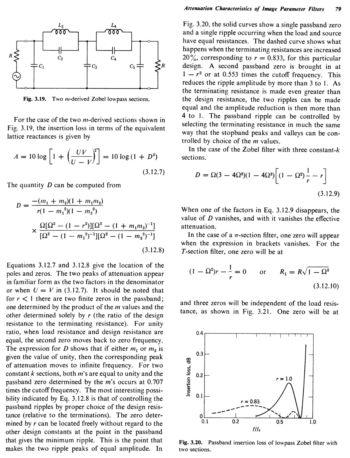
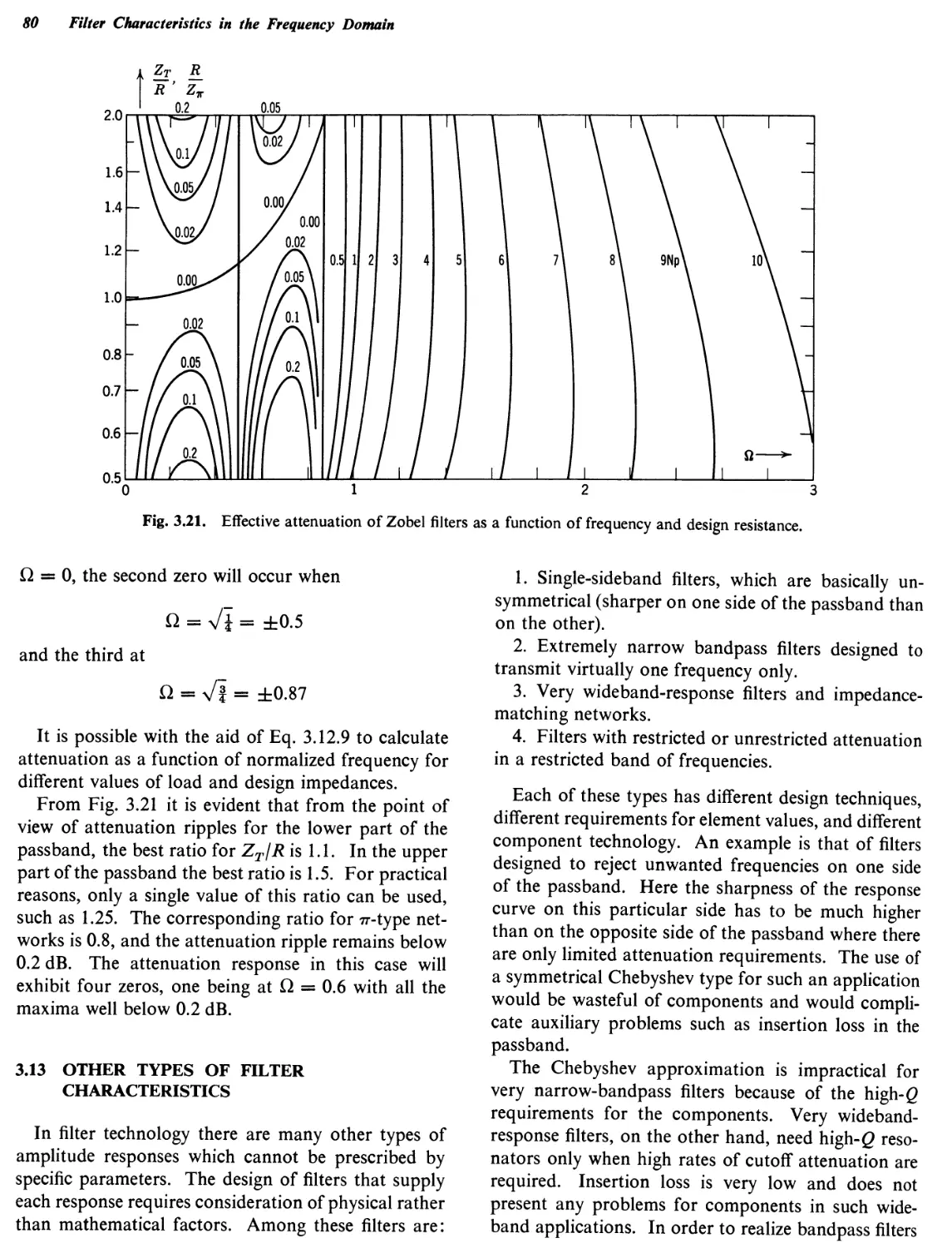
/


Автор: Zverev A.I.
Теги: electronics radio engineering electrical circuits electromagnetic waves filter synthesis
Год: 1967


Текст
Handbook of Filter Synthesis
Handbook of Filter Synthesis
Anatol I. Zverev
Consulting Engineer Westinghouse Electric Corporation
John Wiley and Sons, Inc. New York • London • Sydney
Copyright © 1967 by John Wiley & Sons, Inc. All Rights Reserved. This book or any part thereof must not be reproduced in any form without the written permission of the publisher.
Library of Congress Catalog Card Number: 67-17352
Printed in the United States of America
To my Aunt
Мария Алексеевна Зверева
Preface
This treatment of the electric wave filter is for electronic systems engineers engaged in communication, radar, and any other electronic equipment that depends on selective networks. From the systems engineer’s point of view the filter sets the standards of the system. Today he is able to specify almost any type of stable, single-valued analytic function as a subsystem on a block diagram, with reasonable assurance that it can be approximated and built into an operating unit. The exact mathematical technique is so successful that the newer electronic systems arc literally packed with synthesized passive and active networks. An exact knowledge of filter performance is therefore essential for the systems engineer. In this book he can find information concerning the performance of all possible types of filters in both the time and frequency domains.
In addition, the filter expert can find here a variety of general and specific information pertinent to his speciality. Almost any type of filter can be designed with the aid of the precalculated data presented.
In the evolution of the electronics industry the first two major developments—radio and the vacuum tube—were followed closely by a third, the electric wave filter. Filter technology was officially born in 1915 when K. Wagner (Germany) and G. Campbell (United States), working independently, proposed the basic concept of the filter. Their results evolved from earlier work on loaded transmission lines and the classical theory of vibrating systems.
Over the years filters have so permeated electronic technology that the modern world is hardly conceivable without them. They direct, channel, integrate, separate, delay, differentiate, and transform all kinds of electric energy and signals. It is appropriate to emphasize the fact that filter technology has not only transformed electronics but has itself been transformed into a theoretical tool of great power. Thus a filter is no longer a mere component neatly packaged in a can. In a much broader and more important sense it is a systems technique, almost a philosophical concept, whose generality has been steadily increasing throughout its fifty-year history.
The generalization of the filter concept began when
it was found that filter theory could be used to illuminate problems in mechanical and acoustical systems. By the use of an electromechanical analogy filter theory can be applied to many seemingly unrelated systems in which natural modes of vibration are of interest; for example, loudspeaker design, crystallography, architectural acoustics, airframe behavior, and mechanical systems design. Filter theory shows how to coordinate the action of several resonant elements to obtain uniform transmission over a prescribed frequency range. The concept of an ideal filter with lossless elements, which delivers all of the input energy to its output over the widest possible frequency range, establishes the requirements for broadbanding under prescribed constraints.
Application of filter theory has now gone far beyond these first generalizations. The concepts of exact synthesis techniques for prescribed transfer and immittance functions, of arbitrary functions with realizable rational functions, of time-domain synthesis, matched filters, parametric elements, and various other active devices have added new vitality to an already flourishing technology.
The discovery by Zobel, published in 1923, of a practical method of designing selective filters with an unlimited number of reactances was undoubtedly a work of genius. It was the only known method until about 1940 and the only practical method until the mid-1950s. S. Darlington in the United States and W. Cauer in Germany, both inspired by the work of Norton, published a theory that involved a set of problems relating to modern synthesis procedure. The importance of filter synthesis was not recognized immediately. It could be used to design better low-pass filters but failed to provide such designs in practice because of the extremely heavy burden of computation required. It was not until the advent of relatively cheap computation methods in the 1950s that Cauer-Darlington filters came into widespread use. So many computer-prepared designs have been published that designing an elliptic-function filter involves little more work than copying numbers out of a book, a technique that is actually easier than Zobel’s method.
viii Preface
We now synthesize networks and systems by employing a fusion of many theories produced by many authors. In the considerable body of the literature there are many references to Cauer and Darlington but this bibliographical distincton is currently being superseded. It has been assumed that there is little point in listing the names that everyone now takes for granted.
This treatment has several objectives. The first is to present the underlying theory, concepts, and techniques of selective networks. Subject matter of this kind is treated in Chapters 2, 4, and 5. The second objective is the presentation of responses that can be provided by passive, linear, bilateral filtering structures. This subject matter is treated extensively in Chapters 3 and 7. A third objective is to illustrate the first two by the treatment of specialized networks such as crystal filters (Chapter 8) and helical filters (Chapter 9). Chapter 1 is an introduction to the field of selectivity, written with the intent to project the concept and importance of filters in the world of electronics. Chapter 6 provides information pertinent to polynomial filters with monotonic attenuation curves. Information is presented in tables of lowpass element values and normalized coupling coefficients and quality factors. With the aid of data presented in this chapter predistorted filters can readily be designed. All of Chapter 10 is dedicated to techniques of network transformation. These data are not only practical for filter design but can be applied to any other type of electronic circuit design.
The reader will not find an extensive treatment of active networks and microwave structures for themselves they tend to be a specialized field within filter technology. Microwave filters may consist of metal cavities coupled by openings called “irises”. They may take the form of printed circuit “stripline” networks that appear to be labyrinthine paths of metal foil and contain no components whatever. Yet designers of these devices still talk about Butterworth, Chebyshev, and Bessel approximations, poles and
zeros, and all the other theoretical niceties of network synthesis. In the midst of this diversity there is unity, and the design equations of the microwave engineer are strongly and directly traceable, both historically and ideologically, to the original reflections of Wagner and Campbell fifty years ago.
In addition to being a guide to the solution of filter problems, this book leads into the realm of network synthesis with its specific terminology. It is felt that the wealth of network synthesis theory is still not being fully utilized in design work, and it is hoped that this book will arouse interest in the science of synthesis and help to bridge the gap between the strictly theoretical concepts and the everyday practice in engineering laboratories and scientific establishments.
1 wish to express my gratitude to Professor Dr. Fritzsche, Professor Dr. G. Bosse, and C. F. Kurth for permission to use their publications, and to Dr. D. S. H umpherys for bringing network synthesis to the engineering level evidenced by the tables in this book. Special recognition is due to M. Savetman for his valuable help in the preparation of the final manuscript. I also wish to express my appreciation to R. Anderson, R. Ballesteros, H. Blinchikoff, Dr. E. Khu, S. Russell, and C. Vale, the engineers who were instrumental in devising many of the designs and innovations in filter technique, and to Dr. J. Bobis, P. Geffe, R. M. Morrison, and S. I. Rambo who were helpful in creating the proper atmosphere in the Networks Synthesis Department. Many thanks to the Engineering Management of the Surface Division, Westinghouse Electric Corporation, for their continual encouragement.
Anatol I. Zverev
Baltimore, Maryland
June 1967
Contents
CHAPTER 1 FILTERS IN ELECTRONICS 1
1.1 Types of Filters 1
1.2 Filter Applications 3
1.3 All-Pass Filters 5
1.4 Properties of Lattice Filters 6
1.5 Filter Building Blocks 9
1.6 Higher Order Filters 17
1.7 Coil-Saving Bandpass Filters 17
1.8 Frequency Range of Applications 20
1.9 Physical Elements of the Filter 21
1.10 Active Bandpass Filters 22
1.11 RC Passive and Active Filters 22
1.12 Microwave Filters 25
1.13 Parametric Filters 29
CHAPTER 2 THEORY OF EFFECTIVE PARAMETERS 3 1
2.1 Power Balance 32
2.2 Types of General Network Equations 33
2.3 Effective Attenuation 35
2.4 Reflective (Echo) Attenuation 36
2.5 Transmission Function As a Function Of Frequency Parameter, .s' 37
2.6 Polynomials of Transmission and Filtering Functions 38
2.7 Filter Networks 39
2.8 Voltage and Current Sources 41
2.9 The Function D(s) As An Approximation Function 42
2.10 Examples of Transmission Function Approximation 45
2.11 Simplest Polynomial Filters in Algebraic Form 49
2.12 Introduction To Image-Parameter Theory 50
2.13 Bridge Networks 52
2.14 Examples of Realization in the Bridge Form 53
2.15 Hurwitz Polynomial 54
2.16 The Smallest Realizable Networks 55
2.17 Fourth-Order Networks 57
2.18 Fifth-Order Networks 58
CHAPTER 3 FILTER CHARACTERISTICS IN THE FREQUENCY DOMAIN 60
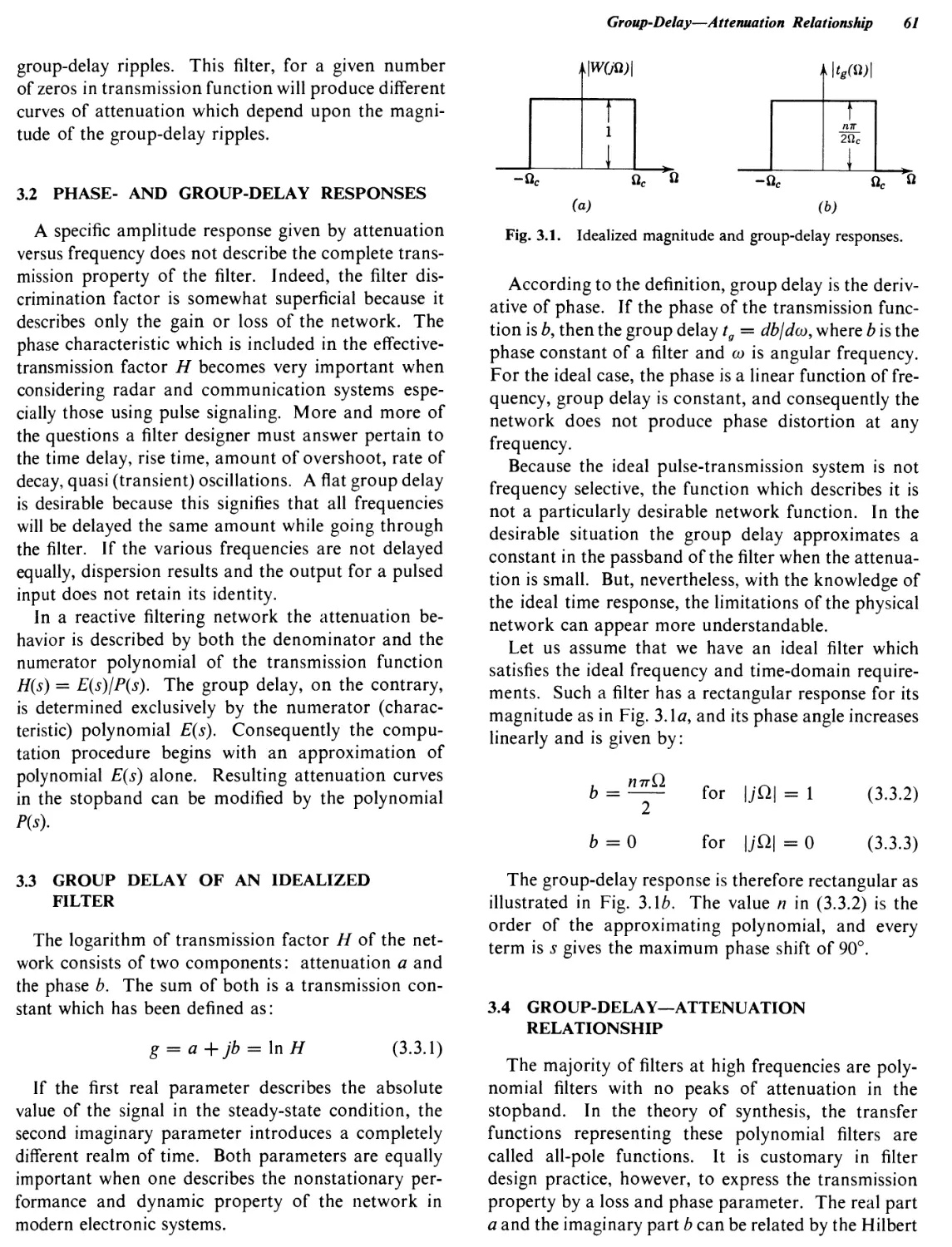
3.1 Amplitude Responses 60
3.2 Phase-and Group-Delay Responses 61
3.3 Group Delay of an Idealized Filter 61
3.4 Group-Delay—Attenuation Relationship 61
3.5 The Chebyshev Family of Response Characteristics 62
ix
Contents
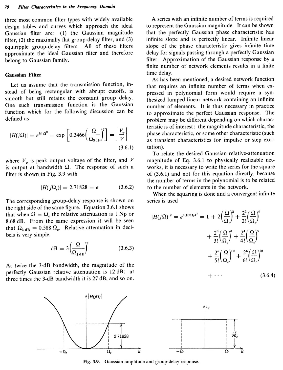
3.6 Gaussian Family of Response Characteristics 67
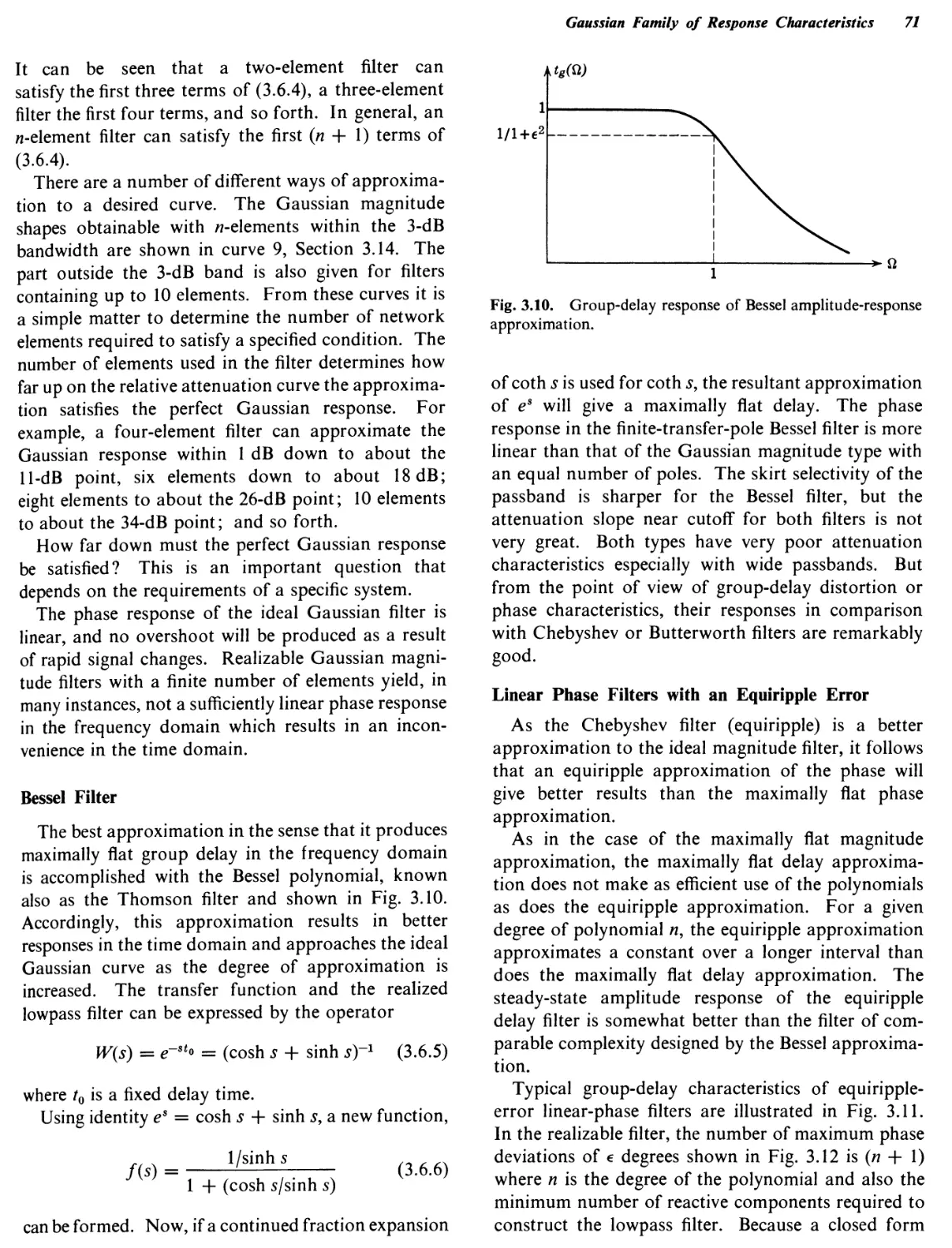
3.7 A Filter with Transitional Magnitude Characteristics 74
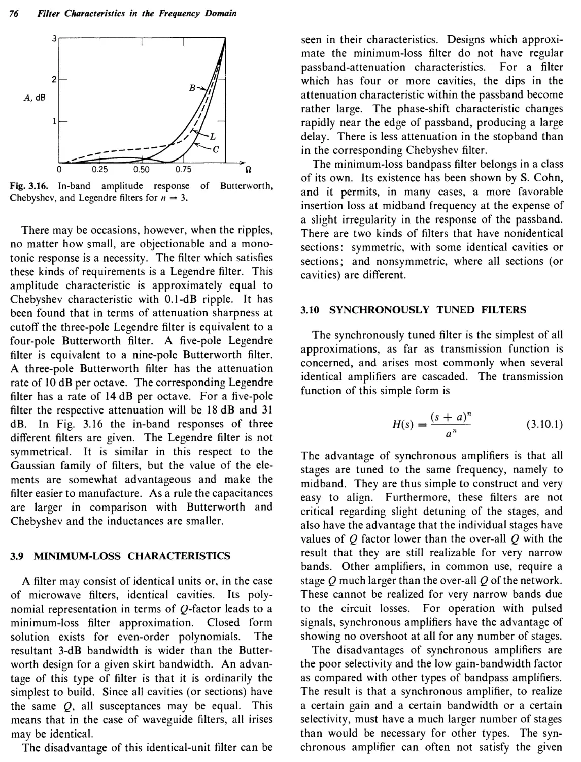
3.8 Legendre Filters 74
3.9 Minimum-Loss Characteristics 76
3.10 Synchronously Tuned Filters 76
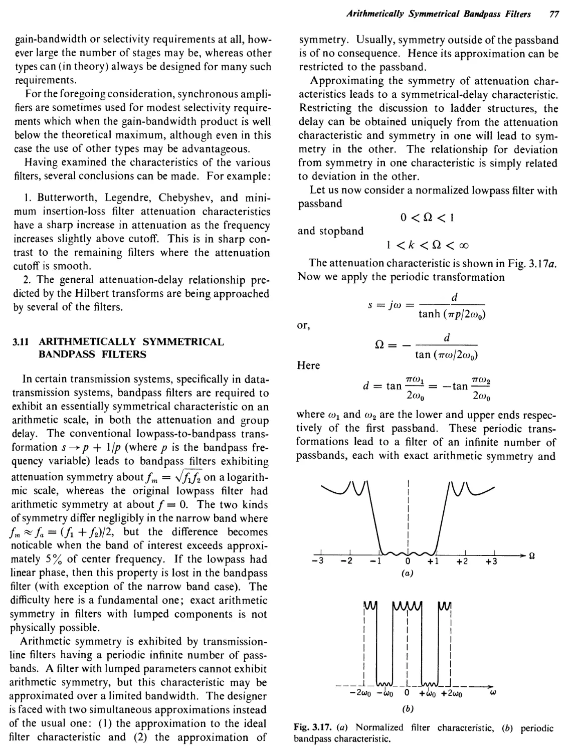
3.11 Arithmetically Symmetrical Bandpass Filters 77
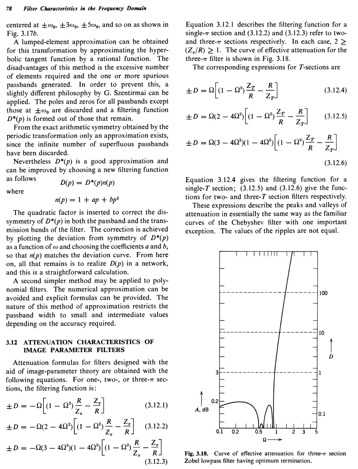
3.12 Attenuation Characteristics of Image Parameter Filters 78
3.13 Other Types of Filter Characteristics 80
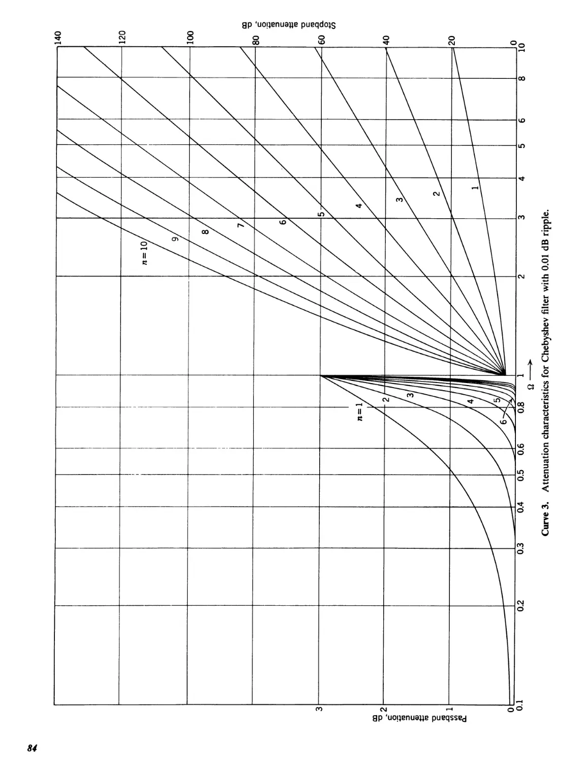
3.14 Plots of the Attenuation and Group Delay Characteristics 81
CHAPTER 4 ELLIPTIC FUNCTIONS AND ELEMENTS OF REALIZATION 107
4.1 Double Periodic Elliptic Functions 107
4.2 Mapping of 5-Plane into w-Plane 109
4.3 First Basic Transformation of Elliptic Functions 110
4.4 Filtering Function in z-Plane 112
4.5 Graphical Representation of Parameters 114
4.6 Characteristic Values of D(s) 115
4.7 An Example of Filter Design 116
4.8 Consideration of Losses 119
4.9 Introduction of Losses by Frequency Transformation 119
4.10 Highpass Filters with Losses 120
4.11 Transmission Functions with Losses 121
4.12 Conclusions on Consideration of Losses 123
4.13 Realization Process 124
4.14 Bandpass Filter with a Minimum Number of Inductors 125
4.15 The Elements of a Coil-Saving Network 127
4.16 Consideration of Losses in Zig-Zag Filters 128
4.17 Realization Procedure 129
4.18 Numerical Example of Realization 131
4.19 Full and Partial Removal for a Fifth-Order Filter 132
CHAPTER 5 THE CATALOG OF NORMALIZED LOWPASS FILTERS 137
5.1 Introduction to the Catalog 137
5.2 Real Part of the Driving Point Impedance 146
5.3 Lowpass Filter Design 148
5.4 Design of Highpass Filters 151
5.5 Design of LC Bandpass Filters 154
5.6 Design of Narrowband Crystal Filters 160
5.7 Design of Bandstop Filters 163
5.8 Catalog of Normalized Lowpass Models 168
CHAPTER 6 DESIGN TECHNIQUES FOR POLYNOMIAL FILTERS 290
6.1 Introduction to Tables of Normalized Element Values 290
6.2 Lowpass Design Examples 292
6.3 Bandpass Filter Design 295
6.4 Concept of Coupling 296
6.5 Coupled Resonators 298
6.6 Second-Order Bandpass Filter 300
6.7 Design with Tables of Predistorted к and q Parameters 305
Contents xi
6.8 6.9 6.10 Design Examples using Tables of к and q Values Tables of Lowpass Element Values Tables of 3-dB Down к and q Values 306 310 311
CHAPTER 7 FILTER CHARACTERISTICS IN THE TIME DOMAIN 380
7.1 Introduction to Transient Characteristics 380
7.2 Time and Frequency Domains 380
7.3 Information Contained in the Impulse Response 383
7.4 Step Response 383
7.5 Impulse Response of an Ideal Gaussian Filter 384
7.6 Residue Determination 385
7.7 Numerical Example 385
7.8 Practical Steps in the Inverse Transformation 388
7.9 Inverse Transform of Rational Spectral Functions 389
7.10 Numerical Example 390
7.11 Estimation Theory 391
7.12 Transient Response in Highpass and Bandpass Filters 392
7.13 The Exact Calculation of Transient Phenomena for Highpass Systems 393
7.14 Estimate of Transient Responses in Narrowband Filters 395
7.15 The Exact Transient Calculation in Narrowband Systems 397
7.16 Group Delay Versus Transient Response 398
7.17 Computer Determination of Filter Impulse Response 398
7.18 Transient Response Curves 400
CHAPTER 8 CRYSTAL FILTERS 414
8.1 Introduction 414
8.2 Crystal Structure 414
8.3 Theory of Piezoelectricity 414
8.4 Properties of Piezoelectric Quartz Crystals 415
8.5 Classification of Crystal Filters 421
8.6 Bridge Filters 423
8.7 Limitation of Bridge Crystal Filters 425
8.8 Spurious Response 427
8.9 Circuit Analysis of a Simple Filter 428
8.10 Element Values in Image-Parameter Formulation 429
8.11 Ladder Filters 431
8.12 Effective Attenuation of Simple Filters 434
8.13 Effective Attenuation of Ladder Networks 437
8.14 Ladder Versus Bridge Filters 439
8.15 Practical Differential Transformer for Crystal Filters 440
8.16 Design of Narrowband Filters with the Aid of Lowpass Model 443
8.17 Synthesis of Ladder Single Sideband Filters 453
8.18 The Synthesis of Intermediate Bandpass Filters 483
8.19 Example of Band-Reject Filter 490
8.20 Ladder Filters with Large Bandwidth 491
CHAPTER 9 HELICAL FILTERS 499
9.1 Introduction 499
9.2 Helical Resonators 499
xii Contents
9.3 Filter with Helical Resonators 505
9.4 Alignment of Helical Filters 513
9.5 Examples of Helical Filtering 518
CHAPTER 10 NETWORK TRANSFORMATIONS 522
10.1 Two-Terminal Network Transformations 522
10.2 Delta-Star Transformation 528
10.3 Use of Transformer in Filter Realization 530
10.4 Norton’s Transformation 530
10.5 Applications of Mutual Inductive Coupling 536
10.6 The Realization of LC Filters with Crystal Resonators 540
10.7 Negative and Positive Capacitor Transformation 545
10.8 Bartlett’s Bisection Theorem 546
10.9 Cauer’s Equivalence 549
10.10 Canonic Bandpass Structures 552
10.11 Bandpass Ladder Filters Having a Canonical Number of Inductors without Mutual Coupling 553
10.12 Impedance and Admittance Inverters 559
10.13 Source and Load Transformation 567
BIBLIOGRAPHY 569
INDEX
573
Handbook of Filter Synthesis
Filters in Electronics
1.1 TYPES OF FILTERS
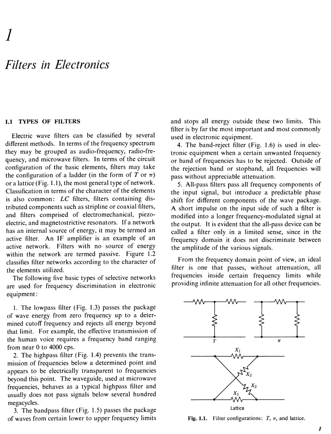
Electric wave filters can be classified by several different methods. In terms of the frequency spectrum they may be grouped as audio-frequency, radio-frequency, and microwave filters. In terms of the circuit configuration of the basic elements, filters may take the configuration of a ladder (in the form of T or 77) or a lattice (Fig. 1.1), the most general type of network. Classification in terms of the character of the elements is also common: LC filters, filters containing distributed components such as stripline or coaxial filters, and filters comprised of electromechanical, piezoelectric, and magnetostrictive resonators. If a network has an internal source of energy, it may be termed an active filter. An IF amplifier is an example of an active network. Filters with no source of energy within the network are termed passive. Figure 1.2 classifies filter networks according to the character of the elements utilized.
The following five basic types of selective networks are used for frequency discrimination in electronic equipment:
1. The lowpass filter (Fig. 1.3) passes the package of wave energy from zero frequency up to a determined cutoff frequency and rejects all energy beyond that limit. For example, the effective transmission of the human voice requires a frequency band ranging from near 0 to 4000 cps.
2. The highpass filter (Fig. 1.4) prevents the transmission of frequencies below a determined point and appears to be electrically transparent to frequencies beyond this point. The waveguide, used at microwave frequencies, behaves as a typical highpass filter and usually does not pass signals below several hundred megacycles.
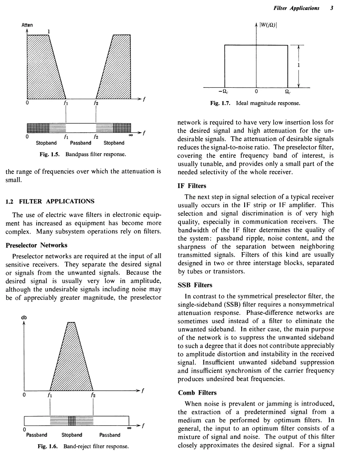
3. The bandpass filter (Fig. 1.5) passes the package of waves from certain lower to upper frequency limits
and stops all energy outside these two limits. This filter is by far the most important and most commonly used in electronic equipment.
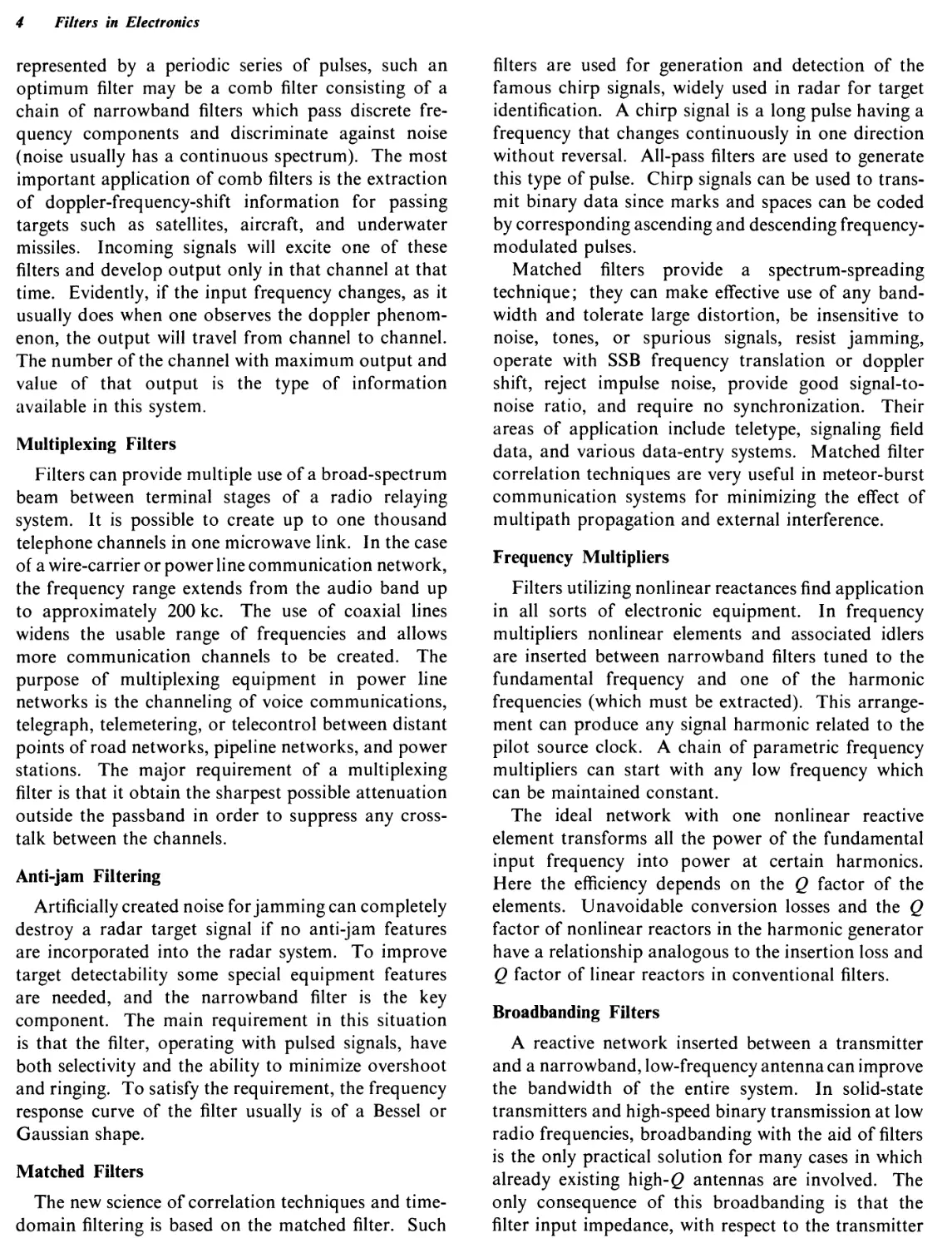
4. The band-reject filter (Fig. 1.6) is used in electronic equipment when a certain unwanted frequency or band of frequencies has to be rejected. Outside of the rejection band or stopband, all frequencies will pass without appreciable attenuation.
5. All-pass filters pass all frequency components of the input signal, but introduce a predictable phase shift for different components of the wave package. A short impulse on the input side of such a filter is modified into a longer frequency-modulated signal at the output. It is evident that the all-pass device can be called a filter only in a limited sense, since in the frequency domain it does not discriminate between the amplitude of the various signals.
From the frequency domain point of view, an ideal filter is one that passes, without attenuation, all frequencies inside certain frequency limits while providing infinite attenuation for all other frequencies.
Fig. 1.1. Filter configurations: T, я, and lattice.
1
2 Filters in Electronics
Fig. 1.2. Classification of filters.
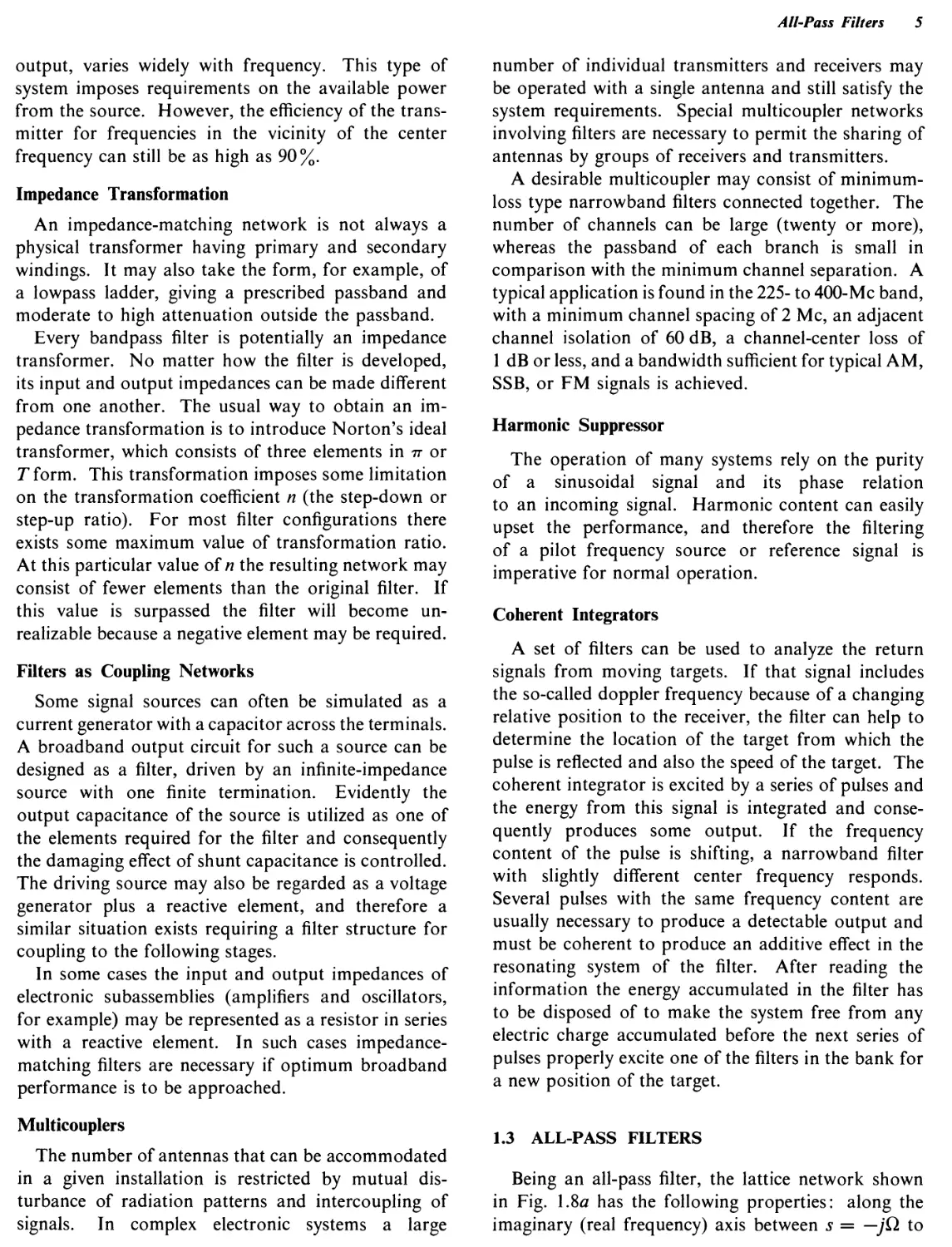
The transfer function |JF(jQ)|, the ratio of output to input quantities in the frequency domain is shown for an ideal filter in Fig. 1.7.
From the time domain point of view, an ideal filter is one whose output is identical to its input except for delay r0, or
^out(0 = ein(? - To) (1.1.1)
Taking the Laplace transform of the above equation and looking at the transfer function in the frequency
domain, we obtain the ideal transfer function
PV(s) = e~T°s Letting 5 = yQ, W(jO) = e~iQ-T(>
(1.1.2)
(1.1.3)
This function is not frequency selective, since it has unity amplitude; its phase decreases linearly with frequency. These conditions may be realized in practice when the delay approximates a constant for
Fig. 1.3. Lowpass filter response.
Fig. 1.4. Highpass filter response.
Filter Applications 3
Fig. 1.5. Bandpass filter response.
the range of frequencies over which the attenuation is small.
1.2 FILTER APPLICATIONS
The use of electric wave filters in electronic equipment has increased as equipment has become more complex. Many subsystem operations rely on filters.
Preselector Networks
Preselector networks are required at the input of all sensitive receivers. They separate the desired signal or signals from the unwanted signals. Because the desired signal is usually very low in amplitude, although the undesirable signals including noise may be of appreciably greater magnitude, the preselector
Passband Stopband Passband
Fig. 1.6. Band-reject filter response.
Fig. 1.7. Ideal magnitude response.
network is required to have very low insertion loss for the desired signal and high attenuation for the undesirable signals. The attenuation of desirable signals reduces the signal-to-noise ratio. The preselector filter, covering the entire frequency band of interest, is usually tunable, and provides only a small part of the needed selectivity of the whole receiver.
IF Filters
The next step in signal selection of a typical receiver usually occurs in the IF strip or IF amplifier. This selection and signal discrimination is of very high quality, especially in communication receivers. The bandwidth of the IF filter determines the quality of the system: passband ripple, noise content, and the sharpness of the separation between neighboring transmitted signals. Filters of this kind are usually designed in two or three interstage blocks, separated by tubes or transistors.
SSB Filters
In contrast to the symmetrical preselector filter, the single-sideband (SSB) filter requires a nonsymmetrical attenuation response. Phase-difference networks are sometimes used instead of a filter to eliminate the unwanted sideband. In either case, the main purpose of the network is to suppress the unwanted sideband to such a degree that it does not contribute appreciably to amplitude distortion and instability in the received signal. Insufficient unwanted sideband suppression and insufficient synchronism of the carrier frequency produces undesired beat frequencies.
Comb Filters
When noise is prevalent or jamming is introduced, the extraction of a predetermined signal from a medium can be performed by optimum filters. In general, the input to an optimum filter consists of a mixture of signal and noise. The output of this filter closely approximates the desired signal. For a signal
4 Filters in Electronics
represented by a periodic series of pulses, such an optimum filter may be a comb filter consisting of a chain of narrowband filters which pass discrete frequency components and discriminate against noise (noise usually has a continuous spectrum). The most important application of comb filters is the extraction of doppler-frequency-shift information for passing targets such as satellites, aircraft, and underwater missiles. Incoming signals will excite one of these filters and develop output only in that channel at that time. Evidently, if the input frequency changes, as it usually does when one observes the doppler phenomenon, the output will travel from channel to channel. The number of the channel with maximum output and value of that output is the type of information available in this system.
Multiplexing Filters
Filters can provide multiple use of a broad-spectrum beam between terminal stages of a radio relaying system. It is possible to create up to one thousand telephone channels in one microwave link. In the case of a wire-carrier or power line communication network, the frequency range extends from the audio band up to approximately 200 kc. The use of coaxial lines widens the usable range of frequencies and allows more communication channels to be created. The purpose of multiplexing equipment in power line networks is the channeling of voice communications, telegraph, telemetering, or telecontrol between distant points of road networks, pipeline networks, and power stations. The major requirement of a multiplexing filter is that it obtain the sharpest possible attenuation outside the passband in order to suppress any crosstalk between the channels.
Anti-jam Filtering
Artificially created noise for jamming can completely destroy a radar target signal if no anti-jam features are incorporated into the radar system. To improve target detectability some special equipment features are needed, and the narrowband filter is the key component. The main requirement in this situation is that the filter, operating with pulsed signals, have both selectivity and the ability to minimize overshoot and ringing. To satisfy the requirement, the frequency response curve of the filter usually is of a Bessel or Gaussian shape.
Matched Filters
The new science of correlation techniques and timedomain filtering is based on the matched filter. Such
filters are used for generation and detection of the famous chirp signals, widely used in radar for target identification. A chirp signal is a long pulse having a frequency that changes continuously in one direction without reversal. All-pass filters are used to generate this type of pulse. Chirp signals can be used to transmit binary data since marks and spaces can be coded by corresponding ascending and descending frequency-modulated pulses.
Matched filters provide a spectrum-spreading technique; they can make effective use of any bandwidth and tolerate large distortion, be insensitive to noise, tones, or spurious signals, resist jamming, operate with SSB frequency translation or doppler shift, reject impulse noise, provide good signal-to-noise ratio, and require no synchronization. Their areas of application include teletype, signaling field data, and various data-entry systems. Matched filter correlation techniques are very useful in meteor-burst communication systems for minimizing the effect of multipath propagation and external interference.
Frequency Multipliers
Filters utilizing nonlinear reactances find application in all sorts of electronic equipment. In frequency multipliers nonlinear elements and associated idlers are inserted between narrowband filters tuned to the fundamental frequency and one of the harmonic frequencies (which must be extracted). This arrangement can produce any signal harmonic related to the pilot source clock. A chain of parametric frequency multipliers can start with any low frequency which can be maintained constant.
The ideal network with one nonlinear reactive element transforms all the power of the fundamental input frequency into power at certain harmonics. Here the efficiency depends on the Q factor of the elements. Unavoidable conversion losses and the Q factor of nonlinear reactors in the harmonic generator have a relationship analogous to the insertion loss and Q factor of linear reactors in conventional filters.
Broadbanding Filters
A reactive network inserted between a transmitter and a narrowband, low-frequency antenna can improve the bandwidth of the entire system. In solid-state transmitters and high-speed binary transmission at low radio frequencies, broadbanding with the aid of filters is the only practical solution for many cases in which already existing high-0 antennas are involved. The only consequence of this broadbanding is that the filter input impedance, with respect to the transmitter
All-Pass Filters 5
output, varies widely with frequency. This type of system imposes requirements on the available power from the source. However, the efficiency of the transmitter for frequencies in the vicinity of the center frequency can still be as high as 90%.
Impedance Transformation
An impedance-matching network is not always a physical transformer having primary and secondary windings. It may also take the form, for example, of a lowpass ladder, giving a prescribed passband and moderate to high attenuation outside the passband.
Every bandpass filter is potentially an impedance transformer. No matter how the filter is developed, its input and output impedances can be made different from one another. The usual way to obtain an impedance transformation is to introduce Norton’s ideal transformer, which consists of three elements in it or T form. This transformation imposes some limitation on the transformation coefficient n (the step-down or step-up ratio). For most filter configurations there exists some maximum value of transformation ratio. At this particular value of n the resulting network may consist of fewer elements than the original filter. If this value is surpassed the filter will become unrealizable because a negative element may be required.
Filters as Coupling Networks
Some signal sources can often be simulated as a current generator with a capacitor across the terminals. A broadband output circuit for such a source can be designed as a filter, driven by an infinite-impedance source with one finite termination. Evidently the output capacitance of the source is utilized as one of the elements required for the filter and consequently the damaging effect of shunt capacitance is controlled. The driving source may also be regarded as a voltage generator plus a reactive element, and therefore a similar situation exists requiring a filter structure for coupling to the following stages.
In some cases the input and output impedances of electronic subassemblies (amplifiers and oscillators, for example) may be represented as a resistor in series with a reactive element. In such cases impedancematching filters are necessary if optimum broadband performance is to be approached.
Multicouplers
The number of antennas that can be accommodated in a given installation is restricted by mutual disturbance of radiation patterns and intercoupling of signals. In complex electronic systems a large
number of individual transmitters and receivers may be operated with a single antenna and still satisfy the system requirements. Special multicoupler networks involving filters are necessary to permit the sharing of antennas by groups of receivers and transmitters.
A desirable multicoupler may consist of minimumloss type narrowband filters connected together. The number of channels can be large (twenty or more), whereas the passband of each branch is small in comparison with the minimum channel separation. A typical application is found in the 225- to 400-Mc band, with a minimum channel spacing of 2 Me, an adjacent channel isolation of 60 dB, a channel-center loss of 1 dB or less, and a bandwidth sufficient for typical AM, SSB, or FM signals is achieved.
Harmonic Suppressor
The operation of many systems rely on the purity of a sinusoidal signal and its phase relation to an incoming signal. Harmonic content can easily upset the performance, and therefore the filtering of a pilot frequency source or reference signal is imperative for normal operation.
Coherent Integrators
A set of filters can be used to analyze the return signals from moving targets. If that signal includes the so-called doppler frequency because of a changing relative position to the receiver, the filter can help to determine the location of the target from which the pulse is reflected and also the speed of the target. The coherent integrator is excited by a series of pulses and the energy from this signal is integrated and consequently produces some output. If the frequency content of the pulse is shifting, a narrowband filter with slightly different center frequency responds. Several pulses with the same frequency content are usually necessary to produce a detectable output and must be coherent to produce an additive effect in the resonating system of the filter. After reading the information the energy accumulated in the filter has to be disposed of to make the system free from any electric charge accumulated before the next series of pulses properly excite one of the filters in the bank for a new position of the target.
1.3 ALL-PASS FILTERS
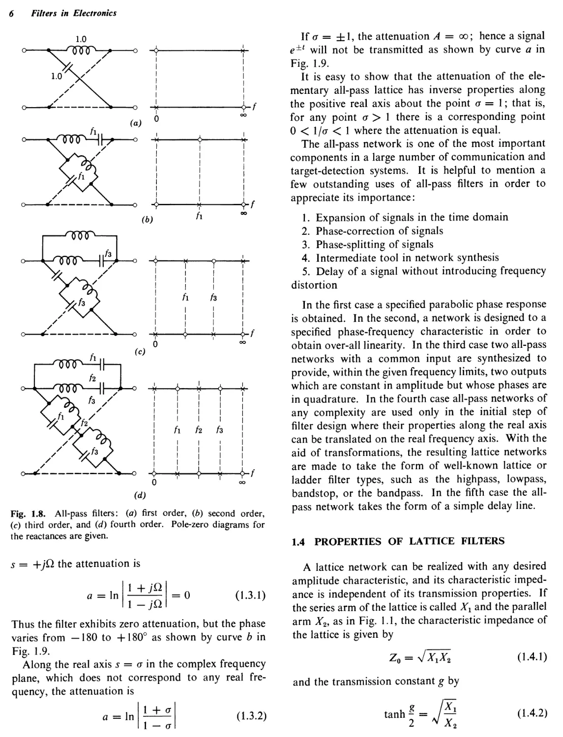
Being an all-pass filter, the lattice network shown in Fig. 1.8я has the following properties: along the imaginary (real frequency) axis between s = —jQ to
6 Filters in Electronics
(d)
Fig. 1.8. All-pass filters: (a) first order, (b) second order, (<?) third order, and (d) fourth order. Pole-zero diagrams for the reactances are given.
5 = the attenuation is
a = ln 1 =0 (1.3.1)
i - jn
Thus the filter exhibits zero attenuation, but the phase varies from —180 to 4-180° as shown by curve b in Fig. 1.9.
Along the real axis 5 = o' in the complex frequency plane, which does not correspond to any real frequency, the attenuation is
a = In
1 + a
1 — O'
(1.3.2)
If o' = ±1, the attenuation A = oo; hence a signal ebt will not be transmitted as shown by curve a in Fig. 1.9.
It is easy to show that the attenuation of the elementary all-pass lattice has inverse properties along the positive real axis about the point o' = 1; that is, for any point o' > 1 there is a corresponding point 0 < I/О' < 1 where the attenuation is equal.
The all-pass network is one of the most important components in a large number of communication and target-detection systems. It is helpful to mention a few outstanding uses of all-pass filters in order to appreciate its importance:
1. Expansion of signals in the time domain
2. Phase-correction of signals
3. Phase-splitting of signals
4. Intermediate tool in network synthesis
5. Delay of a signal without introducing frequency distortion
In the first case a specified parabolic phase response is obtained. In the second, a network is designed to a specified phase-frequency characteristic in order to obtain over-all linearity. In the third case two all-pass networks with a common input are synthesized to provide, within the given frequency limits, two outputs which are constant in amplitude but whose phases are in quadrature. In the fourth case all-pass networks of any complexity are used only in the initial step of filter design where their properties along the real axis can be translated on the real frequency axis. With the aid of transformations, the resulting lattice networks are made to take the form of well-known lattice or ladder filter types, such as the highpass, lowpass, bandstop, or the bandpass. In the fifth case the all-pass network takes the form of a simple delay line.
1.4 PROPERTIES OF LATTICE FILTERS
A lattice network can be realized with any desired amplitude characteristic, and its characteristic impedance is independent of its transmission properties. If the series arm of the lattice is called X± and the parallel arm X2, as in Fig. 1.1, the characteristic impedance of the lattice is given by
z0 = (i.4.i)
and the transmission constant g by
f -
Z w Л. 2
Properties of Lattice Filters 7
Fig. 1.9. Attenuation and phase relationships of all-pass filter of Fig. 1.8a.
The condition of transparency for any lattice filter is very simple. The arm reactances X in the series and parallel arms must be opposite in sign. As soon as the two arm reactances have the same sign (both capacitive or both inductive), the filter stops being transparent.
The amplitude response of the lattice filter depends on only the ratio of the branch reactances and is independent of the input and output impedances. When Хг = X2, tanh g/2 = ±1 and a maximum, or peak, of attenuation occurs. The position of the peak can be modified without impedance change by multiplying Хг by a real positive factor and dividing X2 by the same factor.
Lattice networks must be designed and built with great care in order to balance their impedances. Once reactance values are chosen to resonate at strategic positions in the passband (such as the cutoffs and the center of the passband) the level of the reactances between these strategic positions must be maintained
in both arms in an exactly prescribed fashion. Furthermore, the peak of attenuation outside the passband is controlled by the level of the impedances of both arms when they are of the same nature (capacitive or inductive), whereas the position of the attenuation peak depends upon the sharpness of the reactance curve at cutoff (which is effectively within the passband).
Therefore the peak’s position cannot be controlled by simply changing an inductance or capacitance. Control is very remote and must be applied through the resonances which occur at some frequency in the passband or at cutoff. Although this is an inconvenience, it offers the advantage that the amount of attenuation or the sharpness of the response curve can sometimes be adjusted by a slight variation in the parameters of the resonators. This procedure is often used in crystal filter design but is impractical with conventional coils and capacitors that require precise nominal values and good environmental stability.
A composite lattice has the same basic form as the
L OWPASS SECTION HIGHPASS SECTION
TYPE NUMBER 2 3 1 2 3
ARMS OF FULL SECTION ОАЛЛгО О г' г2 FUNDAMENTAL TYPE .1 C2y M - DERIVED 2T M-DERIVED C’ CzT fundamental type eV* 1 l24 M-DERIVED C’ C2=T l2 : M-DERIVED C1 5 L2 5
ELEMENT VALUES 1 or 'If 'If ’ w- ‘GJ -J о L 1 : m Li’ 1-m2 , 2 L2~ L1 C2 = m C2‘ Li - mLi ' 1-m2 , C--T^C2 C2 : m C2 . _ 1 1 4-wfiR •. R L2 47Tfl ct’ c': — '^ГТТ0'' L-2 L2iT" c,' c1-- — 4 m ,i L1 = 2 L2 1 - m l2 L2= “
ZT=VztZ2 /н Z1 J «2 izt' Z IZTIZ « <E C I/ ! \ |2tIT''\Z'r IztI Л R IztI 0 z*4 L—J <
D 1 co R Vi - л2 0 1 "° zt = r Vi -л2 <=zt» C ZT = R 1 1 <=° У-л2 Л2" % I e Zt'-r/J 0 1 00 ZT - 0 4o 1 °° ' * a”2”H2
z.5^_ / Z1 V 4Z2 R lZ7r| '\ R Iz7r| ] V/ R I Z7rl ! V lz7rl / nL' 4 |Z7r| \ R _ V i |Z7r| R X 1 Z 1
'0 1 "° R ZK */ 2 VI -л2 Z7r" 1 nco "° R— VTn2- ( Z?r \ ) 1 ~ 1-Л2 R Z-rrz > j °C Z7T = 8 led1 I -+= -1^ i °° z„ = -=l=z^l •J П2
ATTENUATION CONSTANT FOR IDEAL ELEMENTS 0 И " 1 /Н -Ud 0 1 fl «О 0 1 «о a1
C ) 4 QO 0 ’ 4o °° ° Л^ 1 -° 0 n„ 1 00
PHASE CONSTANT FOR IDEAL ELEMENTS ^0 OO 4 Щ 0 0 ^oo 1 co
ь, | A 4 LfJJ b' ol 0 ZLU ГТТП
0 1 ю ) 1 лв = 1 л -°
Z1 4Z2 WITHOUT LOSSES d 0 -л.2 o2-1 |-02 л2 Л2- 02-1 ' 1-о2Л2
WITH LOSSES d #= 0 - Л2 (1-id I)(1-jdc ) qZ -1 O2 1 a< ?-1
Л2 ( 1 - jd| ) (1 - Jdc» Л2 (1 - Jd| )(1-jdc ) 1-о2Л2( 1-Jdl) (l-jdc )
DEFINITIONS л -- L- -h. -|4 CJ ~ E ° £ t> 8 -If -|' о 3 f\J ГО " %|- ;i- f|-'
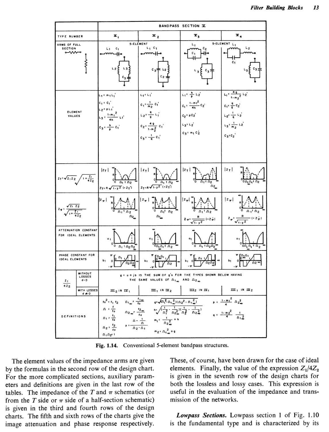
Fig. 1.10. Lowpass and highpass conventional structures.
8
Filter Building Blocks 9
elementary lattice. For example, the all-pass filter of the first order (Fig. 1.8я) consists of a series and a lattice arm. Higher order all-pass structures as shown in Fig. 1.8/), c, and d still have only two arms, but their schematics are more complicated. The number of reactive components is always the same for both branches, but the nature of the reactances is different at every point on the frequency scale from zero to infinity.
In general, the transmission properties of composite lattice filters outside the passband are controlled by the natural frequencies of the branch reactances inside the passband. Similarly, the flatness of the passband, and consequently the flatness of the input and output impedance of the filter is controlled by the natural frequencies outside the passband. If there is a large number of these frequencies in the passband, the attenuation in the stopband may be high and a more rapid transition from passband to stopband can be obtained.
1.5 FILTER BUILDING BLOCKS
The electric wave filter can be visualized as a combination of simple building blocks called sections, an approach similar to combining the blocks of gain of tubes or transistors. Each of these filter blocks is a certain canonic combination of lumped reactances. At microwave frequencies these reactances are distributed, but for the purpose of analysis they can be reduced to an equivalent schematic with lumped components. A lowpass elementary ladder structure is shown in Fig. 1.10 (type 1). In Fig. 1.15a two elementary lowpass lattice structures are shown with their equivalent bridged-T and semilattice circuits. The configuration in the center of Fig. 1.15a is a bridged-T schematic, and the form on the extreme right is the so-called semilattice or differential bridge filter. The lowpass filter with a transformer, such as the differential bridge, is a lowpass filter only in a limited sense because it does not pass direct current. Figure 1.15b shows the reactance of the lattice arms, and Fig. 1.15c, the attenuation curve. Figure 1.10 (highpass type 1) illustrates a highpass elementary structure in ladder form, and Fig. 1.16, the elementary lattice highpass structure and its equivalents. Similarly, an elementary bandpass filter is shown in Fig. 1.11 (bandpass type IJ. It is conventionally known as the /^-constant type. The lattice bandpass filters of Fig. 1.17 possess a ladder equivalent shown as type IV in Fig. 1.13 and can also be shown in a bridged-T or differential bridge form as is customary in crystal filter
practice. The lattice form of the filter is highly uneconomical. It consists of repetitive elements (shown as dotted lines) and consequently is very seldom used. Being the most general type of building block, however, it theoretically permits the realization of a more universal response than any of its partial equivalents.
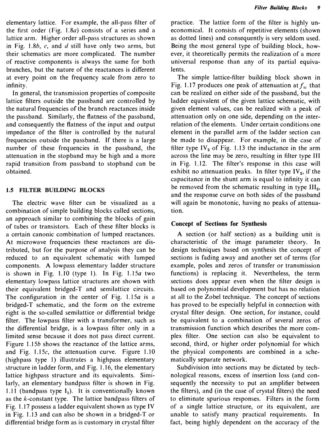
The simple lattice-filter building block shown in Fig. 1.17 produces one peak of attenuation at that can be realized on either side of the passband, but the ladder equivalent of the given lattice schematic, with given element values, can be realized with a peak of attenuation only on one side, depending on the interrelation of the elements. Under certain conditions one element in the parallel arm of the ladder section can be made to disappear. For example, in the case of filter type IV2 of Fig. 1.13 the inductance in the arm across the line may be zero, resulting in filter type III in Fig. 1.12. The filter’s response in this case will exhibit no attenuation peaks. In filter type IV2, if the capacitance in the shunt arm is equal to infinity it can be removed from the schematic resulting in type III2, and the response curve on both sides of the passband will again be monotonic, having no peaks of attenuation.
Concept of Sections for Synthesis
A section (or half section) as a building unit is characteristic of the image parameter theory. In design techniques based on synthesis the concept of sections is fading away and another set of terms (for example, poles and zeros of transfer or transmission functions) is replacing it. Nevertheless, the term sections does appear even when the filter design is based on polynomial development but has no relation at all to the Zobel technique. The concept of sections has proved to be especially helpful in connection with crystal filter design. One section, for instance, could be equivalent to a combination of several zeros of transmission function which describes the more complex filter. One section can also be equivalent to second, third, or higher order polynomial for which the physical components are combined in a schematically separate network.
Subdivision into sections may be dictated by technological reasons, excess of insertion loss (and consequently the necessity to put an amplifier between the filters), and (in the case of crystal filters) the need to eliminate spurious responses. Filters in the form of a single lattice structure, or its equivalent, are unable to satisfy many practical requirements. In fact, being highly dependent on the accuracy of the
BANDPASS SECTION I BANDPASS SECTION IL
TYPE NUMBER xi X2 X3 Hf n2
ARMS OF FULL SECTION оАЛЛгО 9 Z' i 2 FUNDAMENTAL TYPE M-DERIVED у 4-1 M-DERIVED Li L2 C1 °2 ? Й NONSYMMETRICAL M-DERIVED —Д' C2 q=C3 NONSYMMETRICAL M-DERIVED <00, - --Ф
l,'0
ELEMENT VALUES R с<--нгс,' l2= V"" 4m 1 1 - 4m 1 2 1-m2 1+П2<£ °’ 4 m 1 «1 C3'l-m2 1+0^ ’ - 4m 1 ' Ll* 1- m2 1 +O2<£ L2 Сг^(НП^)С2‘ L2=rb L2' 2 2 c2: T^din/ )c2‘ c 4m 4co * L3 = *-2' C3 - m C2‘ Li = m, L |' C1 =^C1‘ L2 z 0L|' C2 = 4“ C' L3 ' c Li сз! 4-c' = 4~L2' c, = oC2‘ l2z j_ l2 C2 = c C2 L3= Л7Г L2' c3 = nr>,c'2
Ll Trfoff^-n,) , a2 -ni C| z 4rr foR (O2-Ot )R 1-2 4irto
Cd 7Г f 0 (0 2" 0 , ) R
J 4Z2 tsl 4 э x 8 vW N 4 0 Я 8 \ / |zT| R izyi oLzvJ
1 л2 Rd/TT2 ZT D Ot 1 Л2 RV0V< = Z T> °C ZT a, a, in_n2' ’° a л/l-v2 R_4r o2 0 Л( 1 02 °° ZT - R л/ 1 - y2 ( - ZT')
Zn:yZZZL_ N 0 /M\ 1 , 1 \ I 7 zttI °C Z 7Г - I IzttI r / t ' \ ГЧ D x 8
C Z7T : n, 1 o2 R /1 -y2 n^n( in2n2 1- ~ £ C Z7T 1 A n|t Л2 " - R (=zi / 1- y2 ) ( 2 77- ~ ~ Of I 02 00 (=2^) 1- y2
ATTENUATION CONSTANT FOR IDEAL ELEMENTS Of <1 0 1\./П 1 <0
0 П(1П2 “ °0 Л Q. |1 П 2^*2 0,0,1 O2a2' 0 n, a(i во ao 0 0| n, 1 q2q2«
PHASE CONSTANT FOR IDEAL ELEMENTS bi Гр m ^Гп. Л I bi о0”%/ L - ° 1 1/Ш2Л21 -ir L i—’ 001 J 4", ZLl 00 n Го, ГТ | b, oLs%/ Цсо |J_y 1П2 H21 b, 0] -7Г ’ O^Ol y^~L |
_LZ,ft2n3 . [у,П2Пл"
Z. WITHOUT LOSSES d 0 -У2 a 2 - 1 ’--4 У 9=0,1 jb( IS THE SUM OF g's FOR TYPES Ш 4 AND rz2 HAVING THE SAME VALUES OF Л2оо ANDA1<o RESPECTIVELY
W 1 TH LOSSES d #=O 1 1 -jdc г 1 "| 2 y2 IS TO BE REPLACED BY 2 , .d n(bjJl 1 A(1-jdc)J 7 (Л2'-П|) 1 I L J
DEFINITIONS 2 fo = f| f2 = ft *2 Л.а2:О. O2 zt oo eo 1 c >ao 00 0 1— n ~ ” - = ° fo Л 2' О , f, 2 I Л.= —- 0 ’ ГТ2 1 f(J f 2 2 L П2'7Г » lae 1 d| = “— n. = —— 1 - 1 WL ’co f 0 a n"7T у П2-О| 1 ! 1 n12 1 e л -- — I fi f2e^ fo2 I 1 T I . ’-m22 nt 2 f0 =0 «0 n 2 । г < 1 0 ) ”| n2oo2 f, । _ 1 q*hniL I 1m22 n, i O. - I Л ^2 1 1 m 2- ‘ 2 lb (1 - — ) ’ 1 ~ | nil I 49 n22 | , । 1 f2 I П л | I ’-m12 П1 J П2‘ | У’Л2’Л’ | _lc' Г 07-<‘-n43’- n ,2“ 1 / ’ ~7^ 1 J - '~m2 (1 n<” ) “ *° | yl n,2 Л2„ n2I| 4hflt„ л2» 1 1
Fig. 1.11. Conventional bandpass structures of the fundamental type (IJ and derived type with two attenuation peaks (I2, I3, III, II2).
10
Filter Building Blocks 11
BANDPASS SECTION HE
TYPE NUMBER ш2 m3 Ш4
ARMS OF FULL SECTION о-Л/W-o Z< I Z2? 3-ELEMENT 3-ELEf L , ilENT С1 l2 сг
L. 4,] c2 = = Li C< L2
l,C = сг
ELEMENT VALUES L _ R . L . 2 Л । R _ R с,. 4 7Г fa R (n.2-ftl)R l2= =l2 4 7Г f a сг= yr fa (Л-г-apR
1 7Г f a ( Л. 2‘ Л. j1 c . n 2 - Л< 4 7Г fa A.j2 R 1 C2= тг f a ( Л. <+ A 2)R 1 7rfa(n.2-Jl<) „ Л.2-Л.1 C,= = C. 4TTfaR 1 (A| + n.^R L ? z 4 7Г f a 7Г fatA^Ag) (Л2-П.1) R l2 - 5- 47T fa C2 * "^2 7Г fa (Л-2’Н.|) R
У i x < 14 N > ” 8
o n(i n2 • ZT= R^/'-y2 < = ZT') 0 n, 1 n 2 e ZT = R v'l -У2 < = ZT> 0 Л| 1 n2 ~ О П.(|Л2 “
l^1 "l/\/1 nlz ! i\* 1 =r D x 8 |Z7rl r|-A-A I nr ill \1
z?r /—Z"j— 'V 1 + 4Z2 о П, 1 л2 "° 0 fl) 1 л2 “ 0 Л, 1 П2 "° Ztt = R 2 (-Z-jf-) 0 n, 1 n2 “ - У 2
ATTENUATION CONSTANT FOR IDEAL ELEMENTS •'KZ1 “’olVzd °'K, /1
0 n2 “ 0 П1 1 П2 «о 0 flf 1 n2 “ О Л-1 1 Л. 2 eo
PHASE CONSTANT FOR IDEAL ELEMENTS », ;lzu bi n[o n< ”1 ь, :L_>n bi -1° <A2 ”1
[o A,1 n2“| .,°L/ i [° n2-| -Л-Г 1
Z1 4Z2 WITHOUT LOSSES d = O см , Cd-CM CM 7 ™ a22-a<2 m2-n2 Л22-Л,2 A 2-fl2 A 22-A|2
WITH LOSSES d # 0 Л2 IS TO BE REPLACED BY П.2 ( 1 - jd, ) (1 - jdc )
DEFINITIONS -k 5 a ~ * -1- £ 7? -1’ CM “
Fig. 1.12 . Conventional 3-element bandpass structures.
values of the elements, they cannot provide a large value of ultimate stopband attenuation. Its response is easily degraded by the spurious response characteristic of crystal resonators. Realization in the form of cascaded semilattice sections can solve these problems. Therefore filters may consist of sections, but the meaning of the word is not a conventional one known from image parameter theory, and they are not elementary building blocks as are Zobel sections. A
section may include 1, 2, or more crystals in a bridge form and may essentially be a part of ladder LC filter (as in the case of very large bandpass filters). Even microwave filters, where the word cavity is usually associated with one resonant circuit or one zero of polynomial, the concept of sections may be employed as a physical division of the structure. In the cases in which coupling is simple and does not produce a transmission zero (or transmission pole) the physical
12 Filters in Electronics
structure may be classified as including several identical or nonidentical sections.
Use of Conventional Filtering Structures
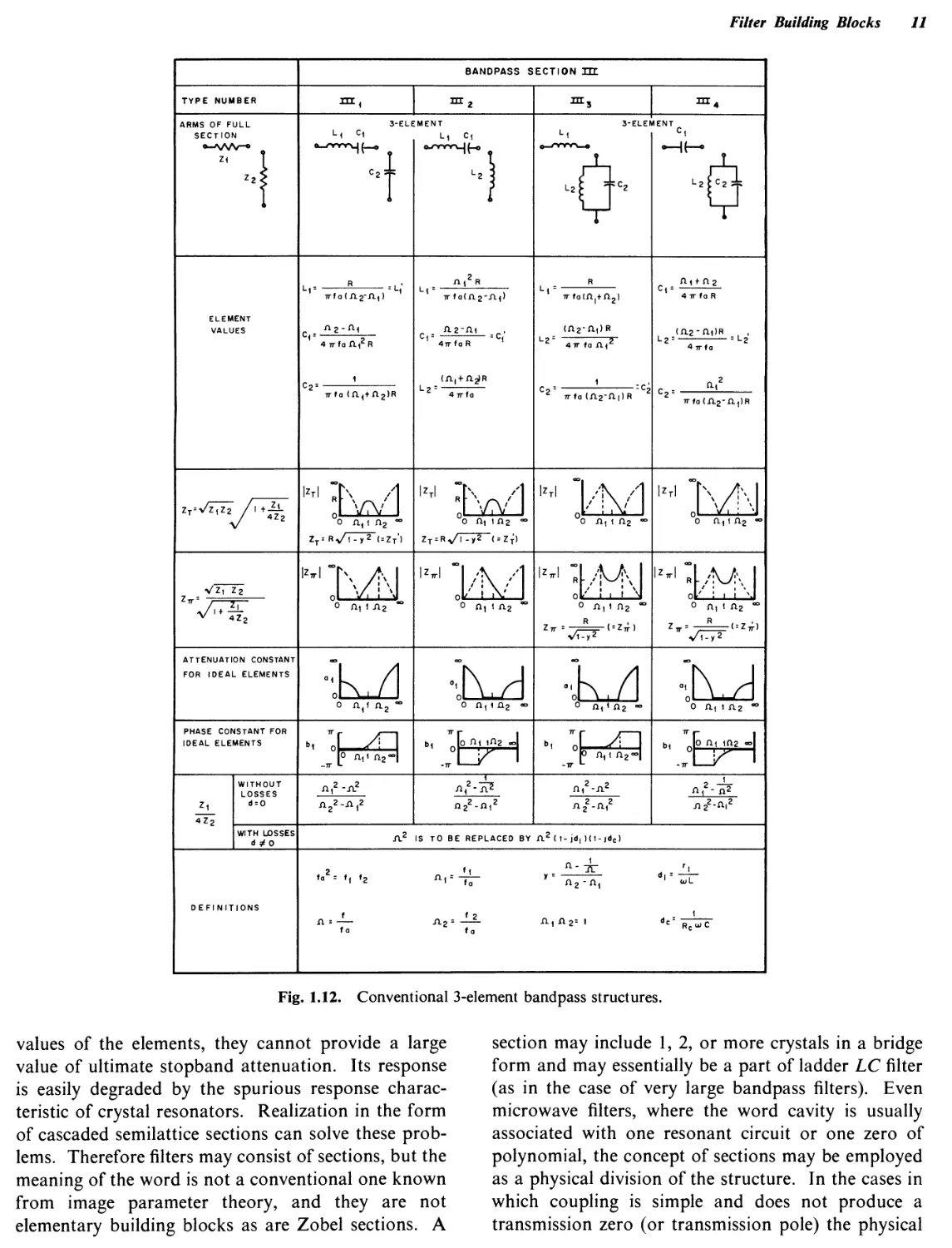
The image parameter filter charts shown in Figs. 1.10 through 1.14 provide design data and information necessary for the development of lowpass, highpass, and bandpass filters.
In the first row the schematics of the series and shunt
arms of the filter are given. These impedances Zx and Z2 as shown in Fig. 1.18, are known as the full series and full shunt impedances, and are the total series or total shunt impedance of a full symmetrical T or tt section. Therefore, in the construction of a full section ladder network of either the T or tt schematic, the impedances Z± and Z2 are modified and connected as shown in Fig. 1.19. The construction of a half-section schematic is shown in Fig. 1.20.
BANDPASS SECTION I ВТ
TYPE NUMBER ^3 дзе4
ARMS OF FULL SECTION 4-ELEM L1 4 L2 « сгХ T ENT L2 5 C2 X с Г" 4-ELE MENT
ELEMENT VALUES CM CM J7 w" c? G - - о ‘VI ” | 'I cm 8 cm 8 rJE - -I? -I’ * - L£J f г. “cm % см _i о _J о E E cm 8“ 8 -1 7 г г -ir ф ф Ilf 7 Д- см см "U с* <м _| о _1 о Е Е "см -см cj с: 1 ° "см 1 1 -- ФТ " J ~ У СМ 8 см 9 смЕ е ! Е Е Ч см см ’ | - Д. 1* 1Е е ci ci с{ L 'к М 1 _1 О -I О Е Е см 8 <*.8 ~ ’<? 3 . ? ? Е- |СМ -.1 CM CM CJ с W W сч 1 о т ™ см <ЕИ -к ё LtX « II „ И » " " — '4. см см — см _1 О _1 О Е Е
zT=V/7T 2 / 4Zz 0 Л, 1 Л2 «о ZT=R</l-y2 ( = Z7‘ ) 0 1 Л2 • ZT = R>/l-y2 (--ZT’) '-1 -| ol ( 1/М1 Э Л1 1 л2 «о Ол, Л(1 Л2 «о
Z Л * / i + zz_ ~Z1 4Z2 |г-' Ml 0 Aji ПгП2 ob;V °Л, (1,1 л2 ’° '-13 с 2ТГ * У/ !• > nt1 л2 • R - (=Z-^) • У 2 л,1 л2 -R Z7T" (-Z7T> <772-
ATTENUATION CONSTANT FOR IDEAL ELEMENTS о 1 Л2 Л2 0(1, n11 л2 ’° 0 ( э л< 1 лгПг’0 °JjLrl 0(1,0,! Л2 ’°
PHASE CONSTANT FOR IDEAL ELEMENTS ь, хмц. |0 Й11Л2Л2] in 7Г г М о| - 7Г 1 0 Л1 m2fl2j
WITHOUT LOSSES (П22-л2^)(Л2-П12} ((1 2-Л ,^)(Л2-Л 22 } (Cl2 ^(Л^Л,2) (Л12-Л|^о)(Л2-Л22)
zl 4Z2 d:O (Л22-Л|2)(П2^-п-2) (л22-л. 2)(П22«-Л2) (л,2-л22)(л,^-л2}
WITH LOSSES d# 0 Л2 IS ТО BE REPLACED BY Л2 (1- jd|)(1-jdc)
DEFINITIONS fa2 = f, f2 л= — fa Л|'77 Лг ~ ~77" R2<J " s’ 2„ л2-л, И л2-- 1 -Ц- 1 dcS^Jc"
Fig. 1.13 . Conventional 4-element bandpass structures.
Filter Building Blocks 13
BANDPASS SECTION 3E.
TYPE NUMBER = 2 T3 3T4
ARMS OF FULL SECTION 5-ELE Li Ci MENT 0 L. 5-ELEMENT L.
-|ci
.0
^0
ELEMENT VALUES Lf = m 1 Ц Ci -- Ci' L2= ₽Ll‘ 1-mi2 , L3=-77-L’ LT= L,' с,г — Cl' Сг'^г’' сзг 4-c’ L1= TL2' l-mf2 , С.= ^-Сг c2= pc2' L3 = L2‘ С3г m, C2 L,= 1-\’22 L2' Cr 7-c2 L2=VL2 L,= — L2' 3 m 2 Сз = С2‘
zt-Л^Т/-^ l"' ?W1 izri ;
0 1 П2 °° ZT= R V'-У2 <= 2т') 0 Af 1 Л2 • ZT = R-/l-y2 ’< =ZT’> Co Af 1 A2 • П2« OAfA^ A2 •*
V'Zi Z2 lZ7rl I z'V Л 1 Т/• 1 nL i i ! » 1 1 2Й 8 or c к N |гтГ|АА | R f / I 1 ' I nl/ j 1 1 \l |z,rl . о ' 'll''
ZTT ’ > ч -/♦ж ° Д.1Л2 <4 0 A,1 A2 *° Ai^ 0 Л|’Л2 “° z ТГ- . < - z 7T> Vi- y2 ( Г- 1 - 3 Л1«л2 ('z;: У 2 I
ATTENUATION CONSTANT FDR IDEAL ELEMENTS •CM 4. /1 ai 0 Ih./I
° a< 1 ЛгАг"0 0а<Л< 1 A 2 • 0 At 1A2n2“ 0A< А^ 1 Л2 •
PHASE CONSTANT FOR IDEAL ELEMENTS ь, u т Го 17TL1.. 1 °l / n2^l ТГ П -7Г • ’An,,/TI
ju- r l \/ Аг00]
Z| 4Z2 WITHOUT LOSSES d -- D WITH LOSSES d #0 9 s a + j b THE HL2 IN ПТ, | IS THE SUM OF g's FOF SAME VALUES OF A, | Ш, IN Ш2 | t THE TYPES SHOWN BELOW HAVING AND A2<e | Ш2 IN LSZf | Ш( IN Ш2
DEFINITIONS fa2= f2 A1<e= fl^A12-A12)(A22-A<^>) p A2^ Л -- -J- f2<e h= /\- -Чк-Ц - -Ц) 2 n2«-- V A2 A2t Л2« 1-m22 1 ai 1 +h 4 A,.2 fa n_ m s x- + h - f2 y s £_ n2« nz=77 лг-л, m p = jLj + 9 n.tn2= 1 ~
Fig. 1.14 . Conventional 5-element bandpass structures.
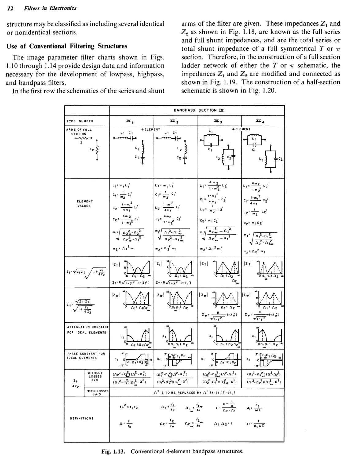
The element values of the impedance arms are given by the formulas in the second row of the design chart. For the more complicated sections, auxiliary parameters and definitions are given in the last row of the tables. The impedance of the T and tt schematics (or from the T side or tt side of a half-section schematic) is given in the third and fourth rows of the design charts. The fifth and sixth rows of the charts give the image attenuation and phase response respectively.
These, of course, have been drawn for the case of ideal elements. Finally, the value of the expression ZX/4Z2 is given in the seventh row of the design charts for both the lossless and lossy cases. This expression is useful in the evaluation of the impedance and transmission of the networks.
Lowpass Sections. Lowpass section 1 of Fig. 1.10 is the fundamental type and is characterized by its
14 Filters in Electronics
monotonic attenuation response. Both lowpass sections 2 and 3 are m-derived sections, providing a peak of attenuation at frequency Qx . It should be noted that 0 < m < 1, and for the lowpass sections
m = Jl- (7-/ (1-5-1)
J (X)
where is the cutoff frequency, and/x is the frequency of the attenuation peak. The phase shift in the passband for all lowpass sections is identical, 180° for a full section.
Lowpass sections 2 and 3 (Fig. 1.10) differ only in their impedance property. By inspection of the curves
of ZT and Z_, it becomes obvious that for the best matching conditions either a full tt section of type 2 or a full T section of type 3 should be used; that is, if from the point of view of impedance the m-derived filter is chosen, the resonant circuits are placed on the input and output sides. For best possible matching the optimum value of coefficient m is 0.62.
For a filter designed with the accent on a specific attenuation requirement, the peak of attenuation provided by the m-derived section could be used for that purpose, according to Eq. 1.5.1. If the impedance property of the network is not important, the resonant circuit could be placed within the network, and a
W
Fig. 1.15. (a) Lowpass filters in lattice and equivalent forms. (/?) reactance of arms Хг and X2 (see Fig. 1.1). (c) attenuation: (1) when Xx and X2 intersect (2) when Xr and X2 do not intersect.
Filter Building Blocks 15
Fig. 1.16. Highpass filters in lattice and equivalent forms.
saving of one element is achieved. For example, with lowpass section 3, the T configuration will consist of three capacitors and two inductors. Referring to Fig. 1.19(7, the schematic of Fig. 1.21(7 is obtained. On the other hand, the tt schematic of Fig. 1.216 consists of three capacitors and one inductor. The elements are obtained by applying Fig. 1.196 to the formulas of element values of type 3.
When the required attenuation is complex and the filter must provide more attenuation than one section can offer, several full or half sections can be connected together. The usual way of terminating the filter is to put ^-derived half sections at the input and output sides. For extremely complex filters mm-derived input and output half sections are necessary. The technique of connecting sections in tandem in the construction of a complex ladder is well known and no special treatment will be offered. It should be noted, however, that the amount of attenuation provided by each halfsection used can be determined from curve 25 of Chapter 3, Section 14.
Highpass Sections. The design of highpass filters are accomplished in a manner similar to that of the lowpass filter, and therefore no specific treatment is given.
It is necessary to understand that the parameter m as applied to highpass types 2 and 3 is
w=71 - (t)2 (l5-2)
x Ji'
where Д is the cutoff frequency and is the frequency of the attenuation peak.
Bandpass sections. Bandpass filters constitute the great majority of all filters designed to satisfy certain specific attenuation requirements. The most popular image parameter bandpass sections are those derived from the fundamental type 1г shown in Fig. 1.11. This fundamental (^-constant) type provides a monotonic attenuation response that is symmetrical about the center frequency on a logarithmic scale. The six-element m-derived sections I2 and I3 (Fig. 1.11) are
O— O
Zi
Fig. 1.17. Lattice bandpass filters.
Fig. 1.18. Series and shunt impedance arms, and Z2.
16 Filters in Electronics
(a)
(b)
Fig. 1.19. Construction of full sections—(a) T-schematic (b) 77-schematic.
similar to the m-derived lowpass sections, except that a bandpass response is obtained with geometric symmetry about the center frequency. One peak of attenuation /100 is at a frequency below the passband, and the other peak /2oo, is located above the passband, so that
(1.5.3)
The calculation of element values is more involved; the formulas include two m-values as well as several auxiliary parameters.
The impedance characteristic of the full section-тт schematic of type IIX, and the full section-T schematic of type II2 are not shown. For these configurations, which are usually not of interest, the impedance curves are functions of the peak positions.
The three-element bandpass filters, sections III of Fig. 1.12, are most popular in engineering practice. These networks are simpler in configuration and are more appropriate for filtering at higher frequencies than any of the other bandpass sections shown. In addition, for comparable bandwidths, the three element sections produce less insertion loss and are easier to tune than the other types. Therefore if an extremely sharp attenuation response is not required, these sections are superior to m-derived networks for bandwidths up to 10-20%. A monotonic attenuation curve is provided with less attenuation below the passband for sections I1IX and I1I3 and more attenuation below the passband for sections II 12 and 1114.
To add the versatility of a peak of attenuation, either above or below the passband, the four-element bandpass sections (type IV of Fig. 1.13) could be used. The peak of attenuation is controlled by the m-values defined in the chart, and the position of this peak does
The position of the peak of “infinite” attenuation is given by
m = Ji - (M = Ji - (1.5.4)
Jo ' J2x
Bandpass sections I2 and I3 differ only in their impedance characteristics as illustrated in the chart.
Bandpass sections IIX and 1I2 (shown in Fig. 1.11) yield schematics identical for sections I2 and I3 respectively. However, sections IIX and 1I2 allow greater flexibility in the positioning of the attenuation peaks; /100 is any frequency below the passband, and /2o0 is any frequency above the passband.
(1.5.5)
о----ЛЛ/V
Zt
(b)
Fig. 1.20. Construction of half-section.
Fig. 1.21. Full sections of lowpass type 3—(a) T-schematic (b) 77-schematic.
Coil-Saving Bandpass Filters 17
Fig. 1.22. Composite lowpass filter consisting of four half-sections or two full sections.
not upset the impedance characteristic in the passband. These sections are seldom used, since they are not economical in the case of complex networks.
The five-element bandpass sections are of interest for low-frequency applications, when a realization is required with the use of mostly one type of reactances. A full 7r-section of type V3 (Fig. 1.14) will consist of three inductors and four capacitors. In the case of networks including many of these sections, the realization will provide a remarkable economy, since fewer inductances than capacitances are required. If, at higher frequencies, the cost of inductances is less than capacitances, types Vx or V4 would be desirable.
1.6 HIGHER ORDER FILTERS
A combination of several building blocks like several stages of amplification is an effort to provide the desired filter response. The conventional way to produce a composite filter is to combine many halfsections in tandem or to use a higher order polynomial for synthesis. The sections must be of the same characteristic impedance if they are designed according to image-impedance theory. In the polynomial filter, the composite filter is a chain of components given by a high-order polynomial. The element values of such a filter is the result of continued fraction expansion of the reactance function and appears to be of the same physical structure as a conventional filter. The difference between synthesized and sectional filters is essentially that polynomial filters cannot be subdivided into sections. They are not a combination of sections in the classical sense. Figure 1.22 shows four blocks connected in tandem and is equivalent to four half-sections of a lowpass filter (lowpass type 1 of
Fig. 1.10) which reduces to a filter with three coils and two capacitors. An equivalent polynomial filter would consist also of three coils and two capacitors, the values of the elements being obtained from a fifth-order polynomial. Although the filter designed from the image-parameter approach has a configuration identical to the polynomial network, the values of the elements of these two filters will be different.
The realization of composite lattices, even with such stable components as crystals, is not always easy because of the necessity of achieving an impedance balance. Designers have therefore sought alternate building blocks, such as a combination of the lattice and the tandem form. Instead of complicated branches in one lattice, less complicated blocks may be connected together to overcome inconveniences. The network shown in Fig. 1.23 consists essentially of two semilattice blocks. In combination, they are equivalent to a more complicated semilattice which would require a much more difficult tuning procedure to meet the required performance.
It is interesting to note that the upper arm in each semilattice can be a regular piezoelectric crystal. The differential transformer is replaced by a differential capacitor in parallel with a transformer. This permits, for very narrow bands of frequencies, the input impedance to be kept high while the electrical center can be adjusted for better bridge balance. The lower arm in each bridge is a tunable capacitor that influences the position of the peak of attenuation.
1.7 COIL-SAVING BANDPASS FILTERS
In Fig. 1.24 the simplest and most usable bandpass filter configurations are tabulated. In order to produce
Fig. 1.23. Two-section semi-lattice filter equivalent to two lattices of Fig. 1.25.
18
19
20
Filters in Electronics
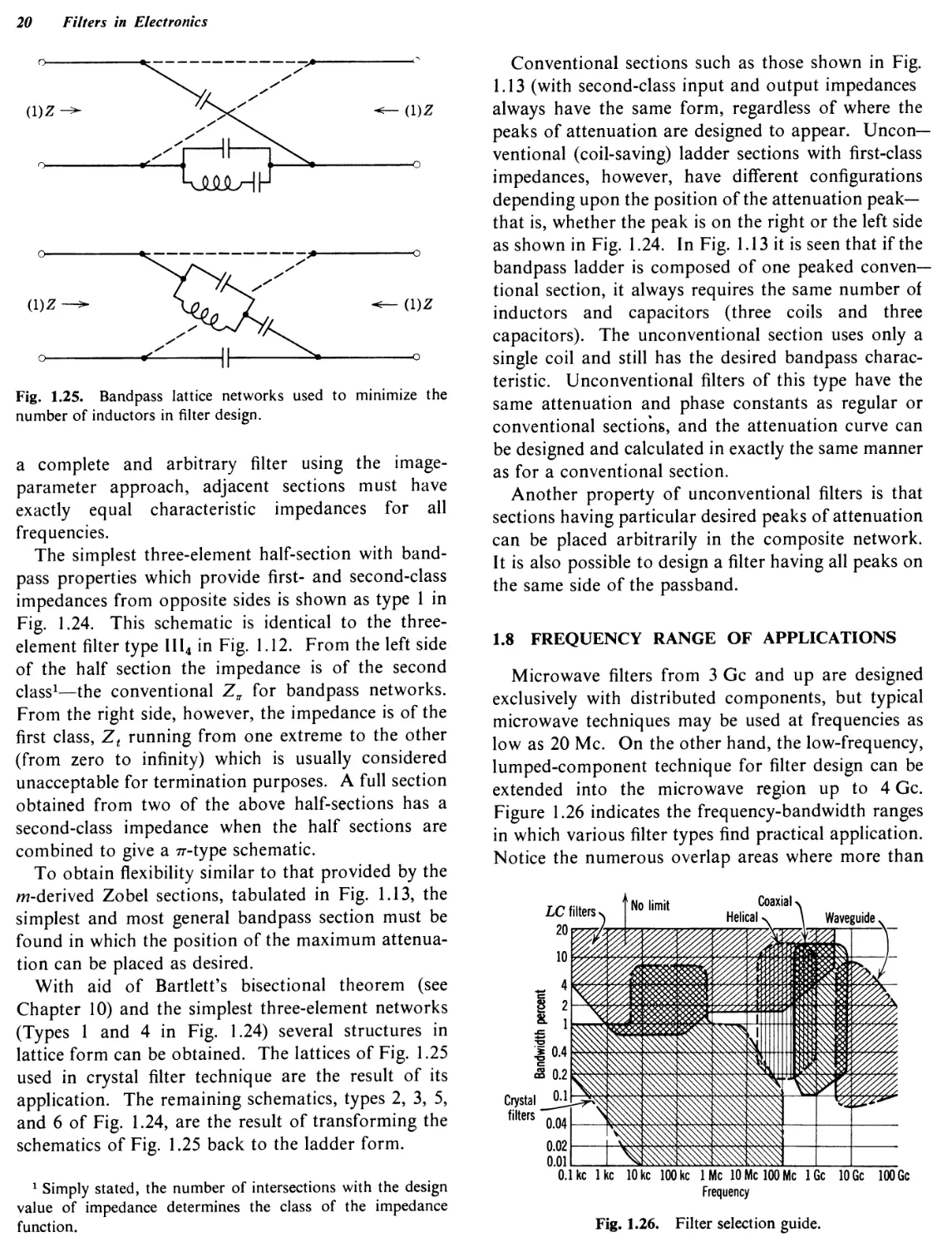
Fig. 1.25. Bandpass lattice networks used to minimize the number of inductors in filter design.
a complete and arbitrary filter using the imageparameter approach, adjacent sections must have exactly equal characteristic impedances for all frequencies.
The simplest three-element half-section with bandpass properties which provide first- and second-class impedances from opposite sides is shown as type 1 in Fig. 1.24. This schematic is identical to the three-element filter type III4 in Fig. 1.12. From the left side of the half section the impedance is of the second class1—the conventional Zn for bandpass networks. From the right side, however, the impedance is of the first class, Zt running from one extreme to the other (from zero to infinity) which is usually considered unacceptable for termination purposes. A full section obtained from two of the above half-sections has a second-class impedance when the half sections are combined to give a тг-type schematic.
To obtain flexibility similar to that provided by the ^-derived Zobel sections, tabulated in Fig. 1.13, the simplest and most general bandpass section must be found in which the position of the maximum attenuation can be placed as desired.
With aid of Bartlett’s bisectional theorem (see Chapter 10) and the simplest three-element networks (Types 1 and 4 in Fig. 1.24) several structures in lattice form can be obtained. The lattices of Fig. 1.25 used in crystal filter technique are the result of its application. The remaining schematics, types 2, 3, 5, and 6 of Fig. 1.24, are the result of transforming the schematics of Fig. 1.25 back to the ladder form.
1 Simply stated, the number of intersections with the design value of impedance determines the class of the impedance function.
Conventional sections such as those shown in Fig. 1.13 (with second-class input and output impedances always have the same form, regardless of where the peaks of attenuation are designed to appear. Unconventional (coil-saving) ladder sections with first-class impedances, however, have different configurations depending upon the position of the attenuation peak— that is, whether the peak is on the right or the left side as shown in Fig. 1.24. In Fig. 1.13 it is seen that if the bandpass ladder is composed of one peaked conventional section, it always requires the same number of inductors and capacitors (three coils and three capacitors). The unconventional section uses only a single coil and still has the desired bandpass characteristic. Unconventional filters of this type have the same attenuation and phase constants as regular or conventional sections, and the attenuation curve can be designed and calculated in exactly the same manner as for a conventional section.
Another property of unconventional filters is that sections having particular desired peaks of attenuation can be placed arbitrarily in the composite network. It is also possible to design a filter having all peaks on the same side of the passband.
1.8 FREQUENCY RANGE OF APPLICATIONS
Microwave filters from 3 Gc and up are designed exclusively with distributed components, but typical microwave techniques may be used at frequencies as low as 20 Me. On the other hand, the low-frequency, lumped-component technique for filter design can be extended into the microwave region up to 4 Gc. Figure 1.26 indicates the frequency-bandwidth ranges in which various filter types find practical application. Notice the numerous overlap areas where more than
Fig. 1.26. Filter selection guide.
Physical Elements of the Filter 21
one type may be selected. Since the behavior of distributed circuits operating in a limited frequency band closely approximates that of lumped inductors, capacitors, and resonant circuits, equivalent lumped ladder filter structures can be realized by distributed circuit elements.
Although microwave filter design methods are based on the filters used at lower frequencies, the structures themselves are radically different. Component parameters are distributed and hardware geometry is an integral part of the filter design.
1.9 PHYSICAL ELEMENTS OF THE FILTER
The main elements of a filter are reactances—lumped capacitances and lumped inductances. It is possible to design some filters by using only capacitors and resistors. This combination is especially useful in the case of active networks or active filters. Regular passive filters require both types of reactances.
To a first approximation, lumped inductance and capacitance can be considered as pure reactances, but closer investigation reveals that losses and reactive impurities are also present. The ordinary inductor at relatively low frequencies is wound on a magnetic core (powdered iron or ferramic); other inductors are simply single-layer solenoids wound on a nonmagnetic coil form. In both cases, although the losses are low in comparison with the value of reactance, they cannot be neglected, especially when one designs a very narrow band filter or desires a very sharp response curve.
Losses tend to decrease the rate of attenuation rolloff, increase the attenuation within the passband, and in certain cases, prohibit the realization of narrow bandpass filters. The parasitic effect of distributed capacitance across the coil or series lead inductance in capacitors is damaging in another respect. In the low-pass filter parasitics will create the effect of a parallel-resonant circuit instead of a coil. The filter may thus
-------------II-----------
о ..........°
(a)
-----Wv-------
о------------II-----------ППЯГ--------о
(b)
Fig. 1.27. Equivalent circuit of (a) inductor and (b) capacitor.
Fig. 1.28. Attenuation characteristics of narrowband bandpass filters having components of different quality factors.
provide unexpected rejection at certain frequencies in the stopband, or even in the passband if the self-resonant frequency of such a coil is sufficiently low. Parasitic reactances in lumped components produce distortion of the amplitude response and may destroy the network response altogether if not neutralized or properly taken into consideration.
Equivalent circuits for an inductor and capacitor are shown, with impurities taken into account in Fig. 1.27. The conventional measure of the quality of any reactance is the quality factor Q, which describes how many times the reactance of a coil or capacitor is greater than the resistance. The most common values of Q of conventional inductors at radio frequencies range from 50 to 300. The Q factor for the capacitor at the same frequencies is usually higher: 500 to 5000. The higher these values are, the better the filter that can be designed. Figure 1.28 illustrates the effect of Q factor on the shape of the response of a bandpass filter.
The demand for quality factor in ordinary lumped components, especially coils, has intensified research to find some substitute for the inductor and capacitor. Historically, the first and most successful substitute was the piezoelectric crystal; next were magnetostrictive components and electromechanical devices. Lumped elements are the oldest filter elements, and they remain the most widely used at low frequencies.
Experience proves that a very good bandpass filter can be made when its components have a Q factor not less than 20 to 25 times where f0 is the center frequency of the filter and Д/is the bandwidth (passband). For the same absolute bandwidth and attenuation characteristic, the filter with the lowest center frequency will need the lowest quality factor. If, for example,/, = 10,000 cycles and Д/ = 3000 cycles, the
22 Filters in Electronics
Q factor cannot be less than 66. When an element that meets these specifications is used, a very good bandpass filter can be designed for a commercial telephone signal. If the frequency f0 = 150,000 cycles and Д/ = 3000 cycles, the Q factor has to be greater than 1000. Even the best coils with ferramic core material cannot provide a Q factor greater than 600 and, therefore, conventional elements cannot be used in such a filter.
1.10 ACTIVE BANDPASS FILTERS
Active filters in most instances are bandpass amplifiers. The main requirement of a bandpass amplifier is to amplify a certain band of frequencies by a certain prescribed amount. Other requirements are the following:
Fidelity Requirements
To ensure distortionless amplification:
1. The amplification within the passband should not fluctuate by more than a certain amount, Лтах, thus resulting in a tolerable frequency distortion.
2. The phase-shift over the entire passband should not depart from linearity by more than a certain amount, thus ensuring a negligible phase distortion. This type of distortion is important in frequency and phase-modulated systems.
3. For pulse amplifiers the rise time, the overshoot and other similar phenomena should be as small as possible.
Selectivity Requirements
To prevent undesired signals from passing through, frequencies outside the passband should be strongly attenuated relative to frequencies within it. Bandpass amplifiers are in this respect similar to wave filters.
Gain-bandwidth Requirements
The gain-bandwidth product per stage of a multistage amplifier depends on the over-all passband width, the over-all gain, the number of stages, the gainbandwidth factor, the tube transconductance, and the total shunt capacity across the tuning coil.
In order to justify the added cost of an active device within a filter, some economic or engineering advantages must be evident. Some such advantages may be listed as follows:
1. The active device can furnish gain and hence may already be present in the system.
2. The design of a complex filter is easier if it is
made up of several sections separated by buffer amplifiers.
3. The alignment of an active filter with isolated sections is much easier.
4. With the advent of molecular and thin-film circuitry, it is possible to build compact and reliable active devices suitable for this application at a very low production cost.
5. For crystal interstage circuits, either a balanced input or output is usually required which is normally accomplished with a balanced center-tapped coil or transformer. In many circumstances molecular or thin-film devices can be used to perform this same function with an accompanying space and weight savings without a loss in reliability.
6. In multichannel comb filters one crystal resonator can be made to do the work of two if an active operational amplifier is introduced.
1.11 RC PASSIVE AND ACTIVE FILTERS
In the low-frequency audio range and even at sonic frequencies, all filters using conventional elements are cumbersome. At frequencies less than 1000 cycles, the Q factor of inductors are so low that a good resonant circuit is difficult to realize. The physical dimensions of coils and capacitors required for resonant circuits became very large and incompatible with modern circuitry using transistors, crystal diodes, and printed circuit techniques. Inductive components, in general, are obstacles in the development of modern low-frequency circuitry, and in filter technology they certainly block the road to progress.
The only way to solve selectivity requirements in this part of the spectrum is to synthesize filters without resonant circuits—RC filters as shown in Fig. 1.29. The advantages of RC filters are these:
1. Simplicity in manufacturing
2. Small physical dimensions
3. Low cost
4. Negligible sensitivity to external electrical fields 5. Practical for use at the lowest possible frequencies
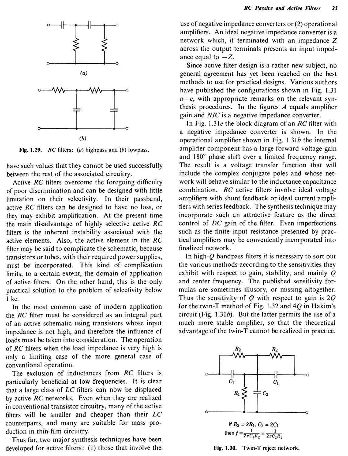
RC filters also exhibit some disadvantages. For instance, they do not have resonating properties and therefore the design of passive RC filters with good selectivity is difficult. One exception to this is the twin-T schematic (Fig. 1.30) characterized by narrowband suppression. Second, the frequency domain of their use is limited; they are unpractical above several hundred kc. This limitation can be explained by the fact that all capacitors in high-frequency RC filters
RC Passive and Active Filters 23
(a)
(b)
Fig. 1.29. RC filters: (a) highpass and (b) lowpass.
have such values that they cannot be used successfully between the rest of the associated circuitry.
Active RC filters overcome the foregoing difficulty of poor discrimination and can be designed with little limitation on their selectivity. In their passband, active RC filters can be designed to have no loss, or they may exhibit amplification. At the present time the main disadvantage of highly selective active RC filters is the inherent instability associated with the active elements. Also, the active element in the RC filter may be said to complicate the schematic, because transistors or tubes, with their required power supplies, must be incorporated. This kind of complication limits, to a certain extent, the domain of application of active filters. On the other hand, this is the only practical solution to the problem of selectivity below 1 kc.
In the most common case of modern application the RC filter must be considered as an integral part of an active schematic using transistors whose input impedance is not high, and therefore the influence of loads must be taken into consideration. The operation of RC filters when the load impedance is very high is only a limiting case of the more general case of conventional operation.
The exclusion of inductances from RC filters is particularly beneficial at low frequencies. It is clear that a large class of LC filters can now be displaced by active RC networks. Even when they are realized in conventional transistor circuitry, many of the active filters will be smaller and cheaper than their LC counterparts, and many are suitable for mass production in thin-film circuitry.
Thus far, two major synthesis techniques have been developed for active filters: (1) those that involve the
use of negative impedance converters or (2) operational amplifiers. An ideal negative impedance converter is a network which, if terminated with an impedance Z across the output terminals presents an input impedance equal to —Z.
Since active filter design is a rather new subject, no general agreement has yet been reached on the best methods to use for practical designs. Various authors have published the configurations shown in Fig. 1.31 a—e, with appropriate remarks on the relevant synthesis procedures. In the figures A equals amplifier gain and NIC is a negative impedance converter.
In Fig. 1.3 le the block diagram of an RC filter with a negative impedance converter is shown. In the operational amplifier shown in Fig. 1.31 b the internal amplifier component has a large forward voltage gain and 180° phase shift over a limited frequency range. The result is a voltage transfer function that will include the complex conjugate poles and whose network will behave similar to the inductance capacitance combination. RC active filters involve ideal voltage amplifiers with shunt feedback or ideal current amplifiers with series feedback. The synthesis technique may incorporate such an attractive feature as the direct control of DC gain of the filter. Even imperfections such as the finite input resistance presented by practical amplifiers may be conveniently incorporated into finalized network.
In high-Q bandpass filters it is necessary to sort out the various methods according to the sensitivities they exhibit with respect to gain, stability, and mainly Q and center frequency. The published sensitivity formulas are sometimes illusory, or missing altogether. Thus the sensitivity of Q with respect to gain is 2Q for the twin-T method of Fig. 1.32 and 4Q in Hakim’s circuit (Fig. 1.316). But the latter permits the use of a much more stable amplifier, so that the theoretical advantage of the twin-T cannot be realized in practice.
If Л2 = 2Л1, C2 = 2Ci
then f = = 2irC2RY
Fig. 1.30. Twin-T reject network.
24 Filters in Electronics
Fig. 1.32. Use of twin-T in active network.
(c)
(e)
Fig. 1.31. Examples of RC filters by (a) Sallen and Key, (b) Hakim, (c) Yanigasawa, (d) Dietzold, and (e) Linvill.
A close study reveals many other complications, indicating that only experience and much thought will eventually disclose the criteria for choosing an optimal design to meet a given performance specification.
Hakim’s method gives satisfactory results for obtaining fractional bandwidths as low as 2%. Narrower bands are obtainable but lead to alarming instabilities and alignment procedures that are difficult and expensive.
A method having the dimensions of a genuine breakthrough is shown in Fig. 1.33. Here the mechanical commutators, shown schematically, would be replaced in practice by transistor diode analog-gates driven by conventional logic circuits at an angular velocity, a>0. The identical RC circuits have a lowpass response which is so modified by the sampling action that VJV2 exhibits a related bandpass response centered at coo. This method shows promise of yielding figures for Q and stability which have previously been obtainable only with crystal filters. Definite results on the performance of this device will be available soon, but it is too new to be evaluated at present.
Figure 1.34 shows the response of a double-tuned circuit obtained by stagger-tuning two Hakim-type designs, each having a Q of 50. In the figure A represents an operational amplifier with a feedback loop
RC
Fig. 1.33. The digital filter.
Microwave Filters 25
/(cps)-----
Fig. 1.34 Response of a double-tuned circuit of the type shown in Fig. 1.31(b).
adjusted to give a stable gain of two, as recommended by Hakim. More recent calculations suggest that greater stability can probably be obtained by raising this figure somewhat and adjusting the other parameters to suit.
1.12 MICROWAVE FILTERS
In contrast with wave filters, which are designed with lumped components such as coils, capacitors, and crystals, the microwave filter is basically different. They do not include, as a rule, any lumped components. Their components are the distributed reactances of resonators. The simplest example of distributed resonators is a piece of symmetrical line or piece of coaxial line. On the other hand, every distributed component could be approximated in a certain frequency range and in a certain band of frequencies to only one type of reactance, capacitance or inductance, and consequently the synthesis of a filter will be to a certain extent similar to the low-frequency filter design.
It is difficult to describe a microwave filter but in the following text, the term microwave filter will be applied to any filter using coaxial, helical, or waveguide cavities or certain types of structures such as a piece of short line, or strip lines. Filters which include
only lumped elements of very small size and are used at microwave frequencies cannot be put in the category of microwave filters, since their design technique is conventional and does not constitute a special distinct category of microwave filter realization.
Filters with Distributed Components
A piece of transmission line may be used in a system as a filter element. It has a resonant frequency determined by the line impedance and the line length. A 3/4 wavelength line is equivalent to 1/4 wave resonator. In the same manner, a 1/2 wavelength line is equivalent to a full wave resonant line.
An electromagnetic wave propagating on a transmission line is continuously attenuated by the lossy elements in the line. When the transmission line is used as a filter component, this effect is apparent in the filter’s passband. The characteristic impedance of a transmission line depends upon the geometry of the line.
In Fig. 1.35 two pieces of symmetrical lines are shown. One line is terminated in a short circuit, the other in an open circuit. The input impedance of such lines with negligible losses is expressible as a trigonometric function; the first as the tangent and the second as the cotangent of the same argument. It is
26 Filters in Electronics
apparent from the figure that the impedance of the given transmission line can behave as a capacitance, inductance, series resonator, or parallel resonator, depending upon the relationship between the length of the line and the wavelength.
One of the most familiar techniques for approximating the characteristics of a lumped reactance at UHF and microwave frequencies is the use of short lengths of open-circuited and short-circuited transmission line sections. Two-terminal networks made from sections of coaxial line are characterized by a relatively high quality factor (1000 and up) and therefore are very useful for UHF circuits.
A stub of short-circuited line very closely approximates a lumped inductance and a stub of open-circuited line behaves as a lumped capacitor, provided its length is much less than a quarter of a wavelength (see Fig. 1.35 between I = 0 and / = Я/4). These can be placed in parallel with a longer strip of coaxial line by connecting them at right angles to the longer line. Stubs can be connected in series with coaxial lines by reentrant lines which may be placed in series with either the outer or inner coaxial conductor.
The series connection can be realized with a rectangular waveguide by placing a stub at the top wall of the waveguide. A stub connected to the side wall of a rectangular waveguide appears in parallel with the main guide. If the width of the stub line is not an appreciable fraction of the wavelength, it acts only at a single point along the line and reflections from discontinuities become significant. Similar considerations apply when the series stub in the waveguide has a high impedance.
Since series stubs are not convenient to use with strip transmission lines, other techniques must be employed to approximate series lumped elements in these lines.
The limitations of the technique of parallel connection of stubs are much the same as those for cascaded lengths of line—that is, the lengths must be short compared to the wavelength, yet long enough that the effects of discontinuities are fairly small compared to the value of the main reactive elements. Fortunately, the elements for practical lowpass and highpass filters fall within usable ranges for coaxial and strip transmission lines. The discontinuities at
Fig. 1.35. The impedances of short- and open-circuited transmission lines are given by the curves as a function of length. The circuit symbols above the curves indicate the associated lumped equivalent of the line impedance at various points along the two transmission lines.
Microwave Filters 27
Fig. 1.36. Schematic representation of a microwave filter having n cavities.
the junction points in waveguides, however, are frequently so large that lumped-element approximation may not be desirable.
Cavity Filters
Narrow bandpass filters require high-Q resonant circuits and wide variations in characteristic impedance for their constituent elements. Approximation of lumped elements by short lengths of transmission line which have inherently limited quality factor and impedance variation does not lead to practical structures. A similar situation at low frequencies leads to extensive use of coupled resonant circuits and consequently to a narrowband structure. Such structures are also used at VHF, UHF, and microwave frequencies. Here the resonant circuits are usually resonant cavities, since ladder structures can be realized by coupled-cavity resonators. The basic coupled-cavity filter structure is shown in Fig. 1.36.
A newer design, based on quarter-wave coupled cavities, incorporates the susceptances of the coupling elements into the susceptances of the cavity irises to form direct-coupled filters. This design permits filters of greater bandwidths (up to about 20% of resonant frequency/0), to be realized.
Whether physical quarter-wavelength coupling or direct coupling is used, it is necessary to include quarter-wavelength coupling lines in the analysis. If physical coupling sections are used, the electrical length varies with frequency, producing an error that increases as (/ — f0) increases. The designer generally ignores the frequency sensitivity of the couplings and uses the concept of narrowband approximation. If the coupling is incorporated in the filter elements, the frequency sensitivity is reduced. This reduction is the main reason why direct-coupled filters corresponds to the design equations over a much greater bandwidth than filters coupled by physical quarter-wavelength sections.
A practical coaxial resonator generally consists of a cavity with a quarter-wavelength center post inside. Energy is introduced into the cavity by inductive loops,
capacitive probes, and the like, and the output is taken by similar means. Conventional coaxial resonators are generally used for filters in the range of 200 Me to 6 Gc. A typical three-cavity coaxial filter is shown in Fig. 1.37.
Coaxial-resonator Q factors are usually very high, making them suitable for most high-quality filters. In the VHF range, however, coaxial-resonator construction becomes bulky compared with active circuit components. The length of a quarter-wave coaxial resonator at 100 Me, for example, is 75 cm or about 30 in.
The physical explanation of coaxial-cavity filtering may be given with the help of Fig. 1.37. Since maximum current is concentrated at the bottom of the center posts, magnetic flux is at maximum there and can be used for magnetic coupling between cavities. This is accomplished by mounting the coupling loops close to the posts. The induced current into an adjacent resonator cavity produces a magnetic field and excites the resonator. The amount of energy introduced into the second cavity is determined by the size of the loop, its proximity to the center post, and the Q factor of the loop. The coupling loop is a lumped element similar to ordinary coils used at low frequencies.
The helical resonator provides a solution to many difficult filter problems in the VHF range where the conventional coaxial resonator is not applicable. Helical filters fill an important “void” in the
Fig. 1.37. Typical three-cavity coaxial filter.
28 Filters in Electronics
Fig. 1.38. Helical resonator.
frequency spectrum. The resonators are similar to other quarter-wave configurations except that the inner conductor is in the form of a single-layer solenoid (see Fig. 1.38). The Q factor in the VHF range is on the order of 1000. Helical resonators are most useful in the region of 20 to 500 Me, where lumped elements and crystal resonators cease to be practical but where coaxial cavity resonators are still too large. They can be used equally well for narrowband or wideband filters, up to 20% of center frequency and can be extremely useful even for higher frequencies when a Q factor between several hundred and 1000 is sufficient.
Both the helices and the cavities are made from highly conductive material such as copper, brass, or aluminium. Each dimension of the helix and the cavity is mathematically related to all the other dimensions of the resonator. The design of a helical filter will be treated in Chapter 9.
At higher frequencies, where the quality factor has to be above 1000 to satisfy the filter design, even the coaxial resonant cavity becomes inefficient. A different kind of resonant cavity is used for narrowband filters at these frequencies. This cavity is essentially a piece of waveguide separated by partitions as shown in Fig. 1.39. Like any other closed cavity with conducting walls, it has an infinite number of discrete resonant frequencies, each corresponding to a different configuration of electromagnetic fields in the cavity. For any one of these resonant modes, the cavity is in many ways like an ordinary resonant circuit and its behavior may be described in terms of three ordinary resonant
Fig. 1.39. Typical 3-cavity waveguide filter.
circuit parameters: center frequency, Q factor, and characteristic impedance. These parameters will, in general, have different values for each of the possible resonant modes.
Stripline Filters
Stripline multiple-coupled resonator bandpass filters are made of half-wavelength strips coupled end-to-end or alternately parallel-coupled as shown in Fig. 1.40.
Parallel coupling offers many important advantages over end coupling since the length of the filter is reduced and symmetrical insertion loss versus frequency response is obtained. The first spurious response occurs at three times the center frequency, and a much larger gap is permitted between parallel adjacent strips. The gap tolerance is also reduced, permitting a broader bandwidth for a given tolerance. The larger gap also permits higher filter power ratings.
Comb- and Interdigital-line Structures
Transmission-line bandpass filters in the form of cascaded cavities or other forms become inconveniently long. A type of filter with resonant lines put side by side, known as a comb structure, results in a more
f----1 F~T—
End-coupled
Fig. 1.40. Stripline arrangements.
Parametric Filters 29
compact package. Transmission-line elements in a comb-line filters are short-circuited at one end and have lumped capacitance between their other end and the ground. A set of filters consisting of such lines is shown in Fig. 1.41. Two impedance-transforming sections are at the ends of the filter, and the loading capacitances are at the top of the posts. The length of the lines is less than a quarter-wavelength at center frequency. Coupling between resonators is achieved by means of fringing fields between resonator lines. In the arrangement shown the coupling is predominantly magnetic.
If the loading capacitances were not present, the resonating lines would be 1/4 wavelength long. The magnetic and electric coupling effects would then cancel each other, and the comb-line structure would become an all-stop structure. Usually it is desirable to make the loading capacitance in this filter large so that the resonator will be 1/8 wavelength or less. The resulting filter will be small, permitting efficient coupling between the resonators. In this type of filter a second passband response always appears. When these lines are only 1/8 of the wavelength at the fundamental frequency, the second passband will be located at slightly over four times the fundamental center frequency.
(=!□□□□ □-□ □
Resonator
Fig. 1.42. Interdigital bandpass filter with n transmission-line elements. Note that alternate ends of the lines are grounded.
Comb-line structures find very broad application in microwave technology. Their attenuation above the primary passband is very high and depends on the electrical length of the resonator lines. Attenuation through the filter is infinite at the frequency for which the resonator lines are 1/4 wavelength long.
The attenuation band of this filter can be very broad because spurious responses can be easily removed. Adequate coupling between resonator elements can be maintained with sizable spacings between physical lines, and this imposes no stringent requirements on tolerances. Filters of this type can be fabricated without the use of dielectric support materials; consequently dielectric losses can be eliminated.
The interdigital filter has the same advantages of the comb-line filter. An example of an interdigitalfilter arrangement is shown in Fig. 1.42. When alternate unloaded quarter-wave resonators in a comb filter are turned end-to-end so that the structure has open- and short-circuited ends alternating, the bandstop becomes a bandpass structure, and we have an interdigital filter. Although comb-line filters are somewhat smaller and are capable of broader stopbands above the primary passband, the resonators in the interdigital structure attain higher quality factors. Interdigital filters have very strong stopbands and moderate coupling tolerances.
Fig. 1.41. Frequency multiplier utilizing comb-line filtering structures.
1.13 PARAMETRIC FILTERS
In Fig. 1.43 a block diagram of a parametric filter is shown. The LC filter shown in the left side of the diagram, in a receiver, is a tunable circuit which can cover the frequency range of operation. The output is fed into a parametric up-converter which is basically
30 Filters in Electronics
(a)
Fig. 1.43. Parametric filter: (a) block diagram and (b) ampli-
tude response.
a mixer and is incidentally a parametric amplifier. The pump signal generator, in essence, is a tunable local oscillator. The pump signal is always much higher in frequency in an up-converter and is higher in power than the incoming signal. Therefore, the mixed
product is of a much higher power level and at a higher frequency.
The signal is now filtered by a relatively narrowband crystal filter. In Fig. 1 Alb the response of the filter is shown. From the flat curve at the bottom it is seen that the response of the LC filter is poor compared to the crystal filter. Its prime function is to act as an impedance matching device between antenna and the parametric up-converter. The necessary selectivity of this receiver front end is provided by the crystal filter. The corresponding curve shows that the filter has both a narrow bandwidth and superior selectivity.
The parametric up-converter is not only a mixer that provides a fixed frequency (sum of pump frequency and signal frequency can always be adjusted by changing the frequency of the pump frequency) but also a low noise amplifier. Over the entire tuning range the output frequency is always constant. The higher the output frequency, the greater the gain that can be realized. The only limitations in this direction are the realizability of the output filter and the stability of the pump oscillator.
The parametric filter can handle extreme levels of input signals simultaneously primarily because of the high pump-power level. This ability is in itself no assurance of interference-free reception. However, since both the desired and undesired signals pass through the up-converter without interaction, the undesired signal will eventually be rejected by the output filter.
Theory of Effective Parameters
There are two competitive methods of filter design. One was originated by Zobel and is well known as the image-parameter method. The second was originated by Norton and Bennett and is known as the exact method, polynomial method, or insertion-loss method.
The image-parameter theory filter is based on the properties of transmission lines. A simple network with lumped components is described in terms of this continuous structure. Several of such elementary networks with equal characteristic terminal impedances, connected together to produce a chain of ladder networks (or a composite lattice), will possess a transmission constant equal to the sum of all the individual transmission constants of the elementary sections.
In the image-parameter theory, the starting point is the impedance system given by equations and the impedance matrix. The parameters of the network are expressed in terms of the characteristic impedances and the image transmission factor. Image-parameter method of filter design is analytical in nature.
In the effective-parameter theory, the starting point is the effective attenuation and the echo attenuation (reflection). The effective values characterize the behavior of the network. Here, the operational boundry can be more closely and economically approximated. Wave or characteristic impedances play no role in the effective-parameter theory. Filter design technique based on this method is essentially a synthesis.
The image-parameter method seems to be in disrepute among the network theorists partially because of the cut-and-try method that is involved and partly because of the restricted freedom of design. The practical significance of the limitation, however, does not seem to have been adequately explored. Also, very little seems to have been done in applying the results of modern theory in an effort to improve the older
design procedure. Polynomial synthesis deals directly with effective parameters and provides an elegant solution to the approximation problem, but it also involves laborious computation for the determination of the element values. This procedure is now greatly simplified by tables, step-by-step design procedures, and design curves. But the theory behind all this is still one for the specialist. In the more general synthesis procedure, a greater range of designs is possible and greater stopband loss can be obtained at the price of greater ripple factor.
The reflection coefficient is directly related to the insertion loss. To obtain a low reflection coefficient it is usually necessary to design an image-parameter filter for flatter transmission than would otherwise be necessary. The filter synthesized by polynomial methods has no practical limitation, even for an extremely severe requirement, such as 5% reflection or lower.
The more general synthesis procedure is always preferable when maximum stopband loss must be obtained at the expense of higher passband ripple, or where very flat transmission is needed to secure low reflections. The result of image-parameter theory can be regarded as a special case of effective-parameter theory.
The fault of the Zobel design is usually not that it cannot give sufficiently flat transmission, but that the transmission is too flat and discrimination is lost in consequence. The Zobel filter approximated in the Chebyshev sense (with the aid of elliptic functions) still has essential limitations in comparison with the modern filter. In practical terms this means that only one Zobel design is possible, having a particular level of passband ripple for each width of transition region.
In practice, either method of calculation can be used,
31
32 Theory of Effective Parameters
depending on the requirements in each specific design case. Fora more economical filter and quicker development, especially when the filter is very complex, the use of image-parameter design technique is certainly justified. In certain other cases, when the requirement accents the minimum number of elements to satisfy an exact performance, it is better to use the optimal design of the effective parameter method. This method certainly is worthwhile for mass production.
In this chapter information as to the theory of effective parameters, the elements of the synthesis procedure, will be described. The purpose is to indicate the scientific background of filter design without exhausting the subject matter.
2.1 POWER BALANCE
The typical operating conditions for a filter are shown in Fig. 2.1, where 7?! and R2 are pure resistances. The output power P2 in the ideal case of matching (and with purely reactive elements) is equal to the maximum deliverable power Pm of the generator. If Vo is the source EMF, the maximum deliverable power is Pm = V^Rv
Ideal matching is understood as the matching of both pairs of terminals, that is, between the load resistance R2 and the network output and between the generator internal resistance 1?! the network input. So seldom is ideal matching achieved that in every practical case a complex power distribution is taking place within the network. Several components of the power must be considered.
1. The power P2, which dissipates in the load.
2. The power Pr9 which is reflected back to the generator as a result of mismatching.
3. The power PLi which is dissipated in the network as a consequence of unavoidable losses in the components.
The sum of these three components must be equal to the maximum deliverable power according to the power balance relation Pm = P2 4- Pr 4- PL. All
Fig. 2.1. Typical filter operating conditions.
three components are frequency dependent. Although Pm remains constant, the contribution of the variable components is a function of frequency. The equation can be modified so that power balance will be expressed by
P / p p \
1 =——— —4-— (2.1.1)
P p \p p j '
1т 1 L 1 m 1 m
It has been assumed that all losses are concentrated in a separate section preceding the purely reactive network.
The effective attenuation is defined as
a = |ln — (2.1.2a)
^2 where
and H is the transmission factor. The attenuation a is in nepers. When the decibel unit is used
A = 20 log \H|
Reflective or echo attenuation is
ae = 1 In (2.1.2b)
or P 1 2
__ e^ae _ ± _ |j-|2
p
is the squared magnitude of the reflection function. Also, the power loss in the network is
flb = iln Pmp (2.1.2c) where
—^2— = e2ttL = fc2
Pm ~ Pl
is the power loss factor in the loss section. Equation 2.1.1 has, therefore, the following form:
1 = e2aL(e~2a + e-2“‘) = k2(-±- + |P|2) (2.1.2J)
\|H|2 /
1 = к2([(Г0Л-4 + 10~°M‘)
From this, the transmission function can be found
|W| = kJ 1 +
= ea = kjl + |D|2 (2.1.3)
where D = H/T is known as the discrimination or filtering function or, more often, as the characteristic function of the network.
Types of General Network Equations 33
If pL = 0, then к = 1, and aL = 0. For a purely reactive network where losses are nonexistant a = In (1 + D2) since
|Я| = Vi + |D|2 (2.1.4)
and the expression for energy balance will be given in the form
e-2« + e-2ae = ! (2.1.5)
Equation 2.1.5 can be written
e2a = 1 + e2{a~ae)
The filtering factor which characterizes the amplitude discrimination is
and therefore,
a — = In |Z>| (2.1.6)
a = —In V1 — p2 Np
A = -10 log (1 - p2) dB
The effective transmission factor H and the discrimination D are both functions of frequency f and both are needed to determine quantities such as impedance, admittance, or the chain matrices. When the quantities H and D are expressed as functions of complex frequencies then each of the functions will be a rational function and represented by the ratio of two polynomials in 5.
In the filter theory to be developed, we operate with the transmission function H(s) defined as the inverse of the transfer function
The conditions that H(s) must satisfy for filters having a finite number of lumped components will be given later in the text.
The relationship between echo attenuation, effective attenuation, and the reflection coefficient p can be
Fig. 2.2. Nomograph relating ae, a, and p.
easily represented by a nomograph, as shown in Fig. 2.2. The abscissa represents effective attenuation and simultaneously shows the value of the reflection coefficient which must be multiplied by 100 to obtain p in percent. The ordinate represents the echo attenuation in nepers. To determine the value of reflection coefficient and the corresponding effective attenuation the procedure is:
1. On the abscissa choose the given value of the reflection coefficient and project that value up to the p line.
2. Project that value on the a line parallel to the abscissa.
3. Project the value on the a line down to the abscissa and read the value of effective attenuation in nepers.
For example, the reflection coefficient is 10%, corresponding to a value of the abscissa of 0.1. An intermediate reading on the ordinate indicates 2.3 Np echo attenuation ae. The intersection of this projection and curve a when projected on the abscissa corresponds to 0.005 Np or an effective attenuation of 0.043 dB.
The relationship between effective attenuation and the filtering function D can also be represented in the form of the nomograph shown in Fig. 2.3. The ordinate is the natural logarithm of D. On the left side negative values of In |Z>| are shown (for small values of Z>), and on the right side positive values are plotted for larger values of D. The larger values of D correspond to larger values of effective attenuation a in nepers. The use of this chart needs no special explanation.
2.2 TYPES OF GENERAL NETWORK EQUATIONS
In Fig. 2.4 a four-terminal network is shown. According to the Kirchhoff’s laws, the following
34 Theory of Effective Parameters
Zn Z12
Z21 Z22
Fig. 2.4. Four-terminal network.
equations can be written
Ki = T /2^12
(2.2.1)
F2 = Л^21 T ^2^22
or, Л= ПГиЧ- И2У12 /2= угу21+ У2У22
The first pair of equations is known as impedance equations and the second pair as admittance equations. From the impedance equation it follows that when /2 = 0 (a secondary open circuit),
Zn = y1 primary open-circuit input impedance
к . . (2-2-3)
Z21 = — transfer open-circuit impedance
When Д = 0,
y2
Z22 = — secondary open-circuit input impedance ^2
v (2.2.4)
Z12 = — transfer open-circuit impedance
^2
From the admittance equations it follows that when V2 = 0 (a secondary short circuit):
Уп = у primary short-circuit admittance
I2 (2*2*5)
У21 = ~ transfer short-circuit admittance
Vi
and when Vr = 0 (a primary short circuit)
У22 = у secondary short-circuit admittance
/ (2.2.6)
У 2 = — transfer short-circuit admittance n
For passive networks generally Z12 = Z21 and У12 = У21. All of the above values are measurable and can be expressed in terms of network elements.
Table 2.1 Network Equations and Physical Meaning of Network Parameters
Impedance System Admittance System Chain System . =z11z1+z12z2 Л = + r12r2 = AY2 + BI2 Network equations Г2 = Z21ZX + Z22Z2 4=^1^1+122^ л=сг2+п/2
Matrix ||Z|| = to to nil = У11 У12 У21 У22 \\M\\ = A В C D
Open Cir Impedan z 11 " Л Physical Z12 = — meaning of network parameters ^21 = ~f f2 Z22 = -7 y2 cuit Short Cir ces Admittar Y П ” Y 7^0 12 " v2 I2 Y21 = y z2=o ki /2 У — —- Zi-0 Г2 JI J! JI Sc "ii 'll 5i 11 -• © © © © b n bo H 0 II II II II g <1? к*. 1 4. . 1 1 1 сл О C ^I> ^1^ ^1^ 3 - О rcuit ge ssion Z 2=0 f2=o 12=0 72=0
Effective Attenuation 35
A different representation of network values can be given by the third pair of equations
V. = V2A 4- I2B
Л = 4- 72£>
(2.2.7)
with a chain matrix given by
\\M\\ =
A В
C D
The determinant of the chain matrices
\M\ = \AD - BC\
has, for all reversible networks, the value one. [Non-reversible networks are those transmitting energy differently in different directions (unilateral) and contain amplifiers or girators.] This form (2.2.7) is especially important and advantageous when several networks are connected in a chain.
The values of Л, B, C, and D are given by
A = = —
Z12 ¥12
B = _L = zuz22 - z122
712 Z12 (2.2.8)
C = _L = У11У22 ~ V
Zi2 Y12
D ___ Z22 _ Jjj
Z12 Ti2
The values А, В, C, and D can be expressed with measurable parameters or can be described in terms of the constituent network elements. Since the filter’s network elements are frequency dependent, the above coefficients are functions of frequency. The exchange of input and output terminals corresponds to an exchange of A and D. With the aid of Eqs. 2.2.8 the open-circuit and short-circuit impedances can be represented as a quotient of two matrix elements so that
Zu = — , = — , Z22 = — , Y22 = — (2.2.9)
С В С В
In Table 2.1, equations describing four-terminal networks are summarized, and the physical meaning of the coefficients are given.
2.3 EFFECTIVE ATTENUATION
Effective attenuation has been defined as half of the natural logarithm of the power ratio (output power P2,
to maximum available power Pm):
p v 2 p
e2“ = ^ = ^-^ = |H|2 (231)
Л 4/?! K22
The transmission function H can be represented as
H = eB = ea+,i> = - — /— (2.3.2)
2 V2 V R,
Often instead of the transmission function H, the natural logarithm of H is used, and called the effective transmission constant g.
g = \nH
Its real part is the effective attenuation and its imaginary part is the effective phase angle b.
g = a +Jb.
According Therefore,
e”
to Fig. 2.1, the value
of I2 = V2/R2.
1 /r2 + RJ / f
2 V R1 VoZ1 \
В r2
From the chain equation (2.2.7) the value of Zx can be expressed by
Fi _ A + BjR2 1, C + D\R2'
(2.3.3)
and by substitution in the previous expression for the transmission function,
For further discussion it is advantageous to introduce normalized impedances and admittances so that all Zik and Yik (also R2 and R^) are related to Rv
In normalized form,
(2.3.5)
(2.3.6)
36 Theory of Effective Parameters
the equation for the transmission function will be
e* = + b + c + d) = H (2.3.7)
Physically, the normalized functions in the form of (2.3.6) can be interpreted as if a network had an ideal transformer with К = just before the terminating resistance. Figure 2.5 shows such a network.
Evidently, from (2.3.6) and (2.3.7), the transmission function H can be expressed by Zik or Yik or by the reactive element values of the network.
Let us consider the circuit shown in Fig. 2.1 with R across the load instead of the reactive network A. The transmission coefficient, expressed by the ratio of the maximum available power of the generator and the power consumed by the termination resistor R2 is
where is the internal resistance of the generator. Obviously, the amount of the last term of this equation will be less than unity only for negative values of R. This means amplification exists. Further pursuing this train of thought, it can be shown that the whole network can be consuming more energy than fed in by the generator. In this case, we are dealing with an active network.
Before proceeding, it must be pointed out that the scope of this book is restricted to linear time-invariant networks. By combining a finite number of resistors, capacitors, coils, and ideal transformers having only positive element values we obtain a passive network which will neither produce nor consume more energy
than forced in any port. The passive network, however, is only one particular type of network. When extending the element values, especially those of resistors, to the negative scale, we obtain networks able to produce or deliver more energy than is forced in. An amplifier, for example, can be built out of a single negative resistor.
2.4 REFLECTIVE (ECHO) ATTENUATION
A similar operation can be performed to express the reflection function (2.1.26)
e2“« = |T|2 = — (2.4.1)
Pr
in terms of the a, b, c, and d parameters.
Since the power
(V! - Vp/2)2
r R1
and
where Ko is the open-circuit voltage of the generator and Ri is the resistance of the generator equal to the load resistance and matched with the network
impedances), ea‘ = |T| = П/2 У1 - Ц./2 = y0 2K - Vo (2.4.2)
The voltage Vx may be determined from the parameters of the four-terminal network shown in Fig. 2.1:
У1 = y0 ——— = y0 -Z1IR1------ (2.4.3)
°z1 + k1 °(ад) + 1
From Eqs. 2.4.2 and 2.4.3 (and dropping the sign of
Transmission Function as a Function of Frequency Parameter, s 37
the absolute value for T),
(2.4.4)
It is easy to show that with normalized network coefficients and Eq. 2.3.3, the reflection function is expressible by the values of the network elements. In terms of the a, b, c, and d parameters:
Fig. 2.6. Examples of odd functions.
д 4- b + c 4- J a 4- b — c — d
(2.4.5)
2.5 TRANSMISSION FUNCTION AS A FUNCTION OF FREQUENCY PARAMETER, s
For the following discussion, Eq. 2.1.4 will be used:
W = J1+ 2 = Vi + |D|2 (2.5.1)
with the network coefficients introduced for both the transmission function and the reflection function, the expression for the filtering function becomes
D _ H _ |(a 4- fe 4- c 4- d)(a + b — c — d)
T a 4" b 4” c 4" d
= l(a + b-c-d) (2.5.2)
The elements of the chain matrix a, b, c, and d are functions of two-terminal impedances zlk or admittances угк and consequently are always functions of joy, or of normalized jQ = 5.
According to Foster’s theorem, any combination of pure reactances in complex two-terminal networks can be expressed by a reactance function with the following properties: (1) The reactance function must be a rational function of the frequency parameter with positive coefficients, and (2) the numerator of the function is always an even (odd) function1 of 5 = jco, and
1 When the mathematician speaks of an odd function he means one like ж, ж3, a?5, and so on, for which
/(5) =
For instance, consider the function x3. If x = 2, x3 = 8, and if x = —2, x3 = —8. The equation above is therefore satisfied and x3 is an odd function. The name odd function comes from the number in the exponent (see Fig. 2.6).
An even function, on the other hand, is one like а?2, z4, z6, and so on (with even exponents) for which
/(5) =/(-5)
For instance, if x = 2, x- = 4, and if x = —2, x2 = 4 also (see Fig. 2.7).
the respective denominator is always odd (even). Physically, this signifies that the impedance or admittance of the reactive network always increases in value when the frequency is increasing and the quotient of voltage and current is always imaginary.
Figure 2.8 shows an example of a reactance function. The reactance function has the mathematical form
= (2.5.3)
(s 4- )(5 4- W4 )
when co22 < co32 < co42
For 5 = jay being odd, the function is purely imaginary and always increases with increasing frequency.
Figure 2.8 shows the plot only for positive ay when X(s) is an odd function. More often, a simpler reactance diagram is used—a pole-zero plot. This pole-zero plot shows only poles and zeros on the positivefrequency axis. Every zero and pole in Fig. 2.8a at finite frequencies represents a pair of zeros or poles in Fig. 2.8Z>. Such pairs are indicated by circles (zeros) or crosses (poles). Poles and zeros at co = 0 or co = 00 are indicated by half marks, as shown in the diagram. Therefore the figure represents a reactance function with five poles and five zeros.
The poles and zeros of the reactance function alternate. A similar property is exhibited by the reactance function with equal losses in the network elements. This property permits one to extract the lossy elements common to both reactances from a lattice filter and place them outside the lattice in the load circuit without changing the filter’s performance. When
Fig. 2.7. Examples of even functions.
38 Theory of Effective Parameters
a network is lossy the impedances will be expressed with a different frequency parameter having the form s' = s 4- €. The numerator is an even function and the denominator is an odd function (or vice versa) in s'.
As long as s' is purely imaginary, the circuit exhibits a purely reactive behavior, but as soon as s' becomes complex (the value of € # 0), the reactance function becomes an impedance function.
From the foregoing it can be seen that for a filter with reactive elements, the value of b and c in Eqs. 2.3.7 and 2.4.5 are always odd functions, but a and d are always even functions. The latter are ratios of two impedances or two admittances and are dimensionless quantities.
If the impedances of the components of a four-terminal network are functions of s, the transmission and filtering function of the four-terminal network, according to Eq. 2.3.7, have to be functions of 5, and in general are rational functions. H(s) and D(s), being composed of sums and differences of all four functions a(s), b(s), c(s), and d(s) must have identical denominators.
H(S) = ^ P(S)
(2.5.4)
D(s) =
F(s)
P(s)
The following are the conditions that these functions must satisfy if they are to correspond to realizable, reactive networks:
1. E(s), F(s), and P(s) must be real polynomials with positive coefficients.
2. The roots of E(s) must have negative real parts. Such functions are known as Hurwitz polynomials. The negative real part is necessary because it appears
Fig. 2.8. Reactance diagram (a), with corresponding pole-zero plot (b).
Fig. 2.9. Roots of P(s), E(s), E(—s), and F(s) polynomials of filter with n = 5.
as eat (where a is the real part of the root) in the transient response of the filter and thereby characterizes the amplitude response as a function of time. If these parts are positive, the amplitude of the signal with time would be increasing and this is physically impossible. The output voltage is stabilized after a transition period, and the steady-state condition is reached.
3. P(s) must be an even or odd polynomial whose degree is lower or at most equal to that of E(s).
4. The absolute value of the transmission function must be greater or equal to one for all real m.
|Я(5)| > 1
The physical meaning of this condition is that the power P2, at the output end, in the case of passive networks, can never be greater than the maximum deliverable power Pm of the source. H(s) is therefore the quotient of two polynomials one of which has zeros in the left half of the s-plane (Hurwitz polynomial) and another polynomial which has an order lower than that of the Hurwitz polynomial. Figure 2.9 shows typical roots of the above polynomials. The order of the transmission function is five.
2.6 POLYNOMIALS OF TRANSMISSION AND FILTERING FUNCTIONS
The functions E(s) and F(s), being rational, can be subdivided into even and odd parts. The previous equations can be written in the following forms:
W(S) =
D(s) =
Fe + Fo
P
(2.6.1)
Filter Networks 39
With the aid of Eqs. 2.3.7 and 2.5.2 the numerators of Eq. 2.6.1 become:
p , p P(a + b + c + d)_
Ee + Eo =---------------------= E (2.6.2)
P(a + b — c — d) _ = -------------------> = F (2.6.3)
The matrix coefficients a and d are even, and b and c are odd functions. Since P(s), according to condition 3 of Section 2.5 is either an even or odd function, two cases should be considered.
1. P(s) is an even function. From (2.6.2),
P{a + d) E 2 (2.6.4)
P{c + b) 2 = E° (2.6.5)
From (2.6.3), P(a ~ d) = г g 2 (2.6.6)
P(b -c) 2 -F- (2.6.7)
Following from the foregoing equations:
Ee + Fe , Eo + Fo a =--------, b =---------
P P
Eo- FO г Ее - Eg c =--------, d =---------
P P
2. P(s) is an odd function. From (2.6.2),
P(a + d) — Eo
2 P(b + c) 2 = Ee (2.6.9a)
From (2.6.3), P(a - d) = Fo
2 P(b - c) 2 = Fe (2.6.96)
With (2.6.9a) and (2.6.9Z>), the network coefficients can be expressed as:
Eo 4- Fo Ee 4- Fe a =--------, b =---------
P P
(2.6.10)
Ee d_E0-F0
P ’ P
Table 2.2 Network Impedance Parameters as Functions of Polynomials E, F, and P
zn
Z22
Z12
У11
У22
У12
A + Fe Eq + Fp
Eq -Fo Ee ~Fe
Ee ~ Fe Eq ~Fq
Eq -Fo Ee ~ Fe
P P
Eo -Fo Ee ~ Fe
Ee -Fe -Fp
Eo + F0 Ee + Fe
Ee + Fe A + Fp
Eo + F0 Ee + F0
P P
Eo + Fo Ee + Fe
With the aid of (2.2.8), the following can be obtained
= - Zo2 = ~ Z12 = “ (2.6.11)
c “ c ~ c
d a 1
Al b У 22 b У12 b (2-6.12)
Therefore the impedances and admittances can be calculated as functions of the frequency parameters from the transmission function H(s) as given in Table 2.2. The network is fully determined by one of these reactances together with the complete set of zeros of P(s). Therefore the circuit elements values can be calculated by partial or full removal of residues at these poles.
2.7 FILTER NETWORKS
From general filter theory it is known that a given attenuation response may be realized by a number of different network configurations of the four-terminal type. In ladder form two different element arrangements can be mentioned, for example, the T and tt shown in Figs. 2.10 and 2.11. They exhibit equal transmission characteristics, but the physical differences are apparent—they are reciprocals in impedance.
For the frequencies where the tt arrangement presents a low-impedance input or output, the T arrangement displays high-impedance behavior. The following is a criterion for impedance reciprocity of two circuits: When in two comparable circuits with equal attenuation characteristics the open-circuit
40 Theory of Effective Parameters
Fig. 2.10. Ladder T lowpass network.
impedance of one equals the short-circuit impedance of the other (within a constant factor), these two circuits are reciprocal. Mathematically, this criterion is expressed by
— = 1 n”
Likewise, with normalized impedance and admittance
-^=1 (2.7.1)
yik
From Table 2.2 we can conclude that Zik will become Yik when Fo and Fe, in one network, are the negatives of those in the other. This means that F(s) is calculated for one network with — F(s) from the other. The exchange has no influence on the attenuation response because the attenuation is expressed in terms of the square of F(s) according to the equation
|Я|2= 1 + |T)|2
It is therefore possible to use the expressions in Table 2.2 for impedance-reciprocal schematics.
In the most general case the load resistance R2 does not match the internal resistance of the generator. Since all resistances are normalized with respect to R19 R± will be set equal to 1, and R2/Ri is then equal to K2, as shown in Fig. 2.12 for a general lowpass
Fig. 2.12. Antimetric (n = 4) lowpass filter.
filter. For frequency Q = 0 the shunt arms Q and C2 present infinite impedances and the series branch reactance equals zero. Then the schematic in Fig. 2.12 is equivalent to that in Fig. 2.13. The transmission function at the point 5 = y’Q = 0 is
A 1^ = ^
1 1 4- K2
~ К = i(K + K-1) (2.7.2)
2 К
For К = 1 then 77(0) = 1. Equation 2.7.2 shows, however, that for Q = 0, attenuation can appear as a result of mismatching. The following theorem can be stated for four-terminal networks: If the effective attenuation at Q = 0 is zero the network is symmetric and its effective load resistance is equal to the source resistance (K = 1).
Let us analyze Eq. 2.5.1. When Я(0) = 1 then Z>(0) = 0. But Z>(0) is equal to zero when F(s) is an odd function. Therefore, when F(s) is an odd function the filter is always symmetric (R2 = R^. When F(s) is an even function or some general rational function the filter is antimetric (Rr # R2).
From Eq. 2.7.2 it follows that
Xi.3 = Я(0) ± Vw) - 1
Each of the solutions are valid.
If Q = 0 and I2 = 0 the ratio V0/V2 = 1- For the same position on the frequency scale (Q = 0) when V2 = 0
-о
o-
/2
A/W
Fig. 2.11. Ladder it lowpass network.
Fig. 2.13. Equivalent circuit of Fig. 2.12 for Q = 0.
Voltage and Current Sources 41
Regarding Fig. 2.12 the situation is easily recognizable.
According to Eq. 2.3.6,
d - J J D = rt K2
Therefore for £) = 0,
К = a(0) and K~' = zZ(O) (2.7.3)
The functions a(s) and d(s) have been expressed previously by Eqs. 2.6.8 and 2.6.10.
2.8 VOLTAGE AND CURRENT SOURCES
Sometimes the network is either connected to a source whose internal impedance is approximately zero or one so high that it can be assumed as infinite.
In Fig. 2.14 the very low-impedance source is shown. The condition is described as:
= constant (constant voltage source)
Figure 2.15 shows a very high-impedance source. The condition is described as:
Д = constant (constant current source)
In practice, naturally, both cases are only approximations to the actual conditions. For a voltage source, the internal impedance of the source is zero. Therefore from Eq. 2.2.6
The voltage will be expressed as:
Уг = АУ2 + В^- (2.8.1)
For a network with a current source
Д = CI2R2 4- I2D (2.8.2)
with normalized values (with respect to R2) the matrix
parameters are
Л ^22 a = A = — ?/12 C = CRj = — g12 SJ. <9- II II to И II tt 1 tt . t- tO to Ito 1 to 1 (2.8.3)
From (2.8.1) and (2.8.2)
^=a+6= К — = H„(s) W (2.8.4)
where Hv(s) is the voltage-transmission function. For the current-transmission function, the expression will be
Ь = c + d = ^ = Hv(s) (2.8.5)
/2 P.(s)
The effective current and voltage attenuation is
a = In I \HV +
Here also, a and d must be even function of 5, and b and c must be odd functions of 5. Separating the
odd and even parts of E„ and we obtain
F(s) = Еуу 4~ Epy Pp (2.8.6a)
/(s) = For an even P function Pei + Epi Pi (2.8.66)
a — — Pv p b = ~ P„ p d = — Pi (2.8.7)
For the constant-voltage generator, by the use of (2.8.3) and (2.8.7),
v — — 2/22 ~~ г
(2.8.8)
and for a constant-current generator (2.8.3) and (2.8.7) show that
Fig. 2.14. Filter with constant voltage source.
For an odd P function the values of zilc and yik can be calculated in exactly the same way. It has to be remembered that in the case of a constant-current generator the power can be said to be flowing in the
42 Theory of Effective Parameters
Fig. 2.15. Filter with constant current source.
opposite direction. An imaginary generator on the right side of Fig. 2.15 has internal resistance R2. Therefore the network can be viewed as being opencircuit terminated. A constant-voltage source of Fig. 2.14 can be also viewed as operating in the opposite direction with a generator having A2 as its internal resistance and with shorted opposite terminals. This is especially important to remember in the case of catalog usage.
There are two more possible modes of operation: (1) the output side is open circuited; the corresponding transmission constant is:
g..,„K = l„?L±A к z12
(2) the output side is a short circuit; the transmission constant in this condition is
„ _ ln _ 1n yi + ’/«1 gs — In — In
л У12
Figure 2.16 shows these conditions.
2.9 THE FUNCTION D(s) AS AN APPROXIMATION FUNCTION
The filtering function (or discrimination function) D(s) is the ratio D(s) = F(s)/P(s), where F(s) and P(s) are real even or odd polynomials in 5, with real coefficients. Function D(s) is less restricted than the function H(s). This determines the attenuation response of the filter.
If H is an effective-transmission factor and a is the
effective attenuation, the value of |Я|2 can be represented by the value of the discrimination D as
|Я|2 = e2a = 1 + |£>|2 and
a= £ In (1 + |Z)|2)
For large values of D, a = In |D\, for small values of D, a = I |D|2 (see Fig. 2.3).
Because 5 = jco, the relation |£(s)|2 = E(s) E(—s) holds and similar ones hold for F and P, and the following important relation can be written
E(s)E(-s) = F(s)F(-s) + P(s)P(-s) (2.9.1)
The polynomial E(s) can be obtained by determining the roots of the polynomial F(s) F(—s) + P(s) P( —s) and multiplying all those roots having negative real parts to form a new polynomial—the Hurwitz polynomial E(s).
When the filtering function is odd
D(s) = — D(—s)
the filter which corresponds to that function is symmetric. When the filtering function is even
D(s) = D(—s)
the filter is antimetric.
In the passband of the filter the reflected power Pr must approach zero; and in the stopband the output-transmitted power P2 must approach zero. That is, in the passband the transmission function |T/(5)| must approach one; and in the stopband it must approach infinity. The last will be satisfied since in Eq. 2.1.4 D(s)-+ oo. The discrimination D as a function of frequency behaves more logically than |7Z(^)|. In the passband the discrimination D approaches zero and in the stopband it approaches infinity (as does the attenuation of the filter). The filtering function D(s) determines the effective-transmission function H(s) within a constant factor. However, it is generally easier to satisfy less stringently the conditions for realizability, and thus simply approximate the values of
Fig. 2.16. Open and short circuit operating conditions.
The Function D(s) as an Approximation Function 43
Fig. 2.17. Filtering function for filters with n = 3, 5, and 7.
zero and infinity. Using H(s) H(—s) only D(s) D(—s) can be determined; not D(s) alone. The components of D(s) and D(—s) may be freely chosen.
The filtering function D(s) forms the basic design quantity for filters whose components are tabulated numerically in Chapter 5. The zeros and poles of the filtering function are distributed on the real-frequency axis, the zeros within the passband to provide the frequencies where the effective attenuation vanishes, the poles within the stopband to provide the frequencies where the effective attenuation are infinite. The distribution of zeros and poles of D(s) is arranged to ensure equal maximum in the passband and equal minimum in the stopband. The following are several filtering functions which can be used to realize filters with poles of attenuation.
For n = 3
For n = 4
DW = sSvTT
D(s)=fis2i±v
s2Qx2 + 1
DM= „ V + £V)(s2 + fl22) w (AV + 1)(s2Q22 + 1)
D(s} = Bs (s2+Q?)(s2+Q22)
(S44 1W+1)
where n is the order of the function and simultaneously the number of series and shunt arms of the ladder
structure, and В is a constant. In Fig. 2.17 the plot of filtering function for filters with poles and zeros of transmission at finite frequencies is shown.
The expression for the filtering function can be generalized: for even-order filters
n'2 s2 4- Q 2
S(s) = B-n 2f)2 * (2-9.2)
z=i s Ц + 1
and for odd-order filters
(n-l)/2 2 . Q 2
= (2ЛЗ)
Equations 2.9.2 and 2.9.3 describe only networks which either have all attenuation poles at finite frequencies or those which have only one pole at infinity. A network with all its poles at infinity is not covered by this type of function. For networks with severe requirements for the stopband, realization without peaks of attenuation leads to more elements in the filter, compared with the realization including peaks at finite frequencies. But from certain points of view, peakfree filter responses may be very important, especially for use at higher frequencies.
For even-order filters without peaks of attenuation (no poles of D(s) on the j(o axis) for 5 = y'Q,
n/2,
D(s) = В П V + V2) (2.9.4)
г-1
For odd-order filters without peaks of attenuation (no
44 Theory of Effective Parameters
Imaginary
Fig. 2.18. Distribution of singularities:
• = zeros of transmission function,
О = zeros of filtering function (same as zeros of attenuation), x = poles of transmission and filtering function (poles of attenuation).
poles on the jco axis)
(n—1)/2
D(s) = Bs П (s2 + Q2) (2.9.5)
2=1
If the filtering functions have to produce a Chebyshev response, both the odd and even functions have to be Chebyshev polynomials. The odd function, Eqs. 2.9.3 and 2.9.5, is equal to zero at 5 = y'Q = 0. This signifies that the attenuation has to be zero.
Functions shown by (2.9.2) and (2.9.3) exhibit
frequency-reciprocal response—that is, when s-1 is substituted for 5 and if В = 1, D(s) becomes 1/D(s). Figure 2.18 shows a typical shape of the filtering function (squared) plotted against the normalized frequency Q for л = 5. Typical attenuation curves for various filtering functions are shown in Fig. 2.19. In Fig. 2.20 two different shapes of responses for the filter with n = 7 are shown.
When the chain of filter sections consists of poleproducing sections and prototype sections (without peaks), the filtering function has the following form: For even-order n
k/2 n/2—k/2 2 । Q 2
D(s) = В ПО2 + tf) П (2-9-6)
2=1 2=1 s Ц 4- 1
For odd-order n
k/2 U-D/2-A72 3 । Q 2
D(S) = BSno2 + ^2) П <2-9-7)
where к is an integer.
In Table 2.3, filter networks and their filtering functions are given. Only the lowpass circuits are shown since the others can easily be derived from the lowpass model with the aid of frequency transformations. Figure 2.21 shows further canonic realization possibilities for one order, n = 5.
It is therefore possible by prescribing peak frequencies £2г and a constant multiplier В in the D-function to describe the effective attenuation of the filter. Then, by considering D as given, F(s) and P(s) can be determined.
Fig. 2.19. Typical Chebyshev response curves.
Examples of Transmission Function Approximation 45
Fig. 2.20. Filters with equal ripple in passbands: (a) has equal minima in the stopband, and (b) has monotonic response in the stopband.
In conclusion, it has been generally shown that the effective parameters of a four-terminal network having a finite number of lumped linear elements, can be expressed with the help of three real polynomials P, E, F of the complex frequency s = <r + yQ:
D = - , H = -, Zin = (2.9.8)
P P E — F
For reactive networks the polynomials are connected in the manner shown by Eq. 2.9.1.
Polynomials P, E, and F are the simplest and most universal characteristic of the network, since knowing these polynomials makes it possible to find all its parameters, both effective and image (see Section 2.12) and also to determine the elements of the schematic.
The problems of synthesis of an electric wave filter, according to effective attenuation, consists in finding a filtering system with the minimum number of elements necessary for the satisfaction of requirements, not to exceed the given ЛШах in the passband and not to be less than the given ^min in the stopband.
This problem can be separated into three parts:
1. The problem of the best approximation of the given requirements with the help of a rational function D = F/P to ensure the minimum number of elements in the system.
2. Determining polynomial E(s) by Eq. 2.9.1.
3. Determining the filter system according to the constructed polynomials P, E, and F.
The problem of determining polynomial E(s) presents the greatest difficulties in designing filters according to effective parameters.
The roots of polynomial E(s) equal the roots of the system’s characteristic equation and correspond to the frequencies of the free oscillations which may occur in a charged network during the transition
processes (see Section 2.5). The Hurwitz polynomial E(s) is the characteristic polynomial of the network. Since in a passive network the free oscillations should be damped, the real part of the roots of E(s) should be negative (see second condition of realizability).
This condition makes it possible to determine the polynomial E(s) by the known roots of the right-hand part of Eq. 2.9.1: all the roots with a negative real part correspond to polynomial E(s), and with a positive real part to polynomial E(—s).
Thus the whole problem is reduced to finding the roots of the right-hand part of (2.9.1).
2.10 EXAMPLES OF TRANSMISSION FUNCTION APPROXIMATION
Before any transmission function H(s) is written, an approximation process has to take place. During this process the elements of the rational function are found from the prescribed requirements. For example, one may require a transmission function for a filter which is supposed to have monotonic frequency response and at zero frequency be maximally flat. The attenuation function which satisfies this type of requirement is
a = J In
= |ln(l + Q2n) (2.10.1)
1 +
coc is a cutoff frequency where the attenuation is 0.35 Np (or 3 dB).
This function, which has a logarithmic argument, is usually called a power function or Butterworth function. Its order, 2n, determines the sharpness of the attenuation characteristic. The following approximations are true:
a ъ i(Q)2”
а ъ n In |Q|
for co larger than coc (in the stopband) for co smaller than coc (in the passband)
Table 2.3 Lowpass Models and Their Appropriate Filtering Functions, D
SCHEMATIC N FILTERING FUNCTION
1 T T 2 d = в (s2 + a j2)
2 0 I О О T U, 3 2 2 D = BS (S + Пх )
3 ' T~1 • . T L. Л T . 4 D = В (S2 +0.2) (S2 +П22)
4 •—r-I L_I о Л T L 5 D = BS (S2 + ft j2) (S2 +ft22)
5 o—-zv» о ° ' ' ° О -O O' T о 2 (s2 + ft.2) D = B~2 — (s2 ft j + 1)
6 3 s2 + ft 2 D = BS~2 1— Sz + 1
7 °—г~т~ —mir-° c 1 1 . 1 X 4 (s2 + ftj2) (S2 + ft22) (S2 ft J2 + 1) (s2 ft22 + 1)
8 c—p—p~~ ° x QjQ p ° I_L о Д I L 5 + csT^ СЧ csj csj a a + СЧ csj"" + cf"-+ a csj csj Q co 0 II Q
9 T T T . ИТ 6 (S2 + ftj2) (S2 + ft22) (s2 + ft32) (S2 ft J2 + 1) (S2 ft22 + 1) (S2 ft 32 + 1)
10 «—pp—-r~ p QiQjQ p 1 1 1 a т т l . T T I о 7 (s2 + ft12) (s2 + ft22) (s2 + ft32) BS(s2ft22+ 1)(S2 ft22+ l)(S2ft32 + 1)
11 c L t 4 (s2 + n 2) (s2 + ft 2) D = B 2^—2 — (S2 ft 3 + 1)
' I1 : J e L_ 11 _u
12 Л—гл a 6 (S2 +ftj2) (s2 + ft22) (s2 + ft32) D В 2 2 2 2 (SZH4 +1) (S Л5 +D
13 8 (S2 + ft 2) (S2 + ft 2) (S2 + ft 2) (S2 + ft 2) n - R 1 r Z_ u ~ ° 2 2 22 22 (szn5 +1) (szH6 +1) (szn7 +1)
TTT T T T
46
Examples of Transmission Function Approximation 47
(when 7/(0) = 1)
- +1
s Jj 1
b J — + -2_ 2 (2.10.2)
--4Ч coc 2 2
/ 5 \3 / 5 V S
W)= (-) +21 — 1 +2-+ 1
\(л)с/ \a>c' coc
In this example the zeros of H(s) can be found in elementary fashion, but in most cases this is not so. Finding the zeros for transmission function of higher orders is a very time-consuming and complicated calculating process, which computers can perform most effectively.
Let us consider another requirement; the transmission function has to provide an effective attenuation in the passband (0 — coc) with equal ripples. The amplitude of the ripple is Лтах. Outside the passband the function exhibits a monotonic response. The condition is satisfied with the following function:
H(s) H(—s) = 1 4- D(s) D(—s) = 1 4- D2 or
Fig. 2.21. Canonic realization of filter with n = 5.
|H(S)|2 = 1 +
COS (n COS 1 s/jeOc) 2 _ (dn - d~n)/2 _
(2.10.3)
where H(s) H(—s) is a polynomial in 5. The expression cos (n cos-1 x) = Cn(x)
is a Chebyshev polynomial in x of wth order.
From the theory of Chebyshev functions it is known that in the range — 1 < x < 4-1 the values of this polynomial oscillates between 4-1 and —1. The
To find the transmission function, the equation which defines the transmission function will be used
ф) = |1п[Я(5)Я(-5)]
Therefore,
/ _ c2\w
H(s)H(-s) = 1 + = 1 + D2
\ a>2 /
D = ±(Q)n
where 5 = jco and s2 = — co2.
All In zeros are on a circle of radius coc all In poles are at infinity (see Fig. 2.22). For n = 3 the function H(s) with three zeros and three poles (at infinity) will be constructed from the following three multipliers
Fig. 2.22. Position of zeros of Butterworth filter with n = 3.
48 Theory of Effective Parameters
Fig. 2.23. Position of zeros of Chebyshev filter with n = 7.
separated and then
sov 1 — d2 . /2 r — 1
— = ------------ Sin I -------- 77
ojc 2d \ 2n t
. 1 + d2
4- j------cos
2d
where v is an integer.
It is relatively easy to prove that the zeros are situated on an ellipse whose center is at 5 = 0. One half-axis of the ellipse is equal to
and the other is
1 - d2
2d
1 4- d2
2d
parameter d determines the maximum loss Лтах inside of the passband
|CO| < Q)c
at frequencies for which the Chebyshev polynomial in
(2.10.3) take the values ±1. Therefore,
g2<lmax = 1 -f-
dn 4- бГ”\2 dn - d~n/
and the value of d will be given as
For small attenuation this value is approximately
The position of the zeros for a filter with n = 7 is shown in Fig. 2.23. Its attenuation curve is shown in Fig. 2.24. All poles are at infinity. The intersection of the ellipse with the imaginary s-axis indicates the passband limit, where the attenuation reaches the 3-dB point in comparison with the average value in the passband, which is equal to dmax/l- (The design cutoff is a)c where a = amax.)
To construct the H(s) polynomial only the «-zeros in the left half of 5-plane (as in the Butterworth example) have to be considered.
For the case of H(s) in the previous case and for H(s) in this more cumbersome example, the values of coefficients in the polynomials can be determined from the closed-loop equations.
A certain generalization will take place when
For the transmission function H(s) the position of zeros in the right side of Eq. 2.10.3 have to be found.
In the previous example, the geometry was simple: the unit had been divided into 2n arcs of equal length and the values of real and imaginary components for every zero could be determined by observation (see the Butterworth example). In this case the zeros sov can be calculated from:
2 / $ov
cos I n arc cos — \ j<oc
After several transformations the zeros will be given by the following formula
SOV . L 1 I • ““ 1
— =7 cosh In I d + J-------------tt
ojc \2n
The real and imaginary quantities can be further
Simplest Polynomial Filters in Algebraic Form 49
instead of a monotonic response curve, the attenuation above cutoff (in lowpass filters) has to have equal minima. H(s), in that case, is a rational function (Zolotarev fraction). Even this case can be handled with explicit formulas. But in contrast with the Chebyshev polynomial filter, the expressions for poles and zeros will include elliptic functions instead of trigonometric functions.
2.11 SIMPLEST POLYNOMIAL FILTERS IN ALGEBRAIC FORM
The first order filter network shown in Fig. 2.25 consisting simply of a shunt capacitance connected between a source that has an impedance 7^ and a load R2 is a convenient starting point. The quantity H which defines the behavior of the network is
H = 1 +Ja>C-^-
R, + K2
or simply,
H = 1 4- jcoCR
The presence of j in this expression shows that there is a phase shift introduced by the filter.
The effective attenuation in dB is
A = 20 log \H\ = 10 log (1 4- oj2C2R2)
In Fig. 2.25 a filter of the second order is also given. The quantity H is
To save writing the transmission factor, H can be expressed by
\H\2 = 1 4- |P|2 = 1 4- a^2 4- a2co4
where a± and a2 are free to choose, and we can do it in such a way that we get a Butterworth or Chebyshev response.
Mathematically, a Butterworth response is 1 4- co2n which here means that the value of a± must be made equal to zero.
A first-order filter cannot have a maximally flat response. In the second-order filter the coefficient of co2 must be equal to zero so that
A = 10 log (1 4- co4L2C2X2) = 10 log |H|2 when
CR„ + — = 2LCK R*
Adding one more capacitor to the previous circuit we obtain a third-order filter for which the transmission factor H is
H = 1 4- jco
(Q + CJR, + ±
Rv
M n 4“ ^2^2) j^3L>C1C2Rp
Rs
The absolute value can be found by the same procedure we used before.
\H\2 = 1 + co2 (G + c2)K„ + ± IL R.„
a>2LC
R2
R1 4“ ^2
2ЦС& + C2R2) Rs
This expression can be simplified by substituting
R1R2
R± + ^2
^1 + ^2 = Rs’
and —= К Ri 4~ R%
jL2(CiRt + C2R2)2
'I R2
2LCiC2 (Ci 4~ C^Rp
thus yielding
H — 1 4~ jw(cRp 4~ —j — co3LCK \ RSJ
To obtain the expression for effective attenuation we must eliminate j by multiplication by the complex conjugate and considering
(c«,4
- 2LCK
4- co4L2C2K2
|H|2 = 1 + ш2
which is the expanded form of the Eq. 2.1.4. The effective attenuation is (see 2.1.2a)
A = 201og|77|
4- aWC^C^Rp2
\H\2 = 1 4- a^2 4- a2w4 4- aecoe = 1 4- |D|2
and the Butterworth response can be found by equating a± and a2 to zero.
A = 10 log (1 4- uWC^C^Rp2)
The ratio of input to output for the all-zero transmission function filter always takes the general form
\H\2 = a0 4- a^2 4- a2co4 4- • • • awco2" (2.11.1)
where n is the order of the network and ab a2,. . . , an depend on the values of resistances, capacitances and
50 Theory of Effective Parameters
Order Network Transmission Factor Я
1 _ P. 7?о „
1ST order Vi == v2 1 +>"C = 1 +juCR til + ti2
2ND order Vi сф v2 1 +jw(CRp + -w2LCK
2ND order i—VA——НЯГР—I г t Bj l J f l+ju(CRp+£)-u2LCK
C = = Я2^> V2 tis
Wv —r -p 1+ло[(С1 + С2)Яр + ^]
3RD order Vi R1 Ci— c2-= д2<: v2 -a>2 i(Ci/?i + C2fi2)
-;o>3LCiC2uRp
Fig. 2.25. Simplest polynomial filters.
inductances. Since a lowpass filter has no attenuation at zero frequency, the term a0 is always unity.
2.12 INTRODUCTION TO
IMAGE-PARAMETER THEORY
Image-parameter theory is not of extreme interest from the point of view of filter design, since we have available precalculated parameters which facilitate the evaluation of circuit elements in terms of effective parameters. However, this theory permits the simplification of the physical analysis and the study of a multitude of filtering structures available for filter design. Moreover, the entire image-parameter technique can be incorporated in a modern synthesis based on the effective-parameter approach in which the most versatile attenuation responses (filters with general
parameters) can be readily designed by combining both methods and using both types of terminology.
A network of high order may be designed by adding simple building blocks (Fig. 1.18) generally known as sections or half-sections. Zobel based his theory on structures known as Zc-constant sections which are merely elementary LC filters of the lowest possible order with reciprocal impedances (Fig. 1.10 and 1.11).
With the aid of an ingenious operation named derivation in m (see Figs. 1.10 and 1.11), Zobel derived the complex structures which are sometimes more advantageous. This theory contributed tremendously to the progress in filter technology. Its historical importance is well established, but the derivation in m does not seem to be either simple or general. It is not simple because it does not provide structures in rising order of complexity and it is not general because
Introduction to Image-Parameter Theory 51
it does not provide all possible structures. The available catalogs, textbooks, and handbooks always include a very limited number of half-sections. The structural analysis which is the essence of the imageparameter theory does not make conspicuous certain Tand 77 networks. Usually they escape treatment.
The complete and logical presentation of Zobel (image parameters) filters has to be based on several appropriate uses of attenuation and impedance functions. This method has been exposed by Cauer and Piloty in a series of remarkable papers.
For every type of filter (lowpass, highpass, bandpass, bandstop) there are two image impedances, zx and z2 (zT and zv) that can be used for synthesis. There are always a multitude of image-attenuation functions which, being associated with zx and z2, define the filter. The simplest (lowest degree) attenuation function q compatible with zx and z2 will generate the elementary filter. In a great majority of cases the elementary filter is a half-section and consists of two branches (two arms). In other cases the elementary filter consists of three branches.
Relation Between the Impedance Matrix and the Image Parameters
The image-parameter filter can be represented by an impedance function and an attenuation function. The impedance Z is generally related to a resistance R, which is the nominal design resistance. Therefore z = Z/R. Similarly the frequency co is related to the fixed reference frequency cor. In the lowpass and high-pass case, cor is the cutoff frequency coc. In the case of bandpass filters cor is situated between co± and co2 in the geometric center of the passband cow, or the arithmetic center coa (as in narrowband crystal filters)
com = \J (0^2
For all normalized cases,
Q = — and s=j— (2.12.1) cor cor
The relations which exist between the characteristic quantities of a reactive network and the transmission parameters (such as phase and attenuation) can take different equivalent forms (2.2.1), (2.2.2), and (2.2.7). It is convenient to use the impedance equations.
The relations between the voltages and currents at the input and the output of an ordinary four-terminal network, as we know, can be shown in the form (2.2.1) with the impedance matrix,
Z ги г12
R z12 Z22
(2.12.2)
In the case of a reactive four-terminal network, zn and z12 are open-circuit reactances of four-terminal networks. z12 is an odd rational function of the variable 5 = y’Q, but it is not necessarily a reactance. Conventionally, we call it the transfer impedance. The values zn, zi2> and z22 must satisfy certain conditions to represent a realizable reactive four-terminal network.
The characteristic impedance is a main design parameter in image-parameter theory. It is determined by __________
20 = \/z^jZ^ z122 (2.12.3)
The image impedances z± and z2 can be obtained from the equation which describes the input impedance of the four-terminal network terminated in z2 for zr and in z± for z2 (see Fig. 2.1). The expression for these imageinput impedances will be:
zi = zJ-> Zz = zJ- P.12.4) Z22 Z11
The image-transmission constant is defined by
ii НЛ
gi = «1 + jbi = I In —
*2'2
when the four-terminal network in Fig. 2.1 is terminated by its image impedances. Value ax represents the image attenuation, and b± is the image phase. One One can verify simply that
fjJl g2g! lZ0 ^11^22^
V2/2 \ 212 '
The formulas giving coth is the most interesting.
q = coth gj = ^211— (2.12.5)
zo
which is the attenuation q function (quantum function) expressed in terms of networks parameters. The relations shown in (2.12.3), (2.12.4), and (2.12.5) express the image parameters as a function of the elements of the impedance matrix and are valuable for any four-terminal network.
Effective Parameters in Terms
of Image Parameters
The effective parameters define the conditions under which a four-terminal network will work if it is inserted between two actual load resistances (see Eq. 2.3.2). The effective-input impedances (when the second pair of terminals are loaded by R2 as shown in Fig. 2.1) will be
_ Zu + V . _ Z22 + z02
zei — , ze2 — (2.12.6)
1+^22 1 +
52 Theory of Effective Parameters
If a source of emf Ko with internal impedance Rx, is connected to the network terminated on the output side by R2, the output voltage when R± equals R2 will be Ио/2И2 = eg. The effective-transmission constant is g = a + jb; a is the effective-attenuation constant and b is the corresponding effective-phase constant. The effective-transmission factor H is given by the equation
rr д (1 + + 222) 212
ri = e =------------------------------
2Z12
= 211 + *22 + го2 + 1 (2.12.7)
2Z12
evaluate the effective parameters of the network.
a = Jln(l + |D|2) ae = iln(l+^-2) (2.12.14)
The matching of a four-terminal network can be characterized by the reflection (echo) constant gr =
+ Д.
Zin + 1 _ Z11 + Z22 + ^Q2 + 1
Zin “ 1 ZH - Z22 + Z02 - 1
(2.12.8)
ae is the attenuation of the reflected wave; be characterizes the phase of the reflected signal. Equation 2.12.8 shows that ae for a reactive network does not depend on the terminals considered. In fact, the change of zn to z22 does not modify the modulus of the rational function.
With the aid of image parameters q and z0, the impedance matrix z and the effective parameters can be expressed. The calculation presents no difficulty. We find:
Z 211 212
Z12 Z22
Ч2 ~ 1
W<72- 1 22«
(2.12.9)
= H = 2o2 + 1 +_1^+ 2г) (2.12.10) 2z0\-q2 — 1
,or = T = ^o2 + 1 + q(zi + z2) л 2 л
г02 — 1 + q(Z1 - г2)
Я = 2о2 - 1 + q(Zi-z2)
Т 2z0q2 - 1
Zin
Z02 + <?г1
i + qz2
(2.12.13)
The values H, T, zin are rational functions of the variable s. These formulas show also that there are no fundamental difficulties in the determination of the effective and echo attenuation when the image impedance and the image attenuation are known.
It is sufficient to evaluate the rational function D with the aid of image parameters zQ and q and then
2.13 BRIDGE NETWORKS
Filter schematics basically take the form of one of two different types: ladder or bridge (see Fig. 1.1). The stopband is obtained in the ladder schematic from the relatively high impedances in the series arms and the low impedances in the shunt arms. Current from the source divides from the series line and returns through the shunt arms as it progresses through the filter. As a consequence of the dividing action, only part of the source signal appears at the load.
Operation of the bridge schematic is quite different from the ladder. In the bridge the source and load are inserted in the diagonal arms. The stopband is achieved when the four impedances are equal; then the bridge is said to be balanced—the better the balance the larger the rejection.
When the matrix of the reactance network is found, the first problem of synthesis is solved. The second part is to find a schematic of the network which corresponds to that matrix. In general there are many such equivalents but usually for a specific problem one of them is more suitable than any other.
From many possible schematics the bridge network and the ladder networks are the most useful. Although, in the majority of filter problems, especially with conventional elements, ladder networks are best, let us analyze the realization with the bridge schematic.
Every symmetrical four-terminal network can be realized by a bridge, which is sometimes called a lattice, consisting of two series and two diagonal arms. The lattice schematic (Fig. 2.26) is equivalent to the bridged-T schematic as shown in Fig. 2.27. The bridged-77 schematic, better known as a differential bridge, is shown in Fig. 2.28. Both of these require only two reactive arms and one ideal transformer, and consequently are more economical than the lattice. The two terminal networks Zx and Z2 of the bridge are
Fig. 2.26. Lattice schematic.
Examples of Realization in the Bridge Form 53
reactances and are uniquely determined by the matrix. The realization of two-terminal networks can be accom
plished by partial fraction or continuous fraction development of the appropriate reactance functions. The effective parameters of the bridge can be expressed by
= £ = ~ W (2.13.i)
E (ZJR + l)(Z,/fi + 1)
and
1 = e~0e Z1Z*IR2 - 1
P e E (ZJR + 1)(Z2/P + 1)
(2.13.2)
The
sum and difference of the foregoing equations include, for the sum Zx only, and for the difference Z2 only. Therefore,
E
F — P
E
Zg
R
Z2/R - 1
z2/r + 1
ZJR - 1
ZJR + 1
E + (F + P)
E — (F + P)
Z± _E + (F - P)
R E — (F - P)
(2.13.3)
(2.13.4)
(2.13.5)
(2.13.6)
When the network is symmetrical the filtering function D = F/P is an odd function. Therefore either F is odd and P even or vice versa. For odd F and even P the determining condition is
E(s)E(—s) = P2(s) - F\s) = (P + F)(P — F)
(2.13.7)
For even F and odd P the analogy holds. In both instances the zeros of (P + F) and (P — F) are mirror images about the imaginary axis. The 2n zeros of E(s)E(—s) have to be equally divided into (P + F) and (P — F). Arm reactances Zx and Z2, in sum, have the same order n as the matrix. The bridge equivalent schematic in the form of T or tt are canonical sche-
Fig. 2.27. Bridged-T schematic.
Fig. 2.28. Differential bridge (semilattice).
matics and require for their realization exactly n elements and one ideal transformer.
2.14 EXAMPLES OF REALIZATION IN THE BRIDGE FORM
Let us consider the same example of Section 2.10 for the Butterworth type of response
/ s \6
H(s) H(-s) = 1 + D(s) D(-s) = 1 + —
VW
(2.14.1)
Consequently D = ±(s/co0)3. We limit ourselves to the negative part and obtain
F = -53, P = 1, E = (5 + 1)G?2 + *£ + 1)
Substituting in the equation for effective parameters the following will be obtained:
---------M2-------------= — (2-14.2)
E (s + l)(s2 + s + 1) 1 + s
We recognize that by the confluent placement of the zeros of the numerator and zeros of the denominator the order of the quotation (F + P)/E is diminished.
Using Eqs. 2.13.3 and 2.13.4 both impedances could be written as functions of s. Impedance Zx consists of one parallel circuit with resonant frequency co0. Impedance Z2 consists of one capacitor.
Zx s Z2 1
R “ s2 + 1 R = 7
The schematic is shown in Fig. 2.29, the element values being
L
c0 = ~ o)qR
when both load resistors are equal to R. The ideal transformer evidently can be merged with the coil of the parallel-resonant circuit. Bridge schematics are difficult for the practical realization of filters, especially
54 Theory of Effective Parameters
o
jCo
2L0
-o
nificance of these numbers is that both reactances in bridge arms can maximally deviate one from the other by about two parts per thousand. Such requirement is often unobtainable. Therefore for filters where high attenuation in the stopband is required only ladder filters are recommended.
z£= 2C0
o------------ - о
Fig. 2.29. Butterworth filter with n = 3 in bridged-T form.
(2.14.3)
when high-attenuation requirements are imposed in the stopband. The explanation for these difficulties is very simple. The attenuation effect is produced by the balancing of the bridge and for high attenuation the balance must be very accurate. The inverse of
the filtering function is
1 _ P _ Z2/R - ZJR D~ F~ Z^/R2 - 1
Differentiation with respect to one of the reactances, for example Zx, will give
8(1/0) _ 1 - Z22/R2
a(zt) p(zxz2/p2 -1)2
The pole of attenuation occurs when
- = 0 D
For the condition Zx must be equal to Z2, and therefore,
3(1/0) _ 1
8Zi p(i - zx2/p2)
For a small change in 1/0 we have
Д( 1 /О) —1----------J------ (2.14.5)
Zx (R/Zj-Zj/P)
When the attenuation peak is positioned on the imaginary axis (real frequency) then Zx is a reactance A\. Therefore,
Д( 1 /О) — •= ---------J------- (2.14.6)
Xx (RIX1 + X1IR1)
When
j
— = 1
R
the value in the parenthesis of Eq. 2.14.6 equals two. If, for example, the attenuation has to be a minimum of 60 dB
— < IO”3 D ~
so the ratio AZX/ZX < 2 x 10⁻³ is required. The sig-
2.15 HURWITZ POLYNOMIAL
For calculation of normalized zik or yik, as we also know, the function E(s) is needed. According to (2.1.4) the square magnitude of the transmission function is equal to
|Я« = 1 + |D«
and
E(s)
P(s)
2
Я5)
P(S)
From the previous discussion it can be seen that: (1) E(s) is the Hurwitz polynomial, and (2) the polynomials F(s) and P(s) are odd or even. This signifies that E(s) can contain odd and even powers of s, but F(s) and P(s) can contain only even or only odd powers of 5.
For 5 = jfl, terms which are even powers of 5 are always real and those which are odd powers of 5 are always imaginary. Consequently the polynomials F(s) and P(s) are either pure real or pure imaginary, but E(s) can be complex on the j£2-axis (see Fig. 2.9).
The zeros of the Hurwitz polynomial are the frequencies at which the network oscillates when excited by pulses. The zeros of the denominator polynomial of H(s) signify the frequencies of infinite attenuation poles; when the order of the polynomial is lower than that of the Hurwitz polynomial, then one or more poles at attenuation are at infinity. In the limiting case the denominator reduces to a constant and H(s) becomes a polynomial with all poles of attenuation at infinity.
If we consider E(s) E(—s), then E(—s) is the complex conjugate value of E(+s), since in the real part only even exponents of 5 will occur and therefore the negative sign will have no influence.
|E(s)|2 = E(s)E(-s)
Similar reasoning is applicable to P(s) and F(s) although they are pure real or pure imaginary and therefore, represents a special type of complex functions. Consequently it holds that
E(s) E(—s)
P(s) P(-s)
(2Л5Л)
P(s)P(-s)
The Smallest Realizable Networks 55
or
E(s) E(—s) _ P(s) P(-s) + F(s) F(—s)
P(s)P(-s) P(s)P(-s)
The squared magnitude will be (see Eq. 2.9.1) |E(s)|2 = E(s) E(—s) = P(s)P(-s) + F(s)F(-s)
This permits us to make some simplifications on the
/«-axis
For odd F F(s) F(-s) = -Л(х) (2.15.3)
For even F F(s) F(-s) = F2(s) (2.15.4)
For odd P P(s)P(-s) = -P2(s) (2.15.5)
For even P P(s) P(-s) = P2(s) (2.15.6)
Substituting with the equation for the squared magnitude of E(s)
1. For odd F and even P one can obtain
|E« = P2(s) - F2(s) = [P(5) + F(i)][P(5) - F(J)]
2. For even F and odd P:
|E(i)|2 = -P2(s) + F2(s)
= [~P(s) + F(j)][P(j) + F(s)]
3. If P and F are both even:
|E(s)|2 = P2(s) + F2(s)
For 1 and 2, the roots of the equation
P(s) + F(s) = 0 (2.15.7)
have to be found, and for 3, the roots of the equation |E(s)|2 = p2(j) + F2(s) = 0 (2.15.8)
must be found.
According to the conditions of realization, the roots St of E(s) can only have negative real parts. Then,
£(s) = В П (s - S,.)
2 = 1
For imaginary s = jo
(2.15.9)
a = | In [H(s)H(-s)]
or also
jb = | in
H(s)
H(-s)
j tan b =
H(s) - H(—s)
H(s) + H(-s)
When H(s) is a polynomial it has to be a Hurwitz polynomial. In such a case
j tan b =
E(s) - E(—s) E(s) + E(-s)
Since E = Ee + Eo
This H(s) is a typical reactance function: The quotient of the odd and even parts of a Hurwitz polynomial is a reactance function. The sum of the numerator and denominator of a reactance function is a Hurwitz polynomial.
2.16 THE SMALLEST REALIZABLE NETWORKS
In the previous pages we have shown that every reactance ladder network can be represented as a chain of partial networks with prescribed attenuation poles (see Fig. 1.18). Here, the smallest possible partial networkswill be described and the formula for element values will be given.
The smallest partial network can be of the following orders:
1. Order one with an attenuation pole at s = 0 or 5 = oo.
2. Order two with a pair of attenuation poles at opposite but equal frequencies on the real or imaginary 5-axis.
3. Order four with four attenuation peaks at conjugate-complex frequencies.
The four-terminal network of order one with an attenuation pole at 5 = oo and 1/(0) = 1 has the polynomials:
E = 1 + ats, F = and
P = 1 with ax > 0 (2.16.1)
The appropriate schematic can be devised immediately for F= +ярУ. The network consists of one series inductance with E = 2^7?. For F = these polynomials are obtained with one shunt capacitor (in the parallel arm), whose value C = ItaJR). Both schematics are shown in Fig. 2.30.
On the other hand, if the first-order network has a pole at 5 = 0 and l/(oo) = 1, the same three polynomials are
E = 1 + F = ± 1, and
P = aYs with ar > 0 (2.16.2)
o--------GT67P----------° °----------------о
L = 2a\R
— — p__^ai
--C “ R
О-------------------- 'О О--------- о
F = +ap$ F = — axs
Fig. 2.30. First order networks with attenuation pole at 5 = oo.
56 Theory of Effective Parameters
о-------11-------о о •----------------о
С = ai27? J
Er. Л g L - ai 2
о----------------о о------------1-------о
F=+l F= —1
Fig. 2.31. First-order networks with attenuation pole at 5 = 0.
In this case, for F= +1 the four-terminal network will have one series capacitor with value C = a^lR. For F = — 1 the network will consist of one shunt coil with inductance L = c^R/2. Both schematics are shown in Fig. 2.31.
The network of second order with attenuation poles at frequencies ±5^, and with unobstructed passage for direct current, //(0) = 1, has the polynomials
E = 1 + a±s + a2s2, F = brs + b2s2, and
P = 1 - s2^2 (2.16.3)
The polynomials have to satisfy the realizability conditions. Therefore av and a2 have to be positive, and because the determinant condition must hold,
(^22-^22K4= 1 (2.16.4)
The realizable schematic cannot be determined directly from the polynomials, but they can be found relatively easily when the impedance or admittance matrix are established. It can be proved that the simplest second-order network in Fig. 2.32 will have one capacitor of value
c = a^1 (2.16.5)
and one shunt inductance
L Д2 + R (2.16.6)
«1 - b,
with an ideal transformer having a transformation ratio К following the partial network, where
К = —s^\a2 + b2) = -1/V(a2 - b2) (2.16.7)
Consequently, the output inductance value L2 has the value
L2 = ai~ biR (2.16.8)
Я1 - bi
The network is shown in Fig. 2.32 corresponding to the above E, F, and P polynomials. The К of the transformer between the strongly coupled windings is positive when 5oo2 is negative, or when the attenuation poles are on imaginary s-axis. The К is negative when the attenuation poles are on real 5-axis.
From Eqs. 2.16.4 and 2.16.7 the coefficient A^can be expressed as
К = ± d2 + bi (2.16.9)
^2 — b2
The positive sign corresponds to imaginary and the minus sign to real attenuation poles. The schematic in Fig. 2.32 is canonic, since it realizes the filter of second order with two reactances (when, naturally, the coil with a tap is regarded as one element).
When one replaces the strongly coupled coils by their equivalent T-network, the noncanonic network shown in Fig. 2.33 is obtained. The values of the inductances will be as follows:
The plus sign is for attenuation poles on the imaginary 5-axis. The value of the capacitor remains unchanged.
One of the inductances in the above circuit is always negative. The network in this form can be realized only when the attenuation pole is on the imaginary axis. In this case the inductance £3, which is part of a resonant circuit responsible for a pole, is positive. The
Fig. 2.32. Second-order polynomial filter in canonic form.
C -----------о
o
Fig. 2.33. Noncanonic network equivalent to Fig. 2.32.
Fourth-Order Networks 57
negative inductance in the series arm must be combined with a positive one in the next filter section. In Fig. 2.34 another equivalent network is shown. The admittance matrix may be represented as sum of several components. The values of the elements included in the network will be given by the following formulas L = (ax + b±)R q a<2 ii zp / 1 ” (fli + bDRX a2 - bj C2 = T (<h + b^R- N a2 + b2' r_ у/а/ ~ b22 Gh + bJR C\C2 + QQ + C3C2 = 0 Even this network is realizable only for an imaginary attenuation pole (upper sign). One of the shunt capacitors is negative and must be combined with a positive capacitor in the neighboring circuitry. In Fig. 2.35 three symmetric networks of order two are shown. In this case when the transformation coefficient К = — 1 the element values are as follows: L = R(a-L + hx) R For the network in the center, with К = 1 t - a%R 2ar c = —r ~ R a1 — b± = 0 For a network with К = 1, having a parallel-resonant pWn —II— C3 --Ci C2-- O" 0 Fig. 2.34. Second-order polynomial filter equivalent to realizations in Figs. 2.32 and 2.33. L = R(ai + djJ о- ° _L r ei-fri T c ~ R K = -1 0- 0 I1 0—" 1- 0 K = 1 K = 1 Fig. 2.35. Symmetric second-order networks. circuit in the line as shown on the right of Fig. 2.35 L = 2a±R «2 C = —— 2a,R + £1 = 0 2.17 FOURTH-ORDER NETWORKS A network of fourth order with 1/(0) = 1 has the following polynomials E = 1 + a±s + a2s2 + a3s3 + F = b±s + b2s2 + b3s3 + P = 1 + d2s2 + d^ which must satisfy the realizability conditions. The formulas for the element values of a realizable network as in Fig. 2.36 can be obtained with the aid of an impedance matrix which can be decomposed in three parts. The first two correspond to a network of second order. Solving for element values the following equations can be obtained: r - 01 ~ bl a R a3 — b3 L,^‘R a3 ~ b3
58 Theory of Effective Parameters
Fig. 2.38. Fourth-order symmetrical network.
Fig. 2.36. Fourth-order networks.
The transformation coefficient Кг here is
к = + Ь4 = </4 = /q4 + h4
1 d4 a4 — Ь4 a4 — Z>4
Because of the determinant condition
a42 - = б/42
K± is positive when all four attenuation poles are complex, real, or imaginary, and it is negative when one pair of poles is real and one pair imaginary.
The third matrix corresponds to a network that consists of parallel-resonant circuits in the parallel arm (across the line) followed by an ideal transformer.
In the most interesting cases of complex attenuation poles, the coefficient of transformation K2 of this transformer is always negative and therefore the equivalent
schematic of the transformer shown in Fig. 2.37 is useful.
The total inductance of this transformer (in series)
j =_ 2f#2
\аг — bi a3 — bj
The resonant frequency of the parallel circuit is
a3 ^3
As a measure of the transformation coefficient, the difference between inductances in the transformer can be used.
T T — T — ^4 \
K2 - 1 4 - b± a3 — bj
The total network which corresponds to all three parts of the total impedance matrix (in Fig. 2.36a) is shown in Fig. 2.36/). Both schematics are canonic since the mutually coupled coils are considered as one inductance.
When the network is symmetric, then the result of both transformations is equal to one absolute value. If Z>4 is positive, and all poles are complex, real, or imaginary, then Kr = +1 and/C2 = — 1. The networks shown in Fig. 2.38 are realizations that have this property.
and К < 0.
Fig. 2.37. Equivalent schematic of transformer with К > 0
2.18 FIFTH-ORDER NETWORKS
Using the polynomials £, F, and P, we can determine the elements of any reactive four-terminal matrix. Consequently, the problem is reduced to determining the circuit from one of the matrices. This problem has been examined in detail by Darlington, Cauer, and many others. In the general case the determination of the network from the given matrix involves enormous arithmetic calculations which have to be performed with great accuracy. However, in the case of symmetrical filters (for odd n < 9) it is possible to derive
Fifth-Order Networks 59
comparatively simple formulas which express the values of the elements in the network directly through the roots of the polynomials E, E, and P. For example, for n = 5, Cauer gives the following formula for the normalized inductances L' and capacitances C' of a lowpass ladder filter shown in Fig. 2.39.
r ' _ _ _ т f _ €iaz ^ai ~ €i ~~ 62
Lx — as 02ei> ^2 —
2 - 4
T f _ _ \ т f _ €2a2 — ^1 — 62
Ез “ ^2(2^1 — — €2), —
2 62
r I _ r _ ci r / _
“ “3 — a2e2> <-2 — > —
Li
In these formulas the auxiliary values аъ a2t and a3 are expressed by the roots of the polynomial E(s) and
Fig. 2.39. Fifth-order realization.
the values of ex and e2 by the roots of the polynomial P(5).
The actual values of L and C are determined from the formulas:
where R is the internal impedance of the generator.
Filter Characteristics in the Frequency Domain
There are several parameters which can characterize a filter's performance. Among the most important are the attenuation, phase, and group delay. All of these parameters may be expressed as a function of frequency, plotted in the form of curves, and may be calculated or measured in the steady-state condition. Besides responses for steady-state signals, such as a sinusoidal signal, there are several important transient responses for nonstationary signals. They characterize the dynamic properties of the filter, revealing performance in the time domain for different types of existing functions.
3.1 AMPLITUDE RESPONSES
There are many different shapes of amplitude-versus-frequency responses of filters which may be described by analytic functions. There are also established design procedures to approximate these types of responses. The following are the main distinctive varieties of responses:
1. Butterworth response (B) with “maximally flat” passband. Filters having this response are sometimes called power-term filters.
2. Chebyshev response (C) with “equal ripple” attenuation in the passband.
3. Inverse Chebyshev response (/C) with equal minima of attenuation in the stopband.
4. Chebyshev complete response (CC) with equal ripple attenuation in the passband and equal minima of attenuation in the stopband. Filters having this response are sometimes called elliptic-integral filters or filters with Cauer parameters.
5. Gaussian response.
6. Bessel response with “maximally flat delay.”
Filters having this response are also known as Thomson filters.
7. Equal-ripple-delay filter response.
8. Legendre filter response.
9. Synchronously tuned-filter response.
10. Minimum insertion-loss filters.
The first four response types belong to the Chebyshev family.
Usually, gain is cheap whereas selectivity is very expensive. For this reason a tremendous effort is made to find the most rational way to design a network with the minimum number of expensive components while satisfying the fundamental requirements of attenuation, phase, and so forth. The mathematical problem posed by these considerations consists primarily in finding a network whose transmission or transfer function fits the appropriate polynomials. In most cases the polynomials that provide the best and most economical solution are of the Chebyshev type.
The next three responses (5, 6, and 7) belong to the Gaussian family in the sense that they may all be conveniently used to satisfy phase and groupdelay requirements. The Gaussian response is represented by the well-known exponential formula. The importance of this response shape cannot be fully appreciated from the point of view of frequency discrimination since the rate of increase in attenuation for Gaussian, Bessel, and equal-ripple-delay filters is very low. Gaussian-response filters should be regarded as compromise designs for pulsed systems where, except for the frequency discrimination, it is the truthful reproduction of the pulse shape that is important.
The amplitude responses of an equal-ripple groupdelay approximation depends upon a special design parameter, characterized by the height of the
60
Group-Delay—Attenuation Relationship 61
group-delay ripples. This filter, for a given number of zeros in transmission function will produce different curves of attenuation which depend upon the magnitude of the group-delay ripples.
3.2 PHASE- AND GROUP-DELAY RESPONSES
A specific amplitude response given by attenuation versus frequency does not describe the complete transmission property of the filter. Indeed, the filter discrimination factor is somewhat superficial because it describes only the gain or loss of the network. The phase characteristic which is included in the effectivetransmission factor H becomes very important when considering radar and communication systems especially those using pulse signaling. More and more of the questions a filter designer must answer pertain to the time delay, rise time, amount of overshoot, rate of decay, quasi (transient) oscillations. A flat group delay is desirable because this signifies that all frequencies will be delayed the same amount while going through the filter. If the various frequencies are not delayed equally, dispersion results and the output for a pulsed input does not retain its identity.
In a reactive filtering network the attenuation behavior is described by both the denominator and the numerator polynomial of the transmission function H(s) = E(s)/P(s). The group delay, on the contrary, is determined exclusively by the numerator (characteristic) polynomial E(s). Consequently the computation procedure begins with an approximation of polynomial E(s) alone. Resulting attenuation curves in the stopband can be modified by the polynomial P(5).
3.3 GROUP DELAY OF AN IDEALIZED FILTER
The logarithm of transmission factor H of the network consists of two components: attenuation a and the phase b. The sum of both is a transmission constant which has been defined as:
g = a +jb = In H (3.3.1)
If the first real parameter describes the absolute value of the signal in the steady-state condition, the second imaginary parameter introduces a completely different realm of time. Both parameters are equally important when one describes the nonstationary performance and dynamic property of the network in modern electronic systems.
Fig. 3.1. Idealized magnitude and group-delay responses.
According to the definition, group delay is the derivative of phase. If the phase of the transmission function is b, then the group delay tg = db/da), where b is the phase constant of a filter and co is angular frequency. For the ideal case, the phase is a linear function of frequency, group delay is constant, and consequently the network does not produce phase distortion at any frequency.
Because the ideal pulse-transmission system is not frequency selective, the function which describes it is not a particularly desirable network function. In the desirable situation the group delay approximates a constant in the passband of the filter when the attenuation is small. But, nevertheless, with the knowledge of the ideal time response, the limitations of the physical network can appear more understandable.
Let us assume that we have an ideal filter which satisfies the ideal frequency and time-domain requirements. Such a filter has a rectangular response for its magnitude as in Fig. 3.1 a, and its phase angle increases linearly and is given by:
b = for l>Ql = 1 (3-3-2)
b = 0 for |jQ| = 0 (3.3.3)
The group-delay response is therefore rectangular as illustrated in Fig. 3.16. The value n in (3.3.2) is the order of the approximating polynomial, and every term is s gives the maximum phase shift of 90°.
3.4 GROUP-DELAY—-ATTENUATION RELATIONSHIP
The majority of filters at high frequencies are polynomial filters with no peaks of attenuation in the stopband. In the theory of synthesis, the transfer functions representing these polynomial filters are called all-pole functions. It is customary in filter design practice, however, to express the transmission property by a loss and phase parameter. The real part a and the imaginary part b can be related by the Hilbert
62 Filter Characteristics in the Frequency Domain
(b)
Fig. 3.2. Hilbert transform of attenuation response into group delay.
transform if H(joj) is conveniently restricted. H(joj) can have neither poles nor zeros in the right half-plane. Fortunately all polynomial filters represented by the transmission function satisfy this necessary requirement.
Let us assume that the response curve has a sharp cutoff as a result of the corresponding group-delay responses given by the Hilbert transform as shown in
Fig. 3.2a and b. The figure shows once more that a sharp cutoff transforms itself into an extremely nonconstant delay. Moreover, the time delay becomes infinite at the ideal cutoff discontinuity. If the cutoff is smooth, then the delay would decrease to some finite value, hence the conclusion: a polynomial filter cannot be made to approximate a function with sharp attenuation cutoffs and at the same time have a constant group delay. The two requirements are not compatible.
If, on the other hand, we know a phase function b which increases linearly from zero to certain negative and positive values depending upon the complexity of the function, by the Hilbert transform the corresponding attenuation can be found. The group delay and attenuation are shown in Fig. 3.3a and З.ЗЙ respectively. As can be seen from these figures, the linear phase shift is accompanied by a rounded attenuation response. The amplitude characteristic belonging to the Gaussian family of responses (synchronously tuned, Bessel, and equal-ripple group-delay) all exhibit rounded amplitude response characteristics. However, the group-delay response characteristics are essentially linear.
3.5 THE CHEBYSHEV FAMILY OF RESPONSE CHARACTERISTICS
(a)
As indicated, the Butterworth, Chebyshev, inverse Chebyshev, and Cauer-parameter filters are closely related to each other and can be developed along similar lines.
Butterworth Filter
The Butterworth lowpass insertion-loss function is expressed by
A = 10 log
= 10 log (1 + Q2w)
A = 10 log (1 + Z)2)dB
(3.5.1)
Fig. 3.3. Transformation of phase response into amplitude response.
where the filter discrimination factor D = Qn, and the normalized frequency Q = а>/а>с is the ratio of the given frequency a> to the cutoff frequency a>c. The first ten Butterworth polynomials are given in Table 3.1.
The attenuation for these filters is 3 dB at Qc. The insertion-loss function has the flattest possible shape at the center of the passband (maximally flat) and is a
The Chebyshev Family of Response Characteristics 63
Table 3.1 Butterworth Polynomials
1. 1 + 5
2. 1 + 1.41425 4- s2
3. 1 + 2.00005 + 2.00052 + 53
4. 1 + 2.61315 + 3.414252 + 2.613153 + 54
5. 1 + 3.23615 + 5.236152 + 5.236153 + 3.236154 + 55
6. 1 + 3.86375 + 7.464152 + 9.141653 + 7.464154
+ 3.863755 + 56
7. 1 + 4.49405 + 10.097852 + 14.592053 + 14.592054 + 10.097855 + 4.494056 + 57
8. 1 + 5.15285 + 13.137152 + 21.846253 + 25.688454 + 21.846255 + 13.137156 + 5.152857 + 58
9. 1 + 5.75885 + 16.581 Is2 + 31.163453 + 41.986454 + 41.986455 + 31.163456 + 16.581757 + 5.758858 + 59
10. 1 + 6.39255 + 20.431752 + 42.802153 + 64.882454 + 74.233455 + 64.882456 + 42.802157 + 20.43 П58 + 6.392559 + 510
monotonically increasing function. Above the cutoff frequency the loss approaches a line drawn from Qc which is linear and increasing on a logarithmic frequency scale at a rate of 6/7 dB per octave.
Butterworth filters require n reactive elements (n appears as an exponent in the foregoing equations). Maximally flat response curves for various values of n are given in Section 3.14, curve 1. For n = 2 the shape corresponds to that obtained for the critically coupled condition of the familiar synchronously tuned circuit.
The Butterworth approximation is useful for many applications, however, its main advantage is its mathematical simplicity. The Butterworth response was derived on the assumption that behavior at zero frequency was far more important than behavior at any other frequency. This leads to a class of filters with good phase response and tolerably good amplitude response but with very poor characteristics around the cutoff frequency. The Butterworth function is unsuitable for applications that require uniform transmission of frequencies in the passband and sharp rise at cutoff. The response to a unit impulse input has overshoot which increases with increasing n, exceeding 11 % for n > 4.
Chebyshev Function
By changing the approximation conditions, it is possible to obtain much better characteristics near
cutoff. One may decide, for instance, that all frequencies in the passband are equally important, and that it is desirable to minimize the maximum deviation from the ideal response. This type of approximation is called a Chebyshev approximation.
Figure 3.4 shows an example of a third-order low-pass filter response with an attenuation typical of the so-called Chebyshev filters where the abscissa is the normalized frequency Q. The insertion loss function for this response is
A = 10 log |1 + e2Cn2(Q)| = 10 log (1 + D2)
where D = eCn(Q), and the parameter e, the ripple factor is given by
€ = V 10° 1?<max — 1
and Cn(Q) is the Chebyshev polynomial of the first kind and of order n. The first 12 orders of Cn are given in Table 3.2. In the passband ( — 1 < Q < 1), the attenuation response varies between the values of zero and Лтах. The maximum passband insertion loss is Лтах — 10 log (1 + e2). At frequencies slightly above Qc (the passband limit), the attenuation will surpass Jmax for the first time. A transition range follows and the stopband begins with frequency Qs. Here the attenuation Jmin is reached for the first time. If the filter is designed according to a Butterworth or Chebyshev polynomial, the attenuation curve will rise monotonically.
Fig. 3.4. Lowpass Chebyshev amplitude response, n = 3.
12
1.6
.17501—
□Q
’15
cc
11.4
.2250
.2125
.2000
.1875
.1625
.1500
.1375
.1000
.0875
.0750
.0625
.0500
.0375
.0250
.0125
-O.1250
.1125
n = 2
.08 .12 .16 .20 .24 .28 .32 .36 .40 .44 .48 .52 .56 .60 .64 .68
.72 .76 .80 .84 .88 .92 .96 1.0
Chebyshev response curves, Q
Fig. 3.5. Chebyshev response curves in passband.
The Chebyshev Family of Response Characteristics 65
Table 3.2 Chebyshev Polynomials
0. 1
1. ft
2. 2ft2 - 1
3. 4ft3 - 3ft
4. 8ft4 - 8ft2 + 1
5. 16ft5 - 20ft3 + 5ft
6. 32ft6 - 48ft4 + 18ft2 - 1
7. 64ft7 - 112ft5 + 56ft3 - 7ft
8. 128ft8 - 256ft6 + 160ft4 - 32ft2 + 1
9. 256ft9 - 576ft7 + 432ft5 - 120ft3 + 9
10. 512ft10 - 1280ft8 + 1120ft6 - 400ft4 + 50ft2 - 1
11. 1024ft11 - 2816ft9 + 2816ft7 - 1232ft5 + 220ft3 - lift
12. 2048ft12 - 6144ft10 + 6912ft8 - 3584ft6 + 840ft4 - 72ft2 - 1
The Chebyshev response (n = 2) corresponds to that obtained with the overcoupled conditions of the familiar double-tuned circuit. In general, this shape has a number of ripples of equal height—a number equal to the number of resonant circuits used. The equal-ripple filter for a given bandwidth has the greatest attenuation outside of the passband of any monotonic stopband or all-pole filter. The rate of increase depends not only upon the number of poles or resonators but also upon a special design parameter—that is, the height of the ripples; the attenuation rate is higher for larger passband ripples. In Fig. 3.5 the family of Chebyshev amplitude responses in the passband is shown. The lower set of curves belongs to the filters designed with low ripples (higher echo attenuation), and the upper set belongs to the similar filters designed for a slightly higher ripple level (0.23 dB). A set of curves for attenuation outside the ripple band is shown in Section 3.14, curves 3, 5, and 7.
The Chebyshev function is exceedingly useful in applications where the magnitude of the transfer function is of primary concern. This approximation gives more constant magnitude response throughout the passband but no improvement in decreasing the overshoot of the impulse response. The class of Chebyshev functions is optimum in the sense that of all possible transmission functions with poles at infinity (all-zero functions) it has the lowest complexity for yielding a prescribed maximum deviation in the passband and the fastest possible rate of cutoff outside
the passband. As a consequence, the transition range for reaching a prescribed attenuation Tmin is a minimum and the attenuation in the stopband is never less than that prescribed attenuation. No other polynomial possessing these optimum properties exists.
Zolotarev Function
The Chebyshev polynomial is a particular example of the Chebyshev rational function. The Zolotarev function is another, when the poles are placed in such a way that all the minima of attenuation of the function in the stopband are identical in their absolute value.
The Chebyshev polynomial includes the restriction that all the zeros of the transfer function lie at infinity. In other words, the reciprocal of the transfer function is required to be a polynomial. On the other hand, the Zolotarev rational functions are not so restricted. Rather, their transfer function takes the form
|wW =
i
1 + €2C/(O)
and the attenuation becomes,
A = 10 log [1 + e2Cn2(Q)]
A = 10 log (1 + D2)
where Cn(Q) is chosen so that it has an equiripple attenuation in the passband and the stopband. Here the filter discrimination factor D = eCn(£l). Depending upon whether it is even or odd, Cn(£l) has one of two forms:
c (Q . № - Ц2)№2 - Q32) • • • (Q2 - Q22„-1) 2" J (Q2 — Q22)(Q2 — Q42) • • • (Q2 — Q2„2)
(3.5.4) or,
B& 2- □?)(□ 2-
C2n+1(i2) - (Q2 _ Q22)(Q22 _ _ Q2w2)
(3.5.5)
In the passband, — 1 <Q< 1, C„(D) must lie between the limits —1 and +1. In the stopband, Cn(£l) should take the maximum possible absolute values for the given degree of n.
Parameters Qj • • • Q2n-i are in the passband, whereas Q2 ’ ’ ’ are in ^e stopband. Moreover, the following relation also holds:
^1^2 — ^2n-1^2n —
(3.5.6)
66 Filter Characteristics in the Frequency Domain
Fig. 3.6. Zolotarev type of amplitude response.
where is the passband ripple bandwidth and Ц. corresponds to the first frequency attenuated by Jmin. In other words, the poles of Cn are the reciprocals of its zeros. The integer n determines the complexity of the function, and specifically, it is equal to the number of Q2 zeros (or poles or a suitable combination of the two types of critical frequencies) that must be specified. Because of the reciprocal relationship between the zeros and the poles of the function its value at any
in the range 0 < Q < 1 is the reciprocal of its value at 1/Qj in the range 1 < Q < oo. If the critical frequencies can be found so that rational function has equiripples in the passband, it will automatically have equiripples in the stopband. In Fig. 3.6 the amplitude response (with n = 5) according to Zolotarev type of rational function from Chebyshev family is shown. Qc = 1 is used as the normalized cutoff frequency which corresponds to Tmax in the amplitude response before entrance into the transition region.
Filters with General Parameters
Under certain conditions all of the filters of the Chebyshev family can degenerate one into another. There is, however, one type of filter, the so-called general-parameter filter which is a part of the Chebyshev family but cannot be directly related by applying the limiting conditions.
The general-parameter filter may have explicit solutions though it might, in certain cases, be explicit only up to the determination of the filtering function. For those cases in which various requirements regarding the attenuation in the stopband also exists, the solution is not explicit to the extent that it can be
© @
Fig. 3.7. Response shapes and realization of a filter with n = 5. The numbers in the circles indicate the position and the number of poles or zeros of the transmission function.
Gaussian Family of Response Characteristics 67
tabulated. When the parameter of the filtering function for those cases have been determined the attenuation curve in the passband can be improved with conventional predistortion methods. It is evident that Zolotarev’s rational function cannot be used. Instead the Chebyshev rational function has to be applied. The difficulties of determining the roots of this very important general case is a recognized obstacle in engineering practice, but surmountable by the use of iteration techniques. In the filter with general parameters the typical Chebyshev response will remain only in the passband, but outside the passband the attenuation curve has a restricted character which could be advantageous from the point of view of economy in the filter construction.
In Fig. 3.7 simple (fifth order) filters with restricted behavior are shown in order to demonstrate the problems involved in their design. These filters are certainly more difficult to tabulate. Nevertheless, when the position of the attenuation peaks are known, the filtering function which provides a Chebyshev response in the passband can be found. This possibility was demonstrated by Fetzer. In the first filter shown, the peaks are at a and infinity; in the second filter, both peaks are at the same frequency; and in the third one, at a and /?.
Properties of the Chebyshev Family of Filters
The universal normalized response of the Chebyshev family is shown in Fig. 3.6. The transition interval between passband and stopband is represented by ДЛ which can be simply related to the transmission function. All design parameters, such as value and position of Лтах and /Imin as well as frequencies Qc and are under control of the designer.
If the stopband attenuation ^min is increased to infinity, the value of will then have to go to infinity, and the defined restricted stopband will be compressed and moved to infinite frequency, in which case the Chebyshev rational function reduces to a Chebyshev polynomial. To design a lowpass prototype filter which exhibits any response of the Chebyshev family we need not go through the complete synthesis procedure. Tables of the element values for normalized lowpass filters are available.
Properties of Chebyshev filters are tabulated in Fig. 3.8. The responses for inverse Chebyshev filters are shown in row 1, column a of the figure. The corresponding locus of the transmission function zeros, shown in column b of row 1 changes from the deformed half circle to a semicircle which is characteristic of Butterworth filters.
The responses in row 3 of Fig. 3.8 belong to the filters with Zolotarev function approximation (Chebyshev in the passband and stopband). The amplitudes of ripple and amount of attenuation guaranteed in the stopband are changing in definite steps from one extreme value to another. The corresponding transmission function zeros remain on a circle, as shown in column b.
In intermediate cases when the ripples in the passband and ripples in the stopband are arbitrary as in row 4 column a, (more ripple may be accepted in the passband in order to get more attenuation in the stopband), the locus of zeros is deformed into an ellipse as shown in row 4 column b, of the figure.
In the case of an arbitrary design with small ripples in the passband and guaranteed minimum in the stopband, the half-circle locus is deformed as shown in row 2 column b. In this case, the half-axis of the ellipse along the real negative direction is longer than the axis along the imaginary direction.
Row 5 illustrates the degeneration of typical Chebyshev responses when limiting conditions are gradually applied. The filter with no ripples in the passband and no poles of attenuation outside it degenerates into a power-term filter with maximally flat amplitude response and with the zeros of the transmission function located on a semicircle.
The plot of zeros and poles for the Chebyshev family of filters indicates that when a curve enters into the transition frequency region, it is sharper when the transfer-function poles are concentrated closer to the imaginary s-plane axis. In the proximity of the poles the effective-phase angle changes more rapidly and the group delay has high peaks.
The curves in column c of Fig. 3.8 are curves of normalized group delay; it may be observed that relatively constant group delay in the passband can be reached only when we avoid using sharp-attenuation curves. A transmission function of the Chebyshev family is thus optimum only from the point of view of the attenuation requirement but not from the point of view of the group delay.
3.6 GAUSSIAN FAMILY OF RESPONSE CHARACTERISTICS
There is a demand in pulse communication systems and other related areas for filters whose impulse responses have the two properties: (1) freedom from ringing or overshoots, and (2) symmetry about the time for which the response is a maximum. A filter that satisfies the above is called a Gaussian filter. The
Fig. 3.8. Tabulated properties of the
68
b с
Chebyshev family of filters for n — 5.
69
70 Filter Characteristics in the Frequency Domain
three most common filter types with widely available design tables and curves which approach the ideal Gaussian filter are: (1) the Gaussian magnitude filter, (2) the maximally flat group-delay filter, and (3) equiripple group-delay filters. All of these filters approximate the ideal Gaussian filter and therefore belong to Gaussian family.
Gaussian Filter
Let us assume that the transmission function, instead of being rectangular with abrupt cutoffs, is smooth but still retains the constant group delay. One such transmission function is the Gaussian function which for the following discussion can be defined as
|H(JQ)| = elnQ2 = exp
/ Q \2“l
0.3466 (-----I
\Озс1В/-
v
(3.6.1)
where Vv is peak output voltage of the filter, and V is output at bandwidth Q. The response of such a filter is shown in Fig. 3.9 with
\H(j£lc)\ = 2.71828 = e (3.6.2)
The corresponding group-delay response is shown on the right side of the same figure. Equation 3.6.1 shows that when Q = Qc the relative attenuation is 1 Np or 8.68 dB. From the same expression it will be seen that Q3 dB = 0.588 Qc. Relative attenuation in decibels is very simple.
dB = 3
(3.6.3)
At twice the 3-dB bandwidth, the magnitude of the perfectly Gaussian relative attenuation is 12 dB; at three times the 3-dB bandwidth it is 27 dB, and so on.
A series with an infinite number of terms is required to represent the Gaussian magnitude. It can be shown that the perfectly Gaussian phase characteristic has infinite slope and is perfectly linear. Infinite linear slope of the phase characteristic gives infinite time delay for signals passing through a perfectly Gaussian filter. Approximation of the Gaussian response by a finite number of network elements results in a finite time delay.
As has been mentioned, a desired network function that requires an infinite number of terms when expressed in polynomial form would require a synthesized lumped linear network containing an infinite number of elements. It is thus necessary in practice to approximate the perfect Gaussian response. The problem may be different depending on which characteristic is of interest: the magnitude characteristic, the phase characteristic, or some other characteristic (such as transient characteristics for impulse or step excitation).
To relate the desired Gaussian relative-attenuation magnitude of Eq. 3.6.1 to physically realizable networks, it is necessary to write the series for the square of (3.6.1) and not for this equation directly, because the number of terms in the polynomial is to be related to the number of elements in the network.
When the squaring is done and a convergent infinite series is used
|H(jQ)|2 = e2(Q/Qc)2
(3.6.4)
Fig. 3.9. Gaussian amplitude and group-delay response.
Gaussian Family of Response Characteristics 71
It can be seen that a two-element filter can satisfy the first three terms of (3.6.4), a three-element filter the first four terms, and so forth. In general, an п-element filter can satisfy the first (n + 1) terms of (3.6.4).
There are a number of different ways of approximation to a desired curve. The Gaussian magnitude shapes obtainable with «-elements within the 3-dB bandwidth are shown in curve 9, Section 3.14. The part outside the 3-dB band is also given for filters containing up to 10 elements. From these curves it is a simple matter to determine the number of network elements required to satisfy a specified condition. The number of elements used in the filter determines how far up on the relative attenuation curve the approximation satisfies the perfect Gaussian response. For example, a four-element filter can approximate the Gaussian response within 1 dB down to about the 11-dB point, six elements down to about 18 dB; eight elements to about the 26-dB point; 10 elements to about the 34-dB point; and so forth.
How far down must the perfect Gaussian response be satisfied? This is an important question that depends on the requirements of a specific system.
The phase response of the ideal Gaussian filter is linear, and no overshoot will be produced as a result of rapid signal changes. Realizable Gaussian magnitude filters with a finite number of elements yield, in many instances, not a sufficiently linear phase response in the frequency domain which results in an inconvenience in the time domain.
Bessel Filter
The best approximation in the sense that it produces maximally flat group delay in the frequency domain is accomplished with the Bessel polynomial, known also as the Thomson filter and shown in Fig. 3.10. Accordingly, this approximation results in better responses in the time domain and approaches the ideal Gaussian curve as the degree of approximation is increased. The transfer function and the realized lowpass filter can be expressed by the operator
РИ(5) = e~st° = (cosh s + sinh s)-1 (3.6.5)
where tQ is a fixed delay time.
Using identity es = cosh s + sinh s, a new function,
/(,) _-------1/sinhs------
1 + (cosh s/sinh s)
(3.6.6)
can be formed. Now, if a continued fraction expansion
Fig. 3.10. Group-delay response of Bessel amplitude-response approximation.
of coth s is used for coth s, the resultant approximation of es will give a maximally flat delay. The phase response in the finite-transfer-pole Bessel filter is more linear than that of the Gaussian magnitude type with an equal number of poles. The skirt selectivity of the passband is sharper for the Bessel filter, but the attenuation slope near cutoff for both filters is not very great. Both types have very poor attenuation characteristics especially with wide passbands. But from the point of view of group-delay distortion or phase characteristics, their responses in comparison with Chebyshev or Butterworth filters are remarkably good.
Linear Phase Filters with an Equiripple Error
As the Chebyshev filter (equiripple) is a better approximation to the ideal magnitude filter, it follows that an equiripple approximation of the phase will give better results than the maximally flat phase approximation.
As in the case of the maximally flat magnitude approximation, the maximally flat delay approximation does not make as efficient use of the polynomials as does the equiripple approximation. For a given degree of polynomial n, the equiripple approximation approximates a constant over a longer interval than does the maximally flat delay approximation. The steady-state amplitude response of the equiripple delay filter is somewhat better than the filter of comparable complexity designed by the Bessel approximation.
Typical group-delay characteristics of equirippleerror linear-phase filters are illustrated in Fig. 3.11. In the realizable filter, the number of maximum phase deviations of e degrees shown in Fig. 3.12 is (n + 1) where n is the degree of the polynomial and also the minimum number of reactive components required to construct the lowpass filter. Because a closed form
72 Filter Characteristics in the Frequency Domain
Fig. 3.11. Typical equiripple group-delay response.
solution to this problem has not been found, an iterative procedure was devised. The roots of the polynomial are found by the iterative scheme, and curves are plotted for two values of e (e = 0.05°, 0.5°) and for n = 2, 3, . . . , 10 in Section 3.14. The polynomials are the ones commonly used for the Bessel filter that is, the phase characteristic approximates a linear function of unit slope. The degree of the polynomial used in this approximation is finite, and consequently the linear phase is approximated over only a finite frequency interval (see Fig. 3.12).
From the root locations all of the frequency- and time-domain properties can be determined. The two most useful frequency-domain characteristics are the phase and the magnitude. The phase however, is the defining feature of this particular filter and hence, is known. On the other hand, the magnitude characteristics, must be calculated from the transmission
zero locations. In Section 3.14 the reader can find the amplitude- and group-delay responses of these filters calculated for different levels of phase error in the passband. As is customary for such representations, a unity 3-dB radian-frequency bandwidth normalization has been used.
From a comparison of the linear phase attenuation curves to the ideal Gaussian attenuation curve several conclusions can be drawn, some of which are:
1. The linear-phase filter, for small e, is approximately Gaussian within the 3-dB passband.
2. The attenuation of the linear-phase filter is higher than that of the Gaussian filter for frequencies just above the passband. This region is sometimes called the transition region.
3. The attenuation of the linear-phase filter approaches 20 n dB per decade for frequencies far removed from the cutoff. This is less than the ideal Gaussian.
As the ripple factor e is increased, it is noted that:
1. The attenuation characteristics become rather “lumpy” and the response of each individual transmission zero can be detected.
2. The attenuation increases rapidly for frequencies above the interval for which a linear phase is being approximated. This is especially true for large e and large n.
In general, it can be concluded that a linear-phase filter does not also have a marked cutoff frequency. Its transition region is broad.
П7Г 2
Fig. 3.12. A typical phase characteristic when a linear function is approximated in an equiripple manner for (a) n odd and (b) n even.
Gaussian Family of Response Characteristics 73
Fig. 3.13. Amplitude and group-delay response of-------Bessel,-------Gaussian,--------Chebyshev-.5-dВ ripple,
......Butterworth.
From the curves of Section 3.14 a filter designer can rapidly determine which value of n and e will most closely satisfy his particular frequency-domain needs.
Comparison of Group-Delay Characteristics in the Frequency Domain
For purposes of comparison, the group delay of Bessel, Gaussian, Chebyshev, and Butterworth filters of second degree are plotted in Fig. 3.13. It should be noted that the group delay of the Bessel filter is flat at the center of the passband, whereas the Gaussian curve drops off more rapidly, and the Butterworth has a pronounced peak at the cutoff frequency. In Fig. 3.14, the curves of the Gaussian and Bessel responses for n = 4 are plotted.
Although the Bessel filter phase characteristic is greatly superior to that of the Chebyshev filter, its disadvantages preclude its use in most cases. The Bessel amplitude response approximates a parabolic curve, so that its voltage standing-wave ratio (VSWR) increases rapidly as the frequency deviates from center frequency. Over most of the 3-dB bandwidth the
VSWR and reflection coefficient are high. As a result, reflection interactions with a slightly mismatched load or generator may seriously affect the otherwise good phase-shift response of this type of filter. For a given selectivity, Bessel filters need more elements than the Chebyshev type. In fact, no matter how many elements are used, this type of filter cannot provide appreciably greater selectivity than a parabolic attenuation-response curve. The multiple-resonator structure for Bessel filters is highly unsymmetrical, with a very large variation in the coupling elements from one end to the other. This large variation makes the design difficult, and values of the couplings are more likely to be in error relative to each other.
In most filter design problems the difficulty is mainly that of obtaining a group delay as nearly constant as possible. In view of the relations already mentioned for a lowpass filter, for example, in order to obtain nearly constant group delay, the attenuation must increase gradually in the passband in a Gaussian fashion. This is illustrated in Fig. 3.15 where the frequency response of attenuation and of group delay are shown for some of the filter types mentioned.
74 Filter Characteristics in the Frequency Domain
3.7 A FILTER WITH TRANSITIONAL MAGNITUDE CHARACTERISTICS
There are several applications for compromise filters which have frequency-domain attenuation characteristics midway between those of the Butterworth filter and those of the linear-phase family of filters. Some of the approximations give a smooth attenuation and group-delay characteristics which resemble the nonefficient Butterworth magnitude and Bessel group-delay characteristics. Some approximations propose a lowpass prototype filter which makes more efficient use of each pole of the transfer function as do the Chebyshev and equiripple group-delay filters. It is known that a filter with Gaussian magnitude characteristics possesses an almost linear-phase characteristic. Hence, the transitional filter should exhibit a linear-phase characteristic near the origin. At the end of the approximation interval the magnitude characteristic, like the Chebyshev filter, will exhibit a sharp break to give a high discrimination for those frequencies outside the passband. In the tables in Section 3.14, the normalized transitional filter is characterized as a filter whose attenuation charac
teristics in decibels approximate the reference function
7?(Q, e, k) = (10£ log 2 ± <0Q2 - (±e) dB
(3.7.1) in an equiripple manner to give an error function which has n peak error deviations of e dB within the interval (0, 1) and also has a zero at Q = 1. The minus sign in (3.7.1) is for n odd. к is a constant related to the number of dB for which the approximation is Gaussian. For example, if к = 4, the approximation will be Gaussian within the range of 0—12 dB.
3.8 LEGENDRE FILTERS
The Butterworth response is monotonic and the amplitude decreases with increasing frequency. The Chebyshev response is monotonic only outside of the passband but equiripple in the passband. A Chebyshev response has better cutoff characteristics than the Butterworth, but by being in the same family with the Butterworth it generates into a Butterworth response if no ripples are allowed. Allowance of ripples, even a fraction of 1 dB, makes a big difference in the stopband.
Fig. 3.15. (a) Effective attenuation of lowpass filters of order n = 5; (b) Group delay of lowpass filters of order n = 5.
75
76 Filter Characteristics in the Frequency Domain
Fig. 3.16. In-band amplitude response of Butterworth, Chebyshev, and Legendre filters for n = 3.
There may be occasions, however, when the ripples, no matter how small, are objectionable and a monotonic response is a necessity. The filter which satisfies these kinds of requirements is a Legendre filter. This amplitude characteristic is approximately equal to Chebyshev characteristic with 0.1-dB ripple. It has been found that in terms of attenuation sharpness at cutoff the three-pole Legendre filter is equivalent to a four-pole Butterworth filter. A five-pole Legendre filter is equivalent to a nine-pole Butterworth filter. A three-pole Butterworth filter has the attenuation rate of 10 dB per octave. The corresponding Legendre filter has a rate of 14 dB per octave. For a five-pole filter the respective attenuation will be 18 dB and 31 dB. In Fig. 3.16 the in-band responses of three different filters are given. The Legendre filter is not symmetrical. It is similar in this respect to the Gaussian family of filters, but the value of the elements are somewhat advantageous and make the filter easier to manufacture. As a rule the capacitances are larger in comparison with Butterworth and Chebyshev and the inductances are smaller.
3.9 MINIMUM-LOSS CHARACTERISTICS
A filter may consist of identical units or, in the case of microwave filters, identical cavities. Its polynomial representation in terms of ^-factor leads to a minimum-loss filter approximation. Closed form solution exists for even-order polynomials. The resultant 3-dB bandwidth is wider than the Butterworth design for a given skirt bandwidth. An advantage of this type of filter is that it is ordinarily the simplest to build. Since all cavities (or sections) have the same Q, all susceptances may be equal. This means that in the case of waveguide filters, all irises may be identical.
The disadvantage of this identical-unit filter can be
seen in their characteristics. Designs which approximate the minimum-loss filter do not have regular passband-attenuation characteristics. For a filter which has four or more cavities, the dips in the attenuation characteristic within the passband become rather large. The phase-shift characteristic changes rapidly near the edge of passband, producing a large delay. There is less attenuation in the stopband than in the corresponding Chebyshev filter.
The minimum-loss bandpass filter belongs in a class of its own. Its existence has been shown by S. Cohn, and it permits, in many cases, a more favorable insertion loss at midband frequency at the expense of a slight irregularity in the response of the passband. There are two kinds of filters that have nonidentical sections: symmetric, with some identical cavities or sections; and nonsymmetric, where all sections (or cavities) are different.
3.10 SYNCHRONOUSLY TUNED FILTERS
The synchronously tuned filter is the simplest of all approximations, as far as transmission function is concerned, and arises most commonly when several identical amplifiers are cascaded. The transmission function of this simple form is
H(5) = (З.Ю.1)
The advantage of synchronous amplifiers is that all stages are tuned to the same frequency, namely to midband. They are thus simple to construct and very easy to align. Furthermore, these filters are not critical regarding slight detuning of the stages, and also have the advantage that the individual stages have values of Q factor lower than the over-all Q with the result that they are still realizable for very narrow bands. Other amplifiers, in common use, require a stage Q much larger than the over-all Q of the network. These cannot be realized for very narrow bands due to the circuit losses. For operation with pulsed signals, synchronous amplifiers have the advantage of showing no overshoot at all for any number of stages.
The disadvantages of synchronous amplifiers are the poor selectivity and the low gain-bandwidth factor as compared with other types of bandpass amplifiers. The result is that a synchronous amplifier, to realize a certain gain and a certain bandwidth or a certain selectivity, must have a much larger number of stages than would be necessary for other types. The synchronous amplifier can often not satisfy the given
Arithmetically Symmetrical Bandpass Filters 77
gain-bandwidth or selectivity requirements at all, however large the number of stages may be, whereas other types can (in theory) always be designed for many such requirements.
For the foregoing consideration, synchronous amplifiers are sometimes used for modest selectivity requirements which when the gain-bandwidth product is well below the theoretical maximum, although even in this case the use of other types may be advantageous.
Having examined the characteristics of the various filters, several conclusions can be made. For example:
1. Butterworth, Legendre, Chebyshev, and minimum insertion-loss filter attenuation characteristics have a sharp increase in attenuation as the frequency increases slightly above cutoff. This is in sharp contrast to the remaining filters where the attenuation cutoff is smooth.
2. The general attenuation-delay relationship predicted by the Hilbert transforms are being approached by several of the filters.
3.11 ARITHMETICALLY SYMMETRICAL BANDPASS FILTERS
In certain transmission systems, specifically in data-transmission systems, bandpass filters are required to exhibit an essentially symmetrical characteristic on an arithmetic scale, in both the attenuation and group delay. The conventional lowpass-to-bandpass transformation 5 —► p + I Ip (where p is the bandpass frequency variable) leads to bandpass filters exhibiting attenuation symmetry about fm = V/i/2 on a logarithmic scale, whereas the original lowpass filter had arithmetic symmetry at about f = 0. The two kinds of symmetry differ negligibly in the narrow band where fm & fa = /2)/2, but the difference becomes
noticable when the band of interest exceeds approximately 5% of center frequency. If the lowpass had linear phase, then this property is lost in the bandpass filter (with exception of the narrow band case). The difficulty here is a fundamental one; exact arithmetic symmetry in filters with lumped components is not physically possible.
Arithmetic symmetry is exhibited by transmissionline filters having a periodic infinite number of passbands. A filter with lumped parameters cannot exhibit arithmetic symmetry, but this characteristic may be approximated over a limited bandwidth. The designer is faced with two simultaneous approximations instead of the usual one: (1) the approximation to the ideal filter characteristic and (2) the approximation of
symmetry. Usually, symmetry outside of the passband is of no consequence. Hence its approximation can be restricted to the passband.
Approximating the symmetry of attenuation characteristics leads to a symmetrical-delay characteristic. Restricting the discussion to ladder structures, the delay can be obtained uniquely from the attenuation characteristic and symmetry in one will lead to symmetry in the other. The relationship for deviation from symmetry in one characteristic is simply related to deviation in the other.
Let us now consider a normalized lowpass filter with passband
0 < Q < 1 and stopband
1 < к < Q < oo
The attenuation characteristic is shown in Fig. 3.17a. Now we apply the periodic transformation
d s = JO) =---------------
tanh (тгр/2со0)
or,
tan (7tco/2co0)
Here
7 7TC01 7T(O2
a = tan------= —tan--------
2c0q 2c0q
where and co2 are the lower and upper ends respectively of the first passband. These periodic transformations lead to a filter of an infinite number of passbands, each with exact arithmetic symmetry and
(a)
Fig. 3.17. (a) Normalized filter characteristic, (b) periodic bandpass characteristic.
78 Filter Characteristics in the Frequency Domain
centered at ±co0, ±3co0, ±5co0, and so on as shown in Fig. 3.17/?.
A lumped-element approximation can be obtained for this transformation by approximating the hyperbolic tangent function by a rational function. The disadvantages of this method is the excessive number of elements required and the one or more spurious passbands generated. In order to prevent this, a slightly different philosophy by G. Szentirmai can be applied. The poles and zeros for all passbands except those at ±co0 are discarded and a filtering function D*(p) is formed out of those that remain.
From the exact arithmetic symmetry obtained by the periodic transformation only an approximation exists, since the infinite number of superfluous passbands have been discarded.
Nevertheless £)*(/?) is a good approximation and can be improved by choosing a new filtering function as follows
Equation 3.12.1 describes the filtering function for a single-7r section and (3.12.2) and (3.12.3) refer to two-and three-тг sections respectively. In each case, 2 > (ZJR) > 1. The curve of effective attenuation for the three-77 filter is shown in Fig. 3.18.
The corresponding expressions for T-sections are
±£) = £2Г(1 — £22)—— —
L R ZTJ
±D = £2(2 - 4£22) (1 - £22)-
±D = £2(3 - 4£22)(1 - 4£22) (1 -
£22) — R
where
D(p) = D*(p)n(p)
n(p) = 1 + ap + bp2
The quadratic factor is inserted to correct the dissymmetry of £>*(/?) in both the passband and the transmission bands of the filter. The correction is achieved by plotting the deviation from symmetry of D*(p) as a function of co and choosing the coefficients a and b, so that n(p) matches the deviation curve. From here on, all that remains is to realize D(p) in a network, and this is a straightforward calculation.
A second simpler method may be applied to polynomial filters. The numerical approximation can be avoided and explicit formulas can be provided. The nature of this method of approximation restricts the passband width to small and intermediate values depending on the accuracy required.
3.12 ATTENUATION CHARACTERISTICS OF IMAGE PARAMETER FILTERS
Attenuation formulas for filters designed with the aid of image-parameter theory are obtained with the following equations. For one-, two-, or three-77 sections, the filtering function is:
±D = -q|"(1 - £22) — - —'
L z„ rj
(3.12.1)
(3.12.4)
(3.12.5)
_RJ zr_
(3.12.6)
Equation 3.12.4 gives the filtering function for a single-T section; (3.12.5) and (3.12.6) give the functions for two- and three-T section filters respectively.
These expressions describe the peaks and valleys of attenuation in essentially the same way as the familiar curves of the Chebyshev filter with one important exception. The values of the ripples are not equal.
±D = — £2(2 - 4£22
!)Г(1 -^2)7
К
R_
(3.12.2)
±D = -£2(3 - 4£22)(1 - 4£22) (1 -
£22) — -
rJ
(3.12.3)
Fig. 3.18. Curve of effective attenuation for three-тг section Zobel lowpass filter having optimum termination.
Attenuation Characteristics of Image Parameter Filters 79
Fig. 3.19. Two ^/-derived Zobel lowpass sections.
For the case of the two m-derived sections shown in Fig. 3.19, the insertion loss in terms of the equivalent lattice reactances is given by
A = 10 log 1 +
= 10 log (1 + D2)
The quantity D can be computed from
D = — ('>Ъ + m2)(l + »h>n2) r( I - m!2)(l - m22)
Q[Q2 - (1 - r2)][Q2 - (1 +
X [Q2 - (1 - m/)’1]^ - (1 - m2Tl]
(3.12.8)
Equations 3.12.7 and 3.12.8 give the location of the poles and zeros. The two peaks of attenuation appear in familiar form as the two factors in the denominator or when U = V in (3.12.7). It should be noted that for r < 1 there are two finite zeros in the passband; one determined by the product of the m values and the other determined solely by r (the ratio of the design resistance to the terminating resistance). For unity ratio, when load resistance and design resistance are equal, the second zero moves back to zero frequency. The expression for D shows that if either or is given the value of unity, then the corresponding peak of attenuation moves to infinite frequency. For two constant к sections, both w’s are equal to unity and the passband zero determined by the m’s occurs at 0.707 times the cutoff frequency. The most interesting possibility indicated by Eq. 3.12.8 is that of controlling the passband ripples by proper choice of the design resistance (relative to the terminations). The zero determined by r can be located freely without regard to the other design constants at the point in the passband that gives the minimum ripple. This is the point that makes the two ripple peaks of equal amplitude. In
Fig. 3.20, the solid curves show a single passband zero and a single ripple occurring when the load and source have equal resistances. The dashed curve shows what happens when the terminating resistances are increased 20%, corresponding to r = 0.833, for this particular design. A second passband zero is brought in at 1 — r2 or at 0.553 times the cutoff frequency. This reduces the ripple amplitude by more than 3 to 1. As the terminating resistance is made even greater than the design resistance, the two ripples can be made equal and the amplitude reduction is then more than 4 to 1. The passband ripple can be controlled by selecting the terminating resistance in much the same way that the stopband peaks and valleys can be controlled by choice of the m values.
In the case of the Zobel filter with three constant-A: sections.
(3.12.7)
D = Q(3 - 4Q2)(1 - 4Q2)
(1 - Q2)- - r r
(3.12.9)
When one of the factors in Eq. 3.12.9 disappears, the value of D vanishes, and with it vanishes the effective attenuation.
In the case of a тт-section filter, one zero will appear when the expression in brackets vanishes. For the T-section filter, one zero will be at
(1 - Q2)r - - = 0 or = Ry/1 - Q2 r
(3.12.10)
and three zeros will be independent of the load resistance, as shown in Fig. 3.21. One zero will be at
Fig. 3.20. Passband insertion loss of lowpass Zobel filter with two sections.
80 Filter Characteristics in the Frequency Domain
Fig. 3.21. Effective attenuation of Zobel filters as a function of frequency and design resistance.
Q = 0, the second zero will occur when
Q = Vl = ±0.5
and the third at
Q = Vt = ±0.87
It is possible with the aid of Eq. 3.12.9 to calculate attenuation as a function of normalized frequency for different values of load and design impedances.
From Fig. 3.21 it is evident that from the point of view of attenuation ripples for the lower part of the passband, the best ratio for ZT/R is 1.1. In the upper part of the passband the best ratio is 1.5. For practical reasons, only a single value of this ratio can be used, such as 1.25. The corresponding ratio for тг-type networks is 0.8, and the attenuation ripple remains below 0.2 dB. The attenuation response in this case will exhibit four zeros, one being at Q = 0.6 with all the maxima well below 0.2 dB.
3.13 OTHER TYPES OF FILTER CHARACTERISTICS
In filter technology there are many other types of amplitude responses which cannot be prescribed by specific parameters. The design of filters that supply each response requires consideration of physical rather than mathematical factors. Among these filters are:
1. Single-sideband filters, which are basically un-symmetrical (sharper on one side of the passband than on the other).
2. Extremely narrow bandpass filters designed to transmit virtually one frequency only.
3. Very wideband-response filters and impedancematching networks.
4. Filters with restricted or unrestricted attenuation in a restricted band of frequencies.
Each of these types has different design techniques, different requirements for element values, and different component technology. An example is that of filters designed to reject unwanted frequencies on one side of the passband. Here the sharpness of the response curve on this particular side has to be much higher than on the opposite side of the passband where there are only limited attenuation requirements. The use of a symmetrical Chebyshev type for such an application would be wasteful of components and would complicate auxiliary problems such as insertion loss in the passband.
The Chebyshev approximation is impractical for very narrow-bandpass filters because of the high-g requirements for the components. Very wideband-response filters, on the other hand, need high-0 resonators only when high rates of cutoff attenuation are required. Insertion loss is very low and does not present any problems for components in such wideband applications. In order to realize bandpass filters
Plots of the Attenuation and Group-Delay Characteristics 81
(with a 10% bandwidth, for example), a tandem combination of low- and highpass filters, is often used instead of direct bandpass synthesis. This technique can simplify the circuit and separate the problem of selectivity from the problem of insertion loss in the proximity of cutoff. It also avoids excessive requirements on inductive and other components used in the circuit.
3.14 PLOTS OF THE ATTENUATION AND GROUP-DELAY CHARACTERISTICS
The following curves are plots of the attenuation and group-delay characteristics for the filter types discussed in this chapter, and are valuable reference material for typical filtering problems. Note that for all curves Q3dB = 1.
PAGE
1. Attenuation characteristics for Butterworth filters 82
2. Group-delay characteristics for Butterworth filters 83
3. Attenuation characteristics for Chebyshev filter with 0.01 dB ripple 84
4. Group-delay characteristics for Chebyshev filter with 0.01 dB ripple 85
5. Attenuation characteristics for Chebyshev filter with 0.1 dB ripple 86
6. Group-delay characteristics for Chebyshev filter with 0.1 dB ripple 87
7. Attenuation characteristics for Chebyshev filter with 0.5 dB ripple 88
8. Group-delay characteristics for Chebyshev filter with 0.5 dB ripple 89
9. Attenuation characteristics for Gaussian magnitude filters 90
10. Group-delay characteristics for Gaussian magnitude filters 91
11. Attenuation characteristics for maximally flat delay (Bessel) filters 92
12. Group-delay characteristics for maximally flat delay (Bessel) filters 93
13. Attenuation characteristics for linear phase with equiripple error filter (Phase Error = 0.05°) 94
14. Group-delay characteristics for linear phase with equiripple error filter (Phase Error = 0.05°) 95
15. Attenuation characteristics for linear phase with equiripple error filter (Phase Error = 0.5°) 96
16. Group-delay characteristics for linear phase with equiripple error filter (Phase Error = 0.5°) 97
17. Attenuation characteristics for transitional filter (Gaussian to 6 dB) 98
18. Group-delay characteristics for transitional filter (Gaussian to 6 dB) 99
19. Attenuation characteristics for transitional filter (Gaussian to 12 dB) 100
20. Group-delay characteristics for transitional filter (Gaussian to 12 dB) 101
21. Attenuation characteristics for Legendre filters 102
22. Group-delay characteristics for Legendre filters 103
23. Attenuation characteristics for synchronously tuned filters 104
24. Group-delay characteristics for synchronously tuned filters 105
25. Image attenuation of w-derived lowpass and highpass image parameter filters 106
Curve 1. Attenuation characteristics for Butterworth filters.
Stopband attenuation, dB
12
0.2 0.4 0.6 0.8 1.0 1.2 1.4 1.6 1.8
Й----->-
Curve 2. Group-delay characteristics for Butterworth filters.
83
oo
Passband attenuation, dB
Curve 3. Attenuation characteristics for Chebyshev filter with 0.01 dB ripple.
Stopband attenuation, dB
36
й —>
Curve 4. Group-delay characteristics for Chebyshev filter with 0.01 dB ripple.
85
Curve 5. Attenuation characteristics for Chebyshev filter with 0.1 dB ripple.
Stopband attenuation, dB
36
Group delay, sec.
n = 10,X
- Q
6^-
5^.
— 4
2
1
0.2 0.4 0.6 0.8 1.0 1.2
Q----->
Curve 6. Group-delay characteristics for Chebyshev filter with 0.1 dB ripple.
87
Curve 7. Attenuation characteristics for Chebyshev filter with 0.5 dB ripple.
Stopband attenuation, dB
89
Curve 9. Attenuation characteristics for Gaussian magnitude filters.
Stopband attenuation, dB
n= 1 3^7 0
--^7 L//
^4
1
1.0 2.0 3.0
й —>
Curve 10. Group-delay characteristics for Gaussian magnitude filters.
91
140
Curve 11. Attenuation characteristics for maximally flat delay (Bessel) filters.
Stopband attenuation, dB
Group delay, sec.
Curve 12. Group-delay characteristics for maximally flat delay (Bessel) filters.
93
Curve 13. Attenuation characteristics for linear phase with equiripple error filter (phase error = 0.05°).
Stopband attenuation, dB
6
1.0 2.0 3.0
Q ----->
Curve 14. Group-delay characteristics for linear phase with equiripple error filter (phase error = 0.05°).
95
$
7l=l( )/ / 9// /7 /
/ 1/
V
2
ж
0.1 0.2 0.3 0.4 0.5 0.6 0.8 1 2 3 4 5 6 8 10
Й --->
Stopband attenuation dB
140
Curve 15. Attenuation characteristics for linear phase with equiripple error filter (phase error = 0.5°).
97
Passband attenuation, dB
Curve 17. Attenuation characteristics for transitional filter (Gaussian to 6 dB).
Stopband attenuation, dB
Group delay, sec.
99
i
Curve 19. Attenuation characteristics for transitional filter (Gaussian to 12 dB).
Stopband attenuation, dB
Curve 20. Group-delay characteristics for transitional filter (Gaussian to 12 dB).
101
Curve 21. Attenuation characteristics for Legendre filters.
Stopband attenuation, dB
Group delay, sec.
n = 10///
/ 9
Z 8/
7 /
— ' z ' 6/
—
3 о
—
°0 0.2 0.4 0.6 0.8 1.0 0.2
Й -----
Curve 22. Group-delay characteristics for Legendre filters.
103
s
Curve 23. Attenuation characteristics for synchronously tuned filters.
Stopband attenuation, dB
Group delay, sec.
Curve 24. Group-delay characteristics for synchronously tuned filters.
105
s
Curve 25. Image attenuation of ///-derived lowpass and highpass image parameter filters.
4
Elliptic Functions and Elements of Realization
In polynomial filters with equiripples in the passband and in which all the poles of attenuation lie at infinity the discrimination function D is a Chebyshev polynomial. The roots of the characteristic polynomial E(s) are situated in the complex frequency plane on an ellipse (see Section 2.10) and expressed by hyperbolic functions. In the similar equiripple case in which the attenuation in the stopband does not go below certain specified limits the discrimination function D is a Zolotarev function. The roots of the characteristic polynomial are also on an ellipse and can be evaluated from zeros of the Zolotarev rational function and expressed by elliptic functions (see Section 3.5). Unlike general Chebyshev functions, the Zolotarev function is completely defined by its zeros and poles. The zeros of the function can be determined by means of tables that give the parameters of the Zolotarev function.
A great majority of filters are based on the transmission function of the lowpass prototype and the translation of lowpass properties approximated in a Chebyshev manner into any other type of response is the subject of the following discussion. Image-parameter filters can be synthesized in a nonelementary fashion when we use the Cauer method, based on the symmetrical lattice structure. The fact that the parametric relations in the lattice are independent permits the stopband property and passband property to be designed independently. Location of the control frequencies to obtain a Chebyshev approximation is the main problem of the nonelementary synthesis of imageparameter filters. The problem of synthesis of filters based on the direct use of effective parameters is begun by letting the required transmission function be, for example, a Zolotarev rational function.
Then, the desired filter is specified by any three of the four parameters («max, tfmin, Qs/Qc, and n). Both
image-parameter and effective-parameter filters use a similar theory and technique in the choice of design parameters. The optimum solution, in both cases, involves the Chebyshev approximation below and above cutoff, and the use of an elliptic function for conformal transformation of the s-plane into the u-plane where the Chebyshev approximation is taking place.
4.1 DOUBLE PERIODIC ELLIPTIC FUNCTIONS
Representation of the filtering function D and the complex frequency 5, involves the Jacobi elliptic functions, which are doubly periodic functions of a complex variable u. The fundamental property of both the circular and the hyperbolic functions is that they are periodic; the former have a single real period тг or 2tt and the latter have a single imaginary period Jtt or у2тг. The elliptic function combines the property of circular and hyperbolic functions and has real and imaginary periods. The ratio of these two periods is an imaginary or complex number. In contrast to trigonometric functions, which have the property of being repeated in strips of the complex plane, the properties of doubly periodic functions are repeated in parallelograms, or, in especially interesting cases, in rectangles.
The most useful functions are the simplest ones; those that assume only one value in each periodic rectangle. Function theory shows that such a function does not exist. The simplest possible doubly periodic functions are those with two poles and two zeros in the periodic rectangle. The elliptic functions of Jacobi, sn(u), cn(uf and dn(u) are functions of this sort in that they have, in each periodic rectangle, two simple poles with the necessary opposite and equal residues
107
108 Elliptic Functions and Elements of Realization
and two simple zeros. They may be represented as the ratio of two entire functions.
The application of Jacobi functions to the approximation problem originated with Cauer in 1931. He achieved an equiripple approximation to constant attenuation in the stopband of image-parameter filters and a constant passband image impedance. Darlington used them (1939) to obtain equiripple attenuation characteristics in both the passband and stopbands of an effective-parameter filter.
Figure 4.1 shows how the poles and zeros of functions sn(u), cn(u), and dn(u) are distributed in the complex plane. (The explicit and picturesque three-dimensional representation of this function may be found in Jahnke and Emde.) The function sn(u) has, in the direction of the real axis, a period equal to 4/f, and in the direction of the imaginary axis a period of j2K'. Table 4.1 summarizes the periods of the elliptic functions.
Both periods may be represented as functions of one parameter (k or k') by complete elliptic integrals of the first kind.
К -Г (4.1.1)
Vl — k2 sin2 ф
= Г (4.1.2)
*^° Vl — k'2 sin2 ф where ф is the amplitude of the elliptic integral and k' is the complimentary modulus.
Г = Vl - k2 or k2 + k'2=l (4.1.3)
1 > k > 0
k' = sin в (4.1.4)
k = cos 6 (4.1.5)
where в is a modular angle as shown in Fig. 4.2. For
Table 4.1
Function Real Period Imaginary Period
sn(u, k) 4K J2K'
cn(u, k) 4K 2(K + jK')
dn(u, k) 2K jtk'
k'2 much less than one, or when 0 (modular angle) is larger than 89.95°,
К ъ In- + -(in— - 1 ]k'2 (4.1.6)
k' 4\ k' /
and
Kf
(4.1.7)
For the elliptic functions 5/?(w; k) and cn(u\ k), one of the periods is equal to the four-fold elliptic integral К of modulus k. The period of dn(u\ k) is only one half of that and equal to 2K—that is, dn(u + 2vK\ k) = dn(u\ k).
The values of the elliptic function of particular interest and difficulty are those where the modulus k approaches unity (for example, k = 0.9999995). The same approximations are valid for the case when k2 is much less than one (k2 « 1), with primed values
Fig. 4.2. Relationship between modulus k and k'.
Mapping of s-Plane into u-Plane 109
exchanged with nonprimed values. The relations between elliptic functions are analogous to those between trigonometric functions, as shown in Fig. 4.3.
sn\u) + cn2(u) =1 (4.1.8)
dn\u) + k2sn\u) = 1 (4.1.9)
Since elliptic functions are functions of two variables, the notation sn(u; k) is sometimes used instead of sn(u) to distinguish functions with different k. Figure 4.4 shows the behavior of all the above functions. If the argument и is real and the argument к remains between 0 < к < 1, the function sn(u \ k) and cn(u; k) will oscillate between — 1 and +1. The value of the elliptic functions for any complex variable can be expressed by the value of the same functions for real variables.
If one of the periods becomes infinitely large, the elliptic function degenerates into trigonometric or hyperbolic functions and the periodic rectangle becomes a strip. For example, if k' approaches 0 and
к approaches 1, then К' = 2тг; К = oo and
lim sn(u) = tanh (u)
k-*l
lim cn(u) =----------- (4.1.10)
fc-i cosh (w)
lim dn(u) = —---------
fc-i cosh (u)
If к -> 0 and k' -> 1, then К tt/2 and K' oo. All zeros which are on the real axis move to oo, and the following relations are true:
lim sn(u) = sin («)
fc-+0
lim cn(u) = cos (u) (4.1.11)
fc-+0
lim dn(u) = 1
fc->0
4.2 MAPPING OF s-PLANE INTO «-PLANE
In passing in the rectangular contour from и = jK' counterclockwise, the function s = sn(u \ k) increases from s = — oo to 5= +oo. The above function, indeed, maps the rectangle ABCD of Fig. 4.5 in the «-plane in the upper half of the s-plane.
The characteristic points of the rectangle corresponds to the values of function s shown in Table 4.2.
In the case where и = jw is variable, the function
/. ixx . sn(w;K')
s = sn(jw; K)=J ———-cn(w; К)
Fig. 4.4. sn(u\k), сп(и-,к), and dn(u\k) for the case when к = 0.5 (K = K' = 1.8541).
A В
J__________I_____
1 -1 0
k
s-plane
I
D I 1 k
c
1
Fig. 4.5. Conformal transformation of s-plane into rectangle in «-plane.
110 Elliptic Functions and Elements of Realization
Table 4.2
s и
s и
s и
s и
— 00
JK'
-1
1
кК+*'
0
0
another auxiliary problem, namely, finding the conditions under which two elliptic functions are algebraically interrelated. For example, if the elliptic function is
I -K+JK'
the second is
s = sn(u; k)
+ 1 К
JK'
is imaginary, and the line between 0 and jK' of the periodic rectangle corresponds to the positive imaginary half-axis of the s-plane.
dn(k) = к'
cn(K + jK) =—j— K
We can write also:
dn(K + JK') = 0
cn(JK') = oo (4.2.1) dn( jK') — oo
This leads one to observe that the cn and dn functions map the fourth quadrant of the s-plane into a rectangle in the u-plane with vertices at О, К, К + jK', and jK (see Figs. 4.6 and 4.7).
4.3 FIRST BASIC TRANSFORMATION OF ELLIPTIC FUNCTIONS
The solution of approximation problems with the aid of elliptic functions can be based on the application of the first basic transformation of the л/th power.
This transformation is, in reality, a solution for
x = sn(u; кг)
When the relationship for the values of full elliptic integrals of the first kind exist, the relation
K' KJ
— = n — К Kr
holds true where n is a number.
To obtain the desired Chebyshev behavior of the discrimination D, D and s will be represented as elliptic functions of the variable z (normalized to 1/4 of the period —K) instead of the variable u. In other words’ U = zK = (x + jy)K (4.3.1)
Figure 4.8a shows the s-plane where the thick line indicates the transition frequencies, Figure 4.8Z> shows the folding of the s-plane, transforming the s-plane into a г-plane, and Figure 4.8c shows the transformed s-plane with all values related to the s-plane inside of the rectangle.
The following function mathematically describes the foregoing procedure:
s = O+jQ=j (4.3.2)
dnfaK, к)
II
0
. k'
-J~k III
s-plane
I
1
s = cn и
jK'
0
IV
«-plane
Fig. 4.6. Mapping of s-plane into «-plane by s = cn u.
Fig. 4.7. Mapping of s-plane into //-plane by 5 = dn u.
Stopband
Fig. 4.8. Consecutive steps in transformation of 5-pIane into //-plane.
Ill
112 Elliptic Functions and Elements of Realization
where xr is a specific value of the parameter z with which Q has become equal to one. (It is not midway between and Qc as shown in Fig. 3.6, but is the point where D = 1 and the effective attenuation is 3 dB). The origin of the 5-plane is mapped into the center of the rectangle.
The real 5-axis goes in the negative ^-direction from the origin. The imaginary 5-axis (and also the axis of real Q) transforms in the direction of the negative y-axis.
The passband limit (±QC of the 5-plane) is mapped into z = 1 and z = 1 + j2(K'/K).
On the right and left from the above points, the transition range between the passband and the stopband of the filter is mapped (up to the point where s = ±j£ls).
Starting with points ±jQs on the vertical lines in Fig. 4.8, the stopband frequencies are mapped. From this illustration, it is evident that the far removed frequencies are mapped in the middle of the vertical lines and that this is another place where the real and imaginary axis meet together.
The mapping function of (4.3.2) translates the right half of the 5-plane into the left half of the rectangle, as shown in Fig. 4.8.
A complete periodic rectangle which occupies the region from z = 0 to z = 2 + j 4(K'/K)9 or и = IK + j 4K' (see Fig. 4.1 for dn) is composed of two
j4K' t J к s ' J
j2K' t ' 4 J > I"" 4
............Л f r Y 5 e. r
к k. к к
. О IS
С.Л.
t r \ \ г
к L J >
Г
к к к
Fig. 4.9. Location of periodic rectangle in «-plane.
rectangles shown in the figure. Every elliptic function has to assume each value twice in the periodic rectangle.
The entire г-plane is covered with conjugate rectangles of the same size without interruptions. The picture of right and left half 5-planes alternate figuratively as white and black squares on a checkerboard as illustrated in Fig. 4.9.
4.4 FILTERING FUNCTION IN z-PLANE
The D rectangle, shown in Fig. 4.10a consists of n (here n = 5) half-period rectangles shown in Fig. 4.10/). The sides of periodic rectangles are dependent upon К and K'. To match the two pictures together, the rectangle belonging to 5 with periods К and K' has to be a-times higher than those belonging to D with periods and Kr'. In other words, the following conditions must be satisfied:
When runs along its axis one time, the property of the function D will be repeated n times. This takes place on the sides of periodic rectangle parallel to imaginary axis upon which passband and stopbands are mapped. When n is an integer, the function D will be a rational function of 5.
The expression for D is basically the same but reconstructed in the following way:
D = «(ijK1L21) t)_
cn^K^ /q)
tn^K^ kJdntxK^ /q) (4.4.2)
This formula includes the elliptic tangent transformation which signifies, generally, displacement without rotation. (The quadrants of the 5-plane occupies the similar position in w-plane.) Together with the mapping expression for s, the formula for D can be used to locate the zeros in г-plane (when dn(zK19 = 0) and the poles. All zeros and poles in г-plane lie on the real Q-axis. There are n different values of Qo and To establish relations between the filter’s specifications and the parameters of the elliptic functions, two special points of periodic rectangle can be investigated. First, consider the left corner of the rectangle (z = 0, the start of the stopband where s = jQ.s is mapped). At that point, the value of effective attenuation will be equal to amin. The corresponding value of the discrimination Z>min is reached for the first time. Because dn(0) = 1,
5 = [dnfaK; k)]-1 (4.4.3)
Filtering Function in z-Plane 113
sn(x\K];k\)
D- —;—„ 7—: an (zK\;k\) cn(x}K\;k\) 1 1Z
. dn(zK'.k)
S~J dn(xiK;k)
(a) (b)
Fig. 4.10. Mapping of fifth-order filter in «-plane.
and according to (4.4.2)
~ sn(a:1K1; kJ z __ . ч ,лл
Z^min — — kJ (4.4.4)
cn\xxKx\ kJ or
е°"чп = Vi + Dm.n2 = [си(жА; kJ]-1 (4.4.5)
Second, consider the middle of the lower side, when z = 1,5 = y‘Qc, and the passband starts. At that point, the effective attenuation is equal to flmax. The corresponding value Z>max is reached for the first time. Here dn(K\ k) = k/; therefore,
dn(x1K', к) sn^K^ kjki cn(x1K1; kJ
(4.4.6)
(4.4.7)
The ratios of two limiting frequencies describe the sharpness of the filter and are equal to
9_S = 1
Qc k'
(4.4.8)
where k' is a basic selectivity parameter for the filter. The corresponding insertion-power ratio or effective attenuation for the filter is
flmax — In (V1 + Dmax)
JnfaKp kJ
-cnf&K^ kj)-
Therefore the difference between the specified attenuation in the passband and the required amin in the stopband can be represented by
е”Ла = dn^Ke, kJ (4.4.10) and
e~^‘ = dn[(l - x^Ke, kJ (4.4.11)
It is relatively easy to show that the sum of the two differences in the transition band
^min ^max and
min max =
can be represented by
Да + Дае = In ( —) (4.4.12)
Xk//
since
dn(x1 K±; kJ dn[(l — zj Kr; kJ = к/ (4.4.13)
This value is a discrimination parameter given by the filter’s specification in one form or another, and for all practical cases, is much less than 1 (к/ « 1).
Instead of specifying the maximum effective attenuation or value of the ripples in the passband, the value of ae min ech° (reflective) attenuation, the reflection coefficient p, or the VSWR can be specified.
The relationship between effective attenuation and reflection coefficient in reactive networks is
= In
Np (4.4.9)
flmax = —ln>/l — p2
(4.4.14)
114 Elliptic Functions and Elements of Realization
For usual values of variation in p, the amount of corresponding effective attenuation is so small that its measurement is impractical. Moreover, its influence is almost always hidden, especially in proximity of cutoff, because of losses. For example, if the reflection coefficient p = 10%, the amax corresponding to that value is 0.005 Np. But the reflective or echo attenuation is 20 dB. The higher the reflective attenuation, the better the system, and better matching is achieved between the filter and the constant load which terminates the reactive network.
In the effective-parameter type of filters, the reflection coefficient, given as VSWR or as p in percent, is incorporated in the filtering function. Realization for any degree of ripples of reflection coefficient does not require supplementary matching arrangements.
The requirement for attenuation and VSWR can be written in the form
Да + Дае «a amin + ae min = In (-Ц (4.4.15) X/c//
The difference of the above quantities is
A л i dn[(\ — ^)Ki; к] л ...
ka — Дяе = In— ----------gJ—A1—-J (4.4.16)
dn(x9Ki; kJ
As an intermediate value for the evaluation of limiting frequencies for optimum design, the product of and Qc can be found:
Q • Q = ~ к]
s c dn(x±K; k)
(4.4.17)
The passband echo attenuation ae min in the case of lossy filters may formally be evaluated from the equation
e2a + a2ae = 1
The filtering function Z>, at the 3-dB point where Q = 1 is
sn(rr1K1; kJ f z T, , 4
kJ
or
/ 1 _ \l/2
= D3dB = _ e_2AaJ (4.4.18)
and finally
/ 1 ___ \V2 / i __ p-barnin \l/2
Di = ---------Ц— = --------------—-------- (4.4.19)
у | 2aeminy
This expression shows that D± has the exact value 1 when amin = ae min; however the deviation of DY from this exact value in all other practical cases is negligible.
The main advantage of the type of normalizing used in this chapter is that the expressions for odd and even values of n are the same (n being the degree of the transmission function). Moreover, this normalizing remains valid even if Qc compresses itself at zero frequency, or when moves to infinity and compresses itself at infinity:
flmax f / M j i / м
---- = /q = 0 and —- = к = 0.
Dmin
This expression signifies that one period has become large (K and —> oo). The periodic rectangle, as we know, degenerates into a strip. A new set of equations can be developed with hyperbolic and trigonometric functions. The same statement is valid for the case of the Butterworth filter. If the minimum value of echo attenuation in the passband is equal to the minimum effective attenuation in stopband, the real axis in the periodic rectangle has a point which, in this case, is equal to one-half. According to definition, it is a reference frequency for normalization where the filtering function D = 1 (3-dB point).
The product of the two limiting frequencies for this specific case is equal to one; also
Qc • = 1
and corresponds to the normalizing scheme by Cauer and others. In the tables in Chapter 5, the cutoff frequency is equal to one (Qc = 1).
4.5 GRAPHICAL REPRESENTATION OF PARAMETERS
Both the sharpness parameter k' and the discrimination parameter kJ are given in the specifications for the filter. Such a pair of values can be used which relate two ratios K'/K and Kj/Kt by an integer n.
One can find this n value from the formulas of first basic transformation of «th power. Special nomographs constructed by Kawakami (see Chapter 5) correlates the design parameters for different-order networks. The numerical calculation of poles and zeros (frequencies of maximum and minimum of the effective attenuation) using the Jacobi elliptic function is, in many cases, relatively difficult.
A curve of attenuation ДЛ + ДАе Jmin + Jemin is shown in Fig. 4.11 as a function of sharpness. The guaranteed attenuation in the stopband is and min is the value corresponding to the maximum admissible reflection factor p in the passband. The
Characteristic Values of D(s) 115
parameter n for the curves indirectly determines the requirements for the elements of the filter. The relationship between к', Лпйп, and p is uniquely indicated.
As an example of the use of Fig. 4.11 for insertionloss estimating, the following requirements are formulated. At normalized frequency Qs/Qc = 1.25, the minimum attenuation ?lmin in the stopband has to be greater than 43 dB. At the same time, the filter in the passband has to have a reflection factor p = 10% or less which corresponds to A = 0.043 dB (Ae = 20 dB). The abscissa Qs/Qc = 1.25 intersects the ordinate A = 63 dB between the curves of order 6b and 7. This means that all three requirements (for Qs/Qc, Л11йп and p), with a filter of order 6b, cannot be satisfied, and the choice of the seventh order will provide a reserve. Every point on the curve for order 7 between 1.16 < 1/k' < 1.25 (same as 63 < Jniin + Ae lllin < 72) will satisfy the requirements and will be sufficient for the given problem.
4.6 CHARACTERISTIC VALUES OF D(s)
To determine the rational function D(s), it is necessary to find the specific values of s where function D has poles and zeros. According to Eq. 4.4.2 the value of D is zero where dnizK^ k±) = 0. In the periodic rectangle the zero values are at
,2v - 1 K'
(4.6.1)
=
n К
where 1 < v < n. This position in the periodic
rectangle corresponds to the frequency
So, £1 = dn{K + j[(2t> - l)/n]K'; k} j dn^K; k)
(4.6.2)
which is a function of a complex argument. If the real and imaginary parts of the function of the complex variable are separated, the value of real frequency
116 Elliptic Functions and Elements of Realization
where the attenuation is zero will be
= Qcsn(l - —------------- K/; fc'| (4.6.3)
\ n /
Analogously, the poles (peaks of attenuation) can be found
oct? _ £2 __ ______________ s_______________
j ” ~~ sn{[l - (2t> - l)/n]K'; k'}
All zeros and poles of the filtering function lie on the real Q axis. There are n different value of Qo and
The places where the function D takes its maximum value in the passband and its minimum values in the stopband lie in the periodic rectangle midway between zeros or corresponding poles. In the passband, these points are at frequencies
f^max —
(4.6.5)
In the stopband the corresponding frequencies are
[sm(1 - 2v/n)K'; k']
(4.6.6)
where 1 < v < n. The transmission function is to be represented now as a rational function in s by developing 1 + D2 as follows:
|Я|2 = 1 + £>2 = e2a = eg(-s)eg{S} (4 6 J)
with zeros which lie in the left half of the 5-plane.
4.7 AN EXAMPLE OF FILTER DESIGN
Consider a lowpass filter that satisfies the following conditions:
1. Amplitude ripples in the passband, from 0 to 10 kc should not exceed 0.05 Np, or 0.43 dB.
2. Effective attenuation in the stopband, from 15.6 kc to infinity is to be less than 6 Np, or 52 dB.
3. The filter is to be connected between source and load impedances of 600 ohms.
SOLUTION
1. The slope of selectivity is k’ = 0.641 (1/k' = 1.56), which corresponds to the modular angle 0 = 39°52'. Assuming 6 = 40°, then k’ = sin 0 = 0.642788 and K'/K = 0.93; fs = 15.557 kc.
2. Total attenuation,
flmin + ae min = 52 + 10 = 62 dB.
3. The degree of filtering function is obtained from the curve n = 5 (Fig. 4.11). The Zolotarev fraction of the fifth degree has the form
D - Q2)(Qo2 - Q2)
(Q^2 - Q2/^2 - Q2)
For further calculations, the value of the function
sn\- K'-9 k'\ = sn'\- K'\ \5 / \5 /
with
1 < v < 5
can be evaluated as a product of trigonometric or hyperbolic functions. With n = 5 and 0 = 40°, the existing tables by Glowatzki provide the following parameters:
= 4k' sn'QK') = 0.278149
a2 = 4k' sn'(lK') = 0.511671
a3 = 4k' sn'(lK’) = 0.676806
a4 = 0.771369
a5 = 4k' = 0.801740
sn'(0) = 0
sn'(iK') = -1 = 0.346931 a5
sn'(U') = - = 0.638201 a5
sn'(fK') = - = 0.844171
sn'(tK') = = 0.962119
sn'(K') = 1
Parameters of Filtering Function
The values of limiting frequencies Qc and must now be found. With Да — Дае = 42, the value of normalizing cutoff frequency in rectangle is equal to 0.8. This gives the product Qc • = 1.38 with
known
k' = — = 0.642788 a,
= V1.39 x 0.642788 = Vo.893475 = 0.945238 and
/ i 39 ,______
Qs = /-----:---= J2.16245 = 1.47053
Ч 0.642788
An Example of Filter Design 117
Also
Q01 = -4 • Qc = 0.909431 «5
Q02 = — • Qc = 0.591443 a5
Q», = -V" = 1.52843
a4/a5
Qx2 = = 2.35019
a2/a5
Omax! = Qc- = 0.327932
Unax 2 = U- = 0.797942 as
Unax 3 = U • 1 = 0.945238
Fig. 4.12. Example of practical realization (n = 5).
for attenuation,
e2a = 1 + (e2amax — 1) |Z>|2
(when Q = 1, the coefficient can be evaluated) and the response curve plotted. Figure 4.12 shows the response with imposed requirements met in both passband and stopband.
The minimum attenuation in the stopband appears at
Unin! = Y = 1-47053
1.47053 <
f^min 2 — = = 1.74198
a3la5 0.844171
1.47053
f^min 3 = = 4.23868
aila6 0.346931
In the Glowatzki tables, normalization is relative to the geometric mean frequency QCQS = 1. Therefore in order to determine the poles and zeros in the case of normalization relative to actual cutoff where the attenuation is equal to amax it is necessary to use the formula in the form
Ц>„ = — and Uo„ = —
The corresponding values of zeros in the passband and poles in the stopband are
U>i = - = 0.962119
«5
Q02 = = 0.638201
«5
Qel = — = 1.61697
□ж2 = — = 2.43767
Transmission Function H(s)
Another rational function to be determined (after the problem of approximation is solved) is the transmission function H with its complex zeros. The regularity found in the transformed frequency plane (г-plane) enables us to deduce the following formulas for the zeros of H.
1 ±JD = 0
or
tn(x1K1; /q)
where zQ values are complex. After separating the real and imaginary parts the values of the zeros will be
Z0v = ±^! +
j(2v - dk;
,2v- I Kf ’ n К
These zeros are all in the periodic rectangle, but are not on the line passing through the center where the zeros of filtering are located. They are on two parallel lines passing distance from the center on both sides of the center. Figure 4.13 shows 10 zeros of the transmission factor and 5 zeros of the filtering factor for the filter with n = 5.
Taking the negative values of x19 the zeros can be expressed by mapping the formula
J dn{ — x1K + j[(2t> - l)ln]K'; k}
°v dnix^K; k)
The real and imaginary parts must be separated and the final expressions for sQv can be written in the following form:
- V1 - 1/U2 Vl - u2 • sn{[(2<! - l)/n]K'} + jcn{[(2v - V)/n]K'} dn{[(2v - l)/n]K'} t _ Ли{[(2» ~ Dln]K'W
The expression for D can be substituted in the formula where sn(zK) is an abbreviation for sn(zK; k).
Q
118 Elliptic Functions and Elements of Realization
£ = 0.93 Zeros of filtering D —► ®
A
X' = 0.64 Zeros and poles of Я—>- x
Fig. 4.13. Poles and zeros in 5- and w-planes.
The values of sOv, for positive x19 will be the same. With the foregoing expression the zeros can be evaluated in the form
SOV= -U±jv
Each pair of zeros is a conjugate complex pair, always with a negative real part. In the case of oddorder filters one of the zeros is negative real.
s =
r ** 1 — 1/QS2
The construction of the E(s) polynomial for the transmission function H is an involved procedure. For the given example the zeros are
501 = -0.087394 ± j 1.016566
j02 = -0.297797 ± j’0.701139
sr = -0.43783
The polynomial will include three multipliers
s2 + 2sUi + Cx (F=l)
s2 + 2sU2 + C2 (K = 2)
j + 0.43783 where
= U^1
C2 = U22 + V22 so that
E(s) = (№ + 2sUr + G)(№ + 2sU2 + C2)(j + C3)
Finally the transmission function for the given
example will be written in the following form:
» w n s5 + £is* + + F2s2 + Eo E
e = it = d----------------------------------= —
? + P2s2 + Po P
The denominator in both rational functions H and D for the given example with n = 5 consists of two factors, s2 + (1.52848)2 and s2 + (2.35019)2 which are directly related to the peaks of attenuation. The denominators are the same in both expressions which signifies that the poles of both functions coincide in the s-plane and in the periodic rectangle.
± D = B s5 + F3s3 + Frs = F j s4 + P2s3 + Po P
where В is a constant which determines the component of transmission function for s = 0 and
P = s4 + 7.85964s2 + 12.90403
The next problem is the realization of the network with aid of E and F. Figure 4.14 shows one of the realizations suitable for the frequency range of interest.
12.5 mH 19.9тЯ 14.5тЯ
3.95 mH к f V U 0 1 -24.5pF = г и и и > 1.42 mH ~ 29 pF
Fig. 4.14. Schematic of filter corresponding to Fig. 4.12.
Introduction of Losses by Frequency Transformation 119
4.8 CONSIDERATION OF LOSSES
In the previous discussion on circuit theory, all network elements were pure reactances. In reality physical inductances and capacitances have resistive as well as reactive components as has been shown in Section 1.9.
The equivalent circuit of an inductance shown in Fig. 1.23 can be once more approximated by a series circuit which includes the ideal inductance and a series resistor which simplifies the synthesis technique. By similar reasoning the equivalent circuit of a capacitor in Fig. 1.23 may be approximated by the combination of a pure capacitor with a parallel resistor. These equivalent circuits are shown in Fig. 4.15. Therefore, for a lossy coil, the impedance will be expressed by
Zl=JcoL + Rl (4.8.1)
and for capacitor by
^- = >c + ^- (4.8.2)
The impedance reciprocity which is recognizable from this expression is valid even for the nonideal case.
For further discussion, the following normalization will be introduced:
ZL ja)Lu)r Rl . co a)rL Rl Rr Rra)r Rr мг Rr Rr
(4.8.3)
(4.8.4)
where Rr is the reference resistance (usually the internal source resistance) and cor is the reference frequency (usually the center frequency for bandpass filters or the cutoff frequency for lowpass filters). The capacitor’s impedance will be
Fig. 4.15. Equivalent circuit of lossy inductor and capacitor.
The corresponding impedances in normalized form will be as follows
1
JQ + cL
1
C(jQ + €C)
(4.8.6)
(4.8.7)
ec and eL here are frequency independent constants. It will be assumed that the losses in every network elements are equal (eL = ec). This permits us to substitute for the frequency variable JQ. a new complex variable
5 + e = / (4.8.8)
Every coil now will possess rL = s'L and every capacitor rc = 1/s'C,
4.9 INTRODUCTION OF LOSSES BY FREQUENCY TRANSFORMATION
In the case of a bandpass circuit, the lossy coil of the lowpass model will be transformed into a series-resonant circuit and the lossy capacitor will be transformed into a parallel-resonant circuit. In such networks, the circuits will be approximately as shown in Fig. 4.16. The normalized impedance with respect to Rr of the series circuit is
rc=R.
7 Г / 1
— = (orCKJjQ + —— \ mtCRc
(4.8.5)
“ Rr \ ~ co2 / Rr
(4.9.1)
Ordinarily the value a)rL/RL is called the quality factor of the coil QL and the value mtCRc is the corresponding quality factor of the capacitor Qc, The reciprocal of a quality factor is a loss factor
1
€L~ Ql
1
—
Qc
With normalized element value such as
j, _ Xu --
Rr
C' = o)rCRr
The same impedance normalized with respect to the bandwidth (co2 — coj will take the form
Fig. 4.16. Lossy resonant circuits.
120 Elliptic Functions and Elements of Realization
Let us call the expression outside the brackets the normalized inductance
/ = -------1 L (4.9.3)
Rr
The bandpass transformation for a series circuit with losses will then be
zs = /(yQ + 6) = l(s + €) = Is' (4.9.4)
In these cases, the value of € corresponds to
e =-------—----- (4.9.5)
(co2 — o>i)L
and the Q for the circuit is
Q = (4.9.6)
Eg
Equation 4.9.5 can be modified, using this definition of 2,
€ __ Mrn _ Mm J (4 9 7) CO2 — COi a)mL co2 — co1 Q
In a similar way, a parallel circuit will be described by the relation
1 1 1 z D =-----------=-----------=-------
(jQ + €)C (s + €)C Cs'
In both cases, e is not simply the reciprocal quality factor of the circuit but the reciprocal product of the relative bandwidth and the quality of the circuit. Losses can be taken into account by the transformation s' = 5 + € to the extent that the quality factors for the series and parallel arms are equal.
When the bandwidth is very narrow and the quality factor is by necessity very high, the value of € has to be, as has been mentioned, sufficiently small to be able to satisfy the necessary condition that it be smaller in magnitude than the smallest magnitude of the real part of any one of the roots of E(s).
4.10 HIGHPASS FILTERS WITH LOSSES
In Fig. 4.17 the canonic form of a lowpass filter with losses is shown. Its configuration has been obtained with the aid of the transformation s' = 5 + e.
Fig. 4.17. Canonic lowpass filter with losses.
For a highpass filter the frequency parameter is the reciprocal of that for a lowpass filter.
where sH is the highpass normalizing frequency parameter and sL is the lowpass normalizing frequency parameter.
When the above transformation is introduced, every element of the circuit will have the complex-frequency parameter
S/f = ~ + € (4.10.2)
j co
Therefore the normalized impedance of the capacitor will be
z
c
C \jco
(4.10.3)
and that of the inductance will be
L
(co.rlj(o + e)
(4.10.4)
The corresponding equivalent circuits are in Fig. 4.18.
This picture of lossy elements is different from the usual representation of those elements. We are accustomed to thinking of losses in the capacitor as resistance in parallel with a pure capacitance and of lossy coils as pure inductances in series with a resistance.
To preserve the usual equivalent circuit and develop the network as shown in Fig. 4.19, the transformation to be introduced is to have the form
(4.10.5)
Fig. 4.18. Equivalent lossy inductor and capacitor pertaining to highpass filter.
Transmission Functions with Losses 121
Fig. 4.19. Canonic highpass filter with losses.
instead of
sn = “ + e-s
The transmission function H, when this transformation is used, must be the same as that obtained by using the transformation in Eq. 4.10.2. To prove the validity of the transformation, the expression which it represents can be replaced by a power series, so that
' 1 1 I Л 3 1 I ... I / i\n-l n-1 _L
SH ='s~ ?+ S* ?+ +(-1} € sn
(4.10.6) or with s = j£l
(4.10.7)
Both parts of this expansion (real and imaginary) converge for e2/Q2 < 1.
This signifies that in the passband of a highpass filter, between 1 < Q < oo, the series is convergent. However, in the stopband, where the normalized frequency is between 0 and 1, the series may diverge. This region is of little interest since we cannot predistort to alter the filter’s characteristics in this region.
If the e parameter is small enough, the high-order terms in (4.10.7) can be neglected. We may approximate the series by
sH’ = - + € for 1 < Q < OO (4.10.8) s Q
At Q = 1 (the cutoff frequency), the series is approximately equal to
SH' = - + € (4.10.9)
5
In lowpass filters,
SL' = S + €
Thus even at the cutoff frequency of the filter, the losses are taken into account by use of the transformation in Eq. 4.10.5.
When Q increases, the value of e/Q2 tends to diminish. Physically this signifies that the influence of losses tend to disappear and the response curve will follow the ideal transfer response of a lossless filter. When e is small, but of the same order of magnitude as the smallest real part of one of the roots of E(s), the response will produce supplementary ripples since the transformation s' = s 4- e is calculated with a constant e value. The effect of assuming constant e can cause a distortion of the passband when the usable passband of a highpass filter is very broad.
It is interesting to note the behavior of the attenuation at frequencies below cutoff. The power series is not convergent in the lowest part of the bandstop range (certainly not at Q = 0). Therefore let us set s = 0 in the expression for sH'. When Q = 0
5Я' = - (4.10.10)
€
In contrast with the transformation for lossless elements, this value is not infinite.
In lowpass filters the attenuation in the stopband reaches the calculated values, except at the peaks, which have finite values of attenuation and are spread over a finite range of frequencies. Here, in the highpass filter, the actual attenuation in the stopband is always below the theoretical value. The magnitude of the attenuation at Q = 0 is easy to find by setting s' = 1 /e, and introducing this into the transmission function.
Similar reasoning is valid for bandstop filters. Evidently Q has a different meaning, namely, the reciprocal of the frequency transformation for a bandpass filter. The expression used for a bandstop filter transformation is
Ss = -J- (4.10.11)
For the details of these transformations see Chapter 5.
Equation 4.10.11 can be represented by a power series and the value of loss coefficient will be
O)r 1 € =-----------
co2 — CO1 Q
where Q is the quality factor of the resonant circuit.
4.11 TRANSMISSION FUNCTIONS WITH
LOSSES
It has been shown that the filtering function and the transmission function are simply related in lossless
122 Elliptic Functions and Elements of Realization
(4.11.1)
filters, and how it is possible to obtain the transmission function from the filtering function. For lossy filters, similar steps can be followed to obtain H(s). In the given transmission function
Я($) =
P(s)
if the polynomial P(s) has zeros at finite frequency, then the function H(s) has poles at real frequencies. When the components of the ladder network are composed of lossy elements, the attenuation does not reach infinite value at the poles, and the ripples of the attenuation response in the passband (in the case of Chebyshev filter) are “smeared.” These have to be taken into consideration, and therefore a filter with lossy elements has to be designed with the aid of a special approximation technique. It it is desired to achieve a required transmission function H(s) despite the presence of losses, a transformation from lossy to lossless “frequency” s = s' — e should be made and a predistorted transmission function obtained before the realization process is begun. When the function H(s) is given, the effective transmission function with losses can be obtained from it by introducing the transformation H'(s) = kH(s). The filter must have a theoretical response which agrees with |7/(^)| (in spite of losses), but this response will be superimposed on a constant (frequency-independent) insertion loss k. Introducing the expression for 5 as a new variable in the expression for H(s) yields the following relation
H"(5') = ^(s) = -----J (4.11.2)
P(s -e)
P(s) can no longer be an odd or even polynomial, that violates the condition for realizability for an odd or even P(s).
It has been mentioned that the compensation of losses imposes considerable requirements on the filter design, and can be accomplished only approximately by introducing Eq. 4.11.2 into E(s) when e is not too large. The passband response will reflect the compensation of losses and its shape will be very close to the exact analytical curve. The response in the stopband will show the error in approximation, but the places where it is evident are only at the attenuation maxima (instead of attenuation poles). In most of the practical cases these phenomena are of no consequence, since the distortion in the passband is the only one of concern to the equipment designer.
Let us assume that the transmission function is given
ВД = -8П~ (4-11.3)
2=1 P(s)
where s{ are the roots of E(s) with negative real parts. With the transformation s = s' — e introduced the transmission function becomes
W) = Bn(5'~\~S,) (4.И.4)
2=1 P(S )
The numerator of this function E'(s') has to be a Hurwitz polynomial in s'. (All roots are in left half of the s'-plane.) This means that e has to stay smaller than the magnitude of the smallest real part of any root sv
The function P(s) stays the same except that s' is substituted for 5. With the function
H'(s') = (4.11.5)
P(s')
realization can be accomplished while first regarding s' as a purely imaginary frequency parameter. P(s') remains an even or odd function of s'. We must also prove that H'(s') is realizable, and that H'(s') > 1 for all the imaginary values of s'.
To determine whether H' remains greater than or equal to one for all imaginary s', the absolute minimum of \H'(s')| for imaginary s' has to be found. Usually it is less than one. To make H'(s') realizable, its value is multiplied by a factor k, which is larger than one. If, for example M = |#'(/)|min at sm' =j£lm, the expression for the realizable function with к = M~r is
H"(s') = кН'(s') = kH(s) (4.11.6)
The factor к is introduced to satisfy the realizability condition.
In Fig. 4.20 the response curves of a fourth-order lowpass filter with and without losses are shown. The figure also illustrates the effect of predistortion. The echo attenuation is drastically reduced, and the flat loss becomes higher proportionally to the amount of predistortion, but the shape of the ideal response is achieved.
In the equation for power balance, the insertion loss was represented by the term laL where aL is the frequency independent attenuation in the passband. Therefore the value к in Eq. 4.11.6 has to be equal to к = e2aL. The rest of the function H(s) is a realizable function with the condition |H(s)\ > 1 satisfied for all imaginary 5 or real Q. Equal losses result in shift of the imaginary axis to the left in the s-plane. The properties of lossless filters at frequencies 5 are the same as those of lossy filters at frequency s — e.
It has been shown that for the calculation of
Conclusions on Consideration of Losses 123
the input or output impedances (consequently admittances), the function F(s) is necessary. Impedance or admittance will now be determined as a function of the new parameter s' = 5 + e. Consequently, the polynomial F'(s') must be determined. On the basis of the relation
2 = ! + F<5) 2
P(s) P(s)
it must be true that
Since H''(s') has a minimum at s' = j£lm and the absolute value of the minimum was changed to one by multiplication of H'(s') by k, the polynomial F'(s') is
F'(s')F'(—s’) = |E"(s')|2 - |P(s')l2 (4.П.8)
The right side of this relation is known, and the equation has twice as many roots, 5/, as the order of the polynomial E"(s'). These roots appear as pairs, such that every root of one pair differs from the other root of the same pair only by sign.
4.12 CONCLUSIONS ON CONSIDERATION OF LOSSES
The addition of losses in the network has the following consequences:
1. The peaks of attenuation are finite. In the complex-frequency plane, the poles are moved into the left half-plane, from the imaginary axis. On the imaginary axis only finite attenuation can be obtained.
2. The transition from passband to stopband is rounded as a result of the influence of the zeros closest to the imaginary axis. (This can be seen in Fig. 4.20.)
3. The minimum value H = 1, which corresponds to zero attenuation, is not obtainable; some insertion loss independent of frequency is always present. In order to compensate for the influence of losses, especially in the passband of the filter, all poles and zeros of H(s) have to be moved toward the right (less e). But that action will violate the realization conditions. Therefore only zeros of H(s) are shifted to the right, and finite attenuation in the stopband will be the consequence. The action of losses brings the zeros to their original position. The quantity e can be
124 Elliptic Functions and Elements of Realization
determined by measuring the Q of the circuit elements to be used at the cutoff frequency (in the case of low-pass filters) or at midband frequency in the case of bandpass filters. An upper permissable limit for e is given by the absolute magnitude of the real part of the root of E(s) that is nearest to the imaginary axis of s. Reactance filters of this kind, with compensation for losses, increases effective attenuation in the passband. If the echo attenuation is decreased, an increase of reflected power in the passband will result. For this reason the applicability of loss compensation is limited.
4.13 REALIZATION PROCESS
As we know, when the transmission function is given, the value of the normalized zik or yik of the network can be determined. Here we will show how to find (from impedance or admittances) the values of the reactive components of a filter.
The zik or Vik are always reactance functions of the parameters s or s'. The meaning of s (or s') will be determined after the normalized elements are found and appropriate frequency transformations are applied. Bandpass and stopband filters designed by the usual frequency-transformation process are treated in Chapter 5 and are frequency-symmetric filters. When zik or yik are given as reactance functions, the values of network elements can be found from a set of л-algebraic equations.
The pole-removal process is much more demonstrative and for the type of reactance functions used in filters is particularly useful. If the reactance function z(s) or y(s) is given, and the circuit has to be of the ladder type, and inductor or capacitor can be removed in the following manner:
z(s) = sL' +z'(s) (4.13.1)
or
y(s) = sC' + y\s) (4.13.2)
z'(s) or y'(s) are then one-order lower-remainder functions, from which a capacitor or an inductance can be removed.
1 . 1 z’(s) S 1 z"(s)
— = sL/ + —
y’(s) y"(s)
(4.13.3)
(4.13.4)
This process leads to a lowpass filter with either a tt- or T-type input, having no poles of attenuation. The elements are fully determined by zn and z22 or yu and y22. For a filter with poles of attenuation, a
o-
J'li
s =Л21 Removal Cf
o
Fig. 4.21. Representation of circuit for removal.
different method of removal has to be used. In fact, the poles = jQ are known from the approximated transmission functions. In the ladder filters the attenuation poles will require either a parallel circuit in the series arms of the ladder or a series circuit in the shunt arms of the ladder. In schematic 10 of Table 2.3, when y’O = Si, the first resonant circuit brings the impedance value to zero and therefore constitutes a pole of attenuation. In the reciprocal schematic the first parallel-resonant circuit produces an impedance equal to infinity at and constitutes a pole of attenuation.
From this it follows that (see Fig. 4.21):
ZnGsi) = s1L1
or
yn(si) =
The capacitor and inductance can be calculated from the above relations. The remainder functions will be z\x and y^ (see Fig. 4.22).
«11С0 = 5L/ + 2n'(5)
7/11(5) = SC/ + 3/u'(j)
Both of these remainder functions have to have a zero at s = since
zn (s) = 2ц(.у) sLr
Ун (0 = 2/nC0 sCi
The first pole circuit can be removed from this function. It is represented by the expression
Krs Xp ~ s2 + Q2
(a)
(b)
Fig. 4.22. Definition of remainder functions (a) to determine ztl' from known ztl (b) to determine 2/n' from known yn.
Bandpass Filter with a Minimum Number of Inductors 125
Fig. 4.23. (a) Removal of resonant circuit from l/zn'. (b) Removal of parallel resonant circuit from 1/з/ц'.
where can be a capacitor or an inductor and is the reactance, impedance, or admittance. When the first pole is expressed by the foregoing formula the remainder function will be (see Fig. 4.23)
1 _ , 1
Z„'(S) s2 + zu"(s) or
1 _ 1 Уп'О) s2 + Qi2 У11"0)
The remainder function z" or y" must be two orders lower than z' or y'. The coefficient and the new coefficients for z" and y" are obtainable in this way by comparison with z' and y’. The elements of the rest of the ladder are in the remainder function, and their values can be found in a similar fashion.
Finally, we note that for the T-network shown in Table 2.3, schematic 10, the last inductance in the series arm does not exist in the primary open circuit impedance, and must be calculated from either the primary short-circuit or secondary open-circuit impedance. The same problem exists with the reciprocal 77-schematic and its last shunt capacitor. When the filter is complicated it is reasonable to start the removal from both sides. The elements in the center of the network have to be at the same value, and that fact alone is a good checking point.
4.14 BANDPASS FILTER WITH A MINIMUM NUMBER OF INDUCTORS
Bandpass filters which produce one pole of attenuation in every arm of a ladder are conventionally called Zig-Zag filters. They were originated by Laurent and developed originally on the basis of imageparameter theory by quantizing the attenuation in half-sections. Being technologically superior to conventional filters they deserve some special attention.
Figures 4.24 and 4.25 show two equivalent bandpass filters. The first is the coil-saving Zig-Zag and the second is the conventional bandpass filter developed from the normalized lowpass schematic shown in Table 2.3, schematic No. 12.
Both have similar attenuation characteristics. The network shown in Fig. 4.25, being a result of a lowpass-bandpass frequency transformation, must have a symmetric amplitude-frequency response and consequently must have a symmetric pole distribution. (A non-symmetric response having an image-parameter structure similar to this is shown in Fig. 1.11, bandpass IIX and II2.) A necessary condition for realization is that the filter have two poles of attenuation: one in its upper and one in its lower stopband.
The same condition must apply to the Zig-Zag configuration in Fig. 4.24. The poles produced by the series arms are always in the upper part of the stopband. The poles produced by the shunt arms of the
Fig. 4.24. Coil-saving bandpass filter with partial impedances shown.
126 Elliptic Functions and Elements of Realization
ИЯЯГЪ ИПЯГЪ ИЯПГ-1
Fig. 4.25. Conventional bandpass filter with four peaks of attenuation.
ladder produce attenuation peaks only below the passband.
In Table 2.3 of filtering functions, for filter No. 12
with n = 6 there is
D = B. (s2 + Qt2)(s2 + Q22)(s2 + Q32) (s2q42+ 1)№2+ 1)
(4.14.1)
Let us use the frequency transformation for a bandpass filter .
s=jQ = Jqb-— I (4.14.2)
From Table 2.2 one of the tabulated functions can be used for element evaluation. Let us limit ourselves to zik, the sixth-order filter which, according to Fig. 4.25, will have impedance functions
s6K6 + 5% + + Ko
s5K5 + s3K3 + sK,
_ s4M4 + s2M2 + MQ г- ~ + ssM3 + sMj
+ s2N2 + No s5N5 + s3N3 + sN,
(4.14.3)
(4.14.4)
(4.14.5)
With Eq. 4.14.2 the values of the impedance may be found as a function of p = jQB; that is, as a function of the normalized parameter p (with a reference frequency equal to geometric midband frequency). This is very important since, in the case of Zig-Zag filters, the separate frequency transformation in the series and parallel arm from lowpass to bandpass with (4.14.2) is no longer possible. When the zik of the conventional filter shown in Fig. 4.25 and zik of the Zig-Zag filter are the same, the filters are equivalent.
Zik(P) = Zik(p) (4.14.6)
Let us investigate to see if the zik has the same order as the rational function zik. In Fig. 4.24 the partial impedances are indicated by dashed lines.
For the impedance z5 (right of the dashed line)
ph z= — “
АЛ + 1
(4.14.7)
zt will be
PCio P2c-Js + 1
Ph [ 1 [ Ph
p2c6le + 1 PCio P2Cs>h + 1
(4.14.8)
Using a common denominator, and bringing this equation to the form of a rational function we obtain a numerator of fourth degree and a denominator of fifth degree. Including the next series-resonant circuit (c4 and /4) and capacitor to the left (c9) for the construction of the reactance function we will find that l/z3 will be a rational function of 7/6 order.
The series arm on the left of z3 also contributes 2/3 to the reactance function and consequently z2 will be of degree 8/9, since both functions contain a common factor 1/p
Order = 0/2 + 6\ 0/8\ _ 8
Order "1\2 6/ 1\8/ 9
The next circuit on the left of z2 is of degree 2/3 and consequently l/z1 is 11/10 order. The series-resonant circuit 4 and has an impedance degree 2/1 and therefore the whole network will have a degree of 12/11. zn is a reactance function of twelfth degree in the numerator and of eleventh degree in the denominator.
For a filter developed in conventional form, the impedances are
1^2,p2i 19
zu=V=2------------= -y (4.14.9)
2=0
i BMP2i+i
^=‘-f------------ (4.14.10)
2 B^p2i~2
2 = 1
2 D2i+1p2i+1
*12 = T----------- (4.14.11)
2 D2i-zP2i-2
2 = 1
The expression that describes the impedance zn of the given Zig-Zag filter is
z _ P12a12 + p10ai0 + p2a3 + • • p2a2 + a0 P11^!! + P9a9 + . . . p3a3 + pa4
(4.14.12)
The orders of the two other impedance functions can be established in a similar way
p9bt + p7b7 + . . . рЬг
*22 “ n10b 1 n8h -i- n2h 1 h (4-14-13)
P b10 + p b3 + . . . p b2 + b0
The Elements of a Coil-Saving Network 127
and
г„= л+ы + р^ p10d10 + p6d6 + p2d2 + d0
All three functions have the same order as the corresponding impedance functions for standard development. The condition of equality is fulfilled when the coefficients a, b, and d of the corresponding functions are equal, is av = Av, bv = dv = Dv.
4.15 THE ELEMENTS OF A COIL-SAVING
NETWORK
Circuits similar to that shown in Fig. 4.24 are shown in Table 4.3. They all have a series-resonant circuit in the series arms on the input side. On the output side the filter begins with a shunt arm which is a parallel-resonant circuit. The networks are basically antimetric and are represented by even-order transmission functions (4, 6, 8, . . .). The number of inductors saved by
this development is equal to the number of normalized attenuation poles in the lowpass model. For the filter considered here, we will use the example shown in Fig. 4.24 to demonstrate the removal process. First of all, it has to be shown that the number of unknowns correspond to the number of known conditions. In this network there are 16 unknown elements. The order of the impedance polynomial is 12. It is necessary to find at least four complementary independent conditions. These conditions are given in the transmission function by the position of the poles (resonant frequencies).
The known resonant frequencies of the pole-producing circuits are
£i8 = (V4^)-1 (4.15.1) Q4 = (vW1 (4.15.3) O3 = (V4a)-1 (4.15.2) = (VAa)"1 (4.15.4)
Q2 and are in the upper stopband, Q3 and Q5 in the lower. There are two more resonant circuits that
Table 4.3 Lowpass models and corresponding coil-saving bandpass filters
NORMALIZED FILTERING FUNCTION
LP MODEL
COIL SAVING В. P.
D = B ЛУ71
G2 + ГУ)(? + П22)(? + ft32) (s42 + 1)(?42 +1)
(? + <\2)(? + + O32)(? + Й?)
(s2£V + l)(s2Ge2 + 1)(AV + 1)
ft^W)
D = ---
nw+ 1)
128 Elliptic Functions and Elements of Realization
cannot produce attenuation peaks and whose frequencies are unknown
= (V/лГ1 (4.15.5)
Ze = (VW"1 (4.15.6)
The direction of removal (from left to right or backwards) is not important and therefore let us proceed from the zn side of Fig. 4.24. The function zn(p) is as given in Eq. 4.14.12.
= pl1 + — + z1 (4.15.7)
PC1
where z± is as shown in Fig. 4.24.
Since a series circuit in the shunt arm /2 and c2 produces a zero in z± at p2 = — Q22
p\ + cr1 гп —
P
। 2 + 1)(Р8^8 + P6^6 + P4^4 + P2^2 + Ьр)
РПЯП + + P^l + + Pai
(4.15.8)
Combining these two terms over a common denominator, and comparing with the numerator of the original equation for zn (4.14.12)
Thus both first circuit elements and the remainder function zr are known and further removal can proceed.
— = pc*7 + ”2“72"““ + (4.15.18)
^1 P +1 Z2
Thus l/z2 must have a zero atp2 = — Q32 so that:
J_ _ I PC2
Zi 7 p2Q2“2 + 1
+ (p2Q3~2 + 1)(p7^7 + P5d5 + p3d3 + pdj p3b3 + p6b6 + p4b4 + p2b2 + b0
(4.15.19)
The remaining removal process presents no new difficulties.
Having determined all circuit elements of the filter it should be remembered that Q2, Q4, Q3, and can be interchanged if so desired. If the calculations lead to negative values for the circuit elements the transmission function cannot be realized in a Zig-Zag configuration.
The disadvantage of this design procedure is that it requires, as a rule, more accuracy in arithmetic computations in comparison with frequency transformation in conventional structures, but this disadvantage is
P12ai2 + P1q^iq + p8as + p6tz6 + p4tz4 + p2a2 + p11a11 + p9a3 + p'a? + p5a5 + p3a3 + pax
the value of must be
l1 = ^ (4.15.10)
an
The rest of unknowns may be expressed as follows:
b^a.-a.cr1 (4.15.11)
b2 = a2 — — аЛ — Ь0С12~2 (4.15.12)
b4 = я4 — — a3l± — b2£l2~2 (4.15.13)
Ь6 = a, - щсг1 - aj. - b£l2~2 (4.15.14)
bs = a3 ^9<?i 1 6Z7/4 b6Q2 2
= fl10Q22 - Яцсг1^2 - «<№ (4.15.15)
Atp2 = — Q22 when the first shunt arm is at resonance, and hence presents a short circuit to the input
jQ2
From this it follows that
compensated for by the economy in inductive components.
4.16 CONSIDERATION OF LOSSES IN
ZIG-ZAG FILTERS
Coil-saving filters cannot be calculated by the method of regular frequency transformation. As a consequence, the effect of losses in circuit elements has to be considered in different fashion. For an estimate of this effect it is necessary to insert the loss factor e (which is assumed to be equal for coils and capacitors) in the transmission function
Since the losses will only be introduced in the Hurwitz polynomial a transformation of the following kind is necessary:
p = p' — e' (4.16.1)
For an approximative evaluation of e' from the e of
-1 Q21"U12 — ^210^10 ^2^8 ^2^6 ^24^4 ^2 ^2 + ^0 । ^2 ^12
— Q210#n + Q28u9 Q26u7 + Q24u5 Q2 u3 64 #n
Realization Procedure 129
the normalized function, the following can be formulated :
/m(p'2+ 1)
Д/ p’
4(p...+..<)2 +..1 (4162)
Д/ p + e'
A power series development then provides the following approximation:
fm\p2 +1 , €дл ^MsL+1
Д/L p Ут-J A/L P
+
Therefore when p2 = —co2/cow2;
(4.16.3)
(4.16.4)
In relatively narrow-band filters the value of co is always approximately equal to cow. Consequently, for such filters the coil quality (or capacitors quality) is approximately
2 = 7 = - ^7 (4.16.5)
e' € Д/
4.17 REALIZATION PROCEDURE
The first step of realization is the selection of suitable reactances from the open circuit and/or short circuit X’s shown in Table 2.2, which have the degree of the polynomial E.
The reactances X() and Xs can be calculated from the polynomials E and F, which are already determined. (See also Table 4.4.)
Table 4.4 Looking at the Network from Its Input Terminals
P even P odd
Xlo Ee-Fe Eq Ee -F„ + Fe
Eo + F0
Eo -Fo Ee ~Fe
Xis Et + Fe Eo + F0
Looking Back from the Output Terminals
P even P odd
x2B Ee+Fe Eq Ee + F0 + Fe
Eo + F0
x2s Eq -Fo E^ -Fe
Ee ~Fe Eo -Fo
The network is completely determined by one of these reactances together with the complete set of poles of the transmission H(s) = [E(s)/P(s)], or zeros of P(s). The circuit elements can be calculated by partial or full removal of the residues at these poles.
Certain limiting rules must be observed in drawing the circuit configuration for the filter. These limitations may be taken into consideration as soon as the set of poles has been determined, before actual calculation.
The poles at finite, nonzero frequencies of Fig. 4.26 are easily seen, since they correspond to parallel-resonant circuits in the series arms and to series-resonant circuits in the shunt arms.
To check the poles at Q = 0, all the series inductances are replaced by short circuits and all the shunting capacitors by open circuits. For example, the filter of Fig. 4.26 has three singular poles at zero frequency, because, after performing this operation, the remaining circuit will be as shown in Fig. 4.27.
Each circuit element means a singular pole at Q = 0. To check those at Q = oo, all the series capacitors are replaced by short circuits and all the shunting inductances by open circuits. The result for the above network is shown in Fig. 4.28.
This means there is one pole at Q = oo. Let us assume that the transmission function H(s) is given
Fig. 4.27. Circuit corresponding to poles at Q = 0.
=±=C4 фс5
Fig. 4.28. Poles at Q = oo.
130 Elliptic Functions and Elements of Realization
and the corresponding schematic is shown in Fig. 4.26. This leads to a discrimination function
and Q3oo (±jQloc, etc.). These are the nonzero roots of the denominator.
= д (S2 + Q/Xs8 + Q22)(s2 + Q32)(s2 + W2 + Q52) s3(? + Qlw2Xs2 + П2«>2Х*2 + ii3oo2)
where В is a constant. The poles in this rational expression are in the denominator. That is,
1. Three poles at Q = 0 (53 in denominator).
2. Two poles at each of the real frequencies Qloo,
3. One pole at Q = 00.
The removal has been done in the following way:
1. Full removal of a pole at Q = 0, which results in a shunting inductance (see Fig. 4 26).
Table 4.5 Steps of removal in example of Fig. 4.26, where В is susceptance
POLE REMOVAL REMAINDER FUNCTION
1 T”t—г 1 Jl ! B|lB-sT
l= S D s = o
2 w J Ф Ip c = SX1 S2 = <oo X2' Xi~ ‘sc’
3 °! к Г J 1 - SX2 2 ~ 2 S = ~ £11 00 J_. J S/L| x3 x2 s2+£ll002
s2 + H1002 C l । £21002
4 • T • ! icl 1 1 1 s s2=-n2 S i‘’ 3 00 B4 = b3 -sc
5 орГП-гО J C c. SB4 S2 = — £1 3 00 1 1 s/c B5 B4 s2+H3 002
+ 3 00 2 5 СП boo2
6 °1—It—r° 1 c 1 1 1 1 1 C = s = -Пл~ 2 00 X7 гХб" sc
7 °i 5, i° 1 jl 1 J Tcl SX7 s2 = -H22OO 1 s 1 _ S/L X Q X 7 S 2 + £1 2 0Q2
S2 + (l 2 co2 C Lil2OO2
8 °! I Г 1 -Lr 1 ! TC1 О к C/> |oD s = oo □D Ф и CD co 1 (Л О
9 °i—К—r° 1 C 1 1 1 1 1 C= 7T-— SX 9 s = o Y = Y L_ ю л9 SC
10 C>1— 1 1 1 oi - । —r° L | 1 L= —— S В Ю s = o —
Numerical Example of Realization 131
2. Partial removal of pole C\ at £2 = 0, in preparation for full removal of the poles at £2 = ±£2lo0. This partial pole removal is shown in Fig. 4.27 as a fraction of the total capacitance.
3. Full removal of pole at £2 = £2100, resulting in the resonant circuit across the line.
4. Partial removal of pole at £2 = oo in preparation for full removal of the poles at £2 = ±£23oo. This partial pole C4 is a fraction of the total capacitance, as shown in Fig. 4.28.
5. Full removal of the poles at £2 = ±£23oo with a parallel-resonant circuit in the series arm.
6. Partial removal of a pole £2 = 0, which is a series capacitor C2 in preparation for full removal of the poles at £2 = ±£22oo.
7. Full removal of the poles on Q = ±£22oo with a series-resonant circuit across the line.
8. Full, final removal of the remainder of the pole at £2 = oo with a capacitor C5 across the line.
9. Full removal of the remainder of a pole at £2 = 0 with a series capacitance C3.
10. Full removal of a pole at £2 = 0 with a shunting inductance. Table 4.5 corresponds to the steps outlined above. Some other rules have to be observed and remembered.
For example, the full removal of an attenuation pole by use of an inductance or capacitance can be done only at £2 = 0 or £2 = oo. Partial pole removals (inductance, capacitance) take place at finite frequencies
in preparation for full pole removal in the form of a resonant circuit. In Table 4.6 the simplest pole removals are tabulated.
In Table 4.7 partial pole removals from left to right are tabulated. The same reactances are being removed, but at finite frequencies. The remainder function is the same as in Fig. 4.26 but partial removal is used as a means to obtain full removal of the following pole.
4.18 NUMERICAL EXAMPLE OF REALIZATION
The Cauer-Chebyshev filter of degree n = 3 with p = 20% and 0 = 21° (£2S = 2.790428) provides a polynomial D
4 s3 + 0.273333s F(s) £>(s) =----------1-----------=------
0.0755665s2 + 0.276463 P(s)
which enables us to make the polynomial F(s) + P(s), of the following form:
F(s) + P(s) = s3 + 0.0755665s2
+ 0.273333s + 0.276463
From this expression the roots of Hurwitz polynomial are determined so that
E(s) = s3 + 0.992009s2 + 0.7625195s + 0.276463
For the realization from left to right we choose
X - E* ~ - °"200952 + 0-276463 ______1
10 “ Eo + Fo “ 2s3 + 1.035852s “ B/s)
132 Elliptic Functions and Elements of Realization
There are two poles of attenuation at Q2 = 1.91273 and a simple attenuation pole at Q = oo. The circuit configuration is given in Fig. 4.29.
According to the rules for removal for s2 = — Q22 = — 3.658536, which are given in Table 4.5 (case 4)
yields a parallel-resonant circuit in the series arm
, = sB2
2 " S2 + n22
-0.517925
-3.352838
= 0.154473
« 2 ~ 2
3 .S =-Q2
-6.281220
-3.352838
1.873404
L2 = ——o = 1.769457
C2Q22
The remainder function is
The remainder function is
B2 = Bj — sC
0.141566s3 + 0.517925s
0.992009s2 + 0.276463
Full removal of the poles at s2 = —Q22 = —3.658536
J_ _ J_ _ s/c2 _ 0075564s2 + 0.276463
B3 ~ B2 s2 + й22 ” 0.141566s(s2 + 3.658536)
= 0.075564(s2 + 3.658536)
0.141566s(s2 + 3.658536)
Fig. 4.29. Third-order lowpass filter with one attenuation peak.
The unnormalizing process does not present any new difficulty.
4.19 FULL AND PARTIAL REMOVAL FOR A FIFTH-ORDER FILTER
In the following text a further explanation of the removal process will be given. The order of the filter
Full and Partial Removal for a Fifth-Order Filter 133
Fig. 4.30. Realization of lowpass filter by partial removal only at Q = oo.
is five, with poles of attenuation at ±Qloo and ±й2оо and oo. The reactance function is shown in Fig. 4.30. In the lower part of the same figure, a realization of the reactance function is shown. As we know, the reactance function is characterized by position of its zeros and poles. We will first try to remove the pole ±j^2oc-
As a preparatory step we subtract from \/X a part of the function at Q = oo, which is part of one pole common to the reactance function and the attenuation.
In the remainder reactance function 1/A\, a zero Q4 has to move to Q2oo as shown in Fig. 4.30. X± now has a pair of poles at ±jQ2oo that can be removed and hence reduce the order of the function by two. The remainder function X2 is now only a third order.
This process now has to be repeated. From 1/X2 a part of the residual function is removed again at Q = oo, so that the residual function 1/X3 has a zero at Qi«j. After removal of a pair of poles at ±j£)100 from X3 the remainder function X4 will be first order. Full removal from 1/X4 finally provides the last pole at Q = oo.
The removal process is completed. All of the steps of the removal and the network are shown in Fig. 4.30. The positions of the appropriate reactance mentioned above are shown also. From this simple example it is evident that the position of the poles cannot be exchanged in the foregoing circuit. If, for example, the pole at ±jQ100 is removed first then in 1/X the zero at Q4 would be forced to travel further to the right than Q2oo. Its position would allow no further partial removal at Q = oo, thus necessitating that Q4 equal Q2oo.
The possibility of realization without mutual coupling is dependent on the two following conditions.
1. At least one pole of attenuation has to be confluent with a pole of the reactance function. The residue of this pole has to be partially removed at Q = 0 or Q = oo. In the case shown in Fig. 4.30, that pole is at Q = oo.
2. Looking from the position of the reactance pole at which the partial removal is taking place, every pole of attenuation is followed by a zero of reactance on the low frequency side.
In Fig. 4.31 realizable and unrealizable distributions of attenuation poles are shown. When both conditions are fulfilled, there exists at least one succession of pole removals which leads to a realizable network without mutual inductances. At every partial removal only as
Realizable
0)1 oo O)2 oo
l I x 2-----------x о----------x- о v
0 00
Unrealizable 0)1 oo ^2oo
X -------------X-----О------X о v
0 00
Fig. 4.31. Realizable and unrealizable distribution of attenuation poles.
134 Elliptic Functions and Elements of Realization much can be removed so that the other poles of attenuation still lie above the corresponding zeros of the reactance function.
If these conditions are not fulfilled, the realization is still possible, but with mutual inductances since the negative elements can be removed simply by using coupled coils.
The method just described allows even more generalizations. The full removals described earlier have been accomplished with the aid of the preliminary partial removals at 5 = 0 or 5 = oo. But the partial removals can be accomplished even at finite frequencies; for example, at the frequency corresponding to a finite attenuation pole. Instead of a coil or capacitor, the partial removal will consist of a resonant circuit that constitutes a pole of attenuation. Since this circuit only partially removes the attenuation pole, full removal of this pole will be performed later in the circuit. Naturally, this signifies more (redundant) elements and can be justified only by some other reasoning; such as the possibility of realizing the network without mutual inductance, the desire to redistribute the reactance power circulating in the components, or the creation of conditions which allow including magnetostrictive and piezoelectric resonators.
Figure 4.32 shows an example of a reactance function similar to the one shown in Fig. 4.30. The partial removal is accomplished at Q2oo. Both blocking-resonant circuits in the series arm are tuned to the same frequency Q2oo which is an attenuation pole of the filter. The partial removal can be accomplished simultaneously at two frequencies to create two attenuation poles. The following full removal will furnish the circuit elements for the poles. The circuit configuration is the familiar bandpass schematic with four parallel-resonant circuits as shown in Fig. 4.25.
The first operation shown in Fig. 4.32 is the partial removal of a reactance zero at Q = oo, as a preparatory step for a partial removal of the resonant circuit. A zero of the reactance (susceptance) function is moved toward the following pole of attenuation in order to place the zero at the frequency of a pole of attenuation (Q2oo, as shown in line 2 from top). From the reactance function as shown in line 3, a part of the attenuation pole Q2oo circuit can be removed. The remaining function is now ready for the next full removal. One must remember that the partial removal of the pole at a finite frequency has to be done in such a fashion that a zero of the reactance function on line 3 is moved to the same frequency as the attenuation pole Qjoo.
Fig. 4.32. Realization of lowpass filter by partial removals at О = oo and O2 00.
With this accomplished, the attenuation pole circuit can be created from the reciprocal functions. This will result in a series-resonant circuit in the shunt arm next to the partially removed blocking-resonant circuit in the series arm of the ladder filter. After the full removal, the reactance function still has sufficient residues to create the pole circuit at Q2oo.
First of all, the full removal at * causes the shifting of the remaining finite frequency zero of the reactance function in line 6 toward the left, and hence satisfies the realizability condition (covering the attenuation pole by reactance zero from below).
The same reactance function therefore permits the partial removal from 1/X3, (on line 6) which produces one capacitor. In Fig. 4.32, on line 7, the remainder function will have a reactance zero which coincides with the attenuation pole position Q2oo. The reactance function can now have the pole at Q2oo removed, as shown in line 8. The reactance on line 9 has a pole at zero frequency and zero at infinity. These are the properties of a capacitor across the line as shown in Fig. 4.32.
Full and Partial Removal for a Fifth-Order Filter 135
Table 4.8 Steps in reactance removal for the bandpass filter
at
S = Q
X
Is
Л“|
3 =
-ft2 u
X„(S2 + ft*) О о
s 2
I I ' Partial removal for S' л >
? „ 1
s2
2
3
= 0
= -'ft2
I 3
d “ (ол2 s2|= ;
2 2
Full removal at S. = - ft_ ’ о
2 Partial removal for S
= - ft2
4 =
- s
-ft?
1
1
1 I I remainder function
1 1 X_ = X
1 sx
s2
s
7 "
S2
s2
c6
-til и
ft2 a
ft 2 a
remainder function
s/c5 s2 + ft2
-a
s2 = -ft
5 =
2
Full removal at S
S X-_____0 s2 +ft2
2 Partial removal for S =
C------—
6 S X_
О
2 2
Full removal at S = ft 2
C7 =
Full removal at S =
C8 =
Full removal at S =
C9 =
Full removal at S =
x7(s2 + S2) 0
1 I
SX8 IS = 0 oo 1 sx9 0
X10
S S = 0
S = oo
I I i
remainder function
I 1 I1 1
I X2 = X1 SJ
I I I
remainder function
1 1 X. =x.
S Co 2
remainder function
I S/C3
3-----2; X4 = X3 - -2“^
3 C-ft, 4 3 S*+ft„
III 3
remainder function
X5 = X4
1
s c.
4
remainder function
— v v S/C7
С7ЛГ,Xe = X? ‘ л2 +a2 remainder function
1 SC8 remainder function L sc X ” X ^9 A10_________9
lX9 = X8
10 =
136 Elliptic Functions and Elements of Realization
Fig. 4.33. Highpass filter with minimum number of inductances.
Filter circuits without mutual coupling between inductive components in general are not canonical; the number of elements involved is almost never the minimum number that could be used. Our previous discussion on this type of removal helps us to understand the reason behind this fact. Partial removals from reactance functions extract reactive elements without lowering the degree of the reactance function. All such elements are redundant. From this point of view, it is advantageous to use partial removals only at 5 = 0 or 5 = oo, since in each case only one
Fig. 4.34. Lowpass filter with minimum number of inductances.
Fig. 4.35. Combination of minimum inductance filters shown in Figs. 4.33 and 4.34 (bandpass filter).
supplementary element is necessary for every removal. Partial removals at finite frequency require two supplementary circuit elements. Moreover, it is desirable to use capacitors as the supplementary elements in partial removals. With this in mind, we have to observe the following rule:
If the partial removal is to be at 5 = 0, the function to remove from has to be an impedance function. On the other hand, if the reactance function is an admittance, the partial removal has to be performed at 5 = oo. A highpass filter obtained in this way is shown in Fig. 4.33; it is a minimum inductance filter. The corresponding lowpass structure shown in Fig. 4.34 is a minimum-coil lowpass structure. The Zig-Zag filter, a coil-saving bandpass structure, is nothing more than combination of both preceding forms and is shown in Fig. 4.35.
In Table 4.8 the tabulated example of removal process is given.
The Catalog of
Normalized Lowpass Filters
5.1 INTRODUCTION TO THE CATALOG
This chapter will show that modern filter design methods can be used by engineers, and that it is not a restricted field for specialists. Frequently, requirements for extreme numerical exactness make the modern design techniques prohibitive. In the simplification of the modern design approach, it is desirable that the element values be precalculated and normalized in a convenient manner and related to the desired filter characteristics. It is also desirable that these relationships be in catalog form, at least for the types of filters most commonly used. For a number of simpler cases, the effective filter parameters have already been published by many authors. The information presented in this chapter is developed along the lines established by Glowatzki, Saal, and Ulbrich. Extensive data will be presented for the Cauer-Chebyshev filter developed with the aid of Zolatarev fractions having equal minima of attenuation in the stopband. In Chapter 6, information in the form of tables will be presented for the lowpass model of the Chebyshev polynomial filter, as well as other all-pole types.
Principles of Tabulation
The properties of the lowpass model can be determined by the following effective parameters:
1. The order of the transmission function which sets the number of necessary reactive elements necessary for the realization.
2. The minimum attenuation in the stopband above a certain limiting frequency, yfmin.
3. The maximum level of ripples in the passband, Лтах«
In Cauer-Chebyshev filters, the most important param
eter is the sharpness of the required response curve. There is a table of useful parameters for the design of filters published by Glowatzki as a function of filter sharpness (£2S/£2C). In modern tabulation, originated also by Glowatzki, instead of normalized frequency, the modular angle 0 was found to be more practical as an input function for the tables. The filter parameters can be classified and tabulated in accordance with the following:
1. Type of response—Butterworth (B), Chebyshev (C), and Cauer-Chebyshev (CC)
2. Order of complexity—n
3. Reflection coefficient p, or ripple factor (Лтах)
4. Modular angle 0.
Responses types (B) and (C) are relatively simple. They do not have modular angles and, therefore, the tables are short. To have (CC) responses without modular angles is senseless since the controllable sharpness of the response is a function of the modular angle. For example, the filter under catalog number CC 09 05 67 means a Cauer-Chebyshev filter of order n = 9 with p = 5 % (reflection) and having a modular angle of 67°. The sharpness of the response is then (see Eq. 4.4.8)
Qs = - = — = 1.086360 k' sin 0
Simplest Tabulation
The simplest tabulated symmetric and antimetric polynomial filters are shown in Table 5.1, where only the type and order of response are included in the code number. For the odd order (symmetric) filters, the realizations having no transformers are easy to obtain. In the case indicated CC 04a, and for all the cases of antimetric filters with magnetically coupled inductances, the tabulated Cauer parameters in the
137
5.1 Table of Simplest Polynomial Filters
Numbers in the circles show the position of zeros in the passband and poles in the stopband.
(2X2) (T)
138
Introduction to the Catalog 139
Glowatzki tables are still valid, and the filter exhibits neither zero attenuation at £) = 0 nor a pole of attenuation Q = oo. To realize such filters without magnetic coupling, a transformation must be performed.
Unlike the schematics for odd orders of filters, where the normalized loading resistances are equal (rx = r2 = 1), schematics for even-order filters require nonequal load resistances, such as
In case b, the last pole is moved toward infinity. In this way, the need for magnetic coupling between inductances may be avoided. Filters of this kind are indicated by the letter b, for example CC 08 1 Ob. To realize filter characteristics with equal input and output load impedances similar to that of odd-order filter, more transformations must be made. Sharpness in the transition region will be somewhat greater. In Table 5.1, the filters of even order and yet having equal terminations are shown (CC 04c). Instead of having finite attenuation at zero frequency, these filters exhibit A = 0 at Q = 0. The numbers shown in the circles in Table 5.1 show the position and the number of poles and zeros of the function.
Estimate of Filter Complexity with Nomograph
Figures 5.1, 5.2, and 5.3 show the nomographs published by Kawakami, which are useful in determining the required degree of transmission function in order to satisfy a given design condition. They avoid direct reference to any elliptic function parameter. The maximum value of ripples in the passband (Лтах) is given at the right side of the nomograph. A straight line is drawn from the value of Лтах permitted through the desired value of attenuation in the stopband (/Imin).
The line runs up to the third vertical line and is then rotated to run parallel to the Q-scale. The desired amount of attenuation at a given frequency will be guaranteed if the filtering function is of the order found at the intersection of the vertical line erected from the Q-scale value and the line which runs parallel to the Q-scale. If the crossing appears between two curves as shown in Fig. 5.4, the order that must be chosen is the largest integer, written above the curve.
Normalizing
The advantages of using normalized parameters in developing filter networks are well known. The most
important advantage is the convenience of the numerical values obtained (from 0.01 up to 100). The resulting normalized network can be used as a basis for a multiplicity of real schematics having specific reference values. Two reference values are generally sufficient: (1) impedance level Rr and (2) reference frequency cor.
Normalized values included in the tables are dimensionless and defined as follows:
1. Normalized frequency
Q =-fr
2. Normalized resistance
R r = — Rr
3. Normalized inductance
Rr
4. Normalized capacitance
C' = MrCRr
The normalized cutoff frequency is £)c = 1 for all lowpass filters. The stopband limit is given as Qs or fs. The numerical value of corresponding frequencies is related by the following expression:
&r~fr
As a rule, the normalized input impedance is equal to unity, signifying that the reference resistance is equal to the source resistance.
Table Values
For the reader’s convenience, tables for normalized lowpass models, tabulated according to p values, have been placed in Section 5.8.
The table values consist of three groups of information : (a) Operating parameters, (b) Pole-zero location in the complex plane, and (c) Element values.
The attenuation of a lowpass filter is completely described in terms of the following operating parameters.
Maximum peak ripple attenuation in the passband, ^4max
Minimum attenuation in the stopband, ^min Normalized stopband limit,
Qs = = &
«V fr
For the transfer function of the third order (n = 3),
140 The Catalog of Normalized Lowpass Filters
which is to be used throughout for an example, the definitive relation between Am&x, ^min, and Qs is
Q \ Q
flmin + i In — I In —~ 5n = 15 (5.1.1) fimax' 1
where a is in Np and A is in dB. This formula is approximate, and valid only for small Amax, large ^min, and small Qs. It is evident that with two given parameters, it is possible to evaluate the third.
The filtering network is usually part of a more
complex system and is preceded and followed by some other network or subsystem. The filter designer is often interested not only in attenuation or phase characteristics but also in the behavior of the input impedance in the passband, or consequently, the value of the reflection coefficient p.
The effective peak ripple attenuation of the reactive networks and the reflection coefficient are interconnected by the following expression:
flmax------1П Vl ~ P2 (5.1.2)
Amax
40
20
10__
9 --
8 --
7 --
6 --
5 --
4 --
3 --
2 --
1 --
0.8 --
0.6 --
0.4 --
0.2 --
0.2 --
0.1 ..
0.09 --
0.06 --
0.04 --
0.02 --
0.01 --
0.005 --
140 т г
130??
120??
110??
100??
90"
80"
70"
60"
50"
40??
30??
20??
1^?
6 --
4 --
2 --
1 --
0.5 --
Fig. 5.1. Nomograph for Butterworth filters.
Introduction to the Catalog 141
A max
40
20
10
9
8
1.0
0 2
0.1
0.08 0.06
0 04
0.02
0.01
0.005
0.001
0.0005
0.0001
0.00005
Fig. 5.2. Nomograph for Chebyshev Filters.
The reflection coefficients, usually specified for electronic equipment, correspond to a very small value of peak ripple attenuation a. Checking the correct realization of the network by means of the attenuation properties in the passband is, therefore, not easily achieved. A much more sensitive criterion for correct design and construction is the input impedance in the passband. In view of this consideration, it has been found useful to use the maximum permissible reflection
coefficient in the passband as a characteristic and as a check quantity for a filter. Furthermore, it is sensible to use only integers for p values. Therefore the reflection coefficient is the basic parameter in the following tabulation.
In Table 5.2, the numerical value of attenuation for some practical values of reflection coefficients are shown along with the corresponding values of VSWR. When the order of filter n has been determined and
142 The Catalog of Normalized Lowpass Filters
Amax
40
20
10.
9 8
1
0.1.
0 08
0 06
0 04
0 03
0 02
0.01
0005
Fig. 5.3. Nomograph for (CC) filters (Chebyshev in both passband and stopband).
one of the eleven values of reflection coefficient are prescribed, the normalized limiting stopband frequency still remains flexible.
For practical design work, it is desirable to have the sharpness tabulation progress in very fine steps especially in the proximity of unity. That fineness is reached when one uses the expression
n, = -Ц e < 90° (5.1.3)
sm и
where 6 is permitted to increase gradually. The density of values when angle 0 becomes large is evident.
The relationship shown in (5.1.1) states the existence of a rigid numerical interrelation between the operating
parameters which constitutes the input data of filter catalogs.
The designer can use the or Jmjn values in order to find the row of data for a specific filter design.
Pole-zero Information
The complex transmission function for the three-pole filter under consideration can be expected by
я(д)_д»’ + + (5.1.4)
s + b0 PF(s)
with normalized complex frequency s = o' + jco, and real constants av and bQ. В is a relatively unimportant constant easily determined from boundary conditions at Q = 0.
Introduction to the Catalog 143
The same expression in factorized form is
W(s) = B <5 + + ffi - J^i)(s + ffi + 7^1)
(s - jQ2)(s + j&z)
= — (5.1.5) PF(s)
where <r0 and (Tj are the real parts of the zeros, £2X is the imaginary part of the conjugate zero, and Q2 is the imaginary part of the imaginary pole (same as the real pole of attenuation). The geometric representation of this frequency in the complex plane (5-plane) involves the pole-zero coordinates (P-Z data). With the aid of known pole and zero data, the transmission function is fully determined. With this information the steady-state filter properties, such as attenuation, phase, and group delay, as well as the dynamic properties, such as step response, can be determined
Table 5.2 Relation Between Reflection Coefficient, Attenuation, VSWR, and Echo Attenuation
/>, % я, Np A, dB VSWR Л, dB
1 0.00005 0.00043 1.020 39.9556
2 0.0002 0.0017 1.041 33.8754
3 0.0005 0.004 1.062 30.4010
4 0.0008 0.007 1.083 27.7952
5 0.0013 0.011 1.105 26.0580
8 0.0032 0.028 1.174 21.7150
10 0.005 0.044 1.222 19.9778
15 0.0113 0.098 1.353 16.5034
20 0.0207 0.18 1.500 13.8976
25 0.032 0.28 1.667 11.7261
50 0.14 1.25 3.000 4.7773
in an elementary fashion. For this reason, the transmission or transfer function parameters <т0, a19 £2b and Q2 are given in the tables.
In the pole-zero diagram there are only finite effective zeros of the transmission function. By adding poles on the opposite side of the yw-axis corresponding to the given zeros (image of zeros) an all-pass pole-zero diagram will appear. Because of symmetry with respect to the /со-axis no attenuation is possible, but the amount of phase shift or group delay that the all pass produces is doubled in comparison with the lowpass filter.
The Element Values
Filters having equal terminations constitute the great majority of all designs. On the other hand, open-circuit operation is very popular in certain systems. Most of the known tables include information for equally terminated cases. In this collection, the tabulation has been extended to open-circuit conditions.
In the three-zero configuration a relatively simple case exists, and it is possible to use some simple basic relations which are derived from the analysis of polezero locations in connection with coefficients: For/С2 = 1,
С/ = — = C3' C2' = —------— (5.1.6)
For K2 = oo,
> _ Q22 T o02 1
113 2a0Q22 2 Q22L'2
L , = 8ffi
0*1 + £2X2 + 2o'0o’1 + o*02
It can be noticed that, in the filter network, the pole-zero parameters are interconnected. For the specific case of n = 3
This relation can Ьё used for checking purposes.
In the case of K2 = oo (open-termination operation) when the attenuation in the passband is small, some element values are negative, as can be seen from Eqs. (5.1.7). The limiting case is the filter having one reactance equal to zero. In the catalog, the element values are in the following order:
С/ = C3', C2', Ц for K2 = 1
С/, C2', Л2', C3' for K2 = oo
144 The Catalog of Normalized Lowpass Filters
and can be directly read from the table. The normalized element values for the dual schematic are given from the bottom of each table.
In the tables for n = 3, negative element values begin to appear when 0 approaches 19° for a 1% reflection coefficient. For 2% reflection, the corresponding value of 0 is 26°. In the schematic at the top of the filter catalog, the capacity С/ is the limiting element. In the dual schematic, at the bottom of the tables, the inductance £/ is the limiting element.
This leads to the natural conclusion that filters with negative element values cannot be realized without mutual coupling. To avoid transformers in the filter, some modification of requirements can be met, or some realization procedure can be modified. First of all, if the order of pole removal is changed, the effect could be sufficient to realize the filter without mutual inductance. If the goal is not achieved, the amount of permissible reflection in the passband must be increased. It is interesting to note that some elements could completely disappear from the schematic at a certain value of the reflection coefficient and a certain value of 6. Figure 5.5 shows the influence of pole removal order. If the first pole is at Q4 and the second is Q2, the negative values for the input capacitor will begin to appear at larger values of в. The case of the reverse order of poles given is illustrated by the dashed line and suggests a very big difference between two cases, especially for a low reflection coefficient.
CC05
----°
oo
О-------------------------------------------------------- -----О
1 2 3 4 5
Fig. 5.5. Influence of pole removal order.
Fig. 5.6. Typical frequency behavior of input impedance.
Impedance in the Passband
Figure 5.6 shows the typical frequency behavior of the input impedance. When the frequency is zero, the filter exhibits a nominal impedance (normalized value R = 1). When the frequency increases, the reactive components will appear negative (reactance), then the curve of impedance will reach the circle of maximum allowable reflection coefficient. Further increase of frequency brings the input impedance back to the nominal value and finally to the second maximum at Q = 1 (catalog number of the filter is CC 03 20 30). All maximum values lie on the circle which outlines the given filter.
Figure 5.7 shows a more complicated filter, namely
Fig. 5.7. Impedance characteristic in passband.
Introduction to the Catalog 145
Fig. 5.8. Schematic and attenuation in the passband of seventh order lowpass.
CC 05 20 30. Its impedance behaves in the same fashion except that it exhibits more ripples in the passband. The attenuation reaches maximum value three times in the passband. The filter of higher complexity, shown in Fig. 5.8, is of the seventh order, and an equally-terminated design of a similar structure.
Its attenuation characteristic in the passband is shown below the schematic. Figure 5.9 shows the corresponding behavior of the input admittance. The calculated and measured values are different. On the base of purely reactive network theory, if the calculated values exhibit equal ripple attenuation up to cutoff
Fig. 5.9. Admittance characteristic inside and outside the passband.
146
The Catalog of Normalized Lowpass Filters
+ 0.5;
-0.5;
Fig. 5.10. Impedance characteristics of Butterworth and Chebyshev filters.
frequency and the impedance varies up to the circumference of equal reflection values, the measured values will deviate since the components are not purely reactive but include the impurity of losses. In the low frequency domain (where these kind of filters find application) most of the losses are concentrated in the coils because the capacitors are approximately ten times better than the coils. Therefore the attenuation response in the passband, especially at cutoff, is very much distorted in comparison with what one is led to expect; the last ripple is completely smeared. A similar effect appears in the impedance curve. The point which corresponds to cutoff frequency is now out of the circle and, consequently, the impedance is different. In Fig. 5.9, the value of admittance at cutoff frequency is exactly on the circle. The solid line shows the actual behavior of admittance. There
fore the distance between two curves illustrates the real part and the imaginary part of the admittance deviation from the calculated value. To complete this discussion, Fig. 5.10 shows the impedance behavior for Butterworth and Chebyshev filters. Both filters belong to one of the simplest categories n = 3. Nevertheless, the characteristics of the input impedance responses are different.
5.2 REAL PART OF THE DRIVING POINT IMPEDANCE
It is well known that a great many circuit problems can be solved with the normalized lowpass model. Among these problems are the property of the real part of the driving point impedance, the attenuation property of all kinds of conventional filters, crystal filters, and transient responses of the lowpass filter. When a catalog of designs is available, the only design work necessary is the transformation and denormalizing. The calculations can be easily accomplished with the aid of a slide rule or a desk calculator. In some instances, the knowledge about the filter’s behavior in the time domain is even more important than its steady-state performance, especially in the application of impulse techniques, radar, and telemetry.
Design of Two-terminal Networks Having a Prescribed Driving Point Impedance
The filter catalog has been computed primarily to provide the tabulated transmission property, namely passband attenuation and stopband attenuation. For a purely reactive network, there is a simple relation between attenuation and the reflection coefficient. For similar networks terminated on only one side, the relation between the driving point impedance (input function) and transfer factor is also simple. With reference to Fig. 5.11, the following relationships can be written:
G(co) = Re ^(jQ)
and (5.2.1)
R(co) = Re Z( jQ)
Fig. 5.11. Dual networks.
Real Part of the Driving Point Impedance 147
The power passing through the network in terms of effective voltage and current is expressed by
P1= IHPG(Q)
and (5.2.2)
Л = |2 A(Q)
No losses are anticipated in the network and, therefore, the input and output power are equal
Л = Л
Therefore the output power in both cases will be
P2= |J/2|2- 1
P2 = |/2|2 • 1
The corresponding transfer factors are as follows:
= K(Q)
У2
2
= G(Q)
(5.2.3)
I w„(^)l2 =
1НХЖ2 =
The transmission function for the network having a voltage or current source of input power can be expressed by the square of the voltages in one case and currents in the other, or by the real part of the driving point impedance function. As a consequence of this property, it is possible to insert a finite reactance in the shunt arm of the network (with Rs = 0) without effecting the real part of the input function (driving point impedance). Attention must be paid to the type of source resistance and the type of the schematic. When the source is of zero internal impedance, or a so-called voltage source, the series branch (T-schematic) must be connected with the source. When the source resistance is equal to infinity (so-called current source) the first reactance facing the source in the network must be a parallel branch (тт-schematic).
Parameters of the Real Part of the Driving Point Impedance
It is advantageous to have some established formal relationship between two-terminal networks to use the tabulated filter values to obtain the necessary design characteristics. Let us introduce the attenuation tolerance scheme for lowpass filters (see Fig. 5.12). The appearance of the impedance tolerance scheme in Fig. 5.13 is similar to that of the transmission function. The details of the responses are shown in Fig. 5.12 and 5.13. The squared magnitudes equation will take the
Fig. 5.12. Tolerance scheme for lowpass filters.
familiar form
|/7(yQ)|2 = e2" = 102J/2° (5.2.4)
The ripple parameter in the passband of the filter Лтах is similar to the ripple parameter of the real part of the impedance given by the following relation:
d = \>2" - 1
(5-2.5)
or for small values of лтах (in Np),
d 2a
(5.2.6)
In the stopband, the deviation parameter will be A = e"niin. So the filter parameters, such as Лшах (consequently p) and Jinin can be translated into ripples of the real part of the driving point impedance d and A. With aid of the filter catalog, the two-terminal network having a prescribed behavior of the real part of the driving point impedance can be easily designed. The entire input function can be theoretically represented by algebraic equations in a similar way, but the direct development for impedance (or admittance) from continuous fraction expansion when the element values are known is much simpler.
Fig. 5.13. Impedance tolerance scheme.
148 The Catalog of Normalized Lowpass Filters
Fig. 5.14. Reversible networks.
(a)
The Elements of Two-terminal Networks
The normalized element values can be found from filter catalog when we consider that, for reversible networks, the open-circuit transmission factor equals the current transmission factor so that
Wo = ^ = Ht = у0 (5-2.7) кг * г
Figure 5.14 shows the schematic for the foregoing conditions. Table values from Section 5.8 can be used when the input side and output side are reversed. (See the following numerical example.)
With the aid of frequency transformation techniques, the behavior of the real part of the driving point impedance of the lowpass model can be transformed into the highpass, passband, and stopband type characteristic. The physical sense behind this transformation is that reactive elements of the lowpass schematic are to be substituted by other simple reactances or combination of reactances.
Numerical Example
The problem here is to find a network with the real part of the driving point impedance practically constant (with negligible deviation from the nominal prescribed value) in a band of frequencies from 0 to 8 kc, as shown in Fig. 5.15.
Fig. 5.16. Normalized and unnormalized two-terminal network.
SOLUTION:
1. The parameters of a two-terminal network in terms of a four-terminal filter are:
<^e2a - 1 =
P x/1 — p2
for small values of p. If the value of p = 2%, then the amount of deviation from the nominal value one is 0.1%.
2. For Qs. = 20/8 = 2.5, from the catalog, for p = 2 %, the closest tabulated values belong to the filter of type CC 03 02 23 with = 2.5593, ^min = 13.72. Figure 5.16a shows the normalized structure. For example, a>r = 50.240, and the reference impedance Rr = 1 Ш. Therefore Lr = Rr/cor = 19.9 mH, Cr = KU1 = 19.9 nF, Lv = L’Lr, and Cv = C/Cr. The schematic of Fig. 5.166 gives the element values of the designed network.
Fig. 5.15. Prescribed real part limitations.
5.3 LOWPASS FILTER DESIGN
Sometimes it is desirable to have more exact knowledge about the attenuation, phase, and group delay characteristics than those given in the tables. Because the catalog includes the eigenvalues, it is possible to determine these more exact characteristics in an elementary fashion. The transmission function of a network with lumped elements can always be represented by a rational function. The zeros are in the numerator, and the poles are given in the denominator. In the third-order case, taken as an example, this expression is given by Eqs. 5.1.4 and
Lowpass Filter Design 149
Fig. 5.17. Pole-zero diagram for lowpass filter (n = 3).
5.1.5 where ст0, a19 £21? and £22 are the values determined in the s-plane shown in Fig. 5.17. Poles are symbolized by (x) and zeros by (0). For s0 = —a0 and Si = —di ±/£2, the transmission function is equal to zero. For s2 = ±the transfer function is infinitely large.
These fixed complex numbers are characteristic to the transfer function. Knowledge of pole-zero data permits us to find all steady-state and dynamic properties of the network. Attenuation, phase, and group-delay characteristics can be constructed directly from Eq. 5.1.5 for H(s). In the steady-state condition, the argument of complex frequency is purely imaginary signifying prolonged sinusoidal oscillation. The value of attenuation can be described by the distances between the reference frequency/£2 and the poles and zeros. Figure 5.17 shows these distances for illustrative purposes. The entire magnitude is evaluated, when the pole and zero distances corresponding to Eqs. 5.1.4 and 5.1.5 are multiplied.
In communication techniques, it is customary to express the transmission function in terms of attenuation so that
7Z(j£2) = ea(Q)e^(Q) for a in Np
H(jty = юЛ(«’/гое//кп) for A in dB
With these, the attenuation will be
Я(£2) = log В + log I;fl —y£22| + log |/£i +j£22|
- log I/O + o0l - log I/O + o-i -piI
- log |p + <T! +pi| (5.3.2)
The meaning of these expressions is that the attenuation is fully determined except for the constant log B, by the sum of the logarithms of the phasors (complex numbers).
The phase can be determined even simpler than the attenuation. The expression for the phase is given by corresponding lines with corresponding signs (with positive signs for zeros and negative signs for poles). See Fig. 5.17—the reference line.
Z>(£2) = arc [—Я(у£2)] or
b(£2) = К - tan"1 -° + tan'1 —-
<r0 tfi
Here К = 0 for |£2| < £22 and К = ±тт for |£2| > £22. The phase is determined within a constant by the sum of the arc tangents.
The group delay /^(£2) is given by the familiar expression represented as a derivative of the phase relative to the frequency:
t (Q) = = -------
Л ’ d£l <r02+Q2
ffl2 + (£1 - £2X2
_|---------------j---------
ffl2 + (£2 + flj)2
(5.3.3)
This expression shows that the total group delay is a sum of partial curves similar to resonance response curves. The purely imaginary places (such as £22) correspond to infinitely large group-delay spikes and therefore are not included.
In conclusion it can be stated that the knowledge of pole-zero geometry and elementary rules of design procedure permits the calculation of the steady-state property of lowpass models of any complexity, if it is linear and has a lumped element equivalent schematic.
Numerical Example Number 1
A lowpass filter is to satisfy the requirements imposed by the tolerance scheme shown in Fig. 5.18. Figure 5.19 shows the normal operating condition.
According to Table 5.2, a reflection factor p = 3 % corresponds to Лтах = 0.004 dB. The requirements dictate ^min = 18 dB at £2S = 2.7. The table with £2S = 2.67 and Ят1п = 18.31, (CC 03 03 22), provides a set of necessary design values for the required filter.
Figure 5.20л shows the normalized network with the reference values cor = 2ir • 15,000 and Rr = 5 x 10³. The reference inductor is Lr = Rr/a)r = 53.1 mH, the circuit inductance is Lv = Lv'Lr. The
150 The Catalog of Normalized Lowpass Filters
f----
Fig. 5.18. The attenuation requirements for the filter.
37.2 mH
45.9 kc
926 PF 324 pF
reference capacitor is Cr = l/cor7?r = 2.12 nF, and the circuit capacitor is Cv = Cv'Cr. Figure 5.206 shows the unnormalized network. The resonant frequency for the LC resonator must equal 45.9 kc.
From the same catalog, the following information will be used for group delay response calculation:
a0 = 2.290
Oi = 0.673
Qi = 1.842
2.290 . 0.673
/g/Q) = -------------- ~h -------------------------
(2.290)2 + Q2 (0.673)2 + (Q - 1.842)2
_____________0.673________ + (0.673)2 + (Q + 1.842)2
The curve of total magnitude can be represented as a sum of three curves.
The partial curves are marked by several characteristic points, for example when
Q - Qi = 0
1 h = -0*1 for
£2 ~~~ £2^ —— o”i
(b)
Fig. 5.20. Normalized and unnormalized lowpass filters.
for
Q — Qi = 2о*1
1
h —
5 and, in general, for
£2 £2,^ — kav
1 1
1 + k2a,
Practically, it is sufficient to have such points to distinguish the partial curves.
Figure 5.21 shows the partial and total curves. It is evident that the group delay inside of the passband is gradually increasing to about 30% of its initial value at the beginning of the scale.
The actual group delay can be found with the aid of the reference time
(5.3.4)
and all normalized rg(Q) values must be multiplied by this reference value. The physical time units are shown on the left-side scale of Fig. 5.21.
Fig. 5.19. Normal operating conditions.
Fig. 5.21. Partial and total curves of group delay.
Design of Highpass Filters 151
Fig. 5.22. Tolerance scheme for broadband amplifier.
Numerical Example Number 2
For a second example, consider a broadband amplifier operating between 0 and 200 kc with a guaranteed attenuation above 800 kc of no less than 40 dB (see Fig. 5.22). According to the catalog, considering p = 2%, the filter CC 03 02 14 will satisfy the requirements with = 4.13 and = 26.7 dB. The load impedances are not equal, and represent an extreme case of impedance transformation (see Fig. 5.23). The problem can be solved with the aid of the circuit transfer concept.
The network to insert is shown in Fig. 5.24 being calculated with the reference values:
иэг = 2тт2 x 10⁵ Rr= 1500 Q
Figure 5.24 shows the schematic with unnormalized element values. Note the reversed position for Ci and
5.4 DESIGN OF HIGHPASS FILTERS
Highpass filters are characterized by their property to pass all frequencies above a certain point and stop frequencies below a certain point. Figure 5.25 shows the attenuation response of highpass filters. The highpass filter is exactly reciprocal in its performance to the lowpass filter. Nevertheless, the steady-state properties of highpass filters and their pole-zero locations can be obtained from the lowpass data. The lowpass-highpass transformation is especially simple when the normalized cutoff frequencies in both cases are equal to one. Here,
(5.4.1)
Оцр = — < 1
Qr.p
Fig. 5.23. Block diagram of broadband amplifier.
I Const
0.567 mH
951 kc
325 pF
49.4 pF 8°-9 ₽F
(b)
Fig. 5.24. Normalized and unnormalized value of coupling filter.
Therefore all characteristics of highpass networks are known. The transformation for complex frequency values is made with the following expression:
sHP = — (5.4.2)
5lp
Highpass pole-zero information is obtained from the normalized lowpass pole-zero information by a simple reflection through the unit circle.
Because in network theory only real or conjugate complex pole-zero data are involved it is sufficient to obtain the angle and find the reciprocal magnitude as a distance of pole or zero location from the origin of the coordinate system as shown in Fig. 5.26. It is important when one uses the transformation of the lowpass pole-zero data, to consider the zeros at infinity.
It should be noted, for completeness, that with the aid of potential analogy the poles and zeros can be developed and thought of as sources and sinks. In special cases of electrical networks the continuity must be fulfilled. The number of electrical sources
Fig. 5.25. Highpass filter attenuation response specification.
152 The Catalog of Normalized Lowpass Filters
Fig. 5.26. Pole-zero diagram of lowpass and highpass filters.
(poles) have to be equal to the number of discrete sinks (zeros). In the catalog for the third-order filter, only two zeros are evident. The third one must lie, by necessity, at infinity. Using the equations of reciprocity (5.4.1) and (5.4.2), it is possible to transform the lowpass information into highpass information. The steady-state property can be evaluated in exactly the same fashion as in the lowpass filter. Here, we can illustrate the use of the tables for a design example. In some special cases, the lowpass and highpass schematics exhibit the same group-delay responses inspite of the fundamental differences in their attenuation responses.
In the Butterworth case, all zeros are on the circle and poles are at infinity (polynomial filter). The imaging about the unit circle in the pole-zero plane is according to Eq. 5.4.2. The pole positions are unchanged, and all the zeros migrate to the origin of the coordinate system. Therefore the group delay does not change with the exception of one point at м = 0 which is ignored.
The evaluation of the actual values of highpass filter elements is reduced to a transformation of the normalized lowpass elements into the normalized highpass elements.
The frequency reciprocal behavior of highpass filters becomes evident from the fact that the elements of this schematic possess the frequency reciprocal property. According to the known law
XL = j£lL
and <5-4-3)
Xc = — jQC
the coils must be substituted by capacitors and vice versa, with the cutoff frequency unchanged. Considering Eqs. 5.4.1 and 5.4.3
and
Chp —
L
lhp —
ClP
(5.4.4)
In Table 5.3 the relationship between the normalized elements and actual physical components of highpass filters are shown.
Numerical Example Number 1
A highpass filter is to satisfy the requirements shown in the tolerance scheme of Fig. 5.27. The sharpness of the response curve given as
Table 5.3 Lowpass to Highpass Transformation
j I--
Normalized । 1 < 1 II
LP component 1 --I L' " 1 1 ’ 1 It c
Actual 1 11 1 L
HP component 1 1 1 1 II C 1 1 1' 1
Value 1 1 c = 1 1 1 L’Rrur 1 1 1 1 C(i)r
Design of Highpass Filters 153
cps
Fig. 5.27. Tolerance scheme for numerical example number 1.
Consequently, the filter CC 03 03 06 will provide the following:
£2S = 9.5668 and ^min = 52.40 dB.
Figure 5.28 shows the normalized and unnormalized schematics. The necessary lowpass to highpass transformation is accomplished with the aid of the design expressions of Table 5.3.
Numerical Example Number 2
A highpass filter is required to pass frequencies from 150kc and up. The peak ripple attenuation in the passband must be no greater than 0.05 dB, and in the stopband the attenuation must be no less than 50 dB. The problem is to find maximum value of for a filter with four reactive elements.
Fig. 5.28. Normalized and unnormalized highpass filter.
Fig. 5.29. Tolerance scheme for numerical example number 2.
In the case of an extreme impedance transformation, and without losing accuracy in calculations, the load impedance can be accepted as nonexistent (short circuit). In this condition, the data from the catalog can still be used. With the known recalculation procedure, the tolerance response can be drawn as shown in Fig. 5.29 which is the familiar lowpass limits. Figure 5.30 shows the normal operating conditions. From the catalog with p = 3 % the corresponding model filter CC 03 03 07 will provide
= 8.2055 and Лппп = 48.38 dB. The maximum unnormalized limiting frequency fs is
/hp = 77- = 18-28 kc
£2Lp
Because the current transfer function is prescribed, the model schematic must be of the form shown in Fig. 5.31. The physical values of the actual network are evaluated with the following reference values:
Rr = 20 kQ
ajr = 2л • 150 x 103 = 9.42 x 10⁵
Lr = — = 21.2 mH
cor
Cr = —— = 53.1 pF
Rr^r
The necessary lowpass to highpass transformation is
Fig. 5.30. Normal operating conditions.
154 The Catalog of Normalized Lowpass Filters
Fig. 5.31. Model schematic (lowpass prototype).
accomplished with the aid of the design expressions
Lnp = —r- and CHP = —-
Figure 5.32 shows the realizable network.
As a checking point for the calculated elements, the following formula can be used.
1
= 15.8kc (5.4.5)
The value of in normalized frequency, is given in the table (zero transmission).
5.5 DESIGN OF LC BANDPASS FILTERS
A conventional bandpass filter can be in the narrowband or broadband category. There is a remarkable difference between narrow and wide bandwidth filters, and the design procedure is also different. The bandpass filter is certainly the most important type of filter. The catalog of lowpass prototype filters provides the necessary information for design, and the problem now is to investigate the method in which the given information can be used to design a bandpass filter.
Bandpass filter design terminology includes the concept of relative bandwidth
co2 0Ji _____ fi fi _ Д/ _ j_
л/со1со2 yjflfz fm a
Fig. 5.32. The realized network (highpass filter).
where f2 and co2 = upper cutoff frequency,
/i and coi = lower cutoff frequency, and a>m = ы2ыг = geometric midfrequency.
These values must be prescribed before the design is started to choose the proper technological domain and the easiest design technique.
If the relative bandwidth is higher than 10%, the theory of purely reactive networks can be used. Both design methods (namely, the image-parameter method and the effective-parameter method) can be applied, and the choice is dependent upon the designer’s decision and the specific problem involved. If the relative bandwidth is narrower than 10%, the best method is to use predistortion techniques or the theory of effective parameters with lossy elements. If the relative passband is less than 1 %, the special theory of small bandwidth crystal filters or intermediate crystal filters must be used. The above speculation does not establish the limits but shows the direction in which the design can go.
When the quality factor of available components is high, it is quite reasonable to use the coil-saving bandpass filter, and design filters with bandwidth narrower than 10% according to the theory of purely reactive networks. In both design methods it is possible to transform the prototype bandpass filter into the Zig-Zag or a similar configuration.
It is known that the filter catalog is based on the theory of reactive networks, and the application of the catalog will therefore be limited by the bandwidth. It cannot be used for narrowband filters. The limit to its usefulness is practically determined by the quality factor of the reactive components available. A second possible limitation is the physical realization of differences of the element values.
Interstage filters (between tubes and transistors) or high-frequency filters as coupling circuits belongs to an intermediate category of a more general class of bandpass filters. They are usually very simple from the point of view of the schematic, and are designed with the consideration of losses.
Calculation of the Steady-state Properties from the Catalog
The frequency transformation from lowpass to bandpass is accomplished with the aid of the normalizing expression
Q = a (Q B------—)
Design of LC Bandpass Filters 155
where Q is the frequency scale of the lowpass model, and is the bandpass frequency which corresponds to this lowpass frequency.
It is evident that for every value of normalized frequency fi there are two corresponding values of normalized frequency £1B and 1/£27j> which are geometrically symmetric since
At the cutoff frequency fl = 1,
Qc = 1 = a(ciBC ~ a(£l^2 f^Bi) (5.5.2)
The bandpass characteristic has two cutoff frequencies; namely, fl/n the upper and flB2 the lower, as illustrated in Fig. 5.33.
The constant a can be determined from the expression
a = (Qbz Q&i) 1 (5.5.3)
If the upper and lower cutoff frequencies are normalized with respect to the reference fr, which is
fr = у/fif» =fm (midband frequency) then,
®bi = (5.5.4)
Jm Jl У J2
A, dB
Fig. 5.33. Typical attenuation specifications for lowpass and bandpass filters.
The constant of transformation
'll
J1 I _ J m __Jm
fj
(5.5.5)
a =
is a reciprocal to the relative bandwidth.
Normalized frequencies in the stopband such as fls can be obtained in the similar way
Qs = - £2S1), (5.5.6)
and the relationship between the stopband and passband limit is
2» = (5 5 7)
^82
which is a measure of the sharpness or selectivity of the response curve.
In general, any normalized frequency in the passband of the filter flB can be found as a function of fl, which belongs to the lowpass prototype and which runs from 0 to oo.
fljr; =/'(fl)
The solution is a quadratic expression
(5.5.8)
For
Q 2a
as in the case of narrow bandpass filters, the expression for passband frequencies will be reduced to the appropriate expression
The last formula suggests that in the case of very narrowband filters the response curve is approaching arithmetic symmetry and the passband frequencies are expressed as a simple deviation from the center (fly; = 1) by certain number of half bandwidths \/2a. Evidently this approximation holds for narrowband realizations. Nevertheless in normalized diagrams, the attenuation is shown as equal on both sides of the passband. The response curve will look very distorted if, instead of a logarithmic frequency scale, a linear scale is used. The attenuation on opposite sides of the passband are related as follows
Л(0) =
When the requirement is formulated (as usually) in arithmetic terms such as so many dB for fm±X
156 The Catalog of Normalized Lowpass Filters
(deviation) the attenuation at fm + X will be lower than at — X.
It is easy to understand this, from the fact that the geometric center is always lower than the arithmetic center. For example, when £2X = 1 and = 25, the geometric frequency is = Vl x 25 = 5 and the arithmetic center is £lam = (1 + 25)/2 = 13.
This property of transformed bandpass characteristic must be considered when one designs the filter attenuation characteristic with geometry symmetry. Pole-zero information of the lowpass filter can be transformed into corresponding information for the bandpass filter by an expression similar to that for frequency:
To every point in the complex frequency plane for lowpass filters, correponds two bandpass eigenvalues. All points in the lowpass pole-zero diagram must be considered. An infinite lowpass value produces a transformed zero at infinity in the bandpass pole-zero plane. Figure 5.34 shows a plot of poles and zeros.
For the narrowband case, a similar significant simplification is applicable:
sB = ± j when 7- « 1
2a 2a
The expression shows that the original pole-zero geometry of the lowpass prototype is displaced two times (about ±j). The evaluation of the physical bandpass elements consists of translation of the
normalized lowpass into a normalized bandpass filter. Table 5.4 relates the lowpass and bandpass data for element values.
The resonant lowpass circuit values are of special practical importance to the corresponding bandpass circuits and are translated into a combination of a series resonant circuit with a parallel resonant circuit. The equivalent circuit, consisting of two parallel resonant circuits connected one after another (in series), provides a more favorable relationship between coils and capacitors and has the possibility of lumping the distributed capacitance of the coil with the physical capacitor which resonates with the coil.
Numerical Example
A bandpass filter is to be designed to satisfy the conditions outlined in the tolerance scheme of Fig. 5.35.
R± = R2 = 20 Ш
A, dB
120 | 140 ।
I I I
I_____I___I______________
0 1 4 LPfi
Fig. 5.35. Tolerance scheme for numerical example.
Design of LC Bandpass Filters 157
Table 5.4 Lowpass to Bandpass Transformation
LP
BP Schematic
BP Values
L = aL' — a)r
1 1
C =----------
aL' Rro)r
L, C -> are unnormalized BP values
1
c+ = - = aC'(l + ft_2)
c_ = - = aC'(l + Q+2) z+
Z+ = = aL'(l + Q_2)
Z_ = — = aL'(l + Q 2) c+
C' and L' are normalized
LP values
c+,l+, c_9 and Z_ are normalized BP values
with
The filter can be designed as a purely reactive network since the available coils at the specified frequency have a good quality factor and the realized network will closely approximate the theoretical characteristic. Most critical is the upper stopband limit. With the approximate formula
«« 1 T —
the information for the equivalent lowpass filter can be calculated. This is done below the bandpass tolerance scheme in Fig. 5.35.
The requirement will be satisfied with the lowpass filter catalog number CC 03 04 07. The corresponding
transmission properties are
4max = 0.008 dB
^min = 50.88 dB
£2S = 8.21
Figure 5.36 shows the normalized schematic.
Using the known reference value, the network components will be calculated.
Lr = — = 24.5 mH
CDr
CT = —= 61.2 pF a>rRr
The inductance in the parallel branch is
Lj = L3 = — Lr = 6.52 mH
158 The Catalog of Normalized Lowpass Filters
0.916
II
0.578 = Q II 0012 = 0.578 о
Fig. 5.36. Normalized schematic (according to catalog).
where
a = — = 6.5 А/
and the capacitance across the line is
Q = C3 = aC' x Cr = 230 pF.
The upper resonant frequency (for the attenuation peak) is
/ /Q \2 Q
Q+ = 71 + (-* + —* = 1.976
N x 2a ' 2a
The lower resonant frequency (for the attenuation peak) is
The unnormalized element values and frequencies for corresponding antiresonant circuits will be found with the following relations:
C_ = - Cr = aC'(l + Q+2)Cr 1+
= 0.383 x 61.2 = 23.4 pF
C+ = y- Cr = aC(l + Q_2)Cr
= 0.098 x 61.2 = 6.0 pF /200=/^+= 256.9 kc flx = /A- = 66.0 kc
L_ = — Lr = 2.614 x 15.9 = 41.6 mH C+
L, = — Lr = 10.191 X 15.9 = 162 mH
C_
All these elements are a part of actual network shown in Fig. 5.37. The schematic is very practical and theoretically flexible, resulting from the direct translation of elements. Tuning is simplified by using only the parallel resonant circuits. Impedance matching can be accomplished by tapping the output coils, and the impedance transformation can be made in wide limits. A de path is available through the input and output coils.
Extreme Impedance Transformation
A bandpass filter having a relative bandwidth less than 10% is to be designed. Its output load is a finite, but the input is considered to be a current source (very high impedance) as shown in Fig. 5.38. The starting point is still the normalized lowpass with termination on one side. Figure 5.39 shows the schematic which resulted in a similar transformation (see previous example).
As a consequence of the small bandwidth, the values of capacitors in the circuits across the line are too large and the corresponding inductances are too small. The solution, in this case, is the use of an autotransforming arrangement which permits an increase of the value of inductances and at the same time a decrease of the values of capacitors down to practical values (the resonant frequency of the combinations are the same).
Let us impose the unloaded quality factors of circuits I, II, and III equal Qo and the unloaded quality of circuit IV = Q4 as in Fig. 5.39. Then (approximately)
Qt Qq Qi
When Qt is known, the value of 04 is then
1
(5.5.10)
(5.5.11)
Qi ilQt-^IQ0
Appropriate tapping of the last coil can bring the agreement between this value of 04 (which is reduced
Design of LC Bandpass Filters 159
R2
Fig. 5.38. Block diagram of extreme impedance transformation.
to the resistance across the coil) to the load resistance R2. Figure 5.40 shows the final schematic without numerical values for this example, since the mechanics of the transformation have already been shown.
Bandpass Filter Transformation
The bandpass circuit computed as an example of reactance transformation, even in its modified form as shown in Fig. 5.37 produces inconveniences. It is found to be impractical with certain conditions and especially at frequencies higher even than 10 kc. The damaging phenomena consists of the stray capacitance between the junction of the parallel circuits in the series arm and ground. But the schematic can be once more modified in such a way that this capacitance is taken into consideration and thereby made harmless.
Let us consider the following example: The catalog filter CC 03 20 21 has the center frequency fQ = 5 Me and the pass band between 4.8 and 5.2 Me. Being equally terminated with 150 ohms require normalized circuit elements for lowpass filter Fig. 5.41 as follows:
c; = c3' = i.i2i
C2' = 0.09247
£22 = 3.195 1 34
The transformation constant a = 10.5529. Attenuation poles of the bandpass filter calculated with tabulated formula will be
£2+ = 1.162781
£2_ = 0.860007
and the reference values for design are
Lr = 4.778
Cr = 212.4 pF
Figure 5.42 shows the schematic of a modified bandpass section. The important design parameter in this case is the value
-•=1 + ^
C3
The maximum value of normalized shunt capacitor to insert between the resonant circuits is:
Стах — aC2 ( 0 ) 2 (t0Q_2 + 1)(Q+2 — 1)
Lvo “ ij
The actual capacitor has to be chosen smaller than that value. The transformation ratio К is thereby fixed and can be obtained from the equation
К
(Q+2-l)--^
aC2A
- K(Q+2 - 1)(1 - Q_2) - (1 - Q_2) = 0
where К is greater than zero.
The normalized element values of the filter are given by the set of following expressions:
Fig. 5.39. Actual schematic for the example of Fig. 5.38.
160 The Catalog of Normalized Lowpass Filters
Fig. 5.41. Normalized lowpass.
In the given example the value f0 will be
tQ = 13.122851
and the capacitance cmax
Стах = 0.332.
With reference capacitor Cr = 212.4 pF one would obtain
Стах = cr • 0.332 = 70.5 pF
If it is decided to choose Сг = 30 pF, the normalized intermediate capacitor will be q = 0.141243 and therefore the equation for the transformation coefficient can be used.
К2 - 0.442K - 1.156 = 0
K = 1.3634
The normalized element values are therefore
Element Normalized Unnormalized
0.0827 0.3952/гН
Cx 12.022 2554 pF /1 = 5.01 Me
Л2 0.491 2.348 /4Н
c2 1.505 320 pF f2 = 5.809 Me
C3 1.492 317pF
ь3 0.9058 4.328 /zH /з = 4.300 Me
G 6.106 1297 pF
•^4 0.162 0.774 /zH ft = 5.023 Me
ct 30 pF
K2^ 279 £2
Fig. 5.42. Schematic of modified bandpass (from Fig. 5.41).
5.6 DESIGN OF NARROWBAND CRYSTAL FILTERS
The basic definition for relative bandwidth was discussed in the previous paragraphs along with the lowpass-bandpass transformation scheme. In dealing with extremely sharp filters another general parameter, that of selectivity, must be added to bandpass theory. The numerical definition of selectivity is
s = 7^7 (5.6.1)
J OO J C
where fc is the cutoff frequency and is the frequency of the closest pole outside of the passband. Design experience indicates that when 5 is less than 60, the filter can be realized with coils and capacitors (LC filters), but if 5 is greater than 60, the filter by necessity is a crystal filter. Because the bandpass filter is the type most used, the catalog information relating to lowpass networks usually must be transformed into bandpass information. All transformation formulas used in previous paragraphs are applicable for quartz crystal filter design.
Crystal resonators as filter elements are somewhat different from LC resonators. Crystals are characterized by their excellent frequency stability and low electrical losses. The equivalent element values are dependent on the types of crystal, cut, frequency range, and packaging.
Crystals in the Filter Network
Many filters in the high-frequency domain consist of lumped inductances and capacitors. All lumped inductances, however, inherit two disadvantages: 1. the loss resistance, which cannot be neglected and 2. an unavoidable distributed capacitance. Since the resistance of the coil can never be eliminated completely, the bandwidth of the filter cannot be made extremely narrow or sharp. When these requirements are to be fulfilled, the network elements must possess a superior quality factor and stability. It is evident that the use of piezoelectric crystals reduces losses by as much as three orders of magnitude and is the answer to the problem of sharp, selective, narrow bandwidth filters up to 30-40 Me range.
Figure 5.43 shows that crystal resonators behave essentially as a capacitor with a quartz dielectric except in a narrow frequency range. In this frequency interval, the crystal exhibits a mechanical series resonance. Figure 5.43 shows the equivalent circuit to possess certain fixed equivalent values. The impedance level is between 10 and 100 MQ. The ratio of parallel
Design of Narrowband Crystal Filters 161
Fig. 5.43. Impedance diagram of crystal resonator.
capacitance to series equivalent capacitance usually is higher than 150. The information to be presented here will be limited to ladder filters, and the passband and stopband characteristics will be related directly to the corresponding resonant frequencies in the series (or parallel arms) of the filter. It is evident that most pronounced rejection, or a pole of effective attenuation, can be produced only by a crystal in the parallel arm.
The attention of the designer must be concentrated on the fact that the losses of inductance play a most critical role in narrowband structures. It is desirable that the series arm of the bandpass filter be a parallel combination of one series resonant circuit with one parallel resonant circuit. Both circuits are to be tuned to the center frequency. This type of schematic is obtained as the original form of the bandpass schematic after it has been correctly transformed from the low-pass prototype. The configuration requires a high quality series circuit with very high impedance level which is determined from \JL/C. Evidently, a crystal element is best suited for this circuit. The parallel resonant circuit can be regarded as a neutralizing capacitance.
The following examples will show that only small в values obtained from the catalog are reasonable to use. The relatively distant attenuation peak is not recommended, on the ground that the parallel resonant circuit will not exhibit a sufficient quality factor.
Numerical Example of Design
A crystal filter is to be designed according to the requirements set forth in the tolerance scheme shown
in Fig. 5.44. The input impedance must be equal or greater than 18 Ш, and the output impedance must be 1 kQ. The problem is to find:
1. Bandwidth parameter and selectivity.
2. Attenuation at ±50 kc.
3. The values of the filter elements. A crystal is to be used in the series arm (Cp/Cs & 200; Ls = 15 mH).
SOLUTION
15,000
50
300
fc _ 15,025
Л-Л 150
100
The distance — fc is shown as equal to 150 kc. Both numbers indicate that a crystal filter is the only possible solution to realize the given bandwidth and selectivity parameters.
2. The equation relating A max, Jmin and Qs. for third-order filter is
>lmin + J In------ I In —------- 5n = 15
>1тах' 1
with n = 3, Qs = i(100)/J(40) = 2.5, and Лтах = 0.0032 Np (which corresponds to 8% reflection).
15 8
Лт1п = -------------J In -2- = 5.5 Np = 48 dB
i 8 >lmax
3. Using the value of a, the bandwidth parameter, the following relations can be solved (see Fig. 5.45).
For the parallel circuit:
,1 1 Rr
C2j) aC2 , E2j)
RTo)T aC2 o)r
A, dB
15,000 f, kc'
Fig. 5.44. Tolerance scheme for numerical example.
162 The Catalog of Normalized Lowpass Filters
For the series circuit:
T I '*r — aL‘2
(Or
C =J_________L-
24 aL2 Rrwr
For the combination of the two circuits, the ratio of capacitors will be
= C.'L/a2
C2, ' ‘
The available crystal has the ratio of Cp/Cs = 200, therefore with
— = 200 C2s
the resonant frequency
2 1 a2C2s л
o2 =-------- = ------= 450
-f-»2 C2 C*2p or
co2 = 21.2
4. From the catalog, the set of values which corresponds to filter CC 03 08 03, with K2 = go, will satisfy the above conditions.
The normalized element values are as follows:
С/ = 0.3855
C2 = 0.0023
C3' = 0.9213
L2' = 0.8954
Reversing the schematic as shown in Fig. 5.45 and using the reference values fr and Rr, and the value of the equivalent motional inductance of the crystal, Ls = 15 mH, the following can be calculated
ls = L2a = 0.8954 x 300 = 269
which corresponds to Ls = 15 mH.
cor = 2tt x 15 x 106 = 94.2 x 10⁶
Rr
Lr
Is
wT
94.2 x 10® x 15 x 10~3
269
5.25 x 10³
94.2 x 10®
= 56 pH
5.25 kQ
Cr = -L= 2.02 pF corRr
5. Using the reference values and the normalized catalog values, the actual unnormalized elements of the bandpass network will be as follows:
Lr = — = 0.484/zH
Ci a
Ci = Ci'a Cr = 234 pF
L3 = — = 0.203 fiH
C3'a
C3 = C2aCr = 558 pF
L2v = ~~~ = 81 pH C2 a
C2p = C2aCr = 1.4 pF
L2s = L2aLr = 15 mH crystal
C2s = -L- CT = 2.9 pF
c2 a
This example shows the design procedure up to the point of actual realization. In the construction of the engineering model of the filter there may be certain difficulties in the realization coils on the input and output sides of the filter. It will be more practical to use auto-transformers instead of straightforward coils and employ an impedance transformation. The coils can be made of the same value, and be optimized from point of view of quality factor. Figure 5.46
L'z
Fig. 5.45. Lowpass prototype and bandpass frequency transformation.
Design of Bandstop Filters 163
shows the configuration of the filter after the appropriate modification. Instead of 0.2 /zH, the input coil is now 13 /zH which is easier to realize at the given frequency. The output coil is 8 /zH, also realizable, and the same type of core material can be used. All circuits are tuned to resonate at the same frequency. The coil in parallel with the crystal serves in neutralizing the damaging parallel capacitance of the crystal.
Theoretically the signal source impedance is assumed to be infinity, and under this condition the open-circuit transmission factor is identical with the current transmission factor. But practically, it is sufficient that the source impedance is large in comparison with the impedance at resonance of the lossy input circuit.
The partial compensation of losses similar to that mentioned for the case of regular bandpass filter can be used. The inductive components with high Q (quality factors of 250 can be realized) permits an almost complete agreement between theory and practice for this specific filter.
5.7 DESIGN OF BANDSTOP FILTERS
Bandstop filters are characterized by having the reverse properties of bandpass filters: Signals are suppressed within a certain finite band of frequencies and passed at frequencies both above and below that band. The bandstop filter presents little attenuation except in its transition region and, of course, in its stopband. Figure 5.476 shows the attenuation requirements for bandstop filters. Once again, the starting point in the development procedure is the lowpass prototype as shown in Fig. 5 Ala. A straight forward transformation will provide a symmetric bandstop response curve.
The bandstop parameter is defined in similar fashion as the bandpass parameter,
a = (5.7.1)
A-A
Fig. 5.47. Attenuation requirements for bandstop filter.
where is the lower cutoff frequency,/2 is the upper cutoff frequency, and fQ is the geometric mid-frequency. When the relative bandwidth 1/a is only a small percent, the losses because of resistances in the inductors and other realization difficulties must be taken into consideration. When bandwidth is made even smaller and is only a fraction of one percent of the center frequency, electromechanical resonators, such as crystals must be used to eliminate the influence of losses. As a rule, bandstop filters offer much less realization freedom than the bandpass realizations.
The design problem consists of simply obtaining the necessary information for bandstop filters by transforming the information tabulated in the catalog of normalized lowpass filters. The transformation can be specified as follows:
Q =________
— 1)
Figure 5.48 shows frequency scales that indicate the
BS
(5.7.2)
| Passband | Stopband I I
I I
0-----------------Qi--------------
I I 1
I I
I___________________I___________
0 +1
| Passband | I l
Й2-----------00 Bandstop
l~ l“
I i
Lowpass
Fig. 5.48. Frequency scales.
164 The Catalog of Normalized Lowpass Filters
Fig. 5.49. Two typical pole-zero plots (lowpass and bandstop filters).
data of bandstop frequencies from QBS = 0 to 1 which can be obtained immediately from the appropriate lowpass data. For higher frequencies the mirror image data must be used. It is evident that the normalized frequency QBS of bandstop filters appear in a form analogous to that of the normalized frequency of bandpass filters, QBp.
When Eq. 5.7.2 is solved, the following expression for is obtained
(5.7.3)
with 0 < Q < oo. Using this equation, the lowpass information from the catalog bandstop behavior can be specified. For large Q values (practically for all frequencies above the passband of the lowpass prototype)
and consequently the following approximate expression holds true
oBS ~ i =f 4; (5.7.4)
This expression suggests that in case of narrowband filters, the normalized frequency for the stopband be regarded as relative deviations from the center frequency.
The exact Eq. 5.7.3 for normalized frequencies indicates a reciprocal quadratic equation
Ж^вя) —
\b2Bs
(5.7.5)
which has been shown in Fig. 5.47. When the attenuation specifications are given for equal arithmetic distances from the center frequency, such as
^s2 1 — 1 ^1
then the upper limiting frequency, Qs2 is the critical frequency which must be considered in the remaining calculations, following in complete analogy with bandpass filters.
Pole-zero information for bandstop filters can be developed from the lowpass pole-zero information given in the catalog, s, which belongs to the complex frequency plane, is to be substituted for у £2. From Eq. 5.7.3
From this expression, it is evident that for every sBS, corresponds two bandstop eigenvalues. All lowpass information, even that pertaining to infinity, must be taken into account. Figure 5.49 shows two typical pole-zero plots. They can serve to illustrate the transformation procedure.
Design of Bandstop Filters 165
For narrow bandstop filters
5bs “ ± j
2as
since the expression under the radical of Eq. 5.7.6 is
— « 1 2as
The original lowpass pole-zero geometric appears reflected, but twice displaced on +j. The knowledge of pole-zero distribution permits the evaluation of the steady-state properties of bandstop filter: its phase, attenuation, and group delay.
The actual element values remain unknown; denormalization proceeds with given reference values which can be represented as a set of design equations. From the physical point of view, the problem of lowpass to bandstop transformation repre
sents the case when the lowpass inductive element must be substituted by one reactive element with places of “transparance” at £2 = 0 and £2 = oo. The reactance with this property is a parallel resonant circuit. Consequently, for the dual lowpass filter, the capacitor must be substituted by a reactance having to block frequencies at £2 = 0 and £2 = oo. The reactance with that property is a series resonant circuit.
In Table 5.5, the relationship between lowpass and bandstop elements is shown along with the relations which provide the element values. Every lowpass structure not dependent on mutual coupling can be transformed into a bandstop structure. But in transforming the parallel resonant circuit from the low-pass model, it is more sensible to use the alternative equivalent BS schematic which includes two parallel resonant circuits in series than the schematic consisting
Table 5.5 Lowpass to Bandstop Transformation LP BS
BS Values
a 1
C = —
L Rrajr a Rr C cor C' 1 C = — ------
a Rrcor
Where L, C are unnormalized values
—II— c
Where L' and C' are normalized values
166 The Catalog of Normalized Lowpass Filters
f, kc
Fig. 5.50. Prescribed attenuation.
of a parallel combination of a series and parallel resonant circuit.
The unnormalized element values for this schematic
are
where
c+ = 4- = r(1 + q-2)_7
(»r L_ L a)rR^
a>r L+ L a>rR
and L' is the normalized inductance from the catalog.
Numerical Example Number 1
A bandstop filter is to be designed consisting of four resonant circuits. Figure 5.50 shows the attenuation requirements. The level of guaranteed attenuation in the stopband ^min must be found if the reflection coefficient in the passband is allowed to be 8 %.
Figures 5.51 and 5.52 show the lowpass prototype. The transformed canonic schematic of such a filter is shown having an input and output resistance equal to 8 kQ. The steps to follow for the solution are:
1. Calculate the stopband parameter a.
0.922
о-------------------------
1.0 4= 0.692 ----------1|--
0.127
0.692
Fig. 5.51. Lowpass prototype for design example.
2. The required response is geometrically symmetric and, therefore,
= ^2^1
Knowing that the critical side is the upper side, the modified lower limit is
А1=Л/. = 21_з = 5,31 fs. 13
This figure indicates the importance of distinguishing between geometric and arithmetic symmetry. The lower limit of the stopband must be moved even lower in order to ensure the necessary amount of attenuation at 30 kc.
3. Using the normalizing equation (5.7.2), the bandstop limit for the low-frequency prototype can be calculated.
Q Л1(Л — fl) ~
12 q = ------- = Z.OU
fsS-ftfl
From the catalog for n = 3 and p = 8 %, the closest precalculated lowpass filter is CC 03 08 23 which corresponds to = 2.56. The guaranteed attenuation in the stopband between 8 and 13 kc is Лт1п = 25.6 dB.
4. From the lowpass normalized schematic shown in Fig. 5.51, and using known relations for the reference inductance and capacitance,
f2-fi 23 - 3 20
With the coefficient of such magnitude, the design based on the theory of lossless reactive networks is possible.
101 mH
Lr = — = 153.2 mH (Or
cr = — = 2.394 nF, Rrcor
212 mH
92.1 mH
8.3 kc
3.98 nF
6.5 kc
HI-3.84 nF
13.3 kc
1.73 nF
92.1 mH
8.3 kc
3.98 nF
Fig. 5.52. Bandstop realization.
Design of Bandstop Filters 167
the element values of the bandstop schematic can be evaluated with the formulas for the shunt circuits.
Lj = L3 = —; LT = 92.1 mH Ci
Ci = C3 = Cr = 3.98 nF a
The normalized frequencies where the peaks of attenuation will take place can be calculated with the equations from Table 5.5.
270
180
90 0
-90
-180
-270
Fig. 5.53. Bandstop phase response curve.
The values of elements which constitute the parallel resonant circuits are:
C_ = -f (1 + Q+2)Cr = 3.84 nF
L_ = — LT = 101 mH C_'
C+ = -t (1 + Q_2)Cr = 1.73 nF L
L.=—Lr = 212 mH C+'
The resonant frequencies of the circuits in Fig. 5.52 are
+ = Q+/r= 13.3 kc and f_ = Q - fr = 6.5 kc.
/, kc
Numerical Example Number 2
The phase response for a bandstop filter with bandwidth parameter a = 1 will be calculated.
1. By using the frequency transformation process, the bandstop filter from lowpass prototype CC 03 08 25 is developed. The load impedances are unequal, and the design is accomplished with K2 = oo. With catalog data, Qs = 2.37, and Q2(=Q00) = 2.70, the following set of data is generated by using the equation for QBS.
О 0 1 2.37 2.70 oo
0 0.618 0.811 0.832 1
BS oo 1.618 1.233 1.202
2. Pole-zero data (<r0, a19 f219 Q2) for the lowpass prototype are used to find the phase of the lowpass model
b(Q) = tan 1 — + tan x — tr0 Oi
Fig. 5.54. Attenuation, phase, group, and phase delay responses of a lowpass filter (n = 3).
168 The Catalog of Normalized Lowpass Filters
with К = 0 or tt for Q < Q2 or fl > Q2. A corresponding set of figures is shown below.
Q 0 ±1 ±2.37 ±2.70 ±oo
0 ±72.80 ±202.4° ±212.7° ±90°
oo ±22.4° ±32.7°
3. There is significant phase shift inside of the passband. (See Fig. 5.53). The relationship between the phase and attenuation (in first approximation) for minimum phase network is given by
, da b —
dot
The phase response can also be obtained graphically from bandstop pole-zero diagram. Figure 5.54 illustrates the total performance of a simple prototype filter with n = 3.
5.8 CATALOG OF NORMALIZED LOWPASS MODELS
The information in this section is presented in tabular form, describing a series of lowpass models by
1. Order of polynomial n
2. Reflection coefficient, p (proportional to Am&x as given in Table 2.2).
3. Modular angle в.
4. Minimum attenuation Jmin, above fls.
The filters are of the CC type, Chebyshev in both bands, and pay tribute to Cauer and Chebyshev. Every filter could be classified by
CC n p в К2.
The even-order filters (n = 4, 6) are of the type b characteristic (see Table 5.1).
Given are filters of complexity n = 3 through n = 7, with p = I, 2, 3, 4, 5, 8, 10, 15, 20, 25, and 50%.
Besides the normal element value information, other data are presented pertinent to the transmission function. With this, the phase and group delay, and transient response can be calculated.
The tables also include component information for open-circuit (or short-circuit) loads.
I 0= 1% |
Iп=3 I
o-4 о
1 2 3
K2= 1.0 K2 = co
0 % Л2 ci = c3 C2 L’2 c’l C2 L2 с’з
c 00 00 2.83850 1.41925 2.60631 00 0.3523 0.0000 0.6446 0.17615 0.00000 0.45559 0.49845
1 57.2987 89.57 2.84045 1.41737 2.60634 66.1616 0.3521 0.0004 0.6441 0.17570 0.00050 0. 45498 0. 49841
2 28.6537 71.51 2.84634 1.41174 2.60647 33.0839 0.3513 0.0014 0.6427 0.17436 0.00202 0. 45312 0.49830
3 19.1073 60.94 2.85622 1.40239 2.60665 22.0595 0.3501 0.0032 0.6403 0.17212 0.00457 0.45002 0.49812
4 14.3356 53.44 2.87016 1.38935 2.60681 16.5483 0.3484 0.0057 0.6369 0.16896 0.00819 0.44568 0.49789
5 11.4737 47.62 2.88828 1.37266 2.60687 13.2424 0.3462 0.0090 0.6326 0.16488 0.01296 0.44010 0.49763
6 9.5668 42.86 2.91074 1.35237 2.60671 11.0392 0.3436 0.0131 0.6273 0. 15983 0.01894 0.43329 0.49735
7 8.2055 38.83 2.93771 1.32858 2.60619 9.4661 0.3404 0.0180 0.6210 0.15381 0.02624 0.42426 0.49710
8 7.1853 35.34 2.96944 1.30136 2.60517 8.2868 0.3368 0.0237 0.6138 0.14676 0.03501 0.41599 0.49691
9 6.3925 32.26 3.00620 1.27084 2.60348 7.3700 0.3326 0.0304 0.6057 0.13865 0.04540 0.40552 0.49683
10 5.7588 29.51 3.04832 1. 23713 2.60091 6.6370 0.3280 0.0381 0.5966 0.12942 0.05764 0.39384 0.49690
11 5.2408 27.01 3.09616 1.20041 2.59726 6.0377 0.3230 0.0468 0.5865 0.11902 0.07200 0.38099 0.49721
12 4.8097 24.74 3.15015 1.16083 2.59233 5.5386 0.3174 0.0566 0.5755 0.10738 0.08883 0.36690 0.49784
13 4.4454 22.64 3.21080 1.11861 2.58589 5.1166 0.3114 0.0678 0.5637 0.09440 0.10855 0.35190 0.49888
14 4.1336 20.71 3.27865 1.07398 2.57772 4.7552 0.3050 0.0803 0.5509 0. 08000 0.13172 0.33575 0.50044
15 3.8637 18.91 3.35433 1.02721 2.56759 4.4423 0.2981 0.0943 0.5373 0.06407 0.15903 0.31863 0.50268
16 3.6280 17.23 3.43854 0.97858 2.55529 4.1688 0.2908 0.1101 0.5228 0.04648 0.19140 0.30063 0.50574
17 3.4203 15.67 3.532Э4 0.92842 2.54063 3.9277 0.2831 0.1277 0.5076 0.02709 0.22997 0.28187 0.50982
18 3.2361 14.20 3.63569 0.87710 2.52344 3.7137 0.2751 0.1475 0.4916 0.00571 0.27625 0.26247 0.51512
19 3.0716 12.83 3.75038 0.82501 2.50359 3.5224 0.2666 0.1697 0.4749 -0.01781 0.33219 0.24263 0.52191
20 2.9238 11.55 3.87710 0.77255 2.48096 3.3505 0.2579 0.1946 0.4577 -0.04371 0.40032 0.22253 0.53049
21 2.7904 10.36 4.01686 0.72016 2.45553 3.1951 0.2490 0.2227 0.4399 -0.07225 0.48403 0.20237 0.54116
22 2.6695 9.25 4.17071 0.66828 2.42731 3.0541 0.2398 0.2542 0.4217 -0.10368 0.58771 0.18242 0.55432
23 2.5593 8.22 4.33972 0.61737 2.39637 2.9256 0.2304 0.2897 0.4033 -0.13830 0.71715 0.16292 0.57037
24 2.4586 7.27 4.52490 0.56784 2.36285 2.8079 0.2210 0.3298 0.3846 -0.17644 0.88000 0.14413 0.58976
25 2.3662 6.40 4.72726 0.52009 2.32698 2.6999 0.2115 0.3749 0.3659 -0.21848 1.08641 0.12627 0.61299
0 % CT1 nl u2 L’rL'3 L'2 C2 L’l L'2 C2 L’3
169
|р = 2%|
I п = 3 I
О о
1 2 3
K2 = 1.0 K2= 00
Q ft s Stin (ав> CTo o-i ftl ft2 C1=C3 C2 L2 c'l C2 L2 с’з
С 00 00 2.21299 1.10649 2.10310 00 0.4519 0.0000 0.7837 0.22594 0.00000 0.57324 0.61780
1 57.2987 95.59 2.21398 1.10556 2.10313 66.1616 0.4517 0.0003 0.7833 0.22558 0.00040 0.57274 0.61776
2 28.6537 77.53 2.21697 1.10277 2.10324 33.0839 0.4511 0.0012 0.7821 0.22452 0.00160 0.57123 0.61762
3 19.1073 66.96 2.22197 1.09813 2.10342 22.0595 0.4501 0.0026 0.7802 0.22274 0.00361 0.56870 0.61739
4 14.3356 59.46 2.22900 1.09164 2.10364 16.5483 0.4486 0.0047 0.7774 0.22024 0.00646 0.56517 0.61707
5 11.4737 53.64 2.23811 1.08332 2.10388 13.2424 0.4468 0.0074 0.7738 0.21702 0.01017 0.56064 0.61669
6 9.5668 48.88 2.24934 1.07318 2.10410 11.0392 0.4446 0.0107 0.7695 0.21306 0.01478 0.55510 0.61624
7 8.2055 44.85 2.26276 1.06125 2.10425 9.4661 0.4419 0.0146 0.7643 0.20834 0.02034 0.54856 0.61575
8 7.1853 41.36 2.27844 1.04755 2.10429 8.2868 0.4389 0.0192 0.7584 0.20286 0.02692 0.54101 0.61521
9 6.3925 38.28 2.29646 1.03211 2.10415 7.3700 0.4355 0.0245 0.7516 0.19659 0.03458 0.53247 0.61468
10 5.7588 35.53 2.31692 1.01497 2.10379 6.6370 0.4316 0.0305 0.7441 0.18951 0.04341 0.52293 0.61416
11 5.2408 33.03 2.33995 0.99616 2.10311 6.0377 0.4274 0.0373 0.7358 0.18159 0.05354 0.51241 0.61367
12 4.8097 30.75 2.36567 0.97574 2.10206 5.5386 0.4227 0.0449 0.7267 0.17280 0.06508 0.50091 0.61327
13 4.4454 28.65 2.39424 0.95376 2.10054 5.1166 0.4177 0.0533 0.7169 0.16311 0.07820 0.48844 0.61299
14 4.1336 26.70 2.42582 0.93028 2.09847 4.7552 0.4122 0.0626 0.7062 0.15248 0.09310 0.47502 0.61286
15 3.8637 24.89 2.46059 0.90537 2.09577 4.4423 0.4064 0.0729 0.6948 0.14086 0.10999 0.46069 0.61296
16 3.6280 23.19, 2.49878 0.87910 2.09234 4.1688 0.4002 0.1602 0.6827 0.12821 0.12917 0.44546 0.61334
17 3.4203 21.60 2.54060 0.85156 2.08809 3.9277 0.3936 0.1802 0.6698 0.11446 0.15097 0.42936 0.61406
18 3.2361 20.10 2.58632 0.82286 2.08293 3.7137 0.3866 0.2021 0.6562 0.09956 0.17581 0.41243 0.61520
19 3.0716 18.68 2.63621 0.79309 2.07676 3.5224 0.3793 0.2261 0.6419 0.08343 0.20418 0.39474 0.61686
20 2.9238 17.34 2.69059 0.76238 2.06949 3.3505 0.3717 0.2526 0.6270 0.06599 0.23670 0.37636 0.61916
21 2.7904 16.07 2.74979 0.73085 2.06106 3.1951 0.3637 0.2818 0.6113 0.04716 0.27413 0.35733 0.62217
22 2.6695 14.86 2.81416 0.69865 2.05136 3.0541 0.3553 0.3140 0.5951 0.02682 0.31741 0.33776 0.62606
23 2.5593 13.72 2.88411 0.66592 2.04035 2.9256 0.3467 0.3496 0.5783 0.00488 0.36769 0.31776 0.63098
24 2.4586 12.63 2.96003 0.63284 2.02796 2.8079 0.3378 0.3889 0.5609 -0.01879 0.42642 0.29743 0.63707
25 2.3662 11.60 3.04238 0.59956 2.01415 2.6999 0.3287 0.4323 0.5430 -0.04433 0.49539 0.27692 0.64455
26 2.2812 10.63 3.13161 0.56627 1.99891 2.6003 0.3193 0.4804 0.5248 -0.07190 0.57685 0.25638 0.65362
27 2.2027 9.70 3.22820 0.53315 1.98221 2.5083 0.3098 0.5337 0.5062 -0.10165 0.67361 0.23593 0.66451
28 2.1301 8.83 3.33262 0.50039 1.96400 2.4231 0.3001 0.5928 0.4872 -0.13377 0.78924 0.21580 0.67746
29 2.0627 8.02 3.44537 0.46818 1.94457 2.3438 0.2902 0.6583 0.4681 -0.16845 0.92814 0.19613 0.69276
30 2.0000 7.25 3.56694 0.43668 1.92373 2.2701 0.2804 0.7309 0.4489 -0.20591 1.09595 0.17706 0.71070
е ft s Min (dB) % ft । ft 2 L'rL3 L2 C2 L’l L2 C2 L'3
170
К2 = to K2 = CD
0 Я8 ^min <db) Co Я^ я i C1=C3 C*2 L2 c’l C2 L2 с’з
с GO 00 1.90393 0.95196 1.86246 co 0.5252 0.0000 0.8704 0.26261 0.00000 0.65512 0.69780
1 57.2987 99.12 1.90460 0.95134 1.86248 66. L616 0.5250 0.0003 0.8700 0.26231 0.00035 0.65468 0.69775
2 28.6537 81.05 1.90661 0.94950 1.86258 33.0839 0.5245 0.0011 0.8690 0.26138 0.00140 0.65334 0.69760
3 19.1073 70.48 1.90998 0.94642 1.86275 22.0595 0.5236 0.0024 0.8672 0.25982 0.00316 0.65108 0.69733
4 14.3356 62.98 1.91471 0.94212 1.86297 16.>483 0.5223 0.0042 0.8647 0.25764 0.00564 0.64794 0.69697
5 11.4737 57.16 1.92083 0.93660 1.86322 13.2424 0.5206 0.0066 0.8615 0.25483 0.00886 0.64390 0.69651
6 9.5668 52.40 1.92837 0.92987 1.86350 11.0392 0.5186 0.0096 0.8576 0.25137 0.01284 0.63896 0.69597
7 8.2055 48.38 1.93735 0.92193 1.86377 9.4661 0.5162 0.0131 0.8529 0.24728 0.01763 0.63314 0.69536
8 7.1853 44.89 1.94781 0.91281 1.86402 8.2868 0.5134 0.0172 0.8476 0.24258 0.02325 0.62641 0.69467
9 6.3925 41.81 1.95980 0.90251 1.86420 7.3700 0.5103 0.0219 0.8415 0.23709 0.02975 0.61879 0.69395
10 5.7588 39.05 1.97336 0.89104 1.86430 6.0370 0.5067 0.0272 0.8348 0.23097 0.03720 0.61028 0.69317
11 5.2408 36.55 1.98857 0.87844 1.86427 6.0377 0.5029 0.0332 0.8273 0.22416 0.04565 0.60089 0.69238
12 4.8097 34.27 2.00549 0.86471 1.86407 5.5386 0.4986 0.0398 0.8192 0.21663 0.05520 0.59061 0.69158
13 4.4454 32.17 2.02418 0.84989 1.86365 5.И66 0.4940 0.0471 0.8103 0.20836 0.06592 0.57947 0.69082
14 4.1336 30.22 2.04475 0.83400 1.86298 4.7552 0.4891 0.0552 0.8007 0.19931 0.07793 0.56744 0.69010
15 3.8637 28.41 2.06727 0.81707 1.86201 4.4423 0.4837 0.0641 0.7905 0.18949 0.09137 0.55458 0.68947
16 3.6280 26.71 2.09187 0.79913 1.86067 4Л688 0.4780 0.0738 0.7795 0.17884 0.10638 0.54887 0.68896
17 3.4203 25.11 2.11864 0.78023 1.85893 3.9277 0.4720 0.0844 0.7679 0.16733 0.12316 0.52634 0.68861
18 3.2361 23.60 2.14773 0.76041 1.85672 3.7137 0.4656 0.0960 0.7556 0.15494 0.14190 0.51099 0.68845
19 3.0716 22.17 2.17926 0.73971 1.85398 3.9224 0.4589 0.1085 0.7426 0.14161 0.16286 0.49488 0.68855
20 2.9238 20.82 2.21340 0.71819 1.85068 3.3505 0.4518 0.1222 0.7290 0.12731 0.18636 0.47803 0.68897
21 2.7904 19.53 2.25031 0.69590 1.84673 3.1,951 0.4444 0.1371 0.7147 0.11198 0.21273 0.46046 0.68977
22 2.6695 18.31 2.29017 0.67292 1.84210 3.0541 0.4366 0.1532 0.6998 0.09558 0.24243 0.44222 0.69100
23 2.5593 17.14 2.33318 0.64930 1.83673 2.9256 0.4286 0.1707 0.6843 0.07800 0.27596 0.42339 0.69278
24 2.4586 16.02 2.37956 0.62513 1.83056 2.0079 0.4202 0.1898 0.6683 0.05622 0.31394 0.40399 0.69516
25 2.3662 14.95 2.42953 0.60050 1.82355 2.6999 0.4116 0.2105 0.6517 0.03915 0.35715 0.38412 0.69828
26 2.2812 13.94 2.48333 0.57548 1.81566 2.6003 0.4027 0.2331 0.6345 0.01771 0.40646 0.36385 0.70223
27 2.2027 12.96 2.54124 0.55017 1.80685 2.5083 0.3935 0.2576 0.6169 -0.00519 0.46300 0.34328 0.70716
28 2.1301 12.03 2.60351 0.52467 1.79708 2.<231 0.3841 0.2844 0.5988 -0.02967 0.52813 0.32250 0.71317
29 2.0627 11.14 2.67046 0.49910 1.78634 2.3438 0.3745 0.3137 0.5803 -0.05581 0.60347 0.30164 0.72045
30 2.0000 10.29 2.74236 0.47354 1.77461 2.2701 0.3646 0.3456 0.5615 -0.08375 0.69107 0.28080 0.72916
31 1.9416 9.49 2.81955 0.44813 1.76190 2.2012 0.3547 0.3805 0.5424 -0.11361 0.79338 0.26013 0.73946
32 1.8871 8.72 2.90234 0.42297 1.74821 2.1368 0.3445 0.4188 0.5230 -0.14554 0.91350 0.23974 0.75158
33 1.8361 8. 00 2.99104 0.39817 1.73356 2.0765 0.3343 0.4607 0.5034 -0.17967 1.05512 0.21980 0.76572
34 1.7883 7.31 3.08600 0.37385 1.71800 2.(199 0.3240 0.5067 0.4838 -0.21617 1.22293 0.20843 0.78211
35 1.7434 6.67 3.18752 0.35011 1.70156 1.0666 0.3137 0.5572 0.4640 -0.25522 1.42261 0.18175 0.80097
0 Я s Atnin (db) 0" 1 ftl Я 2 L’1=L3 L*2 C2 L’l L2 C2 ь’з
171
|р-4%|
I п = 3 I
к2 = 1.0 к2 = 00
е П8 АМШ (db) °0 СТ1 л 1 Л 2 С’1"С3 С2 L2 С’1 С*2 L*2 с’з
с 00 00 1.70606 0.85303 1.71261 00 0.5862 0.0000 0.9321 0.29307 0.00000 0.71971 0.75912
1 57.2987 101.62 1.70653 0.85255 1.71260 66.1615 0.5860 0.0002 0.9318 0.29280 0.00032 0.71931 0.75908
2 28.6537 83.55 1.70806 0.85117 1.71270 33.0839 0.5855 0.0010 0.9308 0.29195 0.00127 0.71807 0.75891
3 19.1073 72.98 1.71061 0.84888 1.71285 22.0595 0.5846 0.0022 0.9291 0.29053 0.00287 0.71598 0.75862
4 14.3356 65.48 1.71419 0.84567 1.71306 16.5483 0.5834 0.0039 0.9268 0.28855 0.00512 0.71308 0.75822
5 11.4737 59.66 1.71882 0.84155 1.71332 13.2424 0.5818 0.0062 0.9239 0.28599 0.00804 0.70934 0.75772
6 9.5668 54.90 1.72451 0.83652 1.71361 11.0392 0.5799 0.0089 0.9202 0.28286 0.01164 0.70478 0.75712
7 8.2055 50.88 1.73128 0.83060 1.71391 9.4661 0.5776 0.0122 0.9159 0.27914 0.01596 0.69940 0.75642
8 7.1853 47.39 1.73916 0.82377 1.71423 8.2868 0.5750 0.0160 0.9110 0.27483 0.02101 0.69317 0.75563
9 6.3925 44.31 1.74817 0.81606 1.71452 7.3700 0.5720 0.0203 0.9053 0.26993 0.02683 0.68615 0.75478
10 5.7588 41.55 1.75835 0.80747 1.71478 6.6370 0.5687 0.0253 0.8991 0.26440 0.03347 0.67827 0.75385
11 5.2408 39.05 1.76973 0.79801 1.71499 6.0377 0.5651 0.0307 0.8921 0.25825 0.04147 0.66958 0.75287
12 4.8097 36.77 1.78236 0.78770 1.71510 5.5386 0.5611 0.0369 0.8845 0.25148 0.04939 0.66007 0.75185
13 4.4454 34.67 1.79629 0.77654 1.71511 5.1166 0.5567 0.0436 0.8763 0.24405 0.05879 0.64976 0.75081
14 4.1336 32.72 1.81156 0.76455 1.71497 4.7552 0.5520 0.0510 0.8674 0.23595 0.06925 0?63862 0.74976
15 3.8637 30.91 1.82824 0.75175 1.71467 4.4423 0.5470 0.0591 0.8579 0.22717 0.08086 0.62669 0.74874
16 3.6280 29.20 1.84639 0.73816 1.71416 4.1688 0.5416 0.0679 0.8477 0.21768 0.09372 0.61397 0.74776
17 3.4203 27.60 1.86608 0.72380 1.71340 3.9277 0.5359 0.0775 0.8368 0.20746 0.10796 0.60046 0.74685
18 3.2361 26.09 1.88739 0.70869 1.71237 3.7137 0.5298 0.0878 0.8254 0.19649 0.12369 0.58618 0.74603
. 19 3.0716 24.66 1.91041 0.69285 1.71103 3.5224 0.5234 0.0991 0.8133 0.18473 0.14111 0.57115 0.74535
20 2.9238 23.31 1.93523 0.67633 1.70933 3.3505 0.5167 0.1113 0.8006 0.17217 0.16039 0.55540 0.74486
21 2.7904 22.01 1.96196 0.65915 1.70725 3.1951 0.5097 0.1244 0.7872 0.15876 0.18176 0.53892 0.74456
22 2.6695 20.78 1.99070 0.64134 1.70473 3.0541 0.5023 0.1386 0.7733 0.14446 0.20548 0.52175 0.74453
23 2.5593 19.60 2.02157 0.62295 1.70174 2.9256 0.4947 0.1540 0.7588 0.12924 0.23184 0.50394 0.74482
24 2.4586 18.48 2.05471 0.60402 1.69824 2.8079 0.4867 0.1705 0.7437 0.11304 0.26123 0.48551 0.74548
25 2.3662 17.40 2.09027 0.58459 1.69419 2.6999 0.4784 0.1884 0.7280 0.09582 0.29408 0.46649 0.74658
26 2.2812 16.36 2.12838 0.56472 1.68955 2.6003 0.4698 0.2078 0.7118 0.09316 0.33087 0.44698 0.74820
27 2.2027 15.36 2.16922 0.54446 1.68429 2.5083 0.4610 0.2287 0.6951 0.05811 0.37224 0.42700 0.75043
28 2.1301 14.41 2.21296 0.52387 1.67838 2.4231 0.4519 0.2513 0.6778 0.03748 0.41889 0.40660 0.75332
29 2.0627 13.49 2.25979 0.50301 1.67178 2.3438 0.4425 0.2757 0.6602 0.01559 0.47170 0.38590 0.75701
30 2.0000 12.61 2.30990 0.48196 1.66447 2.2701 0.4329 0.3023 0.6420 -0.00765 0.53173 0.36495 0.76159
31 1.9416 11.77 2.36350 0.46077 1.65644 2.2012 0.4231 0.3310 0.6235 -0.03233 0.60022 0.34385 0.76719
32 1.8871 10.96 2.42081 0.43953 1.64765 2.1368 0.4131 0.3622 0.6046 -0.05854 0.67868 0.32270 0.77393
33 1.8361 10.19 2.48207 0.41831 1.63812 2.0765 0.4029 0.3962 0.5854 -0.08637 0.76895 0.30161 0.78196
34 1.7883 9.44 2.54749 0.39719 1.62782 2.0199 0.3925 0.4331 0.5659 -0.11593 0.87326 0.28069 0.79143
35 1.7434 8.74 2.61734 0.37626 1.61677 1.9666 0.3821 0.4734 0.5462 -0.14734 0.99435 0.26003 0.80250
36 1.7013 8.06 2.69185 0.35558 1.60499 1.9165 0.3715 0.5173 0.5263 -0.18070 1.13541 0.23980 0.81536
37 1.6616 7.42 2.77127 0.33525 1.59249 1.8692 0.3608 0.5653 0.5063 -0.21617 1.30056 0.22008 0.83019
38 1.6243 6.82 2.85585 0.31533 1.57931 1.8245 0.3502 0.6177 0.4863 -0.25388 1.49458 0.20100 0.84720
39 1.5890 6.25 2.94583 0.29591 1.56548 1.7823 0.3395 0.6751 0.4663 -0.29396 1.72348 0.18266 0.86659
40 1.5557 5.71 3.04147 0.27704 1.55106 1.7423 0.3288 0.7380 0.4464 -0.33657 1.99444 0.16517 0.88856
8 Л g АМШ (db) СТ0 °i Л 1 й2 L1=L3 L2 С2 L'l L*2 С2 ь'з
1 2 3
172
p = s%
к2= 1.0 к2 = : СО
е л s AMin Ob СГ1 П1 Л 2 С’1=С3 С2 L2 С'1 С*2 L2 с'з
1 57.2987 103.56 1.56379 0.78132 1.60724 66.1616 0.6395 0.0002 0.9786 0.3196 0.0003 0.7733 0.8092
2 28.6537 85.50 1.56503 0.78023 1.60733 33.0839 0.6390 0.0009 0.9776 0.3188 0.0012 0.7721 0.8090
3 19.1073 74.93 1.56708 0.77840 1.60748 22.0595 0.6381 0.0021 0.9761 0.3175 0.0027 0.7702 0.8087
4 14.3356 67.43 1.56997 0.77585 1.60768 16.5483 0.6370 0.0037 0.9739 0.3156 0.0048 0.7675 0.8083
5 11.4737 61.61 1.57370 0.77257 1.60793 13.2424 0.6354 0.0059 0.9711 0.3132 0.0075 0.7639 0.8077
6 9.5668 56.85 1.57828 0.76857 1.60822 11.0392 0.6336 0.0085 0.9676 0.3103 0.0180 0.7596 0.8071
7 8.2055 52.82 1.58373 0.76384 1.60854 9.4661 0.6314 0.0116 0.9636 0.3069 0.0148 0.7546 0.8063
8 7.1853 49.33 1.59006 0.75840 1.60887 8.2868 0.6289 0.0152 0.9589 0.3029 0.0195 0.7487 0.8055
9 6.3925 46.25 1.59730 0.75225 1.60922 7.3700 0.6261 0.0193 0.9536 0.2983 0.0248 0.7421 0.8045
10 5.7588 43.49 1.60546 0.74539 1.60955 6.6370 0.6229 0.0240 0.9477 0.2932 0.0309 0.7346 0.8035
11 5.2408 41.00 1.61458 0.73784 1.60986 6.0377 0.6194 0.0291 0.9411 0.2875 0.0378 0.7264 0.8024
12 4.8097 38.71 1.62467 0.72959 1.61013 5.5386 0.6155 0.0349 0.9339 0.2813 0.0454 0.7175 0.8012
13 4.4454 36.61 1.63579 0.72065 1.61033 5.1166 0.6113 0.0412 0.9261 0.2744 0.0540 0.7077 0.8000
14 4.1336 34.66 1.64795 0.71104 1.61046 4.7552 0.6068 0.0482 0.9177 0.2670 0.0634 0.6972 0.7987
15 3.8637 32.85 1.66121 0.70077 1.61048 4.4423 0.6020 0.0558 0.9087 0.2589 0.0739 0.6860 0.7974
16 3.6280 31.14 1.67561 0.68984 1.61037 4.1688 0.5968 0.0640 0.8991 0.2502 0.0854 0.6739 0.7961
17 3.4203 29.54 1.69120 0.67828 1.61011 3.9277 0.5913 0.0729 0.8888 0.2408 0.0980 0.6612 0.7949
18 3.2361 28.03 1.70803 0.66609 1.60967 3.7137 0.5855 0.0826 0.8780 0.2308 0.1120 0.6477 0.7936
19 3.0716 26.60 1.72616 0.65329 1.60903 3.5224 0.5793 0.0930 0.8665 0.2201 0.1272 0.6334 0.7925
20 2.9238 25.24 1.74565 0.63990 1.60815 3.3505 0.5728 0.1043 0.8545 0.2087 0.1440 0.6185 0.7914
21 2.7904 23.95 1.76659 0.62595 1.60701 3.1951 0.5661 0.1164 0.8418 0.1965 0.1625 0.6028 0.7905
22 2.6695 22.71 1.78903 0.61144 1.60558 3.0541 0.5590 0.1294 0.8286 0.1836 0.1828 0.5865 0.7897
23 2.5593 21.53 1.81308 0.59641 1.60383 2.9256 0.5515 0.1434 0.8148 0.1699 0.2052 0.5695 0.7891
24 2.4586 20.40 1.83881 0.58089 1.60172 2.8079 0.5438 0.1585 0.8004 0.1553 0.2298 0.5519 0.7887
25 2.3662 19.31 1.86632 0.56489 1.59923 2.6999 0.5358 0.1747 0.7855 0.1399 0.2571 0.5337 0.7887
26 2.2812 18.27 1.89572 0.54847 1.59633 2.6003 0.5275 0.1921 0.7700 0.1236 0.2873 0.5149 0.7889
27 2.2027 17.26 1.92713 0.53164 1.59298 2.5083 0.5189 0.2108 0.7540 0.1063 0.3208 0.4955 0.7896
38 2.1301 16.30 1.96066 0.51445 1.58916 2.4231 0.5100 0.2309 0.7375 0.0880 0.3580 0.4757 0.7908
29 2.0627 15.37 1.99644 0.49694 1.58485 2.3438 0.5009 0.2526 0.7205 0.0687 0.3997 0.4555 0.7924
30 2.0000 14.47 2.03461 0.47915 1.58000 2.2701 0.4915 0.2760 0.7031 0.0483 0.4463 0.4348 0.7947
31 1.9416 13.61 2.07532 0.46114 1.57461 2.2012 0.4819 0.3012 0.6852 0.0268 0.4986 0.4139 0.7977
32 1.8871 12.77 2.11873 0.44294 1.56865 2.1368 0.4720 0.3284 0.6669 0.0040 0.5577 0.3927 0.8014
33 1.8361 11.97 2.16500 0.42462 1.56210 2.0765 0.4619 0.3578 0.6482 -0.0201 0.6244 0.3714 0.8061
34 1.7883 11.20 2.21430 0.40622 1.55494 2.0199 0.4516 0.3896 0.6291 -0.0456 0.7003 0.3500 0.8117
35 1.7434 10.46 2.26682 0.38781 1.54717 1.9666 0.4411 0.4241 0.6097 -0.0725 0.7868 0.3286 0.8185
е Л S AMin а1 % L1=L3 L2 С2 L’l L2 С2 ь’з
173
|р = 8%|
Qs
К2 = 1.0 к2= 00
е Й8 А_ Мт (dB) ^1 П1 л2 С1=С3 с’г L2 С’1 С*2 L*2 с'з
i 57.2987 107.66 1.29040 0.64484 1.41365 66.1616 0.7750 0.0002 1.0684 0.-3873 0.0003 0.8982 0.9218
2 28.6537 89.59 1.29118 0.64417 1.41373 33.0839 0.7745 0.0009 1.0676 0.3867 0.0010 0.8971 0.9216
3 19.1073 79.03 1.29249 0.64304 1.41386 22.0595 0.7737 0.0019 1.0662 0.3855 0.0023 0.8954 Л). 9213
4 14.3356 71.53 1.29434 0.64147 1.41405 16.5483 0.7726 0.0034 1.0642 0.3839 0.0041 0.8930 0.9280
5 11.4737 65.70 1.29671 0.63945 1.41428 13.2424 0.7712 0.0054 1.0617 0.3819 0.0064 0.8898 0.9202
6 9.5668 60.95 1.29963 0.63698 1.41455 11.0392 0.7694 0.0078 1.0587 0.3794 0.0093 0.8860 0.9194
7 8.2055 56.92 1.30309 0.63406 1.41486 9.4661 0.7674 0.0106 1.0551 0.3764 0.0127 0.8815 0.9185
8 7.1853 53.43 1.30710 0.63070 1.41521 8.2868 0.7650 0.0139 1.0509 0.3730 0.0166 0.8763 0.9175
9 6.3925 50.35 1.31168 0.62690 1.41559 7.3700 0.7624 0.0176 1.0462 0.3691 0.0212 0.8704 0.9164
10 5.7588 47.59 1.31684 0.62265 1.41599 6.6370 0.7594 0.0218 1.0409 0.3647 0.0263 0.8638 0.9151
11 5.2408 45.10 1.32258 0.61797 1.41640 6.0377 0.7561 0.0265 1.0351 0.3599 0.0320 0.8565 0.9137
12 4.8097 42.81 1.32892 0.61284 1.41682 5.5386 0.7525 0.0317 1.0287 0.3546 0.0384 0.8485 0.9123
13 4.4454 40.71 1.33589 0.60729 1.41724 5.1166 0.7486 0.0374 1.0218 0.3488 0.0455 0.8399 0.9107
14 4.1336 38.76 1.34349 0.60130 1.41765 4.7552 0.7443 0.0436 1.0143 0.3425 0.0532 0.8305 0.9090
15 3.8637 36.94 J.35174 0.59488 1.41803 4.4423 0.7398 0.0504 1.0063 0.3356 0.0618 0.8205 0.9073
16 3.6280 35.24 1.36067 0.58804 1.41839 4.1688 0.7349 0.0577 0.9977 0.3283 0.0711 0.8098 0.9055
17 3.4203 33.64 1.37030 0.58078 1.41869 3.9277 0.7298 0.0656 0.9886 0.3205 0.0812 0.7984 0.9036
18 3.2361 32.13 1.38066 0.57310 1.41894 3.7137 0.7243 0.0741 0.9789 0.3121 0.0922 0.7863 0.9016
19 3.0716 30.70 1.39176 0.56502 1.41912 3.5224 0.7185 0.0832 0.9687 0.3032 0.1042 0.7736 0.8997
20 2.9238 29.33 1.40365 0.55653 1.41921 3.3505 0.7124 0.0930 0.9579 0.2937 0.1172 0.7602 0.8977
21 2.7904 28.04 1.41636 0.54765 1.41920 3.1951 0.7060 0.1035 0.9467 0.2836 0.1313 0.7462 0.8957
22 2.6695 26.80 1.42992 0.53838 1.41908 3.0541 0.6993 0.1147 0.9348 0.2730 0.1466 0.7315 0.8937
23 2.5593 25.61 1.44436 0.52873 1.41883 2.9256 0.6923 0.1267 0.9225 0.2618 0.1631 0.7162 0.8918
24 2.4586 24.47 1.45974 0.51871 1.41844 2.8079 0.6851 0.1394 0.9096 0.2500 0.1811 0.7002 0.8899
25 2.3662 23.38 1.47609 0.50833 1.41788 2.6999 0.6775 0.1531 0.8962 0.2375 0.2007 0.6837 0.8881
26 2.2812 22.32 1.49346 0.49760 1.41714 2.6003 0.6696 0.1676 0.8823 0.2244 0.2219 0.6665 0.8864
27 2.2027 21.31 1.51191 0.48653 1.41620 2.5083 0.6614 0.1831 0.8679 0.2106 0.2450 0.6488 0.8848
28 2.1301 20.33 1.53149 0.47514 1.41505 2.4231 0.6530 0.1997 0.8530 0.1961 0.2701 0.6305 0.8834
29 2.0627 19.39 1.55225 0.463'44 1.41366 2.3438 0.6442 0.2173 0.8376 0.1808 0.2976 0.6117 0.8822
30 2.0000 18.47 1.57428 0.45145 1.41203 2.2701 0.6352 0.2362 0.8217 0.1649 0.3276 0.5923 0.8812
31 1.9416 17.59 1.59762 0.43919 1.41012 2.2012 0.6259 0.2563 0.8054 0.1481 0.3605 0.5725 0.8805
32 1.8871 16.73 1.62236 0.42667 1.40794 2.1368 0.6164 0.2777 0.7885 0.1305 0.3966 0.5523 0.8801
33 1.8361 15.90 1.64858 0.41392 1.40544 2.0765 0.6Q66 0.3007 0.7713 0.1121 0.4363 0.5316 0.8801
34 1.7883 15.10 1.67635 0.40095 1.40263 2.0199 0.5965 0.3252 0.7536 0.0928 0.4801 0.5106 0.8805
35 1.7434 14.32 1.70578 0.38780 1.39948 1.9666 0.5862 0.3515 0.7355 0.0726 0.5285 0.4892 0.8814
36 1.7013 13.56 1.73694 0.37449 1.39599 1.9165 0.5757 0.3797 0.7171 0.0514 0.5823 0.4676 0.8829
37 1.6616 12.83 1.76995 0.36105 1.39212 1.8692 0.5650 0.4099 0.6982 0.0292 0.6421 0.4458 0.8849
38 1.6243 12.12 1.80491 0.34750 1.38788 . 1.8245 0.5540 0.4424 0.6791 0.0059 0.7088 0.4238 0.8877
39 1.5890 11.43 1.84194 0.33388 1.38326 1.7823 0.5429 0.4773 0.6596 -0.0185 0.7835 0.4018 0.8912
40 1.5557 10.77 1.88114 0.32022 1.37823 1.7423 0.5316 0.5149 0.6398 -0.0441 0.8674 0.3798 0.8955
е Й8 АМ1П (dB) СТо О-1 Й2 ь’Гь’з Ь*2 С2 L’l L2 С2 ь'з
174
Iп=3 I
К2 =1.0 K2 = ®
0 ns (db) o-o (Г1 П1 с’1=с’з C2 L*2 c’l C’2 L2 с’з
1. 57.2987 109.61 1.17193 0.58568 1.33407 66.1616 0.8533 0.0002 1.1036 0.4265 0.0002 0.9623 0.9786
2. 28.6537 91.55 1.17256 0.58514 1.33415 33.0839 0.8528 0.0008 1.1028 0.4259 0.0010 0.9613 0.9784
3. 19.1073 80.98 1.17362 0.58425 1.33427 22.0595 0.8521 0.0019 1.1015 0.4248 0.0021 0.9597 0.9780
4. 14.3356 73.48 1.17511 0.58300 1.33445 16.5483 0.8510 0.0033 1.0997 0.4233 0.0038 0.9574 0.9775
5. 11.4737 67.66 1.17703 0.58140 1.33467 13.2424 0.8496 0.0052 1.0973 0.4214 0.0060 0.9544 0.9768
6. 9.5668 62.90 1.17938 0.57944 1.33493 11.0392 0.8479 0.0075 1.0944 0.4191 0.0086 0.9508 0.9760
7. 8.2055 58.88 1.18218 0.57713 1.33524 9.4661 0.8459 0.0102 1.0910 0.4163 0.0118 0.9465 0.9750
8. 7.1853 55.39 1.18542 0.57446 1.33558 8.2868 0.8436 0.0134 1.0871 0.4132 0.0155 0.9416 0.9740
9. 6.3925 52.31 1.18911 0.57144 1.33596 7.3700 0.8410 0.0170 1.0826 0.4095 0.0197 0.9360 0.9727
10. 5.7588 49.55 1.19326 0.56807 1.33636 6.6370 0.8380 0.0211 1.0776 0.4055 0.0244 0.9297 0.9714
И. 5.2408 47.05 1.19788 0.56435 1.33679 6.0377 0.8348 0.0256 1.0721 0.4010 0.0297 0.9228 0.9699
12. 4.8097 44.77 1.20299 0.56027 1.33724 5.5386 '0.8313 0.0306 1.0661 0.3960 0.0356 0.9152 0.9683
13. 4.4454 42.66 1.20858 0.55585 1.33770 5.1166 0.8274 0.0361 1.0596 0.3906 0.0421 0.9070 0.9666
14. 4.1336 40.72 1.21468 0.55108 1.33817 4.7552 0.8233 0.0420 1.0525 0.3848 0.0492 0.8981 0.9647
15. 3.8637 38.90 1.22129 0.54597 1.33864 4.4423 0.8188 0.0485 1.0449 0.3785 0.0570 0.8886 0.9628
16. 3.6280 37.20 1.22844 0.54051 1.33909 4.1688 0.8140 0.0555 1.0368 0.3717 0.0655 0.8785 0.9608
17. 3.4203 35.59 1.23613 0.53472 1.33953 3.9277 0.8090 0.0630 1.0282 0.3644 0.0747 0.8677 0.9586
18. 3.2361 34.08 1.24439 0.52859 1.33994 3.7137 0.8036 0.0712 1.0190 0.3567 0.0847 0.8562 0.9564
19. 3.0716 32.65 1.25324 0.52212 1.34032 3.5224 0.7979 0.0798 1.0094 0.3485 0.0955 0.8441 0.9542
20. 2.9238 31.29 1.26269 0.51532 1.34065 3.3505 0.7920 0.0892 0.9992 0.3397 0.1071 0.8314 0.9518
21. 2.7904 29.99 1.27277 0.50820 1.34093 3.1951 0.7857 0.0991 0.9885 0.3305 0.1197 0.8180 0.9494
22. 2.6695 28.75 1.28351 0.50075 1.34114 3.0541 0.7791 0.1097 0.9774 0.3208 0.1333 0.8041 0.9470
23. 2.5593 27.56 1.29493 0.49299 1.34127 2.9256 0.7722 0.1210 0.9657 0.3105 0.1480 0.7895 0.9446
24. 2.4586 26.42 1.30706 0.48491 1.34132 2.8079 0.7651 0.1330 0.9535 0.2996 0.1638 0.7743 0.9422
25. 2.3662 25.32 1.31993 0.47653 1.34126 2.6999 0.7576 0.1458 0.9408 0.2883 0.1809 0.7585 0.9397
26. 2.2812 24.27 1.33358 0.46784 1.34109 2.6003 0.7499 0.1594 0.9276 0.2763 0.1993 0.7421 0.9374
27. 2.2027 23.25 1.34803 0.45887 1.34079 2.5083 0.7418 0.1739 0.9139 0.2638 0.2192 0.7251 0.9350
28. 2.1301 22.27 1.36334 0.44961 1.34036 2.4231 0.7335 0.1893 0.8998 0.2506 0.2407 0.7076 0.9327
29. 2.0627 21.32 1.37953 0.44007 1.33977 2.3438 0.7249 0.2056 0.8852 0.2369 0.2640 0.6895 0.9306
30. 2.0000 20.40 1.39666 0.43027 1.33901 2.2701 0.7160 0.2230 0.8701 0.2225 0.2892 0.6709 0.9285
31. 1.9416 19.51 1.41477 0.42021 1.33808 2.2012 0.7068 0.2415 0.8545 0.2074 0.3166 0.6518 0.9267
32. 1.8871 18.65 1.43392 0.40991 1.33695 2.1368 0.6974 0.2612 0.8385 0.1917 0.3464 0.6322 0.9250
33. 1.8361 17.82 1.45415 0.39937 1.33561 2.0765 0.6877 0.2821 0.8220 0.1752 0.3789 0.6121 0.9235
34. 1.7883 17.00 1.47553 0.33862 1.33405 2.0199 0.6777 0.3044 0.8051 0.1580 0.4143 0.5917 0.9223
35. 1.7434 16.21 1.49812 0.37767 1.33225 1.9666 0.6675 0.3282 0.7878 0.1401 0.4530 0.5708 0.9213
36. 1.7013 15.45 1.52199 0.36653 1.33020 1.9165 0.6570 0.3536 0.7701 0.1213 0.4955 0.5495 0.9208
37. 1.6616 14.70 1.54721 0.35522 1.32789 1.8692 0.6463 0.3806 0.7520 0.1017 0.5421 0.5280 0.9206
38. 1.6243 13.98 1.57384 0.34376 1.32531 1.8245 0.6354 0.4095 0.7335 0.0813 0.5935 0.5061 0.9208
39. Г. 5890 13.27 1.60198 0.33217 1.32243 1.7823 0.6242 0.4405 0.7147 0.0599 0.6504 0.4841 0.9216
40. 1.5557 12.59 1.63171 0.32047 1.31926 1.7423 0.6129 0.4737 0.6955 0.0377 0.7133 0.4618 0.9229
41. 1.5243 11.93 1.66312 0.30869 1.31578 1.7044 0.6013 0.5092 0.6760 0.0144 0.7833 0.4395 0.9249
42. 1.4945 11.28 1.69630 0.29684 1.31198 1.6684 0.5895 0.5474 0.6562 -0.0099 0.8613 0.4171 0.9276
43. 1.4663 10.65 1.73135 0.28496 1.30786 1.6343 0.5776 0.5885 0.6362 -0.0353 0.9486 0.3947 0.9310
44. 1.4396 10.05 1.76838 0.27307 1.30340 1.6018 0.5655 0.6328 0.6159 -0.0619 1.0466 0.3724 0.9353
45. 1.4142 9.46 1.80750 0.26119 1.29862 1.5710 0.5532 0.6805 0.5954 -0.0896 1.1569 0.3502 0.9406
0 Os Amin (db) 0-0 СГ1 П1 П2 L'rL3 L2 C2 L’l L*2 C*2 L,3
Н-о-о*
175
|р-15%|
I n"3 I
K2 =1.0 K2 = CO
0 Л8 Amin (db) °0 Л1 ft2 C’1=C3 C'2 L*2 C’l C’2 L*2 с’з
1. 57.2987 113.19 0.97227 0.48595 1.20782 66.1616 1.0285 0.0002 1.1468 0.5141 0.0002 1.0843 1.0878
2. 28.6537 95.13 0.97271 0.48560 1.20789 33.0839 1.0281 0.0008 1.1461 0.5136 0.0008 1.0834 1.0875
3. 19.1073 84.56 0.97343 0.48502 1.20800 22.0595 1.0273 0.0018 1.1449 0.5126 0.0019 1.0819 1.0871
4. 14.3356 77.06 0.97444 0.48420 1.20816 16.5483 1.0262 0.0032 1.1433 0.5113 0.0034 1.0798 1.0865
5. 11.4737 71.24 0.97574 0.48316 1.20836 13.2424 1.0249 0.0050 1.1411 0.5096 0.0053 1.0771 1.0858
6. 9.5668 66.48 0.97734 0.48188 1.20861 11.0392 1.0232 0.0072 1.1386 0.5076 0.0076 1.0738 1.0849
7. 8.2055 62.45 0.97923 0.48037 1.20890 9.4661 1.0212 0.0098 1.1355 0.5051 0.0104 1.0699 1.0838
8. 7.1853 58.96 0.98143 0.47863 1.20922 8.2868 1.0189 0.0129 1.1320 0.5023 0.0137 1.0654 1.0826
9. 6.3925 55.88 0.98393 0.47665 1.20959 7.3700 1.0163 0.0163 1.1280 0.4991 0.0174 1.0603 1.0812
10. 5.7588 53.12 0.98674 0.47445 1.20999 6.6370 1.0134 0.0202 1.1235 0.4955 0.0215 1.0546 1.0797
11. 5.2408 50.63 0.98986 0.47201 1.21042 6.0377 1.0102 0.0245 1.1186 0.4915 0.0262 1.0483 1.0780
12. 4.8097 48.34 0.99330 0.46934 1.21088 5.5386 1.0067 0.0293 1.1132 0.4872 0.0313 1.0414 1.0761
13. 4.4454 46.24 0.99706 0.46644 1.21137 5.1166 1.0029 0.0345 1.1073 0.4824 0.0369 1.0339 1.0742
14. 4.1336 44.29 1.00116 0.46331 1.21188 4.7552 0.9988 0.0402 1.1010 0.4773 0.0431 1.0258 1.0720
15. 3.8637 42.47 1.00559 0.45995 1.21241 4.4423 0.9944 0.0463 1.0941 0.4717 0.0498 1.0171 1.0698
16. 3.6280 40.77 1.01038 0.45636 1.21296 4.1688 0.9897 0.0529 1.0869 0.4658 0.0571 1.0078 1.0674
17. 3.4203 39.17 1.01551 0.45254 1.21352 3.9277 0.9847 0.0601 1.0791 0.4594 0.0650 0.9979 1.0648
18. 3.2361 37.66 1.02102 0.44850 1.21409 3.7137 0.9794 0.0677 1.0709 0.4527 0.0734 0.9875 1.0622
19. 3.0716 36.22 1.02690 0.44422 1.21466 3.5224 0.9738 0.0759 1.0623 0.4455 0.0825 0.9764 1.0594
20. 2.9238 34.86 1.03317 0.43972 1.21523 3.3505 0.9679 0.0846 1.0531 0.4379 0.0923 0.9648 1.0565
21. 2.7904 33.56 1.03984 0.43500 1.21579 3.1951 0.9617 0.0939 1.0436 0.4299 0.1028 0.9526 1.0535
22. 2.6695 32.32 1.04692 0.43005 1.21634 3.0541 0.9552 0.1037 1.0335 0.4215 0.1141 0.9398 1.0505
23. 2.5593 31.13 1.05443 0.42488 1.21687 2.9256 0.9484 0.1142 1.0230 0.4126 0.1261 0.9264 1.0473
24. 2.4586 29.99 1.06238 0.41949 1.21737 2.8079 0.9413 0.1253 1.0121 0.4033 0.1390 0.9124 1.0440
25. 2.3662 28.89 1.07079 0.41387 1.21784 2.6999 0.9339 0.1371 1.0006 0.3935 0.1528 0.8979 1.0407
26. 2.2812 27.84 1.07967 0.40804 1.21828 2.6003 0.9262 0.1496 0.9888 0.3833 0.1675 0.8829 1.0373
27. 2.2027 26.82 1.08905 0.40200 1.21867 2.5083 0.9182 0.1628 0.9765 0.3726 0.1833 0.8672 1.0339
28. 2.1301 25.83 1.09894 0.39574 1.21900 2.4231 0.9100 0.1767 0.9637 0.3614 0.2001 0.8510 1.0304
29. 2.0627 24.88 1.10937 0.38928 1.21928 2.3438 0.9014 0.1915 0.9505 0.3497 0.2182 0.8343 1.0269
30. 2.0000 23.96 1.12036 0.38260 1.21948 2.2701 0.8926 0.2071 0.9369 0.3376 0.2375 0.8171 1.0234
31. 1.9416 23.06 1.13194 0.37573 1.21962 2.2012 0.8834 0.2236 0.9228 0.3249 0.2582 0.7993 1.0199
32. 1.8871 22.20 1.14412 0.36866 1.21966 2.1368 0.8740 0.2411 0.9083 0.3117 0.2804 0.7810 1.0165
33. 1.8361 21.35 1.15695 0.36139 1.21962 2.0765 0.8643 0.2596 0.8934 0.2980 0.3043 0.7623 1.0130
34. 1.7883 20.53 1.17044 0.35393 1.21947 2.0199 0.8544 0.2792 0.8780 0.2837 0.3299 0.7430 1.0097
35. 1.7434 19.73 1.18464 0.34629 1.21921 1.9666 0.8441 0.2999 0.8623 0.2689 0.3575 0.7233 1.0064
36. 1.7013 18.95 1.19957 0.33847 1.21883 1.9165 0.8336 0.3218 0.8461 0.2535 0.3872 0.7031 1.0032
37. 1.6616 18.20 1.21528 0.33048 1.21833 1.8692 0.8229 0.3450 0.8296 0.2375 0.4194 0.6825 1.0001
38. 1.6243 17.46 1.23180 0.32233 1.21768 1.8245 0.8118 0.3697 0.8126 0.2209 0.4541 0.6615 0.9972
39. 1.5890 16.73 1.24918 0.31402 1.21689 1.7823 0.8005 0.3959 0.7953 0.2036 0.4918 0.6401 0.9945
40. 1.5557 16.03 1.26745 0.30556 1.21594 1.7423 0.7890 0.4237 0.7776 0.1857 0.5327 0.6184 0.9920
41. 1.5243 15.34 1.28668 0.29697 1.21483 1.7044 0.7772 0.4532 0.7595 0.1671 0.5772 0.5964 0.9898
42. 1.4945 14.67 1.30691 0.28824 1.21354 1.6684 0.7652 0.4847 0.7411 0.1478 0.6258 0.5740 0.9879
43. 1.4663 14.02 1.32819 0.27940 1.21206 1.6343 0.7529 0.5183 0.7224 0.1278 0.6790 0.5514 0.9863
44. 1.4396 13.38 1.35059 0.27046 1.21040 1.6018 0.7404 0.5541 0.7033 0.1070 0.7372 0.5286 0.9850
45. 1.4142 12.75 1.37416 0.26142 1.20853 1.5710 0.7277 0.5924 0.6840 0.0854 0.8013 0.5057 0.9842
46. 1.3902 12.14 1.39898 0.25231 1.20645 1.5415 0.7148 0.6334 0.6643 0.0630 0.8719 0.4826 0.9839
47. 1.3673 11.54 1.42511 0.24313 1.20416 1.5135 0.7017 0.6774 0.6444 0.0398 0.9501 0.4595 0.9841
48. 1.3456 10.96 1.45262 0.23390 1.20164 1.4868 0.6884 0.7246 0.6243 0.0156 1.0367 0.4364 0.9849
49. 1.3250 10.40 1.48160 0.22464 1.19890 1.4613 0.6749 0.7754 0.6039 -0.0094 1.1332 0.4133 0.9864
50. 1.3054 9.84 1.51212 0.21536 1.19593 1.4369 0.6613 0.8301 0.5834 -0.0355 1.2409 0.3903 0.9885
0 Л8 Amin (db) % CT1 Л1 ft2 L’1=L’3 L2 C*2 L’l L*2 C*2 L’3
176
Ip-.20^1
I " = 3 I
a.
1 2 3
K2 = l.o K2 = co
9 ft8 A min (db) % CT1 ftl ft2 C'1=C3 C2 L2 C’l C2‘ L*2 с’з
1. 57.2987 115.77 0.84082 0.42027 1.13143 88.1818 1.1893 0.0002 1.1540 0.5946 0.0002 1.1713 1.1717
2. 28.8537 97.70 0.84114 0.42001 1.13150 33.0839 1.1889 0.0008 1.1533 0.5940 0.0008 1.1704 1.1715
3. 19.1073 87.13 0.84189 0.41958 1.13180 22.0595 1.1881 0.0018 1.1522 0.5932 0.0018 1.1890 1.1710
4. 14.3356 79.63 0.84246 0.41899 1.13175 18.5483 1.1870 0.0032 1.1507 0.5920 0.0031 1.1670 1.1704
5. 11.4737 73.81 0.84345 0.41822 1.13194 13.2424 1.1858 0.0050 1.1488 0.5904 0.0049 1.1645 1.1896
6. 9.5668 69.05 0.84468 0.41728 1.13218 11.0392 1.1839 0.0072 1.1464 0.5885 0.0071 1.1814 1.1888
7. 8.2055 85.03 0.84609 0.41617 1.13245 9.4681 1.1819 0.0098 1.1438 0.5882 0.0096 1.1577 1.1675
8. 7.1853 81.54 0.84776 0.41489 1Л3276 8.2888 1.1796 0.0128 1.1404 0.5838 0.0128 1.1535 1.1862
9. 6.3925 58.46 0.84985 0.41344 1.13311 7.3700 1.1770 0.0182 1.1367 0.5807 0.0160 1.1487 1.1647
10. 5.7588 55.70 0.85177 0.41182 1.13350 6.6370 1.1740 0.0200 1.1326 0.5773 0.0199 1.1434 1.1630
11. 5.2408 53.20 0.85413 0.41003 1.13392 6.0377 1.1708 0.0243 1.1281 0.5737 0.0241 1.1374 1.1611
12. 4.8097 50.92 0.85673 0.40807 1.13438 5.5388 1.1672 0.0290 1.1231 0.5898 0.0288 1.1310 1.1591
13. 4.4454 48.82 0.85957 0.40593 1.13486 5.1188 1.1834 0.0342 1.1177 0.5653 0.0340 1.1239 1.1570
14. 4.1338 46.87 0.88266 0.40363 1.13538 4.7552 1.1592 0.0398 1.1119 0.5605 0.0398 1.1183 1.1546
15. 3.8637 45.05 0.88800 0.40115 1.13592 4.4423 1.1547 0.0458 1.1057 0.5554 0.0457 1.1082 1.1521
18. 3.8280 43.35 0.88959 0.39851 1.13849 4.1688 1.1500 0.0524 1.0990 0.5500 0.0523 1.0994 1.1495
17. 3.4203 41.75 0.87345 0.39569 1.13709 3.9277 1.1449 0.0594 1.0919 0.5441 0.0595 1.0902 1.1467
18. 3.2381 40.23 0.87759 0.39270 1.13770 3.7137 1.1395 0.0689 1.0844 0.5379 0.0671 1.0803 1.1437
19. 3.0716 38.80 0.88199 0.38954 1.13833 3.5224 1.1338 0.0749 1.0764 0.5314 0.0753 1.0700. 1.1407
20. 2.9238 37.44 0.88888 0.38821 1.13897 3.3505 1.1278 0.0834 1.0681 0.5244 0.0841 1.0590 1.1374
21. 2.7904 38.14 0.89167 0.38272 1.13983 3.1951 1.1215 0.0925 1.0593 0.5171 0.0935 1.0475 1.1340
22. 2.6695 34.90 0.89895 0.37905 1.14029 3.0541 1.1149 0.1021 1.0500 0.5094 0.1035 1.0355 1.1305
23. 2.5593 33.71 0.90254 0.37521 1.14098 2.9256 1.1080 0.1123 1.0404 0.5013 0.1142 1.0229 1.1269
24. 2.4588 32.57 0.90845 0.37120 1.14162 2.8079 1.1008 0.1231 1.0303 0.4928 0.1256 1.0098 1.1232
25. 2.3882 31.47 0.91469 0.36702 1.14228 2.6999 1.0933 0.1345 1.0199 0.4839 0.1377 0.9961 1.1193
28. 2.2842 30.41 0.92127 0.38288 1.14294 2.6003 1.0855 0.1468 1.0090 0.4746 0.1506 0.9819 1.1153
27. 2.2027 29.39 0.92820 0.35817 1.14358 2.5083 1.0773 0.1593 0.9978 0.4649 0.1843 0.9672 1.1113
28. 2.1301 28.41 0.93550 0.35349 1.14420 2.4231 1.0889 0.1728 0.9859 0.4548 0.1789 0.9519 1.1071
29. 2.0627 27.45 0.94318 0.34884 1.14480 2.3438 1.0802 0.1889 0.9738 0.4443 0.1944 0.9382 1.1029
30. 2.0000 26.53 0.95125 0.34384 1.14538 2.2701 1.0512 0.2019 0.9612 0.4333 0.2110 0.9199 1.0985
31. 1.9416 25.63 0.95973 0.33847 1.14592 2.2012 1.0420 0.2176 0.9483 0.4219 0.2285 0.9030 1.0942
32. 1.8871 24.76 0.96883 0.33313 1.14643 2.1388 1.0324 0.2343 0.9349 0.4101 0.2473 0.8857 1.0897
33. 1.8361 23.92 0.97799 0.32764 1.14689 2.0765 1.0225 0.2518 0.9212 0.3978 0.2672 0.8679 1.0853
34. 1.7883 23.09 0.98780 0.32199 1.14730 2.0199 1.0123 0.2702 0.9070 0.3851 0.2885 0.8498 1.0808
35. 1.7434 22.29 0.99810 0,31819 1.14786 1.9888 1.0019 0.2897 0.8925 0.3719 0.3112 0.8308 1.0762
36. 1.7013 21.51 1.00890 0.31023 1.14796 1.9165 0.9912 0.3103 0.8776 0.3582 0.3355 0.8118 1.0717
37. 1.6616 20.74 1.02024 0.30412 1.14819 1.8892 0.9802 0.3320 0.8823 0.3441 0.3614 0.7919 1.0672
38. 1.8243 20.00 1.03213 0.29788 1.14835 1.8245 0.9889 0.3549 0.8466 0.3294 0.3892 0.7718 1.0627
39. 1.5890 19.27 1.04460 0.29147 1.14842 1.7823 0.9573 0.3791 0.8305 0.3142 0.4191 0.7512 1.0583
40. 1.5557 18.56 1.05768 0.28493 1.14841 1.7423 0.9455 0.4047 0.8141 0.2985 0.4511 0.7303 1.0540
41. 1.5243 17.86 1.07140 0.27825 1.14830 1.7044 0.9334 0.4318 0.7973 0.2823 0.4856 0.7089 1.0497
42. 1.4945 17.18 1.08579 0.27145 1.14810 1.8884 0.9210 0.4605 0.7801 0.2655 0.5228 0.6872 1.0456
43. 1.4683 18.52 1.10089 0.26452 1.14778 1.6343 0.9084 0.4909 0.7627 0.2481 0.5829 0.8851 1.0416
44. 1.4396 15.88 1.11673 0.25747 1.14735 1.8018 0.8955 0.5232 0.7448 0.2301 0.6064 0.6427 1.0378
45. 1.4142 15.22 1.13336 0.25031 1.14679 1.5710 0.8823 0.5576 0.7267 0.2115- 0.6535 0.6200 1.0341
46. 1.3902 14.60 1.15082 0.24304 1.14611 1.5415 0.8889 0.5942 0.7082 0.1923 0.7048 0.5971 1.0307
47. 1.3673 13.98 1.18915 0.23567 1.14528 1.5135 0.8553 0.6331 0.8895 0.1725 0.7607 0.5739 1.0276
48. 1.3456 13.38 1.18840 0.22821 1.14432 1.4888 0.8415 0.6747 0.6705 0.1519 0.8217 10.5505 1.0248
49. 1.3250 12.79 1.20882 0.22067 1.14320 1.4613 0.8274 0.7192 0.8511 0.1307 0.8888 0.5270 1.0223
50. 1.3054 12.22 1.22988 0.21306 1.14192 1.4389 0.8131 0.7668 0.6316 0.1087 0.9621 0.5034 1.0202
51. 1.2868 11.65 1.25221 0.20539 1.14048 1.4137 0.7988 0.8179 0.8118 0.0880 1.0431 0.4797 1.0185
52. 1.2890 11.10 1.27570 0.19788 1.13887 1.3914 0.7839 0.8728 0.5918 0.0625 1.1327 0.4560 1.0173
53. 1.2521 10.58 1.30040 0.18990 1.13709 1.3702 0.7690 0.9319 0.5716 0.0382 1.2320 0.4323 1.0166
54. 1.2361 10.03 1.32839 0.18211 1.13512 1.3498 0.7539 0.9958 0.5512 0.0130 1.3426 0.4088 1.0165
55. 1.2208 9.51 1.35374 0.17431 1.13297 1.3303 0.7387 1.0648 0.5306 -0.0131 1.4682 0.3854 1.0171
56. 1.2062 9.01 1.38253 0.18852 1.13084 1.3117 0.7233 1.1397 0.5100 -0;0401 1.8046 0.3822 1.0184
57. 1.1924 8.51 1.41284 0.15873 1.12811 1.2938 0.7078 1.2210 0.4892 -0.0681 1.7605 0.3393 1.0205
58. 1.1792 8.03 1.44478 0.15098 1.12540 1.2767 0.8921 1.3097 0.4684 -0.0971 1.9388 0.3188 1.0235
59. 1.1888 7.57 1.47842 0.14328 1.12249 1.2803 0.8784 1.4085 0.4476 -0.1272 2.1384 0.2947 1.0274
80. 1.1547 7.11 1.51387 0.13565 1.11939 1.2446 0.6606 1.5127 0.4268 -0.1584 2.3840 0.2731 1.0323
9 ft8 A min (db) °O CT1 ftl ft2 L’rL3 L2 C*2 L’l L2 C’2 ъ’з
177
|р-25%|
I "°3 I
Q«
о
2
К2= 1.0 к2 = со
9 Л8 Амш (db) °0 °-1 Л1 Л2 C’l-C’s С*2 L*2 С’1 С*2 L’2 с’з
1 57.2987 117.81 0.74343 0.37160 1.07910 66.1616 1.3451 0.0002 1.1412 0.6725 0.0002 1.2347 1.2432
2 28.6537 99.74 0.74369 0.37140 1.07916 33.0839 1.3446 0.0008 1.1406 0.6720 0.0007 1.2339 1.2429
3 19.1073 89.18 0.74413 0.37107 1.07926 22.0595 1.3438 0.0018 1.1396 0.6712 0.0017 1.2325 1.2425
4 14.3356 81.67 0.74475 0.37060 1.07941 16.5483 1.3427 0.0032 1.1382 0.6700 0.0030 1.2307 1.2418
5 11.4737 75.85 0.74554 0.37000 1.07959 13.2424 1.3413 0.0050 1.1364 0.6685 0.0048 1.2282 1,2410
в 9.5668 71.10 0.74651 0.36927 1.07981 11.0392 1.3396 0.0072 1.1342 0.6667 0.0067 1.2253 1.2399
7 8.2055 67.07 0.74767 0.36840 1.08007 9.4661 1.3375 0.0099 1.1316 0.6646 0.0091 1.2218 1.2387
8 7.1853 63.58 0.74900 0.36740 1.08037 8.2868 1.3351 0.0129 1.1286 0.6621 0.0120 1.2178 1.2373
9 6.3925 60.50 0.75052 0.36626 1.08071 7.3700 1.3324 0.0164 1.1252 0.6593 0.0152 1.2132 1.2357
10 5.7588 57.74 0.75223 0.36499 1.08109 6.6370 1.3294 0.0202 1.1214 0.6562 0.0188 1.2081 L2339
11 5.2408 55.24 0.75412 0.36359 1.08150 6.0377 1.3260 0.0246 1.1172 0.6527 0.0228 1.2025 1.2319
12 4.8097 52.96 0.75620 0.36205 1.08195 5.5386 1.3224 0.0293 1.1126 0.6489 0.0272 1.1963 1.2298
13 4.4454 50.86 0.75848 0.36038 1.08243 5.1166 1.3184 0.0345 1.1076 0.6447 0.0321 1.1896 1.2275
14 4.1336 48.91 0.76095 0.35858 1.08294 4.7552 1.3141 0.0401 1.1022 0.6402 0.0374 1.1824 1.2250
15 3.8637 47.09 0.76362 0.35664 1.08348 4.4423 1.3095 0.0462 1.0964 0.6354 0.0431 1.1746 1.2223
16 3.6280 45.39 0.76650 0.35456 1.08406 4.1688 1.3046 0.0528 1.0902 0.6303 0.0493 1.1663 1.2195
17 3.4203 43.79 0.76958 0.35235 1.08466 3.9277 1.2994 0.0598 1.0836 0.6248 0.0560 1.1575 1.2165
18 3.2361 42.28 0.77288 0.35000 1.08528 3.7137 1.2938 0.0673 1.0767 0.6189 0.0632 1.1482 1.2133
19 3.0716 40.84 0.77640 0.34752 1.08593 3.5224 1.2880 0.0754 1.0693 0.6127 0.0708 1.1383 1.2099
20 2.9238 39.48 0.76014 0.34490 1.08660 3.3505 1.2818 0.0839 1.0615 0.6062 0.0790 1.1279 1.2064
21 2.7904 38.18 0.78410 0.34215 1.08730 3.1951 1.2753 0.0930 1.0534 0.5993 0.0877 1.1169 1.2028
22 2.6695 36.94 0.78830 0.33926 1.08800 3.0541 1.2685 0.1026 1.0448 0.5920 0.0970 1.1055 1.1989
23 2.5593 35.75 0.79275 0.33624 1.08873 2.9256 1.2614 0.1128 1.0359 0.5844 0.1068 1.0935 1.1950
24 2.4586 34.61 0.79744 0.33308 1.08947 2.8079 1.2540 0.1236 1.0265 0.5764 0.1173 1.0810 1.1908
25 2.3662 33.51 0.80238 0.32979 1.09021 2.6999 1.2463 0.1349 1.0168 0.5681 0.1285 1.0680 1.1866
26 2.2812 32.45 0.80759 0.32635 1.09097 2.6003 1.2382 0.1469 1.0067 0.5594 0.1403 1.0544 1.1822
27 2.2027 31.43 0.81307 0.32279 1.09172 2.5083 1.2299 0.1595 0.9962 0.5503 0.1528 1.0404 1.1777
28 2.1301 30.44 0.81884 0.31909 1.09248 2.4231 1.2212 0.1729 0.9853 0.5409 0.1660 1.0258 1.1730
29 2.0627 29.49 0.82489 0.31525 1.09324 2.3438 1.2123 0.1869 0.9741 0.5311 0.1801 1.0108 1.1683
30 2.0000 28.57 0.83124 0.31128 1.09399 2.2701 1.2030 0.2016 0.9624 0.5209 0.1950 0.9952 1.1634
31 1.9416 27.67 0.83791 0.30717 1.09473 2.2012 1.1934 0.2172 0.9504 0.5103 0.2108 0.9792 1.1584
32 1.8871 26.80 0.84490 0.30293 1.09546 2.1368 1.1836 0.2335 0.9380 0.4993 0.2275 0.9626 1.1533
33 1.8361 25.95 0.85223 0.29855 1.09617 2.0765 1.1734 0.2507 0.9252 0.4879 0.2453 0.9456 1.1481
34 1.7883 25.12 0.85991 0.29405 1.09686 2.0199 1.1629 0.2687 0.9121 0.4761 0.2641 0.9281 1.1429
.35 1.7434 24.32 0.86795 0.28941 1.09752 1.9666 1.1521 0.2878 0.8986 0.4639 0.2841 0.9101 1.1376
36 1.7013 23.54 0.87637 0,28464 1.09816 1.9165 1.1411 0.3078 0.8847 0.4512 0.3054 0.8916 1.1322
37 1.6616 22.77 0.88519 0.27974 1.09876 1.8692 1.1297 0.3288 0.8704 0.4382 0.3280 0.8727 1.1267
38 1.6243 22.02 0.89442 0.27471 1.09932 1.8245 1.1180 0.3510 0.8558 0.4247 0.3520 0.8533 1.1213
39 1.5890 21.29 0.90409 0.26956 1.09984 1.7823 1.1061 0.3744 0.8409 0.4107 0.3777 0.8335 1.1158
40 1.5557 20.58 0.91421 0.26428 1.10031 1.7423 1.0938 0.3990 0.8255 0.3963 0.4050 0.8133 1.1103
41 1.5243 19.88 0.92480 0.25887 1.10072 1.7044 1.0813 0.4251 0.8099 0.3815 0.4343 0.7927 1.1048
42 1.4945 19.19 0.93589 0.25335 1.10107 1.6684 1.0665 0.4525 0.7939 0.3661 0.4656 0.7716 1.0993
43 1.4663 18.52 0.94750 0.24771 1.10136 1.6343 1.0554 0.4815 0.7775 0.3503 0.4991 0.7502 1.0938
44 1.4396 17.86 0.95966 0.24195 1.10158 1.6018 1.0420 0.5122 0.7608 0.3340 0.5351 0.7284 1.0884
45 1.4142 17.22 0.97240 0.23608 1.10173 1.5710 1.0284 0.5447 0.7438 0.3172 0.5737 0.7062 1.0831
46 1.3902 16.58 0.98574 0.23010 1.10179 1.5415 1.0145 0.5792 0.7265 0.2998 0.6154 0.6838 1.0779
47 1.3673 15.96 0.99972 0.22402 1.10176 1.5135 1.0003 0.6158 0.7089 0.2819 0.6604 0.8610 L0728
48 1.3456 15.35 1.01436 0.21784 1.10164 1.4868 0.9858 0.6547 0.6910 0.2635 0.7091 0.6379 1.0678
49 1.3250 14.75 1.02972 0.21157 1.10142 1.4613 0.9711 0.6961 0.6728 0.2445 0.7620 0.6146 1.0631
50 1.3054 14.16 1.04583 0.20520 1.10109 1.4369 0.9562 0.7402 0.6543 0.2248 0.8194 0.5910 1.0585
51 1.2868 13.58 1.06272 0.19875 1.10065 1.4137 0.9410 0.7873 0.6355 0.2046 0.8820 0.5673 1.0541
52 1.2690 13.01 1.08045 0.19223 1.10009 1.3914 0.9255 0.8378 0.6165 0.1837 0.9505 0.5434 1.0501
53 1.2521 12.45 1.09906 0.18563 1.09941 1.3702 0.9099 0.8918 0.5973 0.1622 1.0255 0.5194 1.0463
54 1.2361 11.90 1.11860 0.17897 1.09860 1.3498 0.8940 0.9498 0.5778 0.1400 1.1080 0.4953 1.0429
55 1.2208 11.37 1.13914 0.17226 1.09766 1.3303 0.8779 1.0123 0.5582 0.1171 1.1991 0.4712 1.0398
56 1.2062 10.84 1.16072 0.16551 1.09657 1.3117 0.8615 1.0797 0.5383 0.0935 1.2999 0.4471 1.0372
57 1.1924 10.32 1.18341 0.15872 1.09534 1.2938 0.8450 1.1526 0.5183 0.0690 1.4119 0.4231 1.0351
58 1.1792 9.81 1.20728 0.15190 1.09395 1.2767 0.8283 1.2316 0.4981 0.0438 1.5367 0.3992 1.0335
59 1.1666 9.31 1.23239 0.14508 1.09242 1.2603 0.8114 1.3175 0.477» 0.0178 1.6765 0.3755 1.0326
60 1.1547 8.83 1.25884 0.13825 1.09073 1.2446 0.7944 1.4111 0.4575 0.0091 1.8337 0.3521 1.0323
9 *8 АМШ (db) % Л1 Л2 L’rL*3 L’2 С’2 L'l С’2 ь’з
178
I ""3
К2 = 1 0 Кг = СО
9 пв Amin (db) °о *1 Л1 Л2 С’1яС’з С’2 L2 С’1 С2 L2 с’з
1. 57.2987 124.80 0.45326 0.22658 0.95083 66.1616 2.2062 0.0002 0.9486 1.1031 0.0002 1.3267 1.5775
2. 28.6537 106.73 0.45338 0.22649 0.95089 33.0839 2.2056 0.0010 0.9482 1.1026 0.0007 1.3261 1.5771
3. 19.1073 96.17 0.45359 0.22635 0.95098 22.0595 2.2046 0.0022 0.9475 1.1018 0.0016 1.3250 1.5765
4. 14.3356 88.66 0.45388 0.22615 0.95110 16.5483 2.2032 0.0039 0.9465 1.1008 0.0028 1.3234 1.5757
5. 11.4737 82.84 0.45426 0.22589 0.95127 13.2424 2.2014 0.0060 0.9452 1.0994 0.0043 1.3215 1.5746
в. 9.5668 78.09 0.45472 0.22557 0.95147 11.0392 2.1991 0.0087 0.9437 1.0977 0.0062 1.3191 1.5733
7. 8.2055 74.06 0.45526 0.22520 0.95170 9.4661 2.1965 0.0118 0.9418 1.0957 0.0085 1.3162 1.5717
8. 7.1853 70.57 0.45589 0.22477 0.95197 8.2868 2.1935 0.0155 0.9397 1.0934 0.0111 1.3130 1.5699
9. 6.3925 67.49 0.45661 0.22428 0.95228 7.3700 2.1900 0.0196 0.9373 1.0908 0.0141 1.3092 1.5679
10. 5.7588 64.73 0.45741 0.22373 0.95262 6.6370 2.1862 0.0243 0.9346 1.0879 0.0174 1.3051 1.5656
11. 5.2408 62.23 0.45830 0.22313 0.95299 6.0377 2.1819 0.0294 0.9317 1.0847 0.0211 1.3005 1.5631
12. 4.8097 59.95 0.45928 0.22246 0.95340 5.5386 2.1773 0.0351 0.9284 1.0812 0.0252 1.2955 1.5603
13. 4.4454 57.85 0.46035 0.22174 0.95385 5.1166 2.1722 0.0413 0.9249 1.0773 0.0296 1.2901 1.5574
14. 4.1336 55.90 0.46151 0.22096 0.95433 4.7552 2.1668 0.0480 0.9211 1.0732 0.0344 1.2842 1.5541
15. 3.8637 54.08 0.46276 0.22012 0.95484 4.4423 2.1609 0.0553 0.9170 1.0687 0.0397 1.2779 1.5507
16. 3.6280 52.38 0.46411 0.21922 0.95539 4.1688 2.1547 0.0630 0.9126 1.0640 0.0453 1.2711 1.5470
17. 3.4203 50.78 0.46555 0.21826 0.95597 3.9277 2.1480 0.0714 0.9080 1.0589 0.0513 1.2639 1.5431
18. 3.2361 49.26 0.46708 0.21724 0.95659 3.7137 2.1409 0.0803 0.9031 1.0535 0.0577 1.2563 1.5389
19. 3.0716 47.83 0.46871 0.21616 0.95724 3.5224 2.1335 0.0898 0.8979 1.0478 0.0646 1.2483 1.5346
20. 2.9238 46.47 0.47045 0.21503 0.95791 3.3505 2.1256 0.0998 0.8924 1.0419 0.0719 1.2398 1.5300
21. 2.7904 45.17 0.47228 0.21383 0.95863 3.1951 2.1173 0.1105 0.8866 1.0355 0.0796 1.2309 1.5251
22. 2.6695 43.93 0.47422 0.21256 0.95937 3.0541 2.1087 0.1217 0.8806 1.0289 0.0878 1.2216 1.5201
23. 2.5593 42.74 0.47627 0.21124 0.96014 2.9256 2.0996 0.1336 0.8743 1.0220 0.0964 1.2118 1.5148
24. 2.4586 41.59 0.47842 0.20986 0.96095 2.8079 2.0902 0.1462 0.8677 1.0147 0.1055 1.2016 1.5093
25. 2.3662 40.50 0.48069 6.20841 0.96178 2.6999 2.0803 0.1594 0.8608 1.0072 0.1152 1.1910 1.5035
26. 2.2812 39.44 0.48307 0.20690 0.96264 2.6003 2.0701 0.1732 0.8537 0.9993 0.1253 1.1800 1.4976
27. 2.2027 38.42 0.48556 0.20533 0.96353 2.5083 2.0594 0.1878 0.8462 0.9911 0.1360 1.1685 1.4914
28. 2.1301 37.43 0.48818 0.20369 0.96445 2.4231 2.0484 0.2031 0.8385 0.9826 0.1473 1.1567 1.4850
29. 2.0627 36.48 0.49092 0.20199 0.96539 2.3438 2.0370 0.2192 0.8306 0.9738 0.1591 1.1443 1.4785
30. 2.0000 35.55 0.49379 0.20023 0.96636 2.2701 2.9251 0.2360 0.8223 0.9647 0.1715 1.1316 1.4717
31. 1.9416 34.65 0.49678 0.19840 0.96736 2.2012 2.0129 0.2536 0.8138 0.9552 0.1845 1.1185 1.4646
32. 1.8871 33.78 0.49991 0.19650 0.96838 2.1368 2.0003 0.2720 0.8050 0.9454 0.1982 1.1049 1.4574
33. 1.8361 32.93 0.50318 0.19454 0.96942 2.0765 1.9873 0.2914 0.7960 0.9353 0.2126 1.0910 1.4500
34. 1.7883 32.10 0.50660 0.19252 0.97049 2.0199 1.9739 0.3116 0.7867 0.9249 0.2277 1.0766 1.4424
35. 1.7434 31.30 0.51016 0.19043 0.97158 1.9666 1.9602 0.3327 0.7771 0.9141 0.2435 1.0618 1.4346
36. 1.7013 30.51 0.51387 0.18827 0.97268 1.9165 1.9460 0.3549 0.7672 0.9030 0.2602 1.0466 1.4266
37. 1.6616 29.74 0.51774 0.18604 0.97381 1.8692 1.9314 0.3781 0.7571 0.8916 0.2776 1.0310 1.4184
38. 1.6243 28.99 0.52178 0.18374 0.97495 1.8245 1.9165 0.4023 0.7467 0.8799 0.2960 1.0150 1.4100
39. 1.5890 28.26 0.52598 0.18138 0.97611 1.7823 1.9012 0.4277 0.7360 0.8678 0.3153 0.9985 1.4014
40. 1.5557 27.54 0.53036 0.17894 0.97729 1.7423 1.8855 0.4543 0.7251 0.8554 0.3356 0.9817 1.3927
41. 1.5243 26.83 0.53493 0.17644 0.97848 1.7044 1.8694 0.4822 0.7140 0.8426 0.3569 0.9645 1.3837
42. 1.4945 26.14 0.53968 0.17387 0.97968 1.6684 1.8529 0.5114 0.7025 0.8295 0.3794 0.9469 1.3747
43. 1.4663 25.46 0.54464 0.17123 0.98089 1.6343 1.8361 0.5420 0.6908 0.8161 0.4030 0.9289 1.3654
44. 1.4396 24.79 0.54980 0.16851 0.98211 1.6018 1.8188 0.5741 0.6789 0.8023 0.4280 0.9106 1.3560
45. 1.4142 24.14 0.55518 0.16573 0.98334 1.5710 1.8012 0.6078 0.6667 0.7881 0.4543 0.8918 1.3464
46. 1.3902 23.49 0.56078 0.16288 0.98457 1.5415 1.7832 0.6433 0.6542 0.7736 0.4822 0.8727 1.3367
47. 1.3673 22.86 0.56662 0.15995 0.98581 1.5135 1.7649 0.6805 0.6415 0.7588 0.5116 0.8532 1.3268
48. 1.3456 22.23 0.57270 0.15695 0.98705 1.4868 1.7461 0.7198 0.6285 0.7435 0.5428 0.8334 1.3168
49. 1.3250 21.62 0.57904 0.15388 0.98828 1.4613 1.7270 0.7611 0.6153 0.7279 0.5759 0.8132 1.3067
50. 1.3054 21.01 0.58565 0.15074 0.98951 1.4369 1.7075 0.8947 0.6018 0.7119 0.6110 0.7926 1.2965
51. 1.2868 20.41 0.59255 0.14753 0.99074 1.4137 1.6876 0.8508 0.5882 0.6956 0.6484 0.7718 1.2861
52. 1.2690 19.82 0.59974 0.14424 0.99196 1.3914 1.6674 0.8995 0.5742 0.6788 0.6882 0.7505 1.2757
53. 1.2521 19.24 0.60725 0.14088 0.99317 1.3702 1.6468 0.9511 0.5601 0.6616 0.7307 0.7290 1.2651
54. 1.2361 18.66 0.61509 0.13745 0.99436 1.3498 1.6258 1.0058 0.5457 0.6441 0.7761 0.7071 1.2545
55. 1.2208 18.09 0.62327 0.13396 0.99554 1.3303 1.6044 1.0640 0.5310 0.6261 0.8249 0.6850 1.2438
56. 1.2062 17.53 0.63183 0.13039 0.99669 1.3117 1.5827 1.1260 0.5162 0.6077 0.8772 0.6626 1.2331
57. 1.1924 16.97 0.64077 0.12675 0.99783 1.2938 1.5606 1.1921 0.5011 0.5889 0.9336 0.6399 1.2223
58. 1.1792 16.42 0.65013 0.12304 0.99894 1.2767 1.5382 1.2627 0.4859 0.5697 0.9945 0.6169 1.2114
59. 1.1666 15.88 0.65992 0.11926 1.00001 1.2603 1.5153 1.3384 0.4704 0.5499 1.0604 0.5937 1.2006
во. 1.1547 15.33 0.67017 0.11542 1.00106 1.2446 1.4922 1.4198 0.4547 0.5298 1.1320 0.5703 1.1897
9 Пв Amin (db) °-о ^l П1 Л2 L’rL3 L2 С’2 L’l L*2 С*2 ь’з
179
Пг
П = 4
P = l%
0 Д 5 amin <4 0,2 Оз
с со со -0.6686748 -1.6143238 1.8599986 сь 0.7704367
6.0 10.350843 77.25 -0.6571195 -1.6200284 1.8559428 11.367741 0.7827807
7.0 8.876727 71.89 -0.6529580 -1.6220847 1.8544662 9.747389 0.7872678
8.0 7.771760 67.25 -0.6481638 -1.6244551 1.8527544 8.532615 0.7924650
9.0 6.912894 63.14 -0.6427402 -1.6271388 1.8508036 7.588226 0.7983804
10.0 6.226301 59.47 -0.6366912 -1.6301349 1.8486098 6.833109 0.8050238
11.0 5.664999 56.15 -0.6300211 -1.6334426 1.8461680 6.215646 0.8124058
12.0 5.197666 53.12 -0.6227349 -1.6370611 1.8434724 5.701423 0.8205383
13.0 4.802620 50.32 -0.6148384 -1.6409900 1.8405170 5.266618 0.8294343
14.0 4.464371 47.74 -0.6063379 -1.6452288 1.8372945 4.894214 0.8391082
15.0 4.171563 45.32 -0.5972405 -1.6497773 1.8337969 4.571732 0.8495753
16.0 3.915678 43.07 -0.5875541 -1.6546358 1.8300154 4.289813 0.8608524
17.0 3.690200 40.94 -0.5772876 -1.6598051 1.8259400 4.041300 0.8729572
18.0 3.490065 38.94 -0.5664508 -1.6652865 1.8215599 3.820626 0.8859090
19.0 3.311272 37.04 -0.5550545 -1.6710820 1.8168631 3.623399 0.8997281
20.0 3.150622 35.24 -0.5431111 -1.6771945 1.8118364 3.446101 0.9144362
21.0 3.005526 33.53 -0.5306338 -1.6836281 1.8064656 3.285888 0.9300562
22.0 2.873864 31.89 -0.5176378 -1.6903880 1.8007350 3.140431 0.9466124
23.0 2.753885 30.32 -0.5041398 -1.6974809 1.7946279 3.007807 0.9641301
24.0 2.644133 28.82 -0.4901584 -1.7049154 1.7881263 2.886413 0.9826361
25.0 2.543380 27.38 -0.4757143 -1.7127018 1.7812110 2.774903 1.0021581
26.0 2.450592 25.99 -0.4608307 -1.7208530 1.7738615 2.672139 1.0227251
27.0 2.364885 24.66 -0.4455335 -1.7293846 1.7660564 2.577149 1.0443670
28.0 2.285502 23.37 -0.4298515 -1.7383149 1.7577733 2.489103 1.0671144
29.0 2.211792 22.12 -0.4138170 -1.7476661 1.7489892 2.407283 1.0909986
30.0 2.143189 20.92 -0.3974658 -1.7574639 1.7396807 2.331070 1.1160510
31.0 2.079202 19.76 -0.3808380 -1.7677383 1.7298243 2.259921 1.1423029
32.0 2.019399 18.64 -0.3639779 -1.7785243 1.7193970 2.193363 1.1697851
33.0 1.963403 17.55 -0.3469347 -1.7898615 1.7083773 2.130982 1.1985269
34.0 1.910879 16.50 -0.3297626 -1.8017953 1.6967452 2.072410 1.2285556
35.0 1.861534 15.48 -0.3125208 -1.8143764 1.6844838 2.017322 1.2598955
36.0 1.815103 14.49 -0.2952740 -1.8276612 1.6715803 1.965429 1.2925670
37.0 1.771354 13.53 -0.2780913 -1.8417118 1.6580267 1.916475 1.3265853
38.0 1.730076 12.61 -0.2610468 -1.8565948 1.6438216 1.870229 1.3619590
39.0 1.691083 11.72 -0.2442178 -1.8723817 1.6289715 1.826485 1.3986889
40.0 1.654204 10.86 -0.2276842 -1.8891467 1.6134918 1.785057 1.4367671
В А 5 amin °* 1 °* 3 П 1 Л2 А 3
180
К2= 0.9802 K2z 00
С< c2 l2 c3 L4 C* c2 l2 c3
0.1.380 о.Ьзоб 0.1*279 0.1*21*8 0.1*212 0.1*173 0.1*129 0.1*080 0.1*028 0.3971 0.3909 0.381*3 0.3772 0.3696 0.3615 0.3530 0.31*1*0 О.ЗЗЬЬ 0.321*1* 0.3138 0.3027 0.2910 0.2788 0.2660 0.2526 0.2386 0.221*0 0.2088 0.201b 0.1765 0.1595 0.11*18 0.1235 0.101*5 0.0850 0.061*9 0.000000 0.008635 0.01180 0.0151*9 0.01972 0.021*51 0.02987 0.03583 0.01*21*2 0.01*967 0.05761 0.06630 0.07577 0.08600 0.09729 0.1095 0.1227 0.1371 0.1527 0.1696 0.1881 0.2082 0.2301 0.251*1 0.2801* 0.3092 0.31*09 0.3759 0.1*327 0.1*575 0.5053 0.5586 0.6183 0.6851* 0.7609 0.81*63 0.9087 0.8962 0.8917 0.8865 0.8806 0.871*0 0.8667 0.8587 0.8500 0.81*06 0.8301* 0.8196 0.8081 0.7958 0.7829 0.7693 0.751*9 0.7398 0.721*1 0.7077 0.6905 0.6727 0.651*3 0.6352 0.6155 0.5952 0.571*1* 0.5530 0.531*1* 0.5089 0.1*863 0.1*631* 0.1*1*03 0.1*171 0.3939 0.3708 0.9270 0.9229 0.9211* 0.9196 0.9177 0.9155 0.9131 0.010? 0.9077 0.901*6 0.9011* 0.8970 0.891*3 0.8901* 0.8861* 0.8822 0.8778 0.8732 0.8686 0.8637 0.8588 О.Я537 0.81*85 0.81*33 0.8380 0.8327 0.8271* 0.8221 0.8169 0.8118 0.8068 0.8021 0.7975 0.7933 0.7893 0.7858 0.1*293 0.1*301* 0.1*308 0.1*313 0.1*318 O.h321* 0.1*331 0.1.338 O.b3l*5 O.b353 о.ьзбг O.b372 O.b382 O.b392 О.ЬЬОЗ 0.1*1*15 0.1*b27 O.bb39 O.bb52 o.bb65 O.l*b79 O.l*b93 0.1*507 O.b521 O.b535 O.b5b9 O.b562 O.b575 O.b588 O.b599 O.b6O9 O.b617 O.b62b O.b629 O.b631 О.ЬбЗО 0.21901 0.20631 0.20165 0.19622 0.19001 0.18298 0.17510 0.16633 0.15663 0.14595 0.13424 0.12142 0.10741 0.09212 0.07543 0.05723 0.03736 0.01562 -0.00819 -0.03436 -0.06320 -0.09514 -0.13067 -0.17046 -0.21533 -0.26637 -0.32505 -0.39335 -0.47406 -0.57118 -0.69072 -0.84211 -1.04096 -1.31522 -1.72028 -2.38352 0.000000 0.01348 0.01854 0.02450 0.03144 0.03942 0.04855 0.05892 0.07068 0.08398 0.09903 0.11606 0.13536 0.15730 0.18233 0.21099 0.24399 0.28224 0.32689 0.37944 0.44188 0.51688 0.60804 0.72038 0.86098 1.04002 1.27260 1.58170 2.00348 2.59714 3.46428 4.78961 6.93444 10.67602 17.91955 34.31970 0.59110 0.57392 0.56771 0.56053 0.55238 0.54327 0.53319 0.52213 0.51010 0.49711 0.48314 0.46821 0.45233 0.43550 0.41775 0.39910 0.37959 0.35925 0.33814 0.31633 0.29390 0.27095 0.24762 0.22405 0.20043 0.17695 0.15386 0.13142 0.10991 0.08965 0.07093 0.05405 0.03 926 0.02678 0.01673 0.00914 0.81280 0.81208 0.81188 0.81170 0.81155 0.81146 0.81146 0.81158 0.81186 0.81235 0.81310 0.81419 0.81568 0.81768 0.82028 0.82362 0.82785 0.83316 0.83977 0.84797 0.85810 0.87057 0.88592 0.90482 0.92814 0.95702 0.99296 1.03802 1.09506 1.16816 1.26346 1.39048 1.56499 1.81508 2.19631 2.83622 0.76029 0.76599 0.76805 0.77044 0.77315 0.77618 0.77954 0.78322 0.78722 0.79155 0.79619 0.80113 0.80638 0.81190 0.81769 0.82372 0.82995 0.83635 0.84286 0.84941 0.85592 0.86229 0.86841 0.87412 0.87927 0.88364 0.88704 0.88921 0.88989 0.88882 0.88572 0.88035 0.87251 0.86204 0.84888 0.83308
L1 L г сг L3 C4 L1 L2 C2 L3 C4
181
Пг
П 8 4
P=2%
e ^5 amin Q,\ Л2 Пз
c eo co -0.5445514 -1.3146634 1.6068271 co 0.6655696
6.0 10.350843 83.28 -0.5377497 -1.3182283 1.6046598 11.367741 0.6730071
7.0 8.876727 77.91 -0.5352967 -1.3195150 1.6038718 9.747389 C.6757071
8.0 7.771760 73.27 -0.5324685 -1.3209991 1.6029589 8.532615 0.6788319
9.0 6.912894 69.17 -0.5292659 -1.3226807 1.6019196 7.588226 0.6823855
10.0 6.226301 65.50 -0.5256902 -1.3245594 1.6007519 6.833109 0.6863726
11.0 5.664999 62.17 -0.5217425 -1.3266354 1.5994538 6.215646 0.6907983
12.0 5.197666 59.14 -0.5174243 -1.3289083 1.5980227 5.701423 0.6956683
13.0 4.802620 56.35 -0.5127372 -1.3313784 1.5964560 5.266618 0.7009891
14.0 4.464371 53.76 -0.5076831 -1.3340455 1.5947507 4.894214 0.7067674
15.0 4.171563 51.35 -0.5022640 -1.3369099 1.5929033 4.571732 0.7130108
16.0 3.91&678 49.09 -0.4964822 -1.3399717 1.5909101 4.289813 0.7197274
17.0 3.690200 46.97 -0.4903402 -1.3432314 1.5887669 4.041300 0.7269259
18.0 3.490065 44.96 -0.4838408 -1.3466896 1.5864691 3.820626 0.7346158
19.0 3.311272 43.06 -0.4769873 -1.3503469 1.5840118 3.623399 0.7428069
20.0 3.150622 41.26 -0.4697831 -1.3542046 1.5813894 3.446101 0.7515101
21.0 3.005526 39.55 -0.4622322 -1.3582638 1.5785961 3.285888 0.7607366
22.0 2.873864 37.91 -0.4543388 -1.3625262 1.5756251 3.140431 0.7704984
23.0 2.753885 36.34 -0.4461077 -1.3669941 1.5724696 3.007807 0.7808084
24.0 2.644133 34.84 -0.4375444 -1.3716698 1.5691219 2.886413 0.7916801
25.0 2.543380 33.39 -0.4286547 -1.3765566 1.5655737 2.774903 0.8031275
26.0 2.450592 32.00 -0.4194452 -1.3816583 1.5618162 2.672139 0.8151658
27.0 2.364885 30.67 -0.4099234 -1.3869793 1.5578399 2.577149 0.8278105
28.0 2.285502 29.37 -0.4000974 -1.3925250 1.5536346 2.489103 0.8410782
29.0 2.211792 28.13 -0.3899764 -1.3983017 1.5491895 2.407283 0.8549861
30.0 2.143189 26.92 -0.3795705 -1.4043168 1.5444931 2.331070 0.8695521
31.0 2.079202 25.75 -0.3688912 -1.4105790 1.5395334 2.259921 0.8847950
32.0 2.019399 24.61 -0.3579512 -1.4170983 1.5342977 2.193363 0.9007342
33.0 1.963403 23.51 -0.3467645 -1.4238864 1.5287727 2.130982 0.9173896
34.0 1.910879 22.44 -0.3353470 -1.4309566 1.5229447 2.072410 0.9347818
35.0 4.861534 21.40 -0.3237164 -1.4383243 1.5167997 2.017322 0.9529319
36.0 1.815103 20.39 -0.3118921 -1.4460071 1.5103234 1.965429 0.9718611
37.0 1.771354 19.41 -0.2998960 -1.4540247 1.5035015 1.916475 0.9915910
38.0 1.730076 18.45 -0.2877522 -1.4623998 1.4963199 1.870229 1.0121429
39.0 1.691083 17.52 -0.2754873 -1.4711577 1.4887650 1.826485 1.0335377
40.0 1.654204 16.61 -0.2631307 -1.4803266 1.4808241 1.785057 1.0557959
41.0 1.619289 15.73 -0.2507146 -1.4899380 1.4724856 1.745777 1.0789365
42.0 1.586200 14.87 -0.2382739 -1.5000265 1.4637399 1.708493 1.1029772
43.0 1.554811 14.03 -0.2258466 -1.5106300 1.4545795 1.673069 1.1279335
44.0 1.525009 13.21 -0.2134731 -1.5217894 1.4450000 1.639380 1.1538182
45.0 1.496692 12.42 -0.2011966 -1.5335488 1.4350002 1.607311 1.1806408
46.0 1.469765 11.65 -0.1890621 -1.5459547 1.4245836 1.576760 1.2084069
47.0 1.444142 10.90 -0.1771163 -1.5590558 1.4137580 1.547632 1.2371177
48.0 1.419745 10.18 -0.1654066 -1.5729020 1.4025371 1.519839 1.2667692
49.0 1.396501 9.48 -0.1539802 -1.5875437 1.3909400 1.493303 1.2973522
50.0 1.374345 8.81 -0.1428834 -1.6030309 1.3789919 1.467949 1.3288516
e A 5 amin V 1 a 3 Qi 1 £22 л 3
182
К2 = 0.9608 K2=«o
С, с2 l2 C3 L4 Cl c2 l2 c3 l4
ОЛ379 0.000000 l.Olxl 1.0 81x 0.5168 0.26893 0.000000 0.70935 0.95315 0.87995
ОЛ313 0.007510 1.030 1.080 0.5177 0.25839 0.01114 0.69465 0.95190 0.88436
0.5290 0.01025 1.026 1.078 0.5180 0.25454 0.01527 0.68933 0.95148 0.88595
о.5?бз 0.013UI 1.022 1.077 O.518lx 0.25008 0. 02010 0.68320 0.95103 0.88779
0.5232 0.ОТ 708 1.017 1.075 0.5188 0.24498 0.02568 0.67624 0.95054 0.88989
0.5197 0.02119 1.011 1.073 0.5193 0.23924 0.03204 0.66845 0.95004 0.89223
0.5158 0.02577 l.OOlx 1.071 0.5198 0.23284 0.03923 0.65984 0.94953 0.89482
0.5116 0.03085 0.9973 1.068 O.52OU 0.22575 0.04730 0.65040 0.94904 0.89766
0.5070 0.0361x3 0.9897 1.065 0.5210 0.21797 0.05632 0.64013 0.94859 0.90076
о.5оп 0.0Ь251х 0.9811x 1.062 0.5217 0.20946 0.06637 0.62903 0.94819 0.90410
0Л967 0.01x920 0.9725 1.059 O.5221x 0.20019 0.07753 0.61710 0.94787 0.90769
0.14910 0.0561x3 0.9630 1.056 0.5232 C.19014 0.08992 0.60435 0.94767 0.91154
0.1481x8 0.061x26 0.9529 1.052 0.521x0 0.17927 0.10364 0.59076 0.94761 0.91562
0.14 783 0.07272 0.91x21 1.01x9 0.521x9 0.16753 0. 11886 0.57635 0.94774 0.91995
О.Ь711х 0.0818lx 0.9307 l.ob5 0.5258 0.15488 0. 13574 0.56112 0.94810 0.92452
0. h 61x0 0.09166 0.9187 1.01x0 0.5267 0.14127 0.15449 0.54507 0.94874 0.92932
0.1x563 П.Ю22 0.9061 1.036 0.5278 0.12664 0.17534 0.52822 0.94973 0.93433
О.Ых81 0.1136 0.8929 1.032 0.5288 0.11091 0.19859 0.51057 0.95112 0.93955
0. )П95 0.1257 n.8790 1.027 0.5299 0.09401 0.22460 0.49214 0.95301 0.94497
O.Ii3O5 0.1388 О.86Ц5 1.022 0.5311 0.07584 0.25378 0.47296 0.95548 0.95055
O.h’lO 0.15’9 0.81x95 1.017 0.5322 0.05630 0.28666 0.45304 0.95864 0.95628
O.hll2 0.1660 0.8338 1.012 O.5331X 0.03527 0.32388 0.43241 0.96262 0.96213
0.1x006 0.181x2 O.817lx 1.007 O.53h7 0.01259 0.36622 0.41112 0.96757 0.96806
0.3900 0.9016 0.8005 1.001 0.5360 -0.01190 0.41469 0.38922 0.97366 0.97401
0.3788 0.220lx 0.7830 0.995b 0.5373 -0.03841 0.47053 0.36674 0.98111 0.97995
0.3670 .0.21x06 0.76Ц9 0.9897 0.5386 -0.06718 0.53532 0.34378 0.99017 0.98581
0.351x8 O.?621x 0.71x6? 0.9838 0.5399 -0.09850 0.61113 0.32039 1.00114 0.99150
0.31x21 0.2859 0.7270 0.9779 0.51x13 -0.13272 0.70062 0.29669 1.01438 0.99694
0.3289 0.311b 0.7072 0.9719 O.5lx?6 -0.17027 0.80731 0.27277 1.03036 1.00203
0.3152 0.3390 0.6869 0.9658 0.51x1x0 -0.21169 0.93593 0.24877 1.04963 1.00665
0.3010 0.3690 0.6660 0.9597 0.51x53 -0.25764 1.09289 0.22484 1.07289 1.01065
0.2863 0.1x016 0.61x1x6 0.9535 0.51x66 -0.30897 1.28707 0.20113 1.10102 1.01389
0.2710 0.1x371 0.6228 O.91x7h 0.51x78 -0.36676 1.53097 0.17784 1.13515 1.01620
0.2552 0.1x760 0.6006 O.9I4I2 0.51x90 -0.43244 1.84262 0.15516 1.17676 1.01739
0.2389 0.5187 0.5780 0.9352 0.5501 -0.50790 2.24865 0.13330 1.22779 1.01728
0.2220 0.5655 0.5550 0.9292 0.5511 -0.59572 2.78950 0.11250 1.29091 1.01566
0.201x6 0.6171 0.5317 0.9233 0.5520 -0.69949 3.52866 0.09299 1.36978 1.01234
0.1866 0.671x2 0.5082 0.9175 0.5527 -0.82441 4. 56971 0.07497 1.46970 1.00712
0.1681 0.73 lx 0.1x81x5 0.9120 0.5533 -0.97822 6.08976 0.05866 1.59852 0.99984
0.11x91 0.807? n.1,606 0.9066 0.5537 -1.17304 8.40941 0.04425 1.76847 0.99037
0.1296 O.P861 0. i(?68 0.9015 0.5538 -1.42892 12.15229 0.03185 1.99971 0.97863
0.1095 0.9738 0Л130 0.8967 0.5538 -1.78157 18.65124 0.02157 2.32810 0.96458
0.08899 1.072 0. 389b 0.8923 O.553lx -2.30140 31.14538 0.01341 2.82419 0.94827
0.06800 1.183 0.3660 O.88P3 0.5527 -3.14911 59.13418 0.00732 3.64881 0.92982
0.0Ц660 1.307 0.31x30 0.881x6 0.5517 -4.78850 140.46249 0.00319 5.26589 0.90942
0.021x81 l.lxlx8 0.3201x 0.8815 0.5503 -9.33868 555.83990 0.00083 9.79467 0.88733
Lx L 2 C2 L3 C4 L1 L 2 C2 L3 C4
о_________________1---------------------о
I 2 3 4
183
Аг
П * 4
P = 3%
e A § amin Al Аз А з
c co co -0.4797504 -1.1582199 1.4815623 co 0.6136832
6.0 10.350843 86.80 -0.4747726 -1.1609403 1.4801063 11.367741 0.6192316
7.0 8.876727 81.44 -0.4729762 -1.1619227 1.4795772 9.747389 0.6212446
8.0 7.771760 76.79 -0.4709043 -1.1630563 1.4789644 8.532615 0.6235735
9.0 6.912894 72.69 -0.4685573 -1.1643410 1.4782669 7.588226 0.6262209
10.0 6.226301 69.02 -0.4659355 -1.1657769 1.4774836 6.833109 0.6291901
11.0 5.664999 65.70 -0.4630394 -1.1673641 1.4766131 6.215646 0.6324842
12.0 5.197666 62.66 -0.4598697 -1.1691027 1.4756539 5.701423 0.6361072
13.0 4.802620 59.87 -0.4564269 -1.1709928 1.4746045 5.266618 0.6400633
14.0 4.464371 57.28 -0.4527118 -1.1730347 1.4734628 4.894214 0.6443570
15.0 4.171563 54.87 -0.4487253 -1.1752284 1.4722269 4.571732 0.6489933
16.0 3.915678 52.61 -0.4444682 -1.1775744 1.4708944 4.289813 0.6539776
17.0 3.690200 50.49 -0.4399417 -1.1800731 1.4694629 4.041300 0.6593157
18.0 3.490065 48.49 -C.4351468 -1.1827248 1.4679295 3.820626 0.6650139
19.0 3.311272 46.59 -0.4300849 -1.1855303 1.4662913 3.623399 0.6710787
20.0 3.150622 44.79 -0.4247576 -1.1884902 1.4645449 3.446101 0.6775175
21.0 3.005526 43.07 -0.4191663 -1.1916055 1.4626868 3.285888 0.6843376
22.0 2.873864 41.43 -0.4133131 -1.1948771 .1.4607130 3.140431 0.6915472
23.0 2.753885 39.86 -0.4071999 -1.1983064 1.45 86192 3.007807 0.6991548
24.0 2.644133 38.36 -0.4008290 -1.2018948 1.4564010 2.886413 0.7071695
25.0 2.543380 36.92 -0.3942031 -1.2056442 1.4540534 2.774903 0.7156008
26.0 2.450592 35.53 -0.3873251 -1.2095566 1.4515710 2.672139 0.7244589
27.0 2.364885 34.19 -0.3801980 -1.2136345 1.4489481 2.577149 0.7337543
28.0 2.285502 32.90 -0.3728257 -1.2178808 1.4461784 2.489103 0.7434983
29.0 2.211792 31.65 -0.3652120 -1.2222988 1.4432556 2.407283 0.7537026
30.0 2.143189 30.44 -0.3573616 -1.2268924 1.4401723 2.331070 0.7643796
31.0 2.079202 29.27 -0.3492795 -1.2316659 1.4369213 2.259921 0.7755423
32.0 2.019399 28.13 -0.3409714 -1.2366246 1.4334943 2.193363 0.7872042
33.0 1.963403 27.03 -0.3324435 -1.2417742 1.4298832 2.130982 0.7993795
34.0 1.910879 25.95 -0.3237031 -1.2471217 1.4260788 2.072410 0.8120830
35.0 1.861534 24.91 -0.3147581 -1.2526746 1.4220718 2.017322 0.8253301
36.0 1.815103 23.90 -0.3056174 -1.2584418 1.4178524 1.965429 0.8391366
37.0 1.771354 22.91 -0.2962909 -1.2644332 1.4134104 1.916475 0.8535191
38.0 1.730 0 76 21.94 -0.2867899 -1.2706602 1.4087352 1.870229 0.8684946
39.0 1.691083 21.00 -0.2771267 -1.2771355 1.4038160 1.826485 0.8840805
40.0 1.654204 20.08 -0.2673153 -1.2838737 1.3986419 1.785057 0.9002945
41.0 1.619289 19.19 -0.2573711 -1.2908908 1.3932018 1.745777 0.9171547
42.0 1.586200 18.31 -0.2473112 -1.2982052 1.3874846 1 .708493 0.9346792
43.0 1.554811 17.46 -0.2371546 -1.3058369 1.3814798 1.673069 0.9528861
44.0 1.525009 16.62 -0.2269222 -1.3138086 1.3751773 1.639380 0.9717930
45.0 1.496692 15.80 -0.2166369 -1.3221450 1.3685676 1.607311 0.9914172
46.0 1.469765 15.01 -0.2063239 -1.3308735 1.3616425 1.576760 1.0117750
47.0 1.444142 14.23 -0.1960103 -1.3400240 1.3543953 1.547632 1.0328817
48.0 1.419745 13.47 -0. 1857255 -1.3496288 1.3468211 1.519839 1.0547508
49.0 1.396501 12.73 -0.1755006 -1.3597226 1.3389174 1.493303 1.0773941
50.0 1.374345 12.00 -0.1653688 -1.3703425 1.3306843 1.467949 1.1008207
51.0 1.353215 11.30 -0.1553645 -1.3815275 1.3221254 1.443712 1.1250372
52.0 1.333055 10.61 -0.1455235 -1.3933185 1.3132479 1.420528 1.1500469
53.0 1.313814 9.95 -0.1358816 -1.4057570 1.3040629 1.398341 1.1758494
54.0 1.295444 9.30 -0.1264748 -1.4188854 1.2945862 1.377098 1.2024406
55.0 1.277901 8.68 -0.1173380 -1.4327460 1.2848378 1.356750 1.2298128
6 A 5 amin A 1 A g A j
184
К2=0.9417 K2= 00
Cl c2 l2 c3 L4 Cl C2 l2 C3 l4
0.610$ 0.000000 1.118 1.187 O.57b9 0.30526 0.000000 0.78980 1.04335 0.95411
О.бОЬЬ 0.006985 1.108 1.183 0.5757 0.29580 0.00997 0.77633 1.04180 0.95784
0.6022 0.009532 1.101* 1.182 0.5760 0.29236 0.01364 0.77147 L.04126 0.95919
0Л997 O.O12b9 1.100 1.180 0.576b 0.28837 0.01793 0.76585 1.04066 0.96075
0.5968 0.01586 1.095 1.178 0.5767 0.28383 0.02287 0.75948 1.04000 0.96252
0.5935 0.01965 1.090 1.176 0.5772 C.27872 0.02847 0.75235 1.03929 0.96451
0.5899 0.02399 1.08b 1.17b 0.5776 0.27303 0.03477 0.74447 1.03854 0.96670
0.5860 0.02856 1.077 1.172 0.5781 0.26675 0.04181 0.73583 1.03776 0.96910
0.5817 0.03369 1.070 1.169 0.5787 0.25987 0.04963 0.72644 1.03696 0.97172
0.5771 0.03930 1.062 1.166 0.5793 0.25237 0.05828 0.71628 1.03616 0.97455
0.5721 О.ОЦ539 1.05b 1.163 0.5799 0.24423 0.06783 0.70537 1.03538 0.97760
0.5667 0.05199 i.ob5 1.160 0.5806 0.23543 0.07833 0.69370 1.03463 0.98085
0.5610 0.05912 1.036 1.156 0.5813 0.22595 0.08988 0.68127 1.03394 0.98432
0.5550 0.06679 1.026 1.152 0.5821 0.21576 0.10254 0.66808 1.03333 0.98799
0.51x85 O.O7*?O3 1.015 l.lb8 0.5829 0.20484 0.11644 0.65414 1.03283 0.99188
0ЛЬ17 0.0838? 1.00b l.lbb 0.5838 0. 19314 0. 13169 0.63944 1.0324S 0.99596
O.53h5 0.09331* 0.9923 l.lbo 0.58b7 0.18064 0.14843 0.62399 1.03228 1.00025
<45270 0.1035 0.9800 1.135 0.5856 0.16729 0.16683 0.60779 1.03230 1.00473
0.5191 o.llb3 0.9671 1.131 0.5866 0.15305 0.18707 0.59086 1.03259 1.00940
0.5107 0.1259 0.9536 1.126 0.5876 0.13786 0.20940 0.57320 1.03319 1.01424
0.5020 0.1382 0.9396 1.121 0.5886 0.12166 0.23407 0.55483 1.03417 1.01925
0.1*929 0.151b 0.9250 1.115 0.5897 0.10439 0.26141 0.53575 1.03559 1.02440
0.1*831* 0.1655 0,9098 1.110 0.5909 0.08596 0.29180 0.51598 1.03752 1.02969
0.1*735 0.1805 O.89bO 1.105 0.5920 0.06630 0.32570 0.49556 1.04007 1.03508
0.1*632 0.1966 0.8777 1.099 0.5932 0.04528 0.36367 0.47450 1.04334 1.04056
0.1*521* 0.2138 0.8608 1.093 o.591*b 0.02281 0.40639 0.45284 1.04744 1.04609
0.1*1*12 0.2322 0.8b3b 1.087 0.5957 -0.00126 0.45470 0.43061 1.05252 1.05163
0.1*297 0.2518 0.825b 1.081 0.5970 -0.02709 0.50962 0.40788 1.05876 1.05713
0.1*176 0.2729 0.8068 1.07b 0.5982 -0.05487 0.57245 0.38468 1.06633 1.06255
0.1*051 0.2956 0.7878 1.068 0.5995 -0.08482 0.64481 0.36109 1.07548 1.06783
0.3922 0.3199 0.7682 1.061 0.6008 -0.11720 0.72876 0.33718 1.08649 1.07288
0.3788 0.3b61 O.7b8O 1.055 0.6021 -0.15232 0.82694 0.31305 1.09969 1.07763
0.361*9 O.37b3 0.727b 1.0b 8 O.6O3b -0.19058 0.94281 0.28878 1.11547 1.08197
0.3506 O.hOb8 0.7063 l.Obl O.6Ob7 -0.23244 1.08087 0.26451 1.13434 1.08582
0.3358 O.b378 O.68b8 1.035 0.6059 -0.27847 1.24717 0.24035 1.15690 1.08904
0.3205 O.b735 0.6627 1.028 0.6071 -0.32939 1.44987 0.21645 1.18389 1.09150
0.301*7 0.512b О.бЬОЗ 1.0П О.6О83 -0.38610 1.70022 0.19298 1.21627 1.09305
0.2881* О.55Ц8 0.6175 1.01b 0.6093 -0.44976 2.01396 0.17011 1.25523 1.09355
0.2716 0.6011 0.59b3 1.008 0.6103 -0.52186 2.41366 0.14801 1.30233 1.09 282
0.251*3 0.6518 0.5709 1.001 0.6112 -0.60440 2.93237 0.12689 1.35964 1.09069
0.2365 O.7O7b O.5b71 0.99bb 0.6120 -0.70007 3.61984 0.10693 1.42990 1.08700
0.2182 0.7688 0.5232 0.9879 0.6126 -0.81258 4.55336 0.08834 1.51692 1.08159
0.199b 0.8365 O.b991 0.9816 0.6131 -0.94725 5.85743 0.07128 1.62611 1.07430
0.1801 0.9115 O.b7b9 0.9755 0.613b -1.11191 7.74162 0.05592 1.76539 1.06503
0.1603 0.99b9 0.1*507 0.9697 0.613b -1.31861 10.57807 0.04239 1.94694 1.05368
o.iboo 1.088 0.1*266 0.96bl 0.6132 -1.58692 15.07306 0.03079 2.19043 1.04021
0.1193 1.192 O.bO26 0.9588 0.6128 -1.95080 22.68776 0.02115 2.52995 1.02463
0.0982 1.308 0.3788 0.9539 0.6120 -2.47490 36.81599 0.01346 3.03027 1.00702
0.0766 1.1*39 0.3553 O.9b93 0.6109 -3.29914 66.75732 0.00766 3.83143 0.98749
O.O5U7 1.587 0.3322 O.9b52 0.609b —4. 79337 145.51403 0.00362 5.30341 0.96626
0.032b 1.75b 0.3097 0.91*15 0.6075 -8.35859 462.24884 0.00118 8.84731 0.94355
L1 L2 C2 L3 C4 L1 L2 C2 L3 C4
о----------------1--------------------О
I 2 3 4
185
n« 4
e A 5 Д MIN *1 °3 Al Ag A3
c oo co -0.4367918 -1.0545087 1.4019778 co 0.5807182
6.0 10.350843 89.30 -0.4328080 -1.0567584 1.4009044 11.367741 0.5852342
7.0 8.876727 83.94 -0.4313698 -1.0575711 1.4005143 9.747389 0.5868720
8.0 7.771760 79.29 -0.4297107 -1.0585089 1.4000626 8.532615 0.5887664
9.0 6.912894 75. 19 -0.4278307 -1.0595721 1.3995485 7.588226 0.5909195
10.0 6.226301 71.52 -0.4257302 -1.0607606 1.3989713 6.833109 0.5933335
11.0 5.664999 68.20 -0.4234091 -1.0620747 1.3983300 6.215646 0.5960111
12.0 5.197666 65.17 -0.4208678 -1.0635145 1.3976235 5.701423 0.5989550
13.0 4.802620 62.37 -0.4181066 -1.0650801 1.3968506 5.266618 0.6021684
14.0 4.464371 59.78 -0.4151257 -1.0667719 1.3960101 4.894214 0.6056548
15.0 4.171563 57.37 -0.4119254 -1.0685901 1.3951004 4.571732 0.6094179
16.0 3.915678 55.11 -0.4085063 -1.0705349 1.3941200 4.289813 0.6134618
17.0 3.690200 52.99 -0.4048687 -1.0726069 1.3930671 4.041300 0.6177909
18.0 3.490065 50.99 -0.4010132 -1.0748065 1.3919398 3.820626 0.6224098
19.0 3.311272 49.09 -0.3969403 -1.0771341 1.3907359 3.623399 0.6273236
20.0 3.150622 47.29 -0.3926508 -1.0795904 1.3894531 3.446101 0.6325376
21.0 3.005526 45.57 -0.3881455 -1.0821762 1.3880890 3.285888 0.6380577
22.0 2.873864 43.93 -0.3834251 -1.0848922 1.3866408 3.140431 0.6438898
23.0 2.753885 42.37 -0.3784907 -1.0877395 1.3851056 3.007807 0.6500404
24.0 2.644133 40.86 -0.3733434 -1.0907191 1.3834802 2.886413 0.6565164
25.0 2.543380 39.42 -0.3679846 -1.0938323 1.3817611 2.774903 0.6633250
26.0 2.450592 38.03 -0.3624156 -1.0970808 1.3799446 2.672139 0.6704739
27.0 2.364885 36.69 -0.3566380 -1.1004661 1.3780268 2.577149 0.6779712
28.0 2.285502 35.40 -0.3506538 -1.1039902 1.3760033 2.489103 0.6858253
29.0 2.211792 34.15 -0.3444650 -1.1076554 1.3738696 2.407283 0.6940453
30.0 2.143189 32.94 -0.3380739 -1.1114642 1.3716206 2.331070 0.7026406
31.0 2.079202 31.77 -0.3314832 -1.1154196 1.3692513 2.259921 0.7116211
32.0 2.019399 30.63 -0.3246960 -1.1195250 1.3667558 2.193363 0.7209972
33.0 1.963403 29.52 -0.3177155 -1.1237840 1.3641282 2.130982 0.7307800
34.0 1.910879 28.45 -0.3105455 -1.1282011 1.3613622 2.072410 0.7409808
35.0 1.861534 27.41 -0.3031905 -1.1327811 1.3584510 2.017322 0.7516116
36.0 1.815103 26.39 -0.2956551 -1.1375296 1.3553874 1.965429 0.7626850
37.0 1.771354 25.40 -0.2879449 -1.1424529 1.3521640 1.916475 0.7742141
38.0 1.730076 24.43 -0.2800659 -1.1475579 1.3487728 1.870229 0.7862124
39.0 1.691083 23.49 -0.2720250 -1.1528528 1.3452056 1.826485 0.7986941
40.0 1.654204 22.57 -0.2638299 -1.1583465 1.3414539 1.785057 0.8116739
41.0 1.619289 21.66 -0.2554893 -1.1640491 1.3375087 1.745777 0.8251669
42.0 1.586200 20.78 -0.2470129 -1.1699720 1.3333610 1.708493 0.8391887
43.0 1.554811 19.92 -0.2384115 -1.1761280 1.3290015 1.673069 0.8537553
44.0 1.525009 19.08 -0.2296972 -1.1825311 1.3244208 1.639380 0.8688829
45.0 1.496692 18.26 -0.2208835 -1.1891972 1.3196097 1.607311 0.8845881
46.0 1.469765 17.45 -0.2119853 -1.1961439 1.3145588 1.576760 0.9008874
47.0 1.444142 16.66 -0.2030191 -1.2033907 1.3092596 1.547632 0.9177974
48.0 1.419745 15.88 -0. 1940032 -1.2109590 1.3037037 1.519839 0.9353344
49.0 1.396501 15.13 -0.1849573 -1.2188724 1.2978836 1.493303 0.9535141
50.0 1.374345 14.38 -0.1759034 -1.2271567 1.2917930 1.467949 0.9723518
51.0 1.353215 13.66 -0.1668647 -1.2358397 1.2854269 1.443712 0.9918615
52.0 1.333055 12.95 -0.1578665 -1.2449517 1.2787821 1.420528 1.0120560
53.0 1.313814 12.25 -0.1489357 -1.2545249 1.2718573 1.398341 1.0329467
54.0 1.295444 11.58 -0.1401004 -1.2645936 1.2646540 1.377098 1.0545428
55.0 1.277901 10.91 -0.1313901 -1.2751937 1.2571763 1.356750 1.0768512
e A 5 amin ^3 A 1 A g 3
186
о
К2=0.9231 к2=-
Cl с2 l2 с3 l4 С2 l2 с3 l4
0.6706 0.000000 1.170 1.267 0.6190 0.33528 0.000000 0.85248 1.11080 1.00792
0.661*7 0.006670 1.160 1.263 0.63 97 0.32653 0.00921 С.83980 1.10903 1.01121
0.6626 0.009100 1.157 3.262 0.6200 0.32335 0.01260 0.83522 1.10841 1.01240
0.6601 0.01192 1.153 1.260 0.6203 0.31967 0.01655 0.82993 1.10771 1.01377
O.6$7h 0.01513 1.11*8 1.259 0.6206 0.31547 0.02108 0.82394 1.10693 1.01533
O.65U3 0.01871* 1.11*3 1.256 0.6210 0.31076 0.02621 0.81723 1.10608 1.01707
0.6508 0.02276 1.137 1.25’* 0.6211* 0.30553 0.03196 0.80981 1.10517 1.01900
0.61*71 0.02720 1.131 1.252 0.6219 0.29976 С.03837 0.80169 1.10420 1.02112
0.61*30 0.03207 1.121* 1.21*9 0.6221* 0.29344 0.04547 0.79285 1.10319 1.02343
0.6385 0.03738 1.117 1.51*6 0.6229 0.28657 0.05330 0.78330 1.10214 1.02592
О.бзз7 0.01*315 1.109 1.21*3 0.6235 0.27912 0.06189 0.77304 1.10107 1.02860
О.6?86 0.01*938 1.100 1.21*0 0.621*1 0.27109 0.07131 0.76206 1.10000 1.03146
0.6232 0.05610 1.091 1.236 0.621*8 0.26246 0.08160 0.75037 1.09893 1.03452
O.6171t о.обзз? 1.082 1.232 0.6255 0.25320 0.09283 0.73796 1.09788 1.03776
0.6112 0.07106 1.072 1.228 0.6262 0.24330 0.10508 0.72485 1.09689 1.04118
0.601*7 0.07931* 1.061 1.221* 0.6270 0.23274 0.11843 0.71102 1109596 1.04479
0.5979 0.08820 1.050 1.220 0.6278 0.22148 0.13298 0.69648 1.09512 1.04858
0.5907 0.09761* 1.038 1.а5 0.6287 0.20950 0.14884 0.68123 1.09440 1.05255
0.5831 0.1077 1.026 1.211 0.6296 0.19677 0.16615 0.66529 1.09383 1.05669
0.5752 0.1181* 1.013 1.206 0.6305 0.18325 0.18505 0.64864 1.09345 1.06099
0.5669 О.1?99 1.000 1.201 0.6315 0.16890 0.20572 0.63130 1.09330 1.06546
0.5582 0.11*20 0.9862 1.195 0.6325 0.15368 0.22836 0.61328 1.09342 1.07008
0.51*92 0.151*9 0.9717 1.190 0.6335 0.13752 0.25322 0.59459 1.09387 1.07484
0.5398 0.1687 0.9567 1.181* 0.631*6 С.12039 0.28058 0.57524 1.09469 1.07972
0.5300 0.1833 0.91*12 1.178 0.6357 0.10220 0.31078 0.55525 1.09597 1.08472
0.5198 0.1989 0.9252 1.172 О.6368 0.08289 0.34421 0.53464 1.09777 1.08980
0.5092 0.2155 0.9086 1.166 О.638О 0.06237 0.38136 0.51343 1.10018 1.09496
0.1*983 0.2332 0.8911* 1.160 0.6392 0.04055 0.42279 0.49164 1.10330 1.10016
0.1*869 0.2520 0.8738 1.153 0.61*01* 0.01730 0.46921 0.46932 1.10725 1.10536
0.1*751 O.27S 0.8556 1.11*7 0.61*16 -0.00748 0.52146 0.44650 1.11217 1.11054
0.1*629 0.2936 0.8369 1.11*0 0.61*28 -0.03397 0.58059 0.42323 1.11820 1.11565
0.1*503 0.3166 0.8176 3.133 0.61*1*1 -0.06232 0.64788 0.39957 1.12554 1.12063
0.1*372 0.31*12 0.79'79 1.126 0.61*53 -0.09274 0.72495 0.37557 1.13440 1.12542
0.1*237 0.3676 0.7777 1.119 0.61*66 -0.12548 0.81382 0.35130 1.14503 1.12997
0.1*098 0.3960 0.7570 1.112 0.61*78 -0.16081 0.91707 0.32686 1.15773 1.13418
0.3951* 0.1*265 0.7359 1.105 0.61*91 -0.19909 1.03802 0.30234 1.17288 1.13798
0.3806 0.1*591* 0.711*2 1.098 0.6503 -0.24073 1.18096 0.27783 1.19090 1.14126
0.3653 0.1*91*9 0.6922 1.090 0.6511* -0.28623 1.3515.8 0.25347 1.21234 1.14392
0.31*96 0.5331* 0.6698 1.083 0.6526 -0.33621 1.55741 0.22939 1.23784 1.14583
0.3333 0.5752 0.61*69 1.0/6 0.6536 -0.39145 1.80870 0.20572 1.26822 1.14686
0.3166 0.6206 0.6237 1.068 0.651*6 -0.45292 2.11951 0.18263 1.30451 1.14687
0.2995 0.6701 0.6002 1.061 0.6555 -0.52187 2.50959 0.16027 1.34800 1.14571
0.2818 0.721*3 0.5761* 1.051* 0.6563 -0.59993 3.00718 0.13884 1.40038 1.14324
0.2636 0.7837 0.5521* 1.01*7 0.6570 -0.68924 3.65366 0.11849 1.46385 1.13930
0.21*50 0.81*90 0.5282 1.01*0 0.6575 -0.79269 4.51127 0.09940 1.54139 1.13374
0.2259 0.9211 0.5038 1.033 0.6579 -0.91428 5.67662 0.08175 1.63709 1.12643
0.2063 1.001 0.1*791* 1.026 0.6581 -1.С5973 7.30519 0.06568 1.75674 1.11726
0.1862 1.089 0.1*51*9 1.019 0.6580 -1.23741 9.65829 0.05131 1.90884 1.10613
0.1657 1.188 0.1*305 1.013 0.6577 -1.46024 13.19899 0.03875 2.10640 1.09301
0.11*1*8 1.298 0.1*062 1.007 0.6571 -1.74907 18.80380 0.02804 2.37038 1.07788
0.1231* 1.1*а 0.3822 1.002 0.6563 -2.14002 28.27906 0.01921 2.73702 1.06078
L1 L2 С2 L3 С4 L1 L2 С2 L3 С4
о_________________I---------------------О
I 2 3 4
187
Ag
П 8 4
P=5%
e Ag amin a3 Al A2 A 3
c oo oo -0.4050275 -0.9778230 1.3452476 oo 0.5572198
6.0 10.350843 91.24 -0.4016789 -0.9797660 1.3444158 11.367741 0.5610746
7.0 8.876727 85.88 -0.4004697 -0.9804681 1.3441135 9.747389 0.5624723
e.o 7.771760 81.24 -0.3990745 -0.9812783 1.3437635 8.532615 0.5640888
9.0 6.912894 77.13 -0.3974934 -0.9821970 1.3433651 7.588226 C.5659256
10.0 6.226301 73.46 -0.3957264 -0.9832241 1.3429179 6.833109 0.5679847
11.0 5.664999 70.14 -0.3937735 -0.9843599 1.3424210 6.215646 0.5702682
12.0 5.197666 67.11 -0.3916348 -0.9856046 1.3418737 5.701423 0.5727782
13.0 4.802620 64.31 -0.3893103 -0.9869583 1.3412750 5.266618 0.5755174
14.0 4.464371 61.73 -0.3868003 -0.9884214 1.3406240 4.894214 0.5784885
15.0 4.171563 59.31 -0.3841047 -0.9899941 1.3399195 4.571732 0.5816946
16.0 3.915678 57.06 -0.3812237 -0.9916767 1.3391603 4.289813 0.5851389
17.0 3.690200 54.93 -0.3781575 -0.9934696 1.3383450 4.041300 0.5888249
18.0 3.490065 52.93 -0.3749063 -0.9953733 1.3374723 3.820626 0.5927565
19.0 3.311272 51.03 -0.3714704 -0.9973882 1.3365405 3.623399 0.5969377
20.0 3.150622 49.23 -0.3678500 -0.9995149 1.3355479 3.446101 0.6013728
21.0 3.005526 47.51 -0.3640455 -1.0017540 1.3344925 3.285888 0.6060665
22.0 2.873864 45.88 -0.3600572 -1.0041063 1.3333724 3.140431 0.6110236
23.0 2.753885 44.31 -0.3558857 -1.0065726 1.3321853 3.007807 0.6162494
24.0 2.644133 42.80 -0.3515315 -1.0091538 1.3309287 2.886413 0.6217494
25.0 2.543380 41.36 -0.3469952 -1.0118510 1.3296002 2.774903 0.6275294
26.0 2.450592 39.97 -0.3422776 -1.0146654 1.3281970 2.672139 0.6335958
27.0 2.364885 38.63 -0.3373795 -1.0175982 1.3267160 2.577149 0.6399549
28.0 2.285502 37.34 -0.3323020 -1.0206511 1.3251539 2.489103 0.6466138
29.0 2.211792 36.09 -0.3270460 -1.0238258 1.3235074 2.407283 0.6535797
30.0 2.143189 34.88 -0.3216130 -1.0271242 1.3217728 2.331070 0.6608602
31.0 2.079202 33.71 -0.3160044 -1.0305485 1.3199459 2.259921 0.6684634
32.0 2.019399 32.57 -0.3102219 -1.0341012 1.3180227 2.193363 0.6763979
33.0 1.963403 31.46 -0.3042674 -1.0377851 1.3159984 2.130982 0.6846724
34.0 1.910879 30.39 -0.2981431 -1.0416034 1.3138683 2.072410 0.6932966
35.0 1.861534 29.35 -0.2918515 -1.0455595 1.3116273 2.017322 0.7022800
36.0 1.815103 28.33 -0.2853955 -1.0496574 1.3092698 1.965429 0.7116332
37.0 1.771354 27.34 -0.2787783 -1.0539018 1.3067901 1.916475 0.7213667
38.0 1.730076 26.37 -0.2720036 -1.0582975 1.3041820 1.870229 0.7314921
39.0 1.691083 25.42 -0.2650754 -1.0628501 1.3014390 1.826485 0.7420210
40.0 1.654204 24.50 -0.2579985 -1.0675662 1.2985544 1.785057 0.7529658
41.0 1.619289 23.60 -0.2507782 -1.0724527 1.2955210 1.745777 0.7643394
42.0 1.586200 22.71 -0.2434205 -1.0775176 1.2923314 1.708493 0.7761550
43.0 1.554811 21.85 -0.2359321 -1.0827699 1.2889780 1.673069 0.7884265
44.0 1.525009 21.00 -0.2283206 -1.0882194 1.2854527 1.639380 0.8011682
45.0 1.496692 20.17 -0.2205946 -1.0938772 1.2817475 1.607311 0.8143949
46.0 1.469765 19.36 -0.2127634 -1.0997558 1.2778540 1.576760 0.8281216
47.0 1.444142 18.57 -0.2048380 -1.1058689 1.2737640 1.547632 0.8423639
48.0 1.419745 17.78 -0.1968300 -1.1122318 1.2694691 1.519839 0.8571374
49.0 1.396501 17.02 -0.1887528 -1.1188613 1.2649613 1.493303 0.8724580
50.0 1.374345 16.27 -0.1806209 -1.1257762 1.2602328 1.467949 0.8883416
51.0 1.353215 15.53 -0.1724505 -1.1329968 1.2552764 1.443712 0.9048038
52.0 1.333055 14.81 -0.1642592 -1.1405457 1.2500856 1.420528 0.9218602
53.0 1.313814 14.10 -0.1560663 -1.1484474 1.2446548 1.398341 0.9395254
54.0 1.295444 13.41 -0.1478925 -1.1567284 1.2389798 1.377098 0.9578137
55.0 1.277901 12.73 -0.1397604 -1.1654174 1 ."2330578 1.356750 0.9767381
6 A 5 amin a3 A 1 A 2 A 3
188
г & 2
К2-0.9048 K2-~
С1 c2 l2 c3 L4 Cl c2 l2 C3 *"4
0.7231 0.000000 1.207 1.33b O.65b3 0.36157 0.000000 0.90444 1.16498 1.04995
0.717b о.ообЬб! 1.198 1.330 O.65b9 0.35333 0.00867 0.89233 1.16304 1.05291
0.715b 0.008813 1.19b 1.329 0.6552 0.35034 0.01185 0.88795 1.16236 1.05398
0.7130 0.0115b 1.190 1.327 0.6555 0.34687 0.01556 0.88290 1.16158 1.05522
0.7103 0.0ib6b 1.186 1.325 0.6558 0.34293 0.01980 0.87717 1.16072 1.05662
0.7073 0.0181b 1.181 1.323 0.6561 0.33851 0.0246 0 0.87076 1.15976 1.05820
0.70b0 0.02202 1.176 1.3a 0.6565 0.33360 0.02997 0.86368 1.15873 1.05993
0.7003 0.02630 1.170 1.318 0.6569 0.32819 0.03594 0.85592 1.15763 1.06184
0.6963 0.03100 1.163 1.316 0.657b 0.32227 0.04254 0.84748 1.15646 1.06391
0.6920 0.03612 1.156 1.313 0.6579 0.31584 0.04980 0.83836 1.15523 1.06616
0.687b 0.0bl66 l.lb8 1.310 0.658b 0.30888 0.05774 0.82856 1.15396 1.06857
0.682b o.ob766 l.lhO 1.306 0.6590 0.30139 0.06642 0.81808 1.15265 1.07115
0.6771 o.o5bn 1.132 1.303 0.6596 0.29334 0.07588 0.80692 1.15132 1.07390
0.6715 0.06103 1.122 1.299 0.6603 0.28473 0.08616 0.79508 1.14998 1.07682
0.6655 o.o68b5 1.113 1.295 0.6610 0.27554 0.09733 0.78256 1.14865 1.07991
0.6592 0.07637 1.103 1.291 0.6617 0.26575 0.10945 0.76935 1.14734 1.08316
0.6526 O.O8b82 1.092 1.286 0.662b 0.25534 0.12260 0.75547 1.14607 1.08658
o.6b56 0.09383 1.081 1.282 0.6632 0.24428 0.13685 0.74091 1.14486 1.09016
0.6383 0.103b 1.069 1.277 o.66bi 0.23257 0.15232 0.72568 1.14374 1.09391
0.6306 О.П36 1.057 1.272 0.66b9 0.22015 0.16911 0.70977 1.14274 1.09780
0.6226 0.12bb l.Obb 1.267 0.6658 0.20702 0.18735 0.69320 1.14187 1.10185
O.61b3 0.^359 1.030 1.262 0.6668 0.19313 0.20719 0.67596 1.14118 1.10605
0.6055 0.1b81 1.017 1.256 0.6677 0.17844 0.22880 0.65807 1.14071 1.11038
0.596b 0.1611 1.002 1.250 0.6687 0.16 291 0.25238 0.63954 1.14049 1.11485
0.5870 O.17b8 0.9872 1.2bb 0.6698 0.14651 0.27816 0.62037 1.14057 1.11943
0.5772 0.189b 0.9717 1.238 0.6708 0.12916 0.30642 0.60057 1.14101 1.12412
0.5670 0.20b9 0.9558 1.232 0.6719 0.11082 0.33749 0.58017 1.14186 1.12890
o.556b 0.2213 0.9393 1.226 0.6730 0.09142 0.37172 0.55919 1.14320 1.13375
O.5b55 0.2388 0.9223 1.219 O.67b2 0.07088 0.40959 0.53763 1.14511 1.13865
O.53bl 0.2573 0.90b8 1.212 0.6753 0.04911 0.45163 0.51554 1.14767 1.14358
o.522b 0.2771 0.8868 1.205 0.6765 0.02602 0.49848 0.49294 1.15100 1.14850
0.5103 0.2982 0.8683 1.198 0.6777 0.00149 0. 55C94 0.46988 1.15520 1.15338
o.b978 0.3206 O.8b92 3.191 0.6789 -0.02462 0.60995 0.44638 1.16042 1.15818
O.b8b8 0.3bh6 0.8297 1.18b 0.6801 -0.05244 0.67668 0.42250 1.16681 1.16286
O.b715 0.3702 0.8098 1.177 0.6813 -0.08216 0.75258 0.39830 1.17457 1.16735
O.b577 0.3976 0.7893 1.169 0.6825 -0.11399 0.83946 0.37385 1.18392 1.17160
O.bb35 O.b27O 0.768b 1.161 O.6838 -0.14816 0.93958 0.34921 1.19511 1.17554
O.b289 O.b586 0.7b70 1.15b 0.68b9 -0.18498 1.05582 0.32448 1.20845 1.17908
O.bl38 0.b926 0.7252 l.lb6 0.6861 -0.22477 1.19185 0.29974 1.22432 1.18215
0.3983 0.5293 0.7030 1.138 0.6872 -0.26797 1.35247 0.27511 1.24314 1.18464
0.3823 0.5689 0.680b 1.130 0.6883 -0.31507 1.54395 0.25071 1.26546 1.18645
0.3659 0.6118 o.657b 1.123 0.6893 -0.36670 1.77461 0.22665 1.29194 1.18745
0.3b 90 0.658b O.63bl 1.115 0.6903 -0.42363 2.05572 0.20310 1.32339 1.18752
0.3317 0.7091 0.6105 1.107 0.6912 -0.48682 2.40270 0.18018 1.36082 1.18653
0.3138 O.76b5 0.5866 1.099 0.6919 -0.55751 2.83707 0.15806 1.40552 1.18434
0.2956 0.8251 o.562b 1.092 0.6926 -0.63730 3.38948 0.13691 1.45915 1.18080
0.2768 0.8917 0.5380 1.08b 0.6931 -0.72827 4.10454 0. Ц689 1.52386 1.17578
0.2576 0.9650 0.5135 1.076 0.693b -0.83325 5.04892 0.09815 1.60256 1.16914
0.2379 1.0b6 O.b889 1.069 0.6936 -0.95609 6.32519 0.08085 1.69917 1.16078
0.2177 1.136 О.ЬбЬЗ 1.062 0.6935 -1.10223 8.09682 0.06513 1.81926 1.15058
0.1971 1.235 ОЛ397 1.055 0.6932 -1.27963 10.63514 0.05108 1.97085 1.13848
L1 L2 C2 L3 C4 L1 L2 C2 L3 C4
189
Пг
n« 4
e A § amin ^3 XI3
с oo co -0.3420766 -0.8258460 1.2391832 oo 0.5132865
11.0 5.664999 74.24 -0.3342909 -0.8306545 1.2376691 6.215646 0.5226765
12.0 5.197666 71.21 -0.3328093 -0.8315710 1.2373756 5.701423 0.5244804
13.0 4.802620 68.41 -0.3311984 -0.8325682 1.2370546 5.266618 0.5264483
14.0 4.464371 65.83 -0.3294578 -0.8336462 1.2367053 4.894214 0.5285817
15.0 4.171563 63.41 -0.3275876 -0.8348053 1.2363273 4.571732 0.5308827
16.0 3.915678 61.16 -0.3255876 -0.8360460 1.2359199 4.289813 0.5333535
17.0 3.690200 59.03 -0.3234577 -0.8373685 1.2354822 4.041300 0.5359961
18.0 3.490065 57.03 -0.3211976 -0.8387732 1.2350136 3.820626 0.5388132
19.0 3.311272 55.13 -0.3188073 -0.8402605 1.2345130 3.623399 0.5418072
20.0 3.150622 53.33 -0.3162866 -0.8418309 1.2339797 3.446101 0.5449810
21.0 3.005526 51.61 -0.3136355 -0.8434849 1.2334125 3.285888 0.5483376
22.0 2.873864 49.97 -0.3108537 -0.8452231 1.2328103 3.140431 0.5518802
23.0 2.753885 48.41 -0.3079411 -0.8470461 1.2321720 3.007807 0.5556120
24.0 2.644133 46.90 -0.3048978 -0.8489545 1.2314962 2.886413 0.5595366
25.0 2.543380 45.46 -0.3017235 -0.8509492 1.2307815 2.774903 0.5636580
26.0 2.450592 44.07 -0.2984183 -0.8530309 1.2300264 2.672139 0.5679799
27.0 2.364885 42.73 -0.2949822 -0.8552005 1.2292293 2.577149 0.5725068
28.0 2.285502 41.44 -0.2914151 -0.8574590 1.2283885 2.489103 0.5772430
29.0 2.211792 40.19 -0.2877171 -0.8598076 1.2275020 2.407283 0.5821933
30.0 2.143189 38.98 -0.2838883 -0.8622475 1.2265679 2.331070 0.5873626
31.0 2.079202 37.80 -0.2799290 -0.8647799 1.2255840 2.259921 0.5927562
32.0 2.019399 36.67 -0.2758393 -0.8674063 1.2245479 2.193363 0.5983796
33.0 1.963403 35.56 -0.2716195 -0.8701283 1.2234572 2.130982 0.6042387
34.0 1.910879 34.49 -0.2672700 -0.8729478 1.2223093 2.072410 0.6103396
35.0 1.861534 33.44 -0.2627914 -0.8758667 1.2211013 2.017322 0.6166887
36.0 1.815103 32.42 -0.2581843 -0.8788871 1.2198301 1.965429 0.6232928
37.0 1.771354 31.43 -0.2534494 -0.8820115 1.2184926 1.916475 0.6301591
38.0 1.730076 30.46 -0.2485875 -0.8852424 1.2170854 1.870229 0.6372951
39.0 1.691083 29.51 -0.2435999 -0.8885830 1.2156047 1.826485 0.6447086
40.0 1.654204 28.59 -0.2384877 -0.8920363 1.2140466 1.785057 0.6524080
41.0 1.619289 27.68 -0.2332524 -0.8956060 1.2124071 1.745777 0.6604021
42.0 1.586200 26.80 -0.2278959 -0.8992962 1.2106816 1.708493 0.6686998
43.0 1.554811 25.93 -0.2224201 -0.9031112 1.2088658 1.673069 0.6773110
44.0 1.525009 25.08 -0.2168274 -0.9070558 1.2069544 1.639380 0.6862455
45.0 1.496692 24.25 -0.2111204 -0.9111357 1.2049426 1.607311 0.6955141
46.0 1.469765 23.43 -0.2053025 -0.9153568 1.2028247 1.576760 0.7051277
47.0 1.444142 22.63 -0.1993771 -0.9197259 1.2005952 1.547632 0.7150979
48.0 1.419745 21.84 -0.1933483 -0.9242503 1.1982480 1.519839 0.7254368
49.0 1.396501 21.07 -0.1872210 -0.9289383 1.1957771 1.493303 0.7361569
50.0 1.374345 20.30 -0.1810004 -0.9337992 1.1931760 1.467949 0.7472714
51.0 1.353215 19.56 -0.1746925 -0.9388430 1.1904383 1.443712 0.7587940
52.0 1.333055 18.82 -0.1683044 -0.9440811 1.1875572 1.420528 0.7707386
53.0 1.313814 18.10 -0.1618436 -0.9495260 1.1845259 1.398341 0.7831199
54.0 1.295444 17.38 -0.1553190 -0.9551915 1.1813378 1.377098 0.7959529
55.0 1.277901 16.68 -0.1487403 -0.9610927 1.1779861 1.356750 0.8092528
56.0 1.261143 15.99 -0.1421184 -0.9672467 1.1744644 1.337251 0.8230354
57.0 1.245134 15.31 -0.1354654 -0.9736718 1.1707666 1.318559 0.8373164
58.0 1.229837 14.65 -0.1287947 -0.9803884 1.1668870 1.300636 0.8521119
59.0 1.215222 13.99 -0.1221209 -0.9874188 1.1628208 1.283446 0.8674376
60.0 1.20 1 256 13.34 -0.1154601 -0.9947871 1.1585638 1.266954 0.8833094
6 П 5 amin a3 & 1 XI2 П j
190
2 3
1 К2=0.8519 K2=«o
Cl С2 l2 c3 l4 Cl c2 l2 C3 l4
0.8562 0.000000 1.271 1.493 0.7294 0.42811 0.000000 1.02333 1.28418 1.13759
0.8379 0.02083 1.242 1.479 0.7312 0.40349 0.02625 0.98618 1.27667 1.14543
О.83й4 0.02487 1.237 1.477 0.7316 0.39875 0.03142 0.97911 1.27529 1.14692
0.8306 0.02929 1.231 1.474 0.7320 0.39358 0.03711 0.97142 1.27382 1.14855
0.8264 0.03409 1.224 1.471 0.7324 0.38797 0.04335 0.96312 1.27225 1.15031
0.8220 0.03930 1.218 1.468 0.7328 0.38191 0.05C14 0.95420 1.27059 1.15221
0.8173 0.04491 1.210 1.464 0.7333 0.37540 0.0575 2 0.94466 1.26885 1.15423
0.812? 0.05093 1.202 1.460 0.7338 0.36843 0.06552 0.93450 1.26703 1.15639
0.8069 0.05739 1.194 1.457 0.7344 0.36099 0.07416 0.92372 1.26515 1.15868
0.8012 0.06428 1.185 1.453 0.7349 0.35307 0.08349 0.91232 1.26320 1.16111
0.7952 0.07163 1.176 1.448 0.7355 0.34466 0.09353 0.90030 1.26121 1.16366
0.7889 0.07945 1.166 1.444 0.7362
0.7823 0.08776 1.155 1.439 0.7368 0.33575 0. 10434 0.88766 1.25918 1.16635
0.7753 0.09658 1.145 1.434 0.7375 0.32633 0.11596 0.87441 1.25713 1.16917
0.7681 0.1059 J.133 1.429 0.7383 0.31638 0.12845 0.86053 1.25506 1.17212
0.7605 0.1158 1.121 1.424 0.7390 0.30589 0.14187 0.84605 1.25299 1.17520
0.29484 0.15629 0.83094 1.25094 1.17841
0.7525 0.1263 1.109 1.418 0.7398
0.7443 0.1373 1.097 1.412 0.7406 0.28322 0.17179 0.81522 1.24893 1.18174
0.7357 0.1490 1.083 1.406 0.7415 0.27099 0.18846 0.79890 1.24697 1.18520
0.7268 0.1613 1.070 1.400 0.7423 0.25815 0.20641 0.78196 1.24509 1.18877
0.7175 0.1744 1.055 1.394 0.7432 0.24467 0.22574 0.76443 1.24331 1.19245
0.23052 0.24659 0.74630 1.24165 1.19624
0.7079 0.1881 1.041 1.387 0.7442
O.698O 0.2027 1.026 1.381 0.7451 0.21566 0.26911 0.72758 1.24015 1.20013
0.6877 0.2180 1.010 1.374 0.7461 0.20008 0.29348 0.70828 1.23884 1.20412
0.6770 0.2343 0.9939 1.367 0.7471 0.18373 0.31989 0.68840 1.23776 1.20819
0.6660 0.2514 0.9774 1.360 0.7481 0.16657 0.34858 0.66796 1.23695 1.21233
0.14856 0.37981 0.64698 1.23645 1.21654
0.6547 0.2696 0.9603 1.352 0.7492
0.6430 0.2888 0.9428 1.345 0.7502 0.12964 0.41389 0.62546 1.23632 1.22079
0.6309 0.3091 0.9249 1.337 0.7513 0.10977 0.45120 0.60343 1.23661 1.22506
0.6184 0.3307 0.9064 1.329 0.7524 0.08887 0.49216 0.58090 1.23740 1.22935
0.6056 0.3536 0.8875 1.321 0.7535 0.06688 0.53729 0.55790 1.23875 1.23362
0.04371 0.58718 0.53447 1.24076 1.23784
0.5924 0.3779 0.8682 1.313 0.7546
0.5788 0.4038 0.8484 1.304 0.7557 0.01927 0.64257 0.51063 1.24352 1.24199
0.5648 0.4314 0.8281 1.296 0.7568 -0.00653 0.70431 0.48642 1.24714 1.24603
0.5504 0.4608 0.8075 1.287 0.7580 -0.03383 0.77347 0.46188 1.25175 1.24991
0.5357 0.4922 0.7864 1.279 0.7591 -0.06276 0.85132 0.43707 1.25750 1.25360
-0.09348 C.93944 0.41203 1.26457 1.25704
0.5205 0.5259 0.7649 1.270 0.7601
0.5049 0.5620 0.7430 1.261 0.761? -0.12617 1.03976 0.38684 1.27314 1.26016
O.4S88 0.6007 0.7207 1.252 0.7622 -0.16106 1.15471 0.36157 1.28346 1.26291
0.4724 0.6425 0.6980 1.243 0.7632 -0.19839 1.28733 0.33629 1.29580 1.26521
0.4555 0.6876 0.6749 1.234 0.7641 -0.23846 1.44147 0.31110 1.31048 1.26697
-0.28165 1.62208 0.28609 1.32789 1.26811
0.4382 0.7363 0.6516 1.225 0.765c
0.4204 0.7892 0.6270 1.216 0.7658 -0.32837 1.83558 0.26138 1.34849 1.26853
0.4022 0.8468 0.6039 1.207 0.7665 -0.37916 2.09037 0.23707 1.37285 1.26812
0.3836 0.9096 0.5797 1.197 0.7671 -0.43465 2.39762 0.21330 1.40164 1.26677
0.3644 0.0783 0.5553 1.188 0.7675 -0.49563 2.77238 0.19020 1.43571 1.26435
-0.56311 3.23526 0.16792 1.47609 1.26076
0.3449 1.054 0.5307 1.180 0.7679
0.3248 1.137 0.5059 1.171 0.7680 -0.63833 3.81496 0.14658 1.52412 1.25585
0.3043 1.229 0.4811 1.162 0.Z68O -0.72291 4.55227 0.12635 1.58146 1.24953
0.2834 1.331 0.4562 1.153 0.76/8 -0.81897 5.50637 0.10736 1.65031 1.24166
0.2620 1.444 0.4313 1.145 0.7673 -0.92933 6.76536 0.08973 1.73358 1.23214
-1.05784 8.46416 0.07360 1.83520 1.22090
L1 L2 C2 L3 C4 L2 C2 L3 C4
I —c
к2
2 3
191
0.2
П 8 4
P = IO%
е amin 0\ 0,2 Пз
с со со -0.3138480 0.7576961 1.1948459 со 0.4949214
11.0 5.664999 - 76.20 -0.3073267 -0.7618501 1.1937989 6.215646 0.5029786
12.0 5.197666 73.16 -0.3060851 -0.7626421 1.1935957 5.701423 0.5045257
13.0 4.802620 70.37 -0.3047348 -0.7635040 1.1933732 5.266618 0.5062131
14.0 4.464371 67.78 -0.3032756 -0.7644359 1.1931311 4.894214 0.5080421
15.0 4.171563 65.37 -0.3017073 -0.7654381 1.1928689 4.571732 0.5100144
16.0 3.915678 63. 11 -0.3000298 -0.7665109 1.1925861 4.289813 0.5121317
17.0 3.690200 60.99 -0.2982429 -0.7676546 1.1922821 4.041300 0.5143958
18.0 3.490065 58.98 -0.2963462 -0.7688696 1.1919564 3.820626 0.5168087
19.0 3.311272 5 7.09 -0.2943397 -0.7701563 1.1916083 3.623399 0.5193726
20.0 3.150622 55.28 -0.2922231 -0.7715150 1.1912371 3.446101 0.5220898
21.0 3.005526 53.57 -0.2899962 -0.7729463 1.1908420 3.285888 0. 5249626
22.0 2.873864 51.93 -0.2876586 -0.7744507 1.1904222 3.140431 0.5279936
23.0 2.753885 50. 36 -0.2852103 -0.7760287 1.1899769 3.007807 0.5311857
24.0 2.644133 48.86 -0.2826509 -0.7776809 1.1895050 2.886413 0.5345417
25.0 2.543380 47.41 -0.2799803 -0.7794080 1.1890055 2.774903 0.5380647
26.0 2.450592 46.02 -0.2771983 -0.7812106 1.1884773 2.672139 0.5417580
27.0 2.364885 44.68 -0.2743045 -0.7830896 1.1879192 2.577149 0.5456250
28.0 2.285502 43.39 -0.2712989 -0.7850457 1.1873299 2.489103 0.5496694
29.0 2.211792 42.14 -0.2681812 -0.7870799 1.1867081 2.407283 0.5538951
30.0 2.143189 40.93 -0.2649513 -0.7891933 1.1860522 2.331070 0.5583061
31.0 2.С79202 39.76 -0.2616091 -0.7913868 1.1853607 2.259921 0.5629067
32.0 2.019399 38.62 -0.2581544 -0.7936617 1.1846318 2.193363 0.5677015
33.0 1.963403 37.52 -0.2545873 -0.7960193 1.1838637 2.130982 0.5726952
34.0 1.910879 36.44 -0.2509077 -0.7984609 1.1830544 2.072410 0.5778928
35.0 1.861534 35.40 -0.2471156 -0.8009882 1.1822018 2.017322 0.5832997
36.0 1.815103 34.38 -0.2432112 -0.8036029 1.1813038 1.965429 0.5889214
37.0 1.771354 33.38 -0.2391947 -0.8063067 1.1803578 1.916475 0.5947639
38.0 1.730076 32.41 -0.2350662 -0.8091018 1.1793614 1.870229 0.6008332
39.0 1.691083 31.47 -0.2308262 -0.8119904 1.1783117 1.826485 0.6071358
40.0 1.654204 30.54 -0.2264751 -0.8149750 1.1772059 1.785057 0.6136788
41.0 1.619289 29.64 -0.2220136 -0.8180582 1.1760409 1.745777 0.6204691
42.0 1.586200 28.75 -0.2174424 -0.8212431 1.1748133 1.708493 0.6275145
43.0 1.554811 27.88 -0.2127623 -0.8245329 1.1735197 1.673069 0.6348229
44.0 1.525009 27.03 -0.2079747 -0.8279313 1.1721562 1.639380 0.6424027
45.0 1.496692 26.20 -0.2030807 -0.8314423 1.1707189 1.607311 0.6502627
46.0 1.469765 25.38 -0.1980819 -0.8350702 1.1692036 1.576760 0.6584122
47.0 1.444142 24.57 -0.1929803 -0.8388201 1.1676060 1.547632 0.6668610
48.0 1.419745 23.78 -0.1877780 -0.8426971 1.1659212 1.519839 0.6756193
49.0 1.396501 23.01 -0.1824776 -0.8467075 1.1641444 1.493303 0.6846979
50.0 1.374345 22.24 -0.1770820 -0.8508576 1.1622703 1.467949 0.6941081
51.0 1.353215 21.49 -0.1715947 -0.8551549 1.1602937 1.443712 0.7038617
52.0 1.333055 20.75 -0.1660197 -0.8596076 1.1582088 1.420528 0.7139710
53.0 1.313814 20.03 -0.1603615 -0.8642245 1.1560098 1.398341 0.7244491
54.0 1.295444 19.31 -0.1546252 -0.8690156 1.1536907 1.377098 0.7353095
55.0 1.277901 18.60 -0.1488168 -0.8739921 1.1512453 1.356750 0.7465662
56.0 1.261143 17.91 -0.1429430 -0.8791660 1.1486675 1.337251 0.7582340
57.0 1.245134 17.22 -0.1370115 -0.8845511 1.1459508 1.318559 0.7703278
58.0 1.229837 16.55 -0.1310308 -0.8901622 1.1430892 1.300636 0.7828635
59.0 1.215222 15.88 -0.1250104 -0.8960159 1.1400764 1.283446 0.7958571
60.0 1.201256 15.22 -0.1189613 -0.9021304 1.1369067 1.266954 0.8093252
е ns amin *1 а3 0, 0 2 & з
192
K2=O.8I82 K2-oo
Cl c2 l2 c3 *-4 Cl c2 l2 C3 L4
0.9332 0.000000 1.292 1.580 0.7636 0.46662 0.000000 1.08381 1.34325 1.17766
0.9151 0.020117 1.265 1.566 0.7652 0.44340 0.02469 1.04820 1.33515 1.18457
0.9116 0.0211113 1.259 1.563 0.7656 0.43895 0.02954 1.04143 1.33365 1.18588
0.9079 0.02876 1.2511 • 1.560 0.7659 0.434C8 0.03486 1.03406 1.33204 1.18732
0.9038 0.033117 1.2117 1.557 0.7663 0.42881 0.04069 1.02611 1.33031 1.18887
O.899h 0.03856 1.2111 1Л5Ь 0.766? 0.42313 0.04702 1.01756 1.32848 1.19053
0.89118 0.0111105 1.2311 1.550 0.7671 0.41702 0.05389 1.00842 1.32655 1.19231
0.8898 0.0li991i 1.226 1.5117 0.7676 0.41049 0.06131 0.99869 1.32453 1.19422
0.88115 0.05625 1.218 1.5113 0.7681 0.40353 0.06931 0.98836 1.32241 1.19623
0.8789 0.06298 1.209 1.539 0.7686 0.39612 0.07793 0.97744 1.32022 1.19837
0.8730 0.07015 1.200 1.5311 0.7692 0.38827 0.08718 0.96593 1.31794 1.20062
0.8668 0.07776 1.191 1.530 0.7697 0.37996 0.09710 0.95382 1.31560 1.20299
0.8603 0.08585 1.181 1.525 0.7703 0.37119 0.10774 0.94113 1.31321 1.20547
0.85311 0.091*1*1 1.171 1.520 0.7710 0.36194 0.11913 0.92784 1.31076 1.208C7
0.81162 0.1035 1.160 1.515 0.7716 0.35220 0. 13133 0.91396 1.30828 1.21079
О.Я388 0.1131 1.11*9 1.509 0.7723 0.34196 0.14438 0.89949 1.30578 1.21362
0.8310 0.1232 1.137 1.503 0.7730 0.33121 0.15835 0.88443 1.30326 1.21656
0.8228 0.1339 1.125 1.1*98 0.7738 0.31993 0.17331 0.86878 1.30075 1.21961
O.8U1I1 0.11*51 1.11? 1.119? 0.771*5 0.30811 0.18932 0.85255 1.29825 1.22277
0.8056 0.1570 1.099 1.1185 0.7753 0.29572 0.20648 0.83573 1.29579 1.22604
0.7965 0.1695 1.085 1.1*79 0.7762 0.28275 0.22488 0.81834 1.29339 1.22941
0.7871 0.1828 1.0П 1.1*72 0.7770 0.26917 0.24464 0.80038 1.29106 1.23287
0.7773 0.1967 1.057 1J*65 0.7779 0.25497 0.26586 0.78184 1.28884 1.23642
0.7672 0.2113 1.0h2 1.1*58 0.7788 0.24011 0.28871 0.76274 1.28674 1.24007
0.7568 0.2268 1.027 1.1*51 0.7797 0.22458 0.31333 0.74309 1.28479 1.24379
0.71*60 0.21131 1.011 1.1*1*3 0.7806 C.20833 0.33992 0.72289 1.28304 1.24757
0.73119 0.2603 0.991111 1.1*36 0.7816 C. 19133 0. 36868 0.70215 1.28151 1.25142
0.72311 0.2785 0.9776 1.1*28 0.7826 0.17354 0.39987 0.68089 1.28025 1.25532
0.7116 0.2977 0.960h 1.1*20 0.7836 G.15492 0.43376 0.65912 1.27929 1.25925
0.69911 0.3180 0.91127 1.1*12 0.78>*6 0.13543 0.47069 0.63685 1.27870 1.26320
0.6869 0.33911 0.92116 1.1*03 0.7856 0.11500 0.51104 0.61411 1.27852 1.26715
O.67I1O 0.3621 0.9061 1.395 0.7867 0.09357 0.55527 0.59091 1.27883 1.27108
0.6607 0.3862 О.88Л 1.386 0.7877 0.07109 0.60391 0.56728 1.27969 1.27497
0.61171 0.11117 0.8676 1.377 0.7888 0.04747 0.65760 0.54326 1.28119 1.27878
0.6330 ОЛ389 0.81*78 1.368 0.7898 0.02262 0.71710. 0.51887 1.28341 1.28249
0.6186 O.h678 0.8275 1.359 0.7909 -0.00356 0.78332 0.49415 1.28647 1.28606
0.6038 0.11985 0.8068 1.350 0.793.9 -0.03117 0.85735 0.46915 1.29050 1.28945
0.5886 0.53111 0.7857 1.31*1 0.7930 -0.06035 0.94052 0.44391 1.29562 1.29262
0.5730 0.5665 0.76112 1.331 0.791*0 -0.09125 1.03447 0.41849 1.30200 1.29550
0.5570 0.60m 0.71*23 1.322 0.7950 -0.12404 1.14119 0.39296 1.30984 1.29805
0.51106 0.6lili5 0.7200 1.312 0.7959 -0.15892 1.26319 0.36737 1.31934 1.30019
0.5238 0.6880 0.69711 1.303 0.7969 -0.19613 1.40359 0.34182 1.33077 1.30186
0.5065 0.73118 0.67111* 1.293 0.7977 -0.23595 1.56632 0.31639 1.34443 1.30298
0J1888 0.7855 0.6511 1.283 0.7985 -0.27872 1.75644 0.29117 1.36068 1.30345
0.11707 0.81*01* 0.6275 1.273 0.7993 -0.32482 1.98044 0.26626 1.37994 1.30319
O.U521 0.9000 0.6036 I.263 0.7999 -0.37473 2.24679 0.24179 1.40273 1.30209
O.U331 0.9651 0.5791i 1.253 0.8005 -0.42904 2.56672 0.21787 1.42968 1.30004
0.11136 1.036 0.5551 1.21*1* 0.8009 -0.48846 2.95523 0.19463 1.46154 1.29694
0.3937 1.1111 0.5305 1.231* 0.8012 -0.55388 3.43273 0.17221 1.49925 1.29265
0.3733 1.200 0.5058 1.221* 0.8013 -0.62641 4.02744 0.15074 1.54399 1.28707
0.3525 1.295 0.11809 1.215 0.8013 -0.70748 4.77911 0.13036 1.59725 1.28007
L1 L2 C2 L3 C4 L1 L2 C2 L3 C4
о______________I-----------------о
I 2 3 4
193
n * 4
P=I5%
В As amin °3 A2 A3
с eo eo -0.2648393 -0.6393787 1.1235473 eo 0.4653885
11.0 5.664999 79.77 -0.2601411 -0.6425506 1.1231569 6.215646 0.4715308
12.0 5.197666 76.74 -0.2592458 -0.6431558 1.1230803 5.701423 0.4727092
13.0 4.802620 73.95 -0.2582719 -0.6438144 1.1229963 5.266618 0.4739941
14.0 4.464371 71.36 -0.2572191 -0.6445267 1.1229044 4.894214 0.4753865
15.С 4.171563 68.94 -0.2560873 -0.6452929 1.1228046 4.571732 0.4768874
16.0 3.915678 66.69 -0.2548762 -0.6461132 1.1226964 4.289813 0.4784982
17.0 3.690200 64.56 -0.2535855 -0.6469880 1.1225797 4.041300 0.4802200
18.0 3.490065 62.56 -0.2522151 -0.6479175 1.1224540 3.820626 0.4820543
19.0 3.311272 60.66 -0.2507646 -0.6489021 1.1223190 3.623399 0.4840025
20.0 3.150622 58.86 -0.2492338 -0.6499421 1.1221744 3.446101 0.4860664
21.0 3.005526 57.14 -0.2476224 -0.6510379 1.1220197 3.285888 0.4882475
22.0 2.873864 55.51 -0.2459300 -0.6521899 1.1218543 3.140431 0.4905476
23.0 2.753885 53.94 -0.2441563 -0.6533986 1.1216780 3.007807 0.4929688
24.0 2.644133 52.43 -0.2423011 -0.6546644 1.1214900 2.886413 0.4955130
25.0 2.543380 50.99 -0.2403639 -0.6559879 1.1212899 2.774903 0.4981824
26.0 2.450592 49.60 -0.2383444 -0.6573696 1.1210770 2.672139 0.5009794
27.0 2.364885 48.26 -0.2362423 -0.6588102 1.1208507 2.577149 0.5039063
28.0 2.285502 46.97 -0.2340572 -C.6603101 1.1206101 2.489103 0.5069656
29.0 2.211792 45.72 -0.2317887 -0.6618702 1.1203547 2.407283 0.5101602
30.0 2.143189 44.51 -0.2294364 -0.6634911 1.1200835 2.331070 0.5134928
31.0 2.079202 43.33 -0.2270000 -0.6651738 1.1197956 2.259921 0.5169665
32.0 2.019399 42.20 -0.2244791 -0.6669189 1.1194902 2.193363 0.5205845
33.0 1.963403 41.09 -0.2218733 -0.6687275 1.1191661 2.130982 0.5243501
34.0 1.910879 40.02 -0.2191822 -0.6706005 1.1188223 2.072410 0.5282668
35.0 1.861534 38.97 -0.2164055 -0.6725390 1.1184576 2.017322 0.5323384
36.0 1.815103 37.95 -0.2135429 -0.6745441 1.1180707 1.965429 0.5365688
37.0 1.771354 36.96 -0.2105939 -0.6766172 1.1176604 1.916475 0.5409621
38.0 1.730076 35.99 -0.2075583 -0.6787595 1.1172251 1.870229 0.5455227
39.0 1.691083 35.04 -0.2044357 -0.6809726 1.1167632 1.826485 0.5502552
40.0 1.654204 34.12 -0.2012260 -0.6832580 1.1162733 1.785057 0.5551645
41.0 1.619289 33.21 -0.1979288 -0.6856174 1.1157534 1.745777 0.5602555
42.0 1.586200 32.32 -0.1945440 -0.6880527 1.1152017 1.708493 0.5655338
43.0 1.554811 31.45 -0.1910715 -0.6905660 1.1146161 1.673069 0.5710050
44.0 1.525009 30.60 -0.1875112 -0.6931594 1.1139945 1.639380 0.5766751
45.0 1.496692 29.77 -0.1838630 -0.6958355 1.1133346 1.607311 0.5825504
46.0 1.469765 28.95 -0.1801272 -0.6985967 1.1126338 1.576760 0.5886375
47.0 1.444142 28.14 -0.1763038 -0.7014461 1.1118896 1.547632 0.5949437
48.0 1.419745 27.35 -0.1723931 -0.7043867 1.1110991 1.519839 0.6014762
49.0 1.396501 26.57 -0.1683957 -0.7074221 1.1102592 1.493303 0.6082429
50.0 1.374345 25.81 -0.1643121 -0.7105561 1.1093669 1.467949 0.6152522
51.0 1.353215 25.05 -0.1601430 -0.7137928 1.1084186 1.443712 0.6225128
52.0 1.333055 24.31 -0.1558896 -0.7171369 1.1074108 1.420528 0.6300340
53.0 1.313814 23.58 -0.1515528 -0.7205935 1.1063396 1.398341 0.6378256
54.0 1.295444 22.86 -0.1471343 -0.7241682 1.1052009 1.377098 0.6458981
55.0 1.277901 22.15 -0.1426359 -0.7278671 1.1039904 1.356750 0.6542623
56.0 1.261143 21.44 -0.1380597 -0.7316972 1.1027037 1.337251 0.6629299
57.0 1.245134 20.75 -0.1334082 -0.7356661 1.1013358 1.318559 0.6719132
58.0 1.229837 20.07 -0.1286845 -0.7397822 1.0998819 1.300636 0.6812251
59.0 1.215222 19.39 -0.1238921 -0.7440550 1.0983366 1.283446 0.6908795
60.0 1.201256 18.72 -0.1190352 -0.7484947 1.0966947 1.266954 0.7008906
6 A 5 amin °* 1 a 3 A 1 A 2 A 3
194
12 3 4
K2=0.739l! K2=«©
Cl C2 l2 C3 1-4 Cl C2 l2 C3 l4
1.106 1.088 1.08b 1.081 1.077 1.072 1.068 1.063 1.0^7 l.oij? 1.0b6 i.obo 1.033 1.026 1.019 1.012 1.00b 0.9961 0.9877 0.9790 0.9700 0.9607 0.9510 O.9blO 0.9307 0.9201 0.9092 0.8979 0.8862 0.РЧ2 0.8619 O.8b93 0.8363 0.8229 0.8092 0.7951 0.7806 0.7658 0.7506 0.7350 0.7191 0.7027 0.6859 0.6688 0.6512 0.6332 O.61b8 ОЛ9^9 0.5767 0.4569 0.5367 0.000000 0.02021 0.02Ы1 0.02837 0.03300 0.03801 О.ОЦ339 0.011916 0.05533 0.06191 0.06890 О.О^бЗЗ О.О8Ц19 0.09251 0.1013 0.1106 0.1203 0.1306 o.ibib 0.1528 0.16h8 0.177b 0.1906 O.2Ob5 0.2191 0.23hh 0.2505 0.267b 0.2852 0.30b0 0.3237 O.3hb5 0.366b 0.3895 O.bl39 O.b397 О.Ьб'О O.b959 0.5267 0.5593 О.59Ы 0.6311 0.6707 0.7131 0.7587 0.8076 0.860b 0.9175 0.979b 1.0b 7 1.120 1.306 1.281 1.276 1.271 1.265 1.259 1.252 1.2b5 1.238 l.’30 1.222 1.213 l.’Oh 1.195 1.185 1.175 1.16b 1.153 l.lbl 1.129 1.117 1.10b 1.091 1.077 1.063 1.0b8 1.033 1.018 1.002 0.9861 0.9695 0.9525 0.9341 0.9172 0.8990 0.8803 0.8613 O.8bl8 0.8220 0.8018 0.7812 0.7602 0.7388 0.7171 0.6951 0.6727 0.6b99 0.6269 0.6036 0.5800 0.4461 1. '67 1.753 1.750 1.7h 7 1.7bh 1.7bO 1.737 3.733 1.729 l."2b l.72O 1.915 l.no 1.70b 1.699 1.693 1.687 1.681 1.67b 1.668 1.661 1.65b 1.6b6 1.639 1.631 1.623 1.615 1.607 1.598 1.589 1.580 1.571 1.562 3.552 1.5b3 1.533 1.523 1.512 1.502 l.b92 l.b81 l.b70 l.b'JO l.bb8 l.b37 l.b26 i.hib i.bO3 1.391 1.380 1.368 O.817b 0.8188 0.8191 0.819b 0.8197 0.8200 0.820b 0.8207 0.8211 П.Р716 0.8??0 0.8225 0.8230 0.7235 O.82bO O.82b6 0.8252 0.8258 0.826b 0.8271 0.8278 0.8285 0.8292 0.8299 0.8307 0.8315 0.8323 0.8331 0.8339 O.83b8 0.8357 0.8365 0.837b 0.838b 0.8393 O.8hO2 0.8bll О.8П21 0.8b30 0.8b39 O.8bb8 O.8b57 O.8b66 0.8b75 O.8b83 O.8b91 O.8b98 0.8505 0.8511 0.8516 0.8520 0.55296 0.53201 0.52800 0.52363 0.51890 0.5138C 0.50833 0.50249 0.49627 0.48967 0.48268 0.47531 0.46753 0.45935 0.45076 0.44175 0.43232 0.42245 0.41214 0.40137 0.39014 0.37843 0.36623 0.35352 0.34029 0.32653 0.31221 0.29731 0.28181 0.26569 0.24892 0.23146 0.21329 0.19437 0.17466 0.15412 0.13268 0.11030 0.08692 0.06246 0.03684 0.00996 -0.01826 -0.04797 -0.07928 -0.11236 -0.14740 -0.18460 -0.22423 -0.26657 -0.31199 0.000000 0.02222 0.02656 0.03131 0.03648 0.04210 0.04818 0.05473 0.06176 0.06930 0.07736 0.08597 0.09516 0.10495 0.11537 0.12646 0.13826 0.15079 0.16412 0.17830 C.19337 0.20941 0.22648 0.24466 0.26405 0.28474 0.30685 0.33050 0.35584 0.38303 0.41227 0.44377 0.47777 0.51456 0.55447 0.59789 0.64525 0.69710 0.75405 0.81683 0.88631 0.96356 1.04982 1.14664 1.25589 1.37989 1.52149 1.68428 1.87280 2.09283 2.35181 1.19778 1.16475 1.15846 1.15163 1.14426 1.13633 1.12786 1.11884 1.10927 1.09915 1.08849 1.07727 1.06551 1.05320 1.04034 1.02693 1.01297 0.99847 0.98343 0.96784 0.95170 0.93503 0.91782 0.90007 0.88179 0.86299 0.84366 0.82381 0.80345 0.78258 0.76123 0.73938 0.71706 0.69429 0.67106 0.64741 0.62336 0.59892 0.57412 0.54900 0.52359 0.49792 0.47205 0.446C1 0.41987 0.39369 0.36754 0.34150 0.31564 0.29008 0.26490 1.45588 1.44672 1.44500 1.44315 1.44116 1.43903 1.43678 1.43439 1.43189 1.42926 1.42653 1.42368 1.42073 1.41768 1.41454 1.41132 1.40802 1.40465 1.40123 1.39775 1.39424 1.39070 1.38715 1.38360 1.38007 1.37657 1.37313 1.36976 1.36649 1.36334 1.36034 1.35753 1.35493 1.35258 1.35054 1.34884 1.34754 1.34670 1.34639 1.34669 1.34768 1.34947 1.35217 1.35591 1.36085 1.36714 1.37501 1.38469 1.39644 1.41061 1.42757 1.24446 1.24980 1.25081 1.25192 1.25312 1.25440 1.25578 1.25725 1.25881 1.26046 1.26220 1.26403 1.26595 1.26796 1.27006 1.27225 1.27453 1.27690 1.27935 1.28190 1.28452 1.28723 1.29002 1.29288 1.29582 1.29883 1.30190 1.30504 1.30822 1.31145 1.31472 1.31802 1.32133 1.32464 1.32795 1.33122 1.33444 1.33759 1.34065 1.34357 1.34634 1.34891 1.35125 1.35329 1.35501 1.35632 1.35717 1.35749 1.35720 1.35620 1.35442
C4 I
195
Аг
n = 4
P=20%
9 Ag A MIN a1 А| A 2 A3
C oo oo -0.2315236 -0.5589474 1.0798035 oo 0.4472693
11.0 5.664999 82.35 -0.2278270 -0.5615502 1.0797609 6.215646 0.4523695
12.0 5.197666 79.32 -0.2271222 -0.5620470 1.0797514 5.701423 0.4533475
13.0 4.802620 76.52 -0.2263554 -0.5625877 1.0797405 5.266618 0.4544137
14.0 4.464371 73.93 -0.2255264 -0.5631725 1.0797281 4.894214 0.4555688
15.0 4.171563 71. 52 -0.2246350 -0.5638016 1.0797140 4.571732 C.4568138
16.0 3.915678 69.26 -0.2236809 -0.5644753 1.0796981 4.289813 0.4581496
17.0 3.690200 67.14 -0.2226639 -0.5651938 1.0796802 4.041300 0.4595772
18.0 3.490065 65.14 -0.2215837 -0.5659574 1.0796600 3.820626 0.4610977
19.0 3.311272 63.24 -0.2204402 -0.5667663 1.0796374 3.623399 0.4627122
20.0 3.150622 61.44 -0.2192330 -0.5676209 1.0796121 3.446101 0.4644221
21.0 3.005526 59.72 -0.2179618 -0.5685214 1.0795839 3.285888 0.4662286
22.0 2.873864 58.08 -0.2166264 -0.5694683 1.0795524 3.140431 0.4681332
23.0 2.753885 56.51 -0.2152263 -0.5704620 1.0795174 3.007807 0.4701374
24.0 2.644133 55.01 -0.2137613 -0.5715028 1.0794785 2.886413 0.4722427
25.0 2.543380 53.57 -0.2122310 -0.5725911 1.0794353 2.774903 0.4744510
26.0 2.450592 52. 18 -0.2106351 -0.5737275 1.0793876 2.672139 0.4767640
27.0 2.364885 50.84 -0.2089731 -0.5749124 1.0793348 2.577149 C.4791835
28.0 2.285502 49. 54 -0.2072447 -0.5761464 1.0792766 2.489103 0.4817117
29.0 2.211792 48.29 -0.2054495 -0.5774300 1.0792124 2.407283 0.4843506
30.0 2.143189 47.08 -0.2035871 -0.5787638 1.0791417 2.331070 0.4871025
31.0 2.079202 45.91 -0.2016570 -0.5801485 1.0790640 2.259921 0.4899697
32.0 2.019399 44.77 -0.1996587 -0.5815848 1.0789786 2.193363 0.4929548
33.0 1.963403 43.67 -0.1975920 -0.5830734 1.0788850 2.130982 0.4960603
34.0 1.910879 42.59 -0.1954562 -0.5846151 1.0787824 2.072410 0.4992892
35.0 1.861534 41.55 -0.1932510 -0.5862107 1.0786702 2.017322 0.5026441
36.0 1.815103 40.53 -0.1909759 -0.5878612 1.0785474 1.965429 0.5061284
37.0 1.771354 39.54 -0.1886303 -0.5895675 1.0784133 1.916475 0.5097452
38.0 1.730076 38.57 -0.1862139 -0.5913308 1.0782669 1.870229 0.5134979
39.0 1.691083 37.62 -0.1837262 -0.5931520 1.0781073 1.826485 0.5173902
40.0 1.654204 36.69 -0.1811666 -0.5950324 1.0779333 1.785057 0.5214259
41.0 1.619289 35.79 -0.1785348 -0.5969733 1.0777439 1.745777 0.5256089
42.0 1.586200 34.90 -0.1758302 -0.5989761 1.0775378 1.708493 0.5299436
43.0 1.554811 34.03 -0.1730524 -0.6010424 1.0773138 1.673069 0.5344344
44.0 1.525009 33.18 -0.1702010 -0.6031737 1.0770704 1.639380 0.5390860
45.0 1.4966 92 32.34 -0.1672757 -0.6053718 1.0768061 1.607311 0.5439035
46.0 1.469765 31.52 -0.1642759 -0.6076387 1.0765194 1.576760 0.5488921
47.0 1.444142 30.72 -0.1612014 -0.6099764 1.0762083 1.547632 0.5540573
48.0 1.419745 29.92 -0.1580519 -0.6123872 1.0758712 1.519839 0.5594052
49.0 1.396501 29.14 -0.1548272 -0.6148735 1.0755061 1.493303 0.5649419
50.0 1.374345 28.38 -0.1515269 -0.6174380 1.0751106 1.467949 0.5706741
51.0 1.353215 27.62 -0.1481511 -0.6200837 1.0746827 1.443712 0.5766087
52.0 1.333055 26. 88 -0.1446998 -0.6228137 1.0742197 1.420528 0.5827533
53.0 1.313814 26. 15 -0.1411730 -0.6256316 1.0737192 1.398341 0.5891156
54.0 1.295444 25.42 -0.1375708 -0.6285412 1.0731782 1.377098 0.5957042
55.0 1.277901 24.71 -0.1338938 -0.6315468 1.0725938 1.356750 0.6025279
56.0 1.261143 24.01 -0. 1301423 -0.6346530 1.0719627 1.337251 0.6095961
57.0 1.245134 23.31 -0.1263172 -0.6378650 1.0712816 1.318559 0.6169190
58.0 1.229837 22.63 -0.1224193 -0.6411884 1.0705466 1.300636 0.6245073
59.0 1.215222 21.95 -0.1184499 -0.6446297 1.0697540 1.283446 0.6323724
60.0 1.201256 21.28 -0.1144105 -0.6481957 1.0688996 1.266954 0.6405266
9 As amin "3 A 1 A 2 A 3
196
о-
К2=0.6667 K2=«
С< C2 l2 c3 *-4 C2 l2 c3 L4
1.265 0.000000 1.291 1.936 O.8b3U 0.63253 0.000000 1.27782 1.54262 1.28323
1.260 0.006028 1.28b 1.932 O.8h37 0.61292 0.02076 1.24651 1.53268 1.28756
1.258 0.008216 1.281 1.930 O.8b39 0.60918 0.02480 1.24056 1.53081 1.28838
1.255 0.0107b 1.278 1.928 0.8bl<0 0.60509 0.02921 1.23409 1.52878 1.28928
1.253 0.01362 1.275 1.926 O.8bb2 0.60068 0.03402 1.22710 1.52660 1.29025
1.250 0.01685 1.271 1.92b O.8hh3 0.59592 0.03923 1.21959 1.52427 1.29129
1.2Ц 7 O.O2Ob3 1.267 1.921 O.8hh5 0.59082 0.04485 1.21156 1.52179 1.29240
1.2U3 0.02b36 1.263 1.918 0.8hh8 0.58539 0.05090 1.20302 1.51916 1.29359
1.239 0.02866 1.258 1.915 0.8b50 0.57960 0.05738 1.19395 1.51639 1.29485
1.235 0.03333 1.253 1.912 O.8h53 0.57347 0.06431 1.18437 1.51348 1.29619
1.231 0.03837 1.2b7 1.908 O.8h56 0.56698 0.07171 1.17427 1.51043 1.29760
1.226 о.оьзво 1.2bl 1.90b O.8b59 0.56014 0.07959 1.16365 1.50725 1.29908
1.221 0.0b961 1.23b 1.900 O.8b62 0.55294 0.08798 1.15251 1.50394 1.30064
1.216 0.05581 1.227 1.895 o.8b65 0.54537 0.09689 1.14085 1.50050 1.30227
1.210 O.o62h2 1.220 1.891 O.8b69 0.53744 0.10634 1.12867 1.49694 1.30397
1.20b 0.069hh 1.213 1.886 O.8b73 0.52913 0.11637 1.11597 1.49326 1.30575
1.198 0.07689 1.205 1.881 O.8h77 0.52044 0.12700 1.10276 1.48947 1.30760
1.191 O.O8b76 1.196 1.875 0.8b81 0.51136 0.13826 1.08902 1.48558 1.30952
1.18b 0.09309 1.187 1.870 O.8h85 0.5019C 0.15018 1.07477 1.48159 1.31151
1.177 0.1019 1.178 1.86b 0.8b90 0.49203 0.16279 1.06001 1.47750 1.31358
1.169 0.1111 1.169 1.858 O.8h9b 0.48176 0. 17615 1.04472 1.47333 1.31571
1.161 0.1709 1.159 1.851 0.8b99 0.47107 0.19030 1.02893 1.46908 1.31792
1.153 0.1311 l.lb8 1.8!»5 0.8505 0.45996 0.20527 1.01262 1.46476 1.32019
1.1Ь5 0.1hl9 1.138 I.838 0.8510 0.44842 0.22114 0.99580 1.46039 1.32253
1.136 0.1532 1.126 I.831 0.8516 0.43644 0.23796 0.97847 1.45596 1.32494
1.127 0.1651 1.115 1.82b 0.8521 0.42400 0.25580 0.96063 1.45150 1.32740
1.117 0.1775 1.ЮЗ 1.816 n.8527 0.41109 0.27473 0.94228 1.44701 1.32993
1.108 0.1906 1.091 1.808 0.8533 0.39771 0.29484 0.92344 1.44251 1.33251
1.097 O.2Ob3 1.078 1.800 o.85ho 0.38383 0.31623 0.90409 1.43801 1.33515
1.087 0.7186 1.065 1.792 O.85b6 0.36944 0.33899 0.88426 1.43352 1.33783
1.076 0.2337 1.051 1.78h 0.8553 0.35453 0.36326 0.86393 1.42908 1.34056
1.065 O.2b95 1.038 1.775 0.8560 0.33907 0.38916 0.84312 1.42468 1.34332
1.05h 0.2661 1.023 1.766 0.8567 0.32305 0.41686 0.82183 1.42036 1.34612
1.0b2 0.2835 1.009 1.757 0.857b 0.30644 0.44652 0.80008 1.41614 1.34894
1.030 0.3017 0.9936 1.7h8 0.8581 0.28921 3.47834 0.77786 1.41205 1.35177
1.017 О.З2О8 0.9782 1.738 0.8589 0.27135 0.51256 0.75519 1.40810 1.35461
i.oo5 O.3hO9 0.962b 1.728 0.8597 0.25282 0.54942 0.73208 1.40434 1.35744
0.9916 0.3621 O.9b62 1.718 0.860b 0.23359 0.58924 0.70855 1.40080 1.36026
0.9781 O.38b3 0.9296 1.708 0.8612 0.21362 0.63236 0.68460 1.39751 1.36304
0.96b3 0.h077 0.9127 I.698 0.8620 0.19287 0.67918 0.66027 1.39453 1.36576
0.9501 O.b323 0.8953 1.687 0.8628 0.17129 0.73017 0.63555 1.39189 1.36842
0.9356 O.b583 0.8776 1.676 0.8637 0.14885 0.78589 0.61049 1.38966 1.37098
0.9207 O.b867 0.8595 1.665 0.86b5 0.12547 0.84698 0.58510 1.38790 1.37343
0.905b O.51h7 0.8bll 1.65b 0.8653 0.10109 0.91420 0.55 941 1.38667 1.37573
0.8897 O.5h5h O;8222 1.6b3 0.8661 0.07565 0.98849 0.53346 1.38605 1.37785
O.8’’37 0.5779 0.9030 1.631 0.8670 0.04906 1.07092 0.50728 1.38614 1.37976
0.8573 0.612h 0.783b 1.620 0.8678 0.02124 1.16282 0.48091 1.38703 1.38141
о.еьо5 0.6b91 0.7635 1.608 0.8686 -0.00794 1.26578 0.45440 1.38885 1.38277
0.8233 0.68*1 O.7b32 1.596 O.669h -0.03857 1.38176 0.42781 1.39172 1.38377
0.8057 0.7298 0.7226 1.583 0.8702 -0.07082 1.51316 0.40120 1.39580 1.38436
0.7878 0.77h3 0.7016 1.571 0.8710 -0.10483 1.66297 0.37462 1.40127 1.38449
L1 L2 C2 L3 C4 L1 L2 C2 L3 C4
о-
2 3 4
197
0,2
П 8 4
P=25%
8 as amin A| 0>2 А з
C oo oo -0.2062835 -0.4980125 1.0495570 co 0.4347407
11.0 5.664999 84.39 -0.2032345 -0.5002303 1.0497315 6.215646 0.4391769
12.0 5.197666 81.36 -0.2026531 -0.5006536 1.0497638 5.701423 0.4400273
13.0 4.802620 78.56 -0.2020203 -0.5011144 1.0497985 5.266618 0.4409542
14.0 4.464371 75.98 -0.2013362 -0.5016129 1.0498356 4.894214 0.4419584
15.0 4.171563 73.56 -0.2006004 -0.5021492 1.0498750 4.571732 0.4430405
16.0 3.915678 71.31 -0.1998127 -0.5027235 1.0499166 4.289813 0.4442013
17.0 3.690200 69. 18 -0.1989731 -0.5033361 1.0499602 4.041300 0.4454417
18.0 3.490065 67.18 -0.1980811 -0.5039872 1.0500058 3.820626 0.4467627
19.0 3.311272 65.28 -0.1971367 -0.5046770 1.0500531 3.623399 0.4481651
20.0 3.150622 63.48 -0.1961394 -0.5054058 1.0501020 3.446101 0.4496500
21.0 3.005526 61.76 -0.1950891 -0.5061739 1.0501525 3.285888 0.4512185
22.0 2.873864 60.12 -0.1939855 -0.5069816 1.0502041 3.140431 0.4528719
23.0 2.753885 58.56 -0.1928282 -0.5078293 1.0502569 3.007807 0.4546113
24.0 2.644133 57.05 -0.1916169 -0.5087172 1.0503105 2.886413 0.4564382
25.0 2.543380 55.61 -0.1903513 -0.5096459 1.0503648 2.774903 0.4583539
26.0 2.450592 54.22 -0.1890311 -0.5106156 1.0504194 2.672139 0.4603599
27.0 2.364885 52.88 -0.1876558 -0.5116269 1.0504742 2.577149 0.4624579
28.0 2.285502 51.59 -0.1862251 -0.5126801 1.0505287 2.489103 0.4646494
29.0 2.211792 50.34 -0.1847387 -0.5137758 1.0505828 2.407283 0.4669364
30.0 2.143189 49.13 -0.1831960 -0.5149145 1.0506361 2.331070 0.4693206
31.0 2.079202 47.95 -0.1815967 -0.5160967 1.0506882 2.259921 0.4718041
32.0 2.019399 46.82 -0.1799404 -0.5173230 1.0507386 2.193363 0.4743888
33.0 1.963403 45.71 -0.1782266 -0.5185941 1.0507871 2.130982 0.4770771
34.0 1.910879 44.64 -0.1764548 -0.5199106 1.0508331 2.072410 0.4798712
35.0 1.861534 43.59 -0.1746246 -0.5212732 1.0508761 2.017322 0.4827735
36.0 1.815103 42.57 -0.1727354 -0.5226827 1.0509157 1.965429 0.4857867
37.0 1.771354 41.58 -0.1707868 -0.5241399 1.0509512 1.916475 0.4889135
38.0 1.730076 40.61 -0.1687783 -0.5256457 1.0509820 1.870229 0.4921566
39.0 1.691083 39.66 -0.1667093 -0.5272009 1.0510075 1.826485 0.4955192
40.0 1.654204 38.73 -0.1645794 -0.5288066 1.0510269 1.785057 0.4990045
41.0 1.619289 37.83 -0.1623879 -0.5304639 1.0510396 1.745777 0.5026156
42.0 1.586200 36.94 -0.1601344 -0.5321738 1.0510446 1.708493 0.5063563
43.0 1.554811 36.07 -0.1578183 -0.5339377 1.0510410 1.673069 0.5102303
44.0 1.525009 35.22 -0.1554390 -0.5357567 1.0510280 1.639380 0.5142414
45.0 1.496692 34.38 -0.1529960 -0.5376323 1.0510044 1.607311 0.5183939
46.0 1.469765 33.56 -0.1504888 -0.5395661 1.0509693 1.576760 0.5226922
47.0 1.444142 32.76 -0.1479168 -0.5415597 1.0509213 1.547632 0.5271410
48.0 1.419745 31.96 -0.1452795 -0.5436148 1.0508592 1.519839 0.5317451
49.0 1.396501 31.18 -0.1425764 -0.5457334 1.0507816 1.493303 0.5365099
50.0 1.374345 30.42 -0.1398070 -0.5479175 1.0506869 1.467949 0.5414409
51.0 1.353215 29.66 -0.1369709 -0.5501695 1.0505737 1.443712 0.5465439
52.0 1.333055 28.92 -0.1340676 -0.5524917 1.0504401 1.420528 0.5518253
53.0 1.313814 28.18 -0.1310967 -0.5548869 1.0502844 1.398341 0.5572917
54.0 1.295444 27.46 -0.1280579 -0.5573580 1.0501044 1.377098 0.5629501
55.0 1.277901 26.75 -0.1249510 -0.5599082 1.0498980 1.356750 0.5688081
56.0 1.261143 26.04 -0.1217757 -0.5625410 1.0496628 1.337251 0.5748737
57.0 1.245134 25.35 -0.1185321 -0.5652603 1.0493964 1.318559 0.5811554
58.0 1.229837 24.66 -0.1152201 -0.5680703 1.0490961 1.300636 0.5876625
59.0 1.215222 23.98 -0.1118399 -0.5709758 1.0487589 1.283446 0.5944047
60.0 1.201256 23.30 -0.1083918 -0.5739819 1.0483817 1.266954 0.6013925
e A 5 amin a3 0 A g A j
198
о
К2= 0.600 К2--«=о
С< с2 L2 сз L4 С1 с2 l2 сз l4
1.U20 1.1*01 1.397 1.393 1.389 1.38U 1.?80 1.3?h 1.369 1.363 1.357 1.350 1.311b 1.336 1.329 1.321 1.313 1.305 1.296 1.287 1.278 1.268 1.258 1.21*7 1.237 1.226 1.21h 1.203 1.191 1.178 1.165 1.152 1.139 1.125 1.111 1.096 1.082 1.066 1.051 1.035 1.019 1.002 0.98b7 0.9672 O.9U93 0.9309 0.9122 0.8931 0.8735 0.8535 0.8331 0.000000 0.02091 0.021*91* 0.02933 0.031*11 0.03926 0.01*1*79 0.05072 O.O57O6 0.06379 0.07095 0.07853 0.08655 0.09502 0.1039 0.1133 0.1232 0.1336 0.11*1*5 0.1560 0.1680 0.1806 0.1937 0.2075 0.2220 0.2371 0.2530 0.7б9б 0.2870 0.3052 0.321*3 0.31*1*3 0.3652 0.3873 0.1*101* 0.1*31*7 0.1*603 0.1*872 0.5156 0.51*55 0.5771 0.6106 0.61*60 0.6836 0.7236 0.7662 0.8116 0.8602 0.91’3 0.9683 1.029 1.260 1.238 1.231* 1.229 1.221* 1.219 1.213 1.’07 1.201 1.191* 1.187 1.179 1.171 1.163 1.155 1.11*6 1.136 1.127 1.117 1.106 1.096 1.081* 1.073 1.061 1.01*9 1.036 1.0’3 1.010 0.9963 0.0823 0.96’9 0.9531 0.9380 0.9225 0.9066 0.8901* 0.8739 0.8570 0.8397 0.8221 0.801*1 0.7858 O.767I 0.71*81 0.7287 0.7090 0.6890 0.6686 0.61*79 0.6269 0.6056 2.100 2.081* 2.081 2.077 2.071* 2.070 2.066 2.061 2.057 2.052 2.0h7 2.01*1 2.035 2.030 2.023 2.017 2.010 2.003 1.996 1.988 1.981 1.973 1.965 1.956 1.91*7 1.938 1.929 1.920 1.910 1.900 1.890 1.879 1.869 1.858 1.81*7 1.836 1.821* 1.812 1.800 1.788 1.776 1.763 1.750 1.737 1.721* 1.711 1.69"7 1.681* 1.6’0 1.656 1.61*2 0.8519 0.8529 0.8531 0.8533 0.8535 0.8538 0.80*0 0.851*7 0.851*6 0.851*9 0.8553 0.8556 0.8560 0.8563 0.8567 0.8571 0.8576 0.8580 0.8585 0.8590 0.8595 0.8600 0.8605 0.8611 0.8616 0.8622 0.8628 0.8631* 0.861*0 0.86117 0.8653 0.8660 0.8667 0.867Ц 0.8681 0.8688 0.8695 0.8702 0.8710 0.8717 0.87211 0.873? 0.8739 0.87117 0.8’51* 0.8761 0.8768 0.8’75 0.8781 0.8787 0.8793 0.70993 0.69118 0.68760 0.68370 0.67948 0.67495 0.67009 0.66491 0.65940 0.65356 0.64740 0.64089 0.63405 0.62688 0.61935 0.61148 0.60326 0.59469 0.58575 0.57645 0.56677 0.55672 0.54629 0.53546 0.52424 0.51262 0.50058 0.48811 0.47521 0.46187 0.44807 0.43381 0.41905 0.40380 0.38804 0.37174 0.35488 0.33745 0.31942 0.30076 0.28144 0.26143 0.24070 0.21919 0.19688 0.17370 0.14961 0.12453 0.09839 0.07112 0.04261 0.000000 0.01983 0.02367 0.02788 0.03245 0.03740 0.04273 0.04846 0.05459 0.06115 0.06813 0.07555 0.08344 0.09180 0.10066 0.11004 0.11995 0.13042 0.14148 0. 15316 0.16548 0.17849 0.19222 0.20672 0.22203 0.23820 0.25529 0.27336 0.29249 0.31275 0.33423 0.35703 0.38126 0.40704 0.43451 0.46384 0.49519 0.52878 0.56484 0.60363 0.64547 0.69070 0.73975 0.79309 0.85129 0.91501 0.98504 1.06231 1.14793 1.24327 1.34995 1.33510 1.30513 1.29943 1.29324 1.28655 1.27936 1.27168 1.26350 1.25483 1.24566 1.23600 1.22583 1.21518 1.20402 1.19237 1.18023 1.16759 1.15445 1.14082 1.12670 1.11208 1.09696 1.08136 1.06526 1.04868 1.0316 0 1.01404 0.99599 0.97746 0.95845 0.93897 0.91901 0.89857 0.87768 0.85632 0.83451 0.81226 0.78957 0.76644 0.74290 0.71896 0.69462 0.66991 0.64484 0.61943 0.59371 0.56770 0.54144 0.51496 0.48829 0.46149 1.61737 1.60678 1.60478 1.60262 1.60029 1.59779 1.59513 1.59231 1.58933 1.58619 1.58290 1.57946 1.57587 1.57213 1.56825 1.56424 1.56008 1.55580 1.55139 1.54686 1.54222 1.53746 1.53261 1.52765 1.52261 1.51748 1.51228 1.50702 1.50171 1.49635 1.49096 1.48555 1.48015 1.47475 1.46938 1.46407 1.45882 1.45367 1.44863 1.44374 1.43903 1.43453 1.43028 1.42633 1.42272 1.41952 1.41677 1.41455 1.41295 1.41204 1.41195 1.30465 1.30825 1.30893 1.30968 1.31048 1.31135 1.31228 1.31326 1.31431 1.31542 1.31660 1.31783 1.31912 1.32048 1.32189 ‘1.32337 1.32491 1.32651 1.32817 1.32989 1.33167 1.33351 1.33540 1.33736 1.33937 1.34143 1.34355 1.34572 1.34793 1.35019 1.35250 1.35484 1.35722 1.35963 1.36206 1.36451 1.36696 1.36943 1.37188 1.37431 1.37671 1.37907 1.38137 1.38358 1.38569 1.38768 1.38951 1.39117 1.39260 1.39378 1.39466
L 1 L2 С2 L3 С4 L1 L2 С2 L3 С4
о_________________I______________________о
I 2 3 4
199
0,2
П 8 4
P=50%
0 amin a3 Qt Qz Q3
c oo «0 -0.1282831 -0.3097029 0.9744071 40 0.4036127
11.0 5.664999 91.38 -0.1267466 -0.3109331 0.9750421 6.215646 0.4065895
12.0 5.197666 88.35 -0.1264533 -0.3111680 0.9751629 5.701423 0.4071596
13.0 4.802620 85.55 -0.1261341 -0.3114238 0.9752944 5.266618 0.4077808
14.0 4.464371 82.96 -0.1257888 -0.3117006 0.9754363 4.894214 0.4084536
15.0 4.171563 80.55 -0.1254174 -0.3119984 0.9755889 4.571732 0.4091783
16.0 3.915678 78.30 -0.1250196 -0.3123173 0.9757521 4.289813 0.4099554
17.0 3.690200 76.17 -0.1245955 -0.3126576 0.9759259 4.041300 0.4107855
18.0 3.490065 74.17 -0.1241447 -0.3130194 0.9761103 3.820626 0.4116691
19.0 3.311272 72.27 -0.1236672 -0.3134027 0.9763054 3.623399 0.4126068
20.0 3.150622 70.47 -0.1231627 -0.3138079 0.9765111 3.446101 0.4135991
21.0 3.005526 68.75 -0.1226312 -0.3142349 0.9767275 3.285888 0.4146468
22.0 2.873864 67.11 -0.1220724 -0.3146842 0.9769546 3.140431 0.4157505
23.0 2.753885 65.55 -0.1214861 -0.3151557 0.9771923 3.007807 0.4169111
24.0 2.644133 64.04 -0.1208721 -0.3156498 0.9774408 2.886413 0.4181292
25.0 2.543380 62.60 -0.1202301 -0.3161667 0.9777000 2.774903 0.4194058
26.0 2.450592 61.21 -0.1195600 -0.3167065 0.9779699 2.672139 0.4207418
27.0 2.364885 59.87 -0.1188615 -0.3172697 0.9782505 2.577149 0.4221381
28.0 2.285502 58.58 -0.1181344 -0.3178563 0.9785419 2.489103 0.4235956
29.0 2.211792 57.33 -0.1173783 -0.3184668 0.9788440 2.407283 0.4251155
30.0 2.143189 56.12 -0.1165930 -0.3191014 0.9791568 2.331070 0.4266988
31.0 2.079202 54.94 -0.1157782 -0.3197604 0.9794804 2.259921 0.4283468
32.0 2.019399 53.81 -0.1149335 -0.3204441 0.9798146 2.193363 0.4300607
33.0 1.963403 52.70 -0.1140587 -0.3211529 0.9801596 2.130982 0.4318418
34.0 1.910879 51.63 -0.1131535 -0.3218872 0.9805153 2.072410 0.4336914
35.0 1.861534 50.58 -0.1122174 -0.3226474 0.9808816 2.017322 0.4356110
36.0 1.815103 49.56 -0.1112501 -0.3234339 0.9812585 1.965429 0.4376021
37.0 1.771354 48.57 -0.1102513 -0.3242470 0.9816461 1.916475 0.4396664
38.0 1.730076 47.60 -0.1092205 -0.3250874 0.9820441 1.870229 0.4418056
39.0 1.691083 46.65 -0.1081573 -0.3259554 0.9824527 1.826485 0.4440213
40.0 1.654204 45.72 -0.1070613 -0.3268517 0.9828717 1.785057 0.4463156
41.0 1.619289 44.82 -0.1059321 -0.3277767 0.9833010 1.745777 0.4486904
42.0 1.586200 43.93 -0.1047691 -0.3287310 0.9837406 1.708493 0.4511479
43.0 1.554811 43.06 -0.1035720 -0.3297153 0.9841904 1.673069 0.4536901
44.0 1.525009 42.21 -0.1023401 -0.3307302 0.9846502 1.639380 0.4563195
45.0 1.4966 92 41.37 -0.1010731 -0.3317765 0.9851199 1.607311 0.4590386
46.0 1.469765 40.55 -0.0997703 -0.3328548 0.9855993 1.576760 0.4618500
47.0 1.444142 39.74 -0.0984313 -0.3339660 0.9860884 1.547632 0.4647564
48.0 1.419745 38.95 -0.0970553 -0.3351109 0.9865868 1.519839 0.4677608
49.0 1.396501 38.17 -0.0956419 -0.3362905 0.9870944 1.493303 0.4708662
50.0 1.374345 37.40 -0.0941904 -0.3375056 0.9876110 1.467949 0.4740761
51.0 1.353215 36.65 -0.0927002 -0.3387575 0.9881361 1.443712 0.4773939
52.0 1.333055 35.90 -0.0911706 -0.3400471 0.9886696 1.420528 0.4808232
53.0 ' 1.313814 35.17 -0.0896009 -0.3413756 0.9892111 1.398341 0.4843682
54.0 1.295444 34.44 -0.0879905 -0.3427445 0.9897601 1.377098 0.4880330
55.0 1.277901 33.73 -0.0863385 -0.3441551 0.9903164 1.356750 0.4918221
56.0 1.261143 33.02 -0.0846443 -0.3456089 0.9908793 1.337251 0.4957404
57.0 1.245134 32.33 -0.0829070 -0.3471075 0.9914483 1.318559 0.4997930
58.0 1.229837 31.64 -0.0811259 -0.3486528 0.9920228 1.300636 0.5039854
59.0 1.215222 30.95 -0.0793002 -0.3502466 0.9926021 1.283446 0.5083237
60.0 1.201256 30.28 -0.0774290 -0.3518912 0.9931856 1.266954 0.5128141
6 ft g amin *1 *3 ft 1 *2 I I °3
200
о-
к2«о.зззз K2x«e
Cl c2 l2 c3 1-4 C, C2 L2 c3 *-4
2.283 0.000000 1.011 3.031* 0.7611 1.14159 0.000000 1.40190 1.98851 1.25691
2.259 0.02600 0.9956 3.013 0.7616 1.12377 0.01879 1.37723 1.97504 1.25856
2.25U 0.03099 0,9926 3.008 0.7617 1.12038 0.02241 1.37255 1.97249 1.25887
2.21*9 0.036Ы* 0,9893 3.001* 0.7618 1.11669 0.02636 1.36745 1.96972 1.25921
2.21*1* 0.01*235 0.9858 2.099 0.7619 1.11270 0.03065 1.36195 1.96673 1.25958
2.238 0.01*872 0.9820 2.991* 0.7621 1.10842 0.03528 1.35604 1.96352 1.25998
2.232 0.05557 0.9779 2.988 0.7622 1.10383 0.04026 1.34972 1.96010 1.26040
2.225 0.06289 0,9736 2.982 0.7623 1.09895 0.04559 1.34299 1.95645 1.26085
2.218 0.07070 0,9690 2.976 0.7625 1.09377 0.05128 1.33586 1.95260 1.26133
2.211 O.O79OO 0.961*1 2.969 0.7627 1.08828 0.05734 1.32832 1.94852 1.26184
2.203 0.08781 0.9590 2.962 0.7628 1.08249 0.06377 1.32037 1.94424 1.26237
2.195 0.09712 0.9536 2.955 0.7630 1.07640 0.07059 1.31202 1.93974 1.26294
2.186 0.1070 0,91*80 2.91*7 0.7632 1.07001 0.07780 1.30326 1.93503 1.26353
2.177 0.1173 0.91*21 2.939 0.7631* 1.06331 0.08542 1.29409 1.93011 1.26415
2.168 0.1282 0.9359 2.931 0.7636 1.05630 0.09344 1.28452 1.92499 1.26479
2.158 0.1397 0.9295 2.922 0.7638 1.04899 0.10189 1.27454 1.91965 1.26547
2.11*8 0.1518 0.9228 2.913 0.761*1 1.04136 0.11079 1.26415 1.91411 1.26617
2.137 0.161*1* 0.9159 2.903 0.761*3 1.03343 0.12013 1.25336 1.90837 1.26691
2.126 0.1776 0.9087 2.893 0.761,5 1.02518 0.12994 1.24216 1.90242 1.26767
2.115 0.1915 0.9012 2,883 0.761*8 1.01662 0.14023 1.23056 1.89627 1.26846
2.103 0.2060 0.8935 2.873 0.7651 1.00774 0.15102 1.21855 1.88993 1.26927
2.091 0.2211 0.8855 2.862 0.7653 0.99855 0.16234 1.20613 1.88339 1.27012
2.078 0.2369 0.8772 2.851 0.7656 0.98903 0.17419 1.19331 1.87665 1.27099
2.065 0.2535 0.8687 2.839 0.7659 0.97919 0.18661 1.18009 1.86973 1.27189
2.052 0.2707 0.8600 2.827 0.7662 0.96903 0.19961 1.16646 1.86261 1.27282
2.038 0.2888 0.8509 2.815 0.7665 0.95854 0.21322 1.15242 1.85531 1.27377
2.023 0.3076 0.81*17 2.802 0.7668 0.94771 0.22748 1.13798 1.84782 1.27475
2.009 0.3272 0,8321 2.789 0.7672 0.93655 0.24242 1.12314 1.84016 1.27576
1.991* 0.31*7’ 0.8223 2.776 0.7675 0.92506 0.25806 1.10789 1.83231 1.27680
1.978 0.3691 0.8122 2.762 0.7678 0.91322 0.27444 1.09224 1.82430 1.27785
1.962 0.3911* 0.8019 2.71*8 0.7682 0.90104 0.29161 1.07619 1.81611 1.27894
1.91*6 0.1*11*7 0.7913 2.731* 0.7686 0.88850 0.30962 1.05974 1.80776 1.28005
1.929 0.1*390 0. ?801* 2.719 0.7689 0.87562 0.32850 1.04288 1.79925 1.28118
1.912 0.1*6Ы* 0.7693 2.701* 0.7693 0.86237 0.34832 1.02562 1.79058 1.28233
1.891* 0.1*909 0.7580 2.689 0.7697 0.84876 0.36914 1.00797 1.78175 1.28351
1.876 0.5187 0.7U63 2.673 0.7701 0.83477 0.39102 0.98991 1.77279 1.28470
1.857 0.51*77 0.73Ы* 2.657 0.7705 0.82041 0.41404 0.97146 1.76368 1.28591
1.838 0.5781 0.7223 2.61*1 0.7709 0.80567 0.43828 0.95261 1.75443 1.28714
1.819 0.6099 0.7099 2.621* 0.7713 0.79053 0.46 382 0.93337 1.74506 1.28838
1.799 0.61*32 0.6972 2.607 0.7717 0.77500 0.49078 0.91373 1.73557 1.28963
1.779 0.6782 0.681*2 2.590 0.7721 0.75905 0.51926 0.89370 1.72597 1.29089
1.758 0.7150 0.6710 2.573 0.7726 0.74269 0.54940 0.87328 1.71627 1.29216
1.737 0.7536 0.6576 2.555 0.7730 0.72589 0.58133 0.85247 1.70647 1.29343
1.715 0.791*3 0.61*39 2.536 0.7731* 0.70866 0.61522 0.83128 1.69659 1.29470
1.693 0.8371 0.6299 2.518 0.7739 0.69097 0.65125 0.80970 1.68664 1.29596
1.671 0.8821* 0.6157 2.1*99 0.771*3 0.67282 0.68962 0.78775 1.67663 1.29720
1.61*8 0.9302 0.6012 2.1*80 0.771*7 0.65418 0.73059 0.76543 1.66657 1.29843
1.671* 0.9808 0.5861* 2.1*61 0.7752 0.63505 0.77441 0.74273 1.65649 1.29964
1.600 1.035 0.5711* 2.1*1*1 0.7756 0.61539 0.82140 0.71967 1.64639 1.30081
1.576 1.092 0.5561 2.1*21 0.7760 0.59520 0.87191 0.69626 1.63630 1.30194
1.551 1.152 0.51*06 2.ЫЮ 0.776b 0.57445 0.92638 0.67250 1.62624 1.30302
L1 L2 C2 L3 .1 1 C4 L1 L2 C2 L3 C4
о----------------------------- -о
I 2 3 4
201
I "°5 I
|р-1% I
Й4 82
e ЛК amin °O CT, Л2 Л3
c CD CO 1.26940 -.39226 -1.02697 1.5368 CD 0.9498 CD
2.0 28.6537 153.87 1.27041 -0.39155 -1.02676 1.5364 48.7389 0.9507 30.1274
3.0 19.1073 136.26 1.27168 -0.39067 -1.02650 1.5359 32.4927 0.9519 20.0893
4.0 14.3356 123.75 1.27345 -0.38943 -1.02614 1.5352 24.3697 0.9536 15.0716
5.0 11.4737 114.05 1.27574 -0.38785 -1.02567 1.5342 19.4959 0.9557 12.0620
6.0 9.5668 106.12 1.27855 -0.38592 -1.02508 1.5330 16.2468 0.9583 10.0565
7.0 8.2055 99.41 1.28189 -0.38364 -1.02437 1.5317 13.9260 0.9614 8.6247
8.0 7.1853 93.60 1.28576 -0.38103 -1.02354 1.5301 12.1854 0.9649 7.5516
9.0 6.3925 88.46 1.29017 -0.37809 -1.02258 1.5283 10.8316 0.9690 6.7175
10.0 5.7588 83.87 1.29514 -0.37481 -1.02147 1.5262 9.7486 0.9735 6.0507
11.0 5.2408 79.70 1.30068 -0.37121 -1.02021 1.5240 8.8625 0.9785 5.5057
12.0 4.8097 75.90 1.30679 -0 36730 -1.01879 1.5215 8.1241 0.9840 5.0520
13.0 4.4454 72.40 1.31350 -0.36308 -1.01720 1.5189 7.4993 0.9900 4.6684
14.0 4.1336 69.15 1.32083 -0.35856 -1.01542 1.5160 6.9638 0.9965 4.3401
15.0 3.8637 66.12 1.32878 -0.35375 -1.01345 1.5129 6.4997 1.0034 4.0559
16.0 3.6280 63.28 1.33739 -0.34865 -1.01125 1.5095 6.0936 1.0109 3.8076
17.0 3.4203 60.61 1.34668 -0.34328 -1.00882 1.5060 5.7353 1.0188 3.5888
18.0 3.2361 58.09 1.35667 -0.33764 -1.00614 1.5022 5.4168 1.0273 3.3946
19.0 3.0716 55.70 1.36738 -0.33175 -1.00319 1.4982 5.1318 1.0362 3.2212
20.0 2.9238 53.43 1.37886 -0.32562 -0.99994 1.4939 4.8753 1.0457 3.0654
21.0 2.7904 51.26 1.39114 -0.31925 -0.99638 1.4895 4.6433 1.0556 2.9246
22.0 2.6695 49.19 1.40425 -0.31267 -0.99248 1.4848 4.4323 1.0661 2.7970
23.0 2.5593 47.21 1.41823 -0.30587 -0.98820 1.4799 4.2397 1.0770 2.6807
24.0 2.4586 45.30 1.43314 -0.29888 -0.98354 1.4747 4.0631 1.0885 2.5743
25.0 2.3662 43.47 1.44901 -0.29171 -0.97845 1.4693 3.9007 1.1004 2.4767
26.0 2.2812 41.71 1.46591 -0.28437 -0.97289 1.4638 3.7507 1.1128 2.3868
27.0 2.2027 40.01 1.48390 -0.27687 -0.96685 1.4579 3.6119 1.1257 2.3038
28.0 2.1301 38.36 1.50304 -0.26923 -0.96028 1.4519 3.4829 1.1391 2.2270
29.0 2.0627 36.77 1.52340 -0.26146 -0.95315 1.4456 3.3629 1.1529 2.1556
30.0 2.0000 35.23 1.54507 -0.25357 -0.94542 1.4392 3.2508 1.1671 2.0892
31.0 1.9416 33.73 1.56814 -0.24559 -0.93704 1.4325 3.1460 1.1818 2.0274
32.0 1.8871 32.28 1.59271 -0.23751 -0.92797 1.4256 3.0476 1.1968 1.9695
33.0 1.8361 30.86 1.61889 -0.22936 -0.91818 1.4184 2.9553 1.2123 1.9154
34.0 1.7883 29.49 1.64680 -0.22116 -0.90761 1.4111 2.8683 1.2281 1.8646
35.0 1.7434 28.14 1.67659 -0.21291 -0.89622 1.4036 2.7864 1.2441 1.8170
36.0 1.7013 26.83 1.70839 -0.20463 -0.88396 1.3959 2.7089 1.2605 1.7722
37.0 1.6616 25.55 1.74240 -0.19634 -0.87079 1.3879 2.6356 1.2770 1.7299
38.0 1.6243 24.30 1.77880 -0.18805 -0.85666 1.3798 2.5662 1.2938 1.6901
39.0 1.5890 23.08 1.81780 -0.17978 -0.84152 1.3715 2.5003 1.3106 1.6525
40.0 1.5557 21.89 1.85965 -0.17153 -0.82534 1.3631 2.4377 1.3275 1.6170
41.0 1.5243 20.72 1.90463 -0.16333 -0.80807 1.3544 2.3781 1.3443 1.5833
42.0 1.4945 19.57 1.95305 -0.15518 -0.78967 1.3456 2.3213 1.3610 1.5515
43.0 1.4663 18.45 2.00525 -0.14711 -0.77012 1.3366 2.2672 1.3775 1.5213
44.0 1.4396 17.36 2.06164 -0.13913 -0.74940 1.3275 2.2154 1.3937 1.4926
45.0 1.4142 16.28 2.12266 -0.13126 -0.72749 1.3182 2.1660 1.4094 1.4654
46.0 1.3902 15.23 2.18882 -0.12350 -0.70438 1.3088 2.1187 1.4246 1.4396
47.0 1.3673 14.20 2.26069 -0.11588 -0.68010 1.2992 2.0733 1.4390 1.4150
48.0 1.3456 13.20 2.33894 -0.10840 -0.65467 1.2895 2.0299 1.4527 1.3916
49.0 1.3250 12.22 2.42429 -0.10110 -0.62814 1.2797 1.9881 1.4653 1.3693
50.0 1.3054 11.27 2.51758 -0.09398 -0.60057 1.2698 1.9480 1.4768 1.3481
51.0 1.2868 10.35 2.61976 -0.08706 -0.57207 1.2598 1.9095 1.4870 1.3279
52.0 1.2690 9.45 2.73188 -0.08035 -0.54275 1.2498 1.8724 1.4958 1.3087
53.0 1.2521 8.59 2.85511 -0.07388 -0.51276 1.2396 1.8366 1.5029 1.2903
54.0 1.2361 7.76 2.99077 -0.06767 -0.48228 1.2294 1.8021 1.5084 1.2728
55.0 1.2208 6.98 3.14032 -0.06172 -0.45151 1.2192 1.7689 1.5120 1.2561
56.0 1.2062 6.23 3.30533 -0.05605 -0.42066 1.2090 1.7368 1.5136 1.2402
57.0 1.1924 5.52 3.48754 -0.05068 -0.39000 1.1988 1.7057 1.5133 1.2250
58.0 1.1792 4.87 3.68883 -0.04562 -0.35975 1.1886 1.6757 1.5109 1.2104
59.0 1.1666 4.26 3.91120 -0.04088 -0.33018 1.1785 1.6467 1.5065 1.1966
60.0 1.1547 3.70 4.15678 -0.03647 -0.30152 1.1685 1.6185 1.5002 1.1834
6 amin O', °3
202
1 2 3 4 5
к2» 1.0
С1 С2 L2 С3 С4 L4 С6
0,4860 0.0000 1.050 1.225 0.0000 1.050 0.4869
0.4865 0.0004 1.0492 1.2248 0.0010 1.0481 0.4859
0.4861 0.0009 1.0487 1.2239 0.0023 1.0462 0.4847
0.4856 0.0016 1.0480 1.2228 0.0042 1.0435 0.4830
0.4849 0.0025 1.0471 1.2213 0.0066 1.0402 0.4809
0.4841 0.0036 1.0460 1.2195 0.0095 1.0360 0.4782
0.4831 0.0049 1.0448 1.2173 0.0130 1.0312 0.4751
0.4819 0.0064 1.0433 1.2149 0.0171 1.0255 0.4715
0.4806 0.0081 1.0417 1.2121 0.0217 1.0192 0.4674
0.4792 0.0101 1.0398 1.2091 0.0269 1.0120 0.4628
0.4776 0.0122 1.0378 1.2057 0.0328 1.0042 0.4577
0.4758 0.0146 1.0355 1.2020 0.0393 0.9956 0.4521
0.4739 0.0172 1.0331 1.1980 0.0465 0.9862 0.4461
0.4718 0.0200 1.0305 1.1938 0.0543 0.9761 0.4394
0.4696 0.0230 1.0277 1.1893 0.0629 0.9652 0.4323
0.4672 0.0262 1.0246 1.1845 0.0723 0.9537 0.4247
0.4646 0.0297 1.0214 1.1794 0.0824 0.9413 0.4165
0.4619 0.0334 1.0180 1.1742 0.0934 0.9283 0.4077
0.4590 0.0374 1.0144 1.1686 0.1053 0.9145 0.3984
0.4559 0.0416 1.0106 1.1629 0.1182 0.8999 0.3886
0.4527 0.0460 1.0066 1.1570 0.1321 0.8847 0.3781
0.4493 0.0507 1.0023 1.1509 0.1471 0.8687 0.3671
0.4458 0.0557 0.9979 1.1446 0.1633 0.8520 0.3555
0.4420 0.0609 0.9933 1.1381 0.1808 0.8346 0.3432
0.4381 0.0664 0.9884 1.1316 0.1996 0.8164 0.3303
0.4341 0.0722 0.9833 1.1249 0.2200 0.7976 0.3168
0.4298 0.0783 0.9780 1.1182 0.2421 0.7781 0.3025
0.4254 0.0847 0.9724 1.1114 0.2660 0.7579 0.2876
0.4207 0.0914 0.9666 1.1046 0.2919 0.7371 0.2719
0.4159 0.0985 0.9605 1.0979 0.3201 0.7156 0.2555
0.4109 0.1058 0.9542 1.0912 0.3508 0.6934 0.2382
0.4057 0.1136 0.9475 1.0846 0.3843 0.6707 02202
0.4003 0.1217 0.9406 1.0781 0.4210 0.6473 0.2012
0.3947 0.1302 0.9333 1.0719 0.4613 0.6234 0.1814
0.3889 .0.1391 0.9256 1.0659 0.5056 0.5990 0.1605
0.3829 0.1485 0.9176 1.0602 0.5546 0.5740 0.1387
0.3767 0.1583 0.9092 1.0550 0.6090 0.5486 0.1157
0.3702 0.1686 0.9003 1J0502 0.6696 0.5228 0.0916
0.3635 0.1795 0.8909 1.0461 0.7373 0.4966 0.0663
0.3566 0.1910 0.8809 1.0426 0.8135 0.4701 0.0396
0.3495 0.2031 0.8704 1.0399 0.8996 0.4433 0.0115
0.3422 0.2159 0.8592 1.0382 0.9975 0.4164 -0.0181
0.3346 0.2296 0.8472 1.0376 1.1094 0.3894 -0.0495
0.3268 0.2441 0.8345 1.0383 1.2381 0.3625 -0.0826
0.3187 0.2596 0.8210 1.0405 1.3872 0.3356 -0.1178
L, L2 С2 L3 l4 с4 L6
К2=во
С, С2 L2 С3 С4 L4 С5
0.2434 0.0000 0.6651 0.9495 0.0000 1.0882 0.9561
0.2428 0.0006 0.6644 0.9487 0.0010 1.0869 0.9557
0.2421 0.0014 0.6635 0.9477 0.0023 1.0852 0.9551
0.2411 0.0025 0.6622 0.9462 0.0041 1.0828 0.9543
0.2398 0.0040 0.6606 0.9442 0.0064 1.0707 0.9533
0.2382 0.0058 0.6586 0.9419 0.0092 1.0760 0.9520
0.2362 0.0079 0.6562 0.9391 0.0125 1.0716 0.9505
0.2340 0.0103 0.6534 0.9359 0.0164 1.0664 0.9488
0.2315 0.0131 0.6503 0.9323 0.0209 1.0606 0.9468
0.2286 0.0163 0.6467 0.9283 0.0259 1.0542 0.9446
0.2255 0.0198 0.6429 0.9239 0.0315 1.0470 0.9422
0.2220 0.0237 0.6386 0.9191 0.0377 1.0392 0.9395
0.2182 0.0280 0.6340 0.9139 0.0445 1.0307 0.9367
0.2141 0.0328 0.6290 0.9083 0.0520 1.0215 0.9336
0.2096 0.0380 0.6237 0.9023 0.0601 1.0116 0.9303
0.2048 0.0436 0.6179 0.8959 0.0689 1.0011 0.9267
0.1996 0.0497 0.6118 0.8892 0.0784 0.9899 0.9230
0.1941 0.0563 0.6053 0.8821 0.0887 0.9781 0.9190
0.1882 0.0634 0.5985 0.8746 0.0998 0.9656 0.9148
0.1819 0.0712 0.5912 0.8668 0.1117 0.9524 0.9104
0.1752 0.0795 0.5836 0.8587 0.1246 0.9385 0.9058
0.1681 0.0884 0.5756 0.8502 0.1383 0.9240 0.9010
0.1605 0.0981 0.5673 0.8415 0.1531 0.9089 0.8960
0.1525 0.1084 0.5585 0.8324 0.1690 0.8931 0.8908
0.1441 0.1196 0.5494 0.8231 0.1860 0.8766 0.8854
0.1352 0.1316 0.5399 0.8135 0.2042 0.8595 0.8798
0.1258 0.1446 0.5301 0.8036 0.2238 0.8418 0.8740
0.1158 0.1586 0.5198 0.7935 0.2449 0.8234 0.8681
0.1053 0.1737 0.5092 0.7833 0.2675 0.8044 0.8620
0.0942 0.1899 0.4982 0.7728 0.2919 0.7848 0.8558
0.0825 0.2076 0.4868 0.7622 0.3182 0.7645 0.8494
0.0702 0.2266 0.4751 0.7514 0.3467 0.7436 0.8428
0.0572 0.2473 0.4629 0.7405 0.3775 0.7221 0.8362
0.0434 0.2699 0.4504 0.7295 0.4109 0.7000 0.8295
0.0289 0.2944 0.4375 0.7185 0.4472 0.6773 0.8227
0.0135 0.3212 0.4243 0.7075 0.4868 0.6541 0.8158
-0.0027 0.3506 0.4107 0.6965 0.5302 0.6302 0.8089
-0.0199 0.3828 0.3967 0.6856 0.5778 0.6059 0.8021
-0.0382 0.4184 0.3823 0.6747 0.6303 0.5810 0.7952
-0.0576 0.4577 0.3676 0.6641 0.6884 0.5556 0.7885
L । L 2 С2 L3 >-4 С4 L5
1.0 jo jo кг
О______________I------------1-----------------О
1 2 3 4 5
203
I n=51
|p=2%|
Q4 O2
e ftK amin Ob Q, O3 ft, ft2 ft3 ft4
c CD CD 1.05686 -0.32659 -0.85502 1.3838 CD 0.8552 CD
2.0 28.6537 159.89 1.05754 -0.32612 -0.85489 1.3835 48.7389 0.8558 30.1274
3.0 19.1073 142.28 1.05839 -0.32555 -0.85474 1.3832 32.4927 0.8566 20.0893
4.0 14.3356 129.78 1.05959 -0.32474 -0.85453 1.3827 24.3697 0.8577 15.0716
5.0 11.4737 120.07 1.06113 -0.32371 -0.85425 1.3821 19.4959 0.8592 12.0620
6.0 9.5668 112.14 1.06302 -0.32245 -0.85390 1.3815 16.2468 0.8609 10.0565
7.0 8.2055 105.44 1.06527 -0.32096 -0.85349 1.3806 13.9260 0.8630 8.6247
8.0 7.1853 99.62 1.06787 -0.31925 -0.85300 1.3797 12.1854 0.8655 7.5516
9.0 6.3925 94.49 1.07083 -0.31732 -0.85244 1.3786 10.8316 0.8682 6.7175
10.0 5.7588 89.89 1.07416 -0.31517 -0.85180 1.3774 9.7486 0.8713 6.0507
11.0 5.2408 85.73 1.07787 -0.31280 -0.85107 1.3761 8.8625 0.8747 5.5057
12.0 4.8097 81.92 1.08195 -0.31022 -0.85025 1.3746 8.1241 0.8784 5.0520
13.0 4.4454 78.42 1.08643 -0.30744 -0.84933 1.3730 7.4993 0.8825 4.6684
14.0 4.1336 75.17 1.09130 -0.30444 -0.84832 1.3713 6.9638 0.8869 4.3401
15.0 3.8637 72.14 1.09658 -0.30124 -0.84719 1.3694 6.4997 0.8916 4.0559
16.0 3.6280 69.30 1.10228 -0.29785 -0.84594 1.3674 6.0936 0.8967 3.8076
17.0 3.4203 66.63 1.10841 -0.29426 -0.84457 1.3653 5.7353 0.9021 3.5888
18.0 3.2361 64.11 1.11499 -0.29048 -0.84306 1.3631 5.4168 0.9079 3.3946
19.0 3.0716 61.72 1.12203 -0.28651 -0.84140 1.3607 5.1318 0.9140 3.2212
20.0 2.9238 59.45 1.12954 -0.28237 -0.83959 1.3581 4.8753 0.9204 3.0654
21.0 2.7904 57.28 1.13754 -0.27805 -0.83761 1.3554 4.6433 0.9272 2.9246
22.0 2.6695 55.21 1.14606 -0.27357 -0.83544 1.3526 4.4323 0.9344 2.7970
23.0 2.5593 53.23 1.15510 -0.26892 -0.83308 1.3497 4.2397 0.9419 2.6807
24.0 2.4586 51.33 1.16470 -0.26412 -0.83052 1.3466 4.0631 0.9497 2.5743
25.0 2.3662 49.50 1.17488 -0.25916 -0.82772 1.3433 3.9007 0.9580 2.4767
26.0 2.2812 47.73 1.18566 -0.25407 -0.82469 1.3400 3.7507 0.9665 2.3868
27.0 2.2027 46.03 1.19708 -0.24884 -0.82140 1.3364 3.6119 0.9754 2.3038
28.0 2.1301 44.39 1.20916 -0.24347 -0.81783 1.3328 3.4829 0.9847 2.2270
29.0 2.0627 42.79 1.22194 -0.23799 -0.81396 1.3290 3.3629 0.9943 2.1556
30.0 2.0000 41.25 1.23545 -0.23239 -0.80977 1.3250 3.2508 1.0043 2.0892
31.0 1.9416 39.75 1.24974 -0.22668 -0.80525 1.3209 3.1460 1.0146 2.0274
32.0 1.8871 38.30 1.26486 -0.22087 -0.80036 1.3167 3.0476 1.0253 1.9695
33.0 1.8361 36.88 1.28084 -0.21497 -0.79509 1.3123 2.9553 1.0362 1.9154
34.0 1.7883 35.50 1.29775 -0.20899 -0.78940 1.3078 2.8683 1.0476 1.8646
35.0 1.7434 34.16 1.31565 -0.20293 -0.78327 1.3032 2.7864 1.0592 1.817Q
36.0 1.7013 32.85 1.33459 -0.19681 -0.77668 1.2984 2.7089 1.0711 1.7722
37.0 1.6616 31.57 1.35466 -0.19062 -0.76959 1.2934 2.6356 1.0834 1.7299
38.0 1.6243 30.31 1.37592 -0.18438 -0.76197 1.2884 2.5662 1.0959 1.6901
39.0 1.5890 29.09 1.39848 -0.17811 -0.75379 1.2832 2.5003 1.1086 1.6525
40.0 1.5557 27.89 1.42242 -0.17179 -0.74502 1.2778 2.4377 1.1216 1.6170
41.0 1.5243 26.71 1.44786 -0.16546 -0.73562 1.2723 2.3781 1.1348 1.5833
42.0 1.4945 25.56 1.47491 -0.15911 -0.72557 1.2667 2.3213 1.1482 1.5515
43.0 1.4663 24.43 1.50371 -0.15275 -0.71483 1.2610 2.2672 1.1618 1.5213
44.0 1.4396 23.32 1.53441 -0.14640 -0.70336 1.2552 2.2154 1.1754 1.4926
45.0 1.4142 22.23 1.56718 -0.14005 -0.69113 1.2492 2.1660 1.1892 1.4654
46.0 1.3902 21.15 1.60221 -0.13373 -0.67812 1.2431 2.1187 1.2029 1.4396
47.0 1.3673 20.10 1.63970 -0.12744 -0.66428 1.2369 2.0733 1.2167 1.4150
48.0 1.3456 19.06 1.67990 -0.12119 -0.64959 1.2305 2.0299 1.2303 1.3916
49.0 1.3250 18.04 1.72307 -0.11500 -0.63403 1.2241 1.9881 1.2438 1.3693
50.0 1.3054 17.04 1.76952 -0.10886 -0.61758 1.2175 1.9480 1.2570 1.3481
51.0 1.2868 16.06 1.81959 -0.10280 -0.60022 1.2109 1.9095 1.2700 1.3279
52.0 1.2690 15.09 1.87367 -0.09681 -0.58195 1.2041 1.8724 1.2825 1.3087
53.0 1.2521 14.14 1.93219 -0.09093 -0.56276 1.1973 1.8366 1.2945 1.2903
54.0 1.2361 13.20 1.99566 -0.08514 -0.54267 1.1903 1.8021 1.3060 1.2728
55.0 1.2208 12.29 2.06464 -0.07947 -0.52170 1.1833 1.7689 1.3167 1.2561
56.0 1.2062 11.40 2.13977 -0.07393 -0.49989 1.1762 1.7368 1.3266 1.2402
57.0 1.1924 10.52 2.22177 -0.06854 -0.47730 1.1691 1.7057 1.3356 1.2250
58.0 1.1792 9.67 2.31146 -0.06329 -0.45399 1.1619 1.6757 1.3435 1.2104
59.0 1.1666 8.85 2.40977 -0.05821 -0.43007 1.1546 1.6467 1.3502 1.1966 1
60.0 1.1547 8.05 2.51773 -0.05331 -0.40565 1.1473 1.6185 1.3556 1.1834
e Лк aMIN O0 O| Hi ft2 Л3 I n4
204
1 2 3 4 5
К2=1.0 К2 = ео
Ci С2 l2 с3 Сд С5 с. С2 l2 с3 Сд Ьд С5
0.5848 0.5845 0.5841 0.5838 0.5830 0.5822 0.5813 0.5803 0.5791 0.5778 0.5763 0.5747 0.5729 0.5710 0.5690 0.5688 0.5645 0.5620 0.5594 0.5566 0.5537 0.5506 0.5473 0.5439 0.5404 0.5367 0.5328 0.5287 0.5245 0.5202 0.5156 0.5109 0.5060 0.5009 0.4956 0.4901 0.4845 0.4786 0.4726 0.4663 0.4598 0.4531 0.4462 0.4390 0.4317 0.4240 0.4162 0.4081 0.3997 0.3911 0.0000 0.0003 0.0008 0.0014 0.0022 0.0032 0.0044 0.0057 0.0073 0.0090 0.0110 0.0131 0.0154 0.0179 0.0206 0.0235 0.0266 0.0299 0.0334 0.0371 0.0411 0.0453 0.0497 0.0543 0.0592 0.0643 0.0697 0.0753 0.0812 0.0874 0.0938 0.1006 0.1076 0.1150 0.1227 0.1308 0.1392 0.1480 0.1572 0.1668 0.1769 0.1875 0.1986 0.2103 0.2226 0.2355 0.2492 0.2637 0.2791 0.2955 1.1690 1.1689 1.1684 1.1677 1.1669 1.1658 1.1646 1.1632 1.1616 1.1598 1.1578 1.1556 1.1532 1.1506 1.1479 1.1449 1.1418 1.1384 1.1349 1.1311 1.1272 1.1230 1.1187 1.1141 1.1094 1.1044 1.0992 1.0938 1.0882 1.0823 1.0762 1.0698 1.0632 1.0563 L0491 1.0416 1.0338 1.0257 1.0172 1.0084 0.9991 0.9895 0.9793 0.9687 0.9575 0.9457 0.9332 0.9201 0.9062 0.8915 1.3690 1.3683 1.3675 1.3663 1.3648 1.3629 1.3608 1.3582 1.3554 1.3522 1.3487 1.3449 1.3408 1.3364 1.3317 1.3267 1.3213 1.3157 1.3099 1.3037 1.2974 1.2907 1.2838 1.2767 1.2694 1.2619 1.2542 1.2464 1.2383 1.2302 1.2219 1.2136 12052 1.1968 1Д883 1.1799 1.1716 1.1633 1.1552 1.1473 1.1397 1.1323 1.1254 1.1188 1.1129 1.1075 1.1929 1.0991 1.0964 1.0947 0.0000 0.0009 0.0021 0.0037 0.0059 0.0085 0.0116 0.0152 0.0194 0.0240 0.0292 0.0349 0.0412 0.0481 0.0556 0.0637 0.0725 0.0820 0.0921 0.1030 0.1147 0.1273 0.1407 0.1551 0.1705 0.1869 0.2045 0.2234 0.2436 0.2652 0.2884 0.3134 0.3403 0.3693 0Л005 0.4344 0.4711 0.5110 0.5546 0.6022 0.6544 0.7119 0.7754 0.8459 0.9244 1.0123 1.1112 1.2231 1.3503 1.4960 1.1691 1.1679 1.1662 1.1638 1.1607 1.1569 1.1524 1.1473 1.1414 1.1349 1.1277 1.1198 1.1113 1.1020 1.0921 1.0815 1.0702 1.0583 1.0457 1.0324 1.0185 1.0038 0.9986 0.9727 0.9561 0.9389 0.9210 0.9025 0.8834 0.8637 0.8433 0.8224 0.8009 0.7788 0,7561 0.7329 0.7092 0.6849 0.6602 0.6351 0.6095 0.5835 0.5572 0.5306 0.5037 0.4766 0.4494 0.4221 0.3949 0.3677 0.5848 0.5839 0.5828 0.5813 0.5794 0.5770 0.5742 0.5709 0.5673 0.5631 0.5586 0.5536 0.5481 0.5422 0.5359 0.5290 0.5218 0.5140 0.5058 0.4971 0.4879 0.4782 0.4681 0.4574 0.4462 0.4344 0.4222 0.4093 0.3959 0.3820 0.3674 0.3522 0.3364 0.3199 &Ж7 0.2849 0.2663 0.2469 0.2267 0.2057 0.1837 0.1609 0.1370 0.1121 0.0861 0.0588 0.0302 0.0003 -0.0311 -0.0642 0.2924 0.2919 0.2913 0.2904 0.2893 0.2879 0.2863 0.2844 0.2822 0.2798 0.2771 0.2742 0.2710 0.2675 0.2637 0.2597 0.2553 0.2507 0.2458 0.2405 0.2350 0.2291 0.2229 0.2163 0.2094 0.2021 0.1945 0.1864 0.1780 0.1691 0.1599 0.1501 0.1399 0.1291 0ДМ9 0.1061 0.0937 0.0807 0.0671 0.0527 0.0377 0.0218 0.0051 -0.0125 -0.0310 0.0000 0.0005 0.0012 0.0022 0.0034 0.0049 0.0067 0.0088 0.0111 0.0138 0.0168 0.0200 0.0236 0.0276 0.0319 0.0365 0.0415 0.0469 0.0527 0.0589 0.0656 0.0727 0.0803 0.0884 0.0971 0.1063 0.1162 0.1267 0.1380 0.1500 0.1628 0.1764 0,1911 0.2067 0.Д235 0.2415 0.2609 0.2817 0.3042 0.3284 0.3547 0.3833 0.4144 0.4483 0.4855 0.7796 0.7790 0.7782 0.7770 0.7756 0.7738 0.7717 0.7692 0.7665 0.7634 0.7599 0.7562 0.7521 0.7477 0.7429 0.7378 0.7324 0.7266 0.7206 0.7141 0.7074 0.7003 0.6928 0.6850 0.6769 0.6684 0.6596 0.6504 0.6409 0.6310 0.6208 0.6102 0.5993 0.5880 0Д763 0.5643 0.5518 0.5391 0.5259 0.5124 0.4985 0.4842 0.4695 0.4545 0.4391 1.0841 1.0833 1.0823 1.0809 1.0790 1.0768 1.0742 1.0712 1.0678 1.0640 1.0598 1.0552 1.0503 1.0449 1.0392 1.0331 1.0267 1.0199 1.0127 1.0052 0.9973 0.9891 0.9806 0.9718 0.9626 0.9532 0.9434 0.9334 0.9231 0.9126 0.9018 0.8908 0.8795 0.8681 0.8448 0.8329 0.8209 0.8088 0.7966 0.7844 0.7722 0.7601 0.7480 0.7361 0.0000 0.0009 0.0020 0.0036 0.0057 0.0082 0.0112 0.0146 0.0186 0.0230 0.0279 0.0334 0.0394 0.0459 0.0530 0.0606 0.0689 0.0778 0.0873 0.0975 0.1084 0.1200 0.1324 0.1457 0.1597 0.1747 0.1907 0.2077 0.2258 0.2452 0.2658 0.2877 0.3112 0.3363 0.3632 0.3920 0.4230 0.4564 0.4924 0.5313 0.5735 0.6195 0.6696 0.7244 0.7847 1.2193 1.2181 1.2164 1.2142 1.2113 1.2078 1.2036 1.1988 1.1933 1.1872 1.1805 1.1731 1.1651 1.1565 1.1473 1.1374 1.1269 1.1157 1.1040 1.0916 1.0786 1.0650 1.0508 1.0360 1.0205 1.0045 0.9879 0.9707 0.9529 0.9345 0.9155 0.8960 0.8759 0.8552 0.8340 0.8122 0.7899 0.7671 0.7437 0.7198 0.6955 0.6706 0.6453 0.6196 0.5934 1.0614 1.0617 1.0611 1.0602 1.0592 1.0578 1.0563 1.0545 1.0525 1.0502 1.0477 1.0450 1.0420 1.0388 1.0354 1.0318 1.0279 1.0238 1.0194 1.0149 1.0101 1.0051 0.9999 0.9945 0.9888 0.9830 0.9769 0.9706 0.9642 0.9575 0.9507 0.9437 0.9365 0.9292 0.9216 0.9140 0.9062 0.8983 0.8902 0.8821 0.8739 0.8657 0.8574 0.8492 0.8409
L| *-2 С2 L3 *-4 Сд l5 L| l2 с2 L3 Ьд Сд *-5
205
|р = з%|
В ЛК amin % °"з л. л2 л3 П4
с 00 00 0.94218 >0.29115 -0.76224 1.3067 00 0.8076 00
2.0 28.6537 163.42 0.94272 >0.29079 -0.76215 1.3065 48.7389 0.8080 30.1274
3.0 19.1073 145.80 0.94340 >0.29034 -0.76204 1.3062 32.4927 0.8087 20.0893
4.0 14.3356 133.30 0.94435 >0.28972 -0.76189 1.3059 24.3697 0.8096 15.0716
5.0 11.4737 123.60 0.94558 >0.28891 -0.76169 1.3055 19.4959 0.8108 12.0620
6.0 9.5668 115.67 0.94708 >0.28793 -0.76144 1.3050 16.2468 0.8122 10.0565
7.0 8.2055 108.96 0.94886 >0.28678 -0.76114 1.3044 13.9260 0.8138 8.6247
8.0 7.1853 103.14 0.95093 >0.28545 -0.76079 1.3037 12.1854 0.8158 7.5516
9.0 6.3925 98.01 0.95328 >0.28394 -0.76038 1.3030 10.8316 0.8180 6.7175
10.0 5.7588 93.41 0.95591 >0.28227 -0.75992 1.3021 9.7485 0.8205 6.0507
11.0 5.2408 89.25 0.95885 -0.28042 -0.75940 1.3012 8.8625 0.8232 5.5057
12.0 4.8097 85.45 0.96208 -0.27841 -0.75882 1.3001 8.1241 0.8262 5.0520
13.0 4.4454 81.94 0.96562 -0.27623 -0.75816 1.2989 7.4993 0.8294 4.6684
14.0 4.1336 78.69 0.96947 -0.27389 -0.75744 1.2977 6.9638 0.8330 4.3401
15.0 3.8637 75.66 0.97363 -0.27138 -0.75663 1.2964 6.4997 0.8368 4.0559
16.0 3.6280 72.83 0.97812 -0.26871 -0.75575 1.2949 6.0936 0.8408 3.8076.
17.0 3.4203 70.16 0.98295 -0.26589 -0.75477 1.2934 5.7353 0.8452 3.5888
18.0 3.2361 67.63 0.98812 -0.26292 -0.75370 1.2918 5.4168 0.8498 3.3946
19.0 3.0716 65.24 0.99364 -0.25979 -0.75253 1.2900 5.1318 0.8547 3.2212
20.0 2.9238 62.97 0.99953 -0.25652 -0.75126 1.2882 4.8573 0.8599 3.0654
21.0 2.7904 60.81 1.00579 -0.25311 -0.74986 1.2863 4.6433 0.8654 2.9346
22.0 2.6695 58.74 1.01244 -0.24955 -0.74834 1.2842 4.4323 0.8711 2.7970
23.0 2.5593 56.75 1.01950 -0.24586 -0.74668 1.2821 4.2397 0.8772 2.6807
24.0 2.4586 54.85 1.02697 -0.24204 -0.74489 1.2799 4.0631 0.8835 2.5743
25.0 2.3662 53.02 1.03487 -0.23808 -0.74293 1.2775 3.9007 0.8901 2.4767
26.0 2.2812 51.26 1.04323 -0.23401 -0.74082 1.2751 3.7507 0.8970 2.3868
27.0 2.2027 49.55 1.05205 -0.22981 -0.73852 1.2725 3.6119 0.9042 2.3038
28.0 2.1301 47.91 1.06137 -0.22550 -0.73604 1.2699 3.4829 0.9117 2.2270
29.0 2.0627 46.32 1.07119 -0.22108 -0.73335 1.2671 3.3629 0.9195 2.1556
30.0 2.0000 44.77 1.08156 -0.21655 -0.73044 1.2642 3.2508 0.9275 2.0892
31.0 1.9416 43.28 1.09249 -0.21192 -0.72731 1.2612 3.1460 0.9359 2.0274
32.0 1.8871 41.82 1.10402 -0.20720 -0.72392 1.2581 3.0476 0.9446 1.9695
33.0 1.8361 40.41 1.11616 -0.20238 -0.72027 1.2549 2.9553 0.9535 1.9154
34.0 1.7883 39.03 1.12897 -0.19748 -0.71634 1.2516 2.8683 0.9628 1.8646
35.0 1.7434 37.68 1.14247 -0.19251 -0.71210 1.2482 2.7864 0.9723 1.8170
36.0 1.7013 36.37 1.15672 -0.18745 -0.70755 1.2447 2.7089 0.9821 1.7722
37.0 1.6616 35.09 1.17174 -0.18233 -0.70265 1.2411 2.6356 0.9922 1.7299
38.0 1.6243 33.84 1.18759 -0.17715 -0.69738 1.2373 2.5662 1.0026 1.6901
39.0 1.5890 32.61 1.20433 -0.17192 -0.69173 1.2335 2.5003 1.0132 1.6525
40.0 1.5557 31.41 1.22202 -0.16663 -0.68567 1.2295 2.4377 1.0240 1.6170
41.0 1.5243 30.23 1.24071 -0.16130 -0.67917 1.2255 2.3781 1.0352 1.5833
42.0 1.4945 29.08 1.26049 -0.15594 «0.67221 1.2213 2.3213 1.0465 1.5515
43.0 1.4663 27.94 1.28143 -0.15054 -0.66477 1.2170 2.2672 1.0581 1.5213
44.0 1.4396 26.83 1.30362 -0.14512 -0.65680 1.2127 2.2154 1.0698 1.4926
45.0 1.4142 25.74 1.32716 -0.13968 -0.64829 1.2082 2.1660 1.0817 1.4654
46.0 1.3902 24.66 1.35215 -0.13424 -0.63921 1.2036 2.1187 1.0938 1.4396
47.0 1.3673 23.60 1.37873 -0.12879 -0.62952 1.1989 2.0733 1.1060 1.4150
48.0 1.3456 22.56 1.40703 -0.12334 -0.61921 1.1941 2.0299 1.1183 1.3916
49.0 1.3250 21.53 1.43719 -0.11791 -0.60823 1.1893 1.9881 1.1306 1.3693
50.0 1.3054 20.52 1.46940 -0.11250 -0.59656 1.1843 1.9480 1.1430 1.3481
51.0 1.2868 19.52 1.50384 -0.10711 -0.58418 1.1792 1.9095 1.1553 1.3279
52.0 1.2690 18.54 1.54072 -0.10176 -0.57106 1.1741 1.8724 1.1675 1.3087
53.0 1.2521 17.57 1.58031 -0.09645 -0.55718 1.1688 1.8366 1.1796 1.2903
54.0 1.2361 16.61 1.62286 -0.09119 -0.54251 1.1635 1.8021 1.1915 1.2728
55.0 1.2208 15.67 1.66870 -0.08600 -0.52705 1.1581 1.7689 1.2031 1.2561
56.0 1.2062 14.74 1.71818 -0.08087 -0.51078 1.1526 1.7368 1.2144 1.2402
57.0 1.1924 13.83 1.77170 -0.07583 -0.49371 1.1471 1.7057 1.2252 1.2250
58.0 1.1792 12.93 1.82973 -0.07087 -0.47584 1.1415 1.6757 1.2355 1.2104
59.0 1.1666 12.04 1.89278 -0.06601 -0.45719 1.1358 1.6467 1.2452 1.1966
60.0 1.1547 11.18 1.96146 -0.06125 -0.43778 1.1300 1.6185 1.2541 1.1834
В amin О’! Л, Л2 Л3
206
—о
Д'2
5
2 3 4
К2» 1.0 К2 = со
С1 С2 L2 С3 С4 L 4 С5 С, С2 *-2 С3 С4 l4 С5
0.6560 0.0000 1.2362 1.4610 0.0000 1.2360 0.6560 0.3280 0.0000 0.8571 1.1694 0.0000 1.2984 1.1251
0.6556 0.0003 1.2358 1.4599 0.0008 1.2348 0.6551 0.3275 0.0005 0.8565 1.1686 0.0008 1.2971 1.1246
0.6553 0.0007 1.2353 1.4590 0.0020 1.2332 0.6541 0.3270 0.0011 0.8557 1.1676 0.0019 1.2956 1.1240
0.6549 0.0013 1.2347 1.4578 0.0035 1.2309 0.6526 0.3262 0.0020 0.8547 1.1663 0.0034 1.2934 1.1231
0.6543 0.0021 1.2338 1.4563 0.0056 1.2280 0.6508 0.3251 0.0031 0.8533 1.1645 0.0053 1.2906 1.1220
0.6535 0.0030 1.2328 1.4544 0.0080 1.2244 0.6486 0.3239 0.0044 0.8516 1.1624 0.0077 1.2872 1.1207
0.6527 0.0041 1.2316 1.4521 0.0110 1.2202 0.6459 0.3224 0.0061 0.8497 1.1598 0.0105 1.2831 1.1191
0.6517 0.0054 1.2302 1.4496 0.0144 1.2153 0.6428 0.3207 0.0079 0.8474 1.1569 0.0137 1.2784 1.1173
0.6505 0.0069 1.2286 1.4467 0.0183 1.2097 0.6393 0.3187 0.0101 0.8448 1.1536 0.0174 1.2731 1.1152
0.6493 0.0085 1.2268 1.4434 0.0226 1.2035 0.6354 0.3165 0.0125 0.8419 1.1499 0.0216 1.2672 1.1129
0.6478 0.0103 1.2248 1.4398 0.0275 1.1967 0.6311 0.3141 0.0512 0.8387 1.1458 0.0262 1.2607 1.1104
0.6463 0.0123 1.2226 1.4359 0.0329 1.1892 0.6264 0.3115 0.0181 0.8352 1.1413 0.0313 1.2535 1.1076
0.6446 0.0145 1.2203 1.4317 0.0388 1.1810 0.6212 0.3085 0.0214 0.8314 1.1365 0.0368 1.2458 1.1045
0.6428 0.0169 1.2177 1.4271 0.0452 1.1722 0.6156 0.3054 0.0249 0.8272 1.1312 0.0429 1.2374 1.1013
0.6409 0.0194 1.2150 1.4223 0.0522 1.1628 0.6096 0.3020 0.0288 0.8228 1.1257 0.0495 1.2284 1.0978
0.6388 0.0222 1.2121 1.4171 0.0598 1.1528 0.6032 0.2983 0.0329 0.8181 1.1197 0.0566 1.2188 1.0941
0.6365 0.0251 1.2090 1.4116 0.0679 1.1420 0.5964 0.2944 0.0374 0.8130 1.1134 0.0642 1.2086 1.0901
0.6342 0.0282 1.2057 1.4058 0.0767 1.1307 0.5891 0.2902 0.0422 0.8076 1.1067 0.0724 1.1978 1.0859
0.6317 0.0315 1.2022 1.3997 0.0861 1.1187 0.5813 0.2858 0.0474 0.8019 1.0997 0.0812 1.1864 1.0814
0.6290 0.0351 1.1985 1.3934 0.0962 1.1061 0.5731 0.2811 0.0529 0.7959 1.0923 0.0906 1.1744 1.0768
0.6262 0.0388 1.1946 1.3867 0.1069 1.0928 0.5645 0.2761 0.0587 0.7896 1.0845 0.1006 1.1618 1.0719
0.6232 0.0427 1.1905 1.3798 0.1184 1.0790 0.5555 0.2708 0.0650 0.7829 1.0765 0.1113 1.1486 1.0668
0.6201 0.0469 1.1861 1.3726 01307 1.0644 0.5459 02652 0.0717 0.7760 1.0681 0.1226 1.1349 1.0614
0.6169 0.0512 1.1816 1.3651 0.1438 1.0493 0.5359 0.2594 0.0788 0.7687 1.0593 0.1347 1.1205 1.0558
0.6135 0.0558 1.1769 1.3574 0.1577 1.0336 0.5255 0.2532 0.0864 0.7611 1J0503 0.1475 1.1055 1.0501
0.6099 0.0606 1.1720 1.3495 0.1725 1.0172 0.5145 0.2467 0.0944 0.7531 1.0409 0.1610 1.0900 1.0440
0.6062 0.0656 1.1669 1.3413 0.1883 1.0002 0.5031 0.2399 0.1029 0.7449 1.0312 0.1754 1.0739 1.0378
0.6024 0.0709 1.1615 1.3329 0.2051 0.9827 0.4912 0.2328 0.1120 0.7363 1.0213 0.1907 1.0572 1.0314
0.5984 0.0764 1.1560 1.3243 0.2231 0.9645 0.4788 0.2253 0.1216 0.7273 1.0110 0.2069 1.0399 1.0247
0.5942 0.0822 1.1502 1.3155 0.2422 0.9457 0.4659 02175 0.1318 0.7181 1.0005 0.2241 1.0221 1.0179
0.5898 0.0883 1.1441 1.3065 0.2626 0.9264 0.4524 0.2093 0.1426 0.7084 0.9896 0.2424 1.0037 1.0108
0.5853 0.0946 1.1379 1.2974 0.2843 0.9065 0.4384 0.2007 0.1541 0.6985 0.9786 0.2618 0.9848 1.0036
0.5806 0.1012 1.1314 1.2881 0.3076 0.8860 0.4239 0.1917 0.1664 0.6882 0.9673 0.2824 0.9653 0.9961
0.5758 0.1080 1.1246 1.2787 0.3325 0.8649 0.4088 0.1824 0.1794 0.6776 0.9557 0.3043 0.9453 0.9885
0.5707 0.1152 1.1176 1.2693 0.3591 0.8433 0.3932 0.1726 0.1932 0.6666 0.9439 0.3275 0.9247 0.9807
0.5655 0.1227 1.1103 1.2597 0.3877 0.8211 0.3769 01623 0.2080 0J6552 0.9319 0.3524 0.9037 0.9727
0.5601 0.1305 1.1027 1.2501 0.4184 0.7984 0.3600 0.1516 0.2237 0.6435 0.9197 0.3788 0.8820 0.9645
0.5545 0.1386 1.0949 1.2404 0.4515 0.7753 0.3425 0.1404 0.2405 0.6314 0.9074 0.4071 0.8599 0.9562
0.5487 0.1471 1.0867 1.2307 0.4872 0.7516 0.3244 0.1287 0.2584 0.6190 03949 0.4374 0.8373 0.9477
0.5428 0.1560 1.0782 1.2211 0.5257 0.7274 0.3055 0.1164 0.2776 0.6062 0.8822 0.4898 0.8141 0.9390
0.5366 0.1653 1.0693 1.2115 0.5675 0.7028 0.2860 0.1036 0.2982 0.5930 0.8694 0.5046 0.7905 0.9303
0.5302 0.1750 1.0601 1.2021 0.6129 0.6777 0.2657 0.0901 0.3203 0.5794 0.8565 0.5420 0.7664 0.9214
0.5236 0.1851 1.0505 1.1928 0.6623 0.6523 0.2446 0.0761 0.3441 0.5655 0.8436 0.5824 0.7419 0.9124
0.5168 0.1958 1.0405 11837 0.7164 0.6264 0.2227 0.0613 0.3697 0.5511 0.8306 0.6261 0.7169 0.9033
0.5097 0.2069 1.0301 1.1748 0.7757 0.6002 0.2000 0JD458 0.3974 0.5364 0.8175 0.6735 0.6914 0.8942
0.5025 0.2185 1.0192 11663 0.8409 0.5737 0.1763 0.0296 0.4274 0.5213 0.8045 0.7250 0.6655 0.8850
0.4950 0.2308 1.0077 1.1581 0.9130 0.5469 0.1517 0.0125 0.4600 0.5057 0.7915 0.7813 0.6393 0.8758
0.4872 0.2437 0.9957 1.1503 0.9930 0.5199 0.1261 -0.0054 0.4955 0.4898 0.7786 0.8429 0.6126 0.8665
0.4792 0.2573 0.9832 1.1431 1.0822 0.4927 OJ0994 -0.0243 0.5343 0.4735 0.7659 0.9106 0.5857 0.8574
0.4709 0.2716 0.9699 1.1365 1.1820 0.4654 0.0715 -0.0443 0.5770 0.4567 0.7533 0.9854 0.5584 0.8483
0.4624 0.2868 0.9560 1.1306 1.2943 0.4381 0.0424
0.4536 О.ЗОЗО 0.9414 1.1255 1.4214 0.4107 0.0119
0.4445 0.3201 0.9259 1.1214 1.5661 0.3835 >0.0200
0.4352 0.3385 0.9095 1.1185 1.7318 0.3564 -0.0535
0.4255 0.3581 0.8922 1.1168 1.9229 0.3296 -0.0887
L| L2 С2 L3 l4 с4 L5 I-, *-2 С2 L3 l4 с4 L5
207
| га = 5 |
| p»4%|
Щ 02
в ЛК amin *0 Л 1 Л2 лз П4
с CD CD 0.86460 >0.26718 -0.69948 1.2572 СО 0.7770 со
2.0 28.6537 165.92 0.86506 >0.26687 -0.69941 1.2571 48.7389 0.7774 30.1274
3.0 19.1073 148.30 0.86564 >0.26650 -0.69932 1.2569 32.4927 0.7780 20.0893
4.0 14.3356 135.80 0.86644 >0.26598 -0.69920 1.2566 24.3697 0.7787 15.0716
5.0 11.4737 126.10 0.86748 >0.26531 -0.69904 1.2563 19.4959 0.7797 12.0620
6.0 9.5668 118.17 0.86876 >0.26449 -0.69884 1.2559 16.2468 0.7809 10.0565
7.0 8.2055 111.46 0.87027 -0.26353 -0.69861 1.2555 13.9260 0.7824 8.6247
8.0 7.1853 105.65 0.87202 >0.26241 -0.69833 1.2549 12.1854 0.7841 7.5516
9.0 6.3925 100.51 0.87402 >0.26116 -0.69802 1.2543 10.8316 0.7859 6.7175
10.0 5.7588 95.91 0.87625 >0.25976 -0.69766 1.2537 9.7486 0.7881 6.0507
11.0 5.2408 91.75 0.87874 >0.25821 -0.69725 1.2529 8.8625 0.7904 5.5057
12.0 4.8097 87.95 0.88148 >0.25653 -0.69679 1.2521 8.1241 0.7930 5.0520
13.0 4.4454 84.44 0.88447 -0.25470 -0.69628 1.2512 7.4993 0.7958 4.6684
14.0 4.1336 81.19 0.88773 -0.25273 -0.69571 1.2502 6.9638 0.7988 4.3401
15.0 3.8637 78.17 0.89125 -0.25063 -0.69509 1.2492 6.4997 0.8021 4.0559
16.0 3.6280 75.33 0.89505 -0.24839 -0.69440 1.2481 6.0936 0.8055 3.8076
17.0 3.4203 72.66 0.89912 -0.24602 -0.69364 1.2469 5.7353 0.8093 3.5888
18.0 3.2361 70.14 0.90348 -0.24352 -0.69281 1.2456 5.4168 0.8132 3.3946
19.0 3.0716 67.75 0.90814 -0.24089 -0.69190 1.2443 5.1318 0.8175 3.2212
20.0 2.9238 65.47 0.91310 -0.23813 -0.69090 1.2428 4.8753 0.8219 3.0654
21.0 2.7904 63.31 0.91837 -0.23524 -0.68982 1.2413 4.6433 0.8266 2.9246
22.0 2.6695 61.24 0.92396 -0.23224 -0.68864 1.2397 4.4323 0.8315 2.7970
23.0 2.5593 59.25 0.92988 -0.22911 -0.68736 1.2381 4.2397 0.8367 2.6807
24.0 2.4586 57.35 0.93614 -0.22587 -0.68597 1.2363 4.0631 0.8422 15743
25.0 2.3662 55.52 0.94276 -0.22252 -0.68446 1.2345 3.9007 0.8478 2.4767
26.0 2.2812 53.76 0.94975 -0.21905 -0.68283 1.2326 3.7507 0.8538 2.3868
27.0 2.2027 52.06 0.95712 -0.21548 -0.68106 1.2306 3.6119 0.8600 2.3038
28.0 2.1301 ад 0.96489 -0.21180 -0.67915 1.2285 3.4829 0.8664 2.2270
29.0 2.0627 0.97308 -0.20803 -0.67708 1.2263 3,3629 0.8731 2Д556
30.0 2.0000 47.28 0.98170 -0.20415 -0.67484 1.2240 3.2508 0.8801 2.0892
31.0 1.9416 45.78 0.99077 -0.20019 -0.67243 1.2217 3.1460 0.8873 2.0274
32.0 1.8871 44.32 1.00031 -0.19613 -0.66983 1.2193 3.0476 0.8948 1.9695
33.0 1.8361 42.91 1.01036 -0.19199 -0.66703 1.2168 2.9553 0.9025 1.9154
34.0 1.7883 41.53 1.02093 -0.18776 -0.66401 1.2142 2.8683 0.9105 1.8646
35.0 1.7434 40.18 1.03204 -0.18346 -0.66077 1.2115 2.7864 0.9188 1.8170
36.0 1.7013 38.87 1.04374 -0.17909 -0.65727 1.2087 2.7089 0.9273 1.7722
37.0 1.6616 37.59 1.05606 -0.17464 -0.65352 1.2058 2.6356 0.9361 1.7299
38.0 1.6243 36.34 1.06902 -0.17013 -0.64949 1.2029 2.5662 0.9451 1.6901
39.0 1.5890 35.11 1.08266 -0.16557 -0.64516 1.1998 2.5003 0.9544 1.6525
40.0 1.5557 33.91 1.09704 -0.16094 -0.64051 1.1967 2.4377 0.9639 1.6170
41.0 1.5243 32.73 1.11220 -0.15627 -0.63553 1.1934 2.3781 0.9737 1.5833
42.0 1.4945 31.58 1.12818 -0.15155 -0.63020 1.1901 2.3213 0.9837 1.5515
43.0 1.4663 30.44 1.14504 -0.14680 -0.62449 1.1867 2.2672 0.9939 1.5213
44.0 1.4396 29.33 1.16285 -0.14200 -0.61837 1.1832 2.2154 1.0043 1.4926
45.0 1.4142 28.23 1.18168 -0.13718 -0.61183 1.1797 2.1660 1.0150 1.4654
46.0 1.3902 27.15 1.20160 -0.13233 -0.60485 1.1760 2.1187 1.0258 1.4396
47.0 1.3673 26.09 1.22269 -0.12747 -0.59739 1.1722 2.0733 1.0368 1.4150
48.0 1.3456 25.05 1.24505 -0.12259 -0.58943 1.1684 2.0299 1.0479 1.3916
49.0 1.3250 24.02 1.26878 -0.11770 -0.58095 1.1645 1.9881 1.0592 1.3693
50.0 1.3054 23.00 1.29400 -0.11282 -0.57191 1.1605 1.9480 1.0706 1.3481
51.0 1.2868 22.00 1.32084 -0.10794 -0.50462 1.1564 1.9095 1.0821 1.3279
52.0 1.2690 21.01 1.34944 -0.10307 -0.49100 1.1522 1.8724 1.0936 1.3087
53.0 1.2521 20.04 1.37997 -0.09822 -0.47665 1.1480 1.8366 1.1051 1.2903
54.0 1.2361 19.07 1.41261 -0.09339 -0.46155 1.1436 1.8021 1.1166 1.2728
55.0 1.2208 18.12 1.44757 -0.08860 -0.44570 1.1392 1.7689 1.1280 1.2561
56.0 1.2062 17.18 1.48509 -0.08384 -0.56230 1.1347 1.7368 1.1392 1.2402
57.0 1.1924 16.25 1.52532 -0.07914 -0.55207 1.1302 1.7057 1.1503 1.2250
58.0 1.1792 15.33 1.56889 -0.07448 -0.54122 1.1256 1.6757 1.1611 1.2104
59.0 1.1666 14.42 1.61583 -0.06989 -0.52971 1.1209 1.6467 1.1716 1.1966
60.0 1.1547 13.53 1.66664 -0.06537 -0.51751 1.1161 1.6185 1.1817 1.1834
9 amin *0 с. <?3 Л1 л2 Л3 П4
208
rGRRTH
1 2 3 4 5
К2» 1.0 К2»оо
cl С2 L2 С3 С4 >-4 С5 С1 С2 *-2 С3 С4 L4 С5
0.7148 0.0000 1.2800 1.5300 0.0000 1.2800 0.7148 0.3574 0.0000 0.9173 1.2328 0.0000 1.3548 1.1697
0.7145 0.0003 1.2795 1.5297 0.0008 1.2786 0.7140 0.3570 0.0005 0.9167 1.2320 0.0008 1.3535 1.1692
0.7142 0.0007 1.2790 1.5288 0.0019 1.2770 0.7130 0.3565 0.0010 0.9160 1.2311 0.0018 1.3520 1.1686
0.7137 0.0013 1.2784 1.5276 0.0034 1.2748 0.7116 0.3557 0.0018 0.9150 1.2297 О.ООЗЗ 1.3499 1.1678
0.7132 0.0020 1.2775 1.5260 0.0054 1.2720 0.7098 0.3548 0.0029 0.9137 1.2280 0.0051 1.3471 1.1666
0.7124 0.0029 1.2765 1.5241 0.0077 1.2685 0.7076 0.3536 0.0042 0.9121 1.2258 0.0074 1.3437 1.1653
0.7118 0.0040 1.2753 1.5218 0.0106 1.2644 0.7051 0.3522 0.0057 0.9102 1.2233 0.0100 1.3398 1.1637
0.7106 0.0052 1.2739 1.5192 0.0139 1.2597 0.7021 0.3506 0.0074 0.9080 1.2204 0.0131 1.3352 1.1618
0.7095 0.0067 1.2723 1.5162 0.0176 1.2543 0.6987 0.3488 0.0094 0.9056 1.2172 0.0167 1.3300 1.1597
0.7083 0.0082 1.2706 1.5129 0.0218 1.2484 0.6949 0.3467 0.0117 0.9028 1.2135 0.0206 1.3242 1.1574
0.7069 0.0100 1.2686 1.5093 0.0265 1.2418 0.6908 0.3445 0.0142 0.8998 1.2095 0.0250 1.3178 1.1548
0.7054 0.0119 1.2665 1.5053 0.0317 1.2345 0.6862 0.3420 0.0169 0.8964 1.2051 0.0299 1.3108 1.1520
0.7038 0.0140 1.2641 1.5009 0.0374 1.2267 0.6812 0.3393 0.0199 0.8928 1.2003 0.0352 1.3032 1.1489
0.7020 0.0163 1.2616 1.4963 0.0435 1.2182 0.6758 0.3363 0.0232 0.8888 1.1952 03410 1.2949 1.1456
0.7001 0.0188 1.2589 1.4913 0.0502 1.2091 0.6700 0.3332 0.0268 0.8846 1.1897 0.0473 1.2861 1.1420
0.8981 0.0214 1.2560 1.4860 0.0575 1.1994 0.6638 0.3298 0.0306 0.8801 1.1838 0.0540 1.2767 1.1382
0.6959 0.0242 1.2529 1.4804 0.0652 1.1891 0.6572 0.3261 0.0347 0.8752 1.1775 0.0613 1.2667 1.1342
0.6936 0.0272 1.2496 1.4744 0.0736 11781 0.6502 0.3222 0.0392 0.8701 1.1709 0.0691 1.2561 1.1299
0.6911 0.0304 1.2461 1.4682 0.0826 1.1666 0.6427 0.3181 0.0439 0.8647 1.1640 0.0774 1.2449 1.1254
0.6885 0.0338 1.2425 1.4616 0.0921 1.1544 0.6348 0.3137 0.0490 0.8589 1.1567 0.0863 1.2331 1.1206
0.6858 0.0374 1.2386 1.4548 0.1024 1.1416 0.6265 0.3091 0.0544 0.8529 1.1490 0.0958 1.2208 1.1157
0.6829 0.0412 1.2345 1.4476 0.1132 1.1283 0.6178 0.3042 0.0601 0.8465 1.1410 0.1058 1.2078 1.1105
0.6799 0.0452 1.2303 1.4402 0.1248 1.1143 0.6087 0.2991 0.0662 0.8399 1.1327 0.1165 1.1943 1.1050
0.6768 0.0494 1.2258 1.4324 0.1372 1.0997 0.5991 0.2936 0.0727 0.8329 1.1240 0.1279 1.1802 1.0993
0.6734 0.0538 1.2211 1.4244 0.1503 1.0845 0.5890 0.2879 0.0796 0.8256 1.1150 0.1399 1.1655 1.0934
0.6700 0.0584 1.2162 1.4162 0.1642 1.0687 0.5786 0.2820 0.0869 0.8181 1.1057 0.1526 1.1503 1.0873
0.6664 0.0632 1.2112 1.4077 0.1790 1.0524 0.5676 0.2757 0.0946 0.8101 1.0960 0.1661 1.1345 1.0810
0.6626 0.0683 1.2059 1.3989 0.1947 1.0354 0.5562 0.2691 0.1028 0.8019 1.0861 0.1803 1.1181 1.0744
0.6587 0.0736 1.2003 1.3899 0.2114 1.0179 0.5444 0.2623 0.1115 0.7934 1.0759 0.1954 1.1012 1.0676
0.6546 0.0792 1.1946 1.3807 0.2291 0.9998 0.5321 0.2551 0.1206 0.7845 1.0653 0.2114 1J0837 1.0606
0.6504 0.0850 1.1886 1.3713 0.2479 0.9812 0.5193 0.2475 0.1303 0.7753 1J0545 0.2283 10657 1.0534
0.6460 0.0910 1.1824 1.3616 0.2679 0.9619 0.5060 0.2397 0.1406 0.7658 1.0434 0.2462 1.0471 10460
0.6414 0.0973 1.1760 1.3518 0.2893 0.9421 0.4922 0.2315 0.1515 0.7559 1.0320 0.2651 1.0280 1.0384
0.6367 0.1039 1.1693 1.3418 0.3119 0.9218 0.4779 0.2229 0.1630 0.7457 1.0204 0.2852 1.0084 1.0305
0.6318 0.1108 1.1624 1.3317 0.3361 0.9009 0.4631 0.2140 0.1752 0.7352 1.0085 0.3065 0.9882 1.0225
0.6267 0.1179 1.1552 1.3214 0.3620 0.8796 0.4477 0.2047 0.1881 0.7243 0.9964 0.3291 0.9675 1.0143
0.6215 0.1254 1.1478 1.3110 0.3896 0.8576 0.4318 0.1950 0.2019 0.7131 0.9841 0.3531 0.9463 10059
0.6160 0.1331 1.1401 1.3005 0.4191 0.8352 0.4153 0.1848 0.2165 0.7015 0.9715 0.3786 0.9246 0.9973
0.6104 0.1413 1.1320 1.2899 0.4507 0.8123 0.3983 0.1742 0.2320 0.6895 0.9588 0.4058 0.9024 0.9886
0.6046 0.1497 1.1237 1.2792 0.4847 0.7889 0.3806 0.1632 0.2485 0.6772 0.9459 0.4348 0.8797 0.9796
0.5986 0.1585 1.1151 1.2686 0.5213 0.7650 0.3624 0.1516 0.2661 0.6645 0.9328 0.4657 0.8566 00705
0.5924 0.1677 1.1061 1.2579 0.5608 0.7407 0.3435 0.1396 0.2849 0J6515 0.9195 0.4988 0.8329 0.9613
0.5860 0.1773 1.0968 1.2473 0.6034 0.7159 0.3239 0.1270 0.3049 0.6380 0.9061 0.5342 0.8088 0.9519
0.5793 0.1874 1.0871 1.2367 0.6497 0.6908 0.3036 0.1139 0.3264 0.6242 03926 0.5723 0.7842 0.9424
0.5725 0.1978 1.0771 1.2262 0.6999 0.6652 0.2827 0.1001 0.3494 0.6100 0.8791 0.6133 0.7592 0.9328
0.5854 0.2088 1.0666 1.2159 0.7547 0.6393 0.2609 OJ0858 0.3742 0.5954 0.8654 0.6576 0.7338 0.9230
0.5581 0.2203 1.0556' 1.2058 0.8145 0.6131 0.2384 0.0707 0.4008 0.5804 0.8517 0.7055 0.7080 0.9132
0.5506 0.2324 1.0442 1.1959 0.8802 0.5866 0.2150 0.0549 0.4296 0.5649 03380 0.7574 0.6818 0.9033
0.5428 0.2450 1.0323 1.1864 0.9526 0.5598 0.1907 0.0384 0.4608 0.5491 0.8243 0.8140 0.6552 0.8934
0.5348 0.2583 1.0198 1.1772 1.0327 0.5327 0.1655 00210 0.4946 0.5328 0.8106 0.8758 0.6282 0.8834
0.5265 0.2724 1.0068 11684 1.1215 0.5056 0.1393 0.0028 0.5314 0.5161 0.7971 0.9436 0.6010 0.8735
0.5179 0.2872 0.9931 1.1601 1.2207 0.4783 0.1120 -0.0164 0.5717 0.4990 0.7836 1.0183 0.5734 0.8635
0.5091 0.3029 0.9787 1.1525 1.3319 0.4509 0.0836 -0.0366 0.6158 0.4814 0.7704 1.1009 0.5456 0.8537
0.4999 0.3195 0.9636 1.1456 1.4573 0.4235 0.0539 -0.0579 0.6645 0.4634 0.7573 1.1927 0.5175 0.8440
0.4905 0.3372 0.9477 1.1395 1.5994 0.3962 0.0229 -0.0805 0.7183 0.4449 0.7446 1.2953 0.4893 0.8344
L, L2 С2 L3 Ч С4 L5 L| L2 С2 L3 l4 С4 L5
209
Атах /
A'7\J
f l
и t 1 о, ► □
9 amin ^0 а. Л2 Лз
С СО СО 0.80639 -0.24919 -0.65238 1.2218 СО 0.7551 СО
2.0 28.6537 167.86 0.80679 -0.24892 -0.65232 1.2216 48.7389 0.7554 30.1274
3.0 19.1073 150.25 0.80730 -0.24860 -0.65225 1.2214 32.4927 0.7559 20.0893
4.0 14.3356 137.74 0.80801 -0.24815 -0.65215 1.2212 24.3697 0.7566 15.0716
5.0 11.4737 128.04 0.80893 -0.24757 -0.65202 1.2210 19.4959 0.7575 12.0620
6.0 9.5668 120.11 0.81005 -0.24686 -0.65186 1.2207 16.2468 0.7586 10.0565
7.0 8.2055 113.40 0.81138 -0.24602 -0.65167 1.2203 13.9260 0.7599 8.6247
8.0 7.1853 107.59 0.81292 -0.24505 -0.65144 1.2199 12.1854 0.7613 7.5516
9.0 6.3925 102.45 0.81468 -0.24396 -0.65118 1.2194 10.8316 0.7630 6.7175
10.0 5.7588 97.86 0.81664 -0.24274 -0.65088 1.2188 9.7486 0.7649 6.0507
11.0 5.2408 93.69 0.81883 -0.24140 -0.65055 1.2182 8.8625 0.7670 5.5057
12.0 4.8097 89.89 0.82124 -0.23993 -0.65017 1.2176 8.1241 0.7693 5.0520
13.0 4.4454 86.39 0.82387 -0.23834 -0.64975 1.2168 7.4993 0.7718 4.6684
14.0 4.1336 83.14 0.82673 -0.23663 -0.64928 1.2160 6.9638 0.7744 4.3401
15.0 3.8637 80.11 0.82982 -0.23479 -0.64877 1.2152 6.4997 0.7774 4.0559
16.0 3.6280 77.27 0.83315 -0.23284 -0.64820 1.2143 6.0936 0.7805 3.8076
17.0 3.4203 74.60 0.83672 -0.23077 -0.64758 1.2133 5.7353 0.7838 3.5888
18.0 3.2361 72.08 0.84055 -0.22859 -0.64690 1.2123 5.4168 0.7873 3.3946
19.0 3.0716 69.69 0.84463 -0.22629 -0.64616 1.2112 5.1318 0.7911 3.2212
20.0 2.9238 67.41 0.84897 -0.22387 -0.64534 1.2100 4.8753 0.7950 3.0654
21.0 2.7904 65.25 0.85358 -0.22135 -0.64446 1.2088 4.6433 0.7992 2.9246
22.0 2.6695 63.18 0.85847 -0.21872 -0.64350 1.2075 4.4323 0.8036 2.7970
23.0 2.5593 61.20 0.86364 -0.21598 -0.64245 1.2061 4.2397 0.8082 2.6807
24.0 2.4586 59.29 0.86911 -0.21313 -0.64131 1.2047 4.0631 0.8131 2.5743
25.0 2.3662 57.46 0.87488 -0.21019 -0.64008 1.2032 3.9007 0.8181 2.4767
26.0 2.2812 55.70 0.88097 -0.20714 -0.63875 1.2016 3.7507 0.8234 2.3868
27.0 2.2027 54.00 0.88739 -0.20400 -0.63731 1.2000 3.6119 0.8289 2.3038
28.0 2.1301 52.35 0.89414 -0.20076 -0.63575 1.1983 3.4829 0.8347 2.2270
29.0 2.0627 50.76 0.90126 -0.19742 -0.63407 1.1965 3.3629 0.8407 2.1556
30.0 2.0000 49.22 0.90873 -0.19400 -0.63225 1.1947 3.2508 0.8469 2.0892
31.0 1.9416 47.72 0.91660 -0.19049 -0.63029 1.1928 3.1460 0.8533 2.0274
32.0 1.8871 46.27 0.92486 -0.18690 -0.62818 1.1908 3.0476 0.8600 1.9695
33.0 1.8361 44.85 0.93355 -0.18322 -0.62590 1.1887 2.9553 0.8669 1.9154
34.0 1.7883 43.47 0.94267 -0.17947 -0.62345 1.1866 2.8683 0.8741 1.8646
35.0 1.7434 42.13 0.95225 -0.17565 -0.62081 1.1844 2.7864 0.8815 1.8170
36.0 1.7013 40.81 0.96232 -0.17175 -0.61798 1.1821 2.7089 0.8891 1.7722
37.0 1.6616 39.53 0.97290 -0.16778 -0.61493 1.1797 2.6356 0.8970 1.7299
38.0 1.6243 38.28 0.98402 -0.16375 -0.61166 1.1773 2.5662 0.9051 1.6901
39.0 1.5890 37.05 0.99571 -0.15966 -0.60815 1.1748 2.5003 0.9135 1.6525
40.0 1.5557 35.85 1.00800 -0.15552 -0.60438 1.1722 2.4377 0.9220 1.6170
41.0 1.5243 34.67 1.02092 -0.15132 -0.60034 1.1695 2.3781 0.9308 1.5833
42.0 1.4945 33.52 1.03453 -0.14707 -0.59601 1.1668 2.3213 0.9399 1.5515
43.0 1.4663 32.38 1.04885 -0.14277 -0.59137 1.1640 2.2672 0.9491 1.5213
44.0 1.4396 31.27 1.06395 -0.13844 -0.58641 1.1611 2.2154 0.9586 1.4926
45.0 1.4142 30.17 1.07986 -0.13407 -0.58110 1.1581 2.1660 0.9683 1.4654
46.0 1.3902 29.09 1.09665 -0.12967 -0.57542 1.1551 2.1187 0.9782 1.4396
47.0 1.3673 28.03 1.11439 -0.12524 -0.56935 1.1519 2.0733 0.9883 1.4150
48.0 1.3456 26.99 1.13313 -0.12079 -0.56287 1.1487 2.0299 0.9985 1.3916
49.0 1.3250 25.95 1.15297 -0.11632 -0.55595 1.1455 1.9881 1.0090 1.3693
50.0 1.3054 24.94 1.17399 -0.11184 -0.54858 1.1421 1.9480 1.0195 1.3481
51.0 1.2868 23.93 1.19628 -0.10735 -0.54072 1.1387 1.9095 1.0302 1.3279
52.0 1.2690 22.94 1.21995 -0.10286 -0.53235 1.1352 1.8724 1.0410 1.3087
53.0 1.2521 21.96 1.24513 -0.09838 -0.52344 1.1316 1.8366 1.0519 1.2903
54.0 1.2361 20.99 1.27194 -0.09390 -0.51398 1.1280 1.8021 1.0628 1.2728
55.0 1.2208 20.04 1.30055 -0.08944 -0.50393 1.1243 1.7689 1.0738 1.2561
56.0 1.2062 19.09 1.33113 -0.08500 -0.49326 1.1205 1.7368 1.0847 1.2402
57.0 1.1924 18.15 1.36386 -0.08058 -0.48196 1.1167 1.7057 1.0956 1.2250
58.0 1.1792 17.23 1.39898 -0.07620 -0.47000 1.1128 1.6757 1.1064 1.2104
59.0 1.1666 16.31 1.43673 -0.07186 -0.45737 1.1088 1.6467 1.1170 1.1966
60.0 1.1547 15.40 1.47740 -0.06757 -0.44404 1.1048 1.6185 1.1274 1.1834
9 Пк amin <*0 Л2 Дд
210
1 2 3 4 5
К2» 1.0 К2=<=о
cl С2 L2 с3 с4 L4 С5 Ct C2 l2 c3 C4 L4 C5
0.7664 0.0000 1.3100 1.5880 0.0000 1.3100 0.7664 0.3832 0.0000 0.9671 1.2835 0.0000 1.3983 1.2042
0.7661 0.0003 1.3099 1.5877 0.0008 1.3091 0.7656 0.3828 0.0004 0.9666 1.2827 0.0008 1.3971 1.2038
0.7658 0.0007 1.3095 1.5868 0.0018 1.3075 0.7646 0.3823 0.0010 0.9659 1.2818 0.0018 1.3955 1.2031
0.7654 0.0012 1.3088 1.5855 0.0033 12054 0.7633 0.3816 0.0017 0.9649 1.2804 0.0032 1.3934 1.2023
0.7648 0.0020 1.3080 1.5839 0.0052 1.3026 0.7615 0.3807 0.0027 0.9637 1.2787 0.0049 1.3907 1.2011
0.7641 0.0029 1.3070 1.5820 0.0076 1.2993 0.7594 0.3796 0.0039 0.9621 1.2766 0.0071 1.3874 1.1997
0.7632 0.0039 1.3058 1.5796 0.0103 1.2953 0.7569 0.3783 0.0054 0.9603 1.2741 0.0097 1.3835 1.1981
0.7623 0.0051 1.3044 1.5770 0.0135 1.2907 0.7540 0.3768 0.0070 0.9582 1.2713 0.0127 1.3789 1.1962
0.7612 0.0065 1.3028 1.5739 0.0172 1.2855 0.7507 0.3750 0.0089 0.9558 1.2680 0.0161 1.3738 1.1941
0.7600 0.0080 1.3011 1.5706 0.0213 1.2797 0.7470 0.3731 0.0110 0.9531 1.2644 0.0200 1.3681 1.1917
0.7586 0.0098 1.2991 1.5669 0.0259 1.2733 0.7429 0.3710 0.0134 0.9502 1.2604 0.0242 1.3618 1.1891
0.7572 0.0116 1.2970 1.5628 0.0309 1.2663 0.7384 0.3686 0.0160 0.9470 1.2561 0.0289 1.3548 1.1863
0.7556 0.0137 1.2947 1.5584 0.0364 12586 0.7335 0.3660 0.0188 0.9435 1.2513 0.0341 1.3473 1.1831
0.7538 0.0159 1.2922 1.5536 OJ0424 1.2504 0.7283 0.3633 0.0219 0.9397 1.2462 0.0396 1.3392 1.1798
0.7519 0.0183 1.2895 1.5485 0.0489 1.2416 0.7226 0.3603 0.0253 0.9356 1.2408 0.0457 1.3305 1.1762
0.7499 0.0209 1.2866 1.5431 0.0559 1.2321 0.7165 0.3570 0.0289 0.9312 1.2349 0.0522 1.3212 1.1723
0.7478 0.0236 1.2836 1.5374 0.0635 1.2221 0.7101 0.3536 0.0328 0.9265 1.2287 0.0592 1.3113 1.1682
0.7455 0.0266 1.2803 1.5313 0.0716 1.2115 0.7032 0.3499 0.0370 0.9216 1.2222 0.0667 1.3009 1.1639
0.7431 0.0297 1.2768 1.5249 0.0802 1.2002 0.6959 0.3460 0.0414 0.9163 1.2153 0.0747 1.2898 1.1593
0.7406 0.0330 1.2732 1.5182 0.0895 1.1884 0.6883 0.3419 0.0462 0.9108 1.2080 0.0833 1.2782 1.1545
0.7379 0.0365 1.2694 1.5112 0.0994 1.1760 0.6802 0.3375 0.0513 0.9050 1.2004 0.0923 1.2660 1.1495
0.7350 0.0402 1.2653 1.5038 0.1099 1.1630 0.6717 0.3329 0.0566 0.8988 1.1924 0.1020 1.2532 1.1442
0.7321 0.0441 1.2611 1.4962 0.1210 1.1494 0.6628 0.3281 0.0623 0.8924 1.1841 0.1122 1.2399 1.1387
0.7290 0.0482 1.2567 1.4882 0.1329 1.1353 0.6534 0.3230 0.0684 0.8857 1.1755 0.1231 1.2260 1.1329
0.7257 0.0524 1.2520 1.4800 0.1454 1.1205 0.6437 0.3176 0.0748 0.8786 1.1666 0.1346 1.2115 1.1269
0.7223 0.0569 1.2472 1.4715 0.1588 1.1052 0.6335 0.3120 0.0816 0.8713 1.1573 0.1467 1.1964 1.1207
0.7187 0.0617 1.2421 1.4627 0.1729 1.0893 0.6229 0.3061 0.0888 0.8637 1.1477 0.1595 1.1809 1.1143
0.7150 0.0666 1.2369 1.4537 0.1879 1.0729 0.6118 0.2999 0.0963 0.8557 1.1377 0.1731 1.1647 1.1076
0.7112 0.0718 1.2314 1.4444 0.2038 1J0559 0.6003 0.2935 0.1043 0.8475 1.1275 0.1875 1.1480 1.1007
0.7072 0.0772 1.2257 1.4348 0.2206 1.0383 0.5884 0.2867 0.1128 0.8389 1.1170 0.2026 1.1308 1.0936
0.7030 0.0828 1.2198 1.4250 0.2384 1.0201 05760 0.2797 0.1217 0.8300 1.1061 0.2186 1.1130 1.0863
0.6987 0.0887 1.2136 1.4150 0.2574 1.0015 0.5631 0.2723 0.1312 0.8208 1.0950 0.2355 1.0947 1.0788
0.6942 0.0948 1.2073 1.4048 0.2774 0.9822 05498 0.2647 0.1411 0.8112 1.0836 0.2534 1.0758 1.0710
0.6896 0.1012 1.2007 1.3943 0.2988 0.9625 0.5360 0.2567 0.1517 0.8013 1.0719 0.2722 1.0565 1.0630
0.6847 0.1078 1.1938 1.3837 0.3214 0.9422 0.5217 0.2464 0.1628 0.7911 1.0600 0.2922 1.0366 1.0540
0.6798 0.1148 1.1867 1.3729 0.3455 0.9214 0.5070 0.2397 0.1746 0.7806 1.0478 0.3134 1.0162 1.0465
0.6746 0.1220 1.1794 1.3619 0.3712 0.9001 0.4917 0.2306 0.1870 0.7697 1.0354 0.3357 0.9953 1.0379
0.6693 0.1295 1.1717 1.3508 0.3985 0.8782 0.4759 0.2212 0.2002 0.7585 1.0227 0.3595 0.9738 1.0291
0.6637 0.1374 1.1638 1.3396 0.4278 0.8559 0.4595 0.2114 0.2142 0.7469 1.0098 0.3847 0.9519 1.0202
0.6580 0.1456 1.1556 1.3282 0.4590 0.8331 0.4426 0.2012 0.2290 0.7350 0.9967 0.4115 0.9295 1.0111
0.6521 0.1541 1.1472 1.3168 0.4924 0.8099 0.4252 0.1905 0.2447 0.7227 0.9834 0.4399 0.9067 1.0017
0.6460 0.1630 1.1384 1.3053 0.5283 0.7862 0.4072 0.1794 0.2614 0.7100 0.9699 0.4703 0.8833 02923
0.6397 0.1722 1.1292 1.2937 0.5669 0.7620 0.3885 0.1678 0.2791 0.6970 0.9563 0.5027 0.8595 02826
0.6332 0.1819 1.1198 1.2822 0.6085 0.7375 0.3693 0.1558 0.2981 0.6836 0.9425 0.5374 0.8353 0.9728
0.6265 0.1920 1.1099 1.2706 0.6535 0.7125 0.3494 0.1432 0.3183 0.6697 0.9285 0.5745 0.8106 0.9629
0.6195 0.2025 1.0997 1.2591 0.7022 0.6871 0.3288 0.1300 0.3398 0.6555 0.9145 0.6143 0.7855 0.9528
0.6124 0.2135 1.0891 1.2478 0.7550 0.6614 0.3075 0.1163 0.3630 0.6409 0.9003 0.6572 0.7599 0.9426
0.6050 0.2251 1.0780 1.2365 0.8126 0.6354 0.2855 0.1019 0.3878 0.6259 0.8861 0.7035 0.7430 0.9323
0.5973 0.2372 1.0665 1.2254 0.8756 0.6090 0.2628 0.0869 0.4144 0.6104 0.8718 0.7536 0.7077 0.9219
0.5894 0.2498 1.0545 1.2145 0.9446 0.5824 0.2392 0.0712 0.4432 0.5946 0.8575 0.8079 0.6810 0.9114
0.5813 0.2632 1.0420 1.2039 1.0206 0.5556 0.2147 0.0548 0.4743 0.5783 0.8432 0.8671 0.6540 0.9008
0.5729 0.2772 1.0289 1.1937 1.1047 0.5285 0.1894 0.0375 0.5080 0.5615 0.8290 0.9317 0.6267 0.8903
0.5642 0.2920 1.0152 1.1838 1.1980 0.5013 0.1631 0.0194 0.5447 0.5443 0.8148 1.0027 0.5990 0.8797
0.5552 0.3076 1.0008 1.1744 1.3020 0.4740 0.1357 0.0004 0.5847 0.5266 0.8007 1.0808 0.5711 0.8691
0.5460 0.3242 0.9858 1.1656 1.4187 0.4467 0.1073 -0.0197 0.6285 0.5085 0.7868 1.1672 0.5430 0.8586
0.5364 0.3417 0.9700 1.1575 1.5502 0.4194 0.0777 -0.0408 0.6768 0.4899 0.7731 1.2633 0.5147 0.8482
0.5265 0.3605 0.9533 1.1501 1.6993 0.3921 0.0468 -0.0631 0.7301 0.4708 0.7597 1.3707 0.4862 0.8380
0.5163 0.3805 0.9358 1.1437 1.8693 0.3651 0.0145 -0.0867 0.7893 0.4512 0.7465 1.4914 0.4576 0.8280
0.5057 0.4020 0.9174 1.1382 2.0645 0.3382 -0.0191 -0.1117 0.8554 0.4312 0.7338 1.6279 0.4290 0.8182
0.4948 0.4251 0.8979 1.1340 22902 0.3117 -0.0545 -0.1382 0.9295 0.4107 0.7215 1.7833 0.4004 0.8087
Ч 1-г С2 L3 1-4 с4 L2 C2 L3 l4 c4 L6
211
I n~5 I
|p=8%|
e flK amin <7. Лз fl4
c CO CO 0.68878 -0.21285 -0.55724 1.1548 CO 0.7137 CO
2.0 28.6537 171.96 0.68909 -0.21265 -0.55720 1.1547 48.7389 0.7140 30.1274
3.0 19.1073 154.34 0.68948 -0.21241 -0.55715 1.1546 32.4927 0.7144 20.0893
4.0 14.3356 141.84 0.69002 -0.21208 -0.55708 1.1545 24.3697 0.7149 15.0716
5.0 11.4737 132.14 0.69072 -0.21165 -0.55700 1.1543 19.4959 0.7156 12.0620
6.0 9.5668 124.21 0.69158 -0.21112 -0.55689 1.1542 16.2468 0.7165 10.0565
7.0 8.2055 117.50 0.69259 -0.21050 -0.55677 1.1539 13.9260 0.7175 8.6247
8.0 7.1853 111.69 0.69376 -0.20978 -0.55662 1.1537 12.1854 0.7186 7.5516
9.0 6.3925 106.55 0.69510 -0.20897 -0.55645 1.1534 10.8316 0.7200 6.7175
10.0 5.7588 101.96 0.69660 -0.20807 -0.55626 1.1530 9.7486 0.7214 6.0507
11.0 5.2408 97.79 0.69826 -0.20707 -0.55604 1.1527 8.8625 0.7231 5.5057
12.0 4.8097 93.99 0.70009 -0.20598 -0.55579 1.1522 8.1241 0.7249 5.0520
13.0 4.4454 90.48 0.70209 -0.20480 -0.55552 1.1518 7.4993 0.7268 4.6684
14.0 4.1336 87.24 0.70426 -0.20353 -0.55522 1.1513 6.9638 0.7290 4.3401
15.0 3.8637 84.21 0.70661 -0.20216 -0.55489 1.1508 6.4997 0.7313 4.0559
16.0 3.6280 81.37 0.70913 -0.20071 -0.55452 1.1502 6.0936 0.7337 3.8076
17.0 3.4203 78.70 0.71184 -0.19917 -0.55412 1.1496 5.7353 0.7363 3.5888
18.0 3.2361 76.18 0.71473 -0.19753 -0.55368 1.1490 5.4168 0.7391 3.3946
19.0 3.0716 73.79 0.71782 -0.19581 -0.55319 1.1483 5.1318 0.7421 3.2212
20.0 2.9238 71.51 0.72109 -0.19400 -0.55267 1.1476 4.8753 0.7452 3.0654
21.0 2.7904 69.35 0.72457 -0.19211 -0.55210 1.1469 4.6433 0.7485 2.9246
22.0 2.6695 67.28 0.72825 -0.19013 -0.55148 1.1461 4.4323 0.7519 2.7970
23.0 2.5593 65.30 0.73214 -0.18807 -0.55080 1.1452 4.2397 0.7556 2.6807
24.0 2.4586 63.39 0.73625 -0.18592 -0.55007 1.1444 4.0631 0.7594 2.5743
25.0 2.3662 61.56 0.74058 -0.18370 -0.54928 1.1434 3.9007 0.7634 2.4767
26.0 2.2812 59.80 0.74514 -0.18139 -0.54842 1.1425 3.7507 0.7676 2.3868
27.0 2.2027 58.10 0.74993 -0.17901 -0.54750 1.1414 3.6119 0.7719 2.3038
28.0 2.1301 56.45 0.75497 -0.17654 -0.54650 1.1404 3.4829 0.7765 2.2270
29.0 2.0627 54.86 0.76027 -0.17401 -0.54542 1.1393 3.3729 0.7812 2.1556
30.0 2.0000 53.32 0.76583 -0.17139 -0.54425 1.1381 3.2508 0.7861 2.0892
31.0 1.9416 51.82 0.77166 -0.16871 -0.54300 1.1370 3.1460 0.7912 2.0274
32.0 1.8871 50.37 0.77777 -0.16595 -0.54165 1.1357 3.0476 0.7965 1.9695
33.0 1.8361 48.95 0.78414 -0.16313 -0.54019 1.1344 2.9553 0.8020 1.9154
34.0 1.7883 47.57 0.79090 -0.16023 -0.53862 1.1331 2.8683 0.8077 1.8646
35.0 1.7434 46.23 0.79794 -0.15728 -0.53694 1.1317 2.7864 0.8136 1.8170
36.0 1.7013 44.91 0.80532 -0.15425 -0.53512 1.1303 2.7089 0.8197 1.7722
37.0 1.6616 43.63 0.81305 -0.15117 -0.53318 1.1288 2.6356 0.8259 1.7299
38.0 1.6243 42.38 0.82114 -0.14803 -0.53109 1.1273 2.5662 0.8324 1.6901
39.0 1.5890 41.15 0.82963 -0.14483 -0.52884 1.1257 2.5003 0.8391 1.6525
40.0 1.5557 39.95 0.83852 -0.14157 -0.52644 1.1240 2.4377 0.8460 1.6170
41.0 1.5243 38.77 0.84784 -0.13826 -0.52386 1.1223 2.3781 0.8531 1.5833
42.0 L4945 37.62 0.85761 -0.13490 -0.52109 1.1206 2.3213 0.8604 1.5515
43.0 1.4663 36.48 0.86786 -0.13150 -0.51813 1.1188 2.2672 0.8679 1.5213
44.0 1.4396 35.37 0.87862 -0.12805 -0.51495 1.1170 2.2154 0.8756 1.4926
45.0 1.4142 34.27 0.88991 -0.12455 -0.51156 1.1151 2.1660 0.8835 1.4654
46.0 1.3902 33.19 0.90177 -0.12102 -0.50792 1.1131 2.1187 0.8916 1.4396
47.0 1.3673 32.13 0.91424 -0.11745 -0.50403 1.1111 2.0733 0.8999 1.4150
48.0 1.3456 31.08 0.92736 -0.11384 -0.49987 1.1090 2.0299 0.9084 1.3916
49.0 1.3250 30.05 0.94117 -0.11021 -0.49543 1.1069 1.9881 0.0170 1.3693
50.0 1.3054 29.03 0.95571 -0.10655 -0.49068 1.1047 1.9480 0.9259 1.3481
51.0 1.2868 28.02 0.97105 -0.10286 -0.48560 1.1025 1.9095 0.9349 1.3279
52.0 1.2690 27.03 0.98724 -0.09915 -0.48019 1.1002 1.8724 0.9441 1.3087
53.0 1.2521 26.04 1.00435 -0.09543 -0.47441 1.0979 1.8366 0.9535 1.2903
54.0 1.2361 25.07 1.02246 -0.09169 -0.46825 1.0955 1.8021 0.9630 1.2728
55.0 1.2208 24.11 1.04164 -0.08795 -0.46169 1.0930 1.7689 0.9726 1.2561
56.0 1.2062 23.16 1.06198 -0.08410 -0.45469 1.0905 1.7368 0.9824 1.2402
57.0 1.1924 22.21 1.08360 -0.08044 -0.44724 1.0880 1.7057 0.9923 1.2250
58.0 1.1792 21.28 1.10660 -0.07669 -0.43932 1.0854 1.6757 1.0022 1.2104
59.0 1.1666 20.35 1.13113 -0.07295 -0.43089 1.0827 1.6467 1.0122 1.1966
60.0 1.1547 19.43 1.15731 -0.06923 -0.42193 1.0800 1.6185 1.0222 1.1834
6 flK aMIN йз fl4
212
ИПЯГЪ
1 2 3 4 5
К2=1.0 К2»«о
cl С2 L2 С3 С4 L4 С5 Ct Ч *-2 С3 С4 1-4 С5
0.8973 0.0000 1.3590 1.7270 0.0000 1.3590 0.8973 0.4488 0.0000 1.0809 1.3946 0.0000 1.48729 1.2785
0.8970 0.0003 1.3589 1.7257 0.0008 1.3581 0.8965 0.4483 0.0004 1.0805 1.3939 0.0007 1.48613 1.2760
0.8987 0.0007 1.3584 1.7248 0.0018 1.3588 0.8955 0.4478 0.0009 1.0798 1.3929 0.0017 1.48462 1.2754
0.8962 0.0012 1.3578 1.7235 0.0032 1.3546 0.8942 0.4472 0.0018 1.0789 1.3918 0.0030 1.48261 1.2745
0.8957 0.0019 1.3570 1.7218 0.0050 1.3520 0.8925 0.4484 0.0024 1.0777 1.3899 0.0046 1.47991 1.2733
0.8950 0.0027 1.3560 1.7197 0.0073 1.3489 0.8905 0.4454 0.0035 1.0763 1.3878 0.0067 1.4767 1.2719
0.8942 0.0038 1.3548 1.7173 0.0099 1.3452 0.8880 0.4442 0.0048 1.0746 1.3854 0.0091 1.4729 1.2702
0.8932 0.0049 1.3535 1.7145 0.0130 1.3409 0.8852 0.4429 0.0083 1.0727 1.3828 0.0119 1.4684 1.2883
0.8922 0.0063 1.3519 1.7113 0.0185 1.3360 0.8820 0.4413 0.0080 1.0704 1.3794 0.0151 1.4634 1.2681
0.8910 0.0077 1.3502 1.7078 0.0205 1.3308 0.8784 0.4396 0.0099 1.0680 1.3758 0.0187 1.4578 1.2637
0.8896 0.0094 1.3483 1.7039 0.0249 1.3245 0.8745 0.4377 0.0120 1.0652 1.3719 0.0227 1.4517 1.2810
0.8882 0.0112 1.3482 1.8996 0.0297 1.3180 0.8701 0.4358 0.0143 1.0622 1.3678 0.0271 1.4449 1.2580
0.8868 0.0132 1.3440 1.6950 0.0350 1.3108 0.8654 0.4333 0.0188 1.0589 1.3829 0.0319 1.4376 1.2548
0.8849 0.0153 1.3415 1.8900 0.0407 1.3031 0.8603 0.4308 0.0195 1.0554 1.3579 0.0371 1.4297 1.2514
0.8831 0.0176 1.3389 1.8846 0.0489 1.2949 0.8549 0.4282 0.0225 1.0518 1.3525 0.0428 1.4212 1.2477
0.8811 0.0201 1.3361 1.6789 0.0536 1.2860 0.8490 0.4253 0.0257 1.0475 1.3467 0.0488 1.4121 1.2437
0.8790 0.0228 1.3331 1.6729 0.0608 1.2786 0.8428 0.4222 0.0291 1.0432 1.3406 0.0554 1.4025 1.2395
0.8788 0.0258 1.3299 1.8884 0.0685 1.2887 0.8382 0.4190 0.0328 1.0386 1.3341 0.0623 15923 1.2350
0.8744 0.0286 1.3285 1.8597 0.0767 1.2582 0.8292 0.4155 0.0367 1.0337 1.3272 0.0698 1.3815 1. 2303
0.8719 0.0318 1.3230 1.8526 0.0854 1.2451 0.8218 0.4118 0.0409 1.0285 1.3200 0.0777 1.3702 1.2254
0.8692 0.0351 1.3192 1.8451 0.0947 1.2335 0.8140 0.4080 0.0453 1.0231 1.3125 0.0881 1.3583 1.2202
0.8685 0.0387 1.3153 1.6373 0.1046 1.2213 0.8058 0.4039 0.0500 1.0174 1.3046 0.0950 1.3458 1.2147
0.8838 0.0424 1.3111 1.8292 0.1151 1.2088 0.7973 0.3996 0.0550 1.0114 1.2964 0.1044 1.3328 1.2091
0.8605 0.0463 1.3068 1.8208 0.1282 1.1954 0.7883 0.3951 0.0803 1.0051 1.2878 0.1144 1.3192 1.2031
0.8573 0.0504 1.3023 1.8120 0.1379 1.1816 0.7790 0.3903 0.0658 0.9986 1.2780 0.1249 1.3051 1.1970
0.8540 0.0547 1.2975 1.8029 0.1503 1.1672 0.7892 0.3854 0.0717 0.9917 1.2696 0.1360 1.2904 1.1906
0.8505 0.0593 1.2928 1.5935 0.1834 1.1523 0.7591 0.3802 0.0779 0.9848 1.2600 0.1477 1.2752 1.1839
0.8469 0.0640 1.2875 1.5838 0.1773 1.1389 0.7485 0.3748 0.0844 0.9772 1.2501 0.1801 1.2595 1.1770
0.8431 0.0689 1.2821 1.5738 0.1919 1.1210 0.7376 0.3691 0.0912 0.9895 1.2399 0.1731 1.2432 1.1899
0.8392 0.0741 1.2785 15635 0.2074 1.1045 0.7282 0.3832 0.0984 0.9614 1.2293 0.1868 1.2264 1.1828
0.8351 0.0795 1.2708 15529 0.2237 1.0876 0.7144 0.3571 0.1060 0.9531 1.2185 0.2012 1.2090 1.1550
0.8308 0.0851 1.2648 15421 0.2409 1.0701 0.7022 0.3507 0.1140 0.9445 1.2073 0.2164 1.1911 1.1472
0.8284 0.0909 1.2586 1.5309 0.2590 1.0521 0.8896 0.3440 0.1224 0.9356 1.1958 0.2324 1.1728 1.1391
0.8219 0.0970 1.2521 1.5195 0.2782 1.0336 0.6766 0.3370 0.1312 05264 1.1840 0.2493 1.1539 1.1309
0.8172 0.1034 1.2455 1.5079 0.2985 1.0148 0.8831 0.3298 0.1405 0.9168 1.1720 0.2670 1.1344 1.1224
0.8123 0.1100 1.2386 1.4960 0.3199 0.9950 0.8492 0.3223 0.1502 0.9070 1.1596 0.2857 1.1145 1.1137
0.8072 0.1189 1.2314 1.4838 05428 0.9751 05348 0.3145 0.1805 0.8968 1.1470 0.3054 1.0941 1.1048
0.8020 0.1240 1.2240 1.4715 0.3667 0.9546 0.8200 0.3064 0.1713 0.8863 1.1341 0.3262 1J0732 1.0957
0.7966 0.1315 1.2164 1.4589 0.3922 0.9338 0.8048 0.2979 0.1827 0.8754 1.1210 0.3481 1.0519 1.0884
0.7910 0.1392 1.2084 1.4461 0.4192 0.9122 0.5890 0.2892 0.1947 0.8843 1.1076 0.3713 1.0300 1.0788
0.7853 0.1473 1.2002 1.4332 0.4479 0.8904 0.5728 0.2801 0.2074 0.8527 1.0939 0.3958 1.0077 1.0671
0.7793 0.1557 1.1918 1.4200 0.4785 0.8681 0.5561 0.2706 0.2207 0.8408 1.0800 0.4218 0.9849 1.0571
0.7731 0.1844 1.1830 1.4068 0.5111 0.8453 0.5389 0.2608 0.2348 0.8286 1.0659 0.4493 0.9618 1.0470
0.7688 0.1735 1.1739 1.3934 0.5459 0.8221 0.5212 0.2506 0.2497 0.8160 1.0516 0.4785 0.9379 1.0387
0.7602 0.1830 1.1845 1.3798 0.5830 0.7986 05030 0.2399 0.2654 0.8030 1.0370 0.5096 0.9138 1.0282
0.7534 0.1929 1.1548 1.3662 0.8229 0.7746 0.4842 0.2289 0.2821 0.7896 1.0223 05426 0.8893 1.0155
0.7464 0.2032 1.1447 1.3525 0.6657 0.7502 0.4648 0.2174 0.2998 0.7759 1.0074 0.5779 0.8643 1.0046
0.7392 0.2139 1.1343 1.3387 0.7117 0.7255 0.4449 0.2055 0.3188 0.7617 0.9923 0.8155 0.8389 0.9936
0.7318 0.2251 1.1235 1.3249 0.7614 0.7004 0.4244 0.1931 0.3388 0.7471 0.9771 0.8559 03131 0.9824
0.7241 0.2369 1.1123 1.3112 0.8151 0.6750 0.4033 0.1801 0.3599 0.7321 0.9618 0.8992 0.7870 0.9711
0.7161 0.2491 1.1006 1.2974 0.8733 0.6492 0.3815 0.1888 0.3827 0.7167 0.9463 0.7457 0.7804 0.9597
0.7069 0.2620 1.0885 1.2838 0.9388 0.8232 0.3590 0.1525 0.4070 0.7008 0.9307 0.7960 0.7336 0.9481
0.8995 0.2755 1.0759 1.2702 1.0080 0.5970 0.3358 0.1378 0.4331 0.8844 0.9151 0.8503 0.7063 0.9364
0.8907 0.2897 1.0628 1.2588 1.0819 0.5705 0.3119 0.1225 0.4612 0.6676 0.8994 0.9093 0.6788 0.9246
0.6817 0.3048 1.0491 1.2436 1.1654 0.5438 0.2872 0.1065 0.4915 0.8503 0.8838 0.9736 0.8510 0.9127
0.8723 0.3203 1.0348 1.2308 1.2578 0.5170 0.2617 0.0897 0.5242 0.6325 0.8679 1.0438 0.8229 0.9007
0.8827 0.3389 1.0199 1.2180 1.3599 0.4900 0.2352 0.0721 0.5596 0.8142 0.8522 1.1209 0.5946 0.8888
0.8527 0.3545 1.0044 1.2057 1.4740 0.4630 0.2079 0.0536 0.5982 0.5953 0.8388 1.2058 0.5660 0.8788
0.8424 0.3732 0.9880 1.1939 1.8018 0.4359 0.1795 0.0342 0.6404 0.5759 0.8211 1.2999 0.5373 0.8648
0.6317 0.3931 0.9709 1.1827 1.7459 0.4089 0.1501 0.0138 0.8867 0.5559 0.8057 1.4046 0.5084 0.8528
Li l2 С2 •-3 1-4 с4 L5 L| *-2 С2 L3 1-4 с4 L6
213
Й4 Ог
| п = 5 J t А Г Г
•Атах \ Amin
|р = ю%| -л —7V“ ' 1 1
с 1
f 1 Qe —
6 Лк Amin (То Qi (Тз Л| XI2 Лз
с СО СО 0.63505 -0.19624 -0.51376 1.1266 С D 0.6963 СО
1.0 57.2987 204.02 0.63511 -0.19619 -0.51375 1.1266 97.4775 0.6963 60.2470
2.0 28.6537 173.91 0.63531 -0.19607 -0.51373 1.1265 48.7389 0.6965 30.1274
3.0 19.1073 156.30 0.63565 -0.19586 -0.51369 1.1265 32.4927 0.6969 20.0893
4.0 14.3356 143.80 0.63613 -0.19557 -0.51364 1.1264 24.3697 0.6974 15.0716
5.0 11.4737 134.10 0.63674 -0.19520 -0.51357 1.1262 19.4959 0.6980 12.0620
6.0 9 5668 126.17 0.63749 -0.19475 -0.51349 1.1261 16.2468 0.6987 10.0565
7.0 8.2055 119.46 0.63838 -0.19421 -0.51338 1.1259 13.9260 0.6996 8.6247
8.0 7.1853 113.64 0.63941 -0.19359 -0.51327 1.1257 12.1854 0.7007 7.5516
9.0 6.3925 108.51 0.64059 -0.19289 -0.51313 1.1255 10.8316 0.7019 6.7175
10.0 5.7588 103.91 0.64190 -0.19211 -0.51297 1.1252 9.7486 0.7032 6.0507
11.0 5.2408 99.75 0.64336 -0.19125 -0.51280 1.1250 8.8625 0.7047 5.5057
12.0 4.8097 95.94 0.64496 -0.19031 -0.51260 1.1247 8.1241 0.7063 5.0520
13.0 4.4454 92.44 0.64671 -0.18928 -0.51238 1.1243 7.4993 0.7080 4.6684
14.0 4.1336 89.19 0.64861 -0.18818 -0.51213 1.1239 6.9638 0.7100 4.3401
15.0 3.8637 86.16 0.65067 -0.18700 -0.51187 1.1236 6.4997 0.7120 4.0559
16.0 3.6280 83.32 0.65288 -0.18574 -0.51157 1.1231 6.0936 0.7142 3.8076
17.0 3.4203 80.65 0.65524 -0.18440 -0.51125 1.1227 5.7353 0.7165 3.5888
18.0 3.2361 78.13 0.65777 -0.18298 -0.51089 1.1222 5.4168 0.7190 3.3946
19.0 3.0716 75.74 0.66047 -0.18148 -0.51050 1.1217 5.1318 0.7217 3.2212
20.0 2.9238 73.47 0.66333 -0.17991 -0.51008 1.1211 4.8753 0.7245 3.0654
21.0 2.7904 71.30 0.66637 -0.17827 -0.50962 1.1206 4.6433 0.7274 2.9246
22.0 2.6695 69.23 0.66958 -0.17655 -0.50912 1.1199 4.4323 0.7305 2.7970
23.0 2.5593 67.25 0.67297 -0.17475 -0.50858 1.1193 4.2397 0.7338 2.6807
24.0 2.4586 65.35 0.67656 -0.17288 -0.50799 1.1186 4.0631 0.7372 2.5743
25.0 2.3662 63.52 0.68033 -0.17094 -0.50735 1.1179 3.9007 0.7408 2.4767
26.0 2.2812 61.75 0.68430 -0.16893 -0.50666 1.1172 3.7507 0.7446 2.3868
27.0 2.2027 60.05 0.68847 -0.16685 -0.50592 1.1164 3.6119 0.7485 2.3038
28.0 2.1301 58.41 0.69285 -0.16470 -0.50511 1.1156 3.4829 0.7526 2.2270
29.0 2.0627 56.82 0.69745 -0.16248 -0.50424 1.1148 3.3629 0.7568 2.1556
30.0 2.0000 55.27 0.70228 -0.16019 -0.50330 1.1139 3.2508 0.7612 2.0892
31.0 1.9416 53.77 0.70734 -0.15784 -0.50229 1.1130 3.1460 0.7658 2.0274
32.0 1.8871 52.32 0.71264 -0.15542 -0.50120 1.1120 3.0476 0.7706 1.9695
33.0 1.8361 50.90 0.71819 -0.15294 -0.50003 1.1110 2.9553 0.7755 1.9154
34.0 1.7883 49.52 0.72400 -0.15040 -0.49877 1.1100 2.8683 0.7806 1.8646
35.0 1.7434 48.18 0.73009 -0.14779 -0.49742 1.1089 2.7864 0.7859 1.8170
36.0 1.7013 46.87 0.73645 -0.14513 -0.49596 1.1078 2.7089 0.7914 1.7722
37.0 1.6616 45.59 0.74312 -0.14241 -0.49439 1.1067 2.6356 0.7970 1.7299
38.0 1.6243 44.33 0.75009 -0.13963 -0.49271 1.1055 2.5662 0.8029 1.6901
39.0 1.5890 43.10 0.75739 -0.13680 -0.49091 1.1042 2.5003 0.8089 1.6525
40.0 1.5557 41.90 0.76503 -0.13392 -0.48897 1.1030 2.4377 0.8151 1.6170
41.0 1.5243 40.73 0.77302 -0.13099 -0.48689 1.1017 2.3781 0.8215 1.5833
42.0 1.4945 39.57 0.78140 -0.12800 -0.48467 1.1003 2.3213 0.8281 1.5515
43.0 1.4663 38.43 0.79016 -0.12497 -0.48228 1.0980 2.2672 0.8349 1.5213
44.0 1.4396 37.32 0.79935 -0.12190 -0.47973 1.0975 2.2154 0.8419 1.4926
45.0 1.4142 36.22 0.80898 -0.11878 -0.47699 1.0960 2.1660 0.8490 1.4654
46.0 1.3902 35.14 0.81907 -0.11562 -0.47406 1.0944 2.1187 0.8564 1.4396
47.0 1.3673 34.08 0.82967 -0.11242 -0.47093 1.0929 2.0733 0.8639 1.4150
48.0 1.3456 33.03 0.84079 -0.10919 -0.46758 1.0912 2.0299 0.8717 1.3916
49.0 1.3250 32.00 0.85247 -0.10593 -0.46399 1.0896 1.9881 0.8796 1.3693
50.0 1.3054 30.98 0.86475 -0.10263 -0.46016 1.0879 1.9480 0.8877 1.3481
51.0 1.2868 29.97 0.87767 -0.09930 -0.45606 1.0861 1.9095 0.8960 1.3279
52.0 1.2690 28.98 0.89128 -0.09595 -0.45169 1.0843 1.8724 0.9044 1.3087
53.0 1.2521 27.99 0.90563 -0.09258 -0.44702 1.0825 1.8366 0.9131 1.2903
54.0 1.2361 27.02 0.92076 -0.08918 -0.44203 1.0806 1.8021 0.9219 1.2728
55.0 1.2208 26.06 0.93685 -0.08577 -0.43670 1.0786 1.7689 0.9309 1.2561
56.0 1.2062 25.10 0.95367 -0.08235 -0.43102 1.0766 1.7368 0.9400 1.2402
57.0 1.1924 24.16 0.97159 -0.07892 -0.42497 1.0746 1.7057 0.9492 1.2250
58.0 1.1792 23.22 0.99059 -0.07548 -0.41851 1.0725 1.6757 0.9586 1.2104
59.0 1.1666 22.29 1.01078 -0.07204 -0.41163 1.0704 1.6467 0.9680 1.1966
60.0 1.1547 21.36 1.03227 -0.06860 -0.40430 1.0682 1.6185 0.9776 1.1834
6 flK amin <*О <*3 Л| £ 12 л3 Л4
214
K2=I.O K2»oo
C| C2 1-2 Сз C4 1-4 c5 C| C2 L2 c3 C4 L4 c5
0.9732 0.0000 1.372 1303 OjOOOO 1.372 0.9732 0.4866 0.0000 1.1388 1.4496 0.0000 1.5271 1.3109
0.97315 0.00008 1.37219 1.80298 0.00020 1.37200 0.97302 0.4865 0.0001 1.1387 1.4494 0.0002 1.5268 1.3107
0.97296 0.00031 1.37192 1.80240 0.00080 1.37117 0.97246 0.4863 0.0004 1.1383 1.4488 0.0007 1.5260 1.3104
0.97265 0.00069 1.37148 1.80144 0.00181 1.36978 0.97153 0.4858 0.0008 1.1377 1.4479 0.0016 1.5245 1.3097
0.97221 0.00123 1.37086 1.80009 0.00322 1.36784 0.97022 0.4852 0.0015 1.1368 1.4466 0.0029 1.5225 1.3088
0.97164 0.00192 1.37007 1.79835 0.00503 1.36535 0.96854 4.4845 0.0023 1.1356 1.4449 0.0045 1.5198 1.3076
0.97095 0.00277 1.36909 1.79624 0.00726 1.36230 036649 0.4835 03033 1.1343 1.4428 0.0065 1.5166 1.3062
0.97014 0.00377 1.36794 1.79374 0.00989 1.35870 0.96406 0.4824 0.0046 1.1326 1.4404 0.0089 1.5128 1.3045
0.96920 0.00493 1.36662 1.79086 0.01295 1.35455 0.96126 0.4811 0.0060 1.1307 1.4376 0.0116 1.5085 1.3025
0.96813 0.00624 1.36511 1.78759 0.01642 1.34985 0.95808 0.4797 0.0076 1.1286 1.4344 0.0147 1.5035 1.3003
0.96693 0.00772 1.36342 1.78395 0.02031 1.34460 0.95453 0.4780 03093 1.1262 1.4309 0.0182 1.4980 1.2978
0.96561 0.00935 1.36156 1.77993 0.02464 1.33880 0.95061 0.4762 0.0113 11235 1.4269 0.0221 1.4919 1.2951
0.96416 0.01114 1.35952 1.77553 OJ02941 1.33245 0.94630 0.4742 0.0135 1.1206 1.4426 0.0264 1.4852 1.2921
0.96258 0.01310 1.35729 1.77076 0.03461 1.32555 0.94163 0.4721 0.0159 1.1175 1.4180 0.0310 1.4780 1.2889
0.96087 0.01522 1.35489 1.76561 0.04028 1.31811 0.93657 0.4697 0.0185 1.1140 1.4130 0.0361 1.4701 1.2854
0.95903 0.01750 1.35230 1.76009 0.04640 1.31012 0.93115 0.4672 0.0213 1.1104 1.4076 0.0416 1.4617 12816
0.95706 0.01996 1.34953 1.75421 0.05299 1.30160 0.92534 0.4645 0.0234 1.1064 1.4018 0.0475 1.4528 1.2776
035496 0.02258 1.34658 1.74795 0.06007 1.29253 0.91915 0.4616 0.0276 1.1022 1.3957 0.0538 1.4432 1.2733
0.95272 0.02537 1.34344 1.74134 0.06764 1.28292 0.91259 0.4585 0.0310 13977 1.3892 0.0606 1.4331 1.2688
0.95035 0.02833 1.34012 1.73436 0.07572 1.27277 030565 0.4552 0.0347 1.0930 1.3824 03678 1.4225 1.2640
0.94785 0.03148 1.33661 1.72702 0.08432 1.26209 0.89833 0.4517 0.0387 1.0880 1.3752 0.0754 1.4113 1.2590
0.94521 0.03480 1.33292 1.71933 0.09346 1.25088 0.89062 0.4481 0.0428 1.0828 1.3677 0.0835 1.3995 1.2537
0.94244 0.03830 1.32903 1.71129 0.10316 1.23913 0.88253 0.4442 03473 13772 1.3598 0.0921 13872 1.2482
0.93953 0.04199 1.32495 1.70290 0.11343 1.22686 0.87406 0.4402 0.0519 13714 13516 0.1013 13743 1.2424
0.93647 0.04586 1.32068 1.69416 0.12429 1.21406 0.86521 0.4359 0.0569 1.0653 1.3430 0.1109 1.3609 1.2364
0.93328 0.04993 1.31622 1.68509 0.13577 1.20074 0.85596 0.4314 0.0621 1.0590 1.3341 0.1210 1.3469 1.2301
0.92994 0.05420 1.31156 1.67568 0.14789 1.18689 0.84633 0.4268 03675 1.0524 1.3248 0.1317 1.3324 1.2236
0.92646 0.05866 1.30670 1.66594 0.16068 1.17253 0.83631 0.4219 0.0733 1.0455 1.3152 0.1430 1.3173 1.2169
0.92284 0.06333 1.30164 1.65587 0.17418 1.15766 0.82590 0.4168 0.0794 1.0383 1.3053 0.1549 1.3017 1.2099
0.91906 0.06821 1.29637 1.64548 0.18840 1.14228 0.81509 0.4114 0.0858 1.0308 1.2950 0.1674 1.2856 1.2027
0.91514 0.07330 1.29090 1.63478 020339 1.12639 0.80388 0.4059 0.0925 1.0231 1.2845 0.1805 1.2690 1.1952
0.91106 0.07862 1.28522 1.62377 0.21919 1.11000 0.79227 0.4001 0.0995 1.0150 1.2736 0.1944 1.2518 1.1875
0.90683 0.08416 1.27933 1.61246 0.23584 1.09311 0.78026 0.3941 0.1070 1.0067 1.2624 0.2089 1.2341 1.1796
0.90244 0.08993 1.27322 1.60084 0.25339 1.07573 0.76784 0.3878 0.1147 0.9980 1.2508 0.2242 1.2159 1.1714
0.89789 0.09594 1.26688 1.58895 0.27188 1.05785 0.75502 0.3813 0.1229 0.9891 1.2390 0.2402 1.1972 1.1630
0.89318 0.10220 1.26033 1.57677 0.29139 1.03950 0.74177 0.3745 0.1315 0.9798 1.2269 0.2571 1.1780 1.1544
0.88830 0.10871 1.25354 1.56431 0.31197 1.02066 0.72811 0.3674 0.1404 0.9703 1.2145 0.2749 1.1583 1.1456
0.88325 0.11549 1.24651 1.55159 0.33370 1.00135 0.71403 0.3601 0.1499 0.9604 12018 0.2936 1.1381 1.1365
0.87803 0.12254 1.23925 1.53862 0.35665 0.98158 0.69951 0.3525 0.1598 0.9502 1.1888 0.3133 1.1175 1.1272
0.87263 0.12987 1.23173 1.52540 0.38092 0.96134 0.68456 0.3447 0.1702 0.9397 1.1755 0.3340 1.0963 1.1177
0.86706 0.13749 1.22397 1.51195 0.40660 0.94065 0.66917 0.3365 0.1812 0.9288 1.1619 0.3559 1.0747 1.1080
0.86130 0.14542 1.21594 1.49827 0.43380 0.91952 0.65332 0.3280 0.1927 0.9176 1.1481 0.3790 1.0526 1.0980
0.85535 0.15367 1.20763 1.48438 0.46265 0.89794 0.63702 0.3192 0.2048 0.Э061 1.1341 0.4033 1.0300 1.0879
0.84920 0.16225 1.19905 1.47030 0.49328 0.87594 0.62025 0.3101 0.2176 0.8942 1.1198 0.4291 1.0070 1.0776
0.84286 0.17119 1.19018 1.45603 0.52586 0.85352 0.60301 0.3006 0.2310 0.8820 11052 0.4564 0.9835 1.0670
0.83631 0.18048 1.18101 1.44159 0.56057 0.83069 0.58528 0.2907 0.2452 0.8694 1.0904 0.4852 0.9596 1.0563
0.82956 0.19016 1.17152 1.42699 0.59759 0.80746 0.56704 0.2805 0.2601 0.8564 1.0754 0.5159 0.9353 1.0453
0.82258 0.20025 1.16170 1.41227 0.63717 0.78385 0.54830 0.2699 0.2759 0.8430 1.0602 0.5485 0.9106 1.0342
0.81538 0.21076 1.15155 1.39742 0.67957 0.75986 0.52902 0.2589 0.2927 0.8293 1.0448 0.5832 0.8854 1.0229
0.80795 0.22173 1.14103 1.32849 0.72508 0.73551 0.50920 0.2474 0.3104 0.8151 1.0293 0.6202 0.8599 1.0114
0.80029 0.23317 1.13013 1.36748 0.77404 0.71083 0.48882 0.2355 0.3292 0.8005 1.0135 0.6598 0.8339 0.9998
0.79237 0.24514 1.11884 1.35242 0.82687 0.68582 0.46786 02231 0.3492 0.7855 0.9976 0.7022 0.8076 0.9880
0.78420 0.25765 1.10713 1.33735 0.88402 0.66050 0.44629 0.2102 0.3704 0.7700 0.9815 0.7477 0.7809 0.9760
0.77576 0.27075 1.09497 1.32228 0.94602 0.63490 0.42410 0.1968 0.3931 0.7541 03653 0.7967 0.7539 0.9639
0.76705 0.28448 1.08235 1.30726 1.01351 0.60905 0.40124 0.1828 0.4174 0.7377 0.9490 03496 0.7266 0.9516
0.75805 0.29891 1.06922 1.29232 1.08722 0.58296 0.37770 0.1682 0.4434 0.7208 0.9326 0.9068 0.6989 0.9393
0.74875 0.31408 1.05556 1.27750 1.16804 0.55666 0.35343 0.1530 0.4713 0.7034 0.9162 0.9690 0.6710 0.9268
0.73914 0.33006 1.04132 1.26284 1.25698 0.53019 0.32840 0.1371 0.5014 0.6855 0.8997 1.0368 0.6428 0.9142
0.72920 0.34694 1.02648 1.24841 125531 0.50358 0.30256 0.1204 0.5338 0.6671 0.8831 1.1111 0.6143 0.9016
0.71892 0.36479 1.01097 1.23424 1.46451 0.47688 0.27587 0.1030 0.5690 0.6481 03666 1.1926 03856 0.8888
0.70829 0.38374 0.99477 1.22041 1.58638 0.45013 0.24827 0.0847 0.6073 0.6285 0.8502 1.2826 0.5567 0.8761
Ч L2 C2 L3 l4 C4 l5 L| *-2 C2 4 l4 c4 L5
215
[р~=~15%|
Щ Й2
6 дк AMIN <*О fl2 ЙЗ fl4
с СО СО 0.54025 -0.16695 -0.43707 1.0810 CO 0.6681 CO
1.0 57.2987 207.60 0.54030 -0.16691 -0.43706 1.0809 97.4775 0.6681 60.2470
2.0 28.6537 177.49 0.54046 -0.16682 -0.43705 1.0809 48.7389 0.6683 30.1274
3.0 19.1073 159.88 0.54072 -0.16666 -0.43702 1.0809 32.4927 0.6685 20.0893
4.0 14.3356 147.37 0.54110 -0.16644 -0.43699 1.0808 24.3697 0.6689 15.0716
5.0 11.4737 137.67 0.54158 -0.16615 -0.43694 1.0808 19.4959 0.6695 12.0620
6.0 9.5668 129.74 0.54216 -0.16581 -0.43689 1.0807 16.2468 0.6701 10.0565
7.0 8.2055 123.03 0.54286 -0.16540 -0.43682 1.0806 13.9260 0.6708 8.6247
8.0 7.1853 117.22 0.54367 -0.16493 -0.43674 1.0805 12.1854 0.6717 7.5516
9.0 6.3925 112.08 0.54458 -0.16439 -0.43665 1.0804 10.8316 0.6727 6.7175
10.0 5.7588 107.49 0.54561 -0.16380 -0.43655 1.0802 9.7486 0.6738 6.0507
11.0 5.2408 103.32 0.54675 -0.16314 -0.43643 1.0801 8.8625 0.6750 5.5057
12.0 4.8097 99.52 0.54800 -0.16242 -0.43630 1.0799 8.1241 0.6763 5.0520
13.0 4.4454 96.02 0.54937 -0.16164 -0.43615 1.0797 7.4993 0.6778 4.6684
14.0 4.1336 92.77 0.55085 -0.16080 -0.43599 1.0795 6.9638 0.6794 4.3401
15.0 3.8637 89.74 0.55246 -0.15898 -0.43581 1.0793 6.4997 0.6811 4.0559
16.0 3.6280 86.90 0.55418 -0.15893 -0.43562 1.0791 6.0936 0.6829 3.8076
17.0 3.4203 84.23 0.55603 -0.15790 -0.43450 1.0788 5.7353 0.6846 3.5888
18.0 3.2361 81.71 0.55800 -0.15681 -0.43517 1.0786 5.4168 0.6869 3.3946
19.0 3.0716 79.32 0.56009 -0.15567 -0.43491 1.0783 5.1318 0.6891 3.2212
20.0 2.9238 77.05 0.56232 -0.15446 -0.43463 1.0780 4.8753 0.6914 3.0654
21.0 2.7904 74.88 0.56468 -0.15320 -0.43432 1.0777 4.6433 0.6938 2.9246
22.0 2.6695 72.81 0.56718 -0.15187 -0.43399 1.0774 4.4323 0.6964 2.7970
23.0 2.5593 70.83 0.56981 -0.15049 -0.43363 1.0770 4.2397 0.6991 2.6807
24.0 2.4586 68.92 0.57259 -0.14905 -0.43324 1.0767 4.0631 0.7019 2.5743
25.0 2.3662 67.09 0.57551 -0.14755 -0.43282 1.0763 3.9007 0.7049 2.4767
26.0 2.2812 65.33 0.57858 -0.14599 -0.43236 1.0759 3.7507 0.7080 2.3868
27.0 2.2027 63.63 0.58181 -0.14438 -0.43186 1.0754 3.6119 0.7112 2.3038
28.0 2.1301 61.98 0.58519 -0.14271 -0.43133 1.0750 3.4829 0.7146 2.2270
29.0 2.0627 60.39 0.58874 -0.14099 -0.43075 1.0745 3.3629 0.7181 2.1556
30.0 2.0000 58.85 0.59246 -0.13921 -0.43012 1.0740 3.2508 0.7218 2.0892
31.0 1.9416 57.35 0.59635 -0.13738 -0.42945 1.0735 3.1460 0.7256 2.0274
32.0 1.8871 55.90 0.60042 -0.13550 -0.42873 1.0730 3.0476 0.7295 1.9695
33.0 1.8361 54.48 0.60468 -0.13356 -0.42795 1.0725 2.9553 0.7336 1.9154
34.0 1.7883 53.10 0.60913 -0.13157 -0.42711 1.0719 2.8683 0.7379 1.8646
35.0 1.7434 51.76 0.61378 -0.12953 -0.42621 1.0713 2.7864 0.7423 1.8170
36.0 1.7013 50.44 0.61865 -0.12744 -0.42524 1.0707 2.7089 0.7468 1.7722
37.0 1.6616 49.16 0.62373 -0.12530 -0.42419 1.0700 2.6356 0.7515 1.7299
38.0 1.6243 47.91 0.62903 -0.12311 -0.42307 1.0694 2.5662 0.7564 1.6901
39.0 1.5890 46.68 0.63457 -0.12087 -0.42187 1.0687 2.5003 0.7614 1.6525
40.0 1.5557 45.48 0.64036 -0.11859 -0.42058 1.0679 2.4377 0.7666 1.6170
41.0 1.5243 44.30 0.64641 -0.11626 -0.41919 1.0672 2.3781 0.7719 1.5833
42.0 1.4945 43.15 0.65273 -0.11389 -0.41771 1.0664 2.3213 0.7774 1.5515
43.0 1.4663 42.01 0.65933 -0.11147 -0.41612 1.0656 2.2672 0.7831 1.5213
44.0 1.4396 40.90 0.66623 -0.10902 -0.41441 1.0648 2.2154 0.7889 1.4926
45.0 1.4142 39.80 0.67344 -0.10652 -0.41258 1.0639 2.1660 0.7950 1.4654
46.0 1.3902 38.72 0.68099 -0.10398 -0.41063 1.0630 2.1187 0.8012 1.4396
47.0 1.3673 37.66 0.68888 -0.10140 -0.40583 1.0621' 2.0733 0.8075 1.4150
48.0 1.3456 36.61 0.69714 -0.09879 -0.40628 1.0612 2.0299 0.8140 1.3916
49.0 1.3250 35.57 0.70579 -0.09615 -0.40388 1.0602 1.9881 0.8208 1.3693
50.0 1.3054 34.55 0.71485 -0.09347 -0.40131 1.0592 1.9480 0.8276 1.3481
51.0 1.2868 33.55 0.72436 -0.09075 -0.39856 1.0581 1.9095 0.8347 1.3279
52.0 1.2690 32.55 0.73433 -0.08801 -0.39562 1.0571 1.8724 0.8420 1.3087
53.0 1.2521 31.57 0.74481 -0.08524 -0.39248 1.0560 1.8366 0.8494 1.2903
54.0 1.2361 30.59 0.75581 -0.08245 -0.38912 1.0548 1.8021 0.8570 1.2829
55.0 1.2208 29.63 0.76739 -0.07963 -0.38552 1.0537 1.7689 0.8647 1.2561
56.0 1.2062 28.67 0.77959 -0.07679 -0.38168 1.0525 1.7368 0.8727 1.2402
57.0 1.1924 27.72 0.79245 -0.07392 -0.37757 1.0512 1.7057 0.8808 1.2250
58.0 1.1792 26.78 0.80602 -0.07105 -0.37319 1.0500 1.6757 0.8890 1.2104
59.0 1.1666 25.85 0.82036 -0.06815 -0.36850 1.0487 1.6467 0.8975 1.1966
60.0 1.1547 24.92 0.83554 -0.06525 -0.36350 1.0473 1.6185 0.9060 1.1834
6 flK amin I fl2 fl4
216
К2«|.О
С, Сг l2 c3 c4 l4 C5
1.144 0.0000 1.372 1.972 0.0000 1.372 1.144
1.14392 0.00008 1.37142 1.97200 0.00020 1.37124 1.14379
1.14372 0.00031 1.37116 1.97139 0.00008 1.37047 1.14323
1.14341 0.00069 1.37074 1.97036 0.00181 1.36919 1.14229
1.14296 0.00123 1.37015 1.96892 0.00322 1.36739 1.14097
1.14238 0.00192 1.36938 1.96707 0.00504 1.36507 1.13928
1.14168 0.00277 1.36845 1.96481 0.00726 1.36224 1.13721
1.14085 0.00377 1.36735 1.96214 0.00989 1.35890 1.13477
1.13989 0.00493 1.36607 1.95906 0.01294 1.35505 1.13195
1.13880 0.00625 fl. 36463 1.95558 0.01641 1.35068 1.12875
1.13758 0.00772 1.36301 1.95169 0.02030 1.34581 1.12518
1.13623 0.00935 1.36123 1.94739 0.02461 1.34042 1.12123
1.13475 0.01115 1.35927 1.94269 0.02936 1.33453 1.11690
1.13313 0.01310 1.35713 1.93759 0.03455 1.32813 1.11220
1.13139 0.01522 1.35483 1.93208 0.04018 1.32122 1.10712
1.12951 0.01750 1.35235 1.92618 0.04627 1.31381 1.10167
1.12750 0.01995 1.34969 1.91988 0.05282 1.30589 1.09584
1.12536 0.02257 1.34686 1.91318 0.05984 1.29747 1.08963
1.12308 0.02536 1.34385 1.90609 0.06735 1.28856 1.08304
1.12067 0.02832 1.34066 1.89860 0.07535 1.27914 1.07608
1.11812 0.03146 1.33730 1.89073 0.08385 1.26923 1.06874
1.11543 0.03478 1.33375 1.88248 0.09287 1.25882 1.06102
1.11260 0.03827 1.33002 1.87383 0.10243 1.24792 1.05292
1.10963 0.04195 1.32611 1.86481 0.11254 1.23653 1.04444
1.10651 0.04582 1.32201 1.85541 0.12321 1.22465 1.03558
1.10326 0.04988 1.31773 1.84564 0.13447 1.21229 1.02634
1.09986 0.05413 1.31326 1.83550 0.14634 1.19945 1.01672
1.09631 0.05858 1.30860 1.82498 0.15884 1.18613 1.00672
1.09262 0.06323 1.30374 1.81411 0.17200 1.17233 0.99633
1.08877 0.06809 1.29869 1.80288 0.18583 1.15805 0.98556
1.08477 0.07316 1.29345 1.79129 0.20038 1.14331 0.97441
1.08062 0.07845 1.28800 1.77935 0.21567 1.12810 0.96286
1.07631 0.08396 1.28235 1.76706 0.23174 1.11243 0.95093
1.07184 0.08970 1.27650 1.75444 0.24863 1.09630 0.93860
1.06721 0.09567 1.27043 1.74148 0.26638 1.07971 0.92589
1.06242 0.10189 1.26415 1.72819 0.28504 1.06267 0.91277
1.05745 0.10836 1.25765 1.71457 0.30465 1.04518 0.89926
1.05232 0.11508 1.25093 1.70064 0.32528 1.02726 0.88535
1.04701 0.12207 1.24398 1.68640 0.34700 1.00889 0.87103
1.04152 0.12934 1.23681 1.67186 0.36985 0.99010 0.85631
1.03586 0.13689 1.22939 1.65702 0.39394 0.97088 0.84117
1.03000 0.14473 1.22173 1.64189 0.41933 0.95124 0.82562
1.02396 0.15289 1.21381 1.62649 0.44613 0.93118 0.80964
1.01772 0.16137 1.20564 1.61081 0.47445 0.91072 0.79324
1.01128 0.17018 1.19721 1.59488 0.50439 0.88985 0.77641
1.00463 0.17934 1.18849 1.57869 0.53610 0.86860 0.75913
0.99777 0.18888 1.17950 1.56227 0.56972 0.84696 0.74141
0.99070 0.19879 1.17020 1.54562 0.60543 0.82495 0.72323
0.98340 0.20911 1.16060 1.52876 0.64341 0.80256 0.70459
0.97587 0.21987 1.15068 1.51170 0.68387 0.77983 0.68547
0.96810 0.23107 1.14043 1.49445 0.72708 0.75675 0.66586
0.96008 0.24275 1.12982 1.47704 0.77329 0.73333 0.64576
0.95181 0.25495 1.11886 1.45947 0.82285 0.70960 0.62514
0.94327 0.26769 1.10750 1.44178 0.87612 0.68556 0.60399
0.93445 0.28101 1.09574 1.42397 0.93352 0.66124 0.58230
0.92535 0.29495 1.08356 1.40607 0.99555 0.63664 0.56003
0.91594 0.30957 1.07092 1.38811 1.06279 0.61178 0.53718
0.90623 0.32492 1.05781 1.37012 1.13592 0.58670 0.51372
0.89618 0.34105 1.04418 1.35212 1.21574 0.56140 0.48961
0.88580 0.35805 1.03001 1.33416 1.30318 0.53592 0.46483
0.87505 0.37599 1.01526 1.31625 1.39938 0.51028 0.43935
L! l2 C2 L3 l4 c4 L6
K2«oo
cl C2 l2 C3 c4 l4 C5
0.5720 0.0000 1.2474 1.5546 0.0000 1.5916 1.3749
0.5719 0.0001 1.2473 1J5545 0.0002 1.5913 1.3748
0.5717 0.0003 1.2470 1.5539 0.0007 1.5904 1.3744
0.5713 0.0008 1.2464 1.5530 0.0016 1.5890 1.3737
0.5707 0.0014 1.2456 1.5517 0.0028 1.5870 1.3728
0.5700 0.0021 1.2445 1.5500 0.0043 1.5844 1.3716
0.5692 0.0030 1.2432 1.5479 0.0063 1.5813 1.3701
0.5682 0.0042 1.2416 1.5455 0.0085 1.5776 1.3684
0.5670 0.0054 1.2398 1J5427 0.0111 1.5733 1.3664
0.5657 0.0069 1.2378 15395 0.0141 1.5684 1.3641
0.5642 0.0085 1.2356 1.5359 0.0175 1.5630 1.3615
0.5625 0.0103 1.2331 1.5320 0.0212 1.5570 1.3587
0.5607 0.0123 1.2303 1.5277 0.0253 1.5505 1.3557
0.5587 0.0145 1.2273 1.5231 0.0297 1.5434 1.3523
0.5566 0.0168 1.2241 1.5180 0.0346 1.5357 1.3487
0.5543 0.0194 1.2206 1.5126 0.0398 1.5275 1.3448
0.5518 0.0221 1.2169 1.5069 0.0454 1.5187 1.3407
0.5492 0.0251 1.2129 1.5008 0.0514 1.5093 1.3363
0.5464 0.0282 1.2087 1.4943 0.0579 1.4994 1.3317
0.5434 0.0315 1.2043 1.4874 0.0647 1.4890 1.3268
0.5402 0.0351 1.1995 1.4802 0.0720 1.4780 1.3216
0.5369 0.0388 1.1946 1.4727 0.0797 1.4664 1.3162
0.5334 0.0428 1.1894 1.4647 0.0879 1.4543 1.3105
0.5297 0.0470 1.1839 1.4565 0.0965 1.4417 1.3045
0.5259 0.0514 1.1781 1.4479 0.1056 1.4285 1.2983
0.5218 0.0561 1.1722 1.4389 0.1152 1.4148 1.2919
0.5176 0.0610 1.1659 1.4296 0.1253 1.4006 1.2852
0.5132 0.0661 1.1594 1.4199 0.1360 1.3858 1.2782
0.5086 0.0715 1.1526 1.4099 0.1471 1.3706 1.2710
0.5038 0.0772 1.1455 1.3996 0.1589 1.3548 1.2636
0.4988 0.0831 1.1382 1.3889 0.1712 1.3384 1.2559
0.4936 0.0894 1.1306 1.3779 0.1841 1.3216 1.2480
0.4881 0.0959 1.1227 1.3666 0.1977 1.3043 1.2398
0.4825 0.1027 1.1146 1.3550 0.2119 1.2864 1.2314
0.4767 0.1099 1.1061 15430 0.2268 1.2681 1.2227
0.4706 0.1174 1.0974 1.3307 0.2425 1.2492 1.2138
0.4643 0.1252 1.0883 1.3181 0.2589 1.2299 1.2047
0.4578 0.1334 1.0790 1.3052 0.2761 1.2101 1.1953
0.4510 0.1420 1.0693 1.2920 0.2942 1.1898 1.1857
0.4440 0.1510 1.0594 1.2785 0.3132 1.1690 1.1759
0.4367 0.1604 1.0491 1.2647 0.3332 1.1478 1.1658
0.4292 0.1703 1.0385 1.2506 0.3542 1.1261 1.1555
0.4214 0.1806 1.0276 1.2362 0.3763 1.1039 1.1450
0.4133 0.1914 1.0164 1.2215 0.3996 1.0813 1.1343
0.4049 0.2028 1.0048 1.2066 0.4241 1.0583 1.1233
0.3962 0.2147 0.9928 1.1914 0.4500 1.0348 1.1122
0.3872 0.2272 0.9805 1.1759 0.4773 1.0109 1.1008
0.3779 0.2404 0.9678 1.1602 0.5062 0.9866 1.0892
0.3683 0.2542 0.9548 1.1442 0.5368 0.9619 1.0774
0.3583 0.2688 0.9413 1.1280 0.5693 0.9367 1.0654
0.3479 0.2841 0.9275 1.1116 0.6038 0.9112 1.0532
0.3372 0.3003 0.9132 1.0950 0.6406 0.8853 1.0408
0.3261 0.3175 0.8985 1.0781 0J6797 0.8590 1.0283
0.3145 0.3356 0.8834 1.0611 0.7216 0.8324 1.0155
0.3025 0.3548 0.8678 1.0438 0.7664 0.8054 1.0026
0.2900 0.3752 0.8518 1.0264 0.8146 0.7781 0.9894
0.2770 0.3969 0.8352 1.0088 0.8664 0.7505 0.9762
0.2635 0.4201 0.8182 0.9911 0.9224 0.7225 0.9627
0.2494 0.4448 0.8006 0.9732 0.9830 0.6943 0.9491
0.2347 0.4713 0.7824 0.9553 1.0489 0.6658 0.9354
0.2194 0.4998 0.7637 0.9372 1.1208 0.6371 0.9215
L| 1-2 C2 L3 l4 c4 q
217
I B=°5 I
|p = 20%|
9 ЛК AMIN СТ, я. Л2 ft 3 ft4
С СО СО 0.47472 -0.14670 -0.38406 1.0528 00 0.6506 00
1.0 57.2987 210.17 0.47476 -0.14667 -0.38405 1.0527 97.4775 0.6507 60.2470
2.0 28.6537 180.07 0.47489 -0.14659 -0.38404 1.0527 48.7389 0.6508 30.1274
3.0 19.1073 162.45 0.47511 -0.14646 -0.38402 1.0527 32.4927 0.6511 20.0893
4.0 14.3356 149.95 0.47542 -0.14628 -0.38399 1.0527 24.3697 0.6514 15.0716
5.0 11.4737 140.25 0.47582 -0.14605 -0.38396 1.0526 19.4959 0.6519 12.0620
6.0 9.5668 132.32 0.47631 -0.14577 -0.38392 1.0526 16.2468 0.6524 10.0565
7.0 8.2055 125.61 0.47689 -0.14543 -0.38387 1.0526 13.9260 0.6531 8.6247
8.0 7.1853 119.80 0.47757 -0.14505 -0.38381 1.0525 12.1854 0.6538 7.5516
9.0 6.3925 114.66 0.47833 -0.14461 -0.38375 1.0524 10.8316 0.6547 6.7175
10.0 5.7588 110.06 0.47918 -0.14412 -0.38367 1.0524 9.7486 0.6557 6.0507
11.0 5.2408 105.90 0.48013 -0.14358 -0.38359 1.0523 8.8625 0.6567 5.5057
12.0 4.8097 102.10 0.48117 -0.14299 -0.38349 1.0522 8.1241 0.6579 5.0520
13.0 4.4454 98.59 0.48231 -0.14235 -0.38338 1.0521 7.4993 0.6592 4.6684
14.0 4.1336 95.34 0.48355 -0.14166 -0.38327 1.0520 6.9638 0.6606 4.3401
15.0 3.8637 92.32 0.48488 -0.14092 -0.38314 1.0519 6.4997 0.6621 4.0559
16.0 3.6280 89.48 0.48631 -0.14013 -0.38299 1.0518 6.0936 0.6637 3.8076
17.0 3.4203 86.81 0.48785 -0.13929 -0.38283 1.0517 5.7353 0.6654 3.5888
18.0 3.2361 84.29 0.48949 -0.13840 -0.38266 1.0515 5.4168 0.6672 3.3946
19.0 3.0716 81.89 0.49123 -0.13746 -0.38247 1.0514 5.1318 0.6691 3.2212
20.0 2.9238 79.62 0.49308 -0.13647 -0.38227 1.0512 4.8753 0.6712 3.0654
21.0 2.7904 77.46 0.49503 -0.13543 -0.38204 1.0511 4.6433 0.6733 2.9246
22.0 2.6695 75.39 0.49710 -0.13434 -0.38180 1.0509 4.4323 0.6756 2.7970
23.0 2.5593 73.40 0.49929 -0.13320 -0.38153 1.0507 4.2397 0.6780 2.6807
24.0 2.4586 71.50 0.50159 -0.13201 -0.38125 1.0505 4.0631 0.6805 2.5743
25.0 2.3662 69.67 0.50401 -0.13078 -0.38093 1.0503 3.9007 0.6831 2.4767
26.0 2.2812 67.91 0.50655 -0.12950 -0.38060 1.0501 3.7507 0.6858 2.3868
270 2.2027 66.21 0.50922 -0.12817 -0.38023 1.0499 3.6119 0.6887 2.3038
28.0 2.1301 64.56 0.51201 -0.12679 -0.37983 1.0496 3.4829 0.6916 2.2270
29.0 2.0627 62.97 0.51494 -0.12536 -0.37941 1.0494 3.3629 0.6947 2.1556
30.0 2.0000 61.43 0.51801 -0.12389 -0.37895 1.0491 3.2508 0.6980 2.0892
31.0 1.9416 59.93 0.52122 -0.12238 -0.37845 1.0488 3.1460 0.7013 2.0274
32.0 1.8871 58.47 0.52458 -0.12081 -0.37791 1.0486 3.0476 0.7048 1.9695
33.0 1.8361 57.06 0.52808 -0.11920 -0.37734 1.0483 2.9553 0.7084 1.9154
34.0 1.7883 55.68 0.53175 -0.11755 -0.37672 1.0479 2.8683 0.7122 1.8646
35.0 1.7434 54.33 0.53557 -0.11585 -0.37605 1.0476 2.7864 0.7160 1.8170
36.0 1.7013 53.02 0.53956 -0.11411 -0.37533 1.0473 2.7089 0.7200 1.7722
37.0 1.6616 51.74 0.54373 -0.11233 -0.37456 1.0469 2.6356 0.7242 1.7299
З&О 1.6243 50.49 0.54808 -0.11050 -0.37372 1.0465 2.5662 0.7285 1.6901
39.0 1.5890 49.26 0.55261 -0.10863 -0.37283 1.0461 2.5003 0.7329 1.6525
40.0 1.5557 48.06 0.55734 -0.10672 -0.37187 1.0457 2.4377 0.7375 1.6170
41.0 1.5243 46.88 0.56228 -0.10477 -0.37085 1.0453 2.3781 0.7422 1.5833
42.0 1.4945 45.72 0.56743 -0.10278 -0.36974 1.0448 2.3213 0.7471 1.5515
43.0 1.4663 44.59 0.57281 -0.10075 -0.36856 1.0444 2.2672 0.7521 1.5213
44.0 1.4396 43.47 0.57842 -0.09868 -0.36829 1.0439 2.2154 0.7573 1.4926
45.0 1.4142 42.38 0.58428 -0.09658 -0.36593 1.0434 2.1660 0.7626 1.4654
46.0 1.3902 41.30 0.59039 -0.09444 -0.36448 1.0429 2.1187 0.7681 1.4396
47.0 1.3673 40.23 0.59678 -0.09226 -0.36291 1.0424 2.0733 0.7738 1.4150
48.0 1.3456 39.19 0.60345 -0.09004 -0.36124 1.0418 2.0299 0.7796 1.3916
49.0 1.3250 38.15 0.61043 -0.08780 -0.35945 1.0412 1.9881 0.7856 1.3693
50.0 1.3054 37.13 0.61773 -0.08552 -0.35753 1.0406 1.9480 0.7917 1.3481
51.0 1.2868 36.12 0.62537 -0.08321 -0.35548 1.0400 1.9095 0.7980 1.3279
52.0 1.2690 35.13 0.63336 -0.08087 -0.35329 1.0393 1.8724 0.8045 1.3087
53.0 1.2521 34.14 0.64174 -0.07850 -0.35094 1.0387 1.8366 0.8112 1.2903
54.0 1.2361 33.17 0.65053 -0.07610 -0.34842 1.0380 1.8021 0.8180 1.2728
55.0 1.2208 32.20 0.65975 -0.07368 -0.34573 1.0373 1.7689 0.8250 1.2561
56.0 1.2062 31.25 0.66943 -0.07123 -0.34285 1.0365 1.7368 0.8322 1.2402
57.0 1.1924 30.30 0.67962 -0.06876 -0.33977 1.0358 1.7057 0.8395 1.2250
58.0 1.1792 29.36 0.69033 -0.06627 -0.33647 1.0350 1.6757 0.8470 1.2104
59.0 1.1666 28.42 0.70163 -0.06376 -0.33295 1.0342 1.6467 0.8547 1.1966
60.0 1.1547 27.49 0.71354 -0.06124 -0.32917 1.0333 1.6185 0.8626 1.1834
9 Лк AMIN (У, ft. ft 2 ft з ft4
218
1 2 3 4 5
Кг=|.о К2»оо
с> С2 L2 С3 с4 l4 С5 С2 L2 С3 С4 L4 С5
1.302 0.0000 1.346 2.129 0.0000 1.346 1.302 0.6510 0.0000 1.3234 1.6362 0.0000 1.6265 1.4246
1.30183 0.00008 1.34548 2.12835 0.00020 1.34532 1.30170 0.6509 0.0001 1.3233 1.6360 0.0002 1.6263 1.4244
1.30163 0.00031 1.34523 2.12770 0.00082 1.34459 1.30112 0.6507 0.0003 1.3229 1.6355 0.0007 1.6254 1.4240
1.30130 0.00070 1.34483 2.12660 0.00184 1.34339 1.30016 0.6503 0.0007 1.3223 1.6345 0.0015 1.6240 1.4233
1.30084 0.00125 1.34426 2.12507 0.00328 1.34170 1.29881 0.6498 0.0013 1.3215 1.6332 0.0027 1.6220 1.4224
.1.30024 0.00196 1.34353 2.12311 0.00513 1.33954 1.29708 0.6491 0.0020 1.3205 1.6315 0.0042 1.6195 1.4211
1.29951 0.00282 1.34264 2.12070 0.00740 1.33689 1.29496 0.6483 0.0029 1.3193 1.6294 0.0061 1.6164 1.4196
1.29865 0.00384 1.34159 2.11786 0.01008 1.33376 1.29246 0.6473 0.0039 1.3178 1.6270 0.0083 1.6128 1.4178
1.29766 0.00502 1.34037 2.11459 0.01318 1.33015 1.28957 0.6462 0.0051 1.3161 1.6241 0.0109 1.6085 1.4158
1.29653 0.00637 1.33899 2.11088 0.01671 1.32607 1.28630 0.6450 0.0065 1.3141 1.6209 0.0138 12038 1.4135
1.29527 0.00787 1.33744 2.10675 0.02067 1.32150 1.28264 0.6436 0.0080 1.3120 1.6174 0.0171 1.5984 1.4109
1.29387 0.00953 1.33573 2.10217 0.02506 1.31646 1.27859 0.6420 0.0097 1.3096 1.6134 0.0207 1.5926 1.4080
1.29234 0.01136 1.33386 2.09717 0.02989 1.31094 1.27417 0.6403 0.0116 1.3069 1.6091 0.0247 1.5861 1.4048
1.29067 0.01335 1.33182 2.09172 0.03516 1.30495 1.26936 0.6384 0.0136 1.3041 1.6044 0.0291 1.5791 1.4014
1.28887 0.01551 1.32961 2.08588 0.04089 1.29848 1.26416 0.6364 0.0159 1.3010 1.5993 0.0338 1.5716 1.3977
1.28693 0.01783 1.32724 2.07959 0.04707 1.29154 1.25858 0.6343 0.0182 1.2976 1.5939 0.0389 1.5635 1.3938
1.28485 0.02033 1.32470 2.07288 0.05371 1.28413 1.25261 0.6319 0.0208 1.2941 1.5881 0.0444 1.5548 1.3895
1.28263 0.02300 1.32199 2.06574 0.06084 1.27625 1.24627 0.6295 0.0236 1.2903 1.5819 0.0502 1.5456 1.3850
1.28027 0.02584 1.31911 2.05819 0.06844 1.26790 1.23953 0.6268 0.0265 1.2862 1.5754 0.0565 1.5359 1.3803
1.27778 0.02885 1.31607 2.05021 0.07655 1.25909 1.23241 0.6240 0.0296 1.2820 1.5685 0.0632 1.5254 1.3753
1.27514 0.03205 1.31285 2.04182 0.08515 1.24981 1.22491 0.6211 0.0329 1.2774 1.5612 0.0703 1.5148 1.3700
1.27236 0.03542 1.30945 2.03301 0.09428 1.24007 1.21703 0.6180 0.0364 1.2727 1.5536 0.0778 1.5035 1.3644
1.26943 0.03898 1.30589 2.02379 0.10393 1.22987 1.20876 0.6147 0.0402 1.2677 1.5456 0.0857 1.4916 1.3586
1.26636 0.04272 1.30215 2.01416 0.11414 1.21921 1.20010 0.6112 0.0441 1.2624 1.5373 0.0941 1.4791 1.3525
1.26314 0.04666 1.29823 2.00412 0.12490 1.20809 1.19107 0.6076 0.0482 1.2569 1.5286 0.1029 1.4662 1.3461
1.25978 0.05079 1.29413 1.99368 0.13625 1.19652 1.18164 0.6038 0.0525 1.2512 1.5195 0.1122 1.4527 1.3395
1.25262 0.05511 1.28985 1.98283 0.14819 1.18450 1.17183 0.5998 0.0571 1.2452 1.5101 0.1220 1.4387 1.3327
1.25259 0.05963 1.28540 1.97159 0.16075 1.17203 1.16164 0.5957 0.0619 1.2389 1.5004 0.1323 1.4242 1.3256
1.24877 0.06436 1.28075 1.95995 0.17396 1.15911 1.15106 0.5914 0.0669 1.2324 1.4903 0.1431 1.4092 1.3182
1.22480 0.06930 1.27592 1.94792 0.18783 1.14576 1.14010 0.5869 0.0721 1.2256 1.4798 0.1544 1.3936 1.3105
1.24067 0.07446 1.27091 1.93550 0.20239 1.13196 1.12874 0.5822 0.0777 1.2186 1.4690 0.1663 1.3776 1.3027
1.23638 0.07983 1.26570 1.92270 0.21768 1.11772 1.11700 0.5773 0.0834 1.2113 1.4579 0.1788 1.3610 1.2945
1.23192 0.08543 1.26030 1.90952 0.23371 1.10305 1.10487 0.5723 0.0894 1.2037 1.4464 0.1918 1.3439 1.2861
1.22731 0.09126 1.25470 1.89596 0.25054 1.08795 1.09235 0.5670 0.0957 1.1959 1.4346 0.2055 1.3264 1.2775
1.22252 0.09732 1.24890 1.88203 0.26819 1.07242 1.07944 0.5616 0.1023 1.1878 1.4225 0.2198 1.3083 1.2686
1.21757 0.10363 1.24290 1.86773 028671 1.05648 1.06614 0.5559 0.1092 1.1794 1.4100 0.2348 1.2898 12595
1.21244 0.11019 1.23669 1.85307 0.30614 1.04011 1.05244 0.5500 0.1164 1.1707 1.3972 0.2506 1.2707 1.2501
1.20714 0.11701 1.23028 1.83806 0.32654 1.02332 1.03835 0.5439 0.1239 1.1618 1.3841 0.2671 1.2512 1.2405
1.20166 0.12410 1.22364 1.82269 0.34795 1.00613 1.02386 0.5376 0.1318 1.1525 1.3707 0.2843 1.2313 1.2306
1.19600 0.13146 1.21679 1.80698 0.37044 0.98853 1.00897 0.5311 0.1400 1.1429 1.3570 0.3024 1.2108 1.2205
1.19015 0.13911 1.20971 1.79093 0.39408 0.97053 0.99368 0.5244 0.1485 1.1331 1.3429 0.3214 1.1899 1.2102
1.18411 0.14706 1.20241 1.77455 0.41894 0.95213 0.97798 0.5174 0.1575 1.1229 1.3286 0.3413 1.1686 1.1996
1.17787 0.15532 1.19486 1.75784 0.44510 0.93335 0.96187 0.5102 0.1668 1.1124 L3139 0.3623 1.1467 1.1888
1.17144 0.16389 1.18708 1.74081 0.47265 0.91417 0.94535 0.5027 0.1766 1.1016 1.2989 0.3843 1.1245 1.1778
1.16480 0.17280 1.17904 1.72347 0.50170 0.89462 0.92841 0.4949 0.1868 1.0905 1.2837 0.4074 1.1018 1.1665
1.15794 0.18206 1.17075 1.70583 0.53236 0.87470 0.91105 0.4869 0.1975 1.0790 1.2681 0.4317 12787 1.1551
1.15088 0.19169 1.16219 1.68789 0.56476 0.85441 0.89326 0.4787 0.2087 1.0672 1.2523 0.4573 1.0551 1.1433
1.14359 0.20169 1.15336 1.66967 0.59903 0.83376 0.87504 0.4701 0.2205 1.0550 1.2362 0.4844 1.0311 1.1314
1.13607 0.21210 1.14425 1.65117 0.63534 0.81276 0.85638 0.4612 0.2328 1.0425 1.2198 0.5129 1.0068 1.1193
1.12831 0.22293 1.13484 1.63241 0.67386 0.79141 0.83727 0.4520 0.2457 1.0296 1.2032 0.5431 0.9820 1.1069
1.12031 0.23421 1.12513 1.61339 0.71481 0.76973 0.81771 0.4425 0.2593 1.0163 1.1863 0.5750 0.9568 1.0943
1.11206 0.24596 1.11509 1.59413 0.75841 0.74773 0.79768 0.4327 02736 1J0O26 1.1691 02089 02313 1.0815
1.10354 0.25821 1.10473 1.57465 0.80492 0.72541 0.77717 0.4225 0.2886 0.9884 1.1517 0.6449 02053 1.0685
1.09476 0.27099 1.09401 1.55494 0.85465 0.70278 0.75619 0.4120 0.3044 0.9739 1.1341 0.6833 0.8790 12553
1.08569 0.28433 1.08293 1.53504 0.90794 0.67986 0.73470 0.4010 0.3211 0.9589 1.1162 0.7242 0.8524 1.0419
1.07633 0.29828 1.07147 1.51496 0.96518 0.65667 0.71270 0.3897 02388 0.9435 1.0981 0.7679 0.8254 1.0283
1.06666 0.31288 1.05960 1.49471 1.02684 0.63320 0.69016 0.3779 02574 0.9275 1.0798 02147 0.7981 1.0144
1.05668 0.32817 1.04731 1.47431 1.09344 0.60949 0.66709 02657 0.3772 0.9111 1.0613 0.8650 0.7705 1.0004
1.04636 0.34422 1.03456 1.45379 1.16561 0.58554 0.64344 0.3530 0.3983 0.8942 1.0426 02192 0.7425 0.9863
1.03570 0.36109 1.02134 1.43317 1.24407 0.56138 0.61920 0.3398 0.4207 0.8767 1.0237 0.9777 0.7143 0.9719
1.02467 0.37885 1.00760 1.41247 1.32969 0.53702 0.59435 0.3261 0.4446 0.8587 1.0046 1.0412 0.6858 0.9574
L ! L2 С2 L3 L4 С4 Ч 1-1 Ч С2 L3 L4 С4 L5
219
I re=51
|p = 25%|
e ftK amin °o O’, ft| n2
c CO CO 0.42450 -0.13118 -0.34343 1.0332 OO 0.6386 OO
1.0 57.2987 212.22 0.42454 -0.13115 -0.34342 1.0331 97.4775 0.6385 60.2470
2.0 28.6537 182.11 0.42465 -0.13109 -0.34341 1.0331 48.7389 0.6387 30.1274
3.0 19.1073 164.49 0.42484 -0.13098 -0.34340 1.0331 32.4927 0.6389 20.0893
4.0 14.3356 151.99 0.42511 -0.13082 -0.34338 1.0331 24.3697 0.6392 15.0716
5.0 11.4737 142.29 0.42545 -0.13063 -0.34335 1.0331 19.4959 0.6397 12.0620
6.0 9.5668 134.36 0.42587 -0.13039 -0.34332 1.0331 16.2468 0.6402 10.0565
7.0 8.2055 127.65 0.42637 -0.13010 -0.34329 1.0331 13.9260 0.6408 8.6247
8.0 7.1853 121.84 0.42695 -0.12978 -0.34324 1.0331 12.1854 0.6415 7.5516
9.0 6.3925 116.70 0.42761 -0.12941 -0.34319 1.0330 10.8316 0.6422 6.7175
10.0 5.7588 112.11 0.42834 -0.12899 -0.34313 1.0330 9.7486 0.6431 6.0507
11.0 5.2408 107.94 0.42916 -0.12854 -0.34307 1.0330 8.8625 0.6441 5.5057
12.0 4.8097 104.14 0.43006 -0.12804 -0.34299 1.0330 8.1241 0.6452 5.0520
13.0 4.4454 100.63 0.43104 -0.12749 -0.34291 1.0329 7.4993 0.6463 4.6684
14.0 4.1336 97.39 0.43210 -0.12690 -0.34282 1.0329 6.9638 0.6476 4.3401
15.0 3.8637 94.36 0.43325 -0.12627 -0.34272 1.0328 6.4997 0.6490 4.0559
16.0 3.6280 91.52 0.43448 -0.12560 -0.34261 1.0328 6.0936 0.6504 3.8076
17.0 3.4203 88.85 0.43580 -0.12489 -0.34248 1.0328 5.7353 0.6520 3.5888
18.0 3.2361 86.33 0.43720 -0.12413 -0.34235 1.0327 5.4168 0.6536 3.3946
19.0 3.0716 83.94 0.43870 -0.12333 -0.34220 1.0326 5.1318 0.6554 3.2212
20.0 2.9238 81.66 0.44029 -0.12248 -0.34204 1.0326 4.8753 0.6572 3.0654
21.0 2.7904 79.50 0.44197 -0.12160 -0.34187 1.0325 4.6433 0.6592 2.9246
22.0 2.6695 77.43 0.44375 -0.12067 -0.34168 1.0324 4.4323 0.6613 2.7970
23.0 2.5593 75.45 0.44562 -0.11970 -0.34147 1.0324 4.2397 0.6634 2.6807
24.0 2.4586 73.54 0.44759 -0.11869 -0.34125 1.0323 4.0631 0.6657 2.5743
25.0 2.3662 71.71 0.44967 -0.11763 -0.34101 1.0322 3.9007 0.6681 2.4767
26.0 2.2812 69.95 0.45185 -0.11654 -0.34074 1.0321 3.7507 0.6706 2.3868
27tO 2.2027 68.25 0.45413 -0.11540 -0.34046 1.0320 3.6119 0.6732 2.3038
28.0 2.1301 66.60 0.45653 -0.11422 -0.34015 1.0319 3.4829 0.6759 2.2270
29.0 2.0627 65.01 0.45904 -0.11301 -0.33981 1.0318 3.3629 0.6787 2.1556
30.0 2.0000 63.47 0.46166 -0.11175 -0.33945 1.0317 3.2508 0.6817 2.0892
31.0 1.9416 61.97 0.46440 -0.11045 -0.33906 1.0315 3.1460 0.6847 2.0274
32.0 1.8871 60.51 0.46727 -0.10911 -0.33864 1.0314 3.0476 0.6879 1.9695
33.0 1.8361 59.10 0.47027 -0.10773 -0.33819 1.0313 2.9553 0.6912 1.9154
34.0 1.7883 57.72 0.47339 -0.10631 -0.33770 1.0311 2.8683 0.6946 1.8646
35.0 1.7434 56.37 0.47666 -0.10485 -0.33718 1.0310 2.7864 0.6981 1.8170
36.0 1.7013 55.06 0.48006 -0.10336 -0.33662 1.0308 2.7089 0.7018 1.7722
37.0 1.6616 53.78 0.48361 -0.10182 -0.33601 1.0306 2.6356 0.7056 1.7299
38.0 1.6243 52.53 0.48731 -0.10025 -0.33535 1.0304 2.5662 0.7095 1.6901
39.0 1.5890 51.30 0.49117 -0.09864 -0.33465 1.0302 2.5003 0.7135 1.6525
40.0 1.5557 50.10 0.49519 -0.09699 -0.33390 1.0300 2.4377 0.7177 1.6170
41.0 1.5243 48.92 0.49939 -0.09531 -0.33309 1.0298 2.3781 0.7220 1.5833
42.0 1.4945 47.76 0.50376 -0.09359 -0.33222 1.0296 2.3213 0.7265 1.5515
43.0 1.4663 46.63 0.50832 -0.09183 -0.33129 1.0294 2.2672 0.7311 1.5213
44.0 1.4396 45.51 0.51307 -0.09004 -0.33029 1.0291 2.2154 0.7358 1.4926
45.0 1.4142 44.42 0.51803 -0.08822 -0.32922 1.0288 2.1660 0.7407 1.4654
46.0 1.3902 43.34 0.52320 -0.08636 -0.32807 1.0286 2.1187 0.7457 1.4396
47.0 1.3673 42.27 0.52859 -0.08446 -0.32684 1.0283 2.0733 0.5709 1.4150
48.0 1.3456 41.23 0.53422 -0.08254 -0.32551 1.0280 2.0299 0.7562 1.3916
49.0 1.3250 40.19 0.54010 -0.08058 -0.32410 1.0277 1.9881 0.7617 1.3693
50.0 1.3054 39.17 0.54624 -0.07860 -0.32258 1.0273 1.9480 0.7673 1.3481
51.0 1.2868 38.16 0.55266 -0.07658 -0.32096 1.0270 1.9095 0.7731 1.3279
52.0 1.2690 37.17 0.55937 -0.07453 -0.31922 1.0266 1.8724 0.7791 1.3087
53.0 1.2521 36.18 0.56639 -0.07246 -0.31736 1.0262 1.8366 0.7852 1.2903
54.0 1.2361 35.21 0.57374 -0.07036 -0.31537 1.0259 1.8021 0.7915 1.2728
55.0 1.2208 34.24 0.58144 -0.06823 -0.31323 1.0254 1.7689 0.7980 1.2561
56.0 1.2062 33.29 0.58952 -0.06608 -0.31095 1.0250 1.7368 0.8046 1.2402
57.0 1.1924 32.34 0.59799 -0.06390 -0.30850 1.0246 1.7057 0.8114 1.2250
58.0 1.1792 31.40 0.60690 -0.06170 -0.30588 1.0241 1.6757 0.8184 1.2104
59.0 1.1666 30.46 0.61626 -0.05948 -0.30308 1.0236 1.6467 0.8255 1.1966
60.0 1.1547 29.53 0.62612 -0.05725 -0.30008 1.0231 1.6185 0.8328 1.1834
9 amin °O CT3 ft. u2 a4
220
НЗЯПГн ИЯЯГ-I
1 2 3 4 5
К2.|.о К2» «о
С| С2 Ч С 3 С4 1-4 с5 С| С2 l2 с3 С4 l4 с5
1.456 0.0000 1.307 2.283 0.0000 1.307 1.456 0.7280 00000 1.3772 1.7073 0.0000 1.6431 1.4689
1.45584 0.00008 1.30650 2.28310 0.00021 1.30635 1.45571 0.7279 0.0001 1.3771 1.7071 0.0002 11429 1.4687
1.45563 0.00032 1.30627 2.28240 0.00084 1.30567 1.45511 0.7277 0.0003 1.3768 1.7065 0.0007 1.6420 1.4683
1.45528 0.00073 1.30588 2.28124 0.00190 1.30454 1.45411 0.7273 0.0007 1.3762 1.7056 0.0015 1.6406 1.4676
1.45480 0.00129 1.30534 2.27962 0.00338 1.30295 1.45272 0.7268 0.0012 1.3754 1.7043 0.0027 1.6387 1.4666
1.45418 0.00202 1.30464 2.27753 0.00528 1.30092 1.45092 0.7262 00019 1.3745 1.7025 0.0042 1.6362 1.4654
1.45342 0.00291 1.30379 2.27498 0.00762 1.29843 1.44873 0.7254 0.0028 1.3732 1.7004 0.0061 1.6332 1.4638
1.45252 0.00396 1.30279 2.27197 0.01038 1.29549 1.44615 0.7245 0.0038 1.3718 12980 0.0082 1.6296 1.4620
1.45149 0.00517 1.30163 2.26849 0.01357 1.29210 1.44316 0.7234 0.0049 1.3702 1.6951 0.0108 1.6254 1.4599
1.45031 0.00655 1.30031 2.26455 0.01720 1.28826 1.43978 0.7222 0.0062 1.3683 1.6919 0.0137 11208 1.4575
1.44900 0.00810 1.29883 2.26016 0.02127 1.28398 1.43599 0.7209 0.0077 1.3662 1.6883 0.0169 1.6155 1.4549
1.44754 0.00981 1.29720 2.25530 0.02579 1.27924 1.43182 0.7194 0.0093 1.3639 1.6843 0.0205 1.6097 1.4519
1.44594 0.01170 1.29542 2.24999 0.03075 1.27406 1.42724 0.7177 0.0111 1.3613 1.6799 0.0244 11034 1.4487
1.44421 0.01375 1.29347 2.24422 0.03617 1.26843 1.42227 0.7159 0.0131 1.3586 1.6751 0.0287 1.5965 1.4452
1.44233 0.01597 1.29137 2.23799 0.04206 1.26235 1.41690 0.7140 0.0152 1.3556 1.6700 0.0334 1.5891 1.4414
1.44030 0.01836 1.28910 2.23131 0.04841 1.25583 1.41113 0.7119 0.0175 1.3524 1.6645 0.0384 1.5811 1.4374
1.43814 0.02093 1.28668 2.22417 OJ05523 1.24887 1.40497 0.7097 0.0200 1.3489 1.6586 0.0439 1.5726 1.4331
1.43582 0.02368 1.28409 2.21659 0.06254 1.24147 1.39841 0.7073 0.0226 1.3453 1.6524 0.0497 1.5636 1.4285
1.43337 0.02660 1.28135 2.20855 0.07035 1.23363 1.39146 0.7048 0.0254 1.3413 1.6458 0.0558 1.5540 1.4236
1.43077 0.02970 1.27844 2.20007 0.07865 1.22535 1.38411 0.7021 0.0284 1.3372 1.6388 0.0624 1.5439 1.4184
1.42801 0.03299 1.27537 2.19114 0.08747 1.21663 1.37637 0.6993 0.0316 1.3329 1.6315 0.0694 1.5333 1.4130
1.42512 0.03646 1.27213 2.18177 0.09682 1.20748 1.36823 0.6963 0.0349 1.3283 1.6237 0.0768 1.5221 1.4073
1.42207 0.04012 1.26873 2.17196 0.10671 1.19790 1.35970 0.6931 0.0385 1.3234 1.6156 0.0846 1.5104 1.4014
1.41887 0.04397 1.26516 2.16171 0.11715 1.18788 1.35077 0.6898 0.0422 1.3184 1.6072 0.0929 1.4982 1.3952
1.41552 0.04802 1.26142 2.15102 0.12815 1.17744 1.34145 0.6864 0.0461 1.3130 1.5984 0.1016 1.4854 1.3887
1.41201 0.05226 1.25752 2.13990 0.13975 1.16658 1.33173 0.6827 0.0503 1.3075 1.5892 01107 1.4722 1.3819
1.40835 0.05671 1.25344 2.12834 0.15194 1.15528 1.32162 0.6789 0.0546 1.3017 1.5797 0.1204 1.4585 1.3749
1.40453 0.06136 1.24918 2.11636 0.16475 1.14357 1.31112 0.6750 0.0592 1.2957 1.5698 0.1305 1.4441 1.3676
1.40055 0.06623 1.24475 2.10395 0.17821 1.13144 1.30022 0.6708 0.0639 1.2894 1.5596 0.1411 1.4293 1.3601
1.39641 0.07130 1.24015 2.09112 0.19234 1.11889 1.28892 0.6665 0.0689 1.2828 1.5490 0.1522 1.4141 1.3522
1.39210 0.07660 1.23536 2.07787 0.20715 1.10593 1.27724 0.6621 0.0742 12760 1.5380 0.1638 1.3983 1.3442
1.38764 0.08212 1.23040 2.06421 0.22269 1.09256 1.26515 0.6574 0.0796 12690 1.5267 0.1761 1.3820 1.3358
1.38300 0.08787 1.22524 2.05013 0.23897 1.07878 1.25268 0.6526 0.0853 1.2617 1.5151 0.1888 1.3652 1.3273
1.37819 0.09386 1.21991 2.03564 0.25603 1.06460 1.23980 0.6476 0.0913 1.2541 1.5031 0.2022 1.3479 1.3184
1.37321 0.10009 1.21438 2.02075 0.27391 1.05001 1.22653 0.6423 0.0975 1.2463 1.4908 0.2162 1.3301 1.3093
1.36806 0.10657 1.20866 2.00546 0.29265 1.03503 1.21287 0.6370 0.1040 1.2382 1.4781 0.2309 1.3119 1.3000
1.36272 0.11330 1.20274 1.98978 0.31228 1.01966 1.19880 0.6314 0.1108 1.2298 1.4651 0.2462 1.2932 1.2904
1.35720 0.12030 1.19662 1.97370 0.33286 1.00389 1.18434 0.6256 0.1179 1.2211 1.4518 0.2623 1.2740 1.2805
1.35150 0.12757 1.19030 1.95723 0.35443 0.98774 1.16947 0.6196 0.1253 1.2122 1.4381 0.2791 1.2543 1.2704
1.34561 0.13513 1.18377 1.94038 0.37705 0.97121 1.15421 0.6134 0.1330 1.2030 1.4241 0.2967 1.2342 1.2601
1.33952 (к 14298 1.17703 1.92316 0.40078 0.95429 1.13854 0.6069 0.1410 1.1934 1.4098 0.3151 1.2136 1.2495
1.33324 0.15112 1.17007 1.90557 0.42570 0.93701 1.12246 0.6003 0.1494 1.1836 1.3952 01345 1.1926 1.2387
1.32675 0.15959 1.16289 1.88761 0.45187 0.91935 1.10598 0.5934 0.1581 1.1735 1.3803 0.3547 1.1711 1.2276
1.32006 0.16837 1.15548 1.86929 0.47939 0.90133 1.08908 0.5863 0.1631 1.1631 1.3650 0.3760 1.1492 1.2163
1.31315 0.17750 1.14784 1.85061 0.50833 0.88296 1.07177 0.5790 0.1768 1.1523 1.3494 0.3983 1.1269 1.2047
1.30603 0.18698 1.13995 1.83159 0.53881 0.86423 1.05405 0.5714 0.1868 1.1412 1.3336 0.4217 1.1041 1.1929
1.29868 0.19683 1.13182 1.81224 0.57094 0.84515 1.03590 0.5636 0.1972 1.1298 1.3174 0.4464 1.0809 1.1809
1.29111 0.20707 1.12343 1.79255 0.60485 0.82573 1.01733 0.5555 0.2081 1.1180 1.3009 0.4724 1.0573 1.1687
1.28329 0.21771 1.11477 1.77253 0.64069 0.80597 0.99832 0.5471 0.2195 1.1059 1.2842 0.4997 1.0333 1.1562
1.27524 0.22878 1.10584 1.75220 0.67860 0.78589 0.97888 0.5384 0.2314 1.0934 1.2671 0.5286 1.0089 1.1435
1.26693 0.24030 1.09663 1.73156 0.71878 0.76549 0.95900 0.5295 0.2439 1.0806 1.2498 0.5591 0.9841 1.1306
1.25836 0.25229 1.08712 1.71063 0.76142 0.74477 0.93867 0.5202 0.2570 1.0673 1.2322 0.5914 0.9589 1.1174
1.24952 0.26478 1.07730 1.68941 0.80677 0.72374 0.91788 0.5106 0.2707 1.0537 1.2143 0.6256 0.9333 1.1040
1.24040 0.27781 1.06716 1.66791 0.85508 0.70243 0.89662 0.5007 0.2852 1.0396 1.1961 0.6619 0.9074 1.0904
1.23099 0.29139 1.05668 1.64615 0.90666 0.68082 0.87489 0.4904 0.3004 1.0251 1.1777 0.7005 0.8811 1.0766
1.22128 0.30559 1.04585 1.62414 0.96185 0.65894 0.85267 0.4798 0.3164 1.0102 1.1591 0.7417 0.8545 1.0626
1.21126 0.32042 1.03466 1.60189 1.02105 0.63679 0.82995 0.4688 0.3333 0.9948 1.1402 0.7857 0.8276 1.0483
1.20091 0.33595 1.02307 1.57942 1.08472 0.61439 0.80671 0.4574 0.3511 0.9789 1.1210 0.8328 0.8003 1.0339
1.19022 0.35222 1.01108 1.55674 1.15338 0.59175 0.78295 0.4455 0.3700 0.9625 1.1016 0.8833 0.7727 1.0192
1.17916 0.36930 0.99865 1.53387 1.22766 0.56888 0.75863 0.4332 0.3900 0.9456 1.0820 0.9377 0.7448 1.0044
1.16774 0.38725 0.98576 1.51083 1.30829 0.54581 0.73374 0.4202 0.4113 0.9282 1.0622 0.9965 0.7166 0.9893
L| L2 С2 L3 L4 С4 L5 Ll L2 С2 L3 L4 с4 L5
221
|р = 50%|
9 ЛК amin °-о а. л2 П3 П4
С 00 00 0.26645 -0.08234 -0.21556 0.9842' 00 0.6083 00
1.0 57.2987 219.20 0.26646 -0.08232 -0.21556 0.9842' 97.4775 0.6083 60.2470
2.0 28.6537 189.10 0.26653 -0.08228 -0.21555 0.9842 48.7389 0.60843 30.1274
3.0 19.1073 171.48 0.26664 -0.08223 -0.21555 0.9842 32.4927 0.60861 20.0893
4.0 14.3356 158.98 0.26679 -0.08214 -0.21554 0.9842 24.3697 0.60886 15.0716
5.0 11.4737 149.28 0.26699 -0.08203 -0.21553 0.9843 19.4959 0.60918 12.0620
6.0 9.5568 141.35 0.26723 -0.08190 -0.21552 0.9843 16.2468 0.60957 10.0565
7.0 8.2055 134.64 0.26751 -0.08175 -0.21550 0.9844 13.9260 0.61004 8.6247
8.0 7.1853 128.83 0.26784 -0.08157 -0.21549 0.9844 12.1854 0.61058 7.5516
9.0 6.3925 123.69 0.26821 -0.08137 -0.21547 0.9845 10.8316 0.61119 6.7175
10.0 5.7588 119.10 0.26863 -0.08114 -0.21544 0.9846 9.7486 0.61187 6.0507
11.0 5.2408 114.93 0.26910 -0.08089 -0.21542 0.9847 8.8625 0.61262 5.5057
12.0 4.8097 111.13 0.26961 -0.08062 -0.21539 0.9847 8.1241 0.61345 5.0520
13.0 4.4454 107.62 0.27016 -0.08032 -0.21536 0.9848 7.4993 0.61436 4.6684
14.0 4.1336 104.37 0.27077 -0.08000 -0.21532 0.9849 6.9638 0.61533 4.3401
15.0 3.8637 101.35 0.27142 -0.07965 -0.21528 0.9851 6.4997 0.61639 4.0559
16.0 3.6280 98.51 0.27212 -0.07928 -0.21524 0.9852 6.0936 0.61752 3.8076
17.0 3.4203 95.84 0.27286 -0.07889 -0.21519 0.9853 5.7353 0.61872 3.5888
18.0 3.2361 93.32 0.27366 -0.07847 -0.21514 0.9854 5.4168 0.62000 3.3946
19.0 3.0716 90.93 0.27451 -0.07803 -0.21508 0.9856 5.1318 0.62136 3.2212
20.0 2.9238 88.65 0.27541 -0.07757 -0.21501 0.9857 4.8753 0.62280 3.0654
21.0 2.7904 86.49 0.27636 -0.07708 -0.21494 0.9859 4.6433 0.62432 2.9246
22.0 2.6695 84.42 0.27736 -0.07657 -0.21486 0.9860 4.4323 0.62592 2.7970
23.0 2.5593 82.44 0.27842 -0.07603 -0.21478 0.9862 4.2397 0.62760 2.6807
24.0 2.4586 80.53 0.27953 -0.07547 -0.21469 0.9864 4.0631 0.62936 2.5743
25.0 2.3662 78.70 0.28070 -0.07489 -0.21459 0.9865 3.9007 0.63120 2.4767
26.0 2.2812 76.94 0.28193 -0.07428 -0.21448 0.9867 3.7507 0.63313 2.3868
27.0 2.2027 75.24 0.28321 -0.07365 -0.21436 0.9869 1.6119 0.63514 2.3038
28.0 2.1301 73.59 0.28456 -0.07300 -0.21423 0.9871 3.4829 0.63724 2.2270
29.0 2.0627 72.00 0.28597 -0.07232 -0.21409 0.9873 3.3629 0.63942 2.1556
30.0 2.0000 70.46 0.28744 -0.07162 -0.21394 0.9875 3.2508 0.64170 2.0892
31.0 1.9416 68.96 0.28897 -0.07089 -0.21377 0.9878 3.1460 0.64407 2.0274
32.0 1.8871 67.50 0.29058 -0.07014 -0.21360 0.9880 3.0476 0.64652 1.9695
33.0 1.8361 66.09 0.29225 -0.06937 -0.21341 0.9882 2.9553 0.64907 1.9154
34.0 1.7883 64.71 0.29399 -0.06857 -0.21320 0.9884 2.8683 0.65172 1.8646
35.0 1.7434 63.36 0.29581 -0.06775 -0.21297 0.9887 2.7864 0.65446 1.8170
36.0 1.7013 62.05 0.29770 -0.06691 -0.21273 0.9889 2.7089 0.65729 1.7722
37.0 1.6616 60.77 0.29967 -0.06604 -0.21247 0.9892 2.6356 0.66023 1.7299
38.0 1.6243 59.52 0.30172 -0.06515 -0.21219 0.9894 2.5662 0.66327 1.6901
39.0 1.5890 58.29 0.30386 -0.06424 -0.21189 0.9897 2.5003 0.66641 1.6525
40.0 1.5557 57.09 0.30608 -0.06330 -0.21156 0.9899 2.4377 0.66966 1.6170
41.0 1.5243 55.91 0.30839 -0.06234 -0.21121 0.9902 2.3781 0.67301 1.5833
42.0 1.4945 54.75 0.31079 -0.06136 -0.21084 0.9905 2.3213 0.67648 1.5515
43.0 1.4663 53.62 0.31330 -0.06036 -0.21С43 0.9908 2.2672 0.68005 1.5213
44.0 1.4396 52.50 0.31590 -0.05933 -0.21000 0.9910 2.2154 0.68374 1.4926
45.0 1.4142 51.41 0.31860 -0.05828 -0.20953 0.9913 2.1660 0.68755 1.4654
46.0 1.3902 50.33 0.32142 -0.05721 -0.20902 0.9916 2.1187 0.69147 1.4396
47.0 1.3673 49.26 0.32435 -0.05611 -0.20848 0.9919 2.0733 0.69552 1.4150
48.0 1.3456 48.22 0.32740 -0.05499 -0.20790 0.9922 2.0299 0.69969 1.3916
49.0 1.3250 47.18 0.33058 -0.05386 -0.20728 0.9925 1.9881 0.70399 1.3693
50.0 1.3054 46.16 0.33389 -0.05270 -0.20661 0.9928 1.9480 0.70841 1.3481
51.0 1.2868 45.15 0.33734 -0.05151 -0.20590 0.9931 1.9095 0.71297 1.3279
52.0 1.2690 44.16 0.34093 -0.05031 -0.20513 0.9934 1.8724 0.71767 1.3087
53.0 1.2521 43.17 0.34468 -0.04809 -0.20430 0.9937 1.8366 0.72250 1.2903
54.0 1.2361 42.20 0.34859 -0.04784 -0.20342 0.9940 1.8021 0.72748 1.2728
55.0 1.2208 41.23 0.35267 -0.04658 -0.20247 0.9943 1.7689 0.73260 1.2561
56.0 1.2062 40.27 0.35693 -0.04529 -0.20145 0.9946 1.7368 0.73787 1.2402
57.0 1.1924 39.33 0.36138 -0.04399 -0.20036 0.9949 1.7057 0.74330 1.2250
58.0 1.1792 38.38 0.36604 -0.04267 -0.19918 0.9952 1.6757 0.74888 1.2104
59.0 1.1666 37.45 0.37091 -0.04133 -0.19792 0.9955 1.6467 0.75463 1.1966
60.0 1.1547 36.52 0.37602 -0.03997 -0.19657 0.9957 1.6185 0.76054 1.1834
9 ак amin % СТ, СТ3 а. аг аз а4
222
ИЯЯГн
1 2 3 4 5
К2=|.о К2 zoo
с| С2 Ч С3 С4 l4 С5 Cl С2 L 2 С3 С4 L4 С5
2.320 0.0000 1.035 3.205 0.0000 1.035 2.320 1.1598 0.0000 1.4315 20733 0.0000 1.5567 1.7240
2.31944 0.00010 1.03508 3.20440 0.00027 1.03498 2.31928 1.1597 0.0001 1.4314 2.0731 0.0002 1.5565 1.7238
2.31917 0.00041 1.03491 3.20345 0.00107 1.03448 2.31851 1.1595 00003 1.4311 2.0724 0.0007 1.5558 1.7233
2.31872 0.00092 1.03461 3.20188 0.00240 1.03388 2.31724 1.1592 0.0007 1.4306 2.0714 0.0016 1.5545 1.7225
2.31809 0.00163 1.03420 3.19964 0.00426 1.03250 2.31545 1.1587 0.0012 1.4300 2.0699 0.0028 1.5528 1.7214
2.31727 0.00255 1.03388 3.19678 0.00667 1.03102 2.31318 1.1581 0.0018 1.4291 2.0680 0.0044 1.5506 1.7199
2.31827 0.00387 1.03303 3.19329 0.00961 1.02921 2.31038 1.1573 0.0027 1.4281 20656 0.0064 1.5479 1.7182
2.31510 0.00500 1.03227 3.18918 0.01309 1.02707 2.30705 1.1564 0.0038 1.4269 2.0628 0.0087 1.5448 1.7161
2.31373 0.00653 1.03139 3.18441 0.01711 1.02461 2.30323 1.1554 0.0047 1.4255 2.0596 0.0114 1.5411 1.7136
2.31219 0.00827 1.03039 3.17902 0.02169 1.02181 2.29890 1.1543 0.0060 1.4239 2.0560 0.0144 1.5389 1.7109
2.31048 0.01022 1.02927 3.17300 0.02681 1.01889 2.29406 1.1530 0.0074 1.4222 2.0520 0.0178 1.5323 1.7078
2.30855 0.01238 1.02804 3.18835 0.03249 1.01524 2.28872 1.1515 0.0090 1.4202 2.0475 0.0216 1.5272 1.7045
2.30846 0.01476 1.02688 3.15907 0.03874 1.01147 2.28288 1.1499 0.0107 1.4181 2.0426 0.0258 1.5216 1.7008
2.30417 0.01734 1.02521 3.15116 0.04555 1.00737 2.27852 1.1482 0.0126 1.4158 20373 О.ОЗОЗ 1.5155 1.6067
2.30171 0.02015 1.02381 3.14262 0.05293 1.00295 2.28968 1.1464 0.0146 1.4132 2.0315 0.0352 1.5089 1.6924
2.29905 0.02318 1.02190 3.13346 0.06090 0.99821 2.26230 1.1444 0.0168 1.4105 2.0253 0.0405 1.5019 1.6877
2.29621 0.02640 1.02008 3.12387 0.06945 0.99314 2.25444 1.1422 0.0191 1.4076 2.0188 0.0462 1.4944 1.6828
2.29318 0.02986 1.01810 3.11327 0.07861 0.98775 2.24607 1.1400 0.0216 1.4045 2.0117 0.0522 1.4864 1.6775
2.28995 0.03354 1.01602 3.10224 0.08837 0.98205 2.23720 1.1375 0.0243 1.4012 2.0043 0.0587 1.4779 1.6719
2.28654 0.03745 1.01382 3.09059 0.09875 0.97602 2.22784 1.1350 0.0272 1.3977 1.9965 0.0656 1.4689 1.8680
2.28293 0.04159 1.01149 3.07832 0.10975 0.96968 2.21797 1.1323 0.0302 1.3941 1.9882 0.0729 1.4595 1.6597
2.27913 0.04597 1.00904 3.06544 0.12140 0.96302 2.20760 1.1294 0.0334 1.3902 1.9795 0.0806 1.4496 1.8532
2.27513 0.05058 1.00646 3.05194 0.13370 0.95805 2.19674 1.1264 0.0367 1.3861 1.9705 0.0868 1.4393 1.6463
2.27094 0.05542 1.00375 3.03784 0.14667 0.94876 2.18538 1.1232 0.0403 1.3816 1.9610 0.0974 1.4285 1.6392
2.26654 0.06052 1.00092 3.02312 0.16033 0.94117 2.17353 1.1199 0.0440 1.3774 1.9510 0.1065 1.4172 1.6317
2.26195 0.06586 0.99796 3.00780 0.17468 0.93326 2.18118 1.1164 0.0479 1.3727 1.9407 0.1160 1.4054 1.6239
2.25715 0.07145 0.99487 2.99187 0.18976 0.92504 2.14834 1.1128 0.0520 1.3878 1.9300 0.1280 1.3932 1.6158
2.25215 0.07730 0.99164 2.97533 0.20557 0x91852 2x13.501 L1091 04563 1.3627 U188 0x1365 JL3806 1.6074
2.24693 0.08341 0.98829 2.95820 0.22214 0.90770 2.12119 1.1051 0.0607 1.3574 1.9073 0.1474 1.3675 1.5987
2.24151 0.08979 0.98480 2.94047 0.23950 0.89857 2.10688 1.1010 0.0654 1.3519 1.8953 0.1589 1.3540 1.5897
2.23588 0.09644 0.98117 2.92215 0.25768 0.88914 2.09208 1.0968 0.0703 1.3461 1.8830 0.1710 1.3400 1.5804
2.23003 0.10338 0.97741 2.90323 0.27688 0.87941 2.07680 1.0924 0.0754 1.3402 1.8702 0.1835 1.3255 1.5708
2.22396 0.11059 0.97351 2.88373 0.29653 0.86939 2.06103 1.0878 0.0807 1.3340 1.8571 0.1967 1.3107 1.5609
2.21767 0.11810 0.96947 2.86383 0.31729 0.85907 2.04478 1.0830 0.0882 1.3276 1.8435 0.2104 1.2953 1.5507
2.21116 0.12592 0.96528 2.84296 0.33898 0.84846 2.02804 1.0781 0.0920 1.3210 1.8296 0.2248 1.2796 1.5403
2.20442 0.13404 0.96096 2.82170 0.38185 0.83756 2.01082 1.0730 0.0980 1.3142 1.8153 0.2397 1.2634 1.5295
2.19744 0.14247 0.95648 2.79987 0.38532 0.82637 1.99311 1.0677 0.1043 1.3071 1.8005 0.2554 1.2468 1.5184
2.19023 0.15124 0.95185 2.77747 0.41005 0.81490 1.97493 1.0623 0.1108 1.2998 1.7854 0.2717 1.2298 1.5070
2.18278 0.16034 0.94707 2.75449 0.43589 0.80314 1.95627 1.0568 0.1175 1.2923 1.7899 0.2888 1.2124 1.4954
2.17509 0.16979 0.94214 2.73095 0.46288 0.79111 1.93712 1.0508 0.1245 1.2845 1.7540 0.3068 1.1946 1.4834
2.16715 0.17959 0.93705 2.70884 0.49110 0.77880 1.91750 1.0447 0.1318 1.2764 1.7377 0.3251 1.1763 1.4712
2.15895 0.18977 0.93179 2.68218 0.52059 0.76821 1.89740 1.0385 0.1394 1.2682 1.7211 0.3446 1.1576 1.4587
2.15049 0.20033 0.92638 265695 0.55144 0.75336 1.87682 1.0321 0.1473 1.2596 1.7040 0.3849 1.1386 1.4459
2.14177 0.21129 0.92079 2.63118 0.58372 0.74024 1.85576 1.0255 0.1555 1.2508 1.6866 0.3861 1.1191 1.4328
2.13277 0.22268 0.91503 2.60488 0.61751 0.72685 1.83422 1.0186 0.1641 1.2417 1.8888 0.4083 1.0993 1.4194
2.12349 0.23446 0.09090 2.57799 0.85291 0.71320 1.81220 1.0116 0.1730 1.2324 1.6506 0.4315 1.0791 1.4058
2.11393 0.24671 0.90297 2.55058 0.69003 0.69929 1.78970 1.0043 0.1822 1.2227 1.6321 0.4559 1.0585 1.3919
2.10408 0.25943 0.89687 2.52264 0.72898 0.68513 1.76672 0.9968 0.1918 1.2128 1.6132 0.4814 1.0375 1.3777
2.09392 0.27284 0.89017 2.49416 0.76988 0.67072 1.74325 0.9890 0.2018 1.2025 10939 0.5082 1.0161 1.3832
2.08345 0.28638 0.88348 2.46515 0.81289 0.65606 1.71931 0.9810 0.2122 1.1920 1.5743 0.5363 0.9944 1.3485
2.07268 0.30062 0.87658 2.43563 0.85815 0.64116 1.69487 0.9728 0.2231 1.1812 1.5543 0.5659 0.9723 1.3334
2.06154 0.31544 0.86947 2.40558 0.90586 0.62602 1.68994 0.9643 0.2344 1.1700 1.5339 0.5970 0.9499 1.3181
2.05008 0.33086 0.86214 2.37501 0.95620 0.61064 1.64452 0.9555 0.2462 1.1585 1.5132 0.6298 0.9271 1.3026
2.03827 0.34691 0.85458 2.34394 1.00940 0.59504 1.81881 0.9464 0.2586 1.1468 1.4921 0.6844 0.9040 1.2867
2.02608 0.38382 0.84678 2.31236 1.06572 0.57921 1.59219 0.9371 0.2714 1.1344 1.4706 0.7010 0.8806 1.2706
2.01352 0.38104 0.83874 2.28028 1.12544 0.56318 1.56527 0.9274 0.2849 1.1218 1.4488 0.7397 0.8568 1.2543
2.00056 0.39921 0.83045 2.24770 1.18888 0.54690 1.53783 0.9174 0.2990 1.1088 1.4267 0.7808 0.8327 1.2376
1.98719 0.41819 0.82189 2.21464 1.25643 0.53042 1.50987 0.9071 0.3138 1.0954 1.4042 0.6245 0.8083 1.2207
1.97338 0.43801 0.81304 2.18109 1.32849 0.51375 1.48138 0.8965 0.3293 1.0816 1.3814 0.8710 0.7838 1.2035
1.95913 0.45876 0.80390 2.14705 1.40557 0.49688 1.45238 0.8854 0.3455 1.0673 1.3582 0.9206 0.7586 1.1861
1.94441 0.48050 0.79445 2.11254 1.48823 0.47981 1.42279 0.8740 0.3627 1.0526 1.3346 0.9737 0.7333 1.1883
L| Ч С2 L3 1-4 С4 L5 L| L 2 С2 L3 l4 С4 L5
223
n = 6
p=l%
e Д § A MIN °5 X11 A 2 П3 Л 4 fl5
c co co -0.2594325 -0.7087829 -0.9682154 1.3676454 OO 1.0011859 CO 0.3664595
11.0 5.422373 107.89 -0.2501021 -0.7001221 -0.9801741 1.3603378 7.922792 1.0131764 5.624706 0.3774122
12.0 4.975749 103.33 -0.2483461 -0.6984418 -0.9824704 1.3589464 7.263825 1.0154480 5.160811 0.3795395
13.0 4.598265 99.13 -0.2464438 -0.6966029 -0.9849749 1.3574331 6.706339 1.0179142 4.768680 0.3818685
14.0 4.275108 95.24 -0.2443967 -0.6946023 -0.9876897 1.3557978 6.228589 1.0205742 4.432936 0.3844036
15.0 3.995415 91.62 -0.2422067 -0.6924365 -0.9906171 1.3540403 5.814626 1.0234270 4.142305 0.3871497
16.0 3.751C39 88.22 -0.2398756 -0.6901019 -0.9937598 1.3521603 5.452491 1.0264717 3.888329 0.3901119
17.0 3.535748 85.02 -0.2374054 -0.6875944 -0.9971203 1.3501578 5.133037 1.0297072 3.664543 0.3932961
18.0 3.344698 82.01 -0.2347984 -0.6849097 -1.0007018 1.3480324 4.849152 1.0331320 3.465915 0.3967084
19.0 3.174064 79.15 -0.2320567 -0.6820433 -1.0045072 1.3457840 4.595218 1.0367447 3.288476 0.4003555
20.0 3.020785 76.43 —0.2291828 -0.6789903 -1.0085400 1.3434124 4.366743 1.0405439 3.129050 0.4042447
21.0 2.882384 73.84 -C.2261793 -0.6757455 -1.0128037 1.3409174 4.160091 1.0445277 2.985065 0.4083839
22.0 2.756834 71.37 -0.2230489 -0.6723033 -1.0173022 1.3382989 3.972284 1.0486941 2.854418 0.4127815
23.0 2.642462 69.01 -0.2197945 -0.6686581 -1.0220393 1.3355567 3.800865 1.0530410 2.735370 0.4174467
24.0 2.537873 66.74 -0.2164191 -0.6648035 -1.0270195 1.3326907 3.643786 1.0575659 2.626475 0.4223892
25.0 2.441895 64.55 -0.2129258 -0.6607331 -1.0322471 1.3297007 3.499325 1.0622663 2.526516 0.4276195
26.0 2.353536 62.45 -C.2093180 -0.6564402 -1.0377269 1.3265868 3.366027 1.0671392 2.434463 0.4331490
27.0 2.271953 60.42 -0.2055991 -0.6519174 -1.0434640 1.3233488 3.242651 1.0721813 2.349441 0.4389897
28.0 2.196422 58.47 -0.2017728 -0.6471573 -1.0494636 1.3199868 3.128134 1.0773890 2.270699 0.4451547
29.0 2. 126320 56.57 -0.1978427 -0.6421519 -1.0557314 1.3165008 3.021559 1.0827585 2.197588 0.4516580
30.0 2.061105 54.74 -0.1938129 -0.6368929 -1.0622731 1.3128910 2.922133 1.0882853 2.129549 0.4585144
31.0 2.000308 52.96 -0.1896873 -0.6313717 -1.0690951 1.3091576 2.829163 1.0939647 2.066092 0.4657402
32.0 1.943517 51.23 -0.1854703 -0.6255792 -1.0762038 1.3053006 2.742043 1.0997914 2.006790 0.4733525
33.0 1.890370 49.55 -0.1811662 -0.6195059 -1.0836062 1.3013206 2.660243 1.1057594 1.951268 0.4813699
34.0 1. 840548 47.91 -0.1767795 -0.6131420 -1.0913095 1 .2972177 2.583292 1.1118625 1.899195 0.4898121
35.0 1.793769 46.32 -0.1723150 -0.6064773 -1.0993214 1.2929926 2.510774 1.1180934 1.850277 0.4987006
36.0 1.749781 44.77 -C.1677774 -0.5995011 -1.1076501 1.2886457 2.442321 1.1244444 1.804254 0.5080581
37.0 1.708362 43.25 -0.1631719 -0.5922024 -1.1163040 1.2841777 2.377602 1.1309068 1.760893 0.5179093
38.0 1.669312 41.77 -0.1585035 -0.5845697 -1.1252924 1.2795895 2.316322 1.1374712 1.719987 0.5282807
39.0 1.632449 40.32 -0.1537776 -0.5765912 -1.1346249 1.2748818 2.258218 1.1441269 1.681350 0.5392007
40.0 1.597615 38.90 -0.1489997 -0.5682549 -1.1443119 1.2700557 2.203049 1.1508626 1.644814 0.5506998
e A g amin *1 a 3 n2 u 3 a4 u 5
224
К2=0.9802
С1 C2 L2 C3 C4 L4 C5 L6
0.5161» 0.00000 1.130 1.378 0.00000 1.351 1.153 0.5062
0.5038 0.011*31* 1.111 1.35b 0.02b06 1.31b 1.133 0.5078
0.501b 0.01711 1.108 1.350 O.O287b 1.306 1.130 0.5081
O.b988 0.02015 1.101* 1.31*5 0.03386 1.299 1.126 O.5o8b
0.1*960 0.0231*1* 1.099 1.31*0 О.О39Ы* 1.290 1.122 0.5087
O.U929 0.02701 1.095 1.331* o.ob5b8 1.281 1.117 0.5091
0.1*896 0.03085 1.090 1.328 0.05200 1.272 1.112 0.5095
0.1*861 0.031*98 1.085 1.322 0.05902 1.262 1.107 0.5100
O.l*82h 0.03939 1.080 1.315 0.o665b 1.251 1.101 o.5iob
0.1*785 0.01*1*10 1.071* 1.308 0.07b60 1.2bO 1.095 0.5109
0.1*71*3 0.01*911 1.068 1.300 0.08320 1.228 1.089 o.5iib
0.1*699 0.051*1*3 1.062 1.292 0.09236 1.215 1.083 0.5119
0.1,653 0.06008 1.055 1.281* 0.1021 1.20? 1.076 0.5125
0.1*601* 0.06605 1.01*8 1.276 0.1125 1.188 1.068 0.5131
0.1*553 0.07238 1.01*1 1.267 0.1235 1.17b 1.061 0.5137
0.1*1*99 0.07905 1.033 1.258 0.1352 1.159 1.053 o.5ib3
О.ЬЬЬЗ 0.08610 1.025 1.21*8 O.lb76 l.lb3 l.ob5 o.51b9
0.1*385 0.0935? 1.017 1.239 0.1608 1.127 1.036 0.5156
0.1*3211 0.1013 1.008 1.228 0.17b8 1.110 1.027 0.5163
0.1*260 0.1096 0.9995 1.218 0.1896 1.092 1.018 0.5171
0.1*191* 0.1183 0.9903 1.207 0.2052 1.07b 1.008 0.5178
0.1*125 0.1271* 0.9808 1.196 0.2219 1.056 0.9978 0.5166
0.1*053 0.1370 0.9710 1.185 0.2396 1.036 0.9873 o.519b
0.3978 0.11*71 0.9608 1.17b 0.2583 1.017 0.9765 0.5202
0.3901 0.1577 0.9501* 1.162 0.2783 0.9962 0.9653 0.5210
0.3820 0.1688 0.9396 1.150 0.2995 0.9752 0.9537 0.5219
0.3737 0.1806 0.9281* 1.138 0.3221 0.9536 0.9bl7 0.5228
0.3651 0.1929 0.9170 1.126 О.ЗЬбЗ 0.931b 0.9292 0.5237
0.3561 0.2059 0.9052 1.113 0.3720 0.9086 0.916b 0.52b6
0.31*68 0.2196 0.8931 1.101 0.3996 0.8853 0.9031 0.5256
0.3372 0.231*0 0.8806 1.088 O.h291 0.861b 0.8893 0.5265
L1 L2 C2 L3 L4 C4 L 5 c6
225
IV •
_ V
5 6
2 3
к2
К2«оо
е С1 С2 L2 С3 С4 С5 L6
с 0.25821 0.оооооо 0.70882 1.02394 0.000000 1.21110 1.28556 1.09672
11.0 0.23611 0.02343 0.67998 0.99825 0.02690 1. 17511 1.27467 1.10660
12.0 0.23182 0.02810 0.67448 0.99345 0.03214 1.16828 1.27261 1.10848
13.0 0.22712 0.03326 0.66849 0.98826 0.03788 1.16087 1.27038 1.11052
14.0 0.2220С 0.03894 0.66202 0.98269 0.04414 1.15288 1.26798 1.11273
15.0 0.21646 0.04515 0.65506 0.97675 0.05093 1.14429 1.26540 1.11510
16.0 0.21047 0.05194 0.64762 0.97045 0.05827 1.13513 1.26265 1.11763
17.0 0.20404 0.05933 0.63968 0.96381 0.06617 1.12539 1.25974 1.12033
18.0 0.19714 0.06737 0.63126 0.95682 0.07466 1.11506 1.25665 1.12319
19.0 0.18975 0.07610 0.62234 0.94952 0.08375 1.10416 1.25340 1.12622
20.0 0.18187 0.08556 0.61293 0.94191 0.09347 1.09268 1.24999 1.12941
21.0 0.17347 0.09582 0.60303 0.93401 0.10385 1.08062 1.24642 1.13277
22.0 0.16453 0.10694 0.59263 0.92584 0.11492 1.06799 1.24269 1.13629
23.0 0.15502 0.11899 0.58174 0.91743 0. 12671 1.05478 1.2388С 1.13997
24.0 0.14492 0.13205 0.57036 0.90879 0.13925 1.04100 1.23476 1.14382
25.0 0.13421 0.14623 0.55848 0.89995 0.15259 1.02664 1.23056 1.14783
26.0 0.12284 0.16161 0.54611 0.89094 0.16678 1.01171 1.22622 1.15201
27.0 0.11078 0.17835 0.53326 0.88179 0.18186 0.99620 1.22174 I.15634
28.0 0.09799 0.19656 0.51991 0.87254 0.19788 0.98011 1.21712 1.16084
29.0 0.08443 0.21643 0.50608 0.86323 0.21492 0.96344 1.21237 1.16550
30.0 0.07005 0.23814 0.49178 0.85391 0.23305 0.94618 1.20750 1.17032
31.0 0.05477 0.26192 0.47700 0.84462 0.25235 0.92834 1.20251 1.17530
32.0 0.03856 0.28803 0.46176 0.83542 0.27290 0.90990 1.19740 1.18043
33.0 0.02131 0.31678 0.44606 0.82637 0.29482 0.89086 1.19220 1.18572
34. 0 0.00297 0.34855 0.42992 0.81755 0.31823 0.87121 1.18691 1.19116
35.0 -0.01659 0.38377 0.41335 0.80904 0.34327 0.85094 1. 18155 1.19675
36.0 -0.03745 0.42296 0.39636 0.80094 0.37009 0.83004 1.17613 1. 20248
37.0 -0.05976 0.46677 0.37898 0.79334 0.39889 0.80849 1.17068 1.20834
38.0 -0.08365 0.51597 0.36123 0.78638 0.42990 0.78629 1.16522 1.21434
39^0 -0.10931 0.57150 0.34313 0.78021 0.46337 0.76341 1.15977 1.22045
40. 0 -0.13694 0.63453 0.32471 0.77499 0.49960 0.73985 1.15438 1.22667
в L1 *-2 С2 L3 L4 С4 L5 с6
I.O<-
226
XI д XI 2
П »6
P»2%
8 Xis amin *1 °-3 *5 XI N a XI з XI 4 XI5
С QO co -0.2187321 -0.5975873 -0.8163194 1.2646699 co 0.9258027 co 0.3388673
11.0 5.422373 113.91 -0.2122216 -0.5917062 -0.8249983 1.2600584 7.922792 0.9347674 5.624706 0.3467872
12.0 4.975749 109.35 -0.2109922 -0.5905677 -0.8266635 1.2591794 7.263825 0.9364699 5.160811 0.3483203
13.0 4.598265 105.16 -0.2096589 -0.5893226 -0.8284791 1.2582231 6.706339 0.9383198 4.768680 0.3499969
14.0 4.275108 101.27 -0.2082224 -0.5879690 -0.8304465 1.2571893 6.228589 0.9403169 4.432936 0.3518197
15.0 3.995415 97.64 -0.2066835 -0.5865048 -0.8325674 1.2560778 5.814626 0.9424610 4.142305 0.3537915
16.0 3.751039 94.24 -0.2050432 -0.5849278 -0.8348435 1.2548883 5.452491 0.9447518 3.888329 0.3559156
17.0 3.535748 91.05 -0.2033024 -0.5832354 -0.8372765 1.2536206 5.133037 0.9471891 3.664543 0.3581954
18.0 3.344698 88.03 -0.2014620 -0.5814252 -0.8398684 1.2522744 4.849152 0.9497724 3.465915 0.3606346
19.0 3.174064 85.17 -0.1995232 -0.5794942 -0.8426214 1.2508495 4.595218 0.9525013 3.288476 0.3632373
20.0 3.020785 82.45 -0.1974872 -0.5774395 -0.8455376 1.2493455 4.366743 0.9553754 3.129050 0.3660078
21.0 2.882384 79.87 -0.1953552 -0.5752578 -0.8486195 1.2477623 4.160091 0.9583942 2.985065 0.3689508
22.0 2.756834 77.39 -0.1931285 -0.5729458 -0.8518696 1.2460994 3.972284 0.9615570 2.854418 0.3720714
23.0 2.642462 75.03 -0.1908085 -0.5704999 -0.8552905 1.2443567 3.800865 0.9648632 2.735370 0.3753750
24.0 2.537873 72.76 -0.1883966 -0.56791Z>3 -0.8588853 1.2425338 3.643786 0.9683120 2.626475 0.3788673
25.0 2.441895 70.58 -0.1858945 -0.5651909 -0.8626568 1.2406305 3.499325 0.9719026 2.526516 0.3825547
26.0 2.353536 68.47 -0.1833036 -0.5623194 -0.8666083 1.2386464 3.366027 0.9756338 2.434463 0.3864438
27.0 2.271953 66.45 -0.1806258 -0.5592974 -0.8707431 1.2365812 3.242651 0.9795046 2.349441 0.3905417
28.0 2.196422 64.49 -0.1778627 -0.5561201 -0.8750649 1.2344346 3.128134 0.9835139 2.270699 0.3948560
29.0 2.126320 62.59 -0.1750164 -0.5527826 -0.8795773 1.2322064 3.021559 0.9876601 2.197588 0.3993951
30.0 2.061105 60.76 -0.1720887 -0.5492795 -0.8842844 1.2298964 2.922133 0.9919416 2.129549 0.4041675
31.0 2.000308 58.98 -0.1690818 -0.5456054 -0.8891904 1.2275042 2.829163 0.9963568 2.066092 0.4091827
32.0 1.943517 57.25 -0.1659977 -0.5417545 -0.8942996 1.2250296 2.742043 1.0009037 2.006790 0.4144507
33.0 1.890370 55.57 -0.1628388 -0.5377207 -0.8996166 1.2224724 2.660243 1.0055799 1.951268 0.4199822
34.0 1.840548 53.93 -0.1596073 -0.5334977 -0.9051464 1.2198324 2.583292 1.0103833 1.899195 0.4257887
35.0 1.793769 52.34 -0.1563057 -0.5290787 -0.9108941 1.2171094 2.510774 1.0153108 1.850277 0.4318824
36.0 1.749781 50.79 -0.1529366 -0.5244568 -0.9168651 1.2143034 2.442321 1.0203596 1.804254 0.4382766
37.0 1.708362 49.27 -0.1495026 -0.5196247 -0.9230652 1.2114141 2.377602 1.0255261 1.760893 0.4449852
38.0 1.669312 47.79 -0.1460066 -0.5145746 -0.9295005 1.2084415 2.316322 1.0308067 1.719987 0.4520233
39.0 1.632449 46.34 -0.1424513 -0.5092987 -0.9361772 1.2053857 2.258218 1.0361971 1.681350 0.4594073
40.0 1.597615 44.92 -0.1388397 -0.5037886 -0.9431022 1.2022466 2.203049 1.0416925 1.644814 0.4671543
8 amin *1 a 3 a5 fl1 N a xi 3 a 4 xi 5
227
К2«09608
8 С1 C2 L2 C3 C4 L4 C5 L6
с 0.6125 0.00000 l.’bO 1.505 0.00000 l.bb6 1.290 0.5885
11.0 0.6010 0.013011 1.222 l.b81 0.022b0 l.bll 1.272 0.5898
12.0 0.5988 0.01555 1.219 l.b77 0.0267b i.bob 1.268 0.5901
13.0 0.596Ц 0.01830 1.215 l.b72 0.031b8 1.397 1.26b 0.590b
14.0 0.5938 0.02129 1.211 l.b67 0.0366b 1.389 1.260 0.5907
15.0 0.5910 O.O2U51 1.207 l.b61 O.Ob221 1.381 1.256 0.5910
16.0 О.58РО 0.02798 1.202 1Л55 0.0b822 1.372 1.251 0.5913
17.0 О.58Ц8 0.03170 1.197 l.bb9 0.051*68 1.362 1.2b6 0.5917
18.0 0.581b 0.03567 1.192 l.bb2 0.06158 1.352 1.2bl 0.5921
19.0 0.5778 0.03990 1.187 l.b35 0.06896 1.3bl 1.235 0.5925
20.0 O.57bO O.ObbbO 1.181 1J*27 0.07681 1.330 1.229 0.5929
21.0 0.5700 0.0h917 1.175 l.bl9 0.08517 1.318 1.223 0.593b
22.0 0.5657 0.051122 1.169 l.bll O.O9bO3 1.305 1.216 0.5938
23.0 0.5613 0.05956 1.162 l.b02 0.103b 1.292 1.210 O.59b3
24.0 0.5566 0.06520 1.155 1.393 0.113b 1.279 1.202 O.59b8
25.0 0.5518 0.07111* l.lb8 1.38b 0.1239 1.26b 1.195 o.595b
26.0 O.5U67 0.07739 l.lbO 1.37b 0.1350 1.250 1.187 0.5959
27.0 o.5blb 0.08396 1.133 1.36b 0.1b68 1.23b 1.179 0.5965
28.0 0.5358 0.09088 1.125 1.35b 0.1592 1.218 1.170 0.5971
29.0 о.5зоо 0.0981b 1.116 1.3b3 0.1723 1.202 1.161 0.5977
30.0 0.521*0 0.1058 1.107 1.332 0.1861 1.185 1.152 0.598b
31.0 0.5178 0.1137 1.098 1.321 0.2007 1.167 l.lb3 0.5990
32.0 0.5113 0.1221 1.089 1.309 0.2161 l.lb9 1.133 0.5997
33.0 O.5Ob6 0.1309 1.079 1.297 0.2323 1.131 1.123 0.600b
34.0 0Л976 O.lbOl 1.069 1.285 0.2b95 1.111 1.112 0.6011
35.0 0.b90b O.lb98 1.059 1.273 o.2676 1.092 1.102 0.6019
36.0 0.Ц829 0.1599 1.0b8 1.260 0.2868 1.071 1.090 0.6027
37.0 0.U751 0.1705 1.037 1.2b 7 0.3070 1.050 1.079 0.603b
38.0 О.ЬбП 0.1816 1.026 1.23b '0.3285 1.029 1.067 0.60b2
39.0 O.U588 0.1933 1.015 1.220 0.3513 1.007 1.055 0.6051
40.0 ОЛ5О2 0.2055 1.003 1.207 0.375b O.98b5 1.0b2 0.6059
е L1 L2 C2 L3 L4 C4 L5 ce
228
о
К2«оо
С1 сг L2 С3 С4 С5 L6
0.30625 0.28723 0.28356 0.27954 0.27518 0.27047 0.26539 0.25995 0.25412 0.24791 0.24131 0.23429 0.22686 0.21899 0.21067 0.20188 0.19261 0.18284 0.17255 0.16170 0.15028 0.13826 0.12560 0.11227 0.09823 0.08344 0.06784 0.05139 0.03401 0.01565 -0.00378 0.000000 0.02006 0.02401 0.02836 0.03313 0.03832 0.04395 0.05006 0.05665 0.06376 0.07142 0.07965 0.08849 0.09799 0.10818 0.11911 0.13085 0.14344 0.15698 0. 17152 0. 18717 0.20402 0.22219 0.24181 0.26304 0.28605 0.31103 0.33823 0.36792 0.40040 0.43607 0.81987 0.79413 0.78923 0.78389 0.77811 С.77191 0.76526 0.75818 0.75066 0.74270 0.73430 0.72546 0.71617 0.70643 0.69625 0.68562 0.67454 0.66301 0.65103 0.63859 0.62571 0.61237 0.59859 0.58436 0.56968 0.55456 0.53900 0.52301 0.50659 0.48975 0.47250 0.000000 0.02432 0.С2904 0.03420 0.03982 0.04590 0.05245 0.05949 0.06704 0.07510 0.08370 0.09285 0.10258 0.11290 0.12383 0.13542 0.14768 0.16065 0.17436 0.18886 0.20419 0.22039 0.23753 0.25566 0.27485 0.29518 0.31674 0.33962 0.36394 0.38982 0.41741 1.15198 1.12729 1.12264 1.11761 1.11221 1.10643 1.10028 1.09377 1.08699 1.07969 1.07215 1.06428 1.05609 1.04760 1.03882 1.02977 1.02046 1.01090 1.00112 0.99114 0.98097 0.97066 0.96021 0.94967 0.93907 0.92845 0.91784 0.90729 0.89686 0.88660 0.87658 1.33406 1.29945 1.29289 1.28576 1.27808 1.26983 1.26102 1.25165 1.24173 1.23125 1.22022 1.20864 1.19651 1. 18384 1.17062 1.15685 1.14255 1.12770 1.11232 1.09639 1.07993 1.06293 1.04539 1.02732 1.00870 0.98955 0.96985 0.94960 0.92880 0.90745 0.88554 1.39864 1.38678 1.38453 1.38210 1.37947 1.37666 1.37365 1.37046 1.36708 1.36352 1.35978 1.35585 1.35175 1.34746 1.34301 1.33837 1.33357 1.32860 1.32346 1.31816 1.31270 1.30709 1.30132 1.29541 1.28936 1.28317 1.27686 1.27042 1.26388 1.25724 1.25052 1.18584 1.19350 1.19496 1.19654 1.19825 1.20009 1.20205 1.20^14 1.20636 1.20871 1.21118 1.21378 1.21651 1.21936 1.22234 1.22545 1.22869 1.23205 1.23553 1.23915 1.24289 1.24675 1.25074 1.25485 1.25908 1.2634^ 1.26790 1.27249 1.27719 1.28201 1.28693
ч L2 С2 L3 Ч С4 L5 с6
229
ft ft 2
n «6
P=3%
0 ft 5 amin *1 *5 ft 1 ft 2 ft 3 ft 4 ftg
c oo oo -0.1963077 -0.5363227 -0.7326305 1.2123366 oo 0.8874920 oo 0.3248446
11.0 5.422373 117.44 -0.1910491 -0.5316528 -0.7398178 1.2089007 7.922792 0.8951096 5.624706 0.3314285
12.0 4.975749 112.88 -0.1900544 -0.5307497 -0.7411963 1.2082454 7.263825 0.8965579 5.160811 0.3327009
13.0 4.598265 108.68 -0.1889752 -0.5297624 -0.7426990 1.2075324 6.706339 0.8981323 4.768680 0.3340915
14.0 4.275108 104.79 -0.1878117 -0.5286894 -0.7443272 1.2067614 6.228589 0.8998327 4.432936 0.3356026
15.0 3.995415 101.16 -0.1865645 -0.5275292 -0.7460821 1.2059323 5.814626 0.9016591 4.142305 0.3372361
16.0 3.751039 97.77 -0.1852341 -0.5262801 -0.7479651 1.2050448 5.452491 0.9036115 3.888329 0.3389946
17.0 3.535748 94.57 -0.1838212 -0.5249403 -0.7499776 1.2040987 5.133037 0.9056898 3.664543 0.3408805
18.0 3.344698 91.55 -0.1823264 -0.5235078 -0.7521211 1.2030937 4.849152 0.9078941 3.465915 0.3428968
19.0 3.174064 88.69 -0.1807503 -0.5219804 -0.7543974 1.2020296 4.595218 0.9102241 3.288476 0.3450463
20.0 3.020785 85.98 -0.1790936 -0.5203559 -0.7568082 1.2009062 4.366743 0.9126799 3.129050 0.3473325
21.0 2.882384 83.39 -0.1773572 -0.5186319 -0.7593554 1.1997232 4.160091 0.9152612 2.985065 0.3497587
22.0 2.756834 80.92 -0.1755419 -0.5168059 -0.7620410 1.1984801 3.972284 0.9179679 2.854418 0.3523288
23.0 2.642462 78.55 -0.1736484 -0.5148751 -0.7648671 1.1971769 3.800865 0.9207997 2.735370 0.3550469
24.0 2.537873 76.28 -0.1716778 -0.5128366 -0.7678361 1.1958132 3.643786 0.9237565 2.626475 0.3579171
25.0 2.441895 74.10 -0.1696310 -0.5106874 -0.77095C4 1/1943886 3.499325 0.9268379 2.526516 0.3609442
26.0 2.353536 72.00 -0.1675091 -0.5084243 -0.7742124 1.1929028 3.366027 0.9300435 2.434463 0.3641331
27.0 2.271953 69.97 -0.1653131 -0.5060438 -0.7776249 1.1913556 3.242651 0.9333729 2.349441 0.3674891
28.0 2.196422 68.01 -0.1630441 -0.5035424 -0.7811907 1.1897466 3.128134 0.9368256 2.270699 0.3710179
29.0 2.126320 66.12 -0.1607034 -0.5009163 -0.7849128 1.1880755 3.021559 0.9404010 2.197588 0.3747256
30.0 2.C61105 64.28 -0.1582922 -0.4981614 -0.7887943 1.1863419 2.922133 0.9440984 2.129549 0.3786185
31.0 2.000308 62.50 -0.1558118 -0.4952735 -0.7928387 1.1845455 2.829163 0.9479171 2.066092 0.3827037
32.0 1.943517 60.77 -0.1532637 -0.4922484 -0.7970493 1.1826860 2.742043 0.9518560 2.006790 0.3869884
33.0 1.890370 59.09 -0.1506492 -0.4890811 -0.8014300 1. 1807632 2.660243 0.9559141 1.951268 0.3914805
34.0 1.840548 57.46 -0.1479700 -0.485767C -0.8059845 1.1787765 2.583292 0.9600903 1.899195 0.3961886
35.0 1.793769 55.87 -0.1452276 -0.4823009 -0.8107169 1.1767259 2.510774 0.9643832 1.850277 0.4011215
36.0 1.749781 54.31 -0.1424237 -0.4786773 -0.8156317 1. 1746109 2.442321 0.9687913 1.804254 0.4062889
37.0 1.708362 52.79 -0.1395600 -0.4748905 -0.8207333 1.1724313 2.377602 0.9733127 1.760893 0.4117011
38.0 1.669312 51.31 -0.1366384 -0.4709348 -0.8260266 1.1701869 2.316322 0.9779457 1.719987 0.4173691
39.0 1.632449 49.86 -0.1336609 -0.4668037 -0.8315166 1.1678773 2.258218 0.9826878 1.681350 0.4233046
40.0 1.597615 48.45 -0.1306293 -0.462*4909 -0.8372087 1.1655024 2.203049 0.9875366 1.644814 0.4295204
41.0 1.564662 47.06 -0.1275458 -0.4579894 -0.8431084 1.1630620 2.150602 0.9924894 1.610227 0.4360299
42.0 1.533460 45.69 -0.1244126 -0.4532921 -0.8492219 1.1605559 2.100682 0.9975428 1.577454 0.4428477
43.0 1.503888 44.36 -0.1212320 -0.4483914 -0.8555554 1.1579840 2.053113 1.0026934 1.546369 0.4499893
44.0 1.475840 43.05 -0.1180063 -0.4432796 -0.8621156 1.1553461 2.007733 1.0079371 1.516862 0.4574715
45.0 1.449216 41.76 -0.1147382 -0.4379485 -0.8689096 1.1526423 1.964398 1.0132696 1.488829 0.4653124
e ft g amin *1 a3 a5 fl1 ftg ft 3 ft д ft j
230
K2=O.94I7
С1 С2 L2 C3 C4 L4 C5 L6
0.6825 0.00000 1.300 1.586 0.00000 1.1*91* 1.380 0.61*27
0.6711* 0.0121*2 1.283 1.562 0.02166 1.459 1.362 0.61*39
0.6693 0.00.1*81 1.279 1.557 0.02581* 1.1*53 1.359 0.61*1*2
0.6670 0.0171*3 1.276 1,553 0.0301*1 1.1*1*6 1.355 0.61*1*1*
0.661*5 0.02026 1.272 1.51*7 0.03538 1.1*38 1.351 0.61*1*7
0.6619 0.02333 1.268 1.51*1 0.01*075 1.1*30 1.31*6 0.61*50
0.6590 0.02662 1.261* 1.535 0.01*651* 1.1*21 1.3I-.2 0.61*53
0.6559 0.03015 1.259 1.529 0.05271* 1.1*12 1.337 o.6l*56
0.6527 0.03391 1.251* 1.522 0.05937 1.1*02 1.332 o.6l*59
0.61*92 0.03793 1.21*9 1.515 0.0661*1* 1.392 1.326 0.61*63
0.61*56 0.01*218 1.21*3 1.507 0.07397 1.381 1.320 0.61*67
0.61*18 0.01*670 1.237 1.1*99 0.08196 1.369 1.311* 0.61*71
0.6377 0.0511*7 1.231 1.1*91 0.0901*3 1.357 1.308 0.61*75
0.6335 0.05651 1.225 1.1*82 0.0991*0 1.31*5 1.301 0.61*80
0.6290 0.06183 1.218 1.1*73 0.1089 1.331 1.291» 0.61*81*
0.621*1* 0.0671*3 1.211 1.1*63 0.1189 1.318 1.286 0.61*89
0.6195 0.07332 1.201* 1.1*51* О.1э95 1.303 1.279 0.61*91*
0.611*5 0.07950 1.196 l.l*l*3 0.11*06 1.289 1.271 0.61*99
0.6092 0.08600 1.188 1.1*33 0.1523 1.273 1.262 0.6505
0.6037 0.09281 1.180 1.1*22 0.161*7 1.257 1.251* 0.6510
0.5980 0.09995 1.172 1.1*11 0.1777 1.21*1 1.21*5 0.6516
0.5920 0.1071* 1.163 1.399 0.19U* 1.221* 1.236 0.6522
0.5859 0.1153 1.151* 1.387 0.2058 1.206 1.226 0.6528
0.5795 0.1235 1.11*1* 1.375 0.2210 1.188 1.216 0.6535
0.5728 0.1321 1.135 1.363 0.2370 1.170 1.206 0.651*1
0.5660 0.11*10 1.125 1.350 0.2539 1.151 1.196 0.651*8
0.5588 о.15о1* 1.111* 1.337 0.2716 1.131 1.185 0.6555
0.5515 0.1603 1.10k 1.323 0.2903 1.111 1.171* 0.6562
0.5b39 0.1705 1.093 1.310 0.3Ю1 1.090 1.162 0.6569
0.5360 0.1813 1.082 1.296 0.3309 1.069 1.150 0.6577
0.5278 0.1926 1.070 1.282 0.3529 1.01*7 1.138 0.6581*
0.5191* 0.6592 1.125 1.025 0.3762 1.267 1.058 0.2041*
0.5107 0.6600 1.113 1.002 0.1*009 1.252 1.01*6 0.2167
0.5018 0.6608 1.099 0.9791 0.1*271 1,237 1.033 0.2296
0.1*925 0.6616 1.086 0.9551* 0.1*51*9 1.222 1.020 0.21*32
0.1*829 0.6625 1.072 0.9312 0.1*81*5 1.207 1.007 0.2571*
L1 L2 C2 L3 L4 C4 L5 c6
231
K2S«®
е С1 С2 L2 сз С4 L4 С5 L6
с 0.34124 0.000000 0.89499 1.23295 0.000000 1.40751 1.46464 1.23672
11.0 0.32385 0.01829 0.87088 1.20869 0.02301 1.37353 1.45221 1.24320
12.0 0.32050 0.02188 0.86628 1.20411 0.02746 1.36709 1.44985 1.24443
13.0 0.31684 0.02582 0.86128 1.19916 0.03233 1.36010 1.44730 1.24577
14.0 0.31287 0.03012 0.85587 1.19382 0.03762 1.35255 1.44454 1.24722
15.0 0.30859 0.03479 0.85005 1.18811 0.04335 1.34445 1.44159 1.24878
16.0 0.30398 0.03986 0.84383 1.18203 0.04951 1.33581 1.43844 1.25044
17.0 0.29904 0.04533 0.83719 1.17558 0.05613 1.32661 1.43509 1.25221
18.0 0.29377 0.05123 0.83015 1.16877 0.06322 1.31687 1.43154 1.25408
19.0 0.28815 0.05756 0.82269 1.16161 0.07077 1.30659 1.42780 1.25607
20.0 0.28219 0.06436 0.81482 1.15411 0.07882 1.29576 1.42387 1.25816
21.0 0.27587 0.07164 0.80653 1.14626 0.08738 1.28440 1.41974 1.26036
22.0 0.26918 0.07944 0.79782 1.13808 0.09645 1.27250 1.41542 1.26267
23.0 0.26211 0.08777 0.78870 1.12958 0.10607 1.26006 1.41091 1.26508
24.0 0.25466 0.09667 0.77915 1.12076 0.11624 1.24709 1.40622 1.26760
25.0 0.24680 0.10617 0.76918 1.11164 0.12699 1.23359 1.40134 1.27023
26.0 0.23854 0.11632 0.75879 1.10222 0.13835 1.21956 1.39628 1.27297
27.0 0.22985 0.12715 0.74797 1.09253 0.15034 1.20500 1.39103 1.27581
28.0 0.22072 0.13872 0.73672 1.08257 0.16299 1.1899J 1.38561 1.27876
0.21113 0.15107 0.72504 1.07235 0.17633 1.17431 1.38001 1.28181
зо!о 0.20106 0.16427 0.71294 1.06190 0.19039 1.15818 1.37423 1.28498
31.0 0.19050 0.17838 0.70040 1.05123 0.20522 1.14154 1.36828 1.28825
32.0 0.17942 0.19347 0.68743 1.04036 0.22084 1.12437 1.36217 1.29162
33.0 0.16780 0.20964 0.67403 1.02930 0.23732 1.10669 1.35589 1.29510
34.0 0.15562 0.22698 0.66020 1.01809 0.25470 1.08849 1.34944 1.29868
35.0 0.14283 0.24558 0.64593 1.00674 0.27304 1.06978 1.34285 1.30237
0.12942 0.26559 0.63123 0.99528 0.29241 1.05055 1.33610 1.30616
0.11535 0.28713 0.61610 0.98374 0.31286 1.03081 1.32920 1.31005
0.10058 0.31036 0.60054 0.97216 0.33450 1.01055 1.32216 1.31404
0.08506 0.33546 0.58455 0.96058 0.35739 0.98978 1.31499 1.31813
40.0 0.06875 0.36266 0.56814 0.94902 0.38166 0.96848 1.30769 L.32232
41.0 0.05159 0.39218 0.55131 0.93753 0.40741 0.94667 1.30028 1.32659
42 • 0 0.03352 0.42431 0.53406 0.92618 0.43477 0.92433 1.29276 1.33096
0.01448 0.45939 0.51641 0.91500 0.46390 0.90147 1.28514 1.33542
-0.00562 0.49780 0.49835 0.90407 0.49497 0.87808 1.27745 1.33995
45.0 -0.02685 0.53999 0.47991 0.89345 0.52817 0.85415 1.26969 1.34456
е L2 С2 L3 L4 С4 L5 с6
232
n = 6
P=4%
e ft S Д MIN a3 °5 ftj <M a ft 3 Ю a
c 00 00 -0.1809429 -0.4943453 -0.6752882 1.1785698 00 0.8627730 00 0.3157968
11.0 5.422373 119.94 -0.1764320 -0.4903895 -0.6815677 1.1758262 7.922792 0.8695865 5.624706 0.3215881
12.0 4.975749 115.38 -0.1755779 -0.4896250 -0.6827717 1.1753027 7.263825 0.8708829 5.160811 0.3227061
13.0 4.598265 111.18 -0.1746508 -0.4887893 -0.6840842 1.1747330 6.706339 0.8722924 4.768680 0.3239276
14.0 4.275108 107.29 -0.1736511 -0.4878815 -0.6855061 1.1741170 6.228589 0.8738152 4.432936 0.3252544
15.0 3.995415 103.66 -0.1725789 -0.4869000 -0.6870386 1. 17 34544 5.814626 0.8754513 4.142305 0.3266881
16.0 3.751039 100.27 -0.1714348 -0.4858436 -0.6886827 1.1727450 5.452491 0.8772008 3.888329 0.3282308
17.0 3.535748 97.07 -0.1702191 -0.4847108 -0.6904396 1.1719886 5.133037 0.8790638 3.664543 0.3298845
18.0 3.344698 94.05 -0.1689323 -0.4834999 -0.6923108 1.1711850 4.849152 0.8810404 3.465915 0.3316516
19.0 3.174064 91.20 -0.1675748 -0.4822093 -0.6942976 1.1703340 4.595218 0.8831307 3.288476 0.3335345
2C.0 3.020785 88.48 -0.1661472 -0.4808370 -0.6964016 1.1694354 4.366743 0.8853347 3.129050 0.3355360
21.0 2.882384 85.89 -0.1646499 -0.4793811 -0.6986242 1.1684887 4.160091 0.8876524 2.985065 0.3376588
22.0 2.756834 83.42 -0.1630836 -0.4778396 -0.7009673 1.1674939 3.972284 0.8900840 2.854418 0.3399060
23.0 2.642462 81.05 -0.1614488 -0.4762101 -0.7034327 1.1664506 3.800865 0.8926294 2.735370 0.3422811
24.0 2.537873 78.78 -0.1597462 -0.4744903 -0.7060223 1.1653585 3.643786 0.8952885 2.626475 0.3447874
25.0 2.441895 76.60 -0.1579764 -0.4726778 -0.7087382 1.1642174 3.499325 0.8980614 2.526516 0.3474288
26.0 2.353536 74.50 -0.1561403 -0.4707699 -0.7115825 1.1630269 3.366027 0.9009480 2.434463 0.3502092
27.0 2.271953 72.47 -0.1542385 -0.4687637 -0.7145575 1.1617867 3.242651 0.9039481 2.349441 0.3531331
28.0 2.196422 70.51 -0.1522718 -0.4666563 -0.7176656 1.1604965 3.128134 0.9070617 2.270699 0.3562050
29.0 2.126320 68.62 -0.1502412 -0.4644447 -0.7209093 1.1591560 3.021559 0.9102884 2.197588 0.3594298
30.0 2.061105 66.78 -0.1481475 -0.4621255 -0.7242914 1.1577649 2.922133 0.9136280 2. 129549 0.3628128
31.0 2.000308 65.00 -0.1459916 -0.4596952 -0.7278147 1.1563228 2.829163 0.9170803 2.066092 0.3663595
32.0 1.943517 63.28 -0.1437745 -0.4571502 -0.7314822 1.1548293 2.742043 0.9206448 2.006790 0.3700760
33.0 1.890370 61.60 -0.1414973 -0.4544867 -0.7352969 1.1532842 2.660243 0.9243209 1.951268 0.3739686
34.0 1.840548 59.96 -0.1391611 -0.4517006 -0.7392623 1.1516871 2.583292 0.^281082 1.899195 0.3780440
35.0 1.793769 58.37 -0.1367671 -0.4487877 -0.7433818 1.1500377 2.510774 0.9320059 1.850277 0.3823097
36.0 1.749781 56.81 -0.1343163 -0.4457435 -0.7476591 1.1483355 2.442321 0.9360131 1.804254 0.3867732
37.0 1.708362 55.30 -0.1318102 -0.4425632 -0.7520980 1.1465804 2.377602 0.9401291 1.760893 0.3914430
38.0 1.669312 53.81 -0.1292501 -0.4392421 -0.7567027 1.1447720 2.316322 0.9443526 1.719987 0.3963278
39.0 1.632449 52.37 -0.1266373 -0.4357747 -0.7614774 1.1429099 2.258218 0.9486824 1.681350 0.4014371
40.0 1.597615 50.95 -0.1239733 -0.4321558 -0.7664268 1.1409939 2.203049 0.9531170 1.644814 0.4067811
41.0 1.564662 49.56 -0.1212597 -0.4283795 -0.7715555 1.1390236 2.150602 0.9576548 1.610227 0.4123706
42.0 1 • Э Э□‘tOU 1•50 38 88 48.20 -0.1184981 -0.4244399 -0.7768687 1.1369989 2.100682 0.9622939 1.577454 0.4182172
43.0 1*475840 46.86 -0.1156903 -0.4203307 -0.7823716 1.1349193 2.053113 0.9670321 1.546369 0.4243335
44.0 1.449216 45.55 -0.1128379 -0.4160451 -0.7880701 1.1327847 2.007733 0.9718669 1.516862 0.4307326
45.0 44.26 -0.1099428 -0.4115763 -0.7939701 1.13Q5949 1.964398 0.9767954 1.488829 0.4374292
46.0 1.423927 1.399891 42.99 -0.1070071 -0.4069170 -0.8000779 1.1283496 1.922972 0.9818146 1.462178 0.4444385
47.0 48.0 1.377032 41.75 40.52 -0.104032 7 -0.1010219 -0.4020595 -0.3969959 -0.8064004 -0.8129448 1.1260487 1.1236921 1.883335 1.845375 0.9869209 0.9921100 1.436822 1.412684 0.4517772 0.4594633
49.0 39.31 -0.0979769 -0.3917177 -0.8197188 1.1212797 1.808987 0.9973775 1.389693 0.4675160
50.0 38.12 -0.0949000 -0.3862161 -0.8267306 1.1188113 1.774078 1.0027182 1.367782 0.4759562
6 ft s amin a3 a5 n1 °2 n3 П4 a 5
233
К^О.9231
e ci C2 L2 C3 C4 L4 C5 L6
c 0.7h0h 0.00000 1.338 1.61*8 0.00000 1.521 l.h5o 0.6835
11.0 0.7297 0.01205 1.322 1.621* 0.02125 1.1*88 l.b32 O.68b6
12.0 0.7276 0.011*37 1.319 1.619 0.02535 1.1*81 1.1*28 0.681*8
13.0 0.72% 0.01691 1.315 1.611* 0.02982 1.1*71* l.U?5 o.685o
14.0 0.7229 0.01966 1.311 1.609 O.O3H69 1.1*67 1.1*21 0.6Я53
15.0 0.7’03 0.02262 1.307 1.603 O.O399b 1.1*59 3 J*16 0.6855
16.0 0.7175 0.02581 1.303 1.597 0.01,560 1.1*51 1.1*12 0.6858
17.0 O.71b6 0.02923 1.298 1.590 0.05166 l.bbl 1.U07 0.6861
18.0 0.71Щ 0.03287 1.291* 1.583 0.05811* 1.1*32 l.hO2 0.686b
19.0 0.7081 0.03675 3.’89 1.576 0.06505 1.1*22 1.396 0.6868
20.0 0.701*5 0.01*087 1.283 1.568 0.07239 1.1*11 1.390 0.6871
21.0 0.7008 0.01*523 1.277 1.560 0.08018 1.1*00 1.38h 0.6875
22.0 0.6968 0.01*981* 1.271 1.552 0.0881,3 1.388 1.378 0.6879
23.0 0.6927 O.O5U71 1.265 1.51*3 0.09716 1.376 1.371 O.6883
24.0 0.688Ц 0.05981* 1.259 1.533 0.1061* 1.363 1.36b O.6887
25.0 0.6839 0.06521* 1.252 1.521* 0.1161 1.31*9 1.357 0.6892
26.0 0.6792 0.07091 1.21*5 1.512* 0.1261* 1.335 1.3b9 0.6896
27.0 0.67b2 0.07686 1.237 1.501* 0.1371 1.321 1.3bl 0.6901
28.0 0.6691 0.08311 1.230 1J*93 0.11*85 1.306 1.333 0.6906
29.0 0.6638 0.08966 1.222 1.1*82 0.1605 1.290 1.325 0.6911
30.0 0.6582 0.09652 1.213 1.1*70 0.1730 1.27b 1.316 0.6917
31.0 0.6521* 0.1037 1.205 1.1*59 0.1862 1.258 1.307 0.6922
32.0 0.61*61* 0.1112 1.196 3 .1*1*7 0.2001 l.’hl 1.297 0.6928
33.0 0.61.02 0.1191 1.187 1.1*31* 0.211*7 1.223 1.287 0.693b
34.0 0.6338 0.1273 1.177 1.1*22 0.2301 1.205 1.277 O.69bO
35.0 0.6271 0.1359 1.167 i.boe 0.21*62 1.187 1.267 O.69h6
36.0 0.6202 0.11*1*9 1.157 1.395 0.2631 1.167 1.256 0.6952
37.0 0.6131 0.151*2 1.11*7 1.381 0.2810 l.lh8 1.2h5 0.6959
38.0 0.6057 0.161*0 1.136 1.367 0.2998' 1.128 1.23h 0.6966
39.0 0.5981 0.171*3 1.125 1.353 0.3196 1.107 1.222 0.6972
40.0 0.5902 0.1850 1.111* 1.338 0.31*01, 1.086 1.210 0.6979
41.0 0.5821 0.1962 1.102 1.321* 0.3621* 1.06b 1.198 0.6987
42.0 0.5737 0.2079 1.090 1.308 0.3857 1.0Ц2 1.185 O.699h
43.0 0.5650 0.2201 1.078 1.293 0.1*102 1.019 1.172 0.7002
44.0 0.5561 0.2329 1.065 1.277 0.1*362 0.9963 1.159 0.7009
45.0 О.5Б68 0.21*63 1.052 1.261 0.1,638 0.9728 l.lb5 0.7017
46.0 0.5373 0.2601* 1.039 1.21,5 0.1*930 O.9h87 1.131 0.7025
47.0 0.5275 0.2751 1.025 1.229 0.521*1 О.92Ц2 1.117 0.7033
48.0 0.5173 0.2905 1.017 1.212 0.5573 0.8992 1.102 0.701*1
49.0 0.5069 О.ЗО67 0.9963 1.196 0.5926 0.8737 1.087 0.7050
50.0 0.1*960 0.3238 0.9831* 1.179 0.6301, 0.81*78 1,072 0.7058
e L1 L2 C2 L3 L4 C4 L5 c6
234
K2s —
С1 С2 L2 С3 С4 L 4 С5 L6
0.37021 0.35391 0.35078 0.34736 0.34365 0.33964 0.33534 0.33073 0.32582 0.32059 0.31504 0.30916 0.30295 С.29640 0.28950 0.28223 0.27460 0.26659 0.25818 0.24937 0.24014 0.23047 0.22035 0.20977 0.19869 0.18710 0.17498 0.16230 0.14902 0.13513 0.12058 0.10534 0.08936 0.07259 0.05499 0.03648 0.01701 -0.00350 -0.02514 -0.04801 -0.07222 0.000000 0.01712 0.02047 0.02414 0.02814 0.03249 0.03719 0.04226 0.04771 0.05355 0.05981 0.06650 0.07365 0.08126 0.08938 0.09802 0.10722 0.11700 0.12741 0.13848 0.15027 С.16282 0.17618 0.19042 0.20560 0.22182 0.23914 0.25768 0.27753 0.29884 0.32174 0.34640 0.37301 0.40178 0.43296 0.46685 0.50378 0.54416 0.58845 0.63721 0.69112 0.95339 0.93034 0.92595 0.92116 0.91600 0.91044 0.90449 0.89815 0.89142 0.88429 0.87676 0.86884 0.86052 0.85180 0.84267 0.83314 0.82320 0.81285 0.80210 0.79092 0.77934 0.76734 0.75492 0.74208 0.72882 0.71514 0.70104 0.68651 0.67156 Э.65618 0.64039 0.62416 0.60752 0.59046 0.57298 0.55509 0.53680 0.51811 0.49902 0.47956 0.45973 1.29300 1.26898 1.26444 1.25953 1.25423 1.24856 1.24252 1.23610 1.22933 1.22219 1.21470 1.20687 1.19869 1.19018 1.18134 1.17218 1.16272 1.15295 1.14289 1.13255 1.12194 1.11108 1.09998 1.08865 1.С7711 1.06538 1.05348 1.04144 1.02927 1.01700 1.00466 0.99228 0.97989 0.96754 0.95527 0.94313 0.93117 0.91944 0.90802 0.89699 0.88643 0.000000 0.02217 0.02645 0.03113 0.03621 0.04171 0.04763 0.05398 0.06076 0.06800 0.07571 0.08388 0.09255 0.10173 0.11142 0.12166 0.13247 0.14385 0.15585 0.16848 0.18177 0.19576 0.21048 0.22597 0.24228 0.25945 0.27753 0.29658 0.31667 0.33787 0.36026 0.38393 0.40899 0.43555 0.46374 0.49373 0.52568 0.55979 0.59631 0.63548 0.67765 1.45959 1.42600 L.41964 1.41272 1.40526 1.39725 1.38870 1.37961 1.36998 1.35981 1.34911 1.33787 1.32611 1.31381 1.30099 1.28764 1.27377 1.25938 1.24448 1.22906 1.21312 1.19668 1.17973 1.16227 1.14431 1.12584 1.10687 1.С8741 1.06744 1.04698 1.02602 1.00456 0.98260 0.96015 0.93719 0.91373 0.88977 0.86530 0.84031 0.81481 0.78879 1.51103 1.49820 1.49577 1.49313 1.49029 1.48724 1.48398 1.48052 1.47686 1.47299 1.46892 1.46466 1.46019 1.45553 1.45067 1.44562 1.44038 1.43494 1.42932 1.42351 1.41752 1.41135 1.40499 1.39847 1.39177 1.38489 1.37786 1.37066 1.36330 1.35580 1.34814 1.34035 1.33242 1.32437 1.31620 1.30793 1.29957 1.29113 1.28263 1.27410 1.26555 1.27173 1.27741 1.27849 1.27967 1.28094 1.28231 1.28377 1.28533 1.28698 1.28872 1.29056 1.29249 1.29452 1.29664 1.29886 1.30117 1.30358 1.30608 1.30867 1.31136 1.31414 1.317С1 1.31998 1.32304 1.32619 1.32943 1.33277 1.33619 1.33971 1.34331 1.34700 1.35077 1.35463 1.35856 1.36258 1.36666 1.37082 1.37504 1.37931 1.38363 1.38798
L1 L2 С2 L3 L4 С4 LS с6
235
ft ft g
n«6
P=5%
1 9 amin *1 °3 °5 ft, 1 Л2 П3 ft4 a5
c O OO -0.1693091 -0.4625610 -0.6318701 1.1542411 0.8449631 co 0.3092780
11.0 5.422373 4.975749 121.88 117.32 -0.1653096 -0.1645518 -0.4590887 -0.4584179 -0.6375188 -0.6386017 1.1519649 1.1515305 7.922792 7.263825 0.8512280 0.8524206 5.624706 5.160811 0.3145308 0.3155441
12.0 4.598265 113.12 -0.1637290 -0.4576848 -0.6397820 1.1510578 6.706339 0.8537175 4.768680 0.3166509
4.275108 109.23 -0.1628415 -0.4568885 -0.6410607 1.1505464 6.228589 0.8551189 4.432936 0.3178528
15.0 3.995415 105.61 -C.1618895 -С. 4560278 -0.6424387 1.1499963 5.814626 0.8566249 4.142305 0.3191511
3.751039 102.21 -0.1608733 -0.4551016 -0.6439170 1.1494074 5.452491 0.8582356 3.888329 0.3205477
3.535748 99.01 -0.1597931 -0.4541085 -0.6454967 1.1487793 5.133037 0.8599513 3.664543 0.3220443
3.344698 96.00 -0.1586494 -0.4530473 -0.6471789 1.1481119 4.849152 0.8617720 3.465915 0.3236430
3.174064 93. 14 -0.1574423 -0.4519163 -0.6489648 1.1474051 4.595218 0.8636979 3.288476 0.3253457
20.0 3.020785 90.42 -0.1561724 -0.4507141 -0.6508559 1.1466585 4.366743 0.8657293 3.129050 0.3271549
2.882384 87.83 -0.1548400 -0.4494389 -0.6528535 1.1458719 4.160091 0.8678662 2.985065 0.3290730
2.756834 85.36 -0.1534455 -0.4480890 -0.6549592 1.1450451 3.972284 0.8701087 2.854418 0.3311027
22.0 2.642462 83.00 -0.1519894 -0.4466624 -0.6571745 1.1441778 3.800865 0.8724571 2.735370 0.3332466
23.0 2.537873 80.73 -0.1504721 -0.4451572 -0.6595012 1.1432698 3.643786 0.8749115 2.626475 0.3355080
25.0 2.441895 78.54 -0.1488942 -0.4435712 -0.6619411 1.1423208 3.499325 0.8774719 2.526516 0.3378900
2.353536 76.44 -0.1472561 -0.4419020 -0.6644960 1.1413304 3.366027 0.8801385 2.434463 0.3403961
26.0 2.271953 74.41 -0.1455586 -0.4401474 -0.6671680 1.1402985 3.242651 0.8829113 2.349441 0.3430299
27.0 2.196422 72.46 -0.1438020 -0.4383048 -0.6699592 1.1392246 3.128134 0.8857904 2.270699 0.3457954
28.0 2. 126320 70.56 -0.1419872 -0.4363715 -0.6728718 1.1381086 3.021559 0.8887757 2.197588 0.3486968
29.0 30.0 2.061105 6 8.73 -0.1401148 -0.4343447 -0.6759083 1.1369500 2.922133 0.8918673 2.129549 0.3517386
2.000308 66.95 -0.1381854 -0.4322214 -0.6790711 1.1357486 2.829163 0.8950652 2.066092 0.3549255
31.0 1.943517 65.22 -0.1361999 -0.4299984 —0.6823629 1.1345040 2.742043 0.8983691 2.006790 0.3582626
32.0 1.890370 63.54 -0.1-341590 -0.4276726 -0.6857864 1.1332159 2.660243 0.9017789 1.951268 0.3617553
33.0 1.840548 61.90 -0.1320635 -0.4252403 -0.6893446 1.1318839 2.583292 0.9052944 1.899195 0.3654094
35^0 1.793769 60.31 -0.1299144 -0.4226979 -0.6930405 1.1305078 2.510774 0.9089153 1.850277 0.3692312
1.749781 58.76 -0.1277126 -0.4200416 -0.6968774 1.1290871 2.442321 0.9126412 1.804254 0.3732271
1.708362 57.24 -0.1254590 -0.4172672 -0.7008587 1. 1276215 2.377602 0.9164715 1.760893 0.3774042
1.669312 55.76 -0.1231546 -0.4143706 -0.7049880 1.1261107 2.316322 0.9204058 1.719987 0.3817700
1.632449 54.31 -0.1208007 -0.4113472 -0.7092691 1.1245544 2.258218 0.9244432 1.681350 0.3863325
4olo 1.597615 52.89 -0.1183982 -0.4081924 -0.7137060 1.1229522 2.203049 0.9285830 1.644814 0.3911003
41.0 1.564662 51.50 -0.1159484 -0.4049010 -0.7183029 1.1213037 2.150602 0.9328241 1.610227 0.3960826
42.0 1.533460 50.14 -0.1134525 -0.4014679 -0..7 2 30644 1.1196087 2.100682 0.9371654 1.577454 0.4012892
43.0 1.503888 48.80 -0.1109120 -0.3978876 -0.7279950 1.1178669 2.053113 0.9416055 1.546369 0.4067305
44.0 1.47584Q 47.49 -0.1083281 -0.3941543 -0.7330998 1.1160778 2.007733 0.9461429 1.516862 0.4124179
45.0 1.449216 46.20 -0.1057023 -0.3902620 -0.7383842 1.1142413 1.964398 0.9507756 1.488829 0.4183635
46.0 1.423927 44. 94 -0.1030363 -0.3862041 -0.7438536 1.1123570 1.922972 0.9555016 1.462178 0.4245803
47.0 1.399891 43.69 -0.1003316 -0.3819741 -0.7495140 1.1104248 1.883335 0.9603185 1.436822 0.4310823
48.0 1.377032 42.46 -0.0975900 -0.3775648 -0.7553718 1.1084443 1.845375 0.9652234 1.412684 0.4378844
49.0 1.355282 41.26 -0.0948132 -0.3729689 -0.7614337 1.1064154 1.808987 0.9702134 1.389693 0.4450030
50.0 1.334577 40.07 -0.0920031 -0.3681784 -0.7677068 1.1043378 1.774078 0.9752846 1.367782 0.4524555
0 °s amin *1 a3 a5 a1 ft2 °3 ft 4 Ю a
236
К2=0.9048
С1 С2 L2 С3 С4 Ч С5 Le
0.7913 0.00000 1.365 1.700 0.00000 1.538 1.508 0.7159
0.7807 0.01182 1.31*8 1.675 0.02100 1.505 1.1*90 0.7170
0.7887 0.011*09 1.31-5 1.670 0.02<05 1.1*99 1.1*87 0.7172
0.7765 0.01657 1.31*2 1.665 0.0291*7 1.1*92 1.1*83 0.7171*
0.771*1 0.01926 1.338 1.660 0.031*28 1.1*85 1.1*79 0.7176
0.7715 0.02217 1.731* 1.651* 0.0391*6 1.1*77 1.1*75 0.7179
0.7688 0.02529 1.330 1.61*8 0.01*501* 1.1*68 1.1*70 0.7181
0.7659 0.02863 1.326 1.61*1 0.0510? 1.1*60 1.1*65 0.7181*
0.7628 0.03220 1.321 1.631* 0.0571*1 l.>:50 1.1*60 0.7187
0.7595 0.03599 1.316 1.627 0.061*21 1.1*1*0 1.1*55 0.7190
0.7560 0.01*002 1.311 1.619 0.0711*1* 1.1*30 1.1*1*9 0.7191*
0.7523 0.01*1*28 1.305 1.611 0.07911 1.1*19 1. Ы*3 0.7197
0.71*85 0.01*878 1.299 1.602 0.08722 1.1*07 1.1*36 0.7201
0.71*1*1* O.O535U 1.293 1.593 0.09580 1.395 1.1*30 0.7205
0.71*02 0.05851* 1.287 1.581* 0.101*9 1.382 1.1*23 0.7209
0.7357 0.06381 1.280 1.571* 0.111*1* 1.369 1.1*1? 0.7213
O.73U 0.0693I1 1.273 1.561* 0.121*5 1.356 1.1*08 0.7217
0.7262 0.07515 1.266 1.551* 0.1350 1.31*2 1.1*00 0.7221
0.7212 0.08123 1.258 1.51*3 0.11*62 1*327 1.3,92 O.7??6
0.7160 0.08761 1.250 1.532 0.1579 1.312 1.383 О.72Л
0.710g 0.091*29 1.21*2 0.520 0.1701 1.296 1.371, 0.7236
0.701*9 0.1013 1.231* 1.508 0.1831 1.280 1.365 0.721*1
0.6990 0.1086 1.225 1.1*96 0.1966 1.263 1.356 0.721*6
0.6929 0.1162 1.216 1.1*83 0.2108 1.21*6 1.31*6 0.7252
0.6866 0.121*2 1.207 1.1*70 0.2258 1.228 1.336 0.7258
0.6801 0.1325 1.19? 1.1*57 0.21*11* 1.210 1.326 0.7263
0.6733 0.11*12 1.187 1.1*1*3 0.2579 1.191 1.315 0.7269
0.6663 0.1503 1.177 1.1*29 0.2752 1.172 1.301, 0.7275
0.6591 0.1598 1.166 1.1*15 0.2931* 1.152 1.293 0.7282
0.6516 0.1697 1.155 1.1*00 0.3125 1.132 1.282 0.7288
O.6L39 0.1601 1.11*1* 1.386 0.3326 1.111 1.270 0.7295
0.6360 О.1909 1.133 1.370 0.3538 1.090 1.258 0.7301
0.6277 0.2022 1.121 1.355 0.3761 1.068 1.21*5 0.7308
0.6193 0.2139 1.109 1.339 0.3997 1.01,6 1.232 0.7315
0.6105 0.2263 1.096 1.323 0.1*21*5 1.021* 1.219 0.7323
0.6015 0.2392 1.081* 1.307 0.1*508 1.001 1.206 0.7330
0.5922 0.2526 1.070 1.290 0.1*787 0.9771 1.192 0.7337
0.5826 0.2668 1.057 1.273 0.5082 0.9531 1.178 0.731*5
0.5727 0.2815 1.01*3 1.256 0.5396 0.9286 1.163 0.7353
о.56?5 0.2970 1.029 1.239 0.5730 0.9037 1.11*8 0.7360
0.5520 0.3133 1.011* 1.221 О.6ОВ5 0.8781, 1.133 0.7368
ч L2 С2 *-з L4 С4 L5 с6
237
1.0*—
—►к2
2 3 4 6 °
к2=
е С1 С2 L2 сз С4 L 4 С5 L6
с 0.39565 0.000000 1.00174 1.34101 0.000000 1.49959 1.54668 1.29793
11.0 0.38015 0.01626 0.97947 1.31714 0.02156 1.46626 1.53354 1.30305
12.0 0.37718 0.01943 0.97522 1.31263 0.02572 1.45995 1.53106 1.30403
13. S 0.37393 0.02291 0.97060 1.30774 0.03026 1.45308 1.52835 1.30509
14. С 0.37040 0.02669 0.96561 1.30246 0.03520 1.44568 1.52544 1.30623
15.0 0.36661 0.03080 0.96024 1.29682 0.04054 1.43774 1.52232 1.30746
16.0 0.36253 0.03524 0.95450 1.29079 0.04628 1.42925 1.51898 1.30877
17.0 0.35816 0.04С02 0.94837 1.28440 0.05243 1.42023 1.51543 1.31017
18.0 0.35351 0.04515 0.94187 1.27764 0.05 901 1.41068 1.51168 1.31165
19.0 0.34856 0.05065 0.93498 1.27052 0.06 602 1.40059 1.50772 1.31322
20.0 0.34331 0.05653 0.92771 1.26305 0.07348 1.38997 1.50355 1.31488
21.0 0.33775 0.06280 0.92006 1.25521 0.08139 1.37882 1.49917 1.31661
22.0 0.33189 0.06949 0.91202 1.24704 0.08977 1.36715 1.49460 1.31844
23.0 0.32571 0.07661 0.90359 1.23852 0.09864 1.35495 1.48982 1.32034
24.0 0.31920 0.08417 0.8947 8 1.22966 0.10800 1.34223 1.48483 1.32234
25.0 0.31236 0.09222 0.88557 1.22048 0.11788 1.32899 1.47965 1.32442
26.0 0.30518 0.10076 0.87596 1.21097 0.12829 1.31523 1.47427 1.32658
27.0 0.29764 0.10982 0.86596 1.20115 0.13925 1.30095 1.46869 1.32882
28.0 0.28975 0.11945 0.85556 1.19103 0.15079 1.28617 1.46292 1.33116
29.0 0.28149 0.12966 0.84477 1.18060 0.16293 1.27087 1.45696 1.33357
30.0 0.27284 0.14049 0.83357 1.16989 0.17569 1.25507 1.45080 1.33607
31.0 0.26380 0.15200 0.82196 1.15891 0.18911 1.23876 1.44446 1.33866
32.0 0.25435 0.16421 0.80995 1.14766 ?.20321 1.22195 1.43793 1.34132
33.0 0.24448 0.17718 0.79753 1.13615 С.21803 1.20464 1.43122 1.34408
34.0 0.23417 0.19096 0.78471 1.12441 0.23360 1.18683 1.42432 1.34691
35.0 0.22340 0.20562 0.77146 1.11244 0.24997 1.16852 1.41725 1.34983
36.0 ' .21215 0.22123 0.75781 1.10026 0.26718 1.14973 ; 1.41000 1.35283
37.0 0.20041 С.23785 0.74374 1.08789 0.28529 1.13044 1.40258 1.35591
38.0 0.18815 0.25558 0.72925 1.07535 0.30435 1.11066 1.39499 1.35907
39.0 0.17535 С.27451 0.71434 1.06266 0.32441 1.09040 1.38724 1.36231
40.0 0.16197 0.29476 0.69902 1.04983 J.34556 1.06 965 1.37933 1.36563
41.0 0.14799 0.31644 0.68327 1.03690 0.36787 1.04841 1.37126 1.36903
42.0 0.13338 0.33969 0.66710 1.02389 0.39142 1.02670 1.36304 1.37250
43.0 0.11810 0.36468 0.65052 1.01083 0.41632 1.00449 1.35469 1.37605
44.0 0.10210 0.39159 0.63351 0.99775 0.44267 0.98181 1.34619 1.37967
45.0 0.08534 0.42063 0.61608 0.98470 0.47060 0.95864 1.33757 1.38336
46.0 0.06778 0.45204 0.59824 0.97170 0.50026 0.93498 1.32884 1.38712
47.0 0.04935 0.48611 0.57998 0.95880 0.53180 0.91084 1.31999 1.39094
48.0 0.02999 0.52315 0.56131 0.94605 0.56542 0.88622 1.31106 1.39481
49.0 0.00962 0.56356 0.54224 0.93352 0.60132 0.86110 1.30204 1.39874
50.0 -0.01182 0.60778 0.52277 0.92125 0.63977 0.83550 1.29296 1.40271
е L1 L2 С2 L3 L4 С4 L5 с6
238
Xi 4 XI 2
П *6
P = 8%
9 xi$ amin 'l a3 °5 a, XI2 XI з XI4 a5
C •O «О -0.1455286 -0.3975916 -0.5431203 1.1081482 co 0.8112208 co 0.2969274
11.0 5.422373 125.98 -0.1424411 -0.3949684 -0.5476172 1.1066880 7.922792 0.8165150 5.624706 0.3012327
12.0 4.975749 121.42 -0.14185 54 -0.3944621 -0.5484790 1.1064091 7.263825 0.8175238 5.160811 0.3020620
13.0 4.598265 117.22 -0.1412191 -0.3939090 -0.5494182 1.1061055 6.706339 0.8186211 4.768680 0.3029675
14.0 4.275108 113.33 -0.1405324 -0.3933082 -0.5504356 1.1057771 6.228589 0.8198072 4.432936 0.3039501
15.0 3.995415 109.71 -0.1397954 -0.3926592 -0.5515319 1.1054237 5.814626 0.8210823 4.142305 0.3050111
16.0 3.751039 106.31 -0.1390082 -0.3919609 -0.5527077 1.1050451 5.452491 0.8224467 3.888329 0.3061516
17.0 3.535748 103.11 -0.1381711 -0.3912125 -0.5539640 1.1046413 5.133037 0.8239006 3.664543 0.3073730
18.0 3.344698 100.10 -0.1372840 -0.3904130 -0.5553017 1.1042121 4.849152 0.8254443 3.465915 0.3086768
19.0 3.174064 97.24 -0.1363472 -0.3895613 -0.5567217 1.1037573 4.595218 0.8270780 3.288476 0.3100645
20.0 3.020785 94.52 -0.1353609 -0.3886564 -0.558224S 1.1032767 4.366743 0.8288020 3.129050 0.3115378
21.0 2.882384 91.93 -0.1343253 -0.3876969 -0.5598126 ' 1 1.1027702 4.160091 0.8306167 2.985065 0.3130985
22.0 2.756834 89.46 -0.1332404 -0.3866817 -0.5614859 '1.1022376 3.972284 0.8325223 2.854418 0.3147485
23.0 2.642462 87.10 -0.1321067 -0.3856092 -0.5632459 1.1016786 3.800865 0.8345192 2.735370 0.3164899
24.0 2.537873 84.82 -0.1309243 -0.3844782 -0.5650940 1.1010930 3.643786 0.8366076 2.626475 0.3183249
25.0 2.441895 82.64 -0.1296934 -0.3832869 -0.5670316 1.1004806 3.499325 0.8387879 2.526516 0.3202559
26.0 2.353536 80.54 -0.1284143 -0.3820339 -0.5690601 1.0998412 3.366027 0.8410605 2.434463 0.3222853
27.0 2.271953 78.51 -0.1270873 -0.3807174 -0.5711811 1.0991746 3.242651 0.8434255 2.349441 0.3244159
28.0 2.196422 76.56 -0.1257128 -0.3793354 -0.5733962 1.0984804 3.128134 0.8458835 2.270699 0.3266505
29.0 2.126320 74.66 -0.1242909 -0.3778862 -0.5757072 1.0977585 3.021559 0.8484347 2.197588 0.3289921
30.0 2.061105 72.83 -0.1228221 -0.3763677 -0.5781158 1.0970085 2.922133 0.8510794 2.129549 0.3314440
31.0 2.000308 71.05 -0.1213067 -0.3747776 -0.5806240 1.0962303 2.829163 0.8538179 2.066092 0.3340096
32.0 1.943517 69.32 -0.1197451 -0.3731138 -0.5832337 1.0954235 2.742043 0.8566505 2.006790 0.3366925
33.0 1.890370 67.64 -0.1181377 -0.3713738 -0.5859472 1.0945877 2.660243 0.8595776 1.951268 0.3394968
34.0 1.840548 66.00 -0.1164850 -0.3695551 -0.5887666 1.0937228 2.583292 0.8625993 1.899195 0.3424265
35.0 1.793769 64.41 -0.1147874 -0.3676550 -0.5916943 1.0928284 2.510774 0.8657159 1.850277 0.345486J
36.0 1.749781 62.85 -0.1130454 -0.3656707 -0.5947329 1.0919043 2.442321 0.8689276 1.804254 0.3486803
37.0 1.708362 61.34 -0.1112595 -0.3635993 -0.5978848 1.0909500 2.377602 0.8722345 1.760893 0.3520141
38.0 1.669312 59. 86 -0.1094302 -0.3614376 -0.6011530 1.0899652 2.316322 0.8756369 1.719987 0.3554929
39.0 1.632449 58.41 -0.1075582 -0.3591824 -0.6045402 1.0889497 2.258218 0.8791348 1.681350 0.3591224
40.0 1.597615 56.99 -0.1056441 -0.3568301 -0.6080496 1.0879032 2.203049 0.8827281 1.644814 0.3629086
41.0 1.564662 55.60 -0.1036886 -0.3543771 -0.6116845 1.0868251 2.150602 0.8864169 1.610227 0.3668582
42.0 1.533460 54.24 -0.1016922 -0.3518195 -0.6154481 1.0857154 2.100682 0.8902010 1.577454 0.3709780
43.0 1.503888 52.90 -0.0996559 -0.3491533 -0.6193442 1.0845735 2.053113 0.8940802 1.546369 0.3752755
44.0 1.475840 51.59 -0.0975803 -0.3463741 -0.6233765 1.0833991 2.007733 0.8980542 1.516862 0.3797587
45.0 1.449216 50.30 -0.0954663 -0.3434775 -0.6275491 1.0821920 1.964398 0.9021226 1.488829 0.3844361
46.0 1.423927 49.04 -0.0933148 -0.3404586 -0.6318662 1.0809517 1.922972 0.9062848 1.462178 0.3893168
47.0 1.399891 47.79 -0.0911268 -0.3373125 -0.6363324 1.0796780 1.883335 0.9105401 1.436822 0.3944107
48.0 1.377032 46.56 -0.0889032 -0.3340338 -0.6409524 1.0783704 1.845375 0.9148876 1.412684 0.3997282
49.0 1.355282 45.36 -0.0866451 -0.3306168 -0.6457314 1.0770287 1.808987 0.9193262 1.389693 0.4052809
50.0 1.334577 44.16 -0.0843537 -0.3270557 -0.6506748 1.0756525 1.774078 0.9238547 1.367782 0.4110807
51.0 1.314859 42.99 -0.0820301 -0.3233442 -0.6557883 1.0742415 1.740561 0.9284714 1.346891 0.4171410
52.0 1.296076 41.83 -0.0796756 -0.3194757 -0.6610781 1.0727954 1.708356 0.9331745 1.326965 0.4234760
53.0 1.278176 40.68 -0.0772917 -0.3154432 -0.6665509 1.0713139 1.677386 0.9379618 1.307952 0.4301009
54.0 1.261116 39.55 -0.0748797 -0.3112392 -0.6722135 1.0697967 1.647585 0.9428307 1.289804 0.4370325
55.0 1.244853 38.43 -0.0724411 -0.3068561 -0.6780738 1.0682436 1.618888 0.9477783 1.272479 0.4442888
6 СП C3 amin a3 °" 5 n1 <M a °3 a 4 Ю a
239
K2=OB5I9
е С1 С2 U2 C3 C4 L4 C8 L8
с 0.9206 0.00000 l.h05 1.82b 0.00000 1.55b l.e*f O.TCUt
11.0 0.9102 0.0111*7 1.389 1.799 0.02076 1.523 1.631 0.78J1
12.0 0.908? 0.01367 1.386 1.79b 0.02b75 1.517 1.627 0.7853
13.0 0.9061 0.01608 1.383 1.789 0.02911 1.511 1.623 0.785b
14.0 0.9038 0.01869 1.379 1.783 0.0338b i.5ob 1.619 0.7856
15.0 0.9013 0.02150 1.376 1.777 0.03895 l.b96 1.615 0.7859
16.0 0.8986 0.021*52 1.372 1.771 o.obbbb l.b88 1.610 0.7861
17.0 0.8957 0.02776 1.367 1.76b 0.05033 l.b8o 1.605 0.7863
18.0 0.8927 0.03121 1.363 1.757 0.05660 l.b71 1.600 0.7866
19.0 0.8895 0.031*87 1.358 1.7b9 0.06328 l.h61 1.595 0.7868
20.0 0.8861 0.03876 1.353 1.71*1 0.07038 l.h51 1.589 0.7871
21.0 0.8825 0.01*288 1.3h8 1.733 0.07789 l.bbl 1.583 0.787b
22.0 0.8787 0.0Ц722 1.3h2 1.72b O.O858b 1J*3O 1.576 0.7877
23.0 0.871*7 0.05180 1.336 1.71b O.O9b2b l.b!8 1.569 O.788O
24.0 0.8706 0.05663 1.330 1.705 0.1031 l.b06 1.562 0.788b
25.0 0.8663 O.O6I69 1.32b 1.695 0.112b 1.39b 1.555 0.7887
26.0 0.8617 0.06701 1.317 1.68b 0.1222 1.381 1.5b7 0.7891
27.0 0.8570 0.07259 1.310 1.673 0.1325 1.367 1.539 0.7895
28.0 0.8521 0.0781*1* 1.303 1.662 O.lb33 1.353 1.531 0.7899
29.0 0.81*70 0.081*55 1.295 i.65o O.15b7 1.339 1.523 0.7903
30.0 0.81*17 0.09095 1.288 1.639 0.1666 1.32b 1.51b 0.7907
31.0 О.8362 0.0976b 1.280 1.626 0.1790 1.309 1.505 0.7912
32.0 0.8305 0.101*6 1.271 1.613 0.1921 1.293 l.h95 0.7916
33.0 0.821*5 0.1119 1.263 1.600 0.2058 1.276 l.b86 0.7921
34.0 0.8181* 0.1195 l.?5h 1.587 0.2201 1.259 l.b76 0.7926
35.0 0.8121 0.1275 I.2h5 1.573 0.2352 1.2b2 l.b65 ОС 7931
36.0 О.ЯО55 0.1357 1.2# 1.558 0.2509 1.22h 1.K55 0.7936
37.0 0.7987 0.11*1*1* 1.2^5 1.5Ы* 0.267b 1.206 l.bbh 0.791*1
38.0 0.7917 0.153U 1.215 1.529 0.28b7 1.187 l.h33 O.79b6
39.0 0.781*5 0.1628 1.205 1.511* 0.3028 1.168 l.h21 0.7952
40.0 0.7770 0.1725 1.19b l.h98 0.3219 l.lb8 l.bO9 0.7957
41.0 0.7693 0.1827 1.183 l.b82 0.31*18 1.128 1.397 0.7963
42.0 0.7613 O.193U 1.172 l.h66 0.3628 1.108 1.385 0.7969
43.0 0.7531 O.2Oh5 1.160 l.U*9 0.38b8 1.087 1.372 0*7975
44.0 0.71*1*7 0.2160 l.lh8 l.b32 o.bo8o 1.065 1.359 0.7981
45.0 0.7360 0.2281 1.136 1.1*15 O.h32b 1.0b3 1.3b5 0.7987
46.0 0.7270 O.2hO7 1.123 1.397 O.h581 1.021 1.332 O.799h
47.0 0.7177 0.2539 1.111 1.379 O.b853 0.9981 1.318 0.8000
48.0 0.7082 0.2676 1.097 1.361 o.5ibo 0.97b9 1 303 0.8007
49.0 0.6983 0.2820 1.08b 1.3b 2 o.5U*3 0.9513 1.289 0.801b
50.0 0.6882 0.2971 1.070 1.32b 0.5765 0.9272 1.27b 0.8021
51.0 0.6778 0.3128 1.055 1.305 0.6107 0.9027 1.258 0.8028
52.0 0.6670 0.3293 l.ohl 1.285 O.6b7O 0.8778 1.2b3 0.8035
53.0 0.6559 о.зЬбб 1.025 1.266 0.6857 0.8525 1.227 0.80b2
54.0 о.6Ы*5 О.36Ь8 1.010 1.2b6 0.7271 O.C267 1.210 0.80b9
55.0 0.6327 0.3839 0.991*0 1.226 0.771b 0.8006 1.19b 0.8056
0 L1 L2 C2 L3 L4 C4 L5 <0 Q
240
о
кг=
С1 сг L2 сз С4 L4 С5 L6
0.46030 0.000000 1.11221 1.44625 0.000000 1.58088 1.62094 1.34927
0.44637 0.01460 1.09146 1.42257 0.02042 1.54805 1.60718 1.35327
0.44370 0.01743 1.08751 1.41809 0.02435 1.54182 1.60457 1.35404
0.44078 0.02053 1.08321 1.41323 0.02865 1.53506 1.60173 1.35486
0.43763 0.02390 1.07856 1.40798 0.03331 1.52777 1.59868 1.35576
0.43423 0.02755 1.07356 1.40236 0.03834 1.51994 1.59540 1.35672
0.43058 0.03149 1.06820 1.39636 0.04376 1.51158 1.59190 1.35774
0.42668 0.03572 1.06250 1.38999 0.04956 1.50269 1.58817 1.35884
0.42252 0.04026 1.05644 1.38324 0.05575 1.49327 1.58423 1.35999
0.41811 0.04510 1.05003 1.37613 0.06234 1.48333 1.58007 1.36122
0.41344 0.05027 1.04326 1.36865 0.06934 1.47287 1.57569 1.36251
0.40850 0.05577 1.03613 1.36081 0.07677 1.46188 1.57110 1.36387
0.40329 0.06161 1.02864 1.35261 0.08462 1.45037 1.56628 1.36529
0.39781 0.06781 1.02079 1.34406 0.09292 1.43835 1.56126 1.36678
0.39204 0.07438 1.01257 1.33516 0.10167 1.42581 1.55602 1.36834
0.38600 0.08134 1.00399 1.32591 0.11089 1.41276 1.55057 1.36996
0.37966 0.08870 0.99504 1.31632 0.12059 1.39920 1.54491 1.37165
0.37303 0.09648 0.98573 1.30640 0.13079 1.38513 1.53903 1.37341
0.36609 0.10470 0.97604 1.29614 0.14151 1.37056 1.53296 1.37523
0.35884 0.11339 0.96597 1.28556 0.15276 1.35548 1.52667 1.37712
0.35128 0.12256 0.95553 1.27466 0.16457 1.33991 1.52018 1.37907
0.34338 0.13225 0.94471 1.26345 0.17696 1.32384 1.51349 1.38109
0.33516 0.14247 0.93350 1.25193 0.18994 1.30728 1.50660 1.38318
0.32658 0.15327 0.92192 1.24012 0.20356 1.29023 1.49951 1.38533
0.31765 0.16468 0.90994 1.22803 0.21784 1.27269 1.49222 1.38754
0.30836 0.17673 0.89758 1.21565 0.23281 1.25467 1.48474 1.38982
0.29868 0.18947 0.88482 1.20300 0.24850 1.23616 1.47707 1.39217
0.28861 0.20294 0.87166 1.19010 0.26496 1.21718 1.46921 1.39458
0.27814 0.21720 0.85811 1.17694 0.28222 1.19772 1.46116 1.39705
0.26724 0.23230 0.84416 1.16356 0.30034 1.17779 1.45292 1.39959
0.25591 0.24830 0.82980 1.14995 0.31937 1.15739 1.44451 1.40218
0.24411 0.26528 0.81503 1.13613 0.33935 1.13652 1.43591 1.40485
0.23184 0.28331 0.79986 1.12212 0.36036 1.11518 1.42715 1.40757
0.21907 0.30249 0.78427 1.10794 0.38247 1.09339 1.41821 1.41035
0.20577 0.32291 0.76826 1.09360 0.40576 1.07113 1.40910 1.41320
0.19192 0.34468 0.75184 1.07912 0.43030 1.04842 1.39984 1.41610
0.17749 0.36793 0.73499 1.06453 0.45621 1.02525 1.39042 1.41905
0.16246 0.39281 0.71773 1.04985 0.48360 1.00163 1.38085 1.42207
0.14677 0.41948 0.70003 1.03510 0.51259 0.97756 1.37113 1.42513
0.13040 0.44813 0.68191 1.02032 0.54332 0.95303 1.36128 1.42825
0.11329 0.47896 0.66336 1.00553 0.57596 0.92805 1.35131 1.43140
0.09541 0.51224 0.64438 0.99078 0.61070 0.90263 1.34121 1.43461
0.07670 0.54825 0.62498 0.97610 0.64774 0.87676 1.33101 1.43785
0.05709 0.58732 0.60514 0.96154 0.68735 0.85044 1.32072 1.44112
0.03651 0.62985 0.58488 0.94714 0.72980 0.82367 1.31035 1.44441
0.01490 0.67630 0.56419 0.93296 0.77543 0.79645 1.29991 1.44772
L1 U2 С2 L3 L4 С4 L5 с6
241
a4 n2
n»6
P=IO%
6 Hs amin a1 °3 n. 0,2. C3 a4 As
c OO «О -0.1345398 -0.3675696 -0.5021094 1.0886352 co 0.7969363 eo ' 0.2916989
11.0 5.422373 127.94 -0.1318187 -0.3652817 -0.5061306 1.0874937 7.922792 0.8018460 5.624706 0.2956309
12.0 4.975749 123.38 -0.1313022 -0.3648403 -0.5069011 1.0872756 7.263825 0.8027819 5.160811 0.2963878
13.0 4.598265 119.18 -0. 1407410 -0.3643580 -0.5077409 1.0870381 6.706339 0.8038001 4.768680 0.2972141
14.0 4.275108 115.29 -0.1ЧО1352 -0.3638344 -0.5086504 1.0867811 6.228589 0.8049007 4.432936 0.2981106
15.0 3.995415 111.66 -0.1294850 -0.3632687 -0.5096304 1.0865046 5.814626 0.8060842 4.142305 0.2990783
16.0 3.751039 108.26 -0.1287904 -0.3626602 -0.5106815 1.0862083 5.452491 0.8073507 3.888329 0.3001183
17.0 3.535748 105.07 -0.1280512 -0.3620081 -0.5118045 1.0858922 5.133037 0.8087006 3.664543 0.3012318
18.0 3.344698 102.05 -0.1272679 -0.3613116 -0.5130001 1.0855561 4.849152 0.8101340 3.465915 0.3024200
19.0 3.174064 99.19 -0.1264405 -0.3605698 -0.5142691 1.0851999 4.595218 0.8116514 3.288476 0.3036843
20.0 3.020785 96.48 -0.1255690 -0.3597817 -0.5156126 1.0848235 4.366743 0.8132531 3.129050 0.3050261
21.0 2.882384 93.89 -0.1246537 -0.3589462 -0.5170313 1.0844266 4.160091 0.8149393 2.985065 0.3064471
22.0 2.756834 91.42 -0.1236946 -0.3580624 -0.5185264 1.0840091 3.972284 0.8167105 2.854418 0.3079487
23.0 2.642462 89.05 -0.1226918 -0.3571289 -0.5200989 1.0835708 3.800865 0.8185670 2.735370 0.3095330
24.0 2.537873 86.78 -0.1216456 -0.3561446 -0.5217500 1.0831116 3.643786 0.8205092 2.626475 0.3112017
25.0 2.441895 84.60 -0.1205561 -0.3551082 -0.5234808 1.0826312 3.499325 0.8225375 2.526516 0.3129570
26.0 2.353536 82.49 -0,119423* -0.3540182 -0.5252927 1.0821294 3.366027 0.8246522 2.434463 0.3148009
27.0 2.271953 80.47 -0.1182479 -0.3528732 -0.5271871 1.0816061 3.242651 0.8268538 2.349441 0.3167358
28.0 2.196422 78.51 -0.1170295 -0.3516715 -0.5291653 1.0810609 3.128134 0.8291427 2.270699 0.3187642
29.0 2.126320 76.62 -0.1157687 -0.3504116 -0.5312289 1.0804938 3.021559 0.8315193 2.197588 0.3208886
30.0 2.061105 74.78 -0.1144655 -0.3490918 -0.5333794 1.0799044 2.922133 0.8339841 2.129549 0.3231119
31.0 2.000308 73.00 -0.1131204 -0.3477100 -0.5356186 1.0792925 2.829163 0.8365374 2.066092 0.3254371
32.0 1.943517 71.27 -0.1117334 -0.3462645 -0.5379483 1.0786578 2.742043 0.8391796 2.006790 0.3278673
33.0 1.890370 69.59 -0.1103050 -0.3447531 -0.5403702 1.0780001 2.660243 0.8419112 1.951268 0.3304058
34.0 1.840548 67.96 -0.1088354 -0.3431737 -0.5428864 1.0773191 2.583292 0.8447327 1.899195 0.3330563
35.0 1.793769 66.36 -0.1073249 -0.3415240 -0.5454990 1.0766146 2.510774 0.8476443 1.850277 0.3358225
36.0 1.749781 64.81 -0.1057738 -0.3398016 -0.5482101 1.0758862 2.442321 0.8506465 1.804254 0.3387085
37.0 1.708362 63.29 -0.1041827 -0.3380039 -0.5510221 1.0751337 2.377602 0.8537396 1.760893 0.3417186
38.0 1.669312 61.81 -0.1025517 -0.3361282 -0.5539373 1.0743568 2.316322 0.8569241 1.719987 0.3448574
39.0 1.632449 60.36 -0.1008815 -0.3341718 -0.5569584 1.0735551 2.258218 0.8602002 1.681350 0.3481298
40.0 1.597615 58.94 -0.0991723 -0.3321315 -0.5600881 1.0727284 2.203049 0.8635682 1.644814 0.3515410
41.0 1.564662 57.55 -0.0974247 -0.3300044 -0.5633291 1.0718763 2.150602 0.8670283 1.610227 0.3550965
42.0 1.533460 56.19 -0.0956392 -0.3277870 -0.5666845 1.0709985 2.100682 0.8705809 1.577454 0.3588024
43.0 1.503888 54.86 -0.0938163 -0.3254758 -0.5701574 1.0700948 2.053113 0.8742260 1.546369 0.3626650
44.0 1.475840 53.54 -0.0919567 -0.3230671 -0.5737513 1.0691647 2.007733 0.8779636 1.516862 0.3666911
45.0 1.449216 52.26 -0.0900608 -0.3205571 -0.5774697 1.0682079 1.964398 0.8817939 1.488829 0.3708879
46.0 1.423927 50.99 -0.0881295 -0.3179415 -0.5813162 1.0672241 1.922972 0.8857167 1.462178 0.3752632
47.0 1.399891 49.74 -0.0861633 -0.3152160 -0.5852950 1.0662130 1.883335 0.8897319 1.436822 0.3798254.
48.0 1.377032 48.52 -0.0841631 -0.3123761 -0.5894101 1.0651742 1.845375 0.8930391 1.412684 0.3845895
49.0 *1.355282 47.31 -0.0821296 -0.3094167 -0.5936661 1.0641073 1.808987 0.8980380 1.389693 0.36'95470
50.0 1.334577 46.12 -0.0800638 -0.3063328 -0.5980677 1.0630121 1.77*078 0.9023279 1.367782 0.3947264
51.0 1.314859 44.94 -0.0779664 -0.3031188 -0.6026199 1.0618882 1.740561 0.9067081 1.346891 0.4001327
52.0 1.296076 43.78 -0.0758386 -0.2997691 -0.6073282 1.0607352 1.708356 0.9111777 1.326965 0.4057781
53.0 1.278176 42.64 -0.0736813 -0.2962774 -0.6121983 1.0595528 1.677386 0.9157354 1.307952 0.4116755
54.0 1.261116 51 -0.0714956 -0.2926373 -0.6172363 1.0583407 1.647585 0.9203797 1.«89804 0.4178390
55.0 1.244853 281 39 -0.0692829 -0.2888419 -0.6224489 1.0570986 1.618888 0.9251089 1.272479 0.4242838
56.0 1.229348 39.28 -0.0670443 -0.2848840 -0.6278431 1.0558261 1.591235 0.9299209 1.255935 0.4310265
57.0 1.214564 38. 18 -0.0647812 -0.2807558 -0.6334266 1.0545230 1.564571 0.9348131 1.240135 0.4380850
58.0 1.200469 37.09 -0.0624952 -0.2764492 -0.6392076 1.0531890 1.538846 0.9397824 1.225044 0.4454788
59.0 1.187032 36.01 -0.0601878 0.2719555 -0.6451950 1.0518238 1.514011 0.9448253 1.210630 0.4532294
60.0 1.174224 34.94 -0.0578607 0.2672656 -0.6513985 1.0504271 1.490022 0.9499376 1.196863 0.461Э599
e QS amin °*3 a5 *1 M a W л4 °s
242
KZ«O.8I82
С1 C2 L2 C3 C4 L4 C5 L6
0.9958 0.00000 1.1x13 1.895 0.00000 1.550 1.727 0.81b7
0.9855 0.0111x0 1.398 1.869 0.02079 1.520 1.709 0.8155
0.9835 0.01358 1.395 1.86b 0.021x79 1.51b 1.705 0.8157
0.9813 0.01597 1.392 1.859 0.02916 1.508 1.701 0.8159
0.9790 0.01856 1.389 1.853 0.03390 1.501 1.697 0.8160
0.9765 0.02136 1.385 1.81x7 0.03901 l.b9b 1.693 0.8162
0.9738 0.021x35 1.381 1.81x0 0.0Ы.50 l.b86 1.688 0.816b
0.9710 0.02756 1.377 1.833 0.05038 l.b78 1.683 0.8167
0.9679 0.03098 1.373 1.826 0.05666 I.I169 1.678 0.8169
O.96b7 0.031x62 1.368 1.818 0.0633b l.b6o 1.672 0.8171
0.9613 0.0381x8 1.363 1.810 0.070b2 l.b50 1.666 0.817b
0.9578 O.Oh256 1.358 1.801 0.07793 l.bbo 1.660 0.8177
O.95UO 0.01x686 1.352 1.792 0.08586 l.b29 1.65b 0.8180
0.9501 0.051L0 1.31x7 1.783 0.09b2b l.bl8 1.6b7 0.8182
O.9U59 0.05618 1.31x1 1.773 0.1031 l.hO7 1.6bo 0.8186
O.9U6 0.06119 1.335 1.762 0.1123 1.39b 1.632 0.8189
0.9371 030661x6 1.328 1.752 0.1221 1.382 1.625 0.8192
0.932b 0.07198 1.321 1.71x0 0.332b 1.369 1.617 0.8196
0.9275 0.07776 1.31b 1.729 0.1h31 1.355 1.608 0.8199
0.922b 0.08381 1.30? 1.717 0.15bb 1.3bl 1.600 0.8203
0.9171 0.09013 1.299 1.705 0.1662 1.327 1Л91 0.8207
0.9116 0.09673 1.292 1.692 0.1786 1.312 1.582 0.8211
0.9059 0.1036 1.283 1.679 0.1916 1.296 1.572 0.8215
0.9000 0.1108 1.275 1.665 0.2052 1.280 1.562 0.8219
0.8939 0.1183 l.?66 1.652 0.219b 1.26b 1.552 0.822b
0.8876 0.1262 1.257 1.637 O.23b2 1.2b7 1.5b2 0.8228
0.8811 0.131x3 1.21x8 1.623 0.2b98 1.230 1.531 0.8233
O.87U3 0.11x28 1.239 1.608 0.2661 1.212 1.520 0.8238
0.867b 0.1517 1.229 1.592 0.2832 1.19h 1.509 O.82h3
n.8602 0.1609 1.219 1.577 0.3010 1.175 l.b97 O.P?b8
0.8527 0.1705 1.208 1.560 0.3198 1.156 l.b85 0.8253
O.8b51 0.1805 1.198 3.5bb 0.339b i.lb6 1.U73 0.8258
0.8372 0.1910 1.187 1.527 0.3600 1.116 1.1x60 0.826b
0.8290 0.2019 1.175 1.510 0.3816 1.096 l.lxbB 0.8269
0.8206 0.2132 1.16b 1.1x92 O.bOb2 1.075 1.L35 0.8275
0.8120 0.2250 1.152 l.b75 O.b281 1.05b l.b21 0.8280
0.8031 0.2373 1.139 1.1x56 O.b532 1.032 l.bO7 0.8286
0.7939 0.2502 1.127 1.1x38 O.b796 1.010 1.393 0.8292
O.78U5 0.2636 1.11b 1.1x19 n.507«? 0.987b 1.379 0.8298
O.77U7 0.2777 1.101 1.1x00 0.5369 O.96b5 1.36b 0.8305
0.76,4? 0.2923 1.087 1.381 0.5680 0.9bH 1.3b9 0.8311
O.75U3 0.3077 1.073 1.361 0.6010 0.9173 1.33b O.831T
O.7h37 0.3237 1.059 1.31x1 0.6359 0.8930 1.318 0.832b
0.7327 0.31x05 3 .Obb 1.321 0.6731 0.8685 1.302 0.8330
0.721b 0.3581 1.029 1.300 0.7127 O.8b35 1.286 0.8337
0.7098 0.3766 1.013 1.279 O.75b9 0.8181 1.269 O.83bb
0.6978 0.3961 0.9972 1.258 0.8001 0.7923 1.252 0.8351
0.685b 0.1x165 0.9809 1.237 O.8b86 0.7662 1.235 0.8358
0.6726 0.1x381 0.96Ц1 1.215 0.9008 0.7397 1.217 0.8365
0.6595 ОЛ6О9 0.91x68 1.19b 0.9572 0.73 28 1.199 0.8372
0.61x58 0.1x81x9 0.9291 1.172 КЛ8 0.6856 1.180 0.8379
L1 L2 C2 L3 L4 C4 L5 c6
243
1.0*—
K2z«o
е С1 С2 L2 С3 С4 L4 С5 L6
с 0.49790 0.000000 1.16832 1.49838 о.ооооос 1.61690 1.65621 1.37097
11.0 0.48464 0.01387 1.14825 1.47473 0.01995 1.58428 1.64214 1.37448
12.0 0.48210 0.01656 1.14442 1.47025 0.02379 1.57810 1.63947 1.37515
13.0 0.47934 0.01950 1.14026 1.46539 0.02798 1.57138 1.63658 1.37588
14.0 0.47634 0.02270 1.13576 1.46015 0.03253 1.56413 1.63345 1.37666
15.0 0.47311 0.02615 1.13092 1.45453 0.03745 1.55636 1.63010 1.37750
16.0 0.46964 0.02988 1.12574 1.44852 0.04273 1.54805 1.62652 1.37840
17.0 0.46594 0.03388 1.12022 1.44215 0.04838 1.53922 1.62271 1.37936
18.0 0.46200 0.03816 1.11436 1.43539 0.05441 1.52987 1.61868 1.38038
19.0 0.45782 0.04274 1.10816 1*42827 0.06084 1.51999 1.61443 1.38146
20.0 0.45339 0.04761 1.10160 1.42078 0.06766 1.50959 1.60995 1.38259
21.0 0.44871 0.05278 1.09471 1.41292 0.07488 1.49867 1.60525 1.38378
22.0 0.44378 0.05828 1.08746 1.40470 0.08252 1.48724 1.60033 1.38503
23.0 0.43860 0.06410 1.07986 1.39612 0.09059 1.47529 1.59519 1.38634
24.0 0.43315 0.07026 1.07192 1.38719 0.09910 1.46284 1.58983 1.38771
25.0 0.42744 0.07678 1.06361 1.37790 0.10805 1.44987 1.58425 1.38914
26.0 0.42145 0.08366 1.05496 1.36826 0.11747 1.43639 1.57845 1.39062
27.0 0.41520 0.09093 1.04594 1.35828 0.12736 1.42242 1.57244 1.39216
28.0 0.40866 0.09859 f.03656 1.34795 0.13775 1.40794 1.56622 1.39376
29.0 0.40183 0.10667 1.02682 1.33730 0.14865 1.39296 1.55979 1.39542
30.0 0.39471 0.11519 1.01671 1.32631 0.16008 1.37749 1.55314 1.39713
31.0 0.38729 0.12416 1.00624 1.31500 0.17206 1.36152 1.54629 1.39891
32.0 0.37957 0.13361 0.99540 1.30337 0.18461 1.34507 1.53923 1.40074
33.0 0.37152 0.14358 0.98418 1.29143 0.19775 1.32812 1.53197 1.40262
34.0 0.36316 0.15407 0.97259 1.27918 0.21152 1.31070 1.52450 1.40457
35.0 0.35445 0.16513 0.96061 1.26663 0.22594 1.29279 1.51683 1.40657
36.0 0.34541 0.17679 0.94826 1.25379 0.24104 1.27441 1.50896 1.40863
37.0 0.33601 0.18909 0.93552 1.24067 0.25686 1.25555 1.50089 1.41075
38.0 0.32624 0.20206 0.92239 1.22728 0.27343 1.23622 1.49263 1.41292
39.0 0.31610 0.21576 0.90887 1.21363 0.29080 1.21642 1.48418 1.41515
40.0 0.30556 0.23022 0.89495 1.19972 0.30901 1.19616 1.47554 1.41743
41.0 0.29462 0.24552 0.88064 1.18556 0.32811 1.17544 1.46671 1.41977
42.0 0.28325 0.26170 0.86592 1.17118 0.34816 1.15426 1.45770 1.42216
43.0 0.27145 0.27884 0.85080 1.15658 0.36922 1.13262 1.44850 1.42461
44.0 0.25918 0.29701 0.83526 1.14178 0.39136 1.11053 1.43913 1.42711
45.0 0.24643 0.31629 0.81932 1.12679 0.41466 1.08798 1.42959 1.42966
46.0 0.23318 0.33679 0.80295 1.11163 0.43919 1.06500 1.41988 1.43227
47.0 0.21940 0.35862 0.78617 1.09632 0.46506 1.04156 1.41000 1.43492
48.0 0.20506 0.38188 0.76896 1.08087 0.49237 1.01769 1.39996 1.43762
49.0 0.19014 0.40673 0.75132 1.06531 0.52125 0.99337 1.38977 1.44037
50.0 0.17460 0.43331 0.73325 1.04967 0.55184 0.96862 1.37943 1.44316
51.0 0.15840 0.46182 0.71475 1.03396 0.58429 0.94343 1.36895 1.44599
52.0 0.14151 0.49244 0.69581 1.01822 0.61877 0.91781 1.35834 1.44886
53.0 0.12387 0.52 543 0.67642 1.00247 0.65550 0.89175 1.34761 1.45176
54.0 0.10544 0.56105 0.65660 0.98677 0.69471 0.86527 1.33676 1.45469
55.0 0.08616 0.59963 0.63633 0.97113 0.73667 0.83835 1.32582 1.45764
56.0 0.06596 0.64154 0.61562 0.95562 0.78170 0.81101 1.31479 1.46061
57.0 0.04477 0.68721 0.59446 0.94027 0.83017 0.78324 1.30369 1.46358
58.0 0.02251 0.73716 0.57286 0.92514 0.88252 0.75504 1.29254 1.46655
59.0 -0.00092 0.79202 0.55081 0.91031 0.93927 0.72642 1.28137 1.46950
60.0 -0.02563 0.85252 0.52833 0.89583 1.00103 0.69737 1.27020 1.47241
е U2 С2 L3 L4 С4 *5 с6
244
П4 2
n = 6
P = I5%
e So Q) amin a3 °5 A 2 Аз «4 A5
c co co -0.1149705 -0.3141052 -0.4290757 1.0569384 co 0.7737326 CO 0.2832058
11.0 5.422373 131.51 -0.1128261 -0.3123360 -0.4323275 1.0562814 7.922792 0.7780504 5.624706 0.2865655
12.0 4.975749 126.95 -0.1124187 -C.3119948 -0.4329504 1.0561557 7.263825 0.7788739 5.160811 0.2872116
13.0 4.598265 122.75 -0.1119759 -0.3116222 -0.4336293 1.0560188 6.706339 0.7797700 4.768680 0.2879167
14.0 4.275108 118.86 -0.1114978 -0.3112176 -0.4343645 1.0558706 6.228589 0.7807390 4.432936 0.2886814
15.0 3.995415 115.24 -0.1109844 -0.3107807 -0.4351566 1.0557111 5.814626 0.7817811 4.142305 0.2895065
16.0 3.751039 111.84 -0.1104357 -0.3103108 -0.4360061 1.0555400 5.452491 0.7828966 3.888329 0.2903929
17.0 3.535748 108.64 -0.1098517 -0.3098073 -0.4369136 1.0553574 5.133037 0.7840859 3.664543 0.2913415
18.0 3.344698 105.63 -0.1092325 -0.3092697 -0.4378797 1.0551632 4.849152 0.7853491 3.465915 0.2923532
19.0 3.174064 102.77 -0.1085781 -0.3086973 -0.4389051 1.0549572 4.595218 0.7866868 3.288476 0.2934291
20.0 3.020785 100.05 -0.1078886 -0.3080893 -0.4399904 1.0547393 4.366743 0.7880993 3.129050 0.2945704
21 .0 2.882384 97.47 -0.1071639 -0.3074450 -0.4411364 1.0545094 4.160091 0.7895869 2.985065 0.2957783
22.0 2.756834 94.99 -0.1064042 -0.3067635 -0.4423439 1.0542674 3.972284 0.7911501 2.854418 0.2970540
23.0 2.642462 92.63 -C.1056094 -0.3060440 -0.4436138 1.0540132 3.800865 0.7927892 2.735370 0.2983991
24.0 2.537873 90.36 -0.1047797 -0.3052856 -0.4449470 1.0537466 3.643786 0.7945048 2.626475 0.2998148
25.0 2.441895 88. 17 -0.1039151 -0.3044872 -0.4463444 1.0534675 3.499325 0.7962972 2.526516 0.3013030
26.0 2.353536 86.07 -0.1030157 -0.3036478 -0.4478070 1.0531757 3.366027 0.798167C 2.434463 0.3028651
27.0 2.271953 84.04 -0.1020815 -0.3027664 -0.4493359 1.0528710 3.242651 0.8001147 2.349441 0.3045031
28.0 2.196422 82.09 -0.1011126 -0.3018417 -0.4509322 1.0525534 3.128134 0.8021407 2.270699 0.3062188
29.0 2.126320 80.19 -0.1001091 -0.3008725 -0.4525971 1.0522226 3.021559 0.8042456 2.19 75 8 8 0.3080142
30.0 2.061105 78.36 -0.0990712 -0.2998574 -0.4543320 1.0518784 2.922133 0.8064300 2.129549 0.3098916
31.0 2.000308 76.58 -0.0979988 -0.2987953 -0.4561380 1.0515207 2.829163 0.8086943 2.066092 0.3118531
32.0 1.943517 74.85 -0.0968921 -0.2976844 -0.4580166 1.0511493 2.742043 0.8110392 2.006790 0.3139013
33.0 1.890370 73.17 -0.0957513 -0.2965234 -0.4599693 1.0507639 2.660243 0.8134652 1.951268 0.3160388
34.0 1.840548 71.53 -0.0945765 -012953105 -0.4619977 1.0503645 2.583292 0.8159730 1.899195 0.3182682
35.0 1.793769 69.94 -0.0933678 -0|2940441 -0.4641033 1.0499.06 2.510774 0.8185631 1.850277 0.3205925
36.0 1.749781 68.39 -C.0921253 -0.2927224 -0.4662878 1.0495222 2.442321 0.8212361 1.804254 0.3230148
37.0 1.708362 66.87 -0.0908493 -0.2913433 -0.4685532 1.0490790 2.377602 0.8239927 1.760893 0.3255384
38.0 1.669312 65.39 -C.0895400 -0.2899050 -0.4709013 1.04 86208 2.316322 0.8268335 1.719987 0.3281668
39.0 1.632449 63.94 -0.0881974 -C.2884052 -0.4733341 1.0481473 2.258218 0.8297591 1.681350 0.3309038
4C.0 1.597615 62.52 -0.0868220 -0.2868418 -0.4758538 1.0476582 2.203049 0.8327702 1.644814 0.3337533
41.0 1.564662 61.13 -0.0854138 -0.2852123 -0.4784625 1.0471534 2.150602 0.8358673 1.610227 0.3367196
42.0 1.533460 59.77 -0.0839731 -0.2835142 -0.4811627 1.0466325 2.100682 0.8390510 1.577454 0.3398072
43.0 1.503888 58.43 -0.0825002 -0.2817448 -0.4839569 1.0460952 2.053113 0.8423221 1.546369 0.3430209
44.0 1.475840 57.12 -0.0809955 -0.2799014 -0.4868477 1.0455414 2.007733 0.8456809 1.516862 0.3463658
45.0 1.449216 55.83 -0.0794592 -0.2779809 -0.4898378 1.0449707 1.964398 0.8491282 1.488829 0.3498475
46.0 1.423927 54.57 -0.0778917 -0.2759803 -0.4929302 1.0443827 1.922972 0.8526644 1.462178 0.3534718
47.0 1.399891 53.32 -0.0762933 -0.2738962 -0.4961281 1.0437773 1.883335 0.8562900 1.436822 0.3572451
48.0 1.377032 52.09 -0.0746645 -0.27172 50 -0.4994348 1.0431541 1.845375 0.8600056 1.412684 0.3611741
49.0 1.355282 50.89 -0.0730058 -0.2694630 -0.5028537 1.0425128 1.808987 0.8638114 1.389693 0.3652659
50.0 1.334577 49.70 -0.0713175 -0.2671064 -0.5063885 1.0418530 1.774078 0.8677078 1.367782 0.3695285
51.0 1.314859 48.52 -0.0696003 -0.2646507 -0.5100433 1.0411745 1.740561 0.8716950 1.346891 0.3739701
52.0 1.296076 47.36 -0.0678546 -0.2620917 -0.5138223 1.0404768 1.708356 0.8757733 1.326965 0.3785998
53.0 1.278176 46.21 -0.0660811 -0.2594245 -0.5177298 1.0397598 1.677386 0.8799428 1.307952 0.3834273
54.0 1.261116 45.08 -0.0642805 -0.2566441 -0.5217708 1.0390229 1.647585 0.8842032 1.289804 0.3884629 1
55.0 1.244853 43.96 -0.0624534 -0.2537453 -0.5259504 1.0382660 1.618888 0.8885543 1.272479 0.3937182
56.0 1.229348 42.85 -0.C606007 -0.2507222 -0.530274C 1.0374886 1.591235 0.8929959 1.255935 0.3992053
57.0 1.214564 41.76 -0.0587231 -0.2475688 -0.5347476 1.0366904 1.564571 0.8975273 1.240135 0.4049375
58.0 1.200469 40.67 -0.0568216 -0.2442787 -0.5393775 1.0358710 1.538846 0.9021476 1.225044 0.4109294
59.0 1.187032 39.59 -0.0548972 -0.2408450 -0.5441706 1.0350301 1.514011 0.9068556 1.210630 0.4171968
60.0 1.174224 38.52 -0.0529510 -0.2372603 -0.5491342 1.0341673 1.490022 0.9116500 1.196863 0.4237567
e So СЛ amin a 3 °* 5 a1 fl2 So m
245
K2=0.739l
е С1 C2 l2 C3 C4 L4 C5 L6
с 1.165 0.00000 l.UOlx 2.05h 0.00000 1.518 1.900 0.8613
11.0 1.155 0.0111x6 1.390 2.026 0.02122 l.k89 1.881 0.8620
12.0 1.153 0.01366 1.387 2.021 0.02530 l.h8k 1.877 0.7621
13.0 1.151 0.01606 1.385 2.015 0.02975- l.k78 1.873 0.8622
14.0 1.1U8 0.01866 1.381 2.009 O.O3k58 1.H72 1.669 0.862k
15.0 1.1Н6 ' 0.0211x6 1.378 2.003 0.03979 l.k65 1.86k 0.8625
16.0 1.1кЗ 0.021x1x8 1.37k 1.996 O.Ok538 l.k58 1.860 0.8627
17.0 1.1к0 0.02770 1.370 1.989 0.05136 l.k5o 1.85k 0.8629
18.0 1.137 0.03113 1.366 1.981 0.05775 l.kk2 1.8k9 0.8631
19.0 1.13k 0.031x77 1.362 3.972 0.06k53 1.1x33 1.8k3 0.8633
20.0 1.130 0.0386k 1.357 1.96U 0.07173 l.k2k 1.837 0.8635
21 .0 1.127 0.01x273 1.352 1.95k 0.07935 l.klk 1.830 0.8637
22.0 1.123 0.Ok 70k 1.3U7 1.91x5 O.O87kl l.kOk 1.82k O.86kO
23.0 1.119 0.05158 1.3U2 1.935 0.09590 1.39k 1.817 O.86k2
24.0 1.115 0.05636 1.336 1.92k 0.10k8 1.383 1.809 O.86k5
25.0 1.110 0.06138 1.330 1.913 0.11k2 1.371 1.802 O.86k7
26.0 1.106 0.0666k 1.32k 1.902 0.121x1 1.360 l.?9k 0.8650
27.0 1.101 0.07216 1.318 1.890 O.13k5 1.3k7 1.785 0.8653
28.0 1.096 0.07793 1.3П 1.878 O.lk53 1.33k 1.777 0.8656
29.0 1.091 0.08396 1.305 1.865 0.1567 1.321 1.768 0.8659
30.0 1.086 0.09027 1.297 1.852 0.1686 1.308 1.758 0.8662
31.0 1.080 О.О96В5 1.290 1.839 0.1811 1.29k 1.7k9 0.8666
32.0 1.07k 0.1037 1.282 1.825 0.19kl 1.279 1.739 0.8669
33.0 1.068 0.1109 1.27k 1.811 0.2078 1.26k 1.729 0.8673
34.0 1.062 0.1183 1.266 1.796 0.2220 1.2k9 1.718 0.8676
35.0 1.056 0.1261 1 .258 1.781 0.2369 l.?33 1.708 0.8680
36.0 1.01x9 0.131x2 1.2!x9 1.765 0.2525 1.217 1.697 0.868k
37.0 1.01x2 0.11x26 1.21x0 1.7U9 0.2687 1.200 1.685 0.8688
38.0 1.035 о.151к 1.231 1.733 0.2857 1.183 1.67k 0.8692
39.0 1.028 о.16о5 1.221 1.716 0.3035 1.166 1.662 0.8696
40.0 1.021 0.1700 1.212 1.699 0.3221 I.lk8 1.6k9 0.8701
41.0 1.013 0.1799 1.202 1.682 O.3kl5 1.129 1.637 0.8705
42.0 1.005 0.1902 i.m 1.66Ц 0.3619 1.111 1.62k 0.8709
43.0 0.9967 0.2010 1.181 1.61x5 0.3832 1.091 1.611 O.871k
44.0 0.9883 0.2121 1.170 1.627 o.ko55 1.072 1.597 0.8719
45.0 0.9796 0.2237 1.158 1.607 O.k289 1.052 1.583 0.872k
46.0 0.9706 0.2358 1.11x7 1.588 O.k53k 1.032 1.569 0.8728
47.0 O.96Ux О.21х81х 1.135 1.568 O.k792 1.011 1.555 0.8733
48.0 0.9519 0.2616 1.123 1.5k8 0.5063 0.9896 1.5ko 0.8739
49.0 0.91x22 0.2753 1.110 1.527 O.53k9 0.9681 1.525 0.874b
50.0 0.9321 0.2896 1.097 1.506 o.56k9 0.9k62 1.510 O.87k9
51.0 0.9217 0.301x5 1.08k l.k85 0.5966 0.9239 l.k9k O.R?5k
52.0 0.9111 0.3201 1.070 l.k63 0.6302 0.9012 l.k78 0.8760
53.0 0.9001 О.33б1х 1.057 l.kk2 0.6657 O.878I l.k62 0.8765
54.0 0.8888 0.3535 1.01x2 1.1x19 0.7033 O.85k7 l.kk5 0.8771
55.0 0.8772 0.3713 1.028 1.397 O.7k33 0.8309 l.k28 0.8777
56.0 0.8652 0.3901 1.013 1.37k 0.7858 0.8066 l.kll 0.8782
57.0 0.8529 О.1|О97 0.9972 1.350 0.8312 0.7822 1.393 O.8788
53.0 0.81x02 о.кзок 0.9813 1.327 0.8798 0.757k 1.375 0.879k
59.0 0.8271 0.1x521 0.9651 1.303 0.9319 0.7322 1.357 0.8800
60.0 0.8135 0.1x751 0.9U8U 1.279 0.9879 0.7066 1.338 0.W06
д L1 L2 C2 L3 L4 C4 L5 n Ф
246
о-
О-..., .А --------------------- . .........-о
1 2 4 6
К2» «о
С1 С2 L2 С3 С4 4 С5 L6
0.58265 0.000000 1.27371 1.59836 0.000000 1.67421 1.72259 1.40314
0.57050 0.01270 1.25480 1.57462 0.01925 1.64202 1.70795 1.40584
0.56818 0.01515 1.25120 1.57013 0.02295 1.63592 1.70518 1.40635
0.56565 0.01783 1.24728 1.56524 0.02699 1.62929 1.70216 1.40691
0.56291 0.02074 1.24304 1.55997 0.03137 1.62214 1.69891 1.40751
0.55996 0.02388 1.23848 1.55432 0.03610 1.61446 1.69542 1.40816
0.55679 0.02727 1.23360 1.54828 0.04118 1.60626 1.69170 1.40885
0.55341 0.03090 1.22840 1.54186 0.04661 1.59755 1.68773 1.40959
0.54982 0.03478 1.22288 1.53507 0.05241 1.58831 1.68354 1.41037
0.54601 0.03891 1.21703 1.52789 0.05858 1.57856 1.67911 1.41120
0.54198 0.04331 1.21086 1.52034 0.06512 1.56830 1.67444 1.41207
0.53772 0.04798 1.20436 1.51241 0.07205 1.55752 1.66955 1.41299
0.53324 0.05292 1.19754 1.50412 0.07938 1.54624 1.66442 1.41395
0.52853 0.05815 1.19038 1.49545 0.08710 1.53444 1.65906 1.41495
0.52359 0.06367 1.18289 1.48642 0.09524 1.52214 1.65348 1.41600
0.51841 0.06950 1.17507 1.47702 0.10379 1.50934 1.64766 1.41710
0.51299 0.07564 1.16692 1.46727 0.11278 1.49604 1.64162 1.41824
0.50733 0.08210 1.15842 1.45715 0.12222 1.48224 1.63535 1.41942
0.50143 0.08890 1.14959 1.44668 0.13212 1.46794 1.62886 1.42065
0.49527 0.09605 1.14041 1.43585 0.14249 1.45315 1.62215 1.42192
0.48886 0.10356 1.13089 1.42468 0.15336 1.43788 1.61522 1.42324
0.48218 0.11145 1.12102 1.41316 0.16473 1.42211 1.60807 1.42460
0.47525 0.11973 1.11080 1.40130 0.17663 1.40586 1.60069 1.42601
0.46803 0.12843 1.10023 1.38911 0.18907 1.38913 1.59311 1.42746
0.46054 0.13756 1.08930 1.37658 0.20208 1.37193 1.58530 1.42896
0.45277 0.14715 1.07801 1.36373 0.21569 1.35424 1.57729 1.43049
0.44471 0.15721 1.06636 1.35055 0.22992 1.33609 1.56906 1.43208
0.43634 0.16778 1.05435 1.33706 0.24479 1.31747 1.56062 1.43370
0.42767 0.17888 1.04196 1.32326 0.26034 1.29839 1.55198 1.43537
0.41868 0.19053 1.029 20 1.30915 0.27661 1.27884 1.54313 1.43709
0.40937 0.20278 1.01607 1.29474 0.29363 1.25884 1.53408 1.43884
0.39972 0.21566 1.00255 1.28005 0.31144 1.23838 1.52482 1.44064
0.38972 0.22921 0.98865 1.26507 0.33009 1.21747 1.51537 1.44248
0.37937 0.24348 0.97436 1.24981 0.34962 1.19612 1.50572 1.44437
0.36864 0.25850 0.95967 1.23429 0.37010 1.17432 1.49587 1.44629
0.35753 0.27435 0.94459 1.21851 0.39159 1.15208 1.48584 1.44826
0.34602 0.29107 0.92910 1.20248 0.41414 1.12940 1.47561 1.45027
0.33409 0.30873 0.91320 1.18621 0.43785 1.10629 1.46520 1.45231
0.32173 0.32741 0.89689 1.16973 0.46279 1.08275 1.45461 1.45440
0.30891 0.34719 0.88016 1.15303 0.48905 1.05878 1.44384 1.45652
0.29562 0.36817 0.86300 1.13613 0.51675 1.03439 1.43290 1.45868
0.28184 0.39044 0.84541 1.11904 0.54600 1.00959 1.42178 1.46087
0.26752 0.41413 0.82738 1.10179 0.57694 0.98436 1.41050 1.46310
0.25266 0.43938 0.80890 1.08439 0.60971 0.95872 1.39906 1.46536
0.23721 0.46633 0.78998 1.06687 0.64450 0.93267 1.38747 1.46764
0.22115 0.49515 0.77059 1.04923 0.68151 0.90621 1.37572 1.46996
0.20443 0.52606 0.75075 1.03151 0.72095 0.87935 1.36384 1.47229
0.18701 0.55928 0.73043 1.01373 0.76310 0.85208 1.35183 1.47464
0.16884 0.59508 0.70964 0.99592 0.80826 0.82441 1.33969 1.47701
0.14988 0.63376 0.68836 0.97811 0.85678 0.79635 1.32745 1.47938
0.13006 0.67570 0.66659 0.96034 0.90909 0.76790 1.31510 1.48175
L1 L2 С2 L3 L4 С4 L5 с6
247
n *6
P=20%
9 a8 amin °3 °5 n. Д 2 л3 n4 П5
c 4» co -0.1013110 -0.2767869 -0.3780979 1.0372901 co 0.7593490 co 0.2779410
11.0 5.422373 134.09 -0.0995180 -0.2753269 -0.3808650 1.0369134 7.922792 0.7633198 5.624706 0.2809668
12.0 4.975749 129.53 -0.0991771 -0.2750454 -0.3813950 1.0368412 7.263825 0.7640774 5.160811 0.2815483
13.0 4.598265 125.33 -0.0988066 -0.2747380 -0.3819725 1.0367626 6.706339 0.7649018 4.768680 0.2821827
14.0 4.275108 121.44 -0.0984064 -0.2744044 -0.3825980 1.0366773 6.228589 0.7657935 4.432936 0.2828706
15.0 3.995415 117.81 -0.0979766 -0.2740441 -0.3832719 1.0365854 5.814626 0.7667525 4.142305 0.2836127
16.0 3.751039 114.42 -0.0975172 -0.2736566 -0.3839945 1.0364869 5.452491 0.7677793 3.888329 0.2844097
17.0 3.535748 111.22 -0.0970281 -0.2732416 -0.3847665 1.0363816 5.133037 0.7688741 3.664543 0.2852623
18.0 3.344698 108.20 -0.0965094 -0.2727984 -0.3855882 1.0362695 4.849152 0.7700373 3.465915 0.2861714
19.0 3.174064 105.35 -0.0959610 -0.2723266 -0.3864602 1.0361505 4.595218 0.7712693 3.288476 0.2871379
20.0 3.020785 102.63 -0.0953830 -0.2718256 -0.3873832 1.0360245 4.366743 0.7725704 3.129050 0.2881628
21.0 2.882384 100.04 -0.0947754 -0.2712948 -0.3883577 1.0358914 4.160091 0.7739410 2.985065 0.2892470
22.0 2.756834 97.57 -0.0941381 -0.2707334 -0.3893845 1.0357512 3.972284 0.7753816 2.854418 0.2903917
23.0 2.642462 95.20 -0.0934712 -0.2701409 -0.3904642 1.0356037 3.800865 0.7768926 2.735370 0.2915981
24.0 2.537873 92.93 -0.0927748 -0.2695163 -0.3915976 1.0354488 3.643786 0.7784744 2.626475 0.2928674
25.0 2.441895 90.75 -0.0920487 -0.2688591 -0.3927855 1.0352864 3.499325 0.7801276 2.526516 0.2942009
26.0 2.353536 88.65 -0.0912931 -0.2681682 -0.3940287 1.0351164 3.366027 0.7818526 2.434463 0.2956001
27.0 2.271953 86.62 -0.0905080 -0.2674428 -0.3953282 1.0349387 3.242651 0.7836501 2.349441 0.2970665
28.0 2.196422 84.66 -0.0896933 -0.2666820 -0.3966848 1.0347532 3.128134 0.7855205 2.270699 0.2986016
29.0 2.126320 82.77 -0.0888491 -0.2658847 -0.3980997 1.0345596 3.021559 0.7874644 2.197588 0.3002073
30.0 2.061105 80.93 -0.0879755 -0.2650500 -0.3995737 1.0343580 2.922133 0.7894824 2.129549 0.3018853
31.0 2.000308 79.15 -0.0870725 -0.2641766 -0.4011081 1.0341481 2.829163 0.7915751 2.066092 0.3036375
32.0 1.943517 77.43 -0.0861401 -0.2632635 -0.4027039 1.0339297 2.742043 0.7937432 2.006790 0.3054660
33.0 1.890370 75.75 -0.0851784 -0.2623092 -0.4043626 1.0337028 2.660243 0.7959873 1.951268 0.3073729
34.0 1.840548 74.11 -0.0841874 -0.2613127 -0.4060852 1.0334672 2.583292 0.7983081 1.899195 0.3093606
35.0 1.793769 72.52 -0.0831672 -0.2602723 -0.4078732 1.0332226 2.510774 0.8007063 1.850277 0.3114315
36.0 1.749781 70.96 -0.0821178 -0.2591867 -0.4097281 1.0329690 2.442321 0.8031825 1.804254 0.3135882
37.0 1.708362 69.45 -0.0810395 -0.2580544 -0.4116514 1.0327061 2.377602 0.8057375 1.760893 0.3158335
38.0 1.669312 67.96 -0.0799321 -0.2568736 -0.4136446 1.0324338 2.316322 0.8083722 1.719987 0.3181702
39.0 1.632449 66.52 -0.0787959 -0.2556426 -0.4157094 1.0321518 2.258218 0.8110871 1.681350 0.3206016
40.0 1.597615 65.10 -0.0776309 -0.2543597 -0.4178477 1.0318600 2.203049 0.8138830 1.644814 0.3231309
41.0 1.564662 63.71 -0.0764372 -0.2530228 -0.4200613 1.0315581 2.150602 0.8167609 1.610227 0.3257616
42.0 1.533460 62.35 -0.0752151 -0.2516300 -0.4223521 1.0312459 2.100682 0.8197214 1.577454 0.3284975
43.0 1.503888 61.01 -0.0739646 -0.2501790 -0.4247223 1.0309232 2.053113 0.8227654 1.546369 0.3313427
44.0 1.475840 59.70 -0.0726859 -0.2486676 -0.4271741 1.0305898 2.007733 0.8258937 1.516862 0.3343013
45.0 1.449216 58.41 -0.0713792 -0.2470933 -0.4297098 1.0302454 1.964398 0.8291070 1.488829 0.3373780
46.0 1.423927 57.14 -0.0700446 -0.2454536 -0.4323318 1.0298898 1.922972 0.8324062 1.462178 0.3405776
47.0 1.399891 55.90 -0.0686825 -0.2437458 -0.4350428 1.0295227 1.883335 0.8357922 1.436822 0.3439053
48.0 1.377032 54.67 -0.0672930 -0.2419670 -0.4378455 1.0291439 1.845375 0.8392656 1.412684 0.3473667
49.0 1.355282 53.46 -0.0658764 -0.2401141 -0.4407429 1.0287530 1.808987 0.8428273 1.389693 0.3509677
50.0 1.334577 52.27 -0.0644331 -0.2381839 -0.4437381 1.0283499 1.774078 0.8464780 1.367782 0.3547149
51.0 1.314859 51.10 -0.0629632 -0.2361729 -0.4468343 1.0279341 1.740561 0.8502185 1.346891 0.3586149
52.0 1.296076 49.94 -0.0614672 -0.2340775 -0.4500351 1.0275055 1.708356 0.8540494 1.326965 0.3626753
53.0 1.278176 48.79 -0.0599455 -0.2318937 -0.4533443 1.0270637 1.677386 0.8579714 1.307952 0.3669041
54.0 1.261116 47.66 -0.0583984 -0.2296175 -0.4567658 1.0266084 1.647585 0.8619851 1.289804 0.3713097
55.0 1.2448 53 46.54 -0.0568265 -0.2272444 -0.4603039 1.0261392 1.618888 0.8660909 1.272479 0.3759016
56.0 1.229348 45.43 -0.0552302 -0.2247698 -0.4639631 1.0256560 1.591235 0.8702893 1.255935 0.3806897
57.0 1.214564 44.33 -0.0536101 -0.2221885 -0.4677485 1.0251582 1.564571 0.8745806 1.240135 0.3856848
58.0 1.200469 43.25 -0.0519668 -0.2194953 -0.4716652 1.0246455 1.538846 0.8789650 1.225044 0.3908990
59.0 1.187032 42.17 -0.0503010 -0.2166844 -0.4757190 1.0241177 1.514011 0.8834424 1.210630 0.3963449
60.0 1.174224 41.10 -0.0486135 -0.2137497 -0.4799161 1.0235744 1.490022 0.8880127 1.196863 0.4020366
6 ns amin 'l a3 a5 «1 °2 й3 °4
248
К2=0.6667
С1 С2 *-2 С3 С4 L4 О и» *-в
1.322 0.00000 1.373 2.203 0.00000 З.Ъ69 2.059 0.8816
1.312 0.01172 1.359 2.17U 0.02192 1.Ы12 2.039 0.8822
1.310 0.01397 1.357 2.169 0.02613 1.U37 2.035 0.8823
1.307 О.О16Ц2 1.351* 2.163 0.03072 1.1*31 2.031 0.882b
1.30$ 0.01908 1.351 2.157 0.03570 1.1125 2.027 0.8825
1.30? 0.0П9Ц 1.3U8 2.150 0.0Ы08 1.U19 2.022 0.8827
1.?99 0.02502 1.31*1* 2.1U2 0.0116811 1.Ь12 2.017 0.8828
1.296 0.02831 1.3Ь1 2.135 о.о53(л. 1.U05 2.012 0.8830
1.293 0.03181 1.337 2.126 0.05959 1.397 2.006 0.8831
1.290 0.03553 1.333 2.118 0.06659 1.389 2.000 0.8833
1.286 O.O39U8 1.328 2.108 0.071100 1.380 1.993 0.8835
1.283 О.ОЦ365 1.32U 2.099 0.08185 1.371 1.987 0.8837
1.279 О.ОЦ8О5 1.319 2.089 0.09013 1.362 1.979 0.8839
1.275 0.05268 1.31b 2.078 0.09887 1.352 1.972 O.88hl
1.270 0.05755 1.309 2.067 0.1081 1.31*1 1.96b O.88b3
1.266 0.06267 1.303 2.055 0.1177 1.331 1.956 О.88Ь5
1.261 0.06803 1.297 2.0113 0.1279 1.320 1.9Ь8 О.88Ь8
1.256 0.07365 1.291 2.031 0.1385 1.308 1.939 0.8850
1.251 0.07952 1.285 2.018 O.1U97 1.296 1.930 0.8853
1.2Ц6 0.08566 1.279 2.005 0.1613 1.28b 1.921 0.8855
1.2U0 0.09208 1.272 1.991 0.1735 1.271 1.911 0.8858
1.235 0.09877 1.265 1.977 0.1863 1.257 1.901 0.8861
1.229 0.1057 1.258 1.962 0.1996 1.21Л 1.891 0.886b
1.223 о.пзо 1.’50 1.9U7 0.2136 1.230 1.881 0.8867
1.216 0.1^06 1.2113 1.931 0.2281 1.215 1.870 0.8870
1.210 0.1285 1.235 1.915 0.21*33 1.200 1.859 О.887З
1.203 0.1367 1.226 1.899 0.2592 1.185 1.8Ь7 O.8877
1.196 O.1U52 1.218 1.882 0.2758 1.169 1.835 0.8880
1.189 0.15Ы 1.209 1.8611 0.2931 1.153 1.823 0.888b
1.181 O.163U 1.200 1.8U7 0.3112 1.137 1.811 O.8887
1.17b 0.1730 1.191 1.828 0.3301 1.120 1.798 0.8891
1.166 0.1830 1.181 1.810 0.31198 1.103 1.785 0.8895
1.158 0.193b 1.172 1.791 O.37OU 1.085 1.771 O.8898
1.11*9 0.20)13 1.161 1.771 0.39’0 1.067 1.758 0.8902
1.1U 0.2155 1.151 1.751 o.l*ih5 1.01*9 1.71*1* 0.8906
1.132 0.2272 1.1U0 1.731 0.11381 1.030 1.729 0.8910
1.123 0.239b 1.130 1.710 0.U628 1.011 1.715 0.8915
1.113 0.2521 1.118 1.689 0.U888 0.9910 1.700 0.8919
1.103 0.2653 1.107 1.668 0.5160 0.9711 1.68b 0.8923
1.093 0.2791 1.095 1.6116 0.51*1*6 0.9508 1.669 0.8928
1.083 0.2935 1.083 1.623 0.57U7 0.9302 1.653 0.8932
1.073 0.30811 1.070 1.600 о.бобз 0.9092 1.637 0.8937
1.062 O.32U1 1.057 1.577 0.6397 0.8878 1.620 0.89b2
1.050 0.3UOU l.Obb 1.5511 0.671*9 0.8661 1.603 O.P9b6
1.039 0.357b 1.031 1.530 0.7122 0.81Л0 1.586 0.8951
1.027 0.3752 1.017 1.506 0.7517 0.8216 1.568 0.8956
1.015 0.3939 1.003 1.1*81 0.7936 0.7989 1.551 0.8961
1.002 0.11135 0.9881 1Л56 0.8382 0.7758 1.532 0.8966
0.989b 0.1131Ю 0.9732 1Л31 0.8857 0.7523 1.51b 0.8971
0.9760 0.1.556 0.9578 1.1105 0.9365 0.7286 l.b95 0.8976
0.9623 ОЛ783 0.9U20 1.379 0.9909 0.701*5 1.Ь7б 0.8981
ч l2 С2 *-з L4 С4 LS с6
249
к2=
в с 1 С2 L2 сз С4 4 С5 U6
с 0.66120 0.000000 1.34717 1.67649 о.бпоооо 1.70395 1.77516 1.41686
11.0 0.64973 0.01199 1.32907 1.65255 0.01890 1.67216 1.76С08 1.41904
12.0 0.64753 0.01430 1.32562 1.64801 0.02253 1.66614 1.75722 1.41945
13.0 0.64515 0.01682 1.32187 1.64308 0.02650 1.65959 1.75411 1.41990
14.0 0.64256 0.01956 1.31781 1.63776 0.СЗС79 1.65253 1.75076 1.42039
15.0 0.63978 0.02252 1.31345 1.63205 0.03543 1.64495 1.74716 1.42091
16.0 0.63679 0.С2570 1.30878 1.62595 0.04041 1.63685 1.74332 1.42147
17.0 0.63361 0.02911 1.30380 1.61947 0.04573 1.62825 1.73924 1.422С7
18.0 0.63022 0.03275 1.29852 1.61260 0.05141 1.61913 1.73491 1.42270
19.0 0.62664 0.03663 1.29292 1.60534 0.05745 1.60950 1.73034 1.42337
20.0 0.62284 0.04075 1.28702 1.59771 0.06386 1.59936 1.72553 1.42407
21.0 0.61883 0.04511 1.28080 1.58969 0.07064 1.58872 1.72048 1.42481
22.0 0.61462 0.04973 1.27427 1.58129 С.07780 1.57757 1.71519 1.42558
23.0 0.61019 0.05462 1.26742 1.57252 0.08535 1.56592 1.70967 1.42639
24.0 0.60555 0.05976 1.26025 1.56337 0.09330 1.55377 1.70390 1.42724
25.0 0.60069 0.С6519 1.25277 1.55385 С.10165 1.54113 1.69790 1.42813
26.0 0.59561 0.07089 1.24496 1.54396 0.11043 1.52799 1.69167 1.42904
27.0 0.59030 0.07689 1.23683 1.53370 0.11963 1.51435 1.68520 1.43000
28.0 0.58477 0.08320 1.22838 1.52307 0.12928 1.50023 1.67850 1.43099
29.0 0.57901 0.С8981 1.21959 1.51208 0.13938 1.48562 1.67158 1.43202
30.0 0.57301 0.09675 1.21048 1.50073 0.14995 1.47053 1.66442 1.43308
31.0 0.56677 0.10402 1.20104 1.48902 0.16101 1.45495 1.65703 1.43418
32.0 0.56030 0.11165 1.19126 1.47696 0.17257 1.43890 1.64942 1.43532
33.0 0.55357 0.11963 1.18114 1.46454 0.18465 1.42237 1.64158 1.43649
34.0 0.54659 0.12800 1.17С68 1.45177 0.19727 1.4С537 1.63352 1.43769
35.0 0.53935 0.13677 1.15987 1.43866 0.21046 1.38790 1.62524 1.43894
36.0 0.53185 0.14594 1.14872 1.42521 0.22423 1.36997 1.61673 1.44021
37.0 0.52409 0.15555 1.13721 1.41142 0.23861 1.35157 1.60801 1.44153
38.0 0.51604 0.16562 1.12536 1.39730 0.25364 1.33271 1.59907 1.44287
39.0 0.50771 0.17616 1. 11314 1.38285 0.26933 1.31340 1.58992 1.44426
40.0 0.49910 0.18721 1.10056 1.36808 0.28573 1.29363 1.58056 1.44568
41.0 С.49018 0.19880 1.С8761 1.35299 0.30287 1.27342 1.57098 1.44713
42.0 0.48096 С.21094 1.07430 1.33758 0.32079 1.25276 1.56119 1.44862
43.0 0.47143 0.22368 1.06060 1.32187 0.33953 1.23166 1.55120 1.45014
44.0 0.46157 0.23705 1.04653 1.30585 0.35915 1.21С12 1.54100 1.45169
45.0 0.45137 0.25109 1.03207 1.28955 0.37970 1.18814 1.53060 1.45328
46.0 0.44082 0.26585 1.01721 1.27295 0.40123 1.16574 1.52000 1.45490
47.0 0.42992 0.28138 1.00197 1.25607 0.42382 1.14291 1.50920 1.45656
48.0 0.41864 0.29773 0.98631 1.23892 0.44753 1.11965 1.49820 1.45824
49.0 0.40698 0.31495 0.97025 1.22151 0.47245 1.09598 1.487С2 1.45996
50.0 0.39491 0.33313 0.95377 1.20384 С.49867 1.07189 1.47564 1.46171
51.0 0.38242 0.35232 0.93687 1.18593 0.52629 1.04739 1.46408 1.46349
52.0 0.36949 0.37262 0.91954 1.16778 0.55543 1.02248 1.45233 1.46529
53.0 0.35609 0.39413 0.90178 1.14941 0.58621 0.99716 1.44040 1.46713
54.0 0.34222 С.41693 0.88356 1.13083 0.61878 0.97144 1.42830 1.46898
55.0 0.32784 0.44117 0.86489 1.11206 0.65331 0.94533 1.41603 1.47087
56.0 0.31292 0.46696 0.84576 1.С9311 0.68998 0.91882 1.40359 1.47277
57.0 0.29743 0.49448 0.82616 1.07399 0.72902 0.89192 1.39099 1.47470
58.0 0.28135 0.52388 0.80607 1.05472 0.77067 0.86463 1.37824 1.47664
55.0 0.26463 С.55539 0.78550 1.03533 С.81522 0.83696 1.36534 1.47859
60.0 0.24723 0.58923 0.76442 1.01584 0.86301 0.80890 1.35230 1.48054
е L1 L2 С2 L3 L4 С4 L5 с6
250
Пд II 2
n«e
P»25%
e Us amin a3 °5 Q, 12 2 fl3 Il 4 n5
c CO «О -0.0907744 -0.2480003 -0.3387747 1.0236117 co 0.7493358 co 0.2742759
11.0 5.422373 136.13 -0.0892271 -0.2467529 -0.3411936 1.0234213 7.922792 0.7530737 5.624706 0.2770783
12.0 4.975749 131.57 -0.0889329 -0.2465125 -0.3416569 1.0233847 7.263825 0.7537870 5.160811 0.2776167
13.0 4.598265 127.37 -0.0886130 -0.2462500 -0.3421617 1.0233447 6.706339 0.7545634 4.768680 0.2782039
14.0 4.275108 123.48 -0.0882675 -0.2459650 -0.3427085 1.0233013 6.228589 0.7554031 4.432936 0.2788406
15.0 3.995415 119.86 -0.0878963 -0.2456573 -0.3432974 1.0232544 5.814626 0.7563064 4.142305 0.2795272
16.0 3.751039 116.46 -0.0874995 -0.2453264 -0.3439290 1.0232041 5.452491 0.7572736 3.888329 0.2802645
17.0 3.535748 113.26 -0.0870769 -0.2449721 -0.3446036 1.0231502 5.133037 0.7583050 3.664543 0.2810531
18.0 3.344698 110.25 -0.0866287 -0.2445938 -0.3453217 1.0230927 4.849152 0.7594009 3.465915 0.2818938
19.0 3.174064 107.39 -0.0861548 -0.2441910 -0.3460838 1.0230315 4.595218 0.7605618 3.288476 0.2827873
20.0 3.020785 104.67 -0.0856552 -0.2437634 -0.3468903 1.0229667 4.366743 0.7617880 3.129050 0.2837345
21.0 2.882384 102.08 -0.0851298 -0.2433104 -0.3477418 1.0228980 4.160091 0.7630799 2.985065 0.2847363
22.0 2.756834 99.61 -0.0845787 -0.2428314 -0.3486389 1.0228254 3.972284 0.7644380 2.854418 0.2857938
23.0 2.642462 97.24 -0.0840019 -0.2423258 -0.3495823 1.0227489 3.800865 0.7658627 2.735370 0.2869078
24.0 2.537873 94.97 -0.0833993 -0.2417930 -0.3505724 1.0226683 3.643786 0.7673544 2.626475 0.2880796
25.0 2.441895 92.79 -0.0827709 -0.2412323 -0.3516101 1.0225837 3.499325 0.7689138 2.526516 0.2893103
26.0 2.353536 90.69 -0.0821168 -0.2406431 -0.3526961 1.0224948 3.366027 0.7705412 2.434463 0.2906C12
27.0 2.271953 88.66 -0.0814368 -0.2400245 -0.3538312 1.0224016 3.242651 0.7722373 2.349441 0.2919535
28.0 2.196422 86.70 -0.0807311 -0.2393759 -0.3550161 1.0223041 3.128134 0.7740027 2.270699 0.2933688
29.0 2.126320 84.81 -0.0799996 -0.2386962 -0.3562517 1.0222020 3.021559 0.7758379 2.197588 0.2948485
30.0 2.061105 82.98 -0.0792423 -0.2379847 -0.3575389 1.0220953 2.922133 0.7777435 2.129549 0.2963942
31.0 2.000308 81.20 -0.0784593 -0.2372404 -0.3588788 1.0219839 2.829163 0.7797202 2.066092 0.2980077
32.0 1.943517 79.47 -0.0776505 -0.2364622 -0.3602722 1.0218676 2.742043 0.7817687 2.006790 0.2996906
33.0 1.890370 77.79 -0.0768159 -0.2356493 -0.3617203 1.0217464 2.660243 0.7838896 1.951268 0.3014450
34.0 1.840548 76.15 -0.0759555 -0.2348003 -0.3632242 1.0216201 2.583292 0.7860837 1.899195 0.3032727
35.0 1.793769 74.56 -0.0750694 -0.2339142 -0.3647850 1.0214885 2.510774 0.7883516 1.850277 0.3051761
36.0 1.749781 73.00 -0.0741577 -0.2329898 -0.3664041 1.0213515 2.442321 0.7906943 1.804254 0.3071573
37.0 1.708362 71.49 -0.0732202 -0.2320256 -0.3680826 1.0212091 2.377602 0.7931123 1.760893 0.3092188
38.0 1.669312 70.01 -0.0722571 -0.2310204 -0.3698221 1.0210609 2.316322 0.7956066 1.719987 0.3113631
39.0 1.632449 68.56 -0.0712684 -0.2299727 -0.3716239 1.0209069 2.258218 0.7981780 1.681350 0.3135930
40.0 1.597615 67.14 -0.0702541 -0.2288808 -0.3734897 1.0207469 2.203049 0.8008273 1.644814 0.3159113
41.0 1.564662 65.75 -0.0692144 -0.2277433 -0.3754209 1.0205808 2.150602 0.8035554 1.610227 0.3183212
42.0 1.533460 64.39 -0.0681492 -0.2265582 -0.3774193 1.0204083 2.100682 0.8063633 1.577454 0.3208259
43.0 1.503888 63.05 -0.0670586 -0.2253240 -0.3794868 1.0202293 2.053113 0.8092517 1.546369 0.3234289
44.0 1.475840 61.74 -0.0659428 -0.2240385 -0.3816252 1.0200435 2.007733 0.8122217 1.516862 0.3261339
45.0 1.449216 60.45 -0.0648019 -0.2226997 -0.3838365 1.0198508 1.964398 0.8152741 1.488829 0.3289449
46.0 1.423927 59.19 -0.0636358 -0.2213055 -0.3861229 1.0196509 1.922972 0.8184101 1.462178 0.3318662
47.0 1.399891 57.94 -0.0624449 -0.2198535 -0.3884867 1.0194438 1.883335 0.8216305 1.436822 0.3349022
48.0 1.377032 56.71 -0.0612292 -0.2183414 -0.3909301 1.0192290 1.845375 0.8249363 1.412684 0.3380578
49.0 1.355282 55.50 -0.0599888 -0.2167665 -0.3934557 1.0190064 1.808987 0.8283285 1.389693 0.3413381
50.0 1.334577 54.31 -0.0587240 -0.2151261 -0.3960663 1.0187758 1.774078 0.8318082 1.367782 0.3447488
51.0 1.314859 53.14 -0.0574350 -0.2134172 -0.3987646 1.0185369 1.740561 0.8353762 1.346891 0.3482958
52.0 1.296076 51.98 -0.0561220 -0.2116367 -0.4015537 1.0182893 1.708356 0.8390337 1.326965 0.3519854
53.0 1.278176 50.83 -0.0547852 -0.2097814 -0.4044369 1.0180330 1.677386 0.8427815 1.307952 0.3558246
54.0 1.261116 49.70 -0.0534249 -0.2078477 -0.4074176 1.0177676 1.647585 0.8466206 1.289804 0.3598207
55.0 1.244853 48.58 -0.0520415 -0.2058317 -0.4104994 1.0174927 1.618888 0.8505520 1.272479 0.3639819
56.0 1.229348 47.47 -0.0506353 -0.2037296 -0.4136863 1.0172082 1.591235 0.8545765 1.255935 0.3683166
57.0 1.214564 46.3 7 -0.0492066 -0.2015371 -0.4169825 1.0169136 1.564571 0.8586949 1.240135 0.3728344
58.0 1.200469 45.29 -0.0477559 -0.1992494 -0.4203927 1.0166088 1.538846 0.8629080 1.225044 0.3775453
59.0 1.187032 44.21 -0.0462836 -0.1968618 -0.4239216 1.0162932 1.514011 0.8672164 1.210630 0.3824605
60.0 1.174224 43.14 -0.0447904 -0.1943690 -0.4275746 1.0159667 1.490022 0.8716207 1.196863 0.3875919
6 й8 amin a3 a5 fl1 Q2 n 3 as
251
К2«0.6000
е С1 С2 L2 C3 C4 L4 C5 L6
с 1.U76 0.00000 1.330 2.353 0.00000 l.bl2 ’.’16 0.8855
11.0 1.Ь65 0.01210 1.317 2.323 0.02280 1.387 2.195 0.8860
12.0 1Л63 0. OIL 112 1.315 2.317 О.О2П7 1.382 2.191 0.8861
13.0 1.Ьб0 0.01695 1.312 2.311 O.O319b 1.377 2.187 0.8862
14.0 1.1158 0.01969 1.309 2.30b 0.03712 1.371 2.182 0.8863
15.0 1Л55 0.022611 1.306 2.297 0.0b270 1.365 2.177 0.8865
16.0 1.1152 0.02582 1.303 2.289 0.0b869 1.358 2.172 0.8866
17.0 1.Ы»9 0.02921 1.299 2.281 0.05510 1.352 2.166 0.8867
18.0 1.ЬЬ6 0.03282 1.296 2.272 0.06193 1.3bb 2.160 0.8869
19.0 1J1112 0.03666 1.292 2.263 0.06919 1.336 2.15b 0.8870
20.0 1.Ь39 0.011073 1.288 2.253 0.07689 1.328 2.1b7 0.8872
21.0 1J135 0.01x502 1.283 2.2b3 0.08503 1.320 2.1b0 0.8873
22.0 1.1131 O.OU956 1.279 2.232 0.09362 1.311 2.132 0.8875
23.0 1.1126 O.O5U33 1.2711 2.221 0.1027 1.302 2.125 0.8877
24.0 1.1122 0.05935 1.269 2.209 0.1122 1.292 2.111 0.8879
25.0 1.1117 0.06ll62 1.2611 2.197 0.1222 1.282 2.108 0.8881
26.0 1.1112 0.070111 1.258 2.18b 0.1327 1.271 2.099 O.8883
27.0 1.1107 0.07592 1.253 2.171 O.lh38 1.260 2.090 0.8885
28.0 1J102 0.08197 1.21x7 2.158 0.1553 1.2b9 2.081 0.8887
29.0 1.397 0.08828 1.2L1 ?.lbb O.167h 1.237 2.071 0.8890
30.0 1.391 0.091188 1.2311 2.129 0.1800 1.225 2.061 0.8892
31.0 1.385 0.1018 1.228 2.11b 0.1932 1.213 2.051 0.889b
32.0 1.379 0.1089 1.221 2.098 O.2O7O 1.200 2.0b0 0.8897
33.0 1.373 0.11611 1.21b 2.082 0.221b 1.186 2.029 0.8900
34.0 1.366 0.12b2 1.207 2.066 0.236b 1.173 2.017 0.8902
35.0 1.359 0.1323 1.199 2.0b9 0.2521 1.159 2.006 0.8905
36.0 1.352 0.1U07 1.191 2.031 0.2685 l.lbb 1.99b 0.8908
37.0 1.3115 0.11:95 1.183 2.013 0.2855 1.129 1.981 0.8911
38.0 1.3.37 0.1586 1.175 1.995 0.303b 1.11b 1.969 0.891b
39.0 1.330 0.1681 1.167 1.976 0.3220 1.099 1.956 0.8917
40.0 1.322 0.1780 1.158 1.957 0.3blb 1.083 1.9b2 0.8920
41.0 1.3111 0.1882 l.lb9 1.937 0.3616 1.066 1.928 0.892b
42.0 1.305 0.1989 1.139 1.917 0.3828 1.050 1.91b 0.8927
43.0 1.296 0.2100 1.130 1.Я96 O.bOb9 1.033 1.900 0.8930
44.0 1.288 0.2215 1.120 1.875 O.b28O 1.015 1.885 0.893b
45.0 1.278 0.2335 1.110 1.85b O.b522 0.9977 1.870 0.8937
46.0 1.269 O.2L59 1.100 I.832 O.b775 0.9796 1.855 O.89bl
47.0 1.259 0.2589 1.089 1.809 o.5obo 0.9612 1.8bO O.89b5
48.0 1.2119 0.27211 1.078 1.786 0.5317 0.9b2b 1.82b O.89b9
49.0 1.’39 0.^8611 1.067 1.763 0.5608 0.9233 1.807 0.8952
50.0 1.228 0.3011 1.055 1.739 0.591b 0.9038 1.791 0.8956
51.0 1.217 0.3163 l.Ohb 1.715 0.6236 O.88bO 1.77b O.896O
52.0 1.206 0.3322 1.032 1.690 0.657b 0.8538 1.757 0.896b
53.0 1.19b O.3I188 1.019 1.665 0.6931 O.8b33 1.739 0.8969
54.0 1.183 0.3661 1.006 i.6bo 0.7308 0.8225 1.721 0.8973
55.0 1.170 0.38112 0.9932 1.61b 0.7707 0.801b 1. 703 0.8977
56.0 1.158 0.U031 0.9798 1.588 0.8129 0.7799 1.68b 0.8981
57.0 1.1115 0.11230 0.9660 1.561 0.8577 0.7581 1.665 0.8986
53.0 1.131 О.1Д138 0.9518 1.53b 0.9053 0.7360 1.6b6 0.8990
59.0 1.118 0J1656 0.9373 1.506 0.9561 0.7136 1.627 0.8995
60.0 l.lOli 0.11885 0.9’23 l.b78 1.010 0.6909 1.607 0.8999
в L1 L2 C2 L3 L4 C4 L5 О Ф
252
сд
io*—
>2
° I 2 3 4 5 6 °
к2=
С1 _ L2 сз С4 *"4 С5 L6
0.73795 0.000000 1.39901 1.74513 0.000000 1.71631 1.82337 1.41887
0.72691 0.01153 1.38157 1.72089 0.01876 1.68497 1.80787 1.42067
0.72480 0.01375 1.37824 1.71629 0.02236 1.67903 1.80494 1.42102
0.72250 0.01618 1.37463 1.71130 0.02629 1.67257 1.80174 1.42139
0.72001 0.01881 1.37071 1.70591 0.03055 1.66561 1.79830 1.42179
0.71734 0.02164 1.36651 1.70012 0.03515 1.65813 1.79460 1.42223
0.71447 0.02470 1.36201 1.69394 0.04008 1.65015 1.79066 1.42269
0.71141 0.02796 1.35722 1.68737 0.04536 1.64166 1.78646 1.42318
0.70816 0.03145 1.35212 1.68040 0.05099 1.63267 1.78201 1.42371
0.70471 0.03516 1.34673 1.67305 0.05697 1.62317 1.77732 1.42426
0.70107 0.03911 1.34104 1.66530 0.06331 1.61318 1.77237 1.42484
0.69722 0.04328 1.33505 1.65717 0.07002 1.60268 1.76719 1.42546
0.69318 0.04770 1.32875 1.64865 0.07711 1.59168 1.76175 1.42610
0.68894 0.05235 1.32216 1.63975 0.08458 1.58020 1.75607 1.42677
0.68448 0.05726 1.31525 1.63047 0.09244 1.56821 1.75014 1.42747
0.67983 0.06243 1.30804 1.62080 0.10070 1.55574 1.74398 1.42821
0.67496 0.06787 1.30052 1.61075 0.10937 1.54278 1.73757 1.42897
0.66988 0.07357 1.29268 1.60033 0.11846 1.52933 1.73092 1.42976
0.66459 0.07956 1.28453 1.58952 0.12798 1.51540 1.72403 1.43058
0.65908 0.08583 1.27607 1.57835 0.13795 1.50099 1.71691 1.43143
0.65334 0.09241 1.26729 1.56680 0.14838 1.48610 1.70955 1.43232
0.64738 0.09930 1.25819 1.55489 0.15928 1.47074 1.70195 1.43323
0.64120 0.10651 1.24876 1.54261 0.17067 1.45490 1.69412 1.43417
0.63478 0.11405 1.23901 1.52996 0.18257 1.43860 1.68606 1.43514
0.62813 0.12193 1.22893 1.51695 0.19499 1.42182 1.67776 1.43614
0.62123 0.13018 1.21852 1.50359 0.20796 1.40459 1.66924 1.43717
0.61409 0.13881 1.20777 1.48986 0.22149 1.38689 1.66049 1.43823
0.60670 0.14782 1.19668 1.47579 0.23562 1.36874 1.65151 1.43932
0.59905 0.15725 1.18525 1.46136 0.25036 1.35014 1.64231 1.44043
0.59114 0.16711 1.17347 1.44660 0.26575 1.33108 1.63289 1.44158
0.58297 0.17741 1.16135 1.43148 0.28182 1.31158 1.62324 1.44276
0.57451 0.18820 1.14887 1.41604 0.29860 1.29163 1.61338 1.44396
0.56570 0.19948 1.13603 1.40025 0.31612 1.27125 1.60330 1.44520
0.55676 0.21128 1.12282 1.38414 0.33444 1.25042 1.59300 1.44646
0.54744 0.22364 1.10925 1.36770 0.35359 1.22917 1.58249 1.44775
0.53781 0.23660 1.09531 1.35094 0.37362 1.20749 1.57177 1.44907
0.52787 0.25017 1.08098 1.33387 0.39459 1.18538 1.56084 1.45041
0.51760 0.26441 1.06627 1.31649 0.41655 1.16285 1.54970 1.45178
0.50700 0.27936 1.05117 1.29880 0.43958 1.13990 1.53836 1.45318
0.49605 0.29506 1.03567 1.28082 0.46375 1.11654 1.52681 1.45461
0.48473 0.31157 1.01976 1.26254 0.48914 1.09277 1.51507 1.45606
0.47304 0.32895 1.00344 1.24398 0.51585 1.06859 1.50312 1.45754
0.46096 0.34726 0.98670 1.22515 0.54397 1.04401 1.49098 1.45904
0.44847 0.36658 0.96954 1.20605 0.57362 1.01903 1.47865 1.46057
0.43555 0.38699 0.95193 1.18669 0.60494 0.99366 1.46613 1.46212
0.42219 0.40858 0.93389 1.16708 0.63807 0.96790 1.45342 1.46369
0.40836 0.43145 0.91538 1.14723 0.67318 0.94174 1.44053 1.46527
0.39404 0.45572 0.89641 1.12716 0.71046 0.91521 1.42746 1.46688
0.37920 0.48154 0.87696 1.10687 0.75014 0.88829 1.41422 1.46850
0.36381 0.50903 0.85703 1.08638 0.79245 0.86100 1.40081 1.47014
0.34785 0.53839 0.83659 1.06571 0.83770 0.83334 1.38723 1.47178
ч L2 CM и L3 L4 С4 L5 n Ф
1.0*-
253
a a у
n«6
P = 50%
e as amin a3 °5 <Q j A 2 «3 A 4 Ю a
c a» «О -0.0572662 -0.1564542 •0.2137204 0.9892872 OO 0.7242085 co 0.2650787
11.0 5.422373 143.12 -0.0563819 -0.1557611 -0.2151531 0.9895326 7.922792 0.7273932 5.624706 0.2673530
12.0 4.975749 138.56 -0.0562136 -0.1556276 -0.2154274 0.9895792 7.263825 0.7280014 5.160811 0.2677894
13.0 4.598265 134.36 -0.0560305 -0.1554819 -0.2157263 0.9896298 6.706339 0.7286634 4.768680 0.2682652
14.0 4.275108 130.47 -0.0558327 -0.1553237 -0.2160500 0.9896844 6.228589 0.7293795 4.432936 0.2687808
15.0 3.995415 126.84 -0.0556201 -0.1551529 -0.2163987 0.9897429 5.814626 0.7301501 4.142305 0.2693366
16.0 3.751039 123.45 -0.0553928 -0.1549694 -0.2167725 0.9898055 5.452491 0.7309754 3.888329 0.2699331
17.0 3.535748 120.25 -0.0551506 -0.1547728 -0.2171718 0.9898720 5.133037 0.7318558 3.664543 0.2705708
18.0 3.344698 117.24 -0.0548936 -0.1545630 -0.2175968 0.9899425 4.849152 0.7327915 3.465915 0.2712502
19.0 3.174064 114.38 -0.0546217 -0.1543398 -0.2180478 0.9900169 4.595218 0.7337830 3.288476 0.2719718
20.0 3.020785 111.66 -0.0543349 -0.1541028 -0.2185250 0.9900953 4.366743 0.7348307 3.129050 0.2727363
21.0 2.8823 84 109.07 -0.0540332 -0.1538517 -0.2190287 0.9901775 4.160091 0.7359349 2.985065 0.2735443
22.0 2.756834 106.60 -0.0537165 -0.1535864 -0.2195594 0.9902637 3.972284 0.7370960 2.854418 0.2743965
23.0 2.642462 104.23 -0.0533848 -0.1533064 -0.2201173 0.9903537 3.800865 0.7383147 2.735370 0.2752936
24.0 2.537873 101.96 -0.0530381 -0.1530115 -0.2207029 0.9904476 3.643786 0.7395913 2.626475 0.2762365
25.0 2.441895 99.78 -0.0526763 -0.1527013 -0.2213165 0.9905453 3.499325 0.7409263 2.526516 0.2772259
26.0 2.353536 97.68 -0.0522994 -0.1523753 -0.2219585 0.9906468 3.366027 0.7423203 2.434463 0.2782627
27.0 2.271953 95.65 -0.0519074 -0.1520333 -0.2226294 0.9907521 3.242651 0.7437739 2.349441 0.2793479
28.0 2.196422 93.69 -0.0515001 -0.1516747 -0.2233296 0.9908611 3.128134 0.7452877 2.270699 0.2804825
29.0 2.126320 91.80 -0.0510777 -0.1512991 -0.2240597 0.9909739 3.021559 0.7468622 2.197588 0.2816675
30.0 2.061105 89.97 -0.0506400 -0.1509061 -0.2248202 0.9910904 2.922133 0.7484982 2.129549 0.2829041
31.0 2.000308 88.19 -0.0501869 -0.1504951 -0.2256116 0.9912105 2.829163 0.7501962 2.066092 0.2841933
32.0 1.943517 86.46 -0.0497186 -0.1500656 -0.2264345 0.9913343 2.742043 0.7519571 2.006790 0.2855366
33.0 1.890370 84.78 -0.0492348 -0.1496171 -0.2272895 0.9914617 2.660243 0.7537816 1.951268 0.2869352
34.0 1.840548 83.14 -0.0487356 -0.1491489 -0.2281772 0.9915926 2.583292 0.7556703 1.899195 0.2883904
35.0 1.793769 81.55 -0.0482209 -0.1486604 -0.2290984 0.9917270 2.510774 0.7576243 1.850277 0.2899039
36.0 1.749781 79.99 -0.0476907 -0.1481510 -0.2300537 0.9918650 2.442321 0.7596442 1.804254 0.2914772
37.0 1.708362 78.48 -0.0471450 -0.1476199 -0.2310439 0.9920063 2.377602 0.7617309 1.760893 0.2931118
38.0 1.669312 77.00 -0.0465837 -0.1470664 -0.2320699 0.9921510 2.316322 0.7638854 1.719987 0.2948098
39.0 1.632449 75.55 -0.0460067 -0.1464897 -0.2331323 0.9922990 2.258218 0.7661086 1.681350 0.2965728
40.0 1.597615 74.13 -0.0454140 -0.1458890 -0.2342322 0.9924503 2.203049 0.7684015 1.644814 0.2984028
41.0 1.564662 72.74 -0.0448057 -0.1452634 -0.2353704 0.9926048 2.150602 0.7707651 1.610227 0.3003021
42.0 1.533460 71.38 -0.0441816 -0.1446119 -0.2365479 0.9927625 2.100682 0..7732005 1.577454 0.3022728
43.0 1.503888 70.04 -0.0435417 -0.1439336 -0.2377658 0.9929232 2.053113 0.7757088 1.546369 0.3043174
44.0 1.475840 68.73 -0.0428860 -0.1432275 -0.2390251 0.9930869 2.007733 0.7782911 1.516862 0.3064382
45.0 1.449216 67.44 -0.0422144 -0.1424923 -0.2403270 0.9932535 1.964398 0.7809485 1.488829 0.3086381
46.0 1.423927 66.18 -0.0415270 -0.1417271 -0.2416728 0.9934230 1.922972 0.7836824 1.462178 0.3109199
47.0 1.399891 64.93 -0.0408237 -0.1409304 -0.2430637 0.9935952 1.883335 0.7864940 1.436822 0.3132867
48.0 1.377032 63.70 -0.0401045 -0.1401009 -0.2445011 0.9937700 1.845375 0.7893846 1.412684 0.3157416
49.0 1.355282 62.49 -0.0393694 -0.1392374 -0.2459864 0.9939475 1.808987 0.7923556 1.389693 0.3182883
50.0 1.334577 61.30 -0.0386184 -0.1383382 -0.2475212 0.9941273 1.774078 0.7954084 1.36 7782 0.3209303
51.0 1.314859 60.13 -0.0378515 -0.1374018 -0.2491072 0.9943095 1.740561 0.7985445 1.346891 0.3236718
52.0 1.296076 58.97 -0.0370686 -0.1364264 -0.2507460 0.9944939 1.708356 0.8017653 1.326965 0.3265168
53.0 1.278176 57.82 -0.0362698 -0.1354103 -0.2524396 0.9946 804 1.677386 0.8050725 1.307952 0.3294702
54.0 1.261116 56.69 -0.0354552 -0.1343516 -0.2541898 0.9948688 1.647585 0.8084675 1.289804 0.3325366
55.0 1.244853 55.57 -0.0346248 -0.1332481 -0.2559990 0.9950590 1.618888 0.8119522 1.272479 0.3357215
56.0 1.229348 54.46 -0.0337785 -0.1320977 -0.2578692 0.9952508 1.591235 0.8155281 1.255935 0.3390305
57.0 1.214564 53.36 -0.0329166 -0.1308980 -0.2598029 0.9954440 1.564571 0.8191971 1.240135 0.3424698
58.0 1.200469 52.28 -0.0320390 -0.1296464 -0.2618028 0.9956386 1.538846 0.8229608 1.225044 0.3460461
59.0 1.187032 51.20 -0.0311458 -0.1283404 -0.2638717 0.9958341 1.514011 0.8268212 1.210630 0.3497665
60.0 1.174224 50.13 -0.0302373 -0.1269769 -0.2660125 0.9960305 1.490022 0.8307801 1.196863 0.3536390
6 °s am»n a3 ’’б Л1 £1 g A 3 Я 4 Ю a
254
I К2= 0.3333
С1 С2 L2 сз С4 L4 С5 L6
2.31*0 0.00000 1.01*7 3.267 0.00000 1.089 3.11*0 0.7798
0.01536 1.037 3.226 0.02953 1.070 З.П2 0.7801
0.01830 1.036 3.218 0.03520 1.067 З.Ю7 0.7801
2.319 0.02151 1.031* 2.210 0.01*137 1.063 3.101 0.7802
2.316 0.021*99 1.032 3.201 0.01*807 1.059 3.095 0.7803
2.312 0.02871* 1.029 3.191 0.05528 1.051* 3.088 0.7803
2.309 0.03276 1.027 3.180 0.06302 1.01*9 3.081 0.7801*
2.305 0.03705 1.021* 3.169 0.07130 1.01*1* 3.073 0.7805
2.301 О.ОЦ163 1.022 3.157 0.08012 1.039 3.065 0.7805
2.296 0.01*61*9 1.019 3.11*5 0.0891*9 1.033 3.057 0.7806
2.291 0.05163 1.016 3.132 0.0991*1 1.027 3.01*8 0.7807
2.286 0.05707 1.012 3.118 0.1099 1.021 3.039 0.7808
2.281 0.06281 1.009 3.101* 0.1210 1.015 3.029 0.7809
2.276 0.06881* 1.006 3.088 0.1326 1.008 3.019 0.7810
2.270 0.07518 1.002 3.973 0.11*1*9 1.000 3.008 0.7811
2.261* 0.08183 0.9980 3.056 0.1578 0.9930 2.997 0.7812
2.258 0.08880 0.991*0 3.039 0.1713 0.9852 2.985 0.7813
2.251 0.09609 0.9898 3.021 0.1851* 0.9772 2.973 0.7811*
2.21*1* 0.1037 0.9851* з.ооз 0.2002 0.9688 2.961 0.781$
2.237 0.1117 0.9809 2.981* 0.2156 0.9602 2.91*8 0.7817
2.230 0.1200 0.9762 2.961* 0.2318 0.9513 2.931* 0.7818
2.222 0.1286 0.9713 2.91*3 0.21*87 0.91*21 2.921 0.7819
2.211* 0.1376 0.9663 2.922 0.2663 0.9326 2.906 0.7821
2.206 0.11*70 0.9611 2.901 0.281*6 0.9228 2.892 0.7822
2.198 0.1568 0.9557 2.878 0.3037 0.9128 2.877 0 7821*
2.189 0.16ft) 0.9501 2.855 0.3237 0.9021* 2.861 0.7825
2.100 0.1775 0.91*1*1* 2.832 0.31*1*5 0.8918 2.81*5 0.7827
2.171 0.1885 0.9385 2.807 0.3661 0.8809 2.829 0,7828
2.161 0.1999 0.9321* 2.782 0.3886 0.8698 2.812 0.7830
2.151 0.2118 0.9261 2.757 0.1*121 0.8583 2.795 0.7832
2.иа 0.221*1 0.9196 2ЛЗО 0.1*366 0.81*66 2.777 0.7833
2.130 0.2368 0.9129 2.703 0.1*621 0.831*6 2.759 0.7835
2.120 0.2501 0.9060 2.676 0.1*887 0.8221* 2.71*1 0.7837
2.109 0.263$ 0.8990 2.61*8 0.5161* 0.8099 2.722 0.7839
2.097 0.2782 0.8917 2.619 0.51*53 0.7971 2.703 0.781*1
2.085 0.2931 0.881*3 7.590 0.5751* 0.781*1 2.683 0.781*2
2.073 0.3085 O.8766 2.559 0.6069 0.7708 2.663 0.781*1*
2.061 0.321*5 0.8687 2.529 0.6397 0.7572 2.61*2 0.781*6
2.0h8 0.31*12 0.8607 2.1*97 0.671*1 0.71*31* 2.621 0.781*9
2.035 0.3585 0.8521* 2.1*65 0.7100 0.7293 2.600 0.7851
2.021 0.3765 0.81*38 2.1*33 0.71*76 0.7150 2.578 0.7853
2.007 0.3953 0.8351 2.1*00 0.7870 0.7001* 2.556 0.7855
1.993 0.1*11*8 0.8261 2.366 0.8283 0.6856 2.531* 0.7857
1.978 0.1*351 0.8169 2.331 0.8717 0.6706 2.511 0.7859
1.963 о.1*56з 0.8075 2.296 0.9173 0.6553 2.1*87 0.786?
1.91*8 0.1*783 0.7978 2.260 0.9651* 0.6397 2.1*61* O.786I*
1.932 0.5011* 0.7878 2.221* 1.016 0.6239 2.Ы*0 0.7866
1.915 0.5251* 0.7776 2.187 1.070 0.6079 2.1*15 0.7869
1.898 о.55об 0.7671 2.11*9 1.126 0.5917 2.390 0.7871
1.881 0.5769 0.7563 2.111 1.186 0.5752 2.365 0.7871*
1.863 0.601*5 0.71*53 2.072 1.250 0.5585 2.339 0.7876
ч L2 CM 0 L3 Ч С4 Ls с6
255
К2=оо
8 С1 С2 L2 С3 С4 *4 С5 L«
С 1.16975 '•.000000 1.44629 2.10623 0.000000 1.61389 2.11881 1.31311
11.' 1.15908 0.01113 1.43168 2.07899 0.01993 1.58598 2.10080 1.31393
12.0 1.15704 0.01326 1.42890 2.07382 0.02375 1.58068 2.09738 1.31408
13.0 1.15483 0.01559 1.42587 2.06820 0.02792 1.57493 2.09367 1.31425
14.0 1.15243 0.01812 1.42260 2.06213 0.03244 1.56873 2.08967 1.31443
15.0 1.14985 0.02084 1.41908 2.05562 0.03731 1.56207 2.08537 1.31463
16.0 1.14709 0.02377 1.41531 2.04866 0.04254 1.55495 2.08078 1.31484
17.0 1.14415 0.02689 1.41129 2.04126 0.04812 1.54739 2.07590 1.31506
18.0 1.14102 0.03022 1.40703 2.03341 0.05408 1.53938 2.07073 1.31530
19.0 1.13771 0.03377 1.402 52 2.02512 0.06040 1.53091 2.06527 1.31555
20.0 1.13421 0.03752 1.39775 2.01639 0.06711 1.52200 2.05952 1.31582
21.0 1.13052 0.04149 1.39274 2.00721 0.07419 1.51265 2.05348 1.31610
22.0 1.12664 0.04568 1.38747 1.99760 0.08167 1.50285 2.04715 1.31639
23.0 1.12258 0.05009 1.38195 1.98755 0.08954 1.49261 2.04054 1.31669
24.0 1.11832 0.05473 1.37617 1.97705 0.09782 1.48193 2.03364 1.31701
25.0 1.11387 0.05960 1.37013 1.96612 0.10651 1.47081 2.02646 1.31734
26.0 1.10922 0.06471 1.36383 1.95475 0.11563 1.45925 2.01900 1.31769
27.0 1.10437 0.07007 1.35728 1.94295 0.12518 1.44726 2.01126 1.31805
28.0 1.09933 0.07567 1.35046 1.93071 0.13517 1.43484 2.00323 1.31842
29.0 1.09409 0.08153 1.34337 1.91804 0.14562 1.42199 1.99493 1.31881
30.0 1.08864 0.08766 1.33603 1.90494 0.15653 1.40871 1.98635 1.31921
31.0 1.08298 0.09405 1.32841 1.89141 0.16793 1.39501 1.97750 1.31962
32.0 1.07712 0.10072 1.32052 1.87745 0.17982 1.38088 1.96837 1.32005
33.0 1.07105 0.10767 1.31236 1.86306 0.19222 1.36634 1.95897 1.32049
34.0 1.06476 0.11492 1.30392 1.84824 0.20516 1.35137 1.94929 1.32095
35.0 1.05826 0.12247 1.29520 1.83300 0.21864 1.33600 1.93935 1.32141
36.0 1.05154 0.13034 1.28621 1.81733 0.23268 1.32021 1.92914 1.32189
37.0 1.04459 0.13853 1.27693 1.80125 0.24732 1.30401 1.91866 1.32239
38.0 1.03742 0.14706 1.26736 1.78474 0.26256 1.28740 1.90791 1.32290
39.0 1.03002 0.15594 1.25750 1.76781 0.27845 1.27039 1.89691 1.32342
40.0 1.02238 0.16518 1.24735 1.75047 0.29500 1.25298 1.88564 1.32395
41.0 1.01450 0.17480 1.23690 1.73271 0.31225 1.23517 1.87411 1.32450
42.0 1.00638 0.18481 1.22615 1.71453 0.33022 1.21697 1.86232 1.32506
43.0 0.99801 0.19524 1.21509 1.69594 0.34896 1.19837 1.85027 1.32563
44.0 0.98939 0.20609 1.20372 1.67694 0.36851 1.17939 1.83797 1.32622
45.0 0.98051 0.21740 1. 19204 1.65754 0.38891 1.16002 1.82541 1.32682
46.0 0.97136 0.22917 1.18004 1.63772 0.41020 1.14027 1.81261 1.32743
47.0 0.96194 0.24144 1.16771 1.61750 0.43244 1.12014 1.79955 1.32806
48.0 0.95224 0.25423 1.15505 1.59688 0.45568 1.09963 1.78624 1.32870
49.0 0.94226 0.26757 1.14205 1.57585 0.48000 1.07876 1.77269 1.32935
50.0 0.93198 0.28150 1.12871 1.55442 0.50545 1.05751 1.75889 1.33001
51.0 0.92140 0.29603 1.11501 1.53260 0.53213 1.03590 1.74485 1.33068
52.0 0.91050 0.31122 1.10096 1.51037 0.56011 1.01392 1.73057 1.33137
53.0 0.89929 0.32710 1.08655 1.48776 0.58950 0.99159 1.71605 1.33207
54.0 0.88774 0.34372 1.07176 1.46475 0.62040 0.96890 1.70128 1.33277
55.0 0.87584 0.36113 1.05658 1.44135 0.65294 0.94586 1.68629 1.33349
56.0 0.86359 0.37938 1.04101 1.41756 0.68725 0.92247 1.67105 1.33422
57.0 0.85097 0.39854 1.02504 1.39339 0.72349 0.89873 1.65559 1.33496
58.0 0.83796 0.41866 1.00866 1.36883 0.76183 0.87465 1.63989 1.33571
59.0 0.82455 0.43984 0.99185 1.34389 0.80249 0.85023 1.6 2 396 1.33647
60.0 0.81072 0.46216 0.97460 1.31857 0.84568 0.82548 1.60781 1.33723
в L1 L2 С2 L3 L4 С4 Ls с6
256
е As amin ао СТ1 °5 «1 1 аг Пд Л5 Ag
с 00 00 0331268 0.184975 0.518287 0.748947 1267784 00 1.016684 00 0.564217 00
11.0 52408 132.40 03444163 0.1785830 0.5094545 0.7530752 12618967 11.9886 1.0238421 53732 0.5766752 6.6793
12.0 4.8097 127.08 03469605 0.1773825 0.5077571 0.7538474 12607796 10.9867 1.0251852 4.9307 0.5790812 6.1257
13.0 4.4454 122.17 03497427 0.1760829 0.5059055 0.7546819 12595660 10.1387 1.0266389 4.5568 0.5817102 5.6575
14.0 4.1336 117.62 03527671 0.1746855 0.5038981 0.7555775 12582563 9.4116 1.0282010 4.2367 0.5845661 5.2564
15.0 3.8637 113.38 03560388 0.1731916 0.5017332 0.7565326 12568505 8.7812 1.0298699 3.9597 0.5876525 4.9090
16.0 3.6280 109.41 03595628 0.1716026 0.4994089 0.7575455 12553489 82295 1.0316437 3.7177 0.5909738 4.6052
17.0 3.4203 105.67 03633450 0.1699203 0.4969231 0.7586145 12537519 7.7424 1.0335200 3.5044 0.5945345 4.3374
18.0 3.2361 102.14 03673916 0.1681462 0.4942740 0.7597374 12520598 7.3093 1.0354964 3.3152 0.5983395 4.0995
19.0 3.0716 98.79 03717095 0.1661823 0.4914595 0.7609119 12502727 6.9216 1.0375707 3.1463 0.6023942 3.8868
20.0 2.9238 95.61 03763061 0.1643302 0.4884771 0.7621356 1.2483912 6.5725 1.0397396 2.9945 0.6067043 3.6955
21.0 2.7904 92.58 03811893 0.1622920 0.4853245 0.7634055 12464156 62564 1.0420007 2.8574 0.6112757 3.5226
22.0 2.6695 89.68 03863678 0.1601697 0.4819995 0.7647186 12443463 5.9690 1.0443503 2.7331 0.6161151 3.3656
23.0 2.5593 86.91 03918511 0.1579655 0.4784996 0.7660714 12421838 5.7063 1.0467852 2.6199 0.6212292 3.2224
24.0 2.4586 84.24 0.8976491 0.1556816 0.4748220 0.7674600 12399286 5.4654 1.0493019 2.5164 0.6266255 3.0912
25.0 2.3662 81.68 0.9037728 0.1533203 0.4709643 0.7688804 12375813 52436 1.0518964 2.4214 0.6323116 2.9707
26.0 2.2812 79.21 0.9102341 0.1508839 0.4669241 0.7703277 12351424 5.0388 1.0545645 2.3339 0.6382959 2.8596
27Х) 2*2027 76.83 0.9170457 0.1483750 0.4626982 0.7717969 1.2326127 4.8489 1.0573018 2.2532 0.6445871 2.7568
2&0 2.1301 74.53 0.9242213 0.1457960 0.4582845 0.7732822 12299926 4.6725 1.0601037 2.1784 0.6511943 2.6615
29.0 2.0627 72.30 0.9317759 0.1431497 0.4536799 0.7747775 12272832 4.5080 1.0629652 2.1090 0.6581274 2.5729
30.0 2.0000 70.14 0.9397255 0.1404386 0.4488820 0.7762757 1.2244851 4.3544 1.0658809 2.0445 0.6653965 2.4903
31.0 1.9416 68.04 0.9480876 0.1376657 0.4438879 0.7777692 12215992 4.2106 1.0688456 1.9844 0.6730124 2.4132
32.0 1.8871 66.00 0.9568811 0.1348337 0.4386953 0.7792495 12186264 4.0756 1.0718529 1.9282 0.6809866 2.3410
33.0 1.8361 64.02 0.9661263 0.1319454 0.4333015 0.7807074 12155677 3-9486 1.0748969 1.8756 0.6893308 2.2733
34.0 1.7883 62.09 0.9758456 0.1290041 0.4277041 0.7821324 12124242 3-8290 1.0779708 1-8264 0.6980577 2.2096
35.0 1.7434 60.21 0.9860630 0.1260126 0.4219006 0.7835133 12091969 3.7161 1.0810679 1.7801 0.7071801 2.1497
36.0 1.7013 58.37 0.9968047 0.1229740 0.4158891 0.7848375 1.2058871 3.6093 1.0841809 1.7366 0.7167118 2.0933
37.0 1.6616 56.57 1.0080993 0.1198917 0.4096673 0.7860912 12024959 3.5081 1.0873020 1.6957 0.7266671 2.0400
38.0 1.6243 54.82 1.0199779 0.1167688 0.4032333 0.7872589 1.1990249 3.4121 1.0904233 1.6571 0.7370606 1.9896
39.0 1.5890 53.10 1.0324747 0.1136085 0.3965856 0.7883239 1.1954754 3.3209 1.0935362 1.6206 0.7479078 1.9418
40.0 1.5557 51.42 1.0456269 0.1104143 0.3897227 0.7892673 1.1918489 32341 1.0966318 1.5862 0.7592245 1.8966
41.0 1.5243 49.77 1.0594754 0.1071896 0.3826434 0.7900686 1.1881469 3.1513 1.0997012 1.5537 0.7710272 1.8537
42.0 1.4945 48.15 1.0740651 0.1039377 0.3753470 0.7907051 1.1843713 3.0724 1.1027342 1.5229 0.7833325 1.8129
43.0 1.4663 46.56 1.0894455 0.1006624 0.3678329 0.7911514 1.1805238 2.9970 1.1057212 1.4937 0.7961578 1.7740
44.0 1.4396 45.00 1.1056711 0.0973670 0.3601011 0.7913797 1.1766063 2.9248 1.1086514 1.4660 03095206 1.7371
45.0 1.4142 43.47 1.1228025 0.0940553 03521518 0.7913594 1.1726208 2.8557 1.1115138 1.4397 03234384 1.7019
46.0 1.3902 41.95 1.1409067 0.0907311 0.3439858 0.7910565 1.1685693 2.7895 1.1142972 1.4147 03379287 1.6683
47.0 1.3673 40.47 1.1600581 0.0873979 0.3356045 0.7904334 1.1644541 2.7259 1.1169898 13910 03530094 1.6362
48.0 1.3456 39.00 1.1803399 0.0840595 0.3270100 0.7894488 1.1602775 2.6648 1.1195793 13685 03686972 1.6056
49.0 1.3250 37.55 12018452 0.0807200 0.3182046 0.7880569 1.1560419 2.6060 1.1220530 13470 03850086 1.5763
50.0 1.3054 36.12 12246784 0.0773831 0.3091916 0.7862076 1.1517503 2.5494 1.1243974 13266 03019589 1.5482
51.0 1.2868 34.71 12489570 0.0740528 0.2999752 0.7838450 1.1474047 2.4948 1.1266000 13072 03195617 1.5213
52.0 1.2690 33.32 12748140 0.0707330 0.2905601 0.7809082 1.1430084 2.4422 1.1286459 12887 03378288 1.4956
53.0 1.2521 31.94 13023999 0.0674281 0.2809517 0.7773300 1.1385643 2.3913 1.1305212 12711 0.9567690 1.4709
54.0 1.2361 30.58 1.3318866 0.0641419 0.2711571 0.7730365 1.1340755 2.3422 1.1322110 12543 03763878 1.4473
55.0 1.2208 2923 13634704 0.0608788 0.2611839 0.7679467 1.1295452 22946 1.1337005 12383 03966858 1.4245
56.0 1.2062 2739 13973766 0.0576432 0.2510409 0.7619722 1.1249768 2.2485 1.1349741 12230 13176579 1.4027
57.0 1.1924 26.56 1.4338655 0.0544393 02407384 0.7550167 1.1203739 22039 1.1360161 12085 13392920 1.3817
58.0 1.1792 25.24 1.4732385 0X1512718 02302878 0.7469754 1.1157404 2.1606 1.1368101 1.1946 13615666 1.3616
59.0 1.1666 23.94 1.5158471 0.0481451 02197021 0.7377355 1.1110799 2.1185 1.1373400 1.1814 13844494 1.3422
60.0 1.1547 22.64 1.5621027 0.0450641 02089960 0.7271756 1.1063968 2.0776 1.1375889 1.1689 1.1078943 1.3235
е So (Л amin °о % % л, а & 01 Ад Ф С?
257
К2 = 1.0
в _ 1-2 С3 с« L4 С? С7
с 0.5354 0.0000 1.179 1.464 0.0000 1.5000 1.Й4 030000 1.179 0.5354
11.0 0.53077 0.00593 1.17280 1.44295 0.02366 1.46366 1.43552 031947 1.15152 0.51747
12.0 0.52989 0.00707 1.17163 1.43903 0.02823 1.45676 1.43022 032325 1.14631 0.51404
13.0 0.52892 0.00831 1.17036 1.43478 0.03323 1.44927 1.42448 032739 1.14065 0.51030
14.0 0.52788 0.00966 1.16898 1.43019 0.03866 1.44118 1.41829 033190 1.13454 0.50626
15.0 0.52676 0.01111 1.16750 1.42526 0.04452 1.43251 1.41167 033679 1.12797 0.50190
16.0 0.52556 0.01266 1.16590 1.41999 0.05084 1.42325 1.40460 034206 1.12094 0.49723
17.0 0.52427 0.01433 1.16420 1.41439 0.05761 1.41341 139711 034774 1.11347 0.49225
18.0 0.52291 0.01610 1.16239 1.40845 0.06485 1.40299 138919 035382 1.10554 0.48694
19.0 052146 0.01799 1.16047 1.40217 0.07257 1.39198 138085 036033 139715 0.48130
20.0 0.51992 0.01998 1.15844 1.39556 0.08079 138040 137209 036728 1.08831 0.47534
21.0 0.51830 0.02209 1.15630 1.38862 0.08951 136825 136292 037469 1.07902 0.46905
22.0 0.51659 0.02432 1.15404 1.38134 0.09876 1.35553 135335 038256 1.06927 0.46242
23.0 0.51480 0.02667 1.15167 1.37373 0.10854 1.34224 134339 039093 135907 0.45544
24.0 0.51291 0.02913 1.14918 1.36578 0.11889 1.32838 133304 039982 134841 0.44812
25.0 0.51094 0.03172 1.14657 1.35750 0.12981 131396 132231 0.10924 1.03731 0.44045
26.0 0.50887 0103443 1.14384 1.34890 0.14133 129898 131121 0.11922 1.02574 0.43242
27.0 0.50671 0.03728 1.14098 1.33996 0.15348 128345 129974 0.12980 1.01373 0.42402
28.0 0.50445 0.04025 1.13800 1.33069 0.16627 1.26737 128793 0.14099 1.00126 0.41525
29.0 0.50209 0.04336 1.13489 1.32109 0.17975 125073 127577 0.15284 0.98834 0.40609
30.0 0.49964 0.04660 1.13166 1.31116 0.19394 123355 126329 0.16538 0.97497 0.39655
31.0 0.49708 0.04999 1.12828 1.30090 020887 1.21583 125048 0.17866 036114 038661
32.0 0.49442 0.05352 1.12478 1.29031 022459 1.19757 123738 0.19271 0.94687 037626
33.0 0.49166 0.05721 1.12113 1.27939 024114 1.17878 122398 020759 0.93215 036549
34.0 0.48878 0.06104 1.11734 1.26815 025857 1.15945 121031 022336 0.91698 035429
35.0 0.48580 0.06504 1.11341 1.25658 027693 1.13959 1.19637 024007 0.90137 034265
36.0 0.48269 0.06920 1.10933 1.24468 029627 1.11921 1.18220 025778 038531 033055
37.0 0.47947 0.07353 1.10509 1.23245 031666 1.09830 1.16780 027659 036881 031798
38.0 0.47613 0.07804 1.10069 1.21990 033819 1.07688 1.15320 029656 035187 030492
39.0 0.47267 0.08272 1.09613 1.20702 036091 1.05493 1.13842 031780 033449 029136
40.0 0.46907 0.08760 1.09140 1.19381 038494 1.03247 1.12348 034041 031668 0.27727
41.0 0.46534 0.09268 1.08650 1.18028 0.41037 1.00950 1.10841 036450 0.79844 0.26264
42.0 0.46148 0.09796 1.08141 1.16643 0.43732 0.98602 1.09322 039022 0.77977 0.24743
43.0 0.45747 0.10346 1.07613 1.15225 0.46592 0.96204 1.07796 0.41770 0.76068 023164
44.0 0.45331 0.10918 1.07066 1.13774 0.49632 0.93755 1.06265 0.44713 0.74117 021522
45.0 0.44900 0.11514 1.06498 1.12292 0.52870 0.91255 1.04734 0.47869 0.72125 0.19814
46.0 0.44453 0.12135 1.05908 1.10777 0.56325 038706 1.03204 051261 0.70093 0.18038
47.0 0.43989 0.12781 1.05296 1.09231 0.60021 0.86106 1.01681 0.54914 0.68020 0.16190
48.0 0.43508 0.13456 1.04659 1.07653 0.63983 0.83457 1.00169 0.58857 0.65909 0.14264
49.0 0.43009 0.14159 1.03997 1.06043 0.68243 030759 0.98673 0.63125 0.63760 0.12258
50.0 0.42490 0.14894 1.03308 1.04402 0.72836 0.78012 0.97199 0.67756 0.61574 0.10164
51.0 0.41952 0.15661 1.02589 1.02731 0.77806 0.75216 0.95752 0.72797 0.59351 0.07978
52.0 0.41393 0.16464 1.01839 1.01029 033201 0.72373 0.94339 0.78301 0.57094 0.05693
53.0 0.40812 0.17305 1.01055 0.99297 039083 0.69482 0.92967 034334 0.54804 0.03301
54.0 0.40207 0.18186 1.00234 0.97537 0.95523 0.66544 0.91646 0.90970 0.52482 0.00794
55.0 039579 0.19113 0.99372 0.95749 1.02606 0.63562 0.90384 0.98300 0.50130 -0.01839
56.0 038924 020087 0.98465 0.93933 1.10439 0.60536 039193 1.06436 0.47751 -0.04607
57.0 038242 021114 0.97508 0.92091 1.19149 0.57468 038084 1.15509 0.45345 -0.07525
58.0 037532 022200 0.96495 0.90225 128895 0.54361 037073 125684 0.42918 -0.10606
59.0 036790 023352 0.95419 0.88336 139875 0.51219 036176 137164 0.40470 -0.13869
60.0 036017 024576 0.94272 0.86425 1.52338 0.48046 035413 1.50202 038006 -0.17332
в ч L2 С2 L3 L4 С4 *-5 *-6 с6 *-7
258
К2 = со
Сх с2 L2 сз С4 L4 О (Я С6 L-6 С7
0.267688 0.000000 0.736355 1.068843 0.000000 1.277167 1.393488 0.000000 1.424958 1.197893
0.2588 0.0096 0.7252 1.0431 0.0281 1.2346 1.3650 0.0160 1.4049 1.1905
0.2571 0.0115 0.7231 1.0381 0.0335 12265 1.3596 0.0190 1.4012 1.1891
0.2553 0.0135 0.7208 1.0328 0.0395 1.2177 13538 0.0224 1.3970 1.1875
02532 0.0157 0.7183 1.0270 0.0461 12082 13475 0.0260 1.3926 1.1859
02511 0.0181 0.7156 1.0208 0.0532 1.1980 13408 0.0299 1.3879 1.1841
02487 0.0207 0.7127 1.0142 0.0609 1.1871 13336 0.0341 1.3828 1.1822
0.2462 .0.0235 0.7096 1.0071 0.0693 1.1755 13260 0.0386 1.3774 1.1802
0.2436 0.0265 0.7063 0.9996 0.0782 1.1632 13179 0.0434 1.3717 1.1781
0.2407 0.0297 0.7028 0.9917 0.0878 1.1502 1.3094 0.0485 1.3657 1.1759
02377 0.0331 0.6992 0.9833 0.0981 1.1365 13005 0.0539 1.3594 1.1735
0.2345 0.0367 0.6953 0.9745 0.1091 1.1221 1.2912 0.0596 1.3528 1.1710
0.2311 0.0406 0.6912 0.9652 0.1209 1.1071 12815 0.0656 1.3459 1.1684
0.2276 0.0447 0.6869 0.9555 0.1335 1.0913 1.2714 0.0719 1.3387 1.1657
0.2238 0.0491 0.6825 0.9454 0.1469 1.0748 12608 0.0786 1.3311 1.1629
0.2199 0.0537 0.6778 0.9347 0.1613 1.0576 1.2499 0.0856 1.3233 1.1600
02157 0.0585 0.6729 0.9237 0.1766 1.0398 12386 0.0930 1.3152 1.1569
0.2114 0.0637 0.6677 0.9121 0.1929 1.0212 12270 0.1007 1.3069 1.1538
0.2068 0.0691 0.6624 0.9001 02103 1.0019 1.2150 0.1087 1.2982 1.1505
02020 0.0749 0.6569 0.8877 02289 0.9820 1.2027 0.1172 1.2892 1.1471
0.1970 0.0810 0.6511 0.8747 02488 0.9614 1.1900 0.1260 1.2800 1.1436
0.1918 0.0874 0.6451 0.8613 02702 0.9400 1.1770 0.1352 1.2705 1.1400
0.1863 0.0942 0.6389 0.8473 02930 0.9180 1.1638 0.1447 1.2608 1.1363
0.1806 0.1014 0.6324 0.8329 03175 03953 1.1503 0.1547 1.2508 1.1325
0.1746 0.1090 0.6257 0.8179 03438 03719 1.1365 0.1651 1.2405 1.1286
0.1684 0.1170 0.6188 0.8024 03722 03479 1.1225 0.1759 1.2299 1.1246
0.1618 0.1255 0.6116 0.7864 0.4028 03231 1.1083 0.1872 1.2191 1.1205
0.1550 0.1345 0.6042 0.7698 0.4360 0.7977 1.0940 0.1989 1.2081 1.1162
0.1479 0.1440 0.5965 0.7526 0.4720 0.7716 1.0795 02111 1.1968 1.1119
0.1404 0.1541 0.5885 0.7347 0.5111 0.7449 1.0649 02238 1.1852 1.1075
0.1326 0.1647 0.5803 0.7163 0.5539 0.7175 1.0502 02369 1.1734 1.1029
0.1245 0.1761 0.5719 0.6971 03009 0.6895 1.0356 02506 1.1613 1.0983
0.1160 0.1881 0.5631 0.6773 0.6525 0.6608 1.0210 02648 1.1490 1.0936
0.1070 02009 0.5541 0.6567 0.7098 0.6315 1.0066 02796 1.1364 1.0888
0.0977 0.2146 0.5448 0.6352 0.7734 0.6016 0.9924 02950 1.1235 1.0839
0.0880 0.2291 0.5351 0.6129 0.8447 0.5712 0.9784 03110 1.1102 1.0788
0.0777 02447 0.5252 0.5896 0.9249 0.5402 0.9649 03276 1.0967 1.0737
0.0670 02613 0.5150 0.5652 1.0160 0.5087 0.9518 03450 1.0828 1.0685
0.0557 02792 0.5044 0.5397 1.1201 0.4767 0.9395 03630 1.0686 1.0632
0.0439 02983 0.4936 0.5128 12402 0.4444 0.9280 03819 1.0538 1.0578
0.0314 03190 0.4823 0.4843 13802 0.4117 0.9176 0.4017 1.0386 1.0524
0.0183 03413 0.4708 0.4541 1.5452 03787 03086 04224 1.0228 1.0468
0.0044 03654 0.4588 0.4219 1.7421 0.3456 0.9013 0.4442 1.0063 1.0412
-0.0102 03916 0.4465 03872 1.9805 03125 0.8962 0.4673 0.9891 1.0354
-0.0257 0.4202 0.4339 03495 2.2736 0.2796 0.8938 0.4917 0.9709 1.0296
-0.0420 0.4514 0.4208 0.3082 2.6410 0.2469 0.8948 0.5178 0.9516 1.0238
-0.0594 0.4856 0.4073 0.2622 3.1114 02149 03004 03459 0.9310 1.0178
-0.0780 0.5234 03934 02104 3.7288 0.1836 03118 03763 0.9088 1.0119
-0.0977 0.5652 0.3790 0.1507 45637 0.1535 03311 03096 0.8848 1.0059
-0.1189 0.6118 03642 0.0804 5.7336 0.1250 03613 03466 0.8586 0.9999
-0.1415 0.6640 03489 0.0050 74461 0.0983 13068 03880 0.8298 0.9939
Lx L2 С2 L3 L4 С4 L5 L6 с6 L7
о—
1.0 «•—
о-
---- О
I________I_______I________О
2 3 4 5 6 7
259
е fts amin °o °5 ftl ft2 fts ft6
с 00 00 0.706358 0.157179 0.440407 0.636406 1.193616 00 0.957206 00 0.531209 00
11.0 52408 138.42 0.7162432 0.1525073 0.4340404 0.6396525 1.1897613 11.9886 0.9630380 53732 0.5407826 6.6793
12.0 43097 133.10 0.7181520 0.1516269 0.4328174 03402629 1.1890288 10.9867 0.9641374 4.9307 0.5426279 6.1257
13.0 4.4454 128.19 0.7202378 0.1506728 0.4314835 0.6409237 1.1882327 10.1387 0.9653292 4.5568 0.5446431 5.6575
14.0 4.1336 123.64 0.7225034 0.1496456 0.4300376 03416342 1.1873730 9.4116 0.9666124 4.2367 0.5468307 5.2564
15.0 3.8637 119.40 0.7249521 0.1485462 0.4284781 0.6423937 1.1864499 8.7812 0.9679860 3.9597 0.5491932 4.9090
16.0 3.6280 115.43 0.7275872 0.1473753 0.4268041 03432014 1.1854633 8.2295 0.9694489 3.7177 0.5567335 4.6052
17.0 3.4203 111.69 0.7304125 0.1461337 0.4250140 0.6440560 1.1844134 7.7424 0.9710001 3.5044 0.5544547 4.3374
18.0 32361 108.16 0.7334320 0.1448224 0.4231063 03449567 1.1833001 7.3093 0.9726382 3.3152 0.5573601 4.0995
19.0 3.0716 10431 0.7366503 0.1434424 0.4210794 0.6459021 1.1821236 6.9216 0.9743620 3.1463 0.5604534 3.8868
20.0 2.9238 101.63 0.7400720 0.1419947 0.4189318 0.6468909 1.1808840 6.5725 0.9761699 2.9945 0.5637383 3.6955
21.0 2.7904 98.60 0.7437023 0.1404804 0.4166617 0.6479216 1.1795813 6.2564 0.9780605 23574 0.5672190 3.5226
22.0 2.6695 95.70 0.7475467 0.1389005 0.4142672 0.6489925 1.1782157 5.9690 0.9800319 2.7331 0.5709000 3.3656
23.0 2.5593 92.93 0.7516113 0.1372564 0.4117464 0.6501017 1.1767874 5.7063 0.9820824 2.6199 0.5747857 3.2224
24.0 2.4586 9026 0.7559025 0.1355491 0.4090976 0.6512473 1.1752964 5.4654 0.9842101 2.5164 0.5788813 3.0912
25.0 2.3662 87.70 0.7604272 0.1337801 0.4063186 0.6524270 1.1737429 5.2436 0.9864128 2.4214 05831919 2.9707
26.0 2.2812 8523 0.7651929 0.1319507 0.4034073 0.6536383 1.1721272 5.0388 0.9886884 2.3339 05877232 2.8596
27.0 2.2027 8235 0.7702076 0.1300623 0.4003616 0.6548786 1.1704494 4.8489 0.9910344 2.2532 05924812 2.7568
28.0 2.1301 80.55 0.7754798 0.1281163 0.3971793 0.6561446 1.1687098 4.6725 0.9934483 2.1784 0.5974720 2.6615
29.0 2.0627 7832 0.7810190 0.1261142 0.3938583 0.6574333 1.1669085 4.5080 0.9959274 2.1090 0.6027025 2.5729
30.0 2.0000 76.16 0.7868351 0.1240577 0.3903960 0.6587409 1.1650460 4.3544 0.9984688 2.0445 0.6081794 2.4903
31.0 1.9416 74.06 0.7929388 0.1219482 03867903 0.6600633 1.1631225 4.2106 1.0010694 1.9844 0.6139104 2.4132
32.0 1.8871 72.02 0.7993418 0.1197875 0.3830390 0.6613962 1.1611384 4.0756 1.0037259 1.9282 0.6199031 2.3410
33.0 1.8361 70.04 03060564 0.1175773 0.3791394 0.6627345 1.1590938 3.9486 1.0064351 13756 0.6261658 2.2733
34.0 1.7883 68.11 03130961 0.1153194 0.3750893 0.6640731 1.1569894 3.8290 1.0091928 13264 0.6327072 2.2096
35.0 1.7434 6623 03204755 0.1130155 0.3708862 0.6654057 1.1548256 3.7161 1.0119955 1.7801 03395365 2.1497
36.0 1.7013 6439 03282103 0.1106676 03665278 0.6667259 1.1526027 3.6093 1.0148389 1.7366 0.6466631 2.0933
37.0 1.6616 62.60 03363174 0.1082776 0.3620118 0.6680265 1.1503214 3.5081 1.0177186 1.6957 0.6540973 2.0400
38.0 1.6243 6034 03448153 0.1058474 0.3573358 0.6692993 1.1479822 3.4121 1.0206300 1.6571 0.6618495 1.9896
39.0 1.5890 59.12 03537238 0.1033792 0.3524973 0.6705357 1.1455856 3.3209 1.0235681 1.6206 0.6699307 1.9418
40.0 1.5557 57.44 03630647 0.1008749 0.3474945 0.6717257 1.1431323 3.2341 1.0265277 1.5862 0.6783528 1.8966
41.0 1.5243 55.79 03728615 03983367 03423249 0.6728587 1.1406230 3.1513 1.0295032 1.5537 0.6871278 1.8537
42.0 1.4945 54.17 03831399 0.0957668 0.3369866 0.6739228 1.1380586 3.0724 1.0324890 1.5229 0.6962683 1.8129
43.0 1.4663 52.58 03939278 0.0931675 0.3314776 0.6749047 1.1354396 2.9970 1.0354789 1.4937 0.7057875 1.7740
44.0 1.4396 51.02 03052560 0.0905411 0.3257961 0.6757900 1.1327671 2.9248 1.0384664 1.4660 0.7156993 1.7371
45.0 1.4142 49.49 0.9171579 0.0878898 0.3199404 0.6765627 1.1300421 2.8557 1.0414447 1.4397 0.7260178 1.7019
46.0 1.3902 47.98 03296704 0.0852163 0.3139091 0.6772047 1.1272652 2.7895 1.0444068 1.4147 0.7367578 1.6683
47.0 1.3673 46.49 0.9428341 03825229 0.3077008 0.6776967 1.1244379 2.7259 1.0473449 13910 0.7479345 1.6362
48.0 1.3456 45.02 03566936 0.0798121 0.3013145 0.6780167 1.1215611 2.6648 1.0502514 13685 0.7595637 1.6056
49.0 1.3250 43.57 03712984 03770867 0.2947496 0.6781407 1.1186359 2.6060 1.0531177 13470 0.7716613 1.5763
50.0 1.3054 42.14 0.9867033 0.0743492 0.2880053 0.6780419 1.1156639 2.5494 1.0559354 13266 0.7842435 1.5482
51.0 1.2868 40.73 13029691 0.0716024 0.2810817 0.6776909 1.1126463 2.4948 1.0586953 13072 0.7973268 1.5213
52.0 1.2690 3934 1.0201639 0.0688491 0.2739790 0.6770548 1.1095846 2.4422 1.0613877 12887 03109278 1.4956
53.0 1.2521 37.96 1.0383636 0.0660922 0.2666980 0.6760972 1.1064804 2.3913 1.0640028 12711 03250627 1.4709
54.0 1.2361 36.60 13576535 03633348 0.2592396 0.6747781 1.1033353 2.3422 1.0665300 12543 02397475 1.4473
55.0 1.2208 3524 1.0781296 0.0605797 0.2516056 0.6730526 1.1001512 2.2946 1.0689585 1.2383 02549974 1.4245
56.0 1.2062 33.90 1.0999006 0.0578300 0.2437983 0.6708713 1.0969298 2.2485 1.0712768 12230 02708266 1.4027
57.0 1.1924 32.58 1.1230896 0.0550893 0.2358204 0.6681796 1.0936733 22039 1.0734732 12085 03872477 1.3817
58.0 1.1792 3126 1.1478372 0.0523606 0.2276758 0.6649167 1.0903838 2.1606 1.0755351 1.1946 0.9042711 13616
59.0 1.1666 29.95 1.1743043 03496474 0.2193689 0.6610156 13870635 2.1185 1.0774497 1.1814 03219048 13422
60.0 1.1547 28.64 12026757 0.0469533 0.2109048 0.6564020 1.0837149 2.0776 1.0792037 1.1689 0.9401526 1.3235
6 (0 CJ amin °6 °i °3 ft! & ro ft3 Ад ft5 & Ф
260
К2* 1.0
С! Cz La C3 C4 L4 C5 4 Le C7
0.6301 0.00000 1282 1.579 0.00000 1.575 1.579 0.00000 1282 0.6301
0.62575 0.00545 127567 1.55827 0.02250 1.53919 1.55072 0.01785 1.25594 0.61354
0.62493 0.00650 1.27451 1.55433 0.02684 1.53247 1.54537 0.02130 1.25104 0.61038
0.62403 0.00764 1.27324 1.55004 0.03158 1.52518 1.53956 032508 1.24570 0.60695
0.62306 0.00888 127187 1.54542 0.03672 1.51731 1.53330 0.02919 123994 0.60323
0.62201 0.01021 127039 1.54046 0.04227 1.50887 1.52658 0.03363 123375 0.59923
0.62089 0.01164 1.26880 1.53515 0.04824 1.49986 1.51942 0.03842 122713 0.59494
0.61969 0.01317 1.26711 1.52951 0.05464 1.49029 1.51182 0.04357 1.22008 0.59036
0.61842 0.01479 126531 1.52354 0.06147 1.48014 1.50378 0.04907 121261 0.58549
0.61706 0.01652 126340 1.51722 0.06875 1.46944 1.49530 0.05495 120470 0.58033
0.61563 0.01835 126138 1.51057 0.07648 1.45817 1.48639 0.06120 1.19637 0.57488
0.61412 0.02029 125925 1.50358 0.08468 1.44635 1.47706 0.06786 1.18761 0.56913
0.61253 0.02233 125700 1.49626 0.09335 1.43397 1.46730 0.07492 1.17842 0.56307
0.61085 0.02448 125464 1.48860 0.10252 1.42105 1.45712 0.08240 1.16880 0.55671
0.60909 0.02674 125216 1.48062 0.11220 1.40757 1.44654 0.09031 1.15874 0.55004
0.60725 0.02911 124957 1.47229 0.12239 1.39355 1.43555 0.09868 1.14826 0.54306
0.60532 0.03159 124685 1.46364 0.13313 137899 1.42415 0.10752 1.13735 0.53577
0.60331 0.03419 124401 1.45465 0.14442 1.36389 1.41237 0.11685 1.12601 0.52815
0.60121 0.03691 124105 1.44534 0.15630 1.34826 1.40020 0.12670 1.11423 0.52020
0.59901 0.03975 123796 1.43569 0.16877 1.33209 138766 0.13707 1.10203 0.51193
0.59673 0.04271 123474 1.42572 0.18187 1.31540 1.37474 0.14801 1.08939 0.50331
0.59435 0.04581 123139 1.41541 0.19562 1.29819 136146 0.15954 1.07633 0.49436
0.59187 0.04903 122791 1.40478 0.21006 1.28046 134783 0.17169 1.06283 0.48505
0.58929 0.05239 122429 1.39383 0.22520 1.26221 133386 0.18449 1.04890 0.47539
0.58662 0.05588 122052 1.38254 0.24110 1.24346 131956 0.19798 1.03454 0.46536
0.58384 0.05952 121662 1.37093 025779 122419 1.30493 021220 1.01976 0.45496
0.58095 0.06331 121257 1.35900 0.27531 1.20443 1.29000 022719 1.00454 0.44418
0.57796 0.06725 1.20836 1.34674 0.29370 1.18416 1.27477 024300 0.98889 0.43301
0.57485 0.07134 120400 1.33415 0.31303 1.16340 1.25925 025969 0.97281 0.42144
0.57163 0.07560 1.19948 1.32125 0.33335 1.14215 1.24346 027732 0.95630 0.40945
0.56829 0.08002 1.19480 1.30801 0.35473 1.12042 1.22742 029595 0.93936 0.39704
0.56483 0.08462 1.18994 1.29446 0.37723 1.09820 1.21114 031566 0.92200 0.38420
0.56124 0.08941 1.18491 1.28059 0.40094 1.07550 1.19464 033652 0.90420 0.37090
0.55753 0.09438 1.17970 1.26639 0.42594 1.05233 1.17794 035863 038599 0.35713
0.55367 0.09955 1.17429 1.25187 0.45235 1.02868 1.16105 038208 036735 0.34288
0.54967 0.10492 1.16870 1.23703 0.48027 1.00457 1.14400 0.40700 0.84829 0.32812
0.54553 0.11051 1.16289 1.22187 0.50983 0.98000 1.12681 0.43352 032881 031284
0.54124 0.11633 1.15688 1.20640 0.54119 0.95497 1.10951 0.46176 030891 0.29701
0.53679 0.12239 1.15064 1.19060 0.57450 0.92948 1.09211 0.49191 0.78860 0.28061
0.53217 0.12870 1.14417 1.17448 0.60996 0.90354 1.07467 0.52415 0.76788 0.26362
0.52738 0.13527 1.13745 1.15805 0.64779 0.87715 1.05719 0.55869 0.74675 0.24599
0.52241 0.14212 1.13047 1.14131 0.68825 0.85031 1.03972 059577 0.72521 022770
0.51725 0.14928 1.12321 1.12425 0.73162 0.82304 1.02230 0.63567 0.70328 020871
0.51189 0.15674 1.11567 1.10688 0.77825 0.79533 1.04496 0.67873 0.68095 0.18898
0.50632 0.16455 1.10781 1.08921 0.82854 0.76719 0.98775 0.72531 0.65824 0.16846
0.50054 0.17272 1.09961 1.07123 0.88297 0.73862 0.97073 0.77585 0.63515 0.14710
0.49451 0.18128 1.09106 1.05295 0.94209 0.70964 0.95394 033087 051169 0.12485
0.48824 0.19026 1.08212 1.03438 1.00658 0.68025 0.93745 039099 0.58787 0.10162
0.48171 0.19969 1.07276 1.01551 1.07723 0.65046 0.92133 0.95692 0.56369 0.07736
0.47491 0.20963 1.06293 0.99637 1.15502 0.62028 0.90566 1.02953 0.53918 0.05197
0.46780 022011 1.05259 0.97696 1.24113 0.58973 039053 1.10988 0.51434 0.02536
L1 L2 C2 L3 L4 C4 L5 L6 C6 L7
261
к2 = : оо
е С! с2 *-2 С3 ^4 Л-А Се Le
С 11.0 0.315026 0.3073 0.0000 0-0083 0.844Й 0.8348 1.191989 1.1677 0.0000 0.0256 1393011 13525 1.498631 1.4704 0.0OT0 0.0150 1.519144 1.4986 12Й417 1.2642
12.0 0.3058 0.0099 0.8328 1.1631 0.0306 13449 1.4650 05178 1.4947 1.2626
13.0 03042 0.0117 0.8307 1.1580 0.0360 13365 1.4592 0.0210 1.4905 1.2609
14.0 0.3025 0.0136 03285 1.1526 03420 13275 1.4530 0.0244 1.4860 12590
15.0 0.3006 0.0157 03260 1.1468 03484 13178 1.4463 05280 1.4811 12570
16.0 0.2986 0.0179 0.8234 1.1405 03553 13075 1.4391 0.0319 1.4759 1.2549
17.0 0.2964 0.0203 03206 1.1339 0.0628 12965 1.4315 05362 1.4703 12526
18.0 0.2941 0.0229 03176 1.1269 03708 12849 1.4235 05406 1.4644 1.2502
19.0 0.2916 0.0256 0.8145 1.1194 03794 12726 1.4150 05454 1.4582 12477
20.0 0.2890 0.0285 03112 1.1116 0.0885 12596 1.4061 05504 1.4517 1.2450
21.0 0.2863 0.0316 03077 1.1033 03983 12460 13968 05558 1.4448 1.2422
22.0 0.2834 0.0349 0.8040 1.0946 0.1087 12317 13871 0.0614 1.4377 1.2392
23.0 0.2803 0.0384 0.8001 1.0855 0.1197 12168 13769 05673 1.4302 1.2362
24.0 0.2771 0.0421 0.7960 1.0761 0.1315 12012 13663 05736 1.4224 12329
25.0 0.2737 0.0459 0.7918 1.0662 0.1439 1.1850 13553 0.0801 1.4142 1.2296
26.0 27.0 28.0 29.0 02701 0.0500 0.7873 1.0558 0.1572 1.1682 13439 05870 1.4058 12261
0.2664 0.0543 0.7827 1.0451 0.1712 1.1507 13322 05942 13970 12225
02625 0Л589 0.7778 1.0340 0.1861 1.1325 13200 0.1017 13880 12188
02584 0.0637 0.7728 1.0224 02019 1.1138 13075 0.1096 137Й6 12149
зоЪ 02542 0.0687 0.7676 1.0104 02186 13943 12946 0.1178 13689 12109
31.0 02497 0.0740 0.7621 0.9980 02364 1.0743 12813 0.1264 1.3589 12067
32.0 02451 0.0796 0.7565 0.9851 02553 1.0536 12677 0.1353 1.3487 1.2024
33.0 02402 0Л854 0.7506 0.9718 02754 1.0323 12538 0.1446 1.3381 1.1980
34.0 02352 0.0916 0.7445 0.9581 02967 13104 12395 0.1543 1.3272 1.1935
35.0 02299 0.0981 0.7382 0.9439 03195 0.9878 12249 0.1644 1.3160 1.1888
36.0 0.2244 0.1049 0.7316 0.9293 03438 0.9646 12101 0.1749 1.3046 1.1840
37.0 0.2187 0.1121 0.7249 0.9142 03697 0.9408 1.1949 0.1859 1.2928 1.1791
38.0 02127 0.1197 0.7179 0.8987 03974 0.9164 1.1795 0.1973 1.2808 1.1740
39.0 02065 0.1276 0.7106 03826 0.4271 03914 1.1639 02091 12684 1.1688
40.0 02000 0.1360 0.7031 0.8661 0.4591 03658 1.1480 02214 1.2558 1.1635
41.0 0.1933 0.1448 0.6954 03490 0.4934 03395 1.1320 02342 1.2429 1.1581
42.0 0.1862 0.1541 0.6874 0.8315 05306 03127 1.1158 02474 1.2297 1.1525
43.0 0.1789 0.1639 0.6791 03134 0.5707 0.7854 1.0994 02612 1.2162 1.1468
44.0 0.1713 0.1743 0.6706 0.7947 0.6144 0.7574 1.0830 02756 1.2025 1.1409
45.0 0.1633 0.1853 0.6618 0.7755 05619 0.7289 1.0665 02905 1.1884 1.1350
46.0 0.1550 0.1969 0.6527 0.7556 0.7140 0.6998 1.0499 03060 1.1740 1.1288
47.0 0.1463 02092 0.6433 0.7351 0.7712 03702 1.0335 03222 1.1594 1.1226
48.0 0.1372 02223 0.6336 0.7139 03343 0.6401 1.0171 03390 1.1444 1.1162
49.0 0.1277 02362 0.6235 0.6920 0.9043 0.6094 1.0008 03565 1.1290 1.1097
50.0 0.1178 02509 0.6132 0.6692 03825 0.5783 0.9848 03747 1.1133 1.1031
51.0 0.1074 02667 0.6025 0.6457 13702 0.5468 0.9691 03938 1.0973 1.0963
52.0 0.0966 02835 0.9914 0.6211 1.1695 0.5149 0.9539 0.4136 1.0808 1.0894
53.0 0.0851 03015 0.5800 0.5956 12826 0.4826 0.9392 0.4344 1.0639 1.0824
54.0 0.0731 03208 0.5683 0.5689 1.4125 0.4500 0.9253 0.4562 1.0465 1.0752
55.0 0.0605 03415 0.5561 0.5408 1.5633 0.4172 0.9123 0.4791 1.0285 1.0679
56.0 0.0473 03639 0.5435 0.5113 1.7402 03842 0.9003 0.5032 1.0100 1.0604
57.0 0.0333 03881 0.5304 0.4800 13500 03511 03899 0.5287 0.9907 1.0528
58.0 0.0185 0.4144 0.5170 0.4467 22023 03182 03811 0.5557 0.9706 1.0451
59.0 0.0029 0.4430 0.5030 0.4109 2.5105 02854 03747 0.5846 0.9496 1.0372
60.0 -0.0137 0.4742 0.4886 03721 23934 02530 03710 0.6155' 0.9275 1.0292
е ч L2 О К) L3 L4 С4 | L_b_ L6 О Ф L7
О— 1.0 «•— о K2
12 3 4 5 6 7
262
е Пэ amin °b «1 °5 П1 Пз Пд Аб Аб
с 00 00 0.636566 0.141649 0.396892 0.573526 1.155697 СО 0.926797 со 0.514334 00
11.0 52408 141.95 0.6449099 0.1377737 0.3916554 0.5763352 1.1527628 11.9886 0.9320122 53732 0.5225860 6.6793
12.0 4.8097 136.62 0.6465195 0.1370423 0.3906497 0.5768647 1.1522050 10.9867 0.9329976 4.9307 0.5241753 6.1257
13.0 4.4454 131.72 0.6482777 0.1362492 0.3895527 0.5774384 1.1515985 10.1387 0.9340666 4.5568 0.5259103 5.6575
14.0 4.1336 127.17 0.6501867 0.1353949 0.3883637 0.5780558 1.1509435 9.4116 0.9352184 42367 0.5277930 5.2564
15.0 32637 122.93 0.6522490 0.1344799 03870814 0.5787166 1.1502399 8.7812 0.9364527 3.9597 0.5298255 4.9090
16.0 3.6280 118.95 0.6544674 0.1335047 0.3857050 0.5794199 1.1494876 82295 0.9377686 3.7177 0.5320101 4.6052
17.0 3.4203 115.22 0.6568447 0.1324700 0.3842331 0.5801652 1.1486769 7.7424 0.9391654 3.5044 0.5344393 4.3374
18.0 32361 111.68 0.6593842 0.1313763 0.3726647 0.5809517 1.1478375 7.3093 0.9406422 3.3152 0.5368458 4.0995
19.0 3.0716 108.34 0.6620892 0.1302244 0.3809983 0.5817785 1.1469396 6.9216 0.9421983 3.1463 0.5395024 3.8868
20.0 2.9238 105.16 0.6649635 0.1290149 0.3792327 0.5826447 1.1459931 6.5725 0.9438325 2.9945 0.5423223 3.6955
21.0 2.7904 102.12 0.6680111 0.1277485 0.3773663 0.5835494 1.1449981 6.2564 0.9455440 22574 0.5453087 3.5226
22.0 2.6695 99.23 0.6712363 0.1264262 0.3753977 0.5844913 1.1439545 5.9690 0.9473314 2.7331 0.5484651 3.3656
23.0 2.5593 96.45 0.6746437 0.1250486 0.3733253 0.5854692 1.1428625 5.7063 0.9491937 2.6199 0.5517954 3.2224
24.0 2.4586 93.79 0.6782384 0.1236i67 0.3711475 0.5864816 1.1417221 5.4654 0.9511297 2.5164 0.5553034 3.0912
25.0 2.3662 91.23 0.6820256 0.1221314 0.3688625 0.5875271 i.1405332 5.2436 0.9531377 2.4214 0.5589934 2.9707
260 2.2812 88.76 0.6860111 0.1205936 0.3664685 0.5886041 1.1392961 5.0388 0.9552164 23339 0.5628699 2.8596
270 2.2027 86.37 0.6902011 0.1190043 0.3639639 0.5897105 1.1380107 4.8489 0.9573642 22532 0.5669377 2.7568
28.0 2.1301 84.07 0.6946022 0.1173644 0.3613465 0.5908445 1.1366771 4.6725 0.9595793 2.1784 0.5712018 2.6615
29.0 2.0627 81.84 0.6992215 0.1156751 0.3586144 0.5920035 1.1352954 4.5080 0.9618600 2.1090 0.5756676 2.5729
30.0 2.0000 79.68 0.7040667 0.1139375 0.3557659 0.5931853 1.1338658 4.3544 0.9642043 2.0445 0.5803407 2.4903
31.0 1.9416 77.59 0.7091458 0.1121527 0.3527988 0.5943869 1.1323883 42106 0.9666100 1.9844 0.5852270 2.4132
32.0 1.8871 75.55 0.7144677 0.1103218 0.3497108 0.5956056 1.1308632 4.0756 0.9690748 1.9282 0.5903329 2.3410
33.0 12361 73.57 0.7200418 0.1084462 0.3464999 0.5968377 1.1292906 3.9486 0.9715966 12756 0.5956650 2.2733
34.0 1.7883 71.64 0.7258784 0.1065271 0.3431638 0.5980797 1.1276706 3.8290 0.9741726 13264 0.6012303 2.2096
35.0 1.7434 69,75 0.7319883 0.1045659 0.3397006 0.5993275 1.1260034 3.7161 0.9768003 1.7801 0.6070362 2.1497
36.0 1.7013 67.92 0.7383832 0.1025637 0.3361077 0.6005765 1.1242895 3.6093 0.9794766 1.7366 0.6130905 2.0933
37.0 1.6616 66.12 0.7450760 0.1005221 0.3323831 0.6018220 1.1225288 3.5081 0.9821986 1.6957 0.6194014 2.0400
38.0 1.6243 64.37 0.7520803 0.0974425 0.3285243 0.6030584 1.1207217 3.4121 0.9849630 1.6571 0.6259774 1.9896
39.0 1.5890 62.65 0.7594110 0.0963263 0.3245292 0.6042796 1.1187687 3.3209 0.9877662 1.6206 0.6328278 1.9418
40.0 1.5557 60.97 0.7670739 0.0941752 0.3203955 0.6054791 1.1169700 3.2341 0.9906047 1.5862 0.6399620 1.8966
41.0 1.5243 59.32 0.7751166 0.0919907 0.3161208 0.6066494 1.1150259 3.1513 0.9934745 1.5537 0.6473900 1.8537
42.0 1.4945 57.70 0.7835278 0.0897744 0.3117030 0.6077826 1.1130369 3.0724 0.9963714 1.5229 0.6551223 1.8129
43.0 1.4663 56.11 0.7923381 0.0875279 0.3071398 0.6088697 1.1110034 2.9970 0.9992911 1.4937 0.6631700 1.7740
44.0 1.4396 54.55 0.8015695 0.0852532 0.3024290 0.6099006 i.1089260 2.9248 1.0022288 1.4660 0.6715445 1.7371
45.0 1.4142 53.01 0.8112466 0.0829518 0.2975676 0.6108646 1.1068052 2.8557 1.0051798 1.4397 0.6802581 1.7019
46.0 1.3902 51.50 0.8213958 0.0806256 0.2925567 0.6117494 1.1046416 2.7895 1.0081386 1.4147 0.6893231 1.6683
47.0 1.3673 50.01 0.8320461 0.0782767 0.2873911 0.6125417 1.1024357 2.7259 1.0 i 10998 13910 0.6987529 1.6362
48.0 1.3456 48.54 0.8432295 0.0759067 0.2820700 0.6132267 1.1001881 2.6648 1.0140575 13685 0.7085612 1.6056
49.0 1.3250 47.10 0.8549809 0.0735179 0.2765919 0.6137877 1.0978999 2.6060 1.0170056 13470 0.7187620 1.5763
50.0 1.3054 45.67 0.8673389 0.0711123 0.2709552 0.6142067 1.0955717 2.5494 1.0199374 13266 0.7293702 1.5482
51.0 1.2868 44.26 0.8803463 0.0686918 0.2651585 0.6144634 1.0932043 2.4948 1.0228461 13072 0.7404011 1.5213
52.0 1.2690 42.86 0.8940503 0.0662590 0.2592007 0.6145352 1.0907987 2.4422 1.0257243 12887 0.7518702 1.4956
53.0 1.2521 41.48 0.9085034 0.0638158 0.2530710 0.6143973 1.0883560 2.3913 1.0285644 12711 0.7637935 1.4709
54.0 1.2361 40.12 0.9237642 0.0613648 0.2467987 0.6140218 1.0858770 23422 1.0313582 12543 0.7761875 1.4473
55.0 1.2208 38.77 0.9398980 0.0589084 0.2403533 0.6133780 1.0833631 2.2946 1.0340972 12383 0.7890684 1.4245
56.0 1.2062 37.43 0.9569784 0.0564491 0.2337452 0.6124315 1.0808154 2.2485 1.0367725 12230 0.8024529 1.4027
57.0 1.1924 36.10 0.9750880 0.0539894 0.2269746 0.6111441 1.0782354 22039 1.0393745 12085 0.8163571 1.3817
58.0 1.1792 34.78 0.9943203 0.0515320 0.2200426 0.6094734 1.0756245 2.1606 1.0418931 1.1946 0.8307970 1.3616
59.0 1.1666 33.47 1.0147812 0.0490798 0.2129505 0.6073719 1.0729841 2.1185 1.0443178 1.1814 0.8457876 1.3422
60.0 1.1547 32.17 1.0365919 0.0466357 0.2057000 0.6047870 1.0703160 2.0776 1.0466376 1.1689 0.8613425 1.3235
е (Л а amin ао °i °3 % П1 CJ ю а Ад ю CJ А6
263
К2 = 1.0
е С» с2 Lg Сз . С4 L4 С5 С6 1-6 с7
С 0.6991 0.00000 1.338 1.653 0.00000 1.608 1.653 020000 1338 0.6991
11.0 0.69496 0.00523 1.33147 1.63173 0.02201 1.57363 1.62408 0.01708 131263 0.68327
12.0 0.69417 0.00623 1.33031 1.62775 0.02625 1.56703 1.61866 0.02038 1.30789 0.68024
13.0 0.69330 0.00732 1.32905 1.62342 0.03077 1.55977 1.61278 0.02398 130274 0.67695
14.0 0.69236 0.00850 1.32768 1.61875 0.03589 1.55214 1.60644 0.02790 129718 0.67338
15.0 0.69134 0.00978 1.32621 1.61374 0.04131 1.54385 1.59964 0.03214 129120 0.66954
16.0 0.69026 0.01115 1.32463 1.60838 0.04714 1.53500 1.59238 0.03670 1.28482 0.66543
17.0 0.68910 0.01261 1.32295 1.60269 0.0S337 1.52559 1.58468 0.04159 127802 0.66105
18.0 0.68786 0.01417 1.32115 1.59665 0.06003 1.51563 1.57652 0.04682 1.27080 0.65639
19.0 0.68655 0.01582 1.31925 1.59027 0.06712 1.50511 1.56792 0.05240 1.26317 0.65145
ZU.U 0.68517 0.01757 1.31724 1.58355 0.07464 1.49405 1.55888 0.05834 1.25513 0.64623
21.0 0.68370 0.01943 1.31512 1.57650 0.08262 1.48243 1.54940 0.06464 124667 0.64073
22.0 0.68216 0.02138 1.31288 1.56910 0.09105 1.47028 1.53948 0.07132 1.23779 0.63494
23.0 0.68054 0.02343 1.3Ю53 1.56137 0.09995 1.45758 1.52914 0.07839 122850 0.62887
Z4.U 0.67884 0.02559 1.30806 1.55331 0.10935 1.44435 1.51837 0.08586 121880 0.62250
ZD.U 0.67706 0.02786 1.30548 1.54490 0.11923 1.43058 1.50719 0.09375 120867 0.61584
26.0 0.67519 0.03023 1.30277 1.53617 0.12962 1.41628 1.49558 0.10207 1.19814 0.60878
27.0 0.67324 0.03272 1.29995 1.52710 0.14055 1.40145 1.48357 0.11083 1.18718 0.60162
28.0 0.67121 0.03532 1.29700 1.51769 0.15203 1.38610 1.47116 0.12006 1.17581 0.59406
29.0 0.66909 0.03803 1.29392 1.50796 0.16407 1.37023 1.45834 0.12977 1.16402 0.58619
30.0 0.66688 0.04086 1.29072 1.49789 0.17671 1.35384 1.44514 0.13999 1.15181 0.57800
31.0 0.66457 0.04381 1.28739 1.48749 0.18995 1.33695 1.43156 0.15074 1.13918 0.56949
32.0 0.66218 0.04689 1.28392 1.47676 020383 1.31954 1.41760 0.16204 1.12614 0.56067
33.0 0.65969 0.05009 1.28032 1.46571 021838 1.30163 1.40327 0.17391 1.11267 0.55151
34.0 0.65710 0.05343 1.27658 1.45432 0.23363 1.28322 1.38858 0.18640 1.09879 0.54201
35.0 0.65442 0.05690 1.27269 1.44261 024961 1.26432 1.37354 0.19953 1.08449 0.53218
36.0 0.65163 0.06051 1.26866 1.43057 026635 124493 1.35716 0.21334 1.06976 0.52199
37.0 0.64874 0.06426 1.26449 1.41821 0.28390 i.22505 1.34245 0.22786 1.05462 0.51145
38.0 0.64574 0.06816 1.26015 1.40552 0.30231 1.20468 1.32641 0.24314 1.03905 0.50054
39.0 0.64263 0.07221 1.25566 1.39250 032161 1.18384 1.31007 0.25922 1.02307 0.48927
40.0 0.63940 0.07643 1.25101 1.37916 034188 1.16253 1.29343 0.27617 1.00666 0.47760
41.0 0.63606 0.08080 1.24619 1.36550 036316 1.14075 1.27651 0.29402 0.98983 0.46555
42.0 0.63260 0.08535 1.24120 1.35151 037552 1.11851 1.25931 0.31286 0.97259 0.45309
43.0 0.62901 0.09008 1.23602 1.33720 0.40904 1.09580 1.24186 0.33274 0.95492 0.44022
44.0 0.62529 0.09499 1.23067 1.32257 0.43381 1.07264 1.22416 0.35375 0.93683 0.42691
45.0 0.62144 0.10009 1.22512 1.30762 0.45991 1.04903 1.20624 0.37597 0.91832 0.41316
46.0 0.61744 0.10539 1.21937 1.29234 0.48746 1.02498 1.18811 0.39950 039939 0.39896
47.0 0.61331 0.11091 1.21342 1.27675 0.51657 1.00048 1.16979 0.42444 038004 0.38427
48.0 0.60902 0.11665 1.20725 1.26083 0.54737 0.97554 1.15131 0.45093 036027 036909
49.0 0.60457 0.12262 1.20085 1.24459 0.58002 0.95017 1.13268 0.47909 034009 0.35340
50.0 0.59996 0.12884 1.19422 1.22803 0.61469 0.92438 1.11392 0.50909 031949 033717
51.0 0.59518 0.13532 1.18733 1.21116 0.65158 029816 1.09506 0.54110 0.79848 032038
52.0 0.59021 0.14207 1.18019 1.19396 0.69092 027152 1.07614 0.57532 0.77705 0.30299
53.0 0.58506 0.14911 1.17277 1.17645 0.73297 024446 1.05717 0.61199 0.75521 0.28499
54.0 0.57971 0.15646 1.16506 1.15863 0.77803 021699 1.03720 0.65136 0.73297 026633
55.0 0.57415 0.16415 1.15704 1.14048 032647 0.78912 1.01925 0.69375 0.71032 0.24698
56.0 0.56837 0.17219 1.14868 1.12203 037867 0.76085 1.00038 0.73950 038727 0.22690
57.0 0.56235 0.18060 1.13997 1.10327 0.93517 0.73219 0.98161 0.78903 036383 020603
58.0 0.55609 0.18943 1.13088 1.08420 0.99652 0.70314 0.96300 0.84274 0.63999 0.18433
59.0 0.54956 0.19870 1.12138 1.06483 1.06341 0.67371 0.94460 0.90148 031577 0.16174
60.0 0.54275 020845 1.11142 1.04516 1.13668 0.64392 0.92647 0.96565 0.59117 0.13818
в ч L2 С2 L3 L4 С4 *-5 L6 О 0) L7
264
о
о
1.0 «•- •—ЭН НН — к2
12 3 4 5 6 7
к2 = оо
Ci с2 I *-2 о ы С4 L4 С5 С6 —— С7
0.349565 0.3425 0.3411 0.3396 0.3380 0.3363 0.3344 0.3324 0.3303 0.3281 0.3257 0.3232 0.3205 0.3177 0.3148 0.3117 0.3084 0.3050 0.3015 0.2978 0.2939 0.2899 0.2856 0.2812 0.2767 0.2719 0.2669 0.2617 0.2564 0.2508 0.2449 0.2389 0.2326 0.2260 0.2192 0.2121 0.2047 0.1969 0.1889 0.1805 0.1718 0.1626 0.1531 0.1431 0.1326 0.1217 0.1102 0.0981 0.0854 0.0721 0.0579 0.0000 0.0077 0.0091 0.0107 0.0125 0.0144 0.0164 0.0186 0.0210 0.0235 0.0261 0.0289 0.0319 0.0351 0.0384 0.0419 0.0456 0.0495 0.0536 0.0579 0.0624 0.0671 0.0721 0.0773 0.0828 0.0886 0.0946 0.1010 0.1076 0.1146 0.1219 0.1296 0.1377 0.1462 0.1552 0.1646 0.1745 0.1850 0.1961 0.2078 0.2202 0.2333 0.2473 0.2621 0.2779 0.2948 0.3128 0.3321 0.3529 0.3754 0.3996 0.918275 0.9088 0.9069 0.9050 0.9028 0.9005 0.8970 0.8954 0.8926 0.8896 0.8865 0.8832 0.8797 0.8760 0.8722 0.8681 0.8639 0.8596 0.8550 0.8502 0.7452 0.8401 0.8347 0.8292 0.8234 0.8174 0.8112 0.8048 0.7982 0.7913 0.7842 0.7769 0.7693 0.7615 0.7534 0.7450 0.7363 0.7274 0.7182 0.7086 0.6988 0.6886 0.6781 0.6672 0.6560 0.6443 0.6323 0.6199 0.6070 0.5936 0.5797 1.269836 1.2463 1.2418 1.2369 1.2316 1.2260 1.2199 1.2135 1.2067 1.1995 1.1919 1.1839 1.1755 1.1667 1.1576 1.1480 1.1380 1.1277 1.1169 1.1058 1.0942 1.0823 1.0699 1.0572 1.0440 1.0304 1.0164 1.0020 0.9871 0.9719 0.9561 0.9400 0.9233 0.9062 0.8887 0.8706 0.8520 0.8329 0.8132 0.7930 0.7721 0.7507 0.7285 0.7056 0.6819 0.6574 0.6319 0.6053 0.5776 0.5485 0.5179 0.0000 0.0243 0.0291 0.0342 0.0398 0.0459 0.0525 0.0595 0.0671 0.0751 0.0837 0.0929 0.1026 0.1129 0.1238 0.1354 0.1477 0.1606 0.1743 0.1888 0.2042 0.2204 0.2376 0.2557 0.2750 0.2953 0.3170 0.3399 0.3644 0.3904 0.4181 0.4477 0.4795 0.5135 0.5501 0.5895 0.6322 0.6785 0.7289 0.7840 0.8444 0.9П1 0.9849 1.0673 1.1596 1.2639 1.3825 1.5187 1.6763 1.8608 2.0793 1.461975 1.4226 1.4151 1.4070 1.3982 1.3878 1.3787 1.3680 1.3567 1.3448 1.3322 1.3189 1.3051 1.2906 1.2755 1.2597 1.2433 1.2264 1.2078 1.1906 1.1717 1.1523 1.1323 1.1116 1.0904 1.0685 1.0461 1.0231 0.9995 0.9753 0.9506 0.9252 0.8993 0.8729 0.8459 0.8184 0.7903 0.7617 0.7326 0.7030 0.6729 0.6423 0.6114 0.5799 0.5482 0.5160 0.4836 0.4509 0.4180 0.3850 0.3520 1.559603 1.5314 1.5261 1.5203 1.5140 1.5073 1.5002 1.4926 1.4846 1.4761 1.4672 1.4578 1.4481 1.4379 1.4273 1.4162 1.4048 1.3930 1.3807 1.3681 1.3551 1.3417 1.3279 1.3138 1.2993 1.2745 1.2694 1.2539 1.2381 1.2221 1.2057 1.1891 1.1723 1.1553 1.1380 1.1206 1.1030 1.0854 1.0676 1.0499 1.0321 1.0144 0.9968 0.9794 0.9623 0.9455 0.9293 0.9136 0.8987 0.8849 0.8723 0.0000 0.0144 0.0172 0.0202 0.0235 0.0271 0.0309 0.0349 0.0392 0.0438 0.0487 0.0538 0.0593 0.0650 0.0710 0.0773 0.0839 0.0909 0.0981 0.1057 0.1136 0.1219 0.1305 0.1395 0.1488 0.1586 0.1687 0.1792 0.1902 0.2016 0.2134 0.2257 0.2385 0.2518 0.2657 0.2801 0.2950 0.3106 0.3268 0.3436 0.3612 0.3795 0.3986 0.4185 0.4394 0.4612 0.4841 0.5082 0.5335 0.5603 0.5887 1.572179 1.5514 1.5474 1.5431 1.5385 1.5335 1.5282 1.5226 1.5166 1.5103 1.5036 1.4967 1.4893 1.4817 1.4737 1.4654 1.4568 1.4478 1.4386 1.4290 1.4191 1.4088 1.3983 1.3874 1.3762 1.3647 1.3529 1.3408 1.3274 1.3156 1.3026 1.2892 1.2756 1.2616 L2473 1.2328 1.2179 1.2027 i.1871 1.1713 1.1551 1.1385 1.1216 1.1043 1.0866 1.0685 1.0499 1.0308 1.0110 0.9907 0.9696 1.314598 1.3057 1.3041 1.3022 1.3003 1.2981 1.2959 1.2935 1.2909 1.2882 1.2854 1.2824 1.2792 1.2760 1.2725 1.2690 1.2652 1.2614 1.2574 1.2532 1.2489 1.2445 1.2399 1.2352 1.2303 1.2253 1.2202 1.2149 1.2094 1.2038 1.1981 1.1922 1.1862 1.1800 1.1737 1.1672 1.1606 1.1538 1.1469 1.1398 1.1326 1.1252 1.1177 1.1100 1.1021 1.0941 1.0859 1.0775 1.0690 1.0603 1.0514
L2 О L3 1-4 С4 L5 L6 О Ф L7
' nnn— -c. : T
265
ХЦ
I I ns —>п
е (Л а amin аЬ аз I % П-1 0.2 й3 П-4 1 1. П6
с оо 00 0588343 0.130919 0.530079 1.131146 а> 0.907109 00 0503407 00
11.0 5.2408 144.45 0.5957268 0.1275323 0.3622773 0.5326073 1.1287674 11.9886 0.9119462 53732 05108583 6.6793
12.0 43097 139.12 0.5971502 0.1268926 0.3614039 0.5330845 1.1283149 10.9867 0.9128615 4.9307 05122922 6.1257
13.0 4.4454 13422 05987046 0.1261986 0.3604513 05336019 1.1278229 10.1387 0.9138548 4.5568 05138574 5.6575
14.0 4.1336 129.67 0.6003920 0.1254509 0.3594186 0.5341590 1.1272914 9.4116 0.9149260 42367 0.5155554 52564
15.0 3.8637 125.43 05022144 0.1246496 0.3583052 0.5347556 1.1267204 8.7812 0.9160742 3.9597 05173881 4.9090
16.0 3.6280 121.46 0.6041742 0.1237954 0.3571099 0.5353910 1.1261098 82295 0.9172992 3.7177 0.5193574 4.6052
17.0 3.4203 117.72 0.6062737 0.1228885 0.3558318 0.5360650 1.1254596 7.7424 0.9186004 3.5044 05214655 43374
18.0 3.2361 114.19 05085157 0.1219295 0.3544700 0.5367767 1.1247699 73093 0.9199771 33152 05237147 4.0995
19.0 3.0716 110.84 0.6109030 0.1209189 0.3530230 0.5375256 1.1240405 6.9216 0.9214288 3.1463 05261074 33868
20.0 2.9238 107.66 0.6134387 0.1198572 0.3514899 0.5383110 1.1232715 6.5725 0.9229547 2.9945 05286464 3.6955
21.0 2.7904 104.63 0.6161263 0.1187450 0.3498694 0.5391321 1.1224628 62564 0.9245542 23574 0.5313343 3.5226
22.0 2.6695 101.73 0.6189693 0.1175829 0.3481602 0.5399881 1.1216145 5.9690 0.9262264 2.7331 05341743 33656
23.0 2.5593 98.95 0.6219716 0.1163715 0.3463608 0.5408780 1.1207264 5.7063 0.9279704 2.6199 0.5371696 32224
24.0 2.4586 9629 05251373 0.1151114 0.3444697 0.5418007 1.1197987 5.4654 0.9297852 2.5164 05403235 3.0912
25.0 2.3662 93.73 05284709 0.1138034 0.3424855 0.5427552 1.1188313 5.2436 0.9316699 2.4214 0.5436398 2.9707
26.0 2.2812 91.26 0.6319772 0.1124482 0.3404068 0.5437399 1.1178241 5.0388 0.9336234 23339 05471223 23596
27 0 2.2027 88.88 05356614 0.1110466 0.3382317 0.5447537 1.1167774 43489 0.9356444 22532 05507750 2.7568
28*0 2.1301 86.57 0.6395289 0.1095992 0.3359586 0.5457949 1.1156909 4.6725 0.9377319 2.1784 05546024 2.6615
29.0 2.0627 84.34 0.6435856 0.1081079 0.3335858 0.5468618 1.1145648 4.5080 0.9398843 2.1090 05586089 2.5729
30.0 2.0000 82.18 0.6478378 0.1065707 0.3311115 0.5479525 1.1133990 4.3544 0.9421001 2.0445 05627995 2.4903
31.0 1.9416 80.09 0.6522923 0.1049913 03285338 0.5490650 1.1121938 42106 0.9443779 1.9844 05671792 2.4132
32.0 1.8871 78.05 05569564 0.1033697 0.3258508 0.5501968 1.1109490 4.0756 0.9467161 1.9282 0.5717536 23410
33.0 1.8361 76.07 0.6618379 0.1017068 03230605 0.5513454 1.1096648 3.9486 0.9491127 13756 05765282 22733
34.0 1.7883 74.14 0.6669450 0.1000036 0.3201610 0.5525081 1.1083413 33290 0.9515661 13264 0.5815092 22096
35.0 1.7434 7225 0.6722868 0.0982611 0.3171500 0.5536818 1.1069786 3.7161 0.9540738 1.7801 05867030 2.1497
36.0 1.7013 70.42 0.6778729 0.0964805 0.3140258 0.5548631 1.1055767 3.6093 0.9566340 1.7366 05921161 2.0933
37.0 1.6616 68.62 05837138 03946628 03107861 0.5560481 1.1041358 3.5081 0.9592443 1.6957 05977558 2.0400
38.0 1.6243 6637 0.6898205 0.0928091 0.3074285 0.5572328 1.1026560 3.4121 0.9619022 1.6571 0.6036294 1.9896
39.0 1.5890 65.15 0.6962052 0.0909206 0.3039512 0.5584126 1.1011377 33209 0.9646049 1.6206 0.6097449 1.9418
40.0 1.5557 63.47 0.7028809 0.0889985 0.3003516 0.5595824 1.0995809 3.2341 0.9673499 1.5862 0.6161105 13966
41.0 1.5243 61.82 0.7098616 0.0870442 0.2966279 0.5607366 1.0979857 3.1513 0.9701339 1.5537 0.6227349 13537
42.0 1.4945 6020 0.7171626 03850587 0.2927775 0.5618692 1.0963527 3.0724 0.9729538 1.5229 05296273 1.8129
43.0 1.4663 58.61 0.7248003 0.0830436 0.2887983 0.5629733 1.0946818 2.9970 0.9758063 1.4937 0.6367974 1.7740
44.0 1.4396 57.05 0.7327926 03810002 0.2846882 0.5640413 1.0929736 2.9248 0.9786875 1.4660 05442552 1.7371
45.0 1.4142 55.51 0.7411591 0.0789300 0.2804447 0.5650650 1.0912283 2.8557 0.9815937 1.4397 0.6520113 1.7019
46.0 1.3902 54.00 0.7499208 0.0768345 0.2760659 0.5660351 1.0894461 2.7895 0.9845210 1.4147 0.6600770 1.6683
47.0 1.3673 52.51 0.7591010 03747150 0.2715495 0.5669416 1.0876278 2.7259 0.9874646 13910 05684640 1.6362
48.0 1.3456 51.05 0.7687250 0.0725733 0.2668934 0.5677729 1.0857735 2.6648 0.9904202 13685 0.6771844 1.6056
49.0 1.3250 49.60 0.7788203 03704110 0.2620957 0.5685167 1.0838839 2.6060 0.9933827 13470 0.6862512 1.5763
50.0 1.3054 48.17 0.7894175 03682297 0.2571543 0.5691591 1.0819595 2.5494 0.9963469 13266 0.6956775 1.5482
51.0 1.2868 46.76 03005501 0.0660313 0.2520674 0.5696846 1.0800007 2.4948 0.9993073 13072 0.7054776 1.5213
52.0 1.2690 4537 03122549 0.0638177 0.2468333 0.5700760 1.0780084 2.4422 1.0022579 12887 0.7156657 1.4956
53.0 1.2521 43.99 05245729 0.0615906 0.2414505 0.5703144 1.0759832 23913 1.0051928 12711 0.7262569 1.4709
54.0 1.2361 42.62 05375495 0.0593520 0.2359174 0.5703786 1.0739258 23422 1.0081047 12543 0.7372669 1.4473
55.0 1.2208 4127 05512352 03571039 0.2302330 0.5702448 1.0718369 22946 1.0109871 12383 0.7487116 1.4245
56.0 1.2062 39.93 05656863 0.0548485 0.2243964 0.5698870 1.0697178 2.2485 1.0138325 12230 0.7606074 1.4027
57.0 1.1924 38.60 05809661 0.0525879 0.2184064 0.5692756 1.0675690 22039 1.0166328 12085 0.7729711 13817
58.0 1.1792 3728 05971456 03503245 0.2122631 0.5683779 1.0653919 2.1606 1.0193798 1.1946 0.7858193 13616
59.0 1.1666 35.97 03143049 0.0480607 0.2059661 0.5671575 1.0631874 2.1185 1.0220644 1.1814 0.7991692 13422
60.0 1.1547 34.67 03325351 03457990 0.1995158 0.5655734 1J0609569 2.0776 1.0246774 1.1689 05130371 13235
в (0 а amin °о °3 °5 п1 N CJ ю CJ Ю а Ф а
266
К2 = 1.0
Cl 1 с2 tz 1 с» С4 1 1 *-4 1 С5 С6 I 1 L6 1 I с7
0.7564 0.00000 1373 1.710 0.00000 1.626 1.710 0.0000 1373 0.7564
0.75234 0.00509 136681 1.68833 0.02176 1.59151 1.68058 0.01662 1.34859 0.74095
0*75156 0.00607 136566 1.68431 0.02595 1.58500 1.67509 0.01983 1.34398 0.73800
0.75070 0.00713 136440 1.67993 0.03052 1.57794 1.66914 0.02333 1.33897 0.73479
0.74978 0.00828 136304 1.67521 0.03548 1.57033 1.66272 0.02714 133355 0.73131
0.74878 0.00952 136157 1.67014 0.04083 1.56216 1.65583 0.03125 132773 0.72757
0.74772 0.01086 1.36000 1.66473 0.04658 1.55344 1.64849 0.03568 132151 0.72356
0.74658 0.01228 135833 1.65897 0.05273 1.54417 1.64068 0.04043 1.31489 0.71929
0.74536 0.01380 135654 1.65287 0.05930 1.53435 1.63242 0.04550 1.30786 0.71475
0.74408 0.01541 135465 1.64642 0.06629 1.52399 1.62370 0.05090 1.30043 0.70994
0.74272 0.01711 135264 1.63963 0.07370 1.51308 1.61454 0.05665 1.29259 0.70485
0*74128 0X11892 135053 1.63250 0.08156 1.50164 1.60492 0.06275 1.28436 0.69950
0.73976 0.02082 134830 1.62503 0.08986 1.48966 1.59487 0.06920 127571 0.69387
0.73817 0.02282 134596 1.61722 0.09863 1.47715 1.58437 0.07603 126666 0.68796
0.73650 0.02492 134351 1.60906 0.10786 1.46411 1.57344 0.08324 1.25721 0.68177
0.73475 0.02712 134094 1.60057 0.11758 1.45054 1.56208 0.09084 1.24735 0.67529
0.73292 0.02943 133825 1.59174 0.12780 1.43645 1.55030 0.09885 1.23708 0.66853
0.73101 0.03185 133544 1.58258 0.13854 1.42185 1.53809 0.10729 122641 0.66148
0.72901 0.03437 133250 1.57308 0.14980 1.40672 1.52546 0.11616 1.21533 0.65414
0.72693 0.03701 132944 1.56324 0.16161 139109 1.51243 ' 0.12548 1.20384 0.64650
0.72476 0.03977 132626 1.55307 0.17399 137494 1.49899 0.13528 1.19194 0.63856
0.72250 0.04264 132294 1.54256 0.18697 135830 1.48516 0.14557 1.17964 0.63031
0.72015 0.04563 131950 1.53172 020055 134115 1.47093 0.15637 1.16692 0.62176
0.71770 0.04874 131591 1.52055 021477 132351 1.45631 0.16772 1.15380 0.61289
0.71517 0.05198 131219 1.50905 0*22967 130538 1.44132 0.17962 1.14026 0.60371
0.71253 0.05535 130833 1.49722 024525 128676 1.42596 0.19212 1.12632 0.59420
0.70980 0.05885 130433 1.48506 026157 126766 1*41024 020524 1.111% 0.58436
0.70696 0.06250 130018 1.47258 027866 124808 1.39417 021902 1.09719 0.57418
0.70402 0.06628 129587 1.45976 029656 122803 137775 023349 1.08201 0.56366
0*70097 0.07022 129141 1.44662 031531 120751 136099 024869 1.06641 0.55279
0.69781 0.07430 128679 1.43315 033496 1.18653 134391 026467 1.05040 0.54156
0.69453 0.07855 128200 1.41935 035557 1.16508 132652 028147 1.03398 0.52996
0.69114 0.08295 127704 1.40523 037720 1.14319 130882 029915 1.01714 0.51798
0.68762 0.08753 127191 1.39078 039991 1.12084 129084 031777 0.99988 0.50562
0.68398 0.09229 126659 1.37601 0.42377 1.09805 127258 033740 0.98221 0.49286
0.68020 0.09723 126109 1.36091 0.44888 1.07482 125405 035810 0.96413 0.47969
0.67629 0.10237 125539 1.34549 0.47532 1.05116 123528 037996 0.94562 0.46610
0.67224 0.10771 124949 1.32975 0.50320 1.02706 121627 0.40307 0.92670 0.45207
0*66804 0.11326 124337 1.31368 0.53263 1.00254 1.19705 0.42753 0.90737 0.43759
0.66369 0.11903 123704 1.29729 0.56375 0.97760 1.17763 0.45345 038761 0.42263
0.65918 0.12504 123047 1.28057 0.59671 0.95224 1.15803 0.48095 026744 0.40719
0.65450 0.13130 122366 1.26353 0.63167 0.92647 1.13827 0.51020 0.84685 0.39125
0.64965 0.13782 1.21660 1.24617 0.66884 0.90029 1.11837 0.54133 0.82584 0.37477
0Ь4461 0.14461 120927 1.22849 0.70843 037372 1.09837 0.57455 0.80442 0.35773
0.63938 0.15170 120166 121049 0.75070 034674 1.07827 031007 0.78258 0.34012
0.63395 0.15910 1.19375 1.19217 0.79595 031938 1.05812 0.64812 0.76033 0.32189
0.62831 0.16683 1.18553 1.17352 034452 0.79163 1.03795 0.68898 0.73766 0.30301
0*62243 0.17493 1.17697 1.15456 0.89683 0.76350 1.01778 0.73299 0.71458 0.28345
0.61632 0.18340 1.16804 1.13528 0.95334 0.73499 0.99765 0.78051 0.69109 0.26316
0.60995 0.19230 1.15873 1.11568 1.01461 0.70612 0.97762 033199 0.66720 0.24210
0.60332 020164 1.14900 1.09578 1.08132 0.67689 0.95771 038794 0.64290 0.22021
ч L2 С2 L3 1-4 С4 L5 L6 О Ф L7
267
К2: = со
е Cj С2 •-2 ю о г L4 о и» с6 L6 С7
с 0378216 0.0000 0.975415 1.327583 030000 1.510781 1.602333 0.0000 1.608317 1.343601
11.0 0.3715 0.0072 0.9663 1.3045 03235 1.4720 15742 0.0141 1.5873 1.3344
12.0 0.3703 0.0086 0.9645 1.3001 0.0281 1.4647 1.5688 0.0168 1.5833 1.3327
13.0 0.3689 0.0101 0.9626 1.2953 0.0331 1.4567 1.5630 0.0198 1.5790 1.3308
14.0 0.3674 0.0118 0.9606 1.2901 0.0385 1.4481 1.5568 0.0230 1.5743 1.3287
15.0 0.3657 0.0135 0.9583 1.2846 0.0443 1.4389 1.5501 0.0264 1.5693 1.3265
16.0 0.3640 0.0154 0.9560 1.2787 0.0506 1.4290 1.5429 0.0302 1.5639 1.3241
17.0 0.3621 0.0175 0.9534 1.2724 03574 1.4185 1.5353 0.0341 1.5582 1.3216
18.0 0.3601 0.0197 0.9507 1.2657 0.0646 1.4074 1.5273 0.0383 1.5522 1.3190
19.0 0.3580 0.0220 0.9479 1.2586 0.0724 1.3956 1.5188 0.0428 1.5458 1.3162
20.0 0.3558 0.0245 0.9449 1.2512 03806 13832 1.5099 03476 1.5390 1.3132
21.0 0.3534 0.0271 0.9417 1.2433 0.0894 13703 1.5005 0.0526 1.5320 1.3101
22.0 0.3509 0.0299 0.9383 1.2351 0.0987 13566 1.4907 0.0579 1.5246 1.3068
23.0 0.3483 0.0329 0.9348 1.2265 0.1085 13424 1.4805 03635 15168 13034
24.0 0.3455 0.0360 0.9311 1.2176 0.1190 13276 1.4699 0.0694 1.5087 1.2998
25.0 0.3426 0.0392 0.9272 1.2082 0.1300 13122 1.4588 0.0755 1.5003 1.2961
26.0 0.3396 0.0427 0.9232 1.1985 0.1416 12961 1.4473 0.0820 1.4916 1.2923
27.0 0.3364 0.0463 0.9190 1.1883 0.1540 12794 1.4354 0.0888 1.4825 1.2882
28.0 0.3331 0.0501 0.9145 1.1778 0.1670 1.2622 1.4231 0.0958 1.4731 1.2841
29.0 0.3296 0.0541 0.9100 1.1669 0.1807 12443 1.4104 0.1032 1.4633 12797
30.0 0.3260 0.0583 0.9052 1.1557 0.1952 12259 13973 0.1110 1.4532 1.2753
31.0 0.3222 0.0627 0.9002 1.1440 02104 12068 13839 0.1190 1.4428 1.2706
32.0 0.3183 0Л673 03951 1.1319 02266 1.1872 13700 0.1274 1.4321 1.2658
33.0 0.3142 0.0721 0.8897 1.1195 02436 1.1670 13558 0.1362 1.4210 1.2609
34.0 0.3099 0.0771 0.8842 1.1067 02616 1.1462 13412 0.1453 1.4097 1.2558
35.0 0.3055 0.0824 0.8784 1.0934 02806 1.1248 13262 0.1548 1.3979 1.2506
36.0 0.3008 0.0880 0.8725 1.0798 03007 1.1028 13109 0.1647 1.3859 1.2452
37.0 0.2960 0.0938 0.8663 1.0658 03219 1.0803 12952 0.1749 1.3736 1.2396
38.0 0.2910 0.0999 0.8599 1.0513 03445 13572 12793 0.1856 1.3909 12339
39.0 0.2858 0.1063 0.8533 1.0365 03684 1.0336 12630 0.1968 1.3479 1.2881
40.0 0.2804 0.1130 0.8465 1.0212 03938 1.0094 12464 02083 1.3346 12221
41.0 0.2784 0.1200 0.8394 1.0056 0.4208 03846 12295 02203 13209 12159
42.0 0.2689 0.1273 0.8321 0.9895 0.4495 03593 12123 02328 1.3070 1.2096
43.0 0.2629 0.1350 0.8245 0.9729 0.4802 0.9334 1.1949 02458 12927 12031
44.0 0.2565 0.1431 0.8167 0.9560 05130 03070 1.1772 02593 12781 1.1965
45.0 0.2500 0.1516 02086 0.9385 0.5482 03801 1.1593 02733 1.2632 1.1897
46.0 0.2431 0.1606 03003 0.9207 05859 03527 1.1411 02879 1.2479 1.1827
47.0 0.2360 0.1700 0.7917 0.9023 0.6266 03248 1.1229 03031 12324 1.1756
48.0 02286 0.1799 0.7828 0.8835 0.6706 0.7963 1.1044 03189 1.2165 1.1683
49.0 0.2209 0.1903 0.7736 0.8641 0.7182 0.7674 1.0858 03353 12002 1.1609
50.0 02129 02014 0.7641 03443 0.7700 0.7379 13671 03525 1.1837 1.1533
51.0 0.2045 02130 0.7543 03238 03265 0.7081 1.0484 03703 1.1668 1.1455
52.0 0.1958 02253 0.7441 03029 03885 03777 1.0297 03889 1.1495 1.1376
53.0 0.1867 02384 0.7336 0.7813 03567 03470 13109 04084 1*1318 1.1294
54.0 0.1771 02522 0*7227 0.7590 13322 0.6158 0.9923 0.4287 1.1138 1.1211
55.0 0.1672 02669 0.7115 0.7361 1.1163 0.5842 0.9738 0.4499 1.0954 1.1126
56.0 0.1568 02826 0.6999 0.7125 12104 05523 03556 04721 1*0765 1.1040
57.0 0.1458 02993 0.6878 0.6881 13165 0.5201 0.9376 0.4955 1.0572 1.0951
58.0 0.1344 03172 0.6753 0.6628 1.4370 0.4876 0.9200 0.5200 1.0373 1.0861
59.0 0.1223 03364 03624 0*6365 15750 04549 03030 05458 1*0170 1.0769
60.0 t 0.1097 03570 0.6490 0.6091 1.7344 0.4220 03866 05731 0.9961 1.0675
д Ч *-2 О L3 ^4 * О L5 L6 О ф *-7
268
е (Л а amin °3 °5 Hi &2 Л3 П4 П-6
С со СО 0.551613 0.122745 0.343925 0.496986 1.113416 co 0.892890 co 0.495517 co
11.0 5.2408 146.39 0.5583182 0.1197008 0.3398545 0.4993119 1.1114185 11.9886 0.8974649 53732 0.5024140 6.6793
12.0 4.8097 14i.O7 0.5596101 0.1191252 0.3390728 0.4997512 1.1110383 10.9867 0.8983315 4.9307 0.5037408 6.1257
13.0 4.4454 136.16 0.5610207 0.1185006 0.3382203 0.5002277 1.1106250 10.1387 0.8992722 4.5568 0.5051888 5.6575
14.0 4.1336 131.61 0.5625517 0.1178274 0.3372963 0.5007410 1.1101785 9.4116 0.9002868 42367 0.5067594 5.2564
15.0 3.8637 127.37 0.5642050 0.1171059 0.3362999 0.5012908 1.1096986 8.7812 0.9013750 3.9597 0.5084544 4.9090
16.0 3.6280 123.40 0.5659824 0.1163363 0.3352304 0.5018767 1.1091855 8.2295 0.9025364 3.7177 0.5102753 4.6052
17.0 3.4203 119.66 0.5678862 0.1155192 0.3340867 0.5024984 1.1086390 7.7424 0.9037707 3.5044 0.5122242 4.3374
18.0 3.2361 116.13 0.5699187 0.1146548 0.3328681 0.5031554 1.1080591 7.3093 0.9050774 3.3152 0.5143031 4.0995
19.0 3.0716 112.78 0.5720824 0.1137435 0.3315734 0.5038472 1.1074458 6.9216 0.9064557 3.1463 0.5165142 3.8868
20.0 2.9238 109.60 0.5743801 0.1127857 0.3302017 0.5045731 1.1067991 6.5725 0.9079056 2.9945 0.5188598 3.6955
21.0 2.7904 106.57 0.5768146 0.1117820 0.3287517 0.5053326 1.1061187 6.2564 0.9094263 2.8574 0.5213424 3.5226
22.0 2.6695 103.67 0.5793891 0.1107328 0.3272223 0.5061250 1.1054049 5.9690 0.9110171 2.7331 0.5239649 3.3656
23.0 2.5593 100.90 0.5821070 0.1096386 0.3256122 0.5069496 1.1046575 5.7063 0.9126775 2.6199 0.5267299 3.2224
24.0 2.4586 98.23 0.5849719 0.1084999 0.3239202 0.5078054 i.1038765 5.4654 0.9144066 2.5164 0.5296406 3.0912
25.0 2.3662 95.67 0.5879877 0.1073173 0.3221449 0.5086915 1.1030618 5.2436 0.9162037 2.4214 0.5327002 2.9707
260 2.2812 93.20 0.5911586 0.1060914 0.3202848 0.5096070 1.1022135 5.0388 0.9180680 2.3339 0.5359122 2.8596
27Л) 2.2027 90.82 0.5944889 0.1048226 0.3183375 0.5105507 1.1013316 4.8489 0.9199986 2.2532 0.5392801 2.7568
28.0 2.1301 88.52 0.5979835 0.1035119 0.3163043 0.5115212 1.1004159 4.6725 0.9219944 2.1784 0.5428080 2.6615
29.0 2.0627 86.29 0.6016475 0.1021596 0.3141809 0.5125173 1.0994665 4.5080 0.9240545 2.1090 0.5464997 2.5729
30.0 2.0000 84.13 0.6054863 0.1007666 0.3119664 0.5135374 1.0984834 4.3544 0.9261778 2.0445 0.5503597 2.4903
31.0 1.9416 82.03 0.6095058 0.0993336 0.3096592 0.5145798 1.0974666 4.2106 0.9283629 1.9844 0.5543925 2.4132
32.0 1.8871 79.99 0.6137123 0.0978612 0.3072576 0.5156427 1.0964161 4.0756 0.9306087 1.9282 0.5586030 2.3410
33.0 1.8361 78.01 0.6181124 0.0963504 0.3047596 0.5167239 1.0953319 3.9486 0.9329137 1.8756 0.5629962 2.2733
34.0 1.7883 76.08 0.6227134 0.0948019 0.3021635 0.5178213 1.0942140 3.8290 0.9352764 12264 0.5675776 2.2096
35.0 1.7434 74.20 0.6275229 0.0932164 0.2994673 0.5189324 1.0930626 3.7161 0.9376950 1.7801 0.5723529 2.1497
36.0 1.7013 72.36 0.6325494 0.0915950 0.2966691 0.5200544 1.0918775 3.6093 0.9401683 1.7366 0.5773279 2.0933
37.0 1.6616 70.56 0.6378016 0.0899385 0.2937669 0.5211843 1.0906591 3.5081 0.9426939 1.6957 0.5825091 2.0400
38.0 1.6243 68.81 0.6432891 0.0882478 0.2907586 0.5223187 1.0894071 3.4121 0.9452702 1.6571 0.5879032 1.9896
39.0 1.5890 67.09 0.6490223 0.0865239 0.2876422 0.5234539 1.0881219 3.3209 0.9478948 1.6206 0.5935171 1.9418
40.0 1.5557 65.41 0.6550123 0.0847678 0.2844155 0.5245860 1.0868034 3.2341 0.9505657 1.5862 0.5993584 1.8966
41.0 1.5243 63.76 0.6612710 0.0829806 0.2810764 0.5257103 1.0854518 3.1513 0.9532804 1.5537 0.6054366 1.8537
42.0 1.4945 62.14 0.6678114 0.0811633 0.2776228 0.5268219 1.0840673 3.0724 0.9560363 1.5229 0.6117543 1.8129
43.0 1.4663 60.55 0.6746474 0.0793171 0.2740523 0.5279154 1.0826500 2.9970 0.9588306 1.4937 0.6183260 1.7740
44.0 1.4396 58.99 0.6817943 0.0774430 0.2703626 0.5289847 1.0812001 2.9248 0.9616604 1.4660 0.6251588 1.7371
45.0 1.4142 57.46 0.6892685 0.0755424 0.2665520 0.5300229 i.0797180 2.8557 0.9645225 1.4397 0.6322624 1.7019
46.0 1.3902 55.94 0.6970879 0.0736164 0.2626178 0.5310228 1.0782036 2.7895 0.9674136 1.4147 0.6396469 1.6683
47.0 1.3673 54.46 0.7052719 0.0716664 0.2585580 0.5319761 1.0766574 2.7259 0.97033O2 1.3910 0.6473228 1.6362
48.0 1.3456 52.99 0.7138417 0.0696937 0.2543703 0.5328737 1.0750797 2.6648 0.9732683 13685 0.6553014 1.6056
49.0 1.3250 51.54 0.7228207 0.0676996 0.2500526 0.5337054 1.0734708 2.6060 0.9762240 13470 0.6635945 1.5763
50.0 1.3054 50.11 0.7322341 0.0656858 0.2456027 0.5344600 1.0718310 2.5494 0.9791929 13266 0.6722142 1.5482
51.0 1.2868 48.70 0.7421100 0.0636534 0.2410187 0.5351250 1.0701609 2.4948 0.9821703 13072 0.6811734 1.5213
52.0 1.2690 47.31 0.7524788 0.0616043 0.2362985 0.5356867 1.0684609 2.4422 0.9851514 12887 0.6904757 1.4956
53.0 1.2521 45.93 0.7633747 0.0595400 0.2314399 0.5361296 1.0667313 2.3913 0.9881308 12711 0.7001652 1.4709
54.0 1.2361 44.56 0.7748349 0.0574622 0.2264416 0.5364365 1.0649730 23422 0.9911029 12543 0.7102265 1.4473
55.0 1.2208 43.21 0.7869012 0.0553726 0.2213016 0.5365883 1.0631861 22946 0.9940621 12383 0.7206848 1.4245
56.0 1.2062 41.87 0.7996197 0.0532732 0.2160184 0.5365636 1.0613718 2.2485 0.9970016 12230 0.7315561 1.4027
57.0 1.1924 40.54 0.8130421 0.0511656 0.2105907 0.5363386 1.0595306 22039 0.9999149 12085 0.7428566 1.3817
58.0 1.1792 39.22 0.8272264 0.0490521 0.2050172 0.5358868 1.0576633 2.1606 1.0027947 1.1946 0.7546033 1.3616
59.0 1.1666 37.91 0.8422375 0.0469347 0.1992972 0.5351783 1.0557707 2.1185 1.0056335 1.1814 0.7668131 13422
60.0 1.1547 36.61 0.8581490 0.0448156 0.1934299 0.5341796 1.0538538 2.0776 1.0084229 1.1689 0.7795036 13235
е Us amin °'o °i % A, tO ft) tO CM tO A tO 0» tO
269
Сто*
к2 = 1.0
в С1 с2 1-2 C3 C4 1-4 c5 Сб 1-6 C7
с 0.8068 0.00000 1.397 1.757 0.00000 1.634 1.757 0.00000 1.397 0.8068
11.0 0.80275 0.00500 1.39056 1.73592 0.02164 1.60048 1.72807 0.01633 1.37283 0.79156
12.0 0.80197 0.00596 1.38941 1.73185 0.02570 1.59407 1.72252 0.01948 1.36832 0.78865
13.0 0.80113 0.00701 1.38816 1.72743 0.03034 1.58710 1.71649 0.02292 1.36342 0.78549
14.0 0.80021 0.00814 1.38680 1.72266 0.03527 1.57958 i.71000 0.02665 1.35812 0.78207
15.0 0.79923 0.00936 1.38535 1.71754 0.04058 1.57152 1.70303 0.03068 i.35243 0.77839
16.0 0.79817 0.01067 1.38378 1.71206 0.04629 1.56292 1.69559 0.03502 1.34634 0.77445
17.0 0.79704 0.01207 1.38211 1.70624 0.05241 1.55377 i.68769 0.03967 1.33986 0.77024
18.0 0.79584 0.01356 1.38034 1.70007 0.05893 1.54408 1.67932 0.04464 1.33298 0.76578
19.0 0.79457 0.01514 1.37845 1.69355 0.06586 1.53385 1.67050 0.04993 1.32571 0.76105
20.0 0.79322 0.01682 1.37646 1.68669 0.07322 1.52309 1.66121 0.05555 1.31805 0.75605
21.0 0.79180 0.01859 1.37436 1.67948 0.08101 1.51180 1.65147 0.06152 1.30998 0.75079
22.0 0.79030 0.02046 1.37214 1.67193 0.08925 1.49998 1.64128 0.06783 1.30153 0.74526
23.0 0.78873 0.02242 1.36982 1.66403 0.09793 1.48763 1.63064 0.07450 1.29267 0.73945
24.0 0.78707 0.02448 1.36738 1.65579 0.10709 1.47476 1.61956 0.08154 1.28341 0.73337
25.0 0.78534 0.02665 1.36482 1.64721 0.11671 1.46137 1.60804 0.08896 1.27377 0.72701
26.0 0.78353 0.02892 1.36214 1.63828 0.12683 1.44747 1.59608 0.09677 1.26373 0.72038
27.0 0.78164 0.03129 1.35935 1.62902 0.13745 1.43305 1.58370 0.10499 1.25328 0.71346
283 0.77966 0.03377 1.35643 1.61941 0.14860 1.41813 i.57088 0.11362 1.24244 0.70626
29.0 0.77760 0.03636 1.35339 1.60947 0.16028 1.40270 1.55765 0.12269 1.23119 0.69877
30.0 0.77545 0.03906 1.35022 1.59919 0.17251 1.38677 1.54400 0.13222 1.21955 0.69099
31.0 0.77322 0.04188 1.34693 1.58857 0.18532 1.37034 1.52994 0.14221 1.20750 0.68291
32.0 0.77089 0.04471 1.34350 i.57762 0.19873 1.35342 1.51547 0.15269 1.19506 0.67453
33.0 0.76847 0.04786 1.33994 1.56633 0.21276 1.33601 1.50061 0.16368 1.18221 0.66585
34.0 0.76597 0.05104 1.33624 1.55471 0.22744 1.31812 1.48536 0.17521 1.16896 0.65686
35.0 0.76336 0.05435 1.33241 1.54275 0.24280 1.29975 1.46972 0.18730 i. 15531 0.64756
36.0 0.76066 0.05779 1.32843 1.53046 0.25887 1.28091 1.45370 0.19997 1.14125 0.63794
37.0 0.75785 0.06136 1.32430 1.51784 027568 1.26159 1.43732 0.21326 1.12678 0.62799
38.0 0.75494 0.06507 1.32003 1.50489 0.29327 i.24181 1.42057 0.22721 1.11191 0.61772
39.0 0.75193 0.06892 1.31559 1.49161 0.31168 1.22157 1.40347 0.24183 1.09664 0.60711
40.0 0.74880 0.07293 1.31100 1.47800 0.33096 1.20087 1.38603 0.25719 1.08095 0.59616
41.0 0.74557 0.07709 1.30625 1.46406 0.35116 1.17972 1.36825 0.27331 1.06486 0.58475
42.0 0.74221 0.08141 1.30133 1.44979 0.37233 1.15813 1.35015 0.29024 1.04836 0.57319
43.0 0.73874 0.08579 1.29624 1.43520 0.39454 1.13609 1.33174 0.30805 1.03145 0.56115
44.0 0.73514 0.09055 1.29096 1.42028 0.41785 1.11362 1.31302 0.32678 1.01413 0.54874
45.0 0.73141 0.09539 1.28550 1.40502 0.44234 1.09071 1.29401 0.34651 0.99639 0.53595
46.0 0.72755 0.10041 1.27975 1.38945 0.46810 1.06738 1.27473 0.36729 0.97825 0.52275
47.0 0.72355 0.10564 i.27399 1.37354 0.49521 1.04362 1.25518 0.38922 0.95968 0.50914
48.0 0.71941 0.11107 1.26793 1.35731 0.52380 1.01945 1.23538 0.41237 0.94071 0.49510
49.0 0.71511 0.11671 i.26165 1.34075 0.55396 0.99487 1.21535 0.43685 0.92132 0.48062
50.0 0.71066 0.12259 1.25515 1.32387 0.58585 0.96988 1.19511 0.46277 0.90151 0.46569
51.0 0.70604 0.12870 1.24840 1.30666 0.61962 0.94449 1.17466 0.49026 0.88129 0.45029
52.0 0.70126 0.13506 1.24141 1.28912 0.65544 0.91770 1.15403 0.51944 036065 0.43439
53.0 0.69629 0.14169 1.23416 1.27126 0.69350 0.89252 1.13325 0.55047 0.83959 0.41797
54.0 0.69114 0.14861 1.22664 1.25307 0.73404 0.86596 1.11232 0.58357 031812 0.40102
55.0 0.68578 0.15583 i.21882 1.23455 0.77733 0.83901 1.09129 0.61890 0.79622 0.38351
56.0 0.68022 0.16337 1.21070 1.21571 032366 031168 1.07016 0.65672 0.77391 0.36540
57.0 0.67443 0.17125 1.20225 1.19654 0.87338 0.78399 1.04898 0.69729 0.75И7 0.34667
58.0 0.66841 0.17950 i.19346 1.17704 0.92692 0.75593 1.02776 0.74092 0.72802 0.32728
59.0 0.66215 0.18815 1.18429 1.15723 0.98476 0.72752 1.00656 0.78800 0.70445 0.30719
60.0 t 0.65561 0.19722 1.17472 1.13708 1.04748 0.69875 0.98540 033893 0.68046 0.28635
в , L! L2 C2 L3 . L4 C4 L5 L6 C6 L7
270
1.0
к2
К2 = °о
Ci с2 I l2 С3 С4 1 L4 | С? С6 Le С7
0.403400 0.0000 1.022752 1.373772 0.0000 1.548193 1.635121 0.0000 1.635196 1.365613
0.3970 0.0069 1.0139 1.3510 0.0229 1.5099 1.6069 0.0139 1.6140 1.3562
0.3958 0.0082 1.0122 1.3466 0.0274 1.5027 1.6016 0.0166 1.6100 1.3544
0.3945 0.0096 1.0103 1.3419 0.0322 1.4948 1.5958 0.0195 1.6056 1.3524
0.3931 0.0112 1.0083 1.3368 0.0375 1.4863 1.5896 0.0226 1.6009 1.3503
0.3915 0.0129 1.0062 1.3314 0.0432 1.4772 1.5828 0.0260 1.5959 1.3480
0.3898 0.0147 1.0039 1.3255 0.0493 1.4674 1.5757 0.0296 1.5904 1.3456
0.3881 0.0167 1.0014 1.3193 0.0559 1.4571 1.5681 0.0335 1.5847 1.3430
0.3862 0.0187 0.9988 1.3127 0.0629 1.4461 1.5600 0.0377 1.5786 1.3403
0.3841 0.0210 0.9960 1.3057 0.0704 1.4345 1.5515 0.0421 1.5721 1.3374
0.3820 0.0233 0.9931 1.2984 0.0784 1.4223 1.5426 0.0468 1.5654 1.3344
0.3798 0.0258 0.9900 1.2907 0.0869 1.4095 1.5332 0.0517 1.5582 1.3312
0.3774 0.0284 0.9867 1.2826 0.0959 1.3961 1.5234 0.0569 1.5507 1.3278
0.3749 0.0312 0.9833 1.2741 0.1054 1.3820 1.5132 0.0624 1.5429 1.3243
0.3723 0.0342 0.9797 i.2653 0.1155 1.3674 1.5025 0.0682 1.5348 1.3206
0.3695 0.0373 0.9760 1.2561 0.1261 1.3522 1.4914 0.0742 1.5263 1.3168
0.3666 0.0405 0.9720 1.2465 0.1374 1.3363 i.4799 0.0806 1.5174 1.3128
0.3636 0.0439 0.9679 1.2365 0.1492 1.3199 1.4680 0.0872 1.5082 1.3086
0.3605 0.0475 0.9637 1.2262 0.1617 1.3029 1.4556 0.0942 1.4987 1.3043
0.3572 0.0513 0.9592 1.2155 0.1749 1.2853 1.4429 0.1015 1.4879 1.2999
0.3537 0.0552 0.9546 1.2044 0.1888 1.2671 1.4297 0.1090 1.4787 1.2953
0.3501 0.0594 0.9498 1.1929 0.2034 1.2484 1.4162 0.Н70 1.4682 1.2905
0.3464 0.0637 0.9448 1.1811 0.2188 1.2290 1.4022 0.1252 1.4573 1.2856
0.3425 0.0683 0.9396 1.1688 0.2351 1.2091 1.3879 0.1338 1.4461 1.2805
0.3385 0.0730 0.9342 1.1562 0.2522 1.1886 1.3732 0.1428 i.4346 1.2752
0.3342 0.0780 0.9286 1.1432 0.2703 1.1675 1.3581 0.1521 1.4227 1.2698
0.3299 0.0832 0.9228 1.1298 0.2894 1.1459 1.3427 0.1618 1.4105 1.2642
0.3253 0.0886 0.9168 1.1161 0.3095 1.1237 1.3269 0.1719 1.3980 1.2585
0.3206 0.0943 0.9106 1.1019 0.3308 1.1010 1.3108 0.1824 1.3851 1.2526
0.3157 0.1003 0.9042 1.0874 0.3533 1.0777 1.2943 0.1933 1.3719 1.2466
0.3106 0.1065 0.8975 1.0724 0.3771 1.0539 1.2776 0.2047 i.3584 1.2404
0.3053 0.1131 0.8907 1.0571 0.4024 1.0295 1.2605 0.2164 1.3446 1.2340
0.2997 0.1199 0.8836 1.0413 0.4292 1.0046 1.2431 0.2287 1.3304 1.2275
0.2940 0.1271 0.8762 1.0252 0.4578 0.9792 1.2254 0.2415 1.3159 1.2208
0.2881 0.1346 0.8686 1.0086 0.4881 0.9532 1.2074 0.2547 1.3011 1.2139
0.2819 0.1425 0.8608 0.9916 0.5206 0.9268 1.1892 0.2685 1.2859 1.2069
0.2755 0.1507 0.8527 0.9742 0.5553 0.8998 1.1707 0.2828 1.2704 1.1997
0.2678 0.1594 0.8443 0.9563 0.5925 0.8723 1.1520 0.2977 1.2546 1.1923
0.2617 0.1685 0.8357 0.9380 0.6324 0.8443 1.1331 0.3132 1.2384 1.1848
0.2546 0.1781 0.8267 0.9192 0.6755 0.8159 1.1140 0.3294 1.2219 1.1770
0.2471 0.1882 0.8175 0.7999 0.7220 0.7869 1.0948 0.3462 1.2050 i.1691
0.2392 0.1989 0.8079 0.8802 0.7725 0.7576 1.0754 0.3637 1.1878 1.1611
0.2311 0.2101 0.7980 0.8599 0.8275 0.7277 1.0559 0.3820 1.1703 1.1528
0.2226 0.2220 0.7878 0.8391 0.8875 0.6974 1.0364 0.4011 1.1523 1.1444
0.2137 0.2345 0.7772 0.8178 0.9534 0.6667 1.0169 0.4210 1.1340 1.1358
0.2044 0.2479 0.7663 0.7959 1.0260 0.6357 0.9973 0.4418 1.1153 1.1270
0.1947 0.2620 0.7550 0.7733 1.1065 0.6042 0.9779 0.4636 1.0962 1.1180
0.1846 0.2770 0.7432 0.7501 1.1963 0.5724 0.9586 0.4865 1.0766 1.1088
0.1740 0.2930 0.7311 0.7261 1.2970 0.5403 0.9395 0.5105 1.0566 1.0994
0.1628 0.3101 0.7185 0.7014 1.4107 0.5079 0.9207 0.5358 1.0361 1.0898
0.1511 0.3285 0.7054 0.6758 1.5402 0.4752 0.9023 0.5624 1.0151 1.0800
*-1 L2 С2 L3 L4 С4 *-5 L6 с6 L7
1.0 <—
о-
2 3 4 5 6 7
271
ns amin 1 ао а1 °5 Al n2 I Ю CJ Пд Л5
с 00 00 0.475964 0.105912 0.296758 0.428828 1.079726 00 0.865873 00 0.480523 00
11.0 52408 150.49 0.4814003 0.1034935 02935563 0.4307623 1X784090 11.9886 0X699723 5.3732 0.4864262 6.6793
12.0 4X097 145.16 0-4824469 0.1030358 0.2929414 0.4311283 1X781582 10.9867 0X707501 4.9307 0.4875608 6.1257
13.0 4.4454 14026 02835894 0.1025388 0.2922710 0 4315254 1.0778854 10.1387 0.8715951 4.5568 0.4887986 5.6575
14.0 4.1336 135.71 0.4848289 0.1020028 0.2915442 0.4319536 1.0775905 9.4116 0.8725071 42367 0.4901409 52564
15.0 3X637 131.47 02861670 0.1014280 0.2907607 0.4324125 1.0772736 8.7812 0X734860 3.9597 0.4915888 4.9090
16.0 3.6280 127.50 02876051 0.1008148 0.2899196 0.4329021 1X769345 8.2295 0.8745315 3.7177 0.4931438 4.6052
17.0 3.4203 123.76 02891447 0.1001631 0.2890203 0.4334220 1.0765733 7.7424 0.8756436 3.5044 0.4948075 4.3374
18.0 3.2361 12023 02907877 0X994732 02880621 0.4339719 1X761899 7.3093 0.8768219 3.3152 0.4965814 4.0995
19.0 3.0716 116X8 0.4925360 0X987455 0.2870441 0.4345516 1X757842 6.9216 0.8780663 3.1463 0.4984672 3.8868
20.0 2.9238 113.70 02943916 0Л979802 0.2859654 0.4351607 1X753561 6.5725 0.8793765 2.9945 0.5004668 3.6955
21.0 2.7904 110.67 02963567 0.0971773 02848254 0.4357988 1.0749057 62564 0X807522 2X574 0.5025824 3.5226
22.0 2.6695 107.77 0.4980337 0X963376 0.2836229 0.4364655 1X744328 5.9690 0X821932 2.7331 0.5048158 3.3656
23.0 2.5593 10439 05006251 0X954609 0.2823570 0.4371602 1.0739374 5.7063 0.8836991 2.6199 0.5071695 32224
24.0 2.4586 10233 05029335 0.0945478 0.2810266 0.4378826 1.0734195 5.4654 0.8852695 2.5164 0.5096458 3.0912
25.0 2.3662 99.77 05053620 0X935986 0.2796307 0.4386320 1.0728790 52436 0.8869040 2.4214 0.5122473 2.9707
26.0 2.2812 9730 05079135 0Л926137 02781680 0.4394078 1X723158 5.0388 0X886023 2.3339 0.5149767 2.8596
27.0 2.2027 94X2 0.5105915 0Л915934 02766375 0.4402092 1.0717298 4.8489 0X903639 22532 0.5178369 2.7568
28.0 2.1301 92.62 0.5133993 0X905381 0.2750379 0.4410355 1.0711211 4.6725 0.8921881 2.1784 0.5208309 2.6615
29.0 2.0627 9039 0.5163409 0X894481 0.2733678 0.4418858 1.0704895 4.5080 0.8940746 2.1090 0.5239620 2.5729
30.0 2.0000 8823 0.5194202 0D883240 0 2716260 0.4427591 1.0698350 4.3544 0.8960227 2.0445 0.5272336 2.4903
31.0 1.9416 86.13 05226416 0X871662 02698111 0.4436545 1.0691576 4.2106 0.8980316 1.9844 0.5306493 2.4132
32.0 1.8871 84.09 05260097 0X859752 0.2679214 0.4445707 1.0684571 4.0756 0.9001008 1.9282 0.5342129 2.3410
33.0 1.8361 82.11 0.5295294 0X847515 02659557 0.4455064 1.0677336 3.9486 0.9022294 1X756 0.5379285 2.2733
34.0 1.7883 80.18 05332059 0X834954 02639123 04464603 1.0669871 32290 0.9044167 1X264 0.5418004 22096
35.0 1.7434 7830 0.5370450 0.0822077 02617895 0.4474307 1.0662173 3.7161 0.9066618 1.7801 0.5458329 2.1497
36.0 1.7013 76.46 0.5410526 0X808888 0.2595859 0.4484159 1.0654244 3.6093 0.9089635 1.7366 0.5500309 2.0933
37.0 1.6616 74.66 05452352 0.0795394 02572995 0.4494141 1.0646084 3.5081 0.9113210 1.6957 0.5543994 2.0400
38.0 1.6243 72.91 0.5495998 0.0781599 02549288 0.4504231 1.0637691 3.4121 0.9137330 1.6571 0.5589437 1.9896
39.0 1.5890 71.19 05541538 0X767511 02524718 0.4514406 1X629066 3.3209 0.9161984 1.6206 0.5636694 1.9418
40.0 1.5557 69.51 0.5589053 0.0753136 0.2499267 0.4524640 1.0620210 3.2341 0.9187158 1.5862 0.5685825 1.8966
41.0 1.5243 67X6 0.5638627 0X738482 02472917 0.4534904 1.0611120 3.1513 0.9212838 1.5537 0.5736890 1.8537
42.0 1.4945 6624 05690353 0.0723554 0.2445647 0.4545169 1.0601799 3.0724 0.9239008 1.5229 0.5789957 1.8129
43.0 1.4663 64.65 0.5744333 0X708361 0.2417437 0.4555397 1.0592246 2.9970 0.9265651 1.4937 0.5845095 1.7740
44.0 1.4396 63.09 0.5800672 0.0692909 0.2388268 0.4565552 1.0582461 2.9248 0.9292751 1.4660 0.5902377 1.7371
45.0 1.4142 61.55 0.5859487 0X677209 0.2358117 0.4575591 1.0572445 2.8557 0.9320288 1.4397 0.5961881 1.7019
46.0 1.3902 60.04 0.5920905 0.0661266 0.2326966 0.4585466 1.0562199 2.7895 0.9348241 1.4147 0.6023688 1.6683
47.0 1.3673 58.55 0.5985062 0X645091 0.2294790 0.4595126 1.0551723 2.7259 0.9376586 13910 0.6087885 1.6362
48Ю 1.3456 57.09 0.6052107 0.0628693 0.2261569 0.4604512 1.0541020 2.6648 0.9405302 13685 0.6154563 1.6056
49.0 1.3250 55.64 0.6122200 0.0612081 0.2227281 0.4613561 1.0530088 2.6060 0.9434362 13470 0.6223818 1.5763
50.0 1.3054 54.21 0.6195518 0.0595265 0.2191904 0.4622201 1.0518931 2.5494 0.9463737 1.3266 0.6295752 1.5482
51.0 1.2868 52.80 0.6272252 0.0578255 0.2155413 0.4630353 1.0507550 2.4948 0.9493398 13072 0.6370472 1.5213
52.0 1.2690 51.41 0.6352614 0X561062 0.2117790 0.4637928 1.0495945 2.4422 0.9523314 12887 0.6448091 1.4956
53.0 1.2521 50.03 0.6436834 0.0543698 0.2079008 0.4644830 1.0484121 2.3913 0.9553447 12711 0.6528728 1.4709
54.0 1.2361 48.66 0.6525167 0.0526175 0.2039047 0.4650947 1.0472078 23422 0.9583764 12543 0.6612509 1.4473
55.0 1.2208 47.31 0.6617892 0.0508505 0.1997886 0.4656159 1.0459821 2.2946 0.9614222 12383 0.6699567 1.4245
56.0 1.2062 45.97 0.6715319 0.0490702 0.1955500 0.4660328 1.0447351 2.2485 0.9644779 12230 0.6790041 1.4027
57.0 1.1924 44.64 0.6817792 0.0472778 0.1911870 0.4663303 1.0434672 22039 0.9675389 12085 0.6884078 13817
58.0 1.1792 43.32 0.6925694 0.0454750 0.1866974 0.4664912 1.0421790 2.1606 0.9706002 1.1946 0.6981832 13616
59.0 1.1666 42.01 0.7039452 0.0436632 0.1820794 0.4664963 1.0408706 2.1185 0.9736563 1.1814 0.7083463 13422
60.0 1.1547 40.71 0.7159545 0.0418439 0.1773310 0.4663242 1.0395427 2.0776 0.9767017 1.1689 0.7189142 13235
в & V) amin °о °i °3 °5 еЭ no Ю а Лд Л а <л
272
о
о —
о —
—о—
т _L
«0>2
<-СГ0*
кг = 1.0
С1 сг Lz сз с4 L4 С5 t-6 С7
0.9350 0.00000 1.431 1.874 0.00000 1.634 1374 030000 1.431 0.9350
0.93101 0.00488 1.42497 1.85222 0.02164 1.60084 1.84408 0.01592 1.40835 0.92010
0.93024 0.00582 1.42384 1.84802 0.02579 1.59464 133834 0.01898 1.40407 0.91725
0.92940 0.00684 1.42261 1.84345 0.03033 1.58792 1.83210 0.02233 139942 0.91415
0.92849 0.00794 1.42128 1.83852 0.03524 1.58067 1.82538 0.02596 1.39439 0.91081
0.92752 0.00913 1.41985 1.83322 0.04055 1.57289 1.81816 0.02988 1.38899 0.90720
0.92647 0.01041 1.41832 1.82757 0.04624 1.56458 1.81046 0.03409 138321 0.90335
0.92535 0.01178 1.41668 1.82155 0.05234 1.55575 1.80227 0.03860 1.37706 0.89924
0.92416 0.01323 1.41494 1.81518 0.05884 1.54640 1.79360 0.04342 1.37054 039487
0.92289 0.01477 1.41309 1.80844 0.06575 1.53653 1.78445 0.04854 1.36364 0.89025
0.92156 0.01640 1.41113 1.80135 0.07307 1.52615 1.77482 0.05399 1.35636 0.88537
0.92015 0.01813 1.40907 1.79390 0.08083 1.51525 1.76472 0.05975 134871 0.88023
0.91866 0.01995 1.40690 1.78610 0.08902 1.50384 1.75414 0.06585 134069 0.87483
0.91710 0.02186 1.40461 1.77794 0.09765 1.49193 1.74310 0.07229 1.33228 0.86916
0.91546 0.02387 1.40222 1.76942 0.10674 1.47951 1.73159 0.07907 1.32350 0.86324
0.91374 0.02598 1.39971 1.76056 0.11630 1.46659 1.71962 0.08621 1.31434 0.85704
0.91195 0.02819 1.39709 1.75133 0.12633 1.45317 1.70719 039372 1.30481 0.85058
0.91007 0.03050 1.39434 1.74176 0.13686 1.43926 1.69431 0.10161 129489 0.84384
0.90811 0.03292 1.39148 1.73184 0.14789 1.42486 1.68097 0.10989 128460 0.83683
0.90607 0.03544 1.38850 1.72157 0.15945 1.40997 1.66719 0.11858 127392 0.82955
0.90394 0.03807 1.38540 1.71095 0.17154 1.39460 1.65297 0.12768 126287 0.82198
0.90173 0.04081 1.38217 1.69998 0.18419 1.37875 1.63831 0.13722 125143 0.81414
0.89942 0.04366 1.37881 1.68867 0.19742 1.36243 1.62322 0.14720 123961 030601
0.89703 0.04663 1.37533 1.67701 021124 1.34563 1.60770 0.15766 122740 0.79759
0.89455 0.04972 1.37171 1.66501 022569 1.32837 1.59176 0.16860 121482 0.78888
0.89197 0.05294 1.36795 1.65266 0.24078 1.31065 1.57541 0.18005 120184 0.77988
038929 0.05628 1.36405 1.63997 0.25655 1.29247 1.55864 0.19202 1.18849 0.77058
038651 0.05975 1.36002 1.62694 027303 1.27384 1.54147 020456 1.17474 0.76097
038364 0.06335 1.35583 1.61357 0.29024 1.25476 1.52390 021767 1.16061 0.75105
038065 0.06709 1.35150 1.59986 0.30823 1.23524 1.50594 023140 1.14608 0.74082
037756 0.07098 1.34701 1.58581 0.32704 121527 1.48760 024577 1.13117 0.73027
037436 0.07501 1.34236 1.57142 034670 1.19488 1.46888 026081 1.11586 0.71940
037105 0.07920 1.33756 1.55669 0.36728 1.17405 1.44980 027658 1.10016 0.70819
036762 0.08355 1.33258 1.54162 0.38882 1.15281 1.43035 029310 1.08407 0.69664
036406 0.08806 1.32743 1.52622 0.41138 1.13114 1.41056 0.31042 1.06758 0.68475
036038 0.09275 1.32210 1.51048 0.43502 1.10906 1.39042 0.32860 1.05069 0.67250
035657 0.09761 1.31658 1.49440 0.45983 1.08658 1.36995 034769 1.03341 0.65990
035262 0.10267 1.31087 1.47799 0.48587 1.06369 134916 036775 1.01572 0.64691
034853 0.10792 1.30496 1.46124 0.51325 1.04040 1.32806 038885 0.99763 0.63355
034430 0.11337 1.29885 1.44415 0.54206 1.01672 1.30666 0.41106 0.97913 0.61979
033991 0.11904 129251 1.42672 0.57242 0.99265 128497 0.43448 0.96023 0.60563
033537 0.12494 128595 1.40896 0.60444 0.96820 126301 0.45919 0.94092 0.59105
033065 0.13108 127916 1.39086 0.63829 0.94338 124079 0.48530 0.92120 0.57603
032576 0.13747 127212 1.37242 0.67412 0.91818 121833 0.51293 0.90106 0.56057
032069 0.14412 126481 1.35364 0.71212 039262 1.19564 0.54222 038051 0.54463
031543 0.15107 125724 1.33452 0.75249 036670 1.17273 0.57331 035954 0.52821
030996 0.15831 124937 1.31506 0.79549 034042 1.14963 030638 033815 0.51129
030428 0.16587 124121 129526 034140 031380 1.12636 034162 031634 0.49383
0.79837 0.17378 123271 127511 039053 0.78683 1.10293 0.67927 0.79410 0.47581
0.79223 0.18206 122388 125462 0.94327 0.75952 1.07938 0.71957 0.77143 0.45721
0.78583 0.19074 121467 123378 1.00006 0.73188 1.05571 0.76284 0.74833 0.43800
LJ *-г сг L3 *-4 С4 •-5 L6 ce *-7
273
к2 = : СО
9 С» с2 L2 сз с4 L4 С5 о ф L6 С7
С 0.467517 0.0000 1.130992 1.475112 0.0000 1.623996 1.703432 0.0000 1.687138 1.410984
11.0 0.4618 0.0062 1.1226 1.4528 0.0218 1.5867 1.6752 0.0135 1.6657 1.4010
12.0 0.4607 0.0074 1.1211 1.4486 0.0260 1.5796 1.6698 0.0160 1.6616 1.3991
13.0 0.4595 0.0087 1.1193 1.4440 0.0306 1.5719 1.6640 0.0189 1.6572 1.3971
14.0 0.4582 0.0101 1.1174 1.4390 0.0356 1.5636 1.6577 0.0219 1.6524 1.3948
15.0 0.4568 0.0116 1.1154 1.4337 0.0410 1.5548 1.6510 0.0252 1.6472 1.3924
16.0 0.4553 0.0133 1.1132 1.4280 0.0468 1.5453 1.6438 0.0287 1.6417 1.3899
17.0 0.4537 0.0150 1.1109 1.4220 0.0530 1.5352 1.6362 0.0325 1.6359 1.3872
18.0 0.4520 0.0169 1.1085 1.4155 0.0597 1.5245 1.6281 0.0365 1.6297 1.3843
19.0 0.4501 0.0189 1.1059 1.4087 0.0668 1.5132 1.6196 0.0408 1.6231 1.3812
20.0 0.4482 0.0210 1.1031 1.4016 0.0743 1.5013 1.6106 0.0453 1.6162 1.3780
21.0 0.4462 0.0232 1.1002 1.3941 0.0823 1.4888 1.6012 0.0501 1.6090 1.3746
22.0 0.4441 0.0256 1.0971 1.3862 0.0907 1.4757 1.5913 0.0551 1.6014 1.3711
23.0 0.4418 0.0281 1.0939 1.3779 03996 1.4621 1.5810 0.0604 1.5934 1.3673
24.0 0.4394 0.0307 1.0905 1.3693 0.1091 1.4478 1.5702 0.0660 1.5851 1.3634
25.0 0.4370 0.0335 1.0870 1.3604 0.1190 1.4330 1.5591 0.0719 1.5765 1.3594
26.0 0.4344 0.0364 1.0833 1.3510 0.1295 1.4176 1.5475 0.0780 1.5675 1.3552
27.0 0.4317 0.0394 1.0794 1.3413 0.1405 1.4016 1.5354 0.0844 1.5581 1.3508
28.0 0.4288 0.0426 1.0754 1.3313 0.1521 1.3851 15230 0.0912 1.5484 1.3462
29.0 0.4259 0.0459 1.0712 1.3209 0.1643 1.3679 1.5101 0.0982 1.5383 1.3415
30.0 0.4228 0.0494 1.0669 1.3101 0.1772 1.3503 1.4968 0.1055 1.5279 1.3366
31.0 0.4196 0.0531 1.0623 1.2989 0.1907 1.3320 1.4832 0.1132 1.5172 1.3316
32.0 0.4162 0.0569 1.0576 1.2874 0.2048 1.3132 1.4691 0.1212 1.5061 1.3263
33.0 0.4128 0.0609 1.0527 1.2756 02197 12939 1.4546 0.1295 1.4946 1.3209
34.0 0.4091 0.0651 1.0476 1.2634 02353 12740 1.4397 0.1381 1.4828 1.3154
35.0 0.4054 0.0695 1.0424 1.2508 02518 12535 1.4244 0.1471 1.4707 1.3096
36.0 0.4015 0.0740 1.0369 1.2378 02690 12325 1.4087 0.1565 1.4582 1.3037
37.0 0.3974 0.0788 1.0313 1.2245 02872 12110 13927 0.1663 1.4454 1.2976
38.0 0.3932 0.0838 1.0254 1.2108 0.3063 1.1890 1.3763 0.1764 1.4322 1.2914
39.0 0.3888 0.0890 1.0194 1.1967 0.3264 1.1664 1.3595 0.1869 1.4187 1.2849
40.0 0.3843 0.0944 1.0131 1.1823 0.3476 1.1433 13424 0.1979 1.4048 1.2783
41.0 0.3796 0.1000 1.0067 1.1675 0.3700 1.1197 13249 02093 1.3906 1.2716
42.0 0.3747 0.1059 1.0000 1.1524 03936 1.0955 1.3071 02211 1.3760 1.2646
43.0 0.3696 0.1121 0.9930 1.1368 0.4186 13709 12889 02335 1.3611 1.2575
44.0 0.3644 0.1186 0.9859 1.1209 0.4450 1.0457 12704 02463 1.3458 1.2501
45.0 0.3589 0.1253 0.9785 1.1046 0.4730 1.0201 12517 02596 1.3302 1.2426
46.0 0.3533 0.1324 0.9709 1.0879 0.5027 03940 12326 02734 1.3142 1.2350
47.0 03474 0.1398 0.9630 1.0708 0.5342 03674 12132 02878 1.2978 1.2271
48-.0 0.3413 0.1475 0.9548 1.0533 0.5679 0.9403 1.1935 0.3028 1.2812 1.2190
49.0 0.3349 0.1556 0.9464 1.0354 0.6038 0.9128 1.1736 0.3184 1.2641 1.2108
50.0 0.3284 0.1641 0.9376 1.0172 03422 03848 1.1534 0.3346 1.2467 1.2024
51.0 0.3215 0.1730 0.9286 0.9984 0.6834 03563 1.1330 0.3516 1.2289 1.1937
52.0 0.3144 0.1824 0.9193 0.9793 0.7277 03274 1.1124 0.3692 1.2108 1.1849
53.0 0.3070 0.1922 0.9096 0.9597 0.7755 0.7981 13916 0.3877 1.1923 1.1759
54.0 02993 02026 0.8996 0.9397 03272 0.7684 13706 0.4069 1.1734 1.1666
55.0 0.2913 02136 0.8893 0.9192 03834 0.7383 1.0495 0.4270 1.1541 1.1572
56.0 0.2829 02251 0.8786 0.8982 03446 0.7077 13283 0.4480 1.1344 1.1476
57.0 0.2741 02373 0.8675 0.8767 13117 0.6768 1.0070 0.4701 1.1142 1.1377
58.0 0.2650 02503 0.8560 0.8547 13854 03456 03856 0.4932 1.0937 1.1276
59.0 0.2555 02640 0.8441 0.8321 1.1669 0.6140 0.9642 0.5175 1.0727 1.1173
60.0 0.2455 02786 0.8317 03090 12575 0.5821 0.9429 0.5430 1.0513 1.1067
9 ч L2 С2 _Б_1 С4 | L£_ _1б_| Ls_ L?
274
t I ns —Л
e Hs amin °b ®i ,°5 fll 1 1 Л2 К) CJ 1 Й4 I I Й5 Ae
c CD CD 0.440754 0.098077 0.274805 0.397105 Ш5424 00 0.854404 00 0.474158 CD
11.0 5.2408 152.45 0.4456544 0.0959179 0.2719594 0.3988682 1.0643790 11.9886 0.8583104 5.3732 0.4796616 6.6793
12.0 4.8097 147.12 0.4465974 0.0955090 0.2714131 0.3992021 1.0641798 10.9867 0.8590523 4.9307 0.4807189 6.1257
13.0 4.4454 142.21 0.4476267 0.0950650 0.2708172 0.3995644 1.0639631 10.1387 0.8598584 4.5568 0.4818723 5.6575
14.0 4.1336 137.66 9.4487434 0.0945860 0.2701714 0.3999552 1.0637288 9.4116 0.7607286 4.2367 0.4831227 5.2564
15.0 3.8637 133.42 0.4499485 0.0940723 0.2694751 0.4003742 1.0634770 8.7812 0.8616629 3.9597 0.4844716 4.9090
16.0 3.6280 129.45 0.4512436 0.0935240 0.2687276 0.400^12 1.0632076 82295 0.8626612 3.7177 0.4859200 4.6052
17.0 3.4203 125.71 0.4526299 0.0929412 0.2679285 0.4012962 1.0629205 7.7424 0.8637234 3.5044 0.4874692 4.3374
18.0 3.2361 122.18 0.4541090 0.0923240 0.2670769 0.4017988 1.0626156 73093 0.8648492 3.3152 0.4891207 4.0995
19.0 3.0716 118.84 0.4556827 0.0916729 0.2661723 0.4023288 1.0622930 6.9216 0.8660387 3.1463 0.4908762 3.8868
20.0 2.9238 115.65 0.4573525 0.0909877 0.2652139 0.4028860 1.0619525 6.5725 0.7672916 2.9945 0.4927373 3.6955
21.0 2.7904 112.62 0.4591205 0.0902690 0.2642008 0.4034700 1.0615942 62564 0.8686078 2.8574 0.4947058 3.5226
22.0 2.6695 109.72 0.4609887 0.0895168 0.2631323 0.4040805 1.0612179 5.9690 0.8699871 2.7331 0.4967836 3.3656
23.0 2.5593 106.95 0.4629594 0.0897314 0.2620074 0.4047171 1.0608335 5.7063 0.8714292 2.6199 0.4989727 3.2224
24.0 2.4586 104.28 0.4650348 0.0879129 0.2608253 0.4053795 1.0604111 5.4654 0.8729340 2.5164 0.5012752 3.0912
25.0 2.3662 101.72 0.4672175 0.0870617 0.2595849 0.4060671 1.0599806 5.2436 0.8745012 2.4214 0.5036937 2.9707
2 2812 99.25 0.4695101 0.0861782 0.2582851 0.4067795 1.0595318 5.0388 0.8761305 23339 0.5062303 2.8596
cb.v •П n 2.2027 96.87 0.4719156 0.0852624 0.2569251 0.4075160 1.0590647 43489 0.8778216 2.2532 0.5088878 2.7568
Z/.U те n 2*1301 94.57 0.4744371 0.0843149 0.2555036 0.4082762 1.0585795 4.6725 0.8795741 2.1784 0.5116688 2.6615
4O.U МП 20627 92.34 0.4770777 0.0833358 0.2540194 0.4090592 1.0580757 4.5080 0.8813876 2.1090 0.5145763 2.5729
C3AJ 30.0 2*0000 90.18 0.4798410 0.0823255 0.2524714 0.4098643 1.0575534 4.3544 0.8832619 2.0445 0.5176134 2.4903
31.0 1.9416 88.08 0.4827308 0.0812844 0.2508583 0.4106908 1.0570126 42106 0.8851964 1.9844 0.5207832 2.4132
32*0 1.8871 86.05 0.4857510 0.0802129 0.2491788 0.4115376 1.0564533 4.0756 0.8871906 1.9282 0.5240893 2.3410
зз’о 1.8361 84.06 0.4889058 0.0791113 0.2474315 0.4124037 1.0558753 3.9486 0.8892439 13756 0.5275352 2.2733
34.0 1.7883 82.13 0.4921998 0.0779800 0.2456150 0.4132880 1.0552785 3.8290 0.8913559 13264 0.5311248 2.2096
35.0 1.7434 80.25 0.4956379 0.0768194 0.2437279 0.4141893 1.0546630 3.7161 0.8935258 1.7801 0.5348621 2.1497
36.0 1.7013 78.41 0.4992253 0.0756301 0.2417685 0.4151062 1.0540287 3.6093 0.8957529 1.7366 0.5387514 2.0933
37.0 1.6616 76.62 0.5029676 0.0744125 0.2397354 0.4160371 1.0533755 3.5081 0.8980366 1.6957 0.5427972 2.0400
38 i) 1.6243 74.86 0.5068706 0.0731669 0.2376269 0.4169804 1.0527034 3.4121 0.9003759 1.6571 0.5470044 1.9896
39.0 1.5890 73.15 0.5109409 0.0718940 0.2354415 0.4179342 1.0520122 3.3209 0.9027699 1.6206 0.5513778 1.9418
40*0 1.5557 71.46 0.5151851 0.0705943 02331773 0.4188964 1.0513021 32341 0.9052177 1.5862 0.5559229 1.8966
41.0 1.5243 69.81 0.5196108 0.0692683 0.2308325 0.4198648 1.0505730 3.1513 0.9077182 1.5537 0.5606452 1.8537
410 1.4945 68.20 0.5242258 0.0679166 0.2284053 0.4208368 1.0498249 3.0724 0.9102703 1.5229 0.5655508 1.8129
410 1*4663 66.61 0.5290386 0.0665397 0.2258941 0.4218097 1.0490576 2.9970 0.9128726 1.4937 05706457 1.7740
44*0 1 4396 65.04 05340584 0.0651384 0.2232966 0.4227804 1.0482712 2.9248 0.9155240 1.4660 0.5759368 1.7371
45.0 1.4142 63.51 0.5392951 0.0637133 0.2206110 0.4237455 1.0474658 23557 0.9182229 1.4397 0.5814309 1.7019
46.0 1.3902 62.00 0.5447594 0.0622650 0.2178354 0.4247011 1.0466413 2.7895 0.9209675 1.4147 0.5871355 1.6683
47Л) 1.3673 60.51 0.5504628 0.0607943 0.2149676 0.4256432 1.0457978 2.7259 0.9237564 13910 0.5930584 1.6362
48.0 1.3456 59.04 0.5564180 0.0593018 0.2120054 0.4265670 1.0449352 23648 0.9265875 13685 0.5992079 1.6056
49.0 1.3250 57.59 0.5626386 0.0577886 0.2089468 0.4274675 1.0440537 2.6060 0.9294589 13470 0.6055926 1.5763
50.0 1.3054 56.17 0.5691393 0.0562553 0.2057897 0.4283387 1.0431533 2.5494 0.9323685 1.3266 0.6122219 1.5482
51.0 1.2868 54.76 0.5759364 0.0547028 0.2025317 0.4291745 1.0422341 2.4948 0.9353137 13072 0.6191055 1.5213
52.0 1.2690 53.36 0.5830476 0.0531320 0.1991707 0.4299677 1.0412961 2.4422 0.9382922 12887 0.6262539 1.4956
53.0 1.2521 51.98 0.5904921 0.0515438 0.1957043 0.4307105 1.0403396 23913 0.9413011 12711 0.6336778 1.4709
54.0 1.2361 50.62 0.5982912 0.0499393 0.1921303 0.4313939 1.0393645 23422 0.9443375 12543 0.6413889 1.4473
55.0 1.2208 49.26 0.6064682 0.0483195 0.1884465 0.4320083 1.0383713 22946 0.9473980 12383 0.6493995 1.4245
56.0 1.2062 47.92 0.6150490 0.0466856 0.1846504 0.4325425 1.0373599 22485 0.9504793 12230 0.6577224 1.4027
57.0 1.1924 46.59 0.6240620 0.0450386 0.1807397 0.4329842 1.0363306 22039 0.9535776 12085 0.6663715 1.3817
58.0 1.1792 45.27 0.6335389 0.0433799 0.1767124 0.4333198 1.0352836 2.1606 0.9566889 1.1946 0.6753610 1.3616
59.0 1.1666 43.96 0.6435150 0.0417106 0.1725661 0.4335336 1.0342194 2.1185 0.9598085 1.1814 0.6847063 13422
60.0 1.1547 42.66 0.6540295 0.0400323 0.1682986 0.4336083 1.0331381 2.0776 0.9629320 1.1689 0.6944236 13235
9 so <0 amin °b °i °3 % еЭ no K) a Ад if) a
275
о
+ I
1 ft,
.fig
K2 = 1.0
e Cl c2 l2 Сз C4 |_д C5 c6 Le C7
c 1.010 0.00000 1.437 1.941 0.00000 1.622 1.941 0.00000 1.437 1.010
11.0 1.00569 0.00486 1.43101 1.91876 0.02179 1.58963 1.91043 0.01574 1.41497 0.99482
12.0 1.00491 0.00579 1.42990 1.91446 0.02597 1.58357 1.90456 0.01889 1.41081 0.99198
13.0 1.00407 0.00681 1.42869 1.90979 0.03054 1.57700 1.89818 0.02222 1.40629 0.98889
14.0 1.00316 0.00791 1.42737 1.90475 0.03549 1.56991 1.89130 0.02583 1.40141 0.98555
15.0 1.00218 0.00909 1.42596 1.89934 0.04082 1.56230 1.88392 0.02972 1.39616 0.98196
16.0 1.00112 0.01037 1.42445 1.89356 0.04655 1.55417 1.87604 0.03391 1.39056 0.97811
17.0 1.00000 0.01172 1.42284 1.88742 0.05268 1.54554 1.86767 0.03839 1.38458 0.97402
18.0 0.99880 0.01317 1.42112 1.88090 0.05922 1.53639 1.85880 0.04317 1.37825 0.96966
19.0 0.99753 0.01471 1.41929 1.87402 0.06617 1.52674 1.84943 0.04826 1.37155 0.96505
20.0 0.99619 0.01633 i.41737 1.86677 0.07353 1.51659 1.83958 0.05366 1.36449 0.96019
21.0 0.99477 0.01805 1.41533 1.85916 0.08133 1.50593 1.82924 0.05938 1.35706 0.95507
22.0 0.99328 0.01986 1.41319 1.75119 0.08956 1.49477 1.81842 0.06543 1.34927 0.94969
23.0 0.99171 0.02177 1.41094 1.84285 0.09823 1.48312 1.80711 0.07181 1.34111 0.94404
24.0 0.99007 0.02377 1.40858 1.83415 0.10736 1.47097 1.79533 0.07853 1.33258 0.93814
25.0 0.98834 0.02587 1.40611 1.82508 0.11696 1.45834 1.78307 0.08560 1.32369 0.93197
ос Л 0.98654 0.02806 1.40352 1.81566 0.12703 1.44522 1.77033 0.09304 1.31443 0.92553
ZO.U 27.0 0.98465 0.03036 1.40082 1.80588 0.13759 1.43161 1.75713 0.10084 1.30480 0.91883
2&o 0.98269 0.03276 1.39800 1.79574 0.14866 1.41753 1.74347 0.10903 129480 0.91185
29^0 0.98064 0.03527 1.39507 1.78525 0.16024 1.40297 1.72935 0.11761 1.28443 0.90460
зол 0.97850 0.03789 1.39201 1.77440 0.17237 1.38793 1.71476 0.12660 1.27370 0.89708
31.0 0.97628 0.04061 1.38883 1.76319 0.18504 1.37243 1.69973 0.13600 1.26259 0.88928
32.0 0.97397 0.04345 1.38552 1.75163 0.19829 1.35647 1.68425 0.14585 1.25111 0.88120
33.0 0.97157 0.04641 1.38209 1.73972 0.21212 1.34005 1.66833 0.15615 123926 0.87284
34.0 0.96907 0.04948 1.37852 1.72746 0.22658 1.32317 1.65197 0.16692 122703 0.86419
35.0 0.96648 0.05267 1.37482 1.71484 0.24267 1.30583 1.63517 0.17818 121443 0.85525
36.0 0.96380 0.05599 1.37099 1.70188 0.25743 1.28806 1.61795 0.18995 120146 0.84601
37.0 0.96101 0.05944 .1.36701 1.68856 0.27389 1.26984 1.60031 0.20226 1Д8810 0.83648
38.0 0.95813 0.06302 1.36289 1.67490 0.29107 1.25118 1.58225 0.21512 1.17437 0.82664
39.0 0.95513 0.06674 1.35863 1.66089 0.30902 1.23209 1.56378 0.22857 1.16026 0.81650
40.0 0.95204 0.07060 1.35421 1.64654 0.32777 1.21257 1.54491 0.24264 1.14577 0.80604
41.0 0.94883 0.07461 1.34964 1.63184 0.34736 1.19262 1.52565 0.25735 1.13090 0.79527
42.0 0.94550 0.07877 1.34491 1.61679 0.36784 1.17226 1.50599 0.27274 1.11564 0.78418
43.0 0.94206 0.08309 1.34001 1.60140 0.38926 1.15149 1.48595 0.28885 1.10000 0.77275
44.0 0.93850 0.08757 1.33495 1.58566 0.41168 1.13030 1.46554 0.30573 1.08397 0.76099
45.0 0.93481 0.09222 1.32971 1.56958 0.43516 1.10872 1.44477 0.32341 1.06755 0.74889
46.0 0.93099 0.09705 1.32428 1.55316 0.45976 1.08673 1.42364 0.34195 1.05075 0.73644
47.0 0.92704 0.10206 1.31867 1.53639 0.48557 1.06436 1.40216 0.36140 1.03355 0.72362
48.0 0.92294 0.10727 1.31287 1.51928 0.51266 1.04159 1.38034 0.38183 1.01595 0.71044
49.0 0.91870 0.11268 1.30686 1.50183 0.54114 1.01844 1.35820 0.40331 0.99796 0.69688
50.0 0.91431 0.11830 1.30064 1.48403 0.57111 0.99492 1.33573 0.42590 0.97957 0.68293
51.0 0.90976 0.12414 1.29419 1.46588 0.60269 0.97103 1.31297 0.44970 0.96078 0.66858
52.0 0.90504 0.13022 1.28752 1.44739 0.63601 0.94676 1.28991 0.47479 0.94158 0.65382
53.0 0.90015 0.13655 1.28061 1.42855 0.67123 0.92214 1.26657 0.50130 0.92198 0.63863
54.0 0.89508 0.14315 1.27345 1.40937 0.70851 0.89716 1.24296 0.52932 0.90196 0.62299
55.0 0.88981 0.15002 1.26602 1.38983 0.74806 0.87184 1.21910 0.55900 028153 0.60689
56.0 0.88435 0.15718 1.25831 1.36995 0.79009 0.84617 1.19500 0.59050 0.86069 0.59032
57.0 0.87867 0.16467 1.25031 1.34971 0.83487 0.82016 1.17068 0.62397 023943 0.57325
58.0 0.87276 0.17248 1.24199 1.32912 0.88269 0.79381 1.14616 0.65963 021774 0.55565
59.0 0.86662 0.18066 1.23334 1.30817 0.93390 0.76714 1.12145 0.69769 0.79563 0.53751
60.0 0.86023 0.18923 1.22434 1.28687 0.98889 0.74015 1.09658 0.73842 0.77308 0.51879
e <-1 L2 C2 L3 L4 C4 L5 L6 c6 L7
276
к2 = оо
С1 о ft) L2 сз С4 L4 CS Le
0.504865 0.0000 1.185996 1.525398 0.0000 1.657407 1.735974 0.0000 1.Л8Й7 1.432522
0.4994 0.0059 1.1779 1.5033 0.0214 1.6205 1.7076 0.0133 1.6870 1.4223
0.4983 0.0070 1.1763 1.4991 0.0255 1.6135 1.7023 0.0158 1.6829 1.4204
0.4972 0.0083 1.1746 1.4946 0.0300 1.6059 1.6964 0.0186 1.6785 1.4183
0.4960 0.0096 1.1728 1.4896 0.0349 1.5977 1.6902 0.0216 1.6737 1.4160
0.4946 0.0111 1.1708 1.4844 0.0401 1.5890 1.6834 0.0249 1.6675 1.4135
0.4932 0.0126 1.1687 1.4787 0.0458 1.5796 1.6762 0.0284 1.6630 1.4109
0.4917 0.0143 1.1665 1.4727 0.0519 1.5696 1.6685 0.0321 1.6571 1.4081
0.4900 0.0161 1.1641 1.4663 0.0584 1.5590 1.6604 0.0360 i.6509 1.4052
0.4883 0.0180 1.1616 1.4596 0.0653 1.5479 1.6519 0.0403 1.6443 1.4020
0.4865 0.0200 1.1589 1.4525 0.0726 1.5361 1.6428 0.0447 1.6373 1.3987
0.4845 0.0221 1.1560 1.4451 0.0804 1.5238 1.6334 0.0494 1.6300 1.3953
0.4825 0.0243 1.1531 1.4373 0.0886 1.5109 1.6235 0.0544 1.6224 1.3916
0.4804 0.0267 1.1499 1.4291 0.0973 1.4974 1.6131 0.0597 1.6144 1.3878
0.4781 0.0292 1.1466 1.4206 0.1065 1.4833 1.6024 0.0652 i.6060 1.3838
0.4758 0.0318 1.1432 1.4117 0.1161 1.4687 1.5911 0.0709 1.5973 1.3797
0.4733 0.0346 1.1396 1.4025 0.1263 1.4534 1.5795 0.0770 1.5882 1.3754
0.4707 0.0374 1.1359 1.3929 0.1370 1.4377 1.5674 0.0833 1.5788 1.3709
0.4680 0.0405 1.1320 1.3829 0.1483 1.4213 1.5549 0.0900 1.5690 1.3662
0.4652 0.0436 1.1279 1.3726 0.1601 1.4044 1.5420 0.0969 1.5589 1.3613
0.4623 0.0469 1.1236 1.3620 0.1725 1.3870 1.5286 0.1041 1.5484 1.3563
0.4593 0.0504 1.1192 1.3509 0.1855 1.3689 1.5148 0.1117 1.5375 1.3511
0.4561 0.0540 1.1147 1.3396 0.1992 1.3504 1.5007 0.1195 1.5263 1.3458
0.4528 0.0578 1.1099 1.3278 0.2135 1.3313 1.4861 0.1277 1.5148 1.3402
0.4493 0.0617 1.1050 1.3157 0.2286 1.3116 1.4711 0.1363 1.5029 1.3345
0.4458 0.0658 1.0998 1.3033 0.2444 1.2915 1.4557 0.1452 1.4907 1.3286
0.4421 0.0701 1.0945 1.2905 0.2609 1.2708 1.4399 0.1544 1.4780 1.3226
0.4382 0.0746 1.0891 1.2773 0.2783 1.2495 1.4238 0.1640 1.4651 1.3163
0.4342 0.0793 1.0834 1.2638 0.2966 1.2278 1.4072 0.1740 1.4518 1.3099
0.4301 0.0842 1.0775 1.2499 0.3158 1.2055 1.3903 0.1844 1.4381 1.3033
0.4258 0.0892 1.0714 1.2357 0.3360 1.1827 1.3730 0.1952 1.4241 1.2965
0.4213 0.0945 1.0651 1.2211 0.3573 1.1594 1.3554 0.2064 1.4097 1.2895
0.4167 0.1001 1.0586 1.2061 0.3797 1.1356 1.3374 0.2181 1.3950 1.2824
0.4119 0.1058 1.0519 1.1908 0.4033 1.1113 1.3190 0.2303 1.3799 1.2751
0.4070 0.1119 1.0449 1.1751 0.4283 1.0865 1.3003 0.2429 1.3644 1.2675
0.4018 0.1182 1.0377 1.1590 0.4546 1.0613 1.2813 0.2560 1.3486 1.2598
0.3965 0.1247 1.0303 1.1426 0.4825 1.0355 1.2620 0.2697 1.3325 1.2519
0.3909 0.1316 1.0226 1.1258 0.5121 1.0093 1.2423 0.2838 1.3159 1.2439
0.3852 0.1388 1.0147 1.1086 0.5434 0.9826 1.2223 0.2986 1.2990 1.2356
0.3792 0.1463 1.0064 1.0910 0.5768 0.9555 1.2021 0.3140 1.2817 1.2271
0.3730 0.1542 0.9980 1.0731 0.6124 0.9279 1.1816 0.3300 1.2642 1.2184
0.3666 0.1624 0.9892 1.0547 0.6504 0.8998 1.1608 0.3467 1.2461 1.2095
0.3599 0.1711 0.9801 1.0360 0.6910 0.8714 1.1397 0.3641 1.2278 1.2005
0.3529 0.1801 0.9707 1.0168 0.7347 0.8425 1.1184 0.3823 1.2090 1.1912
0.3457 0.1897 0.9610 0.9972 0.7817 0.8132 1.0969 0.4013 1.1898 1.1817
0.3382 0.1997 0.9509 0.9772 0.8324 0.7835 1.0752 0.4211 1.1703 1.1719
0.3303 0.2103 0.9405 0.9567 0.8874 0.7534 1.0534 0.4418 1.1503 1.1620
0.3222 0.2214 0.9297 0.9358 0.9472 0.7229 1.0313 0.4635 1.1300 1.1518
0.3137 0.2332 0.9185 0.9144 1.0125 0.6921 1.0092 0.4863 1.1092 1.1414
0.3048 0.2457 0.9069 0.8925 1.0840 0.6609 0.9869 0.5102 1.0879 1.1308
0.2955 0.2589 0.8949 0.8700 1.1629 0.6294 0.9646 0.5354 1.0662 1.1199
ч *-2 С2 L3 L4 С4 L5 *-6 С6 L7
о
1.0 <•—
I К2
I_______I_______I
2 3 4 5 6
о
-о
277
г^~
Р = 15%
е fts amin 1 -О al °5 ftl 1 a2 Л4 Пб
с СО 00 0.377675 0.084040 0.235476 0.340273 1.042142 00 0335733 00 0.463797 00
11.0 5.2408 156.02 0.3816903 0.0823008 0.2332010 03417450 1.0415170 11.9886 03393370 5.3732 0.4686768 6.6793
12.0 4.8097 150.70 0.3824627 0.0819710 0.2327642 0.3420241 1.0413979 10.9867 03400222 4.9307 0.469138 6.1257
13.0 4.4454 145.79 03833055 0.0816127 0.2322879 0.3423271 1.0412682 10.1387 03407670 4.5568 0.4706357 5.6575
14.0 4.1336 14124 03842196 0.0812262 0.2317717 0.3426540 13411279 9.4116 03415716 42367 0.4717434 52564
15.0 3.8637 137.00 0.3852060 0.0808115 0.2312151 0.3430047 1.0409770 8.7812 03424357 3.9597 0.4729379 4.9090
16.0 3.6280 133.03 03862657 0.0803686 0.2306177 0.3433791 1.0408156 8.2295 03433594 3.7177 0.4742202 4.6052
17.0 3.4203 12929 03873997 0.0798976 0.2299790 03437771 1.0406434 7.7424 03443429 3.5044 0.4755915 43374
18.0 3.2361 125.76 03886093 0.0793988 0.2292984 0.3441985 1.0404605 7.3093 03453859 3.3152 0.4770528 4.0995
19.0 3.0716 122.41 03898958 0.0788722 0.2285753 0.3446431 13402669 6.9216 03464885 3.1463 0.4786057 3.8868
20.0 2.9238 11923 03912606 0.0783179 0.2278093 0.3451109 1.0400623 6.5725 03476508 2.9945 0.4802513 3.6955
21.0 2.7904 11620 0.3927051 0.0777359 0.2269997 0.3456016 1.0398469 62564 03488726 23574 0.4819914 3.5226
22.0 2.6695 11330 0.3942308 0.0771266 0.2261458 03461151 13396206 5.9690 03501540 2.7331 0.4838273 3.3656
23.0 2.5593 110.53 03958396 0.0764899 0.2252468 0.3466510 1.0393832 5.7063 03514949 2.6199 0.4857609 32224
24.0 2.4586 10736 0.3975333 0.0758263 0.2243020 0.3472091 1.0391349 5.4654 03528952 2.5164 0.4877939 3.0912
25.0 2.3662 10530 03993137 0.0751354 0.2233106 0.3477891 1.0388753 5.2436 03543549 2.4214 0.4899282 2.9707
260 2.2812 102.83 0.4011830 0.0744180 0.2222719 03483908 1.0386046 5.0388 03558739 23339 0.4921659 23596
27.0 2.2027 100.45 0.4031434 0.0736738 0.2211849 0.3490136 1.0383226 4.8489 03574522 22532 0.4945091 2.7568
28.0 2.1301 98.15 0.4051971 0.0729032 0.2200487 0.3496573 1.0380294 4.6725 03590895 2.1784 0.4969602 2.6615
29.0 2.0627 95.92 0.4073469 0.0721063 0.2188625 0.3503214 1.0377247 4.5080 03607858 2.1090 0.4995214 2.5729
30.0 2.0000 93.76 0.4095953 0.0712834 0.2176251 0.3510055 1.0374086 4.3544 03625410 2.0445 0.5021953 2.4903
31.0 1.9416 91.66 0.4119451 0.0704347 0.2163356 0.3517088 1.0370809 42106 03643550 1.9844 0.5049847 2.4132
32.0 1.8871 89.62 0.4143996 0.0695605 0.2149929 0.3524309 1.0367416 4.0756 03662274 1.9282 0.5078924 2.3410
33.0 1.8361 87.64 0.4169618 0.0686608 0.2135958 0.3531711 13363906 3.9486 03681580 13756 0.5109215 22733
34.0 1.7883 85.71 0.4196353 0.0677362 0.2121433 0.3539287 1.0360280 33290 03701467 13264 0.5140750 22096
35.0 1.7434 8333 0.4224237 0.0667866 0.2106340 0.3547028 1.0356534 3.7161 03721932 1.7801 0.5173563 2.1497
36.0 1.7013 81.99 0.4253311 0.0658126 02090667 0.3554925 13352670 3.6093 03742970 1.7366 0 5207691 2.0933
37.0 1.6616 8020 0.4283616 0.0648144 0.2074402 0.3562968 13348686 3.5081 03764582 1.6957 0.5243170 2.0400
38.0 1.6243 78.44 0.4315197 0.0637922 02057529 0.3571146 1.0344582 3.4121 03786759 1.6571 0.5280040 1.9896
39.0 1.5890 76.72 0.4348104 0.0627463 02040037 0.3579447 13340357 3.3209 03809499 13206 0.5318343 1.9418
40*0 1.5557 75.04 0.4382387 05616773 02021910 0.3587856 13336010 3.2341 03832799 1.5862 0.5358123 13966
41.0 1.5243 73.39 0.4418102 0.0605853 02003132 03596361 13331541 3.1513 03856649 1.5537 0.5399427 13537
42.0 1.4945 71.77 0.4455308 0.0594708 0.1983688 03604942 1.0326949 3.0724 03881047 1.5229 0.5442305 1.8129
43.0 1.4663 70.18 0.4494069 05583342 0.1963563 03613582 1.0322233 2.9970 03905985 1.4937 0.5486808 1.7740
44.0 1.4396 68.62 0.4534454 05571760 0.1942738 03622261 1.0317393 2.9248 03931456 1.4660 0.5532992 1.7371
45.0 1.4142 67.09 0.4576536 0.0559963 0.1921200 0.3630956 13312428 23557 03957452 1.4397 0.5580915 1.7019
46.0 1.3902 65.57 0.4620395 0.0547959 0.1898926 0.3639641 13307338 2.7895 03983964 1.4147 0.5630639 1.6683
47.0 1.3673 6439 0.4666117 05535752 0.1875900 03648289 1.0302123 2.7259 03010983 13910 0.5682230 1.6362
48.0 1.3456 62.62 0.4713794 0.0523347 0.1852105 03656868 13296781 2.6648 03038497 13685 0.5735757 1.6056
49.0 1.3250 61.17 0.4763528 0.0510749 0.1827519 03665345 13291313 2.6060 03066495 13470 0.5791293 1.5763
50.0 1.3054 59.74 0.4815427 0.0497964 0.1802123 0.3673681 13285719 2.5494 03094963 13266 0.5848917 1.5482
51.0 1.2868 5833 0.4869609 05484997 0.1775897 03681833 13279997 2.4948 03123889 13072 0.5908711 1.5213
52.0 1.2690 56.94 0.4926204 05471856 0.1748820 03689754 13274150 2.4422 03153256 12887 0.5970763 1.4956
53.0 1.2521 55.56 0.4985352 0.0458547 0.1720869 03697392 13268175 23913 03183047 12711 0.6035166 1.4709
54.0 1.2361 54.19 0.5047207 0.0445077 0.1692024 03704686 13262073 23422 03213244 12543 0.6102019 1.4473
55.0 1.2208 5234 0.5111937 05431453 0.1662262 03711572 13255844 22946 03243827 12383 0.6171427 1.4245
56.0 1.2062 5650 05179729 0.0417683 0.1631560 03717974 13249490 22485 03274774 12230 03243503 1.4027
57.0 1.1924 50.17 0.5250786 05403777 0.1599892 03723812 13243010 22039 03306059 12085 0.6318365 13817
58.0 1.1792 4835 05325335 05389742 0.1567239 03728991 1.0236405 2.1606 03337657 1.1946 0.6396140 13616
59.0 1.1666 47.54 0.5403624 05375588 0.1533575 03733408 13229677 2.1185 03369537 1.1814 05476962 13422
60.0 1.1547 4624 0.5485933 05361325 0.1498874 03736944 13222826 2.0776 03401669 1.1689 0.6560976 1.3235
в fts amin °b °i % % no So 01 еЭ 0» SO Ф
278
«-(Го*
К2: = 1.0
Cl с2 La 10 о Сд U 1 О ф о Le 1 с7
1.178 0.00000 1.423 2.094 0.00000 1.574 2.094 030000 1.423 1.178
1.17422 0.00491 1.41769 2.07019 0.02243 1.54408 2.06138 031598 1.40281 1.16326
1.17343 0.00585 1.41662 2.06566 0.02674 1.53834 2.05518 0.01905 139892 1.16038
1.17256 0.00687 1.41545 2.06073 0.03143 1.53211 2.04844 0.02240 139469 1.15725
1.17162 0.00798 1.41419 2.05541 0.03652 1.52539 2.04117 0.02604 139012 1.15386
1.17062 0.00918 1.41284 2.04970 0.04201 1.51818 2.03337 0.02996 138521 1.15022
1.16953 0.01046 1.41138 2.04360 0.04790 1.51048 2.02505 0.03417 137996 1.14633
1.16838 0.01183 1.40983 2Л3711 0.05420 1.50230 2.01619 0.03868 137437 1.14218
1.16715 0.01329 1.40818 2.03024 0.06092 1.49363 2.00682 0.04348 136844 1.13777
1.16585 0.01484 1.40643 2.02298 0.06805 1.48449 1.99692 0.04859 136217 1.13311
1.16447 0.01648 1.40458 2.01533 0.07561 1.47486 1.98650 0.05402 135555 1.12818
1.16301 0.01821 1.40262 2.00730 0.08361 1.46477 1.97556 0.05976 134860 1.12300
1.16148 0.02004 1.40057 1.99888 0.09206 1.45419 1.96411 0.06582 134130 1.11756
1.15987 0.02196 139840 1.99008 0.10095 1.44315 1.95214 0.07221 133366 1.11185
1.15818 0.02398 139614 1.98090 0.11031 1.43164 1.93967 0.07894 132568 1.10588
1.15641 0.02609 129276 1.97134 0.12014 1.41967 1.92669 0.08602 131735 1.09965
1.15456 0.02831 139128 156139 0.13046 1.40724 131320 0.09345 130868 1.09315
1.15263 0.03063 138868 1.95107 0.14127 139434 139922 0.10124 129966 1.08638
1.15061 0.03305 138598 1.94037 0.15259 1.38100 138474 0.10941 129030 1.07934
1.14851 0.03558 138316 1.92930 0.16444 1.36720 136976 0.11796 128059 1.07203
1.14631 0.03821 138023 1.91785 0.17682 1.35296 135430 0.12691 127053 1.06444
1.14403 0.04096 137717 1.90603 0.18976 1.33827 133835 0.13627 126013 1.05658
1.14166 0.04382 137400 159383 020328 132314 132192 0.14605 124937 1.04844
1.13920 0.04679 137070 158126 0.21739 130758 130501 0.15627 1.23827 1.04001
1.13665 0.04988 136729 156832 023212 129159 1.78763 0.16695 122682 1.03131
1.13399 0.05310 136374 125501 024748 127517 1.76978 0.17809 121501 1.02231
1.13124 0.05644 136006 124133 026352 125832 1.75147 0.18973 120286 1.01303
1.12839 0.05991 135625 122729 028024 124106 1.73270 020188 1.19034 1.00345
1.12543 0.06352 135230 121287 029769 1.22338 1.71347 021455 1.17748 0.99357
1.12237 0.06726 134821 1.79810 031589 120529 1.69380 022779 1.16425 0.98339
1.11920 0.07114 134398 1.78295 033489 1.18680 1.67368 024160 1.15067 0.97291
1.11591 0.07517 133960 1.76744 035471 1.16790 1.65313 025603 1.13673 0.96212
1.11251 0.07935 133507 1.75157 037541 1.14861 1.63215 027109 1.12242 0.95101
1.10899 0.08369 133039 1.73534 039704 1.12893 1.61074 028683 1.10776 0.93959
1.10534 0.08819 132554 1.71874 0.41964 1.10886 1.58891 030328 159272 0.92783
1.10157 0.09286 132052 1.70178 0.44327 1.08842 1.56667 032048 1.07732 0.91575
159767 0.09771 131534 1.68445 0.46800 1.06759 1.54403 033847 156156 0.90333
1.09363 0.10274 130997 1.66677 0.49390 1.04640 1.52099 035730 154542 059056
1.08945 0.10796 130442 1.64872 0.52104 1.02484 1.49757 037703 1.02890 0.87744
158511 0.11338 129868 1.63031 0.54952 150291 1.47376 039771 151201 0.86396
1.08063 0.11902 129274 131153 057943 0.98064 1.44958 0.41940 059474 0.85010
1.07599 0.12488 128659 1.59239 0.61088 035801 1.42504 0.44219 057709 0.83587
1.07117 0.13097 128022 1.57288 0.64398 033504 1.40014 0.46614 055905 0.82125
1.06619 0.13730 127363 155301 057889 031173 137491 0.49136 054063 050623
1.06102 0.14390 126680 1.53277 0.71575 058808 134933 0.51793 0.92181 0.79079
1.05565 0.15077 125972 1.51216 0.75475 056411 132344 0.54596 050259 0.77492
155009 0.15793 125239 1.49118 0.79607 053981 129723 057560 058297 0.75861
154431 0.16540 124477 1.46982 053995 031520 127073 050696 056295 0.74184
153830 0.17320 123687 1.44809 058664 0.79028 124394 054023 054252 0.72459
1.03206 0.18135 122865 1.42597 053646 0.76504 121688 057557 052167 0.70683
1D2556 0.18989 122011 1.40347 058974 t 0.73951 1.18957 021321 050041 0.68856
ч L2 С2 L3 L4 Сд L5 Le О Ф *-7
279
к2 = co
8 Cj с2 L2 C3 C4 L4 ce c6 L6 ^7
С 0.589187 0.0000 1.289299 1.622103 0.0000 1.710023 1.797779 0.0000 1.739136 1.473860
11.0 0.5841 0.0054 12816 1.6002 0.0207 1.6739 1.7692 0.0131 1.7174 1.4632
12.0 0.5832 0.0065 12801 1.5961 0.0247 1.6671 1.7638 0.0156 1.7133 1.4612
13.0 0.5821 0.0076 12785 1.5916 0.0290 1.6597 1.7579 0.0183 1.7088 1.4590
14.0 0.5810 0ЛЮ88 12768 1.5867 0.0337 1.6517 1.7516 0.0212 1.7040 1.4566
15.0 0.5798 0.0102 12749 1.5815 0.0388 1.6431 1.7448 0.0244 1.6988 1.4541
16.0 0.5785 0.0116 12729 1.5759 0.0443 1.6339 1.7375 0.0278 1.6932 1.4513
17.0 0.5771 0.0131 12708 1.5700 0.0501 1.6241 1.7298 0.0315 1.6873 1.4484
18.0 0.5756 0.0148 1.2685 1.5637 0.0564 1.6138 1.7216 0.0354 1.6810 1.4453
19.0 0.5740 0.0165 1.2661 1.5570 0D630 1.6029 1.7129 0.0395 1.6744 1.4421
20.0 0.5723 0.0183 1.2635 1.5500 0.0701 15914 1.7038 0.0439 1.6674 1.4386
21.0 0.5705 0.0203 1.2608 1.5426 0.0775 1.5793 1.6943 0.0485 1.6600 1.4350
22.0 0.5687 0.0223 1.2580 1.5349 0.0854 1.5667 1.6843 0.0534 1.6523 1.4312
23.0 0.5667 0.0245 12550 1.5268 0.0938 15535 13738 0.0586 1.6442 1.4272
24.0 0.5646 0.0267 1.2519 1.5184 0.1026 1.5398 1.6629 0.0640 1.6358 1.4231
25.0 0.5625 0.0291 1.2486 1.5096 0.1118 1.5254 1.6516 0.0696 1.6270 1.4187
26.0 0.5602 0.0316 1.2452 1.5005 0.1215 15106 15398 0.0756 1.6179 1.4142
27.0 0.5579 0.0343 12417 1.4910 0.1317 1.4952 1.6276 0.0818 1.6083 1.4095
28.0 0.5554 0.0370 1.2379 1.4812 0.1425 1.4792 1.6149 0.0883 1.5985 1.4046
29.0 0.5528 0.0399 1.2341 1.4710 0.1537 1.4627 1.6018 0.0951 1.5882 1.3996
30.0 0.5502 0.0429 1.2300 1.4605 0.1655 1.4456 1.5883 0.1022 1.5777 1.3943
31.0 0.5474 0.0460 1.2259 1.4496 0.1778 1.4281 1.5744 0.1096 1.5667 1.3889
32.0 0.5445 0.0493 12215 1.4384 0.1908 1.4099 15600 0.1173 1.5554 1.3833
33.0 0.5415 0.0527 1.2170 1.4268 02043 13913 1.5452 0.1254 1.5437 1.3775
34.0 0.5383 0.0563 1.2123 1.4149 02185 13721 1.5301 0.1337 1.5317 1.3715
35.0 0.5351 0.0600 1.2074 1.4026 02333 13524 1.5144 0.1424' 1.5193 1.3654
36.0 0.5317 0.0638 1.2024 1.3900 02489 1.3322 1.4984 0.1515 1.5066 1.3590
37.0 0.5282 0.0679 1.1972 1.3770 02652 13115 1.4820 0.1609 1.4935 1.3525
38.0 0.5246 0.0721 1.1918 1.3637 02823 12903 1.4652 0.1707 1.4800 1.3458
39.0 0.5208 0.0764 1.1862 1.3501 03001 12686 1.4480 0.1809 1.4661 1.3389
40.0 0.5169 0.0810 1.1804 1.3360 0.3189 12463 1.4304 0.1915 1.4519 1.3318
41.0 0.5128 0.0857 1.1744 1.3217 0.3386 12236 1.4124 02025 1.4374 1.3245
42.0 0.5086 0.0907 1.1682 1.3070 0.3592 12004 13941 02139 1.4224 1.3170
43.0 0.5043 0.0958 1.1618 1.2919 03809 1.1768 1.3753 02258 1.4071 1.3093
44.0 0.4998 0.1012 1.1552 1.2765 0.4037 1.1526 13563 02382 13914 1.3014
45.0 0.4951 0.1068 1.1484 1.2608 0.4277 1.1280 13368 02510 1.3754 1.2933
46.0 0.4903 0.1126 1.1413 1.2446 0.4530 1.1029 13170 02644 1.3590 1.2850
47.0 0.4853 0.1187 1.1340 1.2282 0.4797 15774 12968 02783 13422 1.2766
48.0 0.4801 0.1250 1.1265 1.2113 0.5079 1.0514 12764 02928 1.3250 1.2679
49.0 0.4747 0.1316 1.1186 1.1941 0.5377 1.0250 12555 03078 1.3074 1.2590
50.0 0.4691 0.1385 1.1106 1.1766 05693 03981 12344 0.3235 12895 1.2499
51.0 0.4633 0.1458 1.1022 1.1587 0.6028 03708 12129 03399 1.2712 1.2406
52.0 0.4573 0.1533 1.0936 1.1401 0.6385 0.9431 1.1912 03569 1.2525 1.2310
53.0 0.4511 0.1612 1.0847 1.1217 0.6765 03150 1.1691 03747 12333 1.2213
54.0 0.4446 0.1695 1.0754 1.1026 0.7171 03865 1.1468 03933 1.2138 1.2113
55.0 0.4379 0.1782 1.0659 1.0832 0.7605 03575 1.1242 0.4127 1.1939 1.2011
56.0 0.4309 0.1873 1.0560 1.0633 03072 03282 1.1013 0.4331 1.1736 1.1906
57.0 0.4236 0.1969 1.0457 1.0431 03575 0.7986 1.0782 0.4543 1.1528 1.1799
58.0 0.4160 02070 1.0351 1.0224 0.9118 0.7685 1.0549 0.4767 1.1317 1.1690
59.0 0.4081 02176 1.0240 1.0013 03706 0.7381 1.0314 0.5001 1.1100 1.1578
60.0 0.3998 02288 1.0125 0.9798 1.0347 0.7074 1.0076 0.5247 1.0880 1.1463
в Li L2 C2 L3 L4 C4 L5 L6 c6 L7
280
n^l
Р= 20% |
Л4 II6 л2
е (Л а amin ао °5 П2 П3 П4 1 1 Й6
с 00 00 0333376 0.074183 0.207856 0.300361 1.027677 00 0324133 00 0.457359 00
11.0 52408 158.60 03368216 0.0727069 0.2059359 03016396 1.0273006 11.9886 03275565 53732 0.4618693 6.6793
12.0 4.8097 15327 03374842 0.0724269 0.2055673 0.3018821 1.0272286 10.9867 03282078 4.9307 0.4627349 6.1257
13.0 4.4454 14837 03382070 0.0721227 0.2051653 0.3021455 1.0271503 10.1387 03289160 4.5568 0.4636788 5.6575
14.0 4.1336 14332 03389910 0.0717944 0.2047297 03024298 1.0270655 9.4116 03296810 4.2367 0.4647018 5.2564
15.0 3.8637 139.58 03398368 0.0714421 0.2042600 03027349 1.0269742 8.7812 03305030 3.9597 0.4658048 4.9090
16.0 3.6280 135.61 03407454 0.0710657 0.2037557 03030606 1.0268765 8.2295 03313820 3.7177 0.4669886 4.6052
17.0 3.4203 13137 03417.175 0.0706655 0.2032167 03034070 1.0267722 7.7424 03323181 3.5044 0.4682543 4.3374
18.0 3.2361 12834 03427542 0.0702414 0.2026424 03037739 1.0266614 7.3093 03333112 3.3152 0.4696030 4.0995
19.0 3.0716 124.99 03438566 0.0697935 0.2020323 0.3041612 1.0265439 6.9216 03343616 3.1463 0.4710358 3.8868
20.0 2.9238 12131 03450259 0.0693219 0.2013859 03045688 1.0264198 6.5725 03354691 2.9945 0.4725538 3.6955
21.0 2.7904 118.78 03462631 0.0688267 0.2007027 03049966 1.0262889 6.2564 03366340 2.8574 0.4741586 35226
22.0 2.6695 11538 03475698 0.0683080 0.1999820 0.3054444 1.0261514 5.9690 03378561 2.7331 0.4758515 3.3656
23.0 2.5593 113.10 03489472 0.0677658 0.1992234 03059121 1.0260069 5.7063 03391356 2.6199 0.4776339 3.2224
24.0 2.4586 110.44 03503969 0.0672003 0.1984262 03063994 1.0258556 5.4654 03404725 2.5164 0.4795074 3.0912
25.0 2.3662 10738 03519204 0.0666116 0.1975896 03069062 1.0256974 5.2436 03418669 2.4214 0.4814738 2.9707
ТАЛ 2 2812 105.41 03535196 0.0659999 0.1967130 03074323 1.0255322 5.0388 03433188 2.3339 0.4835348 2.8596
27.0 2 2027 103.03 03551962 0.0653651 0.1957958 03079773 1.0253599 4.8489 03448282 2.2532 0.4856924 2.7568
28^0 2.1301 100.72 03569521 0.0647075 0.1948370 03085410 1.0251805 4.6725 03463952 2.1784 0.4879486 2.6615
290 2.0627 98.49 03587896 0.0640272 0.1938359 03091231 1.0249939 4.5080 03480196 2.1090 0.4903054 2.5729
303 2.0000 96.33 03607106 0.0633243 0.1927916 0.3097231 1.0248001 4.3544 03497017 2.0445 0.4927652 2.4903
31.0 1.9416 94.24 03627177 0.0625990 0.1917033 0.3103408 1.0245990 42106 03514412 1.9844 0.4953303 2.4132
32.0 1.8871 9220 03648133 0.0618514 0.1905700 0.3109757 1.0243905 4.0756 03532384 1.9282 0.4980032 2.3410
33.0 1.8361 90.22 03670001 0.0610817 0.1893908 03116272 1.0241745 3.9486 03550929 13756 0.5007866 2.2733
34.0 1.7883 8829 03692809 0.060290Z 0.1881647 03122949 1.0239511 3.8290 0.8570049 13264 0.5036833 2.2096
35.0 1.7434 86.40 03716588 0.0594768 0.1868906 03129782 1.0237200 3.7161 03589743 1.7801 0.5066963 2.1497
36.0 1.7013 84.57 03741369 0.0586420 0.1855674 03136763 1.0234812 3.6093 03610009 1.7366 0.5098287 2.0933
зло 1.6616 82.77 03767189 0.0577859 0.1841940 03143886 1.0232348 3.5081 03&30846 1.6957 0.5130839 2.0400
38^0 1.6243 81.02 03794082 0.0569087 0.1827692 03151142 1.0229804 3.4121 03652252 1.6571 0.5164652 1.9896
39.0 1.5890 79.30 03822090 0.0560106 0.1812918 . 03158523 1.0227183 33209 03674227 13206 0.5199765 1.9418
40.0 1.5557 77.62 03851253 0.0550918 0.1797607 . 0.3166017 1.0224481 32341 03696767 1.5862 0.5236216 1.8966
41.0 1.5243 75.97 03881618 0.0541527 0.1781742 03173615 1.0221698 3.1513 03719871 1.5537 0.5274046 1.8537
42.0 1.4945 7435 03913231 0.0531935 0.1765312 03181303 1.0218835 3.0724 03743535 1.5229 0.5313300 1.8129
43.0 1.4663 72.76 03946146 0.0522146 0.1748303 03189068 1.0215890 2.9970 03767757 1.4937 0.5354023 1.7740
44.0 1.4396 7120 03980417 0.0512161 0.1730699 03196895 1.0212862 2.9248 03792531 1.4660 0,5396264 1.7371
45.0 1.4142 69.66 0.4016104 0.0501984 0.1712486 03204767 1.0209751 23557 03817855 1.4397 0.5440075 1.7019
46.0 1.3902 68.15 0.4053272 0.0491619 0.1693647 03212666 1.0206555 2.7895 03843722 1.4147 0.5485510 1.6683
47.0 1.3673 66.66 0.4091989 0.0481069 0.1674166 03220570 1.0203275 2.7259 03870128 13910 05532629 1.6362
48.0 1.3456 6520 0.4132331 0.0470339 0.1654026 03228456 1.0199910 2.6648 03897067 13685 0.5581492 1.6056
49.0 1.3250 63.75 0.4174377 0.0459431 0.1633209 03236300 1.0196458 2.6060 03924530 13470 0.5632164 1.5763
50.0 1.3054 62.62 0.4218217 0.0448351 0.1611699 03244071 1.0192920 2.5494 03952511 13266 0.5684715 1.5482
51.0 1.2868 60.91 0.4263943 0.0437101 0.1589477 03251739 1.0189295 2.4948 03981000 13072 0.5739218 1.5213
52.0 1.2690 59.52 0.4311660 0.0425689 0.1566522 03259269 1.0185581 2.4422 0.9009989 1.2887 0.5795753 1.4956
53.0 1.2521 58.14 0.4361480 0.0414118 0.1542814 03266620 1.0181780 23913 0.9039465 12711 0.5854401 1.4709
54.0 1.2361 56.77 0.4413524 0.0402394 0.1518335 03273748 1.0177889 23422 0.9069416 12543 0.5915251 1.4473
55.0 1.2208 55.42 0.4467927 0.0390523 0.1493062 0.3280605 1.0173910 22946 0.9099829 12383 05978398 1.4245
56.0 1.2062 54.08 0.4524835 0.0378510 0.1466974 03287134 1.0169842 22485 0.9130690 12230 0.6043942 1.4027
57.0 1.1924 52.75 0.4584410 0.0366363 0.1440048 03293274 1.0165683 22039 0.9161982 12085 05111991 1.3817
58.0 1.1792 51.43 0.4646830 0.0354088 0.1412261 03298956 1.0161435 2.1606 03193686 1.1946 05182658 1.3616
59.0 1.1666 50.12 0.4712290 0.0341693 0.1383591 03304101 1.0157097 2.1185 0.9225781 1.1814 0.6256067 1.3422
60.0 1.1547 4831 0.4781008 0.0329186 0.1354013 03308621 1.0152669 2.0776 03258247 1.1689 05332348 13235
в (Л а АМ11М °ь °i % % п2 ы п4 ю а (Л
281
(To*
К2 = 1.0
e Cl 1 C2 1-2 c3 c4 L4 C5 C6 1 1 L6 1 1 C7
с 1.335 0.00000 1.389 2240 0.00000 1.515 2.240 0.00000 I I 1389 1335
11.0 1.33064 0.00503 1.38316 221490 0.02330 1.48669 2.20558 0.01637 1.36926 131941
12.0 1.32982 0.00599 1.38214 221011 0.02777 1.48125 2.19903 0.01952 136559 131645
13.0 1.32892 0.00704 1.38102 220491 0.03264 1.47534 2.19192 0.02295 136161 131323
14.0 1.32794 0.00818 1.37982 2.19929 0.03792 1.46897 2.18424 0.02667 135731 130975
15.0 1.32690 0.00941 1.37852 2.19327 0.04362 1.46213 2.17601 0.03068 135269 130600
16.0 1.32577 0.01072 1.37712 2.18683 0.04973 1.45484 2.16721 0.03499 134775 130200
17.0 1.32457 0.01213 1.37564 2.17999 0.05627 1.44708 2.15786 0.03959 134249 129774
18.0 1.32330 0.01362 1.37406 2.17273 0.06323 1.43886 2.14796 0.04451 133691 129321
19.0 1.32194 0.01521 1.37238 2.16507 0.07063 1.43019 2.13750 0.04973 133100 128841
20.0 1.32051 0.01689 1.37061 2.15700 0.07848 1.42107 2.12649 0.05527 132478 128336
21.0 1.31900 0.01866 1.36874 2.14852 0.08677 1.41149 2.11493 0.06113 131823 127803
22.0 1.31741 0.02054 1.36677 2.13964 0.09552 1.40147 2.10283 0.06732 131137 127244
23.0 1.31574 0.02250 1.36470 2.13035 0.10474 1.39100 2.09018 0.07384 130418 126658
24.0 1.31398 0.02457 1.36253 2.12066 0.11443 1.38009 2.07699 0.08071 129666 126045
25.0 1.31215 0.02674 1.36026 2.11057 0.12461 1.36874 2.06327 0.08792 128882 125405
26.0 1.31022 0.02901 1.35788 2.10008 0.13529 135695 2.04901 0.09549 128066 124738
27*0 1.30822 0.03138 1.35540 238919 0.14648 1.34473 2.03422 0.10343 127218 124044
28.0 1.30612 0.03386 1.35281 2.07790 0.15820 133207 2.01890 0.11174 126336 123322
29.0 1.30394 0.03645 1.35012 236621 0.17045 131899 2.00305 0.12044 125423 122572
30.0 1.30167 0.03914 1.34731 2.05413 0.18325 130549 1.98669 0.12954 124476 121794
31.0 1.29930 0.04196 1.34439 2.04165 0.19663 1.29156 1.96980 0.13905 123497 120988
32.0 1.29684 0.04488 1.34136 2.02878 021059 127722 1.95241 0.14898 122485 120154
33.0 1.29429 0.04793 1.33821 2.01552 022516 1.26247 1.93450 0.15935 121440 1.19291
34.0 1.29164 0.05109 1.33494 230187 024036 124730 1.91609 0.17017 120362 1.18399
35.0 1.28889 0.05438 1.33155 138782 025621 123173 1.89717 0.18146 1.19250 1.17479
36.0 1.28603 0.05780 1.32803 137339 027274 121576 137776 0.19323 1.18106 1.16529
37.C 1.28307 0.06135 1.32439 135857 028998 1.19939 135786 020551 1.16928 1.15549
38.0 1.28001 0.06504 1.32062 134336 030794 1.18263 1.83747 0.21832 1.15716 1.14539
39.0 1.27683 0.06887 1.31671 132777 032668 1.16548 1.81659 023168 1.14471 1.13499
40.0 1.27355 0.07284 1.31267 131179 034622 1.14795 1.79524 024560 1.13192 1.12428
41.0 1.27014 0.07696 1.30849 139542 036660 1.13003 1.77342 026013 1.11879 1.11326
42.0 1.26662 0.08123 1.30416 137867 038787 1.11174 1.75113 027529 1.10532 1.10192
43.0 1.26297 0.08566 1.29969 136154 0.41006 1.09308 1.72837 029110 1.09151 139026
44.0 1.25920 0.09026 1.29506 134403 0.43324 1.07406 1.70517 030761 1.07735 137828
45.0 1.25529 0.09504 1.29027 132614 0.45746 1.05467 1.68151 032484 1.06285 136596
46.0 1.25125 0.09999 1.28532 130786 0.48277 1.03493 1.65741 034285 1.04799 135331
47.0 1.24707 0.10513 1.28020 1.78920 0.50926 1.01484 1.63287 036167 1.03278 134032
48.0 1.24274 0.11046 1.27491 1.77015 0.53699 0.99439 1.60791 0.38135 1.01722 132697
49.0 1.23826 0.11600 126943 1.75073 0.56606 0.97361 1.58252 0.40196 1.00131 131327
50.0 1.23362 0.12175 1.26377 1.73092 0.59655 0.95250 1.55672 0.42354 0.98503 039920
51.0 1.22882 0.12772 125791 1.71072 0.62857 0.93105 1.53051 0.44616 036839 038475
52.0 1.22385 0.13394 125184 139014 0.66223 0.90927 1.50390 0.46990 0.95138 036992
53.0 1.21869 0.14040 1.24556 136917 0.69768 038718 1.47690 0.49484 0.93401 035470
54.0 1.21335 0.14712 1.23906 134782 0.73505 036477 1.44952 0.52106 0.91626 033907
55.0 1.20781 0.15412 1.23233 132607 0.77452 034205 1.42177 0.54868 039813 032302
56.0 1.20207 0.16141 1.22534 130392 031628 031902 139365 0.57779 037962 030654
57.0 1.19610 0.16902 121810 138138 036054 0.79570 136518 0.60854 036072 038961
58.0 1.18991 0.17696 121058 135844 0.90754 0.77208 133637 0.64106 034143 037222
59.0 1.18347 0.18525 1.20278 133510 0.95758 0.74817 130723 0.67552 032174 035435
60.0 1.17677 0.19393 1.19467 131134 131098 0.72398 127776 0.71211 030165 033597
в L, LZ C2 L3 L4 C4 L5 L6 c6 L7
282
к2 = со
Ci с2 L2 О ы с4 ф о L6 С7
6.667478 0.0000 1361207 1598055 олШ 1.7%№ 1347593 0.0000 1.750003 1.50Й166
05627 05051 13538 1.6762 0.0204 1.7010 13187 0.0130 1.7283 1.4972
05618 0.0061 13524 15721 0.0243 13943 13133 05155 1.7242 1.4951
0.6608 0.0072 13508 1.6675 0.0285 13870 13073 0.0182 1.7197 1.4928
0.6597 0.0084 13491 1.6627 0.0332 13792 13009 0.0211 1.7149 1.4904
05586 0.0096 13473 1.6575 0.0382 13707 1.7940 0.0243 1.7097 1.4877
0.6573 0.0110 13454 1.6519 0.0435 1.6617 1.7867 0.0277 1.7041 1.4849
0.6560 0.0124 13434 1.6459 0.0493 13521 1.7788 03313 1.6982 1.4819
0.6546 05140 1.3412 1.6397 0.0554 1.6420 1.7706 05352 1.6919 1.4787
0.6531 0.0156 13388 1.6330 0.0619 13313 1.7618 0.0393 1.6853 1.4754
0.6515 0.0173 1.3364 13260 0.0688 13200 1.7526 03436 1.6783 1.4718
0.6498 0.0192 1.3338 1.6186 0.0762 13082 1.7429 0.0482 1.6709 1.4681
0.6481 0.0211 1.3311 1.6109 0.0839 15958 1.7328 0.0531 1.6632 1.4641
0.6462 0.0231 13282 1.6029 0.0920 15829 1.7223 0.0582 1.6551 1.4600
0.6443 0.0253 1.3252 1.5945 0.1006 15694 1.7112 0.0636 1.6467 1.4557
0.6422 0.0275 13221 1.5857 0.1097 1.5553 1.6997 0.0692 1.6379 1.4513
0.6401 0.0299 13188 1.5766 0.1192 1.5407 1.6878 0.0751 1.6288 1.4466
0.6379 0.0323 13153 1.5671 0.1291 15256 15754 0.0813 15193 1.4418
0.6355 0.0349 13118 1.5573 0.1396 15100 15626 0.0877 1.6094 1.4367
0.6331 0.0376 13080 1.5472 0.1505 1.4938 1.6494 0.0945 1.5991 1.4315
0.6306 0.0404 13041 1.5366 0.1620 1.4771 1.6357 0.1015 1.5885 1.4261
0.6279 0.0434 1.3001 1.5258 0.1740 1.4598 15216 0.1088 1.5776 1.4205
0.6252 0.0465 12959 1.5146 0.1865 1.4420 1.6070 0.1165 1.5663 1.4147
05224 0.0497 1.2916 1.5030 0.1997 1.4238 1.5920 0.1245 1.5546 1.4087
0.6194 0.0530 1.2871 1.4911 0.2134 1.4050 1.5766 0.1328 1.5425 1.4025
0.6164 0.0565 12824 1.4789 0.2277 13857 1.5608 0.1414 1.5301 1.3962
0.6132 0.0601 1.2775 1.4663 0.2428 13659 1.5445 0.1504 1.5173 1.3896
0.6099 0.0639 1.2725 1.4534 0.2585 13456 1.5279 0.1598 1.5042 1.3829
0.6065 0.0678 12673 1.4401 02749 13248 15108 0.1695 1.4907 1.3759
05029 0.0719 1.2619 1.4265 0.2921 13035 1.4933 0.1796 1.4768 1.3688
0.5992 0.0761 1.2563 1.4126 0.3101 12817 1.4755 0.1901 15625 1.3614
0.5954 0.0805 12506 13983 0.3289 12594 1.4572 02010 1.4479 1.3539
05915 0.0851 12446 13836 0.3487 12367 1.4385 02123 1.4329 1.3461
0.5874 0.0899 12385 13686 0.3694 12135 1.4195 02241 1.4176 1.3382
0.5832 0.0949 12321 13533 0.3911 1.1899 1.4001 02364 1.4018 1.3300
05788 0.1001 12255 13376 0.4139 1.1658 13802 02492 13857 1.3217
0.5743 0.1055 1.2187 13216 0.4378 1.1412 13601 02624 13692 1.3131
0.5696 0.1111 12117 13052 0.4630 1.1162 13395 02762 13523 1.3043
05647 0.1169 1.2044 12885 0.4895 13908 13186 02906 13351 1.2953
0.5597 0.1230 1.1969 12714 0.5175 13649 12973 03055 13174 1.2861
0.5545 0.1294 1.1891 12540 0.5471 1.0386 12757 03211 12994 1.2767
05490 0.1360 1.1811 12362 0.5783 13119 12538 03373 12810 1.2671
0.5434 0.1430 1.1728 12180 0.6115 03848 12315 03542 12621 1.2572
0.5376 0.1502 1.1642 1.1995 0.6466 03573 12089 03719 12429 1.2471
05316 0.1578 1.1553 1.1806 0.6840 0.9293 1.1860 03903 12233 1.2367
0.5253 0.1657 1.1461 1.1614 0.7238 03010 1.1628 0.4096 12032 1.2262
0.5188 0.1740 1.1366 1.1418 0.7664 05723 1.1392 0.4297 1.1827 12153
05120 0.1827 1.1267 1.1217 0.8120 05433 1.1154 0.4508 1.1619 1.2043
0.5049 0.1919 1.1164 1.1013 0.8609 03139 1.0913 0.4729 1.1405 1.1929
0.4976 02015 1.1058 1.0805 0.9137 0.7841 15670 0.4962 1.1188 1.1813
0.4899 02116 1.0948 15593 0.9707 0.7540 15424 0.5206 15965 1.1695
ч L2 О го L3 L4 С4 L5 L6 с6 L7
о
1.0 *—
283
I n = 7 I />= 25%|
Л4 Лб л2
9 V) a amin CTo °5 III П2 П3 Л4 П5 1 1 n6
с 00 00 0.299064 0.066548 0.186464 0.269448 1.017593 00 0.816046 00 0.452871 00
11.0 52408 160.64 0.3020947 0.0652607 0.1847953 0.2705817 1.0173832 11.9886 0.8193465 53732 0.4571309 6.6793
12.0 43097 155.31 0.3026772 0.0650164 0.1844750 0.2707970 1.0173431 10.9867 0.8199747 4.9307 0.4579482 6.1257
13.0 4.4454 150.41 0.3033127 0.0647509 0.1841258 0.2710308 1.0172993 10.1387 0.8206579 4.5568 0.4588393 5.6575
14.0 4.1336 145.86 0.3040018 0.0644644 0.1837473 0.2712831 1.0172519 9.4116 0.8213961 42367 0.4598051 52564
15.0 3.8637 141.62 0.3047452 0.0641568 0.1833393 0.2715539 1.0172009 8.7812 0.8221894 3.9597 0.4608461 4.9090
16.0 3.6280 137.65 0.3055437 0.0638283 0.1829013 0.2718432 1.0171461 8.2295 0.8230379 3.7177 0.4619634 4.6052
17.0 3.4203 133.91 0.3063979 0.0634788 0.1824331 0.2721509 1.0170876 7.7424 0.8239417 3.5044 0.4631578 4.3374
18.0 3.2361 130.38 0.3073088 0.0631084 0.1819341 0.2724768 1.0170254 7.3093 0.8249008 33152 0.4644303 4.0995
19.0 3.0716 127.03 0.3082773 0.0627171 0.1814042 0.2728210 1.0169593 6.9216 0.8259154 3.1463 0.4657819 3.8868
20.0 2.9238 123.85 0.3093044 0.062305! 0.1808427 0.2731834 1.0168893 6.5725 0.8269856 2.9945 0.4672139 3.6955
21.0 2.7904 120.82 0.3103911 0.0618723 0.1802492 0.2735637 1.0168155 6.2564 0.8281114 23574 0.4687273 3.5226
22.0 2.6695 117.92 0.3115385 0.0614189 0.1796233 0.2739621 1.0167378 5.9690 0.8292930 2.7331 0.4703235 33656
23.0 2.5593 115.14 0.3127479 0.0609449 0.1789643 0.2743783 1.0166561 5.7063 0.8305304 2.6199 0.4720039 32224
24.0 2.4586 112.48 0.3140205 0.0604503 0.1782717 0.2748121 1.0165703 5.4654 0.8318239 2.5164 0.4737698 3.0912
25.0 2.3662 109.92 0.3153577 0.0599353 0.1775451 0.2752634 1.0164804 5.2436 0.8331734 2.4214 0.4756230 2.9707
26.0 2.2812 107.45 0.3167610 0.0593999 0.1767837 0.2757321 1.0163864 5.0388 0.8345792 23339 0.4775648 2.8596
27Л) 2.2027 105.07 0.3182320 0.0588443 0.1759869 0.2762179 1.0162883 4.8489 0.8360411 22532 0.4795973 2.7568
28.0 2.1301 102.76 0.3197723 0.0582685 0.1751540 0.2767206 1.0161858 4.6725 0.8375596 2.1784 0.4817220 2.6615
29.0 2.0627 100.54 0.3213836 0.0576726 0.1742844 0.2772401 1.0160792 4.5080 0.8391344 2.1090 0.4839412 2.5729
30.0 2.0000 98.38 0.3230680 0.0570567 0.1733773 0.2777759 1.0159680 4.3544 0.8407659 2.0445 0.4862566 2.4903
31.0 1.9416 96.28 0.3248273 0.0564209 0.1724319 0.2783278 1.0158525 42106 03424540 1.9844 0.4886706 2.4132
32.0 1.8871 94.24 0.3266638 0.0557654 0.1714473 0.2788955 1.0157324 4.0756 03441989 1.9282 0.4911855 2.3410
33.0 1.8361 92.26 0.3285796 0.0550902 0.1704229 0.2794786 1.0156079 3.9486 0.8460005 13756 0.4937036 2.2733
34.0 1.7883 90.33 0.3305773 0.0543956 0.1693576 0.2800766 1.0154786 33290 0.8478590 13264 0.4965275 22096
35.0 1.7434 88.45 0.3326594 0.0536816 0.1682506 0.2806891 1.0153447 3.7161 0.8497745 1.7801 0.4993600 2.1497
36.0 1.7013 86.61 0.3348286 0.0529485 0.1671007 0.2813157 1.0152060 3.6093 03517469 1.7366 0.5023039 2.0933
37.0 1.6616 84.81 0.3370879 0.0521962 0.1659074 0.2819556 1.0150625 3.5081 0.8537763 1.6957 0.5053622 2.0400
38.0 1.6243 83.06 0.3394405 0.0514250 0.1646692 0.2826083 1.0149140 3.4121 0.8558626 1.6571 0.5085382 1.9896
39.0 1.5890 81.34 0.3418896 0.0506351 0.1633852 0.2832730 1.0147606 3.3209 0.8580059 13206 0.5118351 1.9418
40.0 1.5557 79.66 0.3444389 0.0498268 0.1620542 0.2839490 1.0146021 3.2341 0.8602061 1.5862 0.5152566 1.8966
41.0 1.5243 78.01 0.3470921 0.0490000 0.1606752 0.2846354 1.0144385 3.1513 0.8624632 1.5537 0.5188064 13537
42.0 1.4945 76.39 0.3498534 0.0481551 0.1592468 0.2853313 1.0142697 3.0724 0.8647770 1.5229 0.5224886 1.8129
43.0 1.4663 74.80 0.3527271 0.0472924 0.1577677 0.2860355 1.0140956 2.9970 0.8671474 1.4937 0.5263072 1.7740
44.0 1.4396 73.24 0.3557179 0.0464119 0.1562368 0.2867468 1.0139161 2.9248 0.8695743 1.4660 0.5302669 1.7371
45.0 1.4142 71.70 0.3588308 0.0455141 0.1546525 0.2874640 1.0137311 2.8557 0.8720575 1.4397 0.5343723 1.7019
46.0 1.3902 70.19 0.3620713 0.0445990 0.1530136 0.2881855 1.0135406 2.7895 0.8745967 1.4147 0.5386284 1.6683
47.0 1.3673 68.70 0.3654452 0.0436671 0.1513185 0.2889098 1.0133445 2.7259 0.8771917 1.3910 0.5430405 1.6362
48.0 1.3456 67.24 0.3689588 0.0427185 0.1495656 0.2896349 1.0131428 2.6648 0.8798421 13685 0.5476142 1.6056
49.0 1.3250 65.79 0.3726188 0.0417537 0.1477535 0.2903589 1.0129352 2.6060 0.8825474 13470 0.5523556 1.5763
50.0 1.3054 64.36 0.3764326 0.0407730 0.1458804 0.2910796 1.0127218 2.5494 0.8853073 13266 0.5572709 1.5482
51.0 1.2868 62.95 0.3804082 0.0397767 0.1439446 0.2917943 1.0125026 2.4948 0.8881213 13072 0.5623670 1.5213
52.0 1.2690 61.56 0.3845540 0.0387650 0.1419446 0.2925003 1.0122773 2.4422 0.8909886 12887 0.5676509 1.4956
53.0 1.2521 60.18 0.3888796 0.0377387 0.1398783 0.2931945 1.0120460 23913 0.8939086 12711 0.5731303 1.4709
54.0 1.2361 58.81 0.3933951 0.0366979 0.1377439 0.2938733 1.0118085 23422 0.8968806 12543 0.5788133 1.4473
55.0 1.2208 57.46 0.3981117 0.0356433 0.1355394 0.2945329 1.0115648 22946 0.8999035 12383 0.5847087 1.4245
56.0 1.2062 56.12 0.4030415 0.0345751 0.1332629 0.2951688 1.0113148 22485 0.9029764 12230 0.5908256 1.4027
57.0 1.1924 54.79 0.4081980 0.0334941 0.1309122 0.2957762 1.0110586 22039 0.9060971 12085 0.5971740 13817
58.0 1.1792 53.47 0.4145958 0.0324008 0.1284850 0.2963495 1.0107959 2.1606 0.9092675 1.1946 0.6037644 13616
59.0 1.1666 52,16 0.4192512 0.0312957 0.1259794 0.2968825 1.0105268 2.1185 0.9124829 1.1814 0.6106083 13422
60.0 1.1547 50.86 0.4251822 0.0301795 0.1233928 0.2973682 1.0102511 2.0776 0.9157429 1.1689 0.6177176 13235
9 ns amin ao °i °3 % N a C3 Л4 10 a 5Э <n
284
К 2 : = 1.0
Cl c2 I *-2 C3 c4 I 1 L« 1 1 C5 C6 L6 C7
1.488 0.00000 1.343 2.388 0.00000 1.451 2.388 0.00000 1343 1.488
1.48360 0.00520 1.33783 2.36123 0.02432 1.42409 2.35139 0.01692 1.32479 1.47199
1.48274 0.00620 1.33685 2.35617 0.02899 1.41894 2.34447 0.02017 1.32134 1.46892
1.48180 0.00728 1.33579 2.35068 0.03407 1.41334 2.33695 0.02371 1.31758 1.46558
1.48078 0.00846 1.33464 2.34476 0.03959 1.40730 2.32885 0.02755 1.31353 1.46198
1.47969 0.00973 1.33340 2.33839 0.04553 1.40082 2.32015 0.03170 1.30917 1.45810
1.47851 0.01108 1.33207 2.33160 0.05191 1.39391 2.31075 0.03615 1.30451 1.45395
1.47726 0.01254 1.33065 2.32437 0.05872 1.38656 2.30097 0.04090 1.29955 1.44953
1.47593 0.01408 1.32914 2.31671 0.06599 1.37877 2.29051 0.04597 1.29429 1.44483
1.47451 0.01572 1.32754 2.30862 0.07371 1.37056 2.27945 0.05136 1.28873 1.43987
1.47302 0.01746 1.32585 2.30009 0.08189 1.36191 2.26782 0.05708 1.28286 1.43463
1.47144 0.01929 1.32407 2.29114 0.09053 1.35284 2.25560 0.06312 1.27669 1.42911
1.46978 0.02123 1.32219 2.28176 0.09965 1.34334 2.24281 0.06950 1.27021 1.42332
1.46803 0.02326 1.32021 2.27196 0.10926 1.33342 2.22944 0.07622 1.26343 1.41725
1.46620 0.02540 1.31814 2.26173 0.11936 1.32308 2.21550 0.08330 1.25635 1.41091
1.46428 0.02764 1.31597 2.25107 0.12997 1.31232 2.20099 0.09073 1.24896 1.40428
1.46227 0.02998 1.31371 2.23999 0.14109 1.30115 2.18591 0.09852 1.24127 1.39737
1.46017 0.03243 1.31134 2.22849 0.15275 1.28956 2.17027 0.10669 1.23326 1.39018
1.45799 0.03500 1.30887 2.21657 0.16494 1.27757 2.15407 0.11524 K22496 1.38271
1.45571 0.03767 1.30630 2.20023 0.17770 1.26518 2.13731 0.12419 1.21634 1.37495
1.45333 0.04046 1.30362 2.19148 0.19102 1.25238 2.11999 0.13354 1.20742 1.36690
1.45086 0.04336 1.30084 2.17830 0.20494 1.23918 2.10213 0.14332 1.19818 1.35857
1.44829 0.04638 1.29794 2.16471 0.21946 1.22559 2.08372 0.15352 1.18864 1.34994
1.44563 0.04953 1.29494 2.15071 0.23461 1.21161 2.06477 0.16416 1.17879 1.34102
1.44286 0.05280 1.29182 2.13629 0.25041 1.19723 2.04527 0.17526 1.16862 1.33180
1.43999 0.05620 1.28859 2.12146 0.26678 1.18248 2.02525 0.18684 1.15814 1.32229
1.43701 0.05973 1.28524 2.10622 0.28405 1.16734 2.00469 0.19891 1.14735 1.31247
1.43392 0.06339 1.28177 2.09057 0.30195 1.15183 1.98361 0.21149 1.13624 1.30235
1.43072 0.06720 1.27817 2.07451 0.32060 1.13595 1.96201 0.22460 1.12482 1.29192
1.42741 0.07115 1.27445 2.05805 0.34004 1.11969 1.93989 0.23826 1.11308 1.28118
1.42398 0.07525 1.27060 2.04118 0.36030 1.10308 1.91725 0.25250 1.10101 1.27013
1.42043 0.07950 1.26661 2.02390 0.38143 1.08610 1.89411 0.26734 1.08863 1.25876
1.41676 0.08391 1.26249 2.00622 0.40346 1.06877 1.87047 0.28281 1.07593 1.24706
1.41295 0.08849 1.25823 1.98813 0.42645 1.05108 1.84634 0.29894 1.06290 1.23504
1.40902 0.09323 1.25382 1.96964 0.45044 1.03305 1.82171 0.31576 1.04954 1.22269
1.40495 0.09816 1.24926 1.95074 0.47549 1.01468 1.79660 0.33330 1.03586 1.21000
1.40074 0.10326 1.24455 1.93145 0.50166 0.99597 1.77101 0.35162 1.02185 1.19697
1.39638 0.10856 1.23968 1.91174 0.52902 0.97693 1.74494 0.37074 1.00750 1.18360
1.39187 0.11406 1.23464 1.89164 0.55765 0.95756 1.71841 0.39073 0.99282 1.16986
1.38720 0.11977 1.22943 1.87113 0.58764 0.93786 1.69142 0.41162 0.97780 1.15577
1.38237 0.12570 1.22404 1.85021 0.61906 0.91785 1.66398 0.43348 0.96244 1.14130
1.37737 0.13186 1.21846 1.82889 0.65204 0.89753 1.63609 0.45637 0.94674 1.12646
1.37219 0.13826 1.21269 1.80716 0.68669 0.87689 1.60776 0.48035 0.93069 1.11123
1.36683 0.14492 1.20672 1.78502 0.72313 0.85596 1.57900 0.50551 0.91428 1.09561
1.36127 0.15184 120054 1.76247 0.76151 0.83472 1.54981 0.53194 0.89753 1.07957
1.35551 0.15905 1.19413 1.73950 0.80200 0.81319 1.52021 0.55972 0.88041 1.06312
1.34953 0.16656 1.18750 1.71612 0.84479 0.79137 1.49020 0.58897 0.86293 1.04624
1.34333 0.17439 1.18061 1.69232 0.89009 0.76927 1.45979 0.61980 0.84508 1.02891
1.33688 0.18255 1.17347 1.66809 0.93714 0.74690 1.42899 0.65236 0.82686 1.01113
1.33019 0.19109 1.16606 1.64343 0.98921 0.72424 1.39782 0.68679 0.80825 0.99286
1.32323 0.20001 1.15836 1.61834 1.04364 0.70132 1.36627 0.72328 0.78926 0.97410
L1 L2 C2 L3 L4 Q* L5 L6 <0 О L7
285
К2 = : CO
в Ci О no L2 C3 I C4 L4 C5 C6 Лб c7
с 0.744057 0.0000 1.411805 1.765133 0.0000 1.746286 1.894103 0.0000 1.748136 1.541281
11.0 0.7395 0.0050 1.4046 1.7432 0.0202 1.7115 1.8649 0.0130 1.7266 1.5300
12.0 0.7386 0.0059 1.4032 1.7390 0.0241 1.7049 1.8593 0.0155 1.7225 1.5278
13.0 0.7376 0.0069 1.4017 1.7345 0.0284 1.6978 1.8533 0.0182 1.7180 1.5255
14.0 0.7366 0.0081 1.4001 1.7296 0.0330 1.6900 1.8468 0.0211 1.7132 1.5230
15.0 0.7355 0.0093 1.3984 1.7243 0.0379 1.6817 1.8398 0.0243 1.7080 1.5203
16.0 0.7343 0.0106 1.3965 1.7187 0.0433 1.6729 1.8324 0.0277 1.7025 1.5174
17.0 0.7330 0.0120 13945 1.7127 0.0489 1.6635 1.8244 0.0313 1 £Q£A 1.0300 1.5143
18.0 0.7316 0.0134 13924 1.7064 0.0550 1.6535 1.8160 0.0352 1.6904 1.5110
19.0 0.7302 0.0150 1.3902 1.6997 0.0615 1.6430 1.8072 0.0393 1.6838 1.5076
20.0 0.7287 0.0167 1.3878 1.6927 0.0683 1.6320 1.7978. 0.0437 1.6768 1.5039
21.0 0.7270 0.0184 1.3853 1.6853 0.0756 1.6204 1.7880 0.0483 1.6695 1.5001
22.0 0.7253 0.0203 1.3826 1.6775 0.0832 1.6082 1.7778 0.0531 1.6619 1.4960
23.0 0.7236 0.0223 1.3799 1.6694 0.0913 1.5955 1.7671 0.0582 1.6538 1.4918
24.0 0.7217 0.0243 1.3769 1.6610 0.0998 1.5823 1.7559 0.0636 1.6454 1.4874
25.0 0.7197 0.0265 1.3739 1.6522 0.1087 1.5685 1.7442 0.0692 1.6367 1.4828
26.0 0.7177 0.0287 1.3707 1.6430 0.1181 1.5542 1.7321 0.0751 1.6276 1.4780
27.0 0.7155 0.0311 1.3674 1.6335 0.1280 1.5393 1.7196 0.0813 1.6181 1.4730
28.0 0.7133 0.0336 1.3639 1.6237 0.1383 1.5240 1.7066 0.0878 1.6083 1.4678
29.0 0.7110 0.0362 1.3603 1.6134 0.1491 1.5081 1.6931 0.0945 1.5981 1.4625
30.0 0.7085 0.0389 1.3566 1.6029 0.1604 1.4917 1.6792 0.1016 1.5876 1.4569
31.0 0.7060 0.0417 1.3526 1.5920 0.1722 1.4747 1.6649 0.1089 1.5767 1.4511
32.0 0.7034 0.0446 1.3486 1.5807 0.1846 1.4573 1.6501 0.1166 1.5654 1.4452
33.0 0.7006 0.0477 1.3444 1.5691 0.1975 1.4394 1.6349 0.1245 1.5537 1.4390
34.0 0.6978 0.0509 1.3400 1.5572 0.2110 1.4209 1.6193 0.1328 1.5417 1.4327
35.0 0.6948 0.0542 1.3355 1.5449 0.2251 1.4020 1.6032 0.1415 1.5294 1.4261
36.0 0.6918 0.0577 1.3308 1.5323 0.2398 1.3826 1.5867 0.1505 1.5167 1.4194
37.0 0.6886 0.0613 1.3259 1.5193 0.2552 1.3627 1.5698 0.1598 1.5036 1.4124
38.0 0.6853 0.0650 1.3209 1.5060 0.2713 1.3423 1.5524 0.1695 1.4901 1.4053
39.0 0.6819 0.0689 1.3157 1.4923 0.2881 1.3214 1.5347 0.1796 1.4763 1.3979
40.0 0.6784 0.0730 1.3103 1.4773 0.3057 1.3000 1.5165 0.1901 1.4621 1.3904
41.0 0.6748 0.0772 1.3047 1.4640 0.3241 1.2782 1.4979 0.2011 1.4475 1.3826
42.0 0.6710 0.0816 1.2979 1.4493 0.3433 1.2560 1.4789 0.2124 1.4325 1.3747
43.0 0.6671 0.0861 1.2930 1.4342 0.3635 1.2332 1.4596 0.2242 1.4172 1.3665
44.0 0.6630 0.0908 1.2868 1.4188 0.3846 1.2100 1.4398 0.2365 1.4015 1.3581
45.0 0.6588 0.0958 1.2804 1.4031 0.4067 1.1864 1.4196 0.2492 1.3855 1.3495
46.0 0.6545 0.1009 1.2738 1.3871 0.4299 1.1623 1.3990 0.2625 1.3690 1.3407
47.0 0.6500 0.1062 1.2670 1.3706 0.4542 1.1378 1.3781 0.2762 1.3522 1.3316
48.0 0.6453 0.1118 1.2600 1.3539 0.4798 1.1129 1.3568 0.2906 1.3349 1.3224
49.0 0.6405 0.1175 1.2527 1.3368 0.5068 1.0875 1.3351 0.3055 1.3173 1.3129
50.0 0.6355 0.1236 1.2452 1.3193 0.5352 1.0618 1.3131 0.3211 1.2993 1.3032
51.0 0.6304 0.1298 1.2374 1.3015 0.5651 1.0356 1.2907 0.3373 1.2809 1.2932
52.0 0.6250 0.1364 1.2294 1.2833 0.5968 1.0090 1.2679 0.3542 1.2621 1.2831
53.0 0.6194 0.1432 1.2211 1.2648 0.6303 0.9820 1.2448 0.3719 1.2429 1.2727
54.0 0.6137 0.1503 1.2125 1.2459 0.6658 0.9547 1.2213 0.3903 1.2233 1.2620
55.0 0.6077 0.1578 1.2036 1.2267 0.7036 0.9270 1.1976 0.4095 1.2033 1.2511
56.0 0.6015 0.1656 1.1943 1.2070 0.7438 0.8988 1.1735 0.4297 1.1728 1.2400
57.0 0.5950 0.1738 1.1848 1.1870 0.7867 0.8704 1.1490 0.4508 1.1619 1.2285
58.0 0.5883 0.1823 1.1749 1.1667 0.8326 0.8415 1.1243 0.4729 1.1406 1.2169
59.0 0.5813 0.1913 1.1646 1.1459 0.8819 0.8124 1.0993 0.4961 1.1189 1.2049
60.0 0.5741 0.2008 1.1539 1.1247 0.9349 0.7829 1.0740 0.5205 1.0967 1.1927
e Li L2 C2 L3 L4 C4 L5 L6 c6 L7
1.0
--------_Q
к*
I_______I_________I________о
2 5 4 5 6 7
286
In=7 I I
I /э = 50%I *
it 4 Rg Я>2
/. 1 1 ’ Д-Z UN
t 1 1 ns —►n
e amin °-! °5 Л1 ХХз & w ft5 Иб
c 00 00 0.189249 0.042112 0.117995 0.170507 0.992233 00 0.795709 00 0.441585 00
11.0 5.2408 167.63 0.1910710 0.0413547 0.1170239 0.1712046 0.9924223 11.9886 0.2987116 53732 03452420 6.6793
12.0 4.8097 162.30 0.1914211 0.0412108 0.1168376 0.1713371 0.9924581 10.9867 0.7992838 4.9307 03459431 6.1257
13.0 4.4454 157.40 0.1918029 0.0410546 0.1166345 0.1714811 0.9924971 10.1387 0.7999063 4.5568 03467073 5.6575
14.0 4.1336 152.85 0.1922169 0.0408858 0.1164143 0.1716366 0.9925390 9.4116 03005792 43367 03475353 5.2564
15.0 3.8637 148.61 0.1926634 0.0407046 0.1161769 0.1718036 0.9925840 8.7812 03013027 3.9597 03484277 4.9090
16.0 3.6280 144.64 0.1931428 0.0405108 0.1159222 0.1719820 0.9926319 82295 03020770 3.7177 03493850 4.6052
17.0 3.4203 140.90 0.1936556 0.0403047 0.1156498 0.1721718 0.9926829 7.7424 03029021 3.5044 03504081 4.3374
18.0 3.2361 137.37 0.1942023 0.0400862 0.1153596 0.1723730 0.9927369 73093 03037782 33152 03514976 4.0995
19.0 3.0716 134.02 0.1947833 04)398551 0.1150513 0.1725857 0.9927938 6.9216 03047057 3.1463 03526545 3.8868
20.0 2.9238 130.84 0.1953992 0.0396117 0.1147247 0.1728097 0.9928536 6.5725 03056845 2.9945 0.45387% 3.6955
21.0 2.7904 127.81 0.1960507 0.0393559 0.1143795 0.1730450 0.9929164 6.2564 03067150 23574 0.4551738 3.5226
22.0 2.6695 124.91 0.1967383 0.0390878 0.1140154 0.1732916 0.9929820 5.%% 03077973 2.7331 0.4565382 3.3656
23.0 2.5593 122.13 0.1974627 0.0388072 0.1136321 0.1735495 0.9930505 5.7063 03089318 2.6199 0.4579739 3.2224
24.0 2.4586 119.47 0.1982248 0.0385144 0.1132293 0.1738186 0.9931218 5.4654 03101185 2.5164 0.4594820 3.0912
25.0 2.3662 116.91 0.1990251 0.0382091 0.1128067 0.1740988 0.9931958 5.2436 03113578 2.4214 0.4610636 2.9707
26.0 2.2812 114.44 0.1998646 0.0378917 0.1123639 0.1743900 0.9932727 5.0388 03126499 23339 0.4627201 2.8596
27*0 2.2027 112.06 02007442 0.0375619 0.1119004 0.1746923 0.9933523 43489 03139950 22532 0.4644528 2.7568
28.0 2.1301 109.75 02016647 0.0372199 0.1114159 0.1750055 0.9934346 4.6725 03153935 2.1784 0.4662632 2.6615
29.0 2.0627 107.53 02026272 0.0368657 0.1109101 0.1753296 0.9935196 4.5080 03168456 2.1090 0.4681528 2.5729
30.0 2.0000 10537 02036327 0.0364992 0.1103824 0.1756643 0.9936072 4.3544 03183516 2.0445 0.4701232 2.4903
31.0 1.9416 103.27 02046823 0.0361207 0.1098324 0.1760096 0.9936974 4.2106 03199117 1.9844 03721760 2.4132
32.0 1.8871 101.23 02057773 0.0357299 0.10925% 0.1763654 0.9937900 4.0756 03215264 1.9282 0.4743132 2.3410
33.0 1.8361 99.25 02069189 0.0353272 0.1086636 0.1767315 0.9938853 3.9486 03231958 13756 0.4765365 2.2733
34.0 1.7883 9732 02081084 0.0349123 0.1080436 0.1771077 0.9939829 33290 03249203 13264 0.4788480 2.2096
35.0 1.7434 95.44 02093472 0.0344854 0.1073994 0.1774939 0.9940830 3.7161 03267002 1.7801 0.4812498 2.1497
36.0 1.7013 93.60 02106370 0.0340466 0.1067302 0.1778898 03941854 3.6093 0.8285359 1.7366 0.4837442 2.0933
37.0 1.6616 91.80 02119793 0.0335959 0.1060354 0.1782952 0.9942902 3.5081 0.8304276 1.6957 0.4863333 2.0400
38.0 1.6243 90.05 02133758 0.0331333 0.1053145 0.1787097 03943972 3.4121 0.8323757 1.6571 0.4890199 1.9896
39.0 1.5890 88.33 02148284 0.0326590 0.1045668 0.1791332 03945064 3.3209 0.8343806 1.6206 0.4918064 1.9418
40.0 1.5557 86.65 02163390 0.0321729 0.1037914 0.1795653 03946178 3.2341 0.8364424 1.5862 0.4946956 1.8966
41.0 1.5243 85.00 02179097 0.0316751 0.1029879 0.1800056 0.9947312 3.1513 0.8385617 1.5537 0.4976906 1.8537
42.0 1.4945 8338 02195428 0.0311659 0.1021554 0.1804537 0.9948467 3.0724 0.8407386 1.5229 0.5007943 1.8129
43.0 1.4663 81.79 02212407 0.0306450 0.1012930 0.1809091 0.9949641 2.9970 0.8429737 1.4937 0.5040101 1.7740
44.0 1.4396 80.23 02230058 0.0301128 0.1004002 0.1813712 03950834 2.9248 0.8452670 1.4660 0.5073414 1.7371
45.0 1.4142 78.69 02248409 0.0295692 0.0994758 0.18183% 0.9952045 2.8557 0.8476191 1.4397 0.5107919 1.7019
46.0 1.3902 77.18 02267490 0.0290144 0.0985192 0.1823136 03953273 2.7895 03500302 1.4147 0.5143655 1.6683
47.0 1.3673 75.69 02287331 0.0284485 0.0975292 0.1827924 03954519 2.7259 0.8525006 1.3910 0.5180664 1.6362
48.0 1.3456 7423 02307967 0.0278716 0.0965051 0.1832753 03955780 2.6648 0.8550306 13685 0.5218988 1.6056
49.0 1.3250 72.78 0.2329434 0.0272838 0.0954456 0.1837613 0.9957055 2.6060 03576206 13470 0.5258675 1.5763
50.0 1.3054 71.35 02351771 0.0266853 0.0943500 0.1842495 0.9958345 2.5494 0.8602707 13266 0.5299774 1.5482
51.0 1.2868 69.94 0.2375020 0.0260762 0.0932168 0.1847387 03959648 2.4948 0.8629811 13072 05342337 1.5213
52.0 1.2690 68.55 02399227 0.0254567 0.0920452 0.1852277 0.9960964 2.4422 0.8657522 12887 0.5386422 1.4956
53.0 1.2521 67.17 02424442 0.0248269 0.0908338 0.1857150 0.9962290 2.3913 0.8685841 12711 0.5432087 1.4709
54.0 1.2361 65.80 02450718 0.0241872 0.0895813 0.1861992 0.9963627 2.3422 0.8714770 12543 0.54793% 1.4473
55.0 1.2208 64.45 02478113 0.0235374 0.0882864 0.1866784 0.9964973 2.2946 0.8744309 12383 0.5528417 1.4245
56.0 1.2062 63.11 02506692 0.0228781 0.0869479 0.1871507 0.9966326 2.2485 0.8774460 12230 0.5579225 1.4027
57.0 1.1924 61.78 02536523 0.0222093 0.0855643 0.1876139 0.9967686 22039 0.8805224 1.2085 0.56318% 1.3817
58.0 1.1792 60.46 02567683 0.0215314 0.0841341 0.1880654 03969051 2.1606 0.8836600 1.1946 05686514 1.3616
59.0 1.1666 59.15 02600257 0.0208446 0.0826556 0.1885025 0.9970420 2.1185 0.8868586 1.1814 0.5743171 1.3422
60.0 1.1547 57.84 02634335 0.0201493 0.0811273 0.1889219 0.9971791 2.0776 03901183 1.1689 0.5801964 1.3235
e JO (Л amin °b °i °5 Aj a Ид JO m JO <n
287
К2 = 1.0
в С, Сг L2 СЭ 1 1 С4 1 CS св Le С7
с 2.352 0.00000 1.053 3297 0.00000 1.108 3.297 0.00000 1.053 2352
11.0 2.34567 0D0663 1.04932 326121 0.03184 1.08799 3.24791 0.02156 1.03987 233087
12.0 2.34453 0.00790 1.04858 325439 0.03794 1.08415 3.23857 0.02569 1.03734 222692
13.0 2.34329 0.00928 1.04777 324699 0.04459 1.07999 3.22843 0.03020 1.03458 222262
14.0 2.34194 0.01078 1.04689 323900 0.05180 1.07550 3.21749 0.03508 1.03161 221798
15.0 2.34050 0.01240 1.04595 323042 0.05957 1.07069 3.20574 0.04035 1.02841 221299
16.0 2.33895 0.01413 1.04495 322125 0.06790 1.06554 3.19319 0.04600 1.02499 220765
17.0 2.33729 0.01598 1.04387 321151 0.07681 1.06008 3.17985 0.05204 1.02135 220197
18.0 2.33553 0.01795 1.04273 320118 0.08630 1.05429 3.16571 0.05848 1.01749 229594
19.0 2.33367 0.02004 1.04151 3.19027 0.09638 1.04818 3.15079 0.06532 1.01340 228955
20.0 2.33169 0.02225 1.04023 3.17877 0.10705 1.04175 3.13507 0.07256 1.00909 228282
21.0 2.32961 0.02459 1.03888 3.16671 0.11833 1.03500 3.11856 0.08022 1.00456 227574
22.0 2.32742 0.02705 1.03745 3.15406 0.13023 1.02794 3.10127 0.08830 0.99981 226830
23.0 2.32511 0.02964 1.03596 3.14084 0.14275 1.02056 3.08320 0.09680 0.99484 226051
24.0 2.32270 0.03236 1.03439 3.12704 0.15592 1.01287 3.06434 0.10575 0.98964 225237
25.0 2.32017 0.03522 1.03275 3.11267 0.16974 1.00487 3.04472 0.11513 0.98421 224387
26.0 2.31752 0.03820 1.03103 3.09774 0.18422 0.99656 3.02432 0.12497 0.97856 223501
27.0 2.31476 0.04132 1.02924 3.08223 0.19938 0.98795 3.00315 0.13527 0.97269 222579
28.0 2.31187 0.04458 1.02737 3.06616 021524 0.97903 2.98122 0.14605 0.96659 221622
29.0 2.30887 0.04799 1.02542 3.04952 023182 0.96981 2.95853 0.15731 0.96027 220628
30.0 2.30574 0.05153 1.02339 3.03231 024912 0.96029 2.93508 0.16907 0.95372 2.19598
31.0 2.30249 0.05523 1.02129 3.01355 0.26719 0.95048 2.91088 0.18134 0.94694 2.18531
32.0 2.29911 0.05907 1.01910 2.99623 028642 0.94037 2.88593 0.19414 0.93993 2.17428
33.0 2.29560 0.06308 1.01682 2.97734 030566 0.92997 2.86023 0.20747 0.93269 2.16287
34.0 2.29196 0.06723 1.01447 2.95790 032612 0.91928 2.83379 0.22137 0.92523 2.15110
35.0 2.28819 0.07156 1.01202 2.93791 034744 0.90831 2.80662 0.23584 0.91754 2.13895
36.0 2.28427 0.07604 1.00949 231736 0.36964 0.89705 2.77871 0.25090 0.90961 2.12642
37.0 2.28021 0.08070 1.00686 2.89626 0.39276 0.88551 2.75008 0.26657 0.90145 2.11351
38.0 2.27601 0.08554 1.00415 237461 0.41683 0.87370 2.72072 0.28288 039306 2.10022
39.0 2.27166 0.09056 1.00134 235241 0.44189 0.86161 2.69064 029985 0.88444 2X18654
40.0 2.26716 0.09576 0.99843 232966 0.46799 0.84925 2.65986 0.31751 037558 237247
41.0 2.26250 0.10116 0.99542 230637 0.49517 033662 2.62836 0.33588 0.86648 2.05801
42.0 2.25768 0.10676 0.99231 2.78253 0.52348 0.82373 2.59616 0.35499 0.85715 2.04315
43.0 2.25269 0.11256 0.98909 2.75814 0.55298 0.81058 2.56327 0.37488 024758 2.02789
44.0 2.24754 0.11858 0.98577 2.73321 0.58372 0.79717 2.52968 0.39558 0.83776 2.01222
45.0 2.24220 0.12483 0.98233 2.70773 0.61578 0.78350 2.49541 0.41712 0.82771 1.99614
46.0 2.23669 0.13130 0.97878 2.68171 0.64923 0.76958 2.46045 0.43956 021741 137964
47.0 2.23098 0.13802 0.97511 2.65515 0.68414 0.75542 2.42482 0.46294 020686 1.96272
48.0 2.22508 0.14498 0.97132 2.62804 0.72062 0.74101 2.38852 0.48730 0.79607 1.94537
49.0 2.21898 0.15221 0.96739 2.60038 0.75874 0.72636 2.35155 0.51270 0.78502 1.92758
50.0 2.21267 0.15972 0.96334 257218 0.79863 0.71148 2.31392 0.53920 0.77373 1.90934
51.0 2.20614 0.16751 0.95915 2.54343 034041 0.69636 2.27565 0.56688 0.76218 139066
52.0 2.19938 0.17560 0.95481 2.51413 038420 0.68101 2.23672 0.59579 0.75036 137151
53.0 2.19239 0.18401 0.95032 2.48428 0.93016 0.66544 2.19716 0.62601 0.73829 135189
54.0 2.18514 0.19276 0.94568 2.45386 0.97846 0.64965 2.15695 0.65765 0.72596 133179
55.0 2.17763 0.20186 0.94088 2.42289 1.02928 0.63363 2.11612 0.69080 0.71335 131120
56.0 2.16986 021133 0.93590 239135 1.08283 0.61741 2.07467 0.72556 0.70048 1.79010
57.0 2.16179 0.22120 0.93074 235925 1.13936 0.60097 2.03260 0.76206 0.68732 1.76849
58.0 2.15342 023149 0.92540 232656 1.19914 0.58433 1.98992 0.80044 0.67389 1.74634
59.0 2.14473 0.24223 0.91985 229329 126247 0.56748 1.94663 0.84084 0.66017 1.72364
60.0 2.13570 025345 0.91409 225943 132971 0.55044 1.90275 038346 0.64616 1.70037
в L1 L2 С2 J7J Ьа С4 L5 L6 с6 *-7
288
к2 = : °O
Ci c2 L2 C3 C4 L4 C5 c6 1-6 C7
1.175812 0.0000 1.454830 2.122869 0.0000 1.635410 2.190128 0.0000 1.607506 1.767247
1.1714 0.0048 1.4487 2.0986 0.0216 1.6048 2.1573 0.0141 1.5879 1.7541
1.1705 0.0057 1.4476 2.0940 0.0257 1.5990 2.1511 0.0168 1.5842 1.7516
1.1696 0.0067 1.4463 2.0891 0.0302 1.5927 2.1443 0.0198 1.5802 1.7489
1.1686 0.0078 1.4449 2.0837 0.0351 1.5859 2.1370 0.0230 1.5758 1.7460
1.1675 0.0090 1.4434 2.0779 0.0404 1.5786 2.1292 0.0264 1.5711 1.7428
1.1663 0.0102 1.4418 2.0717 0.0461 1.5708 2.1208 0.0301 1.5661 1.7395
1.1651 0.0116 1.4402 2.0651 0.0521 1.5625 2.1119 0.0341 1.5607 1.7359
1.1638 0.0130 1.4383 2.0581 0.0586 1.5538 2.1024 0.0383 1.5551 1.7321
1.1624 0.0145 1.4364 2.0508 0.0654 1.5445 2.0925 0.0427 1.5491 1.7281
1.1609 0.0161 1.4344 2.0430 0.0727 1.5348 2.0820 0.0475 1.5427 1.7238
1.1593 0.0178 1.4323 2.0349 0.0803 1.5246 2.0710 0.0525 1.5361 1.7193
1.1577 0.0196 1.4300 2.0264 0.0884 1.5139 2.0594 0.0577 1.5291 1.7147
1.1560 0.0215 1.4277 2.0174 0.0970 1.5027 2.0474 0.0633 1.5218 1.7097
1.1541 0.0235 1.4252 2.0081 0.1059 1.4911 2.0348 0.0691 1.5142 1.7046
1.1522 0.0256 1.4226 1.9984 0.1153 1.4789 2.0217 0.0752 1.5062 1.6993
1.1503 0.0277 1.4199 1.9883 0.1252 1.4664 2.0081 0.0816 1.4979 1.6937
1.1482 0.0300 1.4171 1.9779 0.1355 1.4533 1.9940 0.0883 1.4893 1.6879
1.1460 0.0324 1.4142 1.9670 0.1464 1.4398 1.9793 0.0954 1.4804 1.6819
1.1438 0.0349 1.4111 1.9558 0.1577 1.4258 1.9642 0.1027 1.4711 1.6756
1.1414 0.0375 1.4079 1.9442 0.1695 1.4114 1.9485 0.1103 1.4615 1.6691
1.1390 0.0402 1.4046 1.9322 0.1818 13965 1.9324 0.1183 1.4516 1.6624
1.1365 0.0430 1.4012 1.9198 0.1947 1.3812 1.9157 0.1266 1.4413 1.6555
1.1338 0.0459 1.3976 1.9070 0.2082 1.3655 1.8986 0.1353 1.4307 1.6483
1.1311 0.0489 1.3939 1.8939 0.2222 1.3493 1.8809 0.1443 1.4197 1.6409
1.1283 0.0521 1.3900 1.8804 0.2368 13326 1.8628 0.1536 1.4085 1.6333
1.1253 0.0554 1.3860 1.8665 0.2520 1.3156 1.8442 0.1634 1.3968 1.6254
1.1223 0.0588 1.3819 1.8523 0.2679 1.2981 1.8250 0.1735 1.3849 1.6173
1.1191 0.0623 1.3777 1.8376 0.2845 12802 13054 0.1841 1.3726 1.6090
1.1159 0.0660 1.3732 1.8226 0.3017 1.2618 1.7854 0.1950 1.3600 1.6004
1.1125 0.0699 1.3687 1.8073 0.3197 1.2431 1.7648 0.2064 1.3470 1.5916
1.1090 0.0738 1.3639 1.7915 0.3385 1.2239 1.7438 0.2182 1.3337 1.5826
1.1054 0.0779 1.3590 1.7754 0.3580 12044 1.7223 0.2305 1.3200 1.5733
1.1016 0.0822 1.3540 1.7589 0.3784 1.1844 1.7003 0.2433 1.3060 1.5638
1.0978 0.0867 1.3488 1.7420 0.3997 1.1641 1.6779 0.2566 1.2917 1.5540
1.0938 0.0913 1.3434 1.7248 0.4220 1.1434 1.6550 0.2704 1.2769 1.5439
1.0896 0.0961 1.3378 1.7072 0.4452 1.1222 1.6317 0.2847 1.2619 1.5337
1.0853 0.1010 1.3320 1.6892 0.4695 1.1007 1.6079 0.2997 1.2465 1.5231
1.0809 0.1062 1.3261 1.6709 0.4949 1.0789 1.5836 0.3152 1.2307 1.5123
1.0763 0.1116 1.3199 1.6522 0.5216 1.0566 1.5589 03314 1.2145 1.5012
1.0716 0.1171 1.3135 1.6331 0.5495 1.0341 1.5338 0.3482 1.1980 1.4899
1.0667 0.1229 1.3069 1.6136 0.5788 1.0111 1.5082 0.3658 1.1811 1.4783
1.0616 0.1290 1.3001 1.5937 0.6096 0.9878 1.4822 0.3841 1.1639 1.4664
1.0563 0.1352 1.2931 1.5735 0.6420 0.9642 1.4558 0.4032 1.1462 1.4543
1.0509 0.1418 1.2858 1.5529 0.6761 0.9402 1.4289 0.4232 1.1282 1.4418
1.0452 0.1486 1.2783 1.5319 0.7121 0.9159 1.4017 0.4440 1.1098 1.4291
1.0394 0.1557 1.2705 1.5105 0.7501 03912 1.3740 0.4658 1.0910 1.4161
1.0333 0.1631 1.2624 1.4887 0.7904 03663 1.3459 0.4887 1.0718 1.4027
1.0270 0.1708 1.2540 1.4665 0.8331 0.8410 1.3173 0.5127 1.0522 1.3891
1.0204 0.1789 1.2453 1.4440 0.8786 0.8155 1.2884 0.5378 1.0322 1.3751
1.0136 0.1874 1.2363 1.4210 0.9270 0.7896 12591 0.5643 1.0117 1.3608
L1 L2 c2 L3 L4 C4 L5 L6 C6 L7
289
6
Design Techniques for Polynomial Filters
6.1 INTRODUCTION TO TABLES OF NORMALIZED ELEMENT VALUES
A majority of modern high-frequency filters can be designed with the aid of tables of normalized parameters as developed in the previous chapter. This is especially true where polynomial filters are concerned. There are many types of polynomial filters and they are indeed adaptable for tabulation.
Polynomial Filters
The amplitude response of Cauer parameter (CC) filters are characterized by peaks of attenuation in the stopband. The Butterworth, Chebyshev, and other filters to be considered here have no attenuation peaks at finite frequencies. These filters have become known as all-pole (transfer function) filters, since their voltage ratio
^l(s)
is an all-pole function, with zeros only at infinity. To the filter designer, however, the term pole is often linked with “pole of attenuation,” which is exactly opposite to the type of amplitude response expressed by the foregoing ratio. Pole-zero diagrams for transmission function, as we know, include only zeros and no poles which constitute the denominator polynomial in the filtering function. The term polynomial filters will be used here to describe these filters since the rational function that describes the transmission property of the network (for all these cases without poles) degenerates into a polynomial in s. In the Butterworth filter with n = 3
/ s \6
H(s)H(-s) = 1 + D(s)D(-s) = 1 + —
Therefore,
From now on we assume s a normalized parameter (relative to coc).
and
Taking a negative sign for s,
The transmission function is
p
H = - = (s + l)(s2 + s + 1)
which is polynomial in s.
The polynomial filter is physically simpler than the CC filter, since the lowpass model in Fig. 6.1 consists only of inductors in the series arm and capacitors in the shunt arm. The transformation to the highpass, bandpass, and bandstop schematics, as well as the impedance and frequency scaling technique is performed in the same way as for the CC filter.
Principles of Tabulation
Section 6.9 presents the normalized element values for polynomial filters of a variety of response shapes. Included is data describing the Butterworth, Chebyshev, maximally flat delay, linear phase with equiripple
290
Introduction to Tables of Normalized Element Values 291
Fig. 6.1. Odd- and even-order polynomial filters.
error, Gaussian, modified Gaussian, and Legendre types. The tabulation is, of course, divided into groups according to the above types of responses, and within each of the catalogs, the normalized element values are given for filters up to the tenth order.
In order to limit the size of the tables which give element values corresponding to particular approximation, some restrictions must be employed. For example, only a limited number of load to source resistances can be used, and only a finite number of physical quality factors of components can be considered.
Even if the load-to-source resistance ratio and element Q are known, there are still a number of different ladder networks which will give the same
transmission properties. These different networks are characterized by the difference in the location of the reflection coefficient singularities. (See, for example, the tables of CC filters of Chapter 5 where one of the parameters is the reflection coefficient.) It can be seen that if all of the foregoing factors are included, just one simple filter would yield quite a large table.
An extremely useful set of tables can be produced having one limitation imposed: All the reflection zeros must be in the left-half plane. This gives a network with a small input capacitor for some types of filters, and hence a larger gain bandwidth product is possible.
Most filters are either designed with only one end loaded, or equally terminated so that there is a maximum power transfer. For the latter type, at the frequency where the magnitude characteristic is at its largest, there will be an equal amount of loss in the load and in the source. Nevertheless, in order to compliment the two cases, the tables list element values calculated for a variety of ratios of source-to-load impedances. The single-terminated filters are used where it is inconvenient or wasteful of power to use the double-terminated filter. On the other hand, it has been observed that filters designed on the basis of maximum power transfer are less critical to align. In Fig. 6.2 a single-terminated basic circuit is changed into several circuits each with the same frequency transmission properties.
H(W = Ijn/Vout
W--
Vin/Vout
H(jQ) = Vin / Vout H(jQ) = Vjn / Vout
Fig. 6.2. Transformation of single-terminated filter.
292 Design Techniques for Polynomial Filters
is evident that the ideal condition of zero or infinitesource impedance can never be reached. Naturally, either schematic can be reversed, if it is desired that the load instead of the source resistance is to be infinity or zero.
Fig. 6.3. Odd- and even-order polynomial filters, dual schematics of Fig. 6.1.
The element values listed in the tables correspond to the components of the basic lowpass model shown in Fig. 6.1. All element values have been calculated to give a unity 3-dB bandwidth.
The tables set the load, or output resistance as equal to unity and allow the input, or source resistance (7?s) to vary from one to infinity. In the case of n even, Rs increases from unity, and for n odd, Rs decreases. When using the tables, you will note that the schematic at the top of the page corresponds to the top column headings. This schematic always has a тт-type input, and can be used, if desired, with open-circuit input resistance corresponding to an ideal current source. On the other hand, if the lower schematic is used, the column headings at the bottom of the tables are to be used. In this case, the input is always of the T-type as in Fig. 6.3 and it should be noted that for this type of schematic it is permissible to set Rs = 0, corresponding to the short-circuit operating condition of an ideal voltage source. The lower schematic is the dual of the upper schematic. In practice, for the extreme operating conditions (when Rs = 0 or oo) it
6.2 LOWPASS DESIGN EXAMPLES
Butterworth Lowpass Filter with Equal Termination
A Butterworth filter is to be designed to work between equal source and load resistances of 1000 ohms. The filter must pass frequencies between 0 and 10 kc, the maximum attenuation at 10 kc being 3-dB. Not less then 30-dB attenuation must be provided at 15 kc and above.
From the nomogram by Kawakami (Fig. 5.1), it can be determined that the filter must be between the eighth and ninth order. The ninth order must be chosen. The desired information is given on page 314 of the tables, with n = 9, and Rs = 1 the normalized element values can then be read from the table. We are using the schematic at the top of the page, having a tt input, since this schematic contains four inductors and five capacitors. Its dual contains five inductors and four capacitors.
In Fig. 6.4#, the lowpass network is shown with normalized element values. It should be noted that the element values are symmetrical about the center of the filter, constituting a pecularity of equally terminated Butterworth and Chebyshev filters. This fact makes the equally terminated case certainly the easiest and most popular for most practical applications.
The filter may be denormalized by the usual impedance and frequency scaling. A reference
о IB 1.0000 1.8794 1.8794 __Z7nor\ 1.0000 ~
__ ' '00 V 1 0.3473 1.5321= ' UVU ' = 2.0000 = Vvv = 1.5321 = = 0.3473 Z = X1Q
(a)
15.92 mH r?nor\ 29.90 mH __поли 29.90 mH 15.92 mH
VVv ' V V V । V у у < и и и
0 =0.00552 mF = = 0.0244 mF = =0.0318 mF = =0.0244 mF = - Ikfi 0.0552 mF > о
(b)
Fig. 6.4. Butterworth lowpass filter.
Lowpass Design Examples 293
inductor is defined as
<4
Likewise, a reference capacitor is defined as
1
Rra>,
With the known values a)r = 2tt 10,000 rad,
of Rr = 1000 ohms and
and
103 27t104
15.92 mH, **
1 1032tt104
= 0.01592/zF*
values by the normalized
Multiplying the reference element values of Fig. 6.4n, denormalizes the filter, and gives the actual element values of Fig. 6.4£.
We can conclude from this example that the evaluation of circuit elements from the given filter requirements presents no difficulty, and the entire procedure can be accomplished with the aid of a slide rule.
Butterworth Lowpass Filter with Unequal Termination
A Butterworth lowpass filter must operate between a source resistance of 50 ohms and a load resistance of 1000 ohms. The passband is from 0 to 50 kc, the maximum allowable attenuation at 50 kc being 0.2 dB. At 100 kc, the filter must provide no less than a 30-dB discrimination. The ratio of the source to load impedance is
Я
= 0.05
1000
and is such that the extreme case of impedance transformation is to be applied. That is, it can be assumed that Rs = 0. The lower schematic (T-input) is acceptable for this purpose. Here, the lower line is to be used, with 1/RS = INF.
The complexity of the network can be again determined by use of a nomogram. Noting that the maximum passband attenuation is 0.2 dB, we find that a seventh-order filter will provide more than 30 dB at the specified stopband frequency. If the maximum attenuation in the passband were allowed to be 3 dB as in the previous example, a fifth-order filter would be sufficient to provide the necessary attenuation.
The normalized element values are obtained from the catalog, with n = 7 and 1/RS = INF.
Л = 1.5576
C2 = 1.7988
L3 = 1.6588
C4 = 1.3972
L5 = 1.0550
C6 = 0.6560
L7 = 0.2225
The entire structure is not symmetrical and tends to be more difficult to align. The remainder of the design procedure—that is, denormalizing, is similar to the first example.
Chebyshev Filter Design
On pages 315-322 of the catalog, data for the low-pass models of Chebyshev filters are presented in three groups. The first group (pages 315-317) are for filters with a passband ripple of 0.01 dB, or approximately 4.5% reflection coefficient p. Element value information for ripples below 0.01 dB can be found in the upper rows of the catalogs of Chapter 5. The second group (pages 318-320) and the third group (pages 321-322) are element values for Chebyshev filters with 0.1- and 0.5-dB passband ripple, corresponding to approximately 14% and 35% reflection coefficient respectively. The element value information and schematics are presented in the same manner as Butterworth filters.
The Chebyshev response, from many points of view, is more advantageous than the Butterworth response. In order to appreciate the difference we will consider a Chebyshev design in the same way as we did for the Butterworth filter. In the case of the Chebyshev filter there is an accurately definable ripple bandwidth which is, evidently, narrower than a 3-dB bandwidth. Filter specifications can be formulated in terms of ripple bandwidth and correlated with 3-dB data in the tables by Fig. 6.5, giving values of Q3 dB/Qrippie.
Chebyshev Lowpass Filter Having Specifications Similar to Butterworth with Equal Termination
A lowpass filter is allowed to exhibit an equal ripple amplitude behavior in the passband of 0.1 dB. The attenuation at 10 kc must be no more than 3 dB. No less than 30-dB attenuation is required at 15 kc.
It can be shown that such a filter will be of sixth order (six elements). The Butterworth filter design discussed previously required the use of nine elements. Economy of elements is not the only advantage of this
294 Design Techniques for Polynomial Filters
Ratio of Q3dB/^riPpie
Ripple 0.001 dB 0.005 dB 0.01 dB 0.05 dB 0.10 dB 0.25 dB 0.50 dB 1.00 dB
n 2 5.7834930 3.9027831 3.3036192 2.2685899 1.9432194 1.5981413 1.3897437 1.2176261
3 2.6427081 2.0740079 1.8771819 1.5120983 1.3889948 1.2528880 1.1674852 1.0948680
4 1.8416695 1.5656920 1.4669048 1.2783955 1.2130992 1.1397678 1.0931019 1.0530019
5 1.5155888 1.3510908 1.2912179 1.1753684 1.1347180 1.0887238 1.0592591 1.0338146
6 1.3495755 1.2397596 1.1994127 1.1207360 1.0929306 1.0613406 1.0410296 1.0234422
7 1.2531352 1.1743735 1.1452685 1.0882424 1.0680005 1.0449460 1.0300900 1.0172051
8 1.1919877 1.1326279 1.1106090 1.0673321 1.0519266 1.0343519 1.0230107 1.0131638
9 1.1507149 1.1043196 1.0870644 1.0530771 1.0409547 1.0271099 1.0181668 1.0103963
10 1.1215143 1.0842257 1.0703312 1.0429210 1.0331307 1.0219402 1.0147066 1.0084182
Fig. 6.5. Ratios of QjdB/^rippie f°r Chebyshev filters.
design over the Butterworth design. It can be shown that the usable bandwidth in the Chebyshev filter is wider and the response curve is sharper.
Unlike Butterworth filters, Chebyshev filters are distinctively different, so far as even and odd orders are involved. In the case of the odd-order filters (n = 3, 5, . . .,) when symmetrical, they can be realized with equal input and output impedances without any complication. This is reflected in the table in which the Rs column gives the ratio 1.000. For the evenorder filter, however, the ratio is never unity, and is always higher depending on the amplitude of the passband ripples. Therefore, even-order Chebyshev filters always have an impedance transforming ratio within its schematic.
Another peculiarity of even-order filters is that they do not provide a maximum transmission at zero frequency; the attenuation is finite, even in the purely reactive network, and is equal to the maximum value of passband ripple. The finite attenuation at zero frequency is particularly undesirable if pulsed- or step-function information is to be transmitted where a maximum final value of the signal is important. In order to overcome this inconvenience, a small amount of stopband attenuation can be sacrificed to force the maximum transmission to occur at zero frequency.
Chapter 5 explained the method of avoidance of the transforming action of the even-order Chebyshev polynomial filter and how to force, at the same time,
the attenuation at zero frequency to be equal to zero. In Table 5.1 the even-order schematic and passband response near zero frequency are shown.
Second Example of Chebyshev Filter
A lowpass filter is to be developed and is to have a passband from 0 to 3200 cycles. At 4100 cycles an attenuation of 40 dB required. The passband ripple is allowed to be 0.5 dB. The frequency, 3200 cycles, is the half-dB point.
With the nomogram for Chebyshev filters, Fig. 5.2, with 24max =0.5 and /4min = 40, and the ratio £2S/£2C = 1.28, the filter will be of the eighth order and will exhibit a 41-dB loss at 4100 cycles. The filter is antimetric. According to the table on page 322 for n = 8, the minimum ratio of input to output impedance in this filter will be 1.9841. Denormalization of element values is performed in the same manner as before. If one desires to modify the filter so that the input and output impedances are equal, and that zero dB will be obtained at zero frequency, the modified Chebyshev filter can be used.
In Fig. 6.6, the normalized response curves for even-order filters are shown. The curves marked b, belong to the regular Chebyshev realization, and those marked c are the modified Chebyshev realization having equal termination. To appreciate the loss of attenuation outside of the passband as a result of forcing the attenuation to be zero at £2=0, we
Bandpass Filter Design 295
Fig. 6.6. Normalized response curves of even-order Chebyshev filters.
compare the attenuation in this example with the previous example of the sixth-order filter. At Q = 1.5 the unmodified Chebyshev response produced 33.8 dB.
In the corresponding modified filter 6c the attenuation will be 32.8 dB at the same frequency. The comparison shows that the modified filter provides less attenuation at any given stopband frequency, but when the filter is complicated (of higher order) the difference is negligible, and both filters can be considered as equal.
6.3 BANDPASS FILTER DESIGN
A bandpass filter can be obtained from its low-pass prototype which will result in exact geometric
symmetry regardless of the bandwidth. In many low-frequency applications this realization may be attractive since it has the minimum number of reactive components. Three transmission zeros require three pairs of lumped reactances and therefore the resulting network is canonic.
To design a bandpass filter using the above technique, a lowpass prototype filter is first determined (see similar examples in Chapter 5). The impedance level and the 3-dB cutoff of the lowpass prototype are the same as the impedance level and over-all 3-dB bandwidth of the desired bandpass filter. The next step is to place a capacitance in series with all inductors and an inductor in parallel with all capacitances. The values of these added components are
296 Design Techniques for Polynomial Filters
chosen so that they resonate with the series inductor, or parallel capacitance as the case may be, at the geometric mean center frequency (square root of the product of the upper and lower 3-dB cutoff frequencies).
Realization and Narrowband Approximation
The direct, conventional lowpass to bandpass transformation, although theoretically correct, is not always justified practically. The element values may be too small or too large. The parasitic capacitance
Fig. 6.7. Third-order bandpass filter (a), and its narrowband approximations.
to ground cannot be taken into account and therefore may distort the response. The node between a capacitor and a coil in a series arm becomes very sensitive to stray capacitance at some frequencies, and the quality of the series arm has to be very high in order to produce a low level of insertion loss in the passband. It is therefore desirable to simplify the network realization in order to remove the selectivity from the series arm and to substitute added selectivity in the parallel arms.
The conventional transformation for a third-order lowpass filter to a bandpass realization requires three coils and three capacitors. Essentially the same kind of response curve can be realized, however, with three parallel resonators coupled together by mutual inductance, by capacitors, by inductances, or by inductances and capacitances as shown in Fig. 6.7 [(fl — 1) more reactive components].
Variation of the coupling reactances with frequency causes the response of the filter to be nonsymmetrical, although a close approximation of this effect may be taken into account. The original schematic in Fig. 6.7a with three coils and three capacitors will theoretically guarantee the ideal polynomial response. The schematic with only coils or capacitors in the series arm is a narrowband approximation and realizes the transformed theoretical lowpass filter response only for a limited bandwidth. Nevertheless, good accuracy is maintained over a wide range (20 %) of center frequency. The design, almost by necessity, must use coupling circuit terminology, especially for microwave-frequency filters in which the resonators are realized in the form of cavities.
For wideband filters, especially at low frequencies where lumped-element techniques are used, the direct transformation is useful. It does not create too much of a problem except that the number of bulky and expensive coils (especially at very low frequencies) will complicate the realization.
6.4 CONCEPT OF COUPLING
Neither image-parameter theory nor synthesis theory requires a specific concept of coupling in order to design or to explain the physical operation of filters. So-called “half” or “full” sections can be connected together if they have appropriate characteristic impedances. In a discussion of the polynomial filter the term coupling loses its sense, because filter components are a result of the basic design procedure. Coupling in modern filters refers only to the parasitic effects of one component on another. The electronics
Concept of Coupling 297
engineer sometimes uses the term to describe a particular response as being over-coupled, undercoupled, critically or optimally coupled, and transitionally coupled, but even these descriptive terms are being replaced by Chebyshev or Butterworth responses, since they, in reality, describe a shape of an amplitude response.
The term coupling was reintroduced in network synthesis theory by Milton Dishal. There is no physical (magnetic or electrostatic) coupling between coil and capacitor except in the sense of connection, but the value of a coupling term has an effect on the bandwidth similar to that of the familiar magnetic coupling coefficient. Filter design in terms of coupling has become very popular with electronic engineers especially when narrow bandpass filters are concerned. The transmission property of polynomial filters in terms of decrements, relative bandwidths and coupling may be symbolically expressed by
й _ «4+ац
в
where 0 is a frequency parameter, к coupling coefficient, and d a decrement.
Normalized Circuit Parameters
In the previous examples of design all reactive element values were related to a terminating resistance (or source resistance) or to a completely arbitrary normalizing resistance Rr. The reduced impedance level resulted in simplified calculations. Another normalizing parameter was frequency; the frequency of the 3-dB down point was normalized to 1 rad/sec.
The results were tabulated for various types of amplitude responses in the form of normalized element values given in pages 312-340 in Section 6.9.
Another form of normalization results when the reactive component of each element is related to the reactive part of the immediately preceding element, and to a definite bandwidth defined in the same manner as in the first method. Here, the numerical results are not normalized element values, but normalized coefficients of coupling. Structures in terms of coupling include not only bandpass configurations where coupling is used in its original physical sense but also in lowpass, highpass, and bandstop structures.
The resistive component of each element related to its reactive part is called a normalized decrement d or, when inverted, normalized quality factor q.
The first type of normalization has been extensively used throughout the text. In the following treatment, this second form of normalization will be employed, and familiarity with coefficient of coupling к and normalized q is desirable.
Definitions
With reference to Fig. 6.8a the relations between к and q and the circuit elements can be defined. When the first arm is a shunt arm and the last arm is shunt or series, the coupling coefficient gives the ratio
^3dB
where Q12 is the resonant frequency of two adjacent
R2 L2 Я4 ^4
-----гЛЛЛг^Ш^
(°)
(b)
Fig. 6.8. Lowpass filters used for defining к and q values.
298 Design Techniques for Polynomial Filters
elements, and £23 dB is the over-all 3-dB down frequency of the filter.
£^12 _ / . ^23 _ i . £2 34 _ i
o ” 12 ’ o 235 о “ 34
**3dB ^*3dB ^*3dB
where
q12 = O23 = (V^A)-1;
q34 = (Vc^ZI)-1
The expression for resonant frequency shows that it is equal to £23dB times the coupling coefficient kik; &i,k = ^3
The expressions for normalized quality factors of the circuits are
1 _ GJC,
Qi ^3dB
^3 dB^2
<?2 = ------
4з =
<?4 =
r2
£2з dB^3 G3 QadB^a R*
When the lowpass corresponds to Fig. 6.86 having a series arm at one end,
A = — Q3dB
where
£212 — (x/m^)
The remaining resonant frequencies which enter in the expression for Zr’s will be
ii23 = (VcA)-1
q34 = (Vaaf1 etc.
The normalized q's are
1 _ RJL.
Qi £2зйв
^£23dB ^ = —~ G2
^з£2зйв
q3~ R3
Ci^adB
To design a bandpass filter based on the foregoing lowpass model, the total required 3-dB down bandwidth should be inserted in the above expressions for k's and q's.
Every inductance in the series branch of the ladder has to be supplemented by a series capacitor and to every capacitor in a shunt circuit an inductor should be connected in parallel. The configuration will constitute a bandpass filter which includes only resonant circuits (tuned to /w, the midband frequency) instead of single reactances as in a lowpass structure.
The input circuit of the filter is expressed by the reciprocal of q. The value 1/q is given as a ratio of 3-dB level bandwidth of a single element resulting from the resistive load and losses associated with reactance, to the required over-all 3-dB bandwidth of the filter. Thus in Fig. 6.8a the value of 1/^Q expresses the 3-dB radian bandwidth of CT and the conductance G± that must be put across capacitor
If C\ and Gi are properly chosen, the bandwidth of these elements at their 3-dB point will be 1/^ times the required over-all 3-dB bandwidth of the filter.
In most high-frequency designs, especially the microwave type, the use of the normalized value of к may simplify the adjustment procedure since the numerical value of к could be directly applied to the tuning of the actual filter.
6.5 COUPLED RESONATORS
There are basically two types of coupled resonator ladder networks that can be used. The first consists of reactive parallel (tank) circuits which are coupled by a single lumped or distributed reactance. Every following stage may employ a different type of coupling mechanism. This cascade is then terminated at one or both ends in a pure resistance. The second network is the dual of the first—that is, it is made up of reactively coupled series circuits. These two ladders are shown in Figs. 6.9a and 6.96 respectively.
Since the end objective is to obtain a bandpass filter, the lowpass prototype must be designed with a different set of realization properties from those of the lowpass filter in the previous discussion. The actual element values are not tabulated, but rather certain pertinant dimensionless ratios in particular; namely the coefficient of coupling к between the resonators; the input and output circuits normalized q's; and the uniform resonator q0 due to finite losses. These quantities are defined for a lowpass prototype
Coupled Resonators 299
Fig. 6.9. (a) Basic nodal circuit with mutual, inductive, and capacitive coupling, (b) Basic mesh circuit with mutual, inductive, and capacitive coupling.
circuit as follows:
kik = the ratio of the series-resonant frequency of the zth and /с th reactive elements to the 3-dB cutoff frequency.
q. = the (Q) quality of the zth reactive element influenced by the source and load resistance, if present, and is in series or parallel with it.
From a standpoint of realizability it would be desirable if (1) the two end loaded q’s and the coefficients of coupling were equal, and (2) the prototype filter was designed on a maximum power transfer basis so that the alignment will not be so difficult.
Nodal Circuit Design
Knowing the bandwidth Д/, the center frequency fm, and the uniform resonator quality factor Qq due to parasitic losses, the normalized resonator quality factor can be determined from the formula
Jm
If the degree n (also the number of resonators) and the type of polynomial approximation are known, then with the above value of Q, a set of normalized coupling coefficients and loaded q’s can be found from tables for double-loaded networks. If the exact normalized resonator q is not in the tables, interpolation can be used. From the normalized loaded q's and k's the corresponding unnormalized quantities
can be obtained from the formulas
К —к — ^i,k — Ki,k
Jm
fl -
a-,(-
These quantities are directly related to the bandpass circuit elements. However, because the number of circuit elements is greater than the minimum number, the element values are not uniquely defined.
With regard to the nodal circuit of Fig. 6.9a the following relationships must hold:
1. When capacitive coupling is used between the zth and A;th node, the coupling capacitance Cik must be equal to
Ci,к = ^i,k^ C,Ck
where Ki k is the unnormalized coupling coefficient determined previously, and Сг is the total shunt (nodal) capacitance of zth node when all other nodes are shorted to ground.
2. If inductive coupling is used between the zth and /с th node, the coupling inductance Litk is given by
£ _ ^^k
,,k «i.k
where Lt is the total shunt inductance of the zth node when all other nodes are shorted to ground.
300 Design Techniques for Polynomial Filters
3. If mutual inductive coupling is used the inductive 77 formed by using inductive coupling can be transformed into an equivalent transformer where the mutual coupling is more apparent.
4. It is generally undesirable to have more than one type of coupling between the same two resonators since this reduces the frequency range of the narrowband approximation. Indeed, if both inductive and capacitive couplings are used, a point of zero coupling (infinite attenuation) may occur next to or within the passband. Obviously, this is undesirable.
5. With every node except the /th shorted to ground, the /th node must be resonant at fm
f =-----------
J m /---
277x/L,q
6. For double terminated ladders the quality factor Q of the two end nodes with all other nodes shorted to ground and the source and load resistance included fm in the evaluation of the quality factor is equal to
times the corresponding quality factors qY and qn obtained from the tables of к and q values. A similar statement holds for tables and ladders terminated at one end only.
Mesh Circuit Design
A dual set of relationships are required to make a bandpass filter from the mesh circuit (dual of the nodal circuit) of Fig. 6.9/?. Briefly, these relationships are as follows:
1. The value of the coupling capacitance Ciik is
_ V qc7c
where Kitk is the unnormalized coupling coefficient, Сг is the total series capacitive of the /th mesh when all other meshes are open circuited.
2. If inductive coupling is used, the inductance Li.ic is ____
Lj,k K-itk\l* L4L к
where is the total series capacitance of mesh / when all other meshes are open.
3. Regarding multiple or mutual coupling, the same discussion applies to mesh circuits as that used previously for nodal circuits.
4. Each mesh with all others open circuited must resonate at fm.
5. The loaded quality factor of each mesh, independent of all other meshes, is fm/&f times the corresponding quality factor obtained from tables of к and q values.
Some additional arbitrary constraints can be placed on networks designed according to coupled-circuit theory. This added flexibility can be used to simplify the realization problem, to make an impedance transformer from the networks, and so forth. The most practical way to utilize the added freedom is either to make all coupling capacitances identical or equal to commercially available standard values, or to make all nodal (or mesh) inductances equal and a convenient size for the particular frequency range to guarantee the optimum quality factor. For specific application of design tables, see paragraph 6.7.
6.6 SECOND-ORDER BANDPASS FILTER
The design of multiresonator filters generally follows one of two different methods. In the synchronously tuned method, all the resonant circuits are tuned to the desired center frequency at each node. The symmetrically detuned method (staggered tuning) has one or more resonant circuits detuned symmetrically about the center frequency as shown in Fig. 6.10. Strong coupling is equivalent to strong resonant detuning.
Both methods may arrive at the same amplitudefrequency response, but the absolute value of the output at center frequency is generally greater for the synchronously tuned filter. This is the reason for realizing only synchronously tuned filters in practice, especially when the network’s transmission function is higher than the second order.
To understand the physical concept of coupling and selectivity, we should concentrate our attention on simple bandpass filters in the form of a double-tuned circuit, such as that generally used between amplifier stages and similar circuits.
A second-order bandpass filter can produce the same amplitude-frequency response as a two-stage
Fig. 6.10. Partial contribution for maximally flat design.
Second-Order Bandpass Filter 301
tuned amplifier with a single resonant circuit in each stage. Moreover, the response of several stages of single-tuned circuits in cascade can be replaced by a single filter with an equal number of resonant circuits, which may be coupled by either capacitive or inductive reactances. The method of coupling may alternate from each resonant circuit to the next as required by the situation.
Two basic assumptions will be used here. First, we will assume that coupling reactance is independent of frequency; the change in reactance is so small that, within the limits of the frequencies in which the filter is operating, the change can be completely disregarded. Second, we will assume that each resonant circuit is coupled only with the circuit adjacent to it.
The general schematic of the filter with two anti-resonant circuits is shown in Fig. 6.11. It can be shown that five different ways of coupling produce essentially the same response and that all of these may be represented by the schematics of Fig. 6.11.
Figures 6.12 and 6.13 illustrate methods of capacitively coupling two resonant circuits. In Figs. 6.14 and 6.15 methods of inductively coupling the same circuits are shown. The three capacitors in Fig. 6.12 can be transformed into the T configuration of Fig. 6.13, by using the well-known delta-star transformation. A similar transformation may be used for the inductive coupling networks in Figs. 6.14 and 6.15. Formulas to facilitate such transformations are shown in Fig. 6.16.
A filter with magnetic coupling between the first
and second resonant circuits is shown in Fig. 6.17. From transformer theory, we know that two different values of the coupling coefficient can result depending on the sign for mutual inductance Л/, which can be positive or negative (depending upon the polarity of the secondary winding). The value of у in Fig. 6.11 can therefore be either positive or negative. Very often, instead of pure inductive, pure capacitive, or
— Cj CK Ci
C2 = Cn — CK cu gi = dxwmC1 $2 = d2<OmCn
J(2 —. ________________
(G + Q)(C2 + Cx)
у = a)mCK
сг CjCn
Fig. 6.12 . Second-order filter with series capacitive coupling.
<?1 = =
_ Cg(Cb + Cm) ~ Ca + Cb + Cm
„ _ Cb(Ca + Cm)
<r “ ca + cb + cm * b
CgCb CaCb
У Шт ~ Шт
v^a I I
^2 Ca^b CaCb
= (Ca + Cm)(Cb + Cm) ~cj
Fig. 6.13 . Second-order filter with shunt capacitive coupling.
Lk
К 1 Vi
= d1ajmC1
^2 — d^mCii
lxl2
(Li + Lk)(L2 + LK)
1
ЫтУ
1
<omLK
Fig. 6.14 . Second-order filter with series inductive coupling.
302
L
h LbL in ~b Lb И- Lm
LaLb -j- LaLm -j- LmLa --------Lb
La + Lm
/ 2 [ 2
*—m ь-ЧП
(J-m “I” ^a)(^w “Ь Lb) LaLb
Lm Lm
La LkLi(Lk Lu) Lx
L^-L^ 1
Lb LkL\\{Lk — Lj) - , 2 _ T J Lu- Lmr Lu
j _ L^Lu
Lk2 — L^Lu Lk
LaLb И- LbLm + L mLa LaLb
— d2u)mCi
1
Lk —--------
^тУ
Fig. 6.15.
CK
°——II——°
Ci=k фс2
О Д о
Second-order filter with shunt inductive coupling.
2/CC 2/CC
C2 Cl
—II——11-^ _l_zcc Ck o- — о
tCC = CiC2 + C2CK + CKC!
Ca Cb
o- j I j I —о tLL = LaLb + LbLm + LmLo
_tC = Ca + Сь + Cm “T"
tL = Li + L2 + Lk
CqCfr 2C
°-------------1|-----------0
CaCm _CbCm
2C T П” c"
Fig. 6.16. Equivalent schematics and related element values.
Lp+M L§+M
303
304
Design Techniques for Polynomial Filters
±M
Fig. 6.12 and the parallel inductive coupling of Fig. 6.15 the center frequency goes down, and in the two remaining cases it goes up.
Coefficient of Magnetic Coupling
For a magnetically coupled resonant circuit, which is basically a bandpass filter the value of the coefficient of coupling can be obtained from the theory of transformers:
L«2 -
l
LK2 — Ь^Ьп
_ LkL^Lh ~ FTLn
LK2 — LK
Analogously, one can define the coefficient of coupling for the four other types of second-order bandpass filters mentioned above.
The degree of coupling between primary and secondary circuits is the ratio of the reactance of the coupling element to the geometric mean of the opencircuit impedances from opposite terminals.
Therefore the normalized coupling k9 will now be defined as
<?i = dla)mC1
£2 = d2(omCn
1 ------
ЫтУ
Fig. 6.17. Second-order filter with magnetic coupling.
even pure magnetic coupling, we have a mixture of couplings. This may result from such factors as the presence of unavoidable distributed capacitance between the coils. Even in such cases, the general equivalent schematic in Fig. 6.11 is still valid since one type of reactance will generally predominate in each specific frequency range. When у is resonant in the proximity of the passband one no longer has a second-order filter, and this case will therefore not be considered here.
The formulas given in Figs. 6.12, 6.13, 6.14, 6.15, and 6.17 are for the calculation of element values. Also shown are the correspondingamplitude-frequency response curves. From these curves one can see in which direction the passband deviates from resonance. The effects of coupling on the center frequency and insertion loss of the filter are also evident. With increased value of coupling, insertion loss becomes lower. In the proximity of critical coupling, the bandwidth becomes larger and finally, with a further increase in value of coupling, ripples in the passband will appear. In the case of the magnetic coupling shown in Fig. 6.17 the center frequency remains constant. In the case of the capacitive coupling of
x/g!g2
where у is the coupling admittance and gY and g2 are the input and output short-circuit admittances of the filter at resonance frequency. With
= J-; -b- = J1 = l
Ql Qz
it may be shown that
к = ~^= = \ d 1^2
Choice of Coupling
When filter design is performed in terms of coupling coefficients and normalized q of the circuit elements, after setting the total nodal capacitance of each node, it is necessary to decide what kind of coupling mechanism can be used between adjacent nodes. As in Fig. 6.9, the coupling chosen can be either capacitive, inductive, mutual magnetic, or a combination of these. No firm rules exist dictating which type of coupling to chose.
Using the design data, we design the network in steps. The tables give the coupling coefficients, and a simple calculation transforms them into capacitances or inductances necessary to produce the required coupling coefficients. The proximity of ground planes can appreciably affect the value of the true capacitance of a capacitor and will also strongly affect the value of
Design with Tables of Predistorted к and q Parameters 305
self-inductance of an inductor or the mutual inductance of a pair of inductors. Therefore, particularly when small element values are called for, the actual value of coupling capacitors and inductors to be used in the filter cannot always be determined, since the actual values of these components could change because of proximity effects. Because of this, the adjustment procedure given in Section 9.5 is recommended. For setting the coefficients of coupling while tuning the filter, the procedure requires the measurement of bandwidth between two sharply defined response peaks with the filter components in the exact position that they will occupy in the final embodient. It is possible to satisfy each coefficient within 1 % of its required value. Once the correct value has been obtained, g-meter or physical configuration measurement can be used to duplicate these correct values.
In the following example, the evaluation of coupling parameters and the application of the different types of physical equivalents will be demonstrated. Coupling in narrow bandpass filters does not contribute to the amount of discrimination obtained, and therefore does not change the order of polynomial. The selectivity of the filter of given bandwidth is only a function of n.
The minimum number of resonators required to satisfy a certain requirement may be obtained from conventional nomographs or curves. After the number of resonators and the coupling mechanism is determined the components can be found. To obtain the first resonator for the narrowband type of schematic of Fig. 6.7b, c, d, and e, the Q factor at the first node is selected. This means that the source resistance has determined the first node inductance and capacitance. For a very small relative bandwidth, the ratio of coupling to shunt elements is approximately reciprocal to relative bandwidth and is very small. Physically, this means that capacitor coupling is not always realizable and one must sometimes employ a mutual inductive coupling. (See second-order bandpass filters). The remainder of the circuit elements are rigidly determined by a step-by-step design procedure with known values of loaded q and k. To obtain the results predicted by theory, the unloaded Q of each element must be greater than a certain minimum.
In narrow bandpass filters with coupling in the form of single reactances, the mid-frequency reactance of coil or capacitance for internal resonators may be chosen absolutely independently of the response requirements. This property constitutes the greatest advantage of narrowband approximation and appropriate realizations.
The choice of the impedance level can be based on the desire to obtain maximum unloaded Q and some mechanical and economical considerations.
6.7 DESIGN WITH TABLES OF
PREDISTORTED к AND q PARAMETERS
When each of the filter elements has the same finite Q, then the real part of each root (see Chapter 2) can be predistorted by an amount equal to the normalized unloaded decrement of each element.
It is a difficult problem to synthesize a predistorted network if all of the reactive elements do not have the same Q. This means that the excellent Q of capacitances must be degraded with a parallel resistance in order to make their Q the same as that of the lossy inductances. If only moderate accuracy is needed in the network’s frequency characteristics it is sometimes feasible to use a value of Q which is twice as high as that of the inductances and then in the final network the capacitances are left as they are—that is, their Q is not reduced artificially.
It should be noted that from the definitions of Q
У —
„ C
У — шзав
for an inductance and capacitance, that Q is invariant with both frequency and impedance scaling. This last statement makes the use of finite Q tables feasible.
The values of resistance that are placed in series with the inductances and in parallel with the capacitance can be determined from the formulas
D шзйвТ
7\ r —
Q Q шЗйвС
Predistortion Parameter d0
By definition RcCa>3(iB = q0
f^3 dB
for lowpass reactances and
n Qo
4o = — a
for bandpass resonators where a here corresponds to the bandwidth at the 3-dB points.
306 Design Techniques for Polynomial Filters
The resulting modified or predistorted root values are then used in the я-factors that are involved in polynomial expression for voltage transmission function. In the case of lossless element design, the conventional tables with normalized circuit element values can be used. In practice these lossless element design data are mainly applicable to lowpass and wide bandpass filters because the assumption of infinite normalized unloaded Q is almost satisfied for this case.
In the case of narrow bandpass filters the normalized unloaded resonator q0 is equal to unloaded Qo of a resonator divided by normalizing 3-dB bandwidth of the filter.
This value is seldom greater than ten, and unfortunately in many actual cases the normalized quality factor is as low as two or three. Thus the assumption that the unloaded Q is infinite cannot be made. When roots of the approximate polynomial are predistorted by l/^o, the design data can be an important addition to the lossless design data.
In addition to the element values, the tables in terms of к and q also include the fixed insertion loss which is the price paid for using uniform predistortion techniques.
Introduction to the Tables of 3-dB Down к and q Values
Section 6.10 presents, in tabular form, к and q values for polynomial filters just as Section 6.9 provides the normalized element values for these same filters. The tables are divided into groups according to the type of response (Butterworth, Chebyshev, and so forth) and к and q values are given for filters up to the eight order.
The tables, for each type and order of filter given, tabulates the к and q values for various values of qQ, starting from qQ equal to infinity (the lossless case) and then decreasing to a certain finite value. The lossless case, in practice, is used where the quality factor of the components of the filter is such that an insertion loss of 1 dB or less is expected. In many cases of filter design, however, the available elements will be far from ideal, and the tabulated values of predistorted к and q values will here be extremely valuable. Note that for each case of finite qQ, the expected insertion loss of the filter is given. Linear interpolation between values of qQ is usually accurate for most practical design problems.
In many of the tables, two or more solutions are
given for a particular requirement. Choice of which solution to pick is usually dictated by the comparative values of qx to qn and to the range of к values within each solution.
6.8 DESIGN EXAMPLES USING TABLES OF к AND q VALUES
Example of Lowpass Butterworth Filter
A fifth-order Butterworth filter is to be designed having its 3-dB cutoff at 1.5 Me. At this frequency it is not difficult to obtain inductors having a Q of 100.
The normalized unloaded qQ for the inductors of the lowpass ladder is
f^3dB q°~ Rl
where RL is the resistance of the coil. It can be proven that with Q = 100 the values of k’s and q’s have negligible difference from the Ze’s and q’s for the ideal unloaded Q = oo. Therefore the assumption of infinite normalized unloaded q^ can be made. A similar assumption can be made with wide bandpass filters when bandwidth parameter a is small and q^ is large.
From the Butterworth table, Section 6.10 pages 341-343, for n = 5 and qQ = INF, the following values are read:
qx = 0.618
qb =0.618
k12 = 1.0
Z^23 = 0.5559
^34 = 0.5559
^45 = L0
The corresponding circuit is shown in Fig. 6.18. Since qY = qb, the network will be terminated equally on the input and output sides. Also, since Zr12 = £45, and ^23 = ^34» the network is symmetrical.
q* = q* = <?4 = 00 qi = 0.618 = q5
Fig. 6.18. Schematic of example of Butterworth lowpass filter designed by к and q values.
Design Examples Using Tables of к and q Values 307
To absorb the shunt capacitance associated with the signal source, the lowpass ladder with a shunt capacitance for its first element will be used. The lowpass design with the table is accomplished by starting with Rr and working to the right, element by element.
(7i = Ci-^iw3dB = 0-618
The time constant,
C.R, = T = —— шзав or the radian frequency
The following element of the filter is the capacitor C3. Its value can be found from the following expression for coupling coefficient:
(^/£263) 1 = k23co3dB = 0.5559 x 277 x 1.5 x 106
= 277 x 0.833 x 106
(Q)-1 = (277 x 0.833 x 106)212.8 x 10~6
876 x (1.5)2 (О.8ЗЗ)2
1970
0.694
= 2840 pF
The resonant frequency for £2C3 combination is 0.833 x 10⁶cps. A similar technique can be used to evaluate the rest of the circuit parameters
(x/c3£4)-1 = £34w3dB = 0.5559 x 2?7 x 1.5 x 106
l/Cx#! is the radian frequency of the R^ combination, and is the 3-dB down radian frequency of the filter.
Assuming in this example, that the source (and load) resistances are to be 75 ohms,
—= 2тг x 2.423 x 10е RiC.
108
2tt x 2.423 x 75
104
277 x 2.42 x 0.75
= 876 pF
The 3-dB down frequency of the RC combination is 2.423 Me, and can be used to test the correctness of the values of and Q in the finished filter. For the lowpass ladder, the coupling coefficient between CT and L2 is
&i2 = dBV ^1^2) 1
Therefore
= Аг12со3 dB = 1 x 2tt x 1.5 x 106
(QI,)-1 = (2tt x 1.5 x 106)2
(Ц)-1 = (2tt x 1.5 x 106)2 x 876 • 10-12
L2 = (876 x 39.5 x 2.25)-1
= (0.077800 x IO6)-1 = 12.8 /zH
The expression l/x/c^ is of course, the resonant radian frequency of the CT£2 combination. Both element values are known and the resonant frequency is 1.5 Me. Evidently it can be used for checking the correctness of the inductance value by measuring the resonant frequency of C± and £2.
which are
£4 = £2 = 12.8 /zH
C5 = Q = 876 pF
Example of Predistorted Design of a Linear-Phase Bandpass Filter
To illustrate the predistorted design procedure a linear-phase bandpass filter will be designed to the following specifications:
1. The phase ripple is 0.5°.
2. The order of complexity n = 5.
3. The center frequency fm = 20 Me.
4. The 3-dB bandwidth А/ = 1.0 Me.
5. All nodal inductances are chosen to be 2.5 /zH.
6. Capacitive coupling will be used.
7. The quality factor, Qq of each resonator is equal to 120.
8. The filter is terminated at both ends.
solution:
a. Normalized Q factor of resonators.
The normalized quality factor of the resonators due to losses is found:
Qq — ~ Qo — 120 — 6.0
J m
b. Tabulated values.
Using the above q0 the couplings and normalized loaded q's can be found from the table for n = 5, qQ = 6.159 (page 362 of predistorted designs). Two solutions are given for this design in the table. In most cases, when more than one solution is possible, it is best to chose the one in which q±
308 Design Techniques for Polynomial Filters
and qn are of the same order of magnitude.
qi = 0.7793
fc12 = 1.6491
k23 = 0.9616
k3i = 0.5742
fc45 = 1.0233
q5 = 0.7284
c. Denormalized values.
The tabulated parameters are denormalized by the factor /W/A/ or its reciprocal to obtain
f 20
q =J_™q = — 0.7793 = 15.586
А/ 1.0
К12 = — k.2 = — 1.6491 = 0.082455 fm 20
K23 = 0.04808
K34 = 0.02871
K45 = 0.051165
65 = 14.568
d. The nodal capacitance.
With known value of nodal inductance and realizing that it and the nodal capacitance resonates at fm9 the nodal capacitance is easily determined as
CN = [(2тг)У„Л£]-1 = 25.3 pF
e. The coupling capacitances.
The coupling capacitances, where Cl9 CIl9 CIIIf and so forth are all equal to the nodal capacitance Cn9 are now found as follows:
C12 = ^12VqC2 = 2.09 pF
C23 = 1.22 pF
C34 = 0.726 pF
C45 = 1.29 pF
f. Calculation of tuning capacitances.
Knowing the value of all coupling capacitors and the nodal capacitance, the values of the tuning capacitances may be calculated as follows:
G = Cn - C12 = 23.2 pF
G = Cn C12 C23 — 22.0 pF
G = Cn C23 C34 = 23.4 pF
G = Cn C34 C45 = 23.3 pF
G = Cn C45 = 24.0 pF
g. Required load.
The required load and source resistances are found from Q19 Q59 and Qo. First the total resistance, including the parasitic loss resistance is found
= MmLQ1 = 4.89 Ю r5 = 4.57 kQ
The parasitic resistance due to the finite Qo is
Rp = (omLQ0 = 37.7 Ш
Hence, the load and source resistances are
= RiRv = 5 62 kQ R„ - Ri
Rs = 5.20 kQ
h. The completed structure.
The completed filter schematic is shown in Fig. 6.19. The insertion loss of the network will be approximately 4 dB as stated in the design tabulation. The required load and source resistance of this filter is too high to match 50- or 75-ohm cables or loads. If this were required, impedance scaling as well as some sort of impedance transformation performed at both ends of the filter would be necessary.
Design Examples Using Tables of к and q Values 309
i. Tuning.
The final step is to build and align the filter. It is appropriate to note that the coefficients of coupling and quality factors Q are simply related to physically observable phenomenon. This means that the k’s and q's can be set typically to within 1 or 2% of the desired values.
It should also be noted that a more linear phase, or constant group delay filter, can be obtained for wider relative bandwidths if the amplitude response can be made to have a symmetry which is closer to arithmetic than geometric. If geometrical symmetry is present, the high side of a bandpass filter has a slower rate of attenuation than does the low side (this assumes a linear frequency scale). The attenuation rates on the high and low side can, however, be made more nearly equal if inductive coupling is used for nodal circuits and capacitive coupling for mesh circuits. This gives a better arithmetic symmetry and hence, a more linear phase will result.
Example of Butterworth Bandpass Filter Design
Let us assume that the following filter specification is given:
1. Input and output impedance = 50 ohms (voltage source).
2. Passband = maximally flat (no ripples).
3. bwldB = 8.4 Me.
4. bw40 dB = 35 Me. __________
5. Center frequency fm = \lfjz = 100 Me.
solution :
1. Response form factor,
bw40dB/bwldB = 35/8.4 =4.17.
2. From Fig. 5.1, using Лтах = 1 dB, ^min = 40 dB, and at Q =4.17, the required number of resonators falls between three and four. Therefore we must choose n = 4.
3. With bwldB known, and by using the curve of the attenuation characteristics for Butterworth filters in Chapter 3, the value of bw3dB can be easily obtained:
^2 = 0.84 bw3dB
Since bw4 dB = 8.4 Me, then bw3 dB = 10.0 Me. From this same curve, the stopband rejection can be checked. At bw40dB/bw3dB = 35/10 = 3.5, for n = 4, the attenuation will be approximately 42 dB.
4. The к and q values are found in the table for the Butterworth response, page 341. The infinite Q case is normally used if it is possible to obtain elements with high enough Q factor such that the insertion loss of the filter will be 1 dB or less. In order to obtain a 1 dB insertion loss, the value of qQ must be approximately 26, as read from the table. Then the minimum unloaded Q of the internal resonators must be
2т.п = «ог^- = 26—= 260 bw3dB 10
(For additional explanation of 2min see Chapter 9.)
Assuming that the desired value, or a greater one, can be achieved the following parameters are read from the table:
<7i = #4 = 0.7654
fc12 = к34 = 0.8409
fc23 = 0.5412
The insertion loss of the filter will be less than 1 dB, and the response shape will be satisfied providing the minimum unloaded Q of the resonators is 260.
5. The next decision to be made concerns the type of coupling between the resonators. The required Qr of the first resonator may be obtained by choosing the nodal inductance and capacitance (in the case of capacitive coupling) of such a value that the generator resistance produces the desired Qv The alternative method is to use a transforming circuit to couple a nonresonant generator to the first node. For most applications this technique is advisable because it allows one to choose values of L and C that are easily realized in practice. A reasonable value of inductance for a filter designed to operate at 100 Me is about 0.075 /zH. This value will be used for all coils which, by the same token, will require a nodal capacity of 33.8 pF in all cases. The capacitive coupling elements and shunt capacitors can be calculated in the following steps:
c ____к dB /с c
c12 — K12
Jo
where the C’s with subscript Roman numerals designate nodal capacitors.
C12 = 0.84 — 33.8 = 2.48 pF 100
The first nodal capacitor was set at 33.8 so Ca = C, - C12 = 31.32.
C23 = JCnCni = 1.83 pF
310 Design Techniques for Polynomial Filters
C12 C*23 C34
HI----------------II---------------Ih
Fig. 6.20. Four-pole bandpass filter.
where \JCjCn = \JCnCni = • • • = Cr = 33.8 pF. Cb = 33.8 - 1.83 - 2.48 = 39.49 pF. C34 = C12 — 2.48 pF.
Ce = Cb = 29.49 pF.
Cd = Ca= 31.32 pF.
6. The circuit for the above calculated filter is shown in Fig. 6.20. The design is considered to be complete except that the generator impedance must be transformed to produce the required quality factor in the first resonator. The same transformation must
Fig. 6.21. Transformation of impedance.
be performed with the last resonator also. The most practical transformation for the above case is shown in Fig. 6.21, because the shunt capacitor may be used to absorb the distributed capacitance usually associated with the input and output circuits. The transforming circuit can be calculated in the following fashion:
Ci R*
C2
CjC2 ___
G + c2 “ a
where Rx is the transformed value of required to produce the specified Q. The account for incidental coil dissipation (neglecting capacitive losses) can be estimated in the following way:
- = — + — R Q1X1
In this equation R is the value of nodal shunt resistance required to obtain the specific Qout. The transformation is similar to the input transformation. The final circuit of the completed filter is shown in Fig. 6.22.
6.9 TABLES OF LOWPASS ELEMENT VALUES
1. Butterworth Response—2nd, 3rd, and 4th order. 312
2. Butterworth Response—5th, 6th, 7th order. 313
3. Butterworth Response—8th, 9th, and 10th order. 314
4. Chebyshev Response—2nd, 3rd, and 4th order, ripple = 0.01 dB. 315
5. Chebyshev Response—5th, 6th, and 7th order, ripple = 0.01 dB. 316
6. Chebyshev Response—8th, 9th, and 10th order, ripple = 0.01 dB. 317
7. Chebyshev Response—2nd, 3rd, and 4th order, ripple = 0.1 dB. 318
8. Chebyshev Response—5th, 6th, and 7th order, ripple = 0.1 dB. 319
9. Chebyshev Response—8th, 9th, and 10th order, ripple = 0.1 dB. 320
10. Chebyshev Response—2nd, 3rd, 4th, 5th, and 6th, ripple = 0.5 dB. 321
11. Chebyshev Response—7th, 8th, 9th, and 10th, ripple = 0.5 dB. 322
12. Maximally Flat Delay—2nd, 3rd, 4th order. 323
13. Maximally Flat Delay—5th, 6th, and 7th order. 324
14. Maximally Flat Delay—8th, 9th, and 10th order. 325
15. Linear Phase with Equiripple Error—2nd, 3rd, 4th, Phase Error = 0.05°. 326 16. Linear Phase with Equiripple Error—5th, 6th, 7th, Phase Error = 0.05°. 327
17. Linear Phase with Equiripple Error—8th, 9th, 10th, Phase Error = 0.05°. 328
Tables of 3-dB Down к and q Values 311
18. Linear Phase with Equiripple Error—2nd, 3rd, 4th, Phase Error = 0.5°. 329
19. Linear Phase with Equiripple Error—5th, 6th, 7th, Phase Error = 0.5°. 330
20. Linear Phase with Equiripple Error—8th, 9th, 10th, Phase Error = 0.5°. 331
21. Gaussian Response—2nd, 3rd, and 4th order. 332
22. Gaussian Response—5th, 6th, and 7th order. 333
23. Gaussian Response—8th, 9th, and 10th order. 334
24. Gaussian Response to 6 dB—3rd, 4th, 5th, 6th, and 7th order. 335
25. Gaussian Response to 6 dB—8th, 9th, and 10th order. 336
26. Gaussian Response to 12 dB—3rd, 4th, 5th, 6th, and 7th order. 337
27. Gaussian Response to 12 dB—8th, 9th, and 10th order. 338
28. Legendre Response—3rd, 4th, 5th, 6th, and 7th order. 339
29. Legendre Response—8th, 9th, and 10th order. 340
6.10 TABLES OF 3-dB DOWN к AND q VALUES page
1. Butterworth Response—2nd, 3rd, 4th, and 5th order. 341
2. Butterworth Response—6th and 7th order. 342
3. Butterworth Response—7th and 8th order. 343
4. Chebyshev Response—2nd, 3rd, 4th, and 5th order, ripple = 0.01 dB. 344
5. Chebyshev Response—6th and 7th, ripple = 0.01 dB. 345
6. Chebyshev Response—7th and 8th order, ripple = 0.01 dB. 346
7. Chebyshev Response—2nd, 3rd, 4th, and 5th order, ripple = 0.1 dB. 347
8. Chebyshev Response—6th and 7th order, ripple = 0.1 dB. 348
9. Chebyshev Response—7th and 8th order, ripple = 0.1 dB. 349
10. Chebyshev Response—2nd, 3rd, 4th, and 5th order, ripple = 0.5 dB. 350 11. Chebyshev Response—6th and 7th order, ripple = 0.5 dB. 351
12. Chebyshev Response—7th and 8th order, ripple = 0.5 dB. 352
13. Maximally Flat Delay—2nd, 3rd, 4th, and 5th order. 353
14. Maximally Flat Delay—5th and 6th order. 354
15. Maximally Flat Delay—7th order. 355
16. Maximally Flat Delay—8th order. 356
17. Linear Phase—2nd, 3rd, and 4th order, Phase Error = 0.05°. 357
18. Linear Phase—5th and 6th order, Phase Error = 0.05°. 358
19. Linear Phase—6th and 7th order, Phase Error = 0.05°. 359
20. Linear Phase—7th and 8th order, Phase Error = 0.05°. 360
21. Linear Phase—8th order, Phase Error = 0.05°. 361
22. Linear Phase—2nd, 3rd, 4th, and 5th order, Phase Error =0.5°. 362
23. Linear Phase—5th and 6th order, Phase Error = 0.5°. 363
24. Linear Phase—7th order, Phase Error = 0.5°. 364
25. Linear Phase—8th order, Phase Error = 0.5°. 365
26. Gaussian Response—2nd, 3rd, 4th, and 5th order. 366
27. Gaussian Response—6th and 7th order. 367
28. Gaussian Response—8th order. 368
29. Gaussian Response to 6 dB—3rd, 4th, and 5th order. 369
30. Gaussian Response to 6 dB—5th and 6th order. 370
31. Gaussian Response to 6 dB—7th order. 371
32. Gaussian Response to 6 dB—8th order. 372
33. Gaussian Response to 12 dB—3rd, 4th, and 5th order. 373
34. Gaussian Response to 12 dB—6th order. 374
35. Gaussian Response to 12 dB—7th order. 375
36. Gaussian Response to 12 dB—8th order. 376
37. Legendre Response—3rd, 4th, and 5th order. 377
38. Legendre Response—6th and 7th order. 378
39. Legendre Response—7th and 8th order. 379
LOW PASS ELEMENT VALUES
BUTTERWORTH RESPONSE
П ODD
n R s C1 L2 О co L4
2 1.0000 1.1111 1.2500 1.4286 1.6667 2.0000 2.5000 3.3333 5.0000 13.0000 INF. 1.4142 1.0353 0.8485 0.6971 0.5657 0.4483 0.3419 0.2447 0.1557 0.0743 1.4142 1.4142 1.8352 2.1213 2.4387 2.8284 3.3461 4.0951 5.3126 7.7067 14.8138 0.7071
3 1.0000 0.9000 0.8000 0.7000 0.6000 0.5000 0.4000 0.3000 0.2000* 0.1000 INF. 1.0000 0.8082 0.8442 0.9152 1.0225 1.1811 1.4254 1.8380 2.6687 5.1672 1 .5000 2.0000 1.6332 1.3840 1.1652 0.9650 0.7789 0.6042 0.4396 0.2842 0.1377 1.3333 1.0000 1.5994 1.9259 2.2774 2.7024 3.2612 4.0642 5.3634 7.9102 15.4554 0.5000
4 1.0000 1.1111 1.2500 1.4286 1.6667 2.0000 2.5000 3.3333 5.0000 10.0000 INF. 0.7654 0.4657 0.3882 0.3251 0.2690 0.2175 0.1692 0.1237 0.0804 0.0392 1.5307 1.8478 1.5924 1.6946 1.8618 2.1029 2.4524 2.9858 3.8826 5.6835 11.0942 1 .5772 1.8478 1.7439 1.5110 1.2913 1.0824 0.8826 0.6911 0.5072 0.3307 0.1616 1.0824 0.7654 1.4690 1.8109 2.1752 2.6131 3.1868 4.0094 5.3381 7.9397 15.6421 0.3827
n 1/Rs L1 C2 L3 C4
” n s
П EVEN
312
LOW PASS ELEMENT VALUES
BUTTERWORTH RESPONSE
n ODD
n EVEN
n и C1 L2 C3 L4 Q СЛ L6 C7
5 1.0000 0.9000 0.8000 0.7000 0.6000 0.5000 0.4000 0.3000 0.2000 0.1000 INF. 0.6180 0.4416 0.4698 Q.5173 0.5860 0.6857 0.8378 1.0937 1.6077 3.1522 1.5451 1.6180 1.0265 0.8660 0.7313 0.6094 0.4955 0.3877 0.2848 0.1861 0.0912 1.6944 2.0000 1.9095 2.0605 2.2849 2.5998 3.0510 3.7357 4.8835 7.1849 14.0945 1.3820 1.6180 1.7562 1.5443 1.3326 1.1255 0.9237 0.7274 0.5367 0.3518 0.1727 0.8944 0.6180 1.3887 1.7380 2.1083 2.5524 3. 1331 3.9648 5.3073 7.9345 15.7103 0.3090
6 1.0000 1.1 111 1.2500 1.4286 1.6667 2.0000 2.5000-3.3333 5.0000 10.0000 INF. 0.5176 0.2890 0.2445 0.2072 0.1732 0.1412 0.1108 0.0816 0.0535 0.0263 1.5529 1.U1U2 1.0403 1.1163 1.23 63 1.4071 1.6531 2.0275 2.6559 3.9170 7.7053 1.7593 1.9319 1.3217 1.1257 0.9567 0.8011 0.6542 0.5139 0.3788 0.2484 0*1222 1.5529 1.9319 2.0539 2.2389 2.4991 2.8580 3.3687 4.1408 5.4325 8.0201 15.7855 1.2016 1.H1H2 1.7443 1.5498 1.3464 1.1431 0.9423 0.7450 0.5517 0.3628 0.1788 0.7579 0.5176 1.3347 1.6881 2.0618 2.5092 3.0938 3.9305 5.2804 7.9216 15.7375 0.2588
7 1.0000 0.9000 0.8000 0.7000 0.6000 0.5000 0.4000 0.3000 0.2000 0.1000 INF. 0.UU50 0.2985 0.3215 0.3571 0.4075 0.4799 0.5899 0.7745 1.1448 2.2571 1.5576 1.2^70 0.7111 0.6057 0.5154 0.4322 0.3536 0.2782 0.2055 0.1350 0.0665 1.7988 1.8019 1.4043 1.5174 1.6883 1.9284 2.2726 2.7950 3.6706 5.4267 10.7004 1.6588 2.0000 1.4891 1.2777 1.0910 0.9170 0.7512 0.5917 0.4373 0.2874 0.1417 1.3972 1.8019 2.1249 2.3338 2.6177 3.0050 3.5532 4.3799 5.7612 8.5263 16.8222 1.0550 1.2U70 1.7268 1.5461 1.3498 1.1503 0.9513 0.7542 0.5600 0.3692 0.1823 0.6560 O.4U5O 1.2961 1.6520 2.0277 2.4771 3.0640 3.9037 5.2583 7.9079 15.7480 0.2225
n 1/Rs L1 C2 L3 C4 4 c6 L7
n EVEN
313
LOW PASS ELEMENT VALUES
BUTTERWORTH RESPONSE
n Rs C1 L2 C3 L4 C5 L6 C7 L8 C9 L10
8 1.0000 1.1111 1.2500 1.4286 1.6667 2.0000 2.5000 3.3333 5.0000 10.0000 INF. 0.3902 0.2075 0.1774 0.1513 0.1272 0.1042 0.0822 0.0608 0.0400 0.0198 1.5607 1.1111 0.7575 0.8199 0.9138 1.0455 1.2341 1.5201 1.9995 2.9608 5.8479 1.8246 1.6629 0.9925 0.8499 0.7257 0.6102 0.5003 0.3945 0.2919 0.1921 0.0949 1.7287 1.9616 1.6362 1.7779 1.9852 2.2740 2.6863 3.3106 4.3563 6.4523 12.7455 1.5283 1.9616 1.5900 1.3721 1.1760 0.9912 0.8139 0.6424 0.4757 0.3133 0.1547 1.2588 1.6629 2.1612 2.3874 2.6879 3.0945 3.6678 4.5308 5.9714 8.8538 17.4999 0.9371 1.1111 1.7092 1.5393 1.3490 1.1530 0.9558 0.7594 0.5650 0.3732 0.1846 0.5776 0.3902 1.2671 1.6246 2.0017 2.4524 3.0408 3.8825 5.2400 7.8952 15.7510 0.1951
9 1.0000 0.9000 0.8000 0.7000 0.6000 0.5000 0.4000 0.3000 0.2000 0.1000 INF. 0.3^73 0.2242 0.2434 0.2719 0.3117 0.3685 0.4545 0.5987 0.8878 1.7558 1.5628 1.0000 0.5388 0.4623 0.3954 0.3330 0.2735 0.2159 0.1600 0.1054 0.0521 1.8424 1.5321 1.0835 1.1777 1.3162 1.5092 1.7846 2.2019 2.9006 4.3014 8.5074 1.777? 1.879U 1.1859 1.0200 0.8734 0.7361 0.6046 0.4775 0.3539 0.2333 0. 1153 1.6202 2.0000 1.7905 1.9542 2.1885 2.5124 2.9734 3.6706 4.8373 7.1750 14.1930 1.4037 1.879U 1.6538 1.4336 1.2323 1.0410 0.8565 0.6771 0.5022 0.3312 0.1638 1.1408 1.5321 2.1796 2.4189 2.7314 3.1516 3.7426 4.6310 6.1128 9.0766 17.9654 0.8414 1.0000 1.6930 1.5318 1.3464 1.1533 0.9579 0.7624 0.5680 0.3757 0.1862 0.5155 0.3Н73 1.2447 1.6033 1.9812 2.4328 3.0223 3.8654 5.2249 7.8838 15.7504 0.1736
10 1.0000 l.llll 1.2500 1.4286 1.6667 2.0000 2.5000 3.3333 5.0000 10.0000 INF. 0.3129 0.1614 0.1388 0.1190 0.1004 0.0825 0.0652 0.0484 0.0319 0.0158 1.5643 0.9080 0.5924 0.6452 0.7222 0.8292 0.9818 1.2127 1.5992 2.3740 4.7005 1.8552 1 Л1Н2 0.7853 0.6762 0.5797 0.4891 0.4021 0.3179 0.2358 0.1556 0.0770 1.8121 1.7820 1.3202 1.4400 1.6130 1.8528 2.1943 2.7108 3.5754 5.3082 10.5104 1.6869 1.975U 1.3230 1.1420 0.9802 0.8275 0.6808 0.5384 0.3995 0.2636 0.1305 1.5100 1.975U 1.8968 2.0779 2.3324 2.6825 3.1795 3.9302 5.1858 7.7010 15.2505 1.2921 1.7820 1.6956 1.4754 1.2712 1.0758 0.8864 0.7018 0.5211 0.3440 0.1704 1.0406 1.H1H2 2.1883 2.4377 2.7592 3.1895 3.7934 4.7002 6.2118 9.2343 18.2981 0.7626 0*9080 1.6785 1.5245 1.3431 1.1526 0.9588 0.7641 0.5700 0.3775 0.1872 0.4654 0.3129 1.2267 1.5861 1.9646 2.4169 3.0072 3.8512 5.2122 7.8738 15.7481 0.1564
n 1/Rs Li C2 L3 C4 L5 c6 L7 C8 L9 C10
314
LOW PASS ELEMENT VALUES
CHEBYSHEV RESPONSE 1 i 1 T’
RIPPLE = 0.01 db 1 Y i s —1 T
"" n <
n ODD
1.0
n Rs C1 L2 C3 L4
2 1.1007 1.Ш1 1.2500 1.*<вь 1.6&67 2.0000 2.5000 3.3333 5.0000 lO.OOOu IM:. 1.3*72 1.2*72 0.9*3U U.7591 0.6091 0.4791 0.3634 0.2590 0.16*2 О.и781 1.411Я 1.4829 1.5947 1.9974 2.3442 2.749o 3.2772 4.0328 5.2546 7.6498 14.7492 0.741b
3 1.0000 0.9000 0.8000 0.7000 0.6000 0.5000 0.4000 0.3000 0.2000 0.1000 INF. 1.1811 1.0917 1.0969 1.1600 1.2737 1.4521 1.7340 2.2164 3.1934 6.1411 1.5012 1.821U 1.6597 1.4431 1.2283 1.0236 0.8294 0.6452 0.4704 0.3047 0.1479 1.4330 1.1811 1.4802 1.8057 2.1653 2.5984 3.1644 3.9742 5.2800 7.8338 15.3899 0.5905
4 l.lOOf 1.1111 1.2500 1.4286 1.6667 2.0000 2.5000 3.3333 5.0000 10.0000 INF. 0.9500 0.8539 0.6182 0.4948 0.3983 0.3156 0.2418 0.1744 0.1121 0.0541 1.5287 1.9382 1.9460 2.0749 2.2787 2.5709 2.9943 3.6406 4.7274 6.9102 13.4690 1.6939 1.7608 1.7439 1.5417 1.3336 1.1277 0.9260 0.7293 0.5379 0.3523 0.1729 1.3122 1.0U57 1.1647 1.6170 2.0083 2.4611 3.0448 3.8746 5.2085 7.8126 15.5100 0.5229
n 1/Rs L1 CQ О L3 C4
- vn Z
П EVEN
315
LOW PASS ELEMENT VALUES
CHEBYSHEV RESPONSE
RIPPLE = 0.01 db
n ODD
n Rs C1 L2 C3 L4 C5 L6 C7
5 1.0000 0.9000 0.8000 0.7000 0.6000 0.5000 0.4000 0.3000 0.2000 0.1000 INF. 0.9766 0.8798 0.8769 0.9263 1.0191 1.1658 I.3983 1.7966 2.6039 5.0406 1.5466 1.6849 1.4558 1.2350 1.0398 0.8626 0.6985 0.5442 0.3982 0.2592 0.1266 1.7950 2.0366 2.1738 2.3785 2.6582 3.0408 3.5835 4.4027 5.7721 8.5140 16.7406 1.6449 1.6849 1.6412 1.4991 1.3228 1.1345 0.9421 0.7491 0.5573 0.3679 0.1819 1.2365 0.9766 1.2739 1.6066 1.9772 2.4244 3.0092 3.8453 5.1925 7.8257 15.6126 0.4883
6 1.1007 l.llll 1.2500 1.4286 1.6667 2.0000 2.5000 3.3333 5.0000 10.0000 INF. O.851U 0.7597 0.5445 0.4355 0.3509 0.2786 0.2139 0.1547 0.0997 0.0483 1.5510 1.7956 1.7817 1.8637 2.0383 2.2978 2.6781 3.2614 4.2448 6.2227 12.1707 1.8471 1.8411 1.7752 1.4886 1.2655 1.0607 0.8671 0.6816 0.5028 0.3299 0.1623 1.7897 2.0266 2.0941 2.4025 2.7346 3.1671 3.7683 4.6673 6.1631 9.1507 18.1048 1.5976 1.6312 1.6380 1.5067 1.3318 1.1451 0.9536 0.7606 0.5676 0.3760 0.1865 1.1904 0.9372 1.0533 1.5041 1.8987 2.3568 2.9483 3.7899 5.1430 7.7852 15.5950 0.4686
7 1.0000 0.9000 0.8000 0.7000 0.6000 0.5000 0.4000 0.3000 0.2000 0.1000 INF. 0.9127 0.8157 0.8111 0.8567 0.9430 1.0799 1.2971 1.6692 2.4235 4.7006 1.5593 1.5947 1.3619 1.1504 0.9673 0.8025 0.6502 0.5072 0.3716 0.2423 0.1186 1.8671 2.0021 2.0886 2.2618 2.5158 2.8720 3.3822 4.1563 5.4540 8.0565 15.8718 1.8657 1.8704 1.7217 1.5252 1.3234 1.1237 0.9276 0.7350 0.5459 0.3604 0.1784 1.7651 2.0021 2.2017 2.4647 2.8018 3.2496 3.8750 4.8115 6.3 703 9.4844 18.8179 1.5633 1.59H7 1.5805 1.4644 1.3066 1.1310 0.9468 0.7584 0.5682 0.3776 0.1879 1.1610 0.9127 1.2060 1.5380 1.9096 2.3592 2.9478 3.7900 5.1476 7.8019 15.6523 0.4564
n 1/Rc s L1 C2 L3 C4 L5 c6 L7
n EVEN
316
LOW PASS ELEMENT VALUES
CHEBYSHEV RESPONSE RIPPLE = 0.01 db
n Rs C1 L2 C3 L4 C5 L6 C7 L8 C9 L10
8 1-1007 1.1111 1.2500 1.4286 1.6667 2.0000 2.5000 3.3333 5.0000 10.0000 INF. 0.8145 0.7248 0.5176 0.4138 0.3336 0.2650 0.2036 0.1474 0.0951 0.0462 1.5588 1.7275 1.7081 1.7772 1.9422 2.1896 2.5533 3.1118 4.0539 5.9495 11 .65 09 1.8848 1.7984 1.7239 1.4315 1.2141 1.0169 0.8313 0.6537 0.4826 0.3170 0.1562 1.8988 2.0579 2.1019 2.3601 2.6686 3.0808 3.6598 4.5303 5.9828 8.8889 17.6067 1.8556 1.8695 1.8259 1.5855 1.3723 1.1660 0.9639 0.7653 0.5697 0.3770 0.1870 1.7433 1.9796 2.0595 2.4101 2.7734 3.2393 3.8820 4.8393 6.4287 9.6002 19.1009 1.5391 1.5694 1.5827 1.4754 1.3142 1.1369 0.9518 0.7627 0.5718 0.3804 0.1895 1.1412 0.8966 1.0111 1.4597 1.8544 2.3136 2.9073 3.7524 5.1118 7.7668 15.6158 0.4483
9 1.0000 0.9000 0.8000 0.7000 0.6000 0.5000 0.4000 0.3000 0.2000 0.1000 INF. 0.8854 0.7886 0.7834 0.8273 0.9109 1.0436 1.2542 1.6151 2.3468 4.5556 1.5646 1.5513 1.3192 1.1127 0.9153 0.7761 0.6290 0.4910 0.3599 0.2349 0.1150 1.8884 1.9614 2.0330 2.1959 2.4404 2.7852 3.2805 4.0329 5.2951 7.8274 15.4334 1.9242 1.8616 1.6941 1.4930 1.2924 1.0962 0.9045 0.7167 0.5325 0.3518 0.1743 1.8977 2.0717 2.2249 2.4614 2.7808 3.2140 3.8249 4.7444 6.2792 9.3504 18.5641 1.8425 1.8616 1.7402 1.5603 1.3662 1.1688 0.9710 0.7739 0.5780 0.3835 0.1908 1.7261 1.9614 2.1774 2.4565 2.8093 3.2747 3.9223 4.8900 6.4989 9.7114 19.3382 1.5217 1.5513 1.5478 1.4423 1.2927 1.1233 0.9436 0.7582 0.5697 0.3797 0.1895 1.1273 1.5076 1.8793 2.3295 2.9193 3.7637 5.1254 7.7882 15.6645 0.4427
1.1007 0.7970 1.6930 1.7690 2.0395 1.8827 2.0724 1.8529 1.9472 1.5380 0.8773
1.1111 0.7083 1.6714 1.6921 2.0763 1.8281 2.1308 1.8167 2.0310 1.5541 0.9910
1.2500 0.5049 1.7353 I.4005 2.3184 1.5706 2.4371 1.5953 2.3952 1.4574 1.4381
1.4286 0.4037 1.8958 1.1871 2.6178 1.3552 2.7830 1.3895 2.7685 1.3027 1.8327
10 1.6667 0.3255 2.1375 0.9942 3.0205 1.1497 3.2370 1.1863 3.2448 1.1300 2.2923
2.0000 0.2586 2.4932 0.8128 3.5878 0.9497 3.8698 0.9 849 3.9004 0.9484 2.8867
2.5000 0.1988 3.0398 0.6394 4.4418 0.7538 4.8173 0.7849 4.8757 0.7617 3.7333
3.3333 0.1440 3.9619 0.4723 5.8678 0.5612 6.3951 0.5863 6.4939 0.5722 5.0955
5.0000 0.0930 5.8175 0.3103 8.7220 0.3715 9.5486 0.3893 9.7217 0.3814 7.7563
10.0000 0.0451 11.3993 0.1530 17.2866 0.1844 19.0046 0.1938 19.3905 0.1904 15.6234
I NF. 1.5625 1.8978 1.9323 1.9288 1.8907 1.8309 1.7128 1.5088 1.1173 0.4386
n 1/Rs L1 C2 L3 C4 L5 c6 L7 C8 L9 C10
317
LOW PASS ELEMENT VALUES
CHEBYSHEV RESPONSE
RIPPLE = 0.1 db
n ODD
n Rs С1 L2 О со L4
2 о Cm I'd C □ JJ U1 С -P "T O О о о о (Г Г) СГ • О Э Сй О О О' ю т е е L с с с чг U.9771 0.7326 и•Ь597 U.4.169 и.гчзз U.1P.U1 0.086R 1.3911 »— >“* IV СГ ДЗ СП CD Сн <, С 4 <Л О СУ См CD ГО CD Н N <\ IT G. С" Р Д:
3 1.0000 0.9000 0.8000 0.7000 0.6000 0.5000 0.4000 0.3000 0.2000 0.1000 INF. 1.4328 1.4258 1.4511 1.5210 1.6475 L.8530 2.1857 2.7630 3.9418 7.5121 1.5133 1.5937 1.4935 1.3557 1.1927 1.0174 0.8383 0.6603 0.4860 0.3172 0.1549 1.5090 1.4328 1.6219 1.8711 2.1901 2.6026 3.1594 3.9675 5.2788 7.8503 15.4656 0.7164
4 1.3554 1.4286 1.6667 2.0000 2.5000 3.3333 5.0000 10.0000 INF. 0.9924 0.7789 0.5764 0.4398 0.3288 0.2329 0.1475 0.0704 1.5107 2,1476 2.3480 2.7304 3.2269 3.9605 5.1777 7.6072 14.8873 1.7682 1.5845 1.4292 1.1851 0.9672 0.7599 0.5602 0.3670 0.1802 1.4550 1.3451 1.7001 2.2425 2.8563 3.6976 5.0301 7.6143 15.2297 0.6725
n 1/RC s Li С2 L3 С4
- п <
П EVEN
318
LOW PASS ELEMENT VALUES
CHEBYSHEV RESPONSE
RIPPLE = 0.1 db
П EVEN
n ODD
n R s C1 L2 О co L4 C5 L6 C7
5 1,0000 0.9000 0.8000 0.7000 0.6000 0.5000 0.4000 0.3000 0.2000 0.1000 INF. 1.3013 1.2845 1 .2998 1.3580 1.4694 1.6535 1.9538 2.4765 3.5457 6.7870 1.5613 1.5559 1.4329 1.2824 1.1170 0.9469 0.7777 0.6119 0.4509 0.2950 0.1447 1.8069 2.2411 2.3794 2.5819 2.8679 3.2688 3.8446 4.7193 6.1861 9.1272 17.9569 1.7659 1.5559 1.4878 1.3815 1.2437 1.0846 0.9126 0.7333 0.5503 0.3659 0.1820 1.4173 1.3013 1.4883 1.7384 2.0621 2.4835 3.0548 3.8861 5.2373 7.8890 15.7447 0.6507
6 1.3554 1.4286 1.6667 2.0000 2.5000 3.3333 5.0000 10.0000 INF. ♦O.9U19 0.7347 0.5422 0.4137 0.3095 0.2195 0.1393 0.0666 1.5339 2.0797 2.2492 2.6003 3.0679 3.7652 4.9266 7.2500 14.2200 1.8838 1.6581 1.4537 1.1830 0.9575 0.7492 0.5514 0.3’613 0.1777 1.8306 2.2473 2.5437 3.0641 3.7119 4.6512 6.1947 9.2605 18.4267 1.7485 1.53HU 1.4051 1.1850 0.9794 0.7781 0.5795 0.3835 0.1901 1.3937 1.2767 1.6293 2.1739 2.7936 3.6453 4.9962 7.6184 15.3495 0.6383
7 1.0000 0.9000 0.8000 0.7000 0.6000 0.5000 0.4000 0.3000 0.2000 0.1000 INF. 1.2615 1.2422 1.2550 1.3100 1.4170 1.5948 1.8853 2.3917 3.4278 6.5695 1.5748 1.5196 1.3946 1.2449 1.0826 0.9169 0.7529 0.5926 0.4369 0.2862 0.1405 1.85 77 2.2392 2.3613 2.5481 2.8192 3.2052 3.7642 4.6179 6.0535 8.9371 17.6031 1.9210 1.6804 1.5784 1.4430 1.2833 1.1092 0.9276 0.7423 0.5557 0.3692 0.1838 1.8270 2.2392 2.3966 2.6242 2.9422 3.3841 4.0150 4.9702 6.5685 9.7697 19.3760 1.7340 1.5196 1.4593 1.3619 1.2326 1.0807 0.9142 0.7384 0.5569 0.3723 0.1862 1.3786 1.2615 1.4472 1.6967 2.0207 2.4437 3.0182 3.8552 5.2167 7.8901 15.8127 0.6307
n l/R s L1 C2 L3 C4 L5 c6 L7
n EVEN
319
LOW PASS ELEMENT VALUES
CHEBYSHEV RESPONSE
RIPPLE = 0.1 db
n Rs C1 L2 C3 L4 C5 L6 C7 L8 C9 L10.
8 1.3554 1.4286 1.6667 2.0000 2.5000 3.3333 5.0000 10.0000 INF. 0.9234 0.7186 0.5298 0.4042 0.3025 0.2147 0.1364 0.0652 1.5422 2.о4б4 2.2054 2.5459 3.00*29 3.6859 4.8250 7.1050 13.9469 1.9106 1.6453 1.4350 1.1644 0.9415 0.7365 0.5421 0.3'554 0.1749 1.9008 2.2826 2*5554 3.0567 3.6917 4.6191 6.1483 9.1917 18.3007 1.9252 1.6841 1.4974 1.2367 1.0118 0.7990 0.5930 0.3917 0.1942 1.8200 2.2300 2.5422 3.0869 3.7619 4.7388 6.3423 9.5260 19.0437 1.7231 1.5091 1.3882 1.1769 0.9767 0.7787 0.5820 0.3863 0.1922 1.3683 1.2515 1.6029 2.1477 2.7690 3.6240 4.9811 7.6164 15.3880 0.6258
9 1.0000 0.9000* 0.8000 0.7000 0.6000 0.5000 0.4000 0.3000 0.2000 0.1000 INF. 1.2446 1.2244 1.2361 1.2898 1.3950 1.5701 1.8566 2.3560 3.3781 6.4777 1.5804 1.5017 1.3765 1.2276 1.0670 0.9035 0.7419 0.5840 0.4307 0.2822 0.1386 1.8727 2.2220 2.3388 2.5201 2.7856 3.1653 3.7166 4.5594 5.9781 8.8291 17.3'994 1.9584 1.6829 1.5756 1.4365 1.2751 1.1008 0.9198 0.7359 0.5509 0.3661 0.1823 1.9094 2.2957 2.4400 2.6561 2.9647 3.3992 4.0244 4.9750 6.5700 9.7699 19.3816 1.9229 1.6829 1.5870 1.4572 1.3019 1.1304 0.9494 0.7630 0.5736 0.3827 0.1912 1.8136 2.2220 2.3835 2.6168 2.9422 3.3937 4.0377 5.0118 6.6413 9.9047 19.6976 1.7150 1.5017 1.4444 1.3505 1.2248 1.0761 0.9121 0.7382 0.5579 0.3737 0.1873 1.3611 1.2HH6 1.4297 1.6788 2.0029 2.4264 3.0020 3.8412 5.2068 7.8891 15.8393 0.6223
10 1.3554 1.4286 1.6667 2.0000 2.5000 3.3333* 5.0000 10.0000 INF. 0.9146 0.7110 0.5240 0.3998 0.2993 0.2124 0.1350 0.0646 1.5460 2.0279 2.1837 2.5194 2.9713 3.6476 4.7758 7.0347 13.8141 1.9201 1^6346 1.4231 1.1536 0.9326 0.7295 0.5370 0.3522 0.1734 1.9216 2.2777 2.5425 3.0362 3.6647 4.5843 6.1022 9.1248 18.1739 1.9700 1.6963 1.5002 1.2349 1.0089 0.7962 0.5907 0.3902 0.1935 1.9102 2.2991 2.5915 3.1229 3.7923 4.7673 6.3734 9.5681 19.1282 1.9194 1.6805 1.5000 1.2444 1.0214 0.8090 0.6020 0.3987 0.1981 1.8083 2.2155 2.5322 3.0839 3.7669 4.7547 6.3758 9.5942 19.2158 1.7090 1.4962 1.3789 1.1717 0.9741 0.7779 0.5822 0.3871 0.1929 1.3559 1.2397 1.5903 2.1351 2.7572 3.6136 4.9735 7.6148 15.4052 0.6198
n 1/RS L1 C2 L3 C4 L5 c6 L7 C8 L9 cto
320
LOW PASS ELEMENT VALUES
CHEBYSHEV RESPONSE RIPPLE = 0. 5 db
n Rs C1 L2 C3 L4 C5 L6
2 1.98*1 2.500U 3.3333 5.0000 in.oooo INF. 0.9827 0.9086 0.5635 0.3754 0.2282 0.1052 1.3067 1*9497 2.1030 3.1647 4.4111 6.6995 13.3221 0.9748
3 1.0000 0.9*000 0.8000 0.7000 0.6000 0.5000 0.4000 0.3000 0.2000 0.1000 INF. 1.8636 1.9175 1.9965 2.1135 2.2889 2.5571 2.9854 3.7292 5.2543 9.8899 1.5720 1.280U 1.2086 1.1203 1.0149 0.8937 0.7592 0.6146 0.4633 0.3087 0.1534 1.5179 1.8636 2.0255 2.2368 2.5172 2.8984 3.4360 4.2416 5.5762 8.2251 16.1177 0.9318
4 1.9841 2.0000 2.5000 3.3333 5.0000 10.0000 INF. 0.9202 0.8452 0.5162 0.3440 0.2100 0.0975 1.4361 2.5864 2.7198 3.7659 5.1196 7.7076 15.3520 1.8888 1.3036 1Z2383 0.8693 0.6208 0.3996 0.1940 1.5211 1.8258 1.9849 3.1205 4.4790 6.9874 14.2616 0.9129
5 1.0000 0.9000 0.8000 0.7000 0.6000 0.5000 0.4000 0.3000 0.2000 0.1000 INF. 1.8068 1.8540 1.9257 2.0347 2.2006 2.4571 2.8692 3.5877 5.0639 9.5560 1.6299 1.3025 1.2220 1.1261 1.0150 0.8901 0.7537 0.6091 0.4590 0.3060 0.1525 1.7400 2.6914 2.8478 3.0599 3.3525 3.7651 4.3672 5.2960 6.8714 10.0537 19.6465 1.9217 1.3025 1.2379 1.1569 1.0582 0.9420 0.8098 0.6640 0.5075 0.3430 0.1731 1.5138 1.8068 1.9701 2.1845 2.4704 2.8609 3.4137 4.2447 5.6245 8.3674 16.5474 0.9034
6 1.9841 2.0000 2.5000 3.3331 5.0000 10.0000 INF. 0.9053 0.8303 0.505*6 0.3370 0.2059 0.0958 1.4618 2.5774 2.7042 3.7219 5.0554 7.6145 15.1862 1.9799 1.3675 1.2912 0.8900 0.6323 0.4063 0.1974 1.7803 2.7133 2.8721 4.1092 5.6994 8.7319 17.6806 1.9253 1.2991 1.2372 0.8808 0.6348 0.4121 0.2017 1.5077 1.7961 1.9557 3.1025 4.4810 7.0310 14.4328 0.8981
n 1/RS L1 C2 L3 C4 L5 co О
321
LOW PASS ELEMENT VALUES
CHEBYSHEV RESPONSE
RIPPLE = 0. 5 db
n Rs C1 L2 C3 4 C5 L6 C7 L8 C9 L10
7 1.0000 0.9000 0.8000 0.7000 0.6000 0.5000 0.4000 0.3000 0.2000 0.1000 INF. 1.7896 1.8348 1.9045 2.0112 2.1744 2.4275 2.8348 3.5456 5.0070 9.4555 1.6464 1.2961 1.2146 1.1182 1.0070 0.8824 0.7470 0.6035 0.4548 0.3034 0.1513 1.7772 2.7177 2.8691 3.0761 3.3638 3.7717 4.3695 5.2947 6.8674 10.0491 19.6486 2.0306 1.38*18 1.3080 1.2149 1.1050 0.9786 0.8377 0.6846 0.5221 0.3524 0.1778 1.7892 2.7177 2.8829 3.1071 3.4163 3.8524 4.4886 5.4698 7.1341 10.4959 20.6314 1.9239 1.2961 1.2335 1.1546 1.0582 0.9441 0.8137 0.6690 0.5129 0.3478 0.1761 1.5034 1.7896 1.9531 2.1681 2.4554 2.8481 3.4050 4.2428 5.6350 8.4041 16.6654 0.8948
8 1.9841 2.0000 2.5000 3.3333 5.0000 10.0000 INF. 0.8998 0.8249 0.5017 0.3344 0.2044 0.0951 1.4710 2.5670 2.6916 3.6988 5.0234 7.5682 15.1014 2.0022 1.3697 1.2919 0.8878 0.6304 0.4052 0.1969 1.8248 2.7585 2.9134 4.1404 5.7323 8.7771 17.7747 2.0440 1.3903 1.3160 0.9184 0.6577 0.4257 0.2081 1.7911 2.7175 2.8800 4.1470 5.7761 8.8833 18.0544 1.9218 1.2938 1.2331 0.8815 0.6370 0.4146 0.2035 1.5003 1.7852 1.9449 3.0953 4.4807 7.0453 14.4924 0.8926
9 1.0000 0.9000 0.8000 0.7000 0.6000 0.5000 0.4000 0.3000 0.2000 0.1000 INF. 1.7822 1.8267 1.8955 2.0013 2.1634 2.4150 2.8203 3.5279 4.9830 9.4131 1.6533 1.2921 1.2103 1.1139 1.0028 0.8786 0.7436 0.6008 0.4528 0.3021 0.1507 1.7890 2.7162 2.8658 3.0-709 3.3565 3.7621 4.3573 5.2792 6.8474 10.0*212 19.5995 2.0570 1.3922 1.3135 1.2189 1.1075 0.9801 0.8385 0.6850 0.5223 0.3526 0. 1779 1.8383 2.773*1 2.9353 3.1565 3.4635 3.8985 4.5355 5.5207 7.1951 10.5818 20.8006 2.0481 1.3922 1.3165 1.2246 1.1157 0.9900 0.8493 0.6957 0.5318 0.3600 0.1822 1.7910 2.7162 2.8834 3.1102 3.4232 3.8647 4.5087 5.5023 7.1876 10.5925 20.8588 1.9199 1.2921 1.2302 1.1523 1.0568 0.9436 0.8140 0.6700 0.5142 0.3491 0.1770 1.4981 1.7822 1.9458 2.1611 2.4489 2.8426 3.4010 4.2416 5.6390 8.4189 16.7140 0.8911
10 1.98H1 2.0000 2.5000 3.3333 5.0000 10.0000 INF. 0.8972 0.8223 0.4999 0.3332 0.2037 0.0948 1 .4753 2.5610 2.6845 3.6868 5.00-71 7.5446 15.0578 2.0107 1.3683 1.2901 0.8858 0.6289 0.4042 0.1965 1.8386 2.7631 2.9166 4.1383 5.7274 8.7695 17.7624 2.0733 1.U009 1.3246 0.9216 0.6594 0.4266 0.2086 1.8432 2.7795 2.9390 4.2020 5.8399 8.9727 18.2313 2.0494 1.3927 1.3191 0.9238 0.6631 0.4300 0.2107 1.7904 2.71*18 2.8783 4.1540 5.7948 8.9249 18.1644 1.9183 1.2908 1.2306 0.8812 0.6376 0.4154 0.2041 1.4965 1.7801 1.9398 3.0919 4.4804 7.0518 14.5199 0.8900
n 1/Rs L1 C2 L3 C4 L5 c6 L7 C8 L9 C10
322
LOW PASS ELEMENT VALUES
n R Lo Co L.
s 1 2 3 4
1.0000 0.5755 2.1478
1.1111 0.5084 2.3097
1.2500 0.4433 2.5096
1.4286 0.3801 2.7638
n 1.6667 0.3191 3.0993
4 2.0000 0.2601 3.5649
2.5000 0.2032 4.2577
3.3333 0.1486 5.4050
5.0000 0.0965 7.6876
10.0000 0.0469 14.5097
INF. 1.3617 0.4539
1.0000 0.3374 0.9705 2.2034
0.9000 0.3708 0.8650 2.3745
0.8000 0.4124 0.7609 2.5867
0.7000 0.4657 0.6584 2.8575
0.6000 0.5365 0.5576 3.2159
3 0.5000 0.6353 0.4587 3.7144
0.4000 0.7829 0.3618 4.4573
0.3000 1.0283 0.2673 5.6888
0.2000 1.5176 0.1752 8.1403
0.1000 2.9825 0.0860 15.4697
INF. 1.4631 0.8427 0.2926
1.0000 0.2334 0.6725 1.0815 2.2404
1.1111 0.2085 0.7423 0.9670 2.4143
1.2500 0.1839 0.8292 0.8534 2.6304
1.4286 0.1596 0.9406 0.7410 2.9066
1.6667 0.1356 1.0886 0.6299 3.2727
4 2.0000 0.1120 1.2952 0.5202 3.7824
2.5000 0.0887 1.6040 0.4120 4.5430
3.3333 0.0658 2.1174 0.3056 5.8048
5.0000 0.0434 3.1416 0.2013 8.3185
10.0000 0.0214 6.2086 0.0993 15.8372
INF. 1.5012 0.9781 0.6127 0.2114
n 1/RS L1 C2 L3 C4
П EVEN
323
LOW PASS ELEMENT VALUES
n ODD
n R s C1 L2 C3 L4 C5 L6 C7
5 1.0000 0.9000 0.8000 0.7000 0.6000 0.5000 0.4000 0.3000 0.2000 0.1000 INF. 0.1743 0.1926 0.2154 0.2447 0.2836 0.3380 0.4194 0.5548 0.8251 1.6349 1.5125 0.5072 0.4542 0.4016 0.3494 0.2977 0.2465 0.1958 0.1457 0.0964 0.0478 1.0232 0.8040 0.8894 0.9959 1.1323 1.3138 1.5672 1.9464 2.5768 3.8352 7.6043 0.7531 1.1110 0.9945 0.8789 0.7642 0.6506 0.5382 0.4270 0.3174 0.2095 0.1036 0.4729 2.2582 2.4328 2.6497 2.9272 3.2952 3.8077 4.5731 5.8433 8.3747 15.9487 0.1618
6 1.0000 1.1111 1.2500 1.4286 1.6667 2.0000 2.5000 3.3333 5.0000 10.0000 INF. 0.1365 0.1223 0.1082 0.0943 0.0804 0.0666 0.0530 0.0395 0.0261 0.0130 1.5124 0.4002 0.4429 0.4961 0.5644 0.6553 0.7824 0.9725 1.2890 1.9209 3.8146 1.0329 0.6392 0.5732 0.5076 0.4424 0.3775 0.3131 0.2492 0.1859 0.1232 0.0612 0.8125 0.8538 0.9456 1.0600 1.2069 1.4022 1.6752 2.0837 2.7633 4.1204 8.1860 0.6072 1.1126 0.9964 0.8810 0.7665 0.6530 0.5405 0.4292 0.3193 0.2110 0.1045 0.3785 2.2645 2.4388 2.6554 2.9325 3.3001 3.8122 4.5770 5.8467 8.3775 15.9506 0.1287
7 1.0000 0.9000 0.8000 0.7000 0.6000 0.5000 0.4000 0.3000 0.2000 0.1000 INF. 0.1106 0.1224 0.1372 0.1562 0.1315 0.2168 0.2698 0.3579 0.5338 1.0612 1.5087 0.3259 0.2923 0.2589 0.2257 0.1927 0.1599 0.1274 0.0951 0.0630 0.0313 1.0293 0.5249 0.5815 0.6521 0.7428 0.8634 1.0321 1.2847 1.7051 2.5448 5.0616 0.8345 0.7020 0.6302 0.5586 0.4873 0.4163 0.3457 0.2755 0.2058 0.1365 0.0679 0.6752 0.8690 0.9630 1.0803 1.2308 1.4312 1.7111 2.1304 2.8280 4.2214 8.3967 0.5031 1.1052 0.9899 0.8754 0.7618 0.6491 0.5374 0.4269 0.3177 0.2100 0.1040 0.3113 2.2659 2.4396 2.6556 2.9319 3.2984 3.8090 4.5718 5.8380 8.3623 15.9166 0.1054
n l/R s L1 C2 L3 C4 L5 c6 L7
n EVEN
324
LOW PASS ELEMENT VALUES
MAXIMALLY FLAT DELAY
n R s C1 L2 C3 L4 C5 L6 C7 L8 C9 L10
1.0000 0.0919 0.2719 0.4409 0.5936 0.7303 0.8695 1.0956 2.2656
1.1111 0.0825 0.3013 0.3958 0.6580 0.6559 0.9639 0.9813 2.4388
1.2500 0.0731 0.3380 0.3509 0.7385 0.5817 1.0816 0.8678 2.6541
1.4286 0.0637 0.3850 0.3061 0.8418 0.5078 1.2328 0.7552 2.9295
8 1.6667 0.0545 0.4477 0.2616 0.9794 0.4342 1.4440 0.6435 3.2949
2.0000 0.0452 0.5354 0.2173 1.1718 0.3608 1.7153 0.5329 3.8041
2.5000 0.0 360 0.6667 0.1732 1.4599 0.2878 2.1367 0.4233 4.5645
3.3333 0.0269 0.8852 0.1294 1.9396 0.2151 2.8380 0.3151 5.8271
5.0000 0.0179 1.3218 0.0859 2.8981 0.1429 4.2389 0.2083 8.3441
10.0000 0.0089 2.6307 0.0427 5.7710 0.0711 8.4376 0.1032 15.8768
INF. 1.5044 1.0214 0.8392 0.7081 0.5743 0.4253 0.2616 0.0883
1.0000 0.0780 0.2313 0.3770 0.5108 0.6306 0.7407 0.8639 1.0863 2.2649
0.9000 0.0864 0.2077 0.4180 0.4588 0.6994 0.6655 0.9578 0.9730 2.4376
0.8000 0.0970 0.1841 0.4691 0.4069 0.7854 0.5905 1.0750 0. 8604 2.6524
0.7000 0.1105 0.1607 0.5348 0.3553 0.8957 0.5157 1.2255 0.7486 2.9271
0.6000 0.1286 0.1373 0.6222 0.3038 1.0427 0.4411 1.4258 0.6380 3.2915
9 0.5000 0.1538 0.1141 0.7445 0.2525 1.2483 0.3667 1.7059 0.5283 3.7993
0.4000 0.1916 0.0910 0.9278 0.2014 1.5563 0.2926 2.1256 0.4197 4.5578
0.3000 0.2545 0.0680 1.2329 0.1506 2.0692 0.2189 2.8241 0.3124 5.8171
0.2000 0.3803 0.0452 1.8426 0.1000 3.0941 0.1455 4.2196 0.2065 8.3276
0.1000 0.7573 0.0225 3.6704 0.0498 6.1666 0.0725 8.4023 0.1023 15.8408
INF. 1.5006 1.0127 0.8361 0.7220 0.6142 0.4963 0.3654 0.2238 0.0754
1.0000 0.0672 0.1998 0.3270 0.4454 0.5528 0.6493 0.7420 0.8561 1.0781 2.2641
1.1111 0.0604 0.2216 0.2937 0.4941 0.4967 0.7205 0.6668 0.9492 0.9656 2.4365
1.2500 0.0536 0.2488 0.2606 0.5548 0.4408 0.8093 0.5918 1.0654 0.8539 2.6508
1.4286 0.0467 0.2836 0.2275 0.6327 0.3850 0.9233 0.5170 1.2147 0.7430 2.9249
1.6667 0.0400 0.3301 0.1945 0.7366 0.3294 1.0753 0.4423 1.4134 0.6331 3.2885
1 л 2.0000 0.0332 0.3951 0.1617 0.8818 0.2739 1.2879 0.3678 1.6913 0.5242 3.7953
1U 2.5000 0.0265 0.4924 0.1290 1.0995 0.2186 1.6064 0.2936 2.1076 0.4164 4.5521
3.3333 0.0198 0.6546 0.0965 1.4620 0.1635 2.1369 0.2197 2.8007 0.3099 5.8087
5.0000 0.0132 0.9786 0.0641 2.1864 0.1087 3.1971 0.1461 4.1854 0.2049 8.3137
10.0000 0.0066 1.9499 0.0319 4.3583 0.0542 6.3759 0.0728 8.3359 0.1015 15.8108
INF. 1.4973 1.0045 0.8297 0.7258 0.6355 0.5401 0.4342 0.3182 0.1942 0.0653
n i/Rs L1 C2 L3 C4 L5 c6 L7 C8 L9 C10
325
LOW PASS ELEMENT VALUES
LINEAR PHASE WITH EQUIRIPPLE ERROR
PHASE ERROR = 0. 05°
1.0
— vn <
n ODD
n R s C1 L2 C3 L4
2 1.0000 1.1111 1.2500 1.4286 1.6667 2.0000 2.5000 3.3333 5.0000 10.0000 INF. 0.6480 0.5703 0.4955 0.423’5 0.3544 0.2880 0.2244 0.1637 0.1059 0.0513 1.3783 2.1085 2.2760 2.4817 2.7422 3.0848 3.5589 4.2630 5.4270 7.7400 14.6480 0.4957
3 1.0000 0.9000 0.8000 0.7000 0.6000 0.5000 0.4000 0.3000 0.2000 0.1000 INF. 0.4328 0.4745 0.5262 0.5925 0.6805 0.8032 0.9865 1.2910 1.8983 3.7161 1.5018 1.0427 0.9330 0.8238 0.7153 0.6078 0.5015 0.3967 0.2938 0.1931 0.0950 0.9328 2.2542 2.4258 2.6400 2.9146 3.2795 3.7884 4.5487 5.8106 8.3253 15.8472 0.3631
4 1.0000 1.1111 1.2500 1.4286 1.6667 2.0000 2.5000 3.3333 5.0000 10.0000 INF. 0.3363 0.2993 0.2631 0.2275 0.1926 0.1584 0.1250 0.0923 0.0606 0.0298 1.5211 0.7963 0.8810 0.9865 1.1216 1.3009 1.5509 1.9244 2.5448 3.7818 7.4845 1.0444 1.1428 1.0212 0.9012 0.7826 0.6657 0.5502 0.4364 0.3242 0.2139 0.1058 0.7395 2.2459 2.4241 2.6445 2.9254 3.2970 3.8138 4.5844 5.8626 8.4091 16.0266 0.2925
n l/R s L1 C2 L3 C4
П EVEN
326
LOW PASS ELEMENT VALUES
LINEAR PHASE WITH EQUIRIPPLE ERROR
PHASE ERROR = 0. 05е
n EVEN
n ODD
n R s C1 L2 C3 L4 C5 L6 C7
1.0000 0.2751 0.6541 0.8892 1.1034 2.2873
0.9000 0.3031 0.5868 0.9841 0.9904 2.4589
0.8000 0.3380 0.5197 1.1026 0.8774 2.6733
0.7000 0.3827 0.4529 1.2548 0.7648 2.9484
5 0.6000 0.4420 0.3865 1.4575 0.6526 3.3144
0.5000 0.5248 0.3204 1.7408 0.5410 3.8254
0.4000 0.6486 0.2549 2.1651 0.4302 4.5896
0.3000 0.8544 0.1899 2.8713 0.3205 5.8595
0.2000 1.2649 0.1257 4.2817 0.2120 8.3922
0.1000 2.4940 0.0624 8.5082 0.1051 15.9739
INF. 1.5144 1.0407 0.8447 0.6177 0.2456
1.0000 0.2374 0.5662 0.7578 0.8760 1.1163 2.2448
1.1111 0.2120 0.6272 0.6799 0.9726 0.9977 2.4214
1.2500 0.1870 0.7032 0.6023 1.0931 0.8807 2.6396
1.4286 0.1622 0.8008 0.5253 1.2475 0.7652 2.9174
1.6667 0.1378 0.9306 0.4487 1.4530 0.6512 3.2849
2.0000 0.1138 1.1118 0.3725 1.7401 0.5387 3.7958
и 2.5000 0.0901 1.3830 0.2969 2.1698 0.4277 4.5579
3.3333 0.0669 1.8340 0.2217 2.8849 0.3182 5.8220
5.0000 0.0441 2.7343 0.1472 4.3129 0.2103 8.3408
10.0000 0.0218 5.4312 0.0732 8.5924 0.1041 15.8769
INF. 1*5050 1.0306 0.8554 0.7283 0.5389 0.2147
1.0000 0.2085 0.4999 0.6653 0.7521 0.8749 1.0671 2.2845
0.9000 0.2302 0.4488 0.7374 0.6768 0.9687 0.9580 2.4538
0.8000 0.2573 0.3978 0.8274 0.6013 1.0861 0.8489 2.6655
0.7000 0.2919 0.3470 0.9431 0.5258 1.2369 0.7400 2.9375
0.6000 0.3380 0.2964 1.0972 0.4503 1.4381 0.6314 3.2996
7 0.5000 0.4023 0.2461 1.3127 0.3749 1.7196 0.5235 3.8051
0.4000 0.4986 0.I960 1.6356 0.2995 2.1416 0.4163 4.5613
0.3000 0.6585 0.1463 2.1734 0.2242 2.8445 0.3101 5.8180
0.2000 0.9778 0.0970 3.2480 0.1492 4.2496 0.2052 8.3246
0.1000 1.9340 0.0482 6.4698 0.0744 8.4623 0.1017 15.8281
INF. 1.4983 1.0071 0.8422 0.7421 0.6441 0.4791 0.1911
n 1/RS L1 C2 L3 C4 L5 c6 L7
327
LOW PASS ELEMENT VALUES
LINEAR PHASE WITH EQUIRIPPLE ERROR
PHASE ERROR = 0. 05°
n Rs C1 L2 C3 L4 C5 L6 C7 «Г C9 L10
1.0000 0.1891 0.4543 0.6031 0.6750 0.7590 0.8427 1.0901 2.2415
l.llll 0.1691 0.5035 0.5415 0.7500 0.6813 0.9362 0.9735 2.4176
1.2500 0.1494 0.5650 0.4802 0.8435 0.6041 1.0527 0.8588 2.6349
1.4286 0.1298 0.6438 0.4191 0.9637 0.5272 1.2019 0.7459 2.9113
1.6667 0.1105 0.7487 0.3583 1.1237 0.4508 1.4004 0.6345 3.2767
8 2.0000 0.0914 0.8953 0.2978 1.3475 0.3748 1.6776 0.5247 3.7846
2.5000 0.0725 1.1148 0.2376 1.6827 0.2991 2.0927 0.4164 4.5418
3.3333 0.0539 1.4801 0.1776 2.2411 0.2237 2.7833 0.3096 5.7978
5.0000 0.0356 2.2095 0.1180 3.3568 0.1488 4.1627 0.2046 8.3004
10.0000 0.0176 4.3954 0.0*588 6.7021 0.0742 8.2969 0.1013 15.7878
INF. 1.4953 1.0018 0.8264 0.7396 0.6688 0.5858 0.4369 0.1743
1.0000 0.1718 0.4146 0.5498 0.6132 0.6774 0.7252 0.8450 1.0447 2.2834
0.9000 0.1900 0.3724 0.6097 0.5519 0.7513 0.6529 0.9352 0.9382 2.4512
0.8000 0.2125 0.3302 0.6846 0.4905 0.8436 0.5805 1.0481 0.8314 2.6613
0.7000 0.2415 0.2882 0.7807 0.4291 0.9624 0.5079 1.1933 0.7247 2.9315
0.6000 0.2800 0.2463 0.9088 0.3676 1.1207 0.4352 1.3870 0.6184 3.2914
9 0.5000 0.3337 0.2046 1.0880 0.3062 1.3424 0.3624 1.6581 0.5125 3.7941
0.4000 0.4141 0.1631 1.3565 0.2448 1.6749 0.2897 2.0647 0.4075 4.5462
0.3000 0.5478 0.1219 1.8038 0.1834 2.2289 0.2170 2.7420 0.3035 5.7960
0.2000 0.8148 0.0809 2.6977 0.1222 3.3369 0.1445 4.0960 0.2007 8.2890
0.1000 1.6146 0.0403 5.3782 0.0610 6.6602 0.0721 8.1556 0.0995 15.7520
INF. 1.4907 0.9845 0.8116 0.7197 0.6646 0.6089 0.5359 0.4003 0.1598
1.0000 0.1601 0.3867 0.5125 0.5702 0.6243 0.6557 0.7319 0.8178 1.0767 2.2387
1.1111 0.1433 0.4288 0.4604 0.6336 0.5609 0.7290 0.6567 0.9089 0.9608 2.4151
1.2500 0.1267 0.4812 0.4084 0.7127 0.4977 0.8205 0.5820 1.0221 0.8471 2.6323
1.4286 0.1102 0.5486 0.3567 0.8143 0.4348 0.9380 0.5079 1.1672 0.7354 2.908?
1.6667 0.0939 0.6383 0.3051 0.9498 0.3721 1.0944 0.4342 1.3600 0.6254 3.2727
1 л 2.0000 0.0778 0.7637 0.2537 1.1392 0.3096 1.3131 0.3609 1.6291 0.5170 3.7791
1U 2.5000 0.0618 0.9515 0.2024 1.4232 0.2473 1.6408 0.2880 2.0320 0.4102 4.5340
3.3333 0.0460 1.2641 0.1515 1.8961 0.1852 2.1866 0.2154 2.7022 0.3049 5.7860
5.0000 0.0304 1.8885 0.1007 2.8416 0.1232 3.2775 0.1433 4.0406 0.2014 8.2806
10.0000 0.0151 3.7600 0.0502 5.6766 0.0615 6.5485 0.0714 8.0520 0.0997 15.7441
INF. 1.4905 0.9858 0.8018 0.7123 0.6540 0.6141 0.5669 0.5003 0.3741 0.1494
n 1/Rs L1 C2 L3 C4 L5 c6 L7 C8 L9 C10
328
LOW PASS ELEMENT VALUES
LINEAR PHASE WITH EQUIRIPPLE ERROR
PHASE ERROR = 0. 5°
1.0
“ n <
n ODD
n R s C1 L2 CO О L4
2 1.0000 I.1111 1.2500 1.4286 1.6667 2.0000 2.5000 3.3333 5.0000 10.0000 INF. 0.8245 0.7166 0.6160 0.5216 0.4327 0.3489 0.2700 0.1956 0.1258 0.0606 1.4022 1.9800 2.1640 2.3850 2.6603 3.0181 3.5088 4.2329 5.4242 7.7842 14.8185 0.5821
3 1.0000 0.9000 0.8000 0.7000 0.6000 0.5000 0.4000 0.3000 0.2000 0.1000 INF. 0.5534 0.6059 0.6710 0.7540 0.8639 1.0168 1.2448 1.6231 2.3771 4.6332 1.5495 1.0218 0.9213 0.8197 0.7173 0.6141 0.5105 0.4068 0.3034 0.2008 0.0994 0.9820 2.4250 2.5929 2.8046 3.0787 3.4462 3.9625 4.7385 6.0326 8.6197 16.3738 0.4506
4 1.0000 1.1111 1.2500 1.4286 1.6667 2.0000 2.5000 3.3333 5.0000 10.0000 INF. 0.4526 0.3996 0.3486 0.2995 0.2521 0.2062 0.1618 0.1190 0.0777 0.0380 1.4944 0.7967 0.8889 1.0028 1.1481 1.3405 1.6083 2.0079 2.6708 3.9916 7.9426 1.0715 1.2669 1.1137 0.9699 0.8333 0.7024 0.5762 0.4542 0.3358 0.2207 0.1088 0.7889 2.0504 2.2502 2.4866 2.7788 3.1576 3.6769 4.4438 5.7080 8.2168 15.7068 0.3708
n 1/Rs L1 C2 L3 C4
П EVEN
329
LOW PASS ELEMENT VALUES
LINEAR PHASE WITH EQUIRIPPLE ERROR
PHASE ERROR = 0. 5°
1.0
n R s C1 L2 C3 L4 Q СЛ L6 C7
I.0000 0.3658 0.6768 0.9513 1.0113 2.4446
0.9000 0.4027 0.6099 1.0486 0.9157 2.6062
0.8000 0.4485 0.5427 1.1700 0.8182 2.8114
0.7000 0.5069 0.4752 1.3260 0.7189 3.0787
0.6000 0.5843 0.4074 1.5341 0.6181 3.4387
5 0.5000 0.6921 0.3395 1.8253 0.5160 3.9462
0.4000 0.8530 0.2714 2.2623 0.4130 4.7108
0.3000 1.1201 0.2033 2.9908 0.3094 5.9881
0.2000* 1.6524 0.1352 4.4478 0.2057 8.5444
0. 1000* 3.2454 0.0674 8.8185 0.1024 16.2117
INF. 1.5327 1.0180 0.8740 0.6709 0.3182
1.0000 0.3313 0.5984 0.8390 0.7964 1.2734 2.0111
1.I1I1 0.2934 0.6667 0.7446 0.8985 1.1050 2.2282
1.2500 0.2571 0.7515 0.6542 1.0223 0.9549 2.4742
1.4286 0.2219 0.8600 0.5666 1.1787 0.8164 2.7718
1.6667 0.1876 1.0040 0.4812 1.3848 0.6859 3.1529
6 2.0000 0.1541 1.2051 0.3976 1.6709 0.5615 3.6720
2.5000 0.1216 1.5058 0.3155 2.0972 0.4420 4.4362
3.3333 0.0898 2.0058 0.2347 2.8044 0.3266 5.6935
5.0000 0.0589 3.0038 0.1553 4.2137 0.2146 8.1871
10.0000 0.0290 5.9928 0.0771 8.4320 0.1058 15.6296
INF. 1.4849 1.0430 0.8427 0.7651 0.5972 0.2844
1.0000 0.2826 0.5332 0.7142 0.6988 0.9219 0.9600 2.4404
0.9000 0.3118 0.4802 0.7896 0.6322 1.0137 0.8718 2.5953
0.8000 0.3481 0.4271 0.8836 0.5649 1.1287 0.7809 2.7936
0.7000 0.3945 0.3739 1.0043 0.4967 1.2768 0.6875 3.0535
0.6000 0.4560 0.3206 1.1650 0.4277 1.4750 0.5919 3.4051
7 0.5000 0.5416 0.2671 1.3899 0.3580 1.7531 0.4947 3.9025
0.4000 0.6695 0.2136 1.7271 0.2874 2.1714 0.3961 4.6534
0.3000’ 0.8819 0.1601 2.2890 0.2163 2.8700 0.2969 5.9091
0.2000 1.3054 0.1066 3.4127 0.1445 4.2690 0.1974 8.4236
0.1000 2.5731 0.0532 6.7835 0.0724 8.4691 0.0983 15.9666
INF. 1.5079 0.9763 0.8402 0.7248 0.6741 0.5305 0.2532
n l/R s L1 C2 L3 C4 4 CD и 4
П EVEN
330
LOW PASS ELEMENT VALUES
LINEAR PHASE WITH EQUIRIPPLE ERROR PHASE ERROR = 0. 5°
n Ps C1 L2 C3 L4 C5 L6 C7 L8 C9 L10
1.0000 0.2718 0.4999 0.6800 0.6312 0.8498 0.7447 1.3174 1.9626
1.1111 0.2408 0.5567 0.6045 0.7116 0.7452 0.8529 1.1169 2.2146
1.2500 0.2114 0.6271 0.5324 0.8086 0.6506 0.9780 0.9551 2.4766
1.4286 0.1828 0.7173 0.4622 0.9315 0.5612 1.1331 0.8117 2.7837
1.6667 0.1549 0.8373 0.3934 1.0939 0.4753 1.3355 0.6795 3.1715
8 2.0000 0.1276 1.0049 0.3256 1.3201 0.3920 1.6148 0.5550 3.6960
2.5000 0.1009 1.2559 0.2589 1.6580 0.3107 2.0297 0.4362 4.4654
3.3333 0.0747 1.6734 0.1930 2.2194 0.2311 2.7164 0.3220 5.7294
5.0000 0.0492 2.5074 0.1279 3.3400 0.1530 4.0835 0.2114 8.2345
10.0000 0.0242 5.0066 0.0636 6.6971 0.0760 8.1733 0.1042 15.7101
INF. 1.4915 1.0265 0.8169 0.7548 0.6709 0.6318 0.4995 0.2387
1.0000 0.2347 0.4493 0.5914 0.5747 0.7027 0.6552 0.8944 0.9255 2.4332
0.9000 0.2594 0.4045 0.6547 0.5193 0.7754 0.5943 0.9809 0.8427 2.5822
0.8000 0.2900 0.3597 0.7336 0.4635 0.8662 0.5322 1.0895 0.7566 2.7745
0.7000 0.3291 0.3148 0.8348 0.4073 0.9829 0.4690 1.2299 0.6673 3.0283
0.6000 0.3810 0.2699 0.9695 0.3505 1.1388 0.4046 1.4183 0.5753 3.3734
9 0.5000 0.4533 0.2249 1.1580 0.2932 1.3572 0.3392 1.6834 0.4812 3.8629
0.4000 0.5613 0.1799 1.4405 0.2355 1.6854 0.2727 2.0828 0.3855 4.6032
0.3000 0.7407 0.1348 1.9111 0.1772 2.2331 0.2054 2.7508 0.2889 5.8424
0.2000 1.0986 0.0898 2.8522 0.1185 3.3299 0.1373 4.0895 0.1921 8.3246
0.1000 2.1702 0.0448 5.6749 0.0594 6.6230 0.0688 8.1099 0.0956 15.7718
INF. 1.4888 0.9495 0.8044 0.6892 0.6589 0.5952 0.5645 0.4475 0.2141
1.0000 0.2359 0.4369 0.5887 0.5428 0.7034 0.5827 0.8720 0.6869 1.4317 1.8431
1.1111 0.2081 0.4866 0.5218 0.6141 0.6141 0.6729 0.7394 0.8187 1.1397 2.1907
1.2500 0.1827 0.5480 0.4601 0.6972 0.5376 0.7708 0.6394 0.9483 0.9616 2.4734
1.42 86 0.1582 0.6267 0.3999 0.8024 0.4651 0.8922 0.5487 1.1042 0.8122 2.7907
1.6667 0.1343 0.7314 0.3407 0.9416 0.3948 1.0514 0.4631 1.3052 0.6777 3.1847
2.0000 0.1108 0.8777 0.2823 1.1356 0.3263 1.2719 0.3811 1.5809 0.5525 3.7138
10 2.5000 0.0877 1.0969 0.2247 1.4258 0.2591 1.6003 0.3017 1.9888 0.4338 4.4876
3.3333 0.0651 1.4619 0.1676 1.9085 0.1931 2.1451 0.2242 2.6628 0.3200 5.7573
5.0000 0.0429 2.1910 0.1112 2.8724 0.1280 3.2311 0.1483 4.0033 0.2100 8.2726
10.0000 0.0212 4.3764 0.0553 5.7612 0.0636 6.4830 0.0736 8.0118 0.1035 15.7776
INF. 1.4973 1.0192 0.8005 0.7312 0.6498 0.6331 0.5775 0.5501 0.4369 0.2091
n 1/Rs L1 C2 L3 C4 L5 c6 L7 C8 L9 C10
331
LOW PASS ELEMENT VALUES
GAUSSIAN RESPONSE
n ODD
.0
n R c, Lo co L.
s 1 2 3 4
1.0000 0.4738 2.1850
1.1111 0.4204 2.3394
1.2500 0.3681 2.5310
1.4286 0.3170 2.7757
1.6667 0.2672 3.0998
2 2.0000 0.2187 3.5509
2.5000 0.1716 4.2240
3.3333 0.1260 5.3408
5.0000 0.0821 7.5660
10.0000 0.0400 14.2232
INF. 1.3294 0.3894
1.0000 0.2624 0.8167 2.2262
0.9000 0.2892 0.7284 2.3904
0.8000 0.3226 0.6413 2.5943
0.7000 0.3654 0.5554 2.8548
0.6000 0.4222 0.4708 3.2002
3 0.5000 0.5014 0.3877 3.6812
0.4000 0.6199 0.3061 4.3990
0.3000 0.8167 0.2264 5.5901
0.2000 1.2093 0.1486 7.9635
0.1000 2.3844 0.0730 15.0642
INF. 1.4179 0.7167 0.2347
1.0000 0.1772 0.5302 0.9321 2.2450
1.1111 0.1586 0.5859 0.8330 2.4126
1.2500 0.1401 0.6554 0.7349 2.6209
1.4286 0.1219 0.7444 0.6379 2.8871
1.6667 0.1038 0.8627 0.5420 3.2403
4 2.0000 0.0859 1.0279 0.4475 3.7322
2.5000 0.0682 1.2750 0.3543 4.4666
3.3333 0.0507 1.6857 0.2628 5.6856
5.0000 0.0335 2.5055 0.1731 8.1152
10.0000 0.0166 4.9605 0.0854 15.3849
INF. 1.4518 0.8406 0.4905 0.1642
n l/R s L1 О to L3 C4
n EVEN
332
LOW PASS ELEMENT VALUES
GAUSSIAN RESPONSE
П EVEN
П ODD
n R s C1 L2 C3 L4 C5 L6 C7
1.0000 0.1312 0.3896 0.6485 0.9782 2.2533
0.9000 0.1451 0.3493 0.7177 0.8750 2.4222
0.8000 0.1626 0.3092 0.8039 0.7727 2.6322
0.7000 0.1850 0.2693 0.9144 0.6713 2.9007
0.6000 0.2148 0.2297 1.0615 0.5711 3.2569
Э 0.5000 0.2564 0.1905 1.2668 0.4720 3.7532
0.4000 0.3187 0.1515 1.5742 0.3742 4.4943
0.3000 0.4223 0.1130 2.0854 0.2779 5.7245
0.2000 0.6293 0.0748 3.1060 0.1833 8.1767
0.1000 1.2495 0.0371 6.1633 0.0906 15.5150
INF. 1.4655 0.8934 0.6109 0.3684 0.1239
1.0000 0.1026 0.3045 0.5004 0.7050 0.9982 2.2568
1.1111 0.0920 0.3373 0.4490 0.7807 0.8932 2.4263
1.2500 0.0815 0.3782 0.3979 0.8752 0.7891 2.6370
1.4286 0.0711 0.4307 0.3469 0.9963 0.6859 2.9064
1.6667 0.0607 0.5006 0.2963 1.1576 0.5838 3.2638
6 2.0000 0.0504 0.5983 0.2459 1.3829 0.4828 3.7619
2.5000 0.0401 0.7447 0.1959 1.7202 0.3830 4.5057
3.3333 0.0300 0.9883 0.1462 2.2813 0.2846 5.7405
5.0000 0.0199 1.4748 0.0970 3.4019 0.1879 8.2022
10.0000 0.0099 2.9331 0.0482 6.7594 0.0929 15.5689
INF. 1.4713 0.9174 0.6710 0.4792 0.2915 0.0981
1.0000 0.0833 0.2473 0.4055 0.5606 0.7333 1.0073 2.2583
0.9000 0.0923 0.2221 0.4495 0.5033 0.8123 0.9016 2.4280
0.8000 0.1035 0.1969 0.5044 0.4463 0.9110 0.7966 2.6390
0.7000 0.1180 0.1718 0.5749 0.3894 1.0376 0.6926 2.9088
0.6000 0.1372 0.1468 0.6687 0.3328 1.2062 0.5896 3.2667
7 0.5000 0.1641 0.1219 0.7999 0.2764 1.4417 0.4877 3.7655
0.4000 0.2044 0.0972 0.9965 0.2204 1.7944 0.3871 4.5105
0.3000 0.2715 0.0726 1.3237 0.1646 2.3813 0.2878 5.7473
0.2000 0.4056 0.0482 1.9775 0.1093 3.5534 0.1900 8.2129
0.1000 0.8073 0.0240 3.9372 0.0544 7.0659 0.0940 15.5917
INF. 1.4737 0.9286 0.7020 0.5412 0.3918 0.2387 0.0803
n 1/Rs L1 C2 L3 C4 L5 c6 4
П EVEN
333
LOW PASS ELEMENT VALUES
GAUSSIAN RESPONSE
n R s C1 L2 C3 L4 C5 L6 C7 L8 C9 L10
1.0000 0.0695 0.2065 0.3388 0.4658 0.5942 0.7479 1.0116 2.2590
1.1111 0.0624 0.2290 0.3043 0.5166 0.5337 0.8287 0.9055 2.4287
1.2500 0.0553 0.2571 0.2699 0.5800 0.4734 0.9296 0.8002 2.6398
1.4286 0.0483 0.2931 0.2356 0.6614 0.4132 1.0591 0.6958 2.9098
8 1.6667 0.0413 0.3411 0.2015 0.7698 0.3533 1.2314 0.5924 3.2680
2.0000 0.0343 0.4082 0.1674 0.9213 0.2936 1.4723 0.4901 3.7671
2.5000 0.0274 0.5087 0.1336 1.1485 0.2342 1.8331 0.3890 4.5126
3.3333 0.0205 0.6761 0.0999 1.5266 0.1751 2.4336 0.2892 5.7502
5.0000 0.0136 1.0106 0.0664 2.2823 0.1163 3.6330 0.1910 8.2176
10.0000 0.0068 2.0135 0.0331 4.5478 0.0579 7.2275 0.0945 15.6017
INF. 1.4748 0.9341 0.7185 0.5766 0.4529 0.3292 0.2005 0.0674
1.0000 0.0591 0.1761 0.2892 0.3973 0.5025 0.6134 0.7556 1.0137 2.2593
0.9000 0.0656 0.1582 0.3207 0.3570 0.5574 0.5510 0.8373 0.9074 2.4291
0.8000 0.0737 0.1403 0.3602 0.3168 0.6260 0.4889 0.9394 0.8019 2.6402
0.7000 0.0840 0.1225 0.4108 0.2767 0.7141 0.4269 1.0704 0.6974 2.9103
0.6000 0.0978 0.1048 0.4783 0.2367 0.8314 0.3651 1.2448 0.5938 3.2686
9 0.5000 0.1171 0.0871 0.5727 0.1968 0.9956 0.3035 1.4886 0.4913 3.7678
0.4000 0.1460 0.0695 0.7141 0.1571 1.2416 0.2421 1.8538 0.3899 4.5135
0.3000 0.1941 0.0520 0.9496 0.1175 1.6512 0.1811 2.4615 0.2900 5.7515
0.2000 0.2902 0.0346 1.4203 0.0781 2.4698 0.1203 3.6755 0.1915 8.2197
0.1000 0.5785 0.0172 2.8317 0.0389 4.9241 0.0600 7.3141 0.0948 15.6062
INF. 1.4753 0.9367 0.7273 0.5972 0.4907 0.3880 0.2822 0.1716 0.0576
1.0000 0.0512 0.1525 0.2509 0.3451 0.4353 0.5250 0.6244 0.7597 1.0147 2.2594
1.1111 0.0460 0.1692 0.2255 0.3829 0.3912 0.5825 0.5610 0.8419 0.9083 2.4292
1.2500 0.0408 0.1901 0.2001 0.4301 0.3472 0.6543 0.4978 0.9446 0.8028 2.6404
1.4286 0.0357 0.2168 0.1748 0.4907 0.3033 0.7466 0.4347 1.0765 0.6981 2.9105
1.6667 0.0305 0.2525 0.1496 0.5715 0.2596 0.8695 0.3719 1.2520 0.5944 3.2688
10 2.0000 0.0254 0.3024 0.1244 0.6845 0.2159 1.0414 0.3092 1.4973 0.4918 3.7681
2.5000 0.0202 0.3771 0.0*993 0.8539 0.1724 1.2991 0.2468 1.8648 0.3904 4.5139
3.3333 0.0151 0.5017 0.0743 1.1360 0.1290 1.7283 0.1846 2.4765 0.2903 5.7521
5.0000 0.0101 0.7505 0.0*494 1.6999 0.0858 2.5861 0.1227 3.6985 0.1918 8.2206
10.0000 0.0050 1.4968 0.0246 3.3907 0.0428 5.1581 0.0611 7.3609 0.0949 15.6082
INF. 1.4755 0.9381 0.7321 0.6092 0.5142 0.4267 0.3381 0.2456 0.1492 0.0501
n i/Rs L1 C2 L3 C4 L5 c6 L7 C8 L9 C10
334
LOW PASS ELEMENT VALUES
GAUSSIAN RESPONSE TO 6 db
n R s C1 L2 oo О L4 Q Ul L6 C7
1.0000 0.4042 0.8955 2.3380
0.9000 0.4440 0.8038 2.5027
0.8000 0.4935 0.7121 2.7088
0.7000 0.5568 0.6205 2.9739
3 0.6000 0.6407 0.5292 3.3275
0.5000 0.7575 0.4384 3.8223
0.4000 0.9319 0.3482 4.5635
0.3000 1.2213 0.2590 5.7972
0.2000 1.7980 0.1709 8.2605
0.1000 3.5236 0.0845 15.6391
INF. 1.4742 0.8328 0.3446
1.0000 0.4198 0.7832 1.1598 2.1427
1.1111 0.3720 0.8717 1.0279 2.3286
1.2500 0.3256 0.9816 0.9010 2.5539
1.4286 0.2804 1.1220 0.7781 2.8367
1.6667 0.2365 1.3083 0.6587 3.2069
4 2.0000 0.1938 1.5678 0.5424 3.7179
2.5000 0.1524 1.9552 0.4289 4.4761
3.3333 0.1122 2.5982 0.3180 5.7296
5.0000 0.0733 3.8797 0.2095 8.2221
10.0000 0.0359 7.7138 0.1035 15.6717
INF. 1.4871 1.0222 0.7656 0.3510
1.0000 0.4544 0.8457 1.0924 1.0774 2.4138
0.9000 0.4991 0.7622 1.2046 0.9769 2.5746
0.8000 0.5543 0.6781 1.3452 0.8739 2.7797
0.7000 0.6247 0.5936 1.5263 0.7687 3.0475
0.6000 0.7179 0.5086 1.7683 0.6615 3.4087
5 0.5000 0.8476 0.4233 2.1077 0.5527 3.9183
0.4000 1.0411 0.3379 2.6176 0.4428 4.6863
0.3000 1.3621 0.2526 3.4680 0.3321 5.9690
0.2000 2.0019 0.1677 5.1693 0.2212 8.5360
0.1000 3.9166 0.0833 10.2723 0.1103 16.2354
INF. 1.5392 1.0993 1.0203 0.8269 0.3824
1.0000 0.5041 0.9032 1.2159 1.0433 1.4212 2.0917
I.1111 0.4427 1.0079 1.0739 1.1892 1.2274 2.3324
1.2500 0.3853 1.1364 0.9415 1.3611 1.0620 2.5935
1.4286 0.3306 1.2999 0.8145 1.5753 0.9111 2.9053
6 1.6667 0.2779 1.5162 0.6914 1.8557 0.7692 3.3032
2.0000 0.2271 1.8169 0.5713 2.2433 0.6333 3.8456
2.5000 0.1780 2.2654 0.4534 2.8200 0.5016 4.6459
3.3333 0.1308 3.0091 0.3376 3.7758 0.3730 5.9662
5.0000 0.0853 4.4902 0.2235 5.6803 0.2468 8.5904
10.0000 0.0416 8.9199 0.1109 11.3810 0.1225 16.4352
INF. 1.5664 1.2166 1.1389 1.1010 0.8844 0.4062
1.0000 0.4918 0.9232 1.2146 1.1224 1.3154 1.1407 2.5039
0.9000 0.5403 0.8318 1.3393 1.0196 1.4426 1.0434 2.6575
0.8000 0.6001 0.7399 1.4950 0.9141 1.6040 0.9401 2.8593
0.7000 0.6760 0.6474 1.6952 0.8061 1.8144 0.8317 3.1285
7 0.6000 0.7763 0.5545 1.9626 0.6956 2.0986 0.7190 3.4967
0.5000 0.9157 0.4613 2.3373 0.5829 2.5004 0.6029 4.0203
0.4000 1.1236 0.3681 2.9002 0.4684 3.1072 0.4844 4.8129
0.3000 1.4685 0.2750 3.8389 0.3524 4.1232 0.3644 6.1397
0.2000 2.1560 0.1823 5.7166 0.2354 6.1604 0.2433 8.7977
0.1000 4.2137 0.0905 11.3483 0.1178 12.2787 0.1217 16.7743
INF. 1.5950 1.2166 1.2240 1.1784 1.1260 0.8975 0.4110
n l/R L. Co Lo CA L_ C_ L„
s 1 2 3 4 5 6 7
335
LOW PASS ELEMENT VALUES
GAUSSIAN RESPONSE TO 6 db
n Rs C1 L2 C3 L4 C5 L6 C7 L8 C9 L10
1.0502 0.5031 0.9699 1.2319 1.1324 1.4262 1.0449 1.6000 1.9285
1.1111 0.4586 1.0338 1.1286 1.2497 1.2635 1.2099 1.3372 2.2286
1.2500 0.3964 1.1670 0.9831 1.4404 1.0842 1.4259 1.1197 2.5453
1.4286 0.3392 1.3351 0.8487 1.6698 0.9299 1.6706 0.9502 2.8771
8 1.6667 0.2848 1.5571 0.7195 1.9674 0.7863 1.9808 0.7989 3.2846
2.0000 0.2325 1.8656 0.5939 2.3776 0.6487 2.4039 0.6569 3.8326
2.5000 0.1822 2.3255 0.4710 2.9870 0.5151 3.0295 0.5204 4.6374
3.3333 0.1337 3.0879 0.3504 3.9962 0.3840 4.0640 0.3874 5.9636
5.0000 0.0872 4.6062 0.2318 6.0063 0.2547 6.1243 0.2566 8.5995
10.0000 0.0425 9.1467 0.1150 12.0217 0.1268 12.2919 0.1276 16.4808
INF. 1.5739 1.2698 1.2325 1.2633 1.2017 1.1404 0.9066 0.4148
1.0000 0.4979 0.9367 1.2371 1.1589 1.3845 1.1670 1.3983 1.1422 2.5277
0.9000 0.5475 0.8439 1.3648 1.0517 1.5194 1.0673 1.5233 1.0527 2.6698
0.8000 0.6083 0.7505 1.5238 0.9424 1.6894 0.9625 1.6850 0.9540 2.8635
0.7000 0.6854 0.6567 1.7278 0.8306 1.9103 0.8527 1.8996 0.8472 3.1279
0.6000 0.7870 0.5624 1.9998 0.7165 2.2081 0.7383 2.1929 0.7342 3.4938
9 0.5000 0.9280 0.4679 2.3811 0.6002 2.6288 0.6202 2.6105 0.6166 4.0174
0.4000 1.1383 0.3732 2.9537 0.4820 3.2641 0.4993 3.2438 0.4960 4.8118
0.3000 1.4873 0.2788 3.9087 0.3625 4.3274 0.3763 4.3062 0.3734 6.1429
0.2000 2.1829 0.1848 5.8191 0.2421 6.4590 0.2518 6.4381 0.2496 8.8109
0.1000 4.2652 0.0918 11.5490 0.1211 12.8601 0.1262 12.8438 0.1250 16.8186
INF. 1.6014 1.2508 1.2817 1.2644 1.2805 1.2103 1.1456 0.9096 0.4160
1.1372 0.4682 1.0839 1.1516 1.2991 1.3293 1.2748 1.4216 1.1730 1.5040 2.1225
1.1372 0.4682 1.0839 1.1516 1.2991 1.3293 1.2748 1.4216 1.1730 1.5040 2.1225
1.2500 0.4087 1.1987 1.0148 1.4855 1.1389 1.5155 1.1705 1.4593 1.1798 2.5537
1.4286 0.3489 1.3718 0.8744 1.7253 0.9733 1.7813 0.9908 1.7344 0.9878 2.9155
1.6667 0.2928 1.6000 0.7409 2.0334 0.8219 2.1124 0.8338 2.0664 0.8275 3.3380
10 2.0000 0.2389 1.9169 0.6114 2.4574 0.6776 2.5622 0.6868 2.5129 0.6799 3.8995
2.5000 0.1872 2.3893 0.4848 3.0868 0.5377 3.2264 0.5451 3.1699 0.5387 4.7218
3.3333 0.1373 3.1723 0.3606 4.1290 0.4007 4.3241 0.4065 4.2549 0.4011 6.0762
5.0000 0.0895 4.7317 0.2385 6.2048 0.2657 6.5094 0.2698 6.4154 0.2659 8.7681
10.0000 0.0437 9.3953 0.1183 12.4165 0.1322 13.0503 0.1345 12.8837 0.1323 16.8178
INF. 1.6077 1.3178 1.2927 1.3406 1.3070 1.3160 1.2409 1.1733 0.9311 0.4257
n 1/Rs L1 C2 L3 C4 L5 c6 L7 C8 L9 C10
336
LOW PASS ELEMENT VALUES
GAUSSIAN RESPONSE TO 12 db
n R s C1 L2 C3 4 Q tn L6 C7
3 1.0000 0.9000 0.8000 0.7000 0.6000 0.5000 0.4000 0.3000 0.2000 0.1000 INF. 0.4152 0.4560 0.5067 0.5715 0.6573 0.7769 0.9554 1.2517 1.8420 3.6083 1.4800 0.9050 0.8126 0.7202 0.6278 0.5356 0.4438 0.3526 0.2623 0.1732 0.0856 0.8440 2.3452 2.5101 2.7166 2.9825 3.3372 3.8336 4.5775 5.8157 8.2884 15.6955 0.3527
4 1.0000 1.1111 1.2500 1.4286 1.6667 2.0000 2.5000 3.3333 5.0000 10.0000 INF. 0.3097 0.2757 0.2423 0.2096 0.1775 0.1461 0.1153 0.0853 0.0560 0.0276 1.4585 0.6545 0.7262 0.3156 0.9300 1.0821 1.2944 1.6118 2.1393 3.1917 6.3425 0.9300 1.0598 0.9418 0.8268 0.7146 0.6050 0.4980 0.3934 0.2913 0.1916 0.0944 0.6294 2.1518 2.3289 2.5459 2.8203 3.1814 3.6812 4.4241 5.6532 8.0979 15.4048 0.2707
5 1.0000 0.9000 0.8000 0.7000 0.6000 0.5000 0.4000 0.3000 0.2000 0.1000 INF. 0.2909 0.3207 0.3577 0.4051 0.4680 0.5556 0.6865 0.9038 1.3372 2.6347 1.4953 0.5837 0.5253 0.4667 0.4081 0.3495 0.2908 0.2322 0.1738 0.1155 0.0575 0.9388 0.8112 0.8961 1.0019 1.1379 1.3192 1.5727 1.9528 2.5859 3.8515 7.6464 0.7587 0.9660 0.8707 0.7746 0.6777 0.5804 0.4827 0.3850 0.2875 0.1907 0.0947 0.5724 2.3745 2.5377 2.7433 3.0092 3.3650 3.8642 4.6138 5.8631 8.3597 15.8420 0.2592
6 1.0000 1.1111 1.2500 1.4286 1.6667 2.0000 2.5000 3.3333 5.0000 10.0000 INF. 0.3164 0.2813 0.2470 0.2135 0.1807 0.1487 0.1174 0.0868 0.0570 0.0280 1.4732 0.6070 0.6750 0.7597 0.8681 1.0123 1.2136 1.5148 2.0154 3.0146 6.0071 0.9894 0.7962 0.7108 0.6273 0.5452 0.4644 0.3847 0.3060 0.2282 0.1513 0.0753 0.8129 0.7880 0.8826 0.9994 1.1481 1.3451 1.6194 2.0292 2.7098 4.0679 8.1355 0.7484 1.1448 1.0087 0.8804 0.7580 0.6402 0.5263 0.4157 0.3080 0.2028 0.1002 0.5979 2.1154 2.3076 2.5365 2.8209 3.1908 3.6993 4.4522 5.6952 8.1654 15.5460 0.2752
7 1.0000 0.9000 0.8000 0.7000 0.6000 0.5000 0.4000 0.3000 0.2000 0.1000 INF. 0.3207 0.3534 0.3940 0.4458 0.5146 0.6102 0.7531 0.9902 1.4630 2.8780 1.4861 0.6267 0.5641 0.5015 0.4387 0.3758 0.3128 0.2498 0.1869 0.1243 0.0619 0.9693 0.8091 0.8946 1.0015 1.1388 1.3218 1.5781 1.9626 2.6034 3.8851 7.7299 0.8643 0.7753 0.7016 0.6270 0.5513 0.4747 0.3972 0.3189 0.2399 0.1603 0.0803 0.8040 0.9241 1.0176 1.1350 1.2867 1.4899 1.7755 2.2054 2.9236 4.3624 8.6825 0.7689 0.9649 0.8750 0.7824 0.6876 0.5910 0.4931 0.3943 0.2951 0.1961 0.0976 0.6157 2.3829 2.5374 2.7351 2.9937 3.3428 3.8355 4.5779 5.8175 8.2974 15.7326 0.2826
n 1/RS L1 Q to L3 О L5 co О L7
337
LOW PASS ELEMENT VALUES
GAUSSIAN RESPONSE TO 12 db
n R s C1 L2 C3 L4 C5 L6 C7 L8 C9 L10
1.0000 0.3449 0.6565 0.8686 0.8028 0.9701 0.8182 1.2503 2.0612
1.1111 0.3053 0.7304 0.7729 0.9044 0.8550 0.9339 1.0753 2.2930
1.2500 0.2674 0.8221 0.6810 1.0276 0.7489 1.0694 0.9272 2.5445
1.4286 0.2308 0.9394 0.5913 1.1837 0.6480 1.2378 0.7929 2.8444
1.6667 0.1952 1.0953 0.5034 1.3898 0.5504 1.4579 0.6673 3.2267
8 2.0000 0.1604 1.3128 0.4168 1.6764 0.4553 1.7620 0.5476 3.7473
2.5000 0.1265 1.6381 0.3314 2.1045 0.3621 2.2143 0.4323 4.5145
3.3333 0.0934 2.1788 0.2471 2.8155 0.2702 2.9640 0.3203 5.7789
5.0000 0.0613 3.2575 0.1638 4.2343 0.1794 4.4583 0.2111 8.2899
10.0000 0.0301 6.4874 0.0814 8.4843 0.0894 8.9330 0.1044 15.7917
INF. 1.4974 1.0324 0.8943 0.8908 0.8494 0.8098 0.6452 0.2955
1.0000 0.3318 0.6500 0.8467 0.8167 0.9426 0.8239 0.9857 0.9630 2.4140
0.9000 0.3657 0.5852 0.9363 0.7389 1.0390 0.7492 1.0803 0.8785 2.5608
0.8000 0.4078 0.5201 1.0480 0.6602 1.1599 0.6725 1.2003 0.7894 2.7524
0.7000 0.4614 0.4550 1.1914 0.5806 1.3160 0.5936 1.3568 0.6963 3.0070
0.6000 0.5324 0.3897 1.3825 0.4999 1.5251 0.5127 1.5681 0.6001 3.3538
9 0.5000 0.6312 0.3243 1.6500 0.4183 1.8192 0.4301 1.8667 0.5015 3.8460
0.4000 0.7787 0.2590 2.0512 0.3358 2.2620 0.3460 2.3177 0.4016 4.5 897
0.3000 1.0234 0.1938 2.7200 0.2526 3.0021 0.2607 3.0729 0.3009 5.8332
0.2000 1.5113 0.1288 4.0574 0.1687 4.4850 0.1744 4.5875 0.2000 8.3219
0.1000 2.9716 0.0641 8.0692 0.0845 8.9384 0.0875 9.1379 0.0996 15.7849
INF. 1.4917 0.9908 0.9105 0.8770 0.8910 0.8457 0.8022 0.6376 0.2917
1.0139 0.3500 0.6698 0.8817 0.8148 1.0183 0.7949 1.0929 0.7508 1.4303 1.8322
1.1111 0.3092 0.7364 0.7856 0.9200 0.8864 0.9293 0.9147 0.9187 1.1138 2.2110
1.2500 0.2701 0.8290 0.6907 1.0477 0.7734 1.0708 0.7890 1.0712 0.9404 2.4914
1.4286 0.2328 0.9474 0.5992 1.2075 0.6681 1.2428 0.6777 1.2503 0.7978 2.8009
1 A 1.6667 0.1968 1.1046 0.5099 1.4179 0.5671 1.4663 0.5734 1.4791 0.6690 3.1853
1U 2.0000 0.1616 1.3239 0.4221 1.7103 0.4689 1.7746 0.4734 1.7920 0.5483 3.7034
2.5000 0.1274 1.6517 0.3355 2.1467 0.3728 2.2329 0.3761 2.2552 0.4326 4.4640
3.3333 0.0941 2.1966 0.2501 2.8714 0.2781 2.9923 0.2806 3.0215 0.3206 5.7162
5.0000 0.0617 3.2837 0.1658 4.3171 0.1845 4.5061 0.1863 4.5478 0.2114 8.2022
10.0000 0.0303 6.5385 0.0824 8.6473 0.0919 9.0397 0.0929 9.1181 0.1046 15.6293
INF. 1.4826 1.0350 0.9134 0.9263 0.9061 0.9159 0.8654 0.8190 0.6502 0.2973
n 1/Rs L1 C2 L3 C4 L5 c6 L7 C8 L9 C10
338
LOW PASS ELEMENT VALUES
LEGENDRE RESPONSE
n R s C1 L2 C3 L4 C5 L6 C7
1.0000 1.1737 1.3538 2.1801
0.9000 1.2634 1.2481 2.3191
0.8000 1.3705 1.1335 2.5087
0.7000 1.5043 1.0095 2.7700
0.6000 1.6805 0.8766 3.1353
3 0.5000 1.9276 0.7363 3.6613
0.4000 2.3009 0.5906 4.4609
0.3000 2.9285 0.4420 5.7978
0.2000 4.1926 0.2928 8.4664
0.1000 8.0007 0.1448 16.4429
INF. 1.5909 1.4270 0.7629
1.0000 1.0826 1.4769 1.9584 1.5645
1.1111 0.8572 1.7431 1.5976 1.9497
1.2500 0.7192 1.9825 1.3930 2.2200
1.4286 0.5991 2.2677 1.2091 2.5350
1.6667 0.4907 2.6313 1.0324 2.9401
4 2.0000 0.3915 3.1262 0.8581 3.4982
2.5000 0.3004 3.8558 0.6844 4.3266
3.3333 0.2163 5.0593 0.5111 5.6949
5.0000 0.1385 7.4522 0.3386 8.4094
10.0000 0.0666 14.6083 0.1679 16.5000
INF. 1.6120 1.6616 1.4292 0.6399
1.0000 0.9512 1.4780 2.0673 1.5395 1.9990
0.9000 1.0280 1.3432 2.2401 1.4367 2.1246
0.8000 1.1170 1.2022 2.4619 1.3162 2.3125
0.7000 1.2270 1.0548 2.7562 1.1790 2.5825
0.6000 1.3726 0.9025 3.1587 1.0281 2.9643
5 0.5000 1.5787 0.7477 3.7309 0.8672 3.5132
0.4000 1.8921 0.5926 4.5960 0.6994 4.3434
0.3000 2.4209 0.4391 6.0424 0.5269 5.7258
0.2000 3.4878 0.2886 8.9373 0.3519 8.4778
0.1000 6.7041 0.1420 17.6200 0.1757 16.6914
INF. 1.6372 1.7509 1.7358 1.3945 0.6445
1.0000 0.9160 1.4852 1.9857 1.7442 1.9040 1.5763
1.1111 0.7493 1.6903 1.6710 2.0862 1.5976 1.9047
1.2500 0.6344 1.9031 1.4574 2.3724 1.4181 2.1500
1.4286 0.5310 2.1625 1.2599 2.7152 1.2479 2.4521
1.6667 0.4361 2.4970 1.0698 3.1600 1.0768 2.8536
2.0000 0.3488 2.9561 0.8838 3.7756 0.9025 3.4151
6 2.5000 0.2683 3.6372 0.7008 4.6940 0.7250 4.2535
3.3333 0.1937 4.7662 0.5207 6.2197 0.5450 5.6409
5.0000 0.1245 7.0180 0.3437 9.2642 0.3635 8.3942
10.0000 0.0600 13.7648 0.1700 18.3835 0.1815 16.6001
INF. 1.6348 1.8088 1.8223 1.6795 1.3486 0.5793
1.0000 0.8394 1.4770 1.9394 1.7270 2.1506 1.5895 1.8640
0.9000 0.9082 1.3344 2.1177 1.5865 2.3194 1.4918 1.9822
0.8000 0.9861 1.1863 2.3416 1.4328 2.5500 1.3690 2.1725
0.7000 1.0825 1.0333 2.6345 1.2668 2.8662 1.2256 2.4498
0.6000 1.2115 0.8780 3.0307 1.0922 3.3033 1.0679 2.8401
7 0.5000 1.3952 0.7230 3.5898 0.9126 3.9263 0.9004 3.3970
0.4000 1.6759 0.5702 4.4314 0.7302 4.8683 0.7263 4.2345
0.3000 2.1505 0.4209 5.8357 0.5468 6.4434 0.5477 5.6239
0.2000 3.1083 0.2758 8.6447 0.3634 9.5964 0.3663 8.3835
0.1000 5.9964 0.1355 17.0696 0.1809 19.0546 0.1833 16.6105
INF. 1.6391 1.8312 1.8911 1.7988 1.6845 1.3290 0.5787
n 1/H, L1 C2 L3 C4 4 co О L7
339
LOW PASS ELEMENT VALUES
LEGENDRE RESPONSE
n Rs C1 L2 C3 L4 C5 L6 C7 L8 C9 L10
1.0000 0.8205 1.4688 1.9115 1.7672 2.0515 1.8411 1.8501 1.5564
1.1111 0.6826 1.6451 1.6429 2.0600 1.7361 2.1816 1.5863 1.8418
1.2500 0.5801 1.8419 1.4373 2.3360 1.5286 2.4637 1.4226 2.0731
1.4286 0.4863 2.0838 1.2428 2.6725 1.3332 2.8094 1.2593 2.3705
1.6667 0.3998 2.3977 1.0542 3.1112 1.1408 3.2660 1.0906 2.7720
8 2.0000 0.3202 2.8310 0.8696 3.7193 0.9492 3.9045 0.9163 3.3353
2.5000 0.2466 3.4767 0.6885 4.6264 0.7578 4.8621 0.7375 4.1761
3.3333 0.1784 4.5504 0.5108 6.1337 0.5669 6.4572 0.5554 5.5658
5.0000 0.1149 6.6961 0.3367 9.1422 0.3767 9.6449 0.3711 8.3208
10.0000 0.0555 13.1315 0.1664 18.1571 0.1876 19.2009 0.1856 16.5270
INF. 1.6345 1.8542 1.9102 1.8673 1.8019 1.6437 1.2869 0.5372
1.0000 0.7695 1.4555 1.8674 1.7755 2.0662 1.7816 2.1585 1.6134 1.7645
0.9000 0.8328 1.3104 2.0462 1.6202 2.2488 1.6453 2.3201 1.5192 1.8791
0.8000 0.9031 1.1597 2.2682 1.4544 2.4896 1.4886 2.5533 1.3937 2.0738
0.7000 0.9906 1.0054 2.5565 1.2792 2.8129 1.3167 2.8778 1.2463 2.3575
0.6000 1.1088 0.8507 2.9443 1.0981 3.2539 1.1359 3.3265 1.0848 2.7535
0.5000 1.2783 0.6981 3.4897 0.9143 3.8777 0.9501 3.9649 0.9141 3.3147
9 0.4000 1.5379 0.5491 4.3092 0.7295 4.8171 0.7615 4.9292 0.7372 4.1546
0.3000 1.9771 0.4045 5.6760 0.5450 6.3852 0.5714 6.5409 0.5560 5.5439
0.2000 2.8640 0.2648 8.4097 0.3616 9.5222 0.3807 9.7668 0.3720 8.2985
0.1000 5.5379 0.1299 16.6100 0. 1798 18.9317 0.1901 19.4438 0.1863 16.5032
INF. 1.6341 1.8625 1.9349 1.8961 1.8815 1.7860 1.6397 1.2740 0.5358
1.0000 0.7575 1.4454 1.8537 1.7839 2.0327 1.8453 2.0409 1.8953 1.8122 1.5286
1.1111 0.6367 1.6053 1.6118 2.0469 1.7480 2.1553 1.7403 2.2189 1.5 801 1.7832
1.2500 0.5419 1.7907 1.4125 2.3146 1.5395 2.4377 1.5419 2.4925 1.4255 2.0076
1.4286 0.4544 2.0194 1.2214 2.6444 1.3409 2.7857 1.3504 2.8365 1.2654 2.3046
1.6667 0.3738 2.3177 1.0353 3.0760 1.1455 3.2444 1.1589 3.2963 1.0974 2.7076
10 2.0000 0.2996 2.7314 0.8532 3.6751 0.9515 3.8843 0.9665 3.9424 0.9227 3.2726
2.5000 0.2310 3.3500 0.6749 4.5694 0.7585 4.8425 0.7733 4.9133 0.7432 4.1142
3.3333 0.1673 4.3811 0.5004 6.0559 0.5667 6.4374 0.5796 6.5322 0.5600 5.5027
5.0000 0.1079 6.4443 0.3297 9.0242 0.3762 9.6244 0.3860 9.7691 0.3745 8.2524
10.0000 0.0523 12.6366 0.1628 17.9209 0.1872 19.1790 0.1927 19.4749 0.1875 16.4374
INF. 1.6298 1.8741 1.9405 1.9223 1.9102 1.8629 1.7785 1.6082 1.2386 0.5065
n 1/Rs L1 C2 L3 C4 L5 c6 L7 C8 L9 C10
340
3-db DOWN к AND q VALUES
BUTTERWORTH RESPONSE
n о I. L. ql % k12 k23 k34 k,_ 45
2 INF. 14.142 7.071 4.714 3.536 2.82Я 2.357 2.020 0.000 0.915 1.938 3.098 4.437 6.021 7.959 10.458 1.4142 1.4142 1.4142 1.4142 1.4142 1.4142 1.4142 1.4142 1.4142 1.4142 1.4142 1.4142 1.4142 1.4142 1.4142 1.4142 0.7071 0.7071 0.7071 0.7071 0.7071 0.7071 0.7071 0.7071
3 INF. 20.000 10.000 6.667 5.000 4.000 3.333 2.857 0.000 0.958 2.052 3.300 4.742 6.443 8.512 11.157 1.0000 0.8041 0.8007 0.8087 0.8226 0.8406 0.8625 0.8884 1.0000 1.4156 1.5359 1.6301 1.7115 1.7844 1.8497 1.9068 0.7071 0.7687 0.7388 0.7005 0.6567 0.6077 0.5524 0.4883 0.7071 0.6582 0.6716 0.6879 0.7060 0.7256 0.7470 0.7706
4 INF. 26.131 13.066 8.710 6.533 5.226 4.355 3.733 0.000 1.002 2.162 3.489 5.020 6.822 9.003 11.772 0.7654 0.5376 0.5355 0.5417 0.5521 0.5656 0.5819 0.6012 0.7654 1.4782 1.6875 1.8605 2.0170 2.1621 2.2961 2.4159 0.8409 1.0927 1.0745 1.0411 1.0004 0.9547 0.9051 0.8518 0.5412 0.5668 0.5546 0.5373 0.5161 0.4906 0.4592 0.4192 0.8409 0.6670 0.6805 0.6992 0.7207 0.7444 0.7706 0.7998
INF. 32.361 32.361 0.000 1.045 1.045 0.6180 0.4001 0.5662 0.6180 1.5527 0.7261 1.0000 1.4542 1.0947 0.5559 0.6946 0.5636 0.5559 0.5285 0.5800 1.0000 0.6750 0.8106
16.180 16.180 2.263 2.263 0.3990 0.5777 1.8372 0.7577 1.4414 1.0711 0.6886 0.5408 0.5200 0.6160 0.6874 0.7452
5 10.787 10.787 3.657 3.657 0.4036 0.5927 2.0825 0.7869 1.4088 1.0408 0.6750 0.5144 0.5080 0.6520 0.7066 0.6860
8.090 8.090 5.265 5.265 0.4111 0.6100 2.3118 0.8157 1.3670 1.0075 0.6576 0.4844 0.4927 0.6887 0.7290 0.6278
6.472 6.472 7.151 7.151 0.4206 0.6293 2.5307 0.8449 1.3195 0.9722 0.6374 0.4501 0.4732 0.7267 0.7542 0.5681
5.393 5.393 9.425 9.425 0.4321 0.6 508 2.7375 0.8748 1.2675 0.9355 0.6148 0.4103 0.4479 0.7663 0.7821 0.5048
341
3-db DOWN к AND q VALUES
BUTTERWORTH RESPONSE
n о L L. *1 % k12 k23 k34 45 k56 k67
INF. 38.637 38.637 0.000 1.084 1.084 0.5176 0.3179 0.6091 0.5176 1.6276 0.4721 1.1688 1.8246 1.0792 0.6050 0.8492 0.5589 0.5176 0.5986 0.5705 0.6050 0.5162 0.5779 1.1688 0.6803 1.2068
19.319 19.319 in c\j <\j 0.3173 0.6334 1.9792 0.4813 1.8142 1.0553 0.8457 0.5272 0.5955 0.6111 0.5089 0.5503 0.6916 1.1587
G 12.879 12.879 3.808 3.808 0.3208 0.6573 2.2924 0.4922 1.7811 1.0299 0.8326 0.4936 0.5873 0.6503 0.4991 0.5233 0.7108 1.1101
9.659 9.659 5.481 5.481 0.3264 0.6819 2.5936 0.5043 1.7375 1.0039 0.8151 0.4571 0.5762 0.6896 0.4862 0.4950 0.7336 1.0610
7.727 7.727 7.439 7.439 0.3334 0.7076 2.8876 0.5174 1.6873 0.9776 0.7948 0.4171 0.5631 0.7297 0.4693 0.4637 0.7594 1.0113
6.440 6.440 9.791 9.791 0.3416 0.7348 3.1707 0.5315 1.6324 0.9510 0.7722 0.3724 0.5479 0.7713 0.4466 0.4276 0.7882 0.9610
INF. 0.000 0.HU50 0.HH50 1.3H2U 0.6671 0.5268 0.5268 0.6671 1.3424
44.940 44.940 44.940 44.940 1.121 1.121 1.121 1.121 0.2636 0.3360 0.4272 0.6568 1.6995 0.7110 0.4897 0.3496 2.1977 1.7554 1.3980 1.0599 1.0104 0.8400 0.7143 0.5533 0.6940 0.6101 0.5146 0.5702 0.5579 0.5029 0.5740 0.5299 0.5118 0.5938 0.5745 0.7351 0.6835 0.8089 1.1986 1.6355
7 22.470 22.470 22.470 22.470 2.437 2.437 2.437 2.437 0.2633 0.3391 0.4366 0.6939 2.1126 0.7562 0.5047 0.3533 2.1883 1.7324 1.3622 1.0377 1.0076 0.8328 0.7090 0.5146 0.6929 0.6092 0.4901 0.6111 0.5558 0.4872 0.6171 0.5151 0.5050 0.6313 0.5397 0.7117 0.6942 0.7251 1.1487 1.6005
14.980 14.980 14.980 14.980 ? J 5 J O' O' O' & • • • • m m m m 0.2661 0.3449 0.4475 0.7270 2.4907 0.7933 0.5193 0.3591 2.1541 1.6958 1.3225 1.0173 0.9941 0.8191 0.7006 0.4756 O Q О O • • • • 0* 0 0» * О OOD чО UJ чО О QJ 0.5499 0.4688 0.6586 0.4999 0.4962 0.6691 0.5071 0.6873 0.7132 0.6559 1.1027 1.5584
11.235 11.235 11.235 11.235 5.674 5.674 5.674 5.674 0.2703 0.3521 0.4594 0.7593 2.8626 0.8271 0.5341 0.3660 2.1087 1.6530 1.2810 0.9976 0.9757 0.8023 0.6908 0.4347 0.6748 0.5974 0.4342 0.6885 0.5418 0.4471 0.6999 0.4828 0.4846 0.7075 0.4737 0.6622 0.7362 0.5914 1.0585 1.5129
342
3-db DOWN к AND q VALUES
BUTTERWORTH RESPONSE
n qo I. L. ql % k12 k23 k34 k45 к56 к67 кТ8
CO CO CC CD CO CD CO CO O' Ch O' O' eo co co co 7.694 7.694 7.694 7.694 0.2756 0.3605 0.4723 0.7920 3.2330 0.8593 0.5493 0.3738 2.0563 1.6063 1.2383 0.9784 0.9542 0.7836 0.6801 0.3910 0.6622 0.5893 0.4010 0.7278 0.5318 0.4212 0.7418 0.4623 0.4691 0.7470 0.4378 0.6362 0.7622 0.5278 1.0151 1.4654
7 7.490 7.490 7.490 7.490 10.113 10.113 10.113 10.113 0.2818 0.3699 0.4863 0.8255 3.5954 0.8903 0.5650 0.3824 1.9988 1.5568 1.1945 0.9595 0.9304 0.7633 0.6688 0.3436 0.6480 0.5800 0.3630 0.7687 о о о о -4 uJ кЛ 00 00 l\) <Л чО 00 г- 0.4477 0.7879 0.3976 0.6092 0.7915 0.4623 0.9723 1.4164
INF. 0.000 0,3902 0.3902 1.5187 0.7357 0.5537 0.5098 0.5537 0.7357 1.5187
51.258 1.155 0.2251 1.7676 2.5714 1.1739 0.7958 0.6243 0.5367 0.5105 0.6854
51.258 1.155 0.3584 0.4508 1.6793 0.8252 0.6208 0.4937 0.5790 0.5783 1.2471
51.258 1.155 0.3258 0.5156 1.7864 0.8475 0.6164 0.4983 0.5787 0.5691 1.1813
51.258 1.155 0.7059 0.2784 1.0408 0.5475 0.5709 0.5151 0.6144 0.9230 2.0623
25.629 2.513 0.2250 2.2379 2.5623 1.1712 0.7952 0.6242 0.5351 0.5039 0.6955
25.629 2.513 0.3650 0.4646 1.6485 0.8148 0.6234 0.4697 0.6230 0.5402 1.1842
25.629 2.513 0.3302 0.5366 1.7524 0.8369 0.6134 0.4783 0.6229 0.5282 1.1325
25.629 2.513 0.7561 0.2802 1.0213 0.5035 0.6102 0.5082 0.5978 0.9066 2.0352
17.086 4.065 0.2272 2.6783 2.5271 1.1570 0.7874 0.6193 0.5303 0.4957 0.7145
17.086 4.065 0.3732 0.4773 1.6108 0.8001 0.6227 0.4436 0.6652 0.5065 1.1299
17.086 4.065 0.3363 0.5552 1.7107 0.8226 0.6075 0.4564 0.6652 0.4908 1.0906
8 17.086 4.065 0.7988 0.2839 1.0054 0.4606 0.6471 0.5003 0.5806 0.8865 1.9960
12.815 5.848 0.2306 3.1201 2.4800 1.1376 0.7762 0.6120 0.5237 0.4848 0.7375
12.815 5.848 0.3823 0.4898 1.5699 0.7834 0.6206 0.4147 0.7070 0.4730 1.0794
12.815 5.848 0.3433 0.5731 1.6654 0.8066 0.6003 0.4316 0.7072 0.4532 1.0517
12.815 5.848 0.8393 0.2885 0.9910 0.4165 0.6837 0.4903 0.5624 0.8647 1.9513
10.252 7.923 0.2347 3.5677 2.4257 1.1149 0.7630 0.6031 0.5155 0.4700 0.7637
10.252 7.923 0.3922 0.5023 1.5271 0.7652 0.6177 0.3822 0.7493 0.4374 1.0310
10.252 7.923 0.3511 0.5908 1.6179 0.7894 0.5921 0.4030 0.7497 0.4137 1.0146
10.252 7.923 0.8793 0.2938 0.9775 0.3704 0.7210 0.4768 0.5432 0.8418 1.9034
8.543 10.401 0.2396 4.0118 2.3661 1.0899 0.7481 0.5929 0.5056 0.4493 0.7934
8.543 10.401 0.4030 0.5149 1.4828 0.7459 0.6140 0.3452 0.7924 0.3976 0.9841
8.543 10.401 0.3597 0.6086 1.5687 0.7714 0.5831 0.3691 0.7930 0.3705 0.9789
8.543 10.401 0.9195 0.2998 0.9643 0.3214 0.7602 0.4577 0.5226 0.8180 1.8531
343
3-db DOWN к AND q VALUES
CHEBYSHEV RESPONSE RIPPLE = 0.01 db
n % I. L. ql % k12 kftft 23 k34 к 45
2 INF. 14.829 7.415 4.943 3.707 2.966 2.472 2.118 0.000 0.915 1.938 3.098 4.437 6.021 7.959 10.458 1.4829 1.4829 1.4829 1.4829 1.4829 1.4829 1.4829 1.4829 1.4829 1.4829 1.4829 1.4829 1.4829 1.4829 1.4829 1.4829 0.7075 0.7075 0.7075 0.7075 0.7075 0.7075 0.7075 0.7075
3 INF. 23.622 11.811 7.874 5.905 4.724 3.937 3.375 0.000 0.937 2.006 3.227 4.642 6.313 8.351 10.963 1.1811 0.9796 0.9649 0.9686 0.9810 0.9994 1.0230 1.0518 1.1811 1.5869 1.7472 1.8730 1.9817 2.0787 2.1653 2.2408 0.6818 0.7027 0.6785 0.6465 0.6091 0.5667 0.5180 0.4607 0.6818 0.6630 0.6759 0.6917 0.7093 0.7283 0.7491 0.7721
4 INF. 35.703 17.851 11.901 8.926 7.141 5.950 5.100 0.000 0.949 2.046 3.304 4.763 6.486 8.584 11.262 1.0^57 0.7764 0.7588 0.7593 0.7681 0.7825 0.8015 0.8252 1.0U57 1.7588 2.0720 2.3392 2.5867 2.8209 3.0408 3.2399 0.7369 0.8469 0.8418 0.8227 0.7966 0.7659 0.7315 0.6934 0.5413 0.5368 0.5261 0.5121 0.4948 0.4736 0.4468 0.4115 0.7369 0.6717 0.6837 0.7011 0.7211 0.7436 0.7685 0.7968
INF. 51.135 51.135 0.000 0.957 0.957 0.9766 0.6792 0.9157 0.9766 1.9345 1.1146 0.7796 0.9585 0.8320 0.5398 0.5688 0.5060 0.5398 0.5188 0.5943 0.7796 0.6755 0.6691
25.567 25.567 2.069 2.069 0.6608 0.9273 2.3970 1.1733 0.9659 0.8259 0.5660 0.4806 0.5106 0.6328 0.6858 0.6190
17.045 17.045 3.349 3.349 0.6591 0.9472 2.8196 1.2252 0.9553 0.8135 0.5582 0.4541 0.5009 0.6692 0.7027 0.5741
5 12.784 12.784 4.833 4.833 0.6648 0.9717 3.2353 1.2752 0.9361 0.7980 0.5476 0.4256 0.4887 0.7052 0.7231 0.5298
10.227 10.227 6.587 6.587 0.6754 1.0001 3.6507 1.3251 0.9117 0.7806 0.5348 0.3940 0.4730 0.7418 0.7462 0.4837
8.522 8.522 8.719 8.719 0.6898 1.0321 4.0602 1.3755 0.8833 0.7616 0.5199 0.3581 0.4520 0.7794 0.7725 0.4338
7.305 7.305 11.436 11.436 0.7080 1.0680 4.4468 1.4266 0.8514 0.7412 0.5025 0.3161 0.4223 0.8186 0.8030 0.3774
344
3-db DOWN к AND q VALUES
CHEBYSHEV RESPONSE RIPPLE = 0.01 db
n qo I. L. ql % k12 k23 k34 k„c 45 k56 k67
INF. 0.000 0.9372 0.9372 0.8088 0.5500 0.5177 0.5500 0.8088
69.951 0.962 0.6250 2.0966 1.0375 6030 0.5214 0.5189 0.6750
69.951 0.962 1.0775 0.8704 0.8228 0.4863 0.5739 0.5413 0.7732
34.975 2.083 0.6062 2.7015 1.0532 0.6051 0.5180 0.5120 0.6836
34.975 2.083 1.1288 0.8819 0.8217 0.4480 0.6130 0.5287 0.7404
23.317 3.376 0.6031 3.2860 1.0485 0.6011 0.5125 0.5045 0.6998
6 23.317 3.376 1.1766 0.8987 0.8173 0.4118 0.6494 0.5150 0.7086
17.488 4.877 0.6067 3.8912 1.0343 0.5939 0.5053 0.4950 0.7197
17.488 4.877 1.2246 0.9185 0.8113 0.3754 0.6853 0.4989 0.6766
13.990 6.649 0.6145 4.5267 1.0143 0.5846 0.4965 0.4821 0.7428
13.990 6.649 1.2739 0.9405 0.8042 0.3374 0.7221 0.4787 0.6443
11.658 8.803 0.6258 5.1830 0.9901 0.5735 0.4859 0.4642 0.7694
11.658 8.803 1.3255 0.9647 0.7961 0.2970 0.7609 0.4525 0.6112
9.993 11.543 0.6401 5.8295 0.9624 0.5609 0.4731 0.4376 0.8010
9.993 11.543 1.3799 0.990Q n.7869 0.2529 0.8029 0.4164 0.5772
INF. 0.000 0.9127 0.9127 0.8289 0.5597 0.5168 0.5168 0.5597 0.8289
92.164 0.965 0.5914 2.2411 1.0940 0.6295 0.5355 0.5092 0.5219 0.6723
92. 164 0.965 0.7299 1.3038 0.9698 0.5838 0.5452 0.4687 0.6075 0.6323
92.164 0.965 0.8898 0.9870 0.8526 0.5839 0.4613 0.5932 0.5124 0.7644
92.164 0.965 1.2453 0.7496 0.8150 0.4793 0.5497 0.5409 0.5420 0.8742
46.082 2.092 0.5724 2.9791 1.1156 0.6348 0.5354 0.5055 0.5162 0.6795
46.082 2.092 0.7224 1.4318 0.9747 0.5807 0.5503 0.4449 0.6492 0.5728
46.082 2.092 0.9049 1.0228 0.8420 0.5863 0.4300 0.6385 0.4880 0.7352
7 46.082 2.092 1.3471 0.7460 0.8203 0.4330 0.5798 0.5469 0.5244 0.8594
30.721 3.394 0.5682 3.7253 1.1152 0.6330 0.5325 0.5008 0.5102 0.6948
30.721 3.394 0.7264 1.5339 0.9675 0.5740 0.5526 0.4222 0.6880 0.5237
30.721 3.394 0.9247 1.0559 0.8278 0.5862 0.4001 0.6795 0.4646 0.7096
30.721 3.394 1.4327 0.7516 0.8233 0.3907 0.6085 0.5496 0.5072 0.8399
23.041 4.905 0.5702 4.5328 1.1049 0.6278 0.5279 0.4949 0.5024 0.7140
23.041 4.905 0.7359 1.6251 0.9550 0.5653 0.5535 0.3985 0.7258 0.4774
23.041 4.905 0.9473 1.0886 0.8117 0.5851 0.3695 0.7192 0.4396 0.6854
23.041 4.905 1.5131 0.7614 0.8250 0.3494 0.6377 0.5492 0.4894 0.8181
345
3-db DOWN к AND q VALUES
CHEBYSHEV RESPONSE RIPPLE = 0.01 db
n qo I. L. ql % k12 k23 k34 k._ 45 k56 k67 k78
18.433 18.433 18.433 18.433 6.690 6.690 6.690 6.690 0.5762 0.7490 0.9723 1.5919 5.4187 1.7099 1.1216 0.7741 1.0885 0.9392 0.7945 0.8255 0.6204 0.5553 0.5832 0.3075 0.5221 0.5533 0.3371 0.6692 0.4877 0.3726 0.7586 0.5447 0.4917 0.7636 0.4116 0.4703 0.7367 0.4306 0.6619 0.7947
7 15.361 15.361 15.361 15.361 8.857 8.857 8.857 8.857 0.5852 0.7650 0.9997 1.6708 6.3749 1.7901 1.1554 0.7891 1.0676 0.9209 0.7762 0.8250 0.6114 0.5442 0.5809 0.2641 0.5151 0.5520 0.3016 0.7047 0.4787 0.3432 0.7985 0.5338 0.4760 0.8020 0.3786 0.4493 0.7632 0.3810 0.6386 0.7701
INF. 0.000 0.8966 0.8966 0.8430 0.5673 0.5198 0.5098 0.5198 0.5673 о.вНзо
117.783 0.967 0.5690 2.3686 1.1355 0.6495 0.5485 0.5144 0.5063 0.5249 0.6686
117.783 0.967 0.7790 1.1159 0.9016 0.6046 0.5102 0.4777 0.5985 0.4855 0.7656
117.783 0.967 0.8454 1.0031 0.9259 0.5587 0.5724 0.4473 0.5663 0.5541 0.7023
117.783 0.967 1.4106 0.6799 0.8066 0.4813 0.5267 0.5430 0.5196 0.5640 0.9551
58.891 2.099 0.5497 3.2290 1.1614 0.6570 0.5504 0.5133 0.5026 0.5201 0.6745
58.891 2.099 0.7790 1.1833 0.8944 0.6076 0.5043 0.4556 0.6460 0.4492 0.7438
58.891 2.099 0.8539 1.0442 0.9269 0.5473 0.5897 0.4099 0.6058 0.5448 0.6546
58.891 2.099 1.5729 0.6698 0.8180 0.4313 0.5443 0.5595 0.5106 0.5523 0.9534
39.261 3.406 0.5447 4.1324 1.1645 0.6568 0.5490 0.5106 0.4984 0.5153 0.6889
39.261 3.406 0.7871 1.2386 0.8812 0.6075 0.4981 0.4331 0.6887 0.4168 0.7261
39.261 3.406 0.8685 1.0794 0.9206 0.5352 0.6022 0.3761 0.6430 0.5336 0.6158
8 39.261 3.406 1.7062 0.6703 0.8273 0.3859 0.5623 0.5725 0.5006 0.5402 0.9424
29.446 4.924 0.5456 5.1473 1.1572 0.6529 0.5457 0.5070 0.4933 0.5090 0.7074
29.446 4.924 0.7992 1.2893 0.8652 0.6059 0.4918 0.4086 0.7295 0.3846 0.7100
29.446 4.924 0.8864 1.1126 0.9112 0.5226 0.6123 0.3429 0.6803 0.5190 0.5806
29.446 4.924 1.8288 0.6756 0.8352 0.3416 0.5819 0.5830 0.4890 0.5274 0.9272
23.557 6.717 0.5502 6.3053 1.1437 0.6469 0.5413 0.5024 0.4868 0.4999 0.7294
23.557 6.717 0.8140 1.3378 0.8474 0.6035 0.4853 0.3809 0.7696 0.3510 0.6947
23.557 6.717 0.9069 1.1450 0.8998 0.5095 0.6207 0.3090 0.7192 0.4993 0.5473
23.557 6.717 1.9465 0.6839 0.8418 0.2971 0.6046 0.5906 0.4751 0.5141 0.9093
19.630 8.893 0.5575 7.6074 1.1256 0.6392 0.5360 0.4970 0.4787 0.4863 0.7557
19.630 8.893 0.8311 1.3852 0.8282 0.6004 0.4787 0.3486 0.8098 0.3144 0.6798
19.630 8.893 0.9298 1.1770 0.8870 0.4959 0.6278 0.2733 0.7609 0.47*20 0.5151
19.630 8.893 2.0619 0.6944 0.8470 0.2511 0.6327 0.5936 0.4578 0.4999 0.8895
346
3-db DOWN к AND q VALUES
CHEBYSHEV RESPONSE
RIPPLE = 0.1 db
n % I. L. 41 % k12 k23 k34 k._ 45
2 INF. 16.382 8.191 5.461 4.096 3.276 2.730 2.340 0.000 0.915 1.938 3.098 4.437 6.021 7.959 10.458 1.6382 1.6382 1.6382 1.6382 1.6382 1.6382 1.6382 1.6382 1.6382 1.6382 1.6382 1.6382 1.6382 1.6382 1.6382 1.6382 0.7106 0.7106 0.7106 0.7106 0.7106 0.7106 0.7106 0.7106
3 INF. 28.657 14.328 9.552 7.164 5.731 4.776 4.094 0.000 0.926 1.977 3.177 4.567 6.212 8.221 10.801 1.U328 1.2184 1.1922 1.1907 1.2013 1.2202 1.2461 1.2789 1.U328 1.8511 2.0522 2.2158 2.3595 2.4887 2.6045 2.7052 0.6618 0.6539 0.6311 0.6029 0.5703 0.5329 0.4897 0.4380 0.6618 0.6667 0.6807 0.6966 0.7138 0.7325 0.7527 0.7751
4 INF. 45.924 22.962 15.308 11.481 9.185 7.654 6*561 0.000 0.932 1.996 3.217 4.633 6.309 8.354 10.974 1.3^51 1.0380 1.0028 0.9958 1.0017 1.0161 1.0373 1.0652 1.3^51 2.0836 2.4837 2.8404 3.1803 3.5089 3.8226 4.1105 0.6850 0.7279 0.7234 0.7091 0.6895 0.6660 0.6392 0.6091 0.5421 0.5313 0.5200 0.5068 0.4910 0.4715 0.4466 0.4132 0.6850 0.6687 0.6826 0.7002 0.7200 0.7419 0.7665 0.7945
INF. 68.137 68.137 0.000 0.935 0.935 1.3013 0.9470 1.2368 1.3013 2.2887 1.4612 0.7028 0.7849 0.7419 0.5355 0.5382 0.4830 0.5355 0.5234 0.6031 0.7028 0.6667 0.6203
34.069 34.069 2.007 2.007 0.9082 1.2482 2.8755 1.5439 0.7922 0.7416 0.5332 0.4546 0.5156 0.6428 0.6790 0.5770
5 22.712 22.712 17.034 17.034 3.238 3.238 4.668 4.668 0.8977 1.2715 0.8997 1.3018 3.4377 1.6172 4.0108 1.6875 0.7865 0.7356 0.7742 0.7267 0.5258 0.4274 0.5165 0.3991 0.5067 0.6792 0.4957 0.7147 0.6962 0.5377 0.7161 0.4985
13.627 13.627 6.360 6.360 0.9095 1.3375 4.6017 1.7571 0.7576 0.7159 0.5054 0.3686 0.4814 0.7502 0.7387 0.4572
11.356 11.356 8.425 8.425 0.9255 1.3786 5.2012 1.8270 0.7377 0.7035 0.4924 0.3346 0.4620 0.7866 0.7645 0.4119
9.734 9.734 11.068 11.068 0.9472 1.4251 5.7821 1.8974 0.7148 0.6896 0.4771 0.2952 0.4340 0.8244 0.7950 0.3598
347
3-db DOWN к AND q VALUES
CHEBYSHEV RESPONSE RIPPLE = 0. 1 db
n о I. L. 41 % k12 k23 k34 k. 45 k56 k67
INF. 0.000 1.2767 1.2767 0.71U5 0.5385 0.5180 0.5385 0.71U5
95.292 0.936 0.8941 2.4617 0.8244 0.5530 0.5134 0.5252 0.6625
95.292 0.936 1.1990 1.4481 0.6600 0.5526 0.5646 0.4651 0.7524
47.646 2.013 0.8534 3.2171 0.8394 0.5527 0.5084 0.5197 0.6730
47.646 2.013 1.2102 1.5236 0.6287 0.5473 0.6009 0.4237 0.7602
31.764 3.250 0.8406 3.9826 0.8393 0.5490 0.5026 0.5135 0.6891
6 31.764 3.250 1.5923 1.2306 0.7632 0.3864 0.6350 0.5390 0.5997
23.823 4.688 0.8399 4.8071 0.8318 0.5433 0.4956 0.5054 0.7083
23.823 4.688 1.6602 1.2557 0.7636 0.3499 0.6692 0.5272 0.5713
19.058 6.391 0.8464 5.7065 0.8195 0.5360 0.4873 0.4943 0.7306
19.058 6.391 1.7296 1.2844 0.7624 0.3127 0.7049 0.5107 0.5428
15.882 8.467 0.8585 6.6715 0.8038 0.5275 0.4772 0.4784 0.7567
15.882 8.467 1.8017 1.3163 0.7598 0.2738 0.7435 0.4871 0.5137
13.613 11.122 0.8755 7.6585 0.7850 0.5175 0.4647 0.4541 0.7881
13.613 11.122 1.8774 1.3512 0.7557 0.2319 0.7866 0.4525 0.4836
INF. 0.000 1.2615 1.2615 0.7223 0.5U21 0.5155 0.5155 0.5U21 0.7223
127.384 0.938 0.8602 2.6064 0.8524 0.5655 0.5170 0.5089 0.5276 0.6577
127.384 0.938 1.0409 1.7C81 0.8047 0.5301 0.5465 0.4609 0.6086 0.5978
127.384 0.938 1.2395 1.3525 0.7397 0.5608 0.4453 0.6004 0.5059 0.6758
127.384 0.938 1.6528 1.0625 0.7556 0.4674 0.5266 0.5551 0.5291 0.7110
63.692 2.017 0.8183 3.5111 0.8726 0.5682 0.5149 0.5045 0.5237 0.6663
63.692 2.017 1.0201 1.8989 0.8128 0.5239 0.5541 0.4339 0.6517 0.5468
63.692 2.017 1.2580 1.4045 0.7349 0.5643 0.4109 0.6461 0.4844 0.6519
63.692 2.017 1.8079 1.0484 0.7711 0.4200 0.5482 0.5700 0.5124 0.6955
7 42.461 3.258 0.8039 4.4691 0.8765 0.5667 0.5115 0.4996 0.5193 0.6812
42.461 3.258 1.0195 2.0544 0.8113 0.5164 0.5586 0.4097 0.6907 0.5032
42.461 3.258 1.2835 1.4524 0.7266 0.5658 0.3797 0.6866 0.4631 0.6310
42.461 3.258 1.9375 1.0509 0.7817 0.3772 0.5707 0.5801 0.4958 0.6784
31.846 4.701 0.8012 5.5491 0.8723 0.5630 0.5072 0.4938 0.5135 0.6995
31.846 4.701 1.0281 2.1941 0.8053 0.5081 0.5615 0.3855 0.7284 0.4611
31.846 4.701 1.3133 1.4993 0.7166 0.5663 0.3487 0.7253 0.4398 0.6113
31.846 4.701 2.0581 1.0610 0.7898 0.3358 0.5950 0.5864 0.4783 0.6601
348
3-db DOWN к AND q VALUES
CHEBYSHEV RESPONSE RIPPLE = 0.1 db
n q0 I. L. ql % k12 k23 k34 k,_ 45 k56 k67 k78
25.477 6.410 0.8053 6.7852 0.8632 0.5578 0.5019 0.4867 0.5049 0.7211
25.477 6.410 1.0428 2.3243 0.7964 0.4989 0.5630 0.3600 0.7657 0.4176
25.477 6.410 1.3467 1.5465 0.7054 0.5662 0.3167 0.7636 0.4132 0.5921
25.477 6.410 2.1754 1.0759 0.7959 0.2941 0.6227 0.5885 0.4591 0.6411
7 21.231 8.493 0.8145 8.1811 0.8505 0.5514 0.4957 0.4778 0.4918 0.7467
21.231 8.493 1.0624 2.4469 0.7854 0.4889 0.5633 0.3317 0.8035 0.3706
21.231 8.493 1.3837 1.5944 0.6931 0.5656 0.2824 0.8024 0.3813 0.5730
21.231 8.493 2.2921 1.0945 0.8003 0.2510 0.6560 0.5841 0.4374 0.6213
INF. 0.000 1.2515 1.2515 0.7276 o.s^si 0.5160 0.5100 0.5160 0.5*151 0.7276
164.415 0.938 0.8368 2.7279 0.8730 0.5752 0.5222 0.5077 0.5088 0.5293 0.6530
164.415 0.938 1.1103 1.5132 0.7480 0.5812 0.4842 0.4816 0.6023 0.4724 0.6943
164.415 0.938 0.9813 1.8433 0.7552 0.5281 0.5312 0.5437 0.5013 0.4780 0.7531
164.415 0.938 1.3798 1.1950 0.6140 0.5732 0.5426 0.4523 0.5703 0.5050 0.7971
82.207 2.019 0.7941 3.7636 0.8970 0.5798 0.5219 0.5051 0.5050 0.5265 0.6600
82.207 2.019 1.1030 1.6171 0.7431 0.5875 0.4742 0.4592 0.6507 0.4365 0.6805
82.207 2.019 0.9556 2.0894 0.7517 0.5137 0.5278 0.5655 0.5076 0.4297 0.7747
82.207 2.019 1.4414 1.2029 0.5678 0.5762 0.5752 0.4125 0.5935 0.4882 0.8050
54.805 3.264 0.7785 4.8997 0.9037 0.5799 0.5201 0.5020 0.5009 0.5236 0.6736
54.805 3.264 1.1098 1.7021 0.7341 0.5906 0.4658 0.4365 0.6934 0.4045 0.6688
54.805 3.264 0.9500 2.2940 0.7429 0.5004 0.5215 0.5839 0.5170 0.3851 0.7917
8 54.805 3.264 1.4943 1.2205 0.5303 0.5738 0.6080 0.3768 0.6105 0.4736 0.8055
41.104 4.710 0.7743 6.2294 0.9021 0.5776 0.5172 0.4982 0.4959 0.5194 0.6908
41.104 4.710 1.1235 1.7794 0.7231 0.5922 0.4581 0.4119 0.7337 0.3731 0.6577
41.104 4.710 1.2433 1.5437 0.8027 0.4596 0.6244 0.3421 0.6427 0.5663 0.4963
41.104 4.710 2.4825 0.9531 0.8059 0.3411 0.5292 0.6001 0.5125 0.4870 0.7314
32.883 6.422 0.7766 7.8157 0.8954 0.5737 0.5136 0.4938 0.4897 0.5128 0.7114
32.883 6.422 1.1418 1.8527 0.7106 0.5928 0.4507 0.3842 0.7732 0.3403 0.6470
32.883 6.422 1.2703 1.5915 0.7978 0.4459 0.6360 0.3070 0.6805 0.5523 0.4640
32.883 6.422 2.6635 0.9614 0.8179 0.2963 0.5454 0.6145 0.5002 0.4733 0.7181
27.402 8.510 0.7838 9.6910 0.8850 0.5685 0.5092 0.4885 0.4817 0.5022 0.7364
27.402 8.510 1.1638 1.9237 0.6971 0.5927 0.4436 0.3520 0.8126 0.3047 0.6361
27.4C2 8.510 1.3008 1.6384 0.7914 0.4324 0.6456 0.2704 0.7232 0.5291 0.4326
27.402 8.510 2.8402 0.9737 0.8278 0.2498 0.5679 0.6258 0.4833 0.4589 0.7035
349
3-db DOWN к AND q VALUES
CHEBYSHEV RESPONSE RIPPLE = 0. 5 db
n % I. L. ql qn k12 k23 k34 к 45
2 INF. 19.497 9.748 6.499 4.874 3.899 3.249 2.785 0.000 0.915 1.938 3.098 4.437 6.021 7.959 10.458 1.9497 1.9497 1.9497 1.9497 1.9497 1.9497 1.9497 1.9497 1.9497 1.9497 1 .9497 1.9497 1.9497 1.9497 1.9497 1.9497 0.7225 0.7225 0.7225 0.7225 0.7225 0.7225 0.7225 0.7225
3 INF. 37.273 18.636 12.424 9.318 7.455 6.212 5.325 0.000 0.920 1.958 3.140 4.508 6.128 8.109 10.658 1.8636 1.6161 1.5765 1.5685 1.5771 1.5974 1.6275 1.6674 1.8636 2.3388 2.5962 2.8158 3.0140 3.1949 3.3584 3.5C11 0.6474 0.6182 0.5943 0.5680 0.5387 0.5055 0.4667 0.4197 0.6474 0.6718 0.6884 0.7051 0.7224 0.7407 0.7606 0.7825
4 INF. 62.337 31.169 20.779 15.584 12.467 10.390 8.905 0.000 0.923 1.967 3.159 4.541 6.177 8.178 10.748 1.8258 1.4557 1.3966 1.3780 1.3789 1.3927 1.4169 1.4511 1.8258 2.6571 3.1724 3.6570 4.1352 4.6098 5.0723 5.5035 0.6482 0.6477 0.6387 0.6256 0.6093 0.5904 0.5690 0.5447 0.5446 0.5338 0.5225 0.5098 0.4948 0.4763 0.4525 0.4202 0.6482 0.6630 0.6804 0.6991 0.7192 0.7411 0.7656 0.7938
INF. 94.608 94.608 0.000 0.924 0.924 1.8068 1.3689 1.7348 1.8068 2.9013 2.0C51 0.6519 0.6742 0.6836 0.53U1 0.5259 0.4673 0.53*11 0.5298 0.6116 0.6519 0.6547 0.5873
47.304 47.304 1.971 1.971 1.2999 1.7482 3.6468 2.1211 0.6751 0.6866 0.5185 0.4357 0.5236 0.6525 0.6704 0.5500
5 31.536 31.536 23.652 23.652 3.168 3.168 4.557 4.557 1.2746 1.7775 1.2694 1.8166 4.4007 2.2263 5.1999 2.3279 0.6697 0.6848 0.6605 0.6804 0.5104 0.4071 0.5012 0.3788 0.5160 0.6889 0.5062 0.7239 0.6884 0.5151 0.7084 0.4796
18.922 18.922 6.202 6.202 1.2769 1.8637 6.0524 2.4284 0.6484 0.6742 0.4907 0.3491 0.4932 0.7587 0.7309 0.4415
15.768 15.768 00 ОС гм гм IM IM 1.2943 1.9186 6.9443 2.5290 0.6338 0.6664 0.4785 0.3166 0.4751 0.7941 0.7567 0.3990
13.515 13.515 10.795 10.795 1.3205 1.9814 7.8328 2.6299 0.6171 0.6569 0.4640 0.2794 0.4484 0.8307 0.7874 0.3496
350
3-db DOWN к AND q VALUES
CHEBYSHEV RESPONSE RIPPLE = 0. 5 db
n О u4 I. L. ql % k12 k23 k34 k. 45 k56- k67
INF. 0.000 1.7962 1/7962 0.6547 0.5326 0.5191 0.5326 0.65^7
134.067 0.925 1.3159 3.0894 0.6931 0.5300 0.5133 0.5306 0.6474
134.067 0.925 1.7077 2.0078 0.5905 0.5675 0.5535 0.4539 0.7047
67.033 1.974 1.2411 4.0312 0.7004 0.5263 0.5077 0.5274 0.6607
67.033 1.974 1.7177 2.1203 0.5585 0.5705 0.5848 0.4104 0.7193
44.689 3.174 1.2115 5.0368 0.6999 0.5216 0.5015 0.5229 0.6772
44.689 3.174 1.7423 2.2222 0.5303 0.5678 0.6158 0.3720 0.7279
6 33.517 4.566 1.2020 6.1652 0.6948 0.5160 0.4944 0.5166 0.6962
33.517 4.566 1.7746 2.3221 0.5033 0.5604 0.6480 0.3351 0.7334
26.813 6.216 1.2049 7.4439 0.6867 0.5095 0.4861 0.5073 0.7181
26.813 6.216 1.8127 2.4234 0.4765 0.5472 0.6828 0.2981 0.7366
22.344 8.232 1.2169 8.8696 0.6760 0.5020 0.4759 0.4934 0.7437
22.344 8.232 1.8556 2.5279 0.4493 0.5260 0.7216 0.2599 0.7380
19.152 10.821 1.2371 10.3842 0.6631 0.4933 0.4632 0.4713 0.7752
19.152 10.821 1.9032 2.6371 0.4213 0.4925 0.7665 0.2191 0.7375
INF. 0.000 1.7896 1.7896 0.6566 0.5328 0.5155 0.5155 0.5328 0.6566
180.707 0.925 1.2804 3.2369 0.7067 0.5349 0.5113 0.5118 0.5312 0.6411
180.707 0.925 1.5180 2.3193 0.7057 0.4972 0.5530 0.4579 0.6070 0.5745
180.707 0.925 1.7684 1.9068 0.6710 0.5482 0.4342 0.6065 0.5037 0.6211
180.707 0.925 2.2561 1.5464 0.7124 0.4640 0.5080 0.5618 0.5333 0.6129
90.354 1.975 1.2019 4.3436 0.7183 0.5338 0.5075 0.5076 0.5298 0.6522
90.354 1.975 1.4780 2.5930 0.7134 0.4857 0.5636 0.4290 0.6507 0.5319
90.354 1.975 1.7933 1.9817 0.6694 0.5521 0.3967 0.6524 0.4846 0.6013
7 90.354 1.975 2.4863 1.5151 0.7357 0.4178 0.5197 0.5835 0.5198 0.5930
i 60.236 3.177 1.1693 5.5753 0.7211 0.5313 0.5034 0.5028 0.5275 0.6671
60.236 3.177 1.4689 2.8263 0.7143 0.4760 0.5703 0.4037 0.6899 0.4932
60.236 3.177 1.8277 2.0515 0.6650 0.5543 0.3642 0.6925 0.4649 0.5837
60.236 3.177 2.6832 1.5108 0.7525 0.3753 0.5351 0.5997 0.5045 0.5751
45.177 4.572 1.1568 7.0210 0.7189 0.5277 0.4988 0.4972 0.5235 0.6848
45.177 4.572 1.4750 3.0402 0.7119 0.4667 0.5748 0.3793 0.7276 0.4542
45.177 4.572 1.8683 2.1201 0.6589 0.5558 0.3328 0.7304 0.4428 0.5670
45.177 4.572 2.8674 1.5194 0.7658 0.3338 0.5540 0.6121 0.4873 0.5577
351
3-db DOWN к AND q VALUES
CHEBYSHEV RESPONSE RIPPLE = 0. 5 db
n qo I. L. ql % k12 ^23 k34 k, _ 45 k56 k67 k78
36.141 6.225 1.1562 8.7438 0.7134 0.5232 0.4935 0.4902 0.5171 0.7055
36.141 6.225 1.4909 3.2415 0.7072 0.4573 0.5776 0.3541 0.7649 0.4129
36.141 6.225 1.9143 2.1889 0.6516 0.5567 0.3012 0.7679 0.4170 0.5506
36.141 6.225 3.0465 1.5361 0.7764 0.2917 0.5776 0.6203 0.4676 0.5404
7 30.118 8.244 1.1645 10.7756 0.7053 0.5180 0.4875 0.4813 0.5066 0.7303
30.118 8.244 1.5147 3.4318 0.7008 0.4476 0.5787 0.3266 0.8028 0.3674
30.118 8.244 1.9654 2.2585 0.6432 0.5573 0.2679 0.8059 0.3856 0.5341
30.118 8.244 3.2237 1.5592 0.7848 0.2482 0.6081 0.6225 0.4445 0.5229
INF. 0.000 1.7852 1.7852 0.6580 0.5333 0.51И5 0.5106 0.511)5 0.5333 0.6580
234.528 0.925 1.2553 3.3549 0.7167 0.5392 0.5123 0.5072 0.5120 0.5313 0.6359
234.528 0.925 1.6140 2.1046 0.6577 0.5724 0.4647 0.4880 0.6034 0.4662 0.6481
234.528 0.925 1.4479 2.4748 0.6363 0.5191 0.5433 0.5371 0.4856 0.4800 0.7121
234.528 0.925 1.9471 1.7207 0.5632 0.5872 0.5211 0.4658 0.5667 0.4729 0.7188
117.264 1.976 1.1741 4.6001 0.7315 0.5398 0.5100 0.5039 0.5090 0.5310 0.6450
117.264 1.976 1.5960 2.2595 0.6521 0.5821 0.4494 0.4668 0.6520 0.4308 0.6410
117.264 1.976 1.3964 2.8328 0.6265 0.5037 0.5474 0.5590 0.4819 0.4361 0.7411
117.264 1.976 2.0369 1.7295 0.5187 0.6019 0.5441 0.4277 0.5937 0.4492 0.7310
78.176 3.179 1.1393 6.0309 0.7366 0.5387 0.5073 0.5004 0.5054 0.5301 0.6584
78.176 3.179 1.5999 2.3894 0.6447 0.5879 0.4380 0.4445 0.6946 0.3991 0.6340
78.176 3.179 1.3786 3.1427 0.6162 0.4891 0.5463 0.5793 0.4834 0.3934 0.7641
8 78.176 3.179 2.1157 1.7516 0.4816 0.6083 0.5707 0.3917 0.6145 0.4307 0.7362
58.632 4.576 1.1245 7.7719 0.7366 0.5364 0.5042 0.4965 0.5009 0.5279 0.6746
58.632 4.576 1.6148 2.5081 0.6362 0.5919 0.4283 0.4201 0.7347 0.3679 0.6268
58.632 4.576 1.3761 3.4334 0.6053 0.4744 0.5412 0.5987 0.4888 0.3501 0.7836
58.632 4.576 2.1897 1.7816 0.4477 0.6081 0.6013 0.3559 0.6318 0.4144 0.7379
46.906 6.230 1.1214 9.9355 0.7330 0.5332 0.5006 0.4919 0.4950 0.5237 0.6940
46.906 6.230 1.6372 2.6206 0.6268 0.5948 0.4196 0.3926 0.7739 0.3354 0.6193
46.906 6.230 1.3828 3.7148 0.5938 0.4593 0.5317 0.6177 0.4989 0.3050 0.8003
46.906 6.230 2.2612 1.8177 0.4151 0.6004 0.6371 0.3190 0.6464 0.3994 0.7374
39.088 8.252 1.1267 12.6150 0.7267 0.5293 0.4965 0.4864 0.4872 0.5160 0.7177
39.088 8.252 1.6657 2.7289 0.6166 0.5967 0.4117 0.3604 0.8130 0.3002 0.6113
39.088 8.252 1.3963 3.9903 0.5817 0.4433 0.5162 0.6355 0.5158 0.2573 0.8145
39.088 8.252 2.3310 1.8595 0.3831 0.5824 0.6800 0.2801 0.6586 0.3852 0.7352
352
3-db DOWN к AND q VALUES
MAXIMALLY FLAT DELAY
n % I. L. ql % k12 k23 k34 k._ 45
2 INF. 9.078 4.539 3.026 2.269 1.816 1.513 1.297 0.000 1.335 2.734 4.187 5.680 7.270 9.208 11.707 0.5755 0.6100 0.6523 0.7093 0.8138 0.9078 0.9078 0.9078 2.1478 1.7737 1.4920 1.2606 1.0263 0.9078 0.9078 0.9078 0.8995 0.8329 0.7685 0.7068 0.6486 0.6360 0.6360 0.6360
3 INF. 9.547 4.774 3.182 2.387 1 .909 1.591 0.009 1.627 3.311 5.054 6.853 Я.709 10.631 0.3374 0.3625 0.3921 0.4275 0.4706 0.5236 0.5893 2.2034 1.8051 1.5211 1.3085 1.1444 1.0164 0.9157 1.7475 1.5994 1.4537 1.3119 1.1766 1.0512 0.9375 0.6838 0.6580 0.6359 0.6185 0.6076 0.6056 0.6176
INF. INF. 0.000 0.000 0.2334 0.3672 2.2404 0.4982 2.5239 1.8260 1.1725 0.6935 0.6424 0.8880
10.048 10.048 1.855 1.855 0.2 508 0.3891 1 .8384 0.5098 2.3161 1.7120 1.1086 0.6794 0.6292 0.8512
5.024 5.024 3.764 3.764 0.2711 0.4139 1.5536 0.5218 2.1095 1.6009 1.0481 0.6691 0.6189 0.8155
4 3.349 3.349 5.728 5.728 0.2952 0.4420 1.3411 0.5344 1.9046 1.4932 0.9922 0.6635 0.6122 0.7809
2.512 2.512 7.744 7.744 0.3242 0.4740 1.1761 0.5480 1.7022 1.3891 0.9420 0.6644 0.6099 0.7474
2.010 2.010 9.813 9.813 0.3601 0.5104 1.0435 0.5631 1.5029 1.2878 0.8994 0.6742 0.6133 0.7157
1.675 1.675 11.930 11.930 0.4058 0.5514 0.9330 0.580*5 1.3069 1.1860 0.8666 0.6973 0.6243 0.6880*
INF. INF. 0.000 0.000 0.1743 0.3938 2.2582 0.2747 3.3629 1.9094 1.5659 0.7477 1.0580 0.6500 0.6313 1.9872
5 10.442 10.442 2.045 2.045 0.1868 0.4141 1.8595 0.2876 3.1024 1.8152 1.4712 0.7433 1.0204 0.6306 0.6239 1.8593
5.221 5.221 4.143 4.143 0.2012 0.4366 1.5767 0.3017 2.8425 1.7229 1.3788 0.7432 0.9864 0.6127 0.6189 1.7326
353
3-db DOWN к AND q VALUES
MAXIMALLY FLAT DELAY
n % I. L. <11 % k12 k23 k34 k._ 45 k56
3.481 6.291 0.2181 1.3656 2.5833 1.2893 0.9566 0.6167
3.481 6.291 0.4618 0.3173 1.6322 0.7484 0.5967 1.6072
5 2.610 8.491 0.2382 1.2019 2.3253 1.2034 0.9322 0.6179
2.610 8.491 0.4899 0.3346 1.5425 0.7604 0.5833 1.4831
2.088 10.741 0.2625 1.0711 2.0685 1.1217 0.9146 0.6233
2.088 10.741 0.5213 0.3540 1.4520 0.7814 0.5737 1.3610
[NF. 0.000 0.1365 2.2645 4.2787 1.9773 1.3537 1.0260 0.6300
INF. 0.000 0.1803* 0.4499 3.3375 1.6154 1.1753 0.6434 0.9302
INF. 0.000 0.2385 0.2798 2.5687 1.3884 0.6861 0.6788 2.0706
INF. 0.000 0.4145 0.1867 1.9999 0.8105 0.6006 1.2525 3.0377
10.745 2.210 0.1457 1.8714 3.9686 1.8556 1.2940 1.0019 0.6257
10.745 2.210 0.1921 0.4566 3.1054 1.5310 1.1474 0.6409 0.9017
10.745 2.210 0.2525 0.2911 2.4015 1.3478 0.6833’ 0.6631 1.9581
10.745 2.210 0.4338 0.1964 1.9180 0.8139 0.5887 1.1872 2.8455
5.373 4.470 0.1564 1.5917 3.6587 1.7355 1.2370 0.9811 0.6233
5.373 4.470 0.2056 0.4632 2.8744 1.4-481 1.1230 0.6412 0.8739
5.373 4.470 0.2682 0.3034 2.2348 1.3'106 0.6834 0.6486 1.8471
5.373 4.470 0.4551 0.2072 1.8370 0.8220 0.5785 1.1234 2.6544
6 3.582 6.780 0.1687 1.3826 3.3493 1.6171 1.1831 0.9643 0.6233
3.582 6.780 0.2211 0.4698 2.6448 1.3668 1.1026 0.6451 0.8469
3.582 6.780 0.2862 0.3168 2.0686 1.2773 0.6870 0.6357 1.7380
3.582 6.780 0.4787 0.2192 1.7561 0.8360 0.5707 1.0612 2.4644
2.686 9.139 0.1832 1.2201 3.0403 1.5008 1.1332 0.9524 0.6259
2.686 9.139 0.2392 0.4765 2.4168 1.2871 1.0869 0.6533 0.8208
2.686 9.139 0.3067 0.3313 1.9025 1.2485 0.6949 0.6247 1.6310
2.686 9.139 0.5048 0.2327 1.6743 0.8572 0.5659 1.0010 2.2757
2.149 11.546 0.2004 1.090*2 2.7318 1.3868 1.0878 0.9467 0.6317
2.149 11.546 0.2606 0.4832 2.1908 1.2089 1.0768 0.6676 0.7957
2.149 11.546 0.3305 0.3471 1.73'53 1.2249 0.7087 0.6162 1.5265
2.149 11.546 0.5338 0.2479 1.5893 0.8878 0.5656 0.9433 2.0884
354
3-db DOWN к AND q VALUES
MAXIMALLY FLAT DELAY
n % I. L. ql % k12 k23 k34 k,K 45 k56 k67
INF. 0.000 0.1106 2.2659 5.2682 2.4179 1.6474 1.2803 1.0204 0.6319
INF. 0.000 0.1865 0.2424 3.3252 1.6591 1.2931 0.6953 0.6737 2.2028
INF. 0.000 0.1664 0.2876 3.5280 1.7078 1.2521 0.6537 0.7142 2.1500
INF. 0.000 0.4301 0.1396 2.0942 0.8750 0.5867 1.0730 1.7892 4.1096
10.991 2.357 0.1177 1.8788 4.9104 2.2716 1.5679 1.2390 1.0044 0.6294
19.991 2.357 0.1979 0.2513 3.1151 1.5810 1.2726 0.6996 0.6571 2.0850
10.991 2.357 0.1762 0.2979 3.2960 1.6292 1.2287 0.6508 0.7019 2.0502
10.991 2.357 0.4489 0.1470 2.0205 0.8851 0.5794 1.0282 1.6935 3.8616
5.495 4.762 0.1258 1.6024 4.5526 2.1264 1.4903 1.2006 0.9915 0.6285
5.495 4.762 0.2109 0.2608 2.9062 1.5035 1.2552 0.7077 0.6416 1.9683
5.495 4.762 0.1873 0.3090 3.0640 1.5526 1.2089 0.6498 0.6909 1.9520
7 5.495 4.762 0.4696 0.1551 1.9466 0.9002 0.5741 0.9849 1.5991 3.6147
3.664 7.215 0.1351 1.3952 4.1951 1.9822 1.4148 1.1655 0.9822 0.6295
3.664 7.215 0.2257 0.2709 2.6989 1.4265 1.2409 0.7207 0.6272 1.8528
3.664 7.215 0.1998 0.3210 2.8319 1.4-781 1.1936 0.6509 0.6815 1.8556
3.664 7.215 0.4923 0.1642 1.8717 0.9215 0.5712 0.9435 1.5061 3.3688
2.748 9.715 0.1459 1.2339 3.8377 1.8393 1.3418 1.1344 0.9774 0.6326
2.748 9.715 0.2428 0.2818 2.4933 1.3498 1.2301 0.7398 0.6145 1.7383
2.748 9.71 5 0.2141 0.3338 2.5994 1.4057 1.1837 0.6545 0.6737 1.7612
2.748 9.715 0.5174 0.1744 1.7943 0.9506 0.5717 0.9041 1.4148 3.1240
2.198 12.262 0.1586 1.1049 3.4805 1.6976 1.2715 1.1082 0.9782 0.6382
2.198 12.262 0.2628 0.2936 2.2897 1.2727 1.2226 0.7672 0.6039 1.6250
2.198 12.262 0.2307 0.3477 2.3657 1.3'35 3 1.1808 0.6616 0.6682 1.6691
2.198 12.262 0.5452 0.1860 1.7120 0.9897 0.5769 0.8674 1.3255 2.8804
355
3-db DOWN к AND q VALUES
MAXIMALLY FLAT DELAY
n % I. L. ql % k12 k23 k34 45 k56 k67 k78
INF. 0.000 0.0919 2.2656 6.3258 2.8881 1.9547 1.5189 1.2550 1.0246 0.6347
INF. 0.000 0. 1124- 0.4123 5.2298 2.4495 1.7089 1.3508 1.1312 0.6408 0.9742
INF. 0.000 0.1391 0.2418 4.2836 2.0791 1.4838 1.2462 0.6780 0.6973 2.2856
INF. 0.000 0.1922 0.1634 3.3296 1.6987 1.4074 0.7575 0.6136 1.3565 3.4255
INF. 0.000 0.1259 0.2957 4.6152 2.1309 1.5112 1.1853 0.6339 0.7525 2.22 77
INF. 0.000 0.1679 0.1863 3.5556 1.7616 1.3592 0.6968 0.6498 1.4195 3.1366
INF. 0.000 0.2355 0.1413 2.6540 1.6002 0.7776 0.6085 1.1597 1.8453 4.1157
INF. 0.000 0.442» 0.1104 2.1899 0.9390 0.585» 1.0006 1.4723 2.3156 5.2219
11.200 2.489 0.0975 1.8842 5.9216 2.7188 1.8573 1.4616 1.2253 1.0138 0.6333
11.200 2.489 0.1192 0.4169 4.8959 2.3142 1.6364 1.3128 1.1222 0.6417 0.9493
11.200 2.489 0.1474 0.2499 4.0137 1.9766 1.4331 1.2361 0.6818 0.6825 2.1762
11.200 2.489 0.2034 0.1704 3.1367 1.6246 1.3923 0.7691 0.6027 1.2931 3.2425
11.200 2.489 0.1332 0.3052 4.3253 2.0181 1.4629 1.1695 0.6307 0.7436 2.1384
11.200 2.489 0.1772 0.1944 3.3376 1.6876 1.342» 0.6980 0.6410 1.3675 2.9724
11.200 2.489 0.2476 0.1482 2.5022 1.5729 0.7831 0.6019 1.1206 1.7580 3.8868
11.200 2.489 0.4606 0.1161 2.1216 0.9547 0.581» 0.9670 1.4066 2.1941 4.9228
5.600 5.025 0.1038 1.6109 5.5175 2.5502 1.7613 1.4064 1.1986 1.0059 0.6332
8 5.600 5.025 0.1269 0.4215 4.5621 2.1797 1.5655 1.2769 1.1165 0.6448 0.9249
5.600 5.025 0.1567 0.2584 3.7441 1.8753 1.3834 1.2295 0.6885 0.6685 2.0681
5.600 5.025 0.2161 0.1779 2.9451 1.5503 1.3795 0.7854 0.5931 1.2307 3.0608
5.600 5.025 0.1412 0.3155 4.0355 1.9061 1.4177 1.1569 0.6287 0.7361 2.0506
5.600 5.025 0.1876 0.2032 3.1198 1.6149 1.3286 0.7015 0.6334 1.3172 2.8092
5.600 5.025 0.2610 O.L558 2.3498 1.5486 0.7919 0.5966 1.0832 1.6719 3.6590
5.600 5.025 0.4809 0.1224 2.0524 0.9759 0.5789 0.9350 1.3422 2.0737 4.6245
3.733 7.607 0.1111 1.4054 5.1134 2.3823 1.6667 1.3536 1.1753 1.0013 0.6346
3.733 7.607 0.1357 0.4260 4.2285 2.0461 1.4965 1.2432 1.1149 0.6504 0.9010
3.733 7.607 0.1674 0.2674 3.4747 1.7754 1.3347 1.2271 0.6988 0.6554 1.9614
3.733 7.607 0.2305 0.1860 2.7549 1.4756 1.3688 0.8078 0.5853 1.1694 2.8802
3.733 7.607 0.1503 0.3265 3.7458 1.7*948 1.3759 1.1483 0.6279 0.7302 1.9643
3.733 7.607 0.1994 0.2128 2.9020 1.5432 1.3195 0.7078 0.6271 1.2687 2.6471
3.733 7.607 0.2760 0.1642 2.1963 1.5277 0.8049 0.5931 1.0476 1.5871 3.4322
3.733 7.607 0.5033 0.1294 1.9812 1.0038 0.5795 0.9047 1.2795 1.9546 4.3272
2.800 10.236 0.1194 1.2452 4.7093 2.2152 1.5736 1.3036 1.1561 1.0007 0.6378
2.800 10.236 0.1459 0.4304 3.8954 1.9133 1.4294 1.2120 1.1182 0.6591 0.8776
2.800 10.236 0.1607 0.3382 3.4557 1.6840 1.3382 1.1445 0.6286 0.7261 1.8796
2.800 10.236 0.2127 0.2234 2.6838 1.4724 1.3158 0.7176 0.6224 1.2223 2.4862
2.800 10.236 0.1796 0.2769 3.2058 1.6769 1.2867 1.2296 0.7137 0.6436 1.8561
2.800 10.236 0.2470 0.1949 2.5665 1.4002 1.3597 0.8381 0.5797 1.1093 2.7009
2.800 10.236 0.2928 0.1735 2.0407 1.5105 0.8233 0.5916 1.0142 1.5038 3.2067
2.800 10.236 0.5279 0.1373 1.9064 1.0399 0.5836 0.8766 1.2185 1.8368 4.0308
356
3-db DOWN к AND q VALUES
UNEAR PHASE WITH EQUIRIPPLE ERROR
PHASE ERROR = 0.05
n % I. L. ql % k12 k23 ko. 34
INF. 0.000 0.6480 2.1085 0.8555
9.914 1.230 0.6928 1.7421 0.7970
4.957 2.502 0.7526 1.4522 0.7407
2 3.305 3.802 0.8544 1.1807 0.6873
2.478 5.155 0.9914 0.9914 0.6680
1.983 6.738 0.9914 0.9914 0.6680
1.652 8.676 0.9914 0.9914 0.6680
1.416 11.175 0.9914 0.9914 0.6680
INF. 0.000 0.4328 2.2542 1.4886 0.6523
11.708 1.405 0.4661 1.9113 1.3820 0.6371
5.854 2.856 0.5047 1.6618 1.2814 0.6251
3 3.903 4.357 0.5494 1.4753 1.1883 0.6170
2.927 5.915 0.6015 1.3337 1.1040 0.6137
2.342 7.546 0.6620 1.2246 1.0289 0.6169
1.951 9.275 0.7337 1.1380 0.9605 0.6304
1.673 11.148 0.8236 1.0616 0.8897 0.6648
INF. 0.000 0.3363 2.2459 1.9325 1.0483 0.6242
INF. 0.000 0.4934 0.7182 1.6320 0.7181 0.7391
13.427 1.477 0.3640 1.9126 1.7921 1.0121 0.6182
13.427 1.477 0.5189 0.7446 1.5625 0.7227 0.7091
6.713 2.981 0.3973 1.6544 1.6553 0.9784 0.6138
6.713 2.981 0.5457 0.7761 1.4945 0.7335 0.6798
4 4.476 4.510 0.4388 1.4420 1.5230 0.9467 0.6109
4.476 4.510 0.5725 0.8159 1.4270 0.7531 0.6520
3.357 6.058 0.4943 1.2494 1.3965 0.9142 0.6095
3.357 6.058 0.5954 0.8744 1.3574 0.7873 0.6271
2.685 7.618 0.5917 1.0159 1.2815 0.8569 0.6139
2.238 9.255 0.6541 1.0035 1.1964 0.8562 0.6347
1.918 11.024 0.7313 0.9911 1.1074 0.8673 0.6630
357
3-db DOWN к AND q VALUES
LINEAR PHASE WITH EQUIRIPPLE ERROR PHASE ERROR = 0. 05°
n qo I. L. ql % k12 k23 k34 k,K 45 k56
INF. 0.000 0.2751 2.2873 2.3573 1.3112 1.0096 0.6295
INF. 0.000 0.5470 0.4456 1.7988 0.8484 0.5839 1.3717
14.856 1.537 0.2969 1.9936 2.1945 1.2625 0.9959 0.6279
14.856 1.537 0.5725 0.4709 1.7425 0.8610 0.5764 1.2908
7.428 3.104 0.3222 1.7705 2.0362 1.2168 0.9855 0.6277
7.428 3.104 0.6009 0.4990 1.6858 0.8769 0.5710 1.2134
4.952 4.703 0.3521 1.5975 1 .8834 1.1744 0.9788 0.6292
5 4.952 4.703 0.6328 0.5302 1.6281 0.8965 0.5681 1.1405
3.714 6.337 0.3875 1.4619 1.7370 1.1356 0.9767 0.6329
3.714 6.337 0.6696 0.5647 1.5684 0.9201 0.5685 1.0731
2.971 8.013 0.4302 1.3553 1.5976 1.1006 0.9803 0.6393
2.971 8.013 0.7127 0.6026 1.5055 0.9487 0.5729 1.0126
2.476 9.742 0.4822 1.2714 1.4647 1.0695 0.9912 0.6498
2.476 9.742 0.7646 0.6440 1.4369 0.9841 0.5831 0.9599
2.122 11.541 0.5468 1.2051 1.3351 1.0419 1.0129 0.6671
2.122 11.541 0.8285 0.6889 1.3564 1.0302 0.6030 0.9163
INF. 0.000 0.2374 2.2448 2.7277 1.5267 1.2274 1.0113 0.6317
INF. 0.000 0.2952 0.7870 2.4035 1.3859 1.2352 0.7356 0.7124
INF. 0.000 0.3967 0.4679 1.9929 1.3787 0.6832 0.6609 1.5532
INF. 0.000 0.5898 0.3376 1.9556 1.0009 0.5777 0.9428 1.8719
16.255 1.559 0.2563 1.9598 2.5426 1.4670 1.2059 1.0039 0.6305
16.255 1.559 0.3146 0.8107 2.2776 1.3432 1.2293 0.7531 0.6905
6 16.255 1.559 0.4244 0.4865 1.9025 1.3665 0.6792 0.6614 1.4961
16.255 1.559 0.6124 0.3599 1.9041 1.0277 0.5781 0.9103 1.7563
8.128 3.138 0.2787 1.7309 2.3606 1.4097 1.1875 0.9977 0.6298
8.128 3.138 0.3363 0.8387 2.1550 1.3026 1.2237 0.7763 0.6694
8.128 3.138 0.4571 0.5056 1.8146 1.3562 0.6750 0.6651 1.4412
8.128 3.138 0.6356 0.3857 1.8492 1.0613 0.5810 1 0.8790 1 1.6432
358
3-db DOWN к AND q VALUES
LINEAR PHASE WITH EQUIRIPPLE ERROR PHASE ERROR = 0. 05°
n qo I. L. ql % k12 k23 k34 к 45 k56 k67
5.418 4.733 0.3059 1.5383 2.1820 1.3545 1.1730 0.9921 0.6292
5.418 *.733 0.3604 0.8734 2.0357 1.2653 1.2174 0.8070 0.6498
5.418 4.733 0.4967 0.5246 1.7300 1.3476 0.6705 0.6735 1.3884
5.418 4.733 0.6586 0.4165 1.7884 1.1042 0.5875 0.8482 1.5328
4.064 6.343 0.3401 1.3644 2.0071 1.3006 1.1642 0.9855 0.6282
4.064 6.343 0.3864 0.9211 1.9196 1.2333 1.2082 0.8489 0.6329
4.064 6.343 0.5474 0.5415 1.6504 1.3385 0.6648 0.6895 1.3380
4.064 6.343 0.6784 0.4547 1.7172 1.1609 0.5998 0.8164 1.4253
6 3.251 7.962 0.3890 1.1671 1.8329 1.2411 1.1679 0.9665 0.6247
3.251 7.962 0.4092 1.0163 1.8088 1.2148 1.1889 0.9159 0.6219
3.251 7.962 0.6258 0.5466 1.5858 1.3146 0.6521 0.7259 1.2931
3.251 7.962 0.6799 0.5111 1.6204 1.2495 0.6263 0.7727 1.3178
2.709 9.609 0.4443 1.0744 1.6848 1.1880 1.1810 0.9577 0.6357
2.709 9.609 0.7054 0.5669 1.5250 1.3053 0.6698 0.7410 1.2383
2.322 11.335 0.5011 1.0641 1.5509 1.1483 1.1913 0.9808 0.6530
2.322 11.335 0.7697 0.6112 1.4350 1.3354 0.7135 0.7358 1.1783
INF. 0.000 0.2085 2.2845 3.0973 1.7340 1.4137 1.2328 1.0350 0.6405
INF. 0.000 0.3157 0.4841 2.4902 1.4418 1.4463 0.9271 0.5792 1.2602
INF. 0.000 0.3107 0.4963 2.3076 1.5738 1.1950 0.6106 0.7660 1.7390
INF. 0.000 0.6285 0.2745 2.1234 1.1457 0.5988 0.8928 1.2355 2.3237
17.461 1.591 0.2245 2.0311 2.8961 1.6663 1.3861 1.2218 1.0333 0.6408
17.461 1.591 0.3355 0.5085 2.3839 1.3999 1.4387 0.9576 0.5773 1.1937
17.461 1.591 0.3329 0.5146 2.1841 1.5550 1.1846 0.6061 0.7699 1.6911
17.461 1.591 0.6537 0.2926 2.0756 1.1750 0.6033 0.8779 1.1919 2.1858
7 8.730 3.203 0.2430 1.8324 2.6990 1.6012 1.3614 1.2128 1.0334 0.6419
8.730 3.203 0.3581 0.5352 2.2791 1.3590 1.4298 0.9923 0.5777 1.1298
8.730 3.203 0.3585 0.5344 2.0636 1.5399 1.1761 0.6023 0.7751 1.6437
8.730 3.203 0.6817 0.3131 2.0249 1.2082 0.6100 0.8649 1.1503 2.0517
5.820 4.839 0.2647 1.6745 2.5068 1.5390 1.3401 1.2057 1.0357 0.6440
5.820 4.839 0.3842 0.5645 2.1758 1.3193 1.4193 1.0315 0.5810 1.0694
5.820 4.839 0.3881 0.5562 1.9460 1.5286 1.1703 0.5995 0.7813 1.5968
5.820 4.839 0.7131 0.3364 1.9706 1.2455 0.6194 0.8544 1.1110 1.9223
359
3-db DOWN к AND q VALUES
LINEAR PHASE WITH EQUIRIPPLE ERROR PHASE ERROR = 0.05°
n qo I. L. ql % k12 k23 k34 k. c 45 k56 k67 k78
4.365 6.502 0.2905 1.5481 2.3204 1.4797 1.3227 1.2011 1.0406 0.6473
4.365 6.502 0.4146 0.5964 2.0734 1.2812 1.4069 1.0752 0.5876 1.0133
4.365 6.502 0.4227 0.5805 1.8312 1.5213 1.1685 0.5982 0.7886 1.5503
4.365 6.502 0.7491 0.3632 1.9112 1.2877 0.6323 0.8467 1.0740 1.7985
3.492 8.195 0.3215 1.4469 2.1402 1.4230 1.3099 1.1996 1.0488 0.6521
3.492 8.195 0.4509 0.6312 1.9714 1.2450 1.3927 1.1238 0.5980 0.9621
3.492 8.195 0.4636 0.6080 1.7179 1.5180 1.1728 0.5989 0.7966 1.5044
7 3.492 8.195 0.7912 0.3940 1.8448 1.3356 0.6500 0.8424 1.0396 1.6815
2.910 9.926 0.3592 1.3663 1.9663 1.3684 1.3023 1.2023 1.0612 0.6589
2.910 9.926 0.4950 0.5687 1.8684 1.2108 1.3766 1.1782 0.6134 0.9167
2.910 9.926 0.5122 0.6397 1.6035 1.5182 1.1868 0.6026 0.8057 1.4592
2.910 9.926 0.8413 0.4298 1.7675 1.3913 0.6749 0.8421 1.0079 1.5722
2.494 11.705 0.4063 1.3025 1.7970 1.3140 1.3001 1.2122 1.0800 0.6685
2.494 11.705 0.5498 0.7090 1.7618 1.1781 1.3589 1.2414 0.6353 0.8777
2.494 11.705 0.5711 0.6765 1.4821 1.5197 1.2173 0.6117 0.8162 1.4150
2.494 11.705 0.9022 0.4715 1.6713 1.4583 0.7118 0.8469 0.9796 1.4713
INF. 0.000 0.1891 2.2415 3.4121 1.9104 1.5673 1.3971 1.2504 1.0433 0.6397
INF. 0.000 0.2189 0.8566 3.1090 1.8034 1.5506 1.3164 1.2832 0.7803 0.6915
INF. 0.000 0.2701 0.4918 2.7445 1.6959 1.4260 1.4459 0.7572 0.6358 1.4435
INF. 0.000 0.3354 0.3630 2.5854 1.4842 1.6021 1.1594 0.5958 0.8675 1.7334
INF. 0.000 0.2614 0.5236 2.6287 1.7049 1.4627 1.0380 0.5830 0.8942 1.9082
INF. 0.000 0.3221 0.3800 2.3993 1.6415 1.4216 0.7387 0.6255 1.2344 2.0052
INF. 0.000 0.4467 0.2860 2.1377 1.7137 0.7562 0.6672 1.1018 1.3372 2.4016
INF. 0.000 0.6591 0.2371 2.2644 1.2996 0.6187 0.8859 1.1297 1.4686 2.7026
18.724 1.597 0.2036 1.9886 3.1933 1.8350 1.5344 1.3819 1.2460 1.0413 0.6391
8 18.724 1.597 0.2337 0.8803 2.9409 1.7427 1.5300 1.3047 1.2868 0.8024 0.6739
18.724 1.597 0.2897 0.5093 2.6101 1.6488 1.4050 1.4589 0.7629 0.6367 1.3947
18.724 1.597 0.3548 0.3851 2.4942 1.4487 1.5815 1.2088 0.6053 0.8402 1.6341
18.724 1.597 0.2809 0.5392 2.4770 1.6736 1.4552 1.0203 0.5801 0.9092 1.8659
18.724 1.597 0.3416 0.4020 2.2950 1.6218 1.4231 0.7481 0.6197 1.2159 1.9278
18.724 1.597 0.4762 0.3016 2.0687 1.7145 0.7524 0.6778 1.0939 1.2996 2.2917
18.724 1.597 0.6818 0.2533 2.2138 1.3416 0.6261 0.8759 1.1074 1.4153 2.5423
9.362 3.209 0.2206 1.7794 2.9774 1.7617 1.5042 1.3683 1.2436 1.0394 0.6385
9.362 3.209 0.2504 0.9084 2.7765 1.6837 1.5111 1.2955 1.2897 0.8294 0.6572
9.362 3.209 0.3128 0.5270 2.4789 1.6018 1.3846 1.4744 0.7688 0.6401 1.3477
9.362 3.209 0.3762 0.4105 2.4036 1.4169 1.5546 1.2648 0.6194 0.8139 1.5366
360
3-db DOWN к AND q VALUES
LINEAR PHASE WITH EQUIRIPPLE ERROR PHASE ERROR = 0. 05°
n % I. L. ql % k12 k23 k34 k._ 45 k__ DO k67 k78
9.362 3.209 0.3037 0.5550 2.3277 1.6461 1.4503 1.0014 0.5780 0.9283 1.8227
9.362 3.209 0.3631 0.4272 2.1918 1.6048 1.4268 0.7610 0.6136 1.1975 1.8532
9.362 3.209 0.5109 0.3187 2.0010 1.7172 0.7486 0.6919 1.0864 1.2638 2.1851
9.362 3.209 0.7050 0.2720 2.1568 1.3913 0.6361 0.8663 1.0869 1.3636 2.3848
6.241 4.834 0.2410 1.5989 2.7646 1.6904 1.4776 1.3561 1.2438 1.0371 0.6374
6.241 4.834 0.2692 0.9434 2.6162 1.6268 1.4935 1.2903 1.2910 0.8628 0.6421
6.241 4.834 0.3404 0.5444 2.3513 1.5542 1.3655 1.4922 0.7742 0.6472 1.3028
6.241 4.834 0.3995 0.4403 2.3125 1.3910 1.5192 1.3282 0.6397 0.7882 1.4410
6.241 4.834 0.3311 0.5702 2.1807 1.6227 1.4482 0.9806 0.5769 0.9533 1.7778
6.241 4.834 0.3867 0.4570 2.0891 1.5909 1.4329 0.7791 0.6071 1.1781 1.7821
6.241 4.834 0.5528 0.3372 1.9355 1.7210 0.7450 0.7111 1.0786 1.2305 2.0824
6.241 4.834 0.7275 0.2941 2.0905 1.4515 0.6500 0.8566 1.0687 1.3133 2.2301
4.681 6.469 0.2663 1.4321 2.5547 1.6203 1.4556 1.3447 1.2477 1.0326 0.6353
4.681 6.469 0.2902 0.9918 2.4606 1.5733 1.4760 1.2914 1.2891 0.9053 0.6296
4.681 6.469 0.3750 0.5596 2.2285 1.5035 1.3498 1.5115 0.7774 0.6602 1.2606
4.681 6.469 0.4243 0.4769 2.2190 1.3753 1.4713 1.4004 0.6701 0.7618 1.3473
4.681 6.469 0.3651 0.5830 2.0361 1.6029 1.4498 0.9558 0.5774 0.9882 1.7294
8 4.681 6.469 0.4117 0.4938 1.9857 1.5809 1.4422 0.8060 0.5999 1.1549 1.7159
4.681 6.469 0.6060 0.3567 1.8741 1.7237 0.7413 0.7380 1.0693 1.2014 1.9843
4.681 6.469 0.7462 0.3212 2.0083 1.5273 0.6703 0.8453 1.0536 1.2633 2.0784
3.745 8.111 0.3007 1.2372 2.3429 1.5462 1.4427 1.3285 1.2608 1.0149 0.6293
3.745 8.111 0.3110 1.0892 2.3147 1.5284 1.4538 1.3069 1.2783 0.9691 0.6234
3.745 8.111 0.4241 0.5633 2.1136 1.4361 1.3498 1.5251 0.7672 0.6895 1.2254
3.745 8.111 0.4448 0.5305 2.1178 1.3857 1.3969 1.4889 0.7246 0.7260 1.2511
3.745 8.111 0.4133 0.5834 1.8920 1.5845 1.4567 0.9133 0.5821 1.0502 1.6716
3.745 8.111 0.4330 0.5483 1.8804 1.5767 1.4554 0.8579 0.5903 1.1119 1.6602
3.745 8.111 0.6885 0.3730 1.8316 1.7090 0.7324 0.7836 1.0543 1.1838 1.8964
3.745 8.111 0.7448 0.3583 1.8887 1.6385 0.7058 0.8229 1.0452 1.2074 1.9249
3.121 9.774 0.3401 1.1463 2.1555 1.4774 1.4368 1.3177 1.2801 1.0060 0.6361
3.121 9.774 0.4776 0.5817 2.0107 1.3792 1.3449 1.5453 0.7905 0.7017 1.1797
3.121 9.774 0.4660 0.5999 1.7625 1.5677 1.4778 0.8860 0.5992 1.0815 1.6159
3.121 9.774 0.7697 0.3978 1.7763 1.7141 0.7566 0.8092 1.0439 1.1589 1.7975
2.675 11.496 0.3828 1.1364 1.9858 1.4160 1.4291 1.3234 1.2975 1.0224 0.6486
2.675 11.496 0.5309 0.6215 1.9026 1.3492 1.3150 1.5864 0.8473 0.6978 1.1267
2.675 11.496 0.5186 0.6393 1.6331 1.5507 1.5152 0.8930 0.6156 1.0828 1.5679
2.675 11.496 0.8337 0.4361 1.6732 1.7624 0.8102 0.8179 1.0417 1.1241 1.6914
361
3-db DOWN к AND q VALUES
UNEAR PHASE WITH EQUIRIPPLE ERROR PHASE ERROR = 0. 5°
n % I. L. ql % k12 k23 k34 k._ 45
INF. 0.000 0.8245 1.9800 0.7827
11.642 1.056 0.9142 1.6023 0.7365
5.821 2.124 1.1642 1.1642 0.6981
3.881 3.284 1.1642 1.1642 0.6981
2 2.910 4.622 1.1642 1.1642 0.6981
2.328 6.206 1.1642 1.1642 0.6981
1.940 8.144 1.1642 1.1642 0.6981
1.663 10.643 1.1642 1.1642 0.6981
INF. 0.000 0.5534 2.4250 1.3299 0.6353
14.350 1.232 0.5948 2.1350 1.2599 0.6266
7.175 2.511 0.6416 1.9181 1.1958 0.6203
3 4.783 3.848 0.6946 1.7522 1.1379 0.6169
3.588 5.258 0.7551 1.6227 1.0860 0.6170
2.870 6.767 0.8246 1.5191 1.0392 0.6222
2.392 8.413 0.9061 1.4333 0.9951 0.6355
2.050 10.262 1.0054 1.3569 0.9476 0.6645
INF. 0.000 0.4526 2.0504 1.6652 0.9953 0.6204
INF. 0.000 0.5808 1.0256 1.5752 0.7974 0.6559
16.565 1.202 0.5019 1.7129 1.5651 0.9587 0.6160
16.565 1.202 0.5949 1.1171 1.5227 0.8289 0.6332
A 8.282 2.410 0.5854 1.3383 1.4713 0.8919 0.6181
4 5.522 3.670 0.6329 1.3251 1.4079 0.8814 0.6294
4.141 5.011 0.6884 1.3133 1.3479 0.8746 0.6409
3.313 6.450 0.7542 1.3032 1.2905 0.8728 0.6532
2.761 8.017 0.8331 1.2951 1.2336 0.8781 0.6680
2.366 9.760 0.9299 1.2880 1.1717 0.8943 0.6890
2.071 11.764 1.0542 1.2781 1.0867 0.9298 0.7302
INF. 0.000 0.3658 2.4446 2.0098 1.2462 1.0195 0.6360
INF. 0.000 0.6637 0.6111 1.7785 0.9188 0.5761 1.1621
18.478 1.295 0.3954 2.2150 1.8996 1.2142 1.0158 0.6368
5 18.478 1.295 0.6970 0.6469 1.7355 0.9314 0.5739 1.1115
9.239 2.623 0.4297 2.0367 1.7949 1.1842 1.0149 0.6388
9.239 2.623 0.7351 0.6859 1.6924 0.9455 0.5732 1.0652
6.159 3.989 0.4698 1.8966 1.6958 1.1565 1.0169 0.6423
6.159 3.989 0.7793 0.7284 1.6491 0.9616 0.5742 1.0233
362
3-db DOWN к AND q VALUES
LINEAR PHASE WITH EQUIRIPPLE ERROR PHASE ERROR = 0. 5°
n qo I. L. ql % k12 k23 k34 k,_ 45 k56
4.620 5.405 0.5172 1.7854 1.6024 1.1314 1.0222 0.6476
4.620 5.405 0.8313 0.7748 1.6049 0.9804 0.5772 0.9860
3.696 6.886 0.5741 1.6966 1.5141 1.1094 1.0313 0.6552
5 3.696 6.886 0.8930 0.8255 1.5589 1.0035 0.5831 0.9534
3.080 8.454 0.6437 1.6250 1.4292 1.0913 1.0455 0.6659
3.080 8.454 0.9673 0.8810 1.5085 1.0333 0.5932 0.9258
2.640 10.148 0.7309 1.5665 1.3435 1.0773 1.0676 0.6819
2.640 10.148 1.0580 0.9422 1.4478 1.0747 0.6109 0.9035
INF. 0.000 0.3313 2.0111 2.2460 1.4113 1.2234 0.9930 0.6249
INF. 0.000 0.3715 1.2130 2.1610 1.3416 1.2591 0.8592 0.6310
INF. 0.000 0.5524 0.5862 1.8741 1.3552 0.6409 0.7210 1.4294
INF. 0.000 0.6743 0.4919 1.9221 1.1645 0.5925 0.8491 1.5075
20.436 1.245 0.3683 1.6533 2.1085 1.3585 1.2223 0.9662 0.6201
20.436 1.245 0.3864 1.3657 2.0807 1.3294 1.2401 0.9127 0.6194
20.436 1.245 0.6181 0.5874 1.8319 1.3144 0.6251 0.7549 1.3956
20.436 1.245 0.6709 0.5466 1.8580 1.2374 0.6054 0.8061 1.4209
10.218 2.506 0.4084 1.4797 1.9916 1.3107 1.2274 0.9443 0.6264
10.218 2.506 0.6842 0.6013 1.7981 1.2819 0.6289 0.7703 1.3542
6.812 3.815 0.4452 1.4654 1.8933 1.2782 1.2269 0.9486 0.6361
6.812 3.815 0.7309 0.6408 1.7522 1.2880 0.6464 0.7597 1.3045
6 5.109 5.181 0.4890 1.4536 1.7993 1.2478 1.2285 0.9556 0.6456
5.109 5.181 0.7850 0.6853 1.7049 1.2982 0.6651 0.7508 1.2585
4.087 6.617 0.5419 1.4447 1.7092 1.2197 1.2326 0.9660 0.6551
4.087 6.617 0.8487 0.7358 1.6543 1.3139 0.6859 0.7440 1.2164
3.406 8.141 0.6072 1.4393 1.6216 1.1944 1.2402 0.9810 0.6650
3.406 8.141 0.9248 0.7934 1.5972 1.3371 0.7105 0.7399 1.1786
2.919 9.784 0.6895 1.4376 1.5329 1.1715 1.2530 1.0038 0.6766
2.919 9.784 1.0176 0.8597 1.5269 1.3714 0.7433 0.7398 1.1451
2.555 11.597 0.7966 1.4391 1.4342 1.1469 1.2748 1.0427 0.6929
2.555 11.597 1.1335 0.9363 1.4261 1.4227 0.7958 0.7469 1.1163
363
3-db DOWN к AND q VALUES
LINEAR PHASE WITH EQUIRIPPLE ERROR PHASE ERROR = 0. 5°
n qo I. L. ql % k12 k23 k34 k._ 45 k56 к _ 67
INF. 0.000 0.2826 2.4404 2.5763 1.6204 1.4155 1.2459 1.0630 0.6533
INF. 0.000 0.4008 0.6878 2.3244 1.3935 1.4998 1.0789 0.5903 1.0449
INF. 0.000 0.4208 0.6359 2.0793 1.6187 1.1573 0.5971 0.8223 1.6654
INF. 0.000 0.7507 0.3821 2.1536 1.2700 0.6266 0.8909 1.1368 1.9003
21.750 1.319 0.3053 2.2520 2.4380 1.5759 1.4030 1.2389 1.0658 0.6556
21.750 1.319 0.4276 0.7243 2.2476 1.3622 1.4899 1.1098 0.5945 1.0048
21.750 1.319 0.4524 0.6628 2.0000 1.6121 1.1501 0.5950 0.8267 1.6298
21.750 1.319 0.7851 0.4089 2.1145 1.2949 0.6335 0.8861 1.1084 1.8090
10.875 2.665 0.3318 2.1023 2.3050 1.5332 1.3931 1.2330 1.0701 0.6587
10.875 2.665 0.4587 0.7638 2.1723 1.3320 1.4791 1.1424 0.6005 0.9681
10.875 2.665 0.4887 0.6930 1.9236 1.6080 1.1453 0.5937 0.8312 1.5950
10.875 2.665 0.8247 0.4393 2.0740 1.3215 0.6421 0.8833 1.0814 1.7226
7.250 4.041 0.3630 1.9827 2.1778 1.4926 1.3862 1.2285 1.0760 0.6629
7.250 4.041 0.4953 0.8063 2.0986 1.3032 1.4674 1.1768 0.6082 0.9349
7.250 4.041 0.5307 0.7274 1.8496 1.6065 1.1437 0.5933 0.8358 1.5611
7.250 4.041 0.8706 0.4738 2.0314 1.3504 0.6528 0.8824 1.0558 1.6414
5.438 5.458 0.4001 1.8869 2.0564 1.4541 1.3825 1.2257 1.0837 0.6683
7 5.438 5.458 0.5388 0.8522 2.0262 1.2763 1.4550 1.2131 0.6180 0.9052
। 5.438 5.458 0.5797 0.7667 1.7769 1.6080 1.1463 0.5941 0.8406 1.5284
5.438 5.458 0.9246 0.5134 1.9857 1.3827 0.6661 0.8835 1.0318 1.5659
4.350 6.926 0.4450 1.8101 1.9404 1.4177 1.3824 1.2257 1.0932 0.6749
4.350 6.926 0.5915 0.9018 1.9545 1.2520 1.4424 1.2519 0.6301 0.8793
4.350 6.926 0.6378 0.8120 1.7036 1.6128 1.1547 0.5964 0.8459 1.4970
4.350 6.926 0.9886 0.5593 1.9350 1.4201 0.6829 0.8866 1.0097 1.4962
3.625 8.465 0.5006 1.7487 1.8286 1.3831 1.3863 1.2297 1.1053 0.6830
3.625 8.465 0.6565 0.9556 1.8821 1.2306 1.4300 1.2942 0.6452 0.8570
3.625 8.465 0.7077 0.8645 1.6262 1.6214 1.1720 0.6009 0.8521 1.4671
3.625 8.465 1.0657 0.6130 1.8754 1.4656 0.7053 0.8919 0.9899 1.4327
3.107 10.103 0.5709 1.7000 1.7179 1.3491 1.3949 1.2410 1.1216 0.6929
3.107 10.103 0.7386 1.0143 1.8055 1.2123 1.4185 1.3433 0.6647 0.8385
3.107 10.103 0.7937 0.9260 1.5379 1.6335 1.2045 0.6095 0.8601 1.4385
3.107 10.103 1.1598 0.6768 1.7988 1.5245 0.7372 0.9001 0.9731 1.3752
2.719 11.883 0.6631 1.6616 1.6012 1.3102 1.4083 1.2672 1.1477 0.7063
2.719 11.883 0.8454 1.0787 1.7162 1.1943 1.4075 1.4086 0.6932 0.8244
2.719 11.883 0.9022 0.9985 1.4233 1.6449 1.2683 0.6268 0.8713 1.4111
2.719 11.883 1.2768 0.7538 1.6850 1.6068 0.7900 0.9133 0.9605 1.3237
364
3-db DOWN к AND q VALUES
LINEAR PHASE WITH EQUIRIPPLE ERROR PHASE ERROR = 0. 5°
n % I. L. ql % k12 k23 k34 k,_ 45 k56 k67 k78
INF. 0.000 0.2718 1.9626 2.7128 1.7151 1.5264 1.3654 1.2571 1.0096 0.6219
INF. 0.000 0.2874 1.4108 2.6547 1.6811 1.5399 1.3257 1.2853 0.9248 0.6161
INF. 0.000 0.3830 0.6338 2.4179 1.5572 1.4431 1.4972 0.7217 0.6841 1.2854
INF. 0.000 0.4147 0.5627 2.4102 1.4694 1.5269 1.4087 0.6590 0.7554 1.3347
INF. 0.000 0.3824 0.6354 2.2101 1.6910 1.4188 0.9068 0.5726 1.0406 1.8029
INF. 0.000 0.4140 0.5640 2.1832 1.6641 1.4118 0.8113 0.5872 1.1585 1.7885
INF. 0.000 0.6466 0.3785 2.1123 1.6686 0.6795 0.7695 1.0998 1.2471 2.0505
INF. 0.000 0.7422 0.3520 2.1940 1.5174 0.6448 0.8448 1.0863 1.2906 2.1062
23.902 1.267 0.3011 1.6231 2.5507 1.6529 1.5197 1.3394 1.2700 0.9783 0.6189
23.902 1.267 0.4259 0.6290 2.3373 1.4857 1.4633 1.4823 0.7063 0.7144 1.2611
23.902 1.267 0.4267 0.6274 2.1116 1.6692 1.4122 0.8553 0.5819 1.1015 1.7557
23.902 1.267 0.7299 0.3895 2.1096 1.6134 0.6699 0.8117 1.0847 1.2392 1.9875
11.951 2.563 0.3264 1.6066 2.4228 1.6082 1.5100 1.3319 1.2733 0.9835 0.6273
11.951 2.563 0.4579 0.6655 2.2644 1.4561 1.4468 1.5033 0.7330 0.7064 1.2168
11.951 2.563 0.4603 0.6606 2.0305 1.6612 1.4132 0.8471 0.5921 1.0975 1.7199
11.951 2.563 0.7738 0.4177 2.0690 1.6273 0.6877 0.8119 1.0800 1.2091 1.9017
8 7.967 3.898 0.3562 1.5927 2.2995 1.5648 1.5028 1.3261 1.2774 0.9901 0.6354
7.967 3.898 0.4953 0.7060 2.1932 1.4286 1.4288 1.5261 0.7616 0.6997 1.1754
7.967 3.898 0.4994 0.6978 1.9513 1.6554 1.4170 0.8401 0.6019 1.0947 1.6853
7.967 3.898 0.8238 0.4501 2.0258 1.6450 0.7066 0.8134 1.0765 1.1801 1.8201
5.976 5.279 0.3918 1.5820 2.1810 1.5229 1.4983 1.3223 1.2824 0.9984 0.6433
5.976 5.279 0.5395 0.7513 2.1230 1.4038 1.4094 1.5504 0.7923 0.6943 1.1371
5.976 5.279 0.5455 0.7399 1.8733 1.6515 1.4247 0.8347 0.6115 1.0933 1.6517
5.976 5.279 0.8817 0.4877 1.9786 1.6675 0.7275 0.8164 1.0742 1.1524 1.7434
4.780 6.716 0.4350 1.5750 2.0671 1.4824 1.4966 1.3216 1.2885 1.0086 0.6510
4.780 6.716 0.5928 0.8021 2.0532 1.3823 1.3888 1.5766 0.8256 0.6906 1.1023
4.780 6.716 0.6007 0.7882 1.7947 1.6495 1.4380 0.8319 0.6209 1.0935 1.6193
4.780 6.716 0.9496 0.5318 1.9250 1.6963 0.7514 0.8214 1.0731 1.1262 1.6718
3.984 8.226 0.4886 1.5723 1.9568 1.4430 1.4978 1.3252 1.2966 1.0210 0.6588
3.984 8.226 0.6584 0.8593 1.9818 1.3646 1.3675 1.6055 0.8625 0.6888 1.0710
3.984 8.226 0.6676 0.8442 1.7127 1.6485 1.4602 0.8331 0.6305 1.0956 1.5878
3.984 8.226 1.0306 0.5840 1.8606 1.7338 0.7809 0.8288 1.0731 1.1019 1.6057
3.415 9.834 0.5567 1.5743 1.8475 1.4034 1.5019 1.3359 1.3089 1.0367 0.6669
3.415 9.834 0.7411 0.9242 1.9052 1.3509 1.3455 1.6392 0.9055 0.6895 1.0435
3.415 9.834 0.7505 0.9099 1.6212 1.6458 1.4976 0.8413 0.6407 1.1001 1.5570
3.415 9.934 1.1292 0.6469 1.7765 1.7842 0.8212 0.8394 1.0745 1.0803 1.5453
365
3-db DOWN к AND q VALUES
GAUSSIAN RESPONSE
n % I. L. ql % k12 k23 k34 к 45
INF. 0.000 0.4738 2.1850 0.9828
7.787 1.537 0.4976 1.790? 0.8996
3.894 3.189 0.5248 1.5091 0.8180
2 2.596 4.964 0.5566 1.2958 0.7385
1.947 6.864 0.5959 1.1236 0.6620
1.557 8.878 0.6500 0.9710 0.5896
1.298 10.969 0.7787 0.7787 0.5319
1.112 13.468 0.7787 0.7787 0.5319
INF. -0.000 0.2624 2.2262 2.1603 0.7416
7.275 2.032 0.2813 1.7628 1.9646 0.6967
Q 3.638 4.187 0.3032 1.4546 1.7713 0.6544
2.425 6.474 0.3292 1.2348 1.5820 0.6155
1.819 8.901 0.3602 1.0704 1.3989 0.5813
1.455 11.478 0.3977 0.9445 1.2268 0.5532
INF. 0.000 0.1772 2.2450 3.2627 1.4225 0.6913
INF. 0.000 0.2747 0.4083 2.2792 0.7553 0.9896
7.053 2.454 0.1910 1.7484 2.9689 1.3232 0.659b
7.053 2.454 0.2913 0.4213 2.1131 0.7226 0.9268
3.526 5.036 0.2074 1.4285 2.6773 1.2276 0.6304
3.526 5.036 0.3102 0.4349 1.9513 0.6933 0.8650
4 2.351 7.755 0.2268 1.2052 2.3887 1.1371 0.6042
2.351 7.755 0.3318 0.4493 1.7951 0.6687 0.8040
1.763 10.617 0.2504 1.0403 2.1050 1.0532 0.5815
1.763 10.617 0.3566 0.4650 1.6462 0.6503 0.7436
1.411 13.629 0.2796 0.9134 1.8286 0.9783 0.5629
1.411 13.629 0.3847 0.4826 1.5063 0.6411 0.6833
INF. 0.000 0.1312 2.2533 4.4236 1.9894 1.2555 0.6736
INF. 0.000 0.2848 0.2194 2.4001 0.8055 0.7221 2.4514
6.917 2.827 0.1417 1.7377 4.0345 1.8428 1.1872 0.6489
6.917 2.827 0.2999 0.2326 2.2564 0.7829 0.6836 2.2488
5 3.459 5.787 0.1540 1.4117 3.6471 1.6998 1.1229 0.6263
3.459 5.787 0.3169 0.2472 2.1168 0.7646 0.6464 2.0483
2.306 8.887 0.1688 1.1869 3.2623 1.5615 1.0635 0.6063
2.306 8.887 0.3360 0.2638 1.9820 0.7521 0.6108 1.8500
1.729 12.132 0.1867 1.0226 2.8811 1.4296 1.0104 0.5889
1.729 12.132 0.3577 0.2827 1.8527 0.7472 0.5774 1.6540
366
3-db DOWN к AND q VALUES
GAUSSIAN RESPONSE
n <10 I. L. ql % k12 k23 k34 к._ 45 k56 k67
INF. 0.000 0.1026 2.2 56'8 5.6583 2.5620 1.6836 1.1921 0.6663
INF. 0.000 0.1336 0.3694 4.4308 2.0630 1.3810 0.6835 1.0373
INF. 0.000 0.1753 0.2228 3.4119 1.6683 0.7307 0.7520 2.5458
INF. 0.000 0.2908 0.1481 2.5283 0.8608 0.6600 1.5303 3.8038
6.820 3.165 0.1108 1.7290 5.1748 2.3697 1.5829 1.1401 0.6458
6.820 3.165 0.1436 0.3785 4.0699 1.9288 1.3245 0.6650 0.9813
6.820 3.165 0.1871 0.2348 3.1536 1.5936 0.7111 0.7179 2.3589
6 6.820 3.165 0.3048 0.1581 2.4013 0.8468 0.6309 1.4197 3.4918
3.410 6.467 0.1204 1.3993 4.6927 2.1805 1.4863 1.0919 0.6272
3.410 6.467 0.1553 3.3879 3.7110 1.7’977 1.2727 0.6493 0.9261
3.410 6.467 0.2007 0.2479 2.8972 1.5238 0.6940 0.6853 2.1754
3.410 6.467 0.3205 0.1696 2.2774 0.8380 0.6035 1.3115 3.1827
2.273 9.910 0.1319 1.1739 4.2126 1.9955 1.3950 1.0483 0.6105
2.273 9.910 0.1691 3.3974 3.3554 1.6705 1.2269 0.6370 0.8715
2.273 9.910 0.2164 0.2624 2.6438 1.4<601 0.6800 0.6546 1.9956
2.273 9.910 0.3382 0.1827 2.1571 0.8357 0.5782 1.2060 2.8767
INF. 0.000 0.0833 2.2583 6.9676 3.1576 2.0974 1.5597 1.1636 0.6630
INF. 0.000 0.1238 0.2286 4.7111 2.1899 1.4600 0.6914 0.7866 2.6295
INF. 0.000 0.1362 0.1958 4.4462 2.1314 1.5070 0.7257 0.7472 2.6996
INF. 0.000 0.2930 0.1106 2.6644 0.9164 0.6367 1.2941 2.2184 5.1648
6.746 3.477 0.0899 1.7218 6.3900 2.9204 1.9650 1.4832 1.1217 0.6453
6.746 3.477 0.1458 0.2062 4.1096 2.0064 1.4614 0.7142 0.7112 2.4951
6.746 3.477 0.1327 0.2395 4.3369 2.0599 1.4059 0.6729 0.7570 2.4592
7 6.746 3.477 0.3064 0.1184 2.5494 0.9101 0.6135 1.2131 2.0560 4.7531
3.373 7.091 0.0976 1.3897 5.8137 2.6860 1.8364 1.4111 1.0832 0.6292
3.373 7.091 0.1570 0.2175 3.7749 1.8836 1.4211 0.7067 0.6762 2.2930
3.373 7.091 0.1431 0.2513 3.9637 1.9341 1.3560 0.6557 0.7293 2.2929
3.373 7.091 0.3214 0.1273 2.4366 0.9094 0.5921 1.1348 1.8964 4.3448
2.249 10.851 0.1067 1.1639 5.2389 2.4550 1.7128 1.3442 1.0488 0.6146
2.249 10.851 0.1701 0.2300 3.4435 1.7633 1.3869 0.7041 0.6422 2.0932
2.249 10.851 0.1552 0.2643 3.5924 1.8141 1.3112 0.6400 0.7039 2.1308
2.249 10.851 0.3384 0.1375 2.3261 0.9160 0.5729 1.0595 1.7400 3.9398
367
3-db DOWN к AND q VALUES
GAUSSIAN RESPONSE
n % I. L. ql % k12 k23 k34 k,_ 45 k56 k67 k78
INF. 0.000 0.0695 2.2590 8.3490 3.7806 2.5173 1.9006 1.5001 1.1497 0.6615
INF. 0.000 0.0840 0.3404 6.9571 3.2074 2.1751 1.6464 1.2740 0.6679 1.0818
INF. 0.000 0.1027 0.1958 5.7435 2.7079 1.8543 1.4158 0.7021 0.7716 2.7893
INF. 0.000 0.1382 0.1316 4.4806 2.1983 1.6307 0.7746 0.6734 1.6513 4.2385
INF. 0.000 0.0946 0.2346 6.1340 2.7*916 1.8802 1.3530 0.6677 0.8223 2.7081
INF. 0.000 0.1237 0.1480 4.7811 2.2742 1.5750 0.7272 0.7089 1.7065 3.9067
INF. 0.000 0.1691 0.1120 3.6169 1.9117 0.8066 0.6599 1.3853 2.2754 5.1607
INF. 0.000 0.2926 0.0876 2.8076 0.9715 0.6274 1.1913 1.8036 2.8842 6.5640
6.686 3.766 0.0749 1.7159 7.6776 3.4992 2.3538 1.7998 1.4388 1.1145 0.6457
6.686 3.766 0.0904 0.3477 6.4057 2.9832 2.0519 1.5762 1.2408 0.6545 1.0295
6.686 3.766 0.1102 0.2055 5.3005 2.5376 1.7682 1.3818 0.6908 0.7380 2.5935
6.686 3.766 0.1475 0.1397 4.1641 2.0*800 1.5951 0.7704 0.6453 1.5366 3.9172
6.686 3.766 0.1015 0.2442 5.6467 2.6033 1.7909 1.3078 0.6499 0.797 3 2.5546
8 6.686 3.766 0.1324 0.1565 4.4181 2.1500 1.5289 0.7128 0.6848 1.6120 3.6297
6.686 3.766 0.1797 0.1194 3.3706 1.8545 0.7954 0.6386 1.3116 2.1242 4.7747
6.686 3.766 0.3058 0.0937 2.7006 0.9719 0.6082 1.1266 1.6873 2.6760 6.0582
3.343 7.673 0.0812 1.3821 7.0072 3.2201 2.1938 1.7032 1.3818 1.0824 0.6313
3.343 7.673 0.0978 0.3549 5.8551 2.7616 1.9324 1.5099 1.2121 0.6431 0.9777
3.343 7.673 0.1189 0.2159 4.8580 2.3702 1.6853 1.3529 0.6822 0.7053 2.4008
3.343 7.673 0.1582 0.1487 3.8491 1.9628 1.5648 0.7713 0.6185 1.4239 3.5995
3.343 7.673 0.1096 0.2548 5.1612 2.4184 1.7069 1.2656 0.6329 0.7747 2.4049
3.343 7.673 0.1423 0.1662 4.0569 2.0*300 1.4875 0.7002 0.6623 1.5208 3.3552
3.343 7.673 0.1918 0.1277 3.1256 1.8024 0.7870 0.6189 1.2413 1.9760 4.3916
3.343 7.673 0.3206 0.1007 2.5950 0.9784 0.5909 1.0646 1.5739 2.4707 5.5556
2.229 11.725 0.0886 1.1561 6.3381 2.9439 2.0381 1.6119 1.3299 1.0537 0.6181
2.229 11.725 0.1065 0.3622 5.3059 2.5432 1.8177 1.4481 1.1885 0.6343 0.9264
2.229 11.725 0.1291 0.2273 4.4166 2.2064 1.6062 1.3302 0.6769 0.6738 2.2115
2.229 11.725 0.1709 0.1589 3.5370 1.8465 1.5404 0.7790 0.5932 1.3134 3.2854
2.229 11.725 0.1191 0.2665 4.6782 2.2381 1.6299 1.2267 0.6165 0.7549 2.2589
2.229 11.725 0.1539 0.1770 3.6985 1.9151 1.4518 0.6896 0.6414 1.4335 3.0832
2.229 11.725 0.2057 0.1372 2.8826 1.7567 0.7817 0.6011 1.1747 1.8308 4.0116
2.229 11.725 0.3373 0.1089 2.4909 0.9929 0.5760 1.0058 1.4639 2.2684 5.0560
368
3-db DOWN к AND q VALUES
GAUSSIAN RESPONSE TO 6-db
n % I. L. ql qn k12 k23 k34 кл_ 45
INF. 0.000 0.4042 2.3380 1.6622 0.6911
10.393 1.556 0.4345 1.9824 1.5556 0.6694
5.197 3. 192 0.4691 1.7310 1.4574 0.6496
3 3.464 4.927 0.5084 1.5473 1.3690 0.6319
2.598 6.788 0.5531 1.4101 1.2915 0.6165
2.079 8.825 0.6042 1.3057 1.2257 0.6037
1.732 11.126 0.6630 1.2249 1.1717 0.5938
1.485 13.864 0.7315 1.1610 1.1292 0.5877
INF. 0.000 0.4198 2.1427 1.7441 1.0493 0.6344
INF. 0.000 0.5700 0.9137 1.6232 0.7984 0.6816
15.863 1.241 0.4591 1.8365 1.6391 1.0207 0.6284
15.863 1.241 0.5919 0.9679 1.5685 0.8200 0.6567
7.931 2.493 0.5112 1.5611 1.5395 0.9878 0.6226
4 7.931 2.493 0.6083 1.0496 1.5120 0.8556 0.6339
5.288 3.754 0.6000 1.2438 1.4512 0.9245 0.6213
3.966 5.072 0.6520 1.2334 1.3864 0.9187 0.6335
3.173 6.482 0.7135 1.2242 1.3240 0.9182 0.6467
2.644 8.011 0.7872 1.2165 1.2616 0.9252 0.6626
2.266 9.700 0.8777 1.2093 1.1931 0.9438 0.6857
1.983 11.622 0.9941 1.1986 1.0985 0.9828 0.7311
INF. 0.000 0.4544 2.4138 1.6130 1.0404 0.9218 0.6201
INF. 0.000 0.8907 0.6702 1.4178 0.8637 0.5526 1.0457
28.095 0.915 0.4847 2.2480 1.5347 1.0193 0.9247 0.6255
28.095 0.915 0.9305 0.6977 1.3822 0.8795 0.5556 1.0127
14.047 1.844 0.5189 2.1092 1.4579 0.9991 0.9300 0.6323
5 14.047 1.844 0.9753 0.7268 1.3446 0.8973 0.5604 0.9820
9.365 2.786 0.5579 1.9920 1.3824 0.9794 0.9380 0.6411
9.365 2.786 1.0263 0.7575 1.3042 0.9176 0.5675 0.9538
7.024 3.746 0.6027 1.8921 1.3073 0.9599 0.9495 0.6525
7.024 3.746 1.0850 0.7899 1.2595 0.9411 0.5778 0.9285
5.619 4.725 0.6549 1.8054 1.2315 0.9397 0.9657 0.6681
5.619 4.725 1.1538 0.8236 1.2080 0.9688 0.5929 0.9069
369
3-db DOWN к AND q VALUES
GAUSSIAN RESPONSE TO 6-db
n qo I. L. ql % k12 k23 k34 k.c 45 k__ DO
4*682 5.728 0.7167 1.7277 1.1519 0.9160 0.9886 0.6912
4*682 5.723 1.2364 0.8581 1.1443 1.0019 0.6165 0.8904
4.014 6.760 0.7928 1.6501 1.0615 0.8803 1.0227 0.7323
5 4.014 6.760 1.3419 0.8912 1.0546 1.0419 0.6581 0.8837
3.512 8.360 0.8313 1.7933 0.9225 0.7759 1.0288 0.9490
3.512 8.360 0.9558 1.3999 0.9393 0.7246 1.1460 0.7841
INF. 0.000 0.5041 2.0917 1.4820 0.9542 0.8879 0.8212 0.5800
INF. 0.000 0.5674 1.4297 1.4259 0.9118 0.9237 0.7539 0.5794
INF. 0.000 0.8834 0.7519 1.1722 1.0290 0.5952 0.6045 1.0939
INF. 0.000 1.0982 0.6446 1.2072 0.9523 0.5502 0.6743 1.1490
45.379 0.687 0.5427 1.8827 1.4131 0.9280 0.8892 0.8211 0.5838
45.379 0.687 0.5834 1.5158 1.3837 0.9026 0.9125 0.7824 0.5810
45.379 0.687 0.9585 0.7517 1.1407 1.0235 0.5954 0.6200 1.0801
45.379 0.687 1.0932 0.6854 1.1650 0.9806 0.5676 0.6605 1.1093
22.689 1.376 0.5941 1 .6602 1.3433 0.8967 0.8973 0.8153 0.5897
22.689 1.376 1.0678 0.7413 1.1154 1.0113 0.5957 0.6408 1.0697
15.126 2.074 0.6297 1.6408 1.2886 0.8763 0.8958 0.8283 0.6021
15.126 2.074 1.1193 0.7669 1.0771 1.0174 0.6163 0.6410 1.0470
6 11.345 2.783 0.6701 1.6209 1.2330 0.8546 0.8939 0.8447 0.6166
11.345 2.783 1.1771 0.7938 1.0338 1.0239 0.6408 0.6433 1.0259
9.076 3.503 0.7164 1.5994 1.1753 0.8300 0.8908 0.8667 0.6349
9.076 3.503 1.2435 0.8217 0.9827 1.0296 0.6716 0.6487 1.0072
7.563 4.236 0.7709 1.5729 1.1131 0.7991 0.8834 0.8984 0.6614
7.563 4.236 1.3230 0.8496 0.9179 1.0315 0.7137 0.6604 0.9927
6.483 4.983 0.8430 1.5184 1.0332 0.7439 0.8512 0.9607 0.7238
6.483 4.983 1.4401 0.8692 0.8092 1.0107 0.7911 0.6954 0.9944
5.672 8.345 0.7020 3.0098 1.0296 0.7377 0.7333 0.9431 0.9615
5.672 8.345 1.1733 1.1057 1.0415 0.4975 1.0575 0.8795 0.6591
370
3-db DOWN к AND q VALUES
GAUSSIAN RESPONSE TO 6-DB
n % I. L. ql % k12 k23 k34 k. 45 k56 k67
INF. 0.000 0.4918 2.5039 1.4841 0.9443 0.8565 0.8230 0.8164 0.5917
INF. 0.000 0.7297 0.9413 1.3234 0.8230 0.8872 0.8686 0.5419 0.7836
INF. 0.000 0.7364 0.9304 1.12Ч7 0.9546 0.8841 0.5339 0.6333 1.1040
INF. 0.000 1.4389 0.5754 1.1230 0.9555 0.5790 0.6510 0.7772 1.2647
65.716 3.577 0.5148 2.4136 1.4325 0.9253 0.8492 0.8223 0.8255 0.6006
65.716 0.577 0.7597 0.9612 1.2915 0.8115 0.8753 0.8851 0.5542 0.7742
65.716 0.577 0.7681 0.9481 1.0931 0.9468 0.8927 0.5411 0.6376 1.0915
65.716 0.577 1.4795 0.5949 1.0940 0.9673 0.5838 0.6537 0.7695 1.2342
32.858 1.157 0.5401 2.3306 1.3809 0.9058 0.8416 0.8218 0.8361 0.6107
32.858 1.157 0.7927 0.9812 1.2588 0.7998 0.8620 0.9024 0.5686 0.7661
32.858 1.157 0.8025 0.9666 1.0552 0.9376 0.9033 0.5498 0.6423 1.0793
32.858 1.157 1.5242 0.6156 1.0621 0.9790 0.5999 0.6577 0.7625 1.2046
21.905 1.741 0.5679 2.2533 1.3292 0.8855 0.8333 0.8215 0.8488 0.6227
21.905 1.741 0.8293 1.0013 1.2249 0.7875 0.8467 0.9206 0.5859 0.7596
21.905 1.741 0.8401 0.9859 1.0156 0.9262 0.9162 0.5608 0.6478 1.0675
21.905 1.741 1.5739 0.6373 1.0263 0.9903 0.6191 0.6632 0.7564 1.1762
7 16.429 2.328 0.5989 2.1802 1.2768 0.8640 0.8237 0.8209 0.8646 0.6375
• 16.429 2.328 0.8817 1.3058 0.9733 0.9111 0.9321 0.5751 0.6543 1.0565
16.429 2.328 0.8703 1.0210 1.1893 0.7744 0.8285 0.9401 0.6073 0.7552
16.429 2.328 1.6301 0.6601 0.9849 1.0004 0.6426 0.6711 0.7516 1.1492
13.143 2.919 0.6337 2.1081 1.2230 0.8402 0.8112 0.8192 0.8854 0.6572
13.143 2.919 0.9283 1.0255 0.9266 0.8890 0.9519 0.5953 0.6628 1.0468
13.143 2.919 0.9170 1.0396 1.1510 0.7592 0.8053 0.9612 0.6354 0.7542
13.143 2.919 1.6957 0.6837 0.9350 1.0076 0.6725 0.6827 0.7487 1.1243
10.953 3.514 0.6742 2.0285 1.1653 0.8109 0.7913 0.8130 0.9167 0.6887
10.953 3.514 0.9830 1.0428 0.8707 0.8512 0.9772 0.6282 0.6759 1.0410
10.953 3.514 0.9728 1.0545 1.1070 0.7391 0.7705 0.9845 0.6784 0.7607
10.953 3.514 1.7795 0.7070 0.8684 1.0067 0.7146 0.7027 0.7505 1.1037
9.388 4.791 0.6 562 2.6576 1.1313 0.7846 0.7331 0.7700 0.9460 0.8452
9.388 4.791 0.7545 1.7393 1.0986 0.7420 0.7729 0.7293 1.0463 0.6820
9.388 4.791 0.9780 1.1393 1.0341 0.7535 0.6154 1.0678 0.7292 0.7894
9.388 4.791 1.2136 0.9292 1.0878 0.5993 0.7767 0.9966 0.7306 0.8054
8.214 8.459 0.6277 4.3301 1.1366 0.7781 0.7122 0.7248 0.9157 0.9691
8.214 8.459 0.7778 1.8570 1.0866 0.7043 0.7900 0.6096 1.1961 0.5288
8.214 8.459 1.0060 1.2047 1.0025 0.7724 0.4764 1.2164 0.6094 0.7555
8.214 8.459 1.4567 0.8790 1.1331 0.4171 0.9035 0.9958 0.6425 0.7847
371
3-db DOWN к AND q VALUES
GAUSSIAN RESPONSE TO 6-db
n qo I. L. ql % k12 k23 k34 k„_ 45 k56 k67 k78
INF. 0.003 0.5284 1.9285 1.4315 0.9148 0.8467 0.7869 0.8192 0.7734 0.5693
INF. 0.003 0.7862 0.8779 1.2579 0.8534 0.7503 0.9548 0.6713 0.5623 0.8920
INF. 0.003 0.7376 0.9477 1.1237 0.8664 0.9218 0.7075 0.5012 0.7522 1.0888
INF. 0.003 1.3602 0.5967 0.9906 1.0245 0.6263 0.6068 0.7151 0.7993 1.2740
89.114 0.487 0.5496 1.9075 1.3906 0.8985 0.8394 0.7833 0.8214 0.7838 0.5787
89.114 0.487 0.8154 0.8950 1.2311 0.8456 0.7384 0.9550 0.6921 0.5674 0.8819
89.114 0.487 0.7642 0.9661 1.0930 0.8547 0.9261 0.7161 0.5088 0.7532 1.0774
89.114 0.487 1.3975 0.6142 0.9651 1.0256 0.6433 0.6129 0.7156 0.7920 1.2490
44.557 0.975 0.5727 1.8861 1.3495 0.8818 0.8318 0.7793 0.8238 0.7958 0.5892
44.557 0.975 0.8471 0.9126 1.2034 0.8377 0.7256 0.9541 0.7150 0.5741 0.8727
44.557 0.975 0.7929 0.9851 1.0615 0.8412 0.9306 0.7268 0.5173 0.7546 1.0662
44.557 0.975 1.4376 0.6326 0.9372 1.0256 0.6625 0.6204 0.7167 0.7851 1.2245
29.705 1.465 0.5979 1.8639 1.3080 0.8644 0.8233 0.7748 0.8264 0.8099 0.6012
29.705 1.465 0.8240 1.0046 1.0287 0.8252 0.9350 0.7404 0.5270 0.7565 1.0554
29.705 1.465 0.8818 0.9303 1.1746 0.8296 0.7113 0.9513 0.7406 0.5828 0.8645
29.705 1.465 1.4811 0.6519 0.9060 1.0237 0.6842 0.6296 0.7187 0.7787 1.2007
8 22.279 1.959 0.6257 1.8400 1.2656 0.8458 0.8134 0.7691 0.8289 0.8275 0.6156
22.279 1.959 0.8581 1.0243 0.9940 0.8053 0.9386 0.7584 0.5386 0.7593 1.0453
22.279 1.959 0.9202 0.9479 1.1440 0.8210 0.6950 0.9459 0.7701 0.5946 0.8579
22.279 1.959 1.5293 0.6721 0.8702 1.0185 0.7096 0.6416 0.7222 0.773 J 1.1779
17.823 2.457 0.6568 1.8122 1.2217 0.8254 0.8008 0.7606 0.8308 0.8510 0.6347
17.823 2.457 0.8961 1.0433 0.9560 0.7785 0.9396 0.7836 0.5540 0.7636 1.0366
17.823 2.457 0.9636 0.9646 1.1108 0.8111 0.6749 0.9355 0.8058 0.6119 0.8540
17.823 2.457 1.5846 0.6929 0.8273 1.0070 0.7404 0.6582 0.7281 0.7695 1.1568
14.852 2.95 8 0.6933 1.7708 1.1732 0.7998 0.7810 0.7433 0.8287 0.8904 0.6674
14.852 2.958 0.9416 1.0581 0.9099 0.7347 0.9303 0.8262 0.5795 0.7718 1.0328
14.852 2.958 1.0164 0.9774 1.0710 0.7972 0.6443 0.9113 0.8563 0.6438 0.8575
14.852 2.958 1.6570 0.7125 0.7673 0.9788 0.7818 0.6861 0.7408 0.7702 1.1403
12.731 4.872 0.6059 3.4555 1.2000 0.8106 0.7408 0.7219 0.7648 0.9224 0.8423
12.731 4.872 0.8735 1.2580 1.0167 0.8467 0.6058 0.7261 1.0709 0.5783 0.8684
12.731 4.872 0.8538 1.3013 1.1256 0.6916 0.8466 0.5852 0.9510 0.8841 0.6321
12.731 4.872 1.5021 0.7850 1.1270 0.5779 0.6776 0.9600 0.8173 0.6684 0.9177
11.139 8.556 0.5903 5.6102 1.2029 0.8058 0.7308 0.7021 0.7248 0.9042 0.9481
11.139 8.556 0.8705 1.3820 0.9896 0.8561 0.5863 0.6068 1.2117 0.4528 0.8593
11.139 8.556 0.9085 1.2958 1.1196 0.6382 0.8931 0.4485 1.0897 0.8111 0.5513
11.139 8.556 1.8008 0.7593 1.1840 0.4007 0.7491 1.0144 0.7465 0.6274 0.9124
372
3-db DOWN к AND q VALUES
GAUSSIAN RESPONSE TO 12-db
n % I. L. ql % k12 k23 k34 к 45
INF. 0.000 0.4152 2.3452 1.6314 0.6864
10.684 1.524 0.4463 1.9958 1.5287 0.6660
5.342 3.125 0.4818 1.7477 1.4342 0.6476
3 3.561 4.820 0.5220 1.5656 1.3492 0.6313
2.671 6.636 0.5679 1.4291 1.2747 0.6175
2.137 8.619 0.6202 1.3250 1.2113 0.6063
1.781 10.852 0.6804 1.2441 1.1590 0.5986
1.526 13.493 0.7506 1.1798 1.1170 0.5954
INF. 0.000 0.3097 2.1518 2.2212 1.2007 0.6622
INF. 0.000 0.4188 0.7657 1.9888 0.8329 0.7396
10.879 1.685 0.3 396 1.7670 2.0635 1.1480 0.6469
10.879 1.685 0.4374 0.8171 1.9126 0.8470 0.6979
4 5.439 3.400 0.3788 1.4566 1.9134 1.0884 0.6320
5.439 3.400 0.4534 0.8924 1.8388 0.8788 0.6577
3.626 5.135 0.4482 1.0974 1.7709 0.9732 0.6235
2.720 6.978 0.4901 1.0891 1.6836 0.9449 0.6346
2.176 9.034 0.5403 1.0825 1.6072 0.9191 0.6440
1.813 11.397 0.6012 1.0782 1.5434 0.8963 0.6513
INF. 0.000 0.2909 2.3745 2.4267 1.4532 1.1296 0.6603
INF. 0.000 0.5344 0.5032 2.0850 0.9760 0.6052 1.3325
13.981 1.583 0.3159 2.0901 2.2764 1.4095 1.1184 0.6550
13.981 1.583 0.5620 0.5363 2.0323 0.9874 0.5968 1.2586
6.990 3.214 0.3451 1.8793 2.1342 1.3689 1.1106 0.6508
6.990 3.214 0.5936 0.5731 1.9804 1.0003 0.5899 1. 1904
4.660 4.904 0.3797 1.7199 2.0012 1.3313 1.1067 0.6478
5 4.660 4.904 0.6305 0.6139 1.9297 1.0147 0.5845 1.1288
3.495 6.670 0.4211 1.5981 1.8781 1.2973 1.1070 0.6463
3.495 6.670 0.6742 0.6592 1.8802 1.0308 0.5809 1.0743
2.796 8.539 0.4715 1.5041 1.7655 1.2674 1.1120 0.6466
2.796 8.539 0.7267 0.7094 1.8318 1.0497 0.5791 1.0272
2.330 10.556 0.5341 1.4312 1.6625 1.2426 1.1224 0.6490
2.330 10.556 0.7908 0.7653 L.7837 1.0733 0.5798 0.9876
373
3-db DOWN к AND q VALUES
GAUSSIAN RESPONSE TO 12-db
n qo LL. ql % k12 ^3 k34 k. _ 45 k56
INF. 0.000 0.3164 2.1154 2.2817 1.4384 1.2625 1.0528 0.6426
INF. 0.000 0.3716 1.0618 2.1520 1.3505 1.3132 0.8609 0.6550
INF. 0.000 0.5427 0.5585 1.8394 1.4416 0.6857 0.7069 1.46 76
INF. 0.000 0.7280 0.4426 1.9169 1.1881 0.6051 0.8844 1.5958
22.327 1.125 0.3424 1.8739 2.1568 1.3993 1.2583 1.0458 0.6393
22.327 1.125 0.3908 1.1173 2.0691 1.3284 1.3069 0.8933 0.6416
22.327 1.125 0.5869 0.5714 1.7858 1.4334 0.6786 0.7196 1.4318
22.327 1.125 0.7449 0.4736 1.8648 1.2332 0.6124 0.8591 1.5191
11.164 2.255 0.3755 1.6341 2.0329 1.3578 1.2602 1.0327 0.6346
11.164 2.255 0.4090 1.2048 1.9885 1.3124 1.2959 0.9380 0.6309
11.164 2.255 0.6464 0.5788 1.7399 1.4180 0.6682 0.7420 1.3982
11.164 2.255 0.7525 0.5139 1.8006 1.2943 0.6256 0.8281 1.4431
7.442 3.390 0.4222 1.3749 1.9112 1.3069 1.2770 0.9996 0.6321
7.442 3.390 0.7394 0.5737 1.7156 1.3776 0.6567 0.7796 1.3693
6 5.582 4.557 0.4580 1.3641 1.8155 1.2773 1.2826 1.0088 0.6415
5.582 4.557 0.7896 0.6061 1.6631 1.3933 0.6787 0.7705 1.3232
4.465 5.768 0.5002 1.3548 1.7209 1.2481 1.2915 1.0222 0.6511
4.465 5.768 0.8476 0.6420 1.6048 1.4148 0.7044 0.7631 1.2801
3.721 7.031 0.5507 1.3473 1.6260 1.2182 1.3046 1.0421 0.6616
3.721 7.031 0.9157 0.6821 1.5364 1.4436 0.7363 0.7581 1.2406
3.190 8.359 0.6121 1.3416 1.5275 1.1843 1.3229 1.0737 0.6746
3.190 8.359 0.9969 0.7268 1.4496 1.4818 0.7804 0.7570 1.2050
2.791 9.770 0.6888 1.3370 1.4177 1.1362 1.3465 1.1308 0.6950
2.791 9.770 1.0962 0.7766 1.3247 1.5302 0.8525 0.7639 1.1748
2.481 11.290 0.7890 1.3275 1.2741 1.0266 1.3491 1.2777 0.7529
2.481 11.290 1.2257 0.8300 1.0924 1.5633 1.0233 0.8024 1.1578
374
3-db DOWN к AND q VALUES
GAUSSIAN RESPONSE TO 12-db
n qo I. L. ql k12 k23 k34 k45 k56 k67
INF. 0.000 0.3207 2.3829 2.2308 1.4044 1.2626 1.1814 1.0590 0.6595
INF. 0.000 0.4794 0.6886 1.9727 1.2043 1.3588 1.0945 0.5981 1.0149
INF. 0.000 0.4917 0.6647 1.7083 1.4402 1.1811 0.6106 0.7807 1.5407
INF. 0.000 0.9987 0.3942 1.7733 1.2774 0.6413 0.8410 1.0667 1.7974
27.537 1.079 0.3439 2.2284 2.1131 1.3644 1.2517 1.1828 1.0690 0.6640
27.537 1.079 0.5095" 0.7173 1.9054 1.1777 1.3472 1.1307 0.6071 0.9825
27.537 1.079 0.5260 0.6871 1.6306 1.4354 1.1902 0.6127 0.7855 1.5119
27.537 1.079 1.0460 0.4166 1.7254 1.3109 0.6552 0.8385 1.0446 1.7224
13.769 2.173 0.3705 2.1000 1.9974 1.3244 1.2422 1.1863 1.0818 0.6697
13.769 2.173 0.5441 0.7479 1.8374 1.1512 1.3338 1.1705 0.6187 0.9524
13.769 2.173 0.5650 0.7117 1.5515 1.4311 1.2043 0.6165 0.7906 1.4834
13.769 2.173 1.1001 0.4413 1.6714 1.3481 0.6729 0.8379 1.0237 1.6505
9.179 3.282 0.4013 1.9927 1.8834 1.2838 1.2336 1.1925 1.0984 0.6768
9.179 3.282 0.5842 0.7802 1.7679 1.1243 1.3181 1.2150 0.6339 0.9249
1 9.179 3.282 0.6097 0.7389 1.4693 1.4260 1.2256 0.6229 0.7963 1.4554
9.179 3.282 1.16261 0.4687 1.6088 1.3899 0.6960 0.8395 1.0040 1.5817
6.884 4.411 0.4374 1.9027 1.7T02 1.2412 1.2251 1.2027 1.1208 0.6862
6.884 4.411 0.6313’ 0.8143 1.6956 1.0960 1.2987 1.2663 0.6542 0.9004
6.884 4.411 0.6616 0.7690 1.3813 1.4176 1.2578 0.6334 0.8028 1.4281
6.884 4.411 1.2360* 0.4993 1.5330 1.4372 0.7276 0.8440 0.9860 1.5166
5.507 5.563 0.4801 1.8265 1.6564 1.1937 1.2137 1.2181 1.1536 0.6997
5.507 5.563 0.6876 0.8503 1.6184 1.0637 1.2720 1.3289 0.6833 0.8797
5.507 5.563 0.7224 0.8025 1.2825 1.3997 1.3074 0.6519 0.8108 1.4018
5.507 5.563 1.3234 0.5334 1.4352 1.4907 0.7743 0.8533 0.9701 1.4555
4.590 6.743 0.5317 1.7601 1.5385 1.1344 1.1899 1.2399 1.2097 0.7226
4.590 6.743 0.7563 0.8877 1.5318 1.0206 1.2259 1.4130 0.7322 0.8648
4.590 6.743 0.7952 0.8394 1.1630 1.3537 1.3886 0.6892 0.8225 1.3777
4.590 6.743 1.430Б 0.5715 1.2958 1.5472 0.8530 0.8727 0.9581 1.3992
3.934 7.961 0.5971 1.687’9 1.4052 1.0386 1.1022 1.2428 1.3565 0.7943
3.934 7.961 0.8454 0.9222 1.4213 0.9389 1.0858 1.5480 0.8690 0.8724
3.934 7.961 0.8878* 0.8766 0.9906 1.1855 1.5377 0.8096 0.8519 1.3632
3.934 7.961 1.5760 0.6125 1.0414 1.5616 1.0389 0.9368 0.9619 1.3545
375
3-db DOWN к AND q VALUES
GAUSSIAN RESPONSE TO 12-db
n qo I. L. ql % k12 k23 k34 к 45 k56 k67 k78
INF. 0.000 0.3449 2.0612 2.1014 1.3*243 1.1976 1.1332 1.1224 0.9887 0.6229
INF. 0.000 0.3736 1.4137 2.0343 1.2885 1.2157 1.0976 1.1635 0.9042 0.6115
INF. 0.000 0.5108 0.7010 1.8146 1.2287 1.0824 1.3551 0.7861 0.6323 1.1397
INF. 0.000 0.5762 0.6065 1.8108 1.1351 1.1638 1.3132 0.6956 0.6978 1.2003
INF. 0.000 0.4893 0.7459 1.6267 1.2739 1.2807 0.9155 0.5581 0.9114 1.5133
INF. 0.000 0.5490 0.6399 1.5859 1.2622 1.2960* 0.8075 0.5692 1.0232 1.5042
INF. 0.000 0.9073 0.4382 1.4364 1.4879 0.7350 0.6997 0.9540 1.0657 1.7468
INF. 0.000 1.1363 0.3993 1.5295 1.3873 0.6744 0.7699 0.9408 1.1096 1.8132
40.441 0.835 0.3711 1.8470 1.9983 1.2844 1.1873 1.1243 1.1357 0.9887 0.6223
40.441 0.835 0.5921 0.6464 1.7595 1.1406 1.1188 1.3499 0.7372 0.6843 1.1556
40.441 0.835 0.5287 0.7437 1.5512 1.2566 1.2945 0.9033 0.5619 0.9412 1.4862
40.441 0.835 1.1291 0.4255 1.4594 1.4355 0.7037 0.7623 0.9382 1.0831 1.7404
20.220 1.673 0.4032 1.6462 1.8961 1.2413 1.1807 1.1120 1.1564 0.9836 0.6239
20.220 1.673 0.6054 0.6965 1.7040 1.1510 1.0705 1.3794 0.7955 0.6682 1.1130
20.220 1.673 0.5783 0.7361 1.4761 1.2362 1.3149 0.8851 0.5711 0.9746 1.4568
20.220 1.673 1.1101 0.4573 1.3777 1.4823 0.7470 0.7504 0.9401 1.0539 1.6692
13.480 2.521 0.4298 1.6318 1.8113 1.2067 1.1677 1.1089 1.1692 1.0020 0.6342
13.480 2.521 0.6435 0.7219 1.6493 1.1328 1.0447 1.3959 0.8368 0.6705 1.0877
8 13.480 2.521 0.6144 0.7624 1.4088 1.2138 1.3348 0.9001 0.5817 0.9749 1.4336
13.480 2.521 1.1694 0.4798 1.3183 1.4997 0.7833 0.7578 0.9394 1.0372 1.6167
10.110 3.383 0.4602 1.6181 1.7262 1.1701 1.1526 1.1053 1.1853 1.0259 0.6459
10.110 3.383 0.6870’ 0.7490 1.5921 1.1139 1.0138 1.4121 0.8870 0.6758 1.0640
10.110 3.383 0.6553 0.7906 1.3376 1.1837 1.3591 0.9234 0.5940 0.9764 1.4107
10.110 3.383 1.2363 0.5045 1.2470 1.5166 0.8298 0.7687 0.9402 1.0213 1.5660
8.088 4.260 0.4952 1.6048 1.6401 1.1297 1.1323 1.0989 1.2065 1.0602 0.6607
8.088 4.260 0.7372 0.7776 1.5308 1.0931 0.9736 1.4262 0.9526 0.6863 1.0426
8.088 4.260 0.7020 0.8210 1.2600 1.1389 1.3876 0.9624 0.6098 0.9793 1.3885
8.088 4.260 1.3130 0.5317 1.1573 1.5285 0.8938 0.7861 0.9432 1.0067 1.5173
6.740 5.153 0.5361 1.5901 1.5508 1.0818 1.0994 1.0808 1.2346 1.1191 0.6838
6.740 5.153 0.7963 0.8075 1.4624 1.0665 0.9127 1.4298 1.0517 0.7093 1.0254
6.740 5.153 0.7564 0.8531 1.1714 1.0619 1.4144 1.0364 0.6351 0.9851 1.3680
6.740 5.153 1.4035 0.5613 1.0353 1.5203 0.9928 0.8187 0.9515 0.9948 1.4717
5.777 6.342 0.5437 1.9749 1.4606 1.0348 0.9810 0.9714 1.1695 1.3671 0.8693
5.777 6.342 0.6375 1.2867 1.4413 0.9567 1.0501 0.9009 1.2972 1.2941 0.7420
5.777 6.342 0.7869 0.9303 1.3330 1.0’778 0.7341 1.1986 1.4228 0.7967 1.0463
5.777 6.342 1.0000 0.7431 1.4247 0.9010 0.7803 1.3662 1.2447 0.8448 1.0529
376
3-db DOWN к AND q VALUES
LEGENDRE RESPONSE
n Чо I. L. ql qn k12 k23 k34 k._ 45
3 INF. 28.970 14.485 9.657 7.242 5.794 4.828 4.139 -0.000 0.711 1.435 2.592 3.952 5.569 7.551 10.104 1.1737 1.3002 1.5592 1.4090’ 1.3829 1.3856 1.4041 1.4350 2.1801 1.9720 1.6658 2.010*3 2.2247 2.4017 2.5550 2.6867 0.7933 0.7502 0.6787 0.6306 0.5988 0.5627 0.5206 0.4695 0.5821 0.6017 0.6539 0.6952 0.7166 0.7385 0.7620 0.7879
4 INF. 43.161 21.581 14.387 10.790 8.632 7.194 6.166 0.000 0.617 1.421 2.626 4.030 5.696 7.733 10.347 1.0828 1.1876 1.0622 0.9930 0.9807 0.9859 1.0015 1.0253 1.5642 1.4827 1.8913 2.3994 2.7950 3.1557 3.4926 3.7996 0.7908 0.7356 0.6969 0.7013 0.6875 0.6660 0.6392 0.6079 0.5880 0.5868 0.5691 0.5480 0.5291 0.5079 0.4818 0.4473 0.5713 0.6031 0.6650 0.6880 0.7118 0.7370 0.7647 0.7960
INF. INF. 0.000 0.000 0.9512 1.1709 1.9990 1.4337 0.8434 0.6947 0.5721 0.4839 0.5605 0.5764 0.5700 0.7477
65.110 65.110 0.537 0.537 1.0494 1.1847 1.8099 1.5121 0.7861 0.7022 0.5525 0.5050 0.5627 0.5745 0.6060 0.7052
32.555 32.555 1.368 1.368 0.9908 1.2264 2.2216 1.5529 0.7638 0.7333 0.5365 0.4953 0.5484 0.6131 0.6633 0.6183
5 21.703 21.703 2.581 2.581 0.9363 1.2565 2.8958 1 .6196 0.7734 0.7329 0.5309 6.4590 0.5359 0.6612 0.6825 0.5704
16.277 16.277 3.996 3.996 0.9234 1.2885 3.5175 1.6917 0.7672 0.7265 0.5220 0.4262 0.5240 0.7033 0.7049 0.5267
13.022 13.022 5.677 5.677 0.9261 1.3255 4.1423 1.7645 0.7535 0.7170 0.5108 0.3925 0.5095 0.7439 0.7298 0.4822
10.852 10.852 7.731 7.731 0.9384 1.3678 4.7743 1.8382 0.7349 0.7051 0.4973 0.3558 0.4904 0.7847 0.7580 0.4340
9.301 9.301 10.365 10.365 0.9583 1.4158 5.3914 1.9131 0.7125 0.6913 0.4811 0.3137 0.4628 0.8266 0.7911 0.3792
377
3-db DOWN к AND q VALUES
LEGENDRE RESPONSE
n qo I. L. ql % k12 k23 k34 к 45 k56 k67
INF. 0.000 0.9160 1.5763 0.8574 0.5823 0.5373 0.5487 0.5772
INF. 0.000 1.2732 1.0631 0.7271 0.6070 0.4925 0.5097 0.7426
86.811 0.482 1.0042 1.4615 0.7991 0.5630 0.5274 0.5595 0.6193
86.811 0.482 1.0859 1.3173 0.7405 0.5274 0.5090* 0.5894 0.6924
43.406 1.375 0.8214 2.4006 0.8474 0.5611 0.5160* 0.5468 0.6563
43.406 1.375 1.1062 1.3699 0.6625 0.5627 0.5775 0.4737 0.7502
28.937 2.604 0.7819 3.2375 0.8667 0.5599 0.5104 0.5371 0.6741
28.937 2.604 1.4611 1.1069 0.7577 0.4248 0.6226 0.5504 0.6321
21.703 4.039 0.7719 4.0612 0.8660 0.5549 0.5031 0.5280 0.6957
0 21.703 4.039 1.5331 1.1242 0.7601 0.3823 0.6631 0.5360 0.6013
17.362 5.740 0.7733 4.9367 0.8563 0.5478 0.4943 0.5168 0.7201
17.362 5.740 1.6020 1.1474 0.7597 0.3409 0.7034 0.5174 0.5704
14.469 7.818 0.7817 5.8710 0.8410 0.5388 0.4834 0.5010 0.7483
14.469 7.818 1.6718 1.1744 0.7572 0.2984 0.7456 0.4921 0.5389
12.402 10.478 0.7954 6.8308 0.8215 0.5282 0.4699 0.4771 0.7820
12.402 10.478 1.7442 1.2045 0.7528 0.2529 0.7917 0.4560 0.5066
INF. 0.000 0.8394 1.8640 0.8981 0.5909 0.5464 0.5189 0.5409 0.5810
INF. 0.000 1.0632 1.2702 0.7624 0.5781 0.5640 0.4746 0.5096 0.7306
INF. 0.000 0.9288 1.5356 0.8132 0.5335 0.5002 0.4986 0.5924 0.7044
INF. 0.000 1.2109 1.1086 0.6562 0.4957 0.5554 0.5275 0.5617 0.8181
115.998 0.434 0.9188 1.6767 0.8384 0.5675 0.5360 0.5148 0.5503 0.6246
115.998 0.434 1.1099 1.2758 0.7329 0.5570 0.5587 0.4933 0.5260 0.7306
115.998 0.434 0.9649 1.5422 0.7987 0.5408 0.5169 0.5099 0.5742 0.6783
7 115.998 0.434 1.1779 1.1964 0.6854 0.5216 0.5538 0.5139 0.5493 0.7717
57.999 1.361 0.7938 2.6189 0.8859 0.5712 0.5226 0.5130 0.5425 0.6522
57.999 1.361 0.9548 1.6825 0.8263 0.5391 0.5469 0.4712 0.6206 0.5884
57.999 1.361 1.1818 1.2571 0.7476 0.5611 0.4520 0.6145 0.5088 0.6786
57.999 1.361 1.5781 0.9921 0.7586 0.4675 0.5366 0.5692 0.5258 0.7260
38.666 2.596 0.7565 3.6135 0.9075 0.5742 0.5195 0.5076 0.5364 0.6672
38.666 2.596 0.9441 1.8543 0.8322 0.5315 0.5544 0.4402 0.6697 0.5324
38.666 2.596 1.1971 1.3103 0.7408 0.5661 0.4125 0.6657 0.4825 0.6530
33.666 2.596 1.7458 0.9749 0.7744 0.4131 0.5650 0.5815 0.5060 0.7128
378
3-db DOWN к AND q VALUES
LEGENDRE RESPONSE
n qo I. L. ql % k12 k23 k34 к„_ 45 k56 k67 k78
28.999 4.037 0.7458 4.6602 0.9099 0.5722 0.5148 0.5014 0.5302 0.6870
28.999 4.037 0.9481 1.9974 0.8285 0.5230 0.5583 0.4126 0.7134 0.4836
28.999 4.037 1.2215 1.3572 0.7308 0.5680 0.3770 0.7107 0.4565 0.6302
28.999 4.037 1.8777 0.9776 0.7851 0.3650 0.5932 0.5886 0.4865 0.6951
23.200 5.747 0.7457 5.8366 0.9035 0.5676 0.5093 0.4938 0.5220 0.7102
23.200 5.747 0.9597 2.1263 0.8201 0.5135 0.5602 0.3847 0.7552 0.4356
7 23.200 5.747 1.2509 1.4027 0.7189 0.5684 0.3417 0.7538 0.4278 0.6086
23.200 5.747 1.998L 0.9883 0.7928 0.3185 0.6238 0.5910 0.4658 0.6755
19.333 7.834 0.7^21 7.1642 0.8915 0.5611 0.5027 0.4844 0.5096 0.7375
19.333 7.834 0.9766 2.2458 0.8086 0.5030 0.5605 0.3544 0.7969 0.3851
19.333 7.834 1.2842 1.4481 0.7057 0.5679 0.3045 0.7967 0.3941 0.5874
19.333 7.834 2.1143 1.0037 0.7982 0.2715 0.6594 0.5867 0.4430 0.6547
INF. 0.000 0.8205 1.5564 0.9109 0.5968 0.5441 0.5252 0.5145 0.5418 0.5893
INF. 0.000 0.9924 1.1714 0.7864 0.5687 0.5597 0.5215 0.4612 0.5465 0.7403
INF. 0.000 1.0568 1.0927 0.8140 0.5871 0.5049 0.5521 0.5195 0.4982 0.7039
INF. 0.000 1.3603 0.8879 0.6912 0.6034 0.5128 0.4966 0.5031 0.5512 0.8428
145.049 0.398 0.8954 1.4221 0.8510 0.5736 0.5308 0.5207 0.5126 0.5563 0.6379
145.049 0.398 1.0337 1.1729 0.7594 0.5513 0.5452 0.5286 0.4828 0.5560 0.7391
145.049 0.398 0.9262 1.3509 0.8228 0.5545 0.5150 0.5124 0.5154 0.5795 0.6764
145.049 0.398 1.0750 1.1239 0.7267 0.5250 0.5306 0.5378 0.4978 0.5730 0.7696
72.525 1.366 0.7060 2.7608 0.9564 0.5940 0.5272 0.5138 0.5116 0.5421 0.6469
72.525 1.366 0.9568 1.3633 0.7838 0.5883 0.4932 0.4811 0.6180 0.4742 0.6986
72.525 1.366 0.8298 1.7436 0.8164 0.5313 0.5296 0.5625 0.5082 0.4739 0.7597
72.525 1.366 1.1993 1.0584 0.6236 0.5675 0.5698 0.4498 0.5715 0.5185 0.8218
8 48.350 2.610 0.6756 3.8909 0.9824 0.5992 0.5271 0.5099 0.5072 0.5374 0.6605
48.350 2.610 0.9519 1.4562 0.7782 0.5926 0.4864 0.4521 0.6719 0.4345 0.6821
48.350 2.610 1.0719 1.2433 0.8265 0.5020 0.5935 0.4053 0.6125 0.5605 0.5774
48.350 2.61 0 1.9872 0.8103 0.7817 0.4178 0.5221 0.5840 0.5206 0.5165 0.8165
36.262 4.061 0.6663 5.1290 0.9876 0.5987 0.5248 0.5056 0.5019 0.5328 0.6791
36.262 4.061 0.9596 1.5295 0.7673 0.5940 0.4796 0.4243 0.7188 0.3988 0.6678
36.262 4.061 1.0900 1.2845 0.8244 0.4876 0.6090 0.3662 0.6532 0.5488 0.5387
36.262 4.061 2.1808 0.8082 0.7985 0.3673 0.5380 0.6014 0.5093 0.5022 0.8075
24.175 7.881 0. 6701 8.2813 0.9732 0.5902 0.5166 0.4950 0.4868 0.5163 0.7277
24.175 7.881 0.9902* 1.6577 0.7388 0.5927 0.4662 0.3609 0.8063 0.3244 0.6413
24.175 7.881 1.1378 1.3619 0.8114 0.4597 0.6307 0.2896 0.7405 0.5046 0.4700
24.175 7.881 2.5225 0.8219 0.8228 0.2676 0.5828 0.6261 0.4767 0.4729 0.7791
379
7
Filter Characteristics in the Time Domain
7.1 INTRODUCTION TO TRANSIENT CHARACTERISTICS
All previous discussions have been limited to filter behavior in the frequency domain, so important in communication technology. No less important is the behavior of filters in the time domain and the consideration of their response to input signals given as time functions. In pulse and telemetering techniques as well as in modern communications, the attenuation, phase, and group delay each have their counterpart in the time domain. The correlation between frequency and time domain parameters will be described by the Fourier or Laplace transform, since the circuits under consideration are linear and time invariant with lumped components.
It is worthwhile, first, to make a general comparison between these two representations. The stationary or steady-state consideration shows that for every sinusoidal signal on the input side, there is a corresponding sinusoidal signal of the same frequency on the output side. Therefore the transmission process in a linear system can be characterized by: (1) an attenuation or change in amplitude, and (2) a change in phase of these otherwise equivalent signals. Distortion of the signal can be easily explained and described by the frequency dependence of both of these parameters. An important parameter in the frequency domain is the bandwidth Д/.
Design considerations under dynamic conditions put the accent on the form of the signal. Distortion or deformation of the signal will be described by time parameters. One of these is the rise time rr, the time required for an impulse to rise from 10% to 90% of its final value. A long-known fundamental law of electrical communication states the relationship between these parameters in filters as follows:
Д/(зав)Тг^ 0.3->0.45 (7.1.1)
A second dynamic parameter is the pulse width тт. Using the concept of the average pulse length тт and considering the case of unit input impulse signals
Tr (7.1.2)
In Fig. 7.1 the foregoing values are shown as related to a lowpass filter. Since the networks we deal with are linear, calculations can be simplified by applying the method of superposition: It is possible to represent a complex signal as a sum of component signals, as, for example, Fourier synthesis which uses as the basic elements sinusoidal oscillations of different frequencies. Practically, it is sufficient to know the transient response for such fundamental types of signals as delta functions (unit impulse), step functions, and brisk sinusoidal swings.
7.2 TIME AND FREQUENCY DOMAINS
The network may be considered as an operator И%у) which is a function of the complex frequency s = cr + Jo. Also, the time-varying driving function f^t) can be transformed into a corresponding function of frequency F^s) which can be operated upon by РЦя) to give the response
ВД = WX(S) (7.2.1)
A second transformation is then required to find the response as a function of time, f2(t). This method, then, involves the transformation of the resulting response from the frequency domain back to the time domain. In the earlier method of circuit analysis, a time-varying current was calculated as the response of the network to a time-varying applied voltage by solving the network differential equation. In the case
380
Time and Frequency Domains 381
Excitation
System
Fig. 7.1. Comparison of a lowpass system operating under steady-state and dynamic conditions.
Response
of a multimesh network this could lead to differential equations of high order.
One fundamental limitation of the operational method is that the network must be linear—that is the principle of superposition holds and the magnitude of the response must be directly proportional to the magnitude of the driving force. If this linear relationship does not hold in a time-invariant network, modulation will result and additional frequency components which were not present in///) will be present in/2(z).
Before the direct and inverse transformation between the time and frequency domains are considered, a few statements concerning ^(5) are in order. ^(5) is the same function that has been discussed earlier in Chapter 5; it may give the relationship between voltage and current at a single pair of terminals, or it may relate voltage or current at one pair of terminals to voltage at another pair of terminals or to current in another mesh of the network. This function, therefore, may have the dimension of impedance or admittance if it relates voltage to current, or it may be dimensionless when it relates voltage to voltage or current to current. It has been customary to call H^(s) the system function, or the transfer function.
From the previous expression, another definition of the transfer function can be formulated: The transfer function of a linear system is the ratio of the Laplace transforms of the output and input time
functions f2(t) and
W(s) = (7.2.2)
Fi(s)
As a basis for calculation the one-sided Laplace transform in the following form is used
F(s) = \°°f(t)e-stdt (7.2.3)
Jo and
1 pcro+Jco
f(t) = —. F(s)est ds for t > 0. (7.2.4)
2ttJ J(To—3<X)
Advantages of the method of the Laplace transformation are:
7. Simplification of functions. The Laplace transformation transforms the frequently occurring exponential and transcendental functions and their combinations into simple, easier-to-handle algebraic functions. Of particular importance is its ability to transform nonsinusoidal periodic functions and functions with discontinuities or discontinuous derivatives into simple expressions. For example, it is quite difficult to determine the response of a system by the classical approach to excitation functions of types different than sinusoidal, no matter how simple the system is itself. The reader can easily satisfy himself that this is true by trying to find the solution of a
382 Filter Characteristics in the Time Domain
simple first-order differential equation using a non-sinusoidal waveform as the excitation function. With the Laplace transformation, on the other hand, these waveforms present no difficulty; they can all be transformed into simple expressions and add no undue complication to the solution of the system response.
2. Simplification of operations. The Laplace transformation transforms differentiation and integration, respectively, into multiplication and division. It essentially transforms integro-differential equations into algebraic equations, which are, of course, much easier to handle. In this respect, the Laplace transformation is analogous to logarithms, which transforms multiplication, division, and involution, respectively, into the simpler addition, subtraction, and multiplication operations. Whereas logarithmic operation deals with numbers, Laplace transformation deals with functions.
3. Elimination of a second operation to obtain arbitrary constants. In solving the differential equation for a given system by the method of Laplace transforms, a complete solution is obtained; no separate constantdetermining operation is necessary. In the classical method the determination of constants can be a tedious job, especially when there are many—that is, when the order of the differential equation is high.
4. Effective use of step and impulse responses. Briefly, if we know or have determined the response of a system to step or impulse excitation, then we can determine quite simply the response of the system to any other type of excitation function. This enables us to describe, or label, systems or networks in terms of their step or impulse responses. The method of Laplace transforms makes effective use of this property.
The foregoing points should become clear as we gradually expound the techniques of Laplace transformation.
For almost all technically useful time and frequency functions, the Laplace transform presents a valuable mathematical tool. The problem here is to obtain output operational signals as time functions under the influence of a selective system, such as a passive filter, when the input signal is known. Networks composed of linear, passive, bilateral, finite, time-invariant, lumped elements always have rational system functions. System function is a summarizing term for a transmission, transfer impedance, or admittance function. The representation of its roots in the complex 5-plane is the pole-zero diagram. In the filter catalog for Cauer-Chebyshev filters the coordinates of these roots are tabulated. With this information it is not difficult to represent the system function as a sum of partial fractions. Consequently the spectral function can always be expressed in this practical form. The input usually is given as a time function. Therefore, the first step in the analysis is to find the corresponding spectral function by performing a forward (direct) transformation. Generally this is not a tedious task.
For several chosen, but typical, signal forms in Fig. 7.2 the quantative results are collected. The time functions are in the first row and the corresponding spectral functions are in the second row. The spectral function of the response signal can be expressed by Eq. 7.2.1, where
F^s) is a spectral function of the input signal.
W(s) is the transfer function of the system.
F2(s) is the spectral function of response signal.
The remainder of the problem is the translation of F2(s) into the time functionfft). If, on the input side, the function is a unit impulse (delta function), the output time function will be
/(/) = L-41 • fT(5)] (7.2.5)
Driving with a step function yields at the output
Fig. 7.2. Time and spectral representation of important normalized signal forms.
Step Response 383
The problem usually is to choose the parameters of the rational function in such a way that the behavior of the system is optimal; for example, the rise time and overshoot are minimal for a given filter complexity.
7.3 INFORMATION CONTAINED IN THE IMPULSE RESPONSE
From the performance of the ideal system driven by the chosen signal, the conclusion can be drawn as to how the actual circuit will perform. Therefore, these ideal systems will serve as a first approximation to the actual circuit conditions. The most appropriate mathematical tool under the foregoing conditions, the simple time-frequency transformation, will be used.
The ideal lowpass filter transfer function has a magnitude of unity with linearly decreasing phase. For the ideal case the group delay is a constant (see Fig. 3.1/>). Such a filter has the transfer function:
|FK(JQ)| = 1 for -Qc < Q < Qc
= 0 for all other Q (7 3 1)
ft = angle of W(j£l) = —— —
2 Oc
The unit impulse response of the ideal filter is easily determined from the Fourier transform.
ДО = 7- Г' eiSU d£l
2tt J-qc
1
2 77
JQ (7.3.2)
Qc sin [Qct - (И77/2)] 77 [Qct - (И77/2)]
In Fig. 7.3 the impulse response of the ideal filter is shown.
From a purely mathematical point of view n must be infinite in order not to have an output before the impulse is applied to the input (anticipatory phenomenon). It can be seen that the pulse width 2t7/Qc as shown in Fig. 7.3 is inversely related to the bandwidth in the frequency domain. In other words, the wider the pulse width, the narrower the transmitting system (or filter). Conversely, if the transmitting system is very wide, the pulse width is very narrow and nearly equal to the incident pulse in width. This is more or less an obvious conclusion since the Fourier transform of the unit impulse contains all frequencies. On the other hand, the peak impulse amplitude is QJ77 which is proportional to the bandwidth. The larger the bandwidth the higher the amplitude of the impulse response in the time domain. The product of the pulse width and the amplitude of the impulse response is a constant, namely two.
7.4 STEP RESPONSE
To obtain the step response /s(z) one must integrate the impulse response so that
ДО dt = —c f sin (Qcf—dt 77 J—oo (Qct — П7т/2)
(7.4.1)
In Fig. 7.4 the step response fs(t) is shown. With reference to the previous response for the impulse function, we notice that the time of the peak of the impulse corresponds to the time when the step response function reaches the halfway point. This time is equal
384 Filter Characteristics in the Time Domain
to M7t/2Qc. This point on the curve could be used to formulate the definition for the theoretical rise time. The rise time is that time required to go from zero to unity with a slope equal to that at the halfway point. (The usual definition is different. See Section 7.1.) Numerically the slope is equal to the peak amplitude of the impulse response, so that tr = ir/Q.c. Evidently the product of the bandwidth of the lowpass model and the rise time is a constant, namely rr. Two conclusions could be made from visual analysis of the step response curve:
1. The filter has a prolonged oscillation, called ringing of pseudo period 27t/£Ic.
2. Approximately 9% overshoot is present in the step response which makes the first overshoot higher than the original unit step.
Both effects, especially the ringing, are undesirable from a pulse transmission point of view and are present even though we have assumed ideal delay characteristics. The so-called ideal response which assumes rectangular amplitude and linear phase inside and outside the passband is not ideal in the time domain because of these two undesirable phenomena.
Therefore phase correction, sometimes used to supplement a chain of filters, will not improve the timedomain response of the so-called ideal filter, because the phase is already linear.
7.5 IMPULSE RESPONSE OF AN IDEAL GAUSSIAN FILTER
The Fourier transform of an idealized Gaussian characteristic having a constant in the exponential chosen such that |jy(jQc)| = | will provide the following impulse response
Ш =
(Qc/- n./2)2
2^77 In 2 4 In 2
(7-5.1)
A curve of this (impulse) response is shown in Fig. 7.5. The remarkable features of this impulse response are evident from the curve.
1. The impulse response is identical in shape to the absolute magnitude of the frequency response.
2. No overshoot or ringing is exhibited.
The peak of the impulse is within 7 % of the peak of the ideal square-shape frequency response. Both could
Fig. 7.5. Frequency and impulse response of a Gaussian filter.
Numerical Example 385
Fig. 7.6. Step response of a Gaussian filter.
have been made identical by the proper choice of bandwidth.
As in the previous case the step response is obtainable by integrating f^t).
A(0 =
Qc.
2v/7Tn2
exp —
(Qct - И77/2)2 dt 4 In 2
(7.5.2)
The practical procedure requires the use of tables because the step function expression is not integrable. The theoretical rise time from Fig. 7.6 is easily obtained to be
2^77 In 2 _ 195
Qc ~
(7.5.3)
which is quite close to the previous result for the ideal filter.
The Gaussian frequency response is very advantageous from the transient point of view. From the frequency domain point of view the Gaussian filter is usually not sufficiently selective.
7.6 RESIDUE DETERMINATION
Let us assume that F2(s) in (7.2.1) is a rational function and therefore the Heaviside operational method can be employed (instead of 7.2.3 and 7.2.4). For a better understanding of the calculations, first the residue determination will be explained and later the inverse transformation will be shown.
The first step consists of representing the spectral function as a sum of partial fractions.
Given is the rational function
w = c5l+jm±_±£ (7.6.1o)
D(s) bQ + b±s + • • • + sn
= c (S - soi)(s - s0^ ' "(s - S0J
(s - Sloo)($ - S2 J • • • (5 - Sn^)
(7.6.1b)
with n > m, and n and m as integers. From the practical standpoint, it is preferable to work with the expression in (7.6.1b). The roots of the system are available and can be taken from the catalog to find the expression in the form
F(s) = ReS' + Res2 + . . . + ReS«
(S - Sjoo) - S2oo) (* -
(7.6.2)
This introductory description will be limited to the simple poles in (7.6.1). The problem now is to determine the complex values of Res,.
The best known methods of solution are:
1. The coefficient comparison method. The solution is accomplished by equating (7.6.1b) with (7.6.2), and then equating coefficients of like powers of s.
2. The remainder function method. The residue Res, can be regarded as a remainder function of F(s) when the linear factor (5 — sia0) is removed from (7.6.1b) and 5 is replaced by sia0.
3. The graphical method. When the function is very complicated the graphical method can be of great value for practical engineering work. In the pole-zero diagram (in the complex frequency plane) the I Res J can be described (within a constant) by the straight lines from the reference pole to all other roots. The angle of Res, corresponds to the sum of angles with appropriate signs.
The time function which corresponds to F(s) is then the sum of the time functions corresponding to each of the terms in (7.6.2). See Fig. 7.7.
7.7 NUMERICAL EXAMPLE
given: Input v^t) (unit impulse).
system: CC03 10 20 (see Fig. 7.8).
to find : Impulse response r,(t).
386 Filter Characteristics in the Time Domain
Fig. 7.8. Transmission system for numerical example.
Fig. 7.7. Division of transmission system into partial systems. Contributions of complex conjugate transfer poles are combined together.
Fig. 7.9. Determination of residue with reference point
<T0 = 1.263
(Ti = 0.5153
Q, = ±1.341
solution: According to Fig. 7.2 a unit impulse has a constant spectral function of value 1 (normalized representation and therefore, without dimensions).
The pole-zero data of transfer function
W(s) = (7.7.1)
Kx(s)
are found from the catalog of Chapter 5:
The coordinates of the transfer poles (or transmission zeros).
Zero transfer (pole of attenuation) occurs at
Q2 = ±3.35
With this information the pole-zero diagram for the output function can be drawn. This will be a geometric representation of the spectral function that corresponds to the output time function. In this example the spectral function of the input signal given by the value 1 has no poles and zeros.
Determination of Residue
From the known form (with C = 1 for simplicity)
V(S) = (s - 5<>1X5 - soz)
(s - SlooX® - s2oo)(s - S3oo)
(s - j3.35)(s + J'3.35)
(s + 1.263)(s + 0.5153 - jl.341)(s + 0.5153 + JI .341)
(7-7.2)
the equivalent expression can be developed.
.zz v Resi , Res2 , Res3 K(s) = --------- + --------- + ---------
S Sjoo S $2oo S ^3oo
(7.7.3)
The problem is reduced to the evaluation of the residues in (7.7.3). This will be done by methods 2 and 3 of Section 7.6.
Numerical Example 387
With a known reference point such as Px (with coordinates <t0 + JO). (See Fig. 7.9.)
Res = (s ~ 7 A)0 + J A) eS1 (s + (Tj - JQi)(s + <?! + j A)
At s = -1.263
S=—OTQ
(7-7.4)
For the two complex conjugate components in (7.7.11) the following equation can be applied.
a + jb a — jb as + aa ""
s + a — /Q s + a + /Q s2 + 2<ts + Q2 + a2
(—1.263 — j'3.35)(—1.263 + J3.35)
ReSi =----------------------------------1-----—— ---------------= 5.44 + /0.0
(-1.263 + 0.5153 - jl.341)(-1.263 + 0.5153 + /1.341)
or by the graphical method: /Т 2 O 2
|R«.! = ° /. ,’,r = 5-« <”-5>
(<T0 — (TJ +
<£ Resj = 0
With reference point P2 (coordinates + /ОД (See
Fig. 7.10.)
As a result of this recombination the expression for Vi(s) will be simplified.
-4.44s
5 44 V.(s) = J . o
s + 1.263 s2 + 1.0315 + 2.065
|Res2| =
A = v<Ti2 + (A - A)2 (7.7.6)
m2 = V(A + A)2 + <h2 (7.7.7)
= 2Qj (7.7.8)
m2 = VA2 + (CTo — ffi)2 (7.7.9)
(7.7.10)
2
.2
The inverse transformation to the time domain can be achieved with the aid of the expression
Res, ----— -> Resz e
s - s{,
Therefore, with 159.1° = 2.777 rad
(7.7.12)
V(ao al)2 + ^l2
2Qx
At 5 = -0.5153 + /1.341 | Res2| = 2.375
<£ |Res2| = -159.1° Alternatively,
vjj) = Res1eSloof + Res2eS20°* + Res3eS3ooZ
= 5.44e-1-263/ + 2.375e-0‘5153V(1‘34H-2‘777)
= 5.44e"b263f+ 4.75e-0,5153/cos (1.341Z - 2.777)
(7.7.13)
which describes the composite impulse response in the form of an exponential decay plus a damped oscillation.
Res2 =
Res2 =
[-0.5153 +/(1.341 - 3.35)][-0.5153 + /(1.341 + 3.35)]
(-0.5153 + 1.263 + /1.341)7(2.682)
-2.22 -/0.847
With reference point P3 (coordinates — /QJ | Res3| = | Res2| = 2.375 <£ Res3 = — Res2 = 159.1
or
Res3 = -2.22 + /0.847
Therefore for ^(s):
Using different values of /, гг(/) can be calculated and the response curve plotted as in Fig. 7.11. When C equals unity the curve starts out horizontally and equal to one at t = 0. The validity of the general approximation introduced in Eq. 7.1.1 and 7.1.2 is shown by the foregoing example.
In normalized form
F,s) = ^44 ^22 +./0:847
s+ 1.263 s + 0.5153 — jl.341
_ 2.22 — JO. 847
s + 0.5153 + jl.341
0.3 -*0.45 0.3 -> 0.45 „ , „ ,
tm =----------=--------------277 = 1.7 -> 2.6
/зав Аав
with Q3dB = l.l (estimated value, since only the
' ’ ’ ' bandwidth for p = 10% is known exactly). This
388 Filter Characteristics in the Time Domain
range is in complete agreement with the example shown in Fig. 7.11.
7.8 PRACTICAL STEPS IN THE INVERSE TRANSFORMATION
Practical steps in the calculation procedure for the response function can be devised when the system is known and the time function of the input signal is given. With known pole-zero information the determination of the residues and the inverse transformation can be performed in one compact step in a trigonometric formulation. When certain familiarity with the solutions to simple problems is attained one can, for a given rational (spectral) function represented in the pole-zero diagram, write immediately the corresponding time function.
Fig. 7.12. Location of transfer pole pair.
In actual networks only the real poles and the conjugate-complex transfer poles (zeros of transmission) are possible. It is sensible, therefore, to investigate which time function belongs to such fundamental expressions. The complete answer is given in Eq. 7.7.12. For the real pole, the expression in Eq. 7.7.12 is the only one possible. For the conjugate complex pole the corresponding time function exists in a trigonometric form.
In Fig. 7.12 the pole-zero diagram of a transfer pole pair is given.
The transfer function corresponding to this diagram is:
IV(s) = [(s + a, + - JQ,)]-1
=--------—-----+---------—------ (7.8.1)
(s + cr, + ;n,) (s + Oi - j&i)
or
[(s + - JO,)]1 = K1 + K1*(S +
S + <7, - j£2,
At s = -<7; - J'Q,
Ki = (-^ -P,)-1 = (-2A)-1
and
*i* = + JQ + 4 +7ЧГ1 = W1
at 5 = — (yt + j£l.
Therefore in the time domain the time function for
Inverse Transform of Rational Spectral Functions 389
the complex conjugate poles/c(0 is
//A — 1 j 1 е(-<тг—jQJ/
2/П, -2jL\
Q, \ 2j /
= — e-ff,'sin fit (7.8.2)
£2,
The same result may be obtained using Eq. 7.7.12:
fc(t) = | Res, | +
(7.8.3) with
Res,. = — e>270° = J- 1 (7.8.4)
2Q, Q, 2j
or
Ш = - ------= -7^ sin (7.8.6)
Ц 2j Q,
Therefore, the pair of transfer poles with their spectral function
Я0 = [(5 + O'-)2 + О,2]-1 = (s2 4- 2o^ + (Гг2 + £V)-1
(7.8.7)
has a corresponding time function f(t) which is a sinusoidal decay with attenuation decrement 07 The governing factor in amplitude decay is the factor ai9 and the frequency of free oscillation is The normalized amplitude is 1/Ог- and its phase angle is zero. This is indeed the simplest result.
transfer pole pairs should be considered as an operational unit and the calculations therefore will be minimized. The time function for the total system is the arithmetical sum of the partial time functions. With experience, the time function can be written without much difficulty.
When the reference pole is real, Fig. 7.13 permits us to write the following expression (with reference line as indicated).
m ____
Zr(0 = — e~aitei *ReSi <7-9- о
fc=l
with
Res, = 2 P^u - J < Pfk (7.9.2) U=1 k=l
where m = number of zeros and n = number of poles (without Рг). The resulting phase angle either has the value 0° or 180° which corresponds to the plus or to the minus sign.
On the other hand, when a conjugate complex pole is considered as a reference pole (as shown in Fig. 7.10)
m ____
П %
ДО = —n------------e-"‘sin (Q,t + <£ Res,) (7.9.3)
£2,IJPA
7c=1
with
< Res, = 2 < (P^„) - 2 (РЛ) (7.9.4) ?<=1 A’=l
where m — number of zeros and n = number of poles (without Рг) of the transfer function. The complete time function is therefore
7.9 INVERSE TRANSFORM OF RATIONAL SPECTRAL FUNCTIONS
The result just obtained can be used with advantage for the inverse transformations of spectral functions containing only simple transfer poles. This does not present any serious limitation, since the optimum system functions under consideration always contain simple poles. Naturally, the technique can be extended to cover the case of transfer functions with multiple poles. This related development will not be discussed here.
Using the combination of rules explained in the previous text, the following steps for obtaining the solution should be followed. Determine the residue for each pole and immediately transform each into its corresponding time function. The complex-conjugate
у 0
m = + 2/c(0 (7.9.5)
1 1
Fig. 7.13. Pole-zero diagram with real reference pole.
390 Filter Characteristics in the Time Domain
LP CC03 15 24
। - АЛЛ-“iW(r) v,(t)
Fig. 7.14. Transmission system for numerical example.
where у — number of real poles and = number of conjugate-complex pole pairs.
Pl% + ^12* + Рю + Pis — 1^0°
According to Eq. 7.9.5
»s(t) +fR(t) +fc(t)
However, for a unit step input the final value (t = oo) at the output is always unity. Therefore vs(t) must be unnormalized. This is equivalent to multiplying vs(t) by cf0Qs1/Q22- The final result is
7.10 NUMERICAL EXAMPLE
given: The input signal is a step function.
system: LP CC03 15 24 (see Fig. 7.14).
problem: Find the response rs(/).
solution: According to Fig. 7.2, a step function has a spectral function \/s (normalized representation, therefore dimensionless).
From the catalog of pole-zero data the effective
_ q12q12*<t<As ,lt sin Q (710 4) OxO10O22
The pole-zero distribution obeys the following law (which is an important checking equation)
O22 = + 01) (see Eq. 5.1.8) (7.10.5)
<r0 — 2<rj
Poles and zeros cannot be chosen freely in the complex frequency plane. For the case under consideration the following simplification can be made:
vs(t) = 1 - e~°ot
*0 (fo2 + (Qs -QQ *]fog + (O2 + Q,)», - (h)2 + Ox2])4 _ffl, . o, Q/ffo2 + O22) I <h2 + W ’ 1
(7.10.6)
transfer function has the following parameters.
a0 = 1.062
(Ti = 0.4195
Qi = ±1.217
Q2 = ±2.808
Thus the step function response is expressed by the known (tabulated) parameters of the transfer function. It can be seen that at t = 0 the total response equals zero. With the values given in the catalog Eq. 7.10.6 reduces to:
vs(t) = 1 - e1 062‘ - 0.692e-°-4195‘ sin 1.217/
The superposition of the above pole-zero data, and the pole of the input spectral function is shown in Fig. 7.15, which is the geometric interpretation of Eq. 7.9.2. We now refer to Fig. 7.15 with Ps (s = 0) as the reference point.
Therefore о 2
Ч1<Л) with
Qsl2 = (ffl2 + Ox2)
For the reference point Po (s = — cr0)
q 2
= 7ГТ" е~^е~" Р-Ю.2)
QOi <^o
For the reference point Pr (s = + yQJ
= J 0x20.2* ait Q O) (7.Ю.З) Ox OxAo
It is seen that vs(t) consists of a constant component, a decreasing exponential, and a damped sine oscillation which has zero phase.
Fig. 7.15. Pole-zero diagram for design example of Fig. 7.14.
Estimation Theory 391
Fig. 7.16. Calculated step response of filter of Fig. 7.14.
In Fig. 7.16 the calculated step response of the above filter is shown. With the normalization chosen, it is evident that rs(oo) = 1- The derivative of vs(t) at Г = 0 is finite. The normalized rise time is tr = 2 which, once again, is in the limit given by the approximate expression in the beginning of this treatment as:
0.3-^0.45 /зав
= 1.7-> 2.6
or
tr = .6 28
1.1
for Qc = 1.1 (the approximate value, since only the bandwidth for p = 15% is known exactly). The rise time given by this expression is in good agreement with the calculated (or measured) value. The overshoot amounts to 12% of the final value.
7.11 ESTIMATION THEORY
In Fig. 7.17 both the impulse and step responses are shown. In classical system theory the concept of approximating the impulse response by an equivalent rectangle whose width is the average rise time тг and whose area is unity (see Eq. 7.10.7) is well known. The equivalent rectangle is drawn with dashed lines in Fig. 7.17 and provides mathematical simplifications when only an estimate of the system behavior is needed. A second important parameter is the average time delay which can be defined as the time center of gravity of the impulse response, and is
План*
= ------ (7-11.1)
fi(t)dt
Jo
This expression may be simplified further if the normalization is accomplished according to (7.10.7). The denominator in (7.11.1) will then be equal to unity. The step response in estimation theory is understood to be the shaded area shown in Fig. 7.17. It is important to note that in general, the position of the first, and most important, maximum in the response //t) does not coincide with t0. Nevertheless, the value of t0 can be easily determined from the roots of the transfer function (see “pole-zero” discussion, Section 5.1). For the example of Section 7.10, the transfer function is given by:
s2 + Q22
W(s) = В
$3 + (а0 + ^crjs2 + (2<Tocr1 + O'!2 + Qx2)5 + + ^l2
(7.11.2)
The impulse response and step response of the system are important characteristics of the transmission system. The impulse response gives insight into the “fine structure” of the corresponding step response. Practical problems arise when the impulse response of the system is to be measured. The first is to put enough energy into the system. The second is that it may not be permissible to excite the system instantaneously. Often it is enough to know only a characteristic value of the system, such as the rise time, pulse width, etc., instead of a complete description of the system’s properties.
If the normalization is such that step function response/.(oo) = 1, then the “time area” of the corresponding impulse response will be
Гдо^ = 1 (7.10.7)
Jo
where is the impulse response.
Fig. 7.17. Relationship between impulse and step response.
392 Filter Characteristics in the Time Domain
with
D °'о(°'12 + ^i2) SV
Since IT(O) = 1 when 5 = 0
(7.11.3)
| = i or/s(co) = l (see Fig. 7.13) (7.11.4)
о
H^(s) can also be expressed as
and input time function are identical within a constant factor and time lag. All deviations from the ideal response in the actual system can be defined as transmission distortion. Analyzing a network in terms of circulating currents and given voltages leads to a set of differential equations in which these quantities are interrelated. The solution of these equations gives the response of the system. In general, especially
__________________________________________________(1/Q22)s2 + 1_____________________________________________________
[(70((712 + Qi2)]-^3 + {[(<70 + 2<71)s2]/<70(orl2 + ^10} + [(2orocrl + + ^12)/^о(а12 + ^l2)]s + 1
(7.11.5)
Referring to Eq. 7.2.5 it is seen that
Then
ИТХ) = st dt
Jo
dW(s) ds
\ tf№~s‘dt 0
(7.11.6)
At 5 = 0, t0 can be found from 7.11.5 and 7.11.6:
dfK(s) _ 2(70(7! + gx2 + Qt2 ° ds s=o <?o(.ai2 + ^i2)
This value is identical with the group delay for the steady-state condition at Q = 0 expressed by (see Eq. 5.3.3)
for a complex system, solving these differential equations by classical methods is a tedious task. The use of the operational method reduces the tedium considerably. The problem is reduced to solving a set of simultaneous linear equations. The estimation theory approach permits one to eliminate difficulties of calculation from the start, and results in a catalog of output functions. The use of an operational method permits one to express the output function as an integral. The difficulties now are reduced to evaluating these explicit expressions—that is, to finding the values of the integrals.
— 2 , 02 + 2 1 7() 0x2
6Ti2 + (Q + Qi)2
(7.11.8)
While discussing the transient phenomena, we have introduced normalized values in both the frequency and time domains. The transformation to the unnormalized value of time т (with dimensions) presents no difficulty and can be described in terms of reference values as:
rret = — (7.11.9)
coref
T = trre[ (7.11.10)
The estimation theory approach formulated by the introduction of various signals to various system configurations, forms the basis for the design of communication systems. The advantage of this approach lies in the simplicity of calculations, since only typical input functions and only a few system values are involved. One ideal model of a transmission system is shown in Fig. 7.18. Here the output time function
7.12 TRANSIENT RESPONSE IN HIGHPASS AND BANDPASS FILTERS
When the linear system is known by its stationary transfer function
ITQQ) = | ИХ/£1)1 e~jb (7.12.1)
then the output (time) function /2(0 is given by
1 Г00
/2(0 = 7- |Fi(j£2)l -|^(jQ)|
Jo
x sin [£h + ^F/jQ) - fe(Q)] t/£l (7.12.2)
Fig. 7.18. Distortion-free transmission system.
The Exact Calculation of Transient Phenomena for Highpass Systems 393
IW1
Systems frequency response
Time driving function
System analysis fi(t) -> W(jQ)
Output time function
Iwl
Fig. 7.19. Performance of the ideal system.
for a given input time function
or
/1(0 = 7- Г|Л(Ж sin [Qt + ^(jQ)] dQ. 2tt Jo
(7.12.3)
The solution to Eq. 7.12.2 consists in evaluating the integral. Parameters of the integrand
[F/jQ), <£ Л(;£1), mp)l, 6(Q)]
are always relatively easy to measure, and thus the ideal system and input can be described. As an example, consider a very narrow pulse of amplitude 50, and width l/50, or a step function of amplitude So. Let
= value of the transfer function in the passband. Zo = time delay of the system.
= lower cutoff frequency.
□2 = upper cutoff frequency.
The evaluation of Eq. 7.12.2 gives the output time function in terms of
sin x
x
*s-^dy о У
(1.ПА)
Two cases of interest are the pulse response of a highpass system and the step response of a broadband system. The output time functions for these two systems are shown on the right side of Fig. 7.19. The pulse response is
and the maximum value occurs at t0. The step response is the superposition of two Si(x) functions.
7.13 THE EXACT CALCULATION OF TRANSIENT PHENOMENA FOR HIGHPASS SYSTEMS
The estimation theory approach is not sufficiently accurate when a nonideal network is involved. Therefore for exact calculation, as before, the Laplace transform is used. The graphical method which has been explained previously simplifies the exact design procedure. For this case it is necessary to represent
394 Filter Characteristics in the Time Domain
Fig. 7.20. Transmission systems for example of transient calculation.
the driving time function by its spectral function in pole-zero form (see Fig. 7.2). The coordinates of the system function can be easily calculated from low-pass pole-zero information tabulated in the catalog.
For highpass filters:
snp = — (7.13.1)
5 LP
P2> Рз — conjugate complex poles
P4, Ps — conjugate zeros
PQ — simple zero of transfer factor
Fig. 7.21. Pole-zero diagram for example of Fig. 7.20.
For bandpass filters:
(7.13.2)
transformed into highpass values
These expressions are defined in Chapter 5 where
a — - A*1 example °f a time function calculation
will now be given.
given: i\(t) = a unit impulse or step function.
system: Highpass filter CC03 20 12. (See Fig. 7.20.)
to find: Output signal r2(r) (which is the impulse response or the step response).
solution: According to Fig. 7.2, an impulse has a spectral function equal to unity, and a step function has a spectral function 1/s. Both expressions are normalized and therefore without dimension. Both functions can pass from one to the other with aid of integration or differentiation. The step response will be calculated first. From the filter catalog of Chapter 5 the lowpass pole-zero normalized values for the transfer function are:
Poles Zeros
a0 = 0.85673 Q2 = ±5.53857
= 0.40807
Qi = ±1.13438
One additional zero occurs at infinity. With the aid of Eq. 7.13.1 and Fig. 5.26 the above values can be
Poles
Zeros
a0 = 1.1672
<Ti = 0.28078
Qi = 0.78053
Q2 = ±0.18055
Q3 = 0
The superposition of the pole of the transformed input function and the poles and zeros of the system function results in the diagram which is shown in Fig. 7.21. It can be noted that the pole of the input signal cancels the zero of the transfer function at 5 = 0. Consider the reference point (s = — cr0). The component of the time function due to this pole is expressed by
о 2 I 2 f (t\ = -------- - + ff°_________e-’o(
(<r0 - a/)2 + пг
and for P2(s = — <Ti + j’Qj)
A2 + (Qt - IVA8 + (Ut + Q2)2
QiV(<t0 - a,)2 + QL2
X e~°lt sin (£1^ + 180°)
Note, as a result of the symmetry condition for the reactive network (similar to the lowpass case) the resulting residue angle will always be 180°. In other words the free oscillation will be free of phase.
The total response to the step function will be
vs(t) = e~°ot
V<7!2 + (Ux - £22)2ч/<7!2 + (Ox + Q2)2V(<70 - <7j)2 + Qx2 n
О 70 2 _L гт ----------------------------- e Sln
£21(£22 ± (Tq )
Estimate of Transient Responses in Narrowband Filters 395
Multiplication by [(<t0 — aj2 + £212]/[£222 + <^02] will normalize the amplitude so that rs(0) = 1. Substitution of the known pole-zero data for the highpass filter yields
vs(t) = e-i i672« _ o.71138e-°•28078 * sin 0.78053/
This expression shows that the step response is composed of two distinct parts: (1) exponential decay and (2) exponentially damped phase free oscillation.
Since this expression can be written in the general form
vs(t) = e~a()t — Me~ait sin
the impulse response can be obtained directly by differentation of the preceding expression
f,(0 = = -<Л)е~Яо' + Afx/ffi2 + £2/
x e~”lt sin (CV — 6) where
For this example substitution of the numerical values gives
r.(/) = — 1.1672e-1 1672< + 0.5967e-°28078
X sin (0.78053/ - 1.2255)
Both the step and the impulse responses are shown in Fig. 7.22. The area of the equivalent rectangle that represents the impulse response assumes the value one.
Fig. 7.22. Transient and impulse response for example of Fig. 7.20.
Fig. 7.23. Idealized narrowband system.
The validity of the estimation theory in calculating the distance between zeros of the step or frequency response is given for this example in normalized form:
with
£2i £26 ав 1*5
The number 2.1 corresponds to the first zero of the impulse response in Fig. 7.22. The functions v*(t) and i\*(/) in Fig. 7.20 are identical with the normalized functions г/r) an<l vs(t) given by the above expressions within a factor This reduction is a simple result of voltage division by the loading resistances.
The interrelation between the steady state and dynamic properties that becomes evident in the foregoing example is important for many practical problems. The calculation of dynamic responses for broadband bandpass filter systems is in many respects similar to the highpass system.
7.14 ESTIMATE OF TRANSIENT RESPONSES IN NARROWBAND FILTERS
The transient response of narrowband networks can be discussed in essentially the same way as the previous examples. For a better understanding of the different approaches, we will discuss the estimation theory and the exact solutions.
From the previous discussion it is known that the classical estimation theory enables us to determine the response of idealized systems to typical input time functions. In Fig. 7.23 the ideal narrowband system without phase distortion is shown. The transmission band has an absolute value
Д£2 = £22 - £2j (7.14.1)
and relative bandwidth
i=aq = q^5 (7142)
a л/£21£22
396 Filter Characteristics in the Time Domain
Sinusoids whose frequencies lie in the narrow passband will be transmitted through the filter. A typical input time function is shown in Fig. 7.24. The process can be described as a product of a sine wave and a step function. Mathematically f^t) can be described as
ш = I sin (Qor + yO + 3- Г COS(Q Qo)f dQ
Ztt Jo
cos (Q + Q0)t + гр
JO
I Fowl
Fig. 7.25. Amplitude spectrum of a sinusoidal signal shown in Fig. 7.24.
= | sin (Qot + гр)
1 f00 □ sin гр sin Qt — Qo cos гр cos Qt
njo Q2 - Q02
(7.14.3)
In contrast to the constant spectral function which corresponds to an impulse and the 1 /s spectral function which corresponds to a unit step, the spectral function of the sinusoid given in Eq. 7.14.3 has a pole at Qo (see Fig. 7.25). The output of a narrowband filter, when the input is f^t) is approximated closely by
y2(t) = J I iy(/Qo)l sin [Qot + y> - bQ0]
+ 7- -jQ0)l
277 JO
cos [(Q — Qn)t — y> — b(£l — Qo)]
X Q
-7- Г|ИЧУО - jQ0)|
277 Jo
^cos [(Q + Q0)t + y> - b(£l - Qo)] Q
(7.14.4)
Fig. 7.24. Typical input time function.
The response function can be written in a slightly different form:
/2(0 = MO sin [Q0(Z - /0) + y>]
+ A2(z)cos [Q0(z — r0) + yj (7.14.5) where
1 f00
W) = im)l + - l^(jQ)i
77 JO
(7.14.6)
MO = - f °°IPF2(jQ)| C0S Q(t ~ ‘o) did (7.14.7) 77 Jo £2
with
b = QtQ
I ^(jQ)! and I H^a(j£l)| are defined as follows:
I WOl = 1[| - Qo)| + \Wj(Q + Qo)|]
(7.14.8)
that is, the arithmetical mean of the transfer function magnitudes of the sidebands Q — Qo and Qo + Q.
1ВД1 = M|H7(Q - Q0)l - UW + Qo)l]
(7.14.9)
that is, half the difference of the sideband transfer function magnitudes. In symmetrical systems |Wz2(jQ)| will disappear.
From the above expressions for A/t) and h2(t) it is evident that they are similar to the response of a low-pass filter when excited by a step function. In practical engineering work the envelope time function is often used. The envelope is expressed by the geometrical addition of the above functions, and is given by hQ(t),
MO = Л2(0 + M(0 (7.14. IO)
For the special case of a symmetrical narrowband system without phase distortion as shown in Fig. 7.23
The Exact Transient Calculation in Narrowband Systems 397
Fig. 7.26. Transient functions (a) ideal lowpass system and (b) ideal narrowband bandpass system.
and ДП and l/я as previously defined, the integration from 2Q0 — ДО up to 2Q0 + ДО with О 2O0 will result in:
Ш = иф + - /o)1j
I 77 L 2 JJ
X sin [Q0(r - t0) + y>] + ^°-
2tt a
X Si
~AQ(f - t0)~ 2
cos [Q0(t - t0) + v>]
( 77 L 2
X sin [O0(t — t0) + гр]
(7.14.11)
The envelope of the ac response of symmetrical narrowband systems without phase distortion is practically identical with the transient response of the lowpass filters. The phase of the ac signal at the instant of application to the filter has no influence on the shape of the envelope. In Fig. 7.26 the corresponding curves are shown. The earlier discussion relating to rise time, overshoot, etc., of lowpass systems can be directly applied to symmetrical bandpass systems.
7.15 THE EXACT TRANSIENT CALCULATION IN NARROWBAND SYSTEMS
By means of the lowpass-highpass analogy, mentioned in previous paragraphs, transient calculations can be made in the same manner as for lowpass filters. The necessary roots of the system function can be taken from the catalog. Let us consider the following example:
given : Driving function v0(t)—sudden application of a sine-wave.
system : Bandpass filter with bandwidth 1 /a = 5 % and fm = 100 kc. This is a result of a frequency transformation from CC03 25 30, K2 = oo (see Fig. 7.27).
to find: vs(t) or more precisely the shape of the envelope of the output wave (since the frequency of oscillation is already known).
solution: The shape of the response, as has been explained, is identical with the corresponding lowpass step response.
For a symmetrical reactance network the expression given in (7.10.6) is valid.
vs(t) = ±h0(t) = 1 - e~aot -
<*0
^iC^O2 + ^22)
[a/ + (Q2 - адк + (O2 + QOWo - <Л)2 + -ait . n , ------------„TTTv------------ e sin #1 + ^1 /
The data from the catalog is
। VA M <4(0 BP CC03 25 30 K2 = oo
Fig. 7.27. Transmission system used in narrowband example.
Poles
Zeros
Vs(t)
a0 = 0.8312 (Ti = 0.3113 Qi = 1.094
Q2 = ±2.2701
398 Filter Characteristics in the Time Domain
Fig. 7.28. Envelope of output wave for Fig. 7.27.
and it follows that
±A0(r) = 1 - e-°-8312‘ - 0.5691 sin 1.094,
Evaluation of this expression for different values of t results in the curve shown in Fig. 7.28.
The validity of the approximate relation for rise time can be checked.
tr = — 2.4
ДО
where
AQ Af26dB 2.6
which is in good agreement with the value obtained from the exact expression.
The rise time is proportional to the absolute value of bandwidth. For the previous example the rise time can be determined from:
2тг a 1 o
Tr = —a = - = — = 0.2ms
J m
The discussion of the transient characteristics has shown that when the tabulated roots of a filtering system are known, the impulse or step response may be easily determined for any real network. The approximate method provides an alternate approach.
Caution: The substitution of s by 1/s does not necessarily yield a highpass filter having transient characteristics comparable to the lowpass model. For example, the transformation of a lowpass Bessel filter does not yield a highpass filter with low overshoots
in the impulse response. The substitution of 5 by 1/s only preserves the amplitude characteristics.
7.16 GROUP DELAY VERSUS
TRANSIENT RESPONSE
The transient responses in conjunction with the group-delay characteristics show that a constant group delay is a necessary requirement for good pulse transmission. Let us consider the increasing delay characteristics associated with Chebyshev filters. The high frequencies which are required to give a fast pulse rise time are delayed more than the low frequencies and thus give an amplitude peak at a later time (Fig. 7.29). Thus we would expect the rise time to increase as the high frequencies become delayed more and more with respect to the low frequencies. This is indeed the case.
For a filter with drooping group-delay characteristics, such as the synchronous or Gaussian magnitude filters, the high frequencies are delayed less than the low frequencies, thus the impulse response will come to a peak more rapidly and die off rather slowly because the low frequency components arrive at a later time as in Fig. 7.30. Both cases result in non-symmetrical pulse responses.
A constant group delay gives rise to a very desirable symmetrical pulse as shown in Fig. 7.31. The transient response is shown with a 1-sec group-delay normalization. The equal ripple delay filters which closely approximate this type of delay response in the frequency domain have an impulse response that is practically symmetrical about t = 1. (This is especially true for values of n > 4.)
7.17 COMPUTER DETERMINATION OF FILTER IMPULSE RESPONSE
The impulse response of a filter is the voltage-time function measured at the load when a unit impulse is the input signal. A unit impulse and its constituent frequency spectrum is shown in Fig. 7.32. Its duration
Fig. 7.29. Delay-transient correspondence for an increasing delay filter.
Computer Determination of Filter Impulse Response 399
Fig. 7.30. Delay-transient correspondence for a decreasing delay filter.
Fig. 7.31. Delay-transient correspondence for a constant group delay filter.
in time is infinitesimally small and its amplitude is such that the area under this time-amplitude function is unity. The frequency components which synthesize this function are constant with respect to frequency extending to infinity and they are infinitesimally spaced along the frequency axis.
To obtain the impulse response of a filter one must know the analytic expression of the transmission function. Knowing this, the inverse Laplace transform can be obtained which yields the impulse response. Only in simple cases is this function known by the engineer, owing to the effect of losses and tolerances of the elements of the filter.
A more realistic case is that in which only the amplitude and the phase responses of the filter are known from a computer loop equation program. This, however, is enough information to find the impulse response of the filter. A loop equation program prints out the attenuation A, and the phase angle </>, at a finite number of frequencies. Each point represents
A cos(2tt/z - </>) (7.17.1)
A good approximation to applying an impulse to a filter is to have, as an input, a frequency spectrum consisting of equal amplitude sine waves spaced uniformly in frequency. Since it is not necessary to include any frequency components which might be attenuated by greater than, say, 80 dB by the filter, none of these frequency components will be considered. Such a frequency spectrum is shown in Fig. 7.33. Thus it is possible to generate an approximate impulse spectrum which is only one sense is an approximation—that is, it does not extend to infinite frequencies. The fact that the frequency components are finitely spaced along the frequency axis merely means that the impulse repeats itself in time.
If this approximate impulse spectrum was applied to a filter, the output frequency response would be exactly the phase and amplitude printout obtained from the computer loop equation program, as shown in Fig. 7.34. The summation, in time, of the cosine waves from Eq. 7.17.1, by the theorem of superposition, would result in the impulse response of the
t
о
Impulse (a) (b)
Fig. 7.32. (a) Frequency spectrum of (b) true impulse.
400 Filter Characteristics in the Time Domain
llllllllllllllllll_______________Illi
0 Repeating impulse
(a) (b)
Fig. 7.33. (a) Frequency spectrum of (b) approximation to true impulse.
filter. Thus at any one time rA the computer performs the addition.
/ — /80 dB
2 Acos(2^G-^) (7.17.2)
i=/0
One may choose as many times t as are necessary to obtain a smooth curve for the impulse response. At each time tA the computer takes the summation of Eq. 7.17.2. Thus for 200 points from the loop equations frequency-amplitude response and for 300 time inputs, 60,000 numbers found from Eq. 7.17.1 are manipulated.
7.18 TRANSIENT RESPONSE CURVES
If a filter network is to be used for pulse applications, it is desirable that the transient portion of the response die out rapidly. This, in effect, means that the transient response should have little or no overshoot. One cause of the overshoot is the lack of all the frequency components which make up the pulse. Hence, as the bandwidth is widened, the pulse reproduction improves. However, Gibbs phenomena are always present. For a given bandwidth there exists one pulse width such that the overshoot is a minimum.
Butterworth filters, characterized by their maximally flat magnitude response, also have a fast step function response. But overshoot increases with increasing order, and this is undesirable. Bessel filters, which have maximally flat group delay characteristics, have negligible overshoot in the transient response, particularly for the higher order filters. However, the rise time is not so good as in the Butterworth case. There exist filters which are compromises between these two. One such compromise is the transitional Butterworth-Bessel class of filters which can be made to have a response characteristic lying between those
A
Fig. 7.34. Bandpass filter output when approximate impulse is the input.
of the Butterworth and Bessel filters by varying a parameter in the transfer function. One can never obtain both the Butterworth maximally flat magnitude characteristic and the Bessel maximally flat group delay characteristic.
Transient response shapes fall into two different categories:
1. Those having a smooth transient response and, consequently, a relatively constant group delay.
2. Those with oscillatory transient characteristics.
The curves are normalized to unity 3-dB bandwidth. Also, it should be noted that the area under the unit impulse response curves is a constant. The peak of the impulse response should be as high as possible, and the height should be independent of the degree of the approximation. It is here that we suffer the contradiction between high performance in the steady state and in the time domain. It is not possible to realize both simultaneously. The decreasing impulse peak for filters with steep attenuation response can be explained as a consequence of two properties:
1. The nonconstant group delay characteristics, and
2. The fact that the high frequencies, which are necessary for large peaks, are attenuated much more in high rejection type filters.
That the group delay characteristics have an effect on the peak of the impulse is easily verified. For instance, in the case of the equal-ripple delay approximation for 0.5°, we note that:
1. As n increases, a constant delay is approximated more closely over a wide range of frequencies
2. The attenuation increases for increasing w, so that a small frequency spectrum is being transmitted.
3. The peak of the impulse response increases slightly for increasing n.
Examination of the step responses shows that some filters have delays which are two or more times greater than filters of similar complexity, but of different types. The reason for this phenomenon is again obtained by examining the group delay curves. The area under these curves is лтт/2, which bounds the available delay. In the case of sharp attenuation type filters, almost
Transient Response Curves 401
all of the delay appears in the passband. This is not the case for the Gaussian type filters. For example, in the case of n = 8, only about 20% of the total delay area occurs within the passband. But in a Chebyshev filter with 2 dB ripples, practically all of the delay is within the passband. By the Hilbert transformation, we know that the attenuation of a minimum-phase network uniquely specifies the delay. Therefore, two filters with similar attenuation will have similar delay. A practical estimate is obtained by comparing the attenuation of the filter in question with the curves given in Chapter 3.
The rise time for a step input may be defined in one of two ways:
1. The time required to go from 10% to 90% of
the final value. This definition was given in Section 7.1.
2. The time required to go from zero to the final value at the maximum slope which is present in the vicinity of the 50% value. This definition may be encountered in some other text.
The time delay of a step passing through a filter, is arbitrarily taken as the time difference between the application of this step and the moment the output reaches 50% of its final value. This time is also, approximately, the time at which the impulse reaches a peak.
To answer the question as to whether or not the time domain characteristics of a given filter are satisfactory, the transient response information is presented in Curves 1 through 24:
PAGE
1. Impulse response for Butterworth filters 402
2. Step response for Butterworth filters 402
3. Impulse response for Chebyshev filters with 0.01 dB ripple 403
4. Step response for Chebyshev filters with 0.01 dB ripple 403
5. Impulse response for Chebyshev filters with 0.1 dB ripple 404
6. Step response for Chebyshev filters with 0.1 dB ripple 404
7. Impulse response for Chebyshev filters with 0.5 dB ripple 405
8. Step response for Chebyshev filters with 0.5 dB ripple 405
9. Impulse response for Gaussian magnitude filters 406
10. Step response for Gaussian magnitude filters 406
11. Impulse response for maximally flat delay (Bessel) filters 407
12. Step response for maximally flat delay (Bessel) filters 407
13. Impulse response for linear phase with equiripple error filters (phase error = 0.05°) 408
14. Step response for linear phase with equiripple error filters (phase error = 0.05°) 408
15. Impulse response for linear phase with equiripple error filters (phase error = 0.5°) 409
16. Step response for linear phase with equiripple error filters (phase error = 0.5°) 409
17. Impulse response for transitional filters (Gaussian to 6 dB) 410
18. Step response for transitional filters (Gaussian to 6 dB) 410
19. Impulse response for transitional filters (Gaussian to 12 dB) 411
20. Step response for transitional filters (Gaussian to 12 dB) 411
21. Impulse response for Legrendre filters 412
22. Step response for Legendre filters 412
23. Impulse response for synchronously tuned filters 413
24. Step response for synchronously tuned filters 413
0.5
402
0.5
403
0.5
Curve 5. Impulse response for Chebyshev filters with 0.1 dB ripple.
404
0.5
Curve 8. Step response for Chebyshev filters with 0.5 dB ripple.
0.6
406
Curve 10. Step response for Gaussian magnitude filters.
0.6
к
n = 2/ : / / з/ уч/ у у ъ/ъ/! /////!/ 10
III I /
/ / / / ///!/
°Q/ 4 t------>• 6 8
Curve 12. Step response for maximally flat delay (Bessel) filters.
0.6
0.1L
2 4 t—*- 6 8
Curve 13. Impulse response for linear phase with equiripple error filters (phase error = 0.05°).
/ / / / '. / / / / / / 7%/ ' / /
/ / / / / / //'/ и f / / ' / 1 / у/ / / f / /
► 5» 11 V / 11 / / / //// > / I / • / 1 1 '10
/ / / / / 1 / /// / / / / / / / / / / / / / Ф
/ //7/ / / / //, / У 'СУуУУ' /у/
0 2 4 t------------6 8
Curve 14. Step response for linear phase with equiripple error filters (phase error = 0.05°).
408
0.5
Curve 16. Step response for linear phase with equiripple error filters (phase error = 0.5°).
409
0.5
410
Curve 20. Step response for transitional filters (Gaussian to 12 dB).
411
0.5
/ / / / Щ/ / / / ^ !
/ / i n = 2 3/ 4/ / / / L i 1— 1 / / / /I 5/ 6 7/ 8/ -/ / / ' / ^1 / / /
/ / / / / / / / / / / / / '7/7' / / / /
i 77//
/bу // / /
0^^-^ ----------------------------------|_
0 4 8 t----12 16
412
Curve 22. Step response for Legendre filters.
0.6
Curve 23. Impulse response for synchronously tuned filters.
J
n = 2/ -i/1/ / /'///// blyifU^ha
i' /. II III w II ///
III /
Щ/
-----------------------------------------------------------------------------------------------------------L
0 2 4 6 8
t-------
Curve 24. Step response for synchronously tuned filters.
413
8
Crystal Filters
8.1 INTRODUCTION
The demand for precise frequency control and frequency discrimination is inherent in the field of communications. Accordingly, a great deal of effort has been spent in developing highly stable oscillators and extremely selective electrical filters. Crystals, because of their highly sensitive frequency characteristics, provide a remarkable improvement in the stability of signals.
Piezoelectric crystals are also used to construct electric wave filters of excellent quality. In addition, these crystals are used as transducers to convert mechanical or sound energy into electrical energy in such devices as microphones, phonographs, and in sound and vibration-detection systems.
Piezoelectricity was first observed in 1880 by noting the transformation of mechanical force into electrical charge. A year later the reverse effect was demonstrated; when a voltage was applied to a crystal, a displacement occurred which was proportional to the voltage. Reversing the polarity of the voltage reverses the direction of displacement. The term piezoelec-
Fig. 8.1. Atomic lattice of simple cubic crystal, showing unit cell (shaded) and the crystallographic axes.
414
tricity is derived from the Greek word piezein meaning to press. Thus a piezoelectric crystal is one capable of producing electricity when subjected to mechanical force.
8.2 CRYSTAL STRUCTURE
Since all solid matter consists of electrical particles, the piezoelectric phenomenon was not unexpected. In electrically uncharged crystals, the positive and negative charges are balanced, and no piezoelectric properties are observed. It is necessary then to unbalance these charges to produce piezoelectricity. Only crystals possessing certain types of atomic symmetry can become electrically unbalanced.
This atomic lattice may be symmetrical with respect to a point, a line, a plane, or any combination of these. The atomic lattices of these crystals are said to have a center of symmetry. To better understand the nature of crystal symmetry it is helpfnl to consider the crystal classification system.
Crystals are divided into 7 crystal systems and 32 crystal classes. The unit cells (Fig. 8.1) can be considered as the building blocks that form the crystal. The edges of the unit cells are parallel to a set of reference lines called the crystallographic axes and, in piezoelectricity crystals, are commonly identified as X9 У, and Z. The seven crystal systems are determined by the directions of these axes, with respect to each other, and by the length of the unit cell measured along each axis. The 32 arrangements, or types of symmetry, constitute the 32 crystal classes. Only 20 of the 32 crystal classes exhibit piezoelectric properties.
8.3 THEORY OF PIEZOELECTRICITY
A crystal possessing a center of symmetry cannot be electrically unbalanced or piezoelectric. When this
Properties of Piezoelectric Quartz Crystals 415
Fig. 8.2. A molecular structure that has no charge separation when deformed. A crystal with this type of molecular symmetry has no piezoelectric property.
type of crystal is subjected to pressure, the same displacement of positive and negative charges occurs in any direction. A distribution of charges having a center of symmetry is shown in Fig. 8.2.
An example of the distribution of charges for a crystal without a center of symmetry is shown in Fig. 8.3a. Note that the lines connecting like charges form an equilateral triangle and that the geometric centers of the two triangles coincide. As long as the centers coincide the charges remain neutral. If however, a so-called longitudinal stress is applied to this crystal in the direction of the У-axis, a displacement of the charges occurs as shown in Fig. 8.36. In this example, the center of each set of like charges has shifted in opposite directions along the У-axis, thus creating a dipole.
If the stress is applied in the direction of the У-axis, as shown in Fig. 8.3c, the charge separation still occurs along the У-axis, but is of opposite polarity. For this
reason the У-axis is called the electrical axis and the У-axis is called the mechanical axis. (These names are slightly misleading because under certain types of stress a displacement of charge centers will occur along the У-axis.) Perpendicular to these axes is the Z-axis. Because of the optical techniques used to locate this axis in a raw crystal, it is called the optical axis. No piezoelectric effect is associated with the optical axis.
8.4 PROPERTIES OF PIEZOELECTRIC
QUARTZ CRYSTALS
The most commonly used piezoelectric crystal is quartz. Quartz is silicon dioxide (SiO2) and crystallizes in the trigonal trapezohedral class of the trigonal system.
The three lateral axes are always equal and intersect each other at 60° angles. The fourth vertical axis may be shorter or longer than the lateral axis. A drawing of an ideal quartz crystal is shown in Fig. 8.4. In nature, crystals of such perfect symmetry are seldom found and usually only the top formations and parts of the prism faces are visible. The different faces associated with quartz crystals are customarily designated by the lower-case letters m, r9 s9 x9 and z.
In its original form, a raw quartz crystal is not usable in electronic circuits. The quartz crystals must first be formed into various sizes and shapes, called plates or blanks to give them particular piezoelectric properties. By slicing the raw quartz at various angles with respect to its axes it is possible to obtain a variety of blanks having different temperature characteristics. Certain blanks have become standard and are classified into two groups; the У-Group and the У-Group. The thickness dimension of У-Group blanks is parallel
Y Y
(A) (B)
Fig. 8.3. A, model of one molecule of a quartz crystal; when longitudinal force is applied, the effect is shown in B. If a shearing force is applied, the effect is shown in C.
(C)
416 Crystal Filters
X
Fig. 8.4. Ideal quartz crystal, showing the directions of the crystallographic axes. The faces of the crystal are identified by the lower-case letters.
to the У-axis of the raw crystal from which it was cut. In У-Group blanks the thickness dimension is parallel to the У-axis. These standard blanks are identified by symbols such as AT, ВТ, CT, or 5°X,
Listed in Table 8.1 are the principle quartz blanks of two groups including the frequency ranges in which they are ordinarily used.
The resonant frequency of a quartz crystal is generally determined by the size of the plate combined with the mode in which it vibrates. Resonant frequencies achieved in standard quartz plates range from about 400 cps to about 125 Mcs. The lower frequency limit is set by the dimensions of the largest usable plates obtainable from the raw crystal. The upper frequency limit of a quartz plate is reached when its size becomes so small that it is difficult to handle and likely to shatter when put into use.
Table 8.1 Normal Range of Application for Different Cuts of Crystals
У-Group
Name Frequency Range, kc
У 40-20,000
5°У 0.9-500
-18°У 60-350
MT 50-100
NT 4-50
V 60-20,000
У-Group
Name Frequency Range, kc
У 1000-20,000
AT 500-100,000
ВТ 1000-75,000
CT 300-1100
DT 60-500
ET 600-1800
FT 150-1500
GT 100-550
The three basic modes of vibration associated with quartz crystals are the flexure mode, the extensional (or longitudinal) mode, and the shear mode. Flexure motion is a bending or bowing motion, whereas extensional motion consists of a displacement along the length of the plate and away from the center. The more complicated shear motion involves sliding two parallel planes of a quartz plate in opposite directions with both planes remaining parallel. Each type of vibration can occur in a fundamental mode or in an overtone (harmonic) mode. The fundamental vibration of each mode is illustrated in Fig. 8.5. The
(b)
(d)
Fig. 8.5. Fundamental vibrational modes associated with quartz crystal plates, (a) Flexure, (b) extensional (or longitudinal), (c) face shear, and (d) thickness shear.
Properties of Piezoelectric Quartz Crystals 417
practical frequency ranges achieved in vibrating quartz
plates in the three modes, including overtones, are:
Flexure mode 0.4-100 kc
Extensional mode 40-15,000 kc
Shear mode 100-125,000 kc
Quartz plates exhibit an extremely high quality factor, or 2, which guarantees highly stable and efficient performance.
2-Factor
The Q of a circuit is defined as the ratio of reactance to resistance. At the resonant frequency of a circuit, the capacitive and inductive reactances are equal and opposite. Only the resistance of the circuit remains to oppose the flow of current. When this resistance is high, the Q will be low, and more power must be supplied to sustain oscillation. This added power contributes to instability and drift. Thus the higher the Q, the more stable the oscillations and the less the resistive losses.
Most of the losses in electrical-resonant circuits are caused by the high resistance of coils. As a result, the 2 of these circuits is comparatively low, ranging from about 10-400. The losses of a crystal are in its internal dissipation, mechanical mounting, and the damping of its motion by the surrounding air. The sum of these losses is very small when compared to an electrical circuit. Because of this, the Q of a crystal is comparatively high and may range from ten thousand to over one million.
Equivalent Circuit and Applications
Crystals possess two resonant frequencies: a series-resonant frequency and a parallel-resonant (or anti-resonant) frequency. The series-resonant frequency is determined by the equivalent motional inductance Ls and the capacitance Cs as shown in Fig. 8.6a. The parallel-resonant frequency is determined essentially by the parallel capacitance Cp. Figure 8.66 shows the absolute value of impedance versus frequency of a typical quartz plate. The impedance of a crystal is lowest at its series-resonant frequency and highest at its parallel-resonant frequency. In Fig. 8.6c the values of practical Ls are plotted against the frequency of application.
Either the series-resonant or the parallel-resonant characteristics of a crystal may be used in an oscillator circuit. Both resonances are also used in filter circuits.
Under certain conditions it may be desirable to adjust the resonant frequency of a crystal. Slight adjustments can be made by adding a variable capacitor or inductor in series with the crystal in the series-resonant mode and in parallel with the crystal in the parallel-resonant mode. The amount of adjustment can only be very small, but it does provide a means of offsetting frequency drift.
Crystal filters are widely used in narrowband applications, such as intercepting the pilot frequency in a carrier system, or separating the sidebands in a single-sideband radio system, or comb filters used in doppler type of radars. Because of extremely high Q and stability, such networks exhibit superior frequency characteristics and, therefore, are used advantageously as carrier channel filters to multiplex voice-frequency
1000H
300H
100H зон юн
4 3H 1H
300 mH
100 mH
30 mH lOmH
10 30 100 300 Ik 3k IOAj
fo, kc
(c)
Fig. 8.6. Parameters of quartz crystal: (a) equivalent circuit (b) magnitude of motional inductance for different frequencies.
418 Crystal Filters
signals. The sharp cutoff feature permits closer spacing of carrier channels, thereby providing more channels within a given frequency range.
Manufacturing of Quartz Crystal
There are two types of raw quartz crystals, natural and cultured. Natural quartz is mined primarily in Brazil. Cultured (or synthetic) quartz is grown in a process that is analogous to growing cultured pearls. Cultured quartz crystals are usually better formed than natural quartz, resulting in a higher yield of quality plates per crystal.
Making a quartz crystal unit begins by carefully inspecting the natural or cultured crystal for imperfections and then by locating its optical (Z) axis. A face is ground on the raw crystal parallel to the optical axis. Next, the electrical (X) axis is located by an Xray process. The mechanical (У) axis is then known to be perpendicular to the X- and Z-axes.
After locating the axes, the raw crystal is sawed into sections and then into thin wafers along the Z-axis so that the length of the plate is parallel to either the Y- or X-axcs. Each wafer is then diced into small sections called blanks. These blanks are ground to the desired dimensions using a precision grinding process, known as lapping, and then inspected, cleaned, and etched in chemical solutions. After cleaning and etching, a spot of silver is applied to two opposite sides of each blank where the wire leads are to be attached. These same sides are then gold plated to form the electrodes required to electrically connect the crystal to the leads. Next, leads are soldered to the silver spots. The crystal can now be frequency calibrated and placed into a holder, usually a vacuum-sealed glass tube or a hermetically-sealed metal can. After the crystal is mounted in its holder, a final frequency check is made. The crystal unit is then allowed to age for a short period of time, after which it is ready for use in an electronic circuit.
It is impossible to construct a crystal unit that is completely free of imperfections. Consequently, the resonant frequency of a crystal may vary slightly over a period of time. The degree to which the frequency varies depends primarily on the quality achieved in the manufacturing process. Poorly constructed crystals age faster than those made to more exacting standards. Many factors contribute to aging, including such things as leakage through the container, corrosion of the electrodes, material fatigue, frictional wear, presence of foreign matter, various thermal effects, and surface erosion of the crystals. If, however, a
crystal is carefully constructed it will have a long, stable life before deteriorating.
The X-Cut Crystals
The X-cut was the original quartz plate investigated by Curie. This cut was also the first to be used as a transducer of ultrasonic waves, the control element of radio-frequency oscillators and as a filter component. However, because of its comparatively large coefficient of temperature, the X-cut plate is now rarely used for frequency control. As a transducer of electrical to mechanical vibrations, the X-cut is still widely used to produce ultrasonic waves in gases, liquids, and solids.
The X-cut is used in frequency range from 40-20,000 kc in the fundamental mode, and at lower frequencies when coupled as a transducer for generating vibrations in liquids and solids.
The temperature coefficient is —20 to —25 parts per million per degree centigrade. (That is, for each degree of increase or decrease in temperature, the frequency respectively decreases or increases 20 to 25 cycles for each megacycle of the initial frequency—a rise in temperature of 10°C would thus cause the frequency of a 5000 kc crystal to drop 1000 to 1250 cps.)
Advantages of X-cut thickness-extension mode are its mechanical stability, the economy of cut, an efficiency of conversion of electrical to mechanical energy. The disadvantages are the large temperature coefficient, a tendency to jump from one mode to another, and the difficulty of clamping the crystal in a fixed position without greatly damping the normal vibration. These difficulties prevent this element from being preferred for oscillator control.
The temperature coefficient varies with the ratio of width to length of the crystal. Although for long, thin bars the temperature coefficient is only about two parts per million per degree, this is greater than the minimum obtainable with 5°X-cut bars.
For width to length ratios from 0.35 to 1.0, the fundamental length-extensional vibration is not strongly coupled to other modes, and hence the resonance is easily excited and is of good stability except for drift during temperature variations. This element, with temperature control, is reliable for use in low-frequency oscillators, and for long, thin bars, for use in filters. However, its most important application is to produce ultrasonic vibrations, when the ratio of highest to lowest frequency need not exceed 1.1.
Disadvantages of the length-extensional mode include its inefficiency as a transducer since the
Properties of Piezoelectric Quartz Crystals 419
+ 0.004
0.002
0.000
0.002
0.004
0.006
0.008
0.010
0.012
0.014
0.016
0.018
0.020
0.022
0.024
0.026
-0.028
-60 -40 -20 0 20 40 60 +80 +100
Temperature (*C)
Fig. 8.7a. Temperature-frequency characteristics of X-cut.
electromechanical coupling is low. Strong coupling with a flexural mode makes the crystal useless at и // ratios between 0.2 and 0.3 and a weak coupling with a shear mode causes the frequency to decrease as the w//ratio approaches 1.0. This coupling to other modes interferes with the frequency response of the element when used in filters, unless the w/l ratio is 0.1 or less.
An advantage to the length-extensional mode is that it can be used in temperature controlled environments for low-frequency and narrow-bandpass filters. With the thickness dimension ground for a particular high frequency, the same crystal unit may be used to generate either of two widely separate frequencies.
The 5°X-Cuts. The 5°Jf-cut orientation provides a zero temperature coefficient for the lengthwise vibrations of long, thin A'-bars. Thus this cut is preferred over the nonrotated У-cut for use in low-frequency filters and control devices. Its length-extensional, length-width-flexural, and duplex length-thickness-flexural modes are defined as the elements E, H, and J respectively; the last named element, J providing the lowest frequencies. However, the 5°У-elements are also coupled to the other modes, so that for w/l ratios much greater than 0.1 the frequency spectrum is little improved over that of the length-extensional mode of the У-cut. Furthermore, as the w/l ratio increases, so does the temperature coefficient. For these reasons the 5° У-elements are especially advantageous only when the w/l ratio is 0.1 or less. These long, thin bars are used commercially as filters, and
are particularly adaptable for use in telephone carrier systems.
Characteristics of AT-Cut Crystals
This popular type of crystal cut is used in frequency ranges 500-1000 kc (special cuts); 1000-15,000 kc (fundamental vibration); 10,000-100,000 kc (overtone modes). The best known property of this crystal is its low temperature coefficient as shown in Fig. 8.7Z>. This curve gives the total relative frequency deviation for the normal maximum, minimum, and average angles of this element; the temperature coefficient at each point on a curve is the slope at that point in parts per hundred. At ф = 35°15', the temperature coefficient will vanish at 45°C changing from negative to positive as the temperature increases. The curves demonstrate the excellent temperature-frequency characteristics. This element is preferred for high-frequency oscillator control wherever wide variations of temperature are encountered.
Because of its superior temperature-frequency and piezoelectric characteristics as compared with the ^Г-characteristics, the Я Г-element may well be preferred for filters and the control of frequencies in the VHF range.
Because of the large thickness dimensions that would be required, the ЛГ-element is generally not economical for the generation of frequencies below 1000 kc, although special circular cuts have been used at frequencies as low as 500 kc. In its normal high-frequency range, the most troublesome problems are to find the proper length and width dimensions that will permit the desired frequency to be widely separated from other modes. It has been found that the unwanted modes are somewhat restricted by giving the plate a convex contour, and also by the use of circular plates. The convex contour is possible for all but the very thin plates that are used at frequencies above 15,000 kc. A 1000 kc crystal may have a contour of 3- to 5-microns.
+ 0.006
0.004
0.002 '10.000 1 0.002
0.004
S 0.006 J 0.008
0.010 -0.012
-60 40 20 0 20 40 60 80 +100
Temperature (eC)
Fig. 8.7d. Temperature-frequency characteristics of ЛГ-cut.
420 Crystal Filters
Fig. 8.7c. Temperature-frequency characteristics of BT-cut.
Characteristics of BT-Crystals
The BT-cut makes use of the length-thickness-shear mode, or length-width-shear mode, and has a frequency range of application from 1000 to 20,000 kc for the fundamental vibration. Using the overtone mode, the frequency range is from 15,000 to 75,000 kc. The temperature coefficient in Fig. 8.7c shows the total relative-frequency deviation for the normal maximum, minimum, and average angles of this element. The temperature coefficient in parts per hundred per degree centigrade at each point on the curve is the slope at that point. Zero coefficients are obtained at 20°C and 75°C when ф is — 49°16' and — 47°22' respectively.
The temperature-frequency characteristics make this element useful for high-frequency oscillator control where the temperature is not expected to vary too widely from the mean value. It is particularly applicable for use in radio equipment which is to operate at the high end of the high-frequency spectrum. Most high-frequency crystal oscillators employ either the ВТ- or the ЛТ-cut. The ВТ-element exhibits a satisfactory frequency spectrum.
Like the ЛТ-element, the ВТ-element is not suitable for use at lower frequencies because of the large thickness dimension that would be required. The BT-cut requires a higher voltage to maintain oscillations. The temperature coefficient of the BT-cut increases more rapidly than that of the ЛТ-cut when the temperature varies either side of the zero point. Moreover, zero temperature coefficients cannot be obtained at widely separated temperatures, as they can with the ЛТ-cut by slightly varying the orientation angle. This limitation, however, becomes an advantage
in as much as it reduces the percentage error when cutting a crystal to provide a given temperaturefrequency characteristic. As in the case of the ЛТ-cut, a ВТ-blank having a good frequency spectrum will require a certain amount of trial and error in the finishing process.
Characteristics of CT-Cut
The CT-cut uses face-shear mode of vibration. The frequency range is from 300 to llOOkc. Square plates are preferred since they have fewer secondary frequencies. Figure 8.7^ shows the total relative-frequency deviation with temperature for maximum, minimum, and average angles of rotation for a nominal cut of 37°40', the initial temperature being taken at 25°C. Note that as the rotation angle is increased, the zero temperature coefficient is shifted to a higher temperature. For square plates, zero coefficients can be obtained at higher temperatures (50°C to 200°C) by rotation angles from 38°20' to 41°50' respectively.
The CT-cut is essentially a BT-cut rotated approximately 90° so that the face shear of the C-element corresponds to the thickness shear of the B-element. This orientation provides a zero-temperature-coefficient shear mode for generating low frequencies, without requiring a crystal of large thickness dimension.
The C-element is widely used both for low-frequency oscillator control and in filters, and does not require constant temperature control under normal operating conditions. One of its principal applications has been as the control element in frequency-modulated oscillators. But the crystal has certain disadvantages. Because of its larger frequency constant, the CT-element must be cut with larger face dimensions than some other elements to provide the same frequency of vibration. Thus for the generation of very low frequencies the smaller DT-cut is more economical to use. Care must be taken to prevent flexure modes from being strongly coupled to the face-shear mode.
Fig. 8.7<Z. Temperature-frequency characteristics of CT-cut.
Classification of Crystal Filters 421
Fig. 8.7г. Temperature-frequency characteristics of PT-cut.
Recently, a disc-shaped ceramic device with piezoelectric properties has been developed and used in filter circuits. One advantage of the ceramic disc is its characteristic bandwidth, which is about ten times larger than the bandwidth of quartz crystals. However, its Q is limited to below 2,000 and its frequency stability is about 0.1 % variation (as opposed to about 0.01 % for quartz crystals). It is doubtful, therefore, that these devices will compete seriously with quartz crystals in filter applications, except in certain special cases.
Characteristics of DT-Cut
The Z>T-cut makes use of the face-shear mode. The frequency range of application is from 60-500 kc. Square plates are preferred since they have fewer secondary frequencies. The temperature coefficient as shown in Fig. 8.7e demonstrates the total relativefrequency deviation with temperature for maximum, minimum, and average angles of rotation for a nominal cutoff — 52°30', where the initial temperature is taken at 25°C. Note, as the rotation angle is increased, the zero temperature coefficient is shifted to a higher temperature. The upper limit for a zero coefficient is approximately 200°C, when ф = 54°.
Conclusion
Quartz crystals enjoy a very useful position in the communications industry and, from all observations, their usefulness will continue for sometime. In the past, several possible substitutes for quartz crystals were developed, but none were too successful. Prominent among these were ammonium dihydrogen phosphate (ADP), and dipotassium tartrate (DKT). These so-called synthetic crystals were developed because of a shortage of the large size raw quartz crystals required for making filter crystal plates. When the process of growing cultured quartz crystals developed, these substitutes were no longer needed.
8.5 CLASSIFICATION OF CRYSTAL FILTERS
The great majority of crystal filters are bandpass filters. As such they can be classified in the following manner:
1. Narrowband filters.
2. Intermediate-bandpass filters.
3. Wideband filters.
4. Extra-large-bandwidth filters.
The first category of narrowband crystal filters can be realized as either a ladder or a bridge circuit as shown in Figs. 8.8 and 8.9. Narrowband crystal filters consist basically of only two kinds of components: crystals and capacitors. Both forms of realization have advantages and disadvantages which are a result of the physical nature of the quartz element and the properties of the schematics.
Fig. 8.8. Simplest ladder filters with crystal elements.
Fig. 8.9. Simplest bridge filters with crystal elements.
422 Crystal Filters
Crystal Elements
The equivalent electric circuit of the piezoelectric resonator is the dual to the resonator based on the magnetostrictive effect. In order to incorporate an electromechanical resonator into a network, the equivalent electrical properties, frequency range, electrical quality, and technologically achievable ratios of inductances and capacitances must be known. The duality of resonators permits the extension of the relations developed for crystals to schematics using ferrite resonators based on the magnetostrictive effect. Figure 8.10 shows both of the above mentioned electromechanical resonators.
It is worthwhile to review some of the fundamental properties of quartz crystals as reactive components for filters. The reactance as a function of the frequency can be expressed by the following formula:
X =--------1 +LsC^_-------- (8.5.1)
s(s2LsCsCs + Cs + Cs)
where s = jco
Ls = motional inductance of the quartz
Cs = motional (dynamic) capacitance of the quartz
Cp = parallel (static) capacitance across the quartz
The element values can be normalized in the usual fashion for unity impedance and reference frequency, a)r. From Eq. 8.5.1, two important frequencies can be
Fig. 8.10. (a) Equivalent schematic and reactance diagram of crystal resonator, (b) Equivalent schematic of magnetostrictive resonator.
calculated. The series-resonant frequency is
2 1
CO- = ------
LSCS
(8.5.2)
and the parallel-resonant frequency is
= —(1 + —) = tos2fl + —'l (8.5.3)
LSCS\ Cj s\ Cj
Figure 8.10 shows the reactance diagram of the crystal, drawn from Eqs. 8.5.2 and 8.5.3.
The distance between the two resonances is defined
as,
V=A ~fs and therefore from
(8.5.4)
(8.5.5)
the approximate ratio of parallel to series capacitance of the crystal is given by
Gy fs Cs~
(8.5.6)
The obtainable bandwidth of the filter, as is easy to recognize, is dependent on this capacitance ratio. For the ratio Cp/Cs = 140, A/ = /s/280.
Equation 8.5.6 is indeed a very important criterion for the realization of crystal filters. The ratio of CP/CS is dependent on the type of cut and the frequency range. Low-frequency crystals can be made with Cv/Cs ratio as low as 125.
The quality factor Q, of quartz usually lies within 10,000 to 150,000 dependent upon the method of capsulation (in atmosphere, an inert gas, or vacuum). The temperature coefficient of crystals varies with different types of cut, and is between 0.5-6 parts per million per degree centigrade. The relative long-term stability (relative to nominal value) is of the order of 10-5. The achievable exactitude, A///L (the setting frequency tolerance of the crystal) is
— 5 X IO-6
(8.5.7)
Vibrating quartz behaves like a capacitor with a quartz dielectric (Fig. 8.10). In only a narrow band of frequencies does this quartz element exhibit a mechanical series resonance. It can be shown that the theoretical bandwidth of a structure with spreading coils is approximately 14% of center frequency. The
Bridge Filters 423
condition for that ultimate limit requires that the ratio between the static to dynamic capacitance in the crystal is equal to 139. This ratio can be reached only by longitudinally vibrating quartz used in the low-frequency domain up to 300 kc.
Practically, the bandwidth maximum must be reduced to about 7%-10%, since the wiring in the filter will provide a supplementary parasitic capacitance across the crystal.
The equivalent circuit of the crystal, such as given in Fig. 8.10, is a good approximation only near resonance. On the high side of resonance, and sometimes on the low side, so-called spurious responses occur which give random passbands of a few cycles bandwidth. Such occurrences are not predicted by the simple equivalent circuit of Fig. 8.10.
From audio frequencies to around 30 Me, usually first overtone crystals are used. For higher frequency applications higher overtone crystals such as third and fifth may be employed. Their equivalent schematic includes only three reactances and is valid only for a very narrow frequency band about the specific overtone involved. Consequently the parameters of the same crystal at different overtones will be different. Regardless of the center frequency (series-resonant frequency) the equivalent motional capacitance of the crystal at the fundamental mode is in the order of 0.02 pF.
Inspite of the good stability of a crystal with both age and temperature, for extremely-narrow-bandwidth filters and when a wide variation of the environmental conditions is predicted, preaging and a temperature-controlled environment (ovens) may be necessary.
8.6 BRIDGE FILTERS
A full lattice (see also Sections 1.4 and 2.13) is one of the most general bridge network structures, but is not suitable for practical filter application because of component duplication and a lack of common ground between input and output. If, however, transformers are allowed as components, equivalent circuits overcome the faults of the full lattice.
In bridge circuits such as in Fig. 8.9a it is possible to balance the effect of the parasitic, or shunt, capacitance inherent in the crystals, and thus obtain a frequency-symmetrical response curve. Therefore as a filter network, the bridge is a very convenient structure. Their arms may be very complicated and consist of several crystals with lumped inductances and capacitors.
Differential transformers do not add to the selec
tivity of the bridge circuit. However, in the case of the bridged-T schematic of Fig. 8.9Z>, the center-tapped inductance is required as a part of the filter and its presence will increase the selectivity.
The lattice and semilattice, as shown in Fig. 8.11a, are known to be equivalent without any restrictions. Both arms in the semilattice section are the same as Za and Zb in the full lattice provided that the source and load impedances are half of the lattice impedance. Two repetitive arms of the lattice are eliminated, but the complementary component introduced in the semilattice is a differential transformer with a turns ratio of 1:1:1, or center-taped inductance with a turns ratio of 1:-1.
Figure 8.11Z? indicates the possibility of extracting a common capacitance which is included in the design for band limitation. Of course, Cd in the lattice does not include the interelectrode capacitance in the crystal (which naturally cannot be extracted from the crystal element). The presence of the supplementary capacitor across the crystal is an indication that the bandwidth is narrower than a certain maximum which has been discussed already. In Fig. 8.11c an example of a common inductance is shown for band-widening.
In Fig. 8.11J a bridged-T equivalent of the lattice with a spreading coil is shown. The crystal must be shunted by inductance. Many applications of bridge-T equivalent circuits can be found in lowpass and especially band-reject designs. In order to realize this section, the impedance ratio of the branches must be 1:4 if no transformer is used in the circuit.
In the bridge structure, the graphic representation of both reactive arms as a function of frequency contributes to a closer understanding of the physical picture of frequency discrimination. The transmission function of a lattice network may be represented as
[1 + Za(s)][l + Zb(s)] Zb(s) - Za(s)
The effective attenuation of that lattice is given by
a = In
2F2
= In |H(s)| Np
Za and Zb are the reactances of arms in the lattice structure. From the foregoing expression, we can see that when Za = 1/Zb, zeros appear. When Za = Zb the poles of transmission will appear and no energy will flow from input to output. This expression for the transmission functions provides a good means for the physical interpretation of the filtering process.
(a)
(b)
(d)
Fig. 8.11. (a) Lattice and equivalent semilattice, (b) Extracting common capacitance, (c) Extracting common inductance, (d) Bridge T equivalent and Cauer equivalent.
424
Limitation of Bridge Crystal Filters 425
The attenuation curve of the network is dependent on reactances in both arms, and the balancing effect between the reactances. For filters having a requirement of less than 40-dB attenuation, the symmetrical differential transformer provides stability to quite an acceptable degree of perfection.
It is easy to recognize the shape of the attenuation response. The lattice (bridge) structure shown in Fig. 8.11a allows the simplest form of loss compensation in the filter. That compensation will result in the raising of the insertion loss in the passband although the magnitude of the discrimination curve will be only slightly damaged. All the equivalent networks in Fig. 8.11 have only two arms instead of four.
The ideal transformers required by semilattice structures are not entirely realizable but they can be approximated sufficiently well for most applications. Nevertheless, the realization of transformers presents a serious limitation in obtaining bandwidth wider than a particular maximum.
The method of filter design based on a single-section lattice unit suffers severe limitations such as the amount of stopband attenuation that can be obtained; no matter how many crystals are involved in one filter section, the ultimate attenuation cannot be higher than 40-50 dB. For small bandwidths (below 0.4%) such limitations may be overcome by capacitive coupling several two-crystal semilattice filters. In this arrangement the parasitic shunt capacitance of the crystal forms part of the capacitive coupling network. This phenonemon is well known and removal of the common reactance from within the lattice or semilattice (such as illustrated in Figs. 8.11Z? and 8.11c) is a popular design tool. Though extremely useful, this approach is restricted to narrow bandwidths and to responses derivable from polynomial lowpass filters without peaks of attenuation in the stopband.
A simple crystal filter in the form of a semilattice which includes a differential transformer or auto-transformer is an extremely practical building block.
8.7 LIMITATION OF BRIDGE
CRYSTAL FILTERS
The distance Д/, between the series-resonant frequency of the quartz and its parallel resonance in Fig. 8.10a is very small and that physical fact governs the limitation of the bandwidth in crystal filters. In Fig. 8.12, the bridge and conventional ladder schematics are shown. Crystal filters without inductive components (pure crystal filters) can be realized as a ladder or bridge, but the maximum realizable band
width will be a fraction of 1 % of the center frequency. The lower limit for bandwidth is of no practical consequence and depends only upon the quality factor of the elements involved and crystal frequency stability. With two crystals as shown in Fig. 8.12Z?, the bandwidth is doubled in comparison with 8.12a.
When the bandwidth of the filter has to be more than 0.3 % of center frequency the design must include spreading coils. Presence of inductive components increases the bandwidth, and removes the narrowband limitation. In Fig. 8.12c a typical wideband crystal filter with a series spreading coil is shown. The filter with spreading coils in series or in parallel to the crystal are subdivided into two distinctive categories; intermediate band and wideband. Wideband crystal filters are those where the arm reactances produce poles and zeros responsible for attenuation and are all located in the passband of the filter. Poles and zeros responsible for impedance characteristics of the filter are located outside the passband. In intermediatebandpass filters some of the resonant frequencies that are normally responsible for the attenuation are moved from the passband to outside the band and therefore will not contribute to attenuation, but rather to the impedance characteristic in the passband of the filter. The schematics of intermediate and wideband crystal filters are usually the same, but the number of transmission zeros are different. For example, two crystals and coils in a differential-bridge realization will be equivalent to one, two, or three zeros of the transmission characteristic in intermediate band filters, but in a wideband realization the same number of elements will provide four transmission zeros. In Fig. 8.13 the reactance diagram of wideband and intermediate band crystal filters for a specific example of image-parameter design are shown.
By using the inductive elements, a certain amount of instability will be incorporated. Since inductive components are quite poor and unreliable when compared to quartz resonators, good filters with band-spreading inductive elements are difficult to realize, especially when more than 55 dB of channel separation is to be achieved as in high-quality tele-phone-channel filters. The solution to this problem could be in the form of two separate filters having their individual attenuation requirements reduced. When connected in tandem, these two separate filters will provide enough channel separation. Nevertheless, this solution is not the ultimate one and the inconvenience of this type of network is very well known. The bridge requires impedance balance and is therefore extremely sensitive to changes in element values (see
Ид
Fig. 8.12. Crystal filter configurations and their limitations.
426
Spurious Response 427
Fig. 8.13.
(a) Wideband crystal filter.
(/>) Intermediate-band crystal filter.
Section 2.14). The attenuation poles in the stopband of that filter may be displaced with even a small change in one element. Because of the difficulty in obtaining sufficient stability, bridge networks are not used for LC filters.
The inductive elements common to both arms of the bridge, also a common capacitance, can usually be removed from the bridge and merged with load resistance on both sides. The common inductance on the transformer side of the bridge can be incorporated with the transformer itself, making it a finite inductive component.
8.8 SPURIOUS RESPONSE
As stated previously the equivalent circuit of the crystal resonator is valid only near the primary resonance. At frequencies somewhat removed from the main resonance other vibration modes are in existence but are not predicted by the equivalent circuit of the crystal.
Such modes are referred to as spurious modes. These responses are undesirable no matter where they occur. If they are in the passband, the behavior of the filter will be severely distorted. When they occur outside the passband, their presence will be noted by
428 Crystal Filters
one or many narrow irregular passbands in the stopband region. In the case of a single lattice, the unwanted response of each crystal unit will appear in the output. Fortunately, this situation can be overcome if the filter is overdesigned or consists of many sections (preferably of different kinds) placed in a cascade arrangement. Since the narrow spurious passbands seldom coincide from section to section, the cascade of several sections will give the attenuation response in the stopband equivalent to all sections minus the one which has zero attenuation in the narrow band spurious response. The series connection of simple lattices (or equivalent) sections produces essentially a cancellation effect of unwanted responses provided that the spurious responses of the individual crystals are not coinciding. It has been proved that a larger motional inductance (a smaller motional capacitance) widens the spurious-free region. This relationship tends to increase the impedance level of wide-bandwidth filters to an impractically high value and, consequently, is one of the factors preventing an arbitrary wideband filter from being realized.
Spurious oscillations can be regarded as a result of supplementary resonant circuits across the main equivalent circuit of the crystal, their quality factor as a rule being much higher than the quality factor of the fundamental (or overtone) circuit. The resulting bandwidth is so narrow that some of the spurious can be detected only when good quality frequency analyzers with very slow sweep rates are employed.
Fig. 8.14. Practical realization and lattice equivalent of simple filter.
8.9 CIRCUIT ANALYSIS OF A SIMPLE FILTER
Let us assume that in Fig. 8.14a, the transformer is ideal. With that assumption, Figs. 8.146 and 8.14c will be lattice-equivalent networks. The analysis of this schematic will be made assuming that all elements are ideal. The impedances for the reactive arms of the lattice are as follows: (see notation in Fig. 8.12)
C\ is a capacitor which includes the parallel capacitor across the crystal Cv.
Figure 8.15a shows curves of the reactances given by Eq. 8.9.1 for three different cases which are:
1. G < c2
2. C*! = C2
3. C*! > C2
From these curves we can see that the reactances of
the arms have opposite signs between and f2. This range is the theoretical passband. For all frequencies outside of the passband ZA and ZB have the same
where
1 2 2
1 CO! — CO
ja)C1 co22 ~ co2
Zb = 7T
jcoC2
(8.9.1)
(8.9.2)
signs. The network in all three cases is a bandpass filter with its theoretical stopband below fx and above f2. The relative bandwidth is the ratio of absolute
bandwidth
д/=л -л
(8.9.3)
to the arithmetic midband frequency,
fa = M/i +/2) and is expressed by
i =ДГ^ £_
a f„ 2C
(8.9.4)
(8.9.4a)
Fig. 8.15. (a) Branch reactances, (b) amplitude responses, and (c) characteristic impedances of Fig. 8.14.
429
430 Crystal Filters
The widest passband can be obtained when no
complementary capacitor is used across the crystal:
which is approximately equal to the arithmetic center
frequency fa, the nominal impedance at the center
frequency of this filter is expressed as
Assuming in Eq. 8.9.8 that
fm = Va72
Д/max = (8.9.4b)
In the case of a longitudinal У-cut crystal with CP/CS = 140 and center frequency^ = 280 kc, the maximum achievable bandwidth will be:
Д/ = A- = Ю00 cps
280
Additional capacity Cd narrows the passband. This narrowing is inversely proportional to Cd. It is known that piezoelectric resonators cannot be cut with an arbitrary ratio of static capacity Cp to the equivalent motional capacity Cs. Some limiting minimums do exist (see Section 8.5). When the thickness mode is used, the minimum is about 200. Correspondingly, the relative bandwidth of the filter using longitudinalmode crystals theoretically cannot surpass 0.35%, and when using thickness mode crystals, the bandwidth theoretically cannot exceed 0.25%.
In the stopband there is a peak of attenuation at the frequency f^. At this frequency, the reactance Z± = Z2. The peak parameter is defined by:
QC2
(8.9.9)
8.10 ELEMENT VALUES IN IMAGEPARAMETER FORMULATION
Let us assume that 7?0, /, and /2 are given. The frequency of the attenuation peak is also given (the coefficient m can be determined from these data). The unknown values are fs (series resonance of the crystal), motional parameters Ls, Cs, and capacitors Cj and C2. The following set of expressions can be written
(8.10.1)
= (S.9.5)
J2 ~
which is similar to the definition of m in Fig. 1.25.
Equation 8.9.5 reduces to
«0 = -----1-7=
2irfiJC1Ci
And consequently the approximate formulas for the element values can easily be derived:
From here
(8.9.6)
(8.9.7)
It is easy to show that when < C2 the attenuation peak is below the passband. When both capacitors are equal, the peak of attenuation takes place at /=oo, and when Сг > C2 the attenuation peak is above the passband.
Figure 8.156 shows the attenuation curves corresponding to the three preceding cases. In Fig. 8.15c the curves of the characteristic impedance are given.
fs (8.10.2)
Rp c = rn
4тттД/’ s
(8.10.3)
—-— G =--------------
2irfuR0 2irmfaR0)
where
m
A/ = /2-/l
_____________ 1 If 2 _ f2 Z° = ^ZaZ11 = (8’9'8)
In all three cases the impedance is the same.
-fa)
(8.10.4)
(8.10.5)
(8.10.6)
(8.10.7)
Calculations made according to Eq. 8.10.3 give, in comparison with the exact formulas, a relative error no greater than &f/fa which is usually a fraction of 1 %.
Ladder Filters 431
8.11 LADDER FILTERS
The voltage ratio of a doubly terminated lattice shown in Fig. 8.16a is found to be
V2 _ R(ZB - ZJ
Vx (2R + ZA)(2R + ZB)
In terms ofreactances _________________^12^_______________
(R + Zn Z12)(R + Zn + Z12) in terms of matrix coefficients
The input impedance is correspondingly
(2R + ZA)(2R + ZB) ш ZA + ZB + 4R
__ (R + ZX1 — Z12)(R + Zn + Z12)
R + Zu where the ideal value of Z parameters in terms of semilattice reactances ZA and ZB as shown in Fig.
Zb ~ ZA
4
As far as analysis is concerned, the lattice structure is by far the most convenient. Consider initially the single-crystal lattice (crystal in ZA only) structure of Fig. 8.16a. It is seen that the lattice has the same transmission property as a one-resonator ladder terminated in a capacitance at each end (77-section). Since the crystal filter is inherently a narrow bandwidth device, the parallel RC terminations can be transformed at the center frequency to a series RC circuit as shown in Fig. 8.16c.
In addition to bridge circuits, a ladder equivalent circuit composed of piezoelectric resonators and capacitors can find application in the design of narrowband filters especially for high frequencies. See Fig. 8.8.
A method shown in Section 8.5 permits the removal of parts common to both impedances ZA and ZB from the inside of the lattice, placing them at the input and output ends of the lattice without affecting either its input impedance conditions or transmission characteristics. The capacitor across the crystal, 2Q of Fig. 8.16a, may be equal to the capacitor in the lattice arm (2Ci) and therefore can be removed from the inside completely.
Zx/2
/---------------\
M
Cs r
—II—WA
2Ci
2Ci
ft)
(0
Fig. 8.16. Simple crystal lattice and its narrowband approximations for balanced-out parallel capacitance.
432 Crystal Filters
In Fig. 8.166 the removal is illustrated for the special
case of a simple one-crystal lattice. The practical
example of simple-lattice decomposition for the more
general case Cx # C2 will be analyzed later in terms
of image parameters.
It is noted that for the single-crystal bridge filter as shown in Fig. 8.16 the shunt capacitance can be balanced with a capacitance of the identical value in the opposite arm of the bridge. The amplitude response of this filter is therefore monotonic as has been demonstrated before in Fig. 8.15 for the case Cx = C2. These balance conditions are necessary in order to transform the lattice network into a minimumphase ladder. Moreover, they make the transmission property of the lattice obtainable without special frequency transformation from the ordinary lowpass polynomial models tabulated in Chapter 6. The elementary filter structures with Cr # C2 are closer to Cauer parameter models, since they include poles and zeros of transmission. The filter in Fig. 8.16 is equivalent to one transmission-zero network.
In Figs. 8.166 and c equivalent ladder-narrowband structures are shown. In this form they can be treated in the same way as the coupled resonators in terms of к and q values. The network in Fig. 8.166 is a typical narrowband approximation to a lowpass prototype with conventional L and C components. They prove to be adequate for LC filters up to several percent relative bandwidth and are extremely popular with filter designers. Assuming a narrow bandwidth, the response curve of such crystal filters remains symmetrical.
Referring to Fig. 8.16c the following should be noted. Since the complete loop must resonate at center frequency, the resonant frequency of the crystal fs must be lower than center frequency fm of the filter to compensate for the pulling effect by the complex loads. The amount of crystal shifting is determined from the expression
2 = 1 CS+CJ2 2/ 2СЛ Jm 2ttLs CsCJ2 Js \ CJ
where Ce is the equivalent series capacitance of the loading circuit. The value of the crystal motional capacitance Cs is much smaller than Ce of the complex load and therefore the foregoing expression can be substituted by the following approximate formula, always valid in crystal filter design
=/, + <V
\ ce/
where 6/ is the amount of pulling.
For narrowband filters the main design unit is a semilattice, but the lowpass model is a ladder network. In the following discussion, the analysis of simple networks is undertaken and the formulas for the design of simple ladder filters are given. The combination of crystals and capacitors under consideration form one, two, three, and four sections, connected in series. The design is analytical in nature, based on the property of the given structure.
Element Values in Terms of Image Parameters
The 77- and T-networks shown in 8.17a are the elementary ladder filters under consideration. Equivalent
Cd
—Ib~
J—liH
Cp, Cg
C2
±c2
о----.. о
m < 1
Йоо -> pos
Cl
Cl
(a)
Ci Ci
m > 1 S*oo neg
(b)
Fig. 8.17. 77 and T ladder networks with crystal elements.
Ladder Filters 433
Fig. 8.18. Impedance, attenuation, and phase of simple crystal ladder sections.
circuits for both networks are given in 8.176. The characteristic parameters of both circuits are shown in Fig. 8.18. The peak of attenuation of the тг-type circuit is located in the upper attenuation band and for the T-type circuit, in the lower attenuation band.
The characteristic impedance of both circuits has the same form; the impedance is resistive in the passband and varies from zero to infinity (first-order), and it is capacitive in the stopband.
In narrowband filters for which the ratio of the passband width to the center frequency is less than approximately 0.05, simple approximate formulas for element values can be used:
For a тг-type network
1 — m2
47rm/rtK0 А/
27rmfaR0 ’
For a T-type network,
C,
Cs
m
I mRQ I 277 Д/ J
(8.11.1)
2m3 Д/
7r(m2 - l)2/aK0 ’
______m_______
тг(т2 - l)faR0
(m2 - 1)4
(877m3 Д/)
(8.11.2)
434 Crystal Filters
In both cases the peak parameter is:
(8.11.3)
where
f = — £l +f
J 00 2 00 ‘
with the arithmetic center frequency defined as before in Eq. 8.9.4.
In complete similarity with bridge filters, the approximate expression for m in terms of is:
m
floo-1
Ooo+ 1
(8.11.4)
Physical Analysis of the Schematics
Positive values of shape parameter Qx and m < 1 correspond to the 77-network, and negative values of and m > 1 to the T-network.
As is seen from Fig. 8.18, the resonant frequency fs of the piezoelectric resonator coincides with the lower cutoff frequency for the 77-type filter and the parallel-resonant frequency fp of the resonator shunted by the capacitor, coincides with the attenuation peak frequency /да. For the T-type filter, the resonant frequency coincides with the attenuation peak frequency and the anti-resonant frequency with the upper cutoff frequency /2. It is known that the frequencies fs and fp are related as follows: (see Eq. 8.5.5)
r 2 r 2 Q _ 2 Jv Js ~ Js
^1
or approximately
(8.11.5)
where is the total capacitance consisting of the static capacitance Cp of the resonator and the capacitance of the additional capacitor Cd as shown in Fig. 8.17.
The distance on the frequency scale between the series- and parallel-resonant frequencies of the crystal resonator corresponds to the distance between the lower cutoff frequency and the attenuation peak in the 77-type filter. The greatest spacing between the cutoff frequency and the attenuation peak can be obtained in the case when capacitance Сг (Fig. 8.176) equals the static capacitance Cp of the resonator—that is, if the additional capacitance is not connected in parallel to the resonator (Cd = 0). Consequently, it is impossible to select at the same time both the passband
width and the attenuation-peak frequency as initial data for the design of filters without first verifying the possibility of realizing the resonator. To every given value of Д/ corresponds a definite maximum value of normalized frequency where the attenuation peak is taking place.
From (8.9.4) and (8.10.10) it follows that
/, = |Д/ + Д/да
Thus, taking account of (8.11.5), we obtain for Qmax for given values of Д/ and fs
^maxoo ~ . л ~ 1 (8.11.6)
кД/
where к is the ratio of crystal’s capacitors
к = (8.11.7)
The inverse problem is also of interest; for a given value of Qx to find the maximum value of the pass bandwidth. We have from (8.11.6)
дг =---------1*____
/maX к(£)да + 1)
Similarly, for the T-type circuit the corresponding relations will be :
iimax = 1 ~ Д/max = Q
к Д/ k(l - Ода)
In Fig. 8.19 the attenuation curve of one simple 77-section is shown, helping to define the above parameters.
8.12 EFFECTIVE ATTENUATION OF SIMPLE FILTERS
It is possible to compute the effective attenuation of ladder filters having a comparatively small number of elements by using the formulas for bridge circuits.
The lattice equivalents of the 77- and T-type circuits are presented in Fig. 8.17c. As seen from the figures, these equivalents differ only in the relative location of the two-terminal networks forming the arms of the bridge circuit. The attenuation of such bridges is described by the same expression.
Figure 8.19 shows the attenuation that can be realized per simple section (a simple section has 180° of phase shift over the passband), having attenuation peaks placed at various locations above the upper cutoff frequency. The abscissa is expressed in multiples of half-bandwidths. These curves are valid at any
Effective Attenuation of Simple Filters 435
Fig. 8.19. Attenuation in a simple section.
center frequency and any percent of bandwidth within reasonable limits. The curves A, B, and C show the resultant attenuation for sections having attenuation peaks to the right of the passband. It is apparent that attenuation is increased near the passband and drops fast at frequencies on the other side of the peak. To obtain the maximum attenuation near the edge of the band, peak-type sections such as A, B, and C offer sharper response cutoffs than the infinity-type such as D.
To secure peaks of attenuation near the passband, and achieve a flat response in the passband, it is necessary to have elements with sufficient quality factor. In general, if the percent bandwidth decreases, the Q of the respective elements must increase.
The derivation of the expressions for the effective attenuation of a 77-type filter follows. Evidently, T-type networks can also be calculated by means of these formulas.
Effective Attenuation of Single-Section Lattice Filters
The expression to compute the effective attenuation of the single-section lattice circuit as shown in Figs. 8.12 and 8.17 is (according to Eq. 2.1.4)
a = In Vl + = j In (1 + Z>2) (8.12.1)
where D is the discrimination or filtering function
D = r + ХлХв1г (8.12.2)
xA-xB
where
^4 = — , = —> r = — (8-12.3)
A jR B jR Ro
Zi and Z2 are the impedances of the arms of the lattice circuit, R the load resistance of the filter. With Eqs. 8.9.1, 8.9.6, 8.9.9, and 8.11.3;
By substituting in the formula for the calculation of the filtering function D
mr (/2 -/012)(/2 -/022)
1-m2 /2ЛГ-/Л
(8.12.5)
where fQ1 and/^2 are the roots of the equation defining the positions of the zeros in the passband and is a pole of attenuation. In the particular case when (\ = C2 or m = 1 the attenuation pole vanishes and Eq. 8.12.5 is reduced to
р = г(Г-/..Ж^/.Л (8.12.6)
At г = 1 the zeros will merge together and will be equal to the geometric center frequency
/01 =/02 = ТАД (8-12.7)
Consequently Eq. 8.12.6 is reduced to
ffztfz2 -fl2)
(8.12.8)
Calculation of effective attenuation with the aid of this formula requires very high accuracy. Therefore
436 Crystal Filters
the approximate equations will be of certain interest. According to Eqs. 8.9.3 and 8.9.4
h=fa + ^
For any frequency /, we will obtain f = fa+^,
(8.12.9)
(8.12.10)
where
w д/
(8.12.11)
Q is frequency normalized with respect to bandwidth. In the center of the band Q = 0, at/b Q = —1, and at /2, Q = 1 (see Fig. 8.19). For frequencies not too far from fa
J2
With these assumptions and simplifications
1 Q + 1
m Q — 1
XB = m
(8.12.12)
Substituting this expression in (8.12.2) the following approximate expression for D can be derived.
D = - 1 (8.12.13)
where — 1
^О = -ГТ4 (81214)
r + 1
It is evident, when Q = Qo, the effective attenuation is at its minimum, equal to zero. At r = 1, we obtain a very simple equation
D = ° ViV - 1 (8.12.15)
““ ““oo
In this case the attenuation is passing its minimum value, equal to zero at Q = 0 (in other words, in the center of the passband). The expression for D (8.12.15) permits us to conclude that the selectivity of a simple bandpass filter is dependent only upon the passband width (included in Q) and the position of the attenuation peak relative to the passband (^да). Selectivity does not depend on the mean frequency of the filter.
From (8.12.13) and (8.12.15) it can be seen that at Q = |2>| = oo. By increasing |Q| in the filter
with Сг # C2, |£>| decreases and at |Q| —► oo, |P| -* to the limit:
|D|min = ViM - 1 (8.12.16)
According to (8.12.1) when |£>| is minimum, the attenuation a is also passing its minimum which (see Fig. 8.19) is equal to
o.^lnQ^ (8.12.17)
From here we can find the value which corresponds to the curve with required minimum of attenuation:
= e«min (8.12.18)
In the filter without peaks of attenuation Eq. 8.12.13 becomes
D = Vr + IVq - Qo), (8.12.19) 2\ rj
and correspondingly when r = 1,
D = Q (8.12.20)
and
a = In Vl + O2 (8.12.21) Equation 8.12.21 describes the effective attenuation where Cr = C2 and with r = 1, which is symmetrical relative to the ordinate. To illustrate this, Fig. 8.20 shows the effective attenuation of a single-section calculated for the values of
-7, -20, - oo
and for r
r = i,2
From the foregoing formulas it can be seen that the curves remain unchanged if the values r, Q, and —Q are substituted simultaneously by values 1/r, —Qqo, —Q, and Q. These substitutes are shown in brackets in the figures.
The curve r = | is shifted along the abscissa to the right, and for r = 2 is shifted left by the value Q = 0.6. A comparison of these responses with one for r = 1 would show that the deviation r from unity in any direction leads to narrowing of the passband and to increasing of the stopband attenuation.
Design Steps for a One-Section Elementary Filter
The following design steps are recommended for one-section filters:
1. Assume a bandwidth Д/, and a midfrequency fa of the theoretical passband, but keep in mind that Aflfa cannot exceed certain values indicated in the analysis.
2. Choose according to the curves of Fig. 8.20, values of and r satisfying the necessary effectiveattenuation response.
Effective Attenuation of Ladder Filters 437
Fig. 8.20. Magnitude responses of simple filter with mismatched load.
3. Knowing the load resistance R and value r, find the nominal impedance of the filter according to the relation
4. Using the approximate formulas, calculate all element values.
where
f2 _ 1 . r 2 _ 1 / j , 2CS \
71 4772LSCS ’ 72 4ttLsCs\ 2C. + CJ
Using the last formulas, the normalized reactances
of the arms Хл and XB can be obtained:
•2
8.13 EFFECTIVE ATTENUATION OF LADDER NETWORKS
(8.13.3)
1Л m f
XB —
The following expressions can be written for the impedance of the arms of a lattice circuit which is equivalent to a 77-circuit (Fig. 8.17c):
1 /12-/2
+ c2)/(/22 -/2)
(8.13.1)
xB = —^— -
j2nC9f
(8.13.2)
Substituting Хл and XB into Eq. 8.12.2, the expression for D becomes
D = m гЛ/^-Л-СУгУЖ-/2) f8 13 4) Л -f»)
The approximate formulas, by means of which the computation can be carried out with a slide rule, can
438 Crystal Filters
Fig. 8.21. Cascade connection of two semilattice sections and its lattice equivalent.
be given in terms of normalized frequencies (see Eq.
8.12.11). The reactances of the arms are
It is seen that the quantity | Z>| drops when О > 0^. It approaches to the limit
О 4- 1 — m-------
О - 1
(8.13.5)
(8.13.6)
|Z>|min ~ ZQ^VO»2 - 1 (8.13.12)
On the basis of the general expression, the minimum value of the attenuation (effective peak)
The expression for the filtering function will be similar to Eq. 8.12.13. If the load is matched to the characteristic impedance at the center frequency—that is, if r = 1, the discrimination function will take the form of (8.12.15). For SI > Ода the quantity D decreases and approaches the limit of (8.12.16) and consequently
amin In (Ода) Np (8.13.7)
^min In ^ooVi^oo2 1
Two-Section Filter
To compute a two-section filter, let us use the expression for the filtering function D of the two-section bridge filter as shown in Fig. 8.21.
corresponds to the value |Z>|min.
For approximate computations, for Ow 3 it is possible to take
amin 2 In Ода 4-In 2 (8.13.13)
In order to determine the quantity Ода which will guarantee the prescribed attenuation in the stopband at frequencies far from the attenuation peak, it is possible to use the expression
^00
exp
p _ (r + XAXBlr)(XA + XB + XA + ВД {XA‘ - XB)(XA - ВД
(8.13.8)
The quantity of primes indicate the number of the section, and XA and XB are determined from (8.13.5) and (8.13.6).
Let us consider in more detail the case of identical sections, which is of great practical interest.
In this case the expression for D is
л — In 2
2
(8.13.14)
Three-Section Filter
A three-section filter can also be represented as a series connection of two lattice networks; one of them can be equivalent to a two-section 77-type circuit as shown in Fig. 8.22.
or
(r + XAXB/r)(XA + XB)
U = Z-------777---- --------
(Хл - xBr
в ~ /n ~ r + - i)
(Q - QJ2
For r = 1
(8.13.10)
d & - i —I)
(Q - QJ2
(8.13.11)
Fig. 8.22. Cascade connection of three lattice sections.
Ladder Versus Bridge Filters 439
The expressions for the impedances Хл and XB of
the arms of the lattice equivalent to the series connec-
tion of two lattices are (see notation in Figs. 8.21 and
8.22)
Substituting the expressions for the arm impedances into (8.13.8), the filtering function will be, in the case of identical sections,
4(00^ - I)2 - - O)2
(О» - Я)3
For r = 1
(8.13.16)
D ~
- 1
QKQQ» - I)2 - (Oqq - Q)2] (QTO - Q)3
For Q > Qoo the above expression for |Z>| approaches
-10 -8 -6 -4 -2 0 2 4 5 10 20
0
Fig. 8.24. Computed characteristics of effective attenuation of four-simple-section filter.
Four-Section Filter
Let us limit the discussion to the case of practical importance, when all four sections are identical. The series connection of four sections can be transformed into a two-section circuit consisting of two lattices. Here, we can use for the arm impedances values pertinent to the two-section filter treated previously.
The expression for D as a function of Q is
|D|min « 4Q00VQ002 - 1
D^2VQoo2- 1Г--Г +
For Qqo > 3 the estimate can be accomplished with the formula
amin 3 In Qqq + 2 In 2 (8.13.17)
from which
n (a — 2 In 2)
a oo = exp
The computed characteristics of the effective attenuation of a three-section filter are given in Fig. 8.23 for different values of
For r = 1
- I)2 - (Q - QJ2 (Q - QJ*
D ъ 4V<V - 1 - 1)0
x 2(ООда - l)2 — (Q — QJ2 (Q - (IJ1
The minimum value of the attenuation at > 3
amin 4 In + 3 In 2 Np
from which
Fig. 8.23. Computed characteristics of effective attenuation of three simple sections.
Computed characteristics of a four-section filter are given in Fig. 8.24, for r = 1 and different values of Comparatively large nonuniformities of the attenuation appear in the passband for small values of Qw.
8.14 LADDER VERSUS BRIDGE FILTERS
The requirements for the crystal units used in ladder and bridge filters may be very different especially if the sections include several crystals (semilattice as shown in Fig. 8.126). The attenuation peaks, in the case of bridge filters, can be located at any normalized frequency from infinity to one-half the bandwidth
440 Crystal Filters
Fig. 8.25. Filter with two reversed semilattices.
from the cutoff frequency, and the ratio of impedances in series and lattice arms does not change more than 40%.
In the case of ladder filters the picture is drastically different. To achieve nearly equal impedances for the series and shunt arm crystals in one single section requires the placement of attenuation peaks as close as 0.2 part of the bandwidth from the cutoff. This would indicate that for all practical purposes (except very simple crystal filters) the lattice design is the only one having a large latitude for the position of attenuation peaks, and therefore provides the necessary flexibility for filter design.
Any practically encountered filter response can be physically realized with a lattice or with one of its equivalents in terms of peak parameters. The limitations are on the maximum obtainable bandwidth. After a certain limit, different for the various crystal cuts, a combination of LC elements and crystals can be used in a special ladder form which practically removes the upper bandwidth limitation.
The lower limit for bridge filters is a result of losses, mutual inductances, and distributed capacitances associated with auxiliary inductive components such as transformer and coils.
Figure 8.25 shows a transformation of two wideband lattices into a configuration that minimizes the number of transformers. This is essentially a bridge circuit having one center-tapped coil with both halves of the coil tightly coupled to each other. Figure 8.26 shows
the two semilattices of Fig. 8.25 reversed. It should be noted that not only does the differential transformer or center-tapped coil provide a ground connection to the filter, but that the inductance is calculated to provide a band-spreading effect. If no spreading coil is used, an “ideal transformer” with very high inductance is placed across the line to obtain high impedance which eliminates shunting effects to the filter. For small percentage bandwidths, Fig. 8.27 shows another approximate equivalence.
8.15 PRACTICAL DIFFERENTIAL TRANSFORMER FOR CRYSTAL FILTERS
The most characteristic component of bridge-type filters is the differential transformer or its equivalent center-tapped coil. The property of this component has bearing on the general performance of the crystal filter.
Only with an ideal transformer are the schematics shown in Fig. 8.1 la equivalent. Practical transformers, especially at high frequencies, are never ideal but only an approximation. The ideal transformer implies an infinitely large inductance. Large inductors are not always practical, since the windings are always associated with a distributed capacitance. More wire on the coil form means more distributed capacitance. When the transformer design is not supposed to present capacitive reactance in the vicinity of the passband, the self resonance of the transformer must
Fig. 8.26. Filter with two semilattices.
Practical Differential Transformer for Crystal Filters 441
Fig. 8.27. Narrowband equivalent.
be above the frequency range occupied by the filter. Often it is advantageous to use a supplementary tunable capacitor to resonate the transformer at a desired frequency. However, it can easily be shown that this tuning method is unfavorable to the attenuation response of the filter. To obtain a wider passband, the transformer should not be frequency selective.
Further deviation of the transformer from ideal is exhibited by nonideal coupling between primary and secondary and between both parts of the secondary windings. A final deviation from the ideal transformer is the presence of losses in the coils and in the coupling.
The Symmetry of Differential Transformers
The appropriate distribution of differential windings on the coil form improves the symmetry of the transformer, but this technique can diminish the amount of coupling between the two halves of the secondary winding. Bifilar winding leads to better symmetry, but increases the capacitance between the windings and thus increases the losses. Certain improvements in symmetry can be reached by using two capacitors or a differential capacitor (see Figs. 1.19 and 8.27). This type of adjustment is useful, when the distributed coil capacitance puts the self resonance below the passband of the filter or when the capacitor, being a common part of the reactances of the arms, is to provide adjustment of the filter elements. Symmetry is especially important to maintain the designed attenuation in the stopband where the balance of the bridge is of paramount value.
Realization of crystal filters with an asymmetrical response automatically calls for different levels of arm impedances even though they are in the same frequency range. Two specific types of design practices are used to bring the crystal’s motional parameters to somewhat similar values. First, nonsymmetric transformers can be used in the semilattice to reduce the impedance difference between ZA and ZB. Second, a series capacitor can be used to modify the crystal impedance without actually changing the arm impedance (see section \b of Chapter 10).
Equivalent Representation of Differential Transformers
It is possible to represent a physical transformer as a combination of inductances, capacitances, resistances, and one ideal transformer. This type of representation permits a visual picture as to how parasitic reactive elements incorporated in the transformer, being resonant with an opposite type reactance, yield an over-all effect of an ideal transformer for a narrowband of frequencies. In Fig. 8.28 the differential transformer with number of turns n19 n2, and n3 is shown and Z19 Z2, and Z3 signify the respective inductances with losses.
Between different windings appear mutual inductances which are Z12, Z13, and Z23. With this notation, the expression for elements of the equivalent schematics will be as follows:
Z^ = ^z13 (8.15.1)
K.
ZB = ^Z23 (8.15.2)
K.
Z33-----ZJ2 (8.15.3)
Z01 = Z1 + Z12-^Z13 (8.15.4)
J\.
Z02 = Z2 + Z12-^Z23 (8.15.5)
The foregoing equations permit the calculation of any unsymmetric differential transformer and to express nonsymmetry as a parameter of such a transformer. The equivalent circuit of the transformer alone can be supplemented by two capacitors and resistors between the points tz, b, and 0 and one capacitor between points a and b of Fig. 8.29 which usually exist in practical transformer realizations. Finally two reactance arms can be added as the proper filtering components. The
Fig. 8.28. Nomenclature used for differential transformer.
442 Crystal Filters
Z1-/3
CJ_
2XB
\м
2Xa
(1 + £12 - 2£1з)Иь 2(1 - £1з)2Гь k,
АЛЛ,—t------—AM--------^1
2oi ^03 I
ZA 2£13Zl
kl2Zb
м K/2 “ /2
ZB > 2^i3ZL
^02=^01
<——
o 12
Z03
-АЛЛг—
2(1-*1з)21
C=F
Fig. 8.29. Equivalent differential transformer in terms of coupling k.
(a) (b)
Fig. 8.30. Approximate equivalent representation of (a) ideal differential transformer, (Jb) ideal center-tapped coil.
Fig. 8.31. Use of capacitive pad to minimize effect of leakage and mutual inductance.
equivalent transformer circuit with the preceding additions is shown in Fig. 8.29.
Approximations of Practical Transformers
The first approximation to a practical transformer is the neglecting of its dissymmetric losses and stray capacitance and considering only the effect of nonunity coupling and finite inductances as shown on the right
part of the Fig. 8.29. These simplifications permit the differential transformer and auto-transformer used in Fig. 8.11a to be represented by the equivalent circuits in Figs. 8.30a and 8.306 respectively.
For a narrow band of frequencies the capacitive pads shown in Fig. 8.31 and Fig. 8.32 can be used to minimize the effect of leakage and mutual inductance. They effectively introduce the opposite effect
Design of Narrowband Filters with the Aid of Lowpass Model 443
0----------1|----
Cz
C1 = + Mlt)
c 2
2 - Af„)
-*l Ideal k-I I
Fig. 8.32. Use of capacitive pad for the case of centertapped coil.
introduced by inductances and consequently produce an exact single frequency equivalence to an ideal transformer at resonant frequency. As an approximation this structure is valid only for a limited frequency band, unless the coupling coefficient is close to unity.
Another approximation, generally adequate for most bifilar wound transformers (and those with a coefficient of coupling very close to unity), is to assume that the stray (distributed) capacitance represented by C in Fig. 8.29 can be lumped into a single capacitance in parallel with the finite mutual inductance, and that the transformer losses can be shown as single-parallel resistance at the input terminals. This kind of approximation is shown in Fig. 8.33.
8.16 DESIGN OF NARROWBAND FILTERS WITH THE AID OF LOWPASS MODEL
Semilattice filter circuits can be obtained by circuit transformations from a ladder network which has been designed to give the desired frequency-domain characteristic.
For the resulting single-crystal lattice circuit the shunt capacitance of the crystal is balanced by an equal capacitance in the opposite arm. For the two-crystal lattice this balance is achieved by making sure that the shunt capacitances Cx of both crystals are equal. These balance conditions are necessary for such circuits to be equivalent to a simple ladder, and also to make it possible to derive the transmission properties of the lattice from a polynomial prototype filter.
Therefore, our concern is the design of a ladder network which can be easily converted into semilattice circuits. Since the ladder-to-lattice transformation requires one or more transformers whose exact
placement is somewhat arbitrary, several possibilities will be illustrated. From a practical point of view, a simpler circuit is obtained when all crystals have equal motional capacitances and equal loss resistances.
Ladder Equivalent for One-and Two-Crystal Semilattice
In Section 8.11, the lattice-to-ladder transformation for a one-crystal filter has been demonstrated. The method, essentially consists of removal of the common parts from the balanced lattice. The equivalent ladder network in Fig. 8.166 is an exact equivalent to Fig. 8.16c at the center frequency. The analysis of a two-crystal section is similar to the single-crystal section. Each of the two crystals is assumed to have the same motional capacitance Cs, and parallel (parasitic) capacitance CP. The lattice shown in Fig. 8.34a decomposes into the equivalent inductively coupled ladder shown in Fig. 8.34c. According to coupled-ladder theory, each mesh must be resonant at the center frequency. The only way this can occur for the lattice structure is to have it equally terminated at both ends.
Fig. 8.33. Transformer approximation with lumped capacitances and resistances.
444 Crystal Filters
(a)
Fig. 8.34. Crystal lattice and its equivalent ladder network.
The basic networks shown in Figs. 8.16c and 8.34c are constructed in such a manner that they represent one or two meshes equivalent to a one- or two-crystal filter for which coupled-circuit theory is directly applicable. Unfortunately, more complex ladder networks cannot be formed as a cascade of one- and two-crystal semilattices. The problem is thus to design a ladder of Figs. 8.16c and 8.34c and transform them to the ladder type shown in Figs. 8.16b and 8.346. An exact equivalence between the two ladders at any frequency does not exist and therefore several approximations are to be employed.
1. The parallel combination of R and C at frequency fo (see Fig. 8.35a) is equivalent to the series combination of the same kind of elements, but having different
values, namely Ce and Re. This transformation also permits a negative capacitor to be absorbed by a positive capacitor existing in the adjacent circuitry.
2. The 7T-network of Fig. 8.356 with R and Ca in the shunt arm is approximately equivalent to the T-network with the RrC2 combination in the shunt arm. In the network equivalent to two single-crystal semilattices, the resistance in series with the capacitor in Fig. 8.36a may be displaced to the series arm as shown in Fig. 8.366.
Figure 8.37c represents the ladder equivalent to a fifth-order crystal filter of Fig. 8.37a or b. The attenuation response will be symmetrical, since it is derived from a lowpass prototype filter provided that each mesh in Fig. 8.37t/, including the resonant
Design of Narrowband Filters with the Aid of Lowpass Model 445
R~R‘+ «О2С2Д
c= Ce
1 + ы02С2Я2
In addition the normalized values of coupling coefficients (A;’s and #’s) for the desired response characteristic must be available (see Section 6.10). From the given quantities the following intermediate design parameters can be evaluated:
(b)
Fig. 8.35. Useful transformations for narrowband filters.
= ^Qx = ~
Ja a
c =---------
= irSf3La
(8.16.1)
(8.16.2)
(8.16.3)
The remaining design equations differ, depending on the number of crystals used in the filter.
One-crystal filter
Rx = R2 = 2R
circuits and coupling mechanism, is resonant at the center frequency, and the mutual coupling element between each mesh is purely reactive.
In the typical crystal-filter realization as shown in Figs. 8.37a and b, lossy differential transformers or auto-transformers explain the presence of certain amounts of resistance in some of the coupling networks.
The Design Formulas for Narrow-Bandpass Filters
To begin the design of a crystal filter, the transmission requirements of the filter, as well as certain other parameters and constants must be known:
1. The bandwidth of the filter, for example the 3-dB bandwidth Д/3.
2. The center frequency of the passband
fa = —^fm = y/fjz
3. The realizable motional inductance of the crystal
4. The Q of the crystal resonator Qx.
5. The loss resistance of the transformer r.
c c C
2(1 - l/«x)
Л=/а-у(1 - W
The prototype and actual semilattice realization is shown in Fig. 8.38. Single and unequally terminated designs are also possible but are infrequently used.
Two-cry st al filter. To design a two-crystal semilattice filter equivalent to Fig. 8.34 the following additional data must be known:
1. The shunt to motional capacitance ratio CP/C8 = k.
2. The motional capacitance C8, assumed to be the same for both crystals.
Coupled-ladder theory gives the following design relations, referring to Fig. 8.34c:
fi-G‘“&-‘,9=4rrs; <8ЛМ) and
(8.16.5)
(b)
Fig. 8.36. Example of redistribution of losses in coupled networks.
446 Crystal Filters
(a)
Fig. 8.37. Fifth-order crystal filter in form of {a and b) cascaded semilattices, and (c and d) ladder equivalents with five coupled meshes, as shown in d.
Fig. 8.38. Prototype and semilattice one crystal bandpass filter.
where q and &12 values are normalized quality factor and coupling coefficient respectively. The exact value of &12 and q are determined from the normalized lowpass prototype whose bandpass response should be duplicated. Equation (8.16.4) is similar to the one derived for the single-crystal section. Thus by analogy, the solution for the load resistance R is
where, as before
a = —1 (See 8.9.4a)
Design of Narrowband Filters with the Aid of Lowpass Model 447
The center frequency of the crystals using L8 and C8 is
It is also noted that the crystals in each of the meshes of Fig. 8.34c is pulled by the same amount as for the single-crystal section—that is,
« r _ fa __ ____fa_______
«{i+” -+(1/<,)(W
The center frequencies of the crystals fsl and fs2 can now be determined from the coefficient of coupling as follows:
Substituting (8.16.5)
fsl,й = /«(1 =F =F Л/> v = \ a 2 / 2
However,
fso=fa- <V, thus fsl, s2=faT Д/3 ^-2 -
(8.16.7)
In Table 8.2 a set of design equations for the filter with two crystals is given. Similar sets of design information are presented in the Tables 8.3 and 8.4 for third- and fourth-order narrowband filters respectively.
Design Equations for Narrowband Filters with n = 5
By inspection, the normalized 0’s and coupling coefficients, in terms of the element values of the circuit shown in Fig. 8.37 are:
Qi = A (8.16.8)
a rx + 2Re
A WmL (8.16.9)
Qm q2 = q3 = q^ ar,+ 2r23
1 ^mf^s (8.16.10)
Qb = a rx + 2Re
ki2 = л -^12 a — L (8.16.11)
^23 = л/2С. (since Cs« C23) (8.16.12)
a , ^23e + Cl ^23e
V2 C V2 Ct кз. = a —---------& a ------
C34e + 2CS CMS ku = a — where a = —
L Д/з
(8.16.13)
(8.16.14)
As before, these values are given in terms of 3-dB bandwidth, center frequency, and crystal parameters. If the assumption that C23 C34 is made then
cet = cel = C23e = (8.16.15)
^1 + ^34e
to guarantee that each mesh is resonant at the same frequency. In terms of coupling coefficients, the preceding equality will be satisfied if k23 > fc34.
The filter is always designed around several known parameters. For the narrowband filter it is assumed that besides А/, fm, Qx and L, also the transformer loss resistance A23 is known
— ^23
^23 — A £ T
2 77 &f3L
(8.16.16)
Before a proper set of normalized k's and q's can be obtained, the normalized resonator quality qm must be found. The first step towards this is to determine an approximate expression for r23.
From the tables of к and q values, the value of k23 can be found for the infinite Q case. Then using the equation for k23, the value of C23e can be calculated.
^23e
\/2 k23
(8.16.17)
The transformer-loss resistance R23 shown in Fig. 8.37c is in parallel with C23 and is known; thus, from T?23 and C23e we must find г2з? the equivalent-series resistance, and the equivalent-parallel capacitance C23. This is accomplished by using the equivalent approximations in Fig. 8.35. If R and Ce in this figure are given, the value of C = C23 will be
C23 —
^23e
0.5 + 0.5
(8.16.18)
If ^гз2 2&232 then C23 — C23e and
-^23 -^23^232
1 + 2q232/k232 2q232
(8.16.19)
The normalized qm of Eq. 8.16.8 is now easily obtained with qx = Q/a and the tables of predistorted values can then be used to obtain a better value of k23. Then, with this k23, a new qm can be calculated. With a complete set of к and q values, the design can proceed.
448 Crystal Filters
Table 8.2 Design Information for Two-Crystal Semilattice
Schematic
L — Lsl — Ls2 Cjjj Cp2
Given values Qx (crystal) Ql = 72 From tables of 3-dB down
д/зав ^12 к and q values
Resonant frequency of crystals ДГ / 1 1 \ fsl — fm 2 1 a Z” + ^12 ) \71 / Д f /1 1 \ fs2 — fm — ~2 1 ‘ " ^12 j 2 \V1 7a /
Source and load 1 with/?=wM/andC=27r2VA£j (1) ^=^=2^-^) \71 7Я/ c (2) Cjn L’quI; /1 । \ cin 2C„ C^p jn (total capacitance) v?i Qx/ ^out ” — Ст out
The solution of (8.16.8) for Re will result in
41 Qx/
The following steps must be followed in order to find the element values of the network:
1. Load resistances
2k23 + (l/«i>5)--
*in,out = *--------------------
(l/<h,5) - -
<lx
2. Coupling resistance
I к 2\
2R3i = R23 1 + Д
\ k23 J
Cin.out — C
2k232
3. Input and output capacitances
^23\/ 2
:232 + (1/^Fl.s) —
Qx-
2
4. Coupling capacitor C23
^23 = £/^23^/2
5. Capacitor of the coupling network
(^23 H" ^34)
г — г
ь~к *-к 2
к23 к34
Design of Narrowband Filters with the Aid of Lowpass Model 449
Table 8.3 Design Information for Three-Crystal Semilattice.
Cpi
Cin-2Cpl
LS2 CS2
-41—J
C23 “ C23 - 2Cpi - 2CP3
Cp2
Given values L — LS1 — LS2 — Ls$ CP1 — CV2 СРз Cp4 Qx q4 k12 T?23 (equivalent losses of the coupling л r 1 capacitor) 3dB #3 *23
Resonant frequency of crystals with ^23 = ду fs3 = fm 2” (^2^23) Д/ /— fsi = fm~^fV2k23-k12)
Source and load with R = nL Af; C = № _ 2k^ + (l/ft - I/?.)2 Ш - щх) ^к23г + 2(l/?3 - Щх - fc232/2?23)2 2 Щз~ 1/7^232/2^з) V2 £23 с - к23\^1 Cin " С2Л2з2 + (1/7 - № °ut “ С W + 2(1/7з - 1/7« ~ ^2з2/272з)2 С23 = <?/^2(Л23)
6. Series-resonant frequencies of the crystals Although transformer losses have been taken into account in the computations, the shunt mutual
/sl,s2 = fm ~ ~~ (^23\/2 k12) inductance has not been considered. The shunt equivalent-transformer inductance can be compen-
fs3 = fm ~ k23 fs4,s5 = fm ~~ (к2зу/2 ± fc45) sated with the single-frequency approximation by using a capacitance that will make the total coupling susceptance equal the designed value at the center frequency as shown in Figs. 8.37a and b. Example 1 Let us consider the following simple-filter speci-
It has been assumed q232 » 2^232. fication. The primary function of the required filter
450 Crystal Filters
Table 8.4 Design Information for Four-Crystal Semilattice.
Schematic
^sl LS2 LS2 Ls^ Cpi — Ср2 Срз — Срд
Given values Qx ^12 ^34 ^23 Д/3dB #4 ^23
Resonant frequency 7^23 WIth^3=2ffA/£ ДГ ДГ fxl — fm 2~ (^23 + /«3 = /o 2~ (^23 “b ^34) Д/ Д/ fx2 — fm 2” ^23 “ ^12) /г4 ~ /0 (^23 — ^34)
Source and load . - л 1 with R - TTL Д/, C - 2ff2 D _ + (1/?1 - Щх? _ k2? + (l/<?4 - Щх? Rl Щт-Щ. * Cln ~ Ck^ + (1/?1 - 1/^)3 ’ C°“‘ “ ck2/ + (l/?4 - l/^)2 ’ C23 " k^
is to establish a certain noise bandwidth at 30 Me. The minimum 3-dB bandwidth is 25 kc and the attenuation requirement is such that one crystal will be sufficient to satisfy the system’s performance.
From practical considerations (aging and temperature shifting) the bandwidth used will be increased slightly, to Д/з = 28 kc. The available motional inductance of the crystal is L8 = 10 mH, and the unloaded quality factor of the crystal is Qx = 20,000.
1. Determine auxiliary parameters
C =
(a)
1 2т?
6.03 pF
(b) R = tt = 879.65 ohms. The normalized qual-ity of the crystal is
qx = = 18.66
a
Design of Narrowband Filters with the Aid of Lowpass Model 451
cp
Fig. 8.39. Realization of one-crystal filter of example 1.
2. Calculate the resistor across the input and output terminals
= _K0Ut = 2^(1 —Ц = 1665 ohms \
3. Calculate the input and output capacitor of the equivalent semilattice
Cm = Cout = ~ " = 3.18 pF
2(1 - i/qx)
The values of these capacitors is to be reduced by the amount of common capacitance which appears across the crystal (CP) and which is balanced by the bridge schematic by tuning the branch with the trimmer. The numerical value of capacitance to subtract is twice that of CP.
4. Calculate the resonant frequency of the crystal
fsi Uq*)
= 30 x 10* - 13 X 25 x 103 = 29.9868 Me.
5. For completeness, calculate the motional capacitance of the crystal
Ca = —-i—- = 0.00281696 pF
4^L,
6. The schematic to be used is shown in Fig. 8.39.
Example 2
A narrowband filter is to be designed to perform according to the following specifications.
1. Center frequency is 19.557 Me.
2. 3-dB bandwidth is 31 kc.
3. Phase linearity across the band within Г (±0.5° deviation).
4. Total phase shift across 3-dB bandwidth = 240° minimum.
For a linear phase with equiripple error (0.5° ripples) with n = 4, the normalized delay at the center frequency is 2.28 sec (obtained from the
appropriate curve in Chapter 3) which corresponds to
— = tg = 2.28 dco °
or approximately, between the center frequency and
the cutoff
AZ> = 2.28 x 57.3 = 130°
According to the appropriate table of 3-dB down к and q values in Chapter 6,
?1 = 0.581 fc12 = 1.575
qi = 1.03 fc23 = 0.797
&34 = 0.656
The source resistance is
*[k232 + (l/<h - l/^)2] Кщ =
l/9i - ll<lx
The formula for 7?out is identical, except q^ is to be substituted for q19
1. The auxiliary resistance value is calculated, since the available motional inductance Ls = 10 mH, and A/= 31 kc
R = ttLs А/з = 973.9 ohms
Auxiliary capacitance C is
C = [62 x 103 x 772 x 19.557 x 106 x 10 x IO-3]-1
= 8.356 pF
2. Therefore the input resistance (neglecting the contribution by the crystal) is:
_ 973.9[(0.797)2 + (1/0.581)2]
Kin =---------------------------- = ZU3j.4j ohms
1/0.581
and the output resistance is
973.910.6352 + (1/1.06)l_is83ohms 1/1.03
3. The input capacitor of the network is
^23
Cin = c-----
V + (1/91 - W 0 797
Cm = 8.356--------------------= 1.85 pF
(0.6352 + 2.9629)
and the output capacitor is
8.356 x 0.797 r
Cout =-----------------= 4.2187 pF
0.6352 + 0.9434
4. The coupling capacitor is
C23 = — = = 10.484 pF
fc23 0.797 E
452 Crystal Filters
Fig. 8.40. Lattice equivalent and realization of four-crystal filter of Example 2.
5. The resonant frequencies of the crystals are
fsl = 19.557 - 15.5(0.797 + 1.575) = 19.5202 Me
fs2 = 19.557 + 15.5(0.778) = 19.569 Me
fs3 =f0 - 15.5(0.797 + 0.656) =f0 - 15.5(1.453) = 19.5345 Me
/s4 = 19.557 - 15.5(0.797 - 0.656) = 19.5548 Me
As we can see, the calculation of the filter is simple even in the case of the filter with four crystals. In Fig. 8.40 the schematic of the filter is given. The final values of elements are
Ls = 10 • 10~3 H Q = 0.9255 pF C2 = 5.242 pF C3 = 2.1094 pF 7?in = 4070 ohms 7?Out = 3166 ohms
Figure 8.41 is the measured response curve of the filter.
Limitations of the Method Based on Lowpass Polynomial Model
As the required bandwidth is increased, transformers with higher Q or higher inductance, or both, are needed. Considerable passband distortion results when inductive components of insufficient quality factors are employed. The reason for this is that the current through the lossy mutual elements (transformer losses) is not the same for frequencies that are an equal distance above and below the center frequency. Therefore the uniform predistortion techniques relied
Fig. 8.41. Frequency response of n = 4 linear phase filter of Example 2.
Synthesis of Ladder Single Sideband Filters 453
on for design data, are only adequate in the center of
the passband.
The effects of transformer losses can be reduced by choosing a set of coupling coefficients that give a minimum value of k23. This acts to bypass the loss resistance with a larger lossless capacitance.
Finite transformer inductance is another limiting factor. If transformer losses are sufficiently low, as the bandwidth begins to approach about one percent, the transmission zeros created by a finite inductance are close enough to the dominant crystal zeros to influence the response in the passband and thus invalidate the design procedure.
Extremely small-percentage-bandwidth filters encounter difficulties, not from nonideal transformers, but from a lack of sufficient crystal Q and stability. Crystal stability can be increased by the use of a temperature controlled environment, but ultimately, a lower limit is placed on the bandwidth that can be achieved.
Although the foregoing examples recommend the use of predistorted q's and A:’s, it is possible to obtain a simplified circuit with identical crystals, realized when the coupling coefficients (A:’s) and the end q's are symmetrical. If some response degradation is allowed, symmetrical q's and k's can be used with finite- Q elements, but the response characteristic will not be entirely predictable.
8.17 SYNTHESIS OF LADDER SINGLE SIDEBAND FILTERS
As symmetrical bandpass filters are now almost exclusively designed by network tabulations, so asymmetrical SSB bandpass filters with attenuation peaks can also be designed with tables.
The structural appearance of the filters will be identical to those previously analyzed, but the entire network will reflect the property of a lowpass model which will be given in tables of normalized design parameters (such as 3-dB down к and q values).
Dishal, who introduced the characterization of filters by node (or loop) resonances, normalized decrements (J’s), and normalized coefficients of coupling (Ze’s) has extended this characterization to include crystal ladder filters of the SSB type. The schematic of Fig. 8.42 is by far the most realizable and desirable schematic. The greatest use for this network is not single sideband applications, since it can be applied to any system where a narrow, stable bandwidth is required and a slight dissymmetry is not upsetting. Let us make a qualitative description of
Fig. 8.42. Ladder capacitor-crystal lower sideband filter.
the two main variations of crystal ladder filters. In the series-crystal circuit
= Ls^ o)3 dB
which in practical narrowband designs using realistic crystals is moderate ( 300 ohms at 10 kc bandwidth
with L = 6 mH). The shunt crystal circuit shown in Fig. 8.43 on the other hand, is a high-impedance circuit with CJCS = 200.
- = R --------------
G ДсозавСр Aco3(ibCsx200
In this circuit, for the same data given above, R would be more than 1 MQ.
The circuit of Fig. 8.43 depends on the parallel resonance to set the passband thus requiring the use of trimmers in parallel with the crystal. The series crystal circuit of Fig. 8.42 sets the passband with the crystal series resonance, and for most applications the crystal manufacturer can set the frequency so close to requirements that no trimmers are needed in the circuit. Only in a very narrow bandwidth and where the bandwidth must be accurately set is there any need of tuneable elements. Almost symmetrical bandpass requirements can be met with bandwidths up to 0.1 %, but beyond this percentage, up to the limit of about 0.4%, dissymmetry is noted. The parallel-resonant frequency in Fig. 8.42 produces the peak of attenuation expected from the filter. Thus if all the peaks are not precisely coincident owing to variations of parallel capacity, there is no degradation in the performance of the filter. The same cannot be said of the parallel crystal circuit of Fig. 8.43.
The series crystal configuration can be designed by using the tables presented in this section for filters
454 Crystal Filters
Fig. 8.43. Ladder capacitor-crystal upper sideband filter.
with from two to five crystals. The ladder configuration has an advantage over the common half-lattice realization when it comes to ultimate rejection, since far from the passband the filters of Figs. 8.42 and 8.43 are merely ladders of capacitors, acting like a voltage divider. The equivalent half-lattice is dependent upon the balance of its transformer for its ultimate rejection. The problem of spurious responses in the crystals is less bothersome in the ladder schematic since each crystal tends to reject the spurious of the others.
The tables and curves to follow have element values for the Butterworth response, and for the Chebyshev response from 0.01 dB to 1.0 dB ripple. In addition, it is possible to make filters displaying a quasi-Gaus-sian shape which will have a linear phase shift over the passband and low time-transient response.
Frequency Transformation for Nonsymmetrical Filters
In Chapter 5 we discussed the technique of frequency transformation for resonant circuits which reflects symmetrical attenuation responses. Every reactance in the lowpass prototype transforms to a resonator in the bandpass circuit.
The corresponding equations for the series and parallel circuits of the bandpass schematic (see Section 5.5) are:
1 1
Xvi =------------------------- = ;-----------
J^Pi^r0Jm\------------|
\<*>m 0) /
Filter characteristics of the SSB type are never symmetrical. One side (the slow cutoff side) is of
little importance and the attenuation response is monotonic. The opposite side of passband (the sharp cutoff side) has to satisfy a certain attenuation requirement in a restricted, relatively narrow region of frequency in order to suppress the unwanted band of modulation products. Therefore the usual frequency transformation of lowpass to bandpass is not applicable. A similar difficulty was encountered in the case of coil-saving LC filters, where bandpass resonators consisted of three reactances (Section 4.16).
In Fig. 8.44 a basic-ladder narrowband filter is shown. The problem is to modify the ladder in such a way that no inductors will be needed for actual realization, and the blocks in shunt arms will accommodate crystal resonators.
In complete similarity to a conventional nodal network each node is resonated to the same frequency /о (with all other nodes short circuited). It is important to realize that the blocks shown as part of the coupling mechanism are simply impedance converters, the negative elements of which may be absorbed (no physical additions are required to realize the filter network).
— В\хз B12 — В1В2(к12хз) В2з — В2В3(к12хз)
Fig. 8.44. Basic-ladder narrowband filter.
Synthesis of Ladder Single Sideband Filters 455
The Generalized Frequency Variable
The admittance of the shunt arms of Fig. 8.44 can be written in the form
Y=jBtx (8.17.1)
where x is a general frequency variable, and Bt is the susceptance of the shunt arm. For the admittance in this form the regular design data which has been used for frequency symmetrical bandpass filters remains equally valid.
For example, let us consider the case where the admittance of the shunt arm is
У = - - -°) = (8.17.2)
\(Z)0 (D /
where co0 is the resonant frequency of the parallel circuit (see Fig. 8.45) and
В = o)qC
For the narrow bandwidth case considered where co/co0 is between 0.95 and 1.05 (less than 10% of bandwidth) the frequency variable xr of Eq. 8.17.2 approaches the linear bandwidth variable
/ W 2(/ - /Q) = F
\w0 ш} f0
Thus for the parallel circuit in Fig. 8.45 to be used in the filter of Fig. 8.44, the symmetrical generalized variable x in the terms of frequency is
Fig. 8.45. Parallel-resonant circuit and its admittance diagram.
When a crystal is used in Fig. 8.44 instead of a simple parallel circuit, the frequency variable x is more complex, since the equivalent circuit of the crystal consists of three elements and consequently exhibits two resonances.
For such an element (shown in Fig. 8.46) and with the realistic approximation the C<JCi » 1, the admittance of the arm may be expressed by
Y = ja)QCQ----------------
1 + (Co/QXo)»^
Once again for the narrowband case = 0.95 — 1.05) where xx F, the linear variable may be introduced
Y = j<*>0CQ---—-----
q1+(C1/Cs)F
The bandwidth variable F as we know from the previous discussion in Section 8.10 is a very convenient substitute for actual frequency.
The variable x and bandwidth variable are related by
Fig. 8.46. Equivalent crystal resonator and its admittance and impedance diagram.
456 Crystal Filters
where
к = —1 » 1 Cs
_ —
~ k2
The expression for transmission function in terms of symmetrical variable x can be written as
Input _ (Jx)n + A^jx)”'1 + A2(jx)n~2 + • - - An
Output К
where Аъ Аъ An are numbers derived from various combinations of normalized qs and k's.
If the expression for x is substituted in the expression for the transmission function the resulting equation has a numerator which is a polynomial in terms of (JF) of nth order having complex coefficients.1 The resulting denominator К will be not a constant but (1 + kF)n with n equal to the number of crystals in the filter.
If the numerator described the passband behavior in terms of complex zeros in the left half of jF plane, the numerator shows that there are n coincident real frequency-transmission poles which are responsible for the poles of attenuation.
Normalized Transformations
Using the symmetrical variable x belonging to the Chebyshev or Gaussian family (or any other possible type of response shapes) and tabulated parameters normalized to a reference 3-dB bandwidth, the relation between the fractional bandwidth and the symmetrical variable will be expressed as follows:
F = (8.17.3)
1 — kx
At the 3-dB point the symmetrical variable is given the subscript x3 and the corresponding bandwidth variable will be:
x3
F3 =------------
1 - 1/fioo
where kx3 = 1/Q^. When x3 is negative the expression gives the lower 3-dB half-bandwidth. When x3 is positive the expression gives upper 3-dB half-band-
1 The fact that the coefficients of the numerator polynomial are complex, means that these //-zeros do not occur in conjugate complex pairs; each zero has both a real and an imaginary coordinate which is different for any other zeros.
Fig. 8.47. Upper single sideband filter specification.
width. The sum of two magnitudes expresses the total 3-dB bandwidth
Д/з = 1 = x3 fo a j___________1
(8.17.4)
In every expression involving the total bandwidth x3 is a positive (absolute) value.
Д/з _ Д/з fo fo
1
Q 2
Лй,оо
The normalized transformation will be expressed by
where only x can take either positive or negative values. Qqq is an attenuation-peak parameter. With these expressions every symmetrical attenuation curve can be transformed into a nonsymmetrical response with one attenuation peak at When this is done, the resulting passbands are no longer linear phase or Gaussian.
Figure 8.47 shows a typical single sideband specification for an upper sideband filter. Figure 8.48a is the prototype bandpass response in terms of the conventional frequency parameter Q. Figure 8.486 is the same response, bilinearly transformed with aid of Eq. 8.17.5. The prototype curve is transformed in the manner described by the letters in the circle, and valid within the region F < 0.1.
Center Frequency of the Single Sideband Filter
Using the 3-dB bandwidth as the normalizing bandwidth it would be most convenient to express the various parameters in terms of the arithmetic center frequency fa. With x/x3 equal to —1, in (8.17.5) the following expression for center frequency will be obtained
fa — fo +
Д/з-L
2 ^00
Synthesis of Ladder Single Sideband Filters 457
Fig. 8.48. Bandpass response (a) in terms of normalized frequency and (b) bilinearly transformed response into SSB shape.
The transformation formula itself in terms of fa is
Й = ---1 (8.17.6)
Д/з - О
(Here, Й is the same as Q in Eq. 8.12.11.) For the different regions of Fig. 8.48 the magnitude of Eq. 8.17.6 is given in Table 8.5. From Fig. 8.48« we see that the peak of attenuation is obtained when the symmetrical variable Q equals infinity; inserting this value in (8.17.6) results in
й =£> =
A/3/2
which is the same as (8.10.5) for
Thus the parameter sets directly the distance between the frequency of the attenuation peak and the center of the passband for a given 3-dB bandwidth.
In the upper sideband filter, Fig. 8.43, the series-resonant frequencies of the crystals coincide with the frequency of infinite attenuation; therefore the
required crystal frequency is
/.=/a-y|Ow|
For a given number of crystals (ri) and a given value of passband ripple there is an additional characteristic of the attenuation, ?lmin, which is immediately set when the parameter is chosen. The ultimate minimum of attenuation (ЛНти in Fig- 8.48Z>) is reached at a frequency relatively close to the passband. As Fig. 8.48я shows, this minimum attenuation occurs at the transition point between Region A and Region В at Q = The value of minimum attenuation is obtained from calculations when all other values such as Qqo, the number of crystal and the passband ripples are known.
Design Procedure
Given parameters (see Fig. 8.47) are: (1) Required attenuation ?Imin at a specified frequency fc and (2)
Table 8.5 Relationship between П and П
Range Q Q
Magnitude of О
A 0 < Q < Qoo
В О oo < Q < 4- oo
C — 00 < Q < 0
IDool - 1 IDool ~Щ|
IDool Щ1 -1
“IDool l^ooll^l +1 IDool +Щ1
1
458 Crystal Filters
Required ratio of A/s to Д/3/2. The assumed values are (3) Number of crystals and (4) Passband ripple.
To arrive at the exact value of Qx, passband ripple, and the correct number of crystals, the following procedure may be used:
Step 1. From the symmetrical attenuation curves of Chapter 3, obtain the corresponding Q (which is in Chapter 5 when A max is 3-dB).
Step 2. Calculate the required with Eq. 8.17.6.
Q __ (2Afs/Af3)Q - 1
00 Q - (2ДЛ/ДЛ)
Step 3. Use Eq. 8.17.6 to determine at what frequency on the return hill (region В of Fig. 8.48Z>) the specified rejection is obtained, when the of Step 2 is used.
ДЛ
Д/з/2 QS-|QJ
If the stopband between fs and fb is too narrow, then a larger ripple in the passband or a larger number of crystals must be chosen, and Steps 1 through 3 repeated, until the required reject bandwidth is obtained.
Upper Sideband Networks with Identical Crystals
It has already been pointed out that all the series-resonant crystal frequencies are identical. All have the same motional capacitance Cs (or the same motional inductance Ls).
In order to have the same required motional capacitance, the values B19 B2, B3 in Fig. 8.44 must be the same for each node (since к sets the location of the attenuation-peak frequency, which is identical for each node).
The capacitance ratio as a function of is
Cj___ a
The required loading resistor is
Л = 277^(0^ - 1)Д/
where qx is given in the design tables. The frequency of infinite attenuation is given by
_/oo -fa
Д/з/2
The element values of Fig. 8.43 are given by: First coupling capacitor
£ __ _______^12_________
12 4тг2(£1002 — 1) Д/3/а
Shunt capacitor across the first crystal
C __ _______00 ^12
1- 4tt2(Q002 - 1)Д/3/а
Second coupling capacitor
C _____________^23_________
23 4772(QOO2 - 1)Д/зЛ
Shunt capacitor across the second crystal
(J — ^00 ^12 ^23
2~4772(QJ-W3/a
Shunt capacitor across the third crystal
(J ___ Qqo ^23 ^34
3 ~ 4772(QOO2 - 1)Д/зЛ
Parallel-resonant frequency of first crystal
r ____ r __ Д/з 1 ^12^00
* ‘ 2 £l„-k12
Parallel-resonant frequency of second crystal
f — f _ ^f31 ~ ^23)^00
Jp2 — Ja Q — fc — fc
z K12 K23
Parallel-resonant frequency of third crystal
r ____ f __3 1 (^23 ~b ^34)^00
J p3 — J a - q , ,
z ““oo K23 K34
In the network of Fig. 8.44 the equivalent circuit of Fig. 8.46 will be placed. Inside each block there appears a capacitance (Cx) shunting the series-resonant circuit, and from the definition of к the value of Cx is obtained
Cx = — = kCs к
It is important to comprehend that Cx is not the initial minimum CP and is not the shunt capacitance to be used in the realized network. As can be seen from Fig. 8.44 this capacitance CX(C2, C3) inside each box is shunted by two negative capacitors (shown as 2?12 and B23 in the case of the midsection), one from
Synthesis of Ladder Single Sideband Filters 459
the impedance converter preceding it, and one from
the converter following it. Over the small-percentage
bandwidth involved in these filters, the entire coupling
network will appear as capacitor C12.
The sum of the three capacitors that touch each node, for example, C12 + C2 + C23 for node 2, is a constant. For every node:
—1 = =--
**00
This fact can also be used as a convenient double check of the numerical design work.
The parallel-resonant frequency (/0) of each node, with every other node short-circuited, must be the same; equations for/pl,/p2 and Лз give the required value of parallel-resonant frequency to make the nodal frequency the same.
In the case of ЛТ-cut crystals, a minimum possible value of CP/CS is approximately 200 in the 5-Mc region. In the network of Fig. 8.43 the lowest value of Q is CP. The following equation can be used for determining the maximum obtainable bandwidth:
/\ I ^00 I — (^12 ~b ^23)
Itlool2 - 1
Lower Sideband Network
For the lower sideband ladder filter shown in Fig. 8.42 all attenuation data of the previous discussion are
Jmax = peak to valley ripple amplitude.
fa = filter center frequency.
Д/ = filter bandwidth between the 3-dB down points. fao = frequency of infinite attenuation.
f — f
Qa° = J °, parameter telling the location of the in-
finite-attentuation point in units of filter half-band-widths.
Fig. 8.49. Lower single sideband response.
directly applicable if the A, B, and C regions are used to identify the three frequency regions involved. Therefore rather than redraw Fig. 8.48, it is only necessary to properly identify the frequency regions involved in Fig. 8.49.
The following charts and tables are computer results for the design of crystal-ladder filters containing from two to five crystals. All crystals have the same inductance, normalized to unity, and the ladder is made up of extremely simple components. Also, it is physically symmetrical about the center—that is, the same values of components are seen from either end. Consequently, only half the element values are given in the tabular print out.
The following defines the nomenclature used in the tables:
= independent variable to be chosen by the designer. It is the ratio of the frequency difference from the arithmetic center of
2
the passband to the infinite-attenuation point (/да — fa) to one-half the 3-dB bandwidth А/.
—r(AFw n) = constant which is related to the center frequency of the mth and nth crystal. Multiply this normalized value by one-half the 3-dB bandwidth (Д//2) and add the result to the center frequency fa to obtain the series-resonant frequency of the crystal fs.
— = normalized load resistance. To un-J normalize multiply by the bandwidth
hf(COm) fa(Cm)
4-
= normalized capacitance ratio of the mth crystal. To denormalize multiply by fal^f. (This is used only to check realizability of a particular design.)
^ffa(Cmn) = normalized coupling capacitor between the mth and wth crystal. To denormalize divide by the product of the bandwidth Д/ and the center frequency fa-
= normalized crystal shunt capacitance. To denormalize, proceed as above.
Example of Design
A filter is required to have a center frequency of 40.654280 Me, a 3-dB bandwidth of 8000 cycles, and an ultimate attenuation of 100 dB is required far from the passband. Assuming that the filter uses five crystals, with zero-dB peak ripple in the passband,
460 Crystal Filters
and that the attenuation pole (infinite-attenuation
frequency) is located ten half-bandwidths from the
center frequency, then
N = 5, Amax = 0.0 dB, = 10
Д//2
All the design information for this filter is located in Table 8.13. From the design request:
Д/ = 8000 cycles, fa = 40.654280 Me
First, the resonant frequencies of the individual crystals will be found. !^F15, AF2>4 etc gives the frequency deviation of the crystal series resonance with respect to the center frequency fa. Therefore all AF’s calculated must be added to the required center frequency in order to yield the final required crystal frequency.
2
-(AF1>5) = -1.062849
AF15 = -1.062849 j = -1.062849 )
\2/ \ 2 /
AFj 6 = -1.062849 X 4000 = -4252 cps
Thus the first and fifth crystals have series-resonant frequencies of 40.654280 + (AFX 5),
fsl>5 = 40,654.280 - 4.252 = 40,650.028 kc
The remaining series crystal frequencies are calculated in the same manner
/s2.4 = 40.647770 Me, fs3 = 40.649510 Me
The terminating resistance R of the filter is calculated algebraically as are all element values obtained from these tables.
— = 12.568003
А/
R = 12.568003 x Д/
R = 12.568003 x 8000
R = 100,500 ohms
At this point it should be recalled that the inductance of all crystals in these designs is 1 H. Of course, this
is not a limitation since the final schematic can be impedance scaled to any practical inductance value. This value of practical inductance is only learned through experience and close technical consultation with the crystal manufacturer. In this example, an inductance of 4 mH is easily realizable and therefore impedance scaling will be necessary.
The next item in the tables is a check on crystal realizability. The ratio of the parallel to the series capacity can be a minimum of 200:1 in the case of ЛТ-cut crystals. Only the smallest ratio need be calculated as a check.
A/7C02\ —------ = 0.085996
fa \ C2 /
= 0.085996 40’654’280
C2 8000
= 0.085996 x 5.082 x 103
This figure is easily obtained by adding a small capacitor in parallel with the crystal.
The next elements to be calculated are the coupling capacitors:
Д#а(С12) = 0.0194933
C12 = 0.0194933 = 0.0194933
Д#а 8000 x 40,654,280
0 0194933
C12 = = 0 05990 x 10-12 farad
325.6 X 10⁹
In the same manner
C23 = 0.1065 x 10⁻¹² farad
Next, the required shunt capacitors are calculated:
Д#а(С01) = 0.0022897
C01 = ...°00228?? = 0.007042 x 10⁻¹² farad 325.6 x 10⁹
C02 = 0.006694 x 10"12 farad
C03 = 0.006963 X 10~12 farad
Synthesis of Ladder Single Sideband Filters 461
Fig. 8.50. Schematic of five-crystal filter showing element values calculated in text example.
the values of the series crystal capacitances from
Cl,5 = [4772(Xi,5)2 x 4 x IO-3]"1
C2,4 = [47t2(/s2 4)2 x 4 x 10-3]-1, etc.
Figure 8.51 is the calculated response of the filter assuming a crystal Q of 40,000 and that the coupling capacitors Q = 2000. Owing to losses, the 3-dB bandwidth is slightly narrower than the required bandwidth. Inspection of the response shows it to be 7.1 kc instead of the calculated value of 8.0 kc. The slope of the attenuation skirt is such that the ultimate attenuation will be 100 dB.
Next, it is necessary to impedance scale all of the foregoing element values such that the crystal inductance is 4.0 mH. All capacitors are to be multiplied by 250, and all inductors and resistors are to be divided by 250. The resulting schematic is shown in Fig. 8.50. If desired, a computer-loop-equation response can be run for the schematic, after calculating
Fig. 8.51. Computed response of five-crystal filter of text example.
Design Curves and Tables
The following design information is presented in the form of curves and tables:
Crystal Ladder Parameters
n Ripple, dB Chart
0.00 8.1
0.01 8.2
0.05 8.3
2 0.10 8.4
0.25 8.5
0.50 8.6
1.00 8.7
0.00 8.8
0.01 8.9
0.05 8.10
3 0.10 8.11
0.25 8.12
0.50 8.13
1.00 8.14 Table
0.00 8.6
0.01 8.7
0.05 8.8
4 0.10 8.9
0.25 8.10
0.50 8.11
1.00 8.12
0.00 8.13
0.01 8.14
0.05 8.15
5 0.10 8.16
0.25 8.17
0.50 8.18
1.00 8.19
Chart 8.1
4.5 5.0 6.0 7.0 8.0 8.5 Я/ДГ
Chart 8.2
462
463
464
0.015
0.020
0.025
0.030 bffaC 12
Chart 8.7
465
466
0.02 0.03 0.04 bffaC 12
0.01
Chart 8.12
467
О О.О1 0.02 0.03 0.04 bffaC 12
I______________________________I______________________________I______________________________I______________________________I
0 5 10 15 20 Я/Д/
Chart 8.13
0.01 0.02 0.03
“I------------------------------1-----------------------------T“
0.04 Д//ОС12
----1
Chart 8.14
468
69*
9’8
9908000* 2X28000* 5299260* 9096420* 669X60* 8X6250* 986899*8 904466*X- T64968*- 000*06
♦>656000* 0086000* £106X60* 5669420* 449460* 999960* 628684*8 666006*X- 910868*- 000*92
6691X00* 66X2X00* X954060* £626920* 9X4960* 296460' 695666*8 648506*X- 900058*- 000*02
4656X00* OEOSXOO* 6596650* 694X920* X664S0* 966650* 6E566X*6 69X2X6*T- 619298*- 000*91
1498X00* X046X00* 996X4E0* 6656620* 666640* 444440* 96X066*6 0X0626*T- 092458*- 000*21
£818900* 225E200* 9656960* 54X0620* 646490* 040260* 642284*6 T20266*X- 9X6X98*- 000*01
5X99200* 6998200* 9S60EE0* 6689220* E9950X* 9942XX* 255462*OX X5X966*X- 606498*- 000*8
5966200* 6412600* 6EX6XE0* 49X4X20* 6629X1* 910421' 49X109*01 464996*X- 660648*- 000*4
206ES00* 9X99600* 966E620* 9809020* 169651 * 666561* 996601*XX 9SST46*X- 496098*- U00*9
£006500* 0662600* 4459920* 96698X0* 666691* 8X4691' 492946*XT 6X8566*1- 92X268*- 00U*9
66T2600* X069600* 0966620* 65994X0* 965991' 851581* 682666*21 644605*X- 664006*- 008*6
9645600* 095X600* X866220* 68299X0* 664091* 155602* 60X602*51 66XT£9*X- 0942X6*- 000*6
£600900* 94X4500* 9655020* X6XXSX0* 449461* 6X4522* 669226*61 606X99*!- 962056*- U09*£
6466500* 4666900* 46594X0* 96X26X0* 6604X2* 869292* 245940*91 292409*1- 640996*- 000*5
6050900* 9022400* 6X206X0* 68940X0* X99962* 980992* 929562*61 68Х9У9Ч- 690800*1- 009*2
962E900* XE49400* 9249X10* 1692600* 189662* T26206* 480220*22 668T94*X- 261X50*1- u92*2
9695900* 66XX800* 4566600* 6609400* 496692* 606026* 099999*92 969999*1- 090Х2ХЧ- 000*2
6649900* 966E900* 2642400* 5269500* 966692* 2X6X56* X59495*££ 12X966*1- 1664X2*X- 008*1
9995900* 0956900* 6506600* 5950600* 66X652* 260656* 8X8666*46 260892*2- °29206*X- 009*1
9У2Е900* 0252800* 62S9E00* 6490500* 659662* 496625* 505291*29 9S52uq*2- 960448*X- 00b*X
562X900* 99X0800* 6910600* 9X65200* 444X62* 0999X5* 46X805*64 960989*2- 096804*1- 056*1
0XE8500* 4499400* 0X96200* 5020200* 66X062* 966605* 245698*26 290666*2- 566668*1- UOn* X
£806600* XE9X400* 2994X00* 2009X00* 4296X2* 949592* XW64XX*62l 962566*6- 686941*2- 056*1
6684600* 60X6900* 969XX00* 4666000* 46D69X* 140692* 090044*981 942986*6- 496X99*2- 005*1
6258500* 996X900* X609000* 6925000* 401291* 422902* 044QX9*9t>£ 962625*9- 269229*6- 052* 1
X69E200* ££02500* 644X000* 959X000* 8E626U* 446921* 007246*99XT 088699*6- 109904*9- 002* X
9542000*- 6846000*- 9X00000* 9X00000* 949010*- 6666X0*- 000266*62X6 IT 2649ul*66 501601*89 051*1
P664500*- 9696400*- 6S05OOO* 0X56000* 994922*- 0666X5*- 00^9X16*568 6900X9*5 296092*6 uOI*l
(300)’ll V (100)’ll V (R0)°MV (310) (30)’l/(300)IV (10) e)/(IOO))7 IV/8 (*‘'JV)^
496994* =0 961X69* =62X 968068* =2XX 0000* = XVRy
t=t< t»=N boj saaxawvdvd aaaavn их
XTL LADDER PARAMETERS FOR N=4 >L=1
AMAX = .0160 K12= .736952 K23= .541310 qs 1.045709
м‘4Гм’ R/af af (COl)/fo (Cl) af (CO2)/fo(C2) aff0 (CI2J aff0(C23) attQ (COI) atfQ(C02)
1.1 un -2.7U7504 -4.296254 414.792x40 .262639 .185245 .0003512 .0003372 •0066527 .0046923
1.15П -1.615994 -2.728666 142.54lo40 .361534 .257821 .0010332 .□010031 .0091578 .0065307
1.200 -1.282856 -2.245Я49 Я4.182018 .402762 .290204 .0017677 .0017340 .0102021 .0073510
1.25П -1.122404 -2.010732 60.120662 .421513 •3066Я0 •0024993 .0024756 .0106771 .0077683
1.300 -1.02Я514 -1.871261 47.214761 .429458 .315332 .0032117 .0032105 .0108783 .0079875
1.350 -.967199 -1.778720 39.224701 .431556 .319619 .0038995 .0039318 .0109314 .0080961
1.400 -.924219 -1.712694 33.810534 .430252 .321265 •0045610 •0046365 •0108984 .0081377
1.450 -.892565 -1.663118 29.907070 .426882 .321221 .0051963 •0053233 .0108131 •0081366
1.500 -.868385 -1.624458 26.962703 .422229 .320056 .0058061 •0059918 .0106952 .0081071
1.600 -.Я34124 -1.567909 22.820741 .410825 .315666 .0069536 .0072740 •0104063 .0079959
1.Я00 -.795139 -1.499060 18.065178 .385336 .303117 .0089929 .0096308 .0097607 .0076780
2,000 -.774283 -1.458250 15.415201 .360454 .289164 .0107477 .0117382 .0091304 .0073246
2.250 -.759408 -1.425500 13.394851 .332291 .272072 •0126240 .0140720 •0084170 •0068917
2.500 -.750652 -1.403413 12.093461 .307631 .256186 .0142215 .0161237 .0077924 .0064893
3.000 -.741438 -1.375’01 10.513715 .267277 .228561 .0167979 .0195564 .0067702 .0057895
3.500 -.737122 -1.357743 9.588670 .236009 .205857 .0187866 .0223089 .0059782 •0052144
4.000 -.734896 -1.345779 8.980462 .211198 .187063 .0203690 .0245620 .0053497 .0047384
4.500 -.733691 -1.337027 8.549771 .191070 .171320 .0216587 .0264388 .0048399 .0043396
5.000 -.733030 -1.330328 8.228605 .174428 .157970 .0227301 •0280255 .0044183 .0040014
6.000 -.732504 -1.320719 7.781336 .148533 .136599 •0244084 .0305601 •0037624 .0034601
7.006 -.732446 -1.314139 7.484479 .129325 .120277 .0256630 .0324938 .0032758 .0030467
R.000 -.732568 -1.309341 7.2729Я0 .114514 .107419 .0266367 .0340171 .0029007 •0027210
10.000 -.732963 -1.302800 6.991543 .093171 .088474 .0280498 .0362625 .0023600 .0022411
12.000 -.733366 -1.298543 6.812703 .078534 .075196 . 029*0262 .0378375 .0019893 .0019047
16.000 -.734022 -1.293327 6.598261 .059758 .057826 .0302874 .0399004 .0015137 .0014647
20.000 -.734495 -1.290248 6.474154 .048229 .046970 •0310670 .0411913 .0012216 .0011898
25.000 -.734915 -1.287810 6.377198 .038858 .038040 .0317036 .0422542 •0009843 .0009636
30.000 -.735215 -1.286197 6.313669 .032536 .031963 .0321345 .0429782 .0008241 •0008096
Table 8.7
470
XTL LADDER PARAMETERS FOR N=4 »L=1
AMAX = .0500 K12= .701463 K23x .541685 G= 1.225691
r/a< Af(C0l)/fo(Cl) Af(CO2)/fo(C2) Aff0 (CI2) Aff0(C23) Afffl (COI) Affo(C02)
1.100 -1.066747 -1.998414 114.602941 .461521 .322746 .0011296 .0010229 .0116905 .0081752
1.150 -.885553 -1.727397 65.861861 .491267 .347536 .0019883 .0018215 .0124439 .0088032
1.200 -.808207 -1.608202 46.985426 .497957 .356100 .0028174 •0026091 .0126134 .0090201
1.250 -.766046 -1.540679 37.040503 .496021 .358336 .0036103 .0033775 .0125643 .0090768
1.300 -.739952 -1.4R6923 30.916438 .490208 .357536 .0043670 .0041246 .0124171 .0090565
1.350 -.722501 -1.466081 26.770234 .482509 .355103 .0050890 .0048500 .0122221 .0089949
1.400 -.710209 -1.443049 23.778176 .473887 .351735 .0057783 .0055539 .0120037 •0089096
1.450 -.701229 -1.425111 21.517689 .464850 .347813 .0064368 .0062368 .0117748 .0088102
1.500 -.694491 -1.410684 19.749507 .455687 .343562 .0070667 .0068994 .0115427 .0087025
1.600 -.685322 -1.388776 17.162038 .437575 .334585 .0082474 .0081664 .0110839 .0084751
1.000 -.676089 -1.360483 14.030829 .403863 .316407 .01.03363 •0104866 •0102300 •0080147
2.000 -.672352 -1.342593 12.202952 .374202 .299169 .0121277 .0125559 .0094787 .0075780
2.25П -.670858 -1.327427 10.765305 .342365 .279531 .0140394 .0148438 •0086722 •0070806
2.500 -.670905 -1.316684 9.817610 .315367 •262008 .0156648 .0168531 .007*3883 •0066367
3.000 -.672614 -1.302215 8.642899 .272286 .232438 .0182835 .0202115 .0068971 .0058877
3.500 -.674841 -1.292760 7.941929 .239530 .208648 .0203031 .0229021 .0060674 .0052851
4.000 -.676987 -1.286022 7.475492 .213813 .189178 •0219095 •0251031 .0054159 .0047919
4.5Q0 -.678915 -1.280948 7.142424 .193091 .172982 .0232182 .0269356 •0048910 .0043817
5.000 -.680613 -1.276976 6.892517 .176037 .159312 .0243053 .0284842 .0044591 .0040354
6.000 -.683405 -1.271137 6.542237 .149624 .137530 .0260078 .0309569 .0037900 •0034837
7.000 -.685574 -1.267039 6.308268 .130114 .120962 .0272804 .0328424 •0032958 .0030640
8.000 -.687294 -1.263997 6.140831 .115111 .107945 .0282679 .0343271 .0029158 .0027343
10.000 -.689831 -1.259776 5.917050 .093547 .088812 .0297009 •0365148 •0023696 •0022496
12.000 -.691607 -1.256983 5.774254 .078792 .075432 .0306910 •03804A8 •0019958 •0019107
16.000 -.693918 -1.253507 5.602413 .059902 .057959 .0319698 .0400571 .0015173 .0014681
20.000 -.695354 -1.251430 5.502646 .048320 .047056 .0327603 .0413133 .0012240 .0011919
25.000 -.696529 -1.249770 5.424542 .038916 .038096 .0334057 .0423475 .0009857 .0009650
30.000 -.697326 -1.248665 5.373288 .032576 .032001 .0338426 .0430517 .0008252 .0008106
Table 8.8
471
XTL LADDER PARAMETERS FOR N=4 »L=1
AMAX = .1000 K12= .684979 K23= .542090 as 1.345069
^t4F>,« ’ r/m Af(COl)/fa (Cl) Af(C02)/fa(C2) Aff0 (CI2) Aff0(C23) Aff0 (COI) Affa(C02)
1.100 -.706223 -1.404014 72.570^57 .553641 .385503 .0016574 .0014583 .0140239 .0097649
1.150 -.663647 -1.424П84 47.644^94 .551375 .388488 .0025546 .0022743 .0139665 .0098405
1.200 -.644771 -1.389459 36.129961 .542073 .386181 .0034062 .0030662 .0137309 .0097821
1.250 -.634815 -1.368356 29.501921 .530556 .381919 .0042149 .0038338 .0134391 .0096741
1.300 -.629123 -1.353890 25.194501 .518370 .376805 .0049839 .0045777 .0131305 .0095446
1.350 -.625764 -1.343194 22.170196 .506133 .371306 .0057160 .0052987 .0128205 .0094053
1.40П -.623801 -1.334859 I9.929to39 .494120 •365650 •0064140 .0059975 .0125162 .0092620
1.450 -.622722 -1.328108 18.202812 .482457 .359957 .0070803 •0066750 .0122208 .0091178
1.500 -.622227 -1.322481 16.830956 .471203 .354298 .0077170 .0073319 .0119357 .0089745
1.600 -.622311 -1.313516 14.788371 .449982 .343228 .0089097 .0085873 •0113982 .0086941
1.000 -.624497 -1.300962 12.258304 .412457 .322481 .0110177 .0108849 .0104477 .0081685
2.000 -.627567 -1.292268 10.750327 .380580 .303742 •0128243 .0129330 .0096402 .0076939
2.250 -.631524 -1.284311 9.547427 .347039 .282941 .0147513 .0151968 .0087906 .0071670
2.500 -.635221 -1.278296 8.746057 .318957 .264670 •0163892 .0171845 .0080793 .0067042
3.000 -.641537 -1.269635 7.743096 .274609 .234212 .0190273 .0205058 .0069559 .0059327
3.500 -.646563 -1.263604 7.139357 .241164 .209925 .0210616 .0231659 .0061087 .0053175
4.000 -.650597 -1.259120 6.735368 .215026 .190146 .0226794 .0253416 .0054467 .0048165
4.500 -.653888 -1.255641 6.445763 .194028 .173743 .0239974 .0271526 .0049148 .0044010
5.000 -.656615 -1.252855 6.227836 .176784 .159927 .0250922 .0286829 .0044780 .0040510
6.000 -.660864 -1.248664 5.921452 .150131 .137956 .0268066 .0311258 .0038029 .0034945
7.000 -.664014 -1.245654 5.716189 .130480 .121276 .0280881 •0329883 •0033051 .0030720
8.000 -.666441 -1.243385 5.568986 .115388 •108185 .0290825 .0344546 .0029228 .0027404
10.000 -.669929 -1.240188 5.371840 .093721 .088966 •0305255 r0366148 .0023740 .0022535
12.000 -.672315 -1.238041 5.245792 .078912 .075540 .0315224 .0381291 •0019989 .0019134
16.000 -.675365 -1.235337 5.093«45 .059969 .058020 .0328101 .0401115 .0015190 .0014697
20.000 -.677232 -1.233703 5.005495 .048362 .047095 .0336061 .0413514 .0012250 .0011929
25.000 -.678746 -1.232389 4.936262 .038943 .038121 .0342559 .0423718 .0009864 .0009656
30.000 -.679764 -1.231510 4.890796 .032595 .032019 .0346959 .0430668 .0008256 .0008110
Table 8.9
472
XTL LAGDER PARAMETERS FOR N=4 »L=1
AMAX = .25iiJ K12= .663344 K23= .843136 0= 1.570832
r/m Af(COl)/fa (Cl) Af(C02)/fa(C2) Aft (CI2) a AffQ(C23) AffQ (COI) Affa(C02)
1.10П -.385255 -1.04b367 42.017743 .673285 .465904 .0025155 .0021259 .0170545 .0118015
1.150 -.438571 -1.117837 31 .299237 .629497 .440949 .0034183 .0029244 .0159453 •01116°4
1.200 -.408215 -1.154521 25.298.487 .599443 .424715 .004277* .0037015 •0151841 .0107582
1.25П -.487648 -1.17*433 21.470957 .575490 .412128 .0050944 .0044557 .0145773 .0104343
1.300 -.501705 -1.190738 15.817787 .555030 .401487 .0058714 .0051871 .0140591 .0101698
1.350 -.512553 -1.200632 16.870648 .536897 .392060 .0066112 .0058962 •0135998 .0099310
1.400 -.521314 -1.207755 15.380oH2 .520477 .383472 .0073166 •0065637 .0131838 .0097134
1.450 -.528626 -1.213034 14.203*23 .505401 .375512 .0079899 .0072503 .0128020 .0095118
1.800 -.534884 -1.217029 13.25ПЮ7 .491429 .368049 .0086333 .0078968 .0124480 .0093228
1.600 -.545177 -1.222492 11.799185 .466J62 .354297 .0098385 .0091325 .0118080 .0089744
1.А0П -.560312 -1.227931 9.948Ц6 .423673 .330258 .01196R3 .0113943 .0107318 .0083655
2.000 -.571297 -1.229989 8.815^26 .388909 .309599 .0137933 .0134107 .0098512 .0078422
2.250 -.581702 -1.230589 7.894993 .353145 .287308 .0157396 .0156394 .0089453 .0072776
2.500 -.589775 -1.230246 7.273518 .323648 .268079 .0173939 .0175961 •0081981 .0067905
3.000 -.601677 -1.228623 6.485*94 .277648 .236484 .0200580 .0208653 .0070329 .0059902
3.800 -.610137 -1.226776 6.006345 .243301 .211561 .0221122 .0234830 .0061*29 .0053589
4.000 -.616504 -1.225062 5.683100 .216614 .191385 .0237459 .0256236 .0054869 •0048478
4.500 -.621485 -1.223849 5.450185 .195256 .174717 .0250767 .0274051 .0049459 .0044256
5.000 -.62549b -1.222231 5.274^49 .177762 .160714 •0261822 .0289102 .0045028 .0040709
6.000 -.631567 -1.220ПйЗ 5.025907 .150794 .138503 .0279133 .0313123 .0038197 .0035083
7.000 -.635949 -1.218426 4.858867 .130959 .121678 .0292073 .0331433 .0033172 .0030821
Я.ООО -.639265 -1.217119 4•738744 .115751 .108494 .0302113 .0345845 .0029320 .0027482
10.000 -.643954 -1.215198 4.577422 .093950 .089165 .0316684 .1)367074 •0023798 .0022586
12.000 -.647111 -1.213859 4.474uO9 .079069 .075678 .0326751 •0381952 •0020029 .0019169
16.000 -.651098 -1.212120 4.349u63 .060056 .058099 .0339754 .0401424 •0015212 .0014717
20.000 -.653511 —1.211043 4.276^69 .048418 ,047145 .0347791 .0413600 •0012264 .0011942
25.000 -.655454 -1.210163 4.219150 .038978 .038153 .0354353 .0423621 •0009873 .0009664
30.000 -.656756 -1.209867 4.181604 .032619 .032041 .0358796 .0430443 .0008263 .0008116
Table 8.10
473
XTL LADDER PARAMETERS FOR N=4 »L=1
АМДХ = .5000 K12= .64R1R7 K23= .544604 Q= 1.825314
STtAF..< ’ M <4Fm* R/at Af(COl)/fa (Cl) af (C02)/fa(C2) aftQ (ci2) aff (саз) a affQ (con affQ(C02)
i.ton -.224771 -.024210 28.759/81 .754847 .519694 .0032193 .0026380 .0191205 •0131640
1.150 -.’314470 -.95U690 22.885179 .682841 .476034 .0040966 .0033991 .0172966 .0120581
l.?00 -.365741 -1.019867 19.173.:>99 ,638675 .450477 .0049470 .0041530 .0161778 .0114107
1.250 -.399463 -1.063112 16.645084 .606258 .432318 .0057613 •0048098 .0153567 .0109507
1.300 -.423663 -l.Gq2460 14.817o35 .580160 .417980 .0065387 .0056069 .0146956 .0105876
1.350 -.442090 -1.113519 13.437140 .558008 .405923 .0072805 .0063035 .0141345 .0102822
1.400 -.456733 -1.129249 12.358u79 .538500 .395374 .0079886 .0069799 .0136424 .0100149
1.45П -.468749 -1.141360 11.491 al 4 .521173 .385898 .0086651 .0076363 .0132U15 .0097749
1.500 -.478057 -1.150909 tn.780j76 .505342 .377229 .0093120 .0082733 • 012R(i05 .0095553
1.60П -.495085 -1.164845 9.682^25 ,4773uR .361684 .0105243 .0094917 .0120903 .0091616
1.R00 -.517951 -1.181103 R.254o^9 .431415 .335446 .0126680 .0117234 .0109279 .0084970
2.000 -.5337R0 -1.189759 7.364442 .394667 ,313503 .014505b .0137140 .0099970 .0079411
2.250 -.548199 -1.195683 6.632849 .357373 .290218 .0164657 .0159140 .0090524 .0073513
2.50П -.559033 -1.19b905 6.133837 .326901 .270350 .0181310 .0178473 .0082605 .0068481
З.П00 -.574505 -1.201744 5.496Z.34 .279759 .237996 .0208154 .0210761 •0070H64 .0060285
3.500 -.565185 -1.202572 5.104981 .244767 .212650 .0228047 •0236615 .0062o05 .0053865
а.ООО -.593070 -1.202636 4.839920 .217719 .192210 .0245304 .0257753 .0055149 .0048687
ti .500 -.599159 -1.202389 4.648251 .196111 .175365 •0258711 .0275345 .0049675 .0044420
5.000 -.604014 -1.202018 4.503j87 .178444 .161238 .0269048 .0290205 .0045200 •0040842
6.000 -.611286 -1.201191 4.297011 .151256 .138866 .0287288 .0313920 .0038314 .0035175
7.000 -.616480 -1.200412 4.159^23 .131294 .121945 .0300325 .0331994 .0033257 •00308R9
8.000 -.620393 -1.149729 4.059166 .116004 .108699 •0310440 •0346219 .0029304 .0027534
10.000 -.625081 -1.198638 3.924,hO4 .094110 .089297 .0325121 .0367160 .0023838 .0022619
12.000 -.629555 -1.197825 3.838Ы6 .079179 .075770 .0335263 .0381849 .0020056 .0019193
16.000 -.634168 -1.196715 3.734j<)4 .060117 .058151 .0348364 .0401060 .0015228 .0014730
20.000 -.636949 -1.196П01 3.673172 .048457 .047179 .0356462 .0413071 .0012274 .0011951
25.000 -.639181 -1.195404 3.625^25 .039003 .038175 .0363074 .0422955 .0009880 .0009670
30.000 -.640673 -1.194993 3.593h52 .032636 .032056 .0367550 •U429685 .0008267 .0008120
Table 8.11
474
XTL LADDER PARAMETERS FOR N=4 »L=1
AMAX = 1.0000 K12= .635329 K23= .547055 Qz 2.210305
л® R/Af Af (COl)/fa (CD Af (C02)/fa(C2) Affa (CI2) Aff (C23) a AffQ (COD AffQ(C02)
1 .ton -.119650 -.601159 20.136452 .819903 .561432 .0038541 .0030649 .0207684 •0142212
1.150 -.220263 -.837164 16.744ПЗ .725551 .503230 .0046947 .0037816 .0183784 .0127470
I ,’nn -.292113 -.9’5727 14.383J56 .670191 .470427 .0055308 .0045087 .0169761 .0119161
1.25П -.334670 -.982446 12.690016 .631046 .447939 .0063393 .0052260 .0159846 •0113464
1 . ’ПП -.365391 -1.021645 1 1 .426-.4P .60С46Г .430729 .0071151 .0059274 .0152098 .0109105
1 . ЗЬЛ -.368626 -1.050197 10.449699 .575101 .4)6632 .0078573 .0066108 .0145675 .0105534
1 .uon -.407437 -1.071PO9 9.673478 .553270 .404562 .0085671 .0П72753 .014П145 .0102477
l.'Abn -.422076 -1.088655 9.042/07 .533995 •3939Л9 •0092460 .0079210 .0135263 .0099778
l.^lin -.435457 -1.102093 8.51891» ,516674 .384306 .0098957 .0085482 .0130875 .0097346
1 .Ann -.455660 -1.122034 7.701611 .486413 .367372 .0111142 .0097487 .0123210 .0093057
1 . non -.464295 -1.146П82 6.621920 .437772 .339434 .0132707 .01195П0 .0110889 .0085980
p.nno -,5u367o -1.159555 5.93®b64 .399412 .316500 .0151202 •U139149 .0101172 .0080170
2.25П -.521080 -1.169401 5.373216 .360869 .292449 .0170937 .0160880 .0091409 .0074078
2.^00 -.53'1000 -1.175264 4.984/48 .329598 .272U89 .0187714 .0179966 .0083488 .0068921
л. non -.552194 -1.181428 4.483o4p •281516 .239153 .0214739 .0211860 .0071309 .0060578
’’.50П -.564583 -1.154255 4.174526 .246028 .213481 .0235580 .0237400 .0062320 .0054075
Ц .ООП -.573649 -1.JR5652 3.964/58 .216644 .192840 .0252155 .0258282 •0055383 .0048847
<4 .Afin -.540601 -1.18t>356 3.811774 .196827 .175660 .0265658 .0275659 .0049857 .0044546
г ,nen -.566117 -1.186697 3.696и 59 .179015 . J61637 .0276875 .0290337 .0045345 .0040943
A , 0 n n -.594337 -1.150864 3.53b547 .151645 .139143 .0294442 .0313761 .0038412 .0035245
7.non -.600182 -1.186745 3.420n53 .131576 .122149 .0307573 .0331610 .0033329 .0030941
Л.ППЛ -.604559 -1.180533 3.340752 .116217 .108855 .0317762 .0345658 .0029438 .0027573
10.non -.610083 -1.186067 3.232.о Л? .094245 .089397 .0332549 .0366344 .0023872 .0022645
IP.ООП -.614769 -1.185650 3.163^,71 .079272 .075840 .0342765 .0380840 .0020080 .0019211
16.ПСП -.619683 -1.185015 3.079/39 .060169 .058190 .0355962 .U399806 .0015241 .0014740
20.non -.622959 -1.184575 3.030uR8 .048490 .047204 .0364119 .0411664 .0012283 .0011957
25.000 -.625423 -1.184191 2.991473 .039024 .038191 .0370780 .0421420 .0009885 .0009674
30.про -.627066 -1.183°19 2.966/52 ,032651 .032068 .0375289 •0428063 .0008271 .0008123
Table 8.12
475
* XTL LADDER PARAMETERS FOR N=5 ,L=1
MAX = 0.0000 К 12 = 1.000000’ " ' K23 = 0.555893 Q= 0.618034
Qco ST <AFi,»> Л (AF’> «/Af Af(COI)/fo(C 1) Af(C02)/fo (C 2) Af(c<a)/t0(cj)
30.000 -1.019253 -1.577602 -1.136918 10.881043 0.032238 0.031668 0.032116
26.000 -1.022352 -1.581146 -1.140936 10.997907 0.037006 6.036257 0.036845
22.000 - 1 .026640 -1.586073 -1.146485 11.160445 0.043428 0.042398 0.043203
20.000 -1.029467 -1.589334 -1.150136 11.268112 0.047552 0.046319 0.047281
18.000 -1.032966 -1.593383 -1. 154647 1 1.401919 0.052540 _ 0.051038 0.052207
16.000 -1.037409 -1.598546 -1.160363 1 1.572694 0.058694 0.056823 0.058274
14.000 -1.043239 -1.605353 -1 . 167844 11.798197 0.066475 0.064081 0.065929
12.000 -1 .051228 - J.614735 -1 . 178056 12.109724 0.076621 ” 0.073450 0.075884
10.000 -I.062849 -1.628487 -1.192839 12.568003 0.090393 0.085996 0.089343
8.000 -I.081321 -1.650566 -1.216170 13.308374 0.110116 0.103621 0.108505
7.000 -1.095356 -I.667493 -1.233771 13.880279 0.123528 0.115374 0.121451
6.000 -I.115286 -1.691714 -1.258590 14.705648 0.140542 0.130010 0.137768
5.000 -1.145836 -1.729179 -1.296281 15.999934 0.162712 0.148607 0.158824
4.500 -I.168171 -I.756771 —1.323598 16.967690 0.176424 0.159827 0.171715
4.000 -1.198661 -1.794645 -1.360601 18.317211 0.192357 0.172573 0.186546
3.500 -1.242797 -I.849791 -1.413664 20.327509 0.210846 0.186923 0.203514
3.000 -1.312441 -1.937322 -1.496415 23.633270 0.231887 0.202539 0.222399
2.500 -1.438825 -2.097063 -1.644380 30.042884 0.253883 0.217530 0.241291
2.250 -I.550568 -2.238777 -1 •773582 36.146903 0.263119 0.222778 0.248535
2.000 -I.739259 -2.478519 -1.989577 47.382445 0.267433 0.223288 0.250653
1.800 -2.019235 -2.834623 -2.307060 66.202169 0.261833 0.215767 0.243483
1.600 -2.641568 -3.626508 -3.006724 117.245380 0.235762 0.191332 0.217074
1.500 -3.362945 -4.544418 —3.813399 192.334084 0.205637 0.165442 0.188203
1.450 -4.027942 -5.390515 -4.555302 276.709301 0.182550 0.146188 0.166520
1.400 -5.212906 -6.898070 -5.875482 463.106571 0.151219 0.120510 0.137448
1.350 -Z.918118 -10.339461 -8.886056 1061.731598 0.107897 0.085547 0.097694
1.300 -20.293788 -26.081921 -22.648330 6870.306396 0.046310 0.036520 0.041757
1.250 23.536551 29.670679 26.078203 8976.989380 -0.044870 -0.035186 -0.040277
1.200 6.509182 8.011019 7.143663 651.283577 -0.188353 -0.146821 -0.168246
1.150 3.437211 4.102793 3.724238 164.911182 -0.437214 -0.338662 -0.388465
1.100 2.151718 2.466890 2.290626 53.548442 -0.950825 -0.731588 -0.839894
Л00 Affa (CI2) Affa (C23) Affa (COI) Affa (C02) Affa (C03)
30.000 26.000 22.000 20.000 18.000 16.000 14.000 12.000 10.000 8.000 7.000 6.000 5.000 4.500 4.000 3.500 3.000 2.500 2.250 2.000 1.800 1 .600 1.500 1.450 1.400 1.350 1.300 1 .250 1.200 1.150 1.100 0.0232482 0.0229408 0.0225269 0.0222610 0.0219395 0.0215427 0.0210407 0.0203852 0.0194933 0.0182087 0.0173281 0.0161992 0.0146997 0.0137492 0.0126128 0.0112311 0.0095173 0.0073443 0.0060319 0.0045378 0.0032055 0.0017825 0.0010772 0.0007453 0.0004431 0.0001923 0.0000296 0.0000225 0.0003082 0.001^X196 0.003>f<)2 0.0416633 0.0410881 0.0403140 0.0398171 0.0392164 0.0384757 0.0375393 0.0363182 0.0346594 0.0322765 0.0306477 0.0285655 0.0258116 0.0240734 0.0220039 0.0195011 0.0164203 0.0125565 0.0102495 0.0076508 0.0053623 0.0029524 0.0017735 0.0012229 0.0007246 0.0003132 0.0000479 0.0000363 0.0004953 0.0019333 0.0058798 0.0008166 _ 0.0009374 0.0011000-0.0012045 ,0.0013309_ 0.0014867 0.0016838 0.0019408 0.0022897 0.0027893 0.0031290 0.0035600 0.0041215 0.0044689 0.0048725 0.0053408 0.0058738 0.0064309 0.0066649 0.0067741 0.0066323 0.0059719 0.0052088 0.0046241 0.0038304 0.0027331 0.0011730 -0.0011366 -0.0047710 -0.0110748 -0.0240847 О.ОООЙО22 0.0009184 0.0010740 0.001 1733 0.0012928 0.0014393 0.0016232 0.0018605 0.0021783 0.0026247 0.0029224 0.0032932 0.0037642 0.0040485 0.0043713 0.0047348 0.0051304 0.0055101 0.0056430 0.0056560 0.0054654 0.0048465 0.0041907 0.0037030 0.0030526 0.002 1669 0.0009251 -0.0008913 -0.0037190 -0.0085784 -0.0185313 0.0008135 6'. 0009333 0.0010943 0.0011976 0.0013224 0.0014761 0.0016700 0.0019222 0.0022631 0.0027485 0.0030764 0.0034897 0.0040231 0.0043496 0.0047253 0.0051551 0.0056334 0.0061120 0.0062955 0.0063491 0.0061675 0.0054985 0.0047672 0.0042180 0.0034816 0.0024746 0.0010577 -0.0010202 -0.0042617 -0.0098399 -0.0212748 .
Table 8.13
476
д XTL LADDER PARAMETERS FOR _M«5 L« 1 _
** MAX = 0.6166 Kl2« 0.779566 К23» 0.539822 ’" ’ Q= 0.976589'
Xi® £ <AF3> «/д| Af(COI)/fa(C 1) Af(C02)/fa (C 2) At (C»)/f0(C J)
30.000 -0.780690 -1.326027 -1.094033 6.780555 - 0.032488 _0. 031922 -0.032161
~2b\0’00 ’’’—0.780895 '-Т;327102 ’” ' -Т;-09629Т 6.836198’ "”0;037340"” 0.036594 0i036905""
22.000 -0.781189 -1.328591 -1.099390 6.913117 Ь.043896 0.042866 0.043291
20.000 -0.731390 -1.329574 -1.101418 6.963772 0.048120 0.046883 0.047390
18.000 -0.781645 -1.330791 -1.103910 7.026402 __ 0.053243- 0.051731 0.052345
16.000 -0.781981 -1.332339 ""-I; 1070’48' ’ ”7. 10’58’2 5' 0.059588 0.057696 0.058455
14.000 -0.782439 -1.334371 -1.111120 7.209843 0.067648 0.065213 0.066176
12.666 "—0".783б99' -T.33715'9" ” -i; 1’16616 '7'; 3519'8'4' ’ " 0.0'78228 0.074978 ”"6.076239
10.000 -0.784122 -1.341215 -1.124448 7.557922 0.092729 0.088174 0.089892
8.000 -0.785889 —1.347658 -1.136518 7.883T34 0.113819 0.106979 0.109451
7.000 -0.787336 -1.352543 -1.145396 8.128392 0.128414 0.119724 0.122769
6.000 -0.789529 -1.359452 -1.157598 ”8.473821 7T;i«7286 ’ 0.135880 0.139712 -
5.000 -0.793160 -1.369959 -1.175458 8.996795 0.172617 0.156987 0.161931
4.500 -0.795988 -1.377564 -1.187928 9.374136 “0.188822 0.170139 0.175811 ~
4.000 -0.800040 -1.387826 -1.204234 9.882495 0.208332 0.185604 0.192151
3.500 -0.806216 -1.402418 -1.226534 10.604912 0.232222 0.203981 0.211572
3.000 -0.816466 —1.424773 -1.259060 1 1.713885 0.262022 0.226000 0.234794
2.500 —0.835837 -1.463224 -1.311549 13.636983 0.299775 0.252320 0.262361
2.250 -0.853111 -1.495035 -1.352580 15.249979 0.322257 0.267020 0.277579
2.000 -0.881588 -1.544508 -1.413404 17.807807 0.347031 0.282127 0.292963
1.800 -0.921026 -1.609396 -1.489408 21.265974 0.367508 0.293307 0.304006
1.600 -0.995312 -1.725571 -1.619021 27.779388 0.385310 0.300700 0.310653
1.500 -1.062116 -1.826437 -1.727579 33.787470 0.390302 0.300622 0.309830
1.450 -1•110334 -1.898000 -1.803206 38.254511 0.390574 0.298686 0.307389
1.400 -1.174921 -1.992774 -1.902135 44.434931 0.388361 0.294744 0.302834
1.350 -1.265463 -2.124213 -2.037714 53.509309 0.382341 0.287835 0.295184
1.300 -1.400747 -2.318647 —2.236039 68.012173 0.370268 0.276346 0.282802
1.250 -1.623236 -2.635557 -2.556015 94.425222 0.348040 0.257363 0.262742
1.200 -2.053448 -3.243680 -3.164662 154.775867 0.307366 0.225039 0.229113
1.150 -3.221382 -4.884888 -4.796115 381.220066 0.228761 0.165703 0.168177
1.100 -17.591Z52 —25.005553 -24.713266 10704.067383 0.053500 0.038306 0.038740
Xi® Affa (CI2) Affa (C23) Affa (COD Affa (COZ) Affa (СОЗ) _
30.000 26.000 22.000 20.000 13.000 16.000 14.300 12.000 10.000 8.000 7.000 6.000 5.000 4.500 4 . ООО 3.500 3.000 2.500 2.250 2.000 1.800 1 .600 1.500 1 .450 1 .400 1.350 1 .300 1.250 1.200 1.150 1.100 0.0302945 0.0299690 0.0295304 0.0292485 0.0289073 0.0284357 0.0279518 0.0272536 0.0263014 0.0249253 0.0239785 0.0227599 0.0211323 0.0200944 0.0188461 0.0173155 0.0153931 0.0129031 0.0113587 0.0095438 0.0078456 0.0058730 0.0047656 0.0041791 0.0035706 0.0029412 0.0022941 0.0016371 0.0009889 0.0003972 0.0000140 0.0433079 0.0427750 0.0420579 0.0415976 ' 0.0410412 0.0403550 0.0394877 0.0383566 0.0368202 0.0346136 0.0331055 0.0311778 0.0286283 0.0270190 0.0251021 0.0227819 0.0199193 0.0163079 0.0141291 0.0116350 0.0093722 0.0068379 0.0054632 0.0047498 6.0040208 0.0032792 0.0025303 0.0017848 0.0010645 0.0004217 0.0000146 0.0008229 0.0009458 0.0011119 0.0008086 0.0008146
0.0009269 0.0010858 0.0009348 0.0010966
0.0012189 0.00134 8 7 0.’0015094 0.0017135 0.0019815 0.0023469 0.0028831 0.0032528 0.0037308 0.0043724 0.0047829 0.0052771 0.0058823 0.0066371 0.0075934 0.0081629 0.0087904 0.0093091 0.0097600 0.0098865 0.0098934 0.0098373 0.0096848 0.0093790 0.0088159 0.0077857 0.0057946 0.0013552 0.0011876 _0._0013104_ 0.0012004 0.0013259
0.0014614 0.0016519 0.0018992 0.6022335 0.0027098 0.0030326 0.0034419 0.0039765 0.0043097 0.0047014 0.0051669 0.0057247 0.0063913 0.0067637 0.0071464 0.0074296 0.0076168 0.0076148 0.0075658 0.0074660 0.0072909 0.0069999 0.0065191 0.0057003 0.0041973 0.0009703 0.0014807 0.0016763 ”6.6619312 0.0022770 0.0027724 0.0031098 0.0035389 0.0041018 0.0044533 0.0048672 0.0053592 0.0059474 0.0066457 0.0070312 0.0074208 0.0077006 0.0078689 0.0078481 0.0077863 0.0076709 0.0074771 0.0071635 0.0066553 0.0058035 0.0042600 0.0009813
Table 8.14
477
XTL LADDER PARAMETERS FOR N=5 ,L=1
AMAX = б;050б ”KT2’="dV726257 К 23»" О Г5"36688 Q="ГЛ 73513
Пф ZT<*Fi.s> о £Г<ДРгл> If (AFsl Af(COI)/fa(C 1) Af(C02)/fo(Ct) Af(C03)/fa(C3)
30.000 -9.723535 -1.266545 -1.085358 5.621807 0.032548 0.031983 0.032169
26.000 -0.723190 -L.267126 -1.087226 5.664541 0.037421 0.036674 0.036918
22.000 -0.722659 -1.267931 -1.089783 5.723518 0.044009 0.042978 0.043309
20.000 —0.722318 -1.268462 -1.091452 5.762297 0.048257 0.047018 0.047413
18.000 -0.721907 -1.269120 -1.093500 5.810179 0.053413 0.051897 0.052374
16.000 -0.721402 -1.269955 -1.096072 5.870797 0.059804 0.057904 0.058493
14.000 -0.720765 -1.271051 -1.099398 5.950014 0.067931 0.065483 0.066228
"Ti'.'dd’o" -0.719940 -1.272553 -1.103869 6.057954 0.078617 0.075343 0.076313
10.000 -0.718835 -1.274734 -1 .110202 6.213723 0.093294 0.088694 0.090007
8.000 -0.717294 -1 .278190 -1 . 119873 6.458248 0.114715 0.107780 0.109651
7.000 -0.716284 -1.280803 -1.126916 6.641514 0.129596 0.120761 0.123048
“"6.000 -0.715068 -1 .284489 -1 .136499 6.898024 0.148919 0.137278 0.140125
5.000 -0.713642 -1.290075 -1.150322 7.282939 0.175020 0.158981 0.162593
4.500 -0.712890 -1.294102 -1.159833 7.558199 0.191832 0.172589 0.176684
4.000 —0.712203 -1.299517 -1.172093 7.925900 0.212215 0.188696 0.193345
3.500 -0.711785 -1.307178 -1.188545 8.442512 0.237429 0.208022 0.213286
3.000 -0.712193 -1.318828 -1.211908 9.222804 0.269383 0.231544 0.237422
2.500 -0.715133 -1.338633 -1.248118 10.542184 0.311029 0.260509 0.266801
2.250 -0.719115 -1.354798 -1.275245 1 1.618570 0.336801 0.277408 0.283668
2.000 " -0.727214 -1.379558 -Г. 31 3767 13.274219 0.366675 0.295897 0.301771
1.800 -0.740147 -1.411350 -1.359436 15.422744 0.393678 0.311396 0.316512
1.600 —0.766882 —1.466422 -1 .432139 19.227391 0.422497 0.326113 0.329800
1.500 -0.791857 -1.512412 -1.488966 22.498670 0.436327 0.331960 0.334564
1 .450 -0.809973 -1.544065 -1.526728 24.803882 0.442483 0.333994 0.335939
1.400 -0.834091 -1.584794 -1.574146 27.836996 0.447609 0.335031 0.336231
1.350 -0.867325 -1.639147 -1.635909 32.004763 0.450994 0.334544 0.334906
1.300 -0.915302 -1.715314 -1.720434 38.081031 0.451406 0.331640 0.331078
1.250 -0.989323 -1.829700 —1.844539 47.731238 0.446564 0.324707 0.323150
1.200 -I•115850 —2.020651 -2.047472 65.261934 0.431807 0.310496 0.307932
~ T.150 -1.374617 -2.403577 -2.447236 105.816473 0.396100 0.281407 0.277991
1.100 -2.167631 -3.560050 -3.638167 272.231720 0.306032 0.214590 0.211052
ftC0 Affa (CI2) Affa (C23) Affa (COD Affa (C02) Affa (003)
30.000 0.0326406 0.0436559 0.0008245 _ 0.0008101 0.0008149
26.000 22.000 0.0323092 0.0318625 0.0431339 0.0424315 0.0009479 0.0011148 0.0009290 0.0010886 0.0009351 0.0010970
20.000 18.000 0.0315754 0.0312277 0.0419806 0.0414356 0.0012224 0.0013530 0.0011910 0.0013146 0.0012010 0.0013266
16.000 14.000 0.0307983 0.0302542 0.0407635 0.0399139 0.0388062 0.0373014 0.0351404 0.0336637 0.0317762 0.0292803 0.0277051 0.0258290 0.0235582 0.0207570 0.0172222 0.0150883 0.0126432 0.0104200 0.0079188 0.0065523 0.0058384 0.005i040 0.0043494 0.0035757 0.0027857 0.0019856 0.0011907 0.0004489 0.0015148 0.0017207 """ 0. U01991V 0.0023632 0.0029058 0.0032827 0.0037722 0.0044333 0.0048592 0.0053755 0.0060141 0.0068235 0.0078785 0.0065313 0.0092880 0.0099720 0.0107020 0.0110523 0.0112082 0.0113381 0.0114238 0.0114342 0.0113116 0.0109378 0.0100333 0.0077519 0.0014667 0.0016587 0.0014816 0.0016776
12.000 10.000 8.000 7.00 0 6.000 5.000 4.500 4.000 3.500 3.000 2.500 2.250 2.000 1.800 1.600 Г.500" 1.450 1.400" 1 *250 T. 3oo 1 .250 1.200 1.150 1 ; 1 00 0.0295424 0.0285714 0.0271672 0.0262006 0.0249556 0.0232912 0.0222288 0.0209499 0.0193797 0.0174038 0.0148366 0.0132384 0.0113525 0.0095775 0.0074966 0.0063148 0.0056828 0.0050212 0.0043282 0.0036027 0.0028448 0.0020575 0.0012538 0.0004810 0.0019085 0.0022466 0.0027301 O'. 0030589 0.0034773 0.0040270 0.0043717 0.0047797 0.0052693 0.0058651 0.0065988 0.0070268 0.0074952 0.0078877 0.0082605 0.0084086 0.0084602 0.0084864 0.0084741 0.0084005 0.0082249 0.0078650 0.0071281 0.0054356 0.0019330 0.0022799 0.0027775 0.0031168 0.0035494 0.0041185 0.0044754 0.0048975 0.0054026 0.0060140 0.0067581 0.0071854 0.0076440 0.0080173 0.0083539 0.0084746 0.0085094 0.0085168 0.0084833 0.0083863 0.0081855 0.0078000 0.0070416 0.0053460
Table 8.15
478
Пф W(AFI.S > И/At Af(COI)/fQ(C 1) Af(C02)/fo (C 2) Af(C»)/f0(C3)
30.000 -0.698500 -0.697853 -1.240634 -1.081999 "r-l" 083701 5.061438 0.032575 0.C32010 0.032173
26.000 -1.241012 5.098568 0.037456 0.036709 0.036923
22.000 -0.696975 -1.241536 -1.086028 5.149774 0.044059 0.043026 0.043316
20.000 -0.696408 -1.241881 -1.087545 5.183420 0.048318 0.047077 0.047421
18.000 -0.695718 -1.242309 -1.089405 5.224937 0.053488 0.051969 0.052385
16.000 -0.694860 -1.242851 -1.091737 5.277457 0.059899 0.057995 0.058508
14.000 -0.693766 -1.243563 -1.094748 5.346024 0.068056 0.065601 0.066248
12.000 -0.692322 -1.244537 -1.098786 5.439331 0.078788 0.075503 0.076343
10.000 -0.690332 —1.245952 -1.104487 5.573738 0.093542 0.088921 0.090054
8.000 -0.687419 -ГГ248192 -ГЛ 13148 5.ТЙ4160 “07115109 0.108129 0.109732
7.000 -0.6^5396 -1.249883 -1 .119422 5.941424 0.130117 0.121214 0.123161
6.000’ -0.682779 -1.2Б2266 -1.127911 6.150920 0.149638 0.137888 0.140294
5.000 -0.679288 —1.255872 -1.140058 6.488*72 0.176078 0.159850 0.162865
4.500 —0.677084 -1.258467 -1.148344 6.722628 0.193159 0.173657 0.177043
4.000 -0.674486 -1.261951 -1.158940 7.033569 0.213927 0.190044 0.193838
3.500 -0.671433 -1.266870 -1.173003 7.468223 0.239726 0.209781 0.213995
3.000 -0.667957 -1 .274328 -1.192659 8.120033 0.272631 0.233955 0.238512
2.500 -0.664540 -1.286943 —1.222387 9.210036 0.316002 0.264065 0.268645
2.250 -0.663491 -1.297184 -1.244079 10.088658 0.343231 0.281914 0.286198
2.000 -0.664059 -1.312772 -1.274056 1 1.422619 0.375367 0.301862 0.305432
1.800 -0.667506 -1 .<332618 -1.308422 13.124045 0.405268 0.319222 0.321707
1.600 -0.678004 -1.366555 -1.360812 16.061412 0.438981 0.337091 0.337745
1.500 -0.689434 -1.394475 -1.400066 18.516250 0.456739 0.345486 0.344820
1.450 —0.698182 -1.413474 -1.425445 20.209846 0.465510 0.349226 0.347772
1.400 -0.710162 -1 .437664 -1.456609 22.395434 0.473897 0.352402 0.350065
1.350 -0.727011 -1.469505 -1.496151 25.324502 0.481461 0.354672 0.351352
1.300 -0.751617 -1.513299 -1.548582 29.453909 0.487420 0.355455 0.351052
1.250 -0.789562 -1.577315 —1.622534 35.706774 0.490301 0.353693 0.348125
1.200 -0.853162 -1.679738 -1.736929 46.258659 0.487054 0.347254 0.340492
1.150 -0.975902 -1.869887 -1.942975 67.663746 0.470389 0.331138 0.323313
1.100 -1.291655 —2.344682 -2.444903 131.515526 0.418121 0.290303 0.282095
Псо Aff0 (CI2) Affa (C23) Affa (COI) Affa (C02) Affa (003)
30.000 0.0337870 0.0437921 0.0008251 0.0008108 0.0008150
26.000 0.0334527 0.0432750 0.0009488 0.0009299 0.0009353
22.000 0.033 0021 0.0425792 0.0011160 0.0010899 0.0010972
20.odd 0.0327124 0.0421326" 0.0012239 0.0011925 0.0012012
18.000 0.0323616 0.0415927 0.0013549 _ 0.0013164 0.0013269
16.000 0.0319283 0.0409270 0.0015173 0.0014690 0.0014820
14.000 0.0313792 0.0400854 0.0017239 _ 0.0016617 0.0016781
12.000 ' 0.0306609 6.0389882 0.0019957 0 ."do 1912 5"'" 6.6619338
10.000 0.0296807 0.0374977 0.0023695 0.0022524 6.00^5811
8.000 0.0282631 0.0353574 0.0029157 0.0027389 0.0027795
7.000 0.0272869 0.0338948 0.0032959 0.0030704 0.0031197
6.000 0.0260294 0.0320255 0.0037904 0.0034927 0.0035537
5.000 0.0243476 0.0295539 0.0044601 0.0040490 0.0041254
4.500 0^0232737 0.0279941 0.0048928 0.0043988 0.0044846
4.000 0.0219805 0.0261366 0.0054188 0.0048139 0.0049100
3.500 0.0203920 0.0238884 0.0060723 0.0053138 0.0054206
3.000 0.0183918 0.0211153 0.0069058 0.0059261 0.0060416
2.500 0.0157902 0.0176162 0.0080044 0.0066888 0.0068049
2.250 0.0141685 0.0155039 0.0086941 0.0071410 0.0072495
2.000 0.0122522 0.0130830 0.0095082 0.0076463 0.0077367
1.800 0.0104450 0.0108809 0.0102655 0.0080860 0.0081489
1 .600 0.0083204 0.0084009 0.0111195 0.0085386 0.0085552
1.500 0.0071094 0.0070436 0.0115693 0.0087513 0.0087344
1.450 0.0064601 0.0063335 0.0117915 0.0088460 0.0088092
1 .400 0.0057786 0.0056018 0.0120040 0.0089265 0.0088673
1.350 0.0050623 0.0048481 0.0121956 0.0089839 0.0088998
1.300 0.0043089 0.0040726 0.0123465 0.0090038 0.0088922
1 .250 0.0035159 0.0032760 0.0124195 0.0089591 0.0088181
1 .200 0.0026823 0.0024608 0.0123372 0.0087960 0.0086248
1.150 0.0018106 0.0016332 0.0119151 0.0083878 0.0081896
1.100 0.0009188 0.0008134 0.0105911 0.0073534 0.0071456
Table 8.16
479
*JLA^PDLR__P_AfLAMELEBl_lio_R__N_=_5___»_L=i
MAX = 0.2500 K12= 0.672719 K23 = l 0.534400 I Э= 1.539917
Xi® h <AF|.s> it/at af(con/yc i) af(C02)/fa(C2) at <c»)/fo(c»
30.000 26; 000”'" -0.666473 ’’ -O^665515 ’ -1.207943 —1.2080 76 ~ -1.078502 -1.080000 ”47268256 4; 2981’21 0.032609 0.037502 0.032043 6.03675 4”" 0.032177 0.036928
22.000 20". 000 -0.664211 -0.663364 -1.208259 -1.208380 —1.082046 -1.083376 _ 4.339269 0.044122 0.043088 0.043324
4.366281 0.048395 0.047151 0.047431
18.000 16.000 -0.662330 —0.661040 -1.208530 -1.208720 -1.085005 —1.087043 4.399585 4.441672 0.053584 0.052060 _ _Q_-_Q5_23_97
0.060020 0.058110 0.058524
14.000 12.000 -0.659383 -0.657180 -1.208969 -1.209310 -1.089668 -Г.093177 4.496549 4.5 71096’ 0.068216 6.079007 0.065751 0.066271
6.075704 0.076376
10.000 -0.654105 -1.209805 -1.098105 4.678227 0.093861 0.089208 0.090105
8.000 -0.649517 —1.210587 -1.105535 4.845356 0.115613 0.108571 0.109823
7.000 -0.646259 -1.211177 -1.110873 4.969805 0.130783 0.121785 0.123291
6.000 -0.641943 -1 .212007 -1.118033 5.142860 0.150558 0.138658 0.140488
5.000 -0.635956 -1.213260 -1.128147 5.400157 0.177432 0.160946 0.163181
4.500 -0.632006 -1.214160 -1.134955 5.582465 0.194856 0.175004 0.177464
4.000 -0.627119 -1.215366 -1.143547 5.823883 0.216117 0.191741 0.194418
3.500 -0.620931 -1.217065 -1.154743 6.159150 6.242664 0.211996 0.214835“
3.000 -0.612875 -1.219630 -1.169981 6.657305 0.276788 0.236988 0.239809
2.500 -0.602067 -1.223944 -1.192061 7.478692 0.322366 0.268533 0.270851
2.250 -0.595257 -1.227422 -1.207409 8.130780 0.351462 0.287569 0.289234
2.000 -0.587342 -1.232678 -1.227544 9.104770 0.386497 0.309341 0.309833 “
1.800 -0.580331 -1.239301 -1.249115 10.320704 0.420110 0.329023 0.327964
1.600 -0.573474 -1 .250458 -1.279107 12.355682 0.460093 0.350821 6.347330
1.500 -0.570904 -1.259480 -1.299556 13.998845 0.482881 0.362387 0.357199
1.450 -0.570204 -1.265540 -1.311980 15.104084 0.494999 0.368251 0.362059~
1.400 -0.570207 -1.273165 -1.326486 _ 16.498134 0.507561 0.374088 0.366772
1.350 —0.571335 -1.283049 —1.343855 18.312721 “ “ 6.520471 0.379788 0.371215
1.300 -0.574329 -1.296369 -1.365385 20.774226 0.533524 0.385153 0.375180
1.250 -0.580575 -1.315288 -1.393425 24.307199“ 0.546276 0.389820 6.378297
1.200 -0.592983 -1.344270 -1.432764 29.811379 0.557730 0.393040 0.379829
1.150 -0.618745 -1.394237 -1 .495028 39.580694 0.565372 0.393045 0.378066 ~
1.100 -0.681508 -1.500876 -1.618016 61.665032 0.561322 0.384486 0.367915
Xi® Aff0 (CI2) Affe (C23) Affa (COD Affa (C02) Affa (СОЗ)
30.000 0.0353702 0.0439347 0.0008260 0.0008117 0.0008150
26.000 6.0350318 0.0434241 0.0009499 0.0009310 0.0009354
22.000 0.0345757 0.0427370 0.0011176 0.0010914 0.0010974
20.000 0.0342824 0.0422959 0.0012259 0.0011944 0.0012014
_18.p00 0.0339273 0.0417628 0.0013573 0.0013187 0.0013272
16.000 0.0334885 0.0411053 0.0015203 0.0014719 0.0014824
14.000 0.0329326 0.0402744 0.0017279 0.0016655 0.0016787
’ Тг’Го’д’о’”’ 6.0322052 0.0391908 ’’’’О .’00200’13" O’. 0'6191’76’" O’.’OO 19346
10.000 0.0312'124 0.0377191 “ 0.0023775 0.0022597 0.0022824
8.000 0.0297761 0.0356058 0.0029285 0.0027501 0.0027819
7.000 0.0287868 0.0341619 0.0033128" 0.0030849 0.0031230 -
6.000 0.0275121 0.0323166 0.0038137 0.0035122 0.0035586
5.000 0.0258066 0.0298769 0.0044944 0.0040768 0.0041334
4.500 0.0247171 0.0283375 0.0049357 0.0044329 0.0044952
4.000 0.0234047 0.0265044 0.0054743 0.0048569 0.0049247
3.500 0.0217917 0.0242861 0.0061467 0.0053699 0.0054418
3.000 0.0197592 0.0215504 0.0070111 0.0060030 0.0060744
2.500 0.0171124 0.0180993 0.0081656 0.0068020 0.0068607
2.250 0.0154604 0.0160162 0.0089026 0.0072842 0.0073264
2.000 0.0135055 0.0136289 0.0097901 0.0078357 0.0078482
1 .800 0.0116585 0.0114571 0.0106415 0.0083342 0.0083074
1 .600 0.0094812 0.0090100 0.0116543 0.0088864 0.0087980
1.500 0.0082362 0.0076695 0.0122315 0•0691794 0.0090480
1.450 0.0075672 0.0069675 0.0125385 0.0093279 0.0091711
1 .400 0.0068634 0.0062433 0.0128567 0.0094758 0.0092905
1.350 0.0061218 0.0054964 0.0131837 0.0096201 0.0094030
1.300 0.0053388 0.0047260 0.0135143 0.0097560 0.0095034
1.250 0.0045103 0.0039318 0.0138373 0.0098743 0.0095824
1 .200 0.0036318 0.0031135 0.0141275 0.0099558 0.0096212
1.150 0.0026984 0.0022715 0.0143211 0.0099559 0.0095766
1.100 0.0017065 0.0014081 0.0142185 0.0097391 0.0093194
Table 8.17
480
д XTL LADDER PARAMETERS FOR №5 ,L=1
AMAX= 0.5000 K12= 6'.'б51855 K23 = 0.534101 Q« 1.806852
**00 < AF,.S ) 2 Af (AF3) it/at ЛНС01)Д(С 1) af(C02)/fo (C 2) af(c«)/fe(C3)
3C.000 -0.644287 -1.185798 -1 .077091 3.632424 0.032633 0.032066 0.032178
26.000 -0.643122 -1.185772 -1 .078458 3.656989 0.037533 0.036784 0.036930
22.000 -0.641533 -1.185737 -1 .080321 1-690810 jD._0_44L67 0.043130— 0.043327
20.000 -0.640501 -1.185714 -1 .081532 3.712998 0.048448 0.047202 0.047435
18.000 -0.639238 -1.185685 -1 .08301i 3.740339 0.053650 0.052122 0.052403
16.000 -0.637659 -1. 185649 -1 .084859 3.774865 0.060105 0.058188 0.058531
14.000 -0.635629 -1.185601 -1 .087235 3.819842 0.068326 0.065852 0.066281
12.U00 -0.632921 -1.185536 -1 .090402 3.880867 0.079158 0.075841 0.076392
10.000 -0.629128 -1.185441 -1 •094832 3.968417 0.094081 0.089402 0.090132
8.000 -0.623435 -1•185292 -1 •101469 4.104660 0.115963 0.108870 0.109872
7.000 -0.619364 -1.185179 -1 .106204 4.205846 0.131245 0.122172 0.123362
6.000 -0.613932 -1.185020 -1 . 1 12509 4.346188 0.151196 0.139178 0.140597
5.000 -0.606316 -1.184782 -1 •121320 4.554084 0.178370 0.161687 0.163363
4.500 -0.601231 -1.184610 -1 •127181 4.700851 0.196031 0.175914 0.177709
4.000 -0.594806 -1.184381 -1 •134492 4.894537 0.217634 0.192887 0.194761
3.500 -0.586665 -1.184059 -1 •143864 5. 162293 0.244698 0.213490 0.215338
3.000 -0.575694 -1.183573 -1 •156301 5.557608 0.279666 0.239030 0.240599
2.500 -0.560250 —1.182759 -1 .173573 6.203140 0.326771 0.271536 0.272215
2.250 -0.549882 -1.182106 -1 • 184971 6.710321 0.357158 0.291366 0.291123
2.000 -0.536815 -1.181124 -1 •199042 7.459568 0.394195 0.314354 0.312594
1.800 —0.523588 -1.179894 -1 •212850 8.381608 0.430369 0.335582 0.331912
1 .600 -0.506718 -1.177841 -1 •229561 9.893399 0.474672 0.359992 0.353412
1.500 -0.496329 -1•176199 -1 •239149 11.086933 0.500919 0.373664 0.365077
1 .450 -0.490474 -1.175105 -1 •244237 11.876660 0.515338 0.380937 0.371163
1.400 -0.484074 -1.173739 -1 •249481 12.858253 0.530765 0.388540 0.377432
1.350 -0.477012 -1.171983 -1 •254806 14.112510 0.547342 0.396513 0.383906
1.300 -0.469116 -1.169645 -1 •260063 15.773225 0.565254 0.404916 0.390615
1.250 —0.460103 -1.166380 -1 •264946 18.079200 0.584760 0.413842 0.397623
1.200 -0.449462 -1.161498 -1 •268798 21.502496 0.606258 0.423460 0.405055
1.150 -0.436076 -1.153408 -1 •270005 27.125360 0.630487 0.434139 0.413222
1.100 -0.416784 -1.137403 -1 •263636 38.096528 0.659290 0.446947 0.423077
0® atf0 (Ci2) Aff0 (C23) Affa (COD Aff0 (COZ) Aff0 (СОЗ)
30.00G 0.0365547 0.0439926 0.0008266 0.0008122 0.0008151
26.000 0.0362132 0.0434865 0.0009507 0.0009317 0.0009354
_22лР00 _ 0.0357528 0.0428056 0.0011188 0.0010925 0.0010975 __
'* 20.000 0.0354567 0.0423686 ' 6.0012272 0.0011956 0.0012015
18.000 0.0350983 0.0418403 0.0013590 0.0013203 0.0013274
16.000 0.0346554 ' 6.0411888 0.0015225 0.0014739 0.0014826
14.000 0.0340942 0.0403654 0.0017307 _ 0.0016680 0.0016789
12.000 0.0333598 0.0392918 6.6620051 6.0019211 6.0019350
10.000 0.0323574 0.0378336 0.0023831 0.0022646 0.0022831
8.000 0.0309070 0.0357399 0.0029374 0.0027577 0.0027831
7.000 0.0299077 6.0343693 ’~6.0033245 0.0630947 0.0031248
6.000 0.0286200 0.0324813 0.0038298 0.0035254 0.0035614
5.000 0.0268967 0.0360648 ’0.6645182 0.0040956 0.0041380
4.500 0.0257955 0.0285401 0.0049655 0.0044559 0.0045014
¥.060 6.~624466T " ~тг.1я.ъпtr ~ СГ.6655Т27” ' 0.0048859 6.0049334 —
3.500 0.0228376 0.0245283 0.0061983 _ 0.0054078 0.0054546
3.000 0.0207812 6.0218199 0.0070840 0.0060547 0.0060944
2.500 0.0181017 0.0184041 0.0082772 0.0068781 0.0068953
2.250 0.0164279 0.0163428 0.0090469 0.0073804 0.0073742
2.000 0.0144458 0.0139810 0.0099851 0.0079627 0.0079181
i.’doo ’ 070125712 0.0146325 6.6085664 676684674 —
1.600 0.0103586 0.0094127 0.0120236 0.0091187 0.0089520
_ — _ - — - — —. - — _ _ - - - -- - “ *
1.500 0.0090918 0.0080871 0.0126884 0.0094650 0.0092475
1.450 0.0084103 0.0073929 0.0130537 0.0096492 0.0094017
1.400 0.0076930 0.0066767 0.0134444 0.6698418 0.0095605
1.350 0.0069365 0.0059379 0.0138643 0.0100438 0.0097244
1.300 0.0061369 0.0051758 0.6143181 0.0164567 0.0098'644
1.250 0.0052896 0.0043898 0.0148121 0.0104827 0.0100719
1.200 0.6043895 0.0035793 0.6153567 0.0107264 6.6102602
1 • 150 0.0034302 0.0027438 0.0159704 0.0109969 0.0104670
i.ido 6.0024646 0.0618633 6.0167066 0.6113213 0.0l07f6T~
Table 8.18 481
A XTL LADDER PARAMETERS FOR N=5 ,L=1
AMAX = 1.0000 к 12 = 6.63’37 77’ К2Т='О” 534’560 Q’=”2’.’26'76’72’
Q® £ (дгг'«’ i <др’> r/a! At (С01)Д( С 1) Af(C02)/fa (C 2) At (C(B)/f0(C 5)
30.000 -0.625107 -1.167407 -1.077389 2.970017 0.032653 0.032085 0.032178
26.000 -0.623769 -1.167258 -1.078655 2.989501 0.037560 0.036809 0.036929
22.300 -0.621943 -1.167051 -1.080379 3.016311 0.044205 0.043165 0.043327
20.000 —0.620756 -1.166914 -1.081498 3.033889 0.048495 0.047244 0.047435
18.000 -0.619303 -1.166746 -1.082863 3.055538 0.053708 0.052174. 0.052403
’ lb’. o’oo” -0.617485 ’ ”-l.166532 -1.084567 3.082860 0.060178 0.058253 0.058532
14.000 -0.615145 -1.166251 -1.086752 3.118423 0.068422 0.065936 0.066283
’12.00’0” -0;612019 -1.165868 -1.089657 3. 16662 5 0.079289 0.075954 0.076396
10.000 -0.607632 -1.165312 -1.093705 3.235677 0.094272 0.089563 0.090141
8.000 -0.601026 -1.164436 -1.099734 3.342900 0.116265 0.109117 0.109893
7.000 -0.596288 -1.163776 -1.104007 3.422355 0.131643 0.122492 0.123396
6.000 -0.589942 -1.162849 -1.109657 3.532308 0.151746 0.139609 0.140654
5.000 -0.580998 -1.161452 -1.117465 3.694672 0.179179 0.162299 0.163466
4.500 -0.574992 -1.160451 -1.122599 3.808934 0.197045 0.176664 0.177854
4.000 -0.567432 -1.159113 -1.128927 3.959282 0.218941 0.193832 0.194973
3.500 —0.557614 -1.157235 -1.136897 4.166318 0.246450 0.214720 0.215661
3.000 -0.544324 -1.154410 -1.147187 4.470336 0.282141 0.240708 0.241127
2.500 -0.525237 -1.149694 -1.160783 4.962757 0.330553 0.273996 0.273166
2.250 -0.512114 -1.145919 -1.169175 5.346300 0.362042 0.294471 0.292468
2.000 -0.495114 -1.140265 -1.178659 5.907764 0.400783 0.318444 0.314598
1.800 -0.477227 -1.133219 -1.186645 6.590645 0.439131 0.340922 0.334824
1.600 -0.453036 -1.121550 -1.193539 7.691868 0.487084 0.367438 0.357969
1 .500 -0.437074 -1.112291 -1.195234 8.545666 0.516242 0.382806 0.371025
1.450 -0.427611 -1.106159 -1.195061 9.103239 0.532592 0.391212 0.378063
1 .400 -0.416798 -1.098539 -1.193740 9.788261 0.550419 0.400234 0.385544
1.350 -0.404198 -1.088818 -1.190657 10.650863 0.570061 0.410035 0.393599
1.300 -0.389114 -1.075990 -1.184782 1 1 .771515 0.592026 0.420877 0.402450
1.250 -0.370351 -1.058285 -1.174266 13.287988 0.617150 0.433222 0.412496
1.200 -0.345640 -1.032279 -1.155477 15.457075 0.646981 0.447973 0.424542
1.150 -0.310006 -0.990352 -1.120253 18.816666 0.684929 0.467213 0.440480
1.100 -0.249836 -0.911462 -1.045902 24.700511 0.740831 0.497151 0.466004
П® Affa (CI2) Affa (C23) Affa (COI) Affa (C02) Affa (C03)
30.000 0.03,6431 0.0439803 0.0008271 0.0008127 0.0008151
26.000 0.0372986 0.0434785 0.0009514 0.0009324 0.0009354
_ гг.ооо 0.0368341 0.0428033 0.0011197 0.0010934 0.0010975
20.000 0.0365354 0.0423700 0.0012284 0.0011967 0.0012015
18.000 0.0361738 0.0418461 0.0013604 0.0013216 0.0013274
16.000 0.0357269 6.04120do- ”"67doi ’5’24’3- 0.0014756 0.0014826
14.000 0.0351606 о.0403836 0.0017332 _ 0.0016702 0.0016790
12.000 0.034 *«196 0.0393190 0.0020084 0.0019239 0.0019351
10.000 0.0334079 0.0378732 0.0023879 0.0022687 0.0022833
8.000 0.0319439 0.0357973 0.0029450 0.0027640 0.0027836
7.000 0.0309352 0.6343791 “6.0033346 “6.0031028 0.0031257 - -
6.000 0.0296350 0.0325670 0.0038438 _ 0.0035363 0.0035628
5.000 0.0278946 0.0301718 6.0045387 ’ 0.0041111 6.0041407
4.500 0.0267823 0.0286607 0.0049912 0.0044750 0.0045051
4.000 0.0254418 0.0268617 6.00554 59 ” 0.0649098 0.004938*7 —-—
3.500 0.0237934 0.0246854 0.0062427 0.0054389 0.0054628
3.000 0.0217145 6 .0220025 0.0071467 0.0060972 *6.6061078
2.500 0.0190041 0.0186197 0.0083730 0.0069404 0.0069194
2.250 0.0173100 0.6165790 6.0091706 0.0074590 6.6674083
2.000 0.0153027 0.0142415 0.0101520 0.0080663 0.0079689
1.800 0.0134030 0.0121161 ’7Г70ТП233 O ’. ббГбб’357 0.0684812
1.600 0.0111587 0.0097229 0 .01 23380 0.0093073 0.0090675
1.500 0.0098729 0.0084127 0.0130766 0.0096966 0.0093982
1.450 0.0091810 0.0077268 O'. 01 34907 0.0099095 0.0095764
1 .400 0.0084524 0.0070194 0.0139423 0.0101380 0.0097659
1.350 0.0076839 0.0062901 0.0144398 0.0103863 0.0099700
1.300 0.0068715 6.0055381 0.0149962 0.0106609 0.0101942
1 .250 0.0060107_ 0.0047632 0.0156326 0.0109736 0.0104486
1.200 0.0050968 0.0039652 0.0163882 0.0113473 0.0107538
1.150 0.0041247 0.0031450 0.0173495 0.0118346 0.0111575
i. l oo 6.0030912 0.0023054 0.0187655 0.0125930 0.0118040
Table 8.19 482
The Synthesis of Intermediate Bandpass Filters 483
I I
a o-i—1|—пшг—Lo
n-odd
(a)
(b)
Fig. 8.52. Examples of odd and even intermediate-band crystal filters.
8.18 THE SYNTHESIS OF INTERMEDIATE BANDPASS FILTERS
The cascade synthesis technique for narrow-band-width crystal filters, because of the bandwidth limitation, must be supplemented by other design methods which remove these limitations. The synthesis technique for RLCX networks developed by D. S. Humpherys permits the preparation of tables of normalized crystal filter parameters for intermediate bandwidth filters (less than 1 %).
Prototype Lowpass Filters
Though a ladder network is, in general, the preferred filter configuration it is not adaptable to crystal filters of this category, since it is unable to incorporate the quartz-crystal resonator when the bandwidth is extended beyond the limit formulated in the section on single sideband type of filters and it cannot effectively absorb the shunt capacitance of the crystal except in a few special designs. Bridge-type networks are generally used for filters broader than 0.2 to 0.3 % bandwidth.
If the transmission function being synthesized is odd as in Fig. 8.52#, the model with conventional equivalent circuits in the arm is used. On the other hand, if n is even as shown in Fig. 8.52Z) the arms reactances
are unconventional. They will include reactive constants with frequency independent phase. Physically these constants are unrealizable. However, when a lowpass-to-bandpass transformation is performed, they become realizable, being equivalent to a negative capacitance and negative inductance to an excellent degree of approximation.
The arms of the lowpass prototype may contain one or more series LC combinations; by using the conventional lowpass-bandpass transformation
each of these series circuits as shown in Fig. 8.53 transforms into other combinations of the series-resonant circuits. Other LC combinations cannot be incorporated in the multicrystal filter.
For this filter category it is found convenient not to
fm
Li=L2^
2L' Дсо
f\,2^fm±F y-
where F= --2— VZ'C'
Fig. 8.53. Lowpass-bandpass reactance transformation.
484 Crystal Filters
use the exact lowpass-bandpass formulas for the element values but rather the approximate relationships. The reason for introducing the approximation is similar to that used previously for very narrowbandwidth filters; it allows the frequency of the series LC-resonant circuits to be expressed linearly with respect to the bandwidth Д/. The approximate transformation may be written
i i
L* Fai
when s/2a « 1 making the above transformation valid for all narrowband filters. Therefore for the case of crystal frequencies
। ।
----1|—j---о fbi
n-odd
bfii Fbi
—---------------II------
CB
n-even
Fig. 8.55. Equal parasitic and added common capacities can be neutralized outside the bridge by inductances as shown in Fig. 8.56.
/1,2 = fm±F —
where F is a normalized frequency parameter which belongs to the lowpass prototype
The above formula reflects the lowpass geometry into the bandpass plane and shows how far the crystal frequency is shifted from the center of the band (fm =fa)-
The error introduced by the approximation is negligible for bandwidths below 10%. Since the crystal filters discussed here are less than 1 %, the deviation from the exact value is insignificant.
Arms of Bandpass Filters
For л-even, the lowpass prototype arms contain one or more series combinations of inductances and con-
where F= - j?
Fig. 8.54. A constant reactance is approximately equal to the capacitance at frequencies around /0-
stant reactances as shown in Fig. 8.52. Transforming to the bandpass circuit leaves the constant reactance unchanged as in Fig. 8.54. Assuming that the reactance varies little over the frequency range of interest (less than about 5 % of center frequency), the narrowband realization of constant reactance is a capacitance (or inductance).
Utilizing the lowpass-bandpass transformation, the lattice arms of bandpass filter schematics are shown in Fig. 8.55. After impedance scaling to make the smallest inductance of the crystal have a value of unity, the series-resonant circuits can be uniquely determined knowing only the inductance ratios and their series-resonant frequencies. Thus to simplify the design work, normalized resistances, capacitances, inductive relations, and center frequencies of an л-crystal filter section are derived from the parameters of the lowpass prototype as illustrated in Table 8.20 for л = 3. The Chebyshev family of filters (Butterworth, Chebyshev-polynomial, and elliptic function type filters) can be designed from this table.
Bandwidth Limitation
The schematic of bandpass filters with л-odd does not have shunt capacitances. When л is even one of the parallel capacitances in the arms is negative. Herein lies the reason for a bandwidth limitation making filters with bandwidth greater than 1 % unrealizable. It would appear that such networks are not adequate for crystal filter application. Shunt capacitance which, in reality, is always present as part of the crystal equivalent schematic, can be considered as being in parallel with the load and source resistance. At one end of the semilattice an inductance is present.
Table 8.20 Intermediate Band Crystal Filters for n = 3
П* ^min Lai ^FA1 R^f A max = 0.10
00 00 2.0000 1.2999 6.0910
5.0 49.43 2.1068 1.2969 6.2130
4.0 43.46 2.1722 1.2951 6.2853
3.5 39.85 2.2310 1.2935 6.3490
3.0 35.62 2.3280 1.2910 6.4513
2.5 30.52 2.5088 1.2863 6.6335
2.25 27.49 2.6674 1.2824 6.7851
2.00 24.01 2.9246 1.2764 7.0169
1.80 2.79 3.2743 1.2687 7.3079
A max — 0.25
00 00 2.0000 1.1570 4.8206
5.00 53.48 2.0840 1.1564 4.8994
4.00 47.52 2.1348 1.1561 4.9459
3.50 43.90 2.1802 1.1557 4.9866
3.00 39.68 2.2543 1.1552 5.0517
2.50 34.57 2.3902 1.1541 5.1668
2.25 31.54 2.5072 1.1531 5.2617
2.00 28.05 2.6929 1.1515 5.4055
1.80 24.82 2.9384 1.1493 5.5837
1.60 21.02 3.3726 1.1454 5.8714
£,FA3 = -bFAi ^FB2 = 0 Lbz = 1
^аз — Lai
^min *FA1 Rl*f
maximally flat Jmax = 0.00 Butterworth
00 00 2.0000 1.0000 6.2832 |
^max — 0.01
00 00 2.0000 1.8100 9.9863
5.0 39.38 2.2141 1.7910 10.356
4.0 33.42 2.3520 1.7797 10.581
3.5 29.81 2.4807 1.7697 10.782
3.0 25.59 2.7028 1.7537 11.112
2.5 20.51 3.1488 1.7253 11.721
00 00 2.0000 1.4294 7.1448
5.0 46.39 2.1302 1.4235 7.3147
4.0 40.43 2.2106 1.4200 7.4158
3.5 36.81 2.2836 1.4169 7.5053
3.0 32.59 2.4054 1.4119 7.6498
2.5 27.49 2.6359 1.4029 7.9089
2.25 24.46 2.8420 1.3955 8.1267
2.00 20.99 3.1836 1.3841 8.4626
A max — 0.50
00 00 2.0000 1.0689 3.9361
5.0 56.62 2.0714 1.0694 3.9925
4.0 50.65 2.1143 1.0697 4.0255
3.5 47.04 2.1525 1.0699 4.0544
3.0 42.82 2.2145 1.0703 4.1006
2.5 37.71 2.3271 1.0709 4.1818
2.25 34.67 2.4230 1.0712 4.2484
2.00 31.19 2.5736 1.0717 4.3487
1.80 27.95 2.7695 1.0720 4.4722
1.60 24.13 3.1085 1.0722 4.6697
1.50 21.92 3.3872 1.0720 4.8189
A max = 1.00
00 oo 2.0000 0.9971 3.1050
5.0 59.89 2.0620 0.9984 3.1446
4.0 53.92 2.0990 0.9991 3.1678
3.5 50.31 2.1318 0.9997 3.1881
3.0 46.08 2.1850 1.0007 3.2204
2.5 40.97 2.2808 1.0023 3.2770
2.25 37.94 2.3619 1.0035 3.3232
2.00 34.45 2.4879 1.0053 3.3927
1.80 31.21 2.6500 1.0072 3.4776
1.60 27.39 2.9259 1.0100 3.6124
1.50 25.18 3.1488 1.0118 3.7134
1.40 22.67 3.14840 1.0139 3.8542
485
486 Crystal Filters
Fig. 8.56. Intermediate-bandpass filter with compensating inductances.
This inductance is part of the nonideal transformer. Both reactances (capacitance and inductance) can be made to resonate and therefore appear not to be present.
Another loading inductance of value identical to the effective-transformer inductance may be placed at the other end of the filter. Its reactance is tuned out with the effective crystal capacitance in the same manner as the inductance at the transformer side. In Fig. 8.56 the example of an intermediate filter is shown. If the inductance value is high enough (larger than Lja2, where Ls is the smallest crystal inductance), the Q factor of the parallel circuit is still low. By themselves the bandwidths of these parallel circuits are much larger than those of the designed crystal filter. Consequently, the source and load circuits are almost entirely resistive with only a small reactive component. Thus the lowpass model does not include spreading coils to change the property of the lattice arm and does not add more to the complexity of original polynomial. Loading coils simply nullify the unavoidable narrowing effects of the parasitic capacitor across the filter arms.
The shunt capacitance of the crystal, supplemented by the distributed capacitance of the coil, places an upper limit on the value of loading inductance. If the winding is bifilar (for better coupling), the capacitance between the windings is especially high. Therefore, if a large inductance value is required the accent necessarily has to be put on the permeability of core material but not on the number of turns.
If the desired bandwidth is increased to above 1 or 2% of center frequency, the impedance level of the filter increases so that the source and load LC parallel circuits are not loaded enough to have bandwidths greater than the required five times the bandwidth of the filter. As a result of the excessive bandwidth, the necessary inequality condition may also be violated—
that is, the inductance of the tank circuit will become not sufficiently greater than LJa*. In both cases the approximation becomes invalid, and the wideband model which incorporates the spreading (loading) inductance in the network in Figs. 8.55 and 8.56 must be used.
As in the intermediate bandwidth case, the lowpass prototype model of a wideband filter is first synthesized and then transformed into a bandpass filter. The one feature that distinguishes a wideband filter from the intermediate-band filter is that the loading coil resonant circuit can no longer be assumed to have a negligibly high impedance over the passband. Therefore its impedance must be incorporated into the design. In terms of the lowpass prototype this means that each arm of the lattice must have a shunt capacitance. The existance of such an element means that the transmission characteristics must have at least one pole of attenuation at infinity. Furthermore, if the shunt capacitance in each arm is to be equal there must be two such poles.
Thus the only difference in the lowpass prototype of a wideband filter from that of an intermediate bandwidth filter is that a shunt capacitance is added to each arm of the lattice in Fig. 8.55. The arm impedances, on the other hand, are found in exactly the same manner as in the intermediate-bandwidth case except the word admittance is substituted for impedance.
Numerical Example
The following specifications for a filter are required:
1. Center frequency-100 kc.
2. Maximum attenuation in the passband Лтах = 0.5 dB.
3. Bandwidth-1000 cps.
4. Minimum attenuation in the stopband ^min = 40 dB at fm ± 650 cps.
solution :
The type of crystal to be used is У-cut. One section is required since only a 40-dB suppression in the stopband is needed.
a = ^ = — = 100
Д/ 1
= 1.3
The nomograph for CC filters (Fig. 5.3) provides the following data. A filter with n = 6 guarantees more than 45 dB, even with lower ripples (0.25 dB) and a higher selectivity parameter Qs = 1.25. The
The Synthesis of Intermediate Bandpass Filters 487
element values can be calculated
In A arm In В arm
LA2 = 1.687 £Л1 = LB1 = 1.0
^лз = 4.719
ДГЛ1 = 0.3997 = Двз
ДГЛ2 = -0.9286 AFgi = — bFA1
R/kf = 2.393 = — ^FA2
Denormalizing А^вз = ~^FA3
R = Д/ x 2.393 = 2.393 kQ
Lai = 10 H
Laz = 1.687 H
Ьлз = 4.719 H
fAi = fm + у X ДГл1 = 100,200 cps
fA-2 =fm- 500 x 0.9286 = 99,536 cps /аз = 100,000 + 500 x 1.061 = 100,530 cps fBl =fm- 500 x 0.3997 = 99,800 cps
fB2 =fm + у x 0.9286 = 100,464 cps
/вз — &Fb3 = 99,470 cps
Assuming the lowest crystals motional inductance value equal 80 H, and the transformer with total inductance of 40 mH, the lattice structure can be impedance scaled and realized in the semilattice structure of Fig. 8.57.
The loading circuit which includes a tuning capacitor, inductance, and resistance has a bandwidth of 6.6 kc. This value of bandwidth does not distort the
80 н
377.5 H
Fig. 8.57. Example of intermediate-bandpass filter design, one section.
passband characteristic of the filter with its own bandwidth of 1000 cps. The only influence of the load observed is the reduction of the ripples in the proximity of the edges.
The inductance inequality is satisfied since the inductance of the transformer (40 mH) is much larger than Ls/a2 = 8 mH.
Example of Practical Synthesis for Single
Sideband Application
Figure 8.58 shows another example of an intermediate-bandpass filter synthesized to reflect lowpass pole-zero geometry. The filter is realized in two cascaded semilattices with five crystals each. Inductances involved are not strictly part of the filter but rather parts of the load introduced to neutralize parasitic capacitances across the crystals. One crystal in each arm is connected in series with capacitors CS1
Fig. 8.58. Single sideband two-section filter synthesized with ten crystals.
488 Crystal Filters
Fig. 8.59. Practical realization of filter shown in Fig. 8.58.
and Cs2 in order to bring those crystal impedances to a realizable value of the same order as the rest of the crystals.
For the physical network operating in unstable environmental conditions, a certain amount of temperature control is required. Figure 8.59 shows the filter with a heat element placed around the cover. Coils and transformers are realized with the ferramic pot cores that yield the necessary Q value and tuning facility (slug tuning). In Fig. 8.60 the attenuation response is shown. Synthesized filters with such high selectivity permit better control of the magnitude response around the passband edges than does the corresponding image-parameter design.
Cascaded Sections and Coupling Networks
The synthesized transmission function usually approximates zero throughout the passband. If the network is equally terminated, the reflection coefficient will be zero at a finite number of places and almost zero everywhere else in the passband. Consequently, throughout the passband region the input impedance of the network must be very nearly a pure resistance,
equal in value to the source resistance. When that condition is satisfied it is possible to cascade several sections together without increasing the passband ripple appreciably. The many benefits of cascading, mentioned previously, can be realized. Cascading bandpass crystal filters requires the use of coupling networks. A coupling network consists of a parallel combination of a high Q transformer (loading coil), with its loss resistance, and a capacitance (which has been extracted from the inside of the bridge). Together with the crystal’s shunt capacitance Cp this coupling capacitor resonates at center frequency with the inductance of the transformer. This combination must be present at the end of each section, cascaded or not, to absorb the crystal’s shunt capacitance as in Fig. 8.61. Since the coupling network is not considered in the lowpass network, its addition introduces an approximation.
Coupling networks have an effect on the attenuation characteristics, and the following summarizes the effect of different coupling networks:
1. The transition region from the passband to the
The Synthesis of Intermediate Bandpass Filters 489
Fig. 8.60. Response of filter shown in Fig. 8.58.
stopband is essentially unaffected by the choice of coupling networks as long as the loading coils inductance is much larger than the product of the lowest motional inductance and the square of the relative bandwidth (Ls/a2« L).
2. The passband ripple increases with the number of sections cascaded, but the amount of losses introduced by coupling networks is normally small.
3. The passband ripple is reduced slightly by the addition of a lossless coupling network. From this point of view it is desirable to make the parallel resistance of the coupling networks much greater than
the load resistance. Otherwise an impedance mismatch occurs between sections, giving a sizable increase in passband ripple. On the other hand, a lossless coupling network will introduce undesirable passbands, one on each side of the main response. The exact location of these spurious bands is a function of the inductance of the transformer. A larger inductance moves the spurious bands further from the fundamental response. In most practical cases it is impossible to observe spurious bands, since the coupling loss dampens the spurious response to an almost insignificant level. Nevertheless the stopband attenuation can be decreased appreciably in certain frequency ranges. This necessitates some overdesigning. When large coupling inductances are used, the stopband attenuation is essentially the sum of the attenuation of the individual sections in exactly the same fashion as image-parameter-theory design.
4. Cascading can increase the ripple bandwidth considerably if the sections are designed with either low ripple content or a small number of crystals per section.
5. The analysis of cascaded identical sections, as shown in Fig. 8.61, reveals that when the ripples in individual sections are very small, the total ripple of the cascaded network is smaller than the sum of the ripple content of the individual sections. The reverse situation exists when the ripples of the individual sections are very large, for example 1 dB. Here the ripples of the bandpass filter will be greater than the sum of the individual section’s contribution. The obvious conclusion is that this design technique is more appropriate to Chebyshev filters with a low level of ripples in the passband.
6. Sections having small values of ripples have a gradual change in amount of reflection in the proximity of the band limit. When cascaded, moderate reflections can occur at the beginning of the transition region. These reflections reinforce each other at one frequency to give an extremely narrow spurious
Fig. 8.61. Example of cascaded synthesis for filters below 1 % bandwidth.
490 Crystal Filters
passband (for lossless elements). In a physical realizable model with finite Q and practical tolerances, this spurious response is dampened almost completely, but its presence in the calculated response indicates that the transition region is not as narrow as it could be. This is why the filter, in most cases, must be overdesigned.
Filter with Nonidentical Sections
Nonidentical sections are designed in essentially the same way as a cascade of identical sections. Each section is designed individually and one section is chosen as the reference. The load resistances of the remaining sections must be scaled so that they are the same as the reference section. After this operation, the sections can be connected in cascade. It must be emphasized that the main difference between these sections is the shape factor, which implies that the points of maximum attenuation are in different positions.
The study of response characteristics of several filters designed in this manner shows that the response is almost identical to those mentioned before with identical sections. Filters containing identical sections have obvious advantage of simplicity, although nonidentical sections give better spurious control.
Design with Lossy Coupling
When the relative bandwidth is increased beyond approximately 1 %, the previously mentioned inductance inequality condition is difficult to satisfy. Moreover, the transformer losses begin to approach the value of load resistance, and the motional inductance of the crystal has to be increased to keep the passband spurious free. A bandwidth is eventually reached, where the methods of cascaded filter design discussed in previous sections cannot be employed. In the range of bandwidths between 1 and 1.5%, the inductance of the transformer is approximately equal to the square of the relative bandwidth times the inductance of the crystal. The meaning of this expression is that the inductance is too small, and yet the parallel loss resistances must be maintained at a high value so as to be larger than the load resistance. The absolute minimum loading coil Q of 100 must be available. To obtain a somewhat reasonable insertion loss, a Q of much higher value must be used.
In order to overcome this limitation, the coupling network could be substituted by a decoupling network. In the previous example the network between sections was shared by neighboring sections. Decoupling sections between two filters consist of shunt arms
including the loading coil, capacitor, and loss resistance for each section. The coupling between these two networks is made through a series resistance. Therefore the coupling element is, in reality, a resistive тт-pad with characteristic impedance equal to the load resistance. The parallel load resistance can be easily incorporated into the resistance of the pad, and the whole decoupling network then consists of individual coupling circuits separated by a series resistor. The value of this resistance can be uniquely determined from the formula
n __ ^Loss^Load
s P2 J?2 74 Loss 74 Load
8.19 EXAMPLE OF BAND-REJECT FILTER
The design of ultra-narrow-notch filters usually requires very close tolerances. The best schematic for narrow bandwidth use is a ladder. A basic bandpass network is conventionally a result of the frequency transformation of a lowpass ladder prototype. The bandpass network will consist of series-resonant circuits in the series arms and parallel-resonant circuits in the parallel arms. For narrow bandwidths, which are characteristic to every crystal filter, the series arm can be reduced to either a single inductor or a single capacitor without appreciably affecting the response characteristics. This technique is already known and used in modern synthesis of LC filters. The basic band-reject schematic may be derived from a highpass filter in ladder form, and consequently will consist of series-resonant circuits in the parallel arms and parallel-resonant circuits in the series arms as illustrated in Fig. 8.62a and b. Using an argument similar to the one used for bandpass filters with narrow bandwidths, the series arms will reduce to a single capacitor or single inductor which will be assumed a constant reactance in a narrow band of frequencies. The narrowband approximation is given in Fig. 8.62c.
From the preceding, one might consider a possible
Fig. 8.62. (a) Highpass model with three transmission zeros transformed to (b) third-order band-reject filter, (c) narrowband equivalent of band-reject filter.
Ladder Filters with Large Bandwidth 491
Fig. 8.63. Crystal ladder approximating circuit of Fig. 8.62c, and its equivalent schematic.
crystal notch configuration, as shown in Fig. 8.63, if the supplementary crystal capacitance across the resonant circuit can be neutralized. The schematic of this figure, of course, violates the narrowband notch schematic of Fig. 8.62c. The behavior of the schematic of Fig. 8.63 may be made to duplicate the desired notch configuration by adding a shunting inductor across the parallel arms and resonating the parallel combination at the series resonant frequency of the shunt arms. The final schematic is shown in Fig. 8.64. The bandwidth of the parallel-resonant circuit is much larger than the bandwidth of the series circuit. The effect of coil imperfection (g) is negligible.
The final schematic has as its shunt arms a combination of the narrowband bandpass and narrowband band-reject filter, the series arms being the same. One might therefore expect both a bandpass and notch characteristic from this same network by an appropriate choice of element values. This approximation to a bandstop filter results in making the attenuation far above and far below the stopband not equal to zero. Experimentation does varify these results. The synthesis procedure for this network permits optimum performance and allows the filter to be derived from a highpass model which can be of a high order.
8.20 LADDER FILTERS WITH LARGE BANDWIDTH
A relatively wideband filter can be designed as a combination of LC components and crystal resonators in a ladder realization. For example, the input and output circuit may be a conventional LC tank circuit, but the coupling between them in series arm will be a crystal shunted by spreading coil as shown in Fig.
Fig. 8.64. Final band-reject ladder filter.
8.65. The maximum bandwidth for this type of filter is approximately 6% of the center frequency, the widest filter possible with X-cut low-frequency crystals.
In ladder schematics, in general, the attenuation poles are produced by anti-resonant circuits in the series arms or by traps (series-resonant circuits) in the parallel arms. The position of the attenuation poles depends only on the sections where such a circuit is involved. Matching between sections of a complex ladder or between filter and load is simple because the attenuation poles can be prescribed independently in every section without interference to the rest of the filter.
In dealing with extremely sharp filters another general parameter, that of selectivity, must be added to the terminology. The numerical definition of selectivity is
S = —— (8.20.1)
f<x> fc
where fc is the cutoff frequency and is the frequency of the closest pole outside of the passband. Design experience indicates that when S is less than 60, the filter can be realized with coils and capacitors (LC filters), but if it is greater than 60, the filter by necessity is a crystal filter.
The ultimate solution for high attenuation and stability and a wide passband is achieved only with a ladder schematic or with a schematic where only a small part of whole composite network is a bridge,
Fig. 8.65. Simplest configuration of ladder filter with LC-crystal components.
492 Crystal Filters
the majority being a ladder. Attenuation, in the ladder, between the input and output terminals is provided by continuous voltage division between the reactances along the ladder and the reactances across the ladder. The ladder filter is much more stable in contrast with pure bridge filters, since nearly perfect electrical balance is required for the bridge.
Crystal elements can be either inserted in the series arm or in the shunt arm of the ladder. In 1956, Poschenrieder devised the method of inserting the piezoelectric resonator in the parallel arm of a conventional ladder schematic. The design procedure was based on the image-parameter theory. This method of development is analytical in nature.
Synthesized LC Filters with Quartz Elements
The method of synthesis permits us to prescribe the property of the network and, with the aid of the mathematical theory of effective parameters, to translate these properties into the elements of the networks. As we know, the function D is the starting point of the synthesis of a network. The relationship between the discrimination and transmission function is expressed by H(s)H(—s) = 1 + D(s)D(—s) (8.20.2)
|Я|2 = 1 + |Z)|2
Besides the usual necessary conditions for the filtering function, the following supplementary requirements are to be satisfied:
1. At frequency Q = 0, a minimum of one double pole must exist. Theoretically, a simple pole would be sufficient, but from the point of view of realization a multiple pole at Q = 0 permits more structural variations. From the practical approach, this type of flexibility leads to optimum realization of the network components.
2. When the frequency Qj in Fig. 8.66 is realized as the crystal pole Qloo, the distance between Qloo and the following Q2oo should satisfy the following condition
£>20O2|q10O2(i +
+У17 °i=o2 - (Gio? -
СД y L\ a — 1/ \ a + 1/J J/
(8.20.3)
The sign < is valid for normalized bandpass frequencies greater than one and the > sign is valid for normalized frequencies less than one. The relative bandwidth of the network is known to be 1/a, and the
Fig. 8.66. Reactance diagram of the series arm of Fig. 8.65.
value of CJCP is the given ratio of the dynamic to static capacitance of the quartz crystal. The approximating expression (8.20.3) yields the limit for the Q2oo pole position provided that the choice of frequency Qloo is made, the bandwidth coefficient a is known, and the technically realizable ratio Cs/Cp of the crystal is given. Because only the sharpest pole must be realized with the crystal, all the rest of the critical frequencies except Q2oo are still free for choice.
Realization
In bandpass filters with LC and piezoelectric crystals, the schematic usually requires one capacitance and one inductance in parallel with the crystal. The reactance diagram for this combination of elements contain one zero and two poles at finite frequencies, as shown in Fig. 8.66. At zero and infinite frequency simple zeros exist. The expression for reactance can be written in the following form
z _ j 5(S2 + Qp2) (s2 + Q12)(s2 + Q22)
where A is a constant. With the conditions 1 and 2 above, the discrimination function will be uniquely defined as
s2 + Q2v2 D = в------4-----------
P(s)
V
with x = 2, 3, 4, according to the number of poles at 5 = 0. The filtering function D, is defined as the ratio of two polynomials
According to the rules of synthesis, the characteristic polynomial E can be evaluated with the roots of the polynomials P(s) and F(s)
£(5)£(-5) = P(s)P(-s) + £(5)F(-5)
Ladder Filters with Large Bandwidth 493
Xi X5
Fig. 8.67. Complex filter network subdivided in order to introduce a crystal.
The transmission function will be
Sequence of Removals
H(s) = ^ = E‘ + E° P(s) P(s)
where E = Ee + EQ and Ee stands for the even and £0 for the odd part of the function.
The chain matrix for P(s) even is
Ee + Fe Eo + Fo P Eo- Fo Ee — Fe
and for P(s) odd is
IM.I = j
Eo + Fo
Ee - Fe
Ee + Fe Eo-Fo
From these expressions and from knowing the general structure of the network (symmetric or antimetric) one can proceed with the removal of the open-circuit or short-circuit impedances.
The following discussion considers the realization with crystals inserted across the line. This method of realization which has been described in Chapter 4, allows more generalizations. Usually the removal is accomplished only with the aid of preliminary partial removals at s = 0 or s = oo. The generalizations call for a partial removal at finite frequencies, which instead of a coil or a capacitor the partially removed elements would consist of a resonant circuit which constitutes a part of an attenuation pole as mentioned in Section 4.19, suggesting that the full removal of this pole will be performed later in the circuit.
In Fig. 8.67 the parts of a complicated filtering network are shown. The left part of the entire network is developed in the regular manner by the sequential removal of reactive elements up to point 1. The remaining part of the network is developed with the reactance function:
(numerator)
Di (denominator)
The function is prepared for the step of partial removal of the parallel circuit at Q2oo, as shown in Fig. 8.68. (The poles at zero or infinity are already partially removed so that the remainder function suggests the partial removal of the pole at the finite frequency.)
To produce the equivalent schematic of a quartz crystal across the line, the parallel-resonant circuit at Q2oo must be removed in such a manner that the remainder function is able to produce the pole of attenuation Qloo. The remainder function after partial removal of the resonant circuit at Q2oo is expressed by
1 5 __Nj- sD/1/Сз)
C3(s2 + Q2oo2) D/s2 + £12oo2)
The remainder reactance X2 = 0 for s2 = —Qloo2. Therefore,
N1-—sD1 =0
2 Г» 2 V3 S =—£2100
Fig. 8.68. Part of the filter used to illustrate the removal technique.
494 Crystal Filters
After this partial removal operation which is illus-
trated on line X2 of Fig. 8.69, the remainder reactance
will be
The value of inductance L2 is
with
1 - к sDa
l2 n3
S->0
0 < K< 1
Since the pole at Q2oo is onty partially removed,
The remainder reactance is obtainable from
_ ЛГ, - sD/1/Сз)
2 S2 + ^20?
Because the parallel circuit is removed in a special manner so that at Qloo the reactance X2 = 0, the numerator N2 must include the factor (s2 + Oloc2). Therefore it can be constructed as
4 ° г
sL2
X4 = — with N3 = Na.
Da
The following step can be, for example, the partial removal at infinite frequency, so that the remainder impedance has a pole at Q2oo. This step serves as a preparatory step for a full removal of a parallel circuit in the series arm of the network.
The remainder admittance (susceptance) can be made
_ _L _ _ _________
3 X2 L1(s2 + Q1<e2) N3(s2 + Qloo2)
In the numerator of the reactance equation, the factor s2 + Qloo2 must exist and so the following equation is valid:
D2 - — sN3 =0
Ll 82=-П1ОО2
From which the elements of the series-resonant circuit can be obtained
For the remainder function X3, the denominator is
P2 - (l/L1)sAT3 3 s2 +
Then the remainder reactance function is
Y _N_3
Л. о —
D3
The situation corresponding to the reactance function X3 is shown for the reciprocal expression B3 in Fig. 8.69. From this point there are two possibilities: either to remove the inductance L2 of Fig. 8.68 which is in parallel to the series-resonant circuit as a full removal or as partial removal at Q = 0.
or
c2 = —
s2=_Q2CO2
In the case when the following step is a full removal of a parallel resonant circuit, the denominator must consist of
D __ (P4 - sC2N4)
5 С*2 + ^2oo2)
and the remainder reactance function will be of the following form
v _v 1 _ A4 - sD5(1/C4)
C2(s2 + Q2oo2) D5(s2 + Q2to2)
Since the numerator N5 has the factor (s2 + Q2oo2) the following has to be valid:
Nt - — sD5 = 0
C4 s2=—П2оо2
From the above,
sP5
s2=-n2oo2
Li~CQ 2
V4^2oo
Finally the impedance Z5 will be expressed by
z
5"d5
Fig. 8.69. Sequence of partial and full removals.
495
496 Crystal Filters
Fig. 8.70. Bandpass filter of tenth order with three poles of attenuation at finite frequencies.
Figure 8.69 shows the steps in the development and permits a better understanding of the procedure.
After full removal of the series-resonant circuit at frequency Qloo some variation in the development of the residual reactance is possible. For example, the full removal in the series arm may be performed at some other resonant frequency but not at Q2oo. The full removal of Q2oo could be made in some other place of the network. There are also other possibilities.
As an example of realization, a bandpass filter of tenth order will be used. The discrimination function of that filter is
as shown in Fig. 8.70. The configuration given in the schematic of Fig. 8.70 can be transformed to obtain optimized element values as shown in Fig. 8.71a.
Because the transmission function is of the tenth order, the canonic realization would yield five coils and five capacitors. The bandpass minimum coil realization such as shown in Fig. 8.716 will also require five coils but eight capacitors. The special conditions which must be satisfied do not permit this function to be realized with a minimum number of coils. The partial removal of parallel-resonant circuits in the series arm necessary for the full removal of the series-
n _ Л + ^s2 + Q42)(52 + + Q*2)(s2 + Q1°2)
s2(s2 + £V)(s2 + Q32)(s2 + fV)
which has five zeros and three poles of attenuation at finite frequencies, two poles at £1 = 0 and two poles at £1 = oo. The realization procedure with the primary open-circuit impedance provides the schematic
resonant circuit in the parallel branch of the ladder, always requires an additional coil and capacitor for realization. We will now see the method of eliminating these additional elements.
(b)
Fig. 8.71. Crystal filter (a) and minimum coil filter (b) of equal order.
Ladder Filters with Large Bandwidth 497
The Use of Crystals in the Series Arm
of the Ladder Filter
Once more we must begin with the discrimination function D. The conditions 1 and 2 must be fulfilled. From the short-circuit or open-circuit impedance, the circuit elements and schematic are developed. When the schematic is developed, there is no equivalent crystal configuration. But it is important to make sure that the sharpest pole is a parallel circuit in the series branch of the ladder. A series capacitor must come before or after this circuit. The parallel branches of the filter should have capacitors on both sides of the above mentioned combination and also an inductance across the line after the section, as shown in Fig. 8.72.
The dipole in the series branch can be transformed into an equivalent network with a series-resonant circuit having a capacitor across it. But the ratio CJCS in this circuit may happen to be unrealizable with a crystal. The necessary transformation to accommodate the crystal in the circuit is shown in Fig. 8.73. First the network is made symmetrical and then it is transformed into a lattice.
From comparison of matrix coefficients it follows
Co — C3.
Cp = Я i Г' ^CiC2 “I" C1C3 + C2C3 ) Ci -г C2
Г 2C^
5 G + c2
T + C2?
8 2 \ C2 /
The last expression indicates that L8 is considerably larger than L19 generally because capacitor Сг is much larger than C2. Consequently, Cs is very small. The values in this schematic suggest the possibility of inserting crystal resonators.
The transformation permits the conversion of a part of the ladder into a semilattice. Therefore the attenuation between the input and output is not entirely provided by the voltage division action of the ladder schematic but partly by a compensation effect between the arms of the bridge circuit.
Fig. 8.73. Equivalent circuits used to substitute a crystal for the LC circuit of Fig. 8.72.
Fig. 8.74. LC equivalent schematic of tenth-order filter which has been prepared for crystal insertion.
498 Crystal Filters
Fig. 8.75. Practical realization of the network of Fig. 8.74 with one crystal in semilattice circuit.
As long as only a small part of the total network is being transformed into a bridge configuration, the network does not exhibit the disadvantages of a pure bridge. In most cases it is sufficient to transform only one or a maximum of two attenuation poles on the sharpest side of the filter for crystal use.
The requirement for symmetry and exactitude in a partial bridge network is evidently very much lower,
because the largest part of the attenuation is still provided by the ladder part of the complete network.
As an example of the transformation, once more a bandpass filter of the tenth order is used. To satisfy the attenuation requirements, the filter is to have the schematic as shown in Fig. 8.74. With the aid of the relations for network transformation, the extreme right side of the filter is modified as shown in Fig. 8.75.
9
Helical Filters
9.1 INTRODUCTION
In the VHF range, high-selectivity filters cannot be realized by conventional techniques. All filters require certain minimum values for the quality factor of their resonant circuits. At frequencies above 30 Me, high-quality lumped elements, inductances, and capacitances do not exist. The piezoelectric crystal resonator, although of high quality, is not very flexible in realization of filters with wide bandwidths. Finally, the coaxial resonator cannot be used in the VHF range because of its large size. However, in the UHF range the cavity resonator (shown in Fig. 9.1) with tuning adjustment and coupling loops is very useful.
The toroidal inductor is not generally used at frequencies above 30 Me because of its high distributed capacitance. The single-layer solenoid can be used to a degree, but the maximum Q realizable is about 200. Also, in filter applications the coils must be isolated from each other, requiring the use of shields, which, when placed in close proximity to the coils, reduces their Q. The quality factor can be improved by
Fig. 9.1. Coaxial cavity for use in UHF filtering.
increasing the size of the solenoid, but the resulting filter is unproportionally large in comparison with the size of other components used in modern circuitry.
The piezoelectric crystal, although of high Q and small size, becomes impractical at higher frequencies. It is practically impossible to construct crystals whose fundamental frequency is above approximately 35 Me since their physical dimensions become so small that good quality crystals cannot be produced. Harmonic crystals are generally utilized at frequencies above 30 Me. The crystal is a high-quality device, but it has certain performance weaknesses, such as an unpredictable amount of spurious modes above the fundamental frequency (or any harmonic frequency), which discourages its use except for very low-percentage bandwidths (below 1 %). These shortcomings reduce its value for use in filter construction. Any attempt to create wideband crystal filters meets unsurpassable difficulties because of the necessity to include lossy spreading coils, which reduce the obtainable bandwidth from its maximum value. A crystal filter is basically a very-narrow-bandpass element.
For a long time, the filter-design engineer has looked for a new type of resonator which could be used to produce selective, lowloss filters in the VHF domain. Coaxial lines with helical inner conductors have been used in traveling-wave tubes, parametric amplifiers, high-Q resonators, high characteristic-impedance transmission lines, low-frequency antenna designs, and in impedance-matching techniques for frequencies as low as 300 kc. The use of helical resonators for filtering in the VHF-UHF range will be discussed in this chapter.
9.2 HELICAL RESONATORS
Helical resonators of practical size and form factor and with high Q (of theorderof 1000)canbeconstructed for the VHF and UHF ranges. Basically they resemble
499
500 Helical Filters
a coaxial quarter-wave resonator, except that the inner conductor is in the form of a single-layer solenoid, or helix. The helix is enclosed in a highly conductive shield of either circular or square crosssection. One lead of the helical winding is connected directly to the shield and the other end is open circuited.
As an example of space saving and a superior form factor, consider a coaxial resonator at 54 Me with an unloaded Q of 550. The coaxial resonator would be 4.5 ft long by 0.7 in. in diameter. The same quality helical resonator would be 2 in. long by 1.5 in. in diameter.
Figure 9.2 is a sketch of the resonator with a circular cross-section. With these notations, the following set of equations can be given:
L = 0.025aAZ2[1 — d/D2] /zH per axial inch (9.2.1) where
L = the equivalent inductance of the resonator in /zH per axial inch.
d = the mean diameter of the turns in inches.
D = the inside diameter of the shield in inches.
n = l/т = turns per inch, where r is the pitch of the winding in inches. (9.2.2)
Empirically for an air dielectric,
0 75
C =------'-----/z/zF per axial inch (9.2.3)
logio (D/d)
Fig. 9.2. Helical resonator with circular cross section.
This equation is valid only for the following condition,
= 1.5 (9.2.4)
a
where b is the axial length of the coil in inches.
These equations and all those below are accurate for the resonator when it is realized between the following limits:
1.0 < x : 4.o
" d
0.45 < ' - < C 0.6
" D '
b
0.4 < - < 0.6 at - = 1.5
T d
do b
0.5 < x U < 0.7 at - = 4.0
T d
'd
" 2
where d0 is the diameter of the conductor in inches.
The axial length of the coil is approximately equivalent to a quarter wavelength. This actual length is much shorter than the free-space length, which is given by the expression,
- = — IO"6 4 4/0
where c is the speed of light in free-space and f0 is the operating frequency in megacycles per second. The actual length of the coil in inches can be expressed by the following equation :
L 250 b = —-= foy/LC
where fQ is the resonant frequency in megacycles per second.
This expression is based on theoretical considerations, but a working equation can be formulated with the help of the following expression.
(9.2.5)
(9.2.6)
i ., £ - 2тг rad 1000 z_
wave velocity v = f0A =-------= = _______ (9.2.7)
Because of the fringe effect and self capacitance of the coil, the electrical length of the coil is approximately 6% less than a quarter wavelength. The empirical value of b is reduced by 6% and is given below.
b _ »» _ 0235» _
4 /, AVLC
Helical Resonators 501
The number of turns per inch is obtained by substituting Eqs. 9.2.1 and 9.2.3 into Eq. 9.2.8.
_ 1720riog10(D/^4
N = nb =
1 = r~n~ /OML1 - (<WJ
The total number of turns N is given by
1720 Г1оё10(Р/Л)-1'л f0D(d/D)[l - (d/D)\
The characteristic impedance of the expressed by
turns per inch
turns
Zo = 1000,
(9.2.9)
(9.2.10)
resonator is
ohms
(9.2.11)
— = 0.55 and - = 1.5, then N = turns
D d f0D
(9.2.12) and
98000 ,
Zo =-------ohms (9.2.13)
foD
If the shield is of square cross section, the following equations are applicable:
5 = length of one side of the square D/1.2
(9.2.14)
Q = 60Sv//o (9.2.15)
w = 1600 f0S (9.2.16)
1 1600 П~т~ (9.2.17)
81500 zLn — f0S (9.2.18)
d = 0.66Sfor- = 0.55 D (9.2.19)
b = Sfor- = 1.5 d (9.2.20)
H = 1.6S (9.2.21)
Figure 9.3 shows a nomogram constructed from Eqs. 9.2.14 to 9.2.21. This nomogram is to be used for helical resonators in shields of a square cross section, the resonator that physically lends itself best to filter design.
Quality Factor
The helical resonator has solved the problem of high-quality resonators in the VHF range. In a
reasonable volume, they provide a tuned circuit whose Q is higher than the normal lumped circuit. Possible causes of dissipation in the resonator are losses in the conductor, in the shield, and in the dielectric. The Q of a resonator is defined by
6 _ 2n/ . ^rgy stored (, 2 22) power dissipated
Losses in the helical resonator include the actual loss in the helix, a copper loss as influenced by the skin and the proximity effects. There is also an additional loss owing to currents in the shield. The resistance of the coil can be expressed as
R = rnr d$-jf ° 12,OOOd0 or,
n 0.083 Ф 2 /7 L • 1 . 1 /Л /4
Rc =--------— n jrJ/ohms per axial inch (9.2.23)
1000 ndQ
An additional resistance due to the shield is given by
R 937n2b\d/2)\J1.724f
s ~ b[D2(b + d)/8]^
X J— X 10“4 ohms per axial inch Pcu
(9.2.24)
The unloaded Q of a resonabt line is given by
Qu = ~ (9.2.25)
If Rc and Rs are assumed in series, the Q of the resonant line is expressed as
277/qL
+ R
(9.2.26)
In this form, the dielectric losses are neglected. For a resonator with a copper coil and copper shield, Eqs. 9.2.23 and 9.2.24 can be substituted into Eq. 9.2.26 and the final expression for the unloaded Q is
e-- 220 T+~(W 07/7 (9 2-27)
Qu ъ 50DV/0 = 60ЗД (9.2.28)
The simplified equation is accurate to ±10% and is derived with three practical limitations; when
0.45 < - < 0.6, - > 1.0 and d0 > 55
where d is the skin depth.
502 Helical Filters
Resonant
Total turns N 50- 40- Characteristic impedance, ohms zQ -2000 Shield side in. S freq i 1 1000 J 600- 400- jency, /1с ro -800 -500
30" - Coil diameter, in. d Coil height in. b 200- -300
20- -1000^^^ 0.4- -0.6
10- -800 -600 -500 / / p GO ho к—» _1 1 1 1 Hill 1 I I l I l II III О» GO ГО / • / 80Z 50- 30- 2100 -60 -40
8- -400 6= -10 - 20
6- 5- -300 10= 20- -20 10 = -8
4- -200 6- -5
— 4-
3- -3
Turns per in. n Wire size
-200 — 42
Q
200- —
— 38
Shield Shield -100 —
height, in. size in. -80 — 34
H S 300- -60 —
— -50 — 30
-40 —
400- —
1- -0.6 — -30 — 26
- -0.8 500-
-1 — -20 22
_ _ 21 — — 600- — 18
— 700- —
3- -2 800- 2 Ю
4- - ^8 14
-3 1000- -6 —
6- -4 -5 10
— -4
8- —
10- -6 - -3 — 6
— -8 —
-10 -2 2
20- 2000- —
— 000;
30- -20 21
-0.8
3000-
Fig. 9.3. Nomogram for helical resonators in shields of square cross section.
For copper conductors,
9.2.28. For J0/t = 0.5, the wire diameter dQ is given by
. 2.60 x 10⁻³. . /n -
d =-------=----inch (9.2.29)
y/jQ
To show how important the volume of the resonator is, the Qu as a function of volume is
e„ = 5O^V^V7o> (9-2.30)
when
0.4 < - < 0.6 and 1 < - < 3. D d
Figure 9.4 illustrates how rapidly the unloaded Q decreases as a function of d/D and how important it is to keep this ratio between the specified limits.
If the condition dQ > 5<5 is not fulfilled, the Q of the resonator will be lower than that predicted by Eq.
» dDf* • u d0 =-------inches
3,800
(9.2.31)
In a given space, d0 can only be increased if the number of turns is reduced. This means that the inductance must be reduced. Thus for a fixed frequency, the capacitance must be increased.
Measurement of Resonator Q
The problem of finding the unloaded Q of the resonator is not easy. Many methods have been proposed but most have been inconvenient or impractical. However, the unloaded Q can be estimated quite accurately from the loaded Q and the insertion loss. This relation between the insertion loss and Q
Helical Resonators 503
when generator and load impedances are equal, is
L ав = 20 log (9.2.32)
where
у __ Qunloaded
Qminimum
In this case, gmin is the loaded Q determined from the relation
2min = BW3dB
where BW3 dB is the measured 3-dB bandwidth. When loop coupling is used into and out of the resonator, the insertion loss, and hence (Jmin, will be a function of the coupling between loops and the losses in the loop circuits. It is desirable to use very loose coupling in order that the effect of coupling between loops may
Fig. 9.4. Unloaded Q of the helical resonator.
be neglected. Figure 9.5 gives a plot of Eq. 9.2.32. The insertion loss is measured by the substitution method when all coaxial cables are as short as possible. The value of unloaded Q is evaluated by multiplying the value of (Jmin by the value of U which corresponds to the measured insertion loss. If the insertion loss of the resonator is greater than 25 dB, the correction factor for the unloaded Q will be 1.05 or less. At this condition, 6min will only be in error of gunl by 5 % and it is self evident that £)unl could be calculated from
/о
BW3dB
Physical Construction of Resonator
To obtain the predicted unloaded g, several points for construction of the resonator should be remembered. The shield can be cylindrical, rectangular, or any other shape, but for simplicity of calculations, only the shields of circular and square cross sections have been considered. Any seams in the shield parallel to the coil axis should have good physical and electrical connection. Dip-brazed cans have been used extensively. If the coil end is run to the bottom cover of the shield, the cover must be solidly connected to the shield to reduce the losses and ensure the high-quality factor of the resonator. This connection may be done best by soldering, but in actual practice, the use of screws every few inches is permissible.
The length of the shield must be extended beyond the coil on each side by approximately one-quarter of the shield diameter, or for a square shield, by approximately 0.3 times the side of the square. If the coil were carried to the bottom of the resonator can without having this clearance, the lower few turns would be ineffective for storage of energy but would still contribute loss. The clearance at the top of the resonator is to reduce capacitive loading. Actually, the resonator could be built without top and bottom covers, since they have little effect upon the frequency and Q. However, the external field is greatly reduced by the use of these covers.
At the open end of the helix a high voltage exists. The coil should end smoothly, without sharp edges, and should not turn into or out of the helix. The coil form supporting the helix must be made of a low-loss material; otherwise, the quality factor of the resonator will be degraded seriously. Polystyrene rods have been used for this application in many helical filter designs. This material is known for its low-dissipation factor, making it electrically suitable. Two mechanical properties of polystyrene, however, limit its usefulness.
504 Helical Filters
Fig. 9.5. General curve for insertion loss.
First, the softening temperature of polystyrene is relatively low, approximately 82°C. At this temperature distortion of the material occurs. Second, the coefficient of expansion of polystyrene is rather high, and special provisions must be made to achieve a filter which is temperature stable.
Temperature Compensation in Helical Filters
In variable temperature conditions, most of the components used for selective devices and coupling networks, exhibit appreciable change in losses as well as electrical values. For example, the quality factor of a coil decreases as the temperature increases, and the value of inductance usually increases with the temperature increase. Capacitors, such as the silver mica type also exhibit a similar effect, with a positive temperature coefficient.
Experience proves that temperature compensating devices only solve part of the problem, that of stabilizing resonant frequencies, since their presence in the circuit may deteriorate the quality factor of the original network. This is especially true in high-quality, high-frequency filters, where the midband insertion loss is increased due to their use. Since their loss factor is temperature dependent, filters employing temperature-compensating capacitors will still exhibit a varying insertion loss with temperature.
In the helical resonator filter, the polystyrene form on which the coil is wound expands with increasing temperature. This expansion is greater than the expansion of the wire itself, and also greater than the cavity expansion. The expansion of the form tends to force the coil to increase in diameter, and lowers the center frequency of the filter. By using the coil form
of Fig. 9.6, this problem is almost entirely eliminated. Here, four slits running down the form absorb the expansion of the material, and the perimeter of the form will not change. Experiments have shown that the most sensitive part of the helix is the upper, unconnected end. It has been found that only
Fig. 9.6. Coil form used for helical resonator with temperature compensating feature.
Filter with Helical Resonators 505
approximately 60 % of the total length of the coil form
need be slotted to absorb the variation.
When insertion loss variation is critical, the change can be completely cancelled by use of resistive pads with temperature-sensitive resistors. The pads may be of the L or tt variety using one or more sensistors, the temperature-sensitive element, along with regular carbon resistors.
9.3 FILTER WITH HELICAL RESONATORS
To develop a filter, it is first necessary to consider the required attenuation requirements, paying particular attention to the filters relative bandwidth, and its relationship to the minimum quality factor of the resonators necessary to realize the design.
For a given set of specifications, the value of the unloaded Q must exceed a certain 0min for that filter to be realizable. Figure 9.7 shows the relationship between the required (/min [0min = (/min(/0/A/)] for a Butterworth and three different Chebyshev filters.
Fig. 9.7. Relative minimum unloaded Q for Butterworth and
Chebyshev filters.
Example 1
A seven-pole filter (seven resonators) possessing a Butterworth response requires a ^min of 4.6. For a Chebyshev response with a 1-dB ripple in the passband, (/min = 21.9. If guni were equal to (Jmin, the insertion loss would be infinite. It is self evident that the unloaded Q must exceed (Jmin.
For this example, assuming a 1 % bandwidth, gmin equals 460 for the Butterworth filter and 2190 for the Chebyshev. It must be remembered that if components whose unloaded Q is barely equal to (Jmin are used, the response can be achieved, provided certain predistorted values of coupling coefficients are used, but an extremely large value of insertion loss will result.
When the unloaded Q is greater than (Jmin, the loss of the filter does not primarily depend on the number of sections, but is exclusively controlled by the ratio U, given in Eq. 9.2.32. Once the minimum value of unloaded Q is obtained, and the quality factor of available components is determined, the loss in the filter is almost completely defined and varies very little with the shape of the filter, the number of sections, the bandwidth, etc.
Fubini and Guillemin give a curve which shows the minimum insertion loss at midband of Butterworth filters plotted as a function of the ratio C7. The following two conclusions can be made:
(1) For moderate losses, the curves are very close to each other,
(2) The curves for one- and two-section filters are exactly the same and are expressed by Eq. 9.2.32.
From the previous Example 1, of a seven-pole Butterworth filter, assume the available unloaded Q of each section is 3000. The value of U can be computed as follows:
Qnnl 3000
I/ = = 6.52
Qmin 460
From Eq. 9.2.32 or Fig. 9.5,
6.52
E = 20 log— = 20 x 0.072 = 1.44 dB ° 5.52
As mentioned before, this equation is only valid for one and two sections. For the example with seven resonators, a correction factor must be used. Figure 9.8 plots this correction factor and shows that the loss is always greater as the number of sections is increased.
Since the number of sections is seven, the correction factor is 1.27 and the actual insertion loss at midband
506
Helical Filters
Fig. 9.8. Correction factor for insertion loss for more than two sections.
will be
L = 1.44 x 1.27 = 1.83 dB
It should be stated that this method of insertion loss is approximate, due to the empirical correction factor used. An exact method of calculation will be given later.
For a realizable Chebyshev filter, ^min is always higher than that of a Butterworth filter and may be found from Fig. 9.7. For the same unloaded Q and bandwidth, the insertion loss of a Chebyshev filter will be several times higher than that of a Butterworth filter.
Example 2
If the available unloaded Q is 5000 and the relative bandwidth is 1 %, the insertion loss for a four-pole Butterworth filter will be 0.53 dB. For a Chebyshev filter with four poles (3-dB ripple) the expected insertion loss will be 2.67 dB. If the Q factor is only 3000, the former will result in 0.898 dB loss and the latter will exhibit 4.95 dB insertion loss. If the Q is 2000 the corresponding insertion losses will be 1.38 dB and 8.8 dB respectively.
Filter Construction
As previously stated, the only reason for using helical resonators is to reduce the size of the filter and to provide a low insertion loss in the passband. The design of a filter for a Butterworth and Chebyshev response is straightforward, and the evaluation of their circuit elements is well known. More interesting, however, are the equivalent schematics and the mechanical realization of the filter.
Even after carefully calculating the number of turns, and all dimensions of the resonator, it is very possible that the resonant frequency may be in error by as much as 10%. This must be adjusted without any
distortion to the other dimensions so that the predicted Q will be obtained. This adjustment is made by using a tuning screw at the top of the helix. In the equivalent schematic the screw, because it is connected to ground, has the effect of providing capacitive loading for the helix.
Coupling into the Filter
The problem to be considered here is most important, namely, coupling into and out of the helical resonator filter. There are three methods of achieving this coupling: loop, probe, and tap coupling.
For loop coupling, a loop of approximately one turn is placed around the first helix. The loop is usually positioned slightly below the helix, in a plane perpendicular to the helix axis. The distance between the coupling loop and helix can be adjusted until a proper match is achieved between the filter and its load. The use of the loop generally yields relatively low impedance coupling and features a de short to ground.
Loop coupling, although rather simple to use, has disadvantages. First, positioning of the loop so that the desired coupling requirements are satisfied is difficult. Second, supporting the loop so that shock and vibration requirements are satisfied is also difficult.
Next to be considered is probe coupling, in which a probe is placed close to the upper part of the helix. In this manner, no de path is provided, and the coupling is mostly capacitive. A high impedance match can be achieved, and may be adjusted by varying the depth of penetration of the probe into the helical cavity.
The use of tap coupling has been found to be the most practical. This type of coupling has production advantages, as well as offering the necessary stability in order to satisfy shock and vibration specifications. A de path is provided with tap coupling. The approximate position of the tap may be calculated, and the exact position then experimentally determined in the laboratory. Figure 9.9 shows how the tap is made.
The doubly loaded Q of the input and the output resonators are equal for the large Q case and given by
Qa = Q1 = Qn = 1-ql-^~ (9.3.1)
where
n = the number of resonators in the filter
Qd = the doubly loaded Q
qx = normalized quality factor given in tables of 3-dB down к and q values in Chapter 6.
Filter with Helical Resonators 507
Example 3
A helical filter exhibiting Butterworth characteristics is to be placed between the source impedance of 50 ohms and a load whose impedance is 1000 ohms. It is a four-section filter with a 2.5% bandwidth. Each resonator has 71.5 turns and has an unloaded Q of300. The characteristic impedance of each resonator is 3630 ohms. Using Eqs. 9.3.1, 9.3.2 and 9.3.3:
Fig. 9.9. Tap coupling.
Qd = i 0.766—!— = 15.32 2 0.025
^ = -f—--------Ц =0.04865
Zo 4 \ 15.32 300/
For the 50-ohm source,
sin
0.02433 — = 0.0183 3630
For the Butterworth response, the list below may be referred to:
No. of Resonators qr
0 = 1.05°
+ 71.5 x 1.05° л oo, r j j j
tap =------—------= 0.83 turns from grounded end
For the 1000-ohm load,
2 1.414
3 1.000
4 0.766
5 0.618
6 0.518
7 0.445
Applying transmission line theory, the following equation may be obtained.
Rb _ 7T/j_ _ J_\
ZQ 4\Sd Qu/
(9.3.2)
which is divided equally between the generator and the second resonator when tapping the input coil. When tapping the output coil, Rb/Z0 is divided equally between the load and the (n — 1) resonator.
Also from resonant line theory,
sin 0 = 0.0819
0 = 4.70°
Tap = 3.73 turns from the grounded end.
For all three types of end coupling (that is, loop, probe, and tap), fine adjustment of the coupling from the outside of the filter is difficult. To add some flexibility to the filter, a form of fine coupling adjustment is often desirable. Coupling adjustment may be achieved by connecting a variable capacitor between the ground end of the helix and ground as in Fig. 9.10. Tap coupling is calculated as above for the approximate location of the tap. If the variable capacitor is large, the coupling will be unaffected, as if no capacitor were used, and the ground end of the resonator grounded. As the capacitance is decreased, the coupling into the resonator is decreased. This continues until no power is coupled in, which occurs when
sin в =
I *b ^tap 2Z0 Zo
(9.3.3)
where 0 is the electrical angle from the voltage standing wave minimum point (here, the helix ground). The tap is then placed N0/9O° turns from the grounded end of the helix.
Fig. 9.10. Fine adjustment of tap coupling.
508 Helical Filters
that portion of the helix below the tap and the capacitor is at series resonance. As the series capacitor is decreased further, coupling begins to increase. The fundamental frequency of the helix will shift slightly because of the supplementary capacitance, but the shift can be eliminated by the conventional method of tuning the helix.
This modification is especially useful for limited production, where the tap cannot be preset exactly and is of particular advantage when the source and load impedances are not known precisely. A de short does not exist in this configuration.
Coupling Between Resonators
The coupling of helical resonators is considered the most complicated problem in the realization of a specific filter design. The problem arises because of the difficulty encountered in the mathematical analysis of the coupling.
Figure 9.11 defines the dimension h to be that part of one helix exposed to the adjacent helix. The shield may be either open at the bottom or the top of the resonator. The shield is made of the same material as the can and is solidly connected to the sides and top of the can (dip-brazed, or soldered). The dimension h determines the amount of coupling between resonators. The problem of accurately determining the dimension h for helical filters of all practical sizes and frequencies have not yet been solved. However, measurements taken on a coupling test block (Fig. 9.12) have yielded data that may be extended for use at frequencies in the 30-Mc range, with S ъ 1.25.
The test block is actually a two resonator filter, featuring a replaceable shield. The parameters necessary to calculate the coupling was measured,
Fig. 9.11. Position of coupling shield between resonators.
Helix
Fig. 9.12. Coupling test block.
and the results were plotted (Fig. 9.13). With this test block, the shield thickness was g^-inch. Most filters are made with /e-inch thick shields. To obtain h for A-inch material, multiply the value of h obtained from the curve by 1.075.
The curve of Fig. 9.13 has been reduced to
/ЛХ191
к x 10~3 = 0.0711- (9.3.4)
\dj
Use of this design method will yield results accurate to within approximately 6%.
A d
Fig. 9.13. Coupling between resonators as a function of h\d.
Filter with Helical Resonators 509
Fig. 9.14. 540-Mc bandpass helical filter with variable coupling feature.
Openings at the upper part of the resonator yield mostly capacitive coupling, and more attenuation is obtained on the lower side of the passband. Openings in the lower part of the partitions provide mostly inductive coupling, and the filter will exhibit more attenuation on the high-frequency side of the response curve.
When using capacitive coupling, a fine coupling adjustment can be obtained by using a screw inserted through the top of the can in line with the shield. Figure 9.14 shows a 540-Mc filter using this arrangement.
Determination of the Number of Resonators
Given any design problem, the first step is to determine the number of resonators necessary to fulfill the rejection requirement. The attenuation curves of Chapter 3 may be reviewed, or for Butterworth or Chebyshev filters, the nomographs of Figs. 5.1 and 5.2 may be used.
Example 4
A bandpass filter is required with the following specifications:
/о = 30 Me
BW3dB = 1 Me
BW50dB = 4Mc
It is desired that the response shape be Butterworth.
Using the attenuation curve for Butterworth filters in Chapter 3, and keeping in mind
BW 4 л
------= - = 4
BW3dB 1
it can be seen by using four resonators, 48 dB is obtained at the frequency where 50-dB rejection is required. Going to five resonators, 60 dB is obtained.
Determination of Required Unloaded Q
To determine the size of the resonators required for the filter, we must first find the value of unloaded Q necessary to fulfill the insertion loss requirement. The method given earlier, in Examples 1 and 2, is only approximate. An exact method will be given here, making use of the quantities:
Qu = the unloaded Q required
Ql = the loaded Q = /0/BW3 dB
Qo = QJ Ql
q19 qn = the normalized Q of the first and last resonators
k12 * * * ^(n-D(n) = the normalized coupling coefficients The equations for insertion loss given in Table 9.1 are exact for any type response. The equations of Table 9.2 are for very low-loss Butterworth responses. For low-insertion losses, the higher order terms can be neglected.
Example 5
What unloaded Q is needed for a four-pole Butterworth filter with a 1 dB insertion loss, and a 3-dB bandwidth of 15 Me at a center frequency of 500 Me?
SOLUTION
тг _ Г2.62 , 3.41 , 2.62 , Л
IL = 20 log — + — + — + 1
-Qo Qo Qo
for Qo, neglecting the 0O3 term yields
Qo = 22.7
510 Helical Filters
Table 9.1 Insertion Loss Equations for Any Type Response
n = 2
n = 3
n = 4
n = 5
n = 6
n = 7
IL = 20 log 'vqnlqii _ ^12 ' < 1 П" ^0 ^2/_
IL = 20 log _ к12к2з ’ 1 <0? +^o
IL = 20 log
IL = 20 log
Г 1 1 (V + V) VI]
^12^23^34 _Co3 4nQ^ Co 7» _ ) г1 , 1 , <v + + v> < v + v> 2, 2
^12^23^34^45 -Co4 ?n0o3 C#2 4nQo
/ г1 . 1 . <v + v + v + V)
ZU 10g Lc05 7„Co4 Co3
(/-зз2 + ^342 + ^452) , (^232^5q2 + k^k^ + k^k^) k^k^ j
qnQo Co 4n _ I
,r I v9n/q! Г1 u. 1 ^(V + V + V + V + V)
IL = 20 log {;—:—-r-t—-—— 77-Д 4----H--------------------7Г7-------------
[^2^23^34^45^56^67 L^O tfriQb Qo
(V + V + V + k^) (kM + kM + kM + kM + kM + W)
<7„O03 Co2
( (^232^452 + ^232^562 + ^342^562) , z 2/, 2/, 2I1
•---------------—-----------------Г *23 *45 *67 I
VnQo J J
Then
Qu = QlQo = 7^- 6o
BW3(ib
Qu = 756
Predistorted к and q Values
The values of к and q given for the infinite q case in Chapter 6 can be used provided
As mentioned before, if Qu = gmin, an infinite midband insertion loss will result. If Qu is only slightly larger than £>min, the resulting filter will have a high value of insertion loss, and the 3-dB bandwidth of the resulting filter will be narrower than the design bandwidth. Only when
Qu ~ ioemin
or using Dishal’s notation
Qu )#min — Qmin
\ в w3 dB/
Table 9.2 Insertion Loss Equations for Low-Loss Butterworth Responses
n = 2 IL = 20 log | /1.414 \ hr*1/
/2 2 \
n = 3 IL = 20 log | Ь? + <Го + 1/
/2.62 3.41 2.62 \
n = 4 IL = 20 log | W+o7+‘oT + 1/
/3.24 5.23 5.23 3.24 \
n = 5 IL = 20 log 1 |o Is + 1”° IO) Is
/3.84 7.42 9.11 7.43 3.84 \
n = 6 IL = 20 log | — |<s is is is is
/4.46 10.0 14.5 14.6 10.0 4.46
n = 7 IL = 20 log | № + о7 + о7 + о7 + о?+оГ + 1
Filter with Helical Resonators 511
walls, this results in approximately 6 in. remaining for four resonators. Each resonator will have
will the resulting bandwidth be equal to the design
bandwidth.
For the low Q case, when Qu < lO0min, the
predistorted к and q values given should be used in
order to realize the design bandwidth.
This can be summarized as follows: If Qu > 10(?min, use the infinite Q values of к and q. If Qu < 1O0min, use the predistorted values. It should be mentioned, for the high-Q case, an insertion loss of 1 dB or less will result. For the low-0 case, the insertion loss of the network is given in the tables, having been defined as
r r 1 1 Out max . л 1 I^in 2
IL = 10 log—---------:1010g—— (9.3.5)
-* out 4К]. Fout
where
p t out max — ,
4K,
It should be noticed that for most of the predistorted cases, the values of ql and qn are different, and the input and output resonators should be tapped in different points, for the helical filter to be loaded properly.
Example 6
A filter is required with the following specifications:
/о = 30 Me
BW3dn = 0.9 Me
BW50dli = 4.5 Me
Zin = Zout = 50 ohmS
Insertion loss: 3 dB maximum
Maximum dimensions of filter: 6| in. by 1| in. by 2| in.
Response: Butterworth
SOLUTION
1. Determine the number of resonators. Using Fig. 5.1, with Jmax = 3 dB, Jlllin = 50 dB, and Q = 4.5/0.9 = 5.0, we see that between three and four resonators will be required for realization. We must use four resonators.
We could also have used the curve of the Butterworth attenuation characteristics of Chapter 3, to find that a three-pole would only provide 42 dB at the 50-dB point, but the four-pole network satisfies the requirement with 56 dB.
2. Calculate the Q that can be obtained. Since we are using four resonators, five metal thicknesses must be subtracted from the maximum length. For in.
S = 6/4 = 1.5 in. Then,
Qu = 6OSV/0 = 492.9
3. Determine if the high-0 case can be realized. For a four-pole Butterworth, ^min = 2.6
30 2mln=2-6^=86-6
Since Qu < 10£)min, we cannot use the high-g case and obtain the exact bandwidth.
4. Determine predistorted к and q values and insertion loss. Using the table of 3-dB down к and q values for the Butterworth response, with n = 4, and calculating
e /BW^X = 0^ 49Q =
I fo J 30
We could use the к and q values associated with qQ = 13.066, the closest value to the calculated qQ. It is also possible to plot the values given in the table, as done in Fig. 9.15. Here, the abscissa is
do = -
For our example d0 = 0.068, and using the curves of Fig. 9.15 we find
= 0.533
qt = 1.642
Jt12 = 1.076
fc23 = 0.554
k34 = 0.680
IL = 1.9 dB, satisfying the insertion-loss requirement.
5. Computer run (optional). To check the resulting filter, element values can be determined and the filter run on a digital computer to check bandwidth, rejection, and insertion loss. The lumped representation of the helical filter is shown in Fig. 9.16. Figure 9.17 is the computed response.
At the 50-dB rejection points, on the low side 59 dB is achieved, and on the high side the attenuation is 52 dB. The 3-dB bandwidth is 0.9 Me, as required.
512 Helical Filters
Fig. 9.15. 3-dB down к and q values for Butterworth filter with n = 4.
The computed insertion gain is 3.14 dB. The voltage gain due to the impedance step-up is
Tout Tin
1.755
This corresponds to 4.88 dB gain. Since the filter’s actual insertion gain is 3.14 dB, the insertion loss not considering the impedance step-up is 1.74 dB. This checks closely with the 1.9-dB insertion loss obtained previously, and satisfies the specification of the filter.
6. Compute the resonator dimensions. The necessary design quantities are obtained from Eqs. 9.2.16
through 9.2.21.
N = 1^22 = 35.5 turns
foS
1600 „ n
n = —— = 23.7 turns per in.
S2f0
7 81,500 1Q111 ,
Zo =-------= 1811.1 ohms
/oS
d = 0.66S = 0.99 in.
b = S = 1.5 in.
H = 1.6S = 2.4 in.
d0 = — = 0.0210 in., which corresponds to No. 24 copper wire.
7. Compute the shield heights. The dimensions of the coupling shields will now be calculated. We have previously found
k12 = 1.076
k23 = 0.554
k34 = 0.680 Now
„ bBW3dB А = К---------
f0
К = 30 x 10-3k and
K12 = 32.3 x 10"3
K23 = 16.6 x 10“3
K34 = 20.4 x 10⁻³
From Fig. 9.13,
= 0.66 d
= 0.46 d
= 0.52 d
Fig. 9.16. Lumped representation of helical filter of Example 6.
Alignment of Helical Filters 513
Fig. 9.17. Computed response of network of Fig. 9.16.
We have calculated d = 0.99 inches. Therefore,
й12 = 0.653 in.
/i23 = 0.455 in.
й34 = 0.515 in.
We will use Л in. thick material for the shields. As mentioned earlier, the correction factor is 1.075. So,
h12 = 0.702 in.
A23 = 0.489 in.
Л34 = 0.554 in.
This is the opening between adjacent helices, and may be at the top or bottom of the resonator.
8. Calculate the input and output tap. We must determine the position of the input and output tap to match a 50-ohm source and load. We have obtained and calculated the following information.
= 0.533
= 1.642
Qu = 490
Zo = 1811.1 ohms
N = 35.5 turns
Using Eqs. 9.3.1, 9.3.2, and 9.3.3 for the input coil,
Qt = kx = 8.9 f>W3dB
Rh 77/ 1 1 \ л
— = --------------- 0.0866
Zo 4\& QJ
sin 0
0.0346 0 ^0
0 = 1.98°
tap = — = 0.78 turn from ground.
For the output coil the resulting tap position is approximately 0.44 turn from ground.
9. Determine the final outside dimensions of the can. Finally, the dimensions of the can, considering A in. thick metal thickness is
Length = 45 + (5 x Л) = 6.313 in.
Width = 5 + (2 x = 1.625 in.
Height = H + (2 x A) = 2.525 in.
10. Tuning the filter. The necessary design information has now been obtained. Tuning of the filter is accomplished by use of a sweep generator, to be described in Section 9.4.
9.4 ALIGNMENT OF HELICAL FILTERS
When a filter is designed and constructed to the best of the engineering ability, the next very important
514 Helical Filters
problem is to adjust to the specific response or
“tuning up”. The method described is known as
Dishal’s method. Filter constants can always be
reduced to only three fundamental types:
1. /0—the resonant frequency of each resonator
2. J. = l/Q.—the decrement of the zth resonator, defined as the fractional bandwidth between the 3-dB down points, when the resonator is considered separately
3. —the coefficient of coupling between the
zth and the (z + l)th resonator. Here, = (МШо-
All of the required values for К and Q are given for an zz-resonant circuit filter that will produce the response
F / хД/зав
where is the voltage output at the peak of the response curve in the passband.
Most selective circuit designs incorporate a trimming adjustment for setting the resonant frequency of each resonator, such as a tuning screw for the helical resonator filter. The coefficient of coupling between adjacent resonators may be variable, and a method is given for easily adjusting the exact desired value.
In this tuning method, the filter is completely assembled, and attention is concentrated on amplitude phenomena occurring in the first resonator of the filter at the desired resonant frequency. The alignment
procedure will be described using the four-resonator bandpass configuration shown in Fig. 9.18. The procedure is applicable to all coupled-resonant circuit filters, whether they be low frequency, high-frequency, VHF, microwave-frequency or even waveguide filters. The steps of the procedure are as follows:
1. Connect the generator to the first resonator of the filter and the load to the last resonator of the filter in exactly the same manner as they will be connected in actual use.
2. Couple a nonresonant detector directly and very loosely to either the electric or the magnetic field of the first resonator of the filter. A nonresonant detector may be said to be “very loosely” coupled when it lowers the unloaded Q of the resonator by less than 5 %.
3. Completely detune all resonators. A resonator is sufficiently detuned when its resonant frequency is at least 10 passband widths away from passband midfrequency.
4. Set the generator frequency to the desired midfrequency of the filter.
5. Tune resonator 1 for maximum output indication on the detector. Lock the tuning adjustment.
6. Tune resonator 2 for minimum output indication on the detector. Lock the tuning adjustment.
7. Tune resonator 3 for maximum output and lock the tuning adjustment.
8. Tune resonator 4 for minimum output and lock the tuning adjustment.
Fig. 9.18. Four-pole conventional helical network used to illustrate alignment procedure.
Alignment of Helical Filters 515
M
(b)
M
(C)
Ж
(d)
Fig. 9.19. Reproductions of oscillograms of the amplitude frequency phenomenon occurring in resonator 1 as alignment steps are performed.
The alignment of the filter is now complete. Figure 9.19 shows the amplitude-frequency phenomena occurring in resonator 1 as the alignment steps are performed. They may be observed on an oscilloscope, as the filter is swept. It should be realized that since the alignment adjustments depend exclusively on the amplitude of the response at /0, a sweep-frequency generator is not required, and all adjustments can be made with a single-frequency input, /0.
Figure 9.19a is the oscillogram produced when resonator 2 is detuned or short circuited, and the input resonator 1 is adjusted for a maximum signal at /0. Figure 9.196 occurs when the second resonator is tuned for minimum amplitude at /0. The third resonator is detuned. Figures 9.19r and 9.19z/ show the continuation of the procedure as detected in resonator 1.
It can be seen that when the zth resonator is tuned, there will be i peaks and i — 1 valleys produced in resonator 1. It should be remembered that if it is impossible to completely detune all resonators, a single device may be used to short circuit the resonator
immediately following the one being tuned. This short must be effective at the frequency involved.
Measurement of Coupling
The fundamental procedure is based upon the consideration that every pair of adjacent resonators is a double-tuned—that is, a two-pole circuit (with all the other resonators completely detuned). In a double-tuned circuit with QA and QB equal to infinity, the fractional bandwidth between primary response peaks is exactly equal to the coefficient of coupling between resonators A and B. This direct relationship makes this phenomena an excellent one to use as the basis of an experimental procedure for adjusting of coefficient coupling to a desired value.
When the unloaded Q of the resonators are very high, but Q is not infinity, the curve of Fig. 9.20 supplies a way of finding the exact coupling between adjacent resonators. To determine the amount of coupling between adjacent resonators, the following steps must be taken:
1. Designate as A the lower Q resonator and В the higher Q resonator.
2. Couple a nonresonant signal generator directly and very loosely to either the electric or magnetic field of resonator A.
3. Couple a nonresonant detector directly and loosely to either the electric or magnetic field of resonator Л.
4. Completely detune all the resonators in the filter.
5. Tune resonator A for maximum output from the detector. Record the signal generator input and the detector output.
6. Tune resonator В for minimum output from the detector (as in alignment procedure in the previous section). Increase the signal generator input to produce the same output obtained in Step 5 (see Fig. 9.21).
7. The ratio of the signal generator input in Step 6 to that in Step 5 is the abscissa in Fig. 9.20. From the ordinate of this graph, read the ratio of coupling К between resonators A and В to the percentage bandwidth A/p//0 between the amplitude peaks that are now present across resonator A,
8. Carefully measure the bandwidth ДД between the response peaks of resonator A.
9. The exact coefficient of coupling is equal to the fractional bandwidth between these peaks time the ordinate value obtained in Step 7.
For the low-0 case, in a double-tuned circuit with Qa and QB only two or three times the fractional bandwidth, the coefficient of coupling required in the
516 Helical Filters
---p
Fig. 9.20. Method of finding exact coefficient of coupling К between two resonators, when the К required is much greater than the unloaded decrements.
network to produce desirable response shapes are not much greater than the unloaded decrements. The resulting peak to valley ratio will not be very great when the previous procedure is used, and the peaks will not be sharply defined. For this case, the coefficient of coupling can be found in terms of the measured Q of the resonators being used.
In order to determine the amount of coupling between adjacent resonators for the low-2 case, the following steps must be taken:
(Repeat steps 1 through 6, as for the high Q case.)
7. The ratio of signal generator input of Step 6 to that in Step 5 is the abscissa of the graph of Fig. 9.22. From the ordinate of this graph read the ratio of the coefficient of the coupling KAB to the geometric mean of the decrement of the resonators A and B.
8. Carefully measure the Q of each resonator A and В by measuring the 3-dB bandwidth. See Eq. 9.4.7 and related discussion.
9. The exact coefficient of coupling is equal to the
geometric mean of A and В decrement times the ordinate value in Step 7.
Adjustment of Coupling in a Helical Filter
It is often desirable to be able to set or to check each coefficient of coupling of a filter without going through the procedure of converting into a double-tuned circuit. This can be accomplished by measurements made entirely in the input resonator.
There are, in practice, two cases which must be considered. In the first case, the unloaded Q’s of the resonators being used are very much greater than the fractional midfrequency /0/BW3 dB being used— that is, the unloaded individual 2’s are essentially infinite. In the second case, the unloaded 2’s of the resonators are only four, or five, or fewer times /o/BW3 dB.
For the first case above, which is the most common case in helical filtering, the K's can be approximately measured, in consecutive order, by measuring the
Fig. 9.21. Procedure for obtaining coefficient of coupling К between two resonators when the К required is much greater than the unloaded decrement, (a) Resonate circuit A for maximum VAA (B shorted), (b) Resonate circuit В for minimum VAB (short removed), (c) Bandwidth between primary peaks of VAB.
Alignment of Helical Filters 517
7 4 3
Э 2 s i 0.8 0.5 0.3
30 28 26 24 22 20 18 16 14 12 10 8 6 4 2 0
^aa/^B
Fig. 9.22. Method of obtaining exact coefficient of coupling К between two resonators when the К required is not much greater than the unloaded decrements.
bandwidth between the various response peaks appearing in resonator 1, as each of the following resonators is resonated in consecutive order. If the unloaded Q's are approximately 100 times f0/BW3 dB, then this procedure gives exact answers. It should be remembered that there will be i response peaks
For the third resonator,
/ (fc 2 + k 2) = 0
\BW3dB/ BW3dB
yields two solutions:
ДА = о
and
= VW + Л332 ВW3 dB (9.4.4)
This indicates that three peaks are obtained, one at/0, and a lower and higher peak separated by the distance ДА-
For the fourth resonator,
vV3dB/
\BW3dB/
again yields two solutions:
л r /(^i22 + ^232 + ^342) ± V(ki22 + ^гз2 + ^з/)2 — 4(k12k34)2\
= BW3dBl “ I I
(9.4.5)
occurring in the input resonator, when the zth resonator is correctly tuned.
The first step is to be sure that the input resonator is correctly loaded by adjusting the position of the tap. The 3-dB bandwidth of the response of the first resonator is given by
дзйв = В^в (9.4.1)
<h
when the following resonator is shorted. Here, the value of qx is obtained from the tables of 3 dB down к and q values of Chapter 6, and BW3 dB is the desired filter bandwidth.
Next, in tuning the completed filter, we must calculate the frequencies of the peaks obtained as the filter is tuned resonator by resonator. This is done by using Eqs. 9.4.2 through 9.4.5. The values of k, are obtained from the tables of Chapter 6, and BW3 dB is again the desired filter 3-dB bandwidth.
The resulting Д/р is the distance between amplitude response peaks occurring in the first resonator, and by adding to and subtracting from f0 the quantities Д/р/2, the absolute frequencies of the peaks are obtained.
Here, four peaks are obtained; the larger value of Д/р is the distance between the outer pair, the smaller value of Д/р is the distance between the inner pair.
With Eqs. 9.4.2 through 9.4.5, filters up to and including seven poles may be completely tuned. This is done by first working from input to output and then turning the filter around, working from output to input. Figure 9.23 lists values of normalized A/p/BW3dB for the Butterworth response shape for 2-, 3-, 4-, 5-, 6-, and 7-pole filters, as well as values of \/q1 = Д3 dB/BW3 dB for the purpose of adjusting the input and output tap.
For the second case described—that is, where the unloaded Q is only four or five times /0/BW3 dB, the coefficients of coupling should be set or measured in consecutive order as follows: Accurately measure the Q of each resonator in the filter, then precede step by step, through the alignment procedure, accurately measuring and recording the magnitudes of the maxima and minima produced.
The ratio of the detector output obtained when resonator 1 is alone resonated to that obtained when resonator i is resonated is given by
In setting the first resonator,
ДЛ = 0 (9.4.2)
Here, one peak occurring at f0 is obtained and the 3-dB bandwidth is given by Eq. 9.4.1. For the second
1 + P122
1 + P232
resonator,
(9.4.3)
А/*P ^12®^3 dB
1 + ________________
1 + P(»-i)»2
(9.4.6)
518 Helical Filters
Number of resonators 2 3 4 5 6 7
Tuning resonator no. 1, and setting tap. i \ Дзаь J\ BW3db ^3db ' 0.707 1.000 1.305 1.618 1.931 2.247
Tuning resonator no. 2, and setting z #12 I M \ \ BW3db “ 0.707 0.707 0.840 1.000 1.170 1.340
Tuning resonator no. 3, and setting ✓ #23 / Iw \ - \ BW3db “ 1.000 1.000 1.144 1.318 1.498
Tuning resonator no. 4, and setting *34 k*l П VW A6>i fp2 &fpl _ V BW3db ” ' Д/р2 _ BW3db “ 1.154 0.612 1.182 0.470 1.342 0.452 1.518 0.466
Fig. 9.23. Normalized ДД and A3dB for Butterworth filters.
where p122 = and so on, and
к ~^k
Л12 ““ - #12
JO
Since we know the desired value of K, and have measured each Q, we can calculate the required К1Д/ Vlt i ratio from Eq. 9.4.6, and compare to the measured value. The most trustworthy method of making accurate loaded or unloaded Q measurements on a resonator that is part of the filter chain seems to be as follows:
1. Completely assemble the filter.
2. Completely detune all resonators except the one to be measured. Obviously complete detuning of the resonator on each side of the one being measured should be satisfactory.
3. A nonresonant signal generator is coupled directly and very loosely to either the electrical or magnetic field of the resonator.
4. A nonresonant detector is coupled very loosely and preferably to the field opposite to that being used for the generator. In other words, make sure that there is negligible direct coupling between generator and detector.
5. Using an unmodulated wave, or an amplitude-modulated wave checked for negligible frequency
modulation from the signal generator, measure the
frequency difference between the points that are VvlVfi down from the peak response. The resonator Q is given by
fo
(9.4.7)
When high Q’s are to be measured, the setup must be capable of measuring very small-percentage bandwidths.
Sweep Display Setups
Figure 9.24 illustrates a typical sweep display setup for viewing the transmission characteristics of a VHF filter. To view the impedance, characteristics of the filter, the block diagram of Fig. 9.25 can be used. Finally, Fig. 9.26 shows a setup for tuning the filter by means of a small probe placed in the first resonant cavity. The signal from this probe must be approximately 20-dB down, in order not to load down the first resonator.
9.5 EXAMPLES OF HELICAL FILTERING
The filter of Fig. 9.14 is a 540-Mc helical filter which is tuned in order to provide an equiripple group
Examples of Helical Filtering 519
Fig. 9.24. Typical sweep display setup of transmission characteristics of a filter at VHF.
Fig. 9.26. Typical sweep display setup of amplitude phenomena in first cavity for VHF filters.
delay. The can of Fig. 9.27 is used for two filters, with center frequencies at 28 and 32 Me. The length is approximately 4 inches. The filters have 3-dB bandwidths of 1.5 Me and an insertion loss of 1.4 dB was obtained. The coils have approximately 65 turns. Tap coupling was used for the input and output coils, providing an impedance of 75 ohms. One unusual specification for these filters was that at 30 Me, 29 dB ± 0.5 dB was to be provided for both filters.
When a high value of attenuation is needed at frequencies near 3/0, the helical filter must be followed by a lowpass LC filter, since helical filters have a secondary or spurious response at this frequency. Figure 9.28 shows a VHF helical filter-lowpass combination. A minimum attenuation of 60-dB is achieved at frequencies up to 6.6 times /0.
The design shown in Fig. 9.29 is actually two filters in one case. The helical section is a 30-Mc bandpass
Fig. 9.25. Typical sweep display setup of impedance characteristic of a filter at VHF.
filter with a 3-dB bandwidth of 330 kc, and the filter mounted on the vertical printed circuit board is a 1 Me wide LC filter at the same center frequency. Both filters are tuned to provide a Gaussian response. This design is unusual because of the small physical size (1 x 1.5 x 2 inches), made possible with the square layout of the helical resonators.
Use of Helical Filters in Parametric Multipliers
For frequency multipliers, a varactor diode is usually inserted between bandpass filters. The first filter is designed for the fundamental signal to be multiplied, and the output filter is designed for the specific harmonic in which the fundamental frequency is transformed by the parametric diode. The entire network from input to output is still considered as a filter, because the nonlinear diode is absorbed by the adjacent elements in such a fashion that the low-frequency filter presents an appropriate load, and to the harmonic filter, the diode represents a nonlinear capacitor providing a source of harmonic frequencies with high impedance.
Fig. 9.27. Four resonator 28- and 32-Mc filter.
Fig. 9.29. 30-Mc helical and LC filter.
520
Examples of Helical Filtering 521
Fig. 9.30. Schematic diagram of 63 Me x 6 = 378 Me parametric multiplier.
The whole assembly can be designed in such a way that no spurious modes from the varactor will be passed through the high-frequency portion of the network. The fundamental frequency filter, in many cases can be a conventional LC network. The output from the varactor is connected to the input tap of the helical resonator filter. A schematic diagram of such a parametric multiplier is shown in Fig. 9.30. To eliminate unwanted outputs, the helical filter consists of several cavities. The high-quality helical
filter adds only a negligible amount of loss to the multiplier network, in comparison to a conventional LC filter. A narrow passband is usually used since any noise in the initial stage of the harmonic multiplier or synthesizer is very damaging for the following stages at microwave frequencies. This arrangement with helical filters will cover the entire VHF and UHF bands, providing the cleanest harmonic output and the cleanest source of the above mentioned frequencies.
10
Network Transformations
A well-designed filter should satisfy not only the stated attenuation requirements but should also be designed for easy alignment in the manufacturing process. The filter must contain a reasonable number of components. This puts a large premium on basic ladder structures. The quality of such structures may be measured by several factors:
1. The number of components, and in particular, a minimum number of inductances.
2. The ratio of the largest to the smallest inductance in the circuit should be minimized.
3. The ratio of the largest to the smallest capacitance in the circuit should be minimized.
4. The connection of a capacitor in parallel with every inductance in the shunt arms of the ladder, thus having a provision for the absorption of the distributed capacity of the coil.
5. The connection of a capacitor from the “hot” node of any series-resonant circuit in the series arm of the filter to ground, thus avoiding difficulties in the realization of this type of circuit.
6. Proper distribution of tuning circuits which minimizes the sensitivity of the network with respect to terminal mismatches.
/
Let us assume that a filter has been designed by means of some arbitrary method of synthesis, and the schematic of the filter is given in the conventional form. There are numerous methods of modifying the schematic to gain some of the above mentioned conditions. It is possible to deal with the two-terminal (dipoles) within the network, providing a partial modification, or the entire four-terminal network may be analyzed. Looking for the possibility of modifying the entire network by such powerful means as Norton’s transformation and the Star-Delta transformation can provide a variety of noncanonic network structures. In this field many ingenious
522
solutions have been developed with the intent to minimize the number of inductances in the ladder. Laurent introduced the Zig-Zag ladder formulated in the terms of image parameters. Cauer’s treatment of this problem, involving the complicated concepts of group theory presents considerable conceptional difficulties. An equally promising procedure involves the use of approximate reactance transformations. A simple form of this makes use of capacitance inverters included in the ladder structures of bandpass filters without attenuation poles at finite frequencies. This structure was first suggested by Atiya. It was then used by S. Cohn for microwave filters. The apparent versatility and variety of realization procedures associated with the technique of filter synthesis has, however, one serious drawback. The complexity of the involved algebraic manipulation does not allow the direct control of the values of the branch elements— that is, the resulting element values. Personal experience is the most important time-saving factor at this step in design work. An opposite situation prevails in the older and simpler image-parameter technique. Thus, whereas the effective parameter theory provides a predictable and controlled response, it gives no direct insight into the values of the components. On the other hand, the image-parameter theory provides explicit expressions for element values in terms of the original design data, and yet gives no assurance of the response in the critical frequency range.
10.1 TWO-TERMINAL NETWORK TRANSFORMATIONS
In the design of filters, phase-splitting networks, as well as other networks, series and parallel combinations of inductors and capacitors are of the paramount importance. These combinations are commonly referred to as dipoles or two-terminal
Two-Terminal Network Transformations 523
networks, and may contain two or more elements
depending on the complexity of the network required.
It is often necessary for the circuit designer to change the configuration of the network, as we have previously illustrated. For example, change of configuration may be necessary to minimize the high voltages which appear across the elements of a series circuit at resonance.
Changing Configuration
The circuit designer is often required to change the element values of a network while preserving the configuration and the impedance characteristic. On the other hand, he may wish to also change the configuration while retaining the impedance characteristic.
The following tables are designed to minimize the time and effort for making such network transformations. Table 10.1 shows all possible transformations involving three- and four-element networks that use a minimum number of coils and capacitors to realize a particular impedance function. These are known as canonic networks. Below each figure are the necessary equations for performing the transformation.
Table 10.2 shows the various impedance functions which are characteristic of each of the networks. Finally, Table 10.3 lists the applicable equations for calculating the resonant frequencies associated with each network. A symbol key for Tables 10.1 through 10.3 is given in Table 10.4.
Use of the charts is straightforward, involving simple substitution into the various equations. This method, used as a substitute for the conventional methods of synthesis avoids the algebraic manipulations involved in expansion of partial fractions. The charts usually provide more choices of realizable dipole elements and hence can be regarded as a useful tool in everyday engineering practice.
Noncanonic Two-Terminal Networks
One basic and very useful three-element dipole is illustrated in Fig. 10. la, and consists of a series-resonant circuit in shunt with a capacitor. Figure 10.16 is its equivalent circuit. Two conditions of equivalence imposed are: (1) The driving point impedance of the networks must be identical and (2) The basic configuration must be similar.
Figure 10.16 was derived by extracting a common capacitance from the network, and putting it in a different position. This transformation is often applied when the inductance L2 in Fig. 10.1a is rather
large; the inductance LA in Fig. 10.16 will be considerably smaller.
The conditions stated were
1. Zi = z2 = z.
2. LA must be less than L2.
3. The basic configuration must be preserved.
Setting Zi = Z2 and solving for LA, CA, CB, and CM, the following are obtained:
/ C \2
la = (1--^ U2 (10.1.1)
<CM - С3)(СЛ/ - C3 - C2)
CB = -гСмС\ (10.1.3)
For an example, consider an application in crystal filter design, where the value of LA can easily be produced by the crystal manufacturer. Then the ratio of La[L2 is known. L2 is the value of equivalent inductance and found to be of impractical magnitude. Using this ratio, Eqs. 10.1.1 through 10.1.3 can be represented in the following forms:
a = — (10.1.4)
К = 1 + (10.1.5)
1 — a
CM = KC3 (10.1.6)
--------------------------
(K - 1)[(K - 1)C3 - C2]
cB = FZ1 (10L8)
The resonant frequency of LA and CA is designated as/л- With the aid of Eq. 10.1.7
1 KK - 1) ГК- 1 _ j_"
2ttK^ La |_ C2 Сз_
1
laca
(10.1.9)
This frequency fA represents the principal ordering information for the crystal manufacturer. The physical dimensions of both crystals in series and lattice arms can always, by this method, be brought to the same practical values.
Table 10.1 Dipole Transformation
Table 10.1 {continued)
EQUIVALENT NETWORKS
C3* C|C2 /(C|4-C2 )
_ [ L| (C|4-C2)24-L2c| ]
^4 ” 2 2
_________L2 C2(C| + C2)
Lj* L|L2(L|+L2)(C| + C2)2
(L|C,-L2C2)2
l4«L|+l2
C3= (L|C|-L2C2)2
(C| + C2) (L| + L2)2
Сд’С.Сг/^+Сг)
Table 10.2 Impedance Characteristics
EQUIVALENT NETWORKS
L,»Y L2«Z
A = L3 C3 L4 C4
В « L3 C 3 + L 4 C4 + L3 L4
E ‘ L3 L4 C3
0 s L3 + L4
L|«Y L2«Z
A s L3 C3 L4 C4
В 5 L 3 C 3+ L 4C4+ L3 C4
E s L3L4 (Cj + C4)
0 = L4
_ (LiCi + Lzcl)2
C3S------------5------
( L|C|-L2 C2 Г( С, + C2)
C4sC|C2/(C| + C2)
L3’ L|L2(L| + L2)( L| C| — l2C2)2 (L2C|+L2C2)2
L4* li +l2
C3’C,C2( LfC| + L2C2)
(L|C|-L2C2)2
C4«(L?C| +l|c2)/( L| + l2)2
525
526 Network Transformations
Table 10.3 Frequency Equations
Z-Char Fig- "l2 <o22 CO32 <o42
I 1A 1/L/G + c2) l/£iG
I IB 1/£3C3 (C3 + C,)IL2C3C,
II 2A 1/biG (Li 4-
II 2B 1/0* + l4)c2 \!l3c2
III 5A 1/GG (G + C2)/(£4 + ML1C1
III 6B 2/e 1/LSC3 QI2L3L^C3C^
III 7B 2/S !/(£, + £4)C3 Sj2L3L^C3C^
III 5B 2/S (C3 + C^jL^CgCi S/2L3L4C3C4
IV 12A 1IL2C2 {Lx 4- LgJ/LiLgCCi 4- C2)
IV 12B 2/S I/L4C4 S/2L4C4L3C3
IV 13B 2/S (1*3 4* L^jC3L3L^ SI2L,C,L3C3
IV 14B 2jS 1/£з(С3 4- C4) Sj2L^C^L3C3
Example of Calculation of Element Values
Let us assume that two critical frequencies of the lattice network are
f2 = 500.330 kc
/з = 502.585 kc
Calculated motional inductance of one crystal is L2 = 15.92 H
Calculated motional capacitance C2 = 0.006356 /z/zF Interelectrode capacitance C3 = 0.593529 /z/zF
Table 10.4 Symbol Key for Tables 10.1, 10.2, and 10.3
The equations describing the element values of some of the networks can be clarified by the use of more simplified notations. This has been done in the charts by substitution of symbols for some of the more complicated relationships. These symbols represent the following expressions.
(1) The coefficients A, B, D, and E represent various combinations of L and C. They can be determined from the applicable equations on the chart.
(2) W = A{A - P2)}P{AD - PE)
X = {A- P2)/(E - PD)
Y = {AD - PE)I(A - P2)
Z =P(E- PD)I(A - P2)
В + Vb2 - 4A where P =----------------
2
(3) Q = L3C3 + L3C4 + L4C4
+ + L3Q + GQ)2 - 4b3GGG
(4) S = L3C3 + L4C3 + L4C4
+ V(GG + £4C4 + ВД2 - 4L3L4GG
Equivalent motional inductance of the second crystal is L3 = 1.5535 H
Evidently, one of the values of inductances is impractical, because both frequencies are close and the difference in the dimensions of the crystals will be much too great to be practical.
The 15.92 H motional inductance is obviously impractical. This transformation will be applied in order to modify the reactance components, to reduce them to practical values.
A crystal with an equivalent motional inductance of 1.5535 H can easily be manufactured. Therefore LA = 1.5535 H.
From Eq. 10.1.4
LA 1.5535 a = — =-----------= 0.09758
L2 15.92
y/a = 0.312378
From Eq. 10.1.5
K _ 1 + x/a _ 1 + 0-312378 _ 1.312378 __
” 1 - a ~ 1 - 0.09758 ” 0.90242 ~ ’ 43
From Eq. 10.1.6
CM = KC3 = 1.4543 X 0.593529 = 0.86317/z/zF
Fig. 10.1. Noncanonic transformation.
IF
Zi
(b)
Two-Terminal Network Transformations 527
From Eq. 10.1.7
c_____________K2C2C3__________
A~(K- 1)[(K - 1)C3 - C2]
= 0.0667037/z/zF
From Eq. 10.1.8
„ KCS 1.4543 X 0.593529 , n
CB =-------— =--------------------= 1.9 ш/F
(К - 1) 0.4543
From Eq. 10.1.9
fA =------------= 494.413 kc
2^LaCa
This frequency fA is very important because it determines the series resonance of the crystal to be ordered.
This frequency can be rapidly checked by the following formula:
(10.1.10)
fA is always less than /2.
N 0.593529 x 0.312378 x 1.4543 = 494.398 kc
The difference of 15 cps exists since the numbers were not carried out to a sufficient number of decimal places.
Equivalence of Two-Terminal Networks Having Mutual Coupling
The two-terminal network shown in Fig. 10.2a having mutual inductance between Lr and L2 can be transformed into Fig. 10.2Z>, if the coupled coils are regarded as a transformer substituted by its T-type equivalent circuit.
Part of the network between points 3 and 4 can be substituted by an equivalent two-terminal network with a parallel-resonant circuit instead of the series-resonant as in Fig. 10.2Z>. This network is shown in Fig. 10.2c.
Figure 10.2rf shows the simplified schematic. The elements of the first circuit, Fig. 10.2a, and those in Fig. 10.2rf are related in the following way:
c,-c,b
When к = 1, the value of M2 = L±L2 and therefore L5 = 0. The equivalent circuit will be simpler and include only one coil and one capacitor as shown in Fig. 10.2e. Physically the exclusion of inductance Ls from the circuit is explained by the fact that both constituent inductances in Fig. 10.2c are equal but opposite in sign.
If, for example, the value of capacitor C± in the circuit shown in Fig. 10.2a is known then
£ = _____Li___
1 (1 + И)2
_____ 4
----r
LitM I
I*
(d)
Le = L2 t 2M +
where
(e)
Fig. 10.2. Two-terminal network with mutual coupling.
Af — kyj L±L2
528 Network Transformations
where
n
\ ^2 /
If, on the other hand, the value Lx is known then
L2 = L^2 Le Ci = C2-^
where
"=+Vr-‘
And finally, if n =
its transformation into Fig. 10.3c, can be expressed by the following formula:
z = jojL^2 a 1 - ± n)2
where
For the network shown in Fig. 10.3d z _
a 1 - w2L4C2
Both networks are equivalent when Za = Zd. This implies the following:
£ = -L»__
1 (1 + n)2
2
L2 = Le(l + n)2 c,-c,<4^ n
The two-terminal network in Fig. 10.3a with mutual inductance between Lr and L2 can be transformed into Fig. 10.3Z> in the same manner as before. The resulting network is exactly the same as in Fig. 10.3Z> and therefore it can be modified into Fig. 10.3c. When к = 1 (100% coupling) the inductance L3 can be excluded from the circuit.
The impedance of the two-terminal network, after
Ц = L1W2
ЦС2 = LiC^l ± n)2
In complete analogy with the previous case in Fig. 10.2, the element values can be calculated by assuming one element as known:
1. Value of Cj is known:
Li = ~2, L2 = L4 with n = (- 1 И V G
2. The value of Z,4 is known:
L2 = L4
Ci = C2 = ” with n = ±
(1 +«)
3. The total inductance Lt in Fig. 10.3a is known:
Li = — ; L2 = L4; = C2-~
w Lt
where
LitM Cl
4. Ratio n is given:
(b)
then
Fig. 10.3. Dipole transformation with mutual coupling.
b2 c2
10.2 DELTA-STAR TRANSFORMATION
The delta-star transformation is primarily used to modify reactive networks in order to achieve a
Delta-Star Transformation 529
see sec
Ci c2
°—II——II—°
J_ see T CK
S CC= C1C2 + C2CK + CKCr 'ZLL = LaLb + + LmLa
IC= Ca + Cb + Cni
XL = Li +£2+-^^
O ' ----- о
CgCb sc
CgCb _ —II— -CbCm
SC sc
Ll£2 SL
SLL
Fig. 10.4. Star-Delta transformations.
different configuration of elements, or to develop a new relation of element values of some complicated networks. The delta (rr) to star (T) transformation for capacitive elements is shown in line (a) of Fig. 10.4 where the element values of the star are given in terms of the element values of the delta. The reverse transformation, star-to-delta, for capacitors is given in line (b). In a similar manner lines (c), (rf), and (e)
give the transformation for delta, star, and mutually coupled inductive circuits.
The transformations given can be used to change the coupling structure between resonators. In addition, a general star-delta transformation exists, where the elements of the schematic are not purely inductive or capacitive but may be of a complex impedance. With this general case of the star-delta
530 Network Transformations
Fig. 10.7. Use of transformers to modify element values.
Fig. 10.5. Special case of Delta-Star transformation.
transformation it is sometimes possible to generate new structures and possibly to simplify the schematic. This transformation can also be used to introduce crystal elements and magnetostrictive resonators into essentially LC configurations.
A special case of the star-delta transformation is shown in Fig. 10.5. By means of the transformation, the blocking circuit in the series arm may be substituted for a trap circuit in the shunt arm of a lowpass structure or as a part of some other structure. Of course, the other elements will be modified as shown in the figure.
The example of the delta-star transformation to facilitate the use of crystal elements in a schematic will be given later in the text.
inductances may have a low quality factor, making the filter impossible to physically realize. By constructing the filter as shown in Fig. 10.6 making use of transformers, the above difficulty can be avoided. The value of is such as required by the particular design equations. Tightly coupled to is the considerably larger inductance £2, having a higher Q, and resonating with a considerably smaller capacitance than necessary for The resonant frequency of L2C2 may be adjusted even closer to the proper resonant frequency, because the larger number of turns allows finer tuning.
The foregoing principle can be employed in making all (or nearly all) of the values of capacitors in the filter equal. Another application is encountered when a crystal element is to be incorporated into a regular LC schematic. With the aid of the transformer, the crystal can be coupled into either the series or shunt arm.
Figure 10.7 shows a variation of this technique which makes use of the auto-transformer. Here the filter can be substantially improved by making the individual element values of the filter of the same order of magnitude.
10.3 USE OF TRANSFORMER IN FILTER REALIZATION
10.4 NORTON’S TRANSFORMATION
Two very important equivalent networks originated
Some types of filter realizations often yield somewhat unruly elements; capacitors may be relatively large, and inductances rather small. Large capacitors are bulky and expensive, while, even worse, the low
Fig. 10.6. Use of transformers to increase Q
Fig. 10.8. Norton’s first transformation.
Fig. 10.9. Another form of Norton’s first transformation.
Norton ’5 Transformation 531
Fig. 10.10. Norton’s second transformation.
Fig. 10.11. Another form of Norton’s second transformation.
by Norton can be used for network transformations which are extremely useful in the elimination of redundant elements or for the modification of element values. Figure 10.8 shows Norton’s first transformation. By removing the transformer from the schematic on the right and placing it on the left, the remaining тг-network must be modified by changing the element values as shown in Fig. 10.9 which gives Norton’s first transformation in a more useful form.
Depending upon the value of K, the equivalent ^-networks on the right side of Fig. 10.8 and Fig. 10.9 contain one negative element, which is indeed, unrealizable with passive components. However, it will be shown that in the application of this equivalence to certain forms of networks, it is possible to lump the negative element with an existing positive element, thus allowing the network to be practically realized for a certain range of К values.
The ideal transformer shown in these schematics has a finite transformation ratio of K, the turns ratio being numerically equal to 1 /X, by the usual definition. The transformer, being ideal, is considered loss free
Fig. 10.13. Equivalent circuit derived from Fig. 10.9.
and capacitance free, and as having unity coupling coefficient and infinite winding inductances.
Norton’s second transformation is shown in Fig. 10.10, and from it another equivalence, Fig. 10.11 which is more useful in practice, can be derived. As in the previous case, one of the lumped elements from each of the equivalent schematics is negative. It should be noted that in this second case a T-network results, whereas in the first case, the resulting network was of tt-form.
From Norton’s first transformation, Figs. 10.12 and 10.13 can be derived. Likewise, from Norton’s second transformation, it is possible to obtain Figs. 10.14 and 10.15. These transformations are particularly important, since they can be used to change a 7r-input configuration to a T-input, and vice versa.
It should be noted that by the use of each of these transformations, the impedance of the given network is modified on one side of the transformation, all inductances and resistances are to be scaled by the factor 1/X2, and all capacitances are to be scaled by
Fig. 10.14. Equivalent circuit derived from Norton’s second transformation.
Fig. 10.12. Equivalent circuit derived from Norton’s first transformation.
Fig. 10.15. Equivalent circuit derived from Fig. 10.11.
532 Network Transformations
Fig. 10.16. Norton’s first transformation with capacitances.
K2. With the aid of several transformations performed on various parts of a network, it will be possible to eliminate several redundant elements but finally end with an output impedance equal to the input impedance, if desired.
Figure 10.16 illustrates Norton’s first transformation of Fig. 10.9 but with capacitances used for all impedances. This is obtained by using the relation Zoc(l/C). By use of this transformation, we can illustrate an example of the elimination of a redundant element.
Extreme Case of Transformation
Given the bandpass filter of Fig. 10.17, it is desired to economize the network by the elimination of a redundant capacitor. The transformation of Fig. 10.16 will be inserted in the position of the dotted lines A A' of Fig. 10.17 resulting in the schematic of Fig. 10.18. Note, that at this point, it is possible to eliminate either the capacitor resonating with L1? or with L2, or neither of these capacitors could be eliminated but the output impedance would be modified.
To eliminate the capacitor resonating with L19 we set
Ci + (1 - K)C2 = 0
Solving for K,
К = Cl + Cg (10.4.1)
C2
In this case, К will be greater than one, and the transformation will be a step-down transformer; the impedance R/K2 will be less than R.
When the elimination of the capacitor resonating
A' B'
Fig. 10.17. Bandpass filter to be transformed.
with L2 is desired, we set
K(K - 1)C2 + K2C3 = 0
Solving for K, К-------------------------
C2 + C3
(10.4.2)
Now, К will be less than unity, the resulting transformation being a step-up transformer, and the impedance RfK2 will be greater than R.
Note that it also is possible to eliminate either C3 or C5 from Fig. 10.17 by inserting the same transformation at the dashed lines BB'. Also, it would be possible to bring the output impedance of the filter back to the value of R, if we inserted a transformation at BB', and made
K.K2 = 1 (10.4.3)
where Kr is the transformation ratio performed at A A' and K2 is the transformation ratio performed at BB'.
A most interesting consequence results in the use of Norton’s transformation; the resonant circuits modified by its use will resonate at a frequency which is modified by the transformation. For example, if the filter of Fig. 10.17 is designed by the image-parameter approach, the resonant circuits LrC19 L2C39 and T3C5 all resonate at the upper cutoff design frequency /2. By performing the transformation at A A' and eliminating C19 then the resonant frequency of the center tank circuit will be
Fig. 10.18. Bandpass filter with transformation inserted.
Norton ’s Transformation 533
Simplifying,
/=
Since
then
But, for the image-parameter design, C3 = C2. Then
(10.4.5)
Transformation Applied to Fundamental Type Section
The element values of the full fundamental bandpass section given in Fig. 10.19 may be expressed by:
L = R(<o2 - ah)
2 2бо02
, =
1 Rioq2
2
2 —
R(co2 —
(10.4.6)
CO2 — COi
By inspection of the foregoing design formulas it is apparent that, at narrow bandwidths, C2» C\ and L2 « L19 making the filter difficult to realize. By use of the ideal transformer, however, this difficulty can be overcome.
Two ideal transformers will be inserted, such that the input and output impedances of the filter will be equal—that is, KrK2 = 1. The first transformation will be inserted at the dashed line A A' in Fig. 10.19. The transformer inserted in Fig. 10.20a is replaced by its equivalent structure. The capacitor, — 1)C1? must be negative, thus making Kr < 1. By a unique choice of K, it is possible to eliminate the shunt capacitor entirely. Here, however, we will set
= 0.5 and K2 = 2.
A
A*
Fig. 10.19. Bandpass schematic.
60
0.25CiK-2
1ВД-1)х 0.25C1 “Г 0.25C1 4я
(b)
0.5Ci 0.5C1 Lx
(c)
Fig. 10.20. Ideal transformer applied to fundamental type schematic.
The value of Cx, the tuned circuit capacitor of Fig. 10.206, is changed by the transformation
Q = K^C2 + - 1)G
Cx = 0.25C2 - 0.25Q = 0.25(C2 - Q)
The second transformer is to be inserted at a similar position on the right side between the coil and capacitor. This is shown in Fig. 10.206. The value of K2 to be used has been dictated; K2 = 2. This will make the capacitor (1 = X2) 0.25Q negative.
The new element values are shown in Fig. 10.20c where
Cy = 0.25C2 - 0.25G - 0.25Q
Cy = 0.25(C2 - 2Q)
Elimination of Redundant Elements in the Coil-Saving Filter
The initial steps in filter design lead to a structure with a number of individual building blocks or partial networks. The next step is to connect the sections together and to eliminate redundant elements wherever possible. The network shown in Fig. 10.21 will be used to illustrate this final step. In Fig. 10.21a are four elementary filter sections which must be combined. It is assumed that the element values have been determined from Fig. 1.24. Two sections having peaks on opposite sides of the stopband are included. The
(d)
Fig. 10.21. Example of ideal transformer used for elimination of redundant capacitors.
534
Norton*s Transformation 535
input and output sections may be practically considered as impedance converters, because their contribution to the total attenuation response, especially in the proximity of the passband, is small. In Fig. 10.216 the series capacitors are merged together by the usual product-divided by sum rule. The filter now consists of four coils and ten capacitors. With the aid of Norton’s first transformation, two redundant capacitors can be eliminated. For that purpose, an ideal transformer will be inserted in the position indicated by the letters and K2. In the third row the elimination process is shown. Two capacitors, Cx and Cy, are eliminated by adding the negative capacitors from the ideal transformers. This permits us now to combine both series capacitors as shown in Fig. 10.21c. A third ideal transformer, inserted at K3 serves only for establishing the desired impedance level in the output circuit of the completed filter. As the input and output impedances must be the same, the total transformation coefficient has to be equal to unity. That means _ .
K1K2K3 — 1
In row (J) the final schematics are shown, now consisting of seven capacitors and four coils. The schematic on the right side is electrically equivalent to the left schematic. The formulas for the dipole transformations necessary for this equivalence are given at the beginning of this chapter.
Ultimate Transformation of Bandpass Filters with Norton’s Technique
In its final form, the coil-saving configuration of Fig. 10.21 is noncanonic in the sense that the number
of reactors is not the absolute minimum. In its coilsaving form it still can be modified to generate a filter with the minimum number of capacitors. To illustrate the idea of ultimate transformation, let us consider the bandpass filter of Fig. 10.22 consisting of several sections having a minimum number of inductances.
By using the steps illustrated in this figure, the number of capacitors will be systematically reduced until a final stage is reached in which there are only two capacitors per section instead of the original three. Evidently, the input and output impedances are unequal.
The same procedure can be applied in the case of the filter, or part of a filter made up of different sections, such as the one shown in Fig. 10.23, which has a minimum number of inductors. The number of capacitors is again reduced step by step to two per section instead of the original three (ignoring, as before, the terminal elements). It should be noted that in the transformations illustrated in Figs. 10.22 and 10.23, the ideal transformers introduced are either step-up or step-down, and consequently each successive transformation tends to raise the nominal impedances of one end of the filter in relation to that of the other. If the number of sections is large enough, or the transformer ratios are high enough (which tends to be the case for a filter with a narrow passband) unrealizable element values can be generated and the final structures shown in Figs. 10.22 and 10.23 have no practical use. Thus one is forced to carry out only part of the transformation that is theoretically possible or to reverse the direction of each impedance at each successive transformation.
Fig. 10.22. Ultimate transformation of bandpass filter with poles in the series arm.
536 Network Transformations
Fig. 10.23. Ultimate transformation of bandpass filter having poles in the shunt arm (series-resonant circuits).
The transformation illustrated in Figs. 10.22 and 10.23 therefore represents the theoretical limit of what is possible by the methods of Norton’s transformation. The resultant structures obtained are in fact those of a lowpass or highpass filter to which Norton’s transformations are not applicable.
10.5 APPLICATIONS OF MUTUAL INDUCTIVE COUPLING
Transformation of Lowpass Networks
The introduction of mutual inductances permits the reduction of the number of capacitors even in lowpass and highpass filters. To any two equivalent four-terminal networks which are asymmetrical with reference to ground, there are two equivalent three-terminal networks, such as ACE and A'C'E' as shown in Fig. 10.24. The conditions of equivalence are the same in both cases. This fact may be used as a basis for the transformation of lowpass sections. Let ABC be a three-terminal included in a four-terminal network shown in Fig. 10.25a. If there is no mutual inductance between these two networks, the four-terminal network including ABC can be transformed into an equivalent
Fig. 10.24. Equivalence of four-terminal networks asymmetrical with respect to ground are also three-terminal equivalences.
four-terminal network by using the equivalent three-terminal network shown in Fig. 10.25.
Considering the Norton’s transformation, the following can be derived for the network in Fig. 10.26:
(Ca + c„) (Cj + C2) = = ----------------------
Ca cx
Ct = — (10.5.1)
G =
К
Inductance L is used here as an auto-transformer, and the equivalence derived from it is shown in Fig. 10.27. Using the equivalence of Fig. 10.27, the four-terminal lowpass filter transformation shown in Fig. 10.28 can be fulfilled, saving a capacitor. By repeating this transformation in every section of a composite filter, it is possible to reduce the number of capacitors to n + 1 instead of the original 2n + 1 (Fig. 10.29).
For a lowpass filter with a minimum number of inductors we thus obtain the equivalent circuit shown in Fig. 10.29d. It is very similar to Fig. 10.29c as can be seen from observation, and comprises n + 1 capacitors. However, the calculations needed to arrive at Fig. 10.29d appear to be more complicated than those required for the transformation in Fig. 10.29c.
The same method may be applied to the bandpass filters which are already transformed such as shown in Fig. 10.22. A final arrangement embodying only one capacitor per section, apart from the terminal elements, is shown in Fig. 10.30. This form represents
Applications of Mutual Inductive Coupling 537
C
L'=KLi
Lff = KL2
Fig. 10.25. Three-terminal network enclosed in a four-terminal network.
(b)
Fig. 10.26. Four-terminal network equivalence.
an absolute minimum number of elements in the bandpass filter.
Transformation of Highpass Networks
The method used to transform highpass sections differs from the method used for lowpass transformation. Let us examine the transformation of the network of Fig. 10.31a which is a highpass T-section having a single inductor. This network is equivalent to that in Fig. 10.316 where inductor L has been replaced by a tightly coupled transformer, with primary and secondary inductances equal to £. Points A and В are always at the same potential. The arrows indicate the direction of the induced voltages. Consequently, if A and В are connected, there is no change in the distribution of potentials and currents, so that the two circuits are equivalent. The schematic of Fig. 10.316 can be given in the form shown in Fig. 10.31c by interchanging the capacitor and transformer winding in each series branch; this obviously
affects neither the voltage at the terminals of the branch concerned nor the current through it.
The application of Norton’s second transformation to Fig. 10.31c yields the network of Fig. 10.32. The transformer can be eliminated without changing the distribution of potentials and currents on the left side of it, provided all voltages on the right side are multiplied, and all currents on the right side divided by the transformation ratio K. This is shown in Figs. 10.33a and 10.336.
j= = Ca Cb
Q
Fig. 10.27. Three-terminal equivalence.
Fig. 10.28. Transformation of basic lowpass filter by converting three-terminal network P into network Q.
Fig. 10.29. Transformation of a ladder lowpass filter with attenuation peaks.
Fig. 10.30. Reduction of the number of capacitors in bandpass network without redundancy.
M=L
Fig. 10.32. Norton’s second transformation.
I__________________________________________J
538
Applications of Mutual Inductive Coupling 539
Fig. 10.33. Continuation of transformation of Fig. 10.31.
Fig. 10.34. Transformation of a composite highpass filter.
Since К > 1, there is a point P on inductor 5 of Fig. 10.336 having the property that the transformer ratio between and the part of S2 between the coil input and P is unity. As the coupling is tight, P is always at the same potential as terminal A of winding Sp It is therefore possible to join A and P without causing any other change. Thus the circuit in Fig. 10.33c can be obtained.
The equivalence of the circuits in Figs. 10.31a and 10.33c shows the possibility of obtaining a highpass section with one inductor and only two capacitors. Applied section by section to a filter comprising n sections each similar to the one before, this method makes it possible to design the filter having (n + 1) capacitors instead of the original 2n + 1. Figures 10.34a to 10.34J show the various stages in the transformation.
In the same manner as above, an already transformed bandpass filter can be most economically constructed having (n + 2) capacitors instead of the original 2n + 2. The original network is shown in Fig. 10.35a, and the transformed network in Fig. 10.356. The transformation performed in Fig. 10.35
tends to raise the impedance from left to right, whereas the similar transformation of Fig. 10.30 tends to lower the impedance.
Highpass Networks as an Impedance Transformer
It is possible to use a highpass network, such as that in Fig. 10.31 as an impedance transformer.
(a)
(b)
Fig. 10.35. Reducing the number of elements in a bandpass filter type shown in Fig. 10.23.
540 Network Transformations
(a) (b)
(c)
Fig. 10.36. Use of a highpass filter section as an impedance transformer.
(When the attenuation peak is at zero frequency, where C3 = oo, this application is pointless, as capacitor C3 disappears and the inductor can be used as an auto-transformer.) The examination of the equivalent circuit of Fig. 10.31 reveals the possibility of applying to the T-network consisting of capacitors C19 C2, and C3 a Norton transformation with a ratio chosen arbitrarily between C2/(C2 + C3) and (Ci + C3)/CP The impedance Z2 can be modified within certain limits with the transformation shown in Fig. 10.36. If Z2 is increased, the original circuit (a) modifies into circuit (b) where К > 1, then
If Z2 is decreased, circuit (c) is obtained where К < 1 then
r " — ^3
3 ~ к
(10.5.3)
_______C2C3________
K(K - 1)C2 + K2C3
Conclusions on Applications of Inductive Coupling
The various circuit transformations which have been described make it possible to design lowpass or high-
pass filters comprising n whole sections with n coils and n + 1 capacitors and also an entire (or a part of a) bandpass filter comprising n sections with n coils and n + 2 capacitors. The same results can obviously be obtained with filters designed by either the imageparameter method or by synthesis. It has been shown that the final circuits obtained for lowpass, highpass, bandpass filters do not differ from each other except with respect to the terminal capacitors. However, so far as bandpass filters are concerned, the canonic designs can only be obtained if all the preliminary Norton transformations are performed.
This can rarely be accomplished, and consequently the canonical structure is not usually obtained in its entirety. (For further discussion of this matter see Section 10.11.) The same conclusion can be applied in the case of highpass filters whose transformations, just like that of the bandpass type, necessitates changes of impedance.
The procedures explained here, therefore, do not constitute a general method for calculating filters of canonical structure. They are intended for use in parts of filters rather than whole filters, and the manner in which they are used will vary from case to case, depending on economic factors and case of manufacture, as in fact, do Norton transformations, of which they are a kind of generalization.
In the case of lowpass filters where transformation does not involve any change in impedances, the canonical form of Fig. 10.29 can almost always be obtained.
10.6 THE REALIZATION OF LC FILTERS WITH CRYSTAL RESONATORS
Consider the coil-saving LC bandpass filter of Fig. 10.37. The attenuation requirement was formulated such that LC components alone will not be sufficient to satisfy the design. The inband distortion will be excessive and the relative attenuation in the stopband will be insufficient unless elements with better quality factors are introduced.
Let us consider some possibilities of transformation in successive steps to obtain a desirable schematic in order to introduce the equivalent schematic of crystals. First, the impedance level of the crystal is usually much higher than the impedance level of the coil and capacitor and therefore a transformer should be incorporated to match the conventional element with a crystal resonator. In Fig. 10.38 the arrangement of the crystal that is to be used in the shunt arm of the filter is shown. Being inserted practically across the
Fig. 10.37. Design procedure for inserting crystal in LC filter.
Original schematic
Combining together
Splitting in two resonators
Splitting in two resonators
Star-delta transformation
Removal capacitance
Norton transformation
Combining together
Final schematic
541
542 Network Transformations
Fig. 10.40. Schematic to be transformed.
Fig. 10.38. Method of crystal insertion in a ladder schematic and the reactance diagram.
line, the crystal provides a trap for the energy around its resonant frequency, /c, which naturally results in zero transmission through the filter at that frequency, or a peak of attenuation in the filter. But inherently the same crystal also will provide two parallel resonances: one below fc(fa) and the other above
This last resonance fs being in the stopband decreases the amount of attenuation. It can be shown that by the addition of one parallel resonance in the series arm of the ladder filter, the detrimental effect of the parallel resonance f8 in the crystal can be eliminated, and the high-quality series resonance of the crystal fc can be utilized for the filter without being deteriorated by other undesirable phenomena. Figure 10.39 shows the equivalent elements to incorporate in the network to allow the use of piezoelectric resonators. The problem now reduces itself to a modification of the conventional network in such a way that the schematic of Fig. 10.39 is extracted from the complex combinations of coils and capacitors to be substituted by the crystal of Fig. 10.37, in which the illustration of transformation procedure is given.
Fig. 10.39. Equivalent representation of crystal insert.
Step 1. The original schematic is represented in ladder form. Two networks (sections) having different peaks of attenuation (fc and fs) are to be connected together.
Step 2. The two adjacent circuits resonating at and/2 are combined.
Step 3. One resonator is split into two resonators having resonances at fs and fa, the resulting resonance remains at fc.
Step 4. Further splitting is accomplished by connecting two resonators in series, the resulting resonance remains at fs.
Step 5. A star-delta transformation is performed to extract the schematic shown in Fig. 10.39. The equivalent circuit for star-delta transformation is shown in Figs. 10.40 and 10.41.
Step 6. Removal of one capacitor.
Step 7. Norton’s ideal transformation.
Step 8. Combine together.
Step 9. Final schematic.
The shunt dipole in the bottom row of Fig. 10.37 produces an unusually sharp peak of attenuation when replaced by a crystal.
Poschenrieder’s Transformation
The efficient use of crystals in the wideband filters can be obtained under the following conditions:
1. The crystal is to take the largest part of the reactive power conversion in the proximity of the cutoff frequency.
Fig. 10.41. Result of transformation of Fig. 10.40.
The Realization of LC Filters with Crystal Resonators 543
2. The critical and sharpest attenuation pole must
be produced by a quartz resonator in the ladder
schematic.
3. The bandwidth of the network must be as large
as possible.
Much effort has been put on this problem in connection with requirements for the so-called supergroup filters in carrier communication equipment. In Fig. 10.42л a part of an original schematic obtained by network transformation methods is shown. The section shown on the diagram includes a sharp attenuation pole at and another pole, less sharp, at /2 below the passband. The transformed network is shown in Fig. 10.426. It can be proved that both networks may be identical.
To achieve the necessary conditions for the given distribution of poles the following set of equations must be used in the network transformation.
0 =
LjCj L3C3
£2^2 LiCi
a — (LjCj L3C3)
Г 1
£2£*2 £3C3\2 1
£2C72 — LiCi/ CqLi .
x ------------
_£2C2 — L±C
£2" = 0 • L2
Cx£2C2(£x + LlL2ff/L2 + £2")
(£2C2 — £3C3)2
Co' = -^
1O
= (1 + /*)( К + + L2'
\ ^2
oLi J
Ь2(С2 — Cx)
£2C2 — L]C}
(10.6.1)
I f__L3(L3C2 L3C3)
E = L3- L2"
c, _ Co(/? - a)(L2C2 - MG)2 £2CX(£2C2 £зС3)
£/C/ = £3C3
L3'C3 = L1C1 (crystal frequency)
LC = L3C3
Both networks consist of the same number of reactive elements and the same number of meshes. The main goal of the transformation is to shift all the reactive power circulating within the schematic toward the cutoff, and also to obtain a realizable network which would include the equivalent circuit of a quartz resonator in the shunt arm. In the network of Fig. 10.42л a sharp pole is produced by L1C1 in the series
arm. In Fig. 10.426 the sharpest pole is produced by L3C3 in the shunt arm. The capacitance ratio Cp/CXCWQ) is (in the first approximation) inversely proportional to the distance between the pole frequencies /1 and /2. The quantity m determines the capacitance ratio which in the practical case would be greater than 140. The magnitude of m depends mainly on the ratio of the two tuning frequencies of the original ladder section. The shunt inductance L3 in the transformed schematic is eminently suitable for increasing the impedance level of the crystal whose equivalent inductance value may be of the order of several henrys. The transformation may be readily applied to a suitable canonic ladder structure.
Introduction of Crystals into LC Lowpass Ladder Filters
If a lowpass filter, or part of a lowpass filter has a configuration as shown in Fig. 10.43 the following transformation can be used to facilitate the use of crystals, resulting in the schematic of Fig. 10.44. The condition to satisfy for L3 is defined by
LxCx L3C3
3 ” C c2
when LiCx and L3C3 are given (see Fig. 10.43).
With the notation in Fig. 10.44 the element values will be expressed by
r ____£1^1 £3^3
Cin — ~ ~
£1 + £3
& _ ~ ^з^з)
2 ” L3C3
L3 = £x + £3
LgC* = £xC\
C„ = Cin — Q
£46^4 = L3C3 = L2K2
The ratio CP/C8 for crystals is approximately 140 or higher, corresponding to a relatively small difference in the resonant frequency of L1C1 and £3C3. The use of this transformation permits this ratio to be increased by the use of an external capacitance to increase CP. Two capacitors with values +^0 and — Ko may be put in parallel with CP such that (CP + К0)/С8 > 140. Then, using a transformation having a negative capacitance in the structure with — K09 and C5, the negative capacitance can be absorbed.
If the absolute value of capacitor Ko is larger than C5, the modification is impossible and therefore an impedance transformation must be performed before
Fig. 10.42. Network transformation and reactive power distribution in the inductances of a filter (calculated by Poschenrieder).
Fig. 10.43. Lowpass filter before crystal insertion.
Fig. 10.44. Transformation of Fig. 10.43 adapted for crystal.
123456789
Filter CC0920 85
Fig. 10.45. Filter CC09 20 85.
Fig. 10.46. Transformed schematic of Fig. 10.45.
544
Negative and Positive Capacitor Transformation 545
Fig. 10.47. Negative capacitor transformation.
the network is modified for crystal elements. The upper limit for the distance between peaks of attenuation which can be reached with this technique is approximately 200 x IO-4.
The limitations of this technique are dictated by the value of motional inductance of the crystals; it is necessary to keep this value very large in comparison with the values of other inductances, otherwise the realization will lead to less interesting alternatives with transformers or with several identical crystals in parallel.
An example of this transformation is shown in Figs. 10.45 and 10.46. The normalized element values of Fig. 10.45 can be found in the catalog of Chapter 5. The modified element values are between the dashed lines of Fig. 10.46. In the original schematic, the closest peak of attenuation is produced by Z6C6, and is at 143 x 10~4 from the cutoff frequency.
10.7 NEGATIVE AND POSITIVE CAPACITOR TRANSFORMATION
As we know, besides the reduction of circuit elements in a given schematic, certain transformations can lead to new configurations in essentially a conventional network. The new network may then be especially suited for a variety of realizations, such as crystals or for ferramic resonators.
Let us call the equivalence of Fig. 10.47 the negative capacitor transformation. It permits an unrealizable four terminal network, with one negative capacitor to be substituted by another entirely realizable network employing an auto-transformer.
Fig. 10.48. Positive capacitor transformation.
1*2 Z2
Cl C2 ic3 C2 фС1
о--- ' .— i o
Fig. 10.49. Filter used in example of application.
A second transformation permits a network of ladder type to be substituted by a bridged-T network of the type shown in Fig. 10.48. This constitutes the positive capacitor transformation.
In the catalog of Cauer-Chebyshev filters of Chapter 5, it was noted that for filters having a very small value of passband ripple, the filter may exhibit a negative capacitor and is consequently unrealizable. The application of the negative capacitor transformation will permit the filter to be successfully realized.
Examples of Application
The filter of Fig. 10.49 was designed with the use of the catalog of normalized parameters to have a maximum passband ripple of 0.04 dB. The filter has been scaled to have its cutoff frequency at 308 kc and its input and output impedance equal to 1000 ohms. The original element values are:
C1= -155 pF
C2 = 14.935 pF
C3 = 514 pF
L2 = 0.0174 mH
Figure 10.50 gives the transformed network having the following set of element values:
Co = 102 pF
C = 2293 pF
L = 0.11 mH
£2 = 0.0174 mH
The negative capacitor transformation permits the realization of certain ladder filters which otherwise
Fig. 10.50. Transformed schematic of Fig. 10.49.
546 Network Transformations
are possible only as lattice types. Ladder responses
are relatively unsensitive to minor variations of the
element values, and therefore the stability inherent to
ladder filters may be accomplished.
10.8 BARTLETT’S BISECTION THEOREM
It is known from the theory of four-terminal networks that for every symmetrical ladder section there corresponds an equivalent lattice schematic having equal transmission properties and the same characteristic impedances.
According to Bartlett’s method, in order to obtain the equivalent lattice, the ladder network has to be bisected and the short-circuit impedance of the halfsection is used as the series arms of the lattice sections. The open-circuit impedances are used as diagonal arms of the lattice. This procedure is illustrated in Fig. 10.51. Both T- and тг-schematics can be transformed into their lattice equivalent. Conversely the lattice schematic can be, under certain conditions, transformed into tt- or T-equivalent schematic. In Fig. 10.52, the illustration of Bartlett’s theorem for reactive networks is shown. It is necessary to stress that under certain conditions the lattice cannot be transformed into a ladder because of the negative reactances involved in the transformation. On the other hand, every ladder has a lattice equivalent.
Transformation of the All-Pass Chain
Since the all-pass network can be invariably realized in lattice form (or its equivalent bridges) it will be shown that simple lattices in cascade may be transformed into a single equivalent lattice, which then may be transformed to its semilattice form, thus reducing the number of elements used.
The simple first-order networks, as shown in Fig. 1.8a, and even their simplest equivalent forms, are not
Fig. 10.51. Symmetric ladder section and its equivalent lattice.
always practical. This becomes apparent whenever an attempt is made to produce a pair of networks operating over a wide band of frequencies covering several octaves. It is found that a network is, at the same time, acting as a lowpass filter at the higher frequencies with the cutoff inside of the prescribed frequency limits. The cause of this phenomena is the self-capacitance of the coils and lead inductance of the capacitors. One remedy for this is to combine pairs of the first-order networks together and realize them as a second-order network. It is recommended, also, to combine one high-frequency section with one low-frequency section to get a better practical lattice of the second-order. Next to be combined are the highest and lowest of what remains, and so on, until either one or none is left.
In Fig. 10.53 a chain of lattices is shown. In the case of lattices with equal characteristic impedances:
ZaZb = ^an^bn = ^ak^bk = ^q2 (10.8.1)
where к = 1, 2,.. ., n
n is the number of lattices
к is the number of lattices between 1 and n Za, Zb = impedances of the lattice arm Zo, the characteristic impedance, is given by
Z02 = ZaZb (10.8.2)
The transmission constant g for any type of nonequal lattice with equal impedances will be expressed by:
g = gi+gi +• ‘ + gn = n(a +jb) (10.8.3)
The index associated with g shows the number of the lattice to which it refers. The transmission constant for any of the lattices will be expressed by:
gk = 2 tanh-1 = In -1 + Zak (10.8.4) ZbA. 1 ““ zak
According to expression (10.8.3) for the transmission constant, a similar expression in a different form will be
g = ln^-^ = 1пП^-^
1 za 1 1 Zak
This expression can be solved to evaluate the normalized impedance za and zb
7 П(1+^)“П(1“^)
~ — _1________I______
* " " _ " " "
z° П(1+^) + П(1-^)
1 1
z6 I z. = —- == —
547
Fig. 10.54. Principal schematic of phase networks.
Fig. 10.56. Elements of 6-transfer pole network for wide base-band phase splitter.
Fig. 10.57. Cascade connections of two lattices and its one-lattice equivalent.
548
Cauer’s Equivalence 549
This means that za and zb are reciprocal impedances.
If we have equal lattices connected in cascade, as in
the case of pulse-stretching and phase-correcting
networks, the expressions for za and zb will be slightly
modified and will take the following forms:
y (1 + - (1 - ^)B zn =------------------------
(1 + + (1 -
1
Zb = -Za
Practical Steps in Lattice-Transformation Procedure
Let us assume that a phase splitter (such as that used in single sideband systems) shown in Fig. 10.54 has been synthesized by some nonelementary fashion. When the synthesis is accomplished, information has usually been obtained for symmetrical nonequal all-pass lattices of the first order such as shown in Figs. 10.55 and 10.56.
Figure 10.57a shows the cascaded connection of two lattices with equal characteristic impedances and the intermediate step in the transformation to combine two cascaded lattices into a single equivalent lattice is given in Fig. 10.576. The dashed line between the impedance in each arm of Fig. 10.576 shows that at these points the potentials are equal and the points could be connected together.
The addition of three simple lattices can be done in a simple way. The first operation is to combine two of the lattices as has been done previously and then combine the resulting second-degree lattice with the remaining simple first-order lattice. The most practical procedure for combining the simple lattices is to combine, at first, two lattices having the lowest and highest transfer poles. This procedure is used because, in an extreme case, the poles may not be realized in the single-lattice form. Figure 10.58 shows the elements of a first-order and a second-order lattice which will be combined into a single third-order lattice. Both
Ci
HI-
•Ьз Сз C2
O---------------------------II о о----------------------| [ - о
Zbl zb2
Fig. 10.58. Elements of second- and first-order all-pass lattices.
Fig. 10.59. Equipotential points connected for simplification.
lattices are ideal in the sense that no losses are involved.
In the reactances of Fig. 10.59, there are two resonant circuits which resonate at the same frequency. In the upper arm, the first anti-resonance will be produced when Lr resonates with (Cx + C2); the second one with L3i and C3. The second antiresonance is hidden and must be “extracted.” In the lattice arm of Fig. 10.59 the first anti-resonance is produced when Cr resonates with + L2 and the second anti-resonance with C2, C3, and L3. The second resonance in this circuit is also hidden and must also be “extracted.”
The circuit, after the proper dipole transformation has been applied, is shown in Fig. 10.60. The two anti-resonant circuits in each arm of the lattice are resonated at the same frequency and may be combined by the simple addition of impedances.
Figure 10.61 is the equivalent schematic which is chosen for practical realization in semilattice form with a differential transformer and has two reciprocal branches at all frequencies.
10.9 CAUER’S EQUIVALENCE
In Figs. 10.62 and 10.63 two network equivalences introduced by Cauer are shown. The networks a and 6 are equivalent to network c, provided the conditions below the circuits a and 6 are fulfilled. The equations
550 Network Transformations
Fig. 10.60. The dipoles of Fig. 10.59 transformed to facilitate simplification.
below network c gives the element values of that network in terms of the elements of initial structures.
If the condition of Fig. 10.626
— + — + — = o Ci C2 C3
is satisfied, then the elements of Fig. 10.62я in terms of 10.626 are
Fig. 10.62. Initial structures and canonic equivalent.
Li = MC3
L3 =
l2 = —
2 M
C = MC2
M ------
I ^3
1 +(£3/^2 J
Fig. 10.61. Final schematic of the third-order all-pass semilattice.
Fig. 10.63. Initial structures and equivalent form with mutual coupling.
Cauer's Equivalence 551
For Fig. 10.636, if the condition
£1 + L2 + L3 = 0
is satisfied, then the elements of Fig. 10.63a in terms of 10.636 are
Q = ML3
C3 = МЦ
C2 — ml2
L = — with M = С -1 ~l~ --M L± x L3
Transformation of Normalized LP for Canonic Realization
In the tables of Chapter 5 all filters are designed based on prototypes without mutual coupling between the coils. This is the most practical approach, since such structures are reasonably insensitive to minor variation of element values and can easily be adjusted. The disadvantage of the conventional structures is in the number of reactive components. For example, a lowpass of the third order used throughout Chapter 5 as an example, requires four elements, but theoretically three is sufficient as shown in Fig. 10.64. The schematics which include only that theoretical number of reactors (which is correspondent to the order of the numerator polynomial) are called canonic schematics. In the general case they always include elements with mutual coupling.
The canonic structure shown in Fig. 10.64 has evident practical advantages from the point of view of size, weight, price, and tuning time. The ideal transformer which is equivalent to stars of coils (one of which is negative) has lossless windings, strong coupling, and an infinite inductance. Practically, only 98% coupling can be realized and only finite inductance in a somewhat lossy transformer can be achieved. In Fig. 10.65 the equivalent schematics and the conditions for their equivalence are shown. In filter schematics usually the coils are wound in opposite
Case I—Opposite winding direction—£j or L3 are negative (use upper sign).
Case II—Same winding direction—£2 is negative (use lower sign).
Fig. 10.65. Ideal transformer and its equivalent.
directions (see case I in Fig. 10.65). In all-pass networks the direction of coil winding is the same (see case II). In both cases the necessary condition for the star of inductances is as in Fig. 10.62.
Numerical Example
It is assumed that the normalized lowpass network shown in Fig. 10.66 is given. The problem is to calculate the equivalent canonic lowpass network.
Since the voltage transfer function and short-circuit transfer function for bilateral networks are identical, the structure shown in Fig. 10.666 can be designed with the aid of the catalog.
For this example
CC03 02 30 with K2 = oo
The corresponding normalized element values are
£x = -0.206
L2 = 1.096
C2 = 0.177
£з = 0.711
The problem is to substitute the negative star of inductances by mutually coupled coils and one separate coil. In this operation the unrealizable negative inductance will disappear.
canonic forms for n = 3.
Fig. 10.66. Networks having equal transmission properties.
552 Network Transformations
Fig. 10.67. Lowpass filter with n = 3.
From the necessary condition in Fig. 10.62 the value
l3' = ±-L = _2_ Lj L2 0.254 and
L3' = L3 - L3 = 0.457
In Fig. 10.67c the final values of inductances are shown.
10.10 CANONIC BANDPASS STRUCTURES
The conventional lowpass-bandpass transformation essentially leads to the substitution of a series-resonant circuit for all coils and of a parallel-resonant circuit for every capacitor (see Chapter 5). But a complex lowpass filter can be transformed differently on the basis of whole sections. For example it can be subdivided into several partial four-terminal networks such as shown in Fig. 10.68, each transformed separately into bandpass structures and finally supplemented by partial networks which correspond to full removal at Q = oo, realized by conventional substitution.
The final bandpass structure, therefore, consists of conventionally transformed coils and capacitors as given in Table 5.4, and the partial networks corre-
sponding to finite poles which have to be connected together to correspond to a realizable lowpass structure. The disadvantage of the schematic in the table is that they include more network elements than is theoretically necessary.
In a canonic lowpass, the attenuation pole at finite frequency has a form shown in Fig. 10.68a. The network in that figure has no poles at zero or infinity and can be made from two reactive elements as has been shown in Fig. 10.65.
The coils of Fig. 10.68a must then satisfy the conditions written in Fig. 10.62a so that
with
LiL2
Li + L2
(10.10.1)
Л + l2 > о L3 + L2 > 0 £2>0
Fig. 10.68. Canonic lowpass bandpass structures without poles at Q = 0 or Q = oo.
Figure 10.686 shows the basic form of the transformed filter from the lowpass prototype in Fig. 10.68a. Evidently this form is not realizable since some elements in the lowpass and bandpass are negative. With the help of Norton’s equivalences (Fig. 10.11) which can be applied separately to the
Above the nassband
Below the passband
Bandpass Ladder Filters Having a Canonical Number of Inductors Without Mutual Coupling 553
series-resonant circuits in the shunt arm of the basic
bandpass, the final schematic will take the equivalent
form shown in Fig. 10.68c which preserves the
original form of lowpass prototype.
The element values of this network are given in the following set of relations:
(1) h = L,b
(2) lt = /3 + Lj = -LJd
(3) Z2 = L3£l_1id
(4) l_3 = L3dK
(5) l_3 = L^Kb
1 t—2
(8) 6 = 1-
(9) d = 1 + m, + Qx2
(10) = Ь
b2
(11) К = 1 +
The values Q/ and Q^2 are identical with those in Table 5.4. The inductances /3 and l_± are evaluated with Eqs. 10.10.1 and 10.10.2 so that
l3 = b-X-l? ; I =lt-l3 h+l3
The T of coils of Fig. 10.68c satisfies Eq. 10.10.1 and can be realized with mutually coupled coils. The use of ideal transformers can be easily avoided when in the following partial network all inductances are multiplied, and all capacitors are divided by K2. The completed network consists of w-partial networks with the transformation coefficient equal to Kt
к( = ГИ1
1
When in Eqs. 10.10.2, all m are positive, the coefficients Kt will be larger than unity. On the other hand, when all m are negative, Kt will be less than one.
A long chain (ladder) will often lead to an unfavorable ratio between the element values and to a high value of transformation coefficient. If the lowpass filter schematic has an attenuation pole at Q = oo, full removal could be made in a different place and in this manner influence the value of the inductance ratio m. It is desirable to choose the position of the pole at Q = oo in the network in such a manner that the geometric mean of all transformation coefficients is
in the proximity of one. If the schematic has two or more attenuation poles at Q = oo, there are many possibilities to control the impedance ratio (transfer-mation coefficient).
The networks in Figs. 10.62 and 10.63 are dual and the duality relations are shown in the following set of equations.
C1 = zjl2
Сз = ЦГ2
L = /x + l3 (10.10.3)
c2 = —-----------
(/x + Z3)Q2
— = _L = Q2 /c2
The canonic schematic which is shown in Fig. 10.68 has the biggest advantage in the fact that its realization requires the smallest number of elements.
The second advantage is that every lowpass ladder network can be transformed into a bandpass ladder of this form. The configuration also has disadvantages: even “strong” coupling is only an approximation to the necessary unity coupling. Nevertheless, the networks in canonical form are very useful in practice and find many applications.
10.11 BANDPASS LADDER FILTERS HAVING A CANONICAL NUMBER OF INDUCTORS WITHOUT MUTUAL COUPLING
Complex multielement ladder bandpass networks are designed, as a rule, with a minimum number of inductors. Consequently, the number of capacitors are slightly greater than in conventional filters. The lowpass-bandpass transformation procedure in this form is analogous to the previous transformation except that not only Norton’s transformation, but the Cauer equivalences as well are used.
As a starting point in the discussion, we begin with a nonrealizable network, the dual to Fig. 10.68a, having no pole of attenuation at Q = oo. This network is shown in Fig. 10.69a. It is possible to represent the entire filter as a combination of partial networks according to Fig. 10.69. One of the capacitors (Q or C3) will consist of two capacitors, one positive and one negative, to satisfy the conditions in Fig. 10.626. After the formal lowpass-bandpass transformation is performed, the network will be as shown in Fig. 10.69c. Using the relations shown
554 Network Transformations
b2
Fig. 10.69. Filter with canonic number of inductances.
below and the element values of the original lowpass filter, the element values of the coil-saving filter will be obtained.
C1 = C/l - £!_?)
c3 = C3KAI - Q_x2)
I =___1__
2
C2 — C2ti^—1
Cl = -СЛ(1 - Q_!2)
C-3 = -СзГ/l - Q_!2)K2
c_2 = -WxCst/l - Q_12)2 (10.11.1)
I = —-—
“2 Q_12C_3
CXC2
Cq —
c, + c2
where:
In the case when Cr is positive in Fig. 10.69л, all element values in Fig. 10.69c are positive with the exception of c_r and c3.
Such a partial network alone cannot be realized with passive components. Two similar partial networks provide a situation which is extracted in Fig. 10.70. With the aid of Norton’s equivalences, the network of Fig. 10.70л is reduced to 10.70c which is perfectly realizable.
The transformation procedure has been accomplished with the following set of relations.
ct = C3 + K2C(1+1)
Cp = c_ 3(1 K2)
c-t = Kl
ГЛ 2 + Ct)c_t
C_p = K2 ----------------
C-3 + ct + C-t
t1 = i + ГЩ + Q+12
K± = 1 +
The values Qx2 and Q_x2 have a meaning similar to that in Chapter 5, Table 5.4.
Kp = K2Ki
The final schematic has one ideal transformer with a transformation ratio 1 :K on the end of the network. The total transformation coefficient of the entire composite structure which can involve many networks similar to the one in Fig. 10.69 will be equal to
Bandpass Ladder Filters Having a Canonical Number of Inductors Without Mutual Coupling 555
Fig. 10.71. Normalized lowpass CC06 20 21 b.
Every one of n partial networks according to Fig. 10.69c has in the beginning and at the end a negative capacitor, and c3. The lowpass schematic must have a minimum of two poles of attenuation at Q = oo. One pole must be removed on the input side and one on the output side of the filter in order to obtain the realizable network with the relations (10.11.2).
According to the above relations the values of cp and c_p can be negative. In this case a strictly passive network is unrealistic. The basic form of Table 5.4 with the same number of elements is perfectly valid for passive realization, because it permits a different order of attenuation pole removal. The change of the order of pole removal will lead to structures having mutual coupling.
The values cp and c_p are positive when
cf>0 (10.11.3)
and
C-t < ~(ct + C_3)
The configuration of Fig. 10.69 although having a minimum number of coils without mutual coupling, still has disadvantages, considering the amount of calculation necessary with no real certainty that a realizable network will develop. From this point of view, the filters of Table 5.4 are more advantageous. In spite of the difficulties described, the form of filters in Fig. 10.69 is often used, since the advantages are comparatively larger than the difficulties mentioned.
Example of Antimetric Structure Transformation
The bandpass filter to be developed is to be inserted between a 500-ohm source and a 50-ohm output load. The center frequency is 468 kc with a bandwidth 35 kc. The lowpass model of Fig. 10.71 will be transformed into a coil-saving bandpass structure. The element
values of the lowpass are shown in Fig. 10.71 normalized according to
L' = L — Rr
C' = CcorRr
and are taken from the catalog of Chapter 5 for
CC06 20 21 b
Step /. Using complimentary normalization with respect to the bandwidth of the bandpass filter to be developed according to expressions
C" = Cra)rRra
L' = L — a Rr
the normalized lowpass will be as shown in Fig. 10.72 with a relative bandwidth 1/a = 35/468.
Step 2. Representing the lowpass as a combination of partial networks shown in Fig. 10.73 will constitute the second step. The circuit now is prepared for partial network transformations.
Step 3. The equivalent bandpass form will be as shown in Figs. 10.74a and b, both including negative capacitors. The partial networks are now ready for
18.3194 17.6914
Fig. 10.72. Lowpass network normalized with respect to bandwidth.
556 Network Transformations
Fig. 10.73. Subdivision into transformable sections.
18.3194 0.0345
140.8136 113.7871
1:20.4369
(a)
0.0328
-405.7858 299.7204
1:37.6282
(b)
Fig. 10.74. Transformed partial networks.
combining through transformers at the end of the first partial network.
Step 4. The combining of both networks is performed and shown in Fig. 10.75. Two negative elements have vanished. The transformation coefficient is reduced. The transformation of input and output circuits for elimination of the rest of negative elements in the network has taken place.
Step 5. The input inductance in the lowpass model is transformed into a series circuit and added to the input circuit of the first partial network as shown in Fig. 10.76a. The output of the second partial network with a negative capacitor and transformer has to be supplemented by a parallel circuit which is a result of frequency transformation of a capacitor in a lowpass
model in Fig. 10.71. The situation is shown in Fig. 10.766.
Step 6. Combine all ideal transformers into one transformer with transformation ratio 1:10. Transform the series-resonant circuits into parallel-resonant
Fig. 10.75. Combining two partial networks and transformation into bandpass circuit.
Bandpass Ladder Filters Having a Canonical Number of Inductors Without Mutual Coupling 557
Fig. 10.76. Transformation of (a) input and (6) output circuits.
circuits to eliminate damaging distributed capacitances. The normalized network is shown in Fig. 10.77.
Step 7. The denormalizing procedure has taken place. The final schematic is shown in Fig. 10.78 with actual element values.
The transformation procedure of the original low-pass structure can be started with the network dual to 10.626 and shown in 10.62a. The resulting structure will be a canonic one with a canonic number of inductors and capacitors. Therefore a coil-saving structure does not mean the minimum number of inductive components, since the canonic form of a similar filter will require only six coils instead of seven. Moreover the number of capacitors in the canonic filter is seven. In the equivalent coil-saving filter the number is 10, after all possible transformations are performed.
To illustrate the transformation procedure of a lowpass filter into a canonic structure with mutual
coupling, Fig. 10.79 summarizes the steps for a similar example.
Step 1. Normalized lowpass element values are obtained.
Step 2. The element values of the original lowpass filter are renormalized with respect to the bandwidth, which in this case is relatively wide, with a = 2.
Step 3. With aid of Cauer equivalents shown in Fig. 10.62 the partial networks are recalculated and the schematic is shown in Fig. 10.79. The pole at Q = oo is moved between the finite poles.
Step 4. The transformation of lowpass to bandpass structure is performed.
Step 5. Elements are combined and mutual coupling is introduced.
Summary on the Lowpass-Bandpass Transformation
If a lowpass filter has at = oo at least one double pole (such as, for example, a type CC filter with even
Fig. 10.77. Complete normalized network.
0.1236 = 0.1814
0.318 ZX 2.256
1.985
------о
Step 5
Fig. 10.79. Lowpass transformed into canonic bandpass structure. Step 1. Lowpass filter with normalized element values. Step 2. Lowpass filter represented as combination of partial networks normalized with respect to the bandwidth (a = 2). Step 3. Network transformed according to Cauer equivalences. Step 4. Bandpass filter resulting from lowpass-bandpass transformation. Step 5. Elements combined and mutual coupling introduced.
558
Impedance and Admittance Inverters 559
Impedance inverter Admittance inverter
Fig. 10.80. Definition of inverters.
degree case b), the transformation may result in a filter having a minimum number of inductances. The calculation of elements may proceed in several steps. The original lowpass model is taken directly from the catalog. The partial transformation coefficient is to be determined between the sections, allowing the evaluation of the negative capacitor as part of Norton’s transformer. The adjacent positive capacitor in parallel has to be equal to the original capacitor Cx or C3 across the line in the shunt arm of lowpass prototype. The series arm remains unchanged.
In the following step the most complicated operation takes place; several auxiliary quantities for each section have to be calculated, among them being the normalized resonant frequencies. With the aid of these quantities the normalized element values may be evaluated. Some additional circuit transformations may be performed to eliminate the redundant and negative elements from the schematic. In the final step the transformers are eliminated and the normalized element values are evaluated.
10.12 IMPEDANCE AND ADMITTANCE INVERTERS
In deriving design equations for certain types of bandpass and bandstop filters it is desirable to convert the prototypes that use both inductors and capacitors to equivalent forms that use either only inductors or only capacitors. This can be done with the aid of the idealized inverters which are symbolized in Fig. 10.80.
An idealized impedance inverter operates like a quarter-wavelength line of characteristic impedance К at all frequencies. Therefore if it is terminated in an impedance Zb on one end, the impedance Za seen looking in at the other end is
K2
Za = ±- (10.12.1)
^b
An idealized admittance inverter operates like a quarter-wavelength line of characteristic admittance J at all frequencies. Thus if an admittance Yb is
attached at one end, the admittance Ya seen looking in the other end is
J2
Ya = - (Ю.12.2)
*b
As indicated in Fig. 10.80, an inverter may have an image phase shift of either ±90° or an odd multiple thereof.
Because of the inverting action indicated by Eqs. 10.12.1 and 10.12.2, a series inductance with an inverter on each side looks like a shunt capacitance from its exterior terminals. Likewise, a shunt capacitance with an inverter on both sides looks like a series inductance from its external terminals. Making use of this property the prototype circuits in Fig. 10.81 can be converted to either of the equivalent forms in Fig. 10.82 which have identical transmission characteristics to those prototypes in Fig. 10.81. As can be seen from Eqs. 10.12.1 and 10.12.2 inverters have the ability to shift impedance or admittance levels depending on the choice of the К or J parameters. For this reason in Fig. 10.82zz the sizes of Ra, Rb, and the inductances L may be chosen arbitrarily and the response will be identical to that of the original prototype as in Fig. 10.8la, provided that the inverter parameters R are specified as indicated by the equations in Fig. 10.82(7. The same holds for the circuit in
Fig. 10.81. Lowpass prototype circuits.
560 Network Transformations
Fig. 10.82. Lowpass prototypes modified to include impedance or admittance inverters.
Fig. 10.82Z? only on the dual basis. Note that the gk values referred to in the equations in Fig. 10.82 are the prototype element values.
A given circuit as seen through an impedance inverter looks like the dual of that given circuit. Thus the impedances seen from inductor Lal in Fig. 10.82a are the same as those seen from inductance in Fig. 10.8\b except for an impedance scale factor. The impedances seen from inductor La2 in Fig. 10.82a are identical to those seen from inductance L2 in Fig. 10.81a, except for a possible impedance scale change. In this manner the impedances in any point of the circuit in Fig. 10.82a may be quantitatively related to the corresponding impedances in the circuit in Fig. 10.816.
Practical Realization of K- and J-Inverters
One of the simplest forms of inverters is a quarterwavelength of transmission line. Such a line obeys the basic impedance-inverter definition in Fig. 10.80 and it will have an inverter parameter of К = Zo ohms where Zo is the characteristic impedance of the line. Of course, a quarter-wavelength of line will also serve as an admittance inverter as can be seen from Fig. 10.80, and the admittance inverter parameter will be J = Yq where Уо is the characteristic admittance of the line.
Although its inverter properties are relatively narrow-band in nature, a quarter-wavelength line
can be used satisfactorily as an impedance or admittance inverter in narrowband filters. Thus if we have several identical cavity resonators, and if we connect them by lines which are a quarter-wavelength long at frequency co0, then by properly adjusting the coupling at each cavity it is possible to achieve a multiresonator Chebyshev response. Note that if all the resonators exhibit say, series-type resonances, and if they were connected together directly without impedance inverters, they would simply operate like a single series resonator. Some sort of inverters between the resonators are essential to obtain a multiple-resonator response if all of the resonators are of the same type— that is, if all exhibit a series-type resonance or all exhibit a parallel-type resonance.
Besides a quarter-wavelength line, there are numerous other circuits which operate as inverters. All necessarily produce an image phase of some odd multiple of ±90°, and many have good inverting properties over a much wider bandwidth than does a quarter-wavelength line. Figure 10.83 shows four inverting circuits which are of special interest for use as X-inverters (that is, inverters to be used with series-type resonators). Those shown in Fig. 10.83a and b are particularly useful in circuits where the negative Lor C can be absorbed into adjacent positive series elements of the same type so as to give a resulting circuit having all positive elements. The inverters shown in Fig. 10.83c and d are particularly
Impedance and Admittance Inverters 561
(c)
X _ K)ZQ
Zo “ 1 _ £ 2
К = Zo tan
(d) e 2
ohms
Fig. 10.85. An admittance inverter formed from stubs of electrical length 0.
2X 0 = — tan-1 — rad
Fig. 10.83. К inverting circuits.
useful in circuits where the line of positive or negative electrical length 0 shown in the figures can be added to or subtracted from adjacent lines of the same impedance. The circuits shown in Fig. 10.83a and c have an over-all image phase shift of —90° while those in Fig. 10.836 and d have an over-all image phase shift of +90°. The impedance-inverter parameter К indicated in the figure is equal to the image impedance of the inverter network and is analogous to the characteristic impedance of a transmission line. The
J----пяяп—-
В = negative 6 = positive
(b) J=coC
В = positive 0 = negative
Го
(d)
Yp
(c)
networks in Fig. 10.83 are much more broadband inverters than is a quarter-wavelength line.
Figure 10.84 shows four inverting circuits which are of special interest for use as J-inverters (that is, inverters to be used with parallel-type resonators). These circuits will be seen to be the duals of those in Fig. 10.83, and the inverter parameters J are the image admittances of the inverter networks.
Figure 10.85 shows yet another form of inverter composed of transmission line of positive and negative characteristic admittance. The negative admittances are in practice absorbed into adjacent lines of positive admittance.
Numerous other circuits will operate as impedance or admittance inverters, the requirements being that their image impedance be real in the frequency band of operation, and that their image phase be some odd multiple of ±тг/2.
Example 1
Let us convert the shunt impedance Zx of Fig. 10.86a into the series impedance Z2. A К inverter is used. To find the element values Eq. 10.12.1 and Fig. 10.83 can be employed:
Z,"z,
where
yotan
2B .
0 = — tan-1 — rad
Fig. 10.84. J inverting circuits.
co0 being the center frequency of the system. When Zx is given as a parallel-resonant circuit with the same center frequency co0, the equation for the impedance
562 Network Transformations
L\C\ = L2C2 C2 = Ма>о2С2 t - Cl W02C2
Fig. 10.86. Examples of impedance inversion.
Z2 may be expressed in the form
1 + s2L2C2 = 1 + 1
sC2 sL± co0C2
where the resonant frequency of both circuits is the same
Z/jC*! = Z2C2
The elements of the series circuits are
C2 — — L^C2
L2 - CiK2 - ‘
C
The negative capacitors between the shunt arms may be easily combined with positive C2 to yield a realizable capacitor. The negative capacitors at the ends of the section are absorbed by the load being converted into a parallel combination of resistor and negative capacitor.
Example 2
The series impedance of Fig. 10.866 is to be converted into a parallel impedance as shown on the right side of the figure. Using the J-inverting circuit
of Fig. 10.84 the actual network will be as shown in Fig. 10.866. With the notation of impedances the equation for the circuit values may be expressed by
z2 =
X2 =
K2
Zi
1
<o02C2
To make this circuit practical the negative capacitors must be merged with the positive capacitors of the source and load circuit.
Impedance inverters receive wide application in microwave design techniques as a convenient tool for the synthesis of filtering structures. But even in crystal filter techniques, the use of impedance inverters is essential. In Fig. 10.86c the use of impedance inverters in a bandpass network is shown. In all three cases of Fig. 10.86 the inversion is done with capacitive inverters. To demonstrate the practical use of the capacitive inverter, in Fig. 10.87a a normalized lowpass filter with n = 5 is shown. This constitutes the starting point of synthesis. To design a bandpass structure, the frequency transformation must be applied. In Fig. 10.876 the circuit of the bandpass structure is shown.
Impedance and Admittance Inverters 563
w
Fig. 10.87. (a) Normalized lowpass filter with n = 5. (6) After lowpass-bandpass transformation, (c) Using impedance converters the bandpass network is transformed, (d) After combination of the series elements.
In the following step, a frequency inverting structure will be used to remove parallel inductances from the above schematic. The resulting circuit is shown in Fig. 10.87c. Evidently some of the capacitors are negative. If we combine the series positive and negative capacitors in every section of the ladder, we obtain the resulting schematic of the filter which is equivalent to Fig. 10.876 and is shown finally in Fig. 10.87J. In this form the filter is ready for the next type of transformation based on Bartlett’s bisection theorem in order to transform it into a convenient semilattice structure. The ladder of the type shown in Fig. 10.87rf, can be synthesized to give a prescribed characteristic provided its lowpass prototype, such as in Fig. 10.87a, is a ladder with all transmission poles at infinity.
Lowpass-Bandpass Transformation of LC Filters with Inverters
With reference to Fig. 10.88a the series resonant circuit is equivalent to an ideal inverter followed by parallel-resonant circuit and terminated by another ideal inverter. Thus, Fig. 10.886 shows the second consecutive step of the procedure. In row c all
inverters are substituted by capacitors, and row d shows the network after combining positive and negative capacitors. The coefficients a19 a2, a3, etc., are ladder coefficients of the lowpass prototype.
For the network in Fig. 10.886 the element values are
r - Aai
r J^H r JiDa-2 ” J8 */2
Щв — 2 J2 ^3 J 3 ~ w
where J is defined as J = 1/coC' (impedance inverter in this case). The output impedance can be found from
J22J4 KR
for n-odd
for n-even
Considering the input side of the ladder, when the
564
Fig. 10.88. Transformation of conventional bandpass structure into narrowband structure with aid of inverters.
Impedance and Admittance Inverters 565
Fig. 10.89. Negative capacitance transformation.
first inverter J± is replaced by the corresponding set of capacitors, one of the negative capacitors cannot be absorbed. This situation is shown in Fig. 10.88J.
To overcome the inconveniences the circuit in Fig. 10.89a is replaced by the similar one in Fig. 10.896 in which both Rr and C\ are specified. Equating real and imaginary parts of the two impedances at the midband frequency оэт
R_______________jRt
1 + wm2CK2 ” 1 + ош2С?пК? and
________1_______________&b»CjnRi2 1
WmC(l + wm2)C2K2 “ 1 + а>т2С?пК12
where
<om = iTzV/j/a
and /i/2 are limiting bandpass frequencies. Equating all the inductances to the specified value
L = L1 = J12B = А/ 1 ai fm a^CLR
The quantities which belong to the output circuit can be evaluated in like manner.
Direct-Coupled Bandpass Filters
Conventional frequency transformation yields the bandpass filter of Fig. 10.88a. The constants shown
in this figure are given by
D = —A— R Дсо co * m
Дсо
В —
where the conventional transformation frequency is given by
coOT = ZtT'JfJz = 277(4 -4)
An alternative transformation used by S. Cohn which partially corrects the frequency dependence of the inverting networks is
<»m = 277(4 +4 - Vl4 -/i)2 4-ЛЛ] and
A,i„ -МЛ-ЛЛ»
ДС9 COq com
a fifz
For very narrow bandwidths these frequency definitions tend to the conventional definition.
When the ladder coefficients of lowpass prototype filters are given, the following quantities must be specified (see Fig. 10.90).
L—common inductance value (of the order of
R19 R2—the required termination impedances
Cin and Cout—the required input and output capacitors
Then in terms of given parameters the auxiliary design resistance may be determined.
д =__________________________
1 + aMfiS - ШЬШ
The capacity of first inverter is
/ A fcm V1 ----А/
УжиСОжм R.a i m wi l
Fig. 10.90. Final schematic of transformed bandpass filter.
Table 10.5 Five methods of transformating a nonresonant generator and/or load into the first and/or last resonant circuit of the network.
IN ALL CIRCUITS BELOW i. /JL'S IN ALL CIRCUITS BELOW E. E E VQoutRi e' TRANSFORMING CIRCUIT RELATIONS TO OBTAIN Qout
1 L* SOI I1 l2E i+ RCE|FIU d 1 1 1 Rixli)?| ’ER L ♦OOUT SOURCE г kL2t i+(R|XL|>2J L *QOUT 1 041 z H-5C3 EXACT: R1 XL1 XL1 . 1 Qout XL1/Rj %ut
I I ” T
2 1 1 1 I*Lj+L2 .<r L APPROX: h / R° Ч ~ V %utX2 When yi « 1 4 R1 =i->> 1 Ll
I L|+L2 ♦QOUT 4! Y | *QOUT
i i
3 i i !*C|+c2 le :c2 APPROX: C1 / x2 OoutRi When C1 R1 r1<< xL<< 1 C2 XCI
I 1 1 1 1 J l и 1 1 1 -cl+c2 *-QOUT T 1 *"Q 0UT
T 1 1 1
4 1 1 1 1 1 1 1 1 1 1 . CI*C2 ** C । -hCg £ Lc " .c2 ;C| APPROX: C1 /ОомтХ? C2 V R| When C R r1 > > 1 , J- >> 1 C2 XCf EXACT c - /^ 1 V "oRi C1 l\ C1C2 ^SVR1 -1 Ca-C1+C2 wo = NODE RESONANT FREQUENCY R = TRANSFORMED R AT X 0
I CI*C2 4 C| +Cg —POUT 4_ 9 IV «-POUT
5 ro U E|(^) L2 APPROX: h* KtRi 4 X2 WHEN L1 R1 ч 1
I Ll l2 L|H2 ♦QOUT E(y «-POUT
566
Source and Load Transformation 567
where
Cm = —J— w 2 r
The series arm capacities are then given by the
formulas
There is a restriction of choice of the common value of the inductor L; too high a value may yield some of the shunt capacitors negative or some of the series capacitors too small to be practical (for very narrow bandwidth filters).
There is also an upper limit to the value of the input
c C/(l + + ft>w2C/2K2)
1 (1 + ^Ш?) - + aiJC^R2)
r А/ Cm c3 — , /---
fm V ala2
_ А/ Cm
C5 “ , “/---
fm Va2a3
c7 = ^-S= fm
А/ Cm
C9 — —~i————
fm \/& 4^5
п СД1 + tt>w2CoUt/?22)(l + шт2Св'2Я'2)
(1 + (Z)w2C2outK22) - com2CoutC6'R22(l + 0>w2C6'K'2)
The design output resistance in terms of given parameters when order of transmission function n is odd is
R'-----------------—
(\ » 2r2 j? 2^ kR%
(1 O)m CoutK2 J —
Jm
where к is an arbitrary impedance correction factor.
The capacity of last inverter is
_ / fcCOTA/
Vn+1 aJ
Jm
When n is even,
K' =---------------L--------------
(i + «>,№/?/) - 7—^-7 fm kancomL
and
r’ - fa C°
Cn+1 z fm
The values of shunt capacitors across the inductors may be given in terms of the above parameters:
C2 = Cm Ci C3
C4 = Cm — C3 — C5
Go — Cm C6 C9
and output capacitors but this is unlikely to be approached in practice. The restriction on the termination ratio, is likewise not met in practice. Thus nonequally terminated filters can readily be designed from an equally terminated model and conversely.
10.13 SOURCE AND LOAD TRANSFORMATION
The problem of internal transformation in the filter is closely associated with the problem of source and load transformation. The filter has to see a certain amount of resistance in the load circuit and a certain amount of internal resistance in the generator or the source. If the filter realization is for optimum performance their constituent elements are not adaptable to the value of outside resistances; the impedance of the filter (in case of image-parameter design) has to be modified with Norton’s transformation. If on the other hand the filter design has a certain amount of losses in the input and output circuits these circuits must be modified accordingly to provide the proper operating condition from the point of view of g-factor. Therefore the problem now is that of obtaining the proper transformation of the generator and load to produce the required and Qn. Table 10.5 shows five types of transforming circuits and their design equations. Let us consider case four. This is the most
568 Network Transformations
Fig. 10.91. Illustration of source transformation of type 4 of Table 10.5.
practical for many designs because the shunt capacitor may be used to absorb the distributed capacitance usually associated with the input and output circuit. Let us assume that the filter capacitor is Ca. Therefore,
Ci + c2
(10.13.1)
and the ratio between two capacitors will be given by
(10.13.2)
where Rx is the transformed value of Rt is required to produce the specified (20Ufc. Incidental coil dissipation (neglecting capacitor losses) is accounted for in the following way:
l=±+^_
R Rx Qt^l
In this equation, R is the value of the nodal shunt resistance required to attain the specific 0out. The output transformation is similar to the input transformation and the final circuit of the completed filter
will include on both sides one supplementary capacitor. Let us consider the following example:
Ca = 31.32 pF
The measured б-factor of the coil associated with the circuit at/0 is 260. The equivalent schematic of input circuit will be as shown in Fig. 10.91 where L and C are assumed to be perfect elements. The required quality factor, according to reference tables is 0out = 7.66. The reactance of the coil at/0 = 100 Me is
XL = 277 x 100 x 0.075 = 47.1 ohms
The value of transformed resistor from the source will be:
__ (2 OU tQLxL
Ql Gout or
D 7.66 x 47.1 x 260 Jtx /и 260 - 7.66
The ratio between the two capacitors (substituting for the input capacitor) will be
— =J— - 1 = V72 - 1 = 1.64
C2 V R.
Using Eq. 10.13.1 for the capacitance ratio and substituting it into the original expression for the sum of two capacitors, the following will be the solution for C2:
r 31.32 x 2.64 _
C2 =-------—-------= 50.2 pF
1.64
and therefore Cx is equal to 82.4 pF.
Bibliography
CHAPTER 1. FILTERS IN ELECTRONICS
Belevitch, V., Recent Developments in Filter Theory, IRE Trans, Circuit Theory, CT-5, pp. 236-252, December 1958.
Cohn, S., Direct-Coupled-Resonator Filters, Proc. IRE, 45, pp. 187-196, February 1957.
Fritzsche, G., 1st die Wellengrossentheorie noch aktuell? Wissenschaftliche Z. der Tech. Universitat Dresden, 14H6, 1965.
Matthaei, G. L., Interdigital Band-Pass Filter, IRE Trans. PGMTT-10, pp. 479-491, November 1962.
Matthaei, G. L., Comb-Line Band-Pass Filters of Narrow or Moderate Bandwidth, Microwave J., 6, pp. 82-91, August 1963.
Matthaei, G. L., Young, L., and Jones, E., Microwave Filters, Impedance-Matching Network and Coupling Structures, McGraw-Hill, New York, 1964.
Oswald, J., Les filtres elementares, C. & T. N4, 1953.
Zobel, O., Theory and Design of Electric Wave Filters, Bell System Tech. J., January 1923.
Zverev, A., and Blinchikoff, H., Application of Network Synthesis to Broadbanding of Low-Frequency Antennas, IEEE Trans. Communication Systems, CS-12, pp. 237-250, June 1964.
Zverev, A., Introduction to Filters, Electro-Technology, 73, pp. 61-90, June 1964.
Zverev, A., Microwave-Filter Design, Electro-Technology, 74, pp. 46-56, December 1964.
Zverev, A., Composite Filters, Electro-Technology, 75, pp. 48-53, February 1965.
Zverev, A., Unconventional Filter Design, Electro-Technology, 75, pp. 40-46, March 1965.
Zverev, A., The Golden Anniversary of Electric Wave Filters, IEEE Spectrum, 3, pp. 129-131, March 1966.
CHAPTER 2. THEORY OF EFFECTIVE PARAMETERS
Bader, W. Polynomvierpole vorgeschriebener Frequenzabhang-igkeit, Arch. Elektrotech., 34, pp. 181-209, April 1940.
Bosse, G., Synthese Elektrischer Siebschaltungen, S. Hirzel Verlag, Stuttgart, 1963.
Cauer, W., Theory der Linearen Wechselstromschaltungen, Academie Verlag, Berlin, 1954.
Darlington, S., Synthesis of Reactance-Four-Poles which Produce Prescribed Insertion Loss Characteristics, J. Math. Phys., 30, pp. 257-353, September 1939.
Darlington, S., Network Synthesis Using Tchebyshev Polynomial Series, Bell System Tech. J., 31, pp. 613-665, July 1952.
Fetzer, V., Die numerische Berechnung von Filterschaltungen mit allgemeinen Parametern nach der modernen Theorie unter besonderer Beriicksichtigung der Cauerschen Arbeiten, Arch, elekt. iibertr., 5, pp. 499-508, November 1951; 6, pp. 419-431, October 1952.
Fritzsche, G., Die Pole-Nullstellen-Method, Wissenschaftliche Z. der Tech. Universitat Dresden, 11H1, 1962.
Haase, К. H., Zur Aufstellung der charakteristischen Funktion und Berechnung der Betriebsdampfung symmetrischer und antimetrischer Betriebsparameter-Filter, Frequenz, 6, pp. 168-179, May 1952.
Herrero, J., and Willoner, G., Synthesis of Filters, Prentice Hall, 1966.
Laurent, T., Le filtre zig-zag, Ericsson Tech., 4, pp. 3-28, January 1936.
Ming, N., Verwirklichung von linearen Vierpolschaltungen vorgeschriebener Frequenzabhangigkeit unter Beriicksichti-gung iibereinstimmender Verluste aller Spulen und Kondens-atoren, Arch. Elektrotech., 39, pp. 452-471, July 1949.
Piloty, H., Beitrage zur Berechnung von Wellenfiltern., Elekt. Nachrtech., p. 137, 1938.
Piloty, H., Kanonische Kettenschaltungen fur Reaktanzvierpole mit vorgeschriebenen Betriebseigenschaften, Telegr.-Fernspr.-Tech., 29, pp. 249-258, 279-290, 320-325, September-November 1940.
Ufelman, A., A General Rule for the Distribution of the roots of a Characteristic Polynomial, Electrosvyaz N7, 1959.
Van Valkenberg, M. E., Introduction to Modern Network Synthesis, Wiley, New York, 1960.
CHAPTER 3. FILTER CHARACTERISTICS IN THE FREQUENCY DOMAIN
Belevitch, V., Tschebyshev filters and amplifier network, Wireless Engr, 29, pp. 106-110, April 1952.
Humpherys, D., Minimum Insertion Loss Filters of Even Order, IEEE Trans. Circuit Theory, CT-11, pp. 414—416, September 1964.
Humpherys, D., Rational Function Approximation of Polynomials to Give an Equiripple Error, IEEE Trans. Circuit Theory, CT-11, pp. 479-486, December 1964.
Lubkin, Y. J., Papoulis Filters, Electron. Des., 11, pp. 55-56, 1963.
Orchard, H. J., Formulae for ladder filters, Wireless Engr, 30, pp. 3-5, January 1953.
Rumpelt, E., Uber den Entwurf elektrischer Wellenfilter mit vorgeschriebenem Betriebsverhalten, doctoral dissertation, Tech. Hoch., Munich, 1947.
569
570 Bibliography
Storch, L., Synthesis of Constant-Time-Delay Ladder Networks using Bessel Polynomials, Proc. IRE, 42, pp. 1666-1675, November 1954.
Szentirmai, G., The Design of Arithmetically Symmetrical Band-Pass Filters, IEEE Trans. Circuit Theory, CT-10, pp. 367-375, September 1963.
Zverev, A., Filters in Electronics, Westinghouse Engr, 23, pp. 59-64, March 1963.
CHAPTER 4. ELLIPTIC FUNCTIONS AND ELEMENTS OF REALIZATION
Bedrosian, S. D., Elliptic Functions in Network Synthesis, J. Franklin Inst., 271, pp. 12-30, January 1961.
Bosse, G., and Nonnenmacher, W., Einheitliche Formel fur Filter, Frequenz, 13, pp. 33-44, February 1959.
Grossman, A., Synthesis of Tchebyscheff Parameter Symmetrical Filter, Proc. IRE, 45, pp. 454-473, April 1957.
Kurth, C., Ubersicht uber die Berechnung von Filtern, Frequenz, 10, pp. 391-396, 1956; 11, pp. 12-19, pp. 43-53, 1957.
CHAPTER 5. THE CATALOG OF NORMALIZED LOWPASS FILTERS
Christian, E., and Eisenmann, E., Filter Design Tables and Graphs, Wiley, New York, 1966.
Fritzsche, G., and Buchholz, G., Filter Katalog, Nachrichten-technik, 14H4, 1964.
Geffe, P. Simplified Modern Filter Design, John F. Rider, Inc., New York, 1963.
Glowatzki, E., Katalogisierte filter, Nachrtech. Z., 9, pp. 508-513, November 1956.
Humpherys, D., Synthesis of Even Order Filters with Chebyshev Magnitude Response, Electron. Equip. Engng., 12, pp. 55-58, March 1964.
Kawakami, M., Nomographs for Butterworth and Chebyshev Filters, IEEE Trans. Circuit Theory, CT-10, pp. 288-289, June, 1963.
Saal, R., and Ulbrich, E., On the Design of Filters by Synthesis, IRE Trans. Circuit Theory, CT-5, December, 1958.
Saal, R., Der Entwurf von Filtern mit Hilfe des Kataloges Normierter Tiefpasse, Telefunken GMBH, Backnang, W. Germany, 1963.
Ulbrich, E., and Piloty, H., Uber den Entwarf von Allpassen Tiefpassen and Bandpassen mit eines in Tschebyscheffschen Sinne approximeten Konstanten Gruppenlaufzeit, Arch, elekt. Ubertr.
CHAPTER 6. DESIGN TECHNIQUE FOR POLYNOMIAL FILTERS
Atiya, F. S., Theorie der maximal-geebneten und quasi -Tschebyscheffschen-Filter, Arch, elekt. iibertr., pp. 441-450, September 1963.
Dishal, M., Design of Dissipative Bandpass Filters Producing Desired Exact Amplitude-Frequency Characteristics, Proc. IRE, 37, pp. 1050-1069, September 1949.
Feldtkeller, R., Hochfrequenz-Bandfilter, S. Hirzel Verlag, Stuttgart, 1953.
Green, E., Amplitude-Frequency Characteristics of Ladder Networks, Marconi’s Wireless Telegraph Co., Chelmsford, Essex, England, 1954.
Reference Data for Radio Engineers, 4th ed., International Telephone & Telegraph Corp., New York, 1956.
CHAPTER 7. FILTER CHARACTERISTICS IN THE TIME DOMAIN
Craig, J. W., Theory and Design Data for Uniformly Dissipative, Doubly Terminated Bandpass and Lowpass Filters, Lincoln Laboratory Technical Report 411, February 1966.
Dishal, M., Gaussian-Response Filter Design, Elect. Commun., 36, pp. 3-26, 1959.
Eggen, С. P., McAllister, A. S., Modern Low Pass Filter Characteristics, Electro-Technol., 78, pp. 50-55, August 1966.
Fritzsche, G., Anwendungen des Filterkataloges, Nachrichten-technik, 14, H4-12, 1964; 15, Hl-2, 1965.
Henderson, K. W., and Kautz, W. H., Transient Responses of Conventional Filters, IRE Trans. Circuit Theory, CT-5, pp.
333-347, December 1958.
Humpherys, D., A Relationship Between Impulse Response Overshoot and Phase Ripple, IEEE Trans. Circuit Theory, CT-10, pp. 450-452, September 1963.
Humpherys, D., Rational Function Approximation of Polynomials with Equiripple Error, doctoral dissertation, University of Illinois, 1963.
CHAPTER 8. CRYSTAL FILTERS
Dishal, M., Modern Network Theory Design of Single-Sideband Crystal Ladder Filters, Proc. IEEE, 53, pp. 1205-1216, September 1965.
Haas, W., Die Verwendung von Quarzen in Netzwerken die nach der Betriebsparameter Theory berechnet werden, Frequenz, No. 5, March 1962.
Herzog, W., Siebschaltungen mit Schwingkristallen, DVB, Wiesbaden, 1949.
Humpherys, D., Synthesis of Narrow Band Crystal Filters, Electro-Technology, 76, pp. 36-46, November 1965.
Humpherys, D., Insertion Loss Synthesis of RLCX Networks, submitted for publication in IEEE Trans. Circuit Theory.
Indjoudjian, D., and Andrieux P., Les filtres a cristaux Piezo-electriques, Gauthier-Villars, Paris, 1953.
Mason, W. P., Electromechanical Transducers and Wave Filters, Van Nostrand, Princeton, New Jersey, 1948.
Poschenrieder, J., Die Wellen Parameter Theory als Einfaches, Hilfsmittel zur Realizierung von Quartz Band Filters, Nachrtech. Z. 12, pp. 132-138, 1959.
Poschenrieder, Steile Quartz Filter Grossere Bandbreite in Abzweigschaltung, Nachrtech. Z., 9, pp. 561-565, 1956.
CHAPTER 9. HELICAL FILTERS
Dishal. M., Alignment and Adjustment of Synchronously Tuned Multiple-Resonant-Circuit Filters, Elec. Commun., pp. 154-164, June 1952.
Fubini and Guillemin, Minimum Insertion Loss Filters, Proc. IRE, 47, pp. 37-41, January 1959.
Bibliography 571
Macalpine, W. and Schildknecht, R., Coaxial Resonator with Helical Inner Conductor, Proc, IRE, 47, pp. 2099-2105, December 1959.
Zverev, A. and Blinchikoff, H., Realization of Filters with Helical Components, IRE Trans. Component Parts, CP-8, pp. 99-110, September 1961.
CHAPTER 10. NETWORK TRANSFORMATIONS
Colin, J. E., De 1’introduction de cristaux piezoclectriques en des filtres passe-bas et passe-haut en echelle (avec extension aux filtres passe-bande), Cables & Transmission, 16, No. 2, pp. 85-93, April 1962.
Gillard, J., Reducing the Number of Elements in Ladder Networks by the Use of Auto-Transformers, Phillips Tele-commun. Rev., Vol. 24, May 1963.
Norton, E. L., U.S. Patent NR 1681554.
Norton, E. L., U.S. Patent NR 1708950.
Watanabe, H., On the Circuit with a Minimum Number of Coils, IRE Trans. Circuit Theory, CT-7, pp. 77-78, March 1960.
Zverev, A. and Blinchikoff, H., Network Transformations for Wave Filter Design, Electronics, 32, pp. 52-54, June 26,1959.
Zverev, A., Practical Design of All-Pass Networks, Electron. Ind., 24, pp. 77-80, February 1965.
Index
ABCD parameters, 35
Active networks, 22
Admittance, equations, 34
inverter, 559
matrix, 34
Alignment, see Tuning
All-pass filter, 1, 5, 546
All-pole filter, see Polynomial filters
Anti-jam filtering, 4
Antimetric networks, 137
transformation, 555
Approximation function, 42
Arithmetic center, ыа, 51, 156
Arithmetic symmetry, 77, 309
Arm, reactance, 6, 423
Asymmetric response, 3
Attenuation, 6
curves, 81
cutoff, 45
echo (reflective), 32, 36, 113, 143
effective, 32
image, 51
passband, Ащах, 45, 137, 293
stopband, Amin, 45, 137
Balance, of bridge, 52, 425
Bandpass filter, 1
canonic, 552
center of, 51, 154
conventional, 12
crystal, 21, 160, 423
helical, 27, 498
insertion loss, 21, 306, 509
minimum-inductance, 17, 125, 127
sections, 15
single sideband, 3, 80, 453
unconventional, 17, 533
Bandstop (or band reject) filter, 1,
163, 490
Bandwidth, relative, 154
3-dB, 293
Bartlett's bisection theorem, 20, 546 Bessel response (maximally flat delay), 60, 71, 81, 310
Bilinear transformation, 456
Bridge, crystal filters, 423 differential, 52, 423; see also Semilattice sensitivity to accuracy of elements, 54
see also Lattice network
Bridged-pi schematic, 52
В ridged-T schematic, 9, 52, 423
Broadbanding, 4
Broadband system, 393
Butterworth, polynomial, 62 response, 45, 49, 60, 81, 292, 310, 505
Canonic, bandpass, 552
dipole, 523
lowpass, 551
realization, 44, 496
Capacitance, equivalent circuit, 21, 120
motional, 422
parasitic, 21
Capacitive coupling, 299, 509
Cascaded sections, 15
crystal filters, 488
Cauer, W., 51
Cauer-Chebyshev, lowpass models, 168, 290 response, 60, 107, 137
Cauer’s equivalence, 549
Cavity resonator, 27, 498
Center frequency (&mh 51, 154
Chain matrix, 35
Characteristic equation, 45
Characteristic function (D), 32
Characteristic impedance, 6, 51, 559 Chebyshev, amplitude response in passband, 65 family of response types, 60, 62, 67
Chebyshev, polynomial (functions), 47, 63, 107 response, 60, 63, 81, 293, 310, 505
Coaxial resonator, see Cavity resonator
Coherent integrator, 5
Coil-saving bandpass filter, 17, 125, 127, 533
Comb filter, 3
Comb-line filter, 28
Complex frequency, 6, 142
Composite filter, 17
Constant-A: filter, 9
Conventional structures, 12
Coupled circuits, 301
resonators, 298, 432
Coupling, adjustment of, 516
capacitive, 299, 509
coefficient fk), 297
concept of, 296
critical, 297, 304
inductive, 509
loop, 498, 506
lossy, 490
magnetic, 304
network, 5, 488
probe, 506
reactances, 296
shield, 508 tap, 506
Crystal, piezoelectric, 21, 160, 414
AT cut, 416, 419
ВТ cut, 416, 420
CT cut, 416, 420
classes, 414
DT cut, 421
equivalent circuit, 417, 422
mode of vibration, 416
overtone, 423
Q factor, 417 series resonant frequency, 417, 422 spurious modes, 427, 454
573
574
Index
Crystal, temperature-frequency characteristics, 419 temperature-frequency characteristics, 419
X cut, 416, 418
X group, 415
Y cut, 416
Y group, 415 see also Quartz Crystal filters, bridge, 423 bridged T, 423 cascaded sections, 488 image parameter, 429 instability, 425, 427 intermediate bandwidth, 483, 485 LC with crystals, 540 ladder, 431 maximum achievable bandwidth, 429 narrowband, 160, 443 normalized frequency, 436 notch, 490 peak parameter, 429 SSB ladder, 453 semilattice, 423 single section filter, 428 synthesis, 443 wideband ladder, 491 Crystallographic axes, 414 Current source, 41 Current-transmission function, 41 Cutoff frequency, 1
Damped oscillation, 387 Decrement, 297, 389 Delay, time, 2, 6, 60 Delta-star transformation, see Star-delta transformation
Deviation parameter, 147 Differential bridge, 52 requirements for accuracy in, 54 Differential transformer, 440 Dipole, with mutual inductance, 527 Dipole transformation, 522 Direct-coupled resonator filter, 565 Discrimination function (D), 32 Discrimination parameter, 113 Dishal, M., 297, 514 Dissipation, 32 Distributed capacitance, 21, 310 Distributed elements, 25 Double m-derived sections, 15 Double periodic function, 107 Double terminated filter, 291 Driving function, 380 Dual networks, 146, 292 ^-polynomial, 38 Echo attenuation, 32, 36, 113, 143 Effective attenuation, 32 Effective parameters, 31 Effective transmission constant (g), 35
Element values, CC (elliptic function filters), 168 intermediate bandwidth crystal filters, 485 polynomial filters, 310 SSB crystal filters, 461
Elliptic function, 49, 107
filter tables, 168
integral, 108
Equiripple delay, 60, 81, 310
Even function, 37
Even-order filters, 139, 291
Exponential decay, 387
Extensional mode, 416
F-polynomial, 38
Filtering function (D), 32, 115
Flat loss, see Insertion loss
Flexure mode, 416
Foster’s theorem, 37
Fourier transformation, 380
Four-terminal network, 34
Fractional bandwidth, 154
Frequency domain, 380
Frequency multiplier, 4, 519
Frequency range of application, 20
Frequency transformation, 151
Frequency variable, symmetrical, 455
Fringe effect, 500
Full section, 12
Fundamental mode vibration, 416
Fundamental type section, 8, 10, 533, see also fc-constant section
Gaussian, family of response types, 60, 67 modified (transitional), 81, 191, 311 response, 60, 70, 81, 291, 311, 384
General network equations, 33
General parameters* 66
Geometric center 51, 154
Geometric symmetry, 155
Gibbs phenomena, 400
Glowatzki, E., 117, 137
Group delay, 392
curves, 81
of an ideal filter, 61 response, 61, 73, 150, 398
Half section, 12
Harmonic suppression, 5
Helical resonator filter, 27, 498
Highpass filter, 1
sections, 15
Hilbert transform, 62, 401
Humpherys, D., 483
Hurwitz polynomial, 38, 54
Hyperbolic functions, 107
IF filters, 3
Ideal filter, 2
Ideal reactance, 21
Ideal system, 392
Ideal transformer, 36, 440
Norton’s, 530
Image, attenuation falA 51
impedance, 51
phase (b]J, 51, 559
transmission constant fgjA 51
Image parameter theory, 9, 31, 50, 78, 429
Impedance, characteristic, 6
converters, 454
driving point, 144
equations, 34
function, class of, 20
image, 51
input, 144
inverter, 559
matrix, 34
open circuit, 34
reciprocity, 39
response, 146
scaling, 59, 139
short circuit, 34
transfer, 34
transformation, 5, 310, 535
Impulse response, 383
curves, 401
Inductive coupling, 299
Inductors, center-tapped, 440
equivalent circuit, 21, 120
Infinite attenuation, 16
Insertion loss, 306, 509
Interdigital filter, 28
Inverse transformation, 388
Inverter, impedance and admittance, 559, 560
Iris, 28
J-inverter, 560
Jacobi functions, 107
fc-constant section, 9, 50
X-inverter, 560
Kawakami nomographs, 114, 139
Kirchhoffs laws, 33, 292
LC filters, 1
with crystals, 540
Ladder network, 1, 9
Laplace transformation, 380
Lattice network, 1, 6, 9, 423
single section, 425
Laurent, T., 125
Legendre response, 60, 74, 81, 291, 311
Linear bandwidth variable, 455
Linear phase, 61
with equiripple error response, 71, 81, 307, 310
Linear system, 392
Losses, of capacitor, 21, 119
effect of, 21, 122
of inductor, 21, 119
insertion, 306, 509
Index
575
Losses, reflection, see Echo attenuation
Lowpass, canonic, 551
element values, elliptic function filters, 168
element values, polynomial fil-
ters, 310
filter, 1
model (prototype), 44, 137, 295
sections, 13
Lowpass transformations, to bandpass,
154
to bandstop (band reject), 163
to highpass, 152
Lumped elements, 21
m-derived sections, 14
mm-derived sections, 15
Mapping, 109
Matched filters, 4
Matching, ideal, 32
of sections, 17
Matrix, chain, 35
group delay, 60, 81, 310
impedance, 34
magnitude, 45
Maximum attenuation MmoxA 137
Measurement, see Tuning
Mesh circuits, 300
Microwave filter, 25
Minimum attenuation, (Amin)> 137
ultimate, 457
Minimum-inductance filters, 17, 125, 136, 496
Minimum insertion loss filters, 60, 76
Minimum Q- factor, 21
Modes of vibration, 416
Modular angle (9 ), 137
Monotonic response, 45
Motional capacitance, 422
Motional inductance, 422
Multicouplers, 5
Multiplexing filters, 4
Multipliers, frequency, 4, 519
Mutual inductance, 301
Narrowband approximation, 296
Narrowband crystal filter, 160, 443
Narrowband filters, 80
Narrowband system, 395, 397
Negative element values, 144
Negative impedance converter, 23-
Neper (Np), 32
Network, four-terminal, 34
Pi, 1
T, 1
two-terminal, 522
Nodal capacitance, 299, 308
Nodal circuit, 299
Nominal impedance, 429
Noncanonic dipole, 523
Noncanonic network, 56
Normalized circuit parameters (k and q), 297
Normalized element values, 139
Normalized frequency, 139
Normalized impedance, 35
Normalized resistance, 139
Norton, E., 31
Norton’s transformation, 530
extreme case, 532
ultimate, 535
Notch, crystal, 490
Odd function, 37
Odd-order filters, 137, 291
Open-circuit, admittance, 34
impedance, 34
Operator, 380
Order of network, 55, 137
Over-coupled response, 297
Overshoot, 384
P-polynomial, 38
Parallel coupled resonators, see Stripline filter
Parametric filter, 29
Parasitic mode, see Spurious response
Partial network, 552
Partial time function, 389
Passband, 1
distortion, 21, 123
insertion loss, 509
ripple, 45, 136, 293
Passive network, 1
Peak impulse amplitude, 383
Peak of attenuation, 14
Periodic function, 107
Periodic rectangle, 112
Phase, 2
linear with equiripple error, 71
Phase response, 7, 61
Phase splitting network, 548
Piezoelectric crystal, see Crystal, piezoelectric
Piloty, H., 51
Pi-network, 1, 39
Pole, of attenuation, 133, 143, 290
double, 492
single, 492
of transmission, 423
Pole removal, 124, 132
full, 130, 132
partial, 131, 132
Pole-zero diagram, 47, 142, 386
of polynomials (roots), 38
of reactance function, 37, 133
Polynomial filters, 17, 290
simplest, 49
tables of, 311
Polynomials, of filtering function, 38
of transmission function, 38
Polynomial synthesis, 31, 290
Poschenriedefs transformation, 542
Potential analogy, 151
Power, 32
Power, circulating, 543
distribution, 543
Predistorted filters, effect of, 122 к and q parameters, 305, 510 tables of, 306, 311 transmission functions, 122
Preselector networks, 3
Propagation constant, see Transmission constant
Pulling effect, 432, 447
Quality factor (Q), 21, 417, 498
effects of, 21, 123 helical resonator, 501 loaded Q, 307 minimum, 503, 505 minimum required, 21 normalized q, 297 unloaded Q, 306, 501, 505, 509
Quantum function, 51
Quarter-wavelength line, 559
Quarter-wave resonator, 25, 500
Quartz, 415
cultured (synthetic), 418
natural, 418 see also Crystal, piezoelectric
RC active networks, 22
Reactance, arms, 6
Reactance diagram, 38
Reactance function, 37
Reactive power, circulating, 543
Realization process, 124, 129
Reciprocity, 152
Redundant elements, 532
Reference frequency (ы r)> 51
Reference line, 149
Reflection coefficient (p ), 33, 137, 143
Reflection constant (gr), 52
Reflection function (T), 32
Reflective attenuation, 32, 36, 113
Relative bandwidth, 154
Remainder functions, 124
Removal of pole, 124, 132
Residue evaluation, 385
Resonant circuits, coupled, 298, 301
Resonator, coaxial, 27, 499
helical, 27, 499 piezoelectric crystal, 21 Return loss, see Echo attenuation Ringing, 384
Ripple, bandwidth, 293
passband, 45, 137
Rise time, 380, 384
Roots of polynomial, 38
Saal, R., 137
Sections, concept of, 9
conventional, 12 unconventional, 17
Selectivity parameter, 113
Semilattice, 9, 425
Series arm, 12
576
Index
Selectivity (S), 160
Sharpness ((2 $)> 137
Shear mode, 416
Shunt arm, 12
Sine step, 396
Single sideband filters, 3, 80, 453
lower, 459
tables, 459, 461
upper, 456
Singly terminated filters, 143, 291
Solenoid, 498
Spreading coil, 423, 425, 440
Spurious response, crystal resonator, 427, 454 helical filter, 519
Star-delta transformation, 301, 328
special case, 530
Steady-state properties, 60, 81
Step response, 143, 383
curves, 401
Stopband, 1 attenuation 137
frequency (£1$), 43, 139
Stripline filter, 28
Superposition, 380
Susceptance, 130
Sweep display, 518
Symmetric networks, 137
Symmetry, arithmetic, 77
geometric, 155
Synchronously tuned filters, 60, 76, 300
System function, 382
T-network, 1, 39
Temperature compensation (helical filters), 504
Thomson filters, see Bessel response
Time delay, 2, 6, 60
Time domain, 380
Time invariant networks, 36
Tolerance, of element values, 54
Transfer function, 2, 33, 381
Transformations, 522
antimetric structure, 556
dipole (two-terminal), 522
frequency, 151
highpass, 537
impedance, 158, 310, 535
lattice, 549
lowpass, 536
lowpass to bandpass, 154
lowpass to bandstop, 163
lowpass to highpass, 152
negative and positive capacitor, 545
noncanonic, 526
Norton’s, 530
of all-pass, 546
Poschenrieder’s, 542
RC, 444
source and load, 567
star-delta, 301
Transformation ratio (K),531
Transformer, differential, 9, 53, 440
ideal, 36, 440
Norton’s, 530
practical, 442
Transient phenomena, 393, 398
response curves, 400
see also Step response
Transitional magnitude characteristics, 74 Transmission band, see Passband Transmission constant (g), 6, 35, 61
Transmission factor, 32
Transmission function (H), 37, 117, 290
squared magnitude of, 32, 54
Transmission line, 25
Transmission zeros, 38
Tuning, 309, 513, 516, 518
Turns ratio, 531
Twin-T network, 23
Two terminal network, see Dipole
Ulbrich, E., 137
Unconventional bandpass filter sections,
17, 533
Under-coupled response, 297
Uniform dissipation, 305
Unit impulse, 382
Unloaded Q, 306, 501, 509
VHF range, 498
VSWR, 113, 143
Varactor diode, 519
Voltage source, 41
Voltage-transmission function, 41, 147
Waveguide, 28
Wave velocity, 500
Wideband filters, 80
crystal, 491
LC, 540
Zeros, of transmission, 423; see also
Pole of transmission
Zig-Zag filter, 125
Zobel filters, 9, 31, 50
Zolotarev function, 49, 65, 107