/


Текст
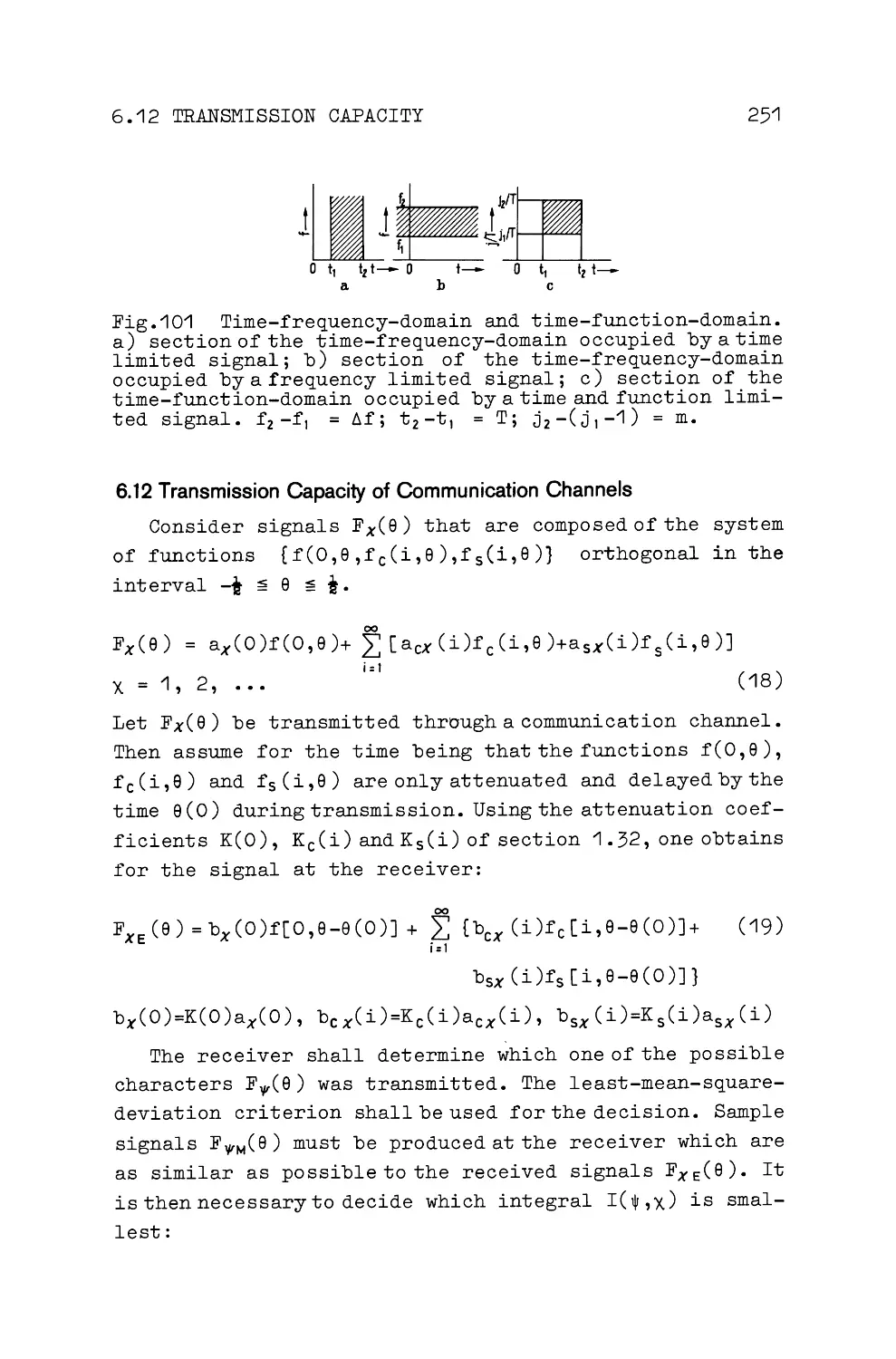
Transmission
of Information
by Orthogonal Functions
Henning F. Harmuth
With 110 Figures
Springer-Verlag
Berlin Heidelberg GmbH 1969
DR. HENNING F. HARMUTH
Consulting Engineer
D-7501 Leopoldshafen /Western Germany
ISBN 978-3-662-13229-6
ISBN 978-3 -662-13227-2 (eBook)
DOI 10.107/978-3 -662-13227-2
All rights reserved
No part of this book may be translated or reproduced in any form
without written permission from Spnnger-Verlag Berlin He1delberg GmbH
© by Springer-Verlag Berlin Heidelberg 1969.
Originally published by Springer-Verlag Berlin Heidelberg New York in 1969
Softcover reprint of the hardcover 1st edition 1969
Library of Congress Catalog Card Number 79-79651
Title-No. 1590
Transmission
of Information
by Orthogonal Functions
Henning F. Harmuth
With 110 Figures
Springer-Verlag Berlin Heidelberg GmbH 1969
DR. HENNING F. HARMUTH
Consulting Engineer
D-7501 Leopoldshafen /Western Germany
ISBN 978-3-662-13229-6
ISBN 978-3 -662-13227-2 (eBook)
DOI 10.107/978-3 -662-13227-2
All rights reserved
No part of this book may be translated or reproduced in any form
without written permission from Spnnger-Verlag Berlin He1delberg GmbH
© by Springer-Verlag Berlin Heidelberg 1969.
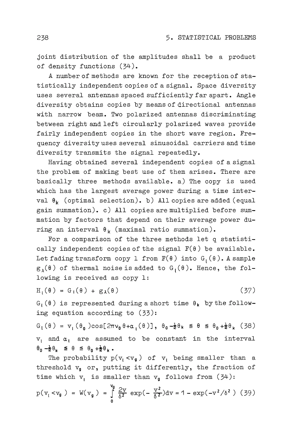
Originally published by Springer-Verlag Berlin Heidelberg New York in 1969
Softcover reprint of the hardcover 1st edition 1969
Library of Congress Catalog Card Number 79-79651
Title-No. 1590
To my Teacher
Eugen Skudrzyk
Preface
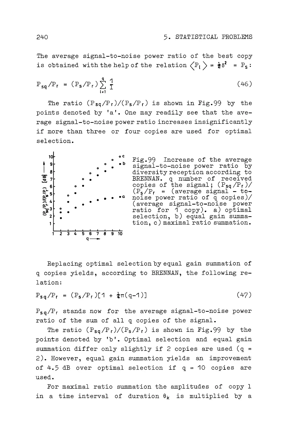
The orthogonality of functions has been exploited in
communications since its very beginning. Conscious and
extensive use was made of it by KOTEL 1 NIKOV in theoretical
work in 1947. Ten years later a considerable number of
people were working in this field rather independently.
However, little experimental use could be made of the theo-
retical results before the arrival of solid state opera-
tional amplifiers and integrated circuits.
A theory of communication based on orthogonal functions
could ·have been published many years ago. However, the only
useful examples of orthogonal functions at that time were
sine.... cosine functions and block pulses, and this made the
theory appear to be a complicated way to derive known re-
sults. It was again the advance of semiconductor techno-
logy that produced the first really new, useful example
of orthogonal functions: the little-known Walsh functions.
In this book emphasis is placed on the Walsh functions,
since ample literature is available on sine-cosine func-
tions as well as on block pulses and pulses derived from
them.
There are two major reasons why so few orthogonal func-
tions are of practical interest in communications. First,
a number of mathematical features other than orthogonality
are required, such as completeness or 1 good 1 multiplication
and shift theorems. One quickly learns to appreciate the
usefulness of multiplication and shift theorems of sine-
cosine functions for multiplexing and mobile radio trans-
mission, whenever one tries to duplicate these applications
VI
PREFACE
by other functions. The second reason is that the functions
must be easy to produce. The severity of this second re-
quirement is readily comprehended if one tries to think
of systems of functions of which a million or more can be
actually produced.
Prior to 1960 is was mainly the orthogonality feature
that attracted attention in connection with the transmis-
sion of digital signals in the presence of noise. But sooner
or later the question had to be raised of why the ortho-
gonal system of sine and cosine. functions should be treated
differently from other systems of orthogonal functions.
This question led to the generalization of the concept of
frequency and of such concepts derived from it as frequency
power spectrum or frequency response of attenuation and
phase shift. The Walsh functions made it possible to de-
sign practical filters and multiplex equipment based on
this generalization of frequency.
Any theory in engineering must offer not only some new
understanding, but must lead to new equipment and this
equipment must be economically competitive. A considerable
variety of equipment using orthogonal functions has been
developed, but there is still much controversy about the
economic potential. This is due to some extend to problems
of compatibility, which always tend to favor previously
introduced equipment and methods. In the particular case
of Walsh functions, the economic competitiveness is inti-
mately connected to the state of the art in binary digital
circuits. It is, e.g., difficult to see why Walsh functions
should not be as important for digital filters as sine-
cosine functions are for linear, time-invariant networks.
The author's work in the area of orthogonal functions
has been sponsored for many years by the Bundesministerium
der Verteidigung der Republik Deutschland; he wants to
take this opportunity to thank Prof .F .A .FISCHER, Dr.E .
SCHULZE and Dr.M .SCHOLZ for their continued support. Dr.
E. SCHLICKE of Allen-Bradley Co. was among the first to
encourage and stimulate work on the engineering applica-
PREFACE
VII
tions of Walsh functions; the author is greatly indebted
to him. Help has been rendered further in scientific as
well as administrative problems by the following gentlemen:
Prof. F.H. LANGE of Rostock University, Prof. G. LOCHS of
Innsbruck University, Dipl. Ing. W . EBENAU and Dr. H. H!JBNER
of the Deutsche Bundespost (FTZ-FI Darmstadt), Dipl.Phys.
N.EILERS of Bosch GmbH, the late Dr.E .KETTEL of AEG-Tele-
funken AG, Prof.K . VON SANDEN and Prof. J .FISCHER of Karls-
ruhe University, Prof.G .ULRICH of Technische Hochschule
Ilmenau, Prof.H .LUEG of Technische Hochschule Aachen and
Prof. J . KANE of the University of Southern California.
Thanks are particularly due to Prof .K.KttPFl"ltl'LLER of Tech-
nische Hochschule Darmstadt who showed great interest and
encouraged the study of the applications described in this
book.
Dr.F.PICHLER of Linz University, Dr.L .TIRKSCHLEIT of
l"lannheim University and Dr. P. WEISS of Innsbruck University
were of great help in improving the mathematical sec,tions
of the book. Prof. D . OLSON of St. Olaf College, l"lrs. J . OLSON
and l"lr.J.LEE of International Telephone and Telegraph Cu.
devoted much time to the editing of the manuskript, a
thankless as well as indispensable task. l"lany of the pic-
tures in this book were first published in the Archiv der
elektrischen ttbertragung; l"lr.F .RttHl"'ANN of S.Hirzel-Verlag
courteously permitted their use. Last but not least, thanks
are due to l"lrs.F .HAASE for the typing and to my wife Dr.
E.HARI"'UTH-HOENE for the proof-reading.
January 1969
Henning F. Harmuth
Table of Contents
INTRODUCTION.•••••••••.••••• .•••••••••••••••••••••••
1
1.MATHEMATICAL FOUNDATIONS
1.1 ORTHOGONAL FUNCTIONS
1.11 Orthogonality and Linear Independence •••••• 5
1.12 Series Expansion by Orthogonal Functions ••• 10
1 .13 Invariance of Orthogonality to Fourier Trans-
formation .................................. 13
1.14 Walsh Functions •••••••••••••••••••••••••••• 19
1. 2 THE FOURIER TRANSFORM AND ITS GENERALIZATION
1.21 Transition from Fourier Series to Fourier
Transform..................................
26
1.22 Generalized Fourier Transform •••••••••••••• 33
1. 23 Invariance of Orthogonality to the Genera-
lized Fourier Transform •••••••••••••••••••• 37
1.24 Examples of the Generalized Fourier Transform 38
1.25 Fast Walsh-Fourier Transform ••••••••••••••• 45
1.26 Generalized Laplace Transform •••••••••••••• 49
1 • 3 GENERALIZED FREQUENCY
1. 31 Physical Interpretation of the Generalized
Frequency..................................
49
1. 32 Power Spectrum, Amplitude Spectrum, Filtering
ofSignals.................................
51
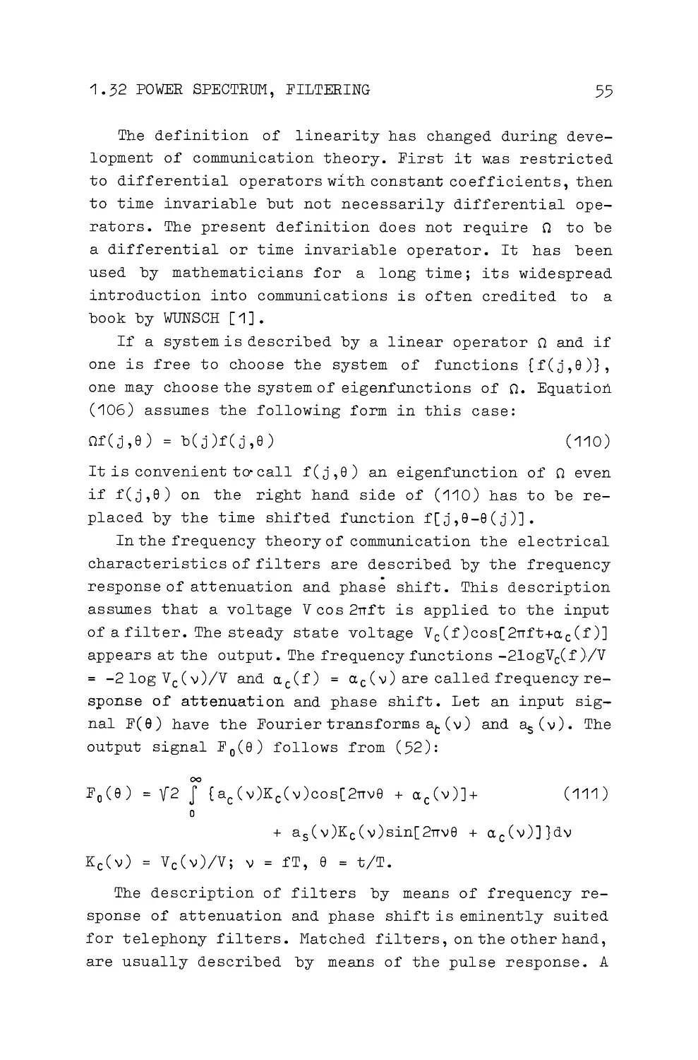
1. 33 Examples of Walsh Fourier Transforms and Power
Spectra....................................
57
TABLE OF CONTENTS
2.DIRECT TRANSMISSION OF SIGNALS
2. '1 ORTHOGONAL DIVISION AS GENERALIZATION OF TII"'E AND
FREQUENCY DIVISION
IX
2.'1'1 Representation of Signals •••••••••••••••••• 60
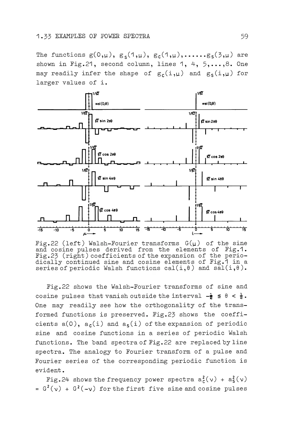
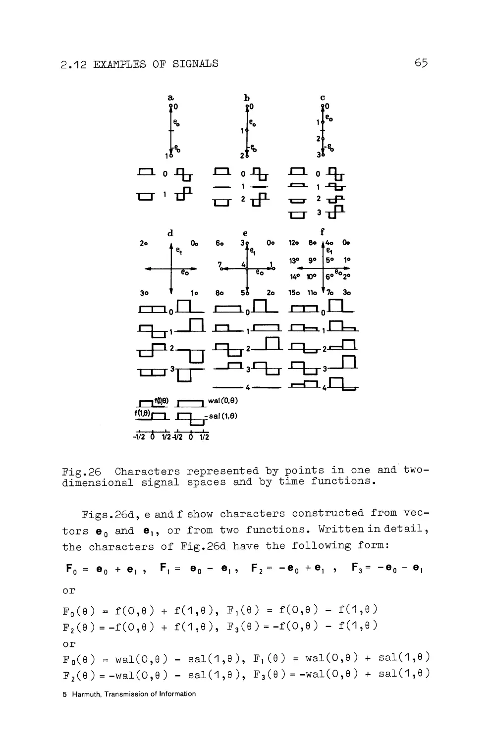
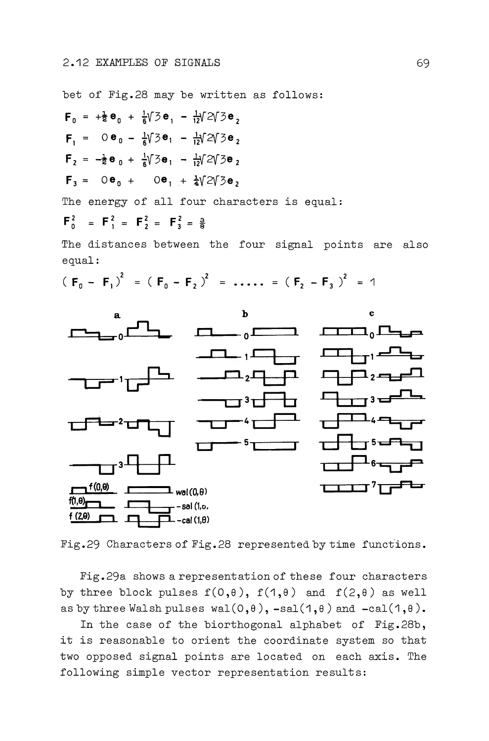
2.'12 Examples of Signals •••••••••••••••••••••••• 64
2. '13 ~p~i tude Sampling and Orthogonal Decompo-
Sltlon••••••••••••••••••••••••••••••••••••• 7'1
2.'14 Circuits for Orthogonal Division ••••••••••• 73
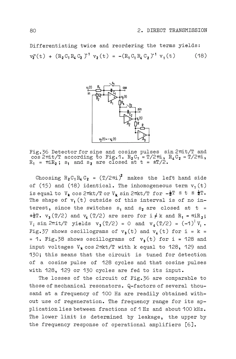
2.'15 Transmission of Digital Signals by Sine and
CosinePulses.••••••••••••••••••••••••••••• 8'1
2.2 CHARACTERIZATION OF COMMUNICATION CHANNELS
2.2'1 Frequency Response of Attenuation and Phase
Shift of a Communication Channel ••••••••••• 86
2.22 Characterization of a Communication Channel
by Crosstalk Parameters •••••••••••••••••••• 91
2.3 SEQUENCY FILTERS BASED ON WALSH FUNCTIONS
2.3'1 Sequency Lowpass Filters ••••••••••••••••••• 94
2.32 Sequency Bandpass Filters •••••••••••••••••• 97
2.33 Digital Sequency Filters ••••••••••••••••••• '104
3.CARRIER TRANSMISSION OF SIGNALS
3.'1 AMPLITUDE MODULATION(AM)
3.'1'1 Modulation and Synchronous Demodulation •••• '106
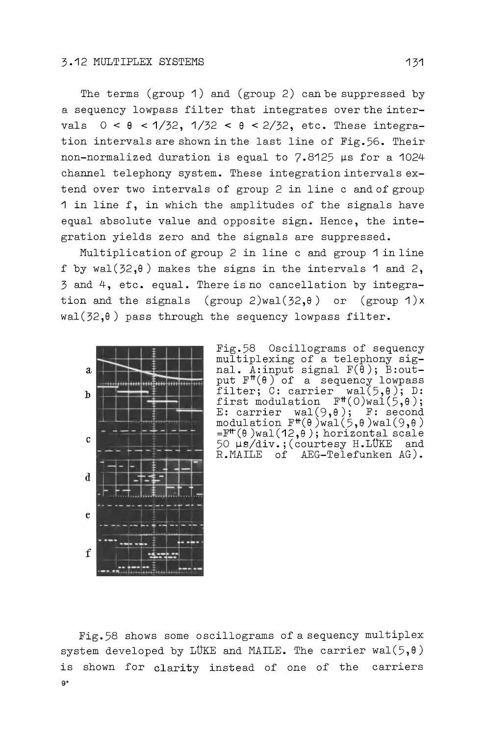
3.'12 Multiplex Systems •••••••••••••••••••••••••• '1'14
3.'13 Digital Multiplexing ••••••••••••••••••••••• '132
3.'14 Methods of Single Sideband Modulation •••••• '134
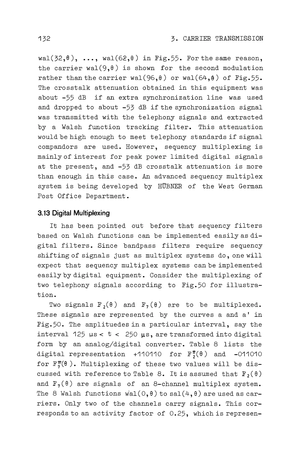
3.'15 Correction of Time Differences in Synchro-
nous Demodulation•••••••••••••••••••••••••• '147
3.2 TIME BASE, TIME POSITION AND CODE MODULATION
3.2'1 Time Base Modulation (TBM) ••••••••••••••••• '155
3.22 Time Position Modulation (TPM) ••••••••••••• '157
3.23 Code Modulation (CM) ••••••••••••••••••••••• '159
X
TABLE OF CONTENTS
3-3 NONSINUSOIDAL ELECTROMAGNETIC WAVES
3.31 Radiation of Walsh Waves by a Hertzian Dipole 160
3.32 Propagation, Antennas, Doppler Effect •••••• 167
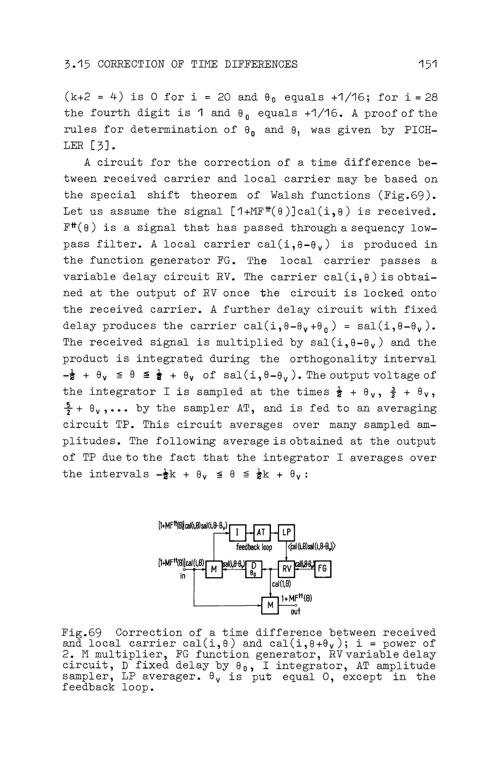
3-33 Interferomet~y, Shape Recognition •.•••..••• 173
4.STATISTICAL VARIABLES
4.1 SINGLE VARIABLES
4.11 Definitions ••.•• .••.•.••••••••.•••••••••••• 181
4.12 Density Function, Function of a Random Vari-
able, Mathematical Expectation •••••••.• .••• 188
4.13 Moments and Characteristic Function ••.••••• 191
4.2 COMBINATION OF VARIABLES
4.21 Addition of Independent Variables •••••••••• 194
4.22 Joint Distributions of Independent Variables 198
4.3 STATISTICAL DEPENDENCE
4.31 Covariance and Correlation ••.•••••.••.••••• 210
4.32 Cross- and Autocorrelation Function •••••••• 214
5.APPLICATION OF ORTHOGONAL FUNCTIONS TO STATISTICAL
PROBLEMS
5.1 SERIES EXPANSION OF STOCHASTIC FUNCTIONS
5.11 Thermal Noise •••••.•••.••.••••.•••••••••••• 217
5.12 Statistical Independence of the Components
of an Orthogonal Expansion••.•••••.•••••••• 222
5.2 ADDITIVE DISTURBANCES
5. 21 Least Mean Square Deviation of a Signal from
SampleFunctions...• .• .••• . .
..
•...••.•••••• 223
5.22 Examples of Circuits •..•••.••••.•.•••••. .•• 227
5.23 Matched Filters •••••••.•••. .• . .•••••••••••• 230
5.24 Companders for Sequency Signals •..••••••. .• 233
5.3 MULTIPLICATIVE DISTURBANCES
5.31 Interference Fading ••...••••.•••••••••••.•• 236
5.32 Diversity Transmission Using Many Copies .•• 243
TABLE OF CONTENTS
XI
6.SIGNAL DESIGN FOR IMPROVED RELIABILITY
6.1 TRANSMISSION CAPACITY
6.11 Measures of Bandwidth •••••••••••••••••••••• 245
6.12 Transmission Capacity of Communication Chan-
nels................................. . . . . . .
251
6.13 Signal Delay and Signal Distortions •••••••• 260
6.2 ERROR PROBABILITY OF SIGNALS
6.21 Error Probability of Simple Signals due to
ThermalNoise....•••••••••••••••••••••••••• 262
6.22 Peak Power Limited Signals ••••••••••••••••• 268
6.23 Pulse-Type Disturbances •••••••••••••••••••• 271
6.3 CODING
6.31 Coding with Binary Elements •••••••••••••••• 275
6. 32 Orthogonal, Transorthogonal and Biorthogonal
Alphabets •••••••••••••••••••••••••••••••••• 280
6.33 Coding for Error-Free Transmission ••••••••• 288
6.34 Ternary Combination Alphabets •••••••••••••• 289
6.35 Combination Alphabets of Order 2r+1 •••••••• 299
REFERENCES ORDERED BY SECTIONS •••••••••••••••••••••• 305
INDEX..••••.
.
.
•..•••..
.
.
.
•...••
.
••..•.•.
.
•....•.
.
.
• 320
Equations are numbered consecutively within each one of
the 6 chapters. Reference to an equation of a different
chapter is made by writing the number of the chapter in
front of the number of the equation, e.g . (4.25) for (25)
in chapter 4.
Introduction
Sine and cosine functions play a unique role in com-
munications. The concept of frequency, based on them, is
defined by the parameter f in the functions V sin (2rrft+a)
and V cos ( 2rrft+a).
There are many reasons for this unique role. It was
hardly possible to produce other functions in the early
days of communications. Electron tubes and transistors
made it possible to produce such simple non-sinusoidal
wave forms as block pulses or ramp voltages. But it was
not before the arrival of the integrated circuits that
almost any functions could be produced economically. A
further factor favoring sinusoidal functions was the
fact that linear time invariant circuits only attenuate
and delay them, the shape and frequency remain unchanged.
Hence, the system of sine and cosine functions had a tre-
mendous advantage over other complete systems of ortho-
gonal functions, as long as resistors, capacitors and
coils were the most desirable circuit elements. The the-
ory of linear, time invariant networks demonstrates the
advantages of sinusoidal functions. The advent of semi-
conductors has brought a radical change. There is no par-
ticular reason why a digital filter, e.g ., analyzing the
fine structure of a radar signal, should be based on sine
and cosine functions. It turns out that digital filters
based on the socalled Walsh functions are simpler and
faster.
Sinusoidal functions are less important for the pro-
pagation of electromagnetic waves in free space or along
conductors. The solution of the wave equation by d 1 ALEM-
BERT and the general solution of the telegrapher 1 s equa-
tion show, that a large class of functions can be trans-
mitted distortion-free or can be regenerated. Similarly,
a Hertzian dipole can radiate non-sinusoidal waves. The
dominance of sinusoidal waves in radio communication can
be partially explained by the invariance of their ortho-
1 Harmuth, Transmission of Information
2
INTRODUCTION
gonality under varying time delays. Cables or open wire
lines that could not, nor need not, transmit sinusoidal
functions have always existed. The telegraph lines of the
19th century, using electromechanical relays as ampli-
fiers, were such lines, and they have recently made a
comeback as digital cables.
One of the most important features of sine and cosine
functions is that almost all time functions used in com-
munications can be represented by a superposition of
sine and cosine functions, for which Fourier analysis is
the mathematical tool. The transition from time to fre-
quency func'tions is a result of this analysis. This is
often taken so much for granted by the communications
engineer, that he instinctively sees a superposition of
sine and cosine fi.mctions in the output voltage of a mi-
crophone or a teletype transmitter. Actually, the repre-
sentation -of a time function by sine and cosine functions
is only one among many possible ones. Complete systems
of orthogonal functions generally permit series expan-
sions that correspond to the Fourier series. For instance,
expansions into series of Bessel functions are much used
in communications. There are also transforms correspon-
ding to the Fourier transform for many systems of func-
tions. Hence, one may see a superposition of Legendre
polynomials, parabolic cylinder functions, etc. in the
output voltage of a microphone.
General complete systems of orthogonal functions in-
stead of the special system of sine and cosine functions
will be used in this book for the representation of sig-
nals and for the characterization of lines and networks.
A consistent theory must include the application of ortho-
gonal functions as carriers, since sine and co sine are
not only used for theoretical analysis, but also as car-
riers in multiplex and radio systems. It will be shown
that modulation methods exist for them, which correspond
to amplitude, frequency and phase modulation. Further-
more, it will be shown that antennas can be designed that
INTRODUCTION
3
radiate non-sinusoidal waves efficiently.
The transition from the system of sine-cosine func-
tions to general systems of orthogonal functions brings
simplifications as well as complications to the mathe-
matical theory of communication. One may~ e.g., avoid
the troublesome fact that any signal occupies an infinite
section of the time-frequency-domain by substituting a
time-function-domain. Any time-limited signal composed
of a limited number of orthogonal functions occupies a
finite section of this time-func~ion-domain.
The generalization of the concept of frequency has
been so far the most satisfying theoretical result of
the theory of communication based on orthogonal functions.
Frequency is a parameter of sine and cosine functions
which can be interpreted as number of cycles per unit of
time. l'1ANN [1], STUMPERS [2] and VOELCKER [3] pointed out,
that frequency may also be interpreted as "one half the
number of zero crossings per unit of time". A sine func-
tion with 100 cycles per second has 200 zero crossings
or sign changes per second. One half the number of zero
crossings is 100 cycles per second numerically and di-
mensionally. Zero crossings are defined for functions in
which the term cycle has no obvious meaning. It is useful
to introduce the more general concept "one half the ave-
rage number of zero crossings per unit of time" in order
to cover non-periodic functions. The new term "sequency"
is introduced for this generalization of frequency. Thus
sequency and frequency are identical for sine and cosine
functions. The term sequency makes it possible to replace
such important concepts as frequency power spectrum or
frequency response of attenuation by sequency power spec-
trum and sequency response of attenuation.
The concepts of period of oscillation T .. 1 /f and
wavelength A = v/f are connected with frequency. Substi-
tution of sequency q> for frequency f leads to the follo-
wing more general definitions:
1*
4
INTRODUCTION
average period of oscillation T =1/rp (average se-
paration in time of the zero crossings multiplied
by 2)
average wavelength A = v/rp (average separation in
space of the zero crossings multiplied by 2, where
v is the velocity of propagation of a zero crossing)
The acid test of any theory in engineering are its prac-
tical applications. Several such applications are known
and they are all intimately tied to semiconductor tech-
nology. The little known system of Walsh functions ap-
pears to be as ideal for linear, time-variable circuits,
if based on binary digital components, as the system of
sine and cosine functions is for linear, time-invariant
circuits, based on resistors, capacitors and coils. Very
simple sequency filters based on these Walsh functions
have been developed. Furthermore, an experimental se-
quency multiplex system using Walsh functions as carriers
has been developed that has advantages over frequency or
time multiplex systems in certain applications. Digital
filters and digital multiplex equipment are among the
most promising applications for the years ahead. They
are simpler and faster when based on Walsh functions ra-
ther than on sine and cosine functions. Their practical
application, however, will require considerable progress
in the development of large scale integrated circuits.
Applications of non-sinusoidal electromagnetic waves
are strictly in the theoretical stage. Only very recent-
ly have active antennas been found to be practical for
the radiation of Walsh functions. Most problems concer-
ning Walsh waves can presently be answered in terms of
geometric optics only, since wave optics is a sine wave
optics. On the other hand, there is little doubt that
non-sinusoidal electromagnetic waves are a challenging
field for basic research. The generation of non-sinusoi-
dal radio waves implies that such waves can be generated
in the region of visible light, and this leads ultimately
to the question of why white light should be decomposed
1.11 ORTHOGONALITY
5
into sinusoidal functions.
The Walsh functions, emphasized in this book, are pre-
sently the most important example of non-sinusoidal func-
tions in communications. These functions are hardly known
by communication engineers although they have been used
for more than 60 years for the transposition of conduc-
tors in open wire lines. Rademacher functions [4], which
are a subsystem of the Walsh functions, were used for
this purpose towards the end of the 19th century. The
complete system of Walsh functions seems to have been
found around 1900 by J.A.BARRETT 1 • The transposition of
conductors according to BARRETT's scheme was standard
practice in 1923 [6],[7], when J.L.WALSH [9] introduced
them into mathematics. Communications engineers and ma-
thematicians were not aware of this common usage until
very recently [8].
1. Mathematical Foundations
1.1 Orthogonal Functions
1.11 Orthogonality and Linear Independence
A system [f(j,x)} of real and almost everywhere non-
vanishing functions f(O,x), f(1,x), ••• is called ortho-
gonal in the interval x 0 ~ x ~ x 1 if the following con-
dition holds true:
XJ
J f(j,x)f(k,x)dx Xjtijk
(1)
xo
tiik=1forj=k,tiik=0forj(=k.
1 JOHN A. BARRETT is mentioned by FOWLE [5] in 1905 as
inventor of the transposition of conductors according to
Walsh functions; see particularly page 675 of [5].
6
1. !11!;THEJ.VIATIC.AL FOUNDATIONS
The functions are called orthogonal and normalized if
the constant X j is equal 1. The two terms are usually
reduced to the single term orthonormal or orthonormalized.
A non-normalized system of orthogonal functions may
always be normalized. For instance, the system {Xj1f(j ,x)}
is normalized, if Xi of ( 1) is not equal 1. Systems of
orthogonal functions are special cases of systems of lin-
early independent functions. A system ( f(j ,x)) of m
functions is called linearly dependent, if the equation
m-1
2: c(j)f(j,x) = 0
(2)
j:O
is satisfied for all values of x without all constants
c(j) being zero. The functions f(j ,x) are called linearly
independent, if (2) is not satisfied. Functions of an
orthogonal system are always linearly independent, since
multiplication of (2) by f(j ,x) and integration of the
productsinthe interval x0 ~ x ~ x1 yields c(j)=0for
each constant c(j).
A system {g(j ,x)} of m linearly independent functions
can always be transformed into a system {f(j,x)} of m
orthogonal functions. One may write the following equa-
tions:
(3)
+ c 11 g(1,x)
f(O,x) =
f(1,x)
f(2,x) =
c 00 g(O,x)
c 10 g(O,x)
c20 g(O,x) + c21 g(1,x) + c22g(2,x)
etc.
Substitution of the f(j ,x) into (1) yields just enough
equations for determination of the constants c pq
Xt
Jf'2(O,x)dx= X0
(4)
xo
Xt
Xt
J f 2 (1,x)dx= X1 , Jf(O,x)f(1,x)dx=O,
xo
xo
Xt
Xt
J f 2 (2,x)dx = X2 , Jf(O,x)f(2,x)dx =0,
x,
Jf(1,x)f(2,x)dx=0
xo
xo
xo
etc.
1.11 ORTHOGONALITY
7
The coefficients X0 , X 1, •••
are arbitrary. They are 1
for normalized systems. It follows from (2) that ( 4) ac-
tually yields values for the coefficients cpq as only a
system {g(j,x)} of linearly independent functions could
satisfy (4) identically.
Figs .1 to 3 show examples of orthogonal functions.
The independent variable is the normalized time 11 = t/T.
The functions of Fig. 1 are orthonormal in the interval
-! ~ 8 ~ !; they will be referred to as sine and cosine
elements. Onemaydividetheminto evenfunctions fc(i,9),
odd functions f 5 (i,8) and the constant 1 or wal(0,8):
f(j,8)=fc(i'e)
'{2 cos 2rri a
= fs (i ,a) '{2 sin 2TTi8
= wal(0,8) 1
=undefined
- ---- ---- --
wal(0,9l
-11 2
0
a-
1/2
9<-!,9>+!
-1/2
0
8•t/T-
(5)
0 0000
1 0001
0010
0011
4 0100
5 0101
6 0110
7 0111
8 1000
9 1001
10 1010
11 1011
12 1100
13 1101
14 1110
15 1111
1/2
Fig.1 (left) Orthogonal sine and cosine elements.
Fig.2 (right) Orthogonal Walsh e~ements. Th~ numbers on
the right give j in decimal a.J?-d b1nary ~orm, 1f the. nota-
tion wal(j,8) is used. wal(21,8) = cal(l,8), wal(2l-1,8)
=sal(i,8).
8
1. MATHEMATICAL FOUNDATIONS
The term 'element' is used to emphasize that a func-
tion is defined in a finite interval only and is unde-
fined outside. The term 'pulse' is used to emphasize that
a function is identical zero outside a finite interval.
Continuation of the sine and cosine elements of Fig.1
outside of the interval -i ~ 6 ~ i by f(j,6) = 0 yields
the sine and cosine pulses; periodic continuation, on the
other hand, yields the periodic sine and cosine functions.
It is easy to see, that the condition (1) for ortho-
gonality is satisfied for sine and cosine elements:
1/2
1/2
J1'{2sin2rri6 d6 = J1'{2cos2rri6 d6 =0
-1/2
- 1/2
112
112
J '{2 sin 2ni6·'{2 sin 2rrk6 d6 = Jy2 cos 2rri6·'{2 cos 2rrk8 d6 •6;k
- 112
-1 /2
1/2
J '{2 sin 2rri6·'{2 cos 2rrk6 d6 = 0
-1/2
1/2
J1·1d6=1
-1 12
Fig.2 shows the orthonormal system of Walsh functions or
-
more exactly - Walsh elements, consisting of a constant
wal(0,6), even functions cal(i,6) and odd functions
sal(i,6 ). These functions jump back and forth between +1
and -1. Consider the product of the first two functions.
Itisequal-1intheinterval-i~6<0and+1inthe
interval 0 ~ 6 < +i. The integral of these products has
the following value:
0
1/2
J(+1)(-1)d6 + J(+1)(+1)d6
0
-1/2
0
The product of the second and third element yields +1
intheintervals-i~6<-i and0~6<+%, and-1in
theintervals-i~6<0 and+i-~6<+t•Theintegral
of these products again yields zero:
-1/4
0
1/4
1/2
J C-1)(-1)d6 + JC-1)(+1)d6 + JC+1)(+1)d6 + JC+1)(-1)d6 =0
- 112
-1 14
0
114
1.11 ORTHOGONALITY
9
One may easily verify that the integral of the pro-
duct of any two functions is equal zero. A function mul-
tiplied with it self yields the products ( +1) ( +1) or
(-1)(-1). Hence, these products have the value 1 in the
whole interval -i ~ 8 ~ +f and their integral is 1. The
Walsh functions are thus orthonormal.
Fig.3 shows a particularly simple system of orthogo-
nal functions. Evidently, the product between any two
functions vanishes and the integrals of the products must
vanish too. For normalization the amplitudes of the func-
tions must be V5.
f(0,6l
II
f (O,v-)
f(1,9)
II
f(l,v)
f(2,6)
II
f(2,v -)
f(3,9)
II
f (3,v -)
f(4,8)
D
H4, v-l
fx(Bl qJ b Fx(v-)
-112
V2
e=t(r
-1
v-=fT
Fig.3 Orthogonalblock pulses
f(j,e) and f(j,v).
Fig.4 Bernoulli polynomials _ ___,. __ ""*""__.., .._- +-T --1- -+-1- -
(top right).
Fig.5 Legendre polynomials
(right).
An example of a linearly independent but not orthogo-
nal system of functions are Bernoulli 1 s polynomials
Bj (x) [4], [5]:
1, B1(x)
X-
10
1. MATHEMATICAL FOUNDATIONS
B j(x) is a polynomial of order j. The condition
m
l::c(j)Bj(x) = 0
j:O
can be satisfied for all values of x only if c(m)xm is
zero. This implies c(m) = 0. Now c(m-1)R .... 1 (x) is the
highest term in the sum and the same reasoning can be
applied to it. This proves the linear independence of
the Bernoulli polynomials.
One may see from Fig.4 without calculation that the
Bernoulli polynomials are not orthogonal. For orthogona-
lization in the interval -1 ~ x ~ +1 one may substitute
them for g(j,x) in (3):
P0(x) =B0(x) =1
P1(x) = c 10B0(x) + c 11B1(x), etc.
Using the constants Xj = 2/(2j+1) one obtains from (4):
1
J1dx=X0=2
-4
l[c10 + c11(x-t)]2dx = X1 =.l..,
J[c 10 +c 11 (x-i)]dx = 0
-1
3-1
The coefficients c 10 =I, c 11 = 1, etc. are readily ob-
tained. The orthogonal polynomials P j (x) assume the fol-
lowing form:
Po(x) 1,P1(x) = x, P2(x) =
-(3x2 - 1)
P3(x) =t(5x3 - 3x), P4(x) =i(35x4 -30x2 + 3)
These are the Legendre polynomials. P j (x) must be multi-
plied with X- 1
•
12 = (j + t) 112 for normalization. Fig. 5
J
shows the first five polynomials.
1.12 Series Expansion by Orthogonal Functions
Let a function F(x) be expanded in a series of the
orthonormal system {f(j,x)}:
00
F(x) = 2:: a(j )f(j ,x)
(6)
i=0
1.12 SERIES EXPANSION
11
The value of the coefficients a( j) may be obtained by
multiplying (6) by f(k,x) and integrating the products
intheinterval of orthogonalityx0 ~ x ~ x1:
X1
J F(x)f(k,x)dx = a(k)
(7)
Xo
How well is F(x) represented, if the coefficients a( j)
are determined by ( 7 )? Let us assume a series l::bC j )f( j ,x)
having m terms yields a better representation. The cri-
terion for 'better' shall be the least mean square devi-
ation Q of F(x) from its representation:
X1
m-1
Q= J [F(x) - 2:: b(j)f(j,x)]2dx
X0
j:O
x1
~
x1
x1 m-1
2
=JF 2 (x)dx- 2 _6b(j)JF(x)f(j,x)dx+ J Cl::b(j)f(j,x)] dx
Xo
j:O
Xo
Xo i=O
Using (7) and the orthogonality of the functions f(j,x)
yields Q in the following form:
Q=
I;a 2 (j) + ~[b(j)- a(j)]2
(8)
j:0
j=O
The last term vanishes for b( j) = a( j) and the mean square
deviation assumes its minimum.
The socalled Bessel inequality follows from (8):
m-1
oo
x1
2:: a2(j) ~ 2:: a2(j) ~ J F2(x)dx
i=O
i=O
x0
(9)
The upper limit of summation may be co instead of m - 1,
since the integral does not depend on m and must thus
hold for any value of m.
The system {f(j,x)} is called orthogonal, normalized
and complete, if the mean square deviation Q converges
to zero with increasing m for any function F(x) that is
quadratically integrable in the interval x 0 ~ x ~ x 1 :
X1
m-1
lim J[F(x) - 2::a(j)f(j,x)]2dx = 0
m-ooxo
i=O
( 10)
12
1. l"'.ATHEl"'.ATIC.AL FOUNDATIONS
The equality sign holds in this case in the Bessel in-
equality (9):
(11)
Equation (11) is known as completeness theorem or Parse-
val's theorem. Its physical meaning is as follows: Let
F(x) represent a voltage as function of time across a
unit resistance. The integral of F 2 (x) represents then
the energy dissipated in the resistor. This energy equals,
according to ( 11 ) , the sum of the energy of the terms in
the suml:a(j)f(j,x). Putt±ng it differently, the energy
is the same whether the voltage is described by the time
function F(x) or its series expansion.
The system { f(j ,x)} is said to be closed 1 , if there
is no quadratically integrable function F(x),
x1
JF 2 (x)dx<oo,
(12)
xo
for which the equality
x1
J F(x)f(j,x)dx = 0
(13)
Xo
is satisfied for all values of j.
Incomplete systems of orthogonal functions do not per-
mit a convergent series expansion of all quaa.ratically
integrable functions. Nevertheless, they are of great
practical interest. For instance, the output voltage of
an ideal frequency lowpass filter may be represented
exactly by an expansion in a series of the incomplete
orthogonal system of sin x functions.
X
1 A complete orthonormal system is always closed. The in-
verse of this statement holds true, if the integrals of
this section are Lebesgue rather than Riemann integrals.
The Riemann integral suffices for the major part of this
book. Hence,
'integrable' will mean Riemann integrable
unless otherwise stated.
1.13 INVARIANCE OF ORTHOGONALITY
13
Whether a certain function F(x) can be expanded in a
series of a particular orthogonal system {f(j ,k)} cannot
be told from such simple features of F(x) as its conti-
nuity or boundedness 1 [5] - [7].
1.131nvariance of Orthogonality to Fourier Transformation
A time function f(j,e) may be represented under cer-
tain conditions by two functions a(j, v) and b(j, v) by
means of the Fourier transform:
f( j, e) r[a(j, \1) COS 2TTV9 + b(j,v) sin2rrv9]dv
( 14-)
-co
a(j, v) = rf(j,S) cos 2TTV9 d9
(15)
-00
00
b(j,v) =Jf(j,9)sin2nve d9 a=t/T, \1 = fT
-00
It is advantageous for certain applications to replace
the two functions a(j,v) and b(j,v) by a single function2:
g(j,v) = a(j,v) + b(j,v)
(16)
It follows from (15) that a(j,v) is an even and b(j,v)
an odd function of v:
a(j,v) = a(j,-v), b(j,v) = -b(j,-v)
(17)
Equations (16) and (17) yield for g(j,-v):
g(j,-v) = a(j,-v) + b(j,-v) = a(j,v) - b(j,v)
(18)
a(j,v) and b(j,v) may be regained from g(j,v) by means
of (16) and (18):
a(j,v) = t[g(j,v) + g(j,-v)]
(19)
b(j,v) = i[g(j,v) - g(j,-v)J
Using the function g(j, v) one may write (14-) and (15)
in a more symmetric form:
1 For instance, the Fourier series of a continuous func-
tion does not have to converge in every point. A theorem
due to BANACH states, that there are arbitrarily many
orthogonal systems with the feature, that the orthogonal
series of a continuously differentiable function diver-
ges almost everywhere.
2 Real notation is used for the Fourier transform to fa-
cilitate comparison with the formulas of the generalized
Fourier transform derived later on.
14
1. MATHEMATICAL FOUNDATIONS
00
f(j,a) J g(j ,'J)( cos 2rr\la + sin 2rr\la )d\1
(20)
-oo
00
g(j,\1) = J f(j,a)(cos2rr\la + sin2rr\la)da
(21)
-oo
The integrals of a(j,\1) cos 2TT\Ia and b(j,\1) sin2rr\la in
(20) vanish since a(j,\1) is an even and b(j,\1) is an odd
function of \1.
Let {f(j,a)} be a system orthonormal in the interval
-te ~ a ~ +te and zero outside. e may be finite or infi-
nite. The functions f(j ,a) are Fourier transformable1 •
Their orthogonality integral,
00
J f(j,a)f(k,a)da = lijk '
(22)
-00
may be rewritten2 using (20):
00
00
J f(j ,a)[ J g(k,'J)( cos 2rr\la + sin 2rr\18 )d\l]d8 liik
-oo
-
oo
00
00
Jg(k,'J)[Jf(j,a)(cos2rr\18 + sin2rr\la)da]d\l liik
-oo
-oo
00
J g(j,\l)g(k,\l)d\1 = lijk (23)
-oo
Hence, the Fourier transform of an orthonormal system
{f(j,a)} yields an orthonormal system {g(j,\1)}.
Substitution of
g(j,\1) = a(j,\1) + b(j,'J),
g(k,\1) = a(k,'J) + b(k,\1)
into (23) yields it in terms of the notation a(j,'J),
b(j,\1):
00
00
Jg(j,\l)g(k,\l)d\1 JCa(j,\1) + b(j,'J)][a(k,'J)+b(k,\l)]d\1
-oo
-oo
00
= J~(j,'J)a(k,\l)+b(j,'J)b(k,\l)]d\1
liik
-oo
1 Orthonormality implies the existence of the Fourier
transform and the inverse transform (Plancherel theorem).
2The integrations may be interchanged, since the inte-
grands are absolutely integrable.
1.13 INVARIANCE OF ORTHOGONALITY
15
'
\
\x·
v
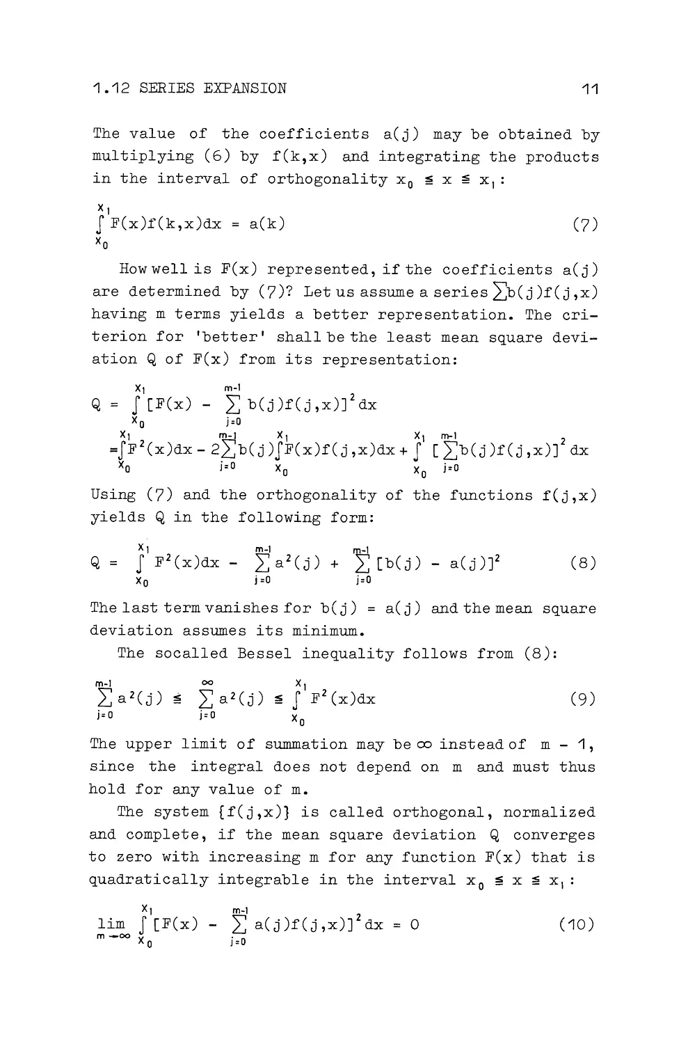
Fig.6 Fourier transforms g(j,v) of sine and cosine pul-
ses according to Fig.1 . a) wal(0,8), b) 1{2sin2rr8,
c) 1{2 cos 2rr8, d) 1[2 sin 4rr8,
e) 1[2 cos 4rr8.
Fig.6 shows as an example the Fourier transforms of
sine and cosine pulses. These pulses are derived from the
elements of Fig.1 by continuing them identical zero out-
side the interval -t § 8 § +t:
g(O,v) =
1/2
J1( cos2rrv8 + sin2rrv8)d8
-1/ 2
sin rrv
TTV
1/2
= J 1{2 cos 2rri8 ( cos 2rrv8 + sin 2rrv8 )d8
-112
_
J..,r 2 (sin rr( v-i)
sin rr( wi))
-
zv
rr(v-i) +
rr(V+i)
1/2
g 5 (i,v) J 1[2sin2rri8( cos2rrv8 + sin2rrv8)d8
-1 /2
= J.,r 2 (sinrr(v-i) _ sinrr(wi))
~v rr (v-i)
rr ( V+i)
(24)
Fig.7 shows the Fourier transformsofWalsh pulses de-
rived by continuing the elements of Fig.2 identical zero
outside the interval -t § 8 § +t:
g(O,v) = fwal(0,8)( cos 2rrv8 + sin2rrv8)d8
- 1/2
sin rrv
TT\1
16
1. MATHEMATICAL FOUNDATIONS
1/2
.
/2
g 5 (1,"V) J sal(1,8)(cos 2TT"V8 + sin2TT"V8)d8 = Sl:"Vl~
- 1/2
.
l.
sin 2 TT"V/4
()
l.
sin 2 TT"V/4
gc(1,"V) = Sln~TT"V TT"V/4
,
g52,"V
=
COS~TT\1 TT"V/ 4
One may readily see from these examples that even time
functions transform into even frequency functions and odd
time functions transform into odd frequency functions.
Negative values of the frequency have a perfectly valid
physical meaning. The oscillation of frequency "V is a co-
sine oscillation with reference to e = 0, if the Fourier
Fig.7 Fourier transforms g(j~v) of Walshpulses according
to Fig.2.
a) wal(O,e), b) sal(1,8), c) -cal(1,e),
d) -sal(2,8),
e) cal(2,8).
1.5
tl1,alJ\ f\tl3,al
I.tO \
1
f(2,8l
I
i
I
-10
10
V=fT-
Fig.8 Fourier transforms g(j, v) of the block pulses f(1 ,e),
f(2,8) and f(3,8) of Fig.3 .
1.13 INVARIANCE OF ORTHOGONALITY
17
transform has the same value for +V and -v; it is a sine
oscillation, if the Fourier transform has the same abso-
lute value but opposite sign for +V and -v.
Fig.8 shows the Fourier transforms g(j, v) of three block
pulses of Fig.3 . They are no longer either even or odd 1 •
f(6,9)- -Vicos(6nB+n/4)
[\,
/""'\.
/""'\.
/1
"'-/
"'-/
'C./
f(5,9l-l'2sin(6nB+n/4)
L"-
~ L"-
C7 ~'C/ 'I
f(4,9J--I'2cos(4:n:B+n/4)
~
~
f(0,9) • constant
I
-t
-t
t
a-t/T-
Fig.9 Orthogonal system of sine and cosine pulses having
jumpsofequalhightate=-iand6=+i.
Fig.9 shows a system of orthogonal sine and cosine pul-
ses. They are time shifted compared with those of Fig.1,
so that all functions have jumps of equal magnitude at
6 = -i and 6 = +i. Their Fourier transforms g(j, v) are
shown in Fig.10:
(. v) _ sinn(v-k)
gJ,
-
n(v-k)
k
I.f
.
=-2J or even J
k = tCj+1) for odd j.
(25)
1 The Fourier transforms of the various block pulses are
different but their frequency power spectra are equal.
The power spectrum is the Fourier transform of the auto-
correlation function of a function, and not the Fourier
transform of the function itself (Wiener-Chintchin theo-
rem). The connection between Fourier transform, power
spectrum and am:Qlitude spectrum is discussed in section
1.32. See also L4].
2 Harmuth, Transmission of Information
18
1. MATHEMATICAL FOUNDATIONS
-5
5
v-fT--
Fig.10 Fourier transforms g(j,v) of the sine and cosine
pulses of Fig.9.
The functions 11t i ( 9) of the parabolic cylinder shown in
Fig.11 and their Fourier transforms g(j,v) have the same
shape [5]:
f(j,9) = Vj(9), g(O,v) = w0 (4rrv)
(26)
j o,2i,2i+1;i 1'2'
•..•
Fig.11 The functions Wi
rabolic cylinder.
Wi (x)
-ix2
e
He.(x); He 1.(x)
vj! V2rr
I
tx2( d )i -tx2
e
-
dxe
x=9or4rrv;j=0,2i,2i+1,i
= 1,2,
••••
wi (9) decreases for large absolute values of 9 propor-
•
2
tionally to 9 J exp( --i-9 ) and 11t. ( 4rrv) decreases for large
I
,
2
absolute values of \1 proportionally to ( 4rrv) 1 exp[ -t (4rrv) ] •
Pulses with the shape of parabolic cylinder functions re-
quire a particularly small part of the time-frequency-
1.14 WALSH FUNCTIONS
19
domain for transmission of a certain percentage of their
energy1 •
1.14 Walsh Functions
The Walsh functions wal(0,8), sal(i,8) and cal(i,8)
are of considerable interest in communications2. There is
a close connection between sal and sine functions, as well
as between cal and cosine functions. The letters s and c
in sal and cal were chosen to indicate this connection,
while the letters 'al' are derived from the name Walsh.
For computational purposes it is sometimes more con-
venient to use sine and cosine functions, while at other
times the exponential function is more convenient. A si-
milar duality of notation exists for Walsh functions. A
single function wal(j ,8) may be defined instead of the
three functions wal(0,8), sal(i,8) and cal(i,8):
wal(2i,8) = cal(i,8), wal(2i-1,8) = sal(i,8)
(27)
i=1,2,
.. ..
The functions wal(j ,8) may be defined by the following
difference equation 3·~:
(j12]•P{
i•P
}
wal(2j+p,8) = (-1)
wal[j,2(8+i)J +(-1) wal[j,2(8-i)J
p=0or1;j=0,1,2,
.•;wal(0,8)=1for-i~8<t;
wal(O,8) 0for8<-1,8>+t.
(28)
'Pulses of the shape of parabolic cylinder functions use
the time-frequency-domain theoretically 'best'. This good
use has not been o.f much practical value so far, since
sine-cosine pulses and pulses derived from sine-cosine
pulses are almost as good, but much easier to generate
and detect.
2 The probably oldest use of Walsh functions in communica-
tions is for the transposition of conductors [18].
3 Walsh functions are usually defined by products of Rade-
macher functions. This definition has many advantages but
does not yield the Walsh functions ordered by the number
of sign changes as does the difference equation. This or-
der is important for the generalization of frequency in
section 1 • 31. Rademacher functions are the functions
-s al( 1 ,8), sal(3,,8), sal(7 ,8), •• in Fig.2 . Walsh functions
may also be defined by Hadamard matrices [19].
~[j/2] means the largest integer smaller or equal fj.
2*
20
1. MATHEMATICAL FOUNDATIONS
For explanation of this difference equation consider
the function wal ( j, 9). The function wal ( j, 28) has the same
shape' but is squeezed into the interval -i :::§ 8 < +i.
wal[j,2(8+i)J is obtained by shifting wal(j,28) to the
left into the interval -t :::§ 8 < 0, and wal[j, 2(8 -i)] is
obtained by shifting wal(j,28) to the right into the in-
terval 0 :::§ 8 <+t.
As an example, consider the
j=2,p =1.Usingthe values
one obtains:
casesj=0,p =1 and
[0/2] == 0 and [2/2] =1
wal( 1, 8)
wal(5,9)
(-1) 0 + 1 {wal[0,2(8+i)J + (-1) 0 + 1 wal[0,2(8-i)l}
(-1) 1+1 {wal[2,2(8+i)J + (-1) 2 + 1 wal[2,2(8+i)J}
It maybeverified from Fig.2 that wal(1,9) = sal(1,8) is
obtained from wal(0,8) by squeezing it to half its width,
multiplying the function that is shifted to the left by
- 1, and the function that is shifted to the right by +1.
wal(5,8) = sal(3,8) is obtained by squeezing wal(2, 8) =
cal(1,8) to halfitswidth, multiplying the function that
is shifted to the left by +1 and the function that is
shifted to the right by -1.
The product of two Walsh functions yields another Walsh
function:
wal(h,8)wal(k,8) = wal(r,e)
This relation may readily be proved by writing the diffe-
rence equation for wal (h, 9) and wal (k, 9), and multiplying
them with each other. It turns out that the product
wal(h,8)wal(k,8) satisfies a difference equation of the
same form as (28).
The determination of the value of r from the difference
equation is somewhat cumbersome. The result is that r
equals the modulo 2 sum of h and k:
wal(h,9)wal(k,8) = wal(hek,8)
(29)
The sign e stands for an addition modulo 2. k and h are
written as binary numbers and added according to the rules
0 e1 = 1 eo= 1, 0 eo= 1 e1 = 0 (nocarry).Addition
1.14 WALSH FUNCTIONS
21
modulo 2 is what a half adder does in binary digital com-
puters. As an example, consider the multiplication of
wal(6,9) and wal(12,9). Usingbinary numbers for 6 and 12
one obtains 10 for the sum 6 E9 12:
0110 ••••• 6
E9 1100 ••••• 12
?j"'(Yj"'Q • • • • •10
It may be verified from Fig.2 that the product wal(6,9)x
wal(12,9) equals wal(10,a).
The product of a Walsh function with itself yields
wal(O,a ), since only the products (+1 )(+1) and (-1 )(-1)
occur.
wal(j,9)wal(j,9) = wal(0,9)
jE9j=0
(30)
The product of wal(j,S) with wal(O,S) leaves wal(j,9)
unchanged:
wal(j,9)wal(0,9)
jE90=j
wal(j,e)
(31)
Since the addition modulo 2 is associative, the multi-
plication of Walsh functions must be associative too:
[wal(h,9)wal(j,9)]wal(k,9)=wal(h,9)[wal(j,9)wal(k,9](32)
Walsh functions form a group with respect to multipli-
cation. Equation(29) shows that the product of two func-
tions yields again a Walsh function; the inverse element
is defined by (30) and is equal to the element itself;
the unit element is wal(0,9) according to (31); the asso-
ciative law is shown to hold by (32). The group of Walsh
functions is an Abelian or commutative group, since the
factors in (29), (30) and (31) may be commuted. Mathema-
tically speaking, the group of Walsh functions is isomor-
phic to the discrete dyadic group.
To determine the number of elements in a group and its
subgroups, consider what numbers can occur, if two numbers
k and h, that are both smaller or equal 25 - 1 , are added
modulo 2. k and h are written as binary numbers:
22
1. MATHEMATICAL FOUNDATIONS
h
25-1
2s-2
1
0
25 -1
P5-1
+ P5-2
+......+p12+p02~
(33)
k q5-1
25-1
+ q5-2
25-2
+ ...... + q121+ qo2o ~ 25 -1
Pot•.p5-1
'
qo•••q5-1
0or1
The modulo 2 sum of h and k yields:
he j = (p5-1 e q )25-1 + ...... + ·(p0e qo)2o
5-1
(34)
The smallest number occurs, if all the factors in front
of the powers of 2 are zero. This number is obtained for
h = j and equals 0. The largest number is obtained, if all
these factors are 1; the resulting number,
is obtained for h = (25 -1) e j. This means, that in bi-
nary notation j has zeros where h has ones and vice versa.
A group thus contains the Walsh functions wal(O, 8) to
wal(2 5 -1,8), a total of 2 5 functions. Subgroups contain
the functions wal(0,8) to wal(2'-1,8), 0 ~ r < s. These
are all the subgroups. Since a subgroup contains 2' ele-
ments it has 25/2' = 25_,
cosets. Evidently, powers of 2
play an important role for Walsh functions.
Using (27) one may rewrite the multiplication theorem
(29) of the Walsh functions as follows:
cal(i,8)cal(k,8)
sal(i,8)cal(k,8)
cal(i,8)sal(k,8)
sal(i,8)sal(k,8)
cal(0,8) = wal(0,8)
cal(iek,8)
sal[[ke(i-1)]+1,8}
sal[[ie(k-1)]+1,8}
cal[(i-1)e(k-1),8]
(35)
The sine and cosine functions sin 2rri8 and cos 2rri8
are orthogonal in the interval -i ~ 8 ~ +1'. This is the
system required for a Fourier series expansion. The Fou-
rier transform requires the system [ sin 2rrv8, cos 2rrv8}
which is orthogonal in the whole interval -CXJ< 8 < +CXl.
Note that i is an integer and thus denumerable, while v
is a real number and thus non-denumerable.
The system of Walsh functions orthogonal and complete
inthewhole interval -CXJ< 8 <CXJ is denoted by [sal(~,8),
1.14 WALSH FUNCTIONS
23
cal(IJ,a)}, where 1-1 is a real number. Itwillbeshown
later on, that this system may be obtained by 'stretching'
sal ( i, a) and cal ( i, a) just as the system (sin 2rr\la, cos 2rr\la}
can be obtained by stretching sin 2rria and cos 2rria • .An-
other definition due to PICHLER 1 starts from the periodi-
cally continued functions sal ( 1, a) and cal ( 1, a). From them
one may define the subset of the Walsh
Rademacher functions [8], [9]:
functions known as
cal(2k,a) = cal(1,2ka), sal(2k,a)
k= :!::1' :!::2' •••; -00<a<+00•
Let now 1-1 be written as binary number;
00
IJ =LIJs2-s
=
• • •IJ222+IJI21 +IJ020+IJ-I 2"1 +IJ-22-2
s:-oo
1-ls is either 1 or 0. 1-1 is called dyadic rational, if the
sum has a finite number of terms. This means, there must
be at most a finite number of binary digits to the right
of the binary point. cal(IJ, a) and sal(IJ, a) are then de-
fined as follows:
00
cal(IJ,a) =TI cal(IJ 5 2-s ,a),
-OO<a<+00
(37)
s:-oo
sal(IJ,a)
={ -cal(IJ,a),
-00<a<0
1.1 . = dyadic irrational
+cal(!J,a), 0 < a <OO
sal(IJ,a)
cal(g2-M ,a)sal(2-M ,a), -OO< a <oo,
g =even number; 1-1 = (g+1)/2M =dyadic rational
cal (IJ, a) and sal C1-1, a) are shown in Figs .12 and 13 for the
1The non-denumerable system of Walsh functions required
for the Walsh-Fourier transform is due to FINE [12], who
also pointed out first the existence of such a transform.
The correct mathematical theory of the Walsh-Fourier trans-
form using sal and cal functions, which are somewhat diffe-
rent from the system used by FINE, is due to PICHLER[9].
A term like Fine or Pichler transform appears fair as well
as shorter than the cumbersome term Walsh-Fourier trans-
form. Mathematicians use this term, because the Walsh-
Fourier transform is a special case of the general Fourier
transforms on topologic groups, published by VILENKIN two
years after FINE's paper [22].
24
1. MATHEMATICAL FOUNDATIONS
intervals -4< J..l < +4 and -3 < 9 < +3. Black areas indicate
the value +1, white areas the value -1. By drawing a line
parallel to the a.. axis one obtains cal(J..L,S) or sal(J..L,S)
as function of 9 for a certain value of J..l · Vice versa, a
line parallel to the J..L -axis shows the values of cal(J..L,S)
or sal(J..L,S) as function of J..l for a certain value of 9.
Fig.12 (left) The functions cal(J..L ,a) in the interval
-3 < 9 < +3, -4 < J..l < +4. A function, e.g . cal(1.5,9),
is obtained by drawing a line at J..l = 1.5 parallel to the
S-axis. cal(1.5,9) is +1 where this line runs through a
black area and -1 where it runs through a white area. At
borders between black and white areas use the value hol-
ding for the absolutely larger J..l• The function cal(J..L,1.5)
is obtained by drawing a l"ine at 9 = 1.5 parallel to the
J..L -axis and proceeding accordingly.
Fig.13 (right) The functions sal(J..L,S) in the interval
-3<9<+3, -4<J..l<+4.Thevalues+1 and-1ofthe
functions are obtained by drawing lines as explained in
the caption of Fig.12 . At borders between black and white
areas use the value holding for the absolutely smaller J..l
or 9. There are no functions sal(O,S) or sal(J..L,O).
The following additional formulas are important for
computations with Walsh functions:
wal(J..L,S)
cal(J..L,S)
sal(J..L,S)
wal(O, 9),
cal(i,S),
sal(i,S),
0
i
i-1
;!! J..l
~ J..l
< J..l
<1
(38)
< i+1
-tl!!9<+t
~i
1.14 WALSH FUNCTIONS
cal(IJ,ae a' )
sal(!J,aee•)
cal(!J,a)cal(!J,a')
sal(!J,a)sal(IJ,a')
25
( 39)
Since a and a• may be positive or negative one has to
extend the definition of addition modulo 2 to negative
numbers -a and -b:
(-a)e(-b)=aeb
(40)
(-a)eb=ae(-b)=-(aeb)
IJ is equal to one half the average number of sign chan-
ges of cal(IJ 'a) or sal(IJ 'a) in a time interval of dui'ation
1. This may easily be veryfied for the periodic functions
cal(i,a) and sal(i,a) by counting the sign changes in
Fig.2 . cal(IJ,a) and sal(!J,a) are not periodic, if IJ is not
dyadic rational, but the interpretation of IJ as one half
the average number of sign changes per time interval of
duration 1 still holds true.
If an arbitrarily small section of a sine function is
known, the function is known everywhere. This feature is
frequently expressed by saying that sinusoidal functions
transmit information at the rate zero. Walsh functions are
quite di-fferent in this respect. Assume that a measurement
has yielded the value +1 for a Walsh function in the inter-
val -t ~ a < +i. It follows from Figs.12 and 13 that this
must be a function cal(1J , a ) with IJ inthe interval 0 "l! 1..1 < 1.
Let an additional measurement in the interval t ~ a < 1
yield -1; the value of IJ is thus restricted to the smal-
ler interval t ~ IJ < 1 according to Fig.12 . A further mea-
surement yields, e.g.
-1
fortneinterval 1 "l! a< 1.5 and
+1 for the interval 1.5 :'§ a < 2; this restricts IJ to the
still smaller interval 0.5 ~ IJ < 0. 75. A doubling of the
time interval D.a reqlll.ired for measurement successively
halfs the interval DoiJ within which the sequency IJ remains
undetermined. The product D.aD.IJ remains constant and may
be interpreted as the uncertainty relation for Walsh func-
tions. The transmission rate of information is not zero,
since more information about the exact value of IJ is ob-
tained with increasing observation interval D.a .
26
1. MATHEMATICAL FDUNDATIONS
A few words may be added for the mathematically inclined
reader about the connection between the systems { wal( 0, 8),
cal(i ,8), sal(i, 8 )} and {1 ;{2 sin 2ni8 ;{2 cos 2ni8}. Both
are orthonormal systems in Hilbert space L 2 (0,1) and one
may base on both of them very similar theories of the Fou-
rier series and the Fourier transform. The reason for this
is that both may be derived from character groups. The
system of circular functions { cos kx, sin kx} is derived
from the group { ei xy } , which is the character group of
the topologic group of real numbers. The system of Walsh
functions may be derived from the character group of the
dyadic group; the dyadic group is the topologic group de-
rived from the set of binary representations of the real
numbers. The most striking difference between the func-
tions - continuity of circular functions and discontinuity
of Walsh functions - is caused by the different topology
of the real numbers and the dyadic group [8,11,12,20].
1.2 The Fourier Transform and its Generalization
1.21 Transition from Fourier Series to Fourier Transform
The Fourier transform belongs to the basic knowledge
of every communication engineer. Its derivation from the
Fourier series is shown here in a special way that will
facilitate understanding of the more general transition
from orthogonal series to orthogonal transforms 1 •
Consider the orthonormal system {f(j ,8 )} of sine and
cosine elements, the first few of which are shown in Fig.1 .
The elements f(j ,8) are divided into even elements fc (i,8 ),
odd elements f 5 (i,8) and the constant f(0,8):
, The transition from the Fourier series to the Fourier
transform has mainly tutorial value. A mathematical cor-
rect transition without an additional assumption is not
possible, since the Fourier series uses a system of de-
numerable functions but the Fourier transform one of non-
denumerable functions. A corresponding remark applies to
the transition from orthogonal series to the generalized
Fourier transforms in section 1.22.
1 • 21 FOURIER TRANSFOR1'1
f(j ,a)
f(o,a)
fc (i,e)
f 5 (i,9)
undefined
wal(O,e)
V2 cos 2ma
V2 sin 2TTia
e=t/T;i=1,2, •••
27
1
-1~a<+I
(41)
a<-1,a>+I
Sine and cosine elements may be continued periodically
outside the interval -t i!! e < +t to obtain the periodic
sine and cosine functions:
f(j,a) !
f(O,e) = 1
fc(i,e) = '[2 cos 2TTi9
f 5 (i,a) = '[2sin2TTi9
-oo<a<+oo
(42)
Periodic continuation of a function in a finite interval
is a special way to extend the interval of definition.
Consider a function F(9) defined in the interval -t i!! 9 < t·
. An example is the triangular function shown on top of
Fig .14a. If conditions required for convergence are satis-
fied, one may expand F(9) into a series of the orthonor-
mal system {f(j, e)} being defined in the same interval as
F(e). The triangular function of Fig.14a is expanded into
a series of sine and cosine elements. If the triangular
function is continued outside its interval of definition,
one must continue the sine and cosine elements in the same
way; two of the possible ways are particularly important:
Periodic continuation of the triangular function requires
periodic continuation of the sine and cosine elements.
Hence, the periodic triangular function of Fig.14a is ex-
panded in a series of the periodic sine and cosine func-
tions. If, on the other hand, the triangular function is
continued by F(e) s 0 outside the interval -t i!! 9 < I, it
has to be expanded in a series of sine and cosine pulses,
which are zero outside that interval.
Let F(e) be expanded in a series of sine and cosine
elements:
28
~. MATHEMATICAL FOUNDATIONS
00
F(B) a(O)f(0,9) + 1.[2 '2: [ac (i) cos 2nj 6 + a 5 (i) sin 2ni6]
1/2
a(O) = JF(B )f(0,9 )dB =
- 1/2
1/2
i:1
1/2
JFCa )de
-112
ac(i) 1.[2 JF(e) cos 2ni6 d9
- 1/2
112
as(i) = 1.[2 JF(6) sin2ni6 dB
-1/2
(43)
The coefficients a(O) and ac(i) are plotted for the tri-
angular function of Fig.~4a in Fig.~5a. All coefficients
asCi) are zero, since the triangular function is an even
function.
Let the variable 6 on the right hand side of (43) be
replaced by t·he new variable 6 1 :
a~..a;s, s>~.
(44)
This substitution "stretches" the elements 1.[2 sin 2ni6,
1.[2 cos 2ni9 and f(O,B) by a factor s. The new interval of
orthogonality is -is ~ 6 <is. The orthogonal system of
the stretched elements 1.[2 sin2ni 6 1 , 1 .[2 cos 2ni6 1 and f(O, 6 1 )
is not normalized, since these functions have the same
amplitude as the original elements but are s-times as wide.
The integral over the square of the stretched functions
yields s rather than~. Hence, the stretched functions have
to be multiplied by s- 112 to retain normalization.
F( 9) is not stretched, but is continued into the inter-
val-H~6<-iandi~6<HbyF(9)=0.Thisconti-
nuation of F(B) and the stretching of f(O,B ), 1.[2 cos 2ni6
and 1.[2sin2ni6 is shownfor s = 2 and s = 4 inFigs.14b
and c.
The expansion of F( 9) in a series of the stretched ele-
ments has the following form:
F(B) =fs{a(s,O)f(0,9 1 ) + 1.[2 ~[ac(s,i)cos2ni6 1 +
+ aS(s,i)Sin2ni9IJ}
(45)
1.21 FOURIER TRANSFORM
29
Fig.14 Expansion of a function F(e) in a series of sine-
cosine elements having various intervals of orthogonality.
a) -i :§! 9 < i, {wal(O,e) '{2cos2rrie, '{2sin2rri8}
b) -1 :§! e < 1, fwal(O,te),y2cos2rr(1l-i)S,'{2sin2rr(Ji)S}
c)-2:§!e<2,
wal(0, 4 8),'{2cos2rr(!i)e,y2sin2rr( 4 i)S}
30
1. MATHEMATICAL FOUNDATIONS
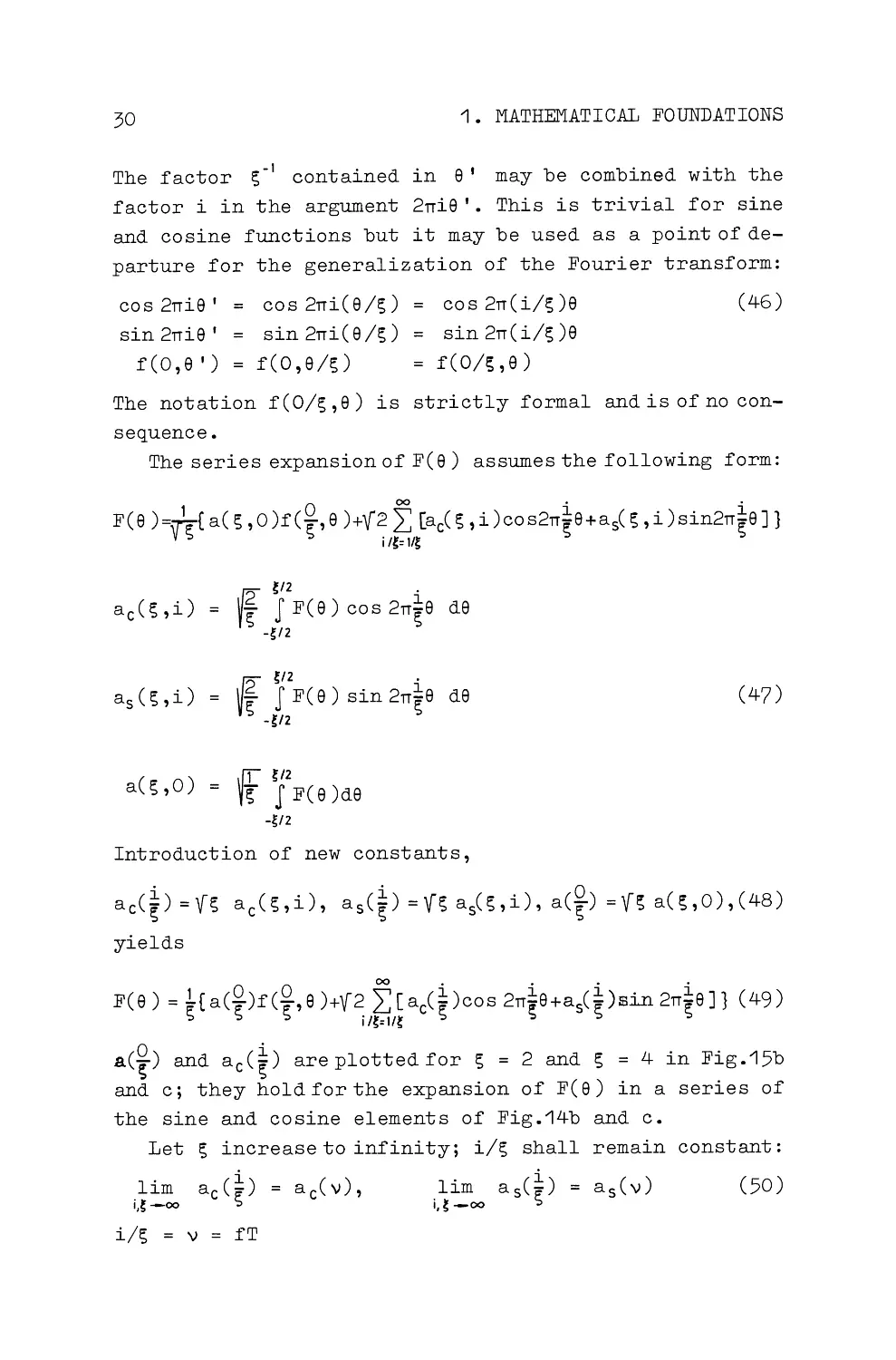
The factor s- 1 contained in 8 I may be combined with the
factor i in the argument 2ni8 1 • This is trivial for sine
and cosine functions but it may be used as a point of de-
parture for the generalization of the Fourier transform:
cos 2ni8 1
sin 2ni8 1
f(0,8 1 )
cos 2ni(8/s)
sin 2Tii(8/s)
f(0,8/s)
cos 2TI(i/s)8
sin 2TI(i/s )8
f(O/s,8)
(46)
The notation f(O/s,8) is strictly formal andisofnocon-
sequence.
The series expansion of F( 8) assumes the following form:
F(8 )=IT( a( s ,0 )f(~, 8 )+\[2 ~ [ac( s ,i)cos2TI~8+a5( s, i)sin2TI~8]}
;t~=ug
I~ ~/2
.
~~ J F(8) cos 2n~8 d8
-g/2
,[2 ~/2
.
V~ J F(8) sin211~8 d8
-~/2
ill ~12
a(s,O) = ~S JF(8)d8
- g/2
Introduction of new constants,
(47)
acC~) =vs acCs,i), a 5 (~) =vs a 5(s,i), a(~) =vs a(s,o),(48)
yields
00
00
•
•
•
•
F(8) = ~( a(~)f(~, 8 )+'{~ 2:: [ ac(~ )cos 2TI~8+a5(~ )min 211~8]} ( 49)
''~= 1/~
.a.(~) and ac(~) areplottedfor s = 2 and s = 4 in Fig.15b
and c; they hold for the expansion of F( 8) in a series of
the sine and cosine elements of Fig.14b and c.
Let s increase to infinity; i/s shall remain constant:
lim
i,~-oo
i/s=v=fT
(50)
1.21 FOURIER TRANSFORM
0.5
t 0.4
0.3
$0.2
~0.1
2
34
c
0
0
i--
0.6
0.5
0.5
tOA
0.3
t 0.4
:;; 0.3
~ 0.2
0.1
s 0.2
~0.1
b0
2
3
4
d
0o
31
4
i/2-
v--
4
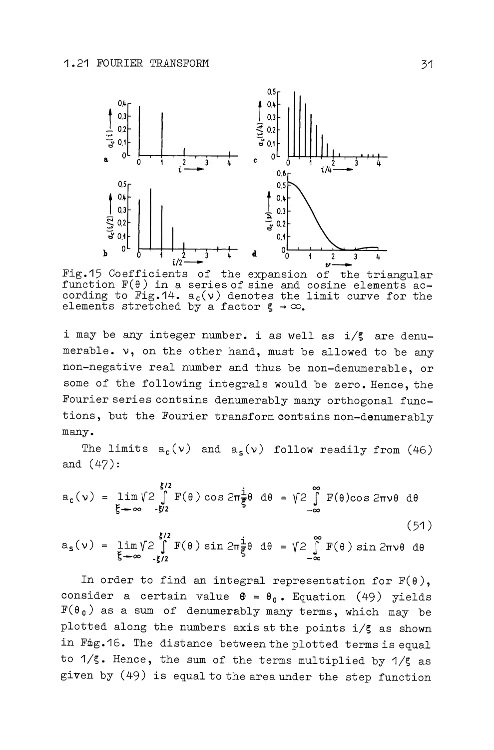
Fig.15 Coefficients of the expansion of -che triangular
function F(9) in a series of sine and cosine elements ac-
cording to Fig.14 . ac(v) denotes the limit curve for the
elements stretched by a factor s .... co.
i may be any integer number. i as well as i/s are denu-
merable. v, on the other hand, must be allowed to be any
non-negative real number and thus be non-denumerable, or
some of the following integrals would be zero. Hence, the
Fourier series contains denumerably many orthogonal func-
tions, but the Fourier transform contains non-denumerably
many.
The limits ac(v) and a 5 (v) follow readily from (46)
and (47):
~/2
.
00
ac(v) = lim 1{2 J F(9) cos 2rr~9 d9 y2 J F(9)cos 2rrv9 d9
~-oo -~2
-oo
(51)
~/2
•
00
a5(v)
lim1{2 I F(9) sin2rr~9 d9 1{2 I F(9) sin2rrv9 d9
~-oo -~/2
-oc
In order to find an integral representation for F(9),
consider a certain value 9 = 9 0 • Equation ( 49) yields
F( 9 0 ) as a sum of denumerably many terms, which may be
plotted along the numbers axis at the points i/s as shown
in Fdlg.16. The distance between the plotted terms is equal
to 1/s. Hence, the sum of the terms multiplied by 1/s as
given by (49) is equal to the area under the step function
32
1. MATHEMATICAL FOUNDATIONS
--
-,
l '!(1/f) ~
l\ >((21> M
L_
-,\ r- -,\
I
I
'-- --
L- -J
0 1IJ 2/f 311 4/1
Fig.16 Transition from Fourier
to Fourier transform.
00
X(O) = a(~)f(~,S 0 )
x(i/s) acCt)'l[2cos2n~S +
+ a 5 (~)'1[2 sin 2n~S
series
of Fig.16. Using (49), one may approximate this area ar-
bitrarily close for sufficiently large values of s by the
following integral:
00
F(S) = '1[2 J[ac(v) cos 2nv9 + a 5 (v) sin2nvS]dv
(52)
0
The lower limit of the integral is zero, because the lo-
wer limit of the sum in ( 49) approaches zero. The first
term of the sum (49) may be neglected, since it contri-
butes arbitrarily little for large values of s. The vari-
able v in (52) must assume the values of all real positive
numbers and not only of denumerably many of them, or the
integral could not be interpreted as a Riemann integral.
Equation (51) shows that ac(v) isaneven and a 5 (v) is
an odd function of v. Hence, .(52) may be rewritten into
the following form:
00
F(a) = JCA(v) cos 2nv9 + B(v) sin2nv9]dv
(53)
-oo
a 5 (v) is identically zero for the triangular function of
Fig.14; ac(v) is plotted in Fig.15d according to the fol-
lowing formula:
3/8
8
ac(v) = 2'1[2 J (1 -~)cos 2nv9 dS
0
3,r2( sin3nv/8)2
8'1
3nv/8
1 • 22 GENERALIZED FOURIER TRANSFORM
33
1.22 Generalized Fourier Transform1
Consider a system of functions (f(O, 9) ,fc (i, 9) ,f5 ( i, 9 )}
orthonormalized in the interval -te ~ e < te. The sub-
script c i.I}.dicates an even function and the subscript s
an odd function. e may be finite or infinite. Hence, the
results will be applicable to functions having an .infinite
interval of orthogonality, such as the functions of the
parabolic cylinder. Let all functions f c ( i, 9) be non-nega-
tive for e = o, and let all functions f 5 (i,9) cross from
negative to positive values at 9 = 0. The functions do not
have to be continuous or differentiable. A function F(S)
defined in the interval -ie ~ e < ie is expanded in a
series:
co
F(S) = a(O)f(O,e) + 2: [ac(i)fc(i,9) + a 5 (i)f5 (i,9 )] (54)
i:I
e/2
e/2
ac(i) J F(S)fc(i,S)de a 5 (i) = J F(9)f 5 (i,S)d9
-e/2
-e/2
e/2
a(o)·= J F(9)f(0,9)d9
-e/2
e is replaced 2 by 9' in the functions f(O,e), fc(i,9)
and f 5 (i,9):
9'=9/y, y =y(s)>1, limy(s)=oo
(55)
~-oo
The expansion ofF( e) in a series of the stretched func-
tions is obtained in analogy to (45):
co
F(9) = vY£aCs,O)f(O,e') +L:[acCs,i)fc(i,e') +
(56)
i:l
1For other generalizations see [1,2].
2 The method used applies to a large class of systems of
functions. Exact mathematical proofs can be obtained with-
out excessive mathematical requirements for individual
systems of functions only. For instance, the results of
this section seem to apply for dyadic rational values of
i/s • 1-l only in the case of Walsh functions; in reality
they apply to all real values of i/s.
3 Harmuth, Transmission of Information
34
i. MATHEMATICAL FOUNDATIONS
The stretched functions are orthonormal in the interval
-tye ~ 9 < tye. F(9) is continued by F(9) =0 into the
intervals-!ye~9<-!®andte~9<tye.
The factor i/y is combined with i so that 9 instead of
9 1 may be written on the right hand side of (56). 2rri ( 9 /s)
had been replaced trivially by 2rr(i/s)9 in (46); since i
and 9 are not necessarily connected as product in f c ( i, 9)
and f 5 (i, 9) the following substitutions must be considered
purely formal until proved otherwise. In particular, i/s
should be considered a symbol rather than a fraction:
fc(i,9 1 )
fs(i,9 1 )
f(o,e I)
f c(i'9/y)
f s(i,9/y)
f(i,9/y)
fcc i/s, 9)
f sci/s,9)
f(O/s,e)
(57)
The series expansion ofF( 9) assumes the following form:
1 y@/2
i
yy J F(8)fs(~,8)d8
- y®/2
y®/2
a(s,O) = vY J F(9)d9
- y®/2
New coefficients are introduced:
(58)
ac(~) = fyac(s,i~ as(~) = fya 5 (s,i), a(~) = fya(s,0)(59)
In order to make (58) and (59) more than a formal notation,
one must demand that the coefficients ac(~) or as(~) have
either the same value for all values of i and s, as long
as i/s = ~ is constant, or that they converge 1 toward a
limit for large values of i and s:
1 The left hand limit shall be taken, if left and right
hand limit differ.
1.22 GENERALIZED FOURIER TRANSFORM
35
(60)
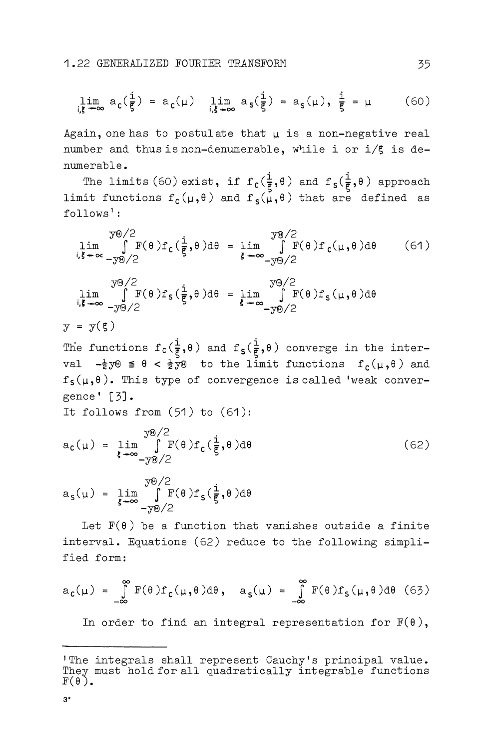
Again, one has to postulate that 1..1 is a non-negative real
number and thus is non-denumerable, w'lile i or i/g is de-
numerable.
The limits (60) exist, if fc(~,a) and f 5 (~,a) approach
limit functions f c(1..1, a) and f 5(1..1, a) that are defined as
follows 1 :
y@/2
.
lim J F(a)fcCi,a)da
1,~-oc -y®/2
':>
y®/2
.
_l im J F(a)f5 (i,a)da
1,( -oo
-y@/2
':>
Y=y(s)
y®/2
lim J F(a)fc(l.l,a)da
~-oo-y®/2
y®/2
=lim J F(a)f5 (1.l,a)da
f-oo
- y®/2
(61)
The functions fc(~,a) and f 5 (~,a) converge in the inter-
val -tye ~a < ~y@ to the limit functions fc(l.l,a) and
fs(l.l,a). This type of convergence is called 'weak conver-
gence' [3].
It follows from (51) to (61):
y®/2
.
acCI.l) = lim J F(a)fc(~,S)d8
~-oo -y®/2
y®/2
.
a 5 (1.l) = lim J F(a)f 5 (~,a)da
~-oo -y®/2
(62)
Let F(S) be a function that vanishes outside a finite
interval. Equations (62) reduce to the following simpli-
fied form:
00
00
J F(S)fc(l.l,S)da, a 5 (1.l) = J F(8)f5 (1.l,8)d8 (63)
-oo
-oo
In order to find an integral representation for F(S),
1 The integrals shall represent Cauchy's principal value.
The;y must hold for all quadratically integrable functions
F(a).
3*
36
1. MATHEMATICAL FOUNDATIONS
consider a certain value 8 = 8 0 • Equation (58) yields
F( 8 0 ) as a sum of denumerably many terms which may be
plotted along the numbers axis at the points i/y = i/y( s)
instead of i/s as in Fig.16. The distance between the
plotted terms is 1/y. Hence, the sum of the terms multi-
plied by 1/y as given by (58) is equal to the area under
a step function. This area may be represented by an inte-
gral, if s and thus y(s) grow beyond all bounds:
00
F(S) = J [ac(~)fc(~,S) + asC~)fs(~,8)]d8
0
(64)
ac(~) and as(~) are called the generalized Fourier
transform of F(S) for the functions fc(~,S) and fs(~,S).
Equation (64) is an integral representation of F(S) or its
generalized inverse Fourier transform. Whether these inte-
grals actually exist cannot be stated without specifying
the functions f c ( ~, 8) and f s (~, 8) more closely. The va-
riable ~ plays the same role as the variable v in the
usual Fourier transform. Hence, ~ is called a generalized
-
and normalized - frequency.
fc(i,S) and fs(i,S) are defined for positive integers
i only. Hence, fc(~,S) and fs(~,S) are defined for non-
negative real numbers ~ only. One may extend the defini-
tions to negative real numbers:
(65)
fc(~,8) is an even function of 8 as well as of ~, and
fs(~,O) is an odd function of 8 as well as of ~·
Equations ( 62) and ( 63) show that ac ( ~) is an even and
as ( ~) i-s an odd function of ~. Hence, ( 64) may be brought
into the form of (53):
00
F( 8) J [A(~)fc(~,S) + B(~)fs(~,S)]d~
(66)
-00
1.23 INVARIANCE OF ORTHOGONALITY
37
1.23 lnvariance of Orthogonality to the Generalized Fourier Transform
Consider the function G(~):
(67)
Since A(~) is even and B(~) is odd, one obtains for G(-~):
G(-~) = V2[A(-~) + B(-~)] = V2[A(~) - B(~)]
A(~) and B(~) may be regained from G(~):
A(~)= tV2[G(~) + G(-~)], B(~) = iV2[G(~)- G(-~)] (68)
Using G(~) one may rewrite (63) and (64) into the form
of (20) and (21):
00
F(e) = iV2 S G(~)[fc(u,e) + f5 (~,8)]d~
(69)
-oo
00
G(~) = iV2 S F(8)[fc(~,e) + f 5 (~,e)]d8
(70)
-oo
Use is made in ( 70) of the fact, that the integrals of
A(~)f5 (~,e) and B(~)fc(~,e) vanish.
Consider a system {f(j ,e)} of orthonormal functions
that vanish outside a finite interval:
00
s f(j,8)f(k,8)d8 6jk
(71)
-oo
Let g(j ,~) denote the generalized Fourier transform of
f(j,8). It follows from (70):
00
g(j,~) = iV2 S f(j,8)[fc(~,e) + f 5 (~,e)]d8
(72)
-oo
Equation (71) may be transformed as follows:
00
00
J f(j,8){iV2 Jg(k,~)[fc(~,e) + f 5 (~,S)]d~}d9 6jk (73)
-oo
-oo
00
00
J g(k,~){iV2 Jf(j,S)[fc(~,s) + f s(~ ' 9)]d8 }~ 6jk
-oo
-co
00
Jg(k,~)g(j,~)~ 6jk
-oo
38
1. MATHEMATICAL FOUNDATIONS
An orthogonal system {f(j ,9 )} that vanishes outside a fi-
nite interval is transformed by the generalized Fourier
transform into an orthogonal system {g(j,~)}.
1.24 Examples of the Generalized Fourier Transform
Consider the generalized Fourier Transform of the tri-
angular function of Fig.17 for Legendre polynomials [1):
B0(x) = 1, P1(x) = x, P2(x) = -(3x2- 1), etc.
The interval of orthogonality is -1 ~ x < +1. x = 29 is
substituted and the following transformations are made:
f(0'9) =p0(29)
fc(i,9)
f 5 (i,8)
i=1,2,
Pc(i,S)
P 5 (i,8)
(-1)i(4i+1f2P2i(28)
(-1); (4i- 13'~2i-1(28)
(74)
The system {f(0,8), Pc(i,8), P5 (i,8)} is orthonormal
in the interval -1 ~ 9 ~ +t. All functions Fe (i ,9) are
positive for 9 = 0, and all functions P 5 (i,9) have a po-
sitive differential quotient. Written explicitely, the
first few polynomials read as follows:
F(0,9)=1, P 5 (1,8)=2'{39, Pc(1,9)=-tV5(1292 -1)
(75)
P 5 (2,9)=-V7(2093 -39), Pc(2,8)=iV9(56084 -12082 + 3)
The coefficients ac(i) and a 5 (i) for Fig.17a may be
readily computed:
112
3/8
-
~8)Pc(i,9)d9
ac(i) = J F(9)Pc(i,9)d9 2 s (1
(76)
- 1/2
0
112
a 5 (i) = J F(S)P5 (i,9)d8
3/8
8
0,a(O)=2J(1-38)d8
-
112
0
ac(i) and a(O) are plotted in Fig.18a.
Let 9 in(75)be replacedby 9' = 8/y, where y = y(s)=
= s = 2. Pc(i,9) and P 5 (i,S) arestretchedoverdoublethe
interval as shown in Fig.17b. The functions (75) are re-
placedbythe streched function-s Pc(i/2,9) and P 5 (i/2,9):
1.24 EXAMPLES OF TRANSFORMS
#~-
--
~ ---
____ ,
Po (28l
--~-- --=-~-- --r~ :~~lo.sJ
P1 (29) ~ ----;
.....
--1::.-.--- ......-q
__
--i
__
· "" P5 (1,8)
a--
~
a.-
,__
-P2(28)- -
... ._;,... .. .....-
-
''l7"-==- - ""l/7 ~ - "'v"" --
Pc (1,8)
I
'
-P (28) ,--- I'
,--- [\,
=
t--,
-
--
~- ~P.(29)
3
?
'~"
'\:
..........-
\J "-
\j .,-~
SI
I
I
--
.1\
•
A -=--
I',
-
-1'
--, 0 (28)
P.4 (29) 1 "-
1" "'
,
·-
•
1
'"'"""
1 ......., 1 -~
1
-·
1
•
1•c
'
-2
-1
0
1
2
a
·
8---
...-------~·------~ _____ .. .. . , F(S)
P0 (28') -------~
'
------
wai(O,B)
P1 (28:)- ----~ =-:_ -
P5(1/2,8)
-Pz (28 l
.,
,
..... ~
Pc(1/2,8)
-P3 (29')-
-
-
'......:['...-=f-=-. -==f'~"-- ~-
-P5 (2/2,8)
P4 (28')
-
: _. :~.-
:k:',::v::- :: - Pc(Z/2,8)
P5 (28') ~--=-==---=--~~h...==-1...=~==---==~~~~::::.,.=~- P5 (3/2,8l
- P6 (28')-
- -\1=- t
t ,...,v .. -
Pc{3/2,8)
-P7 (28') ~ ---- -·t==t--==- 1-==-+-:=~\..., -~- ..., -- P5(4/2,9)
-2
-1I
o
-t-1e-
2
b
-1
-112 I 0 ! 112e·~1
;
' ------ I
;-- F(B)
Po (zei~
I
,--wai(O,B)
P, (28') -~_
I,·
I
S- P5 (V4,8)
- Pz (28') ,z=:
:::::::::::::::# Pc(1/4,8)
- P3 (28') ,J'=-
-=
I
-=:::]' P8 (2/4,9) ·
( ') -1'--..
I
/1> D (2118)
P4 28, ,...
..::=-::
--= =-
= ___...A
•c t'+,
P5 (28) v
-=-
I
I -=== ---
~" P5(3/4,8)
-P6 (28') ,v--=---- --===--1
'
--===--
-- -= -- -,J/ Pc(3/4,8)
-P7 (28') ·J·..............,--==-- L ~--===---- --=-.1'', P5(4/4,8)
'II
'
I
'\J
P8 (28') A·-=--==----~-===- .-l=---== --- _ _ _ _ _ , ..t ., Pc(4/4,8)
P9 (28'J ..:'vc--, ............... ,. .. .. .. -== -.. , '"'f==::: 1.......::::=::: .... - - - - .. ... .. .. ,. .;>1/ P5 (5/4,Bl
- P10 (28'J ·vc- . =-==- ---= --- -== --
.. .. .. .__. .. .. .- ==- - -- -= --,/"\v' Pc(5/4,8)
-~:-1
1
91 18+---~
c
-1/ Z
-1/4
0
1/4 8'-
1/2
39
Fig.17 Expansion of a function F(8) in a series of Legen-
dre polynomials having various intervals of orthogonality.
a)-~ :§ 8 < ~' {wal(0,8), Pc(i,9), P 5 (i,9)}
b) -1 :§ 8 < 1, {wal(0,9), Pc(i/2,9), Ps\i/2,9)}
c) -2 :§ 9 < 2, {wal(0,9), Pc(i/4,9), P 5 (i/4,9)}
40
1. l"'ATHEl"'ATIC.AL FOUNDATIONS
P5 (1/2,8) P 5 (1 ,8/2) 21{3(18)
(77)
p c ( 1/2' 8') Pc (1 ,8/2) -11{5[12(18 i- 1]
P 5 (2/2,8) P 5 (2,8/2) -1{7[20(18)3 - 3(18)]
Pc(2/2,8) Pc (2,8/2) tV9[560(18)4 - 120(!8)2 + 3J
The coefficients ac (i/2) have the following value:
+I
3/8
8
ac(i/2)=JF(8)Pc(i/2,8)d8 =2J (1- 38)Pc(i/2,8)d8 (78)
-1
0
Values of ac(i/2) are plotted in Fig.18b. They do not have
exactly the same values as the coefficients ac(i) of Fig.18a
since, e.g ., Pc(2/2,8) is not equal Pc(1,8).
Let the functions (75) be stretched over four times
the interval by the substitution 8'
=y(s)=s =4 asshowninFig.17c;
8/y, where y =
P5 (1/4,8)
Pc(1/4,8)
P 5 (2/4,8)
Pc ( 2/4,8)
P 5 (1,8/~)
Pc(1,8/4)
P 5 (2,8/4)
Pc (2,8/4)
21{3(:!8)
- 1V5[12(i8/- 1]
- V7[20(i8)3 - 3Ci8)J
iV9[560(i8)4 - 120(i8)2 + 3J
Some coefficients ac(i/4) are plotted in Fig.18c:
(79)
·2
3ffl
8
ac(i/4)=J F(8)Pc(i/4,8)d8 =2 J (1- 38)Pc(i/4,8)d8 (80)
-2
0
In order to compute the limit ac(i/s) for large values
of i and~' one needs PcCi/s,8) = Pc(i,8/s) forlargeva-
lues of i and small values of 8/s. An asymptotic series for
Legendre polynomials Pi(x) is known that holds for large
values of j and for small values of x:
Pi(x)= \[2 ((1 - d.sin[(j+1)cos- 1 x +in]+
Vnj V1-x2
J
-
Rcos[(j+1)cos-1 x + in]}
8j 1-x2
Using (74) one obtains:
Pc(i,8/s)=~ oos 4!8
(81)
1.24 EXAMPLES OF TRANSFORMS
t0.4
0.3
~-u0.2
"
~ 0.1
~
0
a.
t0.4
-03
3'
~0.2
~:s 0.1
"
0
c
0
0
2
i,p.-
4
t 0.4
-
0.3
::1,
- ;;\' 0.2
s 0.1
-; ;\'
b0
41
4
Fig.18 Coefficients of the expansion of the triangular
function F(S) in a series of Legendre polynomials accor-
ding to Fig.17. ac(~) is the limit curve for the polyno-
mials stretched by a factor ~ ... =·
The limit function Pc C~-t,S) and acC~) follow for s ... = :
(82)
00
ac(~) J F(S)Pc(u,S)dS
-00
_
_l_(sin3lr/4)2
-
4'{TT 3~-t 4
(83)
ac C1.1) is the generalized Fourier transform of the tri-
angular function of Fig.17 for Legendre polynomials. It
is plotted in Fig.18a to c. One may readily see how the
coefficients ac(i), ac(i/2) and ac(i/4) converge to acC~).
ac(\1) in Fig.15 and ac(~) in Fig.18 are equal except
for scale factors. One may see from the differential equa-
tion of Legendre polynomials that this is generally so:
(1-X)Z11 -
2XZ1 -
j(j+1)Z=0jj=0!1!2!o••
( 84)
This equation reduces for small values of x and large va-
lues of j to the differential equation of sine and cosine
functions:
z"+jz'=0
(85)
42
1. MATHEMATICAL FOUNDATIONS
Fig.19 Expansion of a function F(8) in a series of Walsh
elements having various intervals of orthogonality.
a) -t ~ 8 < i, {wal(0,8), cal(i,8), sal(i,8)}
b) -1 ~ 8 < 1, {wal(0,8), cal(i/2,8), sal(i/2,8)}
c) -2 ~ 8 < 2, {wal(0,8), cal(i/4,8), sal(i/4,8)}
1.24 EXAMPLES OF TRANSFORMS
43
Hence, the generalization of the Fourier transform is main-
ly of interest for systems of orthogonal functions, that
are not defined by such differential equations, which are
reduced by stretching to the one of sine and cosine func-
tions. Since Walsh functions are defined by a difference
rather than a differential equation, they may be expected
to yield a more rewarding result than Legendre polynomials.
The generalization of the Fourier transform to the Walsh-
Fourier transform is due to FINE. However, FINE did not
distinguish between even and odd functions. This distinc-
tion is important for the applications of Walsh-Fourier
analysis to communications. The mathematically rigorous
theory for Walsh functions separated into even and odd
functions - that is cal and sal functions - is due to
PICHLER [2].
Let the functions f(0,8), fc(i,8) and f 5 (i,8) repre-
sent Walsh functions:
f(0,8)•wal(0,8), fc(i,8)=cal(i,8), f 5 (i,8)=sal(i,8) (86)
The triangular function of Fig.19a yields the coefficients
112
3/B
8
a(O) =I F(8)wal(0,8)d8 = 2 I (1 - 38)d8
-112
0
3/B
8
ac(i) = 2 I (1 - 38)cal(i,8)d8,
0
Fig.20a shows some values of a(O) and ac(i).
With y(s) = s one obtains cal(i/s,8) = cal(i,8/s) and
sal(i/s, 8 ) = sal(i,8/s). Inspection of Fig.19a to c shows
that cal(2i/2,8) and cal(4i/4,8) are equal to the function
cal(i,8) continued periodically over double or four times
the original interval of definition. This result may also
be inferred readily from the difference equation ( 28).
Hence, itholdsintheinterval-!~8<t:
cal(i,8) = cal(~i,8/~)
cal(si/s,8)
44
1. MATHEMATICAL FOUNDATIONS
Inspection of Fig.19a to c shows further that the follow-
ing relations hold in the interval -i ~ 9 < i:
cal(i,9) = cal(2i/2,9) = cal[(2i+1)/2,9]
(87)
= cal(4i/4,9) = cal[(4i+1)/4,9] = cal[(4i+2)/4,9]
= cal[(4i+3)/4,9]
= cal[('Si+TJ)/s,9J
TJ=0,1,•••s-1;s =2r.
Substituting Csi+T])/s = IJ,, i ~ iJ < i+1' one obtains:
cal(iJ,9) = cal(i,9), i ~ iJ < i+1, i
=
1'2'••
(88)
cal(iJ,9) wal(0,9), 0 ~ iJ < 1
-i~9<i
Corresponding relations are obtained for sal ( iJ, 9 ) :
sal(iJ,9) sal(i,9), i-1 < iJ ~ i, i = 1,2, ••
(89)
The limit functions cal(1J,9) and sal(1J,9) have been
derived here in an heuristic manner for the interval
- i ~ 9 < i· PICHLERhasobtained cal(iJ,9) and sal(iJ,9) in
a mathematically rigorous way for the whole interval
- co < 9 < oo, but his proofs require a very good command
of mathematics. Fig.12 and 13 show a very ingenious re-
presentationofthe functions cal(iJ,9) and sal(iJ,9) found
by him (2].
Functions that are identical in the interval -i ~ 9 < i
yield the same expansion coefficients for F( 9). Hence, one
obtains for ac(IJ) and a 5 (1J):
112
ac ( 1-1) = ac(i) = JF(9)cal(i,9)d9
i~iJ<i+1
(90)
-1/2
a 5 C1-1) a 5 (i) tF(9)sal(i,9)d9
i-1<u~i
-1/2
1/2
ac(iJ) = a(0)
JF(9 )d9
0~iJ<1
-1/2
-i~9<f;1 1'2,
1.25 FAST WALSH-FOURIER TRANSFORM
45
0.4
0.4
r·3
t 0.3
-0.2
110.2
.....
. !, ..:t
~0.1
~0.1
~
6
a
0
4
0
c
0
0.4
i-
t 0.3
t 0.3
~0.2
3. 0.2
.....
"'
"'
~ 0.1
---;;-0.1
"'
IIII
0
00
b
0
1
23
4
(2i+tJ)/2-
d
p-
Fig.20 Coefficients of the expansion of the triangular
function F(8) into a series of Walsh elements according
to Fig.19. acCu) isthelimitcurvefortheelements stret-
ched by a factor s .... ro.
ac[(2i+TJ)/2], ac[(4i+TJ)/4] and the limit ac(u) are shown
in Fig. 20b to d for the triangular function of Fig .19.
The computation of the functions acCu) and a 5 (u) is very
simple for Walsh functions, since one has to compute the
coe1'ficients a(O), ac(i) and a 5 (i) only and plot these
values from0to1,from1toi+1,orfromitoi-1to
obtain acCu) and a5(u) in the intervals 0 ~ u < 1,
i~u<i+1ori-1<u~i.
1.25 Fast Walsh-Fourier Transform
The time required to obtain the Fourier transform may
be drastically reduced by means of a method known as fast
Fourier transform. A corresponding fast Walsh- Fourier
transform was found by GREEN [1] and generalized by WELCH
[ 2, 3] • KANE, ANDREWS and PRATT have used a two-dimensional
fast Walsh-Fourier transform for the compression of infor-
mation of pictures [4]. WHELQHEL and GUINN have used it
for signal classification [5]. The form presented here dis-
tinguishes between even and odd functions and lists them
according to the number of sign changes as in Fig.2 .
Consider a function F(a) in some interval. Let this
46
1. MATHEMATICAL FOUNDATIONS
interval be divided into 2n equallywide subintervals. For
illustration, the special case 2 3 = 8 will be discussed.
The average values of F(e) in the 8 intervals are denoted
by A, B, ••• , H. F(e) is thus represented by a step func-
tion that is a least mean square fit of F(e) for this num-
ber of intervals. The Walsh-Fourier transforms ac(~) and
as(~) of these step functions may be obtained from the
average values A, B,
••• , H with the help of Fig.2:
+A+B+C+D+E+F+G+H
a(O)
ac c~)'
0::§~<1
-A -B-C-D+E+F+G+H
as(1) as(~)'
0<~::§1
-A -B+C+D+E+F-G -H
ac (1) ac (~)'
1::§~<2
+A+B-C-D+E+F-G-H
as(2) as c~)'
1<~~2
+A-B-C+D+E-F-G+H
ac (2) ac(~),
2~~<3
-A+B+C-D+E-F-G+H
as(3) as(~),
2<~::§3
-A+B-C+D+E-F+G-H
ac(3) ac (~)'
3~~<4
+A-B+C-D+E-F+G-H
as(4) as c~)'
3<~::§4
There are 2 3 (23 - 1) = 56 or generally 2n(2n- 1) addi-
tions necessary to obtain the 2n coefficients ac (~) and
as(~). The fast Walsh-Fourier transform requires 2nn ad-
ditions only. Note that the Walsh-Fourier transform does
not require multiplications, which are time consuming in
the case of the fast Fourier transform'.
For an explanation of the fast Walsh-Fouriertransform
refer to Table 1. Column 0 lists the 8 amplitude samples
A, B, ••• , H together with a more general notation s~:~ •
Column 1 lists sums and differences of two each of the
samples, again together with amore general notation. Sums
and differences of column 1 are shown in column 2, while
column 3 shows sums and differences of column 2. The ge-
neral notation s kLP shows in each case, which terms of
,m
the previous column are added or subtracted. The third
column yields the Walsh-Fourier coefficients a(O), ac(i)
1 A fast Haar-Fourier transform maybe derived for the com-
plete orthogonal system of Haar functions [6]. This trans-
form may be even better suited for digital computations
than the fast Walsh-Fourier transform (personal communi-
cation from H.C.ANDREWS USCLA).
1.25 FAST WALSH-FOURIER TRANSFORM
47
Table 1. Fast Walsh-Fourier Transform
0
1
2
3
sO,O =A SO,O =+(SO,O+SO,O) sO,IJ,.,+(SO,O+SO,O) sO,O =+(sO,O +SO,O)
o,o
0,1
0,0 1,0 0,2
0,1 I,I 0,3
0,2 I,2
= +A+B
= +.i+B+C+D
=+A+B+C+D+E+F+G+E
so,o=B
1,0
s 0,1 =-( so,o -s o,o)
0,1
0,0 1,0
so,1 =-( so,o -so,o)
0,2
0,1 1,1
s 0,1 =-( so,o -so,o)
0,3
0,2 1,2
= -A+B
= -A-B+C+D
=-A -B -C -D+E+F+G+H
so,o =C
2,0
S0,0 =+ ( SO,O +SO,O )
2,0
2,0 3,0 8 1,0=+(SO,I -S0,1)
0,2
0,1
I,I
SI,O =+( SO,I -SO,I )
0,3
0,2 1,2
= +C+D
= -A+B+C-D
=-A -B+C+D+E+F-G -H
so,o =D
3,0
so,1 =-( so,o -so,o)
1,1
2,0 3,0 S1,1 =-( SO,I
0,2
0,1
+SO,I )
1,1 S1,1 =-(SO,I +SO,I)
0,3
0,2 I,2
= -C+D
= +A-B+C-D
=+A+B-C -D+E+F-G -H
so,o =E
4,0
so,o=+(so,o+so,o)
2,1
4,0 5,0
so,o =+( so,o +So, o)
1,2
2,1 3,1 S2,0 =-( S1,0 +SI,O )
0,3
0,2 1,2
= +E+F
= +E+F+G+D
=+A-B -C+D+E-F-G+H
so,o =F
5,0
so,1 =-(so,o_so,o)
2,1
4,0 5,0
so,1 =-( so,o _ 8 o,o)
1,2
2,1 3,I
S2,1 =+(SI,O -S1,0)
0,3
0,2 1,2
= -E+F
= -E -F+G+D
=-A+B+C-D+E-F-G+H
so,o =G
6,0
so,o =+( so,o +So,o)
3,,1
6,0 7,0
si,O=+(so,l_so,l)
1,2
2,1 3,1
s3,o=-(s1,1 -sl,l)
0,3
0,2 I,2
= +G+H
= -E+F+G-D
=-A+B-C+D+E-F+G-H
o,o H
s7,o=
so,1 =-(so,o_so,o)
3,1
6,0 7,0
Sl,l =-(SO,I +SO,I)
1,2
2,1 3,1
S3,1 =+(SI,I+SI,I)
0,3
0,2 1,2
= -G+H
= +E-F+G-D
=+A-B+C-D+E-F+G-H
and ac(i).
The fast Walsh-Fourier transform can be represented by
a recurrence formula or difference equation that follows
from that of the Walsh functions (29):
si.P
= (-1)[it2]•P [s[it2],x + (-1)i•P s0t2J,x]
k,m
k,m-1
k•l,m-1
[j/2] = largest integer smaller or equal ij
x=0forj=even,x
=1 forj=odd
(91)
k=0,1,••,2"-m-1;m=0,1,••,n;p=0or1;j=o•••m;
2"= number of amplitude samples
Asanexample considerthe termfor j =3, p =1 , k =0,
48
1. MATHEMATICAL FOUNDATIONS
m=3.Itfollowswith[j/2] [3/2]=1andx=1:
s~:~ (-1/[s~:~ + (-1) 4 s~; 12 ]
This is identical with the term in the lower right corner
of Table 1.
The quantities [j/2] and x may be produced in a binary
computer as follows: Let j be represented by a binary num-
ber. Division by 2 shifts the binary point by one place.
The number to the left of the binary point is [j/2], the
number to the right is x. Example:
j=23=10111, !j=11.5=1011.1, [j/2]=11=1011, x=1
The computation starts with the 2" terms s~·.~ , k
= 0••
•• 2"-1. It follows from [j/2] = [0/2] = 0 that the terms
s~:i,k
= 0 ••••2"-
1-1, can be computed. These are the
terms in the second column of Table 1. Further terms with
[j/2] = [1/2] = 0 cannot be computed, since this would re-
quire terms s ~:J while only terms with x "' 0 are available.
The terms s~·r permit the computation of the 2"- 1 terms
s 0·P andthe 2"-1 'terms s 1·P
since x may be zero or 1,
k'2
k,2
'
and j may thus be 0 or 1, both values yielding [j/2] = 0.
The fast inverse Walsh-Fourier transform is obtained
by computing the coefficients A, B, ••• , H from the coef-
ficients a(O), a 5 (1), ••••• a 5 (4). This may be done by in-
verting the recursion formula for the sLP
k,m
from the sum and difference of s L 0 and sL 1
k,m
k,m
• One obtains
the following
two recursion formulas:
(iI2], X
s
k+1, m-1
S (j/2), X
k,m-1
tC-1) [i' 2 l ( si,D_si.1)
k,m
k,m
Both may be written together in one formula:
s[i/2], x
k+p, m-1
p=0or1;x=0forj=even,x
=1forj
odd;
[j/2] = largest integer smaller or equal tj.
(92)
1.31 GENERALIZED FREQUENCY
49
1.26 Generalized Laplace Transform
The Laplace transform X(a,v) of a time function F(S)
and its inverse may be written as follows:
00
X(a,v) J F(S )e-cr 6 ei 2rrv6
dS
(93)
0
00
F(e) = e cr6 J X(a,v)e•i2rrv6d8
(94)
-00
It is apparent that the Laplace transform of F(S) may
be considered to be a Fourier transform of F(8)e-cr 8 • The
factor e-crB makes functions F( 8) Fourier transformable
that are not quadratically integrable. The generalized
Laplace transform in real notation follows from this re-
mark from (93) and (94):
00
J F(8)e-cr 8 f 5 (v,8)d8
(95)
0
00
J F(8)e-cr8 fc(v,S)d8
00
F(S) =
ecr 8 J [ac(a,v)fc(v,S) + a 5 (a,v)f 5 (v,8)]dv(96)
-oo
The integrals (95) do not have the lower limit -co as
do the integrals of the generalized Fourier transform,
since the factor e -ere might make them divergent. F( 8) must
vanish sufficiently fast for large negative values of 8.
The usual assumption F(S) = 0 for 8 < 0 is used here.
1.3 Generalized Frequency
1.31 Physical Interpretation of the Generalized Frequency
Frequency is a parameter that distinguishes the indi-
vidual functions of the systems [ cos 2TTft} or [ sin 2TTft}.
Its usual physical interpretation is "number of cycles
per unit of time". The normalized frequency v = fT is in-
terpreted as "number of cycles in a time interval of du-
ration 1".
The generalized frequency may be interpreted as "ave-
4 Harmuth, Transmission of Information
50
1. MATHEMATICAL FOUNDATIONS
rage number of zero crossings per unit of time divided
by2" oras
"average number of sign changes per unit of
time divided by 2". The normalized, generalized frequency
1..1 . is interpreted as "average number of zero crossings per
time interval of duration 1 divided by 2". The generalized
frequency has the dimension [ s·1 ] :
(97)
The definition of the generalized frequency has been cho-
sen so that it coincides with that of frequency, if applied
to sine and cosine function5. For instance, a sine oscil-
lation with frequency 100 Hz has 100 cycles per second or
200 zero crossings per second. One half the number of zero
crossings per second equals 100, which is the same number
and dimension as that of the frequency 1 • The zero cro s-
sings of sine and cosine functions are equally spaced but
the definition of the generalized frequency makes it appli-
cable to functions whose zero crossings are not equally
spaced and which need not even be periodic.
It is useful to introduce the new term 'sequency' for
the generalized frequency ~· One reason is that the term
generalized frequency is already used in connection with
damped oscillations; another is that there are transver-
sal waves in three dimensional space which have a frequen-
cy as well as a sequency. The measure of sequency is
"average number of zero crossings per second divided by 2",
for which one may use the abbreviation 'zps'.
Consider the Walsh functions cal(i,8) and sal(i,8) in
Fig.2. i equals one half the number of sign changes in
theinterval-t;§8<t and~=i/Tisthesequencyof
the periodically continued functions. If the functions
are stretched by a factor s they will have 2i sign chan-
ges in the interval -ts ;§ 8 < ts; i/s = 1..1. will be one half
1 The number of sign changes per unit of time has been used
to define an instantaneous frequency of frequency modu-
lated sinusoidal oscillations [1,2,3].
1.32 POWER SPECTRUM, FILTERING
51
the average 1 number of sign changes in an interval of du-
ration 1.
Consider as a further example the periodically conti-
nued Legendre polynomials Pc(i,e) andP5 (i,8) of Fig.17a.
They have 2i sign changes in the interval -t :§ 8 < +~.
Stretching them by a factor s makes the duration of this
interval equal s and i/s = l...l becomes one half the average
number of sign changes per time interval of duration 1.
Let the normalized variables v and 8 in sin 2rrv8 be
replaced by the non-normalized variables f = v/T and
t=8T:
sin 2rrv8 = sin 2rr (fT )% = sin 2rrft
(98)
The time base T drops out. Sine and cosine functions con-
tain the three parameters amplitude, frequency and phasw
angle. This is not so for complete systems of orthogonal
functions, which do not have sequency and time base con-
nected by multiplication. Walsh functions sal(l...l, 8) or Le-
gendre polynomials P 5 (1...l,e) have a comma between l...l and e.
Hence, the substitutions ~ = i...L/T and t = 8T yield:
sal(l...l,e) = sal(~T,t/T),
(99)
These functions contain in their general form the four pa-
rameters amplitude V, sequency ~, delay t 0 , and time base T:
( t-to)
Vsal ~T,-T- ,
( t-to)
VP5 ~T,-T- •
1.32 Power Spectrum, Amplitude Spectrum, Filtering of Signals
One may derive the frequency function a~( v) + a~ ( v)
from the Fourier transforms ac(v) and a 5 (v) of (51) and
interpret it as frequency power spectrum. In analogy, one
may interpret the sequency function a~(l...l) + a§CI...l) derived
from the generalized Fourier transforms ac ( l...l) and a 5 ( l...l)
1 The sequency of a periodic function equals one half the
number of sign changes per period. The sequency of a non-
periodic function equals one half the number of sign chan-
ges per unit of time, if this limit exists.
4*
52
1. MATHEMATICAL FOUNDATIONS
of (62) ·and (63) as a sequency power spectrum.
Let (58) be squared and integrated using the notation
of (59) for the coefficients:
100
00
-2 S {a(I)f(I,e)
Y -oo
00
•
•
+ 2:: [ac(!)fc(!,e) +
il~=ll~
+ a5(~)f5(~,S)]r dS
The integrals of the cross-products of different functions
vanish due to the orthogonality of the functions. The inte-
grals of f 2 (0/s,e), f~(i/s,e) andf~(i/s,e) multiplied by
y- 1 yield 1:
The sum has the same form as that of (58). Hence, it may
be interpreted as the area under a step function and the
sum may be replaced by an integral for large values of s
and y = y(s):
00
00
00
J F 2 (9 )de= J [a~(l-l) + a;CI-l)]dl-l = ~ f [a~(l-l) + a~(l.l)]diJ (100)
-oo
0
-oo
Using non-normalized notation one obtains:
00
00
f F 2 (t/T)dt = T f [a~(ctJT) + a~(ctJT)]d(ctJT)
( 101)
-00
0
T[a~(IJ) + a~(l-l)]d1J is the energy of the components
ac(1-l)fc(11,e) to ac(11+dl-l)fc(11+d1J,e) and a5(1-l)fs(1-l ,e) to
a 5 (1-l+dl.l)f 5 (1-l+dl.l,e), if the integral of F 2 (t/T) is inter-
preted as the energy of the signal F(S). Hence, a~(IJ) +
+ a~(IJ) has the dimension of power and maybe interpreted
as sequency power spectrum or sequency power density spec-
trum.
Using the function G(~),
G(v) =A(~)+ B(~) = ~V2[ac(~) + a 5 (~)],
one may rewrite the frequency power spectrum a~ ( ~) + a~ ( ~)
into the following form:
1.32 POWER SPECTRUM, FILTERING
53
a~(~) + a~(~) =2[A2(~) + B2(~)] =G2(~) + G2(-~) (102)
Use has been made of (16), (19) and (52). The sequency
power spectrum may be rewritten als follows:
a~(~) + a~(~) =4[A2(~) + B2(~)] =G2(~) + G2(-~) (103)
The square root [a~ ( ~) + a~ ( ~) ] 112 may be interpreted as
frequency amplitude spectrum. Such an interpretation is
not possible for the square root [a~(~) + a~(~)]112 of the
sequency power spectrum, since a specific feature of sine
and cosine functions is required for it 1 • Using the re-
lation
Asinx +Bcosx = (A2+B2)112cos(x- tg"1~)
one may rewrite (52) as follows:
(104)
00
F(S) = '{2f (a~(~)+ a~(~)] 112 cos (2TT~9 - tg·1 ::e~5]d~ (105)
0
The factor [a~(~) + a~(~)] 112 may be interpreted as fre-
quency amplitude spectrum, since it represents the ampli-
tude of the oscillation with frequency ~ without regard
to the phase angle tg·1 a 5 (~)/ac(~). Systems of functions
that do not have an addition theorem like ( 104) do not
permit this interpretation of the square root [a~ ( ~) +
+ a~(~)] 112 • However, ac(~) and as(~) are just like a((~)
and as(~) the amplitude spectra of the even and odd part
of the function F(S).
Filters or, more generally, systems that change an in-
put signal F(S) into an output signal F 0 (9) may be de-
scribed by operators. The concept of linear operators
describing linear systems is of particular importance in
connexion with complete systems of orthogonal functions.
Let 0 denote an operator and {f(j,S)} a complete system
I The addition theorems of sine and co sine are required
for the derivation of the Wiener-Chintchin theorem in
real notation. Hence, other systems of functions have no
direct analogue to the Wiener-Chintchin theorem. Walsh
functions have an abstract analogue based on the dyadic
correlation function jF(9)G(9$T)d9.
54
~. MATHEMATICAL FOUNDATIONS
of orthogonal functions. Application of 0 to a particular
function or input signal f( j, 6) generates an output sig-
nal g( j, 6):
Of(j,6) = g(j,6)
( ~06)
The operator 0 is called linear if the proportionality
law and the superposition law hold for all functions of
the system {f(j,6)}:
Oa(j)f(j,6) = a(j)Of(j,6)
proportionality law (~07)
00
00
0 2":: a(j )f(j ,6) = 2":: Oa(j )f(j ,6) superposition law (~08)
j:0
j:0
0maybeafunctionofjand8•If0depends on8,the
operator and the system it describes are linear and time
variable; otherwise they are linear and time-invariant.
An example of a linear, time-variable system is the am-
plitude modulator. Let an input signal F(8) be represen-
ted bythe sum Lf.Cj)f(j,8) and the carrier by h(k,8) = o.
h(k,8) may be, e.g., a sine carrier \[2 sin 2TTk8 or a Walsh
carrier wal(k,8). Amplitude modulation with suppressed
carrier yields:
00
00
F(8)h(k,8) = OF(8) = 0 La(j)f(j,8) = l:a(j)g(j,8) (~09)
j:O
j:O
g(j,8) = h(k,8)f(j,8)
It is best to use Walsh functions wal(j,S) for f(j,S)
if h(k, 8) is a Walsh carrier wal(k, 8). One obtains for
g(j,8):
g(j,8) = wal(k,8)wal(j,8) = wal(kffij,8)
If h(k, 8) is a sine carrier \[2 sin 2TTk8 one should use the
functions f(O,S), \[2 sin 2TTi8 and V2 cos 2TTi8 for the sys-
tem {f(j,S)}. The functions g(j,S) are then
g(O ,e) = \[2 sin 2rrk8
g(2i,8) = COS 2TT(k-i)8 - COS 2TT(k+i)8
g(2i-~,8) = sin2TT(k-i)8 + sin2TT(k+i)8
j=0'2i'2i-~;i=~'2'
•••
1.32 POWER SPECTRUM, FILTERING
55
The definition of linearity has changed during deve-
lopment of communication theory. First it was restricted
to differential operators with constant coefficients, then
to time invariable but not necessarily differential ope-
rators. The present definition does not require 0 to be
a differential or time invariable operator. It has been
used by mathematicians for a long time; its widespread
introduction into communications is often credited to a
book by WUNSCH [1].
If a system is described by a linear operator 0 and if
one is free to choose the system of functions [f(j,6)},
one may choose the system of eigenfunctions of o. Equation
(106) assumes the following form in this case:
Of(j,8) = b(j)f(j,8)
( 110)
It is convenient to· call f( j, 8) an eigenfunction of 0 even
if f(j,8) on the right hand side of (110) has to be re-
placed by the time shifted function f[j,8-8(j)].
In the frequency theory of communication the electrical
characteristics of filters are described by the frequency
response of attenuation and phase shift. This description
assumes that a voltage V cos 2nft is applied to the input
of a filter. The steady state voltage Vc(f)cos[2nft+ac(f)]
appears at the output. The frequency functions -21ogVc(f )/V
= -2logVc(\i)/V and ac(f) = Clc(\i) are calledfrequencyre-
sponse of attenuation and phase shift. Let an input sig-
nal F( 8) have the Fourier transforms at ( \i) and 8.s ( \i). The
output signal F 0 (8) follows from (52):
00
F 0 (8) = y2 J [ac(\i)Kc(\i)cos[2TT\i8 + ac(\i)]+
( 111)
+ a 5 (\i)Kc(\i)sin[2n\i8 + ac(\i)]}d\i
Kc(\i) = Vc(\i)/V; \i = fT, 8 = t/T.
The description of filters by means of frequency re-
sponse of attenuation and phase shift is eminently suited
for telephony filters. Matched filters, on the other hand,
are usually described by means of the pulse response. A
56
1. MATHEMATICAL FOUNDATIONS
voltage pulse of the shape of the Dirac function 6(8) is
applied to the input and the shape of the output voltage
D( 8) is determined. No reference to sine and cosine func-
tions is required. Which system of functions is used for
description of a filter is strictly a matter of convenience.
Let the voltages Vfc(~,e) and Vfs(~,e) be applied to
the input of a filter instead of V cos 2rrft. The functions
fc(~,e) and fs(~,e) are the same that occur in the gene-
ralized Fourier transform (63). The steady state voltages
Vc(~)fc[~,8-8c(~)] and Vs(~)fs[~,8-8s(~)] shall occur at
the filter output. Let -2logVc(~)/Vand-2logVs(~)/V be
called attenuation. Sc(~) and Ss(~) are called delay,
since the term 'phase shift' cannot be applied to func-
tions other than sine and cosine. These simple relations
between input and output voltage exist for filters con-
sisting of coils and capacitors if fc(~,e) and fs(~,e)
are sine and cosine functions. However, one may design
filters that contain multipliers, integrators, storages,
resistors and switches, which will attenuate and delay
Walsh functions, but will distort sine and cosine func-
tions. Such filters are better described by Walsh func-
tions than by sine-cosine functions.
Let a signal F(S) have the generalized Fourier trans-
forms ac(~) and as(~). Let the steady state attenuation
anddelaybe -2logVc(~)/V, -2logVs(~)/V and Sc(~), Ss(~).
The output signal follows from (64):
00
F 0(8) = J[ ac(~)Kc(~)fc[~,8-8c(~)]+as(~)Ks(~)fs[~,e-es(~)]}d~
0
(112)
Comparison of (111) and (112) shows that only Kc(v) and
ac(v) occursin(111),butnot Ks(~) and as(v). Such terms
would occur if frequency filters would distinguish between
sine and cosine functions of the same frequency. The in-
put voltage V sin 2rrft would then produce the output vol-
tage Vs(f) sin [2rrft+as (f)] rather than Vc(f) sin [2rrft+ac(f)].
1.33 EXAMPLES OF POWER SPECTRA
57
Such a distinction between sine and cosine requires some
time-variable circuit element and can thus not occur in
frequency filters which are linear and time-invariant.
Filters based on sine and cosine pulses rather than on
the periodic sine and cosine functions distinguish be-
tween sine and cosine. An example of such a filter will be
given later on.
1.33 Examples of Walsh Fourier Transforms and Power Spectra
Fig.21 shows time functions F(8), their Walsh-Fourier
transforms G(iJ,), ac(IJ.), a 5 (1J.) and their sequency power
spectra a~(iJ.) + a~(iJ.):
00
G(iJ.) = tv2 J F(8)[cal(iJ.,8) + sal(iJ.,8)]d8
( 113)
-oo
ac(iJ.)
tV2[G(iJ.) + G(-iJ.)], a 5 (1J.) = ty2[G(iJ.)
-
G(-!J.)]
a~(iJ.) + a~(iJ.) G2 (1J.) + G 2 (-~J,)
1V2~)
a.:(fll
a5 (J!l
~(,u.)+a~(p.)
1wai(O,Bl .r:::=;:==~1 __.£....._........,.....,__
_
...;.1 '71~-+-~.-- ----- _ _ .; .l,_,r;"l.__ _
f{8)
z
2 Zwai(0,29) .r:J
3 6(8)
t
4 sal (1,a> c::::::F---,-
- - - of-Jn,___
5 cai(1,Bl -J0b n 1 n
6sal (2,9) CILJCILJ
U10
7 cal (2,9) nc:Fl:Jn
nIn
Uln
-V2oV2-4b4-4
9--
0
P. --
4-4
n1
u
u
In
u
In
0
~--
4-4
n,n
n,n
n,n
n1n
0
IJ.--
4
Fig. 21 Some time functions F( 8), their Walsh-Fourier trans-
forms G(iJ.), ac(iJ.), a 5 (1J.) and their sequency power spectra
a~(iJ.) + a~(iJ.)
= G2(iJ.) + G2(-IJ,) •
One may see that compression of the first block pulse
by a power of 2 in the time-domain produces a proportional
58
1. MATHEMATICAL FOUNDATIONS
stretchingofthe transform G(~o.d. The delta function.o(S)
is obtained in the limit. Its transform G(fl) has a con-
stant value in the whole interval -OO< IJ. < oo.
One may further see, that the transform G(IJ.) of the
Walsh pulses in lines 1, 4, 5, .. ,8 are 'aequency-limited'.
This is in contrast to the well known result of Fourier
analysis, that a time-limited function cannot have a fre-
quency-limited Fourier transform. The Fourier transforms
shown in Fig.6 for the sine and cosine pulses according
to Fig .1 go on to infinity. Walsh-Fourier transform avoids
the troublesome infinite time-bandwidth products of the
ordinary Fourier analysis; bandwidth refers of course to
sequency bandwidth in the case of Walsh-Fourier transform.
A class of time functions that are time and sequency-
limited may be inferred from Fig.21 . The Walsh pulses
cal(i,S) and sal(i,S) vanish outside the time interval
-t 0§ 8 0§ -t. Their Walsh-Fourier transforms vanish outside
the sequency intervals -(i+1) 0§ IJ. 0§ +(i+1) or -i 0§ IJ. 0§ +i.
Hence, any time function F(S) consisting of a finite num-
ber of Walsh pulses is time and sequency-limited:
I
F(e) =a(0)wal(o,e)+2.::[ac(i)cal(i,e) + a5(i)sal(i,e)](114)
i=1
wal(O,e) ~ cal(i,S) ~ sal(i,S) ~ 0 for lSI > i
Let F(S) have the Walsh-Fourier transform G(IJ.) . It holds:
F(e)-0forI81>t
G(IJ.)
-
0 for 11-ll > 1+1
( 115)
The orthogonality of a system of functions is invariant
to the generalized Fourier transform and that includes the
Walsh-Fourier transform. Hence, one may write G(IJ.) expli-
citly, if the coefficients a(O), ac(i) and a 5 (i) of the
expansion (114) are known. Let g(0,1J.), gc(i,IJ.) and g 5 (i,1J.)
denotethe Walsh-Fourier transforms of wal(O,e), cal(i,S)
and sal(i,S). One obtains the transform G(IJ.) of F(S):
I
G(1J.)
=
a(O)g(O,IJ.) + 2.:: [ac(i)gc(i,IJ.) + a 5 (i)g 5 (i,IJ,)] (116)
i:0
1. 33 EXAl"lPLES OF POWER SPECTRA
59
The functions g(O,~), g 5 (1,~), gc(1,~), ••.• .• g 5 (3,~) are
shown in Fig.21, second column, lines 1, 4, 5, •.. ,8. One
may readily infer the shape of gc(i,~) and g 5 (i,~) for
larger values of i.
-
n
n
-
n
-
m11fl
wol(0,9)
uo=u=
"unnffln::
O 0flsln418
1/(ll
1
1i'( 'l
woi(0,9)
....
n
u
__
flsin418
1/f/11
....
n
~~~5~~-~1o~~-5~~~o~~5~~~1o~~1~5 ~~~s~~-+-ro~~-s~~*b~~5~~~1b~~~~5
~-----..
i-
Fig.22 (left) Walsh-Fourier transforms G(~) of the sine
and cosine pulses derived from the elements of Fig.1 .
Fig.23 (right) coefficients of the expansion of the perio-
dically continued sine and cosine elements of Fig.1 in a
seriesofperiodic Walsh functions cal(i,S) and sal(i,S).
Fig.22 shows the Walsh-Fourier transforms of sine and
cosine pulses that vanish outside the interval -! ~ 8 < ~.
One may readily see how the orthogonality of the trans-
formed functions is preserved. Fig.23 shows the coeffi-
cients a(0), a c(i) and a 5 ( i) of the expansion of periodic
sine and cosine functions in a series of periodic Walsh
functions. The band spectra of Fig.22 are replaced by line
spectra. The analogy to Fourier transform of a pulse and
Fourier series of the corresponding periodic function is
evident.
Fig. 24 shows the frequency power spectra a~ ( v) + a~ ( v)
=
G2 (v) + G2 (-v) for the first five sine and cosine pulses
60
2.DIRECT TRANSMISSION
of Fig.9 and the block pulses o.f Fig.3 . The area under
the curves multiplied by T represents the energy of the
signals. The curves in the whole interval -co< 0 <co are
obtained by continuing them as even functions into the
interval \1 < 0. This continuation is of much less interest
. for power spectra than .for the Fourier transform G(\1) or
the Walsh-Fourier transform G(IJ), since they are always
even functions.
2. Direct Transmission of Signals
2.1 Orthogonal Division as Generalization of Time and
Frequency Division
2.11 Representation of Signals
Consider a telegraphy alphabet containing a .finite num-
ber of characters. An example is the teletype alphabet
having 32 characters. It is usual to represent them by
sets o.f 5 coefficients with value +1 or -1:
character 1: +1 +1 +1 +1 +1 +1
character 2: +1 +1 +1 +1 +1 -1 etc.
In general, the characters may consist o.f sets o.f m coef-
.......... ,r,
1..,
af'-\b/\c
Il'.:\
I I '\;.,
\
I
\:'\\
I V·,\
~\ ·~.d
!\ ','~
,'
\'
I'
\.,
I
...-\
.....-:.:~·
0
33.3
40f[Hz]-lt6.6
Fig.24 Frequency power spectra a~(\l)+a~(\1) = G2 (\I)+G 2 (-\I)
of the sine and cosine pulses of Fig.9 . a) f(O,S); b)
f(1,9),f(2,9); c) f(3,9),f(4,9). Curved isthe.frequ,mcy
power spectrum of the block pulses of Fig.3 i.f they have
five times the energy of the block pulse o.f Fig.9 . The
. frequency scale in Hertz holds for T = 150 ms.
2.11 REPRESENTATION OF SIGNALS
61
ficients having arbitrary values rather than just the va-
lues +1 or -1 . The following notation is appropriate in
this case:
(1)
The representation of characters by time functions is
another important representation. Consider m time func-
tions f(j,8). Let the functions be multiplied by the co-
efficients ax (j) and the products be added. One obtains
the representation of the character x by the time func-
tion Fx(8):
m-1
Fx(8)=2:; ax(j)f(j,8)
i=O
(2)
The coefficients ax(j) may be regained individually
from Fx ( 8), if the system of functions { f( j, 8 )} is linearly
independent. The process is particularly simple if the
functions are orthogonal. Let them be orthogonal and nor-
malized in the interval -i ~ 8 < t. The coefficient ax(k)
is obtained by multiplying Fx(8) with f(k,8) and inte-
grating. the product; the shorter expression 'correlating
Fx(8) with f(k,8)' is generally used for this process:
1/2
m-1
1/2
J Fx(8)f(k,8)d8 = 2: ax(j) J f(j,8)f(k,8)d8 = ax(k) (3)
- 1/2
i=O
- 1/2
Let m equal 5; let ax( 0), ax( 2), axC3) equal +1 and
ax(1), ax(4) equal -1 . Fx(8) has then the shape shown in
Fig.3, if the functions f(j,8) are the block pulses of
Fig.3. Fx(8) represents voltage or current of the usual
teletype signals as function of time.
The values of the coefficients ax( j) transmitted by the
signal Fx(8) of Fig.3 may also be obtained by amplitude
sampling at proper times. Hence, the terms transmission
by time multiplex or by time division are used.
The block pulses of Fig.3 may also be interpreted as
frequency functions f( j·, v). The character x is then repre-
sented by the frequency function F xC v). If Fx( v) is applied
62
2. DIRECT TRANSMISSION
to 5 suitable frequency bandpass filters, one may recover
the coefficients by sampling the output voltages of these
filters. Frequency multiplex or frequency division are
usual terms for this type of transmission.
Recovery of the transmitted coefficients by sampling
in time or frequency domain without further computation
is not possible for most systems of orthogonal functions 1 •
Recovery by means of their orthogonality is always pos-
sible according to (3). The terms orthogonal division or
orthogonal multiplex are appropriate in this case. The
advantage of orthogonal division is that the number of
useful systems of functions is much larger than for time
or frequency division. Hence, there is more freedom of
choice for the best system for a particular application.
Theoretical investigations frequently represent cha-
racters by vectors in a signal space. How is this vector
representation related to the representation by orthogo-
nal functions? Consider m-dimensional, rectangular car-
tesian coordinates having the unit vectors ei. The length
of these vectors equals the integral of the square of the
orthonormal functions f(j,8):
112
I f 2 (j,8)d8 =eiei
- 1/2
(4)
The scalar product of two vectors e i and e k' j f= k,
vanishes since they are perpendicular to each other. The
connection between orthogonal function and vector repre-
sentation may thus be expressed by the orthogonality re-
lation;
112
I f(j,8)f(k,8)d8 =eiek
=
oik
(5)
-1/2
A character X is represented by the vector Fx in signal
1 More than one amplitude sample is then needed to compute
the coefficients. Such a process is, however, a method to
compute the integral (3) and this is not what is generally
understood as time or frequency division.
2.11 REPRESENTATION OF SIGNALS
63
space:
m-1
fx= I; ax(j)ei
(6)
j:O
Instead of m orthogonal vectors one may also use m lin-
early independent vectors. This representation is ob-
tained, if the functions f(j ,8) are not orthogonal but
linearly independent.
As a practical example consider a teletype character
Fx(8) composed of 5 sine and cosine elements according to
Fig.1:
Fx(8) = ax(O)f(O,S) + ax(1)'{2sin4TT8 + ax(2)'{2cos4TT8 +
+ axC3)'{2sin6TT8 + ax(4)'{2cos4TT8
-i~8<i;8=t/T.
(7)
T equals 150 ms if the duration of a teletype character
is 150 ms, which is a much-used standard. The coefficients
ax( j) are +1 or -1 for a balanced system, and +1 or 0 for
an on-off system. Let Fx(8) be applied at the receiver
simultaneously to 5 multipliers which multiply Fx(8) with
the 5 functions f(O,S) to '{2 cos 6TT8. The output voltages
of the 5 multipliers are integrated during the time inter-
val -i ~ 8 < i· The output voltages of the five integra-
tors represent the values of the coefficients ax(j) of
(7) at the time 8 = t· Fig.25 shows oscillograms of the
output voltages of the 5 integrators during the interval
-i ~ 8 < i. There are 32 different traces for each of the
5 output voltages due to the 32 characters of the teletype
alphabets. 16 traces reach a positive value (+1) for 8 = t
and 16 a negative value (-1). This indicates a balanced
teletype system. In an on-off system, 16 traces would as-
sume the value 0 instead of a negative value at 8 = i-
The apparent lack of symmetry between the traces ending
at +1 and those ending at -1 is caused by an additional
signal '{2 sin 2TT8 added to the characters for synchroniza-
tion. The elements '{2 sin 2TT8 and '{2 cos 2TT8 do not appear
in (7) for this reason.
64
2. DIRECT TRANSMISSION
Fig. 2 5 Detection of the coeffici-
ents +1 and -1 by cross-correlation
of 32 different teletype signals
composed of sine and cosine pulses.
Duration of the traces T = 150 ms.
All three discussed representations of signals contain
the coefficients ax(j ). The vectors ei permit the repre-
sentation of m coefficients by one vector fx, the time
function s f(j,8) the representation by one time function
Fx(8 ). Some signals, such as the output voltage of a micro-
phone, are usually available as time functions. Their re-
presentation by coefficients will be discussed in 2.13.
2.12 Examples of Signals
Fig.26a shows two characters F0= e0 and F1= - e0 in
signal space. The same characters are shown below as time
functions for the block pulse f(0,8) or the Walsh pulse
sal(1,8):
Fo.(8) = +f(0,8), F1(8) -f(0,8)
or
-
sal(1,8), F1(8) +sal(1,8)
2.12 EXAMPLES OF SIGNALS
a
.b
c
J: J f-e.,
3
..r::::t o-%
..r::::t o-%
.. r::::L oJtr
Lfl
1--
...e:::L. I
- l:b-
l:::::J" I
--a:::::::r 2-cfl-
=
2 -d1
-c::r 3-rfl-
d
e
f
2o+
1Oo 6+3
e1Oo12o8otOo
7
4
IIJOgoso1o
0
0
w~.~p
3o
1o
8o5
2o15o11o7o3o
moCL. .r::=l.o_o _ mo.D__
~1_[]_
_ r:::}_ l_c:::J_ - L::l::::::L 1~
L:::::f=l2-o -9::r 2_JJ_ ~2xd:l
1:I:J" 3L:J ..J::l. 3~ ..r:::t:r 3_D _
~4.I:b.
-4--
~ ...r::=:t wai(O,e)
f(1·9>o I:t:.::isal (1,9)
-ii 2't112 -112 & 112
65
Fig.26 Characters represented by points in one and two-
dimensional signal spaces and by time functions.
Figs.26d, e and f show characters constructed from vec-
tors e 0 and e 1 , or from two functions. Written in detail,
the characters of Fig.26d have the following form:
or
F 0 (8) ""f(O,S) + f(1,8), F 1 (8) = f(O,S)- f(1,8)
F 2 (8)=-f(0,8) + f(1,8), F 3 (8)=-f(0,8)- f(1,8)
or
F 0 (8) = wal(O,e)- sal(1,8), F 1 (8) = wal(O,e) + sal(1,8)
F 2 (8) =-wal(O,S)- sal(1,8), F 3 (8) =-wal(O,S) + sal(1,8)
5 Harmuth, Transmission of Information
66
2. DIRECT TRANSMISSION
The functions f(0,8), f(1,8), wal(0,8) and sal(1,8) are
shown below Fig.26d; the characters F 0( 8) to F 3( 8) com-
posed of these functions are shown above them.
a.
2«t--- ~ _,o
\
I
\ /eo
\I
/
/
/
b
c
oO
1
2
1
r::ho_[b_ D _ __ o.c:::L D:::t oil:,.
LJ1cP- _[] _1% -o1rfl
cP2LJ -rr2rfl cP-2~
o-3CJ _o3%
Ltr_d]
~elr:J. wal(0.8l
f~ %-sal(1,9)
- 1n--tli2 -1i2 li 1l2
LPSU
--- 6--
Fig. 27 Characters represented by points in a two-dimension-
al si.gnal space and by time functions.
The terms binary, ternary and quarternary may be ap-
plied to the characters of Fig.26, since the individual
vectors or functions are multiplied by coefficients that
assume 2, 3 or 4 different values. Fig.27 shows that terms
like "binary character" are generally not applicable, if
a character consists of more than one vector or function.
Fig.27a shows the three characters of a socalled trans-
orthogonal alphabet. The characters read in vector repre-
sentation as follows:
2.12 EXAMPLES OF SIGNALS
67
f0=t\f3e0 +te1,
f1=Oe0- 1e1, f2= -t\f3e0+te1
e 0 is multiplied by one of the three coefficients tv3, 0
or -t\[3, e 1 by one of the two coefficients tor -1 . If
the vectors e 0 and e 1 are rotated relative to the signal
points, representations are obtained that have three dif-
ferent coefficients for each vector, ortwo different co-
efficients for e 0 and three for e 1 • Signals composed of
the functions f(O,e) and f(1,S)orwal(O,S) and -sal(1,S)
are shown below the vector model:
t\f3f(O,S) + tf(1,S), F 1 (9)
-t'{3f(O,S) + tf(1,S)
- f(1,S),
t\f3wal(O,S) - tsal(1,S), F1 (9)
- i'{3wal(O,S)- tsal(1,S)
+sal(1 ,e)
Fig.27b shows the four characters of a socalled bior-
thogonal alphabet:
These characters look very similar to those of Fig.26d. The
similarity disappears, if the characters are composed of
more than two vectors or functions.
The dashed lines in Fig.27 show distances between cer-
tain signal points. All signal points of the transortho-
gonal alphabet (Fig.27a) have the same distance from each
other. The vectors from signal points 0 to 1, 1 to 2 and
2to0 are f1- F0,
f2-f1 andF0-F2 •Thesquare of
their length equals 3:
(f1 foi (-t\f3eo
3
i
-
z-81
t+t 3
(F2 Fl)2 (i\f3e0+~e/
21
2.+2.
443
(Fo - F2)2 (\[3e0i =3
If the characters are represented by functions rather
than by vectors one must replace scalar products by the
integrals of the products of the respective functions as
shown by (5). It follows:
5*
68
2. DIRECT TRANSMISSION
112
1/2
-
tf(1 ,8 )]2 d8
JCF1(8) F0 ( 8)]2d8
sc-fy3f(0'8)
3
-1/2
-1 /2
1/2
F1(8)]2d8
1/2
-
tf(1,8)] 2 d8
JCF 2 (8)
JC ty3f(0,8)
3
-1/2
- 1/2
1/2
1/2
JCF0(8) - F2(8)]2d8 = J[y3f(0,8)]2d8 = 3
-
1/2
-1/ 2
F1(8) - F0(8) is the function that mustbeaddedtothe
character F 0 (8) in order to obtain the character F 1 ( 8).
1/2
J[F1(8) - F0(8)]2d8 is the energy requiredtotransform
-
1/2
character F 0 ( 8) into character F 1 ( 8), if the integral
1/2
JP~ ( 8 )d8 is the energy of the character F x ( 8). The square
-1/2
of the distance of a signal point from the origin repre-
sents the energy of that character.
a
<
c
d
ll
II;
Fig.28 Characters represen-
ted by points in a three-
dimensional signal space.
Fig.28 shows characters composed of three vectors. The
spheres represent the signal points. The rods between them
represent the distances between adjacent points. No unit
vectors e 0 , e 1 and e 2 are shown. Normalization is dif-
ferent from Figs. 26 and 27. It is chosen so that the dis-
tances between adjacent signal points in Figs.28a, b and
c are equal. The values of the coefficients in vector space
depend on the orientation of the unit vectors ei. For in-
stance, the four characters of the transorthogonal alpha-
2.12 EXAMPLES OF SIGNALS
69
bet of Fig.28 may be written as follows:
fo +f 8 o + tv3e1 - rtf2'{3e2
Fl
oe 0 - tv3e1 - rtf2'{3e 2
F2 -teo+ i'f3e1 - #{2'{3e 2
F3= Oe0+
oe 1 + t'{2'{3e2
The energy of all four characters is equal:
f20 =F~=F22=F:=~
The distances between the four signal points are also
equal:
2
2
(Fo....Fl) =(Fo....F2) =
b
..._Cl__._ __ 0 .[!==:::t
__.. _n __._ 2 rl::::f,
C"'
__
LJ__,.3D 0
.......
2-
LJ ~ ULlJ ===c:::r= 4 c:f......,
nf(0,9)
f(l,eh
f (2,9) 0
LJ
s,,--......,..
.r:::::=:::t• Will (0, 9)
r=-t::::. -s al (1,o.
nL........r., -cal (1,9)
c
I I I 10 [1......_...,
C""T"""1 1 ,...0....
LJ
. ....
., n2 .... ....1"1
L..J
-
C"1
3 ....0...,
LLOJ ......
0~ 4 ....""'i::Oj""i
Ds-
LJ LJ ..... "'""'1:J
,--y--tn~s
... .,
LLJ """'1J'""'
I I I 17~~....
Fig.29 Characters of Fig.28 represented by time funct-ions.
Fig.29a shows a representation of these four characters
by three block pulses f(O,s), f(1,8) and f(2,8) as well
as by three Walsh pulses wal(O,S), -sal(1,8) and -cal( 1 ,8).
In the case of the biorthogonal alphabet of Fig. 28b,
it is reasonable to orient the coordinate system so that
two opposed signal points are located on each axis. The
following simple vector representation results:
70
2. DIRECT TRANSMISSION
These characters composed of three block pulses or three
Walsh functions are shown in Fig.29b.
The characters of the alphabet of Fig.28c maybe writ-
ten in a particularly simple form, if the axes of the co-
ordinate system intersect the surfaces of the cube at their
centers:
Fo=eo+e1+e2
F4 -eo+el +82
Fl=eo+el-e2
Fs
-eo+el -82
F2 =eo
-
el +e2
F& -eo-el +82
FJ =eo
-
el-e2
F7 -eo-el -82
Fig.29c shows these characters composed of three block
pulses and three Walsh pulses.
The perspicuity of the vector representation is lost,
if the characters consist of more than three vectors. The
characters of some alphabets may readilybe specified for
four or more vectors or functions. This is true, e.g . ,
for the characters of the biorthogonal and the binary al-
phabets of Figs.29b and c. Transorthogonal alphabets al-
ready require considerable computation. One may compose
m+1 characters of a transorthogonal alphabet from m func-
tions. These m+1 characters are specified by m(m+1) coef-
ficients ax(j); j = O••••• m-1, X • O••••m. The following
conditions are available for their computation:
a) The energy of all m+1 characters is equal. This
statement yields m conditions.
b) The distances between the m+1 characters are e-
qual. Thereare m + (m-1) + (m-2) +••••+ 1 =-m(m-1)
distances between m+1 characters.
A total of im(m+3) equations are available for the deter-
mination of the m(m+1) coefficients. A considerable num-
ber of coefficients can be chosen freely or fixed by ad-
ditional conditions.
2.13 AMPLITUDE SAMPLING
71
2.13 Amplitude Sampling and Orthogonal Decomposition
The sampling theorem of Fourier analysis states, that
a signal consisting of a superposition of periodic sine
and cosine functions sin 2nft and cos 2nft with frequen-
cies in the interval 0 ~ f ~ 6f is completely determined
by 26f amplitude samples per second if 6f is measured in
Hertz [1 •• 6]. This sampling theorem has been generalized
by KLUVANEC for other complete systems of orthogonal func-
tions [7]. In essence, KLUVANEC's sampling theorem states
that a signal consisting of a superposition of functions
f c (cpT, t/T) and f 5 (cpt, t/T) with sequencies in the interval
0 ~ cp ~ 6cp is completely determined by 26cp amplitude sam-
ples per second if 6cp is measured in zps. It will be shown
in this section, that amplitude sampling of a frequency
limited signal is mathematically equivalent to its decom-
position into the incomplete orthogonal system s*c~f~j·i);
j = 0, ±1, ±2, •••• The corresponding result for sequency
limited signals composed of Walsh functions will be die-
cussed later on. It turns out to be so simple that it is
evident without calculation.
A frequency limited signal F( 8 ) with no components ha-
ving a normalized frequency \I = fT > t may be expanded in
a series of orthogonal functions that vanish outside the
interval -i ~ \1 ~ t. Sine-cosine pulses, Walsh pulses,
Legendre polynomials, etc. are suitable functions. The
following system of sine-cosine pulses will be used, the
phase angle tn being introduced to simplify the result:
g(O,v)
g(2i,v)
=1
g(j,v)={
g( 2i-1 , \I) = \[2 sin ( 2n:i, v+tn)
g(j,v) =0for\I>t and\I< -t;
j=o,2i,2i-1;i 1,2,
(8)
The Fourier transform G(v) of a signal F(S) is expan-
ded in a series of these pulses:
72
2. DIRECT TRANSMISSION
co
G( \1 )=a.( 0 )+ 2:: [a. (2i-1 )'{2sin(2ni\l+~n )+a.( 2i )'{2cos( 2ni\l+:br )]
i=1
1/2
a.(O) = J G(\l)d\1,
-1/2
1/2
1/2
a.(2i) = J G(\1)'{2cos(2ni\l+~n)d\l
-1/ 2
a.(2i-1) = J G(\1)'{2sin(2ni\l+~n)d\l
- 1/2
The inverse Fourier transform yields F(S):
00
F(S) = J [G(\I)(cos2n\19 + sin2n\19)d\l
-co
(9)
The sum (9) is substituted for G(\1). Keepinginmind that
G( \1) is zero outside the interval -t ~ \1 ~ i one obtains:
F(S)= (O) sinn9 ~[ ( 2 i-1 )sinn(9-i) ( 2 . )sinn(S+i)] ( 1 0)
a.
n9+~a.
n(S-i) +ex J.
n(S+i)
•= 1-
A frequency limited signal F(S) may thus be represented
by a series of the incomplete orthogonal system of si~x
functions. It follows from section 1.13 that these func-
tions are orthogonal. One may prove it directly by evalu-
ating the integral
coJ sin n(S+k) sin n(S+,i) de
_
00
n(9+k)
n(S+j)
( 11)
k'j 0'±1'±2'•••
The coefficients a.(O), a.(2i-1) and a.(2i) of (10) may
be obtained by samp-ling the amplitude of the signal F(e)
at thetimes9 =t/T=0, ±1, ±2, •••
For instance, all
functions siilcn(~-i) and sinrr~8ti) are zero for e = 0
sinrr9 n(S-J .)
n( +J.)
and
rr9 is 1. Hence, it holds F(O) = a.(O).
It follows from (11) that the coefficients a.(O), a.(2i)
and a.(2i-1) may also be obtained by orthogonal decomposi-
tion of F(S) by s~nx functions.
{
a.(O)
=
a.(2i)
a.(2i-1)
F(O) forj =0
F(-i) for j i
(12)
F(i) for j
-i
2.14 CIRCUITS FOR ORTHOGONAL DIVISION
73
The equivalence of amplitude sampling and orthogonal
decomposition is not restricted to frequency limited sig-
nals. Let a finite number of discrete oscillations
Ah sin2rrvha and Bh cos 2rrvha with vh > t be added to F(a).
An ideallowpass filter with cut-off frequency v = ~ would
suppress these additional oscillations, and amplitude sam-
pling would again yield the coefficients a(O), a(2i) and
a(2i-1 ). Orthogonal decomposition of the new signal F(a) +
+ Ah sin 2rrvha + Bh cos 2rrvha also yields a(O), a(2i) and
a(2i-1)' since the functions Ah sin 2TTVh a and Bh cos 2TTVh a
yield no contribution:
( 13)
It remains to be shown that continuous bands of oscil-
lations do not yield any contribution either. Let a func-
tion D( a) be added to F( a),. which contains no oscillation
with frequency IvI > t. The Fourier transform of D( a ) must
then be zero in the interval -t ~ v ~ i. On the other hand,
the Fourier transform of the functions s~(~£~)·j) is zero
outside this interval. The two Fourier transforms are thus
orthogonal to each other and the same must hold for the
time functions:
Joo D(a) sinTT(~+,j)da
rr(a+J)
-00
0
2.14 Circuits for Orthogonal Division 1
( 14)
Fig. 30 shows a block diagram for the transmission of
5 coefficients ax(j) by orthogonal division. A function
generator FG generates 5 functions f(O,a) ••• f(4,a)atthe
transmitter, which are orthogonal in the interval -tT ~
t ~ tT. Thefivecoefficients ax(O) ••• ax(4) are represen-
ted by voltages, which have a constant value during the
1See [1]- [11] for a more detailed discussion of circuits.
74
2. DIRECT TRANSMISSION
interval -iT ~ t < iT. The functions f(j ,e) are multiplied
by the coefficients ax(j) in the multipliers. M. The
five products ax(j)f(j,S) are added by the resistors R
and the operational amplifier TA. The resulting signal is
transmitted and enters the receiver through the amplifier
RA. It is then applied to 5 multipliers M. The signal is
multiplied simultaneously with each one of the 5 functions
f(j ,e) used in the transmitter as carriers for the coeffi-
cients. Function generators FG in the transmitter andre-
ceiver must be synchronized. The 5 products of the received
signal with the functions f(j ,e) are integrated in the
integrators I during the interval -iT ~ t < iT. The vol-
tages at the integrator outputs represent the coefficients
ax(O) to ax(4) at the time t = iT.
Another set of five coefficients denoted by ax(O) to
ax(4) is transmitted during the interval iT ~ t < tT. The
functions f(O,S) to f(4,8) of the function generator FG
in the transmitter and receiver are required again. Hence,
these functions are periodic with period T. The voltages
representing the coefficients ax(j) during the interval
-iT ~ t < iT in the transmitter are changed suddenly at
T = iT and represent the coefficients ax(j) during the in-
terval iT ~ t < tT. The integrators in the receiver are
Transmitter
Receiver
Fig.30 Block diagram for signal transmission by orthogo-
nal functions f(j ,e). FG function generator, Mmultiplier,
I integrator, TA transmitter amplifier, RA receiver ampli-
fier.
2.14 CIRCUITS FOR ORTHOGONAL DIVISION
75
reset at t = IT and start integrating the voltages deli-
vered from the multipliers during the interval IT ~ t < fT.
For practical use the block diagram of Fig.30 has to
be augmented by a synchronization circuit. Furthermore,
modems are required to transform the coefficients ax(j)
delivered to the transmitter into the required form and
also to transform the coefficients obtained at the recei-
ver at the time IT into the desired form.
Fig.31 Generator for perio-
dic Walsh functions. B bina-
ry counter, X multiplier =
half adder, z input for trig-
ger pulses, n input for re-
set pulses.
+-waiCO.Bl
l-' f--o -----r--- -sa1C1,8)
l-+-1~-1f-?----cal (1,8)
+-±no......t-h- -+hr---- sal (2,9)
I++~--- cal (2,8!
1-H++..---- sal (3,9)
1-H++-rt---cal (3,9)
t---'= = '-- -+ --H++t-M --sal (4,6)
cal (4,9)
sal (5,9)
cal (5,9)
cal (6,8!
ca1(7,Bl
t----"'::.=c..:. . ..____ . ..__ s al (8,9)
Fig.31 shows a circuit for the generation of periodi-
cally repeated Walsh functions wal(j ,a) or cal(i,a) and
sal(i,a ). This circuit is based on the multiplication
theorem of the functions wal(j , a) as given by (1 •29). Bi-
nary counters B1 to B4 produce the functions wal(1 ,a) =
sal(1 ,a), wal(3,a) = sal(2,a), wal(7 ,a) = sal(4,a) and
wal(15,a) = sal(8,a). The multipliers shown in Fig.31
produce from these Rademacher functions the complete sys-
tem of Walsh functions sal(1,a), cal(1,a), •• , sal(B,a).
The function wal(O,a) is a constant positive voltage. The
76
2. DIRECT TRANSMISSION
multipliers are gates having a truth table as shown in
Table 2, since Walsh functions assume the values +1 or -1
only. Comparison of this truth table with that of the half
adder shows that the multipliers in Fig. 31 may be half
adders, if an output 0 stands for a positive voltage +V
and an output 1 for a negative voltage -V. The generaliza-
tion of the circuit for functions with higher values of
i poses no difficulties.
a
+1
-1
+1
+1
-1
-1
-1
+1
b
0
00
11
1
1
0
Table 2. Truth tables for a mul-
ti~lier for two Walsh functions
(a) and for a half adder (b).
Consider a Walsh function generator having 20 binary
counters rather than 4 as shown in Fig.31. A total of
2 20 = 1 048 576 different Walsh functions can be obtained.
19 half adders are required to produce any one of the 1°
possible functions. The accuracy of their sequency will
depend on the trigger pulse generator driving the binary
counters. There are no drift or aging problems. It is
worthwhile to compare the simplicity of such a generator
to that of a frequency synthesizer delivering a million
discrete sine functions. On the other hand, representative
switching times of the fastest digital circuits are pre-
sently between 100 ps and 10ns. This restricts the highest
sequency of Walsh functions from 108 zps = 100 Mzps to
10 10 zps = 10 Gzps at the present time. Sine waves with
frequencies of 100 J.Vll:Iz to 10 GHz were produced decades
ago.
Fig. 32 shows a function generator for generation of
phase stable sine and cosine oscillations for the pulses
of Fig.1 and 9. The binary counters B1 and B2 produce Ra-
demacher functions, from which the filters extract the
fundamental sinusoidal functions. The first harmonic has
three times the frequency of the fundamental oscillation.
In practical applications it is better to leave out the
2.14 CIRCUITS FOR ORTHOGONAL DIVISION
77
sin 2:n:B
cos2rr8
cos 4rr8
sin4rr8
Fig.32 Generator for phase locked sine and cosine func-
tions. B binary counter, F filter, z input for trigger
pulses. x andy are complementary outputs of the counters.
filters and to produce a better approximation of the sine
functions by a superposition of Rademacher functions.
e
~;f-----~--f-L:L_ cal (i,Sl
+------~cal (t.Bl
- cal(i,8)
r-----r--~~ sal (t,Bl
t---,------~ sal (!,8)
-s al (i,8)
,.-------.._i._
cal (~8)
t------V, cal (k,Sl
;-t---'<:-f~-cal (k,Bl
Fig.33 l"'ultipliers for the multi:(Jlication of an arbitrary
function by Walsh functions. a) single multiplication,
b) multiple multiplication (e.g . filter bank).
There are three basic types of multipliers. The first
multiplies two voltages that can assume two values only,
78
2. DIRECT TRANSMISSION
say +1 V and -1 V. This type of multiplier is implemented
by logic circuits. The second type multiplies a voltage
V1 having arbitrary values with a voltage V 2 that can as-
sume a few values only. Fig.33a shows an example of this
type. Voltage V 2 assumes the values +1 or -1 only. The
output volt age equals either +V 1 or - V1 , where V 1 may have
any value within the voltage range of the operational am-
plifier A. The circuit works as follows: The non-inverting
input terminal ( +) of the amplifier is grounded, if the
field emission transistor FET is fully conducting. V3 must
equal -V1 to bring the inverting input terminal (-) also
to ground potential. Let FET be non-conducting. The non-
inverting terminalisthen at v1 and the inverting termi-
nal must also be at V1 • This requires V3 to equal V1 • A
variation of this multiplier is shown in Fig.33b.
The third basic type of multiplier multiplies two ar-
bitrary voltages. In principle, this type can be imple-
mented by Hall effect multipliers, field emission tran-
sistors and logarithmic elements. These devices are usu-
ally unsatisfactory for practical applications due to low
impedance, temperature drift, price, etc. Fairly suitable
is the diode quad multiplier. Fig.34 shows a representa-
tive circuit. It deviates from the usual one by not using
transformers.
Fig.34 Multiplier using diode quad.
The voltage V2 in Fig.33a assumes the values +1 or -1
2.14 CIRCUITS :B'OR ORTHOGONAL DIVISION
79
only and may be considered to be represented by one bina-
ry digit. Four binary digits represent a voltage that can
assume 16 values. A corresponding multiplier requires four
field emission transistors rather than the one in Fig.33a
and a more complicated resistor network. Such a multiplier
is due to P.SCHMID. It yields excellent results, bu~ the
one voltage must be available in digital form.
Fig.35 shows an integrator. The capacitive feedback of
the operational amplifier yields an output voltage that
is proportional to the integral of the input voltage with
great accuracy. The switch s resets the integrator by dis-
charging the capacitor. The practical implementation of
this switch is usually by a field emission transistor.
R
Fig.35 Integrator
Multiplier, integrator and function generator suffice
in principle for the detection of any function. Superior
circuits are available for special functions. Fig.36 shows
a detector for sine and cosine pulses according to Fig.1 .
This circuit makes use of the fact, that sine and cosine
pulses sin 2rrit/T and cos 2rrit/T are eigenfunctions of
the following differential equation:
The output voltage v 3 (t) of amplifier A1 .of Fig.36 is
v3(t) = -(R1C1/ 1 J v1(t)dt- (R2C2)-1J v2(t)dt.
(16)
The output voltage v4 (t) = -v2(t) of A2 equals:
v4(t)=
-(R4C2)-1J v3(t)dt
(17)
80
2. DIRECT TRANSMISSION
Differentiating twice and reordering the terms yields:
vi'(t) + (R2c,R,c2 T1 v2(t) = -(R,c,R,c2t 1 v,(t)
(18)
Fig.36 Detector for sine and cosine pulses sin 2nit/T and
cos 2TTit/T according to Fig.1. R2C1 = T/2TTi, R 4 C2 = T/2ni,
R1 = TTiR2; s1 and s2 are closed at t = ±T/2.
Choosing R2C1 R4 C2 = (T/2nii makes the left hand side
of (15) and (18) identical. The inhomogeneous term v 1 (t)
is equal to Vk cos 2TTkt/T or Vk sin 2nkt/T for -iT ;§ t ;§ iT.
The shape of v 1 (t) outside of this interval is of no in-
terest, since the switches s 1 and s 2 are closed at t =
±tT. v3(T/2) and v4(T/2) are zero for i ~k andR1 =TTiR2;
Vi sin2nit/T yields v 3 (T/2) = 0 and v 4 (T/2) = (-1)ivi.
Fig.37 shows oscillograms of v 3 (t) and v 4 (t) fori= k =
= 1. Fig.38 shows oscillograms of v 3 (t) fori= 128 and
input voltages Vk cos 2nkt/T with k equal to 128, 129 and
130; this means that the circuit is tuned for detection
of a cosine pulse of 128 cycles and that cosine pulses
with 128, 129 or 130 cycles are fed to its input.
The losses of the circuit of Fig.36 are comparable to
those of mechanical resonators. Q -factors of several thou-
sand at a frequency of 100 Hz are readily obtained with-
out use of regeneration. The frequency range for its ap-
plication lies between fractions of 1Hz and about 100kHz.
The lower limit is determined by leakage, the upper by
the frequency response of operational amplifiers [6].
2.15 SINE AND COSINE PULSES
81
a
b
a
c
b
d
e
c
f
Fig.37 (left) Typical voltages of the circuit of Fig.36 .
A: input voltage v 1 (t) = V sin 2TTt / T; B and C: resulting
voltages v3(t) and v4(t); D: input volta~e v1(t) =
= Vcos2nt/T; EandF: resulting voltages v 3 (t)andv4 (t).
Horizontal scale: 15 ms/div.
Fig.38 (right) Typical voltages of the circuit of Fig.36 .
Circuit is tuned for the detection of sine and cosine puJ:.
ses with i = 128 cycles. Output voltages v 3 (t) shown are
caused by input voltages v 1 (t) with 128 cycles (A), 129
cycles (B) and 130 cycles (C). Duration of the traces is
T = 78 ms. (Courtesy P.SCHl"liD, R.DURISCH and D.NOVAK of
Allen-Bradley Co.)
2.15 Transmission of Digital Signals by Sine and Cosine Pulses1
One block pulse of Fig.3 can be transmitted per second
and Hertz through an idealized frequency lowpass filter.
This is the limit for detection of the block pulses by
amplitude sampling without correction of intersymbol in-
fluence. The same transmission rate holds for the "raised
1 See [1] - [11] for more examples of transmission systems
u s ing orth o g ona l functions.
6 Harmuth, Transmrssion of Information
82
2. DIRECT TRANSMISSION
cosine pulses" in time domain. Some of them are shown in
Fig.39. Those pulses are not orthogonal but linearly inde-
pendent. They may be detected by amplitude sampling. De-
tection by crosscorrelation with sample functions requi-
res circuits to correct the intersymbol influence.
,/)()(\,
0
2T
t-
Fig.39 Raised cosine pulses in time domain: 1 + cos 2nt/T,
1 + cos 2n(t-T)/T and 1 + cos 2n(t-2T)/T.
The pulses sinnc&~~~) permit one to transmit 2 pulses
per second and Hertz. However, these pulses cannot be used
in practice. Arbitrarily large amplitudes can occur, if
a sequence of such pulses is transmitted; any deviation
from ideal synchronization may lead to arbitrarily large
crosstalk between the pulses. There does not seem to be
any way to transmit faster than at half the Nyquist rate
if amplitude sampling is used, at least not without pay-
ing a power penalty.
Sine and cosine pulses of Fig.1 or 9 permit transmis-
sion rates higher than one pulse per second and Hertz
[12,13]. The Nyquist limit of two pulses per second and
Hertz can be approached arbitrarily close by using more
and more complex equipment. This may be seen from Fig.40
which shows three systems of functions. The first consists
of a block pulse of duration T only. Its frequency power
spectrum is shown on the right. The frequency band requi-
red for transmission shall be defined - somewhat arbitrary
-
as 0 :§ f :§ f9 =1/T.Oneblockpulse canthenbe trans-
mitted per second and Hertz.
It is reasonable to ident'ify the block pulse as func-
tion wal(O,S) of Fig.1 and to transmit a block pulse, a
sine pulse and a cosine pulse of duration 3T instead of
3 block pulses of duration T each. The power spectra of
2 .15 SINE AND COSINE PULSES
83
the pulses are shown in Fig.40. The bandwidth required
for transmission is reduced to 0 :!! f :!! f 9 /3 = 2/3T. Hence,
1.5 pulses are transmitted per second and Hertz.
_I
D
T
8~------------------------~
0
---~-5T
b~
..........-=-
~
~-----~-
Fig.40 Comparison of the bandwidth required by various
systems of functions.
Consider a further step. Instead of transmitting a se-
ries of 5 block pulses of duration T each, one may trans-
mit simultaneously one block pulse, 2 sine pulses and 2
cosine pulses of duration 5T. The required frequency band
is redUced to 0 :!! f :!! 3fg /5 = 3/5T according to Fig.40.
This means that 1.67 pulses are transmitted per second
and Hertz.
The required frequency band for the simultaneous trans-
mission of one block pulse, i sine and i cosine pulses of
duration (2i+1 )T equals 0 :!! f :!! (i+1 )/(2i+1 )T. The trans-
mission rate equals (2i+1)/(i+1) pulses per second and
Hertz 1 • This rate approaches 2 for large values of i.
1 See [14] for a detailed discussion of the fraction of
energy outside this band. This paper also discusses the
application of KRETZSCHl"lER' s principle of partial respon-
se to signals consisting of sums of sine and cosine pulses.
6*
84
2. DIRECT TRANSMISSION
Table 3 shows values for the number 2i+1 of different
pulse shapes and for the number (2i+1)/(i+1) of pulses
transmitted per second and Hertz. One may see that the
number of different pulse shapes and thus the complexity
of the equipment increases rapidly as (2i+1)/(i+1) ap-
proaches 2.
Table 3. Number 2i+1 of different pulse shapes and num-
ber (2i+1 )/(i+1) of pulses transmitted per second and
Hertz for a transmission system using sine and cosine
pulses.
2i+1 2i+1
i+1
1
1
3
1.5
5
1.67
7
1.75
"9
1.8
11
1.83
Table 4. Utilization of a '120 Hz wide teletype channel.
Transmission rate is 6.67 characters per second; duration
of a character is 150 ms. First column lists the pulse,
second the frequency of the function from which it is ga-
ted, third the subchannel (su.) and digit (di.) for which
the pulse is used. carr . stands for carrier synchroniza-
tion, sync. for character synchronization.
pulse
f[Hz] su. di.
pulse
f[Hz] su. di .
wal(O,e)
0
carr.
sin 18TT9 60
35
cos 18TT9 60
41
sin 2TT9
6.67 sync.
sin 20TT9 66.67 4 2
COS 2TT9
6.67
cos 20TT9 66.67 4 3
sin 4TT9
13.33 1 1
sin 22TT9 73.33 4 4
COS 4TT9
13.33 1 2
cos 22TT9 73-33 4 5
sin 6TT9
20
13
sin 24TT9 80
51
COS 6TT9
20
14
cos 24TT9 80
52
sin 8TT9
26.67 1 5
sin 26TT9 86.67 5 3
cos 8TT9
26.67 2 1
cos 26TT9 86.67 5 4
sin 10TT8 33-33 2 2
sin 28TT9 93-33 5 5
cos 10TT9 33-33 2 3
cos 28TT9 93.33 6 1
sin 12TT9 40
24
sin 30TT8 100
62
cos 12TT9 40
25
cos 30TT8 100
63
sin 14TT9 46.67 :;;
1
sin 32TT9 106.67 6 4
./
cos 14TT9 46.67 3 2
cos 32TT8 106.67 6 5
sin 16TT9 53-33 3 3
sin 34TT8 113.33
COS 16TT8 53-33 3 4
cos 34TT9 113.33
2.15 SINE AND COSINE PULSES
85
Table 4 lists sine and cosine pulses, the frequencies
of the periodic waves from which they are gated, and their
use in a multichannel teletype system. Transmission is
not 'start-stop' but synchronous. Teletype signals arri-
ving asynchronously must be fed through a buffer from
which they are fed synchronously to the transmitter of
Fig.30 . Start and stop pulses must be added to the signals
at the receiver, so that they may be fed into the usual
teletype equipment. The duration of the teletype charac-
ters is assumed to be 150 ms. A periodic function sin2TTt/T
with T = 150 ms and 1/T = 6.66 Hz has a zero crossing
with negative slope at beginning and end of the characters
and is used as synchronization signal.
A teletype system according to Table 4 can operate some
100 to 200 teletype channels in a telephony channel, de-
pending on the quality of the telephony channel. With such
a large number the question of power loading becomes im-
-7
port ant. Tests have shown, that error rates of 10 and
less can be obtained without exceeding the permissible
power loading. This figure holdsfortransmission between
two sub$cribers, amuch more severe condition than trans-
mission between two telephone exchangers. No coding or
other error-reducing methods were used. For comparison,
the widely used TELEX system accomodates 24 teletype chan-
nels in one telephony channel, but exceeds the permis-
sible power loading by about a factor 3. Exceeding the po-
wer loading is quite usual for high speed data transmis-
sion systems. There is at least one system that requires
the bandwidth of one telephony channel but the power load
of eight channels to transmit 2400 bits/s. It should be
pointed out that synchronous transmission is very sensi-
tive to phase jumps which occur in switched telephone net-
works over long distances. Error rates may increase to
10 -l and more, depending on how fast· lost synchronization
can be reestablished.
One reason, why sine and cosine pulses yield very reli-
able transmission, is that telephony channels are designed
86
2. DIRECT TRANSMISSION
for distortion free transmission of periodic sine and co-
sine functions. Sine and cosine pulses containing very
many cycles come close to the periodic functions and suf-
fer little delay or attenuation distortions. Another rea-
son is that errors in telephone channels are mainly cau-
sed by pulse-type interference rather than thermal noise.
It will be shown in chapter 5 that thermal noise affects
all orthogonal pulse shapes equally. Pulse-type interfe-
rence, however, affects block pulses more than others,
particularly if amplitude sampling is used for detection.
2.2 Characterization of Communication Channels
2.21 Frequency Response of Attenuation and Phase Shift of a
Communication Channel
Communication channels are usually specified by the
attenuation and phase shift of harmonic oscillations as
function of their frequency. A voltage V cos wt is applied
to the input and the steady state voltage at the output
Vc(w) cos w[t-tc(w)] is measured. The quantities lgV/Vc(w)
= ac(w) and wtc(w)=bc(w) are attenuationandphase shift
as function of the frequency w. The parameter c may be
omitted, if attenuation and phase shift of V cos wt and
V sin wt are equal. Since it is well known that periodic
sine and cosine functions transmit information at rate zero
only, it is interesting to investigate why those functions
are used for characterization of communication channels.
Let the communication channel be divided into the trans-
mission line and the circuitry at its ends. The line is
described by a partial differential equation or a partial
difference-differential equation. The terminal circuitry
is described by ordinary differential or difference-dif -
ferential equations, if its dimensions are not too large.
In particular, it will be described by a differential
equation with constant coefficients, if the circuit com-
ponents are such time invariant items as coils, capaci-
2.21 FREQUENCY RESPONSE
87
tors and resistors. A sinusoidal voltage applied to the
input of such a circuit appears in the steady state as an
attenuated and phase shifted voltage at the output; the
sinusoidal shape and the frequency are preserved. Hence,
the circuit may be characterized by the frequency respon-
se of attenuation and phase shift. A characterization by
other functions - for instance Walsh functions - is per-
fectly possible, but more complicated since the shape of
these functions is changed.
Consider a transmission line described by the telegra-
pher's equation [1] - [3].
o2w
o2w
ow
~-LC0tz- (LA+RC)0t-RAw=0
(19)
L, C, R and A are the inductivity, capacity, resistivity
and conductivity per unit length. The line is distortion
free, if LA is equal RC. Its general solution is in this
case as follows:
w(x,t) =e-at [f(x-ct) + g(x+ct)]
(20)
a=(LA+RC)/2LC, c
1/VEC, LA-RC=0.
f(x-ct) and g(x-ct) are arbitrary functions determined
by the initial and boundary conditions. The only change
suffered by these functions during transmission is an at-
tenuation and a delay. This feature also holds for not
distortion-free lines, if they are 'electrically short'.
According to K. W. WAGNER [1] a line of length x is electri-
cally short, if the following condition holds for x [2]:
X<ftV¥=¥, Z=f
(21)
As an example consider an open wire line. The two con-
ductors are copper wires of 3 mm diameter at a distance
of 18 em. The following typical values apply:
L 2.01x1o-3 Henry/kin, C = 5.9x1o-9 Farad/kin
R 4.95 Ohm/kin, A * 0
One obtains Z = 540 Ohm and 2Z/R 225 kin. This line is
88
2. DIRECT TRANSMISSION
like a distortion-free line for distances smaller than
225 km. Inserting regenerative amplifiers at shorter dis-
tances, one may transmit signals distortion-free over any
distance.
As a further example, consider a telephone cable be-
tween exchange and subscriber. The conductors are paper-
insulated copper wires of 0.8 mm diameter. The following
typical values apply:
-4
8
L 7x10 Henry/km, C = 3.3x10- Farad/km,
R 70Ohm/km,Z =145Ohm,2Z/R=4km
This line will be electrically short for some subscribers
but not for all.
The usual coaxial cables have a wave impedance Z be-
tween 50 and 100 Ohm. Let the resistivity be 10 Ohm/km.
2Z/R will then be between 10 and 20 km. This is the order
of magnitude of the usual distances between amplifiers.
However, one must keep in mind that the telegrapher 1 s
equation does not allow for the skin effect. An investiga-
tion of the skin effect for functions other than sine and
cosine seems to be lacking 1 •
Despite these results, sine and cosine functions do
play a distinguished role in the theory of transmission
lines. One important reason is BERNOULLI 1 s method for the
solution of partial differential equation with time in-
variant coefficients. Assume that w(x,t) in (19) may be
represented as the product of a space variable u(x) and
a time variable v(t):
w(x,t) = u(x)v(t)
(22)
1 A practical distortion-free line using semiconductors
was described by MEACHAM [3]. Superconductive cables are
almost distortion-free and transmit switching transients
in the nanosecond region [4,5]. Such superconductive ca-
bles could have great pra~tical potential, if organic com-
pounds can be developed that are superconducting at room
temperature, as some physicists believe to be possible.
2.21 FREQUENCY RESPONSE
89
Substitution of u(x)v(t) into (19) yields two ordinary
differential equations:
d2u
dx2+(\-RA)u=0
(23)
d2v
dv
LCdt2+(LA+RC)dt+v
0
Their eigenfunctions are cos VC \-RA)x,
sin \l \-RA)x and
e 7 1 , where y is defined as follows:
_
_
LA+RC ± [ ..,_(LA+RC)2- ~ ]112
y-
2LC
4
LC
l.JV
(24)
BERNOULLI's method is of great importance for finding
solutions of the telegrapher's equation and of other par-
tial differential equations that satisfy certain initial
and boundary conditions. However, it is the method of so-
lution that favours sine and cosine functions. Time va-
riable lines would of course not permit a separation of
the solution into a time and a space dependent factor.
The propagation of electromagnetic radio waves iB de-
scribed by the wave equation. It is obtained for one-
dimensional propagation as a special case of the telegra-
pher's equation with R = A = 0. Its general solution is:
w(x,t) = f(x-ct) + g(x+ct)
(25)
This solution has the same form as (20), except that
the attenuation term e-at is missing. Hence, a radio link
behaves like a distortion-free line. Radio waves do not
have to be sine waves or be described by sine functions.
Different transmitters do not have to operate in diffe-
rent frequency bands; they may instead operate in diffe-
rent sequency bands. There are excellent practical rea-
sons for allocating radio channels according to frequency,
but these reasons are mainly the simplicity of implemen-
ting receivers and transmitters rather than laws of na-
ture. It will be shown later on that mobile radio commu-
nication is indeed theoretically possible with Walsh waves.
90
2. DIRECT TRANSMISSION
Let us consider characterization of communication chan-
nels from another angle. It is reasonable to describe the
features of a channel by functions that are distinguished
by the transmitted signals. There have been so many pulse
shapes proposed and used for digital transmission that it
would be hard to claim a particular one as the only use-
ful one for characterizing a channel. This does not hold
for telephony signals. It is general practice to regard
telephony signals as a superposition of sine and cosine
functions. Hence, these functions appear preeminent for
the characterization of telephony channels. The difficul-
ty is that there is no overwhelming reason why telephony
signals should be regarded as superpositions of sine and
cosine functions. Consider voice signals represented by
the output voltage of a microphone. A long sustained vo-
wel will produce a voltage consisting with good approxi-
mation of a sum of a few sinusoidal oscillations. The sy-
stem producing the vowel is time-invariant and is activa-
ted by the vocal cords with a sine function. Such a sy-
stem is described by a partial differential equation with
time independent coefficients and a sinusoidal excitation
function. This is not so for voiceless consonants, parti-
cularly sounds like p, t or k. The system producing the
sounds is described by a partial differential equation
with time-variable coefficients and there is no sinusoi-
dal excitation function. There is no particular reason
why one should consider such sounds to consist of a super-
position of sine and cosine functions and not of functi-
ons of some other complete system of orthogonal functions.
Experimental work by KLEIN, BOESSWETTER, TASTO, LUKE,
MAILE and others has shown that voice signals may indeed
be considered to be a superposition of Walsh functions.
LUKE and MAILE have built a telephony multiplex system
using filters that permit Walsh functions up to a sequen-
cy of 4000 zps to pass through rather than sine-cosine
functions up to a frequency of 4000 Hz. There is no dis-
2.22 CROSSTALK PARAMETERS
91
cernible difference of performance. BOESSWETTER has built
an analyzer and a synthesizer for a vocoder using 16 fil-
ters that filter according to the sequency of Walsh func-
tions rather than according to the frequency of sine func-
tions. KLEIN has shown for a few examples, that voice de-
composed by Walsh functions contains "sequency formants"
just as voice decomposed by sine-cosine functions contains
frequency formants; these investigations are continuing.
A theoretical argument explaining these results is given
in section 5.11. SANDY has used Walsh functions in theo-
retical work on speech analysis as early as 1962 [6].
2. 22 Characterization of a Communication Channel by
Crosstalk Parameters
Having shown that communication channels do not have
to be characterized by sine-cosine functions raises the
question, how else they may be characterized. A consistent
theory of communication based on orthogonal functions re-
quires a method of characterization that will apply to
all or at least many systems of orthogonal functions. As
a side effect this more general characterization will sim-
plify the discussion of channel capacity in section 6.1.
Consider a complete system of orthogonal functions
(f (j , 9)}. Let thembe divided into even functions f c(i·, 9),
odd functions f 5 (i,9) and the constant f(O,e). The vol-
tage Vfc (i, 9) instead of Vc cos wt is applied to the input
of a channel. For the time being, let the channel be such
that the steady state voltage Vc(i)fc[i,9-9c(i)] is ob-
tained at the output. This will hold for a large class of
systems of functions ( f ( j, 9)} in the case of a distortion-
free transmission line. Vc (i)/V = Kc (i) or lg V/Vc (i) =
= ac(i) is the generalized attenuation of the communica-
tion channel. 9c (i) = be (i) is the generalized delay,
since the term phase shift is applicable to sine and co-
sine functions only.
An input voltage Vf 5 (i,9) produces the output voltage
92
2. DIRECT TRANSMISSION
V5 (i)f5 [i,8-8 5 (i)]. Attenuation and delay are defined by
V5(i)/V=K5(i), lgV/Vs(i) = a5(i) and 85(i) =b5(i).
The ·constant Vf(0,8) yields V(O)f[0,8-8(0)], V(O)/V=K(O),
lg V/V(O) = a(O) and 8(0) = b(O).
Let the functions of the system (f(0,8),f c(i,9),f s(i,8)}
be stretched by the substitution i ~ i/s = ~· Let i and
s increase beyond all bounds. The system {fc (IJ, 8), f s C~-t, 8)}
is obtained according to section 1.22. Kc (i), Ks (i), ac (i),
a 5 (i), bc(i) and b 5 (i) become Kc(~-t) ••• b 5 (1J). In particu-
lar, one obtains for the special functions fc c~' e) =
• '[2 cos 2rr~-t9 • '[2 cos wt and fs (IJ, 8) -= '[2 sin 2TT~-t8 = '[2 sin wt
the frequency functions Kc(w) •••b 5 (w). The indices c and
s may be omitted, if sine and cosine functions of the same
frequency are equally attenuated and delayed; the func-
tions K(w), a(w) and b(w) are obtained. Hence, the cha-
racterization of communication channels by the frequency
response of attenuation and phase shift is included as
special case.
In general, the functions Vfc(i,e) are not only atte-
nuated and delayed but distorted. The new output function
Vgc(i,e) is obtained instead of Vc(i)fc[i,9-8c(i)]. Let
gc(i,e) be expanded into a series of the system (f[0,8-
9c (i) ,fc [k, 9-Bc (i)], f 5 [k, 9-9 c (i)] }. The value of the delay
Be (i) will be defined later on. The variable is now k,
whileiisa constant(k=1,2,
••• i, ••• ):
00
K(ci,O)f[0,8-9c(i)]+ ~ (K(ci,ck)fc[k,B-ec(i)]+
k=1
+ K(ci,sk)f5 [k,9-9c(i)]}
K(ci,O) = jgc(i,e)f[0,8-9c(i)]d8
-oo
00
K(ci,ck) = Jgc(i,8)fc[k,8-8c(i)]d8
(26)
-oo
K(ci,sk) = jgc(i,8)f5 [k,8-8c(i)]d8
-oo
2.22 CROSSTALK PARAMETERS
93
Consider the integral K(ci,ck) for i = k. Its value
depends on Sc(i). Let Sc(i) be chosen so that K(ci,ci)
assUIJles its absolute maximUIJl. The generalized delay 9 cCi)
= bc(i) and 95(i) = b 5(i) is then defined so, that it ap-
proaches the value for the distortion-free line with de-
creasing distortions.
The coefficients K(ci,O), K(ci,ck) and K(ci,sk) are
generalizations of the attenuation Kc (i) for a distorting
communication channel. Kc (i) has the one variable i and
may be represented by a vector. K(ci,O), K(ci,ck) and
K(ci,sk) have the two variables i and k, and may be re-
presented by a matrix K(ci):
K(ci)
K(c1,0) K(c1,c1) K(c1,s1) K(c1,c2) K(c1,s2) ••
K(c2,0) K(c2,c1) K(c2,s1) K(c2,c2) K(c2,s2) ••
K(c3,0) K{c3,c1) K(c3,s1) K(c3,c2) K(c3,s2) ••
(27)
The output voltages Vg 5 (i,9) are obtained, if Vf 5 (i,8)
instead of Vfc (i, 8) is applied to the input. Coefficients
K( si, 0), K( si, ck) and K( si, sk) are obtained in analogy to
( 26). The matrix K( si) has the form of the matrix ( 27),
but ci is replaced by si.
Transmission of Vf(O,e) yields Vg(O,e) and the coeffi-
cients K(O,O), K(O,ck) and K(O,sk) which may be written
as line matrix:
K(O) = (K(O,O) K(O,c1) K(O,s1) K(O,c2) K(O,s2) •••)
The three matrices K(ci), K(si) and K(O) may be com-
bined into one:
K(O,O) K(O,s1) K(O,c1) K(O,s2) K(O,c2) ••
K(s1 ,o) K(s'1, s'1) K( s'1, c1) K(s'1,s2) K(s'1, c2) ••
K(c'1,0) K(c'1,s'1) K(c1,c1) K(c'1,s2) K(c'1 ,c2) ••
(28)
K
K(s2,0) K(s2,s'1) K(s2,c'1) K(s2,s2) K(s2,c2) ••
K(c2,0) K(c2,s'1) K(c2,c'1) K(c2,s2) K(c2,c2) ••
The terms outside of the main diagonal of K vanish, if
the functions f(j,e) are not distorted, The terms in the
94
2. DIRECT TRANSMISSION
main diagonal become the one-dimensional set of attenua-
tion coefficients K(O) = K(O,O), Kc(i) K(ci,ci) and
K5 (i) = K(si,si).
The delay times 8c(i) of (26) and the corresponding
delay times 8 5 ( i) and 8 ( 0) for the transmission of the
functions Vf 5 (i,8) and Vf(0,8) may also be written as
matrix:
9
8(0)
0
0
0
0
0
0
8c(2).
(29)
The two matricas K and 9 characterize the communica-
tion channel for the system of functions {f(j,8)}.
Distortions in a channel cause crosstalk in multiplex
transmission. One application of the matrix K is for the
correction of this crosstalk. Hence, crosstalk matrix is
an appropriate term for K, while 9 may be called the de-
lay matrix.
2.3 Sequency Filters Based on Walsh Functions
2.31 Sequency Lowpass Filters
It has been shown in section 1. 32 how a
filter
can be characteri-zed by a system of functions {fc (f.!, 8),
fs(f.1,8)} instead of sine and cosine functions [1]- [7].
Equation ( 1.112) had been obtained, that represents the
signal F 0 (8) at the filter output, if the signal F(8) is
applied to the input. Substitution of the system of Walsh
functions {cal(f.1,8),sal(f.1,8)} into (1.112) yields:
F 0 (8) = ftac(f.I)Kc(fl)cal[f.~,8-8c(f.1)] +
(30)
0
The following relations of section 1.24 are needed to
derive filters from (30):
2.31 SEQUENCY LOWPASS FILTERS
95
cal(~, S) wal(O,S)
0;:§!~<1
(31)
cal(~,s) cal(i,S)
i;:§!~<i+1
sal(~.L,S) sal(i,S)
i-1<1-l~i
-i~s<!,i =1'2,
Let a signal G(S) be divided into time sections -! ~
S < i, i- :§! S < t, .....F(S) denotes the sectioninthe in-
terval -! ;;§ S < i. Such a division does not place any re-
strictions on the signal G(S), but a synchronization si-
gnal is required from which the beginning and end of the
intervals can be derived. The coefficients ac c~) and as(~)
of (30) may be computed for F(S) with the help of (31):
'1'2
ac c~)
a(O) = JF(S)wal(O,S)dS
0~1-l<1
(32)
-1/2
ac c~)
ac(i) = JF(S)cal(i,El)dS
i~~<i+1
-1/ 2
as(~) =-
as(i) y
= F(S)sal(i,S)dS i-1 < ~ ~ i
-1 /2
The specific features of the Walsh functions make it
possible to transform the representation of a time limi-
ted function F( S) by an integral into a representation by
a sum:
F(S) = j [ac(u)cal(~,S) + as(~)sal(~,S)]dS
0
00
(33)
a(O)wal(O,S) + L; [ac(i)cal(i,S) + as(i)sal(i,S)]
i=1
The attenuation coefficients Kc (~) and Ks (~) as well
as the delays SeC~) and Ss(~) in (30) determine the fil-
ter. They may be chosen freely within the limits of phy-
sical realization. The following choice is made in order
to be able to represent the output signal by a sum rather
than an integral:
Kc(~) K(O), Sc(~) S(O)
0:;§~<1
(34)
Kc(~) Kc(i), Sc(~) Sc(i)
i~~<i+1
Ks(~) Ks(i), ss(~) Ss(i) i-1 < ~ ~ i
96
2. DIRECT TRANSMISSION
Equation (30) assumes the following form:
00
F 0 (6)=a(O)K(O)wal[0,6-6(0)J+l:fac(i)Kc(i)cal[i,6-6c(i)]+
i=1
(35)
Let us consider a filter for which the following holds:
K(O)=1,6(0)=1;Kc(i)=K5(i)=0
(36)
F 0 (6) follows from (30) to (35):
F 0 (6) jac(~,6-1)d~ = a(O)wal(O,S-1)
(37)
0
The form of the integral suggests calling this a low-
pass filter or - more precisely - a sequency lowpass fil-
ter in order to distinguish it from the usual frequency
lowpass filter. Its block diagram is shown in Fig.41a,
and a time diagram in Fig.41b. An integrator I determines
F(9)=F~t/T)~~ ~(9)
a~.,~
F(9)
/
G(9) ;----~--=""C7'~
d 1----- 'k:-: --..
/]
'OJ~
fi,(9)
G,(9) -+1---+-1_ -- - - - -- - -tl======t-F
·-
b
125
250 t [t'sl- 375
Fig.41 Sequency lowpass filter. a) block diagram, b) time
diagram, c) practical circuit. I integrator, H holding
circuit, A operational amplifier.
2.32 SEQUENCY BANDPASS FILTERS
97
a(O) according to (32). a(O) can be sampled at the end of
the interval -i ~ 8 < i at the integrator output by switch
s 2 • The integrator is then reset by switch s 1• a(0) for
the section of G( 8) in the interval i :§ 8 < t is obtained
by integrating G(8) during that time interval, etc. a(O)
must be multiplied by wal(O, 8 - 1) according to (37).
wal ( 0, 8) is a constant with value 1. Hence, a( 0 )wal ( 0, 8-1)
is the voltage a(O) obtained in the interval -i ~ 8 < i,
sampled at 8=+i' and stored during the interval i' ~ 8 :§ t.
A holding circuit H is shown in Fig.41a, and a practical
version of this sequency lowpass filter is shown in Fig .41 c.
For numerical values consider a frequency lowpass fil-
ter with 4 kHz cut-off frequency. A signal at the output
of this filter has 8000 independent amplitudes per second
according to the sampling theorem of Fourier analysis.
The output signal of the sequency lowpass filter of Fig.41
will have the same information rate, if it also has 8000
independent amplitudes per second. Hence, the steps of
G 0 (8) in Fig.41b must be T = 1/8000 = 125 f.!S long; the
cut-off sequency equals cp = 1/2T = 4000 zps = 4 kzps. Use
is made here of the sampling theorem of Walsh-Fourier
analysis, which happens to be trivially simple for sequen-
cy lowpass filters [8] - [10].
2.32 Sequency Bandpass Filters
Let us derive simple sequency bandpass filters. The
multiplication theorems of Walsh functions derived in sec-
tion 1.14 are needed:
cal(i,8)cal(k,8) cal(i$k,8)
(38)
sal(i,8)cal(k,8) sal[[k$(i-1)]+1,8}
sal(i,8)sal(k,8) cal[(i-1)$(k-1),8]
[cal(0,8) = wal(0,8)]
The multiplication theorems (38) are very similar to those
of sine and cosine functions, except that one term only
stands on the right hand side instead of two terms for the
7 Harmuth, Transmission of Information
98
2. DIRECT TRANSMISSION
sum and the difference of the frequencies. A consequence
is that the modulation of a Walsh carrier by a signal
yields a single ( sequency) sideband modulation. This makes
it possible to implement sequency bandpass filters by a
principle well known but little used for frequency band-
pass filters.
Let the signal F(8) of (33) be "sequency shifted" by
multiplication with cal(k,8). Using (38) one obtains:
F(8)cal(k,8) = a(O)cal(k,8) + ~(ac(i)cal(i$k,6) + (39)
i=1
j,!k
+ a 5 (i)sal[[k$(i-1)]+1,8J) + ac(k)wal(0,8) +
+ a 5 (k)sal[[k$(k-1)]+1,8}
Passing this signal through a lowpass filter described
by ( 36) yields in analogy to ( 37) the output signal F 01 ( 8):
k•1
F 01 (8)=ac(k)wal(0,8-1)= J ac(~)cal(~,8)cal(k,e-1)~ (40)
k
cal(k,8-1) = cal(k,8)
Multiplication of F 01 (8) by cal(k,8-1) shifts the fil-
tered signal to its original position in the sequency do-
main:
k•1
F0(8)=F01 (8)cal(k,8-1)=ac(k)cal(k,8-1)= Jac(~)cal(~,8)d~
k
wal(0,8-1)cal(k,8-1)=cal(k,e-1), cal 2 (k,8-1)=1
(41)
The last integral suggests the name sequency bandpass
filter. For its practical implement ation one must put a
multiplier in front of the sequency lowpass filter of
Fig.41 to perform the multiplication (39). A second multi-
plier after the sequency lowpass filter performs the mul-
tiplication (41). Fig.42 shows such a bandpass filter.
The same function cal(k,8) is fed to both multipliers,
since cal(k,8) has the period 1 and is thus identical with
cal(k,8-1). Suitable multipliers are showninFig.33 . Note
2.32 SEQUENCY BANDPASS FILTERS
99
Fig.42 Sequency bandpass fiiter. M
multiplier for Walsh functions, LP
sequency lowpass filter.
that multiplication by a Walsh function means multipli-
cation by +1 or -1 only; multiplication by +1 leaves a
signal unchanged, multiplication by -1 reverses its am-
plitude.
Fig.43 shows attenuation and delay as function of se-
quency for a sequency lowpass filter with K(O) = 1, and
several bandpass filters. The coefficients Kc (i) and K5 (i)
are zero, except for the values of i for which they are
shown to be 1. The hatched areas at the band limits j..(
•
i
indicate that the func.tion cal(i,S) or sal(i,S) passes
through the filter; cross-hatched areas indicate, that
they do not pass.
KIOI=1
I.t ...... __ _
012
P.-
o 4000 8000 120oos-1
T-125JJ-S
F-
K!OI-1
1~-------
oLII
K,l11=1
r12S)IS
11--------
_o-
I
I
I
::1..
;Jo
K,l21=1
1rE~.!______
oLII1
012
JJ-
0 4000 8000 12000s-1
T•125,us
rp-
K,l11-1
1~---
fL
_o
::1..
~ K,l21=1
;L=
012
p.-
0 4000 8000 s-1
T=125J!-S
f!-
Fig.43 Attenuation and delay of sequency filters.
The normalized bandwidth 11 2 -11 1 =i 2 -i1 = tl11 equals 1 for
all filters of Fig.43. Let us denote the quotient band-
width/(lower band limit) = t111/11 1 as relative bandwidth.
The following relations may be seen to hold for t111/11 1
7*
100
2. DIRECT TRANSMISSION
from Fig.43:
tq.l/IJ.,
1 forKc(1) 1orK5(1)=1
~1-111-1, 1/2 for Kc(2) 1 or K5 (2) 1
~1-1/1-1,=1/kforKc(k)=1 orK5(k)=1
The functions cal(k,8) or sal(k,8) fed into the sequency
bandpass filter of Fig.42 determine the relative band-
width. Relative bandwidths smaller or equal 1 only can be
achieved with this circuit.
The normalized sequency 1-1 as well as the non-normalized
sequency cp = 1-1/T for T = 125 IJ.S are plotted in Fig.43.
The values of cp show the channels that one would use in
multiplexing telephony signals, if each signal may assume
8000 independent amplitudes per second.
The sequency response of attenuation and delay shown
in Fig. 43 are idealized. In practical filters the root
mean square deviation of the filter output voltage lies
between 0.01 and 0.001 at the present. The mean square
deviation is thus between 10-4 and 10-6
,
which means the
attenuation in the stop-bands of Fig.43 is between -40
and -60 dB.
The infinitely steep filter edges shown in Fig.43 also
hold for practical filters. This result is startling to
an engineer used to think in terms of frequency filters.
However, sequency filters use switches that introduce a
time quantization of the signal. Keeping this in mind,
the discontinuous change of attenuation is not surprising.
The discontinuity would disappear, if the Walsh functions
of the whole interval -oo < 8 < +oo
were used rather than
the sections in the interval -! ~ 8 < !.
Attenuation and delay of sequency filters are constant
in the pass-band according to Fig.43. Hence, there are
inherently no attenuation or delay distortions. Delay in
the stop-bands is not defined for ideal filters, since no
energy is passed. Real filters pass energy in the stop-
bands. This delay is shown by dashed lines in Fig.43.
2.32 SEQUENCY BANDPASS FILTERS
101
a
h
c
d
e
f
g
h
Fig.44 (left) Approximation of sinusoidal functions by
Walsh functions.
A: sinusoidal wave, frequency 250Hz;
B: a(O)wal(0,9); C: a 5 (1)sal(1,9); D: ac(1)cal(1,9);
E: as(2)sal(2,9); F is the sum of Band C; Gisthesumof
B,CandD;HisthesumofB,C,DandE.TimebaseT=
= 1 ms; horizontal scale 0.5 ms/div.
Fig.LJ-5 (right) Walsh-Fourier transforms of sinusoidal wa-
ves. A:
sinusoidal waves, frequency 1 kHz, various phases;
horizontal scale 0.1 ms/div. B and C show Walsh-Fourier
transforms ac(~) and a 5 (~) of A; time base T = 1.6 ms;
horizontal scale 625 zps/div.(Both oscillograms courtesy
C.BOESSWETTER and W.KLEIN of Technische Hochschule Darm-
stadt).
Fig.44 shows a sine wave (A) at the input of several
sequency filters and the resulting output signals. B is
the output of a sequency lowpass filter with Kc(O) 1.
102
2. DIRECT TRANSMISSION
C, D and E are the outputs of bandpass filters with K5 ( 1)
= 1,Kc(1)=1 andK5(2)=1.F,GandHaretheoutputs
obtained from several bandpass filters connected in paral-
lel:K£(0) =K 5 (1) =1 (F); Kc(O) =K 5 (1) =Kc(1)=1 (G);
Kc(O) =K5(1) =Kc(1) =K5(2) =1 (H).
Fig.45 shows sequency amplitude spectra of sinusoidal
functions (A) of equal frequency and amplitude but various
phases. The amplitude spectra ac(ll) = ac(rpT) are shown by
B, the amplitude spectra a 5 (IJ.) = a 5 (tpT) are shown by C.
The oscillograms B and C were obtained by sampling the
output voltages of a bank of 16 sequency filters. Squaring
and adding the traces B and C yields the sequency power
spectra.
F0(Bl1 ..-_ -_ .. _.._..
_ ., ._..
_-_-
..--- --- ---- -. . ·
0
5
10
15
9=t/T-
Fig.46 Sequencywide bandpass filter. LP sequency lowpass
filter, H holding circuit.
2.32 SEQUENCY BANDPASS FILTERS
103
Bandpass filters according to Fig.42 permit relative
bandwidths A~/~ 1 = 1, 1/2, 1/3, ••• only. Fig.46 shows a
bandpass filter for relative bandwidths A~/~ 1 = 1,2,3, ••
This circuit uses a lowpass filter LP1 according to Fig.41,
which integrates the input signals over time intervals of
duration T. A further lowpass filter LP2 integrates over
time intervals of duration T/2, or T/3, or T/4,
•••
The
output voltages of the two lowpass filters are shown in
Fig.46a and b; the integration period of LP1 and LP2 is
chosen equal to T/2. The different delay times of LP1 and
LP2 are compensated by the holding circuit SP. The differ-
ence of the voltages of Fig.46a and b yields the output
signal F (9) of this wide bandpass filter.
There is another important difference between the band-
pass filters of Fig.46 and 42 besides the different rela-
tive bandwidth. The functions sal(~, 6) as well as cal ( ~, 9)
may pass the filter of Fig.46 in the pass-band, while on-
ly sal c~ 'e) or calc~' e) may pass a filter according to
Fig.42 .
R
RR
Fi~.47 Sequency highpass filter
(a) and sequency bandstop filter
(b) LP sequency lowpass filter,
BP sequency bandpass filter.
A great variety of filters may be derived from the ba-
sic types discussed. Fig.47 shows a sequency highpass and
a sequency bandstop filter derived from lowpass and band-
pass filters. Parallel connection of several bandpass fil-
ters according to Fig.42 yields filters that let pass
sal(~ ,a) as well as cal(~ ,a) and have relative bandwidths
A~/~ 1 = 1, 1/2, 1/3, ••• ; on the other hand, one may ob-
'104
2. DIRECT TRANSMIS$ION
tain wide bandpass filters that let pass sal(\.l,9) or
cal(\.l,e) only as shown by the oscillograms of Fig.44F-H.
2.33 Digital Sequency Filters
One of the most promising applications of sequency fil-
ters based on Walsh functions are digital filters. The
reason is that numerical Walsh-Fourier transformation of
signals requires additions and subtractions only, while
numerical Fourier transformation requires multiplications.
Fig. 48 Block diagram of a digital sequency filter. LP se-
quency lowpass filter of Fig.4'1; AD analog/digital con-
verter, ST digital storage, AU arithmetic unit performing
additions and subtractions, DA digital/analog converter.
For an explanation of a digital sequency filter con-
sider the block diagram of Fig.48. A signal F( 9) is passed
through a sequency lowpass filter LP. Let the step func-
tion F 1 (9) at its output have steps of duration T/'16. The
amplitudes of the steps are converted by the analog/digi-
tal converter AD into binary digital characters, which are
delivered at the rate of '16 characters per time unit T to
the digital storage ST'1. Let a set of '16 consecutive cha-
racters be denoted by A, B,
.. • ,H, •.• ,P. The fast Walsh-
Fourier transform of section 1.25 may be used to obtain
from these '16 characters the '16 coefficients a(O),a 5 ('1),
ac(1), .•. ,a 5 (8). Additions and subtractions only have to
be performed by the arithmetic unit AU to obtain one, se-
veral or all of these coefficients. Assume the coefficient
ac(5) alone is computed as shown in Fig.48. The '16 coef-
ficients -ac(5), +ac(5), +ac(5), -ac(5), •. withthesigns
corresponding to the signs of cal ( 5, 9) in Fig. 2 are trans-
ferred into the digital s.torage ST2. Reading these '16 co-
efficients out serially through a digital/analog conver-
ter DA yields the analog output signal F 0 ( 9). The connec-
2.33 DIGITAL SEQUENCY FILTERS
105
tion between input signal F( 8) and output signal F 0 ( 8)
follows from (32) and (41):
112
JF(8)cal(5,8)d8 = ac(~)
-
1/2
ac(5)cal(5,8-1) =
6
J ac(~)cal(~,8)d8
5
(42)
Let F 0 (8) be obtainedbyfeeding cal(5,8) into these-
quency filter of Fig.42 . Let F 0 (8) deviate from its no-
minal value according to a Gaussian distribution with mean
square deviation 10- 6 referred to a unit voltage. The
crosstalk attenuation of the coefficients ac(i), i
-:f 5,
and a 5 (i) is then -60 dB. Amuchhigher crosstalk attenu-
ation can be obtained by a digital filter. Let F 1 (8) in
Fig.48 have the mean square deviation 10-6 referred to a
unit voltage. If 2n samples of F 1 (8) are used to compute
ac(5), and if the ~alog/digital conversion introduces a
negligible error, one obtains a mean square deviation of
ac(5) of 10- 6 /2n referred to a unit voltage. The cross-
talk attenuation in dB is thus 10 log 10 - 6 /2n =
-(60 +
+ 10n log 2). For 2n = 16 as used in Fig.48 one obtains
a crosstalk attenuation of -(60 + 40 log 2) ~ -72 dB.
The usual analog filters are capable to filter func-
tions of one variable such as the output voltage of ami-
crophone, which is a function of time. The grayness of
a black-and-white picture is a function of two space va-
riables. Colour pictures or television pictures are func-
tions of two space variables and a third variable that
stands for the three basic colours or the time. Digital
filters can be programmed to filter such functions of two
or three variables even though the functions are fed into
the filter serially like functions of one variable. The
computing effort becomes enormous and the inherent rela-
tive simplicityofdigital sequency filters compared with
frequency filters becomes an important advantage. PRATT,
KANE and ANDREWS have programmed a digital filter for
functions of two variables and used it for the reduction of
information of still pictures, as was pointed out in 1. 25.
3. Carrier Transmission of Signals
3.1 Amplitude Modulation (AM}
3.11 Modulation and Synchronous Demodulation
The transmission of constants ax(j) by a system of or-
thogonal functions {f(j, e) I has been discussed in the
previous chapter. The transmissionoftime functions F(e)
or Fx(S) by means of a system of time functions {~(k,e)l
will be discussed now. These functions ~(k, e) will be cal-
led carriers. F(e) denotes any time function, e.g. the
output voltage of a microphone. The notation Fx( e) is used
to emphasize time functions that contain a finite number
of coefficients ax(j), such as teletype signals:
m-1
Fx(e) =
. 2: ax(j)f(j,8)
j,Q
The carriers ~(k,e) are predominantly sine and cosine
functions at the present. There is, however, neither a
mathematical nor a physical reason why other functions
could not be used. This holds for transmission via wire
lines, wave guides, radio links, etc. Periodic trains of
block pulses are used to some extent as carriers in cables.
Functions that form a group with respect to multipli-
cation are particularly well suited as carriers from the
mathematical point of view. Amplitude modulation of such
functions yields inherently a single sideband modulation.
Multiplex systems using such carriers do not need single
sideband filters. The term single sideband modulation is
used here with a more general meaning than usual. The
exact meaning of this and other terms used in a genera-
lized sense is best explained by an example.
3.11 SYNCHRONOUS DEMODULATION
107
Consider amplitude modulation of a cosine function by
a signal F( 9). Let F( 8) be expanded into a Fourier series
intheinterval-t~8<t:
00
F(8) = a(O) + '{2 L [ac(i) cos 2irr8 + a 5 (i) sin2irr8] (1)
i=l
Let F(8) pass through a lowpass filter that suppresses
all terms of the sum with index i > k. Such filters can
be implemented very much like the sequency filters in sec-
tion 2.31, but implementation is of no importance here.
The filtered signal Ft(a) has i = k rather than i = oo as
upper limit of the sum (1 ). Amplitude modulation of the
carrier 1{2 cos 0 0 8 by F t(e) yields:
k
(2)
Ft(9)'{2 cos 0 0 8 = L [ac(i)cos(0 0 -2rri)9-a 5 (i)sin(0 0 -2ni)8]
i:1
k
+a(0)'{2 cos 0 0 8+ L [ac (i)cos(00 +2rri)8+a 5 (i)sin(0 0 +2rri)S]
i:l
The first sum represents the lower sideband. It fol-
lowstheterm with the frequency 0 0 of the carrier, which
is produced by the DC component of Ft(e). The second sum
represents the upper sideband.
Let F(8) be expanded into a Walsh series:
00
F(8) = a(O) + L [ac(i)cal(i,8) + a 5 (i)sal(i,S)]
(3)
i:l
00
a(O) + L [ac(i)wal(2i,S) + a 5 (i)wal(2i-1,8)]
i=1
Let F ( 8) pass through a sequency lowpass filter that
suppresses all terms with index i > k. The filtered si-
gnal Ftt(8) has i = k as upper limit of the sum (3). The
series expansion of Ft ( 8) and Ftt(e) have thus the same
number of terms. Amplitude modulation of a Walsh carrier
wal(j,S) by Ftt(e) yields:
108
3. CARRIER TRANSMISSION
a(O)wal(j,e) + 2: fac(i)wal(2iffij,8) +
i:1
+ a 5 (i)wal[(2i-1)ffij,8)]}
(4)
Comparison of (4) and (2) shows that the DC component
a(O) is transmitted in both cases by the unchanged car-
rier. There is, however, one sum only in ( 4). Depending
on the value of j, this sum may describe an 'upper',
'lo-
wer' or 'partly upper, partly lower sideband'. Consider,
for example, a number 2k having ~ digits in binary nota-
tion. Let j be larger than 2k and let j have zeros at the
~ lowest binary places. The following relations hold:
2iffij=j+2,j+4, •••• j+2k>j
(5)
(2i-1)ffij j+1'j +3,
.. ..
j+2k-1>j
i 1,2, •••• 2k<j
All indices 2iffij and (2i-1)ffij of the sum (4) are lar-
ger than the index j of the carrier wal( j, 8) for this
choice of j. This corresponds to an upper sideband modu-
lation.
As a further example, let j have ones at the ~ lowest
binary places. One obtains in this case:
2i$j j 2,j
-
4,
.•.. j
-
2k<j
(6)
(2i-1)$j=j
-
1'j -3' ....j
-
2k<j
Now the indices 2iffij and (2i-1 )ffij in the sum (4) are
all smaller than the index of the carrier wal(j,e). This
corresponds to a lower sideband modulation.
The numbers 2iffij and (2i-1)ffij will be for certain va-
lues of i larger than j and for other values smaller than
j, if j has neither zeros only nor ones only on the ~ lo-
west binary places. This corresponds to a partly upper,
partly lower sideband modulation.
Why does amplitude modulation of sine and cosine car-
riers yield two sidebands, but amplitude modulation of
Walsh carriers only one sideband? For the answer consider
3.11 SYNCHRONOUS DEMODULATION
109
the multiplication theorems of sine and cosine:
2 cos iS cos kS +cos(i-k)S + cos(i+k)8
(7)
2 sin iS cos kS +sin(i-k)S + sin(i+k)S
2 cos iS sin kS -sin(i-k)e + sin(i+k)8
2 sin i8 sin kS +COs(i-k)8 cos(i+k)e
There is a sum of two sine or cosine functions on the
right hand sides of these equations. Let cos k8 or sin k8
be carriers and cos ie or sin ie Fourier components of a
signal that are amplitude modulated onto those carriers.
An upper and a lower side-oscillation is produced. Hence,
the double sideband modulation of sine and cosine carriers
is a consequence of the multiplication theorems (7).
Let us consider once more the multiplication theorems
of Walsh functions:
cal(i,S)cal(k,S)
sal(i,e)cal(k,e)
cal(i,e)sal(k,S)
sal(i,e)sal(k,S)
cal(r,e)
sal(r,e)
sal (r, e)
cal (r, e)
r
r
r
r
iEBk
[kEB(i-1)]+1
[iEB(k-1)]+1
(i-1)EB(k-1)
(8)
There is only one Walsh function on the right hand
sides .of (8). Let cal(k,S) or sal(k,8) be carriers and
cal(i,8) or sal(i,S) Walsh components of a signal that
are amplitude modulated onto the carriers. There is not
one upper and one lower 1 side-function 1 but one fun-ction
only. This is the reason why amplitude modulation of Walsh
functions yields a single sideband modulation.
A circuit for amplitude modulation of a Walsh carrier
is shown in Fig.49a.
The cosine carrier V2 cos 0 0 8 modulated by Ft(e)in(2)
may be demodulated by multiplication with V2 cos 0 0 8:
The first term on the right hand side represents the de-
modulated signal. The second term must be suppressed by
a filter. Half the power is lost on the average by this
filtering. This power loss is unimportant, if the product
110
3. CARRIER TRANSMISSION
Ft(e )'{2 cos 0 0 8 can be amplified before multiplication
with '{2cos 008.
Let a signal Dt(S) be transmitted by a carrier'{2 cos 0 1 8.
Synchronous demodulation by '{2 cos 0 0 8 yields:
[Dt(e )'{2 cos 0 1 8]'{2 cos 0 0 8=Dt(8 )[cos(0 0 -0 1 )8+cos(00 +0 1 )8]
( 10)
Let the signals Ft(e) and Dt(e) contain oscillations
with frequencies in the interval 0 ~ v ~ v 9 only and let
the demodulated signals pass through a frequency filter
with cut-off frequency v 9 • F t ( 8) will be received without
interference from nt ( 8), if the frequencies of the carriers
'{2 cos 0 0 8 and '{2 cos 0 1 8 satisfy the following conditions:
1Co0-01)/2nl-v1!1:v9, o~v~v9•
(11)
Let the signal Ft(8)'{2cos0 0 8 be first multiplied by
an auxiliary carrier '{2 cos Oh8
and let the product then
be modulated by multiplication with 2 cos (00 -0h)e:
( 12)
= Ft(8)[1+ cos 2(00 -0h)S+ cos 20h8+ cos 20 0 8]
The desired term Ft(8) is obtained. The three not desired
terms on the right hand side must be filtered.
Let a signal Dt(e )'{2 cos (0 0 -20h)8 be received. Direct
synchronous modulation according to (9) yields:
( 13)
= nt(e)[ cos 20h8 + cos 2(0 0 -0h)8]
The signal (13) may be filtered, if the frequency band-
width of Dt(e) is sufficiently small. Hence, there is no
interference between Ft(e) and this image signal. This is
not so, if the signal Dt(e)'{2cos (00 -20h)8 is first multi-
plied by an auxiliary carrier '{2 cos ohe and then demodu-
lated by multiplication with 2 cos (0 0 -0h)8:
3.11 SYNCHRONOUS DEMODULATION
111
The term Dt(e) appears on the right hand side of (14).
FT(8) is affected by the image signal Dt(a). One may see
from (7) and (14) that the reception of image signals is
a consequence of the multiplication theorems of sine and
cosine. There would be no interference by image signals,
if there were one term rather than two on the right hand
side of (7).
F~B)cal(j,9)
~y
a
cal (j,B)
h
cal(j,9)
Fig.49 Amplitude modulator (a) and demodulator (b) for
Walsh carriers. LP sequency lowpass filter; M multiplier
for Walsh functions.
Let us consider the same processes, if Walsh carriers
are used instead of sine-cosine carriers. Let the signal
Ftt(a)wal(1,8) of (4) be multiplied by wal(j,S):
[Ftt(a)wal(j,S)]wal(j,S) = Ftt(a)wal(O,a) = Ftt(e)
(15)
jEBj=O
There is no high sequency term to be filtered, contrary
to synchronous demodulation of sine-cosine carriers. How-
ever, this difference usually means very little, since
filtering is required anyway in multichannel systems in
order to separate signals from different channels. To show
that, let a signal Dtr(a) be transmitted by a second car-
rier wal(1,8):
k
Dtt(a) = b(S) + 2: [bc(i)cal(i,.S)+ b 5 (i)sal(i,a)J
(16)
i:l
2k
2: c(r)wal(r, 8)
r:O
112
3. CARRIER TRANSMISSION
Synchronous demodulation of D~(a)wal(1,a) by wal(j,a)
yields:
[D~(a )wal(1 ,a) ]wal(j ,a)
D~ (a )wal(lEBj, a)
(17)
2k
2: c(r )wal(lEilje.r,a)
r:O
Let Ftt(a) and ntt(a) contain Walsh functions wal(O,a),
cal(i,a) and sal(i,a) with i 0'§ k only, or Walsh functions
wal(r,a) with r 0'§ 2k only. Let further the demodulated
signals be filtered by a sequency lowpass filter with cut-
off sequency 1-1•k. No Walsh function wal(lEilje.r,a) of (17)
will pass through this filter, if the following condition
is satisfied:
lElljEllr~2k, r
=0,1,
••• 2k
(18)
Only two of the many possible weys to satisfy ( 18) will
be discussed. Let the number 2k have 'rJ binary digits. Let
j and l be larger than 2k and let them have zeros only at
the 'rJ lowest binary places. One obtains:
1Eilr=l,l+1,1+2,
l+2k
(19)
lElljEllr=lEllj,lEllj+1, •••• lEllj+2k
The condition
lEllj>2k
(20)
must be satisfied, in order for (18) to hold. Adding j
modulo 2 on both sides of (20) yields:
l>2kEilj =2k+j
(21)
The last transformation uses the relation j Ell j = 0 and
the fact that 2k has 'rJ binary places only, while j has
zeros at its fJ lowest binary places.
Adding l modulo 2 in (20) yields a second possibility
to satisfy (18):
j>2kElll=2k+l
( 22)
Conditions like (21) and (22) divide the sequency spec-
3.11 SYNCHRONOUS DEMODULATION
113
trum into sequency channels just as the frequency spec-
trum is divided into frequency channels by the require-
ment of certain frequency bandwidths for the channels. A
more general method for allocating sequency channels for
Walsh carriers based on group theory will be given later.
Itispossible to multiplyasignal Ftt(e)wal(j,9)first
with an auxiliary carrier wal(h, 9) and then demodulate it
by multiplication with a carrier wal(jeh,9):
[(Ftt(e)wal(j,9)]wal(h,9)}wal(jeh,e) =
(23)
= [Ftt(e)wal(jeh,e)]wal(jeh,e)
There is no interference by image signals, if Walsh
carriers are used. To show this, let a received signal
Dtt(e)walC1,9) be multiplied first by wal(h,9) andthenby
wal(jeh,9):
[[Dtt(e)wal(l,9)]wal(h,9)}wal(je.h,9)
(24)
2k
L: c(r)wal(l$jEer,9)
r:O
Dtt ( e )wal ( 1 $j ' e) contains no component that could pass
through a sequency lowpass filter with cut-off sequency
1...1 = k, as long as the condition (18) is satisfied. The
absence of image signals can be traced to the occurrence
of only one Walsh function on the right hand side of the
multiplication theorems (8) and (1.29).
Fig.49b shows a block diagram for the synchronous demo-
dulation of Walsh carriers.
Amplitude modulation of functions of other complete,
orthogonal systems may be discussed in very much the same
way. No other systems have shown practical advantages so
far, but this may well be due to an insufficient effort.
Most of the better known functions have multiplication
theorems that produce not one or two terms as in the case
of Walsh or sine-cosine functions, but an infinite series
8 Harmuth, Transmission of Information
114
3. CARRIER TRANSMISSION
of terms. Carriers of periodic block pulses form an ortho-
gonal system but not a complete one. Their amplitude mo-
dulation differs strongly from that of sine-cosine or Walsh
functions.
3.12 Multiplex Systems
One of the most important applications of amplitude
modulation is in multiplexing. Consider a frequency mul-
tiplex system for telephony. m telephony signals are pas-
sed th:!:'ough. frequency lowpass filters and amplitude mo-
dulated onto m sine or cosine carriers. In principle, the
modulated carriers are added and may then be transmitted
via a common link. Single sideband filters are inserted
after the modulators to suppress one sideband.
There are several methods to separate frequency multi-
plex signals at the receiver. Synchronous demodulation is
one such method and it can be applied to· non -sinusoidal
carriers as well. The received multiplex signal is multi-
plied in m modulators by the same m carriers that were
used for multiplexing at the transmitter. The carriers in
the receiver must be synchronized to those in the trans-
mitter. This means the frequency must be right and the
phase difference very small. The demodulated signals pass
through m lowpass filters which suppress the contributions
from signals of wrong channels. A practical frequency mul-
tiplex system differs of course from this principle, since
specific features of sine and cosine functions .are utilized
in practical systems. Here the emphasis is on those fea-
tures, which sine and cosine functions share with other
complete systems of orthogonal functions.
The two methods of quadrature modulation and single
sideband modulation are known in frequency multiplexing.
Two carriers of equal frequency but 90° phase difference
are amplitude modulated by two independent signals of
equal frequency bandwidth in the case of quadrature modu-
lation. Two signals are produced, each of which has twice
3.12 MULTIPLEX SYSTEMS
115
the bandwidth of the original signals. No more bandwidth
than in the baseband is occupied per signal, since both
signals occupy a common frequency band. Only one carrier
of a certain frequency is amplitude modulated by a signal
and one of the generated sidebands is suppressed in single
sideband modulation. There are several methods available
for this suppression.
Corresponding modulation methods exist for sequency
multiplexing [11]. Lackingbetterterms, one may denote
them by quadrature and single sideband modulation too.
There are two Walsh functions cal(i,S) and sal(i,9) for
each sequency i. Quadrature modulation means that cal ( i, 9)
as well as sal(i,9) are amplitude modulated by two inde-
pendent signals. Single sideband modulation means that
either cal(i,9) or sal(i,a) only are modulated. One se-
quency sideband is generated in either case, but the car-
rier sequencies have to be spaced twice as wide apart for
quadrature modulation as for single sideband modulation.
For explanation of the principle of sequency multiple-
xing by meansofWalsh carriers refer to Fig.50. The out-
put voltages of two microphones are applied to points a
and a 1 • They are passing through two sequency lowpass fil-
ters LP. Step voltages appear at their outputs band b 1 •
These are fed to the multipliers M and amplitude modulate
two periodic Walsh carriers applied to points c and c 1 •
The modulated carriers d and d 1 are added in S and the
output voltage e is obtained. This voltage is multiplied
at the receiver in two multipliers M by the same Walsh
functions used at the transmitter. The two voltages ap-
pearing at the outputs g and g 1 of the multiplier are fed
through sequency lowpass filters LP, that are equal to
those used in the transmitter. The step voltages at the
outputsh andh1 areequaltothoseatb andb1• They may
be fed directly into a telephone headset. The lowpass fil-
ters of the transmitter produce a delay of 125 I..LS and
those of the receiver produce another 125 I..LS delay. The
B*
116
3. CARRIER TRANSMISSION
dashed sections of the time diagram of Fig.50 indicate
these delays.
Fig.51 shows a multiplex system with 1024 Channels for
transmission in one direction. Multiplexing of analog sig-
nals will be discussed. There is no problem in modifying
input and output circuits for other types of signals. For
instance, the voltages +V or -V only are applied to the
inputs of the channels for transmission of binary digital
signals. Seven channels are required for the transmission
of a usual PCM telephony signal. Such details are omitted
from the further discussion, since they are no more im-
portant for the principle of sequency multiplexing than
for that of time or frequency multiplexing.
The two-wire line coming from a subscriber is split by
a hybrid circuit into a transmitting and a receiving
branch. A signal on the transmitting branch is applied to
one of the 1024 inputs of the transmitter. It passes a
sequency lowpass filter LP with cut-off sequency of 4 kzps.
The switches of the lowpass filters are driven by pulses
of the timing generator SG. The input signal F( e) is trans-
formed into a step function F1t( 9) ; F( 9) and F1t( 9) are
shown in Fig.52 but without the delay of 125 1-LS between
F(9) and Fft(9)•
After filtering, the signal is amplitude modulated on-
to one of 32 Walsh carriers T1 to T32 in one of the multi-
pliers M. The first four carriers wal(O, 9) to wal(3,9)
are shown in Fig.52. Duration T and position of their or-
thogonality interval coincides with the steps of the sig-
nal F 1t( 9).
32 modulated carriers are combined by the adders S1 to
S32 into one group. As a result, 32 groups with 32 chan-
nels each are obtained as shown in Fig.51. The figure 32
is chosen as example only; principles for judiciously
choosing size of groups and supergroups will be discussed
later.
The output voltages of the adders are amplitude modu-
3.12 MULTIPLEX SYSTEMS
L---1
L---...1
d'
,...-, M
M r-, r, r_,...,
n r=J
...J L:J c::J '-"'
'--' '---'
L..JU L
r=1 L:J r:r-,.~-..r-n_ n u"= "L. . .
g.........CJ.__.__.._r=J__......
==r'-.. ., _-- = --= -= .r=---- _,"l., _, .. .. .,'-l::::=::f-, ..,-l::=lr--
g• ---..,CJ.-.---..,.-LJ-----.-""~1_1-_-_.FF'-~"l'l-._-_-fJ"'~'--==---==-
h'~~=-~
0
125
250
J!S
375
t--
117
Fig. 50 Principle of a sequency multiplex system. LP se-
quency lowpass filter, M multiplier, S adder.
Transmitter
ReceiVer
channel No.
32
32
33
33
64
992
992
1024
1024
Fig.51 Sequency multiplex system with 1024 telephony
channels for transmission in one direction. LP sequency
lowpass filter; Mmultiplier; Sadder; TG, FG, SG trigger,
function and timing generator.
118
3. CARRIER TRANSMISSION
Table 5. Generation of carriers T1 to T32 by the multi-
plication wal(k,a)wal(l,a) = wal(j,a) andofthe carriers
T33 to T64 by the multiplication wal(k, a )wal(l, a )wal(31, a)
= wal(j,e).
car-
index
car-·
index
rier ;
A:
I
rier ;
A:
I
T1
0
0
0
T33
0
0
0
T2
1
1
0
TS4
82
68
0
T8
2
8
1
T35
64
127
82
T4
8
8
0
T36
96
127
0
T6
4
7
3
T37
128
266
98
T8
5
7
2
T38
180
266
84
T7
8
7
1
T89
192
266
32
T8
7
7
0
T40
224
266
0
T9
8
16
7
T41
258
611 224
TlO
9
16
6
T42
288
611 192
T11
10
16
6
T43
820
611 180
Tl2
11
16
4
T44
362
611 128
TIS
12
16
8
T45
384
611
96
T14
18
16
2
T48
418
611
84
T16
14
16
1
T47
448
611
32
T18
15
16
0
T48
480
611
0
T17
18
31
16
T49
612 1023 480
T18
17
31
14
T80
644 1023 448
T19
18
31
18
T61
678 1028 416
T20
19
31
12
T52
808
1023 884
T21
20
81
11
T6S
840 1023 352
T22
21
81
10
TM
872
1023 820
T23
22
81
9
T66
704
1028 288
T24
I
23
81
8
T68
786
1023
266
T26
24
81
7
T67
768
1028 224
T26
26
81
6
T68
800 1023 192
T27
28
81
5
T69
882
1028
180
T28
27
31
4
T80
864
1023
128
T20
28
31
8
T61
896
1028
96
T80
20
31
2
T62
928
1023
64
T81
80
81
1
T63
980
1023
82
T32
81
81
0
T64
992
1023
0
lated onto the Walsh carriers T33 to T64 in the multipli-
ers M. Adder S33 adds the resulting 32 voltages. A step
voltage is obtained at the output of S33. The width of
the steps is equal to (32)-2 x125 ~s * 122 ns. The ampli-
tude of this output signal assumes 8000x(32) 2 = 8 192 000
independent amplitudes per second. The signal occupies
the sequency band 0 ~ cp ~ 4.096 Mzps. This multiplex sig-
nal may be transmitted directly to the receiver or it
may be used to modulate a sine or Walsh carrier.
At the receiver the signal is first multiplied in 32
multipliers M with the carriers T33 to T64 and then in
32 multipliers with the carriers T1 to T32. The demodu-
lated signals pass then through the sequency lowpass fi~
ters LP, which are equal to those in the transmitter.
3.12 MULTIPLEX SYSTEMS
119
Fig.52
FIB) :=--:=:::-.-,~
wall0,8l....C:==:::::Jc:::==:::::r::====::c::==~
-wall1,8) F""l::::::f--,. _ _ _r- -,L..........l~
-wall2,8l~
waii0,8)....C:==:::::Jc:::==:::::r::====::c::==~
sin2n8 '<;::::;>~.....,../"'.......,....~.......,....,...-...,
cos27t8 ~;/"''"'~,c-..~~~
~n4n8 Acf'tf\J\J'd\..F'v%
0
125
250
t-
375 JU 500
Time diagram for the multiplex system of Fig.51.
Table 6. The 2x32 carriers of the sequency multiples sys-
tem of Fig.51.
function
function
calli,Bl, salli,9)
wallj,9)
calli,9), salli,Bl
watlj,9)
i
f
'
;
c,.
d~c .. binary dec. binary
o,.
d~c.
binary
dec.
binary
T1
-
0
00000
0
00000
T38
-
0
000000000
0
0000000000
T2
•
1
00001
1
00001
T34
c
16
000010000
32
0000100000
T3
c
1
00001
2
00010
T35
c
32
000100000
64
0001000000
T4
•
2
00010
3
00011
T86
c
48
000110000
96
0001100000
T5
c
2
00010
4
00100
T37
c
64
001000000
128
0010000000
T6
•
3
00011
5
00101
T88
c
80
001010000
160
0010100000
T7
0
3
00011
6
00110
T39
c
96
001100000
192
0011000000
T8
•
4
00100
7
00111
T40
c'
112
001110000
224
0011100000
T9
c
4
00100
8
01000
TU
c
128
010000000
256
0100000000
T10
•
5
00101
9
01001
T4l!
c
144
010010000
288
0100100000
T11
c
5
00101
10
01010
T43
0
160
010100000
320
0101000000
T12
•
6
00110
11
01011
T~4
c
178
010110000
352
0101100000
T18
c
6
00110
12
01100
T45
c
192
011000000
384
0110000000
T14
•
7
00111
18
01101
T46
c
208
011010000
418
0110100000
Tl5
c
7
00111
14
01110
T47
0
224
011100000
448
0111000000
T18
•
8
01000
15
01111
T48
c
240
011110000
460
0111100000
T17
0
8
01000
18
10000
T49
c
258
100000000
512
1000000000
T18
•
9
01001
17
10001
T50
0
272
100010000
544
1000100000
T19
0
9
01001
18
10010
T51
c
288
100100000
578
1001000000
T20
•
10
01010
19
10011
T52
c
304
100110000
608
1001100000
T21
c
10
01010
20
10100
T58
c
820
101000000
640
1010000000
T22
•
11
01011
21
10101
T54
c
888
101010000
672
1010100000
T2S
c
11
01011
22
10110
T55
0
852
101100000
704
1011000000
T24
•
12
01100
28
10111
T58
0
388
101110000
788
1011100000
T25
0
12
01100
24
11000
T57
c
884
110000000
788
1100000000
T28
•
18
01101
25
11001
T58
c
400
110010000
800
1100100000
T27
0
13
01101
26
11010
T59
c
416
110100000
882
1101000000
T28
•
14
01110
27
11011
T60
c
482
110110000
864
1101100000
T29
c
14
01110
28
11100
T61
c
448
111000000
898
1110000000
TSO
•
15
01111
29
11101
T62
c
482
111010000
928
1110100000
T31
0
15
01111
so
11110
T63
c
480
111100000
980
1111000000
T82
•
16
10000
31
11111
TM
c
496
111110000
992
1111100000
120
3. CARRIER TRANSMISSION
The block diagram of Fig. 51 holds for quadrature modu-
lation as well as for single sideband modulation. The two
methods differ only in the carriers used.
The Walsh functions wal(O,e) to wal(31 ,e) are best used
for the carriers T1 to T32. Their generation by means of
the multiplication theorem ( 1. 29) from the Rademacher
functions -wal(1,e), wal(3,9), wal(7,e), ••• wal(2n-1,e) ••
is shown by Table 5. Rademacher functions can be genera-
ted by binary counters as shown in Fig.31.
The carriers T33 to T64 must be chosen so that no cross-
talk is produced and no sequency bandwidth is wasted. Ta-
ble 6 shows a possible choice of these carriers. Walsh
functions are shown in this table in the notation wal ( j, e)
as well as cal(i,S), sal(i,e). One may see that the last
five digits of the normalized sequency written as a bina-
ry number is always zero. The 32 carriers T1 to T32 may
be fitted between any two of the carriers T33 to T64. The
available sequency band is completely used, there are no
lost sequency bands between adjacent channels.
Concepts of group theory may be used to progress be-
yond the purely· empirical way of chosing the carriers. The
Walsh functions wal(O,e) to wal(1023,9) formagroup with
2 10 elements. The functions wal(O,e) to wal(31,9) are a
subgroup with 2 5 elements. There are 2 10 /2 5 = 32 cosets
of this subgroup. This is just the number of carriers T33
to T64. The Walsh functions generated by the modulation
of the carriers T33 to T64 by the functions wal(O,e) ••••
• • wal(31 ,e) are the elements of the 32 cosets. All possi-
ble functions wal(j,S) usable as carriers T33 to T64 are
obtained by multiplying each one of the functions wal(O,e),
wal(32,8),
••• , wal(992,9) of Table 6 with any one func-
tion wal(O,e), wal(1,9),
••• , wal(31,e). Such,amultj.pli -
cation means only a reordering of the elements of each
coset. One can multiply wal(O,S) with one of the 32 func-
tions wal(O,e), wal(1,e),
••• , wal(31,9). Onemayfurther
multiply wal(32,9) with these 32 functions, then wal(64,9 ),
3.12 MULTIPLEX SYSTEMS
121
etc. Thereareatotalof 32 32 = 2 160 such products, which
means there are 2 160 possible choices of carriers T33 to
T64, none of which would waste sequency bandwidth or pro-
duce crosstalk.
Fig. 52 shows sine and cosine carriers besides the Walsh
carriers wal(O,e) to wal(3,9). One may use them as car-
riers T1 to T32 in Fig.51. The multipliers would have to
be of a more complicated type in this case. The 32 modu-
lated carriers could be added without having to pass a
single sideband filter. This type of quadrature modulation
shows the close connection between frequency and sequen-
cy multiplexing.
One may readily see from Fig.52 that any system of
functions that is orthogonal in a finite interval can be
used for the carriers T1 to T32 of Fig. 51 if the input
signals F( 9) are filtered by sequency lowpass filters.
This does not hold for the carriers T33 to T64. They must
have multiplication theorems similar to those of sine-
cosine or Walsh functions.
Fig.51 shows an extra synchronization line between
transmitter and receiver. Actually, one or more of the
1024 channels can be used for transmission of a synchro-
nization signal. A Walsh function wal ( 2n -1, 9), which is
a Rademacher function, is transmitted if a constant vol-
tage is applied to the channel 2n. The orthogonality of
the Rademacher functions is invariant to shifts. Tracking
filters that lock onto them can be built with relative
ease. The modulated Walsh functions form a statistical
background and can be suppressed by long averaging times
of the tracking filters.
Requirements for synchronization and rise times may be
inferred from Fig.53 . Let the signal ve(t) represent the
output voltage of a telephony multiplex system with 1024
channels. The width of the steps is 122 ns. The informa-
tion of the signal is completely contained in its ampli-
tudes. If the signal ve(t) is transmitted, it suffices
122
3. CARRIER TRANSMISSION
~ in the absence of noise - to sample the amplitudes of
the steps, in order to obtain all the information. The
sampling may be done anywhere in the 122 ns long inter-
vals, and this is the tolerance interval for the synchro-
nization. Consider the rise time. Let the rise time be so
slow that it takes 122 ns to change from ve(T) to ve(2T),
from ve(2T) to ve(3T), etc. as shown by va(t) in Fig.53 .
The original step voltage may be regained by sampling
va ( t) exactly at the points 0, T, 2T, 3T,
••• The maximum
rise time is thus 122 ns, if there is no synchronization
error. In general, rise time plus synchronization error
must be less than 122 ns.
Amplitude sampling is a poor detection· method in' the
presence of noise. However, one may readily see that Va (t)
can be reconverted to v e ( t) by integration, since the in-
tegral over ve(t) taken from, e.g., T to 2T is propor-
tional to ve(2T)- ve(T).
The circuit shown in Fig.53 will transform ve(t) into
va (t), theoretically without any ringing. It is a classi-
cal problem of frequency theory to approximate a filter
which can do this. The simplicity with which this problem
can be solved within the wider framework of sequency theo-
ry is due to the use of a time variable element - the
field emission transistor F - in the filter.
Consider Fig. 54 for a discussion of single sideband
modulation of Walsh functions. The original signal F(8)
and the signal F~(8) filtered by a sequency lowpass fil-
ter are shown on top; the time shift between F(8) and
F~(8) is omitted. The Walsh carriers wal(0,8), wal(2,8),
wal(4,8), wal(6,8), ••••••• are shown. Their time base is
250 1-1 s, which is twice the duration of the steps of Ftt(8).
The filtered signal F~( 8) is represented by the following
expression in the interval 0 ;§ t < 250 iJS:
Ftt(8) = c(O)wal(0,8) + c(1)wal(1,8)
(25)
8=(t-t0)/T;t =1251-1s, T =2501-LSi-t ;§8<i
3.12 MULTIPLEX SYSTEMS
123
F11191-----!:=====t:====c==
wai!0,91 .c::;::::::::::::;:;::::::;:::::::::r::;::::::;:::::::;::::::;::::::::::J.
-wall2,91 .;:::~~l::::::!:::::f=:;;::::::t:::::!::::::IF;:::::::;.
wall4,9)~
-w atl6,91 '"""l:::FL!::PcF7"1::F1:::!:FlF
wai!0,91 :c:::::::::::;:::::::::::::::::r::::::::::::::;:::::::=::::I
~n27t9 ............... ~.~ .. ....- =--=- -..
sin47C9 Oo;;;::J,....--........._..,.~,....--........._..,.c=:-.,
0
125
250
t-
375 )J.S 500
Fig. 53 (left) Finite rise time of a step function and fil-
ter for the conversion of Ve ( t) into v a ( t). The filter
also reconverts va(t) into ve(t).
Fig. 54 (right) Time diagram of a single sideband sequency
multiplex system. Time base for the lowpass filters is
T = 125 ~s; time base for the carriers is T = 250 ~s.
Amplitude modulation of one of the carriers wal(2j,a)
of Fig.54 by F~(a) yields:
F~(e)wal(2j,a) = c(O)wal(2j,a) + c(1)wal(2j+1,e)
(26)
Modulation produces just those Walsh carriers wal(2j+1 ,a)
that are left out in Fig.54. Hence, the modulated Walsh
functions occupy the whole available sequency band.
Fig.54 also shows sine functions with a time base of
250 ~s. Their amplitude modulation by F~(e) does not yield
a (frequency) single sideband modulation. The correspon-
dence between Walsh and sine functions in the case of
quadrature modulation is based on the fact, that wal ( 0, a)
is the first function of a Walsh as well as of a Fourier
series. The signal F~(e) of (25), however, contains the
function wal(1,9), which does not belong to a Fourier
series.
Let the time base of the carriers in Fig. 54 be increa-
124
3. CARRIER TRANSMISSION
sed from 250 1-1s to 500 1-1s or 1000 1-1s without changing the
signal F#(9). Two more examples of sequency single side-
band systems are obtained. The carriers wal( 4j, e) are per-
mitted only for T = 500 llS, and wal(8j, e) only for T =
1000 1-1s; j = 0, 1, 2, •••••• Advantages and drawbacks of
these many possible single sideband systems have not yet
been investigated. Quadrature modulation appears as the
special case of the class of single sideband systems,
where the time base of the carriers is equal to the time
base of the sequency lowpass filters.
A characteristic feature of frequency multiplex systems
compared with time multiplex systems is the ease with
which signals in communication networks or radio signals
can be combined and separated. The reason is that fre-
quency multiplex signals are inherently marked by their
frequency, which is independent of delay times. Time mul-
tiplex signals, on the other hand, having various unknown
delay times need some additional marking in order to be
separable. Since sequency multiplex signals are also in-
herently marked by their sequency, one will expect them
to lead to communication networks that are very similar
to those for frequency multiplex signals.
I
J
I
I
I
I
I
128 fl2 256 320 384 «a laps 51Z
rp-
Fig.55 Occupation of sequency bandsbymultiplexing 4 kzps
wide base bands.
Fig.55 shows a possible sequency allocation for groups
3.12 MULTIPLEX SYSTEMS
125
and supergroups in a communication network. This alloca-
tion is chosen so that group, supergroup A or supergroup
B are cosets of the mathematical subgroup of Walsh func-
tions wal(j ,e) with j smaller than 32, 128 or 256. Single
sideband modulation and a time base of 250 llS are assumed.
The individual channels occupy basebands from 0 to 4 kzps.
Sixteen basebands make a group that occupies the sequency
band from 64 to 128 kzps. The carriers are wal(32+2j,9);
j=o,1, ••••, 15.
Amplitude modulation of the carrier wal(96,9) 1'y a
group shifts the sequency band into the interval from 128
to 192 kzps; the carrier wal(64,9) shifts a group into the
band from 192 to 256 kzps. These 32 channels are marked
supergroup A in Fig.55 .
Modulation of a carrier wal(192,9) by a supergroup A
shifts it into the band from 256 to 384 kzps; the carrier
wal ( 128, 9 ) shifts a supergroup A into the band from 384
to 512 kzps. The resulting 64 channels are denoted by
supergroup B in Fig.55 . Table 7 shows to which position
of the sequency band the channels are shifted. The 16
channels of a group are shifted by the carriers wal(j, 9),
j = 32, 34, ••• , 62, from the baseband. For instance, the
signal in channel 10 is modulated onto the carrier
wal(50, 9). The sequency of wal(50, 9) is equal to 2x50 =
100 kzps and the signal occupies the band from 100 to
104 kzps. The carrier wal(50,9) becomes wal(82,9)bymul-
tiplication with wal(96,e), or wal(114,e) by multiplica-
tion with wal(64,9) in supergroup A. Channel 10 occupies
the band from 2x82 = 164 to 168 kzps or the band from
2x114 = 228 to 232 kzps. Finally, the carrier wal(50,9)
becomes one of the carriers wal(146,9), wal(178,B),
wal(210,9) or wal(244,9) in supergroup B. Channel 10 oc-
cupies one of the 4 kzps wide bands with lower limit
2x146 = 292 kzps, 2x178 = 356 kzps, 2x210 420 kzps or
2x244 = 488 kzps.
Consider the case of a supergroup B, a supergroup A
and a group being transmitted. The signal occupies the
126
3. CARRIER TRANSMISSION
sequency band from 64 to 512 kzps according to Fig.55 .
One may extract the group by means of a sequency lowpass
filter with cut-off sequency of 128 kzps. A lowpass fil-
ter with 256 kzps cut-off sequency will extract the group
and the supergroup A. This simple kind of filtering is
possible only if the cut-off sequency is equal to 2rx4
2r+Zkzps;r =O,1,2, •••
Consider as a further example the transmission of a
supergroup B. Either the 32 channels in the band from
256 to 384 kzps or the 32 channels in the band from 384
to 512 kzps shall be extracted. Supergroup B is multiplied
by the carrier wal ( 128, 9). Table 7 shows that the band
256<tp <384kzps(j=128,
••• , 190) is transposed into
theband0< tp <128kzps(j=0,
••• , 62); the band 384
< tp<512kzps(j=192,
••• , 254) is transposed into the
band128<tp<256kzps(j=64,
.• . , 126). A sequency
lowpass filter having a cut-off sequency of 128 kzps can
extract the band 0 < tp < 128 kzps. A multiplication by
wal(64, 9) can shift it to the band 128 < tp < 256 kzps,
which is the band for a supergroup A.
Let supergroup B be multiplied by wal ( 192, 9) instead
of by wal(128,9). The band 256 < tp < 384 kzps (j = 128,
.•• , 190) is transposed into the band 128 < tp < 256 kzps
(j=64, •••, 126),theband384< tp <512kzps(j=192,
••• , 254)intothe band 0 < tp < 128kzps (j = 0, ••. ,
62).
A sequency lowpass filter can extract the band 0 < tp <
128 kzps, which now contains the other channels of super-
group B.
Any individual channel in the band 2j < tp < 2j+4 kzps
can be extracted by multiplication with wal(j,9), and
filtering by a sequency lowpass filter having 4 kzps cut-
off sequency. The filtered signal may then be shifted to
any position in the sequency spectrum by multiplying it
with the proper Walsh car~ier. The extraction of indivi-
dual channels or groups of channels without need to demo-
dulate and remodulate all channels is very similar to
what can be done in time multiplexing. It may be used to
3.12 MULTIPLEX SYSTEMS
127
Table '?. Transposition of the carriers wal ( 32, 9) •• wal ( 62, 9)
of a group to the carriers wal(64,9) •• wal(126,9) of a
supergroup A and the carriers wal ( 128, 9) •• wal ( 256, 9) of
a supergroup B. The sequency of the carriers is equal to
2jkzpsforT=250 ~s.
supergroup A: 2 groups
group: 16 channels
carrier wal(96,8)
carrier wal(64,9)
96=1100000
64=1 000000
\channel
i
i binary
i
i b1nary
i
i binary
1
32
100 000
64
1000 000
96
1100 000
2
34
100 010
66
1 000 010
98
1100 010
3
36
100 100
68
1 000 100
100
1100 100
4
38
100 110
70
1 000 110
102
1100 110
5
40
101 000
72
1 001 000
104
1101 000
6
42
101 010
74
1001 010
106
1101 010
7
44
101100
76
1 001100
108
1101100
8
46
101110
78
1 001110
110
1101110
9
48
110 000
80
1 010 000
112
1110 000
10
50
110 010
82
1 010 010
114
1110 010
11
52
110 100
84
1 010 100
116
1110100
12
I
54
110 110
86
1 010 110
118
1110 110
13
56
111 000
88
1 011 000
120
1111 000
14
I
58
111 010
90
1 011 010
122
1111 010
I
15
I60
111100
92
i 1 011100
124
1111100
16
62
111110
94
1
1 011110
126
1111110
I
supergroup B: 2 supergroups A
carrier wal(192,9)
carrier wal(128,9)
192=11 000 000
128=10 000 000
i
. ; binary
i
ibinary
i
i binary
t
i binary
128
l 10000000 1
160
10 100 000
192
11000000
224
11100 000
130
10 000 010
162
10 100 010
194
11 000 010
226
11100 010
132
10 000 100
164
10 100 100
196
11 000 100
228
11100100
134
10 000 110
166
10 100 110
198
11 000 110
230
11100 110
136
10 001 000
168
10 101 000
200
11 001 000
232
11101 000
138
10 001 010
170
10101 010
202
11 001 010
234
11101 010
140
10 001100
172
10 101100
204
11 001100
236
11101100
142
10 001 110
174
10 101110
206
11 001110
238
11101 110
144
10 010 000
176
10 110 000
208
11 010 000
240
11110 000
146
10 010 010
178
10110 010
210
11 010 010
242
11110 010
148
10 010 100
180
10 110 100
212
11 010 100
244
11110 100
150
10 010 110
182
10 110 110
214
11 010 110
246
11110 110
152
10 011 000
184
10 111 000
216
11 011 000
248
11111000
154
10 011 010
186
10 111 010
218
11 011 010
250
11111010
156
10 011100
188
10 111100
220
11 011100
252
11111100
158
10 011110
190
10 111 110
222
11 011110
254
11111110
route individual channels through a switched communica-
tion network [14].
It has been assumed so far that the channels and groups
combined into supergroup A or B are synchronized. This
assumption holds true if all channels are combined in the
same exchange into groups and supergroups. Now consider
the case that channels are combined into groups at differ-
128
3. CARRIER TRANSMISSION
ent exchanges and these groups are combined into super-
groups at a higher level exchange. One cannot assume, that
these groups are synchronized. One may, however, assume
that these groups have the same time base T = 250 ~s.
wall31,91
wal(63,9)~
wal(127,91~
wall64,91~
wall96,91~
group1a~1I2~~4~5I6~®&S
group2a1I2®~ 5I6l§.g{§8~
group1c~1I2~M§4~5I6~'!§
group2cI1I21§3m;4s:l5I6®m&~
group1t~~~1I21§004~5I6
group2f~1I2I§Jm4§15I6l§i~
wall32,91 I
I
lowpass Q??~??Z?d$S$SSS$$Sf????2?2?6S$SS$SSS<
0
1/32
1/16 8- 3/32
1/8
0
7.8125
15.625 23.4375 JU 31.25
T-250Jo1S
t-
Fig.56 Principle for the combination of two non-synchro-
nized groups into a supergroup A according to Fig.55 .
The combination of unsynchronized groups with equal
time base will be discussed with reference to Fig. 56 . This
figure shows on top the Rademacher functions wal(31, 8)
and wal(127,8) in the interval 0 ~ e < i. The multipli-
cations
wal(127,8)wal(63,8)
wal(127,8)wal(31,8)
wal (64, e)
wal(96,8)
yield the functions wal(64, 9) and wal(96, 8). These are
the carriers required for transposition of two groups in-
to one supergroup A according to Fig. 55. They are the re-
ference for synchronization.
Lines a of Fig.56 show symbolically the signals of two
non-synchronous groups. These signals consist of sums of
the functions wal(32,8), wal(33,8), ••. , wal(63,8) accor-
ding to Figs.54 and 55; the amplitude of these functions
3.12 MULTIPLEX SYSTEMS
129
depends on the particular signal transmitted. Fig.57 shows
that a signal containing the functions wal ( 32,8), wal ( 33, 8),
••• , wal(63,8)isastepfunction with steps 1/64 wide. The
odd functions wal(33,8), wal(35,8), ••• , wal(63,8) are not
shown in Fig. 57, since they differ only by a factor -1 in
the interval -i ~ 8 < 0 from the evenfunctions wal(32,8),
wal(34,8),
••• , wal(62,8). The signals in the lines a of
Fig.56 are divided into intervals 1/64 wide. Their ampli-
tudes are constant in these intervals. The individual in-
tervals are denoted by 1, 2,
••• One may further see from
Fig.57 that a signal containing the functions wal(32,8),
.•• , wal ( 63, 8) and having the amplitude v in the interval
-i ~ 8 < -i + it: must have the amplitude -v in the inter-
val -i + ~. ~ 8 < -t + -b;. This result holds generally:
the amplitudes have the same absolute value and opposite
sign in any two intervals
and
Lines a· of Fig.56 show such intervals of equal absolute
value of the signal alternatively hatched and not hatched.
The amplitudes have equal absolute value and opposite sign
intheintervals1 and2,3and4,5and6, etc.
Fig.57 Walsh functions wal(j,8) wal(2i,8)
j=2'4' •••' 62.
9 Harmuth, Transmission of Information
cal(i,8).
130
3. CARRIER TRANSMISSION
Sam.pling the signals of lines a at the times indicated
by the trigger pulse of line b and holding the sam.pled
voltages during an interval of duration 1/64 yields the
signals of lines c. They are synchronized with the car-
riers wal(64,e) and wal(96,e ). This synchronization is
not yet sufficient. Group 2 in line c begins at time 8 =
0 with the intervals 1 and 2 in which the am.plitudes have
equal absolute value. Group 1 begins with two intervals
for which this is not so. Shifting the groups by a sam.p -
ling and holding circuit yields the signals of lines f.
Group 1 is now synchronized correctly but group 2 is not.
Group 1 has to be taken from line f and group 2 from line
c for modulationofthe carriers wal(64,8) and wal(96,a).
Note that the problem of synchronization differs from that
of time division, since groups 1 and 2 maybe shifted with
reference to each other by any multiple of 1/32. Such an
arbitrary shift would cause an interchange of channels in
time division.
Written symbolically, the signal of supergroup A has
the following form:
(group 1)wal(64,8) + (group 2)wal(96,9)
Demodulation of supergroup A by wal(64, 8) or wal(96,8)
yields the following two signals:
[(group 1)wal(64,9) + (group 2)wal(96,9)]wal(64,9)
= (group 1) + (group 2)wal(32,9)
[(group 1)wal(64,9) + (group 2)wal(96,9)]wal(96,9)
= (group 2) + (group 1)wal(32,9)
One of the terms on the right hand sides must be sup-
pressed, in order to obtain group 1 or group 2 separate-
ly. It is easier to suppress the terms (group 1) or
(group 2) than the others. This is of no practical conse-
quence, sincetheterms (group 2)wal(32,9) and (group 1)x
wal(32,9) are obtained, which may be demodulated by
wal(32,9):
[(group 2)wal(32,8)]wal(32,8) = (group 2)
[(group 1)wal(32,9) wal(32,9)]= (group 1)
3.12 MULTIPLEX SYSTEMS
131
The terms (group 1) and (group 2) can be suppressed by
a sequency lowpass filter that integrates over the inter-
vals 0 < 9 < 1/32, 1/32 < 9 < 2/32, etc. These integra-
tion intervals are shown in the last line of Fig. 56. Their
non-normalized duration is equal to 7.8125 ~s for a 1024
channel telephony system. These integration intervals ex-
tend over two intervals of group 2 in line c and of group
1 in line f, in which the amplitudes of the signals have
equal absolute value and opposite sign. Hence, the inte-
gration yields zero and the signals are suppressed.
Multiplication of group 2 in line c and group 1 in line
f by wal(32,9) makes the signs in the intervals 1 and 2,
3 and 4, etc. equal. There is no cancellation by integra-
tion and the signals (group 2)wal(32,9) or (group 1)x
wal(32,9) pass through the sequency lowpass filter.
a
b
c
d
e
f
Fig.58 Oscillograms of sequency
multiplexing of a telephony sig-
nal. A:input signal F(S); B:out-
put Ftt(e) of a sequency lowpass
filter; C: carrier wal(5,9); D:
first modulation F!t(O)wal(5,9);
E: carrier wal(9,9); F: second
modulation Ftt(e)wal(5,9)wal(9,9)
=~(9 )wal(12,9); horizontal scale
50 ~s/div.;(courtesy H.LUKE and
R.MAILE of AEG-Telefunken AG).
Fig.58 shows some oscillograms of a sequency multiplex
system developed by LUKE and MAILE. The carrier wal(5,9)
is shown for clarity instead of one of the carriers
g•
132
3. CARRIER TRANSMISSION
wal(32,9),
. .. ' wal(62,9) in Fig. 55. For the same reason,
the carrier wal(9,9) is shown for the second modulation
rather than the carrier wal(96,9) or wal(64,a) of Fig.55 .
The crosstalk attenuation obtained in this equipment was
about -55 dB if an extra synchronization line was used
and dropped to about -53 dB if the synchronization signal
was transmitted with the telephony signals and extracted
by a Walsh function tracking filter. This attenuation
would be high enough to meet telephony standards if signal
companders are used. However, sequency multiplexing is
mainly of interest for peak power limited digital signals
at the present, and -53 dB crosstalk attenuation is more
than enough in this case. An advanced sequency multiplex
system is being developed by HOENER of the West German
Post Office Department.
3.13 Digital Multiplexing
It has been pointed out before that sequency filters
'based on Walsh functions can be implemented easily as di-
gital filters. Since bandpass filters require sequency
shifting of signals just as multiplex systems do, one will
expect that sequency multiplex systems can be implemented
easily by digital equipment. Consider the multiplexing of
two telephony signals according to Fig.50 for illustra-
tion.
Two signals F 2 (9) and F 7 (9) are to be multiplexed.
These signals are represented by the curves a and a' in
Fig.50 . The amplituedes in a particular interval, say the
interval 125 1..1s < t < 250 IJ.S, are transformed into digital
form by an analog/digital converter. Table 8 lists the
digital representation +110110 for F1CS) and -011010
for FVCS ). Multiplexing of these two values will be dis-
cussed with reference to Table 8. It is assumed that F 2 ( 9)
and F 7 (9) are signals of an 8-channel multiplex system.
The 8 Walsh functions wal(O,S)tosal(4,9)areusedascar-
riers. Only two of the channels carry signals. This cor-
responds to an activity factor of 0.25, which is represen-
3.13 DIGITAL MULTIPLEXING
133
Table 8. Digital sequency multiplexing of two signals
Ff(9) and F~(9) according to Fig.50. c, c 1 , ••• g 1 refer
to the respective line in Fig.50 . F(9) stands forthesum
of Ff(9)sal(1,9) + F~(9)sal(3,e).
ccl
d
dl
e
g
gl
-F~(9)x -Ftt(9)x
7
+F(e)x
+F(e)x
sal(1 ,9) sal(3,9) -F( e)
sal(1 ,e)
sal( 3, e)
+1 +1
+110110 -011010 +0011100 +0011100 +0011100
+1 -1 +110110 +011010 +1010000 +1010000 -1010000
+1 -1 +110110 +011010 +1010000 +1010000 -1010000
+1 +1
+110110 -011010 +0011100 +0011100 +0011100
-1
-1
- 1 10110 +011010 -0011100 +0011100 +0011100
-1 +1 -110110 -011010 -1010000 +1010000 -1010000
-1 +1 -110110 -011010 -1010000 +1010000 -1010000
-1
-1
- 110110 +011010 -0011100 +0011100 +0011100
+110110000 -011010000
+110110
- 011010
tative for telephony multiplex channels during peak traf-
fic.
The two carriers -sal ( 1, e) and -sal ( 3, e) can be repre-
sented by 8 digits +1 or -1 as shown in the columns c
and c 1 of Table 8. The negative sign of the carriers is
of no importance here. The carriers -sal ( 1, 9) and -sal ( 3, 9)
amplitude modulated by Ff(9) and F1(e) yield 8 times the
numbers +110110 and -011010 multiplied by +1 or -1 as
showninthe columns d and d 1 • The multiplex signal -F(9)
of column e is obtained by adding the two numbers of the
same line in column c and c 1 • The multiplex signal is re-
presented by numbers having one more digit than Ff(S) or
Fr( e).
The 8x8 digits - including the sign - of the signal
-F(e) may be transmitted in many ways. For instance, o·ne
could use 64- block pulses with amplitudes +1 or -1 . In
this case, sequency division would be used for multiple-
xing and time division for transmission. The 64- pulses
would be the same number . as in time multiplexing of 8
channels, if one parity check digit were added to the 7
digits of each channel. Such a check digit would permit
134
3. CARRIER TRANSMISSION
single error detection but no error correction.
Demodulation of -F(S)isdonebymultiplying -F(e) with
- s al(1,8) and -sal(3,8). The resulting binarynumbers are
shownincolumns g and g'. IntegrationofF(S)sal(1,e) and
F(8)sal(3,8) means adding the 8 numbers in columns g and
g', which yields +110110000 and -011010000. Division by
8 yields the original values of F1Ce) and Ff(e). The prac-
tical way to obtain these numbers would of course be to
apply the fast Walsh-Fourier transformation of section
1.25 to the multiplex signal -F(S). Inclusion of this
less time-consuming method would obscure the explanation
of the principle.
The signal -F(S) contains only numbers with absolute
value 0011100 and 1010000; two of each have negative signs
and two of each positive signs. This is typical for two
active channels. Hence, if one number is changed due to
interference it can be corrected by comparison with the
three unchanged numbers. In most cases it is also possible
to correct two errors, and in many cases more than two
errors can be corrected. There is thus a definite advan-
tage over time division. The underlying reason is that no
useful information is transmitted three fourths of the
time if the activity factor is 0.25 and time division is
used.
A considerable number of variations of the digital se-
quency multiplexing scheme of Table 8 have been investi-
gated. However, the possible number of variations is so
great, that no definite conclusions have been reached yet
about their relative merits.
3.14 Methods of Single Sideband Modulation
Amplitude modulation of sine or cosine carriers yields
a double sideband modulation due to the multiplication
theorems of these functions. There are a number of methods
for the elimination of one sideband that can be analyzed
very well by orthogonal functions.
Consider two transmitters, both radiating sinusoidal
3.14 METHODS OF SSM
135
functions of frequency 0 0 , but having a phase difference
of irr. The carriers, amplitude modulated by time functions
Ft(8) and n+(8), shall have the form F+(8) '[2coso 0 8 and
nt(8) '[2 sin 0 08. It is assumed that the frequency 00 can
be reproduced exactly at the receiver, but that there is
a phase difference a. between the received carriers
'[2 cos 0 0 8, '[2 sin 0 0 8 and the locally produced carriers
'[2 cos (0 0 8+a.), '[2 sin (0 0 8+a.) . Multiplication of a received
signal S( 8),
(27)
by '[2 cos (0 0 8+a.) and '[2 sin (00 8+a.) yields:
S(8) '[2cos (0 0 8+a.) = Ft(8) cosa. + n+(8) sina. +
(28)
+ Ft(8) cos (20 0 8+a.) + D+(8) sin (0 0 8+a.)
S(8) '[2 sin (0 0 8+a.) = -Ft(8) sina. + nt(8) cos a. +
(29)
+ F1(8) sin(2o08+a.)
-
n+(8) cos (20 0 8+a.)
The terms on the right hand sides of (28) and (29) mul-
tiplied by cos(20 0 8+a.) or sin(20 0 8+a.) contain very high
frequency components only;· they shall be suppressed by
filters. The right hand sides contain then F+(8) or n+(8)
only if the phase difference a. vanishes. Hence, two car-
riers of equal frequency but a phase difference irr may
transmit two independent signals F+(8) and n+(8) without
mutual interference. Putting it differently, each frequen-
cy channel can be subdivided into two phase channels which
will be denoted here as sine and cosine channel. Synchro-
nous demodulation permits utilization of both phase chan-
nels.
A certain time function may always be transmitted
through the sine channel, but never through the cosine
channel in order to make them distinguishable. One may,
for instance, replace Ft(8) in (29) by 1 + F+(8) andre-
quire that Ft(8) and n+(8) have practically no energy be-
low a certain frequency. The signal S(8) may then be de-
modulatedbythe circuitofFig.59. The signal [1+MF+(8)]x
136
3. CARRIER TRANSMISSION
(1+Cos2noS)isobtainedatoutput 1, and Dt(S)(1+Cosn 0 S)
is obtained at output 2.
Single sideband modulation is an excellent practical
means for transmitting through sine and cosine channel.
To show this, let a signal F( S) be expanded into a series
of sine and cosine pulses according to Fig.1:
00
F(S)=a(O)f(O,S)+V2 ~ [ac(i) cos 2rriS+a5 (i) sin2rriS] (30)
i=1
Fourier transforms g(O;v), gc(i,v) and g 5 (i,v) of these
pulses are given by (1.24). The first five transforms are
shown in Fig.6.
Fig.59 Correction of the phase difference between recei-
ved and local carrier 1{2 cos n 0 S and 1{2 cos (n 0 S+a). Mmul-
tiplier; LP frequency lowpass filter; HFO high frequency
oscillator; PS variable phase shifter; PD fixed phase
shifter for 90°.
Let us •denote the products f(O,S)1{2 cos nos, f(O,S)x
1{2sinnos, 2cos2niS cos nos, 2cos2rriS sinnos, 2sin2iliSx
cosn 0 s and 2sin2rriS sin0 0 9 by do,cCs), d 0,5(S), dci,c (s),
dci,5(S), d5i,c (S) and d5j,5 (S). The Fourier transforms of
these products are denoted by h0 c(v), ••• , h5j 5 (v):
.
.
h o,cCv)
hcicCv)
.
i1{2[g(O,v-v 0 ) ~> g(O,v+v 0 )]
iV2[gc(i,v-v 0 ) ~~ gc(i,v+V 0 )]
h 5i,c(v) =HtV2[g5 (i,v-v 0 ) + g 5 (i,V+v 0 )]
V0 = n0/2TT
(31)
The signs in parenthesis hold for the Fourier transforms
3.14 METHODS OF SSM
137
h 0,5 (v), hci,s (v) and hsi,s (v).
The Fourier transforms Gc(v) and G5 (v) of the functi-
ons F(S }'[2 cos n09 and F(S }1[2 sin n 09 are obtained from (30)
and (31):
00
a(O)ho,c(v) + 2:: [ac(i)hci,c (v) + a.(i)hsi,s (v)J(32)
i:I
00
G5 (v) = a(O)ho,.(v) + 2:: [ac(i)hci,s (v) + a 5 (i)h 5 ;, 5 (v)]
i:I
Consider the case ac(1) = a 5 (1) = 1 and all other co-
efficients equal zero to get an understanding of the shape
of Gc(v) and G5 (v). The resulting Fourier transforms of
the functions
'1{2 cos 2n9 '1[2 cos n 09, '1[2 cos 2n9 '1[2 sin n 09,
'1[2 sin 2n9 '1[2 cos n 0e, '1[2 sin 2n9 '1[2 sin n 09,
are shown in the first four lines of Fig.60 . Note that
'1[2 cos 2n9 and '1[2 sin 2n9 are cosine and sine pulses, that
equal zero outside the interval -1 ~ 9 ~ t·
The following single sideband signals may be derived
from the transforms in the first four lines of Fig.60:
fcs (9)
cos 2n9 sin n09 + sin 2n9 cos n09
(33)
fccCS)
cos 2n9 cos n09 - sin 2n9 sin n09
fsc (9) cos2n9 sinn09 - sin2n9 cosn09
fss (9) cos 2n9 cos n09 + sin2n9 sinn09
The Fourier transforms of these functions are shown in
lines 5 to 8 of Fig.60 . The functions fcs (9) and f ecCe)
have almost all of their energy in the upper sideband
v > n 0/2n. fsc (9) and f 55 (9) have most of their energy in
the lower sideband v < n 0/2n. Both phase channels are
used, since all four signals (33) contain the sine car-
rier sin n09 and the co sine carrier cos n09 • The practi-
cal implementation of single sideband modulation accor-
ding to ( 33) is usually called second method or phase shift
method of SSB modulation [2]: A signal F(S) is modulated
3. CARRIER TRANSMISSION
onto the carrier sin 0 0 8, and the same signal with all
oscillations 90° phase shifted is modulated onto the car-
rier cos 0 0 8; sum or difference of the modulated carriers
yields single sideband signals. The first method of SSB
modulation obtains the same result by suppressing one
sideband by means of a filter.
ty\ -- -~--- /\(\ 2 cos 2 7T'tl T · cos c.J0l
2
\0/\:7 ----+-- - -- /\(\ 2 cos 2 Trtl T ·sin r.Jo t
J
A ----+-----
1\
v
v
2sin 2 Tft/T ·cosGJ0 t
'
A ----+-- --- A
v
v
2 sin 2 7T'tl T·sin GJ0t
5 \) -----;-- -- -
(\
cos 2TtiT·sinrJ0t + sin27TtiT·cosr .J0
6 1""1
----+ ---- -
(\ cos 27ftlT· r.o.~ GJ0t - sin 27ftiT·sin c.J0t
7
v ----+-----1\
cos 27ftiT·sinGJ0t- sin 27T't/T· cosrJ0t
8
(\----+----- 1\
cos 2 Tftl r ·cos "o' + sin 27ftIT ·sin c.Jof
9
~ ----+- --- -
(\ cos 27ft/ r· cos c .Jof - sin 2 Tft/T. cos "o'
-f0T
0
foT
rr---
Fig.60 Fourier transforms of sine and cosine carriers am-
plitude modulated by sine and cosine pulse.
Line 9 in Fig.60 shows why negative frequencies cannot
be disregarded. This transform looks like the transforms
of lines 5 and 6 for positive values of \1 .. fT; neverthe-
less, this is not a single sideband signal.
Single sideband and double sideband modulation permit
the same number of channels in a certain frequency band,
if the two phase channels of each frequency channel are
used. The exploitation of double sideband modulation in
this way - usually referred to as quadrature modulation-
is handicapped by high crosstalk in the case of telephony
3.14 METHODS OF SSM
139
transmission. Single sideband modulation, on the other
hand causes more distortions in digital signal transmis-
sion if SSB filters are used. A double sideband transmit-
ter transmits all energy either through the sine or the
cosine channel of a certain frequency band; a single side-
band transmitter transmits all energy through the sine
as well as the cosine channel of a frequency band half as
wide. Thermal noise influences both methods equally, pro-
vided of course that phase-sensitive filtering is used
for double sideband signals; otherwise one would receive
the signal from one phase channel but the noise from both
phase channels.
The investigation of amplitude modulation by means of
sine and cosine pulses suffers from the fact that these
functions are not frequency limited and are cumbersome to
plot. The results are simpler to obtain with Walsh func-
tions. Consider the Walsh functions of Fig.2 as frequen-
cy functions wal(O,v), cal(i,v) =wal(2i,v) and sal(i,v)=
wal ( 2i-1, v) instead of time functions. The following time
functions are obtained by a Fourier transformation:
w(2k, 8) = r wal(2k, v) cos 2nv8dv
(34)
-00
00
w(2k+1,8) = J wal(2k+1,v) sin2nv8dv k = o, 1, 2,
•••
-oo
The functions w(j,8)cos008 and w(j,8)sin008, j
=2k
or 2k+1, have the following Fourier transforms:
00
2Jw(2k,8)cos0 0 8cos2nv8d8
-00
00
2Jw(2k,8)sin0 0 8sin2nv8d8
-oo
00
2fw(2k+1,8)cos0 0 8sin2;;v8d8 = wal(2k+1,v-~)+wal(2k+1,v+~)
-oo
00
2Jw(2k+1,8)sin0 0 8cos2nv8d8 =-wal(2k+1,v-~)+wal(2k+1,v+~)
-oo
(35)
140
3. CARRIER TRANSMISSION
The following signals having all energy in the upper
or lower sidebands only may be derived from the time func-
tions (34):
w(O,S )cos00 9 + w(1,0)sin0 0 9, w(O,O)cos0 09 - w(1,0)sin0 0 9
w(O,S )sin00 9 - w(1 ,O)cos0 0 9, w(O,O)sin0 0 9 + w(1 ,O)cos0 0 9
w(2,9 )cos00 9 + w(3,0)sin0 0 9, w(2,0)cos0 0 9 - w(3, 0 )sin0 09
w(2,9 )sin00 9 - w(3,0)cos0 09, w(2,0)sin0 0 9 + w(3,0)cos0 09
(36)
Four Fourier transforms of the functions (36) are shown
in Fig.61. The arrows indicate in which direction the ab-
solute value ofthefrequency of wal(2k,v) and wal(2k+1,v)
increases. The direction of the arrows remains unchanged
for the upper sidebands and is reversed for the lower ones.
w0(0,8)cos !J0B+ w(1,8) sin !J 09
R I --1---+
R
w(0,8)sinQ 08- w(1,8)cos Q 08·
E3
,... __ -+--.a----r-
w(O,B)cosQ 08-w(1,8) sin Q08
3IR
_ ,..._
R
w(O,B)sinQ 08+w(1,9) cosQ 08
4 +,_.. _E3_ .L.
'
r
~+
I
~
I
1-
0
E3
I
>"'
Fig.61 Fourier transforms of some
frequency limited single sideband
signals; v 0 = 00/2TI.
A block diagram for the second method of single side-
band modulation is shown in Fig.62a. The frequency limited
signal F(S) is fed through two phase shifting networks.
Two signals appear at their outputs, whose oscillation
components have a phase difference of 90° but are other-
wise equal. The carriers cos2nv 0 9 and sin2nv 0 9 are am-
plitude modulated. The sum of the products yields an upp-er
sideband signal, the difference a lower sideband signal.
3.14 METHODS OF SSM
141
b
g(9)cos 2n(V"0+1/2)9+
+h(9)sin2n(yO+ 1/2)9
Fig.62 (left) Outphasing method (a) and S.ARAGA' s fourth
method of single sideband modulation (b) of a carrier with
frequency v 0 by a frequency limited signal F( 9). PS phase
shiftin~ network, M multiplier, S adder, BPbandpass fil-
ter, F'(9) single sideband signal.
Fig.63 (right) WEAVER's third method of .single sideband
modulation of a carrier with frequency v 0 +i by a frequency
limited signal F(S ). OS oscillator, M multiplier, LP low-
pass filt.er.
A very similar method is due to S.ARAGA [3]. The car-
riers co1s 2rrv9 and sin 2rrv9 are added to the phase shif-
ted signals according to Fig.62b. The two sums are multi-
plied together. An upper sideband signal is generated; in
addition, signals are produced in the baseband and around
double the carrier frequency 2v 0 • A simple bandfilter sup-
presses these undesirable signals.
A further single sideband modulation method is due to
WEAVER [4]. Fig.63 shows a block diagram for its imple-
mentation. A signal F(S) with no energy outside the band
0~f~1/Tor-1~v=fT~+1ismodulatedontothecar-
riers sinTT9 and cos rr9 with frequency v1= f1T =i or
f 1 = 1/2T. The frequency of the carrier is in the middle
of the band used. The modulated carriers pass through low-
pass filters with cut-off frequencies v g = fg T = i. The
filtered signals are modulated onto the high frequency
carriers sin 2rr(v 0 +t)9 and cos 2rr(v 0 +t)9. The sum yields
142
3. CARRIER TRANSMISSION
an upper sideband signal, the difference a lower sideband
signal.
w(O,Bl
2w(O,B)cosnB
mml¥¥9
4
5
6
- w(1,9)
~
2~(8)= h11 (9) +h12 (8)
~
~(Bl
t3
~7~
~(8)
~n<Bl
tS
8
m
h02~
~2(8)
lei
9
I£E3
~cos2:rr(vg+112)8
2!J1(9)cos2:rr(vg+1/2)8
~--+---~ 10 ~--+--~
2flo(Blsin 2n (V'o+ 1/2) 9
~l sin 2rr (vo+ 1/2) B
~--+---m 11 ~--+--"§3
g0(8JcosMrg+1/2)8+ho(8Jsin2n(\f)+1ma 91(8~2n(~+1/2)9+~(9lsi~/2)8
~--+--m 12 ~--+--~
Fig.64 Fourier trans-
forms of the third me-
thod of single side-
band modulation.
For an explanation of WEAVER's method let the frequen-
cy limited input signal F ( 9) be expanded into a series of
the functions w(2k, 9) and w(2k+1, 9) derived by the Fou-
rier transform (34) from the Walsh functions.
00
F(9) 2: [a(2k)w(2k,9) + a(2k+1)w(2k+1,9)]
C37)
k:O
It suffices to trace one even and one odd function of the
series ( 37) through the circuit of Fig. 63 rather than F( 9).
The simplest functions, w(O, 9) and -w(1, 9), are used. Their
Fourier transforms wal ( 0,\1) and -sal ( 1,\1) are shown in
Fig.64, line 1. The arrows point in the direction of in-
creasing absolute values of \1. Modulation of cos n9 shifts
3.14 METHODS OF SSM
143
the Fourier transforms of line 1 by i to the right and to
the left (line 2). The transform shifted to the left is
shown hatched for clarity. The two shifted transforms are
shown superimposed where they overlap and have equal signs.
Modulation of sin1T8 shifts the transform by i to the
right and the transform multiplied by -1 by i to the left
(line 3). Lowpass filters suppress all components outside
the band -t ;§ v ;§ t (lines 4 and 5). The resulting signals
g0(8) and h 1(8) have oddtransforms (lines 4 and5). Lines
6 to 9 showtheeven transforms of g01(8), g02(8)andh11(8),
h 12 (6) which maybe superimposed to yield g 0 (8) and h 1 (8);
also shown are the odd transforms of h 01 ( 8), h 0z( 8) and
g11(8), g12(8) which yieldthetransforms of h 0(8)andg1(8)
superimposed.
The transforms of lines 6 to 9 have the shape of
wal ( 0, v) and -sal ( 1 , v). Hence, one obtains the transforms
of the following functions with the help of (33):
g 0 (8) cos 2TI(v0 +f)8
to
(38)
as shown in lines 10 and 11. The transforms of lines 4
and 5 are shifted by v 0 +t to the right and left; the shif-
ted transforms are multiplied by +1 or -1 according to
the four possible products of even or odd transforms with
sine or cosine carrier as shown in (35).
The sum of lines 10 and 11 yields the Fourier trans-
forms of an upper sideband signal (line 12). The diffe-
rence yields the transform of a lower sideband signal.
The generally used method of single sideband modula-
tion is the suppression of one sideband by a filter. This
filter causes distortions which are particularly objectio-
nable for the transmission of digital signals. Fig.65a
shows the frequency power spectrum of a signal with prac-
tically no energy outside the band 0 ;§ v ;§ v0 • It is not
necessary for the following investigation that the power
spectrum actually be rectangular in the band 0 ;§ v ;§ v 0
14-4-
3. CARRIER TRANSMISSION
as shown. Fig.65b to d shows the shift of three such si-
gnals into adjacent bands by means of amplitude modula-
tion of carriers with frequencies v 0 , Vc+2v 0 and Vc+4-v 0 •
Band-filters having transmission functions, as shown by
the dashed lines, suppress the lower sidebands. Fig.65c
shows the sum of the upper sidebands. The oscillations in
the hatched frequency areas are partly attenuated and their
phase shift does not vary linearly with frequency. This
causes signal distortions. At the re.ceiver, the signals
are separated by bandpass filters, and additional distor-
tions are introduced (Fig.65f-h). The power spectra of
the demodulated signals shows Fig.65i to k. 'The hatched
areas indicate where oscillations are improperly attenu-
al Cl
Ir
k~.~3I I
I.
02~4Yp6~B~
Fig.65 (left) Power spectra for the modulation and demo-
dulation of three signals by single sideband modulation.
Bandwidth of the signals is 2v 0 ; lowest frequency of the
signals is 0.
Fig.66 (right) Power spectra for the modulation and demo-
dulation of three signals by transposed sideband modula-
tion. Bandwidth of the signals is 2v 0 ; lowest frequency
of the signals is 2V0•
3.14 METHODS OF SSM
145
ated and phase shifted, and thus cause signal distortions.
There are two ways to keep the distortions small. One
may shape the signals, so that most of their energy is lo-
cated in frequency bands, where the single sideband fil-
ters cause little distortion. Or one may locate the edges
of the single sideband filters far away from the frequen-
cy bands which contain most of the signal energy. The first
method is used in vestigial sideband modulation! . This
method is particularly useful, if digital signals are to
be transmitted by time division through existing tele-
phony channels [6]. A detailed account of this method is
given by BENNET and DAVEY [7]. The second method is used
in transposed sideband modulation [8]. Its principle will
be discussed with reference to Fig.66. The signals have
practically all their energy in the frequency band 2 v 0 ~
v ::§ 4v0 (Fig.66a). The width of the empty band 0 < v<2v0
is neither zero nor small compared to the bandwidth 6v =
= 2v 0 of the signal. It is not important that 2v 0 equals
6v. It is only necessary that the empty band 0 < v < 2v 0
be wider than the frequency band, in which the single
sideband filters cause distortions.
Figs.66b to d show the shift of three such signals in-
to adjacent frequency bands by amplitude modulation of
carriers with the frequencies v c - 2v0, Vc and v c + 2v0•
Bandpass filters having the transmission functions shown
by the dashed lines suppress the lower sidebands. The sum
of the three upper sidebands shows iig.66e. The signals
are not distorted, since there is no energy in the fre-
quency areas, where the bandpass filters distort. At the
receiver, the signals are separated by bandpass filters.
Distortions are introduced in the frequency areas shown
hatched (Fig.66f-h). The power spectra of the demodulated
signals show Fig.66i to k. The non-distorted power spec-
tra of the demodulated signals are again located in the
band 2v0 ~ v ::§ 4 v 0 as in Fig.66a. The distorted and fo~-
1 Vestigial sideband modulation goes back to NYQUIST [5].
10 Harmuth, Transmission of Information
146
3. CARRIER TRANSMISSION
ded-over oscillations are located in the unused bands
0~v~2v0andv>4v0•
Fig.67A shows a signal v 1 (t) that can be transmitted
by transposed sideband modulation:
v 1 (t) = +V sin 30rrt/T- V sin 34Tit/T
The binary character +1-1 is transmitted by this signal.
sin 30Tit/T has 15 oscillations in an interval of duration
T and sin 34rrt/T has 17 oscillations. It follows from
Fig.68, that the energy of v 1 (t) is concentrated in the
band (15-1) ~ v = fT ~ (17+1). The lower frequency limit
is equal to 2v 0 = 14; the bandwidth is ~v = 1. The width
oftheemptyband0~v~2v0is14~v/4andisthusmuch
wider than in Fig.66 . The coefficients +1-1 can be re-
gained from this signal according to Figs. 67B and F by
means of a function detector as shown in Fig.36. It is
quite unimportant what other signals are outside the band
14~v~18.Figs.66C,D,EandGshowthatawrongsig-
Fig.67 Detection of digital signals. A:
signal V(+ sin 30TI8 -sin 34rr8); output
voltages of the function detectors for
cos 30TI8 (B), sin 30rr8 (C),cos 32rr8 (D).
sin 32rr8 (E), cos 34rr8 (F) and sin 34rr8
(G). Duration of the traces: T = 150 ms
(Courtesy P.SCHMID,D.NOWAK and R.DURISCH
of Allen-Bradley Co.) .
4
5
32000 <.0000
Fig. 68 Frequency power spectra of the
following pulses according to Fig.1 and
40: ~V2wal(O,e) (a), sin 2rr8 (b)cos 2rr8
(c), sin 4TI8 (d), cos 4TI8 (e), sin 6rr8
(f), COS 6TI8 (g), sin 8TI8 (h), COS 8TI8
(i).8=t/T,v =fT,-~~8~t;fis
written in Hertz for T = 125 ~s.
3.15 CORRECTION OF TIME DIFFERENCES
14-7
nal produces very little output voltage at the sampling
time
3.15 Correction of Time Differences in Synchronous Demodulation
Consider a frequency band limited signal F(9 )"1[2 cos 0 0 9.
It shall be synchronously demodulated by multiplication
with a local carrier "1[2 cos (0 0 9+CL) which has the phase
difference CL with reference to the received carrier
1{2 cos 009 [1]:
F(9)"1[2 cos 0 09"1[2 cos (009+CL )=F(9)[ cos CL+ cos (2009+CL)] (4-0)
Let the signal be frequency-shifted by an auxiliary
local carrier "1[2 cos (Oh9+CLh) and then be demodulated syn-
chronously by the local carrier "1[2 cos [ (00 -oh )9+CL 5 ]:
{[F(9 )"1[2 cos Oo9JV2 cos (Oh9+CLh )}2 cos [(00 -0h )9+CL 5 ]
(4-1)
F( 9 ){cos CL+Cos[2(00 -0 h)9-a. 0 ]+cos ( 20h9+CLo )+cos (20 0 9+CL)}
Equations ( 4-0) and ( 4-1) contain the desired signal F( 9)
multiplied by cos a. and high frequency terms which can
be suppressed by filters. There are a number of methods
for the removal of cos CL. One may derive, e.g .,
a sine
oscillation "1[2 sin (0 0 9+CL) from the local cosine carrier
"\[2 cos (0 0 9+CL). Multiplication of the received signal by
this sine oscillation yields:
F(9 )"1[2 cos 0 0 9"1[2 sin (0 0 9+CL)=F(9 )[ sinCL+ sin (20 0 9+CL)] (4-2)
Let us assume F(9) may be written as sum F(9)=1+l'1Ft(9)
where Ft ( 9) is a signal that contains practically no ener-
gy below a certain frequency and l'1 is the modulation in-
dex. The right hand side of (4-2) assumes the form:
sinCL + l'1Ft(9) sinCL + [1 + l'1Ft(9)] sin (20 0 9+CL)
(4-3)
The second and third term can be suppressed by a fre-
quency lowpass filter. The term sinCL remains. It may be
used in a feedback loop to shift the local carrier
"1[2 cos (0 0 9+CL) and thus "1[2 sin (0 0 9+CL) in such a way, that
sinCL vanishes. CL then equals zero oraninteger multiple
10*
148
3. CARRIER TRANSMISSION
of rr and cos a. equals +1 or -1 . Let the feedback loop be
stable for a. = 0, ±2rr, ±4rr,
and unstable for a. = ±rr,
±3rr,
••• The values cos a.
=
-1 are then unstable. Fig.59
shows a block diagram of a receiver, that corrects the
phase difference in this way. a . is assumed to be zero ex-
cept in the feedback loop, where values holding for a. =0
are shown. A very detailed treatment of synchronous demo-
dulation of sinusoidal carriers is given by VITERBI [2].
Consider the correction of a time difference, if Walsh
carriers are used. The signal Ftt ( 8 )wal ( j, 8) of ( 15) shall
be demodulated by multiplication with the local carrier
wal(j,8-8v). The carriers wal(j,8) and wal(j,8-8v) are
periodic functions and do not vanish outside the interval
-i ~ 8 ~ i. The demodulated signal has the following form:
F*(8)wal(j,8)wal(j,8-8v)
(44)
The product of wal( j,8) and wal(j,8) is known, but not
that of wal(j,8) and wal(j,8-8v). The problem is similar
to that of multiplying '{2 cos 0 0 8 with '{2 cos (0 0 8+a.) in
(40). This multiplication cannot be performed with the
multiplication theorems (7) alone, one needs in addition
the shift theorems of sine and cosine functions:
cos(a.-~) = cos a. cos~ + sin a. sin~ etc.
(45)
'{2 cos(0 0 8+a.) must be decomposed by this shift theorem,
and the multiplication theorems (7) may then be applied.
Multiplication and shift theorems are essentially the same
for sine and cosine functions, since (7) are multiplica-
tion theorems if read from left to right and shift theo-
rems if read from right to left. Walsh functions have ve-
ry simple binary shift theorems (1.39),
wal(j,8~8v) = wal(j,S)wal(j,Sv),
but (44) contains the ordinary subtraction sign and not
a modulo 2 addition or subtraction sign.
Certain special cases of the shift theorem of Walsh
functions may be derived readily. Fig. 2 shows that the
periodically continued functions sal ( 1 , 8) and cal ( 1 , 8)
3.15 CORRECTION OF TIME DIFFERENCES
149
are transformed into each other by a shift of ±t or ±tT
inunnormalizednotation; the shift equals ±i for sal(2,8)
and cal(2,8), ±i for sal(3,8) and cal(3,8), etc. Let i be
a power of 2; the following general formula holds:
cal(2k,e-2 -k -2 ) = sal(2k,e); k = o, 1, 2,
••
(46)
Consider the more general case holding for any inte-
ger value of i:
cal(i,8+8 0 ) = sal(i,e)
(47)
Table 9 shows values of 80 fori= 1, ••• , 32. 80 is de-
termined by ( 46) for i = 2k. These values are marked by
astarinTable9.Onemay seethat80=tfori =3is
equal80 = -:ifori =1withthe signreversed.80for
i=3maythusbecalledthe"image"of80fori=1with
reference to line i = 2 = 21 • One may readily see that
80 for i=5, 6, 7 is the image of 80 for i=3, 2,1 with
referencetolinei =4 =22• Thislaw of imagesmaybe
written as follows:
cal(2k+j ,8+8 0 )
cal(2k-j,8-8 0 )
sal(2k+j,8)
sal(2 k_j, 8)
k=1,2,
••;j=1,2,
.... '
(48)
Equations (46) and (48) are the special shift theorem of
the Walsh functions. It corresponds to the relation sin x
=
cos (x-trr) for sine and cosine functions.
The following relations hold for the sal functions in-
stead of (46) and (48):
sal(2k, 8-2-k - 2 )
sal(2k+j,8+8 0 )
sal(2k-j,8+8 0 )
- c al(2k, 8)
- cal(2k+j,8)
-cal(2k-j,e)
k=1'2'
•••;j=1'2'
••• '
2k-1.
Equations (48) to (50) yield:
cal(i,8+8 0 )
sal(i,8+8 0 )
-cal(i,B-8 0 )
-s al(i,B-8 0 ),
(49)
(50)
(51)
150
3. CARRIER TRANSMISSION
Table 9. Some values of s 0 and s I for the special shift
theorem of the periodic Walsh functions cal(i, S) and
sal(i, s).
i
dec. binary
1 000001
2 000010
3 000011
4 000100
5 000101
6 000110
7 000111
8 001000
9 001001
10 001010
11 001011
12 001100
13 001101
14 001110
15 001111
16 010000
or
cal(i,S+S 0 )
s1=
-21soI •
i
So
81 dec. binary
*-1/4
- 1/2 17 010001
*-1/8
-1/4 18 010010
+1/4
- 1/2 19 010011
*-1/16 -1/8 20 010100
- 1/4
- 1/2 21 010101
+1/8
-1/4 22 010110
+1/4
-1/2 23 010111
*-1/32 -1/16 24 011000
- 1/4
- 1/2 25 011001
- 1/8
- 1/4 26 011010
+1/4
- 1/2 27 011011
+1/16 -1/8 28 011100
- 1/4
- 1/2 29 011101
+1/8
- 1/4 30 011110
+1/4
- 1/2 31 011111
*-1/64 -1/32 32 100000
- cal(i ,s), sal(i ,S+S 0 )
Values of S1 are shown in Table 9.
So
sl
- 1/4
- 1/2
- 1/8
-1/4
+1/4
- 1/2
- 1/16 -1/8
-1/4
- 1/2
+1/8
-1/4
+1/4
-1/2
+1/32 -1/16
-1/4
- 1/2
- 1/8
-1/4
+1/4
- 1/2
+1/16 -1/8
- 1/4
-1/2
+1/8
- 1/4
+1/4
- 1/2
*-1/128 -1/64
-s al(i,S) (52)
It would be cumbersome to obtain s 0 and s I for large
values of i by an extension of Table 9. One can obtain S 1
much faster by writing i as binary number. S1 equals -t,
if the lowest binary digit is a 1. An inspection of Ta-
ble 9 readily shows that S 1 is -t for all odd values of
i. S 1 is -i, if the lowest binary digit is a 0 and these-
cond lowest a 1. Generally holds: S1 equals -2-k-l, if the
k lowest binary digits are zero.
The absolute value of S0 is derived in the same way
from the binary repEesentation of i. I S0 I equals 2-k-~ if
the k lowest binary digits are zero. S0 equals - JS 0 1, if
thedigitk+2is0; S0equals+ISolifthedigitk+2
is 1. Consider as example the numbers i = 20 and i = 28
in Table 9. The two lowest binary digits (k = 2) are zero;
this yields IS01=2-2
-
2 = 1/16. The fourth binary digit
3.15 CORRECTION OF TIME DIFFERENCES
151
(k+2=4)is0fori =20andS0 equals+1/16;fori=28
the fourth digit is 1 and S 0 equals +1/16. A proof of the
rules for determination of S0 and 91 was given by PICH-
LER [3].
A circuit for the correction of a time difference be-
tween received carrier and local carrier may be based on
the special shift theorem of Walsh functions (Fig.69).
Let us assume the signal [1+MFtr(S)]cal(i,S) is received.
Ftr( 9) is a signal that has passed through a sequency low-
pass filter. A local carrier cal(i,S-Sv) is produced in
the function generator FG. The local carrier passes a
variable delay circuit RV. The carrier cal(i,S) is obtai-
ned at the output of RV once the circuit is locked onto
the received carrier. A further delay circuit with fixed
delay produces the carrier cal(i,S-Sv+S 0 ) = sal(i,S-Sv).
The received signal is multiplied by sal(i,S-Sv) and the
product is integrated during the orthogonality interval
-i + Sv "1! S ~ i + Sv of sal(i,S-Sv ). The output voltage of
the integrator I is sampled at the times i + Sv, t + Sv,
f+ Sv,••• by the sampler AT, and is fed to an averaging
circuit .TP . This circuit averages over many sampled am-
plitudes. The following average is obtained at the output
of TP due to the fact that the integrator I averages over
the intervals -tk + 9v "1! S "1! ik + Sv:
Fig.69 Correction of a time difference between received
and local carrier cal(i,S) and cal(i,S+Sv); i =power of
2. JVI multiplier, FG function generator, RVvariable delay
circuit, D fixed delay by S 0 , I integrator, AT amplitude
sampler, LP averager. Sv is put equal 0, except in the
feedback loop.
152
3. CARRIER TRANSMISSION
sal(8,9J-
~ ~;:~~~
cal (7,9) ---
sal(7,9) ---
cal(6,9) ---
sal(6,9) ---
cal(5,9) --- ~ ~
sal (5,9) --- ~ ~
cal (4,9) ---
sal(4,9J ---
cal(3,9) ---
-
~
sal (3,9) --- ~
-
cal(2,9) ---
sal(2,8) ---
cal(l,9) --- ~ ~
fc7st!9vl
sal(1,9) --- ~ ~
wal(0,9) ---
sal(8,9J
cal(7,8)
sal(7,9)
cal(6,8)
sal(6,9)
cal (5,9)
sal (5,9)
cal(4,8)
Fig. 70 Correlation functions for periodic Walsh functions.
<[1 + MFtt(8)]cal(i,8)sal(i,8-8v))
(53)
Let us assume that the average of the second term,
<nF*(8 )cal(i,8 )sal(i,8-8 v) ),
(54)
increases more slowly with increasing averaging time than
the average
<cal(i,8)sal(i,8-8v))
(55)
of the first term. The term (55) dominates then in the
output voltage of the averager. It may be used to shift
the local carrier cal(i,8-8v) and thus sal(i,8-8v), so
that (55)and(54) vanish. Thevaluesof 8v for which (55)
and (54) vanish are obtained from the following integral:
1/2
<cal(i,8 )sal(i,8-8v )) = Jcal(i,8 )sal(i,8-8 v)d8 = :B;,;,s;(8..J (56)
-1/ 2
Fig.70 shows some functions Fc.,c.,(8v) and F .. (8v)inthe
,
51 151
main diagonal. Fti,siC 8 y) is shown just below the main diago-
nal and Fsi,ciC8v) just above. The interval 0 ~ 8v~ 1 is
3.15 CORRECTION OF TIME DIFFERENCES
153
--- sal(8,9)
~~
~ !'~,;~~ --- cal(7,9)
_....,... ~
~ ~ --- sal(7,9)
~~
---
cal(6,9)
~ AJ>4,
--- s al(6,9)
~ ~ --- call5,9)
~ ~ --- sal(5,9)
---
cal 14,9)
--- sall4,9l
---
call3,9l
---
sal(3,9)
---
cal (2,9)
--- sal(2,9)
--- cal(l,ll)
--- sal (1,9)
---
wal!0,9l
sal(4,ll)
call3,9)
sal(3,9)
cal(2,9)
sal(2,9)
call1,9)
sall1,9)
wal(0,9)
shown; the functions have to be continued periodically
outside this interval. Fci,si(9 v) is shown enlarged in Fig. 71.
The dasl;led lines shall give some insight into their struc-
ture; a more detailed discussion of the correlation func-
tions of Walsh functions would lead too deeply into ab-
stract mathematics. One may see, however, from Fig. 71 that
Fc;, 5 ;(9v) vanishesfori=1, 2, 4, 8,
.•• , 2k, if 9v equals
zero or an integer multiple of ±290 = ±1/2i. This result
may also be obtained from (46) and (52). The feedback loop
in Fig.69 may be made stable for 9v = 0, ±2/2i, ±4/2i, ••
and unstable for 9v = ±1/2i, ±3/2i, ••••
Consider the Walsh functions of Fig.2 continued perio-
dically to the left and right. A shift of sal( i,9 ) , i=2k,
by 9v = 0, ±2/2i, ±4/2i,
•••
yields again the periodic
function sal(i,9 ). Things are more complicated if i is
not a power of 2. F,;, 5 ;(9 v) vanishes for certain values 9v
= 9~, but sal(i,9-9n is in general not identical with
sal(i, 9). Hence, the functions cal(2 k, 9) and sal(2 k, 9) are
the most suitable for synchronization. This result has
'154
3. CARRIER TRANSMISSION
Fig.71 Crosscorrelation functions Fci,si (ev) of some Walsh
functions.
already been used in the discussion of the telephone mul-
tiplex system of Fig.51. A Walsh function tracking-filter
according to Fig.69 has been developed by LUKE and MAILE
of AEG-Telefunken for such a multiplex system.
There are a number of ways to generalize, improve or
simplify the discussed method for the correction of time
differences. For instance, the signal [cal(r,8)+MF*(e)]x
cal (i, 8) may be transmitted instead of ['l+MF*( 8) ]cal(2k, 8)
if rEBi equals a power of 2. The three blocks I, AT and TP
in Fig.69 may be combined into one. The feedback voltage
sin a in Fig.59 and (cal(i,8)sal(i,8-8v)) in Fig.69 may
be fed into the oscillator or function generator rather
than into a phase shifter PS or delay circuit RV.
3.21 TIME BASE MODULATION
3.2 Time Base, Time Position and Code Modulation
3.21 Time Base Modulation (TBM)
155
Any carrier can be amplitude modulated if it can be
writtenastime function V~(k,9+9 0 ) = n(k,t/T+t 0 /T). One
will expect that three more individual modulation methods
can be defined, since this carrier contains the normalized
sequency k, the time base T and the delay t 0 besides the
amplitude V. Modulation of T is called a time base modu-
lation.
The basic idea is to replace 9 by a function g( 9). There
are several ways to do this. Let F( 9) be the modulating
signal and M a modulation index. One may use the defini-
tion:
t(k, 9) i[k,g( 9)]
(57)
g(9)= fC1+MF(9)]d9 = ~JC1+MF(t/T)]dt
(58)
This is the approach taken in frequency modulation of
sinusoidal carriers. However, the advantages of this ap-
proach are strongly connected to the fact that frequency
and time are combined as product,
t(k,9) =sin k9,
(59)
for sinusoidal functions. The comma between k and 9 in the
general case makes the following definition of g(9) more
advantageous:
g(9) = 9[1+MF(9)] = t1+~( 9)
IJVIFC 9 )I< 1
(60)
The modulated parameter is now clearly the time base T.
Fig.72 shows, how a sine function and a Walsh function
are changed if the time base T is changed into 3T/4 and
T/2.
The modulation index M may be positive or negative.
Larger values of F(9) reduce the time base forM > 0 and
increase the time base for M < 0. This is in close analogy
to frequency modulation, where an increased voltage of the
'156
3. CARRIER TRANSMISSION
sin2nB
~
- 1/2
_
112
sal (3,9)
L::::J
L:Ji0
Fig.72 (left) Time base modulation of a sine and a Walsh
function.
Fig.73 (right) Block diagram for time base modulation of
Walsh carriers. AT amplitude sampler, I integrator, SV
voltage comparator, SP storage, Z counter, FG function
generator.
modulating signal may increase or decrease the frequency
of the carrier.
Fig. 72 shows that the required bandwidth increases with
the modulation index M. The shortest time base shown is
half as wide as the longest. The frequency or sequency
bandwidth occupied by the short functions sin 2rr8" or
sal(3,9") is twice as large as that occupied by the long
functions sin 2rr9 or sal(3,9). A detailed analysis of
energy distribution as function of sequency for various
values of M and signals F(S) is still lacking.
A possible circuit for time base modulation of Walsh
functions is shown in Fig. 73. Let the signal have the
shape shown by the first line of the pulse diagram. It is
sampled at time 9 = 0 by the amplitude sampler AT (a);
the sampled voltage is stored in the holding circuit SP
(b). An integrator I produces a ramp voltage. A voltage
3.22 TIME POSITION MODULATION
157
comparator SV compares this ramp voltage with the one held
in SP and resets integrator I when both voltages become
equal. A sawtooth voltage (c) results. The amplitude and
duration of the sawteeth is proportional to the voltage
stored in SP.
The pulses (d) from the comparator SV which reset in-
tegrator I are also fed into the counter Z. A pulse (e)
is generated by Z if a certain number of pulses has been
received from SV; this number is 8 in Fig.73. The pulse
(e) clears SP and stores a new amplitude sample of the
signal via sampler AT. Note that the distance between sam-
pling points depends on the sampled amplitude. Counter Z
is reset, when the pulse (e) is generated. This resetting
happens at the times 0, ®, 3®, and 4®. The amplitude of
the signal at time El is twice as la1·ge as at time 0. Hence,
the sawteeth are- twice as long as before. The 8 pulses
(d) generated by the voltage comparator SV in the time
interval ® ~ S :;§ 3® have twice the distance as in the in-
terval 0 · :;§ S :;§ 8. Feeding these pulses into a function
generator for Walsh functions generates time base modula-
ted Walsh functions at its output; Fig. 73 sho-ws the modu-
lated carrier sal(3,S).
3.22 Time Position Modulation (TPM)
The variableS of the carrier Vi(k,S+S 0 ) was replaced
by a function g( S) in the case of time base modulation.
The parameter S0 is replaced by a function h( S) in the
case of time position modulation. Let F(S) again denote
the modulating signal and M a modulation index. The fol-
lowing definitions are introduced:
i(k,S+So) Hk, S+h( s )]
(61)
h(S) = S0 + MF(S)
The modulation index M .may be positive or negative.
i[k,9+S 0 +MF(S)] will be shifted towards larger values of
S for larger values of F( S) if M is negative; the opposite
holds if M is positive. This corresponds to phase modula-
158
3. CARRIER TRANSMISSION
tion, where the phase of the carrier may be advanced or
retarded by a larger amplitude of the signal. Fig. 74 shows
a sinusoidal carrier t ( 1 , 9) = sin 2rr 9 for the three shifts
MF(9) = 0, -i and -t. Below is shown the Walsh carrier
~(3, 9) = sal(3, 9) for the same three shifts. Note that the
section of a function which projects beyond the limits +t
or -t due to a shift is added at the other end of the
function.
sinl1r8
~
~ sin211(9-1/4)=cos2119/:=J
~
~ sm211(8-1/2)•-sin2118
~
- 1/2
sal (3,9)
0
9=t/T-
c::J
L:F"l
sal (3, 9 -1/4)- c•l (3,9)
t=::FLJ
sal (3,9 -1/2)--sal(3,9)
1/2
q
FL:J
b
- 112
0
1/2
9-t/T-
in
a ,V2
11
11
,112
1/,4
g lllllllllllllllllllllliilllllllll
h.---.----.---.----"T
salCJ,a-1/B) sai(J.a -1/4) sai(J.a-1/4) sal(3.8-1/8l
out ;!:--'~~:t-~~::t-~~±-...__,:---"--~
0
8
..c :::JY..2
~2
e~
f TTTTTTT
illlill ill
~
illllill
o Ll8 a- e 9t.LI8 a- Ll9«9
Fig. 74 (left) Time position modulation of a sine and a
Walsh function.
Fig.75 (right) Block and time diagram for the time posi-
tion modulation of Walsh carriers. AT amplitude sampler,
I integrator, SP storage, SV voltage comparator, TG trig-
ger generator, GA gate, U divider, FG function generator.
Fig. 75 shows a block diagram and a pulse diagram for
time position modulation of Walsh carriers. The amplitude
sampler AT samples periodically the amplitude of the in-
put signal at the times 0, e, 28,
and the resulting
voltages are held for a certain time (b) in a holding
3.23 CODE MODULATION
159
circuit SP. An integrator I produces a ramp voltage (c).
A voltage comparator SV generates a pulse (d) as soon as
the ramp voltage reaches the value of the voltage stored
in SP. This pulse cleares SP and resets integrator I.
Positive pulses (b) are obtained at the output of SP, whose
duration is proportional to the amplitude of the sampled
voltage. Trigger pulses (e) may pass from the trigger ge-
nerator TG through gate GA1 as long as pulse (b) is pre-
sent (f).
A d,ivider U1 produces trigger pulses (g) from the trig-
ger pulses (e), that have a much larger period. They pass
through gate GA2 to the function generator FG, which pro-
duces periodic Walsh functions, e.g .,
sal(3, 8). The trig-
ger pulses (f) are added through gate GA2 to the trigger
pulses (g) immediately after the times O, e, 28,
.•• The
output of the function generator FG is a time position
modulated Walsh function, if the period of the pulses (e)
is small compared with that of the pulses (g). The divi-
der U2 produces pulses (h) from the pulses (g) that turn
on the sampling circuit AT at the times 0, e, 2®,
•••
Demodulation circuits for time base and time position
modulated Walsh carriers have been devised. They are based
on the same principles used for the modulating circuits,
but depend strongly on the transmission link envisaged.
3.23 Code Modulation (CM)
Modulation of the normalized sequency k of a carrier
V9?(k, 8+8 0 ) is called code modulation for the following
reason: k distinguishes the functions of a system, which
is evident if a particular system of functions is substi-
tuted for 9.\(k,S), e.g., wal(k,S) with k = 0, 1, 2, •••••
The 128 signals that may be constructed from 7 binary
block pulses form such a system with k = 0, 1,
.•• , 127.
These signals are used for transmission of telephony si-
gnals by means of pulse code modulation. This suggests a
consideration of modulation of the normalized sequency
as a generalization of pulse code modulation.
160
3. CARRIER TRANSMISSION
Code modulation of functions such as sal(i,a) and
cal(i,a) means a discontinuous change of the functions,
since i can assume integer values only. This is in con-
trast to amplitude, time base and time position modula-
tion, which permit continuous changes. However, the func-
tions sal(~,a) and cal(~,a) are defined for all real va-
lues of~ with the exception of sal(O,a). Hence, codemo-
dulation may be continuous, at least in theory.
There is no essential difference between code modula-
tion and time base modulation for sinusoidal functions,
since i and a are connected as product and not separated
by a comma as for Walsh and other functions. It holds:
·
·a
·
it
Sln l
= SlnT
A modulation of i
1/T and vice versa.
(62)
may be interpreted as a modulation of
There are many possible modulators and demodulators for
code modulation. Using integer values of the normalized
sequency i only, one may produce all functions ~ ( i, a) and
connect the proper one through a switch to a common line.
The demodulator may be based on crosscorrelation of the
received functions with all possible ones. Amore ingenious
demodulator for Walsh functions may use the fast Walsh-
Fourier transform of section 1. 25 as was done by GREEN
and collaborators.
3.3 Nonsinusoidal Electromagnetic Waves
3.31 Radiation of Walsh Waves by a Hertzian Dipole
The solution of Maxwell's equations for the Hertzian
dipole may be written by a vector potential A(r,t) and a
scalar potential cp ( r, t) without reference to any particu-
lar system of functions such as sine or cosine:
A(r,t)
cp(r,t)
p(t-r/c)
4nr
_ 1 _(q?( t-r/c)
4ne:0
r2
(63)
rp(t-r/c))
+
r3
(64)
3.31 RADIATION OF WALSH WAVES
161
r is the vector from the dipole to the observation
point and r the distance. p(t) is the dipole moment:
p(t) = q(t)s, p(t) = ttp(t) = i(t)s
(65)
s is the dipole vector, which has the direction of the
dipole and is proportional to its length. q( t) is the va-
riable charge of the dipole and i(t) the current in the
dipole. It is assumed as usual, that s is so small that
q(t) and i(t) do not depend on s. The retarded arguments
t-r/c of p and p indicate the time delay between a change
ofpatthedipole anda changeofAand~attheobser-
vation point. e 0 is the dielectric constant of empty space.
Electric and magnetic forces E(r,t) and H(r,t) may be
computed from A and ~ by means of the following formulas:
E(r,t)
-IJ.o oA~ ~ 't) - grad~(r,t)
( 66)
H(r,t)
rotA(r,t)
\J.o is the magnetic permeability of empty space.
The following solutions for E and H holding in the wave
zone are obtained from (63) to (66) [5]:
E(r,t) 4~r2rx[rxp(t-r/c)]= 4n~~3 di(~tr/c)rx(rxs) (67)
H(r,t)
1 P(t-r/c) r = _1 _ di(t-r/c)s r
4ncr2
x
4ncr2
dt
x
Z0 = 1~*377Ohm,
ve;;
(68)
The wave zone is defined as a region, where r is "suf-
ficiently" large. A more restricted definition will be
given below. The 11sual definition, that r must be large
compared with the wavelength, assumes a sinusoidal cur-
rent i(t).
The near zone is defined as a region, where r is "suf-
ficiently" small. The following formulas for E and H can
be derived for the near zone from (63) to (66) [5]:
Her t) _ P(t-r/c)xr _ i(t-r/c)sxr
(70)
'
-
4nr3
-
4nr3
11 Harmuth, Transmission of Information
162
3. CARRIER TRANSMISSION
The wave zone may now be defined by the requirement
that E and H of (67) and (68) are much larger than E and
H of (69) and (70). The opposite requirement defines the
near zone. The following conditions are obtained:
wave zone for E(r,t)
(71)
r»
wave zone for H(r,t)
(72)
Consider a sinusoidal current i ( t) = I cos 2rrft. The
integral equals 2;f sin 2rrft and the differential -2rrfix
sin 2rrft. Tlie conditions for the wave zone for E and H
become identical in this case:
r2 » c2/(2rrf)2 = A.2/(2rr)2,
r » c/2rrf = A./2rr
It is apparent from (67) to (70) that a sinusoidal cur-
rent i(t) will produce a sinusoidal variation of E and H
with time in the wave zone as well as in the near zone.
This is due to the peculiar feature of sinusoidal func-
tions to remain sinusoidal if integrated or differentia-
ted. This is not so for other functions i(t). E and H will
both vary in the wave zone proportional to ~~ according
to ( 67) and ( 68). In the near zone, however, E will be
proportional to Ji(t)dt and H proportional to i(t). The
time dependence of E and H is thus a function of the dis-
tance between dipole and observation point or between
transmitter and receiver in engineering terms. One may
foresee an application of this effect to aircraft colli-
sion warning. Note that i(t) must have a small differen-
tial quotient, if the transition from near zone to wave
zone is to be far from the transmitter.
The power flowing in the wave zone through the surface
of a sphere with radius r is obtained by integrating Poin-
ting's vector over the surface of the sphere:
P(r, t) = @EC r, t )xH( r, t )dO = 6~~2 ji~t-r/c)
(73)
=
Zo (di(t-r/c))2 s2
s2=
6rrc2
dt
( ss)
3.31 RADIATION OF WALSH WAVES
163
Introduction of the rms-current,
(74)
yields the radiation resistance R 5 from the average radi-
ation power P:
P = (P(r,t)) = (P(r,t 1)) = ~TI~~ (~d~~~ 1)~)
(75)
(di(t I ))2
P/I2 =~<dtI
>
rms
6rrc2 (i2(t1))
As an example, consider the radiation of Walsh waves.
There are two cases that have to be distinguished. One
may feed currents
i(t) =I J sal(k,t 1/T)dt 1 , i(t) =I J' cal(k,t 1/T)dt1 (76)
-U2
-U2
into the Hertz ian dipole. E and H will then vary at a cer-
tain point in the wave zone proportional to sal(k,t/T) or
cal(k,t/T) according to (67) and (68). One may also feed
Walsh-shaped currents into the dipole:
i(t) = Tsal(k,t/T), i(t) = Ical(k,t/T)
(77)
H will then vary proportionally to sal(k,t/T) or cal(k,t/T)
at a certain point in the near zone according to (70) .• E
and H will vary proportionally to the differentiated Walsh
functions in the far zone; an integration of the receiver
input voltage will yield Walsh-shaped voltages. This se-
cond case requires that deviations from the ideal shape
of the Walsh functions are taken into account.
Fig.76 shows integral functions of the Walsh functions
according to (76). Table 10 shows peak current I, rms-
current Irms and radiation resistance R 5 for a Hertzian
dipole into which currents according to Fig. 76 are fed.
For comparison, the values holding for sinusoidal currents
are also shown. :rt is assumed that the average radiated
power is the same in all cases. One may see that I, Irms
and R5 are about the same for sine and Walsh functions of
11*
164
~
~
~
~
/":....
...............
...............
.......... .....
...............
~
"""'"
..........,.._.
/":....,. ... .. ... ..,
/":..../"'::..../'o.,/"'::....
A
A
A
vvv
A
v
A
AAA
~~v
. A.A
~~
A
A
vv
A
.A.A.
A
vvvv
.A.A.
.A.A.
vvvv
. A.A.A .A
vv
vv
A.A. .A.A
vvvv
~
- 1/2
0
a-
1/2
t fsai (1,9)
}fcal(l,Bl
t fsai (2,8)
t fcai (Z,Bl
t fsa1(3,Bl
t fcai(3,8)
+Jsa1(4,8)
fcal (4,8)
Jsa1(5,Bl
fcai (5,8)
fsal(6,9)
fcai(6,9)
fsai (7,9)
feel (7,9)
fsal(8,9)
3. CARRIER TRANSMISSION
Fig. 76 Integral functions of
the Walsh functions.
9
Jcal(i,9) = J cal(i,x)dx
-1 12
Jsal(i,9) = J 9 sal(i,x)dx
- 112
9 t/T
Table 10. Peak current I, rms-current Irms and radiation
resistance R5 for a Hertzian dipole. Z0 * 377 Ohm, c ve-
locity of light, s length of the dipole, T period of the
radiated functions (Fig.76), P average radiated power.
~(
6rrc 2 T2
s
{i;s I
cT;r
cTrms Zs2 Rs
0
J sal(1,9)
1
2=0.5
1
2y3-o .289
4X3=12
sin 2rr9
~;-0.225 12iT0.159
4TT 2 =39.5
J cal( 1, 8), Jsal(2, 8) 1
4-0.25
1
4y3-o.144
16x3=48
sin 2rr9
'{£_
4TT-0 .112
1
4TT-0.079 16TT 2 =158
Jcal(2,8) •• fsal(4,8)
1g-0.125
1
8y3-0.072 64x3=192
sin 8rr9
~~=0.056 1"lrrf=0.040 64n 2 =631
Jcal(4,8)••Jsal(8,8) 1
1
256x3=768
16-0 .063 16V3=0.034
sin 16rr8
..fl.
1
256TT 2 =2520
16TT=0.033 %TT-0 .020
3.31 RADIATION OF WALSH WAVES
165
equal sequency. One may further see that I, Irms and Rs
are exactly equal for Walsh functions
cal(2k,e), sal(2k+1,e), cal(2k+1,e), ••• ,
sal(2k"1 ,e). (78)
I, Irms and Rs depend on the frequency in the case of
sine functions. While the Hertzian dipole is not a true
(frequency) wideband antenna for sinusoidal currents, it
is a true (sequency) wideband antenna for currents having
the shape of integrated Walsh functions. The sequency
bandwidth is determined by the
lta1(3.p
. ---- .,
11
-1
LJ
LJL
+IG r--\ r\
I(~I4t2JVV\::
choice of k.
di~00
dtl]_ZI00
Fig.77 Radiation of a Walsh wave
by a Hertzian dipole.
_vz
41o
t-
rh
ConsJ.der now the case that a Walsh-shaped current is
fed into a Hertzian dipole. Fig. 77 shows the idealized
current Ical(3,t/T) and below a current i(t) with finite
switching time lit. The differential ~~ is also shown. Con-
sider the general case of a Walsh current Ical(k,t/T) or
Isal(k,t/T); the same approximation as for i(t) in Fig.77
shall be used. One obtains the following averages ((~~Y)
and (i2 (t)):
cp=k/T
(79)
(80)
Radiated power and radiation resistance follow from (75):
P=2I2k ~=2I2.L~
Tilt 3rr~
lit 3ITC2
(81)
Rs=~(1
-
~)1 3~~f;2 = 2 a\C1 - re~tY1 ~~~;
(82)
166
3. CARRIER TRANSMISSION
The sinusoidal current I cos 2rrkt/T or I sin 2rrkt/T
yields the following values for radiated power and radia-
tion resistance:
f
k/T
(83)
(84)
The relations (83) and (84) for the sine current depend
on its frequency f alone, while the relations (81) and
(82) for the Walsh current depend on sequency c:p and swit-
ching time 6t. Theoretically, P and Rs may be made arbi-
trarily large for a given sequency and antenna by decrea-
sing 6t. Table 11 shows the quotient of (81) and (83) de-
noted by P5 at1Psin and the quotient of (82) and (84) denoted
by R5 sat IRs sin for a frequency f • 1 GHz and a sequency
'
'
c:p = 1 Gzps. Radiated power and radiation resistance are
about equal for a switching time 6t = 100 ps. A reduction
of the switching time to 10 ps - which is about the tech-
nical limit at the present - makes radiated power and ra-
diation resistance for Walsh functions one order of magni-
tude higher than for sinusoidal functions.
Table 11. Power ratio Psal /Psin and radiation resistance
ratio Rs.sai/Rs,sin foraHertzian dipole. f=1GHz, c:p=1Gzps.
6t Psal
2
~;~n =
1
[ps] psin
=
rr2f6t
rr2 f6t(1-c:pt76)
100
2
1.03
10
20
10.0
1
200
100.0
Let the switching time 6t in Fig.77 be very small com-
pared with the average oscillation period T = 1/c:p. Con-
sider a gate that permits the pulses ~; to pass, but sup-
presses any pulses that arrive at other times. A large num-
ber of independent transmitters may radiate Walsh waves,
all having the same t'ime base but different normalized
di
sequencies i = c:pT. At the receiver, the pulses dt not
3.32 PROPAGATION OF WALSH WAVES
167
arriving at the correct time will be suppressed by the
gate. The timing of the gate must be correct just like
the phase of the local carrier must be correct in synchro-
nous demodulation of sine carriers. The desired transmit-
ter is recognized, however, by the pattern of the positive
and negative pulses, just like the transmitter in syn-
chronous demodulation of sine carriers is recognized by
the proper frequency. The receiver for Walsh carriers can-
not distinguish between a sal and a cal function of the
same sequency any more than the receiver for sine carriers
can distinguish between a sine and a cosine function un-
less a timing signal is provided. Hence, Walsh functions
can be used at least in theory as carriers for mobile ra-
dio communication. This is the first new example of pos-
sible radio carriers for mobile communication - in con-
trast to point-to-point transmission as on microwave links
since the introduction of sinusoidal carriers some 70
years ago. It is much to early to speculate on any prac-
tical applications of non-sinusoidal electromagnetic wa-
ves in mobile communication. However, before disclaiming
the possibility of any such application one may well re-
member that 20 years elapsed between the theoretical pre-
diction of electromagnetic waves by l''LAXWELL and their ex-
perimental verification by HERTZ., while some 45 years had
passed when the development of the electronic tube made
sinusoidal waves useful for large scale practical commu-
nication.
3.32 Propagation, Antennas, Doppler Effect
One of the most important advantages of sinusoidal wa-
ves is the invariance of their orthogonality to time shifts.
For explanation consider a sine carrier V2 sin 2rrn8 am-
plitude modulated by a signal Fn(S). The signal Fn(e) is
practically constant during any period of n cycles of the
carrier 1{2 sin 2rrne. Synchronous demodulation of the mo-
dulated carrier may be represented by the following inte-
gral:
168
3. CARRIER TRANSMISSION
9'+1/2
J Fn( e)'{2sin2rme '{2sin2rrm9 de
9'-112
9'•112
F 0 (9') J '{2sin2rrn9 1{2sin2rrm9 d9 = F 0 (9')1i0 m
9'-1/2
(85)
In the case of mobile radio communication a sum of many
modulated carriers with various time shifts is received.
Hence, F n ( 9 )'{2 sin 2rrne is replaced by
tF 0 (9) '{2sin2rrn(9-9 0 )
n:1
and (85) assumes the following form:
9'•1/2 j
J [2:;F0(9)'{2 sin2rrn(9-9 0 )] '{2 sin2rrm9 de =
(86)
9' -1/2 n=1
= F 0 (9 ')cos 2rrn9 linm
The time shifts 9 0 introduce attenuation but not cross-
talk. The orthogonality of sine and cosine functions of
the same frequency is destroyed by the time shifts but
the orthogonality to functions of different frequency is
preserved. The subsets of functions ['{2 sin k(e-ek )} or
['{2 cos k(S-9 k)} are orthogonal for any values of ek. The
underlying reasons for this are the shift theorems of sine
and cosine functions:
sink(9+9k)
cos k(9+9k)
sink9 cosk9k + cos k9 sink9k
cos k9 cosk9k - sink9 sink9k
Walsh functions have very similar shift theorems:
sal(k,9E99k)
cal(k, seek)
sal(k,e)sal(k,ek)
cal(k,e)cal(k,Sk)
(87)
(88)
The essential difference is that ordinary addition is
replaced by modulo 2 addition. Consider now the one-dimen-
sional wave equation,
(89)
and its general solution
3.32 PROPAGATION OF WALSH WAVES
169
u(x,t) = g(t-x/c) + h(t+x/c).
(90)
The orthogonality of Walsh functions is generally not
preserved because ordinary addition and subtraction signs
occur in the arguments t + x/c and t - x/c. However, the
system [sal(k,9+9k),cal(k,9+9k)} is linearly independent
except for singular cases. Separation of linearly inde-
pendent functions is possible, but more difficult than
separation of orthogonal functions. The systems of the
differentiated sal or cal functions, on the other hand,
remain orthogonal if time shifted.
The Walsh functions of Fig.2 may be considered to re-
present linearly polarized Walsh waves. The first 5 are
shown again in the first column of Fig. 78. The circularly
polarized waves of the second column are obtained from
them by holding fast the "left ends" of the functions and
giving their "right ends" a twist of 360° in th~ sense of
a right hand screw. The third column is obtained by tur-
ning the functions of the second column 90° to the right.
The fourth column is obtained by twisting the functions
of the first column 2x360° in the sense of a right hand
screw.
Fig. 78 Circularly polarized Walsh waves.
170
3. CARRIER TRANSMISSION
The functions of the first line of Fig. 78 are the usual
right polarized waves, having the normalized frequencies
(turns per unit time) 0, 1, 1 and 2. These waves appear
here as the special case of right polarized Walsh waves
with sequency 0. The functions in the second line have
all the normalized sequency 1 and frequencies 0, 1, 1 and
2; the same holds for the functions in line 3. The se-
quency of the functions in lines four and five equals 2,
the frequencies are again 0, 1, 1 and 2.
The Hertzian dipole is the basis of antenna theory for
sinusoidal waves. It is well known that quarter wavelength
or half wavelength dipoles radiate sine waves of proper
frequency much more efficiently. Hence, one will look for
better radiators for Walsh functions based on the Hertzian
dipole. Consider a dipole of length L. Let the wave
sin2rrf(t-x/c) be fed into it. A reflected wave sin2rrfx
(t+x/c) will be produced and the sum of both waves yields
a standing wave if all losses are neglected:
sin 2rrf(t-x/c) + sin 2rrft(t+x/c) = 2 sin 2rrft cos 2rrf'x/c
c/f=A. =4L
( 91)
This dipole may be considered to consist of many Hert-
zian dipoles, but only one power amplifier is required to
feed them all because of the transformation of the wave
sin 2rrf(t-x/c) into a standing wave. It follows from (91)
and (87) that this transformation is due to the shift
theorems of sine and cosine functions.
The following equation for Walsh functions is obtained
instead of (91) from (88):
sal(~T,t/Tex/cT) + sal(~T,t/T$x/cT)
sal(~T,t/T)sal(~T,x/cT)
(92)
Again a standing wave is produced. However, Walsh waves
propagating along a metallic conductor are described by
sal(~T,t/T-x/cT) or sal(~T,t/T+x/cT) rather than by the
expressions sal(~T,t/Tex/cT) or sal(rpT,t/T$x/cT). It is
known how to make a Walsh wave propagate according to the
3.32 PROPAGATION OF WALSH WAVES
171
argument t/TE!i.x:/cT, but the required circuitry is much more
complicated than a metallic conductor. Hence, antennas
based on the standing wave principle do not appear attrac-
tive. Since a power amplifier for Walsh waves is a switch
that feeds either a positive or a negative current to the
antenna, it is more attractive to use many Hertzian di-
poles that are individually fed by such amplifiers. A hun-
dred Hertzian dipoles appear perfectly practical, if the
switches are implemented by transistors, while a thousand
and more are not unrealistic if integrated circuit tech-
niques are used. Walsh waves lead to active antennas as
naturally as sine waves lead to resonance antennas. The
many individually fed Hertzian dipoles do not need to be
arranged along a line but can be arranged in a square area.
Hence, a long one-dimensional antenna may be replaced by
a small two-dimensional antenna.
The radiation pattern of some simple Walsh wave anten-
nas has been calculated. Consider, e.g ., a parabolic re-
flector. Its beamwidth depends on the ratio A/D in the
case of sinusoidal waves, where A is the wavelength and
D the diameter of the reflector. The two ratios A/D and
ct.t/D occur in the case of Walsh waves, where A is now
the average wavelength v/~, t.t is the switching time de-
fined in Fig. 77 and c is the velocity of light. The beam-
width decreases to zero with decreasing switching time t.t
while the ratio A/D may remain constant. A narrower beam
may thus be obtained for a fixed ratio A/D or a smaller
diameter D may suffice for a fixed beamwidth. Actually
the parabolic reflector can be replaced by a circular disc
of diameter D which is covered by many Hertzian dipoles
all radiating the same Walsh function.
Let such an antenna be used to radiate from a space
probe to earth. The almost empty space would have no de-
trimental effect on the waves. Upon hitting the atmosphere
the pulses would be widened and the width of the beam would
be increased. This effect is not important since it occurs
on the last, relatively short section of the transmission
172
3. CARRIER TRANSMISSION
path. On the other hand, the widening of the beam occurs
at the beginning of the transmission path when radiating
from the earth to a space probe and this is very harmful.
Sinusoidal waves would have to have a very high frequency
to obtain the same narrow beamwidth with a given diameter
D of the reflector and would thus be absorbed completely
by clouds. Hence, electromagnetic Walsh waves appear quite
promising in certain applications, but once more one must
caution that no experimental verification is available yet.
A sinusoidal electromagnetic wave E sin 2rrf( t-x/c) is
transformed by the Doppler effect into the wave E sin 2rrf 1 X
(t 1 -x 1 /c). The shifted frequency has the value
f1..f
1[1 - vzfeZ
1-v/c
(93)
where v is the relative velocity of transmitter and re-
ceiver.
A Walsh wave
E(x,t) = E sal (cpT,t/T
x/cT)
(94)
is transformed by the transformation equations of relati-
vistic mechanics
X=
(95)
into the following form:
= Esal (~T,
tl
-
x'/c ~
E(x1,t 1)
(96)
T~ - v2L:c2
1- v/c
In order to bring (96) into the form of (94) one must
define the transformed sequency cp 1 and time base T 1 as
follows:
cpl=cp
1-v/c
(97)
V1 - v2/c2
Tl TV1-v2?2
1-vc
(98)
3. 33 INTERFEROMETRY
173
It follows:
E(x',t') = Esal (rp'T',t'/T' + x'/cT')
(99)
Equations ( ( 97) and ( 9 3) show that sequency rp and fre-
quency f are changed equally by the Doppler effect. The
additional change of the time base T according to ( 98)
generates an invariant of the Doppler effect or of Lorentz
transformation:
T'rp' = Trp
(100)
A sine wave with frequency f radiated by a transmitter
with relative velocity v cannot be distinguished from one
with frequency f' radiated by a transmitter with relative
velocity 0. This is generally not so for Walsh functions.
One may readily see from Fig. 2 that a reduction of the
sequency ql = 8/T of sal(8,9) to rp' = ~rp yields rp' = 6/T,
but the resulting Walsh wave would differ from sal(6,9).
There have been attempts to detect intelligent signals
transmitted from other planets. These attempts were based
on the assumption that such signals would be sine waves.
The Doppler effect of Walsh waves raises the question
whether these waves are not more likely to be used. A
transmitter located on a planet and transmitting sine
waves would be received with a different frequency from
any direction in space and this frequency would also de-
pend on the position of the planet in its orbit. A Walsh
wave, on the other hand, could always be identified as
the same wave, regardless of direction of propagation.
Furthermore, a Walsh wave has twice the average power of
a sine wave with equal amplitude, an important advantage
for weak signals.
3.33 Interferometry, Shape Recognition
Fig. 79c shows the principle of interferometric angel
measurement. Two receivers at the points A and B receive
waves from a far away transmitter which travel practically
parallel along the rays a and b. A measurement of the pro-
pagation time difference liT = AC/c yields the angle
174
a
lt.Tmax • T •(llilclcosd.
6~n • IDtciAI
3. CARRIER TRANSMISSION
R
a
VVVV
(\{\(\(\
b
VV\/v
c &vAJ"J\;
d
e
noon
uuuo
noon
uuuo
~non
1a~o ool?
Fig. 79 (left) Interferometric measurement of ·angles. a)
resolution and resolution range of sine waves; b) reso-
lution and resolution range of Walsh waves; c) geometric
relations for two receivers A and B positioned on the same
meridian.
Fig.80 (right) Reflection of sine and Walsh waves by two
point-like targets.
~ = sin-1 cAT/AB. The smallest measurable time difference
ATmin depends - for sine as well as for Walsh functions -
on the gradient of their zero crossings. Hence, ATmin is
proportional to 1/f for sine functions and proportional
to 1/~ for Walsh functions; the proportionality factor is
denoted by e in Fig. 79a and b. The resolution, that is
the smallest measurable time ATmin or the smallest measu-
rable angle A~ =:: cATmin/AB, is approximately equal for sine
and Walsh functions. However, the resolution range is com-
pletely different. The largest permissible value of AT
must lie between -T/2 and +T/2, if T is the period of the
wave, since a wave delayed by a multiple of T is equal to
the undelayed wave. Hence, ATmaxequals T. Since T equals
1/f in the case of sine functions, ATmax equals ATmin/e •
3.33 INTERFEROMETRY
175
Certain Walsh functions sal(i,e) have a shortest period
T = i/cp and b.Tmax equals then ib.Tmi n /€. Such a Walsh func-
tion is shown for i = 3 in Fig. 79b. Other usable values
are i
2k - 1 according to Table 9 on page 150. A large
value of i increases the resolution range b.Tmax without
increasing the smallest measurable time difference b.Tmin.
The following representative values may be computed
from Fig.79c. Let A and B be two points at a = 5.2°
northern and southern latitude and assume b.Tmin to be
10" 9 s. The distance AB is about 10 000 km and the usable
observation angle 180°- 2a = 76 °. The resolution equals
fli3 = 3x1o-a or ll~ = 0.05". The value of i is obtained from
the following relation:
(101)
An angle of 0.05" corresponds to a distance of about
11monthesurfaceofthemoonandof about3kmonthe
surface of I"'ars when I"'ars is close to Earth. For compa-
rison, the smallest resolvable angle of 0.05" is about
one order of magnitude smaller than the best that can be
done with astronomical telescopes.
This method of angle measurement appears attractive
for space probe tracking. An accurate knowledge of the
distance AB would frequently not be required. Such a case
is guidance of a space probe to the vincinity of another
or to a beacon transmitter. A considerable amount of data
processing equjpment is required. The previously assumed
value i = 106 means that two Walsh functions consisting
of a periodic sequence of 106 block pulses have to be com-
pared. A minimum storage capacity of 2x106 bits would be
required for the comparison. Additional storage capacity
would be needed to improve the signal-to-noise ratio by
averaging over many multiples of 106 pulses. Averaging
over, e.g ., 1000 multiples would require a total of some
12X106 bits storage capacity.
Fig.SO shows a radar R and two point-like targets B1
and B2 that are close together. Lines a and b show sine
176
3. CARRIER TRANSMISSION
waves reflected from B1 and B2. Line c shows the sum. of
these two sine waves which is received by the radar. A
periodic sine wave would look the same whether reflected
by two targets or by a single, more reflecting target. The
pulsed sine wave of line c shows deviations at beginning
and end compared with lines a and b. There are 1000 cycles
and only two of them distorted, if the pulse duration is
1 ~s and the carrier frequency is 1 GHz. Hence, the energy
indicating two targets is in the order of 0.1% of the to-
tal energy of the pulse and is insignificant.
Let us consider the reflection of Walsh waves. Lines
d and e show the waves reflected from B1 and B2, and line
f shows their sum.. The difference between waves reflected
from one or two targets is no longer restricted to begin-
ning and end of a pulse. A periodic Walsh wave would still
tell how many targets there are and what the difference
of their distances are, although the absolute distance could
not be inferred from the shape of the reflected signal.
Since lines d to f in Fig.SO show that the sum. of se-
veral Walsh waves of equal shape but various time shifts
may be a differently shaped wave, one must investigate
the reflection on the radar dish. The proper approach
would be to solve the wave equation for the particular
boundary and initial conditions. This has not been done
yet. Wave optics has been dominated by sine and cosine
functions as much as communications. There is no theory
for Walsh waves or complete systems of orthogonal waves.
It would be wrong to treat Walsh waves as a superposition
of sine and cosine waves and apply the known results of
wave optics to these sine and cosine waves. Sequency fil-
ters, sequency multiplexing and the results for Walsh wave
antennas would never have been found, if the Walsh func-
tions had been treated as a superposition of sine and co-
sine functions.
Lacking a wave theory, one may use geometrical optics
as a first approximation. Fig.81 shows a cut of a parabo-
lic dish. The distances r 2 and r 1 + d are equal. Hence, a
3.33 INTERFEROMETRY
d
a
b
177
r=-p -
1• COSO(
d = r, easel,- r2 easel,
~·r,+d
AE=D~
EG=AB'
GB=B'F
a
b
Fig.81 Reflection of waves
according to geometrical op-
tics by a parabolic mirror
(a) and two perpendicular mir-
rors (b).
Walsh wave radiated from the focal point D will be delayed
equally whether reflected at B or C and will add without
time shift. Vice versa, a signal reflected by a parabolic
dish to the focal point D will not be distorted even though
it is not sinusoidal.
Another example of a distortion-free reflector is the
rectangular mirror shown in Fig.81b. It follows from the
geometric relations shown in that figure that the two pro-
pagation paths a and b are equally long. Hence, there will
be no time shift between Walsh waves reflected from va-
rious points of the reflector, and the Walsh wave will be
reflected without change of shape. It can be shown that
this result also holds for a ~hree-dimensional rectangu-
lar reflector.
In general, a Walsh wave reflected by a target of fi-
nite dimension will no longer be a Walsh wave. The shape
of the reflected wave will yield information about the
geometric size and shape of the target. Consider the re-
flection of a step, like the one of sal(1,8) at 8 = 0 in
Fig.2, from a sphere as shown in Fig.82a. A correct treat-
12 Harmuth, Transmission of Information
178
3. CARRIER TRANSMISSION
a
s
0
ct-
2R
L
d.= o•
u
d.= 3o"
t"
b
0s
ct-
2L
L
t
"
0
ct-
2R
c
cl= o"
¥=1R- xlsincl.
u
d-=30°
"
2ydx
0
ct--
4R
u
ct-
Fig.82 Shapes of step waves reflected by perfect scatter-
ers of various shapes. a) sphere; b) rod of length L and
diameter d« L; c) cylinder; d) circular disc of diame-
ter 2R; e) radar reflector (3 perpendicular mirrors).
3.33 INTERFEROMETRY
179
ment would again require a solution of the wave equation.
A first approximation may, however, be obtained by as-
suming that a spherical wave is radiated from each point on
the surface of the sphere, that is illuminated by the in-
cident wave. The reflected step computed under this as-
sumption is shown on the right of Fig.82a. Initially the
wave is reflected by the points on the surface of the
sphere close to the plane S only. After the time t =
2:(1- sin ~) has elapsed, the wave will be reflected by all
points on the sphere having a distance smaller than ict
from plane S and much more power will be reflected. At
the time t = 2R/c all points on the illuminated half of
the sphere reflect, and there will be no increase of re-
flected power for larger values of t. Since all Walsh
functions may be considered to be superpositions of step
functions with positive or negative amplitude, one may
construct the shape of reflected Walsh functions from
Fig.82a.
The computation of the shape of the reflected step wave
is as follows. The amplitude due to the reflection from
an annular area with distance ict from plane S in Fig.82a
is proportional to its area 2TTR cos ~ Rd~, but only the
fraction sin~ of this area reflects back into the direction
of incidence. The voltage u displayed on an oscilloscope
as function of the angle ~ is thus given by
n:/2-1'
Jcos~· sin~·d~' =KrrR2(1- sin2~)
0
(102)
where K is a factor that corrects the dimension and allows
for attenuation, amplification, reflectivity, etc.
Since u is displayed on an oscilloscope as a function
of time and not of ~ one may substitute
ct 2R(1 - sin~)
from Fig.82a into (102):
12*
180
3. CARRIER TRANSMISSION
2
( ct)2
u(ct)=KnR[1-1-2R ] ,ct~2R; u(ct) =KnR2, ct> 2R
u(ct) is the curve plotted in Fig.82a.
Fig.82b shows the shape of a step wave reflected by a
rod of length L and diameter d << L for various angles a. of
incidence. Fig.82c shows the reflectionby a cylinder, if
the incidence is perpendicular to the axis. Fig.82d shows
the reflection by a circular disc of diameter 2R for va-
rious angles a. of incidence, and Fig.82e that of a radar
reflector consisting of three perpendicular mirrors.
The question arises of which Walsh functions would be
best for shape recognition. Consider sal(8,8) in Fig.2 .
This function is easy to filter and process. However, it
hasashortestperiodof8=t ort =iTandthiscauses
ambiguities, if a target has a larger dimension than icT,
or if there are several targets with distances larger than
icT. The function sal(7,8) is harder to filter and pro-
cess than sal(8,8), but its shortest period is 8 1 or
t = T and ambiguities will occur for targets with dimen-
sion larger than cT.
The function sal(1,8) is equally simple to filter and
process as sal(8,8) and also has the shortest period T.
However, sal(1,8) has 2 steps only, while sal(7,8)has14
steps, and it is the steps that provide information about
the shape of the target, not the constant sections of the
functions. Hence, the more complicated Walsh functions
are better from the theoretical point of view.
Interferometric tracking of space probes and radar tar-
get analysis can be and are done by sinusoidal waves too.
The point here is, that Walsh waves behave inherently very
different from sine waves and thus offer a promising al-
ternative for a more detailed study of resolution and use-
ful signal-to-noise ratios that might be obtained. The
discussion has been restricted to Walsh waves although the
differentiated Walsh waves of Fig. 77 appear much superior.
However, these waves would introduce the additional para-
meter switching time and thus complicate the discussion.
4. Statistical Variables
4.1 Single Variables
4.11 Definitions
Consider a series expansion of a signal F(8):
F(8) = f: a(j)f(j,8)
J=O
There are three basic operations that can be distinguished
with the help of this expansion: filtering, shifting and
signal design. A filtered signal F 1 (8) is obtained by mul-
tiplying a( j) with an attenuation function K( j) and by
time shifting f(j,8) by 8(j):
00
F 1 (8) = L: K(j)a(j)f[j,8-8(j)]
j:O
Shifting F(8) is done by substituting a function k(j)
for the variable j; the inverse function j[k( j )] = j must
exist:
00
F 5 (8) = L: a(j)f[k(j),8]
j:O
k(j) equals kffij for sequency shifting by means of ampli-
tude modulation of a Walsh carrier wal(k,8); it equals
k+j or k-j for frequency shifting by means of single side-
band amplitude modulation of a sinusoidal carrier sin 2nk8.
The system { f ( j, 8)} must, of course, be the system of Walsh
functions in the one case and that of the sine-cosine func-
tions in the other case.
Signal design is the most general process. The coeffi-
cients a(j) are replaced by new coefficients c[a(j)] =
c(j); again the inverse function a[c(j)] = a(j) must exist.
182
4. STATISTICAL VARIABLES
Furthermore, the system [f(j,8)} is replaced by a new
system [g(j,8)}:
00
Fd(e) = l:c(j)g(j,e)
j:O
The transformation a(j) .... c(j) alone is called coding.
Examples of coding have been given in Figs.(26) to (28).
Note that one coefficient a(j) may be transformed into a
set of coefficients c(j).
Filtering and shifting have been discussed in chapters
2 and 3. The extension of the theory of information t:rans-
mission by orthogonal functions into the area of signal
design requires the methods of mathematical statistics.
A short discussion of these methods will facilitate an
understanding of their applications in the last two chap-
ters. An up to date mathematical discussion would have to
start with the concept of a-algebra. A somewhat less up
to date approach is used here, in order to avoid ex-
cessive mathematical abstraction. The degree of abstrac-
tion required should prove satisfactory to most.
Probability was defined by eighteenth century mathe-
maticians as the quotient of the number of favorable re-
sults and the number of possible results, if all results
are equally probable. This definition may be applied to
a game of cards without difficulty. The probability of
drawing a certain card from a deck of 52 equals 1/52, if
each card is represented once in the deck. The condition
"if all results are equally probable" is explained by the
statement "if each card is represented once". This defi-
nition of probability does not suffice for communications,
since the meaning of the condition "if all results are
equally probable" can often not be explained.
KOLMOGOROFF founded an axiomatic theory of probability
based on the theory of sets [1 ,2]. Consider a large number
of measurements yielding the results t = t 1 , t 2, • • • Exam-
ples of 'such measurements are the observation how often
heads or tails occur when flipping coins, or the counting of
4.11 DEFINITIONS
183
letters in the words of a text. t = t1, t2,...
is called
a statistical variable or a random variable.
t= C was a one-dimensional variable in the examples
just given. Consider as a further example a ball that is
dropped onto an irregular surface. Let C and Tl denote the
coordinates of the points where the ball comes to rest.
Each measurement yields two values, and t = t(C,TJ) is a
two-dimensional variable. t is generally a k-dimensional
variable, if it is defined by k values.
Let S denote the set of all possible results t of a
measurement. S i and Sk denote subsets of S. The sum Sj +Sk
is defined as the set of all elements belonging to Si
and/or Sk. The product or intersection Sj S k is the set of
all elements belonging to Sj as well as to Sk• The diffe-
rence Sj -Sk is the set of all elements belonging to Si but
not• to sk.
Consider an example where the length of words in a text
is measured by the number of letters. The shortest pos-
sible word has the length 1, the longest, e.g ., the length
25.Theset of alllengths1 to 25isS.LetSibethe
subset with lengths 9, 10, 11 and 12; let Sk be the sub-
set with lengths 11, 12, 13, 14 and 15. The sum Sj+Sk is
the set with lengths 9, 10, •.• , 15. The product SiSk is
the set with lengths 11 and 12. The difference Si -Si Sk
is the set with lengths 9 and 10.
Sets may be most easily defined by intervals. For in-
stance, the set of real numbers C between 1 and 2 is de-
fined by the interval 1 ~ C ~ 2. A set of complex numbers
t= u+iv maybedefinedbytwointervals a~u~band
c ~ v ~ d. Sets maybe defined by k intervals in an Eukli-
dian space Rk of k dimensions. Addition, subtraction and
multiplication of these sets yield further sets. Let these
operations be performed a finite or a denumerable infinite
number of times. The resulting class of sets is called the
class of Borel sets in Rk. Borel sets are always used in
the following analysis.
A set function assigns a number to each element t of
184
4. STATISTICAL VARIABLES
a set S. The notation t ES shows that the element t be-
longs to the setS, whileS cS shows that Sis a subset
of S. Let us define a set function p(S) = p(tES) with the
additional features p(S) ?: 0 and p(S) = 1. p(S) is called
the probability that t belongs to the set S. p(S) = 1 de-
notes certainty, since each result t of a measurement must
belong to the set S of all measurements. Let t = C be the
result of measuring the length of words and let S i denote
the set with lengths 9, 10, 11 and 12. p(Si) = p(CESi) =
p(9::§C:§12) is the probability of C having one of the values
9, 10, 11 or 12. p(S) is said to define a distribution of
the random variable c.
Consider a subset S of S having no value of C smaller
than k or larger than x:
p(S) p(k:§C:§ x)
(1)
The probability of a two-dimensional variable t = t(C,TJ)
is defined as follows:
(2)
An example is the probability that a word with 10, 11 or
12 letters is found in a sentence with 100, 101,
••, 125
letters:
p(S)=p(10:§C::§12,100::§TJ::§125)
A function W(x) can be defined, if the lower limit k
in(1)is-oo :
W(x) p(-oo<C:§x)
(3)
W(x) is called distribution function.
The first axiom may now be stated: :!'~-§!~J_E~S!:-~!.!:-~§!E!=
~~!~-~-!~-~~~-!~~E~-~~EE~~E~~Q.~-~-~~!_f~~!!~~-Ei§2_~~!=
~~~!;r_Q.~f!~~Q._f~E_§!!!_~~E~!-~~!~_§_!~-~k~-~~~~-!~§!!_E{§2
E~EE~~~~!~-!~~-EE~~~~!!!!;r_~]__ !~~-E~~~!!_~E-~~~~!-~-~~=
!~~gj!~!;L!~_§.:.
The features of p(S) are defined by a second axiom:
:!'~~-f~~!!~~-E{§2_!~_§!_~~~=~~~~!!~~-~Q.-~~!.!:E!~!~!J_~Q.S!:-!=
!!~~-f~~!!~~-!~-~~-~~~~-!~§!!_£{~!2_~-~.:.
4.11 DEFINITIONS
185
These axioms may be expressed by the following formulas:
p(S)~0
p(Sl+Sz+ •.. )
0'§W(x)'§1
W(-oo)
o,
(4)
0
W(+co) =1
SjSk = 0 means that the subsets Sj and Sk have no common
element; putting it differently, the result of a measure-
ment must not belong to Si as well as to Sk.
Consider several series of measurements. The first
yields the results t, the second the results ~' etc. Let
us postulate that any combination of the random variables
t, 11, ••• shall also be a statistical veriable. This third
axiom may be formulated as follows: _!f __tJ.l._.:..:..:.-~r._.§:E~-E~=
~£~-~.§:E!.§:~!~~.l.~J[~£~~!~~~-~.§:E!.§:~!~-1~.1.-.:..:..:..:._~Ll_!~_.§:!~£
a random variable.
For example consider one series of measurements yielding
the length C of words in a text, the second series yiel-
ding the length T] of sentences. A combined variable is
obtained by combining the following pairs: Length of the
first word and the first sentence, length of the second
word and the second sentence, etc. Another example has
been given in the example following ( 2), where the length
of each word of the sentence was combined with the length
of the sentence. According to axiom 3 there shall be no
difference between a combination of two one-dimensional
random variables and one two-dimensional random variable.
Consider a combination or joint distribution Ct,11) of
the two variables t and 11· The distribution of t without
regard to 11 is called a marginal distribution relative to
t of the joint distribution (t,11). It is identical with
the distribution of t. Similarly, the marginal distribu-
tion relative to 11 is identical with the distribution of
11.
Two variables t and 11 have two probability functions
p(S) = p(tES) and p(Q) = p(11EQ). The probability function
186
4. STATISTICAL VARIABLES
p(tES,~EQ) represents the probability that a measurement
yields the result t of the set S and the result ~ of the
set Q. Two new functions can be defined:
p( 'IIEQ itES) p(tES,]EQ)
p(t ES)
P (rEsj~EQ) p(tES,~EQ)
~>
p(~E )
p(tES) > O, p(~EQ) > 0
(5)
The function p(~EQ ltES) is called the conditional pro-
bability of obtaining 11 of the set Q, if t belongs to the
set S. The distribution defined by p(11 EQ ItES) is called
the conditional distribution of 11 relative to the condi-
tiontEs.
For an example, let <: represent the length of words,
~ the length of the sentences containing these words and
let us consider the pairs <:, ~· Among all possible words
those with length <: > 1 are chosen. This set contains all
pairs <: > 1, ~. Consider now the pairs for which the length
ofthesentences liesbetweenL1 andL2, L1 :!! ~ :!! L2• The
frequency of occurrence of sentences with this length in
a text depends on 1, since a very long word can only oc-
cur in a sufficiently long sentence. The conditional pro-
bability of ~ having a value between L 1 and L 2, if C is
larger than 1, will usually differ from the unconditional
probability of ~ having a value between Lt and L 2 •
Let, on the other hand, the pair C, TJ denote the length
of the word k and of the sentence k in a text. The condi-
tional probability of a certain length of a sentence
Lt :!! TJ ~ L2, if C> 1, will usuallybe equal to the un-
conditional probability of a certain length L 1 ~ TJ :!! L 2 ,
since the length of word k has usually no bearing on the
length of sentence k.
This example leads to an important special case of com-
bination of statistical variables: statistical indepen-
dence. Let the following product hold for the sets S and Q:
p(tES,~EQ) = p(tES)p(11EQ)
(6)
4.11 DEFINITIONS
187
One obtains from (5) and (6):
p("'l EQ ltES) p("')EQ), p(t ES) > 0
(7)
p(tESI"'IEQ) p(tES), p("')EQ) > 0
The conditional distribution of t is in this case inde-
pendent of "'I and vice versa. t and "'I are called statis-
tically independent variables and the probabilities p(t ES)
and p("')EQ) are called statistically independent.
Let us assume that (7) rather than (6) is true. Substi-
tution of (7) into (5) yields (6). Hence, the equations
(7), or more precisely each one of the two equations, are
necessary and sufficient conditions for statistical inde-
pendence.
Let us substitute the distribution function W for the
probability function p according to (3):
(8)
W(x,y) = p(C§X,~~y)
Equation (6) assumes the following form:
W(x,y) = W1 (x)W2 (y)
(9)
This equation is necessary and sufficient for statisti-
cal independence of the variables C and ~' if the sets S
and Q are defined by intervals according to ( 1 ) • However,
it can be shown that this restriction is unnecessarily
narrow and that S and Q may be Borel sets.
Again let the length of words be measured by the num-
ber C of letters. Instead of C consider ~ = ~(C) = C2 • The
function ~(C) is called a function of the random variable
c. Let a general function "'l(t) be B-measurable1 , real,
finite and uniquely defined for all real t. The function
1 A function g(x) defined for all elements y of a set S is
Borel- or B-measnrable in S, if the subset S of all ele-
ments x, for which holds g(x) ~ K, is a Borel set for all
real K. Hence, the values of the variable ~ must be the
elements of a Borel set.
188
4. STATISTICAL VARIABLES
1J( 0 is then a random variable having a distribution func-
tion defined by the random variable ~.
Let Q denote a set containing T), and S a set contai-
ning C. The random variable T) shall belong to Q then, and
only then, if C belongs to S. Let p 1 (S) denote the proba-
bility of T) belonging to s, and p 2 (Q) the probability of
TJ belonging to Q. It holds:
PI(S)=p2(Q)
(10)
Substitution of the distribution function according to
(3) yields
( 11)
where Sy is the set of all C for which holds TJ(C) ~ y.
4.12 Density Function, Function of a Random Variable,
Mathematical Expectation
The distribution function W(x) has been defined in (3)
by
W(x) = p( C;§x).
Assume, that the derivative W'(x) exists for all points
x. The derivative is called distribution density or den-
sity function:
w(x) = W' (x)
(12)
C is called a continuous random variable in this case.
A random variable C with distribution function W1 (x) is
transformed into a new random variable T) = aC+b. The dis-
tribution function W2 (y) of TJ is obtained as follows. The
condition TJ ~ y corresponds to C ;§ (y-b)/a for a > 0 and
to C ~ (y-b)/a for a< 0. The distribution function W2 (y)
is obtained from (11):
{
w cy-b)
I
a
'
w2(y) =
1 - w~cY~b),
a>0
(13)
a<0
This formula is correct for a< 0, only if W1 (x) is con-
4.12 DENSITY FUNCTION
189
tinuous at X = (y-b)/a. At discontinuous points, wl (x)
shall be determined so that the function is continuous to
the right.
The density function w 2(y) is obtained from (3), if
W1(x) is differentiable for all values of x:
W~(y) = I~Jw~~
( 14)
W1' (x)
Consider further the function T1 = C2; ; i = 1 , 2,
There are no negative values of T1 and W2(y) equals zero
fory<0.TherelationT1~yyieldsfory~0:
-ylt2i ~ C ~ +Ylt2i
The distribution function W2(y) for T1 is obtained:
0
y<0
W2(y) - [
-
w 1(y112i) _ w 1(-ylt2i), y > 0
( 15)
W1(x) must be continuous at x = -y1t2i. The density function
w 2(y) is obtained if W1 (x) is differentiab~e for all va-
lues of x:
={0'y<0
~iy-~+V2i[w 1 (y112i) + w 1(-y112i)] , y > 0
C~yyieldsC~ylt!2i·llforT1=C2i-1 ;i
Hence it holds:
w1 (y1/!2i-1l ), -=< y <=
0
1 y-1+1/(2i-1) w (y11(2i-1) )
2l-1
1
1, 2,
( 16)
( 17)
Let W(x) be the distribution function of C and g( C)
a certain function. The following Lebesgue integral shall
exist:
00
E[g(C)] J g(x)dW(x)
(18)
-00
E[g(C)] is the mathematical expectation of the random va-
riable g(C). Equation (18) becomes a Riemann integral if
W(x) is differentiable for all x, W' (x) = w(x), and if
190
4. STATISTICAL VARIABLES
g(x) has at most a finite number of discontinuities:
00
E[g(C)] = Jg(x)w(x)dx
(19)
-oo
Fig.83 shows the Bernoulli distribution as an example
for discrete distributions. The probability of C being
equaltox =0,1, •••, l isgivenbytheequation
For any set S not containing one of the points x
•• ,1 holds:
p(CES) = 0
The distribution function W(x) follows from (3):
(20)
o, 1'
The mathematical expectation is represented by the sum
I
E[g(C)] = L g(x)qx(1-q)l-x (~) •
(22)
x:O
g(x) has to be defined at the points x
0,1,••,l only.
10
x-
x-
Fig.83 (left) Probability function and distribution func-
tion of a Bernoulli distributed variable; q = !, l = 11.
Fig.84 (right) Density function and distribution function
of the product of two Gauss distributed variables.
4.13 MOMENTS
191
Fig.84 shows an example of a continuous distribution
defined by the modified Hankel function K 0 (x):
1X
W(x) =p(C~x) = - f K0(y)dy
TT_oo
(23)
It will be shown later that this distribution is obtained
for the product of two variables with Gaussian distribu-
tion. W(x) is differentiable and yields the density func-
tion
(24)
K 0 (x) approaches +oo for x = 0, since the tangent of W(x)
is perpendicular to the x-axis in this point.
The probability of C having a certain value equals zero
for continuous distributions:
p(C=x) = 0
The mathematical expect at ion E[ g( C)] follows from ( 19):
100
E[g(C)] = -I g(x)K 0 (x)dx
TT_oo
(25)
4.13 Moments and Characteristic Function
Let g(C)in(18) bea power of C, g(C) = Ck. The mathe-
matical expectation E( Ck) is called the moment of order k:
00
E(Ck) = I xkdW(x)
(26)
-co
One obtains for the Bernoulli distribution (22):
I
E(Ck) = 2:: xkqX(1 - q)'-x (~)
x:O
(27)
The moments for continuous distributions follow from ( 19):
(28)
-00
The moment of first order is also called mean value m:
E(C)=m
(29)
192
4. STATISTICAL VARIABLES
The moments
k
00
k
E[(C-c)] = JCx-c) dW(x)
(30)
-00
are called moments about the point c. The central moments
are the moments about the points c = m and the notation i-Lk
is used for them:
k
00
k
I-Lk = E[(C-m) ] = JCx-m) dW(x)
-00
Expanding the factor (x-m)k one obtains from (26):
1-Lo
1
i-Ll
0
1-Lz
E(C2)
E(C3)
The second order moment about a point c,
E[(C-c)2 ] = E[(C-m+m-c) 2 ]
00
2
00
00
JCx-m) dW + 2(m-c)J(x-m)dW + (m-c)2 JdW
-oo
-oo
-oo
= 1-Lz + 0 + (m-c)2~ 1-Lz,
has its minimum for c = m.
(31)
(32)
(33)
The equations containing Lebesgue integrals are writ-
ten explicitely for discrete distributions. Let Px denote
the probability of C assuming the value x. The following
general relations are obtained instead of (20),(21),(22)
and (27):
p(C=x) = Px
X
00
W(x) = 2:: Py,
y:-oo
E[g(C)] = 2:: g(x)px,
X=- oo
Equations (29) and (31) yield:
00
m= 2::XPx'
X:-00
00
k
I-Lk = 2:: (x-m) Px
X=-oo
(34)
E(Ck)
(35)
4.13 r101'1ENTS
193
The moments are frequently well suited for the discus-
sion of a distribution. This holds true particularly if
the distribution is obtained by measurements rather than
defined by a simple analytical distribution function. The
moment of first order, m, characterizes the location of
the distribution, since the moment of second order has its
minimum about the point m according to (33). The moment
of second order, 1..1 2 , characterizes the concentration of
the statistical variable around the mean m. The second
order moment is also called variance or mean square devi-
ation and the notation
1..12
= cr2
(36)
is used. cr is called standard deviation.
All moments of odd order vanish if the Q.istribution is
symmetrical about the mean•m. Hence, 1..1 3 characterizes the
deviation from symmetry. The coefficient
Yr =1J3/cr 2
(37)
is called coefficient of skewness.
The mathematical expectation of the special function
exp(ivC) is called characteristic function of the random
variable C; vis real:
00
~(v) = E[exp(ivC)] = Jexp(ivx)dW(x)
(38)
-00
Let W(x) be differentiable. ~( v) is then the Fourier trans-
form of W(x):
QO
~(v) = Jexp(ivx)w(x)dx
(39)
-00
There is a one-to-one correspondence between a distri-
bution function W(x) and its characteristic function ~(v).
Two identical distribution functions yield two identical
characteristic functions and vice versa. Calculations may
be done with characteristic functions rather than with
the distribution functions; this is sometimes easier.
There is a complete analogy to the use of the Fourier
transform in communications.
13 Harmuth, Transmission of Information
194
4. STATISTICAL VARIABLES
4.2 Combination of Variables
4.21 Addition of Independent Variables
Consider two random variables C and Tl having the diffe-
rentiable distribution functions W1 (x) and W2 (y). The ma-
thematical expectations of the functions g 1 (C) and g 2('fl)
are defined by the following integrals:
E[g1(C)] j g1(x)w 1(x)dx
(40)
-oo
j g2(y)w2(y)dy
( 41)
-00
Let C and Tl be statistically independent. It follows
from (9)
dW(x,y) _ w(x,y)
dxdy -
The function
yields the mathematical expectation E[g(C,'fl)]:
00 00
J J g(x,y)w(x,y)dxdy
-oo -oo
00 00
JJ [g1(x) + g2(y)]w 1(x)w2(y)dxdy
-00-00
00
00
00
00
(42)
(43)
(44)
Jg 1(x)w 1(x)dxJw 2(y)dy + J g 2(y)w 2(y)dyJw 1 (x)dx
-00
-00
-00
-00
The expectation of the sum of the random variables g 1 (C)
and g 2( Tl) equals the sum of the expect ations of g 1 (C) and
g 2('fl). This result still holds if the assumption of sta-
tistical independence made here is not satisfied.
The function
(45)
yields the expectation E[h(C,'fl)]:
4.21 ADDITION OF VARIABLES
195
co co
E[h(C,,)] = J J h(x,y)w(x,y)d.xdy
(46)
- co-co
00 00
= J J g1(x)g2(y)w1(x)w2(y)dxdy
-o o-co
00
00
= J g 1(x)w1(x)dxJg2(y)w2(y)dy
-oo
-oo
The expectation of the product of the random variables
g 1 (C) and g 2 (,) equals the productofthe expectations of
g1(C) andg2(11)•
The results about sums and products of random variables
derived here for two continuous variables also apply to
more than two variables and to non-continuous distribu-
tions. The expectations for discrete distributions have
to be calculated according to (34).
Let rp 1 (v), rp 2 (v) and rp(v) denote the characteristic
functions of c, 11 and C+Tl• Substitutionof[l; 1 (C)=exp(ive)
and g 2 (,) = exp(iv,) into (46) yields:
rp(v) = E{exp[iv(C+Tl)]} = E[exp(iv,)exp(ivC)] =
(47)
= E[exp(iv,)]E[exp(ivC)] = rp 1 (v)rp 2 (v)
The characteristic function of the sum of statistically
independent random variables equals the product of the
characteristic functions of the variables.
It is known from Fourier analysis that the inverse of
(39) is the following integral:
100
w(x) = 2n J exp(-ivx)rp(v)dv
(48)
-oo
Denote the distribution function of C+Tl, C and 11 by W( z),
W1 (x) and W2 (y) and the densi~y functions by w(z), w 1 (x)
and w 2 (y). The integrals in (38), (39) and (48) may be
integrated for simple functions and yield the density func-
tion w( z). This retransformation of the characteristic
function (47) into the distribution function can also be
done in a general form and yields:
13*
196
4. STATISTICAL VARIABLES
co
W(z) J W1 (z-y)dW 2(y)
(49)
-co
-co
One obtains from (49) the following Riemann integrals
for differentiable functions:
co
co
W(z) = JW 1 (z-y)w 2(y)dy =JW2(z-x)w 1 (x)dx
(50)
-co
-00
co
co
w(z) = Jw 1 (z-y)w2(y)dy =Jw2(z-x)w 1 (x)dx
-co
-oo
Denote means, variances and moments of third order of
the distribution functions W(z), W1 (x) and W2(y) bym, m1 ,
222
III dI2lE,t.
(44).ldf
m2,cr,cr1,cr2,~3,~3an~3•qQa~on
y~esor
gi(C)=Candg2(~)=~=
Equations (32), (36) and (47) yield:
E(C2)-m~ +E(~2)-m~
E(C2)- E2(C) + E(~2)- E2(~)
E[(C+~) 2 ] - 2E(C~)
-
E2(C) - E2(~)
E[(C+~)z] - Ez(C+~) = crz
The following relation is obtained in a similar way:
(51)
(52)
(53)
Consider as an example two variables C and ~ having a
Gaussian distribution:
w1 (x)
Wz(y)
WI (x)
= VWncrl exp[-(x-ml)2/2cr~]
= VWncr2 exp[-(y-m2)2/2cr~]
= H1 + erfCy2m1)], W2(y) =H1
crl
+ erf( z::!!!.z ..)]
V2cr 2
erf(u) is the tabulated error function:
erf(u) 2 Ju -x2dx - 1
1 -u2
=Vrre
=
-
vrre
0
erf( -u) = -erf(u), erf(oo) = 1
(54)
(55)
The characteristic function cp 1 ( 'V) of w1 (x) follows
4.21 ADDITION OF VARIABLES
197
from (39):
The substitution y = (icr~+m)/y2cr 1 yields
1
~
2
cp 1C\1) = y2'1(rrcr exp (i vm1 -icr~ v2 ) J exp[-(x/V2cr1 -y) ]dx.
1
-~
Using (55) and the substitution (x/V2cr1 -y) 2 = z yields
00
2
cp 1( v) = exp(ivm1-icr~ v2 )xTrrJe-z dz =exp(ivm1-i'cr~v2). (56)
-~
The charact·eristic function cp( \1) of C+TJ follows from ( 47):
Comparison of (57) and (56) shows that the sum C + Tl must
have a Gaussian distribution, since there is a one-to-one
relationship between distribution function and character-
istic function. Density function w(x) and distribution
function W(x) equal w1(x) and W1(x) of (54) if m1 is re-
placed by m=m 1 +m 2 and cr~ by cr 2 = cr~+cr~. Summing 1 inde-
pendent Gaussian variables rather than two, again yields
a variable with Gaussian distribution having the mean
1
m = l::m;
i=1
and the variance
I
cr2 = :2.:: cr~.
i:1
I
(58)
It can further be shown that the sum of 1 independent
variables approaches a Gaussian distribution for large
values of 1 if the variables do not have a Gaussian dis-
tribution. This is the central limit theorem of statis-
tics. It holds under very general assumptions. Mean and
variance of the distribution are equal to the sums of the
means and variances of the variables according to (51)
and (52).
198
4. STATISTICAL VARIABLES
4.22 Joint Distributions of Independent Variables
As a more complicated example of the distribution of
the sum of two random variables consider the following
problem that will be encountered in chapter 6. A variable
C has a Gaussian distribution with mean m = 1 and variance
cr2, a second variable Tl has also Gaussian distribution
with mean m = 0 and variance cr2. The distribution function
of C-IT'!I is wanted. Thedensityfunctions w 1 (x) and w 2(y)
of the variables C and IT'll are
w, (x) = vdvrrcr exp [-(x-1) 2/2cr2]
w 2(y) = ~exp (-y 2/2cr 2)
w2(y) =0
-CO< X <CO
O~y<co
y<0
(59)
x-y shall yield z. Hence, the following relafion must
hold for all values of y:
X=Z+y
.
(60)
The density function w(z) and distribution function W(z)
of the variable C-IT'! I are given by the following equations:
100
w(z)
rrcr 2 J exp [-(z+y-1) 2/2cr 2 ] exp (-y 2/2cr 2 )dy
(61)
0
$a exp [-(z-1) 2/4cr2 ][1 - erf(z2-0
1)] -co< z <co
z
1z
2
W(z) JwCz' )dz = nJ [1 - erf(u)]e-u du,
u
z'-1
2'0
-oa
-oo
i[1 + erf(z)] + t[1 - erf2(z)]
Let us further calculate the density function of C-IT'! I
ifthecondition C!!: 0 mustbesatisfied. w 1 (x) is defined
as follows:
w,(x) = v:iJrrca exp [-(x-1) 2/2cr2]
X~0
(62)
w 1 (x)=0
x<O
100
2
C = 'f2VTIO Jexp[-(x-1) /2cr 2 ]dx = i[1 + erf(1/V2cr)]
0
C cannot be smaller than zero for non-negative values of
4.22 JOINT DISTRIBUTIONS
199
C-ITJii hence, (61) holds for z ~ O, but one hastomulti-
ply by 1/C.
The smallest permissible value of y for z < 0 is not
zerobut-zduetox~0, asmaybeseenfrom(60):
y~-z =IzIfor z:§0
One obtains instead of (61):
100
w(z) = rrca 2 _{exp[-(z+y-1W2a2 ]exp(-y 2 /2a 2 )dy
(63)
= 2V~Ca exp[-(z-1)2/4a2 ][1 - erf(-~~1) z ~ 0
The difference between (61) and (63) is the different sign
of z in the argument of the error function. This makes
it exceedingly difficult to compute the distribution func-
tion W( z). As a cons-equence, the probability of C -I Tl~
C ~ 0, being smaller than zero will be calculated only.
This requires integration of w(z) from -oo to 0. It suffi-
ces to integrate (63), since (61) holds for "z ~ 0 only:
W(O) = 2V~Ca_[exp[-(z-1) 2 /4a 2 ][1 - erf(-2~1 )]dz (64)
2
_
1 + 2erf(1/i2aC - 2erf~1~2a)
-
erf (1/2a)
-
2 1 + erf 1\T2a)]
The integration (64) is very cumbersome. It was accomplish-
ed by KASACK by parameter integration. One substitutes
first W(O) = W(O,s), s = 1/2a, then u = -(z-1)s. It fol-
lows the differentiation dW(O,s)/ds, the substitution
w = y2(u-s) and an integration over s.
Consider next the distribution of the product CTJ of
two statistically independent continuous variables having
density functions w 1 (x) and w 2 (y). The density function
of the joint distribution follows from (42):
The probability of a point with coordinates C and Tl lying
in the area element dxdy equals
w(x,y)dxdy = w1 (x)w 2 (y)dxdy.
(65)
200
4. STATISTICAL VARIABLES
The product CTJ will have a certain value z if the product
xy equals z:
xy=z
(66)
A certain value of z may be obtained in two ways due to
the relation
xy = (-x)(-y) = z.
(67)
The transformation of the differential dy becomes ambi-
guous. In order to make it unique, one may distinguish
thetwocasesx~0andx<0.Givena certainvalueof
z, x may assume any value between 0 and oo or -oo and 0,
provided y has the value
z
y=x' x~o;
z
y=-:x,
X<0
The differential dy is transformed into
(68)
dz
dz
dy=X'X~0;dy=--x'X~0
(69)
The probability of CTJ lying between z and z+dz if C lies
between x and x+dx and if TJ lies between y = i and y+dy=
z~y is given by the following products:
w1 (x)dx w 2Ci)~z
w1 (x)dx w2(~)dz
x-x
X~0
X<0
(70)
It seems reasonable to integrate the first product from
0 to +oo and the second from - oo to 0, since x may assume
all values between -oo and +oo. However, the integrals may
not converge at x = 0 due to the factors ~- A certain in-
terval of width 2e: around x = 0 is left out and the limit
of w(z) for e: ~ 0 is investigated in each case:
w(z)dz =
-c
z1
00
z1
:[w 1 (x)w 2 (:x):xdxdz + ~w 1 (x)w 2 (:x):xdxdz
(71)
Equation (71) may be replaced for even functions by
w(z)dz
(72)
Let C and TJ have a Gaussian distribution with means
m1 = m 2 = 0 and variances cr~ and cr~ • Equation ( 72) yields:
4.22 JOINT DISTRIBUTIONS
201
2
00
z2
21
w(z) = 2rr
Jexp(-x 2 /2cr~)exp[-(-) /2cr 2 ]-dx
cr1cr2 £
x
x
(73)
The substitution s = x 2 /cr~ is made:
1
00
1
w(z) = 2rrcr cr Jexp[-i(z 2 /scr~cr~+s)] 8 ds
1 2 e:~o~
(74)
The integral
Joo
u2
1
!1l
exp[-i(- + s)]-ds = irrH 0 (iu) = 2K 0 (u), u = real, (75)
0
s
s
is tabulated. H~11 (iu) is a Hankel function and K 0 (u) is
a modified Hankel function. Equations ( 74) and ( 75) yield
for e .... 0:
w(z)=- 1
- K0 (-z-)
(76)
rrcr1 cr2
cr1cr2
It follows from (74) that w( z) is even:
w(-z) = w(z)
(77)
w(z) is thus defined for all real z.
The distribution function
1z
u
W(z) = -'-- JK0(--)du
rrcr1 cr2 _00
cr1cr2
(78)
cannot be reduced to tabulated functions. Fig.84 shows
W(z) and w(z) if one substitutes
X=
and
w(-z-) = cr1cr2 w(x),
cr1 cr2
(79)
W(-z-) = W(x) .
cr1cr2
(80)
The Rayleigh distribution is important for problems
involving fading or narrow band noise. Density function
and distribution function of a variable C with Rayleigh
distribution are defined as follows:
2x
52" exp(-x 2 /6~)
1
X~0
(81)
0
X<0
W1 (x) 1- exp(-x 2 /of)
X~0
202
4. STATISTICAL VARIABLES
The mean equals
00
E(C) = m,
= J x w1(x)dx = t'{rr61 ,
0
and the second order moment equals
00
(82)
E(C2) = Jx2w1(x)dx = 6~.
(83)
0
The variance cr~ follows from (29), (32) and (36):
cr~ =E(C2) - E2(C)=6~(1- tTT)
(84 )
Let a variable Tl be independent of C and, have a Ray-
leigh distribution with density function w 2(y):
y§:0
(85)
The density function w(z) of the product CTJ shall be cal-
culated. Equation (71) rather than (72) must be used, since
the density function of the Rayleigh distribution is not
symmetrical about x = 0. Using (81) and (85) one obtains:
4 Joo
C2I2)z
C2I22)1
w(z)=6T62xexp-x6-exp-zxo-dx
12£
IX
2X
(86)
This equation is identical with (73) if one substitutes
2cri = 6; and 2cr~ = o~ into (73) and multiplies by
4z
o~ o~rrcr1cr2
The density function of Crr follows from (86) with the help
of (76):
w(z) = oi~2 Ko(o 2~ )
I2
I2
z§:0
(87)
The distribution function
4
z
2u
W(z) = ~ J uK 0(6'r)du
I2
o
I2
(88)
may be reduced to tabulated functions. The substitution
x = 2ulo1 62 yields:
W(z)
2 z/5152
- tirr J (ix)H101 l (ix)d(ix)
(89)
0
4.22 JOINT DISTRIBUTIONS
203
The integral
(90)
is known. J 0 (y) and N 0 (y) are Bessel functions of first
and second order (Neumann functions). Equation (89) be-
comes:
Let e approach zero. Using the equation
0<€<<1
(92)
one obtains
lime Hf111( ie)
E-0
-2/n
(93)
and
W(z)=1
-
~[-Ht1 ,(2iz )J
o1o2
1 o1o2
•
(94)
The term in the brackets is non-negative for real positive
values of z.
Let us investigate whether (94) equals 0 for z • 0 and
1 for z =oo. With the help of (92) one obtains for z = 0:
The asymptotic approximation
H (1) (. ) ~ 1r,-::::'
-X
-
1lX=~TTXe
holds for large values of x. The second term in (94) va-
nishes thus for large values of z and one obtains W(=)
1. Fig .85 shows the functions of (87) and (94) for 61 =
02=1.
The distribution function of the sum C+~ of two inde-
pendent Rayleigh distributed variables follows from (50):
2z
2
W(z) =52J (1- exp["-(z-x) /o~]}xexp(-x 2 /o~)dx zil:0(95)
20
The lower limit of the integral equals zero, since the
204
4. STATISTICAL VARIABLES
density function w(x) = x exp(-x 2/6~) has to be replaced
byw(x)=0forx<0.Theupperlimitis z·,
since the
distribution function W(z-x) = 1- exp[ -(z-x)2 /6~] has to
be replaced by W(z-x) - 0 for z-x < 0. Substitution of
-
C6f +6~ ) 1/2
k
1
y-X
66
-
Z 6 -r(-:: -6.,2...;.+ -:: -6 .,2"")1~/2
12
112
yields with the help of the integral
Jye-Y 2dy = -ie-Y2
after lengthy transformations:
(96)
W(z)
z2
.ll
z2
z2 62
1 - exp(-62) + k2 exp(-k2 ){exp(-k2 6~) +
(97)
2
2
(z26l) ,r
.2l_ [ (~)
(~)
-
exp-k26~ - vTTk~zerfk62 +erfk61]}z!!!:0
W(z) 0forz<o·k2=62+62
'
1
2
A simpler formula is obtained for 61 = 62 - 1:
-z2 1~ze-z2/2
W(z)=1-e
-
V"2"
erf(z/'{2)
(98)
Consider the distribution of the quotient 11/C of two
independent continuous variables C and T1 having density
functions w1 (x) and w2(y). The density function (68) mul-
tiplied by dx and dy is used again. The relation
~=z
X
must hold if 11/C is to have a certain value z. That value
may be obtained in two ways, just as in the case of the
product T1 C:
z==l=z
(99)
x
-x
Let us consider the cases x ~ 0 and x < 0 separately,
in order to make the differential unambiguous. x may as-
sume all values between 0 and +oo or -oo and 0 for a certain
value of z, provided y has the following value:
y=zx,x~0;y=-zx,x<0
The differential is transformed into
4.22 JOINT DISTRIBUTIONS
205
dy=xdz, x~0;dy=
-xdz, x<0•
(100)
The probability of TJIC lying between z and z+dz, if C lies
between x and x+dx and if TJ lies between y = xz and y+dy
= x(z+dz), is given by the following products:
w,(x)dx w2 (zx)x dz
w1 (x)dx w2 (zx)(-x)dz
X~0
X<0
The probability w( z )dz of TJIC lying between z and z+dz
for arbitrary values of x is obtained by integrating from
X=-cotoX=+oo:
0
00
w(z)dz = -Jw1(x)w2(zx)x dxdz + J w1(x)w2(zx)x dxdz (101)
-co
0
For symmetric functions one may write instead:
w(z )dz
0
1
00
2Jw 1 (x)w2 (zx)x dxdz
0
2
3
4
zo/62-
(102)
Fig.85 (left) Density function and distribution function
of the product of two Rayleigh distributed variables.
Fig.86 (right) Density function and distribution function
of the quotient of two Gauss distributed variables.
As a first example let C and TJ have Gaussian distribu-
tion with density functions w1 (x) and w2 (y) = w·2 (x) of
(54) and with means m1 = m2 = 0. One obtains:
206
4. STATISTICAL VARIABLES
w(z)
1co
-----
Jexp(-x 2/2cr~)exp(-z 2 x 2/2cr~)x dx
ncr1 cr2 0
The substitution u = ix 2 (~ + z:) yields:
cr1
cr2
w(z) =~
1
coJ -ud
TT
cr2 +Z 2cr2 e
u
2
I0
1 £.1..
1
TT cr 2 7(~z~cr-1 ~/~cr-2 ~)2~+~1~
(103)
The distribution defined by this density function is
known as Cauchy distribution or as Student distribution
with one degree of freedom. The distribution function is
an inverse tangens function:
z
We)
_£.1.. s
1
dx
z =ncr2
(xcr 1 /cr 2)2 +1
-co
(104)
Fig.86 shows the functions of (103) and (104).
As a further example consider the distribution of the
quotient ~/C of two Rayleigh distributed variables C and
~· Equations (81), (85) and (101) yield:
400
w(z) = ~ Jx exp(-x2 /5~ )zx exp(-z 2 x 2/5~)x dx
I20
The substitution u = x2 ( 5~ +~:)yields
I
2
zz
co
I
() 2z5152 J -ud
2.2L _
z57 52
wz =(52+z252) ue
u = 5 [(z55)2+1]2•
2
1
0
2
1
2
(105)
The distribution function W(z) is obtained from (105) with
the help of the integral
JX
11
(x2+1)2dx =
-
2 xr+1
zl5,tl52
W(z)=2J
0
X
1
(x2+1)2dx = 1- 7(-zT5-,~/~5-2~)2~+-1~
(106)
Fig.87 shows the functions w(z) and W(z) of (105) and
( 106).
Several joint distributions of a Rayleigh variable C
and a ·Gauss variable ~ will be calculated. The density
functions are as follows:
4.22 JOINT DISTRIBUTIONS
'
: w1(x)
w1 (x)
'Tl
w2(y)
25~x exp(-x2/o2), x ~ 0
0
(2rrY112cr_, exp(-y2/2cr2 ) ,
-oo<x<oo
207
(107)
For the computation of the distribution of the quoti-
ent Rayleigh variable/Gauss variable consider the densi-
ty function of the Gauss variable to equal zero for y < 0.
The density function of the quotient '/'T] computed for this
truncated distribution holds for all positive values x/y
= z > 0. The density function for negative values is its
image about the ordinate. One obtains:
00
w(z) = 2TT~o2 J exp(-x 2/2cr 2)zx exp(-z 2x 2/o 2)x dx
0
1
z2 1/2
The substitution y = x( 2cr 2 + '5'2"") yields:
() 1'{2cr
'{2crz/5
wz =T 5 (2cr2z2752+1)312
z>0
(108)
-4
-3
-z
-1
1z34
z'/211/6-
-4
-3
-z
-l
01234
z'(idfo-
Fig.87 (left) Density function and distribution function
of the quotient of two Rayleigh distributed variables.
Fig.88 (right) Density and distribution function of the
quotient Rayleigh distributed variable/Gauss distributed
variable.
208
4. STATISTICAL VARIABLES
The complete density function is defined by the formula:
w(z)
_
1 1[2a
-2
6
'i.2lz~a/6
(2a2z2 62+1)372
-CO< Z <CO
(109)
W(O) must equal i due to the symmetry of w(z). Hence,
W(z) is defined by:
W(z)
(110)
, c2a2z2 1)-1/2
2 _6_2_ +
z<0
Fig.SS shows the functions of (109) and (110).
The density and distribution function of the quotient
Gauss variable/Rayleigh variable shown in Fig.89 is ob-
tained in a corresponding way:
w(z) =
2 (X)
2na 62 Jx exp(-x 2/6 2 )exp(-z 2x 2/2a 2 )x
0
j_ 6 (1 62z2)-3/2
2 V"2a
+2a2
() l(
fl z/'{2a
)
W z = 2 1 + (62z2/2a2+1)112
dx
( 111)
( 112)
For the computation of the density function of the
product of a Gauss variable and a Rayleigh variable let
the density function of the Gauss variable equal zero for
y < 0. The density function computed with this truncated
distribution and its image about the ordinate yield the
density function for positive and negative values of the
random variable:
w(z) = ~ Jexp(-z 2/2x2a 2 )x exp(-x2/6 2 )~dx
£
The substitutions v = '&.x2 2q = '1 260 yield
6z
'
z
4.22 JOINT DISTRIBUTIONS
01.13
z6/'rla-
4
0123
zV'l/M-
209
4
4
Fig.89 (left) Density function and distribution function
of the quotient Gauss distributed variable/Rayleigh dis-
tributed variable.
Fig.90 (right) Density function and distribution function
of the product of a Gauss distributed and a Rayleigh dis-
tributed variable.
Using the tabulated integral
ooJ
( 1+v2 ) dv 1{2q~ -1/q
exp -2
--
;r:;;: =
qrre
qv vv
0
one obtains
w(z) = V2:oe-y2z/ocr
z~0
The density function holding for positive and negative
values of z follows from the requirement of symmetry about
z=0:
w(z) =v-b8-V2lzl/ocr _00< z <oo
v2cro
The distribution function is defined by:
W(z)
1
1 r -V2x/ocr dx 1 - :., _e-y2z/ocr
=2+V2croJ0e
-e-
=i-e -V21zl/ocr
z<O
14 Harmuth, Transmission of Information
( 113)
z~0
(114)
210
4. STATISTICAL VARIABLES
Fig.90 shows the functions of (113) and (114).
The density function of the sum of a Gauss variable
and a Rayleigh variable is given as the last example:
w(z) = vrfa~2 Jexp[-(x-z) 2 /2cr 2 ]x exp(-x 2/o 2 )dx
(115)
0
li.,
z2
z2 o2
zo
=
2V2{rrcr exp(-p2)[1 + exp(-2a2q2)] + \[iTerf(y2crp)
4.3 Statistical Dependence
4.31 Covariance and Correlation
It has been assumed so far that the random variables
were statistically independent. Some of the definitions
of section 4.1 must be generalized in order to be able
to drop the condition of statistical independence.
Consider a distribution function W(x,y) of the two va-
riables C and ~· The mathematical expectation of a func-
tion g(C,~) is defined by the integral
00 00
E[g(C,~)] = I I g(x,y)dW(x,y)
(116)
-00-00
d 2 W(x,y)
Let W(x,y) be differentiable for all x and y, dxdy __ _
and let g(x,y) be continuous except, at most, at a finite
number of points. Equation (116) may then be replaced by
a Riemann integral:
00 00
E[g(C,~)] = J J g(x,y)w(x,y)dxdy
(117)
-oo-oo
Let g( C, ~) be the product of integer powers of C and ~:
(118)
E( Ck ~l ) is called a moment of order k + 1. The moments
E(Ck~ 0 ) and E(C 0 ~l) are identical with the moments of the
one-dimensional marginal distribution of C and ~·One de-
fines in analogy to (29):
4.31 COVARIANCE AND CORRELATION
211
( 119)
The point with the coordinates C = m 1 , Tl
= m2 is called
the mean of the two-dimensional distribution. The moments
about the mean are called central moments and are denoted
byIJkl :
00 00
1-lkl
= E[(C-m1l (T]-m2)1]
J J (x-m 1 )k(y-mj dW(x,y)(120)
Expansion of
and y yields
1-loo
1' IJo1
I-Lo2
-oo
-oo
the factors (x-m 1 )k(y-m 2 ) 1 into powers of x
with the help of (116), (118) and (119):
1-110 = O, 1-120
E(C2TJ0) - m~
a~ (121)
a~ and a~ a.re the variances of the marginal distributions
for C and Tl. The moment 1-1 11 is of interest here; it is
called mixed moment or covariance of C and Tl· It follows
from the multiplication theorem (46) and (121) that it is
zero for statistically independent variables:
(122)
The mathematical expectation
E([c1(C-m 1)+c 2(T]-m 2)]2 } = ~oL20 c~+21J11 c1 c2 +~oL02 c~ (123)
is the integral of a function that is nonnegative and must
thus be nonnegative too. Hence, the right hand side of
( 123) must be nonnegative. Let at least one moment IJ 20 or
I-Lo 2 be unequal zero. One may rewrite the right hand side
of (123):
( 124)
~ C1-Loh +1J11C1 ) 2 + CIJ2ol-Lo2-l -Lt2t ) c~ J
... 02
1-1 20 and 1Jo 2 are nonnegative for the same reason as (123).
The terms in brackets in (124) will be nonnegative for
arbitrary values of c 1 and c 2 , if the following condition
holds:
14*
2
-
1-111 ~ 0
( 125)
212
4. STATISTICAL VARIABLES
A correlation coefficient p is defined by the follo-
wing equation:
(126)
The relations p2 ~ 1 or -1 ~ p ~ +1 follow from (125).
For statistically independent variables ('; and 'Tl follows
p = 0 from (122) and (126). The inverse relationdoesnot
hold generally; statistical independence cannot be infered
fromp=0.
Assume a linear relationship between ·c; and 'Tl:
Ca.o'Tl+r:lo =a.C'Tl -m2)+r:l
One obtains:
1-12o
E[ ( {;-m t )2] = E[a.2 ( 'Tl-m 2)2 +2a.( [:l-mt ) ( 'Tl-m 2)+( [:l-m 1 )2]
0. 2 IJo2 + 2a.([:l-mt)l-1ot +([:l-mt)2 1Joo = a. 21Jo2+([:l-mt)2
1-1 11
E[ ({;-m 1 )( 'Tl-m 2)] E[a.( 'Tl-m 2i +( [:l-m 1 )( 'Tl-m 2)]
O.IJo2 + ( [:l-m 1 )!Jot
0.1 -102
2
a. l-1o2
------~~---- ~ 1
0.21Jo2 + ([:l-mt i
(127)
p 2 equals 1 for [:l = m1 • The result maybe inverted. Consi-
der first the case that both llo 2 and l.l 20 equal zero. This
means that the marginal distributions of the variables (';
and 'Tl are concentrated in the points m 1 and m2 • Hence, the
two-dimensional distribution is concentrated in the point
x = m1 andy= m2 • The covariance 1-1 11
crl2 must vanish
as a consequence. On the other hand, the relation iJ 02 =
= iJ 20 = l.l 11 = 0 follows for a distribution concentrated
in the points x = m1 and y = m2 • The definition (126) for
p cannot be applied in this case.
At least one of the equations (124) must hold if at
least one of the moments 1-1 02 or 1-1 20 are unequal zero. Let
the equality sign hold in ( 125). The right hand side of
(123) will equal zero if one of the conditions
(128)
4.31 COVARIANCE AND CORRELATION
213
is satisfied according to (124). Let the right hand side
of (123) equal zero. It must hold:
( 129)
since the mathematical expectation .of a nonnegative func-
tion can only be zero if the function vanishes everywhere.
It follows from (128) and (129):
'
.bLz.D. .( rt-m 2) + m1
Iolii
.l!l.J_( rt-m 2) + ml
llo2
ll2o "f 0
(130)
1-l02 "f 0
These equations are identical for 1..1 20 "f 0 and llo 2 "f o, due
to the relation
II
II
-
112
""20""02 - ""I I
•
Hence, the linear relation (130) between ' and Tl always
follows from p2 = 1. From a linear relation, on the other
hand, follows in general only p2 "f 0 and not p2 = 1, ac-
cording to (127).
One may infer from this discussion that the correlation
coefficient p is a measure of the linear independence of
two variables. One says two variables are correlated for
p "f 0 and uncorrelated for p = 0.
As an example consider the density function of a two-
dimensional Gauss distribution:
1
[1
x2 ~+r_J
w(x,y)=
1c-- .e xp-2'1 2)cr2-
cr2
2ncr 1 cr2 y1-p2
'
-p
1
crl cr2
2
( 13'1)
Oneobtainsforp=0andcr1, cr2"f0:
w(x,y) = V"2if~crl exp(- 2~;) V"2'1f~cr2 exp(- 2~;)
(132)
The statistical independence of the variables follows in
this case from p = 0, because of ( 9) and the relation
d 2 [W 1 (x)W2 (y)]/dxdy = w1 (x)w 2 (y). This result holds for
all two-dimensional density functions which factor out in-
to a product of two one-dimensional density functions for
p = 0. For instance, pf(x,y) could stand instead of 2pxy
214
4. STATISTICAL VARIABLES
in (131) and the whole expression could be multiplied by
1 + pg(x,y).
4.32 Cross- and Autocorrelation Function
The indices of the variables 1: = \:1 , \:2 ,
• •••
andn=
Tl1, Tl2, •• • were so far used only to distinguish the
individual results of the measurements. They did not re-
present some ordered sequence. For instance, the result
1: 2 was not necessarily measured after the result 1: 1 • Let
us how assume the indices indicate a sequence. Let a mea-
surement at time t 1 yield 1: 1 ,TJ 1 ; a measurement at time
t 2 > t1 shall yield 1:2,TJ2; etc. The sequence doesnothave
to be a time sequence. 1: 1 , 1: 2 , •••• may be water levels
along the course of a river or the temperature at certain
places.
It makes no difference for the computation of the mean
(1:) of R results \: 1 , ••• I:R,
(c)= rife;,
( 133)
i:1
whether the index i indicates a sequence or not, since the
terms of the sum may be commuted. The same holds for the
mean square deviation
R
(Cc-(c)i)=~?Cc; -(c)i.
I:1
(134)
Given two variables 1: and T], one may con'struct the ex-
pression
(135)
It is important for the value of (135) that \:; is multi-
plied with Tli and not with Tli•1 or Tli-1 •
Equations (133) and (134) are identical with (35) for
R = oo, if this limit exists. Let l:i equal x in r measure-
ments out of a total of R measurements. It holds:
4.32 CORRELATION FUNCTIONS
215
lim r/R •
r,R-oo
LetthepairC=x,Tl=ybeobtainedqtimesinRmea-
surements and let the limit exist
Pxy
One may then write (135) in the form of (35)
00
IJ. kl
L: (x- m1)k(y- m2)1Pxy •
( 136)
x,y:-oo
Let the time sequence C1 , C2 ,
••• be replaced by a time
function f ( 8 i ) which assumes the values Ci at the times 8 i ;
j = 0,1,2, •• f(8) is written instead of f(Si) for a con-
tinuous sequence. Let all values of this sequence be lo-
cated in the interval ·-ie ~ 8 ~ !e, where @ maybe finite
or infinite. One may rewrite (133) and (134) as follows
(all integrals run from -t@ to +t@ but the limits are not
written to simplify the formulas):
m1 = (rca)>= e- 1Jf(8 )d8
(J~ =([f(8 )-~(8 ))J 2)
= e-1 J[f(8)-m 1] 2d8 = e-1 Jf 2(8)d8- m~
Replacing further the sequence '1'1 1 ,'1'1 2 ,
tion g(8) one obtains:
m2 =(g(8)) = e-1 Jg(8)d8
a~ = (Cg(8)-(gCe))J2)
= @-I J[g(8)-m2]2d8 = e-1 Jg2(8)d8 - m~
cr1~ = (Cg(a)-(g(a))J[f(a)-(rCa))J)
(137)
by a time func-
( 138)
= e-1 J[f(8)-ml][g(8)-mz]d8 = e-l Jf(8)g(8)d8- mlm2
p
216
4. STATISTICAL VARIABLES
The integral in the numerator of p is called crosscorre-
lation function Ktg (9 v) for 9v = 0 if B approaches in-
finity:
Ktg (e v)
(139)
The autocorrelation function Ktt (9v) follows for f(9)
g(e):
lim
@-oo
B/2
e-1 f f(9 )f(9+9 v)de
-@/2
(140)
The terms short-time crosscorrelation or short-time
autocorrelation function are used if @ is finite. To show
what may be done with the correlation functions, let us
assume that f(9) and g(9) are not constant; the indeter-
minate form 0/0 is thus avoided for p in ( 138). Let us
further assume that at least one of the means m 1 and m2
equals zero. Ktg(0) =0 yields p =0 andKtg(0) =Kff(0)
yields IpI = 1. Hence, the crosscorrelation function is
a measure of the correlation of two functions. p measures
this correlation for the functions f( 9) and g( e) only, but
K fg (a v) and K ff ( 9 v) yield the correlation for the func-
tions shifted by an arbitrary amount 9 v. Examples of cross-
and autocorrelation functions are shown in Figs. 70 and 71 •
The limits of integration in those figures are not -oo and
+oo, since cal(i,9) and sal(i,9) are periodic functions.
5. Application of Orthogonal Functions to
Statistical Problems
5.1 Series Expansion of Stochastic Functions
5.11 Thermal Noise
Consider a set of time functions gA(a), A = 1, 2,
••,
which do not have to be orthogonal. Each function shall
be expanded ;into a series of the complete orthonormal sy-
stem {f(j,a)} in the interval -i8 ~ a ~ i8:
00
gA(a) =L:aA(j)f(j,a)
j:O
8/2
aA(j) =JgA(a)f(j,a)da
- 8/2
(1)
The coefficients aA(j) have certain values for a fixed
valueofj=j 0 andvariable values of A· L functions gA(a)
yield L coefficients aA(j )• Let q1 of them beinthe in-
terval 0 < A < !::.A, q 2 in the interval !::.A < A < 2t:.A, etc.
The fractions q 1/L, q 2/L, •••• shall be plotted over the
intervals 0 to !::.A, !::.A to 2t:.A, etc. The result is a step
function. Assume that it can be approximated for small
values of t:.A by a continuous density function. This den-
sity function can be different for each value of j. One
calls aA(j) equally distributed with reference to j, if
the density functions are identical for all values of j.
Furthermore let the coefficients aA(j) and aA(k) be sta-
tistically independent for j >}: k. The set of time func-
tions gA(a) is called a sample of white noise with refe-
rence to the orthogonal system {f(j,a)}.
aA(j 0 ) is called Gaussian distributed, if its density
function is the derivative of the error function. The set
218
5. STATISTICAL PROBLEMS
of functions gA(e) is called white Gaussian noise or ther-
mal noise 1 , if the aA (j) are equally distributed with re-
ference to j, statistically independent and Gaussian dis-
tributedfor a certainj =j0•
For the practical measurement of the coefficients a A ( j)
consider a generator for the functions f(j,e). The index
j cannot run from zero to infinity as in (1); j can only
assume a finite number m of values O•••• m-1. Time is di-
vided into non-overlapping intervals of duration @. The
function gA ( 9) in the first time interval is denoted by
g1(9), the function in the time interval Aby gA.(9). A
finite number L of intervals is possible only; A runs from
1 to L. Let them functions f(j,S) be available simulta-
neously and let there be m multipliers and integrators.
Them coefficients a 1 (j), j
= O•••••m-1, can be measured
in the first interval. These coefficients are represented
by the integrator output voltages at the end of the first
time interval of duration e. Repetition of these measure-
ments for all L time intervals yields the mL coefficients
aA(j); j = o••••m-1, A = 1 •••• L.
Assume the set of functions gA(e) is thermal noise.
Let us plot the fraction qr/L of measurements yielding a
value of aA.(j ) in the interval (r-1 )!J.A < A< r!J.A. The
resulting m step functions may be approximated by conti-
nuous density functions wa ( j, A) as shown in Fig. 91 , if
IJ.A is sufficiently small and L sufficiently large. The
equal distribution with reference to j causes the follow-
ing relation to hold for a certain A = A0:
(2)
The distribution of the coefficients aA.(j) generally de-
pends not only on the set of functions a A. ( 9), but also on
1 Use of these terms is not uniform in the literature.
Thermal noise is frequently called Johnson noise [12] or
resistor noise. The noise generated by thermal agitation
of electrons in an ohmic resistor is thermal noise, if
the electrons are described by Boltzmann statistic rather
than Fermi statistic.
5.11 THERMAL NOISE
219
Fig.91 Density functiohs w0 (j,A) of thermal noise. j = 0
•••• m-1; A denotes the normalized output voltages of the
m int·egrators.
the system [f (j , e )}• However, it is independent of the
system {f(j,e)} under very general assumptions for ther-
mal noise.
For a proof of this statement let us replace the
complete orthonormal system {f(j,e)} by another system
{h(j,e)} that is also complete and orthonormal inthein-
terval -t® ~ 8 ~ t®. The functions f( j, 8) and h( j, 8) shall
be bounded. Let the functions h(j,S) be expanded into a
series
h(j,e)
00
L;ci(k)f(k,6), Cj(k)
k:O
8j2
J h(j,8)f(k,8)d8
-812
(3)
The sum L;cj (k) shall converge absolutely. The series (3)
then converges uniformly.
gA(e) is expanded into a series of the system {h(j ,e)}:
00
gA(8) = L;bA(j)h(j,8), bA(j)
j:O
Using (1) and (3) one obtains:
8/2
JgACe)h(j,e)de
(4)
-8/2
220
5. STATISTICAL PROBLEMS
B/2
oo
I g,\(e) 2:ci(k)f(k,e)
(5)
-e/2
k=a
00
Ei/2
2:cj(k) I g,\(9)f(k,9)d9
00
2: c j (k)a-\ (k)
k:O
- Ei/2
k:O
The last sum converges absolutely, if all a-\(k) are boun-
ded.
The sum of statistically independent, Gaussian distri-
buted variables is a Gaussian distributed variable. Hence,
the b-\(j) have a Gaussian distribution, if the a-\(k) are
statistically independent. The mean of the a-\ (k) and of
the b-\(j) is zero.
The density function w0 (k,A) of the a-\ (k) reads for
thermal noise as follows:
Integration over A yields 1/m,
w0(k)=
00
1
Iw0(k,A)dA=m,
-oo
and the sum of m terms w0 (k) yields 1:
00
2:w0(k)=1
k:O
The variance a; in (6) is defined by:
lim
L-oo
The density function of cj(k)a-\(k) equals:
wc[k,cj(k)A] = V~m~a exp[-cj(k)A2 /2cr~]
(6)
(7)
(8)
The density function of the variable b A (j) follows from
(5), (7) and (8):
5.11 THERMAL NOISE
m-1
""0"2
LJ ka
k:O
m-1
= cr2"" c~(k)
aLJ J
k:O
221
(9)
( 10)
The last step in (10) makes use of the initial assumption
that the distribution of a.l. (k) and thus cr; does not de-
pend on k.
If Parseval's theorem (1.11) is satisfied or, putting
it differently, if the functions h(j,8) may be represen-
ted with arbitrary accuracy in the sense of a vanishing
mean square deviation by the system { f( j, 8 )} , one obtains
from (3):
®,/2
®/2 00
2
00
J hj(j,8)d8 = 1 = f [ 2: cj (k)f(k,8)] d8 = 2:cj(k) (11)
- ®/2
- ®/2 k:O
k=O
It follows from (10) and (11), that the condition
cr~=cr;(1+ e)
( 12)
is satisfied and that e approaches zero for sufficiently
large values of m. The variables b .l . ( j) and a.l. ( j) then have
the same variance. The density functions of Fig. 91 remain
unchanged, if the samples g.l .(8) of thermal noise are ex-
panded in a series of the system {h(j,8)} instead of
{f(j,8)}.
Thermal noise is usually defined in the literature by
a Fourier series rather than by the general orthogonal
series (1). One may substitute in (1) the sine and cosine
pulses that vanish outside the interval -i® ~ 8 ~ t® for
the system {f(j,8)}. According to the results of this
section, there is no difference whether thermal noise is
defined by a Fourier series or by a series of functions
{h(j,8)} that canbeexpanded inaFourier series as shown
by (3).
It has been stated in section 2.21 that audio signals
were found to have sequency formants, if decomposed by
Walsh functions, just as they have frequency formants, if
decomposed by sine-cosine functions. Furthermore, audio
222
5. STATISTICAL PROBLEMS
signals filtered by sequency filters could hardlybe dis-
tinguished from signals filtered by frequency filters, if
the information flow was the same. If audio signals had
the distribution of thermal noise, and if the ear could
decompose these signals into an infinite number of compo-
nents according to (1) or (4) one should expect such re-
sults. The experimental results show that audio signals
are sufficiently similar to thermal noise and that the
ear decomposes them into sufficiently many components to
make the results of this section applicable.
The resu,l ts must also apply to noise represented by
electromagnetic radiation, such as light. There is at pre-
sent no device known that could decompose light into Walsh
functions and produce a sequency spectrum. Devices that
decompose light into sinusoidal functions and produce fre-
quency spectra, such as an diffraction grating or a prism,
are time-invariant just like the frequency filters of com-
munications. Hence, a device for decomposing light into
Walsh functions must have an extremely fast time depen-
dence, explaining why no practical suggestion for such a
device has become known yet.
5.12 Statistical Independence of the Components of an
Orthogonal Expansion
It has been assumed in the proceeding section, that the
coefficients a;. (h) and a;. (k) are statistically independent
for h ~ k. It remains to be shown that this independence
also holds for the coefficients b;.(j) and b;. (l) when j ~ l.
These coefficients have a Gaussian distribution and they
are statistically independent, if the correlation coeffi-
cient p or the covariance crj1 vanish. Using the absolute
convergence of the series in (5) one obtains:
(13)
5.21 LEAST MEAN SQUARE DEVIATION
223
lim
L-oo
00 00
L: L cj(h)c1(k)
h:O k:O
lim
L-oo
L
Denote by e the largest sum 1 L; aA. (h)a.l. (k) for any pair
L .l.:1
h,k and a finite value of L; it follows:
( 14)
00 00
~e L:L:cj(h)c1(k)
h:0k=0
(15)
The double sum converges absolutely, since the sums of
cj(h) and c 1(k) converge absolutely:
00 00
L:L:cj(h)c1(k) = K
h=0 k=0
(16)
Equations (15) and (16) yield:
( 17)
e approaches zero for large values of L by definition and
the covariance crj 1 vanishes.
5. 2 Additive Disturbances
5. 21 Least Mean Square Deviation of a Signal from Sample Functions
Let a time function Fx(S) be composed of the first m
functions of the orthogonal system (f(j,S)}:
m-1
Fx(S) = L: ax(j)f(j,S)
( 18)
i=O
Fx(S) is called character of an alphabet. There is only
a finite number of such characters, if the coefficients
ax(j) are not arbitrary but can assume a finite number of
224
5. STATISTICAL PROBLEMS
values only. The teletype alphabet, e.g., contains 32 cha-
racters; m equals 5 and the coefficients ax(j) may assume
two values.
Let Fx(6) be transmitted. A disturbance g"(6) is added
during transmission and the signal
(19)
is received. Let us assume that F(9) can be expanded in
a series:
00
00
F(a) = L a(j )f(j ,6) 2:: [ax(j) + aA.(j)]f(j,6)
(20)
j=0
j=0
812
a(j) = J F(6 )f(j ,6 )d6;
ax(j)=0forj!!:m
-e/2
j runs from 0 to infinityandnot from 0 to m-1. a"(j) is
defined by ( 1 }.
It must be decided at the receiver which character
F,(6), w = 1 •••• x ••• is the one which most probablycau-
sed the signal F(6). The probability of a transformation
of F,(6) into F(6) depends on the probability that F,(6)
was transmitted. Let us assume all characters are trans-
mitted with equal probability. The decision depends then
only on the disturbances g ,.~.( 6). No decision is possible
for a single character, if nothing is known about the set
g,~.(6). However, it is known in many cases, that a disturb-
ance gu.(6) with large energy is received less often than
one with little energy. Putting it differently, the pro-
bability of receiving a disturbance g,~. (6) with energy be-
tween W and W+6W decreases monotonically with increasing
W. The signal F( 6) is most likely produced by a character
F.,( 6) that may be transformed addit'ively with the least
energy into F(6). The energy 1 6Wyr requiredforthis trans-
1 The term energy is used for the definite integral of the
square of a function. Its meaning is the same as the one
generally used in electrical engineering, if the function
represents the voltage across or the current through a
unit resistor.
5.21 LEAST MEAN SQUARE DEVIATION
225
formation is given by the integral
®/2
2
®12
t:.'vJVt = J [F(9)-F1Jf(9)] dB JCF 2 (9)-2F(9)F1Jf(9)+F~(9)]d9.(21)
-®/2
-®/2
The integral of F 2 ( 9) yields the energy of the receiv-
ed signal, the integral of F ,J ( 9) the energy of the cha-
racter FYt(S) with which the signal is compared. The inte-
gral of F( 9 )FYt( 9) is the correlation integral or the cor-
relation of the signal F(S) and the character FYt(S).
The contribution to t:.'vJVt by F 2 (9) is the same for all
characters FYI( 9) and may be ignored. If, furthermore, the
energy of all characters is the same,
®/2
wlJI = S F;(e)de = w,
-®/2
(22)
one may ignore F; ( 9) too. The smallest value 1::. 'v/Vt is deter-
mined by the correlation integral alone in this case:
®/2
t:.'vl =minimum for J F(9)FYt(9)d9 =maximum
- ®/2
(23)
The transmitted character Fx (9) will be detected correctly
if t:.WYt has its minimum for w=x.
Signal detection by means of (21) and (23) is called
detection by the criterion of least mean square deviation.
Samples g~ (9) of thermal noise satisfy the conditions for
which such a detection is proper. There are many types of
additive disturbances for which the conditions are not
satisfied, such as pulse type disturbances or socalled
intelligent interference.
Using adders, multipliers and integrators, one may de-
termine in principle the most probably transmitted charac-
ter from ( 21 ) or ( 23). The effort required, however, is
usually too great. Let an alphabet have n characters. n
energies 1::. 'vJVt or n correlation integrals have to be com-
puted according to ( 21) or ( 23). These computations should
be done simultaneously. Hence, n or n/2 adders, multi-
pliers and integrators are required.
15 Harmuth, Transmission of Information
226
5. STATISTICAL PROBLEMS
Less expensive methods can be obtained by substitu-
ting (18) and (20) into (21):
oo
m-1
m-1
6.WY' = L;a2(j)- 2L;a(j)aY'(j)+L;a;(j)
j:O
j:O
j:O
-1
2
00
L;Ca(j) - a,(j)] + L; a2(j)
j:O
i=m
m-1
6.W"'
minimum for L; [a(j) - a'i'(j )i
j:O
or
m-1
t.W"'
minimum for 2 L;a(j)a"'(j)
i=O
00
minimum
maximum
(24)
The sums !; a~(j) or L;a2(j) may be ignored, since they
J•m
J:O
yield the same value for each W• One obtains from (24)
for characters with equal energy:
m-1
t.W'i' =minimum for L; a(j)a'i'(j) =maximum
j:O
(25)
Equations (20), (24) and (25) show that onlythe coef-
ficients aA.(j), j < m, of the noise sample gA-(9) affect
the decision over which character Fyr(9) was the most likely
to produce the received signal F(9).
m multipliers and integrators rather than n or n/2 are
required for the practical implementation of (24) and ( 25).
This means a reduction from 32 or 16 to 5 in the case of
the teletype alphabet.
Let us substitute the sum ax(j) + aA.(j) from (20) for
a(j) in (24):
m~
m~
6. W'i' =minimum for 2 L; [ax( j )+aA. ( j )] ayr( j )- L; a~( j )=maximum
j:0
j:O
The effect of the disturbances gA. ( 9) on the signal de-
m-1
cision is due to the sum 2 L;aA.(j)~(j). The probability
j:O
5.22 EXAMPLES OF CIRCUITS
227
of a wrong decision depends solely on the statistical
lEl/2
properties of the coefficients aA(j) J gA(a)f(j,a)da.
-lEl/2
Let gA(a) be a sample of thermal noise. The statisti-
cal properties of the coefficients aA(j) are then - under
very general conditions - independent of the orthogonal
system ( f( j, a)} used. The transmitted signal Fx (a) is com-
posed of these functions according to (18). Hence, it is
quite unimportant for the probability of a wrong decision
which functions f( j, a) are used to compose the signal, if
the disturbances are additive thermal noise.
5.22 Examples of Circuits
Let us discuss some circuits that use (24) and (25) for
signal detection. Fig .92 shows how the coefficients a(j)
are obtained from the received signal F(a) by means of
sample functions f(j ,a). This circuit is basically the
same as the one of Fig.30, except that the disturbed co-
efficients a(j) instead of the undisturbed coefficients
ax(j) are obtained.
a(1l Fig.92 Extraction of the coefficients
a(j) from the received signal F(a).
M multiplier, I integrator.
a(Z)
The sums of the products a(j )ayr(j) according to (25)
are produced bythe circuit of Fig.93 . The characters are
composed of three functions, m = 3. Hence, three coeffi-
cients ayr(O), ayr(1) and ayr(2) occur that are represented
15*
228
5. STATISTICAL PROBLEMS
by voltages. The coefficients a/0), a'/1(1) and avr(2), 1Ji =
=1,2,
••• are represented by resistors. The operational
amplifiers A have differential inputs. The inverting input
terminals are denoted by (-), the non-inverting ones by ( +).
Va(O) Va(ll Va(2) +V
Va(Ol Va(1) Va(2l
Vz
Fig. 93 (left) Signal detection by the largest sum. All
characters have equal energy. V0 =V[a(O)a 0 (0)-a(1)a 0 (1) +
-a(2)aoC2)] ; vl = V[a(0)al(0)+a(1)al(1)-a,(2)a1(2)]; v2 =
=V[a(O)a 2 (0)+a(1)a 2 (1)-a(2)a2 (2)].
Fig.94 (right) Signal detection by the smallest sum. The
characters do not have to have equal energy.
V0 V[a~(O)+a~(1)+a~(2)-a(O)a 0 (0)+a(1)a 0 (1)+a(2)a 0 (2)];
V1 V[a~(O)+a~(1)+a~(2)-a(O)a 1 (0)-a(1)a 1 (1)+a(2)a 1 (2)];
V 2 V[a~(O)+a~(1)+a~(2)-a(O)a 2 (0)-a(1)a 2 (1)+a(2)a 2 (2)];
Ri
R/[a~(O)+af(1)+af(2)]; j = 0, 1, 2.
5.22 EXAMPLES OF CIRCUITS
229
For the implementation of (24-) let us note that the sum
of a 2 (j) is the same for all ~W~. This sum may be disre-
garded, if the smallest ~Wyr shall be determined without
any need to know the value of ~Wyr• The sum of a(j)ayr(j)
is produced as before, except that the sign must be re-
versed. Hence, one mayuse the circuit of Fig.93, but the
inverting and non-inverting input terminalsofthe opera-
tional amplifiers must be interchanged as in Fig.94- .
The
sum of a~(j) is produced by an additional line with con-
stant voltage +V and resistors of proper value.
Circuits are required to determine which output vol-
tage V0 , V1 , V2 , ••• in Fig.93 is largest and which out-
put voltage V0 , V1 ,
•••
in Fig.94- is smallest. One type
of circuit that determines the largest or smallest of n
voltages uses a ramp voltage that is compared via n com-
parators with the n voltages. The first comparator to fire
determines the smallest voltage in case of an increasing
ramp voltage; the largest voltage is determined by the
first comparator to fire in case of a decreasing ramp vol-
tage. An advantage of this type of circuit is that the
ramp voltage does not have to vary linearly with time and
that voltage fluctuations are fairly unimportant. The draw-
back is the non-instantaneous operation.
An instantaneous comparator is shown in Fig.95 . The
voltage at the common point of each group of 4- diodes
equals the largest applied positive voltage. Let V3 be
the largest voltage. The voltage at the non-reversing in-
put terminal (-) of amplifier A1 is larger than at the
non-reversing input terminal ( +). Assuming sufficient am-
plification the output voltage B 1 will be at negative
saturation, which shall be indicated by B1 =-1. The ampli-
fiers A 2 and A3 receive a larger voltage at the non-rever -
sing input terminal ( +) than at the reversing one (-).
Both are driven to positive saturation, denoted by B 2 =
B3 = +1. The output voltages B 1 , B2 and B3 indicate the
largest voltage· Vi , j = 0 ••• 7, by representing j as binary
number. The diode characteristics must be very similar
230
5. STATISTICAL PROBLEMS
for good results. r amplifiers are required for comparison
of 2r voltages. Variations of the circuit C'-an detect which
of several voltages has the largest or the smallest magni-
tude.
Fig.96 shows another circuit for determination of the
largest voltage. The three amplifiers A1 , A 2 and A3 are
driven to positive or negative saturation by the diffe-
rences between the three voltages V0 , V1 and V2 • The 3!=
6 possible permutations of the output voltages are shown
in the table of the figure caption. They denote not only
the largest but also the second and third largest - that
is the smallest - voltage. The voltages V0 , V1 and V2 may
be positive or negative. This circuit is much more sensi-
tive than the one of Fig.95, since the voltages are fed
directly to the amplifiers rather than through diodes. Its
drawback is the large number of amplifiers required. A
comparison of n voltages requires measurement of (n-1) +
+ (n-2) + ••• +1 = in(n-1) voltage differences. Hence, a
total of in(n-1) differential amplifiers are needed. The
circuit of Fig.95, on the other hand, requires for n = 2r
voltages lg2 n differential amplifiers only.
5. 23 Matched Filters
It has been assumed so far, that the coefficients a(j)
are obtained by multiplicaiiion of the signal F(8) with
f( j, 8) and integration of the product. A mathematically
equivalent but technically very different method uses
matched filters. It is customary to use the pulse response
rather than the frequency response of attenuation and phase
shift to characterize matched filters. Consider a narrow
block pulse D(8) having the amplitude 1/e inside the in-
terval -ie ~ 8 ~ ie and the amplitude 0 outside. This pulse
approaches the delta function 5(8) for vanishing values
of e. Consider further a bank of filters. Let the pulse
5(8+i) be applied at time 8 = -i to the input of the fil-
ter j. The output function f(j,8), -i ~ 8 ~ +i, of (18)
and (20) shall be produced. f(j,8) is the pulse response
5.23 MATCHED FILTERS
231
R
.-'-'-> I
-f'
IA3 +
83
,l.,h
R
I•
~...E,,
2
.B.. I•
+
~
A1+
R
Fig.95 Detection of the lar-
gest positive voltage V0 to
V7 • The largest voltage is
determined by the values of
B1 ,B 2 and B3 shown.
Vov1v2v3v4VsVsv7
B1 -1
-1
-1
-1+1+1+1+1
B2 -1
-1+1+1-1
-1+1+1
B3-1+1-1+1-1+1-1+1
\v.v.v.v.
v. v.
01234Vssr
Fig.96 Detection of the relative values
s3 of voltages.
largest voltage
Vov1v2Vov1v2
second largest voltage v1 Vo Vo v2 v2 v1
third largest voltage v2 v2 v1 v1 Vo Vo
Bz
Bl
+1-1+1+1-1
-1
B2
+1+1-1+1-1
-1
B3
+1+1-1
-1+1-1
of filter j.
The time function Fx(S) of (18) can be produced by ap-
plying the pulses ax(j)o(S+t) tom filters with pulse re-
sponse f(j,S) and summing the outputs. These filters are
denoted as transmitter filters.
The receiver filters invert the process. The functions
Fx (8) or F(S) are applied to their inputs during the time
interval -i
=' !! 8 ='!! i, and the coefficients ax ( j) or a( j)
in (20) are obtained at the output of filter j at the time
9 = +i. Let the functions f( j, 8) be represented by the
orthonormal system of pulses D(S-ke); k = 0, ±1, ±2, ••• :
232
5. STATISTICAL PROBLEMS
a(j)f(j,S) * a(j) l:;dj (k)D(S-ke)
(26)
k
1/2
kc.o:/2
dj (k)
I f(j ,a )D(S-kE: )da
I f(j,S)d9 * f(j,ke)e
-1 12
ko:-e/2
k=0,±1,
••••• ±1/2e
The functions f( j, 9) are generally not represented
exactly by the system [D(S-ke )} , since the sum in (26)
represents a step function. However, if e becomes suffi-
ciently small the mean square deviation between f( j, 9)
and the step function becomes arbitrarily small for those
functions that can be generated.
Let the receiver filter j produce the output h( j, 9),
-i ~ 9 ~ t, if the input IS (S+t) is applied. The input func-
tion D(S-ke) = D(S'+t) produces the output h(j,S') =
h(j,S-t -ke) if e is sufficiently small. Hence, the func-
tion a(j )f( j, 9) applied to the input produces the follow-
ing output signal:
a(j)l:; di(k)h(j,S-i -ke), k 0, ±1,
•••• ±1/2e
(27)
k
This signal has the value
(28)
at time 9 = +!. Let us substitute f(j,ke)e from (26) for
di (k) in ( 28). The sum yields the area of stripes of width
e and height f( j ,ke)h(j, -ke). This sum may be replaced by
an integral, if e is sufficiently small:
112
a(j)f f(j,9)h(j, -9)d9,
- 112
9=limke
k-oo
e-o
This integral equals 1 for
h(j,S) = f(j,-9).
d9=lime
o:-0
(29)
(30)
The coefficient a(j) is obtained at the output of the
receiver filter at the time 9 = t. The output 0 is obtained
on the other hand, if the function a(l)f(l,S), l 1- j, is
5.24 COMP.AN])ORS
233
applied to the input of receiver filter j:
1(2
1/2
a(l)Jf(l,9 )h(j ,-9 )d9 = a(l)Jf(l,9 )f(j ,9 )d9 = 0 j (= l (31)
-1/2
-112
The pulse response of the receiver filter j must be f(j ,-9)
if the pulse response of the transmitter filter j is f( j, 9).
Transmitter and receiver filters are identical for even
functions f(j,9) = f(j,-9), and for odd functions f(j,9)
= -f(j,-9).
Matched filters do not need multipliers to determine
the coefficient a(j) in (20). This is frequently an ad-
vantage over correlator circuits. In general, one cannot
say whether correlators or matched filters are superior.
Multipliers for Walsh functions, e.g., are very accurate.
Matched filters, on the other hand, do not have to be con-
structed from coils and capacitors, but may be circuits
like the one shown in Fig.36 on page 80.
5.24 Compandors for Sequency Signals
It is well known that instantaneous compression of a
frequency limited signal produces a signal, that is not
frequency limited anymore. The reason for this is that
compression of sine functions always generates harmonics.
This is not so for sequency limited functions composed of
Walsh functions. Fig.97a shows as an example two charac-
ters FA(9) and Fx(9).
00
.
'
7
FA(9) =wal(0,9)+ 2:: (-1) 1 sal(i,9)- 2:: cal(i,9)+ 2:: cal(i,9)
i:1
i=1
i:S
00
•
7
Fx(9) = -wal(0,9) + 2:: (-1) 1 sal(i,9) + 2:: cal(i,9)
i=1
i=1
Sending these characters through a compressor having
the characteristic shown by Fig.97b produces the signals
Fl (9) and F~ ( 9) of Fig. 97c. These signals contain exactly
the same Walsh functions as the characters FA ( 9) and Fx ( 9),
they are only multiplied by different coefficients.
Consider a compressor characteristic T1 = Eerf(t;,/1{2a).
234
5. STATISTICAL PROBLEMS
Let W1 (x) = W1 ( -oo<C;§x) be the amplitude distribution func-
tion of a signal before compression. The function W2 (y) =
W2 (-oo<~;§y) follows from (4.11):
C = '{2cr er[1-! ;§ '{2cr er[1t
cr
-1x_ 2
-1 x_
w2 (y) = f2TI 2E exp(erf Jr) w 1 ('{2cr erf K)
Consider further a signal composed of the 16 Walsh func-
tions of Fig.2. All 16 functions equal +1 in the inter-
val 0 < 8 < 1/16. Among the 2 16 binary characters that
can be produced from the 16 functions there is 1 = c66 )
character with amplitude 16(+1)=16 in this interval; 16
= c66 ) characters ha'Ve the amplitude 15(+1 )+1(-1) = 14;
120 = c66 ) characters have the amplitude 14(+1 )+2(-1 )= 12;
etc. The same result holds for any other time interval.
Hence, binary characters composed of Walsh functions have
a Bernoullian amplitude distribution. Let a character be
composed of m Walsh functions with amplitude +a or -a . The
probability p 6 [(m-2h)a] of sampling an amplitude (m-2h)a
equals:
h=0,1, ••••m
The distribution function is W9 (x),
m[x]m
Ws(x) = (i) 2:: (h)'
h:O
where [x] denotes the largest integer smaller or equal x.
W9 (x) can be approximated for large values of m by the
error function:
The derivative w1 (x) is shown in Fig.98b. Compressor cha-
racteristics ~ = E erf ( C/'{2cr) are shown for cr = 0. 5E, E
and 2E in Fig. 98a. The corresponding density functions
5.24 COl"'PANDORS
-E
-E
Fig.97 Compression of sequency
multiplex signals. a) original
signal, b) compressor charac-
teristic, c) compressed signal.
Fig. 98 (right) Compression of
sequency multiplex signals. a)
compressor characteristics, b)
density function of the statis-
tical variable C, c) density
functions after compression.
w2(y) are shown in Fig.98c:
wz(y)
Wz(y)
t -F exp[(1-cr 2 )(erf-1 tY]
i[1 + erf(cr er[1 f)J
235
Note that the Gaussian distribution of Fig.98b is trans-
formed into an equal distribution for cr = E.
Figs.98a and c also show lines denoted by "13%". They
hold for a non-reversible compressor with the character-
istic~ = C for ICI ~ 1.5E and~ = ±1.5E for ICI ~ 1.5E.
This compressor clips all amplitudes absolutely larger
236
5. STATISTICAL PROBLEMS
than 1.5E, which are 13% of the amplitudes in the case of
a Gaussian distribution. This clipper will be discussed
in more detail in section 6.21 .
5.3 Multiplicative Disturbances
5.31 Interference Fading
Let a radio signal be transmitted via several paths.
The samples of the same signal interfere with one another
at the receiver. Consider as example a sine wave transmitted
via two paths. The samples A1 cos 2rrv 0 9 and A 2 cos 2rrv 0 (9-Sv)
with a delay difference Sv are received. The sum of the
two samples may be written in two forms:
(32)
(A1 + A2 cos2rrv09v) cos2rrv09 + A2 sin2rrv09 sin2rrv09v
2
2 1(2
[A1 + 2A1A2 cos 2rrv09v + A2] cos (2rrv09-a.)
A phase sensitive receiver receives one of the two terms
of the second line. The amplitude of the signal received
varies between A,+A2 and A1-A2 or between A2 and -A2• A
phase insensitive receiver determines the amplitude of the
oscillation in the third line of (32). It varies between
A1+A 2 and 0.
The mathematical reason for this variation of the ampli-
tudes is evidently that a time shift ev = TT of an oscilla-
tion cos 2rrv 0 9 has the same effect as an amplitude rever-
sal, cos2rrv 0 (9-rr)=-cos2rrv 0 9. It appears reasonable to
use other functions for which the equivalence between time
shift and amplitude reversal does not hold or does hold
for large values of Sv only. A general theoretical inves-
tigation of useful functions is mathematically very com-
plicated. It is, however, obvious that a superpositicn of
time shifted, differentiated Walsh functions according to
Fig.77 would not cancel by interference.
A simpler application of orthogonal functions for the
transmission through an interference-fading medium follows
5.31 INTERFERENCE FADING
237
from the narrow bandwidth of the system discussed in sec-
tion 2.15 for teletype transmission. The concept is as
follows: Frequency diversity is a well known method for
improving transmission reliability under the influence of
interference fading. Signals are modulated onto several
carriers rather than one. More than 2 or 3 carriers can
generally not be used due to bandwidth limitations. The
narrow bandwidth required by the system discussed in sec-
tion 2.15 makes it possible to use 10 and more carriers
instead of 2 or 3 without excessive requirements for band-
width. The question is, whether it is worthwhile to spread
a fixed transmitter power over so many carriers. A short
digression into known results of diversity transmission
is necessary before an answer can be given.
Let a harmonic oscillation with frequency v 0 be radi-
ated. Using the Rayleigh fading model, one obtains at the
receiver input a voltage e(S):
e(S) = v(S)cos[2nv 0 S + a(S)]
(33)
v( S) is a slowLy fluctuating envelope, which is practi-
cally constant during an interval S0 -iS k :!!!! S :!!!! S0 +iSk ,
and which has a Rayleigh distribution with the following
density function:
w(v)
v~0
(34)
v<0
62 equals the expectation E(C 2 ) according to (4.83):
52 =(v2) =(v2(s))
(35)
The phase angle a(S) also fluctuates slowly. It shall
have a constant density function:
w(a) 1
2rr
0
-TT :!!!! a :!!!! +TT
(36)
a<-TT,a>+TT
An improvement in transmission reliability requires, that
two or more statistically independent 1 copies 1 of the sig-
nal are received. Hence, the density function of the
238
5. STATISTICAL PROBLEMS
joint distribution of the amplitudes shall be a product
of density functions (34).
A number of methods are known for the reception of sta-
tistically independent copies of a signal. Space diversity
uses several antennas spaced sufficiently far apart. Angle
diversity obtains copies by means of directional antennas
with narrow beam. Two polarized antennas discriminating
between right and left circularly polarized waves provide
fairly independent copies in the short wave region. Fre-
quency diversity uses several sinusoidal carriers and time
diversity transmits the signal repeatedly.
Having obtained several independent copies of a signal
the problem of making best use of them arises. There are
basically three methods available. a) The copy is used
which has the largest average power during a time inter-
val ek (optimal selection). b) All copies are added (equal
gain summation). c) All copies are multiplied before sum-
mation by factors that depend on their average power du-
ring an interval ek (maximal ratio summation).
For a comparison of the three methods let q statisti-
cally independent copies of the signal F( 9) be available.
Let fading transform copy 1 from F( 9) into G1 ( e ) • A sample
g A. ( 9) of thermal noise is added to Gl ( 9). Hence, the fol-
lowing is received as copy 1:
(37)
G1 (9) is represented during a short time ek by the follow-
ing equation according to (33):
Gl(9) = VI Ceo )cos[21TVo9+a.l(9)]' So --iSk ~ e ~ So+tek (38)
v 1 and a. 1 are assumed to be constant in the interval
90-tek~e~90+iSk•
The probability p(v1 <v9 ) of v 1 being smaller than a
threshold v 9 or, putting it differently, the fraction of
time which v 1 is smaller than v 9 follows from (34):
vg 2v
v2
p(v1<v9 ) =W(v9)
J6'2 exp(- p-)dv = 1- exp(-v2/li2 ) (39)
0
5.31 INTERFERENCE FADING
239
Let q statistically independent copies be received, all
having the same distribution. Pq(v1 <v9 ) is the probability
that the amplitudes v 1 of all q copies are smaller than v 9 :
(40)
The average power of the copy G 1 ( 8) in a time interval of
duration 8 k, that is an integer multiple of 1 /v 0 , follows
from (38):
a+8 12
1
0f G~(8)d8= iv~(80) = P1(80) = ivf ""PI
( 41)
a; 80-8k/2
Let P, denote the average noise power ratio received
with copy l. The signal-to-noise power ratio,
P1 /P, = v~/2P,,
(42)
is a quantity that fluctuates due to the fading only. The
probability of P 1 being below a threshold P 9 follows from
(39) and (42):
W(P9 )
W(P9 )
vf/2P, < P9 /P, = vf/2P,
p(P1/P,< P9/P,) = p(v1<v9 ) = W(v9)
1 - exp(-v9/o2) = 1 - exp(-2P9/o2 )
(43)
Let the copy with the largest value P 1 /P, be selected
from the q available copies. The probability that P 1 /P,
is smaller than P 9 /P, for all copies follows from (40),
if all copies are statistically independent:
(44)
The mean of this distribution was calculated by BRENNAN:
<.?R-) = j ~~~ dWq(P1) = j qy(1-e-y )q-i e-Y dy = f iI=1
(45)
Let us denote the average signal-to-noise power ratio
of each copy by P5 /P,:
240
5. STATISTICAL PROBLEMS
The average signal-to-noise power ratio of the best copy
is obtained with the help of the relation (P1 ) = i-62 = P 5 :
q1
Psq/Pr = CPs/Pr)2:: I
1=1
(46)
The ratio (P 5 q/Pr)/(P5 /Pr) is shown in Fig.99 by the
points denoted by 'a'. One may readily see that the ave-
rage signal-to-noise power ratio increases insignificantly
if more than three or four copies are used for optimal
selection.
10
oC
0
9
0
eb
0
•
8
0
•
'ili'7
•
~
0
•
~6
0
•
D.'"
•
~5
0
•
•a
~4
••
•
•
D.' -
•
;33 0
•
••
-
2•
12345678910
q--
Fig.99 Increase of the average
signal-to-noise power ratio by
diversity reception according to
BRENNAN. q number of received
copies of the signal; (P5 q /Pr )/
(P5 /Pr = (average signal - to-
noise power ratio of q copies)/
(average signal-to-noise power
ratio for 1 copy). a) optimal
selection, b) equal gain summa-
tion, c) maximal ratio summation.
Replacing optimal selection by equal gain summation of
q copies yields, according to BRENNAN, the following re-
lation:
Psq/Pr
(P5 /Pr)[1 + irr(q-1)]
(47)
P 5 q/Pr stands now for the average signal-to-noise power
ratio of the sum of all q copies of the signal.
The ratio (P5 q/Pr)/(P5 /Pr) is shown in Fig.99 by the
points denoted by 'b'. Optimal selection and equal gain
summation differ only slightly if 2 copies are used (q =
2). However, equal gain summation yields an improvement
of 4.5 dB over optimal selection if q = 10 copies are
used.
For maximal ratio summation the amplitudes of copy l
in a time interval of duration Sk is multiplied by a
5.31 INTERFERENCE FADING
241
weighting factor which is proportional to the rms -value
of copy l and inversely proportional to the rms-value of
the noise of that copy. BRENNAN derived the following ex-
pression replacing (46) and (47):
(48)
Psq/Pr
Psq /Pr
of the
now denotes the average signal-to-noise power ratio
weighted sum of q copies of the signal.
The ratio (P5 q/Pr)/(P5 /Pr) is shown in Fig.99 by the
points denoted by 1 c 1 • Maximal ratio summation is some-
what better than equal gain summation. The difference is
less than 1 dB for the range of values of q shown and ap-
proaches 1.05 dB for infinite values of q.
The increase of the average signal-to-noise power ratio
provides a good means for comparing the various methods
for utilization of copies of the signal. The fraction of
time during which transmission is possible is, however,
a better measure for the reliability of a link. Equations
(39) and (43) yield such a measure. The first gives the
fraction of time during which a voltage v 1 is below a
threshold vg , the second the fraction of time during which
the average signal-to-noise power ratio P 1/Pr is below a
threshold Pg /Pr. Let us now rewrite (43) by introducing
the median Pg PM for which W(P9 ) equals t:
W(PM) = t
=1
-
exp(-2PM/o2 )
It follows:
(49)
ln2~0.693
(50)
(P9 /PM)ln 2 T 0.693 Pg/PM
Equation (43) may be rewritten:
W(P 9 ) * 1 - exp(-0.693P9 /PM)
(51)
The probability of P1 /Pr being larger than P 9 /Pr becomes:
p(P1 /~>P9 /Pr) = 1- W(P9 ) ~ exp(-0.693P9 /PM)
(52)
p(P 1/Pr>P9 /Pr) is shown in Fig.100 by the curve q = 1.
The ordinate of that figure shows the percentage of the
16 Harmuth, Transmission of Information
242
5. STATJSTICAL PROBLEMS
time during which P 1 is larger than a threshold Pg. Here
P1 and Pg are divided by the median PM for normalization.
If q copies are received one obtains from (44) the pro-
bability that P 1/Pr is larger than Pg/Pr for at least one
copy:
Pq(P,/P,>P9 /Pr) ~ 1- [1- exp(-2P9 /15 2 )]q
One may rewrite this equation using (50):
(53)
Pq(P 1/P,>P9 /P,) is shown in Fig.100 bythe solidlinesfor
q = 2, 4 and 8. These curves give the percentage of the
time during which diversity transmission is possible if
optimal selection is used with 2, 4 or 8 copies and if a
ratio P,/Pr larger than P 9 /PM is required.
The dashed lines in Fig.100 show the percentage of the
time during whichP1 of a sum of 2, 4 or8 copiesislar-
ger than the threshold P 9 • Hence, they give the fraction
of time during which diversity transmission is possible
if equal gain summation is used with 2, 4 or 8 copies and
ifaratio P,/P, larger than P 9 /PM isrequired.These cur-
ves maybe computed with the help of (4.95) for q = 2 'while
numerical methods have to be used for larger values of q.
5.32 Diversity Transmission Using Many Copies
The methods discussed in the previous section for ob-
taining statistically independent copies of a signal usu-
ally provide only a few copies. Polarization diversity
cannot yield more than two copies. Space and angle diver-
sity could theoretically yield manycopies. However, con-
sideration of cost and the space required limit this num-
ber in practice. For instance, antennas have to be spaced
several hundred meters apart for space diversity in the
short wave region. 'Frequency and time diversity are the
only practical methods that can provide many copies of the
signal.
In order to apply the curves of Fig .1 00 to frequency
5.32 DIVERSITY TRANSMISSION
243
99·~ ~.....
'\.\\
•·"'
~... 4\ ...
~··
s
\'\ \
........
~~~\\\
95
"'
\
90
~~
BC
'·~ ~~9dB
"'
.,
99.
5(J
3dB
~~1 ~\
~g
\
·,~ \
1
\
5
.,tx\, \
1
as
~,1\
Q1
\~ ,\
-
-
ODS
om., ..&
12
a-4
o4
12
16
'll''l< ~B)-
Fig.100 Relative time t:.e during
whici... the normalized signal po-
wer of a diversity transmission
exceeds a threshold P 9 /PM (deri-
ved from figures due to BREN-
NAN). q number of received co-
pies; solid lines: optimal se-
lection; dashed .lines: equal
gain summation; dashed-dotted
line: reception without diver-
sity.
and time diversity, one must keep in mind that q 'equal'
signals are radiated while only one signal is radiated for
space and angle diversity. Given a certain average trans-
mitter power, the average power radiated per signal is
smaller by a factor 1/q for frequency and time diversity
than for space and angle diversity. This drawback of fre-
quency and time diversity may, of course, be compensated.
Instead of using q antennas for reception as in space and
angle diversity, one may use one antenna with q-times the
gain; this would just compensate the reduced signal power
of each copy.
Let the transmitter power and the receiver antenna be
fixed. Replacing ordinary transmission (q = 1) by q-fold
frequency diversity will bring an improvement only if the
average signal-to-noise power ratio at the receiver input
is increased, despite the decrease of the signal-to-noise
power ratio of each copy by 1/q. Reduction of the average
signal power per copy by 1/q reduces the median PM in
Fig.100 to PM/q. Given a certain threshold P 9 the r_atio
P 9 /PM becomes qP9 /PM. Using q-fold frequency diversity,
the fraction of time during which the average signal po-
wer exceeds qP9 /PM must be larger than the fraction of
16*
244
5. STATISTICAL PROBLEMS
time'during which the average signal power exceeds P 9 /PM
for ordinary transmission. Consider an example: The curve
q =1 in Fig.100 yields t.S = 95% for 10log Pg/PM = -11 dB,
while the curves for q =2 yield for 10log2P9/PM = -8 dB
the values t.e = 99% and 99.3% . Hence, twofold diversity
increases the fraction of time during which the average
signal power is larger than Pg from 95% to 99% or 99-3% .
One may readily see that such an improvement is possible
if the curves q = 1 and q = 2 are separated horizontally
byatleast10logq=10log2~3dB.Thepointsdeno-
ted by '3 dB' show where this separation is just 3 dB.
Evidently twofold diversity with equal gain summation is
worthwhile if satisfactory operation occurs for more than
40% of the time, while optimal selection will be worth-
while only if satisfactory operation is possible for more
than 55% of the"time.
Based on the same considerations the separation between
thecurvesq=1andq=4mustbeatleast10log4~6dB
andbetweenq=1andq=8 atleast10iog8~9dBin
order to make fourfold or eightfold diversity worthwhile.
The points in Fig.100 denoted by '6 dB' and '9 dB' indi-
cate where these separations are just 6 and 9 dB. Optimal
selection is worthwhile only if satisfactory operation is
possible at least 70% or 80% of the time. For equal gain
summation all three points '3 dB',
'6 dB' and '9 dB' are
located on the line 68 = 40%. Frequency diversity using
equal gain summation is worthwhile if satisfactory opera-
tion is possible at least 40% of the time and is then
best with the largest number of copies.
It has been discussed in section 2.15 that a certain
frequency bandwidth may be well utilized by sine and co-
sine pulses. Six teletype circuits require about 120 Hz
bandwidth according to Table 4, twelve circuits about
240 Hz. A total of 2400 Hz bandwidth are required for ten-
fold frequency diversity transmission of these twelve cir-
cuits. The spacingofthetencopiesbymultiples of 240Hz
is sufficient in the short wave region.
6. Signal Design for Improved Reliability
6.1 Transmission Capacity
6.11 Measures of Bandwidth
It was recognized very early during the development of
communications that the possible transmission rate of sym-
bols of a communication channel depended on its frequency
response of attenuation and phase shift. For instance, the
famous theorem by NYQUIST [1] and KOPFMOLLER [2,3] states
that one independent symbol may be transmitted per time
interval of duration ,. through an idealized frequency low-
pass filter of bandwidth ~f, where
,. = 1/2tlf.
(1)
The transmission rate of symbols is defined in this
casebyt~e number 1/T of independent symbols transmitted
per unit time [4,5]. SHANNON took into account that the
possible transmission rate of information depended on sta-
•
tistical disturbances as well as on the frequency response
of attenuation and phase shift [6, 7]. He obtained the ce-
lebrated formula for the possible transmission rate of
information through an idealized frequency lowpass filter
under the influence of additive thermal noise,
C=tlflg(1+P/PAf),
(2)
where C is the transmission capacity stated, e.g., in bits
per second. llf is the frequency bandwidth of the idealized
lowpass filter and P/PAt is the quotient (average signal
power)/(average noise power in the band 0 ~ f ~ llf).
It is important for the present purpose that ( 1) as
well as (2) contain the frequency bandwidth tlf. A consis-
tent theory of communication based on complete systems of
246
6. SIGNAL DESIGN
orthogonal functions requires a definition of transmission
capacity that does not need the concept of frequency.
First, frequency is eliminated from the average noise
power P~1 in the frequency band 0 ~ f ~~f. To do so let
the noise, represented by a voltage, be applied through
an input resistance R0 to an integrator that integrates
this voltage over a time interval ~t. A total of ~ inte-
grations is performed. The integrator output voltage at
the end of the >..- th integration will be denoted by VA. For
thermal noise the mean valtage (vA) is equal to zero. The
mean square deviation from zero, multiplied by 1/R0 , is
an average power and may characterize the noise just like
Pt.t does:
(vf/Ra) = lim
(3)
1-oo
Using section 5.11 this result maybe generalized. Let
gA(S) of (5.1) be a voltage across.aresistor Ra which is
caused by thermal noise. The notation VA(t) will be used
instead of gA(e) and the functions f(j ,e) in the same
equation are replaced by the normalized voltages V(~,t),
where V is defined as follows:
8,{2
1 T'/2
TI
Jf(j,e)f(k,S)de = TV2 J V(j,t)V(k,t)dt = 1; lr = 8 (4)
-8/2
- T'/2
The coefficients of (5.1) are represented by normalized
valtages using the notation V"1V.a. ( j). Equation ( 5.1) then
assumes the following form:
g.a .(S) =V-1 VA(t) = f:aA(j)f(j,9)=V" 2 f: V.a.(j)V(j,t)
(5)
~0
~0
1
812
•
1 T'/2
•
a.a .(j) =V- V .a .(j) = J g.a.(9)f(J,S)d9 =TVT J V.a.(t)V(J,t)dt
- 8/2
- T'/2
Let the voltages v- 1 V.a.(t)V(j,t) be applied to an inte-
grator and integrated from -iT' to +iT'. The output vol-
tage at the time iT' equals -V .a .Cj) if the time constant
6.11 MEASURES OF BANDWIDTH
247
of the integrator is chosen equal to the unit of time T.
The quantity Vi(j )/R0 , with dimension of power, may be
derived from the output volt age. Let VA ( t) if ( 5) be squa-
red, divided by TR 0 , and then integrated from --fT 1 to iT 1 :
T'f2
oo
~ J V~(t)R-ci dt = 2:: Vi(j)R
-T 'f2
j:O
(6)
Since the left hand side is the average power of the
noise sample gA (9), the right hand side must have the same
meaning. A certain term Vi(j )/Ra in the sum represents the
average power of the component j, or f( j, 9), of the noise
sample gA(9). Averaging the term V~(j)/R over
samples
of noise gA(S),
lim
1-oo
L
1'V V2( ·)R-1
tLJAJa'
A:1
(7)
yields the average power Pj of the component j of the noise
samples or of "the noise". The distribution of VA ( j) is
the same for any j in the case of thermal noise. Hence it
makes no difference which component is averaged. In this
case one may replace 1 the average over A. by the average
over j. Furthermore, the average of m components equals
m times the average of one component:
m-1
<l::v~(j)R~1) = m<v;(j)R~) = mPi
j=O
(8)
The value of P j is quite independent of the orthogonal
system {f(j ,8 )} • Multiplication of the noise samples gA(8)
by the functions of an orthogonal system {h(j,8)}, which
have the same orthogonality intervals as the functions
f( j, 9) and can be expanded into a series according to
(5.3), yield voltages Vl(j) instead of V/j). It follows,
however, from (5.4) to (5.12):
(9)
1 This exchange of time and ensemble average requires that
the ergodic hypothesis is satisfied.
24-8
6. SIGNAL DESIGN
This finishes the investigation about the replacement of
P 61 in (2). Let us now turn to the replacement of ~f in
that equation by a parameter that is independent of sine
and cosine functions.
Assume the m = 21+'1 orthogonal functions f( 0, 8), f c ( '1 , 8),
f 5 ('1,8), ••• ,fc(l,8),f 5 (1,8) may be transmitted through a
communication channel during the orthogonality interval
- i ;§ 8 ~ i. Consider as special case the functions of the
Fourier series:
f( 0' 8) '1, fc(i,8) = '{2cos2rri8, f 5 (i,8) '{2 sin 2rri8 ,
-i;§8~~,i
= '1•••l,8 =t/T•
( '10)
These sine and cosine elements are orthonormal in the in-
- -------
terval -~ ~ 8 ~ i and undefined outside. Let them be stret-
ched by the substitution 8' = 8/s as in section '1.2'1:
f(0,8') = f(O/s,8)
fc (i,8')
f5(i,8 ')
'{2 cos 2rri(8/s) = '{2 cos 2rr(i/S)8
'{2 sin 2rri(8/s) = '{2 sin 2rr(i/s)8
( '1'1)
fcc i/s, 8)
fsCi/s,8)
The duration of the orthogonality interval has been
increased from '1 to s. The number of functions transmitted
per unit of time shall remain constant. s ( 21+'1) functions
must be transmitted in the interval s-times as large. The
index i runs from '1 to k, where k is defined by the equa-
tion
(21+'1)s = 2k+'1, k =sCl+t + '1/2s).
( '12)
Let s approach infinity. The time limited sine and co-
sine elements become the periodic sine and cosine func-
tions with the frequencies i/s = ~ = fT. The frequency ~
runs from~1='1/sto~k =k/ssincei runsfrom '1 tok.
The difference ~k-~ 1 , denoted as the frequency bandwidth
~~, is given by
~~=~fT = lim (~k-~1)
~-oo
lim k/s
~-oo
i(21+'1).
( '13)
6.11 MEASURES OF BANDWIDTH
249
•f _21+1_J_m
L.l
-
2T-2'T"
(14)
m/T is the number of orthogonal functions transmitted per
unit time T. The bandwidth t.v or t.f is a measure of the
number k of orthogonal sine or cosine elements transmit-
ted during the interval of orthogonality, if the number
of elements and their orthogonality interval -is :l!! 9 ~ is
approaches infinity. According to (14) one may use m/T
instead of l::.f which is the number of sine and cosine ele-
ments transmitted per unit time T.
The frequency bandwidth l::.f is only a measure of the
number of sine and cosine functions that can be transmit-
ted. On the other hand, m/T may be interpreted as a mea-
sure of the number of orthogonal functions that can be
transmitted per unit .of time, without reference to sine
and cosine functions. Hence, m/T is a generalization of
the concept of frequency bandwidth.
The difference between t.f and m/T goes beyond the grea-
ter generality of m/T. It is often cumbersome for theore-
tical investigations that every function occupies an in-
finite section of the time-frequency-domain. The hatched
section in Fig.101a shows the section of the time-frequency-
domain occupied by a function that differs from zero in
the interval t 1 ~ t :li! t 2 only. Fig.101b shows the section
occupied by a frequency-limited function that is non-zero
intheinterval f 1 ~ f :l!! f2 • The hatched areas canbe made
finite only by truncating them arbitrarily at some value
of f or t since there are no time and frequency-limited
functions.
It has been shown in section 1. 33 that there is a class
of time and sequency-limited functions. This makes it temp-
ting to replace the time - frequency- domain by a time-
sequency-domain. But this would unnecessarily distinguish
the system of Walsh functions. It is better to introduce
a 'time-function-domain'. Consider a system of functions
(f(j,9)}, which are orthogonal in the finite interval t 1
:l!!t :l!!t2 and zerooutside;j =0,1, •••j1, •••jz,··· Let
250
6. SIGNAL DESIGN
signals be composed of functions with the index j running
from j1 to j 2 • According to Fig.101c, the timeisplotted
along the abscissa and the indices j or j/T = j/(t2 -t 1 )
along the ordinate of a cartesian coordinate system. The
signals considered occupy the hatched section of this time-
function-domain. These signals are exactly time and "func-
tion" limited.
Let us investigate the connection between sequency
bandwidth ~~ and m/T. The system of functions
[f(0,9),fc(i,9),f 5 (i,9)}, i
= 1••.1;-t~9~t
(15)
shall be orthogonal and 2i shall equal the number of zero
crossings in the orthogonality interval. The same conside-
rations apply as for the sine and cosine elements. Equa-
tions (13) and (14) are obtained again, but the normalized
sequency ~ has to be substituted for the normalized fre-
quency v. Furthermore, ~v is replaced by~~:
lim k/s = ~(21+1)
g-oo
( 16)
( 17)
Comparison of (13) and (14) with (16) and (17) shows:
a) The normalized frequency bandwidth ~v is a measure of
the number of functions of the system
['[2 cos 2nv9,
'{2 sin 2nv9} that can be transmitted in a normalized time
interval of duration 1.
b) The normalized sequency bandwidth ~~ is a measure of
the number of functions of the more general system {fc (~,9 ),
f s c~ '9 )} that can be transmitted in a normalized time in-
terval of duration 1.
c) The frequency bandwidth ~f = ~v/T is a special case of
the sequency bandwidth ~~ = ~~/T, but m/2T is an even more
general measure of bandwidth since it applies to all com-
plete systems of orthogonal functions including those to
which the concept of sequency in its present definition
is not applicable. m/2T equals "one half the average num-
ber of functions transmitted per unit time T".
6.12 TRANSMISSION CAPACITY
251
a.
b
c
Fig.101 Time-frequency-domain and time-function-domain.
a) section of the time-frequency-domain occupied by a time
limited signal; b) section of the time-frequency-domain
occupied by a frequency limited signal; c) section of the
time-function-domain occupied by a time and function limi-
ted signal.f2-f1 = t.f; t2-t1 = T; j2-(j1-1)= m.
6.12 Transmission Capacity of Communication Channels
Consider signals F xC 9) that are composed of the system
of functions [f(0,9,fc(i,9),f 5 (i,9)} orthogonal in the
interval-t~9~t·
00
Fx(9) = ax(O)f(0,9)+ L [acxCi)fc(i,9)+a 5 x(i)f 5 (i,9)]
i=I
x=1,2,
(18)
Let Fx(9) be transmitted through a communication channel.
Then assume for the time being that the functions f(0,9 ),
f c(i,9) and f 5 ( i,9) are only attenuated and delayedbythe
time 9 ( 0) during transmission. Using the attenuation coef-
ficients K(O), Kc(i) andK 5 (i) of section 1.32, one obtains
for the signal at the receiver:
00
FXE(9) =bx(O)f[0,9-9(0)] + 2:: [bcx (i)fc[i,9-9(0)]+ (19)
i=I
bsx (i)f5 [i,9-9(0)]}
bx(O)=K(O)ax(O), bcxCi)=Kc(i)acxCi), b 5x(i)=K 5 (i)a5 x(i)
The receiver shall determine which one of the possible
characters F~(9) was transmitted. The least-mean -square-
deviation criterion shall be used for the decision. Sample
signals F~M(9) must be produced at the receiver which are
as similar as possible to the received signals FxE(9 ). It
is then necessary to decide which integral I($, x) is smal-
lest:
252
6. SIGNAL DESIGN
Bo+112
I(w,x) = S [FXE(e)- F'~'"'(e)] 2 de
(20)
e.-112
w=1,2,
...x,....;x=1,2,
...
Let us assume the sample fnnctions F XM( e) could be made
exactly equal to the received signals:
(21)
The integral I(w,w) is thenzero. The integral I(w,x) for
w -1 x must differ from zero by at least AI. The minimum
difference AI cannot be arbitrarily small since it is only
possible to determine a finite difference. It follows from
(19) and (20) due to the orthonormality of the system
(f(O,e),fc(i,e),f5 (i,e)}:
00
I( w,x) = [byr(O)-bx(0)] 2 + L ([bcyr(i)-bcx (i)]2 +
(22)
i:I
+ [b5 \V(i)-b5 x(i)]2 } !': AI
Consider those signals FxE(e) that differ from FyrE(e)
in only one of ~he coefficients ax(O), acxCi) or a 5 x(i);
one of the following conditions must hold:
2
[byr(O)-bx(O)] ~ AI,
[bcyr(i)-bcx(i)] 2 !': AI,
(23)
The minimal values Aa(O), Aac(i) and Aa5 (i) by which the
coefficients of two signals must differ at the transmitter
follow from (19) and (23):
I ayr(O)-ax(o)l ~ Aa(O) = (AI) 112 /K(O)
(24)
lacyr(i)-acx(i)l ~ Aac(i)
Ia5yr(i)-asx(i)I~Aa5(i)
(AI) 112 /Kc(i)
(AI) 112 /K 5 (i)
Let ax(O), acxCi) and a 5 x(i) be restricted to values be-
tween +A and -A . The number of possible coefficients is
thengivenbyr0, rei andr5i:
ro ~ 2AK(O)/(AI)112 +1
(25)
6.12 TRANSMISSION CAPACITY
253
The 'ones' on the right hand sides take into account the
possibility that the coefficients may have the value zero.
The largest integers that satisfy the inequalities (25)
must be taken for r 0 , rei and r 5 i • The permissible values
of the coefficient ax(O) are 0, ±6a(O), ±26a(O), •.• if~
is odd; for even r 0 they are ±t6a(O), ±%6a(O), ...
LetKc(i),fori>lc, andKs(i),fori>15,beso
small that the following relations hold:
1 fori> lc,
(26)
No information can be transmitted with a single function
fc(i,S), fori> lc, or f 5 (i,8), fori> 1 5 • For simpli-
fication let us put
(27)
where l is called the bandlimit. Information can be trans-
mitted beyond the bandlimit but the process is different.
The coefficients of at least two functions fc(i,S) and/or
f 5 ( i, 8), i > l, must be changed to obtain a different si-
gnal. This type of transmission is impossible if the atte-
nuation increases so rapidly beyond the bandlimit that the
condition
(28)
is satisfied for any pair x and W•
The number of distinguishable signals that can be trans-
mitted during a time interval of duration T is then given
by the product
I
ro TTrci rsi •
i:l
The information transmitted per unit of time, or the trans-
mission capacity of the channel, is the logarithm of this
product divided by T:
I
. 2:: (lgrci + lgrsi )]
(29)
i:1
254
6. SIGNAL DESIGN
Let· us consider a special case of ( 29). It follows from
(25)forr0=rei =r5i
r:
K(O) = Kc(i) = K5(i), i
1 ••••• 1
All functions f(O,a), fc(i,a) and f 5 (i,a), i ~ 1, are at-
tenuated equally. It follows from (29):
c 21;1lgr
(30)
If the system of functions used are the periodic sine
and cosine functions one may substitute af from (14) and
obtains:
c=2aflgr=aflgr2
(31)
This formula has the structure of SHANNON's formula ( 2)
although it was derived under different assumptions. It
will be shown in uhe remainder of this section that r in
(30) and (31) is replaced by (1 + P/P61 ) 112 if the same
assumptions are made as in the derivation of (2).
Consider signals Fx(a) composed of r functions f(j ,a).
The orthogonality interval is -1 ~ a ~ I or -fT ~ t ~ IT.
r-1
Fx(a) = L ax(j)f(j,a)
(32)
j:O
(f(j,a)} = (f(O,a),fc(i,a),f 5 (i,a)}; r = 2k+1.
The integral of Fk (a) yields the average power of the si-
gnal:
1/2
S F;(a)da
1 T/2
T J F;(t/T)dt = Px
(33)
-1/ 2
-
T/2
1 T/2 r-1
r-1
-
T sLa;cj)f2(j't/T)dt = L:a;(j)
-T /2 j:O
j:O
Instead of representing a signal by a time function
Fx(a), one may represent it by a point in a r-dimensional
cartesian signal space, according to section 2.11. Let
the unit vectors ei, j = O ••• r-1, point in the direction
of the r coordinate axes. The square of the length of these
unit vectors equals the integral of the square of f( j, a).
6.12 TRANSMISSION CAPACITY
255
112
T/2
J f2(j,9)d9 =et = 1,
J f 2(j,t/T)dt T Tef (34)
-1 /2
- T/2
A signal is represented by the following sum:
r-1
fx= 2.:: ax(j)ei
(35)
j:0
fx rather than Fx(9) is writteninvector representation,
and fx represents a certain point in the r-dimensional
space. Its distance from the origin is Dx:
A sample of thermal noise,
00
g"- (9) = 2.:: a/j )f(j ,9),
(37)
j:O
may also be represented by a vector:
00
g"- =
2.:: a"-(j)ei
(38)
j:O
According to (5.24) and (5.25) onlythe r components f (j,9)
or ei that occur in the signal are important in (37) and
(38). Hence, g"-(9) is divided into two parts g~(9) and
g~(9); the part gA(9) may be ignored:
r-1
r-1
g~(9) = 2.:: a"-(j)f(j,9)
2.:: aA(j)ei
(39)
j:O
j=0
00
g~(9) = 2.:: a"-(j)f(j,9)
i=r
g~
00
L::aA(j)ei
i=r
The distance of the point gl from the origin equals Dl:
r-1
Dl = [T :2.:: aA (j )]112
(40)
j:O
The average power of many noise samples 9A is denoted by
P,, r ; the indices r and T indicate the number of orthogonal
256
6. SIGNAL DESIGN
components of the noise sample and the duration of the
orthogonality interval:
P,, T
lim
L-oo
(41)
It has been showninsections 5.11 and 5.12 under very
general assumptions, that the distribution of the coeffi-
cients a.l.(j) is the same for all j,ifthe g.l.(e) are sam-
ples of thermal noise. Equation ( 41) may thus be rewritten
as follows:
lim
L-oo
(42)
The average over A. for fixed j may be replaced by the
average over j for fixed:>..:
Pr,T
lim
L-oo
(43)
The substitution L = r yields:
lim P,1
r-oo
'
lim
r-oo
(44)
Comparison of (40) and (44) shows that the distance Dl of
all points g~ from the origin approaches (TP ,, 1 ) 112 for large
values of r. The points representing thermal noise are
located in signal space arbitrarily close to the surface
of a r-dimensional sphere with radius ( TP ,, 1 / 12 •
The average power of L signals fx follows from (33):
p
1l
lim-2:Px=
L-oo L X=1
1~r-1
lim - 2_, :Z::: a~(j)
L-oo L X=1 j=0
(45)
This equation may be rewritten, if the coefficients ax(j)
have the same distribution for all j and if they are sta-
tistically independent:
p=
L
lim .E.:Z:::a~(j)=
L-oo L
X=1
lim
L-oo
rL
- "a2(j)
L L_,
X
j=1
(46)
6.12 TRANSMISSION CAPACITY
257
The substitution L = r yields:
limP= lim
(47)
r--oo
r--oo
Comparison with (36) shows that all points Fx are located
arbitrarily close to the surface of a r-dimensional sphere
with radius (TP/2 for large values of r.
A signal with an additive noise sample gA superimposed
is represented by the point
r-1
Fx +g).
=
2:; [ax(j) + a..t(j)]ei.
j:O
The points Fx+g).,
x=1,2,
••• are located arbitrarily
close to the surface of a sphere with radius yT(P+Pr, T i'2
for large values of r:
lim '{T(P+Pr,T )112
(48)
r-oo
One may decide unambiguously which signal Fx caused the
disturbed signal Fx + g; if the distance between any two
signal points is at least 2(TPr,T Y12 • The possible number
of points having this minimum distance from one another
is equal to the possible number of signals. To determine
this number consider the volume V of a r-dimensional sphere
having the radius R [6,7]:
(49)
The volume V£ between two concentric spheres with radius
R and R-e approaches for large numbers r the volume V:
TT r12
r
r
TT r12
r
r
v'" = r(ir+1)[R -(R-e)J = rctr-1) R [1:-(1 - ~) J~ v (50)
Hence, most of the volume of the r-dimensional sphere is
close to its surface. A good estimate of the possible num-
ber of signal points is obtained by dividing the volume
17 Harmuth, Transmission of Information
258
6. SIGNAL DESIGN
1/2
of the sphere with radius '{T(P+Pr,T) by that of a sphere
with radius (TP,,r )"2 :
r/2~
)r/2
TP+Pr,T
=
(1 + P/P )r/2
( Pr,T )112
r,T
(51)
Each signal Fx(S) has the duration T. The limit of the
error-free transmission rate thus becomes:
One may see that r, which is the number of orthogonal
functions in a signal Fx(S), must approach infinity. The
interval of orthogonality -~T ~ t ~ iT may be finite or
infinite. The ratio P/P,,r of the average signal to the
average noise power may also be finite or infinite. Equa-
tion (44) shows that the average noise power Pr,T is infi-
nite for finite T; according to (47) the same holds true
for the average signal power P. The transmission capacity
grows beyond all bounds if T is finite and P/P,,r is not
zero.
Consider two special cases of (52) for which the ortho-
gonality interval approaches infinity. For the first exam-
ple let us use a system of m orthogonal functions {f(j ,9 )}
that vanish outside the interval -ikT 1 ~ t ~ -ikT'+T 1 ,
where k = T/T 1 is an integer. Consider, furthermore, a
system of m orthogonal functions {f(j ,9-1 )} that are shif-
ted by -1 and which may have the same shape as the func-
tions f(j,S). These functions vanish outside the interval
-ikT1+T1 ~ t ~ -ikT1+2T1•
Continue this way until the
system {f(j ,9-k+1 )} is reached which vanishes outside the
interval ikT 1 -T 1 ~ t ~ ikT 1 • The total number of orthogonal
functions produced is then:
mk =r; m, k, r =integers
(53)
The factor r/2T in (52) becomes mk/2kT 1 = m/2T. The
average noise power P,,r becomes Pm,T' because m functions
only are non-zero in any one of the k time intervals and
because T 1 is the duration of the orthogonality interval.
6.12 TRANSMISSION CAPACITY
259
One obtains from (52):
C = ;~!, 2~1 lg (1+P/Pmk,kT') = 2~1 lg (1+P/P"!,T')
(54)
The derivation of this formula shows that one does not
have to wait infinitely long to obtain the information in
the signal Fx (a). Part of the information is available at
the ends of the k time intervals.
As a second example consider m = 21+1 sine and cosine
elements in the interval -iT ~ t ~ iT. These elements are
stretched byafactor ~ > 1. According to (12) one has to
substitute k = s(l+i+1/2s) for 1 in order to keep the num-
ber of functions transmitted per unit of time constant.
The number of orthogonal functions in the interval -i~T
~t~i~Tisgivenby:
r =2k+1 =(2l+1)s =m~
(55)
It follows from (14) that the factor r/2T in (52) is re-
placed by m~/2~T = m/2T = b.f . The average noise power P,, r
is replaeed by Pm~.cr· It follows that Pm~.~T = P61 since the
signals occupy the frequency band 0 ~ f ~ t:.f and all sine
and cos~ne components of the noise samples with frequen-
cies in this band are received. SHANNON's formula is thus
obtained from (52):
1m
t:.f =2 'T
t:.f lg( 1+P/Pat )
(56)
Some care must be exercised in interpreting the formulas
(30), (31), (52), (54) and (56). They hold for the trans-
mission of orthogonal functions with the one independent
variable time. This corresponds to the transmission of
signals represented by voltages or currents. An electro-
magnetic wave travelling in free space in the z-direction
also has the independent variable t only, but has two or-
thogonal positions for the polarization vector, and the
formulas apply to each of them. However, in a wave travel-
ling in a wave guide in direction z, the variables x and y
17*
260
6. SIGNAL DESIGN
may appear in addition to t as independent variables.
These additional degrees of freedom show up as modes and
the formulas apply to each of them. Hence, SHANNON's for-
mula should not only be viewed as the limit of what exis-
ting communication channels can transmit, but as a guide
to better channels. Equations (30) and (52) show that the
number of transmittable orthogonal functions is the prin-
cipal factor determining transmission capacity. A possible
way to increase this number is to use channels that trans-
mit signals which are variables of time and space coordi-
nates. Optical telescopes are used in this way.
6.13 Signal Delay and Signal Distortions
Several simplifying assumptions have been made for the
derivation of the transmission capacity (29). The elimi-
nation of these assumptions will be investigated in this
section.
Let the functions fc (i,9) and f 5 (i,9) in (19) be delayed
by 9c(i) and 95( i) rather than by a common delay time
9 ( 0). The functions in ( 19) are then no longer orthogonal
and 9 ( 0) is no longer the delay time of the signal. For a
more general definition of a signal delay time 1 et f ( 0, 9 ) ,
f c ( i, 9) and f s ( i, 9 ) be transmitted individually. The func-
tions K(O)f[0,9-9(0)], Kc(i)fc[i,9-9c(i)] and K5 (i)f5 [i,
9-9 5 (i)] are then received. Let them be crosscorrelated
with sample functions f(0,9), fc(i,9) and f 5 (i,9). The
time difference between 9 = 0 and the absolute maxima of
the crosscorrelation functions yield the delays 9 ( 0), 9c(i)
and 9 5 (i). The values of the maxima yield the attenuation
coefficients K(O), Kc(i) and K5 (i). Using these coeffici-
ents one may derive a sample function F;MC8) from Fx(9)
in ( 18):
00
F;MC9) = K(O)ax(O)f(0,9) + L [Kc(i)acxCi)fc(i,9) + (57)
i:l
+ K 5 (i)a5 x(i)f5 (i,9)]
The received signal Fx E ( 9 ) has the same shape, but 9 must
6.13 DELAY AND DISTORTIONS
261
be replaced by e-e(o), e-ec(i) or e-e 5 (i) on the right
hand side. Let the crosscorrelation function of FxMCe)
and Fxe (e),
00
J FxeCe)F;Mce-e')de = f(e'),
(58)
-oo
yield an absolute maximum for a certain value of e'= ex.
This value is defined as the delay time or the propagation
time of the signal Fx(e ). Since it is not known at the re-
ceiver which signal is going to arrive, it is advantageous
to define a propagation time independent of x. One may,
for instance, average the values ex, if there are R dif-
ferent signals Fx(e) to define a propagation time eL:
R
et =~L:ex
X=l
(59)
The propagation time of a signal carrying information is
a statistical variable which can be identified in first
approximation only with the concepts of group delay or
signal delay originally defined in optics [2].
The received signal FxeCe) has the shape of (57) if e
is replaped by e-e(O), 9-ec(i) or e-e 5 (i) on the right
hand side. The sample function FxM(e) has this shape too,
but e must be replaced by e-9 L on the right hand side. Let
the functions f[O, e-e (0)] , f c[i,9-ec (i)] and f 5[i,9-e 5(i)]
be expanded in a series of the system (f(O,e-eL),fc(i,e-
eL),f5(i,9-eL)). One obtains in analogyto (2.26)thefol-
lowing equations, in which v = e-eL, f 0 = f[O,e-e(O)],
fc = fc[i,~-ec(i)] and f 5 = f 5 [i,e-e 5 (i)] is written for
abbreviation:
co
K(O,O)f(O,v)+ L [K(O,ck)fc(k,v)+K(O,sk)f 5 (k,v)](60)
k:l
co
K(ci,O)f(O,v)+ L[K(ci,ck)fc(k,v)+K(ci,sk)f5 (k,v)]
k=l
co
K(si,O)f(O,v)+ L [K(si,ck)fc (k,v)+K(si,sk)f 5 (k,v)]
k=l
Let these series be substituted into the formula for
FxeCe). The first term of FxeCe) has the following form:
262
6. SIGNAL DESIGN
{K(O)ax(O)K(O,O) +!: [Kc(i)acx(i)K(ci,O) +
(61)
I=I
+ K5 (i)a5 x(i)K(si,0)]}~(0,6-6L)
There is mutual interference or crosstalk between the co-
efficients. It is possible in principle to devise distor-
tion correcting circuits that compensate the crosstalk
within the accuracy of measurement, so that K(O)ax(O)x
f(0,6-6L) is obtainedinplace of (61). FxE(6) and FxM(6)
are then identical.
Letusfurther assume that f(0,6), fc(i,6) and f 5 (i,6)
are not only attenuated and delayed during transmission
but also suffer a linear, time invariant distortion.
f(0,6), fc(i,6) and f 5 (i,6) are transformed into g(0,6),
gc(i,6) and g 5 (i,6) according to section 2.22 . Let the
functions f( 0,6), fc (i, 6) and f s (i, 6) be transmitted indi-
vidually. The correlation functions of the received func-
tions g(0,6), gc(i,6) and g 5 (i,6) with sample functions
f(0,6), fc(i,6) and f 5 (i,6) is produced. The time shift
between their absolute maxima and 6 = 0 yields the delays
6(0), 6c(i) and 6 5 (i). The valuesofthe maxima yield the
attenuation coefficients K(O) = K(O,O), Kc(i) = K(ci,ci)
and K 5 (i) =K(si,si). Sample functions FJM(6) of (57) may
be constructed with these coefficients. Equation (58)
yields 6x and (59) defines a propagation time 6 L • Now let
the distorted functions g(0,6), gc(i,6) and g 5 (i,6) be
expanded in a series of the system {f(0,6-6L ),fc(i,6-6L ),
f 5 (i,6-6L )} • The resulting expressions are formally the
same as those in (60) and the same conclusions apply.
6.2 Error Probability of Signals
6.21 Error Probability of Simple Signals due to Thermal Noise
Consider the transmission of teletype characters in the
presence of thermal noise. The probability of error shall
be computed for several methods of transmission and de-
tection. The general form of such characters represented
6.21 ERRORS DUE TO THERMAL NOISE
263
by time functions is:
4
Fx(8) = 2.:: ax(j)f(j,8), x = 1 ••• 32, 8 = t/T
(62)
j:0
The functions f( j, 8) are orthonormal in the interval -t ~
8 ~ t. T is the duration of a teletYJ>e character which is
usually 100, 150 or 167 ms. The coefficients ax( j) have
the values +1 and -1, or +a and -a, for a balanced system;
they are +1 and 0 for an on-off system. A sample g.~.. ( 8) of
additive thermal noise transforms the character Fx(8) into
the signal F(8):
00
g.~..(8) = 2.:: a.~..(j)f(j,8),
j:O
F(8) = ~ a(j)f(j,8),
j:O
(63)
112
a.~..(j) Jg/8)f(j,8)d8
-112
The energy of all characters is the same in a balanced
system. Using the least-mean-square-deviation crit-erion
from sample functions F~(8),
4
F~(8) = 2.:: a~(j )f(j ,8 ),
(64)
j:O
one may decide, according to ( 5. 25), which value of 1j1 will
give
fa(j)a~(j)
(65)
j:O
its maximum value. All coefficients a(j) must have the
same sign as the coefficients ax(j) if the maximum is to
occur for 1j1
x. The sum ( 65) then has the following value:
4
a2:ja(j)j,
X=1j1
j:O
If,forexample, a(O) had the opposite sign of ax(O), the
sum (65) would be larger for the character F,(8) with the
264
6. SIGNAL DESIGN
coefficients a"(O) = -ax(O), a"(k)=ax(k), k=1 ••• 4 than
for Fx(S):
1~
+ laCO)I + laC1 )I+ la(2)1 + laC3)1 + laC4~ , lir=Tl
-
2_,a(j)a'P(j)={
a i=o
-laCo)l + laC1 )I+ laC2)1 + laC3)1 + laC4)1 , w=x
The following two conditions must be satisfied, according
to ( 63), in order to have different signs for a( j) and
ax(j):
a) sig ax(j) 1 sig a~(j)
(66)
b) lax(j)l< la~(j)l, equivalent ,:;U~I > 1 or 1:xtB 1 < -1
sig ax(j) means 'sign of ax(j)'.
In the case of thermal noise the probability of a~(j)
being positive is i and the probability of being negative
is also t· Hence, the probability of condition (a) being
satisfied equals t, independent of the sign of ax(j).
The distribution of X= a~(j)/lax(j)l is needed for
the computation of the probability of condition (b) being
satisfied. Since axC j)canbe +a or -a only, Iax(j)I is a
constant. Therefore, x has the same distribution as a~ ( j).
The density function Wa(k,x) is obtained from (5.6) by
substituting x for A. From Wa (k,x) follows the conditional
density function w(x) for the condition k = j. The proba-
bility that k equals one of the m = 5 values of j is 1/m,
since the coefficients a~(j) have the same distribution
for all j in case of thermal noise. Thus the density func-
tion w(x) follows from (5.6) and (4.5):
w(x)
wg(k,x) = 1
exp(-x2; 202 )
m-1
V"2\frrcra
a
(67)
lim 1t ai(j)
L-oo
l~:1
x = a~(j)/Jax(j~
= a~(j)/a
Each coefficient ax(j) in (62) is transmitted with equal
energy. Hence, the average signal power P equals:
1
P=T
T/2
J- T/2
6.21 ERRORS DUE TO THERMAL NOISE
This result may be generalized and solved for a 2 :
a2=P/m
Equation (42) yields for r
~1:
The mean square deviation becomes
cr~ = mPI,T /P = Pm,r/P, Pm,r= mPI,T
'
265
(68)
(70)
where Pm,r is the average power of m orthogonal components
of thermal noiseinan orthogonality interval of duration
T.
Using (56) one may rewrite cr!:
cr~ = P.t. 1 /P, t:.f = m/2T,
(71)
where PM is the average power of thermal noise in a fre-
quency band of width ~f.
The probability p(X>1) + p(x<-1) that x is larger than
+1 or smaller than -1 follows from (67) by integration:
p(X>1 )+p(x<-1)
2
00
y2'{TTO"a ! exp( -x2 /2cr~ )dx
( 72)
1- erf(1/V2cra) = 1- erf(VP/2P.6 1 )
The probability p 1 , that conditions (a) as well as (b)
of (66) are satisfied becomes:
P1 = H1 - erf('JP/2PM)]
(73)
The probability that the conditions of (66) are not satis-
fied is 1-p 1 ; the probability that they are not satisfied
for any of the m = 5 coefficients ax(j) is (1-p1t; the
probability that they are satisfied for at least one of
the m coefficients equals Pm:
(74)
The probability of error p m does not depend on the system
of functions {f(j ,8} used, provided these functions satisfy
the conditions of sections 5.11 and 5.12 .
The numerical values m • 5 and t:.f = ;-T = 0?3 =16.6 Hz
266
6. SIGNAL DESIGN
apply to the much used teletype standard of 150 ms per cha-
racter. Curve 1a 1 of Fig.102 shows Pm = p5 of (74) asfunc-
tion of P/P61 for these values of m and !::.f . The measured
points 1 a 1 were obtained with an early version of the
equipment showninFig.30 with the system (f(j,8)} consis-
ting of sine and cosine pulses according to Fig.1.
'""
I...
10-a
10-4
6
\.
Y"
1\0
\
10
12
~\
\~·
\
\i
,_
\
\\
14
16
18
20
Pll;,[dBJ-
22
24
Fig.102 Error probability p for the reception of teletype
signals superimposed by additive thermal noise. P/Pt.r
=
average signal power/average noise power in a 16.67 Hz
wide band. a) balanced system, detection by crosscorrela-
tion; b) balanced system, filtering by a 120Hz wide ideal
lowpass filter, detection bJ amplitude sampling; c) same
as (b) but on-off system; d) same as (c) but start-stop
synchronization disturbed by the noise.
Let the system (f(j,6)} consist of the functions
f(j,8) _
. . sinn(m8-,j)
-
n(m8-j)
j=0,1,2,
•.
m
sinn)8 1 -,i)
n(8 -j)
5,8 =t/T,81 =t/(T/m).
(75)
Equation ( 74) applies to this system too. The energy of
these functions is concentrated in the frequency band
-i~v =fT/m~iwiththebandwidthH =m/2T=16.6Hz.
According to section 2.13 the same values are obtained
for the coefficients a( j) whether F( 8) is multiplied by
the functions (75) and the product is integrated, or whe-
ther F( 8) is passed through an ideal frequency lowpass
filter 16.6 Hz wide and the amplitudes are sampled. Hence,
( 74) also holds for filtering and amplitude sampling of
6.21 ERRORS DUE TO THERMAL NOISE
267
the pulses (75). A lowpass filter 120 Hz wide increases
the average noise power in ( 74) by 120/16.6 ~ 7. 2 • This
means a shift of the curve 'a' in Fig.102 by 10 log 7.2 i=
8.58 dB; the shifted curve is denoted by 'b'.
Consider an on-off system. The coefficient ax ( j) may
assume the values +b or 0 instead of +a or -a. The follow-
ing conditions must be satisfied in order for a coeffi-
cient ax(j) to be detected as +b instead of 0, or as 0
instead of +b:
a) sig[ax(j)-!b] -F siga,.t(j)
(76)
("){>+1
b) lax(j)-!bl< la..t(j)j, equivalent laxC~)~b/2 1 < _
1
ax(j)-!b may be +tb or -ib, since ax(j) may be +b or 0.
The conditions ( 66) and ( 67) are thus the same, but +a
and -a have to be replaced by +tb and -ib . The average
power of the m coefficients with values +b or 0 equals
P = !mb2 and it follows:
(!b)2 = P/2m
(77)
Comparison of (68) and (77) shows that P has to be re-
placed by !P in the equations holding for a balanced sys-
tem to get the equations for an on-off system. This means
a shift of curves 'a' and 'b' in Fig.102 by 10log2'i:3 dB.
The shifted curve 'b' is denoted by 'c'. The measured
points 'c' were obtained by adding thermal noise to the
block pulses of teletype characters after which the dis-
turbed signals were ,filtered by a 120 Hz wide lowpass fil-
ter and then fed to the receiving magnet of a teletype re-
ceiver. The measured points agree fairly well with curve
'c', although the block pulses did not have the shape of
the pulses in ( 79), the lowpass filter was not ideal, and
the magnet of a teletype receiver works only very roughly
as an amplitude sampler. The measured points 'd' hold for
the same teletype transmission, but start-stop pulses were
transmitted through the noisy channel for synchronization.
The points 'c' and 'd' depend strongly on the care taken
in adjusting the teletype receiver.
268
6. SIGNAL DESIGN
6.22 Peak Power Limited Signals
It has been assumed so far that the average signal po-
wer is the determining factor in the error probability.
However, power amplifiers generally limit the peak power
rather than the average power. Consider an amplifier that
clips amplitudes at ±E and delivers a peak power PE. Ave-
rage power P and peak power PE of a signal consisting of
binary block pulses, having positive or negative ampli-
tudes, are the same. The error probability p 1 of ( 73) for
one digit is plotted in Fig.103 as function qf P/Pa1 = PE/Pa 1
and denoted 'Theoretical limit'.
Let these pulses be amplitude modulated onto a carrier.
The curve 'Theoretical limit' would still apply if the
carrier is a Walsh carrier. The peak power of a sinusoidal
carrier would have to be 3 dB larger to yield the same
average power ; the curve denoted by m/n = 1 in Fig .1 0 3
holds for a sinusoidal carrier, amplitude modulated by
binary block pulses.
Only about one quarter of the channels in a telephony
multiplex system are busy during peak traffic. Using block
pulses for PCM transmission, the amplifiers are used 1/4
of the time only, while no signals, or at least not very
useful signals, are transmitted 3/4 of the time. The peak
power must be increased by 10 log 4 ~ 6 dB to obtain the
same average signal power that the amplifier would deli-
ver if useful signals would be amplified all the time.
The resulting curve is denoted by m/n = 0.25 in Fig.103.
The ratio m/n is the activity factor, m being the number
of busy channels and n the number of available channels.
Very low activity factors occur in the ground stations of
multiple access satellite systems, since the sum of the
activity factors of the ground stations is equal to the
activity factor of the satellite transponder. A represen-
tative curve for m/n = 0.05 is shown in Fig.103.
Consider now the transmission of binary digits by sine-
cosine or Walsh pulses. The resulting signals F(S) have
very large peaks although most amplitudes are much smaller
6.22 PEl~ POWER LIMITED SIGNALS
269
Fig.103 (left) Error probability p as function of PE/Par =
= peak signal power/average noise power in a band of width
t:.f =m/2T. Solid lines: time division, sine carrier, acti-
vity factors 1, 0.25 and 0.05; dashed lines: 4 sine and
4 cosine pulses, percentage of clipped amplitudes shown.
Fig.104 (right) Propability p[F(9)] of the amplitudes of
the 512 signals Fx(9) being in intervals of width 0.1.
Gaussian density function with equal mean and mean square
deviation shown for comparison. ax(O), ax(i), bx(i) = ::1:1;
Fx(9) = ax(O) + '{2 2:~Cax(i) cos 2rri9 + bx(i) sin 2rri9].
than the peaks. Fig.104 shows the probability p[F(9)] of
such a signal having an amplitude within an interval 0.1
wide. Superimposed is a Gaussian density function having
the same mean and mean square deviation. According to the
results of section 5.24 this density function approximates
very accurately the probability function of the amplitudes
of signals consisting of a sum of Walsh pulses. The plots
of Fig.104 are symmetrical for negative values of F(9).
The average power of the signals would be very small
if the large but rare peaks would be transmitted. The large
peaks must be limited to increase the average signal power.
270
6. SIGNAL DESIGN
The dashed lines in Fig.103 show the results of amplitude
clipping for sine-cosine pulses in the presence of addi-
tive thermal noise. The parameters 0.64%, 4.6%, 13% and
32% indicate the percentage of amplitudes clipped. The
curves hold for DC transmission or for transmission by a
Walsh carrier. They also hold approximately for single
sideband modulation of sine carriers. Walsh pulses yield
very similar curves [1]. Little energy is transferred to
adjacent frequency bands by clipping of sums of sine and
cosine pulses [2], while no energy is transferred to ad-
jacent sequency bands by clipping of sums of Walsh pulses.
The following conclusions may be drawn from Fig .103.
Serial transmission of binary block pulses produces the
lowest error rates, if the activity factor is close to 1.
Parallel transmission by sine-cosine or Walsh pulses yields
lower error rates, if the activity factor is 0.5 or less.
The exact percentage of clipped amplitudes is not criti-
cal. The clipper characteristic and the density function
of a clipped Gaussian amplitude distribution is shown in
Fig.98 for 13% of the amplitudes clipped. Note that a de-
crease of the activity factor keeps the energy of a pulse
unchanged in the case of serial transmission, while in the
case of parallel transmission the average power will be
kept constant and the energy of a pulse will be increased
if an automatic gain control amplifier is used.
D.ROTH of Technische Hochschule Aachen has shown that
compandors using the error function characteristic dis-
cussed in section 5.24 yield better results than clipping
for signals composed of Walsh functions, provide<I. the er-
ror probability is below 10- 5
•
An increase of the required peak power is needed for
equal error rates if the block pulses are replaced by
other pulse shapes used in serial transmission. Table 12
shows the increase t:.PE required for some typical pulse
shapes. The solid curves in Fig.103 have to be shifted to
the right by t:.PE to apply to these pulses. The 'raised co-
sine pulse in frequency domain' is defined by the equation
6.23 PULSE TYPE DISTURBANCES
271
Table 12. Increase 6Pe of peak signal power over the peak
power of a block pulse for equal error probability.
pulse shape
1DCblockpulse,Efor0<t <T/n, 0otherwise
2 raised cosine pulse in frequency domain; roll-
offfactorr =1
3 same, r
= 0.75
4same,r =0.5
5 raised cosine pulse in time domain, Fig.39
6 triangular pulse, E(1+nt/T), -T/n < t < 0
E(1-nt/T), 0 < t < T/n
f(t/T) = E sin rrnt/T cos rrrnt~T
TT nt/T 1-(2rnt/ )2
6Pe
[dB]
0
1.8
2.7
4.1
1.2
1.8
r is the so called roll-off factor of the lowpass filter
used for pulse shaping [3], n is the number of channels,
and T/n is the duration of a block pulse if n of them have
to be transmitted during the time T.
6.23 Pulse~Type Disturbances
The error probability of digital signals is independent
of the Rarticular system of orthogonal functions used for
their transmission if the disturbances are caused by ad-
ditive thermal noise. ~his is not so for pulse-type dis-
turbances which are more important than thermal noise· on
telephone lines.
Let us assume that the amplitude of a disturbing pulse
is much larger than the largest amplitude of the undis-
turbed signal. Then let these pulses pass through an am-
plitude limiter. If the rise and fall times of the pulses
are sufficiently short, block pulses of various length but
equal amplitude will be obtained at its output. Let these
pulsesbeobserved during R time intervals of duration T;
there shall be one pulse in r intervals. r/R is the pro-
bability for the occurrence of a pulse during an interval
of duration T, if rand Rare very large. W1 (T) is written
for r /R as r and R approach infinity; W1 ( T) is the distri-
bution function for the occurrence of a pulse.
272
6. SIGNAL DESIGN
Let the duration tiT 5 of the pulses be observed and let
qout ofQhave adurationtiT5 ~T5 • Thelimitq/Qfor
infinite values of q and Q is denoted by W2 ( Ts), the dis-
tribution function for the length of the pulses.
Let the occurrence and the length of the pulses be sta-
tistically independent. The distribution function W(T, Ts )
of the joint distribution is then defined by the product
(78)
W(T,T 5 ) cannot be determined by separate measurement of
W1 (T) and W2 (T 5 ) if statistical independence does not hold.
A total of RQ rather than R + Q measurements would then
be required.
The distribution function W(T,T 5 ) applies when only
one pulse occurs in an interval of duration T. If more
pulses occur, computations get very involved. Hence, it
is assumed that more than one pulse occurs very infre-
quently.
Denote by p the probability that a signal of duration
T is changed beyond recognition by a pulse of duration
tiT 5 ~ T5 • The conditional probability of an error equals
Pb, under the condition that a pulse of duration tiT 5 ~ T5
is received:
(79)
The conditional probability Pb may be calculated for
various pulse shapes and detection methods. p can be com-
puted if W(T, Ts) is known from measurements. The knowledge
of Pb suffices for a comparison of the susceptibility of
various pulse shapes and detection methods to disturbances.
Let the transmitted character consist of m, block pulses
as shown in Fig.3 for m = 5. Each pulse has the duration
T/m. A positive or negative amplitude shall be detected
by amplitude sampling. A disturbing pulse with duration
6T 5 !!; T/m causes an error with probability Pb !!; t since
half of the disturbing pulses change the sign of at least
one of the m sampled amplitudes. The probability Pb in-
6.23 PULSE TYPE DISTURBANCES
273
0.5
/1
1/
h
.-1
0.15
0.4
/I
14z
/
I
J
/
/
J
/
0)
/
/
0.05
0.1
0
0
0020.40.60.81.0
L\T5/CT/ml-
Fig.105 (left) Probability pb of an error caused by a dis-
turbing pulse of duration ~T 5 /(T/m). 1. block pulses of
Fig. 3, amplitude sampling; 2. same block pulses, correla-
tion; 3. Walsh pulses, correlation.
Fig.106 (right) Probability r 5 (k) of the amplitudes bk of
disturbing pulses after amplitude limiting; signals con-
sisting of m = 8 Walsh pulses.
creases linearly with ~Ts in the interval 0 ~ ~Ts ~ T/m,
as shown by curve 1 in Fig.105.
Let the sign of the amplitudes of the block pulses be
determined by crosscorrelation. This means that the inte-
gral of the pulses is sampled. The amplitudes of the re-
ceived signal can be limited at +a and -a if the undis-
turbed signal has the amplitude +a or -a . A disturbing
pulse with positive amplitude superimposed on a signal
pulse with amplitude +a will be suppressed completely. On
the other hand, the amplitude of a negative disturbing
pulse would be limited to -2a since +a-2a is -a, the smal-
lest amplitude the limiter would allow. On the average,
one half of the disturbing pulses have an amplitude +2a
or -2a, the other have an amplitude zero. No error will
occur if the duration ~Ts of the disturbing pulse's is so
short that the following relation holds:
2MT5 < aT/m
~Ts < T/2m
The conditional probability pb depends for
aT/m~2a~r5~2aT/m or T/2m~~T5~T/m
18 Harmuth, Transmission of Information
(80)
(81)
274
6. SIGNAL DESIGN
on the position in time of the disturbing pulse. pb jumps
from 0 to :t at fiTs = T/2m and increases for larger values
of fiTs linearly to i as shown by curve 2 in Fig.105. There
is a strong threshold effect at liT = T/2m.
Consider the transmission of characters composed of m
Walsh functions. Let each function have the amplitude +a/m
or -a/m. The largest and the smallest amplitudes of a sum
of m such functions is +a and -a • .An amplitude limiter
may thus clip at +a and -a without changing the undistur-
bed signal.
Let m be a power of 2. At a certain moment· a character
has the amplitude ak if m-k Walsh functions have the am-
plitude +a/m and k have the amplitude -a/m:
ak =(1-2k/m)a, k =0,1,•••,m
(82)
The probability of ak ocurring is denoted by r(k):
(83)
The amplitude bk of a disturbing pulse superimposed on
the amplitude ak of the signal may have one of the two
following values after amplitude limiting at ±a:
bk a-(1-2k/m)a 2ka/m
(84)
or
bk -a -(1-2k/m)a = -2(1-k/m)a
(85)
The probability r. (k) of having an amplitude b k between
-2a and +2a follows from (833):
(86)
. An example of r 5 (k) is shown form= 8 in Fig.106. Posi-
tive as well as negative disturbing pulses have a Bernoulli
distribution after amplitude limiting.
The crosscorrelation of a binary signal Fx ( 8) composed
of Walsh pulses wal(j,8),
m-1
Fx(8) =~~ ax(j)wal(j,8),
ax(j) ±1,
J=O
6.31 CODING WITH BINARY ELEMENTS
275
yields
T/2
J Fx(9)wal(l,9)dt = ~T, 9 = t/T, 1 = O••• m-1. (87)
- T/2
According to (84) and (85), the absolute value of the am-
plitude of the disturbing pulse c~ot be larger than 2a
and no error can occur if its duration 6T 1 is so small
that the relation 2at..T 5 < aT/m holds. Hence, pb is zero for
6T5 < T/2m.
(88)
This is the same value as for block pulses.
The calculation of the conditional error probability
pb is very tedious for longer disturbing pulses [6). The
result of the calculation is shown by curve 3 of Fig.105.
The error probability is somewhat lower than for block
pulses and has several thresholds.
Better results are obtained if the signal composed of
Walsh or sine-cosine pulses is amplitude limited at the
transmitter as discussed in section 6.22, since the am-
plitude limiter at the receiver may then be set to lower
levels.
6.3 Coding
6.31 Coding with Binary Elements
It has been discussed in section 2.11 that a signal may
be represented by a time function Fx(9), a vector fx or
a set of coefficients ax(j). A set of R different signals
is called an alphabet. A certain function F xC 9 ) is a cha-
racter of the alphabet. Some problems of designing the
characters will be discussed here for which orthogonality
may be used to advantage.
A disturbance of a character may cause it to be mista-
ken for a different character at the receiver. A suitable
choice of the R characters of an alphabet may reduce the
probability of this happening for certain types of dis-
turbances. Some methods for making a suitable choice will
18*
276
6. SIGNAL DESIGN
be investigated. Let the R characters be represented by
m coefficients:
ax(O), ax(1), •••• , axCm-1); 'X.== 1 •••••R
(89)
Such alphabets are called block codes. Using a system of
functions {f(j , a )}, orthogonal in the interval -1 :!! a ~ t,
one obtains the representation by time functions:
rn-1
Fx(a) = L ax(j)f(j,a)
(90)
J.o
Generally, the signal at the input of a receiver may
be a time dependent electric or magnetic field strength,
in other instances a time dependent voltage or current.
It appears reasonable to use the representation by time
functions when looking for alphabets with low error pro-
bability. However, it has been shown in section 5.12 that
the functions f(j ,a) are unimportant and the coefficients
ax ( j) alone decide the probability of error in case of
additive thermal noise. Different systems of functions
{f(j ,a)} require different frequency bandwidths for trans-
mission and the practical difficulties for their genera-
tion and detection are different, but they do not influ-
ence the error rate. One may represent the characters by
the coefficients ax(j) in this special case.
A further simplification is achieved by restricting
the coefficients ax(j) to two values which are usually
denoted by +1 and -1, or by 1 and 0. One often makes the
additional assumption that a disturbance leaves a coeffi-
cient unchanged or changes it to the other permitted value.
This means a character with coefficients ax(O) = +1 and
ax(1) = +1, written in short notation as the character +1+1,
can be changed by a disturbance into one of the four
forms +1+1, +1-1, -1+1 or -1 -1 only and not, e.g., into
+i+t• It has been shown in section 5.21 that the coeffi-
cient ax( j) is changed by a disturbance into a( j) which
may have any value even though ax( j) can be only +1 or -1.
There are a number of reasons why only the values +1 and
6.31 CODING WITH BINARY ELEMENTS
277
- 1 are often permitted for a(j). At the beginning of de-
velopment of coding theory it was usually assumed that the
functions f( j, 6) were block pulses and were decoded by
amplitude sampling. A positive amplitude was interpreted
a13 +1 and a negative one as -1. This quantization changes
the sums in (5.24) and (5.25) and generally increases the
error rate.
Disturbances from sources other than additive thermal
noise require, in principle, an investigation of their
effectsonthe time functions Fx(6) of ax(j)f(j,6) rather
than on the coefficients ax(j). It has been shown in the
previous section 6.23 that the effect of pulse-type dis-
turbances depends on the shape of the functions f( j, 6) and
on the clipping amplitude. Despite these results, it is
customary to consider only the coefficients of code alpha-
bets that are designed for resistance to pulse-type dis-
turbances, and to distinguish only between positive and
negative values of the coefficients. The reasons for this
are the requirement of simple implementation and compati-
bility with existing equipment.
The theory of coding by binary elements is based on the
assumption that the undisturbed coefficients ax(j) as well
as the disturbed coefficients a(j) can be +1 and -1, or
1 and 0, only. The coefficients axC j) and a( j) are usually
called elements in this case. Alphabets consisting of cha-
racters with equal number of elements are called binary
block-alphabets or binary block-codes. Since the undis-
turbed as well as the disturbed characters contain only
the elements +1 and -1, one may consider them to be binary
numbers. Number theory applied to binary numbers may then
be used in the investigation of coaing problems. Binary
coding has been treated in a large number of publications
starting with H.AM1'1ING [1-5]. An excellent summary was gi-
ven in a book by PETERSON [ 6, 7] • Non-binary alphabets have
also been investigated using number theory [8,9].
The value of a code alphabet for communications depends
on the error rate that can be achieved. Computation of
278
6. SIGNAL DESIGN
this error rate is often very difficult. Hence, it is com-
mon to use the 'Hamming distance' for judging the quality
of an alphabet in the theory of coding by binary elements.
It denotes the number of binary elements in which two cha-
racters differ. For instance, the characters +1+1+1+1+1
and +1+1+1+1-1 or 11111 and 11110 have the Hamming dis-
tance 1. The probability of decoding a disturbed charac-
ter x into the wrong character v often decreases with in-
creasing Hamming distance between the two characters. Con-
sider, for instance, characters consisting of a sequence
of block pulses. The larger the number of pulses in which
the characters differ, the larger may be the number of
disturbed pulses without an error occurring. The Hamming
distance is particularly useful if the peak power rather
than the energy of the transmitted signal is limited.
The following example shows that a large Hamming dis-
tance does not necessarely mean a low probability of error.
2m characters can be constructed from m elements +1 or -1 .
The smallest Hamming distance d between two characters is
1. One may increase d by constructing the 2m characters
from m' > m elements. The energy of each transmitted cha-
racter is increased by the factor m'/m if the energy per
element is kept constant. The decrease of the error pro-
bability is partly derived from the construction of the
characters and partly by their larger energy. It is often
reasonable to base the comparison of two alphabets on equal
energy of the characters or on equal average energy. A
character with m' > m elements must then contain m/m'
times the energy per element. Hence, the Hamming distance
is increased, but the probability of error for one element
is also increased, e.g., if the errors are caused by ad-
ditive thermal noise. It cannot be decided without calcu-
lation which effect dominates.
Alphabets with one parity check digit are an example
of a reduction of the error rate under the influe11ce of
additive thermal noise by increasing the smallest Hamming
distance. Consider the 2m = 32 characters of the teletype
6.31 CODING WITH BINARY ELEMENTS
alphabet:
1.11111
2.1111-1
3.111-11
4.111-1-1
etc.
279
(91)
The smallest Hamming distance equals 1. Let a parity check
digit +1 be added to all characters having an odd number
of elements 1 and a check digit -1 to all characters with
an even number of elements 1:
1.111111
2.1111-1-1
3. 111-11-1
4.111-1-11
etc.
(92)
The smallest Hamm~ng distance has thus been increased
to 2. The energy per element must be reduced to 5/6 or ge-
nerally to m/(m+1). The factor m/(m+1) approaches 1 for
large values of m, while the Hamming distance is still
doubled.
The smallest Hamming distance between the characters
of an alphabet may be made 3, 4,
••• or generally d, by
adding sufficiently many check digits. These alphabets
are called systematic alphabets. Making d = 21+1 one may
decode all characters correctly, if no more than l elements
have been reversed by disturbances. d = 21 permits the
correction of l-1 reversals and the detection without cor-
rection of l reversals. Hence, one distinguishes between
l errors-correcting and l errors-detecting alphabets. This
distinction is necessary only if the disturbed coefficients
a( j) are limited to the values +1 or -1. According to
(5.24) and (5.25) the relation D.Wx = D.W'/1 would have to
hold in order to make an error detection without correction
possible. The probability that D.Wx and D.W'/1 are equal is
zero if the disturbances are due to thermal noise. There
are, however, disturbances for which this probability is
not zero.
The 2m characters constructed from m binary elements
280
6. SIGNAL DESIGN
1 and 0 form a group under addition modulo 2. Note that
the Walsh functions have the same feature [11]. An alpha-
bet is called a binary group alphabet or a binary group
code if its characters are a subgroup of this group. A
systematic group code is a systematic code whose charac-
ters form a group.
A special class of binary group codes are the Reed-
Muller codes [5,10]. Their characters contain m elements,
m being a power of 2. The number of check elements is m-k
and the number of characters is 2k, k has the value
r
m
k=~(i), r<m•
1:0
(93)
The smallest Hamming distance is d = 2m-r.
Consider an example where m = 24 = 16 and r = 1 (Reed-
Muller alphabet of first order). It follows d = 2 ,_,
=8
and k = 1+4 = 5. This alphabet contains 2 5 = 32 characters
constructed from 16 elements, 16-5 = 11 of which are check
elements. This alphabet is denoted as (16,5)-alphabet or
generally as a (m,k)-alphabet. Table 13 shows the charac-
ters of this (16,5)-alphabet with the elements represen-
ted by +1 and -1. Compare the signs of the elements of the
first 16 characters with the Walsh functions of Fig.2 .
The signs correspond to the positive and negative ampli-
tudes of the Walsh functions. The signs of tb.e elements
of characters 17 through 32 are obtained by reversing the
signs of the characters 16 through 1. One may thus con-
struct a Reed-Muller alphabet with m characters as follows:
The im Walsh functions wal(j,S), j =0 •••m2 2 , represented
by im plus and minus signs yield one half of the charac-
ters; the other half of the characters are represented by
the functions -wal( j, 9). Thus the Reed-Muller alphabets
belong to the class of orthogonal alphabets.
6.32 Orthogonal, Transorthogonal and Biorthogonal Alphabets
To save space let us consider a (4,3)-alphabet instead
of a (16,5)-alphabet. It contains 2 3 = 8 characters. The
6.32 ORTHOGONAL ALPHABETS
281
Table 13. The coefficients ax(j) of the characters of a
( 16,5 )-alphabet according to REED-MULLER. x = 1 •••• 32,
j = 0 ••••15.
X0123456789101112131415
1+1+1+1+1+1+1+1+1+1+1+1+1+1+1+1+1
2-1
-1
-1
-1
-1
-1
-1
-1+1+1+1+1+1+1+1+1
3-1
-1
-1
-1+1+1+1+1+1+1+1+1-1
-1
-1
-1
4+1+1+1+1-1
-1
-1
-1+1+1+1+1-1
-1
-1
-1
5+1+1-1
-1
-1
-1+1+1+1+1-1
-1
-1
-1+1+1
6-1
-1+1+1+1+1-1
-1+1+1-1
-1
-1
-1+1+1
7-1
-1+1+1-1
-1+1+1+1+1-1
-1+1+1-1
-1
8+1+1-1
-1+1+1-1
-1+1+1-1
-1+1+1-1
-1
9+1-1
-1+1+1-1
-1+1+1-1
-1+1+1-1
-1 +1
10-1+1+1-1
-1+1+1-1+1-1
-1+1+1-1
-1 +1
11-1+1+1-1+1-1
-1+1+1-1
-1+1-1+1'+1-1
12+1 -1
-1+1-1+1+1-1+1-1
-1+1-1+1+1-1
13+1 -1+1 -1
-1+1-1+1+1-1+1-1
-1+1-1+1
14-1+1-1+1+1-1+1-1+1-1+1-1
-1+1-1+1
15-1+1-1+1-1+1-1+1+1-1+1-1+1-1+1-1
16+1-1+1-1+1-1+1-1+1-1+1-1+1-1+1-1
17-1+1-1+1-1+1-1+1-1+1-1+1-1+1-1+1
18+1-1+1-1+1-1+1-1
-1+1-1+1-1+1-1+1
19+1-1+1-1
-1+1-1+1-1+1-1+1+1-1+1-1
20-1+1-1+1+1-1+1-1
-1+1-1+1+1-1+1-1
21-1+1+1-1+1-1
-1+1-1+1+1-1+1-1
-1 +1
22+1-1
-1+1-1+1+1-1
-1+1+1-1+1-1
-1 +1
23+1-1
-1+1+1-1
-1+1-1+1+1-1
-1+1+1-1
24-1+1+1-1
-1+1+1-1
-1+1+1-1
-1+1+1-1
25 -1
-1+1+1-1
-1+1+1-1
-1+1+1-1
-1+1+1
26+1+1-1
-1+1+1-1
-1
-1
-1+1+1-1
-1+1+1
27+1+1-1
-1
-1
-1+1+1-1
-1+1+1+1+1-1
-1
28 -1
-1+1+1+1+1-1
-1
-1
-1+1+1+1+1-1
-1
29 -1
-1
-1
-1+1+1+1+1-1
-1
-1
-1+1+1+1+1
30+1+1+1+1-1
-1
-1
-1
-1
-1
-1
-1+1+1+1+1
31+1+1+1+1+1+1+1+1-1
-1
-1
-1
-1
-1
-1
-1
32 -1
-1
-1
-1
-1
-1
-1
-1
-1
-1
-1
-1
-1
-1
-1
-1
first four are the first four Walsh functions of Fig.2:
1.+1+1+1+1
2.
-1
-1+1+1
3--1+1+1-1
4.+1-1+1-1
(94)
The elements of (94) may be considered to form a matrix1
X. Interchanging rows and columns yields the transposed
matrix X*:
1This matrix is a Hadamard matrix [7-9].
282
(
+1 -1
-1
X*_
+1-1+1
-
+1+1+1
+1+1-1
+1)
-1
+1
-1
The product XX* yields the unit
(~~~~:~:~)(:~=~;~~~)
-1+1+1-1
+1+1+1+1
+1-1+1-1
+1+1-1
-1
6. SIGNAL DESIGN
(95)
matrix E multiplied by 4:
(
+1000)
-
40+100
-
00+10
000+1
(96)
A matrix is called orthogonal if its product with its
t~ansposed matrix yields the unit matrix multiplied by a
constant. An alphabet is called orthogonal if its elements
can be written as the elements of an orthogonal matrix.
The alphabet (94) is an orthogonal alphabet; the charac-
ters 1 to 16 of Table 13 form an orthogonal alphabet, as
do the characters 17 to 32.
Let us omit the third element of all characters in ( 94).
An alphabet with three elements and four characters is
obtained:
1.+1+1+1
2.
-1
-1 +1
3.
-1+1-1
4.+1-1
-1
The product of the matrix Y and
(1 +1 +1)
(+1
y
-1
-1 +1
Y*=+1
-1+1-1
+1 -1
-1
+1
yields
(
+1 -1/3 -1/3 -1/3)
yY*-3
-1/3 +1 -1/3 -1/3 .
-
- 1/3 -1/3 +1 -1/3
-1/3 -1/3 -1/3 +1
(97)
the transposed matrix Y*
-1
-1 +1)
-1+1-1
+1 -1
-1
(98)
The difference between the elements on the principal dia-
gonal and the others is larger for the matrix ( 98) than
for the unit matrix ( 96). For this reason the alphabet
(97) is called transorthogonal. The practical meaning of
transorthogonality is evident from the alphabets (94) and
(97). Both contain four characters and the Hamming distance
6. 32 ORTHOGONAL ALPHABETS
283
between ar_y two characters equals 2. However, the alphabet
(94) requires four elements and the alphabet (97) only
three.
Let the characters of the alphabet ( 97) be represented
by vectors:
1. Fa= +,eo +el +e2
2. F1=
-eo -8~ +82
3. F2=
-eo +81 -e2
4.
FJ=+eo-8~ -e2
The end points of these four vectors are the corners of
a tetrahedron, as shown in Fig.28a, if the origin of the
coordinate system is placed at the center of the tetrahe-
dron and the coordinate system is rotated into a proper
position.
The terms off the principal diagonal of the matrix YY*
are close to zero for transorthogonal alphabets with more
than four characters.
Let the orthogonal alphabet ( 94) be supplemented by the
characters obtained by changing the signs of the elements:
5--1+1-1+1
6.+1-1
-1 +1
7.+1+1-1
-1
(99)
8.
-1
-1
-1
-1
The (4,3)-alphabet consisting of the characters (94) and
(99) is called biorthogonal. The (16,5)-alphabet of Table
13 is also biorthogonal. Any character of a biorthogonal
alphabet has the Hrunming distance d from any other except
for one which :nas the distance 2d. An example of a bior-
thogonal alphabet that is not a Reed-Muller alphabet is
the one shown by the octahedron in F;_g . 28b.
Let the representation of characters by elements or
coefficients be replaced by the representation by time
functions. Consider a system of 16 orthogonal functions
f( j, 9). Each function is multiplied by one of the 16 coef-
ficients of a character in Table 13 and the products are
added. Ifthefunctions f(j,S) are block pulses, the first
284
6. SIGNAL DESIGN
16 characters are represented by the Walsh functions of
Fig.2, the second 16 characters by the same Walsh functions
multiplied by -1 .
Instead of multiplying the 16 block pulses by +1 or -1
and adding the products, one could just as well multiply
one Walsh function by +1 or -1 and the other fifteen by
0 and add the products. The characters are then represen-
ted by the coefficients +1, -1 and 0 as shown in Table 14
where the first row lists the index j of wal(j ,a) and the
first column lists the number x of the character. The
functions wal(j ,a) are multiplied by the coefficients +1,
-1 or 0. The summation of the products is trivial since
one product only is unequal zero for each character.
One has the curious result that the ternary alphabet
of Table 14 and the binary alphabet of Table 13 yield the
same signals. Both alphabets :tn.ust have the same error rate
under the influence of any kind of disturbance.
Instead of representing the characters of the ternary
alphabet of Table 14 by 16 Walsh pulses, one may use the
constant f(O,e), 8 sine and 7 cosine pulses according to
Fig.9 . The frequency power spectra of the first 5 pulses
are shown in Fig.24 by the curves a, b and c. The six-
teenth character would be F 16 ( e) = '{2 sin ( 16n9+hr). Its
power spectrum would be centered at v = 8 in Fig.24. Choo-
sing T = 150 ms, which is a much used standard for tele-
type signals, one obtains the unnormalized frequencies
shown Uhere. The signal F 16(9) would have its energy cen-
tered about 53.33 Hz and there would be practically no
energy above 60 Hz. One should not conclude from this nar-
row bandwidth, that the alphabet of Table 14 is better
than that of Table 13. One may multiply pulses according
to Fig.9 by the coefficients +1 and -1 of Table 13 and
add the products. The resulting 32 signals have almost
no energy above 60 Hz.
One may construct 2 16 characters from 16 binary coeffi-
cients. The (16,5)-alphabet of Table 13 uses 2 5 of them.
It is usual to say, that this alphabet contains 5 infor-
6.32 ORTHOGONAL ALPHABETS
285
Table 14. The coefficients ax(j) of the characters of a
ternary biorthogonal alphabet. x = 1 •••• 32, j
= 0 ••••15.
X0123456789101112131415
1+1000000000000000
20+100000000000000
300+10000000000000
4000+1000000000000
50000+100000000000
600000+10000000000
7000000+1000000000
80000000+100000000
900000000+10000000
10000000000+1000000
110000000000+100000
1200000000000+10000
13000000000000+1000
140000000000000+100
1500000000000000+10
16000000000000000+1
17000000000000000-1
1800000000000000-10
190000000000000-100
20000000000000-1000
2100000000000-10000
220000000000-100000
23000000000-1000000
2400000000-10000000
250000000-100000000
26000000-1000000000
2700000-10000000000
280000-100000000000
29000-1000000000000
3000-10000000000000
310-100000000000000
92-1000000000000000
mation digits and 11 check digits or - better - that each
character contains 5 bits of information and 11 bits re-
dundancy. A total of 3 16 characters may be constructed
from 16 ternary coefficients. The alphabet of Table 14
uses 2 5 of them; one may assign the information 5 bits
to each character. One will, however, be reluctant to as-
sign the redundancy lg2( 316 - 2 5) to them. The concept of
redundancy is useful, if alphabets of a certain order are
considered. Without this restriction there is no reason
why the characters of the (16,4)-alphabet should not be
considered to be derived from the r 16 characters of an
286
6. SIGNAL DESIGN
alphabet of order r rather than from the 2 16 characters of
an alphabet of order 2.
The concept of distance has also proven useful in the
general theory of coding, no longer restricted to binary
elements. For a generalization of the Hamming distance
consider two characters represented by time functions Fx( e)
and F., .( a) in the interval -i :1! e ~ t• The energy required
to transform Fx(S) into F~(e) is Wx.,.:
1/2
wn = J [Fx(e) - F.,.(e)]2de
-112
The energy of the character Fx(S) is w.,.:
1/2
Wx= JF~(6)d6
-1 /2
(100)
(101)
The average energy of all R characters of an alphabet is W,
(102)
where Px is the probability of transmission of character X•
The energy distance 1 dx., of the characters Fx(S) and
F.,.(e) is defined by normalization of the energy Wx., .:
dx.,.
Wx.,!W
(103)
Let Fx(S) and F.,.( a) be constructed fromm orthogonal func-
tions f(j,S):
m-1
m-1
Fx(S) = L: ax(j)f(j,e), F.,(e)
j:O
L: a.,Cj )f(j,e)
j:O
(104)
One obtains for Wx., and Wx:
m-1
Wn = L; [ax(j)- a.,(j)]2
j:O
m-1
Wx = L; a~(j)
j:0
(105)
Let all characters have the same energy W= Wx. It follows:
1 The term 'normalized non-similarity' has been used for
energy distance if the integration interval is infinite
[10].
6.32 ORTHOGONAL ALPHABETS
~2~
2W
1 112
1 - wJFx(e)F'~'(e)de
- 1/2
1-
It holds for the characters of Table 14:
287
(
-1
for x = 32-1\1+1
~
15
~a/j)a'i'(j) = ?: ax(j)a'i'(j) =
+1 forx=1\1
J=0
J=0
0 for x f. 1\1, 32-1\1+1
The following energy distances are thus obtained for the
characters of Table 14:
4forx
0forx
32-1\1+1
1\1
2forxf.1\f,32-1\1+1
The characters of Table 13 yield:
m-1
15
=l
l::axc j )a'~'( j) 2:: ax(j)a'i'(j)
i=O
i=O
dx'i' 4forX 32-1\1+1
0forX 1\1
2forXf.1\1'32-1\1+1
(107)
(108)
-16 for X 32-1\1+1
+16 for X 1\1
0 for X f. 1\1' 32-1\1+1
(109)
·'he distances dx'i' of the characters of Table 13 would have
the values 16, 0 or 8, if Wx'i' in (103) were divided by
W/lg2 m = W/4 rather than by W. This is just the number of
elements in which the characters differ, i.e., their Ham-
ming distance.
The energy distance dx'i' of two characters is equal to
the square of the vector connecting their signal points
in signal space. These vectors are represented by the rods
between the signal points in Fig.28. The term distance has
an evident meaning in the vector representation. Due to
288
6. SIGNAL DESIGN
the normalization of dxyr one must require, for the vector
representation, that the signal points have the average
distance 1 from their common center of gravity.
Let the R characters of a biorthogonal alphabet be lis-
ted in such a sequence that the relation
(110)
is satisfied. It follows:
1 112
{1forx=111
W J Fx(9)Fyr(9)d9 =
-1forX=R-111+1
-
112
0forxf.111,R
-
111+1
( 111)
It follows from (106) that the character x of a biortho-
gonal alphabet has an energy distance 4 from the charac-
ter R-x+1 and an energy distance 2 from all other charac-
ters; x = 1 ••••R.
6.33 Coding for Error-Free Transmission
SHANNON's formula for the transmission capacity of a
communication channel proves that an error-free transmis-
sion is possible as a limiting case. From the derivation
of that formula in section 6.12 it is evident how alpha-
bets may be obtained which approach the transmission ca-
pacity of the channel and which have vanishing error rates
in the presence of additive thermal noise.
Consider a system of Fourier expandable orthogonal func-
tions f(j ,e) in the interval -i ;§ e ;§ .f . Random numbers
a 0 (j) with a Gaussian distribution are taken from a table
and the character F 0 (9) is constructed [1-3]:
m-1
F 0 (9) =2:a 0 (j)f(j,9)
i=O
(112)
One may assume that the numbers a 0 (j) represent voltages.
F 0 (e) is then a time variable voltage. F 0 (9) cannot be
distinguished from a sample of thermal noise if m grows
beyond all bounds.
Using another set of m random numbers a 1 ( j), one may
construct a second character F 1 (e). The general character
6.34 TERNARY COMBINATION ALPHABETS
289
Fx(8) can be constructed by means of m Gaussian distribu-
ted random numbers axC j). The unnormalized duration of
these characters equals T. The transmission capacity of
the channel of (54) follows from m, T and the average si-
gnal-to-noise power ratio P/Pm, 1 :
( 113)
Let n be the largest integer smaller than 2cr and let
n characters Fx(8) be constructed:
x=O, 1, •••, n-1
(114)
These n characters form the first alphabet. Now let L al-
phabets with n characters each be constructed in this way
and pick one alphabet at random. If n and L approach in-
finity, the probability is arbitrarily close to 1 that
this alphabet yields an error rate approaching zero.
These 'random alphabets' are very satisfying from the
theoretical point of view. There are, however, practical
drawbacks. It is not only interesting to see how good the
alphabet is in the limit, but what the probability of er-
ror is for a finite amount of information per character.
ELIAS found the first non-random alphabet approaching the
error probability zero for finite energy per bit of infor-
mation [4,5]. The transmission rate of information was,
however, much smaller than SHANNON's limit. The socalled
combination alphabets also yield vanishing error probabi-
lities and come very close to SHANNON's limit.
6.34 Ternary Combination Alphabets
m orthogonal functions f(j ,8) can transmit m coeffici-
ents ax(j ). A total of R = 3m characters can be construc-
ted if ax(j) may assume the three values +1, 0 and -1 .
Writing (1+2)m instead of 3m yields the following expan-
sion:
(115)
This decomposition divides the set of R characters into
19 Harmuth, Transmission of Information
290
6. SIGNAL DESIGN
subsets of characters containing equally many functions
f(j,S). There is 1 = 2°(~) character containing no func-
tion, because all coefficients ax(j) are zero. Further-
more, there are 2 1 (~) =2m characters, consisting of one
function each, because only one coefficient ax(j) equals
+1 or -1. These characters form the biorthogonal alpha-
bets. In general, there are 2h(~) characters, each con-
taining h functions ax(j)f(j,S), where ax(j) equals +1 or
-1. Since (~) is the number of combinations of h out of
m functions, these alphabets are called ternary combina-
tion alphabets for h f. 0, 1 or m. Table 15 shows the num-
ber 2 (~) of characters in such alphabets.
Table 15. Number of characters in ternary combination al-
phabets. According to KASACK [2], the numbers above the
line drawn through the table belong to 'good' alphabets.
~2
3
4
5
6
7
8
9
10
1
4I6
8
10
12
14
16 18
20
2
4
12 24140
60 84 112 144
180
3
832
80 160 I :.!80
448 672
960
4
16
80 240 560 1120 1 2016 3360
5
32 192 672 1792 4032 8064
6
64 448 1792 5376 13440
7
128 1024 4608 15360
8
256 2304 11520
9
512 5120
10
1024
Equation ( 115) yields, for h = m, the 2m(:) = 2m cha-
racters that contain all m functions ax ( j )f( j, 8) with ax ( j)
equal +1 0r -1. These are the characters of the binary
alphabets.
Consider an alphabet with characters containing h func-
tions f(j,S).Eachcharacter containshcoefficients ax(j)
equal to +a0 or -a0 and m-h coefficients equal to zero.
Let these characters be transmitted. Crosscorrelation of
the received signal with the functions f(j,S) yields the
coefficients ax(j). Let additive thermal noise be super-
imposed on the signal. The coefficients a(j) are obtained,
which have a Gaussian distribution with a mean either +a 0 ,
6.34 TERNARY COMBINATION ALPHABETS
291
<a 1•1; 0.i)) = <a!•ll) = +1,
(116)
<a!o;;i) )= <a!Ol) 0
The variance cr 2 of these distributions followsfrom(60),
(70) and (71):
a~(_;) P
P
hP
cr2 =<
~>=PJh=~r= rJ'
( 117)
h number of coefficients ax(j) with value +a 0 or -a0 ;
n
lg22h(~) = information per character in bits, if all
characters are transmitted with equal probability;
Pn,r = average power of n orthogonal components of thermal
noise in an orthogonality interval of duration T;
P=ha~
= average signal power; ~f = n/2T;
Pt.t = average power of thermal noise in a frequency band
of width ~f.
The average noise power Pn,r rather than Ph,T or Pm,T is
used as a reference in order to facilitate comparison be-
tween binary and ternary alphabets.
The 2m(~) sums
m-1
2:: a(j )avr(j)
(11B)
j:O
must be produced from the m coefficients a( j) received
and the largest one must be determined for decoding accor-
ding to (5.25). m-h of the coefficients avr(j) are 0 for
any 1j1. Consider those sums for which certain coefficients
avr(j) are 0, for instance those for j =O ••• m-h-1. There-
maining h coefficients ayr( j) equal +a0 or -a 0 and yield
2h different sums Svr. The largest of these 2h sums will
contain h positive terms a(j)avr(j), while the remaining
m-h terms are 0. The largest of all 2h (~) sums Svr will be
the sum whose non-vanishing terms contain the h coeffi-
cients a(j) with the largest magnitude. The sum will be
largest for the transmitted character Fx(8) when the ab-
19*
292
6. SIGNAL DESIGN
solute value of the h coefficients a 1•1l(j) and a!-1 1(j) is
larger than that of the m-h coefficients al ol( j), and if in
addition a 1• 11 (j) is larger and a1"11 (j) is smaller than zero.
Hence, the following two conditions must be satisfied for
error-free decoding (see Fig.107):
1. All coefficients a1• 1l= a1• 11 (j )/a0 and -al-1l
are non-negative:
0 :;;;; a1•1l,
-al-11< co
-al-1 l(j )lao
( 119)
2. None of the h coefficients +a1• 1l and -al-11 is smaller
than the absolute value of one of the m-h coefficients
a 101 = a 101 (j)/a 0 • This condition needstobe satisfied only
if condition 1 is satisfied:
+al•ll_ Ia! oll ~
- al-11 lalo ll ~
0
}for 0 ;§ a1•11,
-a1·11 < co
0
( 120)
The density functions w1(x) of a1•11 and w2 (y) of la101 l
are given by (4.59). The probability p(af•1l<O) W1(0) of
condition (119) not being satisfied equals:
p(a1•1l<O) = W1 (0)
1
°
2
2
= i{2VTTCi J exp[ -(x-1) /2o )] dx
-oo
( 121)
= ![1 - erf(1/y2o)]
The probability p( -a1"11 <0) has the same value:
p(-al-ll<O) = ![1 - erf(1/y2o)]
( 122)
p1h31 denotes the probability that the condition ( 119) is
not satisfied for at least one of the h coefficients a1• 1l
and al-11:
p~31 = 1 - [1 - W1(0)]h = 1 - 2-h [1 + erf(1/1[2o)]h (123)
Consider the distribution of a 1• 11 -la10ll, 0 < al•1l< co.
Its density function is given by (4.61) to (4.63). The
probability that the condition (120) is not satisfied for
a certain one of the h(m-h) differences a 1• 11 - la 101 l and -al-11
-
la101 l is
0
W(O) J w(z)dz.
(124)
-00
6.34 TERNARY COMBINATION ALPHABETS
293
0•
,
2
0•
,
_,
0
1
Fig.107 Density functions of
al•1 1, al-11, aiOI , laiDI] and
al•1 I -I a oI for a. ternary
combination alphabet. The
hatched areas indicate er-
rors.
This integral was evaluated in (4.64).
PP~-h denotes the probability, that the condition (120)
is not satisfied for all h(m-h) differences a 1•11 - la1011 and
-al-11_ laiDII :
p 131 = 1- [1- W(O)]hlm-hl
(125)
h,m-h
Equations ( 123) and ( 125) yield the error probability p~~
of ternary combination alphabets, biorthogonal alphabets
and binary (m,m)-alphabets:
pill
m,h
1- (1- pl31)(1- pl31)
h
h,m-h
(126)
t ~ )2 }h(m-hl
=1
-
2-h[1 + erf(1 Ar2cr )]h { _21 q + erf 1J?crj
1v
+erf1 2cr
cr2 = hPAI /nP
Equation (126) yields for h = m the error probability of
a binary alphabet with m coefficients ax(j) and 2m cha-
294
6. SIGNAL DESIGN
racters, which is the same as (74):
p 131 = 1- (1-p131 )(1-p131 ) = 1- c~r[1 + er.f(1/'{2cr)]m
m,m
m
m,O
( 127)
The error probability o.f biorthogonal alphabets .follows
.for h 1:
pl31
m,l
1-(1_pl3I)(1_pl3I)
I
l,m-1
(128)
=1
-
i[1 + er.f(1/'{2cr)] { t [~ : :~~ttf~~'2 }m-t
a2 =P1,1/P=Pt.! /nP, n = lg221(~) =lg22m
Fig.108 shows the error probability .for some biortho-
gonal alphabets. The error probability o.f the binary ( 5, 5 )-
alphabet (curve n = 5, m = 5) and the (16,16)-alphabet
(curve n = 16, m = 16) are shown .for comparison. The curve
n =5,m=5isthesameascurve 'a'inFig.102.
The choice o.f the average signal-to-noise power ratio
plotted along the abscissa requires explanation. The mea-
ning o.f the average signal power P is evident. The average
noise power P 1, 1
o.f one orthogonal component o.f thermal
noise in an orthogonality interval o.f duration T is used
as reference. Plotting P/P1,1 would give a .false impres-
sion, since the characters o.f the various alphabets trans-
mit di.f.ferent amounts o.f information. It is better to use
P/n, the average signal power per bit o.f information, ra-
ther than P. This gives P/PA1 which is used in Fig.108:
(P/n)/P1,T
= P/nP1,1
= P/Pn,T
= P/PAI ; f::..f = n/2T
(129)
Consider the transmission o.f characters with n = 5 bits
o.f information with an error probability o.f 10"3 • Accor~
ding to Fig.108, the binary alphabet (n = 5, m = 5) re-
quires a ratio P/P61 o.f 11 dB and the biorthogonal alpha-
bet (n = 5, m = 16) one o.f 8 dB. Hence, the biorthogonal
alphabet requires 11 - 8 = 3 dB less signal power. The
price paid .for this gain is an increase in the number o.f
6.34 TERNARY COMBINATION ALPHABETS
295
10~
ui2
1Ci3
Hi4
t ui5
n....,
Q.
Q.
m•2rVhh
F¥!1£41n2
-6
10
15
1073
15
Fig.108 (left) Error probability p of biorthogonal alpha-
bets. P average signal power; P61 average power of ther-
mal noise in a frequency band of width t.f = n/2T; n in-
formation of the characters in bit; T duration of the
characters; m number of orthogonal functions in the alpha-
bet. Solid lines: biorthogonal al~habets; dashed lines:
binary alphabets (5,5) and (16,16).
Fig.109 (right) Error probability p of ternary combination
alphabets; P, P 61 , nand m definedinthe caption of Fig.
108. h number of orthogonal functions in a character. Da-
shed lines show the error probabilities of the binary al-
phabets (5,5) and (16,16).
orthogonal functions required from m = 5 to m = 16; a 16/5-
. times larger section of the time-function-domain or, some-
what less precise, a 16/5-times wider frequency band is
required. Consider further the transmission of characters
with n = 16 bits of information with an error probability
of 10-3
•
The binary alphabet (n = 16, m = 16) requires a
ratio P/Pr.1 of 11.7 dB; the biorthogonal alphabet (n = 16,
m = 32 768) one of 5.8 dB. Thus the biorthogonal alphabet
requires only about one quarter of the signal power of the
binary alphabet (11.7- 5 .8 = 5.9 dB). The number of func-
tions required increases, however, from 16 to 32 768.
296
6. SIGNAL DESIGN
The smaller the required error probability the more
justified is the use of a biorthogonal alphabet. For ex-
ample, it requires a ratio P/P~ 1 of 11.2 dB for an error
probability of 10-7 (curve n = 5, m = 16 in Fig.108), while
the binary alphabet (n = 5, m = 5) requires a ratio of
14.8 dB, a possible reduction of the signal power by 14.8
-
11.2 = 3.6 dB. This same difference amounts to somewhat
more than 7 dB for the alphabets n = 16, m = 32768 and
n = 16, m = 16 at an error probability of 10-7
•
Fig.109 shows the error probability of ternary combi-
nation alphabets according to (126). A comparison with
Fig.108 shows that these particular ones need a larger
ratio P/P~ 1 than the biorthogonal alphabet but a smaller
one than the binary (m,m)-alphabets. For instance, the
biorthogonal alphabet n = 10, m = 512 yields an error pro-
bability of 1o-s for a ratio P/PAf of 8 dB; the comparable
combination alphabet n = 9. 9, m = 8, h = 3 requires a ra-
tio of about 10.5 dB.
Fig.109 shows that there are alphabets which transmit
more information n with the same number m of functions
than the binary (m,m)-alphabet and nevertheless yield a
lower error probability. These alphabets do more than ex-
change 'more functions' for 'less signal power'. Consider
thecurven=8.8,m=8,h =3.Acharacterofabinary
(8,8)-alphabet transmits with m = 8 functions the infor-
mation n = 8 bits, which is less than the n = 8.8 bits of
the ternary combination alphabet that requires also m = 8
functions. The error probability of the binary (8,8)-
alphabet is represented by a curve that lies between the
curvesn=5,m=5andn=16,m"'16inFig.109.This
curve is about 3 dB to the right of the curve n = 8.8,
m = 8, h = 3 for error probabilities between 10- 4 and 10- 7 •
Consider the error probability p~~ of (126) for large
values of m and n. Using the approximations
1 -x2
erf(x) = 1 - Vnxe
,
x>>1,and1-y*e-Y ,y<<1,
one obtains:
6.34 TERNARY COMBINATION ALPHABETS
piJl~1-e-se"ll '
m>>1
m,h
2 ~~L
s=rrr p' Tl = 1ln [h(m-h) 1~] P
n
~ii - 4hPt.1
Let n and m approach infinity:
lim pl3l
m-oo m,h
lim pl3 l
m-oo m,h
1forTl>0
0forTl<0
297
( 130)
(131)
Thus, error-free transmission is achieved in the limit
n=roforTl<0.
Using the relation
(132)
one may transform the condition Tl < 0 into the following
condition, holding for a constant value of h:
P/Pt.t > 4ln 2
( 133)
A ratio P/PM larger than 4ln 2 yields error-free
transmission for infinitely large m and n, and finite h;
the error probability is 1 if P/PM is smaller than 4ln 2.
The limit function lim P:;,~ for m ~ ro, n ~ ro is shown in
Figs.108 and 109. This limit is the same for the biortho-
gonal alphabets (h = 1) and the combination alphabets (h
> 1). Hence, the combination alphabets are the superior
ones from the standpoint of functions or bandwidth requi-
red, since the number m of functions required increases
proportional to 2" for biorthogonal alphabets but only
proportional to 2"1hh for combination alphabets.
Let h not remain constant as m and n approach infinity,
but let it increase proportional to m«, 0 ;§ a. < 1. The
condition m >> h of (132) is still satisfied for large m.
The condition Tl < 0 then yields the following condition
in place of (133):
I
1+a.
2
PPM>41""=aln, h =m"',
0;§a.<1.
(134)
Error-free transmmssion is possible if a. is smaller than 1.
298
6. SIGNAL DESIGN
Let us investigate how Shannon's limit of the trans-
mission capacity in the form of (54) is approached by ter-
nary combination alphabets. The average nois.e power Pll.t
must be replaced by Pm, t in ( 130). It follows:
( 135)
The condition ~ < 0 becomes:
1ln [h(m-h) 1 ~] < nhPm
n
Vii
m,T
( 136)
The approximation
m
-
hlg2h' m>> h;issub-
stituted on the left side and the terms are reordered:
m[
ln~
]p
n < '4Tii2 ln mh - iln(lg2~) Pm,T
( 137)
The term in the brackets becomes 1 when m becomes infinite
and h remains finite; it becomes (1-a)/(1+a) for h = ma,
0 ;§ a < 1. The information transmitted error-free per unit
time is equal to n/T since n is the information of each
character transmitted during an orthogonality interval of
duration T:
c£<1m1
P
h
T 2 2T' 'Tii'2 Pm,T
'
constant
( 138)
0£<11-am
1
P
= T 21+a2T'ln2Pm,T
(139)
The logarithm to the base 2 must be used in (54) if the
transmission capacity is to be obtained in bits per unit
time:
p
p-<< 1• (140)
m,T
The right hand side of ( 140) is laTger by a factor 2 or
2(1u)/(1-a) than the right hand sides of (138) and (139).
Hence, a ternary combination alphabet with h = constant
transmits half as much information error-free as permitted
by Shannon's limit, provided the signal-to-noise power
ratio P/Pm,T is small. The physical meaning of the condition
6.35 ALPHABETS OF ORDER 2r+1
299
P/Pm,r << 1 is evident; the coefficients of a ternary al-
phabet p.ave only the three values +1, 0 and -1 . An increase
of the average signal-to-noise power ratio P/Pm,T is worth-
less onee the error probability has reached zero. Use could
be made of an increased ratio P/Pm,r only if the coeffi-
cients could assume more than the three values +1, 0 and
-1. The ternary combination alphabets must be replaced by
alphabets of higher order.
A more detailed investigation of ternary combination
alphabets was recently published by KASACK [2].
6.35 Combination Alphabets of Order 2r+1
Let characters Fx ( 9) be composed of m orthogonal func-
tions f(j ,a), -1:!! 9:!! I, multiplied by coefficients ax(j ).
These coefficients may assume 2r+1 values rather than 3
as for ternary alphabets. A total of (1+2r)m characters
Fx( 9) can be produced. Let ( 1+2r)m be expanded in a bino-
mial series:
(2r )h (~) is the number of characters in the alphabet
containing h of the m functions f( j, 9). This means that
h of the coefficients ax( j) are non-zero; x runs from 1
to (2r )h (~). These characters form a combination alphabet
of order 2r+1. Let all these characters be transmitted
with equal probability. The information per character in
bits equals:
(142)
Each of the h coefficients ax( j) .f 0 may assume 2r va-
lues. They are denoted by aP, p = ±1 •••• ±r. The probabi-
lity of a coefficient ax(j) assuming the value ap is de-
noted by p(p). Let p(p) be independent of j. The average
power of the functions f(j,S) is Pi:
300
6. SIGNAL DESIGN
+r
T/2
P1 = 2::p(p)~J~f2(j,9)dt
p;-~
-T/ 2
.,
2::p(p)=1
pt-b
.,
2:: p(p)a~
(143)
p =-r
10
The average power of the characters composed of h functions
f(j,S) is P:
p =hPj
( 144)
The following assumptions are made:
a) The probability of a coefficient ax(j) having the va-
lue aP is independent of p: p(p) = 1/2r.
b) The difference lap-ap_,l
is independent of p.lap-ap) =
= a 0 • This condition is satisfied if aP is a multiple of
a0: aP =pa0, p =±1•••••±r.
The average power P1 of a function f (j ,9) follows from
(143) and (144):
•r
r
2::p2a~/2r = (aVr)2::p2
p=-r
p=l
(r+1 )(2r+1) a2
6
0
P/h
$0
6P/h(r+1 )( 2r+1)
( 145)
Let a character Fx(B) be transmitted. Crosscorrelation
with the functions f(j ,e) yields the coefficients ax(j) at·
the receiver. Superimposed additive thermal noise changes
these coefficients into a( j). They have a Gaussian distri-
bution with means lpla 0 ,
-lpla0 or 0; IPI =1 •••r. These
coefficients are denoted by al•pl(j), al-pl(j) and a!Ol(j):
( ai·P~(o.j )) = ( al•pl) = P'
(a 10;;i))= (a!ol) = 0
(146)
The variance of these distributions follows in analogy to
(117):
(ai (j )/a0) = h(r+1 )(2r+1 )P1,r /6P
(147)
h(r+1 )(2r+1 )Pn,T /6nP = h(r+1 )(2r+1 )Pt.t /6nP
6.35 ALPHABETS OF ORDER 2r+1
301
h number of non-zero coefficients ax(j);
n
~g 2 (2r )h (~) = information per character in bits, if
all characters are transmitted with equal probability;
2r = number of non-zero values which the coefficients ax(j)
may assume;
Pn,r= average power of n orthogonal components of thermal
noise in an orthogonality interval of duration T;
P = ha~(r+1)(2r+1)/6 = average signal power; Af = n/2T;
P61 = average power of thermal noise in a frequency band
of width Af.
The characters of combination alphabets of higher than
third order are not transmitted with equal energy. One
must determine the smallest energy AWyr according to (5.24)
for the detection of the signal. This means that the
(2r )h (~) sums
m-1
Syr = L; [a(j) - ayr(j)]2
(148)
i=O
must be computed and the one with the smallest value de-
termined. An error occurs if Syr is not smallest for 11r = x,
where 'X. denotes the transmitted character Fx(9).
The smallest value of Syr is obtained if the h smallest
terms [a(j)- ayr(j)] 2 are added. The h terms, for which
a( j) is equal to ax( j) 'I 0 in the noise-free case, will
be the h smallest terms in the presence of additive ther-
mal noise if the following conditions are satisfied (see
Fig.110):
1. None of the h coefficients al•pl = ai•Pl(j)/a 0
= -al·pl(j )/a0 is farther from its correct mean
=
JpJ than from the other means Jp'l = 1 •••• r,
and -al-pl =
lap/a0 1 =
'I P·
2. None of the h coefficients al•pl and -al-pl is farther
from one of the means 1 ••••• r than the absolute value of
one of the m-h coefficients a1°1. This condition must be
satisfied only if condition 1 is satisfied.
These two conditions are essentially equal to the con-
ditions (119) and (120) for ternary combination alphabets.
The calculation of the error probability is much more
302
6. SIGNAL DESIGN
complicated. Only the results will be stated here.
Let p1~..~ 1 denote the error probability due to thermal
noise of a combination alphabet of order 2r+1, using h
out of m functions. For large values m, h, r and small
values of a2,
m>>h>>1,r>>1,a2:;;:hr2Pt>t/3nP<<1,
(149)
one obtains the following formula:
( 150)
'll1 =.1lnh
~p
n
-
8hr P61
1
~p
'll2
= n ln(m-h)h - 4hr pt>t
Let the information n per character grow beyond all bounds:
lim pl2r•ll
m,h
n-oo
lim pl2r•ll
n-oo m,h
1 for T]2 > 0, T]1 arbitrary
( 151)
The case 'll 2 < 0, 'll 1 > 0 is not possible because it holds:
( 152)
The term in the second bracket is equal to Y] 1 • It follows
from 'Ill > 0 that T]2 must be larger than 0. Hence, T]2 < 0
yields the error probability 0 and 'll 2 > 0 yiel"ds the error
probability 1 for n -+ oo. Rewriting 'll 2 yields the following
condition for error-free transmission:
P/P61 > ~~ r 2ln(m-h)h
( 153)
Substitution of n from (149) yields:
I > ±. r2ln 2 ln(m-h~h
p pt.t
3
ln(rm/h
(154)
Letusinvestigate how Shannon's limitinthe form (54)
can be approached by combination alphabets of order 2r+1.
The average noise power Pt.t must be replaced by Pm,T in
formula (150) for T] 2 :
6.35 ALPHABETS OF ORDER 2D+1
Fig.110 Density functions of
a!Ol , al-1 l, al•l l, a 1-pl, al•pl, al-rl
and a'·•l • The hatched areas
indicate errors.
n
=-PmT
m
.
One obtains from (151):
_fS_
A
'A
__[(___ft
1
- 1f'1+1 i" 1p1-1 1p1
I+1
303
J+rl
- -- -+ --- ----- .-.>"--+ --+ --"'
~-1 -r
-r+1
0
r+1
lim p 12 ••1l
= 0 for P/Pm,T > 43mh r 2ln(m-h)h
n -oo
m,h
( 155)
Using the relation
( 156)
which follows from (149) for r » 1, one obtains from (155):
h
{c
3m3
Jp}
n < 2 lg2 4h3ln(m-h)h Pm,T
(157)
One must choose h = h(m) so that the right hand side
of this inequality becomes as large as possible for a cer-
tain value of m and a fixed rati~ P/Pm,r. The expression
is too complicated to find a maximum by differentiation.
One may see, however, that the factor h in front of the
logarithm should be as large as possible. If h becomes
too large, the term in the brackets becomes smaller than 1.
304
6. SIGNAL DESIGN
This term would then become arbitrarily small with in-
creasing m. Eence, h is chosen so that the equation
4h3ln(m-h)h K = constant
( 158)
is satisfied. This suggests the choice
h=m/~lnm•
( 159)
It follows from (157):
(160)
The information n/T transmitted per unit time becomes:
cn
m
1
)
T < 2T (ln m)113 [ lg/P/Pm,T + lg2K l
( 161)
This formula differs from Shannon's limit (54) for large
-1/3
values of P/Pm,T only by the factor (ln m)
• This small
difference is probably accounted for by having chosen an
equal distribution for p(p) rather than a Gaussian distri-
bution. The physical meaning of the condition P/Pm,T » K
is readily understandable. r > 1 had been assumed in ( 149);
many different values for the coefficients ax(j) will per-
mit an error-free transmission only if the average signal-
to-noise power ratio is large.
References ordered by Sections
Introduction
1. MANN, F.A ., Der Zeitablauf von Rauschspannungen, El.
Nachr. Technik 20(1943), 183-189.
2. STUMPERSJ F.L ., Theory of frequency modulation noise,
Proc.IRE 36\1948),1081-1092.
.
3. VOELCKER, H. B.~ Toward a unified theory of modulation,
Proc.IEEE 54(1966;,340-353,735-755.
4. RADEMACHER, H., Einige Satze von allgemeinen Orthogo-
nalfunktionen, Math.Annalen 87(1922),122-138.
5. FOWLE, F.F., The transposition of conductors, Trans-
actions AIEE 23(1905),659-687.
6. OSBORNE, H.S., The design of transpositions for paral-
lel power and telephone line circuits, Transactions AIEE
37(1918),897-936.
7. PINKERT, H.S., Induktionsschutz fur Fernsprechleitun-
~en, Telegraphen- und Fernsprechtechnik, 3. Sonderheft
(1919)' 108-119.
8. KLEIN, W., Die Theorie des Nebensprechens auf Leitun-
gen, Berlin/New York: Springer 1955.
9. WALSH; J .L .,
A closed set of orthogonal functions,
Amer.J.of Mathematics 55(1923),5-24 .
10.HOWE P.W ., The use of Laguerre and Walsh functions in
materiais problems of variable loading at high tempera-
ture, Technical Report AD-434122(1964).
11.FRANCE, M.M ., Walsh functions, normal numbers and pseu-
do-random functions, Technical Report AD-621360(1965).
1.11
1. TRICO~I, F., Vorlesungen tiber Orthogonalreihen, Ber-
lin/New ~ork: Springer 1955.
2. SANSONE, G.,
Orthogonal functions, New York: Inter-
science 1959.
3. LENSE, J., Reihenentwicklmngen in der mathematischen
Physik, Berlin: de Gruyter 1953.
4. MILNE -THOMSON, J.M ., The calculus of finite differen-
ces, London: McMillan 1951.
5. NORLUND, N.E ., Vorlesungen tiber Differenzenrechnung,
Berlin/New York: Springer 1924.
1.12
1:'"'COURANT, R. and D.HILBERT, Methoden der mathematischen
Physik, Berlin/New York: Springer 1931.
2. MORSE, P.M . and H.FESHBACH, Methods of theoretical
physics, New York: McGraw-Hill 4953.
3. LENSE, J., Reihenentwicklungen in der mathematischen
Physik, Berlin: de Gruyter 1953.
4. EIER, R., Signalanalyse mit Laguerreschen Polynomen,
Archiv elek.Ubertragung 20(1966),185-194.
5. WHITTAKER, E.T. andG.N.WATSON, A courseofmodern ana-
lysis, chapter IX, London: Cambridge U. Press 1952.
6. TITCHMARSH, E. C .,
Theory of the Fourier- integral,
London: Oxford U. Press 1937.
7. ALEXITS, G., Konvergenzprobleme der Orthogonalreihen,
Berlin: Deutscher Verlag der Wissenschaften 1960.
20 Harmuth, Transmission of Information
306
REFERENCES
1..:. .1..2.
1. SMIRNOW, W. I . , Lehrgang der hoheren Mathematik, Part
II, Berlin: Deutscher Verlag der Wissenschaften 1961.
2. TITCH1'1ARSH, E. C . , Theory of the Fourier-integral, Lon-
don: Oxford University Press 1937.
3. BRACEWELL, R., The Fourier-transform and its applica-
tions, New York: McGraw-Hill 1965.
4. BENNETT, W.R ., and J.R. DAVEY, Data transmission, New
York: McGraw-Hill 1965.
5. WIENER, N., The Fourier-integral and certain of its ap-
plications, London: Cambridge University Press 1933.
1.14
1. WALSH, J.L ., A closed setoforthogonalfunctions, Amer.
J.of Mathematics 55(1923),5-24 .
2. RADEMACHER, H., Einige Satze von allgemeinen Orthogo-
nalfunktionen, Math.Annalen 87(1922),122-138.
3. HENDERSON, K.W.,
Some notes on the Walsh-functions,
Transactions IEEE EC-13(1964),50-52.
4. LIEDL, R., tlber eine spezielle Klasse von stark multi-
plikativ orthogonalen Funktionensystemen, Monatshefte fur
Mathematik 68(1964),130-137.
5.
-, Walsh-Funktionen und eindimensionale Hilbertraume,
Monatshefte fur Mathematik 70(1966),342-348.
6.
-, tlber gewisse Funktionale im Raum Clvl [0,1] und Walsh-
Fourierkoeffizienten,Monatshefte fur Mathematik 72( 1968),
38-44.
7. WEISS, P., Zusammenhang von Walsh-Fourier-Reihen mit
Polynomen, Monatshefte fur Mathematik 71(1967),165-179.
8. PICHLER, F., Synthese linearerperiodisch zeitvariabler
Filter mit vorgeschriebenem Sequenzverhalten, Arch.elektr.
Ubertragung 22(1968),150-161.
9.
-, Das System der sal- und cal-Funktionen als Erweite-
rung des Systems der Walsh-Funktionen und die Theorie der
sal- und cal-Fouriertransformation, Thesis, Dept. of Mathe-
matics, Innsbruck University, Austria 1967.
10.VILENKIN, N. W ., On a class of complete orthogonal sys-
tems (in Russian), Izv.Akad.Nauk.Ser.Math. 11(1947),363-
400.
11.FINE, N.J ., On the Walsh-functions, Trans.Amer.Math.
Soc. 65(1949),372-414 .
12.- , The generalized Walsh-functions, Trans. Amer.Math,
Soc. 69(1950),66-77.
13.PALEY, R.E ., A remarkable series of orthogonal func-
tions, Proc.London Math.Soc.(2) 34(1932),241-279.
14.SELFRIDGE, R.G. 1 Generaliz,ed Walsh transforms, Pacific
J.of Mathematics 5\.1955),451--480.
15.TONI, S., Su un notevole sistema orthogonale di funzi-
oni, Atti Accad. Sci. Ist. Bologna, Cl.Sci.fis., Ann.246
Rend.XI Ser3 No.1(1958),225-230.
16.MORGENTHALER, G.W., On Walsh-Fourier series, Transac-
tions Amer.Math.Soc. 84(1957),472-507.
17. WIENER, N., Nonlinear problems in random theory, p. 21,
New York: MIT Press and Wiley 1958.
REFERENCES
307
18.FOWLE, F.F ., The transposition of conductors, Transac-
tions AIEE 23(1905),659-687.
19.PETERSON, W.W,, Error-correcting codes. New York: MIT
Press and Wiley 1961.
20.LOOMIS, L.H., An introduction to abstract harmonic ana-
lysis, Englewood Cliffs NJ: Van Nostrand 1953.
21.HAMMOND, J.L. and R.S .JOHNSON, A review of orthogonal
square wave functions and their application to linear net-
works, J.of the Franklin Institute 273(1962),211-225.
22.VILENKIN, N.W. On the theory of Fourier integrals on
topologic groups (in Russian), Math.Sbornik(N.S.) 30(72)
(1952),233-24-4 -.
23 .FINE, N.J.,
The Walsh functions, Encyclopaedic Dic-
tionary of Physics, Oxford: Pergamon Press, in print.
24- .KANE, J., On the serial order of Walsh functions, let-
ter to the editor, IEEE Transactions on Information Theo-
ry, in print.
25.BOUL~ON, P.I ., Smearing techniques for pattern recog-
nition (Hadamard-Walsh transformation), Thesis, Univers.
of Toronto, Canada (1968).
26. SYLVESTER, J. J. , Thoughts on inverse orthogonal matri-
ces, simultaneous sign-successions, and tessalated pave-
ments in two or more colours, with applications to Newton's
rule, ornamental tile-work, and the theory of numbers,
Phil.Mag. 34-(1867),4-61-4 -75. This paper lists already the
positive and negative signs which are characteristical for
the Walsh functions.
1.22
1. MORSE, P.M. and H.FESHBACH, Methods of theoretical phy-
sics, Vol.1, 94-2 -94-5; New York: McGraw-Hill 1953.
2. BRACEWELL, R., The Fourier-transform and its applica-
tions, New York: McGraw-Hill 1965.
3. KANTOROWITSCH, L.W . andG.P.AKILOW, Funktionalanalysis
in normierten Raumen, Chapter VIII, Section 1; Berlin:
Akademie 1964- .
1.24 -
1. HARMUTH, H., Verallgemeinerung des Fourier-Integrales
und des Begriffes Frequenz, Archiv elek. Uoertragung 18
( 1964-) ,4-39 -4 -51.
2. PICHLER, F., Das System der sal- und cal-Funktionen als
Erweiterung des Systems der Walsh-Funktionen und die The-
erie der sal- und cal-Fouriertransformation, Thesis, Dept.
of Mathematics, Innsbruck University, Austria 1967.
~
1. GREEN, R.R.,
A serial orthogonal decoder, Space Pro-
grams Summary, Jet Propulsion Laboratory, Pasadena, Cal.
No.37-39, Vol.IV(1966),24-7-251.
·
2. POSNER, E. C ., Combinatorial structures in planetary re-
connaissance, Symposium on error-correcting codes, Math.
Research Center of the US Army, University of Wisconsin
1968.
3. WELCH, L •.R ., Computation of finite Fourier series, Space
20*
308
REFERENCES
Programs Summary, Jet Propulsion Laboratory, Pasadena,
Cal., No.37-39. Vol.IV(1966),295-297.
4. PRATT, W. K. , J. KANE and H. C . ANDREWS, Hadamard trans-
form image coding, Proc.IEEE, in print.
5. WHELCHEL , J. E. and D. F . GUINN, Fast Fourier-Hadamard
transform and its use in signal re~resentation and clas-
sification, EASCON'68 Record (1968),561-573.
6. HAAR, A., Zur Theorie der orthogonalen Funktionensys-
teme, Math.Annalen 69(1910),331-371.
7. SHANKS, J .L., Optimization of the discrete Walsh trans-
form, IEEE Transactions on Electronic Computers, in print.
1.:J..1
1. STUMPERs, F.L., Theory of frequency modulation noise,
Proc.IRE 36\1948),1081-1092.
2. MANN, P.A., Der Zeitablauf von Rauschspannungen, El.
Nachr.Technik 20(1943),183-189.
3. PANTER, P.F., Modulation, noise and spectral analysis,
New York: McGraw-Hill 1965.
4. HARMUTH, H.,
A generalized concept of frequency and
some applications, IEEE Transactions on Information Theo-
ry IT-14(1968),375-382 •
.:1..:...2£
1. WUNSCH, G.,
Moderne Systemtheorie, Leipzig: Geest &
Portig 1962.
2.11
1. LERNER, R.M ., Representation of signals; design of sig-
nals; in Lectures on Communication System Theory, New
York: McGrawTHill 1961.
2. LUKE, H. D., Binare orthogonale Signalalphabete mit spe-
ziellen Korrelationseigenschaften, Archiv elek.Ubertra-
gung 20(1966),310-316.
3. AKIYAMA, M., Orthogonal PCM transmission with weighted
bit length, J. of the Institute of Electrical Communica-
tions Engineers of Japan 49(1966),1153-1159.
4. SCHMID, P.E., H.S . DUDLEY and S.E .SKINNER, Partial re-
sponse signal formats for parallel data transmission, 1968
IEEE Int.Conf.on Communications, Record pp.811-816.
5. CHANG, R.W. and R.A. GIBBY, A theoretical study of per-
formance of an orthogonal multiplexing data transmission
scheme, 1968 IEEE Int.Conf.on Communications, Record pp.
833-837-
6. LANGE, F.H ., SignaleundSysteme 1, Braunschweig: Vie-
weg 1966.
b.12
1. WHITTAKER, J.M.,
Interpolatory function theory, Cam-
bridge Tracts in Mathematics and Mathematical Physics 33,
London: Cambridge University Press 1935.
2. LEVINSON, N., Gap and density theorems, Amer.Math.Soc.
Coll.Publ. 26(1940).
3. SHANNON, C.E.~ Communicationinthe presence of noise,
Proc.IRE 37(1949),10-21 .
REFERENCES
309
4. GOLDJ:1ANN, s., Informationtheory, Englewood Cliffs NJ:
Prentice Hall 1953.
5. LINDEN, D.A., A discussion of sampling theorems, Proc.
IRE 47(1959),1219-1226.
6. KOHLENBERG, A.,
Exact inter:r;>olation of band-limited
functions, J.~plied Physics 24(1953),4432-1436.
7. KLUVANEC, I. ,
Sampling theorem in abstract harmonic
analysis, Mathematicko fyzkalny Casopis, Sloven.Akad. Vied
15(1965),43-48.
2.14
1. LANGE, F.H .,
Korrelationselektronik, Berlin: Verlag
Techriik 1959.
2. BURR-BROWN Research Corp., Handbook of operational am-
plifier applications, Tucson, Arizona: 1963.
3. PHILBRICK RESEARCHES, Inc. , Applications manual for com-
puting amplifiers, Dedham, Mass.: 1966.
4. JOHNSON, C.K .,
Analog computer techniques, New York:
McGraw-Hill 1963.
5. KORN, G.A. and T.M .KORN, Electronic analog and hybrid
computers, New York: McGraw-Hill 1964.
6. SCHl"'ID, P., D.NOWAK and H.HARl"'UTH, Detection of ortho-
gonal sine and cosine pulses by linear active RC networks,
Proc. 1967 Int.Telemetering Conf.,Washington DC,210-220.
7. SWICK, D.A ., Walsh-fun~tion generation, letter to the
editor, IEEE Transactions on Inf!!1ll1mation Theory, in print.
b12
1. BALLARD, A.H ., Orthogonal multiplexing, Space and Aero-
nautics, Technical Reference Series "Aerospace Electro-
nics, Advanced Communications" 3(1962),Nov., 51-60 .
2. SANDERS, R.W., The digilock orthogonal modulation sys-
tem, Advances in Communication Systems 1(1965),57-75.
3. KUHN, E.G., K.H.l"'OREY and W.B .Sl"'ITH, The orthomatch
data transmission system, IEEE Transactions on Space Elec-
tronics and Telemetry SET-9(1963),63-66.
4. VITERBI, A. J., On coded phase-coherent communications,
IRE Transactions on Space Electronics and Telemetry SET-7
( 1961) '3-14 .
5. MOS~ER, R.R . and R.G.CLABAUGH, Kineplex, a bandwidth-
efficient binary transmission system, Transactions AIEE,
Communication and Electronics 76(1957),723-727.
6. JAFFE, R.l"'.,
Digilock telemetry system for the Air
Force special weapons center's Blue Scout Jr., IRE Trans-
actions on Space Electronics and Telemetry SET-S( 1962),
44-50 .
7. SANDERS, R.W., Communication efficiency comJ2arison of
several communication systems, Proc. IRE 48( 1960), 575-588.
8. DOELZ, l"'.L .,
E. T.HEALD and D.L.l"'ARTIN, Binary data
transmission techniques for linear systems, Proc. IRE 45
( 1957) '656-661.
9. WIER, J .M.,
Digital data communication techniques ,
Proc.IRE 49(1961),196-209.
10.FILIPOWSKY, R.F. and E. I.l"'UEHLDORF, Space communica-
tions systems; Space communications techniques; Englewood
310
REFERENCES
Cliffs NJ: Prentice Hall 1965.
11.KATSUMARU, K., T.H .YASHI, Y.TAKADA and K.OGAWA, Super
multichannel carrier telegraph system by phase modulation
(Rectiplex system), Fujitsu Scientific and Technical .J.1
(1965),261-279.
.
12.H.ARJ.VlUTH, H., On the transmission of information by or-
thogonal time functions, Transactions AIEE; Communica-
tion and Electronics 79(1960),248-255.
13.- , Radio communication with orthogonal time functions,
Transactions AIEE, Communication and Electronics 79( 1960),
221-228.
14.SCHl"'ID, P., H.S .DUDLEY and S.E.SKINNER, Partial res-
ponse signal formats for parallel data transmission, IEEE
Transactions on Communication Technology 1969, in print.
15.0SC
-
A bandwidth-efficient frequency multiplex sys-
tem for non-equalized voice channels, Allen-Bradley Co.,
Internal Report (1968).
16.0SATAKE, T. and K.KIRISAWA, An orthogonal pulse code
modulation system, Electronics and Communications in Ja-
pan 50(1967) ,35-43. Translated by Scripta Electronica Inc.
2.21
1. WAGNER, K.W ., Elektromagnetische Wellen, Bale: Birk_ .
hauser 1953.
2. Sl"'IRNOW, W. I., Lehrgang der hoheren Mathematik, Teil II,
Berlin: Deutscher Verlag der Wissenschaften 1961.
3. MEACHAM, L.A ., Negative impedance boosting for 2-wire
bilateral signal transmission, 1968 IEEE Int.Conf.on Com-
munications, Record pp.165-168; also Bell System Tech.J.
47(1968),1019-1041.
4. RATHBUN, D.K. and H.J.JENSEN, Nuclear test instrumen-
tation with miniature superconductive cables, IEEE Spec-
trum 5(1968),91-99 .
5. ALLEN, R.J. and N.S .NAHl"'ANN, Analysis and performance
of superconductive coaxial transmission lines, Proc.IEEE
52(1964),1147-1154.
6. SANDY, G.F., Square wave (Rademacher-Walsh functions)
analysis, Mitre Corporation, Working Paper WP-1585(1968).
2.22
1:SIEBERT, W.1'1. , Signals in linear time invariant sys-
tems, in Lectures on Communication System Theory, New York:
McGraw-Hill 1961.
b21
1. WAGNER, K.W ., Spulen und Kondensatorleitungen, Archiv
fur Elektrotechnik 8(1919),61-92, received by the publi-
sher on 1/7/1915.
2. CAMPBELL, G.A., Physical theory of the electric wave
Filter, Bell System Tech. J . 1(1922),1-32; US-patent ap-
plied for on 7/15/1915.
3. ZOBEL, O.J ., Theory and design of uniform and composite
electric wave filters, Bell System Tech.J. 2(1923),1-46.
4. BARTLETT, A. C.,
The theory of electrical artificial
lines and filters, New York: Wiley 1930.
REFERENCES
311
5. GAUER, W.,
Siebschaltungen, Berlin: VDI-Verlag 1931.
6. GUILLEMIN, E.A .,
Communication Networks; Vol.1: The
classical theory of lumped constant networks; Vol~2: The
classical theory of long lines, filters, and related net-
works, New York: Wiley 1931.
7. GAUER, W., Theorie der linearen Wechselstromschaltun-
gen, Leipzig: Akademische Verlagsgesellschaft 1941; Eng-
lish edition: Synthesis of linear communication networks,
New York: McGraw-Hill 1958.
8. PICHLER, F.,
Synthese linearer periodisch zeitvaria-
bler Filter mit vorgeschriebenem Sequenzverhalten, Archiv
elektr.tlbertragung 22(1968),150-161.
9. HARMUTH, H., Sequency filters based on Walsh. functions,
IEEE Transactions on Electromagnetic Compatibility EMC-10
(1968),293-295.
10.-, Sequency filters, Proceedings of the Summerschool
on Circuit Theory 1968, Czechoslovak Academy of Science,
Prague.
£:...22 .
1. NOWAK, D.J . and P.E.SCHMID, Introduction to digital
filters, IEEE Transactions on Electromagnetic Compatibi-
lity EMC-10(1968),210-220.
2..: .11
1. COSTAS, J.P., Synchronous communication, Proc. IRE 44
(1956),1713-1718.
2. BLACK, H.S ., Modulation theory, New York: Van Nostrand
1953.
3. SCHWARTZ, M., Information transmission, modulation, and
noise, New York: McGraw-Hill 1959.
4. PANTER, P.F., Modulation, noise, and spectral analysis;
New York: McGrawTHill 1965.
5. VITERBI, A.J., Principles of coherent communication,
New York: McGraw-Hill 1966.
2..:j_g
1. CROWLEY, T.H ., G.G.HARRIS, S.E.MILLER, J.R.PIERCE and
J.P.RUNYON, Modern communications, New York: Columbia U.
Press 1962.
2. HAAS, w., Moglichkeiten des Ersatzes von Induktivita-
ten und Schwingkreisen in zuklinftigen Systemen der Multi-
plextechnik, Frequenz 19(1965),297-307.
3. FLOOD, J.E ., Time division multiplex systems, Electro-
nic Engr. 25(1953),2-5,58-63,101-106,146-150.
4. ROBERTS, F.F . and J.C .SIMMONDS Multichannel communi-
cation systems, Wireless Engr. 22~1945),538-549,576-589.
5. BENNETT, W.R.,
Time division multiplex systems, Bell
System Tech.J . 20(1941),199-221 .
6. RAABE, H., Untersuchungen an der wechselzeitigen Mehr-
fachlibertragung (Mul tiplexlibertragung), Elektrische Nach-
richten-Technik 16(1939),213-228.
7. Technical Staff Bell Telephone Laboratories, Transmis-
sion Systems for Communications, Winston-Salem NC: Western
Electric Co. Technical Publications 1965.
312
REFERENCES
8. Technical Staff Siemens Central Laboratories, Nachrich-
tenubertragung, Berlin/New York: Springer 1966.
9. SCHWARTZ, l"'., W.R .BENNETT and S.STEIN, Communication
systems and techniques, New York: l"'cGraw-Hill 1966.
10.LANDON, V.D., Theoretical analysis of various systems
of multiplex transmission, RCA Review 9(1948),287-351,
438-482.
11.HARl"'UTH, H., Sequenz-l"'ultiplexsysteme fur Telephonie-
und Datenubertragung, 1.Quadraturmodulation, 2.Einseiten-
band-l"'odulation; Archiv elektr. Vbertragung 22(1968),27-
35,102-108.
12.- , Tragersystem fur die Nachrichtertechnik, W.German
patent 1 191 416 (1963).
13.BEBARTH, H.P ., Verfahren zur digitalen Codierung von
Ferngesprachen ••• , W.German patent 1 244 855 (19.64).
14.PICHLER, F., Das Sequenzvielfach, ein neues Sprechwe-
genetz fur vollelektronische Fernsprechvermittlungsamter,
XII. Int. Wiss .Kollo~uium der Technischen Hochschule Ilme-
nau, East Germany 7(1967),15-20.
2.:..:1±
1. HONEY, J.F . and D.K.WEAVER, An introduction to single
sideband communication, Proc. IRE 44(1956),1667-1675.
2. NORGAARD, D.E ., The phase-shift method of single-side-
band signal generation; The phase-shift method of single-
sideband signal reception, Proc. IRE 44(1956),1718-1743.
3. SARAGA, W.,
Single-sideband generation, Electronic
Technology 39(1962),168-171.
4. WEAVER, D.K ., A third method of generation and detec-
tion of single-sideband signals, Proc. IRE 44(1956)1703-
1705.
5. NYQUIST, H.,
Certain topics in telegraph transmission
theory, Transactions AIEE 47(1928),617-644.
6. BECKER, F.K .,
J.R . DAVEY and B.R.SALTZBERG, AnAl"' ve-
stigial sideband data transmission set using synchronous
detection for serial transmission up to 3000 bits per se-
cond, Transactions AIEE, Communication and Electronics 81
(1962),97-101.
7. BENNETT, W.R . and J .R . ,DAVEY, Data transmission, New
York: l"'cGrawTHill 1965.
8. HARl"'UTH, H., P.E .SCHl"'ID and D.L .NOWAK, Transposed side-
band modulation for data transmission, IEEE Transactions
on Communication Technology COl"'-15(1967),868-870 •
.. 2. .:. .1.2.
1. BAGHDADY, E. J,, Analog modulation systems, in Lectures
on Communication System Theory, New York: l"'cGraw-Hill 1961.
2. VITERBI, A.J., Principles of coherent communication,
New York: l"'cGraw-Hill 1966.
3. PICHLER, F., Das System der sal- und cal-Funktionen als
Erweiterung des Systems der Walsh-Funktionen und die The-
orie der sal- und cal-Fouriertransformation, p .47; Thesis
Dept.of Mathematics, Innsbruck University, Austria 1967.
REFERENCES
313
..2.:£1
1. VAN DER POL, B.,
Frequency modulation, Proc. IRE 18
(1930),1194-1205.
2. HUND, A., Frequency modulation, New York: McGraw-Hill
1942.
3. CUCCIA, C.L ., Harmonics; sidebands, and transients in
communication engineering, New York: McGraw-Hill 1952.
4. BLACK, H.S., Modulation theory, Princeton NJ: Van No-
strand 1953.
3.22
1. CROSBY, M.G ., Communicationbyphase modulation, Proc.
IRE 27(1939),126-136.
2. BLACK, H.S ., Modulation theory, Princeton NJ: Van No-
strand 1953.
3. PANTER, P.F., Modulation, noise, and spectral analysis;
New York: McGraw-Hill 1965 •
.. 2. .:.E..2 .
1. OLIVER, B.M ., J .R .PIERCE and C.E.SHANNON, The philo-
sophy of PCM, Proc. IRE 36(1948),1324-1331.
2. MAYER, H.F., Principles of pulse code modulation, Ad-
van.Electron, New York: Academic Press 1951.
3. FLOOD, J.E ., Time division multiplex systems, Part 4,
Electronic Engr. 25(1953),146-150.
4. GOODALL, W.M ., Tele~honyby pulse-code-modulation, Bell
System Tech.J . 26(1947),395-409.
5. de JAGER, F., Delta modulation: A method of PCM trans-
mission using the 1-unit code, Philips Research Report 7
(1952),'+42-466.
6. BENNETT, W.R ., Spectra of quantized signals, Bell Sy-
stem Tech.J . 27(1948),446-472.
2..: .21
.
1. HERTZ, H., DieKrafte elektrischer Schwingungen behan-
delt nach der Maxwell'schen Theorie, Ann.Phys., Neue Fol-
ge 36(1889),1-22 .
2. ZUHRT, H., Elektromagnetische Strahlungsfelder, Berlin/
New York: Springer 1953.
3. SLATER, J.C . and H.FRANK, Electromagnetism, New York:
McGraw-Hill 1947.
4. WARE, L.A., Elements of electromagnetic waves, New York:
Pitman 1949.
5. BECKER, R. and F. SAUTER, Theorie der Elektrizitat Vol.
1, 18th ed., Stuttgart: Teubner 1964.
6. LANDAU, L.D. and E.M .LIFSCHITZ, Lehrbuch der theoreti-
schen Physik Vol.II, Klassische Feldtheorie, Berlin: Aka-
demie 1964.
7. KRAUS, J., Antennas, New York: McGraw-Hill, 1950.
8. SCHEIKUNOFF, S.A., Electromagnetic waves, New York: Van
Nostrand 1943 •
.2..: .2. .2.
1. HARMUTH, H., Grundlagen und mogliche Anwendungen der
314-
REFERENCES
Sequenztechnik. Bulletin des Schweizerischen Elektrotec~
nischen Vereines 59(1968),1196-1203.
4-. 11
1. CR.Al"'ER, H., Mathematical methods of statistics, Prince-
ton: Princeton University Press 194-6 .
2. KOLJVIOGOROFF, A., Foundations of the theory of probabil-
ity, New York: Chelsea 1950.
4-.32
1. SCRLITT, H., Systemtheorie fur regellose Vorgange, Ber-
lin/New York: Springer 1960.
2. MIDDLETON, D., An introduction to statistical communi-
cation theory, New York: McGraw-Hill 1960.
3. LEE, Y.W.,
Statistical theory of communication, New
York: Wiley 1960.
4-.
LEE, Y.W ., T.P.CHEATH.Al"' and J.B. WIESNER, Application
of correlation analysis to the detection of periodic sig-
nals in noise, Proc. IRE 38(1950),1165-1171.
5. GREEN, P.E., The output signal-to-noise ratio of cor-
relation detectors, IRE Transactions on Information Theo-
ry IT-4-(1958),10-18.
6. WIENER, N.,
Generalized harmonic analysis, Acta Mathe-
matica 55(1930),117-258.
7. FISCHER, F.A., Diemathematische Behandlung zufalliger
Vorgange in der Schwingungstechnik, Fernmeldetechnische
Zeitschrift 5(1952),151-158.
2:1.1
1. DOOB, J.L ., Stochastic processes, NewYork: Wiley1953.
2. VAN DER ZIEL, A., Noise, Englewood Cliffs NJ: Prentice
Hall 1954- .
3. RICE, S.O., Mathematical analysis of random noise, Bell
System Tech.J. 23(194-4-),282-332, 24-(194-5),4-6 -156.
4-.
SMULLIN, D. and H.A .HAUS, Noise in electron devices,
New York: Wiley 1959.
5. BENNETT, W.R., Electrical noise, New York: McGraw-Hill
1960.
6. DAVENPORT, W.B.jr. and W.L .ROOT, An introduction to the
theory of random signals and noise, New York: McGraw-Hill
1958.
7. SCHWARTZ, M., Information transmission, modulation, and
noise, New York: McGraw-Hill 1959.
8. ROOT, W.L. and T.S .PITCHER, On the Fourier-series ex-
pansion of random functions, Annals of Math. Statistics 26
( 1955) ' 313-318 •
9. HAUS, H.A. ,
a. o • IRE standards of methods of me a suring
noise in linear twoports, Proc.IRE 4 -8(1960),60-68.
10.DtJRR, K., Die statistische Verteilung der Nulldurch-
gange von Rauschspannungen, Archiv elek. Ubertragung 19
(1965),685-698.
11.SZALAY, G.,
Die Verteilungsdichte der Intervalle bei
einem Rauschsignal mit Schwellwert, Archiv elek.Ubertra-
gung 18(1964-),316-322.
REFERENCES
315
12.JOHNSON, J .B., Thermal a~itation of electricity in con-
ductors, Physical Review 32(1928),97-109.
hl1
1. KOTEL 'NIKOV, V.A ., The theory of optimum noise immuni-
ty (translation of the Russian original published in 1947,
by R.A .SILVERMAN), New York: McGraw-Hill 1959.
2. SIEBERT, W.M. and W.L .ROOT, Statistical decision theo-
ry and communications, in Lectures on communication sy-
stem theory, New York: McGraw-Hill 1961.
3. MIDDLETON, D., An introduction to statistical communi-
cation theory; New York: McGraw-Hill 1960.
4. WAINSTAIN, L.A. and V.D.ZUBAKOV, Extractionof signals
from noise, Englewood Cliffs NJ: Prentice Hall 1962.
5. HARMAN, W.A., Principles of the statistical theory of
commun~cation; New York: McGraw-Hill 1963.
6. WIENER, N., Extrapolation, interpolation and smoothing
of stationary time series, New York: MIT Press and Wiley
1949.
7. HANCOCK, J.C. ,
Signal detection theory, New York:
McGraw-Hill 1966.
8. LEVINSON, N., The Wiener RMS error criterion in filter
design and prediction, J. of Math. and Physics 25(1947),
261-278.
9. KOLJVIOGOROFF,. A .,
Interpolation and extrapolation of
stationary random sequencies, Bulletin de l'academie des
sciences de USSR, Ser.Math. 5(1941),3-14.
10.SHERMAN, S., Non-mean square error criteria, IRE Trans-
actions on Information Theory IT-4(1959),125-126.
11.BODE, H.W., A simplified derivation of linear least-
square smoothing and prediction theory, Proc. IRE 38
( 1950) ,417-426.
12.ARTHURS, E. and H.DYM, On the optimum detection of di-
gital signals in the presence of white Gaussian noise,
IRE Tz:ansactions on Communication Systems CS-10(1962),
336-372.
2.:1.2 .
1. NORTH, D.O., An analysis of the factors which determine
signal/noise discrimination in Eulsed-carrier systems, re-
printed in Proc. IEEE 51(1963),1016-1027.
2. TURIN, G.L ., An introduction to matched filters, IRE
Transactions on Information Theory IT-6(1960),311-329.
3. SCHUSSLER, W., Uber den Entwurf optimaler Suchfilter,
NTZ 17(1964),605-613.
4. SCHLITT, H., Systemtheorie fur regellose Vorgange, Ber-
lin/New York: Springer 1960.
5. ZADEH, L.A. and I.R .RAGAZZINI, Optimum filters for the
detection of signals in noise, Pro c. IRE 40( 1952), 1123-1131.
6. PETERSON, E.L ., Statistical analysis and optimization
of systems, New York: Wiley 1961.
5.24
1. CORRINGTON, M.S . and R.N .ADAMS, Advanced analytical
and signal processing techniques: Application of Walsh-
316
REFERENCES
functions to nonlinear analysis, Technical Report AD-
277942( 1962) •
2. WEISER, F .E ., Walsh function analysis of instantaneous
nonlinear stochastic problems, Thesis, Polytechnic Insti-
tute of Brooklyn (1964).
2..:.21
1. BAGHDADY, E.J., Diversity techniques, in Lectures on
communication system theory; New York: McGraw-Hill 1961.
2. BRENNAN, D.G., Linear diversity combining techniques,
Proc. IRE 47(1959),1075-1102.
3. PIERCE, J.N . and S.STEIN, Multiple diversitywithnon-
independent fading, Proc. IRE 48(1960),89-104.
4. PRICE, R., Optimum detection of random signals in noise
with application to scatter multipath communications, IRE
Transactions on Information Theory IT-2(1956),125-135.
5. PRICE, R. and P.E. GREEN, A communication technique for
multipath channels, Proc.IRE 46(1958),555-570.
6. GLEN, A.B. ,
Comparison of PSK vs FSK and PSK-AM vs
FSK-AM binary coded transmission systems, IEEE Transac-
tions on Communication Systems CS-8(1960),87-100.
7. RIDOUT, P.N. and L.K .WHEELER, Choice of multi-channel
telegraph systems for use on HF radio links, Proc.IEE 110
(1963),1402-1410.
8. TURIN, G.L.,
On optimal diversity reception I, IRE
Transactions on Information Theory IT-7(1961),154-166.
9.
-,On optimal diversity rece~tion II, IRE Transactions
on Communication Systems CS-10(1962),22-31.
10.LAW, H.B., The detectability of fading radiotelegraph
signals in noise, Proc.IEE 104B(1957),130-140.
11. VOELCKER, H.B ., Phase shift keying in fading channels,
Proc.IRE 107B(1960),31-38 .
12.PIERCE, J .N., Theoretical diversity improvement in fre-
quency-shift keying, Proc.IRE 46(1958),903-910.
13.ALNATT, J.W., E.D .JONES and H.B.LAW, Frequency diver-
sity in the reception of selective fadin~ binary frequency
-modulated signals, Proc.IEE 104B(1957),98-11,0.
14.BELLO, P.A . and B.D .NELIN, The effect of frequency se-
lective fading on the binary error probabilities of in-
coherent and differentially coherent matched filter re-
ceivers, IEEE Transactions on Communication Systems CS-11
( 1963) '170-186.
15.BESSLICH, Ph., Fehlerwahrscheinlichkeit binarer Uber-
tragungsverfahren bei Storungen durch Rauschen und Schwund,
Archiv elek. Ubertragung 17(1963),185-197.
16.-, Fehlerwahrscheinlichkeit binarer Ubertragungen bei
Mehrfachempfang und frequenz-se:).ektivem Schwund, Archiv
elek. Ubertragung 17(1963),271-277.
17.ZUHRT, H.,
Die Summenhaufigkeitskurven der exzentri-
schen Rayleigh-Verteilung und ihre Anwendung auf Ausbrei-
tungsmessungen, Archiv elek.Ubertragung 11( 1957) ,478-484.
18.HENZE, E.,
Theoretische Untersuchungen iiber eini~e
Diversity-Verfahren, Archiv elek. Ubertragung 11(1957),
183-194.
19.SCHWARTZ, M., W.R.BENNETT and S.STEIN, Communication
REFERENCES
317
systems and techniques, New York: McGraw-Hill 1966.
20.GROSSKOPF, J., M.SCHOLZ and K.VOGT, Korrelationsmes-
sungen im Kurzwellenbereich, NTZ 11(1958),91-95.
6.11
1. NYQUIST, H., Certain topics in telegraph transmission
theory, Transactions AIEE 47(1928),617-644.
2. KttPFMULLER, K., Uber Einschwingvorgange in Wellenfil-
tern, Elektrische Nachrichten-Technik 1(1924),141-152.
3.
-, Ausgleichsvorgange und Frequenzcharakteristiken in
linearen Systemen, Elektrische Nachrichten- Technik 5
(1928),18-32.
4. HARTLEY, R. V.L ., Transmission of information, Bell Sy-
stem Tech.J . 7(1928),535-563.
5. Ktl"PFJ."'ILLER, K.,
Die Systemtheorie der elektrischen
Nachrichtenlibertragung, Stuttgart: Hirzel 1952.
6. SHANNON, C.E ., A mathematical theory of communication,
Bell System Tech.J. 27(1948),379-423, 623-656 .
7.
-, Communication in the presence of noise, Proc. IRE
37( 1949) '10-21 .
6.12
1. FANO, R.M ., Transmission of information, New York:MIT
Press and Wiley 1961.
2. SCHMIDT, K.O ., Vorschlage zur Berechnung der wirkli-
chen Kanalkapazitat beim Vorhandensein von Verlusten auf
dem Ubertragungswege, Archiv elek. Ubertragung 8(1954),
19-26.
3. ZEMANEK, H., Elementare Informationstheorie, Wien: Ol-
denburg 1959.
4. FEY, P., Informationstheorie, Berlin: Akademie 1963.
5. SOMMERVILLE, D.M.Y., An introduction to the geometry
of N dimensions, New York: Dutton 1929.
6. MADELUNG, E., Die mathematischen Hilfsmittel des Phy-
sikers, Berlin/New York: Springer 1957.
2..:12.
1. HARMUTH, H., Die Ubertragungskapazitat von Nachrich-
tenkanalen nach der Verallgemeinerung des Begriffes Fre-
quenz, Archiv elek. Ubertragung 19(1965),125-133.
2. SOMMERFELD, A., Uber die Fortpflanzung des Lichtes in
dispergierenden Medien, Ann.Phys. 44(1914),177-202.
6.21
1. DAVENPORT, W.B .Jr. and W.L .RGOT, An introduction to
the theory of random signals and noise, New York: McGraw-
Hill 1958.
2. HARMAN, W.W ., Principles of the statistical theory of
communication, New York! McGraw-Hill 1963.
3. WAINSTEIN, L.A. and V. D . ZUBAKOV, Extract ion of sig-
nals from noise, Englewood Cliffs NJ: Prentice Hall 1962.
6.22
1. HARMUTH, H., P.E .SCHMID and H.S .DUDLEY, Multiple ac-
cess communication with binary orthogonal sine and cosine
318
REFERENCES
pulses using heavy amplitude clipping, 1968 IEEE Int.
Conf.on Communications Record pp. 794-799.
2. VANVLECK, J.H.,andD.MIDDLETON, The spectru.mofclip-
ped noise, Proc.IEEE 54(1966),2-19.
3. SUNDE, E.D.,
Ideal binary pulse transmission by .AM and
FM, Bell System Tech.J. 38(1959),1357-1426.
6.23
1.AIKENS, A.J . and D.A.LEWINSKI, Evaluation of message
circuit noise, Bell System Tech.J. 39(1960),879-909 .
2. SMITH, D.B . and W.E.BRADLEY, The theory of impulse
noise in ideal frequency-modulation receivers, Proc. IRE
34(1946),743-751.
3. BENNETT, W.R ., Electrical noise, New York: McGraw-Hill
1960.
4. STUMPERS, F.L., On the calculation of impulse-noise
transients in frequency-modulation receivers, Philips Re-
search Repts •.2(1947) ,468-474.
5. H .ARMUTH, H., Kodieren mit orthogonalen Funktionen, Ar-
chiv elek. Ubertragung 17(1963),429-437,508-518.
2..: ...21
1. H .AMMING, "R.W .,
Error detecting and error correcting
codes, Bell System Tech.J. 29(1950),147-160.
2. SLEPIAN, D.,
A class of binary signaling alphabets,
Bell System Tech.J . 35(1956),203-234.
3. WOZENCRAFT, J.M. l}.D.d B.REIFFEN, Sequential decoding,
New York: MIT Press and Wiley 1961.
4. GALLAGER, R.G., Low-density parity-check codes, Cam-
bridge, Mass.: MIT-Press 1963.
5. MULLER, D.E., Application of Boolean algebra to switch-
ing circuit design and to error detection, IRE Transactions
on Electronic Computers EC-3(1954),6-12 .
6. PETERSON, W.W ., Error correcting codes, New York: MIT
Press and Wiley 1961.
7.
-, Progress of information theory 1960-63, IEEE Trans-
actions on Information Theory IT-10(1963),221-264.
8. LEE, C.Y ., Some properties of non-binary error correc-
ting codes, IRE Transactions on Information Theory IT-4
(1958),72-82.
9. ULRICH, W. Non-binary error correcting codes, Bell
System Tech.J . 36(1957),1341-1388.
10.REED, I.S ., A class of multiple-error -correcting codes
and the decoding scheme, IRE Transactions on Information
Theory IT-4(1954),38-49.
11.WEISS, P., Uber die Verwendung von Walshfunktionen in
der Codierungstheorie, Archiv elek. Ubertragung 21(1967),
255-258 •
. §..:2g
1. GOLOMB, S.W., L.D.BAUl"'ERT, M.F.EASTERLING, J.J .STIFF-
LER and A. J. VITERBI, Digital communications, Englewood
Cliffs NJ: Prentice Hall 1964.
2. H.ARMUTH, H., Orthogonal codes, Proc. IEE 107C(1960),
242-248.
REFERENCES
319
3. ARONSTEIN, R.H., Comparison of orthogonal and block
codes, Proc. IEE 110(1963),1965-1967.
4. HSIEH, P. and M.Y .HSIAO, Several classes of codes ge-
nerated from orthogonal functions, IEEE Transactions on
Information Theory IT-10(1964),88-91.
5. FANO, R. Communication in the presence of additive
Gaussian noise, in Communication Theory, New York: Acade-
mic Press 1953.
6. LACHS, G., Optimization of signal waveforms, IEEE Trans-
actions on Information Theory IT-9(1963),95-97.
7. PALEY, R.E., On orthogonal matrices, J.Math. and Phy-
sics 12(1933),311-320.
8. STANTON, R.G. and D.A . SPROTT, A family of difference
sets, Canadian J.of Math. 10(1958),73-77 .
9. BOSE, R.C . and S.S.SHRIKANDE, A note on a result in
the theory of code construction, Information and Control
2(1959) ,183-194.
10.NEIDHARDT, P. Informationstheorie und automatische In-
formationsverarbeitung, Berlin: Verlag Technik 1964.
£.:..2 .2.
1. WOOD, H., Random normal deviate'S, Tracts for Computers
25, London: Cambridge University Press 1948.
2. US Department of Commerce, Handbook of mathematical
functions, National Bureau of Standards Applied Mathema-
tical Series 55, Washington DC: US Governiilent Printing
Office 1964.
3. The RAND Corporation, A million random digits with
100 000 normal deviates, Glencoe Ill.: The Free Press 1955.
4. PETERSON, W.W ., Error correcting codes, New York: MIT
Press and Wiley 1961.
5. ELIAS, P., Error-free coding, IRE Transactions on In-
formation Theory IT-4(1954),29-37.
6.34
1. HARMUTH, H., Kodierenmit orthogonalen Functionen, II.
Kombinations-Alphabete und Minimum-Energie-Alphabete, Ar-
chiv elek. Ubertragung 17(1963),508-518.
2. KASACK, U., Korrelationsempfang von Buchstaben in bi-
narer bzw. ternarer Darstellung bei Bandbegrenzun~en und
gauBschem Rauschen, Archiv elek. Ubertragung 22\1968),
487-493.
Index
Active antenna
171 continuation of functions 27
activity factor
134,268 continuous variable
188
addition modulo 2 20, 25 correlation function 152,214
aircraft collision
162 correlation coefficient 212
amplitude clipping
270 coset
120
amplitude sampling
122 cosine channel
135
angle diversity
238 covariance
211
angle measurement
173 crosstalk
120,132
antenna, active
171
-
attenuation
105
astronomical telescope 175
-
matrix
94
attenuation coefficient 95
audio signals
222 Delay matrix
94
average oscillation
density function
188
period
4,166 diffraction grating
222
average wavelength
4 diode quad multiplier
78
axioms of probability 184 dipole
170
-
moment
161
Banach's theorem
13
-
vector
161
balanced system
263 distortion free line
87
Bernoulli distribution 190 distribution function
184
-
method
88 distribution density
188
-
polynomials
9 Doppler effect
172
Bessel functions
203 dyadic correlation
53
-
inequality
11
-
group
26
binary character
66
-
rational
23
-
shift theorem
148
biorthogonal
67,280 Eigenfunctions
55
block codes
277 electrically short
87
Boltzmann statistic
218 energy distance
286
Borel measurable
187 ensemble average
247
-
sets
183 equal gain summation
238
ergodic hypothesis
247
Cauchy's principal
error correction
279
value
35
-
detection
279
Cauchy distribution
206
-
function
196
central limit theorem 197 Euklidian space
183
channel routing
127
character group
26 Fermi statistic
218
characteristic
formants
91
function
193
-,sequency
221
circular polarization 169 fourth method of SSM
141
closed systems
12 frequency channel
135
coaxial cable
88
-
diversity
238
code modulation
159
-
division
62
collision warning
162
-
filters
56
combination
185
-
limited
58,249
compandor
270
-
modulation
155
completeness theorem
12
-
shifting
181
complete systems
11
-
synthesizer
76
compressor
233
-
theory
55
compression of infor-
-
tracking filter
147
mat ion
45 function detector
79
conditional probability186 function limited
250
INDEX
321
Gaussian distribution 196 number theory
277
213 Nyquist rate
82
geometric optics
176
group code
280 On-off system
263
-
delay
261 open wire line
87
-
theory
120 operator, differential
55
-, eigenfunctions
55
Haar-Fourier transform 46 -, linear
54
half adder
21, 76 -, time variable
54
Hall multiplier
78 optical telescope
260
Hamming distance
278 optimal selection
238
Hankel function 191,201,203 orthogonal division
62
Hermite polynomials
18 outphasing method of SSM 141
Hertzian dipole
163
Image signal
110
incomplete system
12, 72
integral, Walsh function 164
integrator
79
intelligent interference 225
intersection
183
interval
183
Johnson noise
joint distribution
Legendre polynomials
linear independence
-
operator
Lorentz transformation
lower sideband
218
185
9, 38
6,213
54
173
108
Marginal. distribution 185
mathematical expectation 189
maximal ratio summation 238
Maxwell's equations
160
mean square deviation 193
mean value
191
mixed moment
211
mobile radio
communication 167
Parabolic cylinder
functions 18
parabolic reflector
171
parameter integration
199
parity check digit
278
Parseval's theorem
12
partial response
83
PCM
116,159
periodic continuation
29
phase channel
135
-
modulation
157
-
shift method
137
-
jumps
85
Plancherel theorem
14
Pointing's vector
162
polarized Walsh waves
164
power loading
85
prism
222
probability, axioms 184,185
- , defined
184
-
function
185
product of random
variables
propagation time
polarization diversity
-
vector
199
261
238
259
modified Hankel
Quadrature modulation
114
function 191,201
123,138
modulation index
155,157 quotient of random
modulo 2 addition
20, 25
variables
moments
191
multiple access
268
multiplication theorems 22
multipliers
77, 78
Near zone
161,162
203
127
6
Neumann functions
non-synchronized groups
normalized systems
Rademacher functions
radiated power
radiation resistance
radio communication,
mobile
raised cosine pulse
radar target
receiver filter
204
19' 121
166
163,165
167
82,271
180
231
322
relativistic mechanics
random alphabet
-
variable defined
Rayleigh distribution
rectangular reflector
Reed-Muller alphabet
resolution range
resolvable angle
rise time
roll-off factor
172
289
183
201
237
177
280
174
175
121
271
Sampling theorems
71, 97
scalar potential
160
Schmid multiplier
79
second method of SSM
137
sets
183
sequency allocation
124
-
bandwidth
99
-
definition
50
- filters, 2-dimensional105
-formants
91,221
-
limited
58,249
-
multiplexing
115
-
response
99
-
shifting
181
-
spectra
101
-
tracking filter
151
signal classification
45
-
detection
225
-
delay
261
INDEX
Target analysis
180
tracking
180
transorthogonal
68,280
telegrapher's equation
87
teletype transmisstion
84
TELEX
85
thermal noise, definition 218
third method of SSM
141
time base
51,155
-
diversity
238
- d ivision
61,130
time-frequency-domain
249
time-function-domain
249
time-sequency-domain
249
time-shifts
167
topologic group
26
transposed SSM
144
two-dimensional filters 105
Uncertainty relation
unsynchronized groups
upper sideband
Variance
vector potential
-
representation
voice signals
vocoder
voltage comparison
vestigial SSM
25
128
108
193
160
62
90
91
229
145
-
space
62, 63, 66 Walsh functions, integral 164
shift theorem, sine 148,168 - multiplier
76, 77
-, Walsh
25,148,150 - tracking filter
154
single sideband
107,108 - waves, polarized
169
simultaneous
wave equation
89,168
transmission
83 - guide
250
sine channel
135 - optics
176
skin effect
88- zone
161,162
space diversity
238 weak convergence
35
-
probe
171 wideband antenna
165
special shift theorem 149 Wiener-Chintchin theorem 17
speech analysis
91
standing wave
170 zps defined
statistical independence 186
-
variable
183
Student distribution
206
sum of random variables 196
superconductive cable
88
supergroup
125
switched telephone
network
synchronization
systematic code
85
121
279,280
50