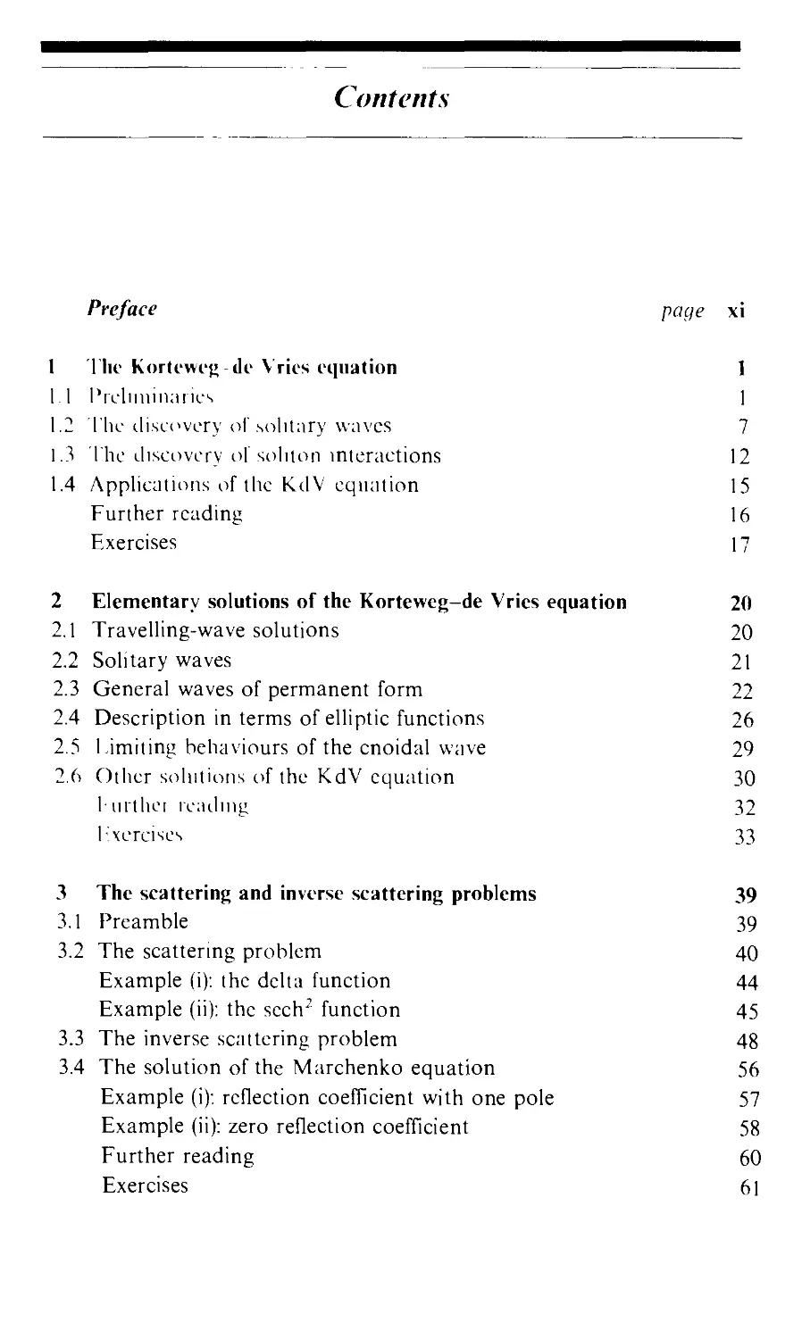
Contents
Preface page xi
1 The Korteweg-de Vrics equation 1
1.1 Preliminaries 1
1.2 The discovery of .solitary waves 7
1.3 The discovery of soliton interactions 12
1.4 Applications of the KdV equation 15
Further reading 16
Exercises 17
2 Elementary solutions of the Korteweg-de Vries equation 20
2.1 Travelling-wave solutions 20
2.2 Solitary waves 21
2.3 General waves of permanent form 22
2.4 Description in terms of elliptic functions 26
2.5 Limiting behaviours of the cnoidal wave 29
2.6 Other solutions of the KdV equation 30
further reading 32
Exercises 33
3 The scattering and inverse scattering problems 39
3.1 Preamble 39
3.2 The scattering problem 40
Example (i): the delta function 44
Example (ii): the sech2 function 45
3.3 The inverse scattering problem 48
3.4 The solution of the Marchenko equation 56
Example (i); reflection coefficient with one pole 57
Example (ii): zero reflection coefficient 58
Further reading 60
Exercises 61

4 The initial-value problem lor (Ik- Korleweg-de Vries equation 64
4.1 Recapitulation 64
4.2 Inverse scattering and the KdV equation 65
4.3 Time evolution of the scattering data 67
4.3.1 Discrete spectrum 68
4.3.2 Continuous spectrum 70
4.4 Construction of the solution: summary 71
4.5 Reflectionless potentials 72
Example (i): solitary wave 73
Example (ii): two-soliton solution 74
Example (iii): /V-soliton solution 78
4.6 Description of the solution when h(k) j= 0 81
Example (i): delta-function initial profile 81
Example (ii): a negative seclr initial profile 83
Example (iii): a positive sech2 initial profile 83
Further reading S6
Exercises 86
5 Further properties of the Korteweg-de Vries equation 89
5.1 Conservation laws 89
5.1.1 Introduction 89
5.1.2 An infinity of conservation laws 92
5.1.3 Of Lagrangians and Hamiltonians 95
5.2 Lax formulation and its KdV hierarchy 97
5.2.1 Description of the method: operators 97
5.2.2 The Lax KdV hierarchy 99
5.3 Hirota's method: the bilinear form 102
5.3.1 The bilinear operator 103
5.3.2 The solution of the bilinear equation 106
5.4 Backlund transformations 109
5.4.1 Introductory ideas 110
5.4.2 Backlund transformation for the KdV equation 112
5.4.3 The KdV Backlund transformation; an algebraic relation 114
5.4.4 Backlund transformations and the bilinear form 116
Further reading 118
Exercises 118
6 More general inverse methods 127
6.1 The AKNS scheme 128
6.1.1 The 2 x 2 eigenvalue problem 128

6.1.2 The inverse scattering problem 131
6.1.3 An example: r ^ q, q = X sech /.* 134
6.1.4 Time evolution of the scattering data 137
6.1.5 The evolution equations for q and r 140
(a) Quadratic in £ 141
(b) Polynomial m £ ' 142
(c) General function of £ 143
6.2 The ZS scheme 144
6.2.1 The integral operators 144
6.2.2 The differential operators 146
6.2.3 Scalar operators 149
(a) The KdV equation 149
(b) The two-dimensional KdV equation 151
6.2.4 Matrix operators 152
(a) The nonlinear Schrodinger equation 152
(b) The sine Gordon equation 154
6.3 Two examples 1 57
Example (i): The nonlinear Schrodinger equation 157
Example (ii): The sine-Gordon equation 160
Further reading 162
Exercises 162
7 The Painleve property, perturbations and numerical methods 169
7.1 The Painleve property 169
7.1.1 Painleve equations 169
7 1.2 The Painleve conjecture 171
7 1.3 Linearisation of the Painleve equations 172
7.2 Perturbation theory 174
7.2.1 Perturbation theory, an example 177
7.3 Numerical methods 180
7.3.1 Spectral methods 182
7.3.2 Finite-difference methods 183
7.3.3 Long-wave equations 184
7.3.4 Nonlinear Klein-Gordon equations 186
7 3.5 The nonlinear Schrodinger equation 187
Further reading 187
Exercises 187
8 Epilogue 190
8.1 Some numerical solutions of nonlinear evolution equations 190

i.2 Applications of nonlinear evolution equations 196
Further reading 200
Exercises 201
Answers and hints ' 205
Bibliography and author index 213
Motion picture index 220
Subject index 221

Preface
The theory of solitons is attractive and exciting; it brings together many
branches of mathematics, some of which touch on deep ideas. Several of
its aspects arc ama/ing and beautiful; we shall present some of them in
tins book. The theory is, nevertheless, related to even more areas of
mathematics, ami has even more applications to the physical sciences,
than the number which are included here. It has an interesting history
and a promising future. Indeed, the work of Kruskal and his associates
which gave us the 'inverse scattering transform' - a grand title for soliton
theory - is a major achievement of twentieth-century mathematics. Their
work was stimulated by a physical problem together with some surprising
computational results. This is a classic example of how numerical results
lead to the development of new mathematics, just as observational and
experimental results have done since the time of Archimedes.
This book has grown out of Solitons written by one of us (PGD). That
book originated from lectures given to final-year mathematics honours
students at the University of Bristol. Much of the material in this version
has also been used as the basis for an introductory course on inverse
scattering theory given to MSc students at the University of Newcastle
upon Tyne. In both courses the aim was to present the essence of inverse
scattering clearly, rather than to develop the theory rigorously and
completely. That is also the overall aim of this book. It is intended for
senior undergraduate students, and postgraduate students, in physics,
chemistry, and engineering, as well as mathematics. The book will also
help specialists in these and other fields to learn the theory of solitons.
However, the theory is not taken as far as the rapidly advancing frontiers
of research.
This book introduces the fundamental ideas underlying the inverse
scattering transform from the point of view of a course of advanced
calculus or the methods of mathematical physics. Some knowledge of the
elements of the theories of linear waves, partial differential equations,
Fourier integrals, the calculus of variations, Sturm-Liouville theory and

the hypergeometric function, but little more, is assumed. Also, some
familiarity with the main ingredients of the theories of water waves,
continuous groups, elliptic functions and 1 lilbert spaces will be useful, but
is not essential. The relevant ideas from one-dimensional wave mechanics
(both scattering and inverse scattering), necessary for the presentation of
the inverse scattering transform, are described. References arc given in the
text (or at the end of each chapter) to help readers to learn more of the
foregoing topics. Some of the diverse applications of the theory of solitons
are mentioned only briefly, either in the main text, or in the exercises at
the end of each chapter. However, the Korteweg-de Vries equation is
derived for a water-wave problem.
The material is presented as simply as we can, and a number of worked
examples are also used to help the reader follow the various ideas. Of
course, some parts of the theory are more exacting than others, and some
problems are more difficult than others. The more difficult sections,
paragraphs and set problems are indicated by asterisks; these passages
may be omitted on a first reading of the book. Further reading is offered
at the end of each chapter to direct the reader to more detailed treatments
of some of the topics. The sections are numbered according to the decimal
system, and the equations are numbered according to the chapter in which
they appear, e.g. equation (1.2) is equation 2 of Chap. 1. The problems
are similarly numbered (e.g. Q1.2), as are the answers (e.g. A 1.2) at the
end of the book.
We are grateful to Miss Sarah Trickett (Figs. 4.5. 4.7. 4.X). Mr Mark
Lewy (Fig. 8.1), Dr Adam Wheeler (Fig. 8.2), Mr Gregory Jones (Figs. X.3,
8.4, 8.6, 8.7) and Dr Stephen Thompson (Figs. 8.8, 8.9) for their
computations and plots of solutions on which our figures have been based; to Miss
Carolyn Pharoah and Miss Alison Davies for their clear draughtsmanship
of the figures; to Professor Neil Freeman (various points) and Dr Andrew
Wathen (§7.3) for technical advice; to Academic Press (copyright of Figs.
8.8, 8.9); and to Mrs Heather Bliss, Mrs Hilary Cartwright and Mrs Nancy
Thorp for their careful and cheerful typing of the text.
Bristol
Newcastle upon Tyne
PGD
RSJ

1
The Korteweg-de Vries equation
1.1 Preliminaries
Wave phenomena abound in mathematical physics, and are met early
in undergraduate courses. They may be first introduced as waves on a
string, or perhaps on the surface of water, or in a stretched membrane.
With a little more background they may be discussed in connection with
sound and then shock waves may be mentioned, or (for the physics
student) the first meeting might be via electromagnetic waves. In all these
areas it is common practice to develop the concepts of wave propagation
from the simplest - albeit idealised - model for one-dimensional motion.
where u{x, t) is the amplitude of the wave and c is a positive constant. This
equation has a simple and well-known general solution, expressed in terms
of characteristic variables (\ r ct) as
//( \,/) = fix - cD + ylx + ct), (1.2)
where / and a are arbitrary functions. (In keeping with the usual
convention, we shall regard t as a time coordinate and x as a spatial
coordinate, although in equation (1.1) these are readily interchangeable
since they differ only by the 'scaling' factor, c.)
The functions/and g (not necessarily differentiate) can be determined
from, for example, initial data u{x, 0), (du/dt)(x, 0). The solution (1.2), usually
referred to as d'Alemhert s solution, then describes two distinct waves, one
of which moves to the left and one to the right, both at the speed c. These
waves do not interact with themselves nor with each other; this is a
consequence of equation's (1.1) being linear, and hence solutions of the
equation may be added (or superposed). Furthermore, the waves described
by (1.2) do not change their shape as they propagate. This is easily verified
if we consider one of the wave components -/' say - and choose a new
coordinate which is moving with this wave, <!; = .* — ct. Then f =/(£,) and

this does not change as x and / change, at fixed £. In other words, the
shape given by /(.*) at f = 0 is exactly the same at later times but shifted
to the right by an amount ct.
Before we develop some further elementary properties of waves, it is
convenient first to restrict ourselves to waves which propagate in only
one direction. It is clear that this is an allowable choice in solution (1.2):
merely set g = 0, for example. A more practical approach is to set-up initial
data on bounded (compact) support, and then after a finite time the two
wave components f and g will move apart and no longer overlap.
Since they never interact, we can now follow one of them and ignore
the other. To be more specific, we may restrict the discussion to the
solution of
M,+ ('1(A = (). (1.3)
where we have introduced the short-hand notation for partial derivatives.
The general solution of equation (1.3) is
u(xj)=f(x~ct),
where f is an arbitrary function and, since we could redefine t as t/c, we
may just as well set c = 1:
if u, + ux = 0 then k(.x, 0 = f(x - t).
(We may also note the connection with equation (1.1): the operator can
be factorised, and either factor may be zero,
(lTc^)(^±c^)"sCv-c2^)" = a
where the signs are ordered vertically.)
When wave equations are derived from some underlying physical
principles (or from more general governing equations), certain simplifying
assumptions are made: in extreme cases we might derive equation (1.1) or
(1.3). However, if the assumptions are less extreme, we might obtain
equations which retain more of the physical detail: for example, wave
dispersion or dissipation, or nonlinearity. Consider, first, the equation
", + "x + "xxx = 0, (1.4)
which is the simplest dispersive wave equation. To see this let us examine
the form of the harmonic wave solution
u(x,t) = ciikx-m,). (1.5)
(We can always choose to take the real or imaginary part, or form
^ei(*x-(M) _|_ compiex conjugate, where A is a complex constant.) Now (1.5)

is a solution of equation (1.4) if
(,) = k-k3\ (1.6)
this is the dispersion relation which determines co(/c) for given k. Here, k is
the wave number (taken to be real so that solution (1.5) is certainly
oscillatory at t - 0) and o is the frequency. From (1.5) we see that
kx (<>t = k{x-(\ -/c2)f},
and so solution (1.5), with condition (1.6), describes a wave which
propagates at the velocity
U) ,
c = -=\-k2, (1.7)
k
which is a function of k. (Note that c changes sign across k = + 1.) In other
words, waves of different wave number propagate at different velocities:
this is the characteristic of a dispersive wave. Thus a single wave profile
w Inch can be represented, let us suppose, by the sum of just two components
each like solution (1.5) will change its shape as time evolves by virtue of
the different velocities of the two components. However, this interpretation
is virtually a repetition of the solution (1.2) of the classical wave equation.
To extend the idea we need only add as many components as we desire
or, for greater generality, integrate over all k to yield
u(x,f)= J A(k)e'''k''ML]'<dk, (1.8)
for some given A(k). (Note that A(k) is essentially the Fourier transform
of /<( \, 0).) The overall effect is to produce a wave profile which changes
its shape as it moves; in fact, since different components travel at different
velocities the profile will necessarily spread out or disperse,
1 he velocity of an individual wave component is given by equation
(1.7), and is usually termed the phase velocity. It is clear that equation (1.6)
will admit another velocity defined by
this is the group iyehcity, which determines the velocity of a wave
packet (see Fig. 1.1). For many (but not all) realistic wave motions it turns
out that
cg^c
and, furthermore, the group velocity is the velocity of propagation of
energy.

Thus far we have tacitly assumed that o(k), the dispersion function, is
real for real k, However this remains true only if we add to equation (1.4)
odd derivatives of u with respect to x. If wc choose to use even derivatives,
taking for example
u, + nt- uVA---0, (1,9)
then the picture is quite different. From equations (1.5) and (1.9) we obtain
o) = k — i/c2,
and so
m(.v, f) = exp {- k2t + \k(x - t)} (1.10)
is a solution of equation (1.9). This describes a wave which propagates at
a speed of unity for all k but which also decays exponentially for any
real k (#0) as t -> + oo. (Note that the sign of the term uxx is important.) The
decay exhibited in solution (1.10) is usually called dissipation. Clearly we
could have equations, like (1.4) or (1.9), which incorporate linear
combinations of even and odd derivatives. In this case the harmonic wave solution
may be both dispersive and dissipative (at least for suitable signs of the even
terms).
Finally, let us briefly look at one rather more involved aspect of wave
motion, namely that of nonlinearity. Most wave equations (like (1.1) and
(1.3)) are valid only for sufficiently small amplitudes. If some account is
taken of the amplitude (irra 'better approximation') we might obtain the
nonlinear partial differential equation
m,+ (1 + u)ux r- (). (Ml)
This equation embodies the simplest type of nonlinearity (u/i,). and
comparison with equation (1.3) might suggest that it is merely a ease ol
replacing c by 1 + u in the solution. It turns out (by the method of
characteristics) that this is correct! From equation (1.11) we see that
dx
u = constant on lines — = 1 + u,
df
Fig. 1.1 A sketch of a wave packet, showing the wave and its envelope. The
wave moves at the phase velocity, c, and the envelope at the group velocity, c
envelope

and so the characteristic lines are x = (1 +u)t + constant. Thus the general
solution is
u(x,t)=f{x-(\+u)t}, (1.12)
where/is an arbitrary function.
Now, given the initial wave profile, u(x,0) =/(x), it is a matter of solving
equation (1.12) for u; this may be far from straightforward, even though
the geometrical construction of the solution by characteristics is easy. In
fact the solution of equation (1.12) (with/ > 0, say, for some x) will generate
a single-valued solution for u only for a finite time; thereafter the solution
will be multi-valued (i.e. non-unique). The solution obtained by
construction exhibits the non-uniqueness as a wave which has 'broken1 (see Fig. 1.2).
(Thus the solution must necessarily change its shape as it propagates.) This
difficulty is usually overcome by the insertion of a jump (or discontinuity)
which models a shock (again, see Fig. 1.2). Strictly, a discontinuous solution
is not a proper solution of equation (1.11) but it may be allowable as a
solution of the integral conservation equation from which (1.11) may have
been derived.
Another complication arises with nonlinear equations: let us suppose
that we have two solutions of equation (1.11), i/Jx, f) and u2{x,t). We have
already met the 'superposition principle' which says that, for linear
equations, any linear combination of ux and u2 is also a solution. However
this is not true, in general, for nonlinear equations. It is easily verified that
//-i/, f u2 does not satisfy equation (1.11). Thus solutions of nonlinear
equations can not be superposed to form new solutions, although a related
principle /s available lor certain nonlinear partial differential equations as
we shall see.
It is clear that, by making suitable assumptions in a given physical
problem, we might obtain an equation which is both nonlinear and
Fig. 1.2 I he evolution of a nonlinear wave as time increases (a) f = f,;
(h) t = 12 > t,; (c) t = 13 > 12. The wave becomes vertical at one point at t = t2,
and thereafter the solution is triple-valued in a region. The solution can be
made single-valued by the insertion of a discontinuity (and the smooth 'lobes'
are then ignored).

contains dispersive or dissipative tonus (01 both). So, for example, wc
might derive
1/,4(1 I i/)n, I //,,, t). (II t|
or
//,1(1 I 1/)1/, //,, t) (I 14)
The first of these is the simplest equation embodying iionlniraiitv ami
dispersion; this, or one of its elementary variants, is known as the
Korteweg-de Vries (or KdV) equation, of which wc shall say much more
later. The second one, equation (1.14), with nonlinearity and dissipation,
is the Burgers equation. In fact the general solution of equation (1.14) has
been known since 1906 (Forsyth, 1906), and it turns out that there are
some pointers in the method of solution which are relevant to the solution
of the KdV equation. (The properties of the Burgers equation will be left
to the reader to explore in the exercises.) Our main concern will be with
the method of solution - and the properties of- the KdV equation, and
other related 'exactly integrable' equations. However, before we embark
upon a more detailed discussion, the various alternative forms of the
equation should be mentioned. We can transform equation (1.13) under
1 + u -> olu, t -> /?f, x -> yx,
where oc,p,y are real (non-zero) constants, to yield
*P P
u, H uux + —.^uxxx = 0.
/ i
This is a general form of the KdV equation, and a convenient choice,
which we shall often use, is
u, - 6uux + uxxx = 0. (1.15)
Some of these transformations of variables (as used above) belong to a
continuous group or Lie group. As an example, consider the transformation,
Gk, of the variables x, f and u into
X = kx, T=kh, U = k-2u,
for real k ^ 0. The application of successive transformations Gk and G, is
equivalent to the single transformation Glk, thereby producing the
multiplication law G,Gk = Glk. This law is commutative since GkGt = Gk, = Gtk.
Furthermore, the associative law is also satisfied because Gk(G,G^\=GkGlm =
Gklm = GklGm — (GkGl)Gm. Clearly Gt is the identity transformation:
G1Gk = Gki = Gk for all k (#0). If we form GljkGk = Gt and GkGijk = Gl5
we see that G, jk is both the left-hand and right-hand inverse of Gk. Therefore
the elements of Gk for all real k # 0 form an infinite group. We call k the

parameter of this continuous group. Now let us apply the transformation
(ik t<> the KclV equation (1.15); it becomes
V, 6UUX+UXXX = 0,
i.e. it is mi ainini under the continuous group of transformations, Gk. This
suggests th.it we seek invariant properties of the solutions. In particular,
we anticipate the existence of similarity solutions which depend only on
invariant combinations of the variables (see Q1.13 and section 2.6).
We have touched on ideas associated with waves in one spatial
dimension, mainly because the KdV equation (and other equations we
shall meet later) take this form. Of course, waves do occur in higher
dimensions; in particular the classical wave equation can be written as
d2u
Ty_c2V2u = 0 (1.16)
where V2 is the Laplace operator in the chosen coordinate system. It is
clear that if we wished to examine more-complicated wave phenomena
(with nonlinearity and dispersion), such as ring waves or waves crossing
obliquely, then we must seek new equations. These might embody some
of the character of both equations (1.15) and (1.16); in fact higher-
dimensional KdV equations (and other integrable equations) do exist, but
their discussion is beyond the scope of this text although one or two will
be mentioned in the exercises.
1.2 The discovery of solitary waves
We have seen that the Korteweg de Vries equation can be written down on
the basis that both nonlinearity and dispersion might occur together.
However, the KdV equation not only is of mathematical interest but also
is of practical importance. To introduce this aspect, let us see how the
solitary wave first appeared on the scientific scene. We shall then mention
some of the analytical properties of this wave, and finally show that the
KdV equation is indeed the relevant one for the solitary wave (and much
more besides).
The solitary wave, so-called because it often occurs as this single entity
and is localised, was first observed by J. Scott Russell on the Edinburgh-
Glasgow canal in 1834; he called it the 'great wave of translation'. Russell
reported his observations to the British Association in his 1844 'Report
on Waves' in the following words:
I believe I shall best introduce the phenomenon by describing the circumstances of

my own first acquaintance with it. I was observing the motion of a boat which
was rapidly drawn along a narrow channel In a pan of horses, when the
boat suddenly stopped - not so the mass of water m the channel which H had pnl
in motion; it accumulated round the prow of the vessel in a state of violent agitation,
then suddenly leaving it behind, rolled forward with great velocity, assuming the
form of a large solitary elevation, a rounded, smooth and well-defined heap of
water, which continued its course along the channel apparently without change
of form or diminution of speed. I followed it on horseback, and overtook it still
rolling on at a rate of some eight or nine miles an hour, preserving its original
figure some thirty feet long and a foot to a foot and a half in height Its height
gradually diminished, and after a chase of one or two miles 1 lost it in the windings
of the channel.
Russell also performed some laboratory experiments, generating solitary
waves by dropping a weight at one end of a water channel (see Fig. 1.3).
He was able to deduce empirically that the volume of water in the wave
is equal to the volume of water displaced and, further, that the speed, r,
of the solitary wave is obtained from
c2=g(h + a), (1.17)
where a is the amplitude of the wave, h the undisturbed depth of water
and g the acceleration of gravity (see Fig. 1.4). The solitary wave is
therefore a gravity wave. We note immediately an important consequence
of equation (1.17): higher waves travel faster. Fig. 1.3 and result (1.17)
apply to waves of elevation; any attempt to generate a wave of depression
results in a train of oscillatory waves, as Russell found in his own
experiments.
To put Russell's formula (1.17) on a firmer footing, both Boussmesq
(1871) and Lord Rayleigh (1876) assumed that a solitary wave has a
length scale much greater than the depth of the water. They deduced,
from the equations of motion for an inviscid incompressible fluid, Russell's
formula for c. In fact they also showed that the wave profile z = C(x, f) is
given by
£(x,f) = asech2{/?(.x-cf)} (1.18)
Fig. 1.3 Diagram of Scott Russell's experiment to generate a solitary wave.
m

where /?~2 =4/r(/i + a)/3a for any a > 0, although the sech2 profile is
strictly only correct if a.'h « I. These authors did not, however, write down
a simple equation for C(-\\') which admits (1.18) as a solution. This final
step was completed by Korteweg & de Vries in 1895. They showed that,
provided i: and a were small, then
(X V'/Y V2 (X (X i ?K\
-"=J, (r.J+:~- + -a^\ (1.19)
a 2\hJ \1 </ c'x 3 (Y/
where y is a coordinate chosen to be moving (almost) with the w-ave. If
we use the change of variables
C = C(X,f), X=y. + c(^j't
then equation (1.19) can be re-cast as the KdV equation
2\hJ ^1+3^^
The parameter a incorporates the surface tension, T, in the form
a =y/i3 — Th/'gp, where p is the density of the liquid (and often T « \cjplr);
e is an arbitrary parameter. We shall not reproduce the work of Korteweg
& de Vries here, but it is instructive to see how the KdV equation arises
from a set of fundamental governing equations. To this end we shall stay
with water waves, but use the rather more satisfying technique of
multiple-scale asyniptotics.
* The governing equations of irrotational two-dimensional motion of an
incompressible inviseid fluid, bounded above by a free surface and below
by a rigid horizontal plane, are
'/'.-.- + S24>xx = 0; ¢, = 0 on z = 0
;+ ^+1^-^ + ^) = 0) (1.20)
¢: = <T((„ + 5«/>x<,x) J
where ¢ is the velocity potential. The variables used here have already
Fig. 1.4 The parameters and variables used in the description of the solitary
wave.
0

Been non-dimensionalised by the use of the undisturbed depth, h, a typical
horizontal length scale, /, and the typical speed (<//i)' 2- The surface is at
z = 1 + a( and on this surface we assume that the pressure is constant (so
that in this simple theory the surface tension is ignored). The parameters
appearing in equations'(1.20) are given by
a = a/U, 8 — /i//,
where a is a measure of the wave amplitude. The two boundary conditions
on z = 1 + a( describe the constancy of pressure at the surface, and the
continuity of the vertical velocity component there.
We are interested in small-amplitude long waves i.e. in the limits as
a->0 and <5-»0. It turns out that one choice we could make and which
leads to the KdV equation for £ - is to set (52 = 0(a) as a -»0. (This seems
reasonable if we note the way in which a and 8 appear in equations (1.20).)
Clearly, however, this is rather special and we would hope that the solitary
wave is a more enduring and general phenomenon than this would suggest.
It is, as the following scaling for arbitrary 8 demonstrates. Introduce
a1'2 a3'2 a1'2
£ = -^-(x-f), T = -Tf' * = -^-^ (1-21)
then equations (1.20) become
d>„ + ad>» = 0; ¢.. = 0 on z = 0
C - O, + aOt + !(0>2 + aO2) = 0 ) , , . (1.22)
0. = a(-C.+ aCt + aO.^)J
(Note that £ = 0(1), <t> = 0{\) and t = 0(y.~l) if <52 = 0(a).) The choice of
variables (1.21) means that equations (1.22) hold in a frame of reference
which is moving with a speed of unity to the right, and then for large
times (f) if t = 0(1) as a->0(for any fixed 8). In other words, scalings (1.21)
describe a particular neighbourhood of (x, f)-space where we hope the KdV
equation will be valid. The appearance of a speed of unity is by virtue of
the non-dimensionalisation; this corresponds to a dimensional speed of
(gh)1'2 (cf. formula (1.17) for small a). Finally, the right-ward propagation
is merely for convenience: we could equally well discuss left-ward motion
by introducing £ = a1/2(x + t)/8.
The solution of equations (1.22), as a ->0, is surprisingly straightforward.
To initiate the analysis we suppose that there exists a solution which takes
the form
00 CO
O ~ I a"On(£, t, z), C ~ £ «"«£, t), as a - 0,
n = 0 n= 0
for fixed £ and t. (Note that ze[0,1 + a(] which is a bounded domain if

£ is bounded.) The leading order approximation now yields
¢),,.. = 0 with O0. = 0 on z = 0,
and so <!>„(£, t. :) = fl0(<;, t), say, an arbitrary function. Furthermore, the
first surface boundary condition requires that £0 = O0? on : = 1 (if we
expand these conditions in a Taylor series about z = 1), and thus Co = 60i.
If we continue the expansion for O then Laplace's equation, m conjunction
with the bottom boundary condition, gives
O ~ 0o + aid, - \z260ii) + a2(02 - Iz201K + ^z40o««)
where/),, = ('„(£, t), n = 0,1,2, are arbitrary functions. The surface boundary
conditions now become
Co + *;, - \0tt, + 5((0,,- «0OK)} + a0Ot+ la0§4 = 0(a2)
and
= a( - C0. - a£,.- + aC0l + a0o?£O4) + 0(a3),
respectively. These two equations require that
C,-0u+ |0o«+ 00,+ I0o4 = O
and
- CO0O« - 01 « + 500«« = - C 1 ; + Cor + 0O^O{,
where 0O> = Co- If we eliminate C, -0,^ then £„(<;, f) must satisfy
XoT + 3;0;0, + K"o«4 = o, (1.23)
the KdV equation. (The interested reader might care to verify that the
higher-order terms, £„, satisfy an equation of the form
2:m + ]CoU{ + ic,«{ = ^,.i, »= 1,2,...,
where ,>„_ t denotes a function of £0, Ci, .,Cn-i ,Co^--- •)
We have seen that the Korteweg-de Vries equation is indeed valid in
an appropriate region of (x, f)-space, for small amplitude waves. However,
we are left with one final connection to make: that between the KdV
equation and the sech2 profile. To demonstrate this, let us return to the
equation as derived by Korteweg & de Vries themselves, equation (1.19).
This has the advantage that it is written in physical variables and can
therefore more readily be related to the work of Russell, Boussinesq and
Rayleigh as expressed in equations (1.17) and (1.18). If the solution of
equation (1.19) is stationary in the frame x then C = C(l) and so
K' + CC' + i<" = 0, (1.24)

wnere tne prime denotes the derivative with respect to %. If we consider
(-►0 as |/1 —>■ oo (as is the case for the solitary wave) then equation (1.24)
can be integrated twice to yield
li'C- + (-' i- o(C)2 = o.
(the second integration requiring the integrating factor ('). This equation
may be integrated once again (see §2.2), but it is more easily verified by
direct substitution that
C(/J = asech2(/?/J
is a solution, provided
a = 4ct/?2 and e=-2a/?2.
The coordinate % <s defined (Korteweg & de Vries, 1895) as
x = x-(ghy2(\-r-
and so the solitary-wave solution becomes
((x, f) = asech2
U'-TU-^UA'
2\<x \ * ' \ 2h
.25)
This agrees with equations (1.17) and (1.18) if we neglect surface tension
(so that (1 = 3¾3) and assume that a/h« 1, for then
«-(*>■»(.♦$ and ,-!(*
Thus Russell's solitary wave is a solution of the KdV equation.
In conclusion, let us make two observations concerning the solitary-
wave result given in equation (1.25). With an amplitude of a, we see that
the speed of the wave relative to the speed of infinitesimal waves (i.e. {gh)X12)
is proportional to a. Also the 'width' of the wave (defined as the distance
between the points of height \a, say) is inversely proportional to a1'2. In
other words, taller waves travel faster and are narrower. Finally, note how
a appears in equation (1.25) and compare this with the way a appears in
the scaled variables (1.21) that were used in our derivation of the KdV
equation.
1.3 The discovery of soliton interactions
Hidden away in Russell's 'Report on Waves' (1844, see plate XLVII) is the
diagram reproduced in Fig. 1.5, and the associated description. One
interpretation of this result (with a little hindsight) is that an arbitrary

initial profile (which in other words is not an exact solitary wave) will
evolve into two (or more?) waves which then move apart and progressively
approach individual solitary waves as t -> oo. (Remember that our solitary
wave is defined on (— x, oc).) This alone is rather surprising, but another
remarkable property can also be observed. If we start with an initial profile
like that given in Fig. 1.5, but with the taller wave somewhat to the left
of the shorter, then the development is as depicted in Fig. 1.6. In this case
the taller wave catches up, interacts with and then passes the shorter one.
The taller one, therefore, appears to overtake the shorter one and continue
on its way intact and undistorted. This, of course, is what we would expect
if the two waves were to satisfy the linear superposition principle. But they
certainly do not: this suggests that we have a special type of nonlinear
process at work here. (In fact, the only indication that a linear interaction
has not occurred is that the two waves are phase-shifted i.e. they are not
in the positions after the interaction which would be anticipated if each
were to move at a constant speed throughout the collision.)
The first hint that there was something unusual in the KdV equation
Fig. 1.5 A sketch of Scott Russell's 'compound' wave. This figure 'represents
the genesis by a large low column of fluid of a compound or double wave of
the first order, which immediately breaks down by spontaneous analysis into
two, the greater moving faster and altogether leaving the smaller'. (Russell.
1844, p. 384)
fig. 1.6 A sketch depicting the interaction of two 'solitons', for times (a)/ = /,:
(b) r = r2 > /,; (<•) r = r3>r2; (d) / = /4>/3.
1 (a) (h)

anu solitary waves came in lv:o. hermi, I'asta & Ulam were working at
Los Alamos on a numerical model of phonoiis in an nnhnrnionic lattice,
a model which turns out to be closely related to a discretisation of
the KdV equation (Fermi, Pasta & Ulam, 1955). 1 hey observed that there
was no equipartition of Energy among the modes. Taking this up in 1965,
Zabusky & Kruskal considered the initial-value problem for the equation
u, + uux + 32uxxx = 0, (1.26)
with periodic boundary conditions (a more complicated problem than our
infinite-domain solitary wave, but well-suited to numerical computation).
They solved equation (1.26) with
u{x, 0) = cos Tt.v, 0 ^ x ^ 2,
and u, ux, uxx periodic on [0,2] for all f; they chose d = 0.022. A set of their
results is shown in Fig. 1.7. After a short time the wave steepens and
almost produces a shock, but the dispersive term (d2uxxx) then becomes
significant and some sort of local balance between nonlinearity and
dispersion ensues. At later times the solution develops a train of eight
well-defined waves, each like sech2 functions, with the faster (taller) waves
for ever catching-up and overtaking the slower (shorter) waves. (And there
is another surprise: after a very long time, the initial profile - or something
very close to it - reappears, a phenomenon requiring the topology of the
torus for its explanation. This is an example of recurrence.)
At the heart of these observations is the discovery that these nonlinear
waves can interact strongly and then continue thereafter almost as if there
had been no interaction at all. This persistence of the wave led Zabusky &
Kruskal to coin the name 'soliton' (after photon, proton, etc.), to emphasise
Fig. 1.7 The solution of the periodic boundary-value problem for the KdV
equation (after Zabusky & Kruskal, 1965). Initial profile at / =0 (dotted line);
profile at t = 1/tt (broken line); profile at t = 3.6/tt (full line).
u(x, t)
i

the particle-like character of these waves which seem to retain their
identities in a collision. The discovery has led, in turn, to an intense study
over the last twenty years. Many equations have now been found which
possess similar properties, and diverse branches of pure and applied
mathematics have had to be invoked to clarify many of the novel aspects
that have appeared. We shall meet some of them in later chapters.
It is not easy to give a comprehensive and precise definition of a soliton.
However, we shall associate the term with any solution of a nonlinear
equation (or system) which (i) represents a wave of permanent form; (ii)
is localised, so that it decays or approaches a constant at infinity; (iii) can
interact strongly with other solitons and retain its identity. (There are
more formal definitions some of which concern discrete eigenvalues of
a scattering problem but these must wait until we have a more substantial
mathematical framework.) In the context of the KdV equation, and other
similar equations, it is usual to refer to the single-soliton solution as the
solitary wave, but when more than one of them appear in a solution they
are called solitons. Another way of expressing this is to say that the soliton
becomes a solitary wave when it is infinitely separated from any other
soliton. Also, we must mention the fact that for equations other than the
KdV equation the solitary-wave solution may not be a sech2 function;
for example, we shall meet a sech function and also arctan(eIX).
Furthermore, some nonlinear systems have solitary waves but not solitons,
whereas others (like the KdV equation) have solitary waves which are
solitons.
1.4 Applications of the KdV equation
We have seen (in §1.1) that the KdV equation is the simplest equation we
can envisage which incorporates both nonlinearity and dispersion. In fact
it is easy to show that this equation should occur often in the description
of real wave propagation. Consider a linear wave motion in one dimension
with dispersion: we already know that the dispersion relation must take
the form
co{k) = kc{k\
since only odd derivatives of u are allowed. (Our choice of dispersion,
represented by a sum of derivative terms, will naturally produce a
dispersion relation like co = kY^=oCnk2n, but a more general functional
dependence, 10 = a){k), can arise which then has this form of expansion as
k -> 0.) Now let us suppose that for infinitely long waves (k -> 0) there exists

a umi-iuu spccu ui propagation, r0, tnen
and usually long waves travel the fastest, and so / > 0. This approximate
dispersion relation is clearly obtained from the equation
u, + c0ux + /mxxx = 0.
Furthermore, if the medium in which the propagation is occurring is a
classical continuum, then the time evolution will be given by the material
derivative (or convective operator) D/Dt = e'et + u(c"cx). If these two
effects are to balance then we shall obtain
u, + ct)ux + y.(uux + /mxxx) = 0,
where a is a small parameter measuring the weak nonlinearity and long
waves. Thus we have
uT + uui + kui^ = 0; I = .v — c0t, x = ar.
the KdV equation for small amplitude long waves, valid in an appropriate
region of the (x, f)-plane (defined by x - c0t = 0(1), t = 0(x~ '), as a->0.)
With these points in mind, we anticipate that the KdV equation will
arise in a number of different contexts. We have already seen how the
equation can be derived for the classical water-wave problem. A few of
the many other applications include internal gravity waves in a stratified
fluid, waves in a rotating atmosphere (Rossby inertial waves), ion-acoustic
waves in a plasma and pressure waves in a liquid gas bubble mixture.
(The other equations which we shall meet later also have a wide application,
and one of them - the nonlinear Schrodinger (or NLS) equation is
perhaps even more generally useful than the KdV equation.) In summary,
we see that the KdV equation is a characteristic equation governing weakly
nonlinear long waves whose phase speed attains a simple maximum for
waves of infinite length.
Further reading
The following, referenced by sections, is intended to give some useful further reading.
1.1 For basic properties of linear and nonlinear waves, see Whitham (1974). For more
information concerning group velocity, see Lighthill (1978). For the application of group
transformations to differential equations, see Bluman & Cole (1974).
1.2 For another derivation of the KdV equation for water waves, see Kevorkian & Cole
(1981); for other water-wave applications see Johnson (1973) for variable depth, Freeman
& Johnson (1970) for waves on arbitrary shears and Johnson (1980) for a review of one-
and two-dimensional KdV equations.

1.3 See the motion pictures of soliton interactions, particularly Zabusky, Kruskal &
Deem (H%5) and F.ilbeck (1-1981). For a comparison of the KdV equation with
ftiiln wave experiments, see Hammack & Segur(1974).
1.4 \ lew ol the many papers: internal gravity waves (Benney, 1966); Rossby waves (Benney.
1966, Kcctekopp & Weidman, 197X); ion-acoustic waves (Washimi & Taniuti, 1966); gas
bubbles in a liquid (van Wijngaarden, 1968).
Exercises
Ql 1 Use the method of characteristics to derive d'Alembert's solution of the
classical wave equation, (1.1).
Q1.2 Express d'Alembert's solution in terms of u(x.0) = p{x) and t<,(.x,0) = </(x).
Q1.3 Find a relation between p(x) and q(x) in Q1.2 which produces a single
wave-component travelling to the right.
Q1.4 Discuss the dispersion relation for the equation
u, + ux + uxxx - uxx = 0.
Q1.5 Compare the dispersion relations for the equations
u, + ux + uxxx = 0
and
u, + uv — uxxt = 0,
particularly in the limiting cases of long and short waves.
Q1.6 Obtain the solution of the equation
w, + (l + u)ux = 0
with
( U„.x, 0 s£ x s£ 1
i((.x,0) = i u0(2-.x), 1 <.xs:2
[0, x < 0, x > 2,
where /(,, is a positive constant.
[Note that this initial profile is not differentiate at ,x = 0, 1,2.]
Q1.7 By using the characteristics, sketch the solution of the problem in Q1.6
at various times.
Q1.8 Find the implicit solution of the equation
u, + uux = 0
with u(x,0) = cos7lx. Show that u first has a point where ux is infinite at
f = 7t"'. What form may the solution take if it is allowed to develop
beyond t = n~ '?
Q1.9 A general nonlinear wave. Suppose that u(x, t) satisfies the equation
u, + c(u)ux = 0, — oc < .x < so, f > 0,
with u(x,0) = f{x), where both / and c are differentiate. Use the method

ot characteristics to find the implicit solution, ;ind hence deduce that ux
remains finite until t = mm ( [i■' \ / (/) \ I'(/) I ').
Q1.10 Linear KdV dispersion. If
", * «,„ = 0
with u(x,0) = /(x) and m, kx,iiax->0 as |x|-> r.„ use the Fourier transform
to show that
«(*,0 = (30-''3J_/<v)AiQ^)dv,
where Ai(z) is the Airy function of 2.
Ql.ll Solitary wave. Obtain the solitary-wave solution of the equation
u, — 6uux + uxxx = 0,
for a wave of amplitude — 2k2.
Q1.12 Rational solitary wave. Show that
ui.i= 6.x —
(.x3+12t)2
is a solution of the KdV equation given in Q 1.11. (Note that this solution
is singular on x3 + 12f = 0.)
[Hint: it might help to write u = (it 2 \f(i]). r\ = xt ' 3 (see Q1.13), and
then to observe that / = — j(log F)". F(n) = ;;' + 12.]
Q1.13 Painleve equation. Show that the KdV equation
u, — 6m«a + uxxx = 0
is invariant under the transformation x-^kx, t ->k't, u ->k 2u (k y-0). Also
verify that t2!3u and .xt-1,3 are invariant under the same transformation.
Show that if u(.x, f)= — (3t)~2!1 F(n), where >/ = .x(3f) ' \ then
F" + (6F-»/)r-2F = 0.
Hence, by setting F= /. dV/dn — V2, V = K(>/), where A is a constant to be
determined, verify that after two integrations the equation for V{n) can
be written as
V"-nV~2Vi = 0,
provided V decays exponentially as either >/-> + x or >/-> — x.
[This equation for V is a Painleve equation of the second kind; see
Chap. 7 and Ince (1927).]
Ql.14 KdV equation. Suppose that the phase velocity of some linear wave is
c(k), where k is the wave number. Now weakly nonlinear waves can often
be described by an equation of the form
u, + uux+ \ K(.x-£)u,{tt)dZ = 0,

where the kernel K is determined from linear theory as the Fourier
transform of c,
1 f"'
K(.x) = — c(k)e,kxdk.
For water waves it is well-known that c2 = (<y/A.')tanh(fc/i) where g is the
acceleration of gravity and h is the undisturbed depth of the water: use
this information to justify the KdV equation for long waves.
*Q1.15 Benjamin- Ono equation. In Q1.14 take c(k) = cn(\ - X\k\\ where c0 and /.
are constants, and hence deduce that
u, + (c0 + u)ux+—\ dc=0,
n J-m C-.x
where ^denotes the Cauchy principal value, provided u, ->0 as |c| -> x.
[This is the Benjamin-Ono equation which arises in the study of internal
waves: Davis & Acrivos, 1967; Benjamin, 1967; Ono, 1975.]

2
Elementary solutions of the
Korteweg-de Vries equation
2.1 Travelling-wave solutions
A travelling wave of permanent form has already been met; this is the
solitary-wave solution of the KdV equation itself. Such a wave is a special
solution of the governing equation which does not change its shape and
which propagates at constant speed. This wave may be localised or
periodic. In the case of linear equations the profile is usually arbitrary,
and is rarely of any special significance; a nonlinear equation, however,
will normally determine a restricted class of profiles which often play an
important role in the solution of the initial-value problem as (-> oo. So,
for example, the classical wave equation
"n - c2uxx = 0
has the travelling-wave solutions f{x — ct) and g{x + ct), for arbitrary f
and g (which together correspond to d'Alembert's solution). On the other
hand the nonlinear equation
u, + (1 +u)ux = 0
has a travelling-wave solution u(x, t) = f(x — ct) only if
(l-c + /)/'=0
and so f = constant: a trivial (non-wave-like) solution. It is obvious that
neither of these examples - as they stand - will teach us very much.
Let us restrict consideration to the more interesting area of nonlinear
equations. The simplest such equation (mentioned above) does not have a
travelling-wave solution at all, and this is to be expected from the general
solution discussed in §1.1. The wave steepens and, if allowed, will 'break'
and become multi-valued; at no stage is a steady profile possible. Similarly
the effects of dispersion alone also produce a wave which forever changes
its shape, but now in the opposite sense in that it causes the wave to
spread out rather than to steepen. Perhaps these two effects may maintain
a balance and thereby produce a wave of permanent form. Of course it
is precisely this balance which gives rise to the solitary wave. (A similar

balance can be struck between nonlinearity and dissipation; see Q2.1(i).)
As an example of the general method for seeking travelling-wave
solutions, let us consider
m,+ (1 +u)ux = v(u) (2.1)
for some function v{u). The required solution must take the form
u(x, t) = f(x — ct), where c is a constant which may play the role of a
parameter (as in the KdV solitary wave, see §2.2) or it may be determined
uniquely. Equation (2.1) now becomes
(\-c + f)f' = v(f)
and so
— d/ = ¢, where c, = x - ct.
v(f)
Let us suppose that equation (2.1) is given with v{u) = u{\ —u2), and for
simplicity we choose c = 1. (The problem for arbitrary c may be undertaken
as an exercise.) Thus we have
//+1
which yields
1+/
l0£
1-/
a it f Ae2i~\
= Ae2i or f = — .
Ae2»+\
where A is an arbitrary constant. This solution is more conveniently written
as
u(x, t) = f{x — t) = tanh (.* - ( - x0),
where A =exp( — 2x0), and this describes a smoothed step propagating
to the right.
2.2 Solitary waves
We now turn specifically to the KdV equation, and briefly discuss the
solitary-wave solution mentioned in §1.2. It is convenient (particularly in
view of the later work) to write the KdV equation in the standard form
u, - 6uux + uxxx = 0. (2.2)
The travelling-wave solutions of this equation are u(x,t) = f(£), where
^ = x — ct and c is a constant. Thus equation (2.2) becomes
-c/'-6//' + /'"=0,

wnicn may be integrated once to yield
-cf-y2 i r- ,1,
where A is an arbitrary constant. If we now use /' as an integrating factor
we may integrate onee more to give
2(f)2 = /' + k/'2 + Af +■ B, (2.3)
where B is a second arbitrary constant. (We shall examine equation (2.3)
for general A, B in the next section.) At this stage let us impose the boundary
conditions f, f, f" —> 0 as c —> ± x which describe the solitary wave. Thus
A and B are both zero,
(f')2 = f2(2f + c) (2.4)
(essentially as we quoted in §1.2), and we can see imniedialelv that a real
solution exists only if (f')2 ^ 0 i.e. if 2 / + c ^ 0.
Equation (2.4) can be integrated as follows: first write
and then use the substitution f = — \c sech2 0 (c ^ 0) to obtain
f(.x - a) = - Vscch2 \\cx 2(.x - c-f - x0)j. (2.5)
where x0 is an arbitrary constant of integration. Note that the choice +
is redundant since the solution is an even function, and also that the
constant x0 (a phase shift) plays a minor role: it merely denotes the position
of the peak at f = 0. The solitary-wave solution (2.5) of equation (2.2) forms
a one-parameter family (ignoring x0), and in fact the solution exists for
all c :> 0 no matter how large or small the wave may be. (The solitary-wave
solution of the original water-wave equations (1.20) exists only up to a
maximum amplitude and its profile is only approximated by a sech2
function.) The fact that /^0 reflects our choice of KdV equation (2.2)
with negative nonlinearity; we may recover the classical wave of elevation
by transforming u—> —u.
2.3 General waves of permanent form
The qualitative nature of the solution /(£,) of equation (2.3), for arbitrary
values of the constants c, A and B, can be determined by elementary
analysis. The quantitative behaviour, however, requires the use of elliptic
functions (see §2.4) or numerical computation.
It is clear that, for practical applications, we are interested only in real

bounded solutions /(£) of
U.f)2=f3 + kcf2 + Af+B = F(f).
Thus we require (as before) (/')2 ^ 0, and the form of F(f) shows that /
will vary monotonically until /' vanishes (i.e. F(f) has at least one real
zero). In other words, we can anticipate that the zeros of F(f) are important.
A little thought shows that the zeros of F(/), according to the values
of c, A and B, must fall into one of the six categories depicted in Fig. 2.1.
Since (/')2 ^ 0, a real - but not necessarily bounded - solution will occur
only in the intervals shaded in the figure. Further, to lay the foundations
for our discussion, we need to consider the behaviour of/ near a zero of
/•'(/) and clearly three cases can arise: F(f) will have a simple, double or
triple zero. Let /•'(/,) = 0 and we then examine each case in turn.
(i) If /, is :i simple zero then
(./-)3 = 2(/ - /,)F(/,) + 0((/ -/,)2),
as / -> /',, which can be solved iteratively to yield
/ = /,+*(S-£,)2F'(/i) + 0((£-£i)3),
as £->£[, where /(£,) ==/,- Thus / has a local minimum or maximum at
^ = £,, as F'(/i) is positive or negative, respectively.
Fig. 2.1 Sketches of the graphs of F(f) for the six different cases. Real solutions,
(/')2 >0, will occur only in the shaded regions.
(a) (b)

(ii) If/, is a double zero then
(.n2=(/ -/.)2'-"'(/. )+<>((/ /,)3).
as /->/,, and this is allowable only if /■'"(/,) ■ 0 (sec Fig. 2.1(/))). This
time we obtain
/-/.^expClcjFXA)!''2] asc^T/. (2.6)
if/ is to be bounded; a is an arbitrary constant. Thus /->/, as £ -> + x
(signs vertically ordered throughout), and the solution can therefore have
only one peak and the wave must extend from — x to + x.
(iii) If /, is a triple zero then there is only one possibility, namely
fi = _c/6 with /4 = 3(e/6)2 and B = (c/6)3: see Fig. 2.1(/). The complete
solution for /(£) is then easily obtained as
where /? is an arbitrary constant. This solution is unbounded at c, = fi.
(Note that there is always available the trivial solution f = /, (for example,
a = 0 in expression (2.6) or \fi\-> x in (2.7)) but this is not a propagating-
wave solution.) Thus, on ignoring (iii) which is not relevant, /' will either
change sign across / = /, (see (i)) or /'->0 as £-> + oc (see (ii)).
Now consider the cases depicted in Figs 2.\(a),(d),(e) and the right-hand
part of (c) (beyond / = fi). If at some point c = £0 (say) on the solution,
the slope is such that /' > 0, then F > 0 for all £ > c0 and /-> + x as
<!; -> + oo. If, however, /'(£) < 0 then / will decrease until it reaches f = /,
(the largest real zero of F); this is a simple zero and so /' changes sign
and once again /—>■ + x as C -> + x. Hence, for these four cases, there is
no bounded solution.
From Fig. 2.1(/)) we see that F has a simple zero at /3 and a double
zero at /,; the solution has a minimum at / = /3 (F'(/3) > 0) and attains
/ = /, as £—>■ + cc'. This, of course, is therefore the solitary-wave solution
with an amplitude /3 — /, ( < 0).
Finally we are left with the left-hand part of curve (c) in the finite region
where (/')2 ^ 0. Here we have simple zeros at both /2 and /3; in fact there
is a local maximum at /2 (since F'(/2) < 0) and a local minimum at /3
(since F'(/3) > 0). Thus /' will change sign at these points and since the
behaviour near them is algebraic (not exponential as in (ii)), consecutive
points / = /2^/ = /3 will be a finite distance apart. The unique solution
will be completely determined if /, and the sign of /', are given at any
point ^ = £0, which then fixes a point on the curve between /2 and /3.
The solution will thereafter oscillate between/2 and/3, with a finite period.

This period can be expressed as
Vl d/ . P d/
(f2>fi)
:->± I T^T^TTTa <18>
1/, ./' J/, (2F(/)}
and the solution itself is given implicitly by
v d/
!/,{2F(/)!
where / '(<: 3) = /, and the + is according to /' ^ 0. Any further discussion
of this solution requires the introduction of Jacobian elliptic functions, as
used by Kortcweg & de Vnes themselves in 1895. In fact they named these
new periodic solutions cnoidal waves (after 'en', the relevant Jacobian
elliptic funetion); we shall examine them more thoroughly in the next
section, where two typical wave profiles are reproduced.
The methods used in this and the next section are applied to the KdV
equation, but it should be noted that they may also be applied to many
other nonlinear partial differential equations (or systems). The methods
describe, qualitatively, the solutions /(£) of any equation which can be
written as
J d/"
for a given 'potential' function V(f), where /' = df/dq. We can at once
obtain the integral
i(/')2 = E-V(/) = F(A
for some constant of integration, £, an 'energy'. We shall see that there
exist periodic solutions /(£) if F(f) is positive between two simple zeros
of F, and there exist solitary-wave solutions if F is positive between a
simple zero and a double zero. Also there exist monotone solutions such
that/(£)->/, as <;->■ + x and /(£) -> /2 as £->■ + ao, if F is positive between
two double zeros, /, and /2. This third case will arise later (in connection
with the sine-Gordon equation); the solution is called a kink or topological
soliton (see Q2.19).
Here is one final and quite general point before we leave travelling waves
of permanent form. We have seen, particularly for the KdV equation, how
such solutions can be found. However, there is no guarantee that such
waves will exist in the practical - or even computational - sense. If these
special solutions are unstable to small perturbations then any physical (or
numerical) disturbance will eventually destroy them. So, strictly, our task
is not complete until we have examined the stability of these waves to at

icasi sinaii ^linear; uisturoances. 1 ms aspect ot the problem goes beyond
the scope of this book, but such analyses have been undertaken. For
example, Benjamin (1972) has shown that the shape of the solitary wave
is stable (i.e. ultimately unchanged) to small distortions (although the effect
upon the phase shift, i.e. position, of the wave over long times is still an
open question). Indeed, the vast amount of numerical work over the years
attests to the amazing stability of the solitary wave. Similarly, Drazin
(1977) has shown that the cnoidal wave is also stable to small disturbances.
*2.4 Description in terms of elliptic functions
A more complete mathematical discussion of the implicit relation (2.8)
requires a brief introduction to elliptic functions and integrals. We shall
present here all the information necessary to enable us to describe the
cnoidal wave.
First we define the integral
r-Jo(l-msin2"0)"2' (19)
where we shall take m, the parameter, such that 0 ^ m ^ 1. We may compare
the integral (2.9) with the elementary integral
where we use t = sin 8 so that w = arcsin \ji or sin w = i/>, and so observe
that integral (2.10) defines the inverse of the trigonometric function, sin.
This led Jacobi (and also Abel) to define a new pair of inverse functions
from (2.9)
snc = sin ¢, cnu = cos(/>. (2-11)
These are two of the Jacobian elliptic functions; they are usually written
sn(u|m), cn(v\m) to denote the dependence on the parameter. (It is not
unusual to work with the modulus, k, where m = k2; however, m is slightly
more advantageous in the present context.)
The two special cases m = 0,1 enable integrals (2.9) and functions (2.11)
to be reduced to elementary functions: if m = 0 then,
v = (j) and so cn(u|0) = cos</> = cosu,
and if m = 1 the integral can be evaluated to yield
v — arcsech(cos 4>) and so cn(uj 1) = sech v.
It therefore follows that cn(u|m) and sn(r|m) are periodic functions for

0 < m < 1, but that periodicity is lost for m = 1. Now the period of en and
sn corresponds to the period 2n of cos and sin. and so the period of these
elliptic functions can be written as
dO f*2 dO
(l-msin20)12 J0 (\-msm20)12'
This latter integral is the complete elliptic integral of the first kind
('complete' because it has fixed limits),
f*'2 dO
K(m)= r-j—,-j. (2.12)
J0 (l-msin20)12
It is immediately clear that K(0) = n/2, and it is also straightforward to
show that K(m) increases monotonically as m increases. In fact
K(m)~i log {16/(1 -m)}
as m -»1", and so K(m) —>■ -*- x asm-»r (see Q2.7). Of course, this just
demonstrates the infinite 'period' of the cn(r| 1) = sech v function.
Algebraic and differential relations between the Jacobian elliptic
functions can also be obtained quite easily. For example
en2 + sn2 = 1
(from the Pythagorean result for the trigonometric functions), and
d d</> d , , d
— cn = —-—— cn = (1 — m sin2 0)1 2—rcos</>,
dv dr a<p d(j>
which is usually expressed in terms of a third elliptic function dn(r|m) =
(1 - msin2 (/))1 2, so that
d A +
— cn = — sndn
dr
(and also we see that dn2 + msn2 = 1). Note that, since the argument (;•)
and parameter (m) are the same throughout these identities, we have
suppressed them altogether.
We may now use this knowledge to derive the solution of equation (2.3),
for the travelling-wave, in the case depicted in Fig. 2.1(c). One possible
method is to use the differential and algebraic relations directly to verify
that there exists a solution of equation (2.3) in the form
/(£) = a + />cn2{a(£-£3)|m},
for certain a,b,x,m. This is left as an exercise for the reader. We shall
It would be more accurate - but noi relevant for us - to write {('<\) cn since the derivative
(?/dm) cn also exists.

„—^. t..w .V..1V..V1115 iiiui^ .-ijsicmdiic appioacn. ine tnree distinct zeros
of F(f) are denoted by A < j\ < /, (see Fig. 2.1 (r)), and so we can write
i = cc, ±
n.</
(2.13)
l,,|2(</- ./,)((/ /,)((/ /,)!''
from equation (2.8). This is transformed into a standard elliptic integral
by using the substitution
9 = .A + (./2 -.A)sin2 0
to give
P* dfl
i-fa±iw.-/.'iIJJBn-».i.-w-
where m = (f2 - A)/(.A - .A) and
f = A + (.A - A) sin2 (/) = .A - (A - A) cos2 (/).
Thus we have
cn[(c -c3)!(/,-.A)''2]l2lm] = cos </>,
where the + is suppressed since en is an even function, and so
Aa = A-(A-.A)cn2[(c-A){(.A-A)/2}1,2lm], (2.14)
the cnoidal-wave solution.
The shape of the cnoidal wave can now be obtained by direct
computation - or from tables of the Jacobian elliptic functions - given
values of AvA'.A- One period of the wave is shown in Fig. 2.2 for two
values of m, 0 < m < 1. It is clear from solution (2.14) that the level / = A
describes the peak of the wave and / = A tnc trough (since 0^ en2 ^ 1
and A < A). anc> so }(A ~ A) could be regarded as the amplitude of the
Fig. 2.2 One period of the cnoidal wave, for m = 0.6, 0.9. The linear wave,
m = 0, is included for comparison. All three waves have been normalised so
that the amplitudes, and wave lengths, are the same. Note that we have plotted
—/so as to present the conventional wave of elevation as m—> 1.
-/
wave length

wave. The wave length can also be determined as
2K(m){2/(/,-/3)}"2,
remembering that cn2(r|m) has a period 2K(m), not 4K{m). Finally the
shape of the wave is governed by the value of the parameter m, as Fig.
2.2 demonstrates. Of course wc have all along been describing a travelling-
wave solution with £ = v — rt, and by comparing equations (2.3) and (2.13)
we see that the speed of propagation is c = — 2(/, + /2 + /3). Thus solution
(2.14) represents a strongly nonlinear wave: the speed, shape and wave
length (or period) all depend on the amplitude of the wave in a quite
complicated way. Any particular cnoidal wave will be completely
determined if the peak, trough and wave length are prescribed, for these will fix
/,,/2 and /3. (Note that for the water-wave problem, /2 and fi are
measured relative to the undisturbed level of the water: see the derivation
of the KdV equation in §1-2.) Cnoidal waves can sometimes be observed
in rivers, although often with slowly varying amplitude and period as in
the case of the train of waves behind a weak bore (the so-called undular
bore).
Finally, there are two points of some mathematical interest which should
not be ignored. We have seen that the dependence on the amplitude is
quite involved, but we anticipate some significant and instructive
simplification if we let the amplitude tend to zero (i.e. the 'linear' limit, which
corresponds to m->0). On the other hand, the 'most nonlinear' limit of
m-*l should also be informative: as m-*\ we should recover the
solitary-wave solution. These two limits are now examined in a little
detail.
*2.5 Limiting behaviours of the cnoidal wave
First we let the amplitude tend to zero: let \(f2 — /3) = a, and then
m = 2fl/(/, - /3) so that m-»0as o-»0. Now, we have
cn(r|m)->cosr asm—>-0,
and therefore
/~/2-2a cos2 [(£ -^)((/,-/3)/2} 1,21 (2.15)
as a->0. The speed of propagation also takes a limiting form,
c--2(/,+2/2) asa^O.
The solution (2.15) can be expressed more conveniently if we introduce
^ = (2(/,-/3)}12 and /2 = /2-a;

f = .f2 -«cos {k(x el 4',) | i ()((/2) as a ► (),
which is a linear wave of amplitude a oscillating about the mean level
f = f2. Furthermore, we can sec that
(0 = kc= -2/,-(/, + 2./,)
= - k(k2 + 6/2) + 0(a)
^-6/(/2-/(-1 asa^O,
which is just the dispersion relation for the equation
",-6/2«x + mxxx=0.
This, in turn, can be obtained by linearising the original KdV equation (2.2)
about u—f2 (i.e. set u->/2 + m,|h| « 1). In other words, the limiting
behaviour of the cnoidal wave (as m->0) generates a linear wave with the
correct dispersion relation.
The solitary-wave limit requires the two simple zeros at ./ =/, ./2 to
coalesce to form a double zero (i.e. Fig. 2.1(c)->(/>)). To accomplish this
we let /2 -*■/]"" (at fixed /3). and this implies that m—>■ 1 ~. Again, recalling
that
cn(rjm) -+ sech r asm-*!"
we obtain
/-/1 ~ (/, -/,)sech2 [(,? - ^)1(/, -/3)/2]' 2]
where £ = .x — cf with f-> —2(2/, +/3) as/,->/,. Now we set /, /', = 2</,
the amplitude of the wave, and hence
f ^f\ -\awc\\2 {W:2(X - at - c,)) (2.16)
where X = x + 6/, f is a coordinate moving at a speed consistent with the
ambient level/ = /,. (Of course, we could always choose/, = 0: this merely
readjusts the undisturbed level below the solitary wave.) Solution (2.16)
agrees with the solution (2,5) (where for c read a), obtained by transforming
the original KdV equation (2.2) under
u -+ /, + u, (.x, f) -+ (x + 6/, f, f).
Thus the limit m—«■!" recovers the classical KdV solitary wave, as we
might expect,
2.6 Other solutions of the KdV equation
The solutions of the KdV equation described in the foregoing sections do
not exhaust the possibilities. Other fairly simple types of solution also

exist, some of which have already been touched on in the exercises at the
end of Chap. 1. The two particular alternatives'of interest to us here are
the similarity solutions and the rational solutions.
Similarity solutions are encountered in elementary studies of partial
differential equations, being a standard procedure for reducing them to
ordinary differential equations. Thus, for example, if u{x, t) satisfies a given
equation then we may seek a solution of the form
u(.x, f) = tmf{>l) where r\ = x/n
and m, n are to be chosen so that f{n) satisfies an ordinary differential
equation. Often both m and n are uniquely determined, but sometimes
these may involve a free parameter so that we can set m = 0, for example,
and thereby generate what is usually the simplest solution in this class.
For example, the nonlinear equation
u, + uux = 0
has the solution u(x, t) = tmf(xt") if m + n = — 1 and
mf-(\ +m)rif' + ff' = 0.
The choice m = 0 then yields /' = 0 so that f = constant, or f = r\. Thus
u(x, t) = x/t is a similarity solution of the nonlinear wave equation.
Similarly, the model dispersive equation
"r + uxxx = 0
has the solution u(x, t) = f(xt~ ' 3), on having again chosen m = 0, where
-k/" + /"' = o
which can be solved in terms of Airy functions (cf. Q1.10). If we combine
these two examples in the form
u, - 6uux + uxxx = 0
we have the KdV equation which can be solved by substituting
u(x,t)= -Qt)-2l3f(r,\ r, = xiQty<3.
(See Q1.13. Note that here both m and n are fixed, and that they can be
determined by requiring that f and r\ are invariant under a group of
transformations which leaves the KdV equation invariant. The numerical
factors are purely for convenience.) The equation for f(n) is then
/'" + (6/-»/)/'-2/ = 0
which can be reduced to a Painleve equation (again see Q1.13) with a
solution describing a wave profile which decays as r\ -* + co, and oscillates
as >?—«--x. The appearance of a Painleve equation (for which each

mv.ouji aiiigumiii^ is a poie: see unap. / ana lnce, 1927) is not by chance.
It is currently thought that there is a direct correspondence between the
occurrence of a Painleve equation for a given partial differential equation,
and the existence of an 'inverse scattering transform' (and therefore soliton
solutions) for that equation.
Finally we take a brief look at rational solutions, that is, solutions which
are rational functions of the independent variables. These are usually more
difficult to find directly, unless we have some idea of their form (or can
at least assume that they take some appropriate form). As it happens we
have already met a rational solution: u(x,t) = x/t is a rational solution of
u, + uux - 0,
as well as being a similarity solution. (We could seek this one by assuming
that u is separable; clearly a very special choice.) The KdV equation
u, - (vtux +«,„ = 0
also has a simple rational solution. Let us assume that u = u(x) only, and
that u,u',u" ->0 as |.x| —>■ 'X, then
— 6uu + u" = 0
which can be integrated twice to yield
(u')2 = 2m\
This can be solved immediately to give
u(.x, f) = 2/.x2,
which is chosen to be singular at .x = 0. This is essentially the solution (2.7)
for the case of a triple zero. The next solution in a hierarchy of 'rational
solitons' for the KdV equation is
«(.x, f) = 6.x(.x3 - 24f)/(.x3 + 12f)2
(see Q1.12). All these KdV rational solutions turn out to be singular, but
for some of the other 'exactly integrable' equations this is not the case -
they prove to be practical and useful solutions. There is, nevertheless, a
connecting theme: all the rational solutions can be obtained by examining
corresponding solitary-wave or soliton solutions in an appropriate limit.
This idea goes a bit beyond the aims of this text, and the method is left
for the reader to explore in Q2.17.
Further reading
2.1 For travelling waves, etc., sec Whitham (1974).
2.2 For more on solitary waves see Whitham (1974). and Stoker (1957) specifically for the
relevance to water waves.

2.3 ") For properties of elliptic functions and integrals, see Abramowitz & Stegun (1964,
2.4 } Chaps. 16 & 17). For more detailed information, and lists of integrals, see Byrd &
2.^ ' 1 ncdmaii (1971). The historical development of the elliptic functions also makes
intciesling leading: sec Kline (1972) and Bell (1937). For the shape of cnoidal waves,
sec Wicgcl (I960).
2 6 I or a detailed discussion of both the role of the Painlevc transcendents, and rational
sohtons, sec Ablowit/ 1¾ Scgur (1981, Chap. 3). The Painlevc equations arc discussed
comprehensively in luce (1927)
Exercises
(,)2.1 laid the travelling-wave solutions, in the form u(x. t) = f(x — ct), for each
of the following equations:
(i) liurcjirs ecjiidlion
it, + nux = uxx,
with u --►() as x-> + x and u->u0( >0) as x-> — cc;
(ii) Modified KdV equation or mKdV equation
u, + 6irux + uxxx = 0, with u, ux,uxx -> 0 as |xI -> x;
(iii) A generalised KdV equation
u, + (n + 1 )(n + 2)u"ux + uxxx = 0,
where « = 1,2, with u.ux. uxx-*0 as j.\| -> x;
(iv) An elastic-medium equation
u„ — uxx + uxuxx + uxxxx, with ux,uxx.uxxx-*0 as |x|-» x,
Q2.2 In Q2.1 (iii). with the sign of the nonlinear term now negative, show thai
solitary-wave solutions exist only if n is odd.
(Zabusky. 1967)
*Q2.3 \ online ur Schrodoiqer equation. Consider the equation
in, +uxx + u\u\2 = 0,
and seek a travelling-wave solution in the form
u = rew + "'\
where r{.\ — ct) and 0(x — ct) are real functions, and c and n are real
constants. Show that
0' = \(c + A/S) and (S')2 = -2F(S),
with S = r and F(S) = S3 - 2(n - [c2)S2 + BS + A, where A and B are
arbitrary (real) constants of integration.
Examine the nature of the zeros of the cubic F, and hence (briefly)
discuss the occurrence and properties of periodic solutions for u. In
particular show that there exist solitary-wave solutions of the form
u{x,t) = cie'1-""-"1^ "'■ sech |.;(\ - ct)^^)
for all a2 = 2(n-|t2)>0.

is a rational solution of the equation
u, + uux + .^(1/,,) = 0
provided that a and h are related to c. What are these relations'1
(Davis & Acrivos, 1967; Benjamin, 1967; Ono, 197.S)
Q2.14 Nonlinear Schrodinger equation. Verify that the equation
\u, + uxx + u\u\2 = 0
has the rational-cum-oscillatory solution
u(x, r) = eir{l —4(1 +2it)/(l + 2x2 + 4f2)}.
(Peregrine, 1983)
*Q2.15 Breather. Transform the modified KdV equation
u, + 6u2ux + vxxx = 0
into
(l + 4>2)Ut>, + 4>xxx) + («$>A4>1 ~ </></>„) = 0
where t/ = vx, 4> = tan (, r) and r->0 as |.v| -> oc.
Hence, or otherwise, verify that
o ( /sin(kx + mt + a)
u{x,t)= ~2 — arctanl
ex \ k cosh (Ix + nt + b),
is a solution if
m = k(k2-3l2) and n =/(3/c2 -/2),
with a and h arbitrary constants.
[This oscillatory-pulse soliton is called a breather or bion.]
Q2.16 The Ma solitary wave. Verify that the nonlinear Schrodinger equation
\u, + uxx + u\u\2 =0
has solutions of the form
u(x, t) = aexp(ia2r){ 1 + 2m(mcos0 + in sin 9)/f},
for all real a and m, where n2 = 1 + m2,Q = 2mna2t and f(x,t) =
n cosh (ma^J 2x) + cos 9.
(Ma, 1979; Peregrine, 1983)
Q2.17 A singular solution. Show that
u(x, t) = 2/c2 cosech2 {k(x - Ak2t)}
is a singular solution of the KdV equation
u,-6uux + uxxx = 0.
Now let /c->0 (at fixed x,t) and hence obtain the rational soliton
u(x, t) = 2/x2.
Further, show that the singular solution can be obtained from the

classical solitary-wave solution,
u(x,t)= -2k2 sech2 {k(x - 4k2t) - x0}
by setting exp(2x0) = —1.
(Ablowitz & Segur, 1981)
Q2.18 The Gardner equation. You are given a mixed KdV-mKdV equation,
namely
u, — 6uux + uxxx = \2&u2ux
for some constant 8. To seek waves of permanent form, assume that
u(x, t) =f(£), where t; = x — ct, and deduce that
- f d/
{"J{2F(/)}"2'
where /'(/) = Sf* +/3 +\cf2 + Af + B for arbitrary constants A, B and
c. By a geometrical argument, or otherwise, show that periodic solutions
may exist for all <5; that if 5 > 0 then either a solitary wave or a kink (i.e.
a topological soliton) may exist; that if S < 0 then a solitary wave may
exist but not a kink.
[Cf. equation (5.11).]
Q2.19 Sine-Gordon equation. Verify that
<p(x, t) = 4 arctan [C exp {(x - h)K 1 - A2)"2}]
is a solution of the sine-Gordon equation
<Pxx ~ 4>„ = sin 4>
(written in laboratory coordinates), for arbitrary real constants C and /.
(UI<1).
[A solution for which </> increases by In is often called a kink, and one
which decreases by 2tc an antikinkl]
Q2.20 Breather for the sine-Gordon equation. Verify that
'(1-A2)1'2 sin{;.(t-t0)}
<b(x,t) = 4arctan. , , , n
1 A coshKl-J.Y'^x-Xo)},
is a solution of the sine-Gordon equation (see Q2.19), where x0,t0 and
X (0 < |/I| < 1) are arbitrary real constants.
[This solution does not propagate, and is therefore a stationary soliton;
see §8.1.]
Q2.21 A moving breather. Show that if x' = y(x — vt) and t' = y(t — vx) where
y = 1/(1 - t)2)1'2 and - 1 < v< 1, then
d24> ,324> ,324> d24>
dx2 dt2 ~ dx'2 vt'1'
Deduce that the sine-Gordon equation is invariant under this
transformation.

Hence, or otherwise, show that the sine-Gordon equation has the
solution
/(1 -A-)1 ■ sin {■//.(/ -r.v /„)]
#x, f) = 4arctan ,,,
V / cosh |v(l -/-") "(V -ci - x„)|
for arbitrary real constants x0, f0, v and a (with — 1 < r, /. < 1 and /. # 0)
[The transformation used here is the special Lorentz transformation
with speed of light unity. This solution is a moving breather; cf. Q2.20
and see §8.1.]
Q2.22 A kink -antikink .solution. Verify that
<fi(x,t) = 4arctan
//coshjx/(l -/2)"2!\
VlJnrTjIt/ir-/.2)71}"/
where 0 < |A| < 1. is an exact solution of the sine-Gordon equation (see
Q2.19). Interpret the solution as the interaction of a kink and an antikink
by examining the asymptotic behaviour of (j> as /-> + co.
[A sketch of the solutions is useful; note that (/> is an even function of
x, but an odd function of i, and that it is instantaneously a constant
at t = 0: see §8.1.]
Q2.23 Two-dimensional Kortewey-de Vries equation. Show that the 2DKdV
equation
(u, — 6uux + uxxx)x + 3u j. = 0
(sometimes also called the Kadomtsev-Petviashvili equation) has the
solitary-wave solution
u(x, i) = -U-2 sech2 {\(kx + ly - on))
where a> = A:3 + 3i2/A.'.
(Kadomtsev & Petviashvili, 1970; Freeman, 1980.)
Q2.24 Another 2D KdV equation. Show that the equation
(u, — 6uux + uxxx)x — 3uyy =0
has the rational solution
>y-*2 + P-2)
u(x,r)= -4
(pV + *2 + p~2)2'
where A" = x + p~ l — 3p2f and p is a real constant.
[Note that v —►) v gives the 2D KdV equation of Q2.23, and that this
rational solution is therefore singular for that equation; see Kadomtsev &
Petviashvili (1970), Freeman (1980,§8.1).]

3
The scattering and inverse scattering problems
3.1 Preamble
The first and most important task that we shall undertake in this text is
the solution of the general initial-value problem for the KdV equation.
(This will be followed in Chap. 6 by a discussion of similar equations.)
The mm, therefore, is to solve
ii, - (mux + uxxx = 0, -x<x<cc, f>0,
for u(x,t), with k(x,0) given. Wc anticipate that u(x,0) will have to satisfy
some conditions in order that u(x, t) exists, but hope that the conditions
will be fairly weak. It will turn out (Chap. 4) that the method of solution
requires a connection to be made between u(x, t) and a scattering problem,
in fact the classical scattering problem of quantum mechanics. It is this
idea which is at the heart of the so-called inverse scattering transform.
Once this connection has been made it is then a matter of recalling the
relevant information from the linear scattering and inverse scattering
theories. To this end we digress in this chapter in order to present the
results that we shall require later. We shall, however, discuss primarily
the features relevant to soliton theory. Thus we shall emphasise the
mathematical aspects, and only mention the quantum mechanical
interpretation in passing. The development will revolve around the Sturm-
Liouville problem on the whole line for the bounded function ij/(x; A), where
ifrxx + (^ - u)i// = 0, — oc < x < oo, (3.1)
given a real potential function u(x). Of course, this is just the time-
independent Schrodinger equation in one dimension, and the eigenvalue
problem defined by equation (3.1), for the parameter A, is then the scattering
problem of quantum mechanics. On the other hand, the scattering data,
i.e. the form of ij/(x;/.) as .*-> + oo, can determine uniquely the potential
u(x) which gave rise to these data; this is the inverse scattering problem.
(There is good reason to use the symbol u for the potential in equation
(3.1), as well as for the solution of the KdV equation, as we shall see later.
At this stage we observe that they are different: one is u(x) and the other

is u(x, t).) We shall now examine the direct and inverse scattering problems
in detail.
3.2 The scattering problem
In order that appropriate solutions exist to the equation
&X* + ('■ - t# = 0,
we shall require that u(x) be integrable, i.e.
|u(x)|dx < cc.
J - cr
In fact, u(x) must decay sufficiently rapidly at infinity so that the Faddeev
condition (Faddeev, 1958),
•>»
(1 +|.v|)|n(.v)|dx<x, (3.2)
J - '.*
is also satisfied. We shall not explain how these conditions arise because
they involve subtle points of analysis that occur in the various existence
theorems, and so are unimportant in the practical solution of problems.
We shall, however, assume that they do hold and since we shall exhibit
certain solutions explicitly the problem of existence is (more-or-less)
avoided (and, as it happens, condition (3.2) is more stringent than we
usually require). We shall further assume - for most problems - that u(x)
is infinitely differentiate, which is also not a necessary condition.
(Potentials which are square wells or delta functions, for example, are
commonly met at an undergraduate level.)
The spectrum of eigenvalues, A, is generally made up of two types
corresponding to X > 0 and X < 0 (and note that X = 0 does not occur if
u(x) /0 for some x). Similarly there are two types of eigenfunction which
can be easily characterised: since u-»0asx-»±oo then
\\ixx X\\i,
and so for all X > 0 (the continuous spectrum) the eigenfunction ip is
(asymptotically) a linear combination of exp( + iA1,2x). If X<0, however,
\j/ will involve exponential growth or decay terms (or both). Let us consider
the (real) solution which decays as x—>■ — oo,
i/>(x)~ae<-A)"2*,
for some constant a; in general this solution will incorporate both the
exponential terms at +co,
tj/(x) ~ /?e(-A)"2x + ye'(-i)U2x as x^ + oo,

where ft and y are also constants. However, this solution is not bounded
as .*->+oo unless fi = 0: the values of I for which fi = 0 constitute
the discrete spectrum of eigenvalues. Thus these eigenfunctions decay
exponentially as x -> ± oo; those corresponding to A > 0 obviously oscillate
at infinity. For a given u(x) there may be no discrete spectrum at all (as
happens if i< ^ 0, — oo < x < oo). Even if there is a discrete spectrum, the
continuous eigenfunctions* may take a particularly simple form as can
happen for special u(x)<0, — oc <x< oo. It should be mentioned also
that, if u(x)^0 for all x and u->0 sufficiently rapidly at infinity, there is
a finite number of discrete eigenvalues. Rather than given formal proofs
of the above statements we shall show how they arise, via examples, later.
We shall not be concerned with degenerate eigenvalues i.e. those for which
there is more than one eigenfunction.
Let us now say something about the nature of the eigenfunctions for
general x. From the original Sturm-Liouville equation, (3.1), we can see
by direct integration that
[« =
(u — /.)[// dx.
(3.3)
Thus, on taking the limit as b—>a we see that \\ix is continuous at every
x = a if the integral in equation (3.3) approaches zero in this limit. This is
usually the case (and, of course, may be so even for discontinuous u), but
if, for example, u is a delta function centred between a and b then more
care is required in the calculation (see example (i) later). Similarly, we can
first integrate equation (3.1) from c to x, and then from b to a to give
(u — X)\j/ dx > dx.
Wl = (a - b)<Px(c) +
and so tj/ is continuous everywhere for all functions u of interest, which
includes the delta function. In other words, we shall be discussing
eigenfunctions ip which are bounded and continuous, and usually at least
once differentiable.
Functions which are bounded and decay exponentially at infinity are
integrable in a number of senses. Thus for the discrete cigcnfunctions we
can say that
| tj/1 dx < oo
and
|^|2dX:
\j/2 dx < oo,
f We shall use this short-hand to denote the eigenfunctions associated with the continuous
spectrum, and similarly for the discrete spectrum.

...*v-i^ mi;, av^unu icsun means tnai if/[X) (wtiicti tiere is real) is 'square
integrable'. The eigenfunctions associated with the continuous spectrum,
however, are not square integrable (the corresponding integral is infinite)
even though the i/'s are bounded.
We are now in a position to introduce the most convenient
representation and notation for the solutions relevant to our purpose. First, for the
discrete spectrum, we define k„ = ( —A)"2 for each of the discrete
eigenvalues (n = 1,2,..., N) and we shall order the eigenvalues according to
the convention k1<k2< •■■ <kn. The bounded solution will then be
characterised by its behaviour at + co by writing
ij/n(x)~cnexp(-Knx) asx->+'X, (3.4)
where the subscript n denotes the nth eigcnftinetiou. The real constant c„
is fixed by normalising the eigcnftinetiou, via the square-integrability, so
that
iAB2dx=1. (3.5)
(Another choice would be to define the solution so that \\in ~ exp (— k„x)
as x -> + oo - the Jost solutions - but (3.5) is more usually adopted in this
context.) For the continuous spectrum we write v'A = k and define the
solution which is a special (linear) combination of the two oscillatory
behaviours at infinity,
t(x;k)~< _ikx 3.6
(ae as x-> — x.
Just as with c„ above, the two complex constants a(k), b(k) can be
determined uniquely from a given u(x). (Again, alternatives would be
[j/ ~ e±>kx as x -> + oo, the Jost solutions for the continuous spectrum, which
are useful in discussing the analytic properties of these eigenfunctions: see
§3.3.)
If we now consider two different discrete eigenfunctions (for the same
u, of course) then
K ~ (Kl + uWn = 0 and i/C - (k2 + t#m = 0,
(on reverting to primes to denote derivatives) and so
(k2 - K2)iA„iAm = tyji"n - \\>n\\i"m = — W(\j/m, i/O, (3.7)
dx
where we define W(a, /J) = a/?' — /Ja' as the Wronskian of a and /?.
Integration of equation (3.7) now yields
[W/(^m,W]^oc=(K„2-K2)fX ^mdx,

and since i//m,4>„^>0 as .*-* + oo we obtain
iAniAmdx = 0 (m/n);
(3.8)
— X
i.e. the functions iAm,iA„ are orthogonal. Furthermore, the continuous
eigenfunction i// is also orthogonal to every discrete eigenfunction, \\in
(see Q3.2). (The discrete and continuous eigenfunctions together form a
complete set, so that any square-integrable function can be represented as
a linear combination of all the i/>„s, plus an integral of \j/ over all k.)
Equation (3.7) shows that, if 6 and </> are two solutions of equation (3.1)
with the same value of X = k2 (>0), then
d
W(0, ¢) = 0
and so
W(6, </>) = constant.
If. moreover, dp is proportional to 6, then W(6,$) = 0 for all .v. On the
other hand, if we introduce \J/ (the continuous eigenfunction) and \p* (its
complex conjugate), then W(ip, i^*) may be evaluated at both +oo (on
using conditions (3.6)) to yield
W($. $*) = llkaa* = 2ife (1 - bb*),
or
|a|2 + |fc|2 = l.
(3.9)
There is not much more that we can expect to learn without prescribing
the particular form of u(x). Once this is done, however, we can use standard
techniques to solve the resulting second-order ordinary differential
equation for i/'fx). Before we explore these ideas further - and clarify some of
the points made earlier - by examining two examples, we shall briefly
relate these details to the quantum scattering problem. The discrete
eigenfunctions are, of course, the bound states (sometimes called 'stationary'
states). The eigenfunction \p, associated with the continuous spectrum, is
interpreted as an incident wave of unit amplitude from + oc (e~'kx), together
with a reflected wave (be'kx) to + co and a transmitted wave (az~'kx) to
Fig. 3.1 Sketch representing the scattering by a potential.
transmitted '
incident
e '**

-_. . .e. „... • iiuj 111^ v^uasKiiiis u,u aie usuany reierred to as
the transmission and reflection coefficients, respectively. The Wronskian
relation, (3.9), also has a meaning: it is a statement of the conservation of
energy in the scattering. Many other details can be extracted, and they
are of considerable interest in quantum mechanics, but are not relevant
to our discussion.
We conclude this section with an analysis of two particular choices for
u{x): a delta function and a sech2 function. The first of these gives a classical
problem in quantum scattering theory, and the second plays an important
role in our study of the KdV equation. We shall demonstrate how the
eigenvalues and eigenfunctions can be determined for them both, and we
shall also take the opportunity to explain what governs the number of
discrete eigenvalues.
Example («'): the delta function
In this case we choose
u(x) = -U05{x) (3.10)
where U0 is a constant, and 8(x) is Dirac's delta function. Before we can
present the results we must first determine the nature of the solution at
x = 0. The first integral, (3.3), of the Sturm-Liouville equation, from — £
to +s, is
l>T-« +
and so as e—>0,
{A+U0S(x)}iP(x)dx = 0
[^1 = -^(0), (3-n)
where [ ] denotes the change in \fi'', provided \p is continuous at x = 0. A
second integration confirms that [j/(x) is indeed continuous everywhere
but, as we have just seen, it is not differentiable at x = 0.
For the discrete spectrum we set k„ = ( — A)1/2, and write
, , , fa„exp( — k.x), x>0
[P„exp(K„x), x<0,
since u = 0 if x/0; i//n is then continuous if a„ = /?„. This solution is
normalised by
*o
a2exp(2K„x)dx +
a„ exp (— 2k„x) dx :
and so a„ = (K„)1/2 if we choose a„ > 0. Finally, the discontinuity in ip'n,

w^M _„._-,*; ' ._A (3.13)
given by equation (3.11), requires that
[tp'„] = - /c„a„ - k„x„ = - L/0a„
and so Kn = j{70. Hence there is only one eigenvalue 0-i = —\U2\
Kl-\Va), and then only if J70>0; if U0 < 0 there is none since
a„ = (k„)'12 = ({7(,/2)1'2 must be real.
The continuous eigenfunction (for /c = /.1/2) can be written down from
conditions (3.6) directly as
+ b(k)etkx, x > 0
{a(k)e~ikx, x<0
which is continuous at x = 0 provided a = \+b. The discontinuity in
if' at a = 0 is accommodated if
14/"]= -\k+b\k-(-\ka)= -U0(\ +b)
or
b(k)=-U0/(U0 + 2lk). (3.14)
In this example the continuous spectrum always exists, but the discrete
spectrum exists only if U0 > 0 (and then it has only one member). Note
further that the pole (in the upper half-plane) of b(k) (and also of a(k))
corresponds to the discrete eigenvalue if k is extended into the complex
plane i.e. at fc = il/0/2, /= -jt/J. This is a quite general result (sec §3.3)
and enables all the discrete eigenvalues to be determined from the
eigenfunction for the continuous spectrum.
It might be thought that a more natural example to introduce these
ideas would be the rectangular-well potential
u(x) = \ ° (3.15¾
v ' [0, a-<0, x> 1,
where U0 is a constant. This choice does have the advantage that both i//
and \\i' are continuous everywhere (and in particular at x = 0.1). However
it turns out that the details are considerably more involved than for the
delta function. The problem arising from the potential (3.15) is left as an
exercise: see Q3.4.
Example (ii): the sech2 function
The choice
u(x) — —U0 sech2 x, (3.16)
where U0 is a constant, will be useful in our discussion of the KdV equation,
it is also a problem we can solve explicitly for i// (by using the hyper-

gviMiivmi, luii^nuii;. iiic oiuiin-Liuuviiie equation is now
<p" + (l+ L/0sech2x)i/> = 0, (3.17)
which is conveniently transformed by the substitution T = tanh x (so that
— 1 < T < 1 for — oo < x < oo). Thus
d , , d , d
--= sech2 x--= ( -72) —
d.x d7 v 'd7
and so
or
" T2)A^r{{] ~ T2)A% H^^1- ^^ = °
^{0-^} + (^o + (1-J7.2)y = 0, (3.18)
which is the associated Legendre equation.
Let us first suppose that U0 = N(N + 1), where N is a positive integer,
and consider the discrete spectrum. (More general U0 will be mentioned
later.) If ).= — k2 (<0), then the only bounded solutions for Te[—1,1]
occur when k„ = n, n = 1,2,..., N, and these solutions are proportional to
the associated Legendre functions, P%(T), where
/-(7) = (-1)-(1-7^^^.(7) and 7^(7)=^^(7^1)^,
(3.19)
PN(T) being the Legendre polynomial of degree N. (The proportionality
constant is chosen to satisfy the normalisation condition for the discrete
eigenfunctions, (3.5).) So, for example, if N = 2 we have the eigenfunctions
ip t(.x) oc P\ (tanh x) = — 3 tanh x sech x
and
ip2(x) °c 72 (tanh x) = 3 sech2 x,
since 72(7) = |(372 — 1)- If ^i and i/>2 are normalised, we obtain
/3y/2 31/2
iAi(x) = l-l tanh x sech x; i/'2(x) = —-sech2x. (3.20)
The corresponding eigenvalues are then At = - 1, A2 = — 4(Kt = 1, k2 = 2).
Let us next consider the continuous spectrum, X = k2 (>0): the solution
of equation (3.18) which behaves like conditions (3.6) as x—«■ — 00 can be
written as
iA(x;fe) = a{k)2ik{sech x)~ ^7(5,/^(1 + 7)), (3.21)

where a = ^- ifc + (U0 + i)1/2, b =4- ifc - (L/0 + |)1/2 and c = 1 - ifc.
F(a,b;c"z) is the hypergeometric function, for which z—>-0+ corresponds
tox—>■ — x, and z—>■ 1 ~ to x—>■ + oo, where z = ^(1 + T). It is a fairly simple
exercise to confirm that
i£(x;fc)~ a(k)e~ikx as.x-»-oo,
and we obtain
r ar(0r(3 + b-c) _ikx ar^rjc-a-l) ikx
iMx; k) ~ —7- e H ^e asx»> + x.
vv ' Ra)r(fc) r(c-a)r(c-fc)
Comparing this with conditions (3.6) we therefore require that
... rwtf) ... a(fc)r(c)r(c-fl-S)
«(fc) = ~ and b(k ) = —-————-—~—, (3.22)
v r(r)r(a + K - c) w r(c-5)r(c-5) v '
which completely determines the scattering coefficients (see Q3.10).
From equations (3.22) we can derive two important and interesting
results. The first of these, that there are certain U0 for which b(k) — 0 for
all k, is perhaps surprising. In terms of the scattering process this implies
that all the incident wave is transmitted, and so these potentials are termed
reflectionless. To see how this arises we need a standard identity relating
gamma functions,
T(| - Z)V({ + Z) = 7I/COS 7IZ,
and hence observe that
r(c-a)r(c-S)=r{i-(t;0+i)1'2}r{i+(t;0+i)1'2} = 7r/cos{7r(t;0+i)1'2].
Consequently b(k) = 0 for all k if
(U0 + l)1i2 = N+^ i.e. U0 = N(N+ 1),
where N is a positive integer; thus the discrete eigenfunctions described
by the associated Legendre functions belong to the class of reflectionless
potentials.
The second result is concerned with the number of discrete eigenvalues
for general U0. Although we may examine the original equation, (3.18),
directly, it is far simpler to make use of the poles (in the upper half-plane)
of a(k) and b{k). These two coefficients have poles where T(a) or V(b) are
undefined, and in the upper half-plane these occur where b= —m
(m = 0,1...), or
k = i{{U0 + W»-(m + $)}.
Thus there is a finite number of discrete eigenvalues (for finite U0) if
(U0+i)ll2>^ i.e. U0>0;

is easily confirmed, for now k = i(N — m) = in, n = 1,2,...,N.) The
total number of eigenvalues, for general J70, is obviously given by
[(^o+ 4)1/2—2] + 1- where [ ] here denotes the integral part. Note,
however, that if {(L/0 +.¾)1 2 - \) is integral then the + 1 is omitted. (The
eigenfunctions corresponding to
Km = (U0 + l)V2-(m + ±) = n
are the associated Legendre functions P(J(T), where v is a root of
v(v+\)=U0.)
In conclusion, this example has introduced the reflectionless potentials
and reinforced the general conditions which must pertain for the existence
of discrete eigenvalues. In particular, if ii0 > 0, a finite number of such
eigenvalues will arise and their values can be determined; if ( 0 <. 0, only
the continuous spectrum is present. (When U() < 0, the corresponding
eigenfunctions are given by solution (3.21) since this solution is valid for
all real U0.) It is also evident from this example that some knowledge and
skill in the solution of second-order ordinary differential equations are
assets in solving scattering problems!
*3.3 The inverse scattering problem
Eigenvalue problems of the type discussed in the previous section were
fairly well understood by about 1850, but it was not until 1951 that the
inverse problem was solved. In physical terms the problem is essentially
one of finding the shape (or perhaps mass distribution) of an object which
is mechanically vibrated, from a knowledge of all the sounds that it makes,
i.e. from the energy or amplitude at each frequency. In our terms, for
example, given b(k) can we find u(x)? This is not so straightforward as the
scattering problem (and it might even seem an impossible task!), but we
shall give a reasonably complete picture of the theory without going into
a lot of detail. All the information relevant to the ultimate aim of developing
a solution of the KdV equation will, however, be presented. As with the
scattering theory, the interested reader may pursue those points which are
beyond the scope of this text. This and the next section are rather technical
and so, at a first reading, you are recommended to skip directly to Chap. 4.
In order to motivate the initial phase of the calculation let us first
consider the classical wave equation for cj)(x,z),
0„-0„ = O. (3.23)
As suggested in § 1.1, this can be solved in many different ways; the method

we adopt here is the use of the Fourier transform. If we write
(j){x,z) = — tl/{x;k)e'lk:dk (3.24)
271 J _x
then
iKx;fc)= $(x,z)e'kzdz (3.25)
is the Fourier transform of 4>(x,z). Hence we can easily see, upon the
substitution of (3.24) into equation (3.23), that ip(x;k) must satisfy
ipxx + k2<p = 0. (3.26)
Thus the cigenfunction equation, (3.26), is the Fourier transform of the
wave equation, (3.23). Further, let us suppose that we are interested in
finding ;i solution of equation (3.26) for which ip ~ e'kx as x -» + oo. This
can be accomplished if we choose
0(x,r) = <5(.x-z) + K(x,z),
where K(x, z) = 0 if; < x, and K(x, z) is a solution of equation (3.23), for then
iA(x; k) = eikx + K(x,z)eikzdz. (3.27)
Now, our aim is to solve the inverse scattering problem for the equation
■>„ + (k2 - t# = 0.
with "a = k2 (i.e. for the continuous spectrum) and where n(x) is given.
This Sturm-Liouville equation is similar to equation (3.26) and is, very
importantly, linear in \p. Moreover, we are seeking solutions for which
ip ~ e'kx as x-» + ce (which describes the Jost solutions for real k). We
consider, first, potentials for which there is no discrete spectrum. To
proceed, therefore, we may seek a solution of the Sturm-Liouville equation
which takes the form (3.27) for some K(x,z). We can anticipate that the
equation for K(x,z) is a wave equation with an additional term (perhaps
uK?), although the connection with u is not clear at present.
If the solution is assumed to be
ij/+(x;k) = eikx +
X(x,z)eitzdz, (3.28)
where the subscript + denotes a solution satisfying conditions asx^ + x,
then a direct calculation shows that
/ dK \ Cx
!A + « = eto( -k2-~-ikk-Kx\+ Kxxeik*dz
where K(x) = K(x, x), the subscripts denote partial derivatives and d/dx

is a total derivative i.e. dK/dx = Kx + K., where the circumflex over the
partial derivative indicates evaluation on z = x. Also, i//1 itself can be
conveniently written as
■v ( \K K.\ If'
after integration by parts twice, provided both K{x,z) and K.(x, z) -> 0 as
z—>■ + oc for fixed x. The Sturm-Liouville equation now becomes
0 = il/+xx + (k2-u)ilj +
I dK\ f x
= - eik*( u + 2-- J + I (K„ - K„ - u(x)K)c"= dz
which is satisfied if
Kxx~Kz:~u(x)K =0 (z>x) (3.29)
and
dK
u(x) = -2--= -2!Kx(x,x) + K-(x,x)}, (3.30)
dx
which together with the conditions
K(x,z),K.(x,z)->0 asz^ + oo (3.31)
defines the problem for K(x, r). Thus, given u(x), K(x,z) is a real-valued
function which satisfies a.wave equation (equation (3.29) where x or z
plays the role of time), with data given on both z = x (from equation
(3.30)) and as z-> + oo. Since z = x is one of the characteristic lines of
equation (3.29), this constitutes a Goursat problem. It is well-known that
the solution exists and is unique (see e.g. Garabedian, 1964), and indeed
K(x,z) can be completely determined using Riemann's method (but this
will profit us little here).
At this stage it is apparent that we are still developing the direct
scattering problem since we are viewing K(x, z) as a function to be found
if u(x) is specified. The crucial point now is that we can investigate the
possibility of inverting equation (3.28) (or something like it) to obtain
X(x,z) from a known ip +(x;fe), and hence use equation (3.30) to find u(x).
This procedure is allowable because we have just shown that K exists.
Before we pursue this line, a small matter of consistency is worth noting:
it is clear from equations (3.29)-(3.31) that K is independent of k, and hence
inversion of equation (3.28) is meaningful in the sense of transforms. Of
course, this merely confirms the interpretation that ip + (x;fe) is the Fourier
transform with respect to z of 5{x — z) + K(x,z).
The eigenfunction for the continuous spectrum is \p (which is to satisfy

conditions (3.6) at infinity as well as equation (3.1)) and we can construct
\p from the function ip+ by writing
!/; = </,* +/>(/# + (3.32)
which gives the correct behaviour as x—>■ +co. (We could equally well
develop the above argument for .x—>■ — oo by suitably altering equation
(3.28), and using the behaviour as .x-> — oo from conditions (3.6); both
approaches give the same result.) From equation (3.32), and the solution
(3.28) for i// + , we obtain
il>(x;k) = c-'kx + b(k)c'kx+ K(x,z)c',k:dz + b(k)\ K{x,z)c]k:dz
since K(\,z) - 0 for z <x. Upon re-arranging this equation to give
K(\,:)c ik:d: = ij}-c->kx-b{k)eikx-b{k)[ K(x,z)clk:dr,
we can invert both sides to yield
i ^' {
K(x,z) = — I \ (Afx; k)-e~ikx - b(k)eikx
-h(k)\ K(x.y)e^dy\e'k:dk, (3.33)
where y replaces z as the variable for the inner integration. Note that we
have here the symmetry relations:
iA(x;k) = | K(x,z)e'k:dz; i/r(.x; -k) = | K(.x,z)e~ik:dz
and
1 fa' 1 C"
K(x,z) = —\ ij/(x;k)e-[k:dk=—\ i//(x; -k)eik:dk.
In J - -r 271 J _ x
It is now convenient to define a function F by
1 f00
f(*) = ^ b(k)e'kxdk, (3.34)
27tJ-„o
which is an integral along the real fc-axis (where b{k) is an entire function
in the absence of any discrete eigenvalues). From equations (3.33) and
(3.34), after interchanging the order of integration in the double integral,
we obtain
X(.x,z) = i- (4> - e-^Vdfc ~F{x + z)-\ K{x,y)F{y + z)dy.
(3.35)

me nrst integral (on tne right-hand side) can be evaluated by introducing
the contour, C, in the upper-half of the fc-plane comprised of a semicircular
arc of radius R and the real line segment [—/?,/?]; sec Fig. 3.2. The
eigenfunction ip has no poles in the upper half-plane and \il/e'kx\ -► 1 as
|fc| —»oo (since it can be shown that |a|->l in this limit; see Q3.10).
Furthermore, on writing the integrand as
(^eitx-l)eiMz"x), (3.36)
it is clear that this decays exponentially as R -> oo on the arc since J(k) > 0
there, and z> x. From Cauchy's theorem, the integral of expression (3.36)
around C is zero and the contribution along the semicircular arc clearly
tends to zero as R—>co. Hence
W-e
-'ikx)eikzdz
0
and so we obtain
K(x, z) + F(x + z) +
K(x,y)F(y + z)dy = 0,
Z > X >
oc, (3.37)
called the Geifand-Levitan equation, or more usually when written in
this form the Marchenko equation for K(x,z), given the function F(x).
Equation (3.37) is a linear Fredholm integral equation which can be solved
in closed form for suitable F, and for which existence and uniqueness of
K (already implied by equations (3.29)-(3.31)) can be confirmed by
constructing the Neumann-expansion solution (see §3.4). We shall discuss
the Marchenko equation, and its method of solution, more fully in the
next section. The potential function, u(x), is then obtained from equation
(3.30).
To complete this analysis we must examine the unresolved problem of
Fig. 3.2 The contour C in the complex fc-plane.

the discrete spectrum. It is fairly easy to confirm that if the discrete spectrum
exists then the formulation of equation (3.35) is unaltered, with k now a
complex parameter (although F(x) given by equation (3.34) is still an
integral along the real axis, of course). The difference arises in the evaluation
of the integral containing ij/, because the expression (3.36) will now have
poles in the upper half-plane corresponding to the poles of a(k). We evaluate
this integral by using the contour given in Fig. 3.2 and ensuring that R
is large enough to enclose all the poles. It then follows immediately from
Cauchy's residue theorem that
{iji-e-ikx)eik!!dk = 2m ^ R„, (3.38)
J -r "=1
where Rn is the residue of ipe'kI at k = i«„ (on noting that elM7"x) has no
poles). In order to obtain Rn we shall need to introduce the other Jost
solution, and derive some identities involving Wronskians.
We define the solution
i/r_(x;fe) = eHtx+ L(x,z)e~i,t::dz, (3.39)
J - 00
for some appropriate L(x, z) (whose existence is equivalent to that of K(x, z):
see Q3.11) so that ip -{x;k) ~e~'kx as.x^- cc. Thus we can write
$ = a(k)ip -=tp%+ b{k)ip + (3.40)
and so
i/f_ =a~1<p*+ba~1<p + , (3.41)
which is an important identity since both \p+ and i/^ are defined at k = \k„.
In fact, from definitions (3.28) and (3.39) we see that we have Jost solutions
i// + {x;\Kn) ~exp(- Knx) as x-> + co; i/>_(x;iK„) ~exp(«„x) as x-> — cc for
the discrete eigenfunctions. In particular we may therefore write
ipn{x) = cntp + (x; \k„) = dntp _ (x; iK„), (3.42)
where dn is some (real) constant at present unknown, and c„ is the
normalisation constant; see equations (3.4) and (3.5). (Note that, with
k = \Kn, the integrals in both equations (3.28) and (3.39) now become
essentially Laplace transforms.)
The Wronskian W(\p _, \p + ) is a constant (see equation (3.7) et seq.) which
can be evaluated by letting x -> + oo (and on using equation (3.41)), to yield
W(iP_,il/ +) = 2\ka'\ (3.43)
(This result may be used to prove that a'1 has zeros at k = i«„ for
n= 1,2,...,N (see Q3.12), and hence a(k) has poles at these points.) The
derivative of equation (3.43) with respect to k (if it is assumed that ip + k

-1 V-—«/5 W-'-V/ *"
WW_k^ + )+W^_^ + k) = 2\a-'-2\k{a'la2) (3.44)
where a' s da/dfe (and equation (3.44) can now be invoked to show that
a(k) has only simple poles; see Q3.12). Furthermore, from the original
Sturm-Liouville equation we can see, upon differentiating with respect to
k, that
<Axxfc + 2k\ji + (k2 - t#t = 0
which, when multiplied by \p, can be combined with
^k^xx + (^2 - u)Mk = 0
to yield
^xx^k - ipipxxk = 2ktp2
or
W(i^) = 2fc iA2dx. (3.45)
In this last result, let us choose \p = \p +, set fe = i«n and take the integral
from — oo to + cc so that
W„+(^ + t,^+)-M/;(^ + t,^+) = 2k„r ^2+dx = ^, (3.46)
since \p +(x;\k„) = ip„/cn and i/f„ is normalised. The notation W* indicates
evaluation at + oo, and at k = \k„. Evaluating equation (3.44) as x -> — oo,
and with k = k„, yields
W-(ijy^,dniPJcn) + W:(cnijyJdn,ijy + k) = 2Kn(a'/a2)n, (3.47)
where equations (3.42) have been incorporated, and ( )„ again denotes
evaluation at k = \k„. Combining equations (3.46) and (3.47), we eliminate
W~(tp+,tp + k) (whose value is unknown) to give
d2 2\k 2d k
W„+(.Kt).M—^.-(^-^-) = -r —W/a\> (3-48)
c c c
where we note that W(4>, i/O = - W(i//, ¢), and also W(afa Pi//) = aPW(fa \jt)
if a, P are constants. The left-hand side of equation (3.48) may be evaluated
directly from definitions (3.28) and (3.39) as zero, and so
(a'/a2)n = i(dncnrl. (3.49)
The determination of the residues of ij/elkz (see equation (3.38)) is now
reduced to a straightforward exercise if we employ the above results. From

equations (3.41) and (3.42) we are able to write
<peikz = a(f# _(x; k)eikz = ^-at// + eitz,
and only a(k) has any poles. The required residue at k — \k„ is therefore
c
R„ = jLi/' + (x;iK:„)exp( —k„z) x {residue of a{k)}
and since a(k) has only simple poles we obtain
residue of a(k) (at k = k„) = - {a2/a')n
and so, from equation (3.49),
Rn = ic„V +(x; i»cn) exp (- k„z).
Note that the value of dn is not required. From equation (3.28) we
immediately have an expression for \p+(x;\Kn), and so
{$ - e~ikx)eikzdz
= - 2n X c\ exp (- k„z)I exp (- k„x) + X(x, >■) exp (- K„y) dy
where the integration variable on the right is chosen as y to avoid any
confusion. If this expression is now used in equation (3.35), we recover the
same Marchenko equation
K(x, z) + F(x + z) + X(x,y)F(v + z)d>' = 0 (3.50)
provided that we redefine F by
N If00
F(X)= Zc„2exp(-K„X) + — b(k)eikXdk, (3.51)
which in turn recovers expression (3.34) if there is no discrete spectrum
(i.e. c = 0, n=l,...,/V).
This completes the formulation of the inverse scattering problem, and
in any future applications we shall just quote equations (3.50), (3.51). These
demonstrate that, given the scattering data comprised of the reflection
coefficient b(k), the discrete eigenvalues, — k%, and the corresponding
normalisation constants, c„, then u(x) can be completely determined from
K(x,z). This final stage, which requires the solution of the Marchenko
equation, will now be examined briefly in conjunction with two illustrative
examples.

X'M = -' o
*3.4 The solution of the Marchenko equation
The Marchenko equation.
K(x,z) + F(x + z) + K(x,y)F(y + z)dy = 0, (3.52)
as we have already mentioned, is a Fredholm integral equation. This is
clear if we write the equation as
K{x, z) + F(x + z) + K(x, y)F{y + z) d v = 0.
with K(x, z) = 0 for z < x; note that x plays the role of a parameter here.
One direct- but formal method of solving equation (3.52) for general
F(x) makes use of an iterative procedure. First, let us define
-F(x + z). z>x
and
K2(x,z) = - /'(x + -)- K,(x,_v)F(v + z)dy,
K,(x. z) = - F(x + z)- K2(x. y)F(y + .-) d v.
and so on. If K„(x,:)->K(x,z) pointwise as n->x then the existence
of the solution is confirmed. The infinite expansion so obtained is the
Neumann series, and this constitutes a formal solution of the integral
equation (3.52). However, it is unlikely that this construction will yield
any simple closed-form solutions (which would obviously be of far more
use to us). Of course, F might have a sufficiently simple form for a solution
to be derived directly by the use of elementary techniques: see example (i)
below.
It so happens that an important special case will arise in our discussion
of the KdV equation which reduces equation (3.52) to a standard problem.
Let us suppose that F(x + z) is a separable function, so that
F(x + z) = £ X„(x)Z„(z),
n= i
where N is finite. The Marchenko equation can therefore be written as
K(x, z) + t Xn(*)Zn(z) + t zn(?) f ' K{x, y)Xn(y) dy = 0

iiuiuium uj ine 2\iurtnt:nh.u equuuon Ji
from which it is clear that the solution must take the form
K(x,z)= tLn{x)Zn(z).
n= 1
Upon this substitution for K(x,z) we obtain, for n = 1,2,...,N,
LJx) + Xn(x) + t Lj(x) f ' Zm(y)Xn(y) d.v = 0, (3.53)
which are N algebraic equations for the N unknown functions, L„(x). The
solution of this system is now straightforward, and at this stage it is left
as an exercise for the reader. We shall, however, present a more detailed
discussion in the next chapter where the integral in equation (3.53) is
evaluated for the particular choice of F(x) which arises in the discussion
of the KdV equation. A simplified version of equation (3.53), with just two
unknown functions, will nevertheless be included as an example in this
section.
We now examine the two illustrative examples which will clarify the
points mentioned above, and show in detail how the potential function is
determined.
Example («'): reflection coefficient with one pole
Here we take the scattering data as
b(k)= -B/(B + ik)\ i/r(x)~^12e-^ asx-» + x,
where /? > 0 is a constant. There is just one discrete eigenvalue, since (1 > 0,
at k = i/J (so that k1 = /J), with r, = /j1'2. From the definition (3.51), Tor F,
we see that
B fT eikX
F(X)=pc-i,x-^\ --7 dfe.
27i J _x B + ifc
The value of the integral is easily found: first consider the contour C as
given in Fig. 3.2 with R > (i. Since J(k) > 0 on the semicircular arc, the
value of the line integral on this part of C approaches zero as R—► x if
X > 0. Thus by Cauchy's residue theorem we obtain
x ikX
„-—dlt = 2)te-'*, X>0.
-,r P + lk
If X < 0, consider a similar contour in the lower half-plane; it immediately
follows, by Cauchy's integral theorem, that
eikX
/TT^0' x<o.

inus r{A) oecomes simply
F{X) = Pe-pxH{-X),
where H(x) is the Heaviside step function (//(x) = 1 if x > 0; H(x) = 0 if
x < 0), and so from equation (3.52) we shall have
K(x,z) = 0 forx + z>0.
However, if x + z < 0, equation (3.52) now reads
K(x,z) + /?e-"(x + z) + /?
K(x,y)e""(y + I)dy = 0,
on remembering that F(y + z) = 0 if y + z>0. One way1 to obtain the
solution of this equation is to integrate by parts to yield
K(x,z) + /?e""u + z) + X(x,x)e-'"x + -")-X(x, - z)
+
Ky{x,y)e-l'(y + z)dy = 0.
It is now clear that one solution of this equation is K(x, z) = — /?, and this
must be the required solution by virtue of uniqueness. Thus we have
K(x, z) = -/?//(- x - z) and so K(x, x) = - /?//( - 2x).
The required potential function is therefore
d
u{x) = 20 —//( - 2.x) = - 2/?(5(x)
dx
since //(— 2.x) can be replaced by //( — x), H'(x) = 5{x) and 5{x) is an even
function. This recovers the potential function (3.10) used in example (i),
§3.2, if we set P=U0/2.
Example (»'): zero reflection coefficient
For this example, we shall suppose that we have two discrete eigenvalues
such that
iZ'i(x) ~c, exp( — Kjx); i/'2(x)~ c2exp(—k2x) asx-»+oo,
where k, / k2 and fr(fc) = 0 for all k. From definition (3.51) we therefore
obtain
F(X) = c\ exp( - KtX) + c22exp{-K2X), (3.54)
+ Another way is to differentiate with respect to z: this is left as an exercise.

and so the Marchenko equation, (3.52), becomes
K(x,z) + c\ exp{ — k,(x + z)} + c2exp{ — k2(x + z)}
+ K(x,y)[c?exp{-K1(y + z)}+ciexp{-K2(y + z)}]dy = 0.
(3.55)
The form of /•'(.* + z), from equation (3.54), shows that F is separable and
therefore we set
K(x, z) = L1(x)exp( - Ktz) + L2(x)exp( — k2z).
From equation (3.55) it follows that L,(x), L2(x) must satisfy
L, + r?exp(-K,x)
+ <■;
L, exp(-2K,y)dy+L2 exp {-(«, + «2)y}dy
L2 + c|exp(-K2x)
+ cl
= 0,
= 0,
L, exp{-(K,+K2)y}dy+L2 exp(-2«:2y)dy
or, upon evaluating the integrals,
L„ + d exp (-«.*) + c„2 t ^exPi^il^M = 0> (3.56)
for n = 1,2.
This system is conveniently written as
AL + B = 0,
where L and £ are column vectors with elements L„ and Bn = cjj exp (— k„x),
respectively, and /1 is the square matrix with elements
™mn ®mn ' ^m
2exp{-(Km + K„)x}
Km + Kn
where dmn is the Kronecker delta. (This formalism, therefore, immediately
allows the extension to N discrete eigenvalues: see Chap. 4.) The solution
for L is
L= -A~XB
and then K(x, x) = £TL, where E is the column vector with elements
£„ = exp (— Knx). The important simplifying observation is to note that
dx
- c2m exp {- (k„ + k„)x) = - BmRn

uuu J\J
"■ ~ ^m^m — ^m^mn "n ~ ^mn ■ Anm, (3.5 /)
when written in subscripted variables and using the summation convention.
However, expression (3.57) is more readily recognised in the form
( AA\ 1 dM| d ,
\ dx / I/41 dx dx
where \A\ denotes det/1, and so
d2
u[x)=-2—jlog\A\. (3.58)
dx
For the two discrete eigenvalues we started with, then
1/11 = jl +~-exp(-2K1x)Nl +^f exp(-2K2x;
2 2
- —Cl- -r, exp { - 2(k, + k-2)x}. (3.59)
(K1 + K2)'
Thus equation (3.58), with (3.59), is the required potential function (To
check the form of this result, let us retain only one eigenvalue by setting
c2 = 0. From equations (3.59) and (3.58) it is now straightforward to show
that
4K,c2exp( —2k,x)
u(x) = - 7 2
c
+ TJ-exp(-2k-,x)
Zk1
= — 2K2sech2(K,x + x0),
where exp(x0) = (2k,)1/2/c,, which is one of the class of reflectionless
potentials; see example (ii), §3.2.)
Further reading
3.2 The mathematical aspects related to second-order ordinary differential equations,
particularly Sturm-Liouville theory, can be found in Ince (1927). For further details
concerning quantum scattering theory see Landau & Lifshitz (1977), or any other
standard physics text.
3.3. The inverse scattering problem is discussed in Gel' fand & Levitan (1951), Marchenko
(1955), Kay & Moses (1956). Information concerning the hypergeometric function, and
also the gamma function, is given in Abramowitz & Stegun (1964).
3.4 Further study of integral equations-a large subject - can be undertaken from any
standard text e.g. Courant & Hilbert (1953).

Other approaches to the formulation of the inverse scattering problem, with particular
reference to the KdV equation, may be found in Lamb (1980), Ablowitz & Segur (1981),
Calogero & Degasperis (1982), Dodd, Eilbeck, Gibbon & Morris (1982).
Exercises
Q3.1 Let y,, v2 be two solutions of the differential equation
y" + p(x)y' + q(x)y = 0.
Define the Wronskian W, of y\ and y2, and show that
W + p(x)W = 0.
Hence deduce that either W = 0 for all x or W never vanishes (provided
x and p(x) remain finite).
Q3.2 Show that a continuous eigenfunction, ij/, of equation (3.1), and any
discrete eigenfunction, i//„, are orthogonal.
Q3.3 Find, if they exist, the eigenvalues and eigenfunctions of
f+ (A-l/oWr = 0,
where U0 is any real constant.
Q3.4 Two classical scattering problems. Find the eigenvalues and eigenfunctions
of
!/>" + {/ u(x)}l/>=0
in these two cases:
~U0, 0<x<l,
(.0, x<0, x>l,
where L'„ is any real constant.
*(ii) u(x) = - U0S(x) - t/,(5(x - 1),
where L'0 and U1 are positive constants, and show that there is only
one discrete eigenfunction if (U0+ U1)/(U0U1)> 1.
Q3.5 Another scattering problem. Find the eigenvalues and eigenfunctions of
iA" + {A-u(x)}iA = 0,
if u{x) is the step potential
fO, x<0
U0, x > 0,
where U0 is a positive constant. Show, in particular, that there is a
continuous eigenfunction, no discrete eigenfunction, and an eigenfunction
which decays as x -► + oo but is oscillatory in x < 0.
Q3.6 Relate the scattering problem with the potential u(x)= — t/0sech2 fix, for
some positive constant /J, to the problem discussed in example (ii), §3.2.
Q3.7 A reflectionless potential. Find the discrete eigenfunctions for N = 3, where
u(x)= —N(N + 1) sech2x (see example (ii), §3.2).

-i^j.8 small-perturbation scattering theory. If
ill" + {a-u(x)}4i = 0,
with u(x) = — f,/(x), such that 0 ^ J^ ^ f(x) dx < oo, discuss both the
continuous and discrete spectra as follows,
(i) Continuous spectrum: With ). = k1 and
(ae~'kx, x-> — oo
le "" + be'k , x-> + oo
deduce that
and
<j(/c;e)~l+~ | /(x)dx
/>(M~ -- | e ^/"(xjdx
2^ .
as e -» 0 for fixed fc.
(ii) Discrete spectrum: Show that, if _[7 /(x)dx >0 and
fye**, x -► — oo
M*>~ -J
(e , x-> +oo,
then there is just oneeigenfunction, and hence show that the
corresponding eigenvalue is
'c = 'ci~2e /(x)dx as e-»0 + .
J — cr
Show, however, that if e->0~ then no discrete eigenvalue exists. If
I-co/Md* = ^ show that the discrete eigenvalue becomes
Ki~if-2 \\ /(x')dx'idx as£-0 + .
[Hints: for (i) use a straightforward asymptotic expansion; for (ii) use
multiple scales e.g. x,.Y = ex with \\i = A(X;e)exp{eg(x,X;e)}.2
(Landau & Lifshitz, 1977; Morse & Feshbach, 1953; Miles, 1978b; Drazin,
1963.)
Q3.9 A sech2 potential. Verify the results (3.22), for a(k) and b(k), by working
from expression (3.21), for \j/, and using the properties of the hypergeometric
function.
Q3.10 The scattering coefficients. With u(x) = -t/0sech2x show, by using the
properties of the gamma function, that a(k) and b(k) (as given by equations
(3.22) and also obtained in Q3.9) satisfy the conditions
(i) \a\2 + \b\2=\-
(ii) a -* 1 and b -► 0 as k -► oo.

Q3.11 Inverse scattering about — oo. Find the equation for L{x,z) if
i/Mx;/c) = e~""+ L{x,z)e''k-'d:
is a solution of ij/" + {a. — u(x)}\p = 0; see equation (3.39). What boundary
conditions must L(x, z) satisfy?
Q3.12 Poles of the transmission coefficient.
(i) Use the identity (3.43) to prove that a' ' has zeros at k = \k„.
(ii) Use the identity (3.44), et seq., to show that a(k) has simple poles at
k = k„.
Q3.13 Integral equations. Find the solutions of the integral equations
(i) K(x,-) + e~u + I)+ K(x,y)e'iy + 2)dy = 0;
(ii) </>(x, 2) + xz + <f>(x, y)yz dy = 0;
(iii) K(x,z)-e*u + z>- K(x,>')e~(>'+Z|d}' = 0;
(iv) 4>{x) = 1 + (/)(>') sin (x + >■) dy.
Jo
Q3.14 Neumann series. Now use a Neumann series to find the solution to Q3.13(i).
Q3.15 Inverse scattering. Reconstruct the potential function, u(x), for which the
reflection coefficient is
h(k) =- p/(P + \k), p<o.
Q3.16 Inverse scattering with zero reflection coefficient. For the case of three
discrete eigenvalues, with b(k) = 0 for all k, find an expression for \A\ (see
example (ii), §3.4) so that the potential function can be written as
d2
dx1

*+
The initial-value problem for the
Kortewegde Vries equation
4.1 Recapitulation
In the previous chapter we discussed the classical scattering problem for
the Sturm-Liouville operator, as well as the corresponding inverse
scattering problem. For the purposes of the development in this chapter,
where we shall describe the connection between inverse scattering and the
Korteweg-de Vries equation, wc need to note only the conclusions of
Chap. 3. We summarise those results here.
If u(x) is the potential function for the Sturm-Liouville equation
<A« + (>• - u)\p = 0, - oc < x < oo, (4.1)
where "a is the eigenvalue, then u can be reconstructed from the scattering
data. These data are described by the behaviours of the eigenfunction, ij/,
in the form
- . (e'ikx + h(k)eikx 3SV-. + T
(4.2)
(4.3)
(n= 1,2,..., N).
(4.4)
where K(x,z) is the solution of the Marchenko equation
K(x, z) + F(x + z) + K(x,y)F(y + z)dy = 0 (4.5)
J ^
and F is defined by
N if00
W= I c2nexp(-KnX) + — b(k)eikXdk. (4.6)
n=l /71 J -a.
Hence the determination of u requires the solution of the linear integral
for a > 0,
for ;. < 0,
Mx:k)~
with k -/.1 !l
<AnM ^
with k„ =(-
We then showed that
U-'kx + b(k)eikx
\a{k)e'ikx
for the continuous
~c„exp(-K„x)
as x-*
as x-*
spectrum,
as x -> +
+ X
— X
and
x ,
A)1'2 for each discrete eigenvalue
d
u(x)= -2~K(x,x),
ax

equation for K(x,z), an equation whose solution is amenable to standard
techniques (as outlined in §3.4).
4.2 Inverse scattering and the KdV equation
We first write the KdV equation in the convenient form (see equation (2.2))
u, — 6uux + uxxx = 0. (4.7)
Then one simple way of showing a connection with the Sturm-Liouville
problem is to define a function v{x, t) such that
u = v2 + vx. (4.8)
(Equation (4.8) is called the Miura transformation.) Direct substitution of
(4.8) into equation (4.7) then yields
2rr, + vx, - 6(;-2 + vx)(2vvx + vxx) + 6vxvxx + 2vvxxx + ixxxx = 0,
which can be rearranged to give
(2v+^j(i,-6v2vx + vxxx) = 0. (4.9)
Thus, if v is a solution of
1-,-61-^ + 1-^ = 0 (4.10)
(a modified KdV equation, sometimes called an mKdV equation: see Q2.1).
then equation (4.8) defines a solution of the KdV equation. (4.7). (Note
that a solution of equation (4.7) does not imply a solution of equation
(4.10) since equation (4.9) contains an additional operator.)
Now, we recognise equation (4.8) as a Riccati equation for r which
therefore may be linearised by the substitution
v = ij/Jij/ (4.11)
for some differentiable function i//(x;f)/0. The fact that time (t) occurs
only parametrically in equation (4.8) is accommodated in our notation
for i]/ by the use of the semicolon. Equation (4.8), upon the introduction
of (4.11), becomes
(Axx-# = 0 (4.12)
which is almost the (time-independent) Sturm-Liouville equation for ip.
The connection is completed when we observe that the KdV equation is
Galilean invariant, that is
u(x, t) -> a + u(x + 6Ar, t), — cc < "/. < co,
leaves equation (4.7) unchanged for arbitrary (real) k. Since the x-

dependence is unaltered under this transformation (and t plays the role
of a parameter) we may equally replace u by u — X. The equation for \\i
now becomes
^„ + (A-t# = 0, (4.13)
which is the Sturm-Liouville equation with potential u and eigenvalue X.
Thus, if we are able to solve for \\i, we can then recover u from equations
(4.11) and (4.8). However, the procedure is far from straightforward since
equation (4.13) already involves the function u which we wish to determine.
The way to avoid this dilemma is to interpret the problem in terms of
scattering by the potential u.
Let u(x, t) be the solution of
u, — 6uux + uxxx = 0,
with u(x, 0) = f(x) given: this defines the initial-value problem for the KdV
equation. Further, let us introduce the function \J/ which satisfies the
equation
iAx* + (>• - ")<A = 0,
for some X, and by virtue of the parametric dependence on t we must
allow X = X(t). The solution of the KdV equation can therefore be described
as follows. At f = 0 we are given u(x,0)=/(x) and so (provided tj/ exists)
we may solve the scattering problem for this potential, yielding expressions
for b(k), Kn and cn (n= \,...,N). If the time evolution of these scattering
data can be determined then we shall know the scattering data at any
later time. This information therefore allows us to solve the inverse
scattering problem and so reconstruct u(x, t) for t > 0. The procedure is
represented schematically in Fig. 4.1, where S(t) denotes the scattering
data i.e. b(k\ f), Kn(t) and cn(t) (n = 1,... ,N).
It is clear that the success, or failure, of this approach now rests on
whether, or not, the time evolution of S can be determined. Furthermore,
it is to be hoped that the evolution is fairly straightforward so that
Fig. 4.1 Representation of the inverse scattering transform for the KdV
equation.
scattering
u(x, 0) »_ S(CV
KdV
u(x. t) scattering

l lint: euuiuiiun uj me sL.unenny uuiu u/
application of this technique does not prove too difficult. We shall
demonstrate in the next section how S(t) can be found and also show that
it takes a surprisingly simple form. However, before we start this, we note
the parallel between the scheme represented in Fig. 4.1 and the use of the
Fourier transform for the solution of linear partial differential equations.
Consider the example discussed in §1.1,
u, + ux + uxxx = 0,
which is one linearisation of the KdV equation. If u(x,0)=/(x) then we
can write
/(*)= I A(k)elk*dk
J ~ 00
or
A(k) = —\ /(x)e-todx,
and A(k) is then analogous to the scattering data S(0). Further, if
u(x,t)= AWe^-^dk
j - X
where co = co(/c), then
aj(k) = k- k\
and the term in o expresses the time evolution of the 'scattering data".
This procedure is shown schematically in Fig. 4.2 where the Fourier
transform (F.T.), and its inverse, correspond to the scattering, and inverse
scattering processes, respectively.
4.3 Time evolution of the scattering data
The first - and probably most surprising - result concerns the constancy
of the discrete spectrum as u(x, f) evolves in time. (Remember that the
Fig. 4.2 Representation of the use of the Fourier transform for a linear partial
differential equation (pde).
u (x, 0) FX A (k)
t
(x, f)
inverse
FT.
A(k)t
time
evolution
-iu(*)r

r ...~ u^wiuui^c uii i icquires / =/(f), in general.) To show this,
we start with the Sturm-Liouville problem for \)/(x;t) where
^xx + (J- — t/)«A = 0, - oc < x < oo, (4.14)
and assume that this equation may be differentiated with respect to x,
^xXx - "x<A + (/ - t#* = 0 (4.15)
and with respect to f,
&«, + (a, - u,Wr + M - t#t = 0, (4.16)
where u(x, f) satisfies the KdV equation
m, - 6uux + uxxx = 0. (4.17)
We shall make use of these results in what follows. Now, it is convenient
to define
R(x,t)=il/, + ux\l/-2(u + 2/.)il/x (4.18)
and then to construct the identity
—(\I/XR - \I/RX) = \l/xx(\l/, + ux\j/ - 2#x - 4ii/g
ox
- ^(^ XX, + "XXX<A - ^X^XX - 2^XXX - 4tyxxx\
Upon the elimination of tyxxx and \j/xx, (using equations (4.15) and (4.16),
respectively) we obtain
—(\j/xR -4/Rx) = iAxx(iA, - 2#x - 4/i/>x) - \ji(uxxx\ji - 4uxtj/xx)
— \(i(u\(it — k\j/t - ).t\\i + u,\(i) + \(i(2u + Ak)(ux\(i — kij/x + uij/x)
which simplifies (on using equation (4.14)) to give
j-^xR - ipRx) = ip2(k, - u, + 6uux - uxxx\
and since u satisfies the KdV equation, (4.17), we finally have
— (<M?-W=;,^2. (4.19)
This equation can now be treated separately, for k < 0 and k > 0, in order
to obtain the time evolution of the scattering data. We shall deal, first,
with the discrete spectrum.
4.3.1 Discrete spectrum
Equation (4.19) is a general result and applies to any eigenfunction
and corresponding eigenvalue. Let us choose k= — k2 and \\i = \j/n

(forn= 1,2,...,N), and then integrate equation (4.19) over all .*,
WnxRn - iPnRn J » „ = - (kI\ j ,/,n2 dx,
where i?„ denotes i? evaluated in terms of k„ and i//„. Since the eigenfunc-
tions, \jj„, are normalised according to
r <An2d-X=l,
J - oc
and i//„ - and so also R„ - decay exponentially as |x|-> oo, we obtain
(k*)( = 0 or k„ = constant. (4.20)
Thus each discrete eigenvalue - k;* (n = 1,2,...,N) is a constant of the
motion: once the k„s have been determined for a given initial potential (i.e.
wave profile), they are fixed for all time.
If we return to equation (4.19), and introduce k„ = constant, then an
integration with respect to x gives
iPnxRn-4,nRnx = gn(t\ (4.21)
where g„ (n = 1,2,...,N) are arbitrary functions of f. However, both i//n
and Rn approach zero as |x|—>oo and hence, for each n, gn = 0 for all t.
Thus from equation (4.21), after a further integration, we obtain
RJiPn = hn(t),
where the hn (n = 1,2,..., N) are also arbitrary functions off. If we multiply
this equation by \\i\, then we obtain
or
\{x\i\\ + (#„2 - 2,/4 + Ak14>1)x = K^n, (4.22)
where equation (4.14) has been used. Again we integrate over all x, and
note that the limits are independent of f, to give
Since ^„ is normalised (as we mentioned earlier) this equation implies that
hn = 0 for each n and all t, and so
Rn = ipn, + uxipn - 2(u - 2K2nWnx = 0, (4.23)
which can be regarded as a time-evolution equation for i//n(x; t). Equation
(4.23) can now be used directly to find the time evolution of the
normalisation 'constant', cn(t). We know that
u->0 and ^(x;f)~c„(f)exp( — k„x) asx-> + co,

ouu uns asympioiic Denaviour usea in equation (4.23) requires that
dc„ ,
-^-4k3c„ = 0 or Cn(f) = cn(0)exp(4;c3f), (4.24)
where c„(0), n = 1,2...,TV, are the normalisation constants determined at
f = 0.
4.3.2 Continuous spectrum
Essentially the same procedure can be adopted in this case, for which
l = /c2 (> 0). Since k may take any real value, we are at liberty to follow
the time evolution at k fixed. With this choice, and 1// = 1// (the continuous
eigenfunction), equation (4.19) is integrated once to give
\j/xR-\j/Rx = g(t\k)
where g is a function of integration, and R denotes R evaluated in terms
of 1//. For the continuous eigenfunction we have
i//(x;f, k)~ a(k;t)e~'kx as x -> — 00,
and so from the definition of R, (4.18), we see that
R(x,t;k)~(-?- + 4\k3a)c-ikx asx^-00
and therefore
i//xR — i//R_x->0 asx^- oc.
Thus g(t;k) = 0 for all f, and integrating once more (paralleling the case
for the discrete spectrum) we obtain
R/tj} = h(t;k) or R = h\j), (4.25)
where h is another function of integration. If we now introduce the
asymptotic behaviour of 1// and R, as x -> — 00, then equation (4.25) requires
that
-^- + 4\k3a = ha. (4.26)
df '
The corresponding behaviour as x —> + 00 is
R(x, t;k) ~~e'kx + 4i/c3(e_i*x - be'kx)
at
with \j/(x;t,k) ~ e~ikx + b(k;t)eikx, and so equation (4.25) implies that
— eikx + 4\k3(e"'kx-be'kx) = h(e~ikx + be,kx). (4.27)

Because e'*x and e ,kx are linearly independent functions, equation (4.27)
gives the two conditions
-- - 4\k3b = hb- h(t; k) = 4\k3 (4.28)
and so equation (4.26) becomes simply
Hence, solving for a and b, we obtain
a{k;t) = a{k;0); b(k;t) = b(/c;0)exp(8i/c3f), forr>0, (4.30)
which describe the time evolution of the scattering coefficients, although
only the reflection coefficient (b) actually varies with f.
This completes the determination of the time evolution of the scattering
data, which we summarise in the form
k„ = constant; c„(t) = c„(0)exp(4;c3f)
and \ (4.3la.b,c)
/)(/c;f) = b(/c;0)exp(8i/c3f). J
Indeed, we see that the time dependence takes a particularly simple form
when u(x, t) evolves according to the KdV equation. (We might ask
whether, if u(x,t) were to evolve according to any other differential
equation, the scattering data would have as simple a time dependence.
We shall pursue this particular generalisation in Chaps. 5 and 6.)
4.4 Construction of the solution: summary
We now describe how the inverse scattering transform can be used to
construct the solution to the initial-value problem for the KdV equation.
In this section we shall summarise the results, and then in §§4.5 and 4.6
we discuss some specific examples.
We wish to solve the KdV equation
u, - 6uux + uxxx = 0, t > 0, — co < x < oo,
with u(x, 0) =/(x). It is assumed that/is a sufficiently well-behaved function
in order to ensure the existence of a solution of the KdV equation and
also of the Sturm-Liouville equation
^xx + (t - u)^ = 0, - co < x < co. (4.32)
The first stage is to set u(x, 0) =/(x) and solve equation (4.32), at least to
the extent of determining the discrete spectrum, — kI, the normalisation

constants, c„(0), and the reflection coefficient, b{k\0). The time evolution
of these scattering data is then given by equations (4.31),
k„ = constant; c„{t) = c„(0)exp(4^f); b(k\ t) = fc(/c;0)exp(8i/c3r).
The function F, defined by equation (4.6) and required for the Marchenko
equation, is written as
a- i f'
F(X;t) = Y ct(0)cxp(&K3nt - k„X) + — b(k;0)exp(8i/c3f + \kX)dk.
Note that F also depends upon the parameter t.
The Marchenko equation, (4.5), for K(x, z;t), is therefore
K(x, z; t) + F(x + z; t) + K(x,y\ t)F(y + =; t)dy - 0
(although the dependence on t here is often suppressed). Finally, the
solution of the KdV equation can be expressed as
n(.\\ f) = - 2 „' - K(x, t) and K(x. t) = K{x, x, f),
( x
where we have used equation (4.4) and again made the time dependence
explicit.
This completes the presentation of the method for solving the KdV
equation. It is clear, however, that we shall still be involved in two stages
which could prove technically difficult, namely solving both the Sturm-
Liouville equation for the given n(x. 0) =/(x), and the Marchenko equation.
Nevertheless, it should be emphasised that this technique has reduced the
solving of a nonlinear partial differential equation to that of solving two
linear problems (a second order ordinary differential equation, and an
ordinary integral equation).
4.5 Reflectionless potentials
The inverse scattering transform method is best exemplified by choosing
the initial profile, u(x, 0), to be a sech2 function - and in particular one of
those which corresponds to a reflectionless potential (i.e. b(k) = 0 for all
k). In this section we shall describe three such examples: first, the
solitary-wave solution (sometimes called the single-soliton solution), then
the two-soliton solution and finally the N-soliton solution. Although the
solitary wave is already known to be an exact solution of the KdV equation
(see §1.2), it is possible to obtain this solution by posing a suitable
initial-value problem without the assumption that the solution takes the

form of a steady progressing wave. This first example then affords a simple
introduction to the application of the technique.
Example (f): solitary wave
The initial profile is taken to be
M(x0)= -2sech2x (4.33)
and so the Sturm Liouville equation, at /=0. becomes
•Axx + (>- + 2 sech2 x)ij/ = 0.
From example (ii) in §3.2. we see that
where T =- tanh x, and then the only bounded solution for / = — k2 ( <0)
oecurs if k = k1 = 1. The corresponding discrete eigenfunction is
i/',(i)xP](tanh.Y)= -sechx,
and since
sech2xdx = 2
the normalised eigenfunction becomes
i//,(x) = 2~ 12 sechx.
(The sign of i//, is irrelevant.) The asymptotic behaviour of this solution
yields
i//,(x) ~ 21 2e~x asx-> + x
so that (-,(0) = 21 2, and then equation (4.3lb) gives
c,(f) = 2,'2e4'.
This information is sufficient for the reconstruction of u(.x, t) since we have
chosen an initial profile for which b(k) =0 for all k (see §3.2, example (ii)).
Now, from §4.4. we obtain
F(X-j) = 2e8'~x
which incorporates only one term from the summation, the contribution
from the integral being zero. The Marchenko equation is therefore
K(.x,z;f) + 2e8,-(JC + !r, + 2 K(x,y;f)e8'-(y4:)d}' = 0,
which implies
K(x,z;f) = L(x,f)e~:

jui owiiiv^ lUllv^UUll Li such mai
L + 2e8'~x + 2Le8'
This can be solved directly to yield
e'2ydy = 0.
_2e8,-x
and then
d ( 2e8'~2x
___8e^8;
(T+e2^81)2
=-2sech2(x-4f), (4.34)
which is the solitary wave of amplitude —2 and speed of propagation 4
(cf. equation (2.16) with a = 4).
Example (ii): two-soliton solution
In this example we make full use of the scattering problem described in
example (ii) of §3.2 (which the reader is advised to consult). Thus we
consider the problem for which the initial profile is
" u(x.0)= -6 sech2 x (4.35)
so that the Sturm-Liouville equation, at t = 0, becomes
i>xx + (^ + 6 sech2 x)ij/ = 0
or
where T = tanh x. This equation has bounded solutions, for /= — k2 (< 0)
if k, = 1 or k2 = 2, of the form
i//,(x)= /1- I tanh x sech x; i//2(x) = ^--sech2 x
both of which have been made to satisfy the normalisation condition. The
asymptotic behaviours of these solutions are
<Mx)~\/6e *'■■ 1A2M ~ 2^/36 2X as x-++ 00
so that
c,(0) = ./6; c2(0) = 2./3;

and then
Cl(0 = V6e > c2(0 = 2,/3e
32r
As in example (i) above, the choice of initial profile ensures that b(k) = 0
for all k and so b(k;t) =0 for all t. The function F then becomes
F(A-;0 = 6e8'-*+ I2e64'~2*
(since there are two terms in the series), and the Marchenko equation is
therefore
K(x,z;t) + 6ea'-<x + z)+ i2e64'-2<* + z>
+ K(x,y;0{6e8'-<* + 2)+ 12e64'-2<>' + -'>} dy = 0.
(This is a particular version of equation (3,55),) It is clear that the solution
for K must take the form
K(x, z; 0 = L, (,v, f)e ~z + L2(x, t)e~2:
since F is a separable function (see §3.4), Collecting the coefficients of e"z
and e 2~, we obtain the pair of equations
L,+66^^ + 66^(1, e-2ydy + L2\ e_3j,dy) = 0;
L2+12e64'-2x+12e64' L, e~3yd}' + L2 e"4My 1 = 0,
for the functions L, and L2. Upon the evaluation of the definite integrals,
these two equations become
1^66^-^+3L,e8'"2x+2L2e8'-3x = 0;
L2 + 12e64,_2x + 4L, e64,~3x + 3L2e64'"4x = 0,
which are easily solved to yield
L1(.x,0 = 6(e72^5x-e8'-x)/D; L2(x,t)= - 12(e64'-2x + e72'"4x)/D
where D(x,0 = 1 + 3e8'"2x + 3e64,_4x+ e72,"6x.
The solution of the KdV equation can now be expressed as
u(x,0=-2^-(Lie-x + L2e-2x)
ox
= 12— {(e8'"2x + e72'-6x-2e64'-4x)/D},
which can be simplified (after a little manipulation) to give
3 + 4 cosh (2x - 8/) + cosh (4x - 64/)
"(X,''~ ~ " {3 cosh (x - 280 + cosh (3x - 360}2' ' ' )

„„..^i, wiuuun. yy nc uciaus in tne aoove calculation are left as
an exercise.)
Here we digress to describe some properties of the solution, and to
explain why it is a 'two-soliton' solution. To do this we shall present
both numerical results obtained directly from solution (4.36), and some
asymptotic results valid as f-> + oo. Since the solution is valid for all
positive and negative i, we may examine the development of the profile
both before and after the formation of the initial profile, (4.35), specified
at i = 0. The wave profile, plotted as a function of x at five different times,
is shown in Fig. 4.3. (Note that we have chosen to plot — u rather than
u; this allows a direct comparison to be made with the application of the
KdV equation to water waves that was described in §1.3.)
The solution depicts two waves (which are almost solitary) where the
taller one catches the shorter, coalesces to form a single wave our initial
profile at /=0- and then reappears to the right and moves away from
Fig. 4.3 The two-soliton solution with u(x, 0) = -6sech2 x(see(c));(a) r = —0.5;
(b) t= -0.1; (d) r =0.1; (e) r = 0.5. Note that -u is plotted against x.

the shorter one as i increases. This interaction might seem, at first sight,
to be a purely linear process but this is not so. A more careful examination
of the plots shows that the taller wave has moved forward, and the
shorter one backward, relative to the positions they would have reached
if the interaction was indeed linear. This important observation is seen
particularly clearly in Fig. 4.4 where the paths of the wave crests are
represented in the (x, 0-planc. In fact it is the appearance of phase shifts
which is the hallmark of this type of nonlinear interaction. Each well-
defined solitary-like wave which occurs as /-> + x, and which interacts
in this special way, is called a soliton; we have therefore described the
two-soliton solution.
The character of this solution is also made evident by examining the
asymptotic behaviour of u{x.i) as 1 -> ± x. For example, if we introduce
k = v 16/. then solution (4.36) can be expressed as
3 + 4 cosh (It + 24/) + cosh (4c)
"(X""_ ~~ '" [3coshoT^ 12/) + cosh(3£ + l20p
which can be expanded as /-> + x, at q fixed. This asymptotic limit
ensures that we follow the development of the wave which moves at a
Fig. 4.4 The paths of the two wave crests, before and after the interaction.
The region where the dominant interaction occurs is inside the circle. The
dotted lines show the paths of the wave crests if linear superposition were to
apply.

o^uv^j iu (ii sucn a one exists). We thus obtain
u(x, i)~ — 8sech2(2£ + ^log3) as/-.- + 00, £=x — 16/,
and a similar procedure can be adopted for the wave which moves at the
speed 4: let r\ = x — 4/,_then
u(x, i)~ — 2sech2(?7 + ^log3) as/-> + oo
at r\ fixed. In fact these two asymptotic wave forms can be combined to
produce a uniformly valid solution, since the error terms are exponentially
small, where
u(x,i) 8sech2(2£+^log3)-2sech2(f7+ilog3) as /-► + oo.
(4.37)
The solution is therefore comprised of two solitary waves at infinity, with
the phase shifts now explicit. From solution (4.37) we see that the taller
wave moves forward by an amount x = ^log^, and the shorter moves
back by x = log3. Finally, in view of the discussion in §4.6, it should be
noted that the solution here contains no other component (such as, for
example, an oscillatory dispersive wave).
Example (in): Nsoliion solution
The method that we have used in example (ii) above can be generalised
by introducing the matrix"formulation given in example (ii) of §3.4. The
initial profile is now taken to be
m(x,0)= -N(N+ l)sech2x,
so that we have N discrete eigenvalues and no continuous spectrum
(i.e. b(k) = 0 for all k). The discrete eigenvalues are X = — k1 where
K = K„ = n, for n = 1,2,...,N, and the discrete eigenfunctions take the
asymptotic form
tp„(x) ~c„e~"x asx-» + oo.
If we use the associated Legendre functions described in equations (3.19),
we have
i/f„(x)ocP£,(tanhx)
(and c„(0) can be determined from the normalisation condition), and then
c„(0 = c„(0)exp(4n30.
The function F in the Marchenko equation is therefore
JV
F(X;t)= ^ c„2(0)exp(8n3/-«X),

and so
JV
K(x,z;t) + X c„2(0)exp{8n3/-n(x + z)}
n- 1
r a. n
+ K(x,v\t) Z c„2(0)exp{8«3/ -n{y + z)}dv = 0.
The solution for K must now take the form
K(x,z;i) = XL„(.x,0e-"2,
and if we follow example (ii) in §3.4 then the integral equation is replaced
by the algebraic system
AL+B=0,
where I. and B are column vectors with elements L„ and B„ =
<,2(0)exp(8n3/ - nx), respectively. The N x N matrix A has the elements
c2(0)
-4mn = <L„ + -^- exp {8m3/ - (m + n)x},
and so from equation (3.58) we can write the solution as
u(x,l)= -2-!-}log\A\.
ex
As in the previous example, the asymptotic form of the solution can be
determined. Thus, if t„ = x — 4k-2 i = x — An11 and I —«■ + a. at c„ fixed, the
behaviour of u is
u(x, 0 2n2sech2 {n(x — 4n2/) + x„)
where the phase, x„, is given by
N
exp(2x„)= f] ,
m=\
m*n
for n = 1,2,..., N. Also, the N-soliton form is evident from the uniformly
valid solution
N
u(x,t) 2 Z n2sech2 {n(x - 4n2l) + x„} as t-> + cc.
n= 1
Thus the asymptotic solution represents separate solitons, ordered
according to their speeds: as t -> + oo the tallest (and therefore fastest)
soliton is at the front followed by progressively shorter solitons behind.
All N solitons interact at I = 0 to form the single sech2 pulse which was
specified as the initial profile at that instant. Some plots of the three-soliton
n — m
n + m
sgn (n-m)

ig. -».j ine inree-sonton solution with u(x,0) = - 12sech2x (see (a));
(b) t = 0.05; (c) i = 0.2. Note that - u is plotted against x.

solution (N = 3; u(.x,0) = — 12sech2.x) are given in Fig. 4.5. where the
emerging solitons are of amplitudes 18, 8 and 2.
4.6 Description of the solution when b(k) ^ 0
So far we have restricted our discussion to reflectionless initial profiles,
but it is clear that a more general choice of w(.x,0) will give rise to a
non-zero b{k). Unfortunately, when b(k) #0, it is not possible to solve the
Marchenko equation for K in closed form. We must content ourselves
with a description of the solution based on numerical or asymptotic
analyses, or preferably both. In this section we shall give a brief outline
of the problem associated with the choice u(x,0) = — U05{x) (see example
(i) in §§3.2 and 3.4). and also we shall present numerical solutions with
u{x,0)= - l/0sech2.\-. for two values of U0 which do not take the form
N{N + 1) where N is a positive integer.
Example (i): delta-function initial profile
In this example we choose
w(x,0) = -U0S(x),
where L'0 is a constant (which we shall assume for the moment is positive),
and S(x) is Diracs delta function. From §3.2 we know that there is a single
discrete eigenvalue k = — k2, where k, = \D0 {U0 > 0), and
(see equation (3.12), et seq.). The continuous spectrum exists, with
b(k)=^U0/(U0 + 2ik).
(see equation (3.14)). and so we have the time evolution of the scattering
data as
-[/0exp(8i/c3/)
Cj(0 = v K'i cxp(4Kif) and b(k;t) =
U 0 t- Z1K
The function F can therefore be expressed as
_ U0 Cx exp(8i/c3/ + i/cX)
F(X-t) = Klcxp^Kilt-KlX)--^\ y) '-dk, (4.38)
but now the Marchenko equation for K cannot be solved completely.
However, it is clear that the solution for u will incorporate the single
soliton associated with the discrete eigenvalue k, =%U0; that is
u(x,t)~ - it/2sech2 {jU 0(x - U20t - x,)} (4.39)

exp(2K,x,) = Ci(0)/2k
or
x, = - Uq 'log2.
In other words, the asymptotic solution (4.39) is generated by the
contribution to F from the first term in expression (4.38); the integral term
is zero where solution (4.39) is valid.
The role of the integral in F can be examined by considering the limit
as t -> + oo for x < 0; in this region of (x, /)-space the soliton is exponentially
small. Although the calculation is beyond the scope of this text, we note
that the integral term in expression (4.38) may be written as
In
exp{i(X3/01/2(8A3 + /)}
dA
, tt l/0(r/X),/2 + 2u
where k = A.(X/t)1/2. This transformation indicates that the solution should
be conveniently expressed in terms of the similarity variable Xt~ "\ and
i, as i -> + oo. This is the case: the solution turns out to be an oscillatory
dispersive wave which propagates to the left with an amplitude which
decays like t~l,i as f-> + co. (The relationship of this wave to the
oscillatory part of the Airy function is seen to be quite close, particularly
when it is noted that, since the wave is of vanishingly small amplitude, it
must satisfy
u. + uxxx = 0,
approximately: see equations (1.4) and (1.8).) The solution is sketched in
Fig. 4.6 where again we have plotted — u in order to represent a soliton
of elevation.
Fig. 4.6 The delta-function initial profile (see(a)). The solution at a later time
is sketched in (b). Note that — u is plotted against x
(a)
(b)
—u
i

unally, it tne delta function is of positive amplitude (i.e. if U0 <0) then
no discrete eigenvalue exists (see §3.2, example (i)). There is no soliton,
and thus only the dispersive-wave component arises in the solution for
I >0: the delta function collapses, and develops into a dispersive wave
train. Since this solution corresponds to an initial wave-profile with a
negative amplitude in the context of water waves, the result agrees with
Russell's observations (see §1.2, and example (iii) below).
Example (ii): a negative sech2 initial profile
This example, and the next one, will be described solely in terms of some
numerical results obtained by integrating the KdV equation itself. (For
numerical methods see Chap. 7.) Here we choose
h(x,0) = - 4 sech2 x,
and from §3.2, example (ii), we have that the total number of discrete
eigenvalues is
where [ ] denotes the integral part. Thus, with U0 = 4, we shall have
two discrete eigenvalues and therefore a solution with two solitons. But,
since U0 = 4 can not be expressed as N(N + 1), for integral N, the solution
will also include a dispersive-wave component. This solution is depicted
in Fig. 4.7 at three different times; the appearance of two solitons is shown
in the last graph. More generally, it can be shown (Segur, 1973) that an
upper bound on the number of solitons, N, is given by
|x|{l +sgnu(x,0)}u(x,0)dx.
- CO
Example (iii): a positive sech2 initial profile
Whenever u(x,0) > 0 the solution of the KdV equation will develop without
the emergence of a soliton. The initial pulse will collapse and degenerate
into a wave train which disperses into x <0. In this example we take
u(x, 0) = sech2x,
and the corresponding solution is given in Fig. 4.8. The relationship to
the Airy function is particularly striking in the final graph which, upon
turning the graph upside down (i.e. with u against — x), closely resembles
the Ai function (see Abramowitz & Stegun, 1964).
We conclude this chapter by returning to the question of how to define
a soliton. (The reader will remember that, in §1.3, we attempted to describe

D „ uU,..vii mjiii unici wave-ilKe
phenomena.) Now that we have shown the connection between the KdV
equation and a scattering problem, we present a less vague definition. In
particular, since the solitons (as described in §1.3) are associated with the
constant discrete eigenvalues of the system - indeed there is a one-to-one
correspondence between them - we might propose the following definition:
Fig. 4.7 Solution with (wo solitons and a dispersive wave, where u(.x, 0) =
- 4sech" v I see (a)): (b) i = 0.4; (c) i - 1.0. Note thai - w is plotted against .v.
-12 -6
(c)
C
-«
4
2
6
I
. 1
12
i
V
X
-12
12 x

A soliton is that component of the solution of a nonlinear evolution
equation which depends only upon one constant discrete eigenvalue (of
the underlying scattering problem) as i -> + cc.
One interesting aspect of this proposal is that it clarifies what is meant
by the 'identity' of the soliton (see §1.3): it is that property which maintains
the constancy of the discrete eigenvalues. Indeed, we can use the value of
the appropriate discrete eigenvalue itself as the identifier. However, we
can see that the permanent and localised natures of the wave at infinity
1 lg 4.X Solution with dispersive wave only, where u(.x,0) = scch2 x (see (a)):
(/)) I 0 1, lei i - 0.5. Note that - u is plotted against x.

_0 c.„. K-itJ 01 n.^ uuiiuiiuii. in mier cnapters, wfiere some
generalisations of the inverse scattering method will be introduced, the
reader may test the usefulness of our definition for the solutions of other
evolution equations.
Further reading
Other accounts of the connection between the KdV equation and inverse scattering are by
Miura (1976); Ablowitz & Segur (1981, Chap. 2); Dodd, Eilbeck, Gibbon & Morris, (1982,
Chap. 3); Newell (1985, Chap. 1). The long-time behaviour of the solutions is discussed by
Ablowitz & Segur (1981, §1.7).
Much of this work on the KdV equation was initiated by the publication of the seminal
papers of Gardner, Greene, Kruskal & Miura (1967.1974).
Exercises
"Q4.1 Alternative derivation.
(i) Show that, if K(.\,z) satisfies the Marchenko equation
K(x,z) + F(x,z) +
where F is a solution of
K(.r,y)F(y,z)dy = 0,
then
Kxx-K„-uK=0, (1)
where u(x) = — 2(d/dx)K(x,x) and K, K,-»0as z-» + x.
(ii) Now suppose that F = F(x, z; t) and K = K(x, z; t), with
F, + 4(F„X + FI„) = 0,
and show that
K, + 4(KXXX + K,„) - 3uxK - 6uKx = 0. (2)
(iii) Use (1) and (2) to show that
K, + — + — K~ 3"<K* + K~) = °
V ex ?z .
and hence that
u, — 6uux + uxxx — 0.
*Q4.2 Concentric KdV equation.
(i) Show that, if K(x,z;t) satisfies the Marchenko equation
K(x,z;t)+F(x,z;t) +
K(x.y;r)F(y,z;r)dy = 0,

where F is a solution of the pair of equations
Fxx-F„^(x-z)F,
3tF, -F + Fxxx + Fzzz = xFx + zF„
then
where
u
u(x, t) = - — K(X, X; t) with X = —~
(\2t)2ScX ' (1201
(ii) Hence show that a solution for F is
F{x, z; t) = /(yt 1/3)Ai(x + y)M(y + z)dy,
J - GO
where / is an arbitrary function and Ai is the Airy function.
Q4.3 Two-soliton solution of the KdV equation. Obtain a solution for F(x, z; t) (see
Q4.1) which depends upon x + z (but not x — z since this would become
trivial on z •= x), and which is exponential in both x + z and t (cf. examples
(i) and (ii), §4.5).
Hence write down a solution for F which is the sum of two exponential
terms, and construct the two-soliton solution of the KdV equation.
Q4.4 Some initial-value problems. Use the inverse scattering transform to find
the solution of the KdV equation
u, - 6uux + uxxx = 0
which satisfies u(x,0) =/(.x), — oo < x < x, where
0)/W=-fsech2(|x);
(ii) f(x) =-12 sech2 x;
f-Kfor -1 <.x<l,
( 0 otherwise,
where V > 0 is a constant.
[Case (iii) is too difficult to solve explicitly, so just give a qualitative
description of the solution for various K]
Q4.5 The character of two-soliton solutions. Show that a special case of the two-
soliton solution obtained in Q4.3 gives a sech2 pulse at t = 0 (see example
(ii),§4.5). Show also that, for suitably defined x, the pulse at t = 0 may have
either one or two local maxima.
[You will find it convenient to define .x so that a symmetric profile
occurs at t = 0.]
(Lax, 1968)
Q4.6 Three-soliton solution. Find the asymptotic form of the three-soliton
solution (see Q4.4, (ii)) as t-> ± oo, and hence determine the phase shifts.
Q4.7 Connection with Fourier transforms. Consider the initial-value problem

iui me ivu v equation, witn u(x, U) = a/ (x), — oo < x < go. Use the inverse
scattering transform to show that, as a-»0, the first approximation to the
solution for u corresponds to the solution obtained by using the Fourier
transform to solve the linear problem
vt + vxxx — 0- u(xi 0) = a/(x). — oo < x < oo.
Q4.8 'Centre of mass' of a solution. Show that, if u satisfies the KdV equation,
then
d
df
xu dx = constant, (1)
provided «->0 (sufficiently rapidly) as |x|-> oo. Interpret this result as the
conservation of linear momentum of a linear mass distribution with density
u. Show that (1) is consistent with the phase shifts associated with the
two-soliton solution (see example (ii), §4.5).
*Q4.9 Eigenfunction expansion (i). Assume that u is a reflectionless potential, so
that b(k) = 0 for all k. From example (iii), §4.5, we know that, for the
N-soliton solution, we may write
K(x,z;t)= t Ux,t)e-".
n= 1
Deduce that L„ is a solution of the Sturm-Liouville equation with
X = — k2„ , k„ = n, and hence (or otherwise) show that
L„(x,r)= - c„(t)i/>„(x; f),
where ij/„ is the discrete eigenfunction (normalised according to equation
(3.5)).
Show also that
N
u(x, 0 = 2 Y, cn(<){ip»x(x'J)- K^n(x;t)}exp(-K„x),
n= 1
and by using the equation satisfied by L„ (and therefore by ij/„), deduce that
N
«(x,t)= -4 £ »c>„2(x;t)-
Hence show that, if u(x,0) is a reflectionless potential and u satisfies the
KdV equation, then u(x, t) < 0 for all t > 0 and for all x.
*Q4.10 Eigenfunction expansion (ii). Describe the form that «(x, t) takes, in terms
of the squared eigenfunctions, if u(x,0) is no longer a reflectionless potential
(see Q4.9).

5
Further properties of the Kortewegde Vries equation
In this chapter wc shall examine four important aspects of the KdV
equation, and each one will enable us to introduce corresponding
properties of other evolution equations. We shall present the ideas,
therefore, primarily as they are relevant to the KdV equation; then, by
use of examples and exercises, other applications will be touched upon
afterwards. In this way we shall discuss: the infinity of conservation laws;
the Lax formulation (in terms of operators); the Hirota bilinear form (which
is particularly useful for the construction of soliton solutions); and the
Backlund transformation between different solutions of the same equation.
Furthermore, we shall mention a few connections between these ideas.
Thus we shall relate - albeit briefly - the infinity of conservation laws to
a Hamiltonian structure which, in turn, is associated with a hierarchy of
KdV equations. It will also be shown that the bilinear form generates a
different hierarchy (but one which takes a simple form in terms of bilinear
operators). Finally, we shall indicate how the bilinear form itself implies
the Backlund transformation for the KdV equation.
It can not be emphasised enough that all the ideas developed in this
chapter are generally applicable to a vast range of evolution equations
which are integrable by the inverse scattering transform.
5.1 Conservation laws
5.1.1 Introduction
Conservation laws are a common feature of mathematical physics, where
they describe the conservation of fundamental physical quantities. Let us
consider, as an example, the familiar problem of one-dimensional gas-
dynamics. If p(xj) is the density of the gas, and u(x,t) the component
of velocity in the x-direction, then the well-known equation of mass
conservation is
dp d
-£ + —(pu) = 0.
dt ox

•\\J rv 1^1
-i ua au^usc inai pu-> constant as |x|-> oo (and therefore there is
an ambient state). Then, if p and (pu)x are integrable for xe(— oo, oo), we
obtain
d^
"dr
and so
pdx =-[p«]?„=0
pdx = constant. (5.1)
Equation (5.1) represents the conservation of total mass in the system,
however p evolves in time. This simple idea can be generalised in the
following manner.
First, an equation of the form
3T dX
^,-+-,- = 0, (5.2)
at ox
where usually neither T (the density) nor X (the flux) involve derivatives
with respect to t, is called a conservation law. In particular, if we are to
apply these ideas to an evolution equation for u(x,t), then T and X may
depend upon x, t, u, ux, uxx, but not u,. Now if both T and Xx are
integrable on (— x, x), so that
X^>constant as |x|->oo,
then equation (5.2) can be integrated to yield
d
dr
Tdx =0 or Tdx = constant. (5.3)
The integral of T, over all x, is therefore usually called a constant of the
motion (if we interpret t as a time-like variable).
The evolution equation of interest to us here is the KdV equation
u, - 6uux + uxxx = 0, (5.4)
which is already in conservation form with
T = u and X = uxx-~3u2. (5.5)
Thus if T and Xx are integrable, and u satisfies equation (5.4), then
u dx = constant, (5.6)
00
and we can see that this condition must therefore apply to all the solutions
discussed in §§4.5 and 4.6 (where u -+ 0 as x-» + co). Note, however, that
equation (5.6) does not hold for all solutions of the KdV equation: if u(x, t)

is a periodic solution (see §2.4), then the analogue of condition (5.6) is the
integral over just one period of the wave.
Now the KdV equation has another simple conservation law, which
becomes clear if we multiply equation (5.4) by u to give
8,, 8
' + —(mm„ - 2"* - 2u3) = 0.
Thus
u2 dx = constant (5.7)
for all solutions, u, of the KdV equation, which vanish fast enough at
infinity.
That both u ;md u2 are conserved densities for the motion, which evolves
according to the KdV equation, is to be expected. From §1.2 we know
that the KdV equation describes a certain class of water waves; in
particular, we have shown that u is proportional to the depth of water
(relative to the ambient level) which, in turn, is also proportional to the
velocity component in the x-direction. (Remember that the foregoing
statements apply only in a shallow-water approximation.) Thus equation
(5.6) describes the conservation of mass, and equation (5.7) the conservation
of (horizontal) momentum, for the water waves. This immediately suggests
that there should be a corresponding conserved density which can be
associated with the energy of the water waves. To confirm this we construct
by adding 3u2 x (KdV) to ux x (8/8 x) (KdV). This gives
3u2(u, - 6uux + uxxx) + ux(uxl - 6u2x - 6uuxx + uxxxx) = 0,
which can be rewritten as
p, p,
~(u3 +iu2x) + —(- |u4 + 3u2uxx - 6uu2x + uxuxxx -§i4) = 0.
at ex
Since this is also a conservation law, we have a third constant of the
motion, as we anticipated,
("3 + 2 ux) d* = constant. (5.8)
c
At this stage one might be forgiven for believing that no further
conservation laws exist. We have, after all, obtained the three standard
conserved quantities which describe a one-dimensional physical system
under the action of conservative forces: the conservation of mass.

—_..._...„... ~*.~ ^ii^i5_y. i luwcvw, uy using very laborious methods, Miura,
Gardner & Kruskal (1968) found eight more conservation laws for the
KdV equation! The next two, for example, have the conserved densities
T4 = 5u4+ 10uu2x + u2xx,
Ts = 2lus + 10¾½2 + 2luu2xx + u2xxx,
where it is obviously convenient to number them so that Tx =u, T2 = u1,
T3 = u3 + 2ul- (One of the eight - a different type -is discussed in Q5.2.)
Now eleven conservation laws are more than we can reasonably expect
in general, and once the three physically important ones have been
exceeded you may wonder whether there is no limit. In other words, is
eleven merely symptomatic of an infinity of conservation laws? It is this
which we shall now investigate.
*5.1.2 An infinity of conservation laws
In the paper cited above, where the higher conservation laws were first
described, an important extension was introduced; we shall follow a similar
path here. First, we recall the Miura transformation, equation (4.8),
u = v2 + vx, (5.9)
which led to the connection between the KdV equation for u and the
Sturm-Liouville problem for ip. It is now, however, convenient to work
with vv, rather than v, where
V=%E~l + £VV
and £ is an arbitrary real parameter. The Miura transformation becomes
U = \e~2 + VV + €2W + £WX
and, since we can always shift u by an arbitrary constant (the Galilean
invariance), we may just as well write
u = vv + swx + s2w2, (5.10)
the Gardner transformation. (We note that vv exists since v does: see §4.2.)
The Gardner transformation is now used in the KdV equation, so that
U, — 6UUX + Uxxx = VV, + CWX, + 2£2H'W, — 6(w + ewx + £2H'2)(WJC + ewxx + 2e2 wwx)
+ w„x + £w«« + 2e2(ww;c)JtJt
= ( l + ZJx + 2£2W ) ^W' ~~ 6(W + £2yv2)w* + w*«}-
Hence u, given by equation (5.10), is a solution of the KdV equation if vv
is a solution of
vv, - 6(w + e2w2)wx + wxxx = 0, (5.11)

but of course not necessarily vice versa (cf. equation (4.10)). It is clear that
if we set £ = 0 then (5.11) becomes the Kd V equation and, correspondingly,
the Gardner transformation reduces to u = vv. Now equation (5.11), for all
£, is already in conservation form
-(w) + —(w„ - 3w2 - 2£2w3) = 0,
ot ox
and so
wdx = constant. (5.12)
In order to genenitc conservation laws for the KdV equation, we take
advantage of the arbitrary parameter c. Since w->u as £->0, we choose
to represent w by an asymptotic expansion in £,
u'(x. /; c) ~ £ e"w„(x, t) as£^0. (5.13)
n = 0
(There is no requirement, therefore, that the expansion for vv be convergent
for some £.) If we treat the constant in equation (5.12) similarly as a power
series in £, then, by writing vv as its asymptotic expansion, we obtain
U'„ dx = constant (5.14)
for each n = 0, 1, 2, Finally we use the asymptotic expansion, (5.13),
in the Gardner transformation, (5.10), and equate coefficients of £n for each
n = 0, 1,2,... (where u is not a function of e). Thus from
X fi"w„ ~ u - £ X E"wnx - £2 ( Z £X
n=0 n=0
it is a simple exercise to see that
w0 = "; w, =-w0x= -ux; w2= -wlx~w20 = uxx~u2;
^3= - vv2jt-2w0w1= ~(uxx-u2)x + 2uux; (5.15)
w4= - w3x - 2w0w2 - w2
= - {2^ - (mxjc - u2),,},, - 2m(mxjc - u2) - u2,
and so on. In particular we note that vv, and vv3 are exact differentials
(inx) and so the corresponding integrals, (5.14), will give us no useful
information. (We assume, of course, that u is sufficiently well-behaved to
ensure that each vvn is integrable on (—co,co).) On the other hand, the
integrals which are generated by vv0, vv2 and vv4 become our first three
integrals (5.6), (5.7) and (5.8), respectively.
The results derived so far suggest that wn is an exact differential if n is

0„ _.* ^^ x^i, u.uuui c, icau 10 a conservation law. However,
it would seem that if n is even then vvn does produce a non-trivial constant
of the motion. In order to confirm this view we must show that every vvn,
n odd, is an exact differential, and that, for n even, vvn is never an exact
differential.
One of the neatest ways to achieve this is to separate the even and odd
terms by associating them with the real and imaginary parts, respectively,
of a new w. First, let us replace e by a purely imaginary parameter ie
(i.e. e —»ic) and then, for real u (independent of e), w = W is now a
complex-valued function. Thus we have an alternative form of the Gardner
transformation (5.10),
u= W +k.Wx -f2W2, (5.16)
with W = a + ip where a and ft are real functions. Transformation (5.16)
can therefore be written as
u = a-r.px- c2(x2 - /)2) + i(/l + zax - 2c2a/0, (5.17)
and so we must have
/? + £ax-2£2a/? = 0 (5.18)
and
a = u + Epx + e2(a2 - /?2). (5.19)
It is convenient to write"
ol~Ac+A0, P~Be + B0, as £-+0,
where ( )e denotes an asymptotic expansion in even powers of r„ and ( )„
is correspondingly in odd powers. If we collect all the even-power terms
in equation (5.18), and all the odd-power terms in equation (5.19), then
Bt(l-2E2At)~-e(A0)x + 2£2A0B0 ]
and I (5.20)
A0(\-2e2At)~e(Bt)x-2E2BtB0, J
respectively, to all orders in £. Since these equations imply that
Bt~-e(A0)x~-e2(Bt)xx, as £^0,
we see (by iteration) that Bt = A„ = 0, an exact solution of equations (5.20).
Thus a ~ Ac (even only) and /J ~ B0 (odd only) which is consistent with the
result obtained by formally replacing £ by i£ in the asymptotic expansion
(5.13). However, we now observe that equation (5.18) can be rewritten as
p = - £«,/(1 - 2£2a) = -^(log 11 - 2£2a|) (5.21)

and so /? is an exact differential to all orders in e: the odd terms w,, vv3, . ,
do not generate conservation laws.
Furthermore, the first iterate for a (from equation (5.19)) is
(a)0 = m,
corresponding to the term in e°. Thereafter the iterates will, in general,
involve terms from both e/?x and £2/?2 which perforce must always include
derivatives of u (see(5.21)), together with a contribution from the term
r.2a2. This latter term will generate, at each iteration, terms which do not
involve any derivatives (together with other terms which do). These specific
polynomial terms are obtained by the iteration
(a)m = u-t-s2{(a)m_,}2, m= 1,2,..., (a)0 = n,
and so wc have the sequence: u, u -+- z2u2, u + c2(u + e2m2)2,.... In other
words, for every c2n, there will be a term proportional to un+i and such
terms are evidently not exact differentials. Thus there will be an infinity
of conservation laws, each density of which is characterised by the inclusion
of a term in u"+ ' (forn = 0,1,2,...). (If we use our notation T„, then each
Tn includes a term u"; see §5.1.1.)
*5.1.3 Of Lagrangians and Hamiltonians
Before we leave the conservation laws, it is worth finally - but very
briefly - noting some deeper results. It is well-known that conservation
laws for many systems arise from variational principles that are invariant
under transformations which belong to a continuous group. For example,
translations (in both x and f), Galilean invariance and rotations are such
transformations. A conservation law then follows from the application of
Nnetlwrs theorem to the Lagrangian function (or density).
Although a detailed study of Noether's theorem is beyond the scope of
this text, it might be useful to digress here and give a brief outline of the
essential idea. Noether considered the invariance of the action integral (the
integral of the Lagrangian function over some time interval) to a
group of infinitesimal transformations. For example, let us consider the
Lagrangian -£?(<j;,<ji), where qt(t) for i= 1,2,...,n are the generalised
coordinates, so that the action integral is
A=\2&(qi,qi)dt.
(Note that £f does not depend explicitly upon t.) Now .£? is invariant to
the transformation t -* t +-1, where t is an arbitrary constant, and the

.„*. ,».,.6,^ umuuic udiisioims according to
>t- &(q„q,)dt.
J'] +T
The Euler-Lagrange equations are thus unaltered by this transformation
since t appears only in the limits.
Noether's approach was to regard t = r(f), where t is now an
infinitesimal, and such that t(f,) = T(f2) = 0. Since <j,-><j,/(l + f)~<j,-(l — f)
as t->0, we obtain
(retaining the first order in t), and then the action integral transforms as
'* nq,,q,)dt- I'* (£pa- tf\idt,
to the same order in t, where pt = c'J'jcqi is the generalised momentum.
(Remember that df -> (1 + f)df.) This transformed variational problem now
has an additional degree of freedom by virtue off, and the corresponding
Euler-Lagrange equation is
-(
or
(£/Vfc -^) = o
£ ptq: — if = constant,
; = l
which is the equation for the conservation of energy.
For the KdV equation
u, - 6uux + uxxx = 0
we set u = (f>x so that
4>xi~b<t>x<t>xx + 0**« = O. (5.22)
It is then easy to confirm that the Lagrangian
^ = ^,-02-^,
generates this alternative form of the KdV equation, (5.22), as the
corresponding Euler-Lagrange equation. Now, the invariance of if under
translations of 0, x and t, together with application of Noether's theorem,
reproduces the three conservation laws of mass, momentum and energy,
respectively. (Since if is also invariant under a Galilean transformation,
Noether's theorem in this case gives the conservation law discussed in
Q5.2.)

Furthermore, the third conserved density (namely energy) for the KdV
equation can be used directly in a Hamiltonian formulation of this equation
by writing
ct ex [du J
where S/fiu is the variational (or Fri'chet) derivative (seeQ5.8). Indeed, by
virtue of the infinity of conserved densities, the KdV equation corresponds
to an infinite Hamiltonian system. The interpretation of an evolution
equation (which can be solved by the inverse scattering transform) as a
Hamiltonian system has, in recent years, become an important aspect of
this work. (References to the above material will be found in the section
on 'Further reading' at the end of this chapter.)
5.2 Lax formulation and its KdV hierarchy
We asked, at the end of §4.3. if the KdV equation was the only equation
with all the special properties we have described here. For example, if
u(x, t) satisfies any other evolution equation, will the time evolution of the
scattering data be as simple? One very important aspect, which goes a
long way to answer this question, was developed by Lax in 1968. This
work - perhaps even more than that on conservation laws introduces
far deeper and more fundamental ideas than we have met hitherto. It will
soon become clear that, indeed, other equations with similar properties
do exist: the KdV equation does not stand alone in this class of evolution
equations.
5.2.1 Description of the method: operators
The argument developed by Lax requires the use of a little functional
analysis, notably the ideas of inner product and self-adjoint operators in
a Hilbert space. We shall remind the reader of the various points as we
need them. This initial phase of the work is presented without reference
to the KdV equation: the application to the KdV equation will be given
in the next section.
First, suppose that we wish to solve the initial-value problem for u,
where u{x, t) satisfies some nonlinear evolution equation of the form
ut = N(u), (5.23)
with u(x,0)=/(x). We assume that ueY for all t, and that N:Y-*Y is
some nonlinear operator which is independent of t but may involve x or
derivatives with respect to x, where Y is some appropriate function space.

,._ —, x iiwwu nui u<- me space oi smootn scalar Junctions
of x, vanishing as x-> + oo. Also N need not be a partial differential
operator, although such a choice is possible, and so equation (5.23) could
be the KdV equation with
N(m) =-6uux — uxxx, — oo < x < cc.
Next, we suppose that the evolution equation, (5.23), can be exnressed
in the form
L, = ML-LM (5.24)
where L and M are some linear operators in x, which operate on elements
of a Hilbert space, H, and which may depend upon u{x, t). (By L, we mean
the derivative with respect to the parameter t as it appears explicitly in
the operator L; for example, if
d2
L = — —--^ + u{x, t) then L, = u,.)
ex
The Hilbert space, H, is a space with ;in inner product, (4>,\fi), which is
complete; we assume that L is self-adjoint, so that (L</>, ip) = (</>, Li/>) for all
</>,i/>eH.
Now we introduce the eigenvalue (or spectral) equation, for [jieH,
Ltj/ = ?.ip for t > 0 and — x < x < cc, (5.25)
where / = i(f). Differentiating with respect to t, we see that
L,i/r + Li/>, = A,i/r + Ai/>,
which becomes, upon the use of equation (5.24),
Xt\\i =(L - /)iA, + (ML - LM)i/,
= (L-;#, + M^-LMi^
= (L-;.)(^,-M^). (5.26)
The inner product of \\i with this equation gives
(i^)A, = (iML-AWr-MM)
= ((L-;#,1/,,-M1A)
since L — / is self-adjoint, and so
(,/,,,/,)/, = (0,i/r,-Mi/0 = 0
or
/, = 0.
Thus each eigenvalue of the operator L is a constant.
From equation (5.26), with A, = 0, we obtain
(L-;.)(i/f,-Mi/0 = 0,

so that ip, — Mi/f is an eigenfunction of the operator L with eigenvalue /..
Hence
[j/t — y[[j/ oc \j/,
and we can always redefine M with the addition of the product of the
identity operator and an appropriate function of t; this will not alter
equation (5.24) (which is a representation of equation (5.23)). Thus we
have the time-evolution equation for ip,
iA, = Mi/r, forr>0. (5.27)
In other words wc have the following theorem:
If the evolution equation
u,-N(u) = 0
can be expressed as the Lax equation
L, + LM-ML = L,+ [L,M] = 0, (5.28)
where [L, M] = LM — ML is the commutator of the operators L and
M, and if
L\p = /.\p,
then k, = 0 and ip evolves according to equation (5.27).
Of course we recognise the choice
and M is presumably associated with the operator appearing in the
definition of R (see equations (4.1), (4.18), (4.23) and (4.25)); the connection
with the KdV equation seems tenable, but clearly some further
investigation is necessary in order to fill in the details.
5.2.2 The Lax KdV hierarchy
The problem we shall address here is the obvious one: how to choose the
operators L and M, which satisfy the conditions laid down in the previous
section. For our present purpose, it is convenient to restrict the discussion
somewhat. We shall consider only that spectral equation which is given
by the Schrodinger operator, i.e.
L=-—i + u, (5.29)
ox
so that L\p = k\p becomes the Sturm-Liouville equation. (Of course, the
L given in (5.29) is self-adjoint.) With L chosen, the problem becomes one
of determining M only.

.._.. ... w ~ ...i>^*i u^iaiui ^iii a; wmcn, it rums out (see Q5.11), is to
be anti- (or 'skew'-) symmetric so that (M<f>,tj/) = (4>, Mi//) for all ¢, i//eH;
a natural choice is therefore to construct M from a suitable linear
combination of odd derivatives in x. (This is quite easy to see: consider
the inner product (4>,.ijj) = \ZX4>^dx, then
(M0,^) =
\b dx = —
, dxnV
<^dx=-(0,M^),
if M = d"/dx" for n odd and ¢,<j>x,...,ij/, ipx--- ->0 as x-> ± oo.) Further,
M is required to have enough freedom in any unknown constants or
functions to enable the operator L, + [L, M] to be chosen so that it is
of degree zero, i.e. a multiplicative operator. The simplest choice is
obviously
M = r' , (5.30)
( x
where we shall take c to be a constant, and then
J!L \^- 'U - —
dx2 /dx Sx\ dx
[L,M]=C( -i-i + U k--C— ~p-2 + « )= "CM,
which is automatically a multiplicative operator! Thus
L, + [L, M] = u, - cux,
and so the one-dimensional wave equation
u,-cux = 0 (5.31)
has an associated spectral problem with eigenvalues which are constants
of the motion. This is not very useful since we can solve the initial-value
problem for equation (5.31) using direct methods. (Note that if we set
c = c(x, f) in the above, then L, + [L, M] is of degree zero only if c = c(t);
this is left as an exercise.)
The next level of complexity is to choose M so that it involves, at most,
a third-order differential operator,
d3 d d
dx dx dx
M=-«^3+t/- + -L/ + A, (5.32)
where a is a constant, U = U(x,t) and A = A(x,t). (We could just as well
write
•8P + B{X^
M = - a ^-^ + B(x, f)— + C(x, f),
but the pattern evident in (5.32) is useful in the later discussion.) It then

follows, after an elementary calculation, that
[L, M] = a.uxxx - Uxxx - Axx - 2ux U + (3,xuxx - 4UXX - 2AX)—
ex
d2
+ (3aux - 4l/x)^2,
which is a multiplicative operator if
U =\au and A = /1(f).
Thus the Lax equation, (5.28). becomes
u, + \auxxx - lxuux = 0,
which is our conventional KdV equation if i = 4. The operator M, defined
by equation (5.32), is therefore
a3 d d
M = - 4—3 + 3u — + 3 — u + A(t)
ex ex ex
and so the time-evolution equation for \p is
¢,= - 4lA*x* + 3"iA* + 3(wi/r)x + /4i/r.
This equation can be recast, on using the Sturm-Liouville equation
iAxx + (a - ")>A = o,
as
tj/, = 4(Xtj/ - utj/)x + 3mj/x + 3(utj/)x + Aip
= 2(m + 2A)i/rx - uxi^ + /4i/>
which, for /1 = 0, is the time-evolution equation, (4.23), for the discrete
eigenfunctions; with A = 4i/c3 we have the corresponding equation for the
continuous eigenfunction (see equation (4.25) with equation (4.28)).
The KdV equation has appeared as the second example within the
framework of the Lax formulation, on having chosen L to be the
Schrodinger operator. It is however - as we noted earlier - the first
non-trivial case. The procedure adopted above can now be extended to
higher-order nonlinear evolution equations. A little trial and error (or
experience with commutators) shows that an appropriate choice for M is
^2n+l „ / d2m^i d2m~i \
M — *dx^\Z\u»Jx^ + ax^u") + A (5J3)
where a is a constant, U„ = U„(x, t) and A = /1(f). (We note that /1(f) plays
no role in the resulting evolution equation, and a is introduced purely for
convenience.) The requirement that [L, M] is to be a multiplicative
operator imposes n conditions on the n unknown functions U„. The case

. 0 „.w ...^.. ^uauuii ^»cc equation p.j/jj, ana lor n = 2 it
can be shown that the evolution equation is
u, + 30u2ux - 20uxuxx - I0uuxxx + uxxxxx = 0, (5.34)
a fifth-order Kd V equation. We have now presented the first three evolution
equations in the KdV hierarchy, every one of which can be solved by the
inverse scattering transform method described in Chap. 4.
We next introduce an important connection with the Hamiltonian
formulation that was mentioned in §5.1.3. The equations in the KdV
hierarchy can also be obtained from
% = U5Jr\ -3,4,....
dt dx\ 5u J
where 8/8u is the variational derivative, k( ^ 0) is an arbitrary real constant
and the T„s are given in §5.1.1. Thus T3 generates the KdV equation (as
we have already seen), T4 gives equation (5.34) and so on (see Q5.15). The
constant k can be removed by replacing t by kt, an elementary rescaling of t.
Clearly, there is an infinity of evolution equations in this hierarchy.
Furthermore, the number of equations generated by the Lax formalism
could be extended in two obvious ways. First, we could investigate other
spectral equations by choosing alternative forms for L. Second, there is
no requirement that L and M should be restricted to the class of scalar
operators; L and M could be matrix operators. This final point turns out
to be a particularly powerful idea; we shall discuss the matrix approach
in the next chapter.
5.3 Hirota's method: the bilinear form
In the previous chapter we discussed the N-soliton solution of the
KdV equation (see example (iii), §4.5), We found, in particular, that
this solution could be expressed in the form
d2
u=- 2-^jlog/, (5,35)
where f(x,t) is the determinant of the appropriate matrix. It is thence
possible to discuss the solution, u, of the KdV equation by transforming
the dependent variable u to /, although this might produce an even more
complicated problem. Hirota, starting in 1971, followed this approach in
a sequence of papers which dealt not only with the KdV equation but
also with many other nonlinear evolution equations. He found that, under
a suitable transformation (analogous to (5.35)), an evolution equation

could eventually be reduced to a bilinear form, a version of the original
equation which requires the introduction of a novel differential operator.
We shall describe the general method in the context of the KdV equation,
and then derive its two-soliton solution.
5.3.1 The bilinear operator
First we construct the equation for /(x, f), using the transformation (5.35),
where u(xj) satisfies the KdV equation
w, - 6uux + uxxx = 0,
with f\, /x,.•■■-»() as x->- + x or x-> — x. (This decay condition is
equivalent to that imposed at infinity for the soliton solutions, although
an extension of the bilinear method allows periodic solutions also to be
obtained; see Matsuno (1984, §2.2.3).) Substitution for u into the KdV
equation yields, after a little manipulation and one integration in x, the
equation for f
ff« ~ fxft + //,«, - 4/x/x„ + 3/xX = 0, (5.36)
where the condition at + x or — x has been used. (It is usually simpler
to first set u = wx, integrate once with h,,hx, »0 asx-» + x, and then
introduce w = — 2fx/f which is essentially the Hopf-Cole transformation:
see Q5.18.) The problem now is how to solve equation (5.36), an equation
which appears a little more difficult than the original KdV equation!
However, a related question - how best to express this new equation which
is solely quadratic in f - allows us to make some headway.
Hirota introduced the bilinear operator, D"D"(a-b), defined as
C 0 \ c c
(5.37)
for non-negative integers m and n. To see how this works, let us consider
the case of m = n = 1 for which
8 d\f d 8 \ , (d d\ ,
a? - f )U - ^rx't)b{x" n^~ 8i hh -aM
= ax,b — a,bx ~ axbv + abx.v.
When this is evaluated on x' = x, t' — t we obtain
D,Dx(ab) = axtb + abxt - a,bx - axb„
and if we choose a = b for all x, t, then
D,D x(a- a) = 2(aaxt— axa,), (5.38)

— .„ ^ ^ ^.iiFc.i^u wiui me iwo ume-aenvative terms appearing in
equation (5.36).
(The bilinear operator has a simple analogue in elementary
differentiation theory: if we consider
d d \
t- + j~r )a(x, t)b(x\f) = axb + abx.,
0 X OX J
then on x' = x, t' = t we obtain
d <
— + ^7 )a(x,t)b(x',t')
ox ex
4w
( x
x = x
Generalising this- result, we find that
(d c V/ r r V rmtn
-+-,-7 — + .-, a(x, t)b(x', I') = , m, „ (ah),
\dt Ct J \cx rV/ x. = x PimPx"
I' - t
the standard derivative of a product.)
As an example with a higher derivative, let us find D*(afc), i.e. take
m = 0 and n = 4. In this case we have
3 t' V
--^7 a(x,t)b(x'j')
CX ( X )
= axxxxb - 4>a^xxbx. + 6axxbx.x. - 4axfcx.x.x. + abx.x.x.x..
If we now evaluate on .v' = .x,f' = f, and again make the special choice
a = ft for all .x, f, we obtain
Dl(a-a)=2(aaxxxx-4axaxxx + 3a2xx). (5.39)
We can see immediately that, if we compare equations (5.38) and (5.39)
with equation (5.36), then the equation for f can be expressed as
DX(D, + D2 )(/-/) = 0, (5.40)
the bilinear form of the KdV equation. (Note here that if we interpret D,
and Dx as d/dt and d/dx, respectively, then D, + Dx becomes the linearised
operator in the KdV equation, obtained by letting u —> 0.) Now this compact
equation looks deceptively simple, but it must be remembered that D
represents a rather unconventional differential operator. We shall discuss
the method of solution of this equation in the next section.
Before we leave these introductory ideas, let us briefly indicate two
generalisations. First, provided solutions exist to some bilinear equations,
we could generate evolution equations by starting from appropriate
bilinear forms. For example, looking at equation (5.40), we might suggest

the equation
DX(D, + D= )(/-/) = 0 (5.41)
(together with the transformation (5.35)) as the next equation in a KdV
hierarchy. (The connection with KdV equations is clear: equation (5.41)
must give rise to a term ut and also a term uxxxxx, together with some mix
of nonlinear terms.) In fact equations (5.41) and (5.35) yield
i/, + 45ir ux -\5uxuxx-\5uuxxx + uxxxxx = 0. (5.42)
the Sawadu Kotera equation (Sawada & Kotera. 1974), which is to be
compared with equation (5.34). Now we have a surprise: these two
fifth-order KdV equations, (5.34) and (5.42), are not equivalent, i.e. there
is no scaling transformation which takes one into the other (see Q5.19).
Thus we can construct two KdV hierarchies, both of which contain the
classical KdV equation as one of their members, and it turns out that
each member in both hierarchies can be solved by the inverse scattering
transform.
The second generalisation is the more difficult, and yet it is the more
natural one to explore. That is, given an evolution equation, how can it
be expressed in bilinear form (assuming such a form exists)? We shall
mention three examples (and leave a few others, and the details, as exercises
at the end of the chapter). An equation which describes one-dimensional
weakly nonlinear dispersive water waves, for waves propagating in both
directions, is
u„ - uxx + 3(u2)xx - uxxxx = 0, (5.43)
the Boussinesq equation (Hirota, 1973b). (A suitable approximation enables
the KdV equation to be derived from this equation, if the wave motion
is restricted to be unidirectional.) Equation (5.43) has the bilinear form
(see Q5.21)
(D,2-D^-D*)(/-/) = 0, (5.44)
where u and / are related by the usual transformation
d2
n(x,f)=-2 —5log/. (5.45)
Again, we note the correspondence between equation (5.44) and the
linearised version of equation (5.43).
It is clear that the transformation (5.45) might not be the appropriate
one to choose for certain evolution equations. Consider u(x,t) which
satisfies the Benjamin-Ono equation
u, + 4uux + 3e(uxx) = 0, (5.46)

1 f°° w(y,f)
(see Q1.14 and Q1.15). If we introduce the transformation
u{xj)=X- — \og{f*lf), (5.47)
where f(x,t) is a complex-valued function, and the asterisk denotes the
complex conjugate, then the bilinear form of equation (5.46) turns out to be
(iD,-Dx2)(.r-/) = 0; (5.48)
see Q5.22.
Finally, let us return to the fifth-order KdV equation. (5.34), which is
a member of the 'Lax hierarchy'. This equation does have a bilinearisation,
but in this case a pair of bilinear equations is necessary. If u and f are
related by the standard transformation, (5.45), and if we introduce an
auxiliary independent variable, t say, then the bilinear form of
u, + 30u2ux - 20uxuxx - I0uuxxx + uxxxxx = 0
is
{Dx(D, + D5x)-iD3x(Dt + D3x))(f-f) = 0
Dx(Dl + D3x)(f-f) = 0;
see Q5.27 for the details.
5.3.2 The solution of the bilinear equation
We now turn to the problem of how to solve bilinear equations. In
particular, we shall discuss the KdV bilinear form,
Dx(D, + D3x)(f-f) = 0, (5.50)
although the method we shall describe is generally applicable. The method
requires the use of some properties of the bilinear operator; these will be
introduced below, but the relevant derivations are left as exercises at the
end of the chapter.
Our starting point is the solitary-wave solution of the KdV equation
u(x, f) = — 2 sech2 (x — At)
(see equation (4.34)), which can be written as
d ( e8'~2* \ d2
(5.49)

Thus the solitary wave, of amplitude — 2, is represented by the choice
f(x,t)= 1 +e8'-2*. (5.51)
First we confirm that f, as given by (5.51), is a solution of the bilinear
equation, (5.50). We note that
D,Dx(a\) = ^- = D,Dx(\a),
otcx
and
DrD;{exp(01)-exp(02)}=(£u2-0),)-(^,-fc2)-exp(01+02)
where 0; = k,x - a),t + a, (see Q5.20). Thus, with/given by (5.51), we have
B(f-f) = B(l■ 1) + B(l e8'"2x) + B(e8'-2"-1) + B(e8'"2x-e8'-2x)
where B is any bilinear operator, and so we obtain
DX(D, + D3x)(f-f) = - 32e8'"2x + 2(-2)4e8'"2x = 0;
/, from (5.51), is indeed a solution of equation (5.50).
The solitary-wave solution, expressed by equation (5.51), is now
generalised to accommodate the N-soliton solution. This is most easily
accomplished by the introduction of an arbitrary parameter e, together
with the assumption that f may be expanded in integral powers of c. (It
will turn out that the series we generate will terminate after a finite number
of terms, and so £ may be assigned arbitrarily.) Let us write
CO
/=1+ L <="/„(*,0. (5-52)
n= 1
and substitute directly into the bilinear equation (5.50). If we collect like
powers of £, we obtain
B(l-l) + eB(/,-l + l-/,) + £2B(/2-l +/,-/, + l-/2)+ ...
+ £'B X /P-v/m +-=0 (5.53)
where /0 = 1 and the bilinear operator here is
B=DX(D, + DJ).
Now B(l ^1) = 0, and each coefficient of cr(r = 1,2,...) must be zero so that
8(/,-1 + 1-/,) = 0,
and so on. This equation for /, reduces to
v5f ' dx3
since B(ab + c-d) = B(a-b) + B(c-<i), provided /,,, /, x, >0 as x-» + oo
+ ^3 )/. =0>

D/,=0 withD = T + -^. (5.54)
ot ox
The next two equations in this sequence can then be expressed as
20/2=-8(/,-/,) and 2D/3=-B(/,-/2+/2-/,). (5.55)
It is easily checked that, if/, =exp(0,) where 6t- k;x — k?t + a,- with fe,
and a, arbitrary constants, then
D/, = 0 and, further, that /2 satisfies D/2 = 0.
Hence we may choose /„ = 0, n = 2,3,..., for all x, f, and the resulting
form of /(x, f) recovers the solitary wave. Furthermore, since the series
(5.52) terminates after n = 1, we may set e = 1 without loss of generality.
(We see that /, already incorporates an arbitrary constant phase shift by
virtue of a,.)
The equation for/,, (5.54), is linear and so we may add any number of
exponential terms: let us suppose that
/, = exp (6,) + exp(62) (5.56)
where 6t is defined above. As before, D/, = 0, but now we obtain from
the first of equations (5.55)
2D/2=-B(/,-/,)
= -B{exp(6>,)-exp(6>,)}-B{exp(£>,)-exp(6>2)}
-B{exp(e2)-exp(61)}-B{exp(62yexp(02)}
and the only non-zero terms are those involving both #, and 62\ thus we
find that
2D/2 = -2{(/c, - k2)(co2 - to,) + (fe, - /c2)4} exp(6>, + 62\ (5.57)
where mi = kf. This equation (5.57), for /2(x, t), has a particular integral
of the form
/2 = /l2exp(0, + 02), (5.58)
and direct substitution yields
X2 = ,/c,+/c2.
The second of equations (5.55) now becomes
2D/3 = - ^{exp^-exp^, + 62)} - A2B{exp(6>, + 02)-exp(0,)}
- /l2B{exp(02)-exp(0, + 62)} - /l2B{exp(0, + 02)-exp(02)}

which can be written as
2D/3 =-2A2{(- k2)(k32) + ( - /c2)4} exp(20, + 02)
-2/l2{(-/c,)(^) + (-/c,)4}exp(202 + 0,)
= 0.
So this time, for /, given by equation (5.56) and f2 defined by (5.58), we
may choose /„ = 0, n = 3,4 for all x and t, and then with c=l we have
another exact solution
(k -k V
/= l+cxp(0,) + exp(02) + -1---M exp(0,+0,); (5.59)
this generates the general two-soliton solution of the KdV equation
(cf. Q4.3).
The method of solution described above can be extended by writing
/, = £ exp (0,). (5.60)
It can then be shown that the series (5.52) terminates after the term /v;
the series generates the N-soliton solution. The construction of this
solution, although fairly straightforward, is tedious and will not be pursued
here. However, the form of / for the three-soliton solution is set as an
exercise (see Q5.29). The solution expressed in this way, like the two-soliton
solution written explicitly in equation (5.59), represents a nonlinear
superposition principle for the construction of the JV-soliton solution of the KdV
equation.
5.4 Backlund transformations
Backlund transformations were developed in the 1880s for use in the
related theories of differential geometry and differential equations. They
arose as a generalisation of contact transformations, i.e. transformations
that take surfaces with a common tangent at a point in one space into
surfaces, in another space, which also have a common tangent at the
corresponding point. One of the earliest Backlund transformations was
for the sine-Gordon equation, sometimes called the SG equation,
uxl = sin u,
an equation originally arising in differential geometry to describe surfaces
with a constant negative Gaussian curvature (Enneper, 1870). The sine-
Gordon equation, so named as a pun on Klein-Gordon, can also be
solved by the inverse scattering transform (see Chap. 6). Indeed, there

vvuuiu seem 10 oe a close relationship between the inverse scattering
transform (1ST) and a Backlund transformation (BT): every evolution
equation solvable by 1ST has a corresponding BT.
In this section we shall describe the general character of the Backlund
transformation, with examples, and then apply the idea specifically to the
KdV equation.
5.4.1 Introductory ideas
Suppose that we have two uncoupled partial differential equations, in two
independent variables x and t, for the two functions u and v; the two
equations are expressed as
P(u) = 0 and Q(r) = 0, (5.61)
where P and Q are two operators, which are in general nonlinear. Let
R; = 0 be a pair of relations,
Ri(u,v,ux,vx,ut,v„...;x,t)=0, (=1,2, (5.62)
between the two functions u and v. Then R{ = 0 is a Backlund transformation
if it is integrable for v when P(u) = 0 and if the resulting v is a solution of
Q(v) = 0, and vice versa. If P = Q, so that u and v satisfy the same equation,
then Rt = 0 is called an auto-Backlund transformation. Of course, this
approach to the solution of the equations P(u) = 0 and Q(v) = 0 is normally
only useful if the relations Rt = 0 are, in some sense, simpler than the
original equations (5.61).
One of the simplest auto-Backlund transformations is the pair (written
with y rather than f)
the Cauchy-Riemann relations for Laplace's equation
uxx + uyy = 0; vxx + vyy = 0.
Thus, if v(x,y) = xy (a simple solution of Laplace's equation), then u(x,y)
can be determined from
ux = x and uy= — y,
and so u(x,y) = %(x2 — y2) is another solution of Laplace's equation.
Another fairly simple application arises in connection with Liouville's
equation, which we shall write as
ux, = eu. (5.63)
First we introduce an auxiliary dependent variable, v, which satisfies
vxt = 0. (5.64)

Now let us consider the pair of first-order equations
ux + vx = s/lt("-v)l2 and u,- vt = Jle(u + V)l\ (5.65)
and cross-differentiate to obtain
"v, + vx
^
V-
and
W,v-f,v =
(ux+vx)e(u + v)'2=e".
(5-66)
It is immediately clear that the two equations (5.66) imply equations (5.63)
and (5.64); thus the pair of equations (5.65) constitute a Backlund
transformation for Liouville's equation and the equation vx, = 0. Now this
latter equation is easily solved and so, from the Backlund transformation
(5.65), we can generate the general solution of Liouville's equation; this is
left as an exercise (see Q5.31).
Finally, in this introduction, let us return to the sine-Gordon equation
written in characteristic form
uxl = s'mu, (5.67)
which might reasonably be regarded as the forerunner of equations with
a Backlund transformation (although the form we shall discuss here is
probably due to Bianchi). Consider the pair of equations
3<u + v)x = a sin
u — v
1 . (u + v\
i(u-„), = -sin( —), (5.68)
where a (/ 0) is an arbitrary real constant. Again, we form the cross-
derivatives
i(" + v)xt = -(u
U — V\ . I U + V\ ( U —V
v), cos I —-— = sin —-— cos
and
> (5.69)
i « - v)tx = —(m + v)
la
cos
u + v
= sin
thus we see that
ux, = sinu
and
cos
vr, = sinf
u + v
(5.70)
(by adding and subtracting, respectively, the equations (5.69)). Since both
u and v satisfy the sine-Gordon equation, equations (5.68) are an
auto-Backlund transformation for equation (5.67).
To see how we can use this transformation, let us adopt a manoeuvre

wi •.» jjcini^uian^ suiicu 10 sowing evolution equations. It is obvious
that the sine-Gordon equation, (5.67), has the zero solution, u{x, t) = 0, for
all x and t. We can now use this trivial solution to generate a non-trivial one.
Let us choose v = 0, then the Backlund transformation, (5.68), becomes
ux = la sin (%u) and u, = (2/a) sin (%u),
and these two equations may be integrated to give
2ax=\ -^-JJ— = 2log|tan\u|+/(f)
J sin(iu)
and
2f/a = 21og|tan|u| +<?(x),
respectively, where/ and g are arbitrary functions. Thus, for consistency,
we must have
tan {\u) = C exp {ax + t/a)
or
u(x, t) = 4 arctan {Cexp(ax+ f/a)}, (5.71)
where C is an arbitrary constant. Since both u and v are solutions of the
sine-Gordon equation, we have obtained a new solution given by (5.71);
in fact equation (5.71) describes the solitary-wave solution of the sine-
Gordon equation (see Chap. 6 and Q2.19).
5.4.2 Backlund transformation for the KdV equation
We have already introduced the Miura transformation (4.8),
u=v2 + vx (5.72)
and shown that, if v is a solution of the modified KdV equation
v,-6v2vx+vxxx = 0, (5.73)
then u is a solution of the KdV equation
u, - 6uux + uxxx = 0. (5.74)
Since we can eliminate higher derivatives from equation (5.73) by use of
equation (5.72), we may regard equations (5.72) and (5.73) as a Backlund
transformation for the KdV equation. However, a more convenient
transformation was developed by Wahlquist & Estabrook (1973), which
we shall now describe.
First, we recall that the KdV equation is Galilean invariant and so we
could work with u — X rather than u; this we choose to do. Thus we write
u = X + v2 + vx, (5.75)

where A is a real parameter, and then the modified KdV equation becomes
v, - 6(t>2 + ).)vx + vxxx = 0 (5.76)
so that equations (5.76) and (5.75) imply the original KdV equation, (5.74),
for u. Further, we see that if v is a solution of equation (5.76) then so is
— v; this suggests that we introduce two functions, u, and u2, defined by
M, = A + v2 + vx; u2 = k + v2 — vx,
for given v and A. These two equations imply that
w, — u2 = 2vx and m, + m2 = 2(A + t'2). (5.77)
At this stage it is convenient to introduce the additional transformation
8W:
".■ = -=-! (i=l,2), (5.78)
ox
so that equations (5.77) become
w,-w2 = 2c (5.79)
and
(w, + w2)x = 2A + i(vv, - w2)2, (5.80)
respectively. (Note that equation (5,79) is obtained by one integration in
x, but the resulting arbitrary function in t can always be absorbed into
the definition of w,- without altering u(.) Equation (5.80) constitutes part
of the Backlund transformation for w, and vv2 which, in turn, generate
solutions of the KdV equation via equation (5.78). Finally, equation (5.76)
can be written as
(w, - w2), -3(w2x -w22x) + (w, -w2)w = 0, (5.81)
by using equations (5.77)-(5.79). This equations (5.80) and (5.81) (with
(5.78)) constitute the auto-Backlund transformation for the KdV equation,
where equation (5.80) describes the 'x' part of the transformation and
equation (5.81) the 'f' part.
To give an example of the use of equations (5.80) and (5.81) we shall
employ the same procedure as for the sine-Gordon equation (described
in §5.4.1). Thus we start from the zero solution: let w2(x,f) = 0 for all x
and f; then equation (5.80) becomes
wlx = 2A + 2-w2, (5.82)
which can be integrated directly to yield
w, (x, f) = - 2k tanh {kx + /(f)} (5.83)
where A = — k2 ( < 0) and f is an arbitrary function. The dependence on

114 Further properties of the KdV equation
t is obtained from equation (5.81), which becomes
wu~2>w2lx+wlxxx = 0. (5.84)
Now, from equation (5.82), we obtain
d 2 2
wlxxx = ^(wxwXx) = wXx+wlwlx
ex
and so equation (5.84) can be written as
w1(-2wlx(wlx-iw?) = ()
or
wu + 4k:2w1;c = 0, (5.85)
if equation (5.82) is used again. Since equation (5.85) has the general
solution
w,(x,f) = c/(x-4;c2f),
for the arbitrary function g then, for consistency with equation (5.83), we
have
/(f) = -4K3f-(OC0,
where x0 is an arbitrary constant. Thus the Backlund transformation yields
the solution
w,(x,f) = -2«tanh {k(x -x0 -4K2f)} (5.86)
and so, from equation (5 78), we obtain
u,(x,r) = - 2k2 sech2 {k(x- x0 — 4>c2f)},
the solitary-wave solution of the KdV equation. (Note that solution (5.83)
is valid if |w,| <2k, but if |w,| > 2k then
w,(x,f)= -2«coth {K(x-x0-4K2f)}, (5.87)
a singular solution.)
5.4.3 The KdV Backlund transformation: an algebraic relation
We have seen how the Backlund transformation can be used to obtain
the solitary-wave solution of the KdV equation; this procedure could be
continued by choosing vv2 to be the solution given by equation (5.86), and
so on. In this way we can derive progressively more complicated solutions
of the KdV equation. However, there is an irritating aspect to all this:
every new solution requires two integrations, one in x and one in t. We
shall now describe an elegant method for obtaining solutions of the KdV
equation without recourse to any further integration (that is, other than
the one already performed in §5.4.2).

Backlund transformations
115
First, it is convenient to relabel the solutions, w,, introduced above. Let
us suppose that we generate two solutions, w, and w2, from the Backlund
transformation, by using the same given solution (w0,say) but two different
values of/ (/, and/2, say). Thus, in particular, we can write equation (5.80)
in the two forms
K + w0)x = 2/,+ i(w, - w0)2
and
(5.88)
(*'2 + Wo)x = 2/2 + |(w2 - w0)2.
Now wc construct another solution, w,2, from w, and /2, and similarly
a solution vv2, from w2 and A,, so that
K2+W,)x=2/2+ 3(^,2 -W,)2 I
and > (5.89)
(w21 + w2)x = 2/, + i(w21 -w2)2. J
Before we proceed we need an important result from the theory
of Backlund transformations. Bianchi's theorem of permutability
(Eisenhart, 1909) states that, if w12 and w21 are defined as above, then
Wl2 = w2l. (5.90)
(The theorem is represented diagrammatically in Fig. 5.1.) This theorem
is widely applicable and is particularly useful in the generation of
multisoliton solutions of evolution equations, as we shall now see.
We subtract the difference of equations (5.88) from the difference of
equations (5.89), and use equation (5.90), so as to produce zero on the left
Fig. 5.1 A diagrammatic representation of Bianchi's theorem of permutability.
V
J*

116
Further properties of the KdV equation
hand side of the resulting equation
0 = 4(/. 2 - ;.t) + 2 {(w12 - w^2 - (w21 - w2)2 - (Wl - w0)2 + (w2 - w0)2}.
Again we use equation (5.90), and solve for w12 (= w21), to give
w12 = w0 , (5.91)
H'[ — VV2
which describes vv12 in simple algebraic terms. Thus it is now possible to
construct solutions of the KdV equation in a remarkably straightforward
manner, although the process is not entirely labour-free. We observe that
equation (5.91) constitutes a nonlinear superposition principle for the
generation of solutions of the KdV equation (cf. equation (5.59)).
As an example of the use of equation (5.91), let us take vv0 = 0,
W[ = — 2 tanh (x —At) and w2 = — 4coth(2x — 32r), so that /.[ and /2 are
— 1 and —4, respectively; thus we obtain
wl2(x, r) = - 6/{2coth (2x - 32r) - tanh (x - 4r)}.
The corresponding solution of the KdV equation is obtained from
Mi2 = cwl2t'cx, so that
4 cosech2 (2x - 32t) + sech2 (x - 4t)
"i2U,t)= - 673 rnth nY _ ,9A _ tnnh , _ 4fU2
= -6
{2 coth (2.x - 32r) - tanh (x - 4r)}'
4cosh2(x-4t) + sinh2(2x-32t)
12cosh(2x-32t)cosh(x-4t)-sinh(x-4t)sinh(2x-32t)}2
3 + 4 cosh (2x - 8t) + cosh (4x - 64t)
{3 cosh (x - 28t) + coshi~3x - 36t)}2'
which is the two-soliton solution (see equation (4.36)). It is interesting to
note that this non-singular solution of the KdV equation requires a
combination of both a non-singular and a singular solution in equation
(5.91).
* 5.4.4 Backlund transformations and the bilinear form
The bilinear form of the KdV equation, for f(x, t), is
Dx(DI + D3)(/-/) = 0, (5.92)
where
A2
'dx
u{x,t)= -2^-jlogf
(see§5.3.1). We shall now use the KdV equation as an example to
demonstrate how the Backlund transformation can be recovered directly
from the bilinear form. In keeping with the notion of a Backlund

Biicklund transformations
117
transformation, let us introduce two functions, fx and /,, both of which
are solutions of equation (5.92), so that
D,(D,+ 0^)(/,-/0 = 0
and
DJDt + Dl)(f2-f2) = 0.
Further, let us construct the equation
./ ?D,(D, + D*)(/2 /,) -f22DJDt + DDif,■/,) = 0, (5.93)
from which it is clear that, if j l satisfies equation (5.92) then so does /2,
and vice versa. Hence equation (5.93) must constitute an auto-Backlund
transformation for the KdV equation. In order to write this transformation
in the more conventional form (with an V part and a 't' part) we must
introduce a parameter X. To this end we add
6aDx(AB)-6XD X(AB) (5.94)
to equation (5.93), where we choose
/t = Di/,'/2) and B=/,/2,
so that the expression (5.94) can be written as
-6/0^(0,(/,-/,))-(/,/,)1+6^^(/,/,)-(0^-/,)}].
Equation (5.93) now becomes
/?D,(D, + Dl)(f2-f2) - 6/0^(0,(/,-/0)-(^/,)]
-/22D,(D, + DlUf, ■/,) + 6XDx\_(fJ2)- (D,(/, ■/,)}] = 0,
and on using the identities given in Q5.36 this becomes, after some
manipulation,
2D,[((D, - 3AD, + 0^)(/,/,))-(/,/,)]
+ 6DX[{(D2X + ^)(/,/0)-(0,(^-/,)}] = 0. (5.95)
(The details in the derivation of this latter equation are left as an exercise.)
It is evident that equation (5.95) is satisfied if
(0,-310, + 0^)(/,/0 = 0 (5.96)
and
(D,2 + A)(/,/0 = 0; (5.97)
it is this pair of equations which corresponds to the Backlund
transformation described in §5.4.2. (The important point about this - apparently
arbitrary - separation of equation (5.95) is that the V part is chosen to
be analogous to the Sturm-Liouville equation as «->0. If we interpret D,
as d/dx then the bilinear operator in equation (5.97) corresponds to

118
Further properties of the KdV equation
(d2/dx2 + X): see §5.2.1 and §4.2.) The connection with the Wahlquist &
Estabrook (1973) representation is now obtained in a fairly straightforward
manner.
First, we note that equation (5.97) can be written in the form
/,/2« +/2/1« - 2flxf2x + XfJ2 = 0 (5.98)
(see§5.3.1). If we introduce
wi= -2^/=-2/,// (.-=1,2)
then equation (5.98) becomes, after a division by \J\j\,
(w1+w2)Jt = 2A+i(w1-w2)2, (5.99)
which is equation (5,80): the V part of the Backlund transformation.
Presumably, therefore, equation (5.96) is the 't' part of the transformation,
and to confirm this we next write the equation as
J\.J2t~J2JU~ 3HJ lJ2x~ J2J\x)+J \J2xxx~ V lxJ2xx + ^J2xJlxx ~ J2J\xxx = 0,
by using the properties of the bilinear operator. If we now divide by /i/2,
differentiate once with respect to x and then introduce wt, we obtain
- 2-(w2 - wj, + §A(w2 - Wl)x + \(Wl - w2)xxx
-i{(wl -wjiwt + w2)x}x + U(wi - w2)3}x = o.
Finally, if we eliminate X by substituting from equation (5.99), the resulting
equation can be simplified to
(w>i - w2), - 3{wjx - wjx) + (W[- w2)xxx = 0
which is equation (5.81) -the 't' part of the Backlund transformation.
Further reading
5.1 The role of conservation laws, and the Lagrangian and Hamiltonian forms, in inverse
scattering theory, are discussed by: Ablowitz& Segur( 1981,§1.6); Calogero & Degasperis
(1982, Chap. 5 and A.23). An introduction to Noether's theorem is given by Gel'fand &
Fomin (1963,§§37,38).
5.2 The Lax approach is described in Lax (1968); Calogero & Degasperis (1982, A.20).
5.3 Hirota's bilinear method is developed in detail in Matsuno (1984).
5.4 Backlund transformations are described in Rogers & Shadwick (1982); Lamb
(1980, Chap. 8).
Exercises
Q5.1 Burgers equation. Show that, if u(x, t) is a solution of
u, + uux = vuxx, — oo < x < oo,
where v is a (positive) constant, then u is a conserved density.

Exercises
119
Q5.2 KdV equation. Show that xu + 3tu2 is a conserved density for the KdV
equation,
u,-6uux + uxxx = Q.
Q5.3 Modijied KdV equation. Find three conservation laws for the modified
KdV equation
u, — 6u2ux + uxxx = 0, — oo<x<oo,
which involve u, u2 and u* respectively.
Q5.4 Regularised long-wave equation. The RLW equation can be written as
u, — uu. — urr, = 0, — 00<X<00.
"in"
,2 , ,.2 „„J ,,3
Show that u, u + ux and u are conserved densities. Note that X is here
allowed to incorporate derivatives of u with respect to t.
[There are no other non-trivial independent conserved densities for the
RLW equation: see Olver (1979). The RLW equation, sometimes called
the Peregrine equation or the BBM equation, is discussed in Peregrine
(1966) and Benjamin, Bona & Mahony (1972).]
Q5.5 Nonlinear Schrodinger equation. Show that, if u(x, t) is a solution of the
NLS equation
\ut + uxx + vu\u\2 =0, — 00<X<00,
where v is a constant, then
M2dx, (u*ux~uu*)dx and (l^l2-iv|u|4)dx
are constants of the motion. (The * denotes the complex conjugate.)
Q5.6 Benjamin-Ono equation. Show that, if u(x, t) is a solution of the Benjamin-
Ono equation,
u, + uux + y?(uxx) — 0, — oo < x < oo,
where Jf is the Hilbert transform (seeQ2.13), then
f°° f°° d f°°
udx, u2 dx, {u1 — 7>uxJff{u)} dx and — 1 xudx
D J-00 J-CC- ^J-CO
are independent of time.
Q5.7 Sine-Gordon equation. Given the sine-Gordon equation in the form
(/),, = sin (/>,
verify the following conservation laws:
(Wl -(1 -cos (/,), = 0 and (1 - cos«/,),- (¾ (/,¾ = 0,
(6^-3^^ + 1^(/)^ + 1^), + ((^^-1^)008(/,), = 0.
(Lamb, 1971)

120
Further properties of the KdV equation
Q5.8 Frechet derivative. The Frechet (orvariational) derivative, 5F/du, of the
operator F{u}, is defined by
f" SF d f«
v—dx = lim — F{u + r.v)dx
J -oo &u t-o&J-«
for all continuous v. Show that, if F(u) =f(u,ux,uxx,...), then SF/Su
corresponds to the Euler-Lagrange operator, i.e.
SF _df d c?/ d2 Cf
Su du dxdu. dx2 cur.
Hence verify that
du (liS
(
du d \ S , ,,1
ct ex [Su J
is the KdV equation.
*Q5.9 Conserved densities and the scattering problem. Consider the classical
scattering problem
<Pxx + (^2 ~ U)*P = 0, — X < X < X.
with
ip(x; k) ~* e~,kx + b{k)e'kx asx-> + oo,
for a given function u(x). Introduce h{x;k) such that
0(x;/c) = a(/c)e ~'kx*h
for all real x and k, where a is the transmission coefficient, and deduce that
hxx — 2ikhx + hl —u = 0.
Now assume that
hx(x;k)~ Y. {2ik)-"g„{x) as k - co
n= 1
and determine
and, in general, that
f/n = —9„-l+ L 9m9n-m-U "1=3,4,....
dx m=1
Further show that, if /c is now complex valued with J(k) > 0, then
— loga~ £ (2i/c)~" </„(x)dx as|fc|-»oc.
« = 1 J - X
If u is a solution of the KdV equation, deduce that j^ </„dx is a constant
of the motion for each n = 1, 2,... .
[The asymptotic technique adopted here is the well-known WKBJ
method; see Miura, Gardner & Kruskal (1968).]

Exercises
121
Q5.10 N-soliton solution. Assume that u(x,t) evolves, according to the KdV
equation, into an N-soliton solution from a given initial profile, u(x,0).
Consider the profile at r = 0, and the solution as t-> oo, and hence show
how the conserved quantities can be used to determine the amplitudes of
the resulting solitons. Use the first two conservation laws, and then the
first three, to verify your method for the two-soliton and three-soliton
solutions, respectively.
(Berezin& Karpman, 1967)
Q5.11 Unharily equivalent operators. Let L be a linear operator which acts on
a Hilbert space H, and which depends on a parameter t. Define the adjoint,
U, of a linear operator U on H, so that the inner product (u, Uv) = (Uu, v)
for all u, veH. Show that, if L(f) is unitarily equivalent to L(0), i.e. if
U(r)L(r)U(r) = L(0) and U(f)U(f) = I,
where I is the identity operator, then L(f) has the same eigenvalues as L(0).
Assuming that such an operator U does exist, show that there exists
an operator M on H such that
U, = MU where M = -M.
Hence deduce that, if L is self-adjoint, then
L, + [L, M] = 0.
(Lax, 1968)
Q5.12 Matrix Lax equation. Show that, if L(f) and M(f) are n x n complex-valued
matrices such that
L, + [L, M] = 0,
where L is Hermitian and Mt) is a real eigenvalue of L, then X is constant.
Q5.13 An ordinary differential system. Cast the system
dx dy
df df
where g{x,y, t) is a given continuous function, into the equivalent form
L, + [L,M] = 0,
finding L as some symmetric, and M as some antisymmetric, real matrix
whose elements depend upon x, y and g (seeQ5.12). Show that the
eigenvalues of L are constant and hence deduce the (otherwise obvious)
result that x2 + y2 is constant for each solution of the system.
Q5.14 Two-dimensional KdV equation. Show that the equation
(u, - 6uux + uxxx)x + 3uyy = 0
can be obtained by choosing
b2 d a3 a f*
L= -+ \-u; M=-4—- + 6u h 3ux + 3 uvdx.
dx2 dy dx3 dx J

122 Further properties of the KdV equation
[Dryuma, 1974; this equation describes a class of waves with almost
one-dimensional propagation (Johnson, 1980). This equation was
introduced in Kadomtsev & Petviashvili (1970). A review of soliton interactions
in two dimensions is given by Freeman (1980).]
Q5.15 Hamiltonian form. Show that the equation
2<^= (■ (t)TA
ft vx \ du J
(seeQ5.8), where 74 is given in §5.1.1, is the fifth-order KdV equation,
(5.34). Also find the next equation in the KdV hierarchy which is obtained
by replacing T4 by T5.
Q5.16 Klein-Gordon equation. Using the Lagrangian density
deduce the nonlinear Klein-Gordon equation
<Pn - V2^ + V'(il>) = 0
by requiring that the integral j^dxdr is stationary with respect to small
variations in \j/.
Find the Hamiltonian Jf = \}itd¥id\}i, — ¥. Deduce that the total
'energy', j jK dx, can be written as
Q5.17 Sine-Gordon equation. Use the Lagrangian density given in Q5.16. with
V'{<p) = sin i// and V chosen as the one-dimensional operator f <\. to obtain
the sine-Gordon equation written in laboratory coordinates,
<Pxx-<P„ = si nf
Q5.18 Burgers equation. Show that the solution of the Burgers equation
u, + uux = vitKK,
where v is a positive constant, can be reduced to tlic solution of the heat-
conduction equation by use of the transformation
h(.v. 0 = /1-- log()(\.0
dx
for a suitable choice of the constant A. Hence show how to solve the
Burgers equation.
[This equation has been used to model turbulent flow in a channel
(Burgers, 1948), and also the structure of a shock wave (Lighthill, 1956).
The transformation is sometimes attributed to Hopf and Cole: see Forsyth
(1906, p. 101), Hopf (1950), Cole (1951).]
Q5.19 Fifth-order KdV equations. Introduce the transformation
u ->au, x ->fix, t ->yt,
where -x, [i and y are real constants, into one of the fifth-order equations,

Exercises
123
(5.34) or (5.42), and deduce that it can not be transformed into the other.
Q5.20 Bilinear operator Prove the following identities, where D™D"(a-b) is the
bilinear operator defined by equation (5.37):
(l) D.D^' 1) = D,Dx(\a) = d2a/dxdt;
(li) D?(«-b) = (- \)mD™(b-a), and hence D?(a-a) = 0 for m odd;
(iii) D?D%a-b)=D"xDT(a-b)\
(iv) DTDx{txp{01)-exp(02)}=(w2-u}1)m(k1-k2)ntxp(61 +02) where
0,. = fc,-.x - co;t, «'=1,2;
(v) Dx{a-b) = Oifaccb.
Q5.21 Boussinesq equation. Show that the bilinear form of the equation
u„ - uxx + 3(u2)„ - uxxxx = 0
is
(D,2-D2-D*) (/-/) = 0,
where u(x, £)= — 2(o2/dx2)log/.
*Q5.22 Benjamin-Ono equation. Show that the bilinear form of the equation
u, + 4uux + Jf(uxx) = 0,
where Jf is the Hilbert transform (seeQ2.13), is
(iD,-D2)(/* -/) = 0,
where u(x, f) = iK'5/'"x)log(/*//) and * denotes the complex conjugate.
[You may assume that /(x, t) = n«-i {x~ x„(t)}, where J(x„) > 0 for
Q5.23 CoMct'/ilnr KJK equation. Show that the bilinear form of the equation
u
u, + — - 6uux + uxxx = 0
IS
where
u(x, t) = - 2 ^- log/ and —(a ■ b) = — {a(x, f)b(x', f')}
ox ox ox
on x' = x, t' — t.
Q5.24 Two-dimensional KdV equation. Show that the bilinear form of the
equation
(u, - 6uux + uxxx)x + 3uyy = 0
is
(DA,+ D* +3D2) (/-/) = 0
where u= — 2(52/5x2)log/
*Q5.25 Sine-Gordon equation. Show that the bilinear form of the equation
4>xx ~ 4>« = sin 4>

124
Further properties of the KdV equation
is the pair
(D2-D,2-l)(/■#) = 0
(D2-D2)(/-/-</- g) = 0,
where (/) = 4 arctan (g/f).
*Q5.26 Nonlinear envelope equation. Show that the bilinear form of the equation
ill/, + 3icc|i/,|2ih + ft^xx + iy^„ + 54<m2 = 0,
where a, ft, 7 and <5 are real constants such that aft = yS, is the pair
(iD, + 0Di+iyD2)(0-/) = O.
?Dj(./7) = «</</*,
where 1// = g/f. f is real and an asterisk denotes the complex conjugate.
(Hirota, 1973a)
*Q5.27 Fifth-order KdV equation {Lax hierarchy). Introduce an auxiliary
independent variable, t, such that
ut - 6uux + uxxx = 0,
and hence show that the bilinear form of the equation
u, + 30u2ux - 20uxuxx - \0uuxxx + uxxxxx = 0
is given by the pair
[DJD, + Dsx) - |D2(Dt + Di)}(/■/) = 0,
DJpt + D3x)(f-f) = 0,
where u= — 2(<32/e;x2)log/.
Q5.28 Solitary-wave solutions. Obtain the solitary-wave solutions of the
equations given in Q5.21-Q5.27 by seeking simple solutions of the
corresponding bilinear form.
[In the case of Q5.27, t appears in the arbitrary phase shift in the
exponent: the exponent is linear in x, t and t.]
Q5.29 Three-soliton solution. Obtain the solution for /(x, t) which represents the
three-soliton solution of the KdV equation, where /satisfies the bilinear
form
Dx(D, + Dx)(f-f) = 0.
Q5.30 Two-dimensional KdV equation: two-soliton solution. Use the bilinear form
(Q5.24) of the 2D KdV equation,
(u, - 6uux + uxxx)x + 3un = 0,
to obtain the two-soliton solution as
/= 1 + £, + E2 + A2ElE2,
where £,- = exp(0,-), 0-, = k,x + lty - to,-f + a,-, w-, = k- + 3lf/kt, for i = 1, 2
and A2 is suitably chosen.
Discuss the behaviour of the solution, u, for 0l fixed, as 02 -* + 00; and
for 02 fixed, as 0] -► + 00.

Exercises
125
Q5.31 Liouville's equation. By using the Backlund transformation for Liouville's
equation, and the equation vx, = 0 (see§5.4.1), obtain the general solution
of Liouville's equation.
Q5.32 Burgers equation. Use the Backlund transformation
vx — — uv/2v, v, = (u2 — 2vux)v/4v
to show that
u, + uux — vuxx and v, = vvxx,
Q5.33 Sine Gordon equation. Use the Backlund transformation for the sine-
Gordon equation (see equations (5.68)) to show that four solutions
w, (i - 1, 4) are related by
[ut-uA a, + a2 (u2-u3\
tan = tan .
V 4 ) al-a1 \ A )
where a,, a2 are non-zero constants.
Q5.34 Sine-Gordon equation: soliton solutions. Use the relation given in Q5.33
to obtain a soliton solution of the sine-Gordon equation (for example,
by choosing u, = 0 and u2 and u3 different solitary-wave solutions).
*Q5.35 KdV equation. Use the algebraic form of the Backlund transformation to
obtain the three-soliton solution of the KdV equation.
Q5.36 Some exchange formulae. Verify these identities for the bilinear operator:
(i) ggDxD,(f-f)-ffn2x(g-g) = 2Dxl{D,(f-g)}-(fg)-];
(ii) ggDx(f-f)-ffDHg-g) = 2Dx\_{DJ(f-g)}ifg)y,
(iii) ggD*x(f-f)-ffDHg-g) = 2Dx\_{Dx(f-g)}ifg)-]
+ 6Dxl{Dx{f-g)}-{Dx(g-f)}l
= 2Dx\.{DJ(f-g)}ifg)-];
(iv) Dx\.{Dx(f-g)}-{Dx{0-f)}] = O.
*Q5.37 Boussinesq equation. Show, from the bilinear form, that a Backlund
transformation for the equation
ls (D, + aD2)(/V/2) = 0
(aD,Dx + Dx + Dx){f ,-/,)^0,
where u(x,t)= - 2(P2/dx2)\ogf and a2 = -3; see Q5.21.
[The term A/,/2, for arbitrary A, may be inserted on the right-hand
side of the second equation in the Backlund transformation to give a more
general transformation.]
*Q5.38 Sawada-Kotera equation. Show, from the bilinear form, that a Backlund
transformation for the equation
u, + 45^2^ - 15uxuxx - 15uuxxx+ uxxxxx = 0
is
D2(/r/2) = Vi/2
(D,-^D2x-lDx)(f ^) = 0,

126
Further properties of the KdV equation
where a is an arbitrary constant and u{x, t) = — 2{d2/dx2) log /; see equation
(5.41).
Q5.39 An NLS equation. Verify that an auto-Backlund transformation for the
NLS equation
iu, + uxx + 2u\u\2 = 0
is the pair
ux + vx = (u-v)(4k2 -|" + i>l2)1/2, (1)
u, + v, = i(ux - vx)[U2 -\u + v\2)1'2 + l2i(u + v)(\u + v\2 + \u~v\2), (2)
where both u and v satisfy the equation. Hence obtain the solitary-wave
solution of this NLS equation (cf.Q2.3) by choosing v~0 for all x, t.
(Konno & Wadati, 1975)
Q5.40 A modified KdV equation. Lei u = wx, and define the operators
P(u) = u, + 6u2ux + uxxx; Q(w) = w, + 2wx + wxxx.
Show that P(u)={Q(iv)};(.
Use the Backlund transformation
^ = -wlx + 2ksin(\v2-w1)
w2, = -wu- 2k{(u2x-ulx)cos(w2 - w,) + (u2 - u2)sin(w2 -w,)},
for u = uj( w = w, (i = 1,2), where k is an arbitrary constant, to show that
Q(Wj) = 0 and so P(u,) = 0.
If w, = 0, for all x and t, show that
w2(x,f) = + 2arctan[exp{2A:(x-x0-4/<:2f)}],
where x0 is another arbitrary constant.
Now, given w0, k1 and k2, introduce the functions w1,w2l w12 and w21
such that
(wi + w0)x = 2klsin{w1 - w0); (w2 + w^ = 2/c2sin(w2 - w0);
(w'i2 +^,)^ = 2fc2 sin(w12- w,); (w21 + w^ = 2k1 sin (w21 - w2).
Use the theorem of permutability (i.e. w12 = w21) to deduce that
f^+k,)
w12 = w0 + 2arctan tan|(w2 — w,)
VCq -fc2)
(Wadati, 1974; Lamb, 1980, p. 257)

6
*More general inverse methods
In Chap. 4 wc discussed the inverse scattering transform for the KdV
equation in detail. Now this novel procedure would be even more useful
if it could be extended or generalised to accommodate other equations.
Indeed, we have already hinted that this is possible. In this chapter we
shall describe two approaches to this generalisation, but which are quite
closely related.
In 1972(1971 in Russian), Zakharov & Shabat (ZS) published the inverse
scattering transform for the nonlinear Schrodinger (NLS) equation,
it/, + mxjc + m|m|2 = 0.
Shortly thereafter they extended the technique to other equations (Shabat,
1973, Zakharov & Shabat, 1974). This extension, which we shall call the
ZS scheme, essentially takes the Lax method and recasts it in a matrix
form (see Q5.12 and Q5.13), leading directly to a matrix Marchenko
equation.
At about the same time, a group at Clarkson College (in Potsdam, New
York State) were developing an equivalent scheme which generalises the
method that we have described here for the KdV equation (and which is
close to the early work of Zakharov & Shabat). This culminated in the
paper by Ablowitz, Kaup, Newell & Segur (AKNS), published in 1974,
which immediately enabled the inverse scattering transform to be applied
to many evolution equations. The AKNS scheme starts from a
generalisation of the Sturm-Liouville equation by regarding it as a pair of first order
equations. (This is usually referred to as a 2 x 2 eigenvalue problem.)
Both the AKNS and ZS schemes are applicable to the KdV and NLS
equations as well as, for example, to the modified KdV (mKdV) and
sine-Gordon (SG) equations. (In particular we shall describe, later in this
chapter, some properties of both the NLS and*SG equations.) It is no
surprise that the two schemes overlap, but the important distinction is
that the AKNS scheme is couched in terms of scattering theory whereas
the ZS scheme (in its final form) is expressed solely in terms of operators.

128
More general inverse methods
We shall describe the main ingredients in the AKNS scheme, although we
shall stop short of presenting all the technical details. We shall also outline
the ZS scheme and briefly mention how the two are related.
6.1 The AKNS scheme
6.7.7 The 2x2 eigenvalue problem
We begin this discussion by introducing the pair of equations
^lx = - '<=>! +#2. (()1)
where \\i is the two-vector ( ' ). The (bounded) functions q(x) and
r(x) - not necessarily real - are potentials and £ is the eigenvalue. It is now
straightforward to demonstrate the connection between the pair of
equations (6.1) and (6.2), and our original Sturm-Liouville equation. First,
the differential of equation (6.2) with respect to x is
(provided rx exists). Then, using equations (6.1) and (6.2), we obtain
<p2xx='^2x + rx<pi +r(-i(iAi + #2)
= 1C1A2* + (rx ~ Kr){tj/2x - it>2)/r + grip2
or
^2xx - y^2x -lqr-\Cy- C2 W2 = 0.
The special choice r = — 1 now gives the Sturm-Liouville equation for i//2,
^2^ + (^ + ^)^2 =0;
see equation (3.1) with A = (2 and u= —g. Thus the system, given by
equations (6.3), recovers the scattering equation required for the solution
of the KdV equation. It should be noted, however, that the choice r = — 1
turns out to be a degenerate case since hereafter, for all other evolution
equations, we assume that both g(x) and r(x) decay sufficiently rapidly as
\x\ -» 00. This ensures the existence of ip for xe(- oo, 00).
We now introduce four solutions of equations (6.3), which are defined

The AKNS scheme
129
by their asymptotic behaviours at infinity
^+(x;C)~e-iCxKj; iA + (x;Q ~ei?*r J, asx-n-oo (6.4)
and
tfU.viO-e-^f j; ^(x;0~e^( t J, asx^-co. (6.5)
These solutions arc written more compactly, in matrix notation, as
These are linearly dependent, and may be connected via the scattering
matrix, S(£), by
4> =T + S where S = (° _b\ (6.7)
The scattering coefficients a, b, a and b are functions of (, and the two-
vectors \p + ,\J/ + , i/r_ and i£_ are, according to equation (6.7), related by
i//^ = at//+ + btj/+; \j/-=bil/+—a$ + . (6.8)
(It should be noted that the scattering coefficients here do not correspond
directly with those introduced for the solution of the KdV equation: see
equation (3.6). The correspondence requires, for example, a~l^>a and
ba~' -*b.) The problem described by equation (6.3), with (6.4), (6.5) and
(6.7), is the 2x2 eigenvalue problem.
The solution of the pair of first order equations, (6.1) and (6.2), can
always be represented by an integral over an appropriate kernel (cf.
equation (3.28)). Thus we assume that the solution for T + can be expressed
as
T + (x;C) = T0(x;C)+ P K(x,y)T0(y;C)dy (6.9)
where K is an appropriate 2x2 matrix with elements K;j (i,j = 1,2), and
„ /e~',Cx 0 \
%>(*;0 = (^ 0 eK*} (6.10)
which describes the behaviours given in (6.4), so that T+ ->-vF0asx->- + oo.
(It is obvious that we can obtain 4*_ from equation (6.7), once T+ has
been determined.) We note that equation (6.9) defines 4* + in terms of a
kernel, K, which is not a function of the eigenvalue, (. That such a kernel
exists will now be demonstrated.

130
More general inverse methods
In order to find the equations satisfied by the elements of K, it is
necessary to ensure that the two columns of T+ are indeed solutions of
equation (6.3a or b). This is most easily accomplished by operating on
equation (6.9) with
'djdx —q \
r —d/dxj'
Immediately, from equations (6.3b) and (6.9), we see that
-iCT+ = -iC(T0+ I \'T0dyY (6.11)
(where we have suppressed the arguments, for simplicity). The first term
on the right in equation (6.9) also gives
where Q is the matrix ( ]. Finally, we operate on the integral in
equation (6.9); this gives
r -d/dx)]x \K2le-™ K22^J [ '
We can now find, for example, the first element (j=j=l) in the
representation of expression (6.13): this is
Ku(x,y)e^dy-<,(x) K2l(x,y)e'^dy
dx
Kxx(x,x)t-^+ Kllxe-^dy-q(x)
K2leKydy,
if K [ [(x, y) -»0 as y -» oo; and similar expressions are obtained for the other
three elements. Collecting these together, we see that the matrix (6.13)
becomes
/K(x,x)T0 - f\ KxV0dy+Q I * XT0 dy
J X J X
and so operating on equation (6.9) transforms it into
-ic(T0+ fX/C4'odyN|= -(]tI-TKy¥0-T\KxV0dy
+ e(T0+l KT0dy I, (6.14)
where I is the unit matrix, and / = ( ). (Observe that P = I.)

The AKNS scheme
131
(6.17)
To cast equation (6.14) into its most useful form we note that, if
K(x, y) ->0 as y -» oo, then
- ii I KV0 dy = K(x, x)T0f + | KyT0/dy,
after an integration by parts. Thus equation (6.14) can be rewritten as
IK(x, x)T0(x; C) - K(x, x)T0(x; QI + 2(x)T0(x; C)
1 /KJx, y)T0(y; C) + Kv(x, y)^F0(y; Q/ - 2(x)K(x, y)T0(y; C)} dy = 0
which is satisfied if K(x, y) is a solution of
IKX + KyI- Q(x)K = 0, (6.15)
and
IK(x, x) - K(x, x)f + Q(x) = 0. (6.16)
(Note that KT0/= K/^Fq.) From equation (6.15) we obtain the set of four
scalar equations,
Km*+ *..,-4*21=0; K22x+K2Iy-rK12=0;
*12x~ *12y - 4*22 = 0; *21x~ *21y_ r*ll =0'
and from equation (6.16) the conditions
K12(x,x)=-i</(x); K21(x,x)=-ir(x). (6.18)
(These equations are a generalisation of those used for the KdV equation:
see equations (3.29) and (3.30), and Q4.1.) It is clear that K(x,y) is not a
function of the eigenvalue (() and, furthermore, it is now possible to show
that the solution for K exists and is unique. In other words the integral
representation, (6.9), is defined.
As in the discussion for the KdV equation, once the potentials q and r
are given, the scattering problem may be solved (at least in principle) and
the scattering matrix determined. On the other hand, in the context of
solving evolution equations, we know that the procedure involves solving
the inverse problem. This 2x2 problem is no exception: that is, given the
scattering matrix S((), we shall need to know how to reconstruct the
potentials q(x) and r(x). It is this aspect which we shall now examine.
6.7.2 The inverse scattering problem
The first stage in this development involves rewriting equations (6.8) as
T„=T + T, (6.19)
where
*-=f^-/fl ^) and 7(0 = (/, £/&\

132
More general inverse methods
From equation (6.9) we now substitute for *F + into equation (6.19) to give
T_=(t0+ pKT0dyV (6.20)
where again we have suppressed the arguments. In order to derive an
integral equation for K, given T((), it is convenient to post-multiply
equation (6.20) by \n~l T0(z;£), for z>x, and then integrate along an
appropriate contour in the complex (-plane from - / + it) to + x +i().
This contour is indented into the upper half-plane for terms involving e'^,
and into the lower half-plane for c_l"; we shall call these contours C +
and C_, respectively. (We shall write more about them later,) Thus
equation (6.20) becomes
^ f T^(x;C)T0(2;C)d( = ^ j^0(x;C)T(C)T0(z;C)dC
K(x,y)T0(y;C)dy T(C)T0(z;C)dC,
2tt_
1
271 j c
(6.21)
where the two contours are represented by C, to allow the equation to be
written in a compact form. (This is analogous to equation (3.33),)
The term involving the double integral in equation (6.21) is expressed,
by changing the order of integration, as
^J°°K(x,y)|f T0(y;C)T(C)T0(z;C)dc|dy.
Further, we note that
where E± = e'cu±x) and an asterisk denotes the complex conjugate. It is
now convenient to define
f(X)
-ei?MC; f(X) = ±-[ ^e-«*dC, (6.22)
27cJc_a(0
b_i0pKxAr. ?_ 1 f b(C).
c+fl(C)
where C+ goes above all the zeros of a(() in the upper half-plane, and C_
below all those of d(() in the lower half-plane. Since we also have
1
271
_'«*-* >dC = <5(z-x),
271 Jc
where d is the Dirac delta function, we see that
^[T0(x;C)T(C)T0(z;C)dC^(^^ %X + Z\
2n}c \f(x + z) -5(z-x)

The AKNS scheme
133
Thus equation (6.21) becomes
— T (x; C)T0(z; 0 d£ = F(x + z) - K(x, z)l + K(x. y)F(y + z) dy,
(6.23)
- /o p
lor z -» \, where the matrix f = I
Finally, by analogy with the argument given in §3.3, it can be shown
that, with (', and C_ as defined earlier,
T_(x;C)To(z;C)dC = 0,
and so equation (6.23) becomes
F(x + z) - K(x, z)l + K(x, y)F(y + z) dy = 0.
This is the matrix Marchenko equation for K{x,z) which can be written in
the more conventional form
K(x,z)+ F(x + z)+\ K(x,y)F(y+z)dy = 0, (6.24)
where /■= -FI, i.e. F = ( ~ j; cf equation (3.37) for the KdV
problem. The solution of this system of equations yields K(x,z) and then
the potentials are given by
q(x) = - 2K12(x,x); r(x) =-2K2l(x,x); (6.25)
see equations (6.18).
In deriving the Marchenko equation in Chap. 3, we found it convenient
to deal separately with the discrete and the continuous spectra. For the
2x2 eigenvalue problem discussed here, the two corresponding
contributions are already implied by the definitions (6.22) of/and/ To see this,
let us suppose that a(() has N simple zeros at C = C„. " = 1,2,...,N, in the
upper half-plane. An application of Cauchy's residue theorem to the closed
contour comprising C + and the real axis gives
f(X) -
1 f* b(k) N
:— -i-(exp(ifcX)dfc-i X c„exp(iC„X), (6.26)
27ij„oca(/c) „=i
where cn = b/(da/d() evaluated at ( = C„- The integral here is now along
the real axis only. (Alternatively, we can find c„ from equations (6.8)
evaluated at ( = £„, so that
i/f,-_ = bipi+ for i = 1,2.

134
More general inverse methods
This allows the determination of b((„) directly, a useful manoeuvre if b(() = 0
for all C ¥= („•) Similarly, if d(C) has M simple zeros at ( = (m,m = 1,2,...,M,
in the lower half-plane, then
/W = H -i{exp(-i/cX)dfe+i X cmexp(-iCmX), (6.27)
27i J _ , a(fe) m= i
where c„, = b/(dd/d() at £ = £m. By analogy with the classical Schrodinger
scattering problem, the zeros of a(() are called the discrete eigenvalues, the
c„ are the normalisation constants and b/a is the reflection coefficient. Thus,
if ft/a = 0 for all real £, the scattering is produced by a rejlectionless potential-
Corresponding interpretations for the lower half-plane are usually
redundant since we are normally concerned with problems where there is a
relation between q and r, e.g. r = — q or r = q*. In such problems a
symmetry exists between a and a, c„ and cm, and so on; some of these
points are discussed in §6.1.5 and also in the exercises at the end of the
chapter.
6.1.3 An example: r = — q,q= X sech Xx
In order to clarify some of the ideas involved in the 2x2 eigenvalue
problem, and its inverse, we shall describe this simple example. First, we
suppose that the scattering problem is defined with r= —q (which will
turn out to be relevant to the solution of the modified KdV equation
(secQ6.7) and the sine-Gordon equation (see§6.1.5(b)).) In particular we
choose the potential
q{x) = X sech kx,
where A is a positive constant. We therefore require the solution of
fdfdx -q \
,,, iiA=-iCiA (6.28)
\-q -d/dxj
(sec equation (6.3b)), for which it is convenient to write \p = E<fr where
£ = c±vv and cp is the two-vector . After substitution into equation
(6.28) it follows that
'dldx 2V=-2^> <6-29)
- q -dldx)
where 6+=y"\ if £ = e + i?x, and 0-=( ? ) if£ = e~i?x.
The solution of equation (6.29), with q(x) = X sech Xx, is surprisingly
straightforward: in the case when E = e + 'Cx suppose that cpl = A sech Xx

The AKNS scheme
135
where A is an arbitrary constant, and then
(f>2x = — A/1 sech2 Ax.
Thus
4>2= - A tanh Ax + B,
where # is a second arbitrary constant and, since
<t>lx— A02sech Ax = — 2i(0,,
we require that B = 2i(/l/A. Hence one solution of equation (6.28) is
A sr ( Xs
* A " V2iC - At
where s(x) = sech Ax and t(x) = tanh Ax. Now, since s-► 0 as x-► + oo, we
may choose A in one of two ways: (i) if i/a2 -~ elCjr as x->+oo then
/4(2iC - X)jX = l;(ii) if i/>2 ei?j:as x-> - oo then /4(2iC + A)/A = - 1. Thus
we have obtained the pair of solutions
r eiix / As \ ~ -e1^ / is \
'^aC^U-Ar) ^- = 2icTlU-Ar> (°0)
(see equations (6.4) and (6.5)). Similarly, if we let 4>2 = A sech Ax when
£ = e~'^ with 9-, we find the pair of solutions
e-"" ^2iC +AtY . e-'f (2% + Xt\
*+=2iCTl( As J' ^ = 2iC^AV As J" (6-31)
The four solutions given in (6.30) and (6.31) are connected, via the
scattering matrix S((), according to equations (6.7) and (6.8). Thus, for
example,
2iC+ At\ ae'** /2iC +At \ beKxf As \ , ,„
2iC-AV ^s J 2iC + AV ^s y 2iC-A V2iC-At
for all x, which is possible only if
0(0 = 1^4 and b(C) = 0 (if a ^0). (6.33)
2iC - A
Similarly, we can show that
a(0 = S^ and ft(C) = 0(if<J#0), (6.34)
so that in this case, where r= — q and q(x) = A sech Ax, we find that d = a*
and the potential is reflectionless (i.e. b = b = 0 for all real (). Furthermore,
we observe that a(() has one zero in the upper half-plane, at ( = jiX (A > 0),
and then d(Q has one zero in the lower half-plane at ( = — ^iA. (Similar

136
More general inverse methods
results hold for /. < 0, although the correspondingforms of equations (6.30)
and (6.31) now differ slightly.) With / > 0 then b($ = 0 for all ( ^ ii/, but
b{ji).) # 0. This is easily demonstrated by considering equation (6.32) for
£ = %u with a = 0, so that
where fct = fc(Ci), Ci = W- This equation holds for all x only if h, -- 1,
and so
b(0 = o, ;^2M;.; /4i;.)=-i.
Similarly, we can show that b( — \u.)= — 1.
Now let us turn to the inverse problem and, as an exercise, reconstruct
the two potentials discussed above. This requires that wc start from the
appropriate scattering data:
,, 2i; +;.
4,) = ^ ■; a(0 = a*(0,
fc(0 = 0,C#iU; ft(ii/)=-l,
£(0 = 0,C#-±i/; ft(-iU)=-l,
for /,>0. Thus we can determine the normalisation constants, cn {n= 1)
and cm (m = 1) (see equations (6.26) and (6.27)), as
Cl=(-l)/(2i/{-2A})= -Ik ^ = (-l)/(2i/2A)=u,
and hence
f(X)=f(X)= -Xc~xxl\
From equation (6.24), because the matrix F is antisymmetric, we obtain
the two (scalar) integral equations
Kn(x,z)-/| K12(x,y)e~^ + z»/2dy = 0; (6.35)
and
+ Kl2{x,z) + /.
Kn(x,y)e~My + z)l2dy = 0, (6.36)
with K22 = Kn and K2l = -K12; this latter identity implies that r= —q
(see equations (6.25)). Equation (6.35) implies that
Kn(x,x) = L(x)e^Xzl2
where
L(x) = A K12(x,y)e-^/2dy. (6.37)

The AKNS scheme
137
Now from equation (6.36) we obtain
Kl2(x,z)= -xe~A<x + z)/2-AL(x)e'Az/2 e'Xydy
= -{/UTAx/2 + L(x)e~Ax}e~Az/2, (6.38)
and so equation (6.37) can be written as
Too Too
L(x) = -A2c"Ax/2 e~AMy-AL(x)e~Ax e~AMy
J X J X
= -{;.eAx'2 + L(x)}e~2^.
Thus
/ie~3AA:/2
and hence equation (6.38) yields
K12(x,x)= -;./(eAx + e"^)
or
q(x) = —2Kl 2(x, x) = A sech ix.
We have therefore reconstructed the two potentials - remembering that
r= — q — from the given scattering data.
This concludes the discussion of the direct and inverse scattering
problems in a 2 x 2 system. We now analyse how these ideas are relevant
to the solution of certain evolution equations.
6.1.4 Time evolution of the scattering data
So far the potentials, q and r, have been functions only of x. The aim now
is to consider the consequences of allowing both q and r to depend upon
a parameter t, i.e. to let them evolve in time. Thus the eigenvectors, tj/, must
now also be functions of t: tj/ = tj/(x; t). In the AKNS scheme, the time
evolution of ip is to be given by
(cf.equations(6.3)), where A(x,t;Q is a 2 x 2 matrix with elements A;j
(i,j = 1,2) and for which ( is not a function of t. (This latter assumption
is the time invariance of the eigenvalues, already proved in the case of the
KdV equation.) Thus ip(x; t) must satisfy the pair of equations
tj/t = Aij/ and tj/x = R<p, (6.39a, b)
where R = (~ .^ ) and dC/dr = 0.
It is clear that, given R, A is not an arbitrary matrix. The elements of

138
More general inverse methods
A must satisfy certain compatibility conditions in order to ensure that the
cross-derivative \pxt exists. Thus we see that
il,xt = Rrf + R\j/t = (Rt + RAty
and
iA« = AxiP + Ail/X = (Ax + ARty,
and so, because \j/xl = 4/lx,
Ax-R, + [/l,.R] = 0,
where [/1, K] = AR — RA as before. This matrix equation is equivalent to
the four equations
AUx + rAi2~qA2i =0;
Al2x + 2lCA]2-q, + ci{Au ~A22) = 0\
A2lx-2KA2l -r,-r(Au-A22)=0;
A22x-{rAl2-qA2l)--=0.
We see immediately from the first and fourth equations that these two are
consistent only if A22 = — An (to within a shift by the addition of an
arbitrary function of t, which turns out to be irrelevant). Thus we shall
work hereafter with the equations
Aiix + rA\2-1A2\=fy (6.40a)
Al2x + 2\CA,2-q,+2qAll=0; (6.40b)
A2lx-2lCA2l -r,-2rAll=0. (6.40e)
The problem now is one of solving equations (6.40) in order to determine
those /1,1, Al2 and A2l for which equations (6.39) areeompatiblc. It turns
out (see §6.1.5) that this calculation itself is only possible if a further
compatibility condition is satisfied: this then yields those evolution
equations (for q and r) which can be solved by the AKNS scheme. However,
it is unnecessary at this stage to proceed further with the analysis of
equations (6.40) in order to find the time evolution of the seattering data.
We shall restrict further discussion to the case
/lu->-a(0, Al2->0, /l2i->0 as |.v|-> 30, (6.41)
which is consistent with both q and r tending to zero as | jc i -» oc. The aim
is to determine how a, b, d and b develop in time, t, if ip evolves according
to equations (6.39), under the constraint of equations (6.40) and (6.41).
Now the eigenfunctions introduced by definitions (6.6), and which satisfy
the asymptotic conditions (6.4) and (6.5), can no longer be used to describe
the time-dependent solutions. (Presumably there will be a time dependence
superimposed on the asymptotic behaviours as x-> + x.)The way forward

The AKNS scheme
139
is as follows. The time-evolution equation, (6.39a), becomes
^'\0 -aT as|x|->cc,
whieh has the asymptotic solution
/V 0 \
<A(-v;r)~ ( Q e-.,Jf(x) as|x|^co,
where /(\) is an arbitrary two-vector. We now introduce matrices ¢+ and
<1> , defined as for equations (6.6), and which also satisfy conditions (6.4)
and (6.5), respeetivciy. Thus we can now express two solutions of the pair
of equations (6.39) as
/V' 0
i// = Q> + E and i/* = <!>_£ where £ =
Wlth 0>_=0> + S (6.42)
(see equation (6.7)).
In order that <$>^E be a solution of equation (6.39a), we obtain by direct
substitution
0>_,£+0>_£, = /40>_E, (6.43)
~ /-1 0\ n
and it is easily shown that E, = — alE where / = 1 J. On
post-multiplication by £_1, equation (6.43) gives
0>_, = /ia>_+a0>_/. (6.44)
If we now differentiate equation (6.42) with respect to t to give
a>-, = <D+,s + a>+s„
and then use equation (6.44), wc obtain
/40>_ + aO>_/ = a> + ,S + 0> + S,.
This and equation (6.42) yield
A<t> + S + a<S> + SI=<S> + tS + <S> + S,. (6.45)
Finally, we evaluate equation (6.45) as x—>■ + oo where
/e"i?x 0 \ J (a 0
<D+~ •, and A-+1
\ 0 e'cV \° -«
we also see that <I> + ,—>-0 as x—«■ + oo, and so equation (6.45) gives
U -a)\b -a) + \b -d)\ 0 aJ~U, -aj

140
More general inverse methods
(Note that the asymptotic behaviour of <I>+ has been cancelled throughout
this equation.) Thus we obtain
a, = 0, d, = 0, b,= — lab,
or
a = a(Q, a = a(C),
b(C; t) = />0(0e "2at and £(£; t) = £0(£)e2
where b = b0(£), and £ = ^o(CX at t = 0.
The time evolution of the scattering data has been determined, and it
is as simple as that already derived for the KdV equation (see§4.3). In
fact, not only are a and a independent of t but this in turn implies that
their zeros do not change. Thus we have maintained consistency with the
original assumption of d(/dr = 0: the discrete eigenvalues are constants of
the motion. It can also be shown that an infinity of conserved quantities
exists (see Q6.5),
The procedure for solving evolution equations now parallels that for
the KdV equation. Given initial profiles for the two potentials (qandr),
the scattering data (a, d,b0,b0) are determined. Provided a(£) is known
(see below), we can therefore obtain b(C; t) and fc(C; t), and hence reconstruct
the potentials at any later time. The only information we lack now is a
description of the class of evolution equations (for q and r) which can be
solved by the AKNS scheme,
6.7.5 The evolution equations for q and r
At this point we return to equations (6.40),
A^x + rAX2-qA2l = Q; \
Ai2x+l\^Ai2-q, + 2qAll = Q: 1 (6.48a,b,c)
A2lx-2lCA2l -r,-2rAn = 0, |
with the corresponding behaviours (6.41) at infinity
An^a(t), Al2^0, A2l^0 as|xl-»oo, (6.49)
and examine their solution. Although an operator method is available for
the construction of the most general evolution equations (see §6.1.5(c) below),
we shall adopt an alternative approach here. Indeed, this approach is more
straightforward and is often more useful in deriving specific evolution
equations. We proceed by exploiting the fact that equations (6.48) involve
the parameter (, and are valid for all (. Thus we could, for example, express
the matrix A(x,r; () as a polynomial in ( and substitute into equations
(6.48). Upon setting the coefficients of the various powers of ( to
b, = 2ab;
(6.46)
for all t, (6.47)

The AKNS scheme
141
zero - remembering that q and r are not functions of £ - we are able to
determine not only A, but also the equations for q and r.
6.1.5(a) Quadratic in C,
One of the simplest cases to investigate is when A is a quadratic polynomial
in C; let us write
/12, = a0 + a,C + a2C2; ^12 = /^0+ /^£ + /^C
2.-
(6.50)
^21 = Vo + ViC + y2C2
where a,,//,- and ^. (J = 0,1,2) are functions of x and t. From equation
(6.48a) the coefficients of C" (n = 0,1,2) give
*jx + rlij-r/j = 0, ) = 0,1,2, (6.51a, b,c)
and from equation (6.48b) the coefficients of C" (n = 0,..., 3) yield
jS2 = 0, (6.52a)
with
0^ + 21/^,+2^ = 0 0=1,2), (6.52b, c)
and
0O„ -9, + 2<ya0 = 0. (6.52d)
Similarly, from equation (6.48c), we obtain
y2 = 0, (6.53a)
yjx - 2iy,-_, - 2ra, = 0 (J = 1,2), (6.53b, c)
}'o* ~r,- 2ra0 = 0. (6.53d)
(We note that this gives eleven equations relating the nine unknowns
oijjlj,)'/, thus we may anticipate that q and r are not arbitrary functions.)
Now from equation (6.51c), with the use of equations (6.52a) and (6.53a),
we see that <x2 = &2(t). Here a, and 6t2 are arbitrary functions. Also, from
equations (6.52c) and (6.53c) we obtain
/?! = lqd2 and y, = \m2,
respectively, and then equation (6.51b) gives a, =dl(t). Thus we are left
with equations (6.51a), (6.52b, d) and (6.53b, d) which become
»0* + rp0 - qy0 = 0, (6.54a)
13^, + 2100 + 2^=0, (6.54b)
0Ol - q, + 2qoc0 = 0, (6.54c)
\dt2rx—2iy0-2nxl=0, (6.54d)
7ox ~r,- 2ra0 = 0, (6.54e)

142
More general inverse methods
respectively. Equations (6.54b, d) immediately give
[J0 = iqal -t«2</x and ^0=1^1 + 2^2^,
respectively, and so equation (6.54a) becomes
a0x =2^2(^), or a0 = \i2qr+d0,
where a0(t) is an arbitrary function. Finally, equations (6.54c,e) can be
written as
qt= lilqx -jx2clxx + %2rcl2 + 2ot0q, (6.55;i)
r,— ldlrx + 2^2^- 3-2cl>"2 + 2i0r, (6.55b)
respectively, which constitute the most general evolution equations for q
and r if the matrix A is quadratic in £ (where 0,-(t), j = 0,1,2, may be
arbitrarily assigned).
A particularly instructive case is afforded by the choice dl = a0 = 0 and
&2 = 2i, for then equations (6.55) become
i'/(-'/.v.l-2ylc/[2 = 0, (6.56)
with r= —q*; thus q satisfies one form of the NLS equation. The matrix
.4 now has the elements
Au = -^22= -ilc/|2 + 2iC2; /1,,= -u/A-2</;;
^21 = - i</? + 2</*C,
and so we observe that if c/ —>• 0 as \x\ -> x then
/ln->-2i£2, /1,2-^0, ^21^0 as|.x|->oo,
and hence a(£)=2iC2 (see equation (6.41)). (The choice r = q* gives
uh - cLx + 2q\q\2 = 0 which, it turns out,does not have any soliton solution
for which \q\ —>-0 as |.x| -> x; see Q6.8.)
6.1.5(b) Polynomial in t, ~l
Another important case arises if we choose the matrix A to be a polynomial
in inverse powers of £ (which makes this a degenerate problem); in fact the
simplest such choice, /IxT1, proves useful. Let us write
^11 = — ^22 = '(x, r)/C; Al2 = m(x,t)/Z; A2l = n(x,t)/C,
and then the coefficients of £° and £_1, from equations (6.48), give
lx + rm — qn = 0;
2im = qt; mx + 2ql = 0;
2in= — rt; nx — 2rl = 0.
Thus
2ilx = - (qr)t; qx, = - 4Uq; rx, = - 4i/r;

The AKNS scheme
143
and one special case is obtained by setting
l = l'icosu, m = n = ^lslnu,
provided q — — r — — \ux where u(x, t) satisfies
uxt = slnu, (6.57)
the sine Gordon (SG) equation. We can see that
.4,,-»- „ and Al2->0, /121->■(),
as u ->0, ii nd so a(C) = i/(4C).
6.1.5(c) General function of C,
In conclusion wc now quote the general form of the coupled evolution
equations. The details are given in Ablowitz & Segur (1981, §1.5). It can
be shown, via an orthogonality condition, that the matrix A(x, r;() exists
only if q(x, t) and r{x, t) satisfy
/T + 2a(i^)|( ) = 0, (6.58)
where y4u->a(Q as |x|—>x (see equation (6.41)), and !£ is the operator
~d (r 0\ fa (a ~r\
dxP _ . (6.59)
dx vo q
(Note that the integral here operates on all functions to the right in
equation (6.58).) Furthermore, equation (6.59) gives
S£ ~\l-—, asx-> + cc,
ox
and so equation (6.58) reads
/—I ]~2a| fif—V |, asx^ + oo,
dt\q/ \ dxj\q/
which is a pair of uncoupled linear equations. Thus for example, if we take
the solution of the linear equation for r as
r=ei(^-a,t); (6.60)
where co = co(k) and a = a((), then
ico(/c) = 2a(/c/2) i.e. a(C) = fico(2C). (6.61)
(This follows when we note that with a(0= a0C, then
/,.5\ ,. ~ dn

144
More general inverse methods
and /2 = /, the unit matrix. If both r and q are proportional to e'kx, so
,i,a,C)-ei"G)-,hen
and equations (6.61) follow for the component r.)
Thus a(£) is related very simply to the dispersion function, <o(k), of the
underlying linear equation; a corresponding result is obtained for q. Of
course, it is the choice of a(0 which now determines the evolution equations
for q and r from equation (6.58). We must note, however, that this choice
extends only to the linear problem and that the nonlinear system described
by equation (6.58) is then completely prescribed. For example, if we take
the linear equation
\r, + rxx = 0
for which cu(k)= k2. equation (6.58) then becomes
H+i,2iMC)=a
This can be simplified, after a little calculation, to give
{'H-'v *£)}(;)-0-
which with r = — q* is the NLS equation, (6.56).
6.2 The ZS scheme
6.2.1 The integral operators
Zakharov & Shabat (1974), as we have already mentioned, generalised the
Lax method. We shall see the connection with the work of Lax soon, but first
we introduce three integral operators. Let F(x,z) and K±(x,z) be N x N
matrices where
K + (x,z)=0 ifz<x, (6.62a)
and
K^(x,z) = 0 ifz>x, (6.62b)
and let ip(x) be an N-vector. (We have chosen a notation similar to that
used earlier, although a direct correspondence is not implied at this stage.)
The integral operators Jf and J+ on ip are defined by
r 00
Jf (1/,)= F(x,z)\]/(z)dz (6.63)

The ZS scheme
145
for all integrable \j/, and similarly
that
hW-
dzKt(x,z)
K + (x,z)i]/(z)dz,
(6.64)
and
J.
dzK_(.x,z).
We now suppose that Jf and Jt are related by the operator identity
(/+J + )(/+Jf) = /+J_, (6.65)
where we assume that I + J+ is invertible so that
/ + JJ,= (/ + J + )"1(/+J-),
i.e. the operator / + Jf is factorisable. (/, as usual, is the unit matrix.)
The identity (6.65), on \j/, can be written as
K + {x,z)ij/{z)dz +
+ K + (x,z)
F(x.z)iHz)dz
F(r,y#(y)dy )dz
K-(x,z)ij/(z)dz, (6.66)
and if we choose to operate in ;> x then the right-hand side is zero.
Furthermore, the double integral may be expressed as
fa f a>
X+(.x,)OF(>',r).A(r)dydz,
where the 'dummy' variables have been relabelled by interchanging _y and
z. Thus equation (6.66) becomes
K+(x,z) + F(x,z)+ K+(x,y)F(y,z)dy\iP(z)dz^O,
(note the use here of equation (6.62a)) for all \p(z). Therefore
K + (x, z) + F(x,;) + K + (x, y)F(y, z) dy - 0, (6.67)
for z> x. Equation (6.67) is the matrix Marchcnko equation for K + (x, r);
cf. equation (6.24). Similarly, if we consider z < x in equation (6.66), it can
be shown (sec Q6.10) that
x, z) = F( x, z) +\ K + (x, y) F{y,-z) dy,
(6.68)
which defines K _ in terms of K + and F. At this stage we have not restricted
the choice of F, and this we will next do.

146
More general inverse methods
6.2.2 The differential operators
In common with our previous analyses, we extend the definitions of the
matrices F and K + , and the vector \j/, so that they all may now depend
upon auxiliary variables, e.g. t,y. We shall describe the evolution off and
K± (in t,y), and hence relate them to certain evolution equations by
introducing appropriate (linear) differential operators. We define the
N x N matrix differential operator A0 on ij/(x; t,y) which has only constant
coefficients and which commutes with the integral operator JF, i.e.
[A0,Jf] = A0J,--J,.A0 = 0. (6.69)
(Note that in the term JfA0,A0 operates on i//(x; r,y) first and then this
is evaluated on x = z for the application of the operator iF.) Further, we
introduce an associated differential operator, A, which is defined by the
operator identity
A(/ + J + ) = (/+J + )A0. (6.70)
(It can be shown that equation (6.70) also holds if J+ is replaced by J_;
see Q6.ll.) The operator A0 is sometimes referred to as 'undressed', and
A as the 'dressed' operator.
Before the general development, we shall consider an example which
will illuminate the meaning of equations (6.69) and (6.70). Let
( d d2
0 V dt dx
where a is a constant scalar, and I is the N x N unit matrix. Thus equation
(6.69), when operated on i//(x; t), becomes
? .. .
F(x,2;r)i//(z;r)dz
c
aJt
d
?.i
F(x,z;t)[ «^-^1 )<A(z;t)dz = 0. (6.71)
After integration by parts, it follows that
r jo
Fx[jzAz= Fzz4iAz,
for all bounded continuously twice differentiable ij/ provided \p,ipz^> 0 as
|z|->oo. Hence equation (6.71) can be written as
(aF,-Fxx + Fzz)ipdz = 0,
and therefore equation (6.69) is an operator identity only if F(x, z; t) satisfies
aF, + Fzz-Fxx = 0. (6.72)

The ZS scheme
147
The associated operator A is now obtained from
A-^(x;t) + K + (x,z;t)i/>(z;r)dz t
d d2
= 3^,-^+ I K + (x,z;t)l«j-t-jpWz;t)dz. (6.73)
Again, we integrate by parts to find
f°°
K , i//rrdz= - K + \]/x + K + 7\J/ + K + zzij/dz,
where K + = K +(a,a;/), and we assume that K + ,K + z—>0 as z—>■ + oo. It
is now convenient to set A = A0 + A1; so that equation (6.73) becomes
+ K + i/^ + K + xi/f-
K + xxi//dz
X+lA,dz + K + lAx-K+;lA
or
X + z_.i//dz
A1+2—K+ U + Aj K + l/,dz + (aX+,-X+« + X + „)^dz=0
since dX+/dx= K + x + K + z, the total derivative in x. Hence if this
equation is valid for all continuous ij/, then
A1(x;t)= -2 — K+ = -2(K + x + K+2)
ax
(6.74)
(so that Aj is of degree zero), and X + (x, z;t) satisfies
aX+, + X+„-X+« + A1X+ = 0. (6.75)
(Equations (6.72), (6.74) and (6.75) should be compared with those discussed
in Q4.1.)
We now return to the main development and describe a further
important step in the ZS scheme. This is to introduce two pairs of operators
A0 and A. A typical choice is
d
and
Atf'-Z^-Mo,
A(1|=/a— -M;
dt
A<-//^,+L0,
A'2»=//?A+L,
dy
(6.76)

148
More general inverse methods
where a and /? are constants, and M0,L0,M and L are differential operators
in x only. Consistent with our notation, M0 and L0 are comprised of
constant coefficients only and so A(0n, A(02) commute. Furthermore, both
A(0U and A(02) are to commute with the same operator Jf so that
[A<0",J,.] = 0 and [A(02>,Jf] = 0. (6.77)
The operators A(i| are defined according to equation (6.70). with the same
J + ,
A(il(/ + J + )=(/ + Jt)A;;\ /=1,2. (6.78)
At this point it is instructive to examine the operator
P = AmA(2)(/ + J ,) - A,21A(11(/ + J + ) (6.79)
which, upon the use of equation (6.78) twice, gives
P=A,1)(/+J+)A<02»-A'2»(/ + J+)A<011
= (/+J + )A<01>A<02>-(/+J+)A<2>A^
= (/+J.)[A,o,,,A'02'].
However, A(0" and A'02) are chosen so that they commute with one another
(see Q6.12); hence P = 0. Thus we obtain
P=[A(1>, A,2>](/ + J+) = 0
and, since I + J + is invertible (an earlier assumption which can be checked
in specific cases), we have
[A,1,,A<2,] = 0, (6.80)
i.e. AUI commutes with A(21. If we now introduce the choice given in
equations (6.76), equation (6.80) becomes
(,4-MX4+L)-K+L)(,^-M)=a
which simplifies to
dL dM
a— + p— + [L, M] = 0. (6.81)
ct oy
This is a generalisation of Lax's equation (5.28) to two auxiliary variables;
the Lax equation is recovered if /J = 0 and a= 1. Equation (6.81) is the
system of nonlinear evolution equations which can be solved by the ZS
scheme.
The procedure for solving equation (6.81) is now described. The variable
coefficients which arise in the 'dressed' operators, L and M, constitute the
functions which satisfy the system of evolution equations. These functions
are known in terms of K+ (cf. equation (6.74)), where X+ is a solution of

The ZS scheme
149
the linear integral equation, (6,67). This equation requires F, and F is
supplied by the solution of a pair of equations (cf. equation (6.72)), a pair
since both equations (6.77) are to be satisfied. Note that the eigenvalue
does not appear explicitly at any stage in the ZS scheme.
The correspondence between the AKNS scheme and the ZS scheme is
now clear. In the first place they both incorporate the same form of matrix
Marchcnko equation (ef. equations (6.24) and (6,67)), although the AKNS
scheme is a 2 x 2 system whereas the ZS is N x N, However, the definitions
of the two /•' functions differ significantly (see equations (6,22) and (6.77)),
In fact, the definition off in the ZS scheme, via the linear partial differential
equations implied by equations (6.77), is often more useful in practice. In
the second place the time evolution of F is particularly simple in both
schemes (from equations (6.46) and (6.47), and one of the pair (6.77)), but
the representations of the evolution equations which can be solved do
differ somewhat (cf. equations (6.58) and (6.81)),
To conclude this discussion of the ZS scheme we shall present some
examples which show how various standard evolution equations can be
obtained. In §6.3 we shall then describe two simple solutions obtained by
employing the schemes described here.
6.2.3 Scalar operators
The simplest choice for the pair of operators Aq1 and A(021 is to let them
be scalars. With this restriction we shall examine two examples, the first
of which recovers the classical KdV equation,
6.2.3(a) The KdV equation
In this case we set
d d3 d2
(see equations (6.76) with a=l, M0= -4<33/Sx3, /J = 0 and L0 =
— d2/dx2), and write
d2
A(2) = L = _ . „(x> t)
OX
so that from equations (6.74) and (6.75) we obtain
d
u(x,t)= -2—K+(x,x;t) where K + z,- K + xx +uK. =0, (6.82)
dx
(since A, is replaced here by u). Similarly, we see that [A(021, Jf] = 0 implies
F„-F„ = 0, (6.83)

150
More general inverse methods
since a = 0 in equation (6.72). The identity [A^,11, Jf] =0 gives
F,+4(FXXX + FZZZ) = 0, (6.84)
obtained by following the analysis which leads to equations (6.72); this is
left as an exercise (seeQ6.13). Finally, we have
dt
where we write M = M0+M,, and M„ = -4c'i/(~'xi, so that equation
(6.78) on ip becomes
-M^+(^+4^-M0f>^d-f>+(l+4£)^d2-
This simplifies to give
Jx
M,iA+j K+lij/dz + 4-^\ K + iAdz-M,| K + \J/dz
= 4 K + 4jz,Az,
which in turn becomes
d2K+ | dK+x
dx2 dx
-4(2^+K + x)^x-4K + ijyxx+4\ K + Xxxijfdz
■4K + ^« + 4K + I^-4K„>-4 K + z:z4»dz, (6.85)
after expanding the term in d^/dx2, and integrating by parts on the term
in ipzzz. (Remember that K+ = K+(x,x;t).) Now suppose that
d
M1=4A(x,t)— + 4B(x,t), (6.86)
ox
then equation (6.85) can be written as
Jd2K+ dK + x ~ ~ \ ( dK+ \
-4l^ + ^ + K+xx-K + zz + B-AK+U-4 h-^- + A U
+ (K + , + 4K+xxx+4K + zzz-4BK+-4AK + x)il,dz = 0.
Thus we choose
.d^ + ,
/1=-3-^ = -^, (6.87)
dx

The ZS scheme
151
and
dx dx
d2K
~ liK+xx ~ K + zz) + K + ..— & +xx — (K+xx + K+xz) -7~Y~
dxz
if wc use equations (6.87) and (6.82). Hence
and so
The resulting evolution equation obtained from equation (6.81), with
dx2
a=l, /J = 0, L=-TH! + "
and
<?3 5
M= -4—-r + 6u—+ 3«*,
ox dx
d2 V „ tl3 , d
d
dx3 ' dx x )\ dx
ut + [ -^-2 + u)( _4y^ + 6"i^:+ 3"j
4^-T + 6u—+ 3U, )( -—2+u ) = 0.
or
u, - buux + uxXX = 0,
our usual form of the KdV equation.
6.2.3(b) The two-dimensional KdV equation
This example is a straightforward extension of the choice required for the
KdV equation; it involves the addition of a second auxiliary variable, y.
Thus we choose
A° ~3t + 4dxi nd ° dy dx2'
with
A(2,= A<02, + u(x,t,y) .„
and
All> = AJ,1* - 6u— - 3ux + w(x, t,y).

152
More general inverse methods
If we follow the development given in §6.2.3(a) we find that
F, + 4(FXXX+F::z)=0
and
F + F -F =0
with
u, -6uux + uxxx-vvv = 0,
where
wx = - 3kv.
The latter two equations can be written, upon the elimination of w, as
(u, - 6uux + uxxx)x + 3uy>, = 0,
namely the 2D KdV (or Kadomtsev-Petviashvili) equation (see Q5.14,
Q6.14).
6.2.4 Matrix operators
Since the operators A(0U and A^21 may be matrices, we anticipate that a
wide class of evolution equations can be found. In this section we shall
give two examples which show how the ZS scheme works for matrix
operators.
6.2.4(a) The nonlinear Schwdinger equation
We start by considering
0 V dt dx J V° mjdx
where /, m and a are real constants, and I is the 2 x 2 unit matrix. From
equation (6.74) we see that
A<»=/^--^J + [/(*,t)
where U = — 2dX+/dx, and from (6.78) we obtain
/ 0'
0 mM<k-K-^+l K+xtdz) + V[t+\ Kipdz
I 0\ ftt (I 0\
0 ny* + \x K+[0 m)*-62' M8)
where we have written A(21 = A^21 + V(x,t). On integrating by parts in the

The ZS scheme
153
last term, equation (6.88) becomes
and so we ehoose
where K+ = I , )• Thus K + (x, z;r) must satisfy
/ 0\ // 0\
0 m/ \0 m/
and if this equation is evaluated on z = x we find, for e> 'in pic. tli.it
IAX= -(l-m)BC and mDx = (/- 'V/<<
The equations for F(x,z;r), from equations (6.77), are
' 0\ // 0\ n
0 m)F' + F\o m) = °
An equation for m(x, t) can be obtained if we let B = < -uhI ( ±u*
(u* is the complex conjugate), so that BC = +|u|2 whic ' imvcs
\ dt ex2) { ±u*x ±(/_/'i,,.-»■;'
and
,„ /I 0\3 , / 0 u
\0 m/ox \+m* 0
The Lax equation, (6.81), with a—>-ia and /?=0, therefo/ becomes
■o-C »)+{(o :)£—(/•::
3x2 V +"? ±(/-»«)|u|2/^JJ
/il+2^T(/~m)l"|2// M* "i
3x2 V +"* + (/-m)|u|2/V J
1 0\ d , / 0 iAI
+ (/_m) =o (6.89)
0 m/ ex \+u* 0/ )

154
More general inverse methods
which, after expanding the operators, implies that
2
ia(/ - m)ut + (1 + m)uxx + — (I- m)(l2 - m2)u\u\2 = 0.
Im
(6.90)
This is a nonlinear Schrodinger equation, with coefficients which depend
on the arbitrary constants /, m and a. (Two elements in the matrix equation
(6.89) are identically zero, one gives equation (6.90) and the fourth is the
complex conjugate of equation (6.90).)
6.2.4(b) The sine Gordon equation
This example exploits the matrix formulation more fully by using 4x4
matrices. Let us define
A'1|= /a - +
0 dt \ 0 I dx
and
A,2,=
I 0\ d
0 0 dx
-, (6.91)
- /0 -!\
where I is the unit matrix (either 4x4 or 2x2), /= and a
is a real constant. (The zeros appearing in the definitions (6.91) represent
2x2 zero matrices, so that we have partitioned the operators into four
2x2 matrices.) We may now obtain A,u and A,2) from a single calculation:
let
d d
A^IaTt + I°8x
so that /0 can be chosen as the matrix used in A'q1 or, with x — 0, as that
in A(02). Now we write
A=A0 + W(x,t)
so that equation (6.78), operating on \j/, becomes
A0 i/,+
K+i)/dz ) + W{ i/,+
K + 4/dz h= A0i// +
X+(A0<A)dz
or
X + ,i//dz + /0 -K + tj/ +
K+Xtdz) + W[ 1/,+
K+tj/dz
K+I0ij/Zdz=-K + I0il/-
K+zI0i//dz,
provided that K+(x, z; t)->0as z—► + oo. (Remember that K+ = K+(x; t) —
K+(x,x;t).) This equation is satisfied if
W+[K + ,/0]=0, (6.92)

The ZS scheme
155
where K+(x,z;t) is a solution of
&K+t + I0K+x + K+zI0+WK+ = 0.
Thus if
A,1|=A(01| + W1(x,t)
then equation (6.92) yields
0 l)\C DJ \C DJ\ 0. I
0 -IB
2C 0
'A B
(6.93)
W,
where K.
then
C D
W,
. Similarly, if
A,2I = A'02,+W2(x,t)
I Q\(A B\ (A B\(I 0
C DM0 0
o o/Vc £>
UJ-] IB
-CI 0
The evolution equation (6.81), with /1 =0, is therefore
«^2,+
/ 0\ d } \(I 0\ d
which can be simplified to read
[/,/1] IB
-CI 0 J,
We now choose
+
[/,,4] 12 \ , ,/[BC,/] [/M]B\
+ 2 'v ~V L h=0. (6.94)
ci oJx \cu,a-] o ) l
[/M]
i /0 w
and
IB--
CI=v =
4\w 0/
1 /eiu/2 0
w = w(x, t),
41 0
,-iu/2
u= u(x,t).
(These require B — —/uand C — vT, since /2= —/, and /4 =
for arbitrary a and b.) Equation (6.94) therefore yields
4brdU o +2[/^2]=°
■6 a-
iw/4,
(6.95)

156
More general inverse methods
and
i /' we'"/2 0
&, + vjI-( Q _we-iu/2) = 0, (6.96)
since the equations for IB and — CI are identical: both give rise to equation
(6.96). Equation (6.95) now becomes
d d\/0 w\ . /0 l\ „
a—-— „ +(sinu) , ) = 0
dt dxj\w 0) v \l 0/
which implies that
saw,— wx + s'mu = 0,
and equation (6.96) gives
au, + ux = w.
Thus, upon the elimination of w, m is a solution of
uxx— a2u„ = sinu; (6.97)
this is the sine-Gordon (SG) equation written in laboratory coordinates.
Alternatively, if we introduce the characteristic coordinates
£=4(.x-r/a), r, = kx + t/z) (6.98)
then equation (6.97) becomes
u?II = sinu; (6.99)
cf. equation (5.67).
The equations for K +
{c »M"c
and
(IA IB\ //4/ 0\
U o)x + \ci o)
==1 ' I, derived from equation (6.93), are
Djx\-C d),_ \ CA CB)
(6.100)
JU,AlA + vC llAlB+vD\0
z \ vA vB )
both for z > x. Equation (6.101) would seem to imply that B = 0, for z > x,
which in turn makes it impossible to generate solutions of the SG equation.
However B #0 if the four-vector, ip, on which equation (6.101) operates
is not comprised of four linearly independent components. Indeed, it can
be shown that the SG problem is degenerate (cf. §6.1.5(b)) in that, if

Two examples
157
where \jjl, i//2 are two-vectors, then \)/l and \j/2 are linearly dependent.
(This property is discussed in Q6.15.) The construction of solutions of the
SG equation, using the ZS scheme, is therefore far from straightforward
even though the equations for F,
(o °o)F* + F<(o o) = 0'
/-/ o\ /'-/ o\
aF' + ( o i)F* + F{ o /j = 0'
look unremarkable.
6.3 Two examples
We end with an outline of how to construct solutions of the NLS
and sine-Gordon equations. Usually the most convenient method is
to work with the ZS scheme, thus avoiding any specific calculations of
the scattering data. However, the difficulties associated with the SG
problem (mentioned above) suggest that we should use the AKNS scheme
in this case. We shall therefore take the opportunity to give one example
of each scheme: first the NLS equation using the ZS scheme, and second
the sine- Gordon equation using the AKNS scheme. We shall describe the
solitary-wave solutions of these equations, but we shall also mention the
generalisations necessary to produce the N-soliton solutions.
Example («'): the nonlinear Schrodinger equation
The nonlinear Schrodinger equation, (6.90), is
2
ia(/ - m)u. + (1 + m)uxx + — (/ - m)(/2 - m2)u\u\2 = 0 (6.102)
Im
which we shall simplify by making a suitable choice of/, m and a (seelater)
so as to enable us to solve
iu,+ uxx + u|u|2=0; (6.103)
this is the equation discussed in Q2.3. From §6.2.4(a) we have the equations
for F(x,z\t) as
0,. (6.104)
0. (6.105)
// 0\ // 0\
(o m)F'+F{o my
and

158
More general inverse methods
If we write
F.(° '*
\s 0,
then equation (6.104) shows that
r = r(mx — /z; t) and s = s(lx — mz; t),
and from equation (6.105) it is clear that there is a simple exponential
solution with
r(x, z; t) = r0 exp {p(mx — h) + ip2(/2 - m2)t/*}
(6.106)
and
s(x, z; t) = s0 exp {a(lx — mz) + \<j2(m2 — /2)t/a}
where r0, s0, p and <r are arbitrary constants.
The equation for K+(x,z;t) is the Marchenko equation
(6.107)
K + (x,z;t)+ F(x,z;t) +
(see equation (6.67)) where we write
K.
X+(x,y;t)F(y,z;t)dy = 0
a b
c d
to give
a b\ /0 r'
c d)+(s 0I+
a bVO r
0
dy = 0
(upon the suppression of the arguments of the functions). Thus, we obtain
the scalar integral equations
a(x,z;t) +
b(x, y; t)s0 exp {a(ly — mz) + i<r2(m2 - /2)t/a} dy = 0
and
b(x, z; t) + r0 exp {p(mx — Iz) + \p2(l2 — m2)t/cn}
+
a(x, y; t)r0 exp {p(my - /z) + ip2(/2 - m2)t/a} dy = 0,
with two similar equations for c(x,z;t) and d(x,z;t). It now follows that
a(x, z;t) = e' °mzL{x, t), b(x, z;t) = c' plzM{x, t)
and thus the above two integral equations become
L + s0M
exp {l(a — p)y + \a2(m2 — /2)t/a} dy = 0

Two examples 159
and
M + r0 exp {pmx + \p2(l2 — m2)t/a}
+ r0L cxp {m(p - a)y + \p2(l2 - m2)t/oc} dy = 0.
The integrals in these equations are defined provided
.#{l(o-p)}<0 and %{m(p-cf)}<0,
and so I and m must be of opposite sign. Let us choose, for example,
1 = 2, m— —\ and a = \,
so that equation (6.102), with the lower sign, becomes
i"< + "xx + 9u|u|2 = 0. (6.108)
Hence, provided ^(<r — p) < 0, we obtain the solution for M,
Mix, t) = roexp^-px + 9ip2t)
jr0s0(p-(r) 2 exp {3(ct - p)(x - 3i(p + <r)t)} - 1
and then
r0exp { —3p(x - 3ipt)}
ir0s0(p-ff)""2 exp [3((j-p)(x-3i(p + ff)t)} - 1'
From §6.2.4(a) we note that the solution of equation (6.108) is therefore
u(x,i) = b(x,x;t),
which is more conveniently expressed by choosing
?r0s0(p - ay 2 = ~ 1,
with p = k + i/, a = — k + \). for /c> 0. The solution given in equation
(6.109) now simplifies to become
b(x, x: t) = - ^r0 exp { - 3Ux + 9i(/c2 - X2)t'\ sech (3/c.x + 18/c/t)
with
r0s0 = - 8/c2.
Finally, the corresponding analysis for the two functions c(x,z;t) and
d(x,z;t), and the requirement that c(x,x;t) = — u*(x,t) (see§6.2.4(a)),
implies that s0 = — r0 and so r0 = + 2 v/2/c. If we compare equations (6.103)
and (6.108) we see that a solution of equation (6.103) is 3b(x,x;t); let us
therefore introduce
a = 3 y/lk and c = — 6A.
A solution to our original NLS equation, (6.103), which represents the
&(*.*;') = ! ; ^f-^V^V^vr-r^r-,-- (6-109)

160
More general inverse methods
solitary wave, is thus
u(x, t)= ± aexp
\{-(x-ct) + nt
sech {a(x - cr)/,^}
where n = i(a2 + ^c2). This is the solution already given in Q2.3 (where
there is no restriction that a > 0).
The generalisation of this method of solution to the construction of the
N-soliton solution is immediate: the solutions given in equations (6.106)
and (6.107) are replaced by sums of exponential terms of this type, e.g.
,v
r(x,z:r)= ^ rBcxp[p„(»i.v-fc) + ip^(/2-»i2V,'aJ:
n l
see Q6.16.
Example (»): the sine - Gordon equation
The sine-Gordon (SG) equation written in the form
uxt — sinu (6.110)
(see equations (6.97) and (6.99)) can be solved by using the AKNS scheme
described in §6.1. Let us first summarise the details of this method as it
applies to the SG equation.
The eigenvector, ij/, satisfies
^HA B
where
/4=iicosM, B = \\s\nu, q=-\ux; (6.111)
see equations (6.39) and §6.1.5(b). Then
q(x,t)= -2Kl2(x,x;t) (6.112)
where
<A,
<A*
-a it,/
Kn(x,z;r) +
Kx2(x,y;t)f(y + z;t)dy = 0
(6.113)
and
Klz(x,z;t)-f(x+z;t)-
Ku(x,y,t)f(y + z-t)dy = 0 (6.114)
(see equations (6.35) and (6.36)) with
f(X;t) = —
in
bJk) N
-^j-exp {\(kX - \t/k)}dk - i L^.exp {\(CnX -**/£,)};
(6.115)

Two examples
161
see equations (6.26), (6.46) and (6.47). (Remember that
A i
-4,,= ►— as m->0
<= 4.,
for the SG equation: see §6.1.5(b).) Here b0(k) and a(/c) are the appropriate
scattering data, and t„, n= \,...,N, are the normalisation constants at
each discrete eigenvalue, £ = £„, all at t = 0; see equations (6.7) and (6.26).
The solitary-wave solution of the SG equation can be obtained by
choosing
q(x, 0) = X sech (Ax + //);
this example was discussed in §6.1.3, although here we have allowed an
arbitrary phase shift (/.i). Prom §6.1.3 we find that
r. 2iC + /
a(t ) = ---^ 7
2lL — /
and
b0(C) = 0, C#ii>-; b0(|i/)=-e~^,
so that there is only one discrete eigenvalue (at ( = Ci = 2'A ^- > 0)- Thus
C , — — 1/.C
and then from equation (6.115) we obtain
f(X;t)= _Ae-(*Jf/2 + ,;* + ").
The pair of coupled integral equations, (6.113) and (6.114), now become
K,, -Ae~," + "A) K12(x,>';t)e"^ + -',,2dy = 0 (6.116)
and
X12+;.e-," + ",|-,|I+z,'2 + Ae-"' + "i,rX11(j(,)»;i)e-% + I"2dy=0,
which imply
Kll(x,z;t) = Ux,t)e'Xz'2.
Hence
and so from equation (6.166) we obtain
L + (Ae_yljc/2 + Le~Ajc)e"2('' + t/yl)" ^-=0.
Thus
^-2^+t/i.)-3Xx/2
L(x, t)=-
1+e'
-2((1 + 1//1+ Aj:|

162
More general inverse methods
which gives
j]e-(/i + l/A)-A(Jc + z),2
and then from equations (6.111) and (6.112) we have
4^ e~(M+ Xx + t/X)
ux(x, 0=--
J 1 £-2((1+Ax + r/A)'
This equation is integrated once to give
u(x,t)= -4arctan(e"+;-A + ,A),
if u —»0 as x—>■ — x, which is conveniently written as
u(x,r) = 4arctan(ce" + ,<*), (6.117)
where c= — e". This is the solitary-wave solution of the sine-Gordon
equation (6.110), for arbitrary constants c and / # 0 (see equation (5.71)).
(Although our derivation has been for /. > 0, solution (6.117) is also valid
for '/. <0 essentially because /=/: see §6.1.3). The solution with /. > 0 is
usually called a 'kink', and with A < 0 it is an 'antikink1; see §8.1.
The generalisation to N-solitons is most easily accomplished by
expressing f(X\ t) as a sum of exponential terms of the type used above, i.e.
f(X;t)=- ^ kBexp{-C2/.BX+ 1//., +nB)};
n= 1
see exercise Q6.17.
Further reading
6.1 The AKNS scheme is described extensively in Ablowitz & Segur (1981) and Lamb (1980).
6.2 The ZS scheme is described in the paper by Zakharov & Shabat (1974) and also in
Appendix 3 of Novikov, Manakov, Pitavskii & Zakharov (1984). Elements from both
schemes arc presented together in Dodd, Eilbeck, Gibbon & Morris (1982, Chap. 6),
and Newell (1985, §3(c)).
Exercises
Q6.1 Symmetries of the eigenfunctions.
(i) Show that, if r= +q is real and i//= l ' ) is a solution of the pair
of equations (6.1) and (6.2), then so is
'4/2(x; -0
\±1A1(x;-0
(ii) Show that, if r = ± q*, where the asterisk denotes the complex conjugate

Exercises
163
/Vi(x;0\.
and \\i = \ is a solution as above, then so is
/i//J(x;C*)
^ V±iAT(.*;C*)v
/VA (<t>i\
06.2 IVroniidan relations. Show that, if and are two solutions of
W \4>i)
the pair of equations (6.1) and (6.2), then
— W(il,, ¢) = 0,
ox
where
Hence deduce that
W(tl/+,ip + )=l and W(i//_ ,i£_) = - 1,
where 1// + ,1// + ,1//. and 1//. are defined by equations (6.4) and (6.5).
Also show that
W(i//.,iK ) = «((),
and obtain similar expressions for 1^(1//.,1//+), 1^(1//.,1// + ) and 1^(1//.,1// + ).
Finally, by considering the form of W(\j/ _ , 1// _) as x -» + x, obtain the
law of energy conservation in the form
aa + bb = 1.
Q6.3 Symmetries of the scattering data. Use the results of Q6.1 and Q6.2 to show
that, if r = ± q (real), then
'iA1 + (x;0\ = /±iA2+(x;-C)
and s$2 + {x;Qj \ iA,+(*;-()
^,.(^0^/ + 1//2.(.^-0^
>2-(x;C)7 \ -iA,-(x;C)
and hence deduce that
d(Q = a(-Q, £(C)=+ft(-C).
Now obtain the corresponding results if r= ± q*.
Q6.4 Symmetries of the Marchenko equation. Use the results of Q6.3 to show
that, if r = ± q (real), then
K21 = +K12 and K22 = Kn,
where
Kn + J K12/d>> = 0; ±K,2+/+| Kllfdy = 0
(see equation (6.24)).
Now obtain the corresponding results if r = ± q*

164
More general inverse methods
Q6.5 Conserved quantities.
(i) Eliminate \\i2 between the pair of equations
i/fu=-i0>,+<ji>2; 1/^ = ^2 + ^1-
and then with the choice i/f, = i/f,_ let i/f,- = e~l?JC+s and obtain the
equation for 0(x;C, f).
(ii) Now, since 0 ->0 as |£| -> x, assume that
i c„(.v,f)
.t0(2iC)"+1
and hence show that
co= -<\r^ ci = -qrx;
c-.-m = 4 — ) + Iv»-»-i (">!)•
(iii) Deduce that
lim (e,;A i/f, _) =a(0
A — I
and hence show that
logos') = I .—-, C.(.X.f)d.X
and thus obtain the conserved quantities
c„(.x, f) d v = constant. n > 0.
(Zakharov & Shabat, 1972)
Q6.6 Conserved quantities again. Use the results of Q6.5 to obtain the first three
conserved quantities in the two cases: (i) r= ±q (real), and (ii) r= ±q*
(see Q5.5).
Q6.7 Modified KdV equation. Show that the choice
Au= -A22 = c{^+12qrC-li(qrx-qxr)};
-412(9, r, 0 = c(i<j£2 - i^C + ii</2 r - \\qxx);
/I21 =^12(^.9,-(),
(see §6.1.5), with r— ±q and c a suitably chosen constant, gives the mKdV
equations
q, + 6q2qx + qxxx = 0-
Q6.8 NLS equation. Show that the equation
iq, + cixX-q\q\2 = 0
(see Q2.4), has a solitary-wave solution for which |<j|-/>0 as lx|-> 00.

Exercises
Q6.9 Sinh-Gordon equation. Show that the choice
i i
/1,, = — /1,3 = — cosh u, /1.,= -/1,= sinhu
with q = r = iux (cf. §6.1.5(b)), gives
ux, = sinh w.
Q6.10 Operator K . Deduce from equation (6.66) the identity
K - (x, z) = F{x, z) + I K + (x, y) F(y, z) d>>
Q6.1 1 Operator identity. Show that, if
A(/+J,) = (/ + J + )A0 and (/+ J+)(/+ Jf) = /+
where A0 and Jf commute, then
A(/+J.) = (/ + J.)A0.
Q6.12 Commutina operators. Verifv that the following pairs of operators c
C " c" „, ^ M llm
cf „=i ox" cy m=1 .-¾
where a, a„,/j and /im are constant scalars;
(ii)A(0"= i* — , A'02| = l . ,
\0 lA Ct £x2) VO mjdx
where a,/ and m are constants;
. ,„ // ON (• /-/ ON rl ,„ // ON 5
(in) A," =-. «-+ —. A<o = —.
\o // cr V o //& Vo oysx
where a is a constant.
Q6.13 KdV equation: operators. Show that, if
,,, 3 ^
Dt oxi
then AJ," and Jf commute provided
F,+4(FXXX + F„2) = 0;
see equation (6.84).
Q6.14 Two-dimensional KdV equation. If
v 53 5 52
A(1>- —+ 4— A<2>- c (;
cf ox oy ox
and we write
A(2) = A<,2) + u(x,r,j>).

166
More general inverse methods
show that
A'-!) = A(0" - 6u 3ux + w(x, t, y).
dx
Hence deduce that
u, — 6uux + uxxx — wy = 0
with
wx = -3uy,
which together give the 2D KdV (or Kadomtsev Petviashvili) equation.
Q.6.15 Sine-Gordon equation.Write
/-1 0\ 1
where R' and A' and 2x2 matrices independent of £ (see §6.1.5(b)) and
introduce the two-vector i//2 defined by
Bi/>, = £i/>2.
Hence obtain the two equations
Lij/X+ Mi/> = £Ni/>, L>, + M'i/> = £N'i/>
for suitable 4x4 matrices L, L', M, A-f and A', A" independent of £ (where
V
L, L', A, A' are constant matrices), operating on the four-vector ij/
Q6.16 NLS equation: soliton solution. Obtain the two-soliton solution of the NLS
equation
M1 + UXX+U\U\2=&,
see §6.3, example (i).
Q6.17 Sine-Gordon equation: soliton solution. Obtain the two-soliton solution of
the SG equation
uxl = sinu
in the form
u{x, t) = 4arctan
/, + A2\exp (0,)-exp(02)
X2J 1 + exp(0, +02) y
where 0t = /,x + t/A, + fit; see §6.3, example (ii).
Q6.18 Sinh-Gordon equation. Use the method of §6.3, example (ii), and Q6.9
to obtain the solitary-wave solution of the equation
uxl — sinhu.
Q6.19 Modified KdV equation. Obtain the two-soliton solution of the mKdV
equation
u, + 6u2ux + uxxx = 0;

Exercises
167
see Q6.7. Also write down the solitary-wave solution of this equation.
Q6.20 Modified KdV equation: breather solution. From the two-soliton solution
of themKdV equation (see Q6.19), obtain the breather solution by choosing
the two eigenvalues to satisfy C2 = — £*•
Q6.21 Sine Gordon equation: breather solution. Let ai = a + i/i and choose a2 =
a*, and hence obtain the breather solution of the sine-Gordon equation
uxt = sinu
from the two-soliton solution given in Q6.17.
Q6.22 Sine Gordon solution: asymptotic behaviour. Describe the behaviour of the
two-soliton solution of the sine-Gordon equation, given in Q6.17, as
l ~» — x ; for I = 0; as t -> + x>.
[You may find it more convenient to work with ux rather than u itself.]
Q6.23 Kinks and antikinks. Take the two-soliton solution of the sine-Gordon
equation, given in Q6.17, and find the conditions necessary for
(i) a kink-kink interaction;
(ii) a kink-antikink interaction.
Q6.24 Davey-Stewartson equations. Show that the choice
v
d ./1 o\ a
V ct dx ) oy \0 —IJvx
leads to
A«» = Ay>-| r. t\ a- = a- ■■( ° "
where </> = </>(x, >', f) and i/f = i//(x, y, f).
Hence obtain the Lax equation for this system in the form of a pair of
equations
ica/,, = liil/xy + iiA(c/> - </>*); My + i<f>x = i|iAI2.
[This system arises in the study of nearly monochromatic, nearly
one-dimensional wave packets on the surface of water: see Davey &
Stewartson (1974), Anker & Freeman (1978a).]
Q6.25 Boussinesq equation. Show that the choice
,„ ; d 8* ,2, e' 8
A ')- A21 I--
f^dt ox2 dx3 dx
leads to
A">= A(0'» + u(x, t); A(2) = A'02) - 6u-— - 3ux + w(x, t).
dx
Hence show that

168
More general inverse methods
and then
un - uxx + 3(u2)xx - uxxxx = 0,
the Boussinesq equation; see Q5.21 and Hirota (1973b).
What pair of equations does F(x, t) satisfy for the above operators?
[This Boussinesq equation admits solutions which describe head-on
collisions between solitons.]

7
* The Painleve property, perturbations
and numerical methods
I'll is chapter is devoted to three additional topics.
The equations we have discussed have been those for which the inverse
scattering transform is applicable. However, given any evolution equation,
it is natural to ask whether it can be solved by the inverse scattering
transform (1ST); in other words, how do we decide if a given equation is
completely integrable'} This question is still open but a promising conjecture
concerns the so-called Painleve property. We shall describe how the
Painleve equations arise, what they are and the conjecture itself.
If the evolution equation cannot be solved by the 1ST, but is close to
one which can be (by virtue of a small parameter), we may adopt the
following procedure. The 1ST method is formulated in the conventional
way but the time evolution of the scattering data now involves the small
parameter. This parameter can be used as the basis for generating an
asymptotic solution of the inverse scattering problem, and hence of the
original equation. We shall outline the development of this argument.
Finally, if neither of the above methods is applicable, or if a graphical
representation of the solution is required, then we may use a numerical
solution. Indeed, the original motivation for the 1ST came from a study
of numerical solutions of the KdV equation. We shall, in the final section
of this chapter, present some numerical methods suited to the solution of
the initial-value problem for evolution equations.
7.1 The Painleve property
7.7.7 Painleve equations
Solutions of ordinary differential equations may incorporate singularities
of one sort or another. So, for example, the solution might have a pole
or a branch point; note that we are thinking of solutions in the complex
plane. Now the singularities of the solutions of linear differential equations

170 Painleve property, perturbations, numerical methods
are always at points which are fixed, i.e. their positions are independent
of the arbitrary constants of integration. A simple example of this type is
the equation
dw
z—+ w=0,
dz
which has the general solution
w(z) = c/z,
where c is an arbitrary constant. This solution has a simple pole at z = 0,
for all c + 0.
Nonlinear ordinary differential equations, on the other hand, may have
solutions which have movable singularities, i.e. whose position does depend
on the arbitrary constants of integration. Thus, for example, the equation
dw ,
--+w2=0
dz
has the general solution
1
w(z) = ,
z~z0
where z0 is an arbitrary complex number; this solution has a simple pole
at the movable point z = z0.
It is convenient to differentiate between poles and all other singularities
of an ordinary differential equation. A critical point is a singularity, i.e. a
point at which the solution is not analytic, which is not a pole. Thus a
critical point might be a branch point or an essential singularity; for
example, the equation
dw
has the general solution
w(z) = log (z-z0),
where z0 is an arbitrary constant. This solution therefore has a logarithmic
branch point at the movable point z = z0.
Now, we are concerned here only with those equations which do not
contain movable critical points. Such equations have long been of interest
to mathematicians. Indeed, in 1884, Fuchs (see Ince, 1927) showed that if
the first order equation
^=F(z,w), (7.1)
dz

The Painleve property
171
where F is rational in w and analytic in z, does not contain any movable
critical points then
-/ = F(z, w) = a(z) + b(z)w + c(z)w\ (7.2)
dz
for some analytic functions a, b and c; this is a generalised Riccati equation.
At the turn of this century, Painleve and Gambier extended these ideas
to equations of the second order,
d2w ( dw
d7- = T'w'd^
2=F[z,w,— \. (7.3)
They found that, similarly, if F is rational in w and dw/dz, and analytic
in z, then there are 50 different cases. Of these 50 equations, all but six
could be solved in finite terms of known functions, i.e. elementary functions
or elliptic functions; the other six equations have solutions which are
called Painleve transcendents. They are usually labelled P-I to P-VI, the
first three being
d2w
P-I: -^ = 6w2 + z; (7.4)
P-II: —£ = rw + 2w3 + a; (7.5)
dz
d2vr 1 /du'V ldw 1 , , , (5
P-lll: ,,-,- ■ + («w2 +/i) + 7w3 +-, (7.6)
a:- w\ clr J z az z w
where a,/tf, / and <) are arbitrary constants. These equations cannot be
reduced to simpler equations: they are irreducible. (A complete description
of these firsit and second order equations is given in Ince (1927, Chaps. 13
and 14).)
7.7.2 The Painleve conjecture
We now turn to the relation between evolution equations which can be
solved by the inverse scattering transform, and the Painleve equations.
First, for convenience, we refer to the absence of movable critical points
for an ordinary differential equation as the Painleve property. Thus the 50
equations mentioned in §7.1.1 are the only rational second order equations
which satisfy the Painleve property.
Before we discuss evolution equations in general, let us recall Q 1.13.
This shows that the KdV equation
u, - 6uux + uxxx = 0

172 Painleve property, perturbations, numerical methods
has the similarity solution
«(x,t)=-(30"2/3F(»?), ^=x(3t)-1/3,
where
F" + (6F - n)F' - IF = 0.
Then if F = AdV/d^ - V2 (for some A) it follows that
V"^r,V + 2V3, (7.7)
provided V decays exponentially as either r]—> + oc or ?;->■— oo. We see
immediately that the equation for V(f;) is the P-II equation with a = 0.
Thus, the KdV equation can be reduced to an associated ordinary
differential equation which has the Painleve property. This, and numerous
similar results, have suggested the Painleve conjecture, first formulated by
Ablowitz, Ramani & Segur (1978; also 1980a,b) and also studied by
McLeod & Olver (1983). This can be expressed as:
A nonlinear partial differential equation is solvable by the inverse
scattering transform if, and only if, every ordinary differential equation
derived from it (by exact reduction) satisfies the Painleve property.
Such an ordinary differential equation may result, for example, from a
search for a wave of permanent form or for a similarity solution. Also, it
may require a further transformation of variables to put it into a standard
Painleve form. This is no more than a conjecture: its proof, or disproof,
is still awaited. However, much evidence and many convincing arguments
have been given recently so that we may regard the conjecture as a practical
test for the existence of an inverse scattering transform. (The Painleve
property has also been related directly to the evolution equations; see
Weiss, Tabor & Carnevale, 1983.)
Reductions of the KdV, modified KdV, concentric KdV and NLS
equations have already been met: see Q1.13, 2.9, 2.10, 2.11, respectively.
Other examples will be found in the exercises at the end of this chapter.
7.1.3 Linearisation of the Painleve equations
The relation between the inverse scattering transform and the Painleve
equations now leads us to a novel result. Since the evolution equations
can be linearised via the Marchenko integral equation, and a special
reduction of an evolution equation is expected to be a Painleve equation,
we should be able to linearise the Painleve equation itself. In the case of
the equations P-I to P-VI this may be a surprise: they can not be solved

The Painleve property
173
in terms of any known functions, indeed they define new functions (the
Painleve transcendents mentioned above).
Furthermore, solutions of the various evolution equations we have
discussed are related by Backlund transformations. Thus we anticipate
that solutions of, for example, the P-I to P-VI equations are related in
the same way, This particular property has been exploited by Airault
(1979) to obtain rational solutions of certain equations of the types P-II,
P-I 11, PI V and P-V,
We end these comments by showing how a particular Painleve equation
(P-II, i.e. equation (7,5)) can be linearised. From Q4.2 we know that the
concentric KdV equation,
u, + " + 6uux + uxxx = 0 (7.8)
has the solution
u{x,^J)2^KiX,Xu, ,7.9)
where X = x/(12t)1/3 and K(x,z;t) is the solution of
K(x,z;t) + F(x,z;t) f
K(x,y,t)F(y,z;t)dy = 0. (7.10)
The function F satisfies the pair of equations
F„-F„ = (x-z)F,
3tFt -F + Fxxx + Fzzz = xFx + zFz,
which has the solution
F{x, z; t) =
f(stl/3)M(x + s)Ai(z + s) ds, (7.11)
where f is an arbitrary function - possibly a generalised function - and
Ai is the Airy function.
Furthermore, if we follow the derivation given in Q2.10, we can show
that equation (7.8) has a similarity solution
where the equation for the function g can be expressed in the form
d2v
Xv-2v3=0, X = x/i\2t)l/3, (7.13)
dx2
if g — 2v2 and g—>0 as A"—»+00. (Remember that the inverse scattering

174 Painleve property, perturbations, numerical methods
transform method requires potential functions, u, which decay sufficiently
rapidly at infinity.) Equation (7.13) is the P-II equation with a=0 (see
equation (7.5)). If we compare solutions (7 9) and (7.12), we see that they
will be the same solution if we are able to choose K(X,X;t) to be a function
only of X. This requires that F is not a function of t, and from equation
(7.11) it follows that this is indeed possible. The relevant solution is obtained
by setting f(s) = kH{s), where H is Heaviside's step function and k is an
arbitrary constant. From equation (7.11) we therefore obtain
F{x,z;t) = k
Ai(x +s)Ai(z + s)ds,
(7.14)
so that there is no t-dependence. Equation (7.10) now gives
L(x,s) + kAi{x + s) + k
where
Ux,p)
A\(p + q)Ai{q + s)dqdp = 0 (7.15)
K{x,z;t) =
L(x, s)Ai(z + s)ds.
It is clear from equations (7.16), (7.9) and (7.12) that
d
v2{X)= -2
dX
L(X,s)Ai(X + s)ds;
(7.16)
(7.17)
in other words, equations (7.15) and (7.17) constitute a linearisation of the
Painleve equation, (7.13). The constant k enables a one-parameter family
of solutions to be generated, although the Neumann expansion obtained
from equation (7.15) is convergent only if 0< k <\. Finally, it turns out
that the solution, v(X), can be expressed in terms of L in another way: it
can be shown that
v(X) = i
1/2
Ux,0).
(The appearance of i here is not particularly significant: the transformation
v^>\v merely changes the sign of the u3 term in equation (7.13).) Further
details concerning the linearisation of the Painleve equations can be found
in Ablowitz & Segur (1977), Johnson (1979) and Fokas & Ablowitz (1981).
7.2 Perturbation theory
The reconstruction of a function, u(x, t), by the inverse scattering transform
method is feasible when the discrete eigenvalues are constant and the
scattering coefficients evolve in an elementary way. Nevertheless, the same

Perturbation theory
175
procedure can be adopted even when the equation is not exactly integrable.
If the terms which make a given equation non-integrable are all associated
with a small parameter, c say, then the derivation given in Chap. 4 can
still be exploited. Now, however, the time evolution of the scattering data
will depend on t; and it can therefore be described asymptotically as e ->0.
We shall outline this argument for the perturbed KdV equation
i/, — 6uux + uxxx = eq(x, t; e), (7.18)
where q may depend on x and t via u(x,t) itself, and q—>0 as |x|—>oo.
Indeed, there is a classical problem of this type where
q(x, t; e) = y{t; e)u{x, £),
which describes the propagation of long waves in water of variable depth
(Johnson, 1973).
The development follows closely that given in Chap. 4. Thus, from §4.3,
for the time evolution of the scattering data, we have
—{ipxR - \jtRx) = iA2(A, -u, + 6uux - uxxx)
ox
where
R = ip,+ uxip — 2(u + 2X)il/x.
Upon the use of equation (7.18) we obtain
—WxR-<lfRx) = ^2(Xt-£q) (7.19)
and so, if the discrete spectrum is A = — kI( <0)withi/' = ^„(n = 1,2,..., N),
then
(k„2), + e
tj/2„qdx = 0. (7.20)
Hence
k„, = 0(e) as e ->(),
at least for t = 0(1), and consequently the discrete eigenvalues will evolve
slowly in £. It is convenient to write
K= -(K„2)( = eiy„, (7.21)
so that equation (7.19) becomes, for the discrete spectrum,
p.

176 Painleve property, perturbations, numerical methods
or
^nxxRn - ^nRnxx = #«(«,. ~ <?)•
If we now use the Sturm-Liouville equation for [//„,
ifrnxx - (kI + t#„ = 0,
the equation for R„(x, K£) can be written as
«„,* - (*» + «)«. = *1 - ^nM>n- (7-22)
Correspondingly, for the eontinuous spectrum / = k2 (>0), equation
(7.19) gives
ipxxR-iPRxx= -eqiji2
if we follow the evolution at fixed k. Thus the equation for R becomes
Rxx + {k2 - u)R = cqiji. (7.23)
It is convenient to express R as
R = ,4(/c)i£ + tr, (7.24)
where /l(/c) is to be determined; this term is included to accommodate the
contribution from the homogeneous equation to the solution for R. We
choose A(k) to be independent of e. The asymptotic behaviours of \j/ and
R, as x—>■ + x, are given in §4.3 as
i£(x; f,/c,c) ~ e"itA + Wx, K(x, f; M ~ (fr, - 4ik3b)cik' + 4i/cJe-i^,
as x -> + x
iA(x; f, k, <-;) ~ «e"itx, R(x, r; /c, c) ~ (a, + 41/:½)e" ,k\ as x -> - x.
and to be consistent we must have
r(.x,f;/c,£)~a1c-i,CA+/^0^ asw+ /.,
where the signs are ordered vertically. These asymptotic behaviours must
satisfy equation (7.24), and so
a + = /j - = 0, A(k) = 4ik\ for all /c,
which then give
«, = £cT, bt-8ik3b = ep\ (7.25)
Note that these equations agree with the theory of §4.3 if we set e = 0. The
functions a~ and /i+ are obtained by solving
t„ + (k2 - u)f = #, (7.26)
as we shall indicate below.
The asymptotic behaviour of the normalised discrete eigenfunction, ip„, is
ipn{x;t,e)~ cnexp(-Knx) as.v^ + oo, (7.27)

Perturbation theory
177
and so equation (7.22) has a solution such that
R„(x,£;c)~a„exp(-K„x) + /?„xexp( — k„x) asx-> + co. (7.28)
The term in (ln is necessary since the asymptotic forcing term, exp(— k„x),
in the differential equation, is also an asymptotic solution of the
homogeneous equation for Rn. Upon the substitution of the behaviours (7.27)
and (7.28) into equation (7.22) wc obtain
2k J„ = eco„c„, (7.29)
since both u and q vanish at + og. These same behaviours and the definition
of R yield
a„ exp ( - k„x) + pnx exp ( - k„x)
~ cn, exp (- Knx) - c„ Kntx exp ( - Knx) - 4k3„ cn exp (-k„x)
from which we obtain
/?„ = - c„Km (7.30)
and
c„, ~4K„3c„ = a„. (7.31)
Equations (7.29) and (7.30) are equivalent. In the absence of a perturbation
term then £ = 0 and a„ = /!„ = 0, and so equation (7,31) recovers the result
given in §4.3; equation (7.29) is identically satisfied.
The procedure for solving this perturbation problem can be easily
described, although the details may prove laborious in specific cases. Let
us suppose that wc have a solution of the KdV equation (i.e. equation
(7.18) with <: = ()), which we wish to perturb for small e. This solution will
therefore be the first term of an asymptotic expansion as e ->0, but it may
also itself evolve on some suitable long scale. For this solution we find
the corresponding eigenfunctions, \pn and ij/, which are then used in
equations (7.20), (7.22) and (7.26). The solutions of these equations enable
h.„(£;e), b(k;t,e) and c„(£;e) to be determined to leading order in the
perturbation. Upon reconstructing u(x,t;e) we shall obtain the leading
order perturbation to the basic solution. This process may be continued,
in principle, by successively iterating on the preceding solution.
7.2.1 Perturbation theory: an example
In order to illustrate how this iteration scheme is implemented in practice,
we shall outline the construction of the solution lor the ease
q(x,t;c) = y(t)u(x,t), (7,32)
and with the basic solution taken to be u solitary wave I he solitary-wave

178 Painleve property, perturbations, numerical methods
solution is
u(x,t) = -2/2 seen2 (/£),
where £ = x — 4l2t, for some positive constant /. We therefore express the
leading term of the asymptotic solution as
u ~ u0(x, t; e) = - 2/2 sech2 (/£) (7.33)
where
dx
? = x - x0(£; e), -— = 4/2 + 0(c) and / = /(/; <;).
dr
(This choice of solution allows for any 'slow' evolution on a suitably long
timescale.) It is supposed that the initial value of I is given as 1(0;e) = /0,
which is not a function of e.
The continuous eigenfunction associated with solution (7.33) is
//c-i/tanh(/m , ., ,
<P0(x;t,k,e.) = l ___l^jeXp{_,fc^+x0)},
so that
a(k;t,e)->- and b(k;t,e)->0 as e->0.
(k-il)
This expression for the transmission coefficient, a, confirms that we have
a discrete eigenvalue at k = i/ (I > 0). Furthermore, we see that we require
a(/c;0, £)=^-^ and fc(fcO,e) = 0,
(k - ''o)
to be consistent with the initial data.
The first approximation to f (see equation (7.24)) is obtained by solving
equation (7.26) in the form
f0xx + (k2 - u0)f0 = yu0<p0,
where f ~ f0 as e ->0, and
J" e'kx as x -> + oo
^a0~e_1,CA: as x-> — oo.
The solution for ^0 (obtained by the variation of parameters, for example)
yields
2iy/(3/c2+/2)
3/c(/ + i/c)2
Po = -f)'7rexp(2i/cx0)cosech(7r/c//).
(The details are rather complicated, even though it turns out that the
complete solution need not be constructed in order to derive the asymptotic

Perturbation theory
179
behaviours.) From equation (7.25) we therefore obtain
2tiyl(3k2+l2"
3/,-(/ + Ik)2
+ o(e)
(7.34)
and
3
>'7iexp(2i/cx0)cosech(nk/l) + o(e) as e->0. (7.35)
The relevant solution for the discrete spectrum is far more
straightforward. The normalised discrete eigenfunction associated with the single
eigenvalue I is
G/)1/2sech(/ft
see §4.5, example (i), and Q3.6. Thus we write
l/,1~l/,10 = (i/)1/2sech(/^) as e -0,
and since
<p2qdx,
00
(see equations (7.20), (7.21)), we obtain
y'3
sech4{/(x — x0)}dx
4-v/2
3)' •
(7.36)
Thus the discrete eigenvalue evolves such that
I, = fey/ + o(e),
which, together with
c,(r,£)~(i/)1/2, (7.37)
gives us sufficient information to begin the reconstruction of the solution
of the perturbed KdV equation. Notice that, to this order at least, it is
not necessary to solve for Rn; the conditions given in equations (7.29) and
(7.31) therefore determine the coefficients in equation (7.28) in terms of /(£; e).
The problem now has become one of obtaining the asymptotic solution,
as e ->0, of the equations (7.34), (7.35) and (7.36); their solution constitutes
the scattering data (although a is not used in the inverse scattering
transform). We shall not pursue the details further, but a few comments
must be made in conclusion. The discrete eigenvalue, from equation (7.36),
becomes
/(£;£)
/0exp<J|e
y(t')dt'
as £—>-0 at fixed f,

180 Painleve property, perturbations, numerical methods
since 1(0; e) = /0. So if, for example, y(t) > Ofort >0, we anticipate difficulties
as £—»00: the asymptotic solution may not be uniformly valid. Indeed, if
wc write
a{k;t,e) = (j~\l+ea) (7.38)
then equations (7.34) and (7.36) show that
d,~§iy//7c as c ->0, (7.39)
so that the expansion implied by equation (7.38) will certainly not be
uniformly valid if there exists lim,,_0w2 ^0. Furthermore, the behaviour
given in (7.39) indicates that there is also a non-uniformity as /c—>0. It is
therefore necessary to examine the whole solution described here for the
case of small k. (We have throughout tacitly assumed that k is fixed as
*:->0, and the solutions do turn out to be uniformly valid as /c—► oo.) These
difficulties, and other points of interest, are discussed by, for example,
Kaup & Newell (1978), Karpman & Maslov (1978), Knickerbocker &
Newell (1980), Candler & Johnson (1981).
7.3 Numerical methods
This section is a brief introduction to numerical methods of solving
nonlinear evolution equations which admit solitary-wave, soliton and
such like solutions. Numerical calculation of solutions and their graphical
presentation are informative and instructive. Indeed, it was the numerical
experiments of Zabusky & Kruskal (1965) which initiated the development
of the concept of the soliton (see §1.3) and the theory of the inverse
scattering transform. Later, numerical calculations were used to indicate
whether nonlinear wave solutions behave like solitons. In recent research
the scattering transform and its analysis have been much more important
than numerical methods. However, many nonlinear evolution equations
do not have soliton solutions, and nonlinear equations with two or three
spatial coordinates are little understood, so numerical results have still
much to reveal.
After the development of numerical analysis, computers and graphics
in the last twenty years, the calculation of soliton solutions has become
easier. Nowadays such calculations provide suitable projects for
undergraduate students. So here we shall discuss a few numerical methods
suitable for some of the evolution equations with one space coordinate
which we have met, and give references for further details. This will be an

Numerical methods
181
introductory manual to enable the reader to write programs and compute
solutions for a project or research.
Nonlinear equations can be expressed in the form (5.23), namely
«, = N(u), (7.40)
where u may be a scalar or a vector field, and N is a nonlinear operator
involving the spatial derivatives only. Also initial conditions and boundary
conditions must be prescribed in order to determine uniquely the solution
u (at least in principle). For computation, we must take finite boundaries,
albeit distant ones; for a single spatial coordinate, x say, we may take
them at x = 0, 2n without loss of generality, by translation and scaling of
the coordinate if necessary. Then the initial condition is the prescription
of u{x,0) for 0^x<27i. It is sometimes convenient to use periodic
boundary conditions or to move the boundaries in order to track a soliton
as it progresses.
We seek to approximate the exact solution u{x, t) for t > 0, 0 ^ x ^ 2n
by calculating the solution u(x, t) of some numerical scheme. We require
the error uix, t) — u(x, t) to be small, and ideally to converge uniformly to
zero as a space step, h say, and a time step, k say, tend to zero. Little is
known theoretically about the convergence of u to u or about the stability
of schemes for nonlinear equations, but much is known for equations
linearised about some constant solution. Implicit schemes are often
unconditionally stable. For linearised stability of an explicit scheme there
is usually a condition giving an upper bound on the time step, the bound
increasing as the space step does. Experience suggests that the stability
criterion for the linearised scheme is a good guide to the corresponding
criterion for the nonlinear scheme.
If exact conservation relations are known analytically for equation (7.40)
then they give useful tests of the accuracy of a numerical solution. Also
the numerical scheme may be devised to ensure that an important
conserved quantity, mass or momentum, for example, is conserved to a
high order of accuracy, with a truncation error which is either zero or small.
In any event, there are many good methods to solve an equation of the
form (7.40), each with its own merits and its own advocates. We shall give
the gist of a few good methods. To do this it helps to note that they belong
essentially to one of two classes: spectral methods and finite-difference
methods. With a spectral method the solution is approximated by some
finite linear combination of a suitable set of functions, each one of which
satisfies the boundary conditions. With a finite-difference method the
derivatives in equation (7.40) are approximated by some differences to

182 Painleue property, perturbations, numerical methods
give a difference equation instead of a differential equation to be solved.
After describing the methods we shall use them to solve the familiar
nonlinear evolution equations (see Chap. 8).
7.3.1 Spectral methods
Choosing {4>p) as any convenient complete set of functions which satisfy
the spatial boundary conditions, we may expand any solution as
i/(a,/)= y w„(i)0,,( \),
and hence seek to approximate the solution by
m(.v, I) -
p= i
(7.41)
for a given 'large' integer P. There is some freedom in the choice of the
basis {<t>p}, but it is often useful to choose it as a set of trigonometric
functions because the fast Fourier transform is an efficient and widely
available algorithm. However, the basis could be chosen as a set of finite
elements such as splines or other pieccwise polynomials. In any event, the
residual error may be defined by
r(.x,f) = M((.x,f)-N(tJ(.x.f)) for 0 < v *= In (7.42)
= I^^W-N(u).
p= 1 Qf
The coefficients up may be chosen in various ways in order to make r
small, for example by Galerkin's method or by collocation. By Galerkin's
method we impose the conditions that
r(x, t)(j)q{x)dx = 0
for q= 1,2,...,P.
Therefore
where
(7.43)
(7.44)
<$)p(x)<bq(x)&x
and
"„(")
N(!#ix)dx.
The method is more properly called pseudospectral than spectral if we use
numerical integration rather than spectral analysis to evaluate nq in terms
of the coefficients up of the expansion (7.41). If the basis is orthogonal then
we may normalise it so that apq = 3pq, the Kronecker delta, and equations

Numerical methods
183
(7.44) become the system of ordinary differential equations,
-"J = n^M| for q=\,2,..., P, (7.45)
d/
where n is a function of the uq. If the basis is not orthogonal then we
mily invert the P x P symmetric matrix with element apq in its pth
row and </th column once and for all to derive a system of equations
of the form (7.45). So we may integrate the system by a standard
method, for example Rungc-Kutta, to find the coefficients u (t) for f > 0
and p — 1,2, A\ substitute into the approximate solution (7.41) and
hence evaluate u(x.t).
7.3.2 Finite-difference methods
In a finite-difference method we specify the solution u(x, t) numerically
only at the discrete points x = mh and t = nk for m = 0,1,..., M and
n = 0, 1,..., where h = 2n/M, say. is the space step and k the time step,
and then devise a scheme to calculate unm as an approximation to u{mh,nk)
for small h and k. Thus, using various truncated Taylor expansions to
approximate the derivatives of u, we may approximate equation (7.40) by
a difference equation. Some commonly used difference equations are of
the forms
u"m ' = U"m + ^N;i(wm) (forward-Euler scheme), (7.46a)
unm+' - unm = /cNJiC :) (backward-Euler scheme). (7.46b)
u"m+ ' = un„ ' + 2kHh{iO (leap-frog scheme), (7.46c)
and
<+l -""m = U;N„(iC)+ N,(u"m+1)} (Crank-Nicolson scheme), (7.46d)
where N^(u^) is some suitable approximation to N(m) at .* = mh, t = nk which
may involve unm, u"m_ ,, u^+1,... in order to represent the spatial derivatives
of u. The forward-Euler and leap-frog schemes are explicit, giving the
solution at the (n + l)th time step explicitly in terms of the solution at
earlier time steps, but the backward-Euler and Crank-Nicolson schemes
are implicit. Also equation (7.46a) is used for odd values of m + n and
(7.46b) for even values in the hopscotch scheme. Sometimes u",+' is replaced
by 2<"m+1 +"m-'i) in order that equation (7.46b) becomes linear in the
'unknowns' u"m+ ' for m = 0,1,...,M and hence easily rendered explicit.
If the error for a scheme is
u"m - u{mh, nk) = 0(h" + kT) as/i,/c->0
then the scheme is said to be of order a in space and t in time. The forward-

184 Painleve property, perturbations, numerical methods
and backward-Euler schemes are of first, and the leap-frog and Crank-
Nicolson schemes of second, order in time. The Crank-Nicolson scheme
is, moreover, unconditionally stable for the usual simple linear discrete
forms of NA.
An implicit scheme requires all the difference equations at one time step
to be solved in order to advance to the next step. There are various
algebraic methods to do this efficiently. The computational time lost in
this way may, however, be offset by the implicit scheme's being more stable
than an explicit one, so that a longer time step may be used.
7.3.3 Long-wave equations
For our first application of numerical methods we take the KdV equation.
Zabusky & Kruskal (1965) originally solved it by using a leap-frog scheme.
They approximated the equation,
u, + uux + uxxx = 0, (7.47)
by
< ' = tC"' ~ i W'~ ' K+ . + < + «"»- ,)(«"„ + , ~ "",- ,)
-Wi-Vm + 2-2«"M+1+2iC-,-iC-2). (7-4«)
This scheme conserves 'mass', so that Y.m = o u"m 's independent of n. Their
choice of the average i{unm +1 + u"t + u"m _ t) to approximate u in the
nonlinear term uux was made to conserve the 'energy' to second order,
giving
1 M-1 1 M- 1
, Z K,+1 )2 - ? Z (""„"l )2 = 0(fc3) as k - 0
if u is periodic (or vanishes near the ends of the interval of integration).
Indeed, the whole scheme is second-order in time. The linearised stability
condition of the scheme is
k^hi/{4 + h2\U\}, (7.49)
where U is the constant solution about which there is linearisation (Greig
& Morris 1976), and which may be taken as the maximum magnitude of
u. Note that k = 0(h3) as h ->0, so that small time steps and therefore quite
long computation times are required. Sanz-Serna (1982) has discussed the
scheme critically and showed how to modify it to conserve 'energy'exactly.
Greig & Morris (1976) used the hopscotch scheme for (7.47),
u"m+1 + Y^: l {H^<+ ^ + j?H&<l}
= < - ~Grm\HM<)2) + ^Hxd2xul\ (7.50)

Numerical methods
185
where the hopscotch switch is defined as
j 1 if m + n is even
m={0 ifm + nisodd
and the difference operators by
<5X, = «l.i2- "I -1,2 and Hxu"m = unm+ l~u"m.)
for all »i, n. This scheme conserves energy to second order in time, and is
stable if
k^h3/\2-h2U\, (7.51)
a condition less stringent than (7.49), but nonetheless one for which
k = 0(¾3) as h —>-0 and therefore one which requires quite long computation
times.
Fornberg & Whitham (1978) used a pseudospectral method, taking a
finite Fourier transform F of u with respect to x, where the approximate
solution u of the Kd V equation (7.47) is defined at IP points of the interval
0 ^ x < In and has period In. Thus they expanded
u{qh,t)=F-lup
= ',, £ u^DC"""' for^ = 0,l 2F-1, (7.52)
{If) p -v
where only half of the contributions at p = ± P arc included in the sum,
h= n P. and
ur(t)= Fit
= ^--2 2Z,»'>e-"iM'p. <7-53)
(2r) 4 = 0
The fast Fourier transform is an efficient method to evaluate these series
when P is a power of two. Then ux is approximated by F~l(\pFu) and
uWI by F~l(-\piFu). With a leap-frog scheme, this gives
u{x,(n + \)k) - u{x,(n - \)k) + 2\kuF~ l(pFu)- 2\kF~ l(p3Fu) = 0,
where u and the inverse transforms are evaluated at x = qh and t = nk.
However, Fornberg & Whitham modified the last term, taking instead
u{x,(n+ l)k)-u(x,(n- \)k) + 2\kuF~ \pFu) - 2\F~ ' (sin (pik)Fu} = 0.
(7.54)
These two schemes are equivalent for small time steps, because sin (pik) =
p3k + O(/c3)as/c->0, but the modified scheme (7.54) represents the linearised
KdV equation, u, + uxxx = 0, exactly and therefore improves the accuracy
for components of high wavenumbers p. The scheme requires three fast

186 Painleve property, perturbations, numerical methods
Fourier transforms per time step, and its linearised stability condition is
that
/c ^ 3/i3/2tt2. (7.55)
A comparative study (Taha & Ablowitz 1984b) shows the scheme to be
faster than the finite-difference schemes.
The method of Fornbcrg & Whitham is also suitable for other
'long-wave' equations of the form
u. + u'ux + K{\ - c)i/;(c./)(1l: - 0.
1 ~ ^ )K+ ' ~ C ') + tM + <)"*< = 0-
where /' is a positive integer and the kernel K is determined by the
dispersion relation of the linearised waves (cf Q1.14. Q1.15).
When Peregrine (1066) proposed the regularised long-wave equation,
u, 4 ux 4 uux — uxxl = 0,
to model an undular bore, he used the numerical scheme,
l - £ \<;' - o + d + o^ haw,; ' + o = o
to integrate the equation. This scheme is only of first order accuracy in
time and second order in space, but is always linearly stable (Eilbeck &
McGuirc 1975, p. 46).
Eilbeck & McGuirc (1975) proposed and used the scheme
<>2\ k
h2)[m m ' h[
whicli is of second order in both space and time. This seems to be more
efficient, although it is a three-level scheme in time (involving n + \,n and
n— 1) and requires an equation with a tridiagonal matrix of coefficients
to be solved. The linearised stability condition is
k2 ^ (4 + h2)/( 1 + U)2,
and so is always satisfied for the small space and time steps required for
accuracy in practice. These and other finite-difference schemes are critically
examined by Bona, Pritchard & Scott (1985). Ben-yu & Manoranj;in(1985)
have solved the RLW equation by a pseudospectral method.
7.3.4 Nonlinear Klein-Gordon equations
Perring & Skyrme (1962) originally solved the sine-Gordon equation by
using a leap-frog scheme. They approximated the equation
uxx ~ uu = sinu, (7.56)

Exercises
187
by using the finite-difference scheme,
<r = -»;;rl +J\<"::,+, + "",- ,) + 2(1 --^V-psin^. (7.57)
The theory of linearised stability shows that this scheme is stable for k < h,
and in practice it is very stable for k <0.95h.
The sine Gordon is the most celebrated of the nonlinear Klein-Gordon
equations of the form,
uxx - u,t = F(u). (7.58)
They all require similar numerical schemes, so a leap-frog scheme is again
suitable. Ablowitz, Kruskal & Ladik (1979) improved the stability of the
scheme of Perring & Skyrme, using the space average of i(u"m+ x +u"m_,)
instead of unm in F{u). and taking k = h, for three examples. This gives
^ = -^+^+. + ^-.-^(1(^+1+^-1)}. (7-59)
This allows the calculations to be performed with only even or only odd
values of m + n. and so halves the computation time.
7.3.5 The nonlinear Schrodinger equation
Taha & Ablowit/. (1984a) give details of eight schemes to solve the NLS
equation, schemes spectral and finite-difference, implicit and explicit.
Thev compared the computing times taken by the schemes to solve
various initial-value problems. The pseudospectral method of Fornberg &
Wluthaiii (1978) or a split-step Fourier method was fastest for each
problem
Further reading
7.1 The Puinlevc property is discussed by Ablowitz & Segur (1981, §3.7).
7.2 Further details of perturbation theory can be found in Ablowitz & Scgur (1981, §3.8);
Newell (1985, §3g).
7.3 Dodd. Eilbeck, Gibbon & Morris (1982. Chap. 10), have reviewed many numerical
methods to solve nonlinear evolution equations, and show many of their solutions.
Exercises
(The reader is advised to recapitulate the problems Q1.13, Q2.9 and Q2.10.)
Q7.1 Movable critical points. Find the general solutions of these equations and
hence decide if the solutions contain critical points, and if the points are
movable:

188 Painleve property, perturbations, numerical methods
dw
(i) 2(z-l)— -w = 0;
dz
dwd3w /d2w^2
(ii) 2 -=3--
' dz dz3 Vdz2
dwd3\v /d2w\2
1 ' dz dz3 Vdz2/
Q7.2 Singular-point analysis. For each of the equations in Q7.1 assume that
w(z) ~~ A(z - :„)" as:-.:,,.
(or, if this fails, w(z) ~ A log(: - :„) as : ->:„). where /1. :0 and M are constants.
Hence decide if the solution has a critical point and if it is movable.
Now apply the same procedure to the P-I equation,
d2vv
— - = 6w2 + z.
dz2
Q7.3 Transformation to P-form. Show that these equations reduce to Painleve
equations under the transformations given:
d2<b
(i) ~y = 6(z + 4>)2 - 4> with 4>(z) = ii-z + w(z - i);
dzz
(ii) 9z2—y = (z - 2)0 + 203 with (/)(z) = z1 3w(:' 3).
Q7.4 Burgers equation. Show that the travelling-wave solution (see Q2.1(i)| and
the similarity solution (see Q2.8) of the Burgers equation
u, + uux = vuxx,
where v is a constant, satisfy, after one integration, appropriate generalised
Riccati equations (see equation (7.2)).
Q7.5 Sine-Gordon equation. Seek a similarity solution of the sine Ciordon
equation,
uxt = sinu,
in the form u(x, t) = F(xt"), for suitable n, and hence show that the
transformation
w(z) = exp{iF(z)}
yields a Painleve equation for w.
Q7.6 Nonlinear Schrodinger equation. Seek a solution of the NLS equation
i"i + uxx + vu\u\2 = 0,
where v is a constant, in the form
u(x,t) = F(x)e'x<,

Exercises
189
where A is a real constant. Obtain the equation for F(x) and, assuming that
F is real, use the singular point analysis of Q7.2 to examine the local nature
of the solution.
Q7.7 A nonlinear Klein-Gordon equation. Seek a similarity solution of the
equation
"t. " uxX = »N,
where N( .> 1) is an integer, in the form
u(x, t) = tmF(xt")
for suitable values of m and n. Obtain the equation for F(z), and for the case
N — 3 use the singular point analysis of Q7.2 to examine the local nature
of the solution.
Q7.8 Sihh Gordon equation. Use the approach adopted in Q7.5 to discuss the
equation
uxt — sinhu.
Q7.9 Two-dimensional KdV equation. Use the similarity form
u(x.f,>-) = f"F(.x(" + /.yV),
for suitable n,p, q and /., and construct the equation for F if u satisfies
(u, - 6uux + uxxx)x + 3uyy = 0;
see Q5.14 and §6.2.3(b). Integrate your equation for F(z) once and suppose
that F, F',... -»0 somewhere. Now multiply by F, integrate again, and show
that r satisfies the P-II equation with F = v1.

8
Epilogue
In this final chapter we shall first use the numerical methods described in
§7.3, discussing a few case studies of solitons and their interaction: this
will also illustrate some of the anaiytie results of earlier chapters. Then
we shall list briefly the major applications of the chief nonlinear evolution
equations.
8.1 Some numerical solutions of nonlinear evolution equations
Wc begin by taking a final look at the two-soliton interaction for the KdV
equation. Hirota's method (see §5.3.2 and Q4.3) for the KdV equation in
the form
h,-6hi<a + i<^ = () (8.1)
gives the two-soliton solution
k2E{ + k22E2 + 2(k2-k[)1E[Ei + A-,(k2.Ei rk\E,)E{E,
u(x,t)=—2 -—"-„—' ",
(1 +E, + E2 + A2ElE2):
(8.2)
where £j = cxp ((),), 0, = /c(-x — fc?r + a,- (/ = 1,2) and A2=(k2- kl)2/(kl +k2)2.
This solution for kl = 1, k2 = v72, a, = a2 = 0 is pictured in Fig. 8.1 in a
frame with respect to which the slower (shorter) soliton is at rest. The
re-assumption of the identities of the two solitary waves after their
interaction is vividly shown, and so are the phase shifts of the two waves.
It can be seen that the taller wave approaches the smaller wave and then,
at a short distance, the waves exchange roles: the smaller wave grows
taller, and the taller becomes smaller, before they separate. This solution
also illustrates the point of Q4.5: the two-soliton solution may have either
one or two local maxima. In fact (Lax, 1968), if k\',k\ >-j(3 + v'5) then
the taller wave first absorbs, then re-emits the shorter wave, i.e. the fast
wave appears to 'pass through' the slow wave, as shown in Fig. 4.3.

Some numerical solutions
191
f-ig. 8 1 Perspective view of the two-soliton solution, (8.2). with k, —- I and
k2 = v'2, where X = x- i.
-50 -50
I'ig. 8.2 Perspective view of the modulus of a solution of an NLS equation,
representing the interaction of two solitons. The plot is of |h(\,i)| versus \
and i, where u satisfies equation (8.3) and
ii(\.(1)= x 2{e'|jr" 5"2sech(.v-5)+eHu ,5"2sech(x- 15)}.
The maximum value of \u\ found on the grid is 2.8313 at x — 10. i =4.2.
m>
^
^¾
X
50
-50 -50

192
Epilogue
A solution of the NLS equation
\u. + u„„ + u\u
2 _
0
(8.3)
is shown in Fig. 8.2. Recall that a solitary-wave solution, given in Q2.3,
is a complex function; it describes a carrier wave with an amplitude
modulation which behaves rather like a KdV solitary wave. The perspective
view given in Fig. 8.2 shows a solution which is close to that of the
interaction of two solitons. The solution has been found by numerical
integration of the equation, using a pseudospectral method, for the given
initial values of u(x,0), which are the linear superposition of two fairly
distinct solitons.
Fig. 8.3 The interaction of two kinks. A solution <j>(x, i) of the sine-Gordon
equation (8.4) is plotted versus x for (u) ( = 0, [b) t = 5, (c) I = 10, (d) I = 15 and
(e) i = 20. (The solution is close to the analytic solution
ip{x,t) =4arctan [Asinh(x/(1 - A2)1'2)/cosh (/.1/(1 -A2)l;2)|-
of Perrmg & Skyrme (1962) with /. = \ after a time shift of 10.) The kinks
proceed with velocities +j except when they interact.

Some numerical solutions
193
Next we shall show a few examples of solutions of the sine-Gordon
equation in the form
<kx ~4>u = sin (j) (8.4)
(i.e. in laboratory coordinates), which have been found by use of a leap-frog
scheme. But first note that the simplest soliton is a kink (sec Q2.19), i.e.
a solution (equivalent to (5.71)) for which
(Tj(x,f) = 4arctan[exp{(x-/f)/(l -A2)1''2}] (8.5)
and cj) increases monotonically from zero to 2n as x increases from — cc
to oo, when —\<?.<\. There also exist antikinks for which <\> decreases
from 271 to zero as x increases from — co to oo. There arc similar kinks
Fig. 8.4 The interaction of a kink and an antikink. A solution tj>(x. 1} of equation
(8.4) is plotted for (a) i=0,(b)t = 7.5, (c) ( = 15, (d) t = 22.5 and (e) t = 30. The
kink advances with velocity 0.6 and the antikink with velocity —0.5 except
when they interact, and the solution vanishes instantaneously between ( = 0
and i - 7.5 (This solution, after a Lorent/. transformation, is essentially the
analytic solution given in Q 2.22.)
(e)
0

194
Epilogue
Fig. 8.5 A stationary breather. This is a sketch of the analytic solution of the
sine-Gordon equation (8.4), given in Q2.20 with f 0 = x0 = 0, /. = 0.2. for various
instants.
Hg. X.6 A moving breather- </>(\.i) versus v for (j) 1 = 0.1. I/') t- 10 and
(c) ( = 20. This is close to the analytic solution.
¢( v.i) = 4arctan[(l - k1)' 2sin [-■/.(« - Vx)\ /.cosh [-,-(1 -A2)' 2(v- V'i)J J
of equation (8.4), where y ^ 1 (1 - - V1)' 2. for V = 0.5 and / = 0.2

Some numerical solutions
195
and antikinks for which an integral multiple of 2n is added to ¢. With
this background we may illustrate Q6.23 and interpret Fig. 8.3, which
shows the interaction of two kinks, and Fig. 8.4 which shows the interaction
of a kink and an antikink. The character of the kinks and antikinks as
topological solitons can be seen clearly as well as their soliton properties
before and after their brief periods of strong interaction.
A stationary breather of the sine-Gordon equation (8.4) (see Q2.20) is
shown in Fig. 8.5 (equivalent to the breather of Q6.21) and a moving
breather (see Q2.2I) in Fig. 8.6. The two are related by a Lorentz
transformation of the frames of reference. With this in mind we may interpret
the interaction of a kink and a moving breather shown in Fig. 8.7.
Although the solution is shown at only a few instants, the soliton
property of the strong interaction is clearly visible.
Finally we present two solutions associated with waves which propagate
in two spatial dimensions. The first (Fig. 8.8) shows a rational solution
Fig. 8.7 The interaction of a kink with velocity ^ and a breather with velocity
—\ and frequency a = 0.2. This shows <j>(x,t) versus x for (a) I =0, (b) I = 7.5,
(c) t = \5,(d)t = 22.5 and (e) ( = 30.
I
(«1

196
Epilogue
of the two-dimensional KdV equation
(u, - 6uux + uxxx)x - 3uy>, = 0
(see Q2.24). This solution is sometimes called the Zakharov-Manakov
(ZM) rational soliton. It propagates with unchanging form, and may
interact with other solutions of the equation to give various types of
N-soliton solution; see Freeman (1980). The second (Fig. 8.9) depicts a
resonant interaction (sec Q8.3) of the other 2D KdV equation
(u, - 6uux + uxxx)x + 3»,., = 0.
The three 'arms' of this solution extend to infinity and the whole structure
constitutes a steadily progressing wave. This wave may interact with other
solitons and, indeed, with other resonant solutions (Anker & Freeman,
1978b; Freeman, 1980).
8.2 Applications of nonlinear evolution equations
We have related how Kortcweg and dc Vrics discovered their equation
as a model of small amplitude waves on shallow water, and described
Fig. 8.8 Perspective view of a rational solution of the 2D KdV equation
(«, - 6uux + uxxx)x - 3uyy = 0 with p = 1 (see Q2.24), on plotting u(X. y) where
X = x+ 1 -3(.

Applications of nonlinear evolution equations 197
many other applications of the KdV equation in §§1.2 and 1.4. The
applications are ubiquitous because the KdV equation is a canonical
equation to describe the amplitude of weakly nonlinear long waves in a
moving medium. This combination of the leading effects of weak non-
linearity and weak dispersion of long waves is emphasised in Q1.14 as well
as §1.4.
For similar reasons the Benjamin-Ono equation describes some weakly
nonlinear long internal gravity waves. The weak nonlinearity is of the
same form as for water waves but the dispersion relation for long linear
waves differs, and so the KdV equation does not arise (see Q1.15).
Fig. 8.9 Perspective view of a resonant interaction with m1 = m2 = 1, nt = 1,
n2 = 2 (seeQ8.3). The amplitudes of the three 'arms' far from the intersection
are -2, -8, -18.

198
Epilogue
If, however, the leading approximation to the weak nonlinearity is of
higher order than quadratic then a modified KdV equation may arise.
Thus a modified KdV equation governs the modulation of the amplitude
A of many weakly nonlinear long waves for which the coefficient of AAX
happens to be zero. Early uses of the modified KdV equations were to
model phonons in an anharmonic (i.e. nonlinear) lattice (Zabusky, 1967)
and an Alfven wave in a eollisionless plasma (Kakutani & Ono, 1969).
However, the quadratic modified KdV equation has attracted attention
mostly because of its close mathematical relation to the KdV equation
(see §§4.2, 5.4.2).
The nonlinear Schrodinger equations similarly have diverse applications
because they are canonical equations. There are essentially only two
different equations after scaling transformations, namely
\A, + AXX±A\A\2 = 0. (8.6a, b)
They are canonical equations because they govern the modulation of the
amplitude A of a weakly nonlinear wave packet in a moving medium (see
Q8.1). (An important generalisation of this argument for a slightly
unstable wave gives the Ginzkurg- Landau equation, namely
A^ + aA^^bA+cAlAW (8.7)
for complex constants a and b determined by the dispersion relation of
linear waves, and c determined by the weakly nonlinear interaction
(Stewartson & Stuart, 1971). However, the Ginzburg-Landau equation
arose originally in the theory of superconductivity.) The most important
applications of the NLS equation are to some phenomena of nonlinear
optics. In this context we write of the self-focussing of the carrier wave
which leads to the envelope-soliton solution (Q2.3) of the NLS * equation
(8.6a) and the self-defocussing which leads to the dark-soliton solution
(Q2.4) of the NLS" equation (8.6b). Other important applications are to
packets of water waves and plasma waves.
Klein (1927) and Gordon (1926) derived a relativistic equation for a
charged particle in an electromagnetic field, using the recently discovered
ideas of quantum theory. Their Klein-Gordon equation reduces to
ia2*.-V** + (^Y* = 0 (8.8)
c2 dt2 T \h r
for the special case of a free particle in three dimensions. This later led to
the mathematical generalisation
i^i-VV+"W = 0 (8.9)

Applications of nonlinear evolution equations 199
for some differentiable potential function V; this is called a nonlinear
Klein-Gordon equation when V is a nonlinear function. Of course, the
equation is invariant under the Lorentz transformation (Q2.21). In
particular, if V'(ip) = sin ij/ and we restrict the equation to one spatial
dimension, then we get the sine Gordon equation
^,,-^ +sin ^, = 0. (8.10)
c
This is in 'laboratory' coordinates. With 'characteristic' coordinates
u --= \{x — el) and r = j(x + ct) it becomes
iA„„ = simA, (8.11)
and clearly an initial-value problem with one form of the equation is not
an initial-value problem with the other.
As we mentioned in §5.4, the sine-Gordon equation first arose last
century in the theory of differential geometry. It arises as a direct model
of physical phenomena also, and as another evolution equation for the
amplitude of various slowly varying waves. Frenkel & Kontorova (1939)
found that the sine-Gordon equation governs the propagation of a
dislocation in a crystal whose periodicity is represented by sin i//; Perring
& Skyrme (1962) posed it as a tentative model of an elementary particle;
and Coleman (1975) showed that it is an equivalent form of the Thirring
model. Again, it governs the propagation of magnetic flux in a long
Josephson-jiinction transmission line, where sin \\i is the Josephson current
across ;m insulator between two superconductors and the voltage is
proportional to i// (cf Bhatnagar, 1979, p.39); this offers good examples of
the experimental observation of soliton interactions. Gibbon, James &
Moroz (1979) showed that the sine Gordon equation governs the
modulation of a weakly unstable baroclinic wave packet in a two-layer fluid, and
thence similar wave packets in a moving medium.
Kadomtscv & Petviashvili (1970) showed that the equations
(u, - buux + uxxx)x ± 3uyy = 0
govern slowly varying waves in dispersive media. The equation with the
upper sign (+) arises in the study of plasmas, and also in the modulation
of long weakly nonlinear water waves which propagate nearly in one-
dimension (i.e. nearly in a vertical plane). The equation then has solutions
which describe the oblique interaction of solitons. ;The equation with the
lower sign (- ) arises in acoustics. This equation has rational solutions,
whereas the equation with the upper sign does not (see Q2.24).
Research into the physical, earth and life sciences has led to the study

200
Epilogue
of hundreds more nonlinear evolution equations. Of these equations only
a few score are known to have soliton solutions. We have had space
enough to treat only a few of the equations and to cover a few more,
briefly, in the exercises. The recommendations for further reading, however,
will help readers who wish to follow up other equations and applications.
Yet one other field of application deserves special mention. The
superficial similarity between the properties of solitons and of elementary
particles is striking. Solitons m;iy propagate without change of form. A
soliton may be regarded as a local confinement of the energy of the wave-
field. When two solitons collide, each may come away with the same
character as it had before the collision. When a soliton meets an antisoliton,
both may be annihilated. Llementary particles share these properties. So,
if an appropriate system of nonlinear field equations admits soliton
solutions then these solitons may represent elementary particles and have
properties which may be confirmed by observations of particles. Quantum
field theories are deep and complicated, so research into their solitary-wave
solutions, although intense now, is at a much more primitive stage than
that into the simple soliton solutions of the KdV. NLS and sine-Gordon
equations. In particular, the Yang -Mills field equations seem to be a
fruitful model unifying electromagnetic and weak forces. They admit
solutions localised in space which represent very heavy elementary
particles. They also have solutions, called instantons. localised in time as
well as space; these are interpreted as quantum-mechanical transitions
between different states of a particle. In further reading on solitons as a
topic in the theory of elementary particles you may note that particle
physicists define a soliton merely as a localised solution of permanent
form, i.e. they omit our defining property (iii) at the end of §1.3. Their
models are too complicated to enable an inverse scattering transform to
be devised at present, although some topological properties of the solutions
are useful. A popular introduction to recent research into the field has
been written by Rcbbi (1979), opening up fascinating vistas.
Further reading
8.2 Bhatnagar (1979, Chap. 2) lists may references about applications of nonlinear wave
equations. Ablowitz & Segur (1981, Chap. 4), describes diverse applications of many
equations in some detail. Craik (1985) derives several canonical amplitude equations
governing the weakly nonlinear interactions of waves, especially those in fluids and
plasmas.
Lcc (1981). Rajaraman (1982) and Vainshtein, Zakharov, Novikov & Shifman (1982)
treat solitons and instantons in the theory of particle physics.

Exercises
201
Exercises
Q8.1 The modulation of a wave packet. A real linear partial differential equation
is given in the operational form
u, + i/( — u-/cx)u = 0,
where / is an odd function. Show that wave solutions u(x,t) = jf{e'il"l'"">}
have the dispersion relation m=J\k).
Consider a wave packet described by u(x,() = M{A(x,t) U(x,()}, where
the amplitude .-1 is a slowly varying complex function, and the 'carrier wave'
U =t'IKx "" has frequency Q=f(K) for a given wave number K^tO.
Deduce that
11-1,^/W-4,!+i/"(K)-4„ = 0
approximately, if / has a Taylor series about K.
You are given further that the addition of some nonlinear terms to the
equation for u results, at leading order for small amplitudes A, in the
addition of a term proportional to \A\2A to the modulation equation for
A, so weakly nonlinear wave packets are governed by the equation,
i{,4, +f(K)Ax} + \f\K)Axx + l\A\2A = 0.
Remove the term in Ax by a Galilean transformation (noting that f'(K) is
the group velocity of the linear wave packet) and rescale x and r to show
that this equation is equivalent to an NLS equation.
[The term in \A\2A arises generally because it is the leading
approximation to the sell-interaction of a weakly nonlinear wave in a homogeneous
medium, homogeneity implying that wave propagation is invariant under
translation.]
QH.2 A simple experimental model for the sine-Gordon equation. Obtain a length
(100 150cm,say) of rubber band about 6mm wide and 2mm thick. Insert
carefully a set of similar pins with large heads into one side of the strip,
placing them centrally and uniformly about 3 mm apart. Clamp each end
of the strip so that the pins hang downwards as a row of simple pendulums,
as illustrated in Fig. 8.10.
Fig. 8.10 A sketch of a short stretch of the rubber band described in Q8.2.

Epilogue
Using the equation
l~Y= — c/sini//
dr
for the motion of a simple pendulum of length I which makes angle i// with
the vertical, and the equation
2r-24> _d2<p
C Jt^'Jx2
for torsional waves along an elastic column, argue plausibly that the angle
of your pins is governed by a sine-Gordon equation.
Seek to develop kinks and kink interactions with your pins and rubber
strip (but do not let your expectations of a very good experimental model
of the sine-Gordon equation bring you disappointment).
(Scott, 1970, §§2.7, 5.5)
A resonant interaction. Take the expression for / given in Q5.30, for the
2D KdV equation, and show that this generates a solution, u, even if A2 = 0.
Examine the nature of this new solution by considering: 0, fixed, 02 -» — x;
02 fixed, 0, -> — x; 03 = 0l — 02 fixed, 0l -> + x.
Introduce a parametrisation of the dispersion relation kiwi — kf + 3/? in
the form
/i, = m,+ /1,, l, = m2-n2, w, = 4(mf + n,3), 1 = 1,2,.
Hence show that /t2 = 0 if, for example, ml = m2. Write 03 =
/c3x + /3>' — o>3f + a3 and show that, if m, = m2, zi3 = n2 and m3 = — /i,, then
/(3(03 = /^ + 3/2.
[These definitions of to3, k3 and /3 (i.e. a>3 = a>2—a}], etc., and wt, kt, /,
satisfying the dispersion relation for i= 1,2,3) are the conditions for a
resonant wave interaction. Miles, 1977; Freeman, 1980.]
The reduced Maxwell-Bloch equations. In the theory of nonlinear optics,
it has been found that an ultrashort pulse of light in a dielectric medium
of two-level atoms is governed by the system of equations,
E, = s, sx = Eu + /.ir, rx= — us and ux = — Es,
where £, s, u and r are functions of x and t, and ^ is a constant.
Show that when ^ = 0 this system has solutions such that u = cos tf), where
E = <f)x, and deduce that tf) satisfies a sine-Gordon equation.
Discuss the wave solutions of permanent form when y. #0. In particular,
seeking solitary waves for which £, r, s-»0 and u-> — 1 as x-* + x, show
that
£(x, t) = a sech Q a{x - 4t/(4^2 + fl2) + <5}]
gives a solution for all a and 5.
[Lamb, 1971; also Gibbon etal., (1973) used the method of inverse

Exercises
203
scattering to solve the initial-value problem for this system and to generate
multisoliton solutions.]
*Q8.5 Vibrations of a monatomic lartice. A crystal may be modelled by a lattice
of equal particles of mass m. The interaction of neighbouring particles is
represented by nonlinear springs. It is given that it follows from Newton's
second law of motion that
mu„ = 2/'(u„)-/("» + i)-/("„-1)
for ;i -- 0, i 1, f 2,. ., where u„ is the displacement of the nth particle from
its position of equilibrium and / is the force function of the springs.
Linearise this system for small un, and show that there are travelling
waves of the form
u„ — <:exp(i()„), 6n = tot — pn
provided that
mco2= -4sin2(^p)/'(0)>0.
For the Toda lattice or Todd chain, take the force function f(u) =
— a{\ — e^1"1) for some constants a,b >0. To solve the system in this case,
define s„ by s„ =/(u„) and by the condition that s„ = 0 when u„ = 0, and
seek a solution of the form s„ =g(0„). Deduce that
-, --^Tr: = 0(0» +P)+ 0(0. -P)~ 20(tf„).
b a + wg(0„)
Show that there exist solitary-wave solutions of this differential-difference
equation having the form s„ = mwb~ ' tatih 0„, if mu>2 = absinh2p.
[Kittel, 1976, Chap. 4; Toda, 1967a, b. It can be shown (i) by use of elliptic
functions that there are periodic nonlinear waves of permanent form,
analogous to cnoidal waves; (ii) that the solitary waves above interact like
solitons; and (iii) that the continuous limit of the discrete system is governed
by a partial differential equation of the form in Q2.1(iv).]
*Q8.6 Modons. It is given that the motion of a thin layer of an incompressible
inviscid fluid on a rapidly rotating sphere is governed approximately by a
two-dimensional vorticity equation of the form
1
K
where \j/ is the stream function and £ = \j/xx + \j/yy is the relative vorticity.
A locally Cartesian frame fixed to the sphere is used, with the .x-axis pointing
eastwards and the y-axis northwards. The constant R is a certain length,
called the radius of deformation, and f) is the value of the northward
derivative of the Coriolis parameter at the latitude where y = 0.
Seeking a wave of permanent form, show that if ij/(x,y, t) = g(x — ct,y)

Epilogue
for some function g and constant velocity c, then
9s* + t)y>-y/R2 +P}' = G(g + cy)
for some differentiate function G of integration.
Show that if
g(r, 0) = ac sin 0 x <
q2Jl(krja)
/c2J,(/0
K^r/a)
forr < a
for ;■ > a
where x = rcosO and y = rsin(), u, /c and q are positive constants, and J,
ion, then
J1(fcr/a)/J1(k) for r<a]
is the Bessel function and K, the modified Bessel function, then
£M) =
a 'eg2 sin 0 x
G(3 + cy) =
K^qr/aj/K,^) forr>a|
Deduce that this gives a solution of the vorticity equation with
'{P/c-(k2+q2)/a2}(g + cy) for r<a\
/S(g + cy),c forr>aJ
\(q = a{R-2 +li/c)1'2.
Verify that for this solution ij/, ij/, and Z, are continuous at r = a if k is
one of the (countable infinity of) roots of
[These localised vortices are called modons. They are generalisations of
well-known solutions for two-dimensional rotational flow (cf. Batchelor
1967, p. 535) which may be important in meteorology and oceanography.
They seem not to be solitons because numerical calculations indicate that
some do not retain their identities after interactions with one another. Stern,
1975; Larichev & Reznik, 1976; McWilliams & Zabusky, 1982.]
The Born-Inf eld equation. Use the variational principled ji^dxdr = Owith
d-",2
u
2»1/2 to deduce that
l+ul)u„ = 0.
the Lagrangian density !£ -
(l-u?)ux
Show that u(x, t) =/(x ± () gives two solutions for all twice differentiable
functions /.
[Born & Infeld (1934) proposed a three-dimensional form of the equation
to model a relativistic particle. See also Barbashov & Chernikov (1967).]

Answers and hints
The answer, if one is given, is designated by the prefix A: for example,
the answer to Q1.1 is A1.1. In some cases a hint to the solution is included.
Chapter 1
A 1.1 u(x,t)=f(x-ct)+g(x + ct).
A 1.2 u(x, 0 = i {p(x - ct) + p(x + ct)} + ;
1
q(y) dy.
A1.3 q(x) = — cdp/dx.
A1.4 Dispersion relation is to = k — /c3 — \k2.
A1.5 First gives to = k — /c3; second gives to = k/{\ + k2) so that to = k — k3 + 0{k5)
as k ->0 and w ~ l/k as k -> x.
f u0(x - ()/(1 + u00. 0 < (x - ()/(1 + u0t) H 1
A1.6u(x,t)=< u0(2-x+t)/(l-u0t), K(x-(-2u0()/(l-u0()^2
V 0, otherwise.
A 1.7 See Fig. Al.
A 1.8 u(x, t) = cos {n(x — ut)}, ux = 71 sin {n(x — ut)}/[l - nt sin {tt(x —uf)}].
A1.9 u(x,t)=f{x-c(u)t}, ux=/(;.)/{1 +(c'(/l)/'(/l)}, where /I = x - c(u)r is
constant on eaeh characteristic.
F(k)t'kxdk
ALIO u(x,t)= F(k)tiikx-M)dk, where to= -/c3 and /(x) =
Remember that Ai(z) = — I exp {\(kz + i/c3)} dk.
271 .
Fig. A.l Sketch of A1.6. (a) t=0, (b) t = \/u0.
(a) (b)
«o-

206
Answers and hints
A 1.11 u{x,t) = — 2k1 sech2 {k{x — Ak21) + A], A arbitrary constant.
A1.13 /2 = 1.
Al. 14 Use c = (gh)]'2{ 1 - ]bk2h2 + o{k2h2)} as kh ~*0 (for c > 0) and remember that
1 fx ■,,
e'1" d/c = <5(x).
2tt
A 1.15 K(x) = c0S(x)
2tc d<
K(x — !;)u. di = c„tix + i/.c„
t""dk.
((,ghk)l-'(k)c'kxdk, where
F(fc) =
u„e ^d;.
A2.
Chapter 2
,i) /(^) = >u0;i-tanh(>0c+ /!)!;
(ii) /(£) = if1 2seeh(c1,2c + A) for all r >0;
(iii) /"(;) = ^rseeh2 (nc1 2; +.4);
(iv) /Ue)=/0 + 6(c2 " I)1 2tanh ;i(r2 - I)1 2c + A),
where A and /0 are arbitrary constants.
A2.2 Sketch the graphs of (/')2 against /.
A2.3 Special solution obtained if A = B = 0.
A2.5 Unstable saddle point at /'=./ =0 if c< —2a, and an unstable node if
c= — 2a. At /' = 0, f = 1 there is a saddle point.
A2.6
m=
/1(1 -e"
A/.
(1-(
«>0
C<0
where / = (c — 1)1 2,^ = (c+ 1)1 2 (c > 1) and /1 is arbitrary. Solitary waves,
for which the solution is sinusoidal in the middle and exponential in the
tails, exist if — 1 < c < 1; periodic waves exist if c < — 1.
A2.7 (i) Compare the series in powers of m for both sides of the equation.
A2.8 m = n = --1, -\nf + \f2 =/', f(n) = -2exp( - WW-,^ exp(- ir)dy.
A2.10 f'" + 6jf'-2(f + 2nf') = 0.
A2.ll Use u(x,!) = r"2/(xrl;2); then/" - ^i(r//)'+ v/|/|2 =0.
A2.12 Try u(x,t) = c +f(x — oct) and deduce that
:H/')2+i(c+/r-ia/2 = 2c3/+!c4, Hence (y'f = (a - 6c V - 4q/ - 1
if 0=1//.
A2.13 Note that Jf(/„) = {JC(f)}xx. Solution requires a = 1/c and b = 4c.
A2.15 First show that v, + 2vl + vxxx = 0. Express </>(x, () = F (kx + mt + a)/ G(/x + nt +/?)
and take F" = - F, F2 + (F')2 = /2, G" = G. G2 - (G')2 = k2
A2.16 Try u(x,f) = aexp(ia2r)U + A + iB) where /i = /ivx,r), B = B(x,t) are both
real.

Answers and hints
207
A2.20 Write </>(x,f) = 4arctan {/(x)/g(()}.
A2.22 As for A2.20, but for a different choice of / and g. If F = tan (£</>) then
F(x, () ~ ± Aexp { ± (x + /1()/(1 - A2)1'2} + Aexp { T (x - /1()/(1 - /I2)1'2}
as r-> + oo, and note that ±/e" = ± exp {0 + \5/(\ -A2)1'2} where 5 =
-2(1 -A2)1'2 log/.
A2.24 One approach is to introduce X and then seek a solution
u(x,y,t)=f(X2,y2)
Chapter 3
A3.2 Form i/»„(l. - /,)i/> — i/>(L + /c2)i/>„ = 0 and integrate from x = — oo to + co,
where L = - d2/dx2 + u.
A3.3 Set n = k—U0. There is a continuous eigenfunction if ^^0 and none
otherwise.
A3.4 (i) If A =/c2 > 0 and I2 = U0 - k2 > 0 then ip{x) = Ae'x + Be-'* for 0<x< 1
etc., and continuity of i/m// at x = 0,l gives a(l T i/c//)e~' = b(l + i/c//)e'*+
(1 + i/c//)e"ik. If A = A:2 >0and/c2- U0 = m2 > 0, then as above with /->im.
If /c = ,/^, then as above with /-»0 and a(k) = e_iV(l -iifc).
(ii) If / = /c2>0 then
o(/c) = 2/c2 cos/c/[{2/c2 - \k(U0 + l/Oje-"1 + i 1/,,1^ sin/c]
and
[2k \ 2k
If /.= -k^ <0 then
{K*-\U0)(Kn-±Ul) = iU0U1txp(-2K„).
Examine slope of y = f(x) ~(x-\U0)(x-X2U {) and
y = g(x) = iU0Ult-lx atx = 0.
A3.5 If /I = k2 > 0 and I2 = /c2 - t/0 > 0 then
[ae~ikx, x<0,
{e~'lx + be'lx, x>0.
with a = 2//(/ + k), b = (/ - k)/(l + k).
If /I = k2 > 0 and m2 = l/0 - /c2 > 0 then
rA _t-ikx + A ikx X<Q
(.Ce m* x>0
with AT=\C(\ + \mjk).
A3.6 Let X = 0x, A = ;./02, u0 = L'o/02.
A3.7 1/^=^,/35(57^- 1), \p2=\^/l5S2T,il/3 = l^/l5S3 where S = sech x,
T = tanh x.
A3.8 (i) Seti^(x;/c,e)~i/'0(x;/c) + e^1(x;/c).

208
Answers and hints
(ii) Set A(X; e) ~ A0(X) + sAx(X), g(x, X;e) ~ g0(x,X) + sg^X) and
K = £K(£), K ~ K0.
A3.10 (i) Use r(z)r(l-r) = 7t/sin7tz.
(ii) Use Stirling's formula, and sin 7i( I — \k) = isinh nk
A3.11 If L, Lz ->0 as z -> - x then
£„ — L._ — u(x)L = 0, r < \.
and
u[x) = 2dL d.v, where L{ x) = l\ \. \).
A3 12 (i) If fc = in-„ then ijj _ x ip , .
(ii) L.h.s. of equation (3.44) # 0 when k = ik„.
A3.13 (i) K(x,z) = -e-(xtrl,(l + ic 2a);
(ii) </>(x,z) = -txz;
(iii) K(x, z) = H(x + z) (see example (i), §3.4):
(iv) (j)(x)~ 1 + (2cos.v + 7tsinx)/(l -in2).
A3.14 K0=0, X, =e-(x + z), K2 = -e-u + z)(l - ^^), etc.
A3.15 N.B. Only the continuous spectrum is present,
u(x) = -2/}<>(.v).
A3.16 |/H=1 + £e,+ I /!,,£,£,+ I ^.A
■ -1 ,»i o=i-
where £, =c2 exp(-2^),2^,, AtJ =[Kl~K])2'[Ki + k})2 and < > denotes /
chosen cyclically with respect to i.
Chapter 4
A4.1 Differentiate appropriately the Marchenko equation, and use integration
by parts as required. For (iii), introduce the derivatives of (1) into (2).
A4.2 (i) Write u(x, () = {\2t)-2>3y(X,t) to give
I2tg, -2g- 4Xgx - 6ggx + gxxx = 0,
and then follow A4.1.
(ii) Let F{x,z; () = a(x,t)b(:,t) so that a = Ai(x + -4), b = Ai(z + A), where A is
an arbitrary constant.
A4.3 F(x,z;()=exp{-/c(x + z) + Skh + a} =g(x,z;t,k,x). If
F(x, z; () = g(x, z; (, /c, a) = g(x, z; (, /, /J) then
u(x,() = - 2(/c + /)2{(c + + /<c_)(c- + + c_//0- (n - s-)2}/(c* + /'c_ )2
where
Cj±=|C0S W + /)x-4(/c3±/3)(} and ^ = (/c + /)/(/c-/) (k +1).
(Emerging solitons are of amplitudes — 2k2, —2/2.)
A4.4 (i) u(x, ()= -fsech2{J(x -9()}.

Answers and hints
209
(ii) Three-soliton solution (see example (iii), §4.5 and A3.16).
(iii) In general, b(k) ^ 0. If V > 0 there are 1 + [2,/v/n] solitons; if V < 0,
none If \ {1 + 4K)1'2 - 1} is integral then b(k) = 0 for all k.
A4.5 See A4.3 with k>l. Evaluate on (=0, and examine u near x = 0. Two
maxima (peaks) if v'3 > k/l > 1; only one maximum tfk/1 > ,/3. N.B. Profile
is sech2 if k =^ 2, I = 1.
A4.6 See AX7 and A3.16. Let ()„ = 8n3 -2nx. Then u(x,t) 2sech2(x-4r) as
( -> — qo and u(x, t) 2 sech2 (x + x0 — 4() as ( -> + oc for fixed 0,, where
xo = ~\ log(^4,2^43,). Similarly for 02, 03 fixed.
A4.7 If u = O(a) then K = O(a) and so F = O(a), a ->0.
A4.8 Use the conserved density of Q5.2. The centre of mass has the x-coordinate
\x xudx/\m udx.
A4.9 Form equation for L„ from that for K, and differentiate it tu obtain d2L„/dx2.
Examine behaviour as x-»oo. Express L„ in terms of ij/„ in the equation
for L„, multiply by (4m//„ — 2ij/'n) and sum. Add this to 2ij/„ux expressed in
terms of i]/„ and summed.
A4.10 Similar to A4.9, to give
2i fE . "
u(x,t)= kb(k;t)^2{x;k,t)dk-4 £ #n (*;')■
Chapter 5
A5.2 (xu + 3tu2), = (I2tu3 - 6tuuxx + 3tu2 + 3xu2 - xuxx + ux)x.
A5.3 u, u2,u* + u2x are conserved densities.
A5.5 Remember that |u\2 = uu*.
A5.6 Note that Jf{ux)= {J?{u)}x, etc.
N
A5.10 u(x,t) Y. kn ^ch2 \k„{x - 4k2t - x„)} as ( -> oo, Let /(x) = u(x,0) then
/(x) dx = u(x, ()dx = - 2 ^ fc„
J - J, J -oc 1=1
and
r=° 4 n
{/(x)}2dx= {u(x,()}2dx = - Y. k»>etc-
j. J-co 3„= 1
A5.ll Show that, if \p0 is an eigenvector of L(0) with eigenvalue a0, then l/^0
is an eigenvector of L(f) with eigenvalue A0. Show that M = 17,(/.
A5.13TakeL = r *j and M = \g(° ~l

210
Answers and hints
A5.15 u, + 2l0uiul - 105ui-420uu1u2-42u1u2 - 105u2u3 -21uu3-u7 = 0,
where u„ = d"ujdx".
A5.18 Requires /1= — 2v.
A5.22 Show that, if w = log(/*//), then
L^A*-*;!" x-xj) „.\x-x* x-xr
A5.25 Show that
(/2 -</2){(D2- D,2- 1)(/,,)} - 2/y{(D2 - Dr2)(//- g-g)} = 0.
A5.26 Show that
{(iD, + /JD2 + iyDx)(g-f)}/f2 + 3i{«gg* - -/D2(/-/) }(/<?,- g.Qlf*
+ g{5gg*-f)D2xU-f)}/P=0.
A5.27 Write Dx(Dt + D3)(/-/) = 0 as //„ -fjx +/2F = 0,
and differentiate to find Fx, Fxx. Form /2F„ + 3FD2(/-/) and DJ(//).
[Note that /2F =//4 - 4/,/3 + 3/2, /„ = 3-//Sx".]
A5.28 (5.21) u= -a2(log/)/ox2,/=l + ee, 6 = kx - wt + a, w2 = k2 + k*;
(5.22) u = {id log(/*//)/Sx = //{A2(x - Ar + x0)2 + 1},
/ = i (x - Ar + x0) + 1/A, A real (cf. Q2.13);
(5.23) /= 1 + kt~l/i\* A2{y)dy where £ = x/(12r)1/3 and k is an arbitrary
constant;
(5.24) /= 1 + e", 0 = kx + ly - wt + a, to = k3 + 3l2/k\
(5.25) /=l,g = e", 0 = 2 {«(x ±t) + (x + t)/a
a;
(5.26) t; = ee,/ = 1 + (a/2v)(/c + k*)~2 exp(0 + 0*),
0 = /cx-f(ii%2-y/c3)t + ,4;
(5.27) /= 1 + e", 0 = /ex - k5t - /c3t + a.
A5.29 /= Ml as given in A3.16.
a »n , {(/^-/^)(^-^,)+(/(,-/^ + 3(/,-/,)2}
A5.30 -4, = —.
{(/c, + /c2)(w, + w2) - (/c, + /c2)4 - 3(/, + /2)2}
A5.31 v(x,t)=f(x) + g(t) and then
u(x,r) = 3(r)-/(x) + 21og[-v/2/{F(x) + G(0}]
where F(x) = f e""/wdx, G(t) = f e"">df.
A5.33 The four solutions are related by the theorem of permutability (see Fig. 5.1)
with w0 = u,, W[ = u2, w2 = u3> wi2 = u*> ^1 =ai. ^2 = a2- Form, and then
eliminate, the terms (u, — u4)x, (u, — uj,.
«1 +«2 ,.,^2-»3^
A5.34 For example u4 = 4arctan< tan }} with anv pair of
[a,-a2 V 4 J]
solutions u2, u3, say tan (u„/4) = exp (0,,), 0„ = a„x + t/a„ + a„ (n = 2,3), giving
the two-kink solution.

Answers and hints
211
A5.35 Use equation (5.91), with w0 = 0, to obtain
w,23 = | I ^Wi(Wj - wk) \ \ £ Uwj-wk
(.(.= 1) J/ (.<>=!>
where <i=l> denotes /,_/",A: taken cyclically. A three-soliton solution
is obtained with a,>a2>/3, w, and w3 regular solutions, and w2
a singular solution. See Wahlquist & Estabrook (1973).
A5.37,5.38 If the bilinear equation is B(//) = 0, then form /i/,B(/2-/2)-
/2/28(/1/1) = 0 ar,d use appropriate exchange formulae.
A5.39 Form d( 1 )1 dx = 0 and 5(1)/5( - d(2)/dx = 0.
Chapter 6
A6.2 W(i/>_>+) = -b, W(i/?_,i/>+) = <3, W(i£_,i£+) = &
A6.3 Show that W($. ,ip+)(Q=W(ip- ,$+)(-Q, W(t£_,i£+)(0
JV(^.,^ + )(-C).Ifr=±^*then ,
1^2./ V 1A1* / W2-/ V-iA*-
and so 1^(^-.. 1// +) = ^(i//* , i/?*), W(tj/. , \p+ ) = ± W(i/>* >* ), i.e. <3 = a*,
b= +b*.
A6.4 If r = ±4 then/= +/;ifr= ± </* then/= +/*, K21 = ±K*2,A'f, = K22
and K21 +/+j; K22/dy = 0; Kn + £ K12/dy = 0.
A6.6 Conserved densities are
(') r. </*+<A<yL + H</2^ + V;
(») M2. </*?:,-wM</,l2-ilfll4-
A6.7 c = - 4i.
A6.X See Q2.4: </^mei<(,+"" as |x|->oo.
A6.10 Operate only in z < x.
1
0
0
1
0
0
/.
A6.15 L = L'= , M= \-r 0 , N ■-
* °' V B 0,
/0 /l-'B-'N /0 0
\B 0 / VO /
A6.18 u(x,f) = 4 arctanh(e'lj:+"'i+").
{£, + £2 + A2(EJE2/4k2 + E^l^kj)}
A6.19 u(x,r) _-^—-^ + fi2/4k]-+-^~£2 + ^£^2/^2^
where £,- = exp(0;), 0,; = /c,x - /c,3( + a,, /i = (/c, - /c2)/(/ci + /c2) and
B = 2/(/c| +/c2)2. The solitary-wave solution is u = /ci sech 0,.
cos 4> — (ill^-) sin 4> tanh 0
1 -f (a<//.)2 sin2 4> sech2 0
0 = 2Ax ■+ 8/1(/12 - 3w2)( + a, </) = 2^x -f 8^(3/12 - ii2)t ■+ /J.
A6.21 See Q2.21.
A6.22 Take, e.g., k{ > —A2 > 0. The solution for ux represents the collision of two
A6.20 u= -4^sech0< ,^.- —} ..where £,=/1-+^.

212
Answers and hints
hump-shaped solitons:cf. KdV equation. (You may take 5, = <52 = 0 without
loss of generality.)
A6 23 (i) E.g. kx > - k2 > 0. (ii) E.g. /,, > A2 > 0. See §8.1 for some interactions in
a laboratory frame.
Chapter 7
A7.! (,) w--- /1(. I)1 -,
(ii) w~ Aj(z z„) t li;
(mi w - A log(c z„) 4 li.
A7.2 For the P-l equation, w(z) ~ (2- ;„) 2asz->z„.
A7.3 (i) d2w/dr/2 = 6w2 + r/, r/ = 2 - i;
(ii) d2w/dr/2 = 2w3 + r/w, r/ = z1 3.
A7.5 w" = (w')2/w - w'/z + i(w2 - l)/z.
A7.6 -A.F + F" + vF|F|2=0, then F~/)(x-x0)_1 as x->x0.
A7.7 If N = 3, then 2F + 4zF' + (z2 - 1)F" = F3 where z = x/t (and m = - 1), and
so F~ A[z - z0)"3 as z->z0.
A7.8 Let u = F(z), z = xt, then zF" + F' = i(ef — e"f). Transform w = ef.
A7.9 n= -f,p= -i<?= -f,;. = -Jj,then
Fiv - 6FF" - izF" - jF' - 6(F')2 = 0
where z = xr~1/3 + (l/12)y2r*/3. If F = r2 then v" = r3 + (l,'12)zi\
Chapter 8
A8.1 In linear theory, /i(-x, 0 = e'li; Ku '"' "":
« exp [i {(/c - A')x - (/c - K)f'(K)t + \(k - K)2f"(K)t] ].
A8.3 A2 = (ml -m2)(ni -n2)/{(m, + "z)(m2 +"i)}-
A8.4 -|(£')2 = g£* + l(A<2 + ^/c)£2 ->- A<B£/c + D/c where £ = £(x - ct)\ for
solitary waves B = D = 0, /1 = — 1.
A8.5 After linearisation mti„ =/'(0)(2u„ — un + 1 - u„_ ,). For nonlinear equation,
s„ = — bm~ l(a + S„)(2s„ — sn+1 — s„_ ,) and try s„ = A tanh(?„.
A8.6 Vorticity equation becomes
d(g + cy, C - g/R2 + /3>>)/5(x, y) = 0; therefore £ - g/R2 + Jfy = G(g + cy). Here
£ = (r0r),/r + 9ee/r2 = (rg,.),./'- - g/r2.
A8.7 Use Euler-Lagrange equation.

Bibliography and author index
1 lie numbers in square brackets following each entry give the pages of this book on
which the entry is cited.
Ablowit/, M. J.,K.;uip, 1). J., Newell, A. C.&Segur, H. (1974). The inverse scattering
transform Fourier analysis for nonlinear problems. Stud. Appl. Math., 53,
249-315. [127]
Ablowitz, M. J., Kruskal, M. D. & Ladik, J. F. (1979). Solitary wave collisions.
SI AM J. Appl. Math., 36, 428 37. [187]
Ablowitz, M. J., Ramani, A. & Segur, H. (1978). Nonlinear evolution equations and
ordinary differential equations of Painleve type Lett. Nuovo Cim., 23, 333-8.
[172]
(1980a, b). A connection between nonlinear evolution equations and ordinary
differential equations of P-type I, II. J. Math. Phvs., 21, 715-21, 1006-15.
[172]
Ablowitz, M. J. & Segur, H. (1977). Exact linearization of a Painleve transcendent.
Phys. Rev. Lett., 38. 1103-06. [174]
(1981). Solitons and the Inverse Scattering Transform. SIAM Studies in
Applied Mathematics, Vol. 4, Philadelphia. [33, 37, 61, 86, 118, 143, 162,187,
200]
Abraniowit/, M. & Stegun, I. \. (ed.) (1964). Handbook of Mathematical Functions.
Washington- Nat. Bureau of Standards. (Also New York; Dover, 1965.) [33,
60, 83]
Airault, 11. (1979). Rational solutions of Painleve equations. Stud. Appl. Math., 61,
33-54 [173]
Anker, D. & Freeman, N. C. (1978a). On the soliton solutions of the Davey-
Stewartson equation for long waves. Proc. Roy. Soc. A, 360, 529-40. [167]
(1978b). Interpretation of three-soliton interactions in terms of resonant
triads. J. Fluid Mech., 87, 17-31. [196]
Aris, R. (1975). The Mathematical Theory of Diffusion and Reaction in Permeable
Catalysts. Oxford University Press (2 vols.). [34]
Barbashov, B. M. & Chernikov, N. A- (1967). Solution of the two plane wave
scattering problems in a nonlinear scalar field theory. Sov. Phys. JETP, 24,
437-42. [204]
Batchelor, G. K. (1967). An Introduction to Fluid Dynamics. Cambridge University
Press. [204]
Bell, E. T. (1937). Men of Mathematics. New York: Simon & Schuster. (Also Penguin
Books, 1965, 2 vols.) [33] ^
Benjamin, T. B. (1967). Internal waves of permanent form in fluids of great depth. J.
Fluid Meek, 29, 559-92. [19, 36]
(1972). The stability of solitary waves. Proc. Roy. Soc. A, 328, 153-83. [26]

214
Bibliography and author index
Benjamin, T. B., Bona, J. L. & Mahony,J. J. (1972). Model equations for long waves
in nonlinear dispersive systems. Phil. Trans. Roy. Soc. A, 227, 47-78. [119]
Benney, D.J. (1966). Long non-linear waves in fluid flows. J. Math. & Thys., 45,
52-63. [17]
Beu-yu, G. & Manoranjan, V. S. (1985). A spectral method for solving the RLW
equation. IMA J. Numcr. Analysis. 5, 307 18. [186]
Berezin, Yu. A. & Karpman, V. 1 (1967). Nonlinear evolution of disturbances in
plasmas and other dispersive media. Sov I'hys JUT I'. 24 (5), 1()49 %. | I 21 |
Bhatnagar, P. L. (1979). Nonlinear Waves in Oiw-dinwiisioiiul Dtspcrsnc Systems.
Oxford/ Clarendon Press. [199, 200]
Bluman, G. W. & Cole, J. 1). (1974). Similarity Methods \ov Dillcreminl 1.quotums.
New York: Springer-Verlag. | 10 |
Bona, J. L., Pritchard. W. Ci. & Scott, 1,. R. (198?). Numerical schemes for a model
for nonlinear dispersive waves../. Computat. I'hys.. 60, 167 86. [186]
Born. M. & lnfeld, 1.. (1934). Foundations of the new field theory. Proc. Roy. Soc. A,
144,425 51. [204]
Boussinesq, J. (1871). Theoric de 1'intumescence liquid appelee onde solitaire ou de
translation, se propageant dans un canal rectangulaire, Comptes Rendus Acad.
Set. {Paris), 72, 755 -9. [8]
Burgers, J. M. (1948). A mathematical model illustrating the theory of turbulence.
Adv. Appl. Mech.. 1, 171-99. [122]
B>rd, P. F. & Friedman, M. D. (1971). Handbook of Elliptic Integrals for Engineers
and Physicists. 2nd edn. New York: Springer-Verlag. [33]
Calogero, F. & Degasperis, A. (1982). Spectral Transform and Solitons I.
Amsterdam: North-Holland. [61, 118]
Candler, S. & Johnson, R. S. (1981). On the asymptotic solution of the perturbed
KdV equation using the inverse scattering transform. Phys. Lett., 86A,
337-40. [180]
Cole, J. D. (1951). On a quasi-linear parabolic equation occurring in aerodynamics.
Quart. Appl. Math., 9, 225-36. [122]
Coleman, S. (1975). Quantum sine-Gordon equation as the massive Tinning
model. Phys. Rev. D, 11, 2088-97. [199]
Courant, R. & Hilbert, D. (1953). Methods of Mathematical Physics (2 Vols ) New
York: Wiley-Interscience. [60]
Craik, A. D. D. (1985). Wave Interactions and Fluid Flows. Cambridge University
Press. [200]
Davey, A. & Stewartson, K. (1974). On three-dimensional packets of surface waves.
Proc. Roy. Soc. .4,338, 101-10. [167]
Davis, R. E. & Acrivos, A. (1967). Solitary internal waves in deep water. .1 Fluid
Meek, 29,593-607. [19, 36]
Dodd, R. K., Eilbeck, J. C, Gibbon, J. D. & Morris, H. C. (1982). Solitons and
Nonlinear Wave Equations. London: Academic Press. [61, 86, 162, 187]
Drazin, P. G. (1963). On one-dimensional propagation of long waves. Proc. Roy.
Soc. /1,273,400-11. [62]
(1977). On the stability of cnoidal waves. Quart. J. Mech. Appl. Math., 30,
91-105. [26]
Dryuma, V S. (1974). Analytic solution of the two-dimensional Korteweg-de Vries
(KdV) equation. Sov. Phys, JETP Lett., 19, 387-8. [122]
Eilbeck, J. C. & McGuire, G. R. (1975). Numerical study of the regularized long
wave equation, I: Numerical methods. J. Computat. Phys., 19, 43-57. [186]
Eisenhart, L. P. (1909). A Treatise on the Differential Geometry of Curves and
Surfaces. Boston, Mass.: Ginn. (Also New York: Dover (1960).) [115]

Bibliography and author index
215
Enneper, A. (1870). Uber asymptotische Linien. Nachr. Konigl. Ges. Wiss.
Gottingen. 493-511. [109]
Faddeev. L. D. (1958). On the relation between the S-matrix and potential for the
one-dimensional Sehrodinger operator. Dokl. Akad. Nauk SSSR, 121, 63-6.
(Also Auwr. Muih. Soc. Transl. (2) (1967) 65, 139-66.) [40]
Fermi, h\, Pasta, J. & Ulam, S. M. (1955). Studies in nonlinear problems. Tech.
Rep., LA-1940, l.os Alamos Sci. Lab. (Also in Nonlinear Wave Motion,(l974)
ed. A. ('. Newell, Providenee, R. 1. Amer. Math. Soe.; and in Collected Papers
of Enrico Eermi, Vol. 11, 1965, pp. 978-88, Chicago University Press.) [14]
Fife, PC. (1979). Mathematical Aspects of Reacting and Diffusing Systems.
Springer Lecture Notes in Biomathematics. Vol. 28 (Heidelberg: Springer-
Verlag). [34]
Fisher, R. A. (1937). The wave of advance of advantageous genes. Ann. Eugenics, 7,
355-69. (Also Collected Papers, Vol. IV, 69-83, University of Adelaide.) [34]
Fokas, A. S. & Ablowitz, M. J. (1981). Linearization of the Korteweg-de Vries and
Painleve II equations. Phys. Rev. Lett., 47 (16), 1096-1100. [174]
Fornberg, B. & Whitham, G. B. (1978). A numerical and theoretical study of certain
nonlinear wave phenomena. Phil. Trans. Roy. Soc. A, 289, 373-404. [185, 187]
Forsyth, A. R. (1906). Theory of Differential Equations, Part IV - Partial Differential
Equations, Vol. VI. Cambridge University Press. (Also New York: Dover,
1959.) [6,122]
Freeman, N. C. (1980). Soliton interactions in two dimensions. Adv. Appl. Mech., 20,
1-37. [38, 122, 196, 202]
Freeman, N. C. & Johnson, R. S. (1970). Shallow water waves on shear flows. J.
Fluid Mech.. 42, 401 9. [16]
Frenkel, J. & Kontorova, T. (1939). On the theory of plastic deformation and
twinning. Eiz. Zhurnal. 1, 137 49. [199]
Garabedian, 1' R (1964). Portia! Differential liquations. New York: Wiley. [50]
Gardnci.C S., Greene, .1 M , Ki usk.il, M. D. & Miura. R. M. (1967). Method for
.solving I lit.- Koitcweg tie Vries equation I'liy.s. Rer. Lett., 19, 1095-7. [86]
(1971) koilcweg <le Vries equation ami generalizations. VI. Methods for
exact solution. Comm. Pure Appl Moth, 27, 97 H.V | 86 |
(IdTaiid, 1. M iSi loiiuu.S. V. (I9(>() Calculus of I anatioiw. linglewood Cliffs, N J:
Prentice Hall. | 118|
Gel'faud, 1. M. & l.evitan, H M (19sl) On ihc deteiauiiation of a differential
equation from its spectial function. I.:v. Akod Ntmk SSSR Ser. Mat., 15, 309-
66. (Also Amer. Math. Soe I nmsl. (2), 1, 2S} 304.) [60]
Gibbon, J. D., Caudrey, P. .1., Bullongh, R. K. & Filbeek, J. C. (1973). An N-soliton
solution of a nonlinear optics equation derived by a general inverse method.
Lett. Nuovo Cim., 8, 115 0. [202]
Gibbon, J. D., James, 1. N.& Moroz, 1. M. (1979). An example of soliton behaviour
in a rotating baroelinie fluid. Proc. Roy. Soc. A, 367, 219-37. [199]
Gordon, W. (1926). Der Comptoneffekt der Schrodingerschen Theorie. Zeit. fiir
Phys., 40, 117-33. [198]
Greig, I. S. & Morris, J. L. (1976). A hopscotch method for the Korteweg-de Vries
equation. J. Computat. Phys., 20, 64-80. [184]
Hammack, J. L. & Segur, H. (1974). The Korteweg-de Vries equation and water
waves Part 2: Comparison with experiments. J. Fluid Mech., 65,289-314. [17]
Hirota, R. (1971). Exact solution of the Korteweg-de Vries equation for multiple
collisions of solitons. Phys. Rev. Lett., 27, 1192-4. [102]
(1973a). Exact envelope-soliton solutions of a nonlinear wave equation. J.
Math. Phys., 14, 805-9. [124]

216
Bibliography and author index
(1973b). Exact N-soliton solution of the wave equation of long waves in
shallow water and in nonlinear lattices. J. Math. Phys., 14, 810-4. [105, 168]
Hopf, E. (1950). The partial differential equation u, + uux = j.iuxx. Comm. Pure Appl.
Math., 3, 201-30. [122]
Ince, E. L. (1927). Ordinary Differential Equations. London: Longmans, Green. (Also
New York: Dover, 1956) [18, 32, 33, 60, 170, 171]
Johnson, R. S. (1973). On the development of a solitary wave moving over an
uneven bottom. Proc. Camb. Phil. Soc, 73, 183 203. [16, 175]
(1979). On the inverse scattering transform, the cylindrical K dV equation
and similarity solutions. Phys. Lett., 72A. (3), 107 '). [174|
(1980). Water waves and Korteweg de Vrics equations. ./. l-'luid Mali., 97,
701-19. [16, 35. 122]
Kadomtsev, B. B. & Petviashvili, V. 1. (1970).On the stability of solitary waves in
weakly dispersing media. Sov. Phys. DokL. 15, 539 41. [38, 122, 199]
Kakutani, T. & Ono, H. (1969). Weak non-linear hydromagnetic waves in a cold
collision-free plasma. J. Phys. Soc. Japan, 26, 1305-18. [198]
Karpman, V. I. & Maslov, E. M.(1978). Structure of tails produced under the action
of perturbations on solitons. Sov. Phys. JETP, 48, 252-9. [180]
Kaup, D. J. & Newell, A. C. (1978). Solitons as particles, oscillators and in slowly
changing media: a singular perturbation theory. Proc. Roy. Soc. A, 361,
413^16. [180]
Kay, I. & Moses, H. E. (1956). The determination of the scattering potential from the
spectral measure function, III. Calculation of the scattering potential from the
scattering operator for the one-dimensional Schrodinger equation. Nuovo
Cim. (10), 3,276-304. [60]
Kevorkian, J. & Cole, J. D. (1981). Perturbation Methods in Applied Mathematics.
New York: Springer-Verlag. [16]
Kittel, C. (1976). Introduction to Solid State Physics. 5th edn. New York: Wiley.
[203]
Klein, O. (1927). Elektrodynamik und Wellenmechanik vom Standpunkt des
Korrespondenzprinzips. Zeit.fur Phys., 41, 407-42. [198]
Kline, M. (1972). Mathematical Thought from Ancient to Modern Times. New York.
Oxford University Press. [33]
Knickerbocker, C. J. & Newell, A. C. (1980). Shelves and the Korteweg de Vries
equation. J. Tluid Mech., 98, 803-18. [180]
Kolmogorov, A. N., Petrovsky, I. G. & Piscounov, N. S. (1937). Study of the
diffusion equation for growth of a quantity of a substance and application to a
biological problem. Bull. Moscow State Univ., Al, (6). [34]
Konno, K. & Wadati, M. (1975). Simple derivation of Biicklund transformation
from the Riccati form of the inverse method. Progr. Theoret.Phys.,53, 1652-6.
[126]
Korteweg, D.J. & de Vries, G. (1895). On the change of form of long waves
advancing in a rectangular canal, and on a new type of long stationary waves.
Phil. Mag. (5), 39, 422-43. [9, 12, 25]
Lamb, G. L., Jr. (197 1). Analytical descriptions of ultrashort optical pulse
propagation in a resonant medium. Rev. Modern Phys., 43, 99-124. [119, 202]
(1980). Elements of Soliton Theory. New York: Wtley-Interscience. [61, 118,
126, 162]
Landau, L. D. & Lifshitz, E. M. (1977). Quantum Mechanics, Non-relativistic
Theory. 3rd. edn. London: Pergamon. [60, 62]
Larichev, V. D. & Reznik, G. M. (1976). Two-dimensional Rossby soliton: an exact

Bibliography and author index
217
solution. Rep. USSR Acad. Sci., 231 (5) (in Russian). (Also in POLYMODE
News, 19, 3, 6 (in English).) [204]
Lax, P. D. (1968). Integrals of nonlinear equations of evolution and solitary waves.
Coinm. Pure Appl. Math., 21. 467-490. [87. 97, 118, 121, 190]
Lee, T. 1). (1981). Particle Physics and Introduction to Field Theory. Chur,
Switzerland: llarwood Academic. [200]
Lighthill, M.J. (1956). Viscosity effects in sound waves of finite amplitude. In
Surveys in Mechanics, ed. G. K. Batchctor & R. M. Davies, pp. 250-351.
Cambridge University Press. [122]
— - (1978). Waves in Fluids. Cambridge University Press. [16]
Ma. Y.-C. (1979). The perturbed plane-wave solution of the cubic Schrodinger
equation. Stud. Appl. Math., 60, 43-58. [36]
McLeod, J. B. & Olver, P. J. (1983). The connection between partial differential
equations soluble by inverse scattering and ordinary differential equations of
Painleve type. SIAM J. Math. Anal., 14, 488-506. [172]
McWilliams, J. C. & Zabusky, N.J. (1982). Interactions of isolated vortices I:
Modons colliding with modons. Geophys. Astrophys. Fluid Dyn„ 19, 207-27.
[204]
Marchenko, V. A. (1955). On the reconstruction of the potential energy from phases
of the scattered waves. Dokl. Akad. Nauk SSSR, 104, 695-8. [60]
Matsuno, Y. (1984). Bilinear Transformation Method. Orlando, Fla: Academic
Press. [103, 118]
Maxon, S. & Viecelli, J. (1974). Cylindrical solitons. Phys: Fluids, 17, 1614-6. [35]
Miles, J. W. (1977). Resonantly interacting solitary waves. J. Fluid Meeh.,19, 171-9.
[202]
(1978a). An axisymmetric Boussinesq wave. J. Fluid Mech., 84, 181-91. [35]
(1978b). On the evolution of a solitary wave for very weak nonlinearity. J.
Fluid Meek, 87, 773-83. [62]
Miura. R. M. (1976). The Korteweg-de Vries equation: a survey of results. SIAM
Rev., 18,412-59. [86]
Miura, R. M., Gardner, C. S.& Kruskal, M. D. (1968). Korteweg-de Vries equation
and generalizations. II. Existence of conservation laws and constants of
motion. J. Math. Phys., 9, 1204-9. [92, 120]
Morse, P. M. & Feshbach, H. (1953). Methods of Theoretical Physics, Part II. New
York: McGraw-Hill. [62]
Newell, A. C. (1985). Solitons in Mathematics and Physics. Philadelphia, Pa: SIAM.
[86, 162, 187]
Novikov, S., Manakov, S. V., Pitacvskii, L. P. & Zakharov, V. E. (1984). Theory of
Solitons: The Inverse Scattering Method. New York: Consultants Bureau.
[162]
Olver, P. J. (1979). Eulcr operators and conservation laws of the BBM equation.
Math. Proc. Camh. Phil. Soc, 85, 143-60. [119]
Ono, H. (1975). Algebraic solitary waves in stratified fluids. J. Phys. Soc. Japan, 39,
1082-91. [19, 36]
Peregrine, D. H. (1966). Calculations of the development of an undular bore. J.
Fluid Mech., 25. 321-30. [119, 186]
(1983). Water waves, nonlinear Schrodinger equations and their solutions. J.
Austral. Math. Soc. Ser. B, 25, 16-43. [36]
Perring,J. K.& Skyrme.T. H. R. (1962). A model unified field equation. Nucl. Phys.,
31, 550-5. [186, 187, 192, 199]
Rajaraman, R. (1982). Solitons and Instantons. Amsterdam: North-Holland. [200]

218 Bibliography and author index
Rayleigh, Lord (1876). On waves. Phil. Mag. (5), 1, 257-79. (Also Sci. Papers Vol. I,
251-71.) [8]
Rebbi, C. (1979). Solitons. Sci. American, 240 (2), 76-91. [200]
Redekopp, L. G. & Weidman, P. D. (1978). Solitary Rossby waves in zonal shear
flows and their interactions. J. Atmos. Sci., 35, 790 804. [17]
Rogers, C. & Shadwick. W. F. (1982). Bdcklund Transformations ami Their
Applications. Vol. 161 in the series Mathematics in Science and T.ntjincering.
New York: Academic Press. [118]
Russell. J. S. (1844). Report on waves. Rep. 14th Meet. Brit. Assix .Uli Sci. ) ork,
311-90. London: John Murray. [7, 12. 13]
Sanz-Serna, J. M. (1982). An explicit finite-difference .scheme with cx.ict conseiv-
ation properties. J. Computat. Phys., 47, 199 210. ] 184]
Sawada, K. & Kotera, T. (1974). A method lor finding JV-sohton solutions of the
K. d. V. equation and K. d. V-like equation. Troqr. Thcoret. Phys., 51, 1355—
67. [105]
Scott, A. C. (1970). Active anil Nonlinear Wave Propagation in Electronics. New
York: Wiley-Intcrsciencc. ]202]
Segur, H. (1973). The Kortewci: tie Vncs equation and water waves: solutions of the
equation. Part 1. .1 lluul Mcch.. 59, 721-36. [83]
Shabat, A. B. (1973). On the Kortcwcg dc Vries equation. Sov. Math. Dokl., 14,
1266-9. [127]
Stern, M. E.( 1975). Minimal properties of planetary eddies. J. Marine Res., 33, 1-13.
[204]
Stewartson, K. & Stuart, J. T. (1971). A non-linear instability theory for a wave
system in plane Poiseuille flow. J. Fluid Meek, 48, 529-45. [198]
Stoker. J. J. (1957). Water Waves. New York: Interscience. [32]
Taha. T. R. & Ablowitz, M. J. (1984a). Analytical and numerical aspects of certain
nonlinear evolution equations. I. Analytical. J. Computai. Phys., 55, 192 202.
[187]
(1984b). Analytical and numerical aspects of certain nonlinear evolution
equations. II. Numerical, nonlinear Schrbdingerequation. J. Computat. I'hvs.,
55, 203-30. [186]
Toda, M. (1967a). Vibration of a chain with nonlinear interaction J. I'hvs. Soc.
Japan, 22, 43 1 -6. [203]
(1967b). Wave propagation in anharmonic lattices J. Phvs. Soc. Japan. 23,
501-6. [203]
Vainshtein, A. I., Zakharov, V. I., Novikov, V. A. & Shifman, M. A. (1982) AHC of
instantons. Sov. Phys. Usp., 25, 195-215. [200]
van Wijngaarden, L. (1968). On the equations of motion for mixtures of liquid and
gas bubbles. J. Fluid Mech., 33, 465-74. [17]
Wadati, M. (1974). Biicklund transformation for solutions of the modified
Korteweg-de Vries equation. J. Phys. Soc. Japan, 36, 1498. [126]
Wahlquist, H. D. & Estabrook, F. B. (1973). Biicklund transformation for solutions
of the Korteweg-de Vries equation. Phys. Rev. Lett., 31, 1386-90. [112, 118,
211]
Washimi, H. & Taniuti. T. (1966). Propagation of ion-acoustic solitary waves of
small amplitude. Phys. Rev. Lett., 17, 996-8. [17]
Weiss, J., Tabor, M. & Carnevale, G. (1983). The Painleve property for partial
differential equations. J. Math. Phys., 24, 522-6. [172]
Whitham, G. B. (1974). Linear and Nonlinear Waves. New York: Wiley. [16, 32]
Wiegel, R. L. (1960). A presentation of cnoidal wave theory for practical application.
J. Fluid Meek, 7, 273-86. [33]

Bibliography and author index 219
Zabusky, N. J. (1967). A synergetie approach to problems of nonlinear dispersive
wave propagation and interaction. In Nonlinear Partial Differential
Equations, cd. W. 1-. Ames, pp. 223 -58. New York: Academic Press. [33, 35, 198]
Zabusky, N. J. & Kiuskal, M. D. (1965). Interactions of'solitons'in a collisionless
plasma ami tne recurrence of initial states. Pins. Rev. Lett., 15, 240-3. [14, 180,
184]
Zakliaim, V. h. & Sliabat, A. B. (1972). Exact theory of two-dimensional self-
locusmg ami one-dimensional self-modulation of waves in nonlinear media.
Sov. 1'hys. JET P. 34. 62-9. [127. 164J
(1973). Interaction between solitons in a stable medium. Sot: Pins. JETP. 37,
823-8. [34, 35]
(1974). A scheme for integrating the nonlinear equations of mathematical
physics by the method of the inverse scattering problem I. Funct. Anal. Appl.,
8,226-35. [127, 144, 162]

Motion picture index
V.wious films about solitons have bcca made. Sonic 16mm ones, which may be
loaned 01 bought, a re listed below. It is very instructive to see, in particular,
coiiiiuiici made animations of solitons and their interactions.
1 ilbcck, J.C. (1-1973). Solitons and Bions in Non-linear Optics. Sound, colour,
() min.
f.ilbeck, J. C. (F1975). Numerical Solutions of the Regularized Long-Wave Equation.
Silent, colour. 3 min.
1-ilbeck, J. C. (1* 1977a). Boomerons. Silent, colour. 6min.
1 ilbcck. J C. (f 1977b). /oomerons. Silent, colour, 6mm.
1-ilbeck, J. C. (1-1978). Two-dimensional Solitons. Silent, colour, 4 min.
1-.ilbcck, .1. ('. (1- 19X1) Non-linear Evolution Equations. Sound, colour. 12 min. [17]
lilbcck, .1 (' (119X?) Kink I iitcriu turns in the ilS Model Silent, colour, 6 min.
1 ilbcck, I (' .Si I onnlalil, I' S il-DX.'i Sou {,onion Solitons Sound, colour,
ft uiiu
1 lie above III ins .uc also available on video lnq nines afoul li mil).' oi buy ui|' .my
ol these should be made lo 1'iofessoi J.C 1-ilbeck, Dcpai liiicnl ol MalheinatK s,
llenoi Walt I linveisity, kicc;uton, Ldtnburgll 1-,1114 4AS, II K
/abusk v, N .1 , Kinskal. M. 1). & Deem. G. S. (1-1965). I-urination. l'iopa,i,ilion and
Interaction o\ Solitons (Numerical Solutions of Differential Equations /Vs. nhiiui
Waie Motions in Nonlinear Dispersive Media). Silent, b/w. 35 mm. [ 17 [
The above film may be loaned from Bell Telephone Laboratories, Inc. film
Library, Murray Hill, New Jersey 07971, U.S.A.

Subject index
action integral, 95
adjoint operator, 121
Airy function, 18, 31. 82, 83, 87, 173
AKNS schemes, 127. 128, 140-4
answers and hints, 205
antikink, 37, 38, 162. 167, 193, 195
antisymmetric operator, 100
associated Legendre functions, 46. 48. 78
auto-Biicklund transformations, 109-11.
113. 117. 126
Backlund transformations, 109, 110, 118
bilinear form, 116
Boussinesq equation, 125
Burgers equation, 125
Cauchy-Riemann relations, 110
KdV equation, 112, 113, 115, 118
Laplace's equation, 110
I louvillcs equation. 110, 125
modified KdV equation. 112, 126
Nl S equation. I2d
S.iw.ula KnU'i.i equation, 12S
Mile- (.onion equation. 111, 12^
knot Imu waves 1')')
HUM equation. I I'l
see ,iImi 1(1 W c-,|ii.ilnill
Ki'll|.UIIIII ( lllci c-qu.lholl. I'), 19/
lulllie.ll I,Mill, ItIS (, I M
enilsei v.[1 loll laws 1 I '>
iutioii.il solution-, r.
Hesscl linn I inns. .'Ill
lii.uu Ill's I lien i .in i,| pri nmlalulilv, |15,
12(.
bllinc.n Ininis, HI.1. 104, I IK
Backknul tiaiislomiatioiis, 116
Benjamin Olio equation, 1(15-6, 123
Boussinesq equation, 105, 123, 125
concentric KdV equation, 123
fifth-order KdV equation, 105, 106, 124
KdV equation, 104, 106-9
nonlinear envelope equation, 124
Sawada-Kotera equation, 105
sine-Gordon equation, 123
two-dimensional KdV equation, 123
bilinear operator, 103, 123, 125
bions, 36
see also breathers
bores, 29, 186
Born-Infeld equation, 204
bound state, 43
Boussinesq equation, 105, 167
Backlund transformation, 125
bilinear form, 105, 123, 125
breaking of waves, 5. 17, 20
breathers, 36, 37, 167, 194-5
Burgers equation, 6, 188
Backlund transformation, 125
conservation law, 118
similarity solution, 34, 188
solution, Hopf-Cole, 122
travelling waves, 33, 188
Cauchy-Riemann relations, 110
Cauehy's integral theorem, 52, 57
Cuucliv's residue theorem, 53, 57, 133
cliaiastei istic vun.ibles, 1
lIl.ll.ulc'llslK's, 4. S.17, IX
i in.id.il waves. 2s, 2X, 29 ?<), 3.3
. olloi.ilioii. IS.1
i..nimiil.Hois, 99, 10(1 1, 138, 146, 148
i oinpleiely uitcgrablc system, 169
lonceiilnc KdV equation, 35
bilinear form, 123
inverse scattering transform, 86, 173
Pamleve equation, 35
similarity solution, 35, 173
conservation laws, 88, 89-95, 118-20, 164
energy, 44,91,96,97, 163, 184
infinity of, 92-5, 120, 140, 164
mass, 89,91,96, 184
momentum, 88, 91, 96
see also constants of the motion
constants of the motion, 69, 90, 118, 119,
120, 140, lfe4
see also conservation laws
contact transformation, 109
continuous groups, 6, 16, 18, 31, 35
continuous spectrum, 40, 62, 70

222
Subject index
Crank-Nicolson scheme. 183
critical point, 170
crystal vibrations, 14, 198, 199, 203
cubic Schrodinger equations, 16, 34
see also NLS equations
cylindrical KdV equation, 35
see also concentric KdV equation
d'Alembert's solution, 1, 17, 20
dark solitons, 198
Davey-Stewartson equations, 167
delta function, 44, 81, 132
density, 90
diffusion equations, 6, 33, 34, 122
see alsu Burgers equation
Dirac delta function, 44, Kt, 132
direct scattering theory, 34 4(1, 61, 62,
64, 128
discrete spectrum, 41. 62, 68, 134
dispersion, 2, 18, 19, 20
dispersion relation, 3, 15, 17, 201, 202
dissipation, 4
dressed operator, 146
eigcnfunctions, 40, 162-3
continuous, 40, 41, 45, 46, 61, 62, 88, 134
discrete, 39, 41, 44, 46, 61, 62, 88, 134,
140
eigenvalue equation, 98
eigenvalue problem, 2x2, 127, 128
eigenvalues, 39, 61, 62, 98, 128, 140
clastic-medium equation, 33
elementary particles, 198, 199, 200, 204
elliptic functions, 25-30, 33, 34
elliptic integrals, 27, 28, 33, 34
energy
conservation, 44, 91, 96, 97, 163, 184
propagation, 3
envelope equation, nonlinear, 124
envelope solitons, 33, 198
Euler-Lagrange equations, 96, 120
evolution equations, 69, 99, 101, 137, 140,
148
exchange formulae, 125
Faddeev condition, 40
fast Fourier transform, 182, 185
Fermi-Pasta-Ulam model, 14
fifth-order KdV equations, 102, 105, 106,
122, 124, 125
films, 17, 220
Fisher's equation, 34
flux, 90
Fourier transform, 3, 18, 19, 49, 67, 87,
182, 185
Freehet derivative, 97, 120
Fredholm integral equations, 52, 56
frequency, 3
Galerkin's method, 182
Galilean transformation, 65. 92, 96, 112,
201
gamma function, 47, 6(1. 62
Gardner equation, 37
Gardner transformation, 92 V ')4
gas bubbles in liquid. 16, 17
(iel'land levit.in equation. V
sec <i/\ii M.nclu'iikci 0|".iIii>iis
(jiii/buig 1 .indau equation, I'JX
(iouisat |>nibleni, Ml
gravity waves. 8 12, 10, 17, 19, 197
gic.it wave ol translation, 7
gioups of transformations.
continuous, 6, 16, 18. 35
mvariance under, 7, 31
Lie, 6, 16, 18,35
group velocity, 3, 4, 201
Hamiltonian, 97, 102 122
heat-conduction equation, 122
Heaviside function, 58, 174
hierarchy of Lax, 99, 106, 124
Hilbert spaces, 97-8
Hilbert transform, 19, 35, 106. 119, 123
Hirota's method, 102, 190
see also bilinear forms
Hopf-Cole transformation, 103, 122
hopscotch scheme, 183, 184
hypergeometnc functions, 34, 46-7, 60, 62
incident wave. 43
inertial waves, 16
initial-value problems, 1, 14, 17, IS. il), 66
87
mstantons, 200
integrable system, 169
integral equations, 52, 63
Fredholm, 52, 56
Gel'fand-Levitati, 52
Marchenko, 52, 55, 56, 59, 64, 73, X(>,
133, 136, 145, 163
separable, 56, 59
internal gravity waves, 16, 17. 19, 197
invariance, 7, 95, 96
see also transformations
inverse scattering theory, 39, 48, o(), 61,
64,65
matrix problem, 131
with one pole, 57, 63
with reflectionless potential, 58, o3
inverse scattering transform, 39, 66
summary, 71
see also AKNS schemes, Lax equation,
and ZS schemes
ion-acoustic waves, 16, 17

Subject index
223
Jacobian elliptic functions, 25-30, 33, 34
Josephson junctions, 199
Jost solutions, 42, 49, 53
Kadointsev l'etviashvili equations, 3K,
121 2, 152, 1(>5 6
see also two-dimensional KdV equations
KdV equations, (>, 9 II, 14. 16, IK, 149,
165
applications, 15-7, 18-9, 196-7
Backlund transformations, 112-6, 118
bilinear form, 106-9
enoidal waves, 25, 28, 29-30, 33
concentric, 35, 86, 123, 173
conservation laws, 88, 90-5, 96, 119, 120
delta-function profile, 81
derivation, 9-11, 18-9
eigenfunction expansion, 88
fifth-order, 102, 105, 106, 122, 124, 125
generalised, 33
Hamiltonian, 97, 102
hierarchy, 99, 102, 105, 106, 122
initial-value problem, 66
inverse scattering, 48, 65-6, 71, 86
Lagrangian, 96
Lax method, 99
linearised, 2, 17, 18, 67, 82, 87-8, 184,
185
modified, 33, 65
see also modified KdV equations
multisoliton solutions, 78-81, 87, 109.
121, 124, 125
numerical methods of solution, 184-5
numerical solutions. 14, 76, 80, 84, 85,
191
l'ainlrve equation. IK, 31, 171 2
pi-noilu boundary conditions, 14
pel iodic solutions, 24, 25, 2K, 91
peitmboil, I7S
rational solutions, IK, .'4, H .', \ i, io
sech2 profiles, 7 (, 74, 7K, K i, K7
similarity solutions, IK, M, 172
singular solutions, IK, 24, (2, M\ 114, IK:
solitary-wave solutions, K, 12, IK, 21 2,
24, 30, 32, 74, 1()6
two-dimensional, lo, IK
see also two-iluiieiisioiial KdV
equations
two-soliton solutions. 74 8, 87, 109, 116,
190-1
variational principle, 96, 120
ZS scheme, 149-51
kink, 25, 37, 38, 112, 162, 166, 167, 192-3,
195, 201-2
Klein-Gordon equations, 109, 198
linear, 198
nonlinear, 122, 186-7, 189, 198-9
numerical methods of solution, 186-7
variational principle, 122
Korteweg-de Vries equation, 6
see also KdV equations
KP equation, 38
see also two-dimensional KdV equations
Lagrangian, 95-6, 122, 204
Laplace"s equation, 110
lattice model of crystal, 14, 198, 203
Lax equation, 99
matrix form, 121, 148, 167
Lax hierarchy, 99, 106, 124
leap-frog scheme, 183-4, 185, 186, 187
Legendre functions, associated, 46. 48. 78
Lie groups, 6, 16, 18, 31, 35
Liouville's equation, 110, 125
Lorentz transformations, 37-38, 193, 195,
199
Ma solitary wave, 36
Marchenko equations, 52, 55, 56, 59, 64,
73, 86, 133, 136, 145, 163
matrix Lax equation, 121, 148, 167
matrix Marchenko equation, 133, 136, 145,
163
Maxwell-Bloch equations, reduced, 202
Miura transformation, 65, 92, 112
mKdV equations, 33, 65
see also modified KdV equations
modified KdV equations, 33. 65
applications, 198
Backlund transformation, 112, 126
breather, 36, 167
conservation laws, 119
inverse scattering, 164
I'aniltvc equation, 35
ration.il solutions, 35
sumlniitv solutions, ^5
solitary waves, 33
two-soliton solution, 166 7
nioiloiis, 203
motion pictures, 17, 220
movable singularity, 170, 187, 188
multisoliton interactions, 78-81, 87, 109,
121, 124, 125
Neumann series, 52, 56, 63, 174
NLS equations, 16, 33-4, 154, 164, 188
AKNS scheme, 142, 144
applications, 198, 201
Backlund transformation, 126
conservation-Jaws, 119
inverse scattering, 142, 152, 157
Ma solitary wave, 36
multisoliton solution, 160
numerical methods of solution. 187

224
Subject index
numerical solutions, 191-2
Painlcve equation, 35, 188-9
rational solutions, 36
similarity solutions, 35
solitary waves, 33, 34, 160. 164
travelling waves. 33, 34
two-soliton solutions, 166, 191-2
ZS scheme, 152-4, 157
Noethcr's theorem, 95 -6, 118
nonlinear diffusion equations, 6, 33, 34
see also Burgers equation
nonlinear envelope equation, 124
nonlinear Klein-Gordon equations, 122
see also Klein-Gordon equations
nonlinear optics, 198, 2(12
nonlinear Sehrodinger equation, lo, 33 4
sec also NLS equation
nonlinearity, 5
normalisation constants, 42, 70, 73, 74, 78,
133-4, 161
numerical methods, 180
collocation. 182
Crank Nicolson, 183
r-uler, 183
finite-difference, 183
Galerkin, 182
hopscotch, 183, 184
leap-frog, 183-4, 185. 186, 187
pseudospectral, 182, 185
spectral, 182
numerical solutions, 14, 76, 80, 84, 85,
191 7
operators,
adjoint, 121
antisymmetric, 100
bilinear, 103, 123, 125
commutative, 146, 148, 165
dressed, 146
Sehrodinger, 99
self-adjoint, 98, 121
skew-symmetric, 100
undressed, 146
unitanly equivalent, 121
Painleve conjecture, 172
Painlcve equations, 18, 31, 33, 35, 169-174,
188. 189
linearisation. 172-4
Painleve property. 171, 187
Painleve transcendents, 33, 171
Peregrine equation, 119
see also RLW equation
periodic boundary conditions, 14
pcrmutabilitv, theorem of, 115, 126
perturbation theory, 174-80, 187
phase shifts, 76-8, 79, 88
phase velocity. 3, 4
plumons in aiili.uinoiiic lattice, 14, 198
plasma waves. Id, 17, 198, 199
poles. 4S, 47, S? 4, S7, 6(, 169 70
potential functions. 2S, V), 4(, 64, 128, 140, 19'
dclla. 44, 58, 81
perturbation of, o2
rectangular, 45, ol
reflectionless, 47, 00, 01. 6(, 72, XX, 1 (4
seeh. 114
seclr. 45, 02, 7(, 74. 78, X (, X /
step, 01
quantum mechanics, 39, 198, 200
quantum scattering, 39, 43, 60
rational solutions, 18, 31, 32, 33
Benjamin-Ono equation, 35
KdV equation, 18, 24, 31-2, 33, 36
modified KdV equation, 35
NLS equation, 36
two-dimensional KdV equations, 38, 196
rectangular-well potential, 45, 61
recurrence, 14
reduced Maxwell-Bloch equations, 202
reflected waves, 43
reflection coefficient, 42-4, 57, 58, 62, 134
reflectionless potentials, 47, 6(), 61, 63, 72,
88, 134
regularised long-wave equation, 119
see also RLW equation
relativistic particles, 198, 204
residue theorem, 53, 57, 133
resonant interaction, 196, 202
Riccati equation, 65, 171, 188
RLW equation, 119
conservation laws, 119
numerical methods, 186
Rossby waves, 16, 17
Russell, J. Scott, 7-8, 12-3, 83
Sawada-Kotera equation, 105, 125
scattering data, 39, 64, 140, 161, 163
time-evolution, 67-71, 99, 101, 137, 140
scattering matrix, 129
scattering theory,
direct, 39, 40," 61, 62, 64, 128
inverse, 39, 48, 60, 63, 64, 65
Sehrodinger equations,
cubic, 16, 33-4
see also NLS equations
linear time-independent, 39
nonlinear, 16, 33-4
see also NLS equations
Sehrodinger operator, 99
sech potentials, 134
sech2 potentials, 45, 62, 73, 74, 78, 83, 87

Subject index
225
self-adjoint operators, 98. 121
self-focussing, 198
separable integral equations, 5o. 59
SG equation. 1()9. 143. 150, loo
sec aha sine Goidon equation
shock waves. 5, 14, 17, 122
similarity solutions. 7, IX, 31, 14, 35. 172.
171 1SX. 1X9
sine (Ionian equation, 25. 37. 1()9. 122.
123 4. 143, 154, 156, 199
AKNS scheme, 143, 100
antikmk. 37, 38, 162, 167, 193, 195
applications. 199, 201, 2()2
Baeklund transformation. Ill, 125
bilinear form, 123
breathers, 37, 167, 194-5
characteristic form, 109, 111, 156, 199
conservation laws, 119
experimental model, 201
inverse scattering, 154, 160. 166
kink, 25, 37, 38, 112, 162, 167. 192. 193.
195. 201-2
laboratory form. 37. 122, ISO I Xo. 19 (,
199
numerical methods of solution. I So
numerical solutions, 192 5
Painleve equation. I XX
similarity solution. IXX
solilons. V/, 11.\ l.M, I ^
two sohton solutions, (X, loo, lo7. |«)2 S
v.ilialiou.il piinc i]ilc. I 22
/S scheme, 1M 7. 100
slllgul.lllU.
Iiu-il. 170
movable, 170. 1X7. 188
siu^ulai solutions. 24, 32, 36, 114, 116
suili Gordon equation, 165, 166, 189
skew-symmetric operator, 100
solitary waves, 7-9, 12, 13-4, 15, 18, 21-2,
24, 30, 32, 33, 74, 106
see also travelling waves and specific
equations
solitons, 13-5, 17, 76-7, 83-5, 200
interactions, 76-80, 124, 166, 167
topological, 25, 37, 195
spectral equation, 98
spectral numerical methods. 1X2
spectrum,
continuous, 40. 02, 7()
discrete, 41. 62. ox. I M
Sturm-Liouvillc theory. V). 49, 61, 64, 65,
66. 73. 74. 101. I2X
superposition. I. s
linear. 1, 5
nonlineai. 1()9. I lo
theorem of pennut.ibihty, lis, 120
Thirring model, 199
time evolution, 66, 67, 69, 71, 99. 101, 137,
140
Toda lattice, 203
topological soliton. 25, 37, 195
transformations, 6
Galilean, 65,92,96, 112, 201
Gardner, 92-3, 94
Hopf Cole, 103, 122
Lorcntz, 37-8, 193, 195. 199
Miura. 65, 92, 112
similarity, 6. 18, 31, 35
translations, 95, 201
transforms,
Fourier, 3, 18, 19. 49. 67. 87. 182, 185
Hilbert, 19. 35, 106, 119, 123
transmission coefficient, 42-4, 62, 63
transmitted waves, 43
travelling waves, 20-1, 29, 32, 33, 34
see also solitary waves
two-dimensional KdV equations. 16, 38
applications. 199
bilinear form. 123
l.ax scheme, 121
numerical solutions, 196, 197
l'aiuleve equation, 189
intioiial solutions. 3X. 196
icsoiianl solution. 190. 2()2
siiiiil.int) solution. 1X9
sohtons, 3X. I9o
iwo-sohton solution, 124
ZS scheme, 151 2, 165-6
undressed operator, 146
undular bores, 29, 186
unitarily equivalent operators, 121
variational derivative, 97, 120
variational principles, 95, 120, 204
see also Hamiltonian and Lagrangian
vortices, 204
vorticity equation, 203
water waves, 7-13. 16. 17. 19. 22, 32, 91,
105, 167, 175, 199
wave dispersion, 2-3
wave equation, 1, 7, 17, 20, 48
wave length, 28, 29
wave number, 3
wave packet, 3, 167, 199, 201
waves, 1-5
breaking, 5, 17, 20
cnoidal, 25,28, 29-30, 33
of depression, 8, 83, 85
dispersion relation, 3, 15, 17, 201, 202
elastic, 33
of elevation. 8

226
Subject index
gravity, 8, 12, lo, 17. I<). I')7
group velocity, 3. 4, 2(11
incident. 43
nicrlial. lo
iiiIl'iii.iI giavitv. Id, I /, ll) I')/
lOll-.KOllstK , 16, I /
pll.lsc Vc'IcHllV. (
|l|.IMII.I «,lu",. Id I ,' I'lS I'l'l
ii-IK-ilcil, 11
KovJn Id I ,'
Jloik '. l-l I / I "
• it ii.in.I.in,,ii )■ i.-.(i '
ii in-,null,-,! I ■
travelling, 20 1. 29. 32. 33. 34
water. 7 13. Id. 17. I1), 22. 32. l)l. 1()5.
l(>7. 175, I')')
weakly iioiilinr.il, 10 Id, IS, l<)7 X, |«)<)
2(H), 201
VVKHI uk-iIkmI I-'0
VV|,>u,ki.ili, -12, I 1, M, dl 1(.1
"i .11ij- Mill-, i i]ii.in,m. -'(Hi
/.iHi.u.iv M.in.ik.n i,Hi,.ii.il .,,111,,11 I'll,
/\ ., h, uci . r ' III I l'i I I ' I .1
l'i ' 1(, • I/, ■

226
Subject index
travelling. 20 I. 29. C, U, .'4
w;iler, 7 13, \o. 17. 19. 22. 12. 91, 1()5,
167, 175, 199
weakly iionlincai, 10, W>, IK, 197 X, I1
2(H), 201
WK1SJ method, 120
Wronskian, 42, 43. 53. ol, 16 (
Yang Mills equations. 2(K)
Zakharov -Manakov rational soliton. 19
ZS schemes, 127, 144, 149 51, 152, 154,
157, 165, 167
gravity, 8, 12, 16, 17, 19, 197
group velocity, 3, 4, 201
incident, 43
inertial, 16
internal gravity, 16, 17, 19. 197
ion-acoustic, 16, 17
phase velocity, 3
plasma waves, 16, 17, 198, 199
reflected, 43
Rossby, 16, 17
shock, 5, 14, 17, 122
of translation, great, 7
transmitted, 43