To Ceres with love: Sixteen years weren't nearly enough . . .
Published by the Press Syndicate of the University of Cambridge
'Hie Pitt Building, Trumpington Street. Cambridge CB2 IRP
'10 West 20th Street, New York, NY 10011, USA
10 Stamford Road. Oakleigh, Melbourne 3166, Australia
«1 Cambridge University Press 1991
I'irst published 1991
I'liiitcd in the United States of America
Library of Congress Cataiogiug-in-Publicalion Data
Horn, Roger A.
Topics in niutrix analysis.
I. Miitrices. I. Johnson, Charles R. II. Title.
III. Title: Matrix analysis.
(MI88.H664 1986 5I2.9'434 86-23310
IMlixli Library Cataloguing in Publication applied for.
ISIIN O-52I-30587-X hardback

Contents
Preface page vii
Chapter 1 The field of values 1
1.0 Introduction 1
1.1 Definitions 5
1.2 Basic properties of the field of values 8
1.3 Convexity 17
1.4 Axiomatization 28
1.5 Location of the field of values 30
1.6 Geometry 48
1.7 Products of matrices 65
1.8 Generalizations of the field of values 77
Chapter 2 Stable matrices and inertia 89
2.0 Motivation 89
2.1 Definitions and elementary observations 91
2.2 Lyapunov'8 theorem 95
2.3 The Routh-Huiwitz conditions 101
2.4 Generalizations of Lyapunov's theorem 102
2.5 M-matrice8, P-matrices, and related topics 112
Chapter 3 Singular value inequalities 134
3.0 Introduction and historical remarks 134
3.1 The singular value decomposition 144
3.2 Weak majorization and doubly substochastic matrices 163
3.3 Basic inequalities for singular values and eigenvalues 170
3.4 Sums of singular values: the Ky Fan A-norms 195
3.5 Singular values and unitarily invariant norms 203
v

vi Contents
3.6 Sufficiency of Weyl's product inequalities 217
3.7 Inclusion intervals for singular values 223
3.8 Singular value weak majorization for bilinear products 231
Chapter 4 Matrix equations and the Kronecker product 239
4.0 Motivation 239
4.1 Matrix equations 241
4.2 The Kronecker product 242
4.3 Linear matrix equations and Kronecker products 254
4.4 Kronecker sums and the equation AX+ XB = C 268
4.5 Additive and multiplicative commutators and linear
preservers 288
Chapter 5 The Hadamard product 298
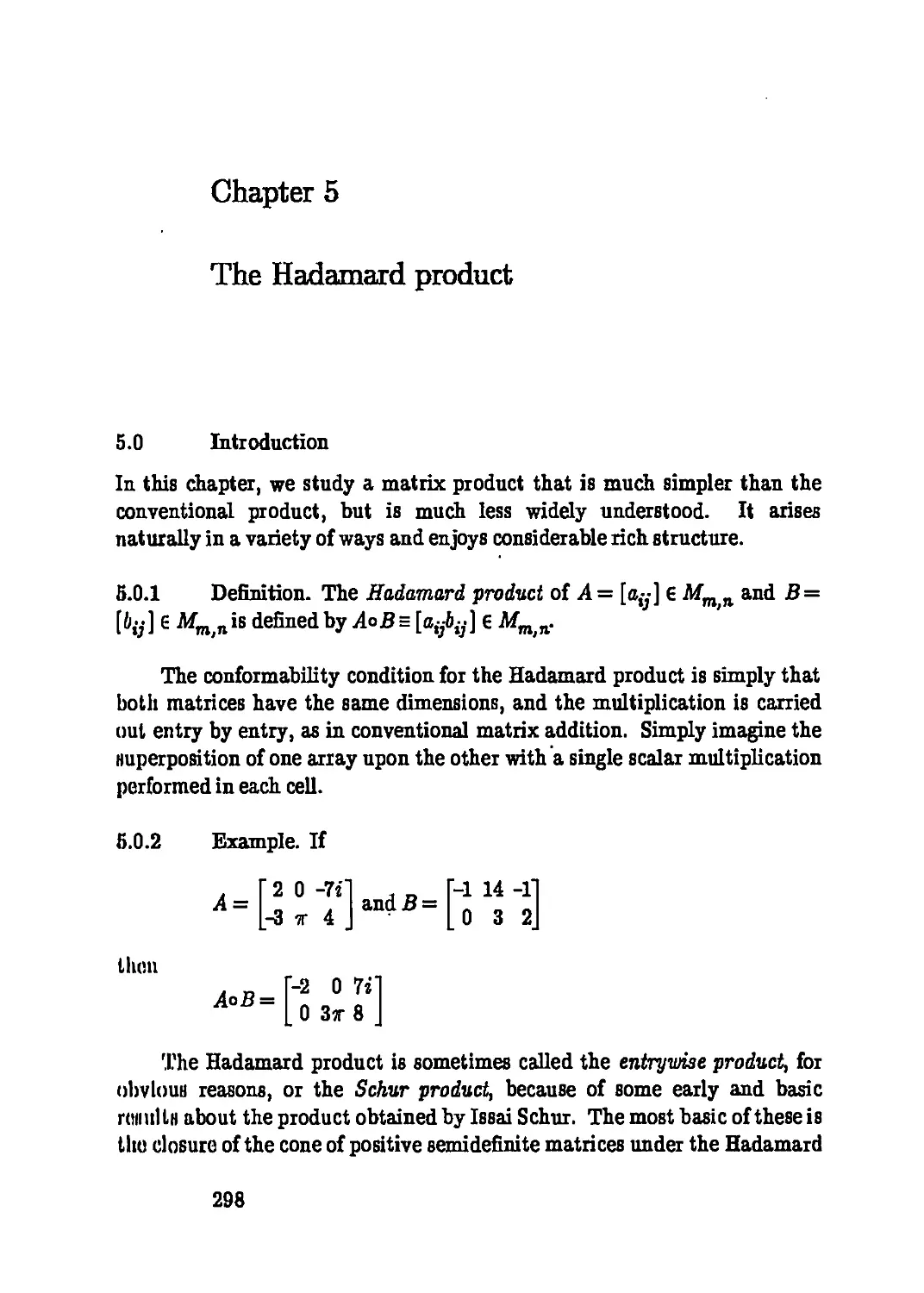
5.O Introduction 298
5.1 Some basic observations 304
5.2 The Schur product theorem 308
5.3 Generalizations of the Schur product theorem 312
5.4 The matrices A o (A-1)1,and A o A-1 322
5.5 Inequalities for Hadamard products of general matrices:
an overview 332
5.6 Singular values of a Hadamard product: a fundamental
inequality 349
5.7 Hadamard products involving nonnegative matrices and
M-matrices 356
Chapter 6 Matrices and functions 382
6.0 Introduction 382
6.1 Polynomial matrix functions and interpolation 383
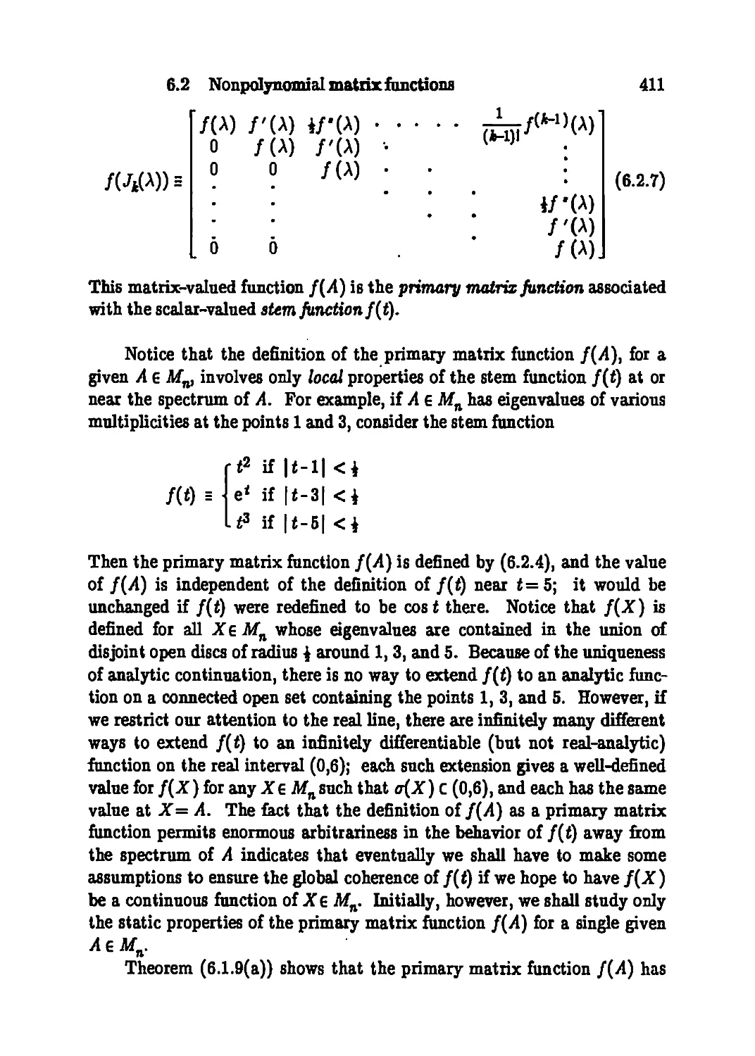
6.2 Nonpolynomial matrix functions 407
6.3 Hadamard matrix functions 449
6.4 Square roots, logarithms, nonlinear matrix equations 459
6.5 Matrices of functions 490
6.6 A chain rule for functions of a matrix 520
Hints for problems 561
References 584
Notation 590
Index 595

Preface
This volume is a sequel to the previously published Matrix Analysis and
includes development of further topics that support applications of matrix
theory. We refer the reader to the preface of the prior volume for many
general comments that apply here also. We adopt the notation and
referencing conventions of that volume and make specific reference to it [HJ] as
needed.
Matrix Analysis developed the topics of broadest utility in the
connection of matrix theory to other subjects and for modern research in the
subject. The current volume develops a further set of Blightly more specialized
topics in the same spirit. These are: the field of values (or classical
numerical range), matrix stability and inertia (including M-matrices), singular
values and associated inequalities, matrix equations and Kronecker
products, Hadamard (or entrywise) products of matrices, and several ways in
which matrices and functions interact. Each of these topics is an area of
active current research, and several of them do not yet enjoy a broad
exposition elsewhere.
Though, this book should serve as a reference for these topics, the
exposition is designed for use in an advanced course. Chapters include
motivational background, discussion, relations to other topics, and literature
references. Most sections include exercises in the development as well as many
problems that reinforce or extend the subject under discussion. There are, of
course, other matrix analysis topics not developed here that warrant
attention. Some of these already enjoy useful expositions; for example, totally
positive matrices are discussed in [And] and [Kar].
We have included many exercises and over 650 problems because we
feci they are essential to the development of an understanding of the subject
and its implications. The exercises occur throughout the text as part of the
vii

development of each suction; tluiy arn fit.iu.i'ally uloinuntary und of liniiu.dl-
alc use in understanding the concept«. We iccominend that Hie reader work
at least a broad selection of thcHc. Problems arc listed (in no particular
order) at the end of sections; they cover a range of difficulties and types
(from theoretical to computational) and they may extend the topic, develop
Hpccial aspects, or suggest alternate proofs of major ideas. In order to
enhance the utility of the book as a reference, many problems have hints;
these are collected in a separate section following Chapter 6. The results of
Home problems are referred to in other problems or in the text itself. We
cannot overemphasize the importance of the reader's active involvement in
carrying out the exercises and solving problems.
As in the prior volume, a broad list of related books and major surveys
in f'iven prior to the index, and references to this list are given via mnemonic
code in square brackets. Readers may find the reference list of independent
utility.
We appreciate the assistance of our colleagues and students who have
offered helpful suggestions or commented on the manuscripts that preceded
publication of this volume. They include M. Bakonyi, W. Barrett, 0. Chan,
(!. Cnllen, M. Cusick, J. Dietrich, S. H. Friedberg, S. Gabriel, F. Hall, C.-K.
hi, M. Lundqui8t, R. Mathias, D. Merino, R. Merris, P. Nylen, A. Souioui,
Ü. W. Stewart, R. C. Thompson, P. van Dooren, and E. M. E. Wennuth.
The authors wish to maintain the utility of this volume to the
community and welcome communication from readers of errors or omissions that
they find. Such communications will be rewarded with a current copy of all
known errata.
R. A. H.
C. R. J.

Chapter 1
The field of values
1.0 Introduction
Like the spectrum (or set of eigenvalues) o(-), the field of values F(-) is a
set of complex numbers naturally associated with a given n-by-n matrix A:
F (A) = {x*Ax: zeVl,z*x=l}
The spectrum of a matrix is a discrete point set; while the field of values can
be a continuum, it is always a compact convex set. Like the spectrum, the
field of values is a set that can be used to learn something about the matrix,
and it can often give information that the spectrum alone cannot give. The
eigenvalues of Hennitian and normal matrices have especially pleasant
properties, and the field of values captures certain aspects of this nice
structure for general matrices.
1.0.1 Subadditivity and eigenvalues of sums
If only the eigenvalues <j[A) and a{B) are known about two n-by-n matrices
A and B, remarkably little can be said about <j[A + B), the eigenvalues of
the sum. Of course, ti(A + B) = tr A + tr B, so the sum of all the
eigenvalues of A + B is the sum of all the eigenvalues of A plus the sum of all the
eigenvalues of B. But beyond this, nothing can be said about the eigenvalues
of A + B without more information about A and B. For example, even if all
the eigenvalues of two n-by-n matrices A and B are known and fixed, the
spectral radius of A + B [the largest absolute value of an eigenvalue of
A + B, denoted by p(A + B)] can be arbitrarily large (see Problem 1). On
the other hand, if A and B are normal, then much can be said about the
1

'). The field of values
(tlfjonvalucs of A + B; for example, p(A + B) < p(A) + p(B) in this case.
Mu inn of matrices do arise in practice, and two relevant properties of the field
t>f vuliioii F(-)axe:
(u) The field of values is subadditive: F(A + B)cF(A) + F{B),
whore the set sum has the natural definition of sums of all possible
pul m, one from each; and
(li) Tlut olßonvalues of a matrix lie inside its field of values: a{A) c
F {A).
( .umhlnliiß llioiio two properties yields the inclusions
o(A I- H) C F {A + B) c F {A) + F(B)
no If the two ficldB of values F (A) and F(B) are known, something can be
mild about the Bpcctrum of the sum.
1.0.2 An application from the numerical solution of partial differential
equations
Suppose that A = [a^] G MJJR) satisfies
(a) A is tridiagonal (a4• = 0 for | «-;| > 1), and
(b) aiii+lai+lii < 0 for i = 1,..., n-1.
Matrices of this type arise in the numerical solution of partial differential
equations and in the analysis of dynamical systems arising in mathematical
biology. In both cases, knowledge about the real parts of the eigenvalues of
A is important. It turns out that rather good information about the
eigenvalues of such a matrix can be obtained easily using the field of values F ( • ).
1.0.2.1 Fact: For any eigenvalue A of a matrix A of the type indicated,
we have
min a„ < Re A < max a,-.-
1 < «<n 1 < t<n
A proof of this fact is fairly simple using some properties of the field of
values to be developed in Section (1.2). First, choose a diagonal matrix D

1.0 Introduction
3
with positive diagonal entries such that D~lAD =À = [âfj-] satisfies ô-,- = -ü{j-
foi jî i The matrix D = diag (^,..., dj defined by
<■?! = !, and d,= £iÜ d^, di>0,i=2,...,n
»■li»
will do. Since  and A are similar, their eigenvalues are the same. We then
have
He a{A) = He o(.4) c Eei^) = F(*(.4 + AT))
= i?(diag(olll...Iann))
= Convex hull of {allr.., ann} = [min a», max oÄ]
j »
The first inclusion follows from the spectral containment property (1.2.6),
the next equality follows from the projection property (1.2.5), the next
equality follows from the special form achieved foi A, and the last equality
follows from the normality property (1.2.9) and the fact that the eigenvalues
of a diagonal matrix aie its diagonal entries. Since the real part of each
eigenvalue A E a{A) is a convex combination of the main diagonal entries aü,
i = 1,..., n, the asserted inequalities are clear and the proof is complete.
1.0.3 Stability analysis
In an analysis of the stability of an equilibrium in a dynamical system
governed by a system of differential equations, it is important to know if the
real part of every eigenvalue of a certain matrix A is negative. Such a
matrix is called stable. In order to avoid juggling negative signs, we often
work with positive stable matrices (all eigenvalues have positive real parts).
Obviously, A is positive stable if and only if -A is stable. An important
sufficient condition for a matrix to be positive stable is the following fact.
1.0.3.1 Fact: Let A e Mn. If A + A* is positive definite, then A is
positive stable.
This is another application of properties of the field of values F ( ■ ) to be
developed in Section (1.2). By the spectral containment property (1.2.6),
Reff(i4)cRei?(i4), and, by the projection property (1.2.5), ReF(A) =

4 The field of values
F(t(A + A*)). But, since A + A* is positive definite, so is \{A + A*), and
lience, by the normality property (1.2.9), F($(A + A*)) is contained in the
positive real axis. Thus, each eigenvalue of A has a positive real part, and A
is positive stable.
Actually, more is true. If A + A* is positive definite, and if P 6 Mn is
any positive definite matrix, then PA is positive stable because
(Pi)-l[PA]pi = piAPi, and
pUpi + (PÏAPÏ)* = PÏ(A + A*)Pi
where & is the unique (Hermitian) positive definite square root of P. Since
congruence preserves positive definiteness, the eigenvalues of PA have
positive real parts for the same reason as A. Lyapunov's theorem (2.2.1)
shows that all positive stable matrices arise in this way.
1.0.4 An approximation problem
Suppose we wish to approximate a given matrix A 6 Mn by a complex
multiple of a Hermitian matrix of rank at most one, as closely as possible in
the Frobenius norm || • ||2. This is just the problem
minimize||A-cza^Ulfor zGCnwith z*a.= land cgC (1.0.4.1)
Since the inner product [A,B] = tr AB* generates the Frobenius norm, we
have
||/l-caa*||2 = [A-aa?tA-cxj?\
= \\A\\l-2Rec[A,xi*] + \c\2
which, for a given normalized x, is minimized by c = [-4,23*]- Substitution of
this value into (1.0.4.1) transforms our problem into
minimize {\\A\\%- | [A.zz*]|2) for see Cnwith ar*i= 1
or, uqnivtilcntly,
maximize | [/I,zz*] | for see Cwith ar*i= 1

1.1 Definitions 5
A vector Xq that solves the latter problem (and there will be one since we are
maximizing a continuous fonction on a compact set) will yield the rank one
solution matrix czar* = [A,^^]^^ to our original problem. However, a
calculation shows that [A.zz*] = tr Axx* = x*Ax, so that determining ig,
and solving our problem, is equivalent to finding a point in the field of values
F (A) that is at maximum distance from the origin. The absolute value of
such a point is called the numerical radius of A [often denoted by r(A)] by
analogy with the spectral radius, which is the absolute value of a point in the
spectrum a{A) that is at maximum distance from the origin.
Problems
1. Consider the real matrices
Lo(l-a)-l or J [-o(l + a)-l -or J
Show that a{A) and a{B) are independent of the value of or E R. What are
they? What is a{A + B)l Show that p{A + B) is unbounded as a-««.
2. In contrast to Problem 1, show that if A, B 6 Mn are normal, then
p(A + B)<p(A) + p(B).
3. Show that "<" in (1.0.2(b)) may be replaced by "<," the main diagonal
entries a,-,- may be complex, and Fact (1.0.2.1) still holds if a.-,- is replaced by
Re a«.
4. Show that the problem of approximating a given matrix A 6 Mn by a
positive semidefinite rank one matrix of spectral radius one is just a matter
of finding a point in F (A) that is furthest to the right in the complex plane.
1.1 Definitions
In this section we define the field of values and certain related objects.
1.1.1 Definition. The field of values of A 6 Mn is
F{A) = {x*Ax:xStn) x*x=l}
Thus, F(') is a function from Mn into subsets of the complex plane.

6 The field of values
F (A) is just the normalized locus of the Hermitian form associated with A.
The field of values is often called the numerical range, especially in the
context of it 8 analog for operators on infinite dimensional spaces.
Exercise. Show that F(I) = {1} and F (od) = {a} for all ore C. Show that
Moo] 1B tne dosed unit interval [0,1], and Moo] is the closed unit disc
{zC-C: \z\ <1}.
The field of values F (A) may also be thought of as the image of the
mirface of the Euclidean unit ball in Cn (a compact set) under the continuous
transformation x-* x*Ax. As such, F (A) is a compact (and hence bounded)
H«t in C. An unbounded analog of F(') is also of interest.
1.1.2 Definition. The angular field of values is
F'(A)z{x*Ax:x£tn,xtO}
lixercise. Show that F'(A) is determined geometrically by F (A); every
open ray from the origin that intersects F (A) in a point other than the
origin is in F'(A), and 0 E F'(A) if and only if 0 E F (A). Draw a typical
picture of an F (A) and F'(A) assuming that 0 f. F(A).
It will become clear that F' (A) is an angular sector of the complex
plane that is anchored at the origin (possibly the entire complex plane). The
angular opening of this sector is of interest.
1.1.3 Definition. The field angle & = Q(A) s ©(^(A)) = Q(F(A)) of
A G Mn is defined as follows:
(a) If 0 is an interior point of F (A), then Q(A) = 2t.
(b) If 0 is on the boundary of 7^ (A) and there is a (unique) tangent to
the boundary of F (A) at 0, then Q(A) s r.
(c) M F (A) is contained in a line through the origin, Q(A) = 0.
(d) Otherwise, consider the two different support lines of F (A) that
go through the origin, and let ®{A) be the angle subtended by
these two lines at the origin. TfO£F (A), these support lines will
be uniquely determined; if 0 is on the boundary of F (A), choose
the two support lines that give the minimum angle.

1.1 Definitions
7
We shall see that F (A) is a compact convex set for every A e Mn, so this
informal definition of the field angle makes sense. The field angle is just the
angular opening of the smallest angular sector that includes F (A), that is,
the angular opening of the sector F' (A).
Finally, the size of the bounded set F (A) is of interest. We measure its
size in terms of the radius of the smallest circle centered at the origin that
contains F {A).
1.1.4 Definition. The numerical radius of A e Mn is
r(A) = max{|z|:zE.F(A)}
The numerical radius is a vector norm on matrices that is not a matrix norm
(see Section (5.7) of [HJ]).
Problems
1. Show that among the vectors entering into the definition of F (A), only
vectors with real nonnegative first coordinate need be considered.
2. Show that both F {A) and F' {A) are simply connected for any A G Mn.
3. Show that for each 0 < 6 < tt, there is an A e M2 with 0(A) = 0. Is
0(A) = 3t/2 possible?
4. Why is the "max" in (1.1.4) attained?
5. Show that the following alternative definition of F (A) is equivalent to
the one given:
F (A) = {sfAx/tfx: x 6 C" and x # 0}
Thus, F ( • ) is a normalized version of F' ( • ).
6. Determine fL J, f\q A, and FU A.
7. If A e Mn and a 6 F (A), show that there is a unitary matrix Ue Mn
such that a is the 1,1 entry of U*A U.
8. Determine as many different possible types of sets as you can that can
be an/!" (A).

8 The field of values
0. Show that F{A*) = Fjl) and F' (A*) = Wß) for all A e Mn.
10. Show that all of the main diagonal entries and eigenvalues of a given
A 6 Mn aie in its field of values F {A).
1.2 Basic properties of the field of values
Ana function from Mn into subsets of C, the field of values F ( • ) has many
UHcr.il functional properties, most of which are easily established. We
catalog many of these properties here for reference and later use. The
I .»portant property of convexity is left for discussion in the next section.
The sum or product of two subsets of C, or of a subset of C and a scalar,
linn the usual algebraic meaning. For example, if S,Tct, then S+T=
{8+t:seS,te T}.
1.2.1 Property. Compactness. For all A e Mn,
F (A) is a compact subset of C
Proof: The set F (A) is the range of the continuous function x—* x*Ax over
thu domain {x: x G Cn, x*x = 1}, the surface of the Euclidean unit ball, which
is a compact set. Since the continuous image of a compact set is compact, it
follows that F (A) is compact. []
1.2.2 Property. Convexity. For all A e Mn,
F (A) is a convex subset of C
The next section of this chapter is reserved for a proof of this
fundamental fact, known as the Toeplitz-Hausdorff theorem. At this point, it is clear
that F (A) must be a connected set since it is the continuous image of a
connected set.
I'Jxcrcise. If A is a diagonal matrix, show that F (A) is the convex hull of the
diagonal entries (the eigenvalues) of A.
The field of values of a matrix is changed in a simple way by adding a
scalar multiple of the identity to it or by multiplying it by a scalar.

1.2 Basic properties of the field of values
9
1.2.3 Property: Translation. For all A 6 Mn and a € C,
F(A + aI) = F{A) + a
Proof: We have F {A + ai) = {x*{A + al)x: x*x=l} = {x*Ax + ax*x:
x*x = l} = {x*Ax+ a:x*x= 1} = {x*Ax:x*x = 1} + or= F(A) + or. Q
1.2.4 Property: Scalar multiplication. For all A e Mn and a e C,
F(aA) = aF(A)
Exercise. Prove property (1.2.4) by the same method used in the proof of
(1.2.3).
For A e Mw E(A) s \(A + A*) denotes the Hermitian part of A and
S(j4)= \(A-A*) denotes the skew-Hermitian part of A; notice that A =
E(A) + S(A) and that E(A) and iS(A) are both Hermitian. Just as taking
the real part of a complex number projects it onto the real axis, taking the
Hermitian part of a matrix projects its field of values onto the real axis.
This simple fact helps in locating the field of values, since, as we shall see, it
is relatively easy to deal with the field of values of a Hermitian matrix. For
a set S c C, we interpret Re S as {Re s: seS}, the projection of S onto the
real axis.
1.2.5 Property: Projection. For all A e M^
F{E(A)) = ReF{A)
Proof: We calculate x*E(A)x= z*${A + A*)x= $(x*Ax+ x*A*x) = $(z*Ax
+ (x*Ax)*) = l(z*Ax+ x*Ax) = Re x*Ax. Thus, each point in F(E(A)) is
of the form Re zfor some z€ F{A) and vice versa. Q
We denote the open upper half-plane of C by UHPs {ze C: Im z > 0},
the open left half-plane of C by LHP = {z e C: Re z < 0}, the open right half-
plane of C by RHP s {z 6 C: Re z > 0}, and the closed right half-plane of C by
RHPq s {z6 C: Re z> 0}. The projection property gives a simple indication
of when F (A) c RHP or RHP0 in terms of positive definiteness or positive
8emidefiniteness.'

10 The field of values
1.2.5a Property: Positive definite indicator fonction. Let A G Mn. Then
F (A) c RHP if and only if A + A* is positive definite
1.2.5b Property: Positive semidefinite indicator function. Let A G Mn.
Then
F (A) c ÄÄP0 if and only if A + A* is positive semidefinite
Exercise. Prove (1.2.5a) and (1.2.5b) (the proofs are essentially the same)
using (1.2.5) and the definition of positive definite and semidefinite (see
Chapter 7 of [HJ]).
The point set of eigenvalues of A G Mn is denoted by o(A), the spectrum
of A. A very important property of the field of values is that it includes the
eigenvalues of A.
1.2.6 Property. Spectral containment For all A G Mw
o(A)cF(A)
Proof: Suppose that A G o(A). Then there exists some nonzero x G Cn, which
wc may take to be a unit vector, for which Ax= Xx and hence A = Xx*x=
x*(\x) = x*AxeF{A). D
Exercise. Use the spectral containment property (1.2.6) to show that the
eigenvalues of a positive definite matrix are positive real numbers.
Exercise. Use the spectral containment' property (1.2.6) to show that the
eigenvalues of Lj J are imaginary.
The following property underlies the fact that the numerical radius is a
vector norm on matrices and is an important reason why the field of values is
so useful.
1.2.7 Property. Subadditivity. For all A, B G Mn,
F(A + B)CF(A) + F(B)
Proof: F(A + B)= {x*(A + B)x: x G Cn, x*x= 1} = {z*Ax+ x*Bx: ig C",

1.2 Basic properties of the field of values
11
z*x=l}c {z*Az: «EC», z*z=l} + {ifBy: y EC", y*y=l}= F(A) +
F(B). Q
Exercise. Use (1.2.7) to show that the numerical radius r(-) satisfies the
triangle inequality on Mn.
Another important property of the field of values is its invariance under
unitary similarity.
1.2.8 Property: Unitary similarity invariance. For all A, Us Mn with
I/'unitary,
F(U*AU) = F(A)
Proof: Since a unitary transformation leaveB invariant the surface of the
Euclidean unit ball, the complex numbers that comprise the sets F(U*AU)
and .F(./l) are the same. Ifi6Cnandar*i= 1, we have ar*(ü*A £/■)!= y*Aye
F{A),vrhaey= Ux,Boy*y=z*U*Uz=x*z=l. Thus, F{U*AU) C F{A).
The reverse containment is obtained similarly. []
The unitary similarity invariance property allows us to determine the
field of values of a normal matrix. Recall that, for a set S contained in a real
or complex vector space, Co(5) denotes the convex hull of 5, which is the set
of all convex combinations of finitely many points of 5. Alternatively,
Co(5) can be characterized as the intersection of all convex sets containing
5, so it is the "smallest" closed convex set containing S.
1.2.9 Property: Normality. If A E Afnis normal, then
F{A) = Co{o(A))
Proof: If A is normal, then A = U*AU, where A = diag (A^..., AJ is
diagonal and {/is unitary. By the unitary similarity invariance properly (1.2.8),
F(A) = F(A)md,ànce
n n
z*Az= £ ï,Vi= 2 \xi\%
1=1 t=l

12 The field of values
/''(A) is just the set of all convex combinations of the diagonal entries of A
(x*x=l implies E,- |x,|2 = 1 and | xt\2 > 0). Since the diagonal entries of A
lire the eigenvalues of A, this means that F {A) = Co(o(A)). []
Exercise. Show that if if is Hennitian, F(H) is a closed real line segment
whose endpoints are the largest and smallest eigenvalues of A.
Exercise. Show that the field of values of a normal matrix is always a
polygon whose vertices are eigenvalues of A. If A e Mn, how many sides may
F (A) have? If A is unitary, show that F (A) is a polygon inscribed in the
unit circle.
Exercise. Show that Co(o(A)) c F {A) for all A 6 Mn.
Exercise. KA,Bç Mn, show that
o{A + B)cF(A) + F(B)
If A and B are normal, show that
o(A + B)C Co(e{A)) + Co(ff(5))
The next two properties have to do with fields of values of matrices that
are built up from or extracted from other matrices in certain ways. Recall
that for A 6 Af_ and B E M_ , the direct sumoî A and Bis the matrix
1 2
If Jc {1,2,..., n} is an index set and if AsMn, then A(J) denotes the
principal submatrix of A contained in the rows and columns indicated by J.
1.2.10 Property: Direct sums. For all A 6 M. and B 6 M. ,
1 2
F{AeB) = Co(F{A)UF(B))
Proof: Note that A o B 6 Mn .j_n . Partition any given unit vector z 6
Cni+n2 as z= [J], where ieCni and yet\ Then z*(A*B)z= x*Ax+
y*By. If y*y = 1 then x= 0 and z*{Ao B)z= fByeF(B), bo F(A<aB)d
F(B). By a similar argument when x*x= 1, F{A »5)3 F{A) and hence

1.2 Basic properties of the field of values 13
F (A o 5) D F (A) U F{B). But since F(AoB) is convex, it follows that
F{A9B)lCo(F{A)\}F(5)) (seeProblem 21).
To prove the reverse containment, let z= LJ 6 Cni+n2 be a unit vector
again. If ar*i = 0, then y*y = 1 and z*(A o B)z = y*fly 6 ^ (5) c Co(.F {A) U
F{B)). The argument is analogous if y*y = 0. Now suppose that both x and
y are nonzero and write
z*(A o 5)z = a*A* + tfBy = a* J —1 + f y\ til
\.x*x J ^v*y
Since z*z + y*y = z?z = 1, this last expression is a convex combination of
*^SF(A) and ££6F(J)
and we have F {A • 5) c Co(,F(A) U ^(fl)). Q
1.2.11 Property: Submatrix inclusion. For all A e Mn and index sets J C
{1 n},
F{A{J))CF{A)
Proof: Suppose that J= {fa..., jjj, with l<Ji <£<•••< j*<n, mà.
suppose 16 C* satisfies ar*i= 1. We may insert zero entries into appropriate
locations in x to produce a vector x 6 C" such that z.-. = zt-, i = 1,2,..., k, and
ij-= 0 for all other indices j. A calculation then shows that x*A(J)x= x*Ax
and x*x=l, which verifies the asserted inclusion. []
1.2.12 Property: Congruence and the angular field of values. Let A e Mn
and supposethat Ce Afnis nonsingular. Then
F'(C*AC) = F'(A)
Proof: Let iE C" be a nonzero vector, so that x*C*ACx= y*Ay, where y =
Cz#0. Thus, F'(C*AC)cF'(A). In the same way, one shows that
F'{A) c F'{C*AC) since A = {C~l)*C*AC{C~l). 0

14 The field of values
Problems
1. For what AeMn does F(A) consist of a single point? Could F {A)
consist of k distinct points for finite k > 1?
2. State and prove results corresponding to (1.2.5) and (l.2.5a,b) about
projecting the field of values onto the imaginary axis and about when F (A)
is in the upper half-plane.
3. Show that F {A) + F (5) is not the same as F (A + B) in general. Why
not?
4. If A, B 6 Mn, is F (AB) cF{A)F (5)? Prove or give a counterexample.
5. If A, B 6 Mw is F'{AB) c F'{A)F'{B)1 Is Q(AB) < Q(A) + 0(5)?
Prove or give a counterexample.
6. If A, B 6 Mn are normal with a{A) = {alt..., a„} and a{B) = {/7lt...,
/?„}, show that a{A + 5) c Co({ai + ßy *> 3= h—, «})■ H 0 < or< 1 and if
U, 76 Mn are unitary, show that p(aU+ (1 - a) V) < ap( U) + (1 - or)p( 7)
= 1, where p( • ) denotes the spectral radius.
7. If A, B 6 Mn are Hermitian with ordered eigenvalues a^ < • • • < an and
ß\< ■" ißn> respectively, use a field of values argument with the
subadditivity property (1.2.7) to show that al-{-ßl< ^ and 7n < an + ßn,
where 7i < • • • < 7n are the ordered eigenvalues of C= A + B. What can
you say if equality holds in either of the inequalities? Compare with the
conclusions and proof of Weyl's theorem (4.3.1) in [HJ].
8. Which convex subsets of C are fields of values? Show that the class of
convex subsets of C that are fields of values is closed under the operation of
taking convex hulls of finite unions of the sets. Show that any convex
polygon and any disc are in this class.
9. According to property (1.2.8), if two matrices are unitarily similar,
llicy have the same field of values. Although the converse is true when n = 2
[see Problem 18 in Section (1.3)], it is not true in general. Construct two
matrices that have the same size and the same field of values, but are not
unitarily similar. A complete characterization of all matrices of a given size
with a given field of values is unknown.
10. According to (1.2.9), if A e Mn is normal, then its field of values is the
convex hull of its spectrum. Show that the converse is not true by consid-

1.2 Baric properties ofthe field of values 15
ering the matrix .A = diag(l,i,-l,-i)e L01 e Jlf8. Show that F(A) =
Co(ff(i4)). but that A is not normal. Construct a counterexample of the
form A = diagfA^ A2, A3) o L J e MB. Why doesn't this kind of example
work for Af4? Is there some other kind of counterexample in Af4? See
(1.6.9).
11. Let z be a complex number with modulus 1, and let
A =
0 1 0'
0 0 1
zfl 0
Show that F {A) is the closed equilateral triangle whose vertices are the cube
roots of z. More generally, what is F {A) HA — [o^ ] 6 AfB has all flf f+i = 1,
ani = z, and all other o^ = 0?
12. If A G Mn and F (A) is a real line segment, show that A is Hennitian.
13. Give an example of a matrix A and an index set J for which equality
occurs in (1.2.11). Can you characterize the cases of equality?
14. What is the geometric relationship between F'(C*AC) and F'{A) if:
(a) Ce Mnis singular, or (b) if Cis n-by-Äand rank C=kl
15. What is the relationship between F (C*AC) and F {A) when Ce Jlfnis
nonsingular but not unitary? Compare with Sylvester's law of inertia,
Theorem (4.5.8) in [HJ].
16. Properties (1.2.8) and (1.2.11) are special cases of a more general
property. Let A e Mn, k < n, and P 6 Jlf„it be given. If P*P =IeMh then P
is called an isometry and FM.P is called an isometric projection of A. Notice
that an isometry P 6 Mn Ä is unitary if and only iik=n. If A' is a principal
8ubmatrix of A, show how to construct an isometry P such that A ' = P*AP.
Prove the following statement and explain how it includes both (1.2.8) and
(1.2.11):
1.2.13 Property: Isometric projection. For all A 6 Mn and P e Mn k with
Jfe< nand P*P= I,F{P*AP) c F{A), and F(P*AP) = F{A) whenJfe= n.
17. It is natural to inquire whether there are any nonunitary cases in which
the containment in (1.2.13) is an equality. Let A e Mn be given, let P 6 Mn h
be a given isometry with k<n, and suppose the column space of P contains

10 The field of values
nil Ihe columns of both A and A*. Show that F' (A) = F1 (P*AP) U {0} and
F{A) = Co(F(P*AP)U{0}). If, in addition, 0 6 F{P*AP), show that
F(A) = F{P*AP); consider A= [J j] and P= [J]/^ to show that if
01 F {P*AP), then the containment F [F*AP) c F (A) can be strict.
18. Let A e Mn and let P 6 Mn ^ be an isometry with k< n. Consider A =
L ]] and P= Wl/fii to show that one can have F(P*AP) = F (A) even if
I he column space of P does not contain the columns of A and A*. Suppose
(7 E Mn is unitary and K4Ü* = A is upper triangular with A = Aj o ■ ■ ■
® Aj, in which each A,- is upper triangular and some of the matrices At- are
diagonal. Describe how to construct an isometry P from selected columns of
U so that F {A) = F(P*AP). Apply your construction to A = I, to A =
diag(l,2,3) G Af3, and to a normal A e Mn and discuss.
19. Suppose that ieMn is given and that G 6 Mn is positive definite.
Show that a(A) c F'(GA) and, therefore, that a[A) c [\{F{GA)-. Gis
positive definite}.
'20. Consider the two matrices
0 0 0 1'
0 0 10
0 0 0 0
10 0 0
and B=
0 0 0 1'
0 0 10
0 10 0
10 0 0
Precisely determine F{A), F(B), and F(aA + (1 - a)B), 0 < a< 1.
21. Let S be a given subset of a complex vector space, and let 51 and 52 be
given subsets of 5. Show that 53 Co(^ U S2) if S is convex, but that this
statement need not be correct if S is not convex. Notice that this general
principle was used in the proof of the direct sum property (1.2.10).
22. Let A 6 Mn be nonsingular. Show that F {A) c RHP if and only if
F(A~l) cRHP, or, equivalently, E(A) is positive definite if and only if
Il(i4_1) is positive definite.
23. Let A G Mn, and suppose A is an eigenvalue of A.
(a) If A is real, show that \eF(E(A)) and hence |A| <p(E(A)) =
III H(i4) UI2, where /.(• ) and |||-|||2 denote the spectral radius and spectral
norm, respectively.

1.3 Convexity
17
(b) If A is purely imaginary, show that A G i?(S(^)) and. hence |A| <
p(S(A)) = III S(A)) life.
24. Suppose all the entries of a given A 6 Mn are nonnegative. Then the
nonnegative real number p(A) is always an eigenvalue of A [HJ, Theorem
(8.3.1)]. Use Problem 23 (a) to show that p(A) < p(R(A)) = \p(A + AT)
whenever A is a square matrix with nonnegative entries. See Problem 23 (n)
in Section (1.5) for a better inequality involving the numerical radius of A.
25. We have seen that the field of values of | 1 is a closed disc of radius
Lo oJ
\ centered at the origin; this result has a useful generalization.
(a) Let S 6 Mm „ be given, let .«4 = [ Je Afm+n, and let a^B) denote
the largest singular value (the spectral norm) of B. Show that F(A) =
{a?Ay: a;ECm, y EC", ||se||| + ||y||| = l}, and conclude that F(A) is a
closed disc of radius Icr^B) centered at the origin. In particular, r(A) =
■WB)-
(b) Consider A = [° J]eM3 with B= [j |] 6 M2. Show that ax{B) =
2. Consider eTAe with e= [1,1, l]r to show that r(A) > 4/3 > \ox{B).
Does this contradict (a)?
26. Let A 6 Mn be given. Show that the following are equivalent:
(a) r(A)<l.
(b) p(H(e,öyl))<lforaUÖ6lR.
(c) AmiB(H(e«öA))<lforalltf6lR.
(d) HI H(e*öA) 11(2 < 1 for aU tf 6 R.
1.3 Convexity
In this section we prove the fundamental convexity property (1.2.2) of the
field of values and discuss several important consequences ofthat convexity.
We shall make use of several basic properties exhibited in the previous
section. Our proof contains several useful observations and consists of three
parts:
1. Reduction of the problem to the 2-by-2 case;
2. Use of various basic properties to transform the general 2-by-2
case to 2-by-2 matrices of special form; and

18 The field of values
3. Demonstration of convexity of the field of values for the special
2-by-2 form.
See Problems 7 and 10 for two different proofs that do not involve
reduction to the 2-by-2 case. There are other proofs in the literature that are
based upon more advanced concepts from other branches of mathematics.
Reduction to the 2-by-2 case
In order to show that a given, set 5 c C is convex, it is sufficient to show that
as + (1 - a)t G S whenever 0 < a< 1 and s, 1G S. Thus, for a given A G Mn,
F (A) is convex if ax*Ax+(l-a)y*Ay S F (A) whenever 0<a<l and
x, y G C" satisfy x*x = y*y= 1. It suffices to prove this only in the 2-by-2
case because we need to consider only convex combinations associated with
pairs of vectors. For each given pair of vectors x, y G C", there is a unitary
matrix If and vectors v, w G €" such that x— Uv,y= Uw, and all entries of v
und w after the first two are equal to zero (see Problem 1). Using this
transformation, we have
ax* Ax + (1 - a)y* Ay = at/* U* A Uv + (1 - a)w* 0*A Uw
= aii*Bv+ (1 - a)w*Bvi
= a?B(llA)t + (1 - a)T?B({l,2})T,
where B = U*A U, B[{1,2}) is the upper left 2-by-2 principal submatrix of B,
and £, 7? 6 C2 consist of the first two entries of v and w, respectively. Thus, it
suffices to show that the field of values of any 2-by-2 matrix is convex. This
reduction is possible because of the unitary similarity invariance property
(1.2.8) of the field of values.
Sufficiency of a special 2-by-2 form
We prove next that in order to show that F (A) is convex for every matrix
A G M2, it suffices to demonstrate that F U {[] is convex for any o, b > 0.
The following observation is useful.
1.3.1 Lemma. For each A G M2, there is a unitary Us M2 such that the
two main diagonal entries of U*AU&ie equal.

1.3 Convexity
19
Proof: We may suppose without loss of generality that tr A = 0 since we
may replace A by A -(Jftr A)I. We need to show that A is unitarily similar
to a matrix whose diagonal entries are both equal to zero. To show this, it is
sufficient to show that there is a nonzero vector u/E C2 such that w*Aw= 0.
Such a vector may be normalized and used as the first column of a unitary
matrix W, and a calculation reveals that the 1,1 entry of W*A Wis zero; the
2,2 entry of W* AW must also be zero since the trace is zero. Construct the
vector to as follows: Since A has eigenvalues ±or for some complex number or,
let x be a normalized eigenvector associated with -or and let y be a
normalized eigenvector associated with -fa. If a= 0, just take w = x. If a^O, x
and y are independent and the vector w = ei0x + y is nonzero for all 6 6 R. A
calculation shows that vJ¥Aw= a(e~%*î,-e,öy*a") = 2ittlm(e-,öar*y). Now
choose Ô so that e~iex* y is real. Q
We now use Lemma (1.3.1) together with several of the properties given
in the previous section to reduce the question of convexity in the 2-by-2 case
to consideration of the stated special form. If A e Af2 is given, apply the
translation property (1.2.3) to conclude that F (A) is convex if and only if
F (A + ai) is convex. If we choose a = -\tv A, we may suppose without loss
of generality that our matrix has trace 0. According to (1.3.1) and the
unitary similarity invariance property (1.2.8), we may further suppose that
both main diagonal entries of our matrix are 0.
Thus, we may assume that the given matrix has the form L q\ for
some c, d e €. Now we can use the unitary similarity invariance property
(1.2.8) and a diagonal unitary matrix to show that we may consider
ri o 1 ro ci ri o I _ ro <xi9\
[0 e-tfj [d oj [o eie\ - [de-* 0 J
for any 66 R. If c= | c|e<0» and d =
the latter matrix becomes e'Vl 1^1 'Jjl
d\ e*h, and if we choose 6 = \(02 - 0{),
with^=i(^+ö2).
Thus, it suffices to consider a matrix of the form e'VL jH with tp e R and
o, b > 0. Finally, by the scalar multiplication property (1.2.4), we need to
consider only the special form
[°J], a,b>0 (1.3.2)

20 The field of valueB
That is, we have shown that the field of values of every 2-by-2 complex
matrix is convex if the field of values of every matrix of the special form
(1.3.2) is convex.
Convexity of the field of valueB of the special 2-by-2 form
1.3.3 Lemma. If A 6 Jlf2 has the form (1.3.2), then F (A) is an ellipse
(with its interior) centered at the origin. Its minor axis is along the
imaginary axis and has length | a- b\. Its major axis is along the real axis and has
length a + b. Its foci are at ±Vö5, which are the eigenvalues of A.
Proof: Without loss of generality, we assume a>6>0. Since z*Az=
(ei6z)*A(eiez) for any 0E R, to determine F (A), it suffices to consider z*Az
for unit vectors z whose first component is real and nonnegative. Thus, we
consider the 2-vector z= [t,ei0(l-#)l]T for 0< t < 1 and 0< 0<2tt. A
calculation shows that
z*Az= t(l-f)$[(a+ 6)co8 0 + i(a-b)àn 0\
As 0 varies from 0 to 2t, the point (a+ 6)cos 0+ i(a-6)sin ê traces out a
possibly degenerate ellipse £ centered at the origin-, the major axis extends
from -(a+ b) to (a + b) on the real axis and the minor axis extends from
i (6 - a) to * (a- b) on the imaginary axis in the complex plane. As t varies
from 0 to 1, the factor t(l-t?)i varies from 0 to j and back to 0, ensuring
that every point in the interior of the ellipse \£ is attained and verifying that
F {A) is the asserted ellipse with its interior, which is convex. The two foci
of the ellipse \£ are located on the major axis at distance
[i(o + b)2 - i(a- è)2]^ = ±Jä5hom the center. This completes the argument
to prove the convexity property (1.2.2). Q
There are many important consequences of convexity of the field of
values. One immediate consequence is that Lemma (1.3.1) holds for
matrices of any size, not just for 2-by-2 matrices.
1.3.4 Theorem. For each A e Mn there is a unitary matrix lf£ Mn such
thai all the diagonal entries of WAUhave the same value tr(.A)/n.
Proof: Without loss of generality, we may suppose that tr A = 0, since we
may replace A by A -[tr(.A)/n]/. We proceed by induction to show that A is

1.3 Convexity
21
unitarily similar to a matrix with all zero main diagonal entries. We know
from Lemma (1.3.1) that this is true for n = 2, so let n > 3 and suppose that
the assertion has been proved for all matrices of all orders less than n. We
have
0 = itrA = iA1 + iA2+...+iAn = 0
and this is a convex combination of the eigenvalues A,- of A. Since each A,- is
in F(A), and since F(A) is convex, we conclude that 0 E F(A). If x6 Cn is a
unit vector such that x*Ax= 0, let W= [x tu2 ... wn] 6 Mn be a unitary
matrix whose first column is x. One computes that
WMW=[° fj.s.CeC»-1.^^
But 0 = tr A = tr W*AW= tr A. = 0, and so by the induction hypothesis
there is some unitary V6 Mn-i such that all the main diagonal entries of
V*A V are zero. Define the unitary direct sum
and compute
(WV)*A(WV)= V*W*AWV=
which has a zero main diagonal by construction. Q
A different proof of (1.3.4) using compactness of the set of unitary
matrices is given in Problem 3 of Section (2.2) of [HJ].
Another important, and very useful, consequence of convexity of the
field of values is the following rotation property of a matrix whose field of
values does not contain the point 0.
1.3.5 Theorem. Let A e ilf_ be given. There exists a real number Isuch
that the Hermitian matrix H(e^A) = \[è°A + e~i0A*] is positive definite if
and only if Of"! F (A).
Proof: If E(eiûA) is positive definite for some OCR, then ^(e»'^) c RHP by
0 z*V 1
VÇ V*Âv\

22 The field of values
(1.2.5a), so 0 i. F(ei9A) and hence 01 F{A) by (1.2.4). Conversely, suppore
0 i F {A). By the separating hyperplane theorem (see Appendix B of [HJ]),
there is a line L in the plane such that each of the two nonintersecting
compact convex sets {0} and F {A) lies entirely within exactly one of the two
open half-planes determined by L. The coordinate axes may now be rotated
so that the line L is carried into a vertical line in the right half-plane with
F [A) strictly to the right of it, that is, for some 0 6 R, F (ei0A) = ei0F {A) c
RHP, so E{eieA) is positive definite by (1.2.5a). □
Some useful information can be extracted from a careful examination of
the steps we have taken to transform a given matrix A e M2 to the special
form (1.3.2). The first step was a translation A-* A-($ti A)I= AQ to
achieve tr A0 = 0. The second step was a unitary similarity Aq —* UAq U* =
Ai to make both diagonal entries of A1 zero. The third step was another
unitary similarity Al —♦ VAl V* = A2 to put A2 into the form
A2 = e*>? Q witha,6>0andpeR
The last step was a unitary rotation A2 -* e~ivA2 = A3 to achieve the special
form (1.3.2). Since the field of values of A3 is an ellipse (possibly degenerate,
that is, a point or line segment) centered at the origin with its major axis
along the real axis and its foci at ±\/ä5, the eigenvalues of -43, the field of
values of A2 is also an ellipse centered at the origin, but its major axis is
tilted at an an angle ip to the real axis. A line through the two eigenvalues of
A2, ±e,-Vä5, which are the foci of the ellipse, contains the major axis of the
ellipse; if ab = 0, the ellipse is a circle (possibly degenerate), so any diameter
ÎB a major axis. Since Al and AQ are achieved from A2 by successive unitary
similarities, each of which leaves the eigenvalues and field of values
invariant, we have F (AQ) = F{Al) = F{A2). Finally,
F ( A) = F ( Aq + [*tr A]I) = F (A0) + *tr A = F {A2) + *tr A
a 8 hi ft that moves both eigenvalues by $tr A, so we conclude that the field of
values of any matrix A e M2 is an ellipse (possibly degenerate) with center at
the point $tr A. The major axis of this ellipse lies on aline through the two
«Igcnvalues of A, which are the foci of the ellipse; if the two eigenvalues
coincide, the ellipse is a circle or a point.
According to Lemma (1.3.3), the ellipse F (A) is degenerate if and only

1.3 Convexity
23
tf ^3 = [b o\ has a= b- Notice that AtAZ = [o a*] ^ ^3 = [Ô 6«] > 80
a = b if and only if .A3 is normal. But A can be recovered from A3 by a
nonzero scalar multiplication, two unitary similarities, and a translation,
each of which preserves both normality and nonnormality. Thus, A3 is
normal if and only if A is normal, and we conclude that for A G M2, the
ellipse F (A) is degenerate if and only if A is normal.
The eigenvalues of A3 are located at the foci on the major axis of F (A3)
at a distance of Jä5 from the center, and the length of the semimajor axis is
$(a+ b) by (1.3.3). Thus, $(a+ 6)-v/äF= ${Jä-iß)2> 0 with equality if
and only if a = b, that is, if and only if A is normal. We conclude that the
eigenvalues of a nonnormal As M2 always lie in the interior of F (A).
For A G M2, the parameters of the ellipse F (A) (even if degenerate) can
be computed easily using (1.3.3) if one observes that a and b are the singular
values of A3 = L 0], that is, the square roots of the eigenvalues of A^A3,
and the singular values of A3 are invariant under pre- or post-multiplication
by any unitary matrix. Thus, the singular values o± > ff210 of -A0 = A -
(4tr A)I axe the same as those of .A3. The length of the major axis of F (.A) is
a+b = ffl + ff2. the length of the minor axis is | a- 61 = d^ - ff2> and the
distance of the foci from the center is [( a + b)2 - (a- 6)2]'/4 = ^/öE = yfä^i =
|det A3|'i= Idet-A^i. Moreover, o\ +o\= tr A\A$ (the sum of the
squares of the moduli of the entries of Aq), so oj ± ff2 = [°T + °2 * 2oiff2]^ =
[tr -AJ-Aq "* 21 det -AqI]^- We summarize these observations for convenient
reference in the following theorem.
1.3.6 Theorem. Let A g M2 be given, and set AQ = A - ($tr A)/. Then
(a) The field of values F (A) is a closed ellipse (with interior, possibly
degenerate).
(b) The center of the ellipse F (A) is at the point $tr A. The length of
the major axis is [tr A%AQ + 21 det A0 \ ]i; the length of the minor
axis is [tr i4^i40-2|det AQ\]i; the distance of the foci from the
center is | det A0 \ I. The major axis lies on a line passing through
the two eigenvalues of A, which are the foci of F (A); these two
eigenvalues coincide if and only if the ellipse is a circle (possibly a
point).
(c) F (A) is a closed line segment if and only if A is normal; it is a
single point if and only if A is a scalar matrix.
(d) F (A) is a nondegenerate ellipse (with interior) if and only if A is

24 The field of values
not normal, and in this event the eigenvalues of A are interior
points of F {A).
Problems
1. Let x, y 6 C* be two given vectors. Show how to construct vectors v,w£
Cn and a unitary matrix UeMn such that x = Uv,y= Uw, and all entries of
v and w after the first two are zero.
2. Verify all the calculations in the proof of (1.3.1).
3. Sketch the field of values of a matrix of the form (1.3.2), with a> 0,
6>0.
4. Use (1.3.3) to show that the field of values of [ 0 01 is a closed ellipse
(with interior) with foci at 0 and 1, major axis of length fi, and minor axis of
length 1. Verify these assertions using Theorem (1.3.6).
5. Show that if A e MB(R) then F (A) is symmetric with respect to the real
axis.
6. If ilr.., xk 6 Cn are given orthonormal vectors, let P = [x±... xk ] 6 Mn k
and observe that P*P= IeMk. If A 6 M^ show that F{P*AP) c F{A) and
that xfAxi^ F{P*AP) for := 1,..., it Use this fact for ifc= 2 to give an
alternate reduction of the question of convexity of 7^ (A) to the 2-by-2 case.
7. Let .A 6 Mn be given. Provide details for the following proof of the
convexity of F (A) that does not use a reduction to the 2-by-2 case. There is
nothing to prove if F (A) is a single point. Pick any two distinct points in
F (A). Using (1.2.3) and (1.2.4), there is no loss of generality to assume that
these two points are 0, a 6 R, a > 0. We must show that the line segment
joining 0 and a lies in F (A). Write Aus A = H+iK, in which H= B.(A)
and K= -tS(.<4)= -ii(A-A*), so that H and K are Hermitian. Assume
further, without loss of generality after using a unitary similarity, that Jf is
diagonal. Let x, y 6 Cn satisfy s?Ax= 0, x*x= 1, y*Ay = a, and y*y = 1, and
let Xj= | Xj\ e J, y-= | y$\e'^', j= 1,..., n. Note that x*Hx= x*Kx= y*Ky =
0 and y*Hy= a. Definez(f) 6 C", 0 < t< 1, by

1.3 Convexity 25
' la^e^-SO*;, o < t <l/3
z}{t) = - [(2 -3t)|a:J.|2.+ (3É-l)|yi|2]^ 1/3 < t < 2/3
\yj\e^^)<Pj, 2/3 < t < 1
Verify that 3*(t)z(t) = l and 2*(i)ifc(f) = 0,0 < t< 1, and note that
2f*(i)AjB(i) = 2*(f)Jïz(f) is real and equal to 0 at 4=0, is equal to a at i= 1,
and is a continuous function of t for 0 < t < 1. Conclude that the line segment
joining 0 and alles in F {A), which, therefore, is convex.
8. If A e Mn is such that 0 6 F {A), show that the Euclidean unit sphere in
the definition of F (A) may be replaced by the Euclidean unit ball, that is,
show that F {A) = {x*Ax:xetn, x*x< 1}. What if 01 F{A)1
9. Let JB(0) 6 Mn be the n-by-nnilpotent Jordan block.
'„(0)i
0 I , °
Show that F(Jn(0)) is a disc centered at the origin with radius p(K(Jn(0))).
Use this to show that F(Jn(0)) is strictly contained in the unit disc. If D 6
Mn is diagonal, show that F(DJJO)) is also a disc centered at the origin
with radius p(E(DJn(0))) = p(E.(\D\Jn(0))). See Problem 29 in Section
(1.5) for a stronger result.
10. Let A 6 Mn be given. Provide details for the following proof of the
convexity of F {A) that does not use an explicit reduction to the 2-by-2 case.
If F (A) is not a single point, pick any two distinct points a, b 6 F (A), and
let c be any given point on the open line segment between a and b. We may
assume that c = 0, a, b 6 R, and a < 0 < 6. Let x, y 6 Cn be unit vectors such
that x*Ax= a, y*Ay = b, so x and y are independent. Consider z(t,ô) =
eiex+ ty, where t and 6 are real parameters to be determined. Show that
f(t,0) = i(t,O)*Mt,0)= bP+a(0)t+a, where oi&) = €-i0x*Ay + è°y*Ax.
If y*Ax- xTAy = re'*" with r> 0 and ip 6 R, then o^ff) is real for 6 = -<p, and
/(*0.-p) = 0 for fo = [-o(-p) + [o(-v»)2 -4a&]*]/26 6 R. Then z^.-p) # 0 and
0 = zMze .F(A) for z= zt^/II^V*
11. Let .A 6 M2 be given. Show that A is normal (and hence F (A) is a line
segment) if and only if AQ = A - ($tr A)I is a scalar multiple of a unitary

26 The field of vaines
matrix, that is, A%AQ = ci for some c > 0.
12. Give an example of a normal matrix A e Mw n > 3, such that F (A) is
not aline segment. Why can't this happen in M2?
13. Let A e AfB be given. If F (vi) is a line segment or a point, show that A
must be normal.
0 A^
IV*2.2+ |0|2]*andthe
Q f J 6 M2. Show that the
14. Consider the upper triangular matrix A =
length of the major axis of the ellipse F {A) is
length of the minor axis is | ß\. Where is the center? Where are the foci? In
particular, conclude that the eigenvalues of A are interior points of F (A) if
and only if ß$0.
15. Let A e Mn be given with 0 g F {A). Provide the details for the
following proof that F (A) lies in an open half-plane determined by some line
through the origin, and explain how this result may be used as an alternative
to the argument involving the separating hyperplane theorem in the proof of
(1.3.5). For zçF(A), consider the function g(z) = z/\z\ = exp(:argz).
Since <?(•) is a continuous function on the compact connected set F (A), its
range g(F(A)) = R is a compact connected subset of the unit circle. Thus, R
is a closed arc whose length must be strictly less than x since F (A) is convex
andO^(A).
16. Let A e Mn be given. Ignoring for the moment that we know the field of
values F (A) is convex, F (A) is obviously nonempty, closed, and bounded,
so its complement F(A)C has an unbounded component and possibly some
bounded components. The outer boundary of F (A) is the intersection of
F (A) with the closure of the unbounded component of F(A)C. Provide
details for the following proof (due to Toeplitz) that the outer boundary of
F (A) is a convex curve. For any given 6 6 [0,2tt], let ei0A = H+ iK with
Hermitian H,Ks Mn. Let An(£T) denote the algebraically largest eigenvalue
of H, let S0= {ieCn: zfO, Hx= Xn{H)x}, and suppose dim(5fl)= k>l.
Then the intersection of F (ei9A) with the vertical line Re z= An(i7) is the
set Xn{H) + i{x*Kx: xeSß, \\x\\2 = 1}, which is a single point if k= 1 and
can be a finite interval if k > 1 (this is the convexity property of the field of
values for a Hermitian matrix, which follows simply from the spectral
theorem). Conclude, by varying 0, that the outer boundary of F (A) is a
convex curve, which may contain straight line segments. Why doesn't this
prove that F(A) is convex?

1.3 Convexity
27
17. (a) Let A 6 Af2 be given. Use Schur's unitary triangulaiization
theorem (Theorem (2.3.1) in [HJ]) and a diagonal unitary similarity to show that
A is unitarily similar to an upper triangular matrix of the form
X1 o{Ah
0 A2 J
where a(A) > 0. Show that ti A*A= \X1\2+\X2\2 + a(A)2 and that a(A)
is a unitary similarity invariant, that is, a{A) = o^UAU* ) for any unitary
UeM2.
(b) UA,BeM2 have the same eigenvalues, show that A is unitarily similar
to flif and only if tr A*A = tr B*B.
(c) Show that A,BeM2 have the same eigenvalues if and only if tr A = tr B
and tr A2 = tr B2.
(d) Conclude that two given matrices A, B e Af2 are unitarily similar if and
only if tr A = tr B, tr A2 = tr B2, and tr A* A = tr B*B.
18. Use Theorem (1.3.6) and the preceding problem to show that two given
2-by-2 complex or real matrices are unitarily similar if and only if their fields
of values are identical. Consider At= diag(0,l,t) for t 6 [0,1] to show that
non8imilar 3-by-3 Hermitian matrices can have the same fields of values.
19. Let A = [atj] 6 Jlf2 be given and suppose F (A) c UHP = {ze C: Im z>
0}. Use Theorem (1.3.6) to show that if either (a) an and a^ are real, or (b)
tr A is real, then A is Hermitian.
Notes and Further Readings. The convexity of the field of values (1.2.2) was
first discussed in 0. Toeplitz, Das algebraische Analogon zu einem Satze von
Fejér, Math. Zeit. 2 (1918), 187-197, and F. Hausdorff, Das Wertvorrat einer
Bilinearform, Math. Zeit. 3 (1919), 314-316. Toeplitz showed that the outer
boundary of F (A) is a convex curve, but left open the question of whether
the interior of this curve is completely filled out with points of F (A); see
Problem 16 for Toeplitz's elegant proof. He also proved the inequality
HI A Hk < 2r (A) between the spectral norm and the numerical radius; see
Problem 21 in Section (5.7) of [HJ]. In a paper dated six months after
Toeplitz's (the respective dates of their papers were May 22 and November
28,1918), Hausdorff rose to the challenge and gave a short proof, similar to
the argument outlined in Problem 7, that F (A) is actually a convex set.
There are many other proofs, besides the elementary one given in this

28 The field of values
section, such as that of W. Donoghue, On the Numerical Range of a
Bounded Operator, Mich. Math. J. 4 (1957), 261-263. The result of
Theorem (1.3.4) was first noted by W. V. Parker in Sets of Complex Numbers
Associated with a Matrix, Duke Math. J. 15 (1948), 711-715. The
modification of Hausdorff s original convexity proof outlined in Problem 7 was given
by Donald Robinson; the proof outlined in Problem 10 is due to Roy
Mathias.
The fact that the field of values of a square complex matrix is convex
has an immediate extension to the infinite-dimensional case. If T is a
bounded linear operator on a complex Hilbert space TL with inner product
<•,•>, then its field of val ues (often called the numerical range) is F ( T ) =
{<Tx,i>: x£7 and <x,i> = 1}. One can show that F(T) is convex by
reducing to the two-dimensional case, just as we did in the proof in this
section.
1.4 Axiomatization
It is natural to ask (for both practical and aesthetic reasons) whether the list
of properties of F (A) given in Section (1.2) is, in some sense, complete.
Since special cases and corollary properties may be of interest, it may be
that no finite list is truly complete; but a mathematically precise version of
the completeness question is whether or not, among the properties given
thus far, there is a subset that characterizes the field of values. If so, then
further properties, and possibly some already noted, would be corollary to a
set of characterizing properties, and the mathematical utility of the field of
values would be captured by these properties. This does not mean that it is
not useful to write down properties beyond a characterizing set. Some of the
most applicable properties do follow, if tediously, from others.
1.4.1 Example. Spectral containment (1.2.6) follows from compactness
(1.2.1), translation (1.2.3), scalar multiplication (1.2.4), unitary invariance
(1.2.8), and submatrix inclusion (1.2.11) in the sense that any set-valued
function on Mn that has these five properties also satisfies (1.2.6). If A 6 Mn
and if 06 <j[A), then for some unitary Ue Mn the matrix U*AU is upper
triangular with ß in the 1,1 position. Then by (1.2.8) and (1.2.11) it is
enough to show that /Je F([ß]), and (because of (1-2.3)) it suffices to show
that 0 G F([0]); here we think of [ß] and [0] as members of Mx. However,
because of (1.2.4), F([0]) = a.F([0]) for any or, and there are only two non-

1.4 Axiomatization
29
empty subsets of the complex plane possessing this property: {0} and the
entire plane. The latter is precluded by (1.2.1), and hence (1.2.6) follows.
Exercise. Show that (1.2.8) and (1.2.10) together imply (1.2.9).
The main result of this section is that there is a subset of the properties
already mentioned that characterizes F(-) as a function from Mn into
subsets of C.
1.4.2 Theorem. Properties (1.2.1-4 and 5b) characterize the field of
values. Thati8, the usual field of values F (•) is the only complex set-valued
function on Mn such that
(a) F (A) is compact (1.2.1) and convex (1.2.2) for all A 6 Jlf„;
(b) F{A + al)= F(A) + a (1.2.3) and F{aA) = aF(A) (1.2.4) for
all a 6 C and all A 6 M„; and
(c) F (A) is a subset of the closed right half-plane if and only if
A + A* is positive semidefinite (1.2.5b).
Proof: Suppose F^-) and F2(-) are two given complex set-valued functions
on Mn that satisfy the five cited functional properties. Let A 6 Mn be given.
We first show that F^A) c F2{A). Suppose, to the contrary, that ß 6 FX{A)
and ßf. F2{A) for some complex number ß. Then because of (1.2.1) and
(1.2.2), there is a straight line L in the complex plane that has the point ß
strictly on one side of it and the set F2(A) on the other side (by the
separating hyperplane theorem for convex sets; see Appendix B of [HJ]). The
plane may be rotated and translated so that the imaginary axis coincides
with L and ß lies in the open left half-plane. That is, there exist complex
numbers ax # 0 and a2 such that Re(o1^+ a2) < 0 while <*iF2(A) + o2 is
contained in the closed right half-plane. However, o,F2(^) + a^ =
F2{a1A + atf) because of (1.2.3) and (1.2.4), so Re0' < 0 while F2{A') lies
in the closed right half-plane, where A' = axA + a2I and ß' = atf + oç 6
F^A'). Then, by (1.2.5b), A' + A'* is positive semidefinite. This,
however, contradicts the fact that F^A') is not contained in the closed right
halfplane, and we conclude that F^A) c F2(A).
Reversing the roles of Fi(-) and F2(-) sho'TS that F2(A) c F^A) as
well. Thus, F^A) = F2(A) for all A 6 Mn. Since the usual field of values
F(') satisfies the five stated properties (1.2.1-4 and 5b), we obtain the

30 The field of vaines
desired conclusion by taking FX{A) = F{A). Q
Problems
1. Show that no four of the five properties cited in Theorem (1.4.2) are
sufficient to characterize F(-); that is, each subset of four of the five
properties in the theorem is satisfied by some complex set-valued function other
than !*"(•).
2. Show that (1.2.2-4 and 5a) also characterize F ( • ), and that no subset of
these four properties is sufficient to characterize F (• ).
3. Determine other characterizing sets of properties. Can you find one
that does not contain (1.2.2)?
4. Show that the complex set-valued function F(-) = Co(o(')) is
characterized by the four properties (1.2.1-4) together with the fifth property
"F(A) is contained in the closed right half-plane if and only if all the
eigenvalues of A have nonnegative real parts" (A is positive semistable).
5. Give some other complex set-valued functions on Mn that satisfy
(1.2.7).
Further Reading. This section is based upon C. R. Johnson, Functional
Characterization of the Field of Values and the Convex Hull of the
Spectrum, Proc. Amer. Math. Soc. 61 (1976), 201-204.
1.5 Location of the field of values
Thus far we have said little about where the field of values F (A) sits in the
complex plane, although it is clear that knowledge of its location could be
useful for applications such as those mentioned in (1.0.2-4). In this section,
we give a GerSgorin-type inclusion region for F (A) and some observations
that facilitate its numerical determination.
Because the eigenvalues of a matrix depend continuously upon its
entries and because the eigenvalues of a diagonal matrix are the diagonal
entries, it is not too surprising that there is a spectral location result such as
Gor8gorin'8 theorem (6.1.1) in [HJ]. We argue by analogy that because the
Bel F (A) depends continuously upon the entries of A and because the field of
values of a diagonal matrix is the convex hull of the diagonal entries, there

1.5 Location of the field of values 31
ought to be some sort of inclusion region foi F (A) that, like the GerSgorin
discs, depends in a simple way on the entries of A. We next present such an
inclusion region.
1.5.1 Definition. Let A = [&.•] G Mn, let the deleted absolute row and
column sums of A be denoted by
ASW-ÉKI» i=1 n
i=X
and
m
respectively, and let
gt{A) = l[R'i(A)+C'i(A)],i=l,...,n
be the average of the ith deleted absolute row and column sums of A. Define
the complex set-valued function GF(')onMn by
Gp(A)zCo\\J {z:\z-an\UHA)}]
Recall Gerfgorin's theorem about the spectrum a(A) of A e Mn, which
says that
a{A)cG{A) = \J{z:\z-aii\<R'i(A)}
*=1
and that
u{A)cG{AT) = \J{z:\z-ajj\<C'j(A)}
3=1

32 Thefidd of vaines
Note that the GerSgorin regions G(A) and G{AT) are unions of circular
discs with centers at the diagonal entries of A, while the set function GF(A)
is the convex hull of some circular discs with the same centers, but with radii
that are the average of the radii leading to G(A) and G(AT), respectively.
The GerSgorin regions G(A) and G(AT) need not be convex, but GP(A) is
convex by definition.
Exercise. Show that the set-valued function Gp(-) satisfies the properties
(1.2.1-4) of the field of values. Which additional properties of the field of
values function F(-) does Gp(-) share?
Exercise. Show that R'i(A)= C'i(AT) and use the triangle inequality to
show that R'i(E{A)) = R'{(\[A + A*]) < gt{A) for all i= 1,..., n.
Our GerSgorin-type inclusion result for the field of values is the
following:
1.5.2 Theorem. For any A 6 Mn, F (A) C GF (A).
Proof: The demonstration has three steps. Let RHP denote the open right
half-plane {ze C: Bez> 0}. We first show that if GF(A) c RHP, then
P {A) c RHP. If Gp (A) C RHP, then Re a,,- > gt{A). Let H(A) = \{A + A*)
= 5= [by]. Since R'-{A*) = C'&A) and R'^B)< gt{A) (by the preceding
exercise), it follows that &,•,• = Re ait- > g£A) > ÄJ(B). In particular, G(B) c
RHP. Since o{B) c G(B) by Gerügorin's theorem, we have o{B) c RHP.
But since B is Hermitian, F(E(A)) = F{B)= Co(a(B)) c RHP and hence
F(A)cRHPby (1.2.5).
We next show that if 01 GP{A), then 0 f. F(A). Suppose 0 f. Gp(A).
Since GP(A) is convex, there is some 0 6 [0,2») such that (7p(e"./l) =
e*öGF(i4) c ÄÄP. As we showed in the first step, this means that F(ei0A) c
RHP, and, since F{A) = e-i0F(ei0A), it foUows that 0 i F{A).
Finally, if ajiGF(A), then 0£GF(A-aI) since the set function
GF(-) satisfies the translation property. By what we have just shown, it
follows that 01F (A - ai ) and hence a i F (A), so F (A) c GF {A). Q
A simple bound for the numerical radius r(A) (1.1.4) follows directly
from Theorem (1.5.2).

1.5 Location of the field of values
33
1.5.3 Corollaiy. For all A 6 Mw
r(A)< nur iSUtyl + lapI)
It follows immediately from (1.5.3) that
[n n ■«
m** SK-I + m*x Siaj«i
1 < t<n y_i 1 < *<n .-«j
and the right-hand side of this inequality is just the average of the maximum
absolute row and column sum matrix norms, ||| A \\\i and ||| A H^ (see Section
(5.6)of[HJ]).
1.5.4 Corollary. For all A e Mw r (A) < Kill A ft +1|| A |y.
A norm on matrices is called spectrally dominant if, for all A e Mn, it is
an upper bound for the spectral radius p(A). It is apparent from the spectral
containment property (1.2.6) that the numerical radius r(-) is spectrally
dominant.
1.5.5 Corollary. For all A 6 M„ p(A) < r (A) < *( ||| A Hlj +1|| A \\l ).
We next discuss a procedure for determining and plotting F (A)
numerically. Because the set F (A) is convex and compact, it suffices to determine
the boundary of F (A), which we denote by dF (A). The general strategy is
to calculate many well-spaced points on dF(A) and support lines of F {A) at
these points. The convex hull of these boundary points is then a convex
polygonal approximation to F (A) that is contained in F (A), while the
intersection of the half-spaces determined by the support lines is a convex
polygonal approximation to F (A) that contains F (A). The area of the
region between these two convex polygonal approximations may be thought
of as a measure of how well either one approximates F (A). Furthermore, if
the boundary points and support lines are produced as one traverses dF(A)
in one direction, it is easy to plot these two approximating polygons. A
pictorial summary of this general scheme is given in Figure (1.5.5.1). The
point8 qi are at intersections of consecutive support lines and, therefore, are
the vertices of the external approximating polygon.

34 The field of values
Figure 1.5.5.1
The purpose of the next few observations is to show how to produce
boundary points and support lines around dF (A).
From (1.2.4) it follows that
e-iûF(eiûA) = F{A) (1.5.6)
for every A e Mn and all $ e [0,2x). Furthermore, we have the following
lemma.
1.5.7 Lemma. If x 6 Cn, x*x= 1, and A e Mn, the following three
conditions are equivalent:
(a) Re x*Ax = max {Re or. a 6 F {A)}
(b) z*B.(A)x= max {r: r 6 F (H(A))}
(c) E(A)x= Xmaz(E(A))x
where Amaa(ß) denotes the algebraically largest eigenvalue of the Hermitian
matrix B.

1.5 Location of the field of values 35
Proof: The equivalence of (a) and (b) follows from the calculation Re x*Ax
= l(x*Ax+x*A*x) = ar*H(.A)a- and the projection property (1.2.5). If
{V\v-> Vn) '8 an orthonormal set of eigenvectors of the Hermitian matrix
H(A) and if H( A)yj = Xß/j, then x may be written as
n n
* = £%•> with 2^= 1
3=1 1=1
since a-*a;=l. Thus,
x*E(A)x= Y^-offo
i=l
from which the equivalence of (b) and (c) is immediately deduced. Q
It follows from the lemma that
max {Re ocaeF (A)} = max {r: r G F (H(A))} = \mjK(A)) (1.5.8)
This means that the furthest point to the right in F(E(A)) is the real part of
the furthest point to the right in F (A), which is XmajB.(A)). A unit vector
yielding any one of these values also yields the others.
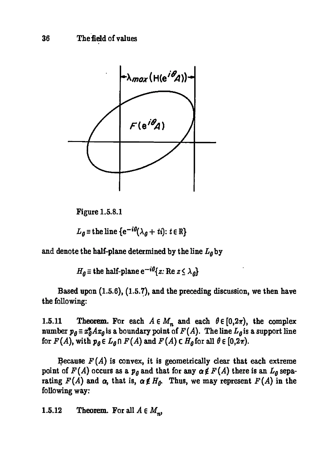
Lemma (1.5.7) shows that, if we compute Amos(H(i4)) and an
associated unit eigenvector x, we obtain a boundary point x*Ax of F (A) and a
support line {XmaJB.{A)) + ti: 1G R} of the convex set F (A) at this
boundary point; see Figure (1.5.8.1).
Using (1.5.6), however, one can obtain as many such boundary points
and support lines as desired by rotating F (A) and carrying out the required
eigenvalue-eigenvector calculation. For an angle 6 G [0, 2u), we define
\0=\mjH.{ê°A)) (1.5.9)
and let x0 G Cn be an associated unit eigenvector
H(ei°A)x0= Xpo, x%x0=l (1.5.10)
We denote

36 The field of values
Figure 1.5.8.1
Le = the line {e_,'ö(Aö + «): 16 R}
and denote the half-plane determined by the line L0by
Eg = the half-plane e~i0{z: Re z < Xe}
Based upon (1.5.6), (1-5.7), and the preceding discussion, we then have
the following:
1.5.11 Theorem. For each A e Mn and each 0 6 [0,2x), the complex
number p0 = x$Azg is a boundary point of F (A). The line L0 is a support line
for F (A), with pe 6 L0[\ F {A) and F (A) c Hefai all 6 6 [0,2x).
Because ^(A) is convex, it is geometrically clear that each extreme
point of F (A) occurs as a p0 and that for any ai F (A) there is an L0
separating F (A) and a, that is, a(.H0. Thus, we may represent F (A) in the
following way:
1.5.12 Theorem. For all A e M^

1.5 Location of the field of values 37
F (A) = Co({pfl: 0 < 9 < 2tt}) = f] H0
0<fl<27T
Since it is not possible to compute infinitely many points p0 and lines
Z/0, we must be content with a discrete analog of (1.5.12) with equalities
replaced by set containments. Let 6 denote a set of angular mesh points,
0 = {^, 02.-. 0*}» where 0<$1< $2< ■'■ < h<2r-
1.5.13 Definition. Let A 6 Mn be given, let a finite set of angular mesh
points 8 = {0 < &i < ' • • < 0k < 2fl} be given, let {p0} be the associated set
•of boundary points of F (A) given by (1.5.11), and let {H0} be the
half-spaces associated with the support lines Lg. for F (A) at the points p0..
Then we define
F/n(A,e)ECo({pöl,...,pöife}),and
FoJA,Q) = H0in---nH0k
These are the constructive inner and outer approximating sets for F (A), as
illustrated in Figure (1.5.5.1).
1.5.14 Theorem. For every AçMn and every angular mesh 8,
FIn(A,Q)cF(A)cF0jA,Q)
The set Fq^A^Q) is most useful as an outer estimate if the angular
mesh points 0- are sufficiently numerous and well spaced that the set n{H0;.
1 < i < k} is bounded (which we assume henceforth). In this case, it is also
simply determined. Let q0. denote the (finite) intersection point of L0. and
La , where i = 1,..., k and i = k + 1 is identified with t = 1. The existence
»+l
of these intersection points is equivalent to the assumption that Fq^^A,®)
is bounded, in which case we have the following simple alternate
representation of FoJA.e):
FoJA>Q) = C\ H0: = CoiUo.,., ?<J) (1-5.15)
l<i<A
Because of the ordering of the angular mesh points 0,-, the points p0.and q0.

38 The field of values
occur consecutively around dF(A) for j= 1,..., k, and dFTn(A,Q) is just the
union of the k line segments [Pg^Pg^ b«M>]>0j]> btyPfJ while
dF0J,A,Q) consists of the Aline segments [g^.g^J,..., [î^.fyj. Uok>9o^
Thus, each approximating set is easily plotted, and the difference of their
areas (or some other measure of their set difference), which is easily
calculated (see Problem 10), may be taken as a measure of the closeness of the
approximation. If the approximation is not sufficiently close, a finer angular
mesh may be used; because of (1.5.12), such approximations can be made
arbitrarily close to F (A). It is interesting to note that F (A) (which
contains a(A) for all A e Mn), may be approximated arbitrarily closely with
only a series of Hermitian eigenvalue-eigenvector computations.
These procedures allow us to calculate the numerical radius r(A) as
well. The following result is an immediate consequence of Theorem (1.5.14).
1.5.16 Corollary. For each AsMn and every angular mesh 6,
max \pg.\ <r(A)< max |gfl.|
l<i<k * l<i<* *
Recall from (1.2.11) that F[A(i')] c F (A) for i= 1,..., n, where A(i')
denotes the principal submatrix of A e Mn formed by deleting row and
column i It follows from (1.2.2) that
Co\\J F[A(i')}
cF(A)
A natural question to ask is: How much of the right-hand side does the
left-land side fill up? The answer is "all of it in the limit," as the dimension
goes to infinity. In order to describe this fact conveniently, we define
Area(5 ) for a convex subset S of the complex plane to be the conventional
area unless S is a line segment (possibly a point), in which case Area(S) is
understood to be the length of the line segment (possibly zero).
Furthermore, in the following area ratio we take 0/0 to be 1.
1.5.17 Theorem. For AtMn with n>2, let A(i')£Mn_l denote the
principal submatrix of A obtained by deleting row and column t from A.
There exists a sequence of constants c^ %,... € [0,1] such that for any
ASM»

1.5 Location of the field of values
AieafCof^F^»')]]]
£ c_, n =
Area[F(yl)]
and lim c„ = 1 as n—» ». The constants
IS
n - 2
"~7n-2- 6[n(n-2)]i
satisfy these conditions, and so do the constants
, _ 2n - 5
c" = 2n + 7
Problems
1. Show by example that there is no general containment relation between
any two of the sets Co(G(A)), Co(G(.Ar )), and GF (A).
2. Show that neither r(i4)<|||./l|||1 nor r(A)<\WA\Wg, holds in general.
Comment in light of (1.5.4).
3. Show that .A=[00li8a case of equality in Theorem (1.5.2). What
are other cases of equality?
4. Show that F(A) c n{0F{U*AU): UeMn is unitary}. Is this
containment an equality for all A e Mn? Prove or give a counterexample.
5. Show that (1.5.2) is the best possible inclusion region based solely on
the 3npiece8 of information a^ RftA), and C'^A), t= 1,.... n. Let s(x,y) be
a given function on [0,a>) * [0,a>), and define
GjiA) = Co\\J{z:\z-att\<àiR\(A),C'{(A))}]
1 f=l J
If F (A) c GjiA) for all A e Mw show that s(x,y) >l(x+ y).
6. Let A = [ay] G Mn with a^ = 1 if exactly one of i, j equals 1, and a^ = 0
otherwise. Let B= [6y]eilfn with 6^-= 0 if i = j and 6i;-= 1 if i{j.
Compare GF(A) and GF(B) with F(A) and F(B) to give examples of how
imprecisely GF{•) can estimate F(-).
(1.5.18a)
(1.5.18b)

40 The field of values
7. Suppose the diagonal entries of A 6 Mn are positive. If A is row
diagonally dominant or column diagonally dominant, then A is positive
stable. Show that DA is positive stable for all positive diagonal D. Show
that if A is row diagonally dominant and column diagonally dominant, then
PA is positive stable for all positive definite matrices P. See (1.0.3).
8. A real square matrix with nonnegative entries and all row and column
sums equal to +1 is said to be doubly stochastic (see Section (8.7) of [HJ]).
Let A e Mn be doubly stochastic.
(a) Use (1.5.2) to show that F (A) is contained in the unit disc. Is there
any smaller disc that contains F (A) for all doubly stochastic A e Afn?
(b) Let Pe Mn be a permutation matrix. Observe that Pis doubly
stochastic and describe F(P) explicitly in terms of the eigenvalues of P;
where are they?
(c) Now use Birkhoffs theorem (8.7.1) in [HJ], (1.2.4), and (1.2.7) to
give another proof that F (A) is contained in the unit disc.
(d) From what you have proved about F (A), what can you say about
the location of the eigenvalues of a doubly stochastic matrix? How does
this compare with what you already know from the Ferron-Frobenius
theorem (8.3.1) in [HJ]? See Problems 18-21 for a sharper statement
about a{A).
9. Show that the points qgM (1.5.15) are given by
Xg.coB Sj-X0j+1
gö.= e-,öi
Aö.+ i-
J sin Si
where ^=.0^-0-.
10. If P is a fo-sided polygon in the complex plane with vertices clt..., ck
given in counterclockwise order, show that the area of P may be written as
Area (P) = *Im [q&j + \% + • • • + cM ck + cfccj
Use this identity to formulate the accuracy estimate
Area(^0Mi(A,e))-Area(^n(A,e))
in terms of the points p0. and q0.. What other measures of accuracy might be

1.5 Location of the field of values
41
calculated easily?
11. If A e Mw show that the numerical radius of A is given by
r(A)= max \p0\ = max \X0\ = max Xg
(K0<2T O<0<2T O<0<2T
12. If A e Mn, show that F (A) is inscribed in a rectangle with vertical sides
parallel to the imaginary axis going through the smallest and largest
eigenvalues of E(A), respectively, and with horizontal sides parallel to the real
axis going through i times the smallest and largest eigenvalues, respectively,
of -iS(A). In particular, conclude that max {Re A: A € o(A)} < max {A: X €
o(H(A)}.
13. For A = [~0 l\ and angular mesh 8 = {0, t/3, 2t/3, t, 4t/3, 5t/3},
explicitly determine and sketch FIn(A,&) and Fp^Afi).
14. If A e Mn is normal, describe a simpler procedure for plotting F (A).
15. Let A e Mn have constant main diagonal, and let A{ £ Mn_1 denote the
principal submatrix formed by deleting row and column tfrom A. Show that
Area
Co
\jFiAd]]fAx*lF{A))>±
that is, a possible choice of the constants cn in Theorem (1.5.17) in this
special case is cB= (n-2)Jn.
16. Let A € Mn be a given Hermitian matrix. If A is positive definite, show
that every principal submatrix A; £ Afn-1 (formed by deleting row i and
column tfrom A) is also positive definite. Show by example that the simple
converse of this statement is false: Each A; can be positive definite and A
indefinite. Now let a denote the smallest and ß the largest of all the
eigenvalues of the Ait i= 1,..., n, and let {cjj^sl be any sequence of constants
satisfying the conditions in Theorem (1.5.17). Show that if all Ai are
positive definite and (a/0) > 1 - cn, then A is positive definite.
17. Consider the constants cn and c'n defined in (1.5.18a,b). Show that the
sequence {c^} increases monotonically to 1, cB > c'n for n = 2,3,..., lim cjc'n
= 1 as n—»cn, and the approximation cn<*c'n as n-m is quite good since
cn-c„ = 9/(2n3) + 0(l/n4).

42 The field of values
The following four problems improve Problem 8's simple estimate that the
field of values of a doubly stochastic matrix is contained in the unit disc.
18. Let m > 2 and let Q= [g{j-] e Mm be a cyclic permutation matrix, that is,
ft i+l = 1 for t = 1,..., m-1, qml = 1, and all other g,y= 0. What does this
have to do with a cyclic permutation of the integers {1,..., m}? Show that
F ( Q) is the convex hull of the m th roots of unity e27r,Vm. k = 1,..., m, which
is contained in the angular wedge Lm in the complex plane with vertex at
z= 1 and passing through e±27rVm :
Lm = |z= 1 + re'"*: r> 0, 10-*\ <^^r} (1.5.19)
Sketch Lm., Notice that the directed graph of Q contains a simple cycle of
length m, that is, a directed path that begins and ends at the same node,
which occurs exactly twice in the path, and no other node occurs more than
once in the path; see (6.2.12) in [HJ].
19. For any B e Mn, define fi{B) = the length of a maximum4ength simple
cycle in the directed graph of B. Notice that 0 < fi(B) < n, and fi(B) = nif
and only if B is irreducible. Now let Blt B2.—» BkeMn be nonnegative
matrices, and let alt a^,..., ak> 0. Show that l>(axBx H + a^Sj)>
mzx{fi{B1),...,fj{B^}.
20. Let P e Mn be a given permutation matrix. Since any permutation of
the integers {1,..., n} is a product of cyclic permutations, explain why P is
permutation similar (hence, unitarily similar) to a direct sum of cyclic
permutation matrices Qit..., Qfa Q;eMn., l<7i,-<n, niH + nk=n,
where fi(P) = max {%,..., nk}. Use (1.2.10) to show that F(P) is contained
in the wedge L /P\ defined by (1.5.19).
21. Let A 6 Mn be a given doubly stochastic matrix. Use Birkhoff s
theorem (8.7.1) in [HJ] to write A as a finite positive convex combination of
permutation matrices, that is,
A=y£taiPil alla^O, £ai=l
* i
Although there may be many ways to express A as such a sum, show that
/i(A)> max/^P^ always, and hence we have the uniform upper bound
F(Pd C L^A) c Ln for all t. Use (1.2.4) and (1.2.7) to show that F(A) c

1.5 Location of the field of values
43
LrfA)c ^n- Conclude that F (A) is contained in the part of the wedge L iA\
(and LJ that is contained in the unit disc. Sketch this set. What does this
say when n = 2? When fj(A) = 2? When A is tridiagonal? Prom what you
have proved about F (A), what can you say about o{A)1 Do not use the fact
that a doubly stochastic tridiagonal matrix must be symmetric.
22. Let A £ MJJR) have nonnegative entries and spectral radius 1. Let fi{A)
denote the length of the maximum-length simple cycle in the directed graph
of A. It is a theorem of Kellogg and Stephens that a{A) is contained in the
intersection of the unit disc and the angular wedge ^uiA) defined by (1.5.19).
(a) Compare this statement with the result of Problem 21.
(b) 1ffi{A) = 2, use the Kellogg-Stephens theorem to show that all the
eigenvalues of A are real, and deduce that all the eigenvalues of a
nonnegative tridiagonal matrix are real. See Problem 5 of Section (4.1)
of [HJ] for a different proof of this fact.
(c) Use the Kellogg-Stephens theorem to show that all the eigenvalues
of a general n-by-n nonnegative matrix with spectral radius 1 are
contained in the intersection of the unit disc and the wedge Ln. Sketch
this set. A precise, but rather complicated, description of the set of all
possible eigenvalues of a nonnegative matrix with spectral radius 1 has
been given by Dmitriev, Dynkin, and Karpelevich.
23. Verify the following facts about the numerical radius function r(«):
Mn-* R+ defined by r(A) = max {| z\ : z6 F (A)}. We write. p{A) for the
spectral radius, \\\A\\\2 for the spectral norm, || A ||2 for the Frobenius norm,
3Jl^ III -^ Uli» IMIL f°r tne maximum column sum and maximum row sum
matrix norms, respectively. The following statements hold for all A , B g
Mn. See Section (5.7) of [HJ] and its problems for background information
about the numerical radius and its relationship to other norms.
(a) r ( • ) is a norm on Mn but is not a matrix norm.
(b) 4r( • ) is submultiplicative with respect to the ordinary matrix product,
that is, ir(AB) < ir(A)ir(B), and 4 is the least positive constant with
this property. Thus, 4r ( • ) is a matrix norm on Mn.
(c) 2r( • ) is submultiplicative with respect to the Hadamard product, that
is, 2r(AoB) < 2r(A)2r(B), and 2 is the least positive constant with this
property, but if either A or B is normal then r(AoB) < r(A)r(B)', see
Corollaries (1.7.24-25).
(d) r(Am) < [r(A)]m for all m = 1,2,...; this is the power inequality for the

44 The field of values
numerical radins. Give an example to show that it is not always true
that r(Afc+mj < r(Ak)r(Am).
(e) p(A) <r(A).
(f) r(A) = r(A*).
(g) illl ^ lib < r (A) < IIIA lib «""* both bounds are sharp.
(h) cn\\ A ||2 < r(A) <\\A ||2 with cn = (4n)~*, and the upper, but not the
lower, bound is sharp. A sharp lower bound is given by cn = (2n)~^ if n
is even and c„ = (2n- l)~i if n is odd.
(i) r ( A) < m A Hb < ( HI A HI HI A* ||| )* for any matrix norm ||| • ||| on Mn. In
particular, r(A) < ||| A |||2 < ( ||| A H^ ||| A ||U)* < i( ||| A H^ +1|{ A HU), an
inequality discovered by I. Schur; see Problem 21 in Section (5.6) of
[HJ].
(j) r(-Ä) i r(A) *0r W principal submatrix A of A.
(k) r(Ax 8 A2) = max {r(AJ, r(A2)} for any Ax 6 Mk and A2 e Mm.
(1) r(A)<r(|A|),whereA = [fl<j]and|A|=[|flij|].
(m) If A > 0, that is, all the entries of A are real and nonnegative, then
r(A) = r(E(A)) = p(E(A)), where E(A) = \{A + AT) is the
symmetric part of A; moreover, r(A) = max {xTAx: are R", x> 0, xTx= 1}.
(n) r(A)<r(\A\) = ip(\A\ + \A\T),vfhe«iA = [aij]asid\A\=[\aij\}.
(°) III ^m lib * 2 r(A)mfor aU ro= 1,2,....
24. Let .A e Afn be given. In the preceding problem we saw that p(A) <
r(A) < m A |||2, so p(A) = m A |||2 implies r(A) = ||| A ffl,. A. Wintner proved
in 1929 that the converse is also true: r(A) = \\\ A |j|2 if and only if p(A) =
HI A |||2. Prove this. A matrix A € Mn is said to be rncftai (some authors use
the term radialoid) if p(A) = ||| A HI2, or, equivalently, if r (A) = ||| A |||2.
25. Provide details for the following sketch for a proof of a theorem of Ptak:
Let A 6 Mn be given with ||| A l^ < 1. Then p(A) = 1 if and only if ||| An |||2 =
1. Proo/- «S={a.eCn: || s;j|2 =|| Ax\\2} is a subspace of C" since it is the
nullspace of the positive semidefinite matrix I-A* A If |||i4n|||2= 1, let
zj)GCn be a unit vector such that || A% ||2= || Zq ||2- Then || -^o ||2 =
II ^% II2 - II -^n-13tl II2 ^ * " ^ II ^"bII2 ^ II ^b II2» so ^ tnese inequalities are
equalities and S0 = Span {a^, Axq,..., A""1^} c S, k= dim «S0 > 1, and AS0 C S0

1.5 Location of the field of values
45
by the Cayley-Hamilton theorem. Let U=[UX U^i E Mn be a unitary
matrix such that the columns of £/, 6 Mn fc form an orthonormal basis of <S0.
Then V*A Uis a block triangular matrix of the form
ü*AU=\U*^Ul *A
where U\A U^ is a Euclidean isometry on <S0 (a linear transformation from <S0
to S0 that preserves the Euclidean length of every vector) and hence is
unitary (see (2.1.4-5) in [HJ]). Thus, 1 = piVfAU^< p(ü*AU) = p{A)<
\\\A\h<l.
26. Modify the proof of the preceding problem to show that if A 6 Mn has
HI A HI2 < 1, then p(A) = 1 if and only if ||| i4m|||2 = 1 for some positive integer
m greater than or equal to the degree of the minimal polynomial of A.
27. Let A g Mn be given. Combine the results of the preceding three
problems and verify that the following conditions are equivalent:
(a) A is radial.
(b) pU)=|p|||2.
(c) r(A) = |p|||2.
(d) IPnlll2 = (IMIIl2)n-
(e) ID Am IH2 = (HI A |||2)m for some integer m not less than the degree of
the minimal polynomial of A.
G) III -** lib = (III ^llb>* for all Ar= 1,2
In addition, one more equivalent condition follows from Problem 37(f) in
Section (1.6); see Problem 38 in Section (1.6).
(g) A is unitarily similar to ||| i4|||2(I/'® B), where U£ Mk is unitary,
1 < i< n, and Be Mn^hasptB) < 1 and|||B|||2< 1.
28. (a) If A 6 Mn is normal, show that A is radial. If A is radial and n= 2,
show that A is normal. If n> 3, exhibit a radial matrix in Mn that is not
normal.
(b) Show that if A e Mn is radial, then every positive integer power of A is
radial, bat it is possible for some positive integer power of a matrix to be
radial without the matrix being radial.
29. Let Jn(Q) denote the n-by-n nilpotent Jordan block considered in
Problem 9 in Section (1.3), where it was shown that F(Jn(0)) is a closed disc

46 The field of values
centered at the origin with radius r(Jn(Q)) = p(H(Jn(0)). If k is a positive
integer such that 2Jfe< n, show that 2-V*< r(J„(0)) < 1. Describe.F(Jn(0))
a8 71—fa..
30. A given A £ Mm n is called a contraction if its spectral norm satisfies
H| A HI2 < 1; it is a strict contraction if ||| A HI2 < 1. T. Ando has proved two
userai representations for the unit ball of the numerical radius norm in Mn:
(a) r (A) < 1 if and only if
A=(I-Z)iC(I+Z)î (1.5.20)
for some contractions C,Zç Mn with ZHennitian; the indicated
square roots are the unique positive semidefinite square roots of
I*Z.
(b) r (A) <1 if and only if
A = 2(I-C*C)*C (1.5.21)
for some contraction Ce Mn.
Verify half of Ando's theorem-show that both representations (1.5.20,21)
give matrices A for which r(A) < 1. See Problem 44 in Section (3.1) for an
identity related to (1.5.21).
31. Use Ando's representation (1.5.20) to show the following for A £ Mn:
(a) r(Am) < [r(A)]m for all m = 1,2 This is the famous power
inequality for the numerical radius; see Problem 23(d).
(b) r (A) < 1 if and only if there is a Hermitian ZtMn such that the
2-by-2 block matrix
ri- Z A ■
L A* I+Z.
is positive semidefinite.
See Lemma (3.5.12).
32. Let p(t) be a polynomial, all of whose coefficients are nonnegative.
Show that r(p(A)) < p(r(A)) for all A 6 Mw and that the same inequality
holds if the numerical radius r(>) is replaced by the spectral radius /"■(•) or
by any vector norm ||-|| on Mn that satisfies the power inequality ||j4*|| <

1.5 Location of the field of values 47
||A||*for *= 1,2,... for all A 6 Mn.
Notes and Further Readings. Most of this section is based on A GerSgorin,
Inclusion Set for the Field of Values of a Finite Matrix, Proc. Amer. Math.
Soc. 41 (1973), 57-60, and Numerical Determination of the Field of Values of
a General Complex Matrix, SI AM J. Numer. Anal. 15 (1978), 595-602, both
by C. R. Johnson. See also C. R. Johnson, An Inclusion Region for the Field
of Values of a Doubly Stochastic Matrix Based on Its Graph, Aequationes
Mathematicae 17 (1978), 305-310. For a proof of Theorem (1.5.17), see C. R.
Johnson, Numerical Ranges of Principal Submatrices, Linear Algebra
Applic. 37 (1981), 11-22; the best possible value for the lower bound c„ in
each dimension n is not yet known. For a proof of the theorem mentioned at
the beginning of Problem 22, see R. B. Kellogg and A. B. Stephens, Complex
Eigenvalues of a Non-Negative Matrix with a Specified Graph, Linear
Algebra Appl. 20 (1978), 179-187. For the precise description of the set of all
possible eigenvalues of n-by-n nonnegative matrices mentioned at the end of
Problem 22, see N. Dmitriev and E. DynUn, Eigenvalues of a Stochastic
Matrix, Izv. Akad. Nauk SSSR Ser. Mat. 10 (1946), 167rl84, and F. I.
Karpelevich, On the Eigenvalues of a Matrix with Non-Negative Elements,
Izv. Akad. Nauk SSSR Ser. Mat. 15 (1951), 361-383. A discussion of the
bounds in Problem 23 (h) is in C. R. Johnson and C.-K. Li, Inequalities
Relating Unitarily Invariant Norms and the Numerical Range, Linear
Multilinear Algebra 23 (1988), 183-191. The theorem mentioned in Problem
24 is in A. Wintner, Zur Theorie der beschränkten Bilinearformen, Math.
Zeit. 30 (1929), 228-282. Ptak's theorem mentioned in Problem 25 was first
published in 1960; the proof we have outlined, and many interesting related
results, is in V. Ptak, Lyapunov Equations and Gram Matrices, Linear
Algebra Applic. 49 (1983), 33-55. For surveys of results about the numerical
radius and field of values, generalizations, applications to finite difference
methods for hyperbolic partial differential equations, and an extensive
bibliography, see M. Goldberg, On Certain Finite Dimensional Numerical
Ranges and Numerical Radii, Linear Multilinear Algebra 7 (1979), 329-342,
as well as M. Goldberg and E. Tadmor, On the Numerical Radius and its
Applications, Linear Algebra Applic. 42 (1982), 263-284. The
representations (1.5.20,21) for the unit ball of the numerical radius norm in Mn are in
T. Ando, Structure of Operators with Numerical Radius One, Acta. Sei.
Math. (Szeged) 34 (1973), 11-15.

48 The field of values
1.6 Geometry
In Section (1.3) we saw that if A 6 M2, then the field of values F (A) is a
(possibly degenerate) ellipse with interior and that the ellipse may be
determined in several ways from parameters associated with the entries of the
matrix A.
Exercise. lîA= | q1 ? 1 eM2, show that F (A) is: (a) a point if and only if
A2 = Xi and ß = 0; (b) a line segment joining X1 and A2 if and only if ß = 0;
(c) a circular disc of radius i\ß\ if and only if A2 = Ai; or (d) an ellipse
(with interior) with foci at X1 and A2 otherwise, and X1 and A2 are interior
points of the ellipse in this case.
In higher dimensions, however, a considerably richer variety of shapes
is possible for the field of values. Any convex polygon is the field of values of
a matrix of sufficiently high dimension; by (1.2.9), one can use a normal
matrix whose eigenvalues are the vertices of the polygon. Thus, any
bounded convex set can be approximated as closely as desired by the field of
values of some matrix, but the dimension of the matrix may have to be large.
Further interesting shapes can be pieced together using the direct sum
property (1.2.10); if two sets occur, then so does their convex hull, but a
direct sum of higher dimension may be required to realize it. Except for
»= 1 and 2, it is not known which compact convex sets in C occur as fields of
values for matrices of a fixed finite dimension n. Our purpose in this section
is to present a few basic facts about the shape of F {A) and its relation to
a{A). These results elaborate upon some of the basic properties in (1.2).
The relative interior of a set in C is just its interior relative to the
smallest dimensional space in which it sits. Â compact convex set in the
complex plane is either a point (with no relative interior), a nontrivial closed
line segment (whose relative interior is an open line segment), or a set with a
two-dimensional interior in the usual sense. What can be said about interior
points of F(A)1 If A 6 Mw the point £tr A always lies in F(A) since it is a
convex combination of points in F (A) (the eigenvalues as well as the main
diagonal entries of A), but somewhat more can be said. The key observation
is that if a convex set C is contained in the closed upper half-plane and if a
strict convex combination of given points in C is real, then all of these points
must be real.
1.6.1 Theorem. Let A = [a^] 6 Mn be given, let Xlt..., Xn denote the

1.6 Geometry
49
eigenvalues of A, and let f^,—, fin be given positive real numbers such that
/*!+•••+ /i„ = 1. The following are equivalent:
(a) A is not a scalar multiple of the identity.
(b) Miûii + • ' * + Mnaim 's in tne relative interior of F {A).
(c) p1Xl H + nnXn is in the relative interior of F (A).
In particular, we have the following dichotomy: Either A is a scalar multiple
of the identity or the point £ tr A lies in the relative interior of F {A).
Proof: If A is a scalar multiple of the identity, then F {A) has no relative
interior, so both (b) and (c) imply (a).
Let ( = ftOn H + /inonn, observe that Ç 6 F {A), and suppose that Ç
is not in the relative interior of F {A). Let B = [b^] = A-(I and observe
that Pibn + • • • + finbnn = 0, 0 6 jF(5 ), and 0 is not in the relative interior
ofF(B). Since F(B)is convex, it can be rotated about the boundary point
0 so that, for some 06 R, the field of values of C= [cfj-] =eieB lies in the
closed upper half-plane VHP = {z 6 C: Im z> 0}. Then 0 6 F (C) C VHP, 0 is
not in the relative interior of F(C), and fi^n + • • • + /*„£„„ = 0. Since
each ctt e F(C), Im ctt- > 0 for all : = 1,..., n. But /^Im cn H + /»„Im cnn
= 0 and each /*,- > 0, so all the main diagonal entries of C are real. For any
given indices i, j'6 {1,.., »}, let T^-denote the 2-by-2 principal submatrix of
C obtained as the intersections of rows and columns i and j, and let Ai, A2
denote its eigenvalues. Since ^(I^-) c F(C) c UFP, wehaveAn A2 E ÜHP.
But Im(A1)+Im(A2) = Im(A1 + A2) = Im(trrij) = 0, so Ai and A2 are
both real and neither is an interior point of ^(r^-) c VHP. It follows from
Theorem (1.3.6(d)) that T^- is normal; it is actually Hermitian since its
eigenvalues are real. Since t and j are arbitrary indices, it follows that C is
Hermitian and hence F(C) is a real interval, which must have 0 as an
endpoint since 0 is not in the relative interior oîF(C). Thus, every point in
F(C), in particular, every cti and every A,-, has the same sign. But MiCn +
••• +M„cnn = 0 and all/z,-> 0, so all ct-, = 0. Since Xl + • •♦ + Xn= cn +
••' + cnn, it follows that all A,- = 0 as well, and hence (7=0. We conclude
that A = (land hence (a) implies (b).
To show that (a) implies (c), suppose ( = /^Ai + • • • + /inAn is not in
the relative interior of .F (A). Choose a unitary Ve Mn such that A = VA V*
is upper triangular and has main diagonal entries A1r.., An. Then F (A) =
F (A), and a strict convex combination of the main diagonal entries of A is
not in the relative interior of its field of values. By the equivalence of (a)
and (b) we conclude that A = (land hence A = V*AV= (I. []

50 The field of values
We next investigate the smoothness of the boundary of the field of
values dF(A) audits relationship with a{A). Intuitively, a "sharp point" of
a convex set S is an extreme point at which the boundary takes an abrupt
turn, a boundary point where there are nonunique tangents, or a "corner."
1.6.2 Definition. Let A e Mn. A point or E dF(A) is called a sharp paint
of F(A) if there are angles 01 and 02 with 0 < 0, < 02 < 2xfor which
Re ei0a = max {Re ß; ß 6 F(e,öyl)} for all 0 E (0^02)
1.6.3 Theorem. Let A E Mn. If a is a sharp point oiF(A), then a is an
eigenvalue of A
Proof: If a is a sharp point of F {A), we know from (1.5.7) that there is a
unit vector x E C" such that
x*B(e^A)x= WH(e«U)) for all 0 e (0V02)
from which it follows that (see (1.5.9))
R(e{0A)x= Xfi for ail 0 6 (0^02) (1.6.3a)
The vector zis independent of 0. Differentiation of (1.6.3a) with respect to 0
yields
E(iei0A)x=\'0x
which is equivalent to
S{ei0A)x=^X'0 x (1.6.3b)
Adding (1.6.3a) and (1.6.3b) gives eiûAx= (Aö-tA&)s, or
Ax=e-i0{X0-iX'0)x
Interpreted as an evaluation at any 0 in the indicated interval, this means
that
a=x*Ax=e-i0{Xe-iX'e)

1.6 Geometry
51
is an eigenvalue of A. []
Since each A e Mn has a finite number of eigenvalues, Theorem (1.6.3)
implies that if a set is the field of values of a finite matrix, it can have only a
finite number of sharp points. Moreover, if the only extreme points of F (A)
are sharp points, then F {A) is the convex hull of some eigenvalues of A
1.6.4 Corollary. Let A 6 Mn be given. Then F {A) has at most n sharp
points, and F{A) is a convex polygon if and only if F(A) = Co{cr{A)).
Although every sharp point on the boundary of F (A) is an eigenvalue,
not every eigenvalue on the boundary of F (A) is a sharp point.
Nevertheless, every such point does have a special characteristic.
1.6.5 Definition. A point X G a{A) is a norma/ eigenvalue for the matrix
AeMni(
(a) Every eigenvector of A corresponding to X is orthogonal to every
eigenvector of A corresponding to each eigenvalue different from
X, and
(b) The geometric multiplicity of the eigenvalue X (the dimension of
the corresponding eigenspace of A) is equal to the algebraic
multiplicity of A (as a root of the characteristic polynomial of A).
Exercise. Show that every eigenvalue of a normal matrix is a normal
eigenvalue.
Exercise. If AeMn has as many as n-1 normal eigenvalues, counting
multiplicity, show that A is a normal matrix.
Exercise. Show that A is a normal eigenvalue of a matrix A e Mn if and only
if it is a normal eigenvalue of UAU* for every unitary matrix f/6 Afn, that is,
the property of being a normal eigenvalue is a unitary similarity invariant.
Our main observation here is that every eigenvalue on the boundary of
the field of values is a normal eigenvalue.
1.6.6 Theorem. If A 6 Mn and if a 6 dF(A) (1 o(A), then a is a normal
eigenvalue of A. If m is the multiplicity of or, then A is unitarily similar to
a/o B, with Je Mm, B e Mnrm) and a f. a{B).

52 The field of values
Proof: If the algebraic multiplicity of or is m, then A is unitarily similar to
an upper triangular matrix T (this is Schur'8 theorem; see (2.3.1) in [HJ])
whose first m main diagonal entries are equal to or and whose remaining
diagonal entries (all different from a) are the other eigenvalues of A.
Suppose there were a nonzero entry off the main diagonal in one of the first m
rows of T. Then T would have a 2-by-2 principal submatrix T0 of the form
T0=[o 2]>7^0. Since -F(r0)i8 either a circular disc about orwith radius
i\f\ or a nondegenerate ellipse (with interior) with foci at or and ß, the point
«must be in the interior of F{TQ). But F{TQ) c F(T) = F {A) by (1.2.8)
and (1.2.11), which means that a is in the interior of F {A). This
contradiction shows that there are no nonzero off-diagonal entries in the first m rows
of T, and hence T= alo B with Je Mm and B 6 M,,.^. The remaining
assertions are easily verified. []
Exercise. Complete the details of the proof of Theorem (1.6.6).
We have already noted that the converse of the normality property
(1.2.9) does not hold, but we are now in a position to understand fully the
relationship between the two conditions on A 6 Mn: A is normal, and F (A)
= Co(o(A)).
1.6.7 Corollary. If a{A) c dF (A), then A is normal.
Proof: If all the eigenvalues of A are normal eigenvalues, then there is an
orthonormal basis of eigenvectors of A, which must therefore be normal. []
Exercise. Show that a given matrix A 6 Mn is normal if and only if A is
unitarily similar to a direct sum A^ o A2 ® • • • ® Ak with a(A-) c dF(A$, i =
1 Jt
J.,..., A.
Two further corollary facts complete our understanding of the extent to
which there is a converse to (1.2.9).
1.6.8 Theorem. Let A 6 Mn. Then ^(^4)= Co{a(A)) if and only if
either A is normal or A is unitarily similar to a matrix of the form L1 ^ 1,
where A1 is normal and F (A2) c F (A^.
1.6.9 Corollary. If A 6 Mn and n < 4, then A is normal if and only if

1.6 Geometry
53
F(A) = Co(a(A)).
Exercise. Supply a proof for (1.6.8) using (1.6.6).
Exercise. Supply a proof for (1.6.9) by considering the geometrical
possibilities allowed in (1.6.8).
We -wish to discuss one additional connection between normality and
the field of values. If Aç Mm n is given and if B = L J is a larger matrix
that contains A in its upper-left corner, we say that B is a dilation of A; by
the submatrix inclusion property (1.2.11), F(A)cF(B) whenever B 6 MN
is a dilation of A 6 Mn. One can always find a 2n-by-2n normal dilation of A,
for example, the matrix B defined by (1.6.11), in which case F(B) =
Co((j(ß)). It is clear that F (A) is contained in the intersection of the fields
of values of all the normal dilations of A, and it is a pleasant observation
that this intersection is exactly F (A).
1.6.10 Theorem. Let A e Mn be given. Then
F(A)=f}{F(B):B=[î J] 6 M2n is normal]
Proof: Since we have already noted that F (A) is a subset of the given
intersection, we need only prove the reverse inclusion. Because F (A) is
closed and convex, it is the intersection of all the closed half-planes that
contain it, a fact used in the preceding section to develop a numerical
algorithm to compute F {A). Thus, it is sufficient to show that for each closed
half-plane that contains F (A), there is some normal matrix B= L J e
Af2n such that F (B) is contained in the same half-plane. By the translation
and scalar multiplication properties (1.2.3-4), there is no loss of generality to
assume that the given half-plane is the closed right half-plane RHPQ. Thus,
we shall be done if we show that whenever A + A* is positive semidefinite,
that is, F(A)cRHP0, then A has a normal dilation BsM2n such that
B + B* is positive semidefinite, that is, F (5) c RHPQ. Consider
"ft* a] ("■")
Then B is a dilation of A and

54 The field of values
a* a — ]■"■ A-{-AA A + A _ dd*
*b-[a* + a** aa* + a*a\-bb^
so B is normal, independent of any assumption about F (A). Moreover, if
A + A* is positive semidefinite, then
B+**=[!+£ ît%\ (L612)
is positive semidefinite, since if y, zG Cn and x= [jj G C2n, then ar*(5 + B*)a.
= {y+z)*{A + A*){y+z)>0. Q
Since the field of values of a normal matrix is easily shown to be convex
and the intersection of convex sets is convex, Theorem (1.6.10) suggests a
clean conceptual proof of the convexity property of the field of values
(1.2.2). Unfortunately, the convexity of F [A) is used in a crucial way in the
proof of Theorem (1.6.10); thus, it would be very pleasant to have a
different proof that does not rely on the Toeplitz-Hausdorff theorem.
The matrix defined by (1.6.11) gives a 2n-by-2n normal dilation of any
given matrix A G Mn. It is sometimes useful to know that one can find
dilations with even more structure. For example, one can choose the
dilation B e M2n to be of the form B= cV, where Vg M2n is unitary and c =
max -QU A HI2,1} (see Problem 22). Moreover, for any given integer k > 1, one
can find a dilation B G M/k+l\n that is a scalar multiple of a unitary matrix
[Am *1
+ + for all m = 1, 2,..., k (see Problem
25).
Problems
1. If A G M2, show that F {A) is a possibly degenerate ellipse with center
at $tr A and foci at the two eigenvalues of A. Characterize the case in
which F (A) is a circular disc. What is the radius of this disc? Characterize
the case in which F {A) is a line segment. What are its endpoints? In the
remaining case of an ellipse, what is the eccentricity and what is the
equation of the boundary?
2. For A = | " 2 G Af2(R), show that F (A) is an ellipse (possibly
degenerate) with center at the point j(a+ d) on the real axis, whose vertices are
the two points j(n+ d± [(<i-d)2 + (6 + c)2]^) on the real axis and the two

1.6 Geometry
55
points $(a+ d*i\b-c\). Show that the degenerate cases correspond
exactly to the cases in which A is normal. Can you find similarly explicit
formulae if A e M2(C)?
3. If A e M2 has distinct eigenvalues, and if A0 = A - ( jtr A)I, show that
A0 is nonsingular and the major axis of F (A) lies in the direction
-(det A0)/|det j40| in the complex plane. What is the length of the major
axis? What is the length of the minor axis?
4. If A e M2, and if one of the eigenvalues of A appears on the main
diagonal of A, show that at least one of the off-diagonal entries of A must be
zero.
5. Show that any given (possibly degenerate) ellipse (with interior) is the
field of values of some matrix A e Af2. Show how to construct such a matrix
A for a given ellipse.
6. Show by example that 4 is the best possible value in (1.6.9), that is, for
every n > 5 show that there is a nonnormal A e Mn with F {A) = Co(a(A)).
7. Let n> 3 be given and let 1 < fc< n. Show that there is some A 6 Mn
such that F (A) has exactly £ sharp points.
8. If .A 6 Mn and if a is a sharp point of F (A), show that a unit vector
x 6 Cn for which a = x*Axis an eigenvector for both A and H(A).
9. Give an alternate, more geometric proof of (1.6.3) along the following
lines: If A e Mn and X G F (A), pick a unitary Ue Maso that A is the 1,1
entry of U*AU. (Howmay l/be constructed?) Since
\sF[(ü*AU)({l,m
it must be a sharp point of F[(U*AU)({l,j})], j= 2,..., n, if X is a sharp
point of F(A). But since F[(U*AU){{l,j})] is either a circular disc, a line
segment, or an ellipse (with interior), it must actually be a line segment with
X as one endpoint in order for A to be a sharp point. But then
F[( U*A U)({l,j})] must be diagonal, and
0*AU= [X] o (ü*AU)({2,..., n})
that is, X is an eigenvalue of A.
10. Give an alternate proof of (1.6.3) along these lines: Let x 6 Cn be a unit

56 The field of values
vectoi and let X = x*Ax be a sharp point of F (A). Let y € Cn be independent
of x. Let /?G Mn denote the (Hermitian) orthogonal projection onto the
two-dimensional subspace spanned by x and y, that is, let {v, w} be an
orthonormal basis of V= Span {i, y}, let P=[v w]e Mn2 be a unitary
projection (see Problem 14 in Section (1.2)), and let H= PP*, so Hz = zil
zG Vand Hz= 0 if zx V. Then A is a sharp point of F(HAH) c F(A). Since
F (HAH) is a (possibly degenerate) ellipse, it must be aline segment with X
as an endpoint, so A is an eigenvalue of HAH and of A, with eigenvector x.
11. If A G Mn and X G o(A), and if z 6 C" is an associated eigenvector, show
that X is a normal eigenvalue of A if and only if x is an eigenvector of both A
and A*. What can be said if the multiplicity of X is greater than one?
12. If X, ft G o(i4) and if ft # A, show that any eigenvector of A* associated
with TZis orthogonal to any eigenvector of A associated with X.
13. Let .A 6 Mn. Show that if x is an eigenvector of both A and E(A), then x
is an eigenvector of A*. How are the eigenvalues related?
14. Give another proof of (1.6.6) using (1.5.7) and the result of Problem 13.
15. Let A G MB. If F (A) is a polygon with at least n-1 vertices, show that
A is normal.
16. Let A G Mn. If at least n-1 of the eigenvalues of A lie on the boundary
of F (A), show that A is normal. Show that the value n-1 is the best
possible.
17. Let A G Mn. (a) If F (A) has finitely many extreme points, show that
they are all eigenvalues of A. (b) If A is normal, show that the extreme
points of F (A) are eigenvalues of A.
18. Show that A G Mn is normal if and only if A is unitarily similar to a
direct sum of square matrices A^ o • • • e Ak, Af G Mn., i = 1,..., k, and each
F(A$ is a polygon (perhaps a line segment or a point) with n; vertices, i =
1,..., k.
19. Let A G Mn be nonsingular and normal, with o{A) = {r^h,..., rBe,0n},
all r,< > 0, and all Ö.-6 [0,2x). If A has some diagonal entry equal to 0, show
that there does not exist a value f such that t< 0t< t+ xfor all i = 1,2,..., n,
that is, the eigenvalues do not project onto the unit circle inside any
semicircle.

1.6 Geometry
57
20. Give another proof that the matrix B defined by (1.6.11) is normal, and
that B+ B* is positive sernidefraite if A + A* is positive semi definite, as
follows: Show that the 2firby-27nnatrix U= LT jl/^ï is unitary, V*BU=
[V* ^*],andü*(B+B*)tf=[; 2(AJ.A*)]. Thus, B and B + B*
are unitarily similar to something obviously normal and something positive
8emidefinite, respectively. How is the spectrum of B determined by Al
Showthat|||5|||2<2|||A||[2.
21. Recall that a matrix A is a contraction if ||| A |||2 < 1. See Problem 30 in
Section (1.5) for an important link between contractions and the field of
values.
(a) If there exists a unitary dilation V= L J of a given square complex
matrix A, show that A must be a contraction.
(b) Conversely, if A 6 Mn is a given contraction, show that A has a unitary
dilation as follows: Let A = PU be a polar decomposition of A, where Us
Mn is unitary and P = (AA*)$ is positive semideOnite. Let
__ r a (/- p*)\v
*-[-{I-I*)*U A
and show that Zis unitary.
(c) If A 6 Mn is a contraction, show that
eM
2n
(1.6.13)
z=
A (I- AA*)i
-(/- A*A)\ A*
El,
2n
(1.6.14)
is also a-unitary dilation of A.
(d) Use the dilation Z in (1.6.14) and the argument in the proof of Theorem
(1.6.10) to show that if A is a normal contraction, then
F(A)= ft {{F{U): U= [t g 6 M2n is unitary]
(e) Combine the normal dilation (1.6.11) with the result in (d) and the norm
bound in Problem 20 to show that if A e Mn is a contraction with ||| A H^ < £,
then
F(A)=p| W): U= [i J] 6 M4n is unitary

58 The field of values
(f) Now consider a third unitary dilation, one that does not require the polar
decomposition, the singular value decomposition, or matrix square roots.
The following construction can result in a dilation of smaller size than 2n;
an analogous construction gives a complex orthogonal dilation of an
arbitrary matrix (see Problem 40). Let A e Mn be a given contraction and let S =
xaak(I-A*A), so 0 < 6 < n with 6= 0 if and only if A is unitary; S may be
thought of as a measure of how far A is from being unitary. Explain why
rank(I- AA*) = S and why there are nonsingular X, Fe Mn with
and/jGMj. Define
B = x['Q'] 6MM, C=-t0 Is)YtMSin,md
UE[0/5]K4*(^)-i[0/4]eMf
and form
A B
Z
ta ai
~=ic d\sM^ (L615>
Use the definitions (*) and the identity A(I-A*A)={I-AA*)A to show
that
x'lAY'll ),]-[? SW"1 <**'
What do (1.6.15) and (**) become when 6=n, that is, when A is a strict
contraction (IIMIIb < W In tnis special c*86. verify that (1.6.15) gives a
unitary matrix. Now consider the general case when S<n\ considerable
algebraic manipulation seems to be needed to show that (1.6.15) is unitary,
(g) Let n and k be given positive integers. Show that a given A e Mk is a
principal submatrix of a unitary U 6 Mn if and only if A is a contraction and
rank(I- A*A) < vain{k, n-k}; the latter condition imposes no restriction on
Ai(k<n/2.

1.6 Geometry
(h) Show that a given A e Mt
contraction.
m,n
59
has a unitary dilation if and only if A is a
22. Let A e Mn be given. Show that there exists a unitary V 6 M2n such
that cV= L *] with c = max {||| A Ife, 1}. Compare with Theorem (1.6.10).
23. Consider
ro n ° * °
A= " JeM2andB,= 0 0 1 6 M,
L J > n n
Show that F(A) = (\{F(B^; ze C and \z\ = 1}. Discuss this in light of
Problem 21.
24. The dilation results in Problem 21 have a very interesting
generalization. Let
LZ21 Z22J
denote any unitary dilation of a given contraction A e Mn, for example, Z
could be any of the dilations given by (1.6.13,14,15), and let fc> 1 be a given
integer. Consider the block matrix V= [ VmIJ'H-i» in which each block V^
is defined by: Vn = A, V1>2 = Z12, 7H1|1 = 4i» ^1,2 = z2*> mi v2,z =
73 4 = • • • = Vjfk+l = ^> wnere tms identity matrix is the same size as 2^,
and all other blocks are zero:
rA
0
V
Zl2 0
/ 0
0 0 0
421
h.2 0
•o
• 0
(1.6.16)
(a) When k= 1, show that V= Z.
[Am *T
+ J for m =
1,..., *, tbat is, each of these powers of V is a unitary dilation of the
corresponding power of A,
25. Let A e Mn and let k > 1 be a given integer. Show that there exists a
[Am *1
+ J for m = 1,2,..., k, where c =

60 The field of values
max -QU A Ife, 1}. Compare with Theorem (1.6.10).
26. Let A e Mn be a given contraction, that is, |||.A|||2< 1. If p(-) is a
polynomial such that | p(z) \ < 1 for all | z\ = 1, use Problem 25 to show that
p(A) is a contraction.
27. Use Theorem (1.6.6) to show that the algebraic and geometric
multiplicities of the Perron root (and any other eigenvalues of maximum
modulus) of a doubly stochastic matrix must be equal, and show by example
that this is not true of a general nonnegative matrix. Show, however, that
this is true of a nonnegative matrix that is either iov/ or column stochastic,
and give an example of such a matrix whose Perron root does not lie on the
boundary of its field of values.
28. Use Corollary (1.6.7) to give a shorter proof of Theorem (1.6.1). Is
there any circular reasoning involved in doing so?
29. A matrix A e Mn is said to be unitarily reducible if there is some unitary
Us Mn such that V*AU= Ax o A2 with Al e Mh A2 e -¥„_*, and 1< k< n;
A is unitarily irreducible if it is not unitarily reducible. If A E Mn is unitarily
irreducible, show that every eigenvalue of A lies in the (two-dimensional)
interior of F (A) and that the boundary of F {A) is a smooth curve (no sharp
points).
30. Let A e Mn be given. Show that Co(o(A)) = ftfFfäiS-1): Se Mn is
nonsingular}. Moreover, if Jn (Aj) ® • ■ • ® Jn (A*) is the Jordan canonical
form of A (see (3.1.11) in [HJ]), show that there is some one nonsingular
SçMn such that Co(o(A))= F {SAS'1) if and only if n,.= l for every
eigenvalue A,- that lies on the boundary of Co( a(.A)).
31. If < •, • > is a given inner product on C", the field of values generated by
<•,-> is defined by F<..>(A) = {<Ax1x>: zeC", <x,i> = 1} for A e M„.
Note that the usual field of values is the field of values generated by the
usual Euclidean inner product <x,y> = y*x. Show that Co(cr(A)) =
ft{F<- •>{■&): <•>•> is an inner product on C"}.
32. Let A e Mn be given. In general, p(A) < r(A), but if p(A) = r(A), we
say that A is spectral (the term spectraloid is also used). In particular, A is
spectral if it is radial, that is, if either ||| A H^ = p{A) or ||| A |||^ = r (A); see
Problems 23,24, and 27 in Section (1.5). If A is spectral and X is any
eigenvalue of A such that | A | = p(A), show that A is a normal eigenvalue of A.
Show that every normal matrix A e Mn is spectral and that the converse is

1.6 Geometry
61
true only for n = 2.
33. use Problem 32 to show that a given A 6 Mn is spectral if and only if it
is unitarily similar to a direct sum of the form X±In e • • • e X/J e B, where
1< k< n, »IJ+ ■•• + nk=n-m,0< to< n-1, BeM^ lAj = ••• = |At| =
p(A),p(B)<p(A), and r(B)<r(i).
34. Use Problem 33 to show that a given A 6 M„ is spectral if and only if it
is unitarily similar to r(A)(U& B), where f/e Mk is unitary, 1 < fc< n, and
B e M„_fc has p(B) < p(A) and r (B) < r (A).
35. Show that a given A e Mn is spectral if and only if r (A*) = r (A)* for all
ft= 1,2,.... Conclude that if A is spectral, then every positive integer power
of A is spectral. For each n > 2, exhibit a nonspectral matrix B e Mn such
that B™ is spectral for all m > 2.
36. Let A e Mn be given with r (A) ^ 1. Show that if p{A) = 1, then r(Am)
= 1 for all m = 1,2,.... Goldberg, Tadmor, and Zwas have proved a
converse: If r (A) < 1, then p(A) = 1 if and only if r(.Am) = 1 for some positive
integer m not less than the degree of the minimal polynomial of A. Use this
result to establish the following:
(a) A is spectral if and only if r (Am) = r (A)m for some positive integer
to not less than the degree of the minimal polynomial of A.
(b) Show that the 3-by-3 nilpotent Jordan block
A =
has p(A) = 0 and r(A2) = r(A)2 = $, but A is not spectral. Explain
why the bound on the exponent in the Goldberg-Tadmor-Zwas theorem
is sharp.
(c) Show that A is spectral if and only if r (An) = r {A) ".
(d) When n = 2, show that A is normal if and only if r (A2) = r (A)2.
Compare the Goldberg-Tadmor-Zwas theorem with Ptak's theorem on
radial matrices and its generalization in Problems 25 and 26 in Section (1.5).
37. Let A e Mn be given. Combine the results of the preceding five
problems and verify that the following conditions are equivalent:
0
0
0
1
0
0
0"
1
0
(a) A is spectral.

62 The field of values
(b) p(A) = r(A).
(c) r(An) = r{A)n.
(d) r (Am) = r (A)m for some integer m not less than the degree of the
minimal polynomial of A.
(e) r(A*) = r(A)*forallJfe=l,2
(f) A is unitarily similar to r(A)(UQB), where I/16 Mfc is unitary,
1 < fc< n, and 5e Jlf^hasp(5) < 1 and r(5) < 1.
Compare with the conditions for a matrix to be radial given in Problem 27 in
Section (1.5).
38. Use Problem 37(f) to prove the assertion in Problem 27(g) in Section
(1.5).
39. The main geometrical content of Theorem (1.6.6) is the following fact:
Any eigenvector of A corresponding to an eigenvalue that is a boundary
point of the field of values is orthogonal to any eigenvector of A
corresponding to any other (different) eigenvalue. Provide details for the
following alternative proof of this fact. We write <x,y> for the usual inner
product. (1) Let A 6 dF (A), and let y. + A be any other eigenvalue of A. Let
x,ybe unit vectors with Ax=Xx and Ay = y.y. Since F (A) is compact and
convex, and A is a boundary point of F (A), there is a supporting line for
F (A) that passes through X. Show that this geometrical statement is
equivalent to the existence of a nonzero c 6 C and a real number a such that
Ira c<Az,z> > a for all unit vectors z, with equality for z=x, that is, Ira cX
= a. (2)Let A^= cA-ial, Xi = cX-ia, and ß^qi-ia. Show that
Im-cAjZ,.^ > 0 for all unit vectors z, X± is real, /ii^Ai, and lm/i,^0.
(3) For arbitrary £, j/gC, note that lm<Al(£x+T]y),(fr+ T}y)> > 0 and
deduce that Im[|7j|fyi + (A1-/i1)^<x,y>] > 0. (4) Show that you may
choOBe T] so that |j?|=1 and Im [(Aj -/Xi)»7<i.y>] = |(^i-Mi)<^y>|!
deduce that Im /x, + | (ÀL -]il)<x,y> \ Ç > 0 for all Ç e R. (5) Conclude that
<x,y> = 0, as desired. Remark: The proof we have outlined is of interest
because it does not rely on an assumption that A is a (finite-dimensional)
matrix. It is valid for any bounded linear operator A on a complex Hubert
space with inner product <•,•>, and uses the fact that F (A) is a compact
convex set. Thus, the geometrical statement about orthogonality of
eigenvectors given at the beginning of this problem is valid for any bounded linear
operator A on a complex Hubert space.
40. Although a given matrix has a unitary dilation if and only if it is a
contraction (Problem 21), every complex matrix has a complex orthogonal

1.6 Geometry 63
dilation.
(a) Let AeMn and let 6 = ivak(I-ATA), so 0 < 6< n -with 6=0 if and only
ifA is complex orthogonal; S may be thought of as a measure of how far A is
from being complex orthogonal. Explain why TKok(I-AAT) = S and use
Corollary (4.4.4) in [HJ] to show that there are nonsingular X, YeMn with
I-AAT = x[Q" J X7 mi I-AtA=YT[q t\Y (r)
and Is G Mg. Define
BBx[lS]eMn)S, C=-[0 Ig]YeMSin,md
D^OIglYA^X^y^sMg
and form
Q=Yc JeM»+* (L617)
Use the definitions (r) and the identity A(I-ATA) = (I-AAT)A to show
that
rO Ol r Jr Ol
x~lAYTU /J-to o]^7"1 trr)
Notice that these calculations carry over exactly to (or from) (**) in
Problem 21; one just interchanges * and T. What do (1.6.17) and (rr) become
when S = n? In this special case, verify that (1.6.17) gives a complex
orthogonal matrix. The algebraic manipulations necessary to establish the general
case are analogous to those needed to establish the general case in Problem
21.
(b) Assuming that (1.6.17) gives a complex orthogonal dilation of A,
explain why the construction of (1.6.16) in Problem 24 gives a complex
[A *~\ rAm *T
* * J 6 ^n+kS sucn ^at •fmi=l* ,J for m =
1 *.
(c) Let n and k be given positive integers. Show that a given A e Mj is a

64 The fidd of values
principal submatrix of a complex orthogonal Q 6 Mn if and only if
iank.(I-ATA) < rnin{/t, n-k}, which imposes no restriction on A if k< n/2.
(d) Show that every A € Mm n has a complex orthogonal dilation.
JVbfes and Further Readings. The proof given for Theorem (1.6.1) is due to
Onn Chan. Theorem (1.6.3) may be found in Section I of R. Kippenhahn,
Über den Wertevorrat einer Matrix, Math. Nachr. 6 (1951), 193-228, where
a proof different from the three given here may be found (see Problems 9 and
10), as well as many additional geometric results about the field of values;
however, see the comments at the end of Section (1.8) about some of the
quaternion results in Section II of Kippenhahn's paper. Theorems (1.6.6)
and (1.6.8) are from C. R. Johnson, Normality and the Numerical Range,
Linear Algebra Appl 15 (1976), 89-94, where additional related references
may be found. A version of (1.6.1) and related ideas are discussed in 0.
Taussky, Matrices with Trace Zero, Amer. Math. Monthly 69 (1962), 40-42.
Theorem (1.6.10) and its proof are in P. R. Halmos, Numerical Ranges and
Normal Dilations, Acta Sei. Math. (Szeged) 25 (1964), 1-5. The
constructions of unitary dilations of a given contraction given in (1.6.13) and
(1.6.16) are in E. Egervary, On the Contractive Linear Transformations of
»-Dimensional Vector Space, Ada Sei. Math. (Szeged) 15 (1953), 178-182.
The constructions for (1.6.15-17) as well as sharp bounds on the sizes of
unitary and complex orthogonal dilations with the power properties
discussed in Problems 24 and 40 are given in R. C. Thompson and C.-C. T.
Kuo, Doubly Stochastic, Unitary, Unimodular, and Complex Orthogonal
Power. Embeddings, Acta. Sei. Math. (Szeged) 44 (1982), 345-357.
Generalizations and extensions of the result in Problem 26 are in K. Fan,
Applications and Sharpened Forms of an Inequality of Von Neumann, pp.
113-121 of [UhGr]; p(z) need not be a polynomial, but may be any analytic
function on an open set containing the closed unit disc, and there are matrix
analytic versions of classical results such as the Schwarz lemma, Pick's
theorem, and the Koebe f-theorem for univalent functions. The theorem
referred to in Problem 36 is proved in M. Goldberg, E. Tadmor, and G.
Zwas, The Numerical Radius and Spectral Matrices, Linear Multilinear
Algebra 2 (1975), 317-326. The argument in Problem 39 is due to Ky Fan, A
Remark on Orthogonality of Eigenvectors, Linear Multilinear Algebra 23
(1988), 283-284.

1.7 Products of matrices
65
1.7 ProductB of matrices
We survey here a broad range of facts relating products of matrices to the
field of values. These fall into four categories:
(a) Examples of the failure of submultiplicativity of F ( • );
(b) Results about the usual product when zero is not in the field of
values of one of the factors;
(c) Discussion of simultaneous diagonalization by congruence;
(d) A brief survey of the field of values of a Hadamard product.
Examples of the failure of submultiplicativity for F( • )
Unfortunately, even very weak multiplicative analogs of the éubadditivity
property (1.2.7) do not hold. We begin by noting several examples that
illustrate what is not true, and place in proper perspective the few facts that
are known about products.
The containment
F(AB)cF(A)F(B), A,BeMn (1.7.1)
fails to hold both "angularly" and "magnitudinally."
1.7.2 Example- Let A = [ J j] and B= [°2 J]. Then F(A) = F(B) =
F(A)F(B) = the unit disc, while F (AB) is the line segment joining 0 and 4.
Thus, F (AB) contains points much further (four times as far) from the
origin than F (À) F (B), so this example shows that the numerical radius r ( • ) is
not a matrix norm. However, 4r(«) is a matrix norm (see Problem 22 in
Section (5.7) of [HJ]).
1.7.3 Example- Let A = [£_}] and B= [}'£]. Then F (A) = F(B)
= F(A)F(B) = the line segment joining -1 and 1, while F (AB) is the line
segment joining -i and i. Also, F'(A) = F'(B) = F'(A)F'(B) = the real
line, while F'(AB) = the imaginary axis. Note that r(AB) < r(A)r(B) in
this case, but that (1.7.1) still fails—for angular reasons; F'(AB) is not
contained in F' (A)F' (B) either.
1.7.4 Example. Let .4= [0 „•]. Then F (A) is the line segment joining

66 The field of values
1 and t, while F (A2) is the line segment joining -1 and 1. Thus, F (A2) is not
even contained in F (A)2, since QeF(A2) and Q£F(A). However,
Co(F(A)2) = Co{-l, t, 1}, so F (A2) c Co(F(A)2).
One reason it is not surprising that (1.7.1) does not hold in general is
that F(A)F(B) is not generally a convex set, whereas F(AB) is always
convex. But, since F (A)F(B) is convex in the case of both examples (1.7.2)
and (1.7.3), the inclusion
F(AB)cCo(F(A)F(B)), A,BeMn (1.7.1a)
also fails to hold in general. Examples (1.7.2) and (1.7.3) also show that
another weaker statement
a(AB)cF(A)F(B) (1.7.1b)
fails to hold, too.
Product results when zero is not in the field of values of a factor
With a realization that the available results must be limited, we now turn to
examining some of what can be said about the field of values and products of
matrices. The importance of the condition that zero not be in the field of
values of one of the factors should be noted at the outset. This means, for
example, that the field of values may be rotated into the right half-plane,
and links many of the results presented.
1.7.5 Observation. If A 6 Mn is nontringular, then F" (A-1) = F'(A).
Proof: Employing the congruence property (1.2.12), we have F1 (A'1) =
F' (AA^A*) = Ff (A*) = WÇIj. 0
Exercise. Verify that F (A*) = F {A) and, therefore, that F1 (A*) = F7^J.
Although (1.7.1b) fails to hold, the following four facts indicate that
certain limited statements can be made about the relationship between the
spectrum of a product and the product of the fields of values.

1.7 Producta of matrices
67
1.7.6 Theorem. Let A,BeMn and assume that O^F(B). Then
a{AB-l)cF{A)jF{B).
Proof: Since Q£F(B), we know from the spectral containment property
(1.2.6) that B is nonsingular. The set ratio F(A)/F(B) (which has the
usual algebraic interpretation) makes sense and is bounded. If A G a{AB~l),
then there is a unit vector are C" such that z*AB~l = Aar*. Then z*A =
Xz*B, z*Az= Xz*Bx, and ar*5i# 0; hence A = z*Az/z*Bz£ F(A)/F(B). Q
1.7.7 Corollary. Let A,BeMn. If B is positive semidefinite, then
a(AB)cF(A)F(B).
Proof: First suppose that Bis nonsingular and set B = C"1. If A G a(AB) =
a(AC~l), then by (1.7.6) we must have A = a/c for some a G F (A) and some
c G F{C). If ßmin and ^ are the smallest and largest eigenvalues of B,
then ßn\n and ß^lx are *ne largest and smallest eigenvalues of the positive
definite matrix C, and F(C) is the interval fjfl^ #^J. Therefore, c"1 G
[^min. ^mo»] = F(B)mdX = air1 G F(A)F(B). The case in which B is
singular may be reduced to the nonsingular case by replacing B with B + el,
e > 0, and then letting e —. 0. Q
1.7.8 Theorem. Let A,BeMn and assume that Ojf^(ß). Then
a(AB)cF'{A)F'(B).
Proof: Since Of!F(B), B is nonsingular and we may write B= C1. By
(l.f.6), for each A G a(AB) = ^(.AC?"1) we have A = a/c for some a G .F(4) C
F'(A). For some unit vector iG C" we have c = z*Cx= (Cx)*B*(Cz) =
y*B*y G /!" (B*) = .F'(fl), where we have set y = Ox. Then c G 2<" (5), c # 0,
and c"1 = c/| c|2 G i!"(5). Thus, A = of1 G ^'(A)F'(fl). Q
1.7.9 Theorem. Let .4 G M„ and A G C be given with A # 0. The
following are equivalent:
(a) \£F'(A);
(b) A G (j(Ävl) for some positive definite H s M^ and
(c) A G a(C* AC) for some nonsingular Cg Mn.
Proof: Since /? is positive definite if and only if H= CC* for some
nonsingular CG Mw and since o(CC*A) = 0(0*AC), it is clear that (b) and (c)

68 The field of values
aie équivalent. To show that (c) implies (a), suppose that A e a(C*AC)
with an associated unit eigenvector y. Then A = y*C*ACy = (Cy)*A(Cy) =
s?Ax for x = Cyt 0, and hence A 6 F'(A). Conversely, suppose A = x*Ax.
Then x # 0 since A # 0, and we let C\ 6 Mn be any nonsingulai matrix whose
first column is x. The 1,1 entry of C\A(\ is A. Let vr be the row vector
formed by the remaining ji- 1 entries of the first row of Cf-ACi and let zT=
-vT/X. Then Gj = L j 1 e Af„ is nonsingular and Gj|j(Cf .ACi)^ = L + •
Thus, A e o^C* AC), where C= C^ is nonsingular. Q
It iB now possible to characterize the so-called H-stable matrices, that is,
those A £ Mn such that all eigenvalues of HA have positive real part for all
positive definite matrices H.
1.7.10 Corollary. Let A g Mn. Then a(HA) c RHP for all positive
definite H 6 Jlf„ if and only if F (A) c ÄÄP U {0} and A is nonsingular.
Exercise. Prove (1.7.10) using (1.7.9).
We have already seen the special role played by matrices for which zero
is exterior to the field of values. Another example of their special nature is
the following result, which amounts to a characterization.
1.7.11 Theorem. Let A g Mn be nonsingular. The following are
equivalent:
(a) A-1 A* = B ~lB* for some B 6 Mn with 0 Jf F (B).
(b) A is *congruent to a normal matrix.
(b' ) -A is ^congruent to a normal matrix via a positive definite
congruence.
(c) A'1 A* is similar to a unitary matrix.
Proof: Since A'1 A* is unitary if and only if (A-1 A*)-1 = (A'1 A*)*, which
holds if and only if A* A = ÄA*, we see that A'1 A* is unitary if and only if A
is normal. The equivalence of (b) and (c) then follows directly from the
calculation S~1A-1A*S= S-1A-\S*)-1S¥A*S= (PASy-^&AS)*; if
S~1A~1A*Sis unitary, then S*AS (a *congruence of A) must be normal, and
conversely.
To verify that (c) implies (a), suppose that U= S~1A~1A*SiB unitary,

1.7 ProductB of matrices
69
and let J/i be one of the (several) unitary square roots of U such that all
eigenvalues of U$ lie on an arc of tne unit circle of length less than x. By
(1.2.9), 0* F(ü*) and by (1.2.12) and (1.7.5), 0* F ((S"1)* tHS"1), where
tHsft/i)-1. Now calculate A'1A* = SUS~1= SiU^y1(U-i)*S-1 =
%U-iyl&{S-1)*iU-iy*S-1= B^B*, with B= (S-^U-iS-1 and 0*
F(B) as (a) asserts. Assuming (a), we may suppose Of. F (A) and then we
may suppose, without loss of generality, that H(A) is positive definite by
(1.3.5). We now show that (a) implies (b') by writing A = H+ S, where
Hs E(A) = i(A + A*) is positive definite and S s S(A) = $(A- A*). If /H
is the inverse of the unique positive definite square root of H, we have
(H-*)*AH-i = H~i(H+ 5)£f4 = /+ H^SH^, which is easily verified to
be normal. Thus, A is congruent to a normal matrix via the positive definite
congruence E(A)-i. Finally, (b') trivially implies (b). Q
We next relate angular information about the spectrum of A to the
angular field of values of positive definite multiples of A. Compare the next
result to (1.7.9).
1.7.12 Theorem. Let r be an open angular sector of C anchored at the
origin, with angle not greater than x, and let A e Mn. The following are
equivalent:
(a) o(A)cT
(b) F1 (HA) c T for some positive definite ffe Mn
Proof: By (3.1.13) in [HJ] there is for each e > 0 a nonsingular Se g Mn such
that S^ASe is in modified Jordan canonical form: In place of every off-
diagonal 1 that occurs in the Jordan canonical form of A is e. Then, for
sufficiently small e, F^AS?) c T if o(A) c V. But, by (1.2.12), we have
F'(S¥eSeASl1Se) = F' (SçASl1) c T. Letting H= S*Se demonstrates that
(a) implies (b).
The proof that fb) implies (a) is similar. If F'(HA)cV, then
F' (HtAH-i) = F' (/Hff/l/H) c T, using (1.2.12) again, where H^ is the
positive definite square root of H and üT"* is its inverse. But o(A) =
a(I&AH-i) c F(HiAH~i) c F' (J!*AjH) c T, which completes the proof. Q
Simultaneous diagonalization by congruence
We now return to the notion of simultaneous diagonalization of matrices by

70 The field of values
congruence (^congruence), which was discussed initially in Section (4.5) of
[HJ].
1.7.13 Definition. We say that Alt A2,..., Am g Mn are simultaneously
diagonalizable by congruence if there is a nonsingular matrix Ce Mn such
that each of C*'Al C, C*A2C,..., C*AmCis diagonal.
 notion that arises in the study of simultaneous diagonalization by
congruence and links it to the field of values, especially those topics studied in this
section, is that of zeroes of the Eermitian form x*Ax.
1.7.14 Definition. A nonzero vector a. 6 Cn is said to be an isotropic
vector for a given matrix A G Mn if x*Ax = 0, and x is further said to be a
common isotropic vectorial -Ai,—, Am G MBif z*Ajz= 0, i= 1,..., m.
Two simple observations will be of use.
1.7.15 Replacement Lemma. Let ori,..., ormGC and Aly..,Am£ Mn be
given. The matrices Alt..., Am are simultaneously diagonalizable by
congruence if and only if the matrices
n
Jj^a,-j4-, Aj, A3,..., Am, cti$Q
i=l
are simultaneously diagonalizable by congruence.
Exercise. Perform the calculation necessary to verify (1.7.15).
If m=2 and if AltA2£Mn are Hermitian, we often study A =
Al + iA2 in order to determine whether A1 and A2 are simultaneously
diagonalizable by congruence. Note that A1 = H(A) and iA2 = S(A).
1.7.16 Observation. Let Alt A2 E Mn be Hermitian. Then A1 and A2 are
simultaneously diagonalizable by congruence if and only if A = A^ + iA2 is
congruent to a normal matrix.
Proof: If A1 and A2 are simultaneously diagonalizable by congruence via
Ce MB, then C*AC= C*A1C+ iC*A2C= Dx + iD2, where Dx and D2 are

1.7 Products of matrices
71
real diagonal matrices. The matrix C*AC is then diagonal and, thus, is
normal.
Conversely, suppose that a given nonsingular matrix B £ Mn is such
that B*AB is normal. Then there is a unitary matrix ET£ Mn such that
V*B*ABU= D is diagonal. Now set C= BU and notice that E(D) =
E(C*AC) = C*E(A)C= C^A^is diagonal and that -iS(£) = -JS{&AC)
= -4C*S(A)C= C*A2Cis diagonal. Q
We may now apply (1.7.11) to obtain a classical sufficient condition for
two Hermitian matrices to be simultaneously diagonalizable by congruence.
Exercise. If Alt A2 £ Mn are Hermitian and if A = Al + iA2, show that
0 j£ F (A) if and only if A^ and A2 have no common isotropic vector.
1.7.17 Theorem. If Alt A2 £ Mn are Hermitian and have no common
isotropic vector, then A1 and A2 are simultaneously diagonalizable by
congruence.
Proof: If A^ and A2 have no common isotropic vector, then 0 j£ F (A), where
A = A1 + iA2. Choosing B= A in (1.7.11a), we conclude from the
equivalence of (1.7.11a) and (1.7.11b) that A is congruent to a normal matrix.
According to (1.7.16), then, Al and A2 are simultaneously diagonalizable by
congruence. Q
Other classical sufficient conditions for pairs of Hermitian matrices to
be simultaneously diagonalizable by congruence follow directly from
(1.7.17).
Exercise. Let Alt A2 £ Mn be given. Show that the set of common isotropic
vectors of Al and A2 is the same as the set of common isotropic vectors of
axA + a2-^2 an(^ -^2 it «i 10. Since a positive definite matrix has no
isotropic vectors, conclude that A1 and A2 have no common isotropic vectors if a
linear combination of Al and A2 is positive definite.
1.7.18 Corollary. If A1 £ Mn is positive definite and if A2 £ Mn is
Hermitian, then A1 and A2 are simultaneously diagonalizable by congruence.
1.7.19 Corollary. If Alt A2 £ Mn are Hermitian and if there is a linear
combination of A1 and A2 that is positive definite, then A1 and A2 are

72 The field of values
simultaneously diagonalizable by congruence.
Exercise. Deduce (1.7.18) and (1.7.19) from (1.7.17) using (1.7.15) in the
case of (1.7.19).
Exercise. Prove (1.7.18) directly, using Sylvester's law of inertia.
Exercise If AltA2£Mn are Hermitian, show that there is a real linear
combination of A± and A2 that is positive definite if and only if A1 and A2
have no common isotropic vector. Hint: Choose 0 < 8 < 2-k so that elBF (A)
C RHP, A = Ax + iA2, and calculate E(eieA) = (cos fl)-/^ - (sin 0)A2.
1.7.20 Example. The simple example Ax = A2 = [ 0 _i ] shows that the
direct converses of (1.7.17), (1.7.18), and (1.7.19) do not hold.
Using (1.7.11) again, however, we can provide a converse to (1.7.17)
that emphasizes the role of the condition "0 £ F (A)" in the study of
simultaneous diagonalization by congruence. We conclude this discussion of
simultaneous diagonalization by congruence for two Hermitian matrices by listing
this converse (1.7.21e) along with other equivalent conditions.
1.7.21 Theorem. Let Av A2 G Mn be Hermitian and assume that A1 and
A = A^ + iA2 are nonsingular. The following are equivalent:
(a) A1 and A2 are simultaneously diagonalizable by congruence;
(b) A is diagonalizable by congruence;
(c) A is congruent to a normal matrix;
(d) A_1A*issimUartoarimtarymatrix;
(e) There is some A 6 Mn with 0 j£ F(l), such that A~lA* = ArlA*\
and
(f) A^-A2 is similar to a real diagonal matrix.
Exercise Prove (1.7.21). These equivalences are merely a compilation of
previous developments. Observation (1.7.16) shows that (a) and (c) are
equivalent, independent of the nonsingularity assumptions. Show that (b)
and (c) are equivalent, independent of the nonsingularity assumptions, using
the theory of normal matrices. Items (c), (d), and (e) are equivalent because
of (1.7.11), and the equivalence of (a) and (1) was proven in Theorem
(4.5.15) in [HJ]. Notice that the assumption of nonsingularity of A1 is
necessary only because of (f) and the assumption of nonsingularity of A is

1.7 ProductB of matrices
73
necessary only because of (d) and (e).
Exercise. Many conditions foi two Hermitian matrices to be simultaneously
diagonalizable by congruence can be thought of as generalizations of
Corollary (1.7.18). Consider (1.7.21f) and show that if A1 is positive definite,
then Ai1A2 has real eigenvalues and is diagonalizable by similarity.
Extensions of the Hermitian pair case to non-Hermitian matrices and to
more than two matrices are developed in Problems 18 and 19.
Hadamard products
Recall that the Hadamard product AoB is just the entrywise product of two
matrices of the same size (see Chapter 5). For comparison, we state,
without proof here, some results relating F(') and the Hadamard product. Tools
for the first of these (1.7.22) are developed at the end of Section (4.2). The
remaining four results (1.7.23-26) may be deduced from (1.7.22).
1.7.22 Theorem. If A, N£Mn and if N is normal, then F{M>A)c
Co(F(N)F(A)).
Proof: See Corollary (4.2.17).
1.7.23 Corollary. If A, HÇ. Mn and if H is positive semidefinite, then
F{lhA)cF{H)F{A).
Exercise. Deduce (1.7.23) from (1.7.22) using the facts that 5"is normal and
F(H)F {A) is convex.
1.7.24 Corollary. If A, BçMn and if either A or B is normal, then
r{AoB)<r{A)r{B).
Exercise. Deduce (1.7.24) from (1.7.22).
1.7.25 Corollary. If A, B 6 M„, then r {AoB) < 2r{A)r{B).
Exercise. Deduce (1.7.25) from (1.7.24) using the representation A =
E(A) + S(A). Contrast this result with the corresponding inequality for
usual matrix multiplication, given in Problem 22 in Section (5.7) of [HJ].

74 The field of valueB
1.7.26 Theorem. If A, Hi Mn and if H is positive definite, then
F{HoA)cF'{A).
Exercise. Deduce (1.7.26) from (1.7.23).
[0 2l
0 g 8how8 that the constant 2
is the best possible in (1.7.25) and that (1.7.22) cannot be generalized to
arbitrary A, Ni Mn.
1.7.28 Example. The example A= N= [l°A shows that the "Co"
cannot be dropped in (1.7.22), even when both A and AT are normal.
Exercise. Show that F' (A) c \i{F (HoA): His positive definite}.
Problems
1. Determine all convex sets K such that KS is convex for all convex sets
S.
2. In spite of the failure of (1.7.1a) and example (1.7.4), show that F (A2)
C Co(F (A)2) for all A 6 M„. Conclude that r {A2) < r (A)2 for all A g M„.
3. The power inequality for the numerical radius, r(Ak)< r(A)k for all
positive integers k [see Problem 23 in Section (1.5)], suggests the conjecture
i?(A*)c Co(i?(yl)*) for all Jfc= 1,2,...
Prove this conjecture and the corresponding numerical radius inequality for
all values of k that are powers of 2. This conjecture is open for arbitrary
positive integers k. Prove it for all k for normal matrices.
4. If A e Mn(R), show that F (A) is symmetric with respect to the real
axis, and therefore F {A*) = F{AT) = F {A).
5. If A 6 Mn(R), show that F' (yH) = F' {A).
6. Under the assumptions of Theorem (1.7.6), show that a(B~lA) c
F(A)/F(B)3iso.
7. If .A is. normal and B is positive definite, show that the eigenvalues of
AB are contained in the convex cone generated by the eigenvalues of A.

1.7 Products of matrices 75
8. Suppose that A&Mn is unitary with eigenvalues e,0l,...,e,0n and
suppose, moreover, that B £ Mn is positive semidefinite with eigenvalues
ßi<"'ißn- Let A = re'0, r> 0, be a given eigenvalue of BA. Show that
ßl<r<ßw and, if all ei0j are contained in an arc of the unit circle of length
less than or equal to x, show that 6is also contained in this arc.
9. Under the assumptions of (1.7.8), explain why one can prove the
apparently better result a(AB) c F (A)F' (5). Why isn't this better?
10. Theorem (1.7.8) shows that some angular information about a{AB)
may be gained in special circumstances. Note that this might be mated with
the value of a matrix norm of A and B to give magnitudinal information
also. Give an example.
11. If A = [a--] £ Mn has positive diagonal entries, define A = [ay ] by
. r(kyl + Kïl)/(2««) a**y
I o if *=y
Let Vt = {reie:r>0,-0Q< B< 0o}, where 0o = arcsin(i), O<0o<fl/2 and
0 < t < 1. Show that if A £ Mn has positive diagonal entries and if p{A) < 1,
t)xenF'(A)zrpay
12. Let A = 0 J and B = K J. Compare the angular information about
a(AB) given by (1.7.8) with that obtained from direct application of Gerä-
goria's The rem (6.1.1,2) in [HJ] to the product AB. Note that F'{A) =
F1 (5) = "Tr. and T^T^ = Tjiß- Note ^^ that P(A) = P(^) = *> s0 these
are cases of equality for the result of the preceding exercise. Either use that
exercise or calculate F* (A) and F' (5) directly.
13. Generalize (1.7.10) for sectors of C other than RHP.
14. Show that F(Ak) c RHP for all positive integers k if and only if .A is
positive definite.
15. Use the ideas of the proof of (1.7.9) to show that the result continues to
hold if all matrices are restricted to be real.
16. If A = H+ S, with H positive definite and S skew-Hermitian, verify-
that H-^SH-i is skew-Hermitian and that H~i(H+ S)H~i is normal.
17. Show that for any A £ Mn there is a real number tg such that A + tlis

76 The fidd of values
congruent to a normal matrix for all t > t$.
18. Let Aly.., Am£ Mn. Show that the following statements are
equivalent:
(a) Ah..., Am are sim-ultaneously diagonalizable by congruence.
(b) A1,...,Am are simultaneously congruent to commuting normal
matrices.
(c) The 2ro Hermitian matrices H(A1), iS(A1), H(-A2), iS(A2),...,
H(i4m), iS(i4m) are simultaneously diagonalizable by congruence.
19. If Ai,...,A2q^ Mn are Hermitian, show that ^,...,^23 are
simultaneously diagonalizable by congruence if and only if A± + iA2, A3 + ii44,...,
A2q_i + iA2„ are simultaneously diagonalizable by congruence.
20. Let a nonsingular A g Mn be given. Explain why both factors in a polar
decomposition A = PU are uniquely determined, where U£ Mn is unitary.
Prove that F'(U) cF'(A).
21. Let A e Mn be given with 0 i F {A) and let A = PU be the polar
factorization of A with U£ Mn unitary. Prove that {/is a cramped unitary matrix,
that is, the eigenvalues of f/lie on an arc of the unit circle of length less than
t. Also show that ©(If) < 0(A), where ©(• ) is the field angle (1.1.3). Show
that a unitary matrix Vis cramped if and only iîO£F(V).
22. Let GC C be a nonempty open convex set, and let At Mnbe given.
Show that a(A) c G if and only if there is a nonsingular matrix S 6 Mn such
thatF(S-1AS)cG.
23. If A, B£Mn are both normal with o(A) = {0.1,..., a„} and o(B) =
{/?!,...,/?„}, show that F(AoB) is contained in the convex polygon
determined by the points a^ßp for t, j= 1,..., n.
24. Let A 6 Mn be given. Show that the following are equivalent:
(a) A* = S^ASfoisome S6 M„with0 £ F(S).
(b) .A* = P~1AP for some positive definite P 6 MB.
(c) j4 is similar to a Hermitian matrix.
(d) A = PK for P,K£Mn with P positive definite and K Hermitian.
Compare with (4.1.7) in [HJ].
25. Let A 6 Mn be a given normal matrix. Show that there is an 5(. A/,,
with 0 t F(S) and A* = S^ASif and only if .4 is Hermitian.

1.8 Generalizations of the field of vaines
77
26. Let j4 6 Afn be given. Show that there is a unitary U£Mn with 0 f.
F{U) and A* = U*AUiî and only if A is Hermitian. Consider A = [ \ 1[ 1
[1 01
q 4 to show that the identity A* = V* A U for a general unitary
If does not imply normality of A.
27. (a) If A 6 Mn and 0 6 F {A), show that | z\ < \\\A - zl^ for all z 6 C.
(b) Use (a) to show that ||| AB-BA -I\\\2 > 1 for all A, B 6 M„; in
particular, the identity matrix is not a commutator. See Problem 6 in Section
(4.5) for a generalization of this inequality to any matrix norm.
(c) If A 6 Mn and there is some z e C such that ||| A - zl\\\2 <\z\, show that
OtF{A).
28. Let nonsingular A, B 6 Mn be given and let C= ABACS'1. If A and C
are normal, AC= CA, and 0 $. F (5 ), show that AB = BA, that is, C=L In
particular, use Problem 21 to show that if A and B are unitary, AC= CA,
and B is a cramped unitary matrix, then AB = BA. For an additive
commutator analog of this result, see Problem 12 in Section (2.4) of [HJ].
Notes and Further Readings. The results (1.7.6-8) are based upon H.
Wielandt, On the Eigenvalues of A + B and AB, J. Research N.B.S. 77B
(1973), 61-63, which was redrafted from Wielandt's National Bureau of
Standards Report #1367, December 27, 1951, by C. R. Johnson. Theorem
(1.7.9) is from C. R. Johnson, The Field of Values and Spectra of Positive
Deflnite Multiples, J. Research N.B.S. 78B (1974) 197-198, and (1.7.10) was
first proved by D. Carlson in A New Criterion for J3-Stability of Complex
Matrices, Linear Algebra Appl. 1 (1968), 59-64. Theorem (1.7.11) is from C.
II. DePrima and C. R. Johnson, The Range of A'1 A* in GL(n,(.), Linear
Algebra Appl. 9 (1974), 209-222, and (1.7.12) is from C. R. Johnson, A
hyapunov Theorem for Angular Cones, J. Research National Bureau
Standards 78B (1974), 7-10. The treatment of simultaneous diagonalization by
congruence is a new exposition centered around the field of values, which
includes some classical results such as (1.7.17).
I. K Generalizations of the field of values
Tlittro is a rich variety of generalizations of the field of values, some of which
liiivo been studied in detail. These generalizations emphasize various alge-
luiilc, analytic, or axiomatic aspects of the field of values, making it one of

78 The field of values
the most generalized concepts in mathematics. With no attempt to be
complete, we mention, with occasional comments, several prominent or
natural generalizations; there are many others. Â natural question to ask
about any generalized field of values is whether or not it is always convex:
For some generalizations it is, and for some it is not. This gives further
insight into the convexity (1.2.2) of the usual field of values, certainly one of
its more subtle properties.
The first generalization involves a natural alteration of the inner
product used to calculate each point of the field.
1.8.1 Generalized inner product: Let Hi Mn be a given positive definite
matrix. For any A g M„, define
Fj£A) = {x*HAx:xt C», x*Hx= 1}
1.8.1a Observation. Since H is positive definite, it can be written as
H= S*S with 5 g Mn nonsingular. Then F^A) = F {SAS-1), so F^A) is
just the usual field of values of a similarity of A, by a fixed similarity matrix.
Proof: Fj£A) = {tf&SAS^Sx: x 6 C», x*S*Sx = 1} = {tfSAS^y: ye C»,
y*y=l} = F{SAS-1). D
Exercise. There are many different matrices SeMn such that S*S=H
Why does it not matter which is chosen? Hint: T£I*T= 5*5, show that
ST-1 is unitary and apply (1.2.8).
Exercise. Consider the fixed similarity generalization FS(A) = F (SAS'1) for
a fixed nonsingular 5e Mn. Show that i^(-) = Fg*£-) = F^-) for H=
S*S, so that the fixed similarity and generalized inner product
generalizations are the same.
Exercise. Why is Fj^A) always convex?
Exercise. Show that o\A) c F^A) for any positive definite matrix H Show
further that f\{F^A): HE Mn is positive definite} = Co(o{A)). Hint: Use
(2.4.7) in [HJ]. For which matrices A does there exist a positive definite H
vnihFJ£A) = Co{a(A))l
Another generalization of the field of values is motivated by the fact
that x*Ax E M1 when x E Cn, so the usual field is just the set of determinants

1.8 Generalizations of the field of values 79
of all such matrices foi normalized x.
1.8.2 Determinants of unitary projections: For any m<n and any
A 6 Mw define
FJA) = {det(.XM*): *e Mn>m X*X = Ie MJ
Exercise. What are F^ • ) and Fn( • )?
Exercise. Construct an example to show that Fm(A) is not always convex.
The so-called fc-field of values is another generalization, which is based
upon replacement of a single normalized vector x with an orthonormal set.
It is more related to the trace than to the determinant.
1.8.3 The k-field of values: Let Jt be a given positive integer. For any
A g Mn, define
F*(A) = {fâAx! + - • - + xXAxfr X= fa ... xh] 6 Jlf„|fcand X*X = 1}
The set Fh(A) is always convex, but the proof is involved, and this fact is a
special case of a further generalization to follow.
Exercise. Show that both Fm(-) and i<*(-) are invariant under unitary
similarity of their arguments.
Exercise. What are F^A) and F^A)"!
Exercise. If A is normal with eigenvalues A,,..., Xn, what is F*(A)1
Exercise. Show that F*{A) c F^-^A) c • • • C F2(A) c F\A).
A further generalization of the Meld of values (1.8.3) is the c^eld of
values in which the equal positive coefficients i, i,--,i are replaced by
arbitrary complex numbers.
1.8.4 The c-field of values: Let c=[c1,...i cn]re Cn be a given vector.
For any A e Mn, define
FC{A) = {clx\Axl + • • - + cnx*Axn:X = fa... xn] 6 M„and X*X= 1}

80 The field of values
Exercise. Show that F*(A) = FC{A) for c=[l I,0,...,0]r/Jfee C». For
what eis ^{A) = F[A)"i
Exercise. Is F*( • ) invariant under unitary similarity of its argument?
Exercise. Show that FC(A) = {ti(CU*AU): Us Mn is unitary}, where C=
diagCci c„).
Unfortunately, the e-field of values F°{A) is not always convex for every
c G £", but it is always convex when c is a real vector. More generally, if
c e C" is given, FC(A) is convex for all A e Mn if and only if the entries of c
are collinear as points in the complex plane. If the entries of c are not collin-
ear, there exists a normal A e Mn such that F°(A) is not convex. When
n > 5, the ordinary field of values of A e Mn can be a convex polygon without
A being normal, but it is known that A is normal if and only if there is some
c 6 R" with distinct entries such that F°(A) is a convex polygon.
A set S c C is said to be star-shaped with respect to a given point ZqÇSH
for every z 6 SQ the whole line segment {az + (1 - a)^: 0 < a < 1} lies in S; a
set S c C is convex if and only if it is star-shaped with respect to every point
in S. Although some c-fields of values fail to be convex, it is known that
F°(A) is always star-shaped with respect to the point |{tr A)(c1+ ••• +
Exercise. Construct an example of a complex vector c and a matrix A for
which F"(i4) is not convex.
Exercise. Consider the vector set-valued function mF(-) defined on Mn by
>"F(A) = {ft A*,..., x*mAxm\T: X= fo... xm\ 6 Mn;mand X*X = 1}
Show that F^-A) is the projection of nF(A) into C by the linear functional
whose coefficients are the components of the vector c. Show that mF(-)is
invariant under unitary similarity of its argument and that if y G mF(A),
then Py e mF (A) for any permutation matrix P 6 Mn.
Naturally associated with the o-field of values is the tynumerical radius
rc(A) = rnax{|z|:zeF-(A)}
= max{|tr(CÜ*yll7)|: 176 Mn is unitary}

1.8 Generalizations of the field of values
81
where c=[clt..., cjre C" and C= diag(c1,.„, c„). When n> 2, the function
rc(») is a norm on Mn if and only if q + • • • + cn $ 0 and the scalars ci are
not all equal; this condition is clearly met for c = e, = [1,0,..., 0]r, in which
case rc(-) is the usual numerical radius r ( • ). It is known that if A, B 6 Mn
are Hennitian, then rc(A) = rc(B) for all c 6 R" if and only if A is unitarily
similar to ±2?.
A generalization of (1.8.4) is the C-field of values.
1.8.5 The C-field of values: Let Ce Mn be given. For any A 6 Mn,
define
Fc{A) = {tr( CD*A U): U 6 Mn is unitary}
Exercise. Show that
FV\CVi(y*A v2) = FC{A) if Vv Vz 6 M„ are unitary.
Exercise. If Ce Mn is normal, show that FC(A) = FC(A), where the vector c
is the vector of eigenvalues of the matrix C. Thus, the C-field is a
generalization of the c-field.
Exercise. Show that i^(C) = FC(A) for all A, Ce Mn. Deduce that i^A)
is convex if either Cat A is Hermitian, or, more generally, if either A or G is
normal and has eigenvalues that are collinear as points in the complex plane.
Known properties of the c-field cover the issue of convexity of C-fields
of values for normal C, but otherwise it is not known which pairs of matrices
C, A 6 Mn produce a convex FC(A) and for which Cthe set FC(A) is convex
for all A e Mn.
Associated with the C-field of values are natural generalizations of the
numerical radius, spectral norm, and spectral radius:
HI A \\\c= max {| tx(CUA V)\: U, Ve Mn are unitary}
rc(A) = mnx{\%i(CUAU*)\: f/e Mnis unitary}
pc(A) = max| y\Xi(A) X^(C) : xis a permutation of 1,..., n
where the eigenvalues of A and Care {A^A)} and {\£C)}, respectively.
For any A, Ce Mn, these three quantities satisfy the inequalities

82 The field of values
Pc(A)<rc(A)<\\\A\\\c (1.8.5a)
Exercise. If C=En = diag(l,0,...,0), show that pc(A) = p(A), rc(A) =
A generalization of a different sort is a family of objects often called the
Bauer fields of values. They generalize the fact that the usual field of values
is related to the ^ vector norm || • ||2. There is one of these generalized fields
of values for each vector norm on C". If || • || is a given vector norm on C", let
|| • \\D denote the vector norm that is dual to || • ||. See (5.412-17) in [HJ] for
information about dual norms that is needed here.
1.8.6 The Bauer field of values associated with the norm || • || on C"; For
any A e Mw define
F^(A) = {y*AX:x, ye C»and \\y\\D=\\4 = fx= 1}
Notice that 2^i.|i(A) is just the range of the sesquilinear form y*Ax over
those normalized ordered pairs of vectors (x,y) e("«£" that are dual pairs
with respect to the vector norm || • || (see (5.4.17) in [HJ]). The set F\\. \\(A)
is not always convex, but it always contains the spectrum a(A). There axe
further norm-related generalizations of the field of values that we do not
mention here, but an example of another of these, a very natural one, is the
set function GP(A) defined in (1.5.1).
Exercise. Show that jP||.il(-^) = F(A) for every A e Mn.
Exercise. Show that o\A) c 2**ii. ii(-^) for every norm || • || on C".
Exercise. Determine Fn. n _i 2 •
Exercise. Show that F^.^A*) = F\\.vlA), where i/(-) = || • \\D.
Exercise. If ||z||^= ||5i|| for a nonsingular 56 Mn, determine jF]|.||X^) in
terms of •*''''.''(•)•
Exercise. Give an example of an Fn. \\(A) that is not convex.
For A E M JIB), it may at first seem unnatural to study F (A), which is
defined in terms of vectors in C". The motivation for this should be clear,

1.8 Generalizations of the field of values 83
though, from the results presented in this chapter so fax. If A e MJJS), there
is a strictly real object corresponding to F (A) that has been studied.
1.8.7 Definition. The real field of values: For any A e M„(R), define
FR{ A) = {xTAx: x 6 R" and xTx = 1}
Notice that FR{A) = FR([A + AT]/2), so in studying the real field of values
it suffices to consider only real symmetric matrices.
Exercise. Show that FR(A)cR and that all real eigenvalues of A e MJJB)
are contained in FR(A).
Exercise. Show that FR(A) is easy to compute: It is just the real line
segment joining the smallest and largest eigenvalues of T£(A) = (A + AT)/2.
In particular, therefore, FR(A) = F(K(A)) is always convex.
Exercise. If A 6 MB(R), show that FR(A) = F(A)i£ and only if A is
symmetric.
Exercise. Which of the basic functional properties (1.2.1-12) does FR(-)
8harewithF(-)?
If x, y e C", y*y = 1, and x*x= 1, then y*x= 1 implies that y = x (this is
a case of equality in the Cauchy-Schwarz inequality). This suggests another
generalization of the field of values in which the Hermitian form x*Ax is
replaced by the sesquilinear form y*Ax, subject to a relation between y and
x.
1.8.8 Definition. The q-field of values: Let ce [0,1] be given. For any
A 6 Mn, define
Fq(A) = {y*^x: x,ye£n,y*y=x*x=l,mdy*x=g}
If 0 < g< 1, Fq(')iB defined only for n> 2.
Exercise. Show that it is unnecessary to consider FJ • ) for a q 6 C that is not
nonnegative, for if q e C with | q\ < 1 and F J • ) is defined analogously (y*x =
q), then Fq(A) = e«'öF| 5| {A), where q = eie\ q\.
Exercise. Let q = 1 and show that F^A) = F (A) for all A. Thus, F^A) is

84 The field of values
always convex.
Exercise. Let g = 0 and show that F0(A) is always a disc centered at the
origin, and hence FQ(A) is always convex. Hint: If z 6 FQ(A), show that
ei0ze Fq(A) for all 66 [0,2*). If z,, z^ are two given points in FQ(A), show
that they are connected by a continuous path lying in F0(A) (any pair of
orthonormal vectors can be rotated continuously into any other pair of
orthonormal vectors). It follows that F0(A) is an annulus centered at the
origin. Finally, show that 0 e FQ(A) by considering tfAx for an eigenvector
xofA and some y that is orthogonal to x.
Exercise. Show that FQ(A) is the set of 1,2 entries of matrices that are
unitarily similar to A. The ordinary field of values may be thought of as the
set of 1,1 entries of matrices that are unitarily similar to A.
N. K. Tsing has shown that FJA) is convex for all q 6 [0,1] and all
AeMwn>2.
Thus far, the classical field of values and all the generalizations of it we
have mentioned have been objects that lie in two real dimensions, with the
exception of the real field of values (1.8.7), which lies in one real dimension.
Another generalization, sometimes called the shell, lies in three real
dimensions in an attempt to capture more information about the matrix.
1.8.9 Definition. The Davis-Wielandt shell: For any A e Mn, define
DW{A) = {[Rex*Ax,Im x*Ax, x*(A*A)x]T: seC", x*x= 1}
Exercise. Let A e Mn have eigenvalues {Aj,...', A„}. If A is normal, show
that DW{A) = Co({[Ke A* Im Aô | At-|2]r: : = 1 ji}).
One motivation for the definition of the Davis-Wielandt shell is that
the converse of the assertion in the preceding exercise is also true. This is in
contrast to the situation for the classical field of values, for which the simple
converse to the analogous property (1.2.9) is not valid, as discussed in
Section (1.6).
There are several useful multi-dimensional generalizations of the field of
values that involve more than one matrix. The first is suggested naturally
by thinking of the usual field of values as an object that lies in two real
dimensions. For any A e Mw write A = Ai + iA2, where Aj = E(A) =
(A + A*)/2 and A2 = -iS(A) = -i(A-A*)/2 are both Hermitian. Then

1.8 Generalizations of the field of values
85
F (A) = {x*Ax: 16 C", ai*a.= 1} = {x*Axx + ix*A2x: x 6 Cn, x*x= 1}, which
(since a-M^ and i*^1 are b°tn rea0 describes the same set in the plane as
{(x*A1x,x*A2x): igC", x*x=l}. Thus, the Toeplitz-Hausdorff theorem
(1.2.2) says that the latter set in R2 is convex for any two Hermitian
matrices Ay A2 G Mn, and we are led to the following generalizations of F (A) and
FR(A).
1.8.10 Definition. The k-dimensional field ofk matrices: Let jfc> 1 be a
given integer. For any Alt..., Ak e Mn define
FC^Alv.., AÙ = {[x*AlX,..., x*A$ T: x 6 C", x*x = 1} c th
Similarly, if Alt..., Ak e Mn(R), define
FR^ AÙ = {[xT-Afr..., xTAkx]T: se R", xTx= 1} c R*
Notice that when Jfc = 1, FC^A) = F {A) and FR^A) = FR{A). For k = 2,
i?C2([i4 + i4*]/2,-i[i4-i4*]/2) describes a set in a real two-dimensional
subspace of C2 that is the same as F (A). If the matrices Av.,., Ak are all
Hermitian, then FCf^A^..., A^) c R*C C*. In considering FCk, the case in
which all of the k matrices are Hermitian is quite different from the general
case in which the matrices are arbitrary, but in studying FRk, it is
convenient to know that we always have FRk{Av..., A£ = FRjJ^A-^ + A\]/2,...,
[Ak + 41/2).
Exercise. For any Hermitian matrices Av A2 6 Mn, note that FC1(i41) c R1
and FC2{A1,A2) C R2 are convex sets. For any real symmetric matrix Al e
M„(R), note that FR^Aj) c R1 is convex.
Exercise. For n = 2, consider the two real symmetric (Hermitian) matrices
Al = [~l°l]**iA2=[il]
Show that FR2{Al,A2) is not convex but that FC2(AltA2) is convex.
Compare the latter set with F{Al + iA2). Hint: Consider the points in
FR2(A1,A2) generated by x= [1,0]' and a.= [0,l]r. Is the origin in
FR2(AVA2)1
The preceding exercise illustrates two special cases of what is known

86 The field of values
generally about convexity of the fc-dimensional fields.
Convexity of FRk :
For n = 1, FRjIA^..., A£ is a single point and is therefore convex for
all Av..., Ak G M1(R) and all k> 1. For n = 2, FR^A) is convex for
every A G M2(R), but for every k> 2 there are matrices Av..., Ak G
M2(R) such that FRk(A1}..., A^ is not convex. For n> 3, FÄ1(A1) and
FÄ2(i41,i42) are convex for all A1} Az G Mn(R), but for every k> 3 there
are matrices A^..., Ak G M„(R) such that FRf^A^..., A£ is not convex.
Convexity of FCkfoi Henni tian matrices:
For n=l, FCk(Alt..., Ak) is a single point and is therefore convex for
all Ah..., Ak G Mi and all Jfc> 1. For n= 2, FC^A^ and FC2(AVA2)
are convex for all Hennitian Av A2 G M2, but for every fc> 3 there are
Hermitian matrices -A,,..., j4fc G M2 such that FCk(Al}..., Ak) is not
convex. For n>3, FC^A^, FC2{Al1A^, and FCi(AvA2,Ai) are
convex for all Hermitian Alt A2, A3 € Mw but for every k> 4 there are
Hermitian matrices -A,,..., AA G Mn such that FTZ^^,,..., Aj) is not
convex.
The definition (1.1.1) for the field of values carries over without change
to matrices and vectors with quaternion entries, but there are some
surprising new developments in this case. Just as a complex number can be
written as z=ai + ia2 with a^, 02 G R and i2 = -l, a quaternion can be
written as ( = a± + io^ + ja^ + ka± with ûj, a^ 03, a4 G R, ti = ß = k2 = -1,
ij = -ji=k, jk=-kj=i, and ki = -ik = j. The conjugate of the quaternion
( = ûj +1*02 + .703 + fto4 is C = ûi " îa2 "i^" ^4! i*8 o&so/utie «a/«e is | £| =
(a\ + a\ +a\ + a|)£; its real part is Re ( = a^. The set of quaternions,
denoted by (), is an algebraically closed division ring (noncommutative field)
in which the inverse of a nonzero quaternion ( is given by C1 = C/ ICI2- The
quaternions may be thought of as lying in four real dimensions, and the real
and complex fields may be thought of as subfields of I) in a natural way.
We denote by Mn(Q) the set of n-by-n matrices with quaternion entries
and write Qn for the set of n-vectors with quaternion entries; for 2.6 (J", z*
denotes the transpose of the en try wise conjugate of x.
1.8.11 Definition. The quaternion field of values: For any A G Mn(Q),

1.8 Generalizations of the field of values 87
define FQ{A) = {&Az: are Onanda-*a.= 1}.
Although the quaternion field of values FQ (A) shares many properties
with the complex field of values, it need not be convex even when A is a
normal complex matrix. If we set
'* 0 0'
0 10
.0 0 1.
and A2 =
tOO'
0 t 0
.0 0 1.
then FQ (A{) is not convex but FQ (A2) is convex; in the classical case,
F(i4j) and jP(i42)are identical. It is known that, for a given Ae Mn«),
FQ{A) is convex if and only if {Re <: C e FQ{A)} = {(: Ce FQ (A) and
( = Re (}, that is, if and only if the projection of FQ (A) onto the real axis is
the 8am e as the intersection of FQ (A) with the real axis.
Notes and Further Readings. The generalizations of the field of values that
we have mentioned in this section are a selection of only a few of the many
possibilities. Several other generalizations of the field of values are
mentioned with references in [Hal 67]. Generalization (1.8.1) was studied by W.
Givens in Fields of Values of a Matrix, Proc. Amer. Math. Soc. 3 (1952),
206-209. Some of the generalizations of the field of values discussed in this
section are the objects of current research by workers in the field such as M.
Marcus and his students. The convexity results in (1.8.4) are in R. West-
wick, A Theorem on Numerical Range, Linear Multilinear Algebra 2 (1975),
311-315, and in Y. Poon, Another Proof of a Result of West wick, Linear
Multilinear Algebra 9 (1980), 35-37. The converse is in Y.-H. Au-Yeung and
N. K. Tsing, A Conjecture of Marcus on the Generalized Numerical Range,
Linear Multilinear Algebra 14 (1983), 235-239. The fact that the e-field of
values is star-shaped is in N.-K. Tsing, On the Shape of the Generalized
Numerical Ranges, Linear Multilinear Algebra 10 (1981), 173- 182. For a
survey of results about the e-field of values and the c-numerical radius, with
an extensive bibliography, see C.-K. Li and N.-K. Tsing, Linear Operators
that Preserve the e-Numerical Range or Radius of Matrices, Linear
Multilinear Algebra 23 (1988), 27-46. For a discussion of the generalized spectral
norm, generalized numerical radius, and generalized spectral radius
introduced in Section (1.8.5), see C.-K. Li, T.-Y. Tam, and N.-K. Tsing, The
Generalized Spectral Radius, Numerical Radius and Spectral Norm, Linear
Multilinear Algebra 16 (1984), 215-237. The convexity of FJA) mentioned

88 The field of values
in (1.8.8) is shown in N. K. Tsing, The Constrained Bilinear Form and the
«^■Numerical Range, Linear Algebra Appl. 56 (1984), 195-206. The shell
generalization (1.8.9) was considered independently and in alternate forms
in C. Davis, The Shell of a Hubert Space Operator, Acta Sei. Math. (Szeged)
29 (1968), 69-46 and in H. Wielandt, Inclusion Theorems for Eigenvalues,
U.S. Department of Commerce, National Bureau of Standards, Applied
Mathematics Series 29 (1953), 75-78. For more information about
FRjlAit..., A$ see L. Brickman, On the Field of Values of a Matrix, Proc.
Amer. Math. Soc. 12 (1961), 61-66. For a proof that FC3(AVA2,A3) is
convex when Ait A2, A$ e Mn are Hermitian and n > 3, and for many related
results, see P. Binding, Hermitian Forms and the Fibration of Spheres,
Proc. Amer. Math. Soc. 94 (1985), 581-584. Also see Y.-H. Au-Yeung and
N. K. Tsing, An Extension of the Hausdorff-Toeplitz Theorem on the
Numerical Range, Proc. Amer. Math. Soc. 89 (1983), 215-218. For
references to the literature and proofs of the assertions made about the quaternion
field of values FQ(A), see Y.-H. Au-Yeung, On the Convexity of Numerical
Range in Quaternionic Hubert Spaces, Linear Multilinear Algebra 16 (1984),
93-100. There is also a discussion of the quaternion field of values in Section
H of the 1951 paper by R. Kippenhahn cited at the end of Section (1.6), but
the reader is warned that Kippenhahn's basic Theorem 36 is false: the
quaternion field of values is not always convex.
There are strong links between the field of values and Lyapunov's
theorem (2.2). Some further selected readings for Chapter 1 are: C. S.
Ballantine, Numerical Range of a Matrix: Some Effective Criteria, Linear
Algebra Appl. 19 (1978), 117-188; C. R, Johnson, Computation of the Field
of Values of a 2-by-2 Matrix, J. Research National Bureau Standards 78B
(1974), 105-107; C. R. Johnson, Numerical Location of the Field of Values,
Linear Multilinear Algebra 3 (1975), 9-14; C. R. Johnson, Numerical Ranges
of Principal Submatrices, Linear Algebra Appl. 37 (1981), 23-34; F. Murna-
ghan, On the Field of Values of a Square Matrix, Proc. National Acad. Sei.
U.S.A. 18 (1932), 246-248; B. Saunders and H. Schneider, A Symmetric
Numerical Range for Matrices, Numer. Math. 26 (1976), 99-105; O. Taus-
sky, A Remark Concerning the Similarity of a Finite Matrix A and A*,
Math. Z. 117 (1970), 189-190; C. Zenger, Minimal Subadditive Inclusion
Domains for the Eigenvalues of Matrices, Linear Algebra Appl. 17 (1977),
233-268.

Chapter 2
Stable matrices and inertia
2.0 Motivation
The primary motivation for the study of stable matrices (matrices whose
eigenvalues have negative real parts) stems from a desire to understand
stability properties of equilibria of systems of differential equations.
Questions about such equilibria arise in a variety of forms in virtually every
discipline to which mathematics is applied—physical sciences, engineering,
economics, biological sciences, etc. In each of these fields it is necessary to
study the dynamics of systems whose state changes, according to some rule,
over time and, in particular, to ask questions about the long-term behavior
of the system. Thus, matrix stability, an initial tool in the study of such
questions, is an important topic that has been a major area in the interplay
between the applications and evolution of matrix theory.
2.0.1 Stability of equilibria for systems of linear, constant coefficient,
ordinary differential equations
Consider the first-order linear constant coefficient system of n ordinary
differential equations.:
£t = A[X(t)-x) (2.0.1.1)
where A G Mjjk) and x (t), x G R|\ It is clear that if x (i) = x at some time t,
x (t) will cease changing at t = t. Thus, x is called an equilibrium for this
nystem. If .A is nonsingular, x(t) will cease changing only when it has
reached the equilibrium x. Central questions about such a system are:
89

90 Stable matrices and inertia
(a) Will x (t) converge to x as t—♦ cd, given an initial point x (0)?
(b) More importantly, will x(t) converge to x for all choices of the
initial data i (0)?
lîx(t) converges to x as t—*w for every choice of the initial data x (0),
the equilibrium î is said to be globally stable. It is not difficult to see that the
equilibrium is globally stable if and only if each eigenvalue of A has negative
real part. A matrix A satisfying this condition is called a stable matrix. If we
define e-^by the power series
Jb=0 '
then eAi is well defined (that is, the series converges) for all t and all A (see
Chapter 5 of [HJ]) and |j e^' = AeAt. The unique solution x {t) to our
differential equation may then be written as
x(t) = eAi[x{0)-x] + 'x (2.0.1.2)
Exercise. Verify that this function x(t) satisfies the differential equation
(2.0.1.1).
Exercise. Just as eat—♦ 0 as t-> m if and only if the complex scalar a satisfies
Re a< 0, show that e**—♦ 0 as t—*w if and only if each eigenvalue X of A
satisfies ReX < 0. Conclude that (2.0.1.2) satisfies a; (f) -» i as f —♦ cd for all
choices of the initial data x (0) if and only if A is stable. Hint: How are the
eigenvalues of e^ related to those of Al If eAi-*0 as i—»od, feR, then
(eA)k—♦ 0 as k-t m,k=l, 2,„„ Now use the criterion in Theorem (5.6.12) in
[HJ] for a matrix to be convergent Conversely, 1116**111= ||| eAP J+^W ||| <
IIKe^Kllllllle^Wlll^lle^llllellMIII for any matrix norm |||.|||, where [t]
denotes the greatest integer in t and {t) = t-[t\ is the fractional part of t. If
A is stable, (eA)l* 1 -♦ 0 as t—> m.
2.0.2 Local stability of equilibria for a nonlinear system of ordinary
differential equations
Stable matrices are also relevant to the study of more general systems of n
not necessarily linear ordinary differential equations

2.1 Definitions arid elementary observations 91
-§ = /[* 0-2.] (2.0.2.1)
where each component of jrRn—»R" is assumed to have continuous partial
derivatives and /(a.) = 0 if and only if x = 0. Again, x(t) stops changing if
and only if it reaches the equilibrium x and questions about the stability of
this equilibrium arise naturally. Now, however, there are many possible
notions of stability, not all of which may be addressed with matrix theory
alone. One that may be so addressed is a notion of local stability. Suppose,
instead of global stability, we ask whether x (t) converges to x for every
choice of the initial value z(0) that is sufficiently close to x, that is, will the
system converge to equilibrium after small perturbations from equilibrium?
The notions of "small" and "sufficiently close" can be made precise, and, by
appeal to Taylor's theorem, the system (2.0.2.1) may be replaced by the
linear system
%=Jf[x{t)-x)
in some neighborhood of x, without altering the qualitative dynamical
properties of the original system. Here
is the n-by-n Jacobian of /evaluated at the origin. Thus, x(t)->x for all
initial values x(0) in this neighborhood (z is said to be a locally stable
equilibrium) if and only if all eigenvalues of the Jacobian J* have negative real
parts, that is, Jt is a stable matrix.
2.1 Definitions and elementary observations
We begin the study of stable matrices by considering the general notion of
inertia for matrices in Ma.
2.1.1 Definition. If A e Mw define:
i+(A) = the number of eigenvalues of A, counting multiplicities, with
positive real part;

92 Stable matrices and inertia
i_(A) = the number of eigenvalues of A, counting multiplicities, -with
negative real part; and
tg(i4) = the number of eigenvalues of A, counting multiplicities, with
zero real part. .
Then, i+(A) + i_{A) + i^{A) = nand the row vector
i(A)*[i+(A),HA),tiA)]
is called the inertia of A. This generalizes the notion of the inertia of a
Hermitian matrix defined in Section (4.5) of [HJ].
Exercise. Show that i(-A)T =
0 1 0
1 0 0
0 0 1
i(A)T.
For Hermitian matrices A, B e Mw Sylvester's law of inertia (Theorem
(4.5.8) in [HJ]) says that B is *congruent to A if and only if * (A) = i(B).
Exercise. For a Hermitian A € Mn, define positive and negative definite and
8emidefinite in terms of i (A).
Although the motivation of this chapter is the study of stable matrices,
for reasons purely of mathematical convenience, we shall speak in terms of
matrices all of whose eigenvalues have positive real parts and use the term
positive stable to avoid confusion. There is no substantive difference if the
theory is developed this way.
2.1.2 Definition. Â matrix A e Mn is said to be positive stable if i (A) =
[n, 0, 0], that is, if :+(A) = n.
Exercise. Show that inertia, and therefore stability, is similarity invariant.
Exercise Show that A e Mn is positive stable if and only if -A is stable in the
sense arising in the study of differential equations mentioned in Section
(2.0); thus any theorem about positive stable matrices can be translated to
one about stable matrices by appropriate insertion of minus signs.
Exercise If A e Mn is positive stable, show that A is nonsingular.
If Ais positive stable, then so are many matrices simply related to A.

2.1 Definitions and elementary observations
93
2.1.3 . Observation. If A e Mn is positive stable, then each of the
following is positive stable:
(a) aA + bl, a> 0, b> 0, a+ b> 0,
(b) A~\
(c) A*, and
(d) A*.
Exercise. Prove the four assertions in Observation (2.1.3).
2.1.4 Observation. If A e Mn(R) is positive stable, then det A > 0.
Proof: Since A is real, any complex eigenvalues occur in conjugate pairs
whose product contributes positively to the determinant, and, since A is
positive stable, any real eigenvalues are positive and hence their product
contributes positively to the determinant. []
Exercise. Let A e Mn(R) be positive stable. Show that Ak has positive
determinant for all integers k.
Exercise, (a) Show by example that the converse of (2.1.4) is false, (b) If A
is positive stable, show by example that A2 need not be.
Exercise. If A e Mn is positive stable, show that Re tr A > 0; if A e Mn(R),
show that tr A > 0.
There is, of course, considerable interplay between the root location
problem of determining conditions under which zeroes of a polynomial lie in
some given region, such as the right half of the complex plane, and the
problem of determining whether a matrix is positive stable. We will not
explore this interplay fully in this chapter, but we note two obvious facts
here. All zeroes of the polynomial p{ • ) lie in the right half-plane if and only
if the companion matrix associated with p( • ) is positive stable, and a matrix
is positive stable if and only if all zeroes of its characteristic polynomial lie in
the right half-plane. Thus, conditions for the zeroes of a polynomial to lie in
the right half-plane and conditions for positive stability of a matrix may be
used interchangeably, where convenient. Also, since the coefficients of the
characteristic polynomial of a matrix are just ± the sums of principal minors
of a given size, polynomial conditions may often be interpreted in terms of
principal minor sums; see (1.2.9-12) in [HJ].

94 StaMe matrices and inertia
Problems
1. If A e Mn is nonsingulai and has all real eigenvalues, show that A2 is
positive stable.
2. Show that A € M2(1R) is positive stable if and only if tr A > 0 and det A
>0.
3. Let A G MjJR) be a given real positive stable matrix with characteristic
polynomial pA(t) =P+ c^-1 + Ojt""2 + • • • + cn_!t+ c„. Show that the
coefficients c,- are all real, nonzero, and strictly alternate in sign: c1 < 0,
Oj > 0, c3 < 0,.... Conclude that Ek{A), the sum of all the fe-by-fc principal
minors of the real positive stable matrix A, is positive, k= 1,..., n. See
(1.2.9-12) in [HJ], where it is shown that E£A) is equal to the sum of all the
(£) possible products of £ eigenvalues of A.
4. Suppose A e Mn is positive stable. Show that Ak is positive stable for
all positive integers k (in fact, all integers) if and only if the eigenvalues of A
are real.
5. Recall that a Hermitian matrix has positive leading principal minors if
and only if it is positive definite. Show by example that positive leading
principal minors are neither necessary nor sufficient for positive stability,
even for real matrices.
6. If A e Mn is partitioned as
L o 4.2.
in which A^ç Mn,, «=1,2 and ^ + ri2 = n, show that i{A)= i(An) +
»(4.2)-
7. Let A e Mn(IR) be given with n > 2. Show by a diagonal counterexample
that the converse to the result of Problem 3 is false; that is, it is possible for
A to have all its principal minor sums Ek(A) positive but not be positive
niable. What is the smallest value of n for which this can happen? Why? If
/%/!) > 0 for k= 1,..., n, there is something useful that can be said about
the location of a{A): Show that all the eigenvalues of A lie in the open
angular wedge Wn = {z= rei0 e C: r> 0, 10\ < it- x/n}. Sketch Wn. What
docs this say for n= 2? What happens for n= 1? Conversely, every point in
Wn is an eigenvalue of some real nrbj-n matrix, all of whose principal minors

2.2 Lyapunov's theorem
95
are positive (not just the principal minor sums Ek(A)); see Theorem (2.5.9).
8. If .A 6 Ma is Hermitian and is partitioned as
jB Ci
A~lc* d\
with B nonsingular, show that i(A)=i(B) + i(D- C^F^C), that is, the
inertia of à submatrix plus that of its Schur complement (see (0.8.5) in
[HJ]).
r-l 2n
9. Consider I _2 3 I to show that a principal submatrix of a positive stable
matrix need not be positive stable.
10. Let A e Mn be such that H(A) = $(A + A*) is positive definite. Use a
field of values argument to show that every principal submatrix of A
(including A itself) is positive stable. Use (1.7.7) or (1.7.10) to show that
DA is positive stable for every positive diagonal matrix D € MJÏÏ) and, more
generally, HA is positive stable for every positive definite H e Mn.
2.2 Lyapunov'8 theorem
In this section we present a basic version of a fundamental theorem about
positive stable matrices. It has many interesting generalizations, several of
which will be discussed in Section (2.4).
Exercise. J£ A e Mn is positive definite, show that A is positive stable.
Exercise. 1£AeMn and if H(A) = $(A + A*) is positive definite, show that
A is positive stable but not conversely. Hint: Use a field'of values argument;
there are straightforward direct arguments also. For a counterexample to
the converse, try a 2-by-2 positive stable triangular matrix with a large
off-diagonal entry.
Positive definite matrices are a special case of positive stable matrices,
but Lyapunov's theorem shows that they are intimately related to all
positive stable matrices. Just as we might think of Hermitian matrices as a
natural matrix analog of real numbers and positive definite Hermitian
matrices as an analog of positive real numbers, positive stable matrices are a
natural matrix analog of complex numbers with positive real part. This

96 Stable matrices and inertia
conceptualization is sometimes helpful and sometimes useless. It can be
useful in remembering Lyapunov's theorem, for if g e R is positive and a el,
then 2Re ag = [ag + (05)*] > 0 if and only if Re a > 0.
2.2.1 Theorem (Lyapunov). Let A e Mn be given. Then A is positive
stable if and only if there exists a positive definite G e Mn such that
GA + A*G=H (2.2.2)
is positive definite. Furthermore, suppose there are Hermitian matrices
G,HeMn that satisfy (2.2.2), and suppose ff is positive definite; then A is
positive stable if and only if Gis positive definite.
Proof: For any nonsingular Se Mn we may perform a "''congruence of the
identity (2.2.2) and obtain 5*GSS-1i45+ S*A*S*~1S*GS = S*HS, which
may be rewritten as
GÂ + Â*G=H (2.2.2)
in which G = S* GS, A = S"1 AS, and ff = S*HS. That is, *congruence
applied to (2.2.2) replaces G and H by ^congruent Hermitian matrices G
and Fand replaces A by a matrix A that is similar to A. Recall that
'•'congruence preserves inertia (and therefore positive definiteness) of Hermitian
matrices, and, of course, similarity always preserves eigenvalues. Thus, any
one of the three matrices G, H, or A in (2.2.2) may be assumed to be in any
special form achievable by simultaneous ^congruence (for G and H) and
similarity (for A).
Now assume that A is positive stable and that A is in the modified
Jordan canonical form in which any nonzero super-diagonal entries are all
equal to e > 0, where e is chosen to be less than the real part of every
eigenvalue of A; see Corollary (3.1.13) in [HJ]. Then set G= le Mn and observe
that the resulting matrix GA + Â*G= À + À* = 2H(Â) = ff e Mn in (2.2.2)
is Hermitian (even tridiagonal, real, symmetric), has positive diagonal
entries (the real parts of the eigenvalues of A), and is strictly diagonally
dominant (see Theorem (6.1.10b) in [HJ]). Thus, G and ff are positive
definite and the forward implication of the first assertion is proved.
Now suppose there are positive definite matrices G and ff e Mn that
satisfy (2.2.2). Then write GA = B, so that B + B* = ffis positive definite.

2.2 Lyapunov'8 theorem 97
Let Gi be the unique positive definite square root of G and let G~i be its
inverse (see Theorem (7.2.6) in [HJj). Multiplication on both left and right
by ff-ivields &AG^ = G-*Bg4, for which G^BG*+ (G-iBG4)* =
G~$HG~i is positive definite. Since G$AG~$ therefore has positive definite
Hermitian part (see the preceding exercise), both it and A (to which it is
similar) are positive stable. This verifies the backward implication of both
assertions.
To verify the last necessary implication, let A, G1 € Mn be such that A
is positive stable, Gx is Hermitian, and G±A + A*G1 = H± is positive
definite. Suppose that G^ is not positive definite. By the forward implication
already proved, there is a positive definite (72 € Mn such that G2A -\-A*G2 =
H2 is also positive definite. Set G^A = B1 and G2A = B2, so that B1 =
*(/?! + SJ and B2 = \{H2 + Sj), with 5lt Äj e Mn skew-Hermitian.
Consider the Hermitian matrix function (7(or) = aG± + (1 -a)G2 for ore [0,1].
All the eigenvalues of (7(0) = G2 are positive, while at least one eigenvalue
of (7(1) = (7} is not positive. Since the eigenvalues of (7(a) are always real
and depend continuously on a, there is some Oq g (0,1] such that at least one
eigenvalue of G(ocq) is zero, that is, (7 is singular. Notice that
G(a0)A = a0Bl + (l-a0)B2
= iooffi + *(1 - QoJfla + H^ + Kl - Oo)Äj
has positive definite Hermitian part. This is a contradiction: A matrix with
positive definite Hermitian part is nonsingular (its field of values lies in the
open right half-plane), while G(qq)A is singular because (7(qq) is singular.
Thus, the original Hermitian matrix G1 could not fail to be positive definite
and the proof is complete. []
The equation (2.2.2) is often referred to as the Lyapunov equation, and a
matrix G for which GA + A*G is positive definite is called a Lyapunov
solution of the Lyapunov equation.
The basic Lyapunov theorem may be refined to indicate the attainable
right-hand sides in (2.2.2) and give a more definitive procedure to test for
the stability of A 6 Mn.
Note that (2.2.2) is a system of linear equations for the entries of G. In
Chapter 4 the linear matrix equation (2.2.2) will be studied and we shall see
(Theorem (4.4.6) and Corollary (4.4.7)) that (2.2.2) has a unique solution G
for any given right-hand side H\i and only if a{A*) fl a(-A) = <j>, a condition

98 Stable matrices and inertia
that is certainly fulfilled if A is positive stable. Thus, as a consequence of
general facts about matrix equations, we have the first assertion of the
following theorem:
2.2.3 Theorem. Let A 6 Mn be positive stable. For each given #6 Mw
there is a unique solution G to (2.2.2). If a given right-hand side His Hermi-
tian, then the corresponding solution G is necessarily Hermitian; if H is
positive definite, then Gis also positive definite.
Proof: The assertion "If is Hermitian implies that G is Hermitian" follows
from the first (uniqueness) assertion, for if Gis the solution to G A + A*G =
H, then H=H* = (GA + A*G)* = G*A + A*G*, and hence G* = G. The
assertion "if is positive definite implies that Gis positive definite" follows
from the last part of (2.2.1). Q
Exercise. Let A e Mn be positive stable. According to (2.2.1) and (2.2.3),
the solution G of (2.2.2) is positive definite for each given positive definite
H Show by example, however, that a positive definite G need not produce a
positive definite H Hint: Choose a positive stable A such that H(v4) =
i(A + A*) is not positive definite, showing that G = /qualifies.
Thus, each positive stable A induces, via Lyapunov's theorem, a
function GA( • ): Mn —♦ Mn given by
GA(H) = the unique solution G to GA + A*G = H
This function is evidently one-to-one, for if GA(H^) = GA(H2), then Hx =
GA(H{)A + A*GA(H1) = GA(H2)A + A*GA(H2) = H2. In particular, the
function GA(-) establishes a one-to-one correspondence between the set of
positive definite matrices and a (typically proper) subset of itself. When A
is diagonalizable, there is a simple explicit formula for the function GA{-);
see Problem 3.
Because of (2.2.1) and (2.2.3), a common form in which Lyapunov's
theorem is often seen is the following:
2.2.4 Corollary. Let A 6 Mn be given. Then A is positive stable if and
only if there is a positive definite matrix G satisfying the equation

2.2 Lyammov's theorem
99
GA + A*G=I (2.2.5)
If yl is positive stable, there is precisely one solution G to this equation, and
G is positive definite. Conversely, if for a given A 6 Mn there exists a
positive definite solution G, then A is positive stable and G is the unique
solution to the equation.
Exercise. If A 6 Mnis positive stable, show that o{A*) n a{-A) = <p.
Exerçât. Prove Corollary (2.2.4).
[—1 —21
2 3 I is positive stable by solving equation (2.2.5)
. and checking the solution for positive definiteness.
A definitive test for the positive stability of a given matrix A 6 Mn may
now be summarized as follows: Choose your favorite positive definite matrix
.ff (perhaps H= I), attempt to solve the linear system (2.2.2) for G, and if
there is a solution, check G for positive definiteness. The matrix A is stable
if and only if a solution G can be found and G passes the test of positive
definiteness. This method has the pleasant advantage that the question of
positive stability for an arbitrary A 6 Mn can be transferred to the question
of positive definiteness for a Hermitian matrix. Unfortunately, the cost of
this transferal is the solution of an n2-by-n2 linear system, although this can
be reduced somewhat. Fortunately, a Lyapunov solution sometimes
presents itself in a less costly way, but this general procedure can be useful as a
tool.
m
Problems
1. Show that if G1 and G2 are two Lyapunov solutions for A, then aG^ +
bG2 is a Lyapunov solution for A as long as a, b > 0 and a + b > 0. A set with
this property is called a (convex) cone. Show that the positive definite
matrices themselves form a cone and that A is positive stable if and only if
its cone of Lyapunov solutions is nonempty and is contained in the cone of
positive definite matrices.
2. (a) Suppose x(t) = [xl{t)]e£n, where each complex-valued function
z,{t) is absolutely integrable over an interval [a,b] C Dt. Show that the matrix
As J x(t)x*(t)dts Mnis positive semidefinite.

100 Stable matrices and inertia
(b) Let Alt..., An e C be given with Re Xt > 0 for t= 1,..., n. Show that the
matrix L= [(A,- + -A.-)"1] 6 Mn is positive semidefinite and has positive main
diagonal entries.
3. Let A 6 Mn be a given diagonalizable positive stable matrix with A =
SA.?"1, S, A E Mn, S nonsingular, and A = diag(A1,..., A,,) with Re A,- > 0 for
t= 1,..., n. Show that G A + A*G= Hi! and only if
G=(5-1)*[L(v4)o(S*ÄS)]5-1
where L(A) s [(A^ + A.-)-1] and o denotes the Hadamard product. Deduce
that the cone of Lyapunov solutions for A is given by
{^)*[L{A)oH]^-h HE Mnis positive definite}
4. Use Problem 3 to determine the cone of Lyapunov solutions for A =
[-S1]-
5. Use the ideas in Problem 3 to give a different, proof of the last
implication demonstrated in the proof of Theorem (2.2.1).
6. If A and B are both positive stable, show that A + Bis positive stable if
A and B have a common Lyapunov solution. Is it possible for A + B to be
positive stable without A and B having a common Lyapunov solution?
7. Give an example of a matrix A G M2, with Ïq(A) = 0, such that (2.2.2)
does not have a solution for every Hermitian He M2.
8. If His Hermitian and there is a unique solution G to (2.2.2), show that
G must be Hermitian.
0. Let A 6 Mn be positive stable and let Hs Mn be positive definite. For
t > 0, let P(t) = e-A*iE&~Ai and show that
m
G = ^ P{t)dt
0
exists, is positive definite, and satisfies GA + A*G=H.

2.3 The Routh-Hurwitz conditions
101
2.3 The Routh-Hurwitz conditions
There is another important stability criterion that focuses on the principal
minor sums or characteristic polynomial of .A 6 Mn(R).
2.3.1 Definition. Let A G Mn. For k= l,...,n, E^A) is the sum of the
(£) principal minors of A of order fc, that is, ± E&A) is the coefficient of tn~k
in the characteristic polynomial of A. For example, tr A = E^{A) and
det A = En(A); see Theorem (1.2.12) in [HJ].
2.3.2 Definition. The Routh-Hurwitz matrix Si(A) G Mn(R) associated
with A G Mn(R) is
... 0
. . . 0
' . o
••• En(A\
The diagonal entries of Ü(A) = [ai^] are u>i{= E^A). In the column above
u>ü are 0^ = Ei+1(A), u>i.2ii= Ei+2(A),... up to the first row u>u or to
En(A), whichever comes first; all entries above En(A) are zero. In the
column below uü are w,-+li,= E^A), w^.2)t= E^A), •••» EM)> *» °» °»
.... down to the last row u>ni. <
The Routh-Hurwitz criterion for A G Mn(R) to be positive stable is that
the leading principal minors of Ù(A) all be positive. Two items are worth
noting, however.
(a) The Routh-Hurwitz stability criterion is a special case of more
general and complicated conditions for determining the inertia of
A G MJJR) in certain circumstances.
(b) The Routh-Hurwitz criterion may equivalently be stated as a test
for "positive stability" of a given polynomial, that is, a test for
whether all its zeroes are in the right half-plane.
2.3.3 Theorem (Routh-Hurwitz stability criterion). A matrix A G
MjJR) is positive stable if and only if the leading principal minors of the
Routh-Hurwitz matrix Ù(A) are positive.
Cl(A) =
E
1
0
.
iW
HA)
H*)
E(A)-
1
0
£5(A)
EM)
•
•

102 Stable matrices and inertia
We omit a proof of the Routh-Hurwitz criterion. One modern
technique of proof may be described as follows: Write the characteristic
polynomial of A in terms of the Ek(A) and construct a matrix of simple form
(such as a companion matrix) that has this polynomial as its characteristic
polynomial. Then apply Lyapunov's theorem (and perform many algebraic
calculations) to obtain the Routh-Hurwitz conditions.
Problems
1. Consider the polynomial p(t) = P + an_1tn~1 + • • • + o^t-\- oq with
real coefficients. Use the Routh-Hurwitz criterion to give necessary and
sufficient conditions on the coefficients so that all roots of p(t) have positive
real part.
2. Prove (2.3.3) for n = 2 and n = 3.
3. Consider the matrix
A =
' X
a
J
a
y
7
6"
c
z_
G M3(R)
Show that DA is positive stable for every positive diagonal matrix D G M3(R)
if (a) all principal minors of A are positive, and (b) xyz > (acß + oryb)/2.
4. Show that the sufficient condition (b) in Problem 3 is not necessary by
considering the matrix
A =
6 S -1
12 5
S -3 1
Show that H(A) = $(A + A*) is positive definite, so DA is positive stable for
all positive diagonal D g M3(R); see Problem 10 in Section (2.1).
Further Reading: For a proof of Theorem (2.3.3), see Chapter 3 of [Bar 83].
2.4 Generalizations of Lyapunov's theorem
Lyapunov's fundamental Theorem (2.2.1) may be generalized in a variety of
ways. We mention a selection of the many generalizations in this section.

2.4 Generalizations (rfLyapunov's theorem 103
These include:
(a) Circumstances under which positive stability may be concluded
when a solution G of (2.2.2) is positive definite, but the right-hand
side His only positive semidefinite;
(b) The general inertia result when the right-hand side 5"of (2.2.2) is
positive definite, but the solution G is Hermitian of general
inertia; and
(c) Positive stability conditions involving possibly varying positive
definite multiples of A.
For additional generalizations that involve the field of values, see Section
(1.7).
Consider the Lyapunov equation
G A + A* G= H, A,G,He Mn (2.4.1)
in which we assume that G, and therefore H, is Hermitian. Define
SsGA-A*G (2.4.2)
so that Sis skew-Hermitian and
2GA=H+S (2.4.3)
We next give a definitive criterion (2.4.7) for positive stability in the
case of a positive definite G for which the matrix Hin (2.4.1) is only positive
semidefinite. Recall that a positive semidefinite matrix is necessarily
Hermitian.
2.4.4 Definition. A matrix A 6 Mn is said to be positive semistable if
i_(A) = 0, that is, if every eigenvalue of A has nonnegative real part.
2.4.5 Lemma. Let A 6 Mn. If GA + A* G = ff for some positive definite
G 6 Mn and some positive semidefinite #6 Mw then A is positive semi-
stable.
Proof: Suppose that X 6 a(A) and Ax= Xx, xi 0. Then 2GAx= 2XGx and
from (2.4.3) we have (H + S)x = 2XGx. Multiplication on the left by x*
gives x*(H+ S)x= 2Xx*Gx, and extraction of real parts yields

104 Stable matrices and inertia
2(ReA)z* Gx=3?Hx (2.4.6)
Since x* Gx > 0 and x*Hx > 0j we conclude that Re A > 0. Q
If the circumstances of the lemma guarantee positive semistability,
then what more is needed for positive stability? This question is answered in
the following theorem.
2.4.7 Theorem. Let As Mw suppose that GA + A*G = H for some
positive definite GEAfn and some positive semi definite #6 Mn, and let S =
G A - A* G. Then A is positive stable if and only if no eigenvector of G^SIies
in the nullspace of H.
Proof: Suppose that x$ 0 is an eigenvector of G~1S that also lies in the null-
space of H. Then, for some X 6 C, XGx= Sx= (üT+ S)x= 2GAx and we
conclude that Ax= $Xx. Since }A is then an eigenvalue of A and by (2.4.6)
2Re X = x*Hx/x*Gx= 0 (because a;is in the nullspace of H), the matrix A is
not positive stable. This means that positive stability of A implies the "no
eigenvector" condition.
Because of (2.4.5), all eigenvalues of A have nonnegative real part. If A
is not positive stable, then there is a X e a{A) with Re X = 0. From (2.4.6),
we conclude that x*Hx= 0 if xi 0 is an eigenvector of A associated with X.
Since 5" is positive semidefinite, this can happen only if Ex= 0, that is, x is
in the nullspace of H. Combining (H+ S)x= 2XGx (a consequence of x
being an eigenvector associated with X G a[A)) and Ex= 0, we conclude that
Sx= 2XGx, that is, x is an eigenvector of Guthat lies in the nullspace of S.
This means that the "no eigenvector" condition implies positive stability for
A. D
bhercisc. Show that Theorem (2.4.7) implies the backward implication of
the first statement in Theorem (2.2.1).
Exercise. Show that Lemma (2.4.5) is just a generalization to nonstrict
inequalities (semidefinite, semistable) of the backward implication in the first
Htalement of Theorem (2.2.1). Prove the lemma by a continuity argument.
Exercise. Unlike the positive stable case, the converse of (2.4.5) does not
hold. Give an example of a positive semidefinite A 6 Mn for which no
positive definite GsMn and positive semidefinite #EMn exist that satisfy
(2.4.1). Hint: Try something with nontrivial Jordan block structure associ-

2.4 Generalizations of Lyaptmov's theorem
105
ated with a purely imaginary multiple eigenvalue.
2.4.8 Definition. Let A 6 Mn, B 6 M^m. The pair of matrices (A, B) is
said to be controllable if rank [5 AB A2B... An~1B] = n.
The concept of controllability arises in the theory of linear control
differential equation systems. Let A 6 Mn(R) and B 6 M (\S) be given. For
any given continuous vector function v(t) G Rm, the initial-value problem
dr.
%=Ax{t) + B<t), *(0) = a%
has a unique solution x (t) for each given Zq E Kn; the vector function v{ • ) is
the control The question of controllability of this system is the following:
For each x, x$ 6 Dtn, is there some I < cd and some choice of the control vector
«(•) such that the solution satisfies x (î) = î? The answer: There is if and
only if the pair (A, B) is controllable in the sense (2.4.8).
2.4.9 Remark. The condition on ff^Sin (2.4.7) is known to be
equivalent statement that the pair (A*, H) is controllable. Thus, if a positive
definite G e Mn and a positive semidefinite He Mn satisfy (2.4.1), then
A 6 Mn is positive stable if and only if the pair (A*, H)is controllable.
We next-turn to information about the inertia of A that follows if one
has a Hermitian (but not necessarily positive definite or positive
semidefinite) solution G of the Lyapunov equation (2.4.1) with E positive definite.
This is known as the general inertia theorem.
2.4.10 Theorem. Let A e Mn be given. There exists a Hermitian G 6 Mn
and a positive definite HçMn such that GA + A*G= H if and only if
•^(A) = 0. In this event, t (A) = i ( G).
Proof: E iQ(A) = 0, recall the form (2.2.2), equivalent to (2.4.1), in which
we again take A = [a^] to be in modified Jordan canonical form with any
nonzero super-diagonal entries equal to e > 0, and choose e < min {| Re À | :
X 6 a(A)}. Now choose G=E= diag(ei,..., e„), in which
C lifReaa>0
L-lifBeajj<0

106 Stable matrices and inertia
The resulting Hermitian matrix H= EÂ + Â*i?has positive diagonal entries
and is strictly diagonally dominant, and therefore it is positive definite. On
the other hand, suppose there is a Hermitian G such that H= GA + A* G is
positive definite, and suppose that i$(A) f 0. Again appeal to the equivalent
form (2.2.2) and take A to be in (usual) Jordan canonical form with a purely
imaginary 1,1 entry. Since the 1,1 entry of G is real, and all entries below
the 1,1 entry in the first column of A are zero, a calculation reveals that the
1,1 entry of the matrix H resulting in (2.2.2) is zero. Such an H cannot be
positive definite, contradicting our assumption that îq(A) # 0. We conclude
that Îq(A) = 0, which completes the proof of the first assertion in the
theorem.
If a Hermitian G (necessarily nonsingular) and a positive definite H
satisfy (2.4.1), we verify that i (A) = i (G) by induction on the dimension n.
For re = 1, the assertion is clear: If Re ga > 0 and g real, then Re a and g
have the same sign. Now suppose the assertion is verified for values of the
dimension up to and including re-1 and again appeal to the equivalent form
(2.2.2). We claim that a nonsingular matrix S 6 Mn can be chosen so that
G=S*GS=
^ .° 1 and A = S*AS=
0 322 J
An ÔJ2
0 ÔJ2
in which G^ 6 Mn_i is Hermitian and An 6 Mn_i. This may be seen by
choosing S^ so that Sf-AS^ is in Jordan canonical form, and then choosing 52
of the form ■&} = o l I >ln wflicn x = -Gil #12 ^^
SfGS1 =
Gll #12
#Î2 522
. <*n 6 M»-i,*i2 eCn_1
If Gn is singular, then the original G may be perturbed slightly, G-* G+ el,
with e > 0 sufficiently small so that neither the positive definiteness of H nor
the inertia of G is altered—note that G itself must be nonsingular—and so
that the resulting Gn is nonsingular. Nothing essential about the problem
is thus changed and so there is no loss of generality to assume that Gn is
nonsingular. Then let 5= 5j52 to produce A and G in (2.2.2) that have the
claimed form. The induction then proceeds as follows: Since GA + A*G =
II is positive definite and since principal submatrices of positive definite
matrices are positive definite, GnAn + AfaGn = H^ is positive definite.

2.4 Generalizations of Lyapunov's theorem 107
Application of the induction hypotheses, together with the observation that
the inertia of a block triangular matrix is the sum of the inertias of the-
blocks, then yields the desired induction step. Note that Re 522^22 = *he
last diagonal entry of 5"(and His positive definite), so the real number j22
has the same sign as Re 022- This completes the proof of the second assertion
and the theorem. [].
Exercise. Show that Lyapunov's theorem (2.2.1) follows from (2.4.10).
Lyapunov's theorem asks for a single positive definite matrix G such
that the Hermitian quadratic form x*GAx has positive real part for all
nonzero x e Cn. If there is such a G, Lyapunov's theorem guarantees that A
is positive stable. This global requirement (one G for all x) can be relaxed
considerably to a very local requirement (one G for each x).
2.4.11 Theorem. Let A e Mn be given. Then A is positive stable if and
only if for each nonzero x 6 Cn there exists a positive definite G (which may
depend on x) such that Re x*GAx > 0.
Proof: Let se Cn be an eigenvector of A associated with a given X e a(A)
and let Ge Mn be any given positive definite matrix. Then R&x*GAx=
Bßx*G(Xx)= Rear*GaA= (ar*Ga.)ReA has the same sign as Re A since
x*Gx > 0. We conclude that if for each nonzero x 6 Cn there is a positive
definite G 6 Mn with Re x* GAx > 0, then A must be positive stable. On the
other hand, if A is positive stable, apply Lyapunov's Theorem (2.2.1) to
produce a G satisfying (2.2.2) with H positive definite. Then, for any
nonzero iE Cn, Re x*GAx= ±(x*GAx + x*A*Gx) = i[X*Hx> 0. □
2.4.12 Definition. Let AeMn and a nonzero vector a.eCn be given.
Define L(A,x) = { G 6 Mn: G is positive definite and Re x* GAx > 0}.
Theorem (2.4.11) says that A is positive stable if and only if L(A,x) t <j>
for all nonzero 16 Cn.
Exercise. Prove the somewhat remarkable fact that, for a given A G Mn,
L(A,x) 4 (f> for all nonzero i€ C" if and only if f\{L(A,x): 0 * x 6 Cn} * tf>.
Exercise. Prove the forward implication of (2.4.11) by direct argument
without using Lyapunov's theorem.

108 Stable matrices and inertia
If H, K 6 Mn are Hermitian, it is a basic fact that if H is positive
definite, then i(HK) = i(K). If His negative definite, the inertia of HKis also
completely determined by that of K In general, there are multiple
possibilities for i (HK) given i(H) and i (K). It is known that A € Mn is similar to a
matrix in MJJk) if and only if A may be factored as A = HK with H and K
Hermitian. These facts are discussed in (4.1.7) in [HJ]. For more
completeness in our discussion of general inertia theory, we include without proof a
description of the possible values of the inertia of the product HK, given
i(H) and i(K), for H, Ks Mn Hermitian and nonsingular, that is, Îq(H) =
%q(K)= 0- In this event, of course, *_(/?)= n-t+(üT) and i_(K) = n-
i+(K), but i$(HK) may be a nonzero even integer. For simplicity in
description, let
S(p,q,n) = {\p+q-n\, \p+q-n\ + 2, \p+q-n\ +4,..., n-\p-q\}
for nonnegative integers p, q< n. Note that \p+ q-n\ and n- \p-q\ have
the same parity.
2.4.13 Theorem, If H, K 6 Mn are Hermitian and nonsingular with
i+(H) = p and i+(K) = q, then
i+(HK) 6 S(p,q,n), i_(HK) 6 S(n-p,q,n)
and
idLHK)e{0,2,i,...,n-\p+ q-n\-\p-q\}
Conversely, if
h^S(p,q,n),i2SS(n-p,q,n)
and
he {0,2,4,..., n-\p + q-n\-\p-q\}
Batisfy ii + t2 + 13 = n, then there exist nonsingular Hermitian matrices
H, Jfe Mn such that
i+(H) = p, i+(K) = q, and * {HK) = ft, %, ij)
Exercise. Verify (2.4.13) in the special case n = 2. Hint: Use [1 01 and
■1 Ol
q 1 to show existence in the "intermediate" cases.

2.4 Generalizations of Lyapunov'B theorem
109
Exercise. Show that n e S(p,q,n) if and only ifp=q, and 0 G S(p,q,n) if and
only if p+ q= n.
There are two useful special cases of Theorem (2.4.13) that follow
immediately from the preceding characterization of the extremal cases in
which0,ne5(p,5,n).
2.4.14 Corollary. Let H, Jfe Mn be Hermitian. Then
(a) If i+(HK) = n, that is, if HKis positive stable, then /fand Ä" are
nonsingular and i (H) = i (K).
(b) If H and K are nonsingular and i+(HK) = 0, that is, if -HK is
positive stable, then i+(H) + i+(K) = nand i_(H) + i_(K) = n.
Exercise. Verify the two assertions of the preceding corollary.
Exercise. Verify that the following statement is equivalent to (2.4.14a): If
A,BçMn are such that A is positive stable, Bis Hermitian and nonsingular,
[-1 21
2 3I1 ^1 =
IUI U U I
Q o , and B2= q i to show that the nonsingularity assumption on B
may not be omitted. Hint: Let K=B~1 and H= AB.
It is well known that if .A, S 6 Mn with A positive definite and B
Hermitian, then i (AB) = i (B) (see (7.6.3) in [HJ]). The preceding exercise shows
that the same conclusion follows from the weaker hypothesis that A is
merely positive stable, if we simultaneously strengthen the hypothesis on B
to include nonsingularity and assume a special interaction between A and B,
namely, that AB is Hermitian. The latter assumption implies that A is
similar to a real matrix (see (4.1.7) in [HJ]) and hence, in particular, o(A)
must be symmetric with respect to the real axis, the Jordan blocks of A
associated with nonreal eigenvalues must occur with a special symmetry,
and so forth. Thus, only a rather restricted class of positive stable matrices
is covered by this result. As a final application of the general inertia
theorem in this section, we now show that we may drop entirely the
assumptions that B is nonsingular and AB is Hermitian if we strengthen the
assumption on A from positive stability to H(A) = \(A + A*) being positive
definite, that is, F (A) is contained in the right half-plane.
2.4.15 Theorem. Let A, B e Mn with B Hermitian and A + A* positive

110 Stable matrices and inertia
definite. Then t (AB) = i (B).
Proof: First assume that B is nonsingular. Since nonsingular congruence
preserves positive definiteness, B*(A + A*)B = BAB+BA*B= B(AB) +
(AB)*B is positive definite, and hence i(AB) = i(B) by (2.4.10). If B is
singular with i^B) = k, let 0*BU= [ 0 q] with f/e Mn unitary and a
nonsingulai diagonal A g Mn_t(lR). Let
U*AU=\AÂn A}2} and yl;, e Jlf__t
be a partition conformai with that of UBU*, and observe that the spectrum
(and hence the inertia) of AB is the same as that of
ü*(AB)U=(ü*AU)(U*BU)=[*n* J]
Thus, the spectrum of AB consists of A; zeroes together with the spectrum of
Ank; in particular, ÎQ(AB) = k + ^(AnA), i±(AB) = i+(AnA), and
i_(AB) = i_(AnA). Since An + A^ is positive definite (An is a principal
submatrix of a matrix with this property) and A is a nonsingular Hermitian
matrix, it follows from the first case that i (AnA) = i (A). Since zq(A) = 0,
t+(A) = i+(B), and t_(A) = i_(B), it follows that * (AB) = i (B). fj
An independent proof of the preceding theorem can be based only on
(1.7.8) rather than on the general inertia theorem (2.4.10); see Problem 11.
Problems
1. Show that A = L J is positive stable by taking G= Je Af2 in (2.4.1)
aud applying (2.4.7). Show further that DA is positive stable whenever
D 6 M2 is a positive diagonal matrix.
2. Suppose A = HK, A, H, Kg Mn, with H and K Hermitian and A
positive stable. If H is positive definite, use the identity bHAhI = B$KH$ to
show that Kmust be positive definite. If /fis merely Hermitian, and
possibly indefinite, use (2.4.10) to show that i(H) = i(K). This gives a proof
of (2.4.14a) that is independent of (2.4.13). Show by example that the
converse does not hold.

2.4 Generalizations of Lyapunov's theorem
111
3. If A e Mn and x e Cn, show that L(A,x) is a convex cone.
4. Let A, B e MB and suppose that L{A,x) n I(ß,z) ^ ^ for all nonzero
z6 Cn. Show that A + 5 is positive stable. Give an example to show that
the converse is not true.
5. If A e Af„ is nonsingular, show that L(A~1,x) = L(i4,i4_1i),. and, if
5 6 Af„ is nonsingular, show that L{SAS-1,x) = PL^S-tyS.
6. The Lyapunov equation (2.2.2) is the basis for (2.2.1), (2.4.7), (2.4.10)
and (2.4.11). Show that there are analogs of all these results based upon the
alternate Lyapunov equation AG+ GA* = H, with the same assumptions
on A, G, and H.
7. Give another proof of the second statement in (2.4.10), equality of
inertias, using the first statement and a continuity argument.
8. Let A, Ge Mn with G Hermitian and nonsingular, suppose H= GA +
A* Gis positive semidefînite, and let S= GA-A*G.
(a) Show that if no eigenvector of G"15 lies in the nullspace of H, then
i,(A) = 0.
(b) If Ïq(A) = 0, show that t (A) = i(G). How are these results related
to (2.4.7) and (2.4.10)?
(c) If Îq(A) = 0, show that either no eigenvector of G-1,? lies in the
nullspace of H or the eigenvectors of G~1S in the nullspace of H are
isotropic vectors (1.7.14) for G. Show by example that this second
possibility can actually occur.
9. The Schwarz matrix, which often arises in stability analysis, is a tri-
diagonal matrix of the form
B=[bij] =
0 1.
0 1
-h h
for real numbers bv 62,..., bn, that is, 6^ = 1, 6i+i.;= -6n+i_t-. &„,„ = bv
and all other 6-= 0. Show that i^B) = 0 if and only if 6,-^ 0, i= 1,..., n, and
show that B is positive stable if and only if 6,, 621—. K > 0. Can yon
determine i (B) in general?
10. Let A = [a;A g Mn(\R) be tridiagonal. Show that if all principal minors

112 Stable matrices and inertia
of A are positive then A is positive stable. Show further that "tridiagonal"
may be generalized to "no simple circuits of more than two edges in the
directed graph of A.n Note that this is a circumstance in which the converse
of the statement in Problem 3 of Section (2.1) is valid. Compare to the case
n = 2.
11. Use (1.7.8) to give an independent proof of Theorem (2.4.15).
12. Use the general inertia theorem (2.4.10) to give a short proof that if
A e Mn and A + A* is positive definite, then DA is positive stable for every
positive diagonal D e Mn, and the same is true for any positive definite
HeMn.
Notes and Further Readings. The treatment up to and including (2.4.7) and
(2.4.9) is based on D. Carlson, B. Datta, and C. R. Johnson, A Semi-definite
Lyapunov Theorem and the Characterization of Tridiagonal 23-Stable
Matrices, SIAM J. Alg. Discr. Meth. 3 (1982), 293-304. Various forms of
(2.4.10) were published independently by H. Wielandt, On the Eigenvalues
of A + B and AB, J. Research NBS. 77B (1973), 61-63 (adapted from
Wielandt's 1951 NBS Report #1367 by C. R. Johnson), 0. Taussky, A
Generalization of a Theorem of Lyapunov, SIAM J. Appl. Math. 9 (1961),
640-643, and A. Ostrowski and H. Schneider, Some Theorems on the Inertia
of General Matrices, J. Math. Anal. Appl. 4 (1962), 72-84. Wielandt, though
earliest, gave only the equality of inertias portion. Theorem (2.4.11) is from
C. R. Johnson, A Local Lyapunov Theorem and the Stability of Sums,
Linear Algebra Appl. 13 (1976), 37-43. Theorem (2.4.13) may be found in C.
R. Johnson, The Inertia of a Product of Two Hermitian Matrices, J. Math.
Anal. Appl. 57 (1977), 85-90.
2.5 M-mainces, P-matrices, and related topics
lu this section we study a very important special class of real positive stable
matrices that arise in many areas of application: the M-matrices. They also
link the nonnegative matrices (Chapter 8 of [HJ]) with the positive stable
matrices. If X, Ye Mm „(Dt), we write X> Y (respectively, X> Y) if all the
entries of X- Kare nonnegative (respectively, positive); in particular, X> 0
means that X has nonnegative entries. For Xs Mn, we denote the spectral
radiusof X by p{X).

2.5 M-matrices, Fmatrices, and. related topics
113
2.5.1 Definition. The set Zn C Mn(\S) is defined by.
Zn = {A = [ac]£Mn(\S):aij<Oiiitj,i,j=l,...,n} '
The simple sign pattern of the matrices in Zn has many striking
conséquences.
Exercise. Show that A = [a{-] e Zn if and only if A e Mn(IR) and A = al- P
for some i>e Afn(IR) with P> 0 and some ore R (even or> 0); one can take
any or> max {aü: i = 1,..., n}.
This representation A = al- P for a matrix in Zn is often convenient
because it suggests connections with the Perrori-Frobenius theory of
nonnegative matrices.
2.5.2 Definition. A matrix A is called an M-jmatrix if A 6 Zn and A is
positive stable.
The following simple facts are very useful in the study of Af-matrices.
2.5.2.1 Lemma. Let A = [o«] € Zn and suppose A = orl-Pwith ore R and
P > 0. Then or- p{P ) is an eigenvalue of A, every eigenvalue of A lies in the
disc {zeC: |*-a| </>(-?)}> "mil hence every eigenvalue A of A satisfies
Re X > a-p(A ). In particular, A is an M-matrix if and only if or > p(P). If
.A is an M-matrix, one may always write A= yl-P with 7 = max {a,-;:
t'= 1,..., n}, P= 7I-A > 0; necessarily, 7> p(-P).
Proof: 1£A = al-P with P> 0 and ore R, notice that every eigenvalue of A
is of the form or-A(-P), where X(P) is an eigenvalue of P. Thus, every
eigenvalue of A lies in a disc in the complex plane with radius p(P ) and
centered at z= a. Since p(P ) is an eigenvalue of P (see Theorem (8.3.1) in
[HJ]), a-p(P) is a real eigenvalue of A. 1£A is an M-matrix, it is positive
stable and hence a- p(P) > 0. Conversely, if a > p(P ) then the disc {z e C:
I z- a\ < p(P )} lies in the right half-plane, so A is positive stable. []
 very important property of the class of M-matrices is that principal
submatrices and direct sums of M-matrices are again M-matrices. Notice
that the same is true of the class of positive definite matrices; there are a
great many analogies between positive definite matrices and M-matrices.

114 Stable matrices and inertia
Exercise. 1£ A is an M-matrix, show that any principal submatrix of A is an
M-matrix. In particular, conclude that an M-matrix has positive diagonal
entries. Show by example that a matrix A$Zn with positive diagonal need
not be an M-matrix. Hint: Use the fact that the spectral radius of a
principal submatrix of a nonnegative matrix Pis no larger than the spectral radius
of P (see Corollary (8.1.20) in [HJ]).
Exercise. Show that a direct sum of M-matrices is an M-matrix. Hint: If
A= (a1/-P1)s---s(afrr-Pju) with all at-> 0 and all i>„->0, consider
or=max a,-andP= od- A.
It is mathematically intriguing, and important for applications, that
there are a great many different (not obviously equivalent) conditions that
are necessary and sufficient for a given matrix in Zn to be an M-matrix. In
order to recognize M-matrices in the immense variety of ways in which they
arise, it is useful to list several of these. It should be noted that there are
many more such conditions and the ones we list are a sélection from the
more useful ones.
2.5.3 Theorem. If A e Z^ the following statements are equivalent:
2.5.3.1 A is positive stable, that is, A is an M-matrix.
2.5-3.2 A = aI-P,P>Q, a> p(P).
2.5.3.3 Every real eigenvalue of A is positive.
2.5.3.4 A + tlis nonsingular for all t > 0.
2.5.3.5 A + D is nonsingular for every nonnegative diagonal matrix D.
2.5.3.6 All principal minors of A are positive.
2.5.3.7 The sum of all k-hy-k principal minors of A is positive for k = 1,...,
n.
2.5.3.8 The leading principal minors of A are positive.
2.5.3.9 A = LU, where L is lower triangular and Uis upper triangular and
all the diagonal entries of each are positive.
2.5.3.10 For each nonzero a; ER", there is an index l<i<n such that
it<Ai),.>0.
2.5.3.11 For each nonzero ze K", there is a positive diagonal matrix D such
thatiri4l>a;>0.
2.5.3.12 There is a positive vector ielRn with Ax>Q.
2.5.3.13 The diagonal entries of A are positive and AD is strictly row
diagonally dominant for some positive diagonal matrix D.
2.5.3.14 The diagonal entries of A are positive and D~lAD is' strictly row

2.5 JUnmatrices, P-matrices, and related topics 115
diagonally dominant for some positive diagonal matrix D.
2.5.3.15 The diagonal entries of A are positive and there exist positive
diagonal matrices D, Esuch. that DAE is both strictly row
diagonally dominant and strictly column diagonally dominant.
2.5.3.16 There is a positive diagonal matrix D such that DA + ATD is
positive definite; that is, there is a positive diagonal Lyapunov
solution.
2.5.3.17 A is nonsingular and A'1 > 0.
2.5.3.18 Ax>0 implies x>0.
We do not give a complete proof of the equivalence of all 18 conditions
in (2.5.3), but do present a selected sample of implications. Other
implications, as well as an ordering of all 18 that gives an efficient proof of
equivalence, should be considered as exercises. Many of the other implications are
immediate. Â longer list of conditions, together with references to proofs of
various implications and of lists of equivalent conditions may be found in
[BP1].
Selected implications in (2.5.3). Numbers correspond to final digits of
listing in (2.5.3.z).
1 «=» 2: See Lemma 2.5.2.1.
3=>2: Since AeZn may be written A=oJ-P, P>0, and a-p{P)£
o(A), (3) means that a-p(P) > 0 or a > p(P).
2 =>4: Given (2), A + tl= {a + t)I-Pand a + t> p(P) for t> 0. Thus,
(2) holds with A replaced by A + tl, and since (2) implies (1),
A + tl£ MJ\R) is positive stable. Since positive stable real
matrices have positive determinant, A + tlis nonsingular if t > 0.
2 => 6: Since (2) is inherited by principal submatrices of A, and because
(2) implies (1), it follows that every principal submatrix of A is
positive stable. But, since A £ MJJR), each of these principal
submatrices has positive determinant.
7 =»4: Expansion of det (A+ tl) as a polynomial in t gives a monic
polynomial of degree n whose coefficients are the Ek(A), which are
all guaranteed to be positive by (7). Therefore, this polynomial
takes on positive values for nonnegative t Since A + tl has
positive determinant for t > 0, it is nonsingular for t>Q.
8=>9: This follows from the development of the L U factorization in
Section (3.5) of [HJ]. See a following exercise to note that both

116 Stable matrices and inertia
factors L and [/are M-matrices if A is an M-matrix.
2 => 17: Since division by a positive number or changes nothing important
in (17), we assume or = 1. The power series 1+ P+ P2 + • • • then
converges since p(P) < 1. Because P > 0, the limit (7- P)"1 = A'1
of this series is nonnegative.
17=» 18:. Suppose that Ax= y> 0. Then x= A~ly> 0 because A-1 > 0.
18=» 2: Write A = al-Pioi some P> 0 and or> 0, and let v be a Perron
vector for P, so 0#v>0 and Pv=p(P)v. If or<p(P), then
A(-u) = [p(P ) - a]v > 0, which contradicts (18), so or > p(P ).
2 =»12: If P>0 is irreducible, let a.>() be a Perron-Frobenius right
eigenvector of P, if P is reducible, perturb it by placing
sufficiently small values e > 0 in the positions in which P has zeroes,
and let x be the Perron-Frobenius right eigenvector of the result.
Then Ax= ax- Px, and Pi is either p{P)x, or as close to it as we
like. In either event, Axis sufficiently close to [a-p(P)]x> 0 so
that-AzX).
12 =» 13: Let D= diag(z) and note that the row sums of AD are just the
entries of ADe = Ax>0, where e == [1,1,..., l]re R". Since all
off-diagonal entries oîAeZn are nonpositive, the diagonal entries
of AD, and therefore those of A, must then be positive and AD
must be strictly row diagonally dominant.
15=» 16: If (15) holds, then DAE + (DAE)Thas positive diagonal entries,
is strictly diagonally dominant, and is, therefore, positive definite.
A congruence by ET1 shows that E~1[DAE+ {DAE)T\E-1 =
(E~1D)A + AT(E-1D) is positive definite also. This means that
E~lD is a positive diagonal Lyapunov solution.
10 =» 6: Note that condition (16) is inherited by principal submatrices of A
and that (16) implies positive stability by Lyapunov's theorem.
Thus, every principal submatrix of A is a real positive stable
matrix and therefore has positive determinant; hence, (6) holds.
11 t=» 1: This follows immediately from the local version of Lyapunov's
theorem (2.4.11).
It should be noted that, for the most part, the conditions of (2.5.3) are
not equivalent outside of Zn. The structure imposed by Zn, mostly because
of its relationship with the nonnegative matrices, is remarkable.
Exercise. Show that no two of conditions (2.5.3.1,6,7, and 8) are
equivalent, in general, in MJJS).

2.5 Afmatrices, P-matrices, and related topics 117
Exercise. Show that (2.5.3.8 and 9) are equivalent as conditions on a matrix
AeMjp).
Exercise. Show that (2.5.3.9) can be strengthened and, in fact, an Af-matrix
may be L[factored with L and [/both Af-matrices. If L and [Tare M-matri-
ce8, is the product L £Tan M-matrix? Hint: Reduce the Af-matrix A to upper
triangular form using only lower triangular type 3 elementary operations
and keep careful track.
There are remarkable parallels between the M-matrices and the positive
definite matrices, for example, the equivalence of (2.5.3.6, 7, and 8). These
parallels extend to some of the classical matrix and determinantal
inequalities for positive definite matrices discussed in Sections (7.7-8) of [HJ].
2.5.4 Theorem. Let A, B e Zn be given and assume that A = [a^] is an
Af-matrix and B > A. Then
(a) B is an M-matrix,
(b) A"1 > S"1 > 0, and
(c) detfl>detA>0.
Moreover, A satisfies the determinantal inequalities of
(d) Hadamard: det A < an • • • ann.
(e) Fischer, det A< det ,4(o.)det./l(o.')forany or£{l,..., n}; and
(n-ll-l f^ll-l
w 0««». ^fc+jJ < Jp[*"1J , Jfc=l,2,...,n-1.
In the Szasz inequality, Pk is the product of all Ä-by-fc principal minors of A.
Proof: Let A and B= [b^] satisfy the stated conditions. .Then (a) follows
from (2.5.3.12), for if x> 0 and Ax> 0, then Bx> Ax> 0. The inequality
(b) now follows from (2.5.3.17) since A-1 - B"1 = A~\B- A)B~1 is the
product of three nonnegative matrices and hence is nonnegative.
To prove (c), proceed by induction on the dimension n. The asserted
inequality is trivial for n= 1, so suppose it holds for all dimensions k =
1,..., n-1. Partition A and B as

118 Stable matrices and inertia
A =
4n Ai2l
*2i O
and 5 =
Bu 512
521 *■■.
with Alv Bn e ^n_1. The principal submatrices An and ß, 1 are M-matri-
ces and Bn > An, so det 5!! > det An > 0 by the induction hypothesis. We
also have A'1 > B~x > 0, det A > 0, and det B > 0. The n,n entry of the
nonnegative matrix A~l-B~l is (det .A^/det A - (det Bn)/det 5 > 0, so
det B > (det 5n/det An) det A > det A > 0.
The Hadamard inequality (d) follows from the Fischer inequality (e),
which follows easily from the determinant inequality (c) as follows: Assume
without loss of generality that or= {!,..., k},l<k<n, and partition
A =
A
L-^21
11 ^12J
21 "^22 J
with An e Mfr A22 € ^n-fr define
A=
11 0 j
so that ^ e Zn and .4 > A. It follows from (c) that det A < det A =
(det A11)(det Â22). which is (e).
Szasz's inequality may be deduced with the same technique used in
Corollary (7.8.2) in [HJ]. • Q
There are many other M-matrix inequalities that are analogs of
classical results for positive definite matrices. See Problem 12(c) for an M-matrix
analog of Oppenheim's inequality and see Problem 15 for a result involving
Schur complements.
Kxercise. Deduce Hadamard's inequality for M-matrices from Fischer's
inequality for M-matrices.
ISxcrcise. Prove Szasz's inequality for M-matrices. Hint: It is possible to
argue directly using Fischer's inequality and (0.8.4) in [HJ], or to use the
fact that inverse M-matrices satisfy Hadamard's inequality (Problem 9)—in
cither event mimicking the proof of Szasz's inequality for positive definite
matrices; see (7.8.4) in [HJ].
Within the set Zn, the M-matrices are natural analogs of the positive

2.5 Afmatrices, P-matrices, and related topics
119
definite matrices. The corresponding natural analogs of the positive semi-
definite matrices are the positive semistable matrices in Zn. According to
Lemma (2.5.2.1), any A 6 Zn can be written as A = al-P with or E R and
P > 0, a-p(P ) is an eigenvalue of A, and every eigenvalue of A lies in a disc
with radius p(P ) and centered at z= a. Thus, if a positive semistable A G
Zn is represented in this way as A = al- P, we must have or > p(P ) and the
only way such a matrix could fail to be positive stable is to have or = p(P ),
that is, A is singular. Thus, a positive semistable matrix A e Zn is an
Afonatrix if and only if it is nonsingular. This observation justifies the
terminology singular M-matrix for an A e Zn that is positive semistable but
not positive stable. Just as for M-matrices, there are a host of equivalent
conditions for a matrix A 6 Zn to be a singular M-matrix, and many follow
easily from the observation that if A is a singular M-matrix then A + c/is an
M-matrix for all e > 0. For example, the following equivalent conditions for
a matrix A e Zn are analogs of conditions (2.5.3.z):
A is positive semistable.
A = ai- P with P > 0 and a > p(P ).
Every real eigenvalue of A is nonnegative.
All principal minors of A are nonnegative.
The sum of all k-by-k principal minors of A is nonnegative for k =
1,2,...,n.
2.5.5 Definition. A nonsingular matrix B 6 Mn is said to be an inverse
M-mairix ÜB'1 is an M-matrix.
It is not surprising that inverse M-matrices inherit considerable
structure from the Af-matrices.
Exercise. Show that an inverse M-matrix B is a nonnegative matrix that
(a) is positive stable; (b) has a positive diagonal Lyapunov solution; and (c)
has the property that DB is an inverse M-matrix for any positive diagonal
matrix D.
Exercise. Show that: (a) The principal minors of an inverse M-matrix are
positive; (b) Every principal submatrix of an inverse M-matrix is an inverse
M-matrix; and (c) If A is an inverse M-matrix and D is a positive diagonal

120 Stable matrices and inertia
matrix, then A + D is an inverse M-matrix. Verification of these facts
requires some effort.
The Afenatrices naturally suggest a number of notions (that of a P-
matrix, instability, etc.) that are also of interest in other contexts.
2.5.6 Definition. À matrix A G M„(R) is called a P-matrix (respectively,
a Pç-matrix, or a Pfc-matrix) if all A-by-fc principal minors of A are positive
(respectively, are nonnegative, or are nonnegative with at least one positive)
for fc=l,..., n.
Just as for M-matrices, there are many different equivalent conditions
for a matrix to be a P-matrix. All of the following are easily shown to be
equivalent for a given A G Mn(R):
2.5.6.1 All the principal minors of A are positive, that is, A is a P-matrix.
2.5.6.2 For each nonzero igR", some entry of the Hadamard product
za(Az) is positive, that is, for each nonzero x = [a.,-] G R" there is
some k G {1,..., n} such that xk(Ax)h > 0.
2.5.6.3 For each nonzero zG R", there is some positive diagonal matrix
D = D{x) G M„(R) such that xT(D{x)A)x > 0.
2.5.6.4 For each nonzero zGRn, there is some nonnegative diagonal
matrix E = E(x) G M„(R) such that xT(E(x)A)x > 0.
2.5.6.5 Every real eigenvalue of every principal submatrix of A is
positive.
Sketch of the implications in (2.5.0). Numbers correspond to final digits of
the listing in (2.5.6.x).
1 => 2: Let 0 # x G R", suppose xo (Ax) < 0, let J = {fo..., fâ C {1,..., n} be
the set of indices for which x^O, 1 < k< n, 1 < j^ < • •• < jfc< n,
let x(J) = [xj ,..., ijjre R*> and consider the principal submatrix
A(J)e Mk. Notice that [A(f)x(J)]{= (Ax)ja i=l,...,fc Then
x(J)o[A(J)x(J)]<Q and there exists a nonnegative diagonal
matrix DçMh such that A(J)x(J) = -Dx(J); the diagonal entries
of D are just the Hadamard quotient of A(J)x(J) by x(J). Then
[A(J) + D]x(f)= 0, which is impossible since det [A(j) + D] >
det A(J) > 0 (see Problem 18) and hence A(J) + D is nonsingulai.
2=> 3: Let 0 # x G R" be given, and let k G {1,..., n} be an index for which

2.5 JUnmatrices, P-matrices, and related topics 121
xk(Ax)k>Q. Then
Zk(Az)k+eYix><Ax)i>Q
in
for some c > 0 and we may take D{x) s diag((f1,..., d^ with dk = 1,
df= eif t"# k.
3=>4: Trivial.
4=»5: Let/= {^.....jjc {l,...,n} be given with 1<^< ••• <jk<n
and 1 < k< n, and suppose A(J)Ç = XÇ with X 6 R and 0 # £ 6 R*.
Let x = [x{ ] 6 R" be defined by aj. = £{, * = 1,..., * and a.,- = 0 if * (. J,
so £ = z(,7). Let E=E{x) 6 M„ be a nonnegative diagonal matrix
such that xT(EA)x>0. Then 0< xT(EA)x= (Ex)T(Ax) =
(£W*W)T(A(J)x(J))= (E\J)0T(K) =KtTm$, which
implies that both X and £TE{J) £ are positive.
5=» 1: Since A is real, its complex nonreal eigenvalues occur in conjugate
pairs, whose product is positive. But det A is the product of the
complex nonreal eigenvalues of A and the real ones, which are all
positive by (5), so det A > 0. The same argument works for every
principal submatrix of A. \\
Exercise. Show that any real eigenvalues of a Pj-matrix are positive.
Hint: Use the fact that det (.4 + tl) > 0 if t > 0 and A is a Pj-matrix; see
Problem 18.
2.5.7 Definition. A matrix A 6 Mn is called D-stable if DA is positive
stable for all positive diagonal matrices D G Mn.
Exercise. Note that the class of P-matrices is closed under positive diagonal
multiplication.
Exercise. Show that every M-matrix is a P-matrix and is .D-stable.
Exercise. If A 6 Mn is positive definite or, more generally, if A + A* is
positive definite, show that A is .D-stable.
Exercise. Show that a D-stable matrix is nonsingular and that the inverse of
a D-stable matrix is D-stable.
Exercise. A matrix A e Mn is called D-semistable if DA is positive semista-
ble for all positive diagonal matrices D G Mn. Show that a principal subma-

122 Stable matrices and inertia
trix of a D-stable matrix is D-semistable, bat is not necessarily D-stable.
Hint: Suppose A is D-stable and aC {1,-, n} is an index set. Let E be a
diagonal matrix with ones in the diagonal positions indicated by a and a
value e > 0 in the other diagonal positions. Now consider DEA, where D is
positive diagonal, and show that a(DEA) (approximately) includes
o{D{a)A{a)).
We next give a basic necessary condition and a basic sufficient
condition for D-stability. Unfortunately no effective characterization of D-stabil-
ity is yet known.
2.5.8 Theorem. Let A € MJJB) be given.
(a) If il is D-stable, then A is a Pj-matrix; and
(b) If A has a positive diagonal Lyapunov solution, then A is D-stable.
Proof: Suppose that A € MjjR) is .D-stable but is not in Pj. Consider the
principal submatrices A(a) € M^ If one of them had negative determinant,
this would contradict the fact that each must be D-semistable; thus, all
fe-by-ftprincipal minors are nonnegative.. Since Ek(A) is the fcth elementary
symmetric function of the eigenvalues of A, not all the &-by-& principal
minors can be zero because A is real and positive stable. Thus, A 6 P$ and
(a) is proved.
Now suppose there is a positive diagonal matrix Es Mn such that
EA + ATE= B is positive definite. Let D 6 M_ be positive diagonal,
consider DA, and notice that {E£tl){DA) + {DAy{ELrl) = EA+ ATE= B,
so the positive definite matrix ED"1 is a Lyapunov solution for DA. Thus,
DA is positive stable for any positive diagonal matrix D, and A is D-stable. []
Exercise. Give examples to show that neither the converse of (2.5.8a) nor
the converse of (2.5.8b) is true.
Exercise. Show that A G M2(R) is D-stable if and only if A e Pj. Show that
A = [otf ] e M3(R) is D-stable if (a) A e P$ and (b) .011022033 > (012023031 +
a2la32ai3)/2' Hint: This may be shown by direct argument or by using the
Ilouth-Hurwitz criterion.
Exercise. Compare (2.5.6.3) and (2.4.11). Why may we not conclude that a
P-matrix is positive stable?
Exercise. Show that if A e M2(R) is a P-matrix, then A is (positive) stable.

2.5 M-matri<ra, P-matrices, and related topics 123
Give an example of a P-matrix in Af3(IR) that is not positive stable.
Except for n< 2, there is no subset-superset relationship between the
P-matrices and the positive stable matrices; not all positive stable matrices
are P-matrices and not all P-matrices are positive stable. However, being an
M-matrix or a P-matrix does have subset-superset implications for
eigenvalue location. There is an open angular wedge anchored at the origin
(extending into the left half-plane if n > 2), symmetric about the real axis,
that is the union of all the eigenvalues of all P-matrices in Mn(R). There is a
smaller angular wedge anchored at the origin (open if n > 2 and equal to the
positive real axis if n= 2), symmetric about the real axis and strictly
contained within the right half-plane, that is the union of all the eigenvalues of
all M-matrices in Mn(R).
2.5.9 Theorem. Let A G Afn(R) be given with n > 2.
(a) Assume that Ek(A) > 0 for all k = 1,..., n, where Ek(A) is the sum
of all the principal minors of A of order k. In particular, this
condition is satisfied if A is a P-matrix or a Pj-matrix. Then
every eigenvalue of A lies in the open angular wedge Wn= {z=
re'0: | ê\ < tt-tt/ti, r> 0}. Moreover, every point in Wn is an
eigenvalue of some n-by-n P-matrix.
(b) Assume that A is an M-matrix. Then every eigenvalue of A lies in
the open angular wedge Wn = {z= reie: r> 0, \0\ < tt/2-*/n) if
n > 2, and in W2 = (0,<b) if n = 2. Moreover, every point in Wn is
an eigenvalue of some n-by-n M-matrix.
Proofs of the assertions in (a) and (b) are outlined in Problem 7 of
Section (2.1) and Problem 20 at the end of this section, respectively.
Constructions to show that every point in the respective angular regions is an
eigenvalue of a matrix of the given type are given in Problems 23 and 21-22.
"2.5.10 Definition. The comparison matrix M[A) = [mi:] of a given
matrix A = [aij]£ Mn is defined by
_ • Kjl ifi=*
mij =

124 Stable matrices and inertia
A given matrix A G Mn is called an H^matrix if its comparison matrix M(A)
is an M-matrix.
Notice that we always have M{A) G Zw that M(A) = Aif and only if
AeZw and that M(A)= \IaA\-(\A\ - | Jo A|) is the difference between
a nonnegative diagonal matrix and a nonnegative matrix with zero diagonal.
Here, \X\ =[\x{j\] denotes the entrywise absolute value of X= [XjA G MB.
Furthermore, a given matrix A G Mn is an M-matrix if and only if M(A) = A
and A is an ff-matrix. The representation A= \Io A\-(\A\- | Jo  | ) =
(Jo A)- [(Jo A) -A] for an M-matrix is an alternative to the usual
representation A = aJ-P that can be very useful; see Problem 6(c) and Corollary
(5.7.4.1).
Exercise. Show that a given matrix A G Mn is an ff-matrix if and only if
there is a diagonal matrix D G Mn such that AD is strictly row diagonally
dominant.
Exercise. Show that an ff-matrix with real entries is positive stable if and
only if it has positive diagonal entries.
Exercise. Show that an ff-matrix with positive diagonal entries has a
positive diagonal Lyapunov solution and is, therefore, D-stable. Hint: Use
(2.5.3.15).
Exercise. Show that a strictly diagonally dominant matrix with positive
diagonal entries has a positive diagonal Lyapunov solution and is, therefore,
D-stable.
Exercise. Show that a nonsingular triangular matrix Tg Mnis an ff-matrix.
Exercise. Show that a triangular matrix T G Mn is £>-stable if and only if the
diagonal entries have positive real part.
For A = [ai}-] G Mm we say that A is strictly row diagonally dominant if
Kil > SKjl fi»i=l,-.-,»
it*
and we say that A is strictly cohmn diagonally dominant iîATis strictiy row
diagonally dominant. A weaker, but also important, concept is the
following:

2.5 Afmatrices, PHmatrices, and related topics 125
2.5.11 Definition. A matrix A = [ay-] G Mn is said to be strictly
diagonally dominant of its row entries (respectively, of its column entries) if
I a... > I «y. (respectively, | afi\ )
for each t= 1,..., nandallj^ t.
Exercise. Note that if A G Mn is strictly row diagonally dominant, then it
must be strictly diagonally dominant of its row entries, but not conversely.
Exercise. Let A = [ay-] G Mn(R) have positive diagonal entries. Show that
A is strictly row diagonally dominant if and only if
ûu+5>fly>°
for all possible 2n_1 choices of ± signs for every * = 1,..., n.
Exercise. If A = [ay-] G Mn(R) is strictly row or column diagonally
dominant, show that det A has the same sign as the product 021022* * * ann °f 'ts
main diagonal entries. Hint: Either reduce to the case in which all a{i > 0,
or let D = diag(o11,...,ann) and consider D + e(A - D) as e decreases from 1 to
0. In either case, GerSgorin's theorem (Theorem (6.1.1) in [HJ]) is the key.
2.5.12 Theorem. If A G Mn(R) is strictly row diagonally dominant, then
A'1 is strictly diagonally dominant of its column entries.
Proof: The Levy-Desplanques theorem ensures that A is invertible because
0 cannot be an eigenvalue of a strictly (row or column) diagonally dominant
matrix; see (5.6.17) in [HJ]. Let A = [oy-] and denote A'1 = [ory-]. Since
<■*„• = (-l)*+'"det AJdet A, where A•• denotes the submatrix of A with row j
and column i deleted, it suffices to show that | det Au\ > | det A^\ for all
t= 1,..., n and all j# t.
Without loss of generality, we take t = 1 and j= 2 for convenience and,
via multiplication of each row of A by ±1, we may also assume that a{i > 0
for i= 1,..., n. By the preceding exercise, det An > 0. To complete the
proof, it suffices to show that det An ± det A12 > 0. But
det An + e det A12

= det
= det
°22 °23 ••
?32 ?33 ■
a22+ca21
+ dct
£a2I °23
c?31 ?33
°23
?33
lly the two preceding exercises, the latter matrix is strictly row diagonally
dominant for c = ±1, and its determinant is positive because all its diagonal
ontrics aie positive. []
Exercise. Let A = [o{j-] G Mn be of the form A = PMD, in which P 6 M„(R) is
a permutation matrix, De Mn is diagonal and nonsingular, and Me Mn is
strictly row diagonally dominant. Show that any matrix B = [6^-] 6 Mnsuch
that 16y| = | Ofjl, i, j= 1,..., n, is nonsingular.
One might ask if there is a converse to the observation of the preceding
exercise, that is, a kind a converse to the "diagonal dominance implies
itonHingularity" version of GerSgorin's theorem. An affirmative answer is
provided by a theorem of Camion and Hoffman.
2.5.13 Definition. A matrix B=[biAeMn is said to be equimodular
with a given matrix A = [o^] G Mn if | by | = | a^ | for all t, j= 1,
n.
2.5.14 Theorem. Let A G Mn be given. Every B G Mn that is equimod-
ular with A is nonsingular if and only if A may be written as A = PMD,
where P G MB(R) is a permutation matrix, D £ MjjR) is a positive diagonal
matrix, and M G Mnis strictly row diagonally dominant.
I'hercise. Suppose that A G MB(R) is a matrix of the type characterized in
Theorem (2.5.14). Show that there is a generalized diagonal such that the
Hlßn of det B is determined by the product of the entries along this diagonal
Tor every B G MJJR) that is equimodular with A.
I'hercise. Show that a matrix of the type characterized in Theorem (2.5.14)
is just a permutation multiple of an U-matrix.
Problems
1. If A G Mn is an M-matrix and P G MjJR) is a permutation matrix, show

2.5 M-matrices, /^matrices, and related topic« 127
that PTAP is an M-matrix.
2. If A G MB is an M-matrix and D G Mn(R) is a positive diagonal matrix,
show that DA and AD are M-matrices.
3. I{A,Be Mn are M-matrices, show that AB is an M-matrix if and only if
AB G Zn. In particular, if A, B G M2(R) are M-matrices, show that AS is an
M-matrix.
4. Consider A =
'q "g J and?!* = r j gl to show that a sum of
M-matrices need not be an M-matrix.
5. If A, B G MB(R) are M-matrices, show that aA + (l-a)B is an M-matrix
for all a G [0,1] if and only if B~1A has no negative real eigenvalues. In
particular, if B~1A is an M-matrix, show that every convex combination of A
and Bis an M-matrix.
. 6. (a) Let A, B G Zn, suppose A is an M-matrix, and assume B>A. Show
that Br1 A and AB~l are both M-matrices, that B~lA < I and AB~l < I, and
that aA + (1 - or)B is an M-matrix for all a G [0,1].
(b) Let A, B G Mn (R) be given M-matrices. Show that B~1A is an M-matrix
if and only if B~lA G Zn.
(c) Let A G Mn(R) be a given M-matrix and write A = (Jo A) - S as in the
discussion following (2.5.10). Notice that 5> 0, 5 has zero main diagonal,
{IoA)> A, and (Jo A) G Z„. Conclude that (Jo A)"1 A = I- (Jo A^Sb
I-T is an M-matrix with T> 0, so p(!T) < 1. This representation A =
(JoA)[I-T] (with T=[t{j] >0, all 4 = 0, and p(T)<l) can be very
useful; see Corollary (5.7.4.1).
7. Show that (2.5.3.7) implies (2.5.3.3) for general matrices A G M„(R).
What about the converse?
8. Determine the cases of equality in Hadamard's inequality and Fischer's
inequality for M-matrices.
9. Show that the determinant inequalities of Hadamard, Fischer,- and
Szasz hold for inverse M-matrices.
10. If A G Mn(R) is an inverse M-matrix, show that there is a positive
diagonal matrix D such that AD is strictly diagonally dominant of its row
entries.
11. If A, 5 G Mn(R) are M-matrices and o denotes the Hadamard product,

128 Stable matrices and inertia
show that A~loB is an M-matrix.
12. (a) Let A, B= [6jj] € MB(R), assume that A is an M-matrix, and
suppose B>0 with all bH> 1 and 0 < b{j< 1 for all ifj. Use Theorem 2.5.4 to
prove that A o B is an M-matrix, A'1 > (A o B )_1 > 0, and
det(>l o 5) > det A
(b) Use this general determinant inequality and suitable choices of B to
prove the Fischer inequality 2.5.4(e) and the Hadamard inequality 2.5.4(d)
for M-matrices.
(c) Use the determinant inequality in (a) to prove the following analog of
Oppenheim'8 inequality for positive definite matrices (see Theorem (7.8.6)
in [HJ]): If A, B € M„(R) are M-matrices with B~l = \ß{j ], then
det(>io2H)>(011.../LJdetA>!g4
13. If vi = [a,ij ] € Mn(R) is an M-matrix, show that
<*ü>£kyl
Hi
for at least one index », that is, at least one row is "strictly diagonally
dominant."
14. Use the result of Problem 13 to show that if A = [a,-,] € MB is an H-
matrix, there must be at least one index t, 1 < i < n, such that
15.
Let
I'd
3*i
A =
"^11 ^12
- ^21 ^22
e*n
bo partitioned so that An and A22 are square. Show that A is an M-matrix
If and only if both An and its Schur complement •422"i^2l(i^ll)~li^l2 aie
M-matrices. Compare with Theorem (7.7.6) for positive definite matrices in
[HJ].
10. Let A = [üij] € Zn and denote t(A) = min {Re(A): A € a(A)}.

2.5 JM-matrice8, P-matrices, and related topics 129
(a) Show that t( A) € <r{A); t(A) is called the minimum eigenvalue of A.
n
(b) Show that t{A) > min S\ aif
(c) If there is a positive vector z€Rn such that Az>ax, show that
r{A) > a.
(d) If Ais irreducible, show that the assumption in (c) that x is positive
may be weakened to x is nonnegative and nonzero without affecting the
conclusion.
(e) May the assumption of irreducibility in (d) be relaxed? Show by
example that it may not be eliminated entirely.
17. Let A =• [djj ] € MB(R) be given and assume aü # 0 for i = 1,—, n. Define
r«<y0E]C.ay./.a«.. *=l,...,n
m
Note that A is strictly row diagonally dominant if and only if r^A) < 1 for
i= 1,..., n.
(a) If A is row diagonally dominant and A,y€ Mn_1(R) denotes the
submatrix of A obtained by deleting row* and columnj, show that
| det A{j\ < r}{A)| det Au\ for all i# j.
(b) Strengthen (2.5.12) by showing that if A is strictly row diagonally
dominant and A'1 = [ay], then | aH\ > | tt^| /ry(A) > | ar^| for all i =
l,...,n,j#t.
18. Let A = [ay] € Mn. Show that
•£- det A = (-1)'+Jdet Ay = the i,j cofactor of A
"aij
Conclude that if A is a P-matrix and De Mn is a nonnegative diagonal
matrix, then det (P+ D)>det P> 0, and det (P+ D) > detP if D*0.
Also conclude that det(A + tl) > det A > 0 if A is a Pj-matrix and t > 0.
10. Let A € Mn(R) be a given M-matrix.
(a) Use the representation A= al-P, with P>0 and a> p(P), to
show that (j(A) lies in a disc of radius p(P) centered at the point a on
the positive real axis. Sketch this region and indicate the point
corresponding to the Perron root p(P).
(b) Let p(A_1) denote the Perron root of A"1 and show that t(A) =

130 Stable matrices and inertia
l/p(A~1) is a positive real eigenvalue of A with the property that Re A >
t{A) for all A € a(A), with equality only for A € t(A). The point t(A) is
often called the minimum eigenvalue of the M-matrix A.
(c) Show that det A > [r{A)]n.
(d) Using the representation A= al-P in (a), show that t(A)= a-
p(P), so this difference is independent of the choice of a and P in the
representation.
20. Let A € MB(R) be a given M-matrix with n > 2, and let j{A) = l/^-A-1)
denote the minimum eigenvalue of .A, as in Problem 10.
(a) If A € a(A), show that \-r{A) = rei0 with r> 0 and \0\< tt/2-
7r/n.
(b) Conclude that a{A) is contained in the open wedge Wn={z= re*6:
r> 0, \0\ < 7r/2-7r/n} in the right half-plane if n> 2 and in (0,o.) if
n = 2, as asserted in Theorem (2.5.9b). Sketch this region.
21. Let n> 2 and let Q= [qtj] € MB denote the cyclic permutation matrix
defined by q^^ = 1 for i= 1,..., n-1, q^ = 1, and all other entries ssexo.
Let B= c*iQ+ a2Ç2 + • • • + «„Ç", «,-€ C; a matrix of this form is called a
circulant. Show that the eigenvalues of the circulant B are {At =
Ej- ae2'r,'y/n : *= 1 n}. If all at> 0 and ax + • • • + an = 1, then B is a
doubly stochastic circulant. Recognize its eigenvalues as points in the closed
convex hull of a polygon with n vertices that lies in the wedge Ln defined by
(1.5.10), or, alternatively, cite Problem 21 of Section (1.5) to conclude that
a(B)cLn.
22. Let n> 2 be given and let A be a given point (in the right half-plane)
such that A-l= rei0 with r>0 and \0\ < ît/2-x/ti. Show that A is an
eigenvalue of an n-by-n M-matrix A with minimum eigenvalue r(A) = 1 (see
Problem 19). Conclude that every point in the open wedge Wn = {z= re*6:
r > 0, \0\ < x/2 - jr/n} if n > 2, or W2 = (O.00) if « = 2, is an eigenvalue of an
iirby-n M-matrix, as asserted in Theorem (2.5.9b).
23. Let n > 2 be given and let A be a given point in the open wedge Wn =
{z- ret0: r> 0, \9\ < Tr-x/n}. Show that A is an eigenvalue of an n-by-n
/'-matrix, as asserted in Theorem (2.5.9a).
24. Deduce from Theorem (2.5.9a) that a 2-by-2 P-matrix is positive
stable, and give a direct proof as well. Why must there be a 3-by-3 P-matrix
that is not positive stable?
25. Let S = {Alt.... An} c £ be given. Show that S is the set of eigenvalues of

2.5 M-matrices, /^matrices, and related topics
131
an Ttrby-n P-matrix if and only if the coefficients of the polynomial p(t) =
(t-\i)(t-\2)"-(i-*iù= tn + al<"~1 + *'* + afi-l*+afi ue re31» non"
zero, and strictly alternate in sign, that is, (-l)*afc > 0 for all k = 1,..., n.
26. Let AeZn. If A has positive main diagonal entries and is irreducibly
diagonally dominant (see (6.2.25-27) in [HJ]), show that A is an M-matrix.
Is this sufficient condition also necessary?
27. Show that a symmetric M-matrix is positive definite and that a
symmetric singular M-matrix is positive semidefinite.
28. Let A, BeMnbe M-matrices and suppose that A>B. Using the
notation in Problem 19, show that j{A) > j{B).
29. Let A €Mn be an M-matrix and let X>€ MB be a diagonal matrix with
positive main diagonal entries dlt ...,dn. Show that t(DA) > t(A) min d{.
l<t<n
30. Provide details for the following alternate proof of the determinant
inequality in Theorem 2.5.4(c): Let A and B satisfy the hypotheses of
Theorem 2.5.4. Write B=ßl-Q with Q> 0 and ß > p(Q). Then 0 < Q=
ßI-B< ßl-AzP,aoA = ßl-Pmth P> Q> 0 and ß> p(P). If A^P),...,
Xn(P) are the eigenvalues of P, the eigenvalues oifi~lA are 1 -pX^P), and
similarly for the eigenvalues of Qand ß'1B. Compute
log det(/K4 ) = £ log(l -pXt{P» = -££ ^ß-KHP))*
t=l t=l Jb=l
= -tr £ k*ß*I*<-%i £ J^/HQ*
Jb=l i=i
= logdet(/?"15)
31. The purpose of this problem is to provide a generalization to complex
matrices B of the basic results in Theorem (2.5.4(a,b,c)). Let A,B= [6j;] €
Mn be given, assume that .A is an M-matrix, and suppose that M{B)>A
(where M(B ) is the comparison matrix (2.5.10)), that is, 16,-,-| > a{i for all i
and | 6;.-| < | a^] =-a;.-for all i+j. Show that:
(a) B is an ^matrix, that is, M(B ) is an M-matrix.
(b) Sisnonsingular.
(c) A"1 > | B"11 > 0.
(d) |detfl| >det>l>0.

132 Stable matrices and inertia
32. This problem gives an extension of the result on convex combinations of
M-matrices in Problems 4 and 5. Let A,BeMn(R) be Af-matrices with
B>A, so that CsAB"1 is an M-matrix, C< I, and aA + (l-a)B is an
M-matrix for all a € [0,1].
(a) Show that aC+ (1 - or)Iis an M-matrix for all a € [0,1].
(b) Verify the identity
aA-1 + (1 - ttjS"1 - (aA + (1 - a)B Y1
= a(l - a)B~lC-\l- Cf(aC+ (1 - a)/)"1
for all p.€C.
(c) Prove Fan's convexity theorem:
(aA + (1 - ttjfl)-1 < aA-1 + (1 - a)B~l for all a€ [0,1].
33. Theorem 2.5.9(a) identifies the precise set Wn C C of all eigenvalues of
all nrby-n P'J-matrices, and part of Wn is in the left half-plane for n > 3.
Show that not all the eigenvalues of a given Pj-matrix A can have negative
real part.
34. Let A = [ay], B= [b^] € Mn be given and suppose B is an M-matrix
with 16.I.-I > | ftjjl for all t f j. Using the notation of Problem 19, let t(B ) =
1M5-1)>0.
(a) Show that every eigenvalue of .A is in the union of discs
n
(J^€C: Iz-auliba-TiB)}
t=i
and compare this result with Fan's theorem (8.2.12) in [HJ].
(b) Suppose, in addition, that &,-,-= |Re aü\ for i= 1,..., n. If A has
exactly k main diagonal entries with negative real parts and exactly
n-k main diagonal entries with positive real parts, show that A has
exactly k eigenvalues A such that Re A < -r(£) and n-k eigenvalues A
with Re A > t(B). In particular, Re A ^ 0 for all eigenvalues of A.
35. We have noted that for n > 3, P-matrices in MJ\R) need not be positive
Blable. They need not, therefore, be ö-stable, although they are closed under
positive diagonal multiplication. Show, however, that if .A € MJJR) is a P-
matrix, then there exists a positive diagonal matrix De Mn(R) such that DA
is positive stable. May the hypothesis on A be weakened?

2.5 M-matrices, P-mat rices, and related topics 133
36. Suppose that A € M„ is a P-rmtrix that also satisfies
det ^({t!,..., Q,{jlt-, j*}) det A^,..., ;*},{•»!,..., ik}) > 0
whenever fa,..., ij differs from {^,..., j*} in at most one index. Show that
A satisfies Fischer's inequality, as well as the more general inequality
, , -.det-Aftt) det A(ß) , ... ri ,
deti4< *—'- *-*■ fatal) ß = {l,...,n}
det A(af\ß)
Give an example to show that general P-matrices need not satisfy Fischer's
inequality. Note that many interesting classes of matrices satisfy the
hypotheses given on A: positive definite matrices; M-matrices; triangular
matrices with positive diagonal; and totally positive matrices, for example.
Notes and Further Readings. In addition to [BP1], for further references on,
and a discussion of, M-matrices, see the surveys Sufficient Conditions for
ZJ-Stability, J. Econ. Theory 9 (1974), 53-62 and Inverse M-Matrices, Linear
Algebra Appl. 47 (1982), 195-216, both by C. R. Johnson. For a proof of
Theorem (2.5.14) see P. Camion and A. J. Hoffman, On the Nonsingularity
of Complex Matrices, Pacific J. Math. 17 (1966), 211-214. For many results
about P-maJrices, M-matrices, and related classes, see M. Fiedler and V.
Ptak, On Matrices with Non-Positive Off-Diagonal Elements and Positive
Principal Minors, Czech. Math. J. 12 (1962), 382-400 and Chapter 5 of
[Fie 86]. For a wealth of inequalities and extensive references to the
literature see T. Ando, Inequalities for M-matrices, Linear Multilinear Algebra 8
(1980), 291-316. More inequalities for Hadamard products of M-matrices
are in Ando's paper and in Section (5.7). For additional results about the
spectra of M-matrices and P-matrices, see R. B. Kellogg, On Complex
Eigenvalues of M and P Matrices, Numer. Math. 19 (1972), 170-175. For
example, Kellogg shows that a point X = rei0 in the right half-plane is an
eigenvalue of an n-by-n M-matrix whose graph contains no Hamiltonian
circuit [fi(A)< n-1 in the notation of Problem 19 of Section (1.5)] if and
only if r>0 and \0\ < 7r/2-7r/(n-l).

Chapter 3
Singular value inequalities
3.0 Introduction and historical remarks
Singular values and the singular value decomposition play an important role
in high-quality statistical computations and in schemes for data compression
based on approximating a given matrix with one of lower rank. They also
play a central role in the theory of unitarily invariant norms. Many modern
computational algorithms are based on singular value computations because
the problem of computing the singular values of a general matrix (like the
problem of computing the eigenvalues of a Hermitian matrix) is
well-conditioned; for numerous examples see [GV1].
There is a rich abundance of inequalities involving singular values, and
a selection from among them is the primary focus of this chapter. But
approximations and inequalities were not the original motivation for the
study of singular values. Nineteenth-century differential geometers and
algebraists wanted to know how to determine whether two real bilinear
forms
n n
VA&V) = S aifiy3 and Vjfav) = £ hi?&j> (3-0-1)
«i ;=1 ». ;=1
• A = [a{j], B= [*»] e MJJR), x= fo], y = fo] e It»
were equivalent under independent real orthogonal substitutions, that is,
whether there are real orthogonal Qv Q2 E MJJR) such that <Pji(x,y) =
P^QfrQiU) for all z, y 6 Rn. One could approach this problem by finding a
canonical form to which any such bilinear form can be reduced by orthogonal
substitutions, or by finding a complete set of invariants for a bilinear form
134

3.0 Introduction and historical remaria
135
under orthogonal substitutions. In 1873, the Italian differential geometer E.
Beltrami did both, followed, independently, by the French algebraist C.
Jordan in 1874.
Beltrami discovered that for each real A e MJJR) there are always real
orthogonal Qv Q2 6 MJJR) such that
Q?AQ2 = E = diagMA),..., an(A)) (3.0.2)
is a nonnegative diagonal matrix, where c'i(.A)2 > ■ ■ • > <rn{A)2 are the
eigenvalues of AAr(and also of ATA). Moreover, he found that the (ortho-
normal) columns of Q1 and Q2 are eigenvectors of AAT and ATA,
respectively. Although Beltrami proposed no terminology for the elements of his
canonical form, this is what we now call the singular value decomposition for
a real square matrix; the singular values of A are the numbers o'i(-A) > • • • >
an(A) > 0. The diagonal bilinear form
VQfAQ&l) = 'lWÉlfc + * * ' + »»W»*» (3-0-3)
gives a convenient canonical form to which any real bilinear form tpA[x,y)
can be reduced by independent orthogonal substitutions, and the
eigenvalues of AAT are a complete set of invariants for this reduction.
Jordan came to the same canonical form as Beltrami, but from a very
different point of view. He found that the (necessarily real) eigenvalues of
the 2flrby-2nreal symmetric matrix
r0 A-]
(3.0.4)
lAT oJ
are paired by sign, and that its n largest eigenvalues are the desired
coefficients Oi(A) on{A) of the canonical form (3.0.3) (see Problem 2).
Jordan's proof starts by observing that the largest singular value of A is the
maximum of the bilinear form xTAy subject to the constraints xTx = yTy =
1, and concludes with an elegant step-by-step deflation in the spirit of our
proof of Theorem (3.1.1). The block matrix (3.0.4) has been rediscovered
repeatedly by later researchers, and plays a key role in relating eigenvalue
results for Hermitian matrices to singular value results for general matrices.
Apparently unaware of the work of Beltrami and Jordan, J. J. Sylvester
(1889/90) discovered, and gave yet a third proof for, the factorization (3.0.2)

136 Singular value inequalities
for real square matrices. He termed the coefficients a£A) in (3.0.3) the
canonical multipliera of the bilinear form <p^{x,y). The leading idea for
Sylvester's proof was "to regard a finite orthogonal substitution as the
product of an infinite number of infinitesimal ones."
In 1902, L. Autonne showed that every nonsingular complex A G AfB can
be written as A = UP, where lf£ Mn is unitary and P£ Mn is positive
definite. Autonne returned to these ideas in 1913/15 and used the fact that
A*A and AA* are similar [See Problem 1(a) in Section (3.1)] to show that
any square complex matrix A e Mn (singular or nonsingular) can be written
as A = VEW*, where V, We Mn are unitary and S is a nonnegative diagonal
matrix; he gave no name to the diagonal entries of E. Autonne recognized
that the positive semidefinite factor E is determined essentially uniquely by
A, but that V and W are not, and he determined the set of all possible
unitary factors V, W associated with A [see Theorem (3.1.1')]. He also
recognized that the unitary factors V and W could be chosen to be real
orthogonal if A is real, thus obtaining the theorem of Beltrami, Jordan, and
Sylvester as a special case; however, Autonne was apparently unaware of
their priority for this result. He realized that by writing A= VEW* =
( VW*)( WSW*) = (TEV*){ VW*) he could generalize his 1902 polar
decomposition to the square singular case. Although Autonne did not consider the
singular value decomposition of a nonsquare A in his 1915 paper, the general
case follows easily from the square case; see Problem 1(b) in Section (3.1).
In his 1915 paper, Autonne also considered special forms that can be
achieved for the singular value decomposition of A under various
assumptions on A, for example, unitary, normal, real, coninvolutory (A = A'1), and
symmetric. In the latter case, Autonne's discovery that a complex square
symmetric A can always be written as A = USUT for some unitary U and
nonnegative diagonal E gives him priority for a useful (and repeatedly
rediscovered) result often attributed in the literature to Schur (1945) or
Takagi (1925) (see Section (4.4) of [HJ]). To be precise, one must note that
Autonne actually presented a proof for the factorization A = Ef Et/7 only for
nonsingular A, but his comments suggest that he knew that the assumption
of non8ingularity was inessential. In any event, the general case follows
easily from the nonsingular case; see Problem 5.
The pioneering work on the singular value decomposition in Autonne's
77-page 1915 paper seems to have been completely overlooked by later
researchers. In the classic 1933 survey [Mac], Autonne's 1915 paper is
referenced, but the singular value decomposition for square complex matri-

3.0 Introduction and historical remarks
137
ces (MacDuffee's Theorem 41.6) is stated so as to suggest (incorrectly) to
the reader that Autonne had proved it only for nonsingular matrices.
In 1930, Wintner and Murnaghan rediscovered the polar decomposition
of a nonsingular square complex matrix as well as a special case (nonsingular
A) of Autonne'8 observation that one may always write A = PU= UQ (the
same unitary U) for possibly different positive definite P and Q\ they also
noted that one may choose P= Q if and only if A is normal. Wintner and
Murnaghan seemed unaware of any prior work on the polar decomposition.
In another 1930 paper, Browne cited Autonne's 1913 announcement
and used his factorization A= VSW* (perhaps for the first time) to prove
inequalities for the spectral radius of Hermitian and general square matrices.
Browne attached no name to the diagonal entries of E, and referred to them
merely as "the square roots...of the characteristic roots of AA*.n
A complete version of the polar decomposition for a rectangular
complex matrix (essentially Theorem (3.1.9) herein) was published in 1935 by
Williamson, who credited both Autonne (1902) and Wintner-Murnaghan
(1930) for prior solution of the square nonsingular case; Autonne's 1915
solution of the general square case is not cited. Williamson's proof, like
Autonne's, starts with the spectral decompositions of the Hermitian
matrices AA* and A*A. Williamson did not mention the singular value
decomposition, so there is no recognition that the general singular value
decomposition for a rectangular complex matrix follows immediately from his result.
Finally, in 1939, Eckart and Young gave a clear and complete
statement of the singular value decomposition for a rectangular complex matrix
[Theorem (3.1.1)], crediting Autonne (1913) and Sylvester (1890) for their
prior solutions of the square complex and real cases. The Eckart-Young
proof is self-contained and is essentially the same as Williamson's (1930);
they do not seem to recognize that the rectangular case follows easily from
the square case. Eckart and Young give no indication of being aware of
Williamson's result and do not mention the polar decomposition, so there is
no recognition that their theorem implies a general polar decomposition for
rectangular complex matrices. They give no special name to the
nonnegative square roots of "the characteristic values of AA*," and they view the
factorization A = WW* as a generalization of the "principal axis
transformation" for Hermitian matrices.
While algebraists were developing the singular value and polar
decompositions for finite matrices, there was a parallel and apparently quite
independent development of related ideas by researchers in the theory of
integral equations. In 1907, E. Schmidt published a general theory of real

138 Singular value inequalities
integral equations, in which he considered both symmetric and nonsymmet-
ric kernels. In his study of the nonsymmetric case, Schmidt introduced a
pair of integral equations of the form
b
<p(s) = \j K(s,t)t{t)dt
a
and (3.0.5)
b
a
where the functions ip^s) and j.(s) are not identically zero. Schmidt showed
that the scalar X must be real since A2 is an eigenvalue of the symmetric
(and positive semidefinite) kernel
b
H(s,t) = J K(s,t) K(t,r) dr
a
If one thinks of K(s,t) as an analog of a matrix A, then H(s,t) is an
analog of AAT. Traditionally, the "eigenvalue" parameter X in the integral
equation literature is the reciprocal of what matrix theorists call an
eigenvalue. Recognizing that such scalars X together with their associated pairs
of functions <p(s) and j.(s) are, for many purposes, the natural generalization
to the nonsymmetric case of the eigenvalues and eigenfunctions that play a
key role in the theory of integral equations with symmetric kernels, Schmidt
called X an "eigenvalue" and the associated pair of functions <p(s) and ^(s)
"adjoint eigenfunctions" associated with X.
Picard (1910) further developed Schmidt's theory of nonsymmetric
kernels but, at least in the symmetric case, refers to Schmidt's "eigenvalues"
as singular values (valeurs singulières). Perhaps in an effort to avoid
confusion between Schmidt's two different uses of the term "eigenvalue," later
researchers in integral equations seem to have adopted the term "singular
value" to refer to the parameter X in (3.0.5). In a 1937 survey, for example,
Smithies refers to "singular values, i.e., E. Schmidt's eigen-values of the
nonsymmetric kernel, and not to the eigen-values in the ordinary sense."
Smithies also notes that he had been "unable to establish any direct
connection between the orders of magnitude of the eigen-values and the singular
values when the kernel is not symmetric." Establishing such a connection

3.0 Introduction and historical remarks
139
seems to have remained a theme of Smithies' research for many years, and
Smithies' student Chang (1949) succeeded in establishing an indirect
connection: Convergence of an infinite series of given powers of the singular values
of an integral kernel implies convergence of the infinite series of the same
powers of the absolute values of the eigenvalues. Weyl (1949) then showed
that there was actually a direct inequality between partial sums of Chang's
two series, and the modern theory of singular value inequalities was born.
Although it is not at all concerned with the singular value
decomposition or polar decomposition, a seminal 1939 paper of Von Neumann made
vital use of facts about singular values in showing that a norm || A || on Mm n
is unitarily invariant if and only if it is a symmetric gauge function of the
square roots of "the proper values of AA*n [Theorem (3.5.18)]. Despite his
familiarity with the integral equation and operator theory literature, Von
Neumann never uses the term "singular value," and hence his pages are
speckled with square roots applied to the eigenvalues of AA*. His primary
tools are duality and convexity, and since the basic triangle inequality for
singular value sums [Corollary (3.4.3)] was not discovered until 1951, Von
Neumann's proof is both long and ingenious.
During 1949-50, a remarkable series of papers in the Proceedings of the
National Academy of Sciences (U.S.) established all of the basic inequalities
involving singular values and eigenvalues that are the main focus of this
chapter. Let Alt..., A„ and <r1,..., an denote the eigenvalues and singular
values of a given square matrix, ordered so that | Ax | > - - - > |A„| and
<>ï > • • • > 0n > 0. Apparently motivated by Chang's (1949) analytic results
in the theory of integral equations, Weyl (1949) showed that | A, • • • Afc|
<ax ••■ o-j for k= l,...,n [Theorem (3.3.13)] and deduced that p(.Ai|)
+ • • • + <f{ | At|) < <f{a{) + ■ ■ • + y{o£} for k= 1,..., n, for any increasing
function ip on [0,a>) such that p(e') is convex on (-a.,m); Weyl was
particularly interested in <p(s) = 3?, p > 0, since this special case completely
explained (and enormously simplified) Chang's results. Ky Fan (1949,1950)
introduced initial versions of variational characterizations of eigenvalue and
singular value sums that became basic for much of the later work in this
area. Pôlya (1950) gave an alternative proof of a key lemma in Weyl'8 1949
paper. Pôlya's insight [incorporated into Problem 23 of Section (3.3)] led to
extensive and fruitful use of properties of doubly stochastic matrices and
majorization in the study of singular value inequalities. None of these
papers uses the term "singular value;" instead, they speak of the "two kinds
of eigenvalues" of a matrix, namely, the eigenvalues of A and those of A* A.
In a 1950 paper, A. Horn begins by saving, "In this note I wish to pre-

140 Singular value inequalities
sent a theorem on the singular values of a product of completely continuous
operators on Hubert space.... The singular values of an operator üfare the
positive square roots of the eigen-values of K*K, where K* is the adjoint of
K." He then shows that
a^AB ) - - • o&AB ) < a^A) . •. a^a^B )---<r£B)
for all k= 1,2,.... [Theorem (3.3.4)] and gives the additive inequalities in
Theorem (3.3.14).
In the following year, Ky Fan (1951) extended the work in his 1949-50
papers and obtained the fundamental variational characterization of
singular value sums [Theorem (3.4.1)] that enabled him to prove basic
inequalities such as Theorem (3.3.16), Corollary (3.4.3), and the celebrated Fan
dominance theorem [Corollary (3.5.9(a)(b))]. He also revisited Von
Neumann's characterization of all unitarily invariant norms [Theorem (3.5.18)]
and showed how it follows easily from his new insights. A novel and
fundamental feature of Fan's variational characterizations of singular values is
that they are quasilinear functions of A itself, not via A*A. They are surely
the foundation for all of the modern theory of singular value inequalities.
In 1954, A. Horn proved that Weyl's 1949 inequalities are sufficient for
the existence of a matrix with prescribed singular values and eigenvalues,
and stimulated a long series of other investigations to ascertain whether
inequalities originally derived as necessary conditions are sufficiently strong
to characterize exactly the properties under study. In this 1954 paper,
which, unlike his 1950 paper, is clearly a paper on matrix theory rather than
operator theory, Horn uses "singular values" in the context of matrices, a
designation that seems to have become the standard terminology for matrix
theorists writing in English. In the Russian literature one sees singular
values of a matrix or operator referred to as s-numbers [GoKr]; this
terminology is also used in [Pie].
Problems
1. Use Beltrami's theorem to show that the two real bilinear forms in
(!).0.1) are equivalent under independent real orthogonal substitutions if and
only if AAT md BBThave the same eigenvalues.
2. Let A e Mm n be given, let q = min {m,n}, and let

3.0 Introduction and historical remarks
0 A-
141
A =
.]
6 M
m+n
.A* 0
Verify that the characteristic polynomial of A can be evaluated as
rl_ flA-\ rtlm -A
1 m+n ' Lo L \ V-A* ti.
=det
tL
t-iAA* 0
-il*
1-
tIJ
t™det(#Im-AA*)
and conclude that the eigenvalues of A are ±ol{A),...,±oq(A) and |ro-n|
additional zeroes. This is a generalization of Jordan'B observation about the
significance of the matrix (3.0.4).
3. Suppose A e Mm n can be written as A = WW*, where V= [vfj] E Mm
and W= [wy] 6 Mn are unitary, andE= [(rfj-] 6 Jlfmnhas a^= 0 for all i # j,
fr,-t- > 0 for t= 1,..., minim,»}.
(a) Verify Browne's upper bound on the singular values o$
a*= I S S W"h P S SI fli*' ' V«l
t=i y=i *=i y=i
(t)
i=i y=i
<*
max V | ajk\ + max £ | ajk\
i t=i * y=i
= *[lPIL + IMIIIi]
where ||| A ||L and ||| .A Mj denote the maximum absolute row and column
sum norms, respectively. Actually, Browne considered only the square
case m= n because he was interested in obtaining eigenvalue bounds.
He knew that every eigenvalue X of A satisfies min aü< | A| < max aü,
and concluded that p(A)< iOII^IIL + IMIHl)- He was apparently

142 Singular value inequalities
unaware of the better bound p(A) < min{ ||| A HL, ||M|||i}.
(b) Use the Cauchy-Schwarz inequality at the point (f) in the
preceding argument to give the better bounds
^•Jmaxf |-»il*]*finKj;|^|^>l*
L * y=i J L j i=i J
for any p 6 [0,1]. What is this for p = $, for p = 0, and for p = 1? Show
that Browne's inequality in (a) follows from the case p=\.
(c) Verify Browne's corollary of the bound in (a): If A 6 Mn is Henni-
tian, then p(A) < \\\ A H^. He was apparently unaware that this bound
holds for all .A € Mw Herraitian or not.
4. In their 1939 paper, Eckart and Young found a criterion for
simultaneous unitary equivalence of two given matrices A, B € Mm n to real
diagonal forms V*AW= E>0, V*BW= F, namely, the two products AB* and
B*A are both Hermitian.
(a) What does this say when m = n and A and B are both Hermitian?
(b) Verify the necessity and sufficiency of the criterion.
(c) The Eckart-Young criterion can be weakened slightly: AB* and
B*A are both normal if and only if there exist unitary V and W such
that FM Wand V*BW are both diagonal (but not necessarily real);
see Problem 26 in Section (7.3) of [HJ].
(d) Show that one can write A = VEW* and B= VFW* with E and F
both nonnegative diagonal if and only if AB* and B*A are both positive
8emidefinite.
5. Let A 6 Mn be a given complex symmetric matrix. Assume that one
can always write A = UVtF when A is nonsingular, where U, S 6 Mn, Uis
unitary, and Sis nonnegative diagonal. Provide details for the following two
arf,ument8 to show that one can also factorize a singular A in this way.
(a) Let uv..., u,, e C" be an orthonormal basis for the nullspace of A, let
U2 = [ui ... %] e Mn>v, and let U= [U^ Uj\eMnbe unitary. Show
that IF'AU= Ax e 0, where Ax 6 M1)rV is nonsingular. Now write Ax =
Vfa W\ and obtain the desired factorization for A.
(b) Consider At = A + tl= U^ËtU^ foi all sufficiently small e > 0 and
use the selection principle in Lemma (2.1.8) of [HJ].
Noies and Further Reading. The following classical papers mentioned in this

3.0 Introduction and historical remarks
143
section mark noteworthy milestones in the development of the theory of
singular values and the singular value or polar decomposition: E. Beltrami,
Sulle Fonziom Bilineari, Giornale de Matematiche 11 (1873), 98-106. C.
Jordan, Mémoire sur les Formes Bilinéaires, J. Math. Pures AppL (2) 19
(1874), 35-54. J. J. Sylvester, Sur la réduction biorthogonale d'une forme
linéo-linéaiie à sa forme canonique, Comptes Rendus Acad. Sei. Paris 108
(1889), 651-653. J. J. Sylvester, On the Reduction of a Bilinear Quantic of
the n** Order to the Form of a Sum of n Products by a Double Orthogonal
Substitution, Messenger of Mathematics 19 (1890), 42-46. L. Autonne, Sur
les Groupes Linéaires, Réels et Orthogonaux, Bull Soc. Math. France 30
(1902), 121-134. E. Schmidt, Zur Theorie der linearen und nichtlinearen
Integralgleichungen, Math. Annalen 63 (1907), 433-476. É. Picard, Sur un
Théorème Général Relatif aux Équations Intégrales de Première Espèce et
sur quelques Problèmes de Physique Mathématique, Rend. Cire. Mat.
Palermo 29 (1910), 79-97. L. Autonne, Sur les Matrices Hypohennitiennes
et les Unitaires, Comptes Rendus Acad. Sei. Paris 156 (1913), 858-862; this
is a Bhort announcement of some of the results in the following detailed
paper. L. Autonne, Sur les Matrices Hypohermitiennes et sur les Matrices
Unitaires, Ann. Univ. Lyon, Nouvelle Série I, Fase. 38 (1915), 1-77. E. T.
Browne, The Characteristic Roots of a Matrix, Bull. Amer. Math. Soc. 36
(1930), 705-710. A. Wintner and F. D. Murnaghan, On a Polar
Representation of Non-singular Square Matrices, Proc. National Acad. Sciences (U.S.)
17 (1931), 676-678. J. Williamson, A Polar Representation of Singular
Matrices, Bull. Amer. Math. Soc. 41 (1935), 118-123. F. Smithies,
Eigenvalues and Singular Values of Integral Equations, Proc. London Math. Soc.
(2) 43 (1937), 255-279. J. Von Neumann, Some Matrix-Inequalities and
Metrization of Matric-Space, Tomsk Univ. Rev. 1 (1937), 286-300; reprinted
in Vol. 4 of Von Neumann's Collected Works, A. H. Taub, ed., Macmillan,
N.Y., 1962. C. Eckart and G. Young, A Principal Axis Transformation for
Non-Hermitian Matrices, Bull. Amer. Math. Soc. 45 (1939), 118-121. S. H.
Chang, On the Distribution of the Characteristic Values and Singular
Values of Linear Integral Equations, Trans. Amer. Math. Soc. 67 (1949), 351-
367. H. Weyl, Inequalities Between the Two Kinds of Eigenvalues of a
Linear Transformation, Proc. National Acad. Sciences (U.S.) 35 (1949),
408-411. K. Fan, On a Theorem of Weyl Concerning Eigenvalues of Linear
Transformations. I, Proc. National Acad. Sciences ( US.) 35 (1949), 652-655.
K. Fan, On a Theorem of Weyl Concerning Eigenvalues of Linear
Transformations, n, Proc. National Acad. Sciences (U.S.) 36 (1950), 31-35. G.
Pôlya, Remark on Weyl's Note "Inequalities Between the Two Kinds of

144 Singular value inequalities
Eigenvalues of a Linear Transformation.11 Proc. National Acad. Sciences
36 (U.S.) (1950), 49-51. A. Horn, On the Singular Values of a Product of
Completely Continuous Operators, Proc. National Acad. Sciences (U.S.) 36
(1950), 374-375: K. Fan, Maximum Properties and Inequalities for the
Eigenvalues of Completely Continuous Operators, Proc. National Acad.
Sciences ( U.S.) 37 (1951), 760-766. A. Horn, On the Eigenvalues of a Matrix
with Prescribed Singular Values, Proc. Amer. Math. Soc. 5 (1954), 4-7.
3.1 The singular value decomposition
There are many ways to approach a proof of the singular value
decomposition of a matrix A e Mm n. A natural route is via the spectral theorem
applied to the positive semidefLnite matrices AA* and A*A (see Problem 1);
we present a proof that emphasizes the nonnlike properties of the singular
values.
3.1.1 Theorem. Let A e Mm n be given, and let q= min{ro,n}. There is
a matrix E = [a^] E Mm<n with a{j = 0 for all ifj, and an > <722 ^ ' " " ^
a.. > 0, and there are two unitary matrices V6 Mm and WsMn such that
A= WW*. If.AeMm „(R), then V and Wmay be taken to be real
orthogonal matrices.
Proof: The Euclidean unit sphere in C" is a compact set and the function
f(x)= ||i4i||2 is a continuous real-valued function, so the Weierstrass
theorem guarantees that there is some unit vector w 6 C" such that \\Aw ||2 =
max {||i4z||2: are C", ||z ||2 = 1}. If \\Aw ||2 = 0, then A = 0 and the asserted
factorization is trivial, with E = 0 and any unitary matrices Ve M^ We
Mn. If \\Aw ||2 # 0, set ai = \\Aw ||2 and form the unit vector v= Aw/a-^ e Cm.
There are ro-1 orthonormal vectors 1^,..., vmeCm so that Vx =
[v V2 ••• vm]eMm is unitary and there are n-1 orthonormal vectors
%,..., wn 6 C" so that Wi = [w v>2 ■ • • wn ] 6 Mn is unitary. Then
Ax = V*1AW1 =
* 1
**
[Aw Av>2 ... Awn]

3.1 The singular value decomposition
145
r * -i
?2
[axv Av>2 ... Awn]
a\ iPAvfy • • • v*Awn
0
ai z*
0 A,
, 2=
ifiAvty
ii*Aw„
Now consider the unit vector ( = L11 j{a\ + z*zft e C" and compute
m(^iOII2 = ll(^^KII2=PiCII2
= [(ol + z*z)* + \\A2zf]/(*1+z*z)
>a\ + z*z
which is strictly greater than d{ if z$ 0. Since this would contradict the
maximality of ax = max {||i4z||2: zG Cn, ||z||2 = 1}, we conclude that z= 0
and Ax = V\A W1 = U1 A 1. Now repeat this argument on A2 6 Mmrln_1
and its successors to obtain the desired unitary matrices V and W as
products of the unitary matrices that accomplish the reduction at each step. The
matrix E = [ay.] E Mmn has a^= «r,- for i=l,..., q. If m<7i, AA* =
( 7EW*)( WErV*) = 7EErV* and EEr= diag (ff?,..., o}), so the nonneg-
ative numbers {<rj are uniquely determined by A; if m< n, consider A*A to
arrive at the same conclusion. If A is real, all the calculations required can
be performed over the reals, in which case the real unitary matrices V and W
are real orthogonal. []
The construction used in the preceding proof shows that if w 6 Cn is a
unit vector such that ||Aw ||2 = max {||^4z ||2: ^ E Cn, ||z ||2 = 1}, then the
n-1 dimensional subspace of C" that is orthogonal to w is mapped by A into
a subspace of C" that is orthogonal to Aw. It is this geometric fact that
permits the successive unitary equivalences that eventually reduce A to E.

146 Singular value inequalities
In the singular value decomposition A = VE W* given in Theorem
(3.1.1), the quantities cr£A) = a^, i = 1,2,..., q= min {ro,n}, are the
singular values of the matrix A E Mm n. We shall usually arrange the singular
values of a matrix in decreasing (nonincreasing) order ffi (A) > ff2(A) > • • • >
ff J A) > 0. The number of positive singular values of A is evidently equal to
the rank of A. The columns of the unitary matrix W are right singular
vectors of A\ the columns of Vare left singular vectors of A.
If A 6 Mn is normal, consider a spectral decomposition A = UAV* with
a unitary U E M„, A = diag(A1,...) A J, and | Aj^ | > — > | A„ |. If we write
S= diag(| Axl,..., |An|), then A = DE, where D= diag(e* 1,...,e ") is a
diagonal unitary matrix. Thus, A=UAV* = ( KD)Eü* = V2W*, which is a
singular value decomposition of A with V= UD and W= U. Also, we see
that the singular values of a normal matrix are just the absolute values of its
eigenvalues. This observation has a converse (see Problem 19) and a
generalization to diagonalizable matrices (see Problem 45).
Notice that the singular values of A = V2W* are exactly the
nonnegative square roots of the g largest eigenvalues of either A*A = WErEfV* or
AA* = VEErV*; the remaining eigenvalues of A*A and AA*, if any, are all
zero. Consequently, the ordered singular values of A are uniquely
determined by A, and the singular values of A and A* are the same.
Furthermore, the singular values of UXA U2 are the same as those of A whenever Ux
and U2 are unitary matrices of appropriate sizes; this expresses the unitary
invariance (invariance under unitary equivalence) of the set of singular
values of a complex matrix.
Unlike the diagonal factor E in a singular value decomposition A =
VE W*, the left and right unitary factors V and W are never uniquely
determined; the degree of nonuniqueness depends on the multiplicities of
the singular values. Let a, > S2 > • • • > sfc > 0 denote the distinct positive
.lingular values of A 6 Mm n with respective positive multiplicities ßlt (J^y-,
Hk, Then /^ H h ftk= r= rank A < q=min{ro.n},
AA* = 7EErV* = V[s\lH e • • - e agl^e0^] V* = V^ V*
und
A*A= WSTEW*= W[s\llii«i...BsilllkBOn_r]W*B WfyW*
where Jp. g Mp. are identity matrices for j= 1,..., k, 0^^ 6 M^, 0„^ 6 Mn_r

3.1 The HJngnlar value decomposition 147
aie zero matrices, and 5,, 5^ are the indicated diagonal matrices. If 7e Mm
and W 6 Mn aie unitary matrices such that A = VSW*, then
AA* = 7^ V* = VSi V*, so S^ V* 7) = ( V* V)S1
and
A*A= W3fcW* = WS2W*,sqS2I<W*W) = {W*W)S2
that is, V* V and W* W"each commutes with a diagonal matrix with equal
diagonal entries grouped together. A simple calculation (see (0.9.1) in [HJ])
reveals the basic fact that V* V and W* W must be block diagonal with
diagonal blocks (necessarily unitary) conformai to those of S1 and 5^, that is,
V= 7[71©---©7fc©7]and W^W^ ••• © Wko W]
for some unitary Vit W{6 Af^., t'= 1,..., k, 7e M,,,.,, W£ Mn^. But since
7EW* = 7EW*, it Mows that V{= W{ for i=l,...,k Thus, we can
characterize the set of all possible left and right unitary factors in a singular
value decomposition as follows:
3.1.1' Theorem. Under the assumptions of Theorem (3.1.1), suppose
that the distinct nonzero Bingular values of A are ^ > • • • > sk > 0, with
respective multiplicities Hi,..., fik > 1. Let ^ + • • • + pk = r and let A =
7EW* be a given singular value decomposition with E = diag(s1/„ ,..., Sj/^,
0^) e Mmn. Let 76 iWmand We Mn be given unitary matrices. Then A =
7EW* if and only if there are unitary matrices U^M^ i =1,..., A,
7e M.^ and We Af^such that
7= 7[ü'1 e... e r/fce 7] and W= W\VX © -. • e Uko W]
One useful special case of the preceding characterization occurs when
m= n and k= r= n or n-1, that is, A is square and has distinct singular
values. In this case, there are diagonal unitary matrices D1 = diag(e*1,...,
e*0*"1,^) and D2 = diag(eiÖ1,..., e^1, dj) such that 7= VDl and W=

148 Singular value inequalities
WD2; if r = n (A is nonsingular), then rfj = i^ and D1 = D2.
The construction used in the proof of Theorem (3.1.1) shows that
ffi(A) = max {\\Ax ||2: x 6 C", \\x ||2 = 1}, so ax = \\Awj\l for some
unit vector v^ 6 C"
a2{A) = max{pa.||2: are Cn, ||z||2 = 1, n to,}, so a2 = \\Aw2\\
for some unit vector «^ e Cn such that t^n^
ak(A) = max{||Ai||2: iE C", ||z||2 = 1, n wx wM}, so ak =
11-4% || for some unit vector wke C" such that wkL v^,...,
Thus, ffi(A) = HI A 11(2, the spectral norm of A, and each singular value is the
norm of A as a mapping restricted to a suitable subspace of C". The
similarity of this observation to the situation that holds for square Hermitian
matrices is not merely superficial, and there is an analog of the Courant-
Fischer theorem for singular values.
3.1.2 Theorem. Let A 6 Mm n be given, let ff1(A) > ff2(A) > • • • be the
ordered singular values of A, and let £ be a given integer with l<k<
min{ro,n}. Then .
crk(A)= min - max \\Ax\\2 (3.1.2a)
\\Ax\\2 (3.1.2b)
(3.1.2c)
(3.1.2d)
=
=
nun
•u-i.....K'Jt_1E
max
m in
«ScC
dim S=n-k+l
max
«ScC
dim S=k ||2
- max ||
C" a.eCn
II *ll2=l
min |
C" I6C"
max ||As||2
ZG«S
Il*ll2-1
min ||As||2
ZG«S
"Il 2=1

3.1 The singular value decomposition
149
where the outer optimizations in (3.1.2(c,d)) are over all subspaces S with
the indicated dimension.
Proof: Use the "min-max" half of the Courant-Fischer theorem ((4.2.12) in
[HJ]) to characterize the decreasingly ordered eigenvalues of A* A:
\£A*A) = min max — —
wl ■"■jneC" O^zeC x*x
•a.-"-! •%.!
= min max II ^z 111
1 M II «||a=l
which proves (3.1.2a) since X/IA*A) = a^A)2. The same argument with the
max-min half of the Courant-Fischer theorem ((4.2.13) in [HJ]) proves the
characterization (3.1.2b). The alternative formulations (3.1.2(c,d)) are
equivalent versions of (3.1.2(a,b)), in which the specification of x via a stated
number of orthogonality constraints is replaced by specification of x via
membership in a subspace—the orthogonal complement of the span of the
constraints. Q
The Courant-Fischer theorem implies useful interlacing theorems for
eigenvalues of Hermitian matrices, so it is not surprising that interlacing
theorems for singular values of complex matrices follow from the preceding
variational characterization. The proof of the following result is formally
identical to the proof of the classical inclusion principle given for Theorem
(4.3.15) in [HJ]. For a different proof, see Theorem (7.3.9) in [HJ].
3.1.3 Corollary. Let A 6 Mm n be given, and let AT denote a submatrix
of A obtained by deleting a total of r rows and/or columns from A. Then
a^A) > fffc(i4r) > o-j^^A), k = 1,—, min {m,n} (3.1.4)
where for .Ye M^weset a^X) = 0iij> min.{p,q}.
Proof: It suffices to consider the case r = 1, in which any one row or column
is deleted, and to show that a£A) > a^A^ > aitfl(i4). The general case

150 Singular value inequalities
then follows by repeated application of these inequalities. If A1 is formed
from A by deleting column s, denote by e, the standard unit basis vector
with a 1 in position s. If x E C", denote by f E Cn_1 the vector obtained by
deleting entry s from x. Now use (3.1.2a) to write
a£A)= min max \\Ax\\2
«i,...,w*.i6C« ieC»
II *l.2=1
> min "max . Il^lb
^ M II «112-1
KW!,. . .^i.e,
min ,«.1 max„ 1 Mi^ II2 = fffc(^l)
1 w Jl!ll2=i
For the second inequality, use (3.1.2b) to write
ffk+l(A) = max „„ mi?n \\A*h
1 *** INI 2=1
W-lBi,...,W»*-l
< max min HAz ||2
«i.---.-%*.i6C» zee»
Il*ll2=1
»«lr ■•.•%*-i.eJ
«!,...,«^hEC*-1 ..fee»;1
. Il Ç|l2=1
51Ù,1 w»*-l
If a row of A is deleted, apply the same argument to A*, which has the same
singular values as A. []
By combining Theorem (3.1.2) with the Couiant-Fischer theorem for
Ilermitian matrices, we can obtain useful inequalities between individual
singular values of a matrix and eigenvalues of its Heimitian part.

3.1 The singular value decomposition 151
3.1.5 Corollary. Let A E Mn be given, let o^A) > • • • > an(A) denote
its ordered singular values, let H(A) = ÜA + A*), and let {\£R(A))}
denote the algebraically decreasingly ordered eigenvalues of H(j4),
Ai(H(A)) > • - • > A„(H(yl)). Then
aM) I h(EiA)) for *= ! n (3.1.6a)
More generally,
a£A) > Xk(E( UAV)) for all k= 1,..., n and aU unitary U, V£ Mn
(3.1.6b)
Proof: For any unit vector x 6 C", we have
x*E(A)x= i(x*Ax+ x*A*x) = Re x*Ax< | zMa.|
<||x||2Px||2=Px||2
Thus,
\k(R(A))= min max ar*H(A)i
tu, •u"fc.ieCn seC"
II *h-l
- min ,„ max„ llAlll2 = ffi(^)
1 M ||«|2=1
2>-1»l V>k-1
The more general assertion (3.1.6b) follows from (3.1.6a) since er^A) =
ad UA V) for every U, 7 E M„. □
We now consider several matrix representations associated with the
singular value decomposition. One way to phrase the spectral theorem for
normal matrices is to say that every n-by-n normal matrix is a complex
linear combination of n pairwise orthogonal Hermitian projections. An
analogous result, valid for all matrices, follows immediately from the
singular value decomposition.

152 Singular value inequalities
3.1.7 Definition. A matrix P G Mm n is said to be a rank r partial
isometry if ax{P) = • • • = a£P) = 1 and oy+i (P) = • • • = <rq{P) = 0, where
q = min {m,n}. Two partial isometries P, Q G M (of unspecified rank) are
said to be orthogonaliiP*Q = 0 and P<? = 0.
The asserted representations in the following theorem are readily
verified.
3.1.8 Theorem. Let A G Mm n have singular value decomposition A =
VSW* with V= [«i ... vm] G Mm and W= [w^ ... wn] G Mn unitary, and
E = [a-«] G Mm n with o-j = <rn > • ■ • > aq = crqq > 0 and q = min {m,n}.
Then
(a) A = öl i3! + • • • + trJP is a nonnegative linear combination of
mutually orthogonal rank one partial isometries, with P{ = Vj-u/*
for t= 1,..., q.
(b) .A = /ijÄ'j + • • • + /jjÄ. is a nonnegative linear combination of
partial isometries with rank ÜQ = i,i= 1,..., 9, such that
(1) Hi = <rt- o-i+1 for i = 1,..., ?-1, nq = <rq;
(2) [i{ + • • • + fiq = a-,-for t= 1,..., ç; and
(3) üf,-= 7ß,IV* for i= 1,..., q in which the first i columns of
2?,-G Mm n are the respective unit basis vectors e,,..., e,- and
the remaining n -1 columns are zero.
Another useful representation that follows immediately from the
singular value decomposition is the polar decomposition.
3.1.9 Theorem. Let A G Mm n be given.
(a) If n>m, then A = PY, where PeMm is positive semidefinite,
P2 = AA*, and Kg Mm n has orthonormal rows.
(b) If m > Ti, then A = XQ, where Q G Mn is positive semidefinite,
Ç2 = A*i4, and A" G Mm n has orthonormal columns.
(c) If m = n, then A = PU= UQ, where Us Mn is unitary, P, Q G Mn
are positive semidefinite, P2 = AA*, and Q2 = A*A.
In all cases, the positive semidefinite factors P and Q are uniquely
determined by A and their eigenvalues are the same as the singular values of A.

3.1 The singular vaine decomposition
153
Proof: If n > to and A = VE W* is a singular value decomposition, write E =
[S 0] and W= [Wx W2], where S=diag(<r1(yl),..., o-JA)) 6 Mm and
»i 6 Mnm. Then A = 7[S 0] \WX Wtf = VSWf = ( VSV*)( VW\).
Notice ttiat P = VSV* is positive semidefinite and Y= VW\ satisfies YY* =
VW\ W1V* = VIV* = I, so F has orthonormal rows. The assertions in (b)
follow from applying (a) to A*. For (c), notice that A= VEW* =
(VSV*)(VW*) = (VW*)(WSW*), so we may take P= 7EV*, Q =
W2W*,&ndU= VW*. D
Exercise. In the square case (c) of Theorem (3.1.9), use the characterization
in Theorem (3.1.1' ) to show that all possible unitary factors {/(left or right)
in the polar decomposition of A 6 Mn are of the form U = V[I® U] W*,
where the unitary matrix Ue M^ is arbitrary, r= rank A, and A = VE W*
is a given singular value decomposition. In particular, conclude that all
three factors P, Q, and {/are uniquely determined when A is nonsingular.
Problems
1. Provide the details for the following proof of the singular value
decomposition:
(a) Let A 6 Mn be given. Then AA* and A*A are both normal and have the
same eigenvalues, so they are unitarily similar. Let Us Mnbe unitary and
such that A*A = U{AA*) U*. Then UA is normal, so there is a unitary
Xe Mn and a diagonal A 6 Mn such that UA = XAX*. Write A = ED,
where S = | A| is nonnegative and D is a diagonal unitary matrix. Then
A = VE W* with V= U*X, W= DX*. This is essentially the approach to
the singular value decomposition used in L. Autonne's 1915 paper cited in
Section (3.0).
(b) If A 6 Mm n with m> n, let Wi,..., u„ be an orthonormal basis for the
nullspace of A*, so v> m-n. Let U2 = [«i ... u^^] E Mm mr^l and let U=
[Ux U^E Afm be unitary. Then
-MM
with A1 E Mn, so

154 Singular value inequalities
rVSW*i rSi
M „ ] = "("•')[„]-V
If m < Ti, apply this result to A*.
2. Let .A 6 Mm n. Explain why the rank of A is exactly the number of its
nonzero singular values.
3. If A 6 Mm n and A = VE W* is a singular value decomposition, what are
singular value decompositions of A*, AT, A and, if m = n and A is nonsingu-
lar, A-1? Conclude that the singular values of A, A*, AT, and 1 are all the
same, and, if A 6 Mn is nonsingular, the singular values of A are the
reciprocals of the singular values of A'1.
4. Let A = [ay] 6 Mmn have a singular value decomposition A = VEW*
with unitary V= [vy ] 6 Mm and W= [w^] e M^ and let 5 = min{m,n}.
(a) Show that each a^ = v^w^cr^A) -\ + v^w^cr^A).
(b) Use the representation in (a) to show that
£ 1 fl»i * £ £ I w*i »M s iW-*> (3-1-10a)
i=l Jb=l i=l fc=l
(c) When to= n, use (a) and the conditions for equality in the Cauchy-
Schwarz inequality to show that
n
RetrA < ^(rt{A) (3.1.10b)
t=l
with equality if and only if A is positive semidefinite.
(d) When to= n, let A = UàW with U unitary and A upper
triangular, let A1(i4),..., Xn(A) be the main diagonal entries of A, and let D =
diag(e*1,..., e* ") with each 0k 6 R. What are the eigenvalues and
singular values of the matrix A UDU*1 Use (c) to show that
n n
RetrA < |trA| < £|At{A)| ^ E^iO4) (3.1.10c)
i=l i=l
Sec (3.3.35) and (3.3.l3a,b) for generalizations of these inequalities.
5. Recall that a matrix Ce Mn is a contraction if a^C) < 1 (and hence 0 <

3.1 The singular value decomposition
155
o-,{C) <1 for all t=l, 2,..., n).
(a) Show that the unitary matrices aie the only rank n (partial) isometries
inM„.
(b) Show that any finite product of contractions is a contraction.
(c) Is a product of partial isometries a partial isometry?
(d) Describe all the rank r partial isometries and contractions in Mn in
terms of their singular value decompositions.
(e) Show that Ce Mn is a rank one partial isometry if and only \lC=xy¥
for some unit vectors x,y 6 C".
(f) For i< r < n, show that every rank r partial isometry in Mn is a convex
combination of two distinct unitary matrices in Mn.
(g) Use Theorem (3.1.8) to show that every matrix in Mn is a finite
nonnegative linear combination of unitary matrices in Mn.
(h) Use Theorem (3.1.8(b)) to show that a given A 6 M„ is a contraction if
and only if it is a finite convex combination of unitary matrices in Mn. See
Problem 27 for another approach to this result.
6. Let AeMmn. Show that ax{A) = max{\x*Ay\: x,ye C" are unit
vectors}. If m = n, show that <ri(A) = max {| tr AC\ : Ce Mn is a rank one
partial isometry}. See Theorem (3.4.1) for an important generalization of
this result.
7. Let A 6 Mn be given and let r be a given integer with 1 < r< n. Show
that there is a partial isometry Cr€ Mn such that ax(A) + ••• + a^A) =
tr^Cy. What is this when r= 1? Compare with Problem 6. See Theorem
(3.3.1) for a proof that ax + • • • + aT = max {| tr ACr\ : Cr 6 Mn is a rank r
partial isometry}.
8. Let .A 6 Mn. Â vector x 6 C" such that Ax=xis called a fixed pointoî A;
the nonzero fixed points of A are just its eigenvectors corresponding to the
eigenvalue A = 1.
(a) If A is a contraction, show that every fixed point of A is a fixed
point of A*.
(b) Consider A = L 01 to show that the assertion in (a) is not
generally true if A is not a contraction.
9. Let A 6 Mn, and let U, Ve Mn be unitary. Show that the singular
values of A and EM V are the same. Are the eigenvalues the same? The
eigenvalues of A2 are the squares of the eigenvalues of A. Is this true for the
singular values as well?

156 Singnlar value inequalities
10. LetAeMn.
(a) Show that ^(A) > p(A) = max {| A | : A is an eigenvalue of A}.
(b) Let x, y e C" and let A = zy*. Calculate ax{A) and p(A). What does
the general inequality a^A) > p(A) give in this case?
11. Let AeMn. Show that a^A) • • - an(A) = \det A\ = | AX(A) • • •
12. Let A = L J e Mn. What are the eigenvalues and singular values of
Al Verify that ax{A) > p{A) and al{A)a2{A) = | A^A) A2(A) | = | det A \.
13. Show that all the singular values of a matrix A 6 Mn are equal if and
only if .A is a scalar multiple of a unitary matrix.
14. Letl<t<nbea given integer and consider the function tr^«): Mn—>
R+. Show that a^cA) = \c\ <rt{A) for all A 6 Af„ and all c E C, and (r^A) > 0
for all A 6 Mn. Is o-,-( • ) a norm on Mn? Is it a seminonn?
15. Verify the assertions in Theorem (3.1.8).
16. State an analog of (3.1.8b) for normal matrices in Mn.
17. If A 6 Mn is positive semidefinite, show that the eigenvalues and
singular values of A are the same.
18. Let A = [aty] G Mn have eigenvalues {A/A)} and singular values
{<r,{A)}, and let A=ULU*= If (A + T)U* be a Schur upper triangular-
ization of A, that is, I/is unitary, A = diag(A1(^),..., \n(A)), and T= [t{A is
strictly upper triangular. Let \\A ||2 = (tr A*A)i denote the Frobenius norm
of A.
(a) Show that
Pill = £ Trf-A)* = ||A||i+||nii > £ |At.(A)|2 (3.1.11)
i=l i=l
with equality if and only if A is normal. Although different Schur upper
triangularizations of A can result in different strictly upper triangular
parts T in (3.1.11), notice that the quantity
|r||2 =
i>^)2-È|At-CA)|2f (3.1.12)

3.1 The singular value décomposition
157
has the same value for all of them. This is called the defect from
normality of A with respect to the Frobenius norm.
(b) Let Xi,...,xn>0 be given and let <fy+1 = v^, *'= 1>—> n-l,
anl = v^> and all other ay = 0. Show that the eigenvalues of A are the
n n th roots of (a^ • • • zn)$ and derive the arithmetic-geometric mean
inequality Xy + ■ • • + xn > «(a^ • • • x$-ln from the inequality in (a).
19. Let A e Mn have singular values ox(A) > • • • > on(A) > 0 and
eigenvalues {Xt{A)} with |AX(A)| > • • • > |\n(A)\. Show that A is normal if and
only if ot{A)= \\{A)\ for all t=l,...,n. More generally, if a^A) =
| A,-(i4)| for i= 1,-.-, k, show that A is unitarily similar to D© B, where D =
àiig(\1,...,\k),BeMnrhmdoh(A)=\\h(A)\>o1(B).
20. using the notation of Theorem (3.1.1), let W= [v^ ... wn] and V=
[vi ... vm], where the orthononnal sets {«j C Cm and {w£ C C" are left and
right singular vectors of A, respectively. Show that Awt = oft, A*vt = o^«.,-,
\\-^*vi\\2 = ai> m^. \\Awji\2= ai *°r *=1.—» min{ro,n}. These are the
matrix analogs of E. Schmidt's integral equations (3.0.5).
21. Provide details for the following proof of the singular value
decomposition that relies on the spectral theorem for Hermitian matrices (Theorem
(4.1.5) in [HJ]): Let A6 Mmn have rankr. Then A*A6 Mn is Hermitian
and positive semidefinite, so A* A = If (A2 o 0) U* = UD (Ir e 0)DU*, where
U£ Mn is unitary, A6 Mris diagonal and positive definite, and fl = AeIn_r
6Af„. Then {AUITl)*(AUirl) = Ir*0, so AMT1^^ 0], where V^
Mm r has orthononnal columns. If V= [ V± Vj e Mm is unitary, then A =
[7/0100*= V(Aeo)C/*= 7EW*.
22. Deduce the singular value decomposition (3.1.1) from the polar
decomposition (3.1.9).
23. According to Corollary (3.1.3), deleting some rows or columns of a
matrix may decrease some of its singular values. However, if the rows or
columns deleted are all zero, show that the nonzero singular values are
unchanged, and some previously zero singular values are deleted.
24. Let x 6 C" be given. If one thinks of x as an nrby-1 matrix, that is,
x£ Mnl, what is its singular value decomposition? What is the singular
value?
25. Suppose A 6 Mn and Oi(A) < 1, that is, A is a contraction. If E(A) =
i(A + A*) = I, show that A = I.

158 Singular value inequalities
26. Let lf£ Mn be a given unitary matrix and suppose U= \{A + B) for
some contractions A,B£ Mn. Show that A = B= U.
27. Let Bn denote the unit ball of the spectral norm in Mn, that is, Bn =
{A e M„: Oi(A) < 1} is the set of contractions in Mn. Like the unit ball of
any norm, Bn is a convex set.
(a) If A 6 Bn and if A is an extreme point of ßn, show that A is unitary.
(b) If £/e Afn is unitary, use Problem 26 to show that If is an extreme
point of Bn.
(c) Conclude that the extreme points of Bn are exactly the unitary
matrices in Mn.
(d) Use (c) to show that AtBn if and only if A is a finite convex
combination of unitary matrices. See Problem 4 of Section (3.2) for a
different approach to this result.
28. Let A 6 Mn be given and let r= rank A. Show that A is normal if and
only if there is a set {a^,..., ay} C CB of r orthonormal vectors such that
| ^Axf\ = a^A) for i = 1,..., r.
29. Let A 6 Mn, B g Mm. Show that the set of singular values of the direct
sum A o B is the union of the sets of singular values of A and B, including
multiplicities. Show that a^A © B) = max {o\(A), ax{B )}.
30. Let AtMn be given. Use (3.1.4) to show that <J\{A) > maximum
Euclidean column or row length in A and <rn(A) < minimum Euclidean
column or row length in A. If A is nonsingular, conclude that k(A) =
a1(A)/an(A), the spectral condition number of A, is bounded from below by
the ratio of the largest to smallest Euclidean lengths of the set of rows and
columns of A. Thus, if a system of linear equations Ax = bis poorly scaled
(that is, its ratio of largest to smallest row and column norms is large), then
the system must be ill conditioned. This sufficient condition for ill
conditioning is not necessary, however. Give an example of an ill-conditioned A
for which all the rows and columns have nearly the same norm.
31. Let A 6 Mn be given and have singular values a^(A) > • • • > on(A) > 0.
If H(j4) = \{A + A*) is positive semidefinite and if or > 0 is a given scalar,
show that at{A + od)2 > a^A)2 + or2 for i = 1,..., n. Show by example that
this need not be true, and indeed a^A + od) < a^A) is possible, if E(A) is
not positive semidefinite.
32. Suppose A 6 Mn is skew-symmetric, that is, A = -AT. Show that the
nonzero singular values of A are of the form s,, s,, s2) s2,..., sk, sk, where

3.1 The singular value decomposition
159
a},..., sj. > 0, that is, A has even rank and its nonzero singular values occur in
pairs.
33. The purpose of this problem is to use the singular value decomposition
to show that any complex symmetric AçMn can be written as A = UHUT
for some unitary U£ Mn and nonnegative diagonal E £ Mn. The approach
suggested is essentially the one used by L. Autonne in his 1915 paper cited in
Section (3.0).
(a) l,etD=dlI»•••••<*,/„ 6 Mn be diagonal with |4| > ••• > \d,.\ >0
and n1+-" + np=n, let a unitary U£ Mn be given, and suppose
DU= jflD. Show that U=U10"-oUtt where each t/,-6 Mn.is unitary
and üi=ü?ifd,*0.
(b) Let 5 6 Mn be a given diagonalizable matrix. Show that there is a
polynomial p(t) of degree at most n-1 such that C= p(B ) satisfies C2 = B.
If, in addition, B = BT, then C= CT. Using the notation and hypothesis of
part (a), show that there is a unitary Z£ Mn such that Z2=U and DZ=
ZTD.
(c) Let A 6 Mn be given and let A = VE W* be a given singular value
decomposition for A. 1£A = AT, show that E( ^W) = ( l^W)rE. Show that
there is a unitary Z such that V= H^Z7)2 and ^E = EZ, and show that
A = (WZT)H(WZT)T= I/SIP, as desired.
34. The interlacing inequalities (3.1.4) have been shown to be necessary
constraints on the singular values of a submatrix of given size, relative to the
singular values of the overall matrix. They are also known to be sufficient,
in the sense that they precisely characterize the possible ranges of singular
values for submatrices (of a given size) of a matrix with given singular
values. The purpose of this problem is to demonstrate their sufficiency in an
interesting special case.
(a) Let A e Mn have singular values o^ > • • • > an > 0. Denote the singular
values of the upper left (n - l)-by-(n -1) principal submatrix of A by Sj > • • •
>s„>0. Show that
*1>«1>*3» et>»2>ei ff^2^V2^fffi» <Vl*Vl^° (3.1-13)
(b) Let ox > • • • > an > 0 be given and let E = diag(oj,..., 0„). Explain why
{ UH U T: UeMn is unitary} is exactly the set of symmetric matrices in Mn
with singular values o^,..., an.
(c) Let ci > • • • > <rn > 0 and s^ > • • • > s^ > 0 satisfy the interlacing

160 Singular value inequalities
inequalities (3.1.13). Show that the set of n-1 numbers {s^-aj, 53,-54,... }
interlaces the set of n numbers {o^-ov},03,-04,...} (in the sense of the
hypothesis of Theorem (4.3.-10) in [HJ]) when both are put into algebraically
decreasing order. Conclude that there is a real symmetric <?6 MjJR) such
that the upper left (n-l)-by-(n-l) principal submatrix of
Qdiag(01,-02, 03,-04,— ) QT = A has eigenvalues slt -*j, s3,-S4,.... Explain
why the singular values of A are 01,..., an and the singular values of the
principal submatrix are s,,..., sn.
(d) Let A e Mn be a given symmetric matrix with singular values o± > • • •
> 0„ > 0 [for example, A = diag(ff1,..., 0^], and let Si > • • • > s^i > 0 be
given. Explain why there is a unitary Ue Mn such that UA U T has singular
values 0i,..., 0n and its upper left (n-l)-by-(n-l) principal submatrix has
singular values s,,..., s,,^ if and only if the interlacing inequalities (3.1.13)
are satisfied.
35. Let A G Mm n be given, suppose it has q= rnin{?n.7i} distinct singular
values, let A=V"SW* be a singular value decomposition, and let A =
VSW* be another given singular value decomposition. If m < n, show that
there is a diagonal unitary D g Mm such that V= VD. l£m>n, show that
there is a diagonal unitary Dg Mn such that W= WD. In these two cases,
how are the other unitary factors related?
36. Let A G Mn be given, let E(A) = \{A + A*) denote the Hermitian part
of A, and let S(A) = \{A - A*) denote the skew-Hermitian part of A. Order
the eigenvalues of B.(A) and S{A) so that Xl{E(A)) > • • • > \n{E(A)) and
Ai(iS(i4)) > • • • > AB(iS(i4)). Use Corollary (3.1.5) to show that
<rk(A) > maX{ I Xk(E(A)) I, I VH1(HM)) I,
l^(S(A))|,|A„.fc+1(S(A))|} (3.1.14)
ford*=l,..., 71.
37. Recall the Loewner partial order on n-by-n Hermitian matrices: A>B
if and only if A - B is positive semidefinite. For A G Mw we write \A\ =
(A*A)i.
(a) If AeMn has a singular value decomposition A=V"£W*, use
CoroUary (3.1.5) to show that \A\ = WSW* > 0. Show that \UA\ =
\A I for any unitary If G Mn.
(b) If H(A) = \{A + A*) has a spectral decomposition E(A) = UAU*

3.1 The singular value decomposition
161
with a unitary UeMn, A = diag(A1(j4),...,Xn{A)), and X^Ajl---
> Xn(A), and if A = vtw* is a singular value decomposition with E =
diagicr^A),..., <rn(A)), use (3.1.6a) to show that Eh A, UW* > E(A),
and (UW*)\A\{UW*)*IE{A), where Z= UW* is unitary. Conclude
that for each given X e Mn there is some unitary ZeMn(Z depends on
X)8uchthatZ|A"|2*>:H(A-).
(c) Show that Corollary (3.1.5) is equivalent to the assertion that for
each given Xe Mn there is some unitary ZeMn such that Z\X\Z*>
E(X).
(d) For each given Xe Mn, why is there some unitary UeMn such that
ra>o?
(e) Let A, Be Mn be given. Show that there are unitary Ult U2 E Mn
such that
\A + B\<Ul\A\U\+U2\B\U*> (3.1.15)
This is often called the matrix-valued triangle inequality.
(f) Show by example that | A + B \ < \ A | + | B | is not generally true.
38. Let A, Be Mm n be given. Show that there exist unitary 76 Mm and
We Mn such that A = VBWil and only if A and B have the same singular
values. Thus, the set of singular values of a matrix is a complete set of
invariants for the equivalence relation of unitary equivalence on Mm n.
39. Let A e Mn be given, and let E{A) = \{A + A*) and S{A) = ${A- A*)
denote its Hermitian and skew-Hermitian parts, respectively. The singular
values of E(A) and S(A) (which are the absolute values of their eigenvalues),
respectively, are sometimes called the real singular values and imaginary
singular values of A; in this context, the ordinary singular values are
sometimes called the absolute singular values of A. Show that
ï>iw2 = 5>.<hm»2 + 1>,<s(a))2
40. Let .A 6 Mm n be given, let q= min{m,n}, and let S= diag((r1(i4),...)
<rq{A)). Use the singular value decomposition to show that the Hermitian
block matrix
 =
0 A-
I A* 0.
e ^rM-n

162 Singular value inequalities
is unitarily similar to the diagonal matrix £œ(-£)®0m+n_28É Mm+n.
Thus, the algebraically ordered eigenvalues oî A are
ffl(A) > •. • > o£A) > 0 = • • • =0 l-o^A) > • • • > -o-^A)
(m+D-2; time..)
This observation, which was the foundation of Jordan's 1874 development of
the singular value decomposition, can be useful in converting results about
Hennitian matrices into results about singular values, and vice versa; see
Sections (7.3-4) of [HJ] for examples.
41. Give an example of A, B e M2 for which the singular values of AB and
BA are different. What about the eigenvalues?
42. Let A e Mn be given. Use Theorem (3.1.1) to show that:
(a) There exists a unitary Us Mn such that A* = UA U.
(b) There exists a unitary Ue Mn such that A Uis Hennitian (even
positive semi défini te).
43. Let A 6 Mn be given.
(a) Use Theorem (3.1.1) to show that there is an A 6 Mn that is
unitarily similar to A and satisfies A*A = S2 = diag(tT1(i4)2,..., <rn{A)2). Let
iE C" be a unit vector such that Ax=\x. Compute \\A \% = ||Az||| and
show that any eigenvalue X(A) of A satisfies <rn(A) < \ X(A) \ < a-^A).
(b) Use the fact that p(A) < ||| A |||^ (simply because the spectral norm is
a matrix norm) to show that a^{A) > | \{A) | > an{A) for every
eigenvalue \(A) of A.
44. Let Ce Mn be a contraction. Use the singular value decomposition to
show that (I-CC*)tC= C(I-C*C)$, where each square root is the
unique positive semidefinite square root of the indicated matrix. This
identity is useful when working with the representation (1.5.21) for the unit
ball of the numerical radius norm.
45. Let A, B 6 Mn be given and suppose A = SBS'1 for some nonsingular
Se Mn. Let «2(5) = t7i(5)/t7n(5) denote the spectral condition number of
S. Use Theorem (4.5.9) in [HJ] to show that
^)/«2(5) < ak{A) < k^S^B), k=l,...,n (3.1.16)
When A is diagonalizable and A = SAS-1 with A = diag(A1(i4),..., Xn{A))
and I A1(A) | > • • • > | Xn(A) \, use these bounds to show that
|Afc(A)|/«2(5) <trfc(A) < «2(S)|Afc(A)|, k=l n (3.1.17)

3.2 Weak majorization and doubly Bubstochastic matrices 163
When A is normal, use (3.1.17) to show that its singular values are the
absolute values of its eigenvalues. See Problem 31 in Section (3.3) for
another approach to the inequalities (3.1.16-17).
46. Show that a > 0 is a singular value of A 6 Mm „ if and only if the block
matrix [ -ai I* ] 6 Mm+n iS 8in8ular-
Notes and Further Readings. The interlacing inequalities between the
singular values of a matrix and its submatrices are basic and very useful
facts. For the original proof that the interlacing inequalities (3.1.4) describe
exactly the set of all possible singular values of a submatrix of given size,
given the singular values of the overall matrix, see R. C. Thompson,
Principal Submatrices DC: Interlacing Inequalities for Singular Values of Subma-
trice8, Linear Algebra Appl. 5 (1972), 1-12. For a different proof, see J. F.
Queirô, On the Interlacing Property for Singular Values and Eigenvalues,
Linear Algebra Appl. 97 (1987), 23-28.
3.2 Weak majorization and doubly substochastic matrices
Because the singular value decomposition A = VEW* is a natural
generalization of the spectral decomposition A = UK U* for a square Hermitian or
normal matrix, familiar properties of Hermitian or normal matrices can
point the way toward interesting results for general matrices. For example,
if A = [a»] 6 Mn is normal and A = UK U* with a unitary U= [tiy] 6 Afn and
diagonal A = diag(A,,..., A„), direct computation shows that the vector
a = [a,-,- ] e C" of main diagonal entries of A and the vector X(A) = [X£A)] 6
€n of eigenvalues of A are related by a linear transformation
a = SX(A) (3.2.1)
in which S= [ \ u^ |2] = [Uo Ü] 6 Mn is doubly stochastic (see Theorem
(4.3.33) in [HJ]), that is, S has nonnegative entries and all its row and
column sums are one.
Let A = [a^] 6 Mm n have a singular value decomposition A = VE W*,
where V= [v{-] 6 Mm and W= [w^] 6 Mn are unitary and E = [a^] 6 Mmn
has a^= ffjiA) for t= 1,..., 5 = min{m)n}. A calculation reveals that the

164 Singular value inequalities
vector of diagonal entries a = [aü ] e €' of A and its vector of singular values
a{A) = [crx{A)] e C« are also related by a linear transformation
a = Zo(A) (3.2.2)
where Z = [vgWg] e M. is the Hadamard product of the upper-left ç-by-ç
principal submatrices of the unitary matrices Vand W. If we let Q = | Z | =
[ | tfyttfyl ], then we have the entrywise inequalities
M=[kN< \Z\a(A) = Qa(A)
Notice that the row sums of the nonsingular matrix Çare at most one since
[ i iviii]2 * i m2 i, ki2 * it \vij\2i h-\2=i
for all * = 1,..., q; the same argument shows that the column sums of Q are
at most one as well.
3.2.3 Definition. Â matrix Q G Mjjk) is said to be doubly substochastic
if its entries are nonnegative and all its row and column sums are at most
one.
The set of doubly substochastic n-by-n matrices is clearly a convex set
that contains all doubly stochastic n-by-n matrices. It is useful to know that
it is generated in a simple way by the set of doubly stochastic 2n-by-2n
matrices. Let Q e Mn be doubly substochastic, let e = [1,.... 1]T e R", and let
Dr = diag( Ce) and De = diag( QTe) be diagonal matrices containing the row
and column sums of Q. The doubly stochastic 2n-by-2n matrix
Q I- Dr
I-De QT
is a dilation of Q. Conversely, it is evident that any square submatrix of a
doubly stochastic matrix is doubly substochastic.
The doubly stochastic matrices are the convex hull of the permutation
matrices (Birkhoffs theorem (8.7.1) in [HJ]). There is an analogous
characterization of the doubly substochastic matrices.
(3.2.4)

3.2 Weak majorization and doubly substochastic matrices 165
3.2.5 Definition. Â matrix P G Mn(R) is said to be a partial permutation
matrix if it has at most one nonzero entry in each row and column, and these
nonzero entries (if any) are all 1.
It is evident that every partial permutation matrix is doubly substo-
chastic and can be obtained (perhaps in more than one way) by replacing
some 1 entries in a permutation matrix by zeroes. Moreover, every square
submatrix of a permutation matrix is doubly substochastic.
If Ç6 Mn(R) is a given doubly substochastic matrix, construct the
2rtrby-2n doubly stochastic dilation (3.2.4) and use Birkhoff 8 theorem to
express it as a convex combination of 2rtr-by-2npermutation matrices. Then
Q is the same convex combination of the upper-left n-by-n principal subma-
trices of these permutation matrices, each of which is doubly substochastic.
The conclusion is a doubly substochastic analog of Birkhoff 8 theorem:
Every doubly substochastic matrix is a finite convex combination of partial
permutation matrices. Conversely, a finite convex combination of partial
permutation matrices is evidently doubly substochastic.
As a final observation, suppose a given doubly substochastic matrix Q
is expressed as a convex combination of partial permutation matrices. In
each permutation matrix summand, replace some zero entries by ones to
make it a permutation matrix. The resulting convex combination of
permutation matrices is a doubly stochastic matrix, all of whose entries are not less
than those of Q. Conversely, a matrix Qe M„(IR) such that 0 < Q< S for
some doubly stochastic S g MJJR) is evidently doubly substochastic. We
summarize the preceding observations as follows:
3.2.6 Theorem. Let Q 6 MJ\SL) be a given matrix with nonnegative
entries. The following are equivalent:
(a) Q is doubly substochastic.
(b) Q has a doubly stochastic dilation, that is, Q is an upper left
principal submatrix of a doubly stochastic matrix.
(c) Qis a finite convex combination of partial permutation matrices.
(d) There is a doubly stochastic S 6 MJJR) such that 0 < Q < S.
There is an intimate connection between doubly stochastic matrices
and (strong) majorization inequalities between the entries of two real n-vec-
tors; see Section (4.3) of [HJ]. If X = [A,-] and a= [a^] are two given real
n-vector8, their entries may be re-indexed in algebraically decreasing order

166 Singular value inequalities
Afij > • • • > X[n] and a^ > • • • > a^
or in algebraically increasing order
fy) * ' ' • < \n) and <!(!)<•■• < <!(„)
The inequalities
k h
ü °I»] - £ \* 1 *°r * = 1'""' nw*t'"1 e(luî^ty for Ä = n (3.2.7a)
i=l t=l
are easily seen to be equivalent to the inequalities
k k
]C °(0 - ^w \0 for * = !>—» » with equality for k = n (3.2.7b)
t=l t=l
These equivalent families of (strong) majorization inequalities characterize
the relationship between the main diagonal entries and eigenvalues of a
Hermitian matrix (Theorem (4.3.26) in [HJ]) and are equivalent to the
existence of a doubly stochastic Se M„(R) such that a = SX. It is not
surprising that a generalized kind of majorization is intimately connected with
doubly substochastic matrices.
3.2.8 Definition. Let x = [a.,-], y = [y ] 6 Rn be given vectors, and denote
their algebraically decreasing^ ordered entries by »« > • • • > &j and j/ni >
• • • > »J. We say that y weakly majorizes xif
k k
&.•'! - L%"] for*= 1>->n (3,29)
t=l i=l
Notice that in weak majorization there is no requirement that the sums
of all the entries of a. and y be equal.
3.2.10 Theorem, Let x = [a.,- ], y = [yt- ] 6 R" be given vectors with
nonnegative entries. Then y weakly majorizes x if and only if there is a doubly
Hub8tochastic Q e MjjR) such that x = Qy.

3.2 Weak majorization and doubly snbstochastic matrices 167
Proof: If Qe M„(IR) is doubly substochastic and Qy = x with x, y> 0, let
Se Mn(R) be doubly stochastic and such that 0< Q< S. If we adopt the
notation of Definition (3.2.8) to denote the algebraically decreasingly
ordered entries of a real vector, and if (Qy)^ = (Çî/)[ij,-. {Qv)ik = (Qv)[fy
then
t=l 3=1 J )=l J i=l i=l
for k= 1,..., n; we invoke Theorem (4.3.33) in [HJ] for the last inequality.
Thus, y weakly majorizes Qy = x.
Conversely, suppose y weakly majorizes x and x,y>0. If x= 0, let
Q=0. If i#0, let e denote the smallest positive entry of x, set 6=(yi-xl) +
• • • + (yn - !„) > 0, and let m be any positive integer such that e > S/m. Let
eH[^,...,inJ5/mJ...,5/m]r6lR»+m
and let
V=[Vi y„, 0,-., 0]reRn+m
Then
k k
£%] - Ety"! forfc=1 m+n
i=l t=l
with equality for k = m + n. Thus, there is a strong majorization
relationship between £ and 77. By Theorem (4.3.33) in [HJ] there is a doubly
stochastic S 6 Mm+B(R) such that Ç = Stj. If we let Q denote the upper left «r-by-n
principal submatrix of 5, Q is doubly snbstochastic and x = Qy. Q
3.2.11 Corollary. Let x= [a;,-], y= [y{] EK" be given. Then y weakly
majorizes z if and only if there is a doubly stochastic S 6 Mn(R) such that the
entrywise inequalities x< Syhold.
Proof: If there is a doubly stochastic 5such that x<Sy, then since there is a
(strong) majorization relationship between Sy and y, x must be weakly
majorized by y. Conversely, suppose x is weakly majorized by y, let e =

168 Singular value inequalities
[1,..., l]rG R", and let K> 0 be large enough so that x + Ke and y + ne are
both positive vectors. Since x + ne is weakly majorized by y + ne, Theorem
(3.2.10) guarantees that there is a doubly substochastic Ce MJJS) such that
x + ne = Q(y + ne)= Qy + nQe<Qy + ne. The conclusion is that x < Qy. Q
Problems
1. The matrix (3.2.4) shows that every n-by-n doubly substochastic
matrix Q has a 2n-by-2n doubly stochastic dilation. Consider Q = 0 to show
that the dilation sometimes cannot be smaller than 2n-by-2n.
2. Let V and W denote any q-by-q submatrices of given unitary matrices
V£ Mm, W£ Mn, q <min{m,n}. Show that | Vo W\ (entrywise absolute
values) is doubly substochastic.
3. Let A = [ay] e Mm n be given and let q = min{m,n}. Let a = [an,...,
aM]r6 C« and a(A) = [a\{A),..., o£A)\T£ R« denote the vectors of main
diagonal entries and singular values of A, respectively, with &i(A) > • • • >
<rq(A). Let | a\ m > • • • > | a\ r^ denote the absolutely decreasingly ordered
main diagonal entries of A and let A= 7EW* be a singular value
decomposition of A. Use the discussion at the beginning of this section and Theorem
(3.2.10) to verify the weak majorization
| o| [ij + • • • + | o| [jtj < <ri(A) + ••- + ak(A) for *= 1,..., q
What does this say if A G Mn is positive semidefinite? For a different proof
of these inequalities and some related results, see Problem 21 in Section
(3.3).
4. (a) Consider the partial permutation matrix [ J. Notice that it is a
convex combination of | 1 and | 1. A generalized permutation
matrix is obtained from a permutation matrix by replacing each 1 entry by
an entry (real or complex) with absolute value 1. Show that each partial
permutation matrix in Mn is a convex combination of two real generalized
permutation matrices.
(b) If G G Mn is a generalized permutation matrix and if a = [ah..., an ]T G
lit" is a nonnegative vector, show that the singular values of diag(Gcr) are
(c) Let ffi > • • • > crn > 0 and s1 > • • • > sn > 0 be given and suppose «! + •••

3.2 Weak majorization and doubly substochastic matrices 169
+ sk< <?!+•••+ akior k= 1,..., n, that is, the values {a,-} weakly majorize
the values {a,-}. Show that diag(s1,..., «„) is a finite convex combination of
matrices, each of which has the same singular values <r1,...l an.
(d) Suppose given matrices Ah..., Am G Mn all- have the same singular
values ci > • • • > an. For each »= 1,..., ro, let aW e Cn denote the vector of
main diagonal entries of A,-, that is, aW = diag(^,). If fa,..., ßn are nonnega-
tive real numbers such that /u + ■ • • + (in = 1, show that the entries of the
vector /tj | aß) \ + • • • + fin\ aCn) | are weakly majorized by the entries of the
vector a= [o^,..., <rn]T.
(e) Let oj > • • • > ffn > 0 and A 6 Mn be given. Prove that A is in the convex
hull of the set of all ra-by-n complex matrices that have the same singular
values ai,..., an if and only if the singular values of A are weakly majorized
by the given values {a{}, that is, o-^A) + • • • + ^A) < a1 + • • • + ak for
allÄ=l,..., n.
(f) Recall that A e Mn is a contraction if a1(A) < 1; the set of contractions
in Mn is the unit ball of the spectral norm. Use (e) to show that A is a
contraction if and only if it is a finite convex combination of unitary
matrices. See Problem 27 of Section (3.1) for a different approach to this result.
5. A given norm || • || on 1R" or €n is absolute if ||z || = || | x\ || for all x (entry-
wise absolute values); it is permutation-invariant if ||z|| = ||Pz|| for all x
and every permutation matrix P e MJJR). It is known (see Theorem (5.5.10)
in [HJ]) that ||-|| is absolute if and only if it is monotone, that is, ||z|| <\\y\\
whenever \x\ < \y\. Let 2"= [s,-], y = [y,-] ER" be given, and suppose y
weakly majorizes x. Use Corollary (3.2.11) to show that ||z|| < ||y || for every
absolute permutation-invariant norm || • || on R".
6. Notice that there is an analogy between the dilation (3.2.4) and the
dilation discussed in Problem 21 of Section (1.6). There is also a doubly
stochastic dilation of a given doubly substochastic matrix that has a
property analogous to the power dilation property considered in Problem 24 of
Section (1.6). If Q 6 Mn is a given doubly substochastic matrix, and if A; is a
given positive integer, let Dr and Dc be defined as in (3.2.4) and define the
(*+ l)-by-(*+1) block matrix S= [S{-] 6 M^y, each S^e Mn, as
follows: Sn = Q, S12 = I- Dn S^x>x = /- D& SH1#2 = QT, Siii+1 = I for i =
2,..., Jb, and all other blocks are zero. Show that S6 Mn/k+1\ is doubly
stochastic and that S™ = J + for m = 1,2,..., fc What is this for * = 1?

170 Singular value inequalities
Notes and Further Readings. For a modern survey of the ideas discussed in
this section, with numerous references, see T. Ando, Majorization, Doubly
Stochastic Matrices, and Comparison of Eigenvalues, Linear Algebra Appl.
118 (1989), 163-248. See also [MOI]. Sharp bounds on the size of a doubly
stochastic S with the power dilation property discussed in Problem 6 are
given in the paper by R. C. Thompson and C.-C. T. Kuo cited in Section
(1.6): If Q = [qA G Mn is doubly substochastic, let S denote the least integer
greater than n-£,-tJ- ?,y- Then there is a doubly stochastic Se Mn+„ 8UCntnat
<Sm= [ * J for ro=l, 2,..., ftifand only if/*>*£.
3.3 Basic inequalities for singular values and eigenvalues
It is clear that one cannot prescribe completely independently the
eigenvalues and singular values of a matrix A 6 Mn. For example, if some singular
value of A is zero, then A is singular and hence it must have at least one zero
eigenvalue. Â basic result in this section is a necessary condition (which we
show to be sufficient as well in Section (3.6)) indicating the interdependence
between the singular values and eigenvalues of a square matrix. We also
develop useful inequalities for singular values of products and sums of
matrices.
The basic inequalities between singular values and eigenvalues, and the
singular value inequalities for products of matrices are both consequences of
the following inequality, which follows readily from unitary invariance and
the interlacing property for singular values of a submatrix of a given matrix.
3.3.1 Lemma. Let Ce Mmn) Vk6 Mmtoand Wk6 Mnkbegiven, where
k< min {m,n} and Vh Wfc have orthonormal columns. Then
(a) <rmCWÙ<ax{C)t i=l *,and
(b) IdetVtCWili^CJ — ^C).
Proof: Since the respective columns of Vk and Wk can be extended to ortho-
normal bases of Cm and €n, respectively, there are unitary matrices Vs Mm
and WeMn such that V=[Vk *] and W=[Wk *]. Since V$CWk is the
upper left h-by-k submatrix of V*CW, the interlacing inequalities (3.1.4)
and unitary invariance of singular values ensure that a^V^CW^i
<Tt{V*CW) = <ri{C),i =l,...,k, and hence |det VJCWJ = ^(vicWj) •••

3.3 Basic inequalities for "angular values and eigenvalues 171
Important necessary conditions relating the singular values and
eigenvalues now follow readily in the following result, first proved by H. Weyl in
1949.
3.3.2 Theorem. Let A 6 Mn have singular values a-^A) > • • • > <rn(A) >
0 and eigenvalues {Ai(./1),..., \n(A)} cC ordered so that | A1(^4)[ > ••• >
|A.(A)|. Then
\\1(A)...\aA)\<c1(A)-.-ak(A){0Tk=l,...,n,
with equality for k = n (3.3.3)
Proof: By the Schur triangularization theorem, there is a unitary UeMn
such that U*AU=A is upper triangular and diag A = (Alt..., A„). Let
Uks Mnk denote the first k columns of U, and compute
U*AU=[Uk *]*A[Uk *] =
U\AUk *
* *
= A
Thus, U\AUk = Ak is upper triangular since it is the upper left ft-by-A
principal submatrix of A, and diag Ak = (A,,..., Aj). Now apply the lemma
with C= A and Vk = Wk = Uk to conclude that
|Ax(A)... Xk(A)\ = |det Afc| = |det V%AUk\ < a^A) •• • ak{A)
When it =71, one sees readily from the singular value decomposition that
| det .A | = Oi(A) - • • an(A), and, since det A = A1(A) • • • Xn(A), we are
done. Q
If the singular values of two matrices are known, what can one say
about the singular values of their product? A useful answer is another
immediate consequence of Lemma (3.3.1), a theorem about singular values
of matrix products first proved by A. Horn in 1950.
3.3.4 Theorem. Let AeMmp and BeMpn be given, let q =
min {n,p,m}, and denote the ordered singular values of A, B, and AB by
*lM > ' ' * > °min{m,p}W > 0, CM >-">- °min{p,n}(B) > 0, and

172 Singular value inequalities
ax{AB) > - • • > o^^AB) > 0. Then
k h
Y[ai(AB)<Y[<rt{A),rt{B), k=l,...,q (3.3.5)
i=i T=i
If n = p = TTi, then equality holds in (3.3.5) for k = n.
Proof: Let AB= VHW* be a singular value decomposition of the product
AB, and let Vk e M^ and Wk e Mnfc denote the first k columns of 7 and W,
respectively. Then V%(AB)Wk = diag((r1(i45)l...l <rk(AB)) because it is the
upper left A-by-fc submatrix of V*(AB)W= E. Since p > Jb, use the polar
decomposition (3.1.9(b)) to write the product BWk£ Mpk as BWk=XkQ,
where Xk 6 M' k has orthonormal columns, Q e Mk is positive semidefiiiite,
C? = (BWk)*{BWk)= W%B*BWh and hence det<32 = det W£(5*fl) Wfc <
<r1(JB*B) • • - <rfc(£*B) = ffi(£)2 • • • fffc(5)2 by Lemma (3.3.1). Use Lemma
(3.3.1) again to compute
o^AB)--- ak{AB)= |det Vt(AB)Wh\ = |det V%AXkQ\
= | det VJAK4 det Ç| < (^(A) • • • ^»(^(B) • • • <rfc(B))
(3.3.6)
If n=p=m, then cr^Afl)... an(AB ) = | det AB | = | det A | |detfl| =
^(AJ.-.^AJ^CB)...^). G
The inequalities (3.3.3) and (3.3.5) are a kind of multiplicative major-
Ization, and if A is nonsingular we can take logarithms in (3.3.3) to obtain
equivalent ordinary (strong) majorization inequalities
k k
£log | X,{A)\ < £log <r£A), k= 1,..., n, with equality for * = n (3.3.7)
t=l t=i
Since our next goal is to show that these inequalities may be exponentiated
lerm-by-term to obtain weak majorization inequalities such as
h h
i=l i=l

3.3 Basic inequalities for singular values and eigenvalues 173
it is convenient to establish that there is a wide class of functions f(t)
(including f(t) = e1 ) that preserve systems of inequalities such as (3.3.7);
such functions have been termed Schur-convex or isotone. The next lemma
shows that any increasing convex function with appropriate domain
preserves weak majorization.
3.3.8 Lemma. Let xx,..., xnl y,,..., yn be 2n given real numbers such
that %y > X2 >••• >xw V\ > !fe >••- > Vn, and
k k
£>,< £%. *=!,..., n (3.3.9a)
i=l t=l
If /(<) is a given real-valued increasing convex function on the interval
[inin{a;n,yn },yi], then /fo) > • • • > f(xn), f{y{) >■> f(yn), and
k k
•£/&)<£/(**). *=l,...,n (3.3.9b)
i=l i=l
If equality holds for k= nin (3.3.9a) and if /(•) is convex (but not
necessarily increasing) on the int erval [yn, yJ, then
t=i i=i
Proof: The asserted inequality is trivial for k= 1 since /(•) is an increasing
function. Let A be a given integer with 2 < k< n. Since x = [a^]^_i E R* is
weakly majorized by y = [y,-]*J=i E Rfc, Corollary (3.2.11) ensures that there
is a doubly stochastic S= [a^-]$_i e Afk(R) such that i < Sy, that is, all
£ n n
*i * I^y-ty«""1 £sij = £sji = 1 for 1=1,..., n
i=i y=i y=i
Notice that the entries of Sy lie in the interval [yn,Vi] and hence are in the
domain of/(•). Using themonotonicity and convexity of/(•), we have

174 Singular value inequalities
i=i
k . i
■ÏÎW
J=l Lt=l
t=l J=l
H equality holds for A= nin (3.3.9a), there is a doubly stochastic Se MJJS)
such that [a.,- Yl=i = 5[y,- ]?=i and hence convexity of /( • ) gives
n , n
n n
SM> = g/lgwrj s EEVW - §«%)
t=l
In this case, there is no need to assume that /(• ) is increasing.
G
Foi a different approach to a class of results that includes this one, see
Problems 15-16.
3.3.10 Corollary. Let alt..., anl ßlt..., ßn be 2n given nonnegative real
numbers such that c^ > • • • > an > 0 and ßi > • • • > ßn > 0. If
k k
(3.3.11)
t=l t=l
Ihen
k k
£«,-<£ ft, *=1 »
(3.3.12a)
i=l i=l
More generally, suppose /(•) is a given real-valued function such that /(e()
Ih increasing and convex on the interval [min{an,/Jn },ßj\. Then
k k
£/(«*)< £/(ft) for*=l,..-,n
(3.3.12b)
i=l
i=l
If equality holds for A = nin (3.3.11), and if /(e*) is convex (but not
necessarily increasing) on the interval [/7n,ft], then

3.3 Basic inequalities for singular values and. eigenvalues 175
£/(«.-) < S/Wi) (3-3-12C)
i=l t=l
Proof: The inequalities (3.3.12a) follow from (3.3.12b) with f(t) = t, so we
must prove (3.3.12b). First consider the case in which all or,- and ß{ are
positive. Then (3.3.11) is equivalent to
k k
2 lo6 "• ^ Slog A"« * = 1'™» n
i=l i=l
The inequalities (3.3.12b) now follow from Lemma (3.3.8) using the function
Now suppose that not all a,-, ß{ are positive. If ßy,..., ßp>0 and jö^,.! =
... = ßn = o, then 0-j.i = • • • = an = 0 and the inequalities (3.3.12a) are
valid for all k if they are valid for k = I,..., p. Thus, it suffices to consider the
case in which all ßi > 0, c^ > • • • > ap > 0, and a.^ = • • • = an = 0. The
validity of the inequalities (3.3.12a) for k= l,...,p has already been
established, so we need to consider only k = p + l,..., n. In this case, for some
6 > 0, the validity of the product inequalities (3.3.11) is preserved if a^,...,
an are replaced by e for any e 6 (0,6]. Since monotonicity of /(•) implies
that /(e) > /(0) for any e e [0,6], we conclude that
p+r p p+r p p+r
LM-) > %fM + £/w > £/(«,) + £/(°)
i=l i=l i=p+l t=l i=p+l
p+r
= 2^a«) forr=l,..., n-p
i=l
The inequality (3.3.12c) follows in the same way from (3.3.9c). Q
Although the multiplicative inequalities (3.3.11) imply the additive
inequalities (3.3.12), the reverse implication is false; see Problem 3. The
following results now follow from Theorem (3.3.2) and Corollary (3.3.10).
3.3.13 Theorem. Let A e Mn have ordered singular values a^A) > • • • >
<rn{A) > 0 and eigenvalues {Ai(A),..., Xn(A)} ordered so that | Ai(A)| > • • •
>|A.(A)|.Thai

176 Singular value inequalities
k k
(a) £|At{A)| < £<r,{A)for*=l,...,n
{=1 i=l
In particular,
(a') |trA | < £<r,{A)
i=l
k k
o>) 2iA«(j4)ip-S<r«^pfor*=1'-'nanda:ayp>0
i=i i=i
More generally, for any real-valued function / such that ip (t) = /(e() is
increasing and convex on the interval [ffnC-d).?!(-d)]. then
k k
(c) £/(l^)l)<£/(^)) for*=l,...,n
i=l f=l
If /is a real-valued function such that ip (t) = /(e*) is convex, but not
necessarily increasing on the interval [cn(^),(r1(A)], then
(d) Ë/(|At<>l)|)<£/(^))
i=l i=l
In particular, if A is nonsingular, then
(e) £|At(A)|P<£(rt.(A)Morallp6lR
t=l i=l
The same reasoning permits us to deduce a host of other inequalities
from the inequalities (3.3.5) for the singular values of a product.
3.3.14 Theorem. Let A e M^p and B 6 M be given, let q =
min {n,p,m}, and denote the ordered singular values of A, B, and AB by
<rx{A) > • - • > amin{Thp} > 0, a^B) > ... > er^^B) > 0, and ax{AB) >

3.3 Basic inequalities for fiingular values and eigenvalues 177
k k
(a) 5>,{AB) < £(Tt<A)(rt<5) for *= 1 q
i=l t'=l
k k
00 £ W-Afl)]»< £MA)<rt{B)]P for *= 1 gand any p > 0
i=l i=l
More generally, for any real-valued function /such that y{C) = f(é) is
increasing and convex on the interval [min{(r (AB),aSA)a.(B)},
»iW»i(*)L
k k
00 £/WAB)) < £/(<rt{AK<B)) for A= 1,..., «
t=l i=l
If m = n = p and if / is a real-valued function such that <p(t) = /(e*) is
convex, but not necessarily increasing, on the interval [an(A)an(B),
a1(A)a1(B)], then
00 EMMiHEMAMQ)
t=l i=l
In particular, if m = n = p and if A and S are nonsingular, then
D n
(e) 2<r«<A5)P* 5>.<A)P '.W for *? e R
i=l i=l
For analogs of the inequalities (a) foi the Hadamard product, see
Theorems (5.5.4) and (5.6.2).
We have so far been concentrating on inequalities involving sums and
products of consecutive singular values and eigenvalues, as in the Weyl
inequalities (3.3.3). There are many other useful inequalities, however, and
as an example we consider singular value analogs of the Weyl inequalities for
eigenvalues of sums of Hermitian matrices (Theorem (4.3.7) in [HJ]). A
preliminary lemma is useful in the proof we give.
3.3.15 Lemma. Let A 6 Mm n be given, let q = min {m,n}, let A have a
singular value decomposition A= VEW*, and partition W=[wl ... wn]

178 Singular value inequalities
according to its columns, the right singular vectors of A, whose
corresponding singular values are o~i{A) > o-2(A) £ " * • If S = Span {tu,-,..., w^,
then max {||i4i||2: i€ «J, ||z||2 = 1} = a^A), i= 1,..., q.
Proof: Jîx= Of-u),- + • • • + anwn and | aA2 + • • • + | orn|2 = 1, then ||Ai|||
= || KEPV*a:||l = ||EW*a: ||1 = cr,.(A)2| «fp + - - - -h crç(A)2| or8|2 < cr,-(A)2. G
3.3.16 Theorem. Let A, B6 Mmn be given and let q = min {m,n}. The
following inequalities hold for the decreasing!y ordered singular values of A,
B, and A + B:
(a) ai+fl(A + B)<<Tl{A) + o){B) (3.3.17)
(b) (^(AB*)^,-^*) (3.3.18)
for 1 < i, j< q and : + j< q +1. In particular,
(c) | alA + B ) - at{A)\ < ay{B) for i = 1,..., ? (3.3.19)
and
(d) al{AB*)<al{A)al(B) for*=l,..., ? (3.3.20)
Proof: Let A = VE^ W* and B = JVEBY* be singular value decompositions
of A and B with unitary W= [wj ... wn], Y= [^ ... j/JêM, and unitary
V= [«j ... vm],X= [a^ ... a.n] 6 Mm. Let * and j be positive integers with
1 < t, j< g and t+ j< q+ 1.
First consider the sum inequalities (3.3.17). Define S' = Span {wit...,
wn} and <?" s Span {y,-,..-. y»}; notice that dim 5' = n- i +1 and dim S' =
n-j+1. Then
v = àim(S' (]S') = äimS' + dim<?"-dim(<?' +<?")
= (n-i+l) + (n-j+l)-àim(S' +S')
>(n-i+i) + (n-j+l)-n=n-(i + 3-i) + l>l
hocause of the bounds assumed for i and j. Thus, the subspace S' n S' has
ponitive dimension vt n-v+l<i+j-1, and we can use (3.1.2(c)) and
I .«mma (3.3.15) to compute
<ri+H(A + B)<a^u+1(A + B)

3.3 Basic inequalities for singular values and. eigenvalues 179
= omin "S* W(A + B)xh
<JcCn ie<?
dim S=v || x||2=1
< max ||(i4 + 5)i||2
a.6«?'n«S*
II *ll2=l
< max ||i4z|U+ max ||2fc|L
l*h=l II «iW
< max |Usc|L + max IIAeIL = a,<A)+ff/B)
165' 165* J
l*h-l 11*112=1
Now consider the product inequalities (3.3.18). Use the polar
decomposition (3.1.9(c)) to write AB* = UQ, where If 6 Mmis unitary and Ce Afmis
positive semidefinite and has the same singular values (which, are also its
eigenvalues) as AB*. Let
S' = Span {U*v^..., ü*vj and<?' = Span {U*Zj,..., ü*ij
so i/=dim(<?' f\S") > n-(i + j-l) + 1 > 1, as before. Since Q= U*AB*,we
have x*Qx=x*U*A~B*x = {A*Ux)*{B*x) < \\A*Ux\\2 \\B*x\\2 for any 16 Cn
and hence we can use (3.1.2(c)), the Courant-Fischer theorem (4.2.11) in
[HJ], and Lemma (3.3.15) to compute
<ri+H{AB*) = oi+H(Q) < Vh-i(^)
x*Qx
= mm
Sctn
dim S=u
max
Z6<?
11*112=1
< max x*Qx< max llvl* C/sc ||2 ||^*5C ||2
II «iW l*h-l
< max M*Ife|U max ||5*a.||2
ll*lW l*h=l

180 Singular value inequalities
< max \\A*Ux\\2 max \\B*x\\2 = a,{A) <r,{B)
11*1.2=1 M2-1
Notice that the increasingly ordered eigenvalues A1(Ç)< ••• < Xn(Q) are
related to the decreasingly ordered singular values a-^Q) > • • • > <rn(Q) by
A,{Ç) = <Wi(G).
The inequalities a^A + B ) < (rt<A) + a^B) and a^AB*) < o&A)ox{B)
follow from setting ;'= 1 in (a) and (b). The two-sided bound in the additive
case now follows from observing that at{A) = at{[A + B ] - B) < at{A + B )
+ a1{-B) = at{A + B) + a1{B). Q
As a final application in this section of the interlacing inequalities for
singular values, we consider the following generalization of the familiar and
useful fact that Iim o^A1")1!™ = | X^A) \ = p(A) as ro-» cd for any A e Mn.
This is a theorem of Yamamoto, first proved in 1967.
3.3.21 Theorem. Let A e Mn be given, and let a\{A) > • • • > <rn(A) and
{A1(i4),...l Xn(A)} denote its singular values and eigenvalues, respectively,
within)! > — > IAa(A)I. Then
lim [tr./A"»)]1/"» = I\t{A)\ for := 1,..., n
Proof: The case t = 1 is a special case of a theorem valid for all prenorms on
Mn (see Corollaries (5.7.10) and (5.0.14) in [ES]). The case i= n is trivial if
A is singular, and follows in the nonsingular case by applying the case t = 1
to A-\ since ^(A"1) = l/cn(A) and | X^A-1)] = | l/Xn(A) \. Use the Schur
triangularization theorem to write A= UàU* with U, à e Mn, Uunitary,
mid A upper triangular with diag A = (Alt..., AJ. For B= [b^] e M„, let
//(,• I denote the t-by-t upper left principal submatrix of B, and let B<i> G
^Vi+i denote the lower right (n-*+ l)-by-{n-t+ 1) principal submatrix
of H; notice that the entry bü is in the lower right corner of Br,i and in the
upper left corner of B<t>.
The upper triangular structure of A ensures that ( Am)ri 1 = ( Arf i)m and
(A»)<4> = (A<{>r, as weU as |AKArf,)| = |A,{A)| and lArfA^I =
I \,{A)\. Thus, the left half of the interlacing inequalities (3.1.3) gives the
lower bound

3.3 Basic inequalities for "angular values and eigenvalues 181
ot{A™) = <r,{A»») > ^(»)pl) = (r,<(Ar,|)m)
Now write Am = [ Lm JZ^ ], where
Äm=i(Am)<J6M»<'""+1
Notice that Rm is obtained from Am by deleting i-1 columns, and that the
singular values of R^ and (A"*)«,',^ are the same since (A"»)^ is obtained
from Rm by deleting zero rows. We can now obtain an upper bound by using
the right half of (3.1.3) with r= i-1 and jfc = 1:
<^m) = ^m) = *i+(i-i)(Am) < *i(Äj
<^l((Äm)<t>) = ^i((A<t>r)
Thus, we have the two-sided bounds
*&*[i\)m)1/m< (rt<A-)i/-< a1((Â<i>)'»)i/m
which yield the desired result since ^(Af.-i)"»)1/"»-» |A/Arji)| = \Xt{A)\
and ^((A^)-)»/»-. |A1(A<i>)| = |aJ4)| asm-.». 0
ProbleroB
1. Explain why the case k= 1 in (3.3.3) and (3.3.5) are familiar results.
2. Use (3.3.3) to show that if A e Mn has rank r, then A has at least n- r
zero eigenvalues, 1 < r < n. Could it have more than n- rzero eigenvalues?
3. Let at! > ' • • > otj, > 0 and ßx > • • • > ßn > 0 be two given ordered sets of
nonnegative real numbers.
(a) For n=2, prove by direct calculation that the multiplicative
inequalities o^ < ß1 and a, q2 < /3i/32 imply the additive inequalities
at! </?! and o^ + Oj < ft + ß^
(b) For n= 2, consider ax = 1, a^ = i, ßi = 5/4, ß2 = i and show that
the additive inequalities do not imply the multiplicative inequalities.
Thus, there is more intrinsic information in the inequalities (3.3.4),
(3.3.5), and (3.3.11) than in the inequalities (3.3.13(a)), (3.3.14(a)),
and (3.3.12), respectively.

182 Singular -value inequalities
4. Let Alt A2,..., Am e Mn for some integer m > 2. Using the notation of
(3.3.14), show that
k k
£ a^ ... A J < £ cjiAJ -.. at{A J for k= 1 n (3.3.22)
i=l i=l
5. Let A, B 6 M„.
(a) Why is a^AB) < al(A)a1(B)1
(b) Consider A = B = [0 J to show that <r2(./lB) > (r2(i4)(r2(B) is
possible.
(c) Does the example in (b) contradict the known inequality 0\(AB) +
a2(AB) < ox{A)ox{B) + a2(A)a2(B)l What are the values of all the
terms of this inequality for the example in (b)?
6. Prove Theorem (3.3.14).
7. Let A e Mn be given. Show that
k k
n c°+'i *«<a> i ) * n i°+<<r«*A>i (3-3-23>
and
k k
JJ [o+ to/AB)] < II [«+ ^M*)] (3.3.34)
for all a, t > 0 and all k= 1,..., n. For a = 1, these inequalities are useful in
the theory of integral equations.
8. Provide details for the following proof of Weyl's theorem (3.3.2) that
avoids direct use of Lemma (3.3.1): Using the notation of (3.3.2), let U*A U
= A be upper triangular with drag A = (A1(..., A„), and write A = [A^ A2]
and &! = I J with Ax e Mnh and A3e Mfc. Then (r^A) =
trt{A) > (T^Ai) = trt{A3) for t = 1,..., fc, so a^A) • • • ak(A) = |det A3| =
9. Deduce Weyl's theorem (3.3.2) from the A. Horn singular value product
theorem (3.3.4).
10. Let A, B 6 Mm n be given and let q = min {m,n}.
(a) Use the inequality (3.3.13(a)) and the product inequalities
(3.3.14(a)) to show that

3.3 Basic inequalities for singular values and eigenvalues 183
9
| tr A*B | < £ «iUMB) (3.3.25)
i=l
(b) Use (a) and the singular value decomposition to show that
max {| tr UA* VB | : U 6 Mn and 7e Mm are unitary} = E^ A)trt{B).
Show that there are choices of If and Kthat yield the maximum and
make both (UA*)(VB) and (VB)(UA*) positive semidefinite; see
Theorem (7.4.10) in [HJ] for an important related result.
11. Use (3.3.17) to explain why the problem of computing singular values of
a given matrix is intrinsically well conditioned. Contrast with the analogous
situation for eigenvalues; see (6.3.3-4) in [HJ].
12. Prove a two-sided multiplicative bound analogous to the two-sided
additive bound in (3.3.19): If A, BeMn, then al(B)al{A)>a^AB)>
an(B )aJiA) for i = 1,..., n. If B = /+ E, verify the multiplicative
perturbation bounds
[l-a^E^A) < at{A[I+E]) < [1 + a^E^A), i= 1,..., n (3.3.26)
What relative perturbation bounds on a£A[I + E])/a£A) does this give for
t = 1,..., rank Ä? What does this say for i > rank Al
13. Let A e Mm n and Xç Mn k be given with k< min {m,n}. Show that
det(X*A*AX) < '[a^A) • • • a^A)]* det X*X.
14. Let A e Mn. Show that | X^A) • • • Xk(A) | = tr^A) • • • <rk(A) for all
k= 1,..., n if and only if Ais normal.
15. Suppose a given real-valued function <p(u) s ^u,,..., u^) of k scalar
variables has continuous first partial derivatives in the domain D^L) =
{u= [«J 6 R*: L < uk< «^ < • • • < -U2 < «j < cb}, where L >-co is given. Let
a = [a,-] 6 ^L) and ß= [/?,-] 6 Î^L) be given, so the real vectors a and ß
have algebraically decreasingly ordered entries.
(a) Sketch Tf^L) for k = 2 and finite L; for L = -a>.
(b) Show that *Pfc(L) is convex.
(c) Explain why f(fy = yi((l -i)a + i/3) is defined and continuously dif-
ferentiable for t e [0,1], and
l
o

184 Singular value inequalities
Show that
k
•=i dui
dul ÖL£l J Löui ÖUMJ
for alii 6 [0,1].
(d) Now suppose that a is weakly majorized by ß, that is,
and suppose that <p( ■ ) satisfies the inequalities
!-?- >^->...>£^->0at every point in Vk(L) (3.3.27)
that is, the vector Vtp{u) is a point in 2?fc(0) for every u e ^L). Show
that y(a) < (/?(/?), so ip is monotone with respect to weak majorization.
(e) Let /-1R-*1R be a given increasing convex and continuously differen-
tiable function. Show that tp(u) =/(u1)+ ••• + /(«*) satisfies the
inequalities (3.3.27) on ^(-œ). Use a smoothing argument to deduce
the result in Lemma (3.3.8), which does not require that /(•) be
continuously differentiable.
10. Suppose a given real-valued function F(u) sFfa,..., u^) of k scalar
variables has continuous first partial derivatives in the domain Vk(0) s
{u= [uj] e R*: 0 < %< ttw < • • • < %2 < i^ < od}, and suppose uo VF(u) e
2^(0) for every u 6 *Pfc(0), that is,
«1— Ï "H > • • • > % ^ ° at every P°int u e ^fcC0) (3-3.28)

3.3 Basic inequalities for Singular Talues and eigenvalues 185
(a) Show that the function tp(u) = F(etl,...,elk) satisfies the
hypotheses in Problem 15 on*Pfc(-a,) and satisfies the inequalities (3.3.27).
(b) Using the notation of Theorem (3-3.2), show that i^(|A1(i4)|....l
I A|(A)| ) < FWA),..., ak(A)) for k= 1,..., n.
(c) Using the notation of Theorem (3.3.4), show that F(a^AB ),...,
o£AB )) < Fia^a^B),..., <rk(A)c£B)) for k= 1,..., min {m,n,p}.
(d) Let the real-valued function f(t) be increasing and continuously
differentiable on [0,cd) and suppose f(e') is convex on (-od.cd). Show that
F(u) = ^(i^,..., Uj) = /(e*1) + • • • + /(e**) satisfies the required
smoothness conditions and the inequalities (3.3.28). Conclude that the
additive weak majorization relations (3.3.13-14(d)) follow from the
product inequalities (3.3.2,4) and the general inequalities in (b) and (c).
(e) Let &■(«!,..., tij) denote the jth elementary symmetric function of
the k scalar variables t^,—, uk) see (1.2.9) in [HJ]. Show that
Sj (li,,..., uk) is a smooth function that satisfies the inequalities (3.3.28).
(f) Using the notation of Theorems (3.3.2,4), conclude that each
elementary symmetric function & (u,,..., uk) satisfies
Sj( | \x{A)|,.., | Xk(A) | ) < Ji (a,(A),..., ak(A))
and
S^AB),., <rk(AB)) < S^^a^B),..., <rk(A)ak(B))
for all appropriate values of k and all j= 1,..., k. What do these
inequalities say when j'= 1?
17. Let A e Mn be given. Using the notation of Theorem (3.3.2), show that
| X^A) • • • AjtMl < tr^A"»)1/"» ... tr^A"»)1/»», jfc= 1,..., n, m= 1, 2,.... If
f(t) is an increasing continuously differentiable real-valued function on
[0,cd), and if/(e4) is convex on (-a>,a>), show that
Jfe k
£/(|AiU)l)< £/K<^m)1/m), *=l,...,n,m=l,2,.... (3.3.29)
which is a generalization of (3.3.13(d)). What happens asm-t»?
18. Let A = [a--], B6 Mm n be given, let q=miu{m,n}, let [A,B]F =
tiB*A denote the Frobenius inner product on MmW and let ||-A||2 =
[A,A \y2 denote the Frobenius norm (the Jj norm) on Mm n.

186 Singular value inequalities
(a) Show that
pii2=[£tifli,-i2l*=ft^)2l* (3-3-3°)
1 i=l 3=1 J L i=l J
(b) Show that
\[A,B]F\<<ri(A)a1(B)+... + cq(A)cq(B)<\\A\\2\\B\\2 (3.3.31)
which gives an enhancement to the Cauchy-Schwarz inequality for the
Frobenius inner product.
(c) Show that
f£KU)-^ß)]2l*<M-ß||2 (3.3-32)
Li=l J
which may be thought of as a simultaneous perturbation bound on all of
the singular values. How is this related to the perturbation bound
(3.3.19) for one singular value? Discuss the analogy with the Hoffman-
Wielandt theorem (Theorem (6.3.5) in [HJ]).
19. Ordinary singular values are intimately connected with the Euclidean
norm, but many properties of singular values hold for other functions of a
matrix connected with arbitrary norms. Let || • || 0 and || • ||j denote two given
norms on Cm and Cn, respectively, and let 5= min {m,n}. For A e Mm n,
define
**(4IHUHU)S min max WAx^ k=l q
<ScCn are«?
dim S=n-h\-l ||z|| 6=1
where Granges over all subspaces with the indicated dimension.
(a) Show that ^(A; ||.||a, ||.y = 0if *> q.
(b) Show that ax{A\ || • || „, || • || b) is a norm on Mm;„.
(c) Show that
(r^1(A + B;||.||w|H|6)<(rt<A;||.||a,||.||6) + (rJ<B;||.||a,||.||&)
for all .A, Be Mmwl<i,j< q,a.ndi + j< q+1.

3.3 Basic inequalities for singular values and eigenvalues 187
(d) Verify the perturbation bounds
l^ + 5;||.||JI-IU)-^;||-LII-ll5)l<^i(5;ll-L,ll-IU)
for all A, B e Mm n and all i = 1,..., q.
20. Let A e Mn be given. There are three natural Hermitian matrices
associated with A: A*A, AA*, and H(A) = $(A + A*). Weyl's theorem
(3.3.2) and A. Horn's theorem (3.6.6) characterize the relationship between
the eigenvalues of A and those of A*A and AA*. A theorem of L. Miisky
characterizes the relationship between the eigenvalues of A and H(A). Let
{X&A)} and {X£K(A))} denote the eigenvalues of A and H(A), respectively,
ordered so that Re Xi(A) > • • • > Re Xn(A) and X^A)) > - • • > Xn(E(A)).
(a) Show that
k k
£Re Xt{A) < £At{H(A)), *= 1»-> «» ™t}i equity for fc= n (3.3.33)
i=l £=1
(b) Conversely, if 2n given scalars {A,}?=1 C C and {j7,-}?=i C R are
ordered so that Re Xx > • • • > Re An and ^ > • • • > T]n, and if
k k
y\Bje A,- < ^\vi> k= 1,..., n, with equality for k= n
i=l f=l
show that there is some A 6 Mn such that {AJ is the set of eigenvalues
of A and {r/J is the set of eigenvalues of H(A).
(c) Use (3.1.6a) to show that
k k k
£ReAt{yl) < £At{H(yl)) * SX<A) for fc=l,...,n (3.3.34a)
i=l t=l t=l
If / is a real-valued convex function on the interval
[A„(H(A)),A1(H(A))], show that
£ /(Re At<A)) < £ /(A,{H(A))) (3.3.34b)
{=1 £=1
If / is a real-valued increasing convex function on the interval

188 Singular value inequalities
[\n(R(A)), a^A)], show that
k k k
£/(ReAt<A)) < £/(At<H(A))) < £/((r,<A)) forfc=l,...,Tl(3.3.34c)
i=l {=1 i=l
(d) Let ffe Mn be a given Hermitian matrix, and write
H= Re H +t'Im IT, where Re /?= (5"+ H)/2 is real symmetric and
Im H= (H-H)/2iis real skew-symmetric. Let Re H= QDQ T, where
Q6 Mn(R) is real orthogonal and D= diag(a1,..., a„) is real diagonal.
Show that a,,..., an are the main diagonal entries of Q THQ, and
conclude, as in (a), that there is a strong majorization relationship
between the eigenvalues of Re Fand the eigenvalues of H.
(e) Let A^ReH^))^... >A„(ReH(i4)) denote the algebraically
decreasingly ordered eigenvalues of Re H(A) = j(H(.A) + H(A)). Use
(d) to show that Re A,{-A) can be replaced by A,<Re E(A)) in (3.3.33)
and (3.3.34a-c).
21. Let A = [ay] 6 Mm n be given and let q = min{m,n}. Let a= [an,...,
açç]re C and o(i4)= fa (A),..., <rq(A)]Teffl denote the vectors of main
diagonal entries and singular values of A, respectively, with 0\(A) > • • • >
cr (A). Let | a\ ni > • - • > | a\ m denote the absolutely decreasingly ordered
main diagonal entries of A.
(a) Use the basic inequalities (3.3.13(a)) or the inequalities (3.1.10a)
(which follow directly from the singular value decomposition) and the
interlacing inequalities (3.1.4) to show that
I o|[!]+••• + M|i]<*iM)+-" +^) forft=l q (3.3.35)
For a different proof of these necessary conditions, see Problem 3 in
Section (3.2).
(b) Use Lemma (3.3.8) to deduce the weaker necessary conditions
I fllfl] + '• ' + I fllffc] < *M)2+ •• • + <rk(A)2Ioik= 1,..., q (3.3.36)
Consider a^ = 1, o^ = iffi, 3! = $, ^ = | to show that there are
values satisfying (3.3.36) that do not satisfy (3.3.35), and hence cannot
be the main diagonal entries and singular values of a complex matrix.

3.3 Basic inequalities for singular values and eigenvalues 189
(c) Consider A = [ " J] 6 M2. Show that [o^A) - <r2(A)]2 = tr A*A -
2|det A| = |a|2+|6|2+|c|2+|d|2-2|oi-ic|> (|a|-|d|)2 +
( 16| - | c\ )2 > ( | a\ - | d\ )2. Using the notation in (a), conclude that
I fll [1] -1 fll p] ^ al(A) - *2(A) for all A 6 M2 (3.3.37)
(d) Consider ax = ^ = 1, a^ = i, ^ = 3/4 to show that there are
potential values for the main diagonal entries and singular values of a 2-by-2
complex matrix that satisfy the necessary conditions (3.3.35) (and
hence satisfy (3.3.36) as well) but do not satisfy the necessary
conditions (3.3.37).
(e) Let ci > 0V} > 0 and a^ oj 6 C be given with | ^ | > | a% \. Suppose
Jojl + |Ojl < cj + (r2 and |a^\ - \a^ < <J\-o<i- Square these
inequalities, show that ±21 la^l -oïojjI < of+^-(|oi|2+ l^l2)» ^d
conclude that | lo^l -axa2\ <2| \alai\ -Ci^l S °i + (^"(lall2 +
lajl2). Sketch the loci of xy = \ lai^l -oi^l m& *? + î/2= <%+ o%-
( | Oj |2 + | Ü212), ar, y 6 R, and explain why there exist real £, r\ such that
£'? = Iûi^I - oiff2 and £2 + rç2 + |o1|2+ |a^l2 = of + o%- Set
.-[w £ 1
show that tr B*B = of + o% and det 5 = cr, cr2, and conclude that S has
singular values ^ and a2- Construct a diagonal unitary D such that
A = DB has main diagonal entries a,, (tj and singular values (r1, o-2.
(f) Explain why there is some A e M2 with given main diagonal entries
a,, 02 6 £ and singular values tri > <r2 > 0 if and only if the inequalities
(3.3.35) (with n= 2) and (3.3.37) are satisfied. Of what theorem for
general n= 2, 3,... do you think this is a special case?
22. We have shown that (weak) multiplicative majorization inequalities of
the form (3.3.5) imply additive weak majorization inequalities of the form
(3.3.14). However, not every weak additive majorization comes from a
multiplicative one. Show by example that (3.3.5) is false if the ordinary
product AB is replaced by the Hadamard product A a B. Nevertheless,
Theorem (5.5.4) says that (3.3.14) does hold when AB is replaced by A o B.
23. Using the notation of Lemma (3.3.8), provide details for the following

190 Singular value inequalities
alternative proof that avoids using facts about doubly snbstochastic
matrices and relies only on the basic relationship between strong majorization and
doubly stochastic matrices. State carefully the hypotheses and conclusions
appropriate to this argument', and notice that one may now have to assume
that /(■) is defined, monotone, and convex on an interval that extends to
the left of the point nàn{xn,yn }. If 6k s E*|Li (y<- xj) > 0, choose points xk+i
and y'k+1 such that xk > 4+1, yk > y'h+1, and Sk = 4+1 - y^. Let x< = x{
and y< = y{ for i = 1,..., k and let x' = [x'{ ], y' s [y\ ] 6 Dt*-*-1. By strong
majorization, there is a doubly stochastic S 6 Af*+i(0l) such that x' = Sy', so
M) +•••+/(**)+ /(4+l)<f(Vl) + '~+f(Vk) + /(»Hi)- Now Me
/(»lt+l)-/(4+l)<0-
24. Based on Lemma (3.3.8), how can the hypotheses of the domain of the
function /(• ) in Theorems (3.3.13-14) be weakened?
25. What do Theorems (3.3.13-14(d)) say for f(t) = 1/f? Can you get the
same result from (3.3.13-14(a))? What about f(t) = H? If A, B 6 Mn are
nonsingular, show that
{=1
12
i^uiw*-1)
£=1 J L i=l
(3.3.38)
26. Let .A 6 Mn be given, and let m be a given positive integer.
(a) Show that
k k
5>,-(^m) < 5>,(^)m forfc=l,...,n
t=l i=l
(b) Show that
k k
2^m)p< S^-4^ forJfc=1 n
i=i t=i
(3.3.39)
for all p > 0.
(c) Show that
| tr A2m | < trpm )*Am] < ti[(A*A)m] for all m= 1,2,... (3.3.40)

3.3 Basic inequalities for angular values and eigenvalues 191
The role of this inequality in statistical mechanics is mentioned in
Section (6.5); see Corollary (6.5.32) for some other functions /(•) that
satisfy inequalities of the form f(A2m ) < f([A*A]m).
27. Let A = [a,ij]çMn be a given Hermitian matrix with algebraically
decreasingly ordered eigenvalues A, (.A) > - • - > Xn(A) and main diagonal
entries dy> •■ • > an. Let /(t) be a given convex function on the interval
[\n(A)MW-
(a) Show that
£/(■*) < if (HA)) (3.3.41)
f=l i=l
and, Hf(t) is also an increasing function,
k k
£/(««) < £/(A,<A)) for k= 1,..., n (3.3.42)
(b) Let {xx,..., ZjJ C £" be a given orthonormal set, and let the values
d[Axi,..., i%Axn be algebraically ordered as ori > • • • > an. Show that
f=l i=l
and, if /( • ) is also increasing,
k k
£M ) < £/(W) toik= 1,..., n (3.3.44)
f=l £=1
28. Let A e Mn be given. Show that every eigenvalue X of A satisfies
ffl(A)>|A|>(r.(A).
29. Let /•R+-»R be a given twice differentiable real-valued function on
(a,b) C R, and let <p{t)=.f{é). Show that if f(t) is increasing and convex,
then vKO i" convex. Conversely, consider /(t) = 1/iand f(t) = lfÛ on (0,a>)
to show that <p(t) can be convex and /can be either decreasing or concave
(but not both at any one point). Comment on the relative strengths of the
hypotheses of parts (c) and (d) of Theorems (3.3.13-14).

192 Singular vaine inequalities
30. Let A, Be Mn be given commuting matrices. If all eigenvalues are
arranged in decreasing absolute value as in Theorem (3.3.21), show that
|AfcUB)| < IAjh^xUJI |A/*)|, j=l,...,k, *=l,...,n(S.3.45)
which implies
\\k(AB)\ <min{p(A) \\k(B)\,p(B) \\,JiA)\}, *=l,...,n
(3.3.46a)
and
p(AB)<p(A)p(B) (3.3.46b)
If, in addition, both A and B are nonsingular, deduce that
\h(AB)\ > |AH^(A)| lA^fOI, j=l n-*+l,
k=l n (3.3.47a)
and
|AnU5)|>|AnU)||An(5)| (3.3.47b)
Give examples to show that these inequalities need not hold if the hypothesis
of commutativity is dropped.
31. Let A 6 Mn be given, let | \\(A) | > • • • > | A„(-A) | denote its absolutely
decreasingly ordered eigenvalues, and let o'i(-A) > • • • > <rn(A) denote its
decreasingly ordered singular values. If A is normal, we know that | \&A)\
= a^A) for i = 1,..., 71, but if A is "almost normal," can we say that j \^A) j
= o&A)ï The defect from normality of A with respect to a given unitarily
invariant norm || • || is defined in terms of the set of all Schur unitary triangu-
larizations of A:
«(A;||-||) = inf {|| r||: A=U(A+T)0*, U is unitary, A is
diagonal, and Tis strictly upper triangular} (3.3.48)
One might consider A to be "almost normal" if <5(.A;||-||} is small. This
measure of nonnormality is perhaps most familiar when || • || is the Frobenius
norm||-||2.
(a) Show that

3.3 Basic inequalities for singular values and eigenvalues 193
KM •1|2)2 = £ WW - I Xt{A) 12] (3.3.49)
Conclude that all | \&A) | = o-,{^) if and only if A is "almost normal" in
the sense that 6{A;\\ • ||2) is small.
(b) Consider the spectral norm ||| - MI2- ^se (3.3.19) and a Schur upper
triangularization A = U(A + T ) 0* to show that
\a£A)-\\t{A)\\ < «[^lIMb) for*=l,....n (3.3.50)
Thus, if A is "almost normal" in the sense that 6{A; HHI^) is small, then
all(r,<A)=|A,<A)|.
(c) Suppose A = SBS'1 for some nonsingular 56 Mn. Use (3.3.20) to
show that
^<5)/«2(5) < I<rt{A)\ < «2(5)^(5) for »= 1,..., n (3.3.51)
where ^(S) = j|| SM2IHS"11||2 denotes the spectral condition number of
S. What does this say when A is normal? See Problem 45 in Section
(3.1) for another approach to the inequalities (3.3.51).
Notes and Further Readings. The basic theorems (3.3.2) and (3.3.4) were
first published in the classic papers of H. Weyl (1949) and A. Horn (1950)
cited at the end of Section (3.0). The proof we give for Theorem (3.3.2) is
similar to the proof of the lemma in Section (2.4) of J. P. 0. Silberstein, On
Eigenvalues and Inverse Singular Values of Compact Linear Operators in
Hubert Space, Proc. Cambridge Phil. Soc. 49 (1953), 201-212. Theorem
(3.3.4) can be generalized to give inequalities for products of arbitrarily
chosen singular values, not just the consecutive ones: If A, B e Mn and
indices 1 < ^ < i^ < - • • < it< nare given, then
ah{AB ) • • - aik{AB ) < minfo^A) • • • a^A^B) • • • a£B),
(3.3.52)
For a proof and a discussion of related results for arbitrary sums of
eigenvalues of sums of Hermitian matrices, see the appendix to [Gan 86], pp. 621-624,

194 Singular value inequalities
or Section 4 of [AmMo]. There are also generalizations of the inequalities
(3.3.18): If A, B e Mn and indices 1< ii < ••• < ik< n, 1< j, < ••• < jk< n
are given with ik + jk- k < n, then
n %^ab> k- n *4a) v5 > (3-3-53)
r=l r=l
For a proof, see R. C. Thompson, On the Singular Values of Matrix Prod-
ucts-n, Scripta Math. 29 (1973), 111-114.
The discovery of inequalities of the form (3.3.13b) seems to have been
stimulated by results in the theory of integral equations. In the 1949 paper
cited at the end of Section (3.0), S.-H. Chang showed with a long analytic
argument that if the infinite series S^=iO',-(Ä')p of powers of the singular
values of an L2 kernel K is convergent for some p > 0, then the series
S^=11Xx{K)\p of the same powers of the absolute eigenvalues of K is also
convergent, but Chang had no inequality between these two series.
Apparently stimulated by Chang's results, Weyl discovered the basic inequalities
in Theorems (3.3.2) and (3.3.13).
The proof given for Yamamoto's theorem (3.3.21) was developed in C.
R. Johnson and P. Nylen, Yamamoto's Theorem for Generalized Singular
Values, Linear Algebra Appl. 128 (1990), 147-158 (where generalizations to
other types of singular values are given) and also in R. Mathias, Two
Theorems on Singular Values and Eigenvalues, Amer. Math. Monthly 97 (1990),
47-50, from which the approach to Weyl's theorem given in Problem 8 is also
taken. There is always a version of the right half of the interlacing
inequalities (3.1.4) for the generalized singular values associated with two
arbitrary norms, as defined in Problem 19; if the two norms have a general
monotonicity property, one also gets a version of the left half—see M.-J.
.Sodupe, Interlacing Inequalities for Generalized Singular Values, Linear
Algebra Appl. 87 (1987), 85-92. The fact that the weak majorization
conditions (3.3.35), together with a general version of (3.3.37), namely,
|o|[!]+••• + M^i]-|a|rnj<cr1+--- + (V_1-crn, are both necessary
and sufficient for 2n given scalars alr.., an 6 C and oj > • • • > an > 0 to be the
main diagonal entries and singular values of some n-by-n complex matrix A
is proved in R. C. Thompson, Singular Values, Diagonal Elements, and
Convexity, SI AM J. Appl Math. 32 (1977), 39-63. If, in addition, one wants
A to be symmetric, then there are some additional conditions that must be

3.4 Sums of singular values: TheKyFan Ji-nonns 195
satisfied; these ate described in R. C. Thompson, Singular Values and
Diagonal Elements of Complex Symmetric Matrices, Linear Algebra Appl.
26 (1979), 65-106. For a characterization of the cases in which equality
holds in the inequalities (3.3.3), (3.3.13a), (3.3.33), or (3.3.35) for some
value of fc, see C.-K. Li, Matrices with Some Extremal Properties, Linear
Algebra Appl. 101 (1988), 255-267.
3.4 Sums of singular values: the Ky Fan jmorms
One way to approach majorization inequalities for the eigenvalues of sums of
Hermitian matrices is via the variational characterization
AjM+.-. + A^A)
= max{tr Ü*.AU^ Ukc M^and U%Uk = I},k=l n
in which the eigenvalues of the Hermitian matrix A e Mn are arranged in
algebraically decreasing order A1>-">All (see Corollary (4.3.18) and
Theorem (4.3.27) in [HJ]). An analogous characterization of the sum of the
A; largest singular values has the pleasant consequence that it makes evident
that tbis sum is a norm. The following result is a natural generalization of
Problem 6 in Section (3.1).
3.4.1 Theorem. Let A 6 Mmtn have singular values a\{A) > • • • >
o£A) > 0, where q = min {m,n}. For each k = 1,..., q we have
k
t=i
= max {\ti AC \: Ce M_mis a rank ifc partial isometry}
Proof: If JfeM^ and Ye M h satisfy X*X=I=Y*Y, notice that
tiX*AY =ttAYX* and C= YX* 6 M^m has C*C= XY*YX* = XX*.
Since the k largest singular values of XX* are the same as those of X*X = I e
My we conclude that C= YX* is a rank k partial isometry. Conversely, if
Ce M^m is a given rank k partial isometry, then the singular value
decomposition of C is

196 Singular value inequalities
C=VVW* = [Vk*]
0 0
[?] = vkw%
where Ik e Mk is an identity matrix, and Vk E Mn k and Wk 6 Mm t are the
first k columns of the unitary matrices 76 Mn and WE M„, respectively.
Thus the two asserted variational formulae are equivalent and it suffices to
show that the second equals the indicated singular value sum. But this is an
immediate consequence of (3.3.13a) and (3.3.14a). Compute
|tr AC\ = | £ Xt{AC)\ < £ \Xt{AC)\ < £ ffi(AC)
i=l i=l t'=l
q *
<£^K<^) = E^) (3-4.2)
i=l i=l
in which all indicated eigenvalues {AJ and singular values {a-} are arranged
in decreasing absolute value. If A = VE W* is a singular value
decomposition of A, let
^=- WPkV*, wherePk-
h 0"
0 0
eM„(m and IteMfc
Then tr ACmax = tiVSW*WPkV* = tr VVPkV* = trEPA = ^(A) + • - • +
t7^(i4), so the upper bound in (3.4.2) can be achieved. Q
The preceding result is useful as a quasilinear characterization of the
sum of the ib largest singular values and it implies majorization relations for
sums of singular values of sums of (not necessarily square) matrices.
3.4.3 Corollary. Let A, B e M have respective ordered singular
values ax{A) > - • • > aq(A) > 0 and ax{B) > • • • > o£B) > 0, 5 = min {m,n},
and let a^{A + £)>•••> aJA + 5) > 0 be the ordered singular values of
A + B. Then
k k k
£^ + *)<£^)+S>t{B), *=1,...,J
t=l 1=1 t=l
Proof: Let Pm n,k denote the rank ifc partial isometries in Mm n. Use (3.4.1)

3.4 SumB of singular values: The Ky Fan it-norms 197
and observe that
k
E^ + B)
1=1
= max{|tr(A + 5)CI:C76Pm|n.t}
= max{\tx(AC+BC)\:CePmtniù
<_m*x{\tT(AC)\ + \tT(BC)\:CePm>n.à
<max{|tr(AC)|:C6Pm^ + max{|tr(5C7)|:C76i'm|n.fc}
k k
= £ flA) + £ ax{B) D
i=l *=1
Except for the largest singular value, individual singular values need
not obey the triangle inequality. For example, with A = [ 0 0 I and B =
J J],it is clear that a2{A + B) = a2{I) = 1 i a2{A) + a2{B) = 0.
Nevertheless, the previous result says that the sum of the jfc largest singular values
does obey the triangle inequality. Actually, somewhat more is true.
3.4.4 Corollary. For AsM^^ let g = min{m,n}, and let Nk(A) =
a1(i4) + • * * + o&A) denote the sum of the k largest singular values of A.
Then
(a) Nfl')iB mormon Mmin{oik=l,...,q.
(b) When m = n, Nj£ • ) is a matrix norm on Mn for ifc = 1,..., n.
Proof; To prove (a), we must show that N£-) is a positive homogeneous
function on Mm^n that satisfies the triangle inequality (see (5.1.1) in [HJ]).
It is clear that Nk(A) > 0, and since Nk(A) > a^A) = ||| A Mj is the spectral
norm of A it is also clear that Nk(A) = 0 if and only if A = 0. If c e C is a
given scalar, then (cA)*(cA)= \c\2A*A, so at{cA) = \c\ at{A) for i =
1,..., q. Since (3.4.3) says that Nk{A + B)< N&A) + N^B), we conclude
that iV)^-) is a norm on Mm n. Now let m=n. To show that Nk{ • ) is a

198 Singular value inequalities
matrix norm on Mw we must snow that N£AB) < N£A)N£B) for all A, B 6
Mn. This follows immediately from (3.3.14a) since
k k k k
t=i t=i t=i y=i
= N&A)N£B) D
The function iV^A) = ax{A) + • • • + cr^A) if often called the Ky Fan
knorm. For a different approach to the preceding result, via VonNeu-
mann'8 theory of unitarily invariant norms, see (7.4.43) and (7.4.54) in [HJ].
The following inequality for singular value sums is very useful in matrix
approximation problems; see Problem 18 in Section (3.5).
3.4.5 Theorem. Let A, B e Mm n be given, and suppose A, B, and A - B
have decreasingly ordered singular values 0\(A) > • • • > aJ^A), ai(B)>•••
>a{B), and a^A-B) > ••• > aJ^A-B), where g=min{m,n}. Define
sx{Aß)=\ox{A)-ox{B)\, i = I q, and let ^(A.B) > ••• > stq]{A,B)
denote a decreasingly ordered rearrangement of the values of sx{A,B), Then
k k
£ 1i ](A,B ) < £ ax{A - B ) for * = 1,..., q (3.4.6)
t=l t=i
That is, if we denote the vectors of decreasingly ordered singular values of A,
B, and A-B by o(A), a{B), and o(A-B)cM, then the entries of
| a(A) - o\B ) | are weakly majorized by the entries of a{A -B).
Proof: Consider the (m + n)-by-(ro + n) Hermitian block matrices
0 A-] _ rO B^
.A* 0
-1 _ rO 5-1
and use Jordan's observation (3.0.4) that the eigenvalues of A are ^a^A),...,
*>a JA), together with ro + n-2q zeroes, and similarly for B (see Theorem
(7.3.7) in [HJ]). Denote the vectors of algebraically decreasingly ordered
eigenvalues of Ä, B, and A - B by X(A), X(B ), and X(A - B ) e Rm+n. Notice
that the entries of \(Â)-\{B) are ^{A)-a^B)),..., ±{<rq{A)-aq{B))

3.4 Sums of -angular values: The Ky Fan jtaoxms 199
together with m+ n-2q additional zero entries. Thus, the q algebraically
largest entries of A(Ä)-A(B) comprise the set {\ai(A)-ai(B)\,...,
| alA)-aq(B)|}. The q algebraically largest entries of X(Ä-B) comprise
the set {a^A-B) o£A-B)}. Since (4.3-27) in [HJ] guarantees that
there is a (strong) majorization relationship between all the entries of
\{A-B) and all the entries of \{A) -\{B) (this also follows from Corollary
(3.4.3); see (3.4.11b) in Problem 8), there is a weak majorization between
the sets of ? largest entries of these two vectors: The q algebraically largest
entries of \(A) - X(B ) arc weakly majorized by the q algebraically largest
entries of A(Ä -B), which is exactly what the inequalities (3.4.6) assert. []
Problems
1. Let A,BsMn be rank k and rank rprojections, respectively. Show that
AB is a contraction with rank at most max {k,r} that need not be a
projection. What can you say about A + Bl
2. Consider the function L^A) = \\i(A)\ + ••• + \\k(A)\ on M„, k =
1,..., n; the eigenvalues are arranged in decreasing order | A11 > • • • > | An |.
Is Ljji • ) a norm on Mn? Why?
3. Define the Ky Fan p-k norm on Mmfl by N^A) = [<ii(A)P.-\ +
o-£A)f\1/P,p>l,k=l,...,mm{m,n}.
(a) Use Corollary (3.4.3) and Lemma (3.3.8) to show that
/(a1(A + 5))+...+/(ai(A + 5))
< f(ffl(A) + ffl(B)) + ... + f(ak(A) + ffk(B))
for k= 1,..., rain {m,n} for every real-valued increasing convex function
/(•)on[0,»).
(b) Take f(t) = P and use Minkowski's inequality to show that #*:„(• )
is a norm on Mm n for all p > 1 and all k= 1,..., q= min {m,n}. When
k= q, JV__(• ) is often called the Schattenp-norm.
(c) When m= n, use Corollary (3.3.14(c)) to show that all the Ky Fan
p-k norms are matrix norms on Mn.
4. Let A e Mn be given, let e = [1 l]r 6 R", and let r(X) denote the
numerical radius norm on Mn.
(a) Show that the Ky Fan n-norm, often called the trace norm, has the

200 Singular value inequalities
variational characterization
Nn(A) = max {\ti AU \: Ü 6 Mn is unitary}
= max{|eT(>loü')e|: UtMn is unitary} (3.4.7)
(b) Explain why the point ïi(AU) is in the field of values of n^C/"and
use Problem 23(b) in Section (1.5) to show that Nn(A) < 4nr(A).
(c) Explain why the point eT (A o J7)eis in the field of values of nAo U
and use Corollary (1.7.24) to show that Nn( A) < n r ( A). Show that this
bound is sharp for every n = 1,2,....
5. Let A 6 Mn be given. Use Theorem (3.4.1) to show that
k
| £af<0ylZi| < ^(.4) + ... + ak(A), k= 1 n (3.4.8)
i=l
for any unitary U$Mn and any orthonormal set {zj,..., ijj C Cn. For each k,
show that equality is possible for some choice of U and {a.,-}.
6. Let A 6 Mn be given, let »i nm and i^,..., fm be given positive
integers with fti + • • • + nm = n = »>i + • • • + »V and let Jn. 6 Mn. and /„. 6
My.be identity matrices for t = 1,..., m. Consider the Bimple families of
mutually orthogonal Hermitian projections
Al = ^ e 0^, A2 = 0ni e Jn2 e O^.^,..., Am = 0,^ • 1^
and
Dl = ^ e 0^. D2 = \ e h2 e 0^^,-.., Dm = 0JH>m» J„m
and let A = A^! + • • • + AmADm.
(a) Notice that À = A1Q--'QAm, where each Aj-eA^.,,. is the
submatrix of A corresponding to the nonzero rows of At- and nonzero
columns of Dt
(b) Show that the set of singular values of À is the union of the sets of
singular values of Alt..., Am, including multiplicities.
(c) If a given singular value fft(-Ä) is a singular value of Ak, show that
corresponding left and right singular vectors zW and j/W of À (that is,

3.4 Snma of singular vaines: TheKy Fan.b-normB 201
Az(0= ok{A)iß and ||^||2 = HlMl2 = *) Can be chosen so that all
entries of zW and j/W not corresponding to the diagonal 1 entries in At-
and Dit respectively, are zero.
(d) H left and right singnlar vectors zC1),..., z(*) and j/1),.--. 1/^ °f -Ä
corresponding to the singular values er^A) > • • • > ^(-Ä) are chosen as
in (c), use Problem 5 to show that
h h k
èff.<A)=it**Avi * Êff«<A)for *=i n <3-4-9)
i=l t=l t=l
(e) Conclude that the singular values of À are weakly majorized by
those of A.
7. Let Pi,..., Pm 6 Mn be m given mutually orthogonal Hermitian
projections, that is, Pi = f*i, P? = P,; for t=l,..., m, P{Pj=0 for all ifj, and
%iPi= I. Let Qi,--, Qm 6 Mn be m given mutually orthogonal Hermitian
projections. The linear operator A —» À = P\AQ^ + • • • + PmAQm on Mn is
sometimes called a pinching or diagonal cell operator because of the form of
the special case considered in Problem 6.
(a) Show that
a^À) + • • • + <rt(A) < ax{A) + • • • + ak(A) for *= 1,..., n (3.4.10)
for every A 6 Mn, so the singular values of À are always weakly
majorized by those of A; that is, every diagonal cell operator on Mn is
norm decreasing with respect to the fundamental Ky Fan it-norms.
(b) As in Problem 3, conclude that /(cr^A)) + • • • + f(<rh(À)) <
/(er^A)) + • ■ • + f(erk(A)) for k= 1,..., nfor every real-valued /(•) on
[0,0.) that is increasing and convex.
8. Let A, B 6 Mn be given Hermitian matrices, and let the eigenvalues
{\&A)}, {\{B)}, and {X^A + B)} be arranged in algebraically decreasing
order Xl > • • • > An. Use Corollary (3.4.3) to deduce the strong majorization
inequalities
k k
%\{A + B)<%[\t{A) + \t{B)] for*=l,...,n
i=l i=l
with equality for k= n (3.4.11a)

202 Singular value inequalities
Conclude that
k k
£[A,<A)-At<5)]<£A,<^-5) for*=l,..,n (3.4.11b)
i=l i=l
0. Corollary (3.4.3), the triangle inequality for the fundamental Ky Fan
A-norms, follows easily from the variational characterization (3.4.1), in
whose proof we used the A. Horn singular value majorization inequalities
(3.3.14a) for the ordinary matrix product to derive (3.4.2). The purpose of
this problem is to give a direct proof of Theorem (3.4.1) that does not rely on
the inequalities (3.3.14a). The following argument uses nothing about
singular values except the singular value decomposition (3.1.1). Let x =
fô]. y= [Vi] 6 R" be given real nonnegative vectors with Zj > • • • > xn> 0
and yx > • • • > yn > 0.
(a) Show that ^y2 + x2y1 = xlyl + a^y2 - (i, - x^{y1 - y2) < xly1 +
(b) For any permutation matrix P 6 MB(R), show that xTPy < xTy.
(c) For any doubly stochastic Sç, Mn(R), use Birkhoffs theorem (8.7.1)
in [H J] to show that xTSy < xTy.
(d) For any doubly substochastic Q 6 Mn(K), use Theorem (3.2.6) to
show that xTQy < xTy.
(e) Using the notation of Theorem (3.4.1) and a singular value
decomposition A = VEW*, show that
max {\tt(X* AY)\: XeMmih YeMnk>X*X=I, Y*Y=I)
=max{|tr(**Er)|: XeMmih Y<LMn>hX*X=I, Y*Y=I}
If X=[xij]G Mmk and Y=[yiA 6MnA have orthonormal columns,
show that tr(^*Sr) = e(A)TZ% where i\ = [r}t] 6 P has T}x = • • • =
Vk= 1. Vk+l = ■ ■ ■ = Vq= 0, o{A) = [o^A),.... a£A)]T 6IR«, and Z=
[»y-Vy]f,j=l-
(f) Now use Problem 2 in Section (3.2) to conclude that
max{\ir{X*AY)\i JfeM^ Y*M%thX*X=I, Y*Y=I]
< ^A)^ = (TX{A) + • • • + ak(A) (3.4.12)

3.5 Singular values and unitarily invariant norms 203
(g) Exhibit Xand Y for which equality is achieved in (3.4.12).
Further Reading. The first proof of Theorem (3.4.1) is in the 1951 paper by
Ky Fan cited at the end of Section (3.0).
3.5 Singular values and unitarily invariant norms
A norm || • || on Mm n is unitarily invariant if || CM K|| = \\A \\ for all unitary
{/€ Mm and Ve Mn, and for all A 6 Mm n. It is clear from the singular value
decomposition that if ||-|| is a unitarily invariant norm, then ||A || =
|| VEW* || = ||E(-A)|| is a function only of the singular values of A. The
nature and properties of this function are the primary focus of this section.
If || • || is a given unitarily invariant norm on Mm n, there is a natural
sense in which it induces a unitarily invariant norm on MT afor any r, s with
1 < r< mand 1 < a< n: For A 6 Mrsl define ||A || = ||.4||, where
A 0
0 0
6 Mm_ (3.5.0)
has been augmented by zero blocks to fill out its size to m-by-n. One checks
that the norm on MT 3 defined in this way is both well defined and unitarily
invariant.
3.5.1 Lemma. Let || • || be a given norm on Mm n and let
pp E max{|tr^C7*|: Ce Mm>w \\C\\ = 1} (3.5.2)
denote its dual norm with respect to the Frobenius inner product. Then || • ||
is unitarily invariant if and only if || • \\D is unitarily invariant.
Proof: Suppose ||-|| is unitarily invariant, and let UtM^ Ve Mn be
unitary. Then
\\UAV\\D = mzx{\ix{UAV)C*\: Ce MmiW \\C\\ = 1}
= muL{\ti(A[V*CV]*)\: C76 MmiW \\C\\ = 1}
= max{|tr(^*)|: Ce M^, ||UEV* \\ = 1}
= max{|tr(^*)|: Ce M^, \\E\\ = 1}

204 Singular valne inequalities
= U\\D
The converse follows from the preceding argument and the duality theorem
for norms: (\\A W0)0 =\\A\\ (see Theorem (5.5.14) in [HJ]). Q
Notice that the duality theorem gives the representation
||A|| = max{|tr^C*|: CeMmin)\\C\\D=l} (3.5.3)
3.5.4 Definition. We write Rjf j = {x = [a.,- ] 6 K": a^ > • ■ - > xn > 0}. For
X 6 M7lhn and a = [at ] 6 R^ i, we write
||jqa=alffl(JO+••• + «,<',(*)
where q = miii{m,n}.
Because of the ordering convention we have adopted for the vector of
singular values o(X), notice that we always have o\X) ElR^i, where Xt
Mm n and q = min{m,n}.
3.5.5 Theorem. Let m, n be given positive integers and let q =
min{m,n}.
(a) For each given nonzero a e R^J.» H^ Ha= °l£rl(j4)^ +
ctjr^A) is a unitarily invariant norm on Mmn.
(b) For each given unitarily invariant norm || • || on Mm n there is a
compact set J/{\\ • ||) C R|i such that
UVi=max{Ufo flt6j*(||-|l)} (3-5-6)
for all A 6 Mm n. One may take the set <*(|| • ||) to be
m\) = W):\\X\\l>=l} (3.5.7)
Proof: Assertion (a) is a simple consequence of summation by parts:
t=i t=i

3.5 Singular vaines and unit arily invariant norms 205
where N£A) = c^A) + • • • + v^A) is the Ky Fan ft-norm. Since the
entries of a are monotone decreasing, (3.5.8) represents ||i4 ||a as a
nonnegative linear combination of the (unitarily invariant) Ky Fan it-norms, in
which at least one coefficient is positive if a£ 0. To prove (b), let üj, U2 €
Mn and Vlt V26 Mm be unitary. Then for any C6 Mmn with \\C\\D = 1,
unitary invariance and (3.5.3) give
> ItrKV^ylC^C*]! = |tr[(VyAUMVtCUtfW
Now use the singular value decompositions of A and C to select the unitary
matrices Uv Vv U2, V2 bo that VXAUX = l(A) and V2CU2 = l(C)) from
which it follows that
U\\c(C) = i>,<>*K<C) < Mil whenever C7€Mm>Band||C7p = l
t=l
Using (3.5.3) again, select C0 € Mm „such that || Cq||i,= 1 and
||A|| = max{|trAC7*|: C7€Mmi7P||C7p=l}=|trAq|
t=i t=i t=i
= ML(co)<IMII
Thus, ||.A || = 11-4 \\afcn) and we have shown that
P||=max{||A||(KC):C€Afmi7P||Cp=l}
as asserted in (b). Q
There are many useful consequences of the characterization (3.5.6) of
unitarily invariant norms.
3.5.0 Corollary. Let A, B € Mm n be given and let q= min{m,n}. The

206 Singular value inequalities
following are equivalent:
(a) || i4 || < || 51| foi every unitarily invariant norm || -1| on Mm n.
(b) N£A)<N£B) for k=l,...,q, where NjJiX)s a1(X) + ••• +
ak(X ) denotes the Ky Fan it-norm.
00 11-4 ll.< IIB ll.fcr all ael^A.
Proof: Since each Ky Fan it-norm JVA(«) is unitarily invariant, (a) implies
(b). The identity (3.5.8) shows that (b) implies (c), and the representation
(3.5.6) shows that (c) implies (a).. Q
Since the conditions (b) of the preceding corollary are just the assertion
that o\A) is weakly majorized by a(B ), we see that every unitarily invariant
norm is monotone with respect to the partial order on Mm „induced by weak
majorization of the vectors of singular values.
3.5.10 Corollary. Let || • || be a given unitarily invariant norm on Mm n,
and let En e Mm „ have the entry 1 in position 1,1 and zeros elsewhere.
Then
(a) pB*||<ffl(A)||5||foraUA,5eAfmjB,and
(b) P||>ffl(A)pn||foraUA6ikrm<B.
Proof: For each k= 1,..., ç we have
k k
HAB*) = %at{AB*) < 2^(4)^5*)
k
= *M)Y,*t<B) = ^(AMB) = Nk(ffl(A)B)
»=1
and
k
H^(A)En) = ax(A) < Y,^) = N&A)
»=l
Then (a) and (b) follow from the equivalence of (3.5.9a,b). []
The following generalization of Corollary (3.5.9) is a final easy conse-

3.5 Singular values and unitarily invariant norms 207
quence of the characterization (3.5.6) of unitarily invariant norms.
3.5.11 Corollary. Let /(£i,..., fy): Dl^-»IR+ be a given nonnegative-
valued function of m nonnegative real variables that is increasing in each
variable separately, that is,
/(*!.—. *i-i« <») U+i h ) ^ f(h>"-> **-i> *i+ e> *»+i h )
for all c, fj,..., tk > 0 and all i = 1,..., fe Let A, 5^..., Bk 6 ATm B be given,
and let q = min{ro,n}. Then \\A || </(||5i||,.., ||5A||) for all unitarily
invariant norms ||-|| if and only if || A IL^/dl^ll „,..., ||SJ|J for all
^Hi-
Proof: The forward implication is immediate. For the reverse implication,
let Oq 6 R^ I be given and use the characterization (3.5.6) and the monotonic-
ity off in each variable to write
/(Pill,-, ||5* ||) = /(max llBrfl. max ||JBA ||J
inm^ WBA^lM^
Since Oq 6 K^.i was arbitrary, we conclude that
P|| = maxP||a</(||51||,...,||5A||)
In every case, the indicated maximum is taken over all a in the compact set
i(|| • ||) for which (3.5.6) holds, for example, the set described by (3.5.7). D
We now wish to use Corollary (3.5.11) to derive a general inequality for
unitarily invariant norms. To do so, we need the following characterization
of positive semi definite 2-by-2 block matrices.
3.5.12 lemma. Let 16 M^ Me M^ and X 6 Mmn be given. Then
[L X-i
6 M_._ (3.5.13)
L.X* JlcfJ m+" '
is positive semidefinite if and only if L and M are positive semidefMte and

208 Singular value inequalities
there is a contraction Ce Mm „(that is, ffi(C) < 1) such that X = IÀCM^.
Proof: Suppose L and M are positive definite. By Theorem (7.7.7) in [HJ],
the block matrix (3.5.13) is positive semidefinite if and only if
1 > p(X*L-lXM-1) = p(M-i X*lTlXM-±)
= p[(L-iXM-*)(L-iXM-i)] = o^L^XM^)2
Setting C= L~iXM~i, we have X = L^CM^, as desired. The general case
now follows from a limiting argument. []
Now suppose that a given block matrix of the form (3.5.13) is positive
semidefinite with X e Mm „ and write X = IÀ CM^. Then
* * k
Y[ot{X) = Y[ot{LiCMi) < Y[ot{Li)ot{C)o,{Mi)
t=l t=l x=l
k
- TT0»^ )W^O* *or *= 1>—> ?= min{m,n}
t=l
and hence
k k
f[<rt{X)p <fl<rt{L)p/HM)p/2 for*=l,...,?
t=l t=l
for any p > 0. Moreover, for any a = («j ] € R^ i we also have
k k
fl<*i(rt{X )P < f[aiot{L )*/\{M)P/* for *= 1 q (3.5.14)
t=l i=l
Corollary (3.3.10) now gives the inequalities
%=i »=i

3.5 Singular values and unitarily invariant norms 209
[£<"<H [g"H'
6 ^m+n
These inequalities say that
for all p>0 and all o.eR.f.1. If we now apply Corollary (3.5.11) with
/(*1> h) = (hhfttwe nave Proved the following:
3.5.15 Theorem. Let L 6 Mm, Me MB, and X 6 Mm „ be such that the
block matrix
tL X-
IX* M.
is positive semidefinite. Then
||(^^/2||2<||IP||||MP|| (3.5.16)
for every p > 0 and every unitarily invariant norm || • ||.
Some special cases of this inequality are considered in Problems 7-10.
In addition to the quasilinearization (3.5.6), there is another useful
characterization of unitarily invariant norms, originally due to Von Neumann.
3.5.17 Definition. A function g: P —• R+ is said to be a symmetric gauge
functioniî
(a) g (x) is a norm on Rî;
(b) s(a.) = 0(|a-|)forall2.eP,where |i| =[|ajj|]; and
(c) g(x) = g(Px) for all a,6R' and every permutation matrix F 6
Mg(R).
Thus, a symmetric gauge function on R? is an absolute permutation-
invariant norm. Since a norm on R? is absolute if and only if it is monotone
(Theorem (5.5.10) in [HJ]), it follows that a symmetric gauge function is
also a monotone norm.

210 Singular value inequalities
3.5.18 Theorem. If || • || is a given unitarily invariant norm on Mm n,
then there is a symmetric gauge function g(-) on OW such that \\A \\ =
g(a{A)) for all A 6 Mm n. Conversely, if g ( • ) is a given symmetric gauge
function on Htf, then || A [| = g ( o\ A)) is a unitarily invariant norm on Mm n.
Proof: If || • || is a given unitarily invariant norm on Mm w for x 6 R* define
g{x) = || XII, where X = [îy]6 Mmn has x^= xit i= 1,..., ?, and all other
entries are zero. That g ( • ) is a norm on R' follows from the fact that || • || is a
norm. Absoluteness and permutation-invariance of g ( • ) on R' follow from
unitary invariance of || • ||: Consider X-* DX or X-t PXQ, where D is a
diagonal unitary matrix and P, Q are permutation matrices.
Conversely, if g(-) is a given Symmetrie gauge function on Rï, for A 6
M define || A || s 5(o"(A)). Positive definiteness and homogeneity of || • ||
follow from the fact that g(-) is a norm, while unitary invariance of ||-||
follows from unitary invariance of singular values. To show that ||-1|
satisfies the triangle inequality, let A, B 6 Mm n be given and use Corollary
(3.3.3) to observe that the entries of the vector o\A + B ) are weakly
majorized by the entries of o\A) + o\B ). Then Corollary (3.2.11) guarantees that
there is a doubly stochastic matrix SeMiR) such that o(A + B)<
S[a{A) + o(B)], and S= i^P^ + • • • + ßffPjf can be written as a convex
combination of permutation matrices. Now use monotonicity, the triangle
inequality, and permutation invariance oig(-)to conclude that
\\A + B\\ =g(a(A + B))< g(S[o(A) + o(B)])
<g(Sa(A)) + g(SoiB))
I
t=l
f
= £/^(*(>0) + <K4B))] = g(o{A)) + g(oiB))
t=l
= Mil + II* Il G
Problem.»
1. Let || «|| be a given unitarily invariant norm on Mm n. For given inte-

3.5 Singular values and unit arily invariant norms 211
gers r, a with. 1 < r< m and 1 < a < n, and for any A 6 MT a, define ||A|| = \\A ||,
where ^ 6 Mm n is the block matrix (3.5.0). Explain why this function || • || :
Mr a —i IR is well defined, is a norm, and is unitarily invariant.
2. Let 11*11 be a given unitarily invariant norm on Mmn and let q =
min{m,n}. Use Theorem (3.5.5) and the identity (3.5.8) to show that
Sa^A) = ÔN^A) < \\A || < 6N9(A) = S^A) +■•• + <rq(A)] (3.5.19)
for all AeMmn, where tf=max{o-1(C): Ce Mmn and ||C||I,= 1} is a
geometric factor that is independent of A.
3. Let || • || be a given unitarily invariant norm on Mn. Recall that || • || is a
matrix norm if ||>151| < ||j11| ||51| for all A, B 6 M„. Let En e M„ denote the
matrix with 1,1 entry 1 and all other entries 0. Show that the following are
equivalent:
(a) || • || is a matrix norm on Mn.
(b) ||>lm|| < ||A|rforaU>leMBandallm=l,2,....
(c) ||A2||<||A||2foralljleMB.
(d) ||iyi>l.
(e) PH^ff^foraUAeM,,.
4. Let A 6 Mm „ be given and let || • || be a given norm on Mmn.
(a) If || • || is unitarily invariant, show that \\BAC\\ < a^B )at{ C)\\A \\
for all ß 6 Mm and all Ce M„. In particular, if B and C are
contractions, then \\BAC\\ < \\A ||.
(b) A norm || • || on Mm n is said to be symmetric if
\\BAC\\ < a^B^C) \\A || for all B 6 Mm and all Ce Mn
Show that || • || is symmetric if and only if it is unitarily invariant.
5. Use Theorem (3.5.18) to show that the Schatten p-norms [a^ A)? + •••
+ alAy^h and, more generally, the Ky Fan p-k norms [ci(Â)p+ • —h
cr^-A)?]1/? are unitarily invariant norms on Mm ^ q= min{m,n}, l<k<q,
p>l.
6. Let A 6 Mm „ be given, and let \A\ = (A*A)$ denote the unique
positive semidefinite square root of A*A, which is the positive semidefinite

212 Singular value inequalities
factoi in the polar decomposition A = U\A\. Show that ||A \\ = \\ \A\ \\ foi
every unitarily invariant norm || • || on Mm n.
7. Let A, Be Mm „ be given, and let ||■ || be a given unitarily invariant
norm. Apply (3.5.16) to [A B]*[A B] and show that
|| | A*B | P ||2 < || {A*A)P || || {B*B )P || for aU p > 0 (3.5.20)
where | X | is defined in Problem 6. In particular, deduce the inequality
|||il**|*|»$ MU* | (3-5-21)
and a Cauchy-Schwarz inequality for ordinary products and unitarily
invariant norms
M**||2< MM || ||*** || (3.5.22)
What does this say when n=l? If a given 2-by-2 block matrix A =
[Aij]% y=1 is positive semidefinite, with An 6 Mk and A22 6 M^j, show that
its (unitarily invariant) norm compression ■4||.i| = [Mm II ]^j^i6 M2 is
positive semidefinite. Show by example that a unitarily invariant norm
compression of a positive semidefinite 3-by-3 block matrix need not be
positive semidefinite.
8. Let A, B 6 Mm n be given and let || • || be a given unitarily invariant
norm. Apply (3.5.16) to the Hadamard product of [A* I]*[A* I] and
[/*]*[/*] and show that
II \A o * \p||2 < || [(AA*) o I]p || || [(***) o I]P || for allp > 0 (3.5.23)
where \A\ is defined as in Problem 6. In particular, deduce a Cauchy-
Schwarz inequality for Hadamard products and unitarily invariant norms
M o * ||2 < || (AA*) o J|| || (***) 0 J|| < || AA* || || *** || (3.5.24)
What does this say when n = 1 and || • || is the spectral norm?
0. Let A, B 6 MB be given, and suppose A = X* Y for some X, Ye Mr n.
Consider the positive semidefinite matrices [X* Y* ] [X* Y*]* and

3.5 Singular values and unitarily invariant norms 213
■Ol(.B)J B ■
B* ^(5)1.
and their Hadamard product. Use Theorem (3.5.15) to show that
Mo*||< ffl(5)Cl(^)Cl(y)||/|| (3.5.25)
for any unitarily invariant norm ||-1| on Mn, where c±(Z) denotes the
maximum Euclidean column length of Ze Mrn. Take ||-|| to be the spectral
norm and deduce Schur's inequality a-^A o B ) < a^Ä^a^B ). If A = [a^] is
positive semidefinite, take X = Y= A$ and deduce another inequality of
Schur: <Ti(A ° B) < <7i(5) max a^.
T\A\ A -i
10. If A 6 MBis normal, show that the 2-by-2 block matrix „ . . is
positive semidefinite, where \A\ is defined in Problem 6. Use Theorem
(3.5.15) to show that v
Mo5|| < |||A|o|5||| (3.5.26)
for all normal A, B 6 Mn and every unitarily invariant norm || • || on Mn. The
hypothesis of normality of both A and B is essential here; there are positive
definite A and nonnormal B for which this inequality is false for some
unitarily invariant norm.
11. Let || • || be a given norm on M^ and define v( A) = || A* A ||$.
(a) If the norm || • || satisfies the inequality
\\A*B ||z < \\A*A || ||B*51| for all A, B6 M„ (3.5.27)
show that v{A) is a norm on Mn. In particular, conclude that v[A) is a
unitarily invariant norm on Mn whenever || • || is a unitarily invariant
norm on Mn. Explain why the Schatten p-norms [a^A)? + • • • +
an(A)p]l/p are norms of this type for p > 2.
(b) Show that the ^ norm ||i4||i = SjJ-|fl^| does not satisfy (3.5.27),
but that the la norm \\A \\a = max. | OfA does satisfy (3.5.27); neither of
these norms is unitarily invariant.
(c) Show that the set of norms on Mn that satisfy (3.5.27) is a convex
set that is strictly larger than the set of all unitarily invariant norms,

214 Singular value inequalities
but does not include all norms on Mn.
12. Let || • || be a given unitarily invariant norm on Mn. For all A 6 Mw
show that
P || = min {||B*£ 11*11^11*: B, CeMBand>l = BC} (3.5.28)
13. For A 6 Mm<w let A be any submatrix of A. Show that ||Â || < ||A || for
every unitarily invariant norm on Mm w where ||Â || is defined as in Problem
1. Give an example of a norm for which this inequality does not always hold.
14. H A, B 6 Mn are positive semidefinite and A>B>0, show that \\A || >
|| B || for every unitarily invariant norm || • || on Mn.
15. A norm i^«) on Mn is said to be unitary similarity invariant if v(A) =
v^UAU*) for all A e MB and all unitary Ue Mn. Notice that every unitarily
invariant norm is unitary similarity invariant.
(a) For any unitarily invariant norm ||-|| on M^ show that N[A) = \\A\\ +
jtr A\ is a unitary similarity invariant norm on Mn that is not unitarily
invariant.
(b) Show that the numerical radius r(A) is a unitary similarity invariant
norm on Mn that is not unitarily invariant.
16. Let || • || be a given unitary similarity invariant norm on Mn. Show that
the function v{A) = || \A\ || is a unitary similarity invariant function on Mn
that is always a prenorm, and is a norm if and only if \\X || < || Y\\ whenever
X, YtMn are positive semidefinite and Y> X > 0. Here, | A | is defined as in
Problem 6.
17. Show that the dual of the Ky Fan A-norm N^A) = ax{A) + • • • +
<rA(yl)onMm)ni8
Nk(A)D = max{N1(A)) Nq(A)/k}fotk= 1,..., q= min{ro,n} (3.5.29)
In particular, conclude that the spectral norm a^{A) = ||| A %, and the trace
norm NJA) = ai(A) + • • • + er.(A) are dual norms.
18. Let A = [0,-j], B = [by] 6 Mm n be given and let q = min{ro,n}. Define
tlio diagonal matrix E(Â) = [a^À 6 Mmn by aii= a^A), all other a^= 0,
wliore cti(A) > • • • > ai A) are the decreasingly ordered singular values of A.
Let a(A) = [cr£A)]*=i 6 01' denote the vector of decreasingly ordered
singular values of A; define l(B ) and a[B ) similarly.

3.5 Singular vaines and unitarily invariant norms 215
(a) Show that the singular vaines of S(A) - E(£ ) are the entries of the
vector | o(A) - o(B) | (which are not necessarily decreasingly ordered).
(b) Use Corollary (3.5.9) and Theorem (3.4.5) to show that
\\A-B\\>\\Ï{A)-Ï{B)\\ (3.5.30)
for every unitarily invariant norm || • || on Mm B.
(c) If B 6 Mm n is any matrix with rank B = r < q, show that
P-SU > ||diag(0,...,0, a^A),..., ^A))|| (3.5.31)
Explain why this has the lower bound cr.(.A)||.£u|| if r< q. Using the
singular value decomposition A = V2(A) W*, exhibit a matrix Br for
which this inequality is an equality.
(d) Conclude that for a given A 6 Mm n and for each given r= 1
rank A there is some Br 6 Mm n that is a best rank r approximation to
A, simultaneously with respect to every unitarily invariant norm || • || on
(e) Let m= n and show that \\A-B || > <rn(-A)||£iill for every singular
B E Mn, where En e Mn has a 1 entry in position 1,1 and zeros
elsewhere. Show that this lower bound is sharp; that is, exhibit a singular
B for which this inequality is an equality.
(f) Derive the following singular value bounds from (3.5.30):
max|^)-ir/JJ)| < ||M-jB|fc (3.5.32)
f,l*tA)-alBtf < \\A-B\\l = J|^-^|> (3.5.33)
i,\alA)-alB)\ < U-B^ (3.5.34)
t=l
19. For any given A 6 Mm n with singular values a-^A) > a^A ) > • • • show
that
<rJfe(ji) = inf{|||yl-.B|||2: B 6 Mm>n and rank B < k} (3.5.35)
for fc=2,...,min{m,7i}. This characterization of singular values extends

216 Singular value inequalities
naturally to infinite-dimensional Banach spaces, whereas the notion of
eigenvalues of A* A does not; see (2.3.1) of [Pie].
20. Let || • || be a given norm on Mn. We say that || • || is self-adjoint if \\A ||
= \\A* || for all A € MB; that || • || is an induced norm if there is some norm
v[• ) on C" such that ||j1 || = max {v[A): x6 C" and u(X) = 1} for all A 6
M„; and that ||«|| is derived from an inner product if there is an inner
product <•,• > on MBx MBsuch that \\A\\ = <A,A>$ for all A 6 Mn. The
spectral norm ||| A H^ = cri(A) is induced by the Euclidean norm on C", and
the Frobeniu8 norm \\A ||2 = (tr AA*)i is derived from the Frobenius inner
product; both are unitarily invariant and self-adjoint. According to
Theorem (5.6.36) in [HJ], the spectral norm is the only norm on Mn that is
both self-adjoint and induced.
(a) Show that || • || is both unitarily invariant and induced if and only if
11-11 = Ill-lib-
(b) Let g (a.) be a given symmetric gauge function on R". Suppose g (x)
is derived from an inner product, so g (a.) = xTBx for some positive
definite BeMn. Show that g(e{) = g(tj) and g(et+ej) = g(ere-) for
all i $ j. Conclude that B = ßl for some ß > 0 and g (a.) = $\\x ||2.
(c) Show that || -1| is both unitarily invariant and derived from an inner
product if and only if || • || = 7|| • U2 for some 7 > 0.
21. Let ip: Mn —* Mn be a given function such that:
(1) tp{ A) and A have the same singular values for all A e MB;
(2) (p{aA + ßB) = a<p(A) + ß<p(B) for all A, B e Mn and all a, ß 6 R;
(3) <p{ip{A)) = AtoTB\lA£Mn.
Let I(ip) = {A 6 MB: tp(A) = A} denote the set of matrices that are invariant
under <p. Show that:
(a) l(A+<p(A))£l(<p)ioii&A£Mn.
(b) I(ip) is a nonempty real linear subspace of Mn.
(c) For all B e l(ip) and for every unitarily invariant norm || • || on Mn,
U-i{A + <*AM = MA-B)-iv(A-B)HU-B\l
Conclude that i(A + ip(A)) is a best approximation to A among all matrices
in I(<p) with respect to every unitarily invariant norm on Mn. Consider
<p(A) = ±A*, ±AT, and ±Ä and verify that the following are best approxima-

3.6 Sufficiency of Weyl'B product inequalities
217
tions to a given A 6 Mn by matrices in the given class with respect to every
unitarily invariant norm on MB: \{A + A*), Hermitian; \(A- A*), skew-
Hermitian; i[A + AT), symmetric; i(A-AT), skew-symmetric; i(A +
Â), real; \{A -A), purely imaginary.
22. Let A = [Aftl^ ^ e Mn be a given positive semidefinite block matrix
with An € Mm and A22 € •WB-m* ^0r a g>ven unitarily invariant norm || • ||
on MB, define || • || on Mk, ft < n, as in Problem 1.
(a) Use Corollary (3.5.11) to show that \\A\\ < \\An\\ + \\A22\\ for every
unitarily invariant norm || • || on MB if and only if i\TA(>l) < Nk(An) +
N1IA22) for k= 1,..., n.
(b) Prove the inequalities in (a) for the Ky Fan A-norms; conclude that
ll-Â.I S Mull + m22.l f°r every unitarily invariant norm || • || on MB.
(c) Show that || An » A22 || < \\A\\ < \\An\\ + \\A22\\ for every unitarily
invariant norm j| • || on Mn. What does this say for the Frobenius norm?
the spectral norm? the trace norm?
(d) If A = ky]?,^i, show that Ddiagfa!,..., oBn)|| < \\A\\ < \\En\\ tr A
for every unitarily invariant norm || ♦ || on Mn.
Notes and Further Readings. Results related to (3.5.6) and (3.5.16) are in R.
A. Horn and R. Mathias, Cauchy-Schwarz Inequalities Associated with
Positive Semidefinite Matrices, Linear Algebra AppL (in press). Ky Fan proved
the equivalence of Corollary (3.5.9a,b) in 1951; this basic result is often
called the Fan dominance theorem. The bound (3.5.31) (for the Frobenius
norm) was discovered in 1907 by E. Schmidt [see Section 18 of Schmidt's
paper cited in Section (3.0)], who wanted to approximate a function of two
variables by a sum of products of two univariate functions; it was
rediscovered in the context of factorial theories in psychology by C. Eckart and
G. Young, The Approximation of One Matrix by Another of Lower Rank,
Psychometrika 1 (1936), 211-218. The results in Problems 3, 20, and 21 are
in C.-K. Li and N.-K. Tsing, On the Unitarily Invariant Norms and Some
Related Results, Linear Multilinear Algebra20 (1987), 107-119.
3.6 Sufficiency of Weyl'B product inequalities
The eigenvalue-singular value product inequalities in Weyl's theorem (3.3.2)
raise the natural question of whether the inequalities (3.3.3) exactly

218 Singular value inequalities
characterize the relationship between the eigenvalues and singular values of
a matrix. Alfred Horn proved in 1054 that they do.
The inequalities (3.3.3) are a kind of multiplicative majorization, and if
A is nonsingular we can take logarithms to obtain the ordinary majorization
inequalities.
k k
2 log | Xt{A) | < 2 log <rt{A), k= 1 n, with equality for k= n (3.6.1)
t=i t=i
Since majorization inequalities of this type are the exact relationship
between the eigenvalues and main diagonal entries of a Hermitian matrix, it
is not surprising that this fact is useful in establishing the converse of
Theorem (3.3.2). The following lemma of Mirskyis useful in this effort.
3.6.2 Lemma. Let A € Mn be positive definite and have decreasingly
ordered eigenvalues Ax(i4) > • • • > An(A) > 0. For k= 1,..., n, let Ak denote
the upper left h-by-k principal submatrix of A, and let the positive real
numbers r,-( A) be defined recursively by
r^A) • • • r£A) = det Ah k= 1,..., n (3.6.3)
Let the decreasingly ordered values of r^A),..., rn(A) be denoted by n« >
^llM) " ' * ^a^) ^ ^i(^) ' ' ' ^a(^) forÄ= 1,..., n, with equality for k= n
(3.6.4)
and A can be represented as A = A*A, where A = [dj-] € Mn is upper
triangular with main diagonal entries d^ = +}/r£A) and singular values <7t{A) =
-.VA^-A) for t= 1,..., Ti, and A may be taken to be real if A is real.
Conversely, let X1 > • • • > AB > 0 and rv..., rB be 2n given positive
numbers and let n^ > ■ • • > nni > 0 denote the decreasingly ordered values
ofri,...,rn. If
tv^ ••• nu< Ax ••♦ AAforft=l n, with equality for k=n (3.6.4')
than there exiBts a real upper triangular matrix A = [<k] 6 MJJB) with main
diagonal entries dü = +Vrç and singular values <t,-(A) = +^/\~ifor t= 1,..., n.

3.6 SuffiriencyofWeyl's product inequalities 219
The real symmetric positive definite matrix A = àTà satisfies
rt ••• rA = det Ak for*=l,...,n (3.6.3')
Proof: For the forward assertion, let A = A* A be a Cholesky factorization
of A with an upper triangular A = [d^] 6 Mn with positive main diagonal
entries {du dnn }, which are the eigenvalues of A. Moreover, A may be
taken to be real HA is real; see Corollary (7.2.9) in [HJ]. Since A|AA = Ak
and r1(i4) • • • r^A) = det Ak = (du •'• • dhk)2 for k= 1,..., n, it is clear that
dH=r^A)i for t=l,...,n. Moreover, «r^A)2 = Ai(A*A) = A,(A) for t* =
1,..., n. UBing Weyl's inequalities (3.3.2), we have
rll)(A)...^(A) = A1(A)2...AJl(A)2
< ffl(A)2 • - • ff^A)2 = X^A) - - - XfjiA) for * = 1,..., n
The case n= 1 of the converse is trivial, so assume that it holds for
matrices of all orders up to and including n-1 and proceed by induction.
The given inequalities (3.6.4' ) are equivalent to
k k
]jT log rfci < ]jT log A,;, k= 1,..., n, with equality for k= n
t'=l t=i
Whenever one has such a majorization, it is always possible to find (see
Lemma (4.3.28) in [HJ]) real numbers 7,,..., 7„_i satisfying the interlacing
inequalities
logA1>71>logA2>72>-"^logAfr-1^7».i>logAn
as well as the majorization inequalities
k k
]jT lognt-i< ]^7t-, &=l,...,n-l, with equality for k= n-1
t=l t=l
Then
*\ > e71 > A2 > e72 > • • - > A^ > e7"-1 > An > 0 (3.6.5)

220 Singular value inequalities
and Lemma (3.3.8) with f(t) = e*gives
rm • • • rta < e71 • ■ • e7i, k= 1 n-1, with equality for k= n-1
eo by the induction hypothesis there exists a real symmetric positive definite
matrix At M^ with eigenvalues e71 e7"-1 and such that t^ ••• rt =
det-Äfc k=l,..., n-1. Since interlacing inequalities of the type (3.6.5)
exactly characterize the possible set of eigenvalues {A^..., A„} of a matrix
A 6 MB that can be obtained from A 6 Mn_1 by bordering it with a single row
and column (see Theorem (4.3.10) in [HJ]), we know that there exists a real
vector y€ R™ and a positive real number a such that the eigenvalues of the
real symmetric matrix
A =
A y
,T
6M„
y- o "
are \v.~, AB. Since Ax • • • AB= rx • • • rB is given, we must have det An =
detA = \1---\n=r1"- r„, as required. The final assertion about the
factorization A = ATA and the properties of  have already been
established in the proof of the forward assertion. []
3.6.6 Theorem. Let eri>er2>-f>ern>0he n given nonnegative real
numbers, let A1,...,AB6C be given with |Ax| > |A2| > ••• > |AB|, and
suppose that
°i ' ' ' ak^ I Ax • • • AA | for Ä = 1,..., n, with equality for k = n (3.6.7)
Thon there exists an upper triangular matrix  6 Mn whose main diagonal
on trios (its eigenvalues) are Xv..., AB (in any order) and whose singular
values are av..., an. The matrix A may be taken to be real if A},..., ABare
real.
Proof: First consider the case in which all the values {ai} and {At-} are
positive real numbers. In this event, o\ • • • <r| > Aj • • • Aj£ for k= 1,..., n, with
equality for k= n. Thus, the converse half of Lemma (3.6.2) guarantees that
thoro is a real upper triangular matrix A = [d^] 6 MjJK) with main diagonal
ontries dü = +ffî = A,- and singular values 0j(A) = +Jo\ = crt-, i = 1,..., n.

3.6 Sufficiency of Weyl'8 product inequalities
221
Now consider the case in which {<rt-} and {A,-} are all nonnegative. If
An > 0, we are done by the previous case. If X1 = 0, then A2 = • • • = A„ = 0
and at least ern = 0, so we may take A to be the real upper triangular matrix
A =
?
0
iVr-l
6M„(IR)
which has all zero eigenvalues and the right singular values since ATA =
diag(0, d\,..., o^). Now suppose X1 > A2 > • • • > Am > 0 and Xmr+1 = • • • =
AB = 0 with 1 <ro< n. The inequalities (3.6.7) imply that ax > • ♦ • > am >
0 and <7m> (Xl • • • Am)/(cr1 • • • o^) = a> 0; notice that ax • • • omr.\Oi =
\'" ^m- Since we fl*ve proved the assertion of the theorem for all
matrices with positive eigenvalues and positive angular values, there is a real
upper triangular matrix BE Mm with eigenvalues Xv..., Xm and singular
values ai,..., am_1, a. Now set ß= (cr^-or^^O (since am> a>0) and
define the real upper triangular matrix
a = k;.]e
B
0
.am+l
6Jkr„(iR)
That is, aij= ö^if 1 < i, j< m, amitn+1 = ß, a^ = am for i = m, m+ 1,...,
71-1, and all other entries of A are zero. Then the eigenvalues of A are
Ai,..., Am (the eigenvalues of 5) together with n-m zeros, and ATA =
jB^,jB©diag(az + j92 = crl2, a^+1,..., crj-), so .4 also has the right singular
values.
Finally, suppose nonnegative real numbers er,, and complex numbers A,-
satisfy the inequalities (3.6.7), and let AA = e' * |At| for k= 1,..., n, 9ke R.
We have just shown that there is a real upper triangular matrix B 6 Mjß)
with real nonnegative eigenvalues |A]J,..., |An| and singular values <7i,...,
an. Finally, let D= diag(e,^,...) e' ") and observe that the upper triangular
matrix  = DB has eigenvalues A^..., An and the same singular values as B
since D is unitary; if Xv..., An are all real, then D is real with diagonal
entries ±1, so  is real in this case.
We have now constructed an upper triangular matrix  with given
singular values and eigenvalues satisfying (3.6.7), in which the main diag-

222 Singular valne inequalities
onal entries of  occur with decreasing moduli. By Schur's triangularization
theorem (Theorem (2.3.1) in [HJ]), Â is unitarily similar to an upper
triangular matrix in which the eigenvalues appear on the main diagonal in
any prescribed order, and the unitary similarity does not change the singular
values. []
Problems
1. Let Ax > • • • > AB > 0 and ax > • • • > an > 0 be 2n given positive
numbers. Explain why the following three statements are equivalent:
(a) There is some A 6 Mn with eigenvalues {A^..., An} and singular
values {alt..., a J.
(b) Ax •••Ajfc< ax ••• erk for k = 1,..., n, with equality for k=n.
(c) There is a positive definite A 6 Mn with eigenvalues {alv.n <7.J and
such that Ax • • • AA = det Akioik= 1,..., n, where Ak denotes the upper
left fc-by-fc principal submatrix of A.
(a) Let
A =
r a
0
cos tp -sin ip
siny. cosy
where r > 0 and a 6 R are given, and let 0 6 R be given. Show that tp 6 R can
be chosen so that tr A Qp = 2r cos $, in which case the eigenvalues of A Qf are
rcos 0 ± ir Bin 0 and the singular values of AQ„ are the same as those of A.
(b) Using the notation and hypotheses of Theorem (3.6.6), use (a) to show
that if any nonreal values At- occur only in complex conjugate pairs, then
there exists a real upper Hessenberg  6 Mn(R) with eigenvalues A^..., An
and singular values C| an. Moreover, Â may be taken to have the block
upper triangular form
A =
whore oach block Ai is a real 1-by-l matrix or a real 2-by-2 matrix with
uonrcal complex conjugate eigenvalues.

3.7 Inclusion intervals for singular values
223
Notes and Further Readings. Theorem (3.6.6) was first proved in A. Horn,
On the Eigenvalues of i Matrix with Prescribed Singular Values, Proc.
Amer. Math. Soc. 5 (1954), 4-7; the proof we present is adapted from A.
Mirsky, Remarks on an Existence Theorem in Matrix Theory Due to A.
Horn, Monatsheß Math. 63 (1959), 241-243.
3.7 Inclusion intervals for singular values
Since the squares of the singular values of A 6 Mm n are essentially the
singular values of the Hermitian matrices AA* and A* A, inclusion intervals
for the singular values of A can be developed by applying GerSgorin regions,
norm bounds, and other devices developed in Chapter 6 of [HJ] to AA* and
A*A. Unfortunately, this approach typically gives bounds in terms of
complicated sums of products of pairs of entries of A. Our objective in this
section is to develop readily computable upper and lower bounds for
individual singular values that are simple functions of the entries of A, rather than
their squares and pairwise products.
The upper bounds that we present are motivated by the observation
that, for A= [o^]6 Afn, o%{A) = p(A*A), the spectral radius or largest
eigenvalue of A*A. Moreover, the spectral radius of a matrix is bounded
from above by the value of any matrix norm (Theorem (5.6.9) in [HJ]), so we
have the bound
.M = \p(A*A)]i < [||| A*A\\\]i < [||| A*\\\ \\\A\\\]* (3.7.1)
for any matrix norm |||-|||. For the particular choice |||-||| = |||*|||i, the
maximum column sum matrix norm (see (5.6.4) in [HJ]), we have ||| A* |||i =
III -A Ilia» the maximum row sum matrix norm ((5.6.5) in [HJ]), and hence the
upper bound
^) = VIM||LIIM|||1=[[max£|a^.|] [max £|afj.|] ]* (3.7.2)
in terms of the largest absolute row and column sums. If A 6 Mm „ is not
square, application of (3.7.2) to the square matrix [A 0] 6 Mm (if m > n) or
0 I 6 Mn (if m < n) shows that the bound (3.7.2) is valid for any A =
To see how the estimate (3.7.2) can be used to obtain an upper bound

224 Singular value inequalities
on cr2{A), delete from A any row 01 column whose absolute sum gives the
larger of the two quantities ||| A Hd or ||| A H^ and denote the resulting matrix
by A^y Notice that A^ 6 M,„_1)n if ||| A W^ > ||| A |||i and a row was deleted,
or Arq 6 MmiVrl if IA |||i > HI A |H„ and a column was deleted. The
interlacing property for singular values (Corollary (3.1.3)) ensures that
aM) > <ri(A(1)) > er2(A) > er2(A{1)) > • • •
so
cr2(A) < ffl(A(1)) < [ HI A{1) Uli »I A(1) IL ]* (3.7.3)
Although the bound in (3.7.3) is readily computed, there is another,
though weaker, bound that is even easier to compute.
3.7.4 Definition. Let A=[aiA^Mmn be given. Arrange the m+n
quantities
n m
Yi lavl' J=1>-> m> a*"1 2 layl> J=li-iB
i=l j=i
in decreasing order and denote the resulting m+n ordered absolute line
sums of A by
h(A)>l2(A)>--->lmi.n(A)>Q
observe that !,(>!) = max {||| A \l, \\\ A|y and l^A) > min {||| A l^ ||| A |y,
HO
IMIIIlllMIILHU)^) (3-7.5)
Moreover, after deleting a row or column of A whose absolute sum gives the
value /j(A), we have ^(At^) < ^(A), ^(^(l)) $ h(^)> aa^imore generally,
h<\i))<MA)> i=l,.-,m+n-l,AeMmin (3.7.6)
ThuH, we have the bounds
a2(A) < ax{A{1)) < [ \\\ A{1) \l \\\ A{1) \l ]* < ft(A^iA(1))]*

3.7 Inclusion intervals for singular values 225
< ft(*M#
The process leading to these bounds can be iterated to give upper bounds for
all the singular values. We have already verified the cases k = 1, 2 of the
following theorem.
3.7.7 Theorem. Let A6 Afmn be given and define At0\ = A. For k=
1,2,... form -A(jfc+i) by deleting from An\ a row or column corresponding to
the largest absolnte line sum !j(4m). Then
^)S'i(Vi))^IVi)liilV*l*
< [WV)>«-W]* * [MWWW]*
< ...
< [«WWV))] * < M W4] * <3-7-8)
for A=l min{m,7i}. The norms |||-Xl||i and IH^HL are the maximum
absolute column and row sums oîX, respectively.
Proof: Since An* is formed from A by deleting a total of it rows or columns,
the interlacing property (3.1.4) gives the upper bound o-^^A) < er^Any).
The further bounds
*i(>W<[iiM(*)iiiim4(*)Hi* <- [yvwv]*
are obtained by applying (3.7.1) and (3.7.5) to A,ky The final chain of
bounds involving successive absolute line sums of At^y Ai^) \iy -^(o)
= A follow from (3.7.6) and the observation that {Atk))(i\ = -^Wi)1
«-*(*)) * UV)) * " * ' * W"W * " * * * W4) 0
The weakest of the bounds in (3.7.8) involves the quantities {,(.4),...,
lmin{m,n}+i(A), which can all be computed directly from the absolute row
and column sums of A without any recursion. The better bounds, involving
the submatrices A,r\ and their two largest absolute line sums, are a little
more work to compute but can be surprisingly good.

226 Singular value inequalities
Exercise. Consider the square matrix
rl 1
A =[%■] =
li
6Afn, n>3
for which o«= 1 if either t= 1 or j= 1, and a^= 0 otherwise. Verify the
entries in the following table, which was obtained by deleting the first row of
A to produce An\ and then deleting the first column of A/x\ to produce A,2y
How good are the upper bounds that are obtained for &2(A) and cr3(A)l
k= 1 2 3 4
«4
«4i)>
«4fl>
III Vi) Hk
IM(M)IIL
[lk(A) l^A)}*
(W^i)) ^(i))l*
[WV ^l(^(2))]*
III Vd Mil VdILI*
*kU)
n
nrl
0
n
n
n
n
n
1
0
nrl
1
ni
(n-1)*
(n-l)i
(n-t)i+i (rH)*4
1
1
1
1
0
0
0
The lower bounds that we present are motivated by recalling from
Corollary (3.1.5) that, for A = [ay] € Mn, the smallest singular value of A has
Hie lower bound crn(A) > \min(H(A)). Since all the eigenvalues of the
Hormitian matrix E(A) = [fty] = [l(ai-+ ay,-)] are contained in the union of
Gorfigorin intervals
\j\zeK:\x-Iteakk\ = \x-hkk\ < £|AA/| = *5>y+ B^|]

3.7 Inclusion intervals for singular values 227
(Bee Theorem (6.1.1) in [HJ]), we nave the simple lower bound
an(A)> A„(H(A)) > min fite att-*£ | ak}-+ âjk\} (3.7.9)
l<h<n\. ftk J
in which X1 > A2 > • • • > An are the algebraically decreasingly ordered
eigenvalues of B.(A). Notice that (3.7.9) is a trivial bound if any main diagonal
entry of A has negative real part, an inadequacy that is easy to remedy since
the Bingular values ak{A) are unitarily invariant functions of A.
3.7.10 Definition. For A = [o,y] 6 Mm>n define DA = diag(e,öl,...,e,ön) 6
Mm where e°kakk= \akk\ if oA^0andffA = 0if akk = 0,k= 1,..., rn.
Since the main diagonal entries of DAA are nonnegative, (3.7.9) gives
the lower bounds
an(A) = an(DAA)>Xn(E(DAA))
> min fla^l-^le^ay + e-^ä^l] (3.7.11a)
1 < ktn L «J k J
> min flaul-^doyl + lo^l)]
l<Knl tfk J
= min {|akk\ -i[R'k(A) + Ck(A)]} (3.7.11b)
l<Kn
in which we use the triangle inequality and write
as in Definition (1.5.1), for the deleted (that is, the term | a,kj.\ is omitted)
absolute & th row and column sums of A. Since there may be some
cancellation between e' kak]- and e~* Jö.-j^ the lower bound given by (3.7.11a) is
generally better than that given by (3.7.11b), but the latter has the
advantage of simplicity since it involves only 2n deleted column and row sums of A
rather than all the n(n-1) off-diagonal entries of DAA.

228 Singular vaine inequalities
In oider to extend the bounds in (3.7.11a,b) to all the singular vaines, it
is convenient to introduce notation for the left-hand endpoints of the Gers-
gorin intervals of E(DAA).
3.7.12 Definition. Let A= [a^-Je M. n be given. Arrange the n row
deficits oiE(DAA),
d£R(DAA)) B | akk\ -iRiWAA)), k= 1,., n
in decreasing order and denote the resulting ordered row deficits of A by
ai(A) > a2(A) > .. • > aJLA) = min {| att| - Äi(H(i^))}
h
Notice that a^A) < 0 is possible, and the lover bound (3.7.11a) may be
restated as
ffn(A)>An(H(ZJ^))>an(A), AeMn (3.7.13)
To see how the estimate (3.7.13) can be used to obtain alower bound on
crn_1(A), delete row p and column p from A, for p such that the p th row
deficit of R(DAA) has the least possible value dp{E{DAA)) = otn(A)\ denote the
resulting matrix by Ar-^n 6 M^. Then At^jn is a principal submatrix of A
and E(DA ,1-^rn-il)1S a principal submatrix of JL(DAA), so the interlacing
eigenvalues theorem for Hermitian matrices (Theorem (4.3.15) in [HJ])
ensures that
K-MDAA)) > XUnDAA)[n.n)
(notice that E{Xra) = E(X)ra). Moreover, the respective ordered row
deficits of A are not greater than those of its principal submatrix Arn-1i, that
in
mid a^A) = o^Dj^A) > \^B{DAA)) by (3.1.6b). Combining these
fncts with (3.7.13) applied to -Ar,*.!] 6 Mn_l gives the bound

3.7 Inclusion intervals for singular values 229
> a^l(^[n-l]) * a»dA)
The method used to develop this lower bound for a^A) can be
iterated to give lower bounds for all of the singular values. We have already
verified the cases k = n, n-1 of the following theorem.
3.7.15 Theorem. Let A 6 Mn be given and define Ani = A. For fc= n,
n-1, Ti-2,... calculate the least ordered row deficit a^Ata) and suppose it is
obtained by using row ik of E((DAA)r*). Form At^ by deleting both row ik
and column t^from Any Then
ff*M > «Jt(^[A]) > <*k(A[k+i]) - " * - ^(^[n-i])
la^A), k= n, n-1, n-2,..., 2,1 (3.7.16)
iYoo,/; Since all the concepts needed to prove the general case have already
occurred in our discussion of the case k = n-1, the following chain of
inequalities and citations provides an outline of the proof. A crucial, if
simple, point is that H((DAA)ra) 6 Mfc is a principal submatrix of H(DAA)
because Ata 6 Mk is a principal submatrix of A. We continue to write the
eigenvalues of H( • ) in decreasing order Ax > A2 > • • • -
erk{A) = ak{DAA) [by unitary invariance]
>Xk(E(DAA)) [by (3.1.6b)]
> Xk(E(DAA)ra) [by Hermitian eigenvalue interlacing]
>ak{A[k]) [by (3.7.13)]
D
Although the preceding theorem has been stated for square complex
matrices, it can readily be applied to nonsquare matrices by the familiar
device of augmenting the given matrix with a suitable block of zeroes to
make it square. We illustrate this observation with an important special

230 Singular value inequalities
case.
3.7.17 Corollary. Let A = [a^] 6 MTlhn be given, let q=min{m,n}, and
let DA = diag(e' V-.e' «) 6 Mq be defined by e' * oM = | o^l ^ 0 and 9k = 0
ifott=0, A=1 q. Then
™2 |W|-*E le^ay+e^S^I-* J) |ayA|]ifm> n
*,(>0>
"?& fltt**|-*£ |e^aw+e-*i^|-* £ |aAj-|]ifm<u
> min {|att|-i[Äi(X)+CX(X)]}
1< A<S
Proo/r There is no loss of generality if we assume that m > n, so let B =
[A 0] 6 Mm. Then q=n and an(A) = on(B) > aB(5). Because the lower
right (m-n)-by-(m-n) submatrix of H(5) is a block of zeroes, the
corresponding row deficits
dk(E(DBB)) = -RÜE(DBB)), k=n+ 1 m
are all nonpositive. Now let
än(B)=min{d1(E(DBB)) dn{E(DBB))}
If q„(5) > 0 then ern(B ) > an(B) = ä^B). If 0^(5) < 0 then it need not be
true that an(B) = öB(5), but the inequality an(B) > än(B) is trivially
natiHued. Thus, in either case we have the desired lower bound
an{A) = an{B)>hn{B)
-min W|-*£ |e%+e%d-* £ |^|]

3.8 Singular value weak majorization for bilinear products 231
> min {lOjttl-iVd^l + I^D-i J \ajk\}
1<*<»1 jfk ^„+1 J
= min {\aa\-i[Ri(A) + C'k(A))} Q
Ki<n
Problems
1. What upper bound is obtained for Ci(A) if the Frobenius norm ||A||2 =
[tr AM]* is used in (3.7.1)?
2. Let A 6 MB be a given nonsingular matrix, and let k(A) = er^A)/ern(A)
denote its spectral condition number. Using the notation of definitions
(3.7.4,12), show that
11 < k(A) < ^ ' 2V ; (3.7.18)
Apply this estimate to A = J, for which k(A) » 2.62. How good are the
bounds?
3. For A = [a^] 6 M^ show that
ffnv
n(A) > min \i[[4\akk\2 + (Rk-C'k)*\i-[R'k + qU]] (3-7.19)
(Compare this lower bound with (3.7.11).
Notes and Further Readings. Most of the results in this section are taken
from C. R. Johnson, A GerSgorin-Type Lower Bound for the Smallest
Singular Value, Linear Algebra AppL 112 (1989), 1-7.
3.8 Singular value weak majorization for bilinear products
Since the basic weak majorization inequalities (3.3.14a) for the ordinary
matrix product have an analog for the Hadamard product (see Theorem

232 Singular value inequalities
(5.5.4)), it is natural to try to characterize the bilinear products for which
these inequalities hold. For convenience, we consider square matrices and
use •: Mnx Mn—» Mn to denote a bilinear function, which we interpret as a
"product" (A,B )-*A»B. Examples of such bilinear products are:
AB (ordinary product)
ABT
ATB
A o B (Hadamaid product)
AoBT
AToB
UAVBW for given U, V, WeMn
and any linear combination of these.
If A = [a^] 6 Mn is given and if Eq 6 Mn has entry 1 in position i,j and
zero entries elsewhere, notice that tr AEu= a^. Thus, a given bilinear
product •:MnxMn-*Mn is completely determined by the values of
tr (A • B )Cfor all A, B, Ce Mn. Associated with any bilinear product • are
two bilinear products *L and *R characterized by the ad jointlike identities
ti(A»LB)C=ttC(A»LB) = tt(C»A)B for all A, B, Ce M„ (3.8.1)
and
tr (A •RB)C= tr A(B • C) for all A, B, Ce M„ (3.8.2)
The notations *L and »R are intended to remind us that the parentheses and
pooition of • are moved one position to the left (respectively, right) in
(3.8.1,2).
Kxercise. If • is the usual matrix product A • B = AB, use the identities
(3.8.1,2) to show that A *L B = AB and A »R B = AB.
I'Jxf.rcise. If • is the Hadamard product A • B = A o B, show that AoLB =
A','oBandAoRB=AoBT.
I'hercise. IiA*B= UAVBW loi given U, V, We Mn, show that A*LB =
VA WBU and A *R B = WAUBV.
3.8.3 Theorem. Let •: Mnx Mn-* Mn be a given bilinear product. The

3.8 Singular value weak majorization for bilinear products 233
following are equivalent:
(a) ForaIU,.BeMB,
k k
£ <rx{A • B ) < Y, ffx<A)(rt{B ) for all * = 1,..., n (3.8.4)
t=l i=l
(b) For all A, B 6 MB,
a^A *B)< a^a^B) (3.8.5a)
^{A.B) < ajüA^aUB) (3.8.5b)
*=1 t=l
n n
£ a£A . B ) < ffl(S)£ ax{A ) (3.8.5c)
i=l i=l
(c) For all A, B 6 M,
n>
^(A • B ) < ^(4)^(5 ) (3.8.6a)
ci(ii •£ S ) < ^(4)^(5 ) (3.8.6b)
er^A »^ 5 ) < a^AfaiB ) (3.8.6c)
(d) | tr P{Q m R ) | < 1 for all partial isometries P, Q, R 6 MB such
that min {rank P, rank Q, rank Ä } = 1.
(e) |trP(QȀ)| < min {rank P, rank Q, ranki?} for all partial
isometries P, Q, R 6 MB.
Proo/- The inequalities in (b) follow easily from (3.8.4) with fc=l and
k= n. Assuming (b), use Theorem (3.4.1), Theorem (3.3.13a), and (3.3.18)
to compute
er^A *LB) = max{|tr(A*LB)C\: <7eMwrank C= 1, a-^C)< 1}
= max{|tr5(C»A)|: C6MB,rank (7=1, cr^C)*!}

234 Singular value inequalities
< maxf ^(rt{B(C* A)): Ce Mw rank C= 1, a^C) < l]
S=l J
<maxj <rx{B)YialC*A): C 6 ilf^rank C= 1, ax(C) <l|
L »=1 J
f a1(B)a1(A)j^at{C): Ce Mn,rank C= 1, a^C) < l]
L »=1 J
<max
= ^(^(5)
The assertion (3.8.6c) for cr1(i4 Ȁ B ) follows in the same way. Now assume
(c) and let P,Q,Re Mn be partial isometries with min {rank P, rank Q,
rank R} = 1. If rank P= 1, use (3.3.13a) again and (3.3.14a) to compute
n
|trP(Q.Ä)| < £^<P(Q»Ä))
< y£ia&P)<rx{Q*R) = a1{P)a1{Q*R)
»=1
= (r1(Q*R)<a1(Q)a1(R) = l
If rankQ=l (respectively, rankÄ=l), one uses (3.8.6b) (respectively,
(3.8.6c)) to reach the same conclusion.
Now assume (d) and suppose p = rank P < min {rank Q, rank R }. Use
Theorem (3.1.8a) to write P= Pj + • • • + Pr as a sum of mutually
orthogonal rank one partial isometries and compute
r r
\txP(Q.R)\ = \tTy£lPt{Q.R)\ = \y£lttPt{Q.R)\
»=1 t=l
r
<£|trPt<Q.Ä)|<r
i=l

3.8 Singular value weak majorization fia bilinear products 235
If Q or Ä has the minimum rank, the same computation using linearity of
Q • R in each factor leads to the desired conclusion.
Finally, assume (e) and use Theorem (3.1.8b) to write
.4 = £«#,. and 5= £ßÄ,.
x=l t=l
as a nonnegative linear combination of partial isometries, in which
rank Qi = rank Rt-= i for t = 1,..., n and
n n
£at-=ffj(>l) and £^=^.(5) forj=l,..,n
i=j i=]
Let Pbe a given rank k partial isometry and compute
\trP(A.B)\ = |trP[(£a^) . [£«] ] |
t=l j=l
n
= |trP[ £ MyQt-Äy]|
«,y=i
n
< £ Mi|trQ,..Äi|
t,y=i
n
< £ a,0ymin{*,<>;}
t,3=l
k
= ^l(A)crt(B)
1=1
The desired inequality now followB from Theorem (3.4.1). []

236 Singular value inequalities
The criteria (3.8.6a-c) permit one to verify the basic weak majorization
inequalities (3.8.4) for a given bilinear product • by checking simple submul-
tiplicativity of the three products •, »L, and »R for the spectral norm. Since
• = »i = »R for the ordinary product A • B = AB, the criteria (3.8.6a-c)
reduce to the Bingle criterion a-^AB ) < a-^A) er^B ), which is just the fact
that the spectral norm is a matrix norm.
For the Hadamard product o, we have AoLB=ATo B and AoRB =
AoBT. Since <r1(XT) = a1(X) for all XeM^ verifying the criteria
(3.8.6a-c) for the Hadamard product reduces to checking that er^AoB)<
eri(A) eri(B ), a fact that was proved by Schur in 1911 (see Problem 31 in
Section (4.2), Theorem (5.5.1), and Problem 7 in Section (5.5) for four
different proofs of this basic inequality).
There are interesting and natural bilinear products that do not satisfy
the basic weak majorization inequalities (3.8.4); see Problem 3.
Problems
1. Show that {*i)i= m, {•r)r = *l> md ("iÙl = ("l)* = • for "V
bilinear product •: Mn x MB-4 Mn.
2. Show that any bilinear product •: Mn* Mn-*Mn may be represented
as
9
A m B = Jö^ VkBWk for all A, B 6 M„ (3.8.7)
£=l
where Uy Kj, and Wj. are determined by •, and N<n6.
3. Let n=pg and consider the block matrices A = [A^]^-^ B =
\ttjj]?ij-l 6 M„, where each Ay, By 6 M-. Consider the two bilinear
products Dj and O2 defined on MB x AfBby
A^B^A^f.^ (3.8.8)
mid
An2B=[flAitf}kj\PiJ=1 (3.8.9)

3.8 Singular value weak majorization for bilinear products 237
(a) When p = 1, show that d1 is the usual matrix product and o2 is the
Hadamaid product, while if q= 1 then a^ is the Hadamard product and
d2 is the usual matrix pioduct. Thus, for a nonprime n, we have two
natural discrete families of bilinear products on Mn x Mn that include
the usual and Hadamard products.
(b) Use the defining identities (3.8.1,2) to show that
A(a1)LB=Abia1B and A {o1)RB=Au1 Bbt (3.8.10a)
and
A{p2)LB = {Ahi)Ta2B anAA{a2)RB=An2{Bbi)T (3.8.10b)
where Ail s [Aj{\\ ^ denotes the block transpose, notice that (Abt)T=
[A^j]* j-i, that is, each block in (Abt)Tis the ordinary transpose of the
corresponding block in A.
(c) Consider p = q= 2, n = 4,
'"11 J»|ll F Ein Etsts
and B= 1Z 22
= r£-2i An"|
'22 û12-
L En E21
and verify that Oj does not satisfy the inequalities (3.8.6b,c).
(d) Consider p = q = 2, n = 4,
= P2 ^2] and5=[^
L .E1«1 En* J L Um«,
hi ^2i
•Ê21 ^11
^22 E:
12
and verify that u2 does not satisfy the inequalities (3.8.6b,c).
(e) Use the method in Problem 7 of Section (5.5) to show that d1 and o2
satisfy the inequality (3.8.6a).
Thus, the bilinear products d1 and o2 are always submultiplicative with
respect to the spectral norm but do not always satisfy the basic weak
majorization inequalities (3.8.4).
Notes and Further Readings. The results in this section are taken from R. A.
Horn, R. Mathias, and Y. Nakamura, Inequalities for Unitarily Invariant
Norms and Bilinear Matrix Products, Linear Multilinear Algebra (in press),
which contains additional results about the bilinear products Dj and o2. For
example, if we let • denote either d1 or a2, there is a common generalization

238 Singular value inequalities
of the inequalities (3.5.22) and (3.5.24) lor the ordinary and Hadamard
products:
\\A.Bf<\\A*A\\\\B*B\\ (3.8.11)
for all unitarily invariant norms || • || on Mn. Moreover, there is also a
generalization of the submultiplicativity criterion in Problem 3 of Section (3.5):
For a given unitarily invariant norm || • ||, \\A • 51| < \\A \\ \\B || for all A, B 6
Mn if and only if \\A || > ax{A) for all A 6 Mn. Thus, it is possible for a
bilinear product to share many important properties with the ordinary (and
Hadamard) product without satisfying the weak majorization inequalities
(3.8.4). See also C. R. Johnson and P. Nylen, Converse to a Singular Value
Inequality Common to the Hadamard and Conventional Product, Linear
Multilinear Algebra27 (1990), 167-187.

Chapter 4
Matrix equations and the Kronecker product
4.0 Motivation
4.0.1 Lyapunov's equation
In Section (2.2), the equation
XA + A*X= H (4.0.1.1)
arose in connection with the study of matrix stability. The matrix A 6 Mn is
given and the right-hand side Hz Mn is Hermitian. The unknown matrix
X 6 Mn is to be determined if possible. We are interested in the solvability
of (4.0.1.1) in terms of properties of A and/or H.
It is important to note that the left-hand side of the matrix equation
(4.0.1.1) is linear in the unknown X. This linearity may be thought of in two
ways: If we define the mapping L: Mn-* Mn by L(X) = XA + A*X, then
HaX + ßY) = aL(X ) + ßl{ Y); but also, the tfl entries of X, thought of as
a vector in Cn , are transformed linearly to another n?-vector by the
transformation L. This latter observation leads to a mechanism for solving (4.0.1.1)
using routine algorithms for systems of linear equations. For example, if
n = 2, (4.0.1.1) may be rewritten as
(an+Ttn)xu + _%^1 + tt2ia:i2 =An
^12a;ll+ (all+022):c21+ a21x22 = A21
Û12a-ii+ (3ll+fl22)a;12+ J*2lx22 =A12
fl12*21 + Ï12I12+ (a22+fl22);r22 =A22
i fan 012I a . rr TAn A«
239
where
X= \x"
X\2
223

240 Mainz equations and the Kronecker product
in matrix notation, this becomes
On+Oji ÏÏ21
ÖJ2 Ol 1+1Î22
ÛJ.2
0
0
Ol2
021 0
0 02 1
Il 1+022 Ï2 1
112 022+122.
Ill
221
a;i2
£22
-
É"
»21
A12
A22
(4.0.1.2)
Notice that the matrices Jf (unknown) and F (known) become vectors in this
formulation of the equation (4.0.1.1); we have adopted the convention of
stacking the first column on top of the second, the second on top of the third,
etc., to produce the vector form. All entries of the coefficient matrix arise
from entries of A.
The process of creating equations like (4.0.1.2) from (4.0.1.1) is
straightforward but tedious, and is usually not very informative. We would
like a more efficient way to represent the coefficient matrix and the linear
system for problems of this sort—a way that allows us to deduce properties of
the linear system (4.0.1.2) directly from properties of A and H. Such a
method is a goal of this chapter.
4.0.2 Commutativity with a given matrix
Given a matrix A € Mn, we may wish to know all matrices X& Mn that
commute with A, that is, all matrices X such that
(a) AX = XA
Tho commutativity condition (a) is equivalent to the linear matrix equation
(b) AX-XA = Q (4.0.2.1)
In tho 2-by-2 case, this linear system may be written again in the extended
form
0 on -021 0
021 022-ttn 0 -021
-O12 0 Ol 1-022 O12
0 -Oi2 021 Û
321
£12
222
=
0
0
0
0
Wo arc interested in the nullspace of the coefficient matrix. Since the sum of
111» entries in the first and last rows of the coefficient matrix is 0 (reflecting

4.1 Matrix equations
241
the fact that scalar multiples of the identity are in the nullspace), the
nullspace has dimension at least one.
Often, some sort of pre-processing of a matrix equation, prior to
presenting it in this extended form, is useful at a conceptual oi analytical (if not
computational) level. Foi example, if Se Mn is nonsingulai, an equation
that is equivalent (has the same solutions) to (b) is
(c) S-1ASS-1XS-S-1XSS~1AS=0
which, with B = S~lAS and Y= S~lXS, may be written as
(d) BY-YB = 0
This is the same form as (b). Appropriate choice of the similarity 5, for
example, one that puts A into upper triangular form, Jordan canonical form,
or some other special form, may make the equation easier to analyze. It is
clear that solutions X to (b) may be recovered from solutions Y to (d).
Although the manipulative techniques developed here are extremely
useful for revealing the theory of matrix equations, they need not lead to
efficient numerical techniques for solving these equations. For efficiency, it
may be important to take account of the special structure, sparsity, and
symmetries of the resulting linear systems, which are typically of size n2 if
the original matrices are of order n.
4.1 Matrix equations
In an equation involving several matrices, one or more is usually designated
as "unknown" and we wish to determine whether or not the equation is
solvable, that is, if there are values of the unknown matrices that result in
the desired equality, and, if it is solvable, what the set of solutions is. We
shall follow the convention of designating unknown matrices with upper case
letters from the end of the alphabet. Often interest focuses upon the extent
to which these questions can be answered in terms of properties of the known
matrices in the equation.
We shall be interested primarily in linear (in the unknown matrices)
matrix equations. Some examples of frequently occurring types are
(a) AX= B,

242 Matrix equations and the Kronecker product
(b) AX+XB=C,
(c) AXB= C,
(d) AlXBl + A2XB2 +•■• + AjpCBk = C, and
(e) AX+ YB= C.
The two examples discussed in Section (4.0), namely, Lyapunov's equation
(4.0.1.1) and the commutativity equation (4.0.2.1) are special cases of (b).
Equation (a) is a special case of (c) which, in turn, is a special case of (d),
while (b) is a special case of both (d) and (e). The form (b) arises in some
derivations of the Jordan canonical form, as well as in other questions
involving similarity.
Some examples of nonlinear matrix equations are the square root
(f) X2-A = 0
which is discussed in Chapter 6, and the matrix Ricatti equation
(g) XTAX+BTX+XTB+C=0, A,B,C,XeMj!R)
which arises in mathematical control theory. When discussing the matrix
llicatti equation it is usually assumed that A and Care symmetric and one is
interested in symmetric solutions X.
Exercise. Show that (g) may be written in partitioned form as
""ir>S][f]-
Exercise. Show that the matrix equation AX + XTB = 0 is linear in the
«n tries of X. What about AX + X*B = 0?
\.'). The Kronecker product
A notion that is useful in the study of matrix equations and other
application.., and is of interest in its own right, is the Kronecker product, direct
product, or tensor product of matrices. This product is defined for two
matricca of arbitrary sizes over any ring, though we shall be interested in
inatriccH over a field F = R or C.

4.2 The Kronecker product 243
43.1 Definition. The Kronecker product of A = [atj] 6 M^Jf) and
B = [6y] 6 Af .(F) is denoted by A 9 B and is defined to be the block matrix
A9B =
ro115....alB5-''
6 ^m*n,(F)
Laml5... amnBi
Notice that i4«jB^5«i4in general.
Exercise. Hz, y 6 F", show that xyT= a.« yT. What about zy* if z, yet"?
4.2.2 Definition. Let A 6 M^JV). The Äth Kronecker power A9k is
defined inductively for all positive integers kby A91 s A and
;!•* s ji •;!•(•«), *=2,3,...
Exercise. UAe Af^^F), what size matrix is A9k7
Exercise. Show that the Kronecker product of Je Mm and Je AfB is Je Afmn
and that ,4®0 = 0®i4 = 0 always.
Some very basic properties of the Kronecker product include:
4.2.3 {aA) 9 B = A 9 {aB) for all a 6 F, A 6 Af^F), B6 AfRg(F)
43.4 {A 9 B)T= AT9 BTiot A 6 Af^F), B 6 Afp>s(F)
43.5 {A9B)* = A*9B*ioiAeMmttt}BeMm
43.6 (A9B)9C=A9(B9C) for AeM^JJF), BeMpft), Ce
43.7 (A + B) 9 C= A 9 C+ 5« C for A, Be M^JJF) and Ce Mpß)
43.8 i4«(5+ C) = i4«5+i4«Cfor>l6 Af^F) and B, Ce AfRg(F)
Exercise. Verify (4.2.3-8).
Exercise. Show that if A, 5 6 AfB are Hermitian, then A» Bis Hermitian.

244 Matrix équations and the Kronecker product
Exercise. Show that A 9 B = 0 if and only if A = 0 or B = 0.
The set Mm n(F) is itself a vector space over the field F. In the study of
matrix equations, it is often convenient to consider members of M^Jf) as
vectors by ordering their entries in a conventional way. We adopt the
common convention of stacking columns, left to right.
4.2.9 Definition. With each matrix A = [a,-.] 6 M^Jf), we associate
the vector vec A 6 Fmn defined by
vec A s [on,.... aml, o^,.... a^,.... o^,.... amn]T
Exercise. Show that if i4 6Mm>B(F) and BeM^Jf), then tri45 =
vec(i4T)2vec B. If A, BtMmn, what is a similar representation for
tr A*Bl Conclude that the function <B,A> s tr A*Bis an inner product on
M^,,. What is this when n= 1?
A simple, but fundamental, property of the Kronecker product is the
following mixed-product property, which involves both the ordinary matrix
product and the Kronecker product.
4.2.10 Lemma. Let JieM (F), 5€Mp,(F), CeM^fjF), and De
JWgr(F). Then(A9B){C9D) = AC9BD.
Proof: The proof is an exercise in partitioned multiplication. Let A = [o^ ]
and C= [cw]. Partitioning according to the sizes of B and D, A»B =
[a^B] and<7«I>= [ckjD]. Thei,jblockof(>l«5)(C«D)is
n _ o -
Stttt5cÄjD= £aftCtf BD
*=l L *=l J
Hut this is the i,j entry of AC times the block BD, which is the i,j block of
A09 BD. fj
4.2. LI Corollary. If A 6 Mm(F) and B 6 Mn(F) are nonsingular, then so is
A » B, and (A 9 5)"1 = A'19 F"1.
Proof: Consider the calculation (A • B){A~l • B~l) = AA~l 9 BB~l = Je /=

4.2 The Kronecker pnxluct
245
/, in which the various identity matrices are of the appropriate dimensions. []
' We can now determine the eigenvalues of the Kronecker product of two
square complex matrices.
4.2.12 Theorem. Let A 6 Mn and B6 Mm. If A 6 o(A) and a.6 Cn is a
corresponding eigenvector of A, and if/j e o(B) and y 6 tm is a corresponding
eigenvector of 5, then A/* 6 a(i4 « 5) and s« y 6 Cnm is a corresponding
eigenvector of A 9 B. Every eigenvalue of A • B arises as such a product of
eigenvalues of A and B. H o(A) = {A^..., A„} and o\B) = {/*!,..., /*„,}, then
a{A 9B) = {Xjif i = I,—, n, j = 1 m} (including algebraic multiplicities
in all three cases). In particular, a(A • B ) = o\B 9 A).
Proof: Suppose Ax = As and By = (iy with x,ytO. Use (4.2.10) to compute
(A9B)(x9y)= Ax9By= \x9py = A/i(ï«y). Schur's unitary
triangularization theorem (Theorem (2.3.1) in [HJ]) ensures that there are
unitary matrices CTe Mn and Ve Mm such that U*AU= àA and V*BV=
Afl are upper triangular. Then
( Ü9 V)*(A 9 B)( Ü9 V) = ( U*AÜ) 9 ( V*BV) = àA 9 àB
is upper triangulär and is similar to A • B. The eigenvalues of A, B, and
A 9 B are exactly the main diagonal entries of A^, Afl, and A^ 0 Ag,
respectively, and the main diagonal of A^ 9 Afl consists of the t? pairwise
products of the entries on the main diagonals of A^ and A^. []
Exercise. Let Aj,..., A. be the distinct eigenvalues of A e Mn, with respective
algebraic multiplicities sh..., sp, and let Ai>—> £„ be the distinct eigenvalues
of ß 6 Mn with respective algebraic multiplicities t^,..., )5g. Show that the
algebraic multiplicity of r in a{ A 9 B) is exactly
S -ft
that is, we consider all the ways (possibly none) that r arises as a product,
one factor from a{A) and the other from o\B).
4.2.13 Corollary. H A 6 Mn and 5 6 Mm are positive (semi)definite

246 Matrix équations and the Kronecker product
Ilermitian matrices, then A« Bis also positive (semi)definite Hermitian.
Proof The Kronecker product A« Bib Hermitian if A and B are Hermitian
by (4.2.5), and its eigenvalues are all positive by Theorem (4.2.12) if the
eigenvalues of A and B are positive. A Hermitian matrix with positive
eigenvalues is positive definite. The argument is similar if the eigenvalues of
A and B are nonnegative. []
Recall that the singular values of A e Mm n are the square roots of the
min{m, ti} largest eigenvalues (counting multiplicities) of A*A, usually
denoted
ax(A) > a2{A) > • • • > o£A) > 0, ç=min{m,n} (4.2.14)
and that the singular value decomposition of A is A = KEW*, where 76 Mm
and WeMn are unitary and E=[o~ç]£ Afmf„ has ffn=o-^A), i=l,...,
min {m,n}, and all other entries zero; see Chapter 3 and Sections (7.3,4) of
[HJ]. The rank of A is evidently the number of its nonzero singular values.
The following result about the singular values of a Kronecker product
follows immediately from the mixed-product property (4.2.10).
4.2.15 Theorem. Let A e Mm n and BçMpj have singular value
decompositions A = VjEj W\ and B = V^ W*\t **<! iet rank A = rx and rank B =
r2. Then A 9 B = ( V1 • V2){\ • 4)( wi * wl)*- The nonzero singular
values of A 9 B are the r±r2 positive numbers {o&A)a^B): l<i<rlt
1 < j< r2} (including multiplicities). Zero is a singular value of A 9 B with
multiplicity min {mp, nq} - r^r2. In particular, the singular values of A 9 B
are the same as those of B 9 A, and rank (A«B) = rank (B«A) = r^.
1'kr.rcise. If {a^,..., x^ c Cm and {y^..., yq} C C? are linearly independent
iiotu, show that {zt-9 ys i= I,..., n, j= 1,..., q} is a linearly independent set
In CmP. Hint: One of many approaches-is to let A = [x^ ... xn] 6 Mm „ and
W o [yt ... y8 ] 6 Afpg and compute rank(i4 9 B).
In our discussion of the Kronecker product so far, we have encountered
«uvoral instances in which some property of A 9 B is the same as that of
H 9 A, for example, the eigenvalues when both A and B are square, the rank
and, more generally, the singular values. In addition, when A»BiB square,
the same phenomenon is observed for the determinant (Problem 13). If A

4.2 The Kronecker product
247
and B aie both square, we find that tt(A »B) = tr(5« A) (Problem 12) and
that A 9 Bis normal if and only if B• A is normal (Problems 9-11). There is
a Bimple, but important, fact underlying these observations: Regardless of
the sizes of A and 5, A 9 B is always permutation equivalent to B 9 A, that
is, B9 A = P(A 9 B) Qîoi some permutation matrices Pand Q. Moreover,
when A and B are both square, one may take P = QT, so the permutation
equivalence between A 9 B and B 9 A is actually a permutation similarity;
see Corollary (4.3.10).
We complete this section by giving some results that relate the Kro-
necker product and the field of values F( • ). Recall that the product of two
sets S1,S2ÇC is defined as 5^ = {hs2: sl 6 5i> ^ 6 •%}•
4.2.16 Theorem. Let A 6 Mm B E M„. Then
(a) F(i4 9 B) 2 Co(F{A)F{B)) D F{A)F{B).
(b) If 4 is normal, then F{A 9 B) = Co{F{A)F{B)).
(c) If eiBA is positive semidefinite for some 0 6 [0,2*), then F (A 9 B)
= F(A)F(B).
Proof: First we show that F{A)F(B)ç F{A9B), a fact that doeB not
depend on any assumptions about A or B. Suppose x 6 Cm, y E Cn, and
3*x = 1 = y*y, and let (af-Aa; )(y*5j/ ) be a given point in the set F(A)F(B).
Then (a; 9 y )*(x9 y ) = (x*x )(y*y ) = 1 and
(z*Ax)(y+By) = (a;* y)*(A • 5)(a;« j/) 6 F(A 9 B)
Thus F(A)F(S) ç F(A 9 B) and hence Co(F(A)F(B)) ç Co(F(>l • 5)) =
F(A®B) Bince the field of values of every matrix is a convex set. This
proves the assertions in (a).
Now assume that A is normal. We need to show that F(A9B)C
Co(F(A)F(B)). Let UeMm be unitary and such that U*AU= D =
diagfaj Ojj is diagonal. Then F(A) = Co({alt..., a„^). Since
(Ü91)*(A9B){Ü91) = D9B and CT«/ is unitary (see Problem 2), we
have F(A9B)= F(D9B) by the unitary invariance property (1.2.8);
F(A) = F(D) for the same reason. Let x 6 inm be a given unit vector. We
must show that x*{D9 B)xe Go{F{D)F{B)). Partition a;as

248 Matrix equations and the Kronecker product
x=[xf,.... x£]T, XfGC", i=l m
Then
m
£affr = 2*3=1
t=i
Assume for the moment that all xi f 0. Then
Al Al
x*(D*B)x= £«,{^5^= £^
i=l i=l
which is a convex combination of the terms
each of which is a point in F{A)F{B) since {x^BxJx*^ 6 F (B). This
means that x*{D9 B)xe Co(F(A)F{B)). The case in which some x{= 0
now follows from a limiting argument since F (A), F(B), and hence
Co(F(A)F(B)) are all compact. This proves (b).
Finally, observe that F(ei*A 9 B) = é°F{A • 5) and F(ei0A)F (B) =
ei0F(A)F(B), so (c) follows from (b) if we show that F(A)F(B) is convex
when A is positive semidefinite. H A is positive definite and its eigenvalues
{a,-} are arranged in increasing order 0 < aj < ... < aB, then F (A) is the
interval [al5aj. If xj, avj 6 F(A)F(B), then a,,- = at-&t-for a-£ [al5aj and
6,6 F(5) for t=l,2. If 0V 02>O and 0x+02=lt then Bince F(B) is
convex we have ff1s1 + (?2a^= ^0^^+ ^2a2^2= ^*i&i + *2&2) 6 ^(^H
F(i4)F(5), where 0 < ax < t = 0xax + 0^ < a„ and t{= Ofy/t for i= 1,2.
This shows that F(A)F(B) is convex when A is positive definite. Convexity
of this product when A is positive semidefinite and singular follows from a
limiting argument Bince both F (A) and F(B) are closed. Q
The following result about Hadamard products is an immediate
consequence of Theorem (4.2.16). It supplies a proof of Theorem (1.7.22) that was
(loforred in Section (1.7).
4.2.17 Corollary. If A, NtMn and if iV is normal, then F(NoA)z
O:
x^Bxi
X*{Xi

4.2 The Kronecker product 249
Go{F{N)F{A)).
Proof: Since iVis normal and No A is a principal submatrix of N»A, we
have Co{F{N)F{A)) = F{N9 A) D F{No A) by (4.2.16b) and (1.2.11). Q
Problems
1. Let AeMn and BeMm be given. Show that det(A»5) =
(det A)™(det 5)"= det {B9Ä). Thus, A 9 B is nonsingular if and only if
both A and B are nonsingular.
2. Let U6 AfB and Ke Mm be given. Show that Ü9 Ve MBjnis unitary if
and only if there is some r> 0 such that rCTand f^Kare both unitary.
3. If A 6 Mn is similar to B 6 Mn via 5, and Ce Mm is similar to E 6 Mm
via T, show that A • Cis similar to B • E via 5« T.
4. If A 6 M,^B and BeMnm) show that (A • 5) 6 MroB has zero as an
eigenvalue with algebraic multiplicity at least | n- m| min {m, n}.
5. Let A, Be Mm n be given. Show that A9B=B9Ait and only if either
A = cB or B = cA for some c 6 C. Consider A 6 C2, 5 6 C3 to show that the
situation is very different when A and B do not have the same dimensions.
What can you say in this case?
6. Let A 6 Mm „and B 6 M_.be given.
(a) Provide details for a proof of Theorem (4.2.15).
(b) Let A have rank rx and set v^ = min {m,n} - 7y, let B have rank r2
and set v2 = min {p,ç} - r2. Show that A • B always has exactly r^
nonzero singular values. Show that A 9 B has exactly v^v2 + v±r2 +
v2rl zero singular values when A and 5 have the same shape (that is,
both m > n and p > ? or both m < n and p < q). What happens when A
and B do not have the same shape?
(c) Use Theorem (4.2.12) and the fact that the eigenvalues of
(A 9 B )(A 9 B )* are the squares of the singular values of A 9 B to
prove Theorem (4.2.15).
(d) Let cr1> ■■ • > bk>0 be the distinct singular values of A with
respective multiplicities Sj sk, so Sj+ ••• + sA = min{m,n}. Let
Tl > • • • > f/> 0 be the distinct singular values of B with respective
multiplicities ^ fy, so iy + - • • + tk = min {p,q}. HA and Shave the
same shape, show that the multiplicity of a. as a singular value of A 9 B

250 Matrix equations and the Kronecker product
is
S «ft
Note that this formula includes a count of the zero Binguiar values.
What happens if A and B do not have the same shape?
(e) State and verify an assertion about forming singular vectors of
A 9 B from singular vectors of A and B analogous to the result about
eigenvectors given in Theorem (4.2.12).
7. Analyze the polar decomposition'of A 9 B in terms of polar
decompositions of A 6 M_ _ and B 6 M_ „.
774,7» y,g
8. Show that "similar" may be replaced by "congruent" in Problem 3.
9. If A 6 Mn and B 6 Mm are normal, show that A» Bis normal.
10. Let A 6 MB and B 6 Mm. Consider the converse to'Problem 9. If B = 0,
Dhow that A • B can be normal without both A and B being normal. If
iioilher A nor B is zero, however, show that A 9 B is normal if and only if
both A and B are normal.
11. Let A 6 MB and 5 6 Mm. Use Problem 10 or the defect from normality
criterion in Problem 26 of Section (5.6) of [HJ] to show that A» Bis normal
if atid only if B 9 A is normal.
12. Let A 6 Mm>n and B 6 Mpiq be given with mp = nq. Then A 9 B and
B9 A are square, so their traces are defined. Show by example that
lr(/l » B) and tr(5 9 A) need not be equal under these conditions. If m = n
and p= q, however, show by direct calculation as well as by applying Theo-
rom (4.2.12) that tr(A 9 B) = (tr A)(tr B ) = tr(5 9 A).
I 'A. Lot A 6 Mm n and B 6 Mp q be given with mp = nq. (Then A 9 B and
II1» A aro Bquare, so their determinants are defined.) Generalize part of the
ion nit in Problem 1 to show that det(-4® ß) = det(ß®-A) under these
i'oiulilionii, but note that A 9 B can be nonBingular only if both A and B are
milium,
14, Show that the mixed-product property (4.2.10) generalizes in two
(lllfoinul wayii:

4.2 The Kronecker product
251
(a) (Ax 9 A2 • • • • • Ad (Bx 9 B2 • • • • • 5*) =
AXBX 9 A2B2 «... « Affib and
(b) (A19B1)(A29B2j...(Ak9Bà =
{AlA2--AÙ*(BlB2--'BÙ.
for matrices of appropriate sizes.
15. If A 6 Mn is positive definite, show that A9k is positive definite for all
tV ^~ Xj aUgaaaa
16. Let A 6 MB and define the matrix U(A) 6 M„j in the following way.
There are n! distinct permutation matrices in M^ let Plt P2,..., P„j be a
fixed enumeration of them. Then let the i,j entry of Tl(A) be the product of
the main diagonal entries of PfAPj. Notice that every main diagonal entry
of n(A) is the product of the main diagonal entries of A, and the other
entries of U(A) are the products of entries along other diagonals of A. A
"diagonal" of A is a set of entries Oj Tn ),..., an,T(n)> wnere Ti') *8 any one °f
the iü distinct permutations of the integers 1,..., n. Show that if A is Hermi-
tian, then U(A) is also Hermitian, and if A is positive definite, then 11(A) is
also positive definite. Show that both det A and per A (see (0.3.2) in [HJ])
are always eigenvalues of II (A). Write out TL{A) for a general A 6 M3.
17. Let AeMn and B 6 Mm, and let || * ||2 denote the usual Euclidean norm.
Show that \\x9 y\\2 = ||i||2 ||y||2 and \\(A 9 B)(x9 y )\\2 = \\A42 \\By\\2for all
16 C" and all y£im. How is the spectral norm of A9B related to the
spectral norms of A and Bl
18. Show that if A 6 M^ 5 6 Mm, and Ce Mp, then
(Am B)9 C={A9 C)m(B9 C)
but it need not be correct that
A9(BmC) = (A9B)*{A*C)
see Corollary (4.3.16).
19. Let p(s,t ) = y\ c^s'V be a polynomial in two scalar variables s and t,
and define
V%(Aß) = YicijAi9Bi

252 Matrix equations and the Kronecker product
for A 6 M„and B 6 M^, where A0 s I_ e M and B° = J e M . Show
that cr(p.(A,5))= {p(^,/ij)}, where a(A)= {Ai,..., ABi} and a(B) =
{Pl,..., p^}. What about multiplicities? Consider p(s,t) = st and deduce
the eigenvalue result in Theorem (4.2.12). Consider p(s,t) = s+t= fis1 +
t1^ and find the eigenvalues of the Kronecker sum (L 9 A) + (B • I ).
20. Recall that A, Be M are said to be equivalent if there exist nonsingu-
lar matrices X 6 Mm and Ye Mn such that B = XA Y. Show that if Ah Bx 6
Mmn are equivalent and A2, b\6 A4_. are equivalent, then Ai• A2 and
i^ « #2 are equivalent.
21. If A 6 Af^., and B 6 MpiÇ, show in at least two ways that rank (A • 5)
= (rank A)(rank B). Use this to show, in the setting of Problem 20, that if
A1 and By are equivalent and A± 9 A2 and B± 9 B% are equivalent, then A2
and B2 are equivalent.
22. Let AtMmn and BtM^ be given. Show that vec(AB) =
(/« A)vec 5.
23. (a) Whenis A •»£=/?
(b) Let CT 6 Mmn and Ve Mpç be given with mp = nq. Show that U9 Vis
«nitary if and only if m= n, p = q, U= cUlt V= dVlt U± and V± are
unitary, and | cd\ = 1. Compare with Problem 2.
24. Let A, B, C, £>€ Mn be given Hermitian matrices. If A-5, C-U, 5,
and Care positive semidefinite, show that A 9 C-B9 Dis positive semidefi-
nite.
25. Let A 6 Mmn, B 6 AfpiÇ, *e Mgn, and Yz Mpiin. Show that
(vec Y)T[A9B]{vecX) = ti{ATYTBX).
20. Let yl6Mro(W 56 M be given and let Ipe M, /„6M^ / 6 M,,
/meAfm be identity matrices. Show that (A9lp)(In9B) = A9B =
Um * & )C^ ® -*g)- Conclude that if m= n and p = q, that is, both A and B
uro square, then A9B = (A• Ip){Im 9B) = (Im9B)(A9lp), so i4«/p
commutes with Im 9 Bin this case.
27. Let Jf 6 Afmnhave singular values o±(X) > • • • > aIX) > 0, where q =
mil) [m,n), and recall that the Schatten p-norms of X are the unitarily
Invariant matrix norms Np(X) = [ax(X)? + • • • + oq(X)P]1/P, 1 < p < » (see
Section (7.4) of [HJ]). For p = 2, this is the Frobenius norm; for p = 1, this

4.2 The Kronecker product
253
is the trace norm; the limiting case p —» cd gives the spectral norm. Use
Theorem (4.2.15) to show that Np{A9B) = Np(A)Np{B) for all A 6 Mmn,
all B 6 Mri) and all p 6 [1,»].
28. Let XÇ. Mmn. Let ||| JVIH^ and ||| *||L, denote the maximum absolute
column sum and maximum absolute row sum matrix norms, respectively.
Let \\X\\p denote the entrywise L norm of X, 1 < p < od; for p = 2 this is the
Frobenius norm; when m= n, this is a matrix norm for p = 1, 2. Let ||• ||
denote any of these norms and show that \\A • B \\ = \\A\\ \\B || for all yl 6
Mm,wBtMpif
29. Give an example of a norm ||*|| on matrices such that ||.A®.8|| <
mil || B || for some A, Be M2. Give an example of another norm on matrices
such that || A • B \\ > \\A\\ \\B || for some A, Be M2.
30. Let A 6 Mn, B 6 Mm be given.
(a) Show that {A9 /)*= Ak9 /and (/« B)k= J« 5* k= 1, 2
(b) For any polynomial p(t), show that p(A9l) = p(A)91 and p(J
•8 5) = /0p(5).
(c) Use the power series definition of the matrix exponential
ex=I+X+ Jf2/2! + ... to show that eA9l= e* 9 /and eT9S = 19 e8.
(d) It is a fact that if C, i?e Mn commute, then ec+D= eceD; see
Theorem (6.2.38). Use this fact and Problem 26 to show that
eA*I+I*B=eA9eB
31. Let i4,56Mmn be given. UseTheorem (4.2.15), Corollary (3.1.3), and
the fact that the Hadamard product A o B is a submatrix of the Kronecker
product A9Btoshow that ||jAo B|||2<||| A|||21||B\\\2. See Theorem (5.5.1)
and Problem 7 in Section (5.5) for three additional proofs of this basic
inequality.
Notes and Further Readings. For a classical summary of properties of the
Kronecker product, see Sections VII-VIII of [Mac]. For a survey of Kro-
necker product results in signal processing with an emphasis on applications
to fast Fourier transforms, see P. A. Regalia and Sanjit K. Mitra, Kronecker
Products, Unitary Matrices and Signal Processing Applications, SIAM
Review 31 (1989), 586-613. The basic mixed-product property in Lemma
(4.2.10) seems to have appeared first in C. Stephanos, Sur une Extension du
Calcul des Substitutions Linéaires, J. Math, pures AppL (5) 6 (1900), 73-128.
Theorem (4.2.16) is in C. R. Johnson, Hadamard Products of Matrices,

254 Matrix equations and the Kronecker product
Linear Multilinear Algebra 1 (1974), 295-307. Some of the topics of this and
subsequent sections are covered in [Gran]; however, the reader should be
aware that there are many errors therein.
Some historians of mathematics have questioned the association of the
9 product in definition (4.2.1) with Kronecker's name on the grounds that
there is no known evidence in the literature for Kronecker's priority in its
discovery or use. Indeed, Sir Thomas Muir's authoritative history [Mui]
calls det (A • B ) the Zehfiiss determinant of A and B because the
determinant identity in Problem 1 appears first in an 1858 paper of Johann Georg
Zehfuss (Über eine gewisse Determinante, Zeit, fir Math, und Physik 3
(1858), 298-301). Following Muir's lead, a few later authors have called
A 9 B the Zehfuss matrix of A and B, for example, D. E. Rutherford, On the
Condition that Two Zehfuss Matrices be Equal, Bull. Amer. Math. Soc. 30
(1933), 801-808, and A. C. Aitken, The Normal Form of Compound and
Induced Matrices, Proc. Lond. Math. Soc. 38 (2) (1935), 354-376. However,
a series of influential texts at and after the turn of the century permanently
associated Kronecker's name with the 9 product, and this terminology is
nearly universal today. For further discussion (including claims by others to
independent discovery of the determinant result in Problem 1) and
numerous references, see H. V. Henderson, F. Pukelsheim, and S. R. Searle, On the
History of the Kronecker Product, Linear Multilinear Algebra 14 (1983),
113-120.
4.3 linear matrix equations and Kronecker products
The Kronecker product can be used to give a convenient representation for
many linear matrix transformations and linear matrix equations. A key
observation is the following:
4.3.1 Lemma. Let A e Mmn(F), B 6 MP)(J(F), and Ce M^F) be given
und let X 6 M JfF) be unknown. The matrix equation
(a) AXB=C
in equivalent to the system of qm equations in np unknowns given by
(b) {BT9A)vecX=vecC

4.3 linear matrix equations and Kronecker products 255
that is, vec{AXB ) = (BT9 A)vec X.
Proof: Foi a given matrix Q, let Q^ denote the A th column of Q. Let B =
[bij]. Then
Ml vec*
Thus,
(AXB)k= A{XB)k= AXBk
= (B^9A)vecX
vec(AXB) =
T
■B\9A-
.B*9A.
vecX
But this product is just BT9 A since the transpose of a column of B is a iow
of BT. Thus, vecC=vec(AXB) = (BT9A) vecX, which completes the
proof. []
We may now rewrite each of the linear matrix equations (a) - (e) of
Section (4.1) using the Kronecker product and the vec(* ) notation:
(a) AX= B becomes
(a') (/• A) vec X= vec 5;
(b) AX+XB=C becomes
(V) [{l9A) + {BT9l)]vecX=vecO,
(c) is covered by Lemma (4.3.1);
(d) A1XB1 + • • ■ + AfPCB^ C becomes
(d') [B^9 Ax + • ■ • + B^9 AJ vec X= vec Q, and
(e) AX+YB=C becomes
(e') {l9A)vecX+{BT9l)vecY=vecC.

256 Matrix equations and the Kronecker product
Exercise. Verify that (a'), (b'), (d'), and (e') are equivalent to (a), (b),
(d), and (e), respectively.
As mentioned in Section (4.0.2), pre-processing of matrix equations can
often be very useful. It is difficult to indicate the variety of transformations
that could be used, but a general principle is that it is usually desirable to
maintain the form of the equation. An example is the transformation of A
and B in (b) by independent similarities. Begin with
AX+XB=C
Multiplication on the left by a nonsingular matrix S and on the right by a
nonsingular matrix T produces
SAXT+SXBT=SCT
und insertion of the identity, appropriately factored, gives
{SAS-^SXT + SXT{ T-^BT ) = SCT
which may be rewritten as
A'X' + X'B' = C
This is an equivalent equation of the same form as the original one, but
now A and B are replaced by independent similarity transformations of
lliomsclves. A transformation of this type may well make analysis of such an
(.filiation simpler, and solutions to the original version can be recovered
oitiiily from the transformed one.
There are, of course, Kronecker versions of the two matrix equations
(HiK'UHBcd in Section (4.0). Lyapunov's equation
XA + A*X= H
niiiy hi) written as
[{AT9 /) + (/« A*)] vec X= vec H
mid lh(! <.<mimulalivity equation

4.3 linear mat rix equations and Kronecker products 257
AX-XA = 0
may be written as
[{l9A)-{AT*I)]vecX=0
The left-hand side of each of the preceding linear matrix equations (a) -
(e) gives a particular linear transformation from matrices to matrices.
There are, of course, many other interesting linear transformations of
matrices, and Kronecker products and the vec(* ) function often offer a convenient
means to study them.
Because the mapping vec: Mmtn—»Cmn given by X—»vecJf is an
isomorphism, and because any linear transformation T: C—» C5 corresponds
to a unique matrix üfe M, r ( T(x) = Kx for all x 6 Cr), we have the following
Bimple, but very useful, general principle.
4.3.2 Lemma. Let 5^ M -*M „ be a given linear transformation.
There exists a unique matrix K(T)e Mpqmn such that vec[T(X)] =
K(T)vecX{oiéHXeMmn.
Sometimes one is given a class of linear transformations T-. M„ n—i
Mj,q with particular properties and the problem is to show that the
corresponding coefficient matrices K(T) have a special form, often some kind of
Kronecker product form. The classical problems of characterizing the linear
transformations from Mn to Mn that preserve the determinant or spectrum
are examples of problems of this type, and they have elegant solutions; see
Section (4.6). Another example is the problem of characterizing the linear
derivations on Mn.
4.3.3 Definition. A linear transformation T-. Mn—» Mn is a derivation if
T\XY) = T{X ) Y+ XT{ Y) for all X, Y6 Mn.
Exercise. Let CtMn be given and let T(X) = CX-XC for *e Mn. Show
that Tis a linear transformation and a derivation.
It may not be obvious that the preceding exercise gives the only
examples of linear derivations on Mn, but that assertion is the interesting half of
the following theorem.

258 Matrix équations and the Kronecker product
4.3.4 Theorem. Let T.Mn-*Mn be a given linear transformation.
Then T is a derivation if and only if there is some C 6 Mn such that T{X) =
CX-XC fox aRXeMn.
Proof: The sufficiency of the representation T(X)= CX-XC has been
established in the preceding exercise; we must prove its necessity. Consider
the defining identity for a derivation
T(XY)=T(X)Y+XT(Y)
valid for all A*, Y 6 Mn, which is equivalent to
vec[T(XY)] = vec[irpO Y] + vec[XT{ Y)]
Let K(T)eMn2 be the unique coefficient matrix corresponding to T
according to Lemma (4.3.2) and note that \ec(AB) = (Je A) vec B for all
A,BeMn. Then
vec[T{XY)] = K( T) vec XY= K( T) (J« X) vec Y
vec[T(X)Y] = [/• T(X)] vec Y
veiXT(Y)) = (l9X)vediT(Y)] = {l9X)K{T)vecY
Thus,
K{T) {19 X) vec Y= [/« T(X)] vec Y+ (/« X) K{T) vec Y
for all A*, Fe Mn, which implies that
K(T) (19 X) = 19 T(X) + (/•» X) K(T)
or
K(T)(I9X)-{I9X)K{T) = I9T(X) (4.3.5)
for all ^6 Mn. Write K(T) in partitioned form as K(T)= [A"»], where
oacli ffy 6 Mn. Then (4.3.5) says that
T(X) = KiiX-XKiii t=l,...,n
(4.3.6)

4.3 linear matrix equations and Kionecker products 259
KyX-XK^O, i,j=l,...,n,Hj
In particular, choose t = 1 in the first identities to get
T{X) = KnX-XKn (4.3.7)
for all Jf 6 Afjp a representation for T of the desired form. []
The mapping T-. Mm tt—» Mn m given by T(X) = X7 is a simple, but
important, linear transformation, whose coefficient matrix K(T) given in
Lemma (4.3.2) is readily characterized and has several useful properties.
Since vec X and vec XT contain the same entries in different positions, it is
clear that the linear mapping vec X —» vec X? must be given by a
permutation.
4.3.8 Theorem. Let m, n be given positive integers. There is a unique
matrix P(m,n) 6 Mmnsuch that
vecXT=P(m)n)vecX forante M^ (4.3.9a)
This matrix P{m,n) depends only on the dimensions m and n and is given by
P(m,n) - £ £ V El = [-«T/lfel m (4.3.9b)
*=13=1 j=l,....n
where each 2?tJ-e Mmn has entry 1 in position i,jand all other entries are
zero. Moreover, P(m,n) is a permutation matrix and P(m,n) = P(n,m)'r=
P^ot)-1.
Proof: Let X = [x^] 6 Mmw let E^t Afmn be the unit matrices described in
the statement of the theorem, and notice that ÉTjXETj = xi;jErf-toi all t =
1,..., manà.j= 1,...,n. ThuB,
*r=££V^=££*Ti*^
t=l 3=1 i=l y=l
Now use the identity for the vec of a threefold matrix product given in
Lemma (4.3.1) to write

260 Matrix equations and the Kronecker product
vecXT= £ £vec(^Jri?T.) = £ £ {Bpfyv* X
t=l i=l t=l j=l
wliich verifies (4.3.9). Since (XT)T= X and XTe Mn m, we have vecX=
P(n,m) vec XT= P(n,m) P(m,n) vec X, so P(n,m) = /\m,n)_1. Finally, let
Etj denote the unit matrices in Mnm} notice that £^ = E J^ and compute
P{n,m) = £ £ £<,•£$ = £ £ ijT.*%
t=l i=l t=l j=l
= EÊ(%«^3;)r=^^)T
i=i i=i •
Since P(m,n) is a matrix of zeroes and ones for which P(m,n)-1 = P(m,n)T,
it is a permutation matrix. []
4.3.10 Corollary. Let positive integers m, n, p, and q be given and let
P(p,m) 6 Mpm and P(n,ç) 6 M denote the permutation matrices defined by
(4.3.9). Then
B9A=P(m,p)T{A9B)P(n,q) (4.3.11)
for all A 6 Mm n and B 6 Mp?, so 5« A is always permutation equivalent to
A 9 B. When m = n and p=q,
B9A = P{n,p)T{A9B)P{n,p) (4.3.12)
for all A 6 Mn and 5 6 AL so 5« A is permutation similar to A 9 B when
both A and B are square, and the permutation similarity depends only on
tlio dimensions m and n. More generally, let Alt..., Ake Mm n and Bv...,
lih P. M g be given. Then
= P(m,p)r[^ «5! + • • - + AA«5A] P(n,?) (4.3.13)
Proof; Consider the linear mapping T-. Mn -» Mm _ given by T(X) =
AXBT= K.so YT=BXTAT. Then Lemma (4.3.1) gives

4.3 Linear matrix equations and Kionecker products 261
vec Y = vec{AXBT ) = (5 « A)vec X (4.3.14)
and
vec YT= vec{BXTAT) = {A*B)vecXT
for all Xe M . Use Theorem (4.3.8) to write vec YT= P(m,p) vec Fand
vec XT=P(n,q) vec Xso that
P(m,p) vecY=(A9B) P(n,q) vec X
which is equivalent to •
vec Y= Pim,p)T(A 9 B ) P(n,q) vec X (4.3.15)
Comparison of (4.3.15) with (4.3.14) verifies (4.3.11). □
Now that we know how A&B and B9 A are related, the underlying
reason for some of the special relationships developed in Section (4.2)
between them is now clarified; see Problems 12-13. When A and B are
square, the fact that A» Bis similar to B 9 A means that both must have the
same Jordan canonical form. If A = SJS~l and B = TKT~l, where J and K
are the respective Jordan canonical forms of A and B, then
A9B={SJS-1)9(TKT~1) = (S9T){J9K){S9T)-1
so the Jordan canonical form of A 9 B is the same as that of J® if. Since J
and K are direct sums of Jordan blocks, we need to consider how their
Kronecker product depends on their direct summands.
4.3.16 Corollary. Let A± AT and jBj,..., Bt be given square complex
matrices. Then (A1 e • • • e Ar)9(B1® -.. mBt) is permutation similar to
the direct sum of A{ 9 5,-, i = 1,..., r, j = 1,..., s.
Proof: There is no loss of generality to consider r= s= 2, as the general
case follows by induction. A direct computation shows that
(^l « A2) 9 {Bx mB2) = [A± 9 (Bx m B2)] m [A2 9 (Bx m B2)]

262 Matrix équations and the Kionecker product
which is permutation (similar to
[(Bl*B2)9Al]*[(Bl*B2)9A2)
= (5i • Ax) • (52 9 Ax) • (Bx 9 A2) m {B2 9 A2)
which is, finally, permutation similar to
{Al9Bl)<B{Al9B2)9(A29Bl)m{A29B2) Q
If the Jordan blocks in the Jordan canonical form of A 6 Mn are 7i,...,
J_ and those of B 6 M,,, are ifi,..., Äj, we see that the Jordan canonical form
of A 9 B is the direct sum of the Jordan blocks in the Jordan canonical forms
of J{9Kj, i= 1,..., p, j= 1,..., q. Each pair of Jordan blocks, one associated
with an eigenvalue of A and one associated with an eigenvalue of B,
contributes independently to the Jordan structure of A • B.
Thus, to determine the Jordan structure of A 9 B, it suffices to
determine the Jordan block structure associated with the one eigenvalue of the
Kronecker product of two given Jordan blocks. The answer hinges upon the
four zero/nonzero possibilities for the eigenvalues of the two blocks. The
Llircc possibilities involving at least one zero eigenvalue follow easily from
tlio mixed-product property (see Problem 14), but no short proof for the
nonsingular case seems to be known.. We state the result but do not include
the lengthy proof that seems to be required; however, some cases, once
Blated, may be verified in a straightforward way.
4.3.17 Theorem. Suppose that in the Jordan canonical form of A 6 Mn
there id a Jordan block of size p associated with an eigenvalue A 6 a{A) and
thul in the Jordan canonical form of B 6 Mm there is a Jordan block of size q
......(.cldled with an eigenvalue fie a(B). Then, independent of any other
oiKOitviihiCB or Jordan structure of A and B, the contribution of this pair of
lilockii lo the Jordan canonical form of A 9 Bis as follows:
(») If A / 0 and pi 0, then associated with the eigenvalue Xft there is
one Jordan block of size p + q-(2k-l) for each k=l,2,...,
min {;., q}.
(It) ITA / 0 and /i= 0, then associated with the eigenvalue 0 there are
/. .Joi'ilun blocks of size q.

4.3 linear matrix équations and Kronecker products 263
(c) If A = 0 and ft $ 0, then associated with the eigenvalue 0 there are
q Jordan blocks of size p.
(d) If A = 0 and (t = 0, then associated with the eigenvalue 0 there are
two Jordan blocks of each size k= 1,2,..., min {p, q}-l (these
blocks are absent if min {p,q} = 1), and \p-q\ +1 blocks of size
min {p, q).
Exercise. In the context of Theorem (4.3.17), check in each case to see that
the sum of the frizes of all the blocks described is pq. Why should this be?
Exercise. Show with and without Theorem (4.3.17) that the Kronecker
product of two diagonalizable square matrices is diagonalizable.
Exercise. Suppose that AeMnis nilpotent. Show that the
largest-dimension Jordan block in the Jordan canonical form of A 9 B is no larger than the
largest-dimension Jordan block in the Jordan canonical form of A.
Exercise. Could
0 10 0
0 0 10
0 0 0 1
0 0 0 0
be the Jordan canonical form of the Kronecker product of two matrices in
M2? How arbitrary may the Jordan canonical form of a Kronecker product
of two nonsingular matrices be?
Exercise. Show that statements (b) and (c) of the theorem are equivalent to
the following: If exactly one of A, (i is zero, the Jordan canonical form of
Jp(\)«Jq(fi) consists of max{psgn |A|, çsgn |/x|} blocks, each of size
max{çsgn |A|, psgn \fi\}. Here, sgnz = z/|z| ifz^O andsgnOnO.
Problems
1. Show that the equation (e) may be written in partitioned form as
'vec(Jf)"
[I9A BT9l]
= vecC
vec(r).
2. Let A,B,C£ Mn. Show that the equation AXB= C has a unique
solution X 6 Mn for every given Cif and only if both A and B are nonsingu-

204 Matrix equations and the Kionecker product
lar. If either A or B is singular, show that there is a solution X if and only if
rank BT 9 A = rank [BT 9 A vec C).
3. Let .4eMmn, 5, JfeMnm, and CeMm. Show that the equation
AX+ XTB = C can be rewritten as [(/« A) + (BT91)F)vec X = [(/« A) +
F(l9BT)]vecX= vec C, where F= P{m,in) is the permutation matrix
given by (4.3.9). What is Fwhen A, B 6 M2?
4. Determine an n2-by-n4 matrix Q of zeros and ones such that vec( AB) =
Q vec(A 9 B) for all A, B 6 Mn.
5. Let Se Mn be a given nonsingular matrix. Show that the similarity
map T-. Mn —i Mn given by 21( Jf ) = 5_1XS is a linear transformation on Mn.
What are the eigenvalues of the linear transformation T? If the fixed
matrix 5 is diagonalizable, what are the corresponding eigenvectors of T?
6. Can the transpose map be represented in the general form (4.3.1a)?
That is, are there fixed matrices A,BçMnm such that XT= AXB for all
7. For A 6 Mn with eigenvalues {Ala..., An}, define spread(A) =
max {| At— A -| : 1 < i, j< n}. Consider the linear transformation ad^: Mn -*
Mn defined by &&A{X)= AX-XA. Show that o(*dA) = {XrXfi,-j=
1,..., n}, and that p(ad^) = spread(A).
8. Given the linear transformation T, explain how to determine the
coefficient matrix K ( T ) in Lemma (4.3.2).
9. Let T-.Mn-*Mnbe& given linear derivation. First use the definition
(4.3.3), then also use the representation in (4.3.4) to show that:
(a) T(I) = 0,
(b) T(A-1) = -A'1 T[A)A~l for all nonsingular A 6 Mn, and
(c) T[ABC) = T(A)BC+ AT(B)C+ ABT[C) for all A, B, Ce Mn.
Aliio Bhow that tr T(A) = 0 for all A 6 M„.
10. Lei 3^ MB-»MB be a given linear derivation, let K(T) 6 Mn2 be such
Utal vcc[T(X)) = K{T)vec Xloi all Xe M„, and let K(T) = [Ä,y] with all
KyC M„. Show that K{T) = (/•» ÜTU)-(üft • /)■ Calculate all üfti in
torniN of üf11 and show that the identities (4.3.6) follow from (4.3.7).
11. What are the linear derivations on M{f

4.3 Linear matrix equations and Kronecker products 265
12. Let A e Mmn and B e Mpq be given. Use Corollary (4.3.10) to show
that A«B and B» A have the same singular values.
13. Let A e Mn and B e Mm be given square matrices. Use Corollary
(4.3.10) to show that [counting multiplicities in (e) and (f)]
(a) det(A«£) = det(.B«yl).
(b) ix{A9B) = ir{B9A).
(c) If A 9 B is normal, then so is B 9 A.
(d) If A 9 B is unitary, then so is B 9 A.
(e) The eigenvalues of A 9 B are the same as those of B 9 A.
(f) The singular values oiA»B are the same as those of B 9 A.
14. Use the mixed-product property (4.2.10) to prove the assertions in (b),
(c), and (d) of Theorem (4.3.17). Unfortunately, it does not seem to be
possible to prove (a) so easily.
15. Let A 6 Mm and B 6 M„ be given and suppose neither A nor B is the
zero matrix. Use Theorem (4.3.17) to show that A«Bis diagonalizable if
and only if both A and B are diagonalizable.
16. Let A 6 Mmn and B 6 Mnp be given. Show that
vec(AB ) = (l9A)vecB = (BT9A)vecI=(BT9l)vecA
In each case, what size is J?
17. When m=n, show that the basic permutation matrix P(n,n) defined
by (4.3.9) is symmetric and has eigenvalues ±1 with respective multiplicities
jn(n± 1). Conclude that tr P(n,n) = n and det Kn,n) = (-l)1*1*-1)/2. In
general, it is known that det P(m,n) = (-i)m(''n-lM'^l)/4 and tr P(m,n) =
1 + gcd(m-l,n-l), where gcd(r,s) denotes the greatest common divisor of
the integers rands.
18. For vectors i6 Cm and y 6 C", show that x9 yT= xyT= yT9x. What
does (4.3.11) give in this case? Use (4.3.9a) to show that P(ro,l) = Je Mm
and P(l,n) = Je M„.
10. There are natural generalizations of the product-reversing identity
(4.3.11) to Kronecker products of three or more matrices. For A e Mm B,

266 Matrix equations and the Kronecker product
B e Mpq, and Ce M9i, show that
C« A 9 B = P{mp,s)T[A 9 B 9 C] P{nq,t)
= P{p,m3)T[B9 C9 A ] ^nt)
= P{p,ms)TP{m,p8)T[A9B9C] P(n,qt) P{q,nt)
= P(p,7na)rP(m)ps)rP(s,mp):r[C9 A 9B] P(t,nq) H*>&) Hü,nt)
20. Use the identities in Problem 19 to deduce that
P[s,Tnp) = P(ms,p) P(ps,m)
and that
P{s,mp) P{m,ps) P(p,ms) = Je Mmpt
Now show that {P(ms,p), P(ps,m), P(pm,s)} is a commuting family.
21. Let A = a e Mml, B= 6re Mlq, and Ce Mti be given. Use Problems
18 and 19 to show that
bT9C9a=[C9(abT)]P{t,q)
Doduce that
where et-e Cm denotes the ith standard unit basis vector, Eu= et-e^ and
In e Mn is the identity matrix. Conclude that
m
P{m,n) = Yiei9ln* e£ ef6 Cm (4.3.18a)
t=l
AIbo Bhow that
n
P(m,n) = £ eJ • Jm • «;. e;6 Cn (4.3.18b)
wlmin /||( (. Mm ia the identity matrix and e-6 C" denotes the jth standard
null Imiilii voctor. Theoe explicit representations for P{m,n) are alternatives
to ('l.:i,()li),
n, I .til 4 ■ ■ («y ), I) =» [fy]e MmjBbe given. Show that

4.3 Linear matrix equations and Kronecker products 267
tx[P(m,n) (AT*B)] = tx(ATB) = £ afa
*.;
where P(m,n) is the permutation matrix defined by (4.3.9).
23. Let A 6 Mm „ be given and let P(m,n) be the permutation matrix
defined by (4.3.9). Let B = P(m,n) {A* 9 A). Show that:
(a) SisHermitian;
(b) tr B = tr A* A — Et- at{A)2 is the Bum of the squares of the singular
values of A; and
(c) B2 = AA*9A*A.
Note3 and Further Readings. The basic identity
vec(ABC) = (CT9A)vecB
in Lemma (4.3.1) seems to have appeared first in W. E. Roth, On Direct
Product Matrices, Bull. Amer. Matk. Soc. 40 (1934), 461-468; it has been
rediscovered many times since. The characterization of a linear derivation
as a commutator with a fixed matrix given in Theorem (4.3.4) has an
extension to the infinite-dimensional case; see J. Dixmeier, Les Algebres
d'Operateurs dans l'Espace Hübertien, 2nd ed., Gauthier-Villars, Paris, 1969, pp.
310-312. The Jordan canonical form of a Kronecker product (4.3.17) has an
interesting history going back to its discovery and first attempts at proofs by
Aitken and Roth in 1934. See R. Brualdi, Combinatorial Verification of the
Elementary Divisors of Tensor Products, Linear Algebra Appl. 71 (1985),
31-47, for a modern proof, historical discussion, and references. One finds
many different names in the literature for the permutation matrix P(m,n)
with the basic properties described in Theorem (4.3.8) and Corollary
(4.3.10), for example, vec-permutation matrix, elementary operator,
permutation matrix, shuffle matrix, permuted identity matrix, universal flip matrix,
and commutation matrix. For a discussion of the history of this matrix,
many identities, and 63 references to the literature, see H. V. Henderson and
S. R. Searle, The Vec-Permutation Matrix, the Vec Operator and Kronecker
Products: A Review, Linear Multilinear Algebra^ (1981), 271-288.

268 Matrix equations and the Kronecker product
4.4 Kronecker sums and the equation AX + XB = C
We illustrate the application of the Kronecker product to matrix equations
with an analysis of the equation
AX+XB=C (4.4.1)
in which A 6 MB, B 6 Mm, and X,C£Mn m. This equation includes several
important special cases, such as Lyapunov's equation and the commutativ-
ity equation. In Kroneckei form, (4.4.1) may be written as
[(Im9A) + {BT9lJ\vecX=vecC (4.4.2)
The Kronecker form (4.4.2) of (4.4.1), as well as the Kronecker forms of
other matrix equations discussed in the preceding section, indicate that
matrices of the special form
(I9A) + (BT9I) (4.4.3)
arise naturally in the study of matrix equations and therefore merit special
Htudy.
4.4.4 Definition. Let A 6 MB and B 6 Mm. The mn-by-mnmatrix
(Im9A) + (B9ln)
is called the Kronecker sum of A and B; the first identity matrix is in Mm
and the second identity matrix is in Mn. Thus, Im« A,B«IW and their sum
arc in Mmn. Whenever the dimension of an identity matrix is clear from the
context, we often omit explicit indication of it.
Just as the Kronecker product of A and B has as its eigenvalues all
poBHible pairwise products of the eigenvalues of A and B, the Kronecker sum
of A and B has as its eigenvalues all possible pairwise sums of the
eigenvalue..! of A and B.
4.4.5 Theorem. Let A 6 Mn and B 6 Mm be given. If A 6 a{A) and x 6
i',n is a corresponding eigenvector of A, and if p, 6 a{B) and ye Cm is a
corresponding eigenvector of B, then A + ft is an eigenvalue of the

4.4 Kronecker sums and the equation AX+ XB = C 269
Kioneckei sum (Jm« A) + (B9ln), and y9x£tnm is a corresponding
eigenvector. Every eigenvalue of the Kronecker sum arises as such a sum of
eigenvalues of A and B, and Im 9 A commutes with B 9 In. If a{A) = {Xx,...,
AJ and o{B) = {ftl pj, then o\{Im9A) + (5«/n))= {At-+^: i=
1,..., n, j= 1 m} (including algebraic multiplicities in all three cases). In
particular, o{(Im»4) + (S«y)= o\{In9B) + {A9/J).
Proof: Use the mixed-product property (4.2.10) to calculate
(Im9A)(B9Q = B9A = (B9lJ(Im9A)
Thus, Im9A and B9ln commute. Let UtMn and 76 Mm be unitary
matrices (guaranteed by Schur's triangularization theorem (2.3.1) in [HJ])
such that U*AU= à.A and V*BV= AB are upper triangular. Then
W= V9 Uç. Mmnis unitary and a calculation reveals that the matrices
W*(Im9A)W=Im9*A =
(there are m copies of A^ 6 Mn) and
W*(B9ln)W=bB9ln =
are upper triangular. Then
W*[(Im9A) + (B9ln)]W=(Im9*A) + (*B9ln)
is upper triangular with the eigenvalues of the Kronecker sum on its
diagonal. Inspection of the diagonal of (Im 9 AA) + ( A5 9 In ) shows that each
diagonal entry of A5 is paired with all diagonal entries of A^, thus verifying
the assertion about the eigenvalues of the Kronecker sum (including
multiplicities). []
Exercise. Verify the remaining assertions in Theorem (4.4.5). State and
verify a formula for the multiplicity of r as an eigenvalue of the Kronecker
Ml'» *
. 0 >m/„

270 Matrix equations and the Kionecker product
Hum (Im «A) + (Bq In) analogous to the formula related to the Kioneckei
product in the exercise following Theorem (4.2.12)
Theorem (4.4.5) allows us to analyze the coefficient matrix of equation
(4.4.2), which is just the Kronecker Bum of A and BT.
4.4.6 Theorem. Let. A 6 M„ and B 6 Mm. The equation AX+XB=C
has a unique solution X 6 M^m for each C 6 M^m if and only if o\A) fl a{-B)
Proof: Since the eigenvalues of BT are the same as those of B, the coefficient
matrix of (4.4.2) has, in view of (4.4.5), a zero eigenvalue if and only if
o\A) fl o\-B) # <f>. Thus, (4.4.1) is nonsingular in X if and only if
o\A)na{-B) = <t>. D
Exercise. Let A$Mn and B 6 Mm. Show that AX-XB = 0 has a nonzero
solution Xt Mn m if and only if a(A) fl o\B) i <f>.
We may also apply (4.4.6) to Lyapunov's equation to obtain the
solvability conditions referred to in Section (2.2).
4.4.7 Corollary. Let A 6 M„. The equation XA + A*X= C has a
unique solution Xe Mn for each Ce Mn if and only if o\A) fl o\-A) = <j>, that
is, if and only if A 6 o\A) implies -Ä je a{A).
Proof: In (4.4.6), replace A with i4* and B with .4 to obtain the necessary
and sufficient condition o\A*) fl o\-A) = <f>. Since o\A*) = o\A) and o\-A)
=> -cr(j4), we are finished. []
Kxercise. Verify that the coefficient matrix for the linear equation XA +
A* X = C in Kronecker form is
(J«i4*) + (i4r«J) (4.4.8)
mid that it is
(I9A) + (Ä9I)
(4.4.9)

4.4 Kronecker sums and the equation AX + XB = C 271
if the equation is written in the alternate form AX+ XA* = C. Show that
the spectrum of the coefficient matrix is the same in either event.
Exercise. Suppose the equation XA + A*X has a unique solution for every
right-hand side C Show that the solution X is Hermitian whenever C is
Hermitian. Hint: Calculate the adjoint of the equation.
We mention for completeness the special case of (4.4.7) that arises in
stable matrix theory. If a(A) lies in the open right half-plane, then clearly
o(i4)n^4) = ç>.
4.4.10 Corollary. Suppose that A e Mn is positive stable. Then the
equation XA + A*X= C has a unique solution Xe Mn for each Ce Mn.
Moreover, if Cis Hermitian, then so is X.
Proof: We need only observe that X*A + A*X= C*, so if Cis Hermitian we
must have X* = X by uniqueness. []
Thus far, we have concentrated on the situation in which A and B are
such that the matrix equation AX+ XB= Cis uniquely solvable for every
right-hand side C. However, there are many interesting situations in which
this is not the case. For the cornrnutativity equation (4.0.2.1), for example,
77i= n, B = -A, and the condition a(A) fl a\-B) = <j> fails completely. Thus,
there are some matrices C for which AX-XA = C has no solution X (either
for a given A, or for any A), and some matrices Cfor which there are many
solutions. A classical theorem of Shoda (4.5.2) reveals an easy way to tell
whether a given Ccan be written as C= AX-XA for some A and some X;
the question of whether C= AX-XA for some X for a given A is more
subtle.
If the equation (4.4.1) is singular, which happens if and only if
o(A) fl cr(-B) $ <f>, what is the dimension of the nullspace of the linear
transformation X—i AX + XB? Consider first the case in which both A and B are
Jordan blocks (see (3.1.1) in [HJ]).
4.4.11 Lemma. Let Jr(0) E MT and .7,(0) 6 Ms be singular Jordan blocks.
Then X 6 M a is a solution to JJiO)X- XJ£0) = 0 if and only if
X= [0 Y], KG Mrt 0 e MriM. if r< a, or
(4.4.12)

272
where
Matrix equations and the Kxonecker product
X=[q], yeM„0e M„,,ifr>a
y=
<*0 "l °V • •
o
«ft
= by]
is, in either case, an arbitrary upper triangular Toeplitz matrix with yi;- =
a^j. The dimension of the nullspace of the linear transformation
x-+jjp)x-xjjlo)
is min {r,s}.
Proof: Let X= [xu], so that
[Jr(0)X]i}.= xi+li}.
[XJs(0)]^xiiH
for i= 1, 2 rand.7= 1,2,..., s
wliero we define i^ . = 0 = a.,- 0. Then [7r(0)Jf- Jf74(0)]y = 0 for all i = 1,
2 randj=l, 2,..., s if and only if
•ti+lj+l = xylol i= 1 rand j= 0,1, 2 s-1
whoro i; g = u = ^r+i j- The resulting matrix X has the form (4.4.12) and it
tloponds linearly on min {r,s} free parameters. []
Lui o(A) = {AJ and o\B) = {/!,•}. Since equation (4.4.1) is equivalent
In SCR = SAXR + SXBR = (SAS-l)(SXR)-(SXR)(R-1(-B)R) for any
iiuiiNliiplar Se Mnandi2£ Mm, we can choose S and Ä so that
SAS'1 =
0
vv
= J.

4.4 Kionecier sums and the equation AX + XB = C
■7m1(-/'l) 0
0
273
m-tyRr1 =
' Jmq(^)
= 1
X-B)
are both in Jordan canonical form. It suffices to determine the dimension of
the nullspace of the linear transformation X—* JAX-XJiBy Write the
unknown matrix A" in partitioned form as
X =
hi-
l!
*i;6 Mn,,m,. i=l,2,...,p, J=l,2,...,g
The equation ./^a"- XJib\ = 0 is equivalent to the set of pg equations
./„.(AJa^- Vm/-ty> = ° for * = l»2 *•• J= -1' 2 ? (4-413)
each of which, by (4.4.6), has only the trivial solution X^ = 0 if A- + fiji 0.
If A,- + fij= 0, however, and if we use the identity Jk(X) = XI+ 7^(0),
equation (4.4.13) becomes
which, by Lemma (4.4.11), has a solution space of dimension min {n^mj.
This argument proves the following:
4.4.14 Theorem. Let A 6 Mn and B 6 M_, and let
A = S
\(h)
JnlK)
S*""1, nJ + n2+'" + nJ,= n
B = R
0
JmM
Ä~ , T/lj + 7M2 + • • • + TO- = TO
0 "rnq\rqj
be the respective Jordan canonical forms of A and B. The dimension of the
nullspace of
AX+XBis
nullspace of the linear transformation L:Mnm—*M given by L:X

274 Matrix equations and the Kronecker product
p i
fcl ,=1
where v^= 0 if At*# -p;-and vtj= min {n,-,roy} if A,- = -y.j.
We have already noted that the case m=n and B = -A is of special
interest, since (4.4.1) is always singular in this event.
4.4.15 Corollary. Let A 6 Mn be a given matrix. The set of matrices in
Mn that commute with A is a subspace of Mn with dimension at least n; the
dimension is equal to n if and only if A is nonderogatory.
Proof: Using the notation of (4.4.14), let B = -A, and then we have p = q,
nt-= m,-, and /*i = -A^ for i= 1,2,..., p. The dimension of the nullspace of
L;X-*AX-XAis
P P P
YlVH* YlVä= Yini=Tl
willi equality if and only if At-# Ay for all i$j, which happens if and only if
(.ach eigenvalue of A is associated with exactly one Jordan block. This
happons if and only if each eigenvalue of A has geometric multiplicity one,
which is equivalent to A being nonderogatory (see (3.2.4.1) in [HJ]). []
Given A 6 Mn, it is clear that any matrix of the form p(A) commutes
with A, where p(t) is any polynomial. On the other hand, consideration of
A a /makes it clear that for some A, there are matrices that commute with
A but aro not polynomials in A.
I'kcrciac. Consider A = 10 01 - Show by direct calculation that B=L J
(■(..uimilOH with A if and only if c= 0 and a = d, that is, if and only if B =
p{A)vtii\ip(t) = a+bt
Wlion must every matrix that commutes with A be a polynomial in At
'To iMiiiwor lliis question, it is convenient to introduce two subspaces of Mn
minimi lo a given matrix A.
4.4.10 Dofinition. Let A 6 Mnbe a given matrix. The centraKzerot A is

4.4 Kronecker sums and the equation AX + XB = C 275
the set
C(A)s{BeMn\AB=BA]
of all matrices that commute with A. The set of all polynomials in A is the
set
P(A) = {p(A): p(t) is a polynomial}
There are some immediate facts about, and a relationship between, the
sets C(A) and P(A).
4.4.17 Theorem. Let A 6 Mn be a given matrix and let qA(t) denote the
minimal polynomial of A. Then
(a) P(A) and C(A) are both subspaces of Mn,
(b) P(A)c_C(A),
(c) degree ?^(t) = dim P(A) < n, and
(d) dim C(A) > n with equality if and only if A is nonderogatory.
Proof: The assertions in (a) are easily verified, and (b) is immediate since
any polynomial in A commutes with A. The dimension of P(A) is the
cardinality of a maximal independent set in {J, A, A2,...}, which is exactly
the degree of a monic polynomial of least degree that annihilates A, so the
degree of the minimal polynomial of A, which is not greater than n by the
Cayley-Hamilton theorem, is the dimension of P{A). The assertions in (d)
are the content of (4.4.15). []
We always have P(A) ç C(A), but if P(A) = C(A) then both subspaces
must have the same dimension, which, by (4.4.17(c) and (d)) happens if and
only if dim P(A) = n = dim C(A). But dim P(A) = n if and only if the
degree of the minimal polynomial qA(t) is n. This is the case if and only if
the minimal and characteristic polynomials of A are the same, which can
happen if and only if A is nonderogatory. This observation, together with
(4.4.17(d)), improves (3.2.4.2) in [HJ], which is the "only if part of the
following:
4.4.18 Corollary. A matrix A 6 Mn is nonderogatory if and only if every

276 Matrix equations and the Kionecker product
matrix that commutes with Ais a polynomial in A.
If A 6 Mn is derogatory (not nondeiogatoiy), then how can one detect if
a given matrix B is a polynomial in Al Commutativity with A, and hence
with p(A), is necessary but not sufficient. Commutativity with the larger
set C(A) is sufficient.
4.4.1D Theorem. Let A 6 Mn be a given matrix. A matrix B 6 Mn is a
polynomial in A if and only if B commutes with every matrix that commutes
with A.
Proof: The forward implication is immediate, so we must establish the
backward implication. The set of matrices that commute with every matrix
in C(A) is a subspace of C(A) that contains P{A), so in order to show that
this subspace is precisely P{A), it will suffice to show that its dimension is
equal to the degree of the minimal polynomial of A. As in the proof of
Theorem (4.4.14), it suffices to assume that the given matrix A is in Jordan
canonical form
A =
\(h)
JnÄK)
lu,
where k<p, the Jordan blocks with the same eigenvectors are placed
contiguously, and each -A,- 6 Mr. is composed of the direct sum of all the Jordan
blocks of A that have the same eigenvalue. TîXe C(A), write
X =
fir
fl*
xkki
>¥%•
(4.4.20)
und observe that AX = XA implies that A,Jf--= X^Ap for all t, j= 1, 2,..., jfe,
which has only the trivial solution if i# jby (4.4.6). Therefore, every matrix
in 0(A) has the block diagonal form
X =
Lll
,*K6Mr.
(4.4.21)
'**
Two matrices of this form commute if and only if their respective diagonal

4.4 Kronecker sums and the equation AX + XB = C 277
blocks commute. Thus, to piove the theorem it suffices to assume that k=
1, T-! = n, and
A =
\W
VA)
with n1 + 7i2+-" + np=n and rij > rtj > • • • > np> 1, and to prove that
the subspace of C(A) consisting of those matrices that commute with every
matrix in C(A) has dimension nj = max {nlt n^,—, np}, since this is the
degree of the minimal polynomial of A.
Notice that Jk(X)Jk(ft) = [XT+ Jk(0))\pl+ Jk(0)} = XfiI+XJk(0) +
ftJkfi) + [JàQ))2 = JlJiß)Jk\^) for any A, /* 6 C, so the matrix
Z=
l(*+l)
■U*+a)
VM
CiW„
whose blocks have distinct eigenvalues, commutes with A. Now let
Y=
Fll-
rpl
fl?
w»J
6Mn, fyeM^.
be a matrix that commutes with every matrix that commutes with A. Since
Y must commute with Z, the argument we have already used to reduce
(4.4.20) to the form (4.4.21) shows that F must have the block diagonal form
Y=
rU.
pp
,Y«eMni
Moreover, the identity yilJn.(A+'0 = Jn.(X+() Yi{ is equivalent to YHJnJfi)
= Jn.(0)Yiit so Lemma (4.4.11) says that each K» is an upper triangular
Toeplitz matrix that depends linearly on nt- parameters. The p matrices
rll>-
Y are not independent, however. Define the p-by-p block matrix

278 Matrix equations and the Kronecker product
W,B
7»
'0
e«.
where the partitioning is conformai to that of A and all the blocks are zero
except for the 1,2 block W12 6 Mn _, which has the form
^12=[o].^Mn2,0 6Mni_B2)n2
This is possible because we have arranged that n1>n2>"->np>l.
Because W12JrBo(A) = Jn (A) Wi2, W± commutes with A and hence W^ must
also commute with Y. The identity W± Y= YWy implies that W12 Y22 =
Yn Wi2> which shows that Y22 i8 determined (in a linear way) by Y^. The
precise form of the dependence of Y22 on Yn is exhibited by the block
identity
^12*22= [o] *» = |>] = ynWl2= [ft g] [J] = [oril]
wlioro wo have partitioned Yn so that Y'n e M is the .upper left r^-by-?^
principal submatrix of Yn. Thus, y22 = Y'n, so y22 '8 completely
determined by Yn.
One can continue in this way for i= 2, 3,..., p-1 to determine Wj6 Afn
to be a p-by-p block matrix with a nonzero block only in the i,i+l position,
and this block has the form
fl ÉMn.n ./EM.. ,06M_-
»t+l'nt+l
Tlio name argument shows that each W{ commutes with A, and each
*'<•!■ I i-H = *"ii*8 tne upper left n;+i-by-n;+i principal submatrix of Yiir
TlniH, all the blocks Yti are determined by Yn (in fact, each r",,- is the
npptir loft ».-by-nt- principal submatrix of Yn), and Y^ depends linearly on
n, piirainoterH. The dimension of the subspace of matrices Fthat commute
with nvnry matrix in C(A) is therefore nv []
If /li Mm and B e Mn do not have disjoint spectra, then the equation
A X XII ■ (! in .lingular and has a solution Xe Mm n only for certain right-

4.4 Kronecker sums and the equation AX + XB=C 279
hand sides C. How might one characterize the relationship of C to A and B
that permits this equation to have a solution? For any X e M„ n consider
the identity
ri jnr>i cm -jn r>i -ax+xb+c]
[o i\[o b\[o i\ = [o b J
which, since
says that
rx ci .... . \a -ax+xb+c]
[g b\ is similar to [0 5 J
Thus, if there is a solution X to the equation AX- XB = C, then
[0 b\ is similar to [0 B\
The converse holds as well.
4.4.22 Theorem. Let A 6 Mm B 6 Mn, and Ce Mm>n be given. There is
Bome X 6 Mm „ such that AK- XB= C if and only if
[0 5 J is similar to [0 B\
Proof: The necessity of the similarity condition has already been shown, so
let us assume that there is a nonsingular S e Mm+n such that
*[*sh-[*s]
Define two Unear transformations T{: Mm+n-* Mm^vf i= 1,2, by
ii«B[o S]*-'[o S] (4-4-23)
*«M=[o £]'-'[o 5] (4-4.24),

280 Matrix équations and the Kronecker product
By the similarity hypothesis, T2{X) = ST^S"1*) for all / 6 Mm+n> so T2(Jt)
= 0 if and only if T^S^Jt) = 0. In particular, the nullspaces of Tx and T2
must have the same dimension.
Now write
X =
Xu X\2
Xn A*22.
with *u 6 Mm X12 6 M w X21 6 M , X22 6 Mn, and calculate
1*1 W =
UQ =
AXi i-Jfi i A AXi >>-Xi oB
-XnA
lirAi2'
BX21-X2iA BX22-X22Bj
AXn-XnA+CX21 AX12-X12B+CX22]
jBAoi-Aoi A
21-*2V
BX22-X22B
If the nullspace of T2 contains a matrix of the form I g11 _/121 then we are
done, for X = X12 would then satisfy AX-XB= C, as desired. In order to
hIiow that there is a matrix of this special form in the nullspace of T2,
condider the two linear transformations
/,■: nullspace Tt—» M^^ i= 1, 2
given by the projections
:»;£]-[*.. jy, i=M
Notice that / 6 nullspace f j if and only if X2i = 0, X22 = 0, AXn - XnA =
0, and AX12-X12B= 0, and that exactly the same four conditions
characterise the nullspace of T2, so the nullspaces of T1 and 12 are identical.
Moreover, notice that
range 1\ = {[X2l X22}\ BX2l - X21A = 0 and BX22 - X22B = 0}
und
range 12 = {[X21 X22]: BX21 - X2lA = 0, BX22 - X22B = 0, and there
exist X^, X12 such that CX21= X^A-AX^
and CX22 = Xl2B - AX12}

4.4 Kronecker sum» and the equation AX + XB= C 281
so range 72 Ç range Tv The basic identity relating the nullspace, range, and
domain of a linear mapping says that
dim nullspace f t- + dim range Tt = dim nullspace 7^ i = 1,2
(see (0.2.3) in [HJ]). Since we have shown that nullspace T1 = nullspace f2
and dim nullspace Tj = dim nullspace T2, it follows that dim range 71 =
dim range T2, and hence the inclusion of the range of T2 in that of T, is
actually an equality: range 72 = range Ty Finally, notice that
nullspace Tlt so [0 -/] 6 rangeTy = rangeai fr°m which it follows
there is some / 6 nullspace T2 of the form
of T, is
[?i*
)ws that
[o11 J12]
which is what we needed to show. []
The proof we have given for Theorem (4.4.22), while completely
elementary, is, like all other known proofs of this result, nonconstructive.
Given that L J and L #1 are similar via a given nonsingular S 6 Mm+n)
for many purposes it would Be desirable to have an algorithm to construct a
0 / J accomplishes this similarity.
A similar argument can be used to prove a second theorem that is
related to the more general linear matrix equation AX- YB= C. Since this
equation has two independent matrix unknowns X and Y, it may be
expected to have a solution under weaker conditions on the given matrices
A, B, and Cthan the more restrictive equation AX-XB= C. This
expectation is realized—one merely replaces similarity in Theorem (4.4.22) with the
weaker notion of equivalence and obtains a general characterization of the
relationship among A, B, and C that permits the equation AX- YB= C to
have a solution. Recall that matrices A, Be Mm n are equivalent if there
exist nonsingular matrices Pe Mm and Qe Mn such that B= PAQ. Two
matrices of the same size are equivalent if and only if they have the same
rank (see Problem 6 in Section (3.5) of [HJ]).
4.4.25 Theorem. Let A 6 M,^ B 6 M_ g, and Ce M,^ be given. There
are matrices X e Mm and Y 6 Afn _ such that AX - KB = C if and only if

282 Matrix equations and the Kronecker product
rank[o B\ =rank[o B\
Proof: For any X e Mng and any Ye M^^ we have
P-fl[o S][f f]-[* F™]
so if the equation AX- KB = C has a solution X, Y, the asserted equivalence
is clear. Conversely, define two linear transformations S{. Mn+q x Mmr^p—»
4W).tf $]i-y[î J]
(4.4.26)
(4.4.27)
where -f 6 Mn+q an^ ^ 6 ^m+p- ^ t^16 are nonsingular matrices ? e Mm+p
and ß 6 Mn+q such that
»[SS]«-[*2]
then S2(X,y) = VS^QX^T} for all X, y, and hence S2(X,y) = 0 if and only if
Si(QX,Tly) = 0. In particular, the nullspaces of Sj and S2 must have the
name dimension.
Now write
<-[%&"•«-»-[% 1$
6 M
m+p
with Jfu 6 Mn, Jf22 6 ^91 ^n 6 ^mi ^22 6 Mp>and calculate
jü^-k^ jly12-k12b-
•5-^21" ^21-^ BX22-Y22B.
If llio »iilliipaco of 52 contains a point (rfj) with
3
^irrnA+CA-21 ^12-y12s+cA-22
■^■^21" ^21-^ BX22-Y22B

4.4 Kronecker sums and the equation AX + XB = C
283
X =
xn xn
*2i -I.
and^ =
Jll M2
*2l -I.
then we are done, for then X = X12 and Y= Y12 would satisfy AX- YB = C,
as desiied. Consider the two linear transformations
Sf nullspace S{-»Mq>nx Mqx Mpmx Mp i = 1, 2
given by the projections
The nullspaces of ^ and £2 are exactly the same since Sy(X,y) = S2(X,y) for
all X, y such that X2± = 0 and X22 = 0. Furthermore, range S2 ç range <S'1
since the points in the ranges of both S1 and S2 must all satisfy the relations
BX2i - Y2iA = 0 and BX22 - Y22B = 0, while the points in the range of S2
must satisfy the additional relations CX21= YnA-AXn and CX22 =
n**-
- AX12. From the general identities for rank and nullity
dim nullspace £,• + dim range S{ = dim nullspace 5t-,
i=l,2
we conclude that dim range Sy = dim range S2 and hence range «Sj =
rangeS2. Since [[o -/] >[o -/ J] *s 'n *^e lulkpace °f ^i. *ne point
(0, -/, 0, -/) is in tfie common range of Sy and S2) so there is some point (X,y)
in the nullspace of S2 with X and y of the form
-_ \xn xu
andj =
which is what we needed to show.
[ll
rl2
Y* -1
u
The preceding result may be thought of as a generalization of the
familiar fact that the square system of linear equations Ax = c has a solution
x€ Cn for a given ce Cn if and only if A e Mn and [A c] 6 •Mn.n+i have the
same rank.

284 Matrix equations and the Kronecker product
Problems
1. Consider A = 16 Mn to explain in a concrete case why a matrix B that
commutes with A need not be a polynomial in A, but if B commutes with
every matrix that commutes with A, then B must be a polynomial in A.
What do polynomials in A look like in this case?
2. Let A, B 6 Mn be given matrices. Show that the equation AX'- XB=Q
has a nonsingular solution X 6 Mn if and only if A and B are similar.
3. If A 6 Mn is nonsingular, then the matrix equation AX= B has the
unique solution X = A~lB. Analyze the solvability of AX = B in general,
given A 6 Mm n, 5 6 Mm . Notice that this is a generalization of the
solvability theory for the linear system Ax= b. You may wish to utilize some
results from that theory and phrase your answer in analogous terms.
4. If A 6 Mn is given, show that there is a nonsingular matrix X such that
AX=XAT. Interpret this result.
5. The proof given for (4.4.5) relies on the fact that J« A and B« I can be
simultaneously upper triangularized, but this is not the only way to prove
Uic result. Provide details for the following argument that the additive
property (4.4.5) of the Kronecker sum follows directly from the
multiplicative property (4.2.12) of the Kronecker product: Note that the eigenvalues
of the matrix (Jn + eA) 9 (Im + eB) = (Jn • /J + «(/„ • B) + e{A • /J +
t2(A 9 B) are {(1 + cAJ(l + (fij)}, and hence the eigenvalues of the matrix
[(In + eA) 9(Jm + €B)-In9lm]f(axe\i + fij + eXfyfor all e# 0. Now let
6. According to (4.4.5), o(F+ G) = o(F) + a{G) if F and G are of the
special form F= I9A and G = B 91, which commute. Recall that if F and
G arc commuting square matrices of the same size, regardless of form,
o(/'M- G)Co(F) + o(G). Show by example that the containment ib not, in
K.!ii..ral, an equality.
7. Show that the necessary and sufficient condition in (4.4.7) for
solvability of Lyapunov's equation is that if the set of eigenvalues of A is reflected
un ..nil the imaginary axis in the complex plane, then no eigenvalue of -A is in
lliin reflected set. What does this say about an eigenvalue that is zero or
pitroly imaginary?
H. I-et Aç, Mn be a given matrix, and let \{ An be the eigenvalues of A.

4.4 Kronecker suns and the equation AX+ XB = C 285
Show that the matrix equation AX-XA = XX has a nontrivial (X^O)
solution X 6 Mn if and only if A = A,- - Xj for some i, j.
0. Let A € Mn be a given matrix with p distinct eigenvalues {Alt A2,...,
A_}, and suppose that the Jordan form of A with respect to each eigenvalue
Xi is a direct sum of the form Jn. (A^) e • ■ • 9 Jn (A^), arranged bo that
"i-l ^ n»,2 ^ "" ^ "tfc.- ^ *• Show that C( A), the set of matrices X 6 Mn that
commute with A, is a subspace of Mn of dimension
P *r P *r
17 = £ £ nÙH {»V,,-. «r,;} =£ J nr.ma» {t,;}
r=l t,y=l r=l i,j=l
P
= E K.l + 3nr,2 + K,3 + • • • + (2**-1) «V.J
Notice that the values of the distinct eigenvalues of A play no role in this
formula, and the dimension of C(A) is determined only by the sizes of the
Jordan blocks of A associated with the distinct eigenvalues of A.
10. Show that A 6 Mn is normal if and only if C(A) = C(A*).
11. Discuss the statement and proof of Theorem (4.4.22) in the special case
in which A 6 MB and B = X 6 C are given, C= y€ Cn is arbitrary, and X =
z 6 Cn is unknown. What does this have to do with eigenvalues of Al
12. Let A, B, Che as in Theorem (4.4.22). Examine the proof of the
theorem and explain why L B J is similar to |0 J if and only if the respective
nullspaces of the two operators defined by (4.4.23-24) have the same
dimensions.
13. Let A 6 Mn have eigenvalues At- with respective algebraic multiplicities
mt-, i= 1,..., k, and suppose A,/ Xjiiifj. Use Theorems (4.4.22) and (4.4.6)
(don't just quote the Jordan canonical form theorem) to show that A is
similar to a block upper triangular matrix Tj o ■ • • e Tk, where each
7j 6 Mm.is upper triangular and has all diagonal entries equal to A;.
14. Let A 6 Mrtttn and Ce M be given. Use Theorem (4.4.25) to show
that the system of linear equations AX= C has a solution X 6 M„. if and
only if A and [A C) have the same rank. Comment on the special case
m=n, g=l.

280 Matrix equations and the Kronecker product
15. Let A, B, Che as in Theorem (4.4.25). Examine the proof of the
theorem and explain why L #1 nas *he same ran^ M [o B ^ ajx^ on*y ^ *ne
respective nullspaces of the two linear transformations defined by (4.4.26-27)
have the same dimension.
16. Two matrices F, Ge Mm are said to be consimilar if there is a nonsingu-
lar 56 Mn such that F= SCS"1 (see Section (4.6) of [HJ]). Let 'A 6 -M^
B 6 Mn, and Ce -M^,, be given. If there is some X e M„^n such that AX-
XB= C, show that L jj] is consimilar to [0 J. The proof of Theorem
(4.4.22) may be modified to prove the converse.
17. Let A 6 Mn be a given nonderogatory matrix. Provide details for the
following Kronecker product proof that C(A) = P(A), which is the easy half
of (4.4.18); for another direct proof see (3.2.4.2) in [HJ]. We are interested
in an upper bound on the dimension of the nullspace of the linear
transformation T(X) = AX-XA, which is at least n since the independent set
{/, A, A2 A71'1} is in the nullspace, and which is the same as the
dimension of the nullspace of the Kronecker sum I« A-AT«I. Since A is similar
to the companion matrix of its characteristic polynomial
C =
■ . 0 ~f0
0 i -vi
it suffices to consider l9C-CT9l, which, by explicit calculation, is easily
Been to have rank at least n(n-l) (focus on -/blocks in the n-1
upper-diagonal positions). Thus, the dimension of the nullspace of Je C- C?Q I is at
most n2-n(n-l).
IH. Let A 6 M^, 56 Mn be given.
(a) Make a list of the norms considered in Problems 27-28 of Section
(4.2) that satisfy the condition ||/|| = 1 for the identity matrix Je Mp
for alip= 1,2,....
(b) Explain why \\A*In+ Im*B\\< \\A\\ + \\B\\ for all of the norms
listed in (a), and show that strict inequality is possible in each case for
some choice of A and B.
(c) Show that ||A«/A + /n« A|| =2||A|| when ||-|| is the maximum
absolute row sum or maximum absolute column sum matrix norm.

4.4 Kronecker sums and the equation AX+ XB = C 287
(d) Show that the identity in (c) does not always hold when || • || is the
spectral norm, but it does hold if A is normal.
19. Use the fact that the Frobenius norm || • ||2 is generated by the Froben-
iu8 inner product, \\X ||2 = [tr^*Jf]i for any XçMmn, to show that
\\A»Iu + Im*BM = r\\A\\l + t4B\\l+ 2Re(trA)(tr5)'for all A tMm
56 M„.
20. How many square roots can a matrix with a positive spectrum have, if
each square root is required to have a positive spectrum? For a different
approach to answering this question, see Problem 37 in Section (6.4).
(a) Let B 6 Mn be given. Note that C(B) ç C(52) and give an example to
show that this containment can be strict. If all the eigenvalues of B are
positive, use the result in Problem 9 to show that C(B) = C(B2) and that,
more generally, C(B) = C(5*) for all k= 1,2,....
(b) Suppose all the eigenvalues of A 6 Mn are positive. Use the result in (a)
to show that there is at most one B 6 Mn with a positive spectrum such that
B2 = A, that is, A has at most one square root, ali of whose eigenvalues are
positive. Since there is always a B with only positive eigenvalues such that
B2= A and B is a polynomial in A [see Example (6.2.14)], it follows that a
complex matrix with a positive spectrum has a unique square root with a
positive spectrum. Compare this with Theorem (7.2.6) in [HJ], which
concerns positive semidefinite matrices.
(c) Explain why "square root" may be replaced by "fcth root" in (b) for each
positive integer k.
Notes and Further Readings. The original statements and proofs of
Theorems (4.4.22) and (4.4.25) are in W. Roth, The Equations AX- YB = C and
AX-XB= Cin Matrices, Proc. Amer. Math. Soc. 3 (1952), 392-396. The
proofs presented for these two theorems are adapted from H. Flanders and
H. K. Wimmer, On the Matrix Equation AX-XB= C and AX- YB=C,
SI AM J. Appl. Math. 32 (1977), 707-710. The consimilarity analog of Roth's
theorem noted in Problem 16 is in J. H. Bevis, F. J. Hall, and R. E. Hartwig,
Consimilarity and the Matrix Equation AX-XB = C in [UhGr]; this paper
also contains consimilarity analogs of many other results in this section,
including a conspectral analog of Theorem (4.4.6) for the equation AX-XB
= C.

288 Matrix equations and the Kronecker product
4.5 Additive and multiplicative commutators and linear preservers
4.5.1 Definition. Let A,BçMn. A matrix of the form AB-BA is
called an additive commutator. If A and B are nonsingular, a matrix of the
form ABA'^B-1 is called a multiplicative commutator.
Exercise. Show that two given matrices A,BeMn commute if and only if
their additive commutator is 0. If they are nonsingular, show that they
commute if and only if their multiplicative commutator is /.
Exercise. Show that an additive commutator has trace 0 and a
multiplicative commutator has determinant 1.
Exercise. Show that the property of being either an additive or
multiplicative commutator is a similarity invariant.
Which matrices are realizable as additive or multiplicative
commutators? We address the additive case first.
4.5.2 Theorem. A matrix Ce MB may be written as C= XY- YX for
some X, Yt Mn if and only if tr C= 0.
Proof: Since tr XY= tr YX, we need only show that if tr C= 0, then the
(nonlinear) matrix equation XY- YX = C can be solved for X, Ye Mn. To
do so, we may replace C by any matrix similar to C because the property of
being a commutator is similarity invariant. Recall from (1.3.4) that any
matrix A 6 Mn is unitarily similar to a matrix whose diagonal entries are all
equal (and hence are all equal to „-tr A). Thus, we may assume without loss
of generality that C= [ci;-] with cn = c22 = • • • = cBB = 0. Now choose
/Vt= diag(zi, 22,..., xn), in which Zj,..., xn arepairwise distinct, but otherwise
arbitrary, complex numbers. With X fixed and C given, XY- YX = C
..(.comes a linear matrix equation in Y that has a simple solution. If
K.-. [vij],ttenXY-YX=[(xrxj)vij]. Thus,
L arbitrary if i = j
Klvnn a noliitlon since x{ t z- when it j, and cü = 0 for % = 1,..., n; there may
!m iimuy iitluii' «oIittioiiB [see Corollary (4.4.15)]. {]

4.5 Commutators and linear preservers
289
Now consider the problem of characterizing multiplicative
commutators. As in the case of additive commutators, we shall find that every matrix
in Mn satisfying the obvious necessary condition is a multiplicative
commutator, but first we make some helpful observations of a broader nature.
Recall that a scalar matrixis a scalar multiple of the identity matrix.
4.5.3 Lemma. Suppose that A 6 Mn is not a scalar matrix, and let a 6 C
be given. Then there is a matrix similar to A that has a in its 1,1 position
and has at least one nonzero entry below the diagonal in its first column.
Exercise. Verify (4.5.3). Hint: First do the case n = 2 by direct calculation,
and then show that verification of the general case may be based upon the
case n= 2.
4.5.4 Theorem. Let A € Mn be given and suppose rank A = k< n; if
k=n, assume that A is not a scalar matrix. Let bv &2,..., 6Band ch eg,..., cn
be given complex numbers, exactly n- ft of which are zero; if k = n, assume
that &i&2""&ncic2"" •c„ = det A. Then there is a matrix B$Mn with
eigenvalues &i, 2^,..., bn and a matrix Ce Mn with eigenvalues ch c2,..., cn
such that A = BC.
Proof: If k = 0, then A = 0 and q,..., c„ may be ordered so that b^j. = 0, i =
1,..., n. The choice B = diag(61,...,6n) and C= diag(c.- ,...,c,- ) then verifies
the assertion in this event.
We now assume that k> 1 and may therefore assume without loss of
generality that 61c1 ^ 0 in order to complete the proof via induction on n.
The case n= 1 is clear and the case n = 2 is a straightforward calculation.
As both the hypothesis and conclusion of the theorem are invariant under
simultaneous similarity, we may assume that A is in any form achievable via
similarity. Because A = [a{;-] is not a scalar matrix, using Lemma (4.5.3) we
may suppose that a11 = bncn and that [a^,..., &ni]Ti 0.
Now, assume that n>3 and that B and Cin the desired factorization
A = BC have the form
L521 522J L° ^22.
and partition A conformally as

290 Matrix equations and the Kionecker product
Here, A J2, A21, B21, Cj"2 6 C""1 and A22, B22, C22 6 M,,^. In order for there
to be a solution of this form, we must have C12 = A12/bl7 B21 = A21fcv and
A22 = B22C22 + £2i Ci2- It follows that B22 and C22 must satisfy B22C22 =
A-22-A2iA12fb^. If -^22'-^21^12/^1 cl6 •Hi-l *8 n0* a nonz?ro scalar
matrix, the induction hypothesis may be applied because
det(A22- AnAl2lbxc{) = (det A)jbxcx
and
id.vk{A22- A^A^/b^j) = fc-1
(see the following exercise). This would ensure matrices £22 Slü^ ^22 "i*0
respective spectra {&2,—,&n} and {fy—,<:„}, which would complete the
proof.
It thus suffices to show via similarity that, for n > 3, it may be assumed
that A22-A2iAi2/biCi is not a nonzero scalar matrix. In the rank deficient
case fc< 71, this is guaranteed by the fact that rank(A22-A21il12/&1c1) =
k-1. Thus, assume that A is nonsingular, n > 3, and A22 - A2iA12/b1c1 = ai
for 0 / ore C. Since rank A > 2, the range of A22 contains vectors that are
not multiples of A21. Thus we may choose to 6 J.*""1 such that wTA21 = 0 and
wTA22 # 0, and let
Then
s-lA5=r6lcl A12+6lClwT-w%2
U21 A22+A21wT
Now compute
(A22 + A21wT)-A21(A12 + &1c1u/T-u/ri-i22)/&1c1
= ^22 "^l-^«/6!0!+ ■42l'u':r^22/6lcl
= oJ+ ^ur^/öiCi

4.5 Commutators and linear preservers 291
Since A2i / 0 and wTA2210, this matrix is a rank 1 perturbation of a scalar
matrix and is, therefore, not a scalar matrix. []
[1 s^l
y B J 6 MB+1. Use
[1 —z^l
0 / J ) *°
show that
det A = det [J ^r] = det (£-ya:T)
and explain why rank A = rank (5- yxT) + 1. How is this result used in the
inductive step of the preceding proof?
Exercise. Show that the factors B and Cguaranteed in (4.5.4) may be
simultaneously upper and lower triangularized, respectively, by similarity.
The multiplicative analog of Theorem (4.5.2) now follows readily; it is
also originally due to K. Shoda.
4.5.5 Theorem. A matrix A 6 Mn may be written as A = XYX~l F"1 for
some nonBïngular X, Fe AfBif and only if det A = 1.
Proof. The necessity of the determinant condition is immediate.
Conversely, suppose that det A = 1. If A is not a scalar matrix, let &,,..., bn be
distinct nonzero scalars and let Cf=b^ for i= 1,..., n. Apply Theorem
(4.5.4) to write A = XZ, with o\X) = {blr.., &.} and o\Z) = {c^..., cj.
But Z is then similar to X~\ so that Z= FX^F"1 for some nonsingular
Ye Mn. It Mows that A = XZ= XYX~l F"1, as was to be shown. If A = ai
for some a 6 C, then or11 = 1 and we may take X = diag(a, a2,.--, a*) and Z=
diag(l, a, a2,..., or*"1). Again, JZis similar to X-1 and the proof is completed
as before. []
Exercise. If A 6 MB has determinant 1 and is not a scalar matrix, show that
A = XYX~l F"1 in which the respective determinants of X and Y may be
arbitrarily prescribed (but nonzero).
Exercise. Use (4.5.2) and (4.5.5) to note that (a) the sum of two additive
commutators is an additive commutator, and (b) the product of two
multiplicative commutators is a multiplicative commutator. It follows that the

292 Matrix equations and the Kronecker product
set of additive commutators forms an additive subgroup of Mn, and the set
of multiplicative commutators forms a multiplicative subgroup of GL{n,i),
the multiplicative group of nonsingular n-by-n complex matrices. It is
difficult to verify these closure properties without (4.5.2) and (4.5.5). In a
general group G, the set of all commutators in G (with respect to the group
operation of G ) is not always a subgroup of G
Over the years, there has been much work done to characterize the
linear transformations (on the vector space of matrices) that preserve a
given feature of a matrix, for example, the determinant, eigenvalues, rank,
positive definiteness, similarity class, congruence class, idempotence,
M-matrices, etc. Two classical examples of such results are the
characterizations of the determinant and spectrum preservers first obtained
in 1897 by Frobenius, who showed that a linear transformation T-. Mn—»Mn
such that det T[X) = c det Xioi some constant c ^ 0 for every XtMn must
either be of the form T\X) = AXB or of the form T(X) = AXTB for all
X 6 MB, where A,B£Mn are fixed matrices such that det AB = c. If, on the
other hand, T{X) always has the same spectrum as X, Frobenius showed
that either T(X)= SXS'1 or T(X)= SXTS~1 for all X, for some fixed
nonsingular 5.
The connection between Frobenius' results and Kronecker products is
apparent from (4.3.1). According to Lemma (4.3.2), each linear mapping
T-. Mn—*Mn can be represented by a matrix in MB2, that is, there is a fixed
matrix K{T)=[Kij]eMn2, each K«eMB, such that vecT(X) =
K(T)vecXhi every Xe MB. By (4.3.1), the mapping T{-) has the form
T(X) = AXBit and only if the matrix K{T) has the form K{T) = BT9 A,
that is, all the blocks K{: have the form ÜTy = b^A, where B = [6{j-]. Thus,
to prove Frobenius' results, or similar theorems about other types of linear
preservers, one must show that certain assumptions about the linear
mapping Timply that the matrix K(T) has a special Kronecker product
structura. A sample of some of the known results about linear preservers is given
in the following theorems.
4.K.G Theorem. Let T-. Mn—» Mn be a given linear transformation. The
following are equivalent:
(a) There exists a nonzero constant ceC such that àetT(X) =
cdetJfforall.X'eM-

4.5 Commutators and linear preservers 293
(b) There exists a nonzero constant cEC such that àetT(H) =
c det H hi every Hermitian Hz M„j
(c) rank T\X ) = rank *for all X 6 M^
(d) rank ^JQ = 1 for aU* 6 M„ with rank *=1;
(e) rank T(X) = n for all Xe Mn with rankX= ra, that is, T(X) is
nonsingular whenever X is nonsingular; and
(f) There exist nonsingular matrices A, Be Mn such that either
T(X) = AXBfoi aU Xe M„, or T(X) = AXTBioi all Xe Mn.
4.5.7 Theorem: Let T-. Mn —» Mn be a given linear transformation. The
following are equivalent:
(a) <t( T\X)) = a{X) for every X 6 M„, that is, X and T[X ) have the
same characteristic polynomials;
(b) er{ T(H)) = a(H) for every Hermitian ff6 Mw that is, .ffand T{B)
have the same characteristic polynomials;
(c) • det T\X) = det Xand tr T(X) = tr Xfor all ^6 M„; and
(d) ' There exists a nonsingular Se MBsuch that either T(X) = SXS'1
for all X 6 Mn or n(jr ) = S^S"1 for all *e Mn.
Problems
1. Give an alternate proof of (4.5.2) by first using the same reduction to a
matrix Cwith zero diagonal entries and letting X= diag(l, 2 n). Then
write the resulting linear system in Y in Kronecker form and analyze its
coefficient matrix. Recall that a (singular) linear system is solvable if and
only if the right-hand side (vec Cin this case) is orthogonal to the nullspace
of the adjoint of the coefficient matrix.
2. If A 6 Mn and B 6 Mm, show that A« Bis an additive commutator if
and only if either A or B is ah additive commutator.
3. Use (4.5.2) to show that the identity matrix (and, more generally, any
nonzero nonnegative diagonal matrix) cannot be an additive commutator.
4. Consider the real vector space Kof all polynomials with real coefficients
and consider the linear transformations Tit T2: V—» 7 defined by Ti(p(t)) s

294 Matrix equations and the Kronecker product
(d/dt)p(t) and T2(p(i))= tp{t). Show that T^T^t)))- T^T^t))) =
p{t) for all p(t) e V, that is, Tx T2 - T2 Tx = /. Doefl this contradict Problem
3?
5. Let A, B e Afn and let ||H|| be a matrix norm on Mn. Provide the details
for the following proof that AB-BAfl: TIAB-BA = /, then 2A = A(AB -
BA) + (AB-BA)A= A2B-BA2 and Ak^1B-BAk+l = {k+ l)Ak for * =
1,2,.... Thus,
(*+l)|M*||| < 2||MH1||| III5III < 2||Mi||| lll^m mß|||
for all k= 1, 2,... and hence ||| 4m||| = 0 if ro + 1 > 21|| A \\\\\\B\\\. But then
Am = 0 =» A"1"1 = 0=> • • • =» i4 = 0. The virtue of this proof (due to H.
Wielandt) is that it does not use the trace function; it extends verbatim to
the infinite-dimensional case to show that AB-BA £ /for bounded linear
operators A, B on a Banach space or, more generally, for elements A, B of a
Banach algebra. These ideas arise naturally in quantum mechanics; the
position operator X and the momentum operator F satisfy the commutation
rule XP-PX= (iA/2*)/, where h is Planck's constant. Wielandt's result
gave a simple solution to a long-open question in quantum mechanics and
showed that operators satisfying auch a commutation rule cannot be
bounded.
6. The identity matrix cannot be a commutator, but how close to the
identity can a commutator be? If |||-||| is a given matrix norm on Mn, show
that HI /- C||| > 1 for any additive commutator Ce Mn, that is, there are no
additive commutators in the |||-||f-open ball of radius 1 around /.
7. If Ce Mn and tr C= 0, show that XY- YX= Ccan be solved with the
spectrum of one of the factors arbitrary, except that repeats are not allowed.
Actually, more can be said: The spectra of both factors can be chosen
arbitrarily, except that repeats are not, in general, allowed in one of the factors,
but this is more difficult to prove.
8. Let X, Ye Mn be given solutions to the commutator equation XY- YX
= Cfor a given Ce Mn. Show that Xmay be replaced by X + Z if and only
HZeMn commutes with Y.
9. Let C= [o o] so that tr C= 0. Show that there is no pair X, Ye M2
such that X has an eigenvalue a with multiplicity 2, y has an eigenvalue ß
with multiplicity 2, and C= XY- YX.

4.5 Commutators and linear preservers
205
10. (a) Show that A e Mn is a product of four positive definite (Hermitian)
matrices if and only if det A > 0 and A £ ai with a 6 C not positive.
(b) Show that A 6 Mn is a product of five positive definite (Hermitian)
matrices if and only if det A > 0.
11. Recall that A e Mn is an involution if A2 = /. Show that if A 6 Mn and
det i4 = ±1, then A can be written as a product of at most four involutions.
12. A matrix A 6 Mn is said to be be Totipotent if A-lis nilpotent. Show
that if A 6 Mn and det .4 = 1, then A can always be written as a product of
three unipotent matrices; only two factors are necessary if A is not a scalar
matrix.
13. Let Cç.Mn have tr C= 0 and consider the possible solutions X, y to the
equation XY-YX= C. Show that one may always choose X to be
Hermitian. If Cis real and skew-symmetric, show that one may choose X and y to
be real and symmetric. If Cis real and symmetric, show that one may
choose X and y to be real with X symmetric and y skew-symmetric.
14. Provide details for A. Wintner's proof that given matrices A, B 6 Mn
cannot have AB-BA = I: UAB=BA + I,\e o{BA), and {BA)x =Xx for
some nonzero ie Cn, then (AB)x= (A + l)x, so A + 1 6 o(AB ); induction
gives a contradiction. This argument, like the one in Problem 5, avoids use
of the trace function and can be extended to the infinite-dimensional case to
show that the commutator of two bounded linear operators on a Banach
space cannot be a nonzero scalar multiple of the identity operator.
15. Let A, B 6 Mn be given nonsingular matrices. When is it possible to
write A = X1X2X3 and B = X^X^^rlz) f°r Bome nonsingular X±, X2, X$
E Mn, where r is some permutation of 1, 2,3? Theorem (4.5.5) plays a key
role in answering this question.
(a) Show that A = CD and B = DC for some nonsingular C, D 6 Mn if
and only if A is similar to B. Conclude that A = XXX2X2 and
B = X2X3X1 or B = X3X^X2 if and only if A is similar to B.
(b) Consider the case A = XXX2X3 and B = X2X^2- Show that the
following are equivalent ( a =>/?=> 7 => a):
(a) det A = det B.
(/3) AB-1 = XYX-1 y-1 for some nonsingular X, Ye Mn.
(7) A = X^2X2 and B = X2XxXy

296 Matrix equations and the Kronecker product
(c) Now consider the case A = XlXiX3 and B = XlXzX2. Modify the
argument in (b) to show that these factorizations are possible if and
only if det .4 = det 5.
(d) Finally, consider the case A = X1X2Xi and B = X3X2Xl. Show
that the following are equivalent (a=> • • • => e=» a):
(a) det .4= det 5.
{ß) AB-1 = XYX-1 Y'1 for some nonsingular X, Ye Mn.
(7) A = CDBC^D-1 for some nonsingular C, D 6 Mn.
(S) C^AD = DBC-1 for some nonsingular C, D 6 Mn.
(e) i4 = J^Xj.*} and B = X3X2XV
(e) To answer the question posed at the beginning of the problem, show
that the asserted simultaneous three-term factorizations of A and B are
possible if and only if: det A = det B when r is not a cyclic permutation
of 1,2,3; A is similar to B when ris a cyclic permutation of 1, 2, 3 that
is not the identity; A = B when r is the identity permutation.
Further Readings. Shoda's theorems (4.5.2,5) are in K. Shoda, Einige Sätze
fiber Matrizen, Japan J. Math. 13 (1936), 361-365. Shoda showed that
(4.5.2) holds for matrices over any field with characteristic zero. The case of
(4.5.4) for nonsingular A was given in A. Sourour, A Factorization Theorem
for Matrices, Linear Multilinear Algebra 19 (1986), 141-147, which also
considers matrices over general fields, not just over C. Applications of
(4.5.4) to obtain previously known results such as Problems 10-12 are also in
Sourour's paper, as are references to the original sources for these results.
For example, the results on products of positive definite matrices in Problem
10 uro originally due to C. Ballantine, Products of Positive Definite Matrices
III, J. Algebra 10 (1968), 174-182 (for real matrices) and Products of
Positiv« Dofinite Matrices IV, Linear Algebra Appl. 3 (1970), 79-114 (for com-
pliix matrices); these papers also contain characterizations of products of
Iwo und three positive definite matrices. Being a multiplicative
conimutator is actually equivalent to having determinant equal to 1 for
imiliicoN over very general fields, there being only a few exceptions-see R.
(!. Thompson, Commutators of Matrices With Prescribed Determinant,
Cumul J. Math. 20 (1968), 203-221. Since the Schur triangularization is not
iivntluhlo over general fields, other tools, such as companion matrices and

4.5 Commutators and linear preservers
297
the rational form (see Chapter 3 of [HJ]), are often used in the general
algebraic setting. Shoda's original version of Theorem (4.5.5) is in his 1936
paper cited previously. Shoda's exact result was that if F is a field with
infinitely many elements, and if A e MJJF) has all its eigenvalues in F, then
det A = 1 if and only if there exist nonBingular C,D£ MJf) such that A =
CDC~1D~1; moreover, D may be chosen to have n distinct eigenvalues.
Shoda also showed that if Aç. Mn(R), then det A = 1 if and only if A is the
product of two multiplicative commutators in Mn(R). The first results on
linear preservers seem to be due to F. G. Frobenius (Über die Darstellung
der endlichen Gruppen durch lineare Substitutionen, Sitzungsberichte der
König. Preuss. Akad. der Wissenschaften zu Berlin (1897), 944-1015), who
showed the equivalence of (a) and (f) of (4.5.6) as well as the equivalence of
(a) and (d) of (4.5.7). I. Schur generalized Frobenius' determinant preserver
result to linear transformations 5^ Mmtn—♦ M^ in Einige Bemerkungen zur
Determinantentheorie, Sitzungsberichte der Preuss. Akad. der
Wissenschaften, Phys.-Math. Kl. (1925), 454-463. For a modern discussion of some
of the results cited in (4.5.6-7) and references to papers where other results
are proved, see M. Marcus and B. N. Moyls, Transformations on Tensor
Product Spaces, Pacific Math. J. 9 (1959), 1215-1221. The elegant norm
argument in Problem 5 is in H. Wielandt, Über die ünbeschränktheit der
Operatoren der Quantenmechanik, Math. Annalen 121 (1949), 21. For
generalizations and variations on the results in Theorem (4.5.5) and
Problem 15, see Ky Fan, Some Remarks on Commutators of Matrices, Arch.
Math. 5 (1954), 102-107. Fan shows that: A unitary {/can be written as
U= VWV^W'1 with unitary Kand Wif and only if det U= 1, and unitary
matrices A, B can be written as A = X1X2Xi and 5= XiX2Xl with unitary
X±, X2, and Xz if and only if det A = det 5; a normal A with det A = 1 can
always be written as A = XYX~l Y'1 with normal X, Y\ a Hennitian A with
det A = 1 can be written as A = XYX~l Y~l with Hennitian X, Fif and only
if A and A'1 have the same eigenvalues.

Chapter 5
The Hadamard product
5.0 Introduction
In this chapter, we study a matrix product that is much simpler than the
conventional product, but is much less widely understood. It arises
naturally in a variety of ways and enjoys considerable rich structure.
5.0.1 Definition. The Hadamard product of A = [ay ] 6 Mm n and B =
[l>ij] 6 Mm,nis defined by AoBb [afa] 6 Mm,tt.
The conformability condition foi the Hadamard product is simply that
both matrices have the same dimensions, and the multiplication is carried
out entry by entry, as in conventional matrix addition. Simply imagine the
Huperposition of one array upon the other with a single scalar multiplication
performed in each cell.
fi.0.2 Example. If
" 2 0 -7i"
-3 7T 4 .
and 5 =
-1 14 -1"
0 3 2
Hum
The Hadamard product is sometimes called the entrywise product, for
obvious reasons, or the Schur product, because of some early and basic
roil ill Id about the product obtained by Issai Schur. The most basic of these is
tlto closure of the cone of positive semidefinite matrices under the Hadamard
298

5.0 Introduction
299
product (5.2.1).
The Hadamaid product arises in a wide variety of ways. Several
examples, such as trigonometric moments of convolutions of periodic
functions, products of integral equation kernels (especially the relationship
with Mercer's theorem), the weak minimum principle in partial differential
equations, and characteristic functions in probability theory (Bochner's
theorem), axe discussed in Section (7.5) of [HJ]. In combinatorial theory,
the Hadamard product arises in the study of association schemes. In
operator theory the Hadamard product for infinite matrices, and facts about
it, has been studied for the alternate analytical structure it induces on the
set of linear operators and because of interest in properties of the linear
transformation on matrices given by the Hadamard product with a fixed
matrix. Several additional illustrations of how the Hadamard product arises
are given in the following subsections.
5.0.3 The matrix Ao(A-1)T
5.0.3a The relationship between diagonal entries and eigenvalues of a
diagonalizable matrix
Suppose B = [by] 6 Mn is a diagonalizable matrix with eigenvalues Xlt A2,—,
An. Thus, there is a nonsingular matrix A 6 Mn such that
5=A[diag(A1,A2,...,AJ]A-l
A calculation then reveals that
I»
&22
= [Ao(A-i)T]
Thus, the vector of eigenvalues of B is transformed to the vector of its
diagonal entries by the coefficient matrix Ao(A~l)T.
In the event that A is unitary (so B is normal), Ao(A~1)T= Ao~Ä is
doubly stochastic (entrywise nonnegative with all row and column sums
one). If, in addition, the eigenvalues Xv A2,..., An are real (so B is Hermi-
tian), it follows that the diagonal entries majorize the eigenvalues. See
(4.3.24) and what follows in [HJ] for more details.

300 The Hadamard product
ß.0.3b The relative gain array of chemical engineering process control
For nonsingular A 6 Mn(R), the matrix Ao(A~l)Tis used extensively in one
approach to the design of chemical engineering plants. There, the gain
matrix A describes the relation between the inputs and outputs in a chemical
process, and the matrix Ao(A~l)T is called the relative gain array. The
dcsignei inspects the relative gain array with the goal of determining a
pairing of inputs and outputs to be used in facility design. The book [McA]
gives an exposition of the motivation foi such an approach and includes
several case studies of its implementation.
5.0.4 Hadamard products and the Lyapunov equation GA + A*G=E
Let A 6 Mn be given with spectrum a{A) = {Ai,..., A„}. According to
Theorem (4.4.6), the Lyapunov equation
GA+A*G=H
hfifl a unique solution G= GA(H) for every Hermitian right-hand side JET if
and only if At-+ A,-£ 0 for all i, ;*= 1,..., n. Let us make this assumption
about the spectrum of A\ in particular, this condition is clearly satisfied if
wo make the stronger assumption that A is positive stable. If, in addition, A
Ik diagonalizable with A = SAS'1 and A = diag(A1,..., AJ, there is a simple
formula for the function GA(H) that involves the Hadamard product.
Write
GA+A*G= G5AS-1 + (S-l)*AS*G= H
which is equivalent to
(S*GS)\ + A(S* GS) = S*HS
l"W imy matrix B= [6tf] 6 Mn, SA + Äfl= [bfa] + [Â.-fy] = [(Â;+ \jjbq],
which In it Hadamard product. If we invoke the assumption that Aj+ A;-# 0
»ml (Infini- L(A) a [(Ä,- + Ay)"1], we have S*GS= L(A)o(S*HS), which yields
Um i'r illicit formula

5.0 Introduction
301
GA{H) = (^[HAM&HS)]?1, A = SAS-1
for the solution to the Lyapunov equation GA+ A*G= H when A is
diagonalizable and A,- + A^ 0 for all A $ A,- € o(A).
5.0.5 Covariance matrices and Hadamard products
Let X= [Xlt..., Xn]Tanà. Y= [Yv ..., Yn]T be real or complex fourth-order
vector random variables with zero means, that is, E(X) = [ü^JQ] = 0 and
E{Y) = 0, where E{-) denotes the expectation operator. The covariance
matrixaîX has the general form
Cov(X) = E([X-E{X)][X-E{X))*)
which takes the Bpecial form Cov(Jf ) = E(XX*) = [E^X^XA] in our case
since E(X) = 0. If X and Y are independent, the second-order vector
random variable ZsXo y has zero mean and has a covariance matrix that is
obtained from the covariance matrices of Jf and Y as a Hadamard product:
Cov(Z) = E(ZZ*) = TOW;)] = WftYft]
= [BiX?C$E{ Yfy] = Cov(^)oCov( Y)
One pleasant property of a covariance matrix is that it is easily shown to be
positive semidefinite:
for any £ = [£;] 6 Cn. In this calculation we have used the facts that the
expectation operator is linear and positive. Thus, since the Hadamard
product of two covariance matrices is itself a covariance matrix, we may
immediately infer that the Hadamard product of two covariance matrices is
positive semidefinite. Since every positive semidefinite matrix is the
covariance matrix of a Gaussian random vector, these observations give a

302 The Hadamard product
probabilistic proof of the Schur product theorem.
Problems
1. (a) What is the identity element of Mm n under the Hadamard
product?
(b) Which elements of Mm n have inverses under the Hadamard product?
2. A matrix A 6 Mn is called essentially triangular if A is similar via a
permutation matrix to an upper triangular matrix. Show that the relative
gain array Ao(A~1)T associated with a nonsingular essentially triangular
matrix A 6 Mn is /, the rt-by-n conventional identity. Give an example of a
4-by-4 nonsingular matrix that is not essentially triangular, but whose
relative gain array is /, and show that 4 is the minimum dimension in which
this can occur.
3. If A 6 Mn is nonsingular, show that all the row and column sums of
Ao(A~1)T are equal to 1. Use this to show that the trace of a diagonalizable
matrix is equal to the sum of its eigenvalues; extend this result to all
matrices by a continuity argument.
4. Suppose that A 6 Mn is diagonalizable, with A = SAS'1 for some
nonsingular 5e Mnand A = diag(A1,..., An). If all the entries of Ä>(5"1)Tare
nonnegative, show that the minimum of the real part of the eigenvalues of A
is less than or equal to the minimum of the real part of its diagonal entries.
Under these circumstances, conclude that A cannot be positive stable if it
has any diagonal entries in the left half-plane. In particular, show that a
normal matrix cannot be positive stable if it has any diagonal entries in the
left half-plane.
5. We have observed in (5.0.3a) that the diagonal entries of a
diagonalizable matrix are related to its eigenvalues by a matrix that is a Hadamard
product. Show that the diagonal entries of any matrix A 6 Mn (no diagonal-
i/.ability assumption needed) are related to its singular values by a matrix
that is a Hadamard product. In particular, if A = VS W* is a singular value
docomposition of A = [aij\ with E= diag(cr1,..., crj, show that 0 =
I VaW]cr, where 0= [a^ .... onn]Tand a= [av .... an]T.
Notes and Further Readings. What we now know as the Schur product
theorem and related results are in J. (Issai) Schur, Bemerkungen zur Theorie

5.0 Introduction
303
der beschränkten Bilinearformen mit unendlich vielen Veränderlichen, J.
Reine Angew. Math. 140 (1911), 1-28. In this paper, Schur states and proves
the quantitative form (5.3.4) of the entrywise product theorem, and he
introduces it as a result that "despite its simplicity seems not to be known."
He also proves the inequality lll-Ao^llk^HMIIblll^lIbi 8ee Theorem
(5.5.1). Since Schur seems to have made the first systematic study of the
algebraic properties of the entrywise product, there is ample justification to
call it the Schur product, and some writers have done so.
The term Hadamard product seems to be more common, however,
perhaps because this appellation was used—exactly once and apparently for
the first time in print-in the 1948 first edition of [Hal 58). This may have
been done because of a well-known paper of Hadamard (Theoreme sur les
Séries Entières, Acta. Math. 22 (1899), 55-63), in which he studied two
Maclaurin series f(z) = Enanzn and g(z) = E^z" with positive radii of
convergence and their composition h(z) = ï*nanbn3p obtained as the coeffi-
cientwise product. Hadamard showed that h(-) can be obtained from /(• )
and g(' ) by an integral convolution, and he proved that any singularity z, of
h(') must be of the form z± = zfä, where ^ is a singularity of /(•) and ^ is a
singularity of $(•). Even though Hadamard did not study entrywise
products of matrices in this paper, the enduring influence of the results in it as
well as his mathematical eminence seems to have linked firmly—at least for
analysts—the name of Hadamard with term-by-term products of all kinds.
As is often the case in the history of science, both Schur and Hadamard
were anticipated in part by even earlier work. In 1894, Th. Moutard (Notes
sur les Équations Dérivées Partielles, J. de L'Ecole Polytechnique 64 (1894),
55-69) showed that if two real symmetric n-by-n matrices A = [a,-,-] and B =
[&,-•] are positive definite, then the sum of the entries of their entrywise
product Ey-ay&.-jis positive. Moutard used this result to obtain a uniqueness
theorem for boundary-value problems for elliptic partial differential
equations, but he did not consider the quadratic form a?(AoB )x at all. Also
interested in partial differential equations, L. Fejér devoted the entire first
section of a 1918 paper (Über die Eindeutigkeit der Lösung der Linearen
Partiellen Differentialgleichung zweiter Ordnung, Math. Zeit. 1 (1918),
70-79) to a review of Moutard's result and to a simple proof that it implies
what he termed the "remarkable theorem of J. Schur."
The connection between Gaussian vector random variables and positive
semidefinite matrices mentioned in (5.0.5) is discussed in H. Cramer,
Mathematical Methods in Statistics, Princeton University Press, Princeton, 1946.
For a survey of basic results on, and applications of, Hadamard products as

304 The Hadamard product
well as a comprehensive bibliography, see R. A. Horn, The Hadamard
Product, in [Joh], pp. 87-169.
5.1 Some basic observations
We record here several elementary algebraic facts that are very useful in
analyzing the Hadamard product. Of course, the Hadamard product of
complex matrices, unlike the usual matrix product, is commutative.
Our first observation relates the Hadamard product to the Kronecker
product by identifying A o B as a submatrix of A • B. Recall [HJ, Section
(0.7)] that for index sets ag {1, 2,..., m) and ßQ {1, 2,..., n}, the submatrix
of Ce Mm n lying in the rows indicated by a and the columns indicated by ß
is denoted by C(a,ß), and, when m = n and ß = a, we abbreviate C(a,a) by
C(a).
5.1.1 Lemma. IîA,Bç. Mm w then
AoB = (A9B)(a,0)
in which a= {1, m + 2,2m + 3,..., m2} and ß= {1, n + 2,2n+3,..., n2}.
In particular, itm = n, Ao Bisd. principal submatrix oîA»B.
Proof: Inspect the positions indicated for the submatrix. []
The next observation indicates that conventional multiplication by a
diagonal matrix and Hadamard multiplication "commute."
5.1.2 Lemma. If A, B e Mm n and if Z>€ Mm and Eç. Mn are diagonal,
then
D{A oB)E= {DAE) oB={DA) o (BE)
= (AE)o(DB) = Ao{DBE)
l'kcrcùe. Verify (5.1.2).
The special case of (5.1.2) in which B = J, the matrix each of whose
oiitricB ÎB 1, shows that ' diagonal equivalence ib the same as Hadamard
multiplication by a rank one matrix with no zero entries.

5.1 Some basic observations 305
Foi oui next several observations, and throughout this chapter, denote
diag(i), the diagonal matrix whose diagonal entries are the components of
the vector x 6t", by D# thus, Dxe = x, in which we conventionally denote
the vector [1,1,..., l]rby e.
The next two observations indicate further relations between Hada-
mard and conventional matrix multiplication.
5.1.3 Lemma. Let A, Be Mm n and let x6 C°. Then the tth diagonal
entry of the matrix ADJ3T coincides with the f th entry of the vector
(Ao B)x,i—1,..., m.
Proof: If A = [Oy], B = [fy], and x = [ay], then
3=1 3=1
for*'=l, 2,..., m. Q
Exercise. Show that the * th row sum of A o B is the ith diagonal entry of
ABT under the assumptions in (5.1.3).
Exercise. Use (5.1.2) and the preceding exercise to verify (5.1.3).
Exercise. Use (5.1.3) to verify the assertion about the relationship between
main diagonal entries and eigenvalues stated in (5.0.3a).
The next observation involves a mixed triple product.
5.1.4 Lemma. Let A, B, Ce Mm n. The tth diagonal entry of the
matrix
{AoB)CF
coincides with the t th diagonal entry of the matrix
(A o C)BT
for i = 1,..., m.
Exercise. Verify (5.1.4) by calculating the tth diagonal entry of each side, as

306 The Hadamaid product
In the proof of (5.1.3).
Exercise. Deduce (5.1.3) from (5.1.4). Hint: Let each iow of the matrix C
in (5.1.4) coincide with the vectoi a; of (5.1.3) and calculate.
Exercise. Show that tt[{Ao B)CtT)= tt[(Ao C)BT) under the
assumptions in (5.1.4).
Our next observation is that the sesquilinear form generated by a
Hadamard product may be written as a trace.
5.1.5 Lemma. For A, Be Mm n, y e tm, and xe tB, we have
y*{AoB)x=tr{D*yADtBT)
Proof: We have
y*(AoB)x= eTDl{A o B)x= e^D^A oB)x} = tr(.CÇjlI?JBBr)
Tin. flccond equality is by (5.1.2), and the third uses (5.1.3) with DtA in
place of A. []
Exercise. Show that the function <•,•>: Mmn* Mmn—»C defined by
<A,B> = tr(AB*) is an inner product (usually called the Frobenius inner
product), and that f(A oB)x = <D*AJ3DX>.
Exercise. Show that x*{A o B )x=ii{D*zAD7BT) = <L^AD^&>.
Our next observation does not deal directly with Hadamard products,
but il is useful in calculations with inequalities involving the Hadamard
product.
(i.1.6 Lemma. Suppose that A e Mn is positive definite and let ß h A-1.
Kor any conformai partitioning
■^11 ^12
A*2 A2z
and 5 =
511 512
-BÎ2 522.
in which /ln, Bn G Mk> the matrix

5.1 Some basic observations
A
307
Bl\ 0
0
■^ll"5!! ^12
Ali
*22J
is positive semidefinite and has rank n-k.
Proof: Since Bl\ may be written as a Schur complement Bl\ = An-
A12A-2\A\2[m, (0.7.3)],wehave
BÏÎ0
■412-422-412 ^12
A12
*22
■^12(^22)
Mm)*
■^12(^22)
(>*22)*
and the assertion follows. Here (A22)$ denotes the unique positive definite
Hermitian square root of A22 and (A22)~$ denotes its inverse. []
Our final observation is that the rank function is Hadamard
submultiplicative.
5.1.7 Theorem. Let A, 56 Mmn. Then
rank(i4 o 5) < (rank A)(rank B )
Proof: Any matrix of rank r may be written as a sum of r rank one matrices,
each of which is an outer product of two vectors [HJ, Section (1.4), Problems
1 and 2]. Thus, if rank A = rx and rank B = r2, we have
ri r2
A = ]£ z$fi and B = ]j£ ty/*-
t=i y=i
in which a.t-, «•€ Cmand yit u.-e Cn, i= 1,..., rx andj= 1,..., r2. Then
»"l p2
A ° B = 2 2 te ° ^fo" ° vi)*
t=i 3=1
which shows that A o 5 is a sum of at most r^ rank one matrices. Thus,
iajxk(A o B)< rtr2 = (rank A)(rank B). []

308 The Hadamaid product
Exercise. Use (5.1.1), the fact that rank is multiplicative with respect to the
Kronecker product, and the fact that rank is nonincreasing with respect to
extraction of submatrices to give an alternate proof of (5.1.7).
Problems
1. Which of the following classes is closed under the Hadamard product,
for matrices of a given size: Hermitian matrices, symmetric matrices, skew-
Hennitian matrices, unitary matrices, normal matrices, entrywise
nonnegative matrices, nonsingular matrices, singular matrices?
2. In what class is the Hadamard product of a Hermitian and a skew-
Hermitian matrix? Of a skew-Hermitian and a skew-Hennitian?
3. Let p(A) denote the Perron root (spectral radius) of an entrywise
nonnegative matrix A E MB(R). Use (5.1.1), properties of the Kronecker
product (Chapter 4), and properties of nonnegative matrices [HJ, Chapter 8]
to show that p(A o B ) < p(A)p(B ) whenever A, B 6 MJS) have nonnegative
entries.
4. Give an example to show that the spectral radius is not Hadamard
Bubmultiplicative on Mw that is, exhibit A,BçMn such that p(A o B ) >
&A)p{B).
5. Use Lemma (5.1.5) and the Cauchy-Schwarz inequality for the Frobe-
nius inner product to show that ||| A o B |||2 < ||| A ^ ||| B %, for all A, B 6 Mn,
that is, the spectral norm is Hadamard submultiplicative.
5.2 The Schur product theorem
The fact that the class of positive (semi)deflnite Hermitian matrices of a
given size is closed under Hadamard multiplication is fundamental for
several reasons. It is a useful fact by itself (see Section (7.5) of [HJ]), and it
Is a very useful lemma in proving other results about the Hadamard product.
It was perhaps the first significant fact published about the Hadamard
product, many results in the field may be viewed as generalizations or
analogs of it, and it is a good example to illustrate that, from an algebraic
|K)int of view, the Hadamard product may be a more "natural" product, in
Home circumstances, than the ordinary matrix product—the class of positive
dcGnite matrices is closed under Hadamard multiplication but not under
ordinary matrix multiplication.

5.2 The Schur product theorem
309
The basic fact in its broadest statement is given in the following
theorem. Note that the Hadamard product of two Hermitian matrices is Hermi-
tian, and a positive semidefinite matrix is necessarily Hermitian.
5.2.1 Theorem. If A, B 6 MB are positive semidefinite, then so is A o B.
If, in addition, B is positive definite and A has no diagonal entry equal to 0,
then Ao Bis positive definite. In particular, if both A and B are positive
definite, then so is A o B. .
Proof: Consider the second assertion and use (5.1.5) to write
x*(A oB)x= ti{B*ADxBT) (5.2.2)
for any given a.e t". Recall (Theorem (7.6.3) in [HJ]) that the inertia of the
product of a Hermitian matrix and a positive definite matrix is the same as
that of the Hermitian matrix itself. For any a.6 tB, the matrix D*ADX is
positive semidefinite; if x$Q and no diagonal entry of A is zero, then
D^ADX 4 0 and hence it has at least one positive eigenvalue. If B is positive
definite, then so is BT. Thus, all the eigenvalues of (D*AD^)BT are
nonnegative and at least one is positive, from which it follows that ti(D*ADxBT ) >
0. From (5.2.2) we conclude that Ao Bis positive definite. The first
assertion now follows by applying the second to Ae = A + el and B€ = B+ el,
e > 0, and letting e -* 0. The last assertion follows from the observation that
if A = [atj] is positive definite, then étiAei = o^ > 0 for all i = 1 n. []
Exercise. Prove the first and third assertions of Theorem (5.2.1) using
Lemma (5.1.1), the fact that eigenvalues multiply in the Kronecker product
[Theorem (4.2.12)], and the fact that a principal submatrix of a positive
semidefinite matrix is positive semidefinite ((7.1.2) in [HJ]). Is it possible to
verify the second assertion in this way?
The proof we have given for Theorem (5.2.1) indicates another way in
which facts about the Hadamard product and the ordinary product are
linked. Section (7.5) of [HJ] contains further discussion of the ideas
surrounding this fundamental theorem.
Problems
1. Let A 6 Mn be positive semidefinite and let a Ç {1, 2 n} be a given

310 The Hadamard product
index set. Show that A(a) is positive definite if and only if x*Ax=0 and
i^O imply there is an i $. a such that xi 4 0.
2. If A, B, Ce Mn are Hermitian with A±Band Cpositive semidefinite,
use (5.2.1) to show that Ao C>Bo Ot see Section (7.7) of [HJ] for a
discussion of the Loewner partial order >.
3. If A, B, C, De Mn are Hermitian with A > B> 0 and C> D* 0, show
that A0CIB0D.
4. Let positive semidefinite A, B 6 Mn have nonzero eigenvalues A},..., Ar
and Hi,..., ßr. respectively (including multiplicities). Let {2^ x.} and
{Vv—1 Vr,} be corresponding independent sets of eigenvectors of A and B,
respectively, that is, Axi = A,x,- and By- = (ia/j- Show that Ao Bib positive
definite if and only if {zjO y-: t'= 1,..., rv j= 1,..., r2} spans C".
5. Give another proof of (5.2.1) using the result of Problem 4.
(1. Show that the Schur product theorem (5.2.1) is equivalent to the
Moutard-Fejér theorem: Let A = [o^] 6 MB be given. Then A is positive
definite if and only if
n
EVy>0 (5.2.3)
*i 3=1
for every nonzero positive semidefinite B = [by] 6 Mn.
7. Let A 6 Mn be given. Show that Re ix(AB )> 0 for all nonzero positive
«emideGnite B 6 Mn if and only if H( A) = \{A + A*) is positive definite.
8. Give an example of A, Be Mn such that A is positive semidefinite, B is
poBitive definite, and Ao Bis positive semidefinite but not positive definite.
I). Provide details for the following alternative argument that the identity
(fi.2.2) implies the full statement of Theorem (5.2.1): Let C=B^TD\A^, so
>j*{A o ß )x= tr( CC*) > 0. If equality holds, then C= 0, so D\aS = 0 (5 is
iiotnilitgitlar). The squared Euclidean row lengths of A* are the diagonal
l'iilrltui of A, which are all positive, so no row o(A$ is zero and hence Dx = 0.
III. I .«I A, li6 Mn be positive deGnite with A = [a^]. Show that Ao B =
All If und only if both /l and B are diagonal. Use Hadamard's inequality
d(.t A < an • • • 0,
(5.2.4)

5.2 The Schur product theorem
311
in which equality holds if and only if A is diagonal, and Oppenheim's
inequality (Section (7.8) of [HJ])
det(A o 5) > (on -. • OdetB (5-2-5)
11. Using the notation of Problem 10, show that Oppenheim's inequality
(5.2.5) implies Hadamard's inequality (5.2.4).
12. Let A, B 6 MB be positive semidefinite. Use Oppenheim's inequality
and Hadamard's inequality to show that
det(A o B) > (det A)(det B ) (5.2.6)
13. Let A 6 Mn be normal, and write A= UAU* with A = diag(A1,..., AJ
and a unitary U= [tt^] 6 Mn. Show that \A\ = (A*A)t, defined in Problem
6 of Section (3.5), may be written as \A\ = I7diag(|At|,..., |AJ) U*.
Notice that \A\ = {A2)i il A is Hermitian, and \A\ = A if A is positive
semi definite. If A,BeMn are both Hermitian, show that \A\ o |5| >
Ao B, that is, \A\ o |5| -(Ao B) is positive semidefinite. Deduce that
A,<|A|o|5|)> X^AoB) for t=l,...,n, where Xi>--->Xn are the
eigenvalues. See Problem 10 in Section (3.5) for related results.
14. Use Problem 13 to show that if A,BçMn are Hermitian, then
IM«*|fcS|||il|o.JB|.fc.
15. Let A, B 6 Mn be given positive semidefinite matrices.
(a) Show that AB = 0 if and only if tr AB = 0. Conclude that the zero
matrix is the only positive semidefinite matrix that is orthogonal to a
positive definite matrix in the Frobenius inner product on Mn.
(b) Let 16 C" be given. Show that the following are equivalent:
(1)2^.0,^=0,
(2)tt(B*xADJ}T) = 0,
(3) a*(>lo5)i=0,and
(4) {A o B)x= 0.
(c) Use the implication (b)(4) =» (b)(1) to give yet another proof that
Ao Bis nonsingular if B is positive definite and A has positive main
diagonal entries.

312 The Hadamard product
5.3 Generalizations of the Schur product theorem
Theorem (5.2.1) establishes the closure of the classes of positive definite and
positive semi definite matrices under the Hadamard product. These are
qualitative results, and in this section we are primarily interested in various
quantitative refinements of them.
Definition. When Xe MB is a matrix with real eigenvalues, Am'in(X) and
Amaz(X) denote its algebraically smallest and largest eigenvalues,
respectively.
A relatively weak quantitative statement follows directly from
recognizing that the Hadamard product of two positive semidefinite matrices
A, Be Mn is a principal submatrix of the Kronecker product A • B (Lemma
(5.1.1)). Since the eigenvalues of A • B are just the pairwise products of the
eigenvalues of A and B, its smallest and largest eigenvalues are
Amin(^)Amin(5) **& XmaÂA)*mJ<B)- But the eigenvalues of any
principal submatrix of a Hermitian matrix lie between its smallest and largest
oigenvalues (Theorem (4.3.15) in [HJ]), so we have the upper and lower
bounds
Kin(AoB)>Xmin(A)Xmin(B)
and
"max
(AoB)<Xmax(A)XmjB)
whenever A, B 6 Mn are positive semidefinite.
Thcfle estimates can be useful, but for many purposes they are not sharp
oitoitgh. For example, if A is positive definite and B = J, the matrix each of
wIioho entries is 1 (whose eigenvalues are n and 0), the preceding estimates
ylulcl the trivial lower bound Ami„(i4) = Ami„(i4 o J) > AmiB(i4)Ami„(7) =
A,.,,-,//!) 0 = 0. Also, if A is positive definite and B = A-1, these estimates
ytnlcl \min{AoA-i)> Xmin(A)XmJA-i)= Xmin(A)/Xmax(A). Here again,
tlio lower bound obtained is not very good; we shall see that a much better
lowctr bound, namely, 1, is available.
Wit flt'fll prcflcnl a pair of inequalities illustrating that the transpose
i »licit (xxitrii naturally, as in Lemma (5.1.5), and that it may sometimes be
rttmovml, Nolo that if 56 MB(C) is Hermitian, BT= B f B if B has any
imiinml on!,.Imi.

5.3 Generalizations of the Schur product theorem 313
5.3.1 Theorem. Let A, Be Mn be given positive semidefinite Hermitian
matrices. Then
(a) Amt.B(^o5)>AmiB(^r)
and
(b) X^AoBUX^AB)
In order to prove Theorem (5.3.1) we use the following lemma, which is
an analog of the familiar fact that the sum of squares of the absolute values
of the eigenvalues of a square matrix is dominated by the square of its Frobe-
nius norm (see Chapters 2 and 5 of [HJ]). Let || A ||2 = [tx(A*A)]$, the Fro-
beniu8 norm of A 6 Mm n.
5.3.2 Lemma. Let C, E 6 Mn be given with Esymmetric (E=ET) and
C nonsingular and normal. Then || C-lECfr\\2 > || E\\2.
Proof: Let C= U*DUbe a unitary diagonalization of C. Then
|| C-^C^Ha = || IPD-1 UElflDÜWi = Hi?"1 UEtPD ||2
>||f/^^||2 = P||2
The second and last equalities follow from unitary invariance of the Frobe-
nius norm (Chapter 5 of [HJ]), and the inequality is due to the fact that
UElFiB symmetric and \t\~l+ \t\ >2forall0# «et. □
We may now prove Theorem (5.3.1). It suffices to consider only
positive definite A, B, as the asserted inequality is trivial if either is singular.
Let lll-HIa B (Am«('4*'4))* denote the spectral norm on Mn. We first prove
(5.3.1b) as follows:
Kin(AoB)=min 3*(AoB)x= min tr^iy**")
||*||2=1 F»||2=l
= min ti{B^TDtAiAiDzBiT)
IP. 11^

314 The Hadamard product
= min tr([-4*Z>J^T]*[il*/?_B*T])
F*ll2=*
= min \\AiD^T\\l= min \\AtâB±DjbT\\l
> HK^^miäZ min H^i?^1-!!!
>lll(^^)lll22-i
= [KJi^^nRiA-^])]-1 = [XnJA-iB-lA-i)]'1
= [XnJAilA^A^A-i)]-1 = [AmflX(5-U-l)]-i
The second inequality follows from (5.3.2), while the first uses the fact that
II RSh ^ \\\R\U\ sII2 for ^y R> 5e Mn- The statement (5.3.1a) is proved
Himilarly by inserting the factor B^TB~^Tinstead:
Xmin(AoB)= min ||^*B**DS**T|I§
\\D*h=i
IP» Ik*1
> »I (AiBiT)-illl^-l = [AmflX(F-^-i)]-i
In Ihifl case, the second inequality is due to the familiar fact that the sum of
ii(|iiiu(!ii of the absolute values of the eigenvalues of any matrix is no greater
thiin lit« flquarc of its Frobenius norm. In all cases the superscript j denotes
Hut unique, positive definite square root. []
I'W 11 moro algebraic proof of Theorem (5.3.1), see Problem 1 in Section
(IM).

5.3 Generalizations of the Schur product theorem 315
Exercise. Show that Theorem (5.3.1) implies the weaker inequality
Kin(AoB)>_Xmin(A)Xmin(B)
Hint: Xmin(AB) = Xmin(AiBAi) = min*A*BA*x>minX^B^Ah\\j
- ^min(Ë )^mtn(-^)i "where the imnimum is over all unit vectors x.
Exercise. Show by example that Amt-B may not be replaced by Xmaz in the
statements in Theorem (5.3.1), whether or not the direction of the inequality
is reversed. It is an open question whether there is any analog of Theorem
(5.3.1) for Xmaxl as there is for the inequality of the preceding exercise.
Exercise. Show by example that the inequalities in Theorem (5.3.1) are not
valid if A is assumed to be only Hermitian. What about the weaker unequal-
ityXmia(AoB)>Xmin(A)Xmin(B)l
5.3.3 Example. If A or B 6 MJJR) the statements (5.3.1a,b), of course,
coincide. In general, when both A and B have complex entries, however, the
spectra of AB and ABT can differ and (5.3.1a,b) can provide different
estimates. For example, if
A=[_i î]andS=[2iY]
then cr(i4£) = {2±v3}, o{ABT) = {Q±fiQ, and a{A o B ) = {4 ± fi}. In
this instance, we have
Remark: If X 6 MB has all real eigenvalues, order them algebraically and
denote them by
W*) = Ai(*) < W < • • • < KV ) = KJi*)
For positive definite A,B£ Mn, Theorem (5.3.1b) states that
X1{AB)<X1(AoB)

316 The Hadamaid product
and Oppenheim's inequality (det i4)(det B)< det{A o 5) (Theorem (7.8.6)
in [HJ]) implies that
f[Xt{AB)<f[Xt{AoB)
t=l i=i
These two facts suggest a conjecture about possible intermediate inequalities
for the increasingly ordered eigenvalues
k k
JjA,<i45)<JjAt<i4o5), Jfe=2,...,n-1 (5.3.3a)
t=l i=l
that is not yet settled. The weaker family of inequalities
k k
Y{\tA)\{B)<Y[\t(Ao B), *=l,...,n (5.3.3b)
t=l t=l
ifl known. All these inequalities are lor positive definite A, Be Mn.
We now give a generalization of Theorem (5.2.1) that emphasizes the
(.pccial role of the diagonal entries of one of the factors. We give two proofs:
The Grst illustrates that a useful quantitative result follows directly from
the qualitative statement in Theorem (5.2.1), while the second uses
properties of quadratic forms that are vital to obtaining sharper statements
about eigenvalues of aHadamard product.
5.3.4 Theorem. Let A,BGMn be Hermitian with A = [aiA positive
.....nidefinite. Any eigenvalue X(A o B ) of A o B satisfies
Kin(A)Xmin(B) < [ min a«] Ami„(5)
l<t<n
<A(i4o5)
< [max aß) Xmaz(B) < XmaJ,A)XmjB) .
1< t<n
/'(•»(////• /; Since /?-Amin(jB)/and A are positive semidefinite, so is A o (5-
A min( 11) I). Let x = [x{ ] be a unit eigenvector of A o B corresponding to an
(tlmtnviihitt X(A o /J). Then

5.3 Generalizations of the Schur product theorem 317
x*[A o (B-Xmin(B)I))x = x*(A o B)x-Xmin(B)x*{A o I)x
= X(AoB)-Xmin(B)fi\ziWi
>X(AoB)-Xmin(B)minaii
i
which gives the asserted lower bound. The calculation for the upper bound
is similar.
Proof#2: Let x= [a.,-] 6 C" be a unit eigenvector of A o B corresponding to
an eigenvalue X(A o B ). Since A is positive semidefinite. there is some
Ce Mn such that A = CC? (C= A$, for example). Partition Caccording to
its columns as C= [q c^ ... c„] so that
D
Also, let C= [eu], so c,-^denotes the ith component of ck. Then
X{AoB) = x*(A o B)x = ix(D*xADtBT)
= iiü(B**cADxBT)
n n
Thus,
= £(4A)ST(^*) = £(ï° c*)*BT(ïo c*)
4=1 4=1
X(AoB)>^Xmin(BT)\\xock\\l
4=1
4=1 i=l

318 The Hadainard product
= W*)£W*£l«al*
t=i *=i
= KJLQ £K-|2a« > Amin(5) min aH
,=1 !<*<»
The calculation foi the upper bound is similar. The outer inequalities now
Mow from thefact that *min(A) < aH< AmM(i4). Q
Exercise. Deduce Theorem (5.2.1) from Theorem (5.3.4), and note that all
parts of Theorem (5.2.1) follow directly from Theorem (5.3.4).
Exercise. Show by examples that Theorem (5.3.1) gives a better lower
bound for AmtB(i4 o B ) than Theorem (5.3.4) in some instances, but
Theorem (5.3.4) is better than Theorem (5.3.1) in others.
The facts about the field of values of the Hadamard product discussed
at the end of Section (1.7) also generalize Theorem (5.2.1), just as the main
results of this section do. In particular, note the assertion in Corollary
(1.7.23).
We now wish to present a generalization of the qualitative assertions in
Theorem (5.2.1) to a situation in which the matrices are presented in
partitioned form. The circumstances discussed in the following theorem occur
naturally in the theory of monotone and convex matrix functions discussed
in Section (6.6). The key observation about the hypotheses of Theorem
(5.2.1) is that a positive semidefinite matrix B has no diagonal entry equal
to zero if and only if B = C2 for some Hermitian matrix C with no zero
columns, that is, each column of Chas (full) rank one.
Ii.3.5 Lemma. Let n, p, r^ np be given positive integers with n± +
• • • .|- n =n. Let B, Ce MB be given Hermitian matrices. Suppose that:
(a) S=C2,and
(h) tt and Care partitioned conformally as 5 = [£.;,•]* . and C=
Kor a jjIv..i. InU'fjor twith t< 1< p, jB^-is positive definite if and only if Q =
| Cfo |'' , l Im t Hi block column of C, has full rank nt>.

5.3 Generalizations of the Schur product theorem 319
Proof: For any x 6 C ', we have
x*BHx = ^(0^*0^= £ WC&glO
4=1 . Jfe=l
with equality if and only if Cjyi = 0 for all k= 1,..., p. Thus, z*Biix = 0 if
and only if Cp= 0, so the positive semidefinite block Bit is singular if and
only if the block column Ci is rank deficient. Q
5.3.6 Theorem. Let n, p, Tii n_ be given positive integers with 74 +
• • • + n_ = n, and let A, Be Mn be given positive semidefinite matrices.
Suppose that:
(a) A and B are partitioned confonnally as A = [4^]* . and 5 =
[Bi']lj=i ™tYl A® Biie MW01 * i= 1,"M Pî
(b) A{) = a- J^ o^- 6t, i, J = 1,..., p, where JP(f denotes an r-by-s
matrix all of whose entries are 1;
(c) A = [ct{;]p, . 6 M_i8 positive definite; and
VJt,J=l V
(d) Bit is positive definite for t = 1,..., p.
Then Ao Bis positive definite.
Proof: Since 5^0, there is a Hennitian matrix Csuch that B= C2.
Partition Cconformally to A and B as C= [Cq]* . and let Ck=[C^]v denote
the k th block column of C. Since each diagonal block Bü is positive definite,
Lemma (5.3.5) ensures that each block column Ct-has full rank nit i= 1
p. Partition any given a; G C" as x = [xt]p , with a^G C"' for i= 1,..., p.
Then
x*(A*B)x=x*{AoC2)x= j£ fl^it(t7j)*C^
t,y=l

320 The Hadamard product
a=i »,y=i
= tll(Cl)*n1x]*A[(CO*n1x]>0
4=1
where (cy* dx is [(Ca)**,-]*..,» as in Problem 3 of Section (3.8). Suppose
x*(A o B)a.= 0. Since A> 0, it follows that (Cy* dx x= 0 for all fc= 1,'..., p.
Thus, for each i= 1,..., p we have (Cjjfc)*a",-= C^-a,,^ ° *°r ^ *= 1>—> ?> tnat
is, CiX{= 0. Since each Ct- has full column rank, this means that all x(= 0.
We conclude that x = 0 and A o B >■ 0. []
5.3.7 Corollary. Let n, p, 7^,..., np be given positive integers with 7^ +
• • • + n_= n. Let .4, B, Ce Mn be given Hermitian matrices, and suppose
that:
(a) A, B, and Care partitioned conformally as A = [A{j-]p, , B =
[Bv]lj=l' ** C=[C^i,j=l ^ A»B» CV* *Z,nj for
i, 3= 1 Pi
(b) A{j = a{j Jn.in, and B{j = ßiffn.in. with ay, ßtj6 C for i, i= 1 P,
where Jr 3 denotes an r-by-s matrix all of whose entries are 1;
(c) A=[aif]p, . is positive definite:
' vJt,j=l
(d) ßyt 0 for i, j= 1,..., p; and
(e) Each block column C;- = [C{j]p 6 Mnn.has full rank n;-, j= 1,...,
P-
Thon A o (Bo C)2 is positive definite.
I'vtutf; Kor each j= 1 p, let jBj- = [By]7., denote the jth block column of
//. Ilociuiiio of the special block structure of B and the fact that all the
(HillIon of 11 uro nonzero, for each j=l,...,p the rows of B-o Cj have the
nimm ii|iiui mi the rows of C-. Thus, rank(&o CA = rank C,-= n;- for j=
I,,,,,;;. Irominii (5.3.5) now ensures that all of the diagonal blocks of

5.3 Generalizations of the Schur product theorem 321
(B o C)2 are positive definite, so the asserted result follows from Theorem
(5.3.6). D
Problems
1. Deduce (5.2.1) from (1.7.23).
2. Show that || RS ||2 < ||| R^ || S||2 for all Ä 6 M„ and all 56 AfnjJfe.
3. . Explain how the result of Problem 2 is used to verify the first inequality
in the proof of (5.3.1b).
4. Do the inequalities in (5.3.4) remain valid if B is assumed to be only
Hermitian?
5. Let B 6 MB be positive semi definite. Show that
m* {Amtn(4 ° B ): A > 0 and \min(A) = 1)= m"1 bii
1< t"<n
and
max i*mJiA~l ° B )'• A ► 0 and Amf.„(A) = 1} = max 6t-t-
1 < t'<n
6. Let A E Mn be positive definite. Show that the matrix Ao Ais
nonnegative and positive definite and that [Amt-B(A)]2 < ^m{n{A o A) < Am(U.(i4 o A)
- I^inaiC-^)]2, Something interesting happens when the last inequality is an
equality; see Theorem (5.5.16).
7. What does Theorem (5.3.6) say in the special cases p = 1 and p = n? In
what sense is Theorem (5.3.6) a generalization of Theorem (5.2.1)?
Notes and Further Reading. For a proof of (5.3.3b) see R. Bapat and V.
Sunder, On Majorization and Schur Products, Linear Algebra Appl. 72
(1985), 107-117. Statements (5.3.1b) and (5.3.2), as well as example (5.3.3),
may be found in C. R. Johnson and L. Eisner, The Relationship between
Hadamard and Conventional Multiplication for Positive Definite Matrices,
Linear Algebra Appl. 92 (1987), 231-240. Statement (5.3.1a) is from A Note
on the Hadamard Product of Matrices, Linear Algebra Appl. 49 (1983),
233-235, by M. Fiedler. As noted in (5.0), (5.3.4) was first proved by I.
Schur.

322 The Hadamard product
5.4 The matrices ^o( A-1) Tand A o A'1
As noted in (5.0.3), the special Hadamard products A o (A~l)T and A o A~l
arise naturally,' not surprisingly, they also have special mathematical
structure.
5.4.1 Definition. If A 6 Mn is nonsingular, we denote
$(>!) = A o A~l
and
$T(A)zAo(A-1)T
We record some simple algebraic facts about $ and $ T in the following
lemma.
5.4.2 Lemma. For any nonsingular A 6 Mn,
(a) All the row and columns sums of $ T (A) are equal to 1;
(b) For any nonsingular diagonal matrices D, E 6 Mn,
(i) $T(DAE) = $T(A),imâ.
(ii) $(£A.E) = (lH.E)-l$(yl)(lH£,);
(c) For any permutation matrices P,QeMn, $T(PAQ) =
(d) $ T (P) = P for any permutation matrix P; and
(e) $(jH) = $(>!), $(AT) = $(A)T, and ^(A"1) = $T(AT).
Exercise. Verify each of the assertions in (5.4.2). Hint: Use (5.1.2) for
(5.4.2b).
Exercise. If 0 / ore C, show that $(ct4) = $(A) and $T(a4) = *y(-A) for
nil nonsingular A 6 Mn.
Exercise. Show that 1 6 er($T(.A)) for every nonsingular A 6 MB.
A key fact about the functions $ and $ y is the following:
5.4.3 Theorem. Let A 6 MB be positive definite. Then

5.4 The matrices A o (.A-1)T and A o A'1
323
(a) Amt.„($(A))>l
and
(b) AmiB($T(A)) = l
Pfoo/r Part (a) follows immediately from (5.3.1b), while part (b) follows
from (5.3.1a) together with the fact that 1 6 o($T(A)) because of (5.4.2a). []
Of course, as with (5.3.1), the two matrices $(A) and $T(A) coincide if
the Hermitian matrix A is real, that is, if A is real symmetric and positive
definite. From (5.4.3) it follows that in the positive semidefinite partial
order
and
$(A) y I
$T{A)>I
(5.4.4a)
(5.4.4b)
for every positive definite A 6 MB. Since 1 6 o($T(A)), the inequality
(5.4.4b) is never strict.
5.4.5 Example. The inequalities (5.4.3a) and (5.4.4a) can be strict for
A E Af3. Consider the positive definite matrix
A =
3 1-t -i
1+i 2 1
i 1 1J
Then
AoA-l-I=
2 -1+i 1-î
1-i 3 -2-t
L 1+i -2+i 3
is positive definite (its smallest eigenvalue is .4746), so $(A) y L
Exercise. If A 6 M2 is positive definite, show that the inequality (5.4.3a) is
always an equality.
As is often the case with matrix inequalities, the inequalities (5.4.4)
may be refined by insertion of intermediate terms. The following result

324 The Hadamard product
proves a generalization of the inequalities (5.4.4a,b) with a straightforward
argument that does not rely on the inequalities (5.4.3).
5.4.6 Theorem. Let a given positive definite matrix A 6 Mn and its
inverse B = A'1 be partitioned conformally as
with An square. Then
'•811 B
hi Biï\
$2 522J
(a) *(A)t
and
$(A)>
and
*(Bn) 0
. 0 *(-422).
*(An) 0
. 0 *(522)
► J
>I
(b) $T(A)h
and
Proof: By (5.1.6),
0 $T(A22\
■*r(Xu) 0
0 *r(Bäl).
► J
► J
0 0
and 5! = 5-
0 0
.0 A-2\
arc positive semidefinite, and A1 0 ^ is positive semidefinite by (5.2.1).
Tliia manne that
This means that
AoB>Ao
0 0
0 A
J
+ Bo
■Bi\ Of
0 0
. 0 *(A22)
which in llio finît inequality involving the first intermediate matrix in (a).
Tim lutcoiid inequality then follows from repeated application of the first
ttnLil ('.ich block in 1-by-l, giving /. The inequalities involving the second

5.4 The matrices A o (A'1) Tand A o A'1
intermediate matrix are verified similarly by using
325
A2 = A
0 0
.o H
Jand52 = 5-
■Al\ 0
0 0
in place of Ax and Bv The inequalities (b) are demonstrated similarly by
using B f in place of Bx and B\ in place of B2. O
Many variants on (5.4.6a,b) may be obtained by using other principal
submatrices resulting from index sets that are not necessarily contiguous.
Exercise. Write down the inequalities analogous to (5.4.6b) that result from
using A f and A $ (in the notation of the proof).
5.47 Example. Another natural conjecture for a refinement of (5.4.4a)
is
$(A)l[
> \HAn)
0 *(A22)\
>I
using the notation of (5.4.6). Unfortunately, this one is not valid, as shown
by the counterexample
A =
3 6 4 5
6 15 9 11
4 9 6 7
5 11 7 9
6M,
6 15| and
4î2= [? gj. we have
*(A)
WAn) 0
L 0 $(A22)J
13 10 -8 -15
10 10 -9 -11
-8 -9 7.2 9.8
-15 -11 9.8 16.2
which is not positive semidefinite; the principal submatrix Lg 7 2] has
negative determinant. For inequalities of the type mentioned in (5.4.6) to
be correct, one block must be chosen from each of A and A'1.

326 The Hadamard product
Exercise. Show that the conjectured inequalities in (5.4.7) are correct for
n = 2 and 3, so 4 is the smallest value of nfor which a counterexample can be
found.
Exercise. Show that successive refinement of (5.4.6a) can yield strings of
inequalities such as
$(A)l
1 0
0 *{A{{2,...,n})\
h 0
[0 *(A({2 n})\
y •■■>■ I
L[0 $(A({frfl,..,n}))J
Exercise. State and verify the corresponding string of inequalities based
upon (5.4.6b).
Since /= AA'1 for any nonsingular A 6 M^ (5.4.4a) has the striking
interpretation
A o A-1 > AA'1
(5.4.8)
for any positive definite Hermitian A 6 Mn, that is, the Hadamard product
dominates the ordinary product of A and A'1 in the positive semideSnite
partial ordering. One may ask how general this phenomenon is; that is, for
which positive definite pairs A, Bib
AoB>AB
always correct? We have in mind pairs A, B in which B = f(A) is
determined in a definite way by A, with f(A) = A'1 as the model example. It
turns out that the inverse function is essentially the only example of this
plumoincnon.
KAI. Definition. A function /(•) that maps the class of positive
définit« rirhy-n matrices into Mn is said to be an ordinary function if there are n
fi..u.t,lotiH f(. IRjf —» R+, i = 1,..., n, such that for any unitary diagonalization
A = IT+diag^!,..., A„)£/, tfe MBunitary, all A,e R+ = (0,a>)
wn hitvn

5.4 The matrices A o(A-1)Tand AoA~l 327
f(A) = ^diagUCAi AJ,..., /„(Ai,..., AJ)U
This definition ensures that /(A) commutes with A, which is necessary
for Af(A) to be Hermitian, and that f(A) actually "depends" upon A. The
assumption that £ maps R£ to R+ ensures that f(A) is positive definite
whenever A is positive definite, so an ordinary function maps the cone of
positive definite matrices into itself. Within these constraints, which are
natural for our question, the definition of an ordinary function is quite
broad.
Exercise. Show that polynomials with positive coefficients, inversion, and
exponentiation are all examples of ordinary functions, and that in each of
these cases each function ft depends upon A,- only and all the functions f{ are
the same. Show that the classical adjoint f(A) = (det A)A-1 is an ordinary
function in which not all of the functions /; are the same, and each /• depends
not only on A,-.
Exercise. Show that the set of ordinary functions is convex.
A converse for (5.4.4a) is the following:
5.4.10 Theorem. Let /(•) be a given ordinary function on positive
definite matrices in Mn. Then A o f(A) > Af(A) for all positive definite
A € Mn if and only if f(A) = o{A)A~1 for each positive definite A e M^
where et( • ) is a positive real-valued function on the n-by-n positive definite
matrices.
Proof: To prove (5.4.10) we need only establish the necessity of the asserted
property of /( • ). Because the asserted inequality is positively homogeneous,
the sufficiency follows from (5.4.4a). Let Jj, fa /n: R£ —» R+ be the
functions that induce the ordinary function /(•), and let Aj, A2 A„>0 be
given positive scalars. We assert that
^lA(^l ^J = ^2/2(^1 ^u) — ' ' ' = *Jn(*l>—> ^n)
Then, since these are the eigenvalues of Af(A), it follows that Af(A) =
A^<Ai AJJ for every t= 1,..., n. Thus, f(A) = o{A)A-1 with a{A) =
^1/1(^1.—. ^n) a positive scalar function, as asserted. Our strategy is to
show that Aj^All...l A„) = A^A},..., A„) for every pair of distinct indices

328
The Hadamard product
k, j. Without loss of generality (the same proof works for any pair) we show
this for k = 1, j= 2. Let
U:
for £= 1, 2. We consider A{ = -AjödiagfAß AJ, i= 1, 2. Since
(Ai o /(Aj)) - Â. /(At.) = pt. o /(xt.)) - Ai /(Ai)] « rv2
where 0n_2 € Mn_2 is the zero matrix, it suffices to consider the implications
of the inequalities
Aio/(At.)Mi/(At.), i=l,2
Tor 2-by-2 matrices. A calculation reveals that
A,=i
Aj-^2 Aj+A2
./(^i) = ;
r/i(A)+/2(A) /!(A)-/2(A)
iU(A)-/2(A) /!(A)+/2(A)
and
. .... i[Ai/i(A)+A2/2(A) A^AJ-A^A)
A^Al> - 2 [a^A) - A2/2(A) X^W+X^X)
iti which we have used f£\) to denote /i(Ax AJ, t= 1,2. It follows that
*i 0/(^1)- V(^i) =
1rA2/1(A)+A1/2(A)-[A1/1(A)+A2^(A)] SAa/a^-A^Aj-A^AJ-A^A)
^.»Aji/atAj-Ai/^AHi/^-A^A) Aa/iM+A^AHA^AHA^A)
Slnco Aiof(A1)-Alf(A1) is positive semidefinite, it is necessary that
A»/a(A) > XJ^X) because [1 1] [^ 0 /(AJ - AJiAj] [ J ] must be
nonnogative. Parallel calculations involving
/lo = r
Ai+A2 A2-Ai
lA2"Ai Ai+A2
ntvot'Ho Iho roles of the first and second variables and functions and lead to
llio iiocond ncccBBary condition Aj/i(A) > A^A). We conclude that A]/i(A)

5.4 Thematrices>lo(>l-1)TandAoA-1 329
= A.}£(A) and that Aj^A) = Ay/J{A) in general, verifying our assertion. []
If we consider $ or $T as a mapping from the nonsingular matrices in
Mn into Mw it is natural to ask what iteration of $ or $ T can produce. We
denote the Jfcth iterate of $ applied to A by $(*)(A) = -ff*^1)^)), with
$(°)(A) = A, and similarly for $£#. Here, there is an implicit assumption
that successive iterates are nonsingular, so that $ or $T may be applied
repeatedly.
Exercise. Give examples of nonsingular A, Be Mn such that $T(A) and
$(£? ) are singular.
Exercise. If A e Mn is positive definite, show that $(*)(A) and $£#(.A) are
nonsingular for all k = 1, 2
For which Ac Mn do *(*)(A) or $£#(.4) converge as k—»od and to
what? In general, this is an open question, but for positive definite matrices
and for ^-matrices (2.5.10), precise results are known. We state them
without proofs.
5.4.11 Theorem. If A e Mn is positive definite, then
(a) lim $(*)(>!) = J
and
(b) lim $£,*)(>!) = J
k-iœ
It is worth comparing Theorem (5.4.11) with the matrix inequalities
(5.4.4a,b), which makes it clear that the convergence is from above and that
the limits are as "small" as possible.
Exercise. If A e Mn is an M-matrix, show that all diagonal entries of $T(A)
are at least 1, and that $7 (.4) - Hb a singular M-matrix.
5.4.12 Theorem. If A e MB is an iï-matrix, then
lim *(*)(>!) = /
k-iœ
In (5.0.3) we discussed how $7maps the eigenvalues of a diagonalizable

330 The Hadamard product
matrix into its main diagonal entries. The most general result in this regard,
whose proof we also omit, indicates that the trace condition is the only
constraint, with an obvious exception.
5.4.13 Theorem. Let a matrix A&Mn and n scalars bu,..., 6BBe C be
given, and suppose A is not a scalar matrix, that is, A fed for any ae C.
There is a matrix B e Mn that is similar to A and has diagonal entries &n,...,
6nn if and only if
Theorem (5.4.13) remains valid if the data and solutions are restricted
to be real, or if they come from any field of characteristic 0 or characteristic
at least tu
Problems
1. We have deduced the matrix inequalities (5.4.4) from the inequalities
(5.3.1) via (5.4.3). However, the proof of (5.4.6) gives an independent,
perhaps more elementary, and certainly more algebraic, proof of the
inequalities (5.4.4). Provide the details of and justification for the steps in the
following proof of (5.3.1) from (5.4.4). First, Xmin(AB )/= \min{B±ABk)I<
dIABI, which implies B^Xmin(AB )5"i < A, or Xmin(AB )B~l < A. Then,
AoB>\min(AB)(B-loB)> Amtn(>15)7, from which (5.3.1b) Mows.
Give the details for an analogous proof of (5.3.1a).
2. Use the same ideas as in Problem 1 to show that
AoB<\mJiAB)BoB-l
and
AoB<\mJiAB,r)Bo(B-l)T
mid thus that
rKJAB)\mat(BoB-l)
*mJAoB)<
AmM(ASr)AmM(So(iHn
for any two positive definite matrices A, B e Mn. Why must the factors
^maJiB ° ß"1) and ^max(B ° (B-1)7) aPPear here. while there are no similar
factors in (5.3.1)? Note that the roles of A and B may be interchanged and

5.4 The matrices A o (.A-1)T and A o A'1
331
that A need only be positive semidefinite.
3. Let x =[xi], z =[Zi] e C" be two given vectors with not all a.,-equal. Use
(5.4.13) to show that there is a nonsingular A e MB such that z= $T(A)zi{
and only ifi1+ ••• + x„= z± + ••• + zn. Show that the condition that not
all xi aie equal cannot be dropped.
4. The condition number of a nonsingular matrix A € Mn relative to a
given matrix norm |||-||| is /<>!) ee ||| ^11||||| ^l"11|| (see Section (5.8) of [HJ]).
Because upper bounds for errors in the solution of linear systems associated
with A are proportional to k(A), diagonal scaling (that is, replacement of A
by DAE, where D and E are nonsingular diagonal matrices) is often used in
an attempt to make the condition number of the scaled system as small (that
is, as close to 1) as possible. It is therefore of interest to know how much one
could hope to improve the condition number of a given nonsingular A by
diagonal scaling. Show that if one uses the spectral norm and its associated
condition number, then
inf {k(DAE): D, Et M„ are nonsingular} > |||$T(A) |||2
Give examples to show that equality may, but need not always, occur in this
bound.
5. Show that the function f(A) = A o A on Mn maps the cone of positive
definite matrices into itself but is not an ordinary function.
Notes and Further Readings. For proofs of theorems (5.4.11-13) and related
results, see C. R. Johnson and H. M. Shapiro, Mathematical Aspects of the
Relative Gain Array A o A~T, SIAM J. Algebraic and Discrete Methods 7
(1986), 627-644. The counterexample in (5.4.7) and the refinements of
(5.4.4a) found in Theorem (5.4.6) are in R. Bapat and M. K. Kwong, A
Generalization of A o A'111, Linear Algebra AppL 93 (1987), 107-112.
Theorem (5.4.10) and Example (5.4.5) are from C. R. Johnson and L.
Eisner, The Relationship between Hadamard and Conventional
Multiplication for Positive Definite Matrices, Linear Algebra AppL 92 (1987), 231-240.
As referenced there also, (5.4.4b) is due to M. Fiedier and (5.4.4a) to C. R.
Johnson.

332 The Hadamard product
5.5 Inequalities for Hadamard products of general matrices:
an overview
Thus fax we have devoted most of our attention to Hadamard products on
special classes of matrices, principally the positive semidefinite Hermitian
matrices. In this section, we consider inequalities for general matrices in Mn
and Mm n, although we include some special inequalities for Hermitian or
positive semidefinite matrices. We survey many classical and recent
inequalities for the Hadamard product, several of which are linked as special
cases of a new basic family of inequalities (5.6.2). The next section is
devoted to this master family of inequalities and how it implies some of the
inequalities in this section. For completeness when this section is used for
reference, we have indicated after statements of some of the results that they
follow from the master inequality (5.6.2) or one of its consequences. For
continuity of exposition, the reader may wish to defer consideration of proofs
of these results until the end of Section (5.6), where they are all collected.
Recall that the singular values <tx(A) > a2{A) > • • • > crJA) > 0 of
A € Mm n are the square roots of the p = min {m,n} possibly nonzero
eigenvalues of A*A; see Sections (7.3) and (7.4) of [HJ]. For convenience, we
adopt the convention that a^A) = 0 if i > p. Recall also that the nonzero
eigenvalues of A* A and A A* coincide. The largest singular value cr^-) is a
unitarily invariant function of A {a^UAV) = cr^A) for all unitary U, Ve
Mn) that is actually a matrix norm on Mn, denoted |||-|||2 and called the
spectral norm (see Chapters 5 and 7 of [HJ]).
The earliest and one of the simplest inequalities involving Hadamard
products and singular values is due to Schur. It says that the spectral norm
is submultiplicative with respect to the Hadamard product (as well as with
respect to the ordinary matrix product).
5.5.1 Theorem. For any A, 5e Mm w
er1{AoB)<a1(A)al(B)
Exercise. Show that it suffices to verify Theorem (5.5.1) for the case m=n.
Exercise. Verify Theorem (5.5.1) using Lemma (5.1.1), Theorem (4.2.15),
and Theorem (7.3.9) in [HJ]. See Problem 7 for alternative proofs.
Exercise. Let A, B e Mn be positive semidefinite. Show that the bound

5.5 Inequalities for Hadamaid products of general matrices 333
KJAoB)<_Xmas(A)XmjB)
mentioned at the beginning of Section (5.3) is a special case of Theorem
(5.5.1).
The bound in Theorem (5.5.1) may be improved in a variety of ways,
and many Hadamard product inequalities are generalizations of it.
5.5.2 Definition. For A = [oy] € Mmn, denote the decreasingly ordered
Euclidean row lengths of A by
ri(A)>r2(A)>_-.->_rm(A)
and the decreasingly ordered Euclidean column lengths by
Ci(A)>^(A)>..->c„(A)
n
That is, rk{A) is the fcth largest value of \y\ | o,--| 2J , i = 1,..., m, and
Simili
larlyfor ck(A).
Exercise. For A € Mm B, show that {r^A)2,..., rm(A)2} is the set of diagonal
entries of AA* and that {c^A)2,—, cn(A)2} is the set of diagonal entries of
A*A.
Exercise. For A € Mm n show that r^A) < a^{A) and cx(A) < er^A). Hint-
Use the preceding exercise and the fact that the largest diagonal entry of a
positive semi défini te matrix is no larger than its largest eigenvalue.
One significant refinement of Theorem (5.5.1) is the following:
5.5.3 Theorem. For any A, B € Mmn we have
rri(.4W.B)-|
ax{A oB)< rx(A)cx(B) < [^{A)^] < a,(A)a1(B)
Proof: In view of the preceding exercise, it suffices to verify only the first
inequality. Since a^{A o B ) = max | x*(A o B )y\ over all unit vectors x, y,
we estimate | x*(A o B )y\ for x e Cm, y e C" as follows:

;i34 The Hadamard product
\a*(AoB)y\ = I ^.VyV/l
I*
Ei^if [Eiw2]
<.i J Li,i J
Ew2Ek;if [£W2£iM2]'
i 3 i 3 *
31*
= t^ctf* )||*||2||y||2
and the asserted inequality follows. The first inequality is the Cauchy-
Schwarz inequality. []
Exercise. Use the commutativity of the Hadamard product to show that
ox(A o B ) < 0,(4)^(5 ) under the same circumstances as in (5.5.3).
Exercise. Analogs of (5.5.1) or (5.5.3) for single indices greater than 1 are, in
general, false. Show by example that cr2(Ao B)< cr2(A)cr2(jB) need not
hold for A, B e Mm n. Hint: Consider B = J, the matrix with all entries +1,
or any other rank one matrix.
There are useful generalizations of the inequality (5.5.1) that involve
the sums of singular values that define the Ky Fan Jt-norms.
5.5.4 Theorem. For any A, B 6 Mmn we have
k k
YtVJiAo B)<%<rt{A)*t{B),k=l,...,n
i=l i=l

5.5 Inequalities for Hadamard products of general matrices 335
This follows from Theorem (5.5.19); see the discussion following the
proof of Lemma (5.6.17).
The sequence of inequalities in Theorem (5.5.4) includes Theorem
(5.5.1) as the case k= 1 and an inequality reminiscent of Cauchy-Schwarz in
the case k=n. The inequalities (5.5.4) are weak majorization inequalities
(see Chapter 7 of [HJ] and Chapter 3); other weak majorization inequalities
will appear later.
One use of the inequalities (5.5.4) is to characterize those unitarily
invariant norms on matrices that, like the spectral norm, are Hadamard sub-
multiplicative. Recall that a norm N{-) on Mm n is unitarily invariant (see
Chapter 5 of [HJ]) if N(UA V) = N(A) for all unitary I/eM^K' M„. An
important theorem of von Neumann characterizes the unitarily invariant
norms as those functions on Mm n that are symmetric gauge functions of the
singular values (see (7.4.24) in [HJ]).
5.5.5 Definition. A norm N{') on Mm B is Hadamard submultiplicative
i£N(AoB)< N(A)N{B) for all A, B e Mm^.
The inequality (5.5.1) says that the spectral norm is Hadamard
submultiplicative. Note that for N(- ) to be a norm on Mn (as opposed to a matrix
norm), the submultiplicativity property N(AB)< N(A)N(B) need not be
satisfied for all A, B e Mn. If it is satisfied, the norm is called a matrix norm.
Hadamard submultiplicativity is Bimply the analogous property for the
Hadamard product, and it is not immediately clear that the two types of
submultiplicativity should be related. However, remarkably, they are
equivalent for unitarily invariant norms. This is another example of the
surprisingly close link between the Hadamard and ordinary products.
5.5.6 Definition. A norm N(-) on Mn is spectrally dominant if N(A) >
p[A), the spectral radius of A, for every A 6 Mn. A norm A(-) on Mm w is
singular value dominant if N{ A) > er^ A) for all A e Mm n.
If a norm on Mn is either (ordinary) submultiplicative or Bingular value
dominant, it is spectrally dominant, but the converse implication is not
correct in general.
5.5.7 Theorem. Let N{-) be a unitarily invariant norm on Mn. The
following are equivalent:

.136 The Hadamard product
(a) N{-) is Bingular value dominant.
(b) N{-) is submultiplicative, that is, N{• ) is a matrix norm.
(c) N{-) is Hadamard submultiplicative.
(d) N{ • ) is spectrally dominant.
Proof: The proof consists of the following sequence of implications: (a) =»
(b) =» (d) => (a) => (c) =» (a). Let $(•) be the symmetric gauge function
associated with the unitarily invariant norm N{-), according to von
Neumann's theorem ((7.4.24) in [HJ]), bo g(x) is an absolute (and hence
monotone) vector norm on R" that is a permutation-invariant function of the
entries of a; and N(A) = ^er^A),^^) crn(A)) for all A e Mn.
(a) => (b): N{AB) = gi^AB ), a2(AB) an(AB)]T)
<s(*l(>l)h(SWiO *JiB)]T)
= crMMWB^B) an(B)]T)
= a1{A)N{B)<N{A)N(B)
The first inequality uses the Weyl inequalities (3.3.20) and the monotonicity
of Hie symmetric gauge function g( • ) [see (3.5.17)]. The second equality uses
llic homogeneity of #(•), and the last inequality uses the hypothesis (a).
(b) => (d): This implication is well known; see Theorem (5.6.9) in [HJ],
(d) =» (a): If A = VU W* is a singular value decomposition of A with unitary
V, We Mnand S = diagfoM an{A)), then N[A) = N(VXW*) = iV(E)
}, p{E) = (Ti[A). Here we have used the unitary invariance of N{>) and the
hypothesis (d) applied to S.
(a) •=> (c): Recall that G(A) < G(B ) for every unitarily invariant norm G (• )
on Mn if and only if Nk{A)<Nk{B) for k=l n, where Nk(C) =
ff|(C)+ ••• +o'i(C') is the sum of the k largest singular values of C
[Corollary (3.5.9)]. Using Theorem (5.5.4) we have
k k k
W*° B)='£tat{Ao B)<'£tat{A)at{B)<'£ta1(A)ai(B)
i=l i=l i=l

5.5 Inequalities foi Hadamaid products of general matrices 337
= Nk(a1(A)B),k=l,2,...,n
It follows that N{A o B) < N{a1(A)B) because N{') is unitarily invariant.
But N{a1(A)B ) = a1(A)N{B ) < N(A)N(B ) because of (a), which yields (c).
(c) => (a): Let En = diag(l,0,0,..., 0) 6 Mn and again let E = diag(cr1(i4)
an{A)). We then have a1{A)N{En)= N[ZoEn)< N(Z)N{En) =
N(A)N(Eu)- The first equality uses the homogeneity of #(•); the
inequality uses the hypothesis (c), and the last equality uses the singular value
decomposition and the unitary invariance of N[ • ). Because of the positivity
of N('), we may divide by N(En) to complete the proof of this implication
and of the theorem. []
The spectral norm is the most obvious example of a norm of the type
characterized in Theorem (5.5.7), so (5.5.7) may be viewed as a
generalization of (5.5.1). Of course, (5.5.7a) makes it clear that the spectral norm is
"minimal" among Hadamard submultiplicative, unitarily invariant norms
on Mw but the theorem also makes it clear that many other familiar norms
are examples.
Exercise. Show in two ways that the Ky Fan ft-norms are Hadamard sub-
multiplicative: Use Theorem (5.5.7) and then use only Theorem (5.5.4).
Exercise. Show that the Schatten p-norms (the unitarily invariant norms on
Mn associated with the L norms as the symmetric gauge functions, p > 1) are
both Hadamard and ordinary submultiplicative. Note that the Schatten
2-norm is just the Frobenius norm (the Euclidean norm on matrices).
It is an important classical fact that there is a strong majorization
between the diagonal entries of a Hermitian matrix and its eigenvalues
(Theorem (4.3.26) in [HJ]). In particular, if 5= [by] 6 Mn is Hermitian, with
decreasingly ordered eigenvalues
Ai(5)>A2(5)>...>A„(5)
and decreasingly ordered diagonal entries
i1(B)>_d2(B)>_--->_dn(B)

338 The Hadamard product
wehave
k k
£<*,{£ ) < YtHB ). *= 1.-. » (5-5-8)
1=1 t=l
with equality foi k=n. Since the diagonal entries of B are just the
eigenvalues of / o B, these inequalities may be written suggestively as
k k
YlHIoB)<Yl\{B\ *=l,...,n (5.5.9)
i=l »=l
This classical majorization theorem may be generalized very nicely by
replacing the identity matrix by any correlation matrix.
5.5.10 Definition. A positive semidefinite Hermitian matrix is a
correlation matrix if each of its diagonal entries is equal to 1.
Exercise. Show that each positive definite Hermitian matrix in Mn is
diagonally congruent to a unique correlation matrix.
ß.U.ll Theorem. Let A, B 6 MBbe given Hermitian matrices and assume
that A is a correlation matrix. Arrange the eigenvalues of A o B and B in
decreasing order X1 > • • • > An. Then
k k
i=l i=l
1'ixercise. Show that to prove Theorem (5.5.11) for a Hermitian B, it suffices
to prove it when B is positive definite. Hint: Translate B by a scalar
multiple) of /and see what happens to the inequalities. Show that
k k
*W5)<£At-04o5)<5>t<5), *=l,...,n
i=l f=l
and explain why this shows that Hadamard multiplication by a correlation
matrix tends to squeeze together the eigenvalues of a Hermitian matrix.
Theorem (5.5.11) is a special case of the following more general result.

5.5 Inequalities for Hadamard products of general matrices 339
5.5.12 Theorem. Let A, B 6 Mn be given positive semidefinite Hermitian
matrices. Arrange the eigenvalues of A o B and B and the main diagonal
entries d£A) of A in decreasing order Aj > • • •> AB and (^(A) > • • • > dn(A).
Then
k k
£At<^o5)<£,i^)At<5), *=l,..,n
»=l »=l
This follows directly from the special case of Theorem (5.5.19) in which
A is positive semidefinite, since At{B ) = a{(B ) when B is positive
semidefinite. It also follows from Theorem (5.6.2) with X = Y= A$; see the
discussion following the proof of Lemma (5.6.17).
Exercise. Deduce Theorem (5.5.11) from Theorem (5.5.12). Hint: Use the
exercise preceding Theorem (5.5.12).
For a fixed matrix A 6 Mm „, Hadamard multiplication by A induces a
linear transformation HA: Mm n -» Mm n defined by
1A(B) = AoB (5.5.13)
Operator theorists have been interested in the Hadamard multiplier
transformation "XA and in its induced norm when the norm on the underlying
vector space Mm n is taken to be the spectral norm (largest singular value).
5.5.14 Definition. If G(-) is a given norm on Mmn, the norm G*(*)
induced by G via the Hadamard product is defined by
GHA) = mBx{G(UB)): 0(B) = 1]
= max{G(i4o£): G(5) = l}
Exercise. Show that for the spectral norm we have ||| A |||£ < ||| A fl^ for all A 6
Mm>n. Hint: Use (5.5.1).
Exercise. Show that ||| A |||§ < Cl{A) and ||| A ||$ < r^A) for all A 6 Mm|B.
Some of the remaining results of this section as well as (5.5.3) were

340
The Hadamard product
originally motivated by an interest in better understanding the norm |||-|||f.
One of these is a Cauchy-Schwarz type inequality for the Hadamard
product. Recall that A is just the entrywise complex conjugate of A € Mm n, so
A o ~Ä has nonnegative entries. The following bound is, like Theorem
(5.5.3), a refinement of Theorem (5.5.1).
5.5.15 Theorem. For any A, B 6 Mm n, we have
|||^o5|||2<|||^oÄ|||||||5ol||||<|||^|||2|||5|||2
Proof: The second inequality follows from Theorem (5.5.1), so we need only
prove the first. Since the'spectral norm |||-|||2 is induced by the Euclidean
norm || • ||2 on €", , let x= [ay] 6 C" be such that ||a; ||2 = 1 and ||| A o BHfe =
\\(A o 5)a;||2. Also let A = [a{j-] and 5= [6{j]. Then
* 3
*E[Ei«#i W*ityi*i*
i l 3 J L k
21 if,
E Ei^i'M E £i»«iai*i
i l 3 J J l i l 3
= UAoJ)\x\\\2\\(Bo^\x\\\2
-HM»7|y|JBo!|b
Tho second and third inequalities are applications of the Cauchy-Schwarz
(.-(.quality; the last inequality is because ||-1|2 is compatible with |||«|||2; and
tltcj last equality is because x is a unit vector. The choice of x yields the
...iiii.rled inequality upon taking square roots. [J
Mxerciae. Use Theorem (5.5.15) to show that ||| A o A |||2 < ||| A o A |||2 for all

5.5 Inequalities for Hadamaid products of general matrices 341
A 6 Mm n. More generally, use facts about nonnegative matrices ((8.1.9)
and Theorem (8.1.18) in [HJ]) or the definition of the spectral norm as an
induced norm to show that ||| SUfe < ||| | B\ Hfe for all B 6 Mmn. Hint: a^B )2
= p(B*B) < p(\B*B\) < p(|B\ T\B\); alternatively, \\Bx\\2 = || |Bx\ ||2 <
111*1 MI.2-
Exercise. For A 6 Mm „, show that [|| A |[g = ||| A Ufe if and only if ||| A o I|||2
= \\\M\%-
Exercise. UUeMn is unitary, show that ||| U\\§ = ||| £% = 1. Hint:
HI CTo"CrUb< 1 by Theorem (5.5.1), and ||| U° T/Hfe> p{U°TJ)= 1 since
Uo U> 0 and all its row sums are 1.
Exercise. Suppose that Ut Mp is unitary and that Ce M^^^is a
contraction QU C|||2 < 1). Show that the block matrix
Batk&alU ill-Hit lb.
For completeness, we mention without proof a structural
characterization of the matrices A such that ||| A |||£ = ||| i41||2.
5.5.16 Theorem. Let A e M^ B be given. The following three statements
are equivalent:
(a) IIIJMIlHPIIfe-
(b) HMo 11112 = 111^1111.
(c) There exist a nonnegative number a, permutation matrices
P e Mm and Q e MB, a unitary matrix J7e M , p < m, n, and a
contraction Ce M^^ such that
Yet another useful set of numbers associated with .4 6 Mm „ is the
following:

342 The Hadamard product
5.5.17 Definition. For A 6 Mm B-, denote the decieasingly ordered main
diagonal entries of P(A) = (AA*)i by
Pl(A)>p2(A)>...>pm(A)>0
and the decreasingly ordered main diagonal entries of Q(A) = (A*A)$ by
9i(A)>q2(A)>'">qJiA)>0
Exercise. For any A 6 Mm w show that
PtiA)<rt{A), i=l,...,m
and
q}{A) < c}{A), j= 1,..., n
Another estimate of ||| A \\\% may be obtained from the following fact.
5.5.18 Theorem. For any A, B 6 Mm n, we have
a1(AoB)<]p1{A)9l(A)]ia1(B\
In particular, if m = n and A = [a^] is positive semidefinite, then
cr1(A oB)< [max aü ] ax(B )
i
Exercise. Show that IMI||§< foi(4)?i(4)]* and that Theorem (5.5.18)
implies Theorem (5.5.1).
Exercise. Verify that the assertion in Theorem (5.5.18) about the special
cone in which A is positive semidefinite follows from the general inequality.
Hint: Show that Pi(A)= Qi{A)= maxa,-,- in this case. Notice that this
generalizes the upper bound in Theorem (5.3.4) since no assumption is made
about B.
Theorem (5.5.18), which suggests a link between Theorems (5.5.4) and
(5.5.12), may be generalized in a variety of ways. First, it may be extended
to a sequence of weak majorization inequalities just as (5.5.1) is extended to
(5.5.4).

5.5 Inequalities for Hadamard produ cts of general matrices 343
5.5.19 Theorem. For any A, B 6 Mm n, we have
k k
5>,<>1 ° B ) < ][>,{>0?t{>0]* at{B ), k= 1,2,., min {m,n}
t=l t=l
In particular, if m = n and A = [a^] is positive semidefinite, then
k k
E^o5)<£^)^5), *=l,2,...,n
t=i t=l
where d^A) > • • • > dn(A) denote the decreasing^ ordered main diagonal
entries of A
This is a special case of Theorem (5.5.25).
Exercise. Show by examples that neither the inequality a^AoB)^
p1(A)a1(B) nor the inequality ai(AoB)< q1{A)a1{B) holds for general
A,BiMmin.
Exercise. Show that Theorem (5.5.19) implies Theorem (5.5.12), and
therefore (5.5.11) as well.
Exercise. Verify that the assertion in Theorem (5.5.19) about the special
case in which A is positive semidefinite follows from the general inequality.
Hint: Show that pt{A) = q£A) = dt{A) in this case. Notice that this
generalizes Theorem (5.5.12) since no assumption is made about B.
Before generalizing Theorem (5.5.19), we.mention some inequalities of
similar form involving the Euclidean column lengths ct- and row lengths rt-
defined in (5.5.2). The first of these extends part of Theorem (5.5.3) just as
Theorem (5.5.4) extends Theorem (5.5.1). Even though statements such as
(compare Theorem (5.5.19))
k k
Yl^{A°B)<y£lPi{A)al{B), A=l,...,m
t=l i=l
or
k k
£^{>l°iO<£?.(jlK<B). *=1 n
i=i i=i

344 The Hadamard product
are not generally valid, corresponding weaker statements involving ct- or rt-
are valid.
5.5.20 Theorem. For every A 6 Mm>w we have
k k
(a) £^oB)<£Cl{4)fft{fl),ft=l R
t=l t=i
and
* k
(b) S^oS)^^)^), *=l,...,m
t=l i=l
These inequalities follow from Theorem (5.6.2) by choosing X= /and
Y= A, or X = A* and F= /; see the discussion following the proof of
Lemma (5.6.17).
The following inequalities also involve the quantities C; and rt-.
B.5.21 Theorem. For every A 6 Mm n, we have
k k
5>iU°5)< J^MAMA)]* <rlB), k= 1,2,...,min{m,n}
t=l t=l
Exercise. Use the arithmetic-geometric mean inequality to show that
Theorem (5.5.21) follows from Theorem (5.5.19).
Remark: It is natural to ask whether inequalities of the form
k k
£ H A o B ) < £ ct{A)° r,(/l)l-° ax{B ) (5.5.22)
t=l t=l
«h- valid for 0 < a< 1 and k = 1,..., min {m,n}. The only values of a for
>• t'i< li limite inequalities have been proved are a = 0, j, and 1; there are no
v it.-*it i imnterexamples for other values of a.
"|: " mi plot e this section by describing a class of generalizations of
11 "■ '• WV In order to do so we introduce some notation. For A 6

5.5 Inequalities for Hadamard products of general matrices 345
Mm w let A = VE W* be a singular value decomposition of A with Ve Mm
and We M_ unitary and
S =
*lU)
°M).
•'mU)
EM.
m.n
Here we assume for simplicity and without any loss of generality that m < n.
Let a s [alt...t aJiT 6 Rm and define
and
P(A)«h KS°V* = V&igfaiA)*1 am{A)am) V*
Q(j1)«h J-7E°W* = Wdiag(ffl(A)al ajA)*-, 0,..., 0) W*
in which we adopt the convention that 00 = 0 for all ß 6 R. Now, let Pi(A,a)
be the fth largest entry on the diagonal of P(A)2a and let qi(A,a) be the iih
largest entry on the diagonal of Q(A)2a. Then
and
Pl(A,a) > p2{A,a) > - ■ - > pm(A,a) > 0
?l(^,a) > 92(A,a) > • - • > ?n(A,a) > 0
As usual, denote the mrvector of ones by e 6 Rm.
(5.5.23)
Exercise. Verify that pt{A,le) = P&A), »=1,..., m, and ?t{A,je) = qt{A),
i= 1,..., n, where {pt-} and { qt} are defined in (5.5.17).
We shall again make use of geometric means of the quantities pt- and qt
and define
tt{A,a) = [pt{A,a)qt{A,e-a)]i, i= 1 m (5.5.24)
We can now state the promised generalization of Theorem (5.5.19).
5.5.25 Theorem. For any A 6 Mm ^ m < n, and any a 6 Rm, we have
J^fflAoB)<^A,a)alB), A=l m

346 The Hadamard product
This follows from Theorem (5.6.2) by choosing X = SaV* and Y=
He~aW*, where A= VHW* is a singular value decomposition; see the
discussion following the proof of Lemma (5.6.17).
Exercise. Show that Theorem (5.5.19) is a special case of Theorem (5.5.25)
in which a=$e.
Problems
1. Prove the classical majorization inequalities (5.5.8) using the
observations of (5.0.3a) and the fact that the relative gain array $(U) of a unitary
matrix {/is doubly stochastic (nonnegative with row and column sums equal
to one).
2. Show that Theorem (5.5.4) follows from Theorem (5.5.19).
3. Use Theorem (5.5.7) to show that the set of unitarily invariant matrix
norms on Mn is convex.
4. Show by example that the set of matrix norms on Mn is not convex for
n > 2. See Problem 9 in Section (5.6) of [HJ].
5. Theorem (5.5.7) contains twelve implications that are valid under the
aHBumption of unitary invariance of the norm N{-) but may or may not be
true without this assumption. Show that the implications (a) 3 (d) and
(b) => (d) are valid without the assumption of unitary invariance, but that
none of the remaining ten implications are.
0. For A = [djj] 6 Mn, let \\A\\m = max {| o,-| : 1 < i, j< n}. Show that a
fifth necessary and sufficient condition
(e) N{A)>\\A\\JoiBRAeMn
may be added to the list in Theorem (5.5.7).
7. Provide details for the following alternative proofs of Theorem (5.5.1)
whan m = n. See Problem 31 in Section (4.2) for another proof,
(it) Lot lll'IHj denote the maximum absolute column sum matrix norm on Mn.
'W'on \\\C\\\Î = P(C*C)< HI C*qil^I« ©»Hi!I« qit for any Ce M„ so
»I A o/?|||§< I« A* o^llUIMoSHl!. But

5.5 Inequalities for Hadamaid products of general matrices 347
IE K K
and consequently ||| A* o B* Hfo < r1(.4)r1(jB ). This is Schur's original proof
of Theorem (5.5.1).
(b) Partition A = [a1 ... on], B= [ôj ... &n], and the identity matrix /=
[et ... en] according to their columns. Set ^e [diag(ai) ... diag(on)] 6
Mnn2 and Bz [ex« 6X ... en9 bn] 6 A-ftt2 B. Verify that AoB = AB
(ordinary product), so ordinary submultiplicativity of the spectral norm gives
\\\A°B Hk = m M lllj < m ^ |||2 m B |||2. Compute the diagonal matrices B*fl and
AJF (for the latter it is convenient to write AT= [a^ ... an] so that af,...,
a? are the rows of A) and show that |||B|].2 = ci(^) an(î IMIIb= ri(-^)*
Deduce Theorem (5.5.1) as in (a).
8. A nonnegative square matrix A is doubly stochastic if all its row and
column sums are 1. A square matrix of the form B= Uo {/for some unitary
{/is said to be orthostochastic.
(a) Show that every orthostochastic matrix is doubly stochastic.
(b) Use the following example to show that not every doubly stochastic
matrix is orthostochastic:
, I"* ° *1
A= W 0
Lo * *J
(c) Show that every doubly stochastic matrix A satisfies p(A) = 1, so
III A Hb > 1 if A is doubly stochastic.
(d) Use Theorem (5.5.1) to show that every orthostochastic matrix B has
HI ß|||2 < 1 and conclude that ||| B^ = 1. Thus, every orthostochastic matrix
is a radial matrix; see Problems 24 and 27 in Section (1.5).
(e) Use the example in (b) to show that a radial doubly stochastic matrix
need not be orthostochastic.
0. This problem extends the discussion of the solution of the Lyapunov
equation given in Section (5.0.4). Let A 6 Mn be a given diagonalizable
positive stable matrix with A = SAS'1 and eigenvalues A,,..., An 6 RHP.

348 The Hadamard product
(a) Consider
0
1 A=l
e *
2
it
to show that the Cauchy matrix L(A) = [l/(At-+ Ay)] is'positive
semidefinite.
(b) Use Theorem (5.5.18) to verify the following bound for the solution
opeiatoi GA{• ) for theLyapunov equation GA + A*G = H
\\\GA(H)\\\2< W \ |fl|,
2 nun Re \t{A)
i
Here, k(S) = ||| SHfe ||| ff"11||2 is the spectral condition number of 5. What
does this give when A is normal?
-(Voies and Further Readings. The original proofs of Theorems (5.5.4) and
(5.5.7) are in R. A. Horn and C. R. Johnson, Hadamard and Conventional
Submultiplicativity for Unitarily Invariant Norms on Matrices, Linear
Multilinear Algebra 20 (1987), 91-106, which also contains a set of examples
to show which pairwise implications among the four conditions in Theorem
(5.5.7) fail for norms that are not unitarily invariant. A proof of Theorem
(5.5.16) and related results (including the original proof of Theorem
(5.5.15)) is in S. C. Ong, On the Schur Multiplier Norm of Matrices, Linear
Algebra Appl. 56 (1984), 45-55. Theorems (5.5.11,12) were first proved by
R. Bapat and V. Sunder, On Majorization and Schur Products, Linear
Algebra Appl. 72 (1985), 107-117. The motivating Bpecial case (5.5.18) of
Theorem (5.5.19) is itself a special case of an inequality given by I. Schur in
hifl flcminal 1911 paper cited at the end of Section (5.0) (see Schur's Satz VI
and the second footnote on his p. 13); Theorem (5.5.18) was also noted
Indopondently by M. Walter in On the Norm of a Schur Product, Linear
Algebra Appl. 79 (1986), 209-213. For some extensions and applications of
Hi« koy idea in Problem 7b, see C. R. Johnson and P. Nylen, Largest
Singular Value Submultiplicativity, SI AM J. Matrix Analysis Appl. (in press).

5.6 Singular values of a Hadamard product 349
5.6 Singular values of a Hadamard product: a fundamental inequality
Several of the results discussed in the preceding section are families of
inequalities of the form
i k
£ff,<Ao5)<£y;<A)<7t.(5), *=l,..,min{m,n} (5.6.1)
t=l t=l
in which the factors ft{A) form a decreasing sequence that somehow depends
upon A: The inequalities (5.5.4, 11, 12, 19, 20a, 20b, 21, and 25) are all of
this form. Our goal in this section is to present and prove a general family of
inequalities that includes each of the inequalities in the list just mentioned,
thus providing proofs that, in some cases, were omitted in Section (5.5). In
addition, the method of proof will be used to produce some additional
inequalities that are not of the type (5.6.1). One of these is a family of
multiplicative weak majorization inequalities.
Our principal result links the conventional product with the Hadamard
product in inequalities involving the Euclidean column lengths defined in
(5.5.2).
5.6.2 Theorem. Let A 6 Mm n be given and let A = X* Y be a given
factorization of A in which X 6 Mr m and Y 6 Mr n. Then
k k
5>iU°5)< Yi^H^l8)' *=l,...,«nin{m,n}
t=l t=l
We first note that the general (nonsquare) case of the theorem follows
from the square case m = n by augmenting nonsquare matrices to square
ones with rectangular blocks of zeroes. Thus, without loss of generality, we
may assume for the proof that m = n. For other potential uses, however, we
state and verify some of the supporting facts for the proof in the general
(nonsquare) case. Recall that a matrix Ce Mm n is a contraction if cr1( C) <
1, and that the set of contractions in Mm n (the unit ball in Mm n with
respect to the spectral norm) is a compact set. We prepare for the proof of
(5.6.2) by developing several facts we shall need in addition to those already
available. The first is the same as Lemma (3.5.12); we record it here for
convenience.

350
The Hadamard product
5.6.3 Lemma. Let L E Mm and Me Mn be given positive semidefinite
matrices, and let A e Mm n. The block matrix
L A'
A* M
CM
m+n
(5.6.4)
is positive semidefinite if and only if there is a contraction Ce Mm „ such
that A = Li CM*.
Foi a given A 6 Mm „ there are several useful choices of L and M that
make the block matrix (5.6.4) positive semidefinite. For example, if A =
X* yfor some X 6 M, „ and Ye M, „, then
[A* Y*Y\~[Y*X Y*Y
= [X Y]*[X Y]
is obviously positive semidefinite. Lemma (5.6.3) also implies that
ai{A)I A "
A* ^(A)/.
(5.6.5)
(5.6.6)
is positive semidefinite, since A/a^A) is always a contraction.
We may now prove a fact weaker than (5.6.2), which will be the first
major step in the proof of (5.6.2).
5.0.7 Lemma. Let A, B e Mn be given. Then
k k
Yl^oB)<y£lct{XHY)a1(B), k=l,...,n (5.6.8)
t=l t=l
for any X, Ye Mr>n such that A = X* Y
Proof: Since the block matrices
X*X A
A* Y*Y
and
^(5)7 B
B* a^B)!
uro positive semidefinite, so is their Hadamard product

5.6 Singular values of a Hadamard product
351
X*X A
A* Y*Y
lohw B
J L B* "x(B)I
= \al{B)Io(X*X) AoB
{AoB)* ^(Sj/offy),
by Theorem (5.2.1). By Lemma (5.6.3) there is a contraction Ce Mn such
that
A o B= <ri(B)[Io {X*X)]i C[Io (Y*Y)]i
Since the singular values of [Jo (X*X)]$ are the square roots of the main
diagonal entries of X*X, which are the Euclidean lengths of the columns of X
(and similarly for the Y* 7term), and all singular values of C are at most 1,
we conclude from Theorem (3.3.4) that
k
L
JJ a{{A o B ) < 4b) JJ ct{X)Ci( Y), k = 1,..., n (5.6.9)
and, according to Corollary (3.3.10), (5.6.9) implies (5.6.8).
D
To proceed to boost the inequality (5.6.8) to (5.6.2) we use the
following special case of Lemma (5.1.4):
trpo5)C] = trpoCr)5r]
for any A, B, CeMn..
(5.6.10)
5.6.11 Lemma. Let A, ifr, üfae Mn be given, and assume that (rx(Kr) =
•••= aJLKj = l, al(K,)=.-- = ag(Kg) = l, and ^(iQ = • ■ • =
min{r,s}
|tr[(Aoifr)ifj| < £ ct(X)ct{Y)
t=l
(5.6.12)
for any X, Yç JkTrn such that X* Y= A.

352 The Hadamard product
Proof: Using (5.6.10), we may assume without loss of generality that s<r.
Let Aj,..., A„be the eigenvalues of (A o Kr)Ks and compute
ItiKAojgjgi = |£a{|< £|a,.|
t=i t=i
t=l t=i
= Y,at(AoKr) < y£ie&XWY)°l(IQ
t=l t=l
Wc have used (3.3.13a) for the second inequality, Theorem (3.3.14a) for the
third inequality, and Lemma (5.6.7) for the last inequality. Q
li.0.13 Définition. A matrix that has r singular values +1 and all other
singular values zero (for example, üfpin Lemma (5.6.11)) is called a rank r
partial isometry.
Theorem (3.1.8) gives two useful representations of any matrix as a
non negative linear combination of partial isometries. For convenience, we
state the portion of Theorem (3.1.8) that we need here.
5.0.14 Lemma. Let 56 Mn have ordered singular values ci(5) > • • • >
f7.,( W ) > 0. Then B may be written as a sum
n
B= Yißpj (5.6.15)
In which (Mich /(fis a rank j partial isometry, ßj >0,j= 1,..., n, and
n
£/>,.= <rA(ß), *=l,...,n (5.6.16)

5.6 Singular values of a Hadamard product 353
A final lemma now allows us to complete a proof of Theorem (5.6.2).
5.6.17 Lemma. For any CtMn and any positive integei k with 1 < k < n,
there is a rank k partial isometry Ck 6 Mn such that
k
t=l
Proof. If C= Kdiag(cr^C) »'„(C)) W* is a singular value
decomposition of C,take Ck = W{En + ••• + E^V*. Q
Let A, B 6 Mn and 1 < k< nbe given, let A = X* Yfoi some X, Ye Jlfr>B,
and let Ck be a rank k partial isometry with the property for A o B that is
guaranteed by Lemma (5.6.17). Then
%ot{AoB) = ti[(AoB)Ck]
i=l
= tr[[Aof^],
[by (5.6.14)]
= E/?,trp o iCpcy < £^|trp o K])Ct]\
3=1 y=i
<-tf}[™f? ct{X)ct{Y)
This completes our proof of Theorem (5.6.2).
[by (5.6.11)]
= £c,<*)c,<n[2>i| =i>t<*)ct{yK<S) [by (5.6.16)]
t=i L/=i J t=i
D
We next indicate how the weak majorizatton inequalities of the form
(5.6.1) from Section (5.5) may be deduced from Theorem (5.6.2). Each case
results from a particular factorization olA = X*Y.

354 The Hadamard product
To show that Theorem (5.5.12) follows from Theorem (5.6.2), note that
Xt{B)= (rt{B), i= 1 n, since Bis positive semidefinite, and factor A as
A = A$Ai. Of course, Theorem (5.5.11) follows from Theorem (5.5.12).
To show that Theorem (5.5.25) follows from Theorem (5.6.2), factor A
asA = (EaV*)*(Ee-aW*), where A = VE W* is a singular value
decomposition of A. Of course, Theorem (5.5.19) is the special case of Theorem
(5.5.25) resulting from the factorization of A as A = (E* l*)*(E* W*), that
is, a=\e.
The inequality (5.5.4) may now be derived from Theorem (5.5.19) with
a little more argument. By (5.5.8) we have
k k k ft I
5>(>1) < J>M *"* Y,9i(A) < Y,KiA)r k= 1,.., n
i=i t=l t=l t=i
Use the arithmetic-geometric mean inequality to conclude that
ft ft ft
£[pt<A)?t<A)]i < ^\pt{A) + qt{A)] < ^(A)
t=l t=l f=l
Tor k= 1 n. Thus, the singular values er^A) weakly majorize the numbers
Exercise. Use summation by parts to verify the following replacement
principle for majorization inequalities.
5.0.18 Lemma. Let ax > • • • > an, ft > • • • > ßn% and 7X > • • • > 7n > 0 be
given decreasingly ordered real numbers such that all 7t> > 0. If
k k
t=i t=l
thou
k k
£°t7,-<£ft7t-. *=l,...,n
tal t=l
IfHliift tliß replacement principle, we may take 7t-Htrt{ß) and replace
tint ntiiiilx.ru aiu[pt{A)qt{A)]l on the right-hand side of the inequality in
Tlu..)K.)ii (li.fi. 10) by tlio numbers ßi = a£A) to obtain Theorem (5.5.4).

5.6 Singular values of a Hadamard product 355
Theorem (5.5.20a) is obtained from Theorem (5.6.2) by factoring A =
IA, that is, X = I, Y= A; and (5.5.20b) is obtained by factoring A = AI,
that is,;r= A*, Y=L
Using ideas of the proof of Theorem (5.6.2) we may piove farther
inequalities of a different type for ert{A o B ). The idea is to apply Lemma
(5.6.3) to the Hadamard product of other choices of positive semidefinite
block matrices. Let Ai 6 Mm n and suppose that
Ai= x*{y{) x{e Mr>w yeMr<n (5.6.19)
is a factorization of A t-, i= 1,..., p. Define the block matrices
A;B
X*{Xt Af
a* ny;
t=i,...,p (5.6.20)
each of which is positive semidefinite by (5.6.5).
Using Theorem (5.2.1) repeatedly, we find that the p-fold Hadamard
product Ai o Xi o • • • o A_ is positive semidefinite, from which it follows that
k
Y[(rx{Ai0...oAp)
t=l
k
< jj *t{[Xi*xi\ o... o ix/xfi* 'm* n • • • • • [ v rj)*
(5.6.21)
t=i
Exercise. Verify (5.6.21).
5.6.22 Theorem. For any A, B 6 Mm n we have
k k
Y[ ax{A o B ) < Yl ct{A)rt{B ), *= 1 min{m,n}
i=l t=l
Proof: Use the case p = 2 of (5.6.21) and factor A as A = IA and B as B =
BL Ö

356 The Hadamard product
Once again, via Corollary (3.3.10) the multiplicative inequalities in
Theorem (5.6.22) imply the following additive ones.
5.6.23 Theorem. For any A, B 6 Mm B we have
k k
E^"ß)<E^)r,{5), *=1 min{m,n} .
t=i t=i
Problem
I. For A, B 6 Mmnt show that
k k
JJ at{A o B ) < JJ ax{{A*A) o (B*B ))*, k= 1,..., min {ro,n}
t=l t=l
Notes and Further Readings. The class of inequalities (5.6.2) and the
derivation of prior inequalities from it (as well as more elaborate inequalities) is
from The Singular Values of a Hadamard Product: A Basic Inequality, Lin-
car Multilinear Algebra 21 (1987), 345-365, by T. Ando, R. A. Horn, and C.
II. Johnson. Some additional references related to ideas of Sections (5.5) and
(5.0) Include: [Pau]; K. Okubo, Holder-Type Norm Inequalities for Schür
Products of Matrices, Linear Algebra Appl. 91 (1987), 13-28; F. Zhang,
Another Proof of a Singular Value Inequality Concerning Hadamard
Products of Matrices, Linear Multilinear Algebra 22 (1988), 307-311.
5.7 Hadamard p redacts involving nonnegative matrices and
M-matrices
lu this chapter we have thus far considered Hermitian (usually positive
iK.midßfinite) matrices and general matrices. We now turn our attention to
iiptM'.liil fact h about Hadamard products involving the closely related classes
of iiouiiogativc matrices (see Chapter 8 of [HJ]), M-matrices, and Zf-matrices
(im.. H<...l..)t. (2.5)). There is a rich variety of these; some resemble facts
ulioiit pou!Uvu definite matrices, and some are notably different.
Wo ilh nil continue to use notation employed previously. The spectral
null.m of A Ç-, Mn in denoted by p(A)\ if all the entries of A are nonnegative

5.7 Nonnegative matrices and if-matrices
357
(A > 0), the Perron-Frobenius theorem guarantees that p(A) 6 o\A). If
A 6 Zn (A is real and all the off-diagonal entries of A are nonnegative), and if
we denote min {Re(A): A 6 o\A)} by r{A) (see Lemma (2.5.2.1) and Problem
19 in Section 2.5), then we know that r{A) e a{A) and r{A) is the "mini-
mam11 eigenvalue of A^the eigenvalue of A that lies furthest to the left in
the complex plane.
Exercise. If A 6 MB is an M-matrix, recall that:A 6 Zn and A'1 > 0. Show
that t{A) = [/-»(.A-1)]-1,- if A is written as A=oJ-P, a>0, P>0, then
r(A)=a-p(P).
For convenience, we extend the definition of the function r( • ) to
general matrices via the comparison matrix M[A) defined in (2.5.10). Recall
that A = M{A) whenever A is an M-matrix.
5.7.0 Definition. For any A 6 M„, t{A) e t{M(A)).
Notice that A € MB is an ff-matrix if and only if t(A) > 0. In the spirit
of the Hadamard product, we shall want to discuss component-wise real
powers of nonnegative matrices; if A = [ay] > 0 and a e R, we denote the
matrix [a*-] by A(a\ As in prior sections, we use the convention 0° = 0 to
ensure continuity in a for a > 0.
We first discuss some basic closure results and elementary observations.
For completeness we define a variant of the Hadamard product.
5.7.1 Definition. Let A = [oy], B = [b{-] 6 Mmn. The Fon product of A
and B is denoted by A * B = C= [c^ ] 6 Mmn and is defined by
cy =
[-aijbij 'di*J
aübi{ ili=j
5.7.2 Observation, (a) If A, B 6 MB are. M-matrices, then so is A * B.
(b) If A, Be Mn are ^matrices, then so is A * B, and Ao Bis nonsingular.
Thus, the classes of M-matrices and j£matrices are both closed under the
Fan product *.
Proof: (a) Let A, B6 Zn be given M-matrices. Clearly, A*Be Zw so
verification of any of the equivalent conditions in Theorem (2.5.3) is

358 The Hadamard product
sufficient to conclude that A *B is an Af-matrix. Taking (2.5.3.13), let D
and E be positive diagonal matrices such that both AD and BE are strictly
row diagonally dominant. One checks that (AD)*(BE) is also strictly row
diagonally dominant (if a > S{ <% and 6 > Ey/3y, then ab > (St- a^) (Sy ß}) >
Efa#). Since (AI>)*(5^) = (A*5)(I>^), another invocation of
(2.5.3.13) gives the desired conclusion that the Fan product A * B is an
Afmatrix.
(b)If A and 5 are ff-matrices, then their comparison matrices M (A) and
M(5) are Ahnatrices, so M(A* B) = M (A) * M (B) is an Afonatrix by
(a), and hence A * B is an Ä-matrix. We saw in (a) that there is a positive
diagonal matrix F such that M(A*B)F is strictly row diagonally
dominant, and this same F also makes (A o B )F strictly row diagonally
dominant. Thus, (ioB)F, and hence A° B itself, is nonsingular by the Levy-
Desplanques theorem (Theorem (6.1.10) in [HJ]). □
5.7.3 Observation. The class of nonnegative matrices is closed under
tlie Hadamard product: If A, B 6 M„, A > 0, and B > 0, then A o B > 0.
A simple estimate for p(A o B ) is the following:
5.7.4 Observation. If AtBeMn, A>0, and 5>0, then p(AoB)<
p(A)p(B).
Proof: We have p(A«B) = p(A)p(B) by Theorem (4.2.12). But since
A 9 B > 0 and 4 o B is a principal submatrix of A • 5 by Lemma (5.1.1),
p(i4 o B ) < p(A 9B) = p(A)p(B ) because of the monotonidty of the Perron
root with respect to extraction of principal submatrices [EJ, Corollary
(8.1.20)]. D
Exercise. Show that the inequality in (5.7.4) can be very weak by taking
H -= J, the matrix of all ones, but also give an example to show that equality
cun occur.
Exercise. Show by example that the analog of (5.7.4) in which the
Hadamard product is replaced by the ordinary product is not valid in general.
Using the estimate in (5.7.4), we can significantly sharpen the
information on the Fan product of two M-matrices given in (5.7.2).

5.7 Nonnegative matrices and Af-matrices
359
5.7.4.1 Corollary. Let A, B 6 Mjjk) be given Af-matrices. Then A_1o fr1
>{A* B)-\ and hence t( A * 5 ) > t(A)t(5 ).
Pfoo/-Define ä = (Joj1)-j1 and S= J-(Jo yfj-ijl, so A = (Joj1)-ä =
(Jo A)[J- 5], 5= [sfj] > 0, and all sti = 0. Then (Jo A)~XA = I-Se Zn is an
Af-matrix by the criterion in (2.5.3.12), so /?(S) < 1 by Lemma (2.5.2.1). In
the same way, write B= (Jo B)[I- T], where T= [ti}-] > 0, all tH= 0, and
p(T)<l. Then A*5= (Jo A)(Io B)[I-(So T)] and J[Sor)<
/j(5)/j(r)<l,so
(A*BY1 = (I-So T)-\Io B)-\Io A)-1
= [S(5or)*
jfe=0
ID
' ' Jb=0
(JoSH/oA)-1
[ [ £s* lof £r*l 1 (/o 5)-i(/o A)-1
LLJb=0 J LJb=0 JJ'
= [(/- S)"1 o (/- I^-l](/o 5 )rl(Jo A)"1
= [(JoA)(/-5)]-lo[(/o5)(/-r)]-l
Finally, p((A * S)"1) < p{A* o B"1) < ^jHW-B"1) by (5.7.4) again, so
t{A * B) = p((A * 5)"1")-1 > dA-1)-1^1)-1 = t(A)t{B ), as asserted. Q
One of the purposes of this section is to give some results much stronger
than (5.7.4), again by analyzing the Hadamard product directly, rather than
arguing via the Kronecker product.
Another closure result is more subtle than (5.7.2) or (5.7.3), but is more
precisely analogous to the closure of the positive definite Hermitian matrices
under the Hadamard product (5.2.1). In fact, the statements are formally
identical when one realizes that the class of inverse positive definite matrices
is just exactly the positive definite matrices themselves.
5.7.5 Theorem. If A, B 6 M_ are Af-matrices, then so is A o S-1.
Proof: Whether or not a given matrix is an M-matrix is unaltered by left
and/or right multiplication by a positive diagonal matrix [see the exercise

300 The Hadamaid product
following (2.5.7)]. As A 6 Zn and has positive diagonal and S"1 > 0, we have
that A o B~x6 Zn and has positive diagonal. Since a diagonally dominant
matrix with positive diagonal in Zn is an M-matrix, in order to verify the
assertion it suffices, using (5.1.2), to replace A by A = AD and B with
B = EB, D and E positive diagonal matrices, so that the resulting matrix
A o if"1 is (row) diagonally dominant. Use (2.5.3.13)^to choose D so that A
is row diagonally dominant and to choose E so that B is column diagonally
dominant (by applying (2.5.3.13) to BT). Then, by (2.5.12), again arguing
on the transpose, -B"1 is diagonally dominant of its column entries. But it is
an immediate calculation to see that the Hadamard product of a row
diagonally dominant matrix and a matrix diagonally dominant of its row entries is
row diagonally dominant, which completes the proof. []
Exercise. Show that if A6 MB is an M-matrix, then $(A) = A° A'1 and
*r(/l) = A o (A-1)Tare both M-matrices.
Exercise. If A 6 Mn is an M-matrix, show that t($ t (A)) = 1.
Later in this section, we shall study the minimum eigenvalue of A o A'1
for an M-matrix A 6 MB.
Ii.7.0 Example. In view of the closure results (5.7.2) and (5.7.5)
involving M-matrices, it is worth noting that the set of inverse M-matrices is
not closed under Hadamard multiplication. Let
yH =
iukI
S-! =
6 -1.8 -1 -1 -1 -1.0001
-1
-1
-1
-1
-2
-2 -1 -1 -1
6 -2 -1 -1
-1 6 -2 -1
-1 -1 6 -2
-1 -1 -1 6
6-3-300 -0.0001
-4 6-1000
-1-56000
0 0 0 8-2-6
0 0 0-38-5
0 0 0-748
no A and B are inverse M-matrices. However, A o B is not an inverse
iW-iridtrix, as the 3,5 and 3,6 entries of (A o B )-1 are both positive.

5.7 Nonnegative matrices and Af-matrices
361
Exercise. Show that in M2 and M3 the set of inverse M-matrices is closed
under the Hadamard product.
We next turn to inequalities for Hadamard products of Hadamard
powers of nonnegative matrices. If A = [a,--] 6 Mm (R) has nonnegative
entries and a> 0, we write A(a) = [afj] for the ath Hadamard power of A.
As we saw in Section (5.3), simple inequalities may often be strengthened.
In this case our primary result may be viewed as a considerable
strengthening of (5.7.4).
5.7.7 Theorem. Let A{ 6 Mw A{ > 0, i = 1,—,/fe, and suppose that a,- > 0,
t= 1,..., k, satisfy ax + • • • + ak > 1. Then
p(a[°iK ... oAia*>)<_p(Al)ai...p(Aàak
Our proof of (5.7.7) will be based upon two special cases involving k = 1
andfc=2.
5.7.8 Lemma. Ifle M„, A > 0, and a> 1, then
p(A(°))<p(A)°
Proof: It suffices to assume that A is irreducible. In this event a positive
diagonal matrix D may be chosen so that D_1AD has all row sums equal to
p{A). Since p^D^AD]^)) = p((Da)-1A(a)Da) = p(A(a)) and the desired
inequality is homogeneous of degree 1 in A, we may assume without loss of
generality that A is row stochastic. But then, for a > 1, A^a) < A, so p(A^a))
< p{A) = 1 = p[A)a, as was to be shown. []
5.7.9 Lemma. Suppose that A, B e MJW) and a 6 R satisfy A > 0, B > 0,
and 0 < a < 1. Then
p(A(°) o ß(i-«)) < p(A)ap(B J1"0
Proof: The inequality is clearly valid if p{A) = 0 or p(B ) = 0 or if a = 0 or
a = 1. Via a standard continuity argument we may assume that A and B are
irreducible, and, then, as in the proof of (5.7.8) we may suppose that both -
A = [at--] and B=[b-] are row stochastic. Under these assumptions we

362 The Hadamaid product
must now show that C= A^ o 5t1-0) satisfies p(C) < 1. Holder's
inequality for the row sums of C(see Appendix B of [HJ]) gives
£%-=i>^r < [t^a[xü1"a=i^=i
3=1 i=i Ly=i J S=i J
so the maximum row sum matrix norm of C, and hence its spectral radius, is
at most 1. []
We may now prove the general assertion in (5.7.7) by induction.
Because of (5.7.8) it suffices to consider the case in which at H + ak=l.
Note that we may assume a^ < 1, and define B > 0 by
If we deGne ßj = ay/(l - aA), j=l,...,k-l, then ß1 + ---+ /?M = 1 and
B = A[^)o...oA^tl)
Now,
P[A[^o^.oAi^]=p[^-^oAi^}
idBf^dA^
i^A^-.piA^f^Y^piA^
-dA^-.-tiAf
lia was to be shown. The first inequality follows from Lemma (5.7.9), and
the second is based upon the natural induction hypothesis. []
ft.7.10 Remark. If each Ait i = 1,..., k, is irreducible and ax + • • • + ak =
1, «quality occurs in the inequality of Theorem (5.7.7) if and only if there
exist positive diagonal matrices £>,-6 Mn and positive scalars 7,-, t = 2,..., n,
mich that

5.7 Noimegative matrices and M-matrice8 363
fiAi=D^A1Dtfi = 2,...,k
Exercise. Show that Observation (5.7.4) is a special case of Theorem (5.7.7).
Exercise. Use a field-of-values argument (Chapter 1) to show that if A e Mn
is nonnegative, then p(A) < p(l[A + AT]).
Thus, forming the entrywise arithmetic mean of A > 0 and AT cannot
decrease the spectral radius. The dual fact that forming the entrywise
geometric mean cannot increase the spectral radius follows from Theorem
(5.7.7).
5.7.11 Corollary. If A 6 M„ and A > 0, then '
p[Att)o(AT)Uî\<p(A)
Proof: According to (5.7.7),
p[Att)o(ATß)]<p(A)ip(AT)i
But, since p(A T ) = p( A), the right-hand side may be replaced by p(A). []
The case of equality in the inequality in Corollary (5.7.11) may be
analyzed directly in the irreducible case UBing (5.7.10). It is interesting that
it involves the notion of diagonal symmetrizability.
Exercise. Show that equality occurs in the inequality in Corollary (5.7.11) if
A is symmetric or if A is similar to a symmetric matrix via a diagonal
similarity.
5.7.12 Theorem. For A 6 MB, A > 0, and A irreducible, the following are
equivalent:
(a) Equality occurs in the inequality in Corollary (5.7.11).
(b) ATis similar to A by a diagonal matrix.
(c) A is similar to a symmetric matrix via a diagonal matrix.

364 The Hadamard product
Proof: Since AT is irreducible when A is, the equivalence of (a) and (b)
follows from (5.7.10). The equivalence of (b) and (c) follows from the
following sequence of equivalent statements:
D~1ATD=A
<=» ATD= DA
<=> DA is symmetric
<=» D~$(DA)D~$ = DtAD~k is symmetric.
Here, as usual, D$ is the positive diagonal matrix whose diagonal entries are
the square roots of those of D, and D t is its inverse. []
For general nonnegative A, B 6 Mn and 0 < a < 1, p[aA + (1 - a)B]
may be larger than, equal to, or smaller than ap(A) + (1 - a)p(B), so the
Bpcctral radius is not a convex function of its nonnegative matrix argument.
Kxerciae. Verify the previous statement with examples to exhibit each
ovuntuality.
However, it is an important fact that the spectral radius, considered as
a function of the diagonal entries of a nonnegative matrix A £ Mn, is a con-
vox function from R£ to R+. This may be proved using (5.7.7) and the
technique- of linearization.
5.7.13 Corollary. Let A = [oy ], B = [b{j-], Dv D2 6 Mn be given nonnega-
livc matrices, and suppose that Dx and D2 are diagonal. Define C(A,B,a) =
[cy]eM„by
r(«y)a(6,;)1_a ***' ,
c,v = 1 for a 6 0,1
* Ua,,+ (l-a)6t, i(i = j
Tlits following inequalities then hold for all a 6 [0,1]:
(a) p(C(A,B,a)) < ap(A) + (1 - a)p(B)
(b) /»(q[/1 + PJ + (1 - a)[A + DÀ) = p(A + aD1 + (1 - a)D2)
< ap(A + DJ + (1 - a)p(A + D2)

5.7 Nonnegative matrices and M-matrices 365
Proof: By continuity, there is no loss of generality to assume that A and B
are positive matrices. For small e > 0, a computation reveals that
(/+ eA)(°) o (/+ e.B)(i-°) = /+ eC(A,B,a) + • • -
For any positive X 6 Mn and small e > 0, Theorem (6.3.12) in [HJ] gives the
perturbation formula
p(I+ cX ) = 1 + ep(X) + • - • (5.7.14)
Now use the preceding formulae to calculate
p((I+ eA)(°) o(/+ eB^1-")) = p(I+ eC(A,B,a) +■••)
= l + tp(C(A,B,a))+---
and
p((I+ eAp))p((I+ eBp-*))
= (1 + eap(A) + • • -)(1 + e[l - a]p(B) +■•■)
= l + t[apiA) + (l-a)p{B)] + ---
The inequality in Lemma (5.7.9) now gives assertion (a). The second
assertion follows immediately from the first if we replace A and B in (a) by
A + D1 and A + D2, respectively. []
Exercise. If Theorem (5.7.7) for arbitrary k (instead of just fc= 2) were used
in the proof of Corollary (5.7.13), what would be the resulting analog of
(5.7.13a)?
We complete this discussion of facts associated with Theorem (5.7.7) by
mentioning results for if-matrices dual to Theorem (5.7.7) and (5.7.10).
5.7.15 Theorem. If Av...} A^t Mn are IT-matrices and alt...,ak>Q
k
satisfy \\ at- > 1, then
t=i

366 The Hadamaid product
r{A[ai) o ... o A{kaà) > riAj*1 • • • riA^
Here, A(a) is again defined entiywise and any scalar definition of aa such
that | oa| = | a|a is allowed.
5.7.16 Remark. If each Ait i= 1,..., Jfc, is irreducible and St-at- = 1,
equality occurs in the inequality in Theorem (5.7.15) if and only if there exist
positive diagonal matrices DieMn and positive scalars 7t-, i= 2,..., n, such
that
1i\Ai\=D*\Al\D{, t=2,...,*
As usual, the vertical bars denote entrywise absolute value.
Exercise. Show that the result about r(>) in Corollary (5.7.4.1) is a special
case of Theorem (5.7.15).
Exercise. Write out the inequality in Theorem (5.7.15) entrywise for the
important case in which Av..., Ak are M-matrices.
Wc next define several scalar quantities naturally associated with a
nonnegative matrix. Though apparently quite different, they turn out to be
identical. For a nonnegativé matrix A 6 M„, the quantity ^[ilWjV^is nonin-
crcasing in t for t> 1 because of Lemma (5.7.8) and is, of course, bounded
below by 0.
5.7.17 Definition. For a given nonnegative A £ Mn, define
A,(>l) = limp[yl(0]i/'
Hc'cuime of the preceding comment, this limit exists for any square nonnega-
II vo matrix.
Wxttrciae. Verify that p(A(0)1/* is nonincreasing in t for t > 1 for any nonneg-
ullvo A (. Mn.

5.7 Nonnegative inatrices and ilf-matrices 367
5.7.18 Definition. Foi a given nonnegative A 6 Mn, define
/22(A) = max
^4^:5>0andp(5)>0
= max{p(>lo5):5>0andp(5)<l}
These two maxima exist because it suffices to consider a compact set of 5s,
due to the homogeneity of the maximands.
Exercise. Verify that &2 is well defined, as asserted.
5.7.19 Definition. Recall that the noim II - ]|ao denotes the maximum
absolute value of the entries of its argument [HJ. Section (5.6)]. Foi a
nonnegative matrix A 6 MB, define
^(A) = inf {||iX4i?~1|I0D: D 6 M„is apositive diagonal matrix}
5.7.20 Definition. The maximum, (simple) cycle geometric mean for a
nonnegative matrix A € Mn is
Ä4(A)=max|jja^
TV*
in which k+ 1 is identified with 1 and the maximum is taken over all
sequences of distinct indices i^,..., ij < n and over all h= 1,..., n.
Exercise. If, in the definition of A4( • ), we omit the distinctness requirement
and allow arbitrary positive integers k, giving an alternate quantity A4, show
that
h'i(A) = hi(A)
for all nonnegative A € Mn.
5.7.21 Theorem. For each nonnegative matrix A e Mw
hi{A) = h2{A) = hz{A) = h^A)

368 The Hadamard product
Proof: We establish the assertion by verifying the following four
inequalities:
h1(A)<fui(A)<hz(A)<hA(A)<h1(A)
hi^htf H A2(-4) = 0»tnen dA) = 0 and h^A) = 0; we assume /^(-A) > 0. H
we denote p(AW) by pt for t > 0, we have
P<< h2{A)pt.l
by the definition of Äj. Then,
p^)-' < pm*^)-*1 < • • • < pMa)~x ± i
The last inequality is just (5.7.4). It follows that lim [/•>(A2(.4)~i]1/* exists
and is at most 1. But this limit is just h1{A)h2(A)-1, from which the desired
inequality follows.
h2<h3: Because of the entrywise monotonicity of the Perron root [HJ,
Theorom (8.1.18)], we have for any positive diagonal matrix DtMn and for any
no it negative 5 6 MB
p(AoB) = p([D-lAD\ oB)< ÏÏD^Amp{B)
and hence h2<hi.
Aj < A4: It suffices to consider irreducible A, so that p[A) > 0. We construct
a positive diagonal matrix D= diag(<2,,..., <■?„) such that HUAD-1!!.,. < hA(A).
[hi fact, the largest entry of DAD~* will be equal to hA(A)]. Since the
uHHiirlion is homogeneous in the entries of A, we may assume hA(A) = 1. Let
D V: (iiag (d^....dj, and set dy = 1. Now, for each given j, 2 < j< n, consider
all Noqucnces of integers (with each integer between 1 and n) 1 = ij, ^,...,
'Ali »a = i and define
Thin maximum is well defined and positive since: (1) only the finite number
or sequences without repetition need be considered because hA(A) = 1, and

5.7 Nonnegative matrices and Af-matrice8 369
(2) A is irreducible, so that at least one'sequence yields a positive product.
Then
d-a--
-!<Z<1
frin.ce the numerator is a sequence product from 1 to j (via i), or 0, while the
denominator is the maximum sequence product from 1 to j. Since h^(A) = 1,
we have found a D with the desired properties.
ft4 < ftp Choose a sequence of indices i1, 'i^,..., ij for which the maximum in
the definition of h^{A) is attained. Define A0 by replacing each entry of A
other than ot- :, a^^,..., a- • with 0. Then Aq < A, and
The inequality follows from the monotonicity of the Perron root. Taking
limits yields the asserted inequality, which completes the proof. []
Exercise. For nonnegative A 6 Mn, define
h^A) = lim sup [navv+ij
in which t1, ^,..., ik+1 < n are indices and k runs through positive integers.
These are path geometric means. Show that h^A) = hi(A) for each
nonnegative A 6 Mn.
Exercise. For nonnegative A, 5 6 M^ show that h^A o B)< h1(A)hi(B ).
Exercise. For nonnegative A 6 Mw show that fcj(.AM) = ^(A)*.
Exercise. For nonnegative A 6 Mw show that ft^A) < /»{A) < nft1(i4).
Exercise. Construct examples to show that neither h^AB ) < h1(A)h1(B )
nor hx{A + B)< hx{A) + h\{B ) holds for all nonnegative A, Be Mn.
According to Theorem (5.7.5), if A 6 Mn is an M-matrix, then so is
$( A) = A o A~l. In particular,

370 The Hadamard product
t(A o A'1) > 0
This observation raises a natural question: Is there a positive lower bound
for t( A o A'1) for all M-matrices A of a given size? We answer this question
affirmatively in Corollary (5.7.32). Moreover, we might also ask if
t(A o A~l) can be uniformly bounded above for all M-matrices A. The latter
question is related to the notion of diagonal symmetrizability, and an answer
is given in the following theorem.
5.7.22 Theorem. Let A 6 MB be an M-matrix. Then
t{A o A'1) < 1
Furthermore, if A is irreducible, then r{A o A'1) = 1 if and only if there is a
positive diagonal matrix Dsuch that ADis symmetric.
Our proof of Theorem (5.7.22) will be based upon an interesting trace
Inequality for the product A~lAT when A 6 MBis an M-matrix.
lixercise. If A 6 MB and 0 JE F (A) (the field of values—Chapter 1), show that
| lt(A-lA*) | < n. Hint: Use Theorem (1.7.11).
Exercise. For general A 6 MB(IR), show by example that tr(-4~1.4T) may be
arbitrarily large.
In general, 0 6 F (A) is possible when A is an M-matrix. Even though
Borne positive diagonal multiple DA of a given M-matrix A 6 M„ satisfies
0jlF{DA) [see (2.5.3.16)], ti{A~lAT) is not obviously related to
li((DA)~\DA)T). Thus, the following trace inequality does not seem to
follow from the general fact about matrices satisfying 0£F(A) noted in the
finit of the preceding two exercises.
Ii.7.23 Theorem. Let A 6 Mn be an M-matrix. Then
tr(il-1jlr)<n
with »quality if and only if A is symmetric.
Uoforo discussing Theorem (5.7.23), we first show that Theorem

5.7 Nonnegative matrices and if-matrices
371
(5.7.22) may be proved using Theorem (5.7.23).
Proof of (5.7.22): For reducible A, the matrices A and A'1, and thus
A o A'1, have irreducible components determined by the same index sets.
Since r{A o A~l) is attained for one of these, it suffices to consider only
irreducible A to verify the general inequality in Theorem (5.7.22). Since
A o A~l is then irreducible, we may suppose that there is a positive
eigenvector x of A o A~l corresponding to t(A o A~l). Let the diagonal
matrix D be defined by x = De, where the vector e€ Rn has all entries 1.
Then {AoA~1)x = r(AoA-l)x implies that [{AD) o (AD)~l]e =
[D-^A o A-l)D)e = t{Ao A~l)e and, therefore, that
eT[{AD) o (AD)-l)e = nr(A o A~l)
or, by Lemma (5.1.5), that
tT[{AD)-1(AD)T) = nr{A o A'1)
Since AD is an Af-matrix, Theorem (5.7.23) implies that nr{A o A~l) < n,
which is the inequality in Theorem (5.7.22). If A is actually irreducible,
Theorem (5.7.23) further implies that r{A o A'1) = 1 if and only if AD is
symmetric, which completes the proof. []
Exercise, (a) Show by example that for a general (possibly reducible)
Af-matrix A 6 M^ t(A o A~l) = 1 may occur without A being symmetrizable
by a positive diagonal multiple, (b) Show that for a general Af-matrix A,
t(A o A~l) = 1 if and only if A has an irreducible component that may be
symmetrized by a positive diagonal matrix.
Since ti(A~lAT) = eT(A o A~l)e by Lemma (5.1.5), the inequality in
Theorem (5.7.23) is equivalent to
eT{AoA-l)e<n (5.7.24)
for any Af-matrix A 6 Afn. Like many matrix inequalities, the inequality
(5.7.24) may be interpolated via insertion of finer inequalities. The basic
inequality we exhibit is the following:

372 The Hadamard product
5.7.25 Theorem. Let A 6 MBbe an M-matrix. Then
eT(A o A-^ei 1 + eT(A({ty) o ^{i}')"1)«
where e 6 R° has all entries 1.
Notice that successive applications of Theorem (5.7.25) give the
inequalities
eT(A o >H)e< k+ e^AHi!,...,^') o ^{v».»*}')-1)« (5.7.26)
for any ft indices l<t1<^<«"<ii<n and any M-matrix A 6 M^ in
particular
eT(>l o A~l)t< 1 + eT(i4({l}') o A({iy)~l)e
<2+ eT(A({l,2y)o A({l,2,}')<)e
< n-1 + eT(>l({n}) o ^{n})"1^ = n (5.7.27)
lOacli of these implies (5.7.24) and thus Theorem (5.7.23).
Thus, we wish to prove Theorem (5.7.25). To do this, we employ a fact
about nonnegative matrices.
5.7.28 Lemma. Let P= [pi}-] 6 MB be an irreducible nonnegative matrix
with right Perron eigenvector u>0 and left Perron eigenvector vT>0.
Then
uTPv > vTPu = p(P)vTu
I'roof: By the weighted arithmetic-geometric mean inequality,
I, Jul
l'ij>°

Thus,
5.7 Nonnegative matrices and Af-matrices
ViffijfvTPu\ vTPu
n
t,y=i
'■=1
^fl> TT f^l *Tpu TT f^l vTPu
vtPu- XllvJ .U^J
Z/ViPift Li"iPift
3-
-m%) *Tpu nta
t=i * i=i j
«,-«,- «j-^
=n[*rT*n(aA=i
t=i « y=i J
373
D
Proof of (5.7.25): We may assume without loss of generality that t = 1. Set
^({1}') = ^i- Then the desired inequality is equivalent to
-T[^-'-[i A']]'so
det A
The matrix B = A- , . E^ is a.singular M-matrix, and a partitioned
matrix calculation reveals that
"»""'-[J x,ïiî,]"wïlB,-i*)
We make two observations about such a singular M-matrix B. First, if
u, v > 0 are nonzero vectors in Dl". such that Bv. = 0 and vTB = 0, then uTBv <
0. To see this we may assume without loss of generality that B is irreducible
and that u and v are positive. Then B = pi- P with P> 0 irreducible and

374 The Hadamard pnxluct
p = p(P) and we calculate v,TBv = pv,Tv - v,TPv < puTv - vTPu = puTv - pvTu
= 0. The inequality is an application of Lemma (5.7.28), as u and v are right
and left Perron eigenvectors of P.
Second, our B has rank n -1, and hence adj B is a rank one matrix of the
form cuvT, c > 0, in which u > 0 is a right Perron eigenvector of B and v > 0 is
a left Perron eigenvector of B.
We may now complete the proof with the following calculation:
A o A'1 ■
1
.0 A
"oAfW
= de^eT(ßoadj5)e=deTÄeT(5o[cit,'!r])e
detA
v.TBv<0
0
Theorem (5.7.22) settles the question of an upper bound for t(A o A~l)
when A is an M-matrix; we next address the question of a positive lower
bound.
5.7.29 Example. Define A 6 M_, n > 2, by A = /- tC, where
C=
0 10 01
0 0 1 0...0
o ''::;: Î
lo. . : oJ
Than A is an M-matrix for 0 < t < 1, and a calculation reveals that
AoA-l = ±p[I-tC)
Tluin,
r{A o A'1) =
1-i2
1+t
l-tn l+iH-^ + '-'+f-1
Hlncii t ..tuy bo arbitrarily close to 1, this shows that no general inequality

5.7 Nonnegative matrices and M-matrices
375
better than
t[AoA-1)>^ (5.7.30)
is possible foi M-matrices A 6 Mn, n> 2. The case n= 2 is special and is
treated in the following exercise, so we omit it from further discussion. It is
not known whether (5.7.30) is valid foi n>3, but we can prove that the
lower bound jj is valid.
Exercise. Show that for any M-matrix A 6 M2, r{A o A~l) = 1.
In pursuit of a lower bound for r{A o A'1), we also exhibit lower bounds
for t{ÀoB~1) for independent M-matrices A,B£Mn. These bounds,
though tight for their level of generality, do not seem strong enough to yield,
upon specialization, the conjectured lower bound of £ for t(A o A~l). Note,
however, that each of these generalizes Theorem (5.7.5) and also that the
first of these is an analog for M-matrices of the lower bound in Theorem
(5.3.4).
5.7.31 Theorem. Let A, B 6 Mn be M-matrices and let B~l B[ß^-]. Then
t{A o B-1) > t(A) min ßü
l<t<n
Proof: Use (2.5.3.14) to choose D so that D~lBD is row diagonally
dominant, and note that the diagonal entries of (D~lBD)~l are the same as those
of B-K Now t{A o S-l) = t(D-\A o B~l)D) = t{Ao (D~lBD)-1). Since
(D~lBD)~l is diagonally dominant of its column entries by Theorem
(2.5.12), A o (D^BD)-1 > A diag(/?n,...,/?nn), and by the result of Problem
28 in Section (2.5), t(A o B~l) > r{A diag(0n /?nJ). But, by the result of
Problem 29 in Section (2.5), r{A diag(/9n ßnJ)> T(A)min0tf, which
completes the proof. []
Theorem (5.7.31) may now be used to bound t(A o A~l) when A e Mn is
an M-matrix.
5.7.32 Corollary. For each M-matrix A 6 Mn, we have
r(AoA-l)>l

3 76 The Hadamard pnxluct
Proof: Since the diagonal entries of A~l aie positive, we may choose a
positive diagonal matrix D so that each diagonal entry of {DA)'1 is 1. Since
DA is an Afmatrix, each eigenvalue of (DA)'1 has positive real part. We
then have
t{A o A'1) = t(D{A o A-^D-1) = t({DA) o (DA)'1)
>t{DA) ?■-—> ^-r = i
p[(DA)-l] ti[(DA)<)
The first inequality is an application of Theorem (5.7.31) under the
assumption about DA, while the second is due to the fact that tr^U-A)-1] >
p[(DA)~l], the excess being the sum of the remaining eigenvalues, each of
which has positive real part. []
Exercise. Show by example that equality may be attained in the inequality
of Theorem (5.7.31), but that the inequality is strict if A and B are
irreducible. Can the conditions under which the inequality is strict be further
relaxed?
We complete this discussion of t(A o A~l) with another inequality for
t{A o S-l).
5.7.33 Theorem. Let A,BeMn be M-matrices with B irreducible.
Suppose that u> 0 and v>0 are, respectively, right and left Perron
eigenvectors ofB. Definew=ttou Then
r(Aog-i)>j4)min^i %>
v ' - i{B) vt! + •" +wn
Proof: Let B~1 = [ßii]. The strategy is simply to estimate ßii% and thus
min ßiit and then apply Theorem (5.7.31).
Let D- diag(v). Since DB is a column diagonally dominant M-matrix,
il follows from Theorem (2.5.12) that (US)-1 is diagonally dominant of its
row entries. This means that for each pair i,j

5.7 Normegative matrices and JW-matrices 377
From S"1tt= r(B)~lv, we have for each i= 1,..., nthat
* JL v-v,-
y=i y=i «
It follows that
to,- U{Vi
— = <ßa
r{B)eTw t{B)v.tv~ n •
Since the denominator in this lower bound foi /?,•,• does not depend on »,
substitution into the inequality of (5.7.31) yields the asserted inequality. []
Exercise. What can one say if the matrix B in (5.7.33) is reducible? Under
what circumstances is the inequality strict?
Exercise. Sinkhorn's Theorem says that for each positive matrix CtMn
there exist positive diagonal matrices DvD2£Mn such that DyCD2 is
doubly stochastic. Use this fact to show that the irreducible case of
Corollary (5.7.32) may be deduced from (5.7.33), and then show that the general
case of the corollary follows from the irreducible case.
Problems
1. Let 56 Mn be an Af-matrix with inverse S"1 = [/?,-•]. Use Theorem
(5.7.31) to show that
min {t(A o B~l): A e M_ is an M-matrix with t(A) = 1} = min ßit
Compare this result with Problem 5 in Section (5.3).
2. For the inequality in Theorem (5.7.7), (5.7.10) gives a characterization
of the case of equality when the Ai are irreducible, i = 1,..., k, and a^ + • • •
+ ah=l. Give a complete description of the case of equality (for general
nonnegative A{ and/or aj + • • • + a^ > 1).
3. For the inequality in Theorem (5.7.15), a characterization of the case of
equality is given when the Ai are irreducible, »'= 1,..., k, and a^ + • • • + ak
= 1 in (5.7.16). Give a complete description of the case of equality (for
general //-matrices Ai and/or aj + • • • + o.j.= 1).

378 The Hadamaid product
4. Foi real numbers a^ o^,..., ak> 0 and given nonnegative matrices
Ax Ak 6 Mn, define A{a) s A[ai) o A%*2) o ... o A^. Suppose that
p(A(a)) is never 0. Show that the function /rRJi.—iffidefined ty f(alt..., aj)
= log p(A(a)) is convex.
5. Prove the analog of Oppenheim's inequality (see Theorem (7.8.6) and
Problems 5 and 6 in Section (7.8) of [HJ]) foi an M-matrix and an inverse
M-matrix. Let A, B e Mn be M-matrices with S"1 = [/?y]. Show that
det(AoB-l)>ßnß22...ßnndetA>^
6. Show that equality occurs in the inequality of Lemma (5.7.28) if and
only if v is a multiple of u and use this to verify the statement about equality
in (5.7.23,24).
7. Let P=[py], o=[îjy]EMn be nonzero with P>0, Q>0, and let
tt, v, x, y € Rn be positive vectors. Define w = yo(Px)/yTPx and zT=
xTo(yTp)fyTpXi Show that
PijVixj
^ > ft PI *ft PIW* ft PI yTPx (5-7.34)
8. To what extent may (5.7.34) be generalized to the situation in which
the vectors tt, v, x, y are nonnegative?
9. Let 0^P=[pjj]eMii satisfy P>0 and suppose tt,.«, z, y e Rn are
positive vectors. Deduce that
in which to, z are as defined in Problem 7. Deduce Lemma (5.7.28) from this.
(0. Let P= [Py] ê Mn be an irreducible nonnegative matrix. Suppose that
x> 0 is a right and y > 0 is a left Perron eigenvector of P, normalized so that
yTx<= 1. Then, for any nonnegative matrix Q= [qtj] e M^ and any positive
vectors u, v £ Rn, show that

5.7 Nonnegative matrices and Af-matrices 379
vTQu>p(Fit\\^}Xiyif\ [M]~pW
. piy>o
11. Let P=\pi:]£ Mn be an irreducible nonnegative matrix with right
Perron eigenvector x > 0 and left Perron eigenvector y > 0 normalized so
that yTx =1. Let u and v be any positive vectors-such that u o v = x o yt and
let Q = [?{.•] ê Mn be any nonnegative matrix. Deduce that
n . PuVi*i
t,y=i py
Pi}>°
In particular, conclude that
vTPu>p{P)
and use this to give another proof of Lemma (5.7.28).
12. Show by example that no constant multiple of t(A)t(B )-1 is a valid
upper bound for t{A o £H) for all A4-matrices A, B e Mn.
13. Define a partial order on nonnegative matrices as follows: Let A =
[a^], B= [by] e Mn be nonnegative. We say A >c B if each cycle product
from A is greater than or equal to the corresponding one from B, that is,
\h.\h ' ' ' \h - *d A* ' ' ' bVi for every se<*uence of * Negers,
1 < ii, %2 tjt < n. Show that A >c B if and only if there exists a positive
diagonal matrix D such that D ~lAD > B.
14. For an irreducible nonnegative matrix P € Mn, show that the following
statements are equivalent:
(a) There exists a nonsingular diagonal matrix D such that D ~^PD is
symmetric.
(b) There exists a positive diagonal matrix 2?such that PEis
symmetric.
(c) There exists a positive diagonal matrix F such that FP is
symmetric.

380 The Hadamard product
(d) There exist positive diagonal matrices G and IT such that GPH is
symmetric.
(e) There exists a positive diagonal matrix if such that K~lPK= PT.
(f) For each sequence i±, i% ik e {1, 2 n), we have
Vi\hVi2h * ' ' Vikh = ViVk ?i*il " ' * P¥ï
(g) p(Ftt)oPm)) = p(P).
(h) 7{.Bo.B-1) = lfor.B=a/-Panda>/)(.P).
(i) If x, y > 0 are right and left Perron eigenvectors of P, and D =
[diag(i) diag(y)-1]i, then D^PDis symmetric.
(j) p(pia) o p^t«)) = p(p) for some 0 < a < 1.
15. Let A, B € Mn(R) be given M-matrices.
(a) Prove the following lower bound for the matrix inequality between
the Fan product and the Hadamard product in Corollary (5.7.4):
A~l o B-l > {A *B)-1 > |{Ao B)~l\
(b) Prove that | det(A o B ) | > det(4 * B) > i{A * B)n > r{A)nT(B )n.
Notes and Further Readings. The closure result (5.7.5) may be found in A
Hadamard Product Involving M-Matrices, Linear Multilinear Algebra 4
(1077), 261-264 by C. R. Johnson. The first discussion of the Fan product is
in K. Fan, Inequalities for M-Matrices, Proc. Koninkl. Nederl. Akademie van
Wctenschappen, Series A, 67 (1964), 602-610. Many inequalities for the Fan
ami Hadamard products as well as numerous references to the literature are
in T. Ando, Inequalities for M-Matrices, Linear Multilinear Algebra 8
(1080), 291-316. Example (5.7.6) is in Closure Properties of Certain
1'oHitivity Classes of Matrices under Various Algebraic Operations, Linear
Algebra Appl. 97 (1987), 243-247 by C. R. Johnson and was found in
collaboration with T. Markham and M. Neumann. The material from (5.7.7)
through (5.7.21) is primarily from Symmetric Matrices Associated with a
Noitnogalive Matrix, by C. R. Johnson and J. Dias daSilva in Circuits,
Syntaris, and Signal Processing 9 (1990), 171-180, and The Perron Root of a
Weighted Geometric Mean of Nonnegative Matrices, Linear Multilinear
Algebra 24 (1988), 1-13, by L. Eisner, C. R. Johnson, and J. Dias daSilva.

5.7 Nonnegative matrices and Af-matrices
381
The lattei contains references to earlier results, such as (5.7.13) and some of
the relations in (5.7.21). The results from (5.7.22) to the end of the section
are partly based upon (1) A Trace Inequality for A^-matrices and the Sym-
metrizability of a Real Matrix by a Positive Diagonal Matrix, Linear
Algebra Appl 71 (1985), 81-94, by M. Fiedler, C. R. Johnson, T. Markham,
and M. Neumann; (2) M. Fiedler and T. Markham, An Inequality for the
Hadamard Product of an M-matrix and an Inverse M-matrix, Linear
Multilinear Algebra 101 (1988), 1-8; (3) some joint work of R. Bapat and C. R.
Johnson; and (4) several observations of R. Bapat (e.g., Problem 7). The
authors would particularly like to thank R. Bapat for several pleasant
conversations leading to useful insights into the Hadamard product. For a
comprehensive discussion of Sinkhorn's theorem (mentioned in the last
exercise of the section), see R. A. Brualdi, S. V. Parter, and H. Schneider,
The Diagonal Equivalence of a Nonnegative Matrix to a Stochastic Matrix,
J. Math. Anal. 16 (1966), 31-50.

Chapter 6
Matrices and functions
6.0 Introduction
If A is a matrix and /(• ) is a function, what could be meant by f(A)l There
are many interesting examples of functions f:Mm n—>Mpq, depending on
the values of m, n, p, and q and the nature of the functional relationship.
Familial examples of such functions are tr A and det A (if m = n), vec A,
A—iAA*(p=q=m), A—>A*A (p=q=n), A—«the fctn compound of A
(P=(TX î=(ï)), A^A9B{BeMrittp = mr,q=n3)t A^f(A) (/(•) a
polynomial, p = q= m = n), A —• A o A (p = m, q= n).
If m = n = 1, we have /• M1(1 —• Mpq, .which is a matrix-valued function
of a single complex or real variable. One can study differentiation,
integration, power series, etc., in this context as a straightforward generalization of
Bcalar-valued functions. We consider some examples of this type in Sections
(6.5-6).
Most of this book has been devoted to the study of square matrices, and
so we shall be particularly interested in the case f: Mn—> Mn.. This gives a
rich class of natural functions because it includes polynomial functions of a
matrix (Section (6.1)). Analytic functions with a power series expansion are
natural generalizations of polynomials and are discussed in Section (6.2),
wlioro we also examine a natural definition of f(A) when /(•) cannot be
rcprosonted by a power series.
The point of view taken in Sections (6.1) and (6.2) is that f(A) should
Ix. donned so as to generalize the natural notion of a polynomial function of a
matrix, but there are other useful notions of f(A) that are fundamentally
different. For example, if one thinks of a matrix A 6 Mn as arising from the
diiicrotization of a continuous integral kernel K(x,y): [a,b] * [a,b] —>i,A —
[oy ] = [Kfaxi )], then one is led to consider (pointwise) powers of the kernel
382

6.1 Polynomial matrix fonctions and interpolation 383
K2(x,y), K3(x,y) and their discretizations, which are the Hadamard
powers Ao A, A o A o A, etc. More general functions of the kernel,
f{K(x,y)), yield Hadamard functions [f(K(xi>xj)] =[f(aij)] of the matrix,
which we study in Section (6.3).
In Section (6.4) we consider some classes of nonlinear matrix equations
of the form f{X) = A that can be solved using canonical forms, matrix
factorizations, and other tools developed in preceding chapters; we have
already considered linear matrix equations in Chapter 4. Finding a square
root (X2 = A) or a logarithm (e^= A) of a matrix are important instances
in which one wants to solve a nonlinear matrix equation.
A matrix A(t) = [a,-, (£)] whose entries are functions of a scalar
parameter t is said to be a continuous, integrable, or differentiable function of t. if all
its entries are, respectively, continuous, integrable, or differentiable
functions of t In Section (6.5) we show how elementary calculus with
matrix functions leads to some remarkable matrix identities and
inequalities.
Because of noncommutativity, the straightforward expression for the
derivative of a polynomial function of a matrix A(t), though easily
calculated, has a complicated form. In Section (6.6) we derive a general formula
for the derivative of f(A(fy), where /(•) is a sufficiently differentiable
function with suitable domain and A(t) is a differentiably parametrized
family of matrices. When A(t) is diagonalizable, this formula has a simple
form involving the Hadamard product, and we use it to characterize matrix
functions that are analogs of ordinary monotone and convex real-valued
functions.
6.1 Polynomial matrix functions and interpolation
In the context of matrix functions, there are several natural notions of
polynomial and associated notions of polynomial function of a matrix.
If p(t) = amtm+ am_1f.m~1 + • • • + a\t + Oq is an ordinary scalar-
valued polynomial with given coefficients Oq, a^,..., om6C, then for any
A 6 Mn one can define
p(A) = amAm + am_xAm-l + • •. + a^A + a^I (6.1.1)
The minimal and characteristic polynomials are polynomial functions of a
matrix of this kind.

384 Matrices and functions
On the other hand, if one has a matrix-valued polynomial
P[t) B Amtm + Am_xtm^ +...+A1t+AQ (6.1.2)
with given matrix coefficients AQl A^,..., Am£ M^ then for any AeMn
there are two equally natural definitions of P(A):
P{ {A) = AmAm + Am_! Am~x +... + A1A + A0 (6.1.3a)
or
P£A) = AmAm + Am~lAm_x + - - • + AAl + AQ (6.1.3b)
Unless A commutes with all the coefficients A0, A±,..., Aw Pt (A) and Pr(A)
may be different. Polynomials with matrix coefficients arise naturally when
one is dealing with matrices whose entries are themselves polynomials. For
example, the matrix adj(tf"- A), which arises in the proof of the Cayley-
Hamilton theorem for matrices whose entries come from a commutative ring
(see Problem 3 in Section (2.4) of [HJ]), is of the form (6.1.2).
Whether one is dealing with polynomials that have scalar or matrix
coefficients, the evaluation of p(A), Pt (A), or Pr(A) can often be simplified,
especially if the degree m of the polynomial is large. Because the powers of a
given matrix AtMn greater than n-1 can always be expressed as a linear
combination of lower powers (this is one consequence of the Cay
ley-Hamilton theorem), polynomial functions of the form (6.1.1) and (6.1.3a,b) can
always be reformulated so as to involve at most A, A2,..., -A""""1; the
reformulation depends on the matrix A, however.
If g{t) =ik+ &A-1**-1 + • • - + blt+ 60 is any monic polynomial of
degree k<m, the Euclidean algorithm (polynomial long division) can be
used to write
p(i) = g(i)q(t) + r(t)
whore q(t) (the quotient) and r(t) (the remainder) are uniquely determined
polynomials, the degree of q (t) is m-it, and the degree of r(t) is at most
k-1. If the polynomial g(t) is chosen so that g{A)= 0 (and hence g{-)
dopond8 upon A), then p(A) = g (A)q {A) + r(A) = r(A). One can always
cIioosq g(t) to be the characteristic polynomial of A, so the degree of r(t)
never needs to be greater than n-1, but if the objective is to obtain a
polynomial r(i) of smallest degree to evaluate, then the best one can do is to
choofle g (i) to be the minimal polynomial of A. We emphasize that since

6.1 Polynomial matrix fonctions and interpolation 385
g (i) has to be chosen to annihilate A, the remainder r(i) depends on A. If
m> 7i, there is no single polynomial r(t) of degree less than n such that
p(JÎ) = r(yl)forallylEMB.
Thus, to evaluate a polynomial function of the form (6.1.1) for A E MB,
one has to deal (at least, in principle) only with polynomials of degree at
mostn-1.
If A 6 Mn is diagonalizable and a diagonalization A = SAS'1 with A =
diag(Ai, ^2>—> A„)is ^own, then (6.1.1) assumes the simple form
p(A) = »(SAS"1) = Spi^S-1 = S
>(Al).# 0
0 '"KAJ
S"1 (6.1.4)
In deriving this formula, we have used the important property of scalar
polynomial functions p(t) that p(SAS~l) = Sp(A)S~i; this property is
shared by scalar analytic functions but not by other functions such as
matrix-valued polynomials.
If A is not necessarily diagonalizable and has Jordan canonical form
A = SJS"1 with
J =
as in (3.1.12) in [HJ], then
p{A) =p{SJS~l) =Sp{J)S~l =S
(6.1.5)
K-yAi)) o
0 ' 'K-UA.))
S"1 (6.1.6)
Moreover, because of the special structure of a h-by-k Jordan block ^(A),
there is a simple general formula for p(.7jfc(A)). Write J^(A) = XI+ N, where
N= J^O). Then
W'=(AJ+iv7i=£[j]A*W
Ê
t=0
and all terms with i > /tare zero because Nk = Q. This gives

386
Matrices and functions
or
iff r iff . ^ w - r <B . i
■ = E'E(^"<=£ÎE^*
■JV»
t=0
£
t=0
= Yil\P{i)(X)Ni> p = min{m,k-l} (6.1.7)
p(A) p'(A) ip'(A)
0 P(A) p'(A)
0 0 p(A)
(W)l
BC^D(A)
*P'(A)
P'(A)
P(A)
(6.1.8)
in which all entries in the t'th superdiagonal are p$[\)/i, the normalized
ith derivative. Only derivatives up to order k-1 are required.
An important, and perhaps somewhat surprising, consequence of the
formulae (6.1.6) and (6.1.8) is that, for any polynomial p(t), the value of
p(A) is determined solely by the values of p(t) and certain of .its derivatives
at the eigenvalues of A.
0.1.9 Theorem. Let Ae Mn be given and let p(t) and r(t) be given
polynomials.
(a) The value for p(A) given by the polynomial function of a matrix
(6.1.1) is the same as the value given by the formulae (6.1.6-8).
(b) Let A have minimal polynomial qA(t) = {t-X^p- ••• (<-Ajr't
with A^—.Ao distinct. Then r(A) = p(A) if and only if
r (*)(At) = pW(A,-) for u = 0,1,..., rt-1 and i = 1,..., fi.
Any polynomial r(t) that satisfies the conditions in (6.1.9(b)) is said to

6.1 Polynomial matrix fonctions and interpolation 387
interpolate p(t) and its derivatives at the roots of qA(t) = 0. If g (t) =
(i- tj)$1 •" (t- tv)$vis any polynomial that annihilates A (for example, g (t)
might be the characteristic polynomial of A), then the minimal polynomial
qA(t) divides g(t). If r(t) is a polynomial that interpolates p(t) and its
derivatives at the roots of g (t) = 0, that is, r (*)(-.;) = p^u\t^ for tt= 0,1,...,
s-1 and i=l,..., v, then r(t) interpolates p(t) and its derivatives on the
roots of qA(t) = 0 (and satisfies some additional conditions as well), so
r(A)= p[A). This observation suggests that interpolation may play a
useful role in evaluating p{A), an idea to which we return at the end of this
section.
If the Jordan canonical form (6.1.5) of A is known and if the derivatives
p'(t), p'{t), etc., of p(t) have been calculated, then (6.1.6) is easily written
down by inspection using (6.1.8). The 2 th block contains p(\-) on the main
diagonal, p' (A^) on the first superdiagonal, \p' (Aj on the second
superdiagonal, and so on until the single entry p^"t-1)(Ai)/(n,- - l)t appears in the upper
right corner of the n^-by-j^ diagonal block corresponding to Jn{Xj)- Notice
that one needs to know derivatives of p(t) only up to one less than the size of
the largest block in the Jordan canonical form of A. This method of
calculating p(A) is the basis of a method to calculate nonpolynomial functions of a
matrix, which we discuss in the next section.
So far, we have been concentrating on how to define and compute a
polynomial function of a matrix, but we also need to know about analytic
properties such as continuity and differentiability. Because of noncommuta-
tivity of Mn, some care may be required to deduce these properties from the
corresponding properties of scalar polynomials. The following theorem takes
care of continuity; we discuss differentiability in Sections (6.5-6).
6.1.10 Theorem. Let |||-||| be a given matrix norm on Mn.
(a) Let p(t) = amtm + • • • + a^t+ Oq be a given scalar-valued
polynomial, and let paht{t) = \ajtm+ ••• + K|i+ |ag|. If p{A) is
defined by (6.1.1), then
»I p(A + E)-p(A) »I < WHIA HI +1112?||D - pabM A III)
<III^II|P^(IPI|| + |||^||D (6.1.11)
for all A, EeMn.

388 Matrices and fonctions
(b) Let Pi {A) and PT(A) be polynomials with matrix coefficients
given by (8.1.3**), and let PabJH) = \\\Am ||| f» + • • • +1|| Ax \\\ t +
1114)111- Then
|||P,U + ^)--P^)lll
\\\Pt{A + E)-PXA)\\\
< ^(IIMIII + IPIID-Pa6^IMI
< III m\ P'alMA 111 + HI 2?§ (6.1.12)
In particular, p{A), Pt (A), and PT[A) are all continuous functions on Mn
that are Lipschitz continuous on each compact subset K of Mn, that is, for
each such K there is some positive L = L(K) such that |||/(jB)-/(-A)|||<
L HI B - A HI for all A, B e K.
Proof: The basic fact common to all three cases is the noncommutative
binomial expansion for (A + E)k, which is easily illustrated for k= 3:
{A + Ef = A3 + {A2E+ AEA + EA2) + {AE2 + EAE+ E2A) + E3
Now subtract A3, take the norm, and use the triangle inequality and submul-
tiplicativity:
|(A + f )»-A'||$S||A|||>||*I + 3Ml^Ml III^IH2 + |||25|||3
= (IMIII + HI^IID3-HMIII3
A simple induction shows that
|||(A + ^)*-A*|||<(|M||| + |||£|||)*-||M|||* (6-1.13)
Tor all fc= 1, 2,..., and hence
|||p(^ + ^)-p(A)|||< £ |afc|[(|||A|||+|||^||D*-||M|||*]
i=o
= pabMM\\ + \\\m-PabM\M\\)

6.1 Polynomial matrix fonctions and interpolation 389
=\\\m\p'ahM)
*MrfJMII+ll*ID
as asserted, where £ is some point in the interval [|||-A|||,|||-A||| + |||£|||].
The mean value theorem has been employed for the final equality and
inequality, where we note that p'aj,a{t) is an increasing function since it is a
polynomial with nonnegative coefficients. Continuity of p(A) now follows
from ordinary continuity of the scalar polynomial Vab,{t). The assertion
about Lipschitz continuity on a compact subset Kc Mn follows from taking
A,BeK,E=B-A, and noting that
III/Ca + is-^-z^iiuip-aiiip^imih+iiis-aiid
<r.\\\B-A\\\
where L = max{p^,(|||.4||| + |||.B-./l|||): A,BeK}. A similar argument
proves the assertions in (b). []
For the final topic in this section, we return to the problem of
determining, for a given A 6 Mn and a given scalar-valued polynomial p{t) of
degree > n, a polynomial r(t) of degree < n-1 such that p(A) = r(A). We
have already observed that any polynomial r(t) that interpolates p(t) and
certain of its derivatives on the spectrum of A will have this property.
Specifically, if g (i) is a given polynomial that annihilates A (and hence is
divisible by the minimal polynomial of A), and if g(t) is given in factored
formas
g (0 = TT ('- A,-)*', A1;..., A,, G C distinct, sx + • • • + s^ = k, all st- > 1
t=l
then we require a polynomial r(i) such that rW(At-)= pM(At) f°r u =
0,1 s—1 and i=l,...)(u. Is there a polynomial of degree <k-l that
satisfies these conditions? If so, how can it be constructed and how does it
depend on the data?
What we have here is a special case of an interpolation problem that
arises again in subsequent sections, so it is worthwhile to examine it
carefully and record some important facts.

390 Matrices and fonctions
0.1.14 The Lagrange-Hennite interpolation problem. Let Al9..., A^ be ß
given distinct real 01 complex numbers. For each i = 1,..., ß let st- be a given
positive integer and let s^ H + s^ = fc Let g(t) = (t-Aj)*1« • ♦((!- AjV
Let /(•) be a given real- or complex-valued function that is defined andhas
derivatives up to order st--1 at A$ i = 1,..., /*. The Lagrange-Hermite
interpolation problem is to find a polynomial r(t) of degree < k-1 such that
rW(^i) = f^X^ù for tt= 0,1,..., st-l and i= 1,..., /*. Such a polynomial
r (i) is said to interpolate f(t) and its derivatives at the roots of g (t) = 0.
In the context in which the interpolation problem arises in this section,
f(t) is itself a polynomial, but this plays no essential role in constructing a
solution and we shall later wish to consider the interpolation problem
(6.1.14) for nonpolynomial functions.
Does the Lagrange-Hermite interpolation problem have a solution? It
is easy to see from general principles that it must. Let r(t) = a^f*"1 + - ■ •
+ ai".+ Oq be a polynomial of degree < k-1 with unknown coefficients org,
a.},..., a^i- Use the notation in (6.1.14) and notice that the homogeneous
interpolation problem
rW(A,)=0 fortt=0,l,...,srlandf=l,...,/i (6.1.14a)
is a system of khomogeneous linear equations for the k unknowns q0, a......
o.jfe.1. If it has a nontrivial solution, these equations assert that the
polynomial r(t) = oj.jt*'1 + H ait + a0 of degree < k-1 is not identically zero
and has at least k zeroes, counting multiplicities. But this contradicts the
assertion of the fundamental theorem of algebra that r(t) can have at most
k-1 zeroes and forces us to conclude that the homogeneous interpolation
problem (6.1.14a) has only the obvious solution r (t) = 0, so Og = ax = • • • =
'*k-\ ~ 0- The standard alternative for systems of linear equations (Section
(O./i) or [HJ]) now guarantees that the nonhomogeneous system
r(«)(Ai) =/(0)(Ai) for tt = 0,1,..., srl and t= 1,..., p
i.ni.tour equations for the unknown coefficients a0, a,,..., a^ has a unique
iioliitlou Tor each given set of values /^(A^) to be interpolated. Thus, the
La/ivanac llnrmitc interpolation problem always has a solution, and it is
nniißa, It in convenient to have available several representations for the
iiitoriioliilhiK ix.lytiomial thai solves the problem (6.1.14).

6.1 Polynomial matrix fonctions and interpolation 391
If all st- = 1, then fi = k and the distinct interpolation points A{all have
multiplicity one. Lagrange 's formula for the solution in this case is
k Je $_\. k ,(A
r(*)=E/(Ai)TT 1= £/(**) —
■fi-'cft
(6.1.15)
where j»(i) = (*-Ax) • • • (i-A^) and p,{i) = f{t){t-A^i). Notice that the
polynomial r (£) is invariant under permutations of the given points Alr..,
If some st- > 1, the Lagrange-Hermite formula for the solution is
•(*)=£
1=1
-I
»=1
£«!
1 <P
u=0
,,-1
dtu
m.
n (-uj^
«=i
E^^CA^i-A^
u=0
(*-A<)«
fc=A,
(*- a,-)'*"
JlCi-A,.)^
(6.1.16)
where j{$ = (i-A^*1 • • • (J-A^and <pt{t) = f(t)(t- A^/tfi)- Notice that
this reduces to the Lagrange formula (6.1.15) if all st- = 1.
There is a third representation for the interpolation polynomial r(t)
that includes both (6.1.15-16) as special cases and makes it unnecessary to
distinguish between the cases of distinct and coalescent interpolation points.
It utilizes divided differences of the function /(•), which are defined as
follows: Let tly.., tkbe k given real or complex numbers, which we will
ultimately permit to have repeated values but which for the time being we
assume are distinct. Set
A°M) = f(h) and A/(*i,<2) = MM = ^ "^ (8.1.17a)

302 Matrices and fonctions
and define inductively
A. . A^/(f1,...,^1,^)-A'-l/(f1,...,^1,^1)
a /i^,..., -;,-, ti+l) = — ,
ft_ fi+i
»=1 *-l (6.1.17b)
Then Newton's formula
r(t) = f(h) + àfihûW- h) + A2/(*i,*2.«3)(*- h){*- k) + -~
+ A^/fo,..., y(t- tj) • - • (t- iM) (6.1.18)
produces a polynomial r (t) of degree < &-1. Notice that r (tj) = /(<i), and
r(*a) = M) + *f(h>Wh-h) = /Ä)-Lf(«i)-/(*2)] = M)- As shown
in Problem 18, r(f.j) = /(0 for afl t = 1,..., ib, so Newton's formula (6.1.18)
and Lagrange's formula (6.1.15) both represent exactly the same
interpolating polynomial r(t) when the points ^ t± are distinct and it-= A,-, f=
1 fe In particular, the coefficient of i*"1 in both formulae must be the
same, so we have the identity
k k
am/(<i,.., g=é m n («i- 9'1 (6-li9)
i=l j'=l
Thus, each of the divided differences defined by (6.1.17) is a symmetric and
continuous function of its arguments, so long as the points tlt..., t^ are
distinct and/(-) is continuous.
In order to relate the Newton formula (6.1.18) to the Lagrange-Hermite
formula (6.1.16), we must consider how to define the divided differences
((1.1.17) when some of their arguments are allowed to coalesce. Since the
divided differences are continuous functions of their arguments when the
arguments are distinct, it is clear that there is at most one way to define
tlioin so that they are continuous for aft values of their arguments. We now
iihow how to do so under two broad sets of hypotheses on /(•) and its
domain.
First suppose that /(•) is analytic in a simply connected open set Dç C
that contains tlt..., tk as interior points. If T c Dis a simple rectifiable curve

6.1 Polynomial matrix functions and interpolation 393
that encloses the points t± tk, the Cauchy integral theorem gives
fa
when the points tlt..., t^ are distinct; by (6.1.19), this is also equal to the
divided difference Aw/(<ii-i **)• Since the left-hand side of (6.1.20) is a
continuous (even analytic) function of tx tk, it provides a representation
for the divided difference for arbitrary points ^ fy 6 D, distinct or not:
Permutation-invariance of this expression with respect to the k variables
ty ftfcis evident, as is its value when all the points ty,..., t^ are the same:
•*"«» »=e§ jj^ - r*V(M)w <8U2>
Sometimes one needs to interpolate a function/(•) that is not
necessarily analytic, but is defined on a real interval and is (sufficiently often)
differentiable there as a function of a single real variable. There is a
representation for the divided differences of /(•) that exhibits their continuity in
this case as well. Let /( ■ ) be a real- or complex-valued function that is
(fc-l)-times continuously differentiable on a convex set D c C that contains
<! tk in its relative interior; if all the points tlt..., t^ are collinear (in
particular, if they are all real), D may be a line segment containing them.
Consider the (k- l)-fold iterated integral
tk-lih *i)s
1 Tk-3 rk-2
j •■•! j /(M)[«i + («2-«i)-ri+ ••■ +(tk-th_1)Th_1]dTh_1.-. drx
0 0 0
(6.1.23)
which is well defined because the argument of the integrand is a convex

304 Matrices and fonctions
combination of i^,..., t^ If the points tx tk are distinct, one integration
gives the identity
... .s tklih **-2> **) - ^*-2(fl>-> lh-l)
9h-\\h y = :—:
which can be recursively computed for it- 3, it - 4 and one checks that
Comparison of these identities with the definition (6.1.17) of the divided
differences shows that 4h-i(h **) = A*-1/^ "!*) when the points
tx tk are distinct. Since the right-hand .side of (6.1.23) is a continuous
function of tlt..., tke D, it provides a representation for the divided
differences for arbitrary tx tk 6 D, distinct or not:
AM/(<i,-, **) =
1 Tk-3 Tk-2
I ...J J fV-V[h + (t2-h)Tl + ~- + (tk-tk_1)Tk_1]dTk_1~. dTl
0 0 0
(6.1.24)
If this iterated integral is thought of as a multiple integral over the convex
hull of ti tk, it is evident that its value is independent of the ordering of
Iho points ti tk, and hence the same is true of the divided difference
A*"1/^! ijfc). Moreover, if ^ = • • • = "!$ = A, we have
1 Tk-3 Tk-2
AM/(A A) = J" ••• J J /(W)(A) drw • - - drx
0 0 0
= Tjfeèl]!/(M)(A) (6'L25)
Wo now summarize what we have learned about polynomial
interpolation,

6.1 Polynomial matrix functions and interpolation 305
6.1.26 Theorem. Let k be a given positive integer, let /(•) be a given
scalar-valued function, and assume that either
(a) /( • ) is analytic on a simply-connected open set D C C; set T> = D,
or
(b) /(") 1B (k-l)-time8 continuously differentiable on a convex set
U C C; let T> denote the relative interior of D.
In either case, for tlt..., tkeV let the polynomial r(t) be defined by the
Newton formula
r(t) s/ft) + A/fo,fe)(*- to + à2f(hM)(t- h)(t- h) + • • •
+ A*-l/(*i,-, tùit-tà • •• (*-fM) (6.1.27a)
where the divided differences are defined by (6.1.21) in case (a) and by
(6.1.24) in case (b). Write
r(t) = aM(ti y**-1 + • • • +ori(«i,..., **)* + ^(ty g (6.1.27b)
Then
(1) All the divided differences A*-1/^.—. t$ and the coefficients
afa ijj, i = 0,l fc-l, are continuous permutation-invariant
functions of tlt..., tk € T>.
(2) For a given choice of the points t± tk, let A,,..., A„ denote their
distinct values, where A,-has multiplicity sit i= 1,..., /*, and Si + • —I-
s^= fe Then r^^Aj = /W(Ai) for u= 0,1,..., sj-1 and i= 1,..., /*, so
r(t) is the solution of the Lagrange-Hermite interpolation problem
(6.1.14).
Proof: Continuity of the coefficients of r(f) follows from expanding the
Newton formula (6.1.27a), collecting terms, and using the fact that the
divided differences are continuous under either of the two hypotheses on
/(•) and its domain. We already know that the divided differences are
permutation-invariant functions of their arguments.
Although the formulae (6.1.27a,b) for r(t) seem to depend on the .
ordering of the points tlr.., tk, we now argue that, in fact, it does not. This
assertion is evidently true when the points tlt..., tk are distinct, for we know

in both ctucH (a) and (b) that r(t) is exactly the Lagrange interpolating
polynomial (6.1.15), which is invariant under permutations of £},..., t^ By
continuity of the coefficients of r (t), invariance of r(i) under permutations
of ii tk must be preserved even if Borne or all of these points coalesce.
Since we may arrange the points t± f4 in any convenient order
without changing r(t), first let t± = • • • = tt = Aj and use (6.1.22) and (6.1.25)
to write
r(t) = f(Xl) + f(X1)(t-X1)+--
+(i1^ï5T/(,1"1)(i"Al)'1"1 + A(t)(i"Al)'1
where R(t) is a polynomial. This representation of r(t) makes it clear that
r(")(Aj) = /(^(Ai) for u= 0,1,..., aj-1. Each of the distinct values of A,-
may now be listed first in this same way to show that r(t) interpolates f(t)
und Itß derivatives to the prescribed order at all of the distinct points A}
V 0
We shall make frequent use of the preceding theorem when k=n and
tlit! interpolation points i\,..., tn are the eigenvalues Ai,..., An of a matrix
A G Mn. Since the eigenvalues of A depend continuously on A (see Appendix
\) of [HJ]), the coefficients a£\lt..., A„) of the interpolating polynomial
given by (6.1.27b) also depend continuously on A. These coefficients are
permutation-invariant functions of A,,..., An, and it is convenient to think of
thorn as functions of A itself.
6.1.28 Corollary. Let n be a given positive integer, let /(•) be a given
Ncalar-valued function, and let A e Mn have eigenvalues \lt..., An (including
algebraic multiplicities) and characteristic polynomial p^(t). Assume that
cither
(a) /(•) is analytic on a simply connected open set Dq C; let T> =
{i4eMn: A1,...,An6i?},
or
(b) /(•) is (n-l)-times continuously differentiable on a convex set
D C C; let T> = {A 6 Mn: Alr.., An are in the relative interior of D).
In either case, for A 6 T>, define the Newton polynomial

rAtö = /(Aj) + àf(XvX2)(t-Ai) + A2/(A„A2,A:,)(/.- A,)(i-A2) + • • •
+ A^/(A1,..,Afl)(i-A1) ••• (*-A„.,) (6.1.29a)
where the divided differences are given by (6.1.21) in case (a) and by (6.1.24)
in case (b), and write
^(*) = «ViM^1 + • • • + ax(A)t+ oo(yl) (6.1,29b)
Then:
(1) Each coefficient at{A), i= 0,1,..., n-1, is a continuous function
olAeV.
(2) For each Ae1>, rA(t) interpolates f(t) and its derivatives at the
roots of pA(t) = 0, that is, r]f)(\j} = /(o)(Af) for u = 0,1,..., sr 1
and i'= 1,...,/*, where s„- is the algebraic multiplicity of the
eigenvalue A,-.
(3) Let At, B( E Mn be given for all c in a deleted neighborhood of
zero, suppose Ae—*A and Bt -» B as c -» 0, and suppose A, Ae 6 T>.
Then rA (Bf) -» rA(B); in particular, rA {Ae)-> rA(A).
Proof: The first two assertions are immediate consequences of the preceding
theorem. For the third, write
%(Se) = [%(*<) - %(*)] + fa.M - rA(B)) + rA(B)
=BE«*K)(^-5*) + £[aW-ai(4)] &+rA(B)
i=0 i=0
Then (3) follows from noting that, for each k=0,l,...,n-l, ak(Af) is
bounded as e -» 0, and B*-» 5* and a&A^ -* a£A) as c -» 0. []
Problems
1. Let A 6 JWB be given. If .4 is not diagonalizable, explain why there could
not be a polynomial g(t) with simple roots such that g(A) = 0. If g(t) is a

398 Matrices and fonctions
polynomial with some multiple roots and g (A) = 0, must A be nondiagonal-
izable?
2. Show that if P(t) is a matrix-valued polynomial of the form (6.1.2),
then P( t) = 0 for all 16 R if and only if all coefficients Ak = 0.
3. Use Problem 2 to show that if P(f) and Q(t) are matrix-valued
polynomials of the form (6.1.2) with possibly different degrees and coefficients,
then P( t) = Q( t) for all 16 R if and only if the respective degrees and
coefficients are identical.
4. The Euclidean algorithm can be used to simplify the evaluation of
matrix-valued polynomials of a matrix of the forms (6.1.3a,b). Let P(t) =
AJF1 + A^t1»-1 + ---+Alt+A0, where Am,..., A0 6 Mn are given and t
is a scalar variable. Let g (t) = i* + 6Wi^"1 + • - • b^t + 60 r>e a given monic
polynomial of degree fc< m. Use the Euclidean algorithm to show that P(t)
= g{tI)Q(t) + R(t) = Q{t)g{tl) + R{t), where Q(t) (the quotient) and R{t)
(the remainder) are matrix-valued polynomials that are uniquely
determined by the requirement that the degree of R(t) (the highest power of t
that occurs) is at most k-1. Show that Pl {X) = Qt {X)g {X) + Rt{X) and
PjiX) = g{X)Q^X) + Rr{X) for all Xe Mn, where Pt(X) and Pr(X) are
computed from P(f) by the formulae (6.1.3a,b); Q\{X) and Qr{X)
(respectively, Äj (Jf ) and RjiX)) are computed in the same ways from Q(t)
(respectively, from R(t)). For a given A 6 M^ now take g(t) to be the
minimal or characteristic polynomial of A, or any other polynomial that
annihilates A, and conclude that Pj (A) = £j (i4) and PjiA) = Är(i4). Since
degree R{t)< k-1 <m-l, evaluating Pr{A) or Pj(i4) in this way may
require much less work than straightforward computation of Pj {A) or PT{A)
if m »A.
Ji. Consider a matrix-valued polynomial of the form
P (f) = Amt™Bm + Vl^1 Vl + ...+AM + A0B0
where A0,..., Am e Mpn and 50,..., 5m 6 MnJ are given. For i4 6 Mn, define
P (^) = ,4m^5m + A^A^B^ + ...+AlABl + A0B0
and note that this includes both (6.1.3a,b) as special cases. If g (t) is a given
monic polynomial of degree k<m that annihilates a given A e Mn,
investigate whether it is possible to apply the Euclidean algorithm to each term of

6.1 Polynomial matrix fonctions and interpolation 399
P(t) and get P(A) = R{A), where R(t) is a matrix-valued polynomial of the
same form as P(t), but of degree at most k-1. What is fundamentally
different from the situation in Problem 4, where this kind of reduction is possible?
6. Provide details for a proof of Theorem (6.1.10b).
7. Verify the i dentity
A-l
Xk-Yk=^ Xm{X-Y)Yh-1-Jm (6.1.30)
fff=0
for any X, Ye Mn. Use it to derive an alternative to the bound (6.1.13):
HI (A + Ef- Ak\U k\\\ *| [max {||| A + E\\\, ||| A \\\}]^
<k\\m\[\\\M\\ + lll^lll]*-1 (6.1.31)
Show that this is a poorer bound than (6.1.13) for all A, all k> 1, and all
nonzero E.
8. Use the definition of the derivative to show that $ip{At) = Ap'(At) for
any scalar-valued polynomial p{t). What are the corresponding formulae for
& Pl {At) and & Pr{At) if Pl {At) and P£At) are given by (6.1.3a-b)?
9. Consider the polynomial matrix function P{t) = Afi + Bt+ C, where
A, B, Ce Mn are all positive definite. Show that if det P{\) = 0, then
Re A < 0.
10. Show that the formula (6.1.6) reduces to the form (6.1.4) if A is diagon-
alizable.
11. Let a given A$Mn have at most two distinct eigenvalues Alt A2,
suppose the minimal polynomial of A has degree at most two, and let p{t) be a
given polynomial. Use the Newton formulae (6.1.27a,b) with k= 2 to
compute explicitly the polynomial r{t) that interpolates p{t) and its derivatives
at the points t1 = X1 and ^ = A2. Verify in this case that the coefficients of
r {t) are continuous functions of Ai, A2 that are invariant under interchange
of A1 and A2. Show that

400 Matrices and functions
p(Ai) - ?(A2)
p(A) =
A + ^ ^ 7uA1#A2
Ai - A-,
h'(*i)A+ [p(*i)-hp'(h))i
if A,
12. Provide details for the following constructive proof that the Lagrange-
Hermite interpolation problem (6.1.14) always has a unique solution: Recall
from (0.9.11) in [HJ] that the Jb-by-Jfe Vandermonde matrix in k variables
V=
1 t, t\
1 t2 t\
• • •
1 h tl
and that
a
(6.1.32)
det7= fliti-tj)
(6.1.33)
Lot r(t) = o^ii*"1 + • • • + ctit+ O.Q and formulate the interpolation
problem (6.1.14) as a system of k linear equations for the unknown coefficients
o0 o.fc_i. Show that the matrix of the resulting linear system can be
obtained from the Vandermonde matrix: For i— 1,..., sh differentiate row i
of V i-1 times with respect to tt and then set ^ = • • • = ts = Ajj for i =
1 *j, differentiate row sx + i of V i-1 times with respect to t. +i and
thon set ts 1+i= ••• = t. +. = A2; proceed similarly with A3,..., A„. Show
that the determinant of the system is obtained from the formula (6.1.33) by
IH.rforming the same sequence of differentiations and substitutions, and that
the result is
ft n "■ nw*
*1111"1J,'A«-Ajl"-"' t6-1'34)
t=i 1=0 t>7
U). Show that the Lagrange-Hermite interpolation formula (6.1.16) reduces
lo the Lagrange interpolation formula (6.1.15) if each interpolation point A;

6.1 Polynomial matrix fonctions and interpolation 401
has multiplicity s,= 1, i = 1,..., p.
14. Let A 6 Mn be given, let p(t) be a given polynomial, and let g(t) =
(t-Xi)1 ••• (£-A„)'t be a given monic polynomial that annihilates A,
where A^,..., A„ are distinct and all s{> 1. Not all of the roots of g{t) = 0
need be eigenvalues of A, but of course they all are if g (t) is the minimal or
characteristic polynomial of A.
(a) If A is diagonalizable, use (6.1.15) to verify Sylvester's formula
where each
(6.1.35)
(6.1.36)
Notice that A{= 0 if At- is not an eigenvalue of A, and that {A{: A,6
er{A), i=l,...,/*} is determined solely by A, independently of the
annihilating polynomial g(t).
(b) If A is not necessarily diagonalizable, use (6.1.16) to verify
Buchheim 's formula
?w=£
x=l
^■^(A^-A,./)« f[{A-X/)'i (6.1.37)
where <p£t) = p(t) (£-At)a,/.?(0- Show that Buchheim's formula
reduces to Sylvester's formula (6.1.35) when all st-= 1.
(c) Use a partial fractions expansion to define polynomials h{(t) by
w
hi(t)
i-.l (t - A,-)«
and use them to define the polynomials
(6.1.38a)

Matrices and functions
gt(t)B '*K=hjfiT\{t-\j>'t, t=l,..,M (6.1.38b)
Show that q^t) H + q^t) = 1 for all t Use these identities to show
that
gM(Ap) = 0 for each pfi and tt= 0,1 ap-l
and that
q^Xj) = 1 and ^°)(At) = 0 for u= 1,..., st--l and i= 1 /*
Now define the Taylor polynomials
««CO a E^CW-Ai)*, t=l M
fc=o
and show that v^XXf) = pM(At-) for tt= 0,1 s^-l and i= 1,...,/i.
Finally, let
r(0=£?,<*M<<)
i=l
and show that r^A^) = ^(AJ for u = 0,1,...,a^l and t"= 1,...,/*.
Explain why p(i4) = r (i4), which is Schwerdtfeger's formula
? ai-1,
P(A) - £ 4 £ IX^MU " V)* (6.1.39)
»=1 4=0
where each A{ = ?,•(■/!).
(d) Continue with the same notation as in (c). Write the Jordan
canonical form of A as A = S[J{i^) a • • • a J[ß„J\S~l, where pj,..., pm
are the distinct eigenvalues of A, and each matrix J(/i,-) is the direct
sum of all the Jordan blocks of A that have eigenvalue /*,% Notice that
{/*!,..., /*,,J c {Alr.., AJ, but not every A4 need be an eigenvalue of A if
5 (t) is not the rainimaTor characteristic polynomial of A. Use (6.1.6-8)
and the interpolation properties of the polynomials q^t) at the points A.-
to show that

6.1 Polynomial matrix functions and interpolation 403
Ai = qt{A) = S[J((h;X^-^J((imiXi)}S-HMn, i=l,...,(i (6.1.40)
where each matrix J(ii{,\p) is the same size as •/(/*,•), J{li{,Xp) = I if Ap =
fib and J{ni,Xp) = 0 if Ap f /*,-. In particular, J(/*^Ap) = 0 for all t= 1,...,
m if Ap is not an eigenvalue of A, so A{ = 0 in this case. Conclude that
{i4t-: At-6a(i4), j=l,...,/*}, the set of Frobenius covarianis of A, is
determined solely by A independently of the choice of the annihilating
polynomial g (t); these are exactly the matrices A{ that are obtained
when g{t)\B the minimal polynomial of A. Show that:
(dl) i41+...+^=J; (6.1.40.1)
(d2) i4t-i4J-= 0 if t# j] (6.1.40.2)
(d3) A\ = i4t.for all k= 1,2,...; (6.1.40.3)
(d4) Each A{ is a polynomial in A, so each Ai commutes with
A] (6.1.40.4)
(d5) At{A - A ,-/)*= 0 for all k > rt-, where rtis the
multiplicity of Af as a zero of the minimal polynomial of A, and
we define rt- s 0 if A,- i a{A)\ (6.1.40.5)
(d6) The Jordan canonical form of AAiis J(At-) a 0 if A,- € a(A)
and is 0 otherwise; (6.1.40.6)
(d7) i4* = i41(i4i41)* + ---+i4^(i4i4p)*forallJfe=0,l,...; (6.1.40.7)
(d8) q{A) = i4,?(i4i4,) + • • • + A^iAA^tot any
polynomial q(t). (6.1.40.8)
(d9) Each A? can be written as
Ai=èè (tI-A)~ldt
where r;- is any simple closed rectifiable curve enclosing
a domain D:such that A.-E Dj, but no other eigenvalues
of A are contained in the closure of £-. (6.1.40.9)
These properties play an important role in Section (6.6). Explain why

M = £ AfflAAà = £ At £ lj»iWAAi-*iW
t=l t=l *=0
ȕ^zi^w-v)*
1=1 Jt=0
II »t-1
-É^îEh^w-v)*
i=l Jb=0
ri_1l
= £*, E-g^AJM-A/)* (6.1.41)
£=l....,/j *=0
which gives another derivation, and a refinement, of Schwerdtfeger's
formula. The last outer sum is over only those indices t such that A,- is
an eigenvalue of A; for such an index, rt- is the multiplicity of A,- as a
Koro of the minimum polynomial of A. Notice that the formula (6.1.41)
in exactly the same as (6.1.39) when g(t) is the minimal polynomial of
A. Explain how this formula illustrates the principle expressed in
Theorem (6.1.9(b)). Also explain how (6.1.41) may be viewed as a way
of gluing together the formulae (6.1.7). Show that Schwerdtfeger's
formulae (6.1.39,41) reduce to Sylvester's formula (6.1.35) when all s^ =
1, and that the matrices /l; defined in (6.1.36) are the Frobenius
«»variants of A (as defined in general by (6.1.40)) when A is
diagonalizable.
IS. Schwerdtfeger's formulae (6.1.39,41) have straightforward
generalizations to polynomials in two or more commuting matrix variables. For
example, let p(s,t) be a given polynomial in two scalar variables
i=o y=o
and lot A, Be Mn be given commuting matrices, so

oil n>2
i=o i=o
Let {A},..., A„} and {v\,—, Vv) ^e tne distinct eigenvalues of /l and B,
respectively, let g{t) = {t-Xj)ai •-• {t-X^ and A(0= ('-i/i/1 •••
(t-7]v) " be the minimal polynomials of A and B, respectively, and let
{^iKsl ^d {B)lj=l denote the Frobenius covariants of A and B,
respectively, computed using (6.1.40). Show that
«1 «2 ai—1 0}—1
P(A,B) = £ £ yl^ £ Xl^yPMCA^yl-A^CB-,/)'
i=0 i=0 *=0 1=0
where
What is the corresponding generalization of (6.1.39)?
16. (a) Show that the Lagrange polynomial given by (6.1.15) has the
asserted interpolation property.
(b) Show that the Lagrange-Hermite polynomial given by (6.1.16) has the
asserted interpolation property.
17. Use (6.1,16) to show that if A 6 Mn is any matrix with minimal
polynomial qA(t) = (t-1)2, then A100 = HMM -99/. Verify that the formula in
Problem 11 gives the same result.
18. Let £},..., tk be distinct and letl<t<fc-lbea given integer. Use the
definition (6.1.17) of the divided differences to show that
and, if t> 2,
^«/(H,..., Wi+l) = A*"2/(«i,..., ««)+ A"/(ti,..-, *i)(<i+i-*W)
+ A«y(t1,...,^1)(«i+1-«i)(il.+1-ti.1)

406 Matrices and functions
Proceed by induction to show that
/(<i+i) = f(h) + A/(«1)<2)(*t+1 -«!) + •••
+ àif(hr~,ti+1)(ti+1-tl)-.- (ti+1-td
Conclude that the polynomial r(t) given by the Newton formula (6.1.18) has
r(tj) = f(tj) for i = I,..., kwhen the points t^,..., tk are distinct.
19. If some of the points th..., tk in (6.1.21) coalesce, let Ai,..., A„ denote
their distinct values, with respective multiplicities slt..., a^ Sy + • • • + sß =
k. Use the Cauchy integral formula to show that, under the hypotheses for
(6.1.21),
£ 1 d*»"1 [/(*)(*- AJ
= 2j :—— t.».-i
^(st.-l)! <ft«
M
teA,
(6.1.42)
where tf(i) = (i- A,)*1 • • • («- A^V. H ^ = ... = tk = A, deduce that
A"/(A,...,A) = -J— /(*-D(A)
(fc-1)!
20. Under the hypotheses for (6.1.24), show that
I *■"/(«!,..., **)l <7r— max {|/(")(<) I :
(fc- 1)!
t! is in the convex hull of t^,..., ijj (6.1.43)
If D is a real interval and f(-)is real-valued, show that
A*"1/^.—. *t) = /(^(r) for some r e [min t,-, max t,- ]
(fc-1)! ' '
(6.1.44)

6.2 Nonrwlynomi al matrix fonctions 407
In particular, if [a,ß]cD is a given compact interval, conclude that
Aw/(*ir»i <t) is uniformly bounded for all t1,..., tk£ [a,ß].
21. Under the hypotheses for (6.1.21), show that
|r| max{|/(t)|: «er}
lA^/C*!,-,**)! < — -^-^ r (6.1.45)
V^ Wl 27r[min {| t - t{\: t 6T, t= 1,..., *}]*
where |T| denotes the arclength of T. In particular, if KC D is a given
compact set, conclude that A^/(t1,..., fj) is uniformly bounded for all
t\t...t tt6 K.
22. Let /• D—» R be a given real-valued function on a real interval D. One
says that /(• ) is convex on Dii
(1 - t)f(a) + tf(b)-f((l - t)a + ib)>0 (6.1.46)
for all a,bzD and all t6 [0,1]. Suppose /(•) is twice continuously
differentiable on D. Use (6.1.44) to show that /(•) is convex on D if and
onlyif/'(£)>0 for aU£eZ>.
Further Readings. For more details, and for alternate forms of the
interpolation formulae, see Chapters V and Vm of [Gan 59, G an 86]. See Chapter I
of [Gel] for a careful treatment of divided differences and representations of
the solution of the Lagrange-Hermite interpolation problem.
6.2 Nonpolynomial matrix fonctions
If f(t) is a continuous scalar-valued function of a real or complex variable
that is not necessarily a polynomial, how should one define the matrix-
valued function f(A) for A € Afn? It seems natural to require that f(A) be a
continuous function of A and that, just as in (6.1.4),
f{A) = S
/(Ai) 0
0 ''-/(AJ
S~l (6.2.1)
whenever A is diagonalizable and A = SAS"1, A — diag(A1,..., A„).
Does (6.2.1) give a well-defined value to f{A), or does it depend on the

408 Matrices and fonctions
ordering chosen for the eigenvalues of A or the choice of the diagonalizing
similarity SI Suppose ij,..., h are the distinct vaines of the eigenvalues
A1)...,An and let A = TMT~* be any diagonalization of A with M=
diagO*!..... fO- Then /*i,..., (in is merely a permutation of Aj,..., An and
Lagrange's formula (6.1.15) may be used to construct a polynomial r(t) of
degree < k-1 such that r (ij) = f(tj) for t = 1,..., k. Then
f(A) = ÄdiagC/CAi),.., /(AJ) S"1 = 5diag(r(A0,..., r(AJ) S"i
= Sr{\) S~l = r(S\S~l) = r(A) = riTMT-1)
= TrfJlOr-1- rdiag(r(/*!),..., r(X)) T"1
= rdiag(/(/il))..,/(/ij)r-1
so the value of /(.A) given by (6.2.1) is independent of the diagonalization
used to represent A.
Since the diagonalizable matrices are dense in Mn, there is at most one
continuous way to define f(A) on Mn that agrees with (6.2.1) when A is
diagonalizable, and we shall show that there is actually a way to do so if f(t)
is smooth enough. It is perhaps surprising that the requirement that f(A) be
a continuous function of A e Mn implies that /(£) must be a differentiable
function of £ when n > 2.
Suppose that the scalar-valued function /(£) is defined in a
neighborhood of a given point A 6 C, and consider the diagonalizable matrices
A
0 A
i.l-
e#0
which have At = St Ae Sf1 with
K =
A 0
0 A+e
.*.=
and Sf1 = -
e*0
Then f{At) is defined by (6.2.1) for all sufficiently small nonzero e and
fW = se
/(A) 0
0 /(A + e)
5-1 =
/(A) [f(A + e)-/(A)]/e
0 /(A + e)
(6.2.2)
Since A( -» J2(A) = [ 0 A1 as e -» 0, if f(A) is continuous at A = J2(A) it is

6.2 Nonpolynomial matrix functions
409
necessary that f(t) be both continuons and differentiable at t = A and the
value of/( J2(A)) must be
/(J2(A)) = lim/(^e) =
e-»0
/(A) /(A)
0 /(A)
Thus, for n > 2, a given open set Dei, and each compact set K c D, in order
for the matrix-valued function f(A) defined by (6.2.1) to be a continuous
function of A on the closure of the set of diagonalizable matrices in Mn whose
spectra lie in K, it is necessary that the scalar-valued function f(t) be
analytic in D. If n > 2 and f(A) is a continuous function of A on all of Mn,
then f(t) must be an entire analytic function.
Now suppose that f(t) is analytic in a (small) disc with positive radius
R centered at t = A G C, and consider the diagonalizable matrices
A 1
A+e 1
A + (M)e.
€Mfo e*0
which have Ae = Se ke Sf1 = Se diag(A, A + e,..., A + (fc- l)e) Sf1. For all
sufficiently small e # 0, let rA (t) and rjn\(t) denote the interpolating
polynomials given by Newton's formula (6.1.29) with n= k, so
and
rAt(X + [j-l]e) = f(X + [j-l}e)îotj=l,...,k
%W(t) = /(A) + /(A) («- A) + - ■ - + /(W)(A) («- A)M/(ft-1)!
Then (6.2.1) gives
f(Af) = St diag(/(A), /(A + e),..., /(A + (*- l)e)) Sfl
= Sf diagfo (A), rA(X + e),...\ rA(X + (k- l)e)) S,"1
Ce c
= rA((At)
Since Af-> J^X) as e-»0, Corollary (6.1.28(3)) guarantees that rA (Ae) -
rj^x^Jf^X)), so continuity of/(id) at A = /A(A) requires that

410 Matrices and fonctions
/(A) /'(A) i/'(A)
0 /(A) /'(A)
0 0 /(A)
(*-l)l
/(^(A)
*/'(A)
/'(A)
/(A).
(6.2.3)
Comparison of this necessary condition with (6.1.6,8) suggests the
following general definition for/(/l).
6.2.4 Definition. Let A[ e Mn be a given matrix with minimal
polynomial qA{t) = (t-\l)ri---(t-\lfii, where At A,, are distinct and all
r,- > 1, and let A have Jordan canonical form A = SJS~l with
J=
^(A/jj) 0
0 ' J4\)l
(6.2.5)
in which 1 < /*,-< pfor »= 1,..., s, each diagonal block Jk(X) is a Jt-by-ifc Jordan
block with eigenvalue A, and ny + • • • + nt= n. Let f(t) be a given scalar-
valned function of a real or complex variable t such that each At- is in the
domain D of /(•), each A; with rt-> 1 is in the interior of D, and /(•) is
(r,-- l)-times differentiable at each A,-for which rf > 1. Then
f(A) = Sf(j)S-l = S
fV4\)) 0
S-1 (6.2.6)
where each diagonal block is defined by

6.2 Nonpolynomial matrix functions
f(JkW) =
/(A) /'(A) */'(A)
0 /(A) /'(A)
0 0 /(A)
(*-l)l
/(*-i)(A)
i/'(A)
/'(A)
/(A)
411
(6.2.7)
This matrix-valued function f(A) is the primary matrix Junction associated
with the scalar-valued stem Junction J{t).
Notice that the definition of the primary matrix function J{A), for a
given A 6 Mn, involves only local properties of the stem function f(t) at or
near the spectrum of A. For example, if A e Mn has eigenvalues of various
multiplicities at the points 1 and 3, consider the stem function
/(*)
t2 if |*-l|<i
e' if |i-3| <i
L0 if |t-5| <i
Then the primary matrix function f(A) is defined by (6.2.4), and the value
of f(A) is independent of the definition of f(t) near t= 5; it would be
unchanged if f(t) were redefined to be cos t there. Notice that f(X) is
defined for all Xç Mn whose eigenvalues are contained in the union of
disjoint open discs of radius £ around 1, 3, and 5. Because of the uniqueness
of analytic continuation, there is no way to extend /(£) to an analytic
function on a connected open set containing the points 1, 3, and 5. However, if
we restrict our attention to the real line, there are infinitely many different
ways to extend f(t) to an infinitely differentiable (but not real-analytic)
function on the real interval (0,6); each such extension gives a well-defined
value for f(X ) for any X e Mn such that a{X ) C (0,6), and each has the same
value at X= A. The fact that the definition oiJ(A) as a primary matrix
function permits enormous arbitrariness in the behavior of f(t) away from
the spectrum of A indicates that eventually we shall have to make some
assumptions to ensure the global coherence of f(t) if we hope to have J(X )
be a continuous function of A" G Mn. Initially, however, we shall study only
the static properties of the primary matrix function f(A) for a single given
AeMn.
Theorem (6.1.9(a)) shows that the primary matrix function J(A) has

412 Matrices and functions
the same value as (6.1.1) foi any yt e Mn if /(£) is a polynomial, and it has
the same value as (6.2.1) if A e Mn is diagonalizable and /(£) is not
necessarily a polynomial. The following theorem shows that it also has the same
value in an important intermediate case between these two extremes.
6.2.8 Theorem. Let f(t) be a scalar-valued analytic function with a
power series representation /(£) = öq + Ojf + a^fl + • • • that has'radins of
convergence R > 0. If A e Mn and p(A) < R, the matrix power series f(A) =
üqI+ a^A + q^A* + ••• converges with respect to every norm on Mn and its
sum is equal to the primary matrix function f(A) associated with the stem
function f(t).
Proof: Lemma (5.6.10) in [HJ] guarantees that there is a matrix norm |||-|||
on Mn such that ||| A ||| < R. It then follows from Theorem (5.6.15) in [HJ]
that the infinite series f(A) = oqI+ a^A + ^/l2 + • • • is convergent with
respect to every norm on Mn. In particular, the scalar infinite series for each
entry off (A) is absolutely convergent. If A has Jordan canonical form given
by (6.2.5), substitution of A = SJS~l into the power series for /(i) shows
thai f(A) satisfies (6.2.6). Finally, the calculations leading to (6.1.7) show
(with m = m and Ne Jk(0)) that
/ma»=ê y(,owNi=s \ifit^x) Ni
1=0 ' t=0
since Nk=0. This is exactly (6.2.7). Q
We now develop some of the fundamental properties of a primary
matrix (unction.
0.2.9 Theorem. Let A e Mn be given and have minimal polynomial
9yj(0= (f-^i)ri '•• ('-•\j)r''. where Aj,..., A^ are distinct and all r,->l.
Lot f(t) and g (t) be given scalar-valued functions whose domains include the
points Ai,..., A„. For each A{ with rt- > 1, assume that At- is in the interior of
tlio domaiiiB off(t) and g(t) and that each function iB (r{- l)-times differen-
tiablo at A,-. Let f(A) and g (A) be the primary matrix functions associated
with the stem functions f(t) and g (t). Then:
(a) There is a polynomial r(t) of degree< n-1 such that f(A) =

6.2 Nonpolynoirual matrix functions 413
r(A); r(t) may be taken to be any polynomial that interpolates
f(t) and its derivatives at the roots of gA(t) = 0.
(b) The primary matrix function f(A) is well defined, that is, the
vaine of f(A) is independent of the particular Jordan canonical
form used to represent A.
(c) /{TAT-1) = Tf{A)T_1 for any nonsingular Te Mn.
(d) f(A) commutes with any matrix that commutes with A.
(e) g (A) = f(A) if and only if ^(Aj) = /(^(Aj) for u= 0,1,..., rr 1
andi=l,...,/z.
(f) If A = Aye ... e Ah then/(id) = f(A1) e .. • 9f(A^.
(g) If A has Jordan canonical form ^.(A^ )® ••• ^Jn(Xß) with
1 < pj< fi for every t= 1,..., s and «i + • • • + nt= n, then the
Jordan canonical form of/(id) is the same as that of /( Jn (A„ )) œ
• •. e /( Jn (A„ )). In particular, the eigenvalues of f(A) are
/(\) (ni times),..., /(A^) (n, times).
Proof: Consider the polynomial r(t) given by the Lagrange-Hermite
formula (6.1.16) with s,- = r,-, 1=1,..., p. Then r(*)(Ai)= /M(A^) for « =
0,1,..., r,-l andt=l,...,/i, so a comparison of (6.1.6,8) with (6.2.6-7) shows
that/(i4) = r(i4).
To prove (b), suppose A = SJS'1 = TJ' T"1, where /and J' are Jordan
matrices. Then J' = PJP T for some (block) permutation matrix P, and
hence (6.2.6-7) gives f(J' ) = Pf(J)P T. Let r(t) be a polynomial such that
r(/) =/(J), as guaranteed in (a). Then
Tf(J' )T-i = TPf(J)PTT~l = (TP)r(/)(rP)-1
= r((rP)J(TP)-1) = r(TPJP fT'1)
= r(TJ' T-1) = r{A) = r(SJS~l)
= Sr(J)S-1 = Sf{J)S~1
so the value of the primary matrix function f(A) is independent of the
Jordan canonical form used to represent A.
For the assertion (c), the key observation is that the Jordan canonical

414 Matrices and fonctions
form of A is not changed by a similarity of A. UA = SJS~\ then TAT'1 =
(TS) JiTS)-1, so
f{TAT-1) = (TS)f(J){TS)-1=T[Sf(J)S-1]T-1=Tf(A)T-1
Assertion (d) follows from (a), since a matrix that commutes with A
must commute with any polynomial in A. Assertion (e) follows immediately
from Definition (6.2.4).
The final assertions (f) and (g) follow immediately from Definition
(6.2.4) if the similarity that reduces the direct sum to Jordan canonical form
is chosen to be the direct sum of the similarities that reduce each direct
Bummand to Jordan canonical form. []
The fact that a primary matrix function f(A) is a polynomial in A is
very important, but it is also important to understand that this polynomial
depends on A. There need not be a single polynomial r(t) such that r(X) =
f(X ) for all X € Mn for which f(X ) is defined.
Kxomple. Let i4eJlfnhave minimal polynomial gA(t) = (t-l)2{t-2), and
nuppose one wishes to compute cos A. We know that cos A = r(A) for any
polynomial r(t) such that r(l) = cosl, r/(l)= cos' t\^i= -sinl, and
r(2) = cos 2. The Lagrange-Hermite interpolation formula (6.1.16) gives a
polynomial of degree two that meets these conditions:
= (,2)^+H1M^Li(H)j + (,1)2[^]
= («- 2) [-cos 1 + (sin 1 - cos 1)(<-1)] + («- l)2(cos 2)
Thin In an explicit polynomial of degree 2 such that r(A) = cos A for any
iiiuLrlx A G Mn of any size whose minimal polynomial is (t-l)2(t-2);
l.i.looil, Hüb statement remains true if the. minimal polynomial of A is a
divitior of (£- l)2{t- 2). Notice that in calculating the polynomial r{t) from
Ihn liitiupolation formula, the only information about the function f(t) that
In mini In It« values and derivatives at the eigenvalues A,-. Its behavior
(iliiiiwIiiiKi In Irrelevant, so any two functions with these same values and

6.2 Nonpolynomial matrix functions
415
derivatives at A j will yield the same polynomial r(t).
In the preceding example, and in Theorem (6.2.9), the minimal
polynomial of A was used to construct a polynomial r(t) such that r(A) = f{A),
but any monic annihilating polynomial will serve the same purpose if f(t) is
smooth enough. If h(t) is a monic polynomial such that h(A) = 0, then the
minimal polynomial gA{t) divides A(i), so every root of qA{t) = 0 is a root of
A(i) = 0 and the multiplicity of each given root of qA(t) = 0 is less than or
equal to its multiplicity as a root of /i(t) = 0. Thus, if /(£) has sufficiently
many derivatives at the eigenvalues of A and (6.1.16) or (6.1.18) is used to
calculate a polynomial r(t) that interpolates f(t) and its derivatives at the
roots of A(f) = 0, then r(t) and its derivatives interpolate f(t) and its
derivatives up to orders high enough at the eigenvalues of A to ensure that r(A) =
f(A); the higher-order and extraneous interpolations forced on r(t) by h(t)
have no effect on the value of r(A). For example, if one has finitely many
matrices Alt..., Am, one can construct a single polynomial r(t) such f(A$ =
r(A$ for all i= 1,..., m (if f(t) is smooth enough) by letting A(i) be the least
common multiple of the minimal or characteristic polynomials of /lj,..., Am.
In particular, the polynomial r(t) that interpolates f(t) and its derivatives
at the roots of the characteristic polynomial of A also has f(A) = r(A).
The fundamental properties of a primary matrix function given in
Theorem (6.2.9) can be used to show that many identities in the algebra of
stem functions carry over directly to matrix algebra identities for the
associated primary matrix functions. If r,(t) and r2(t) are polynomials and the
polynomials r3(i) e r,(t)r2(t) and r4(t.) = r1(r2('t)) are their product and
composition, respectively, then the matrix r3(A) can be written as a product
of two matrix factors, r3(/l) = r1(i4)r2(i4), and r4(/t) can be expressed as a
polynomial in the matrix r2(/t), r4(/l) = r1(r2(>l)). It would be convenient
if these properties held for primary matrix functions that axe not necessarily
polynomials, and they do.
6.2.10 Corollary. Let AtMn, and suppose f(t) and g(t) satisfy the
hypotheses of Theorem (6.2.9). Then
(a) If/(<) = eis a constant function, then f(A) = ci.
(b) If f(t) = t, then f(A) = A.
(c) If h(t) = f{t) + g («), then h(A) = f(A) + g(A).
(d) If h(t) = /(% («), then A(>1) = f(A)g (A) = g (A)f(A).

416 Matrices and fonctions
(e) Suppose g (A) # 0 for every A e a{A) and let h(t) = f(t)/g (t). Then
g (A) is nonsingular and h(A) = f(A)[g (/l)]"1 = [«/(/l)]"1^).
Proo/' Assertions (a), (b), and (c) follow immediately from Definition
(6.2.4). To prove (d), invoke Theorem (6.2.9(a)) to construct polynomials
rt(f) and r2(t) such that f(A) = ri(A) and g (A) = r£A), and let r(i) =
ri(t)r2(t). Theorem (6.2.9(e)) guarantees that r^t) and r2(t) interpolate
f(t) and j(i) and their derivatives, respectively, at the zeroes of the
characteristic polynomial of A. Direct computation using the product rule shows
that h(t) has derivatives up to order r{-1 at each eigenvalue A{ of A, and
/iW(At.) = rM(AJ for u= 0,1,..., r,-l and i= 1,..., p. Thus, A(i4) is defined
and Theorem (6.2.9(e)) ensures that
KA) = r(A) = ri(AMA) = f(A)g(A)
The commutativity assertion follows from the fact that both f(A) and g (A)
arc polynomials in A.
Now let g (t) satisfy the hypotheses of assertion (e) and let t(<) = 1/g (t).
Then 7(1) has the same number of derivatives as g(t) at the eigenvalues of
A, so the primary matrix function t(/1) is defined. Since 1 = g(t)i/{t), 1=
g (A)i{A) and hence >y{A) = [g (A)]'1. Thus, (e) follows from (d). The final
commutativity assertion follows as in (d). []
0.2.11 Corollary. Let A e Mn and g (t) satisfy the hypotheses of Theorem
(0.2.9). Let f(t) be a scalar-valued function of a real or complex variable t,
and assume that each point 5 (At) is in the domain D' of /(•), each point
g(Xt) with rf> 1 is in the interior of D', and /(•) is (rj-l)4imes differ-
cntiable at each point g (A^) such that rf > 1. Let A(i) = f(g (i)). Then the
primary matrix function h(A) is defined and h(A) = f(g (A)), where the
right-hand side of this identity is the composition of the two primary matrix
functions A -» g (A) and g (A) -» f(g (A)).
Proof: Let A have Jordan canonical form given by (6.2.5), so g (A) is given
by (0.2.0). By Theorem (6.2.9(g)), the Jordan canonical form of g (A) is the
(iiroct sum of the Jordan canonical forms of g ( /n.(A„.)), t = 1,..., a. But each
Jordan block in the Jordan canonical form of g (>^n.(A„.)) has size at most n,-,
which is no larger than the exponent corresponding to A„. in the minimal
polynomial of A, i= 1,,,., a. Thus, the domain and differentiability assump-

6.2 Nonpolynoirrial matrix functions
417
tions on g(t) and /(f) aie adequate to ensure that the primary matrix
functions g (A) and f(g (A)) are both defined by (6.2.4). Similarly, repeated
application of the chain rule shows that the function h(t) meets the domain
and differentiability conditions necessary to define the primary matrix
function h(A) by (6.2.4). Use-the Lagrange-Hermite formula (6.1.16) to
construct polynomials r\(ty and r2(i) such that r1M(j(Af)) = /M(5(Aj))
and r2(«)(«j) = $M(fj) for u= 0,1,..., 77-1 and t= 1,..., ß. Then r^/l)) =
fis (A)), r2(A) = g(A), and r^r^A)) = r^g (A)) = f(g (A)) by Theorem
(6.2.9(e)). Now consider the polynomial r3(f) = r1(r2(f)), which, since it is a
composition of polynomials, satisfies r3(A) = r1(r2(i4)). Repeated use of the
chain rule shows that r3(1')(Ai) = A(*)(A^ for u= 0,1,..., r^-1 and i = 1,..., ß,
so h(A) = r3(/l) by Theorem (6.2.9(e)) again. We conclude that h(A) =
ri(A) = r1(r2(A)) = f(g(A)). □
A word of caution: A natural application of the preceding Corollary is
to inverse functions /(f) and g (f), that is, f(g (f)) = t If g (i) is globally
one-to-one on its domain, then its inverse f(t) is a well-defined function on
the range of g (t) and the Corollary can be applied straightforwardly if g (f)
is smooth enough; an example of this situation is g (f) = e* on D' = K and
f(t) = log t (real-valued) on D = (0,<d). However, if g (i) is not globally one-
to-one, then its natural "inverse" is not a function (a "multivalued function"
is not a function) as required by the hypotheses of Corollary (6.2.11). For
example, g(t) =e* on D' =C omits zero and takes every other value in C
infinitely often, so its "inverse" /(f) = log t is not a "function" on C-{0}.
This problem may be resolved by restricting g(t) to a principal domain on
which it is one-to-one, but then some care must be used to interpret the
conclusions of the Corollary.
Despite the warning just expressed about incautious use of inverse
functions, the local character of a primary matrix function permits use of a
Jocai inverse function to obtain a useful sufficient condition for existence of a
solution to the matrix equation f(X) = A.
6.2.12 Corollary. Let a given A € Mn have minimal polynomial qA(f) =
[t- \{fl ' • • (t-XS^, where Aj,..., A„ are distinct and all rt > 1. Let /(<) be
a given scalar-valued function of a real or complex variable. Suppose there
are points fj,..., t^ in the domain of /(•) such that /(ft-) = A,-. For each point
tt such that' rt- > 1, suppose either that /(f) is an analytic function of a
complex variable t in a (two-dimensional complex) neighborhood of ft-, or

418 Matrices and functions
that f(t) is a real-valued function of a real variable t in a (one-dimensional
real) neighborhood of t,- and that f(t) is (rj-lHimes differentiable at t{. If
f(tt) # 0 for each t for which ri>l,i= 1,..., p, then there exists an Xq e Mn
such that f(X0) = A. Moreover, there is a scalar-valued stem function g (s)
such that Xq = g (/l) is a primary matrix function, and hence X0 is a
polynomial in A.
Proof: If all r,- = 1 there is nothing to prove, so let i be an index for which
fj > 1. Under the stated hypotheses, the inverse function theorem
guarantees that there is an open neighborhood I; of A,- on which there is a function
g£s) for which /(.?,•( s)) s s, and g£a) is (r,—l)-times differentiable at s = A,-.
Set Jfi = {AJ for those t for which rf= 1. There is no loss of generality to
assume that J^,...,/, are disjoint. Let D' bUB-iM? For seD', define
9 (s) = 5i(s) if s G h i = 1,..., p. Then f(g (s)) = s for all s e I?', the primary
matrix function g (A) is defined, and Corollary (6.2.11) ensures that
f(g(A)) = A. □
The sufficient conditions in the preceding corollary are not necessary
for the existence of a solution to f(X) = A. For example, consider
*o =
0 0 1 01
0 0 0 1
0 10 0
0 0 0 0
and A =
ro loo
0 0 0 0
0 0 0 1
0 0 0 0
= /2(0)e/2(0)
Note that X§ = PJA(Q)PT for a suitable permutation matrix P, and that
(.Xq)2 = A. The function f(t) = f does not satisfy the basic condition of the
inverse function theorem: / (0) # 0. Nevertheless, /(Xq) = A. Moreover,
Xq is not a primary matrix function of A since no Jordan block of a primary
matrix function of A can be larger than the largest Jordan block of A.
There are a great many identities for matrices and functions that follow
from the three preceding corollaries.
0.2.13 Example. Let A e Mn be nonsingular and let f(t) = 1/t have
domain D= C- {0}. Then /(£) is an analytic function on D and every
eigenvalue of A is in the interior of D, so f(A) may be evaluated as a primary
matrix function; we have seen in (6.2.10(e)) that f(A) = A'1, the ordinary
matrix inverse. Since /M(£) = (-l)*«!/}.1^1, (6.2.7) shows that the inverse
of a nonsingular Jordan block Jk(X) is the upper triangular Toeplitz matrix

6.2 Nonpolynomial matrix functions
410
f(Jk(X)) with first row 1/A, -I/A2,1/A3,..., (-l^/XK Thus, if the Jordan
canonical form of a nonsingular matrix is known, its inverse can be written
down by inspection.
6.2.14 Example. Let A e Mn be nonsingular and consider f(t) = f with
domain D=i. Since /(i) £ 0 for all tf 0, Corollary (6.2.12) guarantees that
there is some Xq e Mn such that A§ = A. Moreover, Xq may be taken to be a
primary matrix function of A, Xq = g (A), and g(s) = </s at or in a disjoint
neighborhood of each eigenvalue of A, where either choice of the square root
may be taken in each neighborhood and at each isolated A,-. Since g (A) is a
polynomial in A, we conclude that every nonsingular matrix A 6 Mn has a
square root (a solution to Xz = A) that is a polynomial in A. Although no
coherence in the choice of square roots in the different neighborhoods is
necessary, it is possible. For example, consider the slit plane De= t-20,
where lg= {re*9: r>0} is a closed ray from 0 to m, choose 0 so that no
eigenvalue of A lies on the ray lg, and let g(t)=^/i on De, where a fixed
choice is made for the branch of the square root (either will do). Then g (t) is
an analytic function on D0, f(t) is analytic on all of C 3 g(D0), and h(t) =
Kg(')) = *on Do- Tnu8> *°r a11 Y&Mn8UCn tnat a(Y)c Do>the Primary
matrix function g ( Y) given by Definition (6.2.4) is a "square root" of Y,
that is, g ( Y )2 = Y. If a nonsingular matrix A is symmetric or normal, for
example, then its square root given by g (A) will also be symmetric or
normal since these properties of A are preserved by any polynomial in A. Not
all possible square roots of a nonsingular matrix arise in this way, however.
For example, | ] is a square root of the identity matrix / that cannot
be a polynomial in / and hence cannot be a primary function of J; see
Section (6.4) for further discussion of this point.
6.2.15 Example. Let A e M,n be nonsingular, and consider f(t) = e'.
Since /'(i) ^ 0 for every te C, Corollary (6.2.12) guarantees that there exists
some Xq 6 Mn such that e ° = A, Xq may be taken to be a primary matrix
function of A, g (A) = Xq, and g (s) = log s at or in a disjoint neighborhood
of every eigenvalue of A, where any choice of argument for the logarithm
may be taken in each neighborhood and at each isolated point A,-. We
conclude, as in the preceding example, that every nonsingvlar matrix A 6 Mn
has a logarithm (a solution to ex= A) that is a polynomial in A. As in the
case of the square root, it is possible to make a coherent choice of the
logarithm function. For example, consider the slit plane D$ defined in Example

420 Matrices and functions
(6.2.14), where 0 is chosen so that no eigenvalue of A lies on the ray Hq. Let
g{t)=\og t on Dq, where a fixed choice is made foi the branch of the
logarithm on Dq (any one will do). Then g ( t) is an analytic function on Dq, f(t)
is analytic on all of C 3 g (D0), and h(t) = f(g (t)) = t on Dq. Thus, for all Ye
Mn such that a{ Y) c Dq, the primary matrix function 5 ( Y) = log 7 given
by (6.2.4) is a "logarithm" of Y, that is, e10« Y=Y. Since /(«) = e* is an
entire analytic function, its associated primary matrix function may be
evaluated either with (6.2.4) or by using the power series for e(, which
converges for all matrix arguments:
for every nonsingular A 6 Mn, where log A is the primary matrix function
defined by (6.2.4) using any choice of argument for the log function at or
near the spectrum of A.
6.2.16 Example. Let g (t) = e(, so g (A) is defined for all A e Mn. If the
domain oîg(t) is restricted to a doubly infinite horizontal strip
Vy = {z£l: y<Imz<j/ + 27r}
for any given y e R, then g (t) is one-4o-one on 5y and its range g (1>y) = Dy is
the slit plane considered in the preceding example. If f(t) s log t on Dy,
where the branch of the logarithm is chosen so that /(Z>y) = T)y [that is, /(t)
is continuous on Dy and /(e^*"*"*)) = i(j/ + it)], then the hypotheses of
Corollary (6.2.11) are met. We conclude that f(g (A)) = log e4 = A and
J (/(<? (>0)) = elo6 eA = eA = g (A) for all A £ ilfn such that crf/l) C »^ Thus,
overy matrix A whose eigenvalues are not spread apart too far vertically in
the complex plane (that is, the spectrum of A is confined to an open
horizontal strip with height 2ir) is a primary matrix function logarithm of a
nonsingular matrix B = eA, and is therefore a polynomial in its argument:
However, not all possible "logarithms" of a nonsingular matrix B are
achieved in this way. For example, 0= \ .1 is a "logarithm" of the
identity /since e^= I, but Ccannot be a primary matrix function of J since
its two eigenvalues are not equal.

6.2 Nonpolynomial matrix functions
421
6.2.17 Example. Let f(t) = i* for a given positive integer k, let D' =
C - {0} denote the punctured complex plane, and let g (t) = e*. Then g (t) is
analytic on D= C, g (D) = D', and h(t) = f(g (t)) = ew. It follows from
Corollary (6.2.11) that eu = h(A) = f(g(A)) = (eA)* for any A e Mn and
k= ±1, ±2,.... Choosing k= -1 gives e~A = (e^)-1.
6.2.18 Example. The functions cos t = (efl + e"")/2 and sin is
(e" - e^l)/2i are entire analytic functions, as are sin2f and cos2f, and sin2f +
cos2}. = 1 for all t e C. The matrix functions sin A and cos A may be
evaluated either from their power series or as primary matrix functions. It follows
from Corollary (6.2.10) that cos2/l + sin2/l = J for every A e Mn.
6.2.19 Example. In the preceding examples, matrix identities have been
derived from function identities, but the reverse is also possible. Let f(t)
and g (t) be scalar-valued functions of a real or complex variable t that are
flumes differentiable at a point t = A in the interior of their domains, let h(t) =
f(t)g («), and let A = ^.+i(A). Then Corollary (6.2.10(d)) gives h(A) =
f(A)g (A), in which each term is to be evaluated using (6.2.7). The 1, k + 1
entry of h(A) is hW(\)/k\. Identifying this with the 1, k+1 entry of the
product f(A)g (A) gives Leibnitz's rule for the kih derivative of a product,
A=l,2,...:
J7klf(t)9(t)]= £ [^]f^(t)9^Xtl k=l,2t... (6.2.20)
6.2.21 Example. Another, but more complicated, function identity
follows from Corollary (6.2.11). Let f(t) and g (t.) be scalar-valued functions
of a real or complex variable. Suppose A and g (A) are interior points of the
domains of g(.-) and /(•), respectively, and assume that each function is k-
times differentiable there. Let h(t)=f(g(t)) and let A = Jj^i(A). Then
Corollary (6.2.11) gives h(A) = f(g (A)), and the 1, k + 1 entry of h(A) is
AW(i)/fc!. To evaluate the corresponding entry in f(g{A)), consider the
polynomials
* 1
ri(i)E£^(p)(w-*)p
_ — A "

422 Matrices and fonctions
for which g (A) = ri(A) and
f(9(A)) = r2(g(A)) = r2{r1{A))
where N= Jk+i(X) - AJ= ^jt+i(0). The multinomial formula permits us to
expand the m th power terms and gives
r * i
= E
«I..--
W(A) i\
,«A>0
°l"
■aL-.ffi'filjrp... [ÄMW'l*'
• • -Qj! L 1! J L fc! J
Eml [^(A) 1 «1 rjW(A)1 «Jt ^1+203+. - • +fcafc
v a,l---atl I 1! J Jfe! J
<*!, ... , ak> 0 l * L
«!+• • •+o^=jn
In this sum, the coefficient of Nk, which is the only term that contributes to
the 1, fc+ 1 entry of (6.2.22), is
m!
!(»,*)
Qjl« • 'Qj!
* r
n
«1 J
(6.2.23)
where J{m,k) is the set of all nonnegative integers Qi,..., ak such that ax +
• • • + ak = m and ax + 2aj + • • • + kak = k Substituting (6.2.23) into
(0.2.22) gives Faa di Bruno's rule for the ftth derivative of a composite
function, k= 1,2,...:

6.2 Noirpolynomial matrix functions 423
at m=l wI(ffl,fc) x * u=l L J
Foi the study of inhomogeneous matrix equations and other purposes,
it is important to know which Jordan canonical forms can be achieved by a
primary matrix function f(A) and which are excluded. If the Jordan
canonical form of A is Jn(Xj) • • • • • Jn (A,), the Jordan canonical form of f(A) is
the direct sum of the Jordan canonical forms of f(Ja.(Xj)), i = 1,—> «■ The
Jordan canonical form of /(^(A)) may have one or more blocks, each of
which has eigenvalue /(Af), but of course none of these blocks can have size
greater than k. The primary matrix function /( • ) either preserves the size k
of the block ^jt(A), or it splits it into two or more smaller blocks.
For example, consider f(t) = &, acting on M2. Every complex number
is in the range of /(•), so all 1-by-l Jordan blocks can be achieved in the
range of /(• ) on M2- The only way a Jordan canonical form oif(A) can have
a 2-by-2 block is for the Jordan canonical form of A to be a 2-by-2 block
and
/(JKA))-/(A)/-[8 f]
so for all A # 0 the Jordan canonical form of /(•/<{(A.)) is ^j(/(A)) = .^(A2);
all nonsingular 2-by-2 Jordan blocks can be achieved in the range of /(•) on
M2. For A = 0, however, /(Jjj(0)) = U q\ = [0] e [0], so in this case alone,
/(•) splits the Jordan canonical form into smaller blocks; notice that /(0)
= 0. Thus, we have a complete list of all the Jordan canonical forms that
can be achieved in the range of /(• ) on Af2; notice that the nilpotent block
J2(0) = L g 1 is not on the list.
Using (6.2.7), we can predict easily when the Jordan canonical form of
/(./jfc(A)) has size A: and when it splits into two or more smaller blocks. The
general fact that is relevant here is that if A is an eigenvalue of B e Mm, then
m-rank(B- XI) equals the total number of all Jordan blocks of ß of all sizes
with eigenvalue A. If /(A) i 0, the special band structure of /(•/*( A)) shows
that /(•/*( A)) -/(A)/ has rank k-1, so the Jordan canonical form of/(JA(A))
must be •/*(/( A)) in this case. On the other hand, if /(A) = 0 and either k=

424 Matrices and functions
2 or /'(A) # 0, then f(Jh(X)) -/(A)Jhas rank Jfe-2, so /(• ) splits the Jordan
block into two smaller blocks, the sum of whose sizes must, of course, be k.
Observation of how the first nonzero diagonal of the nilpotent matrix
/W))-/(A)J
propagates when it is squared, cubed, and so forth, shows that this matrix
has index of nilpotence Jfe/2 if k is even and (&+ l)/2 if k is odd (it may be
helpful to consider k = 4 and 5 as model cases). Since the index of nilpotence
equals the size of the largest Jordan block, and the sum of the sizes of the
two blocks must be A, we come to the following conclusion when /(A) = 0
and either k= 2 or /"(A)# 0: The Jordan canonical form of /(^(A)) is
JkpM * Jk/2(x)if ki* even (* 5 ° mod 2) M"1 iB •/(fc+l)/2(A)ffl J(k-l)/2(x) * *
is odd (A: =1 mod 2).
A similar argument shows that if /(A) = /'(A) = 0 and either k= 3 or
/(3)(A) # 0, then the Jordan canonical form of /(Jfc(A)) has exactly three
blocks, and an analysis of the ranks of powers oif(Jk(X)) -/(A)/gives their
sizes for each of the three values of A: mod 3; see Problem 21.
The general principle here is both simple and useful, and it provides
algebraic insight into the existence result in Corollary (6.2.12) that was
proved with a theorem from analysis; see Problem 43.
G.2.2S Theorem. Let Jf.(X) be a k-by-k Jordan block with eigenvalue A,
Buppose f(t) is (ft-l)-times differentiable at 4= A, and let f(A) be the
primary matrix function defined by (6.2.4). If /(A)£0, the Jordan
canonical form of /(^.(A)) is the single block ^(/(A)). Let p be a given
integer between 1 and k and let k=pq+r, with 0<r<p,that is, k =
rmodp. If /(A) = /'(A)=---=/0>-1)(A) =0 and either p=k or
/(p)(A) ^ 0, the Jordan canonical form of /( J*(A)) splits into exactly p
blocks, each of which has eigenvalue /(A); there are p - rblocks ^8(/(A)) and
rblocks^/tA)).
Proof: Only the last assertion requires verification, and it is trivial for p = A,
no assume p<k-l. For convenience, note that the sizes and numbers of
blocks with eigenvalue /(A) are the same as the sizes and numbers of blocks
in the Jordan canonical form of [^jt(l)]p, a k-by-k matrix with ones on the
p III superdiagonal and zeroes elsewhere. Explicit calculation shows that the
Huperdiagonal of ones in [«/j,(l)p]m= ■/fc(l)'?m is on the mpth superdiagonal
for m= 1,..., q, so it moves to the right p positions for each successive power

6.2 Nonpolynomial matrix functions
425
m= 1,..., q\ JilW has ones down the pqth. superdiagonal; and
[Jfc(l)]P(s+1) = 0. Thus, if we set Am s rank J^l)^ -rank Jj(i)p(»h-1) with
A0sp, then Am = p for m= 0,1,..., q-1, while A.= k-pq=r. This
sequence of rank differences is the same as that observed for powers of the
direct sum of p - r copies of JJl) with r copies of •L+iCl), which verifies the
asserted Jordan canonical form. Q
Although we have motivated the definition of a primary matrix function
by a continuity argument, we have so far been examining only static
properties of a primary matrix function—the value and properties of f(A) for a
single matrix A, which depend only on local properties of the stem function
f(t). We now show that, under appropriate hypotheses on the stem function
/(f), the primary matrix function f(A) is continuous on a suitably defined
domain in Mn.
The natural domains on which a primary matrix function f(A) is
continuous are described in the hypotheses of Corollary (6.1.28). Since the
most common cases are when the domain of the stem function f(t) is an open
set in the complex plane or an open real interval, it is convenient to make
the following definition.
6.2.26 Definition. Let n be a given positive integer and let Dei. be
given. If n= 1, define AJ^D) s {f(t): f(t) is a continuous scalar-valued
function on £>}. If n > 2, suppose either that
(a) D C C is a simply connected open set, in which case define Ân(D) s
{f(t): f(t) is a scalar-valued analytic function on £>};
or
(b) D = (a,b) C R is an open real interval, in which case define AJiD) =
{/(t): f(t) is an (n-Intimes continuously differentiable scalar-
valued function on £>}.
In all of the preceding cases, define Vn(D) = {Aç Mn: o(A) c D}.
In all cases of the definition, An(D) is an algebra of functions that
includes all polynomials and all rational functions that have no poles in D.
Every f(t)£Ân{D) is a stem function whose associated primary matrix
function f(A) is defined for all A e Vn{D).
6.2.27 Theorem. Let n, p, and q be given positive integers and let D C C
be given. If n > 2, let D be either a simply connected open subset of C or an

426 Matrices and fonctions
open real interval. Then
(1) For every /(£) e AJ^D), the primary matrix fonction f(A) is
continuous on 1>n(D).
(2) If f. Vn{D) —t MVi and g: Tfn(D) —> Mp> q are given continuous
functions on T>n(D), then /(A) = g (A) for all A e Jn(D) if and only if
f(A) = g (A) for all diagonalizable A e 5n(J5).
Proo/- The case n=l is trivial, so assume n>2. Assertion (1) follows
immediately from Corollary (6.1.28(3)) if we note that f(A) = rA(A) for all
A e 5n(Z?), where the polynomial r^(t) is given by the Newton formula
(6.1.29) and interpolates f(t) and its derivatives at the zeroes of the
characteristic polynomial of A. The second assertion is an immediate consequence
of continuity of /(•) and g(-) and the fact that the diagonalizable matrices
arc dense in T>n(D); /( • ) and g(-) need not be primary matrix functions. Q
The preceding theorem not only assures us of the continuity of a
primary matrix function, but also provides a uniqueness property that can be
an efficient way to verify certain kinds of matrix identities without onerous
computations. For example, if Dis a simply connected open subset of C or is
an open real interval, and if /(*), g (t) e An{D), then A(f) = f(t)g{t) e AJ.D).
The primary matrix functions /(A), g (A), and h(A) are all continuous
functions of A on 5n(Z?) by (6.2.27(1)), as is the product r^A) = f(A)g(A) of
primary matrix functions. But 77(A) = /i(A) for all diagonal A 6 T>n{D)
.»cause of the scalar identity A(A) = /(A)^(A), and hence for any
diagonalizable A = SAS-1 e Vn(D) we have
h(A) = hiSKS-1) = Shi^S-1 = 5/(A)j(A)5-1
= 5/(A)5-15'5(A)5-1 = fiSXS-^gtfkS-1)
= f(A)g(A)
Thini, (0.2.27(2)) guarantees that rj(A) = h(A) for all A e Vn{D).
The same kind of argument permits easy verification of explicit
functional identities. For example, f(t) = sin It and g (t) = 2(sin f)(cos t) are
Ix.lh analytic functions on £>= C, so the primary matrix functions f(A) and
,(/(/!) are defined and continuous for all A e 5n(i?) by (6.2.27(1)). Since /(f)
' // ( t) for all il e C, it follows that f(A) = g (A) for all diagonal, and hence for

6.2 Nonpolynomial matrix fonctions
427
all diagonalizable, A 6 Mn. Thus, f(A) = g (A) and
sin 2A = 2(sin A)(co8 A) = 2(co8 A)(sin A)
for all A e Mn by (6.2.27(2)).
Theorem (6.2.27) can also be used to prove an important integral
representation for the primary matrix function f(A) when the stem function
f(t) ia an analytic function; see Problem 33 for another proof.
6.2.28 Theorem. Let n be a given positive integer, let f(t) be a given
complex-valued analytic function on a simply connected open set D c C, and
let f(A) be the primary matrix function associated with the stem function
f(t). Then
f(A) = JL.$ /(*) (tl- A)-Ht (6.2.29)
for each A e2>n(.D), where VcDis any simple closed rectifiable curve that
strictly encloses all of the eigenvalues of A.
Proof: Let A e 2>n(Z?) be given, let V C .Dbe a given simple closed rectifiable
curve that strictly encloses all the eigenvalues of A, and let $(A) denote the
value of the right-hand side of (6.2.29). The n2 entrywise line integrals that
comprise $(A) are defined since (tl- A)-1 is a continuous function of t e T
(no eigenvalues of A lie on V). Moreover, A is contained in an open
neighborhood JI(A) C \(D) whose closure J/{A)et (a compact set) has the property
that for every Xe )l(A)d, all eigenvalues of X lie strictly inside Y. Since Y is
a compact set, the Cartesian product Y * J/[A)el is also compact. Thus, the
continuous function (tl- X )_1 on the compact set Y * ll(A)d is uniformly
bounded there. The identity
(tl- A)-1 - (tl- X J"1 = (tl- X )-![A - X](tl- A)"1
then shows that (tl-X)'1 —>(tI-A)~l uniformly in te Y as X—«A, and
hence $(A) is a continuous function on Dn(D). If A e 2>n(-D) is
diagonalizable and A = SA.S'1 with A = diag(A1,..., AB), the Cauchy integral theorem
gives
HA) = ±jf(t)(tI-A)-Ut = ±jf(t)(tI-S\S-i)-idt
r r

428 Matrices and functions
= SàiJ±§f(t){t-\1)-ldt,...,±jf{t){t-\J-ldî\ 5-1
L j. r J
= 5diag(/(A1),...,/(An))5-l
= f(A)
We conclude from Theorem (6.2.27) that $(A) = f(A) for all A e Vn(D). Q
Exercise. With the preceding arguments as a model, use Theorem (6.2.27)
to verify all of the identities in Corollaries (6.2.10-11) without
computations. In each case, argue that each side of the desired identity is a
continuous function on T>n(D) and that the identity holds for all diagonalizable
matrices.
Although we know that a sufficiently smooth scalar stem function gives
a continuous primary matrix function, it may fail to be Lipschitz
continuous; for an example, see Problem 37. There is one important case, however,
in which Lipschitz continuity is assured. The following theorem also gives
an independent proof of the fact that an analytic function of a matrix is
continuous on T>n{D) if the function is represented by a single power series
whose disk of convergence includes D.
0.2.30 Theorem. Let |||-||| be a given matrix norm on Mn, let
Jt=0
liavi! radius of convergence R > 0, and define
Jt=0
I,(iL/1, /<;eAfnbegivenwith ||| A||| + |||£||| < R. Then
\\\f(A + E)-f(A)\\\ < /aJ||A||| + |||^||D-/aJ||A||D
<III^III/0JIM||| + |||S|||) (6.2.31)

6.2 Nonpolyiiomial matrix functions
429
where f(A) is evaluated either as a primary matrix function according to
(6.2.4), or, equivalently, as a power series f(A) = %I+ ajA + (^A2 + • • ■,
and similarly for f(A + E ). In particular, /(A) is a continuous function on
{A 6 Afn: p(A) < R} that is Lipschitz continuous on each compact subset K
of {A 6 Mn: III A HI < Ä/2}, that is, for each such K there is some positive
L=L(K) such that \\\f(B)-f(A)\\\<L\\\B-A\\\{oi all A, Be K. One may
take the Lipschitz constant to be L = max {fabM A \\\ + \\\ B - A |||): A, B e
K}.
Proof: Use (6.1.13) to compute
\\\f(A + E)-f(A)\\\ = |||£ aû(A+E)*-A*]\\\
<ÊlsllH(A + *)*-A*l
Jt=0
<Êi«*i[(iMiii+iii^iii)*-in>iin
Jt=0
= /a6»aiMIII + III^IID-/a*.(IMIII)
= IPIII/>«^)<IPIII/0JM||| + |||S|||)
where ||| A \\\ < f < \\\ A \\\ +1|| E\\\ and we use the mean value theorem and the
fact that fai„{t) is monotone increasing. The continuity assertion follows
from the fact that if p(A) < R, then there is some matrix norm |||-||| on Mn
for which HI A HI < R (Lemma (5.6.10) in [HJ]), and /0 J|| A \\\ + \\\ E\\\) -*
/afrjdll A HI) as E—*6 since /„^(i) is an analytic, and hence continuous,
function of te [0,R]. The final assertion about Lipschitz continuity is proved in
the same way as the corresponding assertion in Theorem (6.1.10). Q
The exponential function f(t) = e( gives a particularly simple
application of this bound since, for it, R = m, /oj,(0 = /(•) because all its Taylor
series coefficients are positive, and /(|||A ||| +1|| E\\\) = /(|||A|||)/(|||£||D
from the functional equation for the exponential.

430 Matrices and fonctions
6.2.32 Corollary. Foi any A,Ee Mw and for any matrix norm [||-||| on
Mw
||e* + *-e*|||< [exp(|||£?||D-l] erp(|M|||)
<|||S|||exp(|||B|||)exp(|||A||D
In particular, the function /: A —»e4 is continuous on Mn and is Lipschitz
continuous on each compact subset of Mn.
If/(f) is represented by a power series f(t) = % + fl^^- a^fi + • • • that
has radius of convergence R > 0, then /(£) is an analytic function on DR =
{te C: 111 < R}. Theorem (6.2.30) shows directly that f(A) = (^1+ a^A +
OqA2 + •" (computed via the power series) is continuous on Dn{pR). We
also know that the primary matrix function f(A) [computed via (6.2.4) from
the scalar-valued stem function /(«)] is continuous on 2>n(-Dfl). Since these
two ways to evaluate f(A) agree on all diagonal, and hence on all diagonaliz-
able, matrices in T>n{DR), it follows from (6.2.27(2)) that they must agree on
all oîTn(DR). This is an independent and essentially computation-free proof
of Theorem (6.2.8).
There are many instances in which a primary matrix function provides
a natural continuation of a matrix function defined as a power series, beyond
its natural circle of convergence.
0.2.33 Example. The scalar power series
El*
has radius of convergence R = 1, and in the unit disk UD = {t e C: \t\ < 1}
it ropniHcnts the principal branch of the function Iog(l-i), that is, $(t) is
<-<>iiMiiuouh in UD, e*(9 = 1 -1 for all «e UD, and $(0) = log 1 = 0. The
Infi iiiio mirioH for the matrix function
tel*
In u.iiviii'mmt Tor all A e 2>n( UD) and is a continuous function of A e 2>n( UD),

6.2 Nonpolynomial matrix fonctions 431
though it is not obvious that e*(il) = A there. Theorem (6.2.27(2))
guarantees that the primary matrix function Iog(J- A) (using the principal branch
of the logarithm) has the same value as $(A) when A e 5n( UD), but it is
defined and continuous on a much larger domain than T>n(D): all A e Mn
whose spectrum lies in the complex plane with a slit from 1 to cd along any
half-line that intersects the unit circle only at t= 1. Throughout this larger
domain, we know that e10^-^) = /- A, which implies, in particular, that
e*(A) = A for all A e 2>n( UD). Thus, the primary matrix function log( J- A)
provides a natural continuous extension of the power series $(A) to a much
larger domain.
So far, continuity is the only smoothness property of a primary matrix
function that has concerned us. For applications to differential equations,
however, for a fixed A e Mn one wants to be able to differentiate f(tA) with
respect to the scalar parameter t, and it is easy to do so. The problem of
differentiating the matrix function f(A(t)) for a general differentiably
parameterized family A(t) 6 Mn is more complicated, and we defer
discussion of this general case to Section (6.6). The following is a simple but useful
special case of Corollary (6.6.19).
6.2.34 Theorem. Let à given A 6 Mn have minimal polynomial qA(t) =
{t-Xtf1 ■ • • (i-A^ /«.-where Xv..., A are distinct and all r„- > 1. Let ^ be a
given nonzero scalar, and suppose /(£) is a given scalar-valued function of a
real or complex variable t such that each point ^A,- is in the interior of the
domain of f(t). Assume that f(t) is (rt—l)-times differentiate in an open
neighborhood of each point i0Ai and is rt-times differentiate at each ^A,-,
*=1,...,/z. Then
(a) The primary matrix function f(tA) associated with the stem
function f(t) is defined for all t in an open neighborhood of t = %.
(b) The primary matrix function /(VO associated with the stem
function / (t) is defined.
(c) fit A) is a differentiable function of t at t = tfg, and
4/(^)L =Af(t0A)=f(tQA)A (6.2.35)
In particular, for f(t) = e1 we have

432 Matrices and functions
j eu = Aeu = eiAA for all A € Mn (6.2.36)
Proof: The differentiability and domain assumptions are sufficient to define
the primary matrix functions f(tA) (for £ in a neighborhood of t$) and
/(igid). Let A have Jordan canonical form A = SJS~\ where /has the form
(6.2.5). Then
f(tA) =f(S[tJ]S~1) = Sf(V)S~l
= 5[/(^1(A1))e...e/(^(A,))]5-l
bo it suffices to prove (6.2.35) in the special case of a single Jordan block.
Let Jk(X) be one of the Jordan blocks in the Jordan canonical form of A,
so f(t) is at least Mimes differentiable at t= t$X and is at least (fc-l)-times
differentiable in a neighborhood of fyA. For 2#0, let St= diag(l, 1/t,...,
1/4*-1) e Mk, and observe that Uk(X) = SJ^Sf1. Then f(tJk(X)) =
SJ^JfJitX^Sf1, which, by (6.2.7), is an upper triangular Toeplitz matrix
whose 1, j entry is f ^/(^(^/(j-l)!, j= I,..., ft; the latter expression for
J(tJfJiX)) is also valid for t=0, when it gives the diagonal matrix f(0)L
Substitution of / ( • ) for /( • ) now shows that / (Îq J^X)) is an upper
triangular Toeplitz matrix whose l,j entry is ■y~1/^(A.A)/(.7-l)!. j=h—,k.
Explicit differentiation now shows that ^/(^(A)) ^ is an upper
triangular Toeplitz matrix whose 1,1 entry is XffaX) and whose 1, j entry is
i0r2/(ri)(i0A)/(j-2)! + X%i-xf^{%X)l{j-1)!, j= 2,..., ft. Since these are
also the entries in the first row of the upper triangular Toeplitz matrix
/'(40JA(A))^(A), we have |ï/(«Ji(A))|fcdb= / (^(A))/^), as asserted.
The commutativity assertion / (t$A)A = Af (t^A) follows from the fact that
liio primary matrix function / (i^A) is a polynomial in îqA. Q
The important formula (6.2.36) shows that a solution to the first-order
vor.Lor initial-value problem ^x(t) = Ax(t), a.(0)eCn given, is x(t) =
(»'^^(O) for any A G Mn and any given initial value x (0). The general theory
of differential equations guarantees that this problem has a unique solution,
exploitation of this fact leads to a simple method to calculate eiA for any
A c. Mn that avoids both power series and the Jordan canonical form; see
Theorem (6.5.35).
Wc have been interested mainly in the primary matrix function f(A)

6.2 Nonpolynomial matrix functions
433
for all A e Mn whose spectrum lies in a suitably defined domain, and we have
found that to ensure continuity of f(A) it is necessary to assume that /(f)-
has continuous derivatives up to order n -1. But if we restrict our attention
just to normal matrices, and especially to the important special case of
Hermitian matrices, there is no longer any need to assume differentiability of
the stem function f(t) in order to obtain continuity of the primary matrix
function f(A).
6.2.37 Theorem. Let D C C be a given set and let Jfn{D) s {A e Mn: A is
normal and a(A) c £>}. If /( é) is a continuous scalar-valued function on D,
then the primary matrix function
is continuous on Jfn(D), where A = UA.U*, A = diag(A1,..., AJ, and t/e Mn
is unitary.
Proof: Let A e Mn be given and let A = UA.U* with U unitary and A =
diag(A1,..., A J. Let p(t) be a polynomial such that p(\) = /(^t) *or * =
1,..., 7i, so f(A) = p(A). Let |||-|||2 denote the spectral norm on Mn, let e > 0
be given, and choose a S > 0 small enough so that
(a) HI p(A) - p(B) Hb < e/3 whenever B e Mn is such that ||| A - B ||b < S
(use Theorem (6.1.10)),
(b) \p(t) -p{\jj| < e/3 whenever 11- A,-| < S, i= 1,..., n, and
(c) I/(*)-/(a3| <e/3 whenever t£Dand | t-A|| < 5, i= 1,..., n.
Let B e^n(I>) satisfy |||i4-B|||2< 5. By the Hoffman-Wielandt theorem
(Theorem (6.3.5) in [HJ]), there is always a unitary Ve Mn such that B =
VMV*, M= diag^,..., pj, and |^-Aj| < 5 for all i = 1,..., n. Using the
unitary invariance of the spectral norm, we have
III /M) -/(B) lib = III P(A) -p(B)-+ p(B) -f(B) ||b
<|||p(>l)-p(ß)llb + ll|p(ß)-/(ß)lll2
= HI p(A) -p(B) ||b +1» Vb(M) -/(M)] V* ||b

434 Matrices and functions
= \\\p(A) -p(B) ||b + |||p(M) -p(A) + p(A) -f(M) ||b
<|||p(>l)-K5)lll2 + IIIPW-P(A)|lb + IIIKA)-/(M)Ub
= \\\p(A)-p(B)\\\2+ max IpM-pMI + max 1/^-/(^1
l<i<n l<*Sn
< e/3 + e/3 + e/3 = e * G
We have seen that many familiar functional identities foi functions of a
single variable have natural analogs for primary matrix functions, and that
they can be discovered or verified with tools such as Theorem (6.2.27) and
Corollaries (6.2.10-11). Unfortunately, many functional identities involving
two or more independent variables do not translate directly into identities
for primary matrix functions if the independent matrix variables do not
commute. To illustrate this point, consider the exponential function f(t) =
e', an entire analytic function whose power series converges for all t G C, and
whose primary matrix function eA is therefore defined and continuous for all
AGMn.
Sometimes it is convenient to compute e-4 as a primary matrix function
rather than as a power series. For example, this point of view makes it clear
immediately that if A},..., An are the eigenvalues of A, then e 1,..., e n are
the eigenvalues of eA, which is therefore nonsingular for all A G Mn. Also, for
wo can read off at once from (6.2.7) that
•Mi!]-"-!!!]
'I'd iiviilnatc cA+B, however, one can avoid diagonalizing the idempotent
matrix A ■]• Ii by using the power series to compute
éufc! à1« (an-i)i ;J

6.2 Nonpolynomial matrix fonctions
435
= cosh(l) /+ sinh(l) (A + B) =
e + e-1 e - e-1
e - e-1 e + e-1
Now compute
■*-["]
and e^-e4
■[ii]
These calculations show that eA+B, e^-e5, and eB-eA can all be
different, and warn us that familiar functional identities for scalar functions may
not carry over to functions of matrices.
6.2.38 Theorem. Let A, Be Mn be given. If A and B commute, then
eA+B = eA-eB = eB-eA. In particular, e~A = (eA)~1 and emA = (eA)m for
any At Mn and any integer m = ±1, ±2,....
Proof: Use the power series for e* to compute
A=0
h=0 3=0
fc=oy=o-
-i±ti*~- sH tir-
n n * r ft 1 ft e-
BP
9=0 p=0
Lj=0
LP=0
= eV
It then follows that e^e5 = eA+B = eB+A = e^e*. With B = -A, we have
/= e° = e*~A = eArA. With B = A, we have e2^ = e4*-4 = eV1 = [e*] 2;
a straightforward induction gives the general case. Q
Although commutativity is a sufficient condition for the identities
qA+B — qA. qB — qB.qA j0 qoi(jj {j is noj ngcgaaafy. The following exercises
show that for noncommuting A, B e M2 it is possible to have e* • eB = e8- e4
= e^"*"5, or e4- es = e^-e4 # e^"*"5, or even e-4«©^ e^-e4 = e^"*"5.
Exercise. Consider

436 Matrices and fonctions
Verify that A and B do not commute, and that eA = eB = eA+B = I.
Conclude that e^.e5 = e8-^ = eA+B. Hint: Bis diagonalizable, so B = SA.S'1
with A = diag(0,2ir£) and es = 5eA5-1 = SIS'1 = J". The same argument
works for A + B.
Exercise. Consider
7tï 0 i , „ rO I'
'-M-MXi]
Verify that A and B do not commute, and that eA = eA+B = -J" and eB =
[ . Conclude that eA-eB = eB- eA # eA+B. Hint: Use the method in the
preceding exercise for e4 and eA+B, and use (6.2.7) for eB.
Exercise. Consider
for a given £# 0. Verify that A and B do not commute, and that
Show that
(>l + B)*=[°^1] forÄ= 1,2,...
and uBe the power series for e* to compute
Now lot £ be a nonzero root of the equation ez-z=l, for example, £ =
8.1)8843...+ v7.461489..., so that eA+B= [J 1f]; conclude that
vA-u,}iltcB'eA = eA+B with this choice of £• See Problem 18 for another
way lo calculate this exponential.
Tlio presence of nonreal complex numbers in the preceding exercises is
liioimoiitlal (see Problem 19 for equivalent real 4-by-4 examples), but the
proiioiico of a transcendental number like iris no accident. It is known that if

6.2 Nonpolynomial matrix fonctions 437
all the entries of id, Be Mn are algebraic numbers and n> 2, then eJ*-es =
eB-eA if and only if AB = BA. An algebraic numberis a root of a polynomial
equation with rational coefficients. Lindemann's famous 1882 theorem on
the transcendence of ir asserts that r is not an algebraic number; in 1873,
Hermite proved that e is not an algebraic number.
Use of the Kronecker sum instead of the ordinary sum can sometimes
permit one to overcome the problem of commutativity in establishing
functional equations for primary matrix functions; See Problems 40 -42.
Problems
1. Show that the formulae of Sylvester (6.1.35-36), Buchheim (6.1.37),
and Schwerdtfeger (6.1.38-39) extend directly to sufficiently smooth
functions f(t) that are not necessarily polynomials. Let A e Mn be given, and let
g(t) = (t-Xi) 1 ••• (i-Aj f be a monic polynomial that annihilates A,
where A,,..., A„ are distinct and all st-> 1. The points {A,-} need not all be
eigenvalues of A, but all the eigenvalues of A are in {A;} and their
multiplicities as zeroes of the minimal polynomial of A are not greater than the
corresponding exponents in g (t). Assume that /(£) satisfies the domain and
differentiability hypotheses in Definition (6.2.4) and let f(A) be the primary
matrix function with stem function /(£). Verify:
(a) Sylvester's formula
h
/(>0 = E/(A<M; (6.2.39)
i=l
when A is diagonalizable; in this case, the Frobenius covariants A 4 of A
are defined in (6.1.36).
(b) Buchheim's formula
i=l
whereat) sf{t)(t- X^/g(t).
(c) Schwerdtfeger's formula
s .-1
Eg^w-vr
u=0
fl
(A-Xjlp (6.2.40)

438 Matrices and fonctions
fW = £ At £ Tf/^MM -V)* (6-2-41a)
i=l Jb=0
where the Frobenius covariants Ai are polynomials in A that are defined
in (6.1.40) for a general A e -Wn. If A{ is not an eigenvalue of A, then
/li = 0. If A,- is an eigenvalue of /l and the Jordan canonical form of A is
A = SJS~1) then Af = SDjS'1, where I?,- is a block diagonal matrix that
is conformai with /; every block of /that has eigenvalue A,« corresponds
to an identity block in Di and all other blocks of D{ are zero. Notice
that [A£A-\{I)]k= /l^/l-A,/)* is the fcth power of a nilpotent
matrix corresponding to the A,-Jordan structure of A. Show that the
refinement (6.1.41) of Schwerdtfeger's formula
r.-l
m= YiAi Ejg/^w-v)* (6.2.4ib)
1=1,... ,/i Jt=0
id also correct in this case. The outer sum in (6.2.41b) is over only those
indices i such that A{ is an eigenvalue of A; for such an index t, rt- is the
multiplicity of A{ as a zero of the minimal polynomial of A. Notice that
(6.2.41b) is exactly the same as (6.2.41a) when g(-) is the minimal
polynomial of A. Explain how (6.2.41b) may be viewed as a way of gluing together
the formulae (6.2.7). In particular, for f(t) = l/(s-1), show that
r—1
(si- AY1 = £ A, £ , * . M - A,-/)* (6.2.41c)
fil EM*-**)*1
wlioiiover s g o(A) and the minimal polynomial of A is q(t) = (£- A^)'1 • • •
(l-AJ '*, At# A- when if j. Notice that this formula glues together the
oxproiiHions for the inverses of Jordan blocks obtained in Example (6.2.13).
TIiIh formula plays an important role in Section (6.6), where we develop a
(.lutln rule formula for the derivative of f(A(t)).
In mich ol Hie preceding three cases, assume that f(t) has whatever
derivative mi.y bo required at the roots of g(t) = 0 in order to evaluate the right-
liuml i.lrto »leach formula.

6.2 Nonpolynomial matrix fanctionfl
439
2. Suppose A e Mn is given and f(A) is any matrix function (not
necessarily a primary matrix function) that has the property (6.2.9(c)). If B e Mn
commutes with A and is nonsingular, show that B~1f(A)B = f(A), and
hence f(A)B = Bf(A). Use a limit argument to show that f(A) commutes
with every Be Mn that commutes with A and use (4.4.19) to conclude from
this that f(A) must be a polynomial in A.
3. Let f(t) be a given scalar-valued stem function, and let A, Be Mn be
such that the primary matrix functions f(A) and /(B) can be defined by
(6.2.4). If A and B commute, show that f(A) and /(B) commute. If f(A)
and /(B) commute, must A and B commute?
4. Use Definition (6.2.4) to show that det eA = eilA for every A e Mn. Use
the power series for e' to come to the same conclusion.
5. Use the fact that every matrix is similar to its transpose to show that
f(AT) is similar to f(A), where f(A) and f(AT) are primary matrix
functions. If A is symmetric, show that f(A) must also be symmetric.
6. Consider the primary matrix functions eA, sin A, and cos A on Mn.
Show that eiA = cos A + i sin A. If A e MJJS) or, more generally, if A e Mn
and tr/1 is real, show that | det e*^ | = 1. Show that cos(/l + B) =
cos A cos B-sin A sin B if A, Be Mn commute, but that this identity does
not hold in general. For any given matrix-norm |||-||| on Mn, show that
HI cos A -cos B||| < coshQH B||| +1|| A - fiffl) -cosh ||| B|||
<|||>l-B|||cosh(I||B||| + |||yl-B|||)
and deduce from these inequalities that the primary matrix function cos A is
continuous on Mw
7. Let A e Mn have the minimal polynomial qA(t) = {t+ l)2(t-2)3.
Express e4 as a polynomial in A.
8. Let A e Mn have the minimal polynomial qA(t) = (t-Xx) (t- A2)2, and
let fit) be any given function that is defined at Ai and in a neighborhood of
A2, and is differentiable at A2. Suppose /(A,), /(A2), and /(A2) are given.
Find an explicit polynomial r(t) of degree two such that r(A) = f(A), a
primary matrix function, for any A and /( • ) that meet these conditions.
9. Show that (eA)* = eA . Show that eA is Hermitian if A is Hermitian

440 Matrices and functions
and that it is unitary if A is skew-Heimitian.
10. Show that every unitary matrix Uz Mn can be written as U=etA for
some Hermitian matrix A e Mn.
11. Show that if A e Mn is skew-Hermitian, then 1+ A is nonsingular and
B = (I-A)(I+ A)'1 is unitary. Conversely, if Be iWn is a unitary matrix
such that 1+ B is nonsingular, show that A = (I-B)(I+ B)~l is skew-
Hermitian. What happens if A (or B) is real? This transformation between
skew-Hermitian and unitary matrices is known as a Cayley transform.
12. Let the scalar-valued function /(f) have domain Dei.
(a) Show that the primary matrix function f(A) is normal for every
normal A e ilfnwith o(A) c D.
(b) If De R, show that the primary matrix function f(A) is Hermitian
for every Hermitian A £ Mn with o(D) c D if and only if f(t) is
real-valued on D.
13. If A e iWn and Jm 6 Afm, use the mixed-product property in Lemma
(4.2.10) to show that (A » Im)k = Ak9 Jmand (Jm» A)k = Im9Akfoi all fc =
1,2 Show that if the primary matrix function f(A) is defined, then so are
Uiu primary matrix functions f(A » J) and /( J» A). Show that f(A »/„,) =
/(/l)»/mand/(/m»>l) = /m»/(yl).
14. Let Jn, A e Mn and /^ Be Mm and recall from Theorem (4.4.5) that
A 9 Im and In » B commute.
(a) Even though e-4"*"0 # e-^e5 in general, use Problem 13 to show that
e m n = eA 9 e°
always. Thus, use of the Kronecker sum and product instead of the
ordinary matrix sum and product can help to preserve the formal
validity of some two-variable scalar functional equations for matrix
functions.
(h) Explain why the ordinary differential equation X ' (i) = AX(t) +
X(t)B, X(0) given, X(t) e Mnm, is equivalent to
~ vec X{t) = (Jm 9 A + B T9 /Jvec X(t)
Show that the latter differential equation has the solution

6.2 Nonpolynomial matrix fonctions 441
vec X(t) = et(Im aA + BTa Jn)vec *(0) = (e^T9etA )vec x^
and explain why this is equivalent to X(t) = eiA X(0) etB.
15. Show that
sin(jl » Im + In » B) = (sin A) » (cos B) + (cos A) » (sin B)
for all A e Mn, B e Mm.
16. Consider the absolute value function f(z) = \z\, Z6 Cn. Discuss if or
how f(A) can be defined for A e Mn. Can it be a primary matrix function?
What about f(A) for Hermitian A e MJ What about setting f(A) =
(/l/l*)*, (^M)*, (Al)i, (ÄA)i, or B (where A = V2W* is a singular value
decomposition of A)1 Which of the fundamental properties in Theorem
(6.2.9) do these satisfy?
17. Show that e^+^J*-e^V^ (BA-AB)P/2 + higher-order terms in t
Conclude that there is some e > 0 such that elA+s)l = e^^'for all te [0,e)
if and only if A and B commute.
18. Show that
\ßl]_\ead-
"lu e*
for any a, b, ce C, where rf= c(e&-e°)/(6-a) if 6# a, and </= cea if b= a.
Use this formula to verify the evaluations of all the matrix exponentials eA,
eB, and eA+B in the three exercises following Theorem (6.2.38).
19. Verify that the complex 2-by-2 examples in the three exercises
following Theorem (6.2.38) can all be converted to real 4-by-4 examples by
identifying each complex entry a + ib with a real matrix | " 1. For
L b a J
example, in the first exercise, identify
and identify
B-[l!i]"«k'"[l!i],i«*>

442 Matrices and fonctions
where 0,1,Xz Af2(R) and X= [ *]. Verify that À and B do not
commute, but e*-e* = e^-e^ = e^+s. What are the corresponding identifications
and conclusions in the other two exercises?
'20. Let A e Mn and A 6 C be given. In the Jordan canonical form of A, show
that the number of Jordan blocks of all sizes with eigenvalue A is equal to
n-rank(i4-A7).
21. Let ft > 3 be a given positive integer and let A € € be given. Suppose /( • )
is a given function whose domain includes a neighborhood of A, suppose f(t)
is (ft- l)-times differentiable at A, and suppose /(A) = /'(A) = 0 and either
ft = 3 or /(3)(A) # 0. Show by a direct calculation that the Jordan canonical
form of the primary matrix function f{J^X)) has exactly three blocks and
that they are:
Jk/z(fW) • JkßifW) • Jk/*(fW) if * h 0 mod 3
•Wî/stfM) « '(*-l)/3(/(A)) • J(k-l)ß(fW)if * = 1 m°d 3
•f(*+l)/3(/(*)) • ^jfe+l)/3(/(A)) • J(h-2)ß(f(x)) if * 2 2 mod 3
Verify that the formula in Theorem (6.2.25) gives the same Jordan canonical
form for f(Jk(X)).
22. Let A, Be M. Even though eA+BfeAeB in general, show that
dot e* + B = det e* det es always.
23. The bound on the modulus of continuity of the matrix exponential in
Corollary (6.2.32) relies on the bound (6.1.13) on the modulus of continuity
of a matrix monomial. Show that if the bound (6.1.31) for the monomial is
iiHdd instead, then the resulting bound for the exponential is
III *A + *-e*III < III S||| expflll *|0 «pi A III) (6.2.42)
Show that this upper bound is always poorer than the one in Corollary
(fl.2.32).
24. Let id, BeMjjbeHermitian.
(a) Show that {eitA: ieR} is a subgroup of the group of unitary
matrices in M„,
(b) Show that ettA commutes with euB for all t, s e R if and only if there

6.2 Nonpolynomial matrix functions 443
is some e > 0 such that e,tA commotes with eilB for all t, s e (-e,e).
(c) K /(-) is an absolutely integrable complex-valued function on R,
denote its Fourier transform by
—■
Show in detail that
J (A) s fe**f(t)dt
—m
where both f(A) and evt4 are primary matrix functions and the integral
has the usual meaning of n2 entrywise ordinary integrals.
(d) Now let /(*) and ff (•) be absolutely integrable functions on R and
assume that eft^ commutes with e"B for all t, s e R. Show that f(A)
commutes with g (B).
(e) Suppose that all the eigenvalues of both A and B lie in the finite real
interval (a,6). It is a fact that there is an absolutely integrable function
/( • ) such that / (u) = u for all u e [0,6]. Use this fact to show that e**4
commutes with e"s for all t, s e R (or, equivalently, just for all t, s e
(-£,6) for some e > 0) if and only if A commutes with B.
25. Let J e M2 and let Ä = [ 1. Show that R is a square root of /.
Why is there no primary matrix function /( • ) such that /(/ ) = Ä?
26. Let f(A) denote the function that takes a positive definite matrix into
its unique positive definite square root, that is, f(A) is positive definite and
f(A)2 = A for every positive definite A. Show that f(A) is a primary matrix
function and use Theorem (6.2.37) to show that it is a continuous function
on the open cone of positive definite matrices in Mn.
27. Using the notation in Example (6.2.16), let A e Afn be given, and
suppose A = SJS'1 is its Jordan canonical form. If D0 is the complex plane
slit from 0 to cd in such a way that o(e*) C Dg, and if log £ is a given branch of
the logarithm on Dg, show that the primary matrix function log e^ is defined
and that log e4 = A + SGS'1, where Gis a diagonal matrix whose diagonal
entries are integral multiples of 2*i
28. Examples (6.2.15-16) and Problem 27 illustrate the difficulties involved
in defining log A as a primary function for nonsingular A 6 Mn. Show that

444 Matrices and functions
Ihese difficulties disappear if one restricts the domain of e4 to \ = {A e Afn:
a(A) c R}. Show that ln is a closed subset of Mn. Show that log A can be
defined as a primary matrix function on 2+ = {A e Mn: a(/4) c (0,<s)}, and
that elo8 A = A for all A C Z+, e^ e Î+ for all A e lw and log e£ = 4 for all
/l 6 ln. As usual, eA may be evaluated either as a primary matrix function
or via its power series.
29. Provide details for the proof of the final assertion about Lipschitz
continuity of f(A) in Theorem (6.2.28).
30. Let Aç.Mn and the scalar-valued function f(t) satisfy the hypotheses of
Definition (6.2.4). Let A have minimal polynomial SJi('5):= (*~Ai) 1 ■•*
(J-A^, where A,,..., A,, are distinct and all rj > 1, and let A have Jordan
canonical form A = SJS'1. Let 111 - HL denote the maximum absolute row sum
matrix norm on Mn. Show that
r--l
HI/04)IL<«(.S) max £ ±-\M\j)\ (6.2.43)
1<»<M £o fc!
where /t(5 ) = ]|| SHL, ||| 5"1 HL, is the condition number of S with respect to the
norm IIHL. For the stem function f(t) = e', conclude that
III*A III < <S) max {eRe W+1: A E o(A)} <k{S) ePW*1
for every A e ilfn.
31. Let D be either a simply connected open subset of C or an open real
interval. Let n be a given positive integer, and suppose f(t) is a scalar-
valued function that is n-times continuously differentiable on D, that is,
/' (0 G An(D). If A e Mn is such that M 6 7n(Z?) for all t in an open
neighborhood J^Iq) of a given scalar t$, use Theorem (6.2.34) and the fundamental
theorem of calculus to prove the following identity for primary matrix
functions:
t
f{tA) = ffaA) + J* Af{sA) ds for all <e jflft)
*0
If, in addition, f(t) is (m+ n)-times continuously differentiable on D, that

6.2 Nonpolynomial matrix fonctions 445
is, /(m+1) e An(D), integrate by parts and show that
m t
f(tA)=y.-(t-iQ)kf(kXiQA)Ak + — f {t-s)mf(m+l\sA)Am+1 ds
(6.2.44)
for ail t e X{to), where all the matrix functions are primary matrix functions.
What does this give when f(t) is a polynomial of degree < m? What does this
give when f(t) = log t, t$=l, and m= 0? In the special case of the stem
function f(t) = e* and its associated primary matrix function f(A) = eA,
show that the integral remainder term in (6.2.44) tends to zero uniformly for
all tin any given compact set as m—»m and conclude that the primary
matrix function eiA can be represented as
for every A e Mn and all f e C, where the convergence of the partial sums of
this series is uniform for all t in any given compact set.
32. Starting with the entire analytic function f(t) = sin t as a stem
function, use an argument similar to that used for the exponential function in
Problem 31 to derive a power series representation for the primary matrix
function f(tA) = sin tA. Show carefully that the integral remainder term in
(6.2.44) tends to zero for each fixed A uniformly for all t in any given
compact set. Let f e Cn be given and set x(t) = (sin tA)£. Show that sf{t) =
-A2x(t), 2.(0) = 0, and x'(0) = AC.
33. Use the explicit form of the inverse of a Jordan block given in Example
(6.2.13) and the Cauchy integral theorem to show directly that, under the
hypotheses of Theorem (6.2.28), the integral formula (6.2.29) agrees with
the value of the primary matrix function f(A) given by (6.2.4). Use this to
show that the primary matrix function f(A) is a continuous function of A G
5n(Z?) whenever f(t) is a complex-valued analytic function on a simply
connected open set D c C.
34. Provide details for the assertions about the Pythagorean identity for
the sin and cos functions of complex and matrix arguments in Example
(6.2.18).

446 Matrices and fonctions
35. Provide details for the calculations leading to Leibnitz's rule in
Example (6.2.18).
36. Provide details for the calculations leading to Faà di Bruno's rule in
Example (6.2.21).
37. Let J5= (0,1) and/(i) = «V2. Show that /(«) is continuously differen-
tiable and has a bounded derivative on D, but the primary matrix function
f(A) is not Lipschitz continuous on 2>2(I>).
38. Suppose /(<) is analytic in the disk DR= {teC: \t\ < R}. Use the
power series for f(t) in DR to prove (6.2.35) under appropriate hypotheses.
Deduce (6.2.36) from this.
39. Consider the second-order initial-value problem
• z* (t) = -Ax (t); x (0) = f, zf (0) = i} are given vectors in Cn
Suppose A e Mn is nonsingular and B is a square root of A, that is, Efi = A.
Consider the primary matrix functions cos Bt and sin Bt, and use Theorem
(6.2.34) to show that x(t) = (cos Bt)Ç +(sin Bt)B~lT} is a solution to the
initial-value problem. Since cos u and (sin u)/u are both even analytic
functions of u, that is, they are functions of u2, show that the solution to the
initial-value problem can be written as
for any A 6 Mn, singular or not. Show that this same conclusion is obtained
by considering the equivalent first-order initial-value problem
y'(t)=Cy(t); y(0) = ltT VT]T^2ni C=[_°A J]
where y(t) = [x(t)T z/(i)T]T. In this case, we always have y(t) = e<cy(0).
< loinputc the explicit 2-by-2 block form of etc.
40. Let A e Mn be given and have eigenvalues Alt..., An (including
multiplicities), and let L{t), i, j= 1,..., n, be n2 given functions that are smooth
onoiigli to define MA) as primary matrix functions. Show that the set of
(.ißfin values of the n2-by-n2 block matrix B= [fdA)] is the union (including

6.2 Nonpolynomial matrix fonctions 447
multiplicities) of the sets of eigenvalues of the n matrices [fiji^k)]> * =
1,..., n.
41. Let AQ, Av...£ Mn be a given infinite sequence of matrices such that foi
some matrix norm |||-||| on Mn either
(a) all HI Ak\\\< K/Rk for some finite positive constant K and some
R > 0, or
(b) Ak # 0 for all sufficiently large k and Hm J/* \ = Ä > 0, or
(c) Him^rai = i>0.
Show that the infinite series
/W=5>/ (6.2.45)
Jfc=0
converges with respect to the norm |||*||| for all feC such that \t\ < R.
Show that both of the infinite series
f(A) = £jM* and ~f(A) = ^AkAk (6.2.46)
Jt=o Jt=o
converge with respect to any norm ||»|| on Mn for all A e Mn such that
p(A) < R.
42. Consider the functions ;4 -» ÏÏ, A-*AT, A-*A*, A-*1teA, A->E(A)
= \{A + A*), A —» (A*A)i, A —» yl-1 (nonsingular j4). Which of these is a
primary matrix function on Afn? On the diagonalizable matrices in Mnl On
the normal matrices in Afn? On the Hermitian matrices in Afn?
43. The inverse function theorem, a result from analysis, was used to prove
Corollary (6.2.12), while the proof of Theorem (6.2.25) is purely algebraic.
Use Theorem (6.5.25) to prove the existence portion of Corollary (6.2.12):
Show that, under the stated hypotheses on A and f(-)'m Corollary (6.2.12),
there is some X0 such that f(XQ) = A, and describe how to construct XQ.
When you construct XQ, what must you do to ensure that it is a primary
matrix function oiA?

448 Matrices and functions
44. Let A, B e Mn be given. If A commutes with B, show that A commutes
with f(B) foi every stem function f(t) foi which the primary matrix function
f(B) is defined.
45. Suppose f(t) is analytic in a simply connected open set De C and let
A E Mn be a given matrix whose eigenvalues lie in D. Use the integral
representation (6.2.29) to prove (6.2.35).
46. Let A e Mn be given.
(a) If A is positive semidefinite, show that it has a unique positive
semidefinite square root B, that is, B2 = A.
(b) If A is positive definite, show that it has a unique Hermitian
logarithm B, that is, eB = A.
(c) If A is Hermitian, does it have a unique Hermitian arctan, that is, a
B such that tan B= At
Further Readings: The problem of finding a continuous (or, more generally,
a bounded) extension to not-necessarily diagonalizable matrices of a function
/(•) defined by (6.2.1) on the diagonalizable matrices is discussed in P. C.
RoBcnbloom, Bounds on Functions of Matrices, Amer. Math. Monthly 74
(1007), 020-926. For more information on primary matrix functions, see
[Cul], [Fer], and Chapter V of [Gan59, Gan86]. For a comprehensive
historical survey of various ways to define f(A), see R. F. Rinehart, The
Kqiii valence of Definitions of a Matric Function, Amer. Math. Monthly 62
(1055), 395-413. The term primary matrix function for the value of f(A)
given in Definition (6.2.4) seems to be due to R. F. Rinehart in Elements of a
Theory of Intrinsic Functions on Algebras, Duke Math. J. 27 (1960), 1-19.
Sec Chapter IX of [Mac] for numerous references and some information
uhoiil "multiple-valued analytic functions" of a matrix. For example, one
can consider extending the meaning of (6.2.6-7) by allowing /( • ) to take
different values on different blocks corresponding to the same eigenvalue;
thin iB discussed by M. Cipolla, Sulle Matrici Expression! Analitiche de
Dn'Altra, Rend. Circ. mat. Palermo 56 (1932), 144-154. [Bel] discusses the
imilrix exponential with many examples. See Problem 33 in Section (6.5)
Tor a bound on ||| eA+E-eA ||| that is better than the one in Corollary (6.2.32).
Our discussion of the possibilities for eA, eB, and eA+B for noncommuting A
and li is taken from E. M. E. Wermuth, Two Remarks on Matrix
Exponentials, Linear Algebra Applic. 117 (1989), 127-132, which contains references
to the literature on this fascinating special topic. For an interesting

6.3 Hadamaid matrix functions
440
generalization of Theorem (6.2.38) on exponentials of commuting matrices,
see Problem 35 in Section (6.5).
6.3 Hadamaid matrix functions
In this section wc consider a notion of "function of a matrix" that is entirely
different from the one we have been discussing in Sections (6.1) and (6.2). If
r? functions f^t) are given for t, j= 1,2,..., n with appropriate domains, and
if A = [c^i] e Mw the function /• A —» f(A) = [fJa^)] is called a Hadamard
function to distinguish it from the usual notion of matrix function.
If each function L{t) is a polynomial
hß) = a*i/«.i)**,y+ ^(«A1 + ' • • + Aofti) (8-3-1)
then f(A) = [fdax)] = [%.(*»i) aijJ+ ' ' ' ] aXL^ we can write the function
/(f) as a matrix polynomial that formally looks like (6.1.2):
/(«) = AmP+Am.1P-l+-..+A0,
m = max {ktf i,j= 1,..., n} (6.3.2)
Then
/(A) = (Am o AM) + (A^ o X(-l)) + • • • + A0 (6.3.3a)
in which A(*) = [a*-] is a Hadamard power and Ako AW is a Hadamard
product. Addition of terms in (6.3.3a) is ordinary matrix addition. Notice
that because Hadamard multiplication is commutative, (6.3.3a) is identical
to
f(A) = (AH o A J + (X(*-l) o A^j) + -. - + A0 (6.3.3b)
If each function fi}(t) is an analytic function with radius of convergence
Rtj> 0, then the Hadamard function f:A—»/(A) = [fda^)] can be written
as a power series
00
/(A)=£AfcoA(*) (6.3.4a)
Jt=0

450 Matrices and fonctions
in which all the powers AW are Hadamard powers and all the products
Ak o A(*) are Hadamard products. We must assume that | a^| < R^ for all
t,j=l,2,..., n.
Notationally and conceptually, the simplest case of (6.3.3a) and
(6.3.4a) occurs when all the functions fi}(t) are the same, so f(A) = [flaij )]•
If/(«) = Sjfcajfe**, then (6.3.4a) becomes
• a
Jt=0 Jt=0
where J 6 Mnhas all entries +1 (this is the "identity matrix" with respect to
Hadamard multiplication). A simple example of this situation is f(t) = ef,
for which
/(A)=[e^]=t^(t)=ÊF^
âj—0 Jt=0
Hadamard functions of a matrix arise naturally in the study of
discretizations of integral operators, integral equations, and integral quadratic
forms. Since positive definite integral operators are common in physical
problems, many known results about Hadamard matrix functions concern
Hadamard functions of positive definite matrices.
6.3.5 Theorem. Let A e Mn be positive semidefinite. If all the
coefficient matrices Af. in (6.3.4a) are positive semidefinite, then the Hadamard
function f(A) defined by (6.3.4a) is positive semidefinite. In particular, if
all the coefficients ak in (6.3.4b) are nonnegative, then the Hadamard
function f(A) defined by (6.3.4b) is positive semidefinite.
Proof: The Schur product theorem (5.2.1) guarantees that each integer
Hadamard power A(k) is positive semidefinite and that each Hadamard
product Ak o A(k) is positive semidefinite. The result follows from the fact that a
Hum of positive semidefinite matrices is positive semidefinite. []
.Since. f(t) = el is an entire function with positive power series coeffi-
cioiilii, tlio Hadamard function e°A = [e *■>] is positive semidefinite whenever
A > < |«,y | in positive semidefinite. Actually, a slightly stronger result holds

6.3 Hadamard matrix fonctions 451
in the special case of the exponential function. A matrix can be something
less than positive semidefinite and still have a positive semidefinite
Hadamard exponential.
6.3.6 Theorem. If a Heimitian matrix A = [a^] e Mn has the property
that x*Ax> 0 for all x= fo] e Cn such that X1 + X2+ h xn = 0, then the
Hadamard exponential e°A = [e '■>'] is positive semidefinite.
Proof: Let e = [1,1,.... l]Te Cn, and observe that for any ie Cn, the vector
x s x-\ ee*x has the property that the sum of its components is zero (e*i =
0). Thus for any x eCn,
0 < i*Ax = (i-lee*x)*A(x-\ ee*x)
= x*{ A -1 ee*A -1 Aee* + ($\e*Ae)ee*}x
This says that there is a positive semidefinite matrix
B = A-l ee*A-\ Aee* + Qf(e*Ae)ee* = [b{j]
and a vector y = lAe-i(l) (eMe)e = [y,] such that A= B+ ye* + ey*,
that is, a{j = 6fj- + yf + ty. But then
eo^leV^+^leV'e*;
and for any z=[zi]£in we have
by Theorem (6.3.5), since B is positive definite. Q
Remark. A Hermitian matrix A e iWn that satisfies the hypothesis of
Theorem (6.3.6) is said to be conditionally positive semidefinite, or, sometimes,
almost positive semidefinite.
Considered as Hadamard functions, f(t) = e* and f(t) = tk for any k=

452 Matrices and fonctions
1,2,... have the property that they take positive semidefinite matrices into
positive semidefinite matrices. What other functions have this property? A
complete answer to this question is not known, but it is not difficult to
develop some fairly strong necessary conditions.
6.3.7 Theorem. Let /( • ) be an (n - l)-times continuously differentiable
real-valued function on (0, »), and suppose that the Hadamard function /(A)
= \f(aij)] is positive semidefinite for every positive semidefinite matrix A =
[afj-] e Mn that has positive entries. Then /(*)(<) > 0 for all t e (0, ») and all
ft=0,1,..., n-l.
Proof: If n = l, the assumptions guarantee trivially that f(t)>0 for all
t>0. We assume that n > 2 and proceed by induction, observing that the
hypotheses guarantee that /(£) is positive semidefinite whenever B 6 Mm is
positive semidefinite and has positive entries, 1 < m < n. Thus, we may
assume that /(*)(£) > 0 for all t > 0 and all k = 0,1,..., n-2, and we must
prove that /(n_1)(<) > 0 for all t > 0.
Let a > 0 and a= [at-]?=16 (Rn so that for all sufficiently small t > 0,
llic matrix A(t) = [a + ta^M -^ is positive semidefinite and has positive
«...tries. But then by hypothesis f{A(t)) = [f(a + totty )]?(fci is positive
iiomidefinite so A(t) = det f(A(t)) > 0. Because /(A(0)) has all columns
identical, A(0) = 0. Furthermore,
for all k= 0,1,..., (n(n-1)/2) -1 because in each case there is at least one
pair of proportional columns in each of the nk determinant terms arising
from the Hold differentiation. Let JV=ti(r-1)/2 and conclude from an
oxplicit calculation that
• 0 F,) ra ra - ra "i^m •••"--•«
wlit'iti I .1 (i -.j,—jrr is the binomial coefficient and

6.3 Hadamaid matrix fonctions
453
V{a) = det
1 Cty Oc{ "• Orf""1
1 02 0% ••• Of1
• • • • • • •
• * • •
1 <*n «2 ... <1J
= Il l*r°i)
l<j'<i<n
is the Vandennonde determinant (see (0.9.11) in [HJ]); notice that V2(a) >
0 if all a..* a-.
Therefore, we find, in general, that f(a)f (a) • • • /(""^(a) > 0 is a
necessary condition, and our induction hypothesis is that /(a), /(a),..., /(*^)(a)
are all nonnegative. Since we cannot conclude directly from this that
/(»-^(a) > 0, recall that g (f) s tn has the property asserted for /(f) and so
the function /(f) + rg(t) has the same property for all r> 0. For r> 0, we
have just shown that
p(-r) = (/(a) + Ta»)(f(a) + ma»"1) • • • (/("-^(a) + rr&a) > 0
Now, p(r) is a polynomial with at most n real zeroes, so for some e > 0,
p(t) > 0 when 0 < r < e. Thus, because we know /(a), / (a),..., /(n-2)(a) are
all nonnegative, we find (/(n-1)(a) + to! a) > 0 for all sufficiently small
t>0. We conclude that/(^(aJ^O for all a >0. □
Remark. The smoothness assumption on /(•) in Theorem (6.3.7) is not
necessary. If /(•) is merely a continuous function, one can use the argument
of the proof to show that all the divided differences of /( • ) up to order n-1
are nonnegative. From this alone it follows that /(•) must be (n-3)-times
continuously differentiable and /(""^(f) must be nondecreasing and convex.
Thus, considerable smoothness of /(•) follows from the property that it
leaves invariant (as a Hadamard function) the cone of positive semidefinite
matrices.
We know that all the integer powers /(f) = tk leave invariant (as
Hadamard functions) the positive semidefinite matrices, but what about
noninteger powers /(f) = fa? The necessary condition in Theorem (6.3.7)
permits us to exclude some values of a at once. If af- > 0, then by af• we
always mean the nonnegative choice of a?-.
6.3.8 Corollary. Let 0 < q< n-2, a not an integer. There is some
positive semidefinite matrix A = [ay] 6 Mn with positive entries such that
the Hadamard power A(a) s [a°j] is not positive semidefinite.

A 54 Matrices and functions
Proof: Apply the theorem to f(t) = f° and observe that if a < n- 2 is not an
integer then not all the derivatives f(t) = tdf**, /"(*)= <*(a-1)**-2,...,
/(»-i)(f)=Q(a-l)(a-2) ••• (a- ti +2)<<M,+1 are nonnegative for t>0. []
Although this corollary shows that the Schur Product Theorem (5.2.1)
cannot be generalized to cover all fractional Hadamard powers of a positive
Hcmidefinite matrix with positive entries, it does identify precisely the
values of a for which the fractional Hadamard powers A(a) are not always
positive semidefinite.
0.3.9 Theorem. Let A = [a{.-] G Mn be a positive semidefinite matrix
with nonnegative entries. If a > n- 2, then the Hadamard power Aia) = [a^]
is positive semidefinite. Furthermore, the lower bound n-2 is, in general,
the best possible.
Proof: H ti =2 and
A =
«hi Hi
al2 °2:
3
in uoiiHinguIar, we have a^ > 0 and det A = Oiya^ - (ai2)2 > G> or "llHî >
(rjjjjj)2. For any a > 0 we also have (an)a > 0 and (on)a(ai2)a > (al2)2a>or
(rij 1)0f(a12)a- (ai2)2a > °- Bv tne determinant criterion in Theorem (7.2.5)
in [IIJ] we conclude that A(a) is positive definite for all a > ti- 2 = 2 - 2 = 0.
The result for a singular A follows from a limiting argument.
Now let n > 3 and assume that the theorem has been proved for all
matrices of order at most n-1 that satisfy the hypotheses. Partition A as
A =
B u) i
luira 0=[ag]*jL,e.Mrllrl and u>T= [a^, a^,..., a^J.
' z\, where ç e £n-1 and z e C, and observe that
r;*/li7 = ?H + 2Re(zf«;) + ann| z\2 > 0
wlmra
I'.
Let
VT =
(6.3.10)
tor nil I ( f.'*""' and all ze C because A is positive semidefinite. If ann = 0,
Hi I ii liuii|UiilUy uIiowb that A cannot be positive semidefinite unless w=0
mill ihn Imit row and column of A vanish. In this event, A(a) is positive

6.3 Hadamaid matrix fonctions
455
semidefinite for all a > (71-1) - 2 = ti-3 by the induction hypothesis.
We may therefore assume that ann>0, and set z = -wTf/ann in
(6.3.10) to obtain if At} = £*(B- wwT/an jf > 0. Since £ e C"-1 is arbitrary,
we conclude that B - u)wTj ann is positive semidefinite. Notice that if we set
C = K «nn I TN*Z = [«In. <hn> ~. ann 1 TM*Z
then
A-CCT=
B-u>tüT/ann 0
0 0
(6.3.11)
which we have just seen is positive semidefinite.
An elementary identity now permits us to conclude the proof. If a> 1
and if a, c > 0, explicit evaluation of the integral shows that
Entrywise application of this identity yields the matrix identity
[a?,-] > AM = (CCT)W +°l[A- CCT] - [tA + (1 - 0CCT]^ at
0
(6.3.12)
for all a > 1. By the Schur product theorem (5.2.1), and because thelast row
and column of A - ££r vanish, the integrand will be positive semidefinite if
the upper left (71- l)-dimensional principal submatrix of tA + (1 - i)CCT h*8
the property that its (a- l)th Hadamard power is positive semidefinite. But
by the induction hypothesis, this is the case if a-1 > (71-1) - 2 = n- 3, that
is, if a> n- 2. The integral term is the limit of Riemann sums that are non-
negative linear combinations of positive semidefinite matrices and hence is
positive semidefinite. The first term on the right-hand side of (6.3.12) is
positive semidefinite because it is of the form ( ££T )( °0 = ( £?C?) = vyTi y% = C?>
which is trivially positive semidefinite. Corollary (6.3.8) shows that n-2 is
the best possible lower bound. []

456 Matrices and functions
Although noninteger Hadamard powers A(a) of a positive semidefinite
matrix Ae Mn need not be positive semidefinite if a< n-2, there are
matrices foi which this is the case. Foi example, if A e Mn is conditionally
positive semidefinite (satisfies the hypotheses of Theorem (6.3.6)) and if
a > 0, then aA is conditionally positive semidefinite and the Hadamard
exponential eoaA= [eaay] = [e°yjlaJ is positive semidefinite by (6.3.6).
This example is typical of all positive matrices that have the property that
all their positive Hadamard powers are positive semidefinite.
6.3.13 Theorem. Let A = [a^] e MJJR) be a symmetric matrix with
positive entries. Then the Hadamard power A(a) = [afj] is positive
semidefinite for all a> 0 if and only if the Hadamard logarithm B = \og°(A)s
[log ag] is conditionally positive definite, that is, x*Bx> 0 for all x = [a.,-] 6
Cn such that x1 + a^ + • • • + xn = 0.
Proof: Let /e Mn be the matrix with all entries equal to +1. If A(a) is
positive semidefinite for all a > 0 and if ze Cn is such that x± + a^ + • • • +
xn = 0, then
3*^A(a)x=x*[-A(a)-^j]x=3*[^[A(a)-j]]x>0
If we let a—»0 in this inequality and use the fact that lim(aa-l)/a = log a
for any a > 0, the necessity of the condition follows. For sufficiency, use
Theorem (6.3.6) to show that A(a) = fe010« °y] is positive semidefinite. Q
The result of Theorem (6.3.13) can be generalized to cover matrices
A G Mn with nonnegative real entries (see Problem 6), and even to Hermi-
tian matrices if care is taken to define the fractional powers a*,• consistently.
A. positive semidefinite matrix A e M,n such that A(a) is positive semi-
(lofinitc for all a > 0 is said to be infinitely divisible. The term comes from
Hid theory of infinitely divisible characteristic functions in probability, which
uro continuous functions ^: R-» C with ^(0) = 1 such that the kernel Ka(s,t)
> > jJw(« -1) is positive semidefinite for all a > 0.
Problem»
I. CoiiBidcr the Hadamard functions fa(A) = [\ a^\ % a> 0. Show that
/„(/l) id positive semidefinite whenever AeMnis positive semidefinite

6.3 Hadamard matrix fonctions
457
provided that a = 2,4, 6,..., 2n-4or a>2n-4, but this need not be true for
a=l.
2. Denote the incidence matrix of A = [a^ ] e ilfm n by M(A) = [p« ], where
rlifa^O
^"loifa^O
If i4 e Mn, A>0, and j4 is infinitely divisible, show that M[A) is positive
semidefinite.
3. If A = [ai}-] 6 MJJR) haB nonnegative entries and if A is infinitely
divisible, show that 3?[M[A)o\og°(A)]x > 0 for all x e Cn such that Af(i4)E = 0. In
the Hadamard product, log0(A) = [log a,--], and we agree that Olog 0 = 0.
4. If A e Mn is such that M[A) is symmetric, show that M(A) is positive
semidefinite if and only if its graph r(M[A)) has the property that if any two
nodes are connected by a path in T(M[A)) then they must be connected by
anarcinr(Af(i4)).
5. Show that the condition on T(M(A)) in Problem 4 is equivalent to the
existence of a permutation matrix Pe Mn such that PM(A)PT= B^ œ B2 ®
• - • œ Bk where each B,-e ilfn.has all entries +1.
6. Use Theorem (6.3.13) and the result of Problem 5 to show that the
necessary conditions in Problems 2 and 3 are also sufficient: If A = [a{A is a
nonnegative symmetric matrix, if M(A) is positive semidefinite, and if
z*[M(A)olog0(A)]x > 0 for all x e Cn such that M(A)x = 0, then A is infinitely
divisible.
7. Let
m
o=n-2
where all at->0, the measure dp is nonnegative (you may take dp(a) =
g(a)da for g(a)>0 if you wish), and the integral is convergent for all ie
[0, K] for some K > 0. Show that the Hadamard function f(A) is positive
semidefinite for all positive semidefinite A = [a{A e Mn (H) with 0 < a^ < K.
8. Show that a Hermitian matrix B= [6y] e Mn is conditionally positive
semidefinite if and only if the matrix

458 Matrices and functions
AB a [ty+ 6^!^! - 5W1 - bmj] .j=1 e M^
iB positive semidefinite.
0. Use Problem 8 to show that a continuously diffeientiable kernel K(s,t)
defined on (a,6) x (o,6) C iR2 has the property that
6 b
K(s,t)t(8)<fi(t)d3dt>0
for all continuous functions ^(*) with compact support in (o, 6) such that
6
J <fi(t)dt=0
if and only if
[ [ ■SmKLaM»)tW àadtlQ (6.3.14)
for all continuous functions $(•) with compact support in (a,b).
10. Let ^: (R —• C be a given infinitely divisible characteristic function. Use
Problem 2 to show that ${t) # 0 for all t e (R.
U. Let A = [ay] e Mn be given with Re a^> 0 for all t, j= 1,..., n, and
suppose -A is conditionally positive semidefinite. Let f(t) = 1/t and show
that the Hadamard reciprocal f(A) = [l/o«] is positive semidefinite. If A
hail real entries, show that f(A) is infinitely divisible.
l'A. Lot Be [max {i,j}] e M^ and let A = [1/max {i,j}] be the Hadamard
mclprocal of B. Use Problems 8 and 11 to show that A is positive definite
and infinitely divisible.
13. Consider the Hilbert matrix A = [a«] = [l/(t + j-1)] e Mn. Use
Theorem. (0.3.13) to show that A is positive definite and infinitely divisible.
14. If A 6 MjJR) is symmetric and has positive entries, a theorem of Marcus
mid Newman guarantees that there is a positive diagonal D 6 MjJR) such
Unit the positive symmetric matrix DAD= B is doubly stochastic. Use this

6.4 Square roots, logarithms, nonlinear matrix equations 459
fact and Problem 11 to prove a theorem of R. Bapat: Show that if A = [a^]
6 MJ\R) is symmetric and has positive entries, and if A has exactly one
positive eigenvalue, then its Hadamard reciprocal [I/a;,-] is infinitely divisible.
Further Readings: For more information about noninteger Hadamard
powers and infinitely divisible matrices see On Infinitely Divisible Matrices,
Kernels, and Functions, Z. Wahrscheinlichkeitstheorie 8 (1967), 219-230 by
R. A. Horn; The Theory of Infinitely Divisible Matrices and Kernels, Trans.
Amer. Math.Soc. 136 (1969), 269-286 by R. A. Horn; On Fractional
Hadamard Powers of Positive Definite Matrices, J. Math. Analysis Appl. 61
(1977), 633-642 by C. H. FitzGerald and R. A. Horn. The results mentioned
in Problem 14 are in M. Marcus and M. Newman, The Permanent of a
Symmetric Matrix, Notices Amer. Math. Soc. 8 (1961), 595; R. Sinkhom, A
Relationship Between Arbitrary Positive Matrices and Doubly Stochastic
Matrices, Ann. Math. Statist. 35 (1964), 876-579; and R. B. Bapat,
Multinomial Probabilities, Permanents, and a Conjecture of Karlin and Rinott,
Proc. Amer. Math. Soc. 102 (1988), 467-472.
6.4 Square roots, logarithms, and nonlinear matrix equations
We have been discussing how to define and evaluate f(A) for A 6 Mn\ we
now consider solving matrix equations of the form f(X ) = A for X e Mn. All
matrix functions in this section are the kinds of ordinary matrix functions
discussed in Sections (6.1-2); Hadamard functions play no role in this
section.
Many examples of linear matrix equations such as AX+ XB+ C=0
have been considered in Chapter 4. In this section we are interested in
finding or characterizing all matrices X e Mn that satisfy an equation such as
(a) X2-I=0
(b) X*-4X+4I=0
(c) e*-5*=0
(d) cos X-1=0
(e) BX2+CX+D=Q, B, C, D e Mn given
(f) X2 = A, AeilfBgiven
(g) ex=A, A G MB given
These examples suggest four general types of matrix equations, not all

460 Matrices and fonctions
mutually exclusive:
0.4.1 p{X ) = 0, where p(t) is an ordinary polynomial with scalar
coefficients. Examples (a) and (b) are of this type with p(i) = t? -1 and
p(*) = 0-«+4.
0.4.2 f(X) = 0, where f(t) is a scalar-valued stem function, perhaps
analytic, and f(X) is a primary matrix function. Examples (c)
and (d) are of this form with f(t) = ei-5t and /(£) = cos t-1.
0.4.3 P(X) = 0, where P[t) is a polynomial with matrix coefficients
(6.1.2) and P(X) is given by (6.1.3a or b). Examples (e) and (f)
are of this type with P(t) = B& + Ct + D and P(t) = I& - A.
0.4.4 f(X) = A, where /(£) is a scalar-valued stem function (perhaps a
polynomial or analytic function) and f(X) is a primary matrix
function. Examples (1) and (g) are of this form with f{t) = f and
Of courBC, equations of types (6.4.1-2) are subsumed under type (6.4.4), but
il .b convenient to analyze them as separate special cases. An equation of
type (6.4.3) can be fundamentally different from the other three types
Ix'.cuusc it might not arise from a primary matrix function associated with a
Bcalar-valued stem function. As a consequence, it might not enjoy the
important similarity invariance property (6.2.9(c)) that is the key to our
approach to the other three types of equations.
If only a diagonalizable solution X is sought, some of these problems
may become more tractable (even trivial) if one substitutes X = SA.S'1 into
tin; fiivcn equation, simplifies, and then looks for diagonal solutions A. For
..Kiunplc, (b) becomes A2-4A + 47= 0, and the only diagonal entries of A
tliul iialisfy this equation aie A{= 2. Thus, A = 21 is the only solution and
Ikiiicc all diagonalizable solutions are of the form X= S2IS'1 = 21. How-
i'vi.r, any matrix whose Jordan canonical form is a direct sum of 2-by-2
hlockB J2(2) and 1-by-l blocks ^(2) = [2], in any combinations, will also be
n noliitioii. The moral is that while one might start by looking for a diagonal-
i'/.iil>l(i Bolution of a given matrix equation, there may be nondiagonalizabie
iioliitioiiB that may require a more careful analysis to discover.
Suppose a given matrix equation can be written in the form f(X ) = A,
wlidi'd f(t) is a scalar-valued stem function and f{X) is its associated pri-

6.4 Sqiiare roots, lof^tlmifl, nonlinear matrix equations 461
mary matrix function. Then Corollary (6.2.12) gives a useful sufficient
condition for the existence of a solution that is itself a primary matrix
function of A. But there may be many solutions that aie not primary matrix
functions of A. How can they be found?
There are some simple general observations, described in Theorem
(6.2.9(c,f,g)), that lead to a systematic way to discover whether there are
any solutions to f(X) = A and, if there are, to characterize and enumerate
them. Suppose A has Jordan canonical form A = SJS'1 with J= JnA^\) •
•••»/„ (Aa), and suppose one wants to know whether f(X ) = A has any
solutions. Consider the following four reductions to successively simpler and
more highly structured problems:
(a) f(X) = A = SJS-1 if and only if /(S^XS) = S~1f(X)S = J, so it
suffices to consider whether f(X ) = J has any solutions.
(b) In fact, we do not have to solve f(X) = /exactly. It suffices to
consider only whether there is an X such that the Jordan
canonical form of f(X) is equal to J; if there is, then there is some
nonsingular Tsuchthat J= T-1f(X)T = f(T~1XT).
(c) Suppose the Jordan canonical form of X is Jx. Since the Jordan
canonical form otf(X) is the same as that off(Jx), it suffices to
consider only whether there is a Jordan matrix Jx such that the
Jordan canonical form oîf(Jx) is the same as J.
(d) Finally, think of Jxas a direct sum Jx= Jm(p{) ©•••©/„, (/*,.)
with unknown direct summands Jm.(\jj and m^ + • • • + mr = n.
Since the Jordan canonical form off(Jx) is the direct sum of the
Jordan canonical forms of f(Jm.(fi^), i= 1.—. r, it suffices to
consider only whether there are choices of p and m such that J=
"^bi(^i) 9 •" 9 Jn (Aa) is the direct sum of the Jordan canonical
forms of matrices of the form f(Jm((i))- An explicit formula for
the Jordan canonical form of f(Jm.(fi^) is given in Theorem
(6.2.25).
Each distinct scalar p for which f(fi) = At* gives rise to a different
possible solution to f(X) = Jn.(\j). If f(ft) = X^ n{> 1, and f((t) # 0, then
the Jordan canonical form of f(Jm(fi)) is Jm(Xj)> aXL^ onty a Jordan block of
size m =ni can be transformed by /( • ) into a matrix similar to Jn.(\j) in this

462 Matrices and fonctions
case. 1£ f(/i) = 0, however, then the Jordan canonical form of f(Jm((t))
Bplits into two or more smaller blocks, whose sizes are given by Theorem
(0.2.25), and hence one must choose a suitable value of m > nt- to have
JB.(A,") M a direct summand in the Jordan canonical form of f(Jm{fi)). In
the latter case, for there to be any solution at all, Jordan blocks of A must be
available to match up with all of the Jordan blocks of f{Jm(fi)) that are split
offby/(.).
The general principles involved in identifying and enumerating the
solutions of f(X) = A are simple in concept but can be complicated in
practice, and an ad hoc approach tailored to the specific problem at hand
may be the most efficient way to proceed. We illustrate with several
examples.
If p(t) is a given scalar polynomial
k
p(t) = tm + a^t*»-1 + - • • + Ht + Oq = J[(t - tp (6.4.5)
i=l
with zeroes tj and multiplicities rit then the matrix equation of type (6.4.1)
p(X) = Xm + a^X™-1 + - • • + a1X+ <^I= 0 (6.4.6)
for Xç.Mn is just the statement that p(t) annihilates X. Observe that
(0.4.6) determines whole similarity classes of solutions, since p(SXS~l) =
S~1p(X)S=Q whenever p(X) = 0. The minimal polynomial of X must
divide any polynomial that annihilates X, so the set of solutions to (6.4.6) is
precisely the set of matrices X£ Mn such that the minimal polynomial q%{t)
divides the given polynomial p(t). The set of monk divisors of p(t) of degree
n or less is
r * l
q (t): q (t) = J[(t- *<)'»', 0<ai<r^al + a2+--+ ah<n\ (6.4.7)
*• t=l J
und the set of matrices X£ Mn with minimal polynomial of this form is
tiHBlly described in terms of the Jordan canonical form of X.
If q (i) = (t- i^Y^t- tj)*2 • • • (t- £*) ** is a given polynomial of the form
(0.4.7), and if ?(t) is the minimal polynomial oi Xe Mn, then the Jordan

6.4 Square nxrts, logarithms, nonlinear matrix equations 463
canonical form of Xmust contain a Jordan block of the form
*4*d =
for every nonzero exponent a,.. If Sj + a2 + • • • + sk = n, this is the only
possible Jordan form for X (permutations of the blocks do not result in
different Jordan canonical forms). If 3j + a% + • • - + sk < n, the defect may
be filled by any combination of diagonal blocks Jn. (t-j, repeated or not, so
long as all orders n,\ < si and the total size of the Jordan form is n, that is,
k
s1 + a2+...+sfc+ £ Eni,= n
There are only finitely many such possibilities, and there are only finitely
many polynomials in the set (6.4.7), so we can make in this way a complete
list of all the finitely many similarity classes of matrices X that satisfy
(6.4.6).
Consider example (a), for which p(f) = i? -1 = (f + l)(t-1) = 0. The
set (6.4.7) of possible minimal polynomials is just
{(* - l)'l(t + l)'2: 0 < s, < 1, 0 < &j < 1, and ^ + *> < n}
If n = 1, the only solutions are X= ±[1], If n > 2, the constraint s1 + ^ < n
imposes no restriction and there are exactly three choices for the minimal
polynomial: (f-1), (i+1), and(i-l)(..+1). In all three cases the roots are
distinct, so all solutions X are diagonalizable and it suffices to consider the
form of A = diag (A,,..., AJ if X= SAS-1. If q^i) = t± 1, then A = *Jand
X= */. If q^t) = (f-l)(f + 1), then at least one A,-must be +1, at least one
must be -1, and the remaining n-2 diagonal entries may be assigned the
values +1 or -1 in any order desired.
Example (b) has p(t) = ■J2-4f+4= (i-2)2, and the set of possible
minimal polynomials is just {(t-2), (i-2)2}if n>2. If q%{t) = t-2, X = 2I.
If q^t) = {t-2)2, then the Jordan canonical form of Xmust contain at least
one block J^). the rest of the Jordan canonical form (of size n-2) may be
filled with 2-by-2 blocks J2(2) or 1-by-l blocks Jx(2) = [2] in any number
and order. Again, this construction determines finitely many equivalence
*i 1
0
: i
u
6JW.,

464 Matrices and functions
classes of solutions of (b) under similarity.
If we have an equation of the type (6.4.2) with a primary matrix
function f{X), then we can consider as possible solutions only those matrices
X£ Mn whose eigenvalues are in the domain of /( • ) and whose Jordan blocks
are not too large with respect to the number of derivatives that /(•) has at
the eigenvalues. Indeed, since we want f(X) = 0 it is clear that the only
eigenvalues of X are at (ordinary scalar) roots of/(i) = 0 and that the size of
the associated Jordan block is limited by the number of derivatives of /(•)
that also vanish at the root.
To be precise, suppose one is given a function f(t) whose domain is an
open set Din K or C such that:
1. /(f) = 0 in Z? if and only if t e {*,-} C D.
2. At each zero £,-, /(•) has dt derivatives (possibly rf,- = +œ) and
either /(*)(£<) = 0 for all k= 1,2,..., in which case we set r,-= +»,
or there is a finite r,- such that f{t^ = /(*,) = f(tj} = •■• =
/(r«_1)(f.) = 0, and either /(7%,-) does not exist or /^(^ * 0.
This number r.- is the multiplicity of the root tt of /(£) = 0. The domain
of the primary matrix function f(X) is the set of all matrices Xç Mw all of
whose eigenvalues {A,} are in D, and such that if A,- corresponds to a Jordan
block of X of size sit then f(t) has at least st--l derivatives at A,-. By a
Holution of f(X) = 0 we mean a matrix Xin the domain of /(•) such that
/(X ) = 0. If the function f(t) is analytic in some open set D of the complex
plane, then all the qualifications about the existence of derivatives in D
disappear.
With this understanding of the meaning of a solution of f(X) = 0, one
Bhould start to solve the equation by first finding the roots tt of f(t) = 0 in D,
thon finding the multiplicity rt- of each one. If /( • ) has only finitely many
zorocß, say k, and if each zero has finite multiplicity r^ then by Theorem
(0.2.9), f(X ) = 0 if and only if p(X ) = 0, where
P(t) = (t-t1)T\t-t2)r>~-(t-tdrk (6.4.8)
and thiB is a problem of type (6.4.1), which we have solved already.
If there are infinitely many zeroes ^ (each of finite multiplicity) of /( • )
in D, then the set of possible minimal polynomials of a solution X is not

6.4 Square roots, logarithms, nonlinear matrix equations 465
finite, but has the form
{(t-hYKt-h)12 •••(*-**)'* 0 < s,< rp i= 1,..., k,
s1 + $2+ '•> + sk<n)k=l, 2,...}
In this case, the solutions are described as before, but there are no longer
finitely many similarity classes of solutions.
If any zero t{ has infinite multiplicity rt- = +ai, then one proceeds to
solve as before except that there is no upper limit on the size of the Jordan
block in X corresponding to the eigenvalue t$ J^t,-) is an acceptable Jordan
block in X for every k< n.
If f(t) is analytic and not identically zero in an open set Dei, then
every root of /(£) = 0 in D must have finite multiplicity and there can be
only finitely many roots of f(t) = 0 in any compact subset of D. In the
analytic case, most of the possible pathology of a general /(• ) disappears.
As an example, consider the matrix equation e^-5.X=0, for which
f(t) = ei-5t. Since this is an entire function, we take Z? = C; the domain of
f(X) is all of Mn. Each root fy of él-5t = 0 (for example, the real root at
ig = 2.5427...) has multiplicity one since f(t$ = e<0-5 = 5*0-5* 0 (£g = l
is not a root). Thus, the only solutions to e.x-$X=Q are diagonalizable
matrices whose eigenvalues are roots of e*- 5f = 0.
To solve cos X-1=0 we must consider the entire function /(<) =
cos t-1 = -fl/21 + i^/4! - • • •, which has zeroes of multiplicity two at t = 0,
±2tt, ±4tt,.... Thus, the solutions of /(X) = 0 have Jordan blocks of size one
or two with eigenvalues 2far, k=0, ±1, ±2,.... All combinations of such
blocks (with total size n) are possible, so there are infinitely many different
similarity classes of solutions.
Problems of type (6.4.3) can also be reduced to problems of type (6.4.1),
but it may not always be efficient to do so. If P(t) is a given polynomial with
matrix coefficients
PW = Amf* + Ant.lf»-l+... + Alt+A{),AkeMn (6.4.9)
then the equation P{X) = Q, Xe Mw has at least two possible
interpretations.
Pl(X) = AmX*+AM.lXm*+~- +A1X+Aq=0 (6.4.10a)

466 Matrices and fonctions
or
P£X ) = XmAm + Xm-1Am_l + .. • + XA1 + Aq = 0 (6.4.10b)
These two equations may have different solutions, of course. We choose to
discuss the former; there is an exactly parallel development of the theory for
the latter.
The Euclidean algorithm can be used on P(t) with tl-Xas the divisor,
and one can divide either on the left or on the right, with respective
remainders Pr(X ) and P, {X):
P{t) = (tl-X)Q(t) + Pr{X) = Q(t){tl-X) + Pt{X)
where Q(t) and Q(t) are polynomials of degree m-1 with matrix coefficients:
Q{t) = Aj^-i + (^ + XAJf»-* + - - -
and
Q(t) = Amt^ + (A^ + AmX)t^ + . •.
If Pt(X) = 0, this identity says that P(t) =Q(t)(tI-X), and hence det P(t)
= det Q(t)det(tl-X)= pj^ijdet Q(t), where pj^t) is the characteristic
polynomial of X. The function det P{t) is a scalar polynomial of degree at
most mnin t, so if we set 0(f) = det P[t) we have the identity
«>(*) = (det Q(i))Pjc(f)
if X e AfB is a solution to P/ (X ) = 0. But pj£X ) = 0 by the Cayley-Hamil-
ton Theorem, so we conclude that f(X) — 0.
The point of this argument is to show that every solution X to the
matrix polynomial equation Pl(X) = 0 is also a solution to the scalar
polynomial equation <f>(X) = 0, where $(£) = det P(t). This is an equation of
typo (6.4.1), and we know that it has finitely many similarity classes of
solutions. If {Jj, Jj}.—> J*} are tne Cutely many different Jordan matrices that
hoIvo ${X ) = 0, then all solutions to ${X ) = 0 are of the form X= SJjS'1 for
nome i = 1,2,..., k and some nonsingular 56 Mn. Not every such matrix is
necessarily a solution to the original equation (6.4.10a), but all solutions to
P\ (X ) = 0 can be represented in this folrm.
If we choose some Jordan matrix solution Ji to $(X) = 0 and compute
l'l (SJjS-1), we obtain the linear homogeneous equation

6.4 Square roots, logarithms, noidinear matrix equations 467
Pl(SJ^~1)S= AmSJy+ A^SJ^1 + . •. + A^J;* A0S= 0 (6.4.11)
foi the unknown similarity S; all the terms A- and Ji are known. Every
nonsingular solution S to (6.4.11) yields a solution SJtS~l to the original
equation (6.4.10a), and every solution to (6.4.10a) is of this form. If (6.4.11)
has no nonsingular solution 5 for any i= 1,..., k, then we must conclude that
(6.4.10a) has no solution Xe Mn.
Even though we have a general procedure to reduce all matrix
polynomial equations (6.4.3) to scalar polynomial equations (6.4.1) and linear
matrix equations (for which we have developed an extensive theory in
Chapter 4), it is often of little practical use in solving a specific problem.
For example, the simple polynomial equation XZ-A = Q with matrix
coefficients has P(t) = &I- A, so if we use the general procedure, our first
step is to compute $(t) = det P(t) = det(i?J- A) = pa(&), where pA(t) is the
characteristic polynomial of A. If A,,..., Xk are the distinct eigenvalues of A
with algebraic multiplicities s,,..., sk, we have
where V^ denotes either square root of the complex number At-; of course,
the same choice of square root must be used in each pair of factors
The next step is to consider all monic polynomial divisors of (j(i), write down
all the Jordan forms J{ that have each divisor as a minimal polynomial, and
then try to solve SJfS~l-A = 0, or SJf-AS= 0 for a nonsingular 5e Mn.
Although the general theory covers this problem, it is more efficient and
illuminating to recast it as an inhomogeneous equation f(X) = A with the
primary matrix function/(Jf) = Xz.
Any solution of the equation X2 = A gives a "square root" of A e Mn.
When n= 1, we know that every complex number has a square root, and
every nonzero complex number has two distinct square roots. In particular,
the "square root" is not a function on C. For matrices, the situation is even
more complicated.
Let A = SJS'1 be the Jordan canonical form of the given matrix A, so

468 Matrices and functions
that if X2 = A = SJS~\ then S~lX2S= (S^XS)2 = J It suffices,
therefore, to solve the equation X2 = J. But if Xis such that the Jordan
canonical form of A'2 is equal to J, then there is some nonsingular T such that J=
TX2T-1 = (TXT-1)2. Thus, it suffices to find an X such that the Jordan
canonical form of X 2 is equal to J. If the Jordan canonical form of X itself is
Jx, then the Jordan canonical form of A'2 is the same as that of (/y)2, so it
suffices to find a Jordan matrix Jx such that the Jordan canonical form of
(Jx)2 is equal to J. Finally, if Jx= •/mi(pi)® ••• ® Jm (fiT), then the
Jordan canonical form of (Jx) 1S the same as the direct sum of the Jordan
canonical forms of Jm{f*i)2, i= 1,—, r. Thus, to solve X2 = A, it suffices to
consider only whether there are choices of scalars p and positive integers m
such that the given Jordan canonical form J is the direct sum of the Jordan
canonical forms of matrices of the form ^m(A)2. lîfifO, we know from
Theorem (6.2.25) that the Jordan canonical form of Jm(p)2 is Jm(f^)i so
every nonsingular Jordan block J^(A)has a square root; in fact, it has
Bquare roots that lie in two distinct similarity classes with Jordan canonical
forms J^t/X). If necessary, these square roots of Jordan blocks can be
computed explicitly using (6.2.7), as in Example (6.2.14).
Thus, every nonsingular matrix A 6 Mn has a square root, and it has
Hquare roots in at least 2^ different similarity classes if A has ft distinct
eigenvalues. It has square roots in at most 2" different similarity classes if
the Jordan canonical form of A is the direct sum of v Jordan blocks; there
arc exactly 2" similarity classes if all the Jordan blocks with the same
eigenvalue have different sizes, but there are fewer than 2" if two or more blocks
of the same size have the same eigenvalue, since permuting blocks does not
change the similarity class of a Jordan canonical form. Some of these non-
similar square roots may not be "functions" of A, however. If each of the v
blocks has a different eigenvalue (that is, A is nonderogatory), a Lagrange-
Ilermite interpolation polynomial (6.1.16) can always be used to express any
square root of A as a polynomial in A. If the same eigenvalue A occurs in two
or more blocks, however, polynomial interpolation is possible only if the
same choice is made for \l for aü of them; if different choices are made in
thi» case, one obtains a square root of A that is not a "function" of A in the
iiunse that it cannot be obtained as a polynomial in A, and therefore cannot
bo a primary matrix function f(A) with a ainglwalued function /(• ). Some
authors have studied extending the notion of "function of a matrix" to allow
multiple-valued /(•) in (6.2.4), with possibly different values of /(A) in
different Jordan blocks with the same eigenvalue.

6.4 Square roots Jogarithou, nonlinear matrix equations 469
Exercise. Consider A = I e M2 and
Show that X2 = I and that X cannot be a polynomial in A. Explain why
there are exactly three similarity classes of square roots of A, with respective
Jordan canonical forms
Mi !W1.!].-[! .J]
Explain why the first two can be achieved by a "function" of A, and the last
one cannot; note that Xis in the similarity class of the last one.
What happens if A is singular? The example A = [ 1 shows that A
might have a square root, while A = \ 1 shows that A might not have a
square root (see Problem 7).
Since each nonsingular Jordan block of A has a square root, it suffices to
consider the direct sum of all the singular Jordan blocks of A. If A has a
square root, then this direct sum is the Jordan canonical form of the square
of a direct sum of singular Jordan blocks. Which direct sums of singular
Jordan blocks can arise in this way?
Let fc> 1. We know from Theorem (6.2.25) that the Jordan canonical
form.of ./Ji(O)2 consists of exactly two Jordan blocks ^1/2(0) • Jkfifi) if * > 1
is even, and it consists of exactly two Jordan blocks
J(k+i)/2(°)ffl J(k-l)/2(°) « * > 1 »s odd.
If k= 1, Ji(0)2 = [0] is a 1-by-l block, and this is the only Jordan block
that is similar to the square of a singular Jordan block.
Putting together this information, we can determine whether or not a
given singular Jordan matrix J has a square root as follows: Arrange the
diagonal blocks of J by decreasing size, so J= Jk (0) e A (0) e • • • e Jh (0)
with fcj > b^ > fcg > • • • > ft_ > 1. Consider the differences in sizes of successive
pairs of blocks: A: = kx -ftfc, A3 = k$ - ftj, As = 1% -fcg, etc., and suppose /is
the Jordan canonical form of the square of a singular Jordan matrix J. We
have seen that Ax = 0 or 1 because either fy = 1 [in which case 7,(0) e J,(0)

..•i»iiMa> mm lunciions
corresponds to (^(0) e ^(O))2 or to J2(Q)2\ or fy > 1 and Jh (0) © A (0)
corresponds to the square of the largest Jordan block in J, which has size
k\ + tj- The same reasoning shows that A3, A5,... most all have the value 0
or 1 and an acceptable square root corresponding to the pair J*.(0)e
Jk. (0) is Jk+i,. (0), t= 1, 3, 5,.... If p (the total number of singular
Jordan blocks in J) is odd, then the last block Jk (0) is left unpaired in this
process and must therefore have size 1 since it must be the square of a
singular Jordan block. Conversely, if the successive differences (and kp, if p
is odd) satisfy these conditions, then the pairing process described constructs
a square root for J.
Exercise. Suppose a given A e Af20 has exactly four singular Jordan blocks
with sizes 4, 4, 3, and 3. Show that A has a square root whose two singular
Jordan blocks have sizes 8 and 6, and another (necessarily nonsimilar)
nqiiarc root whose two singular Jordan blocks both have size 7. The point is
that the pairing algorithm in the preceding paragraph might not be the only
way to construct a square root of the nilpotent part of A.
hbtrciae. Let A = /2(0) e /2(0) e M4. Show that B = J4(Q) is the only
poHHible Jordan canonical form of a square root of A in Af4. Show that there
in no polynomial p(t) such that B = p(A), and conclude that B cannot be a
primary matrix function of A.
Suppose A € Mn is singular and suppose there is a polynomial r (t) such
that B=r(A) is a square root of A. Then r(0) = 0, r(i) = tg{t) for some
polynomial g(t), and A= 52 = A2g(A)2, which is clearly impossible if
rank A2 < rank A. Thus, rank A = rank A2 in this case, which means that
every singular Jordan block of A is 1-by-l. Conversely, if A is singular and
lias minimal polynomial qA(t) = fy-X^f1 ••• (t-XYi1 with distinct
nonzero A,,..., A« and all r{ > 1, let g(£j be a polynomial that interpolates the
function f(t) = l/y-1 and its derivatives at the (necessarily nonzero) roots of
thu polynomial gA(t)/t=0, and let r(t) = tg(t). For each nonsingular
Jordan block Jn.(X-) of A, g(Jn.(X-)) = [Jn.()>j)]~^ and hence Corollary
(0.2.10(d)) guarantees that r(JnfX^) = J^) [Jn.(X^ = JnfX^. Since
ulI the singular Jordan blocks of A are 1-by-l and r(0) = 0, we conclude
from (6.1.6) that r(A) is a square root of A. Thus, a given singular AzMn
lian a square root that is a polynomial in A if and only if rank A = rank A2.

6.4 Square roots, logaritlmifl, nonlinear matrix eqnationB 471
Since this latter condition is trivially satisfied if A is nonsingular (in which
case we already know that A has a square root that is a polynomial in A), we
conclude that a given A e Mn has a square root that is a polynomial in A if
and only if rank A = rank A2.
If we agree that a "square root" of a matrix A e Mn is any matrix
BzMn such that B2 = A, we can summarize what we have learned about the
solutions of the equation X2 - A = 0 in the following theorem:
6.4.12 Theorem. Let A e Mn be given.
(a) K A is nonsingular and has fi distinct eigenvalues and v Jordan
blocks in its Jordan canonical form, it has at least 2P and at most
2" nonsimilar square roots. Moreover, at least one of its square
roots can be expressed as a polynomial in A.
(b) If A is singular and has Jordan canonical form A = SJS~\ let
Jk (0) © JjJiQ) ® • • • ® Jfc (0) be the singular part of J with the
blocks arranged in decreasing order of size: fy>A"2>**>>fc_>l.
Define Aj = fy - Jfcj, A3 = fcj - fc4,.... Then A has a square root if
and only if A,-= 0 or 1 for t= 1, 3,5,... and, if p is odd, Aj,= 1.
Moreover, A has a square root that is a polynomial in A if and
only if k± = 1, a condition that is equivalent to requiring that
rank A = rank A2.
(c) If A has a square root, its set of square roots lies in finitely many
different similarity classes.
Since the sizes and numbers of the Jordan blocks Jk(X) of a matrix A
can be inferred from the sequence of ranks of the powers (A-AI)*, k =
1, 2,..., the necessary and sufficient condition on the sizes of the singular
Jordan blocks of A in part (b) of the preceding theorem can be restated in
terms of ranks of powers. Let A e Mn be a given singular matrix, and let
r0 = n, rk = rank A*, k = 1,2,.... The sequence r0, rlt r2,... is decreasing and
eventually becomes constant. If rk , >rk = rk +1 = • • •, then the largest
singular Jordan block in A has size k^, which is the index of the matrix with
respect to the eigenvalue A = 0. The difference rk < - rk is the number of
singular Jordan blocks of size kv If this number is even, the blocks of size k±
can all be paired together in forming a square root. If this number is odd,
then one block is left over after the blocks are paired and A can have a

472 Matrices and fonctions
square root only if either fy = 1 (so that no farther pairing is required), or
there is at least one singular Jordan block of size fy -1 available to be paired
with it; this is the case only if rk ^~rk -l > rAi-l"rAi B*nce rAi-2"rAi-i
equals the total number of singular Jordan blocks of sizes fy and ky -1. This
reasoning is easily continued backward through the sequence of ranks rk. If
all the differences r^r^^ are even, t"= Aj -1, fy-3,..., then A has a square
root. If any difference r,— r^+y is odd, then r^ - r,- must have a larger value
if A is to have a square root. Since r^-r-y is the total number of singular
Jordan blocks of all sizes, if r0 - r± is odd we must also require that there be
at least one block of size 1, that is, 1 < (# of singular blocks of all sizes > 1) -
(# of singular blocks of all sizes > 2) = (r$-r{) - (rx -r2) = r0 -2rx + r2.
Notice that rk s n if A is nonsingular, so all the successive differences
ri " rf+i are zew an(^ A trivially satisfies the criteria for a square root in this
case.
6.4.13 Corollary. Let A e Mn, and let r„ = n, rk = rank Ahfor k = 1, 2,....
Then A has a square root if and only if the sequence {rk- r^f j}, k = 0,1,2,...
does not contain two successive occurrences of the same odd integer and, if
r0 - rx is odd, r„ - 2r: + r2 > 1.
Although we now know exactly when a given complex matrix has a
complex square root, one sometimes needs to answer a slightly different
question: When does a given real matrix A 6 Mn(0t) have a real square root?
The equivalent criteria in Theorem (6.4.12) and Corollary (6.4.13) are still
necessary, of course, but they do not guarantee that any of the possible
square roots are real. The crucial observation needed here is that if one looks
at the Jordan canonical form of a real matrix, then the Jordan blocks with
nonreal eigenvalues occur only in conjugate pairs, that is, there is an even
number of Jordan blocks of each size for each nonreal eigenvalue. Moreover,
a given complex matrix is similar to a real matrix if and only if the nonreal
blocks in its Jordan canonical form occur in conjugate pairs; for more
details, see the discussion of the real Jordan canonical form in Section (3.4)
of[HJ].
If there is some B E M,a such that B2 = A, then any Jordan block of A
with a negative eigenvalue corresponds to a Jordan block of B of the same
size with a purely imaginary eigenvalue. If B is real, such blocks must occur
in conjugate pairs, which means that the Jordan blocks of A with negative
eigenvalues must also occur in pairs, just like the nonreal blocks of A.

6.4 Square roots, logarithms, nonlinear matrix: equations 473
Conversely, let J be the Jordan canonical form of the real matrix A 6
MjJR), suppose all of the Jordan blocks in /with negative eigenvalues occur
in pairs, and suppose A satisfies the rank conditions in Corollary (6.4.13).
Form a square root for /using the process leading to Theorem (6.4.12) for
the singular blocks, and using the primary-function method in Example
(6.2.14) for each individual nonsingular Jordan block, but be careful to
choose conjugate values for the square root for the two members of eacli pair
of blocks with nonreal or negative eigenvalues; blocks or groups of blocks
with nonnegative eigenvalues necessarily have real square roots. Denote the
resulting (possibly complex) block diagonal upper triangular matrix by C, so
C2 = J. Each diagonal block of Cis similar to a Jordan block of the same
size with the same eigenvalue, so Cis similar to a real matrix R because of
the conjugate pairing of its nonreal Jordan blocks. Thus, the real matrix R2
is similar to C2 = J, and /is similar to the real matrix A, so R2 is similar to
A. Recall that two real matrices are similar if and only if they are similar
via a real similarity, since they must have the same real Jordan canonical
form, which can always be attained via a real similarity. Thus, there is a
real nonsingular StMjJR) such that A = SR2S~1= SRS~1SRS~1 =
(ARS-1)2 and the real matrix SRS~l is therefore a real square root of A.
In the preceding argument, notice that if A has any pairs of negative
eigenvalues, the necessity of choosing conjugate purely imaginary values for
the square roots of the two members of each pair precludes any possibility
that a real square root of A could be a polynomial in A or a primary matrix
function of A. We summarize our observations as the following theorem.
6.4.14 Theorem. Let A e Mn(S) be a given real matrix. There exists a
real B 6 MJJS) with B2 = A if and only if A satisfies the rank condition in
Corollary (6.4.13) and has an even number of Jordan blocks of each size for
every negative eigenvalue. If A has any negative eigenvalues, no real square
root of A can be a polynomial in A or a primary matrix function of A.
See Problem 18 for a reformulation of the latter condition in terms of
ranks of powers.
The same reasoning that we have used to analyze the equation X2 — A
can be used to analyze Xm= A for m= 3,4,.... Every nonsingular A e M,a
has an m th root, in fact, a great many of them, and the existence of an m th
root of a singular matrix is determined entirely by the sequence of sizes of its —
singular Jordan blocks. See Problems 10-13.

474 Matrices and fonctions
Other inhomogeneous matrix equations of the form f(X) = A for a
primary matrix function f(X ) can be analyzed in a similar way. For
example, when f(t) = e', a solution to the equation ex= A may be thought of as a
"logarithm" of the given matrix A.
Since det ex= etr xi 0 for all .X E Mn [see Problem 4 in Section (6.2)],
an obvious necessary condition for solvability of the equation ex= A is that
A be nonsingular, and we saw in Example (6.2.15) that this condition is
sufficient as well.
Following the argument in our analysis of the equation X 2 = A, we
begin by analyzing the possible Jordan block structure of ex. If X = SJS'1
with J= ^(A,) e ... e Jk (Ap), then
ex= esj!Tl = Seis-i = se\W *;~» V^s-1
= S
eV^e-eeV^
so the Jordan canonical form of ex is determined by the Jordan canonical
forms of e *i *\ But the derivative of e* is never zero, so Theorem (6.2.25)
guarantees that the exponential preserves the size of every Jordan block; the
Jordan canonical form of e * is ^(eA).
This analysis shows that every nonsingular Jordan block Jk(X) is
similar to a matrix of the form e *l °B , where log A = log | A | + » arg(A) +
2jm, j= 0, ±1, ±2,..., is any one of infinitely many branches of the complex
logarithm. Except for the singular ones, there are no impossible Jordan
canonical forms for ex. If the Jordan canonical form of the given matrix A is
,/A (X{) ® • • • ® Jf. (A_), then every solution X E Mn to e*- A = 0 will have
Jordan canonical form Jk (log Ai) œ • • • œ Jk (logAJ. Since each value
log A,« may be chosen in infinitely many ways, there are infinitely many
nonftimilar logarithms of each nonsingular matrix A 6 Mn. The same
rtiiuioning used to prove Theorem (6.4.14) shows that a real nonsingular
matrix has a real logarithm if and only if the Jordan blocks corresponding to
«ivory negative eigenvalue of A are paired; see Problems 18-19.
0.4.15 Theorem. Let A E Mn be given.
(a) If A is nonsingular, there are solutions X e Mn to the equation
ex= A that lie in infinitely many different similarity classes; at
least one of these solutions is a polynomial in A.

6.4 Square roots, logarithm, nonlinear matrix equations 475
(b) If A is singular, there is no X e Mn such that ex= A.
(c) Suppose A is real. There is a real Xç. JlfH(R) such that e*= A if
and only if A is nonsingular and has an even number of Jordan
blocks of each size for every negative eigenvalue. If A has any
negative eigenvalues, no real solution of ex= A can be a
polynomial in A or a primary matrix function of A.
One interesting application of the square root primary matrix function
is to prove the following analog of the classical polar decomposition.
6.4.16 Theorem. Let A e Mn be given.
(a) If A is nonsingular, then A = GQ, where Q e Mn is complex
orthogonal (QQT= I), Ge Mn is complex symmetric (G = GT),
and Gis a polynomial in AAT.
(b) Suppose A = GQ, where G= GTand QQT= I. Then G2 = AAT.
If G commutes with Q, then A commutes with AT. Conversely, if
A commutes with AT and if G is a polynomial in AAT, then G
commutes with Q.
(c) If A is real, there are real factors G and Q satisfying the conditions
in (a).
Proof: If A= GQ for some symmetric G and orthogonal Q, then AAT=
GQQTGT= GGT= G2, so G must be a symmetric square root of AAT.
Since A is nonsingular, AATis nonsingular and has nonsingular square roots.
Among the square roots of AAT, use Theorem (6.4.12(a)) to choose one that
is a polynomial in AAT and denote it by G Then G must be symmetric
since AATis symmetric and any polynomial in a symmetric matrix is
symmetric. Now define Q=G~lA and compute QQT= G~1A(G~1A)T=
G-1AAT(GT)-1 = G~1G2G~1 = I, so Qis orthogonal and GQ= A..
If G commutes with Q, then G commutes with Ç"1, which is a
polynomial in Q. Since Q~l = QT, we have ATA = QTG2Q= G2QTQ= G2 =
AAT. Conversely, if AAT= ATA, then G2 = AAT= ATA = (GQ)T(GQ)
= QTG2Q= QTAATQ, so QAAT= AATQ, that is, Q commutes with AAT.
If Gis a polynomial in AAT, Qmust also commute with G
If A is real, Corollary (7.3.3) in [EJ] guarantees that A = PU foi a
unique real Hennitian (real symmetric) positive semidefinite matrix P =
(/l/l*)i =(AAT)i and a real unitary (real orthogonal) matrix U. P is

476 Matrices and fonctions
always a polynomial in AAT; one may use the Lagrange interpolating
polynomial that takes the values +<JX\ at the (necessarily nonnegative)
eigenvalues A,-of AAT. Setting G=Pand Q = Uverifies assertion (c). Q
Although there is a formal analogy between the symmetric-orthogonal
factorization in Theorem (6.4.16) and the positive definite-unitary
factorization in the classical polar decomposition, there are some important
differences. If A is nonsingnlar, the positive definite factor Pin the ordinary polar
decomposition A = PU is always uniquely determined by A, but the
symmetric factor Gin the decomposition A = GQ is never uniquely determined;
it may be taken to be any primary matrix function square root of AAT, of
which there are at least two that are not similar. If A is singular, it always
has a polar decomposition A = PU, but it might not have a factorization of
the form A = GQ. For example, if
then
AAT=[~\ J] and ATA = 0
bo these two matrices are not similar. But if A = GQ, then AAT= G2
would be similar to ATA = QTGZQ, so such a factorization is impossible.
The following theorem, which we present without proof, characterizes
the possibly singular square matrices for which the orthogonal-symmetric
factorization in Theorem (6.4.16) can be achieved.
0.4.17 Theorem. Let A E Mn be given. There exists a complex
orthogonal Q 6 Mn and a complex symmetric G E Mn such that A = GQ if and only
iirank (AAT)k= rank(ATA)kioi k= 1,..., n.
If A is nonsingnlar, then the rank conditions in Theorem (6.4.17) are
trivially satisfied; no conditions need to be imposed to be able to write A =
GQ in the nonsingnlar case. The rank conditions in Theorem (6.4.17) are
«quivalent to assuming that AATa.nd ATAdie similar; see Problem 26. See
Problem 34 for an extension of the theorem to the non-square case.
As a consequence of Theorem (6.4.16), we have the following
generalization of the classical fact (see (4.4.13) in [HJ]) that two complex symmetric

6.4 Square roots, logarithms, nonlinear matrix equations 477
matrices aie similar if and only if they aie orthogonally similar. It may also
be thought of as an analog of the fact that two normal matrices are similar if
and only if they aie unitarily similar (Bee Problem 31 in Section (2.5) of
[HJ]).
6.4.18 Corollary. Let A,BtMn be given matrices and suppose there is a
single polynomial p(t) such that AT= p{A) and BT= p(B). Then A and B
aie similar if and only if they are complex orthogonally similar.
Proof: If there is a nonsingular 5e Mn such that A = S^BS, then AT=
p(A) = p(S~1BS) = S~lp(B)S= S-WS, so A = STB(ST)~1 and hence
S~lBS= A = STBiST)-1. Thus, B(SST) = (SST)B. Now use (6.4.17) to
write S= GQ with G= GT, QQT= I, and G= g (SS?) for some polynomial
g(t). Since B commutes with SST, it also commutes with G= g(SST).
Thus, A = S~lBS= (GQYlB(GQ) = QTG~1BGQ= QTG~lGBQ= QTBQ,
so A is complex orthogonally similar to B via Q. []
6.4.19 Corollary. Let A, B e Mn be given matrices that aie either both
complex symmetric, both complex skew-symmetric, or both complex
orthogonal. Then A and B are similar if and only if they aie complex orthogonally
similar.
Proof: Using Corollary (6.4.18), we need only show that in each case there is
a polynomial p(t) such that both AT= p{A) and BT= p(B). In the
symmetric case, take p(t) = £; in the skew-symmetric case, take p(t) = -t In the
orthogonal case, we can invoke Theorem (6.2.9(a)) and choose for p(t) a
polynomial that interpolates the function f(t) = l/t and its derivatives on
the spectrum of A, which is the same as the spectrum of B. Q
In proving both the classical polar decomposition A = PU (P positive
semidefinite and t/unitary) and the analogous factorization A = GQ (G
symmetric and Q orthogonal) in Theorem (6.4.16), a key step is to show that
the positive definite matrix AA* has a positive definite square root and that
the symmetric matrix AAT has a symmetric square root. Both of these
factorizations are natural generalizations to matrices of the polar form
z= re10 for complex scalar s, but there is another, even more natural,
generalization that may not be as familiar: A = RE, where R is real and ÉË= L
A square matrix satisfying the latter condition is said to be coninvolutory or

478 Matrices and fonctions
circular.
If such a factorization, of the form. A = RE, is possible for a given
nonsmgular matrix A, then lr1A = (ÏÏÊ)-1(RE) = lr1R-1RE= E2 is the
square of a coninvolutory matrix. A simple calculation shows that any
matrix of the form ~Ä~lA is coninvolutory; conversely, Theorem (4.6.11) in
[HJ] ensures that every coninvolutory matrix EtMn is condiagonalizable
and is consimilar to the identity, so E = ~&~lB for some B e Mn. Thus, if we
wish to study the factorization A = RE, we are forced to ask whether an
arbitrary coninvolutory matrix has a coninvolutory square root. It does,
and we can use simple properties of the integral representation (6.2.29) for a
primary matrix function logarithm to prove a useful stronger result. Recall
from Definition (6.2.26) that în(Z?) = {A e Mn: o(A) cDcl}.
6.4.20 Theorem. Let R > 1 and $ e [0,2tt) be given. Let DR e denote the
(simply connected) region in the complex plane between the circles \z\ = R
and \z\ = 1/Ä, excluding the ray segment {z = re*e: 1/Ä< r< R). Let T
denote the boundary of DR e, traversed in the positive sense. For A 6
\(o.R.0). define
Log A s ^<f (log z)(zl- A)-1 dz, T = dD^g (6.4.21)
r
where the principal branch of the scalar logarithm is used, that is, log z is
real for z>0. Then
(a) Log A is a primary matrix function that is continuous on
\(DRt0), andeL°e A = A for all A e 2>n(I>Ä|ö).
(b) For all A e 5n(Z?Ä e) we have
(l)Log£r=(Logj4)J
(2) Log A-1 = - (Log A)
(3) Log^-1)* = Log^*)-1 = - (Log A)*
(c) If A e T>n{^R,-x)< tnat 'si ^ ^ has no negative eigenvalues, and if we
compute Log A with 6= Tin (6.4.21), then
(1) LogÄ=(Lög~I)
(2) Log A-1 = -Log A

6.4 Square roots, logarithms, nonlinear matrix equations 479
Proof: The assertions in (a) are known from Theorem (6.2.28) and are
recorded here for convenience. Notice that (b)(1) follows from the fact that
log Ais a. polynomial in A, and (b)(3) is a consequence of (b)(1) and (b)(2).
To prove (b)(2), make the change of variable z—» (z)-1 in (6.4.21) and notice
that r -» f-1 = -r when we do this. Thus,
Log A = -±§ [log (zJiKz)-1/- A]~l dz/(z)*
-r
and hence
Lög~Ä=2^<f (logr1)^1/-!)-1 dz/z2
-r
= ±-.§(-\ogz)(I-zÄ)-idz/z
r
= ±,§(logz)(I-zA)-ldz/z
r
= ±j (log z)[z*I- (z/-ï-i)-i] dz
r
= -^(f (log z)(zI-~Ä-l)-l\ dz= - Log I"1
r
For the last equality, we use the fact that (log z)/z is a single-valued analytic
function in Dng, and hence its integral around V is zero.
To prove (c)(1), make the change of variable z—» z and notice that T —»
T = -r when we do this; although Z?Ä>T is symmetric with respect to the
2-axis, its boundary T is traversed in the negative sense when z—» z. Thus,
Log A = 2^<J>_(log z){zl- A)'1 dz
f
=±§ (log mi- a)-i a

480 Matrices and functions
= ±j (log z){zI-A)-i dz
and hence
Log A = y~& (log z)(zl-~ÏÏ)~l dz= Log A
r
as asserted. Finally, (c)(2) is a consequence of (b)(2) and (c)(1). Q
6.4.22 Corollary. Let E e Afn be given. The following are equivalent:
(a) ÉË = I, that is, Sis coninvolutory.
(b) E = e*5, where S e iWn(K) is real.
(c) E = F 2, where F e Mn is coninvolutory.
For a coninvolutory E, the real matrix S in (b) may be taken to be 5 =
(Log E)ji (using (6.4.21) to compute Log E), and the coninvolutory matrix
F in (c) may be taken to be F = e'i-5. Thus, both S and F may be taken to
be polynomials in E.
Proof: Suppose E is coninvolutory, so E"1 = E. Choose R > 0 so that
R > max {p(E ), l/p(E-1)} and choose $ e [0,27r) so that no eigenvalues of E
lie on the ray segment {z = rei0: 1/Ä < r < R}. Use these values of R and 0
to construct the domain Dog, use (6.4.21) to compute Log E, and use the
identity ET1 = Ëand (6.4.20(b)(2)) to write
Log E= Log -Ë"1 = - (ïôg~Ë)
Thus, Log E is purely imaginary, so if we set S= (Log E)/i we have the
representation (b). Assuming (b), (c) follows with F= e1'**5. Finally, (c)
implies (a) since EE = FFFF = FIF= I. The final assertions follow from
tiic fact that Log E as defined in Theorem (6.4.20) is a primary matrix
function. Q
We now have all the tools needed to establish a third polar
decomposition theorem.

6.4 Square roots, logarithms, nonlinear matrix equations 481
6.4.23 Theorem. Let A e Mn be a given nonsingular matrix.
(a) A = RE, where Se Mn is coninvolutory {E~E = I), R e MjjR) is
real and nonsingular, and E is a polynomial in A'1 A.
(b) Suppose A = RE, where R, E e Afn, Ä is real and nonsingular, and
E~E= I. Then S2=.!Ä-1i4. If R commutes with E, then A
commutes with i4 (that is, AA is real). Conversely, if A commutes
with A and if Sis a polynomial in ~Ä~lA, then R commutes with E.
Proof: Since A~*A is coninvolutory, Corollary (6.4.22) guarantees that it
has a coninvolutory square root E, that is, -A"1./! = E2 and ÉË= I;
moreover, E may be taken to be a polynomial in A'1 A. Since A'1 A = E 2, we
have i4 = ~AE 2 = (AS )S and hence AE = (ÄE )ÉË = ~ÄE= AE. Thus, R s
AËis real and A = RE.
Suppose A = RE. If R commutes with E, then A~Ä = RERË = RËRE =
AA = A A, so A commutes with A, that is, A A is real. Conversely, if A
commutes with ~&, then RERE= ÄÄ=~ÄA= RÈRE, so ERË= "ÉRE and
hence E2R= E{ERÈ)E= E (ËRE)E= RE2, so R commutes with E2 =
A~lA. If Sis a polynomial in A~lA, it follows that Ä commutes with E. Q
6.4.24 Theorem. Let A e Mm n be given with m > n. There exists a real
matrix R e Mm n(R) and a coninvolutory matrix E e Mn (ËË= I) such that
A = RE if and only if there exists a nonsingular S e ilfn such that A = AS,
that is, if and only if A and A have the same range.
Proof: First observe that if A has a factorization of the desired form
(A = RE), and if S e iWnis nonsingular, then AS= RES= R(ES) and SS e
Mnis nonsingular, so Theorem (6.4.23) permits us to write ES= R'E' with
R' real and E' coninvolutory. Thus, AS= R(R'E') = (RR')E' is a
factorization of the desired form for AS. Also, if S, S-^ e Mn are nonsingular,
A = IS, and Ax s ASlt then Ax = lSS1 = (ÂS^ÇS^SSj) = 1^, where
S2 = S\1SS1 is nonsingular. Thus, the asserted equivalent conditions are ~
both invariant under right multiplication by any nonsingular matrix. Since

482 Matrices and fonctions
there is a permutation matrix PêAfn such that AP=[A1 A2] -with
rank A = rank Ay = r and A^ e Mn T, we may assume that A = [A^ A2 ]
with Ay e Mn r and rank A = rank Ay Since we can then write A2 = AyBîot
some B e ^n-,, we have
r/ 5i
-* = [-*! 4.] = [^1 *l*]-l*l 0][o J
and the indicated block matrix is nonsingular. Thus, we may further assume
that A = [Ay 0] with a full rank Al e Mn r. Now assume that A = ~A~S for
some nonsingular S e Mn and write this identity in block form as
^ = [^1 o] = [¥n Vi2] = Pi o]feU e12l = ^
L hi -*22 J
that is, Q = ~ÄlSli and Al=1lSu = (ÄlSn)Sn = Al(SnSn), or
Ai(I- SnSu) = 0. Since A1 and ~A± have full rank, we conclude that 512 = 0
and ^ii^ii = I, that is, Sn is nonsingular and coninvolutory. Now use
Corollary (4.4.22) to write Sn = E2 for a coninvolutory E. Then A1 =
AiSn = A-^E2, so AiE=A]E=(AlE) = R is a real matrix and A± = RE.
Finally,
E 0-
rE Oi
A = [AX 0] = [RE Q] = [R 0]
is a factorization of the desired form. The converse implication is
immediate, for if A = RE, then A = RE = (ÄE )E=~ÄE2uidE2is nonsingular. Q
Problems
1. How many distinct similarity classes of solutions XzMn are there to
p{X) = X2-I=0l
2. Describe the set of all solutions XçMnto the equation X2 = X. How
does this generalize to the equation Xh = X, k > 2?
3. Describe the set of all solutions XçMnto the equation A* = 0 for given

6.4 Square roots, logarithms, nonlinear matrix équations 483
Jb>l.
4. Let p(t) be a given polynomial with scalar coefficients, and think of
f(t) = p(t) as an entire analytic function. Analyze the solutions to p(X) = 0
as an example of a problem of type (6.4.2) and compare it with the analysis
given in the text for equations of type (6.4.1).
5. Show that every solution to the matrix polynomial equation (6.4.10b)
PR(X) = 0, Xç.Mw is also a solution to the scalar polynomial equation
${X) = 0, where |J(i) = det P(t) and P{t) is given by (6.4.9).
6. Show that every solution X to (6.4.10b) is of the form X = SJS -1, where
/is a Jordan matrix that is a solution to $(X ) = 0 and j(t) is as in Problem
5. If j(J ) = 0, show that X = SJS -1 is a solution to (6.4.10b) if and only if S
is a nonsingular solution to the linear homogeneous equation JmSAm +
Jmr-1SAm.1 + - • • + JSA1 + SA0 = 0.
7. Show by direct calculation that there is no matrix •4=[ J ^ M2
such that A2=\° M.
LO OJ
8. Use the criteria in Theorem (6.4.12) and Corollary (6.4.13) to show that
A = I 1 has no square root.
9. Let A e Mn be given, and let f(X) be a primary matrix function. If
Fe Afnis in the domain of/(•) and if f(Y) = A, show that /(SYS'1) = A
for any nonsingular St Mn that commutes with A. What does this imply if
the given right-hand side A is a scalar matrix, in particular, if A = 0 or J?
10. Use the formulae in Theorem (6.2.25) to analyze the Jordan structure of
the cube of a singular Jordan block Jk(0). Verify that if k = 0 mod 3, then
( Jfc(0))3 has three Jordan blocks of size ft/3; if fc= 1 mod 3, then (J^O))3 has
one Jordan block of size (k+ 2)/3 and two blocks of size (fc-l)/3; if Jb = 2
mod 3, then ( Jjt(0))3 has two Jordan blocks of size (k+ l)/3 and one block of
size(Jb-2)/3.
11. Let A e Mn be a singular matrix, and let JUfi) ® Jjjfi)e Jfjfi)ffl ' "
® Jk (0) be the singular part of the Jordan canonical form of A with k1>k2>
*3> •••>*,.. Let A1= (fci-fcj.Vfy), A4= (*4-*s. h-h) A« =
(ft,— ki+i, ki+i-ki+2), i= 1| 4, 7 Show that A has a cube root if and
only if each A,- is of the form (0,0) or (1,0) or (0,1). If p is not an integer
multiple of 3, we must also require: k = 1 if p s 1 mod 3, or k = k^ = 1 if

484 Matrices and fonctions
p = 2 mod 3. Show that if A has a cube root then it has cube roots in only
finitely many different similarity classes.
12. What aie the analogs of Corollary (6.4.13) and Theorem (6.4.14) for
cube roots?
13. Formulate and prove an analog of Theorem (6.4.12) for m th roots.
14. In the discussion preceding Theorem (6.4.15), it was shown that if the
Jordan canonical form of the nonsingular matrix A e Mn is J= J^i^i)9
•. • e Jk (A ), then every solution X to ex= A has the Jordan canonical
form /^(log Aj) œ • • • œ Jk (log A ). Although this determines the
similarity class of X, it does not give an explicit value for X. Show that if 5{ e Mk. is
a nonsingular matrix such that Sp *» °8 »'Sj1 = Jk.(\i) (Why is there such
an S f.), and if A = SJS'1 is the Jordan canonical form of A, then
x = s[ v^Oog ArfSf1 « • • • « y*(loe W1] -5"1
IB
a solution to ex = A.
15. Analyze the equation sin X- A = 0 for X, A e Mn following the analysis
of ex-A = 0 given in the text. For any complex number z, sin z= (e"~
cr")/2t and cos z = (e» + e"^/2.
16. For X 6 iW4, describe explicitly the complete set of solutions of the
equation cos X-I=0; do the same for the equation sin X-1= 0. What is
the most striking difference between these two sets of solutions and why?
17. Consider the stem function f(t) s e-1/^ for real t # 0, /(0) = 0, which has
continuous derivatives of all orders on all of R but is not analytic in any
neighborhood of t = 0. Every derivative of f(t) vanishes at t= 0. Let f(X)
denote the associated primary matrix function on 2>n(K). What are the
solutions to f(X) = 0 in 2>n(IR), n= 1,2,...? This is a case in which f(t) has a
zero of infinite multiplicity.
18. Let A E Mn be given and let A be an eigenvalue of A. Let r0(A) = n,
rk(X) = rank(j4-AJ)*, fc= 1, 2 n. Show that the number of Jordan
blocks of A with size k and eigenvalue A is equal to [^(A) - r^A)] - [rt(A) -
r*+lM]= rJb-l(A)_2rjt(A) + rj^A), k= 1, 2 Use this observation to
reformulate the Jordan block size conditions in Theorems (6.4.14-15) in

6.4 Square nx)tB, logarithms, nonlinear matrix equations 485
terms of these second differences of ranks of powers.
19. Modify the reasoning used to prove Theorem (6.4.14), as necessary, to
give a detailed proof for the assertions about a real logarithm of a real matrix
in Theorem (6.4.15). Observe that the square root and the logarithm are
both typically real analytic functions: There is always a choice of arguments
for which f(iz) = f(z)\ explain why this observation is important in this
context.
20. Suppose A e Mn is nonsingular and has ß distinct eigenvalues A^..., Xß.
Among the Jordan blocks of A with eigenvalue A,-, suppose there are &t-
blocks with different sizes, i=l,...,fi, and let k = fy + • • • + fc„. Show that
A has square roots in at least 2* different similarity classes. When is this
lower bound exact? Describe how to compute the exact number of similarity
classes that contain square roots of A.
21. Consider
G5[o-ï]>«sH[-îî]>and^ = H[î-î]
Show that Q is orthogonal, G is symmetric, A = GQ, and A commutes with
AT, but G does not commute with Q. Does this contradict Theorem
(6.4.16(b))? Why?
22. The singular value and polar decompositions are equivalent in the sense
that each may be derived from the other and every matrix has both, but the
situation is more complicated for symmetric-orthogonal analogs of these
classical results. Let A e Mn be given. If there are complex orthogonal
Qi, Q2 G Mn and a diagonal A 6 Mn such that A = QyhQ^, show that A can
be written as A = GQ, as in Theorems (6.4.16-17).. Conversely, consider the
symmetric matrix B= \ , which has a trivial symmetric-orthogonal
decomposition B = BI. Compute BTB = B 2 and explain why this B cannot
be written as B = Qi AçJ. In general, it is known that a given A e Mn can
be written as A = Q JVQg for some orthogonal Qi, Q2 and some diagonal A if
and only if ATA is diagonalizable and rank A = rank A TA.
23. Let A 6 Mn be a given complex symmetric matrix, A = AT. If A has a
square root B, show that it has a symmetric square root that is similar to B,
24. If A e Mn can be written as A = GQ for some complex symmetric G 6

486 Matrices and fonctions
Mn and a complex orthogonal <?6 Mn, show that AAT is similar to ATA.
Use this to show that the rank conditions in Theorem (6.4.17) are necessary.
25. Let A e ilfnbe given. If A is nonsingular, use Theorem (6.4.16) to show
that ATA is complex orthogonally similar to AAT. Consider I to show
that this need not be true if A is singular. In general, use Theorem (6.4.17)
to show that AAT is complex orthogonally similar to ATAii and only if
rank (AAT)k = rank (ATA)k for k= 1,2,..., n. Since analogies are often a
fruitful source of conjectures, it is interesting to note that the ordinary polar
decomposition shows that AA* is always unitarily similar to A*A without
any further conditions.
26. Let A e Mn be given. Prove—without using Theorem (6.4.17)—that the
following conditions are equivalent:
(a) rank(i4i4r)* = rank(i4ri4)*forJt=l,...,7i.
(b) i4i4Ti8 similar to ATA.
(c) AAT\s orthogonally similar to ATA.
(d) There exists an orthogonal PtMn such that A=AP commutes
with.4r.
27. Verify the following representations of various classes of matrices in
terms of exponentials and products of matrices.
27a. U£ Mn is unitary if and only if U= eŒ for. some Hermitian ffe M^
one may choose ff to be a polynomial in U, and H may be taken to be
positive definite.
27b. Every A e Mn can be represented as A = PeiHt where P, H e Mn are
Hermitian and P is positive semidefinite; H may be taken to be positive
definite. The factor P is uniquely determined as the unique positive
semidefinite square root of AA*.
27c. Ue Mn is both symmetric and unitary if and only if there is a real
symmetric B e MJJR) such that U=eiB; one may choose B to be a
polynomial in U, and B may be taken to be positive definite.
27d. U e Mn is unitary ( Ü* U = I ) if and only if there is a real orthogonal Q 6
Afn((R) and a real symmetric B 6 Wn(R) such that U= Qe*5; one may choose
B to be a polynomial in ifîu. Thus, every unitary matrix is the product of a
real orthogonal matrix and a complex symmetric unitary coninvolutory

6.4 Square roots, logarithms, nonlinear matrix equations 487
matrix; in particular, this is a simultaneous polar decomposition of U as a
product of a real matrix and a coninvolutory matrix as well as a product of a
complex symmetric matrix and an orthogonal matrix. Also conclude that
every unitary t/e Mn can be written as U = QiDQ2, where Qy, Q2 G Mn(\R)
are real orthogonal matrices and D e Mnis a diagonal unitary matrix.
27e. P e Mn is both positive definite and orthogonal if and only if there is a
real skew-symmetric B e Mn(R) such that P = e**; one may choose B to be a
polynomial in P.
,27£. P e Mn is complex orthogonal (PTP = I) if and only if there is a real
orthogonal Q 6 Afn(R) and a real skew-symmetric B e MJJk) such that
P = QeP] one may choose B to be a polynomial in P*P. Thus, every
complex orthogonal matrix is the product of a real orthogonal matrix and a
positive definite Hermitian orthogonal coninvolutory matrix; in particular,
this is a simultaneous polar decomposition of P as a product of a unitary
matrix and a positive definite matrix as well as a product of a real matrix
and a coninvolutory matrix.
27g. E e Mn is coninvolutory (ÉÉ = I ) if and only if there is a real B e MJ\R)
such that E = e*5; one may choose B to be a polynomial in E.
27h- Every nonsingular A e Mn can be written as A = Be}8, where Ä, B e
MjJR); one may choose B to be a polynomial in A'1 A.
28. Problems 27d and 27f help to explain the perhaps mysterious
similarities and differences between unitary and complex orthogonal matrices. Both
can be written in the form A = Qé8 with Q, B e Mn(\R) and Q orthogonal,
but a unitary A corresponds to a symmetric B and an orthogonal A
corresponds to a skew-symmetric B. What does this say when n = 1?
29. Consider 4 = [io]>Ä=[o-l]> ^ E= [-1 0J• ^0w that ^ =
RE, R is real, 2? is coninvolutory, and A commutes with A, but R does not
commute with E. Does this contradict Theorem (6.4.23(b))? Explain.
30. Use Theorem (6.4.20) to show that if A e MJJR) is real and has no
negative eigenvalues, then A = eB for some real Be MJJR). Contrast this
result with Theorem (6.4.15(c)).
31. If B e Mn is skew-symmetric, show that P = e*5 is complex orthogonal.
Use Theorem (6.4.20) to show that if P 6 Mn is complex orthogonal and has
no negative'eigenvalues, then P = éB for some skew-symmetric BtMn.

488 Matrices and {onctions
However, consider 71= 1, P = -\ to show that not every complex orthogonal
matrix P e Mn can be written as P = e*-8 with a skew-symmetric B e Mn.
32. Use the representation in Problem 27f to show that P 6 Mn is both
orthogonal and Hermitian if and only if there are Q, B e MJJR) such that
P= Qe*£, where Q is real orthogonal, symmetric, and idempotent (QQT =
/, QT= Q, Çp = J), B is real skew-symmetric (BT = -B), and Q commutes
with B. Show that one may take Q = J if and only if Pis positive definite, so
this representation generalizes Problem 27e.
33. Let A e Mn be given. It is always true that A = XA TY for some
nonsingular X, Ye Mw but suppose A = XATX for some nonsingular Xe
Mn. Use Problem 23 to show that there is a symmetric Sc Mn such that
S2 = ATA and rank S = rank A.
34. Let A e ilfm „ be given. When m> n, we wish to write A = QS with
Qe Jlfmn, S=ST£ Mn, and QTQ= /6 Mn. If m< 71 we wish to write
A = SQwith Qe ilfm/n, S= ST£ Mm, and QQT= /e Jlfm.
(a) When m > n, show that the desired factorization can be achieved if
and only if A = [A 0] e Mm can be written as A = QS with ô, S e M^
5 = 5T,andôTo = /.
(b) When m> n, use (a) and Theorem (6.4.17) to show that A has a
factorization of the desired form if and only if AAT is similar to
ATA@0m_n, and that this condition is equivalent to requiring that
rank(i4Ti4)* = rank(i4i4r)*for all Jfc= 1,..., n.
(c) State and verify the analogs of (a) and (b) when m<n.
(d) In all cases, show that A has the desired factorization if and only if
rank(i4Ti4)* = rank(i4i4T)*, Jb= 1,..., n.
35. Let A, B e Mn be given. Show that range A = range B if and only if
there is a nonsingular SeM„ such that A = BS.
36. Restate and verify Theorem (6.4.24) when ro < n.
37. The purpose of this problem is to show that a square complex matrix A
with a positive spectrum has a unique square root with a positive spectrum;
moreover, this square root is a polynomial in A. See Problem 20 in Section
(4.4) for a different approach to this conclusion via an important property of
the centralizer of A.
(a) Let Jm(A) 6 Mm be a Jordan block with positive eigenvalue A. Suppose
Kç. Mm is an upper triangular Toeplitz matrix with positive main diagonal.

6.4 Square roots, logarithms, nonlinear matrix equations 489
Show that K2 = Jm(X)2 if and only if K= Jm{\).
(b) Let /e Mn be a direct sum of Jordan blocks with positive eigenvalues.
Suppose üTe Afn in a block diagonal matrix conformai to J, and suppose that
each diagonal block of Ä" is an upper triangular Toeplitz matrix with positive
main diagonal. Use (a) to show that K2 = J2 if and only if K= J.
(c) Suppose A e Mn has a positive spectrum. Show that there is a primary
matrix function square root of A that has a positive spectrum, that is, there
is a B e Mn such that B is a polynomial in A, B2 = A, and B has a positive
spectrum. Moreover, use (b) to show that this matrix B is the unique square
root of A with a positive spectrum, that is, if Ce Mn has a positive spectrum
and C2 = A = B2, then C= B. Conclude that any matrix that commutes
with A must commute with any square root of A that has a positive
spectrum.
(d) Explain why "square root" may be replaced by "ftth root" in (c) for each
positive integer k.
(e) Compare the results in (c) and (d) with Theorem (7.2.6) in [HJ], which
concerns positive semidefinite matrices.
Further Readings. See Chapter VTII of [Gan 59, Gan 86] for more
information about matrix equations, logarithms, and square roots. See also Square
Roots of Complex Matrices, Linear Multilinear Algebra 1 (1974), 289-293 by
G. W. Cross and P. Lancaster, and On Some Exponential and Polar
Representations of Matrices, Nieuw Archiefvoor Wiskunde (3) HI (1955), 20-32,
by N. G. De Bruijn and G. Szekeres; the latter paper also discusses the
existence of a real square root of a real matrix. Some partial generalizations
of Theorem (6.4.16) to the possibly singular case, numerous examples, and a
conjectured general result are in D. Choudhury and R. A. Horn, A Complex
Orthogonal-Symmetric Analog of the Polar Decomposition, SI A M J. Alg.
Disc. Meih. 8 (1987), 219-225; the conjecture is resolved by Theorem
(6.4.17), which is proved in I. Kaplansky, Algebraic Polar Decomposition,
SIAM J. Matrix Analysis Appl 11 (1990), 213-217. At the end of Problem
22 there is a characterization stated for the matrices that have an
orthogonal-diagonal-orthogonal factorization; for a proof, see D. Choudhury
and R. A. Horn, An Analog of the Singular Value Decomposition for
Complex Orthogonal Equivalence, Linear Multilinear Algebra 21 (1987),
149-162. The results on orthogonal-symmetric and real-coninvolutory
factorizations in Problem 34 and Theorem (6.4.24) are due to Dennis —
Merino.

490 Matrices and fonctions
6.5 Matrices of fonctions
The usual analytic notions of continuity, differentiability, integrability, etc.,
all carry over to vector-valued and matrix-valued functions of a scalar
/• t-i A(t) = [aJt)] if we interpret them entrywise. Thus, A(t) is said to be
continuous, differentiable, or integrable if each entry afj{t) has the respective
property.
If A(t), B(t), A^t) 6 Mn are differentiable, the following formulae are
easily verified:
&(0i4(<) + bB(t)) = a &A(t) + b ^B[t) for all a, 6 e C (6.5.1)
UA(t)B(t)] = [id W] B[t) + A[t) [&B(i)] (6.5.2)
^(^(O-"^(0] = [itA^W — AM (6.5.3)
+ MQ[itAM]MQ—WQ + —
+ A1(t)...Ah_2(t)[liAat)\Ht)
+ A1(ty..Ak_1(t)[llHt)]
|jC= 0 if Ce Mn is a constant matrix (6.5.4)
UA{t)r = [&{$] A^(t) + A(t) [&A(t)] A™-\t) + • • •
+ A-\t) [iA{t)] A{t) + A^{t) [&($] (6-5.5)
If A(t) commutes with $gA(t), then
UA(t)]m = mA™-\t) [&A(t)] = m[&A(t)\ A^(t) (6.5.5a)
If
/(<) = ÏX*m and 5(i) = iXim
«=0 m=0
arc analytic, if p{A(t)) is less than the radius of convergence of g (J), if
p(g(A(t)) is less than the radius of convergence of /(t), and if ^A(t) com-

6.5 Matrices of fonctions 491
mutes with A(t), then (6.5.5a) can be used to show that ^A(t) commutes
with g>(A(t)) and / (g (A(t))), g>(A(t)) commutes with /(g (A(t))), and
ÜMM)) =f(9(Mt)W(A(t))llA(t) (6.5.6)
where the factors on the right can be multiplied in any order.
If A(t) is differentiate and nonsingular at some point t, then
o = y=$i[Mt)A-Ht)\ = [y (*)] A-Ht) + A[t) faA-Ht)]
so the formula
itA-Ht) = -A-Ht)[&A(t)]A-Ht) (6.5.7)
follows from (6.5.2) and (6.5.4). The trace function is a linear function, so
&tiA(t) = tiilA(t) (6.5.8)
Since the determinant function is not linear, its derivative is a bit more
complicated. If
ill(*) ai2(*)l G M
«2i(«) °22(')J 2
A{t) =
then
&etA(t) = $£a11a22-a12a21)
= ail«22 - ai2°21 - a21a12 + «21*11
= detKl ai2l+detKl «12]
La21 a22J La21 a22J
Using the Lagrange expansion by cofactors, one shows inductively that
n n
|jdet A{t) =£det Atfit) =£det A^t) (659)
where Aij.it) is the matrix that coincides with the matrix A(t) except that
every entry in the tth row (equivalently, columns could be used) is differen-

492 Matrices and fonctions
liated with respect to t As a corollary to this formula, observe that
»
|jdet(«/-^)=£det(«/-^)(i)
i=i
= sum of all the (n- l)-by-(n-1) principal minors of (tl- A)
because each term (tl-A)/* has as its t'th row the basis vector e£ Thus,
usi ng the matrix adj X of cofactors of X, a compact expression for the deriva-
tive of the characteristic polynomial is given by the formula
$iPA{t) = ii*di{tI-A) (6.5.10)
As an example of the utility of some of these formulae, consider the
function
iog(i-o=-£^
El*
which has radius of convergence 1. We know that if A e Mn and p(A) < 1,
then the series
log(/-^)=-Vl^ (6.5.11)
ÉÎ*
is convergent. We know from the theory of primary matrix functions [see
Kxample (6.2.15)] that e10«^"-4) = I-A under these conditions. Let us see
how this important identity follows from direct calculation with power
iioricH.
If A e Mn is given, then p(tA) < 1 if 11\ < l/p(A) and p(A) > 0, or
p(tA) < 1 for all (6 C if p(A) = 0. For t in this range, we can consider the
matrix function
B{ t) s log(/- tA) = - V &* (6.5.12)
tel*
Notice that

6.5 Matrices of functions
493
*=i fc=i fc=o
and B(0) = 0. Now consider the matrix function /(f) = é0^1' **), for which
/(0) = elo8(J) = e° = J. Using (6.5.6), we compute
/(t) = £&*V-tA) = _^og(/-M)i4(/_ ^J-l, ^(o) = „A
Now use (6.5.7), (6.5.6), and (6.5.3) to obtain
/ "(i) = |j[- elog(/- *A)>1(/- M)-l]
= [é'&V-WAil-tAY^Ail-tA)-1
- eM'- ")A [(/- tA)~iA(I- tA)~i\
= 0
Thus, / (0 = constant = /(0) = -A and f(t) = -tA + constant = I-tA,
since /(0) = I. We conclude that if Iog(J- tA) is defined by (6.5.12) and if ex
is defined by its power series, then
elog(7-U) = «p [-J) £j1*1 = I-tA (6.5.13)
for all 11\ < l/p(A) if p{A) > 0, and for ail t e C if p{A) = 0. Thus, the
formula (6.5.12) produces a "log" of /- tA for all suitably small t
We already know [see Example (6.2.15)] that the identity elo8(*~<jl) =
I-tA for primary matrix functions holds whenever I-tA is nonsingular, a
condition much less restrictive than requiring that p(tA) <1: The point of
(6.5.13) is that a direct analytic argument, independent of the general
theory of primary matrix functions, can be given to show that the asserted
power series identity holds under the stated hypotheses. This identity can
be very useful in computations.
A similar argument shows that the role of the exponential and
logarithm as inverse matrix functions can be reversed under suitable hypotheses.
If A e Mn is given, then every eigenvalue of J-e1* is of the form 1 -e*',
where A is an eigenvalue of A. Thus, 11 -e**| < exp( | Xt\ ) -1 by Corollary

494 Matrices and fonctions
(6.2.32), so /j(J-eM ) < 1 for all \t\ < (In 2)//j(i4) if p(A) > 0 or for all te C
\lp(A) = 0. For tin this range, consider the matrix function
5(<) = loge" -lo8[/-(/-e")] =-j\ Ul-e")1*
for which g (0) = 0. Now use this series and (6.5.6) to compute
9' (0 = £ (J- eM)W eM i4 = [/- (/- e^)]"1 e" A
k=l
= (etA)~1etAA = A
With one integration it now follows that g(t) = tA +g(Q) = tA. Our
conclusion is that if logfJ-fJ-e1*)] is defined by the power series (6.5.11),
then
logeM s log[/-(/-eM)] = -yJ(/-eM)* = tA (6.5.14)
tel*
for all 11\ < (In 2)jp(A) Mp{A) > 0, and for all «e C if p{A) = 0.
We already know [see Example (6.2.16)] that a branch of the logarithm
can be chosen so that the identity log éA = tA for primary matrix functions
holds whenever the spectrum of tA lies in an open horizontal strip with
height 2ir. In particular, this condition certainly holds if p{A) > 0 and
11\ < ir/p{A), which is less restrictive than requiring \t\ < (In 2)/p(A). The
point of (6.5.14), as with (6.5.13), is that the asserted power series identity
can be proved with a direct analytic argument that does not rely on the
general theory of primary matrix functions.
One consequence of (6.5.13) is that the familiar limit e-< = lim(l -^)m
Iiuh un analog for matrix functions. If A e Mn is given, then for all m > p(A)
wo havo, using Theorem (6.2.38) and the power series (6.5.11),
(/- -LA)m = [eloß(J- A/mÜ m _ emlog(/- A/m)
- e-m [A/m + A2/{2m2) + .43/(3m3) + • • • ]

6.5 Matrices of functions 495
= e-.A + O(l/m) = e-Ae0(l/m)
where the term O(^-»0 as m—*a>. Thus, continuity of the exponential
primary matrix function [for quantitative bounds see Corollary (6.2.32)]
ensures that
lim(I~A)m = e-A (6.5.15)
for any A e Mn.
Another consequence of (6.5.13) is a very useful matrix version of a
famous formula from the classical theory of Lie groups. If A, B e Mn are
given, and if |||-||| is a given matrix norm on Mn, then Corollary (6.2.32)
gives the bound
ll|eMe«-/||| = |||(e^-/) + (e«-/) + (e^-/)(e«-/)|||
<l|eM-/|| + ||e"-/|| + |||e^-/||||||e«-/|||
<[exp(|*|||M|||)-l] + [exp(|f||||B|||)-l]
+ [exp(|«||M|||)-l][exp(|«||||B|||)-l]
= exp[|«|(||M||| + |||B|||)]-l
and hence
p^tA etB_7) < meM etB_j m<!
for all | £| < (In 2)/(||| A ||| +1|| B|||) if either A or B is nonzero, or for all t e C
if A = B = 0. For all tin this range, (6.5.13) guarantees that
eiAeiB = elog[7-(7-e^e<£)l = exp [-£ i(J-eM e1*)*
(6.5.16)
Thus, for each small t, there is some C(t,A,B) e Mn such that e14 eΠ=
eC{i;A,B)t and

496 Matrices and fonctions
C(tiA,B) = -j^\(I-e"e*)'<
fc.1*'
jt=i
= (i4 + B)f+0(i?) (6.5.17)
as t—10. The matrix coefficients C£A,B ) in this power series foi C(tj/4,B)
depend on A and B in a complicated way, but the first coefficient, Ci(A,B)
= A + B, is easily computed; see Problem 18 for some higher-order
coefficients. Substituting (6.5.17) into (6.5.16) gives
etAeiB = et(A + B) + 0[P) (6.5.18)
as J —» 0. Now let t = 1/m and take m th powers of this identity to obtain
[eA/meB/m]m= [eU + B)/m+ 0(l/m2)]"» = e(A + B) + 0(l/m)
as m—* m. Continuity of the matrix exponential as guaranteed in Corollary
(6.2.32) now gives the important Lie product formula:
lim [eAMeB/m]m = eA + B (6.5.19)
which holds for any A, Be iWn. A similar formula holds for e 1 '" * ;
Hce Problem 27.
This formula has the advantage of expressing eA + B (whose value in
terms of eA, eB, and eAeB is, in general, unknown) in terms of a limit of
ordinary products of exponentials of A and B. There are many interesting
applications of the Lie product formula; we consider first some inequalities

6.5 Matrices of fonctions 497
foi matrix exponentials that arise in statistical mechanics, population
biology, and quantum mechanics.
6.5.20 Theorem. Let /- Mn—t C be a continuous function such that
(a) f{XY) =f{YX)for all X, Y€ ilfn, and
(b) | f(X2k)| < f{[XX*f) for all A-E ilfnand all Jb= 1, 2,....
Then
(1) f(XY) > 0 for all positive semidefinite X, Ye Jlfn; in particular,
f(eA) > 0 whenever A e Mnis Hermitian.
(2) | f{eA +B)\< f(eW+A*+B+B*)/2) < f(e(A+A*)/2 e(B+B*)/2) for
all/l, Be Afn7
(3) I f{eA) I < f(e(A+A*V2) for all A e Mn.
(4) 0 < f{eA + B) < /(e^e5) for all Hermitian A, B e Afn.
Proof: If X and y are positive semidefinite, they have positive semidefinite
square roots xi and Y^. Using conditions (a) and (b), compute f(XY) =
f(xixiY) = f{Xi YXi) = f([Xi Yi][X* y*]*) > | f{[X* Y*]2) | > 0, which
verifies assertion (1).
Let X, Y€ Mn be given. For any integer k > 1 we have
f([x*x yy*]2*"1) = f(x*[x yy*x*\ • • • [xyy*x*]x yy*)
= f{[X YY*X*\ • • • [X YY*X*]X YY*X*) [by (a)]
= f([X YY*X*]2h~1) = f([(XY)(XY f]2*"1)
> l/([Jnrrtl [by(b)]
Iterating this inequality gives
\f{[XYf)\ < f([(X*X)(YY*)]^1)
< f([(X*X)\YY*ff''i)

498 Matrices and fonctions
< ... </([(A-*A-)2^1(ry*)2m_1]2fr"m)
< ... < /([x^^r2*"1]2")
= /([^*^]2*"1[ry*]2*"1) (6.5.21)
For given A, B e Mw set X = e2"*-4 and 7= e2"*5 in (6.5.21) to obtain
| /([e2-^ e2"** ]2*) | < /([e2^* e2"^ ^ [e2"** e2"***]2*"1)
= /([e-M*/aw eM/2Wl2M [eW2*"1 ei**/2*-1])
Now let ft—tco and use the Lie product formula (6.5.19) and the continuity of
/(■) to conclude that
| /(e-4 "*- s ) | < f(eW+A*)/2 e{B+B*)/2)
This verifies the outer inequalities in (2).
The outer inequalities in (2) imply both (3) (take B = 0) and (4) (take
A and B to be Hermitian). The inner inequality f(e(A+A +B+B )/2) <
/(e(.A+.A*)/2e(B+B*)/2) in (2) now follows from (4) with A replaced by
{A + A*)/2 and B replaced by (B + B*)/2. The other inner inequality
| f^A + jB) J < f(e{A+A*+B+B*)/2)
in (2) follows from (3) with A replaced by A + B. fj
The motivating special case of the preceding theorem that arose in
Htatistical mechanics was (6.5.20(4)) for the function f(X ) = tr X, for which
condition (a) is trivial. In the process of verifying condition (b) for the trace
function, we can obtain an interesting inequality for unitarily invariant
norms as well.
0.5.22 Corollary. For any X£ Mn, let {Xt{X)} denote the eigenvalues of
X ordered by decreasing absolute value (|Â\(.X)| > |A2(.X)| > ■ • • >
|Än(JO|). For m = 1,..., Ti, define

6.5 Matrices of fonctions
499
/JX)=|Â\(X)| + ... + |Am(X)|
and
VJX).HÂ\(X)Â^(X)...Âm(X)|
Then
(1) Each function /m(-) satisfies the inequalities (6.5.20(1-4)). In
particular, the spectral radius function /}(•) = /,(•) satisfies these
inequalities.
(2) Each function <pm(-) satisfies the inequalities (6.5.20(1-4)).
(3) The trace and determinant functions satisfy the inequalities
(6.5.20(1-4)).
(4) || e^ + B || < || eA e3 || for every unitarily invariant norm || • || on
Mn and all Hermitian A, B e Afn.
Proof: To prove assertions (1) and (2), it suffices to verify that the functions
fm{X) and <pm{X) satisfy the hypotheses of Theorem (6.5.20).
The functions fm(X ) and <pm(X ) are continuous on Mn since the
eigenvalues of a matrix are continuous functions of its entries; they satisfy
condition (a) of the theorem since .XTand YXhave the same eigenvalues.
To verify condition (b) for /m(-), use the additive eigenvalue-singular
value inequalities of Weyl and A. Horn (3.3.13,14) to compute
4(*2*) = Ê IM*")! * £ *«(**)*.£ M*)]2*
i=l i=l i=l
= £ Wi(XX*)]k= £ [A,(XI»)]*- £ A,([XX*]*)
i=l i=l i=l
= /m([XX*]*)
where a^[Z) > ff2(^) > • • • > ffB(£) denote the ordered singular values of Z.
The last equality uses the fact that XX* is positive semidefinite, so all of its
eigenvalues are nonnegative.
A similar calculation with the product form of the Weyl-Horn
inequalities (3.3.2,4) verifies condition (b) for the functions <pm{')'-

ouu matrice« ana îuncuons
vJX^) = f[\Xt{X'^)\<f[ajiX^)<f[at{X)^
1 = 1 1=1 t=l
= f[at{XX*)'' = f[Xt{XX*)'' = f[Xt{[XX*^
i=l i=l i=l
= <pm([XX*)*)
Both the trace and determinant are continuous functions on Mn that
satisfy condition (a) since they aie functions only of the eigenvalues of their
arguments. The determinant satisfies condition (b) since det(-XT) =
det(.X)det(y) for all X, Yz M%. It is easy to see that the trace function
satisfies condition (b) by using the fact that |tr(Jf)| = |A1(Jf) + «--
+ AnPO| ifjix) to* *& x^Mn> and /n(') *** a^eady been shown to
satisfy condition (b): | tr(A"2* ) | < fn(X2* ) < fn([XX *]*) = trflJür *]*).
Finally, assertion (4) follows from (1): Notice that
< er^e8') + • • • + am(eAeB)
and this outer inequality for m= 1,2,..., n is exactly what one needs to
prove (4) by Corollary (7.4.47) in [HJ]. □
See Problems 25, 28, and 29 for upper bounds on, and a refinement of,
the trace inequalities in (6.5.22(3)). For an interesting application of the
inequalities (6.5.22(2)) for products of eigenvalues, see the majorization
inequalities in Problem 41.
As a second application of the Lie product formula, we use it to improve
the bound in Corollary (6.2.32) on the modulus of continuity of the matrix
exponential function in an important special case. First observe that
4e(i - <M e*B = _Ae(i - t)A eiB + e(i -t)A B^iB
at
for any A, B E Mn, and hence

».Ik Mairie«... ol luiiclionB 501
e«-ü/»=Jli(e(l-<)>leü?](ft = J1e(1-0>l(/i /l),.»',// (<$.5.23)
0 0
For any matrix norm |||-|||, the triangle inequality and Bul)iuulll|illi'ullvlly
now give
|||e^-e^|||<|||5-^|||J1|||e(l-')>l||||||e«|||(it (o.n.24)
o
The triangle inequality again, and the power series for the exponential, give
the general bound
l"e*lll -IISh**! * Êill^ll* = «»11*111 (6-5-25)
Jt=0 *=0
for any Xz Mn. Finally, the Lie product formula (6.5.19) permits us to
write
e«» = lim [e«*-^)/»»e«*/mlm
a-tct L J
and hence
HI e« HI = lim|||[e<(B-jl)/'ne^/'"]m|||
< lim sup|||e*<s-jl)/meM/m|||m
< Um sup HI e«(* - A)lm HIm HI eM/"» |||m
m-a
<lim sup[exp(|t| ||| B-A\\\/m)]m |||e**/m|||m
= exp(|i| |||B-^|||)Um ■np|||c"/»|||'» (6.5.26)
mHBD
So far, A, B e Mn have been unrestricted and |||»||| has been any matrix
norm. We now assume that A is normal and that |||-||| is the spectral norm.
For any normal Xz Mn we have |||-X^L, =/j(-X ) (the spectral radius) and

502 Matrices and fonctions
HI ex Hb = p(ex ) = eflx\ where ft{X ) = max {Re A: A e o(X )}, and hence
|||e*x|||2 = e^'Jf) = e'^) = [eK^)]» = |||er|||2') s>0 (6.5.27)
Applying this bound to (6.5.26), we have
l|e*fcSexp<|«| iB-iliy lim npj| e«/-||f
VHS
= exp(|f||||B-^|y|||e^i (6.5.28)
when A is normal. Combining these observations, we have the following
improvement in the bound in Corollary (6.2.32) when A is normal.
6.5.29 Theorem. Let A, Ee Mn be given, with A normal, and let |||-|||2
denote the spectral norm on Afn. Then
ll|e^-e^|||2 < [«xpCIII'IU-1]lle^lH, (6.5.30)
Proof: Since the asserted bound is trivially correct for E=0, assume that
Ef 0, let B = A + E, and use (6.5.24, 27, 28) to write
|||e^-e^||b < llJ.bjVi-O'lblle«!,*
o
<ll|Ä||>J1|||eAlft"l[op(«l|ÄH2)]l|e1llJ*
0
= lll^liyil^llbj1exp(«|||s|y,ft
o
= [exp(|||S|y-l]|||e>% □
It is frequently necessary to compute the matrix function e14, and we
know how to do so, in principle, using either its power series or the definition
of a primary matrix function (6.2.4). The power series definition is useful if
A is nilpotent or has a simple annihilating polynomial, but, in general, it
does not give a finite procedure for determining e14 explicitly.

6.5 Matrices of functions
503
Although it is easy to evaluate e * , using the Jordan canonical form
to compute e1* as a primary matrix function can be inconvenient because
the preliminary reduction of A to Jordan canonical form may not be easily
accomplished. In principle, we know that for each A e Mw every power Ak
for ifc> n can be expressed as a linear combination of /, A, A2,..., A"""1 and
hence, given A, it mnst be possible to express
Jt=o
= /o(*K+ /l(*M + £(*M2 + • • • + frM** (6.5.31)
for some functions {/&)} that depend on A. It is interesting, and useful, to
know that there are ways to compote these functions {/&)} that do not
depend on summing the exponential series or knowing the Jordan canonical
form of A.
The general theory of differential equations guarantees that the first-
order initial-value problem.
§tX(t) = F(X,t), X(0) given (6.5.32)
has a unique solution X(t) in a neighborhood of t = 0 provided that the
right-hand side F(X,t) is continuous in t and is Lipschitz continuous in X in
some neighborhood of the given initial values {X(0), 0). The unknown
function X(t) could be a scalar, vector, or matrix function, and F(X,t) is a
function with the appropriate domain and range. The function F(X,t) is
Lipschitz continuous in X on a given set of pairs (X,t) if there is some
positive real number L such that
\\F(X,t)-F(Z,t)\\<L\\X-Z\\
for all pairs (X,t), (Z,t) in the given set; ||-1| is the ordinary absolute value
function if A and F(X,t) are scalars, and is some given vector or matrix
norm if X and F(X)dxe vectors or matrices.
For our purposes here, we are interested only in initial-value problems
that have a right-hand side of the form F(X,t)= A(t)X+ Y[t), where
A(t) 6 Mn is a given continuous matrix function and Y{t) is a given
continuous function that is vector-valued if X(t) is a vector or is matrix-valued if

504 Matrices and fonctions
Jï(*) is a matrix. In this event, F{X,t)-F(Z,t) = A(t)(X-Z), bo in the
vector-valued case we have
\\F(x,t)-F(z,t)\\ = U(t)(x-z)\\ <M(t)\\\\\x-H < mx-z\\
where |||-||| is a matrix norm that is compatible with the vector norm ||-||;
the constant L may be taken to be the maximum of the continuous function
III M$ IIIin a suitable neighborhood of t= 0. In the matrix-valued case we
have, similarly,
iii^c^.*>-^c^,oiii=iii^c*x^-^)iii<iii^c*)iii m^-^m< ^iiij^-^mi
In either case, F(X,t) is Lipschitz continuous.
Our conclusion is that a first-order initial-value problem of the form
$tX(t) = A[t)X[t) + Y{t), X{0) given
has a unique solution on a real interval (0,6) containing 0 if the given
functions A(t) and Y[t) are continuous on (a,b). In particular, these criteria are
certainly met for (0,6) = (-0,0) if A(t) = A e Mn is a given constant matrix
and Y(t) = 0. Thus, the initial-value problem
&X(t) = AX[t), X(0) = I, X(t) e Mn (6.5.33)
lias a unique solution X(t) for all 16 R.
Since we already know that X(t) = e1* is a solution, and hence is the
only solution, to (6.5.33), our procedure will be to construct a function of the
form
m = fo(t)I+ fl(t)A + f2(t)A* + • • • + UWA*-1 (6-5-34)
such that X(0) = /and ${X(t) = AX(t) for all t e R. By uniqueness, we shall
then be able to conclude that X(t) = e*"*. There are two algorithms due to
Putzer for finding such a function X(t). They both rely on knowledge of an
annihilating polynomial p(t) for A; one could use the characteristic or
minimal polynomial, but any annihilating polynomial will do.
0.5.35 Theorem. (Futzer's algorithm #1) Let j4 € Mn be given, and let
p(t) = (t-Xy) {t- A2) • • • {t- Xjg) be a given polynomial of degree ft such that

6.5 Matrices of fonctions 505
p(A) = 0. Define
L
P0 = /, P^JliA-Xil), 7=1,2,...,*
and let ri(t), r2(t),..., rA(t) be the unique solutions of the first-order linear
scalar differential equations
&r1(t) = \1r1(t), ri(0) = l
&r/0 = A//«) + rH(«), r/0) = 0, j= 2,3,..., k
Then
(6.5.36)
Jfc-1
eM=£r/+1(f)P/ (6.5.37)
Proof: Set
Jfe-l
At) = S ri+iWPi
y=o
and observe that
Jfe-l
so it suffices to show that ^X{t) = AX(t) for all t e R. If we define r0(t) s 0,
we can use the differential equations foi r£t) and the definition of Pj to
compute
it-l Jfc-l
tew=Ytfrj+iWr E^i'v+iC)+r/')]pi
y=o y=o
fc-l Jfc-2
= EAi+1rm(«)Pi+ 2^(0^+!
y=o y=o

506 Matrices and functions
Jfc-2
fc—2
y=o
jfc-2
= EApjrmM + A*rA(i)J,M
y=o
y=o
= iU(o - ( a - AiOPwitf) = iuac-o - iWO
= iUf(«)
where we use at last the fact that Pk = p(A) = 0. []
The functions r3{t) defined by (6.5.36) are very easy to compute since
only a first-order linear differential equation must be solved at each step, but
the expression (6.5.37) for e** is presented as a linear combination of
polynomials in A rather than in the form (6.5.34), to which it can, of course, be
reduced by multiplying out all the products P- and collecting like powers of
A. Putzer has a second algorithm that gives an expression for e*^ directly in
terms of the powers of A, but the internal computations are more involved.
See Problem 8.
As an example, suppose A 6 Mn has only two distinct eigenvalues \v A2
and that p(t) = (t- A1)2(t- A2) annihilâtes A. Then A might be diagonaliz-
able [if 9(0 = (*- Ai)(t-A2) also annihilates A] or not, and if it is not and if
n is large, A could have any one of many different Jordan canonical forms.
Nevertheless, Putzer's algorithm says that if we solve
frl(t) = \1r1(t), »1(0) = 1
toO = A1r2(«) + r1(«), r2(0) = 0
&•»(*) = A2r3(i) + r2(*)) r3(0) = 0

6.5 Matrices of fonctions 507
foi the coefficient functions
r1(t) = eX*i
r2(t)=teXlt
r3(«) = [[(A! - X2)t- l]eAif + eA2f ) /(Ax - A2)*
then .
etA = eh*I+ t eh\A -XlI) + r3(t)(A - \xlf (6.5.38)
independently of the value of n oi the Jordan canonical form of A. See
Problem 12.
Problems
1. Provide details for a proof of (6.5.6).
2. Show that e^7-7**0)) = J- Jp) for all k = 1,2,....
3. Show that, for each A 6 Mn and for all t e C such that 0 < 11\ < l/p{A)
iip(A) > 0, or for all nonzero i 6 C iip(A) = 0,
where pA(t) is the characteristic polynomial of A.
4a. Let A(t) = [aJt)] be a continuous n-by-n matrix-valued function of
16 [0, <q]. The general theory of differential equations guarantees that there
exists a unique solution X(t) 6 Mn to the homogeneous first-order linear
system of differential equations
&*(*) = A(t)X{t), *(0) = /, t e [0,(o) (6.5.39)
Use (6.5.9) to prove Jacobi's identity

508 Matrices and fonctions
det X(t) = exp j tr A(a) ds\ for all t e [0, ^) (6.5.40)
and deduce that X(t) is nonsingulai foi all «6 [0, ^). What does this say
when A(t) = A = constant? Compare with Problem 4 in Section (6.2).
4b. Let X(t) denote the solution to the homogeneous equation (6.5.39).
The Green's matrix of (6.5.39) is the function G(t,s) = X(t)X~l(8). Show
that G(t,t) = / and ^G{t,s) = A(t)G(t,s), and deduce that if y{t) e Cn is a
given continuous function on [0, t$), then
t
x (t) = X(t)x (0) + J G(t,8)y{8) ds
0
is the solution to the inhomogeneous first-order initial-value problem
y (t) = A(t)x (t) + y(t), t e (0,<o), x (0) e C» given (6.5.41)
4c. Now suppose A e Mn is a constant matrix. Show that the Green's
matrix of (6.5.39) is G{t,s) = e^*"*), and that the solution to the
inhomogeneous first-order initial-value problem
Ijz (t) = Ax (t) + y(t), t e (O.f,,), x (0) e C" given
is
t
x (t) = eux (0) + eM J erlAy(s) ds
o
4d. Suppose that x (0) > 0 and that y(t) > 0 and eM > 0 for all t e [O,^), and
let x(t) be the solution to (6.5.41). Show that x(t)>0 for all such initial
conditions z(0) and forcing terms y(t) and all te [0, ig). These are all
etitrywise inequalities.
4e. Show that eu > 0 for all t> 0 if and only if afj-> 0 for all t * j. If A
satisfies these inequalities, use Problem 4d to show that the solution x(t) to
(0.5.41) (with A(t) = A) has nonnegative entries if x (0) > 0 and if y(t) > 0 for
ait t e [o.y.
5a. Let A, B, C7e Mn be given. Verify that X[t) = e_MC7e-tB is a solution
lo the problem

6.5 Matrices of fonctions 509
iiX(t) = -AX{t) - X(t)B, X(0) = C (6.5.42)
(see Problem 14 in Section (6.2) for a derivation). Use the results from the
general theory of differential equations discussed in this section to explain
why this problem has a unique solution.
5b. Let A,B,C£ Mn be given and suppose
lim er^Ce-^O
i-t»
and
et
J e"tACe~<B dt is convergent
0
Use Problem 5a to show that the matrix
et
7= J e-^tfe-1* dt (6.5.45)
o
is a solution to the linear matrix equation AY+ YB = C.
5c. For a given A e Mn, define r{A) s min {Re A: A is an eigenvalue of A}.
Suppose t(A) > 0, that is, A is positive stable. For a given norm || • || on Mn,
show that there exists a positive constant if (that depends on A) such that
|[ e-*^ |[ < üfe-r(j4)'for all *> 0.
5d. If A, B 6 Mn are positive stable, uBe the norm bound in Problem 5c to
show that the two convergence conditions (6.5.43-44) are satisfied for any
Ce Mn, and conclude that the integral (6.5.45) gives a solution to the linear
matrix equation A Y+ YB= C lot any C G Mn.
5e. Let A e Mn be positive stable. According to Theorem (4.4.6), the
Lyapunov equation GA + A*G= H has a unique solution for each given
He Mn. Use Problem 5d to show that the solution can be represented as
03
G= J e-M*fferM <tt
o
Use this representation to deduce that the solution G is Hermitian if the
right-hand side His Hermitian, and that Gis positive definite if Fis positive
(6.5.43)
(6.5.44)

510 Matrices and fonctions
definite. Compare with. Theorem (2.2.3).
0. Give an example of a matrix function A(fy e Mn for which ^A[t)
commotes with A(t), and another example for which it does not.
7. In applying Putzer's algorithm (6.5.35), one most solve repeatedly a
simple linear first-order differential equation of the form y' (t) = ay(t) + z(t),
2/(0) given, where a is a given scalar and z(t) is a known function. Verify that
y(t) = eat J er"* (s) ds + y(0)e°«
(6.5.46)
gives the (unique) solution to this problem.
8. (Putzer's algorithm #2) Let A e Mn and let p(t) = tk+ aH^ + • - -
+ fljf-f Oq be a polynomial such that p(A) = 0. Construct the (scalar)
solution z (t) to the differential equation
Z W(«) + a^Z (W)(*) + - • • + OyZ'it) + OqZ (t) = 0
z (0) = z'(0) = • • • = *(*-2)(0) = 0 and z (^(O) = 1
Let
Z{t) =
z{t)
z'{t)
z («>(*)
andC7=
°1 °2 '•• °Jfc-l l
H ?3 ••;. ! . °
flLl Î ' 0 ' '
LI 0 0J
6 Ml
and define Q(t) =
Qo(t)
by Q(t) s CZ(t). Then show that
y=o
IK If A e Mn is nilpotent of index k<n, compute e14 explicitly using its
power series. Now carry out Putzer's first algorithm (6.5.35) and Putzer's
tmcond algorithm in Problem 8. Compare the results. Verify that each

6.5 Matrices of fonctions 511
solution satisfies (6.5.33). What are the possible Jordan canonical forms for
Al Discuss what would be necessary if (6.2.4) were used to compote ea as a
primary matrix function.
10. Same as Problem 9, but assume that A e Mnis idempotent, A2 = A.
11. Same as Problem 9, but assume that A e Mn is tripotent, A3 = A.
12. Write the solution (6.5.38) in the form (6.5.34) and show that it
satisfies (6.5.33).
13. If A 6 Mn is positive stable, use Problem 5b to show that
et
A-!= Je"M<ft
o
14. If A, B e Mn aie skew-Hermitian and Cis unitary, use Problem 5a to
show that the (unique) solution X({j to
&C(t) = AX(t) + X{t)B,X{0) = C
is unitary for all f 6 (R.
15. Use Corollary (6.5.22(4)) to show that || e^+51| < eAmai(>1) || eB || for all
Hermitian A, B € Mn and any unitarily invariant norm [[ • [[ on Mn.
16. Show that every ilf-matrix A 6 MJJR) has an m th root that is an M-
matrix for every m = 2, 3,....
17. Use the Lie product formula (6.5.19) to show that det(ejles) =
detfe-4 + B ) for all A, B e Mn. Also give an elementary proof using the fact
thatdete*=ete*.
18. (a) Take the determinant of both sides of (6.5.16) and show that
tti(A + B) = ttC(t;A,B) for all sufficiently small t, where eiAetB =
eC{MA,B) „ni C{t',A,B) is given by (6.5.17).
(b) Now use (6.5.17) to show that the matrix coefficients Ck(A,B) in the
power series
03
C(t;A,B) = (A + B)t+ £ C^.B)**
*=2

512 Matrices and fonctions
satisfy tr Ck(A,B ) = 0 for all k = 2,3,.... Conclude from Theorem (4.5.2)
that every coefficient Ck(A,B) is a commutator, that is, for each k= 2, 3,.-.
there are Xh, Yk£ Mn such that Ch(A,B) = XkYk- Y^, It is often
convenient to use the Lie bracket abbreviation for a commutator: [X, Y] =
XY- YX
(c) Calculate the coefficient of the second-order term in the series (6.5.17)
and show that
log[J-(I-e<V*)] = t(A + B) + tf{AB-BA) + 0(f) (6.5.47)
for any A, B e Mn as t—» 0. Thus, the second coefficient G^A^B) = [A,B] is
a commutator of A and B. Verify that the next two coefficients can be
written as
C3{A,B) = ^[A-B,[A,B]]
= ^[(A-B)(AB-BA)-(AB-BA)(A-B)]
and
C4(A,B)=-^[A,[B,[A,B]]]
The appearance of these commutators of commutator., involving A and B is
no accident; the famous Campbell-Baker-Hausdorff theorem asserts that
every coefficient C^Aß) in the power series (6.5.17) for e^e18 is a rational
linear combination of iterated commutators of A and B.
10. Let A, B e Mn be given. Show that
etAetBe-tAe-tB _ et*(AB - BA) + 0(i3) (6.5.48)
IUI t—\ 0. Use this identity to prove that
2
lim[ej4/mes/me-jl/me-s/m]m = eAB-BA (6.5.49)
for any A,B£Mn.
ÎM). A natural conjecture to generalize the exponential trace inequality in
Corollary (6.5.22(2)) is

6.5 Matrices of functions 513
|tr(e^eBec)\ < tr(e^ + B + c) (6.5.50)
for Hermitian A, B, C e Mn, bnt this is not tme in general. Provide details
for the following counterexample in M2: Let
5'l=[l o]> s2=[i o]> ■S3=[o-l]
(these are the Pauli spin matrices that arise in quantum mechanics), show
that (&iSi + OjjÄj + <^S^)2 = &l for all «h. «2. «3 G R, where a = (af + û| +
û§)£, and show that
e°l5l+ ^ + ** = (cosh a) /+ ^(a^ + afo + ^Sg)
Now let
A = tSlt B=tS2, C=t(Si~S2-Sl)
and verify that
tT(eA + B+c) = 2 cosh«
while
Itrfe-^eV7)! =2|coBh2«cosh3i< - 2-Hcosh isinh tsinh3i*
+ t3-*sinh2£sinh3if|
= 2[l-|2 + 0(t6)]cosh<
as t—»0. Thus, the conjectured inequality (6.5.50) is violated for all
sufficiently small nonzero t.
21. If A, B e Mn aie positive semidefinite and a 6 [0,1], show that
tr(Att51"a) < (tr i4)a (tr B )l-° (6.5.51)
22. Use Problem 21 and Corollary (6.5.22(2)) to show that the function
f(X ) = log tr ex is a convex mapping on the Hermitian matrices in Mn, that .,-
is,

514 Matrices and fonctions
tr(e "A + (i - «)*) < (tr e4 )a (tr e* )* " « (6.5.52)
for any Hermitian A,BzMn and any a 6 [0,1].
23. Let A(t) e Mn be differentiable and nonsingular. Use (6.5.9) to prove
that
ilog det A{t) = tr [^(r1^*)] (6-5.53)
Use this to show that if A{t) is positive definite and dA(t)/dt is positive
scmidefinite, then det A(t) is a strictly increasing function of t
24. LetX. re Mn be given.
(a) Use the Cauchy-Schwarz inequality for the Frobenius norm to show
that
|trXY*\ <(trXX*)*(tr YY*)Utfr{X*X+ Y*Y) (6.5.54a)
(b) Let ax{X) > • • • > on(X)> 0 denote the ordered singnlar vaines of
X Show that
" r " ii/»r » 11/»
|tr *y*| < £ <rt(X)fft{Y)<\ 5>,<X)H ^Y)*
»=1 Li=l J Li=l J
< \ f î>,wl + j [ iw H (6-5.54b)
KLt=i j aLt=i j
whenever p, g> 0 and (1/p) + (1/g) = 1. Explain why (6.5.54a) is a
special case of (6.5.54b).
25. Let A, B e Mn be given. Use (6.5.54a,b) to show that the inequalities in
Theorem (6.5.20(2)) for the trace function have the following upper bounds:
|tre^+s| < it{e(A+A*+B+B*)/2)
< tr dA+A*)/2 e(s+s*)/2 < (tr e^+^V^ e»«**)*
< ^t{eA+A* + eB+B*) (6.5.55a)

6.5 Matrices of fonctions 515
and, more generally,
Itre^5! < tt(e(A+A*+B+B*)/*)
< [ tr ef(A+A*)/2 ] V» [ tr e4B+B*)/2 ] i/ï
< I tr e^+A*)/2 + I tr e«<s+sV2 (6.5.55b)
-p ç '
whenever p, q > 0 and (1/p) + (1/g) = 1.
28. For any A"6 A/n and all m =1,2,..., show that
HiX2m\ <ii[{X*)mXm]Ht(X*X)m (6.5.56)
27. Extend the argument used to prove the Lie product formula (6.5.19)
and show that
lim [eA^me^m • • - eAi/m]m = eAl+A*+' ' '+A* (6.5.57)
«Met
for any Alt..., Ak e Mn and all Jfc= 1,2,....
28. Use Problems 26 and 27 to prove the following refinement of the
inequalities in Theorem (6.5.20(2)) for the trace function: For all A, B e Mw
| tr e^+s | < tr (e^+^/a eU+*)*/») < tr e(A+A*+B+B*)/2
(6.5.58)
whenever p, q > 0 and (1/p) + (1/q) = 1.
29. For any .4 e ilfn, use (6.5.58) to show that
| tr êA | < tr(e^ e**) < tr e*+^* < [ n tr SA+A*)] *
Hn+itTe2iA+A*) (6.5.59)
30. Show that the bound (6.5.30) holds for any pair of commuting matrices
A,Ee Mn without any other assumptions.
31. Why is the bound in (6.5.30) better than the bound in Corollary
(6.2.32)? Does it make much difference? Verify with several numerical

516 Matrices and functions
examples.
32. Suppose A,EsMn are both normal. Modify the proof of Theorem
(6.5.20) to show that
|||e^||b<|||e>»||bl||e^|lb (6-5.60)
and deduce that
W+'-^hsM^-^ri^h (6-5-61)
where /*(£) = max {Re A: Ae o(E)} and />(£) = max{|A|: A E o(E)}.
Show that the bound (6.5.30) becomes
■ e*+*-e*fc<£(^-l)ne*|b (6J5-62)
in this case. Show that (6.5.61) is a better bound than (6.5.62) for all normal
A, Et Mw
33. Let lll'IH be a given matrix norm on Mn. Show that the general bound
(6.5.24) implies the bound
HI .^el m < m g||)exp(|M + gm-|MHI)-le q,, A ,|ß (6<5.63)
11 -" -" "' |||A+s|||-||MIH
for all A,Ez Mn, where the ratio is understood to have the value 1 if
HI A + E HI -||| A m = 0. Show that the bound in (6.5.63) is better than (that
is, is always at least as good as) the bound in Corollary (6.2.32).
34. Use the formula (6.2.36) for ^ eM and some of the identities (6.5.1-7) to
show that e~A = (e4)-1 and e""1 = (eA)"1 for every A E Mn and every integer
m= ±1, ±2,....
35. For X, Y E Mn, let [X, Y] = XY- YX and notice that X commutes with
Vif and only if [X, Y] = 0. The objective of this problem is to prove Weyl's
identity (6.5.64), which may be thought of as a generalization of the
assertion in Theorem (6.2.38) that eA eB= eA+B whenever A and B commute.
Let A, B E Mn be given. Define g (t) = e-'^+^e^e** and h(t) s eM5e_tyl.
(a) Show that g' (t) = e-'M+^e^.B ]eiB and g (0) = /.

6.5 Matrices of functions
517 .
(b) Show that h'{t) = [AXt)] = eiA[A,B\e*A, h'{t) = [A,h'{t% Ä(0)
= B,andA'(0) = [i4.ß].
(c) Suppose A commutes with [A,B]. Show that A commutes with
h'{t), h'(t)sO, and eu5e"u= h(t) = B+ t[A,B]. Conclude that
[ëA,B] = t [i-l-Bje*4 in this case.
(d) Now suppose both A and B commute with [A,B]. Show that <j'{t)
= t[A,B]g (t). Define 7(f) = e^.Bl/2; verify that f{t) = t [A,B]i,t)
and 7(0) = J.
(e) Conclude that
eAeB = eA + B+ i[A,B J (6.5.64)
whenever A and Bboth commute with [A,B].
(f) If A commutes with [A,B], show that [A,B] is nilpotent. Let
rn-l(0 = 1 + *+ *2/2! + • • • + in~-7(7i-l)!. Show that
eAeB_eA+B = eAeB{I_ T^-i^B])) = -e*+*(/- T^[A,B]))
whenever A and Bboth commute with [A,B].
36. Let P(t) E Mn be a given differentiable matrix-valued function for t E
(-o-aJclR, a>0. Suppose there is a positive integer m such that P(t)m =
P{£) for all t E (-ffi,a); when m= 2, each P(t!) is therefore a projection. Show
that P(f) commutes with Py (t!) for all f E (-a, a) if and only if P(t) is constant,
that is, P(t) = P(0) for all t E (-a.a).
37. Let a given function f:Mn—ti satisfy condition (b) of Theorem (6.5.20)
for k = 1. Show that | /(eA) | < /(e^e*^ ) for any A E Mn, and that | f(eA) \
< /(e^+^V) if yl is normal.
38. If/(•) satisfies the hypotheses of Theorem (6.5.20), extend the
argument given for (6.5.20(1)) to show that f([XY]k) > 0 whenever X, Fe Mn
are positive semidefinite.
39. Let A E Mn be given. Show that |tr eA+B\ < tr dA+A )/2 and p^*8)
< p(e(A+A V2) for every skew-Hermitian B e Mn. What does this say when
n=l?
40. Let A E Mn be given. We know from a simple field of values argument
[see (1.5.8)] that AmaB(i(i4 + A*)) = max {Re a: a£F(A)}> max {Re A:
A E o\A)}. Use the inequality (6.5.20(3)) with the spectral radius function
to give another proof that

518 Matrices and fonctions
max {Re A: A e a(A)} < X^^A + A*)) (6.5.65)
Explain why this inequality implies the useful bound
P(A) < K*MA + AT)) i°t A > 0 (6.5-66)
41. For X£MW let {A^A-)} denote the eigenvalues of X ordered by
decreasing real part, so Re Â^Jf ) > Re Â2(A) > • ••> Re Xn{X); if A" is
Hermitian, this gives the usual decreasing ordering of its eigenvalues
*mJ* ) = *l(* )>~> KW = W*)- Let A e Mn be given. Use the
inequality (6.5.20(3)) with the absolute eigenvalue product functions <pm(X )
defined in Corollary (6.5.22) to prove themajorization
£ Re \£A) < £ \ti(A + A*)), m = 1 n (6.5.67)
i=l »=l
with equality for m = ft. Notice that the inequality (6.5.65) is the case m =
1 of this majorization.
42. Let {/?;} c C and {t/J c R be two given sets of n scalars each, and assume
that they are arranged so that Re ßi > Re /72 > • • • > Re ßn and jjj > Ty21 ' ' '
> t}n. Show that there is an A e Afn such that a(A) = {/?,} and o(\[A + A*])
= {rj,} if and only if
a m
£ Reft < £ »7,- for m = 1 n (6.5.68)
i=l »=l
with equality for m= n.
43. Using the notation of Problem 41, modify the proof of (6.5.67) to show
that, for any A, B e Mn,
£ReÂ,<^ + B) < j^[\MA + A*)) + \lU(B+B*))],m=l,...tn
i=l i=l
(6.5.69)
What does this majorization say when both A and B are Hermitian? Show
that (6.5.69) implies Theorem (4.3.27) in [HJ]. Show that (6.5.69) for any
A, B e Mn follows from (6.5.67) and Theorem (4.3.27) in [HJ].

6.5 Matrices of functions 519
44. Show that || eA+B || < eX^A) || es || for ali Hennitian A, B E Mn and
any unitarily invariant norm || • || on Mn.
Further Reading: See [Bel] and [Rog] for many results abont matrix
calculus. The simple bounds leading up to (6.5.16) show that the power series in t
for logt-T-ff-e^e*5)] converges absolutely for t=l provided \\\A\\\ and
HI £||| are less than jlog 2 = 0.346..., where |||-||| is any given matrix norm,
but one can do much better; for a proof that absolute convergence actually
holds whenever ||| A \\\ and ||| B||| are less than 1, and for references to the
literature, see M. Newman, W. So, and R. C. Thompson, Convergence
Domains for the Campbell-Baker-Hausdorff Formula, Linear Multilinear
Algebra 24 (1989), 301-310. There is a short proof of the Campbell-Baker-
Hausdorff theorem (referred to in Problem 18) and references for six other
proofs in D. Z. Bokovié, An Elementary Proof of the Baker-Campbell-
Hausdorff-Dynkin Formula, Math. Zeit. 143 (1975), 209-211. For more
about inequalities for the exponential of the type discussed in Theorem
(6.5.20) and Corollary (6.5.22), as well as references to the physics
literature, see C. J. Thompson, Inequalities and Partial Orders on Matrix
Spaces, Ind. Univ. Math. J. 21 (1971), 469-480. Thompson also proves a
theorem of A. Lenard: Every elementary symmetric function of the
eigenvalues (not just the trace and determinant) satisfies the inequalities in
Theorem (6.5.20). For other results of this type, many applications, and
extensive references to the literature, see J. E. Cohen, S. Friedland, T. Kato,
and F. P. Kelly, Eigenvalue Inequalities for Products of Matrix
Exponentials, Linear Algebra Appl. 45 (1982), 55-95. The proof given for
Theorem (6.5.29) is in E. M. E. Wermuth, Two Remarks on Matrix
Exponentials, Linear Algebra Appl. 117 (1989), 127-132; the bound in Problem 33
is also due to Wermuth. See Chapter XI of [Gan 59, Gan 86] for the
representations of various classes of matrices in terms of exponentials and
products of matrices, which arise in the theory of Lie groups. Putzer's
algorithms for computing eu are in E. J. Putzer, Avoiding the Jordan
Canonical Form in the Discussion of Linear Systems With Constant
Coefficients, Amer. Math. Monthly 73 (1966), 2-7. For a detailed discussion and
comparison of various ways to compute a numerical approximation to e**,
see the survey article by C. Moler and C. F. Van Loan, Nineteen Dubious
Ways to Compute the Exponential of a Matrix, SLAM Review 20 (1978),
801-836. The authors warn: "In principle, the exponential of a matrix could'
be computed in many ways....In practice, consideration of computational sta-

520 Matrices and functions
bility and efficiency indicates that some of the methods aie preferable to
others, but that none are completely satisfactory."
6.6 A chain role for functions of a matrix
In the preceding section we have considered varions special cases of the
problem of evaluating ^ f(A(t)), and we have focused on polynomials and on
analytic functions such as /(£) = e* and f(t) = log(l - £). In this section we are
interested in a general formula for the derivative of the primary matrix
function f(A(t)), where /(• ) is a sufficiently differentiable function with suitable
domain and A(t) E Afn is a differentiably parametrized family of matrices.
For example, if A, Be Mn are positive definite and f(t) = yÇ, we want to be
able to evaluate ^ (tA + (1 - t)B )i in a useful way for t € (0,1).
Since the primary matrix function f(A(t)) is defined for each t as
f(A(t)) = S(t)f(J{t))S(t)-l (6.6.1)
where A(t) has Jordan canonical form A(t) = 5(t)J(t)5(t)_1, one
straightforward approach to evaluating ^f{A(t)) would be to use the product rule
lo differentiate the right-hand side of (6.6.1). However, this may not be
possible, even for the identity function f(z) — z. The difficulty is that even if
A(t) is a very smooth function of t, there may be no continuous Jordan
canonical form factorization (6.6.1); see Problem 1 for an example in which
/1(f) is a C" family of 2-by-2 real symmetric matrices. However, even
though the individual factors in the right-hand side of (6.6.1) might not be
differentiable, under reasonable hypotheses their product is differentiable
and there is a useful formula for the derivative.
We begin with the special case of a function /(•) that is analytic in a
domain Dei and a given family A(t) 6 Mn that is defined on an open real
interval (a,b), is differentiable at t=t$£ (a,b), and has o(A(t)) c D for all
t G (a,6). We may use Theorem (6.2.28) to write
for all t in a neighborhood of t = ig, where r C D is any simple closed rectifi-
ablo curve that strictly encloses all the eigenvalues of A[t^). Using (6.5.7),
we compute

6.6 A chain rule for functions of a matrix
521
= 2^i/(s) [[^(^MOI^'-^)]-1] ds (6.6.2)
Thus, f(A(t)) is differentiable at t= <q, and this formula makes it clear that
if A(t) is continuously differentiable in a neighborhood of t = <g, then so is
Since we wish to obtain a formula that is applicable when /( • ) is not
necessarily analytic, we make two observations directed toward elirnination
of the line integral from (6.6.2).
First, recall from (6.2.41b,c) that Schwerdtfeger's formula can be used
to write [si- A{t)Yl in a form that decouples its dependence on the
parameter a from the Jordan structure of A:
[a-AMY1-tt Aß £ , w^fciM-WI1 (6-6-3)
Here, we assume that sfLa(A(t)), A(t) has fi(t) distinct eigenvalues A1(t),...,
A„(rt(t), and their multiplicities as zeroes of the minimal polynomial of A(t)
are r^i),..., r^ty respectively. The Frobenius covariants {Aftfy}^ pt*
are a family of projections onto the generalized eigenspaces of A(t) that have
the properties (6.1.40.1-9)-, in particular, each projection Ait) is a
polynomial in A(t), A:(QA£t) = 0 if j* k, and A:(t)m = Aft) for all m = 1, 2,.... If
A(ty = StyJtySty'1 is the Jordan canonical form of A(t), each Frobenius
covaxiant Aft) may be visualized easily as A}(t) = S^QD^tyS^Qr1, where
Dit) is a block diagonal matrix conformai with J(t); every block of J(t) that
has eigenvalue X£t) corresponds to an identity block of the same size in the
same position in Dit) and all other blocks of Dit) are zero.
Second, observe that
M7T(s-Ayj'+^s- A*)"*1 d\j OX? 2m7T{s-Xj){s- A*)
= dl+m if(Xj)-f(xÙ) = d*+m (f(u)-f{v)\
9AJ dXy[ VA* J du1 dvm\ u~v J
u=A.-
v=\k

522 Matrices and fonctions
where the difference quotient A f(u,v) = [f{v)-f(v)]/(u-v) is to be
interpreted as f(u) when u=v. If we now substitute (6.6.3) into (6.6.2), we
obtain
4/MW) | ^=4ir /M «s/- 'W1 * ^ I «J, [s/- ^Wl"4} *
i,Jt=l 1=0 m=0
Mo
2îTtJT
/(«)&
rr[s-AJ<<o)]'+1[3-AA(<0)]-+i
Finally, (6.6.4) permits us to rewrite this identity as
p(() r..(()-lrfc(()-l
i,Jt=l 1=0 m=0
"t-tt-^ A/(«,w) , ,A (6.6.5)
• linage gvm M^ 'li^t) l '
»=A^<)
for all t e (a,6) at which A(t) is differentiable.
Notice that the indicated derivatives of the difference quotient in
(6.6.5), evaluated at the indicated eigenvalues of A(t), are uniquely
determined by the values of {/<*>( A/i)): k= 0,1,..., 2r:{t) -l,j= 1,2,..., (i(t)}.
Thus, if <q 6 (tt,6) is given and g(>) is any analytic function on D such that
/(*)(AJ<*)) = ?(*)(AJ<*)) for fc=0,l,...,2rj(t)-l and j= 1,2,..., /i(i), then
replacement of /(•) by g (•) does not change the last expression in (6.6.5) for
t=t$. This means that

6.6 A chain nde for fonctions of a matrix
523
^/W))|t=lo = ^?(^(*))|<=lo (6-6.6)
under these conditions. In particular, choose g(t) = r^/i^^/i^t), where
rA(t,)»jl(t,)(') *s tne Newton polynomial defined by (6.1.29a,b) that
interpolates /( - ) and its derivatives at the zeroes of the characteristic polynomial
of Afa)e A^). Then f^^fa)) = ^(^(^(A^)) for k= 0,1,...,
2Sj(^)-l and j=l,...,fi(t), where ^(fy),..., «^((j) are the respective
algebraic multiplicities of the distinct eigenvalues A1('^),..., A-ßVfp) of
i4(<fl). Since s^fy) > r^) for j= 1,..., ^t), it follows that
y(A(t)) | ^ = & ^.^(4*)) | ^ (6.6.7)
a formula that reminds us of the basic identity
for any primary matrix function.
So far, we have assumed that /( • ) is analytic on a suitable domain, but
if the family A(t) has only real eigenvalues (for example, if each A(t) is Her-
mitian), and if /(•) is defined on a suitable real interval and has sufficiently
many derivatives there, then both the Newton polynomial r^/j. x^/j. \(t)
and the difference quotient expressions in (6.6.5) are meaningful, and it is
not unreasonable to hope that (6.6.5) and (6.6.7) might be valid in this case.
Let D be a given open real interval, let A(t) e Mn be a given family with
o(A(t))cD for all t£(a,b), and suppose A(t) is continuous for tc(a,b).
Recall from Theorem (6.2.27) that if /(•) is a given (n-l)-time8
continuously differentiable scalar-valued function on D, then f{A(t)) is defined and
continuous for all te (a,b). Now suppose that A(t) is continuously
differentiable for t € (a,b) and that f(t) is (2n- l)-times continuously differentiable
on D. We shall show that f(A(t)) is continuously differentiable for t e (a,b)
and that both (6.6.5) and (6.6.7) are valid.
Let io e (a,b) be given. Notice that for te (a,b) and tft^, the polyno-
nû** rA(ifi)9A(t)(') interpolates /(•) at each eigenvalue of Afa) and A(t) to
an order equal to one less than the sum of its algebraic multiplicities as
zeroes of the characteristic polynomials of A(t) and Afo), respectively. By

524 Matrices and fonctions
Theorem (6.2.9(e)), we know that f(A(t0)) = rA^i\9A/^(A(t0)) and
f(A(t)) = rAt^\9Au\(A(t)). ^ or(*er t0 verify the formula (6.6.7), it suffices
to show that
lim
ut0
1 wm-Mm
For t in a neighborhood of <g, t # ig, we compute
-^ [mm -/{Aim - fy^^o) - ^m«^^))]
- ta(lo)M(lo)M(*)) - ^e^C^)))
t
= Ï3Ç | M^^^))-^^^))]*- (6.6.8)
Thus, it is sufficient to show that the integrand in (6.6.8) tends to zero
uniformly in r as t—» ig, that is, for every e > 0 it suffices to show that there
exists some 6 > 0 and some norm II • II on M„ such that
II if [rA(tQ)9A(t)(A(T))-rA{i(i)9A{iQ)(A(T)j\ ||
<c
for all t such that | fy - r| < 6.
For any polynomial 5 ( • ), we may use (6.6.2) to write
ir9(A{r))=±§rg(s) [[sI-A^1 [^A{r)] [sI-A(t)]^) 4(6.6.9)
for all r in a neighborhood of t$, where T is a fixed (that is, T is independent

6.6 A chain mie foi fonctions of a matrix 525
of r) simple closed lectifiable curve that encloses D. Let |||-||| be any given
matrix norm and observe that continuons differentiability of A(t) implies
that III 3fj4(t) III < III >!(<,)) I+ 1 for all r in a suitable neighborhood of <„.
Similarly, {||| [si- j4(t)]-1 ||| : 3 € T) is bounded for t in some neighborhood of
£q. Thus, for each r in a neighborhood of t$ we have the bound
lll^5M(r))|||<^|r|max|5(3)||||^^(r)|||max|||[,/-^(r)rM||2
™ «er «er
<K max | g (s) | (6.6.10)
«er
where | T | denotes the length of T and K is a finite positive constant.
Applying this bound to the integrand in (6.6.8) gives
III& [rA{i^A{t){Aij)) -rA{t^A{^{A{T))] \\\
< K max |rA{tQ)9Ait){s)-rMto)9Mto)(s)\
Corollary (6.1.28(1)) now ensures that all of the coefficients of rA^ta)9A{t)( ')
tend to the respective coefficients of rA(<\9jl(in)(*) as t—» <q, so
max I rA{tQ)9A[ip) - rA(iQ)9A(t0)(3) I - 0 as «- <o
and we are done. Notice that it is the smoothness hypothesis in Corollary
(6.1.28), applied to Afy) e Afo) 6 M2n, that requires us to assume that /(•)
has 2n-l continuous derivatives.
In fact, we have actually proved a little more than the assertion (6.6.7):
Using (6.6.9), we have
=^T rW^<o>w {[aI~ i4(<û)1"1 **M I ^[sI- A^)]~1} A
(6.6.11)
Since A(t) and ^A(t) are both assumed to be continuous in a neighborhood

526 Matrices and functions
of <q, Corollary (6.1.28(1)) ensures that the last expression in (6.6.11), and
hence the first also, depends continuously on the parameter <q. The
conclusion is that the stated hypotheses are sufficient to ensure that f(A(t)) is
continuously differentiaUe in a neighborhood of fy, and
4/(40) | fer = & rA(r).jl(r)(^(<))|i=r (6.6.12)
for ali r in a neighborhood of <q.
Finally, it is easy to connect (6.6.7) to the formula (6.6.5). Since
ri4(ii)M(i))(t) ** a polynomial in t, and hence is an analytic function of t,
(6.6.5) can be applied to give an expression for the right-hand side of (6.6.7);
it is just the right-hand side of (6.6.5) in which /(•) is replaced by
^(io)^«,/-)- Each term
du1 flt^l «-•
(6.6.13)
in this expression involves various derivatives of rAtA ^(u)(0 w^tfl respect
to t, evaluated at eigenvalues of A(2q). But since the polynomial
rAf^\9juu\(-) interpolates /(•) and its derivatives at the eigenvalues of
A(<q) • A(<q), each of these derivatives is equal to the corresponding
derivative of /(•). As a consequence, each term of the form (6.6.13) may be
replaced with a corresponding term
d'+m f/(«Q-/(«)]
and hence we have the desired formula

6.6 A chain rale for fonctions of a matrix
527
MO »3(0-1 >*(O-i
j, Jt=l 1=0 «=0
1 flH-m
*=<b
K7
utO'ïtO-i^O-i
i,*=i J=o »=o t=<o
1 0t+m I
The same reasoning shows that (6.6.6) is valid in this case, provided that
g ( • ) is (2n - l)-times continuously differentiable on the interval D.
The following theorem summarizes what we have proved bo far.
6.6.14 Theorem. Let n> 1 be a given positive integer, and let DC C be
either
(a) a given simply connected open set, or
(b) a given open real interval
Let A(t) 6 M% be a given family of matrices that is continuously
differentiable for t in a given open real interval (0,6), let j4'(£) = $j j4(J), and suppose
o(A(t)) C Dfoi all te (a,b). For each te (a,&), let A^i),-, A„™ denote the
fi(t) distinct eigenvalues of A(t), and let r^i),..., r^A denote their respective
multiplicities as zeroes of the minimal polynomial 01 A(t). Let /• D-* C be a
given function; in case (a) assume that /(•)>■ analytic on D and in case (b)
assume that /( • ) is (2n- l)-times continuously differentiable on D. Then
(1) f{A(t)) is continuously differentiable for te (0,6).
(2) In case (a), let ^ € (0,6) be given and let V C D be a simple closed rectifi-
able curve that strictly encloses o(.4(^)). Then
4/(40) =53$ f(s)[[sI-A(t)]~l A>(t)[sI-A(t))-l] ds (6.6.15)

528 Matrices and fonctions
for all t in a neighborhood of ig.
(3) Let <o € D be given and let r^w^^-) denote the Newton
polynomial [defined by (6.1.29a)] that interpolates /(•) and its derivatives at
the zeroes of the characteristic polynomial of Afo) • Afo). Then
y^m^^M^A^iMt))^ (6.6.16)
(4) More generally, let <q € D be given and let g: D-* C be a given function
that satisfies the same smoothness conditions as /(•) in each case (a)
and (b). If /(*>(A/<o)) = j(')(A/<o)) for k= 0,1,.., 2ijfo) -1 and j=
1,2,..., p^), then
^/(^(*))|1=lo = ^5(40)|fc(o (6.6.17)
(5) For each t € (a, 6) we have
*A£t)[A{t)-\ßI]lA>(t)Ah(t)[Mt)-h(t)nm (6.6.18)
where {^,-(0}^if... «(t) are tûe Frobenius covariants of A(t) defined in
(6.1.40) and Af(u,v) = [f(u)-f(v)]/(u-v) for ufv with A/(u,u) =
One immediate consequence of this theorem is the following
generalization of Theorem (6.2.34) and the identity (6.5.5a).
6.6.19 Corollary. With the notation and hypotheses of Theorem
(6.6.14), let £06(0,6) be given and suppose A'fy) commutes with Afy).
Then

6.6 A chain role for fonctions of a matrix 529
Proof: We know that
and it follows from (6.5.5a) that
& ^.W^)) | fc<(> = *(*o) r^).^^))
= ^(<0),Ji(lo)(A(%))A/(to)
since j4'(<o) commutes with ^(i,,). Because
/(*)(A,<<o)) = rig^^AX«) for k = 0,1,..., 2r,<<o) -1
the derivatives of /(•) and r£/,. w^/.. \(«) agree at each eigenvalue A^fg) up
to order 2ri(*0)-2> rfa)-!, and it follows from Theorem (6.2.9(e)) that
^).^)M(<o))=/W<o))- G
We have considered in detail the problem of calculating the first
derivative of/(/4(f)) under various conditions, but the methods we have used also
yield in a straightforward way increasingly complex formulae for the second
and higher derivatives. For the second derivative one obtains the following:
6.6.20 Theorem. With the notation and hypotheses of Theorem (6.6.14)
assume, in addition, that A(t) is twice continuously differentiable for t!€
(a,b) and let A'(t)=^2Ä(t). In case (b) assume that /(•) is (3n-l)-times
continuously differentiable on D. Then
(1) f{A(t)) is twice continuously differentiable for £€ (0,6).
(2) In case (a), let ^ € (a,b) be given and let T C Dbe a simple closed rectifi-
able curve that strictly encloses o^Afo)). Then
&/M0L
fclb

530 Matrices and fonctions
2
+ 5îrfpM il^-^r1 A'(t) [sl-A(t)]-i} ds (6.6.21)
for all t in a neighborhood of t$.
(3) Let <o € 23 be given and let r^t^jUi^AiiA. ' ) denote the Newton
polynomial [defined by (6.1.29a)] that interpolates /(•) and its derivatives
at the zeroes of the characteristic polynomial of i4(^) • A(<„) e A^).
Then
(4) More generally, let <q € 1? be given and let g: D—» C be a given function
that satisfies the same smoothness conditions as /(•) in each case (a)
and (b). If /^(A^)) = g «(Ayfo)) for k= 0,1,..., Siyfo) -1 and j=
1,2,..., fiitc), then
(5) For each t € ( o, b) we have
»CO 'iC'H'.l'Mf,(iH
eM«=!.E E E S nà?
j,A,p=l 1=0 fli=0 9=0 x
K—; ^/(u-u-w)
w=Ap(i)
k ^<t)M(*)-A/<)/]^'(*) Ah(t)[A(t)-Xh<it)ir
^'(t)Ap(t)[A(t)-Xp(t)I]P^

6.6 A chain role for functions of a matrix 531
x A3{t)[A(t)-X3{t)I]U'(t) Ah(t)[A(t)-hmm (0.0.24)
where the divided differences A/(«,v) and A2f(u,vtv>) are deflncd in
(6.1.17a,b).
If A(t) is diagonalizable for Borne te (o,6), then all of the multiplicities
rt{t) are one and the formulae (6.6.18,24) simplify considerably, nnder the
same hypotheses, to
1tlf(A(t))= £ af(\ß,\hmßA'(t)Ak(t) (6.6.25)
and
■&/(*«)-3 £ AVCA^.AaW.A^))^*)^'^)^)^^*)^)
i,A,p=l
+ £ A/(A/«),AA(«))^<0^'(*)^(0 (6-6.26)
For the given point te (a, 6) at which A(t) is diagonalizable, write j4(£) =
S(t) A(i) 5(t)-1, where A(i) is diagonal. Then each Frobenius covariant AÂfy
may be written as Aj[t) = S(i) Dj[t) 5(i)-1, where the diagonal matrix D^t)
has a 1 in position i,i if the t,t entry in A(t) is A/t), t = 1,..., n; all other
entries of D:{t) are zero. Using this notation, (6.6.25) becomes
l±i)
if(A(t))= £ ^WP«^^i'W^^^
i,A=l
= ■*(*) f £ A/(A3<«),AA(*)) ^<«) Mr1^'W S(*)] wl W1 (6-6.27)

532 Matrices and fonctions
Bach term in the preceding sum has the effect of multiplying every entry in a
certain snbmatrix of S(t)~1A'(t) S(t) by a certain difference quotient, so the
overall effect of the sum is to perform a Hadamard product of the matrix
Sit)'1 A'it) S(t) with a matrix of difference quotients. The form of this
Hadamard product may be more apparent if we make two notational
changes: Express each D^t) as a sum of elementary matrices Eiit where the
i,i entry of Eü is one and all other entries are zero; write A(t) =
S(t) A(t) Sit)-1 with A(t) = diag^i),..., An(i)), that is, A,(«),..., An(i) now
denote all the eigenvalues of A(t), including their algebraic multiplicities.
With this new notation we have
y(A(t))=m\it a/(a,<<),a/o) bbIuww m *J s^
= S(t) ([A/(A,<i),A/i))]* ^ c [S(<)-M'(<) S{t)]] Sity1 (6.6.28)
Notice that, under the domain and smoothness hypotheses on /(•) and
/l(-) in Theorem (6.6.14), this formula is valid at each point te(a,b) at
which A(t) is diagonalizable; it is not necessary to assume that A(t) is diag-
onalizable for all t.
If one proceeds in exactly the same way to rewrite the formula for the
second derivative in terms of Hadamard products, the second sum in (6.6.26)
achieves a form identical to (6.6.28) with A'(t) replaced by A'(t). The first
sum becomes
£ A2/(A,<«),A/«),At(«))
i,3,k=l
« sit) EuSity1^^ sit) EäsitylAfit) sit) E^sity1
= ■*(*)[£ S A2/(A,O),A/0,AA(0)
v fc=i i,y=i
x [EiiSit)-iA>it) Sit)] E^Sity^A'it) Sit) eJ Sit)-1

6.6 A chain idle for fonctions of a matrix
533
= %t) £[A2/(A,<*),AJ<<),AA(<))]n.1
c [q(s(«)-M'(0 s(t)) ä*(s(<)-M'(«) s(0)]J sw-i
We have used the symmetry of the second divided difference à2f(u,v,w) in
its three arguments and have written C^X) e Mn t (respectively, Ä^X) 6
Mx J to denote the Jfcth column (respectively, the jfcth row) of X e Mn.
Thus, the complete Hadamard product version of the expression
(6.6.26) for the second derivative at a point t at which A(t) = S(t) A(i) S^)-1
is diagonalizable and A(t) = diag(A1(i),..., AB(t)) is
^2/(^(t)) = 5(t) f 2£ [[A^A^A^A^))]*
Jt=l
o iCk(S(t)-iA'(t) S(t)) R£S(t)-iA'(t) S(t))]
+ [A/(Al<t),A3<t))]^i=l c [S(t)-lA-(t) S(i)]) 5(«)-l (6.6.29)
If A(t) is Hermitian for all te (a,6), then A(t) is diagonalizable for all t e
(a,6) and the formulae (6.6.25-29) apply, but we can improve considerably
on the underlying smoothness hypotheses on /(•) that they inherit from
Theorems (6.6.14,20). The new argument available in this case relies on the
fact that all A(t) are unitarily diagonalizable, so there is a uniform upper
bound available on the norms of the diagonalizing similarities.
6.6.30 Theorem. Let n > 1 be a given positive integer, let D be a given
open real interval, let A(t) e Mn be a given family of Hermitian matrices for t
in a given open real interval (a,b), and suppose a{A{t)) C D for all te (a,b).
For each te (a,6), let A[t) = U{t) A(t) ü(t)*, where U[t) e Mnie unitary and
A(i) = diag(A1(i),..., An(i)). Let /• D—» C be a given function.
(1) If A(') is continuously diflerentiable on (a,b) and /(•) is continuously
diflerentiable on D, then f(A(t)) is continuously diflerentiable for te
(a, 6) and

534 Matrices and functions
= 0(0 ([A/M«),^«))]^ c Mt)* A'{t) U{i)]) W (6-6.31)
foraUt6(o,6).
(2) If A(t) is twice continuously differentiable on (0,6) and f{-)'is twice
continuously differentiable on D, then f(A(t)) is twice continuously
differentiable for t e ( a, b) and
= m UjJ [[A2/(Ai(*).A/0.Ai(0)]^1
+ [A/UMA/i))]"^ ° TO* ^(*) OWl] W (6-6.32)
where Ct(^) 6 jWnjl denotes the ifcth column of Xe Mn.
Proof: For any continuously differentiable function 0( • ) on (a,6), define
m% ■ 0(0 ([a^a^o.a^))]^ » my A'w oka) ceo*
and notice that this expression is linear in (0. By (6.6.28) we know that
|jp(A(t)) = 1>{p;t) for any polynomial p(-). It suffices to show that f(A(t))
is continuously differentiable and $if(A(t)) = 5(/;t) for all t in the interior
of an arbitrary compact subset of D, so let a<ß be given with [a,ß] c 17.
Using the fact that the Frobenius norm || • ||2 is both ordinary and Hadamard
product submultiplicative on Mn and assigns norm *Jn to every unitary
matrix in Mn, compute
\\mt)h=11 m ( [wmwK,^ • to* A'{t) m ) W112

6.6 A chain rale for functions of a matrix 535
< WMU l[MW>W)]%tJalU II Wh IM'(0II2 \\u{t)h \W)*h
= n*\\[At(\^ß)]*^\\2\\A'(t)\\2
<n5/2max{|Aj!(tt,v)|: u,ve[a,ß]} max{||,4'(T)||2: re[aß]}
= Kmax{\t'(T)\:Te[a,ß]}
where K= n5/2 max {^'(r)^: r e [a,/?]} is finite and independent of 0.
Now let {(ifc(*)}ife=i 2 f* a sequence of polynomials such that (^(t) —»
f(t) and ^(i) -•/(«) iinifônnly in te [a,ß] as *—»m. Then
IWiO-3<Mll2 = IW-M)ll2
<ifmax{|/(r)-^(r)|: r€[a,/?]}-.0
uniformly in £e[a,/?] as A—»cd. Since Theorem (6.6.14(1)) ensures that
Kh''t) = ilhtiMi)) is continuous in t and îf^;*)-»^/;*) uniformly on
[a,/7], it follows that 2?(/;É) is a continuous function of te (a,/?). Finally, let
te (a,/?) be given, let Ai# 0 be small enough bo that t+ Ate [aß], and use
the pointwise convergence of ^(t) to /(*) and the uniform convergence of
2(^0 to 5(/;t) to compute
21 [«*(«+ A«))-/(^(*))] = li»2i[«il(«+ A«))-^(*))l
Aï—|0B
k-tm f k-tm j
. t+àt t+bt
Finally, let Af-. 0 and conclude that ^î{A{t)) = V(f\t) for all te {aß).
A similar argument shows that (6.6.32) follows from (6.6.29); the form
of the second factor in the Hadamard product in the sum in (6.6.32) results
from the fact that Rh(X) = Ch(X)* for a Hermitian X. Q

536 Matrices and fonctions
The preceding characterizations of derivatives of a primary function of
a parametrized family of matrices have an interesting application to primary
matrix function analogs of monotone and convex real-valued functions. It is
convenient to denote the set of n-by-n Hermitian matrices with spectrum in
an open real interval (o,6) by En(a,b). Recall the positive semidefinite
partial order on Hn(a,b), sometimes called the Loewner partial order: B>A HA
and B are Hermitian matrices of the same size and B-A'v& positive
semidefinite; we write B > A if B- A is positive definite.
6.6.33 Definition. Let (a,6) be a given open real interval and let n> 1 be
a given positive integer. A real-valued function /(•) on (a,b) is said to be a
monotone matrix function on Sn(a,b) if the primary matrix function /(•) on
Hn(a,b) haB the property that
/(B) V f(A) whenever A, Be ffn(o,6) and B V A (6.6.34)
A monotone matrix function /(•) on Hn(a,b) is said to be strictly monotone
if
f(B) v f(A) whenever A, B e Hn(a,b) and B v A (6.6.35)
Once one has the formula (6.6.31), it is easy to give a useful
characterization of the continuously differentiable functions that are monotone
matrix functions.
0.0.36 Theorem. Let (a, 6) be a given open real interval, let n> 1 be a
given positive integer, and let f:(a,b) —»R be a given continuously
differentiable function. Then
( 1 ) /( • ) is a monotone matrix function on Hn( a, b) if and only if
[*/(*.$? .► 0 for all «!,..., <ne (o,6) (6.6.37)
(2) Let n> 2 be given and suppose /(•) is a monotone matrix function on
//n(o,6). Then f(t) > 0 for all te (a,6). Moreover, /(*„) = 0 for some
<q 6 (a,b) if and only if /(•) is a constant function on (a,6), that is,
f(t) = a for some or 6 N and all t e (a,6).
(3) Let n> 2 be given and suppose /(•) is a monotone matrix function on
IIn(a,b). If /(•) is not a constant function on (a,b), then it is a strictly

6.6 A chain rule for functions of a matrix
537
monotone matrix function on Hn(a,b), that is, /(B) v f(A) whenever
A,BeHn(a,b)mdByA.
Proof: Let A, Be Hn(a,b) be given with B> A, set A{t) = (1 - t)A + W with
<e[0.1], and suppose A(t)= U(t)\{t) U(Q*, where A(i) = diagfA^i),...,
An(i)) and U{t) eilfn is unitary. Then A'{t) = B-A > 0 and (6.6.31) gives
the identity
1
f(B)-f(A) = \ y(A(t))dt
0
= J m ( [A/(A,<«),A/«))]^i=1 c [ U{t)* (B - A) U{t)} ) W dt
The Schur product theorem (5.2.1) now makes evident the sufficiency of the
condition in (1) since the preceding integral is the limit of sums of Hadamard
products of positive semidefinite matrices.
Conversely, let £eCn be given, let A = diag(A1,..., A„) be any given
diagonal matrix in Hn(a, b), and let e > 0 be small enough so that both A = A -
e£? and B = A + etf* are in Hn(a,b). Let A[t) = (1 - t)A + tB, so that 4(i)
= A, A' (*) = 2e££* h 0, and A(s) V i4(«) if s, « e [0,1] and s > t If /(• ) is a
monotone matrix function on Hn(a,b), then
4/MW) | M = £m i M4* + A» -/M(*))]
A>0
is positive semidefinite since it is the limit of positive semidefinite matrices.
But (6.6.31) gives
y (Mt)) IM=ia/ca^]^ » (2i en
so the Hadamard product [A/(Aj,Aj)]* . o (££*) is positive semidefinite.
Now take eT= [1,..., l]Te Rnand compute

538 Matrices and fonctions
Since £ e Cn is arbitrary, we conclude that [A/(A,-,Ajr)]. is positive semi-
definite for all A^..., An e (a,6).
The second assertion follows from the first and the fact that a zero main
diagonal entry in a positive semidefinite matrix most lie in an entire row of
zero entries. If n> 2 and /(•) is a monotone matrix function on Hn(a,b),
then
A/(Mo) A/(V)l r f(h) A/(M
A/(«.*o) A/(*.9
A/(*o,9 /<*)
to
for all tç, te{a,b); in particular, f[t) > 0for all te (a,b). If f{t$) = 0, then
A/(*o,<) = 0 so /(*) = /(«o) for all «e (a,6).
The last assertion follows from the preceding integral representation for
f(B) -f(A), (6.6.37), (2), and the assurance of Theorem (5.2.1) that the
Hadamard product of a positive definite matrix and a positive semidefinite
matrix with positive main diagonal entries is positive definite. Q
Exercise. For f(t) = -l/t, show that A/(s,£) = 1/st for all nonzero s, t, so
the matrix of difference quotients in (6.6.37) is a rank one positive
semidefinite matrix when all tf # 0. Conclude that f(t) = -1/t is a monotone matrix
function on HjQ,m) for all n= 1,2,.... For a direct proof of this fact, see
Corollary (7.7.4) in [HJ].
Exercise. Although f(t) = i2 is a monotone scalar function on (0,a.), show
that A/(s,t) =s+t and the determinant of the matrix of difference
quotients in (6.6.37) is -(% - i2)i when n = 2. Conclude that /(Q = f is not
a monotone matrix function on Hn(a,b) for any n > 2 and any a<b.
One can significantly strengthen the conclusion of (6.6.36(3)) in return
for a stronger, but very natural, hypothesis. If n > 2, t± > - • • > tw and some
values of £,- are repeated [this corresponds to the occurrence of multiple
eigenvalues of A(t) = (l-t)A + tB for some ie (0,1)], the positive semidefinite
matrix [A/( £,-,{.)] is structurally singular because it contains principal (and
noiiprincipal) submatrices in which all the entries are equal. On the other
litutd, if A, Be Hn(a,b) have a common eigenvector for which they have the
name eigenvalue, g(B)-g(A) is singular for every primary matrix function
g(') defined on (a,b); see Problem 34. The following theorem describes a
type of matrix monotonicity that is stronger than strict monotonicity. It

6.6 A chain role for fonctions of a matrix 539
ensures that if the matrix of difference quotients [A/^.k)] is positive
definite whenever that is structurally possible, then f(B) y f(A) whenever
Bt A and it is structurally possible for f(B) -f(A) to be nonaingular.
6.6.38 Theorem. Let (a,b) be a given open real interval and let n > 2 be a
given integer. Let /(•) be a given continuously differenti able real-valued
function on (a,b), and suppose that
(a) [A/(<{,&)]? . ,V0 whenever i^,..., tme (a,b) are distinct and
1 < ro< n.
Then
(1) /(• ) is a monotone matrix function on Hn(a,b); and
(2) If A, B e Hn(a,b) and A V B, and if there is no common eigenvector
of A and B for which they have the same eigenvalue, then
f(B) yf(A).
Proof: Let A(t) = (l-t)A + tB= ü(i)A(i) U{{j* for each ie(0,l), where
U{t) is unitary, A(i) = diagfA^«),..., An(i)), and A^i) > - - • > An(<). It
suffices to show for each 1e (0,1) that
Fix «€(0,1), set V=U[ty, and write L = A(i) = Ax/„«• • * e\pIn =
[£«]*. ,, where l<p<n, Aj> ••• >A_ are the distinct eigenvalues of
■<4(tf), 'nj + • • • + np= n, each L^e Mn. n4 each Lü= A,-/n., and 2^= 0 if
if j. Then A(t) = (l-t)A + tß= W.0*, so
ß=r1[raö*-(i-^]
and
U*(B-A)U=r1(L-U*AU)

540 Matrices and functions
Notice that
[A/CA^A^))]*^ = [A/(A»A^/^Ij^
and hence we wish to show that
Partition A = U*AU=[Aj,-]p. . conformai to the partition of L. Using
Theorem (5.3.6) and the assumption that [A/fA^A^)]* . V 0, it suffices to
show that L^-A^yQ for each t'=l,...,p. Since B-A>0, we have
tU*(B- A)U=L- U*AU=L-AIQ, and hence every diagonal block Lü-A%
of L->( is positive semi défini te for i= 1,..., p. If some diagonal block £#-/#
is singular, there is a nonzero ieC ' such that 0 = (L^-Aii)x=
(kXIn.-Ai^x= Xx-Aijc, so i is an eigenvector of A^ and Atfc= A,<c Define
£ e Cn by £T= [0 ... 0 xT 0 ... Q]T(xin the tth block position of £, zeroes
elsewhere), and compute Ç*(L-A)Ç= x*(Lii-Aa)x=0. Since L-A>0, x
must be in the nullspace of L-Â, so 0 = (L-A)Ç= X&-AÇ, \£ = A£ =
U*AUÇ, and A(UÇ) = A,<UQ. But
B( f/f) = rx[ ULU* - (1 - «)i4]( W£)
= ri[A,<^)-(i-0Al<^)] = A,<^)
so UÇ is a common eigenvector of ;4 and B for which both have the same
eigenvalue A,-. Since this is precluded by hypothesis, it follows that all the
diagonal blocks L^-A^of L -A are positive definite, as desired. Q
0.0.39 Definition. Let (a,b) be a given open real interval. A monotone
matrix function /(•) on Hn(a,b) is said to be strongly monotone if
f(B)> f(A) whenever A, Be Hn(a,b), B>A, and there is no common
eigenvector of A and B for which they have the same eigenvalue.
We have shown that the condition (6.6.38(a)) is sufficient to guarantee

6.6 A chain nile for fonctions of a matrix
541
that a continuously differentiable monotone matrix function is strongly
monotone. If /(• ) is a monotone matrix function on Hm(a,b) foi every m =
1,2,..., then it is known that /(•) satisfies the condition in (6.6.38(a)) for a
given positive integer n if and only if /(•) is not a rational function of degree
at most n-1. This observation implies that f(t) = log t and fjit) = t? for
ore (0,1) are strongly monotone; see Problems 17,18, and 20. The rational
function f(t) = -1/f is a strictly monotone matrix function on Hn(Q,m) for all
n= 1, 2,..., but it is not strongly monotone on Hn(a,b) for any n> 2 and any
6 > a > 0; see Problem 37.
The matrix of difference quotients in (6.6.37) is often called the
Loevmer matrix of /( • ) because it plays a key role in C. Loewner's seminal
1934 paper on monotone matrix functions. Loewner showed that if for some
n > 2 and some open real interval ( a, b) a given real-valued function /( • )—not
assumed to be differentiable or even continuous—is a monotone matrix
function on En(a,b), then it has at least 2n-3 continuous derivatives on
(a,b), its odd-order derivatives up to order 2n-3 are all nonnegative, and
y(2tv-3)(.^ is convex on (a,b). Thus, a monotone matrix function on H2(a,b)
must be continuously differentiable on (a,b), so the hypothesis of continuous
differentiability in Theorem (6.6.36) is needed only for the scalar case n= 1
of (6.6.36(1)) and to show that (6.6.37) is a sufficient condition for matrix
monotonicity. Loewner also showed that /( • ) is a monotone matrix function
on Hn(a,b) îoi every n= 1, 2,... if and only if /(•) is the restriction to (a,6) of
an analytic function on the upper half-plane {z e C: Im z > 0} that maps the
upper half-plane into itself and has finite real boundary values
f(t) = lim /(*+ ie) for ie (a,b)
In particular, such a function must be real-analytic on (a,b). This mapping
criterion can be very useful in deciding whether a given analytic fonction is a
monotone matrix function; see Problems 20-22.
If a, ß e R with a > 0, and if dp is a positive Borel measure on R that has
no mass in the interval (a,b) and for which the integral
r'dpfjj)
is convergent, then any function of the form

542 Matrices and fonctions
a
/(z) = az+/?+J [
*-* u2 + l
(j^tt), Im z > 0 (6.6.40)
maps the upper half-plane into itself and has finite real boundary values on
(a, 6) and therefore is a monotone matrix function on Sn(a,b) for all
n=l, 2,.... Conversely, if /(•) is a monotone matrix function on Hn{a,b) for
every n = 1,2,..., then it has a representation of the form (6.6.40) for
ze (a,b), and this formula gives the analytic continuation of /(•) to the
upper half-plane.
Simple examples of monotone matrix functions can be constructed with
the formula (6.6.40) and measures of the form d[i(t) = m(t) dt, where m(t) >
0 for all t e R and mit) = 0 for all t e (a,b). For example, if m(t) = 1 for t < 0
and m(t) = 0 for t> 0, the resulting function is f(z) = az+ ß + logz. If
m(t) = fö/ir for t < 0 and m(t) = 0 for t > 0, the resulting function is f(z) =
az+ ß- 1/-/J+ -ß- If dfi has point mass 1 at t= 0, the resulting function is
f(z) = az+ ß-1/z. Functions that can be represented in the form (6.6.40)
are sometimes called functions of positive type or Pick functions.
It is easy to show that a continuously differentiable real-valued function
/(• ) on (a,b) has the property that the Loewner matrices in (6.6.37) are
positive semidefjnite for all n= 1, 2,... if and only if the difference quotient
kernel
g/M=/('l:{(0, WW* m
on (a,6) K (a,6) is positive semidefinite, that is
& &
J J Kf(s,t)t(s)j(t)dsdt>Q (6.6.41)
a a
Tor all continuous functions (j(t) with compact support in (a, 6). A function
({(•) on (a,6) is said to have compact support if there is a compact set DC
(a,b) such that <f>(t) = 0 if t e (o,6) and « J? I>.
Thus, the condition (6.6.41) must be equivalent to the existence of a
representation of the form (6.6.40) for f(z). Since the condition (6.6.41)
involves knowledge only of the behavior of the given function /( • ) on the
real interval (a,b), it may be thought of as a test that gives a necessary and
sufficient condition for a function /(•) on (a,b) to possess an analytic contin-

6.6 A chain role for functions of a matrix:
543
uation into the upper half-plane that maps the upper half-plane into itself.
It is certainly fair to say that the connection between positive semi-
definiteness of the Loewner matrices in (6.6.37) and the representation
(6.6.40) is not obvious. That there is a connection is a very pretty piece of
matrix analysis that starts with the simple question of how to generalize the
notion of a monotone increasing scalar function to a function of Hermitian
matrices.
As a final comment about monotone matrix functions, we note that it
may be of interest to know not only whether a given function /(•) on (a,b)
can be continued analytically to give a function that takes the upper half-
plane into itself, but also to know whether this analytic continuation is a
one-to-one function, sometimes called a univalent or schlicht function. It
turns out that this is the case if and only if the kernel Kf(s,t) not only
satisfies (6.6.41), but also satisfies the stronger condition
6 b
J J lfys,t)i{3)4{t) dsdt>0 foralla>0 (6.6.42)
a a
for all continuous functions ${t) with compact support in (o,6). In terms of
the Loewner matrix in (6.6.37), this is equivalent to having
(6.6.43)
be positive semidefinite for all a > 0, all choices of the points th..., tn e (a,6),
and all n= 1, 2,..., that is, the difference quotient kernel Kf(s,t) is infinitely
divisible. Theorem (6.3.13) and the criterion in (6.3.14) can be very useful in
showing that Kf(s,t) is infinitely divisible.
A continuously differentiable function /• (a,b) —» Dt is convex if and only
if its derivative is monotone increasing on (a,b). An analog of this familiar
condition is valid for a natural notion of convex matrix function, but the
exact condition is perhaps not what one might first guess.
6.6.44 Definition. Let 2, m, and n be given positive integers and let C c
Mim be a given convex set.. A Hermitian matrix-valued function f:C—>
Hn(-x,<n), not necessarily a primary matrix function, is said to be a convex
function onC if

544 Matrices and fonction*
(1 - a)f(A) + af(B) fc /((l - a) A + aB) (6.6.45)
for all .4, B e C and all a 6 [0,1]. A convex function /(• ) on C is said to be
strictly convex if
(1 - a)f(A) + af(B) ► /((l - a)A + aB) (6.6.46)
for all A, B e C such that A - B has full rank and all a 6 (0,1).
We are particularly interested in convex primary matrix functions,
which arise by taking C = Hn(a,b) in the preceding definition.
6.6.47 Definition. Let (a,b) be a given open real interval and let n> 1 be
a given positive integer. A real-valued function /(•) on (a,b) is said to be a
convex (respectively, strictly convex) matrix Junction on Hn(a,b) if the
primary matrix function /: Hn(a,b) -» Hn(-w,a>) is a convex (respectively,
strictly convex) function on Hn(a,b).
Let /(•) be a given real-valued function on (0,6). Set A(t) = (1 - t)A +
Œ and write fài\A,B) = ?f(A(t))Ç for ie [0,1], f e C» and A, B e Hn(a,b).
It is easy to show that /(•) is a convex matrix function on Hn(a,b) if and
only if $(t,£\A,B) is a convex function of t for every f e V1; see Problem 24.
Now assume that /(•) is twice continuously differentiable, so $(t;(;;A,B) is
twice continuously differentiable in t Since a twice continuously
differentiable function g: ( a, 6) -» K is convex if and only if g ' ( t) > 0 for all t e ( a,b),
and is strictly convex if g '(t) > 0 for all t e (a,b), we see that j(t;(;;A,B) is
convex in t if and only if
t-(t;t;A,B) = e£2f(A(t))t > 0 for all «e (0,1)
and it is strictly convex if
m.4B)=£*$2/M(*)K > 0 for all «e (0,1)
Since £ e Cn is arbitrary, we conclude that /(-) is a convex matrix function
on Hn(a,b) if and only if

6.6 A chain rale fbi functions of a matrix 545
^2 /((l - t)A + tB) 10 for all t e (0,1) and all A, B e Hn(a,b) (6.6.48)
and /( • ) is a strictly convex matrix function on Hn( a,b) if
4 /((l - t)A + tB) > 0 for all t e (0,1) and all A, B e Hn(a,b)
snch that j4 - B is nonsingular (6.6.49)
Now let A(t)=U{t)A(t)V(t)* with A(t) = diag^ft),..., An(t)) and a
unitary U{t) e jWn, and use (6.6.32) to compute
4 /((i - da+tB)=2 ml Ê [iWimwMt))}].,
o [ch(v{tr (s-*) m) cm*)* (s-*) m*]] ) m* (^-so)
The second term in (6.6.32) is absent because A'(t) = 0. Since each of the
rank one matrices
CtfW (B-A) U{t)) CM*)* (B-A) U(t))*
is positive semidefinite, the Schur product theorem (5.2.1) ensures that
4 /((l - t)A + tB) > 0 for every A, B e ffn(ffi,6) and all « e (0,1), and hence
Qf
/(• ) is a convex matrix function, if
[A2/(*;,*,-.ijfe)]" • . h 0 for all t1,..., tn e (a,b) and all k = 1,..., n
In fact, it is sufficient to require that these conditions hold for any one value
of it To see this, suppose n > 2 and assume that
[A2/( Wi)]" . . 10 for all *,,..., «n e (o,6) (6.6.51)
Let fc be a given integer between 2 and n and let t[ = th t'k = t^, and t\ = tt
for t=2,..., Jfc-1, Jb+ 1,..., n. Let Q= [q-A e Mn denote the permutation
matrix that permutes rows and columns 1 and k, that is, glfc = çw = 1,
gw= 1 for i= 2,..., Jfc-1, Jfc + 1,..., n, and all other entries are zero. Then

546 Matrices and functions
[A2/(tf.fy*i)]" . , 10 and hence
Thus, the condition (6.6.51) is sufficient to ensure that /(•) is a convex
matrix function on Hn(a,b).
To show that (6.6.51) is also a necessary condition, let A = diag(Ai,...,
A J 6 Hn(a,b) be given and let X be any given Hermitian matrix. Choose
6 > 0 small enough so that A s A - eX and B = A + eX are both in Hn(a,b).
Then for A(t) = (1 - t)A + tB we have A(\) = A, A'(t) = 2eX, and
£./M<))|M = 4e £ CAVCAftA^]"^. [C^)C^)*]
Now assume that /(•) is a convex matrix function on Hn(a,b), so
Ê [^/(«.•.«y.y" o[Ck(X)Ck(X)*}
1:0
for all Hermitian XzMn and all choices of th..., tn&(a,b). Finally, let
L > 0, let X= [xq] € Mn have a^ = L, !B1j-= Xjy = 1 for t= 2,..., n, and a^- =
0 for », j= 2,..., n. For any given £ = [fc] e Cn, set jj = fo/L, £2, -, Ê„]Tand
compute
0<»?*( £ [^f^t^^o^X^X)*]^ ] q
it
= £ AV(^«i)ë^+ £ A2/(W*)Uil2/£2
i, y=i *=2

6.6 A chain rule for functiona of a matrix 547
Now let Z/-»od and conclude that [à2f(ti,t^,t1)]n. . h 0 for every choice of
{«!,..., «J C (0,6).
Thus, the condition (6.6.51) is both necessary and sufficient for /(-) to
be a convex matrix function on Hn(a,b). If this condition is satisfied, and if
n> 2, notice that [A2/(*j.*j.*i)]" . „ !: 0 for every choice of i^,..., tne (0,6)
and all ^ E (a,6), which is equivalent to saying that àf(-,t{) is a monotone
matrix function on H„_i(a,b) for every ^ e (a,6). The latter condition then
implies that /(•) is a convex matrix function on ff„_i(ffi,6). In particular,
/(-) is a convex matrix function on Hn(a,b) for every n= 1, 2,.„if and only if
A/(>,2g) is a monotone matrix function on Hn(a,b) for every n= 1,2,... for
all ^ € (a,b).
What we have learned can be summarized as follows:
6.6.52 Theorem. Let (a,b) be a given open real interval, let n> 1 be a
given positive integer, and let /• (0,6) —» R be a given twice continuously dif-
ferentiable function. Then
(1) /( - ) is a convex matrix function on Hn(a,b) if and only if
(2) Let n> 2 be given and suppose /(•) is a convex matrix function on
Hn(a,b). Then /*(<) > 0 for every «e (a,b). Moreover, f(tç) = 0 for
some 2g £ (a,b) if and only if /(•) is a linear function on (a,b), that is,
f(t) = a + ßt for some a, /?e Rand all te(a,b).
(3) If /(•) is a convex matrix function on Hn(a,b), then A/(«,<o) is a
monotone matrix function on tfn_i(ff.6) for every t$ 6 (a,b).
(4) /(•) is a convex matrix function on Hn(a,b) for every n= 1, 2,... if and
only if A/(- ,<q) is a monotone matrix function on Hn(a,b) for every n =
1, 2,... and every "Jq e (0,6).
(5) /(• ) is a strictly convex matrix function on Hn(a,b) if

548 Matrices and functions
£ UtfmtMl^iCkixw)*}
jt=i
y 0 (6.6.54)
foi every nonsingular Hermitian X£ Mn and all ti,..., tn6 (a,b), where
Cfc(Jf ). e Mn ! denotes the fc th column of X e Mn.
Proof: Only assertions (2) and (5) still require some comments. To prove
(2), use (1) and proceed as in the proof of (6.6.36(2)): For any distinct
tj, ^e (a.6) we have
rA2/(*i,*i,*i) tffihM
L A2/(<2,<l,<l) A2/(<2,<2,<l)J
hO
so A2/(<i,<i,<i) = i/'(*i)>0 for all ^£(0,6). If f(tl) = 0, then
0=A2/(<i,<2<i) = (/(«i)-Ä/(i2)<1))/(«1-y) so /(<i)-A/(i2)f1) = 0 for
all ^ e (a,b), which says that /(<) = ffa) + {t- ty)f fa) for all t e (a,6).
Since every Hermitian matrix is a limit of nonsingular Hermitian
matrices, a limiting argument shows that the condition (6.6.54) implies that
/(•) is a convex matrix function on Hn(a,b). For strict convexity it is
HurGcient to have ^/((l -t)A + tB) y 0 for every A, Be En(a,b) such that
A-Bis nonsingular and all 1e (0,1); (6.6.50) shows that this is the case
under the conditions stated in (5). []
Although some ingenuity may be required to verify from first principles
that a given function is a convex or strictly convex matrix function, the
criteria (6.6.52(1),(4)) can be powerful tools for this purpose.
Exercise. For f(t) = f, show that A/(i,<0) = t + £q, which is a monotone
matrix function on Hn(-x,m) for all 71= 1,2,... and all ig e R. Conclude that
f(t) = t2 is a convex matrix function on Hn(-a>,m) for all 71= 1,2,.... Show
that à2f(s,t,u) = 1 and that the sum in (6.6.54) reduces to
£ ck{x)c&xf = x2
jt=i
in this case- Since X2>-0 whenever X is Hermitian and nonsingular,
conclude that /(<) = & is a strictly convex matrix function on the set of

6.6 A chain rale for fonctions of a matrix
549
ra-by-n Hennitian matrices for all n = 1, 2,.... Foi a direct proof of these
results, see Problem 25. Notice that f(t)= It is a monotone matrix
function in this case.
Exercise. For f(t) = 1/t, show that A/(i.)f0) = -1/Hq, which is a monotone
matrix function on Hn(0,w) for all n = 1,2,... and all ^ > 0. Conclude that
f(t) = 1/t is a convex matrix function on Hj0,m) for all n = 1,2,.... Show
that A2f(s,t,u) = (stVu)-1 and that the sum in (6.6.54) reduces to
= t(^)_1]i)i=1 ° [^diagCl/«!,.., l/tn)X]
in this case. Invoice Theorem (5.2.1) to show that this matrix is positive
definite whenever ij,..., tn>0 and X is Hermitian and nonsingular. Conclude
that f(t) = 1/t is a strictly convex matrix function on the set of n-by-n
positive definite matrices for all n= 1,2,.... For a direct proof of these
results, see Problem 26. In this case, f'{t)= -1/t2 is not a monotone matrix
function; see Problem 32.
Exercise. For f{t) = -ft, show that A/(£,i0) = (v/ï+ v^ö)-1. which is a
monotone matrix function on Hn(0,m) for all n= 1,2,... and all 2q > 0 (see
Problem 14). Conclude that f(t) = -ft is a convex matrix function on
Hj0,m) for all 71 = 1, 2,.... Show that
à2f(s,t,u) = (yß+ ft)~H^ + Ju)~\ft + ^_1
and that, in this case, the sum in (6.6.54) reduces to
n
£ [(v^+ v^)-1(v^+ v^-Hv^-r- VQ-1] o [Ck{X)Ck{X)*\
= Zo(ZoX)2
where Z= [(ft^ + ft^T1]* . ,> *i >*•*>*»> 0| ^d -X" is Hermitian and
nonsingular. Problem 13 and Theorem (5.2.1) show that Zo (Zo X)2 is
positive semidefinite, so f(t) = -ft is a convex matrix function on Hn(0,m)

550 Matrices and fonctions
for all 7i= 1,2,.... Since both Zand Zo A'can be singular (see Problem 40),
Theorem (5.2.1) cannot be used as in the preceding exercise to show that
f(t) = -ft is strictly convex. Fortunately, a result stronger than Theorem
(5.2.1) is available and is just what is needed here. Use Corollary (5.3.7) to
show that Zo (Zo X)2 >■ 0 and conclude that f(t) = -ft is a strictly convex
matrix function on the set of n-by-n positive definite matrices for all
n =1,2,....
In 1936, F. Kraus showed that if a given real-valued function—not
assumed to be twice differentiable or even continuous—is a convex matrix
function on Hz{a,b) for some a< b, then /(•) must be twice continuously
differentiable on (0,6). Thus, the hypothesis of twice continuous
differentiability in Theorem (6.5.52) is actually unnecessary for most of its assertions.
Because of criterion (6.6.52(3)) and Loewner's discoveries about smoothness
properties of monotone matrix functions, we see that if ft > 3 and /(•) is a
convex matrix function on Hn(a,b), then it has at least 2(n-l) -3 = 2ft-5
continuous derivatives on (a,b). Since functions that are monotone matrix
functions on En(a,b) for all n= 1,2,... are analytic, have an integral
representation (6.6.40), and map the upper half-plane into itself, it follows
that a function /(• ) on (a,b) that is a convex matrix function on Hn(a,b) for
all ft= 1, 2,... is analytic on (a,b), has an integral representation obtained
from (6.6.40) (see Problem 27), and has an analytic continuation into the
upper half-plane for which Im[(/(z) -/("Jo))/(z- <o)] > 0 whenever Jm(z) > 0
and 2q 6 {a,b).
Problems
1. Consider the real symmetric family A(t) e M2 defined for all t e R by
cos(2/t) sin(2/t)-
• sin(2/<) -cos(2/i).
A{t) = e-VP
fori#0, A(0) = 0
Show that A(t) e C°(IR) but A(t) is not analytic at t= 0. Show that the
eigenvalues of A(t) are {±e-1/^} for t # 0 and are {0,0} for t = 0, so it is possible to
choose the eigenvalues {A1(t),A2('i)} of A(t) as C" (but not analytic)
functions of t e R. For all tf 0, show that the normalized real eigenvectors
corresponding to the eigenvalues e-1/' and - e-1/^are

6.6 A chain rale for functions of a matrix 551
•cos(l/i)-
-sin(l/t).
and ±
• sin(l/t)-
.-cos(l/i).
Although A(t) can be real orthogonally diagonalized foi each 1e R, show that
there is no way to choose a continuons real orthogonal family Q(t) so that
A(t) = Q{t) A(t) Q(i)Tfor all ie R, with A(<) = ting^t)^)).
2. Using the methods in the proof of Theorem (6.6.14), give a detailed
proof of Theorem (6.6.20).
3. Using Theorems (6.6.14,20) as a guide, state and verify the analog of
Theorem (6.6.20) for the third derivative.
4. Using the methods in the proof of Theorem (6.6.30(1)), give a detailed
proof of Theorem (6.6.30(2)).
5. Use the formula (6.6.18) and properties (6.1.40.1-3) of the Frobenius
covariants to give an alternate proof of Corollary (6.6.19).
6. In the spirit of Corollary (6.6.19), generalize the identity (6.5.6) from
analytic functions represented by a power series to primary matrix
functions. Under suitable assumptions on smoothness, domain, and range of
/( • ) and g ( • ) (what are they?), show that
ilf(9(Mt)))=f{g(A(t)))g'(A{t))A^t)
if A(t) commutes with A'(t).
7- Let 7i > 1 be a given integer; suppose A(t) 6 Mn is continuously differen-
tiable in a neighborhood of t = 0 and suppose A(0) = I. If A(t) has only real
eigenvalues in a neighborhood of t = 0 [case (i)], assume that a given scalar-
valued function /(•) is (2n-l)-times continuously differentiable in a real
neighborhood of 1; otherwise [case (it)], assume that /(•) is analytic in a
neighborhood of 1. Use (6.6.28) to show that
^/(i4(i))L0=f(i)i4/(o)
If, in addition, A(t) is twice continuously differentiable in a neighborhood of
t = 0 and /( • ) has 3n-1 continuous derivatives in a real neighborhood of t =
1 [case (t)] or is analytic in a neighborhood of t = 1 [case (t't)], as required by
the eigenvalues of A(t) near £ = 0, use (6.6.29) to show that

552 Matrices and fonctions
&/W0)| =/'(iP'(o)]2 + /(iM-(o)
■ *=o
In particular, if A e Mn is given, state conditions on /(•) under which one
can conclude that
y(*Ai)\ =/(im
11=0
and
|2/(e^)|fco = [/•(!) +/(I)] ^
8. What do the formulae (6.6.15,18,21,24,29) say when n = 1?
9. Suppose a given continuously differentiable function /( • ) is a monotone
matrix function on Hn(a,b) foi some n > 2. Use the criterion (6.6.37) to show
that
/ (s)/ («)(s - i)2 > [/(s) - /(i)]2 for all s, t e ( o,ft) (6.6.55)
In particular, deduce that f (t^) = 0 for some ^ e ( a, 6) if and only if /( • ) is a
constant function on (a,6).
10. Suppose /( • ) is a monotone matrix function on Hn(a,b), g ( • ) is a
monotone matrix function on Hn(c,d), andtherangeof </(•) on (c,d) is contained
in (a,b). Show that the composition f(g(t)) is a monotone matrix function
onHn(c,d).
11. Suppose /(•) is a monotone matrix function on Hn{a,b) for some n > 1.
Show that/(•) is a monotone matrix function on Hm(a,b) for all m = 1,..., n.
In particular, /(•) is an ordinary monotone increasing function on (a,b).
State and prove a similar result for a convex matrix function on Hn(a,b).
12. Let (a,b) be a given open real interval and let n > 1 be a given integer.
Show that the set of monotone matrix functions on Hn(a,b) and the set of
convex matrix functions on Hn(a,b) are both convex cones, that is, they are
closed under convex combinations and multiplication by positive real
numbers. Moreover, show that both sets contain all the real constant functions.
13. Use the identity
-J—= fe^ + ^dr (6.6.56)

6.6 A chain rale for fonctions of a matrix
553
to show that [l/C^+V^)]* . ,IQ for all <!,..., tn e (O.a.). Now use
(6.6.37) to show that f(t) = <flisa. monotone matrix function on HJO,m) foi
all n=l,2.....
14. Use the results in Problems 10, 12, and 13 to show without
computations that f(t) = -1/(a/ï + c) is a monotone matrix function on HjO,m) for all
n= 1,2,..., and all c > 0. Now compute A/(s,t) and use the criterion (6.6.37)
to come to the same conclusion.
15. Use the criterion (6.6.42), Theorem (6.3.13), and the criterion (6.3.14)
to show that the function f(t) = <jl on (0,cd) possesses an analytic
continuation onto the upper half-plane that maps it one-to-one into itself.
16. Use the criteria (6.6.37,53) to show for all u > 0 that f(t) = t/(t + u) is a
monotone matrix function on Hn(-u,m) for all n = l,2,... and -f(t) is a
convex matrix function on Hn(-u,m) for all n = 1, 2,....
17. Let /a(i) = P for t e [O.a.) and a e (0,1). Use the identity
^smHf^i 0<a<l,«>0 (6.6.57)
7T J t + U ' K '
0
to show that /„(•) is a monotone matrix function on HjO,m) for all n= 1,
2,... and -/a(-) is a convex matrix function on HjQ,o>) for all n = 1, 2,....
18. Let (a,6) be a given open real interval. Show for all u < 0 that
f(t) = l/(ii- t) is a monotone matrix function on Hn(u,m) for all n= 1,2,...
and -/(•) is a convex matrix function on Hn(u,<n) for all n= 1,2,.... Verify
that
0
lim I [-^ - —— du = log t for all t> 0 (6.6.58)
Use this identity and Problem 12 to show that f(t) = log fis a monotone
matrix function on ffn(0,ai) for all ti = 1,2,... and -/(i) = log(l/t) is a convex
matrix function on Hn(0,m) for all n= 1, 2,....
19. Consider the linear fractional transformation f(t) = (at + ß)/("yt+ S)
with a, ß, 7, 6e R and 17| + 15\ # 0. If ao-ßi> 0, show that /(«) is a

554 Matrices and fonctions
monotone matrix function on Hn(a,m) foi all n = 1,2,... foi some a e R; one
may take a = -a> if 7 = 0, or a = -61 «/ii 7^ 0. What happens if a6-ßif < 0?
20. Show that the function /(z)=logz= log | z\ + i arg z (use the
principal value of the argument function, for which arg z = 0 when z is real
and positive) maps the npper half-plane onto an infinite strip {z: 0 < Im z <
it} in the upper half-plane and that f(t) is real if t > 0. Show that the
function f(z) = za,Q<a<l, maps the npper half-plane onto a wedge with
vertex at the origin, one side on the positive real axis, and the other side
making an angle of ira with the real axis, and that f(t) is real if t > 0. What
region does f(z) = -1/z map the upper half-plane into? Sketch these three
regions and explain why, if A, Be Mn are positive definite matrices such
that A-B is positive semidefinite, then logj4- logB, (A)a-(B)a
(0 < a < 1), and jB-1 - A'1 must all be positive semidefinite; if A-B is
positive definite, explain why each of these differences must be positive
definite.
21. Let (a,b) c R be a given nonempty open interval. Use Loewner's
mapping criterion to show that f(t) =& is not a monotone matrix function on
Hn(a,b) for all n= 1,2,.... Use the necessary condition (6.6.55) to give an
elementary proof of a stronger result: f(t) = & is not a monotone matrix
function on tf2(ff.ô). Why does this imply that f(t) = & is not a monotone
matrix function on Hn(a,b) for any n > 2?
22. Same as Problem 21, but for/(i) = e*.
23. H A, B e ffn(ffi,6), show that (1 - t)A + tB e Hn{a,b) for all t e [0,1].
24. Let Cc M,m be a given convex set and let f:C—*En(-m,m) be a given
function, not necessarily a primary matrix function. Use Definition (6.6.44)
to Bhow that /(• ) is convex if and only if the real-valued function $(t;Ç;A,B)
s rf*/((l - t)A + tB)£ is convex on t e [0,1] for each $ e Cm and all A, B e C.
25. Let A, B e Mn and a e C be given. Verify that
aA2 + (1 - a)B2 - [aA + (1 - a)B]2 = o(l - a)(i4 - B)2 (6.6.59)
and use this identity to show that f(t) = t2 is a strictly convex matrix
function on Hn(-x,m) for all n = 1,2,....
26. Let A, B G Mn be given nonsingular matrices and let a 6 C. Verify that

6.6 A chain rule for fonctions of a matrix
555
aA-1 + (1 - ajS"1 - [aA + (1 - a)^"1
= oil - a)A-l{B-A)B-l[aB-1 + (1 - e)A-^A-\B- A)^1
(6.6.60)
and use this identity to show that f(t) = 1/t is a strictly convex matrix
function on En(Q,m) for all n= 1, 2,.... This fact is useful in the theory of linear-
optimal statistical designs.
27. Use (6.6.52(4)) and (6.6.40) to obtain integral representations for a
function that is a convex matrix function on Hn(a,b) for all n = 1,2,....
28. Use the criterion (6.6.52(5)) to show that f(t) = 1/fl is a strictly
convex matrix function on Hn(Q,m) for all n= 1, 2,....
29. Let ( o, ft) C K be a given open interval and suppose a given twice
continuously differentiable function /(•) is a convex matrix function on
Hn(a,b) for some n > 2. Use the criterion (6.6.53) to show that
P(sMs)-f(t)-(s-t)f{t)]{s-t)2>m*)-f(t)-(s-t)f{s)]2 (6.6.61)
for all s, i6 (tt,6). In particular, deduce that /'(£,,) = 0 for some <g e (a,b) if
and only if /( ■ ) is a linear function on all of (a,b). Moreover, deduce that
there are distinct points t$, ^ e (a,b) for which f{t^) = /(Eg) + (ij - i^f[t^
if and only if /(•) is a linear function on all of (a,b). What does this mean
geometrically? If /(•) is not a linear function on (a,b), conclude that
[A2/(<„-, i,', ijt)]. . is a positive semidefinite matrix with positive entries for
all fc= 1,..., n.
30. Let (a,b) c R be a given nonempty open interval. Use the criterion
(6.6.53) to show that f(t) = ß is not a convex matrix function on Hn(a,b) for
any n > 2. Also use the necessary condition (6.6.61) to show that f{t) = f3 is
not a convex matrix function on ff2(tt,6).
31. Let (a,b) c Ot be a given nonempty open interval. Show that f(t) = e' is
not a convex matrix function on Hn(a,b) for any n > 2.
32. Consider the function f(t) = 1/t, which is a convex matrix function on
-fl^OjO.) for all n> 1. Use the criterion (6.6.55) to show that /(•) is not a
monotone matrix function on Hn{0,a>) for any n > 2. Evaluate f(-l + i) and
use Loewner's mapping criterion for monotone matrix functions to come to
the same conclusion.

556 Matrices and fonctions
33. Consider the following examples of convex matrix-valued fonctions on a
convex set of matrices that are not primary matrix functions: Let Ce Mnbe
given and consider ç>: Mm n-* Mm given by j(A) s A*CA. Verify the
identity
at(A) + (l-a)4(B)-4{aA + {l-a)B) = a(l-a){A-B)*C(A-B)
■ (6.6.62)
Show that the function j(A) = A*CA on Mm n (Ce M^J is convex if Cis
positive sernidefinite, and it is strictly convex if Cis positive definite and
m>n. What is this for n= 1? What is this for C= /and m=n1 What is
this if C= J, m= n, and the domain of ^(*) is restricted to Hermitian
matrices?
34. Let (a,b) be a given open real interval, let n> 1 be a given positive
integer, and let f:(a,b) —»R be a given continuously differentiable function.
If !.,,..., tn£(a,b) and t,= t: for some ifj, show that the Loewner matrix
[A/( $,-,£■)]* . is singular. If A, Be Hn{a,b) have a common eigenvector for
which A and B have the same eigenvalue, and if /• Hn(a,b) —» Hn{-x,m) is a
primary matrix function, show that f(B) -f(A) is singular.
35. Show that a strongly monotone matrix function on Hn(a,b) is also a
strictly monotone matrix function there. What is the relationship between
these two concepts when n = 1?
36. Use the representation (6.6.56) to show that /(() = ft is a strongly
monotone matrix function on lfB(G>) for all n > 1.
37. Let A,Bç.Mn be nonsingular and let (a,b)c(Q,w) be any given
nonempty open interval. Verify that
A~l - B-1 = A-1 {B-A) B-1 (6.6.63)
Use this identity, and the fact that /(£) = -1/t is a monotone matrix
function on Jfn(0,ai) for all 71= 1,2,..., to show that f(t) = -l/t is a strictly
monotone matrix function on Hn(a,b) for all n= 1, 2,... that is not strongly
monotone for any n > 2.
38. Let /(•) be a continuous real-valued function on an open real interval
(a,b). If the primary matrix function f:Hn(a,b)-* Hn(-x,n) satisfies the
condition (6.6.35), show that it also satisfies (6.6.34) and hence is a

6.6 A chain rule for fonctions of a matrix 557
monotone matrix function on Hn(a,b) that is strictly monotone. Similarly, if
/(•) satisfies the condition (6.6.46), show that it also satisfies (6.6.45) and
hence is a convex matrix function on Hn( a,b) that is strictly convex.
39. Let (a,b) be a given open real interval, let n> 1 be a given integer, and
suppose a given continuously differentiable real-valued function /(•) on
(a,b) is a monotone matrix function on Hn(a,b). For any A, Be Hn(a,b)
define the closed interval
I(A,B) = [min {Amift(^),Amift(ß)}, max {XmJA),XmJB)}] c (a,b)
where Xmin(X) and Xmaz(X) denote the smallest and largest eigenvalues of
a Hermitian matrix X. Use the integral representation
1
f(B)-f(A) = j y{(l-t)A + W)dt (6.6.64)
0
employed in the proof of Theorem (6.6.36) to show that
\\\f(B)-f(A)\k < max{/(<): Ul(A,B)} WlB-A^ (6.6.65)
Conclude that the monotone matrix function /( • ) is Lipschitz continuous on
Hn(a,ß) for any choice of a,ß such that a<a<ß<b. Compare and
contrast this result with Theorem (6.2.30). If A,BeHn(a,b) and By A,
show that
KMB)-f(A)) * ^{f(t)-t^min(A),XmjB)])XmiR(B-A)
and deduce that
|||[/(5)-/(^)]-l||b< [min{/(0: <e [A^^J.A^B)]}]"1!!!^-^-!^
if By A and /(•) is not a constant function on (a,b). For the square root
function f(t) = <Jl use these bounds to show that
lllM-AiHb < Hmax{p-l|||2,|||ß-l|||2}]i|||ß-^|||2
for any positive definite A, B of the same size. If, in addition, ByAyO,

558 Matrices and fonctions
Hliow that
KU^-Ai)>-n\B\\\^Xmin(B-A)
Finally, if B v A V 0, show that
ii(Ä*-ii*r»ifc < aii(B-ii)-»fc(iiÄnb)r*
40. Let <! = 1, «2 = 1/4, and X=\\ 31. Calculate Z a [(^ + VQ"1]2 .,.
Ks [(tit.)'1]. . ... and Z?=diag(Ç1, Ç1). Using these explicit numerical
matrices, show that
(a) X is nonsingular and Hermitian;
(b) (Zo X)2 and Ko [(Zo X)D(Zo X)] are positive semidefinite and
singular and have positive main diagonal entries; and
(c) Zo (Zo X )2 and Ko [Zo (ZoX )2) are positive definite.
Explain why the results in (c) should be expected.
41. The purpose of this problem is to study a sufficient condition for strict
matrix convexity that is simpler, but much weaker, than (6.6.54).
(a) Let m be a given positive integer, let A^..., Am£ Mn be given positive
definite matrices, and let Cii—> Cm e ^n *>e given vectors such that, for any
given x e Cn, x o £k = 0 for all k = 1,..., m if and only if x = 0. Show that
Ê4k-(CiO)vo
(b) Let R be a given positive integer and let /(•) be a given twice
continuously differentiable function on an open real interval (a,b). Show
that /(•) is a strictly convex matrix function on Hn(a,b) if it satisfies the
following strong form of (6.6.53):
[A/(<i,<,,<1)]n V 0 for all t»..., <ne (c.6)
(c) However, show that the criterion in (b) fails to ensure that f(t) = t2 is a
HtricLly convex matrix function on .t72(0,<d), and that it would still fail to do
ho even if we could narrow the criterion by requiring that the points £,,..., tn

6.6 A chain rule for functions of a matrix
559
be distinct.
42. Let {, m, n, and p be given positive integers, let C C Mj m be a given
convex set, let g:C—> Hn(-m,w) be a given convex function on C, let Kt
Hn(-<D,m) be a convex set such that g (C) C K, and let /• K—» .f/p(-a.,a.) be a
convex function on if that is also monotone (respectively, strictly monotone)
in the sense that whenever A, Be K and B>A (respectively, By A), then
f(B) V f(A) (respectively, f(B) y f{A)). Use the definitions to show tliat
the composition A( • ) = f{§ ('))•' C —• HJ-w,w) is a convex function on C that
is strictly convex if g ( • ) is strictly convex on C and /( • ) is strictly monotone
on K. Use this princiciple to show that hi(A) s tr A~l, hi(A) s -tr A$, and
/t3(i4) s tr A~i are all strictly convex real-valued functions on the positive
definite matrices of any given size, and that h^(A) s tr A2 is a strictly convex
real-valued function on the Hermitian matrices of any given size.
43. Let A, B e Afn be given. Suppose U {<r((l - t)A + tB): 0 < t < 1} C D,
where D C C is a simply connected open set if o((l - t)i4 + fß) is not entirely
real for some te[0,l] [case (a)], and D is an open real interval if
<r((l - t)A + tB) c R for all <e[0,lj [case (b)]. Let f:D->l be a given
function that is analytic on Din case (a) and is (2n-l)-times continuously
differentiable on the real interval D in case (b). Let |||*||| be a given matrix
norm on Mn. If A and B commute, show that
MW-fWMlB-Al max |||/((l-i)il + «B)|| (6.6.66)
0< t<l
where f(A), f(B), and/((l -t)A + tB) are all primary matrix functions.
Notes and Further Readings: For a detailed discussion of the basic formulae
(6.6.18,24,31,32) with extensions to the infinite dimensional case, see Ju. L.
Daleckil and S. G. Kreïn, Integration and Differentiation of Functions of
Hermitian Operators and Applications to the Theory of Perturbations, and
Ju. L. Daleckiï, Differentiation of Non-Hermitian Matrix Functions
Depending on a Parameter, pages 1-30 and 73-87, respectively, in American
Mathematical Society Translations, Series 2, Vol. 47, American
Mathematical Society, Providence, R. I., 1965. For a thorough exposition of the theory
of monotone matrix functions and many references to the literature see
[Don]; the original paper is K. Löwner (C. Loewner), Über monotone
Matrixfunctionen, Math. Zeit. 38 (1934), 177-216. Monotone matrix
functions appear naturally in the study of electrical networks, and have

5G0 Matrices and functions
come up in the theory of quantum mechanical particle interactions. For a
concise modern discussion of monotone and convex matrix functions with
numerous examples and counterexamples and references to the literature,
Hce C. Davis, Notions Generalizing Convexity for Functions Defined on
Spaces of Matrices, in Convexity: Proceedings of Symposia in Pure
Mathematics, Vol. Vu, American Mathematical Society, Providence, R. I., 1963,
pp. 187-201; also see Section 16E of [MOI]. The original paper on convex
matrix functions is by a student of Loewner's, F. Krauss, Über konvexe
Matrixfunctionen, Math. Zeit. 41 (1936), 18-42. There is one more paper (by
another student of Loewner's) in this original series of investigations of
generalizations to matrix functions of classical properties of scalar functions:
0. Dobsch, Matrixfunctionen beschränkter Schwankung, Math. Zeit. 43
(1937), 353-388. Dobsch showed that matrix functions of bounded variation
are, in some sense, not very interesting because every ordinary scalar
function of bounded variation on [a,b] is a matrix function of bounded variation
on Hn(a,b) for every order n= 1, 2,.... For details about analytic
continuation to a univalent mapping of the upper half-plane into itself, see On
Boundary Values of a Schlicht Mapping, Proc. Amer. Math. Soc. 18 (1967),
782-787 by R. A. Horn. Many additional properties of monotone matrix
functions are discussed in R. Horn, The Hadamard Product in [Joh], pp.
87-109; in particular, there is a different proof of Theorem (6.6.38). The
original proof of Theorem (6.6.38) is due to R. Mathias; see his paper
Equivalence of Two Partial Orders on a Convex Cone of Positive Semidefi-
nitc Matrices, Linear Algebra Appl. (in press).

Hints for problems
Section (1.0)
2. p(A + B)< \\\A + Bilk, where the matrix norm ]||-||(2 is the spectral
norm (see Section (5.6) of [EJ]). How are p(A) and ||| A |||2 related when A is
normal?
Section (1.2)
4. Consider A = [ t 01 and B= [o -il-
15. Show by example that they are not the same, bnt by (1.2.12) they both
must be "angularly" the same. Thus, the only difference can be stretching or
contracting along rays from the origin.
17. The orthogonal complement of the intersection of the nullspaces of A
and A* is the span of the union of the column spaces of A and A*. Let U=
[P P' ] e Mn be unitary, let U*x = [ jH with f e C* and show that n?Az =
Ç*(P*AP)t.
20. Permute the basis to {e^ e4, 63, 63} and use (1.2.10).
22. x*A-lx=}?A*zioiz=A-1x.
23. (a)If Ax= Xx, then x*Ax=\x*xand x*A*x= Xx*t, add.
25. (a) Let B= VE W* be a singular value decomposition of B and show
that \x*By\ < 0j(B)||3.||2 ||j/||2, with equality when x and y are the first
columns of Vand W, respectively.
$61

562 Hints for problems
Section (1.3)
1. This may be done by applying the Gram-Schmidt procedure to a basis
of Cn whose first two vectors are x and y if x and y are independent, or whose
first vector is just one of them if they are dependent and one is nonzero.
There is nothing to do if both are zero. Householder transformations can
also be used. Try both approaches.
4. Work back from the special form, using the transformations that
produced it.
13. Reduce A to upper triangular form by a unitary similarity and use
(1.3.6).
14. Use (1.3.6).
17. (c) Direct computation or recall the Newton identities in Section (1.2)
of[HJ].
Section (1.4)
1. (a) For the first four, let F(A) = Co(or(i4)).
(b) For all but (1.2.4), let F (A) = {z:ze F(A) and Re z is a minimum}
(c) For all but (1.2.3), let F(A)= Co(F(A)[) {tr A}) or, even simpler,
F{A) = *
(d) For all but (1.2.2), let F (A) be the boundary of F (A)
(e) For the last four, let F (A) be the interior of F (A), when F (A) has
an interior, and let F (A) = F (A) otherwise.
Section (1.5)
5. Consider 2-by-2 examples of the form lj Ô J •
15. For each x= [x^,..., zft]Te Cn, define d*) = fo,..., i^, a^.1>..., xn]T£
C»-1 and consider (a*1)*^1) + • • • + dn)*Andn))/n.
10. Let a denote the smallest, and b the largest, eigenvalue of A, and show
that the area ratio in (1.6.17) is exactly (/?- a)/(a-b); we have ß> a > 0
and we want a > 0.
23. (1) |x*yls|<|s|r|yl| |z|
(m) \x*Ax\<\x\TA\x\ = \x\TE(A)\x\

Section (1.6) 563
(o) Use (g) and (d).
24. If zeCn is a unit vector such that |||.4|ll2 = | ar*^4a;|, use the
Cauchy-Schwaiz inequality and look carefully at the case of equality.
29. Notice that ^JfcC0) is a principal submatrix of J^jfc+iW. an(^ *kat
/2Jt(0)*= [° *] with Je Mw Use Problem 25 in Section (1.2) and the
power inequality in Problem 23(d).
Section (1.6)
1. Use the unitary similarity invariance property to reduce to the case of
an upper triangular matrix and take the two eigenvectors into account.
2. Consider the eigenvalues of H(i4) and S(i4). Write the eigenvalues \lt
A2 in terms of the entries ai;- using the quadratic formula and observe that,
upon performing a unitary similarity to triangular form, the absolute value
of the off-<üagoiial entry is (Ey | a{j\2 - | Xr |2 - | A212)i
6. Consider (1.6.8) and think geometrically.
8. Consider the proof of (1.6.3).
12. Eigenvectors of A* can be thought of as left eigenvectors of A, while
those of A are right eigenvectors.
21. (b) (/- P2)^ and P are simultaneously (unitarily) diagonalizable and
hence they commute. Alternatively, use the singular value decomposition
for A.
(c) Use the singular value decomposition of A.
(f) See the 1982 paper by Thompson and Kuo cited at the end of the section
for an outline of a calculation to verify the general case.
(g) If U= [* J] is unitary, then BzMknrh and B*B = l-A*A, so
rankß=rank(f-i4*i4).
23. See Problem 11 of Section (1.2) and explicitly compute both sides of the
asserted identity.
26. Suppose p( • ) has degree k and let B e M/^^ be unitary and such that
B™= [f1 I] for m = 1,2,..., fc Then we have p(B) = [^ *]. But p(B)
is a contraction by the spectral theorem, so ||| p(A) Mj < ||| p(B) jj^ < 1.

564 Hints fin problems
27. If A is row stochastic, show that every power Am is row stochastic and
hence {Am : m= 1,2,...} is uniformly bounded, which is not possible if the
Jordan canonical form of A contains any Jordan blocks Jk{l) with k > 1.
28. If all the points in o(A) are collinear, then either all of the line segment
L = Co(a(A)) lies in the boundary olF(A) or the relative interior of I lies in
the interior of ^(yl).
30. Use (3.1.13) in [HJ], the direct sum property (1.2.10), and (1.6.6).
31. Use the preceding problem and the characterization of inner products
given in Problem 14 of Section (7.2) of [HJ].
32. Consider A = 1^ e [ o o 1 • Show that a matrix in M2 is spectral if and
only if it is radial if and only if it is normal. Show that for every n > 3 there
are spectral matrices in Mn that are not radial.
35. Use the fact that p(A) = lim || Ak H1/* as *-• œ for any norm || • || on Mn
and the power inequality r (j4*) < r(i4)*j see Problem 23 in Section 1.5.
[A Ri
* * J is complex orthogonal, then Be Mkn_k and BTB =
I-ATA, so rank B>iank(I-ATA).
Section (1.7)
2. Show that [H(j4)]2 - H(j42) is positive semidefinite and hence
KJ*(A2)] < ArnJHM)]*.
11. Use (1.5.2).
14. Use Schur's unitary triangularization theorem (2.3.1) in [HJ] to show
that one may assume without loss of generality that A is upper triangular.
Use the results of the exercises after (2.4.1) in [HJ] to show that it is then
sufficient to consider the 2-by-2 case.
17. Use (1.7.11) and pick ^ so that F (A + IqI) lies to the right of the
imaginary axis.
18. Recall from Theorem (2.5.5) in [HJ] that a commuting family of normal
matrices is simultaneously unitarily diagonalizable.
20. Use (1.7.9).
24. (a) implies that (ei0S)A*= A(ei0S) and A(ei0S)*= (e*S)*A* ho

Section (2.2) 565
AR(eieS ) = E(eiBS )A*. Now use (1.3.5) to choose 0 e R so that P = E(ei0S )
is positive definite, show that K= P~$APb = piA*P~i is Hermitian, and
note that A = P{HkH).
25. See Problem 24. When is a normal matrix similar to a Hermitian
matrix?
26. Use A = U*A*Uto show that A commutes with U2. Let {Xv..., An} =
o{U). Since a{ei0U) c RHPtoi some 9e R, the interpolation problem p\x^)
= At-, * = 1,..., ri, has a polynomial solution p(t) (of degree at most n-1), so
U= j( ifi) commutes with A.
27. (a) tf CE2?(B)then |<|<r(B)<I«B|^
28. Perform a simultaneous unitary similarity of A, B, and C by U that
diagonalizes A and C; the diagonal entries of UBV* are in F (B ).
Section (2.1)
3. Use induction. If p(t) = if1 + 7i<*-1 + 72**~2 + • • • + %-it + % is a
real polynomial with (-l)m7m > 0, m= 1,..., it, show that the coefficients of
the products p(Q(f-A) and p(t)(f-at+ b) both have the same strict sign-
alternation pattern if A, a, b > 0.
5. Use the result of Problem 2 to construct examples in Af2(IR).
7. Let Zq = reiB be in the complement of Wn and consider the value of the
characteristic polynomial pa(zq) = z% - E-^A)^-1 + E^A)^'2 - E3(A)z%~3
+ • • •. What is pjl(0)? If r > 0, what is the sign of Im[(--l)*£Jb(j4).eC-*|?
0 / J*
Section (2.2)
2. (b) Consider (a) with x£t) = exp(A,i), a = -«, 6 = 0.
3. ■ Use Problem 2 and Theorem (5.2.1).
5. Consider a smali perturbation Ae of A that is positive stable and
diagonalizable.
9. Consider J ^P{t) dt
0

566 Hints for problems
Section (2.3)
2. See Problem 2 of Section (2.1).
3. If A satisfies (a) or (b), then so does DA; explain why it suffices to show
that (a) and (b) imply that A is positive stable. Use (2.3.2); check that
E^A^^A) - EZ(A) > 0 if and only if (2xyz- acß - a.76) + (x + y)(xy - oa) +
(x + z)(xz- bß) + (y+ z)(yz- 07) > 0.
Section (2.4)
2. The equation GA + A (7=/has a positive definite solution G, so
(GH)K+K{GH)* = I.
7. If Hermitian G, H, with ff positive definite, satisfy (2.4.1), show that
G2 is positive definite and that G is a Lyapunov solution for each otG +
(l-a)A, 0 < a< 1. Conclude that i(aG+ (l-a)A) is constant, 0 < a< 1, since
no aG + (l-a)A may have an eigenvalue with zero real part, and thus that
*'(A), a = 0, is the same as t'(G), or=l.
8. Carefully follow the development (2.4.1) through (2.4.6).
9. Give a diagonal Lyapunov solution with positive semidefinite right-
hand side and use (2.4.7) or Problem 8.
10. Show that there is a positive diagonal Lyapunov solution with positive
definite right-land side.
11. If B is positive or negative definite, the assertion follows immediately
from (1.7.8). If B is nonsingular and indefinite, let a be a given point in
F(A), let A(t) = (l-t)al+ tA, and observe that F(A(t)) C F(A) c RHPîoi
0 < t< 1. Use (1.7.8) to argue that tr[/4(()5] varies continuously with t and
lies in the union of two fixed disjoint angular cones, so the number of
eigenvalues of A(t)B in each cone is constant as t varies from 0 to 1. Reduce the
singular case to the nonsingular case as in the proof of (2.4.15).
12. Set G-iH-1 and A-* HA.
Section (2.5)
3. Use (2.5.3.17).
5. Write aA + (1 - a)B = aB [B~lA + (cT1-1)1].

Section (2.5)
567
6. (a) Use Theorem 2.5.4(a) and (2.5.3.12); A= B-R with Ä>0, so
B~lA = J- B~lR e Zn. If x > 0 and Ax > 0, then B^Ax > 0. Use Problem 5.
9. Use the fact that, for an index set q£.{1, 2,..., n} and a nonsingular
matrix A e Mw det i4_1(a) = det i4(a')/det 4 (see (0.8.4) in [HJ]).
10. Use (2.5.3.13) and (2.5.12). Prove the same implication if A is llic
inverse of an if-matrix.
11. Use the result of Problem 10.
12. (c)Use (2.5.3.13) and (2.5.12) to find a positive diagonal D =
diag(d1,..., dn) such that BDis strictly row diagonally dominant and (BD )"'
is strictly diagonally dominant of its column entries. Now take E =
diag(/?u/dl,..., ßnjdj and check that (EBD)~l satisfies the conditions in
(a). Then det[j4 o (EBD)~l] > det A. Use Hadamard's inequality for an
inverse Mmatrixin Problem 9.
15. Partition -A"1 conformaliy with A and use the presentation of the
partitioned inverse given in (0.7.3) in [HJ]; the Schur complement of An is
the inverse of the block (A'1)^. If A is an M-matrix, then A~l > 0.
Conversely, use the alternate presentation for the block
(^)ll = Mil)"1 + (AU)-U12[A22 - A2l{An)-H^A2l{An)-^
to show that if An and its Schur complement are Jlfmatrices then A~l > 0.
17. (a) Using the notation of the proof of Theorem (2.5.12), first suppose A
is strictly row diagonally dominant and ali a,,- > 0, det AH > 0. Show that
r2(i4)det An + tdet A12 > 0 by incorporating the factor r2(A) into the first
column of ^4^ in the same way £ was incorporated into the first column of
^12-
18. Use the Laplace expansion for det A (see (0.3.1) in [HJ]) and (2.5.6.1).
20. (b) Show that there is some e> 0 such that (1 -e)I-eA>0 and, for
such an e, define Be= [(l-e)/-£i4]/[(l-e)-eT(i4)]. Show that B€>0,
p(Be) = 1, and Ae = [(1 - e) - eA]/[(l - e) - er{A)] e a[B£) whenever A e a{A).
Use the result of Problem 22c of Section (1.5) (a consequence of the Kellogg-
Stephens theorem) to show that A c lies in the closed wedge Ln defined by
(1.5.19) and deduce that A - r(A) = reie with r> 0 and 0 < x/2 - w/n.
22. Let A(f) = 1 + t- tA, and show that one may choose t > 0 small enough

568 Hints for problems
so that A(i) -1 = <(1 - A) lies in the closed polygon whose n vertices are the
7i th roots of unity {e2***/n: k= 1,..., n}. Then write A(t) = Efcafce2'ra!/nwith
ali ak> 0 and Qi H + an=l. Use Problem21 to conclude that A(£) is an
eigenvalue of a doubly stochastic (circulant) matrix B 6 Afn whose
eigenvalues lie in the wedge Ln defined by (1.5.19). Set Ab [(1 + t)I-B]/t and
show that A is an Jlf-matrix with r(A) = 1 and A 6 a(A).
23. If A > 0, consider A J. Suppose A is nonreal and define A(i) = [0^(7)] e
Mn by a^i+1 = 1 for t = 1,..., n-1, a^ = 7, and all other entries are zero. If
n is odd, let 7 = +1 and show that the characteristic polynomial ol^A{\) +
ai] is ß"[[t- a)71- 1], Consider the coefficients and show that if a, ß > 0,
ß[A(l)+aI] is a P-matrix with fteK1*1)*/* + a] in its spectrum. If
±Im A > 0, show that one can choose a, ß > 0 so that A = #ei('n±1)'r/B + a].
If 71 is even, let 7= -1, show that the characteristic polynomial of ß[A(-l) +
al] is /?"[(£- a)* + 1], show that ß[A(-l) + al] is a P-matrix with the points
^[e,'(n±1)'r/n+ a] in its spectrum, and conclude that A can be represented as
such a point for some a,ß>0.
25. See Problem 3 of Section (2.1) for the necessity of this coefficient
condition. For the sufficiency, consider the polynomial pe(t) = p(t+ e) =
Pi+b1{e)tn~1+•"+ bn_1(e)t+bn(e) for e>0 smali enough that
(-l)*èfc(e) > 0 for all k = 1,..., n. Consider the matrix A£ = [a^] e Mn(JR)
with aii+1 = 1 for t= 1,..., 71-1, aü= e for 1=1,..., n-1, a^.j+i = -&,{e)
for t = 1,..., n-1, ann = -&i(e) + e, and ali other entries zero. Show that Ae
is a P-matrix whose characteristic polynomial is p(t); see Problem 11 of
Section (3.3) of [HJ] regarding the companion matrix.
28. Use Theorem (2.5.4(b)) and Problem 19.
29. Provide justification for the following identities and estimate:
7{DA) = p(A-lLrl)-1> U[a-\ max dj1)/]]"1
= f/j(i4_1) max df\~ = t{A) min dz
L l<*<n J l<*<»
31. Construct a diagonal unitary matrix D such that the main diagonal
entries of DB are positive, let A = ai- P with a > p(P ), and set R 5
ai- DB. Check that | R\ < P, so p(R ) < p( \ R \ ) < p(P) < a. Then
|(Z?ß)~l| = la-^I-a^R)-1] = lEfcQ-^Ä*! < EfcOT^P* = A'1. The
induction argument for Theorem (2.5.4(c)) works here, too; the crucial inequality

Section (3.1) 569
is (det ^u)/det A = (A~\n > | (iH) J = | det 5u/det B\.
33. If Re A < 0, then | A + t\ is a strictly decreasing function of t for small
t > 0, but det(j4 + tl)= | Aj + t\ • • • | Xn + t\ is a strictly increasing
function of t for all t> 0.
34. (a) Write B = od- P as in Problem 19, and use Fan's theorem to show
that the spectrum of A is contained in the union of discs of the form
{\z-aH\: p{P)-Pià- Then show that p{P)-pii=bii-T[B).
(b) Since t{B ) > 0, the hypotheses ensure that the discs in (a) with Re aH <
0 lie to the left of the line Re z = -r{B ), and those with Re a,-,- > 0 lie to the
right of the line Re z = r{B ); use the argument in Theorem (6.1.1) in [HJ].
35. Use induction on n.
36. Use Sylvester's determinant indentity (0.8.6) in [HJ].
Section (3.0)
4. (b) Using the singular value decomposition, it suffices to consider the
case in which A = [ J with a positive diagonal S 6 Mr, with r = rank A.
Write B =
0 0
with blocks conformai to those of A, and use the
■ B21 B%2 •
criterion to show that Bn = 0, Ä21 = 0, SB!{1 = 511S, and B\iS=SBn.
Conclude that Bn is Hermitian and commutes with S.
Section (3.1)
5. (f) Using the notation of (3.1.8(b)(3)), consider E{ and i[(/,•• /^) +
(/,- e (-/„_<))], where Jt e Mk is an identity matrix.
6. |zMj/| < ||.e||2||.4j/||2 < ||z||2l|y|l2^l(-^)* Use tne singular value
decomposition A= VS W* to find vectors x, y for which this inequality is an
equality.
7. Let .4 = y£W* be a singular value decomposition and consider
Cr= WIrV*, where Jp= diag (1,..., 1,0,..., 0) e ilfnhas rones.
8. (a)If Ax = x, then || 2.-i4*2.||§ = || x-A*Ax\\l = ||a:||l-2||i4a:||§ +
\\A*Ax\\l<0.
19. Use the reduction algorithm in the proof of Theorem (2.3.1) in [HJ] to

570 Hüntßfijr problems
construct a unitary triangularization of A\ use the argument in the proof of
Theorem (3.1.1) to show that the resulting upper triangular matrix is
actually diagonal.
25. Write A = I + iB for some Hermitian B e Mn and compute A* A.
26. For any zeC" with ||z||2 = l, show that 4 = 4||Di||§ = ||i4a;||§ +
2x*E(A*B)x + \\Bx \\l < 4. Conclude that A and B are unitary and E(A*B)
= 1. Use Problem 25.
27. (a) If A = V"EW* is a singular value decomposition of A e Bn and if
ak{A) < 1, choose c > 0 so B = 7(E + e%) W* and C = 7(E - e.%) W* are
both in Bn, where Ekk e ilfB has entry 1 in position k,k and ali other entries
are zero. Then A = j(5 + C), so A is not an extreme point of Bn.
28. Use the discussion preceding Theorem (3.1.2) and the Cauchy-Schwarz
inequality to show that a^A)= la^/la.,-! < H^iJ^l o£A) and hence i{ =
c^Axi) with | c,-| = 1.
31. Compute (A + aI)*(A + od) and use Corollary (4.3.3) in [HJ].
32. See Problem 26 in Section (4.4) of [HJ].
33. (a) Write U= [U^\ as a block matrix conformai with D. Notice that
II ^iill3 + li%ll3+-- + 11^113=»
= ll^iill + ll^ull+- + |öiJli
= ll^nlli+|d2/rf1l2ll%lll+--- + Ur/rf1l2ll^illi
(b) If B = SAS"-1, A = diagfAi,..., An), require p(\jl2 = A,-, i= 1,..., n.
37. (e) Let U e Mn be a unitary matrix such that U(A + B')>0 and
compute | A + B \ = H( U(A + B )).
39. Compute tr A*A with A = E(A) + S(i4).
45. Using the notation of Theorem (4.5.9) in [HJ], Xk(AA*) =
XfjiS[BS-1S-+B*\S*) = O^BS^S^B*) = 0££S-+[B*B]S-1).
Section (3.2)
4. (c) Write [sj ... sn]T= Q[oi ... an]T, where Qis doubly substocliau-
tic and hence is a finite convex combination of generalized permutation
matrices.

Section (3.4) 571
Section (3.3)
4. First generalize Theorem (3.3.4).
8. The largest singular vaines of a matrix are unaffected if zero rows are
deleted.
9. Using the notation of the proof of (3.3.2), apply (3.3.4) to the product
U%AUk=Lk
10. {a)\tiX\ = \*MX)\<*i\\i{X)\.
12. The lower bounds are trivial if Bis singular; if not, A = (AB )B~l.
14 See Problem 19 in Section (3.1).
18. (c) Expand [A - B, A - B ]F and use (b).
19. (c) Use the argument given to prove (3.3.17).
20. (a) Let A = C/A U* be a unitary upper triangularization of A, so H(j4)
= r/H(A)£/*. What are the main diagonal entries of H(A)? Apply the
Schur majorization theorem (4.3.26) in [HJ] to H(A), whose eigenvalues are
the same as those of A.
(b) Use Theorem (4.3.32) in [HJ] to construct B=BT= [b{j] e MJJR) with
6« = Re A.-, and eigenvalues {%}. Let QTBQ= diag(Re Aj,...,
Re A„)for Qe Jl^R), QT= CT1- Let C= [c{j] e Mnhave c,.,= A,-, (%= 2b{j
iij> i, and ci}-= 0 if j< i, and take A = QTCQ.
21. (a) Let D be a diagonal unitary matrix such that DA has nonnegative
main diagonal entries, and let Bk£ Mh be the principal submatrix of DA
corresponding to the main diagonal entries |a|m,—, |a|m. Argue that
Ite Bh\ < 'lW + • '' + ff*(S*)< °i(A) + • •• + ak(A).
26. (c) Use induction and Theorem (3.3.14); Lemma (3.3.8); p=2.
30. Use Theorem (3.3.21) and (3.3.18).
Section (3.4)
7. (a)Simultaneously unitarily diagonalize the family {Pt} with F,=
UA-iU*, A,- a direct sum of zero blocks and an identity matrix. Do the same
with the family {QJ, Q,= VD,V*, Dt a direct sum of zero blocks and an
identity matrix. Then U*À V = A^ U*A V)D1 + - • • + Am( U*A V)Dm.

572 Hints for problems
Use Problem 6.
8. A + ai, B + ßl, and ;4 + B + (a + /?) J are all positive definite for some
a,/?>0.
9. (b) Use successive interchanges of pairs of entries to transform Py to y,
and invoke (a) at each step.
Section (3.5)
3. Note that E\1 = En and use Corollary (3.5.10).
7. Write A = B*B and partition B= [Bx Bj, Ble Mnh B2e Mnitrk.
Now write A and det Au m in terms of B^ and B2 and apply (3.5.22) to show
that det Au. m > 0. Problem 6 in Section (7.5) of [HJ] gives a counterexample
in the block 4-by-4 case (the blocks are 1-by-l matrices). For a 3-by-3 block
counterexample, partition this same matrix so that An = j433 = [10] and
A22 = diag(10,10). Compute, the 3-by-3 norm compression obtained with
the spectral norm and show that it has a negative eigenvalue.
8. Use the majorization relation between the main diagonal entries and
the eigenvalues of AA*.
13. Use Corollaries (3.1.3) and (3.5.9).
14. In this case, o(A) > a(B ) entrywise.
16. To prove the triangle inequality for !/(•), use Problem 14 and the
matrix-valued triangle inequality (3.1.15).
20. (c) Use the fact (Section (5.1) of [HJ]) that a norm !/(•) on a real or
complex vector space V is derived from an inner product if and only if it
satisfies the parallelogram identity v(xf + v(y)2 = i[v(x + y) + v{x-y)) for
all x, y e V. Define g (x) = || diag(z) || for all x e Rn and use (b).
22. (a) Let /fo.tj) = *i + % in Corollary (3.5.11) and use (3.5.8).
(b) Write A= U\U* with A = diag^^..., An), A1>--->An>0, and a
unitary U£ Mn. For a given fce {I,..., n}, let Ax = diag(A1)...) Xk, 0,..., 0),
/Vjj e diag(0,..., 0, A^,..., An), BmU^U*, C=U\2U*, and partition
«= [Bij]%j-l and C= [Qy^^conformally with A Then A = B+ Cand
N&A) = Nk(B) = tr B= tr Bn + tr B22 = Nk(Bn) + Nk(B22)

Section (4.2) 573
< Nk{Bn + Cn) + Nk{B22 + C22) = Nk{An) + Nk{A22)
Note that tr B22 = A^Aq) + • • • + \XB2i) = Nk(B22) for r=rank ß22 * *
= rank B, and recall the monotonicity theorem, Corollary (4.3.3) in [HJ].
(c) See Problem 7 in Section (3.4). In fact, the same argument shows that
Il Jf II < \\X II for any unitarily invariant norm || • || on Mn and any pinching X
of X e Mw even if X is not positive semidefinite.
Section (3.6)
1. If (b) holds, let A be a real upper triangular matrix with eigenvalues ■JX]
and singular values V^; take A = ATA. If (c) holds, let A = A*A and show
that diag A = (aA^,-, v^ ) and at{A) = ff,{j4)i
Section (3.7)
3. Apply Theorem (6.4.1) in [HJ] to the block matrix in Problem 46 of
Section (3.1).
Section (3.8)
2. For each choice of indices j,l,m,p one has Efl ■ Emp = E^ q ympiq Eiq.
Show that E{j A Elm B Epq = ajtbmpEiqiî A = fy, ajtEjb B= ^m>vbmpEmp.
Section (42)
10. If the tth row of A is nonzero, consider the ith diagonal block
(AA*){iBB* = (A*A)i{B*Bfiom the identity AA* » BB* = A*A » B*B.
13. Use the formula for rank(i4 » B) given in Theorem (4.2.15).
15. Apply (4.2.13) repeatedly.
16. Realize that 11(A) is a principal submatrix of A9n.
19. Use the same strategy as in the proof of Theorem (4.2.12).
24. Consider (A -B)9C+B9(C-D).
29. Consider the Ky Fan 2-norm N2(X) = al(X) +a2(X) and ±N2(X),
A = diag(2,l), B= diag(3,2).

574 Hints foi problems
Section (43)
5. Express the coefficient matrix K ( T ) of this linear transformation, as in
Lemma (4.3.2), in Kxonecker form (4.3.1b).
14. To describe the Jordan structure of A » B associated with a zero
eigenvalue, it suffices to determine rank (A » B)k = (rank i4*)(rank Bk), and these
values are easily determined from the Jordan structures of A and B. •
16. Use Lemma (4.3.1).
22. Use (4.3.9b).
Section (4.4)
8. Convert this equation to one involving the appropriate Kronecker sum
and examine its eigenvalues.
9. Use the formula in (4.4.14).
13. First use the Schur triangularization theorem to reduce A to upper
triangular form with the respective eigenvalues A,- grouped together.
18. (d) A®In and In » A are normal and commute; Theorem (4.4.5).
20. (a) dim C(B) = dim C(ß*), k=l, 2,... when all the eigenvalues of B
are positive.
(b) If B2 = A = C2 and all the eigenvalues of B and C are positive, notice
that the sizes of the Jordan blocks of A, B, and C are the same; in
particular, Band Care similar. If C= SBS~l and S2= C2, then S commutes with
B2 and hence with B.
Section (45)
2. See Problem 12 of Section (4.2).
6. If B e Mn and trB=n, then ||| B||| >p(B)>l.
10. (b) Use Theorem (4.5.4) to write A = BC in which B and C have
distinct positive spectra. Then write Band Ceach as a product of two positive
definite matrices (see Problem 9 in Section (7.6) of [HJ]). If P\PiP%P\ = aï
and all P^ are positive definite, then PjP2 = oiP^-Pf- and a > 0 becatmc
each pairwise product has positive spectrum.

Section (5.3) 575
11. If det A = 1, use (4.5.4) to write A = BC with a(B) = {1, blt iff1,...,
fy» ^ï1} w*ien » = 2fc + 1 and analogously for C.
12. Use (4.5.4) again.
15. (b) (7) If (0), let X1 = AT, X, = X"1, *3 = Y~lB.
(c) B"1A = A'yA-1y-1.
(d) (7) If (0),th.ea A = (Y-1B)(B-1YX)B{B-1Y)(X~1Y-1B).
(d) (e) If (Ä), let Jf2 = C-1AB=DBC~1.
Section (5.1)
5- III Cllb = max {I ^CVI: z and y are unit vectors}. Recall that ||| CUb is
an upper bound for any Euclidean row or column length of C.
Section (5.2)
6. x*(A o B )x is the sum of the entries of (D*XAD^ o B.
10. (an • • • Odet B>detAB=deA(AoB)>(a11"- ann)det B.
13. Let B = VMV* with iW= diag(pi,..., p„) and V= [%] unitary, and let
x = [x{] e C*. Show that x*(i4 o B )x = Sr/f A^, | Ej a^irv&|2 < ar*( | i41 o
I B| )x and use the monotonicity theorem (4.3.3) in [HJ].
14 max{A1(i4 o B),-Xn(A o B)} = max{|x*{A o B)z|: se C*. ||e||2 = 1}
< max {x*(abs(i4) o abs(B))k ||z ||2 = 1}.
15. (a) If tri4B=0, then tr[( UA U*){ UBU*)} = 0 for every unitary U
Choose U so that UAU* = A.1oO for a positive diagonal A, e-Wr. If
ti[(Aj e 0)( UBU*)] = 0, the first r main diagonal entries of the positive
8emidefinite matrix UBU* die zero, so UBU* = 0 • flg with £2 G M",^
(b) To show that (2) =* (1), apply (a) to (DlADj and BT.
(c) {A o B)i= 0 =» (i^i4Z?Jßr= 0 =» (i>îi4Z?J = 0 =» z = 0.
Section (5.3)
2. Partition S by columns and use the fact that the spectral norm |||-|||2 on
Mn is compatible with the Euclidean norm ||-||2 on Cn. You may wish to
refer to facts in Chapter 5 of [HJ].
3. Let R = (yliB*)-1 and S= AiB^B^DJ^7.

576 Hints for problems
Section (5.4)
4. Use (5.4.2b(i)) and (5.5.1).
Section (5.5)
8. (b) If A = Uo V, write U= [u^] = [i^ v^ «3] with «,-e C3 and show
that «j j. «2 implies t^ii^ = 0. which contradicts û21û22 t 0-
(e) Compute A* A = {1+ iJ.
Section (5.7)
2. Consider the role of the irreducible components, determine the case of
equality in Lemma (5.7.8), and use (5.7.10).
5. Either (1) mimic the proof for positive definite matrices in [HJ], noting
the differences in this case, or (2) apply the monotonicity of det for
M-matrices [Theorem (2.5.4(c))] and the fact that an Af-matrix may be
scaled so that its inverse is diagonally dominant of its column entries,
[(2.5.3.13) and (2.5.12)].
7. Apply the weighted arithmetic-geometric mean inequality (Appendix B
of [HJ]) to the product
VijVi*j
gijviuj/vTQu^
n
t,y=l
Pt/>°
.Pi]Vi*j/vTP*.
yTpx
and simplify, as in the proof of Lemma (5.7.28).
10. Use the result of Problem 7.
15. (b) A o B > A * B. Use Problems 31 and 19 in Section (2.5) and
Corollary (5.7.4.1).
Section (6.1)
2. P(0) = 0 implies AQ = 0, P' (0) = 0 implies Al = 0, and so forth.
9. If P(\)x = 0 and xf 0, consider x*P(\)x. What can you say about the
roots of at2 + bt + c = 0 if a, 6, and c are all positive?

Section (6.3)
577
15. Use (6.1.41) to evaluate p(a,B). Use it again with each of the
polynomials Po,l(Wj), 1= 0,1,...,/3y, j=l,...,v, to evaluate Po.lO4.7?/)- Then use
(6.1.40.4) and the commutativity hypothesis.
22. Calculate A2/(a,fr,(l -t)a + tb) and use (6.1.44). For the converse, use
(6.1.46) with a=Ç-h,b=t + ki divide by A2 and let A-» 0.
Section (6.2)
11. Consider the scalar-valued stem function f(t) = (1 - t)/(l + t). What is
|/(it) | ifielR? What is Re f(t) if 11\ =1?
18. If bf a, explicitly diagonalize the matrix and use (6.2.1). To handie the
case in which b= a, either pass to the limit, use (6.2.7), or use the power
series for e' to compute
e[oa:]=eaf+[o°oc]=eae[Soc]=eaj/+|-ocjj
22. det e* = etr x for any X e ilfn; see Problem 4.
37. Define /(«^(O)) m toe obvious way by continuity and show that if
/(J2(A)) were a Lipschitz continuous function of A 6 (0,1) with respect to a
given norm || • ||, then ||/(J2(A)) -f(J2(°))\\ * iA for some L > °-
40. Let A = SJS'1 be a Jordan canonical form for A. Show that B is similar
to C=]fdJ)\ via the similarity Se-'-eÄ Construct a permutation
matrix Psuch that the diagonal blocks of PTCP are [fd^i)],—> [L{X J] and
observe that PTCP is block upper triangular.
45. Use (6.5.7).
Section (6.3)
1. See the problems at the end of Section (7.5) of [HJ].
2. Consider lim A^a\
10. Let a = inf{t>0: 0(t)= 0} and consider A = [$(trtj)]e M3 with
^ = o, <2 = a/2i and t$ = 0.

578 Hints foi problems
11. \jta = J"V' s*"1 ds/r(a) for any a, t > 0.
0
12. Show that AB = -l and that A = CCT, where C= [cjy] is lower
triangular and cf.-= 1/tfor j= 1,..., ». Show that det A = l/(n!)2.
13. Show that a^=flj-l/{l-a^Tl with ai}-= (*-l)(;'-l)/*;.. Then
log 0.^-= -log *-log j+ SLi(a^*/fc
14. The doubly stochastic matrix B has exactly one positive eigenvalue,
which is its Perron root, and Be = p(B)e. If z6 (Rn and x±e, then x is a
linear combination of eigenvectors of B corresponding to nonpositive
eigenvalues, so xTBz< 0.
Section (6.4)
7. Compute A2 and try to solve the four equations. It simplifies the
calculation to notice that all the eigenvalues of A are zero (since all the
eigenvalues of A2 are zero), so tr A = a+ d = 0. What is the 1,2 entry of
A21
13. What are the allowed forms for the (mrl)-tuples Ax■ = (fy - A^, k^ - Äg,...,
Am-l-U.-?
23. B is similar to a symmetric matrix C (Theorem (4.4.9) in [HJ]), so the
symmetric matrices A and C2 are similar. Use Corollary (6.4.19).
26. Use the argument in the proof of Theorem (1.3.20) in [EJ] to show that
AAT 0i
rank I
AT 0
k
= rank
0 1*
, fc=l,..., n. Conclude that the
nonsingular Jordan blocks of AATaad ATA are identical. What does condi
tion (a) say about the singular Jordan blocks in AATa.nd ATA1 Use
Corollary (6.4.19).
27a. Calculate C=Log Uby (6.4.21) and use Theorem (6.4.20) to show that
C* = -O, take B = C/i. One can also use the spectral theorem.
27b. Use the classical polar decomposition (see (7.3.3) in [HJ]) to write
A = Pf/and use Problem 27a.
27c. Calculate C= Log i7by (6.4.21) and use Theorem (6.4.20) to show that
C= C^and C is purely imaginary.

Section (6.4)
579
27d. Use Problem 27c to determine a real symmetric matrix B such that
ÜTÜ= e2iß, and set Q= Iter*8. Show that Q is unitary as well as
orthogonal, and conclude that it is real.
27e. Calculate C= Log P by (6.4.21) with 0 = ir and use Theorem (6.4.20) to
show that C= -C^and C is purely imaginary.
27£ Use Problem 27e to determine a real skew-symmetric B such that
P*P = e2,s, and set Q = Pe'*8. Show that Qis both unitary and orthogonal,
and conclude that it is real.
32. Use Problem 27f to write P= Qe*8, where Q, Be Mn(\R), QQT= /,
BT=-B, and B is a polynomial in P*P. Since P is normal, use Theorem
(7.3.4) in [HJ] to show that Q commutes with e*8 and compute P = P* lo
show that QT= Q. Then B is a polynomial in P2 = (e*8 )2, so Q commutes
with B. Let C=&B, which is positive definite, and write P =
Ck[dQC$]C$, so P is congruent to a matrix that is similar to Q. Since P
and Q have the same signature, Q = I if P is positive definite.
33. Set B = ATX, so rank B = rank A, A = XB, AT=BX~\ and
ATA = B2.
S\\ S\2\
^12 £22-
34. (a) If [A 0] = QS, write Ö = [Qi Q2] with Q1 e Mmn and 5 =
with Sn 6 Mm. Then A = Q^ + Q2Sf2, 0 = Q\Si2 +
Q2S22, Q1Q1 = I, and Q[rQ2 = 0. Now show that S12 = 0, so A = QiSn.
35. If range A = range £ (that is, the column spaces aie the same), then
rank A = rank B = r and there are permutation matrices P, Q e Mn,
matrices Cj, Gg e ^.n^, and a nonsingular 5X £ iWp such that j4P= [A1 A2 ],
BQ=[B1 B2]' with Al,Bl£Mnr having full rank r, A2 = AXCX,
B2 = B1C2,B1 = AXSX.' Notice that [Ax AxCJ = [^ 0]
0 J
37. (a) Denote the entries in the first row of K by Qq, ax,..., a^i-
Explicitly compute the entries in the first rows of K2 = Jm(X)2, and solve
sequentially for oq, ax,..., a^.
(c) See Example (6.2.14). If C= SJS~\ then C2 = SJ2S~l = A, so B =
p(A) = Sp(J2)S~1. Note that K=p(J2) satisfies the hypotheses in (b). But
B2 = SK2S~l = SJ2S-\ soK= /and B = C.

580 Hints for problems
Section (6.5)
4a. Let X7^) = [zy(t) a^(«) ... xn(i)], where each a^(«)eCn. Note that
det X(t) = det Jf^i) and show that
&d<AX(t) = $ldetX'I'(t) = det[&x2 ... xft] + -.-
= det[[o11z1 + a12a!2+--- + alBag 22 - IJ+""
= detlonXy % ... xj -\ = a11(i{)det X7^) + • • •
= tr i4(«) det *r(i) = tr A(t) det *(i)
Show that this first-order ordinary differential equation has the solution
(6.5.40).
4e. Use the power series, for the matrix exponential to show necessity. Foi
sufficiency, show that al+ A > 0 for some a > 0, so that e* = e-aI+aI+A =
5b. Integrate (6.5.42) to show that
J fcX(s) ds = X(t)- C= -a\\ X(s) &] - [ J X(s) d^B
o L0 J l0 J
Now let i-»<D.
5c. Use (6.2.6) to express e-tjl and show that all of the Jordan blocks of
e^^J'e-*^ remain bounded as t-* m.
8. As in Theorem (6.5.35), show that *(0) = J and j^X(t) = AX{t) if
m = q0(t)I+ gi(t)A + - - - + fluWii-H
15. See Problem 18 in Section (7.3) of [HJ].
16. Use (2.5.3.2) to write A = al-P with P > 0 and a > p(P). Then
M1/m=[/-4p]1/m=i(-D*ffl \Mk='- «
where Q > 0 and p(Q) < 1, so Allm = aVm[LÄ\ V» is an M-matrix. It may

Section (6.5) 581
be helpful to use (5.6.10) in [HJ] to guarantee that there is a matrix norm
IHI for which HI JfP|||<l; recall that Ü) = #-l)(i-2) •■• (i-jfc+l)/«,
even when 'tis not a positive integer.
19. e^e^e-^e-** = eMH'«,iA"^-ull = ... as in (6.5.16-17).
21. It suffices to consider only diagonal A = A = diag(A1,...) AJ. Why?
Compute tr(AaB1_a) and use Holder's inequality.
26. Use (6.5.54a) and see the proof of Corollary (6.5.22).
28. Replace Xby e^/2"»çPI2mïa. (6.5.56) and use (6.5.19) and Problem 27.
29. Write tr eA+A* = eAl + • • • + e\
30. Show that (6.5.23) becomes eB-eA = (B-A)eAf e<<*-^) at when A
0
and B commute.
33. Show that f(t) = (e* - l)/t is monotone increasing on (R and notice that
III 4+ 4IMM III < 111*11
34. Differentiate i4(t) = e-'myl(etjl)m.
35. (f) See Problem 12 in Section (2.4) of [HJ].
36. Differentiate P{t)m = P{t) and left-multiply by P(t).
42. See the preceding problem for necessity. For sufficiency, use Theorem
(4.3.32) in [HJ] to construct a real symmetric B= [by] 6 MjJR) with main
diagonal entries bii = Heßi and a{B) = {j/j}. Let B = PHP T with a real
orthogonal P and a diagonal H= [j/,y] with »;,•,•= fy. Form an upper
triangular A = [dfj] with dii = ßi and iij = 2bi- for all j> i. Check that A s
PAP rhas the asserted properties.
43. Use (6.5.20(2)) with the absolute eigenvalue product functions fm{-)
defined in Corollary (6.5.22). Notice that
f[ \t{eHA+A*) ei(B+B*)) < JT fffeUA+A*) ei(B+B*))
»=l i=l
< f[ a,<ei^+^*))a,<ei(s+B*)) = f[ A,<e*(^*))A .(ei(B+B*))
i=l i=l

582 Hints for problems
form=l,.~, n.
44. See (3.2.18).
Section (6.6)
6. Use Corollary (6.2.11)
9. Consider det [A/(«,,t,)]2 . ,.
10. Use the definition (6.6.33).
17. Using the result in Problem 12, it suffices to consider only the functions
gu(t) = t/(t+v) for v>0.
22. Use a Taylor expansion to show that h2eh> (e*-l)2 is false for all
sufficiently small h > 0.
28. Show that A2/(s,i,u) = (sit^yS + v^_1(V£ + v^)-1 + (st)-*(Js +
Vû)-1(a/ï + Vü)-1(*/s + V^)-1. then show that the sum in (6.6.54) reduces to
Ko[(Zo X)D(Zo X)] + Ko Zo (Zo Xf, where Ks [(*&)-*]*. , Z =
Mi + yfy-1]* .j, D= diagfà1,..., #), ^ > • • • > tn > 0, and X is nonsin-
gular and Hermitian. Although both terms are positive semidefinite, -the
first can be singular; see Problem 40. Use Corollary (5.3.7) [as in the third
exercise following Theorem (6.6.52)] and Theorem (5.2.1) to show that the
term K o [Z ° (Z o X )2] is always positive definite.
29. Consider det [A2/(*i,«,,ti)]^ . .- Note (6.1.44).
31. Use the criterion (6.6.61), then use a Taylor series expansion to show
that e*(eÄ -1 - h)h2 > 2(e* -1 - keh f is false for all sufficiently small h > 0.
-[;
A+ e fle
"* 5=l 0e X+ei
37. Consider
A 0
0 A-c
for A 6 (0,6) and small e > 0.
39. Use an upper bound from Theorem (5.5.18) and a lower bound from
Theorem (5.3.4). Recall that ?Xt>Xmin(X) for any Hermitian matrix X
and unit vector f.

Section (6.6) 583
40. Use Corollary (5.3.7) and Theorem (5.2.1).
43. Use the identity (6.6.64) and.Corollary (6.6.19).

References
The following reference list is ordered alphabetically by author. This
ordering does not always coincide with an alphabetical ordering by
mnemonic code.
Ait A. C. Aitken. Determinants and Matrices. 9th ed. Oliver and
Boyd, Edinburgh, 1056.
AmMo A. R. Amir-Moéz. Extreme Properties of Linear
Transformations, Polygonal Publishing House, Washington, N.J., 1900.
And T. Ando. "Totally Positive Matrices," Linear Algebra Appl. 90
(1987), 165-219.
BGR J. Ball, I. Gohberg, and L. Rodman. Interpolation of Rational
Matrix Functions. Birkhäuser, Basel, 1990.
Bar 75 S. Bamett. Introduction to Mathematical Control Theory.
Clarendon Press, Oxford, 1975.
Bar 79 S. Barnett. Matrix Methods for Engineers and Scientists.
McGraw-Hill, London, 1979.
Bar 83 S. Barnett. Polynomials and Linear Control Systems. Dekker,
New York, 1983.
Bar 84 S. Barnett. Matrices in Control Theory, revised edition. Krieger,
Malabar, Fl., 1984.
BSt S. Barnett and C. Storey. Matrix Methods in Stability Theory.
Barnes & Noble, New York, 1970.
BB E. F. Beckenbach and R. Bellman. Inequalities. Springer-Verlag,
New York, 1965.
BeLy G. R. Belitskii and Y. I. Ljmbich. Matrix Norms and Their
Applications. Birkhäuser, Basel, 1988.
Bel R. Bellman. Introduction to Matrix Analysis. 2nd ed. McGraw-
584

lU.f(.r(!llC(!H
585
Hill, New York, 1970.
IHM A. Bcrman and R. Plemmons. Nonnegative Matrices in the
Mathematical Sciences. Academic Press, New York, 1979.
I)hu R. Bhatia. Perturbation Bounds for Matrix Eigenvalues. Pitman
Research Notes in Mathematics Series, No. 162, Longman
Scientific and Technical, Harlow, 1987.
Boa R. P. Boas, Jr. A Primer of Real Functions. 2nd ed. Carus
Mathematical Monographs, No. 13. Mathematical Association of
America, Washington, D.C., 1972.
Bru R. Brualdi, D- Carlson, B. Datta, C. Johnson, and R. Plemmons,
eds. Linear Algebra and Its Role in Systems Theory (Proceedings
of the AMS-IMS-SIAM Joint Summer Research Conference, July
29-August 4, 1984), Vol. 47 in the Contemporary Mathematics
series, American Mathematical Society, Providence, R. I., 1985.
CaLe J. A. Carpenter and R. A. Lewis. KWIC Index for Numerical
Algebra. U.S. Dept. of Commerce, Springfield, Va. Microfiche
and printed versions available from National Technical
Information Service, U.S. Dept. of Commerce, 5285 Port Royal Road,
Springfield, VA 22161.
Chi L. Childs. A Concrete Introduction to Higher Algebra. Springer,
New York, 1983.
Cul C. G. Cnllen. Matrices and Linear Transformations. 2nd ed.
Addison-Wesley, Reading, Mass., 1972.
Dat B. N: Datta, ed. Linear Algebra in Signals, Systems, and Control.
SIAM, Philadelphia, Perm., 1988.
Dei A. S. Deif. Advanced Matrix Theory for Scientists and Engineers.
Abacus Press, Tunbridge Wells k London, Kent, England, 1982.
Don W. F. Donoghue, Jr. Monotone Matrix Functions and Analytic
Continuation. Springer-Verlag, Berlin, 1974.
Fad V. N. Faddeeva. Trans. C. D. Benster, Computational Methods
of Linear Algebra. Dover, New York, 1959.
Fan Ky Fan. Convex Sets and Their Applications. Lecture Notes,
Applied Mathematics Division, Argonne National Laboratory,
Summer 1959.
Fer W. L. Ferrar. Finite Matrices. Clarendon Press, Oxford, 1951.
Fie 75 M. Fiedler. Spectral Properties of Some Classes of Matrices.
Lecture Notes, Report No. 75.01R, Chalmers University of
Technology and the University of Göteborg, 1975.
Fie 86 M. Fiedler. Special Matrices and Their Applications in Numerical

586 References
Mathematics. Nijhof, Dordrecht, 1986.
Fra J. Franklin. Matrix Theory. Prentice-Hall, Englewood Cliffs,
N.J., 1968.
Gan 59 F. R. Gantmacher. The Theory of Matrices. 2 vols. Chelsea,
New York, 1959.
Gant F. R. Gantmacher. Applications of the Theory of Matrices.
Interscience, New York, 1959.
Gan 86 F. R. Gantmakher. Matrizentheorie. Springer, Berlin, 1986.
GKr F. R. Gantmacher and M. G. Krein. OsztUat.jon5mat.men,
Oszillationskerne, und kleine Schwingungen mechanische Systeme.
Akademie-Verlag, Berlin, 1960.
Gel A. 0. Gel'fand. The Calculus of Finite Differences, GITTL,
Moscow, 1952; 2nd ed., Fitzmatgiz, Moscow, 1959 (Russian).
Differenzenrechnung, Deutscher Verlag der Wissenschaften,
Berlin, 1958. Calcul des Différences Finies, Dunod, Paris, 1963.
GLj I. M. Glazman and L. J. Ljubovit. Finite Dimensional Linear
Analysis: A Systematic Presentation. The MIT Press,
Cambridge, Mass., 1974.
GoKr I. Gohberg and M. G. Kreïn. Introduction to the Theory of Linear
Nonselfadjoint Operators. Translations of Mathematical
Monographs, Vol. 18, American Mathematical Society, Providence,
R.I., 1969.
GLR 82 I. Gohberg, P. Lancaster, and L. Rodman. Matrix Polynomials.
Academic Press, New York, 1982.
GLR 83 I. Gohberg, P. Lancaster, and L. Rodman. Matrices and
Indefinite Scalar Products. Birkhäuser-Verlag, Boston, 1983.
GLR 86 I. Gohberg, P. Lancaster, and L. Rodman. Invariant Subspaces of
Matrices with Applications. Wiley, New York, 1986.
GVI G. Golub and C. VanLoan. Matrix Computations. 2nd ed. Johns
Hopkins University Press, Baltimore, 1989.
GoBa M. J. C. Gover and S. Barnett, eds. Applications of Matrix
Theory (Proceedings of the IMA Conference at Bradford), Oxford
University Press, Oxford, 1989.
Grab. A. Graham. Kronecker Products and Matrix Calculus. Ellis
Horwood, West Sussex, 1981.
Gray F. A. Graybill. Matrices with Applications to Statistics. 2nd ed.
Wadsworth, Belmont, Calif., 1983.
Gre W. H. Greub. Multilinear Algebra. 2nded. Springer-Verlag, New
York, 1978.

References 587
Hal 58 P. R. Halmos. Finite-Dimensional Vector Spaces. Van Noslrand,
Princton, N.J., 1958.
Hal 67 P. R. Halmos. A Hubert Space Problem Book. Van NoHtraiul,
Princeton, N.J., 1967.
Hel J. W. Helton. Operator Theory, Analytic Functions, Matrices and
Electrical Engineering. American Mathematical Society, I'rovl
dence, R. I., 1987.
HeWi I. N. Herstein and D. J. Winter. Matrix Theory and Linear
Algebra. Macmillan, New York, 1988.
HSm M. W. Hirsch and S. Smale. Differential Equations, Dynamical
Systems, and Linear Algebra. Academic Press, New York, 1974.
HKu K. Hoffman and R. Kunze. Linear Algebra. 2nd ed. Prentice-
Hall, Englewood Cliffs, N.J., 1971.
HJ R. A. Horn and C. R. Johnson. Matrix Analysis. Cambridge
University Press, Cambridge, 1985.
Hon 65 A. S. Householder. The Theory of Matrices in Numerical
Analysis. Blaisdell, New York, 1964.
Hou 72 A. S. Householder. Lectures on Numerical Algebra.
Mathematical Association of America, Buffalo, N.Y., 1972.
Jac N. Jacobeon. The Theory of Rings. American Mathematical
Society, New York, 1943.
Joh C. R. Johnson, ed. Matrix Theory and Applications. Proceedings
of Applied Mathematics, Vol. 40, American Mathematical
Society, Providence, R. I., 1990.
Kap I. Kaplansky. Linear Algebra and Geometry: A Second Course.
2nd ed. Chelsea, New York, 1974.
Kar S. Karlin. Total Positivity. Stanford University Press, Stanford,
Calif., 1968.
Kat T. Kato. A Short Introduction to Perturbation Theory for Linear
Operators. Springer-Verlag, New York, 1982.
Kel R. B. Kellogg. Topics in Matrix Theory. Lecture Notes, Report
No. 71.04, Chalmers Institute of Technology and the University of
Göteborg, 1971.
Kow H. Kowalsky. Lineare Algebrat 4th ed. deGruyter, Berlin, 1969.
LaTi P. Lancaster and M. Tismenetsky. The Theory of Matrices With
Applications. 2nd ed. Academic Press, New York, 1985.
Lang S. Lang. Linear Algebra. 3rd ed. Springer-Verlag, New York,
1987.
LaH C. Lawson and R. Hanson. Solving Least Squares Problems.

588 References
Prentice-Hall, Englewood Cliffs, N.J., 1974.
Mac C. C. MacDuffee. The Theory of Mairices. J. Springer, Berlin,
1933; Chelsea, New York, 1946.
Mar M. Marcus. Finite Dimensional Multilinear Algebra. 2 vols.
Dekker, New York, 1973-5.
MMi M. Marcus and H. Mine. A Survey of Matrix Theory and Matrix
Inequalities. Allyn and Bacon, Boston, 1964.
MOI A. W. Marshall and I. OlMn. Inequalities: Theory ofMajorization
and Its Applications. Academic Press, New York, 1979.
McA T. J. McAvoy. Interaction Analysis. Instrument Society of
America, Research Triangle Park, 1983.
Meh M. L. Mehta. Elements of Matrix Theory. Hindustan Publishing
Corp., Delhi, 1977.
Mir L. Mirsky. An Introduction to Linear Algebra. Clarendon Press,
Oxford, 1963; Dover Publications, New York, 1982.
Mui T. Muir. The Theory of Determinants in the Historical Order of
Development. 4 vols. Macmillan, London, 1906, 1911, 1920, 1923;
Dover, New York, 1966. Contributions to the History of
Determinants, 1900-1920. Blackie, London, 1930.
Ner E. Nering. Linear Algebra and Matrix Theory. 2nd ed. Wiley,
New York, 1963.
New M. Newman. Integral Matrices. Academic Press, New Yorku
1972.
NoDa B. Noble and J. W. Daniel. Applied Linear Algebra. 3rd ed.
Prentice-Hall, Englewood Cliffs, N.J., 1988.
Oue D. Ouellette, "Schur Complements and Statistics," Linear
Algebra Appl. 36 (1981), 187-295.
Par B. Parlett. The Symmetric Eigenvalue Problem. Prentice-Hall,
Englewood Cliffs, N.J., 1980.
Pau V. Paulsen. Completely Bounded Maps and Dilations. Pitman
Research Notes in Mathematics Series, No. 146, Longman
Scientific and Technical, Harlow, 1986.
Per S. Pedis. Theory of Matrices. Addison-Wesley, Reading, Mass.,
1958.
Pie A. Pietsch. Eigenvalues and s-Numbers. Cambridge University
Press, Cambridge, 1987.
Rod L. Rodman. An Introduction to Operator Polynomials. Birk-
häuser, Basel, 1989.
Rog G. S. Rogers. Matrix Derivatives. Lecture Notes in Statistics,

References
580
Vol. 2. Dekker, New York, 1980.
Rod W. Rudin. Principles of Mathematical Analysis. 3rd ed. McGraw-
Hill, New York, 1976.
Sehn H. Schneider. Recent Advances in Matrix Theory. University of
Wisconsin Press, Madison, Wis., 1964.
Schw H. Schwerdtfeger. Introduction to Linear Algebra and the Theory
of Matrices. 2nd ed. P. Noordhoff N.V., Groningen, 1961.
Sen E. Seneta. Nonnegative Matrices. Springer-Verlag, New York,
1981.
Ste G. W. Stewart. Introduction to Matrix Computations. Academic
Press, New York, 1973.
StSu G. W. Stewart and J.-g. Sun. Matrix Perturbation Theory.
Academic Press, Boston, 1990.
Str G.Strang. Linear Algebra and Its Applications. 3rded. Harcourt
Brace Jovanovich, San Diego, 1988.
STy D. A. Suprenenko and R. I. Tyshkevich. Commutative Matrices.
Academic Press, New York, 1968.
Tod J. Todd (ed.). Survey of Numerical Analysis. McGraw-Hill, New
York, 1962.
Tur H. W. Turnbull. The Theory of Determinants, Matrices and
Invariants. Blackie, London, 1950.
TuA H. W. .Turnbull and A. C. Aitken. An Introduction to the Theory
of Canonical Matrices. Blackie, London, 1932.
UhGr F. Uhlig and R. Grone, eds. Current Trends in Matrix Theory.
North-Holland, New York, 1987.
Val F. A. Valentine. Convex Sets. McGraw-Hill, New York, 1964.
Var R. S. Varga. Matrix Iterative Analysis, Prentice-Hall, Englewood
CUfis, N.J., 1962.
Wed J. H. M. Wedderburn. Lectures on Matrices. American
Mathematical Society Colloquium Publications XVTL American
Mathematical Society, New York, 1934.
Wie H. Wieland t. Topics in the Analytic Theory of Matrices. Lecture
Notes prepared by R. Meyer. Department of Mathematics,
University of Wisconsin, Madison, Wis., 1967.
Wil J. H. Wilkinson. The Algebraic Eigenvalue Problem. Clarendon
Press, Oxford, 1965.

Notation
(R the real numbers
(Rn vector space (over R) of real »-vectors thought of as columns,
R^l decreasingly ordered nonnegative nr-vectors, 204
C the complex numbers
Cn vector space (over C) of complex nr-vectors thought of as
columns, Mn j(C)
F usually a field (usually R or C)
Fn vector space (over the field F) of »wrectors with entries from
F thought of as columns, Mn ,(F)
$ the quaternions, 86
()n module (over ()) of quaternion nr-vectors thought of as
columns, Mnl((|),86
Mm n(F) m-by-re matrices with entries from F
Mm n m-by-n complex matrices, Mm n(C)
Mn n-by-n complex matrices, Mn n(C)
A, B,.„ matrices, A = [aéj] e Mm/n(F)',...
x, y,... column vectors, x= [*„• j e Fn,...
Jn identity matrix in Mn(F), 268
I identity matrix when the dimension is implicit in the
context, (0.2.4) in [HJ]
0 zero scalar, vector, or matrix
E- matrix with entry 1 in position i,j and zeroes elsewhere
A entrywise conjugate of A e Mm n(C) or Mm n((|)
AT transpose, ATs [a^] is n~by-roif A = [a,--] is trirby-n, (0.2.5)
in[HJ]
590

A* Ilormitian adjoint of A e M„,n(C) or Mm „(Q), AT, (0.2.5) in
[HJ]
/l-1 inverse of a nonsingular A e Mn(F), (0.5) in [HJ]
Ai a square matrix such that (A$)2 = A
\A\ either the entrywise absolute value [|a--|] or (A*A)i, the
unique positive semidefinite square root, depending upon
the context, 124,211,311
.dt Moore-Penrose generalized inverse of A e Mm w Problem 7
in Section (7.3) of [HJ]
e; i th standard basis vector in Fn (usually)
e vector of all ones, e = e1 + • • • + en e Fn (usually), 451
e base of natural logarithms, 2.718...
A > B entrywise inequality for A, B e Mmn(IR), aVj- > 6^ 112
i4 V B Loewner partial order, A-Bib positive semidefinite, 160
adj A adjugate (classical adjoint) of At Mn(F), the transposed
matrix of cofactors, (0.8.2) in [HJ]
A ■ B bilinear product of matrices, 232
A*LB,AmRB associated bilinear products of matrices, 232
[£J binomial coefficient, n(n-l)- • •(n-A4-l)/*(Jfe-l)' • «2-1
OS boundary of the set S, 50
C{A) centralizer of A e Mn, 274-5
pA(fy characteristic polynomial of A e Mn(F), det(tf- A), (1.2.3)
in[HJ]
C&X) Jbth column of Xt Mm/n(F), Ck(X) e Mm/1,533,548
cx{A) z th (decreasingly ordered) Euclidean column length of
^Mm/B>333
[X, Y] commutator (lie bracket) of X, Y e Mn(F), .XT- YX, 288
Af(A) comparison matrix, 123; see also incidence matrix, 457
5e complement of the set S, 26
k(A) condition number (for inversion, with respect to a given
matrix norm) of a nonsingular A 6 Mn, 331
k£A) spectral condition number of a nonsingular At Mn
(condition number for inversion, with respect to the spectral
norm), 193
Co(S ) Convex hull of the set S, 11
(5(/4;||-||) defect from normality of A eMn with respect to a given
unitarily invariant norm [| • [|, 192
dt{A) i th (decreasingly ordered) row deficit of A e Mm n, 228

592 Notation
C'i(A) i th deleted absolute column Bum of A e Mm w 31
R'{(A) i th deleted absolute row sum of A e Mm w 31
gt{A) ^Ri(A) + Ci(A)],31
det A determinant of A e Mjf), (0.3.1) in [HJ]
© direct sum, 12
r(i4) directed graph of A e Mn(f), (6.2.11) in [HJ]
A'/(*i>—,£{+i) t th divided difference of the function /, 391-4
\\-\\D dual norm ofa vector norm |[• ||, 203
fD( • ) dual norm of a pre-norm /( • ), (5.4.12) in [HJ]
A eigenvalue of A e Mn (usually)
Amas(i4) algebraically largest eigenvalue if a(A) c Ot, 312
^min(A) algebraically smallest eigenvalue if a{A C R, 312
{At{ A)} set of eigenvalues (spectrum) of j4 e Afn
n! factorial, n(n-l)---2-l
A * B Fan product of A, B e Mm/n, 357
F (j4) field of values (numerical range) of j4 e Mn, 5
F'(A) angular field of values of A£Mn, 6
FIn(A,Q) constructive inner approximation for field of values, 37
F0üi(A,Q) constructive outer approximation for field of values, 37
G{A) GerSgorin region of A e Mn, 31
GF{A) GerSgorin-4ype inclusion region for F (A), 31
GL(nfi) group of nonsingular matrices in Mw (0.5) in [HJ]
A o B Hadamard product of A, B e Mmn(F), [a^ ], 298
H(i4) Hermitian part of A e iWn, i(4 +'A*), 9
Hn(a,b) all n-by-n Hermitian matrices with spectra in (0,6) c B, 536
Af(/4) incidence matrix, 457; see also comparison matrix, 123
t (A) inertia of A e Mn, (t+U). *-(^)> *oU))> 91~2
Jjt(A) Jordan block of size k with eigenvalue A, 25,385
Nk(A) Ky Fan fc-nonn of A e Mmn, 198
« Kronecker (tensor) product, 243
LHP open left half-plane in C, 9
lt{A) ith (decreasingly ordered) absolute line sum of At Mm n,
224
qA(t) minimal polynomial of A e Mn(f), (3.3.2) in [HJ]
t(A) min {Re A: A 6 cr(A)}, minimum eigenvalue of a ^-matrix,
M-matrix, or general matrix, 128-9,359
Tjjj^A) Newton polynomial for A e Mn, 396-7
|| • ||i li norm (absolute sum norm) on Cn or Mm n, (5.2.2) in [HJ]
and Section (5.6) of [HJ]

Notation
593
II «Il2 t, (Euclidean) norm on Cn; Frobenius, Schur, or Hilbert-
Schmidt norm on Mm w (5.2.1) in [HJ] and Section (5.6) of
[HJ]
|[ • II. lm (maximum absolute value) norm on Cn or Mm w (5.2.3) in
[HJ] and Section (5.7) of [HJ]
||.||p L,normonC»orMm/BJ(5.2.4)in[HJ]
III • \\\i maximum absolute column sum norm on Mm n, (5.6.4) in
[HJ]
HI • IH2 spectral norm on Mm n, induced by Euclidean norm on
vectors, (5.6.6) in [HJ] '
HI • HI. maximum absolute row sum norm on Mm n, (5.6.5) in [HJ]
U\\a «iffiM + cW'4) + • • • for ^ e Mmin, âu a,- > 0,204
r (A) numerical radius of A e Mn (usually), 7
x orthogonal complement, (0.6.6) in [HJ]
p£A) decreasingly ordered main diagonal entries of (AA*)i, 342
P{A) algebra of all polynomials in A e Mn, 275
per A permanent of A e Mn{f), (0.3.2) in [HJ]
*(j4) A o A'1 for nonsingular A e Mn(F), 322
*t(j4) A o (i4-1)Tfor nonsingular A e Mw 322
q^A) decreasingly ordered main diagonal entries of (A*A)i, 342
rank 4 rank of 4 e Mmn(f), (0.4.1) in [HJ]
RHP open right half-plane in C, 9
RHPq closed right half-plane in C, 9
r£A) tth (decreasingly ordered) Euclidean row length of
^eMm/W333
Rk(X) Jfeth row of *e MmJf), R^X) e M1/R, 533
sgn signum of a permutation or sign of a real number (±1 or 0),
(0.3.2) in [HJ]
{<rt{A)} singular values of A eMm>w ax > a2> • • • > <rmin{m>ny>0,
. 146
0~i(i4) largest singular value of A e Mm n, |[| A Hb, 146
Span S span of a subset Sofa vector space, (0.1.3) in [HJ]
S(i4) 8kew-Hermitian part of A e Mw ±(A - A*), 9
p{A) spectral radius of j4 e Mn, 5
a(A) spectrum (set of eigenvalues) of A e Mn, 1
A(a,ß) submatrix of A e Mm n(F) determined by the index sets a, ß,
(0.7.1) in [HJ]
i4(a) principal submatrix A(a,a), (0.7.1) in [HJ]

Ir A trace of A e Mn(t% (1.2.5) in [HJ]
UUP open upper half-plane in C, 9
P(m,n) vec-permutation matrix in Mmn, 259
vec A vector of stacked columns of A e Mm/n(F), 244
Zn set of real 7fr-by-n matrices with nonpositive off-diagonal
entries, 113

Index
absolute column sums, deleted, 31
absolute line nuns, 224
absolute row sums, deleted, 31
absolute singular values, 161
absolute value of a matrix, 124, 211-3,
311,441
algebraic number, 437
almost normal matrix, 193
almost positive semidefinite matrix, 451
analytic matrix equations, 465
Ando's theorem, 46
angular field of values, see field of values,
angular
approximation
best in various classes, 217
best rank r, 215
(by) Hermitian matrix, 4
arithmetic mean, entrywise, 363
association schemes, 299
Autonne's theorem, 159
Bapat's theorem, 459
Bauer field of values, 82
bilinear product
Cauchy-Schwars inequality, 238
examples, 232
not submultiplicative, 237
representation, 236
singular value majorization, 231, 233,
237
Birkhoffs theorem, 40, 42,164
Buchheim's formula, 401,437
c-field of values, 79, 81
595
c-numerical radius, 80-1
CMield of values, 81
C-epectra] norm, 81
C-spectral radius, 81
Cannon-Hoffman theorem, 126,133
Campbell-Baker-Hausdorff theorem, 512,
519
Cauchy integral formula, 393, 427, 478,
521
Cauchy matrix, 300, 348
Cauchy-Schwarz inequality, 212, 238,308,
340
Cayley transform, 440
centraliser
definition, 274-5
dimension of, 285
chain rule for matrix functions
diagonalisable case, 532-3
first derivative, 527
Hermitian case, 533-4
integral representation, 521, 527,530
motivation, 520
primary matrix function, 551
second derivative, 530
third derivative, 551
characteristic function, 299,456
characteristic polynomial, derivative, 492
circulant, 129
circular matrix, 478
column sum, deleted, 31
common isotropic vector, 70
commutation matrix, 267
commutativity criterion for polynomial in
a matrix, 276

commutativity with a given matrix, 274
commutativity with derivative, 528, 551
commutator
additive, 288
approximate I in norm by a, 77, 294
CampbcU-Baker-Hausdorff theorem,
512
definition, 288
exponential of, 512, 517
Hennitian multiplicative, 207
-Tis not a, 77, 294-5
multiplicative, 77, 288, 291
normal multiplicative, 297
quantum mechanics, 294, 297
unitary multiplicative, 297
Weyl«s identity, 516-7
commuting matrices, eigenvalue
inequalities, 192
comparison matrix, 123,131,358
complex orthogonal dilation, tee dilation,
complex orthogonal
complex orthogonal matrix
characterisation of principal
submatrix of a, 63-4
dilation to a, see dilation, complex
orthogonal
every matrix is a principal submatrix
of a, 62-4
factorisation, 487
Hennitian, 488
positive definite, 487
complex orthogonal similarity, 477
complex symmetric matrix
Autonne's theorem, 159
similarity via a complex orthogonal
matrix, 477
singular value decomposition, 159
square root, 488
symmetric square root, 485
unitary, 486
compression, norm, 212
condiagonalisable matrix, 478
condition number, 158,162,193, 231, 331,
348
conditionally positive semidefinite matrix,
451,456-7
congruence
angular field of values, 13
diagonalisation, 72
positive definite, 68
simultaneous diagonalisation by, 70-1,
76
coninvolutory matrix
definition, 477
exponential representation, 480, 487
logarithm, 480
square root, 480
consimilarity, 286-7
contraction matrix
basic properties, 155
convex combination of unitary
matrices, 158,169
criterion for positive semidefinite
matrix, 207, 350 '
definition, 46
identity, 162
normal, 57
controllable pair of matrices, 105
convex cone, 99
convex function
composition, 559
definition, 407, 544
examples, 556
of a matrix, 543
spectral radius a, of diagonal entries,
364
spectral radius not a, 364
convex matrix function
characterisation, 547
convex cone, 552
definition, 544
examples, 548-9
integral representation, 555
inverse, 549, 555
logarithm, 553
monotone matrix function criterion,
547
necessary condition, 555
smoothness, 550
square, 548, 554
square root, 549, 555
strictly convex, 544, 548-9, 558
convexity, 17,86
convolution, 303
correlation matrix
definition, 338
Hadamard multiplier, 338
cosine of a matrix, 421, 439, 445-6
Courant-Fischer theorem, 149
covariance matrix, 301
cramped unitary matrix, see unitary
matrix, cramped
critical exponent of a matrix, 453-4

clitic root of n nintrix
rnnk criterion, 483
similarity dosiies, 484
cycle product, 379
cyclic permutation matrix, 42
ZT-semistable matrix, 121
27-fitable matrix
definition, 121
necessary condition, 122
relationship to P-matrix, 132
sufficient condition, 122
Davis-Wielandt shell, 84
defect from normality, 157,192
deleted absolute column sum, 31
deleted absolute row sum, 31
derivation
characterization, 258
definition, 257
only examples of linear derivations, 257
determinant
derivative of, 491 '
(of an) exponential, 439
(of a) Kronecker product, 249
logarithmic derivative of, 514
partial derivative of, 129
determinant preserver, 293, 297
diagonal cell operator, 201, 217
diagonal entries, equal, 20
diagonalixation by congruence, 72
difference quotient, 522, 526, 528, 532,
534,536, 539,541-3
dilation
complex orthogonal, 62-4
complex orthogonal power embedding,
63-4
définition, 53
doubly stochastic, 64,165,169-70
doubly stochastic power embedding,
64,169-70
normal, 53-4, 64
nnimodular, 64
unimodular power embedding, 64
unitary, 57-9, 64
unitary power embedding, 59, 64
direct product, 242
direct sum, 12
divided differences
bounds on, 406-7
definition, 391-4
integral representation, 393-4, 406
Dinitriev-Dynkin-Karpelevich theorem,
43,47
doubly stochastic dilation, tee dilation,
doubly stochastic
doubly stochastic matrix
characterisation of principal submatrix
of a, 170
definition, 40,164
dilation to a, see dilation, doubly
stochastic
field of values, 40, 42-3
Kellogg-Stephens theorem, 43, 47
majorisation, 170
Marcus-Newman theorem, 458-9
1 is a normal eigenvalue of a, 60
orthostochastic, 347
positive matrix diagonally equivalent to
a, 377, 381,459
positive symmetric matrix diagonally
congruent to a, 458-9
Sinkhorn's theorem, 377, 381, 459
spectrum, 40, 43
weak majorisation, 166
doubly substochastic matrix
definition, 164
(and) weak majorisation, 166
duality theorem for norms, 204
dual norm
definition, 203
(of) Ky Fan Jb-norm, 214
eigenvalue inequalities
commuting matrices, 192
matrix sums, 201
elementary operator, 267
ellipse, 20
elliptic partial differential equations, 303
entrywise product, see Hadamard product
equal diagonal entries, 20
equilibrium, 89
equimodular, 126
essentially triangular matrix, 302
Euclidean algorithm, 384, 398,466
exponential
(of a) commutator, 512, 517
(of a) Kronecker sum, 440
exponential of a matrix
advice on computing, 519-20
determinant formula, 439
examples, 434-6, 441-2, 448
limit of powers, 495
perturbation bound, 430, 442, 502, 516

exponential of a matrix (cont.)
power ner.es, 445
Putser's algorithms, 505, 510,519
exponential of a matrix sum
commutative case, 435
commutator, 512,517
determinant formula, 442,511
Lie product formula, 496
noncommutative case, 435
norm inequalities, 519
trace inequalities, 499, 513-6, 517
Wermuth's theorem, 502, 519
Weyl'a identity, 516-7
exponential representation of a matrix
complex symmetric unitary matrix, 486
coninvolutory matrix, 480
positive definite orthogonal matrix,
487-8
unitary matrix, 486
extreme points, nuit bau of spectral norm,
158
Paa di Bruno's rule, 422
Fan, Ky
convexity theorem, 132
dominance theorem, 205-6, 217
Jb-norm
definition, 198
dual of, 214
Hadamard product, 334
Hadamard submultiplicative, 337
triangle inequality, 196
p-k norm, 199, 211
product, 357, 380
field angle, 6
field of values
angular, 6,13, 66-7, 69,74
approximation, 37
axiomatuation, 28
basic properties, 8
Bauer field of values, 82
boundary, 50,62
c-field of values, 79, 81
C-field of values, 81
characterisation, 29
compactness, 8
congruence, 13
connected Bet, 8
convex hull of spectrum, 11, 52
convex polygon, 51
convexity, 8,14,17, 24-5, 27, 73
Davis-Wielandt shell, 84
definition, 5
determinant of unitary projection, 79
direct sums, 12
eigenvalue on boundary, 51
ellipse, 20, 23, 54
failure of submultiplicativity, 65
generalisations, 77
generalised inner product, 78
generated by inner product, 60
geometry, 48
Gertfgorin-type inclusion region, 30-2
Hadamard product, 73-4, 76, 248-9
infinite dimensional case, 28
inner approximation, 37
interior, 48-9
intersection of Gelds of normal
matrices, 53
isometric projection, 15
i-dimensional field of Jfc matrices, 85
It-field of values, 79
Kronecker product, 247
location, 30 '
n < 4 and normal, 52
normality, 11,14, 52, 64
outer approximation, 37
outer boundary, 26
plotting, 33
polygon, 56
positive (serni)defiiiite indicator
function, 10
powers, 74
principal aubmatrix, 38
projection, 9
9-field of values, 83
quaternion field not convex, 87-8
quaternion field of values, 86, 88
real field of values, 83
relative interior, 48-9
scalar multiplication, 9
sharp point, 50-1
spectral containment, 10,14, 67
snbadditivity, 10
aubmatrix inclusion, 13
translation, 9
(of a) 2-by-2 matrix
nonnormal,' 23
normal, 23
special form, 19
triangular, 26
unitary similarity, 14
unitary similarity invariance, 11
sen not in, 21, 66-8,72, 76-7

Mueller's inequality, 117, 127,133
fixed point, 155
FrobeniuB covarianta, 403, 437-8, 521
FrobeniuB norm, 4, 43,156-7,185,192,
216-7, 231, 252-3, 287, 313-4, 337, 514,
534
function of positive type, 542
gain matrix, 300
Gel'fand's theorem, generalisation, 180
general inertia theorem, 105
generalised permutation matrix, 168
geometric mean
entrywise, 363
maximum simple cycle, 367
GerSgorin-type inclusion region, 30-2
globally stable, 90
Goldberg-Tadmor-Zwas theorem, 61, 64
Green's matrix, 508
JSF-matrix
closed under Fan product, 357-8
comparison matrix, 124,131, 358
convex combination, 365-6, 377
definition, 124
determinant inequalities, 131
Fan product, 357-8
Hadamard product, 356-8, 365-6, 377
iterative limit, 329
minimum eigenvalue, 357, 365-7
itatable matrix
characterisation, 68, 77
definition, 68
Hadamard convolution theorem, 303
Hadamard exponential, 451
Hadamard function
definition, 449
example, 457
positive semidefinite matrix, 450
preserve positive semidefinite
matrices, 452
Hadamard'B inequality, 117, 127, 310
Hadamard logarithm, 456-7
Hadamard multiplier transformation,
339-42
Hadamard power
critical exponent, 453
definition, 449
integral representation, 455
preserve positive semidefinite, 453-4,
456
spectral radius, 361, 366
Hadamard product
basic properties, 304
bibliography, 304
Cauchy-Schwars inequality, 212, 308
covariance matrix, 301
definition, 73,298
determinant Inequalities, 378
determinant supermultiplicativity, 311
diagonal multiplication, 304
eigenvalue inequalities, 338-9
extremal eigenvalues, 312-3, 330
field of values, 73-4, 76, 248-9
-ff-matrix, 356
inverse Ataoatrix, 359-60, 378
linear transformation induced by, 339
Loewner partial order, 310, 326
Lyapunov equation, 300
«•-matrix, 127-8, 356, 359, 378
norm inequalities, 212, 340, 347
norm submultiplicativity, 308, 311
numerical radius, 43, 73
one factor is a correlation matrix, 338
one factor is positive semidefinite,
342-3
Oppenheim's inequality, 128, 311, 378
positive definite product, 309, 311, 319
positive semidefinite factors, 309, 311
rank submultiplicative, 307
singular, 311
singular value inequalities, 332, 334,
342-5, 349-50, 355-6
spectral norm submultiplicativity, 332
spectral radius, 308, 358
submatrix of Kronecker product, 304
survey, 304
trace, as a, 306
unitarily invariant norm, 213
Hadamard reciprocal, 458-0
Hadamard submultiplicative, 335
half-plane,
left, 9
right, 9
upper, 9, 541-3, 550,553-4, 560
Hermitian complex orthogonal matrix,
488
Hermitian part of a matrix, 9
llilbert matrix, 458
llorrmnn-Wielandt theorem, 186, 433
Horn, A.
matrix product theorem, 171
sufTkioncy theorem, 220

ill-conditioned matrix, 158
imaginai? singular values, 161
incidence matrix, 457
index
(of a) matrix with respect to an
eigenvalue, 471
(of) nilpotence, 424, 510
induced norm, 216
inertia
definition, 91-2
general inertia theorem, 105
product of noriBfflgular Hermitian
matrices, 108
Schur complement, 95
infinitely divisible kernel, 543
infinitely divisible matrix, 456-9, 543
integral root of a matrix, 484
interlacing inequalities, 149,159, 163
inverse Af-matrix
definition, 119
determinant inequalities, 127
Fischer's inequality, 127
Hadamard's inequality, 127
Hadamard product, 359-60
minimum eigenvalue, 375, 377
not closed under Hadamard product,
360
survey, 133
Ssass's inequality, 127
irreducibly diagonally dominant, 131
isometric projection, 15
isometry, 15
isotone function, 173
isotropic vector, 70
Jacobi's identity, 507
Jordan block
commute with, 271-2
conjugate pain for real matrix, 109
general, 385
inverse of, 418-9
Kronecker product, 262-3
nilpotent, 25
sises determine dimension of
centraliser, 285
Jordan canonical form, 385
^-dimensional field of k matrices, 85
«-field of values, 79
Kaplansky's theorem, 476,489
KeUogg-Stephens theorem, 43, 47
Kraus' theorem, 550
Kronecker polynomial, 251
Kronecker power, 243
Kronecker product
common properties of A • B and B • A,
265
definition, 243
determinant, 249
diagonalisability, 265
direct sums, 261
eigenvalues, 245
exponentials, 253
field of values, 247
Hadamard product as submatrix of,
304
Jordan structure, 262
Kronecker polynomial, 251
linear matrix equations, 268
(of) matrix exponentials, 440
mixed-product property, 244, 250-1
(of) normal matrices, 250
normal product, 250
norms, 286
permutation similarity, 247, 260
positive (semi)definite, 245
rank, 252
singular value decomposition, 246, 249
singular values, 246, 265
Kronecker sum
definition, 268
eigenvalues, 268, 284
exponential of, 440
Kronecker polynomial, 252
Ky Fan, aee Fan, Ky
Lagrange interpolation formula, 391, 400
Lagrange-Hermite interpolation formula,
391
Lagrange-Hermite interpolation problem,
390, 395,400,407
left half-plane, 9
left singular vector, 146
Leibnits's iule, 421
Levy-Desplanques theorem, 125
Lie bracket, 512
Lie product formula, 496, 511, 515
linear derivation, aee derivation
linear matrix equations
examples, 241-2, 268
existence theorem, 279, 281
integral representation for solution,
509
uniqueness theorem, 270

vec correspondence, 254
linear preserver
definition, 292
determinant, 293,297
rank, 293
spectrum, 293
trace, 293
Loewner mapping criterion, 541, 553-5
Loewner matrix, 541-2, 556
Loewner partial order, 160, 310, 326, 536
log-convex function, 513-4
logarithm of a matrix
Cauchy integral formula, 478
coninvolutory matrix, 480
convex matrix function, 553
existence theorem, 474
explicit expression, 484
monotone matrix function, 553
nonsffigular matrix, 419-20
polynomial in the matrix, 474
positive definite, 448
positive spectrum, 444
power series, 430, 492-3
primary matrix function, 474
real logarithm, 475
similarity classes, 474
logarithm of a real matrix, 475
Lyapunov equation
bound on solution, 348
definition, 97
diagonalisable case, 347-8
example of vec formulation, 239-40
Hadamard product, 300
Lyapunov solution, 97
Lyapunov theorem, 95-6
Af-matrix
closed under Fan product, 357-8
comparison matrix, 124
convex combination, 127, 132
definition, 113
determinant inequalities, 117,131
equivalent conditions, 114
Fan convexity theorem, 132
Fan product, 357-9
Fischer's inequality, 117
Hadamard's inequality, 117
Hadamard product, 127-8, 133, 356,
359
inequalities, 133
integral roots, 511
inverse, 119
minimum eigenvalue, 120-30, 375, 377
Oppenlieim's inequality, 128
products, 127
references, 133
singular, 119, 329
spectrum, 130, 133
sums, 127
Ssass's inequality, 117
trace inequality, 370
majorisation
Ando's survey, 170
bilinear products, 231, 233
definition, 166
eigenvalues
(and) diagonal entries, 337
(of a) Hermitian matrix, 346
(of) Hermitian part, 518
strong, 165-7,172,188,190,199, 201
unitarily invariant norms, 206, 210
weak, 166-9,172-3,184,189,194,108,
201
Marcus-Newman theorem, 458-9
matrix equations
analytic, 465
linear, see linear matrix equations
nonlinear, 459
polynomial, 462, 465
matrix factorisations
complex orthogonal-flvmmetric, 475-6,
488
Hermitian-uaitary, 477
miscellaneous, 486-7
polar decomposition, 152, 475,477,
481,487
resJ-coninvolutory, 477-8, 487-8
singular value decomposition, 144
matrix function
absolute value, 441
analytic, 392, 412, 427, 428
chain rule, see chain rule for matrix
functions
commutativity, 439
continuous, 383, 387-8, 408-9, 502
convex, see convex matrix function
differentiable, 383, 431
Hadamard, 449
integrable, 383
(of a) Jordan block, 411
Lipwhits continuity, 388, 428, 444
monotone, set monotone matrix
function
multiple-valued, 448

matrix function (conl.)
nonpolynomial, 407
norms, 444
polynomial, 383, 386
power series, 412, 447
primary, «ee primary matrix function
strongly monotone, «ee monotone
matrix function, strongly monotone
two variables, commuting, 404
matrix norms
set of all is not convex, 346
set of unitarily invariant is convex, 346
matrix product
eigenvalues of factors, 289
positive definite factors, 295-6
singular values, 171-2,178,193-4
matrix-valued functions
derivative formulae, 490-1
differential equations, 507
matrix-valued polynomial, 384, 398
matrix-valued triangle inequality, 161
maximum simple cycle geometric mean,
367
Mercer's theorem, 299
Merino's theorem, 481, 489
minimum eigenvalue
(and) Fan product, 359 ■
general matrix, 357
J£matrix, 129, 359, 374-7, 380
^-matrix, 128-9, 357
Mirsky's theorem, 187
mixed-product property, 244,251, 440
monotone matrix function
characterisation, 536
composition, 552
convex cone, 552
criterion for convex matrix function,
547
definition, 536
fractional powers, 553
integral representation, 542
inverse, 538
linear fractional transformation, 553
Lipschits continuous, 557
logarithm, 553
necessary condition, 552
norm inequalities, 557
smoothness, 541
square root, 553
strictly monotone, 536, 541
strongly monotone, 539-41, 556
Moutard-Fejer theorem, 310
Newton formula, 305
Newton Interpolation formula, 392
Newton polynomial
(and) chain rule, 523
continuity of coefficients, 397
definition, 396-7
nonderogatory matrix
centraliser and polynomials, 286
characterisation, 275
dimension of centraliser, 275
nonlinear matrix equations, 459
norm
derived from inner product, 216
duality theorem for, 204
Hadamard submultipllcative, 335
singular value dominant, 335
spectrally dominant, 335
unitarily invariant, «ee unitarily
invariant norm
norm compression, 212
normal contraction, 57
normal dilation, «ee dilation, normal
normal eigenvalue, 51
normal Kronecker product, 250
normal matrix
absolute value of, 311
characterisation of, via
centraliser criterion, 285
singular values and absolute
eigenvalues, 157
congruent to a, 68, 70
continuous primary matrix function of,
433
dilation to, «ee dilation, normal
field of values of a
general, 11
Hadamard product of two, 76
Hadamard product with a, 73
2-by-2, 23
multiplicative commutator, 77
normal eigenvalue, 51
numerical radius of Hadamard product
with a, 73
positive semidefimte block matrix
constructed from a, 213
power inequality for a, 74
intersection of fields of values, 53
spectra] matrix, 60-1
spectrum of sum, 14
sufficient condition
field is polygon with enough vertices,
56

spectrum and boundary of field, 52
numerical radius
approximation, 38
bounds, 33, 44
c-numerical radius, 80-1
^numerical radius, 81
definition, 7
Hadamard product, 43, 73
power inequality, 43-4, 74
properties, 43
spectrally dominant, 33
submultiplicative, 43
trace norm inequality, 200
numerical range, see field of values
Oppenheim's inequality
inverse JM'-matrix, 128, 378
.«-matrix, 128,378
positive semidefinite matrices, 311
ordered row deficits, 228
ordinary function, 326
orthogonal matrix, see complex
orthogonal matrix
orthostochastic matrix
definition, 347
doubly stochastic, 347
radial matrix, 347
outer boundary, 26
P-matrix
characteristic polynomial, 130-1
definition, 120
eigenvalue location, 123,133
Fischer's inequality, 133
spectrum, 133
J>0-matrix, 120
PJ-matrix, 120
partial isometry
orthogonal, 152
rank r, 152,352
partial permutation matrix, 165
path geometric means, 369
Pauli spin matrices, 513
permutation matrix, 267
permuted identity matrix, 267
Perron eigenvector, 372, 378-9
Perron-Frobenius theorem, 17,40
Perron root, 60
Pick function, 542
pinching, 201, 217
polar decomposition
complex symmetric-orthogonal, 475,
477, 487
positive semidefinite-unitary, 152, 477
real-coninvolutory, 477-8, 481, 487-8
singular value decomposition, 152,157
uniqueness of unitary factor, 153
polynomial matrix equations, 462, 465
polynomial function, see matrix function,
polynomial
positive definite indicator function, 10
positive definite matrix
complex orthogonal, 487
Hadamard product, 309
logarithm of, 448
positive semidefinite indicator function,
10
. positive semidefinite matrix
contraction criterion, 207, 350
Hadamard multiplier, 342-3
Hadamard product, 309,311,319
infinitely divisible, 456
positive definite Hadamard product,
309, 311,319
square root of, 448
positive semistable matrix, 103
positive stable matrix
criterion, 101
definition, 92
integral representation for inverse, 511
linear matrix equation solution, 500
necessary condition, 302
power inequality, 43-4, 74
primary matrix function
basic properties, 412-3
chain rule, 551
composition of, 416
continuity, 433
continuous extension from diagonal
matrices, 426
convex matrix function, 544
cosine, 421
definition, 410-1
differentiable, 431, 520
exponential, 430
fractional power, 553
functional identities, 415-6
integral representation, 427
inverse matrix, 418
inverse function, 417
inverse of a Jordan block, 410
(of a) Jordan block, 411

primary matrix function (cent.)
linear fractional transformation, 553
logarithm, 419-20,430, 474, 478,484,
493, 553
mean value theorem type bound, 559
monotone matrix function, 536
(of a) normal matrix, 433
reference«, 448
aine, 421
splits Jordan block, 424
square root, 419, 471, 485,488, 553, 555
strictly convex matrix function, 544
strictly monotone matrix function, 536
strongly monotone matrix function, 540
Taylor formula, 444-5
verification of functional identities, 426
principal submatrix
complex orthogonal matrix, 62-4
doubly stochastic matrix, 64, 165,
169-70
field of values, 38
normal matrix, 53-4, 57, 59
unimodular matrix, 64
unitary matrix, 57-9, 64
projection, 9
Ptak's theorem, 44, 61
Putsert algorithms, 504-5, 510, 519
Pythagorean identity for matrices, 445
ç-field of values, 83
quantum mechanics, 294, 297
quaternion
absolute value, 86
conjugate, 86
field of values
definition, 86-7
not convex, 87-8
real part, 86
radial matrix, 44-5, 62,347
radialoid matrix, see radial matrix
rank preserver, 293
rank r partial isometry, 152, 352
real field of values, 83
real logarithm of a real matrix, 475
real singular values, 161
real square root of a real matrix, 473, 489
relative gain array
basic properties, 322
definition, 300
iterative limit, 329
replacement lemma, 70
replacement principle for majorisation,
354
Ricatti equation, 242
right half-plane, 9
right singular vector, 146
root location, 93
rotation property, 21
Roth's theorem, 279, 281
Routb-Hurwits conditions, 101
Routh-Hurwits matrix, 101
Routh-Hurwits stability criterion, 101
row deficits, 228
row sum, deleted, 31
«-numbers, 140
Schatten p-norm, 199,211,252, 337
Schur complement, 95
Schürt inequality, 44, 332
Schur product, see Hadamard product
Schur product theorem
block form, 318
classical, 309
generalisation, 312, 318
probabilistic proof of, 302
Schur's theorem on spectral norm of
Hadamard product, 213
Schur-convex function, 173
Schwars matrix, 111
Schwerdtfeger's formula, 402, 404, 437-8,
521
self-adjoint norm, 216
separating hyperplane theorem, 22
sharp point, see field of values, sharp
point
shell, 84
Shoda's theorem, 271, 288,291, 296
shuffle matrix, 267
similarity map, 264
simple cycle
length m, 42
maximum length, 42
simultaneous diagonalisation, by
congruence, se« congruence,
simultaneous diagonalisation by
sine of a matrix, 421,439, 445-6
singular Af-matrix, se« M-tmkàx, singular
singular value decomposition
Autonne, 136-7,153, 159
Beltrami, 135
complex orthogonal-symmetric analog,
485
complex symmetric matrix, 159

Index
605
Jordan, 135
Kronecker product, 246,249
polar décomposition, 152,157
proof via spectral theorem, 157
Sylvester, 135-6
theorem, 144
uniqueness of unitary factors, 147
singular value dominant norm, 335
singular value inequalities, Hadamard
product, see Hadamard product,
singular value inequalities
singular values
absolute, 161
characterisation
Beltrami's, 135
block matrix #1,135,141
block matrix #2,163
Jordan's, 135,141
rank approximation, 215-6
variational, 148
definition, 135,146
'eigenvalue product inequalities, 171
eigenvalue sum inequalities, 176
eigenvalues of Hermitian part, 151
elementary symmetric functions, 185
Frobenius norm, 156,186
(A.) Horn product theorem, 171
imaginary, 161
inclusion intervals, 223
interlacing inequalities, 149,163
Kronecker product, 246,265
lower bounds, 227, 229-31
norm inequalities, 215
normal matrix, 157
product inequalities, 176,182,194
rank, 154
real, 161
skew-symmetric matrix, 158
sum inequalities, 195-6
symmetric gauge function, 210
trace inequality, 183
2-by-2 case, 189
upper bounds, 223, 225
weak majorisation, 168, 233
Weyl inequalities, 171
• Weyl product-sum inequalities, 178
singular vector, 146
Sinkhorn's theorem, 377, 381, 459
skew-Hermitian part of a matrix, 9
skew-symmetric matrix
similarity via orthogonal, 477
singular values, 158
Soûles' matrix, 251
Sourour's theorem, 289, 296
Specht's theorem, 2-by-2 case, 27
spectral condition number, 158,162,193,
231, 348
spectral containment, 10
spectral matrix, 60-1
spectral norm
definition, 148
extreme points of unit ball, 158
spectral radius
bounds, 518
convex function of diagonal entries, 364
definition, 5
geometric mean, 363
Hadamard power, 361, 366
Hadamard product, 308, 358
not a convex function, 364
spectrally dominant norm, 33, 335
Bpectraloid matrix, see spectral matrix
spectrum
definition, 1
preserver, 293
spread of a matrix, 264
square root of a matrix
complex symmetric matrix, 485, 488
coninvolutory matrix, 480
convex matrix function, 549, 555
existence theorem, 471-2
Jordan structure, 467-8
monotone matrix function, 553
need not be a primary matrix function,
443
nonexistence, 483
nonsingular case, 419, 468
polynomial in the matrix, 471
positive semidefinite matrix, 448
positive spectrum, 488
primary matrix function, 471
rank criterion, 472
real square root, 473, 489
references, 489
.similarity classes, 471
singular case, 469-70
square root of a real matrix, 473
stable matrix, 92
star-shaped set, 80
stem function, 411
strict contraction, 46
strictly column diagonally dominant
matrix, 124
strictly convex function of a matrix, 544

•trictly convex matrix function
definition, 544
examples, 548-9
sufficient condition, 548, 558
■trictly diagonally dominant of
column entries, 125
row entries, 125
strictly monotone matrix function, tee
monotone matrix function, strictly
monotone
■trictly row diagonally dominant matrix,
124
strongly monotone matrix function, see
monotone matrix function, strongly
monotone
subadditivity, 10
submatrix inclusion, 13
Sylvester's formula, 401, 437
Sylvester's law of inertia, 15
symmetric gauge function
definition, 209
unitarily invariant norms, 210
weak rnajorisation, 169
symmetric matrix, »ee complex symmetric
matrix
symmetric norm, 211
Stass's inequality, 117, 127
tensor product, 242
Toepliti theorem, 26
Toeplits-Hausdorff theorem, 8,17,27
totally positive matrix, vii
trace inequality, 183, 217, 370,381, 499,
513-5
trace norm, 154,199,217
trace preserver, 293
triangle inequality
Ky Fan Ahnorm, 196
matrix-valued, 161
trigonometric moments, 299
typically real function, 485
unimodular matrix
characterisation of principal submatrix
of a, 64
dilation to a, see dilation, unimodular
unitarily invariant norm
characterisation, 204
definition, 203
derived from inner product, 216
exponential of matrix sum, 499
Hadamard product, 212-3
Hadamard submultiplicative, 336
inequalities, 206-7, 209, 212, 215
power inequality, 211
set of is convex, 346
singular value dominant, 211, 336
spectrally dominant, 336
submultiplicative, 211, 336
symmetric gauge functions, 210
unitarily irreducible matrix, 60
unitarily reducible matrix, 60
unitary dilation, tee dilation, unitary
unitary invariance, 146
unitary matrix
characterisation of principal
submatrix of a, 57-9
complex symmetric, 486
cramped, 76-7
dilation to, set dilation, unitary
every matrix a positive linear
combination of, 155
exponential representation, 486
unitary projection, 79
unitary similarity
field of values, 11,14
2-by-2 case, 14, 27
unitary similarity invariance, 11, 214
universal flip matrix, 267
upper half-plane, »ee half-plane, upper
Vandermonde determinant, 400, 453
Vandermonde matrix, 400
vec
definition, 244
permutation matrix, 259, 265-6
triple product identity, 255, 267
Von Neumann's theorem, 210, 335
weak rnajorisation
definition, 166
doubly stochastic matrix, 167
doubly substochastic matrix, 166
singular values and bilinear products,
233
unitarily invariant norms, 206
weak minimum principle, 299
Wermuth's theorem, 502,519
Weyl identity, exponential of a sum,
516-7
Weyl inequalities, singular values of sums
and products, 178

index
Weyl product inequalities
singular values and eigenvalues,
sufficiency, 217
Weyl'a theorem, 171,194
Wintner'a theorem, 295
Yamamoto't theorem, 180,194
^-matrix
comparison matrix, 124
definition, 113
minimum eigenvalue, 128-9
Zehfusa determinant, 254
ZehfnsB matrix, 254