Engineering design handbook AMCP 706-117 Enviromental series p.3 Induced enviromental factors (1976)

Теги: military affairs engineering design handbook

Год: 1976

Похожие

Engineering design handbook AMCP 706-202 Helicopter engineering p.2 Detail design (1976)

Engineering design handbook AMCP 706-203 Helicopter engineering p.3 Qualification assurance (1972)

Engineering design handbook AMCP 706-201 Helicopter engineering p.1 Preliminary design (1974)

Engineering design handbook AMCP 706-238 Recoillless rifle weapon system (1976)

Текст

ЯМС PAMPHLET
АМСР 706-117
ENGINEERING DESIGN
HANDBOOK
ENVIRONMENTAL SERIES
FART THREE
INDUCED ENVIRONMENTAL
FACTORS
PRICES SUBJECT TO CHAN
REPRODUCED BV
NATIONAL TECHNICAL
INFORMATION SERVICE
U. 0. DEPARTMENT OF COMMERCE
SPRINGFIELD, VA. Dili
HEADQUARTERS, US ARMY MATERIEL COMMAND
JANUARY 1976
АМСР 706-117
DEPARTMENT OF THE ARMY
HEADQUARTERS UNITED STATES ARMY MATERIEL COMMAND
6001 Eisenhower Ave., Alexandria, VA 22333
AMC PAMPHLET 20 January 1976
No. 708-117
ENGINEERING DESIGN HANDBOOK
ENVIRONMENTAL SERIES, PART THREE
INDUCED ENVIRONMENTAL FACTORS
TABLE OF CONTENTS
Paragraph Page
LIST OF ILLUSTRATIONS............................viil
LIST OF TABLES................................... xvi
PREFACE.......................................... xix
CHAPTER 1. INTRODUCTION
CHAPTER 2. ATMOSPHERIC POLLUTANTS
2-1 Introduction and Definitions..................... 2-1
2-2 Properties of Atmospheric Pollutants ......... 2-4
2-2.1 Sulfur Dioxide .................................. 2-4
2-2.2 Hydrogen Sulfide................................. 2-6
2-2.3 Nitric Oxide .................................... 2-6
2-2.4 Nitrogen Dioxide................................. 2-6
2-2.6 Carbon Monoxide.................................. 2-7
2-2.6 Hydrocarbons .................................... 2-8
2-2.7 Peroxyacetyl Nitrate ............................ 2-9
2-2.8 Particulate Pollutants...........................2-10
2-2.8.1 Particle Size Distribution ......................2-10
2-2.8.2 Sorption.........................................2-11
2-2.8.3 Nucleation.......................................2-11
2-2.8.4 Adhesion ........................................2-13
2-2.8.5 Motion ..........................................2-13
2-2.8.6 Optical Properties ..............................2-13
2-2.8.7 Composition......................................2-14
2-3 Sources of Atmospheric Pollutants................2-14
2-3.1 Gaseous Sulfur Pollutants........................2-15
2-3.2 Carbon Monoxide..................................2-15
2-3.3 Nitrogen Oxides .................................2-17
2-3.4 Hydrocarbons (Ref. 10) ..........................2-17
2-3.6 Particulate Matter...............................2-18
2-4 Atmospheric Scavenging...........................2-19
2-4.1 Sulfur Oxides and Hydrogen Sulfide ..............2-20
2-4.2 Carbon Monoxide..................................2-22
2-4.3 Nitrogen Oxides .................................2-22
2-4.4 Hydrocarbons ....................................2-22
2-4.6 Particulate Matter ............................2-22
I
AMCP 708-117
TABLE OF CONTENTS (con.)
Paragraph Page
2-5 Concentration and Distribution of
Atmospheric Pollutants................................2-22
2-5.1 Gaseous Pollutants ....................................2-24
2-5.2 Particulate Pollutants.................................2-28
2-6 Measurements ..........................................2-30
2-6.1 Measurement Principles ................................2-36
2-6.2 Calibration Techniques.................................2-41
2-6.3 Reference Methods......................................2-42
2-6.4 Instrumentation .......................................2-50
2-7 Effects of Atmospheric Pollutants on
Materials ............................................2-50
2-7.1 Mechanisms of Deterioration............................2-53
2-7.2 Factors that Influence Atmospheric
Deterioration.........................................2-55
2-7.3 Methods of Measuring Material
Deterioration.........................................2-56
2-7.4 Materials Damage.......................................2-56
2-7.4.1 Ferrous Metals............................................2-56
2-7.4.2 Nonferrous Metals......................................2-58
2-7.4.3 Building Materials.....................................2-62
2-7.4.4 Textiles ..............................................2-62
2-7.4.5 Paints ................................................2-63
2-7.4.6 Leather ...............................................2-63
2-7A7 Paper .................................................2-63
2-7.4.8 Dyes...................................................2-64
2-7.4.9 Glass and Ceramics ....................................2-64
2-7.5 Electronic Systems and Component Damage................2-64
2-7.6 Case Histories ........................................2-64
2-8 Protection Against Atmospheric Pollutants .............2-65
2-9 Test Facility Requirements ............................2-66
References............................... ..............2-66
CHAPTERS. SAND AND DUST
3-1 Introduction............................................. 3-1
3-2 Properties of Sand and Dust Environments .............. 3-1
3-2.1 Concentration .............................................. 3-2
3-2.1.1 Method of Expression................................... 3-2
3-2.1.2 Typical Atmospheric Concentrations .................... 3-2
3-2.1.3 Concentration vs Altitude in Duststorms ............... 3-2
3-2.1.4 Concentrations Associated with Vehicular
Activity............................................. 3-3
3-2.1.5 Concentrations Associated with Aircraft ............... 3-4
3*2.2 Particle Size.......................................... 3-4
3-2.3 Size Distribution ..................................... 3-5
3-2.3.1 Methods for Displaying Particle Size .................. 3-5
3-2.3.2 Vehicle Air Inlet Size Distributions................... 3-6
H
AMCF7M-117
TABLE OF CONTENTS (cun.)
Paragraph Р®вв
3-2.3.3 Size Distribution Associated with Aircraft ............. 3-9
3-2.3.4 Size Distribution vs Altitude ......................... 3-9
3-2.4 Particle Shape................................................3-12
3-2.4.1 General ................................................3-12
3-2.4.2 Particle Shape Factors .................................3-12
3-2.Б Composition and Hardness................................3-12
3-3 Measurements ...................................................3-13
3-3.1 Sampling Methods .......................................3-13
3-3.2 Particle Size Analysis .................................3-16
3-3.2.1 Means of Separation.....................................3-16
3-3.2.2 Correlation of Data From Different Methods..............3-17
3-3.2.3 Instrumentation.........................................3-17
3-4 Factors Influencing the Sand and Dust
Environment ........................................................3-17
3-4.1 Terrain ......................................................3-18
3-4.2 Wind .........................................................3-18
3-4.2.1 Pickup Speed ...........................................3-20
3-4.2.2 Typical Windspeeds......................................3-20
3-4.2.3 Vertical Distribution ..................................3-20
3-4.3 Humidity and Precipitation..............................3-21
3-4.4 Temperature ............................................3-21
3-5 Effects of Sand and Dust................................3-21
3-Б.1 Errosive Effects........................................3-21
3-Б.1.1 Erosion ............................................... 3-21
3-Б.1.2 Abrasive Wear of Mechanisms............................. . 3-23
3-Б.2 Corrosive Effects.......................................3-23
3-Б.2.1 Chemically Inert Particles..............................3-2Б
3-Б.2.2 Chemically Active Particles ............................3-2Б
3-5.3 Electrical Insulators...................................3-27
3-5.4 Electrical Contacts and Connectors . . ,................3-29
3-Б.Б Electrostatic Effects . ................................3-29
3-5.6 Guided Missile Operation................................3-30
3-5.7 Effects on Visibility ..................................3-30
3-5.8 Other Effecis...........................................3-30
3-6 Sand and Dust Protection ...............................3-31
3-7 Design and Test ........................................3-31
3-8 Test Faculties .........................................3-32
3-8.1 Simulation Chamber .....................................3-32
3-8.2 Desert Tev- ing Facilities .............................3-33
References...............................................3-33
CHAPTER 4. VIBRATION
4-1 Introduction............................................ 4-1
4-2 Sources of Vibration.................................... 4-3
4-2.1 Vehicular Vibrations ......................................... 4-4
4-2.1.1 Road Vehicles............................................... 4-4
Ш
АМСР7ОГЙ7
TABLE OF CONTENTS (con.)
Paragraph Page
4*2.1.2 Rail Transport.........................................4-12
4-2.1.3 Air Transport .........................................4-14
4*2.1.3.1 Fixed-wing Aircraft ...................................4-14
4-2.1.3.2 Helicopters............................................4-26
4*2.1.3.3 Missiles and Rockets...................................4-26
4*2.1.4 Water Transport........................................4-28
4*2.2 Stationary and Portable Equipment .....................4*31
4*2.3 Natural Sources...................................... 4*31
4-3 Measurements .......................................... 4*34
4-3.1 Sensors................................................4-35
4*3.2 Data Recording.........................................4-37
4-3.3 Data Analysis .........................................4-37
4-3.4 Modeling...............................................4-42
4-4 Effects of Vibration ....................................4-44
4-4.1 Materiel Degradation...................................4-44
4-4.2 Personnel Performance Degradation .....................4-48
4-6 Vibration Control .......................................4-63
Isolation and Absorption...............................4-54
Passive Systems ......................................4-54
4-6.1
4-6.1.1
4-5.1.2
4-5.2
4-6.3
4-6.4
44
4-6.1
4-6.2
Active Systems .....................................4-58
Damping ............................................4-58
Detuning and Decoupling.............................4-58
Vibration Control in Rotating Machinery.............4-63
Simulation and Testing.................................444
General.............................................4-64
Teets .....................................................4-66
4-6.2.1 Bounce Test...................................................4-65
44.2.2 Cycling Test....................................................446
44.2.3 Resonance Test..................................................446
44.3 Simulation of Field Response...............................446
4-7 Test Facilities ............................................446
4-8 Guidelines and Specifications ..............................449
References.................................................441
CHAPTER 6. SHOCK
5-1 Introduction and Definition............................... 6-1
5-2 Units of Measure ......................................... 6-1
5-3 Definitions and Associated Terminology.................... 5-2
5-4 Shock Environments......................................... 64
5-4.1 Transportation ......................................... 6-4
5-4.2 Handling ............................................. 6-4
5-4.3 Storage................................................. 6-4
5-4.4 Service ................................................ 5-6
5-6 Shock Characteristics .................................... 5-6
5-6.1 Inherent ............................................... 5-6
5-5.1.1 Time Domain ............................................ 5-5
5-5.1.2 Frequency Domain ........................................ 54
hr
АМСР 7OS-117
TABLE OF CONTENTS (con.)
Paragraph Pa«e
5-5.2 Response.................................................... 6-8
5-5.2.1 Time Domain .............................................. 5-8
5-Б.2.2 Frequency Domain ......................................... 5-9
5-6 Typical Shock Levels...................................6-10
5-6.1 Transportation .............................................6-10
5-6.1.1 Aircraft ............................................6-10
5-6.1.2 Rail ................................................. 6-12
Б-6.1.3 Water .................................................6-17
5-5.1.4 Highway.............................................6-23
5-6.2 Handling ..............................................6-24
5-6.3 Storage................................................6-37
5-6.4 Service ...............................................6-37
5-7 Measurement! ..........................................6-37
5-7.1 General............................................... 6-37
5-7.2 Accelerometers.........................................5-38
5-7.2.1 Piezoelectric Accelerometers ..........................6-38
5-7.2.2 Strain Bridge Accelerometers...........................5-39
5-7.2.3 Potentiometer Accelerometers ..........................5-39
Б-7.2.4 Force Balance Accelerometers...........................5-40
5-8 Effects on Materials ..................................5-41
5-9 Protecting Against Shock...............................5-41
5-9.1 Functions of Cushioning................................5-42
5-9.2 Cushioning Selection Factors...........................6-42
5-9.3 Representative Cushioning Materials....................5-47
5-9.4 Methods of Cushioning..................................5-50
5-10 Shock Tests ......................................... 5-62
5-10.1 Specifications.........................................5-52
5-10.2 Methods ...............................................6-65
References.............................................5-55
CHAPTERS. ACCELERATION
6-1 Introduction........................................... 6-1
6-2 Units, Definitions, and Laws........................... 6-1
6-2.1 Units.................................................. 6-1
6-2.2 Definitions ........................................... 6-1
6-2.3 Laws .................................................. 6-3
6-3 Typical Environmental Levels .......................... 6-5
6-4 Measurement............................................ 6-6
6-4.1 Transducers............................................ 6-6
6-4.2 Calibration Methods ................................... 6-7
6-5 Effects of Acceleration................................6-10
6-6 Methods of Preventing Acceleration
Damage................................................6-11
6-7 Acceleration Testa.....................................G 12
6-8 Specifications ........................................6-15
v
AMCF 708-117
TABLE OF CONTENTS (con.)
Paragraph Page
6-9 Tert Facilities ..............................................6-16
References.............................................6-17
CHAPTER 7. ACOUSTICS
7-1 Introduction 7-1
7-1.1 Definitions and Unita.................................. 7-1
7-1.2 Propagation of Sound................................... 7-8
7-1.3 The Army's Acoustic Environment........................ 7-7
7-2 Measurement of Sound .............................. 7-7
7-2.1 Microphone Characteristics............................ 7-7
7-2.1.1 Types of Microphones...................................... 7-7
7-2.1.2 Calibration of Microphones............................ 7-9
7-2.2 Microphone Selection............................... 7-9
7-2.3 Microphone Location and Measurement
Accuracy..............................................7-10
7-2.4 Sound-level Meters ....................................7-12
7-2.6 Frequency Analysis.....................................7-17
7-3 Effects of Noise and Blast on Hearing..................7-17
7-3.1 Threshold Shifts in Hearing............................7-17
7-3.2 Susceptibility to TTS..................................7-18
7-3.3 Impulse Noise and Threshold Shift......................7-21
7-3.4 Blast and its Effects on Hearing...................... 7-24
7-4 Effects of Hearing Lou on Performance..................7-24
7-4.1 Detection of Low-level Sounds..........................7-24
7-4.2 Reception of Speech ...................................7-24
7-6 Subjective and Behavioral Responses
to Noise Exposure ....................................7-26
7-6.1 General Observations...................................7-26
7-6.2 Masking of Auditory Signals ..........................7-26
7-6.3 Masking of Speech by Noise ..........................7-27
7-6 Physiological (Nonauditory) Responses to
Noise Exposure........................................7-30
7-6.1 Low-level Stimulation .................................7-30
7-6.2 Risk of Ipjury or Death from Intense Steady
Noise.................................................7-32
7-6.3 Blast and Impulse-noise Effects........................7-32
7-7 Design Criteria........................................7-33
7-7.1 Noise Exposure Limits.......................................7-33
7-7.2 Blast Exposure Limits .................................7-34
7-7.3 Speech Interference Criteria ..........................7-36
7-7.4 Workspace Noise Criteria...............................7-39
7-7.6 Community Noise Criteria ..............................7-39
7-7.6 Hearing Protection ....................................7-39
References.............................................7-46
vi
AMCF7OS-117
TABLE OF CONTENTS (con.)
Paragraph Page
CHAPTER 8. ELECTROMAGNETIC RADIATION
8-1 Introduction and Description ......................... 8-1
8-2 The Electromagnetic Environment....................... 8-3
8-2.1 Analytical Techniques ................................ 8-3
8-2.2 Communication and Microwave Sources................... 8-6
8-2.3 Optical Sources....................................... 8-8
8-2.4 X-ray Sources......................................... 8-8
8-2.6 Lightning.............................................8-10
8-2.8 Electromagnetic Pulse (EMP) Energy....................8-13
8-3 Detection and Measurement of Electromagnetic
Radiation........................................................8-14
8-3.1 Radio Frequency Radiation ................................8-16
8-3.2 Short Wavelengths ........................................8-17
8-4 Effects of Electromagnetic Radiation .................8-18
8-4.1 Effects on Materiel...................................8-19
84.1.1 Interference.............................................8-19
84.1.1.1 Subtree Interactions ..............................8-19
84.1.1.2 Electroexplosive Devices (EED’s) ..................8-20
84.1.2 Overheating and Dielectric Breakdown ..............8-23
8-4.1.3 Static Electricity .....................................8-29
84.2 Effects on Man........................................8-30
84.2.1 Optical Radiation..................................8-31
84.2.2 Microwave Radiation ...............................8-31
84.2.2.1 Thermal Effects ...................................8-35
84.2.2.2 Nonthermal Effects ................................8-37
8-5 Design ...............................................8-38
8-6 Test Facilities ......................................8-39
8-7 Government Standards..................................8-40
References............................................8-63
CHAPTER 9. NUCLEAR RADIATION
9-1 Nuclear Radiation.....................................9-1
vii
ЫМ..' ИЖ-117
LIST OF ILLUSTRATIONS
Fig. No. Title Page
24. Size Ranges of Various Туpes of Atmospheric Particulate Matter . . 2-4
2-2. Atmospheric Nitrogen Dioxide Photolytic Cycle ................................ 2-7
2-3. Effect of 6 a.m. 9 a.m. Hydrocarbon Concentrations on Maximum
Daily Oxidant Concentration!............................................ 2-9
2-4. Concentrations of Various Gases In Photochemically Active Air . . 2-10
2*5. First-order Dependence of PAN Formation on Nitrogen Trioxide
Concentration............................................................ 2-10
2-6. Complete Atmospheric Aerosol Size Distribution................................ 241
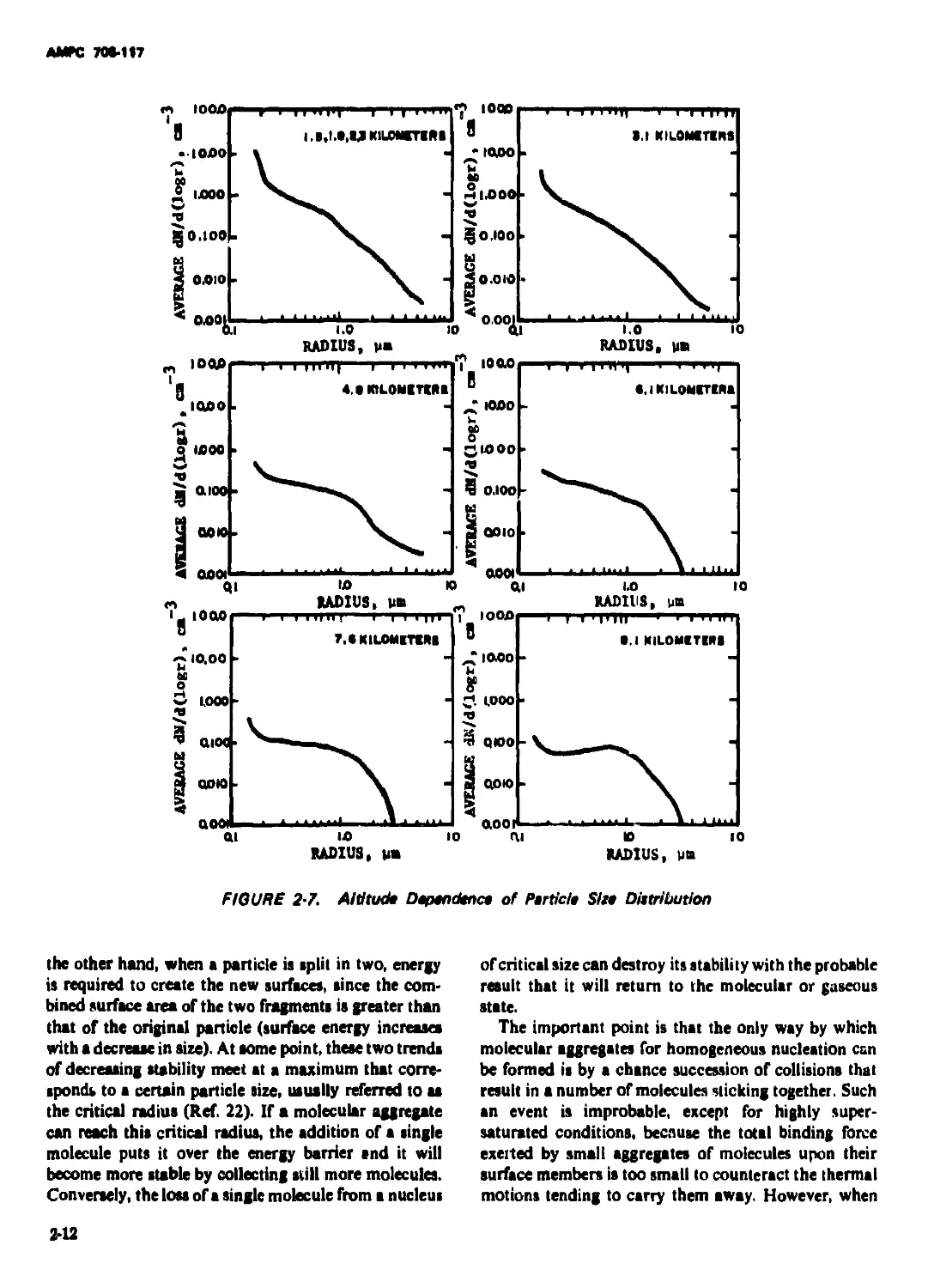
2-7. Altitude Dependence of Particle Size Distribution.............. 2-12
2-8. Particle Size Dependence of Mean Residence Time (Ref. 18) . . . 2-13
2-9. Sources of Atmospheric Pollutants in the United States ..................... 2-15
2-10. Volume of Atmospheric Pollutants by Type In the United States . . 2-15
2-11. Sources of Particulate Matter ............................................... 2-20
2-12. Environmental Sulfur Circulation............................................. 2-21
2-13. Maximum Average SulfUr Dioxide Concentrations for Various Aver-
aging Times.............................................................. 2-25
2-14. Frequency Distribution of SuifUr Dioxide Levels, 1962-1967 . . . 2-26
2-15. Diurnal Variation of Carbon Monoxide Levels on Weekdays In
Detroit.................................................................. 2-28
2-18. Diurnal Variation in Concentrations of Selected Pollutants .... 2-29
2-17. Monthly Mean Nitric Oxide Concentrations at Four Urban Sltea . . 2-29
2-18. Monthly Mean Nitrogen Dioxide Concentrationa at Four Urban Sites 2-30
2-19. Diumal Variation in Concentrations of Nonmethane Hydrocarbons . 2-35
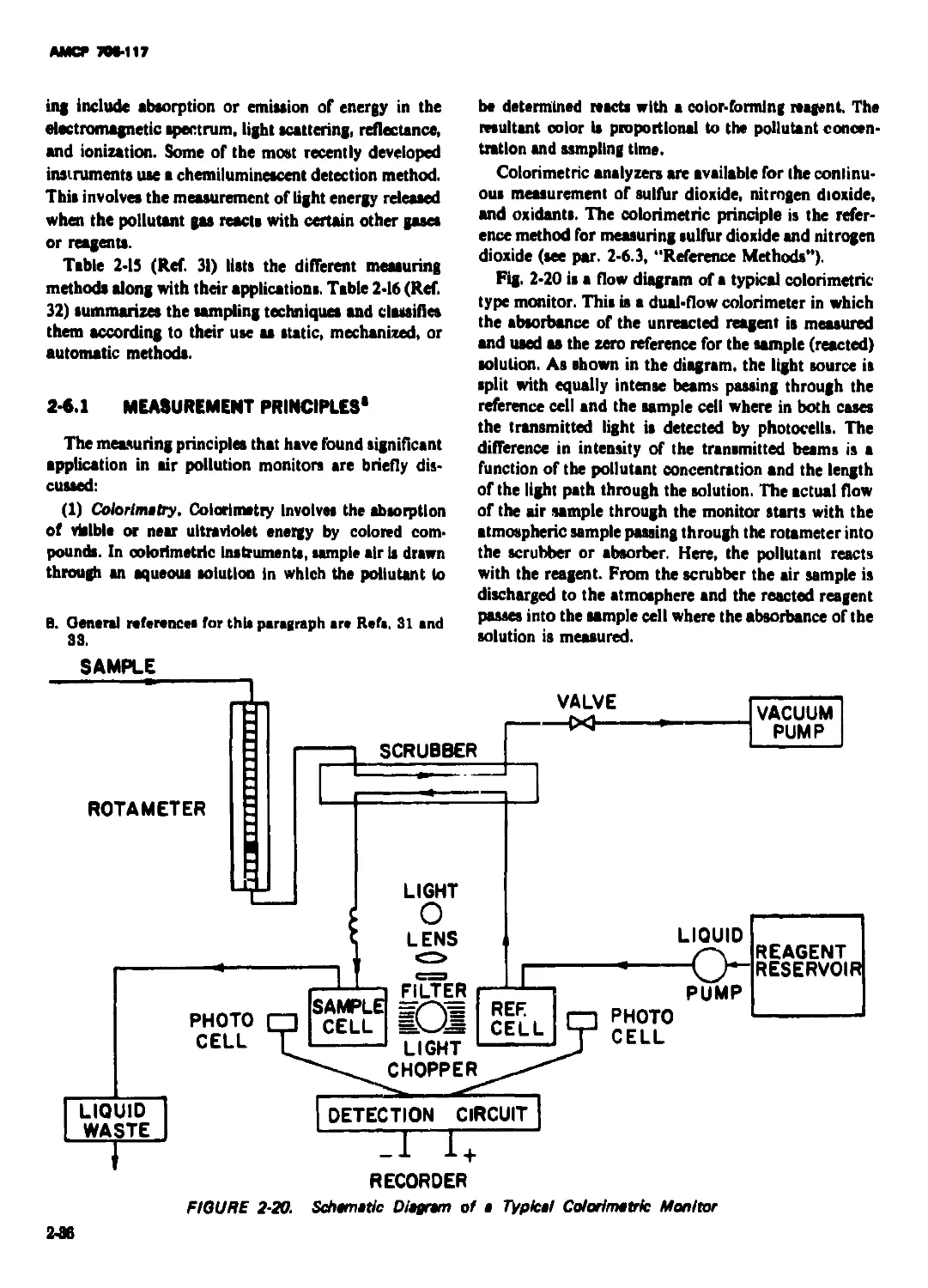
2-20. Schematic Diagram of a Typical Colorimetric Monitor.......................... 2-36
2*21. Schematic Diagram of a Coulometric SuifUr Dioxide Monitor . . . 2-38
2*22. Schematic Diagram of a Typical SuifUr Dioxide Conductivity
Monitor.................................................................. 2-39
2*23. Schematic Diagram of a Typical Flame Photometric SuifUr Monitor . 2-40
2*24. Schematic Diagram of a Typical Flame Ionization Monitor .... 2-40
2-25. Schematic Diagram of a Chemiluminescent Nitric Oxide Analyzer 2-41
2-26. Permeation Tube Calibration System ........................................ 2-42
2-27. Nitric Oxide and Nitrogen Dioxide Calibration System......................... 2-43
2*28. Exploded View of Typical High-volume Air Sampler Parts .... 2-45
2-29. Assembled High-volume Air Sampler anti Shelter .............................. 2-45
2-30, Schematic Diagram of a Typical Tape Sampler ................................. 2-46
2-31. Schematic Diagram of a Typical Nondisperslve Infrared Carbon Mon-
oxide Monitor ........................................................... 2-48
2-32. Typical Flow Diagram of a GC-FID Hydrocarbon Monitor .... 2-55
2-33. Relationship Between Corrosion of Mild Steel and Corresponding
Mean Sulfur Dioxide Concentration for Varying Length Exposure
Periods ................................................................. 2-57
2-34. Effects of SulfUr Dioxide and Oxidant Concentrations on Depth of
Corrosion of Carbon Steel Exposed for 10 yr ............................... 2-58
2-35. Effect of 8ulfUr Dioxide and Relative Humidity on Corrosion Rate
of Zinc ............................................................................... 2-59
2-36. Relation Between Corrosion Rate of Copper and Concentration of
SulfUr Dioxide In Atmospheres of High Relative Humidity . . . 2-60
2-37. Atmospheric Corrosion of Aluminum at л Relative Humidity of 52
Percent and SulfUr Dioxide Concentration of 280 ppm .... 2-61
vill
АМСРЯК.117
LIST OF ILLUSTRATIONS (non.)
Flo. No.
Thte
2-38. Atmoapheric Corroriou at Super Purity and SOOS Aluminum at Rei-
atm Humiditloe of 72 and 88 Percent and Suiter Dioxide Con-
«eatntton of 280 ppm.............................................................. 241
2-89. Effect at Sulfation on Breaking Strength at Cotton Fabrics .... 248
240. Effect of Atmospheric Sulfur Dioxide Concentration on BnaMng
Strength of Cotton Ooth............................................. 24S
8-1. Settling Velodtios for Partidee in 8Ш1 Air..................... 8-5
8-2. Lognormal Dhtributioa of hsrtidos....................................... 84
8-8. Logarithmic Plot of Particle Star Distribution.......................... 34
84. Cumulative Log-probability Cum ....................................... 8-7
8-6. ffotldaSlM Dlattibutioa of Duat Clouds Generated by Tanka ... 34
84. Partide Stee Distribution of Standard Dusts and Dusts Removed
from Used Paper Elements Received from Abroad ..................................... 84
8-7. Stee Distribution of Dutt Entering the Model Air Cteaaere (in the
teste on the Overland Train ML П).................................. 3*10
84. Stee Distribution of Dutt Passing die Model Air Oeanen (In the teats
on the Overland Train, this duet is repreeentative of the dust
reaching the gas turbines.) ....................................... g-10
84. Typioal Particle 8tee Distribution, Lee Drop Zone, Ft. BennlnfOa. 8-11
8.10. Typioal Partide Sias Distribution, Phillips Drop Zone, Yuma, Aria. 8-11
Ml. Typioal Partide Stee Distribution, Vehicle Dutt Course, Yuma, Arte. 8-11
Ml Partide States Models................................................. 8-18
M8. Sand Particle Dynamics................................................ 8*20
M4. Brorion of a Soft, Ductile Material .................................. 3-22
M6. Brorion of a Hard, Brittle Material . ................................ 8-28
8-16, Test Dust Partide Stee Distribution................................... 8*24
M7. Erosion LornssaFunction of Partide Slae............................... 8-24
M8. Erosion Loa м a Function of Partldo Velocity....................... . . 8-24
MS. Brorion Loa м a Function of Temperature .............................. 8-28
8-20. borion Loan Dutt Concentration........................................ «-26
8-21. Effect of Dust 8tee ou Energy ........................................ 8-26
8-21 Rate of Rutting n Duetfall ........................................... 8-27
8-21 6O-H1 Flashover Voltage of Dirty Insulators .......................... ,«28
3-24. Potential Gradient Record for Sahara Dutt Devil ...................... 8*2S
8-25. Alr-to-earth Cunvat and Potential Gradient of a Dutt Cloud Over
Wott Africa......................................................... 840
8-26. Functional Diagram of Dutt Test Chamber................................ 842
4-1. Periodic Waveforms (Ref. 1)............................................ 4.2
4-1 Random Disturbance (Ref. 1) ........................................... 4*8
4*1 Model at Stngie-degrnbof-frvedoni Isolated System (Ref. 1) .... 4*8
44. Nobs Generated by a 10-ton Truck, Normal and With ModHteatlons
(Ref. 17)............................................................ 44
44. Vertical Vibration Spectra of Tractor-trailer (Ref. 18)................ 4*7
44. Vertical Vibration Spectra of Rebuilt Tractor-trailer (Ref. 19) ... 44
4*7. Vibration Spectra of Rebuilt Tractor-trailer at Various Speeds
(Ref. 19)........................................................... 4*8
44. Vertical Vibration Spectra for Loaded s ->d Empty Tractor-tralers
(Ref. 19)......................................................................... 4*9
4*9. Vortical Vibration Spectra at Different Potata on Trailer (Ref. 19) . 4-9
lx
AMPC 7W-117
LIST OF ILLUSTRATIONS (con.)
Fig. No. Title Page
4-10, Vibration Spectra of Rebuilt Tractor-trailer In Three Dimensions
(Ref. 19)...................................................... 4*10
4-11. Vertical Vibration. Spectra of Flatbed Truck With Normal Road Con-
ditions (Ref. 20) ............................... 4-10
4-12. Vertical Vibration Spectra of Flatbed Truck on Rough Roads
(Ref. 20) ..................................................... 4-11
4-13. Companion of Truck Vibration Spectra on Paved and Rough Roada
(Ref. 21)..................................................... 4-1'1
4-14. Compartion of Vibration Spectra for Empty and Loaded Trucks
(Ref. 21)...................................................... 4-11
4-16. Vertical Vibration Spectra of a Tractor-trailer With Air-ride Suipen-
rion (Ref. 32)................................................. 4-13
4-16. Vertical Vibration Spectra of Panel Truck (Ref. 38)..................... 4-13
4-17. Accelerometer Location! on М113 Tracked Penonnel Carrier
(Ref. 24) ..................................................... 4-14
4-18. Velocity Dependence of Vibration Amplitude (Acceleration) for
M118 Personnel Carrier (Ref. 24) ........................... 4-15
4-19. Vibration Frequency Spectra for Railroad»— Various Condition»
(Ref. 21)...................................................... 4-16
4-20. Vibration Frequency Spectra for Railroad»—Variou» Speeds (Raf. 21) 4-16
4-21. Directional Comporite of Railroad Vibration Spectra (Ref. 21) . . 4-17
4-22. Comporite Vertical Vibration Spectra of Railroad Flatcar (Ref. 25) . 4-17
4-23. Comporite Transverse Vibration Spectra of Railroad Flatcar
(Ref. 25) ..................................................... 4-18
4-24. Comporite Longitudinal Vibration Spectra of Railroad Flatcar
(Ref. 25) ................................................. 4-18
4-25. Companion of Directional Frequency Spectra of Railroad Flatcar
(Ref. 25)...................................................... 4-19
4-26. Aircraft Acceleration Spectra (Overall Composites) (Ref. 21). . . 4-19
4-27. Comporite Vibration Spectra for Different Type» of Aircraft
(lief. 25) .................................................... 4-20
4-28. Vertical Vibration Spectra of Turbojet Aircraft for Varioua Flight
Pham (Ref. 25)............................................... 4-21
4-29. Maximum Acceleration! Measured During Three Pham of Flight
(Ref. 29)...................................................... 4-22
4-80. Sample Power Spectral Denaitiei for STOL and Boeing 727 Aircraft
During Gratae; Vertical Direction (Ref. 29) ................. 4-22
4-31. Typital One-third Octave Band Vibration Spectra Measured During
Takeoff Roll From a Munition Dispenser Carried on a Jet Air-
plane and a Single Store Carried on a Propeller Airplane (Ref. 80) 4-24
4-83. Typical Variation of Overall Vibration and Acoustical Environment
aa a Function of Airspeed and Attitude for a Munition Dispenser
Carried on a Jet Airplane (Ref. 80).......................................... 4-25
4-83. Example of Gunfire Response Spectra Measured on a Store During
Flight (Ref. 80)............................................... 4-36
4-84. Vibration Amplitude Data Measured 2 ft From M61 Gun Muzzle
(Ref. 31)...................................................... 4-37
4-35. Vibration Amplitude Data Measured 25 ft From M61 Gun Muzzle
(Ref. 31)...................................................... 4-27
x
АМСР 7M-117
LIST OF ILLUSTRATIONS (con.)
Fig. No. Title Page
4*36. Amplitude vs Occurrence Plot of Overall Flight Gunfire, Signal
Within 2Б In. of Gun Muzzle (Ref. 82) ............................ 4-27
4-37. Composite Vibration Spectra of HH-48B Helicopter (Ref. 2Б) . . . 4*28
4*88. Helicopter Vibration Envelope (Ref. 34).............................. 4.28
4*39. Vibration Frequencies Measured During a Typical Static Rocket
Motor Firing (Ref. 88)......................................................... 4-29
4*40. Vibration Charactertotlai of Seven Operational Missiles During Boost
Phase (Ref. 37) ............................................................... 4-29
441. Vibration Characteristics of Four Operational Missiles During Sus*
talned Flight After Boost (Ref. 37)............................... 4-31
442. Ship Vibration Spectra (Ref. 21)..................................... 4*32
4*43. Effr.'t of Sea State on Vibration of a Ship S20 ft Long (Ref. 21) . . 4*32
444. Effei of Sea State on Vibration of a Ship 380 ft Long (Ref. 21) . . 4*38
44Б. Seismic Probability Map of the United States (Ref. 42)............... 4-33
4-46. Laser Vibration Analyzer Optical System (Ref. 4Б) ................... 4*38
447. Typical Discrete Frequency Spectrum (Ref. 2) ........................ 4*37
44S. Typical Probability Density Plot (Ref. 2) 4*38
449. Typical Autocorrelation Plot (Ref. 2)................................ 4-88
4-60. Typical Power Spectral Density Function (Ref. 2)..................... 4*39
4-51. Typical Joint Probability Density Plot (Ref. 2)....................... 440
4-62. Typical Cron Correlation Plot (Ref. 2) ............................... 441
4-БЗ. Functional Block Diagram for Multlple-fllter-type Spectrum Ana-
lyzer (Ref. 2).................................................................. 442
4-Б4. Functional Block Diagram for SIngle-fllter-type Spectrum Analyzer
(Ref. 2) ....................................................................... 443
4-ББ. Effect of Width-to-iength (W/L) Ratio on Vibrations of Circuit
Boards (Ref. 62) .......................................... 444
4-Б6. Natural Frequencies of Printed-circuit Boards (Ref. Б2) ................... 447
4-Б7. Practical Guide to Condition of Rotating Machinery—Chapman
Curves (Ref. Б8)............................................................... 4-49
4-Б8. A Comparison Between the Observed Annoyanca Levels and the ISO
Proposals (Ref. Б7) ........................................................... 4-Б2
4-Б9. Shock and Vibration Isolator (Ref. 1)................................ 4-54
4-80. Shock and Vibration Absorber (Ref. 1) ............................... 4-64
4*61. Springs Used for Vibration Isolation (Ref. 63) ...................... 4*56
4*62. Liquid Spring or Dashpot (Ref. 68)................................... 4-55
4*63. Pneumatic Spring (Ref. 68) .......................................... 4-5Б
4-64. Solid Elastomer Isolator (Ref. 63) 4-66
446. Flexible Ring Baffles (Ref. 1)....................................... 4-56
4*66. Viscous-pendulum Damper (Ref. 1)..................................... 4*56
447. Suspended-chain Damper (Ref. 1) 4*67
4-68. Elasto-plasto-viucous Point Damper (Ref. 1) ......................... 4*69
4-69. varlable-stlffness Polymeric Damper (Ref. 1)......................... 4-69
4*70, Wire-mesh Isolator (Ref. 1) ......................................... 4-69
4*71. Automatically Controlled Air-spring Suspension System (Ref. 1) . . 4-61
4*72. Active Vibration Isolator (Ref. 1)................................... 4-61
4-73. Active (Servo-control) Вам-motion Isolation System (Ref. 1) . . . 4-62
4*74. Viscoelastic Damping Plates (Ref. 1) 4-62
4*76. Modes of Printed-circuit Board Vibration (Ref. 1).................... 4-63
xi
АМСР 706-117
LIST OF ILLUSTRATIONS (con.)
Fig. No. Title Page
4-76. Vlbntlon-abaorber Application to Electric Motor (Ref. 1) .... 4-64
4Л7. Effect of Absorber on Vibration of Electric Motor (Ref. 1) .... 444
4-78. Block Diagram* of Vibration Teet System* (Ref. 37)
Type* of Equipment Most Often Subjected to Vibration Tert 445
4-79. (Ref. 88) - • 4-78
5-1. Six Example* of Shock Motion* (Ref. 5).................................. 5.6
5-2. Example* of Shock Pub* Time Hiitorie* and Their Fourier Tram-
form* (Ref. 18)................................................ 5-9
5-3. A Single-degree-of-freedom System (Ref. 17)...................... 5-10
54. Shock Spectra of Several Typical Shock Pulee* (Ref. 18).......... 5-11
5*5. Effect of Pube Shape on Shock Spectra (Ref. 18).................. 6-12
5-6. Cargo Shock Environment* for Ate Tramport (Ref. 8)................ 542
5-7. Maximum Railroad Tranilent Acceleration Envelope*, Over-the-road,
Standard Draft Gear (Ref. 8) .............................................. 544
5-8. Railroad Coupling Shock Spectrum, 3.4 mph, Fore/Aft, Standard
Draft Gear (Ref. 8) ........................................... 544
5-9. Railroad Coupling Shock Spectrum, 3.4 mph, Vertical, Standard
Draft Gear (Ref. 8) ....................................................... 544
5-10. Railroad Coupling Shock Spectrum, 3.4 mph, Lateral, Standard
Draft Geu (Ref. 8) ............................................ 545
5-11. Railroad Coupling Shock Spectrum, 6 mph, Fore/Aft, Standard
Draft Gear (Ref. 8) ....................................................... 545
5-12. Railroad Coupling Shock Spectrum, 8 mph, Vertical, Standard Draft
Geu (Ref. 8)............................................................... 545
5-13. Railroad Coupling Shock Spectrum, 8 mph, Vertical, Standard Draft
Geu (Ref. 8)............................................................... 545
5-14. Railroad Coupling Shock Spectrum, 10 mph, Vertical, Standard
Draft Geu (Ref. 8) ........................................... 5-18
5-15. Railroad Coupling Shock Spectrum, 10 mph, Fore/Aft, Standard
Draft Geu (Ref. 8) ........................................... 5-16
5-16. Railroad Coupling Shock Spectrum, 10.0 mph, Lateral, Standard
Draft Geu (Ref. S) ....................................................... 5-16
5-17. Railroad Coupling Shock Spectrum, 8.7 mph, Fore/Aft, Cuthioned
Draft Geu (Ref. 8) ....................................... 546
5-18. Railroad Coupling Shock Spectrum, 6.8 mph, Fore/Aft, Cuihioned
Draft Geu (Ref. 8) ....................................... 5-17
5-19. Railroad Coupling Shock Spectrum, 9.8 mph, Fore/Aft, Cuihioned
Draft Geu (Ref. 8) ........................................... 5-17
5-20. Railroad Coupling Shock Spectrum, 12 mph, Fore/Aft, Cuahioned
Draft Geu (Ref. 8) 5-17
5-21. Rail Tramport Shock Spectra (Ref. 28) ............................ 548
5-22. Field Survey of Impact Spaed* (Cumulative Impact*) (Ref. 7) . . . 5.19
5-23. Cargo Environment* for Rail Tramport (Ref. 6)............ 549
5-24. Duration of Tranilent*, S-1V Tramporter on Barge, Heavy Sea* (Ref.
21) .......................................................... 5-20
5-25. Transient Vibration Leveb, S-1V Barge Deck, Heavy Sou (Ref. 21) . 5.20
5-26. Tramient Vibration Leveb, S-1V Tramporter on Barge, Heavy Seu
(R«f. 21)..................................................... 5.20
5-27. Maximum Acceleration Leveb, S-IV Stage on Freighter (Ref. 21) . . 5.21
xii
АМСР 709-117
LIST OF ILLUSTRATIONS (con.)
Fig. No. Title Page
6*28 Ship Transhnt Acceleiwtion Envelope (Ref. 8) .................... 6-21
5-29. Cargo Environments for Sea Transport (Ref. 8).................... 5-22
5-30. Shock Data—Truck Backing Into Loading Dock, Longitudinal, For-
ward on Truck Bed (Ref. 24) .................................. 5-25
5 31. Shock Data—Truck Driving Across Railroad Tracks at 45 mph, Verti-
cal. Aft on Truck Bed (Ref. 24) ........................................... 5<28
5-82. Shock Data—Truek Driving Across Cattle Guard at 45 mph, Vertical,
Aft on Truck Bed (Ref. 24).................................... 5-27
5-33. Shock Data—Truck Driving Across Potholes at Truck Stop, Aft on
Truck Bed (Ref. 24)........................................... 5-28
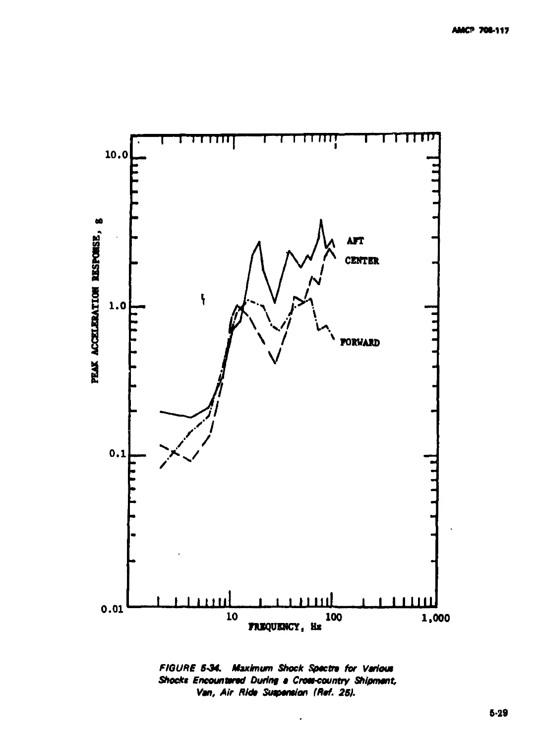
5-84. Maximum Shock Spectra for Various Shocks Encountered During a
Cross-country Shipment, Van, Air Ride Suspension (Ref. 25) . . 5-29
5-85. Cargo Shock Environments for Highway Transport (Ref. 8) . . . . 5-80
5-38. Maximum Shocks Recorded During Airline Test Shipment (Ref. 26) 5-31
5-37. Drop Height Distribution Cubical Cleated Plywood Box Sent by
Railway Exprees (Ref. 11) .................................... 5-32
5-88. Drop Height Distribution, Railroad Depot Loading Operation, Sever-
est Handling Operation (Ref. 11).............................. 5-38
5. 39. Drop Height ve Package Weight, Railroad Depot, Severest Handling
Operation (Ref. 11) ....................................................... 5-34
540. Effect of Package Height on Drop Height, Railroad Depot, Severest
Handling Operation (Ref. 11) .............................................. 5-34
5-41. Number of Drops by Drop Height of Package Sent by Railway Ex-
press (Ref. 11) ........................................................... 5-35
5-42. Number of Drops by Drop Height of Package Sent by Rail (Ref. 11) 5-38
5-43. Impact Pulse Durations for Container Comer Drops on Typical
Stacking Surfaces (Ref. 27)................................... 5-37
5-44. Impact Pulse Durations for Container Flat Drops on Typical Stack-
ing Surfaces (Ref. 27) ................................... 5-87
5-45. Piezoelectric (Crystal) Accelerometer (Ref. 80).................. 5-38
5-48. Strain Bridge Accelerometer (Ref. 30)............................ 5-39
547. Potentiometer Accelerometer (Ref. 30) ........................... 5-39
5-48. Force Balance Accelerometer (Ref. 80) ........................... 5-40
5-49. Amplification Factors Resulting From Three Fundamental Pulse
Shapes (Ref. 32) ......................................... 540
5-50. Item Characteristics That Determine the Selection of Cushioning
Material (Ref. 33)......................................................... 5-48
5-51. Characteristics of Cushioning Materials (Ref. 33) ............... 5-46
5-52. Application of Fiberboard (Ref. 83) 5-49
5-53. Methods of Cushioning—Floated Item (Ref. 33)..................... 5-51
5-54. Methods of Cushioning—Floated Package (Ref. 38) ................. 5-51
5-55. Methods of Cushioning—Shock Mounts (Ref. 33)..................... 5-53
5-56. Ideal Pubes With Tolerance Limits (Ref. 35)...................... 5-54
5-57. Impulse-type Shock Test Machine (Ref. 80) ...................... 5-55
6-1. Tangential and Normal Components of Acceleration.................. 6-4
6-2. Total Acceleration as the Vector Sum of the Normal and Tangential
Components .................................................... 6-4
8-3. Venus Entry Deceleration (Ref. 7) ................................ 6-5
64. Potentiometric Accelerometer...................................... 6-6
xill
АМСР 709 -117
LIST OF ILLUSTRATIONS (con.)
Fig. No. Title Page
6-5. Inductive Accelerometer ............................................ 6.7
6-6. Vibrating String Accelerometer...................................... 6-8
6-7. Cantilever Beam Accelerometer ...................................... 6-8
6-8. Piezoelectric Accelerometer........................................ 6-8
6-9. Gravitational Calibration of Accelerometer.......................... 6-9
6-10. Accelerometer Mounted on Centrifuge for Calibration................. 6-9
6-11. Crude Comparison of G-Tolerances for Human Subjects In Four
Vectors of G (Ref. 16).......................................... 6-12
6-12. Component Mounted on Vehicle In Motion (Ref. 20) .................. 6-18
6-13. Proper Mounting of Test Specimen on Centrifuge (Ref. 20) .... 6-13
7-1. Frequency-response Characteristics for Standard Sound-level Meters
(Ref. 2) ........................................................ 7-4
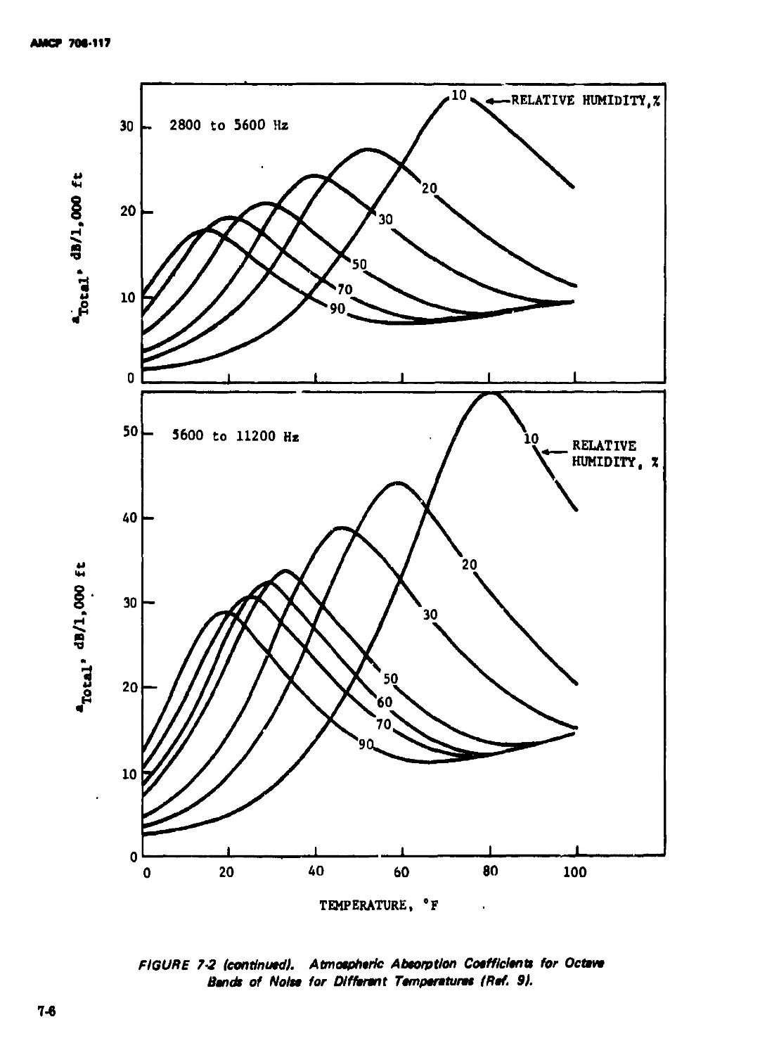
7-2. Atmospheric Absorption Coefficients for Octave Bands of Noise for
Different Temperatures (Ref. 9)................................................ 7-6
7-2. Atmoapheric Absorption Coefficients for Octave Banda of Noles for
Different Temperatures (Ref. 9) (Cont.)...................................... 7.6
7.8. Accuracy Curves of Condenser Microphone Output for Free-fleid
0.5-In. and 1-in. Cartridges Mounted on a Tripod................ 7-13
7-4. Accuracy Curves of Condenser Microphone Output for Diffuse-field
0.6-In. and 1-In. Cartridges Mounted on a Tripod................ 7-14
7-6. Temporary Threshold Shift (TTS) as a Function of Sound Pressure
Level (SPL) for Exposure to an Octave Band of 2 to 4 kHz
(Ref. 31)....................................................... 7-18
7-6. Relation Between Exposure Frequency and Temporary Threshold
Shift (TTS) for Octave Bands of Noise (Ref. 32)................. 7-18
7-7. Temporary Threshold Shift (ITS) at 4 kHz From Exposure to 2 to 4
kHz Octave Band Noise (Ref. 31) ................................ 7-19
7-8. Distribution of Temporary Threshold Shift (TTS) Resulting From
Б-min Exposure to Broadband Noise (Ref. 30)..................... 7-19
7-9. Recovery From Temporary Threshold Shift (TTS) (Ref. 46) ... 7-20
7-10. Conversion of TTS to TTS] With TTS as the Parameter (Ref. 44) . . 7-20
7-11. Recovery From Temporary Threshold Shift (TTS) (Ref. 61) ... 7-21
7-12. Temporary Threshold Shift (TTS) as a Function of Peak Pressure
Level for Ears Exposed to 10 Impulses Produced by Various
Weapons (Ref. 49)............................................... 7-21
7-13. Temporary Threshold Shift (TTS) at 4 kHz as a Function of Peak
Level of Clicks (Ref. 60)................................................... 7-22
7-14. Average Growth of Temporary Threshold Shift (TTS) From Con-
stant Rate Impulses (Ref. 60)................................... 7-22
7-16. Distributions of TTSa Following Exposure to 26 Gunfire Impulses
(Ref. 27)....................................................... 7-23
7-16. Masking as a Function of Frequency for Masking by Pure Tones of
Various Frequencies and Levels (Ref. 77)........................ 7-28
7-17. Relationship Between Modified Rhyme Test (MRT) and Phoneti-
cally Balanced (PB) Test Scores (Ref. 81)....................... 7-29
7-18. Worksheet for Calculating Articulation Index (Al) by the Octave-
band Method Using ANSI Preferred Frequencies (Ref. 80) . . . 7-30
7-19. Relation Between Articulation Index (Al) and Various Measures of
Speech Intelligibility (Ref. 80)................................ 7-81
xiv
АМСР 708-117
LIST OF ILLUSTRATIONS (con.)
Fig. No. Title Pago
7-20. Blast Exposure Limits as a Function of Peak Overpmsure and Dura-
tion (Ref. 90)........................................................... 7.88
7-21. Damage Risk Contours for One Exposure Per Day to Octave and
1/3-octave or Narrower Banda of Noise (Ref. 24)............. 7.86
7*22. Damage Risk Contours for One Expoaun Per Day to Pun Tonn
(Ret. 24)................................................... 7-85
7-28. Contours for Determining Equivalent A-welghted Sound Level . . 7-86
7*24. Basic Limits for lmpulao4iobe Expoaun........................... 7-87
7-25. Correction Factors To Be Added To Ordinate of Fig. 7-22 To Allow
for Daily Impulse-noise Exposures Different From 100 Impulses
(Ref. 94)................................................... 7-88
7-26. Speech Interference Lewis (Ref. 95) ................................ 7-88
7-27. Noise Criteria Referred To Preferred Octave Bands and Commercial
Octave Bands (Ref. 97)...................................... 7-40
7-28. Theoretical and Experimental Transmission Loom for Studlm
Double-leaf Walls. (—): Experimental Curve; (o): theoretical (Ref.
98) ...................................................................... 742
8-1. The Electromagnetic Spectrum (Ref. 1)............................ 8-2
8-2. Near-fleld and Far-Held Relationships............................. 84
8-8. Antenna Radiation Patterns (Ref. 4) ............................. 8-5
84. Worldwide thunderstorm Distribution (Ref. 4).................... 8-12
8-5. Time Sequence of Events In Lightning Discharge (Ref. 4)......... 8-18
84. Waw Shape of Typical Lightning Stroke Current (Ref. 4).......... 8-14
8-7. Normalized Spectrum for Lightning Discharges (Ref. 4) .......... 8-14
8-8. Eloctroexplosiw Device (EED) Components (Ref. 4) ............... 8-21
8-9. Ignition of Explosive Charge by Thermal Stacking of RF Pulse
Energy (Ref. 4)............................................. 8-24
8-10. Peak Currents That Cause Permanent Faults in Telephone Cable
(Ref. 4) ................................................... 8-27
8-11. Examples of Triggered Lightning Involving Conductors Connected to
the Earth (Ref. 82) ..................................................... 8-28
8-12. Exampin of Triggered Lightning Involving Conductors In Free
Flight (Ref. 32)............................................ 8-29
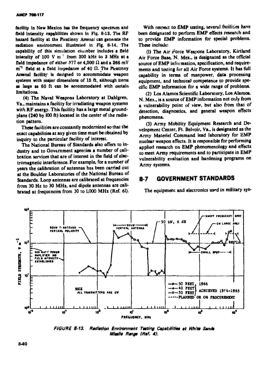
8-18. Radiation Environment Testing Capabllltln at White Sands Missile
Range (Ref. 4) ........................................................... 840
8-14. Radiation Environment Testing Capabllltln at Plcatinny Arsenal
(Ref. 4) ................................................................. 841
xv
АМОР 766-117
LIST OF TABLES
Table No. Title Page
3-1. Concentrations of 0мм Comprising Normal Dry Air .......................... 2-1
3-2. Air Pollution Damage to Varioua Materials............................... 2*2
2*3. Physical Properttes of SuifUr Dioxide................................... 2-6
24. Physical PropertiH of Carbon Monoxide................................... 2-8
34. Physical Propertim of Peroxyacetyl Nitrate .............................. 24
24. Competition of Particulate Emisrioni.................................. 2*14.
2*7. Atmospheric Sulfur Dioxide Emtssions In 1963 and 1966 by Source (U.S.) 2*16
24. Carbon Monoxide Emission EatlmatM by Source Category................... 2*17
24. Summary of Nationwide Nitrogen OxidM Emission», 1968 .................. 2*18
2*10. EatlmatM of Hydrocarbon Embdens by Source Category, 1968 .... 2*19
2*11. 1968 Emiaaion Inventory of Particulate Material, Metric Топа Per Year . 2*20
2*12. Pollutant Concentrationa and Composition................................. 348
2*18. Background Concentrations of Sulfur Dioxide ............................ 2-27
2-14, Suspended Partide Concentrations (Geometric Moan of Center City Sta-
tion) In Urban Anas, 1961 to 1966 .................................. 2-81
2-18. Meosunasent PrindptM la Air Quality Monitoring........................... 244
2-16. Common Ambient Air Polutlon Sampling Techniques.......................... 247
2-17. National Air Quality Standard Reference Methods ......................... 244
2*18. Performance Evaluation of Continuous Monitors ........................... 249
249. Suggested Performance Spedflcationa For Automatic Monitors .... 241
2-20. Commercial Equipment for MeMUriag Suspended Particulates.......... 248
2-21. Chemical Resistance of Materials to Pollutants........................... 244
2*22. Predicted Useful Life of Galvanised Sheet Steel With 68-pm Coating at
Average Relative Humidity of 66 Percent.............................. 240
8-1. Dust Concentratioas In Various Regions........................... 8-2
84. Variation of Dust Concentration with Altitude..................... . 8-8
84. Average Dust Concentratlonr-M48 Tank Operating Over DoMrt Terrain . 84
84. Average Duet Concentrations—H-21 Helicopter...................... 84
84. Dust Concentrations—Varioua Aircraft .................................... 84
84. Partide 81m Distributions of Dust Collected at Air Inlets of Army Tanks
(Percent Within Range)........................................ 84
8-7. Variation of Pattide Sim Distribution with Height In Duststorm .... 8-12
84. Constituents of Natural Dusts................................... 8-13
84. Characterisation of 8o8 Samples................................. 8-14
8-10. Effect of Departure from Isokinetic Conditions on Sample Concentrations 8-16
8-11. Definitions of Particle Diameter ...................................... 8-18
8-12. Instruments for Sample Colection................................ 8-19
8-18. Ma|or Deserts of the World ............................................ 8-20
8-14. Corrotion of Open-hearth Steel Specimens........................ 8-27
8-16. VMbilty In Diet (Ref. 4)........................................ 8-81
4-1. Vibration Parameters (Ref. 12)................................... 44
4-2. Origins of Vehicle Nohe (Ref. 17) ....................................... 44
4-8. Filter for Characterisation of Vibrations on Trucks (Ref. 18).... 4-7
44. Comparison of Overall Acoustic and Vibration Environment Within a
Munition Dispenser to The Acoustic Environment Measured at the
Adjacent Dispenser Surface (Ref. 80)....................................... 4-28
44. Sources of VBnation in Various Missile Operational Phases (Ref. 86) . . 440
xvi
АМСР 708-117
LIST OF TABLES (con.)
Tabla No. Title Page
4-6. Vibration Induced Damage to Electrical and Electronic E'^iipment
(Ref. 37)..................................................................... 446
4-7. Human Body Resonance* (Ref. 66)............................... 4-60
4-8. Effect* of Helicopter Vibration on Pilot Performance (Ref. 56) .... 4411
4-9. Comparison of Different Type* of Elastic Elements (Ref. 63)... 4-60
440. Vibrational Testing Capabilities of Launch Phase Simulator (Ref. 70) . . 4-69
441. Performance Characteristics of Hydraulic Ram* (Ref. 76) 4*70
442. Package Vibration Test from MIL-STD-810 (Ref. 68) ..................... 4-71
448. Vibration Test* From Federal Test Method Standard 101B (Ref. 68) . . 4-78
444. Vibration Test From MIL-STD-331 (Ref. 68)................................ 4-74
446. Bounce Test Specifications (Ref. 68) .................................... 4-76
4-16. Cycling Test Duration* (Ref. 68)......................................... 4-76
447. Cycling Test Sweep Requirement* (Ref. 68) ............................... 4-76
4-18. Resonance Test Specification* (Ref. 68).................................. 4-76
449. Test Specifications and Standards (Ref. 83) ............................. 4-77
4-20. Types of Test Procedure* in Test Specifications and Standards (Ref. 88) . 4-78
4-21. Cycling Test Parameters (Ref. 83) 4-79
4-22. Endurance Test Parameters (Ref. 83)...................................... 4-79
4-28. Random Vibration Test Parameter* (Ref. 83)............................... 4-80
4-24. Test Specification* Most Often Referenced (Ref. 88) ......... 4-80
6-1. Conversion Factor* For Common Unit* of Speed.............................. 6-2
6-2. Conversion Factor* For Displacement Unit* ................................ 6-2
6-8. Distribution of Vertical Acceleration Peaks, Braking After Touchdown,
NC-135 Aircraft (Ref. 22) ............................... 6-18
6-4. Distribution of Vertical Acceleration Peaks Takeoff, NC-136 Aircraft
(Ref. 22)..................................................................... 648
6-5. U-Shaped Fiat-bed Trailer Data .......................................... 6-22
6-6. Army M36 Truck Data............................................... 6-23
6-7. Cargo-handling Field Test Results: Peak Acceleration, G (Ref. 11) . . . 6-81
6-8. Properties of Selected Cushioning Materials (Ref. 33) .................... 646
6-1. Linear Acceleration Conversions (Ref. 3) ................................. 6-2
6-2. Acceleration Characteristics of The Abie Serie* of Rockets (Ref. 8) . . 6-6
6-3. Effect of Acceleration on Military Equipment (Ref. 16) .................. 6-11
64. G Levels For Structural Test (Ref. 21) 6-14
6-6. G Level* For Operational Test (Ref. 21)........................... 6-16
74. Terms and Units Used in Acoustics.................................. 7-2
7-2. Relationship Between Unit* of Sound Pressure....................... 7-3
7-3. Center and Limiting Frequencies for Octave-band Analyzer* ............... 74
74. Sound* Encountered In Army Environment ................................... 7-8
7-6. Response* and Associated Tolerances............................... 7-16
7-3. Summary of Standard* Requirement*.................................. 746
7-7. Apparent Detector Time Constant v* Meter Reading.................. 7-16
7-8. ISO Audlomeiric Zero vs Chaba*-Llmit TTS........................ 7-26
7-9. Chart for Determining Class of Hearing Impairment (Ref. 69)....... 7-28
7-10. Representative Subjective and Behavioral Response* to Noise Exposure . 7-27
7-11. Worksheet for Calculating Articulation Index (Al) (Ref. 80) ............. 7-81
742. Wabh-Hsaley Act Permissible Daily Noise Exposure*................. 7-86
7-18. Low Frequency and Infrasonic Noise Exposure Limit* (Ref. 94) ... . 7-87
xvii
АМСР7М-117
LIST OF TABLES (con.)
Tabic No. Title Pago
7-14. Recommended NC Curve* for Variou* Work Space*.............................. 7-41
7-1Б. Range of Noise In dBA Typical for Building Equipment at 3 ft (Ref. 99). 7-43
7-16. Range of Building Equipment Notoe Level* To Which People Are Ex-
poeed (Ref. 99)......................................................... 744
8-1. RF Source» (Ref. 4) ....................................................... 8-6
8-2. RF Sources *n=’ Characteristic* At A Typical Military Initallation (Ref. 4) 8-9
88. Some Arvy/Nnvy Equipment Designators* (Ref. 7)............................ 8-10
84. Source* of Electromagnetic Interference By Equipment ..................... 8-11
84. Mlcr iwave Band Designation* (Ref. 8) 8-12
84. Some Electroexplorive Device (EED) Type* (Ref. 4)......................... 8-21
8-7. Baric Aerospace Ordnance Device* (Ref. 4) 8-22
8-8. Failure Mode* (Ref. 28)................................................... 8-26
8-9. Maximum Permitted Exposure to Laser Energy (Ref. 34)...................... 8-32
8-10. Maximum Permissible Exposure Level* for Laser Radiation at the Cornea
for Direct Illumination or Specular Reflection at Wavelength w 694.3
mm (Ref. ЗБ)........................................................... 8-88
8-11. Permitted Energy Falling Directly on Cornea (Ref. 33)...................... 8-38
8-12. Recommended Maximum Permlulble Intensities for Radio Frequency
Radiation (Ref. 39) ................................................... 8-88
8-18. Summary of Biological Effect* of Microwaves (Ref. 42) ..................... 8-87
8-14. Applicable Military Documenta .............................................. 842
xvill
АМС? 700-117
PREFACE
Thb handbook, Aidvewf EmrirwwMatof Fecton, b the third in a series on the nature
and effecta of the environmental phenomena. As the title impiiea, the handbook addrassei
a aet of Induced environmental factor» which, for the purpose of thia textrcomprise:
n. Atmoapheric Pollutant*
b. Sand and Dust
c. Vibration
d. Shock
e. Acceleration
f. Acoustics
g. Electromagnetic Radiation
h. Nuclear Radiation.
There particular fectora nr» chosen aa beat representing the need» of the dmign
engineer. It la recognized that thia aet b arbitrary and that natural fencer contribute,
sometimes In a major way, to these environmental parameters.
The information la organlaed aa follows:
a. Description of the factor, its measurement, and its distribution
b. Description of the effecta of the factor on materiel and the procedures for design
so aa to avoid or reduce advene effects,
c. Enumeration of the testing and simulation procedures that assure adequate design. ... .
Thus, the design engineer b provided with a body of practical information that will
enable him to design materiel so that Its performance during use is not affected seriously
by the environment. It is impractical to acknowledge the assistance of each Individual or
organisation which contributed to the preparation of the handbooks. Appreciation,
however, is extended to the following organizations and through them to the individuals
concerned:
a. Frankford Arsenal
b. US Army Engineer Topographic Laboratories
c. US Army Tank-Automotive Command
d. US Army Transportation Engineering Agency
s. Atmospheric Sciences Laboratory, US Army Electronica Command.
The handbook wee prepared by the Research Triangle Institute, Research Triang*e
Park, NO—for the Engineering Handbook Office of Duke University, prime contractor to
the US Army Materiel Command—under the general direction of Dr. Robert M. Burger.
Technical guidance and coordination were provided by a committee under the direction
of Mr. Richard C. Navarin, Hq, U8 Army Materiel Command.
The Engineering Design Handbooks fall Into two basic categories, those approved for
release and sale, and those dassifled for security reasons. The US Army Materiel Com-
mand policy 1» to release these Engineering Design Handbooks In accordance with current
DOD Directive 7230.7, dated 18 September 1973. All undaasifled Handbooks can be
obtained from the National Technical Information Service (NT1S). Procedures for acquir-
ing those Handbooks follow:
a. All Department of Army activities having need for the Handbooks must submit
their request on an official requisition form (DA Form 17, dated Jan 70) directly to:
Commander
Letterkenny Army Depot
ATTN: AMXLE-ATD
Chambenburg, PA 17201
xix
AMPC7W-117
(Requssts for classified documenta must be submitted, with appropriate “Need to Know'*
justification, to Letterkenny Army Depot.) DA activltiei will not requlaition Handbooks
for further free distribution.
b. All other requestors, DOD, Navy, Air Force, Marine Corps, nonmiiitary Govern-
ment agencies, contractors, private industry, individuals, universities, and others must
purchase these Handbooks from:
National Technical Information Service
Department of Commerce
Springfield, VA 22161
Classified documenta may be released on a “Need to Know" basis verified by an official
Department of Army representative and processed from Defense Documentation Center
(DDC), ATTN: DDC-T8R, Cameron Station, Alexandria, VA 22314.
Comments and suggestions on this Handbook are welcome and should be addressed
to:
Commander
US Army Materiel Development
and Readineas Command
ATTN: DRCRD-TV
Alexandria, VA 22333
(DA Forms 2028, Recommended Changes to Publicetions, which are available through
normal publications supply channels, may be uaed for commenta/suggestions.)
XX
AMO 706-117
CHAPTER 1
INTRODUCTION
Thia handbook, containing information on eight in-
duced environmental foctors, is Part Three of the Envi-
ronmental Series of Engineering Design Handbooks.
The complete aeries includes:
Part One, Aufc Environmental Concepts, AMCP
706-11$
Part Two, Natural Environmental Factors, AMCP
706-116
Part Three, Induced Eniiminnta! Factors (thia
part), AMCP 706-117
Part Four, UN Cycle Environments, AMCP 706-118
Part Five, Environmental Glossary, AMCP 706-119.
' The environmental frctors included in this hand-
book—atmospheric pollutants, sand and dust, vibra-
tion, shock, acceleration, acoustics, electromagnetic
radiation, and nuclear radiation—are those that are
derived primarily from human activities. It is apparent,
however, that natural forces contribute, sometimes in
a nu^oc way, to the effects of these environmental
parameters. For example, many air pollutants are pro-
duced by nature. These include suiftir oxides and dust
from volcanic activities, hydrocarbons from decaying
vegetation and other organic materials, and the smoke
and vapors emanating from naturally occurring, forest
fires. Large quantities of sand and dust are also pro-
duced naturally but, in this case, it was decided that the
sand and dust derived from human activities was more
important in its effects on materiel than that of natural
origin. Vibration, shock, and acceleration are less in-
fluenced by nature although the extremely destructive
forces of earthquakes would be classified with these
factors, as would forces associated with winds and
waves. Natural contributions to the acoustical environ-
mental factor are primarily associated with meteoro-
logical disturbances such as thunderstorms or with vol-
canic activity. The natural background electromagnetic
radiation can reach a destructive magnitude in the case
of lightning, but otherwise is overshadowed by artificial
sources.
Each of these induced environmental factors is also
influenced greatly by natural environmental factors.
Rah will wash many pollutants from the atmosphere
or winds will disperse them; rah or humidity will sup-
press sand and dust; and the other induced environ-
mental factors are influenced by temperature, humid-
ity, or other natural phenomena.
Because these induced environmental factors are
derived from human activities, they are subject to con-
trol. Each of them can be eliminated by eliminating its
source, but this is not usually desirable. The various
mechanical factors associated with transportation of
materiel cannot be completely eliminated without also
halting transportation. Electromagnetic radiation in
the environment cannot be eliminated without sacrific-
ing radio and television broadcasting, many communi-
cation links, power-distribution networks, or medical
diagnostic equipment. Thus it is with each of the in-
duced environmental factors. The benefits derived from
the sources of eacn factor are such as to outweigh the
detrimental effects of that factor, therefore, the empha-
sis must be on reducing such effects.
The effects of environmental factors may . be reduced
either by reduction nt the source or by protective meas-
ures employed in design. Source reduction is particu-
larly obvious in the consideration of air pollutants;
hence, it is presently being vigorously attempted in the
United States. The magnitude of sand and dust effects
can be greatly reduced by paving road surfaces and by
encouraging natural ground cover. The reduction of
vibration, shock, and acceleration is accomplished by
giving attention to the source. Thus, in the transporta-
tion system where many of these mechanical forces are
found, the r- v of improved suspensions, roadbeds, and
vehicle-operating techniques are effective for reducing
these forces. Noise is now recognized as a form of
environmental pollution, and noise suppression tech-
nology is rapidly advancing. Electromagnetic radiation
may be reduced either by proper shielding of radiating
sources or by improved broadcasting and detection
technology. The nuclear radiation environment is
primarily associated with the use of nuclear weapons,
nuclear power reactors, and nuclear instrumentation.
In all of these applications the nature of the expected
radiation is careftilly considered, and, when necessary,
protection is provided.
Materiel can be protected very adequately from the
effects of many induced environmental factors. Thus,
the effects of air pollution may be reduced by proper
choice of materials, better surface coatings,OT by prov-
iding hermetic enclosures for sensitive items. Protec-
tion against the effects of sand and dust follow much
1-1
AMCP 7M-117
the nine procedure, with the sealing of sensitive items
from sand and dust being most effective. In other cases
it is necessary to provide more resistant surface coat-
ings or operationally to avoid sand and dust exposure.
The design of shock mounts, cushioning materials, and
packaging techniques allows the protection of many
materiel items from, vibration, shock, or acceleration.
However, since it is impossible to avoid completely
such forces, the mechanical engineer has learned how
to compensate or design for such forces. Personnel, on
whom the acoustical factor has the most effect, can be
protected from such effects with acoustical insulation,
ear protectors, or similar devices. Methods to protect
materiel from the effects of acoustics are very similar
to those employed to protect against vibration. Electro-
magnetic and nuclear radiation protection of materiel
is dependent primarily upon shielding and hardening
technology. In the first case the design engineer at-
tempts to prevent such radiation from entering into
sensitive regions of the design, while in the second in-
stance the engineer attempts to provide designs that
will not be affected by such radiation.
All information on the induced environmental fac-
tors is not included in this handbook. A prominent
example of such limited treatment is vibration. A var-
iety of texts, journals, and other information sources
deal with vibration in all of its many aspects. Only such
information on vibration as is deemed of particular
importance to the military design engineer is included.
Even with this limitation, it is apparent that a number
of omissions have occurred. These result primarily
from efforts to obtain a coherent presentation within
the limitations of time and effort.
The nature of the data presented varies considerably
among the various induced environmental factors. The
amount of information available on electromagne'ic
radiation, nuclear radiation, or vibration exceeds that
available on sand and duat, acceleration, or acoustics
by orders of magnitude. However, a very brief presen-
tation is provided on nuclear radiation because of its
classified nature and because of the extensive treatment
given to it in other Engineering Design Handbooks—
specifically, AMCP 706-235 and AMCP 706-335
through -338.
It is only in the laboratory that the effect of a single
environmental factor can be ascertained. In any real
situation a large number of environmental factors act
in concurrence and often in synergism. However, for
the induced environmental factors, the effects of any
one or all of them can usually be reduced to a level
where they have no detectible effect. Likewise, a num-
ber of the natural environmental factors may be con-
trolled to where their effect is minimal. Thus, effects of
terrain, solar radiation, rain, solid precipitation, fog,
wind, salt, ozone, macrobiological organisms, and mi-
crobiological organisms may be eliminated in a con-
trolled environment. However, the effects of tempera-
ture and humidity are always present and constitute a
controllable factor.
In any field exercise involving materiel, a larger set
of environmental factors is always present. The particu-
lar factors in the set vary with time, place, and opera-
tional modes. The selection of the factors that describe
a given environment constitutes a definition of the test
or operating environment.
In the various chapters of this handbook, the Inter-
national System of Units (SI) is preferred. Often, how-
ever, available data and practical considerations have
made it necessary to present data in units that are not
part of this system. In some cases, data may be given
in several sets of units in order to relate the less familiar
units to those that have been in common usage.
1-2
АМС? 7М-117
CHAPTER 2
ATMOSPHERIC POLLUTANTS
2-1 INTRODUCTION ANO
DEFINITIONS
The atmosphere оГ the earth is a gaseous envelope
consisting mostly of nitrogen, oxygen, and water vapor.
This blanket of air is finite and is almost completely
contained within the troposphere, that layer of the at-
mosphere extending from the surface of the earth to an
altitude of about 10 mi in the tropics and 6 mi in the
temperate zone. Approximately one-half of all the air
lies within 3.5 mi of the surface of the earth (Ref. I).
The composition of the atmosphere has undergone
great qualitative and quantitative changes since the earth
was first formed (Ref. 2) and continues to undergo
change; therefore, It is necessary to define or specify
'normal* air In order to discuss atmospheric pollution.
Tebbena (Ret 3) combined recently collected data from
various researchers and presented the contents of Table
2-1 es representing good estimates of the concentrations
in parts per million (ppm), by volume, of the major and
several minor gaseous components of the normal dry
atmosphere of the earth at the surface level.
Normal air contains water vapor in addition to the
gases listed in Table 2-1. Water vapor content varies at
100 percent relative humidity from about 100 ppm at
-407, to about 70,000 ppm at 1007 (Ref. I).
Air pollution is a complex and diverse problem. It
may be defined as the presence of foreign matter sus-
pended in the atmosphere in the form of solid particles,
liquid droplets, gases, or in various combinations of
these forms in sufficient quantities to produce undesira-
ble changes in the physical, chemical, or biological
characteristics of the air (Ref. 4).
Atmospheric pollutants exhibit a variety of undesira-
ble effects on the environment and its inhabitants.
Some of the most obvious of these effects ere (1) annoy-
ance to the senses, (2) impairment of visibility and
darkening of the sky, (3) soiling, (4) impairment to
health of human beings and other animals, (5) damage
to vegetation, and (6) damage to materials (Ref. 3). A
great number of elements and compounds have been
identified as atmospheric pollutants but some of them
are not distributed widely in the atmosphere. Rather,
they are characteristic of a particular area usually be-
cause of some specialized induatrial process being per-
TABLE 2 1. CONCENTRATIONS OF GASES
COMPRISING NORMAL DRY AIR
ties Concentration, ppm
Nitrogen 780,900
Oxygen 209,400
Argon 9,300
Carbon dioxide 315
Neon 18
Helium 5.2
Methane 1.0-1.2
Krypton 1
Nitrous oxide 0.5
Hydrogen 0.5
Xenon 0.08
Nitrogen dioxide 0.02
Ozone 0.01-0.04
formed in that area. The Environmental Protection
Agency (EPA) now monitors over 40 atmospheric pol-
lutants. recognizing that, in sufficient quantities, any
one or combination of these pollutants would prove
detrimental to the health and/or welfare of people.
Most discussion of air pollution tends to emphasize
one of the first four of the listed effects because they are
more readily perceived and understood than arc effects
on vegetation and materials. However, the increased
rate of deterioration of materials resulting from atmos-
pheric pollution is a significant economic factor in any
heavily industrialized area. This chapter focuses on
those air pollutants to which most of the material dam-
age can be attributed.
Direct damage to structural metals, surface coatings,
fabrics, and other materials is related to many types of
pollutants. However, the majority of damage ia at-
tributable to acid gases (e g., SO,, SOt, and NO,), oxi-
dants of various kinds, hydrogen sulfide, and particu-
late matter (Ref. 6).
Table 2-2 (Ref. 7) summarizes the material catego-
ries, how they are affected by atmospheric pollutants,
and the specific pollutants involved. From this table it
can be seen that the majority of damage is done by a
relatively few pollutants in synergism with such envi-
2-1
£
TABLE 2-2. AIR POLLUTION DAMAGE TO VARIOUS MATERIALS
Materials Typical manifestation Measurement Principal pollutants Other environ- mental factors
Metals Spoilage of surface, loss of metal, tarnishing Weight gain of corrosion products, weight loss after removal of corro- sion products, reduced physical strength, changed reflectivity or conductivity SO?, acid gases Moisture, temperature
Building materials Discoloration, leaching Not usually measured quantitatively SO?, acid gases, sticky par- ticulates Moisture, freezing
Paint Discoloration, softened finish Not usually measured so2, h2s, sticky par- ticulates Moisture, fungus
Leather Powdered surface, weakening Observation, loss of tensile strength S02> acid gases Physical wear
Paper Embrittlement Decreased folding resistance SO?, acid gases Sunlight
Textiles Reduced tensile strength, spotting Reduced tensile strength, altered - fluidity SO?, acid gases Moi sture, sunlight, fungus
Dyes Fading Fading by reflectance measurements NO,, oxidants, so2 Sunlight, moisture
Rubber Cracki ng, weakening Loss in elasticity, increase in depth of cracks when under tension Oxidants, 03 Sunlight
Cerami cs Changed surface appearance Changed reflectance measurements Acid gases Moisture
АМСЯ 706-117
ronmental factor* as moisture, temperature, and sun-
light.
Design engineers concerned with military materiel
must have knowledge of air pollutants for several rea-
sons. First, materiel is stored and used in a polluted
atmosphere that can adversely affect the performance
of certain items of materiel. Second, personnel must
sometimes be provided with materiel to negate the ef-
fect of atmospheric pollutants. Finally, the military
establishment and other Federal agencies have been
directed to design, operate, and maintain equipment,
vehicles, and other facilities so as to minimize pollutant
emissions.1
Certain classes of pollutants are listed below with
introductory comments about each:
(1) Gaseour sulfur pollutant». Sulhir pollutants an
responsible for a significant fraction of both past and
present air pollution problems. As can be seen from
Table 2-2, sulhir dioxide (SO,) is the most frequently
listed principal air pollutant causing damage to the dif-
ferent materials. The oxides, sulhir dioxide (SO,) and
sulhir trioxtde (SO,); the corresponding acids, sulftirous
acid (H, SO,) and sulfuric acid (H, SO,); and the salts of
these acids are recognized a* atmospheric pollutants. By
tar the most prevalent, and the one that will receive the
most attention In this chapter, is sulfur dioxide. The
ratio of the atmospheric concentration of suihir dioxide
to sulfur trioxide has been estimated to be about 100 to
1 (Ref. 3). Suihir trioxlde emitted into the atmosphere
react* almost immediately to form sulfuric acid. There-
fore, sulhir trioxide in the atmosphere is generally in
particulate form as sulfuric aeld droplets snd is discussed
in the paragraph on particulate matter.
Another gaseous sulfur pollutant is hydrogen sulfide
^HaS). An occasional air contaminant, it is almost al-
ways associated with some specific incident or isolated
source. The importance of hydrogen sulfide as an air
pollutant stems from its unpleasant odor even at low
concentrations, and its ability to tarnish silver and to
darken leadbased paints.
(2) Gaseous nitrogen pollutants. In the early 1930's,
the photochemical smog reaction wii identified as a
significant air pollution factor in a large number of
major urban areas. This has focused attention on the
role of nitrogen oxides in urban air pollution. Of the
various oxides of nitrogen, the most important a* air
pollutants are nitric oxide (NO) and nitrogen dioxide
(NO]). Nitrous oxide (N2O) is the only other oxide of
I. Executive Order I t3O7 Prevention, Control, end Abatement
of Air end Water Pollution at Federal Facilities.
nitrogen present in the atmosphere in measurable con-
centrations (Ref. 8). It is not generally considered s
pollutant because there is no evidence that nitrous ox-
ide is involved in photochemk *1 reactions. The term
NO, is used to represent the composite concentration
or emissions of NO and NO,.
Ammonia p* (NH,) is normally present In trace
amounts. High atmospheric concentrations of ammonia
are usually associated with accidental release of the gas
from an Industrial source, the maximum measured
concentration of 8 ppm (before 1966) is below the level
known to produce any significant effect (Ref. 3).
Ammonium (NHJ and nitrate (NO,) compounds
arc present as aerosol* and are treated aa particulate
matter.
(3j Carbon monoxide. Carbon monoxide (CO) i*
the most abundant and widely diitributed air pollutant
found in the atmosphere (Ref. 9). Total emissions of
carbon monoxide to the atmosphere exceed those of all
other pollutants combined. Interest as an air contami-
nant is focused on its known toxic properties.
The increased use of the internal combustion engine
and the development of a number of technological pro-
cesses wherein carbon monoxide is produced have in-
creased ambient carbon monoxide concentrations in
the last several decades. Carbon monoxide pollution no
longer is confined to buildings or work environments
but includes the ambient air in cities.
(4) Gaseous hydrocarbons. Hydrocarbon molecule»
consist of atoms of hydrogen and carbon only. If then
an fewer than four carbon atoms per molecule, the
hydrocarbons are gaseous at ordinary temperatures.
Those with more than four carbon atoma per molecule
are liquids or solids In the pure state. Methane (CH4)
usually accounts for at least 60 percent of the total
hydrocarbons in the atmosphere. It Is the nonmethane
hydrocarbon content that is of most interest in sir pollu-
tion since methane is photochemically Inactive. Gener-
ally, principal effects are not caused by hydrocarbons
directly, but by compounds derived from atmospheric
reactions of hydrocarbons and their derivatives with
other substances (Ref. 10). Therefore, an appraisal of
the effects of atmospheric hydrocarbon pollution is
made relative to th* damage resulting from the second-
ary pollutants.
(3) Photochemical oxidants. Sunlight-induced at-
mospheric reactions involving hydrocarbons and ox-
ides of nitrogen produce new compounds (secondary
pollutants) referred to as oxidants (Ref. 11). The second-
ary pollutants produced in this manner include ozone,
2-3
AMCP 700-117
formaldehyde, organic hydroperoxides, peroxyacetyl
nitrates, and several aldehydes (Ref. 6). The two oxi-
dants of primary concern as air pollutants are ozone
and peroxyacetyl nitrate (PAN). A complete chapter
(Chap. 12 of Part Two) is devoted to the treatment of
ozone because of its importance. PAN is known to have
a detrimental effect on vegetation and certain micro-
organisms but unlike ozone does not affect materials
such as natural rubber.
(6) Particulate matter. Aerosols are defined as dis-
persed, solid, or liquid matter In a gaseous medium, in
this case, air. The particle sizes In the atmosphere range
from individual aggregates larger than a single small
molecule (about 0.002 дт In diameter) up to particles
about Б00 дт In diameter. Because many of the prop-
erties of particles are a function of size, they are usually
classified by size Intervals. Rg. 2-1 (Ref. 12) relates
meteorologic nomenclature for aerosols to the particle
sizes. In this chapter, particle size, unless otherwise
specified, will refer to particle diameter or Stokes*
diameter. This discussion of size classes should not
obscure the fact that there Is a continuous spectrum of
sizes among the particles In the atmosphere and a cor-
responding continuous graduation of all their size-
dependent properties.
2. A seneral reference for this paragraph it Ref. 13.
Particulate matter damages materials by any one of
five mechanisms—abrasion, soiling, direct chemical ac-
tion, indirect chemical action, and electrochemical cor-
rosion.
2-2 PROPERTIES OF ATMOSPHERIC
POLLUTANTS
2-2.1 SULFUR DIOXIDE’
At standard temperature and pressure sulftir dioxide
is a nonflammable, nonexplosive, colorless gas. At con-
centrations above 0.3 to I ppm in air, most people can
detect it by taste; in concentrations greater than 3 ppm,
it has a pungent, irritating odor. The gas is highly
soluble in water: 11.3 g/ЮО ml at 20*C, as compared to
0.004, 0.006, 0.003, and 0.169 g/ЮО ml for oxygen,
nitric oxide, carbon monoxide, and carbon dioxide, re-
spectively. The physical properties of sulftir dioxide are
listed in Table 2-3 (Ref. 13).
Sulfur dioxide at room temperature can act as a re-
ducing agent or as an oxidizing agent. In the atmos-
phere sulfur dioxide reacts either photochemicaliy or
catalytically with various other atmospheric pollutants
to form sulftir trioxide, suiftiric acid, and salts of suifti-
ric acid.
FIGURE 2-f. Site Range» of Variout Type» of Atmoapheric Particulate Matter
24
AMCP 70S-117
TABLE 2-3. PHYSICAL PROPERTIES OF 8ULFUR DIOXIDE
Molecular weight 64.06
Density (gas)* g/11 ter 2.927 at 0°Ci 1 atm
Specific (liquid) gravity 1.434 at -10°C
Molecular volume (liquid), ml 44
Melting point, °C -75.5
Bolling point, “C -10.0
Critical temperature, °C 157.2
Critical pressure, atm 77.7
Heat of fusion, kcal/mole 1.769
Heat of vaporization, kcal/mole 5.96
Dielectric constant (practical units) 13.8 at 14.5’C
Viscosity, dyn s/cm 0.0039 at 0°C
Molecular boiling point constant, “C/100 g 1.45
Dipole moment, debye units 1.61
SuifUr dioxide oxidizes hydrogen sulfide to form ele-
mental sulfur and water. This is known as the Claus
reaction and generally utilizes a catalyst to increase the
rate of reaction.
2H,S + SO, — 2S + 2H,0 (2-1)
As a reducing agent at room temperature, in the pres-
ence of such catalysts as finely divided platinum, char-
coal, van&dic oxide, graphite, chromic oxide, ferric ox-
ide, or the nitrogen oxides, the gas will react with
oxygen to form sulfUr trioxide.
so> + 1/2o*7S5wso’ <2’2>
In the presence of oxygen and moisture, and with
ferrous sulfate (FeSO,) as a catalyst, sulfur dioxide is
oxidized directly to sulftiric acid.
H.0 + so. + 1/20. тгтг------— h.so4
1 1 1 FeSO4 + moisture * 4
(2-3)
Also, some metal oxides will oxidize sulfUr dioxide
directly to the corresponding sulfate. Magnesium oxide
(MgO), ferric oxide (РеаО3), zinc oxide (ZnO), man-
ganic oxide (Mn2O3), cerous oxide (CejOj), and cupric
oxide (CuO) are examples.
4MgO 4- 4S0, - 3MgSO4 -I- Mgs (2-4)
Four reactions utilized for determining the concentra-
tion of atmospheric sulfUr dioxide are:
(1) The oxidization of sulfur dioxide by lead perox-
ide (РЬО:) to form lead sulfate (PbSO.)
PbO, + SO, * PbSO4 (2-5)
(2) The use of hydrogen peroxide (HjOj) to oxidize
sulfUr dioxide to sulfUric acid, the amount of which is
determined conductometrically or by titration
H,0, + SO, - H,S04(aqueous) (2-6)
2-5
AMCP TIM-117
(3) The reaction of sulftir dioxide with iodine in an
aqueous starch solution to form suiftiric acid and hy-
drogen iodide (the degree of decolorization of the
starch iodine mixture is directly related to the sulftir
dioxide concentration)
(4) The reaction of sulftir dioxide with water to
form sulftirous acid (31,800
SOj + H,Oro HtSO, (2-7)
Sulftirous add reacts directly with many organic dyes
to change their color, a property that is used by the
West-Gaeke method.
2-2.2 HYDROGEN SUUIDE
Hydrogen sulfide has a density of 1.539 g/1 and a
specific gravity of 1.1895 (S.G. of air « I), a melting
point of —82.9*C, and a boiling point of — 59.6X2.
Hydrogen sulfide is notorious for its rotten-egg odor.
It is as poisonous as hydrogen cyanide and four times
as poisonous as carbon monoxide (Ref. 14). Besides its
unpleasant odor, at low concentrations it has the ability
to darken some paint pigments (Ref. 7). The odor
threshold of hydrogen sulfide has bon reported to be
leas than 2 ppb, whereas the toxic level is well above Ю0
ppb. Because of the low odor threshold, most air pollu-
tion agencies have set low tolerance leveb. For exam-
ple. the California Air Retirees Board has fixed the
maximum tolerable level for hydrogen sulfide at 30 ppb
for 1 hr (Ref. 13).
Hydrogen aulfide released to the atmosphere is rap-
idly oxidized to sulftir dioxide by ozone. It is also oxi-
dized by sulftir dioxide to form elemental sulftir and
water (see Eq. 2-1). Hydrogen sulfide bums to produce
water and either sulftir or sulftir dioxide, depending on
the temperature and the oxygen supply. It b a mfid
reducing agent and can, for example, reduce the ferric
ion to the ferrous ion.
2Fe~* + HgS(g) * 2Fe** + S(s) + 2H*
(2-9)
1 A gsneial reforsnee for thiapan<sph is Raf. 8.
2-2.3 NITRIC OXIDE’
Nitric oxide (NO) is a colorless and odorless gas. It
is slightly soluble in water (7.34 ml of NO per Ю0 ml
water), has a melting point of — I61*C, and a boiling
point of - 151*C. It is the primary product formed
during high-temperature oombustion processes when
atmospheric oxygen and nitrogen combine according
to the following endothermic reaction:
Nj+^ttZNO (2-9)
2-2.4 NITROGEN DIOXIDE
Nitrogen dioxide (NO0 is a reddbh-orangc-brown
gas with a characteristic pungent odor. It has a specific
gravity relative to air of 1.448 at 20*C. The melting and
boiling points are —9.3*Cand 21.3*C, respectively. The
low partial pressure of nitrogen dioxide in the atmos-
phere restricts it to the gas phase at usual pressures.
The nitrogen dioxide molecule contains an odd number
of valence electrons (five from the nitrogen and six
from each of the oxygens) and is, therefore, paramag-
netic. When nitrogen dioxide gas is cooled, the color
fades, and the paramagnetism diminishes. This is inter-
preted to mean that two nitrogen dioxide molecules
pair up (dimerize) to form • single molecule of nitrogen
tetroxide (N,O0. At the dilute concentrations found in
the atmosphere, nitrogen tetroxide cannot be present in
more than trace amounts; thus, thb reaction is proba-
bly of minor importance. Nitrogen dioxide is corrosive
and highly oxidizing, and may be physiologically ir-
ritating and toxic.
Most of the atmospheric nitrogen dioxide occurs as
the product of the conversion of nitric oxide to nitrogen
dioxide in the atmosphere. A generally accepted mech-
anism to explain the reaction of nitric oxide with oxy-
gen to form nitrogen dioxide b
NO+Oj^NOj, NO, + NO * 2N0,
(2-10)
The rate constants applicable to these reactions permit
significant formation of nitrogen dioxide only when the
nitric oxide concentration is in the range of Ю0 ppm
and above.
During daylight hours, atmospheric nitric oxide, ni-
trogen dioxide, and oxygen undergo a series of reac-
tions resulting in the cyclic formation and decompoei-
AMCP TOC-117
FIGURE 2-2. Atmoiphorlc Nitroten Dioxide Photolytic Cycle
tion of nitrogen dioxide. This is referred to as the
nitrogen dioxide photolytic cycle and is pictured
schematically in Fig. 2-2. To initiate the cycle, ultravio-
let energy from the sun breaks one of the N-0 bonds
in a nitrogen dioxide molecule producing nitric oxide
and atomic oxygen. The oxygen atom combines with
oxygen to form ozone (O3) that then reacts with the
nitric oxide molecule reforming nitrogen dioxide and
oxygen. The result, if there were no interfering reac-
tions, would be a rapid cycling of nitrogen dioxide with
nc overall net effect. However, in the atmosphere the
interaction of hydrocarbons with the cycle increases
the rate of the nitric oxide to nitrogen dioxide conver-
sion and thereby unbalances the cycle in flavor of nitro-
gen dioxide formation.
2-2.5 CARBON MONOXIDE
There are no known chemical reactions by which
atmospheric carbon monoxide is oxidized to carbon
dioxide in any appreciable quantities. Two oxidation
reactions, although very slow, do occur in the lower
atmosphere. These reactions are the oxidation of car-
bon monoxide by oxygen
CO + O, * CO, + О (2-11)
and, in the presence of moisture,
CO + H,0 - CO, + H, (2-12)
These reactions occur more readily on the surfaces of
certain catalysts, usually metal oxides.
Carbon monoxide also can be oxidized by ozone snd
nitrogen dioxide. The rate of reaction is very slow at
atmospheric temperatures and concentrations in the
case of ozone, and the reaction involving nitrogen diox-
ide requires such a high activation energy that it proba-
bly does not occur at all in the atmosphere.
In the upper atmosphere s small amount of carbon
2-7
МЛ№ 7OS-117
TABLE 24. PHYSICAL PROPERTIES OF CARBON MONOXIDE
Molecular weight
Melting point
Bolling point
Specific grav у relative to air
Density
At О С, 760 mm Hg
At 25’C, 760 rm Hg
Explosive limits In air
Solubility In water
At O’C
At 25’C
Conversion factors
At O’C. 760 mm Hg
At 25’C, 760 mm Hg
28.01
-207’C
-192’C
0.968
1.25 g/1
1.15 g/1
12.5-74.2% by volume
3.54 ml/100 ml
2.14 ml/100 ml
3
1 mg/m • 0.800 ppm
1 mg/n? 0,874 ppm
♦Volume of CO Indicated 1s at O’C, 760 mm Hg.
monoxide is formed by the photo-dissociation of car-
bon dioxide
CQj -i- hp(photon) - CO + О (2-13)
The dissociation of carbon dioxide into carbon
monoxide is appreciable only above a height of ЮО km
due to the rapid decrease in intensity of active ultravio-
let radiation below this level. Also, carbon monoxide
may be reformed by a three-body collision. Carbon
monoxide is a colorless, odorless, tasteless gas that is
slightly lighter than air. It does not support combustion
but is flammable and burns with a bright blue flame.
The physical properties are given in Table 24 (Ref. 16).
2-2.6 HYDROCARBONS'
From an air pollution point of view, the hydrocarbons
an important becauae of their Involvement In photo-
chemical reactions. The secondary contaminants and
reaction Intermediates account for nearly ail the detri-
mental effects of hydrocarbon air pollution. Methane
(CH.), the simplest and most predominant hydrocarbon,
does not naet photochemically and Is, thenfon, usually
4. A seneral reference for this paragraph to Ref. 10.
not considered a pollutant. Fifty-six hydrocarbon com-
pounds have been Identified in urban air. Each com-
pound behaves In a different manner rendering an over-
view of the total atmospheric reaction process very
difficult. The chemistry of thaae reactions and their
products are not understood hilly. However, the most
important features of the observed behavior of photo-
chemical air pollution can be explained.
Sunlight alone has no significant effect on hydrocar-
bons in the air. Hydrocarbons become involved in
photochemical processes because of their reactions
with atomic oxygen, excited oxygen, ozone, and free
radicals generated by the action of sunlight on other
atmospheric components. The speed with which photo-
chemical air pollutants are formed is related directly to
the rate of decrease in concentration of hydrocarbons.
However, becauae individual hydrocarbons have differ-
ent reactivities, the hydrocarbon composition is con-
tinuously changing making it difficult to predict accu-
rately the rate of consumption of hydrocarbons in
photochemical reactions.
Fig. 2-3 (Ref. 11) indicates a direct relationahip be-
tween early morning hydrocarbon concentration and
the maximum daily oxidant concentration; however,
due to the techniques and assumptions used in the
analysis of these atmospheric data, a rigorous interpre-
tation is unwarranted.
2-8
АМОР ЯМ-117
HYDROCARBON CONCENTRATION, pp" wfcn
FIGURE 2-3. Effect of 6 aan. - 9 a.m. Hydro-
carbon Concentration» of Maximum Daily Oxidant
Concentration*
2-2.7 PEROXYACETYL NITRATE
Peroxyacetyl nitrate (PAN) is an unstable com-
pound whose known physical properties are listed in
Table 2-5 (Ref. II).
The exact mechanism of formation of PAN in the
polluted atmosphere is still somewhat uncertain. Fig.
2-4 (Ref. 17) shows that PAN does not appear in the
photolysis of polluted air until after the nitric oxide has
been reduced to a very low concentration, the nitrogen
dioxide has reached its maximum, and the ozone has
begun to build up in concentration. The concentration
variations of hydrocarbon and aldehyde are also
shown. Hydrocarbon ir a prerequisite for PAN forma-
TABLE 24.
PHY8ICAL PROPERTIES OF PEROXYACETYL NITRATE
Physical state
Chemical formula
Molecular weight
Bolling point
Vapor pressure
at room temperature
Conversion factors
At 0“C, 760 mm Hg
At 25“C, 760 пт Hg
Colorless liquid
ch3coono2
121
No true boiling point,
compound decomposes
before boiling
About 15 mm Hg
-3
1 ppm 5398 pg m
1 ppm 4945 pg m'^
24
Mt» 700-1V
FIGURE 2-4. Concentration of Varioue Gaeta In
Photochemically Active Air
don and aldehyde is a product of the reactions. The
data in Fig. 2-4 show that the quantitative formation of
PAN <kx« not correlate with nitrogen dioxide or ozone
concentrations, but the data in Fig. 2-5 show that it
NOg CONCENTRATION, melss/lltsr
FIGURE 24. Fliet-ordar Dependence of FAN
Formation on Nitrogen Triotide Concentration
3-10
does correlate very closely with the nitrogen trioxide
concentration.
One reaction that has been suggested as the final step
in atmospheric PAN formation is
О О
СН,С - О + NO, - CH,C - О - NO,
. (2-14)
but thia reaction has not been proved by experiment.
The mechanism of formation of PAN, that, is still
uncertain.
2-2.8 PARTICULATE POLLUTANT*
A sample of air from an urban atmosphere may con-
tain particles of fume, dust, soot, fibers, and liquid
droplets. Each particle is different in shape, size, and
composition, and has an individual history in the at-
mosphere with relation to mode of origin, growth, in-
teraction, and decay (Ref. 18).
2-2.8.1 Particle Sizn Distribution
Most of the available experimental and theoretical
information on the size distribution of atmospheric
aerosols indicates a continuous distribution of the form
n(r) dN/d(log r) a Ar'B, cm"®
(2-15)
where
/(/) = log radius-number distribution,
cm-3
N = number per unit volume of
particles with radius smaller
than r, dimensionless
r = radius of particles, pm
log r “ log)0r, dimensionless
A “ constant that varies with
location
В = slope of the curve (dJV/dflog r)
vs plotted on a log-log scale
The number distribution or number density some-
times requires explanation. Continuous distribution
curves are represented such that the number of parti-
cles in a size interval, say dr, is represented by the area
over this interval and not by the value of the ordinate.
For atmospheric particles, because of the wide range of
700-117
sizes and concentrations, it is necessary to use logarith-
mic scales. In Eq. 2-15, the number distribution я(/)
multiplied by dflog r), the size interval, gives the num-
ber of particles in the size interval, dN.
Fig. 2-6 (Ref. 19) shows в complete size distribution
of atmospheric aerosol from 0.01 to 100 pm particle
radius. This composite distribution has three different
slopes and two transition zones. The slopes are:
0.01 pm —dff/d(logr) - (Constant) r1-*
2-30 pm — dN/d(log r) - (Constant)
50-100 pm — dff/d(log r) - (Constant) г*1’
This graph was constructed from various sets of
measurements made over an extended period of time
and in different types of atmospheric environments. It,
therefore, does not represent any one type of atmos-
phere (i.e., urban, rural, ocean, etc.) but should be satis*
f ictory for making a first estimate of the size distribu-
tion of an aerosol sample collected by the high-volume
method.
PARTICLE RADIUS, ри
FIGURE 24. Compbti Atmuphtrie Atrotoi
Sin DMbudon
Fig. 2-7 (Ref. 20) gives particle size distributions for
different altitudes. The measurements show a decrease
in concentration of particle sizes on both ends of the
distribution. This is consistent for higher altitudes (as-
suming older aerosols at higher altitudes), the theory
being that coagulation acts to reduce the concentration
of small particles, white sedimentation and rain remove
the larger particles.
2-2.R.2 Sorption
Surface properties Include sorption, nucleation, and
adhesion. Sorption is a general term used to describe
the attachment of foreign molecules to a solid surface
regardless of whether adsorption, absorption, or some
combination of these or other phenomena are involved.
Adsorption is a process whereby the molecules are at-
tracted and held to the surface of a solid. There are at
least two types of adsorption (Ref. 21). The first type is
known as van der Waals' adsorption or physical ad-
sorption. In this case the force of attraction is physical
in nature, involving an interaction between dipoles nr
induced dipoles. Physical adsorption is reversible, so
that if the ambient pressure is reduced, the molecules
escape from the surface. The second type of adsorption
is referred to as chemisorption. This involves forces of
interaction between the adsorbent and the molecule
that are chemical in nature. These forces are much
stronger than those for van der Waals’ adsorption, and
chemisorption is not reversible. For certain рл and
solid combinations, the van der Waals' adsorption may
pass over into chemisorption as the temperature is
raised.
2-2.8.3 Nucleation
A vapor (i.e„ a gas below its critical temperature),
present in quantities comparable to its equilibrium va-
por pressure, may lead to a deepened sorbed layer on
atmospheric particles. This layer, as it thickens, takes
on the character of z layer of true liquid. If the vapor
is supersaturated, a droplet or crystal may grow by
ftirther condensation on the sorbed layer. The net result
is heterogeneous nucleation.
A pure vapor, free of particles, must be highly super-
saturated before a condensed phase will form from it,
because an energy barrier separatee the molecular from
the particulate state. Such nucleation is called homo-
geneous.
Two like molecules of gss will not generally stick
together, and an aggregate of throe molecules is still lees
likely to retain its identity for any length of time. A
«mall aggregate of molecules is therefore unstable. On
АМГС 70S-117
at ю io ai to io
RADIUS, UM RADIUS, ум
FIGURE 2-7. Altitude Dependence of Perticle Site Dittributlon
the other hand, when a particle is split in two, energy
is required to create the new surfaces, since the com-
bined surface area of the two fragments is greater than
that of the original panicle (surface energy increases
with a decrease in size). At some point, these two trends
of decreasing stability meet at a maximum that corre-
sponds to a certain particle size, usually referred to as
the critical radius (Ref. 22). If a molecular aggregate
can reach this critical radius, the addition of a single
molecule puts it over the energy barrier and it will
become more stable by collecting still more molecules.
Conversely, the loss of a single molecule from a nucleus
of critical size can destroy its stability with the probable
result that it will return to the molecular or gaseous
state.
The important point is that the only way by which
molecular aggregates for homogeneous nucleation can
be formed is by a chance succession of collisions that
result in a number of molecules sticking together. Such
an event is improbable, except for highly super-
saturated conditions, because the total binding force
exeited by small aggregates of molecules upon their
surface members is too small to counteract the thermal
motions tending to carry them away. However, when
2-12
АМСР 706-117
a suitable surface is present, nucleation (condensation,
ice deposition, freezing) will occur on it and the energy
barrier to producing a droplet is avoided. Such surfaces
may be foreign particles (condensation nuclei, freezing
nuclei) or larger surfaces of foreign substances or of the
same substance. Since particles are always present in
the atmosphere, nucleation on them is of widespread
occurrence.
2-2.S.4 Adhesion
The last of the surface properties of consequence is
adhesion. All available evidence suggests that solid par-
ticles with diameters leu than about I gm (and liquid
particles regardleu of size) always adhere when they
collide with each other or with a larger surface. Other
factors being equal, reentrainment or rebound becomes
increasingly probable with increasing particle size. Al-
ternatively. the adhesive property can be considered in
terms of the surface energy of small particles or in
terms of the more complex shear forces acting to dis-
lodge the larger particles.
2-2.8.S Motion
Another major dau of properties common to all
particles, regardless of composition, is th? mode mo-
tion. The mass of a particle less than about O.l gm in
diameter is so small that it experiences large random
motions due to the buffeting action of individual mole-
cules. This oscillating behavior is known as Brownian
motion and increucs in magnitude with decreasing
particle size.
For particles between 0.1 and I gm in diameter, the
gravitational settling velocities become larger than
molecular impact velocities but are still small com-
pared to average air motions. The particle size for
which the two velocities ere equal is the point of mini-
mum particle activity. It represents the most difficult
particle size to remove from the air. Particles larger
than I gm have significant settling velocities, and their
motions can vary greatly from the motion of the ambi-
ent air.
Although actual settling times in the atmosphere
tend to differ from those computed from Stokes* Law,
because turbulence tends to offset gravitational fall, the
particles larger than 5 or 10 gm to a large extent are
removed by gravity and other inertial processes. The
size distribution of a freshly generated aerosol may
contain particles u large as 500 gm. These large parti-
cles settle rapidly. In the size range of approximately 5
to 10 gm, significant time periods are required to effect 5
5. A general reference for thi> peregraph it Ref. 23.
FIGURE 2-8. Partide Sin Dependance of Mean
Residence Tima (Ref. 181
elimination from the distribution. Fig. 2-8 (Ref. 18)
shows a range for the mean time r that a particle re-
mains in the atmosphere as a function of particle size.
2-2.S.6 Optical Properties’
The optical properties of an aerosol vary with the
nature of the suspended material, being dependent on
its index of refraction and particle shape. However,
optical properties are influenced to a greater degree by
particle size. There are three light-scattering regimes of
interest. They are determined by a, the ratio of the
circumference of the particle to the wavelength of the
light X (a = 2irr/X).
Particles less than about 0.1 gm (a > 0.5) are much
smaller than the wavelength of light and scatter light
in all directions. This is referred to as Rayleigh scatter-
ing in which the intensity of light scattered per unit
illumination is proportional to r‘/X4. For pnrticles in
the intermediate size range (i.e., between 0.1 and 5
gm), the scattering pattern eases its symmetry and
becomes a complicated function of a and the angle of
observation with respect to the forward direction of
illumination. This (Unction, known as the Mie scatter-
ing function, requires numerical solutions and is
beyond the scope of this discussion. Because the parti-
cle dimensions are of the same order of magnitude as
the wavelength of light, interference phenomena play a
complicating role, and a given scattering behavior may
correspond to several particle size distributions For
the largest particles (r > 5 gm) geometrical optics
213
AMCP 70S-117
TABLE 24. COMPOSITION OF PARTICULATE EMISSIONS
(percent by weight)
Constltuent Source*
1 2 3 4 5
Fe2°3 89.1 7.1 9.6 3.7 2.0-26.8
sw2 0.9 36.3 18.8 9.7 17.3-63.6
A12°3 0.5 25.7 7.1 14.9 9.81-58.4
Mno 0.6 0.2 <1
P2°5 0.5 <1 0.07-47.2
S/S02/Sulfates 0.4 8.0 25.0 0.12-24.33
CaO 8.8 40.9 <1 0.12-14.73
MgO 1.4 2.8 2.5 0.06-4.77
Na20/K20 10.4 8.4 3.0 3.0-3.9
тю2 0.9 0.1 <1 0-2.8
V2°3 4.7
C 18.4 0.37-36.2
Carbonate (C03) 0-2.6
Ether soluble 4.4
♦Source Identification:
1. Open-hearth furnaces
2. Incineration
3. Cement plants
4. Fuel oil combustion
5. Coal combustion
plus diffraction effects apply, with scattering propor-
tional to r’.
2-3 SOURCES OF ATMOSPHERIC
POLLUTANTS
2*2.8.7 Composition
The chemical composition of particulate pollutants
depends on the source from which they are derived and
is highly variable. Data derived from various emission
sources are given in Table 2-6 (Ref. 12).
Natural phenomena such as volcanic eruptions,
earthquakes, forest fires, and biological processes con-
tribute to atmospheric pollution. The vast majority of
air pollution, however, is derived from man-made
sources. Fig. 2-9 (Ref. 4) gives the primary sources of
2-14
AMCP Xtt-117
FIGURE 2-9. Sourtet of Atmotpheric Poiluttntt
In the United Stetet
air pollution in the United States, the percentage of
total emissions for each source, end the weight of emis-
sions in tons/year for each source. Also, Fig. 2-Ю (Ref.
4) gives the yearly weight of emissions over the United
States for the five most common pollutants, it should
be noted that all other pollutants combined account for
only 2 percent by weight of total emissions
The five mqjor classes of pollutants, with a descrip-
tion of the sources of each, are described in paragraphs
that follow.
2-3.1 GASEOUS SULFUR POLLUTANTS
Sulfur compounds in the atmosphere come from
both the natural environment and from urban pollution
sources. Of the common atmospheric sulfiir pollutants,
sulfiir dioxide (SO)), sulfiir trioxide (SO3), and hydro-
gen sulfide (H)S) originate from pollutant sources
by Type In the United Steiee
while hydrogen sulfide and sulfate compounds are pro-
duced in the natural environment (Ref. 24).
Sulfur dioxide pollution results principally from the
combustion of fossil fiiels, the refining of petroleum,
the smelting of sulfiir-containing ores, the manufactur-
ing of sulfiiric acid, the burning of refiue, papermaking,
and the burning or smoldering of coal refine banks. In
ail these processes a small amount of sulfiir trioxide or
sulfiiric acid is also emitted. For example, combustion
of the fiiel in power plants forms sulfiir oxides in the
ratio of fiom 40 to 80 parts of sulfiir dioxide to 1 part
of sulfiir trioxide (Ref. 13). The estimate of worldwide
emissions of gaseous sulfiir dioxide per year is 80 mil-
lion tons (Ref. 23).
Naturally occurring sulfiir compound emissions in-
clude sulfate aerosols produced in sea spray, and hy-
drogen sulfide from the decomposition of organic mat-
ter in swamp areas, bogs, and tidal flats. Volcanic
activity and industrial emissions are minor sources of
hydrogen sulfide (Ref. 24). The emittion rate of hydro-
gen sulfide from natural sources has been estimated as
high as 300 million tons per yr (Ref. 25).
Table 2-7 (Ref. 13) presents the mqjor emission
sources and quantities of sulfiir dioxide released to the
atmosphere for the years 1963 and 1966 in the United
States.
Using 1967 U S Statistical Abstracts from the U S
Government Printing Office and air pollution emission
factors from the U S Public Health Service, the annual
worldwide pollution emissions of sulfiir dioxide were
estimated to be 146 X 10* tons in 1965. Also, previous
estimates have been quoted as 69 X 10* tons in 1937
and 78 X 10* tons in 1940 (Ref. 24).
2-3.2 CARBON MONOXIDE
Carbon monoxide emission exceeds that of all other
contaminants combined. Worldwide emissions are es-
timated at 200 million tons per yr (Ref. 25). It is thus
regarded as one of the prime indicators of air pollution.
Motor-vehicle exhaust emissions are responsible fm
over 58 percent of the total carbon monoxide emitted
into the atmosphere (Ref. 16). Carbon monoxide emis-
sions estimates by source and by weight for the United
States in 1968 are given in Table 2-8. The total estimate
of 101.6 million tons is considerably more than the
yearly discharge rate given in Fig. 2-Ю which probably
represents a yearly average extending over several
years.
2-15
TABLE 2-7. ATMOSPHERIC SULFUR DIOXIDE EMISSIONS IN 1963 AND 1966 BY SOURCE (UX)
Process Sulfur dioxide*
1963 1966
Tons Percent of total emissions Tons Percent of total emissions
Burning of coal: Power generation (211,189.000 tons, 1963 data)... ... 9,580.000 41.0 11,925,000 41.6
Other combustion (112.630.000 tons. 1963 data)... ... 4.449,000 19.0 4,700.000 16.6
Subtotal ...14.029,000 60.0 16,625,000 58.2
Conbustion of petrolexn products: Residual oil ... 3,703,000 15.9 4.386.000 15.3
Other products ... 1,114,000 4.8 1,218,000 4.3
Subtotal ... 4.817,000 20.7 5,604.000 19.6
Refinery operations ... 1.583,000 6.8 1.583.000 5.5
Sial ting of ores ... 1.735,000 7.4 3,500.000 12.2
Coke processing ... 462,000 2.0 500,000 1.8
Sulfuric acid manufacture ... 451,000 1.9 550.000 1.9
Coal refuse banks ... 183,000 0.8 100.000 0.4
Refuse incineration ... 100,000 0.4 100,000 0.4
Total Emissions ...23,360,000 100.0 28,562.000 100.0
small amount of tnis tonnage is converted to sulfuric acid wist before discharge to the atmosphere. The
rest is eventually oxidized and/or washed out. Only under unusual Meteorological renditions does accumulation
occur.
АМСГ 7M-117
TABLE 2-в. CARBON MONIXIDE EMISSION ESTIMATES BY SOURCE CATEGORY
(in U^. • 1M8)
Emissions
Source 6
10 tons/yr Percent
Transportation 63.8 62.8
Motor vehicles 59.2 58.2
Gasoline 59.0 58.0
Diesel 0.2 0.2
Aircraft 2.4 2.4
Vessels 0.3 0.3
Railroads 0.1 0.1
Other nonhighway use of motor
fuels 1.8 1.8
Fuel combustion-stationary 1.9 1.9
Coul 0.8 0.8
Fuel oil 0.1 0.1
Natural gas N N
Wood 1.0 1.0
Industrial processes 11.2 11.0
Solid waste disposal 7.8 7.7
Miscellaneous 16.9 16.6
Man-made 9.7 9.5
Forest fires 7.2 7.1
Total 101.6 100.0
N = Negligible
2-3.3 NITROGEN OXIDES
The major component of worldwide atmospheric ni-
trogen oxides (NO,) is biologically produced nitric ox-
ide (NO) (Ref. 8). Nitrogen dioxide (NO2) and nitric
oxide are the major nitrogen oxides emitted from man-
made sources. Combustion processes in which the tem-
peratures are high enough to fix the nitrogen in the air
and in which the combustion gases are cooled rapidly
enough to reduce the subsequent decomposition are the
primary cause of technology-associated NO, emissions
(Ref. 26). It is estimated that the ratio between man-
made and natural emissions of nitrogen oxides is almost
I to I5. Table 2-9 (Ref. 8) summarizes the man-made
sources and emission levels of nitrogen oxides in the
United States for the year I968. Stationary sources and
motor vehicles account for over 83 percent of the total
emissions. Global emissions of nitrogen dioxide from
combustion processes are estimated at 32.9 X 10* tons
per yr and nitric oxide produced by biological action at
501 X 10* tons per yr (Ref. 26).
2-3.4 HYDROCARBONS (Ref. 10)
Methane is the predominant hydrocarbon emitted to
the atmosphere from natural sources. All anaerobic
bacterial decomposition of organic matter in swamps,
lakes, marshes, and sewage produces hydrocarbons.
The production rate of methane from natural sources
has been estimated at more than 3 X 10* tons per yr.
Volatile terpenes and isoprene constitute a separate
class of hydrocarbons produced by natural sources.
The natural emission rates of these hydrocarbons have
been estimated at 4.4 X 10* tons per yr. The total
2-17
MM* 7W-117
TABLE 2-в. SUMMARY OF NATIONWIDE NITROGEN OXIDES EMISSIONS. 1068
Emissions
Source
10° tons/yr Percent
Transportation 8.1 39.3
Motor vehicles 7.2 34.9
Gasoline 6.6 32.0
Diesel 0.6 2.9
Aircraft* Nb N
Railroads 0.4 1.9
Vessels 0.2 1.0
Nonhighway 0.3 1.5
Fuel combustion -
stationary 10.0 48.5
Coal 4.0 19.4
Fuel oil 1.0 4.8
Natural gasc 4.8 23,3
Wood 0.2 1.0
Industrial processes 0.2 1.0
Solid waste disposal 0.6 2.9
Miscellaneous 1.7 8.3
Forest fires 1.2 5.8
Structural fires N N
Coal refuse 0.2 1.0
Agricultural 0.3 1.5
Total 20.6 100.0
Emissions below 3,000 ft.
bN Not reported. Estimated less than 0.05 x 106 tons/yr.
cIncludes LPG and kerosene.
nationwide emission* of hydrocarbon» and related or-
ganic compound* to the atmosphere from technologi-
cal source* for the year 1968 were estimated to be about
32 X 10* ton*. Table 2-Ю (Ref. Ю) Hat* the technologi-
cal source* and estimate* of their emission rate* of
hydrocarbon* for 1968.
From these data it is clear thet natural source* are
responsible .'or most of the atmoapheric hydrocarbon»
and that, of all the technological sources, motor vehi-
cles account for nearly 30 percent of the total emis-
sions.
2-18
2-3.5 PARTICULATE MATTER
Natural dust is always present in the atmosphere at
varying level* of concentration. These dust particles are
made airborne either by high winds or by vehicular
action, e.g., a truck traveling along an unsurfaced road
or s helicopter'hovering over a dusty field. Once air-
borne, the smaller particles, less than about Ю f»m in
diameter, may be kept aloft for an extended period of
time by turbulent wind conditions arising from, for
example, large temperature gradients.
AMCP ТОв-117
TABLE 2-10. ESTIMATES OF HYDROCARBON EMISSIONS BY SOURCE CATEGORY, 19S8 (AP-M)
Emissions
Source 106 tons/yr Percent
Transportation 16.6 51.9
Motor vehicles 15.6 48.7
Gasoline 15.2 47.5
Diesel 0.4 1.2
Aircraft 0.3 1.0
Railroads 0.3 1.0
Vessels 0.1 0.2
Nonhighway use. motor 0.3 1.0
Fuel combustion-stationary 0.7 2.2
Coal 0.2 0.7
Fuel oil 0.1 0.3
Natural gas N N
Wood 0i4 1.2
Industrial processes 4.6 14.4
Solid waste disposal 1.6 5.0
Miscellaneous 8.5 26.5
Forest fires 2.2 6.9
Structural fires 0.1 0.2
Coal refuse 0.2 0 6
Organic solvent evaporation 3.1 9.7
Gasoline marketing 1.2 3.8
Agricultural burning 1.7 5.3
Total 32.0 100.0
N Negligible
Industrial particulate matter consisting of both liq-
uid and solid particles is emitted primarily from com-
bustion processes. Table 2-11 (Ref. 12) shows typical
annual emissions of particles from various types of
sources in the area of St. Louis, Mo., with a combined
population of 2,331,000 and in Ankara, Turkey, with a
population of 906,000. Both sets of data were collected
using identical procedures.
An estimated 11.3 million tons of particulate matter
were emitted to the atmosphere from mqjor sources in
the United States in 1966. Fig. 2-11 givea the mqjor
suutces and the weight of particulate matter emitted by
wb source.
2-4 ATMOSPHERIC SCAVENGING
Primary pollutants are removed from the atmos-
phere by (1) deposition and (2) conversion to other
atmospheric constituents. In both cases chemical reac-
tions facilitate the process. The atmosphere of the earth
has been described as a vast chemical reactor (Ref. 2)
where some of the primary pollutants undergo chemi-
cal changes thus forming other substances. In some
cases the intermediate or final products can be more
damaging than the original reactant, but these products
may be in a form that is readily removed from the
atmosphere.
2-19
AMCP 70В-117
TABLE 2-11. 1ИВ EMISSION INVENTORY OF PARTICULATE MATERIAL,
METRIC TONS PER YEAR
Source category City
St. Louis Mo. , Ankara, Turkey
Transportation Motor vehicles 5,220 2,090
Other 2,760 240
Subtotal 7,980 2,330
Stationary fuel combustion Industry 60,900 4,870
Residential 2,760 7,470
Commercial, Institutional, governmental 4,940 4,580
Electric generation 49,400 1,210
Subtotal 118,000 18,130
Refuse disposal Incineration 2,180 N
Open burning 3,140 1,200
Subtotal 5,320 1,200
Industrial processes 37,500 3,210
Evaporative losses
GRAND TOTAL 168,800 24,870
N * Negligible
POWER ж
GENERATION
S MILLION
MOBILE
O.S MILLION
INCINERATION
I MILLION
SPACE HEATING
I MILLION
FIGURE 2-11. Sountt of Ftrticulato Mttttr
(tont/yr)
INDUSTRIAL
5 MILLION
In the lower atmosphere, deposition is the primary
means of removal; the oxidation and/or combination of
pollutants result in solid or liquid particles, or adsorbed
phases on such particles, that won settle out of the
atmosphere because of their large size. In the upper
atmosphere, conversion to other atmospheric constitu-
ents is aided through the breaking down of complex
molecules by high energy radiation from the sun.
The five nuyor classes of pollutants an listed with
descriptions of the natural scavenging processes that
tend to exhaust them from the atmcaphere.
2-4.1 SULFUR OXIDES AND HYDROGEN
SULFIDE
Sulfur oxides in the atmosphere are mostly in the
2-ao
AMCP 700-117
form of sulfur dioxide with small amounts of sulftir
trioxide. A large part of the sulftir dioxide in the air is
oxidized to sulftir trioxide that reacts with water vapor
to form suiftiric add mist. The transformation of sulftir
dioxide to the add occurs in approximately 4 days (Ref,
24). The acid ftirther reacts with other materials in the
air to form sulfates, usually ammonium and calcium
sulfhtes. Also, it has been theorized that a substantial
portion of the atmospheric sulftir dioxide И directly
neutralized by ammonia, calcite dust, or other airborne
alkalies and to then oxidized by the nir to the corre-
sponding sulfates. The salts are finally removed from
the atmosphere by predpitation. The time from emis-
sion to removal of sulftir dioxide to estimated at 43 days
or leas on the average (Ref. 13). Sulftir dioxide ia also
scavenged from the atmosphere by vegetation. For a
concentration of I ppb, a deposition rate of 2.3 jig
m~} day'1 has been calculated (Ref. 24).
Robinson and Robbins (Ref. 24), using their own
calculations along with data from the literature, es-
timated the mass flow of sulftir in various compound
forms through the environment. Fig. 2*12 shows the
circulation pattern. Some of the values are reasonably
well known, e.g., pollutant emissions and total deposi-
tions; however, some such as land and sea emissions of
hydrogen sulfide are estimates that were adjusted to
balance the cycle. The end result of this cycle shows an
accumulation of sulftir in the oceans of 93 X 10*tons-
/yr. This is the sum of pollutant emissions, sulftir ap-
plied to the soil, and rock weathering.
The lifetime of hydrogen sulfide in the atmosphere
ranges from about 2 hr in urban areas to about 2 days
in remote unpolluted areas. The hydrogen sulfide to
oxidized to sulftir dioxide in the troposphere by ozone
in a heterogeneous reaction usually occurring on the
surface of aerosol particles.
FIGURE 2-12. Environmental Sulfur Circulation (Unite: 10* tonZ/rf
241
AMCP 7M -117
2-4.2 CARBON MONOXIDE
There are no identified scavenging processes for car-
bon monoxide. However, in the absence of removal
processes, the estimated worldwide emissions would be
sufficient to raise the atmospheric background concen-
tration by 0.03 ppm per yr creating a current back-
ground level of i ppm. Measurements of the back-
ground level indicate an average concentration level
much less than I ppm with no indication that the level
is increasing (Ref. 16). Therefore, it is postulated that
some sink or removal process exists. One possibility is
that in the upper atmosphere ultraviolet energy from
the sun converts the carbon monoxide to carbon diox-
ide (Ref. 25). Recent research carried out by Inman and
Ingersoll (Ref. 27) to identify and quantify sinks for
atmospheric carbon monoxide produced the following
results: (I) of the approximately IS species of green land
plants tested, none demonstrated any tendency to take
carbon monoxide out of the atmosphere; (2) soil tests
showed that the capacity for carbon monoxide uptake
by the soil is mediated by a biological mechanism; nnd
(3) of the 200 plus species and strains of fungi, yeasts,
and bacteria tested, i6 (ail were fungi) proved capable
of removing atmospheric carbon monoxide. On the ba-
sis of these laboratory studies, an estimate of the
capacity of the soli to act as a sink of atmospheric
carbon monoxide was calculated to be in excess of 500
million metric tons per yr. This is over twice the es-
timated worldwide production of carbon monoxide by
man.
2-4.3 NITROGEN OXIDES*
The major portion of oxides of nitrogen released to
the atmosphere become involved in photochemical
reactions in which nitric oxide and nitrogen dioxide are
converted to nitrogen-containing organic compounds.
The oxides of nitrogen are usually converted within
hours of their exposure to sunlight.
The oxides of nitrogen that are not converted by
photochemical processes diffuse throughout the atmos-
phere and are removed by oxidation of nitric oxide to
nitrogen dioxide while, at higher levels in the atmos-
phere, ozone can react with nitrogen dioxide to form
nitrogen pentoxide and trioxide. These then react with
alkalies to form nitrates that are removed from the
atmosphere by precipitation. Also, nitrogen dioxide
may react directly with ammonia giving nitrogen and
water vapor. Nitrogen dioxide can be transferred from
6. A (eneral reference for this paragraph ia Ref. 25.
М2
the lower atmosphere to the ocean as inorganic nitrates
and nitrites. Robinson and Robbins (Ref. 26), in deriv-
ing an atmospheric nitrogen cycle, arrived at a resi-
dence time of 3 days for nitrogen dioxide releaaed to the
atmosphere.
2-4.4 HYDROCARBONS*
Hydrocarbons in the atmosphere form radicals when
exposed to sunlight. Ozone, nitrogen dioxide, and
peroxides serve ns light sensitizers or initiators for these
reactions. Radicals are subject to farther degradation
until the end products are carbon dioxide, carbon
monoxide, and water. Radicals may also be removed by
polymerization and adsorption on suspended particu-
lates that are, in turn, removed from the atmosphere by
precipitation.
The rates of reaction of these processes are insuffi-
cient to prevent high concentration levels from building
up when the right combination of emission nnd local
meteorological conditions exist.
2-4.5 PARTICULATE MATTER*
The principal mode of removal of panicles larger
than 5 to 10 gm in diameter from the atmosphere is
gravitational settling. Some of these smaller particles,
between about I and 10 gm in diameter, settle slowly
and may be removed from the lowest atmospheric layer
by inertial processes such as impaction on the surfaces
of obstacles such as buildings and trees.
Clouds and rain act to cleanse the higher layers of
the troposphere of particles larger than about 2 gm.
Smaller soluble particles, such as sea salt and nitrates,
grow substantially in size by accumulating water from
the clouds or rain and are thus brought to the ground
by rain.
Smaller particles less than about 0.1 gm coagulate as
a result of their high collision rate and form larger
particles that are then subject to settling, precipitation,
and impaction.
2-5 CONCENTRATION AND
DISTRIBUTION OF
ATMOSPHERIC POLLUTANTS
Pollutant concentrations vary in time and space as a
result of (I) variations in the location of pollutant
TABLE 2-12. POLLUTANT CONCENTRATIONS ANO COMPOSITION
Particulate pollutants In urban areas*
Pollutant Typical concentration,
Solid particles Combustible carbon/soot and miscellaneous organic particles Metal oxides, salts, and non- combustible soot particles Silicates and mineral dusts Liquid particles Total particulates 110* 25 75 10 10 120
Gaseous pollutants
Chemical content of particulates?
Chloride
Nitrate
Phosphate
Sulfate
Aliarinua
Caldim
Iron
Amaonlum
Lead
Silicon
Zinc
Pollutant Typical concentration, ppn by volte*
Urban Rural
Organic gases 3.0* 1.0
Hydrocarbons (90S CH.) 2.8 1.0
Others 0.2 0.05
Total aldehydes 0.05 0.01
Inorganic gases Oxides of nitrogen Nitric oxide 0.05** 0.01
Nitrogen dioxide 0.05** 0.02
Oxides of sulfur Sulfur dioxide 0.05** 0.005
Sulfur trtoxlde < 0.001 < 0.001
OkIdes of carbon Carbon monoxide 7.0** 0.1
Carbon dioxide 350 315
Others Ammonia 0.1 0.01
Hydrogen chloride 0.05 0.005
Hydrogen fluoride 0.01 0.003
Hydrogen sulfide 3.003 < 0.001
(hone 0.05** 0.02
«Rural values re approximately Э0Х of the urban values.
**From National Air Surveillance Networks.
*Based on the NASN average for suspended particulates of 100 >g n"3 and
a dustfall value of 300 tons art"2 •
IF Ifteen other elements are known to be present at lower concentration
levels.
ё
AMCP 7M-117
sources, (2) changes in source activity with time, (3)
continually changing meteorological conditions, and
(4) transient distributions of chemical reactions in the
atmosphere. Patterns of concentration variation are
peculiar to the specific locality but usually show dis-
tinctive features for certain regions. For example, met-
ropolitan areas on the U S East Coast are character-
ized by high concentrations of sulfiir dioxide, while on
the U S West Coast, high concentrations of ozone and
nitrogen oxides are the rule.
Concentration data for a particular pollutant are
often subject to variations traceable to (I) the different
measuring techniques and equipment employed, (2)
different sampling times, and (3) in some instances, the
location of the aampling site (e.g.. on the ground or on
a rooftop). The values given in this paragraph are to
serve as guides for the concentration levels that one
may expect to encounter under various conditions.
Table 2-12 (Ref. 28) presents a list of representative
urban and rural values for the concentrations of a
majority of the air pollutants. Several of the values, as
indicated in the table, are annual averages of data from
the National Air Surveillance Networks. The other
data were assimilated from a variety of studies as re-
ported in the literature. Concentration characteristics
of some of the more important pollutants will be dis-
cussed in the paragraphs that follow.
2-5.1 GASEOUS POLLUTANTS
Concentration values for gaseous pollutants are gen-
erally reported as parts per million (ppm) by volume.
In instances where the concentration level is very low,
it is more convenient to give the volumetric concentra-
tion as parts per hundred million (pphm) or parts per
billion (ppb). Conversions are simple multiples: 100
pphm “ 1 ppm and Ю00 ppb = 1 ppm. A gravimetric
designation, weight of pollutant per unit volume of air
(gg/m1), is sometimes used in such work areas u tox-
icology and metal corrosion. To convert from gravi-
metric to volumetric units, it is necessary to assume
some standard conditions of gas temperature and pres-
sure. For 25’C and 760 mm the conversion is approxi-
mately
gg/ms з ppm X 41.3 x molecular
weight (2-16)
Concentration data are usually given as maximum or
average values, and as distribution plots that show the
percentage of time that the pollutant concentration ex-
234
ceeds a certain level. The distribution plots give a more
complete insight into the dynamic characteristics of a
pollutant for a given site. Moat concentration measure-
ments are not real time but represent the average value
for the time period over which the sample wu col-
lected. The most frequently used averaging or sampling
times are 5 min, 1 hr, 8 hr, I day, 1 mo, and I yr.
Therefore, for an exact interpretation and/or compari-
son of concentration data from different sources, the
averaging times employed in collecting the data must
be known. Techniques for computing concentrations
for averaging times other than the one used in collect-
ing the data are' discussed in Refs. 3 and 29. As an
example, the annual expected maximum concentration,
for a particular averaging time follows a general
law of the type:
= C'f (2-17)
where
t = averaging time, hr
a = slope of the line plotted on a
logarithmic scale
C •« a constant, the value of which
can be determined from the
measured data
(I) Suffur dioxide. Two monitoring programs spon-
sored by the U.S. Environmental Protection Agency
have produced statistics on atmospheric sulfiir dioxide
concentrations in and around several U.S. cities. The
Continuous Air Monitoring Project (CAMP) has
monitored sulfiir dioxide concentrations in six large
cities since 1961. The National Air Surveillance Net-
works provide 24-hr-sample data for about 100 loca-
tions on a 26 times-per-year basis (Ref. 13).
Fig. 2-13 (Ref. 13) gives the maximum average con-
centrations for various averaging times for 12 cities.
Nearly all cities show an increasing maximum average
concentration with a decrease in averaging time right
down to the 5-min interval. This indicates short-term
variations in the concentration levels giving rise to the
possibility of experiencing relatively high levels of sul-
fur dioxide for short periods of time. The graph shows
that the highest concentration value wm over 2 ppm
and occurred in New York City. All 5-min maxima fall
between 0.3 ppm and 2 ppm for this 3-yr period. Fig.
2-14 (Ref. 13) gives the frequency distribution of sulfiir
dioxide levels for six U S cities over a 5-yr period.
These data show higher sulfiir dioxide concentrations
for cities east of the Mississippi River then for those on
the West Coast.
1&0
0.10
0.01
0.001
В mln
10 yr
S hr 1 day 4 days 1 mo
AVERAQINQ TIME
FIGURE 2-13. Maximum Average Sulfur Dioxide Concentration»
for Venom Averaging Timet
Meaauranenta of sulfur dioxide levels in unpolluted
areas are, as would be expected, much leas plentiful
than those for polluted areas. However, Robinson and
Robbina (Ref. 24), in an effort to arrive at an estimate
for the average tropospheric sulfUr dioxide concentra-
tion on a global basis, assembled the data in Table 2-13.
From the data, an estimate of 0.2 ppb was made for the
average global sulftir dioxide concentration.
A general reference for thia paragraph Is Ref. 80.
(2) Hydrogen sulfide.'1 There I* little data on concen-
tration levels of hydrogen sulfide. A mixture of sulftir
dioxide and hydrogen suiflde would be expected in most
areas with the hydrogen sulfide concentration higher In
areas where sulfur dioxide emissions are small. Measure-
ments made in Bedford, Mass., in 1960 showed a sur-
prisingly constant concentration that was in the range 8
to 9 pg/m* regardless of wind direction. Measurements
made in New York City in 1967 showed a low and con-
stant hydrogen sulfide concentration. The maximum
2-26
AMCP TOE-117
NT RATION, ppm
PERCENT OF TIME CONCENTRATION la EXCEEDED
FIGURE 2-14. Frequency Distribution of Sulfur Dioxide Levelt,
1962-1967 (1-hr evereging time)
2-26
AMCP 7M-117
TABLE 2-13. BACKGROUND CONCENTRATIONS OF SULFUR DIOXIDE
Location Concentration
Nebraska .........................
Hawaii ...........................
Florida (southeast coast) ........
Antarctica .......................
Panama Canal Zone ................
Central Atlantic .................
<0.3 ppb in upper troposphere
0.3 ppb
1.0 ppb
0.3-1 ppb
0.3-1 ppb
<0.3 ppb
reading from 249 determination» was 7.6 pg/m1 with an
avenge value of 3 pg/m*.
(3) Carbon monoxide. The average concentration of
carbon monoxide for urban areas has been estimated to
be 7 ppm and, for rural areas, 0.1 ppm (Ref. 28). Values
of Ю0 ppm for buay streets, 3 ppm for cities, 0.2 ppm
for urban areas, and 0.08 ppm for unpolluted areas
have been given (Ref. 30). Values as high as 147 ppm
have been measured in Los Angeles highway traffic
(Ref. 9).
(a) Diurnal patterns. Community atmospheric
carbon monoxide levels follow a regular diur-
nal pattern of variation dependent primarily
on human activity. Carbon monoxide levels
generally correlate well with total traffic
volume in urban areas. Fig. 2-i5 (Ref. 16)
shows the daily variation of carbon monoxide
levels on weekdays in Detroit. The two peak
levels occur during rush hour traffic, one at
approximately 8 a.m. and the other at 6 p.m.
This type of variation is probably typical of
all urban areas.
(b) Seasonal patterns Community atmospheric
carbon monoxide levels reveal seasonal
changes that result primarily from changes in
the meteorological patterns. Concentrations
are generally highest in the fall, followed by
the summer, spring, and winter, respectively.
(c) Annual variations Data from continuous
measurements at 46 sampling sites (located
mainly In California) over a period of years (4
to 12) indicate that no essential change in an-
nual average concentration has occurred dur-
ing this time period (Ref. 16).
(4) Nitrogen oxides The ambient concentration of
nitrogen oxides varies greatly with time and place. The
most significant gaseous pollutants in this group are
nitric oxide and nitrogen dioxide. Robinson and Rob-
bins (Ref. 26), after studying the data on nitrogen diox-
ide and nitric oxide concentrations as reported in the
literature, estimated the following mean concentrations
on a global basis. In land areas between latitudes 65 deg
N. and 63 deg S„ NO = 2 ppb and NO: = 4 ppb. In
other land areas and all ocean a'eas, NO — 0.2 ppb
and NO] = 0.3 ppb.
(a) Diurnal patterns On a normal day in a city,
ambient nitrogen oxide levels follow a regular
pattern with the sun and traffic. Fig. 2-16
(Ref. 8) illustrates the diurnal variation of
nitrogen oxide concentrations in Los An-
geles, Calif. The pattern is probably represen-
tative of the daily variation of nitrogen oxides
in most cities although the concentration lev-
els may be higher than would be found in
other cities. The graph shows that, as human
activity, especially automotive traffic, in-
creases in the morning hours between 6 and
8 a.m., the concentration of the primary con-
taminant, nitric oxide, increases. As the ul-
traviolet light intensity increases, a rapid and
almost quantitative oxidation of nitric oxide
to nitrogen dioxide is observed (Ref. 8). By
about 9 a.m. the nitric oxide concentration
has reached and remains nt a minimum until
near sundown. The nitrogen dioxide level re-
mains relatively high throughout the daylight
hours and drops to a lower level after dark.
(b) Seasonal patterns Concentration data show a
2-27
AMCP 700-117
A LODGE-FORD FREEWAY INTERCHANGE
• GRAND CIRCUS PARK (COMMERCIAL AREA)
GM TECHNICAL CENTER, WARREN (RESIDENTIAL AREA)
MEAN CONCENTRATION,
12 2 4 6 8 10 12 2 4 6 S 10 12
——— a ,m. >|e — --P • m •-
HOUR OF DAY
FIGURE 2-IS. Diurnal Variation of Carbon Monox/do Levelt on
Weekdays In Detroit
marked leaaonal variation in nitric oxide level*
but no wt pattern it evident for nitrogen
dioxide level*. A* Fig. 2-17 (Ref. 8) indicate*,
the concentration level* of nitric oxide an
highest during the late fall and winter. This i*
a result of leu overall atmospheric mixing and
generally le** ultraviolet energy for converting
nitrie oxide to nitrogen dioxide during these
month*. Also, there I* probably increased
nitric oxide emission* bom power and heating
sources during the winter months. Fig. 2-18
(Ref. 8) gives the monthly mean nitrogen
dioxide concentrations for the same period of
time and cities as In Fig. 2*17. As previously
stated, there I* no recognizable predominant
pattern in these data.
(c) Annual trends. At the present time there are
not sufficient long-term data for computing
cyclical variation*. For example, there is no
clear way to separate the effect* due to a
change in emissions and those due to long-
term change* in the meteorological factors
that affect ambient concentration*.
(5) Hydrocarbons. The atmospheric concentration
of nonmethane hydrocarbons follow* a diurnal pattern
similar to that of the traffic density in urban areas. Fig.
2-19 (Ref. 10) shows the diurnal pattern for four U S
cities. The pattern*, while not exactly the same, ail
show a fairly sharp rise in concentrations at about 6
a.m. which remain high throughout the daylight hour*.
The data for Washington, D.C., do not, however, fit
this pattern but do show the typical rise at 6 a.m. with
a low occurring about I p.m. followed by a steady in-
crease from about I p.m. to midnight. Instantaneous
concentrations of total hydrocarbon* have been mea-
sured as high as 40 ppm (as carbon) in Loa Angeles.
2-5.2 PARTICULATE POLLUTANTS
Particulate pollutants are observed ss either suspended
particulate matter or as matter that settie* bom the air,
l.e„ dustfall. Most of the data on suspended particulate
matter were obtained from hip' tlume filter samples.
Average suspended particle mass concentrations range
from 80 to 220 щ m’* for urban areas, depending on
the size of the city and on it* Industrial fhdlitie*. In
248
AMCP ТОН 17
FIGURE 2-16. Diurnal Variation in Concentrations of Selected Pollutants
(Los Angeles, f-hr average concentrations)
MO, ppm
FIGURE 2-IF. Monthly Mean Nitric Oxide Concentrations at Four
Urban Sites
2-20
AMCP 701-117
FIGURE 2-18. Monthly Moon Nitrogen Dloxldt Concentration» at
Four Urban Sine
heavily polluted areas, concentration! as high as 2,000
jjg nr* have been measured over a 24-hr sampling
period. Average values range from about 10 jug nr* for
remote nonurban areas to about 60 jug nr’ for near
urban environments. Table 2*14 (Ref. 12) gives the
average suspended particle concentrations for 60 cities In
the United States. There Is a factor of three In particu-
late matter concentrations between the most polluted
atmosphere (Chattanooga) and the least polluted one
(Miami).
Particle concentrations have diurnal and seasonal
cycles. For most cities these cycles are predictable. In
northern cities that experience cold winters, the peak
concentrations will occur in midwinter due to the in-
creased emissions from fuel combustion for heating
purposes. A daily maximum in the morning between
about 6 and 8 a.m. is usually the result of an increase
in the strength of sources of particulates, including
automobile traffic, and to a combination of meteorolog-
ical factors.
Dustfall measurements are expressed as dust weight
deposited on a unit area in a time unit (usually one
month). Dustfall is the usual measurement index for
particles in the size range that is separated from the
atmosphere by gravitational forces.
Typical dustfall values for urban areas are0.35 to 3.5
mg/em’/mo (10 to 100 tons/mi’/mo). Values ap-
proaching 70 tng/em’/mo (2,000 tons/mi’/mo) have
been measured near especially large sources (Ref. 12).
2-6 MEASUREMENTS
Several methods have been used in measuring air
pollutants since the need for monitoring wii first
recognized in the mid-1950's. The first air pollution
instruments were adapted from those in use in the
chemical process industry nt the time. The majority of
these “first generation" instruments operated on chem-
ical prir-:ples. In these, the sample air is passed
through an aqueous solution in which the pollutant
(gas) to be determined reacts (I) to form a colored
solution, (2) to form an electrolytic solution, or (3) to
oxidize/reduce a compound in the solution. Some of
the wet-chemical methods are still being used. In gen-
eral these methods are not specific for a particular
pollutant and lack the sensitivity necessary for continu-
ous ambient air monitoring.
Physical methods employed in air pollution monitor-
2-30
TABLE 2-14. SUSPENDED PARTICLE CONCENTRATIONS (GEOMETRIC
MEAN OF CENTER CITY STATION) IN URBAN AREAS. 1961 TO 1966
Total
suspended particles
Standard metropolitan statistical area --------------------
О
ug m Rank
Chattanooga----------------------------------------------- 180 1
Chicago-Gary-Hammond-East Chicago------------------------- 177 2
Philadelphia---------------------------------------------- 170 3
St. Louis------------------------------------------------- 168 4
Canton---------------------------------------------------- 165 5
Pittsburgh------------------------------------------------ 163 6
Indianapolis---------------------------------------------- 158 7
Wilmington------------------------------------------------ 154 8
Louisville------------------------------------------------ 152 9
Youngstown------------------------------------------------ 148 10
Denver---------------------------------------------------- 147 11
Los Angeles-Long Beach------------------------------------ 145.5 12
Detroit--------------------------------------------------- 143 13
Baltimore------------------------------------------------- 141 14.5
Birmingham---------------------------------------------— 141 14.5
Kansas City----------------------------------------------- 140 16.5
York------------------------------------------------------ 140 16.5
New York-Jersey City-Newark-Passaic-Paterson-------------- 135 18
Akron----------------------------------------------------- 134 20
Boston---------------------------------------------------- 134 20
Cleveland------------------------------------------------- 134 20
Cincinnati------------------------------------------------ 133 22.5
Milwaukee------------------------------------------------- 133 22.5
Grand Rapids---------------------------------------------- 131 24
£
AMCP 706-117
s
TABLE 2-14 (Continued). SUSPENDED PARTICLE CONCENTRATIONS (GEOMETRIC
MEAN OF CENTER CITY STATION) IN URBAN AREAS. 1961 TO IMS
Standard metropolitan statistical area
Total
suspended particles
AMCP 706-117
pg m"3 Rank
Nashville-----------------------------------------------
Syracuse------------------------------------------------
Buffalo-------------------------------------------------
Reading--------------------------------------------------------------------------------------------------
Dayton--------------------------------------------------
Al1entown-Bethlehem-Easton------------------------------
Columbus------------------------------------------------
Memphis-------------------------------------------------
Portland (Oreg.)----------------------------------------
Providence----------------------------------------------
Lancaster-----------------------------------------------
San Jose------------------------------------------------
Toledo--------------------------------------------------
Hartford------------------------------------------------
Washington----------------------------------------------
Rochester-----------------------------------------------
Utica-Rome----------------------------------------------
Houston-------------------------------------------------
Dallas--------------------------------------------------
Atlanta-------------------------------------------------
Richmond------------------------------------------------
New Haven-----------------------------------------------
Wichita-------------------------------------------------
Bridgeport----------------------------------------------
Flint---------------------------------------------------
Fort Worth----------------------------------------------
New Orleans---------------------------------------------
Worcester-----------------------------------------------
128 25
127 26
126 27.5
126 27.5
123 29
120.5 30
113 31.5
113 31.5
108 34
108 34
108 34
105 36.5
105 36.5
104 38.5
104 38.5
103 40
102 41
101 42
99 43
98 44.5
98 44.5
97 46
96 47
93 50
93 50
93 50
93 50
93 50
TABLE 2-14 (Continued). SUSPENDED PARTICLE CONCENTRATIONS (GEOMETRIC
MEAN OF CENTER CITY STATION) IN URBAN AREAS, 1961 TO 1965
Standard metropolitan statistical area
Total
suspended particles
pg m“3 Rank
Albany-Schenectady-Troy-----------------------------------
Minneapolis-St. Paul--------------------------------------
San Diego-------------------------------------------------
San Francisco-Oakland-------------------------------------
Seattle---------------------------------------------------
Spri ngfi eld-Holyoke-------------------------------------
Greensboro-High Point-------------------------------------
Miami-----------------------------------------------------
91.5 53
90 54
89 55
80 56
77 57
70 58
60 59
58 60

AMCP 70A-117
TABLE 2.15. MEASUREMENT PRINCIPLES IN AIR QUALITY MONITORING
Classification Application Measurement principle Energy transducer
Infrared absorption Gases-CO, hydrocarbons Absorption of IR energy Thermistors, thermo- piles, capacitor mi croDhones 1
Ultraviolet absorption Gases-O^, N02 Absorption of UV energy Phototubes
Light scattering Aerosols Scattering of visible light Phototubes
Reflectance Filtered particulates Visible light reflectance Phototubes
Ionization Hydrocarbons Ionization current measurement Ionization chamber
Colorimetry Reactive gases-0,, NO, S02, HF J Absorption of visible or near UV energy by colored comoound Barrier layer cells, phototubes
Conductometry Acid gases-SO? Electrical conductivity Conductivity cell
Coulometry Electroreducible and oxidiz- able gases-Op S02 Electrical current measurement Coulometric or gal- vanic cell
Fluorescence Fluorescible materiaIs-fluorides Emission of UV or near UV energy Phototubes
Chemi 1 umlnescents Gases-O^, NO, S02 Emission of light energy Phototubes
AMD* 7OB-117
(MAY THROUQH AUGUST AND OCTOBER, 1961)
I _J______L...L—J________I____I____I____I_____I___L
NONMETHANE HYDROCARBONS, ppa
LOCAL TIME
FIGURE 3-19. Diurnal Variation In Concentration» of Alonmathana
Hydrocarbon» (Hourly avaraeat udng Rama ioniaadon analyrar)
2«
AMCP 706-117
ing include absorption or emission of energy in the
electromagnetic spectrum, light scattering, reflectance,
and ionization. Some of the most recently developed
instruments use a chemiluminescent detection method.
This involves the measurement of light energy released
when the pollutant gas reacts with certain other gases
or reagents.
Table 2-13 (Ref. 31) lists the different measuring
methods along with their applications. Table 2-16 (Ref.
32) summarizes the sampling techniques and classifies
them according to their use as static, mechanized, or
automatic methods.
2-6.1 MEASUREMENT PRINCIPLES*
The measuring principles that have found significant
application in air pollution monitors are briefly dis-
cussed:
(1) Colorimetry, Colorimetry Involves the absorption
of risible or near ultraviolet energy by colored com-
pounds. In colorimetric Instruments, sample air Is drawn
through an aqueous solution in which the pollutant Io
B. General references for thia paragraph are Refs. 31 and
33.
be determined reacts with a color-forming reagent. The
resultant color Is proportional to the pollutant concen-
tration and sampling time.
Colorimetric analyzers are available for the conlinu-
ous measurement of sulfiir dioxide, nitrogen dioxide,
and oxidants. The colorimetric principle is the refer-
ence method for measuring sulfiir dioxide and nitrogen
dioxide (see par. 2-6.3, “Reference Methods”).
Fig. 2-20 is a flow diagram of a typical colorimetric
type monitor. This is a dual-flow colorimeter in which
the absorbance of the unreacted reagent is measured
and used as the zero reference for the sample (reacted)
solution. As shown in the diagram, the light source is
split with equally intense beams passing through the
reference cell and the sample cell where in both cases
the transmitted light is detected by photocells. The
difference in intensity of the transmitted beams is a
function of the pollutant concentration and the length
of the light path through the solution. The actual flow
of the air sample through the monitor starts with the
atmospheric sample passing through the rotameter into
the scrubber or absorber. Here, the pollutant reacts
with the reagent. From the scrubber the air sample is
discharged to the atmosphere and the reacted reagent
passes into the sample cell where the absorbance of the
solution is measured.
SAMPLE
RECORDER
FIGURE 2-20. Schematic Diagram of a Typical Colorimetric Monitor
2-36
TABLE 2-18. COMMON AMBIENT AIR POLLUTION SAMPLING!
TECHNIQUES
Type Use Specificity Common averag- ing tine Relative cost Required training of personnel Remarks
STATIC
Settleable particu- lates (dustfall) Sulfation devices Mapping and definition of special problem areas Mapping and general survey for sulfur dioxide Total settled particu- lates and general classes of pollutants Responds to oxides of sulfur, hydrogen sul- fide, and sulfuric acid 1 no 1 no Collection, low; analysis, high Collection, low; analysis, high Collection, low; analysis mod- erate Collection, low, analysis mod- erate to high Wei 1-equipped laboratory required for analysis only for definition of problem areas where a chwical analysis will pinpoint a particular source. Sensi- tive to temperature, wind, and huaidity
MECHANIZED
Hi-vol Gas sanpier Integrated quantifica- tion of suspended particulate Integrated quantifica- tion of gases Total suspended parti- culate and multiple specific pollutants Sulfur dioxide, nitro- gen dioxide, mercury, and other gases and vapors 24 hr 24 hr Moderate Moderate Moderate High Detailed chemical analysis of Hi-vol and gas samples requires sophisticated laboratory, trained chem- ists; cost is high
Spot tape sampler Relative soiling index 2 hr Low Low Provides only a rough, rela- tive index of particulate soiling
AUTOMATIC
Gas Particulate: soiling (auto- matic tape) Continuous analysis of gaseous pollutants Continuous analysis of soiling rate Single gas or group of related gases Unknown Continuous; sample inte- gration usu- ally i-15 min Continuous; sample inte- gration usu- ally 1-15 min Moderate to high Moderate Moderate to high Moderate to high Continuous measurerents allow use of any desired averaging time by computa- tion. .Accuracy is gener- ally much better than other methods. Calibration is simplified. Data are available instantaneously
Cost basis: low, 0 to 1500; moderate. $500 to $2000; high, above $2000.
Personnel training: low, maintenance level; Moderate, technician; high, experienced technician or professional support staff.
Mtsr 700-117
(2) Coulometric method. Coulometiy Is mode of
analysis wherein Um quantity of electrons or charga
required to oxidise or reduce a desired substance is
mens used. This laaaauied charft, expressed as coulombs,
is proportional to the mm of the reacted material
according to Faraday's law. Coulometric titration cells
for the continuous measurement of sulfur dioxide,
oxidants, and nitrogen dioxide have been developed
uring this principle.
Fig. 2-21 la a schematic diagram of a coulometric
sulftir dioxide monitor. The principle of operation of
thia monitor ia baaed on the stoichiometric reaction of
sulftir dioxide with bromine in a titration cell. A redox-
potential (originating from Br,) ia established between
two electrodes and compared to a reference voltage.
Sulftir dioxide scrubbed from the sample air stream
reduces the bromine to bromide lowering the bromine
concentration and the potential of the cell. The charge
required to reestablish the original redox-potential is
directly proportional to the concentration of sulftir di-
oxide in the sampled air stream.
The principle of operation la similar to other coulo-
metric Instruments, although different reagent systems
are used.
(3) Conductometry. The conductance of elec-
trolytes in solution ш proportional to the number of
ions present and their mobilities. In dilute sample solu-
tions, the measured conductivity can be directly related
to the concentration of ionizable substance present.
Sulftir dioxide has been measured by this procedure in
continuous recording instrumentation for more than 23
yr. Fig. 2-22 is a schematic diagram of a typical con-
ductivity monitor. Most conductometric analyzers use
distilled water reagent modified by the addition of hy-
drogen peroxide and a small amount of suiftiric acid.
This modified reagent forms suiftiric acid when reacted
with sulftir dioxide.
(4) Flame photometry. Flame photometry is baaed
on the measurement of the intensity of specific spectral
lines resulting from quantum excitation and decay of
elements in the heat of a flame. Volatile compounds are
introduced into the flame by mixing them with the
flammable gas or with the air supporting the flame.
Nonvolatile compounds are aspirated from a solution
into the flame. The specific wavelength of interest ia
isolated by means of narrowband optical filters, diffrac-
tion gratings, or by means of a prism. The intensity of
the specific wavelength is measured by means of a
FIGURE 3-31. Schematic Diagram of a Coulometric Sulfur Dioxide Monitor
248
AMCP 70S-117
CAPILLARY LIQUID _ u___a
METERING TUBE AIR METER
ABSORBING
COLUMN
AIR
CONDENSATE
SODA
LIME
TUBE
AIR RELIEF AIR FLOW
VALVE REG. VALVE
CONDUCTANC
CELL
VALVE
METERING
PUMP
SAMPLE VALVE
LIQUID
SUPPLY
BOTTLE
LIQUID
CHECK CELL
FILLER
CONSTANT
HEAD TUBE
STOPCOCK
+
VACUUM
PUMP
(•"METER OVERFLOW
DRAIN
DRAIN CUP
FIGURE 2-22. Schematic Diagram of a Typical Sulfur Dioxide
Conductivity Monitor
phototube or photomultiplier tube and associated elec*
tronics. A schematic diagram of a typical flame pho-
tometric sulflir monitor is given in Fig. 2-23.
(3) Flame ionization. When hydrocarbons are
burned in a hydrogen flame, a flow of ions is produced
which can be measured electrically. The number of ions
produced by a hydrocarbon molecule is proportional to
the number of carbon atoms in the molecule. There-
fore, this technique is not specific for particular hydro-
carbons. The energy from a hydrogen flame is not suffi-
cient to ionize most other gases. Fig. 2-24 is a schematic
diagram of a typical flame ionization monitor. A more
detailed discussion of this method is given in par. 2-6.3
as the reference method for measuring hydrocarbons.
(6) Chemiluminescence. Small quantities of light
energy ve produced by certain chemical reactions.
Such reactions are being used to measure ozone and
nitric oxide. When the pollutant of interest reacts with
certain other gases or reagents, the quantity of light
released is proportional to the pollutant concentration.
This technique is usually highly specific for a given
pollutant. It has been designated as the reference
' method for measuring photochemical oxidants (ozone)
and is proving to be, perhaps, the best method for
measuring nitrogen oxides. Fig. 2-23 is a schematic
diagram of a chemiluminescent nitric oxide analyzer.
In this instrument the phototube is used to detect the
light emitted from the chemiluminescent gas phase
reaction of nitric oxide and ozone according to the
following reaction
NO + Os * NO} + Ofc * NO, + Ot + hp
(2-18)
where NOJ indicates an excited state of nitrogen diox-
ide that emits a photon (hv) and becomea stable nitro-
gen dioxide as indicated.
(7) Infrared absorption. Certain pollutant mole-
cules have a sufficiently characteristic infrared absorp-
tion spectrum that the absorption of infrared energy
can be used as a measure of the concentration of a
pollutant. Carbon monoxide is uniquely suited to this
technique of detection since its absorption characteris-
tics and typical concentrations make possible direct
sampling. Nondispersive infrared spectrometry is the
reference method for measuring carbon monoxide and
is discussed in more detail in par. 2-6.3.
(8) Suspended particulates. Suspended particulates
24B
ЛМЮР 7М-117
FIGURE 2-23. Schematic Diagram of a Typical Fiame Photometric
Sulfur Monitor
AIR
SUPPLY
FIGURE 2-24. Schematic Diagram of a Typical Flame lonliation Monitor
2-40
AMCP 70S-117
NEEDLE VALVE
AUXILIARY
VALVE
FILTER
ORIFICE
OZONATOR
AMBIENT AIR
SOLENOID VALVE
SONIC ORIFICE
COARSE FILTER
micron filter
DRYER
OPTICAL FILTER
coarse filter
PHOTOTUBE
LOW PRESSURE
REGULATOR
J-WAY SOLENOID
VALVE
VACUUM DACE
VACUUM
PUMP
CALIBRATION
OAS
TIME
programmer
— OPTICAL
WINDOW
CRYER
OXYGEN
LOW PRESSURE REGULATOR
1
L.
L
MEASURING
ELECTRONICS
cooled hcusii.s
rower supply
HIGH VOLTAGE
POWER SUPPLY
RECORDER OjTnu’
METER
FIGURE 2-25. Schematic Diagram of a Chemilumineecent Nitric
Oxide Analyzer
can be measured in a variety of ways. The selection of
a particular technique should be determined by the
environmental conditions under which the measure*
ments are to be made and the objectives of the measur-
ing program.
Perhaps the most reliable method, and the only one to
be discussed here, for determining the mass concen-
tration of suspended particulate matter Is nitration. The
measurement of suspended particulate matter by fil-
tration is accomplished using a hlgh-volume sampler.
Also, for sampling periods less than 24 hr, a tape sampler
can be used. Both systems an described In par. 2-6.8.
Equipment and techniques for measuring particle
number and size distributions of particulate pollutants
are discussed in detail by Giever (Ref. 34).
2-6.2 CALIBRATION TECHNIQUES
The validity of the data derived from air monitoring
instrumentation is dependent upon the type and extent
of the quality control procedures employed. The first
and perhaps most critical element of data quality con-
trol is instrument calibration. Calibration determines
the relationship between the observed and true values
of the variable being measured. Instrument calibration
provides maximum quality control in the collection of
reliable date ^Ref. 31).
Most pres* t-day monitoring instruments are sub-
ject to drift an*.'1 variation in internal parameters; there-
fore, they do not maintain accurate calibration over
long periods of time. It is necessary to check and stand-
ardize operating parameters on a periodic basis. These
are predetermined by the manufacturer and usually are
listed in the operator’s manual.
To calibrate an instrument, the method used must
deliver a known pollutant quantity to the system. The
instrument must be calibrated in the monitoring mode
and should sample the calibrating gas nt identical set-
tings and flow rates at which the instrument will oper-
ate in the field. The calibration involves measuring and
adjusting all instrument parameters or subsystems that
have a direct bearing on measurement. Typically this
includes flow rates, base line, lag and response time,
and system response to an input of known standard
pollutant concentrations over the entire operating
range. Since input levels are varied and instrument
parameters are adjusted during this process, it is re-
ferred to as dynamic or multipoint calibration. A cali-
bration check, by which a known amount of pollutant
241
АМОР TIN-117
is introduced to the system to verity the initial calibra-
tion at one point or level, is utilized to simplify the
procedure normally required Гог performing mul-
tipoint calibrations.
Static calibrations, sometimes referred to as opera-
tional checks, may be carried out using a material hav-
ing the same effect on the sensor aa the pollutant of
interest. In this case only the sensor is being calibrated
and not the complete system. Permeation tubes are
available for use as s source of known concentration in
calibration of sulfiir dioxide and nitrogen dioxide moni-
tors (Rets, 8,38). A tube made of Tsflon® containing
pure sulftir dioxide or nitrogen dioxide maintained at
a constant temperature has a constant permeation rate
that can be determined gravimetrically to three signifi-
cant digits. Calibrated permeation tubes are commer-
cially available. Fig. 2-26 shows a typical permeation
tube calibration system.
8. Teflon li trademark of E. I. du Pont de Nemours
and Co.
Standard gases prepared to exact concentrations in
pressurized cylinders are available commercially for
the calibration of carbon monoxide and hydrocarbon
monitors. Mixtures of carbon monoxide in helium or
nitrogen and methane in air or nitrogen are stable for
periods of several months. Calibration checks can be
made by direct introduction of the standard gas tn the
monitor. A diagram of the apparatus used for calibrat-
ing the chemiluminescent nitric oxide (NO) analyzer in
Fig. 2-23, using a standard mixture of NO in nitrogen,
is given in Fig. 2-27.
2-6.3 REFERENCE METHODS
Reference measurement methods and sample averaging
times have been specified for instrumentstlon to meet
national air quality standards for six pollutants (Ref.
86). Other methods for measuring sulfur dioxide, nitro-
gen dioxide, and suspended particulates have been evalu-
ated by standard test procedures and defined as equiva-
FIGURE 3-26. Parmaatfon Tuba Calibration Syatam
343
АМС? ЛЖ-117
OZONE
FIGURE 2-27. Nitric Oxide and Nitrogen Dioxide Calibration System
lent to the reference methods (Ref. 36). Table 2-17 list*
the reference methods and averaging time* u specified,
(i) Sulfur dioxide The reference method for the
determination of sulfur dioxide in the atmosphere is the
pararosaniline method utilizing the calorimetric detec-
tion principle.
Sulfur dioxide is absorbed from the air sample in a
solution of potassium tetrachloromercurate (TCM)
forming a dichlorosulfltomerourate complex. This
complex is reacted with pararosaniline and formalde-
hyde to form the intensely colored pararosaniline
methyl sulfonic acid. The absorbance of the solution is
measured spectrophotometrically.
This method has serious shortcomings and the valid-
ity of the measurements is subject to question unless
temperature, pH, and purity of the reagents are care-
fully controlled, Under controlled conditions, concen-
trations of sulfhr dioxide in the range of 0.01 to 0.40
ppm can be measured.
(2) Particulate matter. The high volume sampler
method is the reference method for sampling laige
volumes of air for suspended particulates. The sampler
operates somewhat like a vacuum cleaner. The essential
components are a filter and a vacuum pump. Dust-
laden ambient air is drawn through the filter where the
particulate matter is trapped. The usual procedure is to
weigh the filter before and after the sampling period
and use the average airflow rate through the filter to
give an average concentration in weight per unit
volume (units are usually pg m '’). The sample may be
used for other analyses such as particle count, particle
size, particle shape, or chemical composition.
2-43
АМРС 705-117
TABLE 2-17. NATIONAL AIR QUALITY STANDARD REFERENCE METHODS
Pollutant Averaging time Reference method Principle of detection
so2 3 hr, 24 hr, annual Pararosaniline Colorimetric
Particulate matter 24 hr, annual H1-vol sampler Gravimetric
CO 1 hr, 8 hr Nondlspersive Infrared spectrometry Infrared
Photochemical oxidants (ozone) Hydrocarbons (nonmethane) 1 hr 3 hr Gas phase 0,-ethylene reactionJ(cal1brated against neutral buffered KI method) Gas chromatographic Chemiluminescence Flame Ionization
no2 Annual 24-hr Integrated samples collected 1n alkaline solution Colorimetric
In actual sampling situations, to insure a high degree
of uniformity in filter exposure, the sampler should be
operated in a vertically oriented shelter with the filter
in a horizontal position. Shelter design may affect the
collection characteristics of sampling equipment; there-
fore, care should be exercised when comparing data
from samples collected at sites where different types of
shelters have been used.
The standard shelter provides an air opening, slightly
larger than the filter area, around the circumference of
the sampler. This opening is oriented so that the Intake
airflow is vertically upward. Therefore, with an average
velocity of 64 ft* mln'1 across the horizontal air Inlet
portai of the shelter, the collection of particles Is gener-
ally limited to those 100 pm or less In diameter. Particles
too large to remain airborne are excluded and variations
caused by shifting winds are minimized. Figs. 2-28 and
2-29 give an exploded view and an assembled view,
respectively, of a lilgh-voirme sampler and standard
shelter.
Concentrations of suspended particulates as low as I
|xgm'J can be obtained when the sampler is operated
at an average flow rate of approximately 40 ft'
min'1 based on a sampling period of 24 hr. Weight of
particulates should be determined to the nearest milli-
gram, air flow rate to the nearest cubic foot per minute,
and time to the nearest 2 min.
Although it is not a reference method, the tape sam-
pler method is required for sampling particulates at less
than 24-hr intervals (e.g., one sample every 2 hr), as
would be necessary under emergency episode condi-
tions. The correlation of the tape-sampler method with
the high-volume sample has been found not to be uni-
form in all areas of the United Stntes; however, this
method is the only one available for short-term moni-
toring of particulates. Fig. 2-30 is the schematic dia-
gram of a typical tape sampler.
Air is drawn through a 1-in.-diameter spot (white
filter paper) at a flow rate of 7.0 liters/min (0.25 ft1
min1) for periods up to 4 hr. At the end of the sam-
pling period, the tape advances automatically by means
of a timing mechanism, placing a clean section of filter
paper at the sampling port. The collected spot is posi-
tioned under a photoelectric transmittance head that
measures the optical density of the spot. The greater the
amount of particulate matter filtered out of the air, the
darker the spot. The quantity of nir sampled is ex-
2-44
AMCP 70*417
FIGURE 2-28. Exploded View of Typical High-volume Air Sampler Part*
FIGURE 2-29. Attembled High Volume Air
Sampler and Shelter
246
AMK 7М-117
SAMPLE AIR
TIMING
MECHANISM
FIGURE 2-30. Schematic
Diagram of a Typical Tape Sampler
pressed in linear feet and the results reported as COM
(coefficient of haze) per 1,000 linear feet of air. The
units of 1,000 linear feet XFare determined as follows:
LF (units of 1000) » Q x */(1000 x A)
(2-19)
where
LF = linear feet
Q = sample airflow rate, ft3 min-1
t = sampling time, min
A = cross-sectional areas of
sampling spot, ft1
2-46
ню 7М-И7
The СОН unit can be defined и the quantity of
particulate matter that produce* an optical density of
0.01 when measured by light transmittance in the re*
gion of 373 to 450 nm. The transmittance of a clean
filter is used as a reference and is set at 0.0 density (Ю0
percent transmittance). The light transmitted through
the filter tape is expressed as follows:
Optical density = log ( Zq/Z ) (2-20)
where
4 “ initial transmittance of light
through clean spot
/ “ transmittance of light through
solid spot.
For estimation purposes, 1 COH unit equals approxi-
mately 125 |sg m*1.
The preceding description is general and applies to
all makes of tape sampler*. Deluxe model* are available
which have direct readout of percent transmittance or
COH's on recorder paper, direct printout on tape,
telemetering hardware, or computer interfacing.
The optimal range for optical density measurements
is from 0.05 to 0.3. The sampling interval usually is
adjusted so that optical density falls in this range.
(3) Carbon monoxide The nondbpersive iafrared
(NDIR) method is the reference method for measuring
carbon monoxide. A typical analyzer (as shown in Fig.
2-31) consists of в sampling system, two infrared
sources, sample and reference gas cells, detector, con-
trol unit and amplifier, and recorder. The reference cell
contains * noninfrared-absorbing gas while the sample
cell is continuously flushed with the sample atmos-
phere. The detector consists of в gas cell having two
compartments (both filled with carbon monoxide un-
der pressure) separated by a diaphragm whose move-
ment change* the electrical capacitance in an external
circuit and, ultimately, an amphf 'd electrical signal
suitable for input to a servo-type recorder.
During operation the optical chopper intermittently
expose* the reference and sample cells to the infrared
sources. A constant amount of infrared energy passes
through the reference cell to one compartment of the
detector cell while в varying amount, inversely propor-
tional to the carbon-monoxide concentration in the
sample cell, reaches the other detector cell compart-
ment. The unequal quantities of infrared energy reach-
ing the two compartments of the detector cell cause
unequal expansion of the detector gas. This unequal
expansion moves the detector cell diaphragm, a move-
ment that alter* the electrical capacitance of the detec-
tion circuitry.
The measuring range of NDIR carbon monoxide
analyzer* is normally 0 to 50 or 0 to Ю0 ppm. Filter
cells are used to minimize interferences from carbon
monoxide and water vapor.
(4) Photochemical oxidants (atone). The reference
method for measurement of ozone is the chemilumines-
cent reaction between ozone and ethylene. This method
is discussed in the chapter on ozone (Chap. 12, Part
Two).
(5) Hydrocarbons (nonmethane). The reference
method for measuring hydrocarbon* corrected for meth-
ane I* the ga* chromatographic-flame ionization
detection (GC-FID) method. Fig. 2-32 is a typical flow
diagram for a GC-FID hydrocarbon monitor.
Measured volumes of air ere delivered semieontinu-
ously (4 to 12 times per hour) to the hydrogen flame
ionization detector to measure It* total hydrocarbon
(THC) content An aliquot of the same air sample 1*
introduced Into the atripper column that remove* water,
carbon dioxide, and hydrocarbon* other than methane.
Methane and carbon monoxide are passed quantitatively
to th* gm chromatographic column where they are
separated. The methane 1* passed unchanged through a
catalytic reduction tube Into the flame ionization detec-
tor. Hydrocarbon concentrations corrected for methane
then are determined by subtracting the methane value
from the THC value. The method Is used for semicon-
tlnuoua operation with the capability of performing one
analysis every Б mln.
Instruments such a* the Beckman 6800 (see Table
2-18) using the GC-FID method measure carbon
monoxide and methane as well as total hydrocarbons.
(6) Nitrogen dioxide. The 24-hr sampling method,
often referred to a* the Jacobs-Hochheiaer method, was
published by EPA as the reference method for the
measurement of nitrogen dioxide in ambient air. This
method is applicable to collection of 24-hr integrated
samples in the field with subsequent analysis in the
laboratory.
Nitrogen dioxide is collected by bubbling air through
a sodium hydroxide solution to form a stable solution
of sodium nitrite. The nitrite ion produced during sam-
pling is determined colorimetrically by reacting the
exposed absorbing reagent with phosphoric acid, sul-
fanilamide, and N-l-naphthylethylenediamine dihydro
chloride. This method is capable of measuring nitrogen
dioxide concentration* ranging from 0.01 to 0.4 ppm.
Much criticism has been directed at the extremely low
collection efficiency and the inability to automate the
system. The chemiluminescent reaction between nitric
247
МЛ» 7W-117
Recorder
Reference
Cell
Control Unit
FIGURE 2-31. Schematic Diagram of a Typical Nonditpenive Infrarad
Carbon Monoxide Monitor
2-4S
AMCP 700-117
TABLE 2-1B. PERFORMANCE EVALUATION OF
CONTINUOUS MONITORS
Manufacturer **0411 Pol 1utant <4llur|d "•hiurrwnl yin< tple Kanqe, UJt.-. Hml un detecteble cuncentrdttun <esponw Time, n1n 1 low rete, 11tars/mi n (.orre let 1 on coe’fident of calibre* tiun site Approx. Coiti i* Re<4 rift
BSCtaSR CO. 2600 Harper Ibd. rulisrtQR, Cal**. |293< 9Ю 1 «..ulnmeti 0*1 0 .030 5.И 0.15 0.843 3.200 interference from NO
Tuemn Electron Corn, 11 Pleat Avenue Nel than. mM|. 02111 10 « r> cher < lui-mrvcent 0*1 v 0 00/ 0.42 0.4 0.990 7,260
А» ГОС he*" Etlotrcn laboratories, Inc. Princaton, n.j. NO ch#pi luNn*M?nj <1*0.5 0 011 U.7‘i 0.01 0.991 1,000 (4»tl* ns ted for produc- tion "Odel)
Beckman instrument Co. 909 coulo'-et* ic 0*1 U J.O3 13.70 0.15 0.821 3,200
Technician Controls, Inc. Tirrvtowfi, NY, IQ5O2 Air monitor TV colorimetric 0*0.5 0.01? 5.9 0,51 0.947 5,240
4Kt Devil eoment co. 0 a coulometric 0*0.5 0.П05 1.7 0.19 0.993 950 negative interference» from reducing spent» tuck 4ft 50^
Rachman mitrunent, Co. 901 0 coulorwtric 0*0.5 u.012 5 H 0 16 0.96) 2,995
Power Oeilnnt Pacific IS62 Mine ionization detector {»10) J-го o.l) 0.8 0.0) 0.999 4,000 minimal interierenceft
Be склеп initrumenta* t ion 6800 THC co C44 Gf-F|O 0*10 0-70 n-5 2.6 0.01 0.967 *0.117 •0.913 1,000
Mine 4QV AopH* aneei Co. Ill N. Iraldoch Ave. Pittsburgh, U. 200LIia rn >ID|P n-ltfl 1 'J 1.50 0.852 4,000
Pollution ton!ion, Inc Ш 4est Fullerton Ave. Chicaeo, 111. 60611 colorimetric 0*0.5 0 ОГ И 4Л 1.00 0.070 1.180
Phillips, me. Eindhoven, Netherlands (U.S. Representative) V'? coulometric 0*0.7 0.004 3.1 0.15 U.994 5,250 minimal interference»
lechmen Instrument Co. 9Q6A r,,’2 COulo'WtrU П-О.5 0.011 4 40 U 16 0.990 2.750
leeda I Northrup SumnevCown Pike North Hiles, ₽*. 19454 7H6O (.indue t i-wlr ic G-IJ. 5 0.012 4.СП 2.3b 0.967 2,670
Helper An Americen-Stenderd comoanv 7700 Ari Innton Blvd. fells Church, Vi. 27016 LL-IIOO-IM |OD 0-1.0 O.OD5 l.l 0.20 0.4IJ 3,750 Respond» to ell volatile sulfur com* pounds. SO, usually c accounts for over 90» of gaaeous sul- fur in air.
Tricon, Inc. 6100 Tracer une Austin, Teals 71721 ?*jOH "’г M-' u 0- 1.0 11.006 0.006 3 0 0.0! 0.805 0.5Ю 4,000
•In lit, l»7?
2-49
AMCP 709-117
oxide and oeone u described In par. 2-6.1(8) (see Fig.
2-25) la capable of measuring nitric oxide and total
nitrogen oxldei (l.e., nitrogen dioxide reduced catalyti-
cally to nitric oxide and total nitrogen oxide, and meas-
ured with nitric oxide to give total nitrogen oxldei).
Nitrogen dioxide la then determined by taking the differ-
ence between the two nhiee. This chemiluminescent
method will probably replace the Jacobs-Hochheber
method ea the reference method for monitoring nitrogen
dioxide.
2*6.4 INSTRUMENTATION
With the great number of monitoring Inatrumenta
commercially available, the aelectlon of a particular
instrument for specific application! can be difficult. In
order to select the moat appropriate analyzer, the ueer
must know the operational characteristics for each
Inatrument. Suggeated performance apeciflcetlona for
automatic monitors for aulfur dioxide, carbon mon-
oxide, photochemical oxidanta, nitrogen dioxide, and
nonmethane hydrocarbona are given In Table 2-19 (Ref.
33). Since all of the apeciflcationa may not be required
In all monitoring eltuatioiu, the uaer muat select the onea
important to hto application. The speciflcations ahown
an realistic and can be met by Inatrumenta that are
currently available.
(I) Pollutant moniton—gases. A great number of
companiea manufacture air pollution measuring instru-
ments. For example, in preparation for an evaluation
study of sulfiir dioxide inatrumenta, a survey in April
of 1967 showed that 16 monitors were commercially
available (Ref. 37). Undoubtedly, many more are now
on the market. Many of these instruments have not
been collaboratively tested and, even if teat date were
available, modiflcationa and new techniquea being in-
troduced continually make it imperative that the very
latest performance data be evaluated before purchasing
an instrument.
Operational data on many of the sulfur dioxide in-
struments can be gained from a laboratory and field
evaluation conducted by Rhodes, et al. (Refs. 37,38).
Twelve sulfiir dioxide instruments using coulometry,
conductivity, and colorimetry detection methods were
evaluated from September 1967 through February 1968.
A comparison of the different instruments showed that
correlation coefficients ranged from a maximum of
0.96 to a minimum of 0.40. Downtime varied from 0.0
to 30.3 percent of total operating time; total estimated
monthly coat of reagents, electrical power, and chart
paper ranged from $6.00 to $21.00; and unattended
operation performance varied from I to 8 days. Also,
operational date such as calibration drift, sensitivity,
interferences, nnd operating range vary between instru-
menta as well aa between detection principles. With
these differences in instrument performance, the Im-
portance of studying the results of evaluation tests,
when they exist, before selecting an instrument is
readily seen.
A more recant field evaluation of ambient air moni-
toring Instruments Involved Instruments for measuring
sulhir dioxide, ozone, oxidanta, nitric oxide, nitrogen
dioxide, hydrogen sulfide, methane, carbon monoxide,
total hydrocarbon, ethylene, and acetylene (Ref. 39).
These Instruments are Identified by manufacturer and
detection principle In Table 2-18. For thia evaluation
program tbe Instruments were placed in a mobile
laboratory and operated for a 3-mo period in Los An-
geles, followed by a 6-mo period In St. Louis. Approxi-
mately 30 instruments were included In the evaluation.
Operational type data on some of the Instruments tested
are given In the table. These date should be represen-
tative of what can be achieved by field monitoring In-
struments insofar ss sensitivity, range, and calibration
drift are concerned. An Indication of the price range for
each Instrument is included. Calibration data for the test
period were used to determine a single linear regression
estimate of the calibration curve for each instrument.
The correlation coefficient as listed In column 9 of Table
2-18 can be used as an indication of the long-term sta-
bility of that Instrument. The higher the value, the
greater the stability. Instruments having correlation
coefficients greater than about 0.990 show very little
drift between calibrations while values below about 0.96
show considerable drift.
(2) Pollutant moniton—particulates Commercial
equipment for measuring suspended particulate matter
is given in Table 2-20. Evaluation data were not availa-
ble on any of these instruments. The list is not all
inclusive and the omission of any manufacturer of this
type equipment is not intentional.
2-7 EFFECTS OF ATMOSPHERIC
POLLUTANTS ON MATERIALS
A majority of the data on the effects of air pollutants
on materials has been derived from outside exposure
studies. For example, most data on metals show the
rate of corrosion associated with the general types of
atmospheres such aa marine, rural, and industrial. In
moat cases time-varying mixtures of several pollutants
were present, making it difficult to ascertain the effects
240
тгг
TABLE 2-19. SUGGESTED PERFORMANCE SPECIFICATIONS FOR AUTOMATIC MONITORS
Specification Pollutants
Sulfur dioxide Carbon monoxide Photochemical oxi dant* Nitrogen dioxide Hydrocarbons (СНд)
Range 0-2620 ug/m3 (0-1 ppm) 3 0-58 mg/m (0-50 ppm) 0-880 ug/m3 (0-0.5 ppm) 0-1880 ug/m3 (0-1 ppm) 0-16 mg/m3 (0-25 pom)
Miniтин detectable sensitivity 26 ug/m3 (0.01 ppm) 3 0.6 mg/m (0.5 ppm) 18 ug/m3 (0.01 ppm) 188 ug/m3 (0.1 ppm) 0.16 mg/m3 (0.25 ppm)
Rise time, 90S 5 min 5 min 5 min 5 min 5 min
Fall time, 90S 5 min 5 min 5 min 5 min 5 min
Zero drift + IS per day and + 2% per 3 days ♦ 1% per day and +. 2% per 3 days +_ 1% per day and ♦ 2% per 3 days +. 1% per day and ♦_ 2% per 3 days +_ 1% per day and ♦ 2% per 3 days
Span drift *_ 1% per day and + 2% per 3 days *_ 1% per day and + 2% per 3 days 1% per day and + 2% per 3 days 1% per day and +_ 2% per 3 days +_ 1% per day and ♦ 2% per 3 days
Precision + 2% + 4% + 4% ♦ 4» ♦ 4%
Operation period 3 days 3 days 3 days 3 days 3 days
Heise + 0.5% (full scale) ♦ 0.5% (full scale) ♦ 0.5% (Л111 scale) + 0.5% (full scale) + 0.5% (full scale)
Interference equivalent 26 ug/m3 (0.01 ppm) 1.1 mg/m3 (1 ppm) 20 ug/m3 (0.01 ppm) 19 ug/m3 (0.01 pom) 0.32 mg/m3 (0.5 opm)
Operatina tempera- ture fluctuation 5 deg C + 5 deg C + 5 deg C ♦ 5 deg C + 5 deg C
Linearity 2% (full scale) 2% (full scale) 2% (full scale) 2% (full scale) 2% (full scale)
♦Corrected for NOg 4 SOg
AMCP 709-117
ггг
TABLE 2-19 (Continued). SUGGESTED PERFORMANCE SPECIFICATIONS
FOR AUTOMATIC MONITORS
ш-ми owv
Specification definitions
Range: The minimum and maximum measurement limits.
Himinum detectable sensitivity: The smallest amount of input concentration which can be detected as concentra-
tion approaches zero.
Rise time 90 percent: The interval between initial response time and time to 90 percent response after a step
increase in inlet concentration.
Fall time 90 percent: The interval between initial response time and time to 90 percent response after a step
decrease in inlet concentration.
Zero drift: The change in instrument output over a stated period of iradjusted continuous operation, when the
input concentration is zero.
Span drift: The chance in instrument output over a stated period of unadjusted continuous operation, when the
input concentration is a stated upscale value.
Precision: The degree of agreement between repeated measurements of the same concentration (which shall be the
midpoint of the stated range) expressed as the average deviation of the single results from the mean.
Operation period: The period of time over which the instrument can be expected to be operated unattended within
specifications.
Noise: Spontaneous deviation from a mean output not caused by input concentration changes.
Interference equivalent: The portion of indicated concentration due Лг the total of the interferences commonly
found in ambient air.
Ooeratinq temperature fluctuations: The temperature range over which .tated specifications will be met.
Linearity: The maximum deviation between an actual instrument reading and the reading predicted by a straight
line drawn between upper and lower calibration points.
АМСЯ 7IN-117
TABLE 2-20. COMMERCIAL EQUIPMENT FOR MEASURING SUSPENDED PARTICULATES
Manufacturer and address Pollutant measured Measurement principle Approx. Cost $* Remarks
Gelman Instrument Co. P.O. Box 1448 Ann Arbor, Mich. 48106 Soiling Tape sampler 1,000 With reader & recorder
Instrument Development Co. 1916 Newton Square So. Reston, Va. 22070 II Tape sampler 400 Without reader & recorder
Research Appliance Co. Route 8 & Craighead Road Allison Park, Pa. 15101 •1 Tape sampler 750 With reader & recorder
Gelman Instrument Co. P.O. Box 1448 Ann Arbor, M1ch. 48106 Suspended particu- lates Filtration 500 With flow recorder
General Metal Works A1r Sampling Equipment Cleves, Ohio 45002 II II 350
Research Appliance Co. Route 8 & Craighead Road Allison Park, Pa. 15101 II II 398 With flow recorder
The Staplex Co. 774 5th Ave. Brooklyn, N.Y. 11232 II II 150 W1 thout fl ow recorder
♦In late 1972
due to one individual pollutant. Some materials are
attacked by more than one pollutant; several pollutants
exhibit synergistic effects on materials. For these rea-
sons, effects on materials by atmospheric pollutants
will be discussed for a material or class of materials
rather than for the individual or class of pollutants.
Further information on effects is found in Chaps. 11 and
12 of Part Two of this handbook series which deal with
salt and ozone, respectively.
Table 2-21 (Ref. 28) summarizes the chemical resist-
ance of materials to air pollutants. Some of the tabu-
lated information is substantiated in the literatureand
will be discussed later; however, some of the informa-
tion is only expert opinion. The resistance of the
material to a given pollutant is rated as excellent (E),
good (O), fair (F), or poor (P). These pollutants are
organics, nitrogen oxides, sulfor oxides, particulates,
and a separate group consisting of carbon oxides, am-
monia, hydrogen chloride, and hydrogen sulfide.
As seen from the table, more materials have poorer
resistance to sulfor oxides and particulate pollutants
than to all other pollutants combined. Nearly all of the
materials have good or excellent chemicel resistance to
nitrogen oxides. Several materials show poor or fair
chemical resistance to organic pollutants. Only five ma-
terials show poor chemical resistance to the combined
group of carbon oxides, ammonia, hydrogen chloride,
and hydrogen sulfide; however, 12 are rated as fair.
2-7.1 MECHANISMS OF DETERIORATION
Yocom and McCaldin proposed the following five
mechanisms by which air pollutants damage materials
(Ref. 7).
2-63
AMCF 700-117
TABLE 2-21. CHEMICAL RESISTANCE OF MATERIALS TO POLLUTANTS*
Material Pollutant** Material Pollutant**
0 N S С P 0 N S С P
Ferrous Grav Iron Malleable Iron Alloy steel Carbon steel Stainless steel Nonferrous Aluminum Brass, bronze Chromium ... Copper Gold Magnesium Molybdenum Load Nickel Tin Silver Zinc Stone, clay, glass Building stone Building brick Cement, concrete Glass Carbon, graphite Other materials Wood Paper Leather Bituminous materials Finishes, coatings Paint F E P F P G E F F F G E P P P G E P P F E E E F F G E F G 6 E E F P P E E G G G G E P P P EEEGG G E F G G E E G G G G E E G F E E F F E E E P F F E E P F F F E P F P G E P G F G E G G F G E P G G E E E G E E E E E E G G F F F G E P G F G G P G F G G E G G G G F P P Plastic, rubber Synthetic rubber Natural rubber Polyethylene Polystyrene Polyvinylchloride Phenolics Polypropylene Urea and melamine Polyesters,, i Acrylics • ABS Colluloslcs Epoxfes Acetate Nylons Fibers Cotton Wool Rayon Acetate Acrylics Nylons Polyester Polyolefins P G G E P P G F E P G G G E G P E E E P P G E E P F G E E P G G E E F E G G E P F G G E P P G G E P F G P F P F G G j P E G E E P G G F F P G G P F G G G P F P E G F E F F G P F P P G P G P P G E E P G F P G P P G G G P P F E G P
* E excellent, G good, F fair, P poor
** 0 - organic; N - nitrogen oxides; S - sulfur oxides; C - carbon oxides, ammonia,
hydrogen sulfide; P - particulates
(I) Abrasion. Solid particle* of sufficient size that
an moving nt high velocities can cause destructive
abrasion when striking an object. Abrasive damage is
also caused by particles lodged between moving sur-
faces u in a bearing assembly.
(2) Deposition end removal Solid and liquid parti-
cles settling on material have a soiling effect and, al-
though there may be no chemical interaction with the
material, deterioration results from increased fre-
quency of cleaning.
2-64
(3) Direct chemical attack. Some air pollutants are
chemically active and react directly arid irreversibly
with material*. The tarnishing of silver by hydrogen
sulfide and the etching of metals by acid mist* are
examples.
(4) Indirect chemical attack Certain materials ab-
sorb pollutants and are damaged when the pollutants
undergo chemical change*. For example, suliur dioxide
when absorbed by leather is converted to sulfiiric acid
that deteriorates the leather.
AMCF 706-117
FIGURE 2-32. Typical Flow Diagram of a GC-FID
Hydrocarbon Monitor
(3) Electrochemical corrosion An electrochemical
process is believed responsible for the initial rusting of
steel in the atmosphere. The settling of particulate mat-
ter on a steel or any ferrous metal surface can create
small electrochemical cells. The electrolyte may form
from water and natural or pollutant ions scavenged
from the atmosphere. An electric current results, i.e.,
metal goes into solution at the anode and hydrogen is
deposited at the cathode, when a difference in potential
exists between any two surfaces contacting the elec-
trolyte. Surface potential differences between two met-
als or two sreas of a metal surface can provide the
driving potential for the corrosive action.
2-7.2 FACTORS THAT INFLUENCE
ATMOSPHERIC DETERIORATION
The severity with which atmospheric pollutants at-
tack materials will in general vary with the locale and
the season. The rate of attack is influenced by the rela-
tive humidity, the extent of industrial pollution, the
quantity and frequency of rainfall, air movement char-
acteristics, the frequency of occurrence and duration of
fog, the proximity to the sea, the amount of solar radia-
tion, and temperature ranges.
(1) Molature. There would be very little, If any, at-
mospheric corrosion even In the most severely polluted
environments without moisture (Ref. 7). Most metals
have a critical relative humidity threshold below which
the rate of corrosion Is very slow but when exceeded
produces a rapid rise In the rate of corrosion. Rain can
increase the corrosion rate of some metals while It de-
creases that of others. By washing the surface of a
specimen, rain can remove corrosive pollutants that have
collected on the surface, thus reducing the corrosion
rate. In other cases It can remove soluble corrosion
products that had been protecting the metal against
further corrosion. Fogs and dews are, in general, dam-
aging because they have no washing effect on the surface
but rather form surface films of moisture which absorb
pollutants from the atmosphere.
(2) Temperature, Temperature influences the rate
of those chemical reactions that cause material deterio-
ration. The temperature also determines the rate of
drying or the length of time that a surface remains wet.
During an atmospheric temperature inversion, exposed
objects, especially metals, lose heat rapidly and cool to
temperatures below that of the ambient air. If their
surface temperature falls below the dewpoint, the sur-
face becomes moist and, in the presence of corrosive
pollutants whose concentrations are increasing due to
the temperature invention, creates a situation condu-
cive to material damage (Ref. 5).
(?) Solar radiation. Sunlight energy is an important
element in the nitrogen dioxide photolytic cycle in
which damaging agents such as ozone and hydrocarbon
free radicals are formed in a series of complex photo-
chemical reactions in the atmosphere (Ref. 11).
(4) Air movement. Air movement serves to disperse
2-66
ЛИСТ 706-117
pollutants throughout the atmosphere. Airspeed and
atmospheric turbulence determine the residence time of
airborne particulate matter, the deposition site, i.e.,
whether it impacts on vertical surfaces or settles as
dustfell on horizontal surfaces, end, for solid particles,
the extent of abrasion (Ref. 7). Periods of low wind-
speeds are often associated with temperature inver-
sions. In areas such as Los Angeles, high concentra-
tions of atmospheric pollutants build up because of the
lack of mixing or turbulent air currents in the inversion
layer. Wind direction can be the most important varia-
ble, especially if the emissions are from one msjor
source.
2-7.3 METHODS OF MEASURING MATERIAL
DETERIORATION
In order to provide quantitative measures of material
deterioration resulting from air pollutants, methods
have been developed for different classes of materials.
These methods, described in the following subpara-
graphs, are sometimes employed as an approximate
measure of the integrated pollutant concentration dur-
ing the period of exposure.
(1) Metals. Many methods have been used to evalu-
ate the results of corrosion tests. They include appear-
ance ratings, weight losses, weight gains, pit depths,
and losses in strength (Ref. 40). Most corrosion data
are presented as weight gain or loss. In tests of short
duration, a metal sample will gain weight due to the
formation of corrosion products. However, weight
gains are not completely satisfactory for quantitative
purposes because some of the corrosion products may
be separated from the specimen. In any case weight
gains should be supplemented with an analysis of the
corrosion products.
Weight-loss measurements are usually preferred for
test periods of long duration. For this measurement a
clean, weighed sample is exposed for a period of time,
then cleaned and reweighed. The loss in weight repre-
sents the corrosion that has occurred. The usual units
are milligrams of weight loss per square decimeter of
surface per day or for the period of the test
(mg/dmVday). Some data obtained as weight loss are
converted to and reported as loss of metal thickness in
mils per year. Bending, tension, fatigue, impact, and
electrical resistance measurements are also used in spe-
cial purpose tests. For example, the electrical resistance
across a set of points is used as a measure of the damage
caused by air pollutants to electrical contact materials
(Ref. 41).
(2) Fabrics. The primary means of sample evalua-
tion for textiles is to measure the loss in tensile strength.
This may be reported as percent breaking strength re-
tained (Ref. 42). Also, for undyed samples the degree
of soiling can be determined by reflectance measure-
ments. For materials such as knits, a test of tensile
strength of a sample does not subject fibers to straight-
line tension; therefore, damage is usually measured
visually. In a study conducted to determine the damage
to nylon hose by sulftir dioxide and sulftir trioxide, the
exposed stockings were stretched over inverted jars end
microscopically examined for fiber breaks (Ref. 7).
(3) Dyes Some dyed fabrics display a pronounced
color change when exposed to polluted environments
containing above-average concentrations of ozone, ni-
trogen oxides, or both. The color change is evaluated
by means of specially designed colorimeters that detect
small changes of color within narrow ranges of the
visible spectrum.
(4) Building materials it is generally agreed that
sulftir dioxide does attack building stone but no care-
ftilly planned exposure tests comparable to those for
metals have been conducted (Ref. 28). The usual
method of evaluating damage to stone and mortar by
atmoapheric pollutants is to visually note the discolora-
tion and loss of material due to leaching over a period
of yean. Also, the settling of particulate matter such as
soot on the walls of buildings can be evaluated visually
by comparing photographs of a building before and
after cleaning.
(3) Other materials The measurement of damage to
lead-based paint from hydrogen sulfide is usually ac-
complished by observing the color change or darkening
of the paint. Quantitative data are usually derived from
exposure chamber tests using simulated polluted at-
mospheres because hydrogen sulfide tends to produce
a mottled effect in actual outdoor exposures making it
difficult to evaluate the color change of the paint (Ref.
7). The weakening of leather and embrittlement of pa-
per caused by sulftir dioxide have been observed but
have not been quantitatively measured.
2-7.4 MATERIALS DAMAGE
2-7.4.1 Ferrous Metals
The electrochemical theory of corrosion is used to
explain the initiation of atmospheric corrosion on fer-
rous surfaces (Ref. 43). However, once the first rust has
formed, the mechanisms and rates of ftirther corrosion
become very complex. For example, when iron remains
246
AMCP 70в-117
dry for an appreciable time, a protective oxide film is
formed which greatly reduces ttie rate of corrosion.
Controlled laboratory tests have shown that the air-
developed film protects iron from corrosion in clean air
at relative humidities as high as 99 percent. If, however,
the film is exposed to 0.01 percent or more of sulfUr
dioxide at this high relative humidity, corrosion occurs.
Also, once the oxide film has been exposed to sulfur
dioxide, it no longer protects the surface against corro-
sion in clean air at relative humidities of 80 percent and
above.
A few seconds exposure to air is all that is needed for
a 'stainless* chromium steel to develop an invisible ox-
ide film on its surface which renders it inert to most
atmospheric pollutants. Parts made of stainless steel
located on the Empire State Building have been ex-
posed for 30 yr with no loss of utility or beauty due to
corrosion (Ref. 28).
Low carbon (0.019 percent) low copper (0.028 per-
cent) mild steel, because of its sensitivity to atmos-
pheric corrosion, has been used in atmospheric corro-
sion studies (Ref. 44). Results from the tests show good
correlation between corrosion losses and sulfur dioxide
concentrations, and little if any correlation between
corrosion losses and dustfell or suspended particulate
matter. Fig. 2-33 shows corrosion loss as a function of
sulfur dioxide concentrations. A regression analysis of
these data yields the relationship;
Y = 54.1 S + 9.5 (2-21)
where
Y corrosion weight loss, grams
per hundred grams of panel (4
X 6 X 0.035 in.)
S = mean sulfur dioxide
concentration, ppm
The regression coefficient was statistically significant
at the 1-percent level. Suspended particulate matter
measurements were made and analyzed for their con-
tribution to the corrosion loss. Statistical analyses
showed that the influence of sulfur dioxide was signifi-
cant whereas that of suspended particulate matter was
not. Dustfall measurements did not show a statistically
significant correlation with corrosion rates.
Results from other laboratory and field studies indi-
cate that particulate matter can be an important factor
in the corrosion of metals, especially in the presence of
suifur dioxide.
The critical relative humidity for corrosion of ferrous
metals is between 70 and 80 percent. The corrosion rate
MEAN SULFUR DIOXIDE CONCENTRATION, ppm
FIGURE 2-33. Reletionthip Between Corrocion of
Mild Steel end Correeponding Moan Sulfur Dioxide
Concentration for Varying Length Expoture Perlode
is relatively slow for humidities lower than 70 percent
but accelerates markedly for values above approxi-
mately 80 percent. Laboratory studies using bare and
varnished steel panels that were treated with a combi-
nation of various powdered oxides, salts, and dusts and
then exposed to atmospheres of pure clean air and air
containing sulftir dioxide (very low concentration but
not specified) at various humidities produced the fol-
lowing results (Ref. 13):
(I) Filiform corrosion, characterized by a filamen-
tal configuration, the primary phase in electrolytic cor-
rosion, was noted in all cases.
(2) For relative humidities less than about 70 per-
cent, corrosion rates are low but increase at higher
humidities.
(3) The addition of traces of sulftir dioxide to the
test atmospheres greatly increased the rate of corrosion
in all instances.
(4) In most cases corrosion increased with an in-
crease in relative humidity even in clean air.
Analysis of exposure data for carbon steel shows that
increasing the level of oxidants actually retards the rate
of corrosion (Ref. 45). Fig. 2-34 shows the relationship
between corrosion rate, sulftir dioxide concentration,
and oxidant concentration. The ability of oxidants to
decrease the corrosion rate can be caused (1) by inhibit-
ing the mechanism or (2) by improving the protective-
247
AMCP 70*117
SULFUR DIOXIDE, ug in
FIGURE 2-34. Effect* of Sulfur Dioxide and Oxidant
Concentration» of Depth of Corrosion of Carbon Steel
Exposed for 10 yr
ness of the rust film. The corrosion rate is proportional
to the sulfate accumulation in the oxide film. Such
accumulation occurs when the iron oxides react with
sulfur dioxide to form sulfates. If oxidants remove the
sulfur dioxide from the reaction by oxidizing it to sulfur
trioxide, then the rate of corrosion should decrease,
thus explaining the data. Also, the protectiveness of the
oxide film is increased by oxidizing ferrous oxide and
magnetite to the more protective ferric oxide.
2-7.4.2 Nonferrous Metals
The nonferrous metals, as with the ferrous metals,
are affected primarily by the presence of sulfur dioxide.
The reactions involved in the effects are dependent on
the specific metals as is the degree of damage. The more
common of these metals are discussed in the following
subparagraphs:
(1) Zinc. Zinc is used in galvanizing to protect fer-
rous metals from atmospheric corrosion but is itself
subject to corrosion under certain conditions. The two
variables most important in determining the amount of
corrosion are relative humidity and atmospheric sulfur
dioxide concentration.
Special high-grade commercial zinc (99.9 percent
pure) panels were exposed at eight rural and eight ur-
ban sites for periods of 4, 8,16, 32, and 64 mo (Ref. 46).
Weight-loss data, measured as grams per panel, were
converted to corrosion rates in micrometers per year.
Sulfur dioxide concentrations and relative humidity
were monitored for the duration of the test. The rela-
tionship among rate of corrosion, relative humidity,
and sulfur dioxide concentration ss determined from
the study is given by
У = о. 001028(ЯЯ - 48.8)SO2, дт yr'1
(2-22)
where
у = zinc corrosion rate, pm yr'1
RH - юепце relative humidity, %
SO] - average SOt concentration, pg m'5
These results are graphically presented in Fig. 2-35.
Eq. 2-22 accounts for 92 percent of the variability in the
average zinc corrosion rates. The critical relative hu-
midity for zinc in sulfur dioxide free air is approxi-
mately 70 percent; however, as Eq. 2-22 indicates, in
the presence of sulfUr dioxide, the surface will be wet
and corrosion will occur at relative humidities down to
approximately 49 percent. The reaults of the study were
used to predict the useful liL of galvanized products in
different types of environments (see Table 2-22).
Nickel-brass wire springs used in telephone relays
have been damaged by high nitrate concentrations in
airborne dust (Ref. 8). Nickel-brass wires, under mod-
erate stress and with a positive electrical potential, suf-
fer a form of stress-corrosion cracking when surface
nitrate concentrations are above 2.4 pg cmand when
the relative humidity is above 50 percent. The relative
humidity is an important controlling factor. When zinc
is left out of the nickel-brass alloy, stress corrosion no
longer occurs.
(2) Copper and silver. Copper and copper alloy*—in
the absence of hydrogen sulfide and sulfUr dioxide—
2-58
АМСЯ 706*117
ZINC CORROSION RATE, un
ATMOSPHERIC FACTOR: SO2,/Afl m'3*(RH 48.8%)
FIGURE 2-36. Effect of Sulfur Dioxide and Medea
Humidity on Corroeion Rate of Zinc
2-69
AMCP 706-117
TABLE 2-22. PREDICTED USEFUL LIFE OF GALVANIZED 8HEET 8TEEL WITH
83-дт COATING AT AVERAGE RELATIVE HUMIDITY OF 86 PERCENT
SOg concentration! yg/m3 Type of environment Useful Hfe, years
Predicted best estimate* Predlcted range* Observed range**
13 Rural 244 41- 30-35
130 Urban 24 16-49 -
260 SemiIndustrial 12 10-16 15-20
520 Industrial 6 5.5-7 -
1,040 Heavy Industrial 3 2.9-3.3 3-5
*From Eq. 2-22.
♦♦SOg concentrations and relative humidity were not observed.
develop a thin, stable surface film that inhibits further
corrosion. The critical relative humidity in the presence
of sulfur dioxide is about 63 percent. At low relative
humidities sulfur dioxide has very little if any influence
on the oxidation of copper; however, at high humidities
(above 63 percent) the corrosion rate increases rapidly.
Fig. 2-36 (Ref. 47) shows the effects of humidity and
sulfur dioxide concentration on the corrosion of cop-
FIGURE 2-36. Reledon Between Comeion Rete
of Copper end Concentntlon of Sulfur Dioxide In
Atmotpheree of High Relethe Humidity
2-80
per. The minimum, occurring at a l-percent concentra-
tion of sulfur dioxide, is a result of the change in com-
position of the corrosion product fiim as the sulfur
dioxide concentraiion varies about this value. Below I
percent, the film is the basic sulfate; at I percent, it is
normal copper suifate; and above I percent, it is the acid
salt. The atmospheric concentration of sulfur dioxide is
much less than 1 percent.
Both copper and silver tarnish rapidly in the pres-
ence of hydrogen sulfide. Copper that has developed a
surface film in clean air shows a high resistance to
hydrogen sulfide. Both moisture and oxygen must be
present for hydrogen sulflde to tarnish silver. The for-
mation of a sulflde coating on copper and silver electri-
cal contacts greatly increases their contact resistance
and reduces the useful lifetime of the contacts (Ref. 41).
(3) Aluminum. Aluminum Is resistant to concentra-
tions of sulftir oxides normally found In polluted at-
mospheres. An oxide film normally present on the sur-
face provides excellent protection against, atmospheric
attack. When in contact with normal humid atmos-
pheres, the film slowly thickens providing even more
protection. However, suifur dioxide or sulftir trioxlde
gases can break down the film and attack the metsl.
Figi. 2-37 and 2-38 (Ref. 47) show the weight gain of
two samples of aluminum for 62, 72, and 86 percent
relative humidities and a euifur dioxide concentration of
280 ppm. One sample was super purity (8P) aluminum,
the other was alloy 3003 aluminum. Although the
concentration of suiftrr dioxide Is much higher than that
found in the most polluted environments, the results still
AMCP 70C-117
TIME, hr
FIGURE 2-37. Atmospheric Corrosion of Aluminum
st a Relative Humidity of 62 Percent and Sulfur
Dioxide Concentration of 280 ppm
FIGURE 2-38. Atmospheric Corrosion of Super
Purity and 3003 Aluminum at Relative Humidities
of 72 end 85 Percent and Sulfur Dioxide Concen-
tration of 280 ppm
2-61
АМСЯ 7М-117
help explain the meehani*m of atmospheric corroeion of
aluminum by suihir dioxide. In Fig. 2-87 both typei of
aluminum ehow the same rate of corroeion at 62 percent
relative humidity. This curve is very nearly the same as
that for the oxidation of aluminum without bulfur di-
oxide, indicating that even high concentrations of sulftir
dioxide do not appreciably attack aluminum at low
relative humidities. Fig. 2-38 shows that at the higher
relative humidities at which these data were obtained,
the rate of corrosion Is greater initially but approaches
aero after about 60 hr except for 3003 alloy at 86
percent (note the change from pm to mg on the ordinate
scales when comparing Fig. 2-38 to Fig. 2-37). At 86
percent relative humidity the rate of corrosion for the
3003 alloy continues to Increase even after 100 hr. At
the higher humidities (72 and 86 percent), analysis of
the white powdery deposit formed on the surface
showed It to be Ala(SO4)> *18 H, O, which Indicates
that sulfur dioxide plsys an essential role in the corro-
sion of aluminum at high humidities.
(4) Nickel. The characteristic fogging of a nickel
surface produced by exposure to polluted atmospheres Is
due to the simultaneous presence of sulfur dioxide and
water vapor (Ref. 47). The critical relative humidity is
about 70 percent below which the nickel surface wlii
remain bright Indefinitely. At humidities greater than 70
percent, the catalytic oxidation of atmospheric sulfur
dioxide to sulfur trioxide by the nickel surface forms a
dilute solution of sulfuric acid on the surface. In the
beginning stages of attack, the surface film can be re-
moved by wiping. As corrosion progresses, the bssic sul-
fate is precipitated and the film becomes adherent giving
the surface an etched appearance. After exposing a
specimen to an industrial atmosphere for 88 days, the
surface film was shown to have the formula NISO4*0.33
Ni(OH), upon analysis.
Nickel panels exposed to rain do not corrode as rap-
idly aa those that are sheltered. This is attributed to the
fact that rain washes the acidic solutions from the sur-
face, keeping it comparatively uncontaminated and free
from attack. It has also been shown that preexposure
of the sample to an atmosphere containing hydrogen
sulflde will suppress corroeion. This effect is believed to
be due to a poisoning of the catalytic activity of the
surface and not to the formation of a protective surface
oxide film as has been the case for other metals such as
copper.
Nickel parts of telephone crossbar switches conode
and form a bright-greenish corroeion product. This mi-
grates to the region of the switch contacts causing open
circuits. The corroeion is promoted by the presence of
anions, principally nitrates, in accumulated dust.
(5) Magnesium. The critical relative humidity for
magnesium is about 90 percent. For relative humidities
above this value, magnesium hydroxide, believed to be
the primary corrosion product, is formed. The mag-
nesium hydroxide absorbs carbon dioxide from the at-
mosphere to form magnesium carbonate (MgCOJ and
this in turn reacts slowly with sulftir dioxide to form
magnesium sulfate (MgSO4) (Ref. 47).
2-7.4.3 Building Materials
Building materials are affected by atmospheric pollu-
tants in a variety of ways. Perhaps the most familiar
effect is the soiling of buildlnp by particulate matter.
Tarry or carbonaceous materials resulting from Ineffi-
cient combustion of soot-producing fuel are likely to be
acidic as weii an sticky. If these are not removed by rain
or special washings, they adhere to surfaces and can
result in a physicalchemical degradation of the material
in addition to their soiling effects.
Limestone (CaCO,) in the presence of moisture reacts
with sulfur dioxide and sulfur trioxide to form calcium
sulfate (CaSO4) and gypsum (CaSO4-2H,0), both of
which are partially soluble In water. Also, carbon
dioxide in the presence of moisture produces carbonic
acid that then converts limestone Into a water-soluble
bicarbonate that is then leached away.
2-7.4.4 Textiles
A variety of natural and synthetic textile fibers are
susceptible to damage by aulftir dioxide. Particulate
matter acts as a soiling agent with deterioration occur-
ring mainly due to increased frequency of cleaning.
Outside exposure studies of cotton fabrics have shown
a direct correlation between air pollution and the accel-
erated degradation of the fabric (Ref 42). The primary
means of sample evaluation used in these studies was to
measure the breaking strength retention. Abo, the
degree of soiling on undyed samples was determined by
reflectance measurements. Results of the study showed e
strong relationship between retained breaking strength
and mean sulfation rate aa shown in Fig. 2-38. A dmllar
relationship was observed between retained breaking
strength and mean sulfur dioxide concentration as
shown in Fig. 2-40. Dustfall and suspended particular
measurements also correlated with fabric degradation
and soiling but not as well as sulfation rate and sulhir
dioxide concentration. In heavily contaminated sites, the
degradation rate was four to five times that of the least
polluted sites aa shown by Fi₽. 2-39 and 2-40.
2-82
АМСЯ 7OS-117
FIGURE 2-39. Effect of Sulfation on Snaking
Strength of Cotton Fabrica
FIGURE 2-40. Effect of Atmospheric Sulfur
Dioxide Concentration on Breaking Strength of
Cotton Cloth (5-mo expoture)
2-7.4.S Paints
Painted surfaces are affected by such atmospheric
pollutants as sulfiir dioxide, hydrogen sulfide, and par-
ticulate matter.
Newly applied paints exposed to sulfiir dioxide con-
centrations of I to 2 ppm experience drying times from
50 to Ю0 percent longer than normal. The results nre
either a softer or a more brittle finish than that achieved
in the absence of sulfiir dioxide. Sulfui dioxide, in the
presence of moisture and ammonia, can form small
crystals of ammonium sulfate on paint and varnish
surfaces. The crystals become noticeable on the surface
as a spreading blemish or bloom. Sulfiir oxides have
little effect on dry, hard paint films.
Paints containing lead compounds are rapidly dark-
ened when exposed to even low concentrations (as little
as 0.05 ppm) of hydrogen sulfide by the formation of
Mack lead sulfide. The degree of discoloration is a fiinc-
tion of the amount of lead in the paint, concentration
of hydrogen sulfide in the air, duration of exposure, and
moisture available at time of exposure. It has been
observed, however, that the black lead sulfide is oxi-
dized to lead sulfate turning the paint film white Again
in the absence of hydrogen sulfide (Ref. 7).
Settled dust particles can seriously impair the an-
ticorrosive properties of freshly applied varnish and
paint films. The particles can act as wicks providing a
means for corrosive pollutants to reach the underlying
metal surfaces.
2-7.4.6 Leather
Leather has a strong affinity for sulfiir dioxide,
which causes it to lose much of its strength and ulti-
mately to disintegrate (Ref. 13). Leather originally free
of sulfuric acid was found to accumulate as much as 7
percent acid by weight when exposed to a sulfiir dioxide
polluted atmosphere (Ref. 7). One reaction that has
been suggested is that minute quantities of iron in the
leather serve as catalysts to oxidize sulfiir dioxide to its
acid form.
2-7.4.7 Paper
Paper absorbs sulfiir dioxide that is oxidized to sulfu-
ric acid with the small amounts of metallic impurities
serving to accelerate the conversion. Exposures to sul-
fiir dioxide (2 to 9 ppm) for 10 days resulted in embrit-
tlement and a decrease in the folding resistance of both
book and writing paper. The sulfiiric acid content of
some papers has been observed to be as high as 1 per-
cent, making the paper extremely brittle (Ref. 7).
In general, cellulosic vegetable fibers—such as linen,
hemp, cotton, rayon, jute, and aynthetic nylons—are
particularly sensitive to attack by sulfiir oxides. Sulfii-
ric add reacts with cellulose fibers producing a water-
soluble product with a greatly reduced tensile strength
(Ref. 13).
Field studies have shown that absorbed nitrogen ox-
ides reduce the breaking-strength of combed cotton
yarn aamplea. Samples were exposed to filtered air
2-48
AMCP 706-117
while other* were exposed to unfiltered air for a period
of 56 days; those exposed to unfiltered air suffered a 10
percent greater loss in breaking strength than Где unex-
posed.
27.4.8 Dyes
An exposure study involving 69 dye-fabric combina-
tions indicated a high susceptibility of nearly one-
fourth of the combinations to fading when exposed to
urban environments (Ref. 48). Fading is much greater
at urban sites than at corresponding rural control sites
for these dye-fabric combinations showing a high de-
gree of fading. Controlled exposures to irradiated or
nonirradiated automobile exhaust show that photo-
chemicully produced components of the atmosphere
cause the fading. Also, the study revealed synergistic
effects of pollutants in combination. The addition of
sulfur dioxide to the irradiated automobile exhaust
emissions produced more than an additive effect on the
fabrics, when compared to the effects of sulfur dioxide
in clean air or in irradiated auto exhaust without added'
sulfUr dioxide.
Certain dyed cellulosic fabrics show fading when
exposed to nitrogen oxides at relative humidities
greater than about 50 percent. Fading occurs in certain
blue and green shades, representing dyes from four
major classes—direct, sulfUr, vat, and reactives
dyes—when exposed to different field environments in
the absence of light (Ref. 8).
2-7.4.9 Glass and Ceramics
Glass and ceramics show very good resistance to
atmospheric pollutants, One major item of interest,
however, is the effect of atmospheric pollutants on elec-
trical insulators. Although air pollutants do not in
themselves damage the insulator, particulate matter
deposited on the surface of insulators used on high-
voltage power lines will, in the presence of moisture,,
form conducting paths resulting in leakage currents,
flashover, or puncture of the insulator. For a more
detailed discussion of these effects see Chap. 3, par. '
3-5.4, "Electrical Contacts and Connectors", and espe-
cially Fig. 3-23 that compares 60-Hz flashover voltages
for clean and dry, clean and wet, anu dirty and wet
insulators.
It is well known that hydrogen fluoride (HF) will
etch glass. The concentrations required to produce visi-
ble damage to glass and other materials are believed to
be far in excess of those required to kill many types of
9. A gansrai reference for thia paragraph ia Ref. 49.
vegetation. Therefore, the probability of military equip-
ment being exposed to high levels of hydrogen fluoride
is very low.
2-7.5 ELECTRONIC SYSTEMS AND
COMPONENT DAMAGE
A survey of manufacturers of electronic components
indicated that airborne particulates are considered re-
sponsible for most of the damage to components rather
than sulfur dioxide as had been previously indicated
(Ref. 49). Particulates cause damage to electronic com-
ponents in five different ways, i.e.,
(I) Interference with the important photoengraving
techniques used in fabrication of many components
(2) Spot formation on the screens of TV and cath-
ode ray tubes
(3) Contamination of vacuums by releasing ab-
sorbed gases
(4) Creation of microscopic surface leakage paths
in semiconductors and integrated circuits
(5) Creation of gross current leakage paths in all
electronic equipment.
The effects of air pollutants on computers are sum-
marized as follows: "silver contacts in relays build up
a high resistance surface, copper wiring connectors
become unreliable, gasket seals deteriorate, protective
finishes become tacky or erode away, bearing life is
shortened, reaction products plug small orifices and
interfere with precision adjustments, and in general
adversely affect the operating life of a computer" (Ref.
50).
2-7.6 CASE HISTORIES*
Very few case histories of air pollutant damage have
been assembled because of the difficulty in confirming
damage caused by air pollutant*. For example, how
much paint degradation can be attributed to pollutant*
a* compared to the natural environmental factors? What
cauie* an electrical switch to fail? Among the damage
Incident* that have been traced to air pollutant* s* the
prime causative factor are the following:
(I) Navigation aids facility— FAA. A very high fre-
quency omnidirectional ranging (VOR) station oper-
ated by the Federal Aviation Administration (FAA)
near Charleston, W Va., started experiencing problems
about one year after the equipment was installed. The
mqjor problem was sulfiding of silver-plated contact*
resulting in arcing and pitting to the extent that re-
placements were required.
2-64
AMCP 706-117
The two main sources of pollutants in the area were
chemical plants emitting a variety of substances, in-
cluding gaseous sulfur compounds, and a nearby
municipal burning dump producing all the pollutants
associated with combustion.
The solution arrived at by the FAA was to install an
air-conditioning system with activated-charcoal Alters.
(2) Telephone switching equipment—N.Y. Bell
Telephone Company. A New York Bell Telephone
Company's switching center, containing complex com-
puter-controlled electronic switching networks and
located close to a power generating station, experienced
erratic computer behavior. Evaluation of the situation
by IBM engineers showed that outside particulate con-
tamination was the cause.
The installation of a high-efficiency air filter elimi-
nated the computer malfunctions and decreased main-
tenance for other switching equipment.
(3) Others. Many case histories of electronic com-
ponents and systems that are affected by air pollutants
have been tabulated. They include examples of photo-
chemical oxidants reacting to form an insoluble scum
or film on silicon wafers during processing, inoperative
electronic equipment such as FM tuners that only
needed cleaning to restore normal operation, and in-
creased rejection rates experienced by a manufacturer
of sensitive components when a freeway ramp was con-
structed approximately 400 ft from the manufacturing
building.
2-8 PROTECTION AGAINST
ATMOSPHERIC POLLUTANTS
Specific design steps for protection against the effects
of pollutants are not common since protection is nor-
mally obtained by methods employed for protection
against other environmental factors. A preferred
method, which is receiving much attention, Is to avoid
such effects by reducing pollution levels or by avoiding
legions with high pollution levels. On a local level, elec-
tronic facilities can be isolated from areas In which large
amounts of engine exhausts or combustion products are
produced. In specific instances, the Information In the
following subparagraphs may be usefill:
(1) Metal components and structures. Metals ex-
hibit varying degrees of susceptibility to atmospheric
pollutants. Therefore, the proper choice of metai or
alloy is important for equipment components that will
be exposed to polluted atmospheres.
Aluminum and stainless steels develop thin continu-
ous oxide films that provide protection to the underly-
ing metal in all but the most severely polluted areas.
Copper develops a corrosion product film that retards
further attack. However, ordinary carbon steels require
some form of protection when exposed to atmospheric
conditions. Protective methods available include coat-
ing with a highly resistant metai such as zinc or alumi-
num, an epoxy or vinyl paint coating, and electroplat-
ing with a chrome-nickel-copper combination. The
most common methods of protection for exposed struc-
tures are galvanizing and painting or a combination of
both (Ref. 51).
Since most of these preventive measures apply to
systems that are likely to be exposed to marine and high
humidity environments as well as polluted environ-
ments, it seems reasonable to assume that any equip-
ment designed to operate outdoors (e.g., vehicles,
weapon systems, etc.) will be operated in at least one
of these highly corrosive environments during its life
cycle.
(2) Electronic systems. Complex precision elec-
tronic systems, such as computers and switching net-
works, have been affected by high concentrations of
particulate matter and sulfttr dioxide. The solution to
date has been to install air filtering and conditioning
systems in the building in which the equipment is
located. This does not mean that the equipment itself
could not have been designed or redesigned to preclude
the effects of air pollutants. For example, the equip-
ment could be housed in an airtight container with a
built-in cooling system if necessary. Such an approach
may be necessary for electronic systems operating un-
der conditions that make it unfeasible to install air
conditioning in a building. This could include equip-
ment operating ia combat areas or any mobile or
semimobile electronic equipment. Design changes of
thia type also improve the equipment ability to operate
in sand and dust, marine, and high humidity environ-
ments.
(3) Electronic devices Semiconductor devices, inte-
grated circuits, relays, switches, etc. have proved to be
susceptible to air pollutants, starting with the fabrica-
tion stage and extending throughout their useftil life. In
some highly industrialized areas with high concentra-
tions of air pollutants, it hss been necessary to fabricate
semiconductor devices and integrated circuits in “clean
rooms'*. Once fabricated they are encapsulated (her-
2-65
ЛМСГ 7М-117
inetically sealed) either in a metal can or some type of
ceramic compound that precludes any future damage
from air pollutants.
electrical contacts, such as those on relays and switch-
es, are susceptible to particulate matter, hydrogen
sulfide, and sulftir dioxide. These components should be
hermetically sealed when possible to prevent damage
from air pollutants. Damage to electrical contacts during
the fabrication stage does not appear to be a serious
problem. In applications In which hermetic sealing Is not
practical, the contact points are plated with a noble
metal, such ss gold, that haa a high resistance to damage
from air contaminants.
2-9 TEST FACILITY REQUIREMENTS
Most material testing has been in the form of outside
exposure tests to determine the effects of a particular
type of environment on a specific piece of material. The
minimum exposure time required in order to acquire
valid quantitative data can range from months to years
except in special cases where s susceptible material is
being tested In a highly polluted atmosphere. Ac-
celerated tests have been studied but none are consid-
ered adequate for predicting long-term effects due to a
particular environment (Ref. 40).
For meaningful quantitative testing of military equip-
ment, a test chamber In which different environmental
conditions can be simulated Is required. One such
chamber used by IBM to test the effecta of air pollution
on computers Is described by Steading (Ref. 60), In this
case one chamber measuring 8 by 8 by 8 ft Is used for
exposing the tost Item to various concentrations and
mixtures of particulate matter and another chamber is
used for dynamic sin^s gaseous testing. Although It
would be expensive and possibly difficult to achieve, a
test chamber is desired In which an Item could be ex-
poeed simultaneously to a variety of pollutants, both
particulate and gaseous, because pollutants act syner-
gistically In their effect on materials. An example is the
combined effect of particulate matter and sulftir dioxide
on the corroeion of steel.
Due to the high coot and technical problems involved
in building and maintaining a multipollutant test
chamber large enough to accommodate large pieces of
equipment such as gun systems or vehicles and, since
the probability that thia type of equipment would be
used in highly polluted arena for king periods of time
is small, it appears that tome form of component test-
ing is the moat practical approach. For example, sam-
ples of the metals, metal alloys, paints, metal-paint
combinations, and relatively small subsystems of differ-
2-86
ent systems can be tested in small environmental cham-
bers from which an estimate of the system overall re-
sistance to air pollutants can be made.
Pollutants that should be included in a test program
are (1) different compositions of particulate matter, and
(2) sulftir dioxide, nitrogen dioxide, and ozone. The test
system must be so designed that pollutant combina-
tions and concentrations, relative humidity, and tem-
perature are controllable and variable over ranges suffi-
cient to allow simulation of environmental conditions
likely to be encountered by military equipment.
There are, nt present, no standard testa or require-
ments relating to atmospheric pollutant effects on
materiel. Susceptibility to many of the pollutant effects
is adequately indicated by the salt spray testing as de-
scribed in Chap. 11 of Part Two, Natural Environmental
Factors.
REFERENCES
1. J. P. Dixon, "The State of Oar Atmosphere”,
in Proceedings of the Third National Confer-
ence on Air Pollution, Washington, D.C.,
December 12-14, 1966, pp. 18-22.
2. W. T. Sproull, Air Pollution and Its Con-
trol, Exposition Preu, N.Y., 1969.
3. B. D. Tebbens, “Osseous Pollutants in the
Air”, Air Pollution, Second Edition, Vol. I, A.
C. Stem, Ed., Academic Preu, Inc., N.Y.,
1968, pp. 23-46.
4. S. L. Silver, "Electronics Helps Fight Air Pol-
lution”, Electronics World, September 1971,
pp. 414
5. J. E. Yocom, "Deterioration of Materials in
Polluted Atmospheres*’, Corroeion, 19, 51-5
(October 1959).
6. L. A. Chambers, "Clauification and Extent of
Air Pollution Problems”, Air Pollution, Sec-
ond Edition, Vol. II, A. C. Stem, Ed., Aca-
demic Press, Inc., N.Y., 1968, pp. 121.
7. J. E. Yocom and R. O. McCaldin, “Effects of
Air Pollution on Materials and the Economy'*,
Air Pollution, Second Edition, Vol. I, A. C.
Stem, Ed., Academic Preu, Inc., N.Y., 1968,
pp. 617-54.
8. AP-84, Air Quality Criteria for Nitrogen
Oxides, Environmental Protection Agency,
Washington, D.C., January 1971.
9. L. S. Jaffe, "Ambient Carbon Monoxide and
Its Fate in the Atmosphere”, Journal of the
Air Pollution Control Association, 18, No. 8,
534-40 (August 1968).
AMCP 706-117
10. AP-64, Air Quality Criteria for Hydrocarbont,
U.S. Department of Health, Education, and
Welfare, Washington, D.C., March 1970,
11. AP-63, Air Quality Criteria for Photochemical
Oxidants, U.S. Department of Health, Educa-
tion, and Welfare, Washington, D.C., March
1970.
12. Air Quality Criteria for Particulate Matter, Re-
port by Committee on Challenges to Modern
Society/NATO, Expert Panel for Air Quality
Criteria, R. E. Engel, Chairman, November
1971 and, AP-49 Air Quality Criteria for Par-
ticulate Matter, U S Department of Health,
Education, and Welfare, Washington, D.C.,
January 1969.
13. AP-50, Air Quality Criteria for Sulfur Oxides,
U S Department of Health, Education, and
Welfare, Washington, D.C., January 1969.
14. M. J. Sienko and R. A. Plane, Chemistry, Sec-
ond Edition, McGraw-Hill Book Company,
Inc., N.Y., 1961.
13. R. K. Stevens, “Review of Analytical Methods
for the Measurement of Sulftir Compounds in
the Atmosphere”, Presented at 11 th Confer-
ence on Methods in Air Pollution and Indus-
trial Hygiene Studies, California State Depart-
ment of Public Health, March 30-April 1,
1970.
16. AP-62, Air Quality Criteria for Carbon Monox-
ide, U S Department of Health, Education,
and Welfare, Washington, D.C., March 1970.
17. P. L. Hanst, “Mechanism of Peroxyacetyl Ni-
trate Formation", Journal of the Air Pollution
Control Association, 21, No. 3, 269-71 (May
1971).
18. N. A. Esmen and M. Com, “Residence Time
of Particles in Urban Air", Atmospheric Envi-
ronment, 5, No. 8, 643-31 (August 1971).
19. К. E. Noll and M. J. Pilat, “Siie Distribution
of Atmospheric Giant Particles", Atmos-
pheric Environment, 5, No. 7, 327-40 (July
1971).
20. 1. H. Biifford, Jr., and L. D. Ringer, “The Size
and Number Distribution of Aerosols in the
Continental Troposphere", Journal of the At-
mospheric Sciences, 26, No, 4, 716-26 (July
1969).
21. S. Glasstone and D. Lewis, Elements of Physi-
cal Chemistry, Second Edition, D. Van Nos-
trand Company, Inc., Princeton, N.J., I960.
22. H. R. Byers, Elements of Cloud Physics, The
University of Chicago Press, Chicago, Ill.,
1965.
23. D. A. Lundgren and D. W. Cooper, “Effects
of Humidity on Light-Scattering Methods of
Measuring Particle Concentration”, Journal of
the Air Pollution Control Association, 19, No.
4, 243-7 (April 1969).
24. E. Robinson and R. C. Robbins, “Gaseous Sul-
ftir Pollutants from Urban and Natural
Sources”, Journal of the Air Pollution Control
Association, 20, No. 4, 233-3 (April 1970).
25. A. J. Haagen-Smit and L. G. Wayne, “Atmos-
pheric Reactions and Scavenging Processes”,
Air Pollution, Second Edition, Vol. 1, A. C.
Stem, Ed., Academic Press, Inc., N.Y., 1968.
26. E. Robinson and R. C. Robbins, “Gaseous Ni-
trogen Compound Pollutants from Urban and
Natural Sources”, Journal of the Air Pollution
Control Association, 20, No. 5, 303-6 (May
1970).
27. R. E. Inman and R. B. Ingersoll, "Uptake of
Carbon Monoxide by Soil Fungi”, Journal of
the Air Pollution Control Association, 21, No.
10, 646-7 (October 1971).
28. R. L. Salmon, Systems Analysis of the Effects
of Air Pollution on Materials, APTIC Report
No. 19169, Midwest Research Institute, Kan-
sas City, Mo., 1970.
29. R. I. Larsen, “A New Mathematical Model of
Air Pollutant Concentration Averaging Time
and Frequency”, Journal of the Air Pollution
Control Association, 19, No. 1,24-30 (January
1969).
30. С. E. Junge, Air Chemistry and Radioac-
tivity, Academic Press, Inc., N.Y., 1963.
31. R. J. Bryan, “Air Quality Monitoring", Air
Pollution, Second Edition, Vol. Il, A. C. Stem,
Ed., Academic Press, Inc., N.Y., 1968, pp.
425-63.
32. S. Hochheiser et al., “Atmospheric Surveil-
lance: The Current State of Air Monitoring
Technology”, Environmental Science and
Technology, S, No. 8, 678-84 (August 1971).
33. Field Operations Guide for Automatic Air
Monitoring Equipment, PEDCo-Environmen-
tal Specialists, Cincinnati, Ohio, Contract No.
CPA-70-124, Environmental Protection
Agency, Washington, D.C., 1971.
34. P. M. Giever, “Analysis of Number and Size
of Particulate Pollutants”, Air Pollution, Sec-
ond Edition, Vol. II, A. C. Stem, Ed., Aca-
demic Press, Inc., N.Y., 1968, pp. 249-80.
35. National Primary and Secondary Ambient Air
Quality Standards, Federal Register, 36, No.
84 (April 30, 1971).
AMCP 706-117
36. Requirements for Preparation, Adoption, and
Submittal of Implementation Plans, Federal
Register, 36, No. 138 (August 14, 1971).
37. С. E. Rhodes et al., “Performance Characteris-
tics of Instrumental Methods for Monitoring
Sulfur Dioxide: Part I, Laboratory Evalua-
tion", Journal of the Air Pollution Control
Association, 19, No. 8, 575-84 (August 1969).
38. H. F. Palmer et al., "Performance Characteris-
tics of Instrumental Methods for Monitoring
Sulfur Dioxide: Part II, Field Evaluation",
Journal of the Air Pollution Control Associa-
tion, 19, No. 10, 778-86 (October 1969).
39. L. F. Ballard et al., Field Evaluation of New Air
Pollution Monitoring Systems: St. Louis Study,
Phase I, Interim Report, Research Triangle
Institute, Research Triangle Park, N.C., Con-
tract No. CPA 70-101, Environmental Protec-
tion Agency, Washington, D.C., 1971.
40. H. R. Copson, "Design and Interpretation of
Atmospheric Corrosion Tests", Corrosion, 15,
43-51 (October 19!>9).
1 41. R. V. Chiarenzel l< :> nd E. L. Joba, “The Effects
of Air Pollution on Electrical Contact Materi-
als: A Field Study", Journal of the Air Pollu-
tion Control Association, 16, No. 3, 123-7
(March 1966).
42. R. J. Brysson et al., "The Effects of Air Pollu-
tion on Exposed Cotton Fabrics", Journal of
the Air Pollution Control Association, 17, No.
5, 294-8 (May 1967).
43. С. P. Larrabee, "Mechanisms by Which Fer-
rous Metals Conode in the Atmosphere", Cor-
rosion, IS, 36-9 (October 1959).
44. J. B. Upham, "Atmospheric Corrosion Studies
in Two Metropolitan Areas", Journal of the
Air Pollution Control Association, 17, No. 6,
398-402 (June 1967).
45. F. H. Haynie and J. B. Upham, "Effects of
Atmospheric Pollutants on Corrosion Behav-
ior of Steels", Materials Protection and' Per-
formance, 10, No. 12 (December 18, 1971).
46. F. H. Haynie and J. B. Upham, “Effects of
Atmospheric Sulfur Dioxide on the Corrosion
of Zinc", Materials Protection and Perform-
ance, 9, No. 8, 35-40 (August 1970).
47. P. M. Aziz and H. P. Godard, “Mechanism by
Which Non-Ferrous Metals Corrode in the
Atmosphere", Corrosion, 15, 39-43 (October
1959).
48. R. L. Ajax et al., "The Effects of Air Pollution
on the Fading of Dyed Fabrics”, Journal of the
Air Pollution Control Association, 17. No. 4,
220-4 (April 1967).
49. A Survey and Economic Assessment of the Ef-
fects of Air Pollutants on Electrical Compo-
nents, Final Report, International Telephone
and Telegraph Corporation. Contract No.
CPA 70-72, Environmental Protection
Agency, Washington, D.C., 1971.
50. T. W. Steading, “Environment Simulation for
Studying the Effects of Air Pollutants on Com-
puters", Journal of the Air Pollution Control
Association, 15, No. 3, 99-101 (March 1965).
51. F. W. Finkel al., Technical-Economic Evalua-
tion of Air-Pollution Corrosion Costs on Metals
in the US, Battelle Memorial Institute,
Columbus, Ohio, February 1971 (PB 198 463).
2-68
AMCP 706-117
CHAPTER 3
SAND AND DUST1
3-1 INTRODUCTION
Airborne nnd and dust may be the single most dam-
aging environmental factor for military equipment (Ref.
1). A dust-laden atmosphere can present serious prob-
lems to the operation and maintenance of mechanical
and electrical equipment, can Initiate and/or accelerate
the deterioration of many materials, and in some in-
stances can be detrimental to the health and well-being
of people (Ref. 2).
Desert areas are especially susceptible to low-level
sandstorms that damage glass and painted surfaces on
vehicles, equipment, and structures (Ref. 3). However,
the sand and dust problem is not confined to desert
areas. Dry periods of sufficient duration occur in all
regions such that vehicular activity can produce heavy
dust (Ref. 4). In fact, with the increased use of more
and faster vehicles and the increased reliance on heli-
copters, these localized machine-generated duststorms
have become more detrimental to overall military oper-
ations than the less frequent naturally occurring dust-
storms in desert areas.
The purpose of this chapter is to establish qualita-
tively and, if possible, quantitatively (I) the physical
characteristics (e.g., concentration and size distribu-
tion) of the sand and dust in the environment to which
Army equipment will be exposed, (2) the duration,
location, and frequency of these exposures, (3) the deg-
radation potential of sand and dust, (4) methods for
protecting against the deleterious effects of sand and
dust, and (3) procedures for testing to determine the
capability of the equipment to function in a sand and
dust environment.
The reporting of experimental data on sand and dust
environments seldom if ever distinguishes between the
two. In most cases, either of the terms “particles" or
“dust" is used to describe all the particulate matter
present; however, for test purposes and for other spe-
cial purposes, more limiting definitions of sand and
dust have been used. For example, the standard test
dust, “140 mesh silica flour", contains particles up to
ISO gm in diameter. Also, an international commit-
tee—the goal of which is to establish internationally
accepted test procedures for sand and dust testing—has
t. This chapter wai written by F. Smith of the Research Triangle
Institute. Research Triangle Park, N.C.
defined sand and dust as hard particles with dust rang-
ing in diameter up to ISO gm and sand ranging from
150 gm to 800 gm (Ref. 5).
Since discussion of sand and dust does not distin-
guish between the two categories of airborne particu-
late matter, the context of the terms used in this chapter
is that used in the data source. It is assumed that, if one
category of particulate matter is used, the data apply
equally to both unless a specific distinction is made.
3-2 PROPERTIES OF SAND AND
DUST ENVIRONMENTS
A sand and dust environment is usually described by
giving values for parameters such as concentration,
particle size distribution, shape, composition, nnd
hardness. However, it should be understood that quan-
titative values of the parameters alone are insufficient
to aliow one to make an overall evaluation of the envi-
ronment nor will it necessarily allow him to make valid
comparisons between environments. Because of the
sensitivity of the data to the various measuring tech-
niques and to the different conditions under which
measurements are made, it is necessary to describe test
conditions and techniques as well as the parameter
values in order to accurately describe a dust environ-
ment.
Engelhardt and Knebel (Ref. 4) listed the mqjor vari-
ables for which data are required in quantitative de-
scriptions of sand and dust environments as:
(I) Dust producer
(a) Type
(b) Size
(c) Traction media
(d) Speed
(2) Terrain
(a) Particle size
(b) Surface compaction
(c) Mineralogy
(3) Climatology
(a) Windspeed
(b) Wind direction
(c) Humidity
(d) Air density
3-1
AMCP 7ОЯ 717
(4) Sampling Technique
(a) Location of sampler
/ Distance from dust source
2 Height above terrain
3 Location with respect to wind direction
(b) Sampling time
(c) Sampler characteristics.
3-2.1 CONCENTRATION
3-2.1.1 Method of Expression
Concentration is one of the most important parame-
ters used in describing a sand and dust environment.
Quantitative expressions of concentration are useless,
however, unless the conditions under which the meas-
urements were made are described adequately and the
range of particle sizes is specified. Concentration values
for a given test are highly sensitive to such variables as
the dust producer, climatology, the terrain, and the
sampling technique.
Concentration can be expressed as number of particles
per unit volume of air or м the weight of particles per
unit volume. Both expressions are used In the literature.
However, weight per unit volume Is the most common
term In test specifications. Optical measuring Instru-
ments are used occasionally and give concentration in
particles per unit volume. We|ght-per-unlt-volume data
are usually given In grams per cubic meter In countries
using the cgs system and In grams per cubic foot In the
United States and Great Britain (g ft'3 X35.3 = g m‘J).
To convert panicles per unit volume to weight ner
unit volume, or vice versa, one has to know something
about the particle size distribution, particle shape, and
average density of the sample. The information can be
gained from (I) a size analysis, (2) visual or microscopic
inspection, and (3) chemical and mineralogical analy-
sis. One such conversion for air-floated dirt in Arizona
was reported by Engelhardt and Knebel (Ref. 4):
Cr = 3.894 X io'8 C„, g ft* (3-1)
where
Cw - concentration, g ft’3
Cn = concentration, million particles ft'3
In deriving the equation, it was assumed that the parti-
cle distribution followed certain conditions and that
particles were similar in size to those found in previous
measurements of air-floated dirt in Arizona. These as-
sumptions allowed the following constraints to be used
in the derivation:
(1) Fifty percent of the number of particles are
equal to or less than 0 .75 p.m in diameter.
(2) Ninety percent of the number of particles are
equal to or less than 2.5 jam in diameter.
(3) Ninety percent of the weight of the sample is
composed of particles greater than 3 цт in diameter.
This equation may only be valid for a sample meeting
the three constraints; the accuracy of the conversion
decreases as the sample deviates from those values
(Ref. 4). In general, the assumptions are not fulfilled
and this conversion is difficult to make.
3-2.1.2 Typical Atmospheric
Concentrations
The concentration of sand and dust in the atmos-
phere varies widely with geographic location, climatic
conditions, and the degree of activity. In metropolitan
and industrial areas, industrial activity may be the ma-
jor source of atmospheric dust. Pauly (Ref. 6) reported
concentration ranges, as given in Table 3-1, of atmos-
pheric dust measured at various points within regions
having a temperate climate. Although these data may
not be quantitative, they show that atmospheric dust is
always present in varying amounts throughout the
country, in general, this variation is more related to air
pollution than to natural sand and dust.
3-2.1.3 Concentration vs Altitude in
Duatatorms
Typical concentration values are presented in Table
3-2 from measurements made at various altitudes by
TABLE 3-1. DUST CONCENTRATIONS IN
VARIOUS REGIONS
Region Average dust concentration» ug ft’3
Rural and suburban 1.3 to 3.2
Metropolitan 3.2 to 13.0
Industrial 13.0 to 48.5
3-2
AMCF 7OS-117
TABLE 3-2. VARIATION OF DUST CONCENTRATION WITH ALTITUDE
Weather condition Height, ft A1r temperature, •c Mean concentration, g ft’3 x IO’6
Clear to slight 500 33.0 6.0
haze; visibility 1000 30.5 6.3
about 80 ml 2000 30.0 4.9
4000 29.0 3.9
6000 19.0 1.5
Slight haze; 500 34.0 6.7
visibility 1000 33.0 7.4
about 20 ml 2000 32.0 5.7
4000 27.0 3.9
6000 21.5 5.4
Moderately dense 500 27.0 57.0
duststorm; v1s1- 1000 25.0 493.0
Mlfty about 2000 24.0 197.0
1,000 ft; wind 3000 23.0 51.0
20 to 25 kt 4000 22.0 18.0
flying an aircraft over an Australian desert (Ref. 6).
The methods used in collecting these data were not
discussed. The occurrence of the maximum concentra-
tion values at 1,000 fl was thought to be due to the
rolling nature of the duststorm and to the thermal up-
currents. '
3-2.1.4 Concentrations Associated With
Vehicular Activity
Engelhardt and Knebel made several measurements
in an effort to determine the effects of vehicle speed and
distance on concentration (Ref. 4). The duration of the
dust cloud generated by the vehicles varied from 4 to
34 s. The sample collected for the duration of the cloud
gave an average value of the concentration. The data
exhibit a wide variance, and no conclusions about the
relationships of speed and distance to concentration
were drawn. However, specific examples are given as
indications of the range of concentrations that can be
expected under similar conditions.
Dust produced by two convoys of mixed vehicles
moving at 13 tnph and ranging in size from l/4-ton to
heavy tractor-trailer units was sampled. One convoy
consisted of 27 vehicles and the other 26. Concentra-
tions were 0.09 and 0.11 mg ft"1 (assumed to be averages
from the onset of the first dust cloud to the passing of
the last), windspeed was 1,200 ft min"1, the terrain was
slightly dusty, and the sampler distance from the road-
way was 27 ft (Ref. 4).
Typical average ambient dust concentrations sur-
rounding the U S Army Overland Train Mark 11 while
in desert operation (Yuma Proving Ground, Yuma,
Ariz.) were 4.0 and 5.4 mg ft"1 at heights of 10 and 8
ft, respectively. These were averages of eight test runs.
The range was from 2.6 to 5.2 mg ft-1 at the 10-ft
height and 2.8 to 7.1 mg ft"1 for the lower position
(Ref. 7).
Concentrations as great as 100 mg ft"1 measured
about 6 ft above ground occurred adjacent to tanks
moving across deserts. Table 3-3 shows average con-
centrations for an M48 Tank operating over desert ter-
rain (Ref. 6).
3-3
AMCP 706-117
CABLE 3-3. AVERAGE DUST
CONCENTRATIONS—M48 TANK
OPERATING OVER DESERT TERRAIN
Cult concentretIon, mg ft"3
Single Convoy
Crew compartment (hatches open) 6 8
Crew compartment (hatchai doted) 18 •
Engine compartment 170 -
4 ft abova carburetor 4 13
1 ft above carburetor 1.2 4
TABLE 3-4. AVERAGE DUST
CONCENTRATIONS—H-21 HELICOPTER
Hover height, ft Oust concentration, mg ft"^
Phillips Drop Zone, Yuma, Ariz Vahlde Dutt Course, YuM» Ariz. Lee Drop Zone Ft. Benning, Ga.
1 12,4 15.5 10.4
10 18.5 18.1 17.6
75 5.3 13.6 3
3-2.1.5 Concentrations Associated With
Aircraft
The dust cloud generated by a tandem-rotor H-21 heli-
copter was studied as a function of soil type, hover
height, and disk loading at three heights at each of three
test sites. The highest concentrations were measured
directly below the rotor blade overlap and the lowest
were beneath the rotor hubs. The average dust concen-
trations at the point of highest density (i.e., rotor blade
overlap) are given in Table 3-4 (Ref. 8).
Dust concentrations of 40 mg ft-3 were measured
during takeoff and approach maneuvers. With another
helicopter hovering in the immediate area, concentra-
tions were 64 mg ft-3.
Maximum and minimum concentrations near the ro-
tor plane of various aircraft are given in Table 3-5 (Ref.
9). The maximum, 85 mg ft-3, measured at the engine
intakes of the KAC Mockup of an X-22 is less than the
170 mg ft"3 measured in the engine compartment of the
M48 Tank (see Table 3-3).
3-2.2 PARTICLE SIZE
In general, particle size refers to the mean diameter of
the particle in a dust sample. However, because the
shapes of sand and dust particles range from almost per-
fect spheres to irregularly shaped objects with protru-
sions, jagged edges, nnd cracks, methods for analyzing
particle size must be specified (see par. 3-3, MEASURE-
MENTS). For this discussion, “size” ordinarily refers to
2. See psr. 3-3.2. t—the Stoker diemeter, applied to an irregu-
larly shaped parlicte, il the diameter of a ipherical parlicte with the
aame density and settling velocity.
3-4
particle diameter or Stokes’ diameter.2 Settling veloci-
ties In still air for various Stokes’ diameters are shown In
Fig. 3-1 (Ref. 10); these velocities are used to divide the
range of sizes of natural sand and dust Into the following
three categories:
(1) Instantaneously airborne dust. Particle sizes of
150 gm and larger have falling velocities in still air
greater than 90 cm s '. These settling velocities are
greater than the air motions usually encountered;
therefore, to become airborne, these larger particles
must be thrown by some artificial means such as vehi-
cles, helicopters, or missiles. Their residence time in the
air is normally short. Particles in this size range remain
close to the surface and usually account for less than
50 percent by weight of the dust in suspension (Ref. 4).
(2) Temporarily airborne dust. Dust particles less than
about 150 дт In diameter may be raised either by artifi-
cial means or by natural winds of relatively high speeds.
Particles between 2 and 150 jum have settling velocities
between approximately 2 and 90 cm s'1. Although parti-
cles In this size range are to a large extent removed from
the atmosphere by gravity, their settling velocities are
sufficiently low to allow them to remain airborne for a
considerable time, particularly If the airflow is turbulent
(Ref. 11). Particles In this category typically comprise
between 50 and 100 percent by weight of the dust In
suspension.
(3) Permanently airborne dust. For particles less
than 2 pm, settling velocities in still air, though finite,
are small compared with air motions. Atmospheric
residence times of 9 to 90 yr have been estimated for
particles of 1 цт diameter (Ref. II). Dust particles of
this size range are permanently airborne in the sense
that gravitational fallout is not significant. Their pro-
portion by weight of the total dust in suspension is
typically less than 3 percent.
AMCP 701-117
TABLE 3-6. DU8T CONCENTRATIONS—VARIOUS AIRCRAFT
Source of test data «3 Maximum, mg ft -3 Minimum, mg ft
Full-scale dual tandem test rig, two Lycoming T-53 engines 31 -
KAC mockup of X-22 at engine Intakes 85 -
Kaman НТК helicopter 8 2.7
Kaman НТК helicopter hovering near an HOK helicopter 24.5 5.4
Vertol Model 107 helicopter 7.5 1.0
SETTLING VELOCITY OF PARTICLE, cm
103f
1СГ1 10° IO1 10® 10® 104
DIAMETER OF PARTICLE , ya
FIGURE 3-1. Settling Veiocitiea for Partfclea In
Still Air (at 0°C and 760 torr for partlclea having
a denaity of 1 g cm"3).
3-2.3 SIZE DISTRIBUTION
3-2.3.1 Methods for Displaying Particle
Size
Atmospheric dust (previously classified as perma-
nently airborne) constitutes a continuous spectrum of
sizes with a definite largest value and a smallest value.
Experimentation has shown that Gaussian or normal
distributions of particle sizes rarely, if ever, occur. Par-
ticle sizes usually approximate closely a lognormal dis-
tribution (Ref. 12). Fig. 3-2 (Ref. 10) and Fig. 3-3 (Ref.
13) show the linear and logarithmic frequency distribu-
tion curves for the lognormal distribution. In each fig-
ure, the area under the curve has a numerical value of
one and the ordinate is the probability of the particle
having a diameter within l цт of the abscissa value.
When plotted using log-probability scales, a cumula-
tive lognormal distribution is a straight line. Such a plot
is shown in Fig. 3-4 (Ref. 13). In actual practice, the
straight line is fitted to the data points visually or math-
ematically, as required by the spread of the data.
A lognormal distribution curve can be specified in
terms of (I) the most probable size, which in this distri-
bution is identical with the geometric mean M,, or (2)
the geometric standard deviation a*,. It can be shown
that the 50-percent point of the cumulative graph (Fig.
3-4) corresponds to , while the ratio of the 84.1-
percent point to the 50-percent point is <r,.
3-5
AMCP 70*117
0.Ц
COUNT MODI to.atft мп)
COUNTMEDIAN (to Uffil
ARBITRARILY SET AT ONE
COUNT MEAN (1.272 ^ffl]
о
PARTICLE DIAMETER, ЦГП
FIGURE 3-2. Lognormal Dittribution of Partidet
(Varlout average diametnrt are thown. The graph
It drawn from probability theory, auuming a count,
median diameter of 1 pm and thowt tha numeri-
cal vaiuee relative to that diameter of taverai other
weighted-average diemeten diacuaed in the text.)
The lognormal distribution has the same o( for mo-
ments about the count, area, and weight mean geometric
diameters. Thus, for the area distribution, after Mf and
of for the count distribution are known,
DIAMETER UP AVERAGE
MAM 12.DM ^m)
AREA MEDIAN (2.014
AREA MEAN (3.324 ДАГН) •
MASS MEDIAN К.726/4М)
MASSMEAN •
(6.374 p.m|
e
In Мл In Mt + 2a J
(3-2)
and for the weight distribution
In Afr In Mt + 3a• (3-3)
FIGURE 3-3. Logarithmic Plot of Particle Site Dit-
tribution (If the particle tire dittribution it lognor-
mal, the graph it tymmetricai when plotted logarith-
mically; contract the figure with Fig. 3-2).
where M„ and M„ are the geometric means of the area
and weight distributions, respectively.
Averages of particle size may be baaed on averages
of numbers, areas, masses, etc. Several of the most
important averages are indicated in Fig. 3-2; the
numerical values calculated for the distribution are
given relative to a count (number) median diameter of
1 gm. More extensive mathematical treatments of parti-
cle statistics are given by Orr and Dalia Valle (Ref. 12)
and by Herdan (Ref. 14).
Two convenient and often used means of displaying
particle size distribution data an tables and the percent-
age smaller diagram. These methods an applicable to
any data whether lognormal or not. For example, If sift-
ing data an presented on a percentage smaller diagram
(Fig. 3-Б), the percentage weight of all particles that
passed through a specific sieve Is plotted against the size
of the sieve aperture (particle diameter), nad off the
abscissa. Starting with the largest sieve mesh, a series of
points Is obtained, until the weight of particles passing
through the finest sieve is small or zero. The ordinate
gives the percentage of all the ssnd and dust having a
particle diameter that is smaller than that of the corre-
sponding abscissa. The percentage of particles with sizes
between dt and dt Is given by the dlffennce Pt — P2
between the corresponding ordinates. The predomlnsnt
diameter for the sample Is at the point of greatest slope
of the curve.
3-2.3.2 Vehicle Air Inlet Size Distribution*
The particle size distributions of airborne dust sam-
ples collected from the interior and usually in front of
tanks driven in the dust cloud of a preceding tank are
given by Fig. 3-5 (Ref. 2). Data were taken from two
tank ranges, both in the Fort Knox, Ky„ area. The
distributions from both ranges are almost identical.
T.ie data show that the duat contains approximately 22
percent by weight of particles below an equivalent
diameter of 3 gm, and 33 percent by weight of particles
less than 10 gm. The predominant diameter is es-
timated to be approximately 17 gm. Particles larger
than about 70 gm were rare.
Table 3-6 (Ref. 4) contains data on the size distribu-
tions collected at the air inlets for engine air for two
types of tanks and the crew air for one of the tanka. The
distribution of coarse test dust was included in the table
for comparison, since it is supposed to be representative
of airborne dust. In all but one particle size class, the
coarse test duat specification fell within the range of the
measured data; for the greater than 40-gm size, the
coarse test duat specification of 39 percent was larger
than any of the three measured values.
AMO> roe-117
PARTICLE SIZE, urn
CUMULATIVE PERCENT OF NUMBER OF PARTICLES
FIGURE 3-4. Cumulative Log-probabliity Curve (Thia It for tie dietribution of
Fig. 3-2. [In a cumulative plot, the experimental point! fall on a etraight line
when the tire dittribution in lognormal. The SOpercent point corratpondt to the
geometric mean, Mf (1.0 pm In thh cote), and the ratio of the 84.1-percent
point to thia (about 1.8/1.0 or 1.8, In tilt cate} it the geometric ttandard
deviation, of. In practice, the experimental point! uauaity He near a tfraight
line.])
3-7
AMCP 706-117
PARTICLE DIAMETER, pm
FIGURE 3-5. Particle Sin Distribution of Dutt Cloutit Generate J by Tankt
TABLE 3-6. PARTICLE SIZE DISTRIBUTIONS OF DUST COLLECTED AT
AIR INLETS OF ARMY TANKS (parcant within rang*)
Size range, pm M4A1 Tank, engine air, % ** M48 Tank, engine air, % M48 Tank, crew air, % ** Coarse test dust, % *
0-10 12.5 42.4 60.2 24
10-20 28.0 13.7 15.7 14
20-40 43.0 16.8 12.2 23
> 40 11.5 27.1 10.9 39
•Coarse dust for testing air cleaners per Society of Automotive
Engineers “A1r Cleaner Test Code," also known as AC Coarse dust.
**No explanation was given 1n the reference for data 1n these
columns not adding up to 100%.
3-8
АМСР 706-117
О 20 40 60 80 100 120 140
PARTICLE SIZE, um
। ।_____I________i
300 200 150 100
U.S. MICRO-MESH MESH
B. S. SIEVE SIZE
Dust no.
1
2
3
4
6
6
7
8
9
10
11
12
Area
Naw South Wales, Australia
Nairobi, Kenya
Rangoon, Burma
Joe, Maldurguri, Northern
Nigeria
Mexicali, Mexico
Lagoa, Nigeria
Gippoiand, S.E. Victoria,
Austrails
Maldurguri, Northern Nigeria
Tijuana, Mexico
Safat, Kuwait
Cunnamutla, S.W. Queensland,
Australia
Canada
FIGURE 3-6. Particle Sin Dittribution of Standard
Duttt and Durta Removed From Utad Paper Element*
Received From Abroad.
Fig. 3-6 shows the particle size distribution of urn-
pies obtained from the analysis of air filters of vehiclea
operating in various geographical localities. These data
show particle sizes up to 150 gm, with the percentage
by weight for particles larger than 74 gm ranging from
a high of about 55 percent to a low of 10 percent.
Tests were conducted to deteimine the particle size
distribution of the dust passing through the air cleaners
and entering a gas turbine engine powering the U S
Army Overland Train Mark II at the Yuma Proving
Ground, Yuma, Ariz. Model air cleaners were used to
duplicate the performance of the main engine air clean-
ers (Ref. 7). Particle size distributions of the dust enter-
ing and passing the filters are given in Figs. 3-7 and 3-8,
respectively. These figures show that the dust encoun-
tered by the Overland Train is finer than standard AC
fine test dust. Approximately 50 percent by weight of
the particles was larger than 3.0 gm.
3-2.3.3 Size Distribution Associated With
Aircraft
Dust clouds generated by a tandem-rotor H-21 heli-
copter were studied as a function of soil type, hover
heights, and disk loading (Ref. 8) at three sites (Phillips
Drop Zone and Vehicle Dust Course, both in Yuma,
Ariz., and Lee Drop Zone at Ft. Benning, Ga.). Figs.
3-9, 3-10, and 3-11 compare the particle size distribu-
tions at three hover heights (1,10, and 75 ft; measured
from ground to wheel; the sampler was at least 6 ft
higher) with the size distributions for the three sites.
The sample station was located on the starboard side
in the zone of blade overlap. This was the point of
highest dust concentrations. All distributions were nor-
malized to a maximum particle size of 500 gm because
no particles greater than 500 gm were found in any of
the samples; however, even with the helicopter at 75 ft,
there was a significant percentage of 100 gm and larger
particles.
Similar tests conducted on V/STOL aircraft (Ref. 9)
operating in ground proximity show that the particle
size distribution of the airborne sample collected at the
rotor plane more nearly approaches that of the particle
size and distribution of the terrain sample than did the
helicopter samples.
3-2.3.4 Size Distribution va Altitude
Table 3-7 (Ref. 6) gives the particle size distributions
expected in duststorms at varying heights. These data
3-9
AMCP 706-117
FIGURE 3-7. Site Distribution of Dutt Entering the Mode! Air Cletnert
(in the tettt on the Overland Train Mk. Hi
STORES' EQUIVALENT SPHERIC?,.. DIAMETER Н$е> МШ
FIGURE 3-8. Site Dlttribution for Dust Pasting the Model Air Cltanert
(In the tettt on the Overland Train, th it dutt it npratentative of the dutt
reaching the gat turbines.)
3-10
AMCP 706-117
FIGURE 3-9. Typical Partida St га Dittribution. Lea FIGURE 3-10. Typical Partida Site Dittribution,
Drop Zona, Ft. Banning, Ga. Phillipa Drop Zona. Yuma. Arit.
PARTICLE SIZE, yn
FINER BY WEIGHT
FIGURE 3-11. Typical Partida Site Dittribution,
Vahide Dutt Count, Yuma, Arit.
3-11
AMCF 706-117
TABLE 3-7. VARIATION OF PARTICLE SIZE
DISTRIBUTION WITH HEIGHT IN DUSTSTORM
Height, ft Particle size distribution, um percent by count
0-5 5-10 10-20 20-40 over 40
500 25.0 35.0 30.0 8.0 2.0
1000 43.0 31.0 19.5 5.6 0.9
2000 50.0 28.0 15.5 4.5 2.0
3000 66.5 22.0 9.0 2.1 . 0.4
4000 64.0 21.0 11.5 2.8 0.7
were collected by (lying an aircraft through duststorms.
The data, given as percentages by count, cannot be
directly compared with size data given by weight. How-
ever, the use of Eq. 3-3 would allow construction of the
weight distribution.
3-2.4 PARTICLE SHAPE
3-2.4.1 General
Shape influences the abrasiveness and penetrative-
ness of individual particles. For example, the more an-
gular, the greater the ability to abrade (Ref. 6). To some
extent the shape is determined by the material from
which the dust originated and in part by the relative
humidity of the air. Long exposure to wind and water
erosion tends to smooth sharp edges (Ref. 15).
The perfect, nonambiguous shape would be a sphere;
however, sand particles vary in shape from almost per-
fect spheres, for grains that have been exposed to wind
and water abrasion for long periods of time, to sharply
angled particles, for freshly ground or broken powders
or sand. As a result of this nonsphericity, the compari-
son of particle size determinations by different methods
requires the use of factors of proportionality called
shape factors.
3-2.4.2 Particle Shape Factors1
Shape factors have three functions: (I) they deter-
mine proportionality between particle sizes measured
by different methods; (2) they are the conversion fac-
tors for expressing size measurements in terms of an
equivalent sphere; and (3) they transform the second
3. A general reference for thn paragraph ia Ref. 14.
and third power of the variable, particle diameter, to
the particle surface and volume, respectively.
With respect to point (I), investigations of the shape
factor, which corrects the difference between particle
sizes measured by sedimentation and by sieving (i.e.,
Stokes* diameter divided by the sieve opening), have
resulted in values ranging from 1.2 to 0,9. The ratio of
the projected diameter, obtained by microscopic analy-
sis, to the sieve aperture, through which the particle
will just pass, is constant at approximately 1.4 for a
great range of material.
To transform or compare particle size expressed as
a linear measure such as the mean projected diameter
dp to the mean surface diameter (Stokes' diameter)
ds, as determined by sedimentation or elutriation, the
following relationship is used:
dst = (3-4)
where a, is the surface shape factor for that sample and
is defined in this instance as:
average surface area of particle=&$>
(3-5)
Likewise, to compare dr to the mean equivalent
diameter dr, the diameter of a sphere having the same
density and volume as the particle, the following ex-
pression is used:
de = d$iav/ir
(3-6)
where a, is the volume shape factor for the sample
defined as
average volume of particle = avd3p
(3-7)
Several experimentally determined values are
crushed quartz, a, = 0.27 to 0.28 and a, = 2.0 to 2.5;
white sand, a, = 2.1 to 2.7.
3-2.5 COMPOSITION AND HARDNESS
The mineralogical composition of airborne dust var-
ies with time and location (Ref. II); however, the most
common highly abrasive component is silica (SiOJ.
Silica when dry has a value of 7 on the Mohs’ scale of
hardness, and this value decreases only to between 6.5
3-12
AMCP 706-117
to 5.5 when the silica becomes hydrated (Ref. 3).
Therefore, both states would be erosive to a variety of
materials. Most test dusts contain a high percentage of
silica in an effort to represent the worst-case conditions.
Evidence indicates, however, that other components
may be significant in evaluating the erosive and corro-
sive properties of a particular dust.
Soil samples from the southeast Aslan area had china
day (AijO.i^SiOj^HjO) as the prindpal constituent
(Ref. 3). China clay breaks down exothermally at ap-
proximately 200(fF to alumina (AljOj) having a hard
ness value of about 9. The heat evolved from this re-
action Is similar In amount to that of the thermite re-
action, which has been used for welding. Therefore, In
addition to releasing enough energy to possibly cause
high temperature corrosion, the reaction forms partides
of alumina, which are even harder than silica partides
(Ref. 3).
In particular localities, materials other than silica
may be important constituents of sand. These include
the white gypsum sands (hardness 2), of Southwestern
United States, the black seashore sands containing
magnetite (hardness 6) found in various parts of the
world, some stream sands containing corundum (hard-
ness 9), and sands made of calcite (hardness 3) in ma-
rine or former marine locations (Ref. 16).
The principal constitutents of naturally occurring
sand and dust and the relative hardness values of the
particles are listed in Table 3-8.
Kuletz and Schafer carried out an extensive study to
determine quantitatively the constituents of sand and
soil samples collected from widely scattered locations
around the world (Ref. 3). Analytical data on 43 of the
264 samples are in Table 3-9. These data show that the
three principal constituents are silica, alumina, and
iron oxide and that the percentage of each of the three
major constituents varies widely from sample to sam-
ple. Of special interest is the variation in silica from a
Iowof0.l3 to a high of 95 percent. Although a chemical
analysis does not reveal the actual composition of the
particles (Ref. 6), it does in this case clearly show that
silica or quartz is not always the major constituent.
Several surface soil samples taken from two tank
ranges in the Ft. Knox, Ky., area were analyzed for
silica content (Ref. 2). The percentage composition var-
ied from a low of 68 percent to a high of 78 percent
indicating that a fairly large variation is possible in
samples taken from within the same general area.
3-3 MEASUREMENTS
The information required to accurately describe a
TABLE 3-8. CONSTITUENTS OF NATURAL
DUSTS
Constituent Composition Hardness Mohs' scale
Quartz S102 7
Feldspar KA1S1308 NaAlSi 308 CaA72S120g 6
Limestone CaC03 MgCOj 3
Pure clay, kaolin, china clay Al2O3-2SiO2.2H2O 2
sand or dust environment includes (I) concentration
(count or weight), (2) particle size distribution, (3) par-
ticle shape, (4) chemical composition, and in some
cases, (5) surface area or volume. In a limited number
of cases, the information may be obtained directly from
the suspended particles, but, in the majority of cases, it
is necessary to collect a sample before making an analy-
sis.
Concentration and panicle size distribution are the
two most frequently measured parameters. In both in-
stances, using techniques that will insure the collection
of a valid sample is as important as the accuncy of the
analysis.
3-3.1 SAMPLING METHODS
Sample collection from a laminar flow of dust parti-
cles generally requires isokinetic sampling (i.e., air
velocity inside the sample piobe is equal to the air
velocity outside the probe). For particles larger than
about 5 |xm, the inertial effect can cause selective or
erroneous samples if the sampling velocity is not the
same as the flowstream velocity at the sampling point.
The error, which is a function of particle size, increases
as the particle size increases. Table 3-10 (Ref. 17) gives
some ranges of the effects due to nonisokinetic sam-
pling that adequatel y covers most dust size distribu-
tions encountered. For airborne particles having no
appreciable inertia and small terminal velocity, a valid
sample may be collected regardless of sampling rate.
Separation of dust from air (i.e., sampling method) inay
be accomplished in several ways, but only those meth-
ods suitable for field use and applicable to a wide range
of particle sizes are discussed here, namely:
3-13
AMCP 7DS-117
TABLE 3-9. CHARACTERIZATION OF SOIL
SAMPLES
Location Competition (percent by weight)* Na2O lenttlonb lot*. 8 Denilty, g/c*3 Average particle *Ue. и
sio2 «Л f.2o3 1IO} *0 CaO **> KjO
Da Nang, Vietnam Ю.21 7.41 8.49 0.48 0.08 3.35 2.735 20
Herat. Thailand 77.37 В 90 3.97 0 67 0.29 1.93 2.454 28
Subic lay। AMlIlpine Bland* 39.07 29.22 15.34 1.70 0.20 13.27 2.851 14
MM| КОЯ| 74.75 11 94 2.59 0.40 0.06 0.84 0.13 3 30 0.88 1.00 2.70 9
Naha, Okinawa 47.59 12.15 4.59 c 5 37 1.46 1.41 2.731 21
Iwokene, Japan 17.94 И 17 4 13 c 2.92 0.89 2.14 2.626 32
At*ugl, Japan a. 5< 24.45 15.40 c 1.02 1.96 13.97 5.128 d
iixbo, Japan 69.63 12.44 4 72 c 0.31 0.63 6.9J 2.700 22
Apana, fiua* 14.09 24.75 IS. 37 c 12.28 0.40 27.31 3.239 17
FIJI liland 43 99 23.01 12.23 0.93 0 14 3 74 2 9B 0 27 2 33 7.43 3 03 4
foorea, Tahiti IS.19 2.IS 1.93 0.33 0.03 35.51 2.22 0 33 0.77 39.69 2-93 8
Papa Paya, Ливр. Saaea 13.75 4.08 4 29 0.93 0 10 M 23 3.65 0 Z9 0.6S 28,63 3.20 7
Wake liland 0.11 Nil 0 99 -- 51.12 1.23 44.54 2.780 36
Midway liland 29.99 22 14 21.37 c 2 88 0 91 16 57 3 391 15
Oahu, Hawaii 31.71 21.73 26.32 c 0.60 0.94 14.62 4.546 13
innlifat1, Queen*land. Au*t. 32 Bl 28.32 22.69 2.85 0 и 0.75 0 55 0.05 П.15 12.06 3.08 5
Adak 61, Alaaho M If 25.49 1.80 c 11.45 4 37 0.40 2.899 188
Adak аг, AUiu 31.09 13.15 2.30 c 2.86 0 49 44.78 2.012 22
Anchorage, Ala*ha 44 94 15.84 5 69 0.90 0.70 1 84 4.19 2.728 35
todlak. Aleik* S7.06 16.39 6 16 c I 98 1.54 11.34 2 387 10
Tanana Valley. Alaiha Bl.43 7 IS 3 37 0.63 1 80 1 44 1.52 2.690 45
Alcan Highway {Daw*on Creek- Delta Junction) St. 70 14 I i 6 48 0 85 7 75 3 65 7.91 2.744 8
White Hone, Yukon IB 14 13.72 3 13 0 60 5 66 1 88 3.96 2 476 20
Sea-Tae, va*h 46.60 14.1’2 3.70 0.73 0.58 3.17 a 30 2.543 34
China Uk«, Call». 49.50 13 27 3 97 c 5.47 1.15 2.58 2.685 61
Sferra Nevada (7 l*h Oeeh), CaHf. 54 17 IS № 10 37 c 6 71 3 20 3.00 2.296 36
Yum, ArMuiio к.or 5 80 I.M 0 28 4.B4 1.55 2.75 2.646 47
' i*toff. Arliona 54.ZB 1H.3I 10.57 c 6. 33 2 44 5.3B 3.274
-State Comer*, U s 83 01 6 2? 1.37 c ? oo 0.65 2 R7 2.777 •25
>dence, A. 1 it.ai 11.41 7 » 1 64 0 43 4 75 2.7 1 20
'burg, Pa (-3.41 13.22 5 )5 1 10 1 10 1.63 7 46 2.711 10
«>, Vo. M.IS 14.16 7 28 1 37 2 28 1 35 6.39 2 735 19
.i AFB, Ila. 45 in 1 94 0 31 0.49 0 52 1.10 2 644 ’52
uudteMalo Cityi buoterwla 42.74 20.07 7 <1 5 45 1 IS 17.99 2.796 19
It Clayton, Panama > 1) 25 tt 16.71 • 0 37 0 44 1 2.23 4.239 11
Coco Solo, Panama 44.50 24.55 10.08 c 0 21 0 99 12 38 4.b00 11
benwuda i H 1.75 0.79 I 50 05 0 95 47.46 2.699 26
flawy AFfi, Puerto Rico МЛ1 1 10 3.33 0 0 08 75.43 0.75 0 57 0 6? 24,20 2.93 7
Argent la. Newfoundland 15 73 9.79 3.49 0 48 0 06 1 39 1 19 1.10 1.81 63.M 1.34 19
Keflavlh, Iceland 31.34 23.86 15.25 c 3 89 1 27 15.99 3.368 6
Boyford, England 49 77 7.40 4 99 0 47 0 14 4 42 0 48 1 41 0.42 8.34 2.9 7 8
aou liland, Antarctica 44,17 14 36 13 89 3 55 0 ?l 9 27 8 61 1 83 2.86 0.79 3.09 12
Taylor Volley, Antarctica 60. V 12.96 7.OR 1 08 0 1? 5 61 4 74 ?.25 2.95 2.11 2.98 10
MOTE: Ataence of dot* m conpoiltion cecllen doe* nol nean onde* were not ament; depend* on taitlnq techniaue.
*A11 aetel* reported it oat de*.
^Ignition Io**: 1 hr et 1292'F
cAny *11100 «muri of 110? would be Included In the AljOj value.
Sorojlty too high, out of range Particle* are large fu»ed aeglMrate* which cru*h to micron *Ue particle*,
344
AMCF ЛМ -117
TABLE 3*10. EFFECT ON DEPARTURE FROM
ISOKINETIC CONDITIONS ON SAMPLE CONCEN-
TRATIONS
u0/“’ c/c„b
Range Typical Value
0.6 0.75-0.90 0.85
0.8 0.85-0.95 0.90
1.2 1.05-1.20 1.10
1.4 1.10-1.40 1.20
1.6 1.15-1.60 1.30
1.8 1.20-1.80 1.40
a и /и strea? velocity
uo' sampling velocity
b r/c „ concentration measured
L'Lo true concentration
(1) Filtration. Filter* are among the most com-
monly used sample collection devices. Samples col-
lected on Alters are suitable for determining (a) concen-
tration by weight, (b) size distribution, and (c) chemical
composition. The choice of Alter media is governed by
the types of tests to be undertaken and the information
that is sought. For example, in the determination of
weight concentration per unit volume of air, the pri-
mary objective is to collect a weighable quantity of dust
within a reasonable sampling period by using a Alter
that has comparatively low resistance to high Aow
rates. For determination of the size distribution and the
shape of particles, a membrane Alter must retain parti-
cles on its surface and prevent them from penetrating
into the interior of the Alter bed; Alters are available for
sampling particles down into the submicrometer re-
gion. For chemical or spectrographic analysis of the
particles, the Alter must be free from organic or inor-
ganic impurities that might cause interference.
(2) Impingement. Wet or dry impinger* are available
for the collection of particle*. Wet Impinger* collect
particles on a surface submerged In a liquid. Dry Im-
pinger* (Impacton) collect particle* by Impaction on a
dry surface. In both types of apparatus, collection oc-
cun a* a result of inertial forces, a* the partidea tend to
resist a change In direction when the alntnam to deflect-
ed by a surface or other obstacle.
After collection in a wet impinger, analysis may be
performed of weight, particle size, or chemical compo-
sition. Samples collected on impacton also lend them-
selves to direct examination under the microscope.
In general, high collection efficiencies are obtained
by impingement for particle size* down to about 2
gm or when operated at sonic velocities, for particles
as small as 0.1 gm with wet impingen (Ref. 18).
The greatest disadvantage of using impactors for
sample collection is that the high airflow velocities can
cause agglomerated particles to separate and thus yield
an erroneously high number of fine particle* in the
sample.
(3) Sedimentation. The effectiveness of this tech-
nique depends on natural sedimentation of particles
from the airstream. In still air, particles larger than
about 3 gm settle out and are collected as dustfall. In
actual practice with even small turbulence* to keep the
smaller particles airborne, the smallest particles *e>
tling out are about 10 gm in diameter. Dustfall values
are given as weight per unit area.
This technique is used to give comparative measure*
of the amount of dustfall in a particular area over a
period of time. The sample can be ftirther analyzed for
particle size, shape, and composition. The concentra-
tion (number) of airborne dust particles Crnay be ap-
proximated by
C = J/V, cm-1 (3-8)
where
J = dustfall, cm-1 s~’
V - settling velocity, cm s'1
The settling velocity is determined by the area mean
size (Stokes' diameter) of the dust particles (Ref. 19).
The collected sample distribution favors the larger par-
ticles with large fallout velocities and is truncated on
the lower end where settling velocities are les* than the
turbulent forces keeping the particles airborne.
(4) Centrifugal A much used method of separating
dust particles from the airstream is to accelerate the
airstream into a spiraling motion. The spiral becomes
smaller as the air progresses through the collector and
the centriftigal forces impel the particles outward to the
side of the collector. This method is most efficient for
3-15
AMCP 70»-117
sampling high concentrations of large particles (Ref.
20), and it is particularly well suited for high flow rates;
e.g., a reasonably sized sample must be collected in a
short period of time when sampling vehicle-generated
dust clouds.
3-3.2 PARTICLE SIZE ANALYSIS*
3-3.2.1 Mean* of Separation
Particle size is basically determined by (1) sieving, (2)
microscopy, (3) sedimentation or elutriation, and (4)
impaction. No one method is applicable for the overall
size range of sand and dust. The first three methods are
suited best to analysis on a discrete sampling basis in
an offstream environment. They cannot be applied to
airstream, real-time monitoring. In the fourth method,
cascade impactors automatically separate the sample
into particle size ranges; however, the deposited
materia) has to be removed for weighing and for any
further analyses. Impactors can be used onstream but
not for real-time monitoring. A fifth method, radiatioh
scattering, is available for particle size analysis under
laboratory or controlled conditions, but because it is
not presently adaptable to field test conditions, it is not
included in the following discussion.
(1) Sieving. Dry sieving is usually the first step in
size analysis of particles greater than 74 jxm in diame-
tei. Particle size is taken as the diameter of a sphere
that will just pass through the aperture of the smallest
sieve. Sieving may be carried out with one sieve at a
time or with a series of sieves, each having progres-
sively smaller openings. The particles retained by each
screen are weighed to give the particle size distribution
by weight of the sample.
The American Society for Testing and Materials
Standard STP 447, Manual on Test Sieving Meth-
ods, sets forth the proper methods for conducting sieve
operations.
Sieving is one of the oldest, most direct, and simplest
me, ns for determining the size and size distribution of
sand and dust particles. Dry sieving is used universally
in size differentiation of particles larger than 74 цт in
diameter (Ref. 4).
The arithmetic mean diameter of a sieve sample is
the sum of the weight fractions retained on each sieve,
multiplied by the corresponding diameter (taken as the
size of the openings of the last sieve the sample passed
through) and then divided by the total weight of the
sample.
Particles that pass through a 74-p.m sieve are gener-
ally referred to as subsieve particles, even though wet
4. A general reference for this paragraph is Ref. 21.
3-16
sieving can be used to extend the lower limit to 37
цт. Particle diameter has been defined in a number of
ways for the subsieve-sized panicles, and some of these
definitions extend into the sieve-sized range as well.
(2) Microscopy* Of the many different methods
available for analyzing particle size, microscopy Is the
only direct method. Microscopic measurements and
counts are extremely tedious and time consuming but
reliable and reproducible If performed by experienced
technicians.
The sizes of irregularly shaped particles, when deter-
mined by microscopic measurement, are stated as pro-
jected diameters or statistical diameters. The projected
diameter is the diameter of a circle equal in area to the
profile of the particle viewed normal to the position of
greatest stability. The two most commonly used statis-
tical diameters are Feret’s and Martin's diameters, as
shown in Fig. 3-12. Feret’s diameter is the mean of the
distances between two tangents on opposite sides of
each particle image in the sample, the tangents being
drawn perpendicular to the direction of traverse. Mar-
tin's diameter is the mean of the lengths of a line that
intercepts each particle image in the sample and divides
it into equal areas (Л, and Л2); the bisecting line is
always parallel to the direction of traverse. Martin's
(A) Martin’s diameter measuring mean length of
line dividing particle Into equal areas
(B) Feret’s diameter measuring mean distance be-
tween tangents on opposite sides of pertlde Image
FIGURE 3-12. Particle Sizing Models (Each particle
shown Is representative of all particles in the sample
which are measured and avenged.)
АМСР 708-117
diameter is slightly smaller than the mean projected
diameter, and Feret’s is greater. The projected diameter
more nearly corresponds to the Stokes* diameter
derived from sedimentation and elutriation measure-
ments.
(3) Sedimentation.5 The sedimentation method of
particle size analysis Is based on the terminal settling
velocity at which particles fall under gravity through the
sedimentation medium. The particle diameter deter-
mined by this method Is termed the Stokes* or sedimen-
tation diameter, and may be defined for Irregular parti-
cles as the diameter o' a sphere having the same settling
velocity under gravlt.' and the same density as the parti-
cle being observed. In some cases, a term called the re-
duced sedimentation or equivalent diameter Is used for a
sphere of unit density having the same settling velocity
as the particle.
Stokes' diameter is calculated from the following re-
lationship:
d = - P,W/a, cm
(3-9)
where
v] — absolute viscosity of
sedimentation medium, poises
L/, = terminal settling velocity of the
particle in the sedimentation
medium, cm s 1
Pr = density of particle, g cm 3
P, = density of sedimentation
medium, g cm 3
g = acceleration due to gravity, 980
cm s’2
The sedimentation medium can be either a gas or a
liquid.
(4) Elutriation.1 In both the sedimentation and the
elutriation methods, the size of the particle Is calculated
from Its rate of fall by the use of Stokes* law. In elutria-
tion, the dust sample Is Introduced Into an upward
moving stream of liquid or gas of known and adjustable
velocity, so that different particle fractions are lifted or
elutriated and the sizes are calculated from the known
velocity of the medium. This technique requires a mini-
mum quantity of several grams of sample to perform
particle size classification.
(5) Impaction. Impactors (described in par. 3-3.1)
can be used for both concentration and particle size
analyses. By connecting several stages in series so that
each stage collects all particles above a certain cutoff
diameter, the sample is separated into size groups.
Seven stages have been successfully used for particle
size analysis (Ref. 21). Each successive stage has a
smaller cutoff diameter than the previous one, and the
particles collected on each stage have diameters be-
tween two fixed values. The smallest particle size col-
lected on the last stage of a typical commercial cascade
impactor is well into the submicron range.
3-3.2.2 Correlation of Data From Different
Methods
Definitions found in the literature are presented in
Table 3-11 (Ref. 4). In previous studies, particle size in
the subsieve range has been measured in a variety of
ways. This variation makes data comparisons between
data sources difficult and in many cases invalid unless
the specific measuring techniques are defined and the
particle shape factor for that sample is known. For
example, particles classified according to their geomet-
rical similarity (as in sieving and microscopy) and ac-
cording to similarity in hydrodynamic or aerodynamic
behavior (as in sedimentation or elutriation) will in
most cases show great variations in equivalent diame-
ters. Factors of proportionality between particle sizes
determined by different methods are defined as shape
factors (discussed in par. 3-2.4.2).
3-3.2.3 Instrumentation
Table 3-12 summarizes the instruments available for
sample collection. This table excludes those limited to
laboratory applications and includes the types most
frequently used in sand and dust field studies.
3-4 FACTORS INFLUENCING THE
SAND AND DUST ENVIRONMENT
The sand and dust environment is influenced or con-
trolled by such factors as terrain, wind, temperature,
humidity, and precipitation. None of these factors
alone will dictate whether an area has a dust problem
or not; rather a critical combination of two or more is
usually required. In the most severe naturally occur-
ring situations, such as in desert areas, all factors gener-
ally have values in the range that is highly conducive
to heavy dust concentrations.
5. A general reference for this paragraph is Ref. 21.
3-17
AMCP 7M-117
TABLE 3-11. DEFINITIONS OF PARTICLE DIAMETER
Parameter Description
Diameter Measured diameter of a sphere or particle in one direction
Area-diameter (projected) Diameter of a circle having the same area as the projected area of the particle
Area-length diameter Diameter obtained by dividing projected area by measured diameter
Volume-surface diameter Diameter obtained by dividing the volume of a particle by the surface area
Area-diameter Diameter of a sphere having the same cross- sectional area as the particle
Volume (mass) diameter Diameter of a sphere having the same density and volume or mass as the particle
Stokes1 diameter Diameter of a sphere having the same density and free falling velocity as the particle in air
3-4.1 TERRAIN
Particle size, surface compaction, and mineralogical
composition are the prime characteristics of a soil that
establish the potential dustiness of a particular area.
The general guidelines developed by Engelhardt (Ref.
4) point out that a soil with about 9 percent by weight
of particles less than 74 gm can experience moderate
dust conditions and a soil with about 14 percent or
higher by weight of particles less than 74 gm can result
in heavy dust conditions; this indicates that many
localities outside of the desert areas might experience
moderate to heavy dust conditions. Even tropical areas
such as Vietnam have sufficiently dry periods for the
soil, under heavy traffic conditions, to produce a dusty
environment (Ref. 3). Also, physical features of the
terrain that encourage strong winds and/or dry soil
conditions increase its potential as a dust producer. A
topographic feature such as a mountain notch increases
windspeed materially as air is forced through the con-
striction. Another condition that produces local winds
of sufficient speed to cause duststorms is associated
with many of the basins of interior drainage. A basin
with a playa, salt flat, or lava flow in the lowermost
portion experiences a marked diurnal wind ryde (Ref.
3-18
22); i.e., during the day the air over the fiat basin
surface is heated and forced upward over the center of
the basin, and at night the action reverses. These two
features, although very important to the military when
operating in these areas, account for only a small per-
centage of the total dust producers of the earth.
In general, the physical geography of the surface of
the earth determines those areas where high concentra-
tions of airborne sand and dust may be encountered.
The nuyor deserts of the earth listed in Table 3-13 are
the primary sources of naturally occurring windblown
sand and dust (Ref. 6). The nuyor deserts constitute
about one-fifth of the total land area of the earth.
3-4.2 WIND
Wind affects the environment by carrying sand and
dust into suspension. The ability of wind to initiate and
sustain sand and dust movement depends on the parti-
cle size and degree of coherence of the surface over
which the wind is moving. Wind erodes the surface and
translocates the particles. Its effectiveness depends,
among other things, upon the speed, direction, angle of
attack, and gustiness (Ref. II).
TABLE 3-12. INSTRUMENTS FOR SAMPLE COLLECTION
SdBpIing method Instruments Possible analyses Particle size range. Required skill for analysis Required operator skill Renarks
Sedimentation Dust jars, screens, glass plates, boxes Count, weight, chemical > 1 Considerable Considerable Gives weight per unit area, simple equipment, useful for size analysis.
Iicpi ngement Cascade impactors Count, weight, chemical 0.1-100 Considerable Some Fractioning aerosols. Not suitable for high concentra- tions or large samples. Good for short sampling per- iod. where small sample is adequate.
Greenburg- Smith i^iinger Count, chemical l-> 500 Considerable Some Collects sample in liquid. Good for smmling non- agglomerated hard particles and low volume sampling.
Centrifugal Cyclones Weight, count, chemical, sizing > 1 Considerable Some Inexpensive, rugged and simile, good for field use as high volim* saaqilers in high concentrations of large particles.
Filters Fiber filters Weight, chemical > o.s Considerable Some ' Low resistance to sir flow, some are difficult to stabi- lize for weighing.
Granular filters Count, chemical, weight > 1 Same See S<ae are made of soluble materials, e.g., sugar or salicylic acid, for easy separation from collected sample.
Controlled pore filters Particle sizing; count, weight, chemical > 0.1 Same Some Collects sample on the sur- face, can be made transpar- ent with mineral oil for counting or sizing by micro- scope. Hay be dissolved or ashed to recover sample.
3-19
АМСР 7M-117
AMCP 706-117
TABLE 3-13. MAJOR DESERTS OF THE WORLD
Name Location Estimated area, 10^
Sintra North Africa 3.0
Austral lan Australia IJ
Arabian Arabian Peninsula 1.0
Turkestan Southwest Russia 0.75
N ’•th American United States and 0.5
Mexico
Patagonian Argentina 0.26
Thar India and Pakistan 0.23
Kalahari South Africa 0.22
Takia Makan China 0.20
Iranian Iran 0.15
Atacama«Peruvlan Chile and Peru 0.14
3*4.2.1 Pickup SpMd
One of the most important factors involved in sand
movement is the shear stress produced at the sand
surface by the wind. When the shear speed exceeds a
critical or threshold value, the sand particles start to
move. Fig. 3-13 shows the variation of the threshold
speed with grain size (Refs. 15,22,23). The fluid thresh-
old is defined as the windspeed at which sand move-
ment is initiated by wind pressure alone. The impact
threshold is the windspeed required (I) to bounce roll-
ing grains into the air, and (2) as they descend down-
wind, to knock other grains into the air by impact, the
impinging grains generally rebound into the air. The
ordinate of the graph in Fig. 3-13 is not a measurement
of windspeed; it is a measure of wind gradient whose
threshold value varies directly with the square root of
grain diameter. Higher wind gradients are required to
transport grains of larger sizes. This graph, a summary
of research performed principally in a laboratory above
smooth surfaces with incoherent sand, shows that the
wind gradient necessary to set particles in motion is a
minimum for particles approximately 100 gm in diame-
ter and that it increases as the particle size either in-
creases or decreases (Ref. 15).
The relationship between windspeed and shear speed
or wind gradient is a linear function for a particular
surface. Windspeeds of 763,914, and 1190 cm s'* meas-
ured 1 fl above the sandbed resulted In shear speeds of
39, 47.6, and 70 cm s*1 respectively, when calculated
from Zlngg’s formula (Ref. 23). There are, however, so
many variables Involved that In general the pickup speed
of wind is not unique for a given particle size. Therefore,
a graph of windspeed vs particle size similar to the plot
of wind gradient vs particle size (Fig. 3-13) would have
little value or application for field conditions. Neverthe-
less, the relationship has been investigated In the labora-
tory and in the field, and some useful generalizations
about speed ranges can be made. These generalizations
are cited by Clements (Ref. 22): (1) winds of 50 mph or
mon are required to set In motion particles as large as
3-20
2,000 gm; (2) particles between 1,000 and 2,000 gm
will be transported, under Ideal conditions, by winds of
36 to 45 mph; (3) winds between 11 and 30 mph tnns-
port particles from 80 to 1,000 gm; and (4) as the parti-
cle diameter decreases below about 80 gm, the pickup
speed required Increases, and particles of 2 gm or lass are
not moved by winds up to 50 mph.
3-4.2.2 Typical Windspwds
Windspeeds as high as 103 mph have been recorded
for duststorms in the Sudan (Ref. 24) and 85 mph in
the United States (Ref. 22). However, measurements
made in the desert areas in Southwestern United States
over the past several years indicate that: (I) winds over
50 mph are extremely rare and probably occur only as
gusts, (2) only about 1 percent of the time does the
windspeed exceed 30 mph, and (3) only about 20 per-
cent of the time does it exceed 15 mph (Ref. 22).
3-4.2.3 Vertical Distribution
Studies of the vertical distribution of windblown
sand and dust indicate that approximately 95 percent,
by weight, of the total is carried within 10 in. of the
ground and that at least 50 percent remained below the
2-in. level (Ref. 22). Particle size decreases rapidly with
altitude, as shown by Table 3-7; these data show that
at 3,000 and 4,000 ft there aie few particles 40 gm and
PARTICLE DIAMETER, цп
FIGURE 3-13. Send Particle Dynemkt
АМСР 70S-117
larger. In West Africa, aircraft crews have reported
dust layers at altitudes in excess of 12,000 ft (Ref. 23),
and analysis showed the particles to be mostly tn the 0.1
and 0.3 gm range. Although no particle size data were
given, aircraft crews reported dust clouds up to 17,000
ft over England (Ref. 26); this dust is believed to have
originated in the southern Sahara 3 or 4 days pre-
viously.
See Chap. 10, "Wind**, in Part Two of this handbook
series, for land areas that experience continuous or
seasonal high winds.
3-4.3 HUMIDITY AND PRECIPITATION
Experiments in the laboratory have demonstrated
that moisture increases the threshold shear speed nec-
essary to initiate sand movement. For a given wind-
speed, the number of particles becoming airborne
would decrease with an increase in moisture content.
For a particular size sand, under laboratory conditions,
a change in the relative humidity of the ambient air
from 40 to 100 percent changed the threshold shear
speed from 35 cm s 1 to approximately 42 cm s '.
Also, a change in water content of the sand, as ex-
perienced when precipitation occurs, from approxi-
mately 0.1 to I percent changed the threshold shear
speed from 35 to 34 cm s '. This latter change in shear
speed corresponded roughly to a change in windspeed
from 29 to over 40 ft s 1 (Ref. 23).
The preceding data Indicate a decrease In the number
of particles becoming airborne, and thus a reduction in
concentration, as the moisture in the atmosphere or In
the soli Increases. However, measurements of dust con-
centrations In London Indicate that, for relative humid-
ity fluctuations, between 30 and 60 percent of the con-
centration level Is unaffected, but a rapid Increase In
concentration occurs when the relative humidity rises to
a range between 50 and 100 percent (Ref. 0). It has been
estimated that deserts and other areas that have a mini-
mum of precipitation cover approximately 40 percent of
the land area of the earth and that another 40 percent Is
seasonally dry, which means potentially severe dust
conditions for part of the year. To locate areas having
little rainfall and low relative humidity, see Chap. 4,
“Humidity”, and Chap. 7, "Rain”, In Part Two of this
handbook series.
3-4.4 TEMPERATURE
High air temperatures combined with low relative
humidities aid in drying out the soil, thereby reducing
the cohesion of the surface particles and increasing the
probability of dust movement. Large temperature
gradients may produce convection currents capable of
carrying dust particles to high altitudes (Refs. 22,27).
For world areas where high temperatures are normally
encountered see Chap. 3, “Temperature**, in Part Two
of this handbook series.
3 5 EFFECTS OF SAND AND DUST
Sand and dust, consisting of finely divided solid par-
ticles in various sizes having various degrees of hard-
ness and chemical reactivity, may act as agents of
deterioration either chemically, physically, or both. It
depends on the particular circumstancesand the nature
of the material they contact.
Physically, sand and dust carried in forceftil winds
may abrade moving parts of machinery or stationary
surfaces. Sharp-edged particles penetrate cracks, crev-
ices, bearings, seals, and electrical connections causing
a variety of-damage to equipment.
Chemically, various mineralogical components of
sand and dust can have a deteriorating effect on materi-
als because in the presence of moisture they can cause
an acid or alkaline reaction. For example, hydrated
aluminum silicates found in many clays give alkaline
reactions, while other hydrated salts give acid reactions
(Ref. 2g).
Practically all military materiel is subject to varying
degrees of damage from sand and dust under certain
environmental conditions. The types of damage are
generally (1) abrasion, (2) clogging and blocking, and
(3) corrosion (Ref. 16).
3-5.1 EROSIVE EFFECTS
3-5.1.1 Erosion
Sand and dust, blown by winds of high velocity, can
erode stationary surfaces, and particles made instan-
taneously airborne by moving vehicles (especially heli-
copters and V/STOL aircraft) can cause similar dam-
age. Erosion can promote or accelerate the corrosion of
metallic surfaces by removing or disturbing protective
coatings. The cutting effect of windblown sand and
dust is very noticeable on wooden objects (telephone or
telegraph poles) in desert areas. Glass components such
as car windshields can become pitted and frosted dur-
ing sandstorms (Ref. 22).
Wind-driven sand and dust can roughen the surfaces
of insulants and insulators, thus impairing their surface
electrical properties. The surface conductivity of phe-
nolics with roughened surfaces has been measured as Ю
3-21
AMO 700-117
time* greater than identical materials with smooth sur-
faces, at a relative humidity of SO percent.
Bitter (Reft. 29,30) derived an expression describing
the wear or erosion of materials as a function of particle
velocity, angle of impact, and material properties based
on the postulation that two separate mechanisms are
involved in the removal of material by the impact of a
particle.
First, the impacting particles with speed high enough
to cause plastic deformation of the surface will, after a
sufficient time, worit-harden the surface to such an
extent that brittle fracture will occur. This mechanism,
called deformation erosion loss WB, is a function of the
component of particle velocity perpendicular to the
specimen surface.
The second mechanism of erosion is due to the cut-
ting action of the particle. The cutting erosion loss
Wc is a function of the component of particle velocity
parallel to the specimen surface.
Both types of wear occur simultaneously and total
erosion loss IF, equals the sum of the two types of loss.
Fip. 3-14 and 3-13, respectively, show total wear
curves of a soft, ductile material and a hard, brittle one
under the same conditions. For soft materials and rela-
tively small impact angles, the erosion is due primarily
to cutting; as the material becomes harder and the
impact angle approaches 90 deg, deformation becomes
the main cause.
DfPINGBMENT ANGLE, dag
FIGURE 3-14. Erodon of a Soft, Ductile Material.
Bitter’s analysis included the effects of several
parameters, some of which are very difficult to meas-
ure. Wood (Ref. 31), in making certain simplifying as-
sumptions, derived the following expression for total
wear IF, composed of measurable quantities:
W, - ♦ Wc
Vl . ? >" «)*jr + (U/2)M(V coa afj У, g
(3-10)
where
WD > deformation erosion loss, g
Wc “ cutting erosion loss, g
M^mass of dust Impacted on
specimen, g
V = particle velocity, cm s'1
а angle of Impact, deg
7 density of specimen mate-
rial, g cm"’
g w acceleration due to gravity,
980 cm e"1
e deformation energy value
(energy required to remove
a unit volume of material
from the specimen surface
by deformation erosion
with units of (g-cm) cm"1 in
cgs units)
p ® cutting energy value (same
units aa e)
In Figs. 3-16 through 3-21, the results of a set of
experiments designed and conducted by Wood to
evaluate the degree of erosion caused by airborne dust
under various conditions are compared with the com-
puted values using Wood’s equation (Ref. 31). Fig. 3-16
gives the particle size distributions of the different test
dusts (quartz, commonly referred to as silica flour).
Fip. 3-17 through 3-19 show erosion loss as a function
of particle size and impact angle, particle speed, and
specimen temperature, respectively. Eq. 3-Ю does not
account for any effects due to concentration; however,
Fig. 3-20 shows a slight increase in erosion loss as the
concentration decreases over the range tested.
The relationships of p and < to particle size for a
given set of conditions are presented in Fig. 3-21. The
generally good correlation between the experimental
results and theory supports the postulated dual mech-
anism of erosion and indicates that erosion loss of vari-
ous metals may be adequately described by Eq. 3-Ю
8-22
АМСР 7М-117
IMPINGEMENT ANGLE, dag
FIGURE 3-15. Eradon of • Hard, Brittle Materid.
with an additional factor or term to account for effects
of concentration.
Examples of erosion by sand and dust are numerous.
Oas turbine engines powering the Overland Train
Mark II (Ref. 7) and operating 200 hr without air
filters, in dust concentrations estimated to range from
approximately 4.7 down to 0.73 mg fl-1, required ma-
jor overhauls because of excessive erosion in the com-
pressor section caused by ingested dirt. After installing
an air filter that was attested 86 percent efficient in
removing dust from the airstream, the turbines oper-
ated for an additional 468 hr with no damage to either
the turbine or the compressor.
‘ Helicopter rotor blades have been severely eroded
after a few minutes of operation in dusty areas. An H-21
helicopter had three layers of wood on the leading
blade edge worn away after only 20 min of hovering in
dust (Ref. 8). Metal blades were then installed and the
leading edges were covered with a 1/8-in. polyurethane
film, which provided excellent protection; however, the
unprotected tip caps were completely eroded through
after leu than 2 hr of hovering over a dusty surface.
A 45-hp gas turbine engine with an 1800-cfrn airflow
wu tested in an atmosphere containing quartz dust
with a maximum particle diameter of 74 gm and a
controlled concentration of 6 mg ft"1. After IS hr of
operation at rated power, the engine wu effectively
destroyed—the turbine scroll, nozzle vanes, and com-
pressor and turbine blades were severely eroded (Ref.
31).
Windblown low-level sandstorms have been known
to seriously damage painted surfaces and glass on sta-
tionary vehicles, equipment, and structures within a
few hours (Ref. 32).
3-5.1.2 Abrasive Wear of Mechanisms
Abrasive wear may be defined u the scrubbing or
cutting action of extraneous material introduced be-
tween two rubbing or sliding surfaces. Mechanisms
tliat require air for operation (e.g., the internal combus-
tion engine) are particularly susceptible to abrasive
wear through the ingestion of airborne sand and dust.
The wear can be reduced by air filtering (Ref. 7).
A series of wear tests wu conducted on an aircraft
engine to determine the most damaging dust sizes (Ref.
28). Various quantities, concentrations, and sizes of
synthetic dusts were Injected into the engine under con-
trolled conditions. The results showed that generally the
amount of wear was proportional to the weight of the
Ingested dust and that the amount of wear produced by
a specific weight decreased as the dust concentration
increased. (The latter result agrees with the erosion data
In Fig. 8-20.) Abo, wear Increaaed as the mean particle
size decreased from 126 /rm down to about 16 до,
where the wear curves peaked and started to decrease as
particle size became smaller; the erosive effects of 100
до particles were only approximately one-half those
caused by 16 до dust.
The braking systems of vehicles are particularly sus-
ceptible to the abrasion by sand and dust. Particles
penetrating the brake drum area greatly increase the
rate of wear of the brake drum surfaces. In both engines
and braking systems, sufficiently high temperatures are
experienced to cause china clay to break down exother-
mally (aa discussed in par. 3-2.6), releasing energy to
further increase the ambient temperature, and forming
the highly abrasive compound alumina. The high per-
centage of china clay in the dirt samples from Southeast
Asia and the high failure rate of engines and braking
systems of vehicles operating in that area support the
possibility of this occurring.
3-5.2 CORROSIVE EFFECTS
Airborne sand and dust may produce objections!
effects merely by settling on surfaces. Particulate mat-
ter in conjunction with other environmental factors
3-23
FIGURE 3-17. Erotion Lott at t Function of Par- FIGURE 3-18. Erotion Leet at a Function of Par-
ticle Site (Material type: 4140 ttaei; dutt velocity: dele Velocity (Materia! Type: C-1060 tteei; mattrial
800 fpt; material temperature: ambient; dutt die: temperature: ambient; dutt velocity: tee code
tee code above.! above; dutt tin: 0-74 pm.)
3-24
EROSION WEIGHT LOSS c/10*-g of dust)
EROSION WEIGHT LOSS (g/104-g of duet)
WEIGHT PERCENT OF SAMPLE
UNDFR DIAMETER SHOWN, Z

AMCP 708-117
IMPACT ANGLE, dag
FIGURE 3-19. Erotion Lott at a Function of Tam-
pantun (Material type: Multimat; material tamp.:
taa coda above; duet velocity: 600 fpt; duet tin:
0-74 pm.) (Multimet it the tradename for an alloy
with the competition 21% Cr, 20% Mi, 20% Co,
3% Mo, 2.6% W, and the balance Fe.)
are also believed to be responsible for the conversion of
absorbed gases to the corresponding oxidized acids.
Carbonaceous dust increases the rate of corrosion in
the presence of sulfur dioxide traces, presumably
through the absorption of sulfur dioxide, winch s
transformed to highly reactive sulfuric acid, under the
catalytic action of traces of metals, especially iron
(Refs. 10,13,19). Monel 400 (30 percent copp?' and 70
percent nickel) has superior corrosion resistance, but it
becomes pitted when soot particles accumulate; it has
been hypothesized that the unbumed carbon in the soot
leads to the formation of local galvanic cells, resulting
in premature perforation and accelerated attack of the
metal sheet (Ref. 19).
Inert nonabsorbent particles have little effect on the
corrosive process except by helping to retain the mois-
ture and by screening the metal at the point of contact,
which results in differences in the concentration of oxy-
gen over the surface. These differences may cause in-
tensive localized corrosion. Silica particles are inert and
nonabsorbent and do not accelerate the rate of metal
corrosion even in the presence of sulfur dioxide (Ref.
19); however, removal of the deposited particles usually
results in erosion of the protective surface (oxides or
paint) and leaves the surface exposed to other more
corrosive atmospheric compounds.
3-5.2.2 Chemically Active Particles
such as moisture and sulfur dioxide (SO2) plays an
important role in the corrosion of metals (Ref. 33).
Particles may contribute to accelerated corrosion in
two ways. First, they may be capable of absorbing ac-
tive gases (such as SO2) from the atmosphere. The na-
ture and extent of the deterioration depend on the
chemical activity of the particles in their environment,
and on the relative susceptibility of the receiving metal.
Secondly, inert hygroscopic particles can act as cor-
rosion nuclei or as catalysts for other corrosion reac-
tions on metal (Ref. 10).
3-5.2.1 Chemically Inert Particles
A film of hygroscopic particles on a surface tends to
maintain higher levels of moisture and of any corrosive
gases present in the stmoaphere on the surface than
would otherwise exist at equilibrium with the ambient
air. Thus, the particles become agents of deterioration
indirectly by facilitating the actions of other atmos-
pheric constituents. For example, charcoal (carbona-
ceous) particles are not only condensation nuclei but
Particles originating from natural or industrial
sources may be chemically active and may provide cor-
rosive electrolytes when dissolved. Many clays, which
are principal sources of natural dusts, are hydrated
silicates of aluminum and give alkaline reactions, while
some soils contain several of the soluble sulfate salts
that give acid reactions (Ref. 28).
Active hygroscopic particles, such as sulfate and
chloride salts and sulfuric acid aerosols, act as corro-
sive nuclei. On a metal surface, they can initiate corro-
sion, even at low relative humidities (Ref. 19). Field
experiments show that the rate of corrosion for various
metals is accelerated in urban and industrial areas be-
cause of the greater atmospheric concentrations of both
particulate matter and sulfur compounds. Fig. 3-22
(Ref. 10) shows the relationship between rate of rusting
for steel specimens and the dustfall levels in four di-
verse areas, ranging from a heavily industrialized area
to a rural area. Table 3-14 (Ref. Ю) ranks types of
atmospheres by their corrosive effects on steel speci-
mens.
Corrosion rates are usually low when the relative
3-26
АМСР УМ-117
10
Г3
8
6
4
2
10"4
___1 I. .111111 I I I Ml „
2А 6 10-3 2 4 6 10"* 2 4 6 10"
-3
DUST CONCENTRATION, g ft
FIGURE 3-20. Erotion Lott v> Dutt Concentration
(Material typo: noted; mattrial temperature: mt-
blent; dutt velocity: 475 fpe; dutt tire: 0-74
pm.l
MEDIAN DUST DIAMETER,
VALUE
FIGURE 3-21. Effect of Dutt Sin on Energy
(Dote obtained with type 4140 tteel at ambient
temperature and a dutt velocity of 800 ft «**Л
3-26
AMCP 700-117
FIQURE 3-2Z Rate of Rutting vt Duttfall (At
four location», the figure plot* the rote of netting
of mild tteei venut duttfall, and ahowt that cor-
rotion h four timet at rapid in an induttrial area
(Sheffield) at It Rin the rural area (Llemrertyd Wellt).)
humidity is below a critical level, which for many met-
ah i> about 70 percent (Ref. 34); but they increaie with
increaaed humidity even in clean air, and they increase
greatly with traces of sulfar dioxide in the air. In some
cases where suspended particulate levels correlated
well with weight loss due to corrosion, farther analysis
indicated that sulfur dioxide concentrations had the
dominant influence on corrosion (Ref. 35).
3-5.3 ELECTRICAL INSULATORS
Silica sand and the majority of dusts (natural and
industrial) usually deposited on insulator surfaces are
poor conductors when dry. However, when wetted by
high humidity, fog, or rain, the soluble compounds go
into solution forming a conducting electrolyte. The in-
soluble particles remaining on the surface tend to retain
the electrolyte on the surface and to increase the effec-
tive thickness of the moisture film. This can be a very
serious problem in areas such as California where the
summers are rainless and dust can collect over a 3- to
4-mo period forming a thick layer of electrolyte when
wetted by the first autumn rain (Ref. 36).
As a result of the conductivity of such surface films,
the leakage currents flowing over contaminated power-
line insulators can be on the order of one million times
those that flow through clean, dry insulaton. Fig. 3-23
(Ref. 36) compares the arcing distances for 60-Hz volt-
ages on clean and dry, clean and wet, and dirty and wet
insulators. In recent years, increased power require-
ments have caused power companies to gradually in-
crease transmission line voltages from about 230 kV to
as high as 750 kV. This has increased the rate of insula-
tor breakdown, resulting in flashover problems as well
as the less dramatic power losses due to leakage cur-
rents.
TABLE 3-14. CORROSION OF
OPEN HEARTH STEEL SPECIMENS
Location Type of atmosphere Annual weight loss, g Relative corrosivity
Khartoum, Sudan ..... Dry Inland-— --—- 0.16 1
Abisko, North Sweden Unpolluted-— 0.46 3
Aro, Nigeria Tropical inland- 1.19 8
Singapore, Relays Tropical marine 1.36 9
Basrah, Iran--— —— Dry inland----—— 1.39 9
Арара, Nigeria — Tropical marine- 2.29 15
State College, Pa., USA Rural 3.75 25
Berlin, Germany—————— Semi-Industrial 4.71 32
Llanwrtyd Wells, British Isles Semi marine—— 5.23 35
Cal shot, British Isles ...... Marine - 6.10 41
Sandy Hook, N.J., USA Ma rlne-seml-Industrial---- 7.34 50
Congella, South Africa—— Marine—————— 7.34 50
Motherwell, British Isles Industrial - 8.17 55
Woolwich, British Isles Industrial---------------- 8.91 60
Pittsburgh, Pa., USA Industrial — 9.65 65
Sheffield Univ., British Isles Industrial 11.53 78
Derby South End, British Isles Industrial 12.05 Bl
Derby North End, British Isles— Industrial-——- 12.52 84
Frodingham, British Isles — Industrial-—------------- 14.81 100
8-27
AMCP 7N-117
60-Hz FLASHOVER, kV r«
ARCING DISTANCE, in.
FIGURE 333. 60-Hz Flathover Voltage of Dirty
Inaulaton (varloua typoa and tint, plotted at a
function of the arcing dittance).
3-2B
-ЛСР 70S-117
For insulators in a strong electric field such as on
high voltage powerlines, the buildup of the film is aided
by the attraction of airborne particles to the areas hav*
ing large voltage gradients. Silica and silicate dust are
not as critical in this phenomenon as salts or certain
deliquescent atmospheric pollutants. See Chap. 2, "At-
moapheric Pollutants", for a more detailed discussion
on this subject.
3-5.4 ELECTRICAL CONTACTS AND
CONNECTORS
As previously stated, industrial particulate matter
can, under certain conditions, accelerate the corrosion
rate of metals. Robbins (Ref. 37) states that the effects
of particalate material from industrial sources on elec-
trical contacts are almost entirely chemical rather than
physical or mechanical. These effects are discussed in
Chap. 2 of Part Two of this handbook series.
Naturally occurring sand and dust particles are gen-
erally poor conductors, especially when dry. Therefore,
on switches, relays, or any electrical contacts, they de-
grade the component operating characteristics by in-
creasing the contact resistance (Ref. 34). For low volt-
ages, a sand particle between the contacts can cause
system malfunction; for high voltages, the increased
contact resistance can cause arcing and rapid deteriora-
tion of the contact surfaces.
The accumulation of sand and dust in electrical con-
nectors can (I) make connections and disconnections
difficult, (2) erode the contact surface area through
abrasive action when connections and disconnections
are made, and (3) increase the contact resistance.
3-5.5 ELECTROSTATIC EFFECTS
Electrons an easily attached to grains of sand- or
dust-containing compounds, such as silicon dioxide, be-
cause of ths high electron affinity of the oxygen. Dif-
ferent theoretical calculations of the maximum number
of electrons that can be attached to a grain of dust 10
tan in diameter and with a density of 2.3 g cm'3 have
been made. The results vary from values less than 2,800
e to 7,800 e, where e Is the electronic charge (Ref. 38).
The mechanism of dust electrification has been stud-
ied in laboratory experiments and, although the prob-
lem is still not fully understood, some essential conclu-
sions about silica dust are summarized as follows (Ref.
27): (I) electrification of dust particles occurs at the
instant of dispersal into a cloud; (2) the larger, heavier
particles acquire positive charges, and the finer, lighter
ones, negative charges (the larger ones settle out leav-
ing a negative potential gradient); (3) small concentra-
tions of dust in the air are enough to give a measurable
potential, the magnitude of which incre vith the
dust concentration; and (4) humidity has no. _,nificant
effect on electrification unless it is so high that the
particles stick and cannot be dispersed.
Measurements of the vertical electric field at ground
level and I m above ground level were made by Bicknell
and reported by Stow (Ref. 39). For a moderate storm,
the potential at I m was 5 kV m 1 and at ground level
was 30 к V m1. For a more severe storm, readings
greater than 20 kV m1 were observed at I m, and
greater than 200 kV m_| at ground level. Bicknell sug-
gests that the field was due mainly to positively charged
sand particles blowing along the ground rather than
dispersed clouds of negatively charged particles at alti-
tudes greater than one meter.
Fig. 3-24 (Ref. 40) Is a record of the electric field as a
function of time associated with a large dust devil In the
Sahara Desert. The dust devil was estimated to be be-
tween 100 and 200 m high and about 8 m In diameter,
and Its distance of closest approach to the immuring
instrument wu about 30 m. Fig. 3-25 (Ref. 27) Is a
24-hr record of the potential gradient and the air-to-
earth current flow during the dry windy seasoa
(Harmattan season) around the Sahara Desert. This la a
typical diurnal reversal for this season of 4,500 V rn1.
The positive potentials, usually leu than 100 V as'1, oc-
cur at night and are referred to as normal fair-weather
values. The reversals In potential are common around
noon as a result of sand particles being kept aloft by
convection currents.
FIGURE 3-24. Potential Gradient Record for
Sahara Dutt Devil (29 SEP S9, vdth doeett
approach of 30 m).
3-29
AMCP 70S-117
FIGURE 3-25. Alr-toearth Current and Potential Gradient of a Dutt Cloud
Over Watt Africa (note scale for negative values.)
3-5.6 GLIDED MISSILE OPERATION
The subsystems of a guided missile system and its
support equipment are subject to the same deleterious
effects of sand and dust previously described in this
chapter. The following specific effects have been re-
ported (Ref. 16):
(1) The control of the guided misaile system can be
endangered by the additional friction produced in the
hinge bearings of control surfaces or jet vanes.
(2) The sensitivity of the guidance system can be
reduced by abrasion of the radome and/or tracking
window, or by interference with the propagation of
electromagnetic radintion.
(3) Ex; losions or motor burnout can occur because
of hot spots produced in cooling passages of regenera-
tively cooled liquid rockets.
(4) Sand and dust in propellants or propellant sys-
tems can clog up ftiel-metering passages and thus cause
erratic operation or even explosions; particulate im-
purities contacting heavily concentrated hydrogen
peroxide have also caused explosions.
3-5.7 EFFECTS ON VISIBILITY
Particle size and shape as well as concentration of the
dust affect visibility in a dust environment. Thus, con-
sistent correlation between visibility and concentration
is difficult to achieve since most visibility measure-
menu were merely observations of people caaght in the
storm.
A series of tests measuring the concentration of dust
clouds created by moving vehicles also Included visibility .
evaluations by an observer standing by the sampling
Instrument (Ref. 4). Tests where the partide si» distri-
bution was 28 percent by weight lees than 74 pm-dlame-
ter gave the results shown In Table 3-1Б.
Clements (Ref. 22) states that in desert sandstorms
where most particles are withsn 2 or 3 ft of the surface,
the visibility of a person standing is usually on the order
of hundreds of feet.
3-5.8 OTHER EFFECTS
(1) Cooling systems. A dust layer on wet or oil/
surfaces of cooling systems, particularly heat exchang-
ers and condensers, reduces the rate of heat transfer
from the surface and thereby lowers the cooling effi-
ciency of the system (Ref. 6).
(2) Lubricated surfaces. Sand and dust on lu-
bricated surfaces such as on bearings, control cables,
and hydraulic struts mix with the lubricant, forming a
highly abrasive compound that increases the rate of
wear of the components (Ref. 28).
(3) Paint films. Dust particles on wet varnish and
paint films produce visible imperfections and reduce
the electrical resistance and anticorrosive properties of
the film. Laboratory tests have shown that dust settling
on freshly painted metal panels during the drying
3-30
AMCP 7M-117
TABLE 3-15. VISIBILITY IN DUST (Ref. 4)
Dust concentration. Visibility,
mg ft-3 ft
0.1 No effect
0.2 No effect
0.231 50
0.235 50
0.87 10
2.41 10
2.5 0
period is ж significant factor in initiating corrosion of
the metal (Ref. IO). Also, dust particles embedded in a
paint film can act as a wick and allow corrosive gases
and liquids to reach the underlying surface.
3-6 SAND AND DUST PROTECTION
The deleterious effects of sand and dust can be re-
duced or eliminated by one ur more of the following
procedures:
(1) Choose abrasive-resistant materials for exposed
surfaces; for example, cover metal helicopter blades
with a l/8-in, polyurethane film (Ref. 8), and keep the
radius of curvature of bends in air ducts large and use
a hard substance.
(2) Provide filters in the air intake systems of air-
breathing engines and crew or instrument compart-
ments requiring outside air for proper operation.
(3) Provide dust shields for exposed surfaces sus-
ceptible to abrasion, such as bearings.
(4) Recommend frequent greasing and cleaning of
equipment.
(3) Place delicate instruments and equipment in
protected positions.
(6) Ground and/or shield properly all electronic
equipment installed in localities having a high sand-
storm risk in order to avoid build-up of electrostatic
charge.
(7) Use hermetic sealing where possible, especially
for electronic equipment such as relays and switches.
(8) Provide a conditioned environment, such as
those designed for telephone relay stations, to protect
against the stress corrosion cracking of wire spring
relays due to high concentrations of nitrate dust (Ref.
37); this involves installation of filter, dehumidifier,
and air conditioner.
(9) Adopt designs that minimize formation of sand
and dust films on surfaces.
3-7 DESIGN AND TEST
An infinite number of combinations are possible for
types of military equipment and for the sand and oust
environments that the equipment is likely to be exposed
to during its life. However, three broad levels of dust
exposure appear to cover nearly all military materiel:
(1) The first and least severe level pertains to equip-
ment likely to be subjected to normal background con-
centrations of airborne particulate matter—industrial
dust and occasional moderate concentrations of dust
picked up and transported by wind from dry, loose
surfaces (Ref. 16).
(2) The second level Is the dust environment resulting
directly from military activities; equipment subjected to
this environment Includes all stationary and auxiliary
equipment exposed to the dust clouds generated by
other equipment and all ground vehicles used in normal
military operations.
(3) The third and most severe level would include
all aircraft and all items used in association with heli-
copters and other light aircraft that take off and land
on unpaved surfaces.
The first two levels are somewhat normal conditions
for military equipment, whereas the third is classified
as severe.
With minor changes, the test dust specified by MIL-
STD-810, Environmental Test Methods, would be ade-
quate for levels one and two (Ref. 41). One possible
change would b<* to specify quantities of other minerals
in the test dust. Other minerals might include corun-
dum, which is more abrasive than quartz; jeweler's
rouge (Fe2O3), which has a polishing effect on metal
surfaces; and china clay, because of its possible break-
down at high temperatures, with the release of large
quantities of energy and the resultant formation of
highly abrasive particles.
For testing against the severe dust condition, as ex-
perienced by vehicles operating on dry dusty terrain,
the most representative, and perhaps the most
economical method would be to test under actual envi-
ronmental conditions. For example, the dust-sampling
exercises carried out with tanks, the Overland Train
3-31
АМСР 706-117
FIGURE 3-26. Functional Diagram of Dutt Tatt Chamber,
Mark II, helicopters, and VTOL aircraft (reported in
this chapter) on concentration and particle size distri-
butions demonstrated very convincingly the severity of
the dust environment generated by these vehicles. The
Vehicle Dust Course at Yuma Proving Ground was
disked prior to the testings. This serves to leep the
surface conditions as standard as possible from test to
test which is desirable even if it does resi'lt in a condi-
tion more severe than will normally be encountered by
the vehicle. Support equipment could also be tested by
subjecting it to the rotor downwash of a helicopter
hovering over such a prepared dry surface.
3-8 TEST FACILITIES
3-8.1 SIMULATION CHAMBER
The dust test facility of the U S Army Electronic
Proving Ground at Yuma, Ariz., fulfills the require-
ments of MIL-STD-810, when operated in accordance
with MTP 6-2-337. The facility is used to determine the
adverse effects of simulated dry-dust (fine sand) laden
atmosphere on the performance and physical charac-
teristics of communication, surveillance, and avionic
electronic equipment relative to requirements ex-
pressed in applicable documents on Required Opera-
tional Capability (ROC). Data describing the test
chamber follow:
(1) Chamber configuration. The inner exposure
chamber measures 4 by 4 by 4 ft. It has a dusttight door
with an observation window that forms the front wall
and substantial gratings that form the essentially open
ceiling and floor. The door contains a window for ob-
servation of test conditions. Within the inner chamber,
racks support test items of various configurations in the
exposure zone without affecting the dust flow. Fig. 3-26
shows a functional schematic diagram of the inner and
outer test chambers.
(2) Air circulation system. The low velocity fan cir-
culates the dust-laden air through the chamber at velo-
cities between 100 and 500 fpm, and the high velocity
fan increases the airflow up to about 2,000 fpm.
(3) Relative humidity control. Low relative humidity
levels are maintained by Introduction of about 4 ft3
3-32
AMCP 70A-117
mln*1 of compressed air that has been dried to a relative
humidity of leas than 6 percent by a desiccant-type de-
hydrator unit.
(4) Dust density control system. Dust (silica flour
140-mesh) is dispensed from a hopper to the chamber
through a valve regulated by a dust density control
unit, which maintains a chamber dust concentration of
0.3 ± 0.02 g ft-1. This unit is a smoke meter which
senses the density of dust in a light beam falling on a
photoelectric cell and gives a continuous real-time
readout of density in g ft-1.
(5) Temperature control system. The circulating air
is maintained at a selected temperature by the com-
bined action of cooling, heating, and control systems.
The regulating span is approximately I deg F. The set-
tings normally used are 73’ and 145*F.
3-8.2 DESERT TESTING FACILITIES
The Yuma Proving Ground, Yuma, Ariz., consists of
some 876 ml3 of American desert set aside for testing
military equipment such as trucks, tanks, and helicopters
to determine their capability to function In a desert envi-
ronment. Since It Is a natural desert, the combination of
high temperature, low humidity, and full solar radiation
la realizable a high percentage of the time. Also, an
abundance of sand and dust sized particles can bs
assured by plowing and disking the tast surface before
and, If necessary, during the test.
The severity of the dust environment attainable by
this method is established by the results of the tests on
the U.S. Army Overland Train Mark II (Ref. 7) and the
H-21 helicopter test (Ref. 8). Both tests were conducted
at the Yuma Proving Ground.
REFERENCES
1. Thomas L. House and Donald R. Artis, Envi-
ronmental Effects on Army Helicopter Flight
Controls, Report No. A71-1543O, US Army
Aviation Material Laboratories, Ft. Eustis,
Va., 1970.
2. C. A. Kruse and P. H. Carey, Silica Content of
Dust from Tank Rangers, Army Medical Re-
search Laboratory, Ft. Knox, Ky., 1947 (AD-
806 393).
3. Edward Kuletz and Howard C. Schafer, Sur-
vey and Study on Sand and Dust, NWC-TP-
5170, Naval Weapons Center, China Lake,
Calif., 1971.
4. Robert E. Engelhardt and George W. Knebel,
Characteristics of the Dust Environment in the
Vicinity of Military Activities, Southwest Re-
search Institute, San Antonio, Tex., 1968
(AD-665 439).
5. David Askin, Report on Working Group No.
7 of IES/TC 50, on Dust and Sand Tests, in
Annual Technical Meeting Proceedings, Insti-
tute of Environmental Sciences, Mt. Prospect,
III., 1965, p. 573.
6. J. Pauly, The Dust Environment and its Effect
on Dust Penetration, Wright Air Development
Center, Wright-Patterson Air Force Base,
Ohio, September 1956 (AD-110 472).
7. Dust Concentration Measurement on the US
Army Overland Train Mark II, Donaldson
Company, Inc., Minneapolis, Minn., April
1964 (AD-604 027).
8. Sheridan J. Rogen, Evaluation of the Dust
Cloud Generated by Helicopter Rotor Down-
wash, MSA Research Corp., Evans City, Pa.,
1968 (AD-669 676).
9. M. George et al., Investigation of the Down-
wash Environment Generated by VSTOL Air-
craft Operating in Ground Effect, Dyna-
sciences Corp., Blue Bell, Pa., 1968 (AD-674
644).
10. AP-49, Air Quality Criteria for Particulate
Matter, National Air Pollution Control Ad-
ministration, 1969.
11. G. B. Hoidale et al., A Study of Atmospheric
Dust, Atmospheric Sciences Laboratory,
White Sands, N. Mex., March 1967 (AD-654
990).
12. C. Orr, Jr., and J. M. Dalia Valle, Fine Particle
Measurement, The Macmillan Co., N.Y.,
1959.
13. Air Quality Criteria for Particulate Matter,
CCMS/NATO Expert Panel on Air Quality
Criteria, November 1971.
14. G. Herdan, Small Particle Statistics, Second
Revised Edition, Academic Press, Inc., N.Y.,
1960.
15. R. A. Bagnold, F. R. S., The Physics of Blown
Sand and Desert Dunes, Methuen and Co.,
Ltd., London, 1954.
16. P. A. Blackford and H. S. McPhilimy, Sand
and Dust Considerations in the Design о/ Mili-
tary Equipment, Report No. ETL-TR.-72-7,
U S Army Engineering Topographic
Laboratories, Ft. Belvoir, Va., 1972.
17. B. D. Bloomfield, “Source Testing'*, Air
Pollution, Second Edition, Vol. II, A. C. Stem,
Ed., Academic Press, Inc., N.Y., 1968, pp.
487-535.
18. E. R. Hendrickson, “Air Sampling and Quan-
3-33
AMCP TOS-117
tity Meuurement", Air Pollution, Second Edi-
tion, Vol. II, A. C. Stern, Ed., Academic Pre»»,
Inc., N.Y., 1968, pp. 3-52.
19. Richard L. Salmon, Systems Analysis of the
Effects of Air Pollution on Materials, AP-
19169, Midwest Research Institute, Kansas
City, Mo., 1970.
20. L. C. McCabe, Ed., Air Pollution. Proceedings
of the United States Technical Conference on
Air Pollution, McGraw-Hill Book Co., Inc.,
N.Y., 1952.
21. P. M. Giever, “Analysis of Number and Size
of Particulate Pollutants", Air Pollution, Sec-
ond Edition, Vcl. II, A. C. Stem, Ed.. Aca-
demic Press, Inc., N.Y., 1968, pp. 249-79.
22. T. Clements et al., A Study of Windbome Sand
and Dust in Desert Areas, Tech. Report ES-8,
U S Army Natick Laboratories, Natick,
Мам., 1963 (AD-417 036).
23. Peirre-Yves Belly, Sand Movement by
Wind, Univ, of California at Berkeley, Berke-
ley, Calif., 1964 (AD-429 785).
24. T, J. Lawson, “Haboob Structure at Khar-
toum", Weather, 26, 3, 105-12 (March 1971).
25. D. J. Harris, “Atmospheric Electric Field
Measurements in Northern Nigeria During
the Dry Season”, Journal of Atmospheric and
Terrestrial Physics, 33, 58 (1971).
26. Catherine M. Stevenson, "The Dust Fall and
Severe Storms of 1 July 1968”, Weather,
24, 4, 126-32 (April 1969).
27. A. I. I. Ette, "The Effect of the Hannattan
Dust on Atmospheric Electric Parameters",
Journal of Atmospheric and Terrestrial Phy-
sics, 33, 295-300 (1971).
28. Glenn A. Greathouse and Carl J. Weasel,
Deterioration of Materials, Reinhold Publish-
ing Corp., N.Y4 1954.
29. J. G. A. Flitter, “A Study of Erosion
Phenomena: Part I”, Wear, 6, 5-21 (Jan./Feb.
1963).
30. J. O. A Btter, “A Study of Broslon Phenome-
na: Part II”, Wear, 6,160-90 (May/June 1968).
31. Charles D. Wood, “Erosion of Metals by the
High Speed Impact of Dust Particles”, 1966
Annual Technical Meeting Proceedings, Insti-
tute of Environmental Sciences, Mt. Prospect,
Ill., pp. 55-63.
32. H. C. Schafer, Environmental Criteria Deter-
mination fir Air-Launched Tactical Propulsion
Systems, Part 3. Description of the Environ-
ment, NWC-TP-4464, Part 3, Naval Weapons
Center, China Lake, Calif., 1968.
33. Y. E. Yocom and R. O. McCladin, “Effects of
Air Pollution on Materials and the Economy”,
Air Pollution, Second Edition, Vol. I, A. C.
Stem, Ed., Academic Press, Inc., N.Y., 1968.
34. R. V. Chiarenzelli and E. L. Jobs, “The Effects
of Air Pollution on Electrical Contact Materi-
als: A Field Study”, Journal of the Air Pollu-
tion Control Association, 16,3, 123-7 (March
1966).
35. J. B. Upham, “Atmospheric Corrosion Studies
in Two Metropolitan Areas”, Journal of the
Air Pollution Control Association, 17,6, 398-
402 (June 1967).
36. H. Frey, “Insulator Surface Contamination”,
Transactions of the American Institute of
Electrical Engineers, 67, Part II, 1420-5
(1948).
87. Robert C. Robbins, Inquiry Mo the Economic
Effects of Air PoBution on Electrical Contacts,
Stanford Research Institute, Menlo Park, Calif.,
April 1970 (NTIS No. PB192 478).
38. Moody L. Coffman, “Changing Grains of
Dust”, Journal of Geophysical Research,
68, 5, 1565-6 (March 1, 1963).
39. C. D. Stow, "Dust and Sand Storm Electrifica-
tion”, Weather, 24, 4, 134-40 (April 1969).
40. G. D. Freier, “The Electric Field of a Large
Dust Devil”, Journal of Geophysical Re-
search, 65, 10, 3504 (October 1960).
41. MIL-STD-810, Environmental Test Meth-
ods, June 1967.
8-84
АМСР 70S-117
CHAPTER 4
VIBRATION
4*1 INTRODUCTION
Military materiel is exposed to vibration in both
logistical and operational phases of its life cycle. Vibra-
tion constitutes an important environmental factor that
often degrades performance of materiel and otherwise
affects military operations. It is important to note that
much materiel, because of its innate nature or because
its ultimate operational use has required vibration-
resistant design, can survive any common vibratory
stress. A second large category of materiel is readily
susceptible to vibration damage. This includes most
electronic equipment, precision instruments, and many
complex assemblies.
The most severe vibration encountered by most
materiel is that found in transportation systems. The
transport vehicle as well as the handling and service
systems is often characterized by severe vibratory
stresses. Thus, data on vibrations encountered in trans-
portation systems as well as techniques for packaging
or cushioning to shield materiel from vibrations are
important to the consideration of this environmental
factor.
This chapter provides a general framework of infor-
mation on vibration for the design engineer who re-
quires such knowledge in his activities; it is not directed
to the specialist. Sufficient source information is pro-
vided to direct the handbook user to more comprehen-
sive data sources when these are required. Subjects
included in thii chapter are the background basic engi-
neering knowledge (included in this introduction), a
description of vibration sources, measurements, compi-
lations on vibration effects, vibration control methods,
simulation, testing, and specifications.
Vibration combines with other environmental fac-
tors to produce additive or synergistic effects on
materiel. The relationships of vibration to acoustics,
shock, and acceleration are particularly strong. In ad-
dition, natural environmental factors such as tempera-
ture, wind, and humidity affect both vibration and the
effects of vibration on materiel. Information relevant to
these combined effects is found in this chapter as well
as in other chapters of this handbook and in other parts
of the Environmental Series of Engineering Design
Handbooks.
The remainder of this introduction is directed to-
ward introducing the subject of vibration. This is ac-
complished by describing the semantics and math-
ematical tools employed in the field. Vibration is a large
and complex field of science and engineering to which
a large number of texts are devoted and in which cur-
rent research justifies several specialized journals.
Vibration is an oscillating motion of a mechanical
system about an equilibrium condition. The nature of
the vibration as a function of time determines whether
it is clsssified as a periodic or random vibration. A
periodic vibration repeats itself exactly, after a period
of time called the period, as expressed by the equation
y(f) - y(t + T) (4-1)
where
Xri = any quantity associated with
the vibration, such as
displacement, acceleration, or
stress
t = time
T я period of the vibration
The frequency of the vibration /is given by
/-1/Т (4-2)
Periodic phenomena—also called steady-state vibra-
tions—can be separated into harmonic and complex
types. A simple harmonic vibration can be described by
a sine or cosine function. Such a function is shown in
Fig. 4-l(A) as is a more complex periodic function for
comparison, Fig. 4-l(B).
Complex periodic phenomena can be represented in
a series of harmonic ftmctions using a Fourier series
expansion. The components of such a series are at fre-
quencies that are multiples of a fundamental frequency
4-1
AMCP 700-117
as expressed mathematically by
У(0 Co + Cx COS + Ф1)
+ Cf COS (frfit + ф8)
+ Cj cos Ф9) ...................
- co + £ C„ cos (ЗгаДГ + </>„)
Я"1
-3)
where
X = fundamental frequency of the
periodic function
y(t) = any property of the vibration,
e.g, displacement
Q.. .C, « constants describing the
amplitude of the Fourier
components
ф ™ phase angle of Fourier
components
This expansion states that a periodic function con-
sists of a DC component Q and an infinite number of
sinusoidal components having amplitudes C„ and
y(t) DISPLACEMENT y(t)
(A) Simple harmonic
(B) Complex
FIGURE 4-1. Periodic Wovelbrme (Ref. Ц.
T
P
phases Ф,. The frequencies of the sinusoidal compo-
nents are all multiples of X, the fundamental frequency.
Many periodic functions consist of only a few compo-
nents. A simple sine wave harmonic motion has a
Fourier series in which all values of C„ are zero except
that n — 1. For aperiodic or random vibration, the
amplitude«time history never repeats itself exactly. In
essence, any given sample record presents a unique set
of data and is a sample of a large set of possible records
that might have occurred. The collection of all possible
records that might have occurred is called an ensemble,
which describes the random process (Ref. 2). Because
a random process is not an explicit function of time but
is probabilistic in nature, a prediction of exact ampli-
tudes at some ftiture time is not possible. Consequently,
a random process is described in terms of statistical
averages rather than exact analytic (Unctions. The tech-
niques for analyzing and interpreting random vibration
data are different, therefore, from those employed with
periodic vibration data. Fig. 4-2 is representative of a
random disturbance. Statistically, the probability of
finding the instantaneous magnitude of the vibration
within a certain range can be predicted.
With the specification of the vibration input to a
system, it is possible to perform a mathematical analy-
sis and obtain the system response. One of the simplest
models of a vibration system is a single-degree-of-free-
dom system consisting of a mass on a spring with a
damper or damping factor (see Fig. 4-3). If the system
behaves linearly, then the equation of motion for no
external force applied is
m{dly/dt*} + C(dy/dt) + ky 0 (4-4)
where
m' = там of the isolated system, g
к = spring or isolator stiffness, g«**
C = damping, g s'1
у — displacement, m
When a force fit) is applied to the system, the equation
of motion becomes
m(d*y/dt’) + C(dy/dt) + ky /(0
(4-5)
Solution of the equation gives the displacement y(t) of
the там m produced by the excitation fit). The analy-
sis of various types of systems and their response to
various types of vibration inputs are discussed in detail
in the literature (Refs. 3-Ю),
4-2
АМСР 704-117
FIGURE 4-2. Random Dieturbance (Ref. 1).
Two parameters, amplitude and frequency, are re-
quired to describe simple harmonic motion, in actual
tests, the amplitude can be that of the linear or angular
displacements, velocity, or acceleration measured with
respect to arbitrarily chosen rectilinear axes (Ref. il).
Each of these parameters of motion is a function of
time. If the vibratory motion is complex periodic mo-
tion, then the amplitude and frequency of each sinusoi-
dal component must be described. Random vibration
can be described in the same manner. However, since
random vibration actually has an infinite number of
sinusoidal components, special methods must be used
in analyzing the data. A term often used in vibration
testing is the root mean square of the amplitude (rms).
The rms value is the square root of the average of the
squared amplitudes. For sinusoids it is 0.707 of the
peak amplitude. For complex periodic motion, the rms
value is the square root of the sum of the squares of the
ns values of the component sinusoids. The power as-
sociated with the vibration is directly proportional to
the square of the rms values of the acceleration. A
proportionality factor (a function of the mass and natu-
ral frequency of the system) is usually ignored so that
the square of the rms values is usually—although incor-
rectly—called power.
FIGURE 4-3. Model of Slngle-degree-of-freedom
Itoleted Syetem (Reif. 1).
Thus, a variety of vibration parameters can be meas-
ured. In one study (Ref. 12) the vibration parameters
and unit* of measurement* in Table 4-1 were suggested
as being useful In the measurement and analysis of data.
In actual practice, acceleration I* the parameter most
often employed because It* measurement 1* easier than
either displacement or velocity.
4-2 SOURCES OF VIBRATION
Since the predominant source of vibration in the
environment is transportation systems, most of the
available data derive from this source. The data include
on-road and off-road vehiculrr transportation, air
transport, rail transport, water transport, and the im-
portant transportation system interfaces characterized
as handling. A second important source of vibration is
that related to weapons, both the firing of guns or
launching of rockets and the explosion of the ammuni-
tion upon delivery. A third important source of vibra-
tion is that related to machinery, primarily rotating
machinery, the most common type. The propulsion
machinery in the transportation system is a primary
contributor to vibration but, in addition, generators,
electric motors, and other types of machinery generate
vibrations to which all materiel is exposed. In some
industrial environments—such as printing plants, ma-
chine shops, and textile mills—vibrations are extremely
intense. Other vibration sources are important at times,
e.g., seismic vibrations associated with earthquakes.
It is important to note that the source of vibrations
need not be in direct contact with a structure or with
materiel in order to affect it. Par. 4-2.1.3.1 discusses the
coupling of vibrations between aircraft structures by
acoustical transmission. A number of other examples
follow, wherein acoustically coupled vibrations are im-
portant. The muzzle blasts of major caliber guns pro-
duce acoustic pressure levels that can provide sufficient
loading on nearby structures to induce structural vibra-
tion. Explosions both underground and aboveground
also induce structural vibrations. One of the most com-
mon relatively high-level acoustic disturbances encoun-
tered in everyday life is the sonic boom caused by the
passage of an aircraft whose speed exceeds that of the
speed of sound. Hubbard surveys the aerospace vehicle
noise-induced vibration problem (Ref. 13). In this dis-
cussion an example is included that deals with the effect
of sonic boom on house wall vibrations. The sonic
boom as measured had an approximate duration of 0.3
to 1.0 *. The house wall response to the sonic boom
contains large amplitude, low frequency vibrations that
4-3
АМСГ 704-117
TABLE 4-1. VIBRATION PARAMETERS (R«f. 12)
Vibration parameter Common units of measurement
Displacement Meters (Inches) peak-to-peak (or double amplitude)
Velocity Meters (Inches) per second, peak, or average
Acceleration Gravitational units g, peak, average, or root-mean-square
Jerk g per second, peak
Force Newtons, pounds, or tons
were identified with resonance of the vertical wall
studs of the house. Higher-frequency responses were
superimposed on the low frequency ones and were
caused by resonances of the panels between the vertical
wall studs of the house. Because the sonic boom tends
to load the entire wall surface of the building in phase,
the studs are very efficiently excited. Extensive discus-
sions of vibration induced by acoustic waves are availa-
ble in the literature (e.g., Chap. 48 of Ref. IO).
In addition to acoustic waves inducing vibration in
structures, vibration in equipment and structures can
also induce acoustic waves in the air. A wide variety of
commercial and industrial machines, as a result of their
operation in some vibratory mode, produce acoustical
noise levels that are undesirable. These equipments in-
clude printing presses, air-handling systems, book-
trimming machines, nailmaking machines, air-condi-
tioning systems, gearing systems, and textile
machinery.
Traffic movement is another source of vibration in
man-made structures such as bridges, buildings, and
other portable or movable equipment. In certain ap-
plications that require significantly vibration-free envi-
ronments, the effects of local traffic are important.
In the subparagraphs that follow, descriptive data on
the vehicular components of the transportation system,
on machinery, and on seismic vibrations are presented.
4-2.1 VEHICULAR VIBRATIONS
Transportation systems expose nearly all types of
materials to vibration. Although large classes of
materiel are unaffected by this exposure, the detrimen-
tal effects of vibration are sufficient to cause modifica-
tion or alternate selection of materiel types. Packaging
of materiel to survive the many environmental factors
characterizing the transportation system—of which vi-
bration is one of the more important—has become an
important factor, as described in AMCP 706-121,
Packaging and Pack Engineering(Ref. 14). Some modes
of transport are sufficiently stressful to warrant sepa-
rate consideration as given in AMCP 706-130, Design
for Air Transport and Airdrop of Materiel (Ret. 15). The
reduction of vibration is an important design engineer-
ing task, as described in, for example, AMCP 706-356,
Automotive Suspensions (Ref. 16).
Although the stress of the transportation system on
materiel is one receiving much attention, materiel is
still damaged in transit. The purpose of this paragraph
is to describe vibration associated with vehicles,
primarily as concerned with transport, but, because of
the close association, is broadened to include opera-
tional vehicles. More data and information are availa-
ble than could be included here and can be obtained
from the references cited.
4-2.1.1 Road Vahlclaa
The vibration environment experienced in road
transport interacts with both personnel and materiel to
produce a number of undesired effects. Personnel are
subject to an upper vibration limit to which they may
be subjected without degrading their ability to perform
usefill functions. Similarly, there is a limit to the type
АМСР 70V-117
or intensity of vibration to which materiel can be ex-
posed without damage. Finally, the vehicles are sub-
jected to vibrations originating at the road-vehicle in-
terface plus those vibrations contributed by the engine
or other internal operating machinery. An important
factor in vehicle vibration is the acoustic noise level
that results. Some transport vehicles have inherent
noise levels that may cause hearing loss to the occu-
pants (see Chap. 7 of this handbook). In addition, noise
associated with the vibration environment is an annoy-
ance and a distraction.
In a study of road vehicle noise, Priede has found
that vibration in a road vehicle results from three dif-
ferent sources: (I) the engine, transmission system, and
accessories; (2) road excitation; and (3) air buffeting
(Ref. 17). Air buffeting is negligible except at very high
speeds; since even then it is not usually the predomi-
nant vibration source, it generally can be ignored. Most
vehicular vibration is caus.J by engine and road-
excited vibratory sources. These are coupled directly or
acoustically to the vehicle surfaces, causing them to
vibrate. These emit noise, which adds to the direct noise
from sources such as the exhaust, air inlet, grilles, en-
gine, transmission, cooling fan, and tires. The noise
level is a good qualitative measure of vehicular vibra-
tions. Vibrations can be reduced by vehicle modifica-
tions. Fig. 4-4 indicates the noise generated by a 10-ton
diesel truck and the effect of certain modifications on
that noise. The origins of vehicular noise are listed in
Table 4-2.
FHKQUBNCY. Hl
FIGURE 4-4. NoNa Generated by a 10-ton Truck,
Normal and INIth Modification» (Ref. 171.
The vibration environment of cargo is defined as the
motion of the surface or structure supporting the cargo
or its container. Vibration frequencies in trucks, for
example, depend on the natural frequency of the un-
sprung там on the tires, the natural frequency of the
suspension system, natural frequencies of the body
structure, and the various internal vibration sources.
Vibration amplitudes depend on road conditions and
speed of travel. Road shocks can result in extreme body
displacements and can cause uniashed cargo to bounce
on the floor of the carrier. The vibrations due to sources
other than the road inputs and occasional wind gusts
are normally of low amplitude, provided that the vehi-
cle has received proper maintenance. Poorly main-
tained vehicles can exhibit large vibration amplitudes
that originate within the vehicle.
Extensive measurements of the vibration environment
on a flatbed tractortrailer have been reported by Foley
(Ref. 18). Measuremente were made at various locations
on the cargo floor of a tractor-trailer combination both
unloaded and with a cargo of radioactive material casks
weighing 16 tons. Sixteen different road conditions wen
encountend, and npresentatlve da*a an presented for
each and for the various speed and roadtype combina-
tions likely to be encountered In a crosscountry trip.
Fig. 44» presents the data for the loaded trailer. A aeries
of filters, as described In Table 4-3, wen employed in
the data acquisition system.
In Fig. 4-6 the data an plotted for the center
frequencies of the filten and give the probabilities that
the peak acceleration will be Ims than a given value for
that frequency band. Measurements made at various
locations on the cargo floor In the vertical direction only
an summarized In the flgun. The environment over
most roads consists of low-level, complex vibrations
upon which an superimposed a gnat number of
repetitive shock pulses.
A similar study wu performed on a modified
tractortrailer combination (Ref. 19). In these tests the
effects of rebuilding and reinforcing the trailer were
determined. Fig. 4-8 presents the data measured in the
vertical diraction for the various locations on the cargo
floor for all road typM and vehicle speeds. Weighting
factors were employed to account for the probability of
occurrence of the various road speeds and road-type
combinations. Measurements for the lateral vibration
direction and for the longitudinal direction were of
lower amplitude. Rebuilding and reinforcing the trailer
produced a significant reduction In the vibration levels at
the high frequendM. Fig. 4-7 shows data at 10,40, and
60 mph (l.e„ the speed effect). Fig. 4-8 glvre data for
loaded and unloaded trucks, and Fig. 4-9 gives the effect
4-6
МСГ 70S-117
TABLE 4-2. ORIGINS OF VEHICLE NOISE (Ref. 17)
Origin of noise Noise Inside the vehicle Noise outside the vehicle
Eng’ne vibration Major source of low frequency noise Not Important
Engine airborne noise Major source of high frequency noise Major source of high frequency noise
Engine exhaust Not Important Major source of low frequency noise
Engine Inlet Not Important Major source of low frequency noise following exhaust
Fan noise May be noticeable Can be significant 1n low and middle frequency ranges
Road-exdted vibration Major source of low frequency noise Not Important
Road-exdted tire noise Not Important Important
of location on the truck bed on the vibration
environment. The effect of direction of measurement Is
shown In Fig. 4-10 hy plotting the 90-perce.it
probability curves. From these data, the following
conclusions are drawn:
(1) Higher speeds result in higher levels of
acceleration
(2) An unloaded vehicle experiences higher levels of
acceleration than a loaded one
(3) The aft location is leu seven than the forward
location In the vicinity of the filth wheel.
An additional item of significance is that the peak
amplitude levels an approximately 10 times larger than
the rms values.
In another study Foley investigated the vibration
environment on a 2-1/2 ton flatbed truck (Ref. 20). Not
only wen the normal operating conditions of the vehicle
Investigated but also certain tbnormal conditions wen
Included. The abnormal conditions wen
4-6
(1) Driving with two wheels on the shoulder of the
road
(2) Driving completely on the shoulder
(3) Driving off the road In desert brush
(4) Driving on the median of a four-lane highway
(6) Driving on a dirt road.
Fig. 4-11 presents the data for normal on-road condi-
tions. Comparisons of the normal with abnormal con-
ditions indicated little difference between the two. In
the figure, weighting factors were applied to account
for the frequency of occurrence of the various condi-
tions investigated. Fig. 4-12 presents the data for the
2-1/2-ton flatbed truck under abnormal conditions. The
curves represent the vertical direction composite. In
this study, Foley concluded that the severest vibrations
occur in the vertical direction and result from potholes
and bumps. The location of the cargo on the truck bed
had an effect on the severity of the vertical inputs. The
cargo located over the rear wheels received the rough-
est ride.
AMCP 706-117
FIGURE 4-5.
Vertical Vibration Spectra of Tractor-trailer (Ref. 18).
TABLE 4-3. FILTER FOR CHARACTERIZATION
OF VIBRATIONS ON TRUCKS (Ref. 18)
Bandwidth, Center frequency,
Hz Hz
0 to 2.5 1.25
2.5 to 5 3.75
5 to 10 7.5
10 to 15 12.5
15 to 23 19
23 to 30 26.5
30 to 44 37
44 to 63 53.5
63 to 88 75.5
88 to 125 106.5
125 to 175 150
175 to 283 206.5
283 to 313 . 275.5
Schock and Paulson have examined the effect of road
conditions on the vibration environment (Ref. 2I). Fig.
4-13 presents some of these data. The upper curve in-
cludes peak values representing the environment expe-
rience in tiaversing rough roads, ditches, potholes, rail-
road crossings, and bridges. The lower curve was
obtained using paved road data. These two curves show
the differences in vibration levels between vibrations
that occur while traversing various types of rough
roads and a maximum vibration environment occur-
ring during operation on paved roads.
Fig. 4-14 shows the effects of cargo load. Tests were
conducted with three standard commercial tractor-
trailer combinations. Teats were run at two load condi-
tions, empty and full over a first-class asphalt road.
Vertical accelerations were monitored at three loca-
tions on the cargo floor—over the fifth wheel, the cen-
ter of the van floor, and over the rear axle. It can be
seen from these curves that the vibration levels are little
affected by load in the lower frequency ranges. In the
higher frequency ranges, however, the vibration levels
are reduced for loaded trucks.
The vibration environment on the cargo floor of an
air-ride trailer van has been determine! (Ref. 22). Air-
ride vans employ air bags instead oi springs for the
suspension system. Fig. 4-I5 summarizes the vertical
4-7
AMCP 7M-I17
0.01
10
0.1
1.0
10 100
FREQUENCY, Hz
1,000
10,000
рш лстчАпои
FIGURE 44. Vertical Vibration Spectra of Rebuilt Tractor-trailer fRef. 19).
FREQUENCY, Hl
FIGURE 4-7. Vibration Spectra of Rebuilt Tractor-trailer at Verioua Speed»
fRef. 19).
4-8
AMCF 7NM17
тгом
FIGURE 4-8. Vertical Vibration Spectra for Loaded end Empty
Tractor-trailer» (Ref. 191.
FIGURE 4-9.
Vertical Vibration Spectra it Different Point* on Trailer
(Ref. 191.
4-0
АМСР 708-117
PEAK AC
FIGURE 4-10. Vibration Spectra of Rebuilt Trot tor-traitor in Three
DimentloM (Ref. 19).
FIGURE 4-11.
Vertical Vibration Spectra of Flatbed Truck With Normal
Road Conditions (Rat. 20).
4-10
AMCP 70a-117
PEAK ACCFLFTATION
FIGURE 4-12. Verticil Vibration Spectra of Flatbed Truck on Rough Roada
(Raf. 20).
FREQUENCY, Hi
FIGURE 4-13. Compariaon of Truck Vibration
Spectra on Paved and Rough Roada (Ref. 21).
FREQUENCY, Hl
FIGURE 4-14. Compariaon of Vibration Spectra
for Empty and Loaded Trucka (Raf. 21).
441
AMCP 709-11?
FIGURE 4-1S. Vertical Vibrat.on Spectra of a Tractor-trailer With
Air-ride Surpenalon (Ref. 22).
component of the vibration environment recorded dur-
ing cross-country shipment of fragile components.
The vibration on a single rear axle panel truck with
leaf spring suspension is shown in Fig. 4-16 (Ref. 23).
Only the vertical vibrations are shown because the lon-
gitudinal and lateral vibrations were relatively minor.
The most severe vibrations occurred at the rear center.
The lowest levels of vibration were recorded at two
positions, a position far forward and in the center of the
truck.
To illustrate the vibration environment on a tracked
vehicle, the dynamic environment of an MI13 Armored
Personnel Carrier has been measured (Ref. 24). Data
were obtained over a range of vehicle speeds and road
conditions, and measurements were made at a number
of points on the vehicle itself. Basically, vibration data
were accumulated for vehicle speeds between 5 and 35
mph on both dirt and asphalt roads. Fig. 4-17 shows the
accelerometer locations used in the teat. Measurements
were made on both hard (concrete) and dirt tracks at
speeds of 5, Ю, IS, 20,25, 27, 30, and 34 mph. Broad-
band acceleration levels for all of the measurement
locations A through E are presented in the graphs of
Fig. 4-18. As would be expected, the vibration levels
increased with vehicle speed. Some exceptions occurred
in the measurements made on the vehicle deck and the
floor (positions 2?and C). These locations exhibited the
highest vibration levels at 29 mph. In most cases, the
longitndinal vibration was lowest. Another significant
feature is that a strong spectral peak was observed at
the tread engagement frequency. This frequency is
equal to the velocity divided by the tread leagth. This
spectral peak appeared in all the data in varying magni-
tudes, usually being higher in value at the higher
speeds.
4-2.1.2 Rail Transport
Vibrations in railroad cars result from a variety of
sources. Vertical vibrations are caused by unevenness
or roughness of the rail, discontinuities at the rail
joints, flat spots on the wheel, and wheel unbalance.
Lateral vibrations are caused by the tapered wheel
treads and the wheel flanges as well as by the tracks.
Longitudinal vibrations are caused by starts, stops, and
slack run-outs and run-ins. Slack run-outs and run-ins
are caused by the slack In each coupler, which can build
up to large values on long trains. Data from a number
of sources have been compiled to describe the vibration
environment in rail cars (Ref. 21).
4-12
АМСР 704-117
FIGURE 4-16. Vertical Vibration Spectra of Panel Truck (fief. 231.
Fig. 4-19 shows the transient and continuous vibra-
tion environments for standard draft gear. These data
represent the highest vibration levels that would be
encountered during over-the-road operations. In the
lower half of Fig. 4-19. the effect that soft-ride equip-
ment has on the over-the-road vibration environment is
indicated. These data were obtained from the maxi-
mum acceleration recorded on the floor of a MINUTE-
MAN transporter railroad car during cross-country
operation. The truck-suspension system for this missile
car consisted of a combination air and coil spring sys-
tem in the vertical direction and a pendulum system
with snubbers in the lateral direction. Damping is pro-
vided in both directions of motion. In the longitudinal
direction, isolation is provided by a sliding center seal
and a hydraulic cushioning device.
Fig. 4-20 shows the effect of train speed on vibration
levels for speeds of 20, 40, 73, and 80 mph. The data
at 20 mph cannot be correlated with the other speed
data because m this case frequencies greater than 25 Hz
were not measured, whereas, at the other speeds, the
frequency ranges of interest were 20 to 10,000 Hz. Fig.
4-21 shows the effect of orientation or direction of meas-
urement on the vibration environment. In these data,
the effect of transient vibration has been omitted. These
data indicate that the vertical vibration environment is
the moat severe, particularly in the lower frequency
ranges.
In a survey of environmental conditions Involved In
the transportation of materials, Ostrem and Libovicz
(Ref. 26) presented data on the railroad environment
compiled by Gens (Ref. 26). Their frequency spectral
data for flatcars are in Ftp. 4-22, 4-23, and 4-24. Fig.
4-22 presents the data for the vertical direction, Fig.
4-23 for the transverse direction, and Fig. 4-24 for the
longitudinal direction. Events Included In there data are
train leaving switching yards, stopping, crossing Inter-
secting track, climbing a hill, going downhill with brak-
ing, on level runs at 40 mph, crowing switches, crossing
bridges, on rough track, on curves, and In tunnels. Rat-
ing factors were used to account for the probability of
occurrence of there events when developing the data
presented In the figures. In Fig. 4-25, data are presented
to compare the 90-percent probability curves for the
longitudinal, vertical, and transverse reactions. As can be
seen from the figure, the vertical vibmtion environment
Is consistently higher than the other two directions. In
this study it was concluded that the rail environment
consists of low-level random vibration with a number of
repetitive transients superimposed on the low frequency
ranges.
4-13
AMCP 704-117
FIGURE 4-17. Accelerometer Locetione on Ml 13
Trecked Penonnel Cem'er (Ref. 24).
4*2.1.3 Air Transport
While air transport, including missiles and rockets,
is of increasing importance, it actually transports a low
percentage of the required materiel to an area of opera-
tions. However, the materiel conveyed by air is often
the more critical and more complex items that are sen-
sitive to vibration, all of which must be capable of air
transport. Of equal importance, fixed-wing aircraft,
helicopters, and other aircraft serve as operational plat-
forms for a variety of materiel that is exposed to the
environmental factors associated with such vehicles.
4-2.1.3.1 Fixed-wing Aircraft
Composite aircraft vibration envelopes for propeller-
driven aircraft, jet aircraft, and helicopters have been
prepared (Ref. 21). These data are presented in Fig.
4-26. These data were obtained by using the maximum
4-14
vibration levels for the respective classifications. Data
for the C-123, C-130, and C-133 aircraft were used in
developing the curve for propeller-driven aircraft. The
curve for the jet aircraft was developed using data from
the KC-135 aircraft. The curve for the helicopter em-
ployed data on the H-37 helicopter. It can be seen from
the figure that the vibration levels are highest for the
helicopter and lowest for the jet.
The vibrations encountered in aircraft result from
runway roughness, propulsion or power plant dynam-
ics, unbalance in propellers or rotors, aerodynamic
forces, and acoustical pressure fluctuations. For the
propeller-driven aircraft, characteristic frequencies are
associated with the blade passage frequencies. Further,
the surrounding air can also induce vibrations due to
its turbulent nature. A survey of pre-1969 vibration
measurements on various aircraft operating under a
variety of conditions is available (Ref. 27). These data
RMS ACCELERATION, g
FIGURE 4-18. Velocity Dependence of Vlbretlon Amplitude (Acceleretion)
for Ml 13 Pereonne! Cerrier (Ref. 24).
RMS ACCELERATION, g
• e ь s s c s
AMCF 7M-117
<H*tO£
FREQUENCY, Hr
FIGURE 4-20. Vfbretion Frequency Spectre for
Railroede-Verioue Speede (Ref. 21).
AVERAGE ACCELERATION, g
ЛИ» 704-117
FREQUENCY, Но
FIGURE 4-21. Directionel СотроаП» of RaHned Vibration Spectra (Ref. 21).
FIGURE 4-22. Compoeite Vortical Vibration Spectra of Railroad Flatcar
(Ref. 28).
4-17
AMCP 7M-117
FIGURE 4-23. Compoeite Tranwene Vibration Spectra of Railroad Flatcar
(Ref. 251.
PEAK ACCELZKAHOI
FREQUENCY, Hi
FIGURE 4-24. Composite Longitudinal Vibration Spectra of Railroad Flatcar
(Ref. 25).
4-18
АМСР 708117
FIGURE 4-2S. Competitor! of Direc сопл! Frequency Spectra of Railroad
Flatcar (Ref. 2SI.
FREQUENCY, Hz
FIGURE 4-29. Aircraft Acceleretion Spectra
(Overall Compotitae) (Ref. 211.
449
AMCP ТОО-117
are summarized in Fig. 4-27 (Ref. 25). Comparison
with Fig. 4-26 reveals that, although minor differences
do exist in the data from these two surveys, the overall
levels and general shapes of the curves are very similar.
More recent dats on the vibration environment of a
KC-135 transport—a version of the commercial Boeing
707 jet—are available (Ref. 28). The severest environ-
ment was measured in the vertical direction and oc-
curred during takeoff. Fig. 4-28 presents the frequency
spectral data in the vertical direction for this turbojet
aircraft and the peak values of the vibration environ-
ment encountered are given. More recent measure-
ments of the vibration environment on the cargo floor
of C-130 and C-133 turboprop aircraft are available
(Ref. 22). In the C-130 aircraft it was found that the
maximum vibration environment was obtained during
takeoff. The predominant frequency or the frequency
of highest acceleration occurred at 68 Hz, which corre-
sponds to the propeller blade passage frequency. For
the C-133 turboprop aircraft, the takeoff condition also
represents the most severe vibration environment, and
there is a corresponding peak in the vibration spectrum
at the propeller blade passage frequency, which in this
case is 48 Hz.
Catherines has Investigated the vibration environment
of a STOL aircraft (Ref. 29). Measurements were made
during evaluation of the operating characteristics of s
STOL aircraft In the New York area. The aircraft is a
four-engine turboprop, deflected-slipstream aircraft
capable of takeoffs and landings over 50-ft obstacles
within a distance of approximately 1,000 ft. Fig.
4 -29(A) Is a histogram of the maximum accelerations
measured during three phases of the flight: takeoff,
cruise, and landing. Both lateral and vertical accelera-
tions were measared. The data were compiled by aveng-
ing the maximum aecelemtlons that occurred during aix
takeoff and landing exercises. For compariaon purposes
In Fig, 4-29(B), similar acceleration measurements were
made during a single flight between New York and New-
port News, Va., on a Boeing 727. It can be seen that the
magnitude of the vibratory responses are essentially the
same during takeoff and landing maneuvers for the
STOL aircraft and for the 727 aircraft. During cruise
conditions, however, the acceleration levels of the 8TOL
aircraft are significantly larger than those measured on
the 727.
Fig. 4-30 shows typical power spectral density plots
measured in the vertical direction on the STOL and the
0.01
1.0
100
1,000
rStqUOICY, Hl
FIGURE 4-27. Compotit» Vibration Spectra for Diffaront Type» of Aircraft
(Raf. 2S).
4-20
10,000
ЛИСТ 7М-117
»4K0l'KNCY. Hl
FIGURE 4-28. Vertical Vlbntion Spectra of Turbolot Aircraft for Veriout
FUtht Phases (Ref. 26).
727 aircraft during cruise condition*. Power spectral
density to the limiting mean-square value (e.g., of accel-
eration, velocity, displacement, stress, or other random
variable) per urnt bandwidth; i.e., the limit of the mean-
square value in a given rectangular bandwidth divided
by the bandwidth, as the bandwidth approaches zero.
ТЪе data were obtained over 12-min periods of level
flight for each aircraft. The tnqjor response of the
STOL aircraft occurs at a frequency of stout 0.Ю Hz
and to characterized by slow boatlike motions. For the
727 aircraft, the response doe* not peak out above a
frequency of 0.05 Hz, indicating a quasi-steady-state
motion.
In the aircraft data presented to this point, the meas-
urements have been made within the passenger or
cargo areas of the aircraft; i.e., they have been made
inside the aircraft. From a transport standpoint, how-
ever, a significant number of aircraft stores are carried
externally on aircraft during captive flight These stores
include armament photographic equipment ftiei, and
a wide variety of ether materiel. A detailed study of the
sources of and responses to the vibration environment
of externally carried aircraft stores has been made (Ref.
30). Significant vibration occur* throughout the flight
including taxi, takeoff, flight to the mission, maneuvers
during mission accomplishment, return to the base, and
landing. Since the character of the environment varies
appreciably throughout the flight, it to necessary to
specify the more severe maxima that occur across the
frequency spectrum and the time duration of these
maxima during each mission.
During takeoff and landing, the two important
sources of vibration are engine noise and runway
roughness. Table 4-4 show* a comparison of the inter-
nal acoustic and vibration environments measured in
the vicinity of the external microphones mounted on
the surface of the aircraft. These data indicate that the
internal vibration environment to produced primarily
by the jet engine noise impingement. During takeoff
roll, some of the highest vibration level* measured be-
low Ю0 Hz are recorded. The dominant vibrational
levels are associated with the ftiaelage and wing/pylon
natural frequencies. These vibrations, which are intro-
duced into the vehicle through the landing gear, vary
randomly in amplitude. In general, the amplitudes in-
crease with increasing aircraft forward speed. Fig. 4-31
presents typical vibration spectra measured on a muni-
tion dispenser on a jet airplane and on a single store on
a propeller airplane during takeoff roll. Although the
weight of the two stores to approximately the same, the
4-21
АМСР 7M-117
Q VERTICAL
В FIRST
VERTICAL
IMPULSE
S LATERAL
(A) STOL AIRCRAFT
FIGURE 4-29. Maximum Acceiarat'ont Maaaured During Three Phaeea of
Flight (Ref. 29).
CRUIGE
(B) BOEING 727 AIRCRAFT
PUVEA SFECTlA
FIGURE 4-30 Sample Power Spectral Dantltioe
for STOL and Boeing 727 Aircraft During Cruite;
Vertical Direction (Ref. 29).
six stores on the propeller-driven vehicle are carried on
single pylons, three to a wing.
In general, the vibration levels are consistent, except
near 100 Hz, which is associated with propeller blade
passage frequency. Further analysis of the data has
shown the environment to be broadband random (ap-
proaching Gaussian distribution) in character except
for sinusoidal traces at some propeller blade passage
and engine harmonics.
Fig. 4-32 shows continuous recordings of overall vi-
bration and acoustic environments measured on a mu-
nition dispenser during flight on a jet aircraft. The
overall levels shown were measured continuously as the
aircraft slowly increased its speed at altitudes of 3,000,
15,000, and 30,000 ft, respectively. The data are from
flush-mounted external microphones and from internal
microphones and accelerometers located in the front
* Is of the forward store on a multiple ejection rack
(MER) carrying four stores located under the fuselage
and on the inboard shoulder stores of a triple ejection
rack (TER) attached to the inboard wing pylon as
4-22
AMCP 704-117
TABLE 4-4. COMPARISON OF OVERALL ACOUSTIC AND VIBRATION
ENVIRONMENT WITHIN A MUNITION DISPENSER TO THE ACOUSTIC
ENVIRONMENT MEASURED AT THE ADJACENT DISPENSER SURFACE
(Raf. 301
Location External microphone, dB Internal microphone, dB Equipment rms vibration, g Bulkhead nns vibration, g
Aft fuselage 145 136 0.6 9.0
Aft wing 138 128 0.4 4.5
Fwd wing 136 127 0.4 3.5
Fwd fuselage 138 126 0.3 3.3
shown in the figure. Levels increase uniformly with
aircraft velocity and decrease with increasing altitude.
The firing of guns on the aircraft structure generates
large vibrations. Fig. 4-33 shows the vibration response
to 20-mm gunfire during a flight at 250 kt and at 3,000-
ft altitude (Ref. 30). The gunfire-induced vibrations are
10 times higher than those measured just before gunfire.
The measured vibration was induced both by gun blast
impingement on the nose of the store and from the
mechanical motion of the gun that is transmitted
through the pylon.
In addition to the vibration environment induced by
gunfire on externally mounted stores, gunfire in-
troduces vibration into the structure of the aircraft. The
ground and flight vibration environment within the
A-7D Corsair II tactical fighter aircraft produced by
the rapid fire M61 Gun has been measured (Ref. 31).
This six-barreled gun fires 20-mm rounds at selected
rates of either 6,000 or 4,000 shots per minute (spm)
compared to 960 spm for the older Mk 12 Gun, such
as used on the earlier A-7 A. Figs. 4-34 and 4-35 present
typical gunfire and no gunfire data plots measured 2
and 25 ft from the M6I muzzle. From these data it is
concluded that the vibration environment induced by
the M6I Gun has the characteristics of those produced
by a periodic pulse-type input similar to that of a slower
rate Mk 12 Gun. The vibration environment produced
by the Mk 12 gunfire is a series of shock pulses spaced
60 ms apart. The amplitude of each shock pulse in-
creases to a maximum, then decays to its initial condi-
tion before the next round is fired. This allows the
equipment located in the vicinity of the gun to absorb
the shock pulse and return to equilibrium before the
next shock pulse is initiated. The vibration environ-
ment produced by the M6I Gun, however, is a series of
shock pulses spaced 10 ms apart. The amplitude of this
vibration increases for th first few rounds, then
becomes relatively constant throughout the remainder
of the steady-state firing because the time between
successive rounds is short and the shock pulse from one
round does not have time to decay before the next pulse
is initiated. Consequently, the vibration problems asso-
ciated with the M61 Gun are magnified with respect to
the lower rate Mk 12 weapon.
In a similar study the statistical characteristics of the
structural response were measured on the A-7 airplane
while firing the M61 rapid-fire Gun (Ref. 32). Amplitude
versus frequency plots from narrowband analysis and
amplitude versus occurrence plots are presented, which
provide a graphic presentation of the gunfire signal char-
acteristics and the environment Induced by operation of
the gun on the aircraft structure. Fig. 4-38 Is the ampli-
tude versus occurrence plot of the overall flight gunfire
signal within 25 In. of the gun muzzle. This plot has a
Gaussian shape indicating a random amplitude distribu-
tion. Analysis of the signals present In the amplitude
spectrum charts Indicates that the lower harmonics tend
toward a constant amplitude distribution (Ref. 32).
From this analysis, it is deduced that the gunfire funda-
mental and first two or three harmonic frequencies have
a constant amplitude distribution while the remaining
higher order harmonics have an Increasingly random
amplitude characteristic. The Increase In randomness at
the higher harmonics Is due In part to the randomly
distributed firing rate deviations, which produce a nor-
mal fluctuation of 10 percent In the gunfire fundamental
4-23

w w; ****’^ »₽»w «ад я*ад •
ммДОу W » “° ДЧМ*О «*•*» ио/ципп • шоу //oy умщ вирпц
jMMNW •9*45 *>fi*4IA (мяв 9M>ao fiWUQ W*U 1C+ ЭНПОЫ
«н ‘лэыяпЬяш
000‘S OOS'Z OST'T 0£9 STE 09T 08 0* 0? ОТ
мпзэпхзя uo чвээу - ST ’ZT '8Л
SUMBdjnba
p*9«TOR7 по х»з»вол»1«ээу - oxa JBaqSyj йолд
THIRD OCTAVE BAND RMS VIBRATION LEVEL
Ш-МС «MV
AMCP 704-117
OVERALL PRESSURE LEVEL, dB OVERALL RMS VIBRATION LEVEL
8
о
о
(ы
й
MACH NUMBER AND ALTITUDE
FIGURE 4-32. Typical Variation of Overall Vibration and Acouaticat
Environment aa a Function of Ainpeed and Altitude for a Munition
Ditpenaer Carried on a Jet Airplane (Ref. 30).
4-26
AMCP 706-117
100
10
C 1 ‘J
RMS VIBRATION,
0.1
10 100 1,000
1
FREQUENCY, Hz
FIGURE 4-33. Example of Gunfin Ratponaa
Spectra Maaaured on a Store During Flight
(Raf. 30).
and harmonic frequencies. Thia Is reinforced by the tun-
ing-detuning effect of the aircraft structure resulting
from the changing flight loads during the time the gun-
fire maneuver Is performed.
It is concluded in thia study that the gunfire response
may best be described as a series of periodic signals
with varying amplitudes occurring at the gunfire rate
and its harmonics, superimposed on a broadband ran-
dom vibration background.
4-2.1.3.2 Helicopters
The vibration characteristics of the HH-43B helicopter
have been measured (K»f. 33). This helicopter hu a pair
of contrarotating rotors with blades 47 ft long and Is
powered by a turbojet engine. Events studied were
motor starts, rotor engagement, takeoff, hover, climb,
cruise at 90 kt, straight flight, and descent. A summary
of the data Is given In Fig. 4-37. Major conclusions from
this study were:
(1) Hovering produces the severest vibration environ-
ment, while rotor start and engagement produce the
least.
(2) The longitudinal vibration In the helicopter Is larg-
est.
(3) Straight or level cruise results In Insignificant lev-
els when compared to hover, climb, and high speed
events.
Inflight vibration data on a series of helicopters have
been obtained for upgrading of environmental design
criteria and verification of dynamic prediction tech-
niques (Ref, 34). Three different helicopters were used
In this study. Helicopter A is a «Ingle-engine aircraft In
the 9,000-lb weight class. The aircraft minions are to
transport personnel and equipment, medical evacuation,
and ambulance service. When equipped with armament,
It may be used to deliver point target and area firepower.
Helicopter В Is s lightweight, single-engine, four-place
helicopter. The missions of this helicopter are observa-
tion, target acquisition, reconnaissance, and command
control. When equipped with an armament subsystem, it
is capable of defense against groundbased fire from auto-
matic weapons and small arms. Helicopter C Is an armed
tactical vehicle with two seats and weighs approximately
6,000 lb empty with a gross weight of 9,500 lb. The
primary mission of helicopter C Is fire support.
The vibration amplitudes were measured with a vi-
bration transducer located in the nose and cargo areas
of each of the three helicopters. The data represent the
maximum levels measured in the three orthogonal di-
rections for all of the flight conditions of the test. Fig.
4-38 is a summary plot showing the maximum double
amplitude levels measured for all of the helicopters.
Low frequency accelerometers with a response from 0
to 160 Hz were employed to obtain the maximum vibra-
tion levels on the cabin floor of each of the three heli-
copters. Vertical and lateral direction data were ob-
tained. Further details of the data analyais, a» well as
detailed data presentation are in the reference (Ref. 34).
4-2.1.3.3 Missiles and Rockets
Missiles and rockets have a distinctive environment
associated with their operation. Table 4-5 lists the oper-
ational phases of a space vehicle mission and possible
sources of vibration in each phase (Ref. 35). Of course,
in the prelaunch phase, the missile must be tested ac-
cording to vibration testing specifications and, usually,
static firing of ths vehicle takes place. Also, the launch
vehicle must be transported to a launch site. During the
transportation phase, it undergoes the vibration envi-
ronment associated with the particular mode of trans-
portation. During the initial launch readiness phases of
the mission while the launch vehicle is in place on the
firing pad, local ground wind can exert forces on the
missile and induce vibrations. The vibration environ-
ment associated with the actual operation of the space
vehicle, however, is considerably more complex.
4-28
AMCP 706-117
ACCELERATION, g
(B) No gunfir*
FIGURE 4-34. Vibration Amplitude Date Meoturod
2 ft From MtSI Gun Mutate (Ref. 31).
PEAK ACCELERATION, g
FIGURE 4-36. Amplitude w Occurrence Mot
of Overall FHght Gunfire, Signal Within 2S in.
of Gun Mutate (Ref. 32).
ACCELERATION, g
ACCELERATION, g
(B) No gunfire
FIGURE 4-3S. Vibration Amplitude Data Meeeurad
2S ft From M61 Gun Mutate (Ref. 31).
The sinusoidal vibration of solid propellant motors of
the POSEIDON missile has been investigated (Ref. 36).
During early testing of the developmental motou for the
POSEIDON missile, severe vibration environment were
observed in the data from both first and second stage
motors. An 80-Hz oscillation was measured on the first
stage motor which began 8 s after Ignition and lasted for
about 12 s. Fig. 4-39 show* a frequency versus time plot
from a typical motor. An envelope of frequencies meas-
ured during all ground test firings of tactical configura-
tion motors Is also shown. The frequency profile from
motor to motor Is nearly identical. The peak-meaaured
amplitudes were ±8 G on the forward dome, ±10 G on
the aft dome, and ±22 G on the nozzle, which is con-
nected to the motor by flexible joint. The largest accel-
erations occurred In the longitudinal direction.
In a description of the environmental factors in-
volved in missile operation, vibration data ол Ю differ-
ent missiles are presented (Ref. 37). Fig. 4-40 summa-
rize* the vibration characteristic* of seven operational
4-27
АМСР 708 -117
FREQUENCY, Hz
FIGURE 4-37. Compotite Vibration Spec tn of HH43B Helicopter (Ref. 26).
missiles during the boost phase. Fig. 4-41 summarizes
the vibration characteristics of four operational mis-
siles during subatained flight after boost.
4-2.1.4 Water Transport
In ships the propellers, the propeller shafting, power
plants, auxiliary machinery, and the hydrodynamic
forces as the ship passes through the water all contrib
ute to the vibration environment. Phenomena at the
ship-water interface include slamming, pounding, and
wave-induced motion of the ship. Slamming is the im-
pacting of the ship with the water after the bow has left
the water, pounding is the impacting of the waves on
the ship when all portions of the bottom are submerged,
and wave-induced motion is the motion of the ship in
response to the waves. Buchmann describes tn detail
the vibration sources in ships (Ref. 38). Measurements
on Ю ships ranging from 70 to 1,000 ft in length are
given. Another summary of vibration data for many
sizes and types of ships is available (Ref. 27). A detailed
discussion of ship motion due to wave action is given
by St. Dennis (Ref. 39).
A characteristic vibration frequency associated with
ships is the blade passage frequency, which results from
the nonuniform pressure field acting on the hull as each
propeller blade passes near the hull.
To obtain the vibration environment on dry-cargo
vessels, seven accelerometers were installed at various
locations aboard a 550-ft dry-cargo ship operating in
regular North Atlantic service (Ref 40). Data were
recorded intermittently over a 15-mo period. Wave-
induced acceleration reached a maximum of 0.88 G in
the vertical direction at the bow. Slamming produced
higher frequency vibrations in excess of 1.5 G. An anal-
ysis of the data involved in slam resulted in the conclu-
sion that, operating on the same route over a 7-yr span,
the most probable maximum bow acceleration on the
vessel would be 2.97 G (peak-to-peak).
A survey of shock and vibration environments in
transportation includes data on ship vibrations (Ref.
21). Fig. 4-42 depicts the vibration or acceleration en-
velopes for ships under normal maneuvers in calm seas,
for maximum vibration in rough seas, and slam and
emergency maneuvers. Data for these curves were ob-
tained on a 572-ft-long, single-propeller ship.
Figs. 4-43 and 4-44 show the effect of sea state for
two different ship lengths; one 820 ft long, and the
other 380 ft long. As indicated in the curves, the accel-
eration levels increase with increasing frequency from
4 to Ю Hz and are relatively constant at high frequen-
cies. The accelerations for the small ship are almost
twice as large as those for the larger ship. For both
4-28
Mt» 7W>117
FREQUENCY, Hs
FIGURE 44ft Helicopter Vibretion Envelope (Ref. M).
TIM ЛИИ Fl lit IGMITIOH,
FIGURE 448, Vibmtton Froquondee Meetured
During « Typicei StMfc Rocl»t Motor Firing
(Ref. XI.
FIGURE 440. \Rbntion ChencterMce of Seven
Openthnei Mheilte During Eoaet Fheee (Ref. 37).
449
мя» яе-117
TABLE 4-6. SOURCES OF VIBRATION IN VARIOUS MISSILE
OPERATIONAL PHASES (Rat 36)
Operation Phase Source
Prelaunch Functional checkout Transportation: A1r Ground Water Launch readiness Vibration testing Static firing Air turbulence Propeller noise Rough highways Rough water Ground wind
Launch Liftoff Ascent Staging Ignition Engine noise Tiedown release Engine roughness Aerodynamlc noise/buffet Pogo phenomena Control system 1nstabi11ty Separation Stage ignition
Space On station Control system instability
Atmospheric Entry Aerodynamic noise/buffet Aerodynamic stability
4-30
АМСР 70М17
FIGURE 4-41. Vibration CheracterMce of Four
Operational MittHt During Sustained Flight After
Eoott (Ref. 37).
ship*, the acceleration increases by a factor of two in
rough sea. The vibration frequencies above Ю Hz ere
due to machinery vibrations and thus are less a function
of sea state than the lower frequency motions.
A rather recently developed water transport craft is
the hovercraft. These sir-cushion effect vehicles are
being used increasingly in estuaries, rivers, swamp
lands, and sea transportation. Lovesey has investigated
hovercraft noise and vibration (Ref. 41). These vehicles
have been designed to travel at high speed over the
short-wavelength, high-amplitude waves that exist in
the marine environment. Wavelengths that are shorter
than half of the cushion length are, in effect, damped
out by the air-cushion suspension system and have little
effect on the motion of the hovercraft. Wavelengths
equal to or slightly greater than the cushion length
produce maximum pitch forces and the hovercraft mo-
tion depends upon the cushion stiffness and damping.
When wavelengths are many times the cushion length,
the craft will tend to follow the water surface and pro-
duce high-amplitude, low frequency oscillations. In
hovercraft, motion is confined almost exclusively to the
vertical axis. Low frequency vibrations in the longitudi-
nal and transverse axes are very small because of the
stiffness of the hovercraft structure. In a comparison of
a 28-ft launch traveling over smooth sea at 28 kt with
a small hovercraft over smooth sea at 43 kt, it was
found that accelerations in the vertical direction for the
hovercraft were less than one-third as much as those for
the launch. At wave frequencies of approximately I..1
Hz, the acceleration measured on the hovercraft was
0.I4 G, while that on the launch was 0.6 G.
4-2.2 STATIONARY AND PORTABLE
EQUIPMENT
All rotating machinery is subject to vibration as a
result of mass unbalance that imposes a once-per-revo-
lution acceleration on the system. The msss unbalance
of a system is related to mass distribution in the rotat-
ing piece. In reality, because of factor* such as material
heterogeneity, machining errors, keyway*, slots, and
windings, complete balance is never achieved. Much
time and effort is extended each year on the dynamic
balance of rotating machines using both stationary and
portable balancing equipment.
Pei haps the most common vibration environment
induced by the rotation of unbalanced masses occurs in
the automotive industry with the wheels of vehicles. It
is necessary to balance vehicle wheels in order to elimi-
nate the vibration associated with the mass unbalance
during high-speed operation. Every rotating system
must be balanced if vibration is not to become objec-
tionable at high-rotation rates. The rotating systems of
internal combustion engines—the crankshafts and the
other moving components of the system including pul-
leys, drive shafts, drums, and other components -on
motor vehicles must be balanced. For electrical ma-
chinery the rotating members must also be balanced if
severe vibration environments are to be avoided. All
rotating equipments produce significant vibration envi-
ronments under certain conditions.
Vibrations are also introduced in cutting operations
with machine tools and in high-friction devices (brakes)
used to slow rotating equipment. The vibrations in-
duced by cutting operations are not caused by simple
unbalance but rather are due to inhomogeneities in the
work piece material, disturbances in the work piece or
tool drives, interrupted cutting, and the cutting proceu
itself. Chatter is a self-induced vibration that is induced
and maintained by forces generated in the cutting or
braking process. More information on the vibration of
rotating machinery is available (Ref. IO).
4-2.3 NATURAL SOURCES
Although all of the matter comprising our environ-
ment is made up of constantly moving particles, rela-
tively few sources of significant vibration occur natu-
rally. Water waves that occur naturally, e.g., wind
induced, are discussed in par. 4-2.1.4 and will not be
ftirther covered in this paragraph. The remaining two
m^jor sources of vibration in the environment are those
that can be attributed to earth crustal movement and
wind.
4-31
НЮР ЛК-117
FREQUENCY, Hz
FIGURE 442. Ship Vibration Spectra (Ref. 21).
FREQUENCY, Hz
FIGURE 443. Effect of See Suu on Vibration of a Ship 820 ft Long
(Ref. 21).
4-82
AMCP 700*117
PEAK ACCELERATION
FREQUENCY, He
FIGURE 444, Effect of See State on Vibration of a Ship 380 ft Lonp
(Ref. 21).
Sica of dota indicate!
relative magnitude
of past earthquake!
FIGURE 4-4S. SMmfc Probability Мер of the United SIMM (Ref. 42).
4-M
AMCP 70в-117
Moderate ground winds can produce large periods
oscillatory motion in large tall structures. Smokestacks
are particularly vulnerable to thia mode of excitation.
In addition, long slender elastic space launch vehicles
in the prelaunch configuration can be excited into vi-
bration as a result of ground winds in what is known
as the Karman vortex phenomenon (Ref. 37). The
stresses generated during these vibrations can result in
structural failure in the launch vehicle. The conditions
required to produce this dangerous effect are not al-
ways apparent because a unique combination of booster
geometry and ground windage is necessary. Other tall
structures, such as some of the skyscrapers in our larger
cities, an subject to vibration under the effects oT wind.
Indeed, it is not uncommon to experience displace-
ments perceptible to the average person while standing
on the top of tall buildings.
The most destructive naturally occurring vibrations
are those caused by earthquakes. Seismic waves can
induce vibrations sufficient to destroy most man-made
structures. Basically, an earthquake produces a motion
of the ground by the passage of stress waves that origi-
nate from the rupture of stressed rock. Earthquakes
may occur in all parts of the world; however, certain
regions have higher frequencies of occurrence than oth-
ers. The three major earthquake zones are the
Himalayan region of northern India, the Mediter-
ranean-Near East area, and the Circum-Pacific belt
(Ref. 10). California, which lies in the Circum-Pacific
be|t, has experienced a number of severe and destruc-
tive earthquakes. The central and eastern parts of the
United States have on occasion experienced strong
earthquakes but the frequency of occurrence is signifi-
cantly leas than that in California. Fig. 4-45 indicates
seismic activity in the United States. The relative mag-
nitudes of past earthquakes are indicated by the size of
the dote (Ref. 42). On this figure, the United States is
divided into zones that show the probable severity of
earthquake damage.
Earthquakes may originate at depths as great as 400
mi beneath the earth surface, but gronnd motions of
significance are always produced by shallow shocks
originating less than SO mi beneath the surface. The
immediate cause of a shock is a shear-type failure on a
fault plane in the rock of the crust of the earth. When
slow shearing deformation of the crust takes place,
stresses build up on the fault; when a portion of the
fault ia overstressed, slipping begins. The sudden re-
lease of stress by the slipping of the fault diminishes the
strain energy in the rock, thus sending out stress waves.
I. General references far thia paragraph are Refs. 2-10.
4-34
The intensity with which the surface of the ground
shakes depends upon the amount of strain energy that
is released by the slipping. A detailed discussion of the
vibration of structures induced by seismic waves is
available (Ref. 10). The base of a structure is moved by
the ground both horizontally and vertically during an
earthquake. The two perpendicular horizontal compo-
nents are approximately of equal intensity. The vertical
component is usually less intense with a higher fre-
quency spectrum than the horizontal.
At El Centro, Calif., during the earthquake of May
18,1940, the ground motion lasted for a total of 43 s,
but the most severe part of the earthquake occurred
during an interval of only 10 to 15 s (Ref. 43) The
maximum acceleration of 0.33 G measured at El Cen-
tro was the strongest ground motion that has been
recorded with the possible exception of very recent
earthquakes.
Seismic-induced earth vibrations not only can cause
destruction of buildings but, even when intensities are
nol sufficient to destroy buildings, significant damage
can occur as the result of vibration of equipment con-
tained within the structure. For example, relays are
particularly susceptible to such vibration. In certain
critical applications involving perhaps nuclesr power
plants and nuclear weapons, measures to safeguard
against defects in control systems as a result of seismic-
induced vibrations in the structure must be careftilly
taken into account.
4-3 MEASUREMENTS1
To measure the vibration environment either in the
laboratory or in the field, an instrumentation system is
required.
Basically, measurement is the accumulation of data.
To measure the vibration environment, those parame-
ters that vary in the vibration environment must be
monitored using sensors or transducers capable of
providing an output related to the parameters that are
varying. Measurement is not enough, however. The
data accumulated by the sensors arc usually complex,
so that the raw data cannot be used for anything but
the most general conclusions. In addition, sensors and
transducers are capable of producing these complex
data at rates beyond the capacity of the human mind
to absorb. For this reason two other steps are required
in quantifying the vibration environment of any given
item or materiel; data recording and data analysis. All
three of these topics will be discussed.
АМСР 7W-117
4-3.1 SENSORS
Vibration la msMuied with nbrance to a point fixed
tn apace. Two basically different types of Inatrumenta
are employed: (1) a fixed reference Instrument In which
one terminal of the Instrument la attached to a point
whose motion la to be measured, and (2) massepring
Instruments or seismic Instruments In which the only
terminal Is the base of a там-spring system, which Is
attached at the point where the vibration Is to be meas-
ured (Ref 9). The >tion of the point Is Inferred from
the motion of thi nase relative to the baae. In moat
applications the eelsmic4ype Instrument ie employed for
the measurement of vibration becauae It Is impossible to
establish a fixed reference on the vehicles that are to be
measured. Basically, three quantities can be measured In
vibration studies: (1) displacement, (2) velocity, and (3)
acceleration. Of course, these three quantities are Inter-
related mathematically, velocity being the derivative
with respect to time of the displacement and accelera-
tion being the second derivative. Aa a result, If any one
of these quantities Is known, simple differentiation or
Integration permits recovery of the other two. In early
studies of vibration, velocity wn the parameter most
often monitored. Velocity meters, however, tend to be
rather large and difficult to use. Consequently, with the
advent of sensitive, small acceleration transducers
(accelerometers), most vibration studies have employed
accelerometers es the measuring transducer. Not only are
accelerometers much smaller than velocity transducers,
but their uscfkil frequency range Is considerably greater.
An important consideration in measuring the vibra-
tion environment is that the transducer must generally
be attached to the structural member whoae vibration
response is being measured. If the transducer is large,
the measured vibration is that associated with an area
rather than a point on the structure. Further, if the
transducer mass is large, it can affect the vibration
response being measured.
Frequency response to another important property of
vibration transducers. Early vibration studies and
measurements considered the common upper fre-
quency limit to be approximately 30 Hz. Today, how-
ever, many vibration analyses and measurements re-
quire frequency responses of 5,000 Hz or above. Two
reasons account for this interest in the higher frequency
range; (1) fast moving vehicles, especially aircraft and
space vehicles, have been developed, and (2) the vibra-
tion encountered in these vehicles aa well as in a num-
ber of ground environments are of a random nature
rather than being periodic. Analyses of randomly oc-
curring vibration phenomena require a wider frequency
response in the sensor in order to obtain meaningfill
results.
Most of the sensors used for Army materiel tests
have electrical outputs and are called transducers be-
cauae they transform mechanical motion into an elec-
trical output. Displacement and velocity transducers
have a relatively soft suspension while the accelerome-
ter has a stiff suspension. The displacement transducer
measures the movement of the case with relation to a
soft-sprung internal там or an external stationary ref-
erence. In a displacement meter, the natural frequency
of the internal mass to low since it to mounted so that
the ratio of the exciting frequency to the natural fre-
quency to high. A differential transformer to often used
to measure relative motion. In a differential trans-
former, the relative motion between the transformer
core and the windings generates flux as the core cuts
through fields of the primary and secondary winding.
The electrical output so produced is proportional to the
absolute displacement.
A displacement meter to relatively large and heavy in
order to allow sufficient space for the relative move-
ment to take place without interference from the case.
This limits the usefulness of these meters since the
weight will change the natural frequency of any light-
weight equipment on which it is mounted.
One type of displacement meter that uses a fixed
reference is a capacitance pickup. To measure displace-
ment, a probe is brought near a vibrating object. The
meter measures the change in capacitance, which varies
directly with the displscement. The advantage of this
type of meter is that it does not touch the specimen and,
therefore, does not change the frequency of vibration.
One disadvantage is the errors in amp >ude measure-
ments that are caused by irregular contivr of the speci-
men.
The velocity pickup is a small, electromagnetic gen-
erator that measures the instantaneous velocity of a
vibrating object. Either the coil or the magnet of the
generator to mounted on a soft suspension and remains
stationary with respect to the case throughout the usa-
ble frequency range of the meter. The velocity meter
requires no external power for operation but to rather
large and heavy because of the large relative motion
required.
The accelerometer has a high natural frequency since
the там is suspended by means of a stiff spring. The
case and the там have essentially the same motion. By
using a sensing unit that has an output proportional to
the force, the acceleration of a vibrating object can be
accurately determined. Two types of sensing elements
«3S
ПК» 7М-17
an commonly uaadtaacoelerometm: wire strain gages
and ptosoelocCric crystals.
Strata gage acooterosnotora contain raatotancc-wire
strata gagas co which a maaa to attached. When the
accelerometer ia subjected to a force, the change in
acceleration causes a proportional change in resistance
which to detected by a Wheatstone bridge.
Piezoelectric accetarometera are by far the moat
popular tranaduoer used in vibration and shock tearing.
Piezoelectric crystals generate an electrical output pro-
portional to the acceleration of the internal mass, and
are high frequency response, high impedance devices.
The piezoelectric crystal may be mounted so that it to
bent or to compraaaad by the load maaa. Piezoelectric
materials uaad in transducers include ammonium dihy-
drogn phosphate (ADP), quarts, and ceramic materi-
als such as barium titanate.
Still another type of sensor to the optical pickup. Thia
to a noncontact device in which a light beam to deflected
or reflected by the vibrating object. Optical vibration
measuring instruments are presently in a period of
rapid development and offer the possibility of being
very uaeflil vibration measuring instruments. One of
their primary advantages to that they do not mechani-
cally load the vibrating item and. consequently, do not
change its natural frequency, aa does any attachment-
type transducer. The mqior disadvantages of optical
tranaducers are their high cost and their reputation for
being laboratory inatrumenta rather then field instru-
ments. For convenience, vibration-measuring instru-
ments have been given a variety of names: vibrographs,
vibrometers, mechanical recording accelerometers,
seismographs, electronic vibration meters and record-
ers, visual displacement indicators, measuring micro-
scopes, stroboscopes, framing cameras, and mechanical
strain recorders. A number of these are described in the
Shock and Vibration Handbook, as are A number of
special purpose vibration tranaducers and inductive-
type pickups (Ref. 9). The ISA Transducer Compen-
dium also contains a very complete compilation of vari-
ous transducer types and an excellent sampling of
commercially available vibration transducers (Ref. 44).
A recently developed portable Instrument for vibra-
tion analysis and transducer calibration employe the
laser (Ref. 45). Ihto unit uses an acoustically driven
liquid diffraction cell to modulate the frequency of a
reference or ‘local oscillator* laser beam. A second
unmodulated beam Is reflected from the vibrating sur-
face. When the two beams are combined on a photo-
detector, a beat frequency at 25 MHz to produced.
Periodic motion of the reflecting surface then modulates
sidebands about the 25-MHs boat frequency. The ampli-
tude and frequency of the vibration are determined by
demodulation of the phase-modulated 25-MHz signal or
by direct measurement using a spectrum analyser. Meas-
urements of vibration amplitudes from 0.25 in. to less
than 0.04 In. and frequencies from 10 Hz to 700 kHa
have been made with this Instrument. Fig. 446 to a
schematic diagram of the laser vibration analyser optical
system.
FIGURE 448. Ltatr Vibration Anotynr Optical Syttm (Ref. 481.
4-M
AMCP ТОв-1’7
4-3.2 DATA RECORDING
Once the vibration information has been obtained by
the sensor, it is necessary to record or display the infor-
mation in order for it to be useful. Many types of instru-
ments are available for recording vibration measure-
ments. The specific instrument chosen depends on the
type of environment to be recorded апЦ on whether a
transient indication or a permanent record is desired.
One of the most popular output devices is the oscillo-
scope. An oscilloscope presents the output of a trans-
ducer on a cathodc-ray tube. An osc ’loscope can be
used with the appropriate transducer to indicate the
level of displacement, velocity, or acceleration. The
instantaneous presentation from a nonperiodic tran-
sient can be photographed for subsequent study. A
storage oscilloscope with a long persistence screen can
be used to retain an image for study. Oscillographs
differ from oscilloscopes in that they provide a perma-
nent record of the transducer output by writing on a
moving strip of paper. An oscillograph will make a
reproduction of wave shapes within its frequency
range. One type of oscillograph writes mechanically on
the paper. Consequently, its frequency response is re-
stricted io about 100 Hz. Another type of oscillograph
known as a galvanometer type employs the varying
voltage from the transducer to move a low inertia mir-
ror. The movement of the mirror deflects a light source
and performs a trace on sensitized paper. The result is
a quickly developed permanent record of vibration data
with a frequency response up to approximately 3,000
Hz.
In addition to visual displays, photographic record-
ings, and paper tape recording, magnetic tape record-
ing is widely used. When extensive analysis of the vi-
bration data is required, magnetic tape recording is
indispensable. The frequency response of magnetic tape
recording is sufficient to record the output of any vibra-
tion transducer.
4-3.3 DATA ANALYSIS’
Two types of analysis are employed for vibration data.
The first determines the various frequencies present and
their amplitudes; the second, the statistics of the data.
Data analysis systems can vary from very simple system!
In which meters are used to determine only the general
level of vibration present to extremely complicated
systems capable of a variety of frequency and statistical
analyses. An important first step Is to determine whether
the vibration Is random or periodic. The procedures for
2. A general reference for this paragraph is Ref. 2.
reducing, analyzing, and Interpreting data representing a
random vibration are different from those for a periodic
vibration. A periodic vibration Is completely described
by a Fourier series, which gives the amplitude, fre-
quency, and phase of all harmonic components of the
vibration. In practice, however, only the amplitudes and
frequencies are necessary for engineering applications.
For this, a periodic vibration Is described by a discrete
frequency spectrum. A typical discrete frequency spec-
trum is Illustrated In Fig. 4-47. Each harmonic compo-
nent appears In the frequency spectrum as a line with
zero band width and an Instantaneous amplitude y. The
peak amplitudes of the components (Co, C|t C2, etc.)
are equivalent to the coefficients in the Fourier series for
the periodic vibration. The fundamental vibration fre-
quency has an amplitude C( at a frequency ft. The
mean square amplitude of the vibration oy Is equal to
the sum of the mean square values of the Individual
components minus the square of the mean.
FIGURE 4-47. Typictl DiKnte Fitqutncy Spectrum
(Rtf. 2).
4-37
FIGURE 449. Typical Autocorrelation Plot
(Ref. 21.
Utinilldnv
7M-117
AMO 70S-117
FREQUENCY
FIGURE 4-Б0. Typical Power Spectral Dentity
Function (Ref. 21.
For random vibrations, a reasonably detailed de-
scription is given by three functions. The first of these
is the amplitude probability density function, which is
a statistical description of the amplitude characteristics
of the vibration. A typical probability density plot is
given in Fig. 4-48. The second descriptor is the autocor-
relation function, which is a statistical representation of
the fine correlation characteristics of the vibration. Fig.
4-49 gives a typical autocorrelation plot. The third de-
scription is the power spectral density function, which
is a statistical description of the frequency composition
of the vibration. Fig. 4-50 gives a typical power spec-
trum.
If data from two or more vibration measurements are
made simultaneously on the same system, further infor-
mation can be obtained ftom several joint properties.
These properties include the joint amplitude probabil-
ity density function, the cross correlation function, the
cross power spectral density function, and the coher-
ence function. Fig. 4-51 is a typical joint probability
density plot. In this the probability density P(x,yJ is
plotted versus x and y. The volume under the joint
probability density plot bounded by the amplitudes
x„ Xj, yp and y, is equal to the probability that x(t) and
y(t) will simultaneously have amplitudes within those
ranges at any given time. The total volume under the
4-39
АМСР 7М-117
p(x,y)dxdy Pj 2
p(x,y)dxdy - 1
FIGURE 4~S1. Typical Joint Probability Ucntity
Plot (Raf. 2).
plot is equal to unity since the probability of the two
vibration responses simultaneously having any ampli-
tudes must be unity. A typical cross correlation plot is
illustrated in Fig. 4-32. The value of the cross correla-
tion function for two vibration responses indicates the
relative dependence of the amplitude of one vibration
response at any instance of time on the amplitude of the
other vibration response that had occurred r seconds
before. Cross correlation functions are useful tools for
localizing vibration sources by determining time delays
in structural transmission paths. The cross power spec-
440
tral density function has applications to the evaluation
of structural transfer characteristics; however, because
of its mathematical complexity, discussion of this func-
tion is not given in this handbook but may be found in
Ref. 2.
In general, the cross correlation (Unction is used for
investigation of structural transmission paths and time
delays while the cross power spectrum is used for eva-
luating structural transfer characteristics. The coher-
ence function is used as a measure of the linearity of a
structure. For example, if two vibration responses in a
Mtar 70S-117
LAG TIME
FIGURE 4-62. Турка/ Croat Correlation Mot
(Rtf. 2A
structure are completely uncorrelated ((incoherent),
then the coherence function will equal zero. If the two
vibration responses are correlated in a linear manner,
the coherence (Unction equals unity. Nonlinearities will
produce a coherence (Unction for the input-output rela-
tionships that to taa than unity.
When a sample vibndon response record in the form
of an analog voltage signal to given, a discrete frequency
spectrum for tlx e sample data can be obtained using a
wave analyzer ст spectrum analyzer. Of the two basic
types of spectrum analyzer, one employs a collection of
contiguous, bandpasa filters and the other employs Д
single, narrow frequency, bandpass Alter. In the first
type the filter» may have either a constant bandwidth
or bandwidth» that are proportional to their center
frequencies. When a periodic signal to applied to the
bank of filters, each filter passes those frequencies lying
within its pass band and excludes all others. The output
amplitudes from the filter» are then detected and re-
corded simultaneously as a function of time. As a re-
sult, the spectrum of the applied signal to separated Into
as many intervals as there are Alters in the bank. This
multiple-fllter-type analyzer to sometimes called a real-
time spectrum analyzer because Its operation is sub-
stanti lly instantaneous; this to its primary advantage.
The primary disadvantage of such a Alter to its high
coat. If high frequency resolution to to be obtained,
large numbers of expensive Alters and amplitude detec-
tors must be employed in the analyzer. Fig. 4-53 to a
functional block diagram of such a multiple-fllter-type
spectrum analyzer.
441
AMCP 7W-117
FIGURE 4-53. Functional Block Diagram for Multiple-filter-typa
Spectrum Analyzer (Ref. 2).
The second type of spectrum analyzer has a single,
narrow frequency, bandpass filter. The vibration signal
is tuned in frequency by heterodyning it with a tunable
oscillator such that the output of the filter is the spec-
trum for the applied signal. The primary advantage of
this type of spectrum analyzer is its very high resolu-
tion. Since only a single fixed filter is used, its charac-
teristic ia optimized at low cost. The basic disadvantage
of the siugle-filter-type analyzer is that the time re-
quired to perform an analysis is relatively long because
the entire frequency range of the signal must be
scanned with the one narrow bandpass filter. Fig. 4-34
is a functional block diagram of a single-flher-type
spectrum analyzer.
Both types of spectrum analyzers have an output
amplitude detector circuit that computes one or more
of three different amplitude functions: the peak ampli-
tude, the rectified average amplitude, or the mean
square amplitude. The relationships among these three
signals for a simple harmonic vibration that can be
expressed as
y(t) = C eln <277/0 (4-6)
are as follows:
Instantaneous amplitude = C sin 2irft
Peak amplitude = C
Rectified average amplitude “ 0.636 C
Mean square amplitude » 0Л C’
Root mean square (rms) amplitude » 0.707 C
A more detailed discussion of the various data analy-
sis techniques may be found in the Vibration Manual
(Ref. 2) and other references (Reft. 1,3,4,3,7,8, and 9).
4-3.4 MODELING
If during the design of an equipment the vibration
442
АМСР 704-117
FIGURE 444. Function^ Block Diegnm for Slngle-filter-type
Spectrum Anetynr (Ref. 21.
characteristics have been determined, it may be possi-
ble to calculate the response of a system to a given
vibration environment by the use of a mathematical
model. Usually the fundamental natural frequencies
and vibration modes in be easily calculated. The natu-
ral frequencies of a linear system depend on the unique
arrangement of the mass and elasticity parameters of
the system. The vibration mode is the configuration of
the vibration when a system vibrates at its natural fre-
quencies. After the formulation of a mathematical
model, several methods of solution are available. Two
of the basic methods of solution are the Stodola
Method (Ref. 46) and the Holzer Method (Ref. 47).
These two basic techniques allow the use of newer
mathematical methods and the digital computer to cal-
culate natural frequencies of systems. For example, sev-
eral computer codes are available for natural frequency
calculation in the NASA Computer Software Manage-
ment and Information Center (COSMIC) at the Uni-
versity of Georgia. For general vibration analysis of
large structures, the SAMIS system is a large capacity
computer program usefril for natural frequency calcu-
lations in which the specific problem must be modeled
to fit the format of the computer program (Ref. 48). A
second large computer program named NASTRAN
(M4SA STRuctural ЛЛЫуш) is capable of performing
static and dynamic analysis of large complicated sys-
tems (Ref. 49). Both of these programs can be obtained
through NASA's COSMIC Center.
Another technique employed in vibration analysis is
to build scale models of the system. Models are particu-
larly valuable for the analysis and design improvement
of complicated or irregularly shaped structures or of
machinery structures on distributed foundations. A
model study gives good understanding of the behavior
of the entire structure. A variety of materials are used
to construct the models. In some cases, special materi-
als are required for accurate modeling. Plastic, how-
ever, has a number of advantages:
(1) Deflections are large and consequently easily
measured.
(2) The drive forces required to excite the structure
are small.
(3) The model natural frequencies are relatively low
so that small models can be used.
(4) Model cost is low.
(3) Structural modifications can be made easily.
(6) High impedance foundations are usually availa-
ble.
The accuracy of the results obtainable with plastic
models depends on:
(I) The incorporation of details in the model
(2) The accuracy of fabrication of the model parts
(3) The care with which the joints are made
(4) The accuracy with which the characteristic prop-
erties of the material of which the model Is fabricated
an known.
443
МЛ» ЛК-117
Plattic models can be used for four main types of
teat:
(1) Static deflections and stresses
(2) Natural frequencies
(3) Vibration amplitudes and stresses
(4) Mode shapes (Ref. 30).
In summary, knowledge and insight gained in plastic
model studies of a structure permit the designer to
optimize the design and achieve minimal operating de-
flections and stresses for given weight and coat.
4*4 EFFECTS OF VIBRATION
Vibration in the environment can degrade materiel
and impair personnel efficiency, thereby creating needs
for additional or more suitable materiel to protect
against vibration, to better endure vibration, to reduce
vibration, or to change the frequency of vibration. All
of the effects of vibration are not detrimental; in a
vibration-free environment it to sometimes necessary to
introduce vibration in order to free an electric meter
movement to obtain a correct reading or to obtain a
flow of granular material in a desirable mode. In thia
discussion, only the detrimental effects are considered.
These are categorized into direct effects on materiel
and penonnel.
4-4.1 MATERIEL DEGRADATION
Vibration may affect materiel in many ways. Gener-
ally, these may be classified into one or more of the
following categories:
(1) Malfunction of sensitive electric, electronic, and
mechanical devices
(2) Mechanical and/or structural damage to struc-
tures both stationary and mobile
(3) Excessive wear in routing components
(4) Frothing or sloshing of fluids in containers.
Rather than attempt to detail the effects of vibration
on materiel, several examples of the effects on particu-
lar structures and components will be given. First, in
a general sense, the response of a structure to shock and
FIGURE 4-55. Effect of Width-to-iength (W/U Rttio on Vibndonc of
Circuit Board! (Raf. B2).
4-44
ЛМСР 706-117
vibration is dependent not only upon the magnitude of
the disturbance, but also upon the dynamic characteris-
tic! of the structure itself. A continuous vibration of the
same frequency as the natural frequency of a structure,
even though the vibration amplitude is small, may
damage the structure. A different vibration frequency,
even though of much greater amplitude, may produce
no effect. It is important to note that vibration can
cause the progressive deterioration known aa fatigue
that leada to failure of material or parts.
Failure can occur either through fatigue, excessive
single stress, or excessive deflection. Fatigue failures
usually imply a large number of stress cycles; however,
when a component is vibrating at hundreds of cycles
per second, the total time required for failure may be
short. Excessive single stresses may cause brackets or
other supporting structures to yield or fracture. Exces-
sive deflection of parts may result in mutual collisions
with high impact, causing failure. In the aerospace pro-
gram, several launch vehicles have experienced ‘pogo-
type* longitudinal vibration incidents (caused by cou-
pling between propulsion or control systems and
longitudinal vibration modes of the mechanical struc-
ture), which caused excessive loads and resulted in
booster malfunction (Ref. 35). In another case, control
system coupling with the hunch vehicle structure in
the hunch mode required engine shutdown to prevent
failure from vibration of the structure while the vehicle
was supported on the hunch stand, thus requiring con-
trol system redesign (Ref. 35). Another example oc-
curred with respect to the POSEIDON missile. In this
case, the motor vibration environment on the second
stage forward dome was very severe (Ref. 36). The
firing units attached to the second stage forward dome
were unable to survive motor vibration test and a vibra-
tion isolator was required to protect these packages.
Another rather severe vibration environment is that
of gunfire vibration in aircraft. Tests have demon-
strated that equipments most susceptible to gunfire are
those located within a 3-ft radius of the gun muzzle nnd
mounted on the structural surface exposed to the gun
blast. Prime examples of such equipment are UHF an-
tennas and their accessory hardware. Next in order of
failure susceptibility is equipment mounted on drop-
down doora and access panels, equipment mounted in
cavities adjacent to the aircraft surface, and, finally,
equipment located in the interior of the vehicle struc-
ture. Typical equipments in these latter categories are
auxiliary hydraulic and power units (including mount-
ing bracketry); switches; relays; infrared, photo-
graphic, communication, and navigation equipment;
and radar systems (Ref. 51).
Vibration can also cause bouncing of motor and gen-
erator brushes; sticking of switches and valves; misa-
lignment of optical equipment; and fracturing of pro-
pellant, pneumatic, and hydraulic lines.
The effects of vibration on sensitive electrical and
electronic equipments and their associated mechanical
hardware have been summarized (Ref. 37). Data taken
from a series of tests indicated the kinds of damage
given in Table 4-6. An example of the vibration effects
on electronic components is found in printed circuit
boards, which are used for mounting components in a
variety of electronic equipments. The boards are sub-
jected to the vibration experienced by the overall pack-
age and are normally packaged in rows in a chassis. It
is possible for excess vibratory motion to cause impact
between boards. In one test of printed circuit boards of
varying length-to-width ratios, the vibration response
to an acceleration input of 2.8 О with a sweep rate of
0.5 octave min-1 was measured (Ref. 52). Resonant
frequencies were noted and a slow sweep through the
lowest resonant area was conducted to determine the
fundamental frequency. Fig. 4-55 demonstrates the ef-
fect of the width-to-length ratio on the vibratory re-
sponse. In these tests the spacing between supports was
varied. Fig. 4-56 demonstrates the effect of width-to-
length ratio and support on the natural frequency.
High intensity acoustic waves can also cause vibra-
tion difficulties with sensitive electronic, mechanical,
and hydraulic equipment. Permanent failure of the
equipment due to mechanical damage of one or more
of the parts can occur, or malfunction can occur only
during the portion of time when the equipment is ex-
posed to the intense sound waves. With permanent
failures, the susceptible points in the equipment can
usually be determined by inspection. However, when
malfunctions occur only during exposure to the acous-
tic environment, location of the failure is much more
difficult and simulation may be required in order to
observe the malfunctions. I^rge, poorly supported pa-
nels are extremely susceptible to acoustically induced
vibration and damage.
Although the vibration environment is within the
normal vibration specifications of particular units, un-
der certain circumstances when other environmental
factors are near their specified limits, damage can oc-
cur. For examnle, in the transportation environment
when materiel is shipped in containers that are sensitive
to humidity or moisture, the presence of humidity or
moisture can significantly change the ability of the con-
tainer to withstand vibration in its environment. Tem-
perature at extreme limits can also cause significant
4-45
АМСР 704-117
TABLE 44. VIBRATION INDUCED DAMAGE TO ELECTRICAL AND
ELECTRONIC EQUIPMENT (Ref. 371
Campoment category Damage observation
CrtlMt Md fr«M itrvctures Among some 200 equiomant cabinet and frar.e structure* subjectad to ihock and vibration, damage Included 30 permanent datama- tion!. 17 fracture* In areas of stress concentration, two fracturea at no apparent itron concentration*, 23 fracture* In or near nalda, and 2d mlicelleneoua undefined failure*.
CMlill Kearly 300 chilli* subjected to ihock and vlbrotlon experienced 18 permanent deformations, light fracture* In or near Midi, nine fracture* at no apparent itress concentration*, at fracture* at point* of itreil concentration, and 12 miscellane- ous f>1lure*.
Cathoda-ray tubes CathodfMiy (OR) tube! art susceptible to vibration damage if they ar* Improperly mounted and supported. OR tube* al th icnona larger than 5 In. are particularly luiceptlbla. Of 31 cathode-riy tubal subjected to ihock and vibration, tha deflection platei of one tub* became deformed, another had a filament failure, five luffemd envelope fracture*, and one had a glass-,ocket teal break.
Meter* and indicator* Although the moving coll type of nater corprliet th* majority of unit* In this catenary, othar Indicator* such ai Bourdon tube* and drive-type lynchroi ear* allo tilted. Of the 1 attar group, molt of the fallurei war* *1th*r erratic performance or aero shift difficulties. kaarly 200 unit* were tubjectad to •hock Ind vlbretlon. Two tuffered permanent dafnrr.atinn 'f th* caae. on* had element* Innsened. V n*ve errctfr ’•azd'-;', on* hid th* glass face fractured, two oev.iloPad internal opr circuit*, two had loose or J*w<i«d p.„it*, th','* had deformed pointer*, and 10 other* failed from miscellaneous causa*.
Relay* Rally* preient a particularly difficult problem for dynamic condltlona becauie of th* difficulty in balancing all of th* mechanical moment*. Shock generally cauiei failure In the form •f the armature failing to hold during the shock. A total of 300 relay* were * objected to thock and vibration. Aimatur* difficulties accounted for 29 defects, four relays had contact* fuse or burn beceuae o' arcing, nn* had the coil loosened on the pivoti, two had tha spring* disengaged from tha irmatura, and four sustained miscellaneous defect*.
Wiring Wiring failure from shock and vibration 1* a serious problem. A defect not only result* in malfunctioning of tn* equipment but presents a difficult troubleshooting job in Inciting the wire break. In a number of equipments subjected to shock eng vibra- tion, the failure* were as follows: 10 cold adder joints opened. Id lead-supported component* had the lead* fail. Insufficient clearance caused three cases of arcing, and Insufficient slack caused nine lied failure*. In addition, three plastic cable damp* fractured, 14 solder joints or connections failed, 16 solid conductor wires broke, and 92 sustained miscellaneous failures.
Trans f erasers In electronic equipments transformers an probably the heaviest and densest componenta found on an electronic chassis. Because of th* weight and size of transformers, shock and vibration are mor* likely to produce mechanical rather than electrical fellure*. While not all mechanical fallurei immediately prevent th* transformer from functioning properly, they even- tually result In destruction of th* transformer and damage to surrounding components Of 80 traniformer* subjected to shock and vibration, 17 had th* mounting stubs break at the Mid, four had th* bottom frame fall, and two suffered broken Internal leads due to motion of the col! in the caae.
4-46
NATURAL FREQUENCY, Hz
3-in.-л/ide Support
AMCP 70S-H7
difficulties with certain materiel under normal vibra-
tion environments or vibration environments within
the limits of specifications. Elastomeric materials lose
their resiliency as the temperature is lowered. When
temperature becomes sufficiently low, the elastomeric
materials become brittle and snbject to failure by vibra-
tion that would ordinarily be within the vibration limits
of the elastomeric material. An example is the failure
of rubber engine shock mounts on vehicles in the cold
climates. Other structural materials, when their tem-
peratures are raised near the deformation point of the
material, are significantly more susceptible to fhilure
from vibration.
Under some circumstances, vibration from various
sources can contribute additively to the stresses placed
on materiel and cause failure For example, acousti-
cally induced or ieiam<caily induced vibration can be
superimposed on the normal vibration environment of
materiel and contribute, by their joint action, to failure
of the materiel. When considering the vibration envi-
ronment of materiel, the possibility of more than one
source contributing to the vibration environment of the
materiel should be considered. Further, the effects of
other environmental factors on vibration should also be
careAilly evaluated.
In a publication of the Naval Submarine Base, New
London, Conn., the problem of recommended noise
and vibration levels for diesel-, electric-, and nuclear-
powered submarines is discussed (Ref. 53). In this pub-
lication it is pointed out that for more than Ю yr, oper-
ating forces and auxiliary machinery repair groups
have desired numbers that would classify machinery
operational performance qualities relative to probabil-
ity of failure. In this publication a series of curves
known as “Chapman Curves’* establish six zones of
machinery condition based on the measured vibration
levels of the rotating machinery. These zones and their
meaning are shown in Fig. 4-57. The ordinates on the
graph show peak-to-peak vibration amplitudes in mils
and the conversion to displacement decibei levels. The
abscissa line indicates the frequency in Hz or revolu-
tions per second. The opinion is voiced in this paper
that rotational unbalance in machinery is the most im-
portant factor influencing degradation of bearings and
that monitoring vibration levels can serve as a tool for
preventive maintenance.
4-4.2 PERSONNEL PERFORMANCE
DEGRADATION
Vibration is one of the most pervasive environmental
factors in human experience. Indeed, even the unborn
fetus is subject to vibration as a result of locomotion of
4-48
the mother and other vibration influences to which the
mother is subjected. Vibration is usually considered an
externally applied stress (Ref. 54). Yet, this is not al-
ways the case since many forms of vibration are self-
induced as the result of various forms of human loco-
motion, such as walking, running, swimming, and
jumping. However, most scientific investigations into
the vibration environment of man have been primarily
concerned with externally applied vibrations. Much of
the early work was involved in defining and ascertain-
ing ride comfort conditions in various forms of trans-
port. Certainly, many of the earlier forms of transporta-
tion provided a more uncomfortable environment from
the standpoint of vibration than the modern automo-
bile, train, or airplane under normal operation. An
example is the severe vibration environment on a
loaded wagon drawn by a team over the rough and
unsurfaced roads of the 19th centuiy.
The human organism in its sensing of vibration clas-
sifies vibration in a variety of ways, ranging from pleas-
ant to unpleasant, discomfort, and even injury. The use
of vibratory energy for massaging muscles is a widely
established custom as is the use of special vibrating
machines installed in chairs, beds, or other such de-
vices, which are then applied to the human body (or
upon which the human body is positioned) in order to
undergo pleasant vibration stimulation.
Considerations of tha vibration effects upon the hu-
man being are chiefly concerned with their influence
upon his physical comfort, health, sensory and mental
acuity, and proficiency in performing assigned tasks.
Of interest are such periodic mechanical forces that
displace or damage body organs, rupture tissue, or pro-
duce perceptible feelings of pain, annoyance, or fatigue.
In general, these are high amplitude, low frequency
vibrations, although vibrations in the audiofrequency
range can cause damage to hearing.
The effect of vibrations on the human body depends
upon the physical parameters of the impinging energy,
its direction of application relative to the axes of the
body, and the mechanical impedance and absorption
coefficients of body tissue, organs, and the body as a
whole. Furthermore, since the applied frequencies will
react with the natural frequency of the body and of its
parts to produce resonances, the resonant frequencies
of the body and Its parts assume special importance
(Ref. 16).
With the advent of high speed modem transport,
vibration as an environmental hazard has taken on new
significance. Injury and other physiologic and pathologic
effects are becoming Important In the study of vibration
environment.
The range of human sensitivity to vibration is much
AMCP 701-117
VIBRATION FREQUENCY, rpm
DECIBEL DISPLACEMENT (Referenced to s displacement of 1 In. w 120 dB)
PEAK-TO-PEAK VIBRATION AMPLITUDE, mils
FREQUENCY, Hz (Corresponds to rps when dynamic unbalance
is the cause of vibration)
FIGURE 4-87. Pnctictl Guide to Condition of Rotating Machinery-
Chapman Curvet (Ref. 53).
4-49
АМСР 7OS-117
broader than the range of human hearing, extending
from well below I Hz up to at least 100 kHz (Ref. 53).
Oscillations in the lowest frequencies (0.1 to 3 Hz) are
characteristic of large artificial structures, such as tall
buildings, large ships, and long suspension bridges, that
transmit vibration to man. The range of 3 to 30 Hz
principally comprises those vibrati that are encoun-
tered in commonplace events inv, ing vehicles and
machinery. Vibrations ir. many building components,
such as walls, floors, and house frames, that are caused
by a variety of natural and man-made sources also fall
in this range. For frequencies above 30 Hz, human
sensitivity to vibration merges with and, generally
speaking, becomes subordinate to the response to audi-
ble noise. In this higher range, smaller building compo-
nents, such as panels, wall fittings, windows, and
glasses on shelves vibrate when stimulated.
The human being has a variety of sensory mech-
anisms that respond to vibration. The two means of
sensing vibration are indirect sensory mechanisms
(which involve seeing and hearing the surrounding en-
vironment vibrate) and the organs of direct vibratory
sensation. Two basic types of organs of direct sensation
permit the sensing of vibration. First, the organs of
balance, which connect the inner ear with the brain, act
as integrating accelerometers. Their principal function
is to detect tilts and turns of the head, induced in the
normal range of bodily activity and movement. These
organs can produce false information (as can many
other human sensors), which can lead to total disorien-
tation. Under proper stimulus they can also produce
physiologically disturbing effects, e.g., motion sickness.
In addition to the organs of balance, large numbers
of small mechanoreceptors distributed throughout the
body sense vibratory forces and displacements. Those
found in the muscles, tendons, and joint capsules sense
slow changes or sustained mechanical stimuli and pro-
vide information about load and position of the limbs
and trunk to the brain, which is required for the normal
regulation of static and active posture. Receptors in the
skin and in connective tissue inside the body form a
vibrotactile array that responds most strongly to those
vibrations ranging from approximately 30 Hz up into
the audiofrequency range. They provide the touch sen-
sation and also detect high frequency, ground structure
borne vibration.
The human body itself is an elastic structure subject
to resonant vibrations. Different parts of the body are
resonant at different frequencies. Table 4-7 lists some
of the body resonances that fall within the range of 3
to 40 Hz. Induced motion of an organ or part of the
body as a result of resonance mayjMuae physical dam-
4410
TABLE 4-7. HUMAN BODY RESONANCES
(Ref. Ml
Body part Frequency, Hz
Axial compression of the spine 11-14
Hand 17-25
Eyeball 10-70
Muscles of the face 10-30
Whole body 5
age as a result of unnatural displacement of body parts
with respect to each other. Even if physical damage is
not caused, performance of the human organism can be
affected. For example, induced motion of the hand and
eye significantly degrades the performance of an in-
dividual.
One of the striking facts about the scientific and
technical literature concerning the effects of vibration
on human organisms is that the results obtained in
different studies vary widely and the conclusions are
different. No doubt a significant portion of this varia-
tion results from differences in method plus inadequate
measurements or characterization of the vibratory en-
vironment. Another factor is that many of the vibration
studies have involved subjective evaluations whose re-
sults are expressed in qualitative terms, thus contribut-
ing to the difficulty of comparing research results.
In evaluating the effects of helicopter vibration on
pilot performance, five indexes of pilot performance—
tracking, visual acuity, orientation and vertigo, speech,
and reaction time—are considered (Ref. 36). The ef-
fects of vibration on these indexes are given in Table
4-8.
Vibration is a fundamental factor in the human envi-
ronment; therefore, it is important to assess the effect
of vibration on man. The International Standards Or-
ganization (ISO) has been working on the problem for
some time. A study of the effect of sinusoidal vibration
on man has been compared with proposed recommen-
dations by the ISO (Ref. 37). In this study, data were
obtained on vibration annoyance levels on man in the
standing position. The data indicate a minimum sen-
sitivity at 1.7 Hz, with a greater sensitivity at 0.7 Hz,
AMCP 7М-Н7
TABLE 4*8. EFFECTS OF HELICOPTER VIBRATION ON PILOT
PERFORMANCE (Ref. SB)
Performance Index Effect
Tracking ability Transverse vibration degrades tracking performance more than vertical vibration. Steady-state vibration over comparatively long periods degrades tracking performance. Immediate post-vibration tracking ability has been found to be worse than performance on preliminary tests. Other factors such as stress, motivation, and fatigue are believed to operate but have not yst been reliably measured. On simple motor tasks, those that require the maintenance of Intensity, for example, the strength of grip, sre not generally affected by vibrations. Precision of muscular coordination on the other hand is degraded.
Visual acuity Visual acuity 1s degraded during vertical sinusoidal vibrations at frequencies above 15 Hz, particularly in the bands 25 to 40 Hz and 60 to 90 Hz but degradation of v'sual acuity at frequencies down to 8 Hz are reported.
Orientation and vertigo As a result of several studies and interviews with helicopter pilots, it is concluded that vibration can produce difficulties in both vision and balance. Visual problems associated with rotor shadow flicker effects, reflected light from the rotors, and the passage of white clouds are also involved in orientation and vertigo difficulties experienced by helicopter pilots, but the interaction among these visual effects and vibration has not been determined.
Speech Speech degradation due to vibration is the subject of conflicting reports. However, the majority report some speech degradation, particularly at forcing frequencies between 3 snd 15 Hz when acceleration amplitudes exceed 0.5 g.
Reaction time Several studies of reaction time as a function of the vibration environment in helicopters have not yielded any significant correlation between reaction time and the vibration environment.
4-61
AMCP 7M-117
and maximum sensitivity occurring between 6 and 15
Hz. Fig. 4-58 compares the observed annoyance levels
for vertical vibration in the standing position with the
ISO recommendations. The comparison shows good
agreement within the common frequency range of I to
20 Hz. Basically, the ISO proposals are designed to
cover safe exposure, fatigue-decreased performance
(FDP), and comfort.
Seven! studies have been made on the combined ef*
facts of vibntlon and other environmental factors on the
tracking performance of human beings. Heat and noise
are considered to be normal environmental factors that
are likely to occur In the vibration environment. In some
studies, no effect has been determined while, In others,
additive-type effects appear to be oresent. One study of
the combined effects of vibration and noise emphasized
mental performance that Is not normally affected by
vibration (Ref. 58). By avoiding the direct effects of
vibration, those effects that are primarily due to effects
on the central nervous system were sought. Results indi-
cate that 110-dB noise combined with 5-Hz vibntlon at
a peak of 0.25 G produces a significant reduction In
mental performance, while the same level of vibntlon
combined with lower Intensities of noise produced no
significant effects. No significant effects of noise alone
were found in the tests. In another experiment, It was
concluded that a 5-Hz vibntlon decreased mental per-
formance more than either 7 or 11 Hz when all three
frequencies are presented In conjunction with high
Intensity noise. This agrees with the genenl pattern of
sensitivity found for subjective judgments and tncklng
performance. It Is concluded that the combined effect of
high Intensity noise and vibration at 5 Hz produces a
greater degradation in performance than either stress
alone.
Vibration effects on human beings have been sum-
marized by Hanes (Ref. 59). After an extensive survey
of the literature, the following conclusions were drawn:
(I) Sensitivity to vertical (foot-to-head direction)
sinusoidal, or approximately sinusoidal, vibration var-
ies with frequency, but the data for various studies
show so little agreement that no clearly defined narrow
region of maximum sensitivity can be defined.
(2) The first conclusion also applies to sensitivity to
horizontal (front-to-back or side-to-side direction)
sinusoidal, or approximately sinusoidal, vibration.
(3) Among the various investigations, sensitivity to
s
hi
z
о
FREQUENCY, Hz
FIGURE 4-58. A Cotnperiton Between the Obaerved
Annoyance Lavela and the ISO Propaaah (Ref. S7).
4-62
AMCP 706-117
vertical vibration has not been shown consistently to be
either (renter or smaller than sensitivity to horizontal
vibration.
(4) Interaction occurs among frequencies end
among axes of vibration, but the available data are not
sufficient to permit specification of such effects.
(5) Sensitivity to random vibration within narrow
frequency bands also appears to vary with the fre-
quency region.
(6) Individual differences and sensitivities are very
large and highly sensitive to procedural differences.
(7) Evidence suggests that, for actual vehicles, a
single index, such as mean square acceleration for only
one axis of motion, might well provide as good a practi-
cal measure of vibration sensitivity as is possible.
(8) The available data on human sensitivity to vi-
bration provide no satisfactory basts for choosing any
one of the recommended comfort limits in preference
to any other.
Additional information on the effects of vibration on
man can be found in Refs. 10, 16, 60, and 61.
4-5 VIBRATION CONTROL
When the vibration environment to which materiel
is subjected becomes severe enough to cause malfunc-
tion or failure either in the short term or in the long
term, then measures must be taken to permit the
materiel to survive in such an environment. The pro-
cess of reducing the effects of the vibration environ-
ment on materiel is known as vibration control. Essen-
tially, vibration control conaiats of varying the
structural properties of mechanical systems—such as
inertial, stiffness, and damping properties—in order to
attenuate the amount of vibration transmitted to the
materiel or to reduce the effects of the vibration trans-
mitted to the materiel.
A variety of techniques can attenuate vibration. Ob-
viously, a very effective method is to reduce the vibra-
tion present in the environment, i.e., to reduce the vi-
bration at its source. Although not practical in many
applications, this method of control is sometimes much
easier than modification of the materiel to achieve vi-
bration resistance. If the vibration cannot be eliminated
or reduced at the source sufficiently for the materiel to
survive the environment, then it becomes necessary to
reduce the effects of that environment on the materiel.
Damping is a term that refers to the process of pro-
ducing a continuing decrease in the amplitude of the
vibration. Such reduction of vibration amplitude is gen-
erally accomplished by employing frictional losses that
dissipate the energy of the system with time or distance.
Thus, damping is a very general term that can be ap-
plied to the use of any energy-absorbing mechanism or
device when used to attenuate the effects of vibration
on materiel. Structural damping is a more specific term
that involves the modification of the elastic properties
of the mechanical structure of the materiel. Structural
damping is achieved by employing high energy-dis-
sipating material or mechanical structures to reduce
the amplitude of vibration (usually necessary in the
neighborhood of structural sources). Structural damp-
ing techniques include the use of rigid or slip-friction
damping, viscoelastic damped structural composites,
and slip-friction, viscous shear, or viscoelastic shear
damping structural joint assemblies. Viscoelastic
damping materials have proved to be the most success-
fill structural damping approaches.
Additional techniques, other than structural damp-
ing, that involve modification of the elastic properties
of the mechanical structure of the materiel include
making the structure more rigid, detuning, and decou-
pling the structure (Ref. 62). When the structure is
rigidized, the result is a decrease in its deflection under
load, an increase in its resonant frequency, and an in-
crease in its overall strength. This technique, therefore,
to usefill only when the resonances of the structure have
been raised sufficiently so that all structural resonances
are higher in frequency than that existing in the vibra-
tion environment.
Detuning of a structure separates the resonant fre-
quencies of structural members and components from
other structural resonant frequencies by adjusting iner-
tial and stiffness properties to eliminate coincident
resonant frequencies. Decoupling decreases the num-
ber of coupled resonators that exist between the vibra-
tion environment and the component to be protected by
designing the mechanical structure to possess a mini-
mal number of resonances in the frequency range of the
vibration environment.
For damping, in the general sense, several methods
are used for dissipating energy in a vibrating mechani-
cal system (Ref. 16). Some common methods are solid
friction or hysteresis damping, environmental damp-
ing, viscous damping, coulomb damping, inertial
damping, and electromechanical damping.
Solid friction (or hysteresis damping) occurs in all
mechanical vibrating systems that have restoring forces
derived from elastic elements such as springs. It seems
to arise from slight relative displacements between ad-
jacent crystals or minute elements of the spring
material and to often referred to as internal friction.
Environmental damping is the dissipation of energy
4-68
AMCP 708 -117
from system vibrating in air or a fluid. As the там
vibrates, It displaces the surraundlng air or fluid against
the opposition of the fluid friction. In the majority of
engineering applications, the force developed by environ-
mental damping Is approximately proportional to the
square of the viscosity of the fluid.
In viscous damping, also called velocity damping,
the damping force resisting the motion is a linear func-
tion of the velocity. It occurs where there is relative
motion between two well-lubricated surfaces and where
a viscous fluid is forced through a relatively long pas-
sage of small croas-sectional area.
Coulomb damping, also called dry friction damping,
arises from the nibbing of dry surfaces with each other.
The damping force is assumed to be independent of the
velocity and acceleration of the oscillating mass and
thus a function only of the materials involved and of the
normal force acting on them. In friction damping the
energy dissipated with each oscillation is directly pro-
portional to the amplitude, whereas the vibratory en-
ergy is proportional to the square of the amplitude.
Inertial damping produces a damping force directly
proportional to the acceleration of the vibrating mass.
Its amplitude decay characteristics are similar to those
of viscous damping, i.e., they result in a logarithmic
decrease, thus making inertial damping suitable for
large amplitude vibrations. Inertial damping is consid-
erably more responsive than viscous damping since it
is not only proportional to the accelerating force, but
also acts in direct opposition to it. The viscous damping
force lags the accelerating force since it is proportional
to the velocity, not the acceleration.
Electromechanical and electromagnetic damping
make use of interactions between electrical or electro-
magnetic phenomena and physical components of the
vibrating system. Damping forces that are associated
with magnetic hysteresis and eddy currents are exam-
ples of this type of damping.
In the paragraphs that follow, more detailed infor-
mation is given on vibration isolators and absorbers as
vibration control devices. In addition, several examples
will be given of vibration control that employ damping
techniques, detuning, and decoupling. Finally, the vi-
bration control of rotating machinery is discussed in
general terms.
4-5.1 ISOLATION AND ABSORPTION
Before discussing the various types of vibration ab-
sorbers and isolators, it is important to differentiate
between the two classes of devices. A vibration isolator
(see Fig. 4-59) is a rerilient support that attenuates
444
steady-state disturbances applied at the moving base.
In the diagram, the mass constitutes the isolated item
and the isolator is composed of stiffness and damping.
A vibration absorber (see Fig. 4-60) is a device that
dissipates energy to modify the response of the mass
that houses a vibration source.
Generally speaking, vibration isolation is suitable for
controlling harmonic, periodic, and broadband random
vibration excitation. On the other hand, vibration ab-
sorption is effective over a relatively narrow frequency
band and gra .rally must be used to control vibrations
at a single frequency. Vibration isolation and absorp-
tion systems are also characterized as active or passive,
An active vibration isolation or absorption system is
one in which external power is required for the system
to perform its function.
4-5.1.1 Passive Systems
Classical passive isolation devices includes variety of
springs and dashpots. Fig. 4-61 depicts various spring
configurations employed in vibration isolation systems.
Fig. 4-62 shows the construction of a typical liquid
spring or more commonly called dashpot (Ref. 63). The
liquid spring has inherent local damping and a high
FIGURE 4-S9. Shock and Vibration itoiator
(Rat. 1).
FIGURE 440. Shock and Vibration Abtorbor
(Raf. 1).
АМСР 706-117
Retainer
(A) Helical coil spring
Piston
Trapped
Liquid
Housing
FIGURE 4-62. Liquid Spring or Dethpot (Ref. 63).
(В) Stranded wire spring
(C) Ring spring
(0)
FIGURE 4-61. Spring! Ueed for Vibntion leoletion
(Ref. 631.
FIGURE 4-6J, Pneumetic Spring (Ref. 63).
4-66
MCP 700-117
FIGURE 4-64. Solid Elattomer laolator (Ref. 631.
FIGURE 4-65. Flexible Ring Bafflaa (Ref. If.
Flexibte Baffle
(A) Self-positioning
flexible-baffle
configuration
(B) Flexible-baffle and
structural-stiffener
configuration
FIGURE 4-66. Vhcouependulum Damper (Ref. If.
4-»6
МСГ ЛК-117
wave propagation velocity. Its basic operation is based
upon fluid compressibility, and its stroke can be de-
signed to be long or short depending upon the overall
geometry and the fluid reservoir size. Fig. 4-63 shows
the basic configuration of a pneumatic spring that is
similar in characteristics and mechanism to the liquid
spring except that the medium is air rather than a
liquid. The flexibility of a pneumatic spring can be
adjusted, of course, by variation of air pressure.
Another simple, commonly employed vibration
isolator is the solid elastomer. A typical configuration
for a solid elastomer isolator is shown in Fig. 4-64. In
thia type of device, the elastomer is placed either in
compression or in shear and can provide high damping
of the vibration input.
In addition to their uses in detuning, decoupling, and
structural damping, open cell foams are also attractive
materials for use in vibration isolation. Open cell foam
exhibits two separate phenomena that produce the re-
sisting force to the vibration. One component of the
force is due to the distortion of the porous elastomeric
structure, which behaves as a nonlinear viscoelastic
media. The other force component to caused by the air
pressure generated as a result of distortion of the foam
cell structure. Open cell polyurethane foam has large
energy dissipation capecity and produces effective at-
tenuation of high frequencies. One of its most attractive
features is the ease with which it can be shaped. Since
the use of such foams in shock and vibration isolation
FIGURE 4-67. SuapandaduMn Damper (Raf. 1).
4-67
АМСР 706-117
systems is relatively new, some questions concerning
their long-term behavior are still unanswered.
In addition to the classical spring or dashpot isola-
tors, a number of unusual devices for shock and vibra-
tion isolation have been developed in recent yean. For
example, the liquid slosh problems in large tanks result-
ing from vibration have been solved by using flexible
ring baffles (see Fig. 4-65). Fig. 4-66 shows a viscous-
pendulum damper that can be used to suppress struc-
tural vibrations. Lead slugs moving in a pendulous mo-
tion in a viscous liquid are used. If the damping is used
as a tuned absorber, the natural pendulum frequency of
the lead slugs is designed to match the structural-exci-
tation frequency.
A similar principle for tall flexible structures is the
use of suspended plastic-covered chains (see Fig. 4-67)
to damp wind-induced structural vibrations. Tig. 4-68
indicates the design of an elasto-plasto-viscous point
vibration damper similar to that used on the Mariner
[V spacecraft (Ref. 64). A variable-stiffness polymeric
damper is shown in Fig. 4-69. In this design a heating
element is embedded within the polymeric damping
material. By varying the temperature of the polymeric
material, the stiffness or energy absorption of the
damper can be varied. Fig. 4-70 demonstrates the con-
cept of the wire-mesh isolator.
Table 4-9 compares some of the various types of
elastic elements on the basis of performance, cost, and
maintainability.
4-5.1.2 Active Systems .
Fundamentally, active vibration isolatiol and ab-
sorption systems consist of sensors, signal processors,
and actuators. They are basically servomecha.iisms in
which sensors detect the vibration environment and
provide feedback signals that are proportional to the
vibration. These signals are modified by signal-process-
ing circuits and are used to control actuators that apply
forces or induce motions in accordance with the sensed
vibration environment. These systems have a basic
disadvantage in their relative complexity. Fig. 4-71 de-
monstrates an automatically controlled air-spring sus-
pension system that can be used as a vibration absorber.
Basically, it consists of an air spring with variable stiff-
ness (air pressure) and a closed-loop control of the
air-spring height. The various components of the sys-
tem are labeled on the diagram.
Fig. 4-72 is a block diagram of an active vibration
isolator system. This active vibration isolator can iso-
late transient and steady-state disturbances and main-
4-68
tain a predetermined equilibrium position of an isolated
body. The basic parts are the sensing elements, which
measure the dynamic response of the flexible load and
position of the actuator; the electrical control net-
works, which compare the signals of the sensing ele-
ments with preset standards to provide an output to the
actuator; and the actuator, which applies a force to the
isolated mass or structure to null its response and main-
tain a fixed equilibrium position.
Fig. 4-73 depicts an active (servo-control) base-
motion isolation system that is contiolled by gyro-
scopes and level sensors mounted on a massive conven-
tional pneumatic isolator. For frequencies below 0.012
Hz, the system is controlled by the servo level; from
0.012 to 25 Hz the gyroscopes in the active system
maintain control; and above 25 Hz the leveling system
is locked out and the test device and massive frame act
as an inertial system mounted on springs. This results
in a 1.0-Hz damped vibration system that provides a
stable seismical 1 у inactive test platform for instrument
calibration and performance testing (Ref. 65).
A thorough discussion on the overall subject of the
design of vibration isolation systems is given in a book
prepared by the Society of Automotive Engineers (Ref.
66).
4-5.2 DAMPING
As already discussed, structural damping is used to
reduce vibration in the neighborhood of structural
resonances. A number of special structural assemblies
have been designed to provide damping. Of these the
most effective structural damping techniques have in-
volved the use of viscoelastic damping techniques. Fig.
4-74 shows the configuration of viscoelastic shear-
damped solid plates and viscoelastic shear-damped
honeycomb plates. Such structural composites with vis-
coelastic shear-damped cores provide a large vibration
attenuation capability. Structural composites with vis-
coelastic inserts can be used as frames and supports.
The constrained viscoelastic material acts as a barrier
against transmission of vibration. Since structural loss
factors and stiffness values for these composites have
been well documented, design data on damped struc-
tural shapes are available for use in electronic chassis
and cabinet design (Ref. 67).
4-5.3 DETUNING AND DECOUPLING
Decoupling and detuning can be used in a variety of
situations. One example in which these techniques are
AMCP 70*117
Crou Section View
FIGURE 4-68. Eiaeto-plaeto-viacout Point Damper
(Ref. Ц
FIGURE 4-69. VariablMtiffnea Polymeric Damper
(Ref. V.
FIGURE 4-70. Wlre-meah Itolator (Ref. 1).
4-69
AMCP 706-117
TABLE 4-6. COMPARISON OF DIFFERENT TYPES OF ELASTIC ELEMENTS
(Ref. 631
fACttr [leant type
I Nr«6H«Mt A. АррфММу ItlttMII HIpAtr Mrwulci 1. OBBBIM LlRNr. RSR* llRttr C. ASjUUblllty Stiff NMI iMft* 6. Ulltblllty LORfMlty Jetty 1. MblCUblllty f. IrhIrr NkMrIcsI »prlR| fRMMtlC S*flR| RySnvlIC IprlRI thsumric iprlRi
Mtllcili UTlIiMl tRf telltvlils, HFiabl* •IMA Нмбг 9P llRBir farglRt AM tr»nl- M|ll|lbl6 iPltPMl НЧ (I.OOM) Mtft Will (fry нвирт Ulutlly flats by fetlr Her* Uwtlly difficult taulltAt Very ilwlt ♦ 10 ptftORt Ml« ItlffMM 6MtoMtlc«lly cftMMft мин Ims u biIauIa <M«ttRt fr«* Alanit Mvtr hilly iRClMM lR St* |1fR, VMWtlly «Ml* 1 iRHr hilly vsrlH hilly writs hilly vtrltb OttS twit ♦ 1 strcMi ItlffMII 1* RMlIlRMP IM ltr*H fHMtlM Of tRaptrilurt Alatil миг ha si pMMMtic flats by Sei*aS flvis Hilly writs AtliKvtly flats Ulr Capita ♦ t perctH Sall Stlfffttll II RSRllRttr, bMt CtR St HRMrlMS ftP MH RTCMlI StfltCtlM UNlttS IMtreat SMtlRt (S.M »• M) NtM Nat ЙММ GttS Vtry tltplt ♦ ii perttM RHIm
II CHt A. iRflRNPlRI AMlytll VtrlflutlM Itbsrettry QUSHU 4Mh trtl I. febriutlM G iRlUllStlM lAl|l«l TmrIri UrlflestlMi r 641114 lattrhee 1. *lRltRtR66 IMRSIIM NrlHlC Sll- flKSMRt •f tat* pOMRil MPflfWNS RPlflUtlM I ft *f€* » » » f f S s I I f f t u t t t E £ f t I I it it t f f Very blfb MSN HsSIm Very hlffi vtry tapMinvt MtSlw MlfR Mlffl LW 1Ы1« Rl|b Ml*h IMIm HtSlM Lett Lm Lett LtM И10 М1|й Let LtM Lew HtSlNB
ill ite(RUiMbiHt> AMHSlbllltf mH BlMdty VlrtMlly мм rt- «ilrtl IM II sifflct!t II AWritHc btl MtiHic ah* UttRCt btflRltS* ly PHMlrtS IlfflCSH StM rORtPtl MKtpt BM* tlblt AtfrtOttltR each
4-60
AMCP 7M*117
FIGURE 4-71. Autometlcelly Controlled Atr-epring Suepention Syttem (Ref. U.
FIGURE 4-72. Active Vibntlon leoletor (Ret. V.
441
АМСР 7М-117
Q Stod-Frame-RoMivo
Syttem inertia
20,000 lb -ft -wc*
35,000 lb
0 Active System Pivot
0 Active System Drive
Q A^Sprlng Barry Servo
Level
I Hx Natural Frequency
0 Test ТЬЫе (50001b)
FIGURE 4-73. Active (Servo-control) Bate-motion Itoletion Syttem (Ref. 1).
(B) Shear-damped honeycomb platee
FIGURE 4-74. Viecoelattk Damping Platte (Ref. 1).
4-в?
AMCP 706-117
effective is in the vibration protection of printed-circuit
board components in electronic packages exposed to
broadband vibration. By insuring that the components,
circuit board, and chassis resonate at different frequen-
cies, it is possible to reduce component vibration by this
detuning technique. Additional vibration attenuation
can be obtained by decoupling with the use of encapsu-
lation compounds to reduce the number of coupled
resonators. When encapsulation is employed, the com-
ponents and the circuit board experience vibration as a
mechanical system with distributed inertial and stiff-
ness properties instead of the components vibrating at
their vvious resonant frequencies, based on their in-
dividual inertial and stiffness properties. Fig. 4-73
shows some modes of printed-circuit-board vibration.
Predicting printed-circuit-board response and design-
ing printed-circuit boards for limited shock and vibra-
tion response are discussed by Derby and Ruzicka (Ref.
67) who have used structural composites with visco-
elastic material layers to induce system damping. En-
capsulated assemblies are generally more reliable than
unencapsulated printed-circuit boards since the struc-
tural integrity is improved and the likelihood of compo-
nent resonances that can cause lead breakage is re-
duced. An encapsulated assembly usually has a greater
mass and can be susceptible to loosening and removal,
however, particularly as a result of shock excitation.
4-5.4 VIBRATION CONTROL IN ROTATING
MACHINERY
Rotating machinery is considered separately be-
cause, depending upon conditions, it can be a vibration
source that either applies vibration to other materiel o~
applies sufficient vibration to its own components to
cause its malfunction. For example, consider the case
when a motor or a recorder generates vibration that
does not interfere with the operation of the unit itself
but transmits the vibration to other materiel in the
surrounding environment. Three approaches are possi-
ble in such a situation: (1) isolation, (2) elimination of
excitation, or (3) absorption of excitation. The use of
vibration isolators for vibration control is similar to the
other applications of vibration isolators; however, in
this case the excitation originates within the machine
and the forces transmitted to the base of the machine
must be attenuated.
Certainly, the most straightforward method of con-
trolling a vibration is to remove its source. In high-
speed rotating machines, mass unbalance, gear inac-
curaciec. and belt fluctuations can be minimized
•hrough carefal design, machining specifications, and
dynamic-mass balancing, Rotor balance is mandatory,
of course, for high-speed rotating machines. Rotor un-
balance is only one of the sources of vibration in high-
speed rotating machinery, but all rotating machines are
susceptible to vibration caused by unbalance. Static
unbalance occurs when the rotor center of gravity is
eccentric to the rotor centerline of rotation. The magni-
tude of rotor unbalance is consequently a weight (rotor
weight) multiplied by the distance (eccentricity). Dy-
namic unbalance occurs when the total inertia (associ-
ated with the center of gravity) with reference to the
rotational center line is nonzero. The balance problem
becomes more difficult when rotors are flexible since
the characteristics change with rotation speed. Unbal-
ance can be caused by geometrical errors, non-
homogeneity of materials, or distortion due to speed,
load, or temperature, in addition to simple mass unbal-
ance. An extensive discussion of the balancing of rotat-
ing machinery is found in Chap. 39 of Ref. Ю.
The third vibration control measure is the mass-
vibration absorber, which can have either rotational or
linear motion. The vibration absorber functions by in-
troducing to a system an opposing excitation that can-
cels the vibration response of the original rotating sys-
tem. Such a mass-vibration absorber can be designed to
eliminate unwanted internal motion although it does
not eliminate internal machine stress. Fig. 4-76 is a
block diagram of a vibration absorber on an electric
motor or drum recorder. The natural frequency of the
absorber must coincide with the motor speed for maxi-
mum effectiveness. The main disadvantage of this sys-
tem is that it is effective at only one frequency, and two
resonant peaks are obtained. Fig. 4-77 shows the sys-
tem response without the vibration absorber and with
the vibration absorber. Synchronized gyroscopic vibra-
tion "bsorbers have been developed for multiple speed
absorption.
FIGURE 4-76. Modtf of Printed-circuit Boerd
Vibntlon (Ref. If.
4-63
АМСР 706117
FIGURE 4-76. Vibration-abtorber Application to
Electric Motor (Ref. 1).
complex. For example, in the transportation environ-
ment, numerous sources of vibrational disturbances
may exist in the transporting vehicle or vessel, the
causes can be randomly distributed, and the mechani-
cal connection to these vibration sources can be com-
plex. Since the vibrational environment is so complex,
a test to accurately reproduce such environments can
be an expensive, time-consuming, and sophisticated en-
deavor. Only when equipment cost is very high or relia-
bility is extremely important (such as in the aerospace
program) are such tests carried out. Although sophis-
ticated testing and simulation techniques are used rou-
tinely in many applications, most materiel is of such a
nature that expensive testing is not feasible. Conse-
quently, instead of trying to accurately simulate the
4-6 SIMULATION AND TESTING
4*6.1 GENERAL
Vibration can be simulated by the use of rotating
eccentric weights or a crank-type mechanism that
translates rotary, mechanical, or hydraulic motion into
approximate sinusoidal vibration. However, such me-
chanical or hydraulic units are useftil only up to about
800 Hz. The most widely used method of producing
sinusoidal vibration employs an electrodynamic
shaker, which operates on the same general principle as
the radio speaker. This type of equipment has a useful
frequency range of from approximately 3 to 2,000 Hz.
The armature (or moving element) of the shaker is
excited by an AC signal while in a IX? magnetic Held.
The AC signal can be produced by a variable-speed
motor-generator set or through the use of an electronic
signal generator and amplifier. The latter technique
provides the flexibility of being able to build up any
waveshape at various frequencies.
Since most actual vibration environments are aperi-
odic or quasirandom, rhe validity of sinusoidal vibra-
tion testing has been questioned. Some form of shaped-
spectrum, random vibration testing is a more accurate
simulation of the environment. Investigations have
shown no apparent correlation between sine wave and
random vibration testing.
Fig. 4-78(A) is a block diagram of a typical sinusoi-
dal vibrator. A block diagram of the complex equip-
ment required to generate random vibrations, to com-
pensate for the various responses of test fixtures, and io
assure proper inputs to test specimens is shown in Fig.
4-78(B).
As already pointed out in the discussion of the vibra-
tional environment, under most circumstances in real
life situations, the vibration environment is extremely
(A) Without vibration absorber
' Regular Absorber
-------Parallel- Damped Absorber
J----------------1--------------1______________I______________i______________
I 2 3
NORMALIZED FREQUENCY
(B) With vibration absorbers
FIGURE 4'77. Effect of Abeorber on Vibration of
Electric Motor (Ref. IL
444
AMCP КМ-117
(A) Sinusold«1 vibrator
FIGURE 4-78. Block Diqnmt of Vibntlon Tttt Sytttmt (Rtf. 37f.
environment, a number of leu sophisticated tests have
been devised.
4-6.2 TESTS
In the testing of packages, three types of vibration
tests are currently used for evaluating packages: the
bounce test, the cycling test, and the resonance tut
(Ref. 66).
4-6.2.1 Bounce Tost
The bounce test is intended as a loose cargo vibration
test but is frequently employed as a general purpose
vibration test. In this test the peckage is placed, unat-
tached, on a sturdy wooden platform that is driven
mechanically at constant frequency and amplitude for
a specified period of time. The testing machines com-
monly used have a fixed peak-to-peak amplitude of 1 in.
Some have circular motion in a vertical plane while
others have simple vertical linear motion. The bounce
test to specified in two ways: some specifications require
that the vibrational frequency be adjusted so that a thin
feeler can be passed between package and platform
without difficulty while other specifications require a
specific peak platform acceleration that defines a spe-
cific frequency.
♦-6.2.2 Cycling Teat
While the bounce tut is not an attempt to simulate
the environment, the cycling tut represents the simplest
attempt to simulate actual transportation vibrational
environments. Basically, It requires a vibrational source
that allows adjustment of amplitude u well aa frequency
(as noted previously, the bounce test to of fixed ampli-
tude). In the cycling tut the Item to be tuted Is attach-
ed to the table of the vibrational source, nnd the tut Is
conducted by sweeping a band of frequencies according
to a specified amplitude versus frequency schedule. For
simulation of transportation vibration enviionmento, the
schedule used to baaed directly on meuured or expected
vibrational spectra.
Three types of frequency . weep are commonly em-
ployed. The most widely used is the logarithmic sweep
in which the total time per sweep is usually specified.
The second method of sweeping the frequency range is
a piecewtoe-linear sweep. This type of sweep is em-
ployed whenever the available testing apparatus does
not allow a continuously variable or programmable
sweep rate but rather provides several or r any con-
4-66
АМСР 706 -117
stant sweep rates. The piecewise-linear sweeps are ar-
ranged to best approximate the logarithmic sweep. The
third and simplest technique of providing a frequency
sweep consists of testing at a discrete number of fre-
quency-amplitude pairs. A total time of dwell at each
pair is chosen so that the net effect best approximates
the logarithmic sweep, within the constraints imposed
by the center frequencies available on the particular
machine.
4-6.2.3 Resonance Test
Resonance tests consist of a single frequency sweep
across a specified frequency spectrum in order to iden-
tify those frequencies at which the test item exhibits
resonance. Following identification of the resonances
of the test item, the unit is vibrated at some or all of the
resonant frequencies. Specifications generally require a
dwell of certain duration at each resonance, the ampli-
tude being taken from a specific amplitude versus fre-
quency schedule. Resonance ia usually detected by
means of an accelerometer fitted to the package and is
indicated by a peaking of the ratio of package accelera-
tion to table acceleration as the frequency is slowly
swept.
4-6.3 SIMULATION OF FIELD RESPONSE
At least one aspect of vibration testing is concerned
with evaluating the structural and/or functional integ-
rity of a system. The success of such a test depends
upon the accuracy of the simulation of the field envi-
ronment that the materiel will experience during its
service life. A number of vibration test techniques are
employed in various kinds of vibration testing. Some of
these techniques are motion control, motion-limiting,
force-limiting the input to the test item, force-motion
product control, reproduction of field responses, mul-
tipoint input control, and multiaxis input control (Ref.
69).
Briefly, motion-controlled vibration tests in which
the input is maintained constant can be classified as
infinite-apparent-weight testing since the test item is
not allowed to affect its environment as it does in the
field. Motion-limiting is a technique that prevents the
vibratory response at various levels on the test item
from exceeding specified levels. If the motion exceeds
a specified limit, the input power is reduced. Force-
limiting prevents the input force to the test item from
exceeding specified levels. Reproduction of field re-
sponse represents one of the greatest advancements to-
ward realistic vibration testing. Laboratory reproduc-
es
tion of field data using computers is becoming an
important testing method. The field data, recorded on
magnetic tape and controlled by computer, are used as
the input to the vibration devices that excite the item
to be tested. The multipoint input control test tech-
niaue utilizes two or more shakers to supply the vibra-
tory input to the system. Each shaker is individually
controlled, usually to a different input specification.
This technique can be used to simulate field tests on
equipments that employ multipoint mounts in the field.
Multiaxis input control is a test technique in which all
three axes of a test item are vibrated simultaneously.
This technique is still in the early stages of develop-
ment.
A rather unusual vibration environment is that which
occurs during earthquakes. Vibration test criteria for
evaluating the earthquake resistance and reliability of
electrical switchgear are being developed (Ref. 70).
Further discussion of test methods is given in par.
4-8. The simulation capabilities of a number of rather
complex vibration testing and simulation facilities are
discussed in par. 4-7.
4-7 TEST FACILITIES
A large number of Government facilities, private
companies, and independent testing laboratories have a
capability for performing vibration testing of various
kinds. These facilities range from the relatively simple
and uncomplicated shakers maintained by small com-
panies to extremely complex and expensive facilities
maintained by large companies and the Government.
In order to illustrate the variety of types of vibration
facilities available, the discussion that follows contains
some typical examples of a number of different types of
facilities.
One of the largest facilities for vibration testing, par-
ticularly in the area of wheeled vehicles, is that oper-
ated by the U.S. Army at Aberdeen Proving Ground,
Md. Facilities at this center permit performance of
complete ground vehicle field tests. Specially con-
structed roads containing such hazards as embedded
rock, staggered bumps, corrugations, and vertical walls
are provided for evaluation of a complete ground vehi-
cle under a shock and vibration service environment.
Other facilities at the Aberdeen Proving Ground in-
clude a frame-twister road that imparts severe torsional
stresses to the vehicle structure and a specially con-
structed 6-in. washboard road. This road consists of
6-in. waves 72 in. apart. The frequency of the vibration
imparted to a vehicle may be varied by altering the
speed of the vehicle as it travels over the washboard
AMCP 706-117
road. Foi example, a vehicle traveling at 5 mph will be
subjected to a vibration frequency of 1.22 Hz. In addi-
tion to the rough roads, the facility has cross-country
courses that embody hills, mud, and severe terrain.
Fording and swimming tests arc conducted in special
troughs.
Extreme environmental tests are conducted at
Yuma, Ariz (desert environment) and Ft- Churchill,
Manitoba, Canada (arctic environment). The desert
course at Yuma has hills, sand dunes, and sloped sand
and dust vehicle courses. The arctic course provides
deep snow and frozen lakes for the operating areas.
Temperatures on the order of — 35'F are frequent in
the winter (Ref. 37).
The Naval Research Laboratory, Washington, D.C.,
has developed a rough-road simulator that employs
rotating drums with detachable road profiles, or
bumps, that are interfaced with a wheeled vehicle to
provide a random shock and vibration environment
(Ref. 7I). The upper surfaces of the drums are at floor
level with associated equipment mounted below floor
level. The steel drums are driven by V-belt drives pow-
ered by two hydraulic motors to give a speedometer
reading of approximately 38 mph for a 2-l/2-t<,n 6 X
6 military truck. The speed controls of each set of
drums are independently adjustable. The fore and aft
drums are not driven in phase. Heavy vehicles can be
driven by the simulator at speeds up to 40 mph. Greater
speeds are possible for powered vehicles if the engines
are used to boost the driving power of the hydraulic
motors. In testing vehicles on this simulator, three
separate phenomena occur:
(I) At low speeds (5 to IS mph), forced vibration of
the vehicle body on its springs takes place. This corre-
sponds to a low frequency vibration with displacement
amplitudes dependent on the spacing and heights of the
road irregularities and on the speed of the vehicle. The
input acceleration levels are substantially below I G.
(2) At higher speeds (I5 to 40 mph), over the same
irregularities as for the first phenomenon, a severe
wheel bounce occurs, producing a random vibration.
(3) A single road discontinuity of large magnitude
is traversed at sufficient speed to cause the body of the
vehicle to strike the rubber pads (snubbers) on the ax-
les. During the time the axle pad and the body are in
contact, the suspens’on system is changed by the effec-
tive removal of the main springs from the system, thus
giving the body of the vehicle a large acceleration or
deceleration. This impset can produce a medium level
shock pulse of IO G maximum for a duration of several
milliseconds.
The U S Army Armament Command (ARMCOM)
ai Rock Island, 111., has a variety of facilities that per-
mit the testing of vehicular armament systems under
simulated field conditions. One such facility contains
simulation equipment that can simulate the motic < of
various kinds of weapon mounts and also permits field
flring of weapons on vehicles such as tanks, helicopters,
and other armored vehicles. The variable-flexibility
gun mount simulator consists of two rectangular load
springs with hydraulic pressure pads to provide adjust-
able spring rates in a single degree of freedom (in the
direction of gun recoil). Attached to the firing platform
are two variable orifices that provide a variable damp-
ing ratio. With this equipment, it is possible to simulate
present and future weapon mounting interfaces. The
spring rate can be varied from 90 to 100,000 lb in. *' and
the damping ratio can be changed from 0.05 to 0.30.
This simulator is capable of supporting weapons up to
and including 40-mm calibers, weighing up to 350 lb,
and having a muzzle energy and impulse up to 120,000
ft-lb and 70 Ib-s, respectively. Under these maximum
conditions and with nominal damping (demping ratio
equal to 0.10) the simulator is subjected to about 25,000
lb force and peak accelerations of 100,000 in. s'2. The
simulator is located in a facility 194 ft long which also
contains a 1,000-in. range, target drop, sand butt, high
bay area with overhead crane, and extra-high, double
doors for equipment access. The simulator is located on
a reaction mass at one end of the range. Hydraulic
power supplies for the simulator, vibration excitation
equipment, and other accessories are located near the
reaction mass.
The ARMCOM simulator permits motions only in
one diiection (the line of fire); however, a more com-
plex multiple-degree-of-freedom gur mount has also
been installed. This gun mount consists of a flexible
suspension system having spring and damping charac-
teristics for six-degrees-of-freedom simulation—thus
permitting transiatory motion along and rotation about
the three principal axes induced by the flring of the
armament subsystem and resisted by the spring rate
and damping ratio that are characteristic of the vehicle
in a particular condition. As originally conceived, the
simulator actually supports sections of full-size heli-
copters and lightweight tank cupolas. With the help of
this simulator, the weapon may be traversed, elevated,
or depressed. The flexible suspension system, cantilev-
ered from a concrete column, consists of six hydraulic
actuators attached at both ends by universal joints. By
proper excitation, simulation of the roll, pitch, and yaw
4-G7
АМСР 706-117
effects of the helicopter, as well u the torque of its
roto., is possible (Ref. 72).
A variety of multiple-degree-of-freedom motion
simulator systems for various environments are de-
scribed in a report (Ref. 73). One system was a five-
degrees-of-fireedotn railcar simulator that will excite
entire vehicles and structures such as equipment shel-
ters and transportation containers. The first test pro-
gram using this system entailed simulation of the rail-
car shipping environment on automobiles to develop
solutions to railcar shipping damage problems. The
railcar simulator consists of:
(1) A platform constructed from a section of tripak
railcar using minimum stiffening and restraint so that
the test platform will exhibit high frequency local re-
sponses similar to those of the actual railcar platform.
(2) Six hydraulic actuators with associated ser-
vovalves, displacement feedback transducers, hydrau-
lic power supply, and control electronics. Four actua-
tors are positioned in the vertical axis and two are
horizontally oriented to impart motion through the
center of gravity of the platform in the lateral and
longitudinal diiections.
(3) Fixtures, air springs, spherical bearings, and a
parallel cable assembly.
(4) Automobile tiedown devices to establish the
proper relationship of the chain tiedown from the vehi-
cle underbody to the tiedown track on the railcar deck.
The vertical and longitudinal actuator displacement
capacities are 4.0 in., and the lateral actuator displace-
ment capacities 8.0 in. Force requirements were 13,600
lb for the lateral and longitudinal actuators and 27,400
lb for the vertical actuators. Frequency response was
0.5 to 25 Hz. The structural beams used to react the
actuator loads were preloaded with existing reaction
masses and designed to be resonance free in the 0.5 to
25 Hz range. The system is capable of providing motion
in three orthogonal directions as well as pitch and roll
rotational directions (Ref. 73).
Another simulation system is the three-axis vibration
test system. This is used to simulate helicopter flight
environments and originated with a requirement by the
U S Army Aviation Test Board to create a vibration
environment that is representative of the vibration en-
vironment encountered by the AN/ARC-II5 radio set
when installed in an OH-58 helicopter. Other simula-
tors being designed include a 50-ton tracked and
wheeled vehicle-road simulator, a wheel-rail dynamics
test facility, and a high force vibration test facility (Ref.
73).
A new spacecraft test facility, the launch phase
simulator, has been developed by NASA (Ref. 74). The
combined launch and environmental conditions of
steady or sustained acceleration, acoustic noise, pres-
sure profile, and mechanical vibration can be simu-
lated. Physically, the facility is a large centrifuge (60-ft
radius to the payload center of gravity) weighing ap-
proximately 500,000 lb. It has a cylindrical test cham-
ber (12 ft in diameter and 22 ft long) mounted on the
end of the centrifuge arm. The chamber houses the
acoustic, vacuum, and vibration systems and can ac-
commodate a payload or spacecraft configuration that
weighs up to 5,000 lb and can be defined in an envelope
10 ft in diameter and 15 ft long. The centrifuge is located
in an enclosure or rotunda 157 ft in diameter and 27 ft
high. For the purposes of this discussion, only the vi-
bration capabilities of this test facility are described.
The vibrational capabilitiea are mechanical vibration
having three degrees of freedom (longitudinal or thrust,
lateral, and pitch) from 0.5 to 200 Hz with both
sinusoidal and random capability. Multiaxis motion
with this system may be either independent or simul-
taneous. The system is capable of being operated on the
centrifuge arm or in an offboard condition mounted on
a seismic reaction mass. The sinusoidal and random
vibration schedules for the system are listed in Table
4-10.
At Its engineering and research center In Denver,
Colo., the U S Bureau of Reclamation has Installed a
vibration test system to study the effects of simulated
earthquakes and other dynamic forces on test structures
(Ref. 75). This test facility has been used primarily for
determining the structural response of reinforced
concrete specimens. The test facility Is housed In a 53-
by 42-ft building with a high celling of 28 ft 8.5 In. A
major feature of the building Is a 250-ton seismic mass.
The reinforced concrete mass Is 28 ft by 17 ft by 5 ft
8.75 In. with a 5- by 5- by 12-fl buttress at one end.
Two hydraulic rams (or exciters) are used to produce
static or dynamic forces. Characteristics of the rams are
given In Table 4-11. Control equipment permits general
sine wave dynamic testing using two oscillator systems.
Both may be operated either Individually or simultane-
ously to drive two exciters In a closed-loop configuration
to maintain a preset acceleration, velocity, or displace-
ment level. The oscillator produces a sinusoidal signal
from 5 to 5,000 Hz or 5,005 to 10,000 Hz. Logarithmic
sweep rates at 132 different speeds range from 0.3 to
335 deg mln*1 on a circular 220-deg scele. Closed-loop
control of acceleration from an accelerometer signal can
be performed only above 10 Hz. Other oscillators caps-
4-68
AMCP 7М-117
TABLE 4-10. VIBRATIONAL TESTING CAPABILITIES OF LAUNCH PHASE
SIMULATOR (Ref. 701
Vibration SCHEDULE
Motion Force
Sinusoidal Longitudinal or thrust Lateral Pitch + 4 g, l-1n. double amplitude motion + 2 g, 1-1n. double amplitude motion +10 rad s angular acceleration, 0.015 rad double amplitude motion
Random Longitudinal or thrust Lateral Pitch RMS 2.8 g(Peak 8.4), 1-1n. double amplitude motion RMS 1.4 g(Peak 4.2 g), l-1n. double amplitude motion RMS 7 rad s angular acceleration, 0.015 rad double amplitude motion (Ref. 74)
ble of producing sinusoidal, triangular, or square wave-
forms In five ranges from 0.005 to 50,000 Hz are avail-
able with either logarithmic or linear sweep r»tes.
Random noise generator are also available to drive the
system. Finally, a curve follower Is available to generate
arbitrary waveshape signals. The system Is capable of
performing most civil engineering tests In which the
dynamic responses of structural elements or models are
to be studied. Future projects envisioned for this facility
include hydrodynamic effects on submerged structures,
structure-found ition Interaction, and the effects of
nonatructural elements In frame structures.
It has not been possible to include all of the vibration
facilities both governmental and orivate that are availa-
ble within the United States. The examples were given
for the purposes of ^lustration to demonstrate the spec-
trum of facility types among the more complex and
extensive facilities. In no sense are these illustrations
intended to be exhaustive of the vibration facilities
available.
4-8 GUIDELINES AND
SPECIFICATIONS
Vibration specifications are necessary in order to in-
crease the capability of materiel for performing its in-
tended function in the operational vibration environ-
ment and after exposure to the transportation vibration
environment. As noted in par. 4-6, simulation of the
field environment, or even the transportation environ-
ment, of materiel is a distinctly complicated, difficult,
and expensive task. These two types of environmental
conditions are distinct because, in the transportation
environment, materiel is not actually operating and can
be protected, while, in the operational environment, the
equipment is in use.
A number of specifications detail the conditions under
which materiel shall be transported, Basically, these
specifications Involve the manner In which the materiel
shall be packaged for different kinds of transportation
and storage environments. These are supported by engi-
neering Information such as Is contained in AMCP
708-130, Deeign for Air Tnntport and Airdrop of Mate-
riel (Ref. 15). This handbook presents general technical
and operational air transport and airdrop requirements
and provides detailed airdrop design criteria. Because
materiel developed for air transport or airdrop must
meet the limitations Imposed by thr characteristics of
the aircraft, the handbook Includes s chapter on the
statistical-logistical data of Army and Air Force aircraft
that transport or airdrop Army equipment. Selected
commercial aircraft that may be utilized to transport
equipment are Iso Included.
Another engineering handbook involving the trans-
port environment is AMCP 706-121, Packaging and
4-69
AMCP 766-117
Pack Engineering (Ref. 14). This handbook discusses
the fundamental principles, policies, and limitations of
military packaging and pack engineering and is in-
tended to serve as an introduction to military packag-
ing and pack engineering, including protection from
vibration. A major portion of the text is devoted to a
broad treatment of the subject, emphasizing the ra-
tionale of military packaging and directing the user to
other authoritative publications for information on
how to perform a specific engineering task.
Another related document is TM 38-230-1, Preserva-
tion and Packaging, Vol. 1, Preservation, Packaging
and Packing of Military Supplies and Equipment (Ref.
76). This manual presents the fundamental principles
and approved methods employed in the protection of
military supplies and equipment against deterioration
and damage during shipment and storage. It empha-
sizes the importance of preservation and packaging of
military supplies and equipment, and contains detailed
information concerning the requirements to accom-
plish such operations.
Packing, which deals with exterior containers and
the placing of supplies therein—together with block-
ing, bracing, cushioning, strapping, weatherproofing,
marking, or other equivalent action to prepare material
for shipment—is covered in TM 38-230-2 (Ref. 77);
preparation of freight for air shipment is covered in
more detail in TM 38-236 (Ref. 78), which should be
consulted when known air transportation requirements
exist. Also, a variety of other packaging specifications
or criteria are published in the following publications:
(I) TM 38-250, Packaging and Handling of Dan-
gerous Materials for Transportation by Military
Aircraft
(2) AEC Regulation, Title I0CFR, Part 71, Pack-
aging of Radioactive Material for Transport
(3) DOD Regulation 4500.32R, Military Standard
Transportation and Movement Procedures
(MILSTAMP)
(6) AR 55-55, Transportation qf Radioactive and
Fissile Materials Other Than Weapons
(7) AR 53-56, Transportation of Chemical Ammu-
nition, Chemical Agents, and Other Dangerous
Chemicals
(8) AR 55-203, Movement pfNuclear Weapons, Nu-
clear Components, and Related Classified Nonnuclear
Material
(9) AR 55-228, Transportation by Water cf Explo-
sives and Hazardous Cargo
(11) AR 220-10, Preparation for Overseas Movement
of Units
(12) AR 70-44, DOD, Engineering for Transporta-
bility Program
(13) Safety Series No. 6, International Atomic En-
ergy Agency, Vienna, 1967, Regulations for the Safe
Transport of Radioactive Materials
(14) DOT Regulation, 49 CFR, Paris 170-190
(15) FAA Regulation, Transportation of Dangerous
Articles and Magnetized Materials by Commercial Air,
14 CFR, Part 103
(18) Coast Guard Regulation, Rules and Regulations
for Military Explosives end Hazardous MurJtlons, 46
CFR, Parts 146-149 (CG 108 and CG 187)
(17) U S Post Office Department, Postal Laws and
Regulations, Title 39 CPR, Parts 14 and 13, U S Postal
Guide, Parts 124 and 125
(18) IATA International Air Transport Association,
Montreal, Quebec, IATA Regulations Relating to the
Carriage of Restricted Articles by Air, 20th Edition,
1969
(19) Motor Carriers Explosives and Dangerous Arti-
cles Tariff, Dangerous Articles Tariff No. Id, December
1969, published by and available from American
Trucking Association, Inc., 1616 P Street, N.W.,
Washington, D.C.
(20) Official Air Transport Restricted Articles Tariff
No. 6-D, governing the transportation of restricted arti-
cles by air. Published by and available from Airline Pub-
TABLE 4-11. PERFORMANCE CHARACTERISTICS
OF HYDRAULIC RAMS (Ref. 78)
MR n«*«r 1 2
VocUr fores» lb WiOQO 30.000
Sull fores, lb 7F ,000 37,WO
Strati, Ik. 1 10
NSKtMl velocity. Ips 11 30
NoiIrmr froqusficy. Hg ООО 100
4-70
АМСР 706-117
lliher, Inc,, Agent, Washington, D.C. These transport-
ability regulations and specifications have been ex-
cerpted from Ref. 79.
Most vibration test specifications include some com-
bination of bounce, cycling, or resonance testing as
described in par. 4-6.2. The three most widely used
vibration test standards today are MIL-STD-810, Envi-
ronmental Test Methods, Method 514 (Ref. 51); Federal
Test Method, Standard 101B (Method 5020 and Method
5019) (Ref. 80); and MIL-STD-331 (Test 104.1) (Ref.
81). MIL-STD-810 (Method 514) prescribes tests for
many categories of equipment in aircraft and missiles
and in addition has a separate category for packaged
equipment transported by common carrier, land, and
air. Separate tests are required for packages tied down
during transport and for loose cargo. The test for tied-
down cargo includes a combined cycling and resonance
test, and the loose cargo test is comprised of a bounce
test and a resonance search. Separate amplitude vers’ts
frequency schedules are prescribed for air transport
and for three classes of land transport. Table 4-12 sum-
marizes these tests.
The vibration tests of Federal Test Method, Stand-
ard I01B, are also widely used. Method 5020 includes
low and high frequency range cycling tests and a reso-
nance test. Method 5019 is a bounce test. Vibration tests
TABLE 4-12. PACKAGE VIBRATION TEST FROM MIL-STD-810
(Ref. 88}
CARGO TIED DOWN
1. Amplitude vs frequency schedules are as shown in this speci-
fication for four classes of transport; air; tracked vehi-
cles; trucks, tractor-trailers, and railroad; and two wheeled
trailers. Package weight 1s taken into account 1n the air
transport schedule.
2. Test frequency range is 2-500 Hz, except for air transport
of packages whose weight exceeds 100 lb. In the exceptional
cases, the upper limit frequency is decreased with increasing
weight.
3. Test time is 15 min per axis per 1,000 mi of land transport
and 1 hr per axis per 1,000 mi of air transport. If both
modes are included, the land transport test time shall apply
only to the frequency range from 2 Hz to the intersection
with the air transport schedule, and the air transport time
applies to the frequency range from that intersection to the
upper limit frequency.
4. Resonance search is conducted by a single sweep of the fre-
quency range for each axis at amplitudes reduced from the
schedules.
5. Resonant dwell Is taken at the four most severe resonances
along each axis 1f that many are clearly defined. Dwell time
is 2.5 min per 1,000 mi of land transport or 10 mln per 1,000
mi of air transport.
6. Cycling test is used for the remainder of the test time. A
logarithmic sweep at the rate of 15 min per sweep 1s pre-
ferred, although a piecewise-11near sweep is acceptable.
4-71
AMCP 704-117
from Federal Test Method, Standard I0IB, are summa-
rized in Table 4-13.
MIL-STD-331, Test 104.1, is a vibration teat com-
monly used for the transport of explosive materials. It
includes two procedures, which are described in Table
4-14. Procedure 1 includes a cycling test and a resonance
test, and Procedure 2 includes only a cycling test over
a restricted frequency range.
Most bounce tests are performed on special testing
machines having a 1 in. peak-to-peak displacement.
Other parameters to be specified during bounce tests
are the frequency (or peak vibrational acceleration) and
test duration. A summary of a number of the mqjor
bounce test specifications is given in Table 4-15.
Cycling tests require specification of the amplitude
versus frequency schedules, the test duration, and the
details of the sweep; i.e., type of sweep and sweep rate.
The amplitude versus frequency schedules are given in
the pertinent specifications. Table 4-16 is a summary of
the specified test durations per axis for the nuqor
specifications, and Table 4-17 is a summary of the speci-
fied sweeps.
The resonance test consists of a resonance search
followed by dwells at the resonant frequency discov-
ered. Specifications do not vary greatly from one to the
other on the resonant search, which is conducted as a
sweep at levels somewhat lower than used in the cycling
tests. The specifications do not specify the positions of
the accelerometers or the number of accelerometers to
be emp'oyed. As a result, accelerometer locations must
be chosen appropriate to the package being tested, it
being presumed that the accelerometer should be
located in positions appropriate to detect any reso-
nances that may occur during the search. When a speci-
fication requires a cycling test in addition to resonance
tests, the dwell levels at the resonant test are usually
taken the same as in the amplitude-frequency schedule
of the cycling test. If the resonance search fails to reveal
any resonances, then the resonant dwells are often re-
placed by additional cycling time. Table 4-18 is a sum-
mary of several resonance test specifications. The fre-
quency ranges to be employed in the resonant search,
the dwell time to be used at each resonant frequency,
and an indication of the dwell level are given.
None of these vibration tests duplicate or presume to
duplicate actual transport vibrational environments. It
is recognized that duplication of the actual environ-
ment would be too costly and time-consuming. Ran-
dom vibration testing at accelerated levels also has not
been employed for package testing due to the higher
cost. The most serious approaches toward environmen-
tal simulation have been taken in the area of the cycling
tests, particularly those of the land transport schedules
in MIL-STD-810 (Ref. 51) and in USATECOM MTP
4-2-804 (Ref. 82). These specifications were developed
through extensive road testing and reduction of data at
Aberdeen Proving Ground. Tests were conducted on
three types of military vehicles: tractor-trailers, tracked
vehicles, and two-wheeled trailers. In addition, both
specifications relate ihe £.-at duration to the actual dis-
tance and/or tLm<' jf transport. The vibration environ-
ment is simulated to a much lesser degree in the reso-
nance test, which should be viewed as a damage
simulation test. In this test it is assumed that vibra-
tional damage results almost entirely from vibrational
inputs at those frequencies for which the package ex-
hibits resonance. Another explicit assumption in the
resonance test is that damage incurred by simultaneous
excitation at a number of frequencies is equivalent to
the cumulative damage resulting from separate excita-
tion at each of those frequencies as experienced in the
test. Emphasis in the mgjor test specifications is much
heavier on the resonance test than on the cycling test;
for example, MIL-STD-8K) (Method 514.1) requires
two-thirds of the testing time for tied-down packages to
be devoted to the resonant dwells.
The bounce test provides the least degree of environ-
mental simulation. Even so, it has received very wide
acceptance, partly because it is usefril in estimating the
endurance of a package subject to transport vibrations.
Good correlation between results in bounce and per-
formance in vehicular tests has been demonstrated. A
package that is tested by the bounce test is, in effect,
subjected to a great many low velocity impacts with the
wooden testing platform. The shocks resulting from
these impacts generate very broad spectrum vibrations
in the package, so that it might be supposed that all
package resonances should receive some excitation
from these recurring impacts. Whatever the vibration
test employed, for those packages constructed from
humidity-degradahle materials, it is recommended that
a preconditioning exposure to a high humidity atmos-
phere be given prior to testing. Such preconditioning is
generally required for all types of loading tests.
In order to demonstrate the quantity of military
specifications pertinent to vibration testing and to
make some additional comparisons among these
specifications, the results of a recently conducted sur-
vey of vibration test procedures in use by the Air Force
is reviewed (Ref. 83). In this survey, specifications and
standards containing vibration test procedures in use
by the Air Force are compiled. A representative sample
of hardware specifications was examined to establish
the direction and extent of use of vibration tests offered
in the various test specifications and standards. A total
4-72
АМСР 704-117
TABLE 4-13. VIBRATION TESTS FROM FEDERAL TEST METHOD STANDARD 101B (Ref. 68)
METHOD 5020
1. The low-frequency cycling extends over the range from 2-5 Hz.
Test level 1s 1-fn. double amplitude and the test time Is 15
mln per axis. The sweep 1s to be a logarithmic sweep at 2
mln per octave. However, a discrete frequency alternate Is
acceptable; 5 mln each at 2, 3, and 5 Hz.
2. The high frequency cycling test schedule from 5-500 Hz 1s as
Illustrated 1n the specification, except that the upper limit
frequency Is taken as 1n the aircraft portion of the MIL-STD-
810 test. Test time 1s 15 mln per axis. Again a logarithmic
sweep Is preferred, end although the sweep rate 1s not speci-
fied, 1t 1s required that at least four 5-max freq. - 5 Hz sweeps
be executed. Two alternates are allowed In the sweep:
Time, s Freq., Hz Double amplitude, 1n.
70 5-7.56 0.673
Piecewise- 70 7.56-11.44 0.295
1 Inear >0 11.44-17.3 0.129
sweep 70 17.3-26.6 0.055
105 26.6-50 0.036
70 6.15 0.673
Discrete 70 9.3 0.295
freq. 70 14.07 0.129
sweep 70 21.6 0.055
70 32.7 0.036
70 49.5 0.036
3. The resonance test specifies a 15-mln dwell at each resonant
frequency.
LOOSE CARGO
1. Bounce test 1s taken at l-1n. double amplitude (I.e., peak-to
peak displacement) at 284 rpm (4.73 Hz). Test time Is 30 mln
on each face, for a total test time of 3 hr.
2. Resonant search 1s conducted over the. range from 10-55 Hz with
a minimum double amplitude of 0.003 1n., by Increments of 1-Hz
steps and maintaining at least 10 s at each frequency. This
test 1s run solely to establish that the resonant amplication
factors do not exceed 2.0.
4-73
AMCP 706-117
TABLE 4-14. VIBRATION TEST FROM MIL-STD-331 (Rif. 68)
PROCEDURE I
1. Cycling test 1s divided Into two ranges, 10-60 Hz and 60-500 Hz.
Ten sweeps per axis (10-60-10 Hz) are taken over the lower range
and 14 sweeps per axis over the high range (60-500-60). A
logarithmic sweep 1s specified such that each sweep requires 20
mln. The amplitude schedules are given 1n the specification.
2. Resonance test consists of a 20-m1n dwell at each resonant
frequency, the amplitude taken as 1n the cycling test. If no
resonances are found, two extra !5-m1n sweeps are required 1n
each of the cycling ranges.
3. A discrete frequency alternate Is allowed. For the cycling
test, this alternate requires 60-m1n dwells at each of the
following frequencies:
a. Longitudinal axis: 10, 17, 28, 46, 76, 128, 212, 350 Hz
b. Transverse axis I: 12, 20, 33, 54, 91, 152, 250, 417 Hz
c. Transverse axis II: 14, 24, 38, 65, 107, 178, 297, 500 Hz
If no resonances are detected, the resonant dwells are replaced
by 15-mln dwells (each axis) at 10, 46, 152, and 500 Hz.
PROCEDURE II
1. Cycling test over range 10-60 Hz requires 16 logarithmic sweeps
(10-60-10 Hz) of 15-mln duration, following the schedule given
in the specification.
2. The discrete frequency alternate requires 10 mln each at the
following frequencies:
10, 11, 12, 14, 15, 16, 17, 18, 20, 22, 24, 26, 28, 30. 32,
35, 38, 41, 44, 47, 51, 55, 60 Hz.
METHOD 5019
1. Bounce test 1s taken at l-1n. double amplitude at a frequency
such that a 1/16-in. feeler may be slid freely between speci-
men end platfornLor, alternatively at a 1-G peak acceleration.
Test time 1s 2 hr 1f testing 1n only one position or 3 hr 1f
tested In more than one position.
4-74
АМСР 7М-117
TABLE 4-1Б. BOUNCE TEST SPECIFICATIONS (Ref. 68)
Specification Frequency adjustment Test duration
Federal Test Method 1/16 1n. feeler or 1 g Single position
Standard 101В ? hr
(Method 5019) Multiple position 3 hr
MIL-STD-810 (Method 514.1) 4.73 Hz (1.14 g) 30 mln each face
MIL-T-4734 4.73 Hz (1.14 g) 15 mln each face
ASTM D 999-68 1.0-1.1 g Unspecified
National Safe Trans- it Committee Test Procedures 1/16 1n. feeler 1 hr
MIL-W-21927 4.5 Hz (1.03 g) 30 mln each axis,
(outdated) or 1 hr, single axis
TABLE 4-18. CYCLING TEST DURATIONS (Ret. 68)
Specification Test duration per axis
MIL-STD-810 Land A1r 15 m1n/l,000 ml 1 hr/1,000 ml
Federal Test Method Standard 101 8 105 mln
MIL-STD-331 8 hr
USATECOM MTP 4-2-804 Land Trucks-tractor trailers-two-wheeled trailers, 15 min/1,000 ml Tracked vehicles, 20 m1n/l,000 mi
A1r Actual flight time or 3 hr (lesser)
MIL-E-4970 48 mln
4-76
AMCP 706-117
TABLE 4-17. CYCLING TEST SWEEP REQUIREMENTS (Raf. 68)
MIL-STD-810 Log sweep, 15 mln for complete cycle (5-500-5 Hz)
Federal Test Method Standard 101B Log sweep, 2 m<n/octave In 2-5 Hz range, minimum of 4 cycles 1n 5-500 Hz range Alternate I, piecewise-linear sweep In the 5-500 Hz range Alternate II, discrete frequency sweep in the 5-500 Hz range
MIL-STD-331 Procedure I, log sweep, 20 min for com- plete cycle (10-500-10 Hz) Alternate I, discrete frequency sweep Procedure II, log sweep, 15 min for com- plete cycle (10-60-10 Hz) Alternate III, discrete frequency sweep
MIL-E-4970 Constant sweep rate, 1 Hz/s
MIL-STD-167 (Type I) Discrete frequency sweep in 1 Hz intervals 5-min dwell at each.
TABLE 4-18. RESONANCE TEST SPECIFICATIONS (Raf. 68)
Specification Frequency renge Dwell tine
MIL-ST0-B10 (Mathod 514.1) 5-500 Hz Land: 2.5 n-'n/l ,000 ml A1r: lOmln/1,000 ml
Federal Tait Method Standard 1018 (Mathod 5020) 2-500 Hz 15 mln
Mll-STO-331 (Tait 104) Procedure t 10-500 Hz 15 min
USATECCH MTP 4-2-804 4.5-500 Hz Two-wheeled triilers trucks, trector-treil- erv 2,5 min/1,000 ml Tracked vehicles: 3.3 mln/1,000 ml Mr: 171 of fliflht time or 30 mln
Mll-t-4870 2-500 HZ 30 mln
M1L-F-7935 2-50 Hz 1 hr
MJl-STO-18? 5-33 Hz 2 hr total
H1L-V-21927 end UR-11 2-50 Hz 30 mln
4-76
AMCP 70S -117
TABLE 4-19. TEST SPECIFICATIONS AND STANDARDS (Rd. 83)
Number Title Date of origin Last revision
MIL-E-5272 (formerly 41065) Environmental Testing of Aeronautical and Associated Equipment 12/7/45 1/20/60
MIL-E-5009 Turbojet and Turbofan Air- craft Engines 6/14/46 11/13/67
MIL-T-945 Test Equipment for Elec- tronic Equipment 7/2/47 4/11/68
MIL-E-5400 Airborne Electronic Equip- ment 12/1/49 5/24/68
MIL-T-5422 Environmental Testing for Airborne Electronic.Equip- ment 12/1/49 11/15/61
MIL-STD-202 Test Methods for Electronic and Electrical Component Parts 1/29/53 4/14/69
MIL-STD-167 Mechanical Vibrations of Shipboard Equipment 1/29/53 4/14/69
MIL-C-172 Vibration for Aircraft Electronic Equipment Cases 12/15/53 12/8/58
MIL-T-7743 Store Suspension Equip- ment Testing 12/5/56 3/22/C2
MIL-T-4807 Ground Electronic Equip- ment Vibration and Shock Tests 10/7/58 10/7/58
MIL-STD-750 Test Methods for Semi- Conductor Devices 1/19/62 8/26/68
MIL-STD-810 Environmental Test Methods 6/14/62 6/15/67
MIL-STD-1311 Test Methods for Elec- tron Tubes 4/19/68 7/10/69
MIL-STD-883 Test Methods for Micro- electronics 5/1/68 5/1/66
4-77
АМСЯ 704-117
РЕЯСКГГ
EQUIPMENT TYPES
FIGURE 4-79. Types of Equipment Most Often
Subjected to Vibretion Test (Ref. 83J.
of 5,917 detailed hardware or equipment specifications
pertaining to Air Force materiel were selected at ran-
dom. Of these 1.381 or approximately 23 percent con-
fined vibration test specifications. Fig. 4-79 indicates
the types of equipment most often subjected to vibra-
tion tests. It can be seen that electrical and electronic
equipment comprises the bulk of major equipment that
is subjected to vibration tests. In this survey a number
of test specifications and standards are compared to
determine the number and type of vibration tests pre-
sented in the specifications. Table 4-19 lists the test
specifications along with their title, date of origin, and
revisions as of 1971. Table 4-20 indicates the types of test
procedures contained in the various specifications and
standards. As can be seen resonance testing is a very
common test procedure. The resonant dwell may be
followed by cycling tests to check for equipment mal-
function or for internal resonances that are difficult to
detect. In early test procedures, only cycling tests are
required. Table 4-21 shows a range of test parameters
for typical cycling-type tests and for a variety of equip-
ment locations.
One additional type of test with sinusoidal excitation
is the endurance test, which is also listed in Table 4-20.
This is a fatigue test and is generally of longer duration
than the resonant or cycling test. Table 4-22 indicates
TABLE 4-20. TYPES OF TEST PROCEDURES IN TEST SPECIFICATIONS
AND STANDARDS (Ref. 83)
Spec. No- Resonance C.ycl i ng Endurance Random Vib. Temp. Vib. Weight Allow Vib. Total Vib. Tests
Steady Cycl1 ng
MIL-E-5272 4 4 1 1 0 1 1 12
MIL-E-5009 1 0 0 0 0 0 0 1
MIL-T-945 1 2 0 0 0 0 0 3
MIL-E-5400 0 4 0 0 0 0 0 4
MIL-T-5422 2 0 0 0 0 1 0 3
MIL-STD-202 1 5 0 0 1 0 0 7
MIL-STD-167 1 1 0 0 0 0 0 2
MIL-C-172 2 0 0 0 0 2 0 4
MIL-T-7743 0 0 1 0 0 0 0 1
MIL-T-4807 0 1 0 0 0 0 0 1
MIL-STD-750 0 1 1 0 0 0 0 2
MIL-STD-810 14 6 0 0 2 1 14 37
MIL-STD-1311 0 2 3 1 0 0 0 6
MIL-STD-883 0 1 1 0 0 0 0 2
TOTAL ZF 27 7 7 7 5 75
4-78
AMCP 7И-117
TABLE 4-21. CYCLING TEST PARAMETERS (R«f. 83)
For equipment mounted on Double ampl., in. Accel., 8 Freq., Hz Total vib. time, hr
Recip. and gas turb. eng. 0.036-0.10 1-20 5-500 9
Turbojet engine 0.036-0.10 1-20 5-2,000 9
Aircraft structure on mounts 0.010 2 5-500 9
Heli cop. structure on mounts 0.036-0.10 2-5 5-500 9
Helicop. structure, no mounts 0.10 2 5-500 9
Air-launched missiles, captive phase 0.036-0.10 1-10 5-500 6
Air-launched missiles 0.036-0.10 1-10 5-2,000 1.5
Grnd-launched missiles 0.06-0.20 1-50 5-2,000 1.5
Grnd. supt. vehicles 0.06-0.10 1-50 5-2,000 9
TABLE 4-22. ENDURANCE TEST PARAMETERS (Ref. 83)
Equipment type Double amplitude, in. Acceleration, 9 Frequency range, Hz Total test time, hr
Microelectronic 0.06 20 20-60 96
Suspended store 0.03 10 50 300
Engine mounted (on turbojet or turbofan) 0.01-0.05 20 15-250 36
4-79
AMCP 704-117
TABLE 4-23. RANDOM VIBRATION TEST PARAMETERS (Rtf. 83)
Equipment type Power spectral density Overall rms g Total time
All equipment attached 0.02 5.2 3 mln to 8 hr
to structure of air 0.04 7.3 in one or three
vehicles and missiles 0.06 9.0 directions as
powered by high 0.10 11.6 specified in
thrust jets and 0.20 16.4 detail specif1-
rocket engines 0.30 20.0 cation
0.40 23.1
0.60 28.4
1.00 36.6
1.50 44.8
TABLE 4-24. TEST SPECIFICATIONS MOST OFTEN REFERENCED
(Rtf. 83}
No. Specification Percentage
MIL-STD-202 Test Methods for Electronic and Electrical Component Parts 12.4
MIL-E-5400 Airborne Electronic Equipment 1.7
MIL-T-5422 Aircraft Electronic Equipment Environmental Testing 1.7
MIL-STD-810 Environmental Test Methods 10.7
MIL-E-5272 Environmental Testing of Aeronau- tical and Associated Equipment 51.3
4-80
АМСР 706-117
parameters associated with some type of endurance
test. Only two of the specifications, MIL-STD-810 and
MIL-STD-202, recommend random vibration testing.
Table 4*23 indicates typicM parameters for random
vibration tests.
Of the 14 general requirements documents reviewed
in this summary, five were found to contain the
majority (74 percent) of the vibration tests described.
These documents are listed in Table 4-24. Of all the
specifications, MIL-STD-810 is the most detailed, has
been recently revised, and contains the most vibration
tests presented. Further, MIL-STD-810 is the only test
specificatio.i surveyed that describes a gunfire test and
only one of two (the other is MIL-STD-202) that pre-
sents random vibration test procedures. MIL-E-5272,
which wu referenced far more frequently than MIL-
STD-810, presents vibration tests formulated for the air
vehicles and equipment of 15 to 20 yr ago. The apparent
reason for such infrequent reference to an updated im-
proved specification seems to lie in the regulations con-
cerning automatic review of specifications at 5-yr inter-
vals. The requirements of MIL-E-5272 appear to be
baaed on 1950 to 1955 technology. On the other hand
MIL-STD-810 is a much more recent document, having
been available since 1962. It does seem clear that MIL-
STD-810 in its latest revision represents the most com-
plete and up-to-date vibration test specification cur-
rently in use by the military.
Virtually al! of the specifications discussed previously
are concerned with equipment that will be subjected to
an external vibration environment. Yet, many types of
materiel are themselves vibration sources. This is particu-
larly true with rerpect to rotating machinery. Some basic
guidelines have been published In the literature on the
vibration levels In rotating machinery that are generally
accepted. For example, Richart et al. discusses general
machinery vibration severity (Ref. 84). The vibration
severity is given In terms of horizontal peak velocity (In.
s‘‘) and compared with machine operation. For exam-
ple, horizontal peak velocity of 0.005 In. s"1 is con-
sidered to be extremely smooth, 0.010 to 0.020 in. s’1 is
considered smooth, 0.040 to 0.080 In. s*1 is considered
good, 0.180 to 0.315 In. s'1 is considered slightly rough,
0.315 to 0.630 in. s'1 is considered rough, and anything
greater than 0.630 in. s’1 is considered very rough.
REFERENCES
1. R. L. Eshleman, Shock and Vibration Tech-
nology with Applications to Electrical Systems;
A Survey, National Aeronautics and Space Ad-
ministration, NASA SP-5100, Washington,
D.C., 1972.
2. George C. Marshall Space Flight Center Vibra-
tion Manual, by the MSFC Vibration Commit-
tee, Marshall Space Flight Center, Huntsville,
Ala., undated.
3. R. E. D. Bishop and D. C. Johnson, The Me-
chanics of Vibration, Cambridge Univ. Press,
London, I960.
4. R. A. Anderson, Fundamentals of Vibra-
tions, The Macmillan Co., N.Y., 1967.
5. F. S. Tse et al.. Mechanical Vibrations, Allyn
and Bacon, Boston, 1963.
6. С. T. Morrow, Shock and Vibration Engineer-
ing, John Wiley and Sons, Inc., N.Y., 1963.
7. R. H. Wallace, Understanding and Measuring
Vibrations, Wykeham Publications, London,
1970.
8. A. P. French, Vibrations and Waves, W. W.
Norton & Co., Inc., N.Y., 1971.
9. С. M. Harris and С. E. Crede, Edo., Shock and
Vibration Handbook, Vol. 1, McGraw-Hill
Book Co., Inc., N.Y., 1961.
10. С. M. Harris and С. E. Crede, Eds., Shock and
Vibration Handbook, Vol. 3, McGraw-Hill
Book Co., Inc., N.Y., 1961.
11. Materiel Test Procedure 2-1-003, Aberdeen
Proving Ground, Md., 22 December 1965
(AD-717 987).
12. A Study of Transportation of Hazardous
Materials, Highway Research Board and
Committee on Hazardous Materials, National
Academy of Science—National Research
Council, Washington, D.C., July 1969.
13. H. H. Hubbard, “Aero Space Vehicle Noise-
Induced Structural Vibrations*’, Sound and
Vibration, December 1971, pp. 14-17.
14. AMCP 706-121, Engineering Design Hand-
book, Packaging and Pack Engineering-
15. AMCP 706-130, Engineering Design Hand-
4-81
AMCP 708-117
book, Design for Air Transport and Airdrop of
Materiel.
16. AMCP 706-356, Engineering Design Hand-
book, Automotive Series, Automotive
Suspensions.
17. T. Priede, "Origins of Automotive Vehicle
Noise”, Journal of Sound and Vibration, 15,
No. I, 61-73 (1971).
18. J. T. Foley, The Environment Experienced by
Cargo on a Flatbed Tractor Trailer Combina-
tion, Research Report SC-RR-66-677, Sandia
Corporation, Albuquerque, N. Mex., Decem-
ber 1966.
19. Data Package of 182 Documents from AEC/-
DOD Environmental Data Bank, Sandia
Laboratories, Albuquerque, N. Mex., Febru-
ary 1971.
20. J. T. Foley, Normal and Abnormal Environ-
ments Experienced by Cargo on a Flatbed
Truck, Development Report SC-DR-67-3003,
Sandia Laboratories, Albuquerque. N. Mex.,
February 1968.
21. R. W. Schock and W. E. Paulson, “A Survey
of Shock and Vibration Environments in the
Four Major Modes of Transportation", The
Shock and Vibration Bulletin, No. 35, Part 5,
pp. 1-19.
22. J. W. Schlue and W. D. Phelps, “A New Look
at Transportation Vibration Statistics”, The
Shock and Vibration Bulletin, No. 37, Part 7
(January 1968).
23. С. B. Blaudrot, Observed Vibration Environ-
ment of a Panel Van for Representative Urban
Road Conditions, TM-3 3-427, Jet Propulsion
Laboratory, California Institute of Tech-
nology, Pasadena, Calif., October 1969 (N70
13084).
24. G. M. Pomonik and N. G. Tinling, “Dynamic
Environment of M-113 Armored Personnel
Carrier”, The Shock and Vibration Bulletin,
No. 35, Part 5, pp. 115-28.
25. F-. E. Ostrem and B. Libovicz, A Survey of
Environmental Conditions Incident to the
Transportation of Materials, Final Report,
General American Research Division, General
American Transportation Corp., Niles, III.,
GARD Project No. 1512-1, Contract No.
DOT-05-00038 (Phase I), October 1971.
26. M. B. Gens, “The Rail Transport Environ-
ment", 77ie Journal of Environmental Sciences,
July/August 1970, pp. 14-20.
27. F. E. Ostrem and M. L. Rumerman, Shock
and Vibration Transportation Environmental
Criteria, Report MR 1262-1, General Ameri-
can Research Division, General American
Transportation Corp., Niles, III., September
1965.
28. R. A. Harley, "Impromptu Vibration Data
Acquisition with EL 1-31 Recorder”, 13th An-
nual Technical Meeting Proceedings, Vol. 1,
April 10-12, 1967, Institute of Environmental
Sciences, Mt. Prospect, 111., pp. 83-93.
29. J. J. Catherines, "Measured Vibration Ride
Environments of a STOL Aircraft and a High-
Speed Train”, Shock and Vibration Bulletin,
No. 40, Part 6 (December 1969), pp. 91-6.
30. J. F. Dreher et al., “Vibracoustic Environment
and Test Criteria for Aircraft Stores During
Captive Flight", Shock and Vibration Di-
gest, Bulletin 39, Supplement 39 (April 1969),
pp. 15-40.
31. J. A. Hutchinson and R. N. Hancock, “A
Method to Simulate Gunfire Induced Vibra-
tion Environment”, Shock and Vibration
Bulletin, No. 40, Part 6 (December 1969), pp.
27-34.
32. J. A. Hutchinson and B. G. Musson, “Effects
of Flight Conditions Upon Gunfire Induced
Vibration Environment”, Shock and Vibration
Bulletin, No. 41, Part 4 (December 1970), pp.
133-9.
33. M. G. Gens, "A Preliminary Observation of
the Dynamic Environment of Helicopters",
1968 Proceedings, Institute of Environmental
Sciences, Mt. Prospect, 111., pp. 423-32.
34. P. G. Bolds and J. T. Ach, “Inflight Vibration
and Noise Study of Three Helicopters”, Shock
and Vibration Bulletin, No. 41, Part 4 (Decem-
ber 1970), pp. 221-32.
36. J. S. Archer, NASA Space Vehicle Design Cri-
teria (Structures): Structural Vibration Predic-
tion, National Aeronautics and Space Admin-
istration, Washington, D.C., 1970 (N71-19281).
36. L. R. Pendleton, “Sinusoidal Vibration of
Poseidon Solid Propellant Motors”, Shock and
Vibration Bulletin, No. 42, Part 3 (January
1972), pp. 89-98.
37. Design Handbook (Series 1-0), Environmental
Engineering, March 1971.
38. E. Buchmann, Environmental Vibration on
Naval Ships, Technical Note AVL-244-962,
Naval Ship Research and Development Cen-
ter, Washington, D.C., April 1969.
4-82
AMCP 7M-117
39. M. St. Dennis, “Floating Hulls Subject to
Wave Action”, in J. J. Myers et al., Eds.,
Handbook of Ocean Engineering, McGraw-
Hill Book Co., Inc., N.Y., 1969, pp. 12-56 to
12-104.
40. F. C. Bailey et al., Acquisition and Analysis of
Acceleration Data, Report SSC 159, Ship
Structure Committee, Washington, D.C.
41. E. J. Lovesey, "Hovercraft Noise and Vibra-
tion", Journal of Sound and Vibration, 20, No.
2, 241-5 (1972).
42. U S Coast and Geodetic Survey: U.S. Earth-
quakes 192b, et seq., Government Printing Of-
fice, Washington. D.C.
43. R. H. Prause and D. A. Ahibeck, "Seismic
Evaluation of Electrical Equipment for Nu-
clear Power Stations", Shock and Vibration
Bulletin, No. 42, Part 2 (January 1972), pp.
11-13.
44. G. F. Harvey, Ed., ISA Transducer Compen-
dium, Second Edition. Part 2, Instrument So-
ciety of America, Pittsburgh, Pa., 1970.
45. G. A. Massey and R. R. Carter, “Portable
Ijuer Instrument for Vibration Analysis and
Transducer Calibration”, Shock and Vibration
Bulletin, No. 37, Part 2 (January 1968), pp.
1-6.
46. A. Stodola, Dampf und Gasturbinen, Julius
Springer, Berlin, 1924.
47. H. Holzer, Die Berechnung rier
Drehschwingungen, Springer-Verlag, Berlin,
1921 (Republished by J. W. Edwards, Ann
Arbor, Mich.. 1948).
48. B. Wada, Stiffness Matrix Structural Analysis,
Rept. 32-774, Jet Propulsion Laboratory, Cali-
fornia Institute of Technology, Pasadena, Calif.,
1965.
49. R. H. MacNeal, NASTRAN Theoretical
Manual, NASA-SP-221, National Aeronau-
tics and Space Administration, Washington,
D.C., Scpi amber 1970.
50. D. Y. Wright and R. C. Bannister, “Plastic
Models for Structural Analysis, Part 1: Testing
Types", Shock and Vibration Digest, 2, No.
11, 2-10 (November 1970).
51. MIL-STD-810, Environmental Test Meth-
ods, Method T5I9, Gunfire Vibration, Air-
craft, 15 June 1967.
52. N. M. Isada and J. C. Shear, “Vibratory Re-
sponse of Printed Circuit Boards", S'lock and
Vibration Bulletin, No. 40, Part 3 (December
1969), pp. 111-18.
53. R. Y. Chapman, Chapman Curves, Technical
Memorandum No. 7-70, Naval Submarine
Base New London, Groton, Conn., July 1970.
54. G. Allen, "Human Reaction to Vibration”,
Journal of Environmental Sciences, XIV, No.
5, 10-15 (September/October 1971).
55. J. C. Guignard, “Human Sensitivity to Vibra-
tion", Journal of Sound and Vibration, 15, No.
I, 11-16 (1971).
56. T. B. Malone et al.. Effects of Noise and Vibra-
tion on Commercial Helicopter Pilots. Results
of Phase I Research, Final Report, Human
Factors Div., Matrix Corp., Alexandria, Va.,
April 1970 (N71-2OII3).
57. C. Ashley, “Equal Annoyance Contours for
the Effect of Sinusoidal Vibration on Man",
Shock and Vibration Bulletin, No. 41, Part 2
(December 1970), pp. 13-20.
58. C. S. Harris and H. C. Sommer, Combined
Effects of Noise and Vibration on Mental Per-
formance, Aerospace Medical Research
Laboratory, Wright-Patterson Air Force Base,
Ohio, August 1971 (AD-731 146).
59, R. M. Hanes, Human Sens'tivity to Whole-
body Vibration in Urban Transportation Sys-
tems: A Literature Review, APL/JHU TPR
004. Applied Physics Laboratory, Johns Hop-
kins Univ., Silver Spring, Md., May 1970 (PB
192 257).
60. Compendium of Human Responses to the
Aerospace Environment, NASA CR-1205, Na-
tional Aeronautics and Space Administration,
Washington, D.C., November 1968.
61. P. L. Altman and D. S. Dittmer, Eds., Envi-
ronmental Biology, Federation of American
Societies for Experimental Biology, Bethesda,
Md., 1966.
62. J. E. Ruzicka, “Fundamental Concepts of Vi-
bration Control", Sound and Vibration, July
1971, pp. 16-23.
63. R. L. Eshleman, “Shock Isolation of Hardened
Facilities, Part 1: Specifications and Con-
cepts", Shock and Vibration Digest, 3, No. 5,
2-12 (May 1971).
64. J. C. Peck, Analysis and Design of Elasto-Plas-
to-Viscous Point Vibration Dampers, NASA
CR-68787, National Aeronautics and Space
Administration, Washington, D.C., 1965.
65. H. Weinstock, Design of a Precision Tilt and
Vibration Isolation System, NASA TR-R-281,
National Aeronautics and Space Administra-
tion, Washington, D.C., 1968.
66. Society of Automotive Engineers, Design of
4-83
AMCP 7M-117
Vibration Isolation Systems, SAE Committee
G-3, Aerospace Shock and Vibration, The
Macmillan Co., N.Y., 1962.
67. T. F. Derby and J. E. Ruzicka, Lob Factor and
Resonant Frequency of Viscoelastic Shear-
Damped Structural Composites, NASA-CR-
1269, National Aeronautics and Space Ad-
ministration, Washington, D.C., February
1969.
68. A. N. Henzi, A Survey of Test Methods Cur-
rently Used for Simulating the Transportation
Environment, Final Report, General Ameri-
can Research Division, General American
Transportation Corporation, Niles, Ill.,
GARD Project No. 1312-1, Contract No.
DOT-OS-00038 (Phase II), April 1971.
69. J. V. Otts, “Methods Used to Realistically
Simulate Vibration Environments”, Shock and
Vibration Bulletin, No. 41, Part 6 (December
1970), pp. 29-34.
70. E G. Fischer, “Sine Beat Vibration Testing
Related to Earthquake Response Spectra”,
Shock and Vibration Bulletin, No. 42, Part 2
(January 1972), pp. 1-8.
71. H. M. Forkoil and E W. Clements, “Develop-
ment of a Rough Road Simulator and Specifi-
cation for Testing of Equipment Transported
in Wheeled Vehicles”, Shock and Vibration
Bulletin, No. 42, Part 1 (January 1972), pp.
. 169-90.
72. A. Hammer, “Simulation Techniques in De-
velopment Testing”, Shock and Vibration
Bulletin, Mo. 42, Part 3 (January 1972), pp.
111-13.
73. T. K. DeClue et al., “Multi-Degree of Free-
dom Motion Simulator Systems for Transpor-
tation Environments”, Shock and Vibration
Bulletin, No. 41, Part 3 (December 1970), pp.
119-32.
74. E. J. Kirchman and C. J. Arcilesi, “Advanced
Combined Environmental Test Facility”,
Shock and Vibration Bulletin, No. 37, Part 3
(January 1968), pp. 175-83.
75. R. M. McCafferty, “USBR Vibration Test Sys-
tem”, Shock and Vibration Bulletin, No. 41,
Part 3 (December 1970), pp. 109-17.
76. TM 38-230-1 Preservation, Packaging, and
Packing of Military Supplies and Equip-
ment, Vol. 1, Preservation and Packaging,
1968.
77. TM 38-230-2 Preservation, Packaging, and
Packing of Military SuppUes and Equip-
ment, Vol. 2, Packing, 1967.
78. TM 38-236, Preparation of Freight for Air
Shipment, 22 December 1969.
79. Draft, Joint Regulation; Research Л Develop-
ment, Transportability Criteria All Modes,
Worldwide Dimensional and Environmental
Limitations, U.S. Army Transportation Engi-
neering Agency, Military Traffic Management
and Terminal Service, Newport News, Va.,
October 1971.
80. FED-STD-101B/GEN, Preservation, Packag-
ing, and Packing Materials, Test Procedures,
15 January 1969, with Change Notice 2, 8 Oc-
tober 1971.
81. MIL-STD-331, Environmental and Perform-
ance Tests for Fuse and Fuze Components, 10
January 1966, with Change Order 5, 1 June
1971 (Test 104.1).
82. MTP 4-2-804, Laboratory Vibration Tests,
U S Army Test and Evaluation Command
(USATECOM), 1969.
83. W. B. Yarcho, “Survey of Vibration Test Pro-
cedures in Use by the Air Force”, Shock and
Vibration Bulletin, No. 42, Part 1 (January
1972), pp. 11-17.
84. F. E Richart, Jr., et al., Vibrations of Soils and
Foundations, Prentice-Hall, Inc., Englewood
Cliffs, N.J., 1970.
4-84
АМСРЛЖ.117
CHAPTER 5
SHOCK
5*1 INTRODUCTION AND DEFINITION
Materiel designed for military applications must be
capable of surviving, without damage, the shock envi-
ronment induced by transportation, handling, storage,
and maintenance systems as well as that experienced in
the operational environment of the equipment. Because
of its ultimate application, some materiel is designed
sufficiently strong to operate in extreme shock environ-
ments and thus requires no special considerations for
the nonservice environments. However, other items,
such as delicate instruments and electronic equipment
designed to operate in a relatively shock-free environ-
ment, require some form of packaging or cushioning to
prevent damage due to shock during the nonopera-
tional phases of their life cycles.
In order to minimize materiel damage resulting from
these nonservice environments effectively and effi-
ciently, it is necessary to have a quantitative description
of each environment. Such a description of the shock
environments associated with the transportation, han-
dling, storage, and maintenance systems is the primary
objective of this chapter. The operational environment
for a particular item is usually fully described in the
design specifications and therefore will not be treated
here.
Shock is often considered a special case of vibration
wherein the excitation is a relatively short-term dis-
turbance that has not reached or has ceased to be
steady-state. The excitation is nonperiodic, usually in
the form of a pulse, step, or transient vibration. The
word “shock” implies a degree of suddenness and se-
verity. For analytical purposes, the important charac-
teristic of shock is that the motion of the object upon
which the shock acts contains both the excitation fre-
quency and the natural frequency of the object. Shock,
then, may be defined as “a transient force or motion
whose variation in time is sufficiently rapid to induce
transient vibration at the natural frequencies of the
object upon which it is imposed” (Ref. 1).
5-2 UNITS OF MEASURE1
Shock excitation is generally described by a time
history of the rapid variation in the force applied to the
system, or by displacement, velocity, or acceleration
shock motions imposed upon a particular point in the
system. A measurement of any one of these parameters,
as a function of time, is sufficient for quantifying the
shock environment. Acceleration is by far the most
frequently measured parameter, and force is seldom, if
ever, used as a shock measurement. In special situa-
tions, such as occur during handling operations, the
Shock levels are represented in terms of drop heights.
By the use of known drop-height values, velocity
shocks can be computed. Units applicable to accelera-
tion, velocity, and displacement are as follows:
(1) Acceleration. The unit of linear acceleration is
denoted by О and is equal in magnitude to the accelera-
tion produced by the force of the gravity of the earth.
Since the force of gravity varies with the latitude and
elevation of the observer, the value of G has been stand-
ardized by international agreement as follows:
1 G (standard) = 980.665 cm s* = 386.087 In.t2
= 32.1739 ft s*2
The values used for most calculations are aimplifled to:
1 G = 981 cm s ’ = 386 in. s’2 = 32.2 ft s’2
The unit of measure for angular acceleration is radi-
ans per second squared (rad a-2). The conversion to
other often used units of angular acceleration is as
follows:
1 rad s"2 = 57.30 deg s’2 = 0.1592 rev s'2
(2) Velocity. Linear velocity is expressed in a variety
of units. The units used for any one occasion are usually
determined by the magnitude of the velocities involved.
For example, velocities relating to transportation are
usually given in miles per hor.r. kilometers per hour, or
knots. Impact velocities of dropped packages may be
given in feet, inches, centimeters, or meters per second.
Table 5-1 gives some of the common units and their
respective conversion factors.
1. General referencei for thia pera*raph r-e Reh. 2 and 3.
AMCP 7 ОН 17
TABLE 6-1. CONVERSION FACTORS FOR COMMON UNITS OF SPEED
ft SCC 1 km hr"1 ms"1 mi hr"1 cm s"1 kt
1 foot per sec- ond 1 1.097 0.3048 0.6818 30.48 0.5925
1 kilometer per hour 0.9113 1 0.2778 0.6214 27.78 0.5400
1 meter per second 3.281 3.6 1 2.237 100 1.944
1 mile per hour • 1.467 1.609 0.4470 1 44.70, 0.8689
1 centimeter per second 3.281 X 10'2 3.6 x 1O‘Z 0.01 2.237 x IO'2 1 1.944 x Ю‘2
1 knot • 1.688 1.852 0.5144 1.151 51.44 1
Row unit equals table entry times column unit
Angular velocity is expressed in radians per second
(rad/s) and in revolution* per minute (rpm). The fol-
lowing expression indicates their relationship:
I ips = i?.O w rad min '1
(3) Displacement. The meter is the standard unit of
displacement. Table 5-2 gives the conversion factors for
units commonly found in the literature.
5-3 DEFINITIONS AND ASSOCIATED
TERMINOLOGY
The definitions that follow are given to introduce the
terminology of mechanical shock and vibration. The
definitions are based on recommendations of the USA
Standards Institute (now American National Stand-
ards Institute) (Ref. 4).
(1) Mechanical shock. Occurs when the position of
a system is changed in a relatively short time in a
nonperiodic manner.
(2) Applied shock. Any excitation that, if applied to
a mechanical system, would produce mechanical
shock. The excitation may be either a force applied to
the system or a displacement, velocity, or acceleration
shock pulse imposed upon a particular point in the
system.
(3) Shock pulse. A substantial disturbance charac-
terized by the rise and decay of force, displacement,
velocity, or acceleration excitation from a reference
magnitude in a short period of time.
(4) Transient vibration. A temporarily sustained vi-
bration of a mechanical system. It may consist of forced
or free vibration, or both.
(5) Shck pulse duration. The time required for the
excitation quantity represented by the shock pulse to
rise from and decay to specified fractions of the maxi-
mum magnitude of the shock pulse.
(6) Shock pulse rise time. The interval of time re-
quired for the leading edge of the pulse to rise from
some specified small fraction to some specified larger
fraction of the maximum magnitude of the shock pulse.
(7) Impulse. The time integral of force over the
interval during which the force is applied, where the
force function is time dependent and equal to zero
immediately before and after the force is applied.
(8) Impact, h. sirgle collision of one body upon
another either in motion or at rest.
(9) Sustained acceleration. A constant level of ac-
celeration, usually measured as a multiple of accelera-
tion due to gravity, that is maintained for an extended
length of time.
TABLE 6-2. CONVERSION FACTORS FOR DISPLACEMENT UNITS
cm m km In. ft mi
1 centimeter * 1 meter 1 kilometer * 1 Inch 1 foot 1 statute mile • 1 100 105 2.540 30.48 1.609 x 10S 10"2 1 1.000 2.540 x IO'2 0.3048 1,603 10'5 10"3 1 2.540 x WS 3.048 x 10"4 1.609 0.3937 39.37 3.937 x 104 1 12 6.336 x 104 3.281 x 10"Z 3.281 3,281 8.333 x 10"Z 1 5,280 6.214 x 10"6 6.214 x 10"4 0.6214 1.57b x I0"5 1.894 x 10"4 1
Row unit equals table entry times column unit.
6-2
AMCP 7M-117
(10) Displacement. A vector quantity that specifies
the change of the position of a body or particle and is
usually measured from the mean position or position of
rest. In genial, it can be represented by a translation
or rotat'jn vector, or both.
(II) Velocity. A vector that specifies the time rate of
change of displacement wi,h respect to a frame of refer-
ence.
(12) Acceleration. A vector that specifies the time
rate of change of velocity with respect to a frame of
reference.
(13) Jerk. A vector that specifies the time rate of
change of acceleration with respect to a f'ame of refer-
ence.
(14) Oscillation. The variation with time of the mag-
nitude of a quantity with respect to a specified refer-
ence, when the magnitude is alternately greater and
smaller than the reference.
(15) Mechanical vibration. An oscillation wherein
the oscillatory quantity is a mechanical parameter such
as force, stress, displacement, velocity, or acceleration.
(16) Dynamic excitation. An external vibratory force
(or other type of input such as acceleration, velocity, or
displacement) applied to a system that causes the sys-
tem to respond.
(17) Vibration response. The motion (or other type of
output such as acceleration or velocity) resulting from
dynamic excitation under specified conditions.
(18) Free vibration. Vibration that occurs in the ab-
sence of forced vibration.
(19) Forced vibration. Vibration that occurs if the
system is caused to experience a dynamic response as
a result of the imposed dynamic excitation.
(20) Amplitude. The zero-to-peak value correspond-
ing to the maximum magnitude of the harmonic vibra-
tion time history.
(21) instantaneous magnitude. The value (positive or
negative) of the time history representing the vibration
or shock phenomenon at a given instant of time.
(22) Continuous spectrum. A spectrum whose com-
ponents are continuously distributed over a frequency
region.
(23) Combined spectrum. A spectrum representing a
superposition of a discrete and a continuous spectrum.
(24) Power density spectrum. A graphical presenta-
tion of values of power density displayed as a function
of frequency. It represents the distribution of vibration
energy with frequency.
(25) IVhite noise. A type of random vibration for
which the spectral density has a constant value for all
frequencies from zero to infinity.
(26) Stationary vibration. That type of vibration for
which properties—such as the mean magnitude, the
root mean square (rms) magnitude, the spectral d<-.i-
sity, and the probability distribution of the random
vibration magnitude—are independent of time. The
condition of stationarity for random vibration is analo-
gous to the steady-state condition for periodic vibra-
tion.
(27) Periodic vibration. Ar, oscillation having u wave-
form that is repeated at certain equal increments or the
independent time variable.
(28) Period T. The smallest increment of time t for
which the waveform of a periodic vibration is repeated.
(29) Cycle. The complete sequence of magnitudes of
a periodic vibration that occurs during a complete
period.
(30) Frequency f. The reciprocal of the period of vi-
bration; i.e., / - l/Г Hertz (Hz) is the accepted unit
of cyclic frequency.
(31) Angular frequency (circular frequency) to in
radians per unit time. The cyclic frequency /multiplied
by 2ir; i.e., a> = lirf.
(32) Phase of a periodic vibration. The fractional part
of a period through which the periodic vibration has
advanced, measured from an arbitrary reference. The
phase angle ф ~ at,, where tL is the time lag or lead
that exists between the periodic vibration and the refer-
ence.
5*4 SHOCK ENVIRONMENTS
One of the major problems in transporting materiel
between any two locations is the shock environment to
which it is exposed. For military operations that may
be worldwide, these problems in transporting materiel
arc magnified greatly because any particular item of
cargo may be subjected to a number of different pack-
aging techniques and to mixed modes of transportation.
Also, the increasing variety of both military cargoes
and transport vehicles with their differing size, mass,
and internal cushioning has compounded the effort re-
quired to define adequately the shock environment that
a piece of materiel is likely to encounter during the
nonservice phases of its life cycle.
The four major modes of transporting materiel are
by air, rail, water, and highway. Other relevant shock
environments are handling, storage, and maintenance.
5-3
АМСР ИЖ-117
5-4.1 TRANSPORTATION
Shock* associated with the transportation environ-
ment are discussed in the subparagraphs that follow:
(1) Air. Shock forces on cargo-hair ng aircraft typi-
cally mult from runway surface roughness, landing
Impact, braking (Including propeller reversal), wind gusts
ano buffet loads, and jet-assist or catapult takeoff (Ref.
6). Tha aircraft shock environment may be characterized
by shock pubes or югсе* of magnitudes up to 12 G with
dilutions of leu* than about 0.1 s (Ref. 6). The most
severe and most frequently occurring shocks are In the
vertical <l.rection. It is recommended In ТВ 56-100 that
the shock acceleration normally encountered during
landing should be based on a velocity (not stated but
assumed to be vertical velocity) at touchdown for the
aircraft of 10 ft a'1.
(2) Rail The primary source of shock excitation in
rail vehicles is impact resulting from switching, hump-
ing, braking, and alack runouts tn the coupling system
(Ref. 7). The shock environment associated with hump-
ing and coupling operations is predominantly one of
large longitudinal and vertical shock forces resulting
from impact of two cars at speeds ranging tip to about
12 mph (Ref. 5). Maximum shock accelerations result-
ing from humping operations have been as high as 30
to 30 O, depending on ca.-go type (Ref. 6). Braking and
slack runouts result in high-amplitude transient vibra-
tions having frequency components predominantly in
the range of i to 200 Hz (Ref. 3).
During norma! running conditions (i.e., relatively
constant speed), longitudinal shock* in trains ere the
result of road contour, engineer ineffectiveness, and
type of draft gear (a device used to isolate shock in the
longitudinal direction in railroad cars) on the particu-
lar car. The magnitude of the shock is a function of
train speed and length as well as the location of the car
in the train. Under normal operating conditions, these
shock accelerations are leas than 2 G (Ref. 7).
Vertical force* imposed on can when switched or
humped depend on the type of draft gear and the type
of snubbing employed. For normal running conditions,
vertical force depend* on speed, track condition, spring
travel, and snubbing.
(3) Water. The shock environment experienced by
cargo aboard ship is generally much lea* severe than
that for the other three modes of transport. Shock exci-
tations occur primarily during emergency maneuvers,
slamming in rough seas, and docking operations. The
acceleration shocks are very seldom greater than 2 G
and are, of course, a function of the size of the ship.
(4) Hijhvay. Typical sources of shock forces en-
countered by truck cargo include road surface rough-
ness, wind loads, starts, stops, and impact* from colli-
sion (e.g., when the truck strikes the loading dock).
Examples of road surface roughness include cattle and
railroad crossings, abrupt changes in the type of road
(e.g., paved to gravel or dirt), and bridges. The truck
environment is characterized by relatively small shock
forces in comparison to the train environment and by
forces of about the same magnitude as those ex-
perienced by air cargo. The maximum shocks measured
in either vertical, longitudinal, or lateral directions are
nearlv always less than 10 G and are usually much
smaller, falling in the range of from I to 2 G (Ref. 9).
In developing a shock index classification for highway
vehicles, Kennedy (Ref. 10) concludes that for a specific
vehicle the percent of loading relative to the rated load
factor has the largest effect on the magnitude of shock
forces experienced for a fixed set of conditions. The
maximum allowable load (percent rated load factor of
100) results in the smallest shock forces.
5-4.2 HANDLING
The handling shock environment includes those
shocks resulting from the loading and unloading of
transport vehicles and from depot handling operations.
Result* from a number of test shipments indicate that
the severest environment, regardless of mode of trans-
portation employed, occurs during the handling opera-
tions (Ref. II). Handling shocks are usually generated
by flat drops on a hard surface—such as dropping a
package on a concrete surfi. ee from the tailgate of a
truck during unloading operations; by the fall of a
package from a conveyor to a handcart during loading,
unloading, or depot handling; or by rotational corner-
drops of a large package being maneuvered during
loading or unloading (Ref. 5). Handling shocks usually
are described by the impact velocity or the drop height
and angular orientatioi. at impact. The shocks are gen-
erally less severe than a 36-in. drop on concrete, which
corresponds to a velocity change of approximately 163
in. s'1.
5-4.3 STORAGE
The storage shock environment include* those
shock* experienced by materiel while in warehouses or
storage areas for any extended period. Shock* typically
occur from being moved by forklift and from being
struck by other package* during stacking operations.
Although few data are available for evaluating the se-
verity of the shock environment associated with
54
АМО7М-117
materiel storage, one isolated sample involving the
overseas shipment of electronic shelters resulted in the
maximum shock excitations being recorded when the
shelters were skidded on a warehouse floor (Ref. 12).
The values of the accelerations wire 5.18 О vertically
and 2.35 G longitudinally.
5-4.4 SERVICE
The service shock environment includes those mo-
tions experienced while the item is in the repair shop.
Service shocks consist primarily of impacts by tools or
dropped articles, and by rotational drops about the
comer of a piece of equipment during servicing on the
work bench (Ref. 5). Although the shock levels are not
in general as severe as those encountered in the han-
dling environment, it must be remembered that during
service and .epair operations the equipment is usually
not packaged or protected against the shock forces.
Thus, equipment is more susceptible to low-level shock
forces during service and repair activities than it is in
any of the other nonoperational environments.
5-5 SHOCK CHARACTERISTICS
5-5.1 INHERENT
5-5.1.1 Time Domain
Impact of objects having various elastic-plastic
deformation properties results in shock waveforms that
vary in shape from an impulse (i.e., rectangular pulse
of short duration) to a step function. Typical shock
waveforms commonly encountered in cargo transpor-
tation and handling systems are illustrated in Fig. 5-1
(Ref. 15). The most frequently used means of describing
or specifying a shock pulse is by use of the acceleration
time history. However, in some instances, a velocity or
a displacement time history may be desirable and is
therefore included in Fig. 5-1. Common shock wave-
forms are characterized as follows:
(I) Impulse or rectangular. The rectangular pulse
shape results from the impact of a rigid body with a
deformable pad of uniform cross section. The accelera-
tion time history is expressed mathematically by3
a(t) =A for (0< / < To) (5-1)
and
a(f) = 0 for (M 0, t > To) (5-2)
Basically, two methods are used to describe a shock
environment. One method is to describe the inherent
properties of the shock phenomenon. This may be ac-
complished in the time domain by obtaining a time
history of a shock parameter—such as acceleration,
velocity, or displacement—over the period that the
shock is active or in the frequency domain by a Fourier
spectrum (Ref. 13). The Fourier spectrum defines a
shock pulse in terms of the amplitude and phase of its
frequency components and is typically given graph-
ically as a plot of acceleration in units of G versus
frequency.
The second method of describing shock is by measur-
ing the response of a system to the shock excitation.
This method may also be used in the time domain or
in the frequency domain; i.e., the system response can
be expressed in terms of a time plot of acceleration,
velocity, or displacement of the system over the dura-
tion of the pulse or in the form of a shock spectrum.
The shock spectrum, sometimes referred to as the re-
sponse spectrum, is a plot of acceleration in units of G
versus frequency as measured at a point on the system.
It differs from the Fourier spectrum in that the natural
frequencies of the system are involved (Ref. 14).
where the amplitude of the acceleration aft) abruptly
changes from zero to A at the initiation (t = 0) and
from A to zero at the termination (t = T0)of the shock
pulse.
In the situation where Tn -> 0, the mathematical
expressions for the acceleration, velocity, and displace-
ment time histories as shown in Fig. 5-l(A), respec-
tively
a(t) = V6(t) (5-3)
where 3(t) = 0 when t X 0, 3(1) = x> when t = 0,
and J***. 6(t)dt = 1, and Hs an acceleration impulse
function.
V(t) = V for (t > 0) (5-4)
2. Acceleration, velocity, and displacement are repre-
sented by a, u, and x, respectively. Constant values are
represented by A, V, and X, respectively.
ББ
АМСР7М-117
TYPE OF ACCELERATION
SHOCK TIME-HISTORY
MOTION
a(t)
VELOCITY DISPLACEMENT
TIME-HISTORY TIME HISTORY
(A) IMPULSE
(RECTANGULAR)
limit TQ_^. о
OTo t
(B) STEP -----------
О t
(C) HALF -
SINE
(D) DECAYING
SINUSOID
FIGURE 6-f. w/x Example» of Shock Motiont (Ref. Б).
5-6
AMCP 706-117
and
x(t) » Vt for (t > 0) (5-5)
(2) Step. The acceleration step and accelerating im-
pulse waveforms represent the classical limiting cases
of shock motions (Ref. 13). To mathematically describe
the step pulse, the unit step function 1(1) is first defined
as a function that has a value of zero for all t <0 and
a value of unity for all t > 0. The mathematical expres-
sions describing the acceleration step as shown in Fig.
5-l(B) are:
«(*) = А[1(П] (5-6)
v(/)=Af[l(f)] (5-7)
and

(5-8)
(3) Half-sine. When a rigid carriage, on which a test
specimen is rigidly mounted, impacts a linear spring,
the specimen encounters an acceleration half-sine
shock pulse, provided that the spring is stressed within
its elastic limit. This situation is approximated by trans-
port vehicles such as truck and train cars in which the
shock forces act through the spring system of the vehi-
cle
An acceleration half-sine pulse of duration Te and
magnitude Л, M shown in Fig. S-I(C) can be repre-
sented mathematically by the expression
a(t) = Ao sin (irt/TQ) for (0 < t < To)
(5-9)
and zero at all other times. By successive integrations,
the corresponding velocity and displacement functions
are:
v(t) = (А0Г0/ж)[1 - cos (?rf/r0)]
for (0 < / < To) (5-10)
and
v(f) a 2A0T0/ir for (t > To) (5-11)
Also,
x(f) = (A0T§V)[7rf/T0 - sin (rf/T0)]
for (0 < t < To) (5-12)
and
x(t) = (2А0Т0/тг)(/ - To/2) for t > To
(5-13)
(4) Decaying sinusoid. Vibrations that do not persist
long enough to be treated as a stationary process are
called transients, and a transient vibration whose dura-
tion is shorter than thr decay time associated with the
natural resonances of the system to which it is applied
is classified as a shock. Transient vibrations encoun-
tered in the transportation environment are frequently
of the form that can be represented mathematically as
a decaying sinusoid. A graphical illustration is given in
Fig. 5-l(D). For the initial condition as illustrated (i.e.,
acceleration is zero for t = 0), the appropriate math-
ematical expression is of the form:
a(t) = A exp (- kt) Bln wf for t > 0
(5-14)
Generally, the decaying sinusoid is the waveform
used to represent the response motion of a system to
shock excitation. The waveform, then, is a function of
(he damping and natural frequencies of the system as
well as the shock pulse characteristics. The velocity and
displacement time histories are further governed by the
initial conditions of the system. For these reasons, only
a general equation representing the acceleration time
history is given with no treatment of the velocity and
displacement curves. A detailed treatment of the decay-
ing sinusoid as the response of a damped single-degree-
of-freedom system is given by Pennington (Ref. 13).
(5) Triangular pulses. Triangular shock waveforms
are frequently encou itered in the transportation sys-
tem. The exact forms vary from a leading-edge saw-
tooth through the isosceles triangle to the terminal-
edge sawtooth. These three forms are illustrated in rig.
5-l(E). The terminal-edge sawtooth pulse will be dis-
cussed here because it is one of the easiest waveforms
to produ' c, consequently, it is utilized in many shock
tests. A waveform shaped as an isosceles triangle has
approximately the same churacteristics js a half-sine
pulse, and the leading-edge sawtooth waveform is leas
frequently encountri <1 and is difficult to generate;
therefore, these two pulse shapes will not be treated at
this time.
Б-7
АМСР ЛМ-117
The terminal-edge sawtooth pulse with correspond-
ing velocity and displacement functions can be repre-
sented by the following expressions:
a(t) a mt for (0 < t < To)
(5-15)
with the requirement that o(l) is finite, or
< ee
(5-22) .
and zero at all other times where m is the slope of the
rising saw*;X>th. If A is the maximum acceleration, then
A a mT0
(5-16)
v(t) = mt*/2 -Af«/(2T0)
for(0<f<T0) (5-17)
v(f) » AT0/2 for t > To (5-16)
x(t) = mt*/6 = Ai7(6T0)
for(0</<T0) (5-19)
and
x(t) = (ATo/6)(3f - 2T0) for t > r0
(5-20)
(6) Complex shock motion. Transient vibrations of
a system may be in the form of a complex motion
similar to the diagram in Fig. 3-l(F). Because of its
highly complex nature, a shock motion of this type
cannot be defined by an analytical function; therefore,
the corresponding velocity and displacement time his-
tories must be obtained by numerical or graphical tech-
niques, or by analog integration of the acceleration
function.
5-B.1.2 Frequency Domain
The Fourier spectrum of a nonperiodic transient
wave is a continuous function and is obtained by inte-
gration. The Fourier integral F(to} of a shock wave is
as follows:
F(w) = f e(f) exp (-(5-21)'
where
t = time
ш = angular frequency
J = V^=T~
a(l} = acceleration
F(v) = Fourier integral, i.e.,
acceleration expressed as a
fhnction of frequency
A Fourier spectrum shows the frequencies or frequency
ranges that are important in terms of the instrumenta-
tion necessary for measuring the shock as well as es-
timating system response to that particular type of exci-
tation.
Examples of a rectangular, terminal-edge sawtooth,
and half-sine shock pulses and their Fourier transforms
are given in Fig. 3-2.
As seen from the graphs, the magnitude of the trans-
form is zero at certain frequencies for the rectangular
and half-sine pulses. In contrast, the transform of the
terminal-edge sawtooth has a continuous and finite
value for all frequencies with a gradual and somewhat
linear decay rate. These differences in Fourier spectra
are important for estimating the response of a given
system to a shock pulse type. For example, it is obvious
that the response of a system with natural frequencies
of l/T0, 2/7J>, etc., would be more drastic when sub-
jected to a terminal-edge sawtooth pulse than it would
be for either of the other two pulse types. The signifi-
cance of these difference, will be discussed in greater
detail in par. 5-5.2.
5-5.2 RESPONSE
5-5.2.1 Time Domain
Response characteristics of a given system to a shock
pulse are described In the same manner as are the inher-
ent characteristics of a shock pulse in the preceding para-
graph; i.e., time history plots of acceleration, velocity, or
displacement. In the case of response characteristics, the
measurements an made at some point on the system;
whenas, in describing inherent characteristics, the meas-
unments represent the input to the system. For exam-
ple, the response of a system to shock is influenced by
the magnitude, duration, and shape of the input shock
15-8
AMCF7M-117
pulse as well as by the structural properties of the sys-
tem Itself.
5-5.2.2 Frequency Domain
In representing the response of a system to a shock
pulse by means of a shock spectrum, the system is
hypothesized as an array of single-degree-of-freedom
elements (Fig. 3-3) whose natural frequencies are con-
tinuously distributed over a wide range (Ref. 17). The
single-degree-of-freedom system is restricted to dis-
placement in only one coordinate and is completely
defined by its natural frequency w, and damping factor
£ os follows: 1
a>„ s yfii/m and t = (j/(2^m) (5-23)
t
(A) Rectangular shock pulse
where
w„ — natural frequency, Hz
m = mass, g
к = spring constant, dyn cm-1
{ = damping factor, dimensionless
C — system damping, dyn s cm-1
The effect of a particular shock pulse, then, is to excite
the system to vibrate over the frequency range in-
dicated by the Fourier spectrum of the pulse with the
magnitude of the vibrations controlled by the natural
frequencies and damping of the system. A shock spec-
trum incorporates all the preceding parameters. The
shock spectrum as discussed here is a two-dimensional
graph showing for each frequency the maximum accel-
eration that occurred in the system subjected to the
shock. In other words, if several single-degree-of-free-
dom elements—each with a different natural frequen-
cy—were mounted at a point on the system and sub-
jected to the same shock input, a graph of the
maximum response of each element as a function of
resonant frequency is the response or shock ipectnun
for that shock input.
In most cases it has become customary to include,
along with the maximum or primary spectrum (maxi-
mum response during shock input), the residual spec-
trum (response after shock input). The shuck spectra of
several shock pulse types are given in Fig. 5-4 (Ref. 18).
Important characteristics of the maximum response
shock spectrum as gained from studying the examples
given in Fig. 3-4 are:
(1) A shock spectrum is always zero at zero Hz.
(B) Terminal-edge sawtooth shuck pulse
(C) Half-sine shock pulse
FIGURE Б-2. Exempt" of Shock Pul" Timo
Hittori" and Their Fourier T,•entforma
(Ref. 16).
5-9
AMCP 706-117
ABSOLUTE
DISPLACEMENT
OF MASS
MASS
DASHPOT
i JC
RELATIVE
DISPLACEMENT
OF MASS
INPUT SHOCK MOTION
o(t),v(t).м(t)
FIGURE 5-3. A Singla-degree-of-fntdom Syttem (Rtf. 17).
(2) It rises to an initial maximum amplitude that is
not exceeded at higher frequencies.
(3) Within certain limits, it remains relatively flat
as the frequency increases.
(4) The pulse shape has comparatively little effect
on the maximum response spectrum. This is also seen
in Fig. 5-5 where the effect of pulse shape on spectra
is shown.
The undamped residual spectrum R (w) is related to
the Fourier spectrum F(w) by the following relation-
ship:
4, • B(ton) » |F(wn)| (5-24)
where ы„ is the natural frequency of an undamped
single-oegree-of-fr< edom system. It is a plot of the max-
imum response of a single-degree-of-freedom element
after the shoe*, pulse has been completed. The residual
spectrum provides important information pertaining to
dynamic loading and fatigue loading due to flexural
motion.
An important characteristic of the residual response
spectrum is that for both the square pulse and the
half-sine pulse the spectrum goes to zero at certain
frequencies, indicating that there is no "ringing" at
these frequencies upon termination of the pulse. How-
ever. the residual response spectrum of a terminal-edge
sawtooth pulse is the same as the primary response
spectrum and, therefore, imposes an equally severe
loading at all frequencies.
5-6 TYPICAL SHOCK LEVELS
5-6.1 TRANSPORTATION
The measurement of the shock environment of trans-
portation and handling systems is still a rather crude
science. Differences in methodology, instrumentation,
and data interpretation can result in considerably dif-
ferent sets of data taken from nearly identical environ-
mental conditions. Also, the shock motions encoun-
tered in transportation—whether by air, rail, water, or
highway—depend greatly upon the characteristics of
the cargo and loading geometry (Ref. 19). The lack of
consistency in measuring and reporting in the same
shock parameters and/or units makes it difficult to
compare the testing results.
In order to adequately define the shock environment
and to be of maximum use to future users, the data
should (I) be graphical in format, (2) be statistical in
nature, (3) represent those parameters that can be con-
trolled in the laboratory as well as measured in the
field, and (4) lend themselves to alternative means of
combination or analysis (Ref. 20).
In any new measurement program, the first effort is
generally directed toward evaluating the worst case
conditions. Much of the data presented herein is repre-
sentative of such conditions. In general, the lack of
adequate data limits the drawing of meaningful conclu-
sions.
5-6.1.1 Aircraft
A great deal of data exists on the vibration levels of
different aircraft, but only a very limited amount on
shock levels. The curve in Fig. 5-6 envelopes the maxi-
mum shock levels recorded in Held studies conducted
by the Transportation Corps. These data are from tests
in which short recording periods were used and high
5-10
AMCP 70S-117
(A) Helf-sine
о T
a
(B) Square
tl
о T
о
MAXIMUM AND RESIDUAL
RESPONSE
(C) Triangular
1 1 rui'I\
0 2п 4tt 6n 0
(D) Spike
a
0 \
0.9T
о
(E) Spike
a
Time history Frequency spectra
----MAXIMUM RESPONSE
— RESIDUAL RESPONSE
FIGURE 6-4. Shock Spectra of Several Typical Shock Pulaet (Time t Zr given
In terne of the natural period To. Acceleration / in arbitrary unite. Fre-
quency Zf given in termt of wTo, dlmentlonlett.) (Ref. 18).
Б-11
AMCF7M-117
Т1М history Frequency epee true
FIGURE S-б. Effect of Pulae Shape on Shock
Spectra (Ref. 18).
input loadings were simulated consistent with test
safety. These data cover both helicopters and fixed-
wing aircraft. Shock levels encountered under emer-
gency conditions would probably exceed those repre-
sented here.
Shock and vibration measurements made on a Sat-
urn S-1V stage during air transport aboard a modified
Boeing 377 Stratocruiser indicate about a 1-percent
probability of the S-IV stage experiencing an accelera-
tion os great as 4 G (Ref. 21).
Measurements made in the aft passenger compart-
ment of ar. NC-135 jet aircraft show acceleration peaks
of approximately 1 G dnring braking after touchdown
(Table 5-3) and values as high as 4 G during takeoff
(Table 5-4). The data are given as the percentage of
accelerations at the corresponding magnitude. In order
to find the number of times that a given level wu
recorded, the percentage given in the table is multiplied
FIGURE 64. Carpo Shock Environment! for Air
Transport (Ref. 61.
by the samples per channel for that channel. The data
in these two tables are predominantly for vibration;
however, it is assumed that the highest readings are
representative of the shock levels encountered.
5-6.1.2 Rail
The major portion of the data presented here is re-
ported by Schock and Paulson (Ref. 8) in a paper sum-
marizing the results of a project wherein all the availa-
ble information and test data pertaining to the
transportation shock environment are evaluated. Over
300 reports were reviewed and 55 agencies that are
active m the transportation field were contacted by
Schock and Paulson in preparation of the paper. The
data are preunted in the form of acceleration versus
frequency graphs. The magnitudes represent values
that had been reported in the literature prior to 1966.
In some of the original reports, the data were in the
form of peak acceleration versus duration. For these
data, unleu the pulse shapes were given, a half-sine
wave wu used to compute a frequency spectrum.
Fig. 5-7 represents the high-amplitude transient vi-
brations that occur during starts, stops, slack runouts,
and run-ins. This graph wu constructed by enveloping
all reliable data (pre-1966) for all types of railroad cars,
rail conditions, directions, and speeds. Therefore, it
represents the maximum values encountered in over-
the-road operations.
The largest shock excitations occur during coupling
and/or humping operations. Figs. 5-8 through 5-20
contain shock spectra data in the form of peak accelera-
tion versus frequency graphs for different coupling-
Zhumping speeds, damping factors, and types of draft
gear used. The damping factor is defined as
C = c/ce
where
С « actual damping of system, dyn s cm’1
C, » smallest value of C that prevents system
oscillation (critically damped)
Values of actual system damping used here are:
C — 0, C = 0.005 C', and C ® 0.05 Ce. Equivalent
damping factors are: ( = 3, ( = 0.005, and £ = 0.05,
respectively.
As can be seen from the graphs, the maximum shock
levels occur at frequencies above approximately Ю0 Hz.
For a fixed aet of conditions, vertical shocks are the
most severe, followed by longitudinal (fore/aft), then
lateral. The percent of critical damping (% C/C£
shows a significant inverse relationship to the shock
levels. A comparison of Figs. 5-8 and 5-20 indicates
5-12
AMCP 700-117
TABLE 5-3. DISTRIBUTION OF VERTICAL ACCELERATION-BEAKS,
BRAKINO AFTER TOUCHDOWN, NC-136 AIRCRAFT (Ref. 22)
(Dlitribution In percent)
Acceleration. В Frequency bend of channel Hi
20- *0 40- 80 80- 120 t?0- too 180- 240 240- 350 350- 500 500- 700 700- 1,000 t.OOO- 1.400 1,400- 1,900 1,900- 2,500
1.40, 0.36 0.46
1.00 0.72 ....... 0.21
0.52 0.37 0.27 ......... ......... ......... ......... ......... ......... ....... - 0.72
......... ......... 0.06 0.77 n.82
--------- ......... - 0.23 0Л8 1.39 0.62 1.97
- 0.20 0.52 0.43 t.65 1.65 0.66
0.1« ......... - 0.90 0.77 0.91 1.34 2.47 21.71
0.14 0.10 100.00 - 1.88 90.15 100.00 3.53 98.47 2.13 97.87 2.59 95.32 1.93 98.37 1.95 96.46 3.36 89.93 6.80 87.42 73.68 1.97 100.00
0.0
Semple* per channel
И 89 510 809 1,005 1,295 t ,640 t ,937 485 162 4
TABLE B4. DISTRIBUTION OF VERTICAL ACCELERATION PEAKS
TAKEOFF, NC-136 AIRCRAFT (Ref. 22)
(DMHbution In percent)
Acceleration, В Frequency bend of channel, Hi
20- 40 40- 80 80- 120 120- 180 180- 240 240- 350 350- 500 500- 700 700- 1,000 1,000- 1,400 1,400- t,900 1,900- 2,500
5.20 0.14 0.05 0.05 0.17

3.70
2.70 - 0.14 0.02

1.90 0.23
0.90
t .40 0.09 9.60 1.11 0.63 0.05

6.40 1.31

1.00 1.97 26.14 9.40 4 37 2.71
18.61 0.56
0.72 21.36

12.96 23.77 20.87 16.91 24.25 2.77 6.19
0.82

22.05 26.10 17.57 24.39 27.04 21.53 7.92 9.78

0.37 t9.97 22.25 11.17 19.04 22.00 12.90
15.86 t3.06
0.27 17.14

10.54 14.46 4.77 10.80 12.77 6.76 19.69 15.50
0.194 IV 11

24.40 8.55 9.11 2.52 5.88 7.41 3.79 17.42 29.44
0.144 - МД4

25.81 4.58 8.26 2.32 4.19 5.46 3.11 19. IS 21.54
0.10
2JL i 100.00 39.80 15.93 2.91 4.80 1.43 4.29 3.90 t.H te.42 0.23
Seaples per channel
155 304 496 721 1,086 1,468 2,076 2,873 4,218 6,032 7,772 o
5-13
AMCP 706-117
1.0
100 1,000
FREQUENCY, Ha
FIGURE 5-8. Railroad Coupling Shock Spectrum,
3.4 mph. Fora/Aft, Standard Draft Gear (Raf. 8).
railroad shipment extending over 500 mi. The top
curve, representing the most severe condition of hump-
ing operations with an impact velocity of II mph, shows
a range in intensity from 10 to approximately 450 G.
Gens estimates (Ref. 23) that the probability of these
shock levels being encountered in a typical railroad
Ю
shipment is about 0.01.
The middle curve represents values measured during
switching and coupling operations at speeds of 2 to 5
mph. These values are, on the average, a factor of Ю
lower than those for ll-mph humping operations at a
given frequency. Gens estimates that there is a proba-
bility of 0.93 of these shock levels being encountered by
rail cargo.
Data for the bottom curve were recorded while the
train, traveling at about 45 mph, crossed tracks perpen-
dicular to its own, or switched from one set of tracks
to another.
One general observation made by Gens from this test
is that transverse shocks are the most severe at the
lower frequencies, but that the vertical shocks become
most severe at the high frequencies.
Fig. 5•22 shows the distribution of coupling speeds
based on 3,369 measured impacts. Data are presented
in terms of percent of total impacts versus coupling
speed. The data show that 50 percent of the couplings
are made at impact speeds greater than 5 mph. Pulse
shape, duration, and magnitude as determined by
Transportation Corps studies are given in Fig. 5-23.
These are envelopes of the maximum values recorded
while using standard commercial railcars impacted at
Ю mph.
FREQUENCY, Ha
FIGURE 6-9. Railroad Coupling Shock Spectrum,
3.4 mph. Vertical, Standard Draft Gear (Raf. 8).
5-14
АМСЯ 708-117
FREQUENCY, Ht
FREQUENCY, Ht
FIGURE 5-10. Railroad Coupling Shock Spectrum,
3.4 mph, Lateral, Standard Draft Gaar (Ref. 8).
FIGURE 6-11. Railroad Coupling Shock Spectrum,
6 mph, Fore/Aft, Standard Draft Gear (Ref. 8),
FREQUENCY, Ht
FIGURE 5-12. Railroad Coupling Shock Spectrum,
6 mph, Vertical, Standard Draft Gear (Ref. 8).
FREQUENCY, Ht
FIGURE 5-13. Railroad Coupling Shock Spectrum,
8 mph, Vertical, Standard Draft Gear (Raf. 8).
6-15
AMCP 701-117
FREQUENCY, Hl
FIGURE 5-14. Railroad Coupling Shock Spectrum,
10 mph, Vertical, Standard Draft Geer (Ref. 81.
1.000 —
E
1.0 B --- OX C/Cc
5 ...0.5Z C/Cc
‘ .— 5Z C/C.
o.i Ljuiiiiii U.IIIIIH i nun
1.0 10 100 1,000
FREQUENCY, Hi
FIGURE 5-15. Railroad Coupling Shock Spectrum,
10 mph, Fore/Aft, Standard Draft Gear (Ref. 8},
FREQUENCY, Hi
FREQUENCY, Hl
FIGURE 5-17. Railroad Coupling Shock Spectrum,
3.7 mph, Foro/Aft, Cushioned Dreft Geer (Ref. 8}.
FIGURE 5-16. Railroad Coupling Shock Spectrum,
10.0 mph, Lateral, Standard Draft Geer (Ref. 8).
6-16
AMCP70S-117
FREQUENCY, Hz
FIGURE 5-18. Railroad Cowling Shock Spectrum.
6.8 mph, Fore/Aft, Cuahloned Draft Gear (Ref. 8}.
FREQUENCY, Hl
FIGURE 5-19. Railroad Coupling Shock Spectrum,
9.8 mph, Fore/Aft, Cuahloned Dreft Goer (Ref. 81.
м
FREQUENCY, Hi
FIGURE 5-20. Railroad Coupling Shock Spectrum.
12 mph, Fora/Aft, Cuahloned Draft Goar (Ref. 8).
5-6.1.3 Water
The shock environment associated with sea transport
if not as severe as those of rail, highway, and air trans-
port. This is perhaps the reason for the scarcity of data
in this area. One set of data defines the shock environ-
ments experienced by a Saturn S-IV stage while aboard
(1) a seagoing barge, and (2) a seagoing freighter (Ref.
21).
The seagoing barge is towed from place to place at the
end of a 1,000-ft cable. The data givea In Figi. 5-24,
5-25, and 5-26 were tecorded during heavy seas (8- to
10-ft chops). Hie shock excitations resulted from the
“spanking” action of the barge. The distribution of
transient durations is given in Fig. 5-24. Also, prob-
ability distributions of the shock levels are given in FK.
5-26 for measurements made on the transporter that
supported the miasje stage while on the barge and In
Hg. 5-25 for measurements made on the barge deck.
The freighter wu of the Victory type, approximately
300 ft long with a 10,000-ton displacement and a 28-ft
draw. Normal cruise speed la about 17 kt. Fig. 5-27
gives the maximum acceleration levels measured
aboard the freighter. These maximum accelerations
were recorded during rough weather and had periods
ranging from 4 to Ю s. These accelerations, then, are
5-17
AMCP 705-117
ACCELERATION RESPONSE
FIGURE 5-21. Rail Trantpon Shock Spectra
(Raf. 23).
5-18
AMCP 7M-117
FIGURE 6-22. Field Survey of Impact Speech
(Cumulative Impact»! (Ref. 2).
FIGURE 6-23. Cargo Environment* for Rail Tnmport (Ref. 6).
5-1V
AMCP 70A-117
FIGURE 6-24. Duration of Transients, S-IV
Transporter on Barge, Heavy Seat (Raf. 21).
FIGURE 5-26. Transient Vibration Levels. S-IV
Barge Deck, Heavy Seat (Ref. 21).
I V-TRANSPORTER, AFT-LATERAL
\v TRANSPORTER, FORWARD-VERTICAL
J“ TRANSPORTER, FORWARD LATERAL
и'*’ X.4'-. Ччх*- ^-TRANSPORTER, AFT-VERTICAL

0.1
0.2
0.3
0.4
COMPOSITE ACCELERATION, G_ „
0-P
FIGURE 6-26. Transient Vibration Levels, S-IV Transporter on Berge, Heavy
Seas (Gq^> “ the acceleration In g measured from the baseline to tha peak
whether negative or positive) (Raf. 21).
6-20
AMCP 7QB-117
ACCELERATION, Gpk
FIGURE 6-27. Maximum Acceleration Lavoie, S-IV
Stage on Freighter (Ref. 21).
FREQUENCY, Hz
FIGURE S-28. Ship Trandent Acceleration Envelope
(Ref. 81.
5-21
АМСР УМ-117
FIGURE 5-29. Cargo Environment! for See
Transport (Ref. 6).
TABLE 6-6. U-SHAPED FLAT-BED TRAILER DATA
Station Location of accelerometer* Di rection Truck speed. mph Road condition Predominant fund, freq., Hz + Peak shock, g
' 1 Center of Vertical 7 Ditches & potholes 2-5 1**
flat bed
2 On wood near uertical 7 1
tire
1 12 No signal
2 12 2
1 18 No signal
2 18 2.5
1 25 2.1
2 25 1.7
*The accelerometers remained in the same/location for all tests.
♦♦These data were obtained on a stretch of hard-pncked-sand road, approximately 12D yd
long, with a random distribution of ditches and potholes.
5-22
AMCP 708-117
not shock excitations, however, since they are the maxi-
mum values measured, it may be assumed that there
were no shock levels exceeding these values.
Fig. 3-28 was constructed by enveloping all available
test data (up to 1966) pertaining to slamming and emer-
gency operations. Some of the data may not have been
recorded in cargo areas but should represent an upper
limit for the cargo environment.
A time history envelope of the maximum ship shock
environment as measured by the Transportation Corps
is given in Fig. 5-29.
5-6.1.4 Highway
Lahood (Ref. 7) made shock and vibration meiinre-
ments using two different types of Army trucks during
a series of rough-road tests. One of the trucks was a
6-wheel conventional cab with a U-shapcd flat-bed
trailer (M39O). The testing component was mounted on
the trailer. The other was an M36 (10-wheel) truck. In
both tests the cargo specimen was rigidly tied down by
means of steel cables or chains.
The shock levels recorded on the flat-bed trailer as
given in Table 5-5 are maximum values measured at the
peak of one cycle. The measured waveforms are quasi-
sinusoidal with the amplitude decaying to a negligible
level in 5 to 10 cycles. Table 5-6 contains the data for
the M36 Truck. The levels reported are averages of two
cycles of vibration. Shock excitations measured on the
M36 decayed to zero amplitude in two to four cycles.
Results from a series .if tests, in which a 2-1/2-ton
flat-bed truck was loaded with cargo consisting of a
distributed-mass dummy mounted on an isolated pallet
TABLE Ь-B. ARMY M34 TRUCK DATA
Station Location of accelerometer* Direction .-иск speed, mph Road condition Predominant fund. freq., Hz i» 8
1 2 3 4 Specimen floor, 2-3 ft left o# CG Specimen floor, 2-3 ft right of CG Specimen floor, CG Truck bed, back end Verti cal 2 5 Hard-pack and-gra •d sand- /el road 1.5- 3.5 0.3 0.5 0.5 0.6
1 2 3 4 13 9-1n. pot io les 2.0-4.0 1.0 1.0 0.5 1.2
1 2 3 4 14 Cobblesto io hill 4.0- 5.0 0.65 0.4 0.4 0.7
1 2 3 4 3 c 8-1n. x 8-1n. x 4-ft wooden block under each wheel 2.0- 7.0 1.0 1.0 1.0 1.4
1 2 3 4 3 5 Railroad track 2.0-4.0 1.4 0.9 1.1 0.8
1 2 3 4 4 D Railroad track 2.0-4.0 1.1 0.9 1.0 0.7
*The accelerometers remained 1n the same station location for all tests.
6-23
AMCP 7N-117
with piezoelectric transducers located ahead of and be-
hind the truck/load interface on main members of the
truck bed, are reported by Foley (Ref. 24). The cargo
was tied down with chains so that the shock response
of the truck bed would be the shock input to the cargo.
Several environments were sampled. Four events suffi-
ciently transient to warrant analysis in terms of shock
spectra were (1) backing into loading docks, (2) crossing
railroad tracks at low and high speeds, (3) crossing a
cattle guard at high and low speeds, and (4) hitting
potholes at high speed. Fip. 3-30 through 5-33 give the
acceleration time history of each event and the associ-
ated shock spectrum. The shock spectra are the re-
sponse spectra of single-degree-of-freedom systems
with critical damping ratios of 0.0, 0.03, and 0.Ю, re-
spectively. Foley interprets the damping ratios as fol-
lows: the 0.0 damping spectrum represents the upper
limit of response severity, the 0.03 spectrum is an esti-
mate of the response severity produced on nonisolated
сы-go systems, and the 0.10 spectrum is an estimate of
the response severity produced on Isolated or cush-
ioned cargo systems.
In all instances the vertical shocks were the most
severe, with the one exception being that of backing
into the loading dock, in which case shocks along the
longitudinal axis were the most severe. One of the con-
clusions drawn from the test results is that the location
of the cargo on the truck bed has a significant effect on
the severity of vertical inputs, with cargo located di-
rectly above or near the rear wheels experiencing the
most severe excitations. Location has no effect on lon-
gitudinal shock levels.
Fig. 5-34 give» the maximum shock spectia as nwa»-
ured at three different positions on a van during a cross-
country shipment. The most severe shocks were re-
corded at the aft position with the maximum value being
about 4 G.
An envelope of maximum shock excitations recorded
during field studies conducted by the Transportation
Corps is given in Fig. 3-33. No explanations of the test
conditions or equipment were given.
5-6.2 HANDLING
A comprehensive literature survey and search of the
cargo-handling shock environment was conducted by
Ostrem, who published a summary in 1968 (Ref. II).
Over 150 reports and articles were reviewed, and over
50 organizations were contacted during the conduct of
the prqject. Much of the data presented herein is from
6-24
that report. The original publications are referenced by
Ostrem and are not repeated here. His findings are
summarized as follows:
(I) Pleak accelerations. Thirty-three shipping con-
tainers of various shapes and weights, instrumented
with I mpact-O-Graph’accelerometers, were shipped by
air, truck, and ship within a radius of 200 mt of Wash-
ington, D.C. The results, given in Table 5-7 as peak
accelerations, show that the smaller containers (60 to
90 lb) experienced the largest peak accelerations. Fig.
3-36 shows the maximum shocks recoided during a test
shipment involving many handling operations and dif-
ferent modes of transport. Both longitudinal and verti-
cal shocks were monitored by using two impact record-
ers. The test specimen was a wooden box having a total
weight of 73 lb. Results from this test show clearly that
shock excitations recorded during handling operations
are much more severe than those encountered during
transport by air or road.
(2) Drop heights. Drop height distributions have
been developed for various package weights and con-
figurations, handling operations, and distribution sys-
tems.
Results from a wiles of tests Involving the shipment of
434b plywood boxes via Railway Express and air height
are given in Fig. 5-37. The tests were conducted by the
Wright Air Development Center, Wright-Patterson AFB,
Ohio, and Involved 13 boxes, each Instrumented with an
Impact-O-Graph accelerometer. From a total of 862
recorded drops, 5 percent were from heights greater than
21 in. and 50 percent were above 8 In. A somewhat
similar test was conducted by the Packaging and Allied
Trades Research Association, Surrey, England, whereby
Instrumented fiberboard boxes weighing 22 lb were ship-
ped by railroad in mlxea-goods consignments. The
results from 1,479 recorded drops showed that 5 percent
were greater than 20 In. and 50 percent were above 8 in.
Fig. 3-38 demonstrates the effect of horizontal load-
ing distance on drop height. These data were obtained
from observational studies. Curve I represents the han-
lling procedure for transferring packages from a con-
veyor to a handcart. Data were taken only during the
loading of the first layer on the extreme end of the cart.
Curve 2 represents the less severe handling procedure
for transferring packages from a railroad car to a hand-
cart. As before, the packages loaded on the bottom
layer received the highest drops, and were the only ones
3. Impact-O-Oraph it a trademark of the Impact-O-Oraph Cor-
poration.
cn
ACCELERATION
<A) Acceltration tiae history
(B) Shock spectrue
FIGURE 5-30. Shock Data-Truck Backing Into Looting Dock, Longitudinal,
Fonard on Truck M (Urf. 24).
AMCP 70B-117
AHCf 7W-117
ACCELERATION
(A) Acceleration time history
(B) Shock spectrum
FIGURE 5-31. Shock Data-Truck Driving Acroa Railroad Tracks at 45 mph,
Vertical, Aft on Truck Bed (Ref. 24k
ACCELERATION
CA) Acceleration tiae history
(B) Shock spectruB
F'^UHE 5-32 SHoar Data-Тгжк Driving Acme Cattle Guard at 45 mph.
Vertical. Aft on Truck Bad (Raf. 24).
>M№P 70B-117
100r
50
uni
Hill
MtKP 70S-117
s
м
§
и
2
2
О
т
................ mniiiiiii
IIIIIMIIIIIIinillll ШШ1Щ
1Г11 IIWTHW 111
' ,1Г "" " Г1 Г1 и чтти
। I Ji ь F,| j Д1 11 .j 1И
IAIJI. '№ 1111 КЦЫВ
о
40бS5O
1200 1600 2000 2400 3000 3200
TIME, as
FBBQDEMCY, Hz
Acceleration tiae history
(B) Shock spectrue
FIGURE 5-33. Shock Dato-Тпкк Driving Acroac Po^oiaa at Truck Stop, Aft
on Truck Bad (Hof. 24).
МНЮ* TOt-117
FIGURE 6-34. Maximum Shock Spectra for Varioua
Shockt Encountered During a Cnaa-country Shipment,
Van, Air Rida Suapenaion (Raf. 26).
6-29
AMCP ЯМ-117
TIME, a
FIGURE 636 Cargo Shock Environment! for
Highway Transport (Raf. 6}.
recorded. All observations for Curve I and Curve 2
were made at two transfer points in a large railroad
depot where express freight weighing less than 80 lb is
handled.
Drop height as a (Unction of package weight for the
handling operation of loading a handcart from a con*
veyor is indicated in Fig. 5-39. The maximum drop
height recorded was 24 in. for a 2-lb package The data
show that, in general, drop height decreases with an
increase in package weight.
The effect of package height on drop height is shown
in Fig. 5-40. These results apply to the same handling
operation as described in the previous paragraph. The
data show that drop height decreases with an increase
in package height.
(3) Number of drops. Shock damage to cargo items
can be cumulative; therefore, a knowledge of the num-
ber of drops at different heights that an item is likely
to encounter may be as important as the knowledge of
maximum drop heights. Figs. 5-41 and 5-42 show the
number of drops above different heights for boxes
shipped via Railway Express and by rail, respectively,
as mixed goods. Data for Fig. 5-41 were taken from the
same tests aa described for Fig. 5-37. Fig. 5-42 was
constructed from data obtained by the shipment of
instrumented, 22-lb, fiberboard boxes by rail as mixed
goods. These results show that Ю percent of the 43-lb
boxes experienced at least 30 drops of 3 in. or higher
and approximately 3 drops of 24 in. or higher. In con-
5-30
AMCP 700-117
TABLE 6-7. CARGO-HANDLING FIELD TEST RESULTS:
PEAK ACCELERATION, g (Ret 11)
Container shape Container weight, lb
Length: width: height, ft Small, 60-90 Medium small, skid-mounted, 150-250 Medium, skid-mounted, 250-500 Large, skid-mounted, 500-1,500
Average (3:2:2) 3-144 (41) 4-131 (31) 3-24 (14) 3-43 (21)
Long (3:1:1) 4-50 (30) 3-38 (20) 4-35 (19) 3-14 (18)
Tall (1:1:2) 3-76 (29) 3-41 (22) 3-50 (17) 3-17 (9)
Data presented are ranges, followed by means (in parentheses).
FIGURE 5-36. Maximum Shock! Recorded During
Airline Tact Shipment (Raf. 26).
5-31
AMCP 705-11?
DROP HEIЛТ
PERCENT OF DROPS ABOVE INDICATED HEIGHT
FIGURE 6-37. Drop Height Dittribution Cubic»!
Cleeted Plywood Box Sent by RtUwey Expnn
(434b, 19 x 19 x 19 In.) (Ref. 11).
5-33
AMCP TIM-117
DROP HEIGHT
PERCENT OP DROPS ABOVE INDICATED HEIGHT
FIGURE 5S8. Drop Haight Dittribution. Railroad Depot Loading Operation,
Saverett Handling Operation (Raf. 111.
кля
AMCP 7M-117
FIGURE 6-39. Drop Height ve Package Weight, Railroad Depot, Se^ereet
Handling Operation (Ref. 11).
FIGURE 6-40. Effect of Package Height on Drop Height, Railroad Depot,
Severeet Handling Operation (Ref. 11).
б .34
AMCP ЛХ-117
NUMBER OF DROPS
PERCENTAGE OF PACKAGES HAVING AT LEAST
N DROPS ABOVE HEIGHT INDICATED
FIGURE 6-41. Number of Drape by Drop Height of Peckage Sent by Railway
Expreu (Mixed Goode) (43-lb Cleeted Plywood Box, 19 x 19 x 19 In.)
(Ref. 11).
5-35
AMCP 7W-117
HUMBER OF DROPS
PERCENTAGE OF PACKAGES HAVING AT LEAST
N DROPS ABOVE HEIGHT INDICATED
FIGURE 5-42. Number of Dropa by Drop Height of Package Sant by Rail
(Mixed Gooda) (22-ib Corrugated Fiberboard Box, 17.5 x 12 x 11.5 in.)
(Ref. 11).
6-36
AMCP 7N-117
FIGURE 6-43. Impact Pulre Duration! for
Container Comer Drops on Typical Stacking
Surfecet (Ref. 27).
treat, Ю percent of the 22-lb boxes received fewer than
15 drops higher than 3 in. and fewer than 2 drops above
24 in.
(4) Shock pulse duration. In designing against
shock damage to certain types of equipment, both the
magnitude and duration of the shock excitation are
important. Fig. 5-43 shows the pulse duration for con-
tainer comer drops from several drop heights and for
different impact surfaces. Fig. 5-44 shows the results of
flat drops on different impact surfaces. The results in
both cases show that lhe pulse duration is practically
independent of drop height. It is, however, very sensi-
tive to the type cf impacting surface. Comer drops are
characterized by much longer pulse durations than are
flat drops. The longest pulse duration, approximately
31 ms, was recorded for a comer drop on packed send.
The test container used in this study weighed 45 lb and
measured 16-1/4 X 12-3/16 X 9-3/8 in.
PALLET
(MIDSPAN)
PACKED
SAND
CONCKETE
FIGURE 6-44. Impact Pulse Durations for
Container Flat Drops on Typical Stacking
Surfaces (Ref. 27).
5-6.3 STORAGE
Handling operations characteristic of the storage envi-
ronment are probably the source of the most seven
shocks encountered In this environment. Although there
were no data pertaining to the storage environment per
ее, It seems evident that the severity of the shocks result-
ing from the normal handling activities of storage would
be on the same order of magnitude as those reported for
the handling environment. Many operations-euch as
loading a handcart or forklift truck from a stack of pack-
ages, railroad car, or truck-are common to both environ-
ments.
Until more definitive data are available Гог the stor-
age environment, it is recommended that the handling
environment data be used as a guide for design require-
ments.
5-6.4 SERVICE
Data are not available for defining the service envi-
ronment. The shocks are those received as a result of
drops or bumps during servicing on the work bench.
Also, in cases where the piece of equipment has to be
transported across base or over short distances for re-
pair, the shock levels encountered would be related to
the particular mode of transport employed. Under
these conditions the equipment would in all probability
be insufficiently packaged or protected from shock
forces.
Shocks encountered on the work bench would proba-
bly be no more severe than a 2- to 3-in. comer drop.
When the equipment is transported over short dis-
tances from its operational station to the repair facility,
the unpackaged equipment that is placed unrestrained
in the back of a «mall truck may be representative of
the worst case conditions.
5*7 MEASUREMENTS
5-7.1 GENERAL
The need for accurate and reliable shock data has
increased greatly in recent vears. This increase is a
direct consequence of the increased mobility ofthe field
army and the increased use by the Army of fragile and
sensitive materiel.
The measurement of shock forces involves measur-
ing the position, velocity, or acceleration of a point on
the teat item as я function of time. Devices used for
making such measurements range from a purely me-
chanical system that indicates the resulting motion by
5-37
АЛГС 706-117
means of a mechanical pointer, to transducers that pro-
vide a usable electrical output in response to a specific
stimulus. The type of transducer most commonly used
in shock measurements is electromechanical, i.e., one
that converts the energy of mechanical motion into
electrical energy (Ref. 28).
Although shock excitations and response can be de-
scribed in terms of velocity, displacement, or force, the
vast majority of measurements are made of acceleration
as a function of time. The shocks that are encountered
vary from less than 1 G to several thousand G with
durations of from a few to over 100 ms (Ref. 29). This
wide dynamic range makes it difficult to have a single
measuring system capable of recording all the shock
encountered by an item of cargo during intermodal
transport, for example. The transducer most often used
because of its wide dynamic range and high natural
frequency is the piezoelectric accelerometer. If frequen-
cies above about 400 Hz are of interest, the piezoelec-
tric accelerometer nearly always is used (Ref. 2).
5-7.2 ACCELEROMETERS
An accelerometer is a transducer whose output
quantity varies in proportion to the acceleration that it
experiences. A seismic system consisting of a mass sus-
pended from a base by a spring and usually constrained
to move in only one direction is employed in accelerom-
eters as the sensing element (Ref. 2). In the operating
frequency range of the transducer, which is below its
resonant frequency, the mass undergoes nearly the
same acceleration as the body of the transducer The
mass exerts a force on the support that is directly pro-
portional to the magnitude of the component of accel-
eration, and the output is a known function of the force.
The types of accelerometers most generally used for
shock measurements are described in the paragraphs
that follow.
5-7.2.1 Piezoelectric Accelerometers
Piezoelectric (crystal) accelerometers utilize the abil-
ity of certain crystalline materials to generate electrical
charge motion when subjected to mechanical stress.
These piezoelectric materials contain crystal domains
comprising electric dipoles oriented either by natural or
artificial polarization. The slight relative motion of
these domains, resulting when a load is applied, causes
a charge flow to be generated. The material, under a
varying load, functions electrically as a charge-generat-
ing capacitor. One type of crystal accelerometer con-
sists of a seismic mass compressed between a spring and
a wafer of piezoelectric material. The inertial force ex-
5-38
perienced by the mass causes a proportional change in
strain within the crystal. This change in strain causes
an electrical potential to be developed across the crystal
in proportion to the inertial force or acceleration ex-
perienced by the mass. The compression spring is pre-
loaded in such a way that the crystal wafer is always
maintained in compression. The resulting mechanical
system exhibits a high i esonant frequency and virtually
no damping. A typical crystal accelerometer is shown
in Fig. 5-45.
Crystal accelerometers are available with or without
an electrically isolated case. Some models are con-
structed with the seismic mass compressed between
two crystal elements. Accelerometers of improved de-
sign, with the crystal bonded to a button- or mush-
room-shaped mass, avoid the influence of case distor-
tion.
Due to the high i esonant frequency (on the order of
30 kHz) of crystal accelerometers, they are well suited
for the measurement of both vibration and shock. They
can be used to measure shock on the order of 10,000 G
(peak) and sinusoidal vibration up to 1,000 G (peak).
Instrumentation for shock measurement usually in-
cludes low pass filters to avoid falsification of data by
“ringing" at resonant frequencies. Some progress has
been made in the damping of piezoelectric accelerome-
ters. This decreases the ringing and extends the linear
frequency response. The range of linear frequency re-
sponse (±5 percent) is on the order of 10 Hz to 10 kHz.
The operational temperature range of crystal accele-
rometers is approximately —67* to S00*C. However,
models that will operate down to — 22O*C and measure
FIGURE 5-46. Pitzotltctric (Cryttal) Acctitromtftr
(Rtf. 301.
АМСР 706-117
th motion of surface* at temperatures to +2,200*C
using liquid cooling are available. Instruments de-
signed for extreme temperature environments are gen-
erally supplied with calibration curves obtained at vari-
ous temperatures.
5-7.2.2 Strain Bridge Accelerometers
The electrical resistance of a wire increases when it
is stretched, and decreases when it is compressed axi-
ally or when an initial tension is relieved. The operation
of strain bridge accelerometers is based upon this prin-
ciple. One type of bridge accelercmeter consists of a
mass suspended by a strain wire spring and a damper.
The inertial force experienced by the mass when it is
accelerated induces a change in the strain on the sup-
porting wires, and thus a change in their electrical
resistances. Damping of the strain bridge accelerometer
varies somewhat with temperature. The a xelerometer
caae is generally filled with a viscous fluid that consti-
tutes the damping medium. If part of the damping fluid
is lost, the decrease in damping can be detected by
measuring the frequency response. This response will
be peaked at the resonant frequency when damping is
low. Since the electrical circuit is passive, it must be
powered externally. The power supply can be either a
direct current or an alternating current source. To ob-
tain adequate sensitivity, the strain wires are arranged
electrically in the form of a Wheatstone bridge. The
bridge is balanced externally. The electrical unbalance
of the bridge circuit is then proportional to the acceler-
ation experienced by the instrument. An illustration of
a strain bridge accelerometer is shown in Fig. 3-46.
FIGURE 6-46. Strain Bridge Accelerometer
(Ref. 30/.
Unlike crystal accelerometers, the strain bridge type
can be used to measure low acceleration levels at fre-
quencies down to zero. The relatively low nature1 fre-
quency of stiuin bridge accelerometers (on the order of
50П Hz) limits the frequency range of linear response
(±5 percent) to approximately 0 to 300 Hz.
These instruments are generally used for measuring
accelerations to approximately 2,000 G (peak). Strain
bridge accelerometers can be used for low-level shock
measurement when high frequency information is not
desired. The higher frequencies will be mechanically
attenuated by the instrument. Strain bridge accelerom-
eters, calibrated over a temperature range of approxi-
mately — 65* го + 25O*F, are available.
5-7.2.3 Potentiometer Accelerometera
The potentiometer accelerometer consists of a mass-
spring-damper system and a potentiometer circuit (Ref.
31). The potentiometer wiper is connected to the seis-
mic mass. A constant voltage is maintained across the
resistance clement of the potentiometer. When the in-
strument experiences an acceleration, the maw is dis-
placed, causing a proportional change in the output
voltage of the potentiometer circuit. The mass-spring
system for some models is the form of a cantilever
beam. Viscous fluid is generally used for the damping
medium. A potentiometer accelerometer is illustrated
in Fig. 5-47.
To obtain adequate sensitivity, the mass-spring system
generally has a natural frequency of approximately 16
Hz, and the system is usually damped from 70 to 140
percent critical. The low natural frequency limits the
frequency range of linear response to approximately 0 to
10 Hz. These Instruments are generally used for meas-
uring very low accelerations at low frequencies. A
typical Instrument might be calibrated for a range ± 0.6
G with a sensitivity of 6 V perG.
POTENT IOMETER
WIPER
HOUSING
FIGURE 6-47. Potentiometer Accelerometer
(Raf. 30).
6-39
AMCP 70S-117
VllSl'J.DN
л/Г. 1 Га**
SERVO
AMPLIFIER
PULSE DURATION/NATURAL PERIOD
(A) RECTANGULAR
| MASS | MOVING
I"] COIL
TERMINALS
FIGURE 5-48. Foret Balance Acceleromettr
(Raf. 30).
(B) HALF-SINE
5-7.2.4 Force Balance Accelerometer*
The force balance accelerometer is basically an elec-
tromechanical feedback system actuated by a seismic
mass. The essential components of the instrument ate
illustrated in Fig. 3-48. When the instrument is excited
along its sensitive axis, the seismic mass tends to move.
This causes a change in the output current of a small
servoamplifier. The output current is passed through a
moving coil, inducing a torque on the mass support
arm which is equal to, and opposite from, the torque
due to the inertia force experienced by the mass. There-
fore, the current output of the amplifier is proportional
to the acceleration experienced by the seismic mass.
The acceleration is measured as a voltage drop across
a resistor in series with the output of the amplifier.
(C) SAWTOOTH
FIGURE 5-49. Amplification Factor» Resulting
From Three Fundamental Pulao Shape» (Ref. 32).
The force balance accelerometer is generally used for
measuring low-level accelerations at low frequencies.
The instrument has a low natural frequency and is
damped considerably. The frequency range of linear
response is on the order of 0 to 100 Hz. Force balance
accelerometers can be operated over a temperature
range of approximately —40* to 200*F. A typical in-
strument might be calibrated for a range of ± 10 G with
a sensitivity of 0.8 V per G.
540
AMCP TOt -117
5-8 EFFECTS ON MATERIALS
Equipment subjected to shock loads responds in a
complex way. The shock load can overstress and de-
form the basic equipment structure (structural re-
sponse) and/or damage fragile components attached to
the structure (inertial response) (Ref. 32). Both re-
sponses exist together, with their relative intensities
being a (Unction of the scape, duration, and intensity
of ths shock pulse; the geometrical configuration; total
mass; internal mass distribution; stiflhess distribution;
and damping of the item or equipment (Ref. 26).
in the case of a completely resilient, eingle-degree-of-
freedom system with negligible damping, the structural
response varies from a small fraction of the shock pulse
magnitude to twice the magnitude depending on the
shape of the pulse. Gain or amplification factors for the
structural response 4, and inertial response 4 are given
for the rectangular, half-sine, and sawtooth pulse
shapes in Fig. 5-49.
A common, characteristic response to all three pulse
shapes is, for a structure or object whose natural period
is long compared to the pulse duration (the ratio of
pulse duration 7^ to the natural period T is less than
1/4), that the amplification factor for the structural
response is less than 1 and becomes smaller es the above
ratio decreases. This implies that a structure with a low
resonant frequency may withstand a large short-dura-
tion pulse because the structural amplification factor is
low. However, as the ratio TJ ТХикхтл smaller than
about 1/4, the inertial amplification factor becomes
equal to or greater than the structural amplification
factor. For this situation, then, the load on the struc-
ture is less significant than the load on the components
within the structure.
As can be seen from Fig. 5-49, no oscillation occurs
after the termination of the pulse when ТУ Г is an
integer (even or odd) in the case of a rectangular pulse
and an odd integer for a half-sine pulse. The sawtooth
pulse results in an amplification factor that is approxi-
mately 1 after the pulse termination for all values of
/у /"greater than about 1/4. This relates to the damage
resulting from transportation shock in that the package
or container may act as the structural element while the
contents of the package would experience shocks as
governed by the inertial amplification factor.
In keeping with the preceding discussion, the effects
on materia ‘i can be treated in terms of structural or
inertial effects. Shock can contribute to or cause fatigue
failure of metab, reinforced plastics, and other struc-
tural materials. During a sufficiently violent shock ex-
citation, structural components can be overstressed and
permanently deformed. In the shipment of military
equipment, perhaps the most costly damage along these
lines is the weakening or destruction of packages or
containers. This renders the contents susceptible to
damage when exposed to fiiture shocks, vibrations, or
any number of other undesirable environments. In in-
termodal transport, for example, the high shock forces
encountered in the railroad environment could have
such an effect on the container and packing material as
to reduce their shock isolating capabilities to a point
where even the much lower shock leveb common to
ship transport would result in equipment damage.
Efforts of shock resulting from inertial response vary
from reduced reliability to malfunction or complete
failure of equipment. Forms of damage include break-
age of brittle or fragile components, displacement of
massive components, and a change in the geometrical
relationship between components.
5-9 PROTECTING AGAINST SHOCK
In the shipment of military cargo, it is impossible to
eliminate the sources of shock excitations. The alterna-
tives, then, are (1) isolation of the equipment from the
shock forces through proper packaging and stowing
techniques, or (2) design of the equipment in such a
fashion as to render it unsusceptible to the shock envi-
ronment. Economic factors generally favor the use of
isolation techniques rather than overdesigning the
equipment.
The resistance of an item to shock constitutes its
ability to withstand impact without damage. The
fragility rating of an item is a quantitative decription of
this ability. Fragility rating b expressed as an accelera-
tion in G units. Specifically, it is a measure of the
maximum shock leveb that an item can withstand yet
still (Unction properly. Therefore, if the estimated ship-
ping and handling shock environment is greater than
the fragility rating of the item, some form of shock
mitigation system must be employed Fundamentab of
package design, barrier, cushioning, and container ma-
teriab are discussed in AMCP 706-121 (Ref. 26) and in
TM 38-230-1 (Ref. 33).
641
AMCP 7M-117
Cushioning is the generic name applied to several
method* of packaging to prevent shock damage as well
as for other purposes. It is summarized in the para-
graphs that follow.
5-9.1 FUNCTIONS OF CUSHIONING
Cushioning is the protection from physical and me-
chanical damage afforded an item by means of com-
pressible and resilient materials, known as cushioning
materials, designed to absorb the energy of shocks and
vibration caused by external forces. In order to utilize
properly the many cushioning materials, it is necessary
io understand the functions of cushioning. Among
these ftinctions, the more important are—
(I) Minimize movement and vibration. Cushioning,
when properly applied, controls the movement of the
item within the barrier or container and dampens vi-
bration.
(2) Protect fragile or delicate components. When
fragile or delicate components form a part of an other-
wise rugged item, they may be disassembled and pack-
aged separately. If disassembly is not permitted and
they must be left in place, cushioning is applied to give
them protection.
(1) Prevent rupture of barriers and containers. Many
items have sharp comers or projections that could
puncture the barriers or containers in which they are
packaged, resulting in the entry of moisture or water.
Cushioning is applied to these projections or comers to
insure that waterproof or water-vaporproof barriers are
not rendered useless by such damage.
(4) Distribute forces. Cushioning materials reduce the
effects of shock to an item by distributing the damaging
forces over a large area thus lowering the energy concen-
tration at any one point on the surface of the Item.
(5) Prevent abrasion. Items with highly finished
surfaces that may be marred by blocking or strapping,
or by contact with other items in the container must be
protected against abrasion by cushioning. Usually,
lesser amounts and thicknesses of cushioning materials
are employed to accomplish this cushioning function.
(6) Absorb shocks. Perhaps the most frequent and
important use of cushioning t* to absorb the energy
resulting when a container is subjected to impact. This
shock energy is absorbed as the cushioning material is
compressed by the item.
(7) Multipurpose cushioning, The foregoing func-
tions of cushioning should not be considered separately
because cushioning is often used for more than one
purpose in the same package. Material selected to pro-
tect an item against shock may at the same time mini-
mize movement, prevent abrasion, protect barriers, and
cover sharp projections. Many cushioning materials
also act aa good insulation to protect items against
drastic temperature changes. Cushioning may be re-
quired to absorb liquid* and, consequently, must have
liquid-absorbing qualities to prevent liquid flow in case
of breakage of the containers.
When cushioning materials are used within water-
proof or water-vaporproof barriers, they must be as dry
as practicable, noncorrosive, and, if the item is coated
with a preservative, the preserved item must first be
wrapped in a greaseproof barrier.
5-9.2 CUSHIONING SELECTION FACTORS
Several factors must be considered in selecting the
appropriate cushioning material for a given applica-
tion. The nature and physical limitations of the item,
the favorable and unfavorable characteristics of the
cushioning material, the destination of the packages,
and the means of transportation must all be taken into
consideration before an item can be properly cush-
ioned.
(I) Nature of the item. In planning to cushion an
item, the nature and physical limitations of the item
must first be considered. The shock resistance, size,
weight, shape, surface finish, and the degree of disas-
sembly permitted will influence the way an item is to
be cushioned (Fig. 5-50).
(a) Shock resistance or fragility. Fragility cannot
be determined by eye alone. The tendency is to over-
cushion seemingly fragile items and to undercushion
seemingly sturdy items. Fragility—the greatest amount
of energy an item can withstand without destruction—
can be measured with scientific instruments. The term
‘G-factor’ luu been accepted as the indicator of the
shock resistance of an item. This resistance is deter-
mined by measuring the acceleration of an item during
a specific fall and dividing this by the acceleration due
to gravity. This is expressed as: G-factor = Accelera-
tion/Gravity. The G-factor values of many military
items are being determined. In the absence of known
G-factor values, the determination of the right cushion-
ing must be based on the history of previous shipments
and, whenever practicable, on actual drop testing of the
completed package.
(b) Size. A large item may require a thinner layer
of cushioning than a smaller item of the same weight
because less load per square inch is applied to the cush-
542
AMCP 7W-117
FIGURE 5 SO. Item Characterlttlat That Determine
The Selection Of Cuahioning Material IRef. 33/.
543
AMCP 70A-117
ioning. This should be kept in mind when an item is
irregular in shape—more cushioning may be required
at the small end than at the large end.
(c) Weight. Weight in motion results in force, and
force can cause damage. Thus, the weight of an item
controls the thickness, quantity, and firmness of the
cushioning material to be used. Generally, the heavier
the item, the firmer the cushioning must be.
(d) Shape. A regular-shaped item will ordinarily
fit snugly into a container with a minimum of cushion-
ing, while an irregular-shaped one may require a com-
plicated arrangement of pads and cells or foamed-in-
place cushioning to bring it to a more regular shape.
Light, small items that are irregular in shape can be
made regular and at the same time positioned and held
in the container merely by wrapping with cushioning
material. Large, irregular items may make it impracti-
cal to use cushioning materials to make them regular.
Blocking and bracing in copjunction with cushioning
will have to be employed to protect such items.
(e) Static stress. Tables of cushioning performance
factors usually present data based on static stress (the
weight per unit area). This is determined by dividing
the weight in pounds by the area in square inches.
(0 Surface finish. An otherwise sturdy item may
have highly finished surfaces that could be damaged by
the rubbing action of harsh abrasive cushioning
material, or the surfaces may be corroded and pitted by
chemical action due to the prejence of moisture and
acidic or basic elements in the cushioning material.
(g) Disassembly. The disassembly of a highly ir-
regular item may allow a reduction in its volume and
permit simpler cushioning to give the necessary protec-
tion. Before disassembly, however, competent advice
should be obtained as to the feasibility of reassembly
and calibration, if necessary, in the field.
(2) Characteristics of cushioning materials (Table
5-8). The many chemical and physical properties of
cushioning materials may display both desirable and
undesirable characteristics. These characteristics vary
in importance for different applications. A characteris-
tic that might be highly desirable in one application,
may be detrimental in another; e.g., high moisture ab-
sorbency is required for packaging liquids, but is not
desirable when packaging corrodible metal items.
(a) Compression set is the difference between the
original thickness of a cushioning material and the
thickness of the same material after having been
released from compression. Compression set is undesir-
able since it creates fret-moving space in the container
(Fig. 5-51).
(b) Resilience is the ability of a material to absorb
a series of shocks and return to itt original shape and
thickness after each shock. Few materials are com-
pletely resilient and this quality is often greatly altered
by changes in temperature. Rubber, for instance, is
highly resilient in temperate zones, but loses its resili-
ence under extreme cold conditions (Fig. 5-51).
(c) Rate of recovery, or the time it takes for a
cushioning material to return to its original shape after
compression, is also important .imee some materials
have a too rapid rate of recovery and “spring back" so
quickly that damage to the item may result (Fig. 5-51).
(d) Dusting, which results from the breakdown
and disintegration of certain materials used for cush-
ioning, allows small particles to become detached and
work into crevices and critical working surfaces of the
cushioned item.
(e) The corrosive effect of some cushioning materi-
als is undesirable when packaging items with critical
surfaces. When this cannot be avoided, the item must
be shielded from such materials by a neutral wrap or
liner. Cushioning materials with a high acidic or basic
content must not be enclosed within waterproof or wa-
ter-vaporproof barriers.
(f) Fungus resistance of some materials is low,
which allows for the growth of mold, mildew, and other
ftingi. Many materials can be treated to inhibit such
growth. However, such treated materials are often very
corrosive to metal surfaces and must be isolated from
them.
(g) The abrasive characteristics of some materials
are factors that must be considered when protecting
precision surfaces such as the lenses of optical instru-
ments. Some soft-textured cushioning materials gener-
ally can be placed in contact with easily marred sur-
faces. Coarse-textured materials should not be used on
such surfaces.
(h) Low temperature performance of certain cush-
ioning materials makes them suitable for use in high
altitude transport and in shipments to cold regions be-
cause they remain relatively soft and resilient.
(1) Other characteristics that should not be neglected
in choosing cushioning materials are fltv resistance or
flammability (Fig. 3-8), and possible skin Irritation to
personnel who come In contact with it.
(3) Destination of the item. The destination of the
item is a factor in cushioning. Many cushioning materi-
als change their characteristics under extreme climatic
544
5-45
TABLE 54. PROPERTIES OF SELECTED CUSHIONING MATERIALS*
(Ref. 33)
MUrlll Оамрсм» айм Mt niNihf Aback luritliB* IhNsity DarJw Gm wl canoalw МаШмн Лкви*. Um NiUbn CM*Mt LmMm»
Animal hair, bonded sheet molded Slight Slight Good Good Average Varies Slight Slight Slight Slight Slight Slight Low High Poor Poor Fair Fair*
Foam rubber. molded Slight Good High Sense Slight Much High Poor Good

Blown vinyl flexible foam Souse Good High None Slight Much Low Good Poor
Ajr pillow—vinyl ends None Fair Low None None None None Excellent Good

Vfwyi № *“гчтйт None Pair Low None None None None Excellent Good

Springs Negiig. Poor None None None None Ев i flllaqt Good

Canvas sHags Negiig. Fair None None Some Varies Poor Good

Himeywmb, Kraft paper Much* Excellent* Low None Slight Medium Low Poor Good
Exerisior Much Excellent Average Very high Much High High Poor Poor
Shredded «це Much Excellent Average Very high Much High Varies Poor Good
4* - a* * S vomgasM воспоега Much Excellent* Low Slight None High Varies Poor Good
Plasties foams: Poiyethyieae, molded PotyetyieMg Molded Slight Varies Slight Slight Much Slight Excellent Good Excellent ExceDcst Excellent Frrdhnt Average Low Low Low Varies Varies Slight Slight Slight Slight High Slight None None None None None None Low Slight Slight Slight Low High None Low Low Low Low High Good Good Good Good Good Good Good Good Good Fab- Good Good
Strands '
WaaiHewt sheet Polyurethane, rigid Polyurethane, flexible
Cdhdooe wadding: Craped Much Varies Excellent Excellent Average Variss Much Varies None None Varies Varies Low Low Poor Poor Good Good
Homogeneous
Cotton __ Much Excellent Low Much None Much Varies Poor Good

Plant fiber», rubber boaM Slight Fair Average Slight Slight Slight Low Foor Fair
Fibregias Slight Fair Average Slight Slight Slight Low Good Good
• WiH— m ——I. MiHm Mi Urn *toa bn вав wy tmH, щДц «* trw «Г ашшЫ, амт* «4 end amMhm rf вм. OnaS
»ri*nm Mb* qiiSi
’ ГшН» «t *вЫаа ta akaeab sag aa* ЫтвК Aack.
'▼alaaa «* №< ia Balaam ar ЛЛ.
•»ark rtainHn fcrgen aa nH*rhl спмкаа aa*r rI, Hill akaak.
taaataaafe aa* aaa* * аваЫ аааЫвв at *aar fcagaa aaatataaaa.
•<S*m nhm МЫ.
AMCP 7M-117
AMCP 70C-117
DURING CQMPfEiilON
CUSMOMN0 ЯРОМ
COMMUSiON
COMMISSION SIT
n (SIL If NCI
CWMCHNO MFC*f
COMMISSION
»Ptl COMMISSION
IKOVUtY
FIGURE S-51. Cheracterittics of Cushioning Mtteriais (Ref. 33).
Б4в
АМСР ТОв -117
conditions. Some materials become so rigid or brittle at
extremely low temperatures that they are useless as
cushioning materials. In tropical climates, some mate-
rials soften and lose their cushioning qualities. In jun-
gles or rainy locations, some materials will pick up
excessive moisture, resulting in the loss of resilience
and leading to growth of ftingus and accelerated corro-
sion.
(4) Means of transportation. The means of transpor-
tation must not be overlooked. Hazards and handling
situations vary greatly between air, motor, rail, and
ship. For example, considerable difference may exist
between the amount of handling that an item being
transshipped from truck, to rail, to ship would get and
one that is being shipped by air freight. Likewise, an
item to be delivered by air drop would require different
protection from one that would be delivered by truck.
5-9.3 REPRESENTATIVE CUSHIONING
MATERIALS
Representative cushioning materials for shock pro-
tection are described as follows:
(1) Bound fiber cushioning materials. These materi-
als may consist of any suitable natural hair, vegetable
fiber, or synthetic fiber bound with an elastic material.
Horse hair, sisal, and cactus fibers sprayed with latex
are common examples. The materials are furnished in
four types according to firmness from soft (capable of
supporting loads up to 0.01 lb in. 2) to firm (capable of
supporting loads up to 1.3 lb in. 2). They may be sup-
plied as noncompressed flat sheets for general cushion-
ing applications, or in molded forms shaped to fit the
contours of the item. The materials have a high degree
of resilience, low compression set, and fair damping
quality, and they do not disintegrate easily. They are
neutral and have a low water-soluble acidity so that
their corrosive effects are slight. Moisture content and
moisture absorption are both low; however, the materi-
als may need to be treated to improve ftingus resistance.
Their performance is reduced at low temperature. They
are intended to protect items against vibrational and
impact shocks where resilient and water-resistant cush-
ions are required.
(2) Cellulosic cushioning material. This material
may be made of any kind of cellulosic matter that will
result in a product that meets specification require-
ments. The cellulosic matter used may be cotton,
bonded fibers, natural fibers, or creped wadding. The
material is ftimished in two types—Type I, water ab-
sorbent, and Type II, water-resistant. It is available in
two classes—Class A, low tensile strength (filler
material), and Class B, high tensile strength (wrapping
material). The material is required to be noncorroaive.
However, even when it is water-resistant, water may be
absorbed and retained within its pores. Cellulosic cush-
ioning material is readily moldable and fairly resilient.
Its compression set is high, its damping ability excel-
lent, but dusting is great enough to require an excluding
wrap around items susceptible to dust damage. Its per-
formance in cold temperature is good. This material is
intended for use in packaging lightweight, fragile items;
as a protection against abrasion; and Type I, specifi-
cally, for absorbing liquids from containers broken in
transit.
(3) Fibrous glass cushioning material, This material
consists of glass fibers matted, bonded, or otherwise
treated to meet specification requirements. The surface
of Type II material is coated with an elastomeric
material to prevent dusting. This material can be sup-
plied in various classes of density ranging from a very
soft material with a load range from 0.2 to 0.3 lb
in. '2 to a very firm material with a load range from SO
to Ю0 lb in. 2. The resilience of the material is high, its
compression set low, its damping fair, and its dusting
slight, especially in the Type II material. It is highly
flame-resistant and water-resistant. The material is
neutral and will produce no corrosive effects. Moisture
content and moisture absorbency qualities are low. The
material is fungus-resistant and performs well at low
temperatures. Fibrous glass cushioning is intended for
use in protecting packaged or installed equipment
against shock and vibration. A temporary skin irrita-
tion may occur as a result of handling the uncoated
type (Type •). Minute fibers sticking to the skin are
readily ren.o /cd by ordinary washing. Suitable precau-
tions and adequate ventilation should be used when
there is any possibility of particles getting into the eyes
or of accumulation of glass dust in the air.
(4) Cellular, plasticised, polyvinyl chloride cushion-
ing material This material consists of plasticized, lead
stabilized, nonhygroscopic polyvinyl chloride, supple-
mented with dyes, pigments, and fillers as necessary to
meet the specification requirements. The surface of
Type 1 is coated with a permanently bonded flexible
material for abrasion resistance. It is ftimished in four
densities, ranging from low (8 to 12 lb ft-3) to high
density (20 to 30 lb ft'1). The material may be coated
or uncoated, as specified, and supplied in a standard
commercial grade or a special low temperature grade.
It is ftimished in either flat sheets or in molded forms,
5-47
AMCP 7М-117
u required. The compression set is low, resilience high,
damping good, and dusting low. The material is neutral
and does not produce corrosive effects. Its moisture
absorbency is nil and moisture content low. It is fun-
gus-resistant and fire-resistant. The low temperature
performance is poor for the commercial grade and good
for the low temperature grade.
(5) Paper honeycomb cushioning material. This
material consists of kraft fibers constructed into sheets
of paper board that resemble honeycomb. This material
is primarily used as an energy-dissipating medium for
the landing shock to which air-dropped objects are
subjected. It may also be used for special packaging
requirements.
(6) Wood excelsior in fabricated pads and bulk form.
ЕхсеШбг is made of shredded, straight-grained soft
wood, free from mold, decay, and pitchy accumulations.
It to furnished as bulk excelsior or as pads. The pads may
be either waterproof or nonwaterproof. The bulk excel-
sior is obtainable In six grades, from superfine wood
wool to coarse or ribbon excelsior. The pads are obtain-
able in 12 weights, from light to extra heavy. The mate-
rial has a high compression Mt, medium resilience, and
excellent damping qualities. Its moisture content and
absorbency are high and the corrosive effects art con-
siderable because of the wood adds present. It has poor
fungus resistance, is highly flammable, and has poor low
temperature performance. Its dusting characteristics are
high and, If the moisture content gets too low, the mate-
rial disintegrates Into fine particles. It Is abrasive and
should not be used against finished surfaces that may be
marred by scratching. Excelsior is best used for packag-
ing in the waterproof pad form or as a cushioning layer
between the walls of an Inner and an outer container,
with a waterproof liner to keep out excess moisture. The
finer grades of excelsior are for cushioning the lighter,
more fragile items, and the coarser grades are best adapt-
ed for cushioning rugged items.
(7) Hair Jell Hair felt consists of cleaned, washed,
and sterilized cattle hair. It is finished in five types
based on the fabrication process. It is available in rolls
of 3-, 6-, or 9-ft width. It is also available in a variety
of thicknesses and densities. It has an average degree of
resilience, low compression set, poor damping, and
some amount of dusting. It will withstand repeated
compression and abrasion without disintegrating. The
felt must be free from acids. It will retain moisture and
is subject to ftingus attacks unless treated. It is used
mainly as cushioning and padding of cradles for large
articles. It should be glued in place and kept dry.
(8) Solid and corrugated fiberboard. Both solid and
corrugated fiberboard are used in cushioning, but cor-
5-48
rugated is more frequently used because it has greater
cushioning value. The moat common forms of fiber-
board applications are die-cuts, open end cells, trays,
pleated pads, and flat pads. Generally, cells and trays
should be held in shape with tape. Those surfaces of the
cell or tray that are perpendicular to the contracting
surface of the item are called bracing supports and are
the load-bearing members. To utilize all of the strength
of these bracing supports, they should bear directly on
the item. Pleated pads have greater resistance to break-
down than open end cells because the load is spread
over a large area rather than on bracing supports.
Therefore, they should be used to cushion heavier loads
(up to 2 lb in.-’). Flat pads are used to block shallow
projections, to level otY projecting screw hwds, and to
separate items within a container. They can be «lotted
to form partitions, or may be die-cut or punched to fit
articles of irregular shape as shown in Fig. 3-92.
(9) Solid fiberboard. This fiberboard is made from
cane, wood, or other vegetable fiber by a felting or
molding process that incorporates e sizing agent to
form uniform solid sheets, blocks, or special fabricated
shapes. The board is made in two types—single ply and
laminated multiple ply. The single ply is furnished in
1/2- and 3/4-in. thicknesses. The material is available
in a density of between 14 and 19 lb ft"1. It has average
resilience, low compression set, low damping quality,
and performs fair in cold weather. Its dusting qualities
are low. The material is required to be neutral and low
in water-soluble acid content. The moisture content
and moisture retention qualities are low, and it has a
low corrosive effect. It is also treated to improve mois-
ture resistance.
(10) Waxed, shredded paper. This is a commercial-
quality paper composed of cellulosic fibers coated with
a petroleum-based wax. The waxed paper is supplied in
two types—long shreds and short shreds—and is com-
pressed in bales and famished by the pound. The
material has a high compression set, low resilience,
excellent damping, low density, very high dusting, and
high corrosive effect. Hence, it cannot be used against
critical metal surfaces without isolation by a neutral
wrap. Its moisture content is low, moisture absorption
high, fungus resistance poor, but its low temperature
performance is good. This material is used to position
items in containers and to offet limited shock protec-
tion. Because of the wax present, the material should
not be utilized in containers that are exposed to unlim-
ited outdoor storage in tropical climates.
(I I) Cushioning, wrapping paperboard. This is a pa-
perboard composed of a corrugated sheet or a soHd
molded pulp sheet firmly cemented to a backing flat
AMCP 70S-117
FIGURE 5-62. Application of Fiberboard (Rtf. 33).
649
AMCP 7W-117
sheet of unbleached sulfate fiber paper. The paperboard
is furnished in two types—light and henvy-duty, and in
two styles: Style I—backing sheet, landatory; and
Style 2—backing sheet, optional. It is furnished in
sheets or rolls, as desired. This material has high com-
pression, low resilience, excellent damping, and some
dusting. The moisture content and moisture absorption
are high. The material is not neutral and, hence, has a
high corrosive effect. Its performance in cold weather
is poor, and it is neither fungus- nor flame-resistant.
Critical metal items must first be wrapped in a chemi-
cally neutral or greaseproof barrier.
(12) Rigid or elastic polyurethane foam. This
material consists of both rigid and elastic types of
foamed products obtained through the proper blending
of complex synthetic chemical compounds. By proper
combinations, reaction mixtures can be poured or
pumped into various shaped cavities. Carbon dioxide is
given off by the reactions, causing the rapidly stiffening
resin to expand, completely filling the space. The
material then sets rapidly to a lightweight, solid, porous
structure that has excellent cushioning properties. The
material is furnished in a form suitable for foaming-in-
place application or it may be preformed and supplied
in rolls, flats, sheets, or molded shapes. Strong rigid
foams, tough elastic foams, soft flexible foams, and
spongy watei -absorbent foams can be obtained by the
choice of ingredients. Foams with densities as low as 2
to 3 lb ft-1 may be obtained. These foams can be ad-
justed to give a high or low compression set, excellent
or poor damping, and high or low resilience. In other
words, the material can be tailored to meet the require-
ments of any type of cushioning required. Dusting is no
problem, moisture content is exceedingly low, absorp-
tion capacity can be varied, ai.d the corrosive effect is
negligible. The material is flame- and fungus-resistant.
It stiffens in cold climates.
(13) Chemically blown, cellular rubber. This rubber
is made by subjecting the compound to a gas, such as
nitrogen, under high pressure. Under these conditions,
a certain amount of gas dissolves in the compound.
When the pressure is lowered, the mass expands and
the product becomes a myriad of individual noncon-
nected gastight cells. This material may be obtained in
soft, medium, and firm classes; oil-resistant or non-oil-
resistant grades; and fire-retardant or combustible
kinds. It is furnished in sheets or specially molded
shapes, as required. The material has a high resilience,
low compression set, fair damping, little dusting, slight
corrosive effect, high moisture content and absorbency,
and poor-to-average low temperature performance.
(14) Resilient, expanded, polystyrene cushioning
material. This is a resilient cushioning material of ex-
panded polymers or copolymers of styrene for use in
cushioning and packaging applications. It is available
in two types: Type I—sheet form, classed as soft,
medium, firm, and extra firm; Type II—roll form, with
the same classes as Type I. The material is nonabrasive,
and fungus- and mold-resistant. It is used as a cushion-
ing material within packages to protect items from
damage due to shock, vibration, abrasion, and concen-
trated forces during handling and shipment. It is espe-
cially suited to packaging problems where a high de-
gree of energy absorption is required in a minimum
space and with a minimum weight of cushioning; to
packaging problems in which the cushioning material
should also provide temperature insulation; and to
packaging problems in which the cushioning material
must perform at extremely low temperatures. Resilient
polystyrene cushioning material may be furnished in
special converted forms, sizes, and shapes, such as with
paper backing, paperboard backing, cloth backing,
pressure-sensitive adhesive surface, die-rut holes, or in
the form of comer pads of special shapes.
Caution: Expandable polystyrene cushioning materi-
als contain gaseous hydrocarbons, which are explosive.
Seven days exposure to the atmosphere after expanding
is required to dissipate the hydrocarbons so that the
products are no longer dangerous.
5-9.4 METHODS OF CUSHIONING
Cushioning is generally accomplished by one of the
following methods:
(1) Floated item The item is floated in cushioning
material and placed within a unit container (Fig. 5-53).
This is perhaps the method most commonly used for
cushioning small, lightweight, fragile items against
shock, vibration, and abrasion. In this case the dryness
and noncorrosiveness of cushioning materials arc most
important since both the item and the cushioning
material will be enclosed in the unit container. The
accepted practice today is to make the cushioning the
first wrap. Grease proof barriers are required if the item
is preserved. Cushioning materials must be secured
about the item. Loose cushioning may result in either
the displacement of the material when the package is
subjected to shock, its disintegration under repeated
5-50
AMCP 706-117
AMCP ЯМ-117
vibration, or the production of dust or loose particles,
which will be entrapped within the package. Since a
container may be dropped on any one of its faces, edges,
or corners, the cushioning material must be designed to
withstand the full impact of the ent e weight of the
item in any direction.
(2) Floated package. The item is packaged in an
interior container, which in turn is floated in cushion-
ing material (Fig. 3-54). This method is generally used
in connection with semifragile items of medium size
and weight. The item is initially packaged (which may
include cushioning or blocking) in an interior con-
tainer, then floated in cushioning and placed into an
exterior container. In this method, the noncorrosive-
ness and moisture content of the cushioning materials
are not critical since the materials will not come in
contact with the item. The use of absorbent cushioning
materials, when used in this method, should be gov-
erned as follows:
(a) When both the interior and exterior containers
are water-resistant, the cushioning material may sim-
ply be placed between the two containers.
(b) When either container is nonwater-resistant,
the cushioning material must be placed in the form of
pads wrapped in a water-resistant barrier material.
(c) Another alternative for the second case ((b)
preceding) is to provide the interior container with a
sealed water-resistant wrap and the exterior container
with a sealed liner. The cushioning material is then
placed between the two barriers.
(3) Shock mounts. The item is cushioned by means
of shock mounts (Fig. 5-55). This method is used to
cushion fragile items and sensitive instruments or
mechanisms that can be damaged by shock and vibra-
tion. The weight and size of the item may vary from
light and small to heavy and large. The shock mounts
may consist of metal springs with damping or rubber
blocks. This method of cushioning may be accom-
plished in four main ways:
(a) The item may be suspended directly by means
of shock mounts.
(b) The item may be blocked in a cradle with the
cradle suspended by means of shock mounts.
(c) The item may be boxed in an intermediate
container with the intermediate container suspended
by means of shock mounts.
5-10 SHOCK TESTS
5-10.1 SPECIFICATIONS
Shock testing is performed to evaluate the ability of
an item or piece of equipment to survive undamaged
the transportation and handling environments. The
problems involved in defining the shock environment
and simulating this environment in the laboratory are
very complex. Due to this complexity, two different
approaches to shock test definition have evolved. One
approach has been to define the test environment in
terms of the type of shock machine to be used and the
procedure to be followed in executing the test, the
second, most frequently used approach, is to define the
test environment in terms of a shock pulse (e.g., accel-
eration time history) or the associated shock spectrum
to which the specimen must be subjected.
Shock tests as specified in MIL-STD-202 (Ref. 34)
are examples of the first approach; i.e., the type of
shock machine and the test procedures are specified.
This is a drop test and as such has a nearly constant
pulse duration regardless of drop height. The test lev-
els, then, are given as drop heights or peak acceleration
at impact. This type of test does not duplicate the mag-
nitude-time duration relationship of the different shock
waveforms encountered in the handling and transpor-
tation environments.
The shock test as specified in Method 516 of MIL-
STD-810 (Ref. 35) is designed to determine thet the
structural integrity and the performance of equipment
are satisfactory with respect to the shock levels that
may be encountered in handling and transportation
activities. In this test the pulse shape, peak value, and
duration are specified. Fig. 5-56 shows the terminal-
edge sawtooth and half-sine pulses with tolerance limits
as specified in the test procedure. All points of the
measured acceleration waveform must fall within the
area enclosed by the tolerance limit lines. The only
restriction on the type of shock machine used for this
test is that it be capable of producing the input shock
pulse as specified.
A shock spectrum (i.e., acceleration level in G units
vs frequency) is another means of specifying shock test
requirements (Ref. 18). The advantages of this method
over pulse shape specification are (I) the shock spec-
trum correlates with a theory of damage, (2) it is easier
5-63
AMO 7M-117
FIGURE 6-65. Method* of CuahioningShock Mount* (Raf. 33}.
6-63
AMCP 70S-117
(В) Half-sine
FIGURE 5-56. Ideal Pulut With Tolerance Umlte
(Ref. 35/.
6-64
AMCP 709-117
to define tolerance limits, end (3) actual service condi-
tions can be reproduced (Ref. 13). On the other hand,
Schell (Ref. 36) favors the pulse shape definition be-
cause he believes that spectra specification can lead to
large errors. He states that small changes in the spec-
trum can yield very Urge changes in the acceleration
time signature. Shock spectra specification gives the
test engineer the option of using any pulse shape that
will produce the required spectrum.
5-10.2 METHODS
Railroad humping operations represent the source of
the most severe shocks encountered in the transport
phase. Therefore, most transportation shock tests have
been developed for the purpose of simulating this envi-
ronment. The most frequently ilsed methods are the
incline impact teat, the pendulum impact test, the rail-
car impact test, and the shock machine tests.
The incline impact test is conducted using a wheeled
dolly running on a steel track inclined at some fixed
angle to the floor with a sturdy barrier perpendicular
to the track and located at the lower end of the track.
The test specimen is placed on the dolly, which is raised
a certain distance up the track, then released to impact
against the barrier (Ref. 23).
The pendulum impact test may also be used to simu-
late rail humping shocks. In this test the package or teat
item is either placed on a platform that can swing
through an are, or slung to a single support with cables.
In both cases the platform and/or package is raised a
specified distance through the arc, then released to
impact the package against a solid barrier.
The railcar impact test is conducted by first placing
the test items onto a railcar. By means of a humping
ramp or a switch locomotive, the test car is then ac-
celerated to a specified speed and impacted into a sta-
tionary car.
Mechanical shock machines used for equipment test
ing are of two basic types. One type is referred to as an
impulse machine in which the test item is mounted to
a moving object, called the hammer, which impacts
against a stationary object called the anvil. The second
type, an impact machine, has the test item mounted on
the anvil. In this case, the anvil is struck by the moving
hammer.
One type of impulse machine is pictured in Fig. 3-57
(Ref. 30). This machine employs a drop table (hammer)
whose fall is arrested in a sandbox. By attaching a
variable number of hard wooden blocks to the under-
side of the table and adjusting the drop height, shuck
FIGURE 5-67. Impulse-type Shock Tut Machine
(Raf. SOI.
pulses varying from 30 to 100 О in magnitude and 8 to
10 ms in duration can be achieved. In some impulse
machines of this type, spring or elastic cords are used
to aid in accelerating the drop table. One such machine
allows the equivalent of a 100-ft drop in just 11 fl.
Impact machines consisting of heavy pivoted ham-
mers capable of swinging through wide arcs and im-
pacting against an anvil can produce complex shocks of
magnitudes up to 2,000 G (Ref. 25).
REFERENCES
1. AMCP 706-115, Engineering Design Hand-
book, Environmental Series, Part One, Basic
Environmental Concepts.
2. H. N. Norton, Handbook qf Transducers for
Electronic Measuring Systems, Prentice-Hall,
Inc., Englewood Cliffs, N.J., 1969.
3. D. Halliday and R. Resnick, Physics for Stu-
dents of Science and Engineering, Part II, Sec-
5-55
ЛМС* 706-117
ond Edition. John Wiley and Sons, Inc., N.Y.,
1962.
4. J. E. Ruzicka, “Mechanical Vibration and
Shock Terminology", Sound and Vibration, 1,
No. 5,20 (May 1967).
5. J. E. Ruzicka, “Characteristica of Mechanical
Vibration and Shock", Sound and Vibration,
1, No. 4, 14-31 (April 1967).
6. ТВ 53-100, Transportability Criteria Shock
and Vibration, April 1964.
7. J. W. Lahood, “Shock and Vibration Data Ob-
tained From Truck and Rail Shipment",
Shock, Vibration, and Associated Environ-
ments Bulletin, No. 33, Part IV (March 1964),
pp. 99-110.
8. R. N. Schock and W. E. Paulson, “A Survey
of Shock and Vibration Environment! in the
Four Мд|ог Modea of Transportation", The
Shock and Vibration Bulletin, No. 35, Part 5
(February 1966), pp. 1-19.
9. J. E. Rice, “A Survey of Vibration Environ-
ment in Vehicles Traveling Over Paved
Roads”, Shock, Vibration, and Associated En-
vironments Bulletin, No. 33, Part IV (March
1964), pp. 93-7.
10. R. Kennedy, Shock Index Classification for
Highway Vehicles, U S Army Transportation
Engineering Agency, Newport News, Va.,
January 1972.
II. F. E. Ostrem, “Survey of the Cargo-Handling
Shock and Vibrations Environment", The
Shock and Vibration Bulletin, No. 37, Part 7
(January 1968), pp. 1-17.
12. В. E. Prothro, Field Study on Temperature,
Humidity and Shock Environments in Overseas
Shipment of S-141/G Electronic Shelters,
USA TEA Report 63-4, U S Army Transpor-
tation Engineering Ageitcy, Ft. Eustis, Va.,
April 1965.
13. D. Pennington, “Basics of Shock and Vibra-
tion Theory", Environmental Quarterly, Sep-
tember 1962, pp. 18-24.
14. O. S. Forte, “Shock Analysis and Synthesis”,
1965 Proceedings, Institute of Environmental
Sciences, Mt. Prospect, Ill., pp. 263-9.
15. S. Rubin, “Concepts in Shock Data Analysis”,
Shock and Vibration Handbook, Vol. II, С. M.
Harris and С. E. Crede, Eds., McGraw-Hill
Book Company, Inc., N.Y., 1961.
16. J. T. Brock and H. P. Olesen, “The Frequency
Analysis of Mechanical Shock”, Sound and
Vibration, 4, No. 3, 30-7 (March 1970).
5-66
17. С. E. Crede, “Fundamentals of Shock Test-
ing”, 1963 Proceedings, Institute of Environ-
mental Sciences, Mt. Prospect, III., pp. 491-2.
18. S. M. Ostergren, "Shock Testing to Shock
Spectra Specifications”, The Shock and Vibra-
tion Bulletin, No. 35, Part 6 (April 1966), pp.
185-96.
19. A Study of Transportation of Hazardous
Materials, National Academy of Sciences, Na-
tional Research Council, Washington, D.C.,
1969.
20. J. T. Foley, “An Environmental Research
Study", 1967 Proceedings Vol. II, Institute of
Environmental Sciences, Mt. Prospect, Ill., pp.
363-74.
21. R. W. Trudell and К. E. Elliott, “The Dy-
namic Environment of the S-lV Stage During
Transportation", Shock, Vibration, and Associ-
ated Environments Bulletin, No. 33, Part IV
(March 1964), pp. 111-25.
22. B. A. Harley, “Impromptu Vibration Data
Acquisition With the ELI-31 Recorder”, 1967
Proceedings, Vol. I, Institute of Environmental
Sciences, Mt. Prospect, III., April 1967, pp.
83-93.
23. M. B. Gens, “The Rail Transport Environ-
ment”, The Journal of Environmental
Sciences, 13, No. 4,14-20 (July/August 1970).
24. J. T. Foley, “Normal and Abnormal Dynamic
Environments Encountered In Truck Transpor-
tation”, The Shock and Vibration Bulletin, No.
39, Part 6 (March 1969), pp. 31-46.
25. A Survey of Test Methods Currently Used for
Simulating the Transportation Environment,
General American Transportation Corpora-
tion, Contract No. DoT-05-00038 (Phase II),
Final Report, April 1971.
26. AMCP 706-121, Engineering Design Hand-
book, Packaging and Pack Engineering.
27. M. A. Venetos, “Development of Velocity
Shock Recorder for Measurement of Shipping
Environments”, The Shock and Vibration
Bulletin, No. 36, Part 6 (February 1967), pp.
173-81.
28. I. Vigness, “Vibration Measurement”, in
Handbook of Noise Control, С. M. Harris, Ed.,
McGraw-Hill Book Company, Inc., N.Y.,
1957.
29. J. C. Riedel, 'The Accurate Measurement of
Shock Phenomena”, 1962 Proceedings, Insti-
tute of Environmental Sciences, Mt. Prospect,
III., pp. 83-8.
AMCF 704-117
30. G. C. Manhall Space Flight Center Vibration
Manual, by the MSFC Vibration Committee,
Marihall Space Flight Center, Huntsville,
Ala., undated.
31. W. Bradley, Jr., and E. E. Eller, “Introduction
to Shock and Vibration Measurements", in
Vol. 1, Shack and Vibration Handbook, С. M.
Hi rris and С. E. Crede, Eds., McGraw-Hill
Bo *k Company, Inc., N.Y., 1961, pp. 12-1 to
12-24.
32. H. Ginsberg, “The Dual Response to Shock",
Machine Design, 42, Na 25, 148-52 (October
15, 1970).
33. TM 38-230-1, Preservation, Packaging, and
Packing of Military Supplies and Equipment
Preservation and Packaging.
34. MIL-STD-202, Terr Methods for Electronic
and Electrical Component Parts.
35. MIL-STD-810, Environmental Test Methods,
36. E. H. Schell, “Errors Inherent in the Specifica-
tion of Shock Motions by Their Shock Spec-
tra", Annual Technical Meeting Proceedings,
Institute of Environmental Sciences, Mt. Pros-
pect, III., 1966, pp. 439-48.
5-67
АМСР 706-117
CHAPTER б
ACCELERATION
6-1 INTRODUCTION
A rmy materiel subjected to relatively long periods of
acceleration suffen the same types of damage which
result from exposure to shock and vibration environ-
ments but with much less frequency and severity. Ac-
celeration is defined as the time rate of change of
velocity with respect to a reference system (Ref. 1).
Whereas acceleration is the parameter most often used
to describe the vibration and shock environment, the
term as used in this chapter refers to accelerations that
are of longer duration than shock pulses and that differ
from vibration in that they are either nonperiodic or,
if periodic, of very low frequency. It includes but is not
restricted to sustained acceleration, defined as a con-
stant level of acceleration that is maintained for an
extended length of time (Ref. 2). In terms of the
materiel itself, any acceleration whose period is long
compared to the resonant period of the materiel iq<on
which it acts satisfies the definition of acceleration as
given in this chapter.
Acceleration causes a mechanical force to act on an
item so that its ability to survive acceleration is a meas-
ure of its structural strength and integrity. Failures are
similar, therefore, to those observed under static loads,
or for operating mechanical devices, to those observed
under high dynamic loads or excessive friction.
Army equipment designed to perform reliably under
static conditions may, if not properly protected during
shipping and handling, experience acceleration levels
sufficient to reduce equipment reliability or, in some
cases, to make it inoperable upon reaching its destina-
tion. Fragile or sensitive equipment transported by air-
craft, missile, or rocket must be protected against dam-
age from acceleration as well as shock and vibration.
Equipment designed to operate in shock and vibra-
tion environments will in most cases survive the opera-
tional acceleration environment with no ill effects.
However, certain devices such as panel meters, elec-
tromechanical time-delay relays, and accelerometers
may be affected more seriously by acceleration than by
shock or vibration.
6-2 UNITS, DEFINITIONS, AND LAWS
6-2.1 UNITS
Linear acceleration is commonly expmeed In units of
feet par second per second (ft s-2) or meten per second
per second (m s-2). However, the moat frequently used
unit of measure Is the acceleration due to gravity, or O.
The standard value of G is 32.1740 ft s-2 (9.80666 m
s-2). Conversion factors for units of linear acceleration
are given in lible 6-1 (Ref. 3).
Angular acceleration is expressed as radians per sec-
ond per second (rad s~2) or as revolutions per minute
per second (rpm s‘‘) (Ref. 4).
6-2.2 DEFINITIONS
The following definitions are necessary in the treat-
iuem ot acceleration (Refs. 2,5).
(I) Uisplar 'me.ii. Displacement is a vector quantity
that specifies the change of the position of a body or
particle and is usually measured from the mean posi-
tion or position of rest. In general, it can be represented
by a translation or rotation vector, or both.
(2) Velocity, Velocity is a vector that specifies the
time rate of change of displacement with respect to a
frame of reference.
(3) Acceleration. Acceleration is a vector that speci-
fies the time rate of change of velocity with respect to
a frame of reference.
(4) Jerk. Jerk is a vector that specifies the time rate
of change of the acceleration with respect to a frame of
reference.
(5) Sustained acceleration. Sustained acceleration is
a constant level of acceleration that is maintained for
an extended length of time.
(6) Rectilinear motion. The motion of an object is
rectilinear when it is confined to a straight-line path.
(7) Curvilinear motion. The motion of an object is
curvilinear when it travels in a curved path.
(8) Circular (rotary) motion. Circular motion is a
6-1
<?•
to
TABLE 5-1. UNEAR ACCELERATION CONVERSIONS (Rot. 3J
,*2 ate"2 hr*2 hr*1,*1 tn. ,'2 th. ain*2 tn, hr*2 ft ,*2 ft ain*2 ft ein*1,' 1 hi ,*2 ai sin*2 ai hr*2 ai hr*’,*1
1 a,*2 • 1 3.6000 x 103 1.29600 x 107 3.6000 x 10s 3.9370 x IO1 1.41732 x 105 5.10235 x IO» 3.28063 1.18110 x 10* 1.9605 x 102 6.21373 x 10й 2.23694 8.05299 x 103 2.23694
1 ain"2 * 2.77778 xlO** 1 3.6000 x IO3 1 1.09361 x IO*2 3.93700 x IO1 1.41732 x 10* 9.11343 x 10** 3.28083 5.46806 x 10*2 1.72604 x IO*7 6.21373 x 10** 2.23694 6.21373 x 10**
1 hr"2 7.71605 X 10*« 2.77778 X 10** 1 2.77778 x 10** 3.03781 X 10** 1.09361 x IO*2 3.93700 x IO1 2.53151 x Ю1 9.11343 x 10** 1.51890 x 10*5 4.79454 x 10*” 1.72604 x IO*7 6.21373 x 10** 1.72604 x 10*7
1 .hr-1,-1 - t.rrm x IO*4 1 3.60000 x IO3 1 1.09361 x 10*2 3.9370 x IO1 1.41732 x IO5 9.11343 x 10** 3.28083 5.46806 x ia*2 1.736035 x IO*7 6.21373 x 10** 2.23694 6.21373 x 10**
1 In. ,"2 - 2.54000 x Ю"2 9.14400 X IO1 3.29134 x IO5 9.14400 x IO1 1 3.6000 x IO3 1.29600 x IO7 8.33333 x IO*2 3.00000 x 102 5.0000 1.57829 x IO*5 5.0183 x 10*2 2.04546 x 102 5.6090 x IO 2
1 th. ain”2 * 7.055555 x 10** 2.54000 x IO*2 9.14400 x IO1 2.5400 x IO*2 2.77778 x 10** 1 3.60000 x 103 2.31481 x IO*5 8.33333 x 10*2 1.38689 x 10fc3 4.38413 x 10*’ 1.57829 x 10*5 5.0183 x IO*2 1.57829 x IO*5
1 tn. hr"2 - 1.95M0 x 10*’ 7.05556 x 10** 2.54000 x 10*2 7.05556 x 10** 7.71605 x 10** 2.77778 x 10** 1 6.43004 x 10*’ 2.31481 x IO*5 3.85803 x 10е7 1.21781 x IO*’2 4.38413 x 10*’ 1.57829 x IO*5 4.38413 x 10*’
1 ft,"2 « 3.04000 x IO*1 1.09728 x IO3 3.950208 x 10* 1.09728 x IO3 12 4.32000 x 10* 1.55520 x 10* 1 3.60000 x IO3 6.00000 x lo’ 1.89394 x 10** 6.81820 x IO*1 2.45455 x IO3 6.81820 x 10*’
1 ft Bin*2 - 8.46667 X IO*5 3.04800 x 10*’ 1.09720 X 103 3.04800 X 10*’ 3.33333 X IO*3 12 4.32000 x 10* 2.77770 xlO** 1 1.66667 x 10*2 5.26096 X 10** 1.89394 X 10** 6.81820 X 10*’ 1.89394 x 10*’
1 ft ain*’s' ’• 5.08000 x Ю"3 1.82880 x IO1 6.58368 x 10* 1.82880 x IO1 2.0000 x 10*’ 7.20000 x IO2 2.5920 x 10^ 1.66667 x IO*2 60 1 3.15657 x 10** 1.13537 x IO*2 4.09092 x io’ 1.13637 x IO*2
1 ,*2 • 1.60434 x 103 5.79364 x 10® 2.71931 x IO10 5.79364 x 10® 6.33600 x 10* 2.28096 x 10* 8.211456 x 5.28000 x IO3 1.90080 x IO7 3.16800 x IO5 1 3.6000 x IO3 1.29600 x 107 3.6000 x IO3
1 nt .tn”2 * 4.47040 X IO*1 1.60934 X IO3 7.55364 x 10* 1.60934 x IO3 1.76000 x io’ 6.33500 x 10* 2.28096 x 10* 1.46667 5.28000 x IO3 8.8000 x IO1 2.77778 x 10** 1 3.6000 x IO3 1
1 at hr*2 - 1.241778 к 10"* 4.47040 x 10*’ 2.09823 x 103 4.47040 x 10*’ 4.88889 x IO*3 1.76000 x io’ 6.33600 x 10* 4.07407 x 10** 1.46667 2.44444 x 10*2 7.71605 x 10** 2.77778 x 10** 1 2.77778 x 10**
1 at hr*1,"' 4.47040 x 10'* 1.60934 x IO3 7.55364 x 10® 1.60934 x 103 1.76000 X IO1 6.33600 x 10* 2.28096 x 10* 1.46667 5.28000 x 103 8.80000 x IO1 2.77778 x 10** 1 3.60000 x IO3 1
AMCP 706-117
AMCP 706-117
special case of plane curvilinear motion in which the
object moves in a path of constant radius.
(9) Tangential acceleration. In curvilinear motion,
the tangential acceleration is that component of the
total acceleration taken in the direction of the velocity
tangent to the path of travel.
(10) Normal acceleration. In curvilinear motion, the
normal acceleration is that component of the total ac-
celeration, taken in a direction perpendicular to the
velocity, directed toward the center of curvature of the
path of travel.
Displacement, velocity, and acceleration are related
as follows (Ref. I):
(I) Linear (rectilinear):
v » dx/dt
a a dzx/dt* a dv/dt
(6-2)
(2) Angular (rotational):
Ш a d6/dt
(6-1)
(6-3)
a a d*9/dt* a du/dt (B-4)
where
x = linear displacement
9 = angular displacement
v = linear velocity
ш = angular velocity
a — linear acceleration
a — angular acceleration
t = time
Newton’s second law relating force, mass. and accel-
eration is expressed as follows:
changing in magnitude and/or direction. Mption in
which the velocity is changir. is called accelerated
motion, and the time rate at wh . h the velocity changes
is by definition acceleration.
(1) Acceleration in rectilinear motion. The motion
of an object is rectilinear when it is confined to a
straight-line path. Acceleration then results from a
change in the magnitude of the velocity and not in the
direction. Under these conditions the acceleration is
parallel to the direction of motion with a magnitude
given by
a » dv/dt
where dv/dt is the time derivative of velocity.
(2) Acceleration in curvilinear motion. The velocity
of an object moving along a curved path changes in
direction from point to point and may also change in
magnitude. It follows, then, that acceleration is always
present when an object is undergoing curvilinear mo-
tion even though the apeed remains constant.
If the velocity of an object undergoing cnrviliaear
motion changes in direction only, the resulting acceler-
ation is perpendicular to the direction of motion and
directed toward the center of curvature. Acceleration
in any direction other than perpendicular to or parallel
to the direction of motion is the result of velocity
changing in both magnitude and direction (Ref. 6).
For convenience the total acceleration is usually re-
solved into two components. One component, a,, taken
in the direction of motion, is tangent to the path of
travel and is referred to as the tangential acceleration.
The second component, a,, ti*ken perpendicular to the
direction of motion and directed toward the center of
curvature, is called the normal or centripetal accelera-
tion.
Treating a short segment of the curvilinear path as
an arc of a circle with radius гм diagrammed in Fig.
6-1, the values of a, and a, are given by the following
equations:
/ a ma
(6-5)
<*n 3 «*/**
(6-6)
where
/ = force (resultant of all forces
acting on mass m)
m = mass
where
a, = normal acceleration
v — linear velocity
r — radius
and
6-2.3 LAWS
Objects seldom move with constant velocity. In al-
most all cases, the velocity of an object is continually
at dv/dt
(6-7)
where a, =• tangential acceleration.
6-3
AMCP 7OA-117
FIGURE 6-1. Tangential and Normal Component»
of Acceleration.
terms of angular units. Angular acceleration is the time
rate of change of angular velocity aa given by the rela-
tionship
1 a = dw/dt (64a)
where
a = angular acceleration
dui/dt = time rate of change in angular
velocity
When radians are used as the unit of angular meas-
ure, the relationship between angular acceleration and
the tangential component of the linear acceleration is
given by the equation
at ra (6-10)
The normal component of the linear acceleration is
given by
a„ a rut = t//r
(6-11)
The total acceleration is the vector sum of the nor-
mal and tangential components as illustrated in Fig.
6-2. The magnitude and direction of the acceleration
are given by the following equations:
a . («-«)
and
tan В a at/aH (6-9)
The two extremes of acceleration in curvilinear mo-
tion can be stated thusly: (a) when the total accelera-
tion is equal to the tangential acceleration (i.e., the
normal acceleration is zero), the object is moving in a
straight line, and (b) when the total acceleration is
equal to the normal acceleration, the object is in rotary
or circular motion.
(3) Acceleration in circular motion. The motion of
an object moving in a circle is usually described in
since ш =" v/r.
FIGURE 6-2. Total Acceleration as the Vector
Sum <?' the Normal and Tangential Component».
64
AMCP 706-117
(4) Acceleration fonts. According to Newton’s sec-
ond law of motion, an object subjected to the action of
an unbalanced force will experience an acceleration a
proportional to the force /and inversely proportional
to the mass tn of the object (Ref. 6). This relationship
can be expressed by rearranging Eq. 6-5,
a = f/m
Both a and /are vector quantities. Since the unbalanced
force, in this equation, is the resultant of all the un-
balanced forces acting on the individual particles of
mass composing the object, it must act through the
center of gravity of the object (Ref. 5). Rearranging this
equation to a form more pertinent to the objectives of
this chapter, we can state that an object of mass m
constrained to undergo an acceleration a will experi-
ence a force/acting through its center of mass, given
by Eq. 6-5,
/ = ma
Substituting in Eqs. 6-6 and 6-7 we see that for an
object having curvilinear motion there must be a nor-
mal effective force given by:
/ = mtP/v
(6-12)
and a tangential effective force
FIGURE 6-3. Vtnut Entry Denitration (Rtf. 7).
ft =» m(dv/dt)
(6-13)
6-3 TYPICAL ENVIRONMENTAL
LEVELS
When a vehicle accelerates from 0 to 60 mph in 30
s, the acceleration is approximately 2.9 ft s 2; to do so
in 10 s, the acceleration is 8.8 ft s 2. In terms of G, these
accelerations are 0.09 and 0.27 G, respectively. This
gives some indication of the nature of the acceleration
environment since a high performance automobile can
reach 60 mph in 10 s. Commercial aircraft do not ex-
ceed these G levels in normal operation. To reach a
takeoff speed of 120 mph in 30 s, the acceleration is
approximately 0.18 G; in normal flight, the maximum
acceleration is from 0.04 to 0.06 G; and in maneuvers
such as a turn with a 30-deg bank angle, the maximum
acceleration is 0.25 G. Thus, normal accelerations on
land vehicles and commercial aircraft will fall below
0.3 G.
High performance military aircraft experience larger
accelerations; e.g., a fighter plr.ne may experience ac-
celerations in excess of 6 G, and space vehicles and
missiles similarly experience high sustained accelera-
tion or deceleration. Unmanned rockets can experience
greater loads. The deceleration time-history computed
for a probe entering the atmosphere of Venus (as per
NASA Specification SP 3016) is given in Fig. 6-3 (Ref.
7). The maximum deceleration is approximately 310 G
and is sustained for about 1 s; the deceleration is greater
than 160 G for about 4 s.
Approximate maximum longitudinal accelerations
for the Able series of rockets as derived from engine
thrust and vehicle mass characteristics are given in
Table 6-L The data show that the maximum accelera-
tions occur at the end of burning of the third stage
boosters. The maximum acceleration experience.? by
the payload is 30 G for Able-I. Maximum lateral accel-
erations of 2 to 3 G with accelerations due to vehicle
spin of up to 13 G were expected for the Able series of
multistage space vehicles (Ref. 8).
6-5
АМСР 706-117
TABLE 6-2. ACCELERATION CHARACTERISTICS
OF THE ABLE SERIES OF ROCKETS (Ref. 8|
Pint ttiqi Stcand St4Q6 Third itIQF Payload
Ab1t«l (Р10П66Г II) II G ? G 30 c 30 fi
AbU.] (Fnploror VI) 11 7 13 4
Thur Able-4 (SpK6) 1 1 R 20
Alla» Ablt-4 (lunar) 6 5 7
The inability of man to withstand high G values
limits the permissible accelerations in manned space-
craft. Values as high as IO G for IO s have been sustained
by man in a supine position. For short periods of time,
as much as 14 G can be tolerated by conditioned in-
dividuals with specialized supporting clothing (Ref. 9).
This value is sutftciently high to permit travel into
space.
The important loadings to consider when shipping
equipment by air transport are the dynamic loadings
that occur during turbulent atmospheric conditions.
These are differentiated from shock loadings in that
they consist of fairly high magnitude accelerations im-
posed for a prolonged period of time.. These accelera-
tions can be as high as 2 ’o 3 G during normal operation
of large transport aircraft (Ref. Ю). During evasive
actions and emergency landings, higher accelerations
can be expected.
6-4 MEASUREMENT
The measurement of acceleration, either to deter-
mine the environmental levels of the different modes of
transportation or to monitor the acceleration levels ap-
plied to u piece of equipment or component during
evaluation or acceptance testing, demands a measuring
system that is not only rugged, but also meets many
other criteria. For example, an ideal measuring system
should be able to operate over a wide dynamic range.
It must not be significantly affected by spurious inputs.
Its characteristics must be stable with time and use, and
it must be able to withstand the extreme temperature
variations inherent in military applications, such as the
testing of missiles and aircraft.
6-4.1 TRANSDUCERS
Requirements of a transducer, In addition to the cri-
teria "previously described, are that (a) It must not sig-
nificantly alter the motion of the structure or compo-
nent to which it is attached, (b) It must not produce
significant errors due to nonacceleiatlon mechanical
effects, and (c) it must be convenient to mount on the
test structure or a component (Ref. 11),
Most accelerometer transducers measure the force
needed to prevent a seismic mass (proof mass) from
being accelerated relative to the case within which it is
mounted. The force and acceleration are proportional
and, of necessity, in the same direction. Although this
principle is common to most accelerometers, a differ-
ence exists in their performance it* terms of accuracy,
sensitivity, frequency response, stability, and consist-
ency in adverse conditions; e.g., humidity, heat, and
magnetic fields.
An excellent reference that lists and describes the
large variety of acceleration transducers available has
been published by the Instrument Society of America
(Ref. 12). The more important of these are discussed in
the following subparagraphs-
(I)-Potentiometric accelerometers. In this type of
transducer, displacement of the force-summing device
causes a wiper arm io sweep across a resistance wind-
ing. The resistance change produced may be linear,
sine, cosine, logarithmic, exponential, etc., depending
on lhe manner in which the resistance wire is wound.
Fig. 6-4 illustrates this principle.
Potentiometric-iype accelerometers offer high out-
put voltage and, consequently, no signal amplification
or impedance matching is necessary. These devices re-
quire a large displacement and have a relatively low
frequency response of 10 to 20 Hz. The unit has high
mechanical friction, with the resolution usually repre-
sented by a finite number (Ref. 4).
FIGURE 6-4. Potentiometric Accelerometer.
6-6
AMCP 706-117
FIGURE 66. Inductive Accelerometer.
(2) Inductive accelerometer. A schematic герпмп-
tation of a typical inductance-bridge type of inductive
accelerometer is shown in Fig. 6-5. Inductive acceler-
ometers employ a pair of coils connected as a half-bridge
(the other half can be a matched pair of resistors) and a
magnetically coupled mass. When acceleration acts on
the mass, the armature deflects so that the inductance of
one coll increases and that of the other coll decreases,
making the two inductance changes additive in crest1 g a
bridge Imbalance.
Inductive accelerometers are used to measure static
or dynamic accelerations with high output and essen-
tially continuous resolution (Ref. 4). They have a low
frequency response and are susceptible to error in mag-
netic fields. Inductive accelerometers arc used in ap-
plications where the upper frequency is 80 Hz or less.
(3) Vibrating string accelerometer. A vibrating
string accelerometer as illustrated in Fig. 6-6 is sensi-
tive to accelerations along the string axis. Tension dif-
ferences result, and the natural frequencies (/ and
/) of the two supporting strings vary accordingly (Ref.
13). A transducer using this principle has been used for
space booster acceleration telemetry where an overall
meaaurement-system accuracy within ±0.25 percent
of full scale was required (Ref. 1).
Elaborate instrumentation is required to obtain in-
sensitivity to cross-axis acceleration and, because the
accelerometer is difficult to design and manufacture, it
is costly. However, the transducer itself measures the
applied acceleration with an error of less than ±0.1
percent of full scale.
(4) Cantilever beam accelerometer. A cantilever
beam accelerometer as illustrated in Fig. 6-7 has four
strain gages bonded to the cantilever beam and it sensi-
tive to acceleration perpendicular to the beam in the
bending plane of the beam. The gages are connected as
four legs of a Wheatstone bridge, generating an electri-
cal output proportional to acceleration. In actual in-
struments the housing containing the beam and proof
mass is often filled with a damping fluid. Piezoelectric
elements such as barium titanate bonded to the beam
are as effective as the conventional wire strain gages
(Ref. 13).
This type of strain gage accelerometer may be ex-
cited by either AC or DC voltage. It offers continuous
resolution, and can be used to measure either static or
dynamic phenomena.
(5) Piezoelectric accelerometers. The piezoelectric
effect is utilized in a variety of transducer designs. The
self-generating accelerometer illustrated in Fig. 6-8
uses a piezoelectric crystal in compression to self-gen-
erate an output voltage proportional to acceleration. In
the spring-mass system consisting of a proof weight
pressed against the top of the crystal, a highly com-
pressed soft spring reduces creep instability. Linearity
is good over a wide range of accelerations (Ref. 13).
Quartz is the only natural material used extensively
in acceleration transducers. Ceramic crystals are used
much more frequently than natural crystals (Ref. I).
The first ceramic material used in commercial trans-
ducers was barium titanate. Ceramic materials such as
lead metaniobate can operate al temperatures up to
570*C. Generally, piezoelectric accelerometers are used
when the desired frequency range extends above about
400 Hz.
6-4.2 CALIBRATION METHODS
Constant linear acceleration can be developed by two
methods. The first uses the constant gravitational field
of the earth; the second uses a horizontal rotary accel-
erator (Ref. 14). These static methods are commonly
used for calibrating linear-acceleration transducers.
Gravitational calibrations use the gravitational field
of the earth to apply acceleration levels from 0 to ± 1
G to the accelerometer by turning the sensitive axis of
the accelerometer through ±90 deg. Fig. 6-9 illustrates
the mounting of an accelerometer on a rotatable plat-
form for calibration using gravity. The component of
acceleration applied along the sensitive axis of the ac-
celerometer is
a - G sin 9 (6-14)
where 6 is the angle of inclination of the platform.
6-7
AMCP 7M-117
SENSITIVE
AXIS
FIGURE 6-6. Vibrating String Accelerometer.
HOUSING
FIGURE 6-7. Centilever Beam Accelerometer.
SENSITIVE
AXIS
FIGURE 6-8. Piezoelectric Accelerometer.
6-8
AMCP 706-117
FIGURE 6-9. Gravitational Calibration of Accelaromatar.
FIGURE 6-10. Accalaromator Mounted on
Centrlfuga for Calibration.
6-9
AMCP 708-117
The second method of applying constant linear ac-
celeration is by a horizontal rotary accelerator or cen-
trifuge. The accelerometer is mounted on the centrifuge
(see Fig. 6-10) and subjected to a centripetal (normal)
acceleration given by the equation
a„ = (6-15)
where
a, = the centripetal acceleration
w ~ the angular velocity
r — the radial distance between the
center of the proof mass of the
accelerometer and the center of
the centrifuge
6-5 EFFECTS OF ACCELERATION
Moat items of materiel are designed to operate within
a narrow band of acceleration forces centered on the
normal gravitational force of 1 G. Many items are de-
signed to utilize this acceleration force—mechanical
linkages, liquid transfer systems, friction drive systems,
and liquid manometers. When the acceleration differs
appreciably from IG, these items fail to function prop-
erly. Considerable stresses may be set up in the struc-
ture of a guided missile system by the acceleration
forces resulting from the environmental conditions en-
countered. These stresses usually determine the
strength requirements and thus, ultimately, the type
and amount of material used in the construction of the
system. However, these requirements imposed by ac-
celeration are normally taken into account in design.
The effects of large acceleration on equipment in-
clude stiuctural and mechanical failures, abnonnal op-
eration of electron tubes, characteristic changes in vi-
bration isolators, and malfunctions oue to deformation
of parts (Ref. 9). Typical effects of acceleration on
different types of equipment and components are listed
in Table 6-3.
Sustained acceleration exists in a dynamic environ-
ment when a constant level of acceleration is main-
tained for an extended length of time. Spacecraft and
satellites experience quasi-sustained acceleration while
in orbit about the earth, moon, or other celu tial bodies.
Sustained acceleration forces can range from zero to
several G and aie for many purposes indistinguishable
from an increase or decrease in gravitational fields.
The direction in which acceleration occurs relative to
an item is of importance in many cases. An acceleration
that reduces G to a value less than I can be as important
as one that increases it. Deleterious effects of reducing
gravity below IG are continuous and increase in sever-
ity as zero gravity is approached. The effects of zero
gravity on equipment include (Ref. 9):
(I) Springs assume new equilibrium positions when
their normal preload is due to a supported mass. Shock
and vibration isolators change characteristics. Mechan-
ical devices depending on a pendulum or a spring-
weight mechanism malfunction.
(2) Gu bubbles will not tend to rise in liquids, nor-
mally due to density differences. Hydraulic systems may
become vapor-locked and pumps may malfunction due
to the absence of hydraulic head. Gas bubbles generated
in batteries will remain in contact with the plates, thus
contaminating active surfaces and degrading electro-
chemical action.
(3) Liquid-level devices will malfunction. Manome-
ters, for example, will be totally inoperative due to the
absence of weight in the indicating fluid.
(4) The convective movement of air due to thermal
density gradients will cease. This lack of convective
heat transfer presents serious problems in the heating
and cooling of equipment (Ref. 16).
(5) Complex mechanisms with direction-sensitive
components may malfunction due to the absence of
component weight. Thus, equipment that will not func-
tion properly in an inverted attitude at I G may mal-
function in a zero-gravity environment.
Materiel requirements are also affected by the bio-
logical effects of acceleration forces. Normally, the ef-
fects of acceleration on man are described In terms of a
coordinate system such that the «-axis I* down the spine,
the x-axls is front to back, and the y-axls is right to left.
Thus, a positive r-axis acceleration, + G(, displaces the
heart towaid the feet, + Gx displaces the heart against
the spine, and + Gy displaces the heart to the left. In
Fig. 6-11, the average acceleration tolerance for human
subjects is plotted for x- and у-accelerations. It is inter-
esting that the impulse required to achieve earth orbit-
measured in Geeconds or G multiplied by seconds (10 G
for 30 s is 800 G-a)-is 820 Ge while that required to
achieve an escape velocity of 25,000 mph is 1,140 Ge,
The actual magnitude and duration of G varies with
mission profile (Ref. 16).
The effects of acceleration on human subjects are
cardiopulmonary in nature; they are related to heart
and lung function and to the displacement of blood in
the body and are evidenced by grayout, blackuut, or
unconsciousness. As can be seen in Fig. 6-11, the body
0-10
AMCF 7M-117
TABLE 6-3. EFFECT OF ACCELERATION ON MILITARY EQUIPMENT
(Rat. IB)
Item Effect
Mechanical: moving parts, structures। fasteners Pins may bend or shear; pins and reeds deflect; shock mounts may break away from mounting base; mating surfaces and finishes may be scoured.
Electronic and electrical Filament windings may break; items may break away if mounted only by their leads; normally closed pressure contacts may open; normally open pressure contacts may close; closely spaced parts may short.
Electromagnetic Rotating or sliding devices may be displaced; hinged-part may temporarily engage or disengage; windings and cores may be displaced.
Thermally active Heater wires may break; bimetallic strips can bend; calibration may change.
Finishes Cracks and blisters may occur.
Materials Under load, materials may bend, shear, or splinter; glue lines can separate; welds can break.
la very sensitive to the direction of the acceleration, being able to endure five times the acceleration forward compared to downward (Ref. 16). At the low G forces to which Army personnel are normally exposed, moat of these physiological effects are minor, although in aircraft operations accelerations up to S G may be encountered 6-6 METHODS OF PREVENTING ACCELERATION DAMAGE The primary means of protecting materiel against damage from the acceleration environment is through proper packaging. In order to effectively package an item for shipment or on-bomd use, the fragility rating
6-11
AMCP 70S-117
TIME, mln
FIGURE &11. Crude Comparlton of G-toleranx
fir Human Subject* In Four Vector* of G
(Rtf. 16/.
of the item must be known as well as the environmental
levels that are likely to be encountered. The fragility
rating of a piece of equipment should be available from
the designer or manufacturer. Military packaging tech-
niques and packing requirements are prescribed in
AMCP 706-121 (Ref. 10).
Equipment that is a part of or is being transported
by space vehicles, where packing per se is not practical,
must be designed sturdy enough to survive the environ-
ment. One example is that vibration isolators under a
high acceleration field can be driven to the limit of their
travel, thus rendering them ineffective against the vi-
bration environment. In this situatibn vibration isola-
tors with nonlinear characteristics should be employed
to protect against vibration and/or acceleration.
In general, any design techniques used to preclude
damage from the shock environment will also aid in
preventing damage due to the.acceleration environ-
ment. Such technique* include the use of shock
mounts, the selection and use of the correct types of
materials in terms of weight, strength and flexibility,
and proper structural mounting of component parts.
For a more detailed discussion see Chap. 3 of this
handbook.
As rockets, satellites, and space vehicles become
larger, more powerful, and more numerous, the impor-
tance of designing equipment to operate in a zero-G
environment will increase. The designer of such equip-
ment must be aware of and compensate for the fact that
weight forces do not exist; hence, liquids with a free
surface, or ullage, have no hydrostatic head and, conse-
quently, buoyancy and natural connections do not ex-
ist. This poses a multitude of problems of design in the
many systems of a space vehicle that utilize fluids.
Son of these are pumping fluids from point to point,
restarts of propulsion devices with partially filled tanks,
lubrication systems that require a constant flow of a
cooling fluid. In short, all the effects given in par. 6-5
must be compensated for or designed out of the system.
6-7 ACCELERATION TESTS
Acceleration tests are necessary to insure that equip-
ment (packaged or unpackaged) will survive the han-
dling, transportation, and service acceleration environ-
ments that it is likely to encounter during its life cycle.
Acceleration tests are carried out on centrifuges or
6-12
AMCP 704-117
track and rocket sled. Because it is not possible, in all
cases, to reproduce the exact natural environment with
either a rocket sled or centrifuge alone, it may be neces-
sary to employ a combination of tests for a full investi-
gation of the physical processes leading to the degrada-
'ion or failure of the equipment being tested. The test
parameters that may affect the type and degree of fail-
ure are (I) acceleration level, (2) time duration of the
test, (3) jerk, i.e., rate of change of acceleration, and (4)
direction of acceleration.
Perhaps th; simplest means of simulating a zero-G
environment is by placing the specimen in free fall (Ref.
17). However, simply dropping the specimen through
the atmosphere is inadequate since the buildup of air
drag rapidly results in the disappearance of the force.
To surmount this problem, the specimen container is
placed in a second container or blast shield. Most such
facilities are limited to approxit.iate’.y 10 s, which re-
stricts the specimen volume to a few cubic centimeters.
To increase the duration of the zero-G periods, air-
craft flying a parabolic flight path have been utilized.
The aircraft goes into a shallow dive to build up air-
speed, then makes a 2.5-G pullup to start the zero-G
portion of the flight which continues over the top of the
parabola and downward until the airspeed builds up to
certain limits at which time a 2.5-G pullout is executed
and the aircraft resumes normal flight. Periods of
weightlessness in excess of 40 s have beer achieved in
this manner (Ref. 18).
For packaged equipment, insofar as the package ex-
terior is concerned, acceleration loads could be repre-
sented by static loading. However, for complex pack-
ages and containers and for packages with isolation
systems, a static load test cannot simulate the relation-
ship between package and contents (Ref. 19). If this
relationship is believed to be critical to the performance
of the package, an acceleration test must be performed
to evaluate the transportability of the package. Of
course, the test must be conducted on the complete
package (i.e., with the actual or simulated contents in
place) to achieve valid results.
In simulating a linear acceleration by means of a
rotary accelerator or centrifuge, the test item must be
mounted so that the resulting force will be in the proper
direction. A component, package, or system mounted
or stored in a vehicle whose direction of motion is as
shown in Fig. 6-12, must be mounted on the centrifuge
as shown in Fig. 6-13 in order to achieve a valid test
(Ref. 20).
Two disadvantages hinder the simulation of a linear
acceleration with a centrifuge. One is that any devia-
tion in angular velocity results in a tangential accelera-
<on, which in effect changes the magnitude and direc-
FIGURE 6-12. Component Mounted on a Vehicle
In Motion (Ref. 20).
FIGURE 6-13. Proper Mounting of Teat Specimen
on Centrifuge (Component "A" In fig. 6-12)
(Ref. 20).
6-13
АМСГ 708-117
tion of the resultant acceleration force on the test item.
The second and perhaps the most serious disadvantage
is thet an acceleration gradient develops across the test
specimen as s result of the increasing radius arm from
front to rear of the test item.
In testing equipment such as gyroscopes, inherently
sensitive to angular rotation, a counter-rotated centri-
fuge is particularly useftil. It consists of a small satellite
platform, mounted on the main arm of the centrifuge
and arranged so that the angular velocity of the small
turntable is zero relative to the earth while it orbits
about the vertical axis of the centriftige. This machine
can be used to subject test items to an acceleration field
that varies sinusoidally in amplitude at relatively low
frequencies and is used for dynamically calibrating test
instruments.
An alternate method of developing sustained acceler-
ation for relatively short periods is to use one of the
linear acceleration test devices, such as the rocket-pow-
ered sled at Holloman Air Force Base (Ref. 9). These
devices permit linear acceleration and deceleration
with relatively large payloads and have the advantage
of a zero acceleration gradient across the test package.
This advantage is outweighed for most applications by
the short acceleration periods available, the large space
requirements, and the cost of the test apparatus. For
example, the test vehicle must include space for all
sled-borne measuring nquipment and provision must be
made for instrument protection against shock, heat,
windblast, and other extreme environmental condi-
tions. Vibration isolation of the instrumentation is
often necessary as well.
In some instance; it may be desirable to perform
acceleration and vibration testing simultaneously. This
can be accomplished in either of two ways: a vibrator
can be mounted on a centriftige, or a specially designed
centrifuge may be placed on a vibration table.
TABLE 64. 0 LEVELS FOR STRUCTURAL TEST {Ref. 21)
Vehicle category Direction
Fore Aft Up Down Lateral
Aircraft and helicopters 9.0 3.0 4.5 13.5 6.0
Manned aerospace vehicles i 9.0 to 18.0 3.0 to 6.0 4.5 to 9.0 13.5 to 27.0 6.0 to 12.0
Air launched missiles 13.5 to 45.0 4.5 to 15.0 7.0 to 23.0 20.0 to 23.0 4.5 to 30.0
Ground launched missiles Liquid boosters 9.0 to 18.0 3.0 to 6.0 —- 6.0 to 12,0
Solid boosters 9.0 to 45.0 3.0 to 15.0 6.0 to 30.0
6-14
АМСР 7И-117
TABLE B-6. G LEVELS FOR OPERATIONAL TEST (Ref. 21»
Vehicle category Direction
Fore Aft Up Down Lateral
Aircraft and helicopters 6.0 2.0 3.0 9.0 4.0 '
Manned aerospace vehicles 6.0 to 12.0 2.0 to 4.0 3.0 to 6.0 9.0 to 18.0 4.0 to 8.0
Air launched missiles 9.0 to 30.0 3.0 to 10.0 4.5 to 15.0 13.5 to 45.0 6.0 to 20.0
Ground launched . missiles Liquid boosters 6.0 to 12.0 2.0 to 4.0 — —•* 4.0 to 8.0
Solid boosters 6.0 to 30.0 2.0 to 10.0 —— —- 4.0 to 20.0
6-8 SPECIFICATIONS
MIL-STD-810 Method 513.1 (Ref. 21) requires that
the item be tested either on a centrifuge or on a track
and rocket sled facility. If the peak forward accelera-
tion A of the particular vehicle is known, and the spe-
cific orientation of the item relative to the vehicle is
known, the item is tested for 1 min in each of six direc-
tions. If A is unknown, a value of 2.0G is to be assumed
for A and, if the orientation is unknown, all six direc-
tions are to be tested at the most severe level (i.e., 6.73
A for airplanes and 3.25 A for helicopters). The re-
quired acceleration levels for nonoperating structural
testing are given in Table 6-4. Those for operational
testing are given in Table 6-5.
MIL-STD-202, Method 212 (Ref. 22), requires that
electronic and electrical components be tested on a
centrifuge. The item is subjected to one of three possi-
ble test conditions as specified for that item. One teat
condition specified 5-min acceleration in each sense of
three mutually perpendicular directions for a total of
30 min at either 17,30, or 100 G. Another teat condition
specifies a 1-min acceleration at nominally Ю,000 or
20,000 G. The third test condition specifies that the
specimen be subjected to the vslue of acceleration spec-
ified in the individual specification for 10 min in each
sense of three mutually perpendicular directions.
6-9 TEST FACILITIES
Numerous acceleration test facilities are located
throughout the United States. The trend in recent years
has been toward combined environmental testing. The
following five acceleration facilities were listed as
representing the ultimate combined environments) ca-
pability in the country by Begg and Sando (Ref. 23) in
1966.
(1) Edwards Air Force Base, Cal(f,
Combined Environmental Test
Facility
Arm radius = 22-ft radius
Max. accelera-
tion = 33 G
Max. payload = 30,000 lb
Vibration = 5,000 ft-lb, 20 to 3,000 Hz sine
and random, at 32 G radial
6-16
AMCP TOC-117
Environmental
chamber = Temp, range of — 300* to
+ 500*F, 300,000 ft altitude 3
X 3 X 4 ft test specimen
Main drive = Hydraulic (400 HP)
G-lb rating = 1,000,000 G-lb
Humidity = 30 to 93% RH
(2) Goddard Space Flight Center, Greenbelt, Md.
Launch Phase Simulator
Arm radius = 60.0-ft radius (178.0-ft pit
diameter)
Max. accelera-
tion = 30.0 о
Payload = 3,000 lb 10.0 ft D X 15.0 ft L
Agena-Centaur and Titan Class
satellite packages upgrading
capability for newer systems.
Main drive = Two 1250 HP DC direct drive
motors. Capability of adding
two additional 1250 HP
motors.
Acoustic = 150 dB, 100 to 12,000 Hz Air
modulator type sound
generator
Vibration = Hydraulic in 3 deg of freedom
(3) Manned Spacecraft Center, Houston, Tex.
“ The Flight Acceleration
Facility’ (A Man-Rated
System)
Arm radius = 50.0-ft radius
Max. onset = 10 G-s
Max. accelera-
tion = 30.0 G
Payload = Three Apollo astronauts with
full flight equipment (3,000 lb)
1st axis gimbal
== 30 rpm, Static load on 1st axis
is in excess of 27,000 lb
2nd axis gim-
bal = 30 rpm
Gondola size = 12.0-ft diameter
Environments:
Temp. « 40* to 200*F
Altitude -= 125,000 ft
Humidity = 5 to 95% RH
Vibration = None at present. Study has
been made to add 1 or 2 axis
vibration.
Main drive = 6,700 HP DC direct drive
continuous duty
Control = Two 4,000 word, 24 bit digital
computers with memory
exchange unit.
Data acquisi-
tion = 630 sliprings and pulse coded
modulation for environmental
and physiological monitoring.
(4) Sandia Corporation, Albuquerque, N. Mex.
25-ft Radius, 300-G Centrifuge
Facility
Arm radius = 25-ft radius
Max. accelera-
tion
Main drive
Vibration capa-
bility
= 300 0
= Hydraulic, 1300 HP
= Two 7,500 electrodynamic
exciters physically coupled and
driven push-pull. A hydrostatic
bearing slip table supports
exciters’ coupling and reacts
acceleration load. The gross
weight of the vibration system
is 15,000 lb and the system is
designed to take 100 lb package
t) 50 G sine in 100-G constant
acceleration field.
Teat specimen
size = 18 X 18 X 18 in.
Other environ-
ments = None
G-lb rating of
centrifuge = 1,600,000 G-lb
(5) Wright Field, Dayton, Ohio
Dynamic Escape Simulator (A
Man-Rated System)
Arm radius = 19.5-ft radius
Max. accelera-
tion = 20 G (55 rpm)
Onset capabil-
ity = 10 G-s (20 G max.)
Main drive = 330 HP DC
1st axis gimbal
— 30 rpm max
2nd axis gim-
bal = 150 rpm max
Degnsiof
motion within
cab =6 deg of freedom, hydraulic
drive
6-16
AMCP 7M-117
±6.0 in. vertical
±3.0 in. horizontal
±3.0 in. longitudinal
±18 deg roll
±30 deg pitch
±3 deg yaw
Type of con-
trol = Digital, 18 bit, 4,000 word
memory, minimum cycle time
10 gs. Pilot is passive element
only in control system.
Cab environ-
ments = 5-95% RH
40* to 12’F
3 psig to 12 psia
REFERENCES
I. H. N. Norton, “Acceleration”, in Handbook of
Transducers for Electronic Measuring Sys-
tem, Prentice-Hall, Inc., Englewood Cliffs,
N.J., 1969, pp. 93-141.
2. J. E. Ruzicka, Mechanical Vibration and
Shock Terminology, Sound and Vibration, 4,
No. 5, 20-2 (May 1967).
3. W. L. Wolf, Ed., Handbook of Military Itfra-
red Technology, Office of Naval Research,
Washington, D.C., 1965.
4. G. D. Goodrich, “Acceleration Measure-
ment”, in Handbook of Applied Instrumenta-
tion, D. M. Considine and S. D. Ross, Eds.,
McGraw-Hill Book Co., Inc., N.Y., 1964, pp.
5-22—5-31.
5. S. Fairman and C. S. Cutshall, Engineering
Mechanics, Second Edition, John Wiley and
Sons, Inc., N.Y., 1946.
6. R. L. Weber et al., College Physics, McGraw-
Hill Book Company, Inc., N.Y., 1959.
7. M. J. Shumaker and W. L Harvey, “Simulat-
ing A 300-G Entry Deceleration”, The Journal
of Environmental Sciences, October 1969, pp.
19-22.
8. S. C. Morrison, “Environmental Specifications
for the “Able* Series of Space Vehicles”, ir
Proceedings of the Institute of Environmental
Sciences, I960, Institute of Environmental
Sciences, Mt. Prospect, Ill., pp. 181-5.
9. A. E. Surosky et al., "Gravity-Zero Gravily-
—Environmental Continuum", in Proceedings
of the Institute of Environmental Sciences,
1959, Institute of Environmental Sciences, Mt.
Prospect, III., pp. 189-92.
10. AMCP 706-121, Engineering Design Hand-
book, Packaging and Pack Engineering.
11. С. B. Sal an, “Choosing an Accelerometer”,
Test Engineering, June 1968. pp. 36-7.
12. G. F. Harvey, Ed., ISA Transducer Compen-
dium, Part 2, Second Edition, Instrument So-
ciety of America, Pittsburgh, Pa., 1970.
13. H. B. Sabin, "17 Ways to Measure Accelera-
tion”, Control Engineering, February 1961, pp.
106-9.
14. L Moskowitz, Accelerometer Calibration, Part
I, Measurement of Applied Acceleration, In-
struments and Control Systems, 34, 257-60
(February 1961).
16. 0, W. Bessenr, Missile Engineering Handbook,
D, Van Nostrand Co., Inc., Princeton, N.J.,
1958.
16. E. M. Roth, Ed., Compendium of Human Re-
sponses to the Aerospace Environment, Vol. II,
NASA CR-1205 (11), National Aeronautics
and Space Administration, Washington, D.C.,
1968.
17. R. Lepper, “Northrop Space Laboratories
Zero Gravity Simulation Facilities”, in Pro-
ceedings of the Institute of Environmental
Sciences, 1963, Institute of Environmental
Sciences, Mt. Prospect, Ill., pp. 461-4.
18. R. A. DiTaranto, “Some Aspects of Material
Testing in Hyper Environments", in Proceed-
ings of the Institute of Environmental Sciences,
1959, Institute of Environmental Sciences, Mt.
Prospect, III., pp. 173-81.
19. A. N. Henzi, A Survey of Test Methods Cur-
rently Used for Simulating the Transportation
Environment, Contract No. DOT OS-0038
(Phase II), Office of Hazardous Materials, De-
partment of Transportation, Washington,
D.C., 1971.
20. C. F. Carver, Jr., “Acceleration Testing", Test
Engineering, January 1965, pp. 34-5.
21. MIL-STD-810, Environmental Test Meth-
ods, Method 513.1, Acceleration, October
1969.
22. MIL-STD-202, Test Methods for Electronic
and Electrical Component Parts, Method 212,
Acceleration, September 1963.
23. I. C. Begg and M. D. Sando, “Design Concepts
and Requirements for a Combined Environ-
mental Acceleration System”, in Proceedings
of the Institute of Environmental Sciences,
1966, Institute of Environmental Sciences, Mt.
Prospect, Ill., pp. 183-91.
6-17
AMCP 7M-117
CHAPTER 7
ACOUSTICS 1
7-1 INTRODUCTION
Acoustics is the science of sound. In the broadest
sense, acoustics deals with the production, control,
transmission, reception, and effects of sound. Each of
these aspects of acoustics is an important subject area,
but Aill treatment of any one of them is beyond the
scope of this chapter. The content of this chapter is
restricted to airborne sound, its measurement, and its
effects on man and materiel, i.e., acoustics as an in-
duced environmental factor.
By far the most significant aspect of sound to man
is its relationship to communication by speech and
hearing. Speech and its accurate perception are abso-
lutely essential to the normal existence of man; that
speech perception is adversely affected by excessive
noise or by hearing loss is obvious. Consequently, every
reasonable effort must be made to insure that the prob-
ability of inadvertent hearing loss is minimized. Much
of this chapter is concerned with this aspect of acous-
tics—the effects of unwanted (and often intense) sound
on hearing and the possible ways to limit exposure to
unwanted sound.
Above certain sound intensity limits, exposure to
sound has physical and physiological effects in addition
to its effects on hearing. Sufficiently intense airborne
sound can destroy materiel and kill exposed personnel;
this is not surprising since sound consists of rapid varia-
tions in air pressure. These nonaural effects of sound
are discussed in par. 7-6.
7-1.1 DEFINITIONS AND UNITS
Airborne sound refers to a rapid variation in ambient
atmospheric pressure. By definition, noise is unwanted
sound. Steady-state sound is a periodic or random
variation in atmospheric pressure having a duration in
excess of 1 s. An impulse sound is a nonperiodic varia-
tion in atmospheric pressure having a duration of leu
than 1 s, and a peak to root-mean-square (rms) pressure
ratio greater than Ю dB Blast is a poorly defined term
most frequently used to describe very large amplitude,
ioug-duration pressure waves accompanying the dis-
charge of large-caliber weapons, the ignition of tocket
1. This chapter is based on a report on noise and blast by D. C.
•edge and O. R. Oarinther of the Human Engineering Labora-
Aberdeen Proving Ground, Md. (Ref. 1).
motors, or the detonation of conventional and nuclear
explosives. Taken together, sound, noise, and blast all
refer to airborne acoustical phenomena whose energy
may be described both in terms of their physical char-
acteristics (amplitude, frequency content, and dura-
tion) and their effects on human physiology and behav-
ior. Some common terms and units used in physical and
psychological acoustics are shown in Table 7-1.
Definitions of physical characteristics follow:
(I) Amplitude. The amplitude of sound at any given
point is expressed as sound-pressure level (SPL). Its
physical unit is the decibel (dB), given as:
SPL - 20 log (p/pj, dB (7-1)
where
p ” sound pressure being measured,
pN tn-2
po “ a reference pressure, usually 20
micronewtons per square
meter, pN m-2
The reference pressure of 20 gN m'2 is approximately
equal to the lowest pressure that a young person with
normal hearing can barely detect at a frequency of 1,000
Hz. Other measures of sound pressure are encountered
in the literature, such as dynes per square centimeter
(dyn cm'2), microbars (gbar), and pounds per square
inch (psi). Table 7-2 shows the relationship between
four such measures.
Common examples of representative SPL include:
(2) Speed. The speed of sound is dependent only
upon the absolute temperature of the air, assuming that
air behaves as an ideal gas. The equation for the speed
of sound C in metric units is
C - 20.05/7, m sec-1 (7-2)
where
T — absolute temperature in kelvins
(273.2 plus the temperature in
degrees Celsius). Thus the
speed of sound at 21.1 C is
about 344 m s'1
7-1
AMCP 700-117
TABLE 7-1. TERMS AND UNITS USED IN ACOUSTICS
Physical Psychological
Term Unit Term Unit
Frequency Hertz (Hz) Pitch Mel
Amplitude Decibel (dB) re 20 pN m"z 2 2 Newtons/meter (N m ) 2 -2 Dynes/centimeter (dyn cm ) Microbar (pbar) Pounds/inch (psi) Loudness Phon Sone
Duration Seconds; minutes Duration Seconds; minutes
In English units
C - 49.03/7?, ft sec'1 (7-3)
where
R — temperature in degrees Rankine
(459.7 plus the temperature in
degrees Fahrenheit). At 70*F
the speed of sound at sea level
is about 1,12ft ft s'1.
(3) Wavelength. The wavelength A of a sound is the
distance the wave travels during one period or cycle. It
is related to the speed of sound and to frequency by the
equation
X - C/f (7-4)
where
C « speed of sound, m a"1 or ft s"1
/ — frequency, Hz
For example, during one period a iOO-Hz wave would
move 3.44 m or 11.3 ft at 70T (21.ГС). From Eq. 7-4,
as frequency increases, wavelength becomes shorter.
7-2
(4) Frequency. The unit of frequency is hertz (Hz);
i.e„ cycles per second. Nominally, the human range of
aurally detectable sounds is 20 to 20,000 Hz. Pressure
oscillations at frequencies above this range are called
ultrasonic waves or ultrasound. These frequencies can-
not be heard by man, but at high SPL they produce
some biological effects and are discussed in a later para-
graph. The effects of infrasonic frequencies ( < 20 Hz)
vre also covered briefly. The terms "supersonic" and
“subsonic**, which are related to the speed of sound,
should not be confused with those terms when used to
describe frequency range.
When describing sound, measuring only the overall
SPL is not sufficient. The sound must also be analyzed
to determine how the sound energy is distributed over
the frequency range. A sound is usually analyzed by
passing it through a constant-percentage bandwidth
filter, such as an octavr-band analyzer, in which each
passband has upper and lower limiting frequencies hav-
ing a ratio of 2:1. An octave-band analysis is usually
sufficient to determine the effect of steady-state noise
upon human beings and the sui rounding community.
A 1/3-octave (or narrower) analysis is required when
localizing the component in a system that is the major
contributor to a noise problem, or if the noise contains
a pronounced nerrow-band frequency component.
The “preferred" series of octave bands for acoustical
measurements is identified as multiples and submulti-
ples of 1,000 Hz, which describe the center frequency
AMCP 706-117
TABLE 7-2. RELATIONSHIP BETWEEN UNITS
OF SOUND PRESSURE*
dB N m'2 ubarf psi
0 0.00002 0.0002 2.94 x 10*’
14 0.0001 0.001 14.70 x IO"9
34 0.001 0.01 1.47 x IO'9
54 0.01 0.1 1.47 x 10"6
74 0.1 1 14.70 x IO"6
94 1 10 147.0 x 10"6
114 10 100 1.47 x 10"J
134 100 1,000 14.70 x 10"3 *
154 1,000 10,000 147.0 x 10"3
174 10,000 100,000 1.47
•All quantities In same row are equal.
+A1so note that 1 ubar 1 dyn an Л
of each band. Another series of octave bands that has
been widely used in the past is the “commercial” octave
bands. These are normally described by their band-
limiting frequencies. Table 7-3 compares the commer-
cial and preferred octave bands in terms of their center
and limiting frequencies.
Another type of frequency analysis that is gaining im-
portance Is the "weighting network", included In all
sound-level meters that meet the requirements of the
ANSI Standard for Sound Level Meters (Ref. 2). The
weighting networks consist of three alternate frequency-
response characteristics, designated A-, B-, and C-
weighting, as Illustrated in Fig. 7-1.2 These characteris-
tics are Implemented by electronic filters that for a con-
stant amplitude sound level give the Indicated relative
sound level measurements as are presented in the figure.
Whenever one of these networks is used, the reading
obtained must be identified properly. For Instance, If an
A-welghted sound level of 90 Is obtained, It would be
reported as 90 dBA. The A-welghtlng network Is particu-
larly valuable If a quick estimate of the Interference of
noise upon "peech co<nmunlcation Is requited (Ref. 6).
Also, a trend has recently developed toward using the
A-welghting network for evaluating the hearing hazard
of steady-state noise when It is not possible or practical
to реЛогт a complete octave-band analysis (Rets. 6,7).
2. These frequency response curves sre derived from lhe len-
illivity characteristics of the normal ear u functions of frequency
nd ioudnesa level; see Ref. I for details.
(5) Definitions peculiar to impulse noise and blast.
(a) Peak pressure level. The highest pressure level
achieved, expressed in dB (re 20 jlvN m 2) or in psi.
(b) Rise time. The time taken for the single pres-
sure fluctuation that forms the initial or principal posi-
tive peak to increase from ambient pressure to the peak
pressure level.
(c) Pressure wave duration (А-duration). The time
required for the initial or principal pressure wave to rise
to its positive peak and return momentarily to ambient.
(d) Pressure envelope duration (В-duration). The
total time that the envelope of pressure fluctuations
(positive and negative) is within 20 dB of the peak
pressure level Included in this time is the duration of
that pan of any reflection pattern that is within 20 dB
of the peak level.
(6) Psychological terms. The measures of loudness
are the phon and the sone. Sones are obtained by a
conversion of eight octave bands into sones from an
appropriate table. The phon is merely a transformation
of the sone into a logarithmic scale. Sounds that are
perceived as equally loud to the human ear will have
the same sone or phon value. The mel is used as a
subjective measure of the pitch differences in frequency
between sounds.
7-1.2 PROPAGATION OF SOUND
In an ideal, homogeneous, loss-free atmosphere, SPL
decreases, through spherical divergence, inversely with
distance in the far field. That is, a 6-dB decrease in SPL
occurs for each doubling of distance from the source.
In addition, when sound travels through still, homo-
geneous air, a significant amount of energy is extracted
through “molecular absorption", a phenomenon
related to the relaxation behavior of gas molecules.
This “excess attenuation" depends not only on fre-
quency, but also on temperature and humidity, and is
in addition to losses resulting from spherical diver-
gence. Fig. 7-2 shows engineering estimates of excess
attenuation as a function of distance and frequency for
air temperatures ranging from 0* to IOO*F and over a
lelative humidity range from 10 to 90 percent. Data arc
given for the preferred octave bands ranging from 500
to 8,000 Hz. While some absorption occurs in the lower
bands, it can usually be neglected. A more nearly com-
plete discussion of atmospheric absorption is given in
a report by the Society of Automotive Engineers (Ref.
9). In certain cases, “classical absorption" should also
be considered. This encompasses those losses due to
7-3
AMCP 706-117
TABLE 7-3. CENTER AND LIMITING FREQUENCIES FOR OCTAVE-BAND
ANALYZERS
Cownerclal frequencies ANSI 224.10 (Ref. 3) Preferred frequencies ANSI SI.6 (Ref. 4)
Octave-band limits, Hz Center frequency, Hz Octave-band limits, Hz Center frequency, Hz
37.5 - 75 53 . 44 87 63
75 - 150 106 87 175 125
150 - 300 212 175 350 250
300 - 600 425 350 700 500
600 1,200 850 700 - 1,400 1,000
1,200 - 2,400 1,700. 1,400 - 2,800 2,000
2,400 - 4,800 3,400 2,800 - 5,600 4,000
4,800 - 9,600 6,800 5,600 - 11,200 8,000
♦Higher or lower preferred frequencies are obtained by successive multiplication or
division by a factor of 2.
FIGURE 7-t. Fraquancy-naponaa Charactarlstica for Standard Sound-laval
Matan (Raf, 2).
7-4
АМСР ?0<И17
inertial and frictional forces involved in molecular mo-
tion. Classical absorption is proportional to the fre-
quency squared, is independent of humidity, and, typi-
cally, has many fewer effects than those of molecular
absorption (Ref. 10).
In addition to the preceding, the refraction of sound
waves produced by meteorological conditions between
the surface of the earth and Jtitudea of 3 to 4 km is
sometimes significant. This phenomenon may cause
sound waves produced at or near the surface of the
earth to be focused in areas removed some distance
from the sound source. This refraction is due to
changes in speed of sound with altitude resulting from
variations in temperature, humidity, and wind with
altitude. The SPL for various refraction conditions and
their focal points may be calculated by a modified ray-
acoustic method if the directivity characteristics of the
source are known. Experience has shown that the ef-
fects of refraction and focusing do not often occur (ex-
cept in regions where thermal inversions occur fre-
quently), and the SPL approaches that predicted for a
homogeneous medium. For example, although the con-
ditions causing focusing do sometimes occur in the
Cape Kennedy, Fla., area, they are not prevalent (Ref.
ID.
€
€
5
3
о
0
60
40
20
80
100
TEMPERATURE. *F
FIGURE 7-2. Atmoapheric Abaorption Coefficient» for Octave Bend» of Nolee
for Different Temperature» (Ref. 9).
7-6
AMCP 7M*117
Total’ "A»0*» ** W d»/1,000 ft
FIGURE 7-2 (continutd). Atmospheric Absorption Coefficient! for Octavo
Bonds of NoIto for Different Tempontune (Ref. 9).
7-6
AMCP 706-117
7-1.3 THE ARMY’S ACOUSTIC
ENVIRONMENT
Sound-pressure levels of interest in the Army's
acoustic environment cover roughly 20 decimal orders
of magnitude, i.e., a 200-dB range. Extremely low envi-
ronmental SPL’s, in the range 0 to 20 dB, are of interest
in nighttime clandestine operations in remote areas,
while the firing of a large artillery piece will produce
peak pressures in the crew area near 190 dB SPL. The
hearing threshold of some young adults at certain fre-
quencies (around 2,000 Hz) is —10 dB SPL; such acute
hearing is a substantial asset for night sentry duty in a
war zone.
Any common Army small arm (all arms up to and
including cal .60 and shotguns) produces impulse noise
levels in excess of 140 dB SPL (see Ref. 12). That such
levels of impulse noiae constitute a potential hazard to
hearing is well established. Most if not all of the mech-
anized equipment in the Army produces steady-state
noise environments that can interfere with direct per-
son-to-person communication, i.e., sounds in the
speech frequency range that are over 60 dB SPL at the
listener’a ears. Many mechanized items produce suffi-
cient steady-state noise to be potentially hazardous to
hearing. Table 7-4 summarizes some sound levels and
their sources in the Army setting. The significance of
the various sound levels is also indicated.
7-2 MEASUREMENT OF SOUND1
The basic measuring system for evaluating the physi-
cal characteristics of sound consists of the following
elements:
(1) Transducar (microphone)
(2) Electronic amplifier and calibrated attenuator
(3) Octave-band or other acoustic spectrum analyzer
(4) Readout and/or recorder.
Taken together, Items (I), (2), and (4) make a sound-
level meter, the system most widely used for basic
sound measurements. Item (3) must be added whenever
the sound contribution from a particular frequency
band must be determined.
7-2.1 MICROPHONE CHARACTERISTICS
Acoustical measurements start with the transducer
(microphone), which converts audio sound pressure
into an electrical signal. Ideally, the microphone dis-
torts neither the sound field by its very presence in the
3. Much of this paragraph it baaed on the Hewlett-Packard
leousftct Handbook (Ref. 8).
field nor the electrical signal due to any inherent non-
linearities in the microphone. The ideal microphone,
including any required preamplifier, must therefore
satisfy the following requirements:
(1) Cause negligible diffraction of the sound field,
i.e., its dimensions must be small compared to the
shortest wavelength of interest
(2) Have a high acoustic impedance (more nearly
accurate, acoustic driving-point impedance) compared
to the medium to which it is coupled (usually air) and
so absorb no acoustic energy
(3) Have a flat frequency response
(4) Introduce zero phase shift (or a phase shift that
varies linearly with frequency) between the sound-pres-
sure signal and the electrical output
(3) Have a pressure response independent of the
pressure level
(6) Have a 0-dB noise figure
(7) Be independent of the environment; i.e., stable
with respect to time, temperature, humidity, and static
air pressure.
While these requirements cannot be met by any micro-
phone, thjy do form a basis against which microphone
performance can be evaluated. Specifications have been
established for laboratory standard microphones and
are described in an ANSI (American National Stand-
ards Institute) Standard (Ref. 13).
7-2.1.1 Typen of Microphones
The variety of functions require J of microphones has
necessitated the development of various types. For ex-
ample, for intelligible voice communication by tele-
phone, a microphone of only limited frequency range
is required; however, it must be rugged and sensitive
and require no preamplifier. The carbon granule micro-
phone more than fulfills these requirements. The
broadcast industry, on the other hand, needs micro-
phones that not only have a broad frequency range for
good fidelity but also are highly directional to reduce
interference from unwanted sounds. The ribbon micro-
phone handles this job well. Although microphones
such as these play important roles in their specific areas
and do, indeed, convert sound pressure to voltage, their
relatively loose operating characteristics make them
unsuitable for accurate sound measurements. The three
most widely used microphones for sound measure-
ments are the ceramic, high frequency condenser, and
condenser microphones.
(I) Ceramic microphone. The ceramic microphone
gets its name from its ceramic cartridge, which exhibits
piezoelectric properties. Thus the cartridge produces a
7-7
AMCP 708-117
TABLE 7-4. BOUNDS ENCOUNTERED IN ARMY ENVIRONMENT
SPL, dB re 2x10'* uber Typical source Impulse or steady-state S1gn1f1cancn/act1oh required
0 ........... Steady-state Threshold of hearing at 1,000 Hz
30 Rustling of leaves by 11 ght breeze Steady-state Good sleeping environment
SO Office notse Steady-state Little Interference with mental tasks
6S - 70 Speech at 3 ft Steady-state Normal voice-level coaanunlratlon
75 Auto Interior at 60 mph Steady-state Voice must be raised for conversation
80 Typewriter at 6 ft Impulse Concentration dlfficult/cloit office door to reduce annoyance.
85 Interior of jeep at 45 mph, rough road Steady-state High vocal effort for reliable speech reception
SO Steady-state Maximum allowed at 2,000-4,000 Hz for Army Materiel Command equipment without hearing protection
98 Heavy truck interior at 60 mph Steady-state Ona hour exposure will cause temporary 25 dB hearing loss at 4,000 Hz.
110 Jet aircraft, full power at 500 ft Steady-state Hearing protection Is essential for other than brief (takeoff-landing) exposures.
14U ........... Steady-state Threshold of pain
ISO Atlas launch at 160 ft Steady-state Hearing protection alone (plugs, muffs, er both) Is not adequate to prevent temporary hearing loss, even for brief exposures.
140-170 Small arms fire Impulse Hearing protection required for repeated exposure
175-190 Artillery Impulse Hearing protection essential; body protection desirable
voltage as a result of strain caused by sound pressure.
Unlike the high frequency condenser and condenser
microphones, the ceramic microphone requires no po-
larization voltage, an advantage in circuits designed for
portable operation. However, the ceramic microphone
has some disadvantages as well. Its upper frequency
range is somewhat limited, alxnit 10 to 12 kHz; its fre-
quency response, ±8 dB for frontal field and ±4 dB
for random and parallel fields, is not as good as that of
the condenser microphone, although moat of the varia-
tion occurs above about 8 kHz; and it is about 14 dB less
sensitive than a condenser microphone of the same
dimensions.
(2) High frequency condenser microphone. The high
frequency condenser microphone gets its name from
the fact that (I) it utilizes a condenser (capacitor) as the
transducer, and (2) the condenser forms part of the
frequency-determining network of a high frequency
(about 10 MHz) oscillator. Since the diaphragm of the
microphone is one plate of the condenser, the sound
pressure varies the spacing of the condenser plates and,
thus, the capacitance. As a result, the oscillator fre-
quency is modulated by the sound, and the audio is
recovered by detecting the FM signal. The high fre-
quency condenser microphone has somewhat better
7-8
characteristics than the ceramic microphone. Its great-
est advantage is that its low frequency limit can be
extended to zero Hz. However, compared to the con-
denser microphone, the typical high frequency con-
denser microphone is 10 dB less sensitive, and its fre-
quency response (±6 dB for frontal field) is not as
good. The high frequency condenser microphone re-
quires only a low polarization voltage.
(3) Condenser microphone. The condenser micro-
phone’s fiat frequency response (± 1 dB from 20 Hz to
20 kHz for a 0.5-in. diameter version) and high sen-
sitivity (s 1.5 mV/jxbar for 0.5 in., 5 mV/gbar for I in.)
are advantages that more than outweigh its one disad-
vantage: the requirement for a high polarization volt-
age (=200 V).
The condenser microphone also gets its name from
the fact that it utilizes a condenser to convert sound
pressure to voltage. The general physical construction
of a condenser microphone consists of a membrane
(diaphragm) forming one plate of the condenser or
capacitor, and a polarization electrode forming the
other plate of the capacitor. The membrane is attached
to the housing, at ground potential, while the 200-V
polarization voltage is applied to the polarization elec-
trode. A quartz insulator supports the polarization
AMCP 7W-117
electrode as well as insulates it from the housing. With
the polarization voltage applied, the spacing between
the membrane and polarization electrode is about 0.6
mm. Air holes in the polarization electrode relieve thr
air that otherwise would be trapped behind the mem-
brane. These holes lower the resonant frequency of the
microphone cartridge, increase its sensitivity, and im-
prove its frequency response. A small capillary, hole
through the housing allows some airflow so that the
static pressure within the capsule always equals the
ambient atmospheric pressure. However, the hole is
small enough so that it permits only long-term pressure
equalization. Thus, the acoustic loading is the same on
both sides of the membrane even at frequencies well
below 20 Hz.
(Thus far the term “microphone” has been used
rather loosely, sometimes meanin^ the entire micro-
phone assembly, including the associated preamplifier
electronics, and sometimes just the microphone car-
tridge. Henceforth, the term “microphone" will mean
the entire assembly; “microphone cartridge” and
“preamplifier” will be used where necessary to distin-
guish these from the assembly. This definition of terms
has no bearing on the preceding discussion because
microphone characteristics are determined primarily
by the cartridge.)
The condenser microphone cartridge generates a
voltage because the voltage across a capacitor having a
given charge is proportional to the distance between the
plates. The charge is supplied by the polarization volt-
age. If the polarization voltage source has an imped-
ance high enough to prevent significant current flow
even at the lowest frequency, then the charge on the
condenser can be considered constant. Since one plate
of the condenser is the microphone membrane, and the
displacement of the membrane from its rest position is
proportional to sound pressure, the generated voltage
is also proportional to sound pressure.
Because the transducer is a condenser or capacitor,
its impedance is frequency dependent. In a typical
0.5-in. condenser microphone, the value of capacitance
is 27 pF. At 20 Hz. the source impedance of this micro-
phone is approximately 300 megohms. Thus the con-
denser must be connected to as high a load resistance
as possible. On the other hand, the capacitance shunt-
ing the load resistance must be as small as possible to
avoid atten'iating the output from the cartridge. These
factors require that the microphone cartridge be con-
nected directly to an impedance converter or pream-
plifier. Furthermore, the preamplifier must not inter-
fere with the sound field; to do so would degrade the
accuracy of the measurements. For this reason, most
preamplifiers are designed to fit into a cylindrical hous-
ing having the same diameter as the cartridge.
7-2.1.2 Calibration of Microphones
In order to make sound measurements, the sensitivity
of the mlerophone over the frequency range of Interest
must be known. That Is, the sound pressure to voltage
conversion factor must be determined. At present the
most widely used method for absolute calibration of
microphones Is the so-called reciprocity method. This
method is described In detail in ANSI Standard S1.10
(Ref. 14). Generally, the reciprocity method Is used to
calibrate only the cartridge, but, since the cartridge is
the primary factor In determining the characteristics of
the microphone assembly, for all practical purposes the
entire assembly Is also calibrated. Calibration In the
laboratory and In the field to a secondary standard Is
often satisfactory, In which case a pistonphone may be
used. A pistonphone Is s small, battery-powered pr -
cisIon sound source that attaches to the microphone to
be calibrated. Although the pistonphone typically cali-
brates only at a single sound-pressure level and s single
frequency, this calibration Is very accurate (better than
± 0.6 dB), rapid, and convenient.
7-2.2 MICROPHONE SELECTION
Microphones are available in a variety of sensitivi-
ties. When very low sound levels are to be measured,
the minimum SPL to which a microphone can respond
should be the determining factor in selection. The self-
noise of the microphone (and the entire measuring sys-
tem for that matter) must be at least 10 dB below the
sound that is to be measured in each frequency band of
interest. On the other hand, for measuring high-level
noises such as those produced by gas turbines or rocket
engines, the choice of microphone to be used will be
limited by the maximum SPL to which the microphone
can respond without excessive distortion or failure.
After these two considerations have narrowed the se-
lection, the microphone that should be selected is the
one having the smoothest frequency response over the
frequency range of interest.
The frequency response of microphones typically
varies with the direction of arrival of the sound wave. At
low frequencies (below 1 kHz), where the size of the
microphone is small In relation to the wavelength of
sound, most microphones are omnidirectional. However,
7-9
AMCP 706-117
at higher frequencies the direction In which the micro-
phone Is pointed, often specified as Its Incidence angle,4
must be careftilly considered. The manufacturer's specif-
ications should be consulted to obtain the Incidence
angle that provides she smoothest frequency response.
И a moving sound source is to be measured, a micro-
phone that has its best response at O-deg (normal) inci-
dence should not be used since the measured spectrum
will change with sound-source location. In this case, a
microphone with good response at 9O-deg (grazing)
incidence should be selected and positioned so that the
moving sound source is always at 90-deg incidence to
the microphone.
The principal limitations in the measurement of im-
pulse noise lie in the ability of the transducer and its
associated equipment to respond to the pressure pulse
accurately (Refs. 15,16). The minimum qualities of the
transducers and associated equipment for such meas-
urements are:
(1) A good phase response
(2) A uniform amplitude response characteristic
over a wide frequency range. A bandwidth of from 100
Hz to 70 kHz is adequate for measuring most short-
duration impulses such as from small arms, but longer-
duration impulses such as from large-caliber weapons
and sonic booms require an extension of the low fre-
quency response and may permit relaxation of the up-
per limit (Ref. 17)
(3) Less than 1.5 dB ringing and overshoot at the
pressure being measured (ringing should be completely
damped after 100 p.s)
(4) Rise-time capability of 10 ps or less at the pres-
sure being measured
(5) Sufficient robustness to withstand damage from
the pressure pulse being measured
(6) Sufficient sensitivity to allow a signal-to-noise
(S/N) ratio of 25 dB or greater
(7) Minimum drift caused by temperature instabil-
ity.
The angle of microphone incidence is even more im-
portant for measuring impulse noise than for measur-
ing steady-state noise. At O-deg (normal) incidence the
measured peak pressure level of various microphones
may differ by as much as 10 dB (Ref. IS). Since the peak
readings obtained from various microphones should
theoretically be, and are in fact found to be, in good
agreement at 90-deg incidence, the transducer should
be oriented for impulse measurements at an angle ot 90
deg (grazing incidence) between the longitudinal axis of
4. The incidence angle for a microphone ia that angle subtended
between ita longitudinal axis and a line drawn between the sound
source and the microphone.
740
the transducer and the direction of travel of the pres-
sure pulse or shock wave.
With the transducer positioned at grazing incidence,
rise-time characteristics will be affected by the transit
time of the wave across the sensing element. Therefore,
the transducer selected must have a sensitive di mtir-
of about 4 mm or less.
7-2.3 MICROPHONE LOCATION AND
MEASUREMENT ACCURACY
Using the proper microphone for a given measure-
ment does not insure that good data will be obtained.
The placement of the microphone, the existence of in-
terference, and a number of other factors affect meas-
urement accuracy. These are discussed in the following
subparagraphs:
(I) Placement and orientation of the microphone.
This paragraph is concerned with measuring sound in
terms of man’s reaction to it. The sound a listener
would have heard, had he been present, must therefore
be measured. This condition requires that the micro
phone be placed at the normal location of a listener’s
head, i.e., at a height of 80 cm (31.5 in.) above the seat
for sitting locations and 165 cm (65 in.) above the floor
for standing locations and at an appropriate distance
from the source.
The orientation of the microphone Is Immaterial In a
diffute acoustic field? However, since even omnidirec-
tional microphones exhibit some directional qualities,
orientation Is Important In a field that Is wholly or part-
ly directional. In this case, the microphone should be
oriented so that the directional part of the field Is front-
ally Incident, because, for most microphones, frequency
response Is flattest for such Incidence. The transition
from a directional sound field to a diffuse Held In a
room can be estimated from the formula
rG = 0.14^A (7-5)
where
ro = distance from the source at which the
sound field changes from directional to
diffuse
a = acoustic absorption coefficient of the
walls
A = surface area of the walls, floor, and
celling
5. A diffute acoustic field ii one in which sound comes from ill
directions equally (with random phase relationships). As a general
rule, indoor acoustic measurements should assume s diffuse field
(because of reflections), in outdoor messurements, ayJwfield—in
which sound pi opagates by spherical divergence and is directionai-
—is more often encountered.
AMCP 700-117
For a factory .-oom 30 X 40 X 5 m (98 X 130 X
16 ft) in size, ra is about 2.5 m or 8 ft. In some special
measurement situations, the microphone may be
located very close to the sound source. If the sound
includes very high frequencies, standing waves mny
exist between the microphone and source, greatly in-
fluencing the measurement results. For such situations,
the microphone should be oriented at some small angle,
say 5 deg, with respect to the direction of the sound to
avoid the creation of standing waves. This angle has
virtually no effect on microphone frequency response.
Many measurement procedures are standardized,
and many other standards are being considered. In
these the location and oiientation of the microphone
are specified, and these instructions should be followed
to obtain meaningful results. Examples include meas-
urement of aircraft and motor vehicle noise, determina-
tion of characteristics of loudspeakers, measurement of
noise emitted by machines, and determination of noise
rating numbers with respect to annoyance and to con-
servation of hearing and speech communication. These
are described in more detail and references are given in
par. 7-7.
(2) Interference. Interference can be defined as
those factors that are not normally associated with a
sound field and that affect the accuracy of its measure-
ment. For the most part, interference is caused by ob-
jects introduced into a sound field in order to measure
it. Such objects include the microphone, its supporting
structure, associated measuring instruments, and even
the observer himself. Furniture, machines, and walls
affect the sound field, but are not considered interfer-
ence factors because they are permanent structures in
the field. Outdoor measurements can be complicated
further by wind, temperature, and humidity, so these
factors must be accounted for when they differ from the
norm for the area.
In general, a diffuse field is affected much less by
interfering objects than is a free field. However, it is
often difficult to judge whether a field is free or diffuse,
even with the aid of Eq. 7-5. As a general rule for such
cases, indoor measurements should be treated as dif-
fuse-field measurements, outdoor measurements as
free-field measurements. These interference factors can
be quantified, based on the knowledge that the numbers
apply primarily to free-field measurements.
As the transducer, the microphone is the only part
of the measuring system that must actually be located
in the sound field, and, since its dimensions are often
significant compared to the wavelength of the sound
signal being measured, it does indeed affect the nature
of the field. However, as noted previously, the design
of a microphone usually accounts for this interference,
and the output of the microphone very closely approxi-
mates that of an ideal microphone.
A microphone can be supported in a number of
ways. Because of its small size and light weight, it can
easily be mounted on a tripod or held in the hand;
moreover, sometimes it is an integral part of the in-
dicating equipment. The first of these, a tripod, gener-
ally includes, in addition to the legs, a vertical cylindri-
cal rod to which the microphone is attached. Assuming
this rod is 1 in. in diameter and the microphone is
suspended 6 in. (150 mm) from it, between it and the
sound source, the maximum free-field measurement
error under such circumstances exceeds 2 dB above 4
kHz, diminishing with frequency below 4 kHz as the
dimensions of the rod become less significant with re-
spect to the wavelength of the sound signal. In reality,
the microphone is “suspended* at one end of the tod,
a position that diminishes its effect somewhat. How-
ever, the legs of the tripod add additional reflected
signals that add vectorially ic that of the vertical sup-
port. The net effect is a maximum expected error of
about 2 dB for frequencies of 4 kHz and above. In the
case of the hand-held microphone, the observer is a
reflecting object that affects the sound field. The degree
to which a measurement is affected cannot be stated
with any precision because of the unpredictability of
the observer's size and dress. Nevertheless, a measure-
ment error greater than 3 dB is a virtual certainty, with
4 or 5 dB quite likely.
When the microphone is an integral part of the in-
dicating instrument, the effect of the instrument must
be considered. In some cases, the instrument is square;
in others, tapered. If the instrument case is a sphere 6
in. in diameter and the microphone is suspended 6 in.
from the sphere between it and the sound source, the
maximum error would be about ±2 dB at frequencies
of I kHz and above. The instrument with a tapered case
behind the microphone reduces this figure somewhat.
The square case does not. To improve the situation,
microphones associated with square-case instruments
are often mounted on an arm that is pivoted where it
connects to the instrument. The microphone can then
be suspended above the instrument rather than between
its flat front surface and the source. Although the dis-
turbance of the field is less at this point, the angle of
incidence is 90 deg, so the directional characteristics of
the microphone must then be taken into account. Of
course, any additional supporting structure must also
be considered.
Based on these considerations, accuracy is improved
if the observer and the measuring equipment are some
7-11
AMCP 706-117
distance from the microphone, particularly when larger
instruments are used.
(3) Measurement accuracy. A number of factors ii ।
addition to interference affect measurement accuracy.
When these are considered together, the overall meas-
urement accuracy can be predicted. These additional
factors include:
(a) Equipment setup. The first, and perhaps most
important, step toward accurate sound measurements
is the proper setup of the equipment. Both the measur-
ing instruments and the observer can have considerable
effect on free-field measurements, and, while the effect
is much less for diffuse-field measurements, good prac-
tice dictates the use of care here as well. If the indicat-
ing instruments are well out of the way, only the micro-
phone support need be considered. In the case of a
tripod, measurement accuracy is affected by less than
2 dB for free-field measurements, negligibly for diffuse-
field measurements.
(b) Microphone correction factor. Acoustic measur-
ing equipment is calibrated on the basis of the nominal
sensitivity of a given size of microphone, e.g., 5 mV/дЬаг
for 1-in. condenser microphones. However, due to manu-
facturing tolerances of the cartridge itself, plus the atten-
uating effect of the input capacitance of the associated
preamplifier (small compared to the manufacturing
tolerances), the sensitivity of the microphone assembly
Is seldom the same as the nominal sensitivity. Deviation
from nominal sensitivity ranges from +1 to - 4.5 dB.
Fortunately, this deviation Is Independent of frequency.
The deviation typically is noted In a calibration report
that Is furnished with precision microphones, indicating
the correction that must be made to the measurement.
After thia correction Is made (some manufacturers add a
microphone correction factor switch to their various
acoustic Instruments), the residual error Is typically leu
than 0.2 dB. This figure Is useful for determining overall
aecuracy.
(c) Frequency response. Frequency-response
curves, as well as the microphone correction factor, are
supplied with each microphone assembly. Use of these
curves implies a knowledge of the frequency distribu-
tion of the sound being measured either because of its
limited frequency range or because of the use of filters.
For broad-band measurement, the full variation of mi-
crophone response must be considered. For a typical
0.5-in. condenser microphone, this variation is only ± I
dB from 20 Hz to 20 kHz; for a l-in. microphone, ± 1.5
dB from 20 Hz to 16 kHz.
(d) Type of field and orientation. The discussion
of frequency response deals only with frontal free-field
measurements. However, many measurements, partic-
ularly those indoors, are in diffuse fields, and not all
7-12
free-field measurements are with frontal incidence.
Since even omnidirectional microphones exhibit some
directional qualities at higher frequencies, these must
be accounted for in measurements. At those frequen-
cies requiring corrections, the best accuracy that can be
expected is about ±2 dB. Again, this applies to single
frequency or narrowband measurements. For broad-
band measurements, the error can be up to the full
value of the correction indicated by the manufacturer’s
curve for diffuse-field versus free-field response, per-
haps a 5 dB error.
(e) Absence of the observer. The effect of an ob-
server on a sound field is sufficient to recommend that
he remove himself from the vicinity of the microphone
while measurements are being made. Yet the objective
is to measure the sound an observer would hear if he
were present. This seems paradoxical, but measure-
ments should be repeatable; i.e., similar equipment
should give similar results under similar conditions.
The problem with the observer is that no two observers
will be acoustically alike; no standard observer exists.
Therefore, measurements are made with the observer
absent, and the results are equated to what an average
observer would hear. This is done automatically with
weighting curves and correction factors designed into
the indicating equipment.
(f) Overall accuracy. Figs. 7-3 and 7-4 summarize the
various factors discussed previously and show the accura-
cy that can be expected from condenser microphones
for frontal free-field and dlff :se-fleld measurements. The
figures do not include Instrumentation error. They do
show that a series of narrow-band measurements pro-
vides much greater accuracy than a single broad-band
measurement. In addition, narrow-band measurements
better enable equating the measured sound to the subjec-
tive aensaticn of hearing. Of course, broad-band meas-
urements may ue made for reasons of simplicity, con-
venience, or economy. In any event, the observer, to
evaluate his measurements property, should be aware of
the nature and degree of any errors.
7-2.4 SOUND-LEVEL METERS
When the sound signal is in electrical form, it must
be processed ir a meaningful way. The sound-level me-
ter was among the first instruments developed to pro-
vide correlation between an objective measurement and
the subjective sensation of hearing. Frequency re-
sponse, detection, and measurement for sound-level
meters are discussed in the following subparagraphs:
(1) Frequency response. The sound-level meter is
basically an audio rms voltmeter. In measuring the
electrical signal from the microphone, then, it provides
AMCP 70S-117
FIGURE 7-3. Accuracy Curvet of Condeneer Microphone Output for Free-
field 0.6-In. end 1-In. Cartridge Mounted on a Tripod (tolid linet diow
narrowband accuracy; dathed linet, broadband accuracy).
a measure of a physical quantity, i.e., sound pressure.
This fact is important tn evaluating the sound-level
meter. The sound-level meter differs from a voltmeter
in that the frequency response of a voltmeter is made
as flat as possible, while that of the aound-level meter
is deliberately altered by weighting networks to ac-
count, to a first-order approximation, for the frequency
response of the ear. Actually, three frequency-response
curves have been standardized because the response of
the ear depends upon pressure level as well as fre-
quency. These aie the so-called A, B, and C curves, and
approximate the inverse of the 40-, 70-, and 100-phon
equal loudness curves of Fig. 7-1.
The three most widely used standards describing
sound-level meters are IEC Publication 123, Recom-
mendation for Sound Level Meten (Ref. 18); IEC Publi-
cation 179, Precision Sound Level Meter (Ref. 19)*, and
ANSI Standard S1.4, Specification for Oeneml-Purpou
Sound Level Metan (Rat. 20).* A consideration of these
standards, including the similarities and differences, Is
relevant.
/Ml three standards specify virtually the same A, B.
and C curves, and all three state that the tolerances for
6. A new ANSI standard (SI.4) became available in late t97l.
It is similar to IEC 179 in many respects but is mors comprehen-
"Ivo.
the curves relate to the entire system; i.e., microphone,
attenuator, amplifier, weighting networks, and indica-
tor (meter). All three are also imprecise regarding the
effects of extraneous factors such as temperature, hu-
midity, and electromagnetic interference. In general,
the standards requite the manufacturer to state the
range for such factors over which instrument accuracy
is not adversely affected.
At this point the standards diverge. The cur.es and
tolerances in IEC 123 specify performance in absolute
terms, i.e., with respect to a true sound-pressure level.
The curves in IEC 179 and S1.4 are simple frequency-
response curves providing only relative data. In addi-
tion, the A and В curves in S1.4 are relative to the C
curve, so the tolerances specified for the A and В curves
must be added to those of the C curve. Table 7-5 lists
values and tolerances for nil three standards. (The tol-
erances for the A and В curves under S1.4 are the total
tolerances.)
The problem is to derive a set of figures from these
data for absolute accuracy. Both IEC 179 and Sl.4 allow
a ± 1 dB tolerance for absolute calibration at a refer-
ence frequency. All three standards provide tolerances
for making measurements at sound-pressure levels dif-
ferent from the calibration level. Included ire range
errors in the attenuator and meter (indicator), as well
7-13
АМСР 706-117
FREQUENCY, Hz
FIGURE 7-4. Accuracy Curvet of Condenser Microphone Output for
Diffuse-field 0.5-in. and t-ln. Cartridges Mounted on a Tripod {solid
lines show narrowband accuracy; dashed lines, broadband accuracy).
a libration and resolution errors. Table 7-6 summa-
r ihese factors. The total addition tolerance shown
i>. able 7-6 must be added to the tolerances of Table
7-5 to obtain overall performance. Although these
curves show the worst possible case, the worst case
must be allowed for in evaluating accuracy if a particu-
lar sound-level meter is specified only to meet a given
standard. In summary, IEC123 is a loose standard, 1EC
179 somewhat tighter, and SI.4 in between.
All three standards recognize that sound-level meas-
urements with the specified instruments are at best
first-order approximations of human hearing. Never-
theless, these standards have established limitations
within which measurements made at different times, in
different places, with different equipment, can be com-
pared. As instrumentation improves, the standards will
undoubtedly reduce the tolerances; so accuracy in a
sound-level meter is important.
The standards specify performance for the whole
system: microphone and preamplifier, attenuator,
weighting networks, amplifier, and indicator (meter).
However, in practice the microphone is not always an
integral part of the sound-level meter but is connected
to the rest of the system with a cable. This is desirable,
particularly in free-field measurements, in order to
remove the indicating unit from the sound field. In
such cases, the microphone usually can be detached
from the indicating unit, so a variety o' microphone-
meter combinations can be used.
(2) Detection mode and detector dynamics. Accu-
rate acoustic measurements involve more than proper
frequency response. The detection mode and the dy-
namic characteristics of the sound-level meter are
equally important. The detection mode is dictated by
the manner in which sound is heard and measured.
Subjective reaction to sound is in proportion to its in-
tensity (analogous to electrical power), while sound
pressure or sound-pressure level (analogous to voltage)
is measured. To easily equate one with the other, rms
values must be measured to avoid errors when the
sound signal deviates from a pure, continuous-wave
sinusoid.
By definition, the rms value of the signal from the
microphone is
/1 CT • \1/я
^гПЯ = {~1 V‘dt) (7-6)
' 1 •'О /
7-14
AMCP 706-117
TABLE 7-6. RESPONSES AND ASSOCIATED TOLERANCES
Curve А, 41 Curve |( 41 Ссг<« С. 40 IEC 123. 41 ICC 171, 40 SU
Curve А. 41 Curve i« 41 Curve С, di
Я >00.8 •34.3 •0.3 ♦А " 20 ♦ 1 -
Я >44.? • J04 • 44 ♦ А 20 4 4. «4.8 *3. -3.0 • 3. X*
31.8 • 30.4 11.1 •3.0 1» 23 ♦ 3.8. «4 ♦ 2.8, • 3 ♦ 1.1 3
40 • ме •14.2 •3.0 *4.1 23 ♦ 1 13 ♦ 3. -1* ♦ 1. «IX
К «30.2 • Н.О «1.3 ±4 23 13 11 21
•3 • Ml • М •0.0 14 23 13 13 21
к • ns • 7.4 •0.0 23.8 23 13 13 21
100 • 10,1 •8.8 •0.3 23.8 21 11» 13 21
120 •10.1 4.1 11 23 21 218 13 21
IK -13.4 10 •01 23 21 2 2.8 11.» 2 1
яо -10.» 10 0 *3 21 11* 11.* 11
МО -0.0 •1.3 0 13 21 13.» 11.1 21
11* • 0.0 1* 0 13 2 1 22 11* 21
400 .4.0 •0.0 0 13 21 11 211 21
КО «3.2 •0.3 0 23 21 11 21.8 21
КО .1.0 •0.1 0 13 2 1 13 11* 21
ко .0.0 0 0 *1* 21 и.* 11* 21
1К0 0 0 0 11 21 13 13 11.*
12К ае 0 0 22.8 11 13 13 11.*
1НО 1.0 0 «0.1 13 21 и* 13» 11
хоо 1.2 01 •0.3 ±3 1) 23 13 208
жю 1.3 •0.3 0.3 4 4, -3 21 «4, -3* ♦ 4. >38 *11 3
31К 1.2 0.4 •0.0 ♦ А 1« 11 ♦ 8. -4 ♦ 8. «4 ♦ 4.8. -3.0
4000 1.0 • 0.7 •0.0 ♦ 11 -4 11 ♦ 80. -4.0 *11 -4* ♦ 8. 4
0000 0.0 «1.2 • 1.3 40. -4.0 11.» .1 .* «А » ♦ 0.0, -4.0
ОКО >0.1 •1.0 •10 40. >8 11.А 1 ♦ а». *• •11 -А» ♦ 0 «8
км ‘ 1.1 • 1.» •3.0 10 ♦ 1.А • 1 за* 111 1*
10 000 «2.0 •4.3 •4.4 ♦А • 4 2. >4 ♦ А —
12 000 .4.3 • 0.1 • 11 ♦ А - 43. >0
TABLE 7-6. SUMMARY OF STANDARDS REQUIREMENTS
IEC 123 IEC 179 SI .4
Frequency range, Hz 3’.5 to 8,000 20 to 12,500 20 to 10,000
Frequency response One network required (A, S, or C) One network required (A, B, or C) Three networks required (A, B, and C)
Frequency response calibration Absolute (free field) Relative (free field) Relative (diffuse field)
Tolerance for absolute calibration « * • * 1 dB ♦ 1 dB
Preferred calibrating frequency - - 1 kHz 400 Hz
Additional tolerance for range change + 1 dB ♦ 0.5 dB ♦ 1 dB (+ 0.5 dB between •dj*cent~ranges)
Additional tolerance for mter accuracy and resolution «1 dB ♦ 0.4 dB + 0.5 dB
Total additional tolerance for absolute accuracy + 2 dB ♦ 1.9 dB + 2.5 dB
7-15
AMCP 7N-117
where
V — instantaneous value of the
microphone output voltage
T = interval of time over which the
integration is carried out
The rms detector must, therefore, include a squaring
circuit, an integrator, and a root extraction network.
Since many sound signals are nonsinusoidal, the detec-
tor must be able to handle a relatively high crest factor
(ratio of peak to rms voltage). Many circuits have been
developed to approximate the square-law function, but
perhaps the most widely used circuit is the quasi-rms
detector. In this detector an integrating capacitor
biases a rectifier so that no current flows until the
absolute value of the input signal exceeds the voltage on
the capacitor. Above this point, a linear relat: nship
exists between the input signal and the detector cur-
rent. By appropriate selection of component values,
deviation from the ideal is held within acceptable limits
(usually ±1 dB) up to a crest factor of three. The
quasi-rms detector more than satisfies the requirements
of IEC and USA standards for sound-level meters. In
practice, the detector is a resistance-capacitance
(RC) averaging detector wherein the AC time constant
is chosen to provide meter response appropriate to that
stipulated in the standards for “fast” and “slow” detec-
tion characteristics. The standards stipulate overall
sound-level meter performance (designated “fast” in
the IEC standards) in response to a single 200-ms burst
of a l;kHz sinusoidal signal. IEC 179 requires the meter
to read 1 dB ± 1 dB below the steady-state value, while
IEC 123 and Si.4 require a meter reading between 0 and
4 dB below the steady-state value.
The reduction in meter rea''ing (from the steady-
state value) for various apparent ACtime constants can
be calculated from the formula
AL - 10 log [1 - exp (- t/c)] (7-7)
vhere
AZ = meter reading in dB below the
steady-statu value
t =* duration of the tone burst, 200
ms in this case
c = apparent time constant of the
detector
(The formula is valid provided that the crest factor
capability of the detector is not exceeded, and instru-
ment response is determined by the detector.) Table 7-7
shows some values of apparent time constants and cor-
responding meter readings.
TABLE 7-7. APPARENT DETECTOR TIME
CONSTANT VS МЕ7-Й READING
Time constant c, ms Deviation AL, dB
53 - 0.1
100 - 0.63
127 - 1
200 - 2
390 - 4
In response to a single O.b-s burst of a 1-kHz tons, the
sound-level meter should indicate a nominal 4 dB below
the steady-state value. IEC 179 puts a ± 1 dB tolerance
on the reading; IEC 123 and SI .4, ± 2 dB. The “slow”
mode reduces meter jitter in measunments of rapidly
varying sound fields by providing a longer avenging
time. For “slow”, the nominal detector time constant is
about 1 s.
(3) Measurements with the sound level meter. In the
final analysis, the sound-level meter measures the fre-
quency- and time-weighted rms value of sound pres-
sure. The frequency weighting is selected u dB(A),
dB(B), or dB(C). As noted previously, these res;x>nse
curves make the sound-level meter respond to single
tones at various frequencies in approximately the same
way as the human ear. As broadband devices, however,
sound-level meters cannot indicate the spectral compo-
sition of a particular sound; i.e., no correlation exists
between our subjective response due to this factor and
meter indication. This is the main reason that substan-
tial differences—10 dB and more—can exist between
subjectively measured loudness level in phons and
sound-pressure level in dB. Furthermore, other factors
that contribute include the inability of the sound-level
meter to account for masking effects (discussed in par.
7-5) and the impossibility of selecting the right weight-
ing function for all spectral components at once.
Since no reasonable degree of correlation between
the loudness levels of widely differing sounds and
sound-level meter readings con be achieved, usually no
attempt is made to select the most appropriate weight-
ing curve—A, B, or C—for the levels encountered. The
quantity that is measured is almost always the A-
weighted sound level, even at levels where the high
attenuation of low frequency components would not be
justified from a physiological point of view.
7-16
AMCP 7И-117
By itself, then, ihe sound-level meter can be used
only to compare sounds from similar sources. For ex-
ample, one automobile can be compared with another,
“standard” automobile, perhaps as a quality check.
However, the automobile cannot be compared with a
typewriter because of the different character of the two
sounds.
7-2.5 FREQUENCY ANALYSIS
Frequency analysis may be accomplished with either
manual systems or spectrum analyzers:
(1) Manual systems. The simplest frequency-anal-
ysis systems are manually operated, octave-band sys-
tems. In general, these systems employ a sound-level
meter, operating in its linear mode, as the indicating
device. The filters themselves are usually supplied as a
set with selectable single filters with center frequencies
from 63 Hz to 8 kHz. An octave-band analysis enables
determination of the part of the spectrum that contrib-
utes most heavily tj the overall loudness. In noise
abatement studies, octave-band analysis can help pi i-
point the true offender as well as evaluate correct! e
action.
The technique of sound analysis using manual sys-
tems depends somewhat upon the nature of the sound.
Continuous and repetitive sounds can be evaluated on
the spot; sufficient time elapses to select each octave
band in turn and note the meter reading. To evaluate
discontinuous and tranaient sounds, however, other
methods are required. The tape recorder is widely used
to preserve a sound in its original form; the sound can
then be reproduced rs often as necessary to complete
the analysis. For convenience, the section of tape con-
taining the particular sound to be evaluated is often cut
out of the roll and made into a continuous loop. The
tape can be played over and over without stopping to
rewind it each time, however, in making the loop, care
must be taken not to make it so short that the repro-
duced sound takes on the nature of a repetitive signal,
because the spectrum is then altered. The loop should
be long enough to allow time to note the meter reading
and change filters before the sound is repeated. Signal
level recorders provide a convenient means of obtaining
a permanent record of measurement results.
To simplify certain measurements, octave filter sets
have provisions for setting the gain through each filter
separately. The variable-gain mode permits precalibra-
tion of an indicating unit in terms of the measurement
criteria. The variable-gain mode can also be used to
flatten the frequency response of a measurement sys-
tem, for example, to compensate for frequency non-
'4nearities in the sound source
(2) Spectrum analyzers. Many applications occur in
which the purely physical data provided by a spectrum
analyzer are more useftil than weighted data. These
applications include measurement of acoustical proper-
ties of materials; studies of sound propagation in gases,
liquids, and solids; and determination of frequency re-
sponse of transducers. Even in subjective acoustics, dif-
ferent methods of sound evaluation and the procedure
for determining noise rating numbers start with physi-
cal data.
A variety of real-time audio spectrum analyzers is
available for use when detailed acoustical characteris-
tics such as these are needed. Depending upon what is
required, 24 or more third-octave channels are pro-
vided, and digital computer interfacing may be em-
ployed (Ref. 21).
7-3 EFFECTS OF NOISE AND BLAST
ON HEARING
Thia paragraph treats the factors influencing the ac-
quisition and recovery of hearing loss for steady-state
and impulse noise, and for a blast (a special case of
impulse noise). Specific criteria for minimizing hearing
losses from noise exposure are discussed in par. 7-7.
7-3.1 THRESHOLD SHIFTS IN HEARING
The sensitivity of human hearing at a particular test
frequency is referred to as the threshold of audibility.
Thresholds stated with reference to standard crite-
ria—snch as Ref. 22 or audiometric zero (Ref. 23)—are
called hearing levels with respect to the appropriate
reference level. When a loss of sensitivity is temporary,
i.e., when hearing returns to the normal baseline after
a suitable recovery interval, it is referred to as a tempo-
rary threshold shift(rTS). A loss of sensitivity that does
not return to baseline is called a permanent threshold
shift (PTS). TTS is usually measured at 2 min or longer
after exposure, and is referred to as TTS, or, sim-
ply, TTS,.
Some relation is assumed to exist between TTS, ex-
perienced on a near-daily basis and the likelihood of
eventual accumulation of PTS. CHABA Working
Group 46 (Ref. 24) assumed that 10 yr of near-daily
exposure would result in PTS|0 >r = TTS, mln. TTS
measures are widely used in assessing noise effects on
hearing because (1) TTS is a valid measure of the tem-
porary effects of noise exposure, and (2) TTS can affect
man’s ability to perform tasks requiring maximum
hearing sensitivity. In fact, wuere life-or-death deci-1
sions rest on the acuteness of man’s hearing, ns in
7-17
АМСР 7И-117
reception of speech signals over a communication link
or in the perceiving of aurJ warning signals, preven-
tion of excessive TTS is the most important considera-
tion. Absence of TTS may be responsible for saving
human life. TTS is used in this paragraph as the pri-
mary indicant of noise effects on hearing threshold
sensitivity.
7-3.2 SUSCEPTIBILITY TO TTS
The concept of “susceptibility” here refers jointly to
two facts: (1) for a given noise exposure, different ears
demonstrate varying amounts of TTS, and (2) for a
given sample of ears, different noise conditions may
produce varying distributions of TTS. Because of the
unpredictable and uncontrollable variability in ear re-
sponses to noise—between days and among noise con-
ditions—the possibility of developing criteria for pro-
tecting specific ears from excessive TTS is at best slim
(Refs. 25,26,27). As a result, criteria for determining
hazardous and nonhazardous noise exposures are, in
reality, a form of actuarial or statistical table in which
the responses of certain proportions of noise-exposed
populations are predicted. The acquisition of and
recovery from TTS are discussed separately:
(1) Acg sition of TTS. The many factors influenc-
ing the acquisition of TTS from steady sound and noise
exposure have been reviewed by various authorities
(Refs. 28,29,30). Some of the salient aspects are sum-
marized here, including one important concern, the
interaction of variables. The present discussion will be
limited primarily to TTS measured 2 min or longer
after exposure and is given in terms of the individual
factors as follows:
(a) Stimulus amplitude. TTS2 increases linearly
with average SPL over the range of 75 to 120 dB and
possibly higher. The difference between TTS produced
by 85- and 90-dB noise is about the same as the differ-
ence between that produced by 90- and 95-dB SPL.
This relationship is illustrated in Fig. 7-5.
(b) Exposure frequency. For equal SPL in octave
bands of noise, low frequencies present less hazard to
the ear than higher frequencies up to 4 kHz. This is due
to the frequency-response characteristics of the human
ear. Fig. 7-6 illustrates the general relation between
exposure frequency and TTS for octave bands of noise.
Pure tones produce more TTS than corresponding
octave bands of noise of the same amplitude. The overall
level of an octave band must be about 5 dB higher than a
pure tone at the octave center frequency to produce an
equal amount of TTS (Ref. 33). This б-dB correction hu
OCTAVE BAND SPL, dB
FIGURE 7-5. Temporary Threshold Shift (TTS)
at a Function of Sound Presture Level (SPL) for
Exposure to on Octave Bond of 2 to 4 кНг
(Ref. 31).
been adopted for use in the CHABA steady-state noise
damage-risk criterion.
Investigations of TTS from broadband noise show
that when pure tones below 2 kHz are present, the
combined tone and noise condition produces more TTS
than noise alone, even if the overall SPL for the two
conditions are equated (Ref. 34). Investigations of TTS
FIGURE 7-6. Relation Between Exposure Fre-
quency end Temporary Threshold Shift (TTSI
for Octave Bends of Noise (the iso-treumstic
lines ere based on TTS end ore for four Inde-
pendent tots of dote. Within any one tot of
dote, the some exposure time or TTS criterion
wot used) (Ref. 32).
7-18
AMCP 708 -117
FIGURE 7-7. Temporary Threshold Shift (TTS) ,
at 4 kHz From Exposure to 2 to 4 kHz Octave-
band Noise (Ref. 31).
from infrasonic tones conclude that the most hazard-
ous conditions are at or above 141 dB SPL in the range
of 10 to 12 Hz (Refs. 35,36).
Evidence indicates that exposure to ultrasonic tones
up to 120 dB SPL is unlikely to produce TTS (Ref. 37).
No clear evidence exists upon which to assess the effect
of higher SPL.
(c) Duration of exposure. TTS2 from steady noise
grows linearly with the logarithm of exposure time, as
illustrated in Fig. 7-7. Most experiments have involved
relatively short exposures (£ 8 hr), but the rule is possi-
bly valid for exposure times of up to 720 hr (Ref. 38).
The effects of intermittent noise exposure have been
reviewed, and the conclusion is that, in general, inter-
mittent exposures produce less TTS than continuous
exposures (Refs. 28,39,40).
(d) Test frequency. TTS involves areas, not points, on
the basilar membrane7 (Ref. 28). Thus, virtually any
type of tone or noise exposure affects auditory thresh-
olds over a range of test frequencies. For SPL above 60
dB, maximum TTS occurs at a frequency on the order of
0.6 to 1 octave above the stimulating frequency for pure
tones and bands of noise. The relative TTS occurring at
various frequencies with a broadband (white) noise ex-
posure Is shown In Fig. 7-8.
7. The basilar membrane it the part of the inner ear that it set
in motion by sound at the eardrum. Its movement -timulstei the
hair cells, which in turn activate auditory nerve fibers.
TEST FREQUENCY, kHz
FIGURE 7-8. Distribution of Temporary Thresh-
old Shift (TTS) Resulting From S-mln Exposure
to Broadband Noise (Ref. 30).
(e) Preexposure hearing level. This discussion has been
based almost entirely on ears with "normal" sensitivity.
Impaired ears may demonstrate different results. Ears
with conductive* hearing losses, for example, would be
expected to show less TTS because leas energy Is trans-
mitted to the cochlea. Ean with pure sensorineural*
losses should also show less TTS than normal ears, but
this Is due to their having less remaining sensitivity to
lose.
(0 Sex and age. No systematic differences in TTS
as a function of sex and age hive been reported (Refs.
41,42). Nor have any systematic trends in TTS growth
been reported solely as a function of age.
(g) Monaural vs binaural exposure. In general,
monaural exposures are accompanied by about 5 dB
more TTS than binaural exposure to the same condi-
tion (Ref. 25).
(2) Recovery of TTS, When TTSj does not exceed
about 40 dB, and is induced by relatively short expo-
sures to continuous blocks of steady-state noise, ITS
recovers linearly in log time and occur» within a maxi-
mum of 16 to 48 hr (Refs. 28,43). Under these condi-
tions recovery rate is independent of test frequency.
The slope of the recovery rate is also independent of
8, Hearing losses are of two types, conductive and
sensorineural. In conductive loss, the conduction of
sound to the cochlea Is attenuated due to some outer or
middle ear problem. In a sensorineural loss, either the
sensor, I.e., the cochlea, or the audltorynerve Is defec-
tive.
7-19
AMCP 7W-117
tat frequency. The slope of the recovery function, how-
ever, may vary u a function of the amount of TTS2.
Repreaentative recovery functions are shown in Fig.
7-9.
FIGURE 7-9. Recovery From Temporery Thnehold
Shift (TTS) (Ref. 45).
Since subsequent recovery is usually quite predicta-
ble once the value of TTSj is known, generalized recov-
ery functions can be developed for TTS < 40 dd. Such
functions permit TTS measured at various timet after
exposure to be converted backward or forward to
TTSj for purposes of direct comparison. A graph for
converting TTS to TTS] ia shown in Fig. 7-Ю (Ref. 44).
When TTS is induced by exposura to steady noise
longer than 8 hr, or by intermittent noise, these gener-
alized recovery functions are probably invalid. Ward
(Ref. 39) stata that intermittent noise causa a signifi-
cant increase in recovery time, for equal TTS; Yuganov
et al. (Ref. 38) and Milla et al. (Ref. 46) report similar
findings for exposures of 12 to 720 hr.
As TTS] exceeds about 40 dB, a change in the recov-
ery function may be noted. Recovery from high valua
of TTS is linear in time, rather than linear in log time,
as illustrated in Fig. 7-11.
TIME, a
FIGURE 7-10. Convtnioo of TTS to TTSi
(Ref. 44).
With TTS м the Penmeter
7-20
AMO* 7OS-117
(A) Average course of recovery at
3 and 4 kRa following expoaura
to 105 dB 8FL 1.2 to 2.4 kHs
noieo vhoee duration was
sufficient to produce 50 dB TTS.
(B) Data replottad in tarns of
tins instead of log tine.
FIGURE 7-11. Recovery From Temporary Threshold Shift (TTS)
(S subjects) (Ref. SI).
7-3.3 IMPULSE NOISE AND THRESHOLD
SHIFT
An impulse is defined as an aperiodic pressure phe-
nomenon of less than i-s duration, having a fast rise
time and a peak-to-rms ratio greater than 10 dB. Such
a vague definition fails to define a “gray” area of pres-
sure phenomena that may be considered as either long
impulses or short steady sounds. Impulses are, how-
ever, characteristic of many working environments,
and cdtnmon examples include the sound of gunfire,
impact and power-operated tools, drop forges, and pile
drivers.
The impulse-noise-efiects literature has been re-
viewed extensively (Refs. 16,28,47,48). As is the case
with steady noise, the interaction of variables is an
extremely important consideration. Some of the more
important findings are summarized:
(1) Acquisition of TTS from impulse noise.
(a) Peak pressure level. The higher the peak pres-
sure level, the greater is thv risk of TTS, other parame-
ters being equal. This relation is illustrated in Fig. 7-12
by data from the classic studies of Murray and Reid
(Ref. 49) and in Fig. 7-13 by data from Ward et al. (Ref.
50). The peak pressure level where TTS is first pro-
duced depends in part on other parameters, such as
impulse duration or the number of impulses presented,
as well as on individual susceptibility.
FIGURE 7’12. Temporary Threshold Shift (TTS) ее
e Function of Reek Pneeure Level for Eure Exposed
to 10 Impulses Produced by Veriota Weepone
(Ref. 49).
7-21
AMCP 701-117
FIGURE 7-13. Temporary Threshold Shift (TTS}
et a 4 kHt as a Function of Peek Level of Clicks
(Ref. SO}.
NUMBER OF PULSES
FIGURE 7-14. Average Growth of Temporary
Threshold Shift (TTS) From Constant Rata Im-
pulses (Note that In contract to steady nolee,
TTS from Impulses Increases linearly with time
or with number of impulses) (Ref. SO).
(b) Impulse duration. It has been shown that, for
a peak level of 166 dB, Ю to 25 impulses of 92-gs
duration have about the same effect as 75 to Ю0 im-
pulses of 36-gs duration (Refs. 42,52). Other research
shows that cal .22 rifles fired in the open (short dura-
tion) do not constitute a hazard to hearing, whereas the
same rifles fired in an indoor reverberant range (long
duration) do constitute a borderline hazard (Ref. 53).
The relation between impulse duration and risk of TTS
is best described by reference to the CHABA damage-
risk criterion for impulse-noise exposure.
(c) Rise time. Many impulses have rise times less
than 1 pa since a shock wave ia a major component of
the event. To date, however, no serious attempt has
been made to relate impulse rise time to the risk of TTS,
and this variable is not treated systematically in dam-
age-risk criteria.
(d) Spectrum. Recently, spectral analyses of im-
pulses with a computer have become possible (Ref. 21).
Few data exist,Tiowever, relating the spectrum of im-
pulse* to risk of TTS, and considerably more investiga-
tion will be required before such information will be of
any real benefit.
7-22
(e) Number of impulses. TTS appears to grow
linearly with the number of impulses, or linearly in time
for a constant rate of presentation, as illustrated in Fig.
7-14.
(f) Rate of impulse presentation. Fl'S growth rate
from impulses don not differ significantly when the
interpulse interval is between 1 and 9 s. At less than 1
s between pulses, TTS growth rate is reduced because
of the protective action of the aural reflex. Also, when
as many as 30 s elapse between successive impulses,
TTS grows more slowly because of the recovery that
takes place between impulses (Refs. 50,54).
(g) Ear orientation. When the impulse noise in-
cludes a shock wave, the orientation of the external ear
with respect to the shock front is of considerable impor-
tance. Hodge et al. (Ref. 55) show that when the ear is
at normal incidence to the shock wave, the TTS pro-
duced is approximately equivalent to that produced by
an impulse having 5 dB greater amplitude but arriving
at grazing incidence. Golden and Clare (Ref. 56) report
a similar difference. Hodge and McCotntnons (Ref. 27)
have shown that when the shock strikes one ear at
AMCP 70e 117
normal incidence, the other ear is shadowed ipro-
tected) by the head and evidences considerably less
TTS. This explains why right-handed rifle shooters
usually demonstrate more TTS in the left than in the
right ear: tlu right ear is partially protected by the
head's shadow.
(h) Test Frequency. TTS from impulse-noise expo-
sure occurs over a wide range of frequencies, with the
maximum TTS usually occurring in the region of 4 to
6 kHz. This effect is illustrated in Fig. 7-15.
(i) Monaural vs binaural exposure. On the aver-
age, TTS growth rates for binaural and monaural expo-
sure do not differ significantly when the interpulse in-
terval is 2 s (Ref. 57). Large individual differences
occur among the subjects, but no consistent trend fa-
vors either type of exposure.
(2) Recovery from TTS. A growing body of data
indicates that recovery from TTS induced by various
types of intermittent noise differs radically from that
caused by steady noise exposure. Research in 1965
found instances of individual subjects with TTS3 x 25
dB who showed little or no recovery for periods of up
to 1 hr after exposure, but thereafter recovery became
FIGURE 7-15. Dittributiont of TTSj Following Exptieure to 25 Gunfire
Impultee (16 aubjeett) (Note that whereat mean and media TTS ere be-
tween 0 end +10 dB at all frequenciee, t s дои of effect It from —25
dB (aeneltintion) at 3 kHe to +35 dB (k ' 4 kHz. Aleo note that
thit exposure produced TTS at frequendee up to 18 kHr) (Ref. 271.
7-23
AMCP 70S-117
approximately linear in log time (Ref. 38). Later re-
search hu identified four types of recovery curves for
impuise-noise-induced TTS in human beings and mon-
keys: (1) linear recovery in log tim>' (2) no apparent
recovery for periods of up to 1 hr followed by linear in
log-time recovery; (3) slight recovery followed by an
increase in TTS; and (4) slight recovery followed by a
long plateau of no change, and then Anther recovery
(Ref. 59). These diverse functions occur for TTS £ 30
dB in human beings, and suggest that considerably
more research will be required to derive averaged, gen-
eralized recovery functions for impulse-noise-induced
TTS.
For TTSj > 40 dB, recovery may be very slow. As
long as 6 mo of recovery may be necessary to accurately
assess residual PTS from excessive exposure io gunfire
noise (Ref. 60).
7-3.4 BLAST AND ITS EFFECTS ON
HEARING
Blast differs little from impulse noise insofar as the
hearing mechanism is concerned. The term “blast" is
typically used to refer to much higher pressures and/or
longer durations than are usually associated with com-
mon impulse-noise sources. However, insofar as the
development of TTS is concerned, the preceding dis-
cussion of impulse-noise parameters is equally applica-
ble to the parameters of blast.
Single, large-amplitude blast waves may rupture the
eardrum. The threshold for eardrum rupture is about
5 psi; at 15 psi, 50 percent of eardrums will probably be
ruptured. When the eardrum is ruptured, loss of hear-
ing is severe in the affected ear. After healing (2 to 6
wk), the ear’s sensitivity may return to normal, particu-
larly if the middle ear ossicles are intact (Refs. 61,62).
Rupture of the eardrum thus serves u a "safety valve”.
If the eardrum is not ruptured by the blast, profound
PTS may result from a single exposure, particularly at
the higher frequencies of hearing (Refs. 63,64).
7-4 EFFECTS OF HEARING LOSS ON
PERFORMANCE
Son* persons are likely to suffer TTS or PTS from
notoe exposure In spite of the application of safety cri-
teria or the use of protective equipment. Other perrons
may hare PTS from disease or trauma. Accordingly, the
effects mf TTS and PTS on performance will be consid-
•i»d briefly.
7-4.1 DETECTION OF LOW-LEVEL SOUNDS
Par. 7-3 notes than an ear’s threshold sensitivity (hear-
ing level) is stated with reference to audiometric zero,
such u the Ref. 33 or Ref. 23 values. Audiometric zero
at various test frequencies represents the lowest SPL that
can be detected, on the average, by listeners having
"normal” hearing. Table 7-8, Column 2, shows the SPL
representing ISO audlometrie zero at selected frequen-
cies. Column 3 shows the "allowable TTS” permitted by
the CHABA damage-risk criteria for steady and Impulse
noise (Reft. 24,66). Column 4 shows the minimum
detectable SPL, on the average, by a listener whose base-
hearing sensitivity equals ISO audlometrie zero and
whv has the CHABA-Umlt TTS at the various frequen-
cies These values also describe the detection limits for a
listener who hu PTS in the amounta shown In Column 3
of the table.
Given a knowledge of the spectral characteristics of
a low-level sound that must be detected, and of the
lowest SPL at various test frequencies that a particular
listener can detect, predictions can be made of the lis-
tener’s ability to detect the low-level round. A conven-
ient example from the military context may be cited.
Sounds created by people walking over various types of
terrain contain energy primarily in the 3- to 8-kHz
range. This knowledge permitted the hypothesis that
persons having TTS or PTS in this range of frequencies
would be leu able to detect such sounds than persons
with normal hearing sensitivity; the hypothesis has
been confirmed by experimental tests. These results
suggest that, for example, military personnel receiving
TTS from daytime exposure to weapon noiae should
not be assigned nighttime duty for perimeter sentry
duty where the preservation of human life may depend
on maximum hearing sensitivity, unimpaired by slowly
recovering TTS. These results farther suggest that in
any detection situation, the listeners selected should
have the most sensitive hearing possible, free of TTS or
PTS.
7-4.2 RECEPTION OF SPEECH
The spectral characteristics of speech must be con-
sidered in assessing the effects of ITS or PTf on speech
reception. Speech sounds range in frequency from 0.1 to
7 kHz; peak energy occurs at about 0.5 kHz. Speech
sounds are of two basic types—vowels and consonants.
Vowel sounds fall roughly into the frequencies below
1.5 kHz, and consonants, above 1.5 kHz (Ref. 66). Vow-
els are thus more powerful (i.e., contain more energy)
7-24
AMCP 7M-117
TABLE 7-8. ISO AUDIOMETRIC ZERO VS CHABA* LIMIT TTS
Frequency, Hz SPL for TSO zero, dB re 20 uN CHABA allowable TTS, dB Minimum detectable «2+ SPL, dB re 20 uN m ‘r
500 11 10 21
1,000 6.5 10 16.5
2,000 8.5 IC 23.5
3,000 7.5 20 27.5
4,000 9 20 29
6,000 8 20 28
8,000* 9.5 20 29.5
* CHABA Committee on Hearing, Bioacoustics, and Biomechanics (of the
National Academy of Sciences-National Research Council)
+ This Interpretation assumes that the listener's preexposure hearing
sensitivity was equal to ISO audiometric zero.
than consonants. Vowel sounds indicate that someone
is saying something, but consonants aid in discriminat-
ing what is being said. Thus, consonants convey more
information than vowels.
A person with TTS or PTS only in the range of 0.1
to 1,5 kHz has difficulty hearing speech unless it is quite
loud, and he is unable to hear soft voices. If the talker
raises his voice level, the listener will be able to under-
stand what is being said.
The person with TTS or PTS only in the range of 1.5
to 7 kHz, on the other hand, hears vowels normally but
finds it difficult to discriminate consonants. Increasing
the speech level aids little, but careftil enunciation by
the talker is of benefit. This type of TTS or PTS is a
particularly severe problem in occupational deafness
since the loss of hearing sensitivity frequently occurs
first in the 3- to 6-kHz range. The problem is com-
pounded by the presence of background masking noise,
since the low-level consonant sounds are masked to a
greater extent by broadband noise than the higher-level
vowel sounds. This fact has led some hearing conserva-
tion groups to develop criteria for protecting hearing nt
frequencies up to 4 kHz (Ref. 67). In the United States,
however, only frequencies of 0.5 to 2 kHz are consid-
ered in assessing occupational hearing impairment
(Ref. 68).
Table 7-9 shows classes of hearing handicap defined
by the average of PTS at 500,1,000, and 2,000 Hz. In
general, TTS of the same amount will constitute an
equivalent degree of impairment although, of course,
the impairment disappears when the TTS hu recov-
ered.
7-5 SUBJECTIVE AND BEHAVIORAL
RESPONSES TO NOISE
EXPOSURE
In par. 7-4, the effects of noise that are demonstrated
after exposure and that are indicative cf a decrease in
the responsiveness or neural activity in the auditory
receptors are considered. In this paragraph, by con-
trast, noise effects that occur concurrently with expo-
sure and that result in increased neural activity are
considered. These responses are discussed in terms of
general observations, the masking of auditory signals,
and the masking of speech perception. Methods for
measuring speech intelligibility and assessing the effect
of noise on speech intelligibility are presented. (Other
discussion of background noise is presented in par. 7-
7.)
7-5.1 GENERAL OBSERVATIONS
Broadbent and Bums (Ref. 70) and Cohen (Ref. 71)
have reviewed the effects of noise on behavior and psy-
chological state. In some respects the existing literature
does not yet support firm conclusions, but representa-
tive subjective and behavioral responses are summa-
rized in Table 7-10.
7-25
AMCP ТОв -117
TABLE 7-8. CHART FOR DETERMINING CLASS OF HEARING IMPAIR-
MENT (Ref. Ml.
Class Degree of handicap Average hearing level at 500, 1,000 and 2,000 Hz In the better ear*, dB Ability to understand ordinary speech
At least Less than
A Not significant - 15 No significant difficulty with faint speech
В Slight 15 30 Difficulty with faint speech only
C Mild 30 45 Frequent difficulty with normal speech
0 Marked 45 60 Frequent difficulty with loud speech
E Severe 60 80 Can understand only shouted or amplified speech
F Extreme 80 - Usually cannot understand even amplified speech
*if the average cf the poorer ear 1s 25 dB or more greater than that for the better
ear, add 5 dB to the average for the better ear.
7-5.2 MASKING OF AUDITORY SIGNALS
The amount of masking is the number of decibels
that the quiet threshold of a signal must be raised to be
intelligible because of the presence of masking sound.
Masking effects are classified as monaural and inte.au-
ral. Monaural masking occurs when the signal and
noise reach the earfs) at the same time; this type of
masking is most critical in working environments
where personnel are not wearing earphones. Interaural
masking occurs when the signal reaches one ear and
noise the other ear. No interaural masking occurs un-
less the noise exceeds about 40 to SO dB SPL, since
below this level the listener can readily distinguish be-
tween the sounds heard separately in his two ears. At
higher levels the noise is transmitted to the “signal” ear
via bone conduction; thus this situation may be re-
garded as a special case of monaural masking with the
head serving as an attenuator. Interaural masking is a
problem generally when the SPL in one ear is much
higher than in the other. This is a particular problem
when the telephone or radiotelephone is used in a noisy
environment.
The monaural masking effect of a pure tone, or of a
noise having a strong pure-tone component, is greatest
7-26
near the frequency of the tone, but also extends to
frequencies adjacent to the masking tone. Curves of
masking effects as a function of frequency are shown in
Fig. 7-!6. Audible beats near the frequency of the mask-
ing tone increase the audibility of the signal and thus
reduce the degree of masking al these frequencies. For
tones of low intensity, masking is confined to a region
near the masking tone; for higher intensities, the mask-
ing is extended, particularly at frequencies above the
masking tone.
The masking effect of narrowband noise is quite
similar to that for pure tones, except that the dips due
to audible beats are absent.
Masking of signals by broadband noise whose level
does not exceed about 60 to 70 dB SPL is governed by
the “critical band" concept. At low noise levels, a pure
tone signal is masked by only a narrow range of fre-
quencies whose width defines the critical band for that
signal frequency. The width of the critical band varies
from about 40 to 200 Hz, over the range of 0.5 to 8 kHz.
Within this range, and for low noise levels, an increase
of 10 dB in noise lev-4 results in about 10 dB additional
masking of tones within the critical band. Above mask-
ing levels of about 70 dB SPL, however, the width of
AMCP 7M-117
TABLE 7-10. REPRESENTATIVE SUBJECTIVE AND BEHAVIORAL
RESPONSES TO NOISE EXPOSURE
Conditions of exposure Reported disturbances Reference
SPL. dB Spectrum Duration
150* 1-100 Hz 2 mln Reduced visual acuity, chest wall vibrations; gag sensations; respira- tory rhythm changes 72
120 Broadband - Reduced ability to balance on a thin rail 73
110 Machinery noise 8 hr Chronic fatigue 71
105 Aircraft engine noise Reduced visual acuity, stereoscopic acuity, near-po1nt accommodation 74
90 Broadband Continuous Vigilance decrement; altered thought processes: Interference with mental work. 70
85 1/3-octave at 16 kHz Continuous Fatigue, nausea, headache 75
75 Background noise In spacecraft 10-30 days Degraded astronauts* performance 38
60 Speech frequencies 80 s/hr Annoyance reactions 1n 50% of community residents 76
*In this study subjects wore protective devices to prevent hearing loss.
the critical band increaaca markedly in both directions.
A Ю-dB increase in noise level will still cause about 10
dB more masking of frequencies within the noise band,
but it may also increase the masking effect at more
distant frequencies by as much as 20 dB.
7-5.3 MASKING OF SPEECH BY NOISE
Moat of the energy required for near-perfect speech
intelligibility is contained in the range of 0.2 to 7 kHz.
Thia range may be narrowed to 0.3 to 4.5 kHz without
significant lose in intelligibility. In reducing the fre-
quency range, 1.5 kHz constitutes the “center of irnpor-
’nce" of speech, and narrowed pass-bands of a com-
'ication system should be centered on about 1.5
kHz. Consonants, such as contain energy at frequen-
cies above 1.5 kHz; whereas vowels, such u O, contain
lower-frequency energy. Unfortunately, the conso-
nants, which convey most of the information in Englwh
speech, contain relatively little energy. Thus, they are
more subject to interference (masking) from noise than
are vowels. Speech masking by noise is important in the
design of communication systems, in recognizing
speech intelligibility factors, and in meast rement of
speech intelligibility. These are discussed in the follow-
ing subparagraphs:
(1) Communication system destfn. Important In
communication is the malnteaance of a high speech sig-
nal-to-noise (S/N) ratio In each frequency band, with
particular emphasis on those bands that contribute moat

AMCP 70B-117
FREQUENCY, Hz
FIGURE 7-16. Masking at » Function of Frequency for Masking by Pun
Tones of Various Frequencict and Leveit (Number it top of each graph It
the frequency of masking tone. Number of each tune h level above thresh-
old of maaklng tone) (Raf. 77).
to intelligibility. Another consideration ia the point of
overload of the hearing mechanism, i.e., the speech SPL
level above which Intelligence le no longer easily extract-
ed by the ear from the stimulus. The overload effect ean
be demonstrated quite readily in a noisy environment
when a voice comes over a loudspeaker at a very high
level. A listener will find the amplified speech more in-
telligible when his ean are plugged than when he listens
without earplugs. This effect occurs because, with the
eon plugged, the speec signal no longer overloads the
hearing mechanism, and the slgnal-to-noise ratio Is not
changed. Overloading of the ear due to speech amplitude
begins when the overall ms level of the speech signal ia
about 100 dB SPL at the normal listener’s ear.* In addi-
tion to not contributing to Intelligibility, prolonged lis-
tening to high levels of speech signals produces discom-
fort, TTS, and, with sufficient exposure, even PTS.
9. The avarage overall rms level of speech may be approximated
by aubtractina 3 dB from the arithmetic average of the peak level
observed on a sound-level meter set for alow meter damping on the
C-ecale in a quiet environment.
7-28
(2) Factors in speech intelligibility. Two types of
communication must be considered in discussing
speech intelligibility—electrically aided and direct. The
effectiveness of both types of voice communication is
determined by the following parameters:
(a) Level and spectrum of ambient noise at the ear
(includes both acoustical noise and electronically in-
duced noise)
(b) Voice level and spectrum of speech
(c) Distance between the speech source and the
listener's ear
(d) Complexity and number of alternative mes-
sages available to the listener
(e) Characteristics of the talker's enunciation and
of the listener’s ears.
Electrically aided speech more specifically depends
upon the characteristics of all the components of the
transmission and receiving systems.
(3) Recommended approaches to measurement qf
speech intelligibility. Speech intelligibility is measured
AMCP 7M-117
by determining the percentage of words correctly re-
ceived by listeners. Such measurement may be done
through subjective tests with talkers and listeners, or by
calculations based on the signal-to-noise ratio in vari-
ous frequency bands. The choice of approach will be
determined by the amount of time, personnel, and/ur
instrumentation available. Representative tests include
the following:
(a) Phonetically Balanced Word Intelligibility Tut.
In the military setting, the Intention Is usually to dis-
criminate among, or evaluate, highly effective communi-
cation systems. This requires a sensitive test of speech
intelligibility—one that Is capable of detecting small
differences between systems. Therefore, the use of the
Aonetlcally Balanced (PB) Monosyllabic Word Intel-
ligibility Test (Ref. 78) Is recommended for applications
requiring maximum evaluation accuracy. Some aspects
of the test procedure follow.
The PB test material consists of 20 lists of 50
phonetically balanced words each. Each list is of ap-
proximately the same difficulty. The talker reads the
words in a “carrier sentence” at 4-s intervals, and the
listener writes down each key word. The hearing level
of both talkers and listeners must average no more than
Ю dB overall, with no more than 15 dB at any of the
frequencies 0.25,0.5,1, 2, and 4 kHz (Ref. 22). Talkers
must have no obvious speech defects or strong regional
or national accents. Listeners must be completely
familiar with ench of the 1,000 words and with the
speech characteristics of the talkers. The teat must al-
ways be given in its entirety (all 1,000 words must be
used), and if the test is к he repeated several times with
the same personnel, the order of words within lists
should be randomized for each presentation. Normally,
8 to 10 hr of talker and listener training are required to
properly use the PB intelligibility lest.
PB intelligibility scores may be acceptable in certain
instances with values as low u 50 percent; i.e., when
half the words spoken are correctly perceived. Only
rarely is a PB intelligibility score as high as 90 percent
required. For example, single digits may be transmitted
with greater than 99-percent reliability with a system
providing a PB score of 60 to 70 percent, since the
listener has only 10 alternatives. The criterion of accept-
ability for communication systems should be a manda-
tory score of 70 percent and a desirable score of 80
percent when the ANSI PB method is followed.
(b) Modeled Rhyme Tesr(MRT). If testing time is
limited, or time is not available to thoroughly train
subjects for the PB method, the second recommended
choice is the /Wbdiflcd ffiiyme 7bst (MRT) described
by House et al. (Ref. 79). The test material consists of
300 words (hat are printed on an answer sheet in 50
groups of six words each. The talker reads one of the
six words in the first group, and ea^h listener selects
one word from the dosed set of six atives. Unlike
the PB test, little account is taken of word familiarity
or of the relative frequency of occurrence of sounds in
the language. This test has the advantage of requiring
little or no training and does not require a written
response, as is the case with PB tests. A chart for
converting MRT scores to PB test scores is shown in
Fig. 7-17.
FIGURE 7-17, Relationship Between Modified
Rhyme Tut (MRT) end Phonetically Balanced
(PB) Tert Score* (Ref. 81).
(c) Articulation Index calculation. Intelligibility of
speech in noise may also be calculated from measures
of the speech and noise levels through use of the
An Iculation Jhdex (AI) (Ref. 80). AI can be calculated
from octave-band measurements using the worksheets
shown in Fig. 7-I8 and Table 7-11, provided that the
noise does not have any severe pure tone components
and is steady in character without an extremely sloping
spectrum. (Additional worksheets are available for the
situation requiring the use of i/3-octave band measure-
ments (Ref. 80).)
The octave-band method of calculating AI employs
the following steps:
1. Plotting of ths measured octave-band SPL of
the noise
2. Adjustment of the Idealized speech spectrum
shown t n the worksheet to reflect its actual level
3. Measurement of the difference between the
7-29
AMCP 706-117
CENTER FREQUENCIES OF OCTAVE BANDS CONTRIBUTING TO SPEECH INTELLIGIBILITY
8 8 8
8 8 °. «. -
<4 CJ *•*

MAXIMUM TOLERABLE LEI 7EL 7/"
UNCLIPPED SPEECH
SPEECH PEAK CLIPPED 12 dB - / SPEECH PEAK CLIPPED 24 dB '
SPEECH PEAKS ABOVE THE APPRO- 4 PRIATE CURVE DO NOT CONTRIBUTE
BAND TO INTEJ NO. ELIGIBILITY t
IDEALIZED LONG TERM (LONG TERI SPEECH PEAKS , MALE VOICES
4 ms LEVEL OVERALL - 65 dB

OCTAVE-BAND THRESHOLD AUDIBILITY FOR SOUNDS CONTINUOUS SPECTRA OF

L— 1 1— 1 1 .1 1 1 1—1 I -11
2 3 456789 2 3 456789
100 1,000 10,000
FREQUENCY, Hz
FIGURE 7-18. Worksheet for Calculating Articulation Index (Al) by the
Octave-band Mathod Using ANSI Preferred Frequencies (Ref. 80).
speech and noise In each band, and assignment of a value
between 0 and 30 dB
4. Multiplication of this assigned value in each
band by the appropriate weighting factor (to account for
the difference in the Importance among the several
bands)
5. Addition of the resultant numbers. This num-
ber, which is between 0 and 1, Is the Al that may then
be converted to PB intelligibility score through the use
of Fig. 7-19.
The Al method of calculating speech intelligibility
may be used for either direct or electrically aided com-
munication , provided only that the speech signal and
noise levels at the ear are known.
7-6 PHYSIOLOGICAL
(NONAUDITORY) RESPONSES TO
NOISE EXPOSURE
7-6.1 LOW-LEVEL STIMULATION
That noise exposure can affect human physiological
7-30
АМСР7М-117
TABLE 7-11. WORKSHEET FOR CALCULATING ARTICULATION INDEX
(Al) (Ref. 80)
Col 1 Col 2 Col 3 Col 4
Octave band, Hi Frequency, Hz Speech peak-to-nolse difference in dB Weight Col. 2 x Col 3
1. 180- 335 250 0.0018
2. 355- 710 500 0.0050
3. 710-1,400 1,000 0.0075
4. 1,400-2,800 2,000 0.0107
5. 2,800-5,600 4,000 0.0083
Al К
-------1-------1 I 1 I i I । ।
0 o.l 0.3 0.1 0.4 0.3 0.4 0.7 ".3 0.9 1.0
MTtCVUTIOK tUDU (Al)
FIGURE 7-19. Reletion Between Articuletion l„dex (A!) end Veriout Meeeune
of Speech Ineligibility (Ref. 80).
7-31
АМС?70*-117
ргосеме* and that measurable effects are obtained with
noise exposure conditions involving little or no risk of
TTS are now well established. The main concern of
researchers is whether these effects of noise, which in
some instances appear to be correlated with pathologi-
cal effects and/or behavioral alterations, may represent
a real hazard to the health and well-being of exposed
persons.
Jansen divides physiological responses to noise into
(1) stress reactions, and (2) vegetative reactions (Ref.
82). Stress reactions to unfamiliar stimuli, in general,
show adaptation with repeated exposure as the stimuli
become familiar and gain meaning to man, and, hence,
are of little concern in the present context. Vegetative
reactions to meaningless noise stimulation are of pri-
mary concern here. “Meaningless” noise refers, for ex-
ample, to the background noise found in work environ-
ments and in living environments. Representative
observations from various studies are summarized here
(Reft. 82,83):
(1) Noise exposure eauaes Increases In the concen-
tration of corticosteroids in the blood and brain and
affects the size of the adrenal cortex. Continued ex-
posure is also correlated with changes in the liver and
kidneys and with the production of gastrointestinal ul-
cers.
(2) Electrolytic imbalances (magnesium, potas-
sium, sodium, and calcium) and changes in blood glu-
cose level are associated with noise exposure.
(3) The possibility of effects on sex-hormone secre-
tion and thyroid activity is indicated.
(4) Vasoconstriction, fluctuations in blood pres-
sure, and cardiac muscle changes have been reported.
Vasoconstriction in the extremities, with concomitant
changes in blood pressure, has been found for noises of
70 dB SPL, and these effects become progressively
worse with higher levels of exposure.
(5) Abnormal heart rhythms have beer, associated
with occupational noise exposure. This and other evi-
dence supports the tentative conclusion .that noise can
cause cardiovascular disorders. Panian (Ref. 74) states
that in Russia these cardiovascular symptoms are col-
lectively referred to as “noise sickness”.
Yuganov et al. (Ref. 38) state that Ю to 30 days of
exposure to noise levels of 73 dB produced electroen-
cephalograph and cardiovascular alterations in as-
tronauts similar to those described previously. Reduc-
tion of the noise level to 65 dB resulted in no such
observations at all for exposures of up to 60 days.
With respect to mpub+nciae exposure, Yuganov et
al. (Ref. 84) report that repented exposure to simulated
sonic booms having peak levels up to 9 kg m' ’
(s= 133 dB n 20 jtN m-1), caused alterations in elec-
7-32
trocardiogram and electroencephalogram traces as well
as moderate bleeding in tympanic membrane epi-
thelium. Subjectively, exposed individuals reported
headache, tinnitus, and “fullness” in their ears.
7-6.2 RISK OF INJURY OR DEATH FROM
INTENSE STEADY NOISE
Studies of very intense steady acoustic stimulation
have been carried out primarily with animals, and few
data are available for human exposures. Three relevant
observations follow:
(1) One instance of a ruptured human eardrum has
been reported for exposure to 159 dB SPL at 6.5 kHz
for 5 min (Ref. 85).
* (2) Mohr et al. (Ref. 72) report no risk of bodily
injury to astronauts from the intense, low frequency
noise simulating a space rocket launch, but a number
of questions remain unanswered in this regard. Expo-
sure to tones in the 1 to 100 Hz range should not exceed
2 min or 150 dB SPL, as these values appear to be close
to the limits of human tolerance.
(3) Parrack (Ref. 86) calculates that, for a 2-kHz
whole-body exposure (probably not attainable in a
practical situation), human lethality from overheating
would require from 3 min at 167 dB SPL to 40 min at
161 dB. At 6 to 20 kHz, the exposures required for
lethality range from 5 min at 187 dB to 40 min at 181
dB SPL. Parrack indicates that ultrasonics pose no
special hazard to human life until the SPL exceeds 180
dB.
7-6.3 BLAST AND IMPULSE-NOISE EFFECTS
The effects of high-inter.sity blast waves on man are
classed as primary, secondary, and tertiary. Primary
effects are those resulting from the impact of blast
wavea on tissues; secondary effects are caused by flying
debris set in motion by the blast; and tertiary effects
result from propulsion of the body by the blast. Only
the primary effects of blast on man are summarized
here.10
The following extrapolations of animal data to hu-
man exposure are valid only for exposure, to single,
fast-rising Nut waves involving classical or near-classi-
cal waveforms:
(1) Risk of injury or death increases with increased
pressure and/or duration, and with the presence of
nearby acoustically reflecting surfaces.
10. Ths effects of blast on materiel are more properly
considered shock, rather than an acoustical phenomena.
8ee Chap. 6 for discussion of blast effects on matoriel.
AMCP 704-117
(2) Risk of Injuiy 1: lessened with Increased rhe time
and with hlgher-than-nui mal ambient pressures.
(3) Gas-contalnlng orgars (ears, lungs, intestines) are
very susceptible to bleat injury.
(4) The eardrum Is most susceptible; its threshold for
rupture is about 5 pel overpressure.
(5) Ths lungs are most critical with regard to possible
lethality. The threshold for lung damage (minor hemor-
rhage) Is about 10 psi overpressure.
(6) Animals expend to blast show evidence of central
nervous system (concusslve) damage—ataxia, paralysis,
convulsions, dazed appearance, and lethargy—and often
do not respond to noxious stimuli.
(7) Fig. 7-20 shows 99-percent survival limits snd lung
damage thresholds for human beings u a function of
peak overpressure snd blast duration.
(A) 99X-eurvlval Halts
1 • long of body parallel to blast wava
2 - long axis of oody perpendicular to blast wavs
3 - thoran near a reflecting surface rhat is
perpendicular to blaat wave
FIQURE 7-20. Blatt Expotun Llmltt * a Function
of Peak Overpnttun and Durat'on (All curvet relate
to tubjtcts facing any direction) (Rtf. 90).
Few studies have been made of the effect of repeated,
high-amplitude blast waves and impulse-noise waves.
De Candole (Ref. 87) states that repeated blast expo-
sure is responsible for the syndrome known as battle
fatigue. Anecdotal reports indicate that instructors in
the use of large-caliber weapons who are exposed to 50
impulses per day at about 10 psi complain of chest
pains, nausea, and sleeplessness. Jacobson et al. (Ref.
88) consider it necessary for subjects exposed to re-
peated impulses from a howitzer to wear a foam rubber
"chest protector" at levels of 6 psi and higher. Tanen-
holtz (Ref. 89) recommends that artillery crewmen not
be exposed to repeated blasts at pressures above 7 psi,
even when using protection.
7-7 DESIGN CRITERIA
Noise and blast will never be eliminated from man's
environment, much less from the Army environment.
Therefore, steps must be taken to insure that the noise
that reaches man's receptors is tolerable. The term "tol-
erable” may be interpreted in several ways. It may refer
to the prevention of excessive hearing loss and unpleas-
ant subjective sensations; criteria for this purpose ate
discussed in par. 7-7.1. Prevention of injury from blast
is also considered. Further, tolerable noise exposure
refers to limiting background noise levels to the extent
required to minimize masking of speech communica-
tions, and to providing noise levels in work areas that
do not interfere with the performance of duties. Fi-
nally, community noise levels must be limited to pre-
vent annoyance, complaints, or threats of legal action.
7-7.1 NOISE EXPOSURE LIMITS
Documents developed to aid in specifying noise ex-
posure limits are variously referred to as damage-risk
criteria (DRC), damage-risk contours, and hearing
conservation criteria. The first two names point to a
consideration which must not be ignored. “Damage
risk” implies just that: the risk of some TTS or PTS in
a portion of the noise-exposed population always exists.
Because of the wide range of susceptibility to hearing
loss, DRC that will protect everyone are neither philo-
sophically realistic nor economically feasible to enforce
(Ref. 91). A risk always exists that someone will lose a
portion of his hearing sensitivity either temporarily or
permanently. Thus, the user of any DRC must under-
stand the risks involved.
The noise limits imposed by DRC refer to the noise
that actually enters the ear canal. If the environmental
noise exceeds the allowable limits, several means are
available for reducing the levels to or below acceptable
738
АМСРЛММ17
limits. These protective measures are discussed in par.
7-7.6.
Noise exposure limits are specified in bc:h the Army
and CHABA documents described in the following
subparagraphs:
(1) HEL STD S-1-63C and ТВ MED 251. The
Army Human Engineering Laboratory (HEL) stand-
ard on noise, Materiel Design Standard for Noise Leveb
ofArmy Material Command EfuQ>ment(Hef. 92), is the
basic regulatory document governing maximum noise
levels in Army equipment. This standard, however, is
not to be considered as s hearing damage-risk criterion;
its use is specifically limited to the design of military
equipment. The maximum safe level for unprotected
exposure for a period of 8 hr day"1 is 85 dBA.
ТВ MED 251, Noise and Conservation of Hear-
ing, officially defines dangerous noise levels for the
Army and specifies methods for controlling noise expo-
sures, and for conserving hearing in high-noise environ-
ments (Ref. 12).
(2) Steady-state and intermittent noise DRC
(a) CHABA DRC. The CHABA DRC were devel-
oped through the efforts of Working Group 46 of the
NAS-NRC Committee on Hearing, Bioacoustics, and Bio-
mechanics (CHABA) (Ref. 24). The DRC acceptable
limits for end-oMay TTS* an: 10 dB at or below 1
kHs, 15 dB at 2 kHa, and 20 dB at or above S kHa, In M
percent of exposed ean. These TTS limits an considered
equal to the maximum acceptable amounts of PTS after
about 10 yr of near-daily expoaun. The allowance of
less TTS In the lower frsquenciss Is designed to provide
additional protection for the speech-range frequencies,
and the 10-15-20 dB TTS limits an related to the bor-
derline criteria for compensable hearing lorn. The at-
tempt to extrapolate the criteria to pievent PTS at Inter-
mediate numbers of years or to protect dlffennt
amounts of hearing b r.ot safe. For such Indlviduallxed
applications, special criteria should be developed.
The CHABA steady noise DRC are presented in the
form of 11 graphs relating the trade-offs among (I) spec-
trum, (2) exposure time up to 8 hr, and (3) SPL. Fig.
7-21 shows the exposure limits for octave (and nar-
rower) bands of noise, and Fig. 7-22 gives the limits for
exposure to pure tones.
(b) Wabh-Htaley Pub'lc Contracts Act. The Depart-
ment of Labor in 1969 revised the Walsh-Healey Act to
Include limits on occupational noise exposure. These
limits apply to all contractor* doing mote than $10,000
worth of business annually with the UJ. Government.
Noise expoaun limits are stated In terms of A-weightod
sound ,evals, and Txble 7-12 show* the permissible leveb
for exposures of 15 min to 3 hr per day. For octaveband
SPL data, a graph is provided fir determining equivalent
A weighted sound leveb, as shown In Fig. 7-23.
(c) Noise limits for extended exposure to noise. To
obviate the possibility of TTS during extended missions
(up to 60 days), the background noise level should not
exceed 65 dB overall (Ref. 38).
(d) Ultrasonic noise limits. To prevent TTS and
unpleasant subjective responses to ultrasonic noise, the
noise level should not exceed 75 dB SPL in 1/3-octave
bands centered at 8 to 16 kHz, or 110 dB SPL nt 20 to
31.5 kHz (Ref. 75).
(e) Low frequency and infrasonic noise limits. To
prevent physiological injury from low frequency and
infrasonic noise (1 to Ю0 Hz), the noise level should not
exceed the limits shown in Table 7-13. Even at these
limits, experienced personnel may report transient un-
pleasant sensations. ABOVE THESE LEVELS
WEARING OF HEARING PROTECTIVE DE-
VICES IS MANDATORY.
(3) Impulse-noise limits. The moat comprehensive
DRC for impulse-noise exposure are those published
by CHABA (Ref. 93) based on the formulations of
Coles et al. (Refs. 16,47). These DRC assume the same
TT S limits as do the earlier CHABA steady-noise DRC
(Ref. 24). However, the impulse-noise DRC are de-
signed to protect 95 percent of pars exposed. The basic
DRC (Fig. 7-24) assume a daily exposure of Ю0 im-
pulses distributed over a period of from 4 min to several
hr, and that the impulses reach the ear at normal inci-
dence.
Two correction factors are included in the DRC.
First, if the pulses reach the ear at grazing incidence
(rather than normal), the curves can be shifted upward
by 5 dB. Second, if the number of impulses in a daily
exposure is some value other than Ю0 (i.e., 1 to 1,000),
an adjustment can be made according to the curve
shown in Fig. 7-25.
It should also be noted that ТВ MED 251 (Ref. 12)
requires hearing protection for all impulse-noise expo-
sures exceeding 140 dB peek.
7-7.2 BLAST EXPOSURE LIMITS
To minimize temporary or permanent hearing loss
from blast, the impulse-noise criteria stated previously
are used. To avoid other physiological injury from fast-
rising, long-duration blast waves, the following pres-
sure» should not be exceeded:
(1) 5 psi (unprotected) to prevent eardrum rupture
(2) Ю psi (ears protected) to prevent lung damage.
(See Fig. 7-20.)
7-34
AMCP7W-1t7
ЛЮ CIWTI* П1411ЕЖГ* , Hl
FIGURE 7-21. Damage RM Contoun for Ona Expoaure Par Day to Octave
(LH ordinate) and 1 Д-Octave or Narrower (RH ordinate) Banda of Nolte
(Ref. 24).
FIGURE 7-22. Damage RM Contoun for One Expoaure Per Day to Pure
Tonea (Ref. 24).
7-85
AMCP 706-117
TABLE 7-12. WALSH-HEALEY ACT PERMISSIBLE
DAILY NOISE EXPOSURE*
Duration, hr Sound level, dBA
8 90
6 92
4 95
3 97
2 100
1.5 102
1 105
0.5 110
< 0.25 115
♦When the exposure 1s Intermittent
at different levels, the fraction
Cj/Tj + Cg/Tg..-Cr/Tr should not
exceed unity to meet the exposure
limit.
Сп = total exposure time at the
specified noise level.
Tn > total exposure time permitted
at the specified level.
7-7.3 SPEECH INTERFERENCE CRITERIA
In par. 7-S.3(c), the calculation of the Articulation
Index (Al) is discussed. Al, as a method of estimating
the masking effect of noise on speech intelligibility, is
quite involved. A relatively simple method devised by
Beranek (Ref. 95) is known as "speech interference
level" (SIL). SIL is mainly used for determining the
effect of noise upon direct person-to-person speech. It
is obtained by averaging the noise levels in the three
commercial octave bands between 600 and 4,800 Hz.
(With data from a preferred octave-band frequency
analyzer, the bands centered at 500, 1,000, and 2,000
Hz should be averaged (Ref. 5).) If the level in the 300-
to 600-Hz band exceeds that in the 600- to 1,200-Hz
band by 10 dB, Beranek suggests that it also be included
in the average.
Once the SIL value has been calculated, reference to
Fig. 7-26 may be made to determine the voice level
required to provide acceptable intelligibility at a given
talker-to-iistener distance. “Acceptable intelligibility"
here corresponds to a PB intelligibility score of 75 per-
cent without lipreading.
FIGURE 7-23. Contoun for Determining Equivalent A-weightod Sound Level.
7-86
АМСР7М-117
TABLE 7-13. LOW FREQUENCY AND INFRASONIC NOISE EXFCWRE LIMITS
(Raf. 04)
Frequency»* Hz SPL, dB Duration»* min/day Notes
1 - 7 150 4
8-11 145 4 Use of ear plugs will reduce unpleasant sensations
12 - 20 140 4
21 - 100 135 20 Without protection
21 - 100 150 20 With ear plugs
♦Refers to pure tones» or to octave bands with center frequencies
as Indicated.
^Refers to one exposure per day» with at least 24 hr elapsing be-
tween successive exposures.
FIGURE 7-24. Batic Llmlu for Impuito-noioo Expotun
747
АМСЯ 700-117
в

12 5 10 20 30 100 200 500 1,000
NUMBER OF IMPULSES
*>
FIGURE 7-25. Correction Factor* To Be Added to Ordinate of Fig. 7-22
To Allow for Dally Impulte-nolae Expoaun* Different From 100 Impultet
(Ref. 94).
FIGURE 7-26. Speech Interference Levale (in dB ra 20pN m'*) (Ref. 96).
7-38
AMCP 706-117
7-7.4 WORKSPACE NOISE CRITERIA
Beranek (Kef. 96) pnienta criteria for limiting back-
ground noise In workspaces In which communication In-
terference, loudness, or annoyance of noises ia an im-
portant deaign consideration. These noise criterion (NC)
curves are widely used as workspace design criteria. Fig.
7-27 shows the allowable octave-band SPL (for both
commercial and preferred octave bands), and Table 7*14
Identifies typical workspaces with the appropriate NC
cm 'vs. These curves are derived in such a way that each
octave band contributes equally to the loudness of the
background noise. To be acceptable, the noise level in
each octave band must not exceed the level permitted by
the selected NC curve. When commercial frequencies are
used, the NC number is also the SIL for that particular
spectrum.
As a general rule, solving the problem of excessive
noise In workspaces is best left to the specialist—the
acoustics engineer. Theoretical solutions to sound trans-
mission through structures typically are difficult to ob-
tain. For example, a recent paper describes a theoretical
method for computing the sound transmission loss
through a double-leaf wall" (Ref. 98). Even for thia
problem, various simplifications are necessary to obtain
an analytical solution. Fig. 7-28 compares the analytical
results with experimental ones for various leaf weights
and spacings.
The ranges of sound levels produced by various
building equipment are shown in Table 7-15. The ranges
of sound level reductions obtained from various build-
ing features and sound isolation treatments are shown
in Table 7-16.
7-7.5 COMMUNITY NOISE CRITERIA
Tlte final decision on criteria for community noise
exposure is an administrative one. Scientific and techni-
cal data may aid in answering questions, but legal and
administrative officials must make the final decisions
concerning community noise (Ref. 100).
As a guideline on community noise, the following
references are relevant:
(I) FAA noise limits for new commercial aircraft
(Ref. 101)
(2) Department of Defense permitted noise level
limits for land-use planning around airports (Ref. 102)
(3) Zoning ordinances for limiting community
noise (Ref. 103).
11. A double-laaf wall ia one containing two planar
members к para ted (usually) by an air space, such as
occurs in diy-wail (sheetrock) construction.
7-7.6 HEARING PROTECTION
Four general approaches may be taken io prevent
unwanted sound from reaching the ear. The person
may be removed to a distance from the noise source so
that spherical divergence and excess attenuation reduce
the noise level io an acceptable extent. A physical bar-
rier may be placed between the noise blast source and
the person. The natural "aural reflex" action of the
human middle-ear muscles may be stimulated as a
means of protection. Finally, a mechanical hearing pro-
tector may be placed over, or in, the ear canal to attenu-
ate ambient sound energy. Implementation of this me-
chanical approach is treated here.
(I) Mechanical hearing protection. In situations in
which it is neither economical nor practical to remove
people io a distance from a noise source or to place a
barrier between them and the source, the use of me-
chanical hearing protection is recommended to reduce
thq noise io a level that is not hazardous to hearing
and/or will permit effective communication.
Hearing protectors will often Improve person-to-per-
son and loudspeaker-to-person communication In noise
(Ref. 104). The same speech signsl-to-noise ratio reaches
the ear with and without protection in such cases, but
the use of protection may cause the speech signal to
reach the ear at a level In the optimal range for speech
intelligibility (overall rm level of about 70 dB). This
effect may, therefore, Influence the selection of hearing
protection for use In a given situation. For example,
recommending a highly effective hearing protector for
use in a relatively low noiM level wculd be undesirable,
since this might reduce the speech signal to below the
optimum speech level.
Mechanical hearing protectors fall into lour general
categories—earplugs, semi-inserts, earmuffs, and hel-
mets.
(a) Earplugs. Earplugs are available in two forms:
(1) preformed rubber or plastic plugs supplied in up to
seven sizes, and (2) disposable plugs, such as wax-
impregnated cotton, or “glass down" (a very fine,
nonirritating glass wool). Dry cotton is not recom-
mended for use since ii provides negligible sound at-
tenuation (2 to 5 dB in the lower frequencies; 6 to 10
dB at the higher frequencies) and may provide a false
sense of security.
In order to be maximally effective, earplugs must be
properly fitted for size. Ii is nut unusual to find people
who require a different size of plug for each ear. Fur-
thermore, the plugs must be properly inserted each
time they are used; they must be tight to be effective.
7-39
АМСЯ ИЖ-117
OCTAVE BAND CENTER FREQUENCIES, Hz
FIGURE 7-27. Nolte Criteria (NC Curvet) Referred to Preferred Octave Bandr
(Lower Abtcitu) and Commercial Octave Barn* (Upper Abacitta) (Ref. 97).
7-40
TABLE 7-14. RECOMMENDED NC CURVES FOR VARIOUS WORK SPACES
NC curve Type of work space Comeunlcatlon equivalent Office application
90 • Noise-attenuating headset required Not recomeended
80 Ccmmmlcatlon very difficult; telephone use unsatisfactory. Not recommended
70-80 Raised voice range 1-2 ft; shouting range 3-6 ft; telephone use very difficult. Not recoHMnded
60-70 Raised voice range 1-2 rt; telephone use difficult Not recoamended
55-60 Very noisy; not suited for office; tele- phone use difficult Not rec amended
55 Spacecraft during non- powered flight
50-55 Unsatisfactory for conferences of over 3 people; telephone use slightly diffi- cult; normal voice at 2 ft; raised voice at 3 ft. Areas with typists and accounting machines
40-50 Restaurants, sports coli- seums Conferences at 4-5 ft table; telephone use slightly difficult; normal voice at 3-6 ft; raised voice at 6-12 ft. Large drafting rooms
35-40 Conferences at 6-8 ft table; telephone use satisfactory;normal voice at 6-12 ft. Med1ma-stzed offices
30-35 Libraries, hospitals, motion picture theatres, home sleeping areas, assembly halls Quiet office; conferences at 15-ft table; normal voice at 10-30 ft. Private or semiprivate offices; reception rooms; conference rooms for up to 20 people
25-30 . Court rooms, churches, home sleeping areas, assembly halls, hotels and apartments, TV studios, music rooms, school rooms Very quiet offices; large conferences. Executive offices; conference rooms for 50 people
20-25 Legitimate theater, con- cert halls, broadcasting studios
ui-euaowv
к
ы
TRANSMISSION LOSS, dB
125 250 500 Ik 2k 4k 125 250 500 Ik 2k
FREQUENCY, Hl FREQUENCY, Hi
TRANSMISSION LOSS, dB
AMCP 700-117
TABLE MB. RANGE OF NOISE IN dBA TYPICAL FOR BUILDING
EQUIPMENT AT 3 FT (Ref. 88)
Ballast
Fluorescent Lamp
Fan Coil Unit*
Diffusers, Grilles Register
Induction Units
Dehumidifiers
Humidifiers
Mixing Boxes,
Termlnei Reheat Units, etc.
Unit Heaters
Transfer mars
Elevators
Absorption Machines
Boilers
Rooftop
Airconditioning Units
Pumps
Steam Velvet
Self-contained
Airconditioning Units
Chiller - Rotary
Screw Compressors
Condensers - Air-Cooled
Pneumatic
Transport Systems
Central Station
Airconditioning Unit
Chil’er - Reciprocating
Compressor
Electric Moton
Fane
Chiller - Centrifugal
Compressor
Air Compressor
Cooling Towsn
Diesel Engines
Ges Turbines
А-weighted sound level
743
AMCP 70*117
TABLE 7-1 в. RANGE OF BUILDING EQUIPMENT NOISE LEVELS TO
WHICH PEOPLE ARE EXPOSED (Raf. W)
LAM» 1ALLA1T!
ANO VAPOR
амиши»
MIXING IDXCS
I AH COIL
trahvmimri
MIMK
KILOM
ГПАМ VALVIS
СИНИМ
ILtVATORI
А1ЯСОМГММОМ
COOLING TOWIRI
RAM
OltlSL IMIRG8NCY
OINIRATOR
• HOUR LEVIL AT 1 PT FROM SOuRCK
О нам LtVIL AT occupant i POIITION
Finally, the plug» must be kept clean to minimize the
possibility of ear infections.
(b) Semi-inserts. These are available in one size
only and are pressed against the entrance to the ear
canal by a light, spring-loaded headband. If frequent
donning and doffing are required, they are very conven-
ient and, unlike bulky earmuffs, may easily be hung
around the neck when not in use. On the other hand,
semi-inserts may not provide as effective a seal against
sound as either earplugs or earmuffs.
(c) Earmuffs. These are made in one size only and
almost everyone can be fitted satisfactorily with little
difficulty. They attenuate sound as well as, or better
than, earplugs at high frequencies, but are slightly
poorer than plugs below 1 kHz. The primary disadvan-
tages of earmuffs are their bulk and relative expense. To
their credit, however, they do not involve the fitting
and insertion problems of earplugs. Another advan-
tage, in some situations, is that a supervisor can readily
determine from a distance whether all of his personnel
are wearing their hearing protectors. Where very in-
tense noise levels exist, wearing both earplugs and ear-
muffs may be desired. The total sound attenuation does
not, of course, equal the sum of the individual protector
attenuations, but this ombination will ordinarily pro-
vide increased attenuation at must frequencies with
particular benefit being derived at the low frequencies
(Ref. 103).
(d) Helmets. These can provide more attenuation
than the other devices if they cover the greater portion
of the head. The acoustical importance of a helmet
increases when the SPL reaches the point that bone-
conducted sound transmission through the skull
becomes a controlling factor. In cases other than this,
the use of helmets for hearing-protective purposes
alone is not justified. The maximum attenuation that
can be provided by a plug, muff, or semi-insert is about
35 dB at 250 Hz and is greater at higher frequencies
(Ref. 106). After reductions of this magnitude, the re-
maining sound is conducted through the bones of the
skull directly to the inner ear (Ref. 58), unless a helmet
(such as that worn by an astronaut) that seals off the
whole head is used, in which case an additional 10 dB
of protection is provided. Beyond this point, conduc-
tion of sound by the body is the limiting factor.
744
AMCP 704-117
REFERENCES
1. D. C. Hodge and G. R. Garinther, “Noise and
Blast", in A. P. Gagge, Ed., Bioastronautics
Data Book, Revised Edition, National
Aeronautics and Space Administration. Wash-
ington, D.C., 1972.
2. Sound Level Meters, S1.4 (IEC 123), American
National Standards Institute, N.Y., 1971.
3. American Notional Standard Specification for
an Octave-band Filter Set for the Analysis of
Noise and Other Sounds, Z24.10, American
National Standards Institute, N.Y., 1953.
4. Preferred Frequencies and Band Numbers for
Acoustical Measurements, SI.6 (agrees with
ISO R266), American National Standards In-
stitute, N.Y., 1967.
5. R. G. Klumpp and J. C. Webster, "Physical
Measurements of Equally Speech Interfering
Navy Noises", Journal of the Acoustical So-
ciety of America, 35, 1328-38 4’963).
6. J. H. Botsford, “Simple Method for Identify-
ing Acceptable Noise Exposure", Journal of
the Acoustical Society of America, 42, 810-19
(1967).
7. J. H. Botsford, "Using Sound Levels to Gauge
Human Response to Noise", Journal of Sound
and Vibration, 3, 16-28 (10).
8. Hewlett-Packard, Acoustics Handbook, Appli-
cation Note 100, Hewlett-Packard Company,
Palo Alto, Calif., 1968.
9. Standard Values of Atmospheric Absorption as
a Function of Temperature and Humidity for
Use in Evaluating Aircraft Flyover Noise, ARP
866, Society of Automotive Engineers, N.Y.,
1964.
10. W. L. Nyborg and D. Mintzer, Review of
Sound Propagation in the Lower Atmos-
phere, WADC Tech. Report 54-602, Wright-
Patterson Air Force Base, Ohio, May 1955.
11. H. Chenoweth and O. Smith, Frequency of At-
mospheric Conditions Producing Acoustical
Focusing Over Cape Canaveral, Florida, Re-
port MTP-AERO-61-61, Manned Spaceflight
Center, Cape Canaveral, Fla., 1961.
12. ТВ MED 251, Noise and Conservation of
Hearing, Washington, D.C., March 1972.
13. Specifications for Laboratory Microphones,
SI. 12 (redesignation of Z24.8-1949), Ameri-
can National Standards Institute, N.Y., 1967.
14. Method for the Calibration of Microphones,
SI. 10 (revision and consolidation of Z24.4-
1949 and Z24.11-1954), American National
Standards Institute, N.Y., 1971.
15. G. R. Garinther and J. В Moreland, Trans-
ducer Techniques for Measuring the Effect of
Small Arms' Noise on Hearing, Tech. Memo.
11-65, Human Engineering Laboratory, Aber-
deen Proving Ground, Md., July 1965.
16. R. R. A. Coles and C. G. Rice, “Speech Com-
munications Effects and Temporary Thresh-
old Shift Reduction Provided by V-51R and
Selection-К Earplugs Under Conditions of
High Intensity Impulsive Noise’, Journal of
Sound and Vibration, 4, 172-86 (1966).
17. M. J. Crocker, Measurement of Sonic Booms
With Limited Frequency Response Instrumen-
tation, Report WR 66-20, Wyie Laboratories,
Inc., Huntsville, Ala., 1967.
18. Recommendation for Sound Level Meters,
Publication No. 123, International Elec-
trotechnical Commission (IEC), Geneva.
19. Precision Sound Level Meter, Publication No.
179, International Electrotechnical Commis-
sion (IEC), Geneva.
20. Specification for General-Purpose Sound Level
Meters (formerly Z24.3-I944), S1.4 (same as
Ref. 2], American National Standards Insti-
tute, N.Y., 1961.
21. C, G. Pease, Obtaining the Spectrum and
Loudness of Transients by Computer, Tech.
Report I, Institute of Sound and Vibration Re-
search, University of Southampton, England,
December 1967.
22. Specifications for Audiometers (formerly,
Z24.5-1951), S24.5 (revision and redesignation
of Z24.5-1955, Z24.12-I952, nnd Z24.13-
1953), American National Standards Institute,
N.Y., 1969.
23. Standard Reference Zero for the Calibration of
Pure-tone Audiometers, ISO R389, 1964, and
Addendum 1, Additional Data in Conjunction
With 9-A Coupler, International Organization
for Standardization, 1970. (Available from
American National Standards Institute, N.Y.)
24. Hazardous Exposure to Intermittent and
Steady-State Noise, Report of Working Group
46, NAS-NRC Committee on Hearing, Bioa-
coustics and Biomechanics (CHABA), Wash-
ington, D.C., January 1965.
25. W. D. Ward, *’ Temporary Threshold Shift
Following Monaural and Binaural Expo-
7-45
AMCP 706-117
sures”, Journal of the Acoustical Society of
America, 38, 121-5 (1965).
26. W. D. Ward, “Susceptibility to Auditory -
Fatigue**, in W. D. Neff, Ed., Advances In Sen-
sory Physiology, Vol. 3, Academic Press, Inc.,
N.Y., 1968, pp. 191-226.
27. D. C. Hodge and R. B. MqCommons, A
Behavioral Study qf the Sound-Shadow Effect
in Impulse Noise, Tech. Memo. 12-67, Human
Engineering Laboratory, Aberdeen Proving
Ground, Md., July 1967.
28. W. D. Ward, "Auditory Fatigue and Mask-
ing**, in J. Jerger, Ed., Modern Developments In
Audiology, Academic Press, Inc., N.Y., pp.
240-86.
29. W. D. Ward, "Effects of Noise on Hearing
Thresholds**, in W. D. Ward and J. E. Fricke,
Eds., Noise as a Public Health Hazard: Pro-
ceedings of the Conference, American Speech
and Hearing Association, Washington, D.C.,
1969, pp. 40-8.
30. S. Nakamura, “Some of the Basic Problems in
Noise Trauma”, Paper presented at 65th Sym-
posium of Japan Ear, Nose, and Throat
Science Association, May 1964 (Tech. Transl.
FSTC-HT-23-869-68, US Army Foreign
Science and Technology Center, Washington,
D.C.).
31. H. Shoji et al., "Studies on TTS Due to Expo-
sure to Octave-Band Noise**, Journal of the
Acoustical Society of Japan, 22,340-49 (1966).
32. R. Piomp et al., “Relation of Hearing Loss to
Noise Spectrum”, Journal of the Acoustical
Society of America, 36, 1234-40 (1963).
33. N. Carter and K. D. Kry ter, Equinoxious Con-
tours for Pure Tones and Some Data on the
“Critical Band” for TTS, Report 948, Bolt,
Beranek, and Newman, Inc., Cambridge,
Mass., August 1962.
34. A. Cohen and E. C. Bauman, “Temporary
Hearing Losses Following Exposure to Pro-
nounced Single-frequency Components in
Broad band Noise”, Journal of the Acoustical
Society of America, 36, 1167 75 (1964).
35. J. Jerger et al., “Effects of Very Low Fre-
quency Tones on Auditory Thresholds**, Jour-
nal of Speech and Hearing Research, 9,150-60
(1966).
36. B. R. Alford et al., “Human Tolerance to Low
Frequency Sound", Transactions of the
American Academy of Ophthalmology and
Otolaryngology, 78, 40-7 (1966).
37. W. I. Acton and M. B. Carson, “Auditory and
746
Subjective Effects of Air-Borne Noise from In-
dustrial Ultrasonic Sources”, British Journal
of Industrial Medicine, 24, 297-304 (1967).
38. Ye. M. Yuganov et al., “Standards for Noise
Levels in Cabins of Spacecraft During Long-
Duration Flights”, in V N. Chernigovskiy,
Ed., Problems In Space Biology, Vol 7: Opera-
tional Activity, Problems in Habitability and
Biotechnology, Nauka Press, Moscow, 1967.
39. W. D. Ward, "Temporary Threshold Shift and
Damage Risk Criteria for Intermittent Noise”,
Journal of the Acoustical Society of America,
48, 561 (1970).
40. A. Cohen and E. Jackson, Threshold Shift in
Hearing as a Function of Bandwidth and Mode
of Noise Exposure, Report RR-12, Bureau оГ
Occupational Safety and Health, U S Public
Health Service, Cincinnati, Ohio, February
1969.
41. W. D. Ward et al., "Susceptibility and Sex”,
Journal of the Acoustical Society of America,
31, 1138 (1959).
42. M. Loeb and J. L. Fletcher, ‘Impulse Dura-
tion and Temporary Threshold Shift", Journal
of the Acoustical Society of America, 44,
1524-8 (1968).
43. R. P. Smith and M. Loeb, “Recovery From
Temporary Threshold Shifts as a Function of
Test and Exposure Frequency”, Journal of the
Acoustical Society of America, 45, 238-9
(1969).
44. K. D. Kryter, “Exposure to Steady-State
Noise and Impairment of Hearing”, Journal of
the Acoustical Society of America, 35,1515-25
(1963).
45. W. D. Ward et al., “Relation Between Recov-
ery From Temporary Threshold Shift and Du-
ration of Exposure”, Journal of the Acoustical
Society of America, 31, 600-2 (1959).
46. J. H. Mills et al., “Temporary Changes of the
Auditory System Due to Prolonged Exposure
to Noise", Journal of the Acoustical Society of
America, 47, 85 (1970).
47. R. R. A. Coles et al., "Hazardous Exposure to
Impulse Noise”, Journal of the Acoustical So-
ciety of America, 43, 33643 (1968).
48. C. G. Rice, “Deafness Due to Impulse Noise",
Philosophical Transactions of the Royal So-
ciety of London, A, 263, 279-87 (1968).
49. N. E. Murray and G. J. Reid, “Temporary Deaf-
ness Due to Gunfire", Laryngoscope, 61,
91-121 (1946).
AMCP 708-117
SO. W. D. Ward et al., “Exploratory Studies on
Temporary Threshold Shift From Imputes",
Journal of the Acoustical Society of America,
33, 781-93 (1961).
Si. W. D. Ward, “Recovery From High Values of
Temporary Threshold Shift", Journal of the
Acouatical Society of America, 32, 497-300
(1960).
32. J. L. Fletcher and M. Loeb, “The Effect of
Pulse Duration on TTS Produced by Impulse
Noise”, Journal of Auditory Research, 7,
163-7 (1967).
S3. W. I. Acton et al., “Hearing Hazard From
Small Bore Rifles”, Rifleman, 74.9-12 (1966).
34. W. D. Ward, “Effect of Temporal Spacing on
Temporary Threshold Shift From Imputes",
Journal of the Acoustical Society of America,
34, 1230-2 (1962).
53. D. C. Hodge et al., Preliminary Studies of the
Impulse-Noise Effects on Human bearing
(Project HumlN),TecK Memo. 15-64, Human
Engineering Laboratory, Aberdeen Proving
Ground, Md., December 1964.
S6. P. M. Golden and R. C. Clare, The Hazards to
the Human Ear From Shock Waves Produced
by High Energy Electrical Discharge, Report
E-l/63, U.K. Atomic Energy Authority,
Atomic Wenpona Research Establishment, Al-
dermasron, Berkshire, England, 1963.
57. D. C. Hodge and R. B. McCommons, Growth
of Temporary Threshold Shift From Impulse
Noise, A Methodological Study, Tech. Memo.
10-67, Human Engineering Laboratory, Aber-
deen Proving Ground, Md., July 1967.
38. C. G. Rice and R. R. A. Coles, Impulsive Noise
Studies and Temporary Threshold Shift, Paper
ЪЫ, Sth International Congress on Acoustics,
Liege, Belgium, 1965.
S9. G. A. Luz and D. C. Hodge, “Recovery from
Impulse-Noise Induced TTS in Monkeys and
Men: A Descriptive Model”, Journal of the
Acouatical Society of America, 49, 1770-7
(1971).
60. J. L. Fletcher and A. B. Calms, “Recovery
F-om Impulse Note Induced Acoustic
Trauma”, Journal of Auditory Research, 7,
35-9 (1967).
61. C. A. Hamberger and G. Liden, “The Progno-
sis in Hearing Injuries Following Acoustic
Shot Trauma”, Acta Oto-Laryngologica, 39,
160-5 (1931).
62. M. Akiyoshi et al., “On the Pathogenesis of
Acoustic Trauma of the Cochlea in Rabbits
and Guinea Pigs Due to Explosion”, Interna-
tional Audiology, S, 270-1 (1966).
63. W. D. Ward and A. Olorig, “A Case of Fire-
cracker-induced Hearing Lou”, Laryngo-
scope, 61, 1590-6 (1961).
64. D. Singh and K. J. S. Ahluwalie, “Blast Inju-
ries of the Ear", Journal of Laryngology and
Otology, 82, 1017-28 (1968).
65. R. F. Chaillet et al., High-intensity Impulse
Noise: A Mqjor Problem, Tech. Note 4-64, Hu-
man Engineering Laboratory, Aberdeen Prov-
ing Ground, Md., August 1964.
66. J. Sataloff, Hearing Loss, Lippincott, Phila-
delphia, 1966.
67. R. A. Piease et al., Hearing Conservation in
Industrial Noise, Report 19, Commonwealth
Acoustic Laboratories, Sydney, Australia,
June 1962.
68. T. B. Bonney, Industrial Noise Manual, Sec-
ond Edition, American Industrial Hygiene As-
sociation, Detroit, 1966.
69. Guide for Conservation of Hearing in Noise,
Revised Edition, Callier Speech and Hearing
Center, Dallas, 1964.
70. D. C. Broadbent and W. Bums, Effect of Noise
on Hearing and Performance, RNP Report
65/1057, Royal Naval Personnel Research
Committee, Medical Research Council, U.K.,
April 1965.
71. A. Cohen, “Effects of Note on Psychological
State”, in W. D. Ward and J. E. Fricke, Ed.,
Noise as a Public Health Hazard: Proceedings
of the Conference, American Speech and Hear-
ing Association, Washington, D.C., 1969, pp.
74-88.
72. C. G. Mohr et al., “Effects of Low Frequency
and Infrasonic Note on Man”, Aerospace
Medicine, 36, 817-24 (1965).
73. C. W. Nixon et al., Rail Test to Evaluate Equi-
librium in Low-level Wideband Noise, AMRL
Tech. Report 66-85, Wright-Patterson Air
Force Base, Ohio, 1966.
74. Z. Panian, “Influence of Note on Certain
Functions of the Eye”, Vojnosanitetski Pre-
gled, 20, 19-26 (1963). (Transi. No. J-1397,
Office of Assistant Chief of Staff for Intelli-
gence, Department of the Army, Washington,
D.C., February 1967.)
75. W. I. Acton, "A Criterion for the Prediction of
Auditory and Subjective Effects Due to Air-
Borne Noise From Ultrasonic Sources”, An-
nals of Occupational Hygiene, 11, 227-34
(1968).
7-47
AMCP7tM-117
76. P Borsky, Some of the Human Factor» Under-
lying Community Reaction» to Air Force Noise,
Paper presented to NRC Committee on Hearing
and Bioacoustics, Washington, D.C., 1958.
77. R. L. Wegei and С. E. Lane, "The Auditory
Masking of One Pure Tone by Another and Its
Probable Relation to the Dynamics of the In-
ner Ear”, Physics Review, 23, 266-85 (1924).
78. Method for Measurement of Monosyllabic
Work Intelligibility, S3.2, American National
Standards Institute, N.Y., 1960 (reaffirmed: R
1971).
79. A. S. House et al., Psychoacoustic Speech Tests:
A Modified Rhyme Test, TDR 63-403, Elec-
tronic Systems Division, L. O. Hanscom Field,
Bedford, Мам., June 1963.
80. K. D. Kryter, “Methods for the Calculation
nd Use of the Articulation Index", Journal of
the Acoustical Society of America, 34,1689-97
(1962).
81. K. D. Kryter, “Relationship Between MRT
Test Scores and PB Test Scores", unpublished
data.
82. G. Jansen, Effects of Noise on Physiological
State”, in W. D. Ward and J. E. Fricke, Eds.,
Noise as a Public Health Haxard: Proceedings
of the Conference, American Speech and Hear-
ing Association, Washington, D.C., 1969, pp.
89-98.
83. J. R. Anticagiia and A. Cohen, Extra-auditory
Effects of Noise as a Health Haxard, Paper
presented to American Industrial Hygiene As-
sociation, Denver, Colo., May 1969.
84. Ye. M.Yuganovet al., “Material on the Physi-
ological-Hygiene Basis of the Allowable Levels
of Impulse Noises (Sound Shocks)”, in V. V.
Parin, Ed., Problems of Space Medicine: Data
on the Conference of24-27May 1966, Ministry
of Public Health, Moscow, pp. 396-7. (Tech.
Transl. 66-34698 (JPRS 38-272), Clearing-
house for Federal Scientific and Technical In-
formation, Springfield, 7a., 21 October 1966.)
83. H. Davis et al., “Hazards of Intense Sound and
Ultrasound”, Annals of Otology, Rhinoiogy,
and Laryngology, 58, 732-8 (1949).
86. H. O. Parrack, “Effects of Air-Borne Ul-
trasound on Humans”, International Audi-
ology, 5, 294-308 (1966).
87. C. A. de Candole, “Blast Injury”, Canadian
Medical Association Journal, 96, 207-14
(1967).
88. B. Jacobson et al., Effectiveness of the V-SIR
Earplug With Impulse Pressures Up to 8 psi.
Tech. Memo. 1-63, Human Engineering
Laboratory, Aberdeen Proving Ground, Md.,
November 1962.
89. S. D. Tanenhoitz, Research on Acoustic Prob-
lems of the Military: A Review and Future As-
pect, Tech. Report 69-ff-PR, U S Army Na-
tick Laboratories, Natick, Mau., October
1968.
90. I. G. Bowen et al., Estimate of Man’s Toler-
ance to the Direct Effects of Air Blast, DASA
Report 2113, Lovelace Foundation, Al-
buquerque, N. Mex., October 1968.
91. A. Cohen, “Damage Risk Criteria for Noise
Exposure: Aspects of Acceptability and Valid-
ity”, American Industrial Hygiene Associa-
tion Journal, 24, 227-38 (1963).
92. HEL STD S-l-63, Materiel Design Standard
for Noise Levels of Army Materiel Command
Equipment, Human Engineering Laboratory,
Aberdeen Proving Ground, Md., September
1972.
93. Proposed Damage-risk Criterion for Impulse
Noise (Gunfire), Report of Working Group 57,
NAS-NRC Committee on Hearing, Bioacous-
tics, aiid Biomechanics (CHABA\ Washing-
ton, D.C., January 1968.
94. G. A. Wilhold et al., A Technique jbr Predict-
ing Farfield Acoustic Environments Due to a
Moving Rocket Sound Source, Tech. Note D-
1832, National Aeronautics and Space Ad-
ministration, Washington, D.C., August 1963.
95. L. L. Beranek, “The Design of Speech Com-
munication Systems”, Proceedings of the Insti-
tute of Radio Engineers, 35, 880-90 (1947).
96. L. L. Beranek, Noise Reduction, McGraw-Hill
Book Co., Inc., N.Y., 1960.
97. T. J. Schultz, “Noise-Criterion Curves for Use
With the USASI Preferred Frequencies”,
Journal of the Acoustical Society of America,
43, 637-8 (1968).
98. R. J. Donato, “Sound Transmission Through
a Double-Leaf Wall", Journal of the Acousti-
cal Society of America, 51, 807-15 (1972).
99. Report to tha President and Congress on Noise,
NRC 500.1, US Environmental Protection
Agency, Washington, D.C., December 1971.
100. W. J. Galloway and H. E. von Gierke, In-
dividual and Community Reactions to Aircrqft
Noise: Present Status and Standardisation, Pa-
per presented to London Noise Conference,
1966.
101. “Noise Standards: Aircraft Type Certifica-
tion”, Federal Register, November 1969.
748
AMCP 700-117
102. AFM 86-5, TM 5-365, NAVDOCKS ?-98,
Land Use Planning With Respect to Aircraft
Noise, October 1964.
103. H. M. Fredriiuon, “Noiie Control on the Lo-
cal Le-el", Archive* of Environmental Health,
20, 651-4 (1970).
104. W. I. Acton, ‘'Effect of Ear Protection on
Communication!", Annali of Occupational
Hygiene, 10, 423-9 (1967).
105. J. C. Webeter and E. R. Rubin, “Noiie At-
tenuation of Ear Protection Device*’’, Sound,
1, 34-46 (1962).
106. J. Swiilocki, “Dcaign and Tetting of Ear-
muflb”, Journal of the Acouitical Society of
America, 27, 1154-63 (1955).
7-49
AMCP 706117
CHAPTER 8
ELECTROMAGNETIC RADIATION
8-1 INTRODUCTION AND
DESCRIPTION
A century ago, man’s electromagnetic environment
stemmed entirely from natural phenomena—lightning
discharges and solar radiation. Because solar radiation
produces many effects on both man and materiel, it is
an important environmental factor. Solar radiation is
discussed in Chap, b, Part Two, of the Environmental
Handbook Series (AMCP 706-116). Lightning is also a
frequently occurring environmental phenomenon —it is
discussed in this chapter. The electromagnetic environ-
ment of today, however, is much more complex than
that of the 19th century. Electromagnetism has become
a major tool of modem technology, and the various
emissions of energy associated with it constitute an
omnipresent environmental factor to which everyone
and everything is exposed. Under certain circum-
stances this environment is capable of affecting and
constituting a hazard to people and equipment.
Certain types of electromagnetic energy found in the
environment are excluded from the discussion in this
chapter. Solar radiation, as previously pointed out, is
one such type. The gamma spectrum, associated with
nuclear events, is discussed in Chap. 9 of this hand-
book, although electromagnetic pulse effects that are
derived from nuclear events are discussed in this chap-
ter.
While the electromagnetic environment is composed
of emanations from a multiplicity of sources, only a few
such sources produce radiation of sufficient intensity as
to merit consideration. These include:
(1) The near-fieid radiation from communication
and television transmitting antennas
(2) Radiation in the immediate vicinity of dia-
thermy equipment, microwave ovens, and induction
heating apparatus
(3) The focused microwave beams associated with
all types of radar
(4) Laser-generated coherent light beams
(5) Medical and industrial X-ray apparatus
(6) High intensity and/or high frequency light
generated by nuclear events, ultraviolet lamps, and
similar sources
(7) The electromagnetic pulse (EMP) effect, associ-
ated with nuclear events
(8) The electromagnetic field accompanying light-
ning.
Except for the radiations originating with the enor-
mous energy releases of nuclear events or the highly
focused energy beams of radar and lasers, intensities
sufficient to produce observable effects occur only in
close proximity to the sources. The multiplicity of
sources in the environment, however, causes the proba-
bility of such exposure to be relatively high. In military
operations, for example, both materiel and personnel
are readily exposed to radar beams.
The breadth of considerations related to the electro-
magnetic environment prohibits comprehensiveness in
this chapter. Electromagnetic theory is only briefly dis-
cussed, for example. Lasers and X rays are considered
only as radiation sources. The interactions between
radiation sources, e.g., electromagnetic compatibility
and interference, are not considered in any detail. Only
those subjects relating to the generation of effects are
discussed in detail.
The electromagnetic spectrum covers an enormous
frequency range from the very low frequency band, 0
to approximately IO4 Hz, up through the cosmic ray
region, extending from IO22 to IO2‘ Hz. This extremely
broad spectrum includes low electrical power transmis-
sion line frequencies as well as high frequency penetrat-
ing radiation such as gamma rays and X rays. Within
the limits of this spectrum are contained a number of
subdivisions or frequency bands that are used by man
for various purposes plus a variety of natural sources
of electromagnetic radiation. The best-known bands
are those associated with communications such as ra-
dio and television transmission, 0.5 X 10* to 10“ Hz,
and the visible region of the spectrum, 3.8 >. IO14 to
7.6 X 10u Hz.
In Fig. 8-1, the various regions of the electromagnetic
spectrum are shown. The very low frequency (VLF)
band Includes the audible and Infrasonic ranges. The
communications and broadcast bands Include low fre-
quency (LF), medium frequency (MF), high frequency
(HF), very high frequency (VHF), and ultra high fre-
quencies (UHF). These extend from approximately 2 X
10* Hz to approximately 2 X 10’ Hz. The microwave
band, which Includes most radar systems, overlaps the
upper part of the communications band beginning in the
region of 2 X 10s Hz and extending to over 10*1 Hz.
These bands are known as the super high frequency
8-1
s
MWQBKTH 3«W 3«W, 31— ЗЦИ» W » » 3" »< 3» Ua
wmSlvERYLOW FREQUENCY(VLFU IF I MF I Hf' I VHF I UHF I SHF I EHF
I I -~-l I -~UI>| . Ry.-J-W B:
ACIWIIkS MimRi - - Iwfci - ~ Шмийа -> fci— -.
HEQU0KT* № Я* 1** M>№ !* >GHt *** WGHt
U3ca 3i'Wl 31W4 3alM 31W4 31Ик 31 3i»4 31»4 31W4 31ИЧ 31H-4 311*4 31И’А
> INFRARED VISIBLE ULTRAVIOLET 1 1 । । X-RAY GAMMA-RAY COSMIC-RAY
iMkLu. Mrt*t -—.—ti-m - -Г—kw
J 1 1 inn ияъ 1 l_ UMk ИЧ* ИЧк МЧк МЧк ИЧк Шк ** 1 1 1 m ** мчк **
FIGURE 3-1. T^etectnmagneticSptctnm (M. 11.
AMCP 7OZ-117
(SHF) and the extremely high frequency (EHF) band*.
From 10‘1 Hz to slightly above 10*7 Hz Is a region
occupied by the optical spectrum. It consists of three
parts: the infrared extending from 10* * to approxi-
mately 5 X 10*4 Hz; the visible region, which Is a nar-
row band of frequencies between the Infrared band and
the ultraviolet band, the latter comprising frequencies
between 10*1 and 10*7 Hz. At higher frequencies an
the mon energetic penetrating radiation Including
X-rays beginning around 10*4 and extending up to 10*9
Hz, gamma rays extending from 10* ’ through 10s 1 Hz,
end cosmie rays extending from IO51 through 101’ Hz.
In many cases the X-ray region is classified to include
both the ultraviolet and the gamma ray regions, as well
at that band previously defined.
Basically, the electromagnetic environment consists
of two categories of radiation: (I) naturally occurring
radiation and (2) radiation generated by man-made
equipment. For the purposes of this discussion, the very
low frequency waves are not considered to be environ-
mentally important because the radiated power densi-
ties are relatively small and because, at their long wave-
lengths, the energy absorption by materiel is negligible.
In the communication bands, the electromagnetic envi-
ronment consists primarily of radiation from manmade
equipment. Of course, frequency components within
this spectrum do occur in nature as is evident from the
noise sometimes heard on AM radio broadcasts. This
noise usually consists of the naturally occurring dis-
turbances called static, which results from lightning
discharge.
In the microwave region, environmental radiation
also originates from man-made sources. In the optical
region, from infrared through ultraviolet to the X-ray
region, sources are both man-made and naturally oc-
curring. In the cosmic ray region, the relatively small
amount of radiation found in the environment is natu-
rally occurring. However, transient, man-made radia-
tion in these frequency ranges can be generated by
nuclear explosions. In the paragraphs that follow, the
electromagnetic environment is described by source,
frequency, and other special characteristics. Detection
and measurement of electromagnetic radiation and the
effects of this radiation environment on materiel and on
man will be explored in some depth. Buie techniques
used to minimize the effects of the electromagnetic
environment on man and materiel are reviewed, and
the large scale test facilities are described. Finally,
standards applicable to electromagnetic radiation in
the environment, both u it applies to materiel and to
man, are discussed.
1
8-2 THE ELECTROMAGNETIC
ENVIRONMENT
At any point, the electromagnetic radiation environ-
ment may be characterized by a power density spec-
trum. This is a plot of the power level (rate at which
energy flows) as a function of frequency. The acquisi-
tion of a power density spectrum for the complete elec-
tromagnetic spectrum, however, is complex if not im-
possible. To obtain it empirically, it would be necessary
to employ a large array of instrumentalion, to calibrate
it carefully, and to process a large amount of data. This
can be accomplished for certain regions of the spec-
trum—the RF range up to 100 GHz or the visible spec-
trum—but not all 24 orders of magnitude of frequency.
Analytically, the power density spectrum at a point
in space can be described at times when only a few
sources need to be considered. For more than a few
emitters or in a complex environment with structures
and shielding, analysis is impossible.
Thus, a description of the electromagnetic radiation
environment cannot be derived, generally, from either
measurement or analysis. Instead it must depend on
some detailed knowledge of the source characteristic*.
In most cases, the power density spectrum is ade-
quately characterized by one or several dominant
sources. Consider the dominant radiation sources in
various locations:
(I) Broadcast antennas: AM, FM, and TV
(2) Radars: battlefield, air traffic control, search,
aircraft and missile defense, marine, and weapon fire
control
(3) Microwave heaters: ovens, diathermy, and in-
duction furnaces
(4) Optical sources: lasers, searchlights, nuclear
events, and solar X rays
(5) Medical: high voltage power supplies
(6) Industrial: nondestructive testing.
Many of these have short ranges and the presence of the
source should be obvious. In other cases general knowl-
edge of the source type is available. Knowledge of the
source makes it possible to obtain analytical worst-case
estimates or to make measurements in the indicated
frequency bands to adequately characterize the envi-
ronment.
8-2.1 ANALYTICAL TECHNIQUES
The theory of electromagnetic fields la well developed
and can be reviewed In a number of texta (see Ref. 2, for
8-3
AMCP 70в-117
example). Analytical approaches ан possible for a
limited number of electromagnetic sources, the moet
prominent example being the radio or radar transmitting
antenna.
Free-space electromagnetic radiation consists of
time-varying electric and magnetic fields that are
related to each other by mathematical expressions
known as Maxwell’s equations. The free-space velocity
of wave propagation is approximately equal to the
speed of light, which is 3 X 10* ms' *. The wavelength
of the propagated electromagnetic wave ia related to
the frequency and free-space velocity by the formula
X » 300//, m (8-1)
where
A = wavelength, m
/ = frequency, MHz
Radiation from a directive microwave antenna is one
of the best examples of a strong electromagnetic field.
The maximum radiated power is in the center of the
beam and is equal to the product of the transmitter
power output and the antenna gain. The power density
PD of a single radiator is given by the formula
PD -PfG/aird*), W m’2 (8-2)
where
P, = transmitter power output, W
G = antenna gain, dimensionless
d = distance from the radiator, m
The power density is related to the electric field
strength by the formula
PD = E*/Z, W m1 (8-3)
where both £ and H are vector quantities that are
perpendicular to each other and to the direction of
propagation. Commonly, the medium surrounding an
antenna is divided into two different sections, one
called the near-field or Fresnel region, the other the
far-fieid or the Fraunhofer region. Fig. 8-2 illustrates
the relationships involved. The distance from the an-
tenna to the boundary between the near- and far-fieids
can be calculated approximately by the formula
d = 2t*/X, m (8-5)
where
d = distance from the antenna to
the boundary, m
il “ length of the antenna, m
X = wavelength, m
In this illustration, the antenna is considered to be an
isotropic radiator; i.e., it is a point source that radiates
in a spherics* pattern. Not ail antennas radiate in such
a pattern. Indeed, most antennas are designed to pro-
vide a specific shaped pattern. Fig. 8-3 indicates two
other types of antennas and their resultant radiation
patterns.
One must note, however, that the electromagnetic
radiation from antennas represents one of the easier-to
calculate examples of energy sources. Spurious radia-
tions from equipment or other sources are not so amen-
able to calculation or prediction.
In describing the electromagnetic environment, a
large majority of the energy originates from known
source classes. The principal classes of such sources are
considered in the paragraphs that follow. Further in-
formation is contained in the Handbook on Radio Fre-
quency Interference (Ref. 3).
where
E ~ field strength, V m~*
Z = impedance of the transmitting
media, П
For free space where Z = 120тг I), the electric field
strength £ is given by
£ = 5.5(F(G)1/,/d, Vm’1 (8-4)
Electromagnetic energy radiated into space is de-
scribed by an electric field £ and a magnetic field H
8-4
FIGURE 8-2. N—r-fWd and Fer-fWd ReMoruhlpi
AMCP 7M-117
TYPE OF ANTENNA
RADIATION PATTERN
Vertical
Perspective
SAIN
FIGURE 8-3. Antenna Radiation Pattarna (Ref. 4).
8-2.2 COMMUNICATION AND MICROWAVE
SOURCES
The frequency band extending from approximately
IO4 to IO4 Hz is used primarily for communication
purposes. Most of the mass communication media and
a significant portion of the personal communication
frequencies are in this band. Frequency regions of some
interest are thoae assigned by the Federal Communica-
tions Commission for commercial AM (533 to 1605
kHz), FM (88 to Ю8 MHz), and television (VHF at -I
to 216 MHz and UHF at 470 to 890 MHz) broadcasting
services. The two basic signal classifications are com-
munication signals and interference. When two or
more communication systems are operating on the
same or nearby frequencies and within range of each
other, mutual interference may occur. Thus, a signal
providing communication to one user may be interfer-
ence to another. Other sources of natural and man-
made interference also are present.
The number, complexity, and power output of elec-
tronic systems in use are ail expanding rapidly as are
the number of other radiation sources. In early 1971
there were 7,86? broadcasting stations on the air,
categorized as 596 VHF and 296 UHF television sta-
tions, 4,327 AM stations, and 2,649 FM stations. Of the
AM radio stations, 131 were 50 kW outlets, that being
the maximum allowable radiated power, while ‘here
were 209 FM stations, which radiate effective powers
of at least Ю0 kW. The maximum allowable effective
radiated power of television stations ranges from 100
kW for VHF channels 2 to 6,216 kW for VHF channels
7 to 13, to 500 MW for UHF channels 14 to 83 (Ref. 5),
The frequency allocation chart in Table 8-1 indicates
the wide variety of activities within the communication
band. This table lists the frequency, function for which
that part of the spectrum is used, and the maximum
allowable effective iadiated power of the sources. The
various uses made of! Ms frequency band are listed in
descending order of annual expenditure rate for them
in the United States (Ref. 6):
(1) Military; for command, control, and guidance
8-6
TABLE 8-1. RF SOURCES (Ref. 4)
Frequency, MHz Service Power, M Frequency, MHz Servi ce Power, W
Below 0.010 e.oio-o.014 Not allocated Long range navigation 1.200 8.476- 8.315 Marine 140,000
0.014-0.07C Fixed public and marine 50,000 8.815- 9.500 International fixed public 50,000
0.070-0.130 Radiodetermination (Loran C) 300.000 9.500- 9.775 International broadcast 500,000
0.130-0.160 Marine 80.000 9.775-11.700 International fixed public 50,000
0.160-0.200 International fixed 50,000 11.700-11.975 International broadcast 500,000
0.200-0.415 Radiodetermination, aeronauti- 1,200 11.975-12.714 Marine 8,000
0.415-0.510 Marine, mobile cal 40,000 12 714-13.200 Marine 140,000
0.510-0.535 Government <R • 13.200-15.100 International fixed public 50,000
0.535-1.605 Comer ci al AM 50,000 15.100-15.450 International broadcast 500,000
1.605-1.750 International fixed public 50,000 15.450-16.460 International fixed public 50,000
1.750-1.800 Land mobile 10,000 16.460-16.952 Marine 8.000
1.800-2.000 Radiodetermination, amateur 1,200 16.952-17.360 Marine 140,000
2.000-2.107 Marine, mobile 8,000 17.360-17.700 International fixed public 50,000
2.107-2.850 International fixed public 50,000 17.700-17.900 International broadcast 500,000
2.850-3.155 Aeronautical 400 17.900-21.000 International fixed public 50,000
3.155-3.400 International fixed public 50,000 21.000-21.450 Amateur 1,000
3.400-3.500 Aeronautical 400 21.450-21.750 International broadcast 500,000
3.500-4.000 Amateur 1,000 21.750-22.400 International fixed public 50,000
4.000-4.063 International fixed public 50,000 22.400-22.720 Marine 54,000
4.063-4.238 Marine 8,000 22.720-24.990 International fixed public 50,000
4.238-4.438 Marine 140,000 24.990-26.950 Land mobile 500
4.438-5.450 International fixed public 50,000 26.950-26.960 International fixed public 50,000
5.450-5.730 Aeronautical 400 26.960-29.800 Amateur 1,000
5.730-5.950 International fixed public 50,000 29.800-30.000 International fixed public 50,000
5.950-6.200 International broadcast 500,000 30.000-32.00 Land mobile 500
6.200-6.525 Marine 140,000 32.00 -33.00 Government — —
6.525-7.000 Aeronautical 50 33.00 -34.00 Land mobile 500
7.000-7.300 Amateur 1,000 34.00 -35.00 Government • «R
7.300-8.195 International fixed public 50.000 35.00 -.«.00 Land mobile --
8.195-8.476 Marine 8.000 36.00 -37.00 Government --
TABLE B-1 Iwwttniiirt.
Frequency, MHz Service Power, V
37.00 - 38.00 Land Mobile 500
38,00 - 39.00 Goverment
39.00 - 4G. 00 Land Mobile 500
40.00 - 42.00 Governaant
42.00 - 50.00 Land Mobile 500
50.00 - 54.00 Amtaur 1,000
54.00 - 72.00 Comerdal television 100,000*
72.00 - 74.50 Fixed 500
74.60 » 76.00 Radlodeteral nation 2,000
75.00 - 108.00 Comerdal, TV. FM 100,000*
108.00 - 117.975 Radlodeteralnatlon 2,000
117.975- 144.00 Aeronautical, space 50
144.00 - 148.00 Amtaur 1,000
148.00 - 151.575 Land Mobile * 500
151.575- 151.625 Marine 1,000
151.525- 174.00 Land Mobile 600
174- 215 Coenercial 316,000
216- 225 Amtaur 1,000
225- 250 Radlodeteral nation 2,000
250- 420 Governaant
420- 450 Amtaur iuxx>
450- 470 Land Mobile 500
470- 890 Comerdal
television 5,000,000*
890- 960 Fixed 30
960-1 .215 Aeronautical 50
1.215-1.300 Amtaur 1,000
1.300-1 .535 Aeronautical MM
1.535-1,850 Governaant
1.850-2.200 Fixed 18
2,200-2.300 Governaant MM
r ... . _ . *F’factive radiated power
RF ROURCtt (Raf. 4).
Frequency, №z Service V
2,300- 2,450 Amteur 1,000
2,450- 2,700 Fixed 12
2,700- 3,300 Radlodetenrination
3,300- 3,500 Amteur 1,000
3,500- 3,700 Goverment **
3,700- 4,200 Fixed 100
4,200- 5,650 Goverment
5,650- 5,925 Amteur 1,000
5,925- 6,425 Fixed 100
6,425- 6,575 Land mblle 100
6,575- 6,875 Fixed 7
6,875- 7,125 Land mblle 100
7,125-10,000 Goverment
10,000-10,500 Amteur 1,000
10,600-10,550 Public safety 40
10,550-10,680 Land mblle 6
10,680-12,200 Land Roblle and fixed tea
12,200-13,250 Fixed 5
13,250-19,400 Goverment
19,400-19,700 Land mblle and fixed 5
19,700-21,000 Goverment
21,000-22,000 Amteur 1,000
22,000-27,525 Goverment
27,525-31,300 Fixed 5
31,300-38,600 Goverment *oa
38,600-40,000 Land mblle and fixed 5
All above 40,000 Amteur 1,000
AMCP 709-117
of friendly forces and weapons as well as for detection,
surveillance, deception of hostile weapon activities and
forces
(2) Television broadcasting
(3) Mobile communication to and from aircraft,
ships, and land vehicles
(4) Navigation
(5) Long distance radio relay of telephone calls
(6) AM and FM radio broadcasts
(7) Public safety communications by law enforce-
ment agencies, fire services, civil defense, etc.
1.8) Space telecommunication
(9) Geodesy
(Ю) Atmospheric research by remote electromag-
netic probing
(11) Voice of America broadcasts
(12) Citizens band radio
(13) Amateur radio
(14) Dissemination of time and frequency standards.
Table 8-2 lists some typical military RF sources and
their characteristics while Table 8-3 provides informa-
tion on the equipment designator system, which identi-
fies the type of source involved. In addition to the wide
variety of energy sources indicated by the lists of equip-
ment and uses in the preceding paragraphs, s large
number of other sources radiate electrical energy in the
communication band, some of which are given in Table
84.
The microwave region of the electromagnetic spec-
trum extends from approximately 0.1 to iO2 GHz. The
upper portion of this frequency band is allocated al-
most completely to radar systems, and is subdivided
into bands as designated in Table 8-3 by letter symbols
with the remaining portions being assigned for com-
munications and miscellaneous applications such as
medical diathermy, microwave ovens, and microwave
dryen. These sources are becoming numerous enough
to expose many people and much materiel to fields of
significant intensities. Such exposure is limited to the
immediate vicinity of the equipment or to the path of
a focused beam of energy.
Microwave emitters, being confined largely to line-
of-sight applications, are typically in the low-power
range. Communication transmitters in this range sel-
dom exceed 100 W in radiated power. An exception is
the tropospheric scattering communication systems,
wb . h use 10 kW or more power output. Pulse radars,
with their low duty cycles, operate at peak power ex-
ceeding 10 MW for missile and aircraft defense systems
but exceeding 100 kW for normal air and surface sur-
8-8
veiHance activities. In terms of average power, most
radars operate in the 100- to 1,000-W range.
8-2.3 OPTICAL SOURCES
The optical region of the electromagnetic spectrum
includes the portion from infrared through visible to
ultraviolet; 10*’ to 101’ Hz (10~’ to 10'*m). Of course,
from an environmental standpoint, the sun is the larg-
est single radiator of light in our environment. In addi-
tion, the many man-made sources of light include both
those whose primary function is to produce light for
illumination as well as those that produce light inciden-
tal to their primary purpose. Some light sources are so
intense u to constitute an environmental hazard. One
such example is the very bright light, rich in ultraviolet
energy, produced during welding. Because its effects on
the eyes are quite harmful, protection in the form of
dark glasses is required. In addition, within both the
industrial and military complexes, the use of lasers is
increasing at a ven fapid rate. Applications that either
exist or are being investigated include surveying,
weapon guidance, optical radar, communications,
computation, image procsssing, target illumination and
designation, machining, and nondestructive structure
testing. Because of the coherent nature of laser radia-
tion (i.e., the energy can be confined to a narrow beam
similar to microwave energy but with a much nar-
rower, more concentrated beam because of the short
wavelength), the direct or reflected energy that can be
received by a receptor such as the human eye is large
Lasers are capable of generating extremely high energy
densities within a small area. Most lasers generate suffi-
cient energy to cause permanent damage to the retina
of the eye. As a result, eye protection must be consid-
ered wherever lasers are in use..
Another hazardous man-made source of light Is the
light emitted by a nuclear explosion. The energy den-
sities an so large In such explosions, even though the
person may be protected from blasts, that the light pulse
from the explosion can cause destruction of the retina
with resultant blindness. The requirement for protection
of the eyes from nuclear flashsa has been dearly recog-
nized. Eye protection equipment hu been developed to
permit the observation of deliberate nudear explosions
in the atmosphere of the earth. Of course, nudear explo-
sions in ths atmosphere are now banned by treaty (Ref.
9).
8-2.4 X-RAY SOURCES
X-rays occupy that portion of the eledromagnetlc
spectrum from approximately 101 ’ to 1011 Hz. This
band overlaps the upper end of the ultraviolet kegion ar
AMCP 7M-117
TABLE 8-2. RF SOURCES AND CHARACTERISTICS AT A TYPICAL
MILITARY INSTALLATION (Raf. 4)
Emitter Frequency. MHz Input power. W Antenna gain G, dB ERP*, W
FRT-24 1.8-26 1,000 8 6.3xlO3
FRC-6 1.8-26 1,000 2 1.6xlO3
TCS 1.8-26 40 2 6.3x10
FRT-15 1.8-26 3.000 2 5.8xlO3
TCB 1.8-26 400 2 6.3xlO2
TDO 100-150 25 2 4.0xl03
GRT-3 225-390 100 10 l.OxlO3
GRC-27 225-390 100 10 l.OxlO3
TED 225-390 50 10 5.0xl02
AN/GMD-2 225-390 30 10 2 3.0x10
FRW-2 400-500 10.000 15 3.2xlO5
AN/ARSR-1 1,300 4,000 34 l.OxlO7
MPS-19 2.600-3.400 200 33 4.0xl05
SCR-584 2.700-2.900 300 35 9.5xl05
AN/FPS-6A 2.700-2.900 4,500 39 3.6xlO4
VERLORT 2.800 150 28 9.5xlO4
AN-APS-2OC 2,800 400 34 l.OxlO6
M-33 3,000 1,300 39 l.OxlO7
AN/FPS-68 5,400-5,700 275 40 2.8xl06
AN/SPS-5 5,400-5,700 285 28 1.8xl05
AN/MPS-26 5,400-5,700 80 38 4.8xl05
AN/FPS-16 5,500 1,707 44 4.3xl08
AN/CPS-9 9,063 1,300 30 1.3xl06
*ERP Effective Radiated Power
M
мкгт-щ
TABLE М. SOME ARMY/NAVY EQUIPMENT DESIGNATORS* (Rd. 7)
First letter: Installation
Second letter: type of equipment
A - Piloted aircraft
C - Air transportable
F - Fixed ground
G - General ground use
M - Ground mobile
S - Water surface craft
T - Ground transportable
C - Carrier
D - Radiac
M - Meteorological
P - Radar
R - Radio
E - Nupac
Third letter: purpose
В - Bombing
C - Comnunications
D - Direction finding, reconnaissance, and/or surveillance
Q - Special
R - Receiving
S - Detection and/or range and bearing, search
W - Automatic flight
*The three letter designation system is sometimes but not always
preceded by AN/ and is more comprehensive than given here. The
ARC-63 1s one in a series of aircraft radio communication sets,
for example. Complete Information can be obtained from MIL-
STD-196 (Ref. 7).
the lower part of the gamma иу rpvctrum. X-raya are
generated In the environment both deMbetatety end
arddentaDy. The dettbente gMwration сотом from the
нее of X-raya in medicine for vtauallaing hard body atruc-
tuna aa wel aa indmtrial and ariUtary apphcatiooe far
noudaatnietiv» taatteg. In addition, aouta X-ray аошеац
although not primarily deti^wd tn produce X-raya,
produce them tncidentaSy to accoopUahing another
deatrvd function. Thia often oeeua, for example, In the
ertremeij high vnUa» power tuppSaa uaad in radar,
taievirioo, rmearch, particle aecvhmton, power trana-
mhainn, and rimUar appfcatfooa. Three Ngh roKage
anpplaa ere often ddeided In order to prevent apurioua
Xeey eaabahm.
9-2Л LIGHTNING
Lightning ia a naturally occurring environmental
aource of electromagnetic energy Basically, lightning
ia a aecondary effect of electrification within a thunder-
atorm cloud ayatem. Updrafte of warm, moiat air firing
in cold air can cauae email cumulue clouda to grow into
the large cumulonimbus cloud ayatema aaaodated with
thiradentonna. Theae turbulent cloud ayatema tower
high in the atmoaphere and dominate the atmoapheric
circulation and electrical field over a wide ana. The
tranaitwo of a email cloud into a thunderhead can oc-
cur in m little an 30 mm.
Aa a thunderhead devdopa, interaction of charged
partidea, external and internal electrical fidda, and
complex energy eachany produce a large dectrical
field within the cloud. The distribution of electricity in
a thunderstorm cloud uaually mnaiati of a concen-
trated poritive charge in the frozen upper dood byen
and a large negative charge in the lower portion of the
cloud. The earth normally negatively charged with
S-10
AMCP MS-117
TABLE 8-4. SOURCES OF ELECTROMAGNETIC INTERFERENCE BY
EQUIPMENT
Class Examples
Rotating machinery Mechanical switches Motors and generators Manual switches, relays, voltage regulators
Transmission lines Power lines, telephone and and telegraph lines
Lighting Incandescent, fluorescent, mercury-vapor, and sodfurn- vapor lamps
Oscillators Radio and television receivers
Electronic devices Discharge tubes, diodes, rectifiers, pulsed oscil- lators, linear oscillators, electronic voltage regulators
Industr1al-ml11tary equipment Arc welders, resistance welders, RF heating equip- ment (Including medical) X-ray machines, business machines, electrosurolcal apparatus, electrical controller equipment, htgh-power radars, commu- nication and control equipment
imped to the atmoaphere. Aa the thundentorm реме*
over the ground, the negative charge in the base of the
cloud induce* a positive charge on the earth below and
for several mile* around the atom. The earth charge
follow* the atom like an electrical ahadow, growing
Wronger a* the negative cloud charge increase». The
attraction between positive and negative charges makes
the positive earth charge flow upward on buildings,
trees, and other elevated objects ia an effort to establish
a flow of current
Air, a poor conductor of electricity, prevents the
flow of currant until large electrical chargee are built
up. Lightning occurs when the difference between the
positive and negative charges becomes groat enough to
overcome the resistance of the insulating air. The po-
tential required can be as much as 10* V.
At any given time, an estimated 1,800 thunderstorms
are in progress over the surface of the earth, and light-
ning strikes the earth about Ю0 times each second. The
number of days per year on which thunderstorms occur
worldwide is given in Fig. 8-4. In Chap. 7, "Rain”, of
Part Two of this handbook scries (AMCP 706-116),
isopleth maps are included that indicate worldwide av-
erage number of days per quarter on which thunder-
storms occur. These maps allow an estimate of the
probability of lightning. Thus, in central Florida, fewer
8-11
AMCP 7М-117
TABLE 8-в. MICROWAVE BAND DESIGNATIONS
(Ref. 8)
Letter designator Frequency band, GHz Wavelength range, cm
P 0.225-0.390 133.3-76.9
L 0.390-1.550 76.9-19.3
S 1.55-5.20 19.3-5.77
X 5.20-10.90 5.77-2.75
К 10.90-36.00 2.75-0.834
Q 36.0-46.0 0.834-0.652
V 46.0-56.0 0.652-0.536
w 56.0-100.0 0.536-0.300
than 5 day» with thunderstorms occur in the winter but
over 30 occur in the summer. Within the United Stites,
approximately ISO people are killed by lightning each
year, and the property loss amounts to more than $10
billion annually (Ref. 10).
Associated with lightning are strong electric fields,
massive flows of current, and large electromagnetic
energy flow in the atmosphere. Fig. 8-5 demonstrates
the time sequence of events involved in the production
of lightning bolts. The formation of the stepped leader,
the first return streamer, and then dart leaders and
subsequent return streamers a»e shown. The time val-
ues shown are approximate—there is little quantitative
information available concerning the actual time dura-
tion and velocity of propagation of the stroke (Ref. 4).
Cloud-to-earth discharge begins with a pilot streamer
that propagates earthward at about 0.1Б m jus*1 .followed
by a leader consisting of a series of short, stepped
strokes. When the stepped leader reaches the earth, the
FIGURE 8-4. Woridwida Thundantom D it tri button (N'unbar of dayt par jwer
with thundarttormt) (Raf. 4).
8-12
AMCP 708-117
TIME, nonlinear scale, units are pa
•Velocity is
given aa percent
of velocity of light
FIGURE 84. Time Sequence of Event* In Lightning Diecherqe (Ref. 41.
negative charp on th* eloud la brought closer to the
earth with the mult that the potential gradient or elec-
tric field la Increased. Currents Involviag the stepped
leader an normally leu than 200 A. At this point, the
charge formerly on the doud Is suspended on a column
ftom the doud to the earth. The head of the positively
charted column propagates from the earth upward
toward the doud to neutralise the negative cloud charge.
The main stroke of the lightning discharge constitutes
this neutralising proem. It has a velocity of about 180
mps*1, and currents reach a magnitude of 1,000 to
200,000 A. The radiated electromagnetic field from the
lightning bolt Is proportional to the time rate of change
of the electric field. The change of field from the main
stroke Is approximately three orders of magnitude Im in
time than that of the leader; consequently, most of the
electromagnetic radiation from a lightning discharge Is
that from the main stroke. The wave shape of the
current of a typical lightning stroke Is given In Fig. 8-6.
A lightning discharge, of course, has associated with
it both sound and light as well as radiation in the form
of electromagnetic, electrostatic, and induction fields.
No standard lightning discharge spectrum exists; the
electromagnetic spectra of lightning discharges have
been observed and found to be different in various ports
of the world and, indeed, even in the same thunder-
storm. Fig. 8-7 presents a composite source spectrum
baaed on average spectral data from a number of ob-
servers. The response at 7,000 Hz is taken as Ю0, and
the response et other frequencies is normalized to this
value.
8-2.6 ELECTROMAGNETIC PULSE (EMP)
ENERGY
Nuclear explosions generate a multiplicity of
phenomena. In addition to blast, shock, light, and radi-
oactivity, a large electrical charge is transported in a
short period of time. This produces the large transient
pulse of electromagnetic energy known as electromag-
netic pulse or EMP. EMP is characterized by three
transient effects. First, a pulse of ground current flows
radially from the point of the explosion. This is fol-
lowed by a magnetic field that propagatea away from
B-13
маср 700-117
FIGURE РЛ. Htnw Shape 0» TjfpM U^Unhtg
Spate Currant fSef. 4/.
the point of the explooioa, followed by * correepoading
ввскпс пм.
Two aaechuninm hove been suggested to eaplnin
these phenomena (Ref- И). Ia the flrat hypotheeb в
nuclear explosion сонме electrons to be c^efied from
the center of the explosion in aU directions eqaaDy and
couridrabbiy baler than ions become of the once dMJer-
cBO0u wet me схрювов ю occv m BomopEMtMi
space, the electron movement would be completely
symmetrical and the propagated fields would be neu-
tnHmd—the*, no BMP would be produced. When the
explosion hat or near the surface of the earth, however,
the dectroa uaovcaocat ia prevented tram being sym-
metrical so that electric and mapwtir fields are propa-
The second proponed mechanism ia hypotheriaed to
operate in coanectian with the flrat; 1л, the volume of
highly conductive, ionteed gases developing around the
explosion suddenly excludes the magnetic Held of the
earth, thus earning a magaetir poke. The eflocts of
BMP can be nonridcrad to be very amnlar to the more
common phenomena of a lightning stroke. It should he
noted, however, that the ungnitade of the Heids re-
quired to simulate a nuclear BMP in fhr greater than
tlmt observed ia lightamg. Although the magnitude
and extent of BMP far exceed electromagnetic fields
created by any other means, the deration is less than
Ian (Ref. 9). The electromagnetic sipral from the BMP
oonabts of a rnutiannm rpactrum with aaoat of the
energy centered about a median frequency of Ю to IS
kHz.
8-3 DETECTION AND MEASUREMENT
OF ELECTROMAGNETIC
RADIATION
Detection aad measurement of electromagnetic
radiation b probably m advanced and sophisticated «
b that for any physical quantity. For the RF (radio
frequency) and optical regions of the spectrum, a large
variety of inatrumentatian b available; for the higher
energy gamma and X-ray ranges, the choice b mote
limited. In thh paragraph, the RF range includes aU
frequendea less than 3 X IO" Hz, the high energy
range n above 3 X 10” Hz, and the optical range b
FIGURE S-7. NomataoS Spectvm for UjtOtine
ЫкРагря fUtef. 41-
B-14
МКР7М-1П
between there two. Lightning aad EMF an tacluded in
the dbcraatan of RF мы nunrntalinn became the nacre
important portion of their osergim be fat the RF fre-
qraucy range.
The drtortion aad aeeaouremata of etectromagMtic
rndiatirei oomprire а complex aphere of eriotMIt aad
eagtaeeriag activitia employing the talents of many
people. A number of eueUeet texts on available in-
cluding those of Termon aad Fctit, Stannic Kuan-
manta (Ref. QX Norton, Htauttaoftqf Ttaaarincwsjbr
Rfacfranir Measuring S)e*eou(Rcf. 13), and Kna, An-
ttmet (Ref. ИХ In ***** dbcraohm, emphaata h placed
on thermal detection ia which total power over a broad
мм < плвфмкм ooonBQ м аррами > UK СЮ*
tailed power density spectra that are important in eho-
tronaagnetic cotnpatftility, Interfcrraoe, and warfare
R-Xl RADIO FREQUENCY RADIATION
Syatema ranging from амшмПу operated to com-
pletely automatic mmoureraesit systems an available
for the RF spectrum. Moat such systems consist of
bandpass receivers. Generally speaking, ia order to per-
form toots throughout the entire RF spectrum, several
different receivers an required Using calforatod anten-
uaa aad such apedaliaod receivers, the user b able, by
moving the antenna to various points, to plot RF field
tateraity aa a ftanction of position. Such systems pmer-
sDy ace used to survey a region in which interference
eflbete have been experienced or in which sensitive
equipment b to be ailed.
An rr amyls of a highly enphbtimted system la ths
flswtott Patkard Model 8M0A sssbs, an antos&adc gpee-
tnm analyser ayatem coveting ths 10 kHx to 18 GHs
map. It hsi aonaBMty down to -180 dBm1 (1O'1S
mW) and a bandwidth adfaalabb from 10 Ha to 800
kHx. tt provMw far autnamtif frequency seaaaing and
dbyteys fas power apeetram on as «udDoseopeor re-
cords B (Rot IS).
Instead of datermtatag fas ctoctranapnetie Baida
psseent around a system, somsttam it la deaired to
datanbae the emwptfoWty of a ayatem to variom kinds
of ebctremapaetic bbtfarenes. In oadar to do fab,
apeetelaad bb taatrmmntattea b required eoadating of
catibanted automat and various RF sources often ean-
ptoyed b a ahtoded "soase" room srifa noamfloctita
stab. Bbetroaaagnattc mdtattas tovab me eaeafaBy eon-
tooBed along whh fae frequency, aaodatetfon, and poiar-
I. dBu to a aail for ths eirNWina of power levels ia deritab
with reference to power of I eiW.
batten of tbs BaM. On asms oecaotoan It b necaaeaay to
mmi IbAwhI свимШ hi condMiosi iMtasd off
tkM tovefti with sobmi якЬ явмвфмйм
В b peaefab far a atobb to cany RF energy Into the
system on ths otae. Tb bat for fab bind of esetoneted
aadto frequency anesgy, dsvtrea amh m ctampon emrant
proto* ham tern dwilspid to aaaaauw fas RF renette
BaM sat up by tto cannot. They am be need to detest
euawb at andto faaqraratm and mdto fraqrancha.
Electronic and electrical materiel are moat snaccpti-
bte to the effects of efoctramagnetic radiation. Indho-
tronicaaacmbiba, certain components nach m the Umar
or aohd-etate digital сомроаимв are wret araoeptibb
to damage. An important snrnpte of anch a compommt
is the initiator in an ctectrocxpioaiva device (BED). For
tot pnrpoeea BED'S ere placed in dectraaaafawtfc
Adds that are aaore intense than mpooted in normnl
operation. To aaaamne anch Baida, as wdl as to eharno-
Uriae Adds taduced in the equipment by other parts,
aubotitnfanml truneduoan or acuaors are aaaptoyad.
Fartape one ares hi which these typaa of tranadnoara
have been moat widely need b in the determfaation of
the amount of RF energy induced in bridgewiraa of
EED4. Basically, detector* need to ouch appMcotiona
fall into two categories: 0) those that are haat-aanakive,
aad (2) those that are voitage-eeaaitive. As the паем
implies, heat-eansing detectors are used primarily to
detect the tire in tempontato of a component as a
гопак of the dissipation of RF energy (current) in the
oonponent A number of anch detectors are available
on the commercial amrkeL Several are dbcraaod in the
contest of senaiag the rim hi temperature of a bridge
wire due to RF energy (Ref. 4):
(1) Tbs Ctabax СЫ04 detoetar h a neitaibn mWlde
eaB wWi a peek spectral wsporse at OjM yonextondtog
beyond 1 gm Into the totaled. Radtotion toptofaag on
tha eaB сапам tto маЬЬма of the caB to daaonm.
Gouaealy, the coll can detect infraaed eadtofon from a
bridgawire that paoeadm vtobb 0owh« of fae bridfa-
wte. Thb type of detector h useful far taattag at the
Bring level of aaoet abetroaxpfaaive device tottatam or
at a point fact above fae nodha tevd and b appBeahte In
ottor inatanem wham the effect of the RF h to teat a
(S) A Kodak Bktreu N3 detector b a teodaulfida cH
wtth a peak spectral icaponae at 8 gm so that It h abo
aafaloyed far ttoamai dateettoau teach detoetoa am
ммКу <ямпЫ и Mtated vtai hi в hMat cteevM with
one caB exposed to aanbbut tewpeeataw and the ottor
to tto cndicitog aource. With aneb qratora, hriggrwire
power bvab alfadftcauiiy below the ao-Br* bvui of aaony
conventional RBD teittotaa can be measured.
(8) A ttaamoooupb era to med to setae tto tempere-
8-16
ЛИСП 7OS-117
tun of an RF-hmted component. Vacuum-deposited
tbermocouplM han bean installed within 0.003 in. of a
bridgewiie (Ref. Id). The output of the thermocouple ia
detected with a sensitive recorder or nderovoitmeter. It
has a threshold aenaltMty of 50 pW. In ют» саам,
micronMniatun thannocouptea available commercial?
have boon employed. Such units do n> have the fabrica-
tion difficulties that are Involved In . ^cuum deposition
of thermocoupha but they do lack sensitivity when com-
pared with the vacuum-deposited devices.
(4) Thermistors are extremely email devices whose
reaiitance rhanpra rapidly with temperature. One ouch
device exhibits a nominal resistance of 5 kf) and a
resistance change of approximately 70 ft (deg F)‘.
When ouch a thermistor io mounted above the bridge-
wire of an initiator, it can detect a relatively email
temperature rise in the bridgewire. Where extreme
precision ia required, thermistors are used in matched
pain in a bridge circuit co that the second thermistor
can compensate for changes in ambient temperature.
Thermiatore are notoriously sensitive to drift aa a result
of ambient temperature fluctuations, however, even
when used in matched pain and, thus, arc unsatisfac-
tory for many precise measurements.
(5) The Oolay Cell is a beat-sensing device consist-
ing of a gas chamber that is heated by the thermal
energy to be detected. Heating of the gas in the cham-
ber causes s change in the pneumatic premure within
the chamber. A mirror-aurfticed diaphragm on one wall
of the chamber flexes, causing a light beam directed to
the mirror to be displaced. By using a remotely located
light source and photocell to detect the change in cur-
vature of the diaphragm, Oolay Cells can be used to
measure small temperature excursions.
Two voltage-sensitive detectors are the crystal-diode
detector and the stray voltage detector. The crystal-
diode detector it connected across a test device when
RF voltage detection is desired. It rectifies the induced
RF current, providing an output to ал indicating in-
strument proportional to the level of the induced RF
voltage. The stray voltage detector is a one-shot-type
detector that can be placed in the circuit being exam-
ined. It » similar to a ftise, consisting, in some cases,
of a fiisible wire element that melts if a predetermined
transient power level» exceeded at any time during the
test or check-out Stray voltage detectors can be made
to dose a switch or trigger an alarm, thus indicating the
time nt which the predetermined level is exceeded.
These various substitutional detectors are designed
to detect temperature rises due to induced RF current
heating. While developed for the important case of elec-
troexplodve device tearing, the same techniques are
readily employed in a variety of equipment. It must be
8-16
noted, however, that these tests are very frequency-
sensitive in that the induced RF energy in any conduc-
tor is a strong function of the conductor, nearby con-
ductors, frequency, orientation, and other factors.
Thus, such detectors are most useftil in testing a spe-
cific component in a particular RF field.
In addition to determining the susceptibility of
equipment to electromagnetic radiation or the effects of
electromagnetic radiation on equipment, the hazard to
man as a result of radiated electromagnetic energy
must sometimes be evaluated as well. Generally speak-
ing, the measurement of electromagnetic fields hazard-
ous to man is a complex process. Indeed, the wide
disagreet>.jnt within the literature concerning the haz-
ard to man indicates the inadequacy of conventional
equipment in determining radiation hazard from elec-
tromagnetic sources.
As an example of the difficulty of quantifying haz-
ardous electromagnetic fields, the reader is referred to
a review article (Ref. 17). In this paper, the complica-
tions and problems of quantifying hazardous electro-
magnetic fields involving source-subject coupling, reac-
tive near-field components, multipath components, and
arbitrary polarization are examined. Dosimetric meas-
urements and hazard survey measurements are dis-
cussed in general, and basic considerations for the de-
sign of field probes are mentioned as well. Suitable
parameters for quantifying complicated electromag-
netic fields and essential, desirable characteristics for
hazard survey meters are recommended. In addition,
several recently designed hazard survey probes capable
of measuring those parameters in complex fields are
mentioned.
Another discussion of the measurement of electro-
magnetic wave effects in biologic tissues points out that
the only practical way to quantify biological damage
accurately in terms of incident power levels is through
animal experimentation or by irradiation of biological
specimens in vitro (Ref. 18). The various parameters
and their suitability as an index to absorbed doses are
discussed. Generally speaking, proposed parameters
are directly proportional either to the magnitude or to
the squ*re of the magnitude of the electric field in the
tissues. Radiation survey meters are discussed, and
their shortcomings for indicating the actual effects oc-
curring in tissue are pointed out. A new thermographic
technique for measurement of absorbed power density
is discussed in some detail.
The radio frequency and microwave radiation haz-
ards to personnel aboard Navy ships are described
(Ref. 19). Typical communication, command and con-
trol, surveillance, fire control, and navigation equip-
ment are discussed; and techniques for the prediction
МЛСГ 700-117
and measurement of the microwave fields produced
thereby are outlined. A hazard evaluation survey con-
ducted aboard a fictitious ship, closely resembling that
performed on actual ships, is described. Methods and
techniques used to define and control the potentially
hazardous environment that is unique to the Navy are
also discussed. This situation is similar, in many re-
spects, to other activities with a concentration of elec-
tronic equipment.
Equations for calculating the on-axis power density
radiated from large apartuie antennas and methods for
measuring power density are given in a technical
manual, Radio Frequency Radiation Hazards, pub-
lished by the Department of the Navy (Ref. 20).
The proper operating characteristics of instruments
for measuring voltages and powers at radio frequencies
along with a discussion of various instruments and
their performance capabilities such u sensitivity, ac-
curacy, antennas, input impedance, selectivity and
bandwidth, and rejection of spurious signals for radio
noise and field-strength meters in the frequency band
0.013 to 30 MHz are contained in published standards
(Ref. 21). These standards include information on radio
noise and field-strength meters in the 20- to 1,000-MHz
frequency band and the methods of measurement of
radio noise voltage and radio noise field strength for
low voltage electric equipment and nonelectric equip-
ment in the frequency range 0.015 to 25 MHz.
A recommended practice for accurate measurements
of radio frequency generating equipment for the fre-
quency range above ?00 MHz is available (Ref. 22).
This document gives a brief introduction to two funda-
mental methods of measuring field intensity using
dipole-reflector and hom antennas. General precau-
tions and techniques regarding impedance matching,
accuracy, and equipment associated with measurement
are also given. Another very usefill detailed discussion
of electromagnetic interference measurement is given
in the Handbook on Radio Frequency Interference (Ref.
3).
One of the most widely used methods for detection
of lightning depends upon the generation of atmos-
pheric interference u a result of the electromagnetic
pulse propagated from a lightning strike. In ordinary
radio receivers, for example, a nearby lightning strike
is evidenced by static occurring on the output of the
radio receiver. These atmospheric bursts of energy,
called atmospherics or sferics, can easily be counted by
using an ordinary broadcast receiver that is tuned away
from any strong station in order to listen to the burati
of static that occur. A small transistor radio operating
in the broadcast band, therefore, can be used to detec t
the approach of a lightning storm, and the number of
lightning discharges can be used to give some estimate
of the type and intensity of the storm.
Other mon sophisticated equipment has also been
developed for forecasting lightning danger. MacCnady
(Ref. 23) has reported on a potential-gradient recorder
that can give a 20- to 90-mln warning of dangerous light-
ning conditions. The potential-gradient system utilizes
the fact that the potential gradient change varies Inverse-
ly as the third power of the distance from a discharge.
The unit described constats of a highly Insulated radio-
active probe (which Ionizes to couple the probe to the
voltage of the air), an electrometer amplifier, and a re-
corder to record the potential gradient trace. Sharp fluc-
tuations In the trace Indicate lightning dischargee. The
magnitude of the trace la related to the buildup of doud
electrification nearby. In forecasting lightning danger
using thia equipment, possible lightning danger la Indi-
cated when the signal nachos 2 V cm*1 or when the
signal shows several sharp fluctuations denoting light-
ning. Immediate lightning danger la Indicated when the
signal nachos 4 V em*1 or the signal shows lightning
fluctuations exceeding 2 V cm'1. It Is pointed out that
possible lightning danger remains in effect 40 min after
the signal has returned to normal. For details on the use
of such equipment In foncasting lightning, the nader la
referred to ths refennee.
The nuclear electromagnetic pulse (EMP) is a part of
the complex environment produced by nuclear explo-
sions. The detailed frequency spectrum and the magni-
tude of the EMP are classified information. Nuclear
EMP is comparable in its effects to that of lightning,
according to some authors. The differences between the
protection problems are significant since the magnitude
of nuclear EMP may produce more drastic effects than
lightning strikes. Because most of the information con-
cerning EMP is classified and because the ban on at-
mospheric nuclear weapon testing limits the occur-
rence of EMP to simulation, this chapter does not deal
with the measurement of EMP phenomena (Ref. 24).
8-3.2 SHORT WAVELENGTHS
The hazards associated with electromagnetic energy
in the optical region of the spectrum (infrared, visible,
and ultraviolet) generally apply to man rather than to
equipment. Since infrared energy can be sensed ty ther-
mal receptors in the skin, other warning is not usually
required except for extremely high energy pulsea. On
the other hand, ultraviolet light poses a problem since
the skin receptors are not sensitive to ultraviolet, and
dangerous skin dosages can be received without a per-
son’s knowledge. For example, conjunctivitis and ery-
thema can occur from prolonged or intense ultraviolet
8-17
МКГ 768-117
radiation. An exposure to 36 pW cm3 of radiation at
a wavelength of 253.7 nm produce* an erythema in
about 15 min. The banc measurement technique used
for Mating incident ultraviolet energy b photoelectric
dotage intensity meter*. Such unit* are commercially
available from n variety of sources.
Within the optical band, lasers are a distinct hazard
to man. Because of the extremely high energy that can
be concentrated in laser beams, the hazard is perhaps
more acute because damage can occur very rapidly as
a result of an extremely short exposure. Generally
speaking, the output power from lasers can be mea-
sured using power metera that are commercially availa-
ble such as photometers and light ureters.
A variety of nathods can detect and meaaure X-ray
dosage. One ctaaricel technique Involvw the uss of an
ionization chamber and an stoetromiter combination to
detect Incident X-ray energy. Thb technique Is outlined
In a publication of the Bectronie Industries Association
(Ref. 26).
Another method for measuring radiation dosage
from X ray* involves the use of dosimeter* (film badge),
which employ photographic Alm. These dosimeter» are
cither worn by the person whose environment it is
detired to monitor or placed in a particular position at
which it is desired to measure the total X-ray dosage.
The exposed photographic Alm is then developed. The
darkness of the Alm is an index of the total X-ray
exposure. Dosimeters are limited, of course, to measur-
ing the total dosage received during the exposure
period and are energy dependent. A variety of more
sophisticated X-ray detectors employing scintillation
crystals, thermoluminescent devices, and solid-state
radiation detectors have abo been employed to meas-
ure X-ray radiation as well a* dose rate. Specialized
reports on the operation and use of such equipment to
measure X-ray tadiation are available in the literature.
One example of these more sophisticated systems b the
pulse height spectrometer, which is employed to meas-
ure gamma energy (Ref. 26).
0-4 EFFECTS OF ELECTROMAGNETIC
RADIATION
In considering the effects of electromagnetic radia-
tion, it is useful to consider the several mechanisms
whereby these fields prodr.ee undesirable effects. Some
of these effects are specific to various wavelengths of
electromagnetic radiation. For example, the effects of
electromagnetic radiation within the frequency spec-
trum allotted to the communications band are gener-
ally not believed to cause significant effects on man. On
8-18
the other hand, it is documented and well known that
the effects of X rays, lightning strikes, high intensity
light pubes, and even microwaves—under the right
combination of conditions—can produce hazardous ef-
fects on biologic systems, including man.
For electronic equipment operating within the com-
municatiou and microwave bands, environmental
electromagnetic Adds can be harmful in three basic
ways: (I) interference, (2) overheating, and (3) electric
breakdown. Fust, the presence of extraneous electro-
magnetic Adds can produce interference, particularly
in communication channels, but abo in othef dcctfotttc
equipment such as navigation, radar, and command
and control units. This interference to a system can be
caused by (I) other systems operating in frequency
ranges that interfere with the operation of the deaired
equipment, and (2) undesired signab generated by the
system itself. Good design practice and proper siting of
equipment are usually sufficient to eliminate problems
encountered in the second category.
Electromagnetic interference is classified in a num-
ber of way* but, for measurement purposes, it b usually
classified according to its spectral characteristics. The
two general dastifM-atinne are broadband interference,
in which a wide range of frequencies are involved, and
narrowband interference, which b centered about
discrete frequency. In addition, the interference b clas-
sified with respect to its duration. That which is con-
stant without interruption b called continuous wave or
CW interference. Interference that b periodic and oc-
curs in bursts with a regular period b called pube
interference. Pube interference can be either narrow-
band or broadband depending upon the pube duration.
In addition, nonrepetitive short duration bursts of
broadband noise are called transient interference.
Lightning, for example, b a typical example of tran-
sient interference. Electromagnetic interference can be
coupled into equipment cither by direct radiation or by
conduction on power lines or structures.
Through proper frequency management, many inter-
ference problems can be reduced. Unfortunately, the
problem b complicated because the electromagnetic
environment contains not only the desired electromag-
netic radiation, but abo spurious and undesired inter-
ference from both natural and man-made sources. As
the number, complexity, and output power of elec-
tronic systems in use grow, the problem of the electro-
magnetic environment and equipment compatibility
become* more serious. For example, within the mili-
tary, the density of electronic equipment in the Add has
grown to the point that hundreds of equipments now
occupy the same operatijnal environment as did a few
equipments in World War II. It b noted that, in db-
AMCP 708-11’’
cussing electromagnetic interference, the fields usually
spoken of are not high enough to cause permanent
damage to the system or equipment under considera-
tion.
When electromagnetic Adds becomr very large, per-
manent damage can occur to operating equipment. For
example, if the dectrical Add becomes sufficiently
high, electric breakdown can occur, destroying the
equipment. On the other hand, at some intermediate
values of Add strength, overheating can occur in which
the RF Add induces currents that contribute to the
beat load already present m a consequence of operation
of the equipment. This overheating can lead to failure
of components and malfunction of the system.
In addition to the effecu of electromagnetic radia-
tion on equipment, another consideration involves the
effects of the electromagnetic environment on man and
the extent that this must be considered in the design of
electronic mateneL Basically, the effects produced by
electromagnetic Adds on man are rhesifird into ther-
mal and nonthennal. Some portions of a man’s physi-
ology are particularly susceptible to certain frequencies
of deptromagnetic energy. One of the prime areas of
environmental concern involva the effect of mi-
crowave on human beings. The effects of micro* avea,
as well as other frequency bands, on human beings are
discussed in detail in pur. 8-4.2 and are considered
because of (1) the requirements that may be placed on
materid to provide protection from such effects, and
(2) the design and operating brritations that may be
placed on materid to limit personnel exposure to such
radiation.
As an example, it h well documented that mi-
crowavu produce cataracts in the eyes of persons who
are subjected to strong microwave Adds for long peri-
ods of time. Other effects also occur in man, but cata-
racts seem to appear first. The importance of nonther-
mal effects is a source of scientific discuseion; sufficient
evidence h not yet present to specify the nonthennd
effects that are both important and originate with the
electromagnetic environment
In the paragraphs that follow, three effects of electro-
magnetic Adds on hardware are discussed: (I) tiectro-
magneiic interference, (2) overheating, and (3) dectric
breakdown. This is followed by a more detailed discus-
sion of the effects of electromagnetic radiation on bi-
ologic systems in general and on man in particular.
14.1 EFFECTS ON MATERIEL
B4.1.1 krtnrfarnnce
Generally, electromagnetic interference refers to the
situation in which electromagnetic energy produces a
temporary undesirable effect on the functioning of
equipment without producing permanent damage. The
term electromagnetic interference finds its widest usage
ia those arena in which communication and control
signals are transmitted via electromagnetic waves. In
these cases, electromagnetic interference usually in-
volves the coupling of undesirable signals into equip-
ment so that the desired signals are degraded or com-
pletely obscured. For example, most communication
equipment is unable to reject undcsired signals that are
present in the frequency band to which the communica-
tion equipment h tuned. National and international
agreements on the allocation at frequencies for particu-
lar users and particular uses are an attempt to hdp
eliminate as far as possible the effects of electromag-
netic interference caused by multiple users operating at
the same frequency.
In addition to the electromagnetic interference pro-
duced by multiple users of the same frequency band,
some interference effects are produced by equipment
whose primary function is not to produce electromag-
netic energy. Such interference can be produced from
a variety of sources, including rotating machinery, me-
chanical switches, telephone and telegraph equipment,
and power and lighting circuits (see Table 8-4).
8-4.1.1.1 Source Interactions
The extent to which electromagnetic interference is
a problem is a function of the density of equipments
producing electromagnetic radiation. If large numbers
of equipments produce electromagnetic energy within
a given frequency spectrum, the probabibiy of electro-
magnetic interference is high. By the same token, if a
large number of equipments producing electromagnetic
energy are present either deliberately or accidentally
within a small geographic area, the probability of elec-
tromagnetic uiterference is also increased. Since elec-
tromagnetic energy flux decreases as the reciprocal of
the square of the distance from the source, a high den-
sity of electronic equipment! or electrically operated
machinery in a given area is more Hkefy to produce
electromagnetic interference than the same number of
equipments spread out over a large geographic area.
For example, military installations have a large number
and variety of electronic equipments; most weapon sys-
tems include communication and surveillance equip-
ments employing electromagnetic radiation. As a
consequence, the probability of electromagnetic inter-
ference around military installations is higher than in
the overall general environment.
When interference is the result of propagation in
space beyond the near field, a number of mechanisms
8-19
AMCP 70A-117
can be propagating the interfering electromagnetic en-
ergy to the site where interference takes place. When
ijne-of-sight conditions prevail between the interfering
source and the source being interfered with, then direct
free-space propagation of the interfering source signal
is moat important. Transmission can also occur well
beyond the line of sight under certain circumstances.
For example, when a sharp rise in atmospheric temper-
ature or a drop in iter vapor content of the air occurs
with an increase altitude above the surface of the
earth, then the refractive index of the atmosphere can
be changed sufficiently to cause a radio wave to be bent
back downward to the earth. It can be reflected upward
again and refracted downward again by the atmos-
phere, producing an effect known as tropospheric duct-
ing.
Another mechanism whereby interfering energy can
reach an equipment beyond direct line of sight is the
diffraction of radio frequency energy by obstructions.
If a sharp terrain feature su h as a ridge or mountain
peak occurs between a transmitter and a receiver, then
the received signals can be much larger than if the
obstacle were not present. Another mechanism of
beyond-the-horizon propagation is called tropospheric
scatter. In this mechanism it is hypothesized that en-
ergy Learned into the atmosphere at a low elevation
angle with respect to the horizon is scattered due to the
vuiations in the refractive index of the atmosphere.
Tropospheric scatter occurs in the range of 40 to 10,000
MHz.
Another electromagnetic transmission mechanism is
surface wave propagation in which radio waves tend to
travel along the interface between the surface of the
earth and the upper atmosphere. For frequencies less
than approximately 30 MHz, the ionosphere acts as a
metallic reflector causing waves to be reflected back to
earth, and long distance transmissions over several
thousand miles can be obtained. For frequencies of 30
to 60 MHz, a small fraction of the energy that is
beamed into the ionosphere is scattered downward to
earth. Thia scattering is thought to be caused by ir-
regularities in electron density in the ionosphere caus-
ing variations in the refractive index. This propagation
mechanism is called ionospheric scatter. Finally, large
particles (meteors) falling into the atmosphere of the
earth produce ionized trails as a result of the ionization
of the evaporated meteoric materiel. These ionized
trails provide a mode of communication by scattering
or reflecting a portion of incident RF energy back to
the earth. These propagation mechanisms provide
propagation paths for both desirable signals and un-
wanted electromagnetic interference (Ref. 27).
8-4.1.1.2 Electroexplosive Devices (EED’s)
Many types of electromagnetic interference are trou-
blesome—in some cases very hazardous situations can
be produced. For example, an experience common to
virtually ail automobile users is to encounter signs, near
construction sites where blasting is occurring, that in-
struct the automobile user to I urn off two-way radios.
These signs are necessary to prevent transmiasion of
electromagnetic energy by two-way radio tranaiuittera
that could initiate the firing of explosives in the area.
This rather simple civilian example is illustrative of a
considerably greater hazard in military installations
where weapon systems employing EED’s exist in rela-
tively high density. In this environment, it is extremely
important that systems be designed to eliminate as far
as possible any hazardous effects caused by stray elec-
tromagnetic fields.
EED’s are widely used in the Army because of their
light weight, small size, high reliability, low energy
requirements, and their variety of input and output
characteristics. The following discussion of EED’s has
been adapted from Hardening Weapon Systems Against
RFEnergy, AMCP 706-23S (Ref. 4). The basic pans of
an electroexplosive device are the lead wires, header,
bridgewire, case, and charge as shown in Fig. 8-8. Table
8-6 lists a few types of electroexplosive devices with
typical input characteristics and Table 8-7 lists some
aerospace ordnance devices.
The transducer, which receives the electrical firing
impulse and initiates the explosion, is the most sensitive
component with respect to electromagnetic radiation.
This component is carefully protected from stray elec-
tromagnetic fields in order to prevent indesired deto-
nation of the explosive. Basically, the transducer in an
EED converts the electrical energy supplied to the
transducer into another form of energy that is used to
activate the explosive. Generally speaking, the applica-
tion governs the choice of EED transducer. For exam-
ple, an antitank projectile making use of a shaped
charge frequently requires functioning times on the or-
der of several microseconds. Such a projectile has very
little space for control circuitry and power sources so
that a transducer requiring very small amounts of en-
ergy to initiate the bridge is required. For such applica-
tions, a carbon-bridge detonator may be used. Such a
device is extremely sensitive and requires a very small
power source to initiate firing. Its extreme sensitivity,
however, makes it susceptible to detonation by spurious
electromagnetic fields. Other devices, such as explosive
bolts used to hold missiles on their launching plat-
forms, can employ virtually any desired power supply
8-20
АМСР70Ы17
FIGURE 8-8. Electrotxplotlve Device (EED) Component* (Ref. 4).
TABLE S-в. SOME ELECTROEXPLOSIVE DEVICE (tED) TYPES (RH. 4)
Transducer DC resistance, ohms Sensitivity
No-f1 re All-f1re
Hot wire bridge, standard 0.1-10 0.1 A 1.0 A
Exploding bridgewire Gapped Ungapped 0.01-0.1 1 pF 800 V 1 pF 800 V 1 pF at 2,000 V 1 pF at 2,000 V
Conductive mix 0.01-106 0.1 A 10 A
Carbon bridge 800-12,000 10 V 1,000 V
8-21
AMCP7W-117
TABLE B-7. BASIC ЛЕROBBACE ORDNANCE DEVICES (Ref. 4).
NMt Description Application
Igniter A cmqileta Ignition systee consisting of aa Initiator and a deflagrating notorial of a pyrotechnic or propel1sat type- Pro- duces sustained generation of hot parti- cles. flaaas.and gas. For Ignition of solid- and liquid- propellant rocket Baton and gas genera- tors.
Initiator Can bo divided Into 3 groups: squibs, prlnars. detonators. Squibs prockice a hot flash and little brisance; prleers produce a brisant hot flash; detonators produce high-velocity shock waves. Prluers and squibs Initiate the burning of Igniters la pres-ure cartridges, gas gen- erators, rochet rotors, flares, and spot- ting charger. Detonators provide high- order detonation In high explosives, explosive bolts, Primcord, and other hlgh-exploslva systero.
Squib A flane producer tritb no brisance, l.o., produces no high-explosive effect and Is used to Ignite deflagrating Mixtures. (See “Initiator* above). For actuation of explosive valves, drogue guns, thrust- reversal and torolnatlon system, shear- pla system, and pressurization of snail vo lunes.
Priam- Produces higher brisance than a squib and Is lower In energy production than a detonator. (Sae “Initiator* above)
Detonator Produces high brisance and high-velocity shock waves aloost Instantaneously. (See “Initiator* above)
Pressure cartridges Consist of an Initiator (squib or prlner) and a mln charge which contains a pressure-producing propellent. For pressurization of systaro with high- energy hot gas for operation of linear end rotary actuators, explosive valves, disconnects, stnqe-separation devices, thrust-reversal and teralnatlon system, detent and unlatch nee han Isas, thrusters, pia pullers, and reoflng-llne cutters.
Boosters Produce high-order shock waves to detonate high explosives Initiate P.'leecord. line charges, destruc- tors, IOF, FLSC, and other high explos- ives.
Explosive bolts Fragaenting and nonfragnenting special o- standani bolts with an Integral or sep- arately Installed high- explosive charge. N1s:1le-stage separation, nosecone separa- tion, booster-rotor release, rocket-sled release, thrust teralnatlon and reversal; Jettisoning of special devices, solar panels, and antenna deployront, eisslla- launcher separation, destruct.
Sas generators Het or cool gas. essentially snail rocket engines consisting of a propellant, an Initiator. Igniter, and a pressure- regulating nozzle. Produces hot or cool gas at controlled pressure. Operation of APU, APS, CAD, hydraulic props, gyroscopes, turbo blowers; for pressurization of liquid-propellant sys- tem, hydraulic accuoulatois, end fire extinguishers; Inflation of flotation units; and Ignition ef solid and liquid propellants.
ЛШ№ 70S-117
since the firing current см be obtained from equipment
that cm generate a large current.
The normal firing stimulus for an EED is usually
specified by the manufacturer. In operation, this elec-
trical stimulus u applied to the transducer with a mag-
nitude and shape so as to initiate the explosion with
high reliability. Unfortunately, electromagnetic fields
from other equipment operating in the area, from light-
ning, from static electricity, from electrical transients,
or from othe. sources cm be picked up by the external
circuit 'nd coupled into the eiectroexpiosive device in
such a manner as to produce a stimulus that initiates
action of the EED.
These extraneous excitations см also produce effects
other than an instantaneous initiation. For example, if
the magnitude of the stimulus is very low but is applied
for a sufficiently long time, initiation of the explosive
may eventually be produced by cook-off or thermal
stacking. Thermal stacking refers to the process by
which an area of a component or circuit receives en-
ergy, then dissipates it in the form of heat. The continu-
ous input of heat causes a gradual rise in temperature
of the component or circuit. After sufficient time this
additional heat may be adequate to initiate the EED.
The passage of current lev than the no-fire current
through a transducer cm produce dudding as well.
When electromagnetic radiation induces current in the
transducer or other component of the EED, the tem-
perature of the device may slowly rise. If the tempera-
ture remains below that of autoignition for a significant
period of time, the explosive mix adjacent to the trans-
ducer may decompose. When the normal firing stimu-
lus is applied, the decomposed mixture см prevent
ignition of the EED.
Cook-off is a related term involving basically the
same kinds of thermal problems. Each explosive mix
has some particular autoignition temperature. For ex-
ample, the autoignition temperature for lead styphnate
is 35O"C. If additional heat provided by electromagnetic
pickup slowly raises the temperature of the explosive
mix to the point of autoignition, this process is called
cook-off. Normally, this condition is minimized by
providing a large heat sink. If the EED is surrounded
by poor thermal conducting material, the possibility of
cook-off should not be ignored. A special case of cook-
off occurs when pulsed RF energy is encountered. Fig.
8-9 indicates the manner by which a pulsed electromag-
netic field (for example, a high-powered, pulse radar
system) см lead to ignition of м EED. The transducer
temperature will increase when a pulse is being received
Md will decrease when there is no pulse present. If the
transducer temperature does not fall to its previous
'alue in the time between the pulses, then successive
pulses will gradually increase the temperature of the
transducer as indicated by the dotted line in Fig. 8-9.
If pulses continue to be received, it is possible for the
transducer temperature to exceed the threshhold tem-
perature required for ign'tion. It cm be seen from this
discunion that the exact result of electromagnetic
pickup by м EED is difficult to predict.
To illustrate the variable effects that см be produced
by an electromagnetic signal, a typical case that cm
occur for тму eiectroexpiosive devices is outlined.
When electromagnetic energy at a frequency of approx-
imately 1.5 MHz is coupled into the transducer of the
EED, localized heating of the transducer occurs. In this
case, the voltage would be low, the RF current large,
Md the RF power required to initiate the EED would
be comparable to the DC power required for initiation.
If the energy is absorbed at other points within the
device, for example, between the pins and the case of
the EED, a different situation occurs. The pm-to-case
impedMces of a typical EED at this frequency consists
of a small resistive part Md a large reactive part. Be-
cauae of the large reactive part, a small quMtity of RF
power cm produce a large RF voltage. This cm result
in electrical breakdown between the pins Md the case.
Determining the actual electromagnetic energy lev-
els that will produce damage in a system is difficult.
Measurement of RF current or voltage is often of little
value unless the impedance at the point h known.
Determination of the impedance at the exact point of
interest is difficult at high frequencies. As a result, it is
frequently necessary to use an empirical approach to
establish the sensitivity of a component to electromag-
netic energy.
Sources of information on eiectroexpiosive devices
Md problems associated therewith include the Harry
Diamond Laboratories, Washington, D.C.; Frankford
Arsenal, Philadelphia, Pa.; Picatinny Arsenal, Dover,
N.J.; Md the Army Missile Command, Redstone Arse-
nal, Ala.
8-4.1.2 Overtwating end Dielectric
Breakdown
In addition to interference effects, electromagneve
radiation cm produce localized heating, within equip-
ment other thM EED’s, that cm In turn lead to thermal
breakdown. Further, when RF fields an very high,
dielectric materials break down as a result of the high
voltages sustained. In par. 8-4.1.1.2, overheating effects
on eiectroexpiosive devices are discussed. Most modern
electronic equipment, both commercial Md military,
employ a variety of electrical dreuiL subject to over-
heating or electrical breakdown in the presence of elec-
tromagnetic fields.
8 23
АМСР 700-117
FIGURE 8-9. Ignition of Explotivt Charge by Thermal Stacking of RF Ptilee
Energy (Ref. 4).
The trend in electronic equipment has been to use
more semiconductors and integrated circuits, and
fewer vacuum tubes and discrete components. Even
discrete component circuitry employing transistors is
disappearing with the advent of integrated circuits. The
discrete component circuit uses a number of individual
components such as transistors, resistors, capacitors,
and inductors to implement the circuit, whereas in inte-
grated circuits all of the components are fabricated
within a small silicon substrate. The amount of extrane-
ous electromagnetic energy that the small integrated
circuit can intercept is small compared to vacuum tube
or discrete component circuits employing semiconduc-
tors. Unfortunately, the interconnecting wiring and
structures surrounding the integrated circuit increase
the amount of RF energy that is intercepted. The very
small size of integrated circuits prevents them from
dissipating as much heat as conventional circuits, and
8-24
reduces the magnitude of voltage gradients they can
withstand without failure. Thus, integrated circuits are
particularly susceptible to damage by absorbed electro-
magnetic energy, and the induced currents may inhibit
normal operation or cause temporary failure of the
devices (Ref. 4).
Another special case is that of electronic memories
in which are stored instructions and data pertinent to
successful performance of the equipment. Induced volt-
age transients can readily modify the stored informa-
tion, thereby providing erroneous instructions or false
data. This is a particularly serious problem with vari-
ous types of guided missiles and Airing systems.
Discrete component circuits are also susceptible to
component failure as a result of electromagnetic radia-
tion. The stress that causes failure in a component
depends on the nature of the component. For example,
an electrolytic capacitor is sensitive to overvoltage ar
AMCP 7M-117
to excessive reverse voltage. In addition, at high fre-
quencies the dielectric of the capacitor may absorb elec-
tromagnetic energy and dissipate it in the form of heat.
The voltage breakdown rating of a capacitor decreases
with an increase in temperature. Therefore, the in-
crease in temperature renders the component more sus-
ceptible to failure.
Abrupt failure of devices and components occurs in
two fashions: the device can develop either an open or
a short circuit. For example, a resistor in the presence
of a high magnitude field can fail by arcing or by burn-
out. Table 8-8 is a summary of the failure mode (open
circuit or short circuit) by which various electronic
components normally fail.
The sensitive parameters that indicate damage to
various components as a result of abrupt failures are
very easy to detect. Slow deterioration over a period of
time is more subtle, however, and much more difficult
TABLE 8-8. FAILURE MODES (Ref. 28)
Part type
Abrupt failure mode,
S occurrence
Short Open
Capacitors
Ceramic (general purpose) Ceramic (temp, comp.) IS 5
80 20
Glass 90 10
Mice (dipped) 90 10
Mice (molded) 90 10
Paper 80 20
Metallized (paper Mylir) 80 20
Polystyrene Teflon 90 10
80 20
Mylar Tantalum 90 10
Solid 90 10
Wet slug Wet foil Resistors 80 75 20 25
Carbon composition 90 10
Carbon film 5 95
Metal film 5 95
Power (wire-wound) 5 95
Precision (wire-wound) 5 95
Variable (composition) 10 90
Variable (wtre-wound) 10 90
Variable (metil film) 10 90
Variable (carbon film) to 90
Translators 90 10
Diodes 90 to
Traneformeri Chokes and colts so *0
Single layer 5 95
Multilayer 50 50
to recognize. A component is said to fail by deteriora-
tion when some given parameter has exceeded s speci-
fied limit. The parameter and the limit depend on the
type of component and its application. Variation of the
parameters of some components over a fairly wide
range can be tolerated without significant deterioration
of the performance of the system, whereas in other
applications, slight changes in certain parameters
might cause unacceptable performance.
Lightning is a specialized case of the very high mag-
nitude electromagnetic radiation field. A direct strike
by a lightning bolt can render virtually any electronic
system completely useless. Fortunately, direct strikes
are relatively rare. Near strikes, however, are frequent.
A lightning strike generates an electromagnetic field
that can damage components in much the same manner
as other forms of electromagnetic radiation. The haz-
ards to electronic components from near lightning
strikes are the result of five basic phenomena:
(1) The electrostatic field that exists prior to a light-
ning stroke
(2) The dynamic electric field that occurs during
the leader and main strokes
(3) The dynamic magnetic field that emanates from
the main stroke
(4) The electric field set up in the earth as a result
of the main stroke
(5) The direct conduction of current from the main
stroke.
For example, enormous charge displacements can oc-
cur in clouds or objects on the ground during the light-
ning stroke process. These charge displacements occur
rapidly, causing sizable charge movements in the elec-
trical ground. This in turn can cause large DC currents
to be induced in the electrical circuits of equipment
with significant damage. The very strong magnetic field
associated with a lightning stroke can penetrate the
usual electromagnetic shielding of electronic equip-
ment, thereby coupling energy into the system and
causing heavy current flow and damage or failure to
system components.
As another example, missiles in flight are exposed to
hazards from both direct and induced effects of light-
ning. Jet aircraft seem to encounter fewer lightning
strikes than propelier-driven aircraft, probably because
of the higher altitude at which jet aircraft normally
operate. In an experimental study it was demonstrated
that abrupt changes in the electric field occur inside an
aircraft when lightning strokes pass within SOO yd (Ref.
29).
When in flight, most lightning hazards are cloud-to-
earth discharges. Cloud-to-cloud discharges do not
8-25
AMCP 7N-117
contain the return stroke component characteristic of
cloud-to-earth discharges, and the maximum current
for doud-to-cloud discharge is approximately three or-
ders of magnitude leas than that for cloud-to-earth dis-
charge. In addition, the time rate of change in both the
magnetic and electric fields is considerably less so that
the induced effects are greatly reduced. On the average,
every aircraft in the world is hit by lightning once a
year or once every 2,700 flying hr. In Europe, the aver-
age it three times greater- Approximately one-fourth of
the lightning strokes bum holes in the aircraft, but the
rest cause little or no damage. Lightning tends to strike
all-metal aircraft in two places, at the nose and toward
the wing tips. Bums through the structure seem to
occur when the aircraft h caught in the path of a posi-
tive discharge from the top of the clouds (Ref. 30).
In many cases damage from lightning occurs to out-
side equipment such as power and telephone equip-
ment. Fo* power equipment, power lines, and tele-
phone equipment, the most common damage from
lightning is the result of a direct strike. It can cause
short circuits in electrical cables by damaging the insu-
lation and can melt conductor wires, thus causing open
circuits. In Fig. 8-Ю the failures produced by lightning
current surges in telephone cables are given. In the time
notation used, the first figure is the time to peak current
and the second figure is the time to reduction of the
current to one-half of the peak value. For example, a
IO X 130 ps surge is one with a 10 gs time to peak
current and a 150 gs time required to fall to one-half of
the peak value.
Sheathed or shielded aerial cables may puncture
when subjected to a direct lightning strike. In such
cases, the shielding is punctured at the point of strike,
and additional punctures from the shield or sheath to
the internal conductors can occur.
Although serial cables an most susceptible to light-
ning strikes, even buried cables an not immune. The
nsistivity of the soil in which the cable Is buried has an
Influence on the hazard to the cable. Ground currents to
and from the cable an affected by the nsistivity of the
soli. High nsistivity soils an the worst for buried cables
because of the higher potential gradients produced. Con-
sequently, lightning strokes will arc a greater distance to
cables that an buried in high resistivity soils as com-
pand to low nsistivity soil. Cable punctun cannot be
prevented by providing heavy insulation around the
cahls because the magnitude of the cunents Involved
makes this approach impractical; the amount of insula-
tion required would cost too much.
The induced voltages on telephone aerial equipment
resulting from lightning have been measured (Ref. 31).
In this study, it is concluded that:
8-26
(1) Voltages may be generated in cables u a result
of the inactivity of lightning protectors until a peak
voltage of 600 V is reached at the terminals of the line.
(2) The incidence of voltages exceeding 40 V peak
may, on the average, exceed 15 on a day during which
thunderstorms occur.
(3) The most extreme condition met in telephone
service, insofar as wave shape is concerned, is а Ю X
600 im pulse.
These conditions apply to telephone fines that were
provided with gsp protectors.
Pierce (Ref. 32) discusses unusual lightning incidents
Involving triggered lightning and its effects. Triggered
lightning te defined as that cawed by some human mod-
ification of the natural atmospheric environment with
the emphasis, of course, on the human modification of
the natural atmospheric environment with the emphasis,
of course, on the human modification. Virtually all
Instances of lightning being triggered by man Involve the
Introduction of » long electrical conductor into a
thunderstorm In which the electric field is on the order
of 10 kV m'1. If the potential discontinuity between the
tip of the conductor and the ambient atmosphere be-
comes approximately 1 MV, then a leader streamer Is
initiated and triggered lightning can occur. The two main
categories of triggered lightning are those in which the
conductor Is connected to the earth and those In which
It ia in free flight. In the first category are tall structures
including buildings, rocket launch towers, and antennas,
aa well u tethered balloons, wire-controlled rocke's, and
even water columns Initiated by depth charges. Even
kites are included in thia category and, indeed, some
fatalities to kite fliers have been reported as a result of
triggered lightning. In the second category, In which the
conductor la In free flight, the two prime examples are
rockets and aircraft. For examples of category one, see
Fig. 8-11. Examples of triggered lightning Involving free
flight conductors are illustrated In Fig. 8-12.
One of the well-publicized incidents involving trig-
gered lightning is that which occurred during launch of
the Apollo 12 space vehicle on November 14, 1969.
Lightning flashes occurred when the vehicle was within
clouds at altitudes of approximately 2,000 and 4,400 m.
Lightning had not been reported in the immediate
vicini'y of the launch pad, but a few isolated flashes had
no doubt occurred within 30 km of the area during the
30 min prior to launch. The clouds above the launch
pad were not classified as active thunderheads at the
time, but they were considered to be strongly electri-
fied. Estimates have been given that the surface field
was approximately 3 to 4 kV m~*. Using a number of
aaaumptions regarding typical values, Pierce calculated
AMCP 70S-117
(A) 10 x 150 pe Surge
(B) 20 x 450 ps Surge
FIGURE 8-10. Peak Current* That Cauea Permanent Feult* In Telephone Cable
(Ref. 41.
8-27
AMCP 7N-117
(B) CARGO-HELICOPTER
(A) TALL STRUCTURE
FIGURE 8-11. Example» of Triggered Lightning Involving Conductor» Connected
to the Earth (Ref. 33).
THUNDERCLOUD
that the voltage discontinuity at the tip of the missile
could have reached approximately 2 MV (Ref. 32).
Vulnerability of solid-state circuitry involving semi-
conductors and low signal microcircuits has already
been discussed. On the other hand, an interesting point
involves the fact that computer operations are espe-
cially vulnerable to lightning. The effects of power
surges associated with lightning can range from mere
lost time to very serious damage to magnetic disks,
recording arms, and other components. Magnetic and
electromagnetic fields radiated by a lightning flash can
seriously modify the core memory cells of any com-
puter that is insufficiently shielded. Consequences of
such an accident in areas such as military logistics, for
example, could be disastrous, and damage to computer-
controlled weapon systems could be worse.
With peak voltages of up to 600 V induced in electri-
cal circuits and with a waveform described by a 10 X
600 jxs pulse, some components will be unaffected
8-28
while others will be destroyed unless protective steps
are taken (beyond high-tension arrestors and low volt-
age gaps). As noted before, semiconductor devices are
particularly vulnerable. Because of the wide variety of
semiconductor devices available, it is not possible to
specify a general limiting value of waveshape that will
protect all such components. Components being con-
sidered for application in electronic systems should be
evaluated for ability to survive lightning-created
surges.
Field-effect transistors of the metal-oxide-semicon-
ductor type are even more prone to damage than are
junction transistors. The mere act of inserting and
removing such transistors in styrofoam blocks for stor-
age and shipping purposes has resulted in their destruc-
tion by the static charge generated. Since the sensitivity
of such devices to static electricity has been recognized
by the electronics industry, special storage and ship-
ping precautions are taken. Precautions include the i*
AMCP 70»-117
FIGURE 8-12. Example» of Triggered Lightning Involving Conductor» in
Free Flight (Ref. 32).
of conductive foam for packaging and the bundling of
lead» and shorting them together. During wiring, the
installer is grounded and a wire clip is employed to
shunt sensitive portions of the device. The clip is
removed only after installation is complete. Such ex-
treme sensitivity underscores the difficulties of protect-
ing such circuits from lightning surges.
8-4.1.3 Static Electricity2
In the discussion on lightning, the buildup of static
electric fields associated with thunderstorms and its
effect on components has been discussed. This is not
A jenenl reference for thia paragraph is Ref. 4.
the only case in which static electricity can be a hazard.
Basically, the electrostatic hazard can be characterized
as primarily a high voltage, low current, breakdown
phenomenon. The electrostatic discharge pulse is very
closely related to the capacitor discharge pulse. How-
ever, the electrostatic discharge damages components
in the same modes as RF energy and is very similar to
high frequency radar pulses with respect to the damage
it causes. The parameter of importance in this case,
however, is the DC resistance rather than the complex
impedance that is the significant paiumeter when deal-
ing with RF energy.
Electric charges are transferred when two masses
come in contact, particularly when the masses are non-
8-29
AMCP ЯМ-117
conductors. Multiple contact, such as created by rub-
bing or by multiple particles impacting on a surface,
can greatly increase this charge transfer. In addition, a
charged body does not actually have to come in contact
with a second body to induce a redistribution of the
charge in the second body. Examples of electrostatic
charge mechanisms are relatively common in modem
Army materiel. For example, a projectile, passing
through rain or dust, a plastic cover removed suddenly
from a weapon, or the presence of a highly charged
thunderhead can all provide methods of producing a
charge buildup. Any contact or rupture of insulation
between a charged body and a circuit component can
result in an electric discharge through the component.
EED’s are particularly sensitive to static electricity that
is stored on some object or on the human body and is
applied to the EED leads during handling, causing a
current to flow through the explosive material to the
case and igniting the explosive material.
One of the sources of static electricity is the electric
field from a lightning storm. This electric field exists
either in the form of a static field around the cloud or
in dynamic form being discharged from a cloud. EED’s
have been fired with voltages on the ordei of 2,000 V
applied pins-to-case from a 500 pF capacitor. Some
have been fired with potentials applied from current-
limited DC sources of 500 V. A serious hazard exists
in that they could be explosively coupled to extremely
large amounts of explosive or propellant. Unless ade-
quate precautions are taken to prevent their inadver-
tent ignition, the results could approach подог disaster
proportions.
8-4.2 EFFECTS ON MAN
In the study of the effects of electromagnetic radia-
tion on man, certain aress of the electromagnetic spec-
trum have received significantly more attention than
others. Within the communication band little attention
has been given to any human hazard Involved at these
frequencies because little evidence of hazard exists. For
example, In the telecommunications range radiated
powers are limited by Federal statute. For AM broadcast
transmitters the maximum power output Is Б0 к W over
the frequency range БЗБ to 160Б kHz. This can result In
signal strengths of some tans of volts per meter at 0.1 ml
from the antenna. For FM broadcut transmitters in the
frequency range 88 to 108 MHz, the maximum allowed
radiated power la 100 kW. A dipole antenna 2,000 ft
above the surrounding terrain emitting 100 kW would
yield a field strength of about 1 Vm'1 approximately 1
ml from the antenna; at 10 ml the field strength would
be epproximately 0.1 V m*1 (see Eq. 8-4). Commercial
8-30
television stations can emit Б MW In the 470 to 890 MHz
range. The field strength under the same conditions for
FM transmission at 1 mi la about 20 V m'1 and at 10 mi
la about 2 V m"1. Them specifications by the Federal
Communications Commission are made by-and-iarge to
reduce the poulbllltles of Interference between stations
rather than because of any hazard to man.
The microwave frequency spectrum has received
most of the interest and emphasis on electromagnetic
radiation hazard to man. Much literature exists on the
various effects caused by microwaves, including debate
concerning the levels of signals that constitute a hazard
to man.
In the optical region of the electromagnetic spec-
trum, several hazards are worthy of note. Retinal bums
and blindness can be caused as a result of exposure to
the flash from nuclear explosions. During the period of
atmospheric testing of nuclear devices, it was necessary
to provide protection to observers to prevent impair-
ment of vision as a result of exposure to nuclear flashes.
Indeed, specialized goggles have been devised for this
purpose. Although the possibility of exposure to flash
from nuclear explosion is still a consideration with the
military, it seems to be, at least under the present cir-
cumstances, a relatively low probability event. Another
hazard occurring in the visible spectrum involves the
use of lasers. A great number of lasers are in use, partic-
ularly within the industrial and military environments.
In recent times many new laser applications have also
appeared on the commercial market. The trend indi-
cates that lawn will continue to be used at an expand-
ing rate and will ром a hazard in the environment for
man. The подог hazard of lasers is the possibility of
retinal bum with the resulting visual effects.
The X-ray portion of the electromagnetic spectrum
clearly constitutes a hazard to mankind. The diagnostic
and therapeutic uses of X rays in medicine and uk of
X rays in nondestructive testing have increased signifi-
cantly in recent yean. The uk of high voltages in color
television receivers has added an additional environ-
mental X-ray hazard. Regulation of the amount of X
rays emitted by color television receivers has been nec-
essary; standards have been Kt by the Federal Govern-
ment to insure that X-ray radiation from color televi-
sion receivers is I <pt within specified limits. Within the
industrial and military environments are additional X-
ray hazards. Many equipments that require extremely
high-voltage power supplies are capable of generating
X rays of sufficient intensity to be harmfiil. Generally
speaking, these equipments include effective shielding
techniques and interlocks to prevent operation of the
equipment when the shielding is removed. These unin-
tentional producers of X-ray energy can be overlook'
AMCP 7M-117
in considering the X-ray dosage received by personnel.
Particularly in the industrial and military environment
where such high-voltage supplies are encountered by
personnel, the potential hazard of inadvertent X-ray
exposure should be recognized.
In the previous discussion of equipment hazards,
lightning has been included as a hazard, both for its
direct effects resulting from a direct stroke and the
indirect effects resulting from the magnetic and electric
fields generated by the stroke. Of course, a direct light-
ning strike is not only hazardous but usually fatal to
man. Direct strikes certainly constitute the greatest
hazard to man from lightning. Because of the extremely
low probability of a direct strike, lightning effects on
man will not be considered in detail. For discussion of
safety rules to reduce the possibility of receiving a di-
rect lightning strike, the reader is referred to a pam-
phlet entitled Lightning (Ref. 10) or other such compi-
lations.
8*4.2.1 Optical Radiation
That many lasers operate at power levels sufficient to
cause retinal damage is an undisputed fact. In a report
by the Bureau of Radiological Health, the available
specifications and regulations concerning the use of
lasers and the hazards Involved In laser use are enumer-
ated (Ref. 33). For example, in Air Force Regulation
161-24 the “retinal hazard exposure level’* for a ruby
laser, Q-switched with a pulse duration of 10 to 100 ns,
ia given as an energy density of 0.126 J cm"1 Incident on
the retina. An Iris diameter of 7 mm under night condi-
tions and 3 mm under daylight conditions is used for
calculating the exposure of the retina. In a British
standard the maximum permitted exposure to laser
energy Is given as defined in Table 8-9 (Ref. 34).
The American Conference of Governmental Indus-
trial Hygienists gives as the maximum permissible ex-
posure levels for direct illumination or specular reflec-
tion at a wavelength of 694.3 nm the levels as listed in
Table 8-Ю (Ref. 35). The levels given in the table can
be adjusted for other wavelengths by use of a graph
given in the original document. The U.S. Atomic En-
ergy Commission lists the overall permitted energy val-
ues given in Table 8-ii for the infrared, visible, and
ultraviolet portions of the spectrum (Ref. 33). In this
document the exposure of the skin, not including the
eye, in the ultraviolet, visible, near-infrared, and infra-
red portions of the spectrum is limited to a maximum
incident intensity of 0.1 J cm'1 per pulse or 1.0 W cm"1
fnt continuous-wave operation.
<n addition to lasers, one other potential hazard to
man occurs in the ultraviolet spectrum. Because of its
ultraviolet components, sunlight exposure on the skin
causes tanning and, if exposure is too long, painftil
sunburning. Except for personnel with extreme sen-
sitivity, sunlight exposures do not produce hazardous
effects unless unusually long exposure durations are
involved. Most people have learned to deal with the
ultraviolet problem as far as naturally occurring sun-
light is concerned. In addition to this naturally occur-
ring source of ultraviolet radiation, however, some
commercial and medical applications use ultraviolet
light. One example h the use of an ultraviolet lamp as
a substitute for sunlight in order to obtain a tan. Pro-
longed exposure under ultraviolet tanning lamps can
produce very painftil bums.
A number of ultraviolet lamps of various kinds are
produced for use in hospitals, nurseries, and operating
rooms, all designed to produce ultraviolet energy suffi-
cient for disinfection purposes. In order to control the
amount of exposure given to patients, staff, and by-
standers in hospitals, nurseries, and operating rooms,
the American Medical Association has produced a re-
port recommending acceptable exposures (Ref. 36). In
this report t’.c iuaximuin intensity <?f ultraviolet radia-
tion emanating directly from disinfectant lamps and
diffusely reflected from the walls and fixtures incident
on the occupant for 7 hr or less is specified as 0.5
pW cm-1. For continuous exposure of 24 hr a day, the
energy should not exceed 0.10 gW cm'2. These figures
are given based upon a wavelength of 253.7 nm. As an
indication of the hannftii effects of more intense ul-
traviolet radiation, exposure of human skin to an inten-
sity of 36 gW cm'2 of radiation of wavelength 253.7
nm produces an erythema in about 15 min.
8-4.2.2 Microwave Radiation
The widespread use of microwave generators for
navigation, tracking, communications, food ovens, and
other industrial and medical purposes poses a potential
hazard to the health of personnel concerned with their
operation and to those who might be exposed in some
other manner. Microwave generators can produce not
only microwaves but also X rays and small amounts of
ultraviolet radiation, which may constitute a local haz-
ard. Modern, high-powered radars are capable of pro-
ducing high-power densities at appreciable distances
from the source. The potential hazards of these devices
were recognized early in their development, the con-
cern for health Hazards dating back to the early days
of World War II.
That microwaves constitute a hazard to human be-
8-31
AMCP 708-117
TABLE 841. MAXIMUM PERMITTED EXPOSURE TO LASER ENERGY
(Raf. 34)
Condition Type of pulse rim. Permitted energy density falling ddMUon on ;et1na
1. Single pulse 0.001 to 1 US 0.001 J cm-2
2. Single or train of pulses 1 to 1,000 us 0.01 J cm"2
3. Pulses or train of pulses 0.1 s 0.1 J cm"2
4. Continuous-wave retina shall makes ab 1. W cm-2 and b Image on the laser power Incident upon the not exceed that value which 0; where a power at the retina greatest dimension of the retina, mm.
5. Any part of body except eye: total Incident laser energy during any 1-s period shall not exceed 0.1 J cm-2.
Acceptable alternatives to the above conditions:
Condition 1.
Where the eye cannot resolve the image, the energy density at
the pupil of the eye must not exceed 0.02 erg cm"2 Indoors or 0.2
erg cm"2 1n bright sunlight out-of-doors. Where the eye can resolve
the Image from a diffuse reflector, viewing 1s permissible if the energy
density at the diffuse reflector does not exceed 0.03 J cm-2 indoors or
0,3 J cm-2 in bright sunlight out-of-doors. These levels must be reduced
threefold 1f optical glint occurs.
Condition 2,
Same as alternatives to Condition 1, except permissible energy den-
sity Is Increased by a factor of 10.
Condition 3,
A continuous-wave laser of power output less than 50 pW may be
viewed under any conditions.
8-32
AMCP 7M-117
TABLE 8-10. MAXIMUM PERMISSIBLE EXPOSURE LEVELS FOR LASER
RADIATION AT THE CORNEA FOR DIRECT ILLUMINATION OR SPECU-
LAR REFLECTION AT WAVELENGTH - 8В4Л mm (Raf. 36)
Condition Q-swItched 1 ns to 1 us pulse (PRF* > 10), erg cm"2 Non-Q-sw1tched 1 us to 0.1 s pulse (PRF* > 10), -2 erg cm Contlnuous- wave exposures, u -2 uW cm
Daylight (3-mm pupil) 0.5 5.0 50
Laboratory (5-mm pupil) 0.2 2.0 20
Night (7-mm pupil) 0.1 1.0 10
*PRF Is "pulsed reoccurrence frequency".
TABLE 8-11. PERMITTED ENERGY FALLING DIRECTLY ON CORNEA
(Raf. 33)
Type of laser Type of pulse Duration of single pulse Permitted energy or power density directly falling on cornea
Infrared 0 Single, Not specified -2 0.1 J cm ‘ pulse
(> 14,000 A) continuous -- 1.0 W cm”2
Visible and Pulses with < 100 ns 0.1 W cm-2 peak
near Infrared an off time power .
(4,000 to о between pulses > 100 ns 0.1 erg cm"4 per
14,000 A) of > 100 ms pulse о
Continuous 3 цЫ cm
Ultraviolets Not specified Not specified 0.5 pH cm-2 aver-
(< 4,000 A) age power
8-33
AMCF 70И17
inp under certain conditions h an uncontested fact.
The degree of the hazard, however, is a highly con-
tested issue. Many people (Ref. 37) feel that little or no
hazard to man is involved in exposure to low-power
microwaves, while others feel that a potential hazard
may exist (Ref. 38). Nearly everyone is in agreement
thet when microwave energy is sufficiently high to
cause thermal effects in tissue, then microwaves consti-
tute a hazard to man. The question being debated per-
tains to nonthermal effects of microwaves. Effects of
microwaves in which no evidence of microwave heating
has occurred are widely reported in the literature, par-
ticularly the foreign literature and especially the Rus-
sian literature. The debate centers around two points:
(I) whether or not nonthermal effects do, indeed, occur,
and (2) if they do occur, whether they constitute a
hazard to man.
Because of the increasing uses to which microwaves
are being put and the resultant increase in the possibil-
ity of exposure to low-power microwaves by the general
public, the question of the relative hazard to man is of
much interest. In addition to such microwave sources
as radar sets and communications gear, new applica-
tions continue to be made of microwaves. For example,
the cooking of food by microwaves is becoming fairly
widespread, as is the use of microwaves in industrial
drying and heating processes. The use of microwaves in
medicine is increasing.
In medicine microwaves are used for two purposes:
heating of tissue and diagnostic uses (Ref. 18). Dia-
thermy, the heating of tissues, is certainly the oldest
application in medicine. Diathermy is used to produce
heating of tissues beneath the skin to the point that
therapeutic benefits are achieved through localized in-
creases in metabolic activity and through increased
blood flow due to dilation of the blood vessels. Other
heating applications include rewanning of refrigerated
whole blood, thawing of frozen human organs, produc-
tion of differential hypothermia in connection with
cancer treatment, and certain localized heating treat-
ments in connection with open-heart surgery. In the
diagnostic area, microwaves are used to measure the
dielectric constant in order to determine the properties
and conditions of certain biological tissues, while re-
flectance and transmission measurements are used to
assess significant parameters such as blood or respira-
tory volume changes.
Johnson and Guy (Ref. 18) point out that electro-
magnetic fields in the spectrum between 1 MHz and 100
GHz have special biological significance because they
can be readily transmitted through, absorbed by, and
reflected at biological tissue boundaries in varying de-
grees. The effects of this electromagnetic energy can be
either medically beneficial or biologically damaging,
depending upon the conditions. The recommended
maximum safe power density for long-term human ex-
posure in the United States is Ю mW cm'2 while that
in the U.S.S.R. is 0.01 mW cm'2. Thia represents a
difference of over 1,000 in the allowed exposure. Medi-
cal uses of microwaves involve irradiation during dia-
thermy treatments of many areas of the human body
with power densities of up to 590 mW cm'2. The maxi-
mum permissible dosage for human beings is not yet
known because of the conflicting results of research
and the inadequate data that exist on the biological
effects of microwaves.
In order to highlight this problem, it is perhaps ap-
propriate to discuss the recommended maximum per-
missible intensities of exposure to RF energy that have
been assigned by various countries. In the discussion of
the biological response to microwaves, a number of
problems are involved because of the complexity of the
interactions. For example, the frequency spectrum is
extremely wide, a large number of physical and biologi-
cal variables exist, and the microwave signals them-
selves can be characterized by a number of different
characteristics, including frequency, power level, wave-
form (for example, continuous wave, pulsed, modu-
lated), and the orientation of the radiation source.
Other factors include exposure time versus intensity
factors; environmental conditions such as temperature,
humidity, and air circulation rate; and shielding. The
wide number of variables and the possible interrelation-
ships among these variables, therefore, contribute to a
very difficult situation with respect to analyzing the
maximum exposure that can be tolerated without harm
to man. Another factor contributing to the general lack
of agreement in this field is the fact that a difference
exists between the responses of the biologic organism:
one that represents some sort of physiologic adjustment
and another that represents a pathophysiologic decre-
ment. The point is that it may be possible to have
biological short-term effects that produce no long-term
decrement in the functioning of the organism. Much of
the controversy in this area has arisen as a result of
trying to separate the temporary effect from the posi-
tive hazard.
Basically, tha United States has set up microwave
exposure criteria on the basis of the premise that the
thermal factors are the Important ones m evaluating
microwave radiation hazards. With respect to the addi-
tional heat load (thermal effecta) Imposed by microwave
radiation, some comments about the ability of the body
8-34
AMCP 7И-117
to dissipate heat an In order. The following comment!
on body thermal load an excerpted from Michaelson
(Ref. 39). Under normal condition! the body l! able to
diMipate an average of about 5 mW cm'2. Thia flgun hu
been derived on the bmla of an energy supply2 from
food of 3,000 kcal days'*, an efficiency of slightly be-
low 30 percent, and a body surface ana of approxi-
mately 2 m2. The body hu a capacity to dissipate 10
mW cm*1 and can, under very tivonble condition!, dis-
sipate perhaps as much м 50 mW cm'2. Based on this
reasoning, Michaelson concludes that If only half the
body is exposed et one Ums, an absorbed energy of 10
mW cm*2 can easily be considered to be a safe thermal
load and, therefore, tolerated by the body.
When this U.S. standard was established, wave-
length, duration of exposure, environmental condi-
tions, portion of the body exposed, or physiologic
status of the individual were not considered. Table 8-12
lists the recommended maximum permissible intensi-
ties for radio frequency radiation in various countries.
It can be seen that the United States of America Stand-
ards Institute and Canada have both adopted a maxi-
mum permissible intensity of Ю mW cm'2 over the
frequency range 10 to 100,000 MHz as averaged over
any poasible O.l-hr period. Further recommendations
by USASI include cautions against other environmen-
tal factors that might increase the heat load on the
body, such as physical labor, high ambient tempera-
ture, clothing, humidity, etc.
In the U.S.S.R., the maximum permissible levels of
microwave radiation for frequencies greater than 300
MHz are 0.01 mW cm'1 over an entire workday (6 hr);
0.1 mW cm 2 for no more than 3 hr during a work day
(protective goggles required); 1.0 mW cm'2 for not
more than 15 to 20 min during a work day (protective
goggles required). In Czechoslovakia, the standards
recommended by the U.S.S.R. are followed more or
less for pulsed fields. For CW operation a level of 0.025
mW cm'2 is accepted since CW radiation is deemed to
be less biologically effective than pulsed radiation. As
can be seen, the various other standards fall somewhere
between these two extremes.
RuMian scientists have conducted a large number of
scientific research and clinical studiea on the effects of
UHF electromagnetic fields on biological organisms.
They have concluded that the central nervous system
is most vulnerable, followed by the cardiovascular sys-
3. The phyiiologisi umi u a measure of eneriy ihe large calorie
or kllogram-calcde ai opposed to the more common gram-calorie.
Thus, the 3,000 kcal/day used here is Ihe small calorie more famil-
iar to engineers and is equivalent to 3,000 calories/day in Ihe units
employed by physiologists (or dietician»).
tern. EEG studies on rabbits have indicated biopoten-
tial changes in brain activity from the direct effect of
UHF fields on the brain tissue. Soviet researchers also
feel that pulsed microwaves have a greater biological
effect than do CW microwaves. They appear convinced
that microwave field intensities not sufficient to pro-
duce a thermodynamic effect do, indeed, affect neural
structures. As a consequence of the consideration of
these nonthermal effects that occur at much lower val-
ues of microwave field intensity, the accepted maxi-
mum field intensities of the U.S.S.R. reflect this caution
with the 0.01-mW cm'2 day'1 standard. Generally,
U.S.S.R. authorities have agreed that a microwave field
intensity exceeding Ю mW cm'2 constitutes и definite
occupational hazard and adversely affects the central
nervous system. In the U.S.S.R., workers exposed to
centimeter wav? intensities have a 6-hr work day while
certain other workers are granted an additional 14-day
vacation (Ref. 40).
8-4.2.2.1 Thermal Effects
Thermal effects in the body occur when electromag-
netic radiation is absorbed by the tissue to the extent
that a heat load is imposed on a part of the body beyond
its heat dissipation capability. It ia accepted that certain
organs of the body are more susceptible than others to
microwave radiation. The increased susceptibility of
these organs appears to be due to the difference in the
magnitude of blood flow, which in turn affects the rate
of heat removal from these tissues during exposure.
Organs that have limited blood flow cannot sustain as
much absorption of microwave energy without a con-
current rise in temperature.
With respect to the eye, it is noted that a high inci-
dence of cataracts existed among technicians at distant
early warning radar installations in Canada. Most evi-
dence linking microwaves and cataracts has been in-
conclusive. In a news release (Ref. 41), Dr. Russell L.
Carpenter, Chief of the Biological Effects Branch at the
Public Health Services, Bureau of Radiological Health,
Northeastern Radiological Health Laboratory, reports
the case history of a 38-yr-old man who was treated
with a 2,440 MHz diathermy unit to cure a painfill
neck sprain. Twelve 15-min treatments were given over
a 6-rno period. A month after the last treatment, blur-
ring of vision occurred; 6 mo later, an examination
revealed cataracts in both eyes. Reconstructing the
treatment, it was determined that the eyes of the patient
were exposed to radiation intensity of 22 mW cm'2.
Since other causes for cataracts were not found, it was
concluded that the cataracts were caused as the result
of microwave radiation of the eyes.
The potential hazard to the eye is one of the most
845
AMCP 70в-117
TABLE B-12. RECOMMENDED MAXIMUM PERMISSIBLE INTENSITIES
FOR RADIO FREQUENCY RADIATION (Raf. 39)
Maximum permissible Intensity Frequency, MHz Country or source Specifications
10 mN cm"2 10-100,000 USASI 1966; Canada 1966 .5 1 mWhr cm for each 6 min
30-30,000 Great Britain 1960 Dally exposure
All U.S. Army and Air Force 1965 10 mW cm cont. exp. 10-100 mW cm"2, L1m. Occupancy [exposure (mln hr"b] X [power density (mW cm‘‘) <6,000
Sweden 1961 Occas. exp.
1 mW cm"2 700-30,000 U.S. Electronics and Communlcat. Ind, 1956 Whole body
All Sweden 1961 General public prolonged occupat. exp.
> 300 U.S.S.R. 1965; Poland 1961 15-20 m1n/day
0.5 mN cm"2 All NATO 1956 ---
0.1 mN cm"2 > 300 U.S.S.R. 1965; Poland 1961 2-3 hr/day
.2 0.025 mW cm > 300 Czechoslvakla 1965 CW, 8 hr/day
0.01 mW cm"2 > 300 U.S.S.R. 1965 Poland 1961 Czechoslovakia 1965 6 hr/day Entire day Pulsed, 8 hr/day
20 V m-1 0.1-30 U.S.S.R. 1969
10 V m'1 0.01-300 ' Czechoslovakia 1965 Pulsed, 8 hr/day
5 V m"1 30-300 U.S.S.R. 1965 ---
♦Original references for these data are in Ref. 39.
AMCP 700-117
serious aspects of microwave exposure (Ref. 42). The
eye has a relatively poor blood supply and cannot toler-
ate large heat loads without sustaining a rise in temper-
ature. In addition, the cavities near the eye, the high
electrical conductivity of the intraocular fluids, and the
consequent short penetration of electromagnetic radia-
tion into the eyeball ail affect the ability of the eye to
conduct excessive heat to other parts of the body. The
lens is at a disadvantage since it does not have a cooling
system, i.e., a vascular system, as other tissues do. The
lens cannot repair itself since it does not have available
either microphages to remove dead cells or replacement
cells. As a result, when damage to the lens occurs, it is
generally irr*versible. Ceils damaged by microwave
radiation slowly lose their transparency, with opacity
possibly not occurring until sometime after exposure.
In addition, microwave radiation can produce damage
to other ocular structures such as the conjunctiva, cor-
nea, and iris.
The testes are extremely sensitive to elevation of tem-
peruture; indeed, spermatogenesis can take place only
at temperatures below that of the body core. Normal
human testicular temperature averages 2 deg C below
body temperature.
The testes seem to be the most sensitive organs in
terms of i he minimum exposure required to produce a
detectable change. The changes that occur in the testes
include some degeneration of tissue as well as a reduc-
tion in the number of maturing spermatocytes. Reduc-
tion of testicular function due to heating appears to be
temporary and is probably reversible except in severe
cases. The genetic effects of microwave radiation have
not been determined (Ref. 42).
One of the questions still to be answered with respect
to the effects of microwave radiation on human beings
is the matter of the possibility of cumulative damage
resulting from repeated exposures. This entire area has
been little explored, although a number of researchers
have examined various aspects of the problem. A sum-
mary of some observed biological effects of micro waves
is given in Table 8-13.
In summary, indirect effects caused by the reaction
of the body to the heat load induced by microwave
exposure include such changes as cataracts cardiovas-
cular changes, neuroendocrine alteration, and effects
on skin receptors. Secondary effects of uncompensated
thermal regulation include fluid loss, hemoconcentra-
tion leading to shock, local loss of circulation with the
resulting bums, local vascular degeneration, specific
regional cooking, or coagulation (Ref. 43).
8-4.2.2.2 Nonthermal Effects
A variety of effects are attributed to microwaves in
the literature that do not appear to be associated with
TABLE 8-13. SUMMARY OF BIOLOGICAL EFFECTS OF MICROWAVES
(Ref. 42)
Frequency, MHz Wavelength, cm Site of major tissue effects Major biological effects
Less than 150 Above 200 - Body 1s transparent to waves above 200 cm
150-1,200 200-30 Internal body organs Damage to Internal organs from overheating
1,000-3,300 30-10 Lens of the eye Damage to lens resulting from tissue heating
3,300-10,000 10-3 Top layers of the skin, lens of the eye Skin heating with the sensation of warmth
Above 10,000 Less than 3 Skin Skin surface acts as reflector or ebsorber with heating effects
8-37
AMCP 70C-H7
any generalized heating of the animal. Of course, some
researchers deny that nonthermal effects exist. Among
these, opinion is divided into (1) those who deny the
existence of му low level effects whatsoever that con-
stitute a hazard to man, Md (2) those who admit the
possibility of low level effects of microwaves but who
consider these effects merely to be due to microthermal
affects. Indeed, the Russim literature contains a con-
troversy as to whether the low level effects observed by
various Russian researchers can be attributed to micro-
thermal effects or to nonthermal effects. A. S. Presnun,
one of the leading researchers in the field of the effects
of microwaves on living orgMisms in the U.S.S.R.,
appears to attribute the stress stimuli from microwaves,
regardleu of the frequency or power level, not only to
the stimulation of thermal receptors in the skin but also
to other sensory skin receptors. He discusses the im-
pulses that flow from the skin receptors to the cortical
areas of the brain Md then to specific target orgMs or
systems (Ref. 44).
Observations of behavioral disturbances associated
with exposure to microwave radiation of low or moder-
ate intensities have been reported. In some of these
investigations, a threshold irritant u low as 0.01 to
0.02S mW cm"1 см induce behavioral changes. The
olfactory sensitivities of 358 workers exposed to mi-
crowaves are reported to be less than among members
of a controlled group (Ref. 45). In a survey of the
literature on the influence of low intensity microwaves
on nervous function, several experiments in which mi-
crowaves were employed to induce hallucinatory
sounds in subjects were discussed (Ref. 46).
Buzzing, ticking, hissing, or knocking sounds are
sensed by human beings exposed to тем power densi-
ties u low as 0.1 mW cm-1. It appears that the peak
power, density is a more critical measure than тем
power density in these measurements. The peak power
threshold for the hallucinatory sounds do not appear to
be associated with the eyes, ears, or teeth, but they см
be blocked by shielding a small arm of the cerebral
cortex just above the temporal lobe.
A recent report details the effects of low intensity
microwaves on performMce (Ref. 47). In this investiga-
tion rhesus monkeys were exposed to microwave radia-
tion for 10 to 95 min, during which time the monkeys
were performing an operant-conditioned task in order
to establish the effects of microwaves on activity level.
The intensity levels of microwave exposure were Ю Md
13 mW cm-2 at 750 MHz, Md 3 Md 8 mW an"1 at
1,000 MHz. The results of the tests indicated that expo-
sure to microwaves decreased perfornunce rate di-
rectly proportional to the field intensity Md the expo-
8-38
sure time. In the experiments, no difference was
observed in the overall effects of the two frequencies of
750 Md 1000 MHz. In addition, no difference was
observed between continuous radiation Md pulsed
radiation (2 to 12 Hz). Microwave radiation at the low
intensity of 3 mW cm-2 seemed to produce two effects
on performance: (I) a stimulation during short expo-
sure, Md (2) м inhibition during longer exposure. The
author concludes that farther deterioration of perform-
Mce can be expected under the following circum-
stMces: (1) if the psychological tasks are made more
complex, or (2) if the intensity of radiation is increased.
The rate of performance decrease was found to be pro-
portional to the power level Md to the duration of
exposure.
A number of experiments have Involved experimental
animals In which microwaves have been observed to pro-
duce various neuroelectric responses. Microwave Intensi-
ties a* low as 30 mW cm"1 average and 80 mW cm*3 peak
have produced evoked responses In the brain stem of
cats. Microwave stimulation has produced alteration in
the electroencephalogram. Microwave stimulation la of-
ten followed by Increased amplitude Md decreased fre-
quency of EEG components or by decreased amplitude
Md Increased frequency. In addition, exposure to radia-
tion produces increased conduction speed, decrease In
refractoriness, Md changes In action currant amplitude
In frog nerve fiber with exposures of 1 to 11 mW cm"3
(Ref. 46).
Additional discussions of biological experiments Md
biophysical mechanisms are contained in a special issue
on the biological effects of microwaves in the IEEE
Transactions on Microwave Theory and Techniques
(Ref. 47). Effects of low intensity microwave radiation
(Ref. 48) Md pulse modulated UHF energy (Ref. 49),
effects on the central nervous system (Ref. 50), Md
Russim research (Ref. 40) are discussed in the litera-
ture as cited.
8-5 DESIGN
Methods for the suppression of the effects of electro-
magnetic radiation are diverse, encompassing a com-
plex technology for electronic materiel, a cautious de-
sign approach for other materiel, Md м awareness of
safety measures with respect to personnel hazards. In
this paragraph, these various design considerations are
outlined Md specific references are cited to provide a
starting point for more detailed analysis of specific de-
sign problem areas. The electronic design engineer is
normally aware of the interference Md compatibility
problems associated with the equipment that he is de-
AMCP 7M-117
signing. He may be leas aware of the damage it may
cause to other materiel or to personnel. The optical
design engineer is alert to the personnel hazards of laser
radiation but is less aware of possible effects on
materiel. Although lightning protection is a routine
provision for some materiel, in other types it is not
considered. Protection against the effects of EMP is
receiving considerable attention with respect to sur>
viva! of strategic and retaliatory missile defense systems
but less attention with respect to other materiel. With
the proliferation of electromagnetic energy sources and
the growth in their radiated power levels, more atten-
tion must be given to the electromagnetic environment
and its many interactions with materiel and personnel.
The design techniques that an used to alleviate the
effects of electromagnetic interference on equipment an
wide In scope and extremely detailed In their method-
ologies for implementation. With nspect to the com-
munications and microwave bands, the most widely used
techniques of electromagnetic Interference suppression
Include physical siting of equipment to avoid near-fleid
effects, specialized antennas, shielding, bonding, ground-
ing, filters, special suppneslon networks, and special
attention during the design process to eliminate sources
of Interference originating within the equipment Itself.
Detailed discussions of these techniques are found in
Reb. 3, Б1,52,53.
For biological hazards of microwaves, the basic ap-
proach has been to limit exposure. This has been ac-
complished in two ways: (1) by limiting the microwave
radiation around personnel, and (2) in those cases
where it is not feasible to limit microwave radiation to
a safe level, by employing warning devices such as
signs, lights, etc., indicating the presence of hazardous
electromagnetic fields and the necessity for the use of
protective clothing and goggles (Refs. 19,54).
Within the optical spectrum, including ultraviolet
and inferred, primary emphasis has been on the biologi-
cal effects of lasers as an environmental hazard. Gener-
ally speaking, areas in which high-power lasers are
being used are posted with warning signs. Protective
goggles are required for eye protection. Discussions of
the recommended precautions with respect to the use
of lasers are found in the pertinent specifications on
laser hazards listed in par. 8-4.2.I. Some specialized
weapon systems and equipments employ electromag-
netic energy within this portion of the frequency spec-
trum for guidance, control, detection, and measure-
ment purposes. Of course, both man-made and natural
sources of interference can interfere with the proper
operation of these equipments. Discussion of the elec-
tromagnetic interference problem with respect to these
highly specialized equipments is beyond the scope of
this handbook.
X-radiation and other nuclear radiation present a
definite problem tc the designer. Basically, if equip-
ment or personnel must operate in a high radiation
environment, shielding is the only feasible design
choice that will achieve protection. A number of arti-
cles in the open literature discuss the fundamentals of
shielding design for nuclear radiation. An example of
the overall approach to the design of shielding for nu-
clear radiation can be found in a report issued by the
Oak Ridge National Laboratory (Ref. 55).
The problems of lightning protection and protection
from the EMP effects are very similar except for the
differing magnitudes of the signals. Lightning protec-
tion involves the use of lightning rods, lightning arres-
tors, overvoltage protectors, fuses, and grounding tech-
niques (Ref. 4). Although many of the techniques used
in lightning protection are also usefill in EMP protec-
tion, additional shielding of sensitive components is
required. Discussions of the particular requirements
associated with EMP phenomena are given in the fol-
lowing handbooks: Design Engineers* Nuclear Effects
Manual (a comprehensive series of documents on nu-
clear weapon effects) (Refs. 56-59), DASA EMP
Handbook (Ref. 24), and the TREE (Transient Radia-
tion Effects on Electronics) Handbook (Ref. 60).
8-6 TEST FACILITIES
In spite of the efforts to eliminate electromagnetic
interference problems from equipment and systems, the
necessary tests that simulate the expected electromag-
netic radiation environment must be made. Many Gov-
ernment and military laboratories maintain a variety of
test equipment and facilities used for testing and simu-
lation. Among the large-scale facilities are the follow-
ing (Ref. 4):
(1) The US Army Electronics Command, Ft.
Monmouth, N.J., maintains a portable 1.5 X 1(P volt,
1.25 X 104 ampere Artificial Atmospheric Generator,
which is used for evaluating weapon system vulnerabil-
ity to lightning.
(2) The Lightning Transient Research Institute of
Minneapolis, Minn., has facilities for conducting tests
on components and. subsystems, and the Picatinny
Arsenal, Dover, N.J., also has some provisions for
making lightning tests on components and subsystems.
(3) The U.S Army hu two large RF facilities that an
used to expose complete weapon systems to electro-
magnetic radiation. Ths White Sands Micella Range
8-39
AMCP 706-117
facility In New Mexico hu the frequency spectrum and
field intensity capabilities shown in Fljf. 8-13. The RF
hazard facility at ths Picatlnny Arsenal can generate the
radiation environment Illustrated in Fig. 8-14. The
capability of this simulation chamber includes a field
intensity of 100 V tn ' from 300 kHz to 3 MHz at a
field Impedance of either 377 or 4,000 SI and a 266 mV
m'1 field at a field impedance of 40 Я. The Picatlnny
Arsenal facility Is designed to accommodate weapon
systems with major dimensions of 16 ft, although Items
u large as 60 ft can be accommodated with certain
limitations.
(4) The Naval Weapons Laboratory at Dahlgren,
Va., maintains a facility for irradiating weapon systems
with RF energy. This facility has a large metal ground-
plane (240 by 100 ft) located in the center of the radia-
tion pattern.
These facilities are constantly modernized so that the
exact capabilities at any given time must be obtained by
inquiry to the particular facility of interest.
The National Bureau of Standards also offers to in-
dustry and to Government agencies a number of cali-
bration services that are of interest in the field of elec-
tromagnetic interference. For example, for a number of
years the calibration of antennas has been carried out
at the Boulder Laboratories of the National Bureau of
Standards. Loop antennas are calibrated at frequencies
from 30 Hz to 30 MHz, and dipole antennas are cali-
brated at frequencies from 30 to 1,000 MHz (Ref. 61).
With respect to EMP testing, several facilities have
been designated to perform EMP effects research and
to provide EMP information for special problems.
These include:
(1) The Air Force Weapons Laboratory, Kirtland
Air Force Base, N. Mex., is designated as the official
source of EMP information, specification, and require-
ments and testing for all Air Force systems. It has full
capability in terms of manpower, data processing
equipment, and technical competence to provide spe-
cific EMP information for a wide range of problems.
(2) Los Alamos Scientific Laboratory, Los Alamos,
N. Mex., is a source of EMP information not only from
a vulnerability point of view, but also from that of
detection, diagnostics, and general weapon effects
phenomena.
(3) Army Mobility Equipment Research and De-
velopment Center, Ft. Belvoir, Va., is designated as the
Army Materiel Command lead laboratory for EMP
nuclear weapon effects. It is responsible for performing
applied research on EMP phenomenology and effects
to meet Army requirements and to participate in EMP
vulnerability evaluation and hardening programs on
Army systems.
8-7 GOVERNMENT STANDARDS
The equipment and electronics used in military sys-
FIGURE 8-13. Radiation Environment Tatting Capabilitiea at White Sanda
MiaaHa Range (Ref. 4k
8-40
AMCP 706-117
10*
10'
Ю'
10*1—
IO'1
SIMULATION CHAMBER
HIBH Z FIELD
377 OK 4,000 Я
(266 eV a"1 AT 40 0)
TO «00 Ht
10'
SWEEP; > MHt-ieCHx
modulations:
t. PULSE 0.1%-50% DUTY CYCLE
t. AM
s. cw
4 SQUARE WAVE
,<Дл
note:
FIELD INTENSITY LEVELS NOT ESTABLISHED
ABOVE I0 6H1. HORIZONTAL ANO VERTICAL
POLARIZATIONS AVAILABLE WHERE
CIRCULAR IS PLOTTED.
(FIELDS APPROXIMATELY SAME)

-----OH PBOCURDUENT
—о— VERTICAL, 63 ft
—•— HORIZONTAL, 63 ft
—6— VERTICAL, 45 ft
—A— HORIZONTAL, 45 ft
—X— CIRCULAR, 10 ft
10*
10*
10’
10'
FREQUENCY, MHz
FIGURE 6-14. Radiation Environment Totting CapabHitiee at Picatlnny
Anena! (Ref. 4).
terns must meet specific radio frequency interference
and electromagnetic interference requirements to be
acceptable. These specifications have as their objective
the prevention of interference and resulting degrada-
tion of performance in actual use of the equipment. In
order to indicate the nature of the variety of these
specifications, Table 8-14 is included. In this table the
document number, its title, the using agency, the scope
of the specification, and some comments on the specifi-
cation are given (Ref. 3). These specifications are re-
vised at intervals, and users should be certain to have
the latest issue. In general, the primary specifications
in the field of RFI/EMI are MIL-STD-461, MIL-STD-
462, and MIL-STD-463.
In addition to these Military Standards, the U.S.
Government sets certain standards that apply to manu-
facturers for the civilian markets as well. These stand-
ards primarily concern electromagnetic interference
and the hazard to personnel from radiation. Informa-
tion on these specifications is published by the Bureau
of Radiological Health (Ref. 33). Another nonmilitary
Government agency concerned with electromagnetic
interference is the National Aeronautics and Space Ad-
ministration, which also issues electromagnetic com-
patibility specifications (Refs. 62,63). Bonding and
grounding, filtering, transient protection, and lightning
protection are specified and specific tests and limits are
defined.
841
£
TABLE 8-14. APPLICABLE MILITARY DOCUMENTS
NO.
Title
Mandatory
use by
Scope
.Connents
AMCP 706-117
MIL-STD-449
Measurement of
Radio Frequency
Spectnmi Char-
acteristics
Army, Navy
Air Force
This technical standard
establishes uniform
measurement techniques that
are applicable to the deter-
mination of the spectral
characteristics of radio-
frequency transmitters and
receivers. The ultimate
goal is to insure the
compatibility of present
and future systems.
Successful operation of most
weapon systems depends upon
the transfer of information
to and from the system, usu-
ally in the form of radio
waves. Operation is degraded
if other energy source inter-
fere with this flow of informa-
tion; therefore, it is de-
sirable to know the spectral
characteristics of both the
on-board and support receiv-
ers and transmitters. This
standard establishes uniform
measurement techniques of the
spectral characteristics of
the receivers and transmitters
and gives forms for recording
these data. This information
is available to the designer
and can be used to determine
the characteristics of the
receivers and transmitters
that will be associated with
the
weapon system.
MIL-STD-461
Requirements for
Electromagnetic
Interference
Characteristics
Army, Navy
Air Force
This standard establishes
the requirements for the
measurement and deter-
mination of electromagnetic
purposes of the standard
as follows:
To insure that inter-
The
are
(a)
ference control design is
TABLE 8-M (oom.). APPLICABLE MILITARY DOCUMENTS
NO.
Mandatory
Title use by
Scope
Comments
£
CO
MIL-STD-461
(cont.)
MIL-STD-462
Measurement of Army, Navy,
Electromagnetic Interference Air Force
Characteristics
interference characteristics
(emission and suscepti-
bility) of equipment,
systems, and subsystem.
This standard establishes
the accepted techniques
used for the measurement
and determination of
incorporated into equipment,
subsystems, and systems, and
that applicable requirements
are met.
(b) To specify levels of
electromagnetic interference
emanation and interference
susceptibility for equipment
and subsystems that will
enable coeqiatible operation
in a aw lex electromagnetic
environment. The limits and
referenced tests are estab-
lished to increase the prob-
ability that operational
system or equipment will be
compatible. This standard
contains the requirements
that are to be met when per-
forming the tests specified
for the electronic, elec-
trical, or electromechanical
equipment being purchased.
The required tests referenced
in this standard are found in
MIL-STD-462.
This standard takes the re-
quirements set forth in MIL-
STD-461 and presents a de-
tailed discussion on how the
at-eoz aowv
8-44
TABLE 8-14 (conL). APPLICABLE MILITARY DOCUMENTS
Mandatory
use by
AMCP 706-117
No.
Title
Scope
Comments
MIL-STD-462 (cont.) electromagnetic inter- ference characteristics (emission and suscepti- bility) of electrical, electronic and electrome- chanical equipment, sub- systems, and systems in the frequency range of 20 Hz to 20 GHz (optional 40 GHz). tests are to be conducted.
MIL-STD-463 Electromagnetic Interference Characteristics, Definitions, and System-of-Units Army, Navy, Air Force This standard establishes the system of units to be used. The International System of Units, as adopted by the United States Bureau of Standards, is used in MIL- STD-461 and MIL-STD-462. MIL-STD-463 contains a complete description of these units.
MIL-STD-826 Electromagnetic Interference Test Requirements and Test Methods Air Force This standard establishes uniform test methods for testing equipment, systems, and subsystems to determine their electromagnetic interference and suscepti- bility characteristics. Superseded by MIL-STD-461 and MIL-STD-462.
TABLE 8-14 (cont.). APPLICABLE MILITARY DOCUMENTS
Title
Mandatory
use by
Scope
Comnents
MIL-STD-833 Minimization of
Hazards of
Electromagnetic
Radiation to
Electroexplosive
Devices
Air Force
This standard delineates
criteria to be applied to
the design of electro-
explosive devices (EED's)
and their application in
systems.
The purpose of this stand-
ard is to minimize the
hazards of electromagnetic
radiation to electro-
explosive-devices. The
standard will apply to the
design selection and ap-
plication of electro-
explosive o'evices and their
firing circuits for all new
development programs of
systems that use electro-
explosive devices.
This standard is used by the
Air Force. It differs from
the other MIL-STD's in that
it deals with the hazard of
electromagnetic energy to
electroexplosive devices
(EED’s). EED's are required
to meet one of the following
standards:
(1) EED's will not fire as a
result of the application of
1 W of DC power for 5 min and
also will not fire as a result
of the application of 1 A of
DC for 5 min. This requirement
must be met without the use of
external shunts.
(2) EED's with electroexplo-
sive elements that do not
meet the above l-U/l-A/5-min
standard will be designed so
that the integral unit will
survive in an electromagnetic
field intensity of 100 W m
(3) Recommended circuit
configuration and shielding
practices are included.
I
TABLE 8-14 (cam.). APPLICABLE MILITARY DOCUMENTS
No. Title Mandatory use by Scope Consents
MIL-A-3933 Attenuators, Fixed Navy, Air Force, Army This specification covers attenuators for use as attenuating elements in coaxial lines and wave- guides. These attenuators are used for Armed Services application in the trans- mission lines of radar, radio, and associated equipment. This specification documents the various methods of mea- suring the worst-case loss of an attenuator using match- ing systems.
MIL-B-5087 Bonding, Electri- cal, and Lightning Protection for Aerospace Systems Navy, Air Force This specification covers the characteristics, ap- plication, and testing of electrical bonding 7or aerospace systems, as well as bonding for the installation and inter- connection of electrical and electronic equipment therein, and lightning protection. This specification is used by the Air Force and the Navy and deals with the bonding of metal-to-metal surfaces to provide pro- tection against RF, light- ning, and static electri- city. Recommended proce- dures for preparing of the surface of the two metals to be joined is given. Methods of bonding are illustrated.
MIL-E-6051 Electrical- Electronic System Compatibility and Interference Control Require- ments for Aero- nautical Weapons Army, Navy, Air Force This specification outlines design requirements and tests necessary to control the electronic interference environment of weapon systems, associated electronic and electrical This specification can be considered as a guide for the contractor who is submitting equipment for approval. It tells what tests must be run but does not tell how to conduct the
AMCP 704-117
TABLE 8-14 (cont.).
MILITARY DOCUMENTS
NO.
Title
Mandatory
use by
Scope Coasients
MIL-E-6O51
(cont.)
MIL-F-55301 Electromagnetic Алву
Compatibility
subsystems, and aircraft. test. Test procedures are referred to MIL-I-6181. Superseded by MIL-STD-461 and MIL-STD-462. *
This specification covers the electromagnetic inter- ference reduction design requirements, emission and susceptibility limits, and Superseded by MIL-STD-461 and MIL-STD-462.
test procedures for assuring
the electromagnetic compati-
bility of all equipments and
systems intended for use by
the Department of the Army.
It includes all types of
items that are capable of
generating cr being adversely
affected by electromagnetic
interference.
MIL-I-6181 Interference Army,
Control Require- Navy,
ments, Aircraft Air Force
Equi pment
This specification covers design requirements, inter- ference test procedures, and limits for electrical and electronic aeronautical Superseded by MIL-STD-461 and MIL-STD-462.
equipment to be installed in
or closely associated with
aircraft.
r
848
TABLE 8-14 (cont.). Al
No. Title Mandatory use by
MIL-P-24014 Preclusion of Hazards from Electromagnetic Radiation to Ordnance, General Requirements for Navy
MIL-E-4957 Enclosure, Elec- tromagnetic-Shield- ing, Demountable, Prefabricated for Electronic Test Purposes Navy, Air Force
MIL-E-8881 Enclosure, Elec- tromagnetic- Shieldinq, De- mountable, Pre- fabricated, General Specifi- cation for Апцу, Navy, Air Force
PPLICABLE MILITARY DOCUMENTS
Scope Consents
AMCP ’Oa-117
This specification estab-
lishes general require-
ments for weapon systems
to preclude hazards from
environsental electro-
magnetic fields in the
frequency range of 10 Hz
to 40 GHz. These require-
ments apply to all Navy
weapon systems, Including
safety and emergency
devices and other ancillary
equipment that contain
electrically Initiated,
explosive or pyrotechnic
components.
This specification is used
by the Navy and deals with
the hazards of electro-
magnetic energy to electro-
explosive devices.
This specification covers
shielding enclosures (screen
rooms) that provide specified
frequency ranges for the
purpose of test and alignment
of electronic equipment and
other related purposes.
This specification covers
shielding enclosures that
provide specified degrees of
attenuation of electromagnetic
fields for the purpose of test
and alignment of electronic
equi patent.
TABLE 8-14 (corn.). APPLICABLE MILITARY DOCUMENTS
No. Title Mandatory use by Scope
MI L-E-18639 Enclosures, Elec- tromagnets c-Shi end- ing, Knockdown Design Navy This specification covers shielding enclosures that shall provide stated minimum degrees of attenuation to electromagnetic fields for the purpose of test alignment of electronic equipment and for otner related purposes.
MIL-E-15733 Filters, Radio In- terference, General Specification for Army Navy, Air Force This specification covers the general requirements for current-carrying filters (AC and DC), for use primarily in the reduction of broadband radio interference.
MIL-I-11683 Interference Suppression, Radio, Require- ments for Engine Generators and Miscellaneous Engines Aiiiiv Superseded by MIL-STD-46'i and MIL-STD-462.
MIL-1-25171 Interference Limits and Tests for Modified or Reconditioned Ai rvraf t Air Force This specification covers interference limits applicable to aircraft being modified or reconditioned.
6h8
TABLE 8-14 lowttj. APPLICABLE MILITARY DOCUMENTS
No. Title Mandatory use by Scope
MIL-1-26600 Interference Control Require- ments, Aeronautical Equipment Air Force Superseded by MIL-STD-461* and MIL-STD-462.
MIL-S-5786 Suppressor, Electrical Noise, Radio Frequency Air Force This specification covers one type of radio frequency noise suppressor.
MIL-S-10379 Suppression, Radio Interference General Requirements for Vehicles (and Vehicular SubasseafcHes) Any, Navy, Air Force Superseded by MIL-STD-461 and MIL-STD-462. •
MIL-S-12348 Suppression, Radio Interference General Require- ments for Railway Rolling Stock, and Maintenance r.f May Equi pment Any, Navy, Air Force Superseded by MIL-STD-461 1 and MIL-STD-462.
MIL-S-13237 Suppression, Radio Interference Re- quirements for Watercraft Any Superseded by MIL-STD-461 * and MIL-STD-462.
AMCP 704-117
TABLE 8-14 (cont.). A
No. Title Mandatory use by
MIL-STD-220 Method of Insertion-Loss Measurement for Radio Frequency Filters Анту, Navy, Air Force
MIL-I-11748 Interference Reduction for Electrical and Electronic Equi pment Army
MIL-I-16165 Interference Shielding, Engine Electrical Systems Navy
MIL-I-16910 Interference Measurement, Electromagnetic, Methods and Limits Navy
£
APPLICABLE MILITARY DOCUMENTS
Scope
This standard covers a method of
measuring, in a 50-a system, the
insertion loss of single and
multipie-circuit radio frequency
filters at frequencies up to l
GHz.
Superseded by MIL-STD-461 and
MIL-STD-462.
This specification covers require-
ments for interference shielding items
and shielded harnesses for engine electrical
systems aboard Naval ships, at
advance bases, and in the vicinity
of electronic installations. It
includes the allowable interference
limits for such items and the
permissible limits for auxiliary
devices normally installed on electrical
wiring systems associated with these
engines.
Superseded by MIL-STD-461 and
MIL-STD-462.
AMCP 70»-
TABLE 8-14 (cont.1. APPLICABLE MILITARY DOCUMENTS
No. Title Mandatory use by Scope
MJL-1-17623 Interference Measurement, Electromagnetic, Methods and Limits, for Electric Office Machines, Printing and Lithographic Equipment Navy Superseded by MIL-STD-461 and MIL-STD-462.
MIL-STD-285 Attenuation Measurements for Enclosures, Electromagnetic Shielding, for Electronic Test Purposes, Mathod of Агщу, Navy, Air Force This standard covers a method of measuring the attenuation char- acteristics of electromagnetic shielding enclosures used for electronic test purposes.
AMCP 706-117
REFERENCES
1. Electromagnetic Spectrum Chart, Doc. SPF-F-
1000, Spectrum Plant and Program Branch,
Frequency Management Division, Federal
Aviation Administration, Washington, D.C.,
February 1969.
2. R. F. Harrington, Time-Harmonic Electro-
magnetic Fields, McGraw-Hill Book Co., Inc.,
N.Y., 1961.
3. Handbook on Rada Frequency Interference,
Vol. 1, Fundamentals of Electromagnetic In-
terference, Vol. 2, Electromagnetic Interfer-
ence Prediction and Measurement, and Vol. 3,
Methods qf Electromagnetic Interference—
Fr-.< Design and Interference Suppression,
Frederick Research Corporation, Wheaton,
Md., 1962.
4. AMCP 706-235, Engineering Design Hand-
book, Hardening Weapon Systems Against RF
Energy.
5. R. A. Tell, “Broadcast Radiation—How Safe
is Safe”, IEEE Spectrum, 9, No. 8,43 (August
1972).
6. H. O. Booker and C. G. Little, “Atmospheric
Research and Electromagnetic Telecommuni-
cations: Part I”, IEEE Spectrum, August
1965, pp. 44-52.
7. MIL-STD-196, Joint Electronics Type Desig-
nation System.
8. Reference Data for Radio Engineers, Fifth Edi-
tion, Howard W. Sams and Co., Inc., In-
dianapolis, Ind., 1968.
9. S. Gladstone, Ed., The Effects of Nuclear
Weapons, Revised Edit* on, U.S. Atomic En-
ergy Commission, Washington, D.C., 1964.
10. Lightning, NOAA/PI 70005, National
Oceanic and Atmospheric Administration,
Washington, D.C., 1970.
11. J. B. Hays, “Protecting Communications Sys-
tems From EMP Effects of Nuclear Explo-
sions", IEEE Spectrum, May 1964, pp. 115-22.
12. F. E. Terman and J. M. Petit, Electronic
Measurements, McGraw-Hill Book Co., Inc.,
N.Y., 1952.
13. H. N. Norton, Handbook of Transducers for
Electronic Measuring Systems, Prentice-Hail,
Inc., Englewood Cliffs, NJ., 1969.
14. J. D. Kraus, Antennas, McGraw-Hill Book
Co. Inc., N.Y., 1950.
15. 1972 Hewlett-Packard Electronic Instruments
and Systems for Measurement/Analysis, Com-
putation, Hewlett-Packard Co., Palo Alto,
Calif., 1972.
16. NAVORD OD 10773, Safety Principles for
Operations Involving Electroexplosive De-
vices, 13 July 1959.
17. P. F. Wacker and R. R. Bowman, “Quantify-
ing Hazardous Electromagnetic Fields: Scien-
tific Basis and Practical Consideration”, IEEE
Transactions on Microwave Theory and Tech-
niques, MTT-19, No. 2, 178-87 (February
1971).
18. С. C. Johnson and A. C. Guy, “Nonionizing
Electromagnetic Wave Effects in Biologicsl
Materials and Systems", Proc, of the IEEE, 60,
No. 6,692-718 (June 1972).
19. Z. R. Glaser and G. M. Heimer, “Determina-
tion and Elimination of Hazardous Microwave
Fields Aboard Naval Ships”, IEEE Transac-
tions on Microwave Theory and Techniques
MTT-19, No. 2, 232-8 (February 1971).
20. NAVSHIPS 0900-005-8000, Radio Frequency
Radiation Hazards, Naval Ship Systems Com-
mand, Washington, D.C., 1966.
21. USASI-C63.3-1964, Specifications for Radio-
Noise and Field Strength Meters, 20 to 1000
Megacycles/Second, 1964, and USASLC63.4-
1963, Methods qf Measurement of Radio-Noise
Voltage and Radio-Noise Field Strength, Q 015
to 25 Megacycles/Second, Low Voltage Electric
Equipment, and Nonelectric Equipment, 1963,
United States of America Standards Institute
(USAS1). (USASI is now the American Na-
tional Standards Institute, N.Y.)
22. Recommended Practice for Measurement of
Field Intensity Above 300 Megacycles From
Radio Frequency, Industrial, Scientific, and
Medical Equipments, Standard No. 139, Insti-
tute of Electrical and Electronic Engineers,
N.Y., April 1952.
23. P. B. MacCready, Jr., “Equipment for Fore-
casting Lightning Danger", in Recent Ad-
vances in Atmospheric Electricity: Proceedings
of the Second Conference on Atmospheric
Electricity, May 20-23,1958, L. G. Smith, Ed.,
Symposium Publications Division, Pergam on
Press, N.Y., 1958, p. 413-20.
24. DASA EMP Handbook, DASA 2114-1 and
Classified Supplement 2114-2, Defense
Atomic Support Agency (now Defense Nu-
clear Agency) Washington, D.C., 1968.
25. Recommended Practice for Measurement ofX-
8-68
AMCP 700-117
Radiation from Display Cuthode Ray Tubes,
JEDEC Publication No. 64, Electronic Indus-
tries Association, Washington, D.C., 1967.
26. D. A. Ross and С. C. Harris, The Measure-
ment of Clinical Radioactivity, Document No.
ORNL-4153, Thermoelectric Division, Oak
Ridge National Laboratory, Oak Ridge,
Tenn., February 1968.
27. L. Valcik and R. B. Schulz, “Propagation Con-
siderations in RFI”, Electronic Industries,
December 1960, pp. 80-86.
28. С. M. Ryerson, “Modem Buie Concepts on
Component Reliability”, Microelectronics and
Reliability, 5, 239-50 (1966).
29. M. Newman et al., Electromagnetic Hazards
Inside Aircraft, Tech. Report AFAL-TR-66-
215, Lightning and Transients Research Insti-
tute Report No. 449, Minneapolis, Minn.,
Sept. 1966.
30. New Scientist, 25 May 1972, p. 440.
31. J. B. Hays and D. W. Bodie, 'Electrical Pro-
tection of Tactical Communication Systems”,
Tech. Report No. 6, Contract DA-36-O39-SC-
73089, Bell Telephone Laboratories for U.S.
Army Signal Research and Development
Laboratory, Ft. Monmouth, N.J.
32. E. T. Pierce, “Triggered Lightning and Some
Unsuspected Lightning Hazards”, Naval Re-
search Reviews, March 1972, pp. 14-28.
33. L. R. better et al., Regulations, Standards, and
Guides for Microwaves, Ultraviolet Radiation,
and Radiation From Lasers and Television Re-
ceivers, PHS No. 999-RH-35, Bureau of Ra-
diological Health, Rockville, Md., April 1969
(NTIS No. PB-189 360).
34. Laser Systems—Code of Practice, British Min-
istry of Aviation, London, 1965.
35. A Guide for Uniform Industrial Hygiene Codes
or Regulations, Supplement 7, The American
Conference of Governmental Industrial Hy-
gienists, Cincinnati, Ohio, 1968.
36. “Report of the Council on Physical Medi-
cine”, Journal of the American Medical As-
sociation, 137, 1600-3 (1948).
37. H. P. Schwan, “Microwave Radiation: Biophys-
ical Consideration and Standards Criteria”,
IEEE Transactions on Biomedical Engineering,
BME-19, No. 4,304-12 (July 1972).
38. A. H. Frey, “Biological Function as In-
fluenced by Low-Power Modulated RF En-
ergy”, IEEE Trans, on Microwave Theory and
Techniques, МТГ-19, No. 2,153-64 (February
1971).
39. S. M. Michaelson, Microwave Standards: A
Comparative Analysis, Dept, of Radiation Bi-
ology and Biophysics, Univ, of Rochester,
Rochester, N.Y., 23 April 1969 (N70-12450).
40. D. A. Vavala, Soviet Research on the Patho-
physiology of Ultrahigh Frequency Electromag-
netic Fields, AMD-CR-01-03-68, Aerospace
Medical Division, Air Force Systems Com-
mand, Brooks Air Force Base, Tex., 15 May
1968.
41. Industrial Research, Feb. 1971, p. 26.
42. W. Moore, Jr., Biological Aspects of Microwave
Radiation, Bureau of Radiological Health,
Rockville, Md., July 1968 (NTIS No. PB-185
964).
43. Biological Effects of Microwaves: Future Re-
search Directions, Special Panel Discussion,
Lt. Col. Alvin M. Burner, USAF, Chairman,
Boston, Mass., March 22, 1968, San Francisco
Preu, Inc., San Francisco, Calif., 1968.
44. A. S. Presman, “Problems of the Mechanism
of the Biological Effect of Microwaves”, Us-
pekhi Sovremennoy Biologii (U.S.S.R.), 5,
161-79 (1963).
45. Ye. A. Lobanov and Z. V. Gordon, “investiga-
tion of the Olfactory Sensitivity in Persons
Subjected to the Influence of UHF’, in Biolog-
ical Action of Ultrahigh Frequencies, A. A.
Letavet and Z. V. Gordon, Eds., OTS 62-
19175, Academy of Medical Sciences, Mos-
cow, 1960.
46. R. J. MacGregor, A Brief Survey of Literature
Relating to the Influence of Low Intensity Mi-
crowaves on Nervous Function, RAND Corp.,
Santa Monica, Calif., September 1970 (NTIS
No. N71-14482).
47. “Biological Effects of Microwaves", IEEE
Transactions on Microwave Theory and Tech-
niques, MTT-19, No. 2 (February 1971).
48. J. P. Jankovich, Effects of Low Intensity Mi-
crowaves on Performance, RDTR No. 187, Re-
search and Development Department, Naval
Ammunition Depot, Crane, Ind., I July 1971
(AD-730 105).
49. A. H. Frey and E. Seifert, "Pulse Modulated
UHF Energy Illumination of the Heat Associ-
ated With Change in Heart Rate”, Life
Sciences, 7, Part II, 505-12 (1964).
50. Yu. A. Kholodov, "The Effect of Electromag-
netic and Magnetic Fields on the Central
Nervous System", Academy of Sciences,
U.S.S.R., Institute or Higher Nervous Activity
and Neurophysiology, Izdatel’stvo Naukc,
844
AMCP 7N-117
Moscow, 1966. NASA Technical Translation
F-465 Washington, D.C., June 1967.
51. R. Morrison, Grounding and Shielding Tech-
niques in Instrumentation, J. Wiley and Sons,
Inc., N.Y., 1967.
62. E. A. Lindgren, Contemporary RF Enclosures,
Erik A. Lindgren and Associates, Ine., Chicago,
П1., 1967.
53. “Special Issue on Filtering”, IEEE, Electro-
magnetic Compatibility Group, EMC10,
Number 2 (June 1968).
54. D. A Reins and R. A. Weiss, Physiological
Evaluation of Effects on Personnel Wearing
Microwave Protective Suit and Overgarment,
Navy Clothing and Textile Research Unit, Na-
tick, Mass., July 1969 (AD-690 895).
55. T. Jaeger, Principles of Radiation Protection
Engineering, L. Dresner, Oak Ridge National
Laboratory, Trans!., McGraw-Hill Book Co.,
Inc., N.Y., 1965.
56. AMCP 706-335 (SRD), Engineering Design
Handbook, Design Engineers' Nuclear Effects
Manual, Vol. I, Munitions and Weapon Sys-
tems (U).
57. AMCP 706-336 (SRD), Engineering Design
Handbook, Design Engineers’ Nuclear Effects
Manual, Vol. II, Electronic Systems and Logis-
tical Systems (U).
58. AMCP 706-337 (SRD), Engineering Design
Handbook, Design Engineers’ Nuclear Effects
Manual, Vol. Ill, Nuclear Environment (U).
59. AMCP 706-338 (SRD), Engineering Design
Handbook, Design Engineers' Nuclear Effects
Manual, Vol. IV, Nuclear Effects (U).
60. R. K. Thatcher, TREE (Transient-Radiation
Effects on Electronics) Handbook (U), Ed. No.
3 (Confidential), DNA 1420H-1, Battelle
Columbus Laboratory, Columbus, Ohio,
December 1971.
61. H. E. Taggart, “Field Strength and RFI Stand-
ards at the National Bureau of Standards”,
IEEE Electromagnetic Compatibility Sym-
posium Record, July 23-24, 1968, pp. 149-58.
62. MSFS SPEC-279, Electromagnetic Compata-
biiity, George C. Marshall Space Flight Cen-
ter, Huntsville, Ala., June 1964.
63. Electromagnetic Interference Compatibility
Standard for Equipments Used in the Checkout
of MSEC STD Space Modules/Stages/Vehiclu,
George C. Marshall Space Flight Center,
Huntsville, Ala., June 1970.
8-66
AMCP 700-117
CHAPTER 9
NUCLEAR RADIATION
Nuclear radiation is an induced environmental fac-
tor of increasing importance to military activities be-
cause of the increasing capacity for employment of
nuclear weapons and because of the variety of applica-
tions of nuclear reactions for other purposes. The im-
portance of the nuclear radiation environment has led
to the compilation of an Engineering Design Hand-
book, Design Engineers’ Nuclear Effects Manual
(DENEM), which is published in four volumes as fol-
lows:
Vol. I, Munition} and Weapon Systems (Ref. I)
Vol. II, Electronic Systems and Logistical Systems
(Ref. 2)
Vol. Ill, Nuclear Environment (Ref. 3)
Vol. IV, Nuclear Effects (Ref. 4)
The Design Engineers' Nuclear Effects Manual in-
cludes voluminous information on the interactions be-
tween the nuclear weapons environment and materiel.
Because of this, it includes much information that is
not pertinent to nuclear radiation as an induced envi-
ronmental factor. Such effects include airblast and
shock, thermal radiation, and the electromagnetic
pulse. It does, however, consider the nuclear radiation
environment in detail and discusses effects of this envi-
ronment on a variety of materiel. This discussion of
effects is separated into three categories: weapons, elec-
tronics, and survival and logistical support systems.
The manual has, in addition, seven appendixes:
I. Blast
II. Thermal Radiation
III. X-radiation
IV. Nuclear Radiation
V. Electromagnetic Pulses (EMP)
VI. Transient Radiation Effects on Electronics
(TREE)
VII. Degradation of Electromagnetic Waves
Apperdix IV, “Nuclear Radiation", and Appendix
VI, “Transient Radiation Effects on Electronics", con-
tain the information on the nuclear radiation environ-
ment that is of interest in this chapter.
The components of the nuclear radiation environ-
ment are gamma rays, X rays, and neutrons. Many
other types of nuclear particles are produced in nuclear
reactions, but these are normally of very short range
and are unimportant in the environment. X rays are
electromagnetic radiation similar to those of visible and
ultraviolet light but of much shorter wavelength. X
rays, such as those employed in medical diagnostics,
are generated by the impact of electrons on metallic
targets. Higher energy, shorter wavelength X rays are
produced in high voltage nuclear accelerators and by
nuclear reactions. It is important to note that X rays
are the electromagnetic radiations that accompany
electronic transitions; therefore, they include all ener-
getic photons originating outside an atomic nucleus,
including those due to the energy transition of other
elementary particles. In contrast, gamma rays are elec-
tromagnetic radiations that originate in transitions
within the atomic nucleus. The energy spectrum of
these two forms of nuclear radiation overlap, although
the center of the X-ray spectrum is at about 100 pm
(picometer) while that of the gamma ray spectrum is at
about 1 pm.
Neutrons are small particles produced in nuclear
reactions. They exist as an element in the nuclear radia-
tion environment because of their long range, which in
turn results from their lack of electrical charge. Since
other nuclear particles possess charge, they interact
strongly with matter of all types. Thus, their range is
very limited.
To one unfamiliar with nuclear radiation, the units by
which such radiation Is measured may be confusing.
Gamma-ray exposure is generally given In terms of roent-
gens (r) or In terms of Incident energy per unit area
(MeV cm"3). The roentgen Is defined as the quantity of
gamma radiation that produces ions carrying one electro-
static unit quantity of charge of either sign per 0.001293
g of dry air which corresponds to 1 cma of air at stan-
dard temperature and pressure (0°C and 760 mm Hg).
The most common unit of absorbed dose of gamma
radiation is the rad, defined as the absorption of 100 erg
g*‘ of material. For practical purposes a roentgen Is
about 2 X 10’ MeV cm"1 or 3 X 10s erg cm"1. For
many materials, gamma radiation ia absorbed relatively
uniformly throughout the volume and a relationship
exists between the Incident gamma-ray Intensity and the
absorbed dose. For etample, at an exposure of 1 r, air
will absorb 0.877 rad, while silicon, the semiconductor
material employed in most devices, will absorb 0.90 rad.
9-1
AMCP 708-117
X-ray exposure Is normally expressed In cal cm"2
when 1 cal cm"2 is equal to 4.18 X 10’ erg cm"3 or 2.6
X 1013 MeV cm"1. Thus, 1 cal cm"3 is approximately
equal to 1.3 X 10* r, although the Intensity of X-rsdla-
Uon generally is not expressed In roentgens when dis-
cussing nuclear weapon effects. Since X rays are ab-
sorbed exponentially in a material, the absorbed dose at
the surface of entry of a thick target will bo considerably
greater than the absorbed dose at the rear. The absorbed
dose for X-radlation is generally measured In terms of cal
g*1 where 1 cal g'1 equals 4.18 X 10s rad.
Neutron exposure is normally given as the total flu-
ence (neutrons cm*2). For many applications, expres-
sions of the absorbed dose in rad provides a measure of
damage but, in others, damage is a strong function of
the incident neutron energy. For this reason, exposure
is often given in terms of the 1-MeV-equivalent neutron
fluence. This unit is a direct measure of the damage
potential of the neutrons in a specified material, ex-
pressed in terms of the damage produced by |-MeV
neutrons within the ssme material.
The effects of nuclear radiation are derived from the
amount of energy deposited within a material by the
radiation and the form that the energy deposition as-
sumes. Thus, if a material absorbs little radiation, it
may be unaffected in many applications. If the energy
deposition is large, however, a n aterial may lose its
structural integrity. Most effects fall between th rae ex-
tremes. Solid-state electronic devices, for example, are
extremely sensitive to nuclear radiation effects because
their operation is very sensitive to the structure of the
material. Absorbed radiation that ionizes an atom or
displaces an atom in a semiconductor will affect the
operation of a device that utilizes that material. In
order to obtain a comprehensive understanding of the
effects of nuclear radiation on materials, it is necessary
to utilize the classified literature such u the Design
Engineers' Nuclear Effects Manual
Damage to materials is classified into two categories:
transient radiation damage and permanent radiation
damage. This categorization is derived from the fact
that many incidents of nuclear radiation in the environ-
ment are transient and produce transient effects in
material. The magnitude of such effects decays with
time and the performance o' material exposed to a
transient radiation event will often return to its initial
state. Transient damage is usually associated with low
doses. Relatively larger amounts of deposited energy,
however, produce permanent and cumulative damage.
The design of materiel that will be exposed to a
nuclear radiation environment can be extremely com-
plex. Of prime consideration is the radiation level for
which the item is being designed. For a given radiation
level, the materials that are employed in a given item
must be carefiilly considered. Materials tha* have a low
absorption coefficient for the radiation are often chosen
for the active parts. For example, in the design of semi-
conductor devices for r.vclear radiation environments,
the use of gold, whiUi hns a large absorption cross
section, is sometimes avoideo. For items that are sensi-
tive to nuclear radiation, the use of shielding is often
considered. In this case, a material that has a large
absorption coefficient, such u lead, is chosen. Employ-
ing shielding as an enclosure for a sensitive item lessens
the dosage and serves to protect it. Other design meth-
ods are applicable. In electronic circuits, for exampie,
knowledge of the radiation sensitivity of particular cir-
cuit elements is employed in the design so as to provide
for continued operation of the circuit even when the
properties of the sensitive elements vary within wide
limits.
A variety of methods are used for simulating the
nuclear radiation environment that is derived from
weapons. Nuclear reactors, nuclear accelerators,
pulsed nuclear reactors, and similar facilities are em-
ployed. The large interest in building systems that will
survive a nuclear radiation environment has led to the
development of a large number of such simulation
facilities. The use of these facilities and the interpreta-
tion of results obtained are the province of experts in
nuclear radiation effects. Complex procedures and
computer simulation techniques have been developed
for evaluating nuclear radiation effects and for deriving
radiation-hardened designs.
Most specifications and regulations relative to the
nuclear radiation environment are classified since they
depend upon the nature of weapons.
This chapter is not intended to give more than a brief
introduction to the nuclear radiation environment. Its
inclusion in this handbook is in recognition of the fact
that nuclear radiation is an important induced environ-
mental factor. Its limited treatment is in recognition of
the complexity of the subject and the necessity for clas-
sification of any document that provides a comprehen-
sive treatment of the subject. The excellent handbooks
(Refs. 1-4) to which reference has already been made
provide such information in comprehensive and com-
plete terins.
8-2
AMCP 703-117
REFERENCES
I. AMCP 706-335(SRD), Engineering Design
Handbook, Design Engineers’ Nuclear Effects
Manual, Vol. I, Munitions and Weapon Sys-
terns (U).
2. AMCP 706-336(SRD), Engineering Design
Handbook, Design Engineers’Nucieai Effects
Manual, Vol. II, Electronic Systemsand Logis-
tical Systems (U).
3. AMCP 706-337(SRD), Engineering Design
Handbook, Design Engineers'NuclearEfftcts
Manual, Vol. Ill, Nuclear Environment (U).
4. AMCP 7 06-338(SRD), Engineering Design
Handbook, Design Engineers' Nuclear Effects
Manual, Vol. IV. Nuclear Effects (U).
9-3
AMCP 700*117
INDEX
A
Abrasion by dust, 3*23
Acceleration, 6-1, 6*1
effects of, 6-10
Its effects on materiel, 6-10
Its effects on personnel, 6*10
magnitudes, 6-6
measurement, 6-6
specifications, 6-16
test facilities, 6-16
transducers, 6-6
Acceleration damage prevention, 6-11
Acreleration tests, 6*12
Accelerometer, 4-35, 6-6
Accelerometers, 5*38
calibration, 6-7
Acoustic environment, 7-7
Acoustic vibration, 4-3
Acoustic vibrations, 4-46
Acoustical frequency analysis, 7-17
Acoustical Interference, 7-11
Acoustics, 7-1
units, 7-1
Adhesion, 2-13
Aerosols, 2-4
optical properties, 2-13
Air pollutants,
effects on building materlab, 2-62
effects on dyes, 2-64
effects on electronics, 2*64
effects on glasses, 2-64
effects on leather, 2-63
effects on metab, 2-66
effects on paints, 2-63
effects on paper, 2*63
effects on textUes, 2*62
protection against, 2-66
testing, 2*56
Air pollutants and air movement, 2-56
Ah pollutants and mobture, 2-56
Air pollutants and solar radiation, 2-66
Air pollutants and temperature, 2*55
Ah pollution damage, 2-1,2-63
Air pollution Instrumentation, 2-50
Air pollution instruments, 2-30
Airborne dust, 3-4, 3-6
Aircraft,
effect of lightning on, 8-26
Aircraft engine noise, 4-21
Aircraft vibrations, 4-14
Aluminum,
effect of air nollutants on, 2-60
AMCP 706-121, 4-4, 4-69
AMCP 706-130, 4-4,4-69
AMCP 706-235,1-2
AMCP 706*335 through *338,1*2
AMCP 706*356, 4*4
Antenna patterns, 8*5
AR 220-10, 4-70
AR 55-203, 4-70
AR 55-228, 4-7U
AR 55-335, 4-70
AR 55-55, 4-70
AR 55-56, 4-70
AR 55-8, 4*70
AR 70*44, 4-70
Articulation Index, 7*29
Atmosphere,
composition, 2*1
dust concentration, 3-2
Atmospheric pollutants, 2*1
concentrations, 2*22
dbtrlbution, 2-24
effecU on materials, 2*50
measurements, 2*30
synergism», 2-55
Atmospheric scavenging, 2-19
Autocorrelation function, 4-39
В
Parge,
shock and vibration, 5*17
Basilar membrane, 7*19
Blas’, 7-1, 7-24
Hut exposure limits, 7-34
Bounce test, 4-65
Broadband noise, 7*26
Broadcasting stations, 8-5
Brownian motion, 2*13
Building materiab,
effect of air pollutants on, 2-62
C
Cadmium-sulflde cell, 8-15
Cantilever beam accelerometer, 6*7
1-1
AMCP TOC -117
INDEX (con.)
Carbon monoxide, 2-3,2-7,247
concentration, 2-27
scavenging, 2-22
кипи, 2-15
Cellular cushioning material, 547
Cellular rubber, 5-50
Cellulosic cushioning material, 647
Coramie microphone, 7-7
Chapman Curves, 448
Chemihimlneecenes, 2-39
ChendlundnMeent nitric oxide analyser, 2-39
China day, 8-13
Circuit boards,
vibrations, 448
Cireulu motion, 6-4
Claur re action, 24
Colorimetry, 2-38
Communication system design, 7-27
Community noise criteria, 7-39
Complex mock, 8-8
Condenser microphone, 7-8
Conductive hearing losses, 7-19
Coaductometry, 2-88
Cook-off, 8-23
Cooling systems,
effect of duat on, 8-30
Copper,
effect of air pollutants oa, 248
Corrosion, 2-65,2-66
Corrosion tests, 2-66
Corrosive effects of dust, 8-23
Connie rays, 84
Coulomb damping, 4-64
Coulometric sulfUr dioxide monitor, 2-38
Coulometry, 2-38
Cross correlation function, 440
Crystal-diode, 8-16
Curvilinear motion, 8-3
Cushioning, 642
Cushioning materials, 644
Cycling test, 4-66
Cycling tests, 4-72
D
Damping, 443,4-58
Dashpot, 4-54
Decaying rtnuooid shock, 6-7
Decoupling, 448
Design,
to minimize electromagnetic effects, 8-88
Detection,
electromagnetic radiation, 8-14
Diathermy, 8-34
Dielectric breakdown, 8-23
Diffraction, 8-20
Discrete frequency spectrum, 4-87
Displacement, 6-1
Displacement meter, 4-85
Dosimeters, 8-18
Drop height distributions, 5-24
Dust, 8-1
composition, 8-12
concentration, 3-2
effects of, 3-21
hardness, 3-12
Ma effect on corrosloa, 8-23
its effect on electrical contacts, 8-29
Its effect on electrical insulators, 8-27
Its effect on guided missile, 8-30
Its affect on visibility, 8-30
measurement, 3-13
properties, 3-1
sampling, 3-18
simulation, 3-32
size, 3-1
synergism with terrain, 8-18
synergism with wind, 3-18
tert faculties, 3-32
vertical distribution, 3-20
Dust and humidity, 3-21
Dust and temperature, 3-21
Dust filters, 3-16
Dustfail, 3-15
Duststorms, 3-2, 3-9
Dyes,
effects of air pollutants on, 2-84
E
Earmuffs, 744
Earplugs, 7-39
Earthquake simulator, 448
Earthquakes, 4-34
Electric field,
atmospheric, 8-26
Electric field strength, 8-8
1-2
AMCP 708 -117
INDEX (con.)
Electrical contacts,
effect of duet on, 3-29
Electric Insulators
effect of dust on, 3-27
Electroexplosive device, 8-16
Eleetroexplosive devices, 8-20
Electromagnetic Interference, 8-18
Electromagnetic pulse, 8-13
Electromagnetic radiation, 8-1
effects of, 8-18, 8-19
effects on personnel, 8-16
Its effeeti on man, 8-30
nonthermal offsets, 8-37
sources, 8-6
teste, 8-39
thermal effects, 8-86
Electromagnetic radiation hazards, 8-17
Electromagnetic radiation sources, 8-1
Electromagnetic radiation standards, 8-40
Electromagnetic apectrum, 8-1
Electronic components,
effects of electromagnetic radiation on, 8-24
effects of vibration on, 4-46
Electronic equipment,
effect of electromagnetic radiation on, 8-18
Electronic memories,
effects of electromagnetic radiation on, 8-24
Electronica,
effects of air pollutants on, 2-84
Electrostatic effects of dust, 3-29
Elutriation, 3-17
Environmental damping, 4-63
Environmental factors,
effects of, 1-1
Environmental Series of Engineering Design
Handbooks, 1-1
Erosion by dust, 8-21
Excelsior, 6-48
Exposure studies, 2-60
Eye damage,
optical, 8-31
F
Failure modes, 8-24
Failures,
electronic components, 8-24
Fatigue, 4-45
Fsret’s diameter, 3-18
Fiberboard, 6-48
Field-strength meters, 8-17
Filiform corrosion, 2-67
Flame Ionization, 2-39
Flame Ionization monitor, 2-39
Flame photometric aulfur monitor, 2-39
Flame photometry, 2-38
Floated cuahlonlng, 6-60
Force balance accelerometers, 6-40
Fourier expansion, 4-1
Fourier spectrum, 5-6, 5-9
Fraunhofer region, 8-3
Frequency bands, 8-1
Fresnel region, 8-3
Fungus resistance, 5-44
G
Gamma rays, 9-1
Gas chromatographic-flame Ionization detection
method, 2-47
Gaseous pollutants,
unite, 2-24
Glass,
effect of air pollutants on, 2-64
Glass cushioning material, 6-47
Golay Cell, 8-16
Guided missile,
effect of dust on, 3-30
Gunfire vibration, 4-46
Gunfire vibrations, 4-23
Gyroscopes, 8-14
H
Hair felt, 6-48
Half-sine shock, 6 7
Handling environment, 6-4
shock, 6-24
Hearing,
effect ot noise on, 7-17
Hearing levels, 7-17
Hearing loss,
effect of, 7-24
Hearing protection, 7-39
HEL STD 8-1-88C, 7-34
Helicopter vibration, 4-61
Helicopter vtbrationa, 4-26
1-3
AMCP 7M-117
INDEX (con.)
Helmets, 7-44 Heterogeneous nucleation, 2-11 High volume sampler, 2-43 Homogeneous nucleation, 2*12 Honeycomb cushioning material, 548 Hovercraft, 4-31 Human body resonances, 4-50 Human exposure to microwave energy, 8-34 Humidity and dust, 3-21 Hydraulic rams, 4-70 Hydrocarbon pollutants, 2-3 concentration, 2-28 scavenging, 2-22 sources, 2-17 Hydrogen sulfide, 2-3, 2-6 concentration, 2-25 lifetime, 2-21 Lead-sulflde cell, 8-15 Leather, effects of air pollutants on, 2-63 Life cycle, 4-1 Lightning, 8-10,8-25 Lognormal distribution, 3-5 Lubrication, effect of dust on, 3-80 M Machinery, vibrations, 4-63 Machinery vibrations, 4-45 Magnesium, effect of air pollutants on, 2 62 Magnetic theory, 8-4 Man,
1 effects of electromagnetic radiation on, 8-30 Martin's dlsmeter, 3-16
Impacton, 8-17 Impingers, 3-15 Impulse, 5-2 Impulse machine, 6-55 Impulse noise, 7-21 Impulse shock, 5-5 Impulse sound, 7-1 Incline Impact test, 5-55 Inductive accelerometer, 6-7 Inertial damping, 4-54 Infrared absorption, 2-39 Infrared energy, 8-18 Integrated circuits, effects of electromagnetic radiation on, 8-24 Interference, 8-19 Intermittent noise, 7-23 Material deterioration, measurement of, 2-56 Measurement, e'actronrgnetlc radiation, 8-14 Measurements, shock, 5-37 vibration, 4-34 Mel, 7-3 Metals, effects of air pollutants on, 2-56 Methane, 2-3 Microphone, calibration, 7-9 Microphone correction factor, 7-12 Microphone selection, 7-9 Microphone usage, 7-10 Microphones, 7-7 Microwave radiation, 8-8
J effects of, 8-31 Mie scattering, 2-13
Jacoba-Hochheiaer method, 2-47 Jerk, 5-3,6-1 MIL-A-398f, 8-63 MIL-B-5087,8-53 MIL-E-15733,8-53 MIL-E-18637, 8-53
1. MIL-E-4957,8-63 MIL-E-5272,4-81
Lawn, 8-8,8-18,8-31 Launch phase simulator, 4 67 Laws of motion, 6-3 MIL-S-55301,8-53 MIL-B-6061,8-53 MIL-E-8881,8-53
АМСР 701-117
INDEX (con.)
MIL-I-11683,8-53
MIL-I-11748,8-53
M1L-I-16165, 8-53
MIL-I-16910,8-53
MIL-I-17623, 8-53
MIL-I-25171,8-53
М1Ы-26600,8-53
MIL-I-6181,8-53
MIL-P-24014,8-53
MILS-10379,8-53
MIL-S-12848, 8-53
MIL-8-13237, 8-58
MIL-S-5788,8-53
MIL-STD-202, 5-52,6-15
MIL-STD-220, 8-53
MIL-STD-285, 8-53
MILSTD-331, 4-72
MIL-STD-449, 8-53
MIL-STD461, 8-53
MIL-STD462,8-53
MIL-STD463, 8-53
MIL-STD-810, 8-31, 3-32,4-72,8-15
MIL-STD-826, 8-53
MILrSTD-833, 8-53
Military specification», 4-72
Missile vibration», 4-26
Motion,
atmospheric particle», 2-18
Motion simulator systems, 4-87
MTP 4-2-804,4-72
MTP 6-2-537, 8-38
Munition dispenser,
vibration», 4-22
N
NASTRAN, 4-43
Neutrons, 9-1
Nawton's second law, 6-3
Nickel,
effect of air pollutant» on, 2-62
Nitric oxide, 2Л
Nitrogen dloUde, 2-6
Nitrogen oxides, 2-3
concentrations, 2-28
scavenging, 2-22
sources, 2-17
Noise, 7-1
design criteria, 7-83
Noise (con.)
injury from, 7-32
Its effect on auditory signals, 7-26
its effect on hearing, 7-17
physiological response to, 7-30
Noise exposure, 7-25
Noise exposure limits, 7-33
Noise levels of equipment, 7-89
Noise vulnerability, 7-18
Nondlspetrivo
infrared carbon monoxide mo,.
Nuclear explosions, 8-13
Nuclear radiation, 9-1
affects of, 9-2
Nuclear weapoas environment, 9-1
Nucleation, 2-11
Number density, 2-10
2-47
О
Occupational noise exposure, 7-34
Octavo bands, 7-2
Optical radiation,
exposure levels, 8-31
Optical sources, 8-8
P
Print films,
effect of dust on, 3-30
Paint*,
effect of air pollutants on, 2-63
PAN, 2-9
Paper,
effects of air pollutants on, 2-68
Pararosaniline method, 2-43
Particle shape, 3-12
Particle size,
dust, 84
Partide size distribution, 2-10, 3-5
Particle size separation, 3-16
Particle pollutants, 24,2-10
concentrations, 2-30
sources, 2-19
Peak pressure level, 7-3
Pendulum Impact test, 5-56
Nriodic phenomena, l-l
Nrmanent threshold shift, 7-17
1-5
AMCP 708-117
INDEX (con.)
Peroxyacetyl nitrate, 2-9
Personnel,
affect* of vibration* on, 448
Phon, 7-3
Photochemical oxidant», 2-3
Photochemical smog, 2-3
Pickup ipeed, 3-20
Plesoelectrie accelerometer*, 4-86,5-88. 8-7
Pneumatic spring, 4-67
Pollutants,
effect* of, 2-1
Polystyrene cushioning material, 5-60
Polyurethane foam, 5-60
Potential-gradient recorder, 8-17
Potentiometer accelerometer», 5-89
Potentiometric accelerometers, 8-8
Powei density,
electromagnetic, 84
Power dentity spectrum, 5-3,8-3
Power spectral densities, 4-20
Power spectral density, 442
Probability density, 4-89
R
Rad, 9-1
Radiation damage, 9-2
Radio frequency radiation, 8-16
Rail transportation,
shock and vibration, 5-12
Railcar Impact test, 5-66
Railcar simulator, 4-87
Railroad cars,
vibration, 4-12
Random vibration, 4-2
Rectilinear motion, 8-3
Refraction,
sound, 7-5
Resonance test, 4-86,4-72
Resonant frequencies,
structures, 4-63
Rhyme test, 7-29
Road shocks, 4-5
Road vehicle no!**, 4-5
Roentgens, 9-1
Rotating machinery, 4-31,448
Rough-road simulator, 447
Sand, 8-1
concentration, 3-2
effect* of, 8-21
properties, 8-1
else, 3-1
Sand and dust protection, 8-31
Scavenging, 2-19
Sea state, 4-28
Sedimentation, 3-16,3-17
Seismic Instruments, 4-35
Seismic warn, 4-84
Service environment, 5-6,6-37
Settling velocities, .84
Shear speed, 3-20
Shielding,
nuclear radiation, 9-2
Ship vibrations, 4-28
Ship*,
shock and vibration, 5-17
Shock, 5-1
aircraft, 64,6-10
definitions, 5-2
frequency domain, 5-8
handling environment, 6-24
highway transportation, 54,5-23
Its effects on materials, 541
rail transportation, 5 4,5-12
time history, 54
types, 6-6
units, 6-1
water transportation, 54,6-17
Shock characteristics, 5-5
Shock damage, 5-37
Shock levels, 5-10
Shock measurements, 5-37
Shock mounts, 5-62
Shock protection, 641
Shock pulse, 5-2
Shock spectrum, 5-6
Shock tests, 5-62
Stoving. 3-16
Sliver,
effect of air pollutants on, 2-68
Simple harmonic motion, 4-3
Simulation,
nuclear radiation, 9-2
vibration, 444
14
AMCP 708-117
INDEX (ООП.)
Sinusoidal vibrator, 444
Sire distribution,
duri, 3-5
Solar radiation, 8>1
Solid Motion, 443
Bona, 7-3
Sonic boom, 4-3
Sorption, 2-11
Sound, 7*1
in buildtags, 7-89
measurement, 7-7
Sound amplitude, 7-1
Sound detection, 7-14
Sound field, 7-10
Sound frequency, 7-2
Sound Level Meters, 7-3,7-12
Sound measurement accuracy, 7-12
Sound-proesuro level, 7-1
Sound propagation, 7-3
Sound wavelength, 7-2
Spectrum,
sound, 7-2
Spectrum analyser, 441,8-16
Spectrum analy: ,л, 7-17
Speech, 7-1
Speech and hearing, 7-25
Speech Intelligibility, 7-27,7-29
Speech interference criteria, 7-36
Static electricity, 8-29
Stop shock, 5-6
Stokes* diameter, 84,8-17
Stokes' Law, 2-13
STOL aircraft,
vibration, 4-20
Storage environment, 54,5-37
Strain bridge accelerometer», 5*89
Strain pgs accelerometers, 4-35
Structure,
effect of shock on, 541
Sulfur dioxide, 2-8,24
SulfUr dioxide conductivity monitor. 2-38
SulfUr oxides,
concentration, 2-24
SulfUr pollutants, 2-3
scavenging, 2-20
sources, 2-14
Suspended-chain damper, 4-58
Suspended particulates, 2-39
T
Tape sampler method, 244
ТВ MBD 251,7-84
Temperature and dust, 3-21
Temporary threshold shift, 7-18
Terrain,
synergism with dust, 8-18
Test faculties,
electromagnetic radiation, 8-39
Testing,
shock, 5-52
Textiles,
effects of air pollutants on, 242
Thermal effects of electromagnetic radiation, 8-35
Thermal stacking, 8-23
Thermistor», 8-16
Thraahold of audibility, 7-18
Thunderstorms, 8-10
TM 88-280-1,4-70
TM 88-280-i, 4-70
TM 88-286,4-70
TM 88-250,4-70
Tranducer»,
acceleration, 64
Transistors,
effect of electromagnetic radiation on, 8-28
Transportability, 6-13
Transportation environment, 44,54
Triangular shock, 5-7
Tropospheric scatter, 8-20
Truck,
shock environment, 5-28
vibrations, 44
U
Ultrasonic notoe, 7-84
Ultraviolet light, 8-17
Ultraviolet radiation,
effects of, 8-81
Unite, 1-2
acceleration, 6-1
Utilities,
effect of lightning on, 8-28
AMCP 708-117
INDEX (conJ
V
Vehicle note, 4-5
Vehicular vibrations, 4-4
Velocity, M
Velocity pickup, 4-86
Vibrating string accelerometer, 6-7
Vibration, 1-2,4-1,5-1
air tramport, 4-14
damping, 4-68
definition, 4-1
affects of, 444
highway transportation, 44
its effects on electronic components, 445
Its effects on personnel, 448
natural sources, 4*81
Vibration absorption, 4-54
Vibration analysts, 4-87
Vibration annoyance levels, 4-50
Vibration control, 4-58
Vibration filters, 4-7
Vibration Isolator, 4-54
Vibration measurements, 4-84
Vibration models, 442
Vibration parameters, 4-8
Vibration recording, 4-87
Vibration sensors, 4-35
Vibration simulation, 4-84
Vibration sources, 4-8
Vibration specifications, 4-69
Vibration spectra,
aircraft, 4-20
helicopter, 4-26
railroad, 4-12
ships, 4-28
tractor-trailer, 44
truck, 4-6
Vibration test facilities, 4-86
Vibration test system, 4-68
Vibration testing, 4-65
Vibrations,
gunfire, 4-28
helicopter, 4-26
missiles and rockets, 4-26
rail tramport, 4-12
tracked vehicles, 4-12
water transport, 4-28
Vibrations of machinery, 445
Viscous damping, 4-54
Viscous-pendulum damper, 4-58
Visibility,
effect of dust on, 3-30
W
Water vapor,
atmospheric, 2-1
Wavelength,
electromagnetic, 8-4
White noise, 5-3
Wind,
synergism with dust, 3-20
Wind gradient, 3-20
Windspeeds, 3-20
Wire-mesh isolator, 4-63
Word Intelligibility test, 7-29
X
X-ray hazards, 8-31
X-ray sources, 8-8
X-rays, 8-3,8-18,9-1
Z
Zinc,
effects of air pollutants on, 2-58
1-8
AMCP 706-117
(AMCRD-TT)
FOR THE COMMANDER:
OFFICIAL: /
, —•
C. J. HAROLD
LTC, GS
Adjutant General
DISTRIBUTION:
Special
ROBERT L. KIRWAN
Brigadier General> USA
Chief of Staff
<к|| )U
M>llYlV41li< UUMl aUlHAIb*
>1Ч»П«д' I'W -ULJUMI »MKW
-004 tMt
&
1*1 »*•••! ’ J” •*!•«•» !»»»"*•♦ «4»kJ*W» л->||<Й ₽*• 4*4IJh* i«| M|
tU<< H |a hriimk »оцтдв|н l**l<*4'«4 ищим
•«IH*i’*l*< '«l»>pi»lpui tiBkiu 'мри»»* манна» *kaiu< mij^ m 'm
•laiaMMi »M1« It» lorn va 'uiV-lUlft ouv *|>44 '•« ILVM'IOII»! »>I| vtf «. |Ц||||<|
sxooaaNVH NOisaa оышзаыюнз