DARCOM PAMPHLET
КШ P 706-470
ENGINEERING DESIGN
HANDBOOK
METRIC
CONVERSION
GUIDE
HQ,US ARMY MATERIEL DEVELOPMENT AND READINESS COMMAND
JULY 1976
DARCOM-P 706-470
DEPARTMENT OF THE ARMY
HEADQUARTERS US ARMY MATERIEL DEVELOPMENT AND READINESS COMMAND
5001 Eisenhower Avenue
Alexandria, VA 22333
DARCOM PAMPHLET	5 July 1976
No. 706-470
ENGINEERING DESIGN HANDBOOK
METRIC CONVERSION GUIDE
TABLE OF CONTENTS
Paragraph	Page
LIST OF ILLUSTRATIONS .................................   iii
LIST OF TABLES ......................................... iii
PREFACE ................................................. v
CHAPTER 1
INTRODUCTION
1-1	GENERAL ................................................. 1-1
1-2	ORGANIZATION OF HANDBOOK ................................ 1-1
1-3	METRICATION IN THE UNITED STATES ........................ 1-2
REFERENCES ............................................. 1-3
CHAPTER 2
THE INTERNATIONAL SYSTEM OF UNITS
2-1	THE THREE CLASSES OF UNITS IN THE SI ................. 2-1
1-2	BASE UNITS OF THE SI ................................. 2-1
2-2.1	SUMMARY ............................................... 2-1
2-2.2	DEFINITIONS OF BASE UNITS ............................. 2-2
2-2.3	DISCUSSION OF BASE UNITS .............................. 2-2
2-2.3.1	Unit of Length ........................................ 2-2
2-2.3.2	Unit of Mass .......................................... 2-3
2-2.3.3	Unit of Time .......................................... 2-3
2-2.3.4	Unit of Electric Current .............................   2-3
2-2.3.5	Unit of Thermodynamic Temperature ..................... 2-3
2-2.3.6	Unit of Amount of Substance ........................... 2-3
2-2.3.7	Unit of Luminous Intensity ............................ 2-4
2-3	SUPPLEMENTARY UNITS ..................................... 2-4
2-4	DERIVED UNITS ........................................... 2-6
2-5	MULTIPLE AND SUBMULTIPLE PREFIXES ...................... 2-14
REFERENCES ............................................ 2-15
CHAPTER 3
GUIDELINES FOR USE AND APPLICATION OF
THE INTERNATIONAL SYSTEM OF UNITS
3-1	GENERAL USE OF SI .................................... 3-1
DARCOM-P 706-470
TABLE OF CONTENTS (cont’d)
Paragraph	Page
3-2	MIXED UNITS ..................................... 3-1
3-3	USE OF PREFIXES.................................. 3-1
3-4	STYLE............................................ 3-2
3-5	METRE/LITRE OR METER/LITER SPELLING	....... 3-3
3-6	TEMPERATURE ..................................... 3-4
3-7	NON-SI UNITS WHICH CAN BE USED WITH SI	UNITS .... 3-5
3-8	GUIDELINES FOR SELECTION OF UNITS AND PREFIXES .. 3-6
REFERENCES ...................................... 3-7
CHAPTER 4
CONVERSION OF UNITS
4-1	CONVERSION OF SINGLE QUANTITIES ................ 4-1
4-2	ACCURACY IN CONVERTING UNITS ................... 4-4
4-2.1	SIGNIFICANT DIGITS ............................. 4-4
4-2.2	ROUNDING ....................................... 4-5
4-2.3	SIGNIFICANT DIGITS IN CALCULATIONS.............. 4-5
4-2.4	ACCURACY IN THE CONVERSION OF UNITS ............ 4-6
4-3	MASS, FORCE, AND WEIGHT ........................ 4-8
4-3.1	BASIC CONCEPTS ................................. 4-8
4-3.2	SYSTEMS OF-MECHANICAL UNITS .................... 4-9
4-4	CONVERSION OF THE UNITS OF DERIVED QUANTITIES... 4-12
4-5	CONVERSION OF TEMPERATURE UNITS ................ 4-16
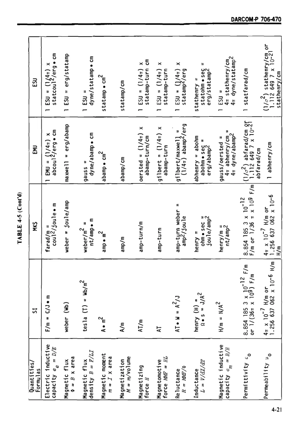
4-6	ELECTROMAGNETIC UNITS .......................... 4-18
4-7	EQUATIONS ...................................... 4-19
4-7.1	DIMENSIONAL ANALYSIS OF EQUATIONS............... 4-22
4-7.2	MODIFICATION OF EQUATIONS FOR USE IN THE SI .... 4-23
REFERENCES ..................................... 4-27
CHAPTER 5
CONVERSION FACTORS, MEASURED CONTANTS,
AND DIMENSIONLESS CONSTANTS
REFERENCES ....................................... 5-1
CHAPTER 6
METRIC^T ON OF ENGINEERING DRAWINGS
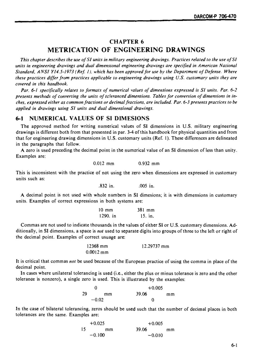
6-1	NUMERICAL VALUES OF SI DIMENSIONS ................. 6-1
6-2	CONVERSION OF TOLERANCED DIMENSIONS TO SI UNITS ... 6-2
6-2.1	GENERAL CONSIDERATIONS ............................ 6-2
6-2.2	TOLERANCED DIMENSIONS WITHOUT ABSOLUTE LIMITS ..... 6-3
6-2.3	DIMENSIONS WITH ABSOLUTE LIMITS.................... 6-5
6-2.4	SPECIAL SITUATIONS ................................ 6-6
6-2.5	INCH-MILLIMETRE CONVERSION TABLES ................. 6-8
ii
DARCOM-P 706-470
TABLE OF CONTENTS (cont’d)
Paragraph	Page
6-3	FORMATS FOR DIMENSIONING IN MILITARY ENGINEERING
DRAWINGS ..................................... 6-8
6-3.1	ENGINEERING DRAWINGS USING U.S. CUSTOMARY UNITS ...	6-11
6-3.2	ENGINEERING DRAWINGS USING SI UNITS ............... 6-11
6-3.3	DUAL DIMENSIONING.................................. 6-11
6-3.4	DUAL DIMENSIONING, TABULAR FORMAT ................. 6-14
REFERENCES .................................... 6-14
CHAPTER 7
EXAMPLES
7-1	BODY DIMENSIONS FOR USE IN EQUIPMENT DESIGN ........ 7-1
7-2	GRILLE FACE AIR VELOCITY............................ 7-6
7-3	EFFECTS OF WORKING ENVIRONMENT
ON HUMAN PERFORMANCE ............................. 7-7
7-4	CALCULATION OF THERMAL ENERGY ABSORBED BY
VEHICLE BRAKES ................................... 7-8
INDEX ............................................. 1-1
LIST OF ILLUSTRATIONS
Fie. No.	Title	Page
2-1	Plane and Solid Angle SI Units ....................................... 2-5
4-1	Temperature Unit Conversions .......................................... 4-17
6-1	Reference Planes in Truncated Cone ................................... 6-7
6-2	Dual Dimensioned Drawing Using [ ] Notation ........................... 6-15
6-3	Dual Dimensioned Drawing Using Positional Notation .................... 6-16
6-4	Tabular Listing of Inch-Millimetre Equivalents in Engineering Drawing . 6-17
7-1	US Amry Men (1966): Breadth and Circumference Measurements ........... 7-2
7-2	US Army Men (1966): Standing and Sitting Measurements ................ 7-4
7-3	Grille Airflow Test Set-up and Instrumentation Diagram................ 7-6
7-4	Construction of Graph Coordinates With Different System of Units ..... 7-9
LIST OF TABLES
Table No.	Title	Page
2-1	Base Units......................................................... 2-2
2-2	Supplementary Units................................................ 2-4
2-3	The International System of Units ................................. 2-7
2-4	SI Prefixes .......................................................... 2-14
3-1	Avoid Mixed Units ................................................. 3-1
DARCOM-P 706-470
CHAPTER 1
INTRODUCTION
1-1 GENERAL
For most scientific and technical work it generally is accepted that the international System of Units (SI)
is superior to all other systems of units. The SI is the most widely accepted and used language for scientific
and technical data and specifications. The National Aeronautics and Space Administration (NASA) and
the Environmental Protection Agency (EPA) now require that all contractor and internal reports use SI
units. In 1975, the Deputy Secretary of Defense established policies (1) of using the “international metric
system” (i.e., the SI) in all activities of the Department of Defense (DOD) consistent with operational,
economical, technical, and safety considerations; and (2) of considering the use of the SI in the procure-
ment of all supplies and services and particularly in the design of new materiel. These new policies of the
DOD establish clearly a trend of increasing use of the SI within the DOD and in particular in the US Army
Materiel Development and Readiness Command (DARCOM), and establish the need for this handbook.
The general purpose of this handbook is to prepare DARCOM personnel — technicians and engineers
— for increased use of the SI, or as it is generally referred to, the metric system. This means, specifically,
giving DARCOM personnel (1) the tools required to convert the units of physical quantities and equations
to SI units, (2) the information needed to interpret specifications and the results of the work of others
expressed in SI units, and (3) the information needed to write specifications and document their own work
in SI units. Additionally, information on the history of metrication in the United States is presented in par.
1-3.
1-2 ORGANIZATION OF HANDBOOK
The organization of this handbook is intended to facilitate use of the information presented herein by in-
dividuals in DARCOM. Each chapter addresses specific and related aspects of the International System of
Units, its use, and the conversion of the units of quantities and equations. To the extent practical, each
chapter is presented such that it can be read, understood, and used without studying the entire handbook or
even the preceding chapters. For example, Chapter 4 can be studied for the purpose of learning how to con-
vert the units of quantities and equations independently of the remainder of the handbook.
The following outline of the contents of the handbook, chapter-by-chapter, can be used as a guide to the
user of this handbook:
1.	CHAPTER 2 THE INTERNATIONAL SYSTEM OF UNITS. This chapter contains all information
related to what constitutes the SI. This includes the definitions of SI units, brief descriptions of the develop-
ment and evolution of metric units, and prefixes that are used with the SI units. Table 2-3, in particular,
should be consulted when there are questions concerning what units are SI or are non-SI but may be used
with SI units. Additionally, Table 2-3 contains references to pages in this handbook which contain informa-
tion related to specific units and categories of units.
2.	CHAPTER 3 GUIDELINES FOR THE USE AND APPLICATION OF THE INTERNATIONAL
SYSTEM OF UNITS. This chapter is intended to assist in achieving uniformity in the use of SI units in
reports and documentation (with the exception of engineering drawings which are covered in Chapter 6).
Subjects covered include proper use of prefixes, the formation of derived units, numerical value format,
and spelling. Table 3-7 lists preferred prefixes for specific units, exceptions to the rules for prefixes and
derived units, and special non-SI units which are used in specific industries and disciplines.
3.	CHAPTER 4 CONVERSION OF UNITS. Methods for converting the units of quantities and
equations are presented in this chapter. Dimensional analysis is the basis for the conversion method;
dimensional analysis is not treated rigorously but as a practical and logical tool. Basic concepts in
mechanical and electromagnetic quantities are presented to facilitate the conversion of mechanical and
1-1
DARCOM-P 706-470
electromagnetic units. Significant digits and accuracy of measurement and estimates as they relate to con-
version of units are covered.
4.	CHAPTER 5 CONVERSION FACTORS AND NUMERICAL FACTORS. Unit conversion factors
are listed both alphabetically and by category of physical quantity. Also presented are lists of “dimen-
sionless” constants and physical constants in SI units.
5.	CHAPTER 6 ENGINEERING DRAWINGS. The use of SI units in engineering drawings, including
“dual dimensioning”, is covered in this chapter. Methods for converting toleranced dimensions to SI are
presented.
6.	CHAPTER 7 SAMPLE CALCULATIONS. Examples of conversion to SI units of quantities,
equations, graphs, and tables taken from a number of US Army Materiel Command Engineering Design
Handbooks are presented.
The remainder of Chapter 1 relates a brief history of metrication in the U.S.
1-3 METRICATION IN THE UNITED STATES
The history of metrication in the U.S. is one of proposals, consideration, and, until recently, little action.
This history is covered adequately and at various levels in a number of sources (Refs. 1,2, and 3). Some of
the most interesting and important events of the past 200 yr are presented in the paragraphs that follow:
1790: Thomas Jefferson proposed a decimal system of weights and measures in a report accepted by
Congress. Jefferson’s system was based on a unit of length, a “new foot”, which was approximately equal
to the “old foot” and was based upon the swing of a standard pendulum. This pendulum having a period of
two seconds was also to be the time standard for the U.S. The new foot was to be divided into ten new in-
ches and was to be the basis for deriving standard units for area, volume, weight, and force. The proposal
was not adopted by Congress. (At this time, the Paris Academy of Sciences was developing a radically
different system based upon scientific principles and a unit of length named the metre defined as a specific
fraction of the earth’s circumference. Decimal relationships were established for forming larger and smaller
units of length and other quantities.)
1821: John Quincy Adams proposed to the Congress a two-phase plan which would lead to an inter-
national and uniform metric system of measurement. Adams clearly identified five advantages of the metric
system: the “invariable” standard of length, the single unit for weight and single unit for volume, the
decimal relationship between units, the relationship of weight units to French coinage, and the uniform and
precise terminology. Congress again took no action on Adam’s proposal.
1832: The Treasury Department adopted English standards to meet the needs of customs houses.
1863: A committee of the National Academy of Sciences (which had been formed by President Lin-
coln) was appointed at the request of the Secretary of the Treasury to reconsider weights, measures, and
coinage. This committee submitted a report favorable to adoption of the metric system. The report was
received with approval by Congressman John A. Kasson, chairman of the newly established House Com-
mittee on Coinage, Weights and Measures. Consequently, this same House Committee reported favorably
to the Congress three metric bills which were eventually passed in 1866. These bills provided for the
following:
1.	Use of the metric system was legalized.
2.	Use of metric scales for foreign mail was directed.
3.	Distribution of metric standards to the states was directed.
1873: Considerable public interest had developed along with strong controversy among educators con-
cerning the advantages of adopting the metric system. In 1873, the American Metrological Society was
founded and did much to inform people about the metric system and to maintain interest in and considera-
tion of the metric system.
1875: Following five years of meetings in Paris, seventeen nations including the U.S. ratified the Treaty
of the Metre. This convention and treaty accomplished the following: the metric system was reformulated
1-2
DARCOM-P 706470
and the accuracy of its standards was refined, the construction of new physical standards and distribution
of copies to member nations was provided for, organization and machinery for international action on
weights and measures was established, and the International Bureau of Weights and Measures was created.
1893: The Secretary of the Treasury by administrative order established the new metric standards of
length and mass as the fundamental standards of the U.S. The U.S. customary units — yard, pound, etc. —
were defined as fractions of the standard metric units.
The most significant events in the preceding are the Act of 1866 which legalized the metric system and the
1893 administrative order establishing metric standards as fundamental standards of the U.S. These es-
tablish a legal basis for voluntary metrication by industrial and governmental sectors of the country. They
are, in fact, the legal basis for all metrication activities in the U.S. at the present.
1896: A bill making the metric system the only legal system was passed by Congress, but, in a recon-
sideration of the bill, it was sent back to committee and never reappeared. Following the failure of this bill,
the arguments for and against metrication solidified and there was much controversy and no action. At the
turn of the century the opposition was so strong that proponents of metrication gave up for a number of
years.
1916: The American Metric Association was formed in New York. One year later the World Trade
Club, a pro-metric organization, was established in San Francisco. In spite of these organizations and as a
result of international economic and political situations, the metric question was not seriously considered
until the 1950’s. Then, the opening of the space age and the reemergence of European nations as industrial
powers again focused attention on the need for an international system of measurement.
1960: The metric system became the common system of measurement for all 43 Treaty of the Metre
signatories including the U.S.
1968: Public Law 90-472 authorizing the Department of Commerce to conduct the United States
Metric Study was passed by Congress.
1975: The Deputy Secretary of Defense established the following policies for all components of the
Department of Defense (Ref. 4):
1. The Department of Defense will use the international metric system in all of its activities consistent
with operational, economical, technical, and safety considerations.
2. Effective immediately, the international metric system will be considered in the procurement of all
supplies and services and particularly in the design of new materiel. It will be used when determined to be in
the best interest of the Department of Defense.
On December 8, 1975, Metric Bill S-100 was passed by the U.S. Senate and signed into law (PL 94-168)
by the President on December 23, 1975 (Ref. 5). This law declares that it is the policy of the U.S. to coor-
dinate and plan the increasing use of the metric system in the U.S., and the law establishes a United States
Metric Board (USMB) to coordinate voluntary conversion to the metric system. This board consists of
seventeen members representing engineers, scientists, manufacturers, commerce, labor, the States, small
business, construction, standards making organizations, educators, consumers, and other interests.
Although the board has no compulsory powers, it is engaged in very important activities that can strongly
influence the course of metrication in the U.S. The board develops and carries out a broad program of
planning, coordination, and public education. Two of the most significant activities of the board are:
1. The preparation of a report to be submitted in one year to the Congress and the President. This report
will make recommendations on the need for and implementation of a structural mechanism for converting
the units used in statutes, regulations, and other laws at all levels of Government.
2. The submission of annual reports to the Congress and the President on the status of metrication and
recommending legislation or executive action needed to implement programs accepted by the board.
REFERENCES
1.	NBS SP 345, A Metric America: A Decision Whose Time Has Come, Dept, of Commerce, National
Bureau of Standards, July 1971.
2.	NTIS AD/A-006 038, The Impact of Metrication on the Defense Standardization Program, Dept, of
1-3
DARCOM-P 706-470
Commerce, National Technical Information Service, November 1974.
3.	American National Standards Institute, Measuring Systems and Standards Organizations, ANSI, NY,
n.d.
4.	National Bureau of Standards, Metric Information Office, Current Metric Activity, July 1975.
5.	Public Law 94-168, 94th Congress, H. R. 8674, December 23, 1975, 89 STAT. 1007-1012.
1-4
DARCOM-P 706-470
CHAPTER 2
THE INTERNATIONAL SYSTEM OF UNITS
The International System of Units, abbreviated SI, as defined in International Standard ISO 1000 (Ref 2) is
described in this chapter. International Standard ISO 1000 was approved by International Organization of
Standards (ISO) Member Bodies from 30 countries including the United States.
The SI consists of the following:
I.	Seven base units
2.	All the derived units
3.	Two supplementary units
4.	The series of approved prefixes for multiples and submultiples of units.
These units, their definitions, their symbols, some information on their evolution to present form, and the for-
mation of multiple and submultiple units are presented in this chapter. Information related to style, use, and
format is given in Chapter 3.
2-1 THE THREE CLASSES OF UNITS IN THE SI
The units of the International System of Units are divided into three classes (Ref. 1):
1.	Base units
2.	Derived units
3.	Supplementary units.
Scientifically and technically this classification is partially arbitrary. The 10th General Conference of
Weights and Measures (1954) adopted as base units of the SI the units of the quantitites: length, mass, time,
electric current, thermodynamic temperature, amount of substance, and luminous intensity which by con-
vention are regarded as dimensionally independent (Ref. 1). Associated with these quantities are seven well-
defined units. This action was taken in the interest of achieving the advantages of having a single, practical,
internationally accepted system for trade, education, science, and technology.
The derived units are the units of quantities that can be formed by combining base quantities and other
derived quantities according to the rules of algebra. The units of these derived quantities are such that no
numerical factors (factors of proportionality) are introduced into the fundamental equations defining these
quantities. Thus the SI — composed of seven base units, a growing number of derived units, and the
supplementary units discussed in the paragraphs that follow and par. 2-4 — forms a coherent system of
units.* Examples of derived quantities are speed, energy, and magnetic flux.
Two units were adopted by the 11th General Conference of Weights and Measures (1960) as supplemen-
tary units primarily because it was not agreed that the two units were either base units or derived units (Ref.
1). The quantities involved are plane angle and solid angle. Actually they may be regarded as base units or
as derived units (Ref. 2).
2-3 BASE UNITS OF THE SI
2-3.1 SUMMARY
The SI is based on the units of seven physical quantities which by convention are considered dimen-
sionally independent and by international agreement and acceptance are uniformly defined. The quantities,
unit names, and symbols are given in Table 2-1 (Ref. 2).
* A coherent system of units is one in which all derived units can be expressed as products of ratios of the
base units (and, in the SI, the supplementary units) without the introduction of numerical factors.
2-1
DARCOM-P 706-470
TABLE 2-1
BASE UNITS
Quantity	Base Unit name	Symbol
length	metre	m
mass	kilogram	kg
time	second	s
electric current	ampere	A
thermodynamic temperature	kelvin	К
amount of substance	mole	mol
luminous intensity	candela	cd
2-2.2 DEFINITIONS OF BASE UNITS
The seven base units of the SI are defined, as follows, in International Standard ISO 1000 (Ref. 2):
1.	metre. The metre is the length equal to 1 650 763.73 wavelengths in vacuum of the radiation cor-
responding to the transition between the levels 2p10 and 5dj of the krypton-86 atom.
2.	kilogram. The kilogram is the unit of mass; it is equal to the mass of the international prototype of the
kilogram.
3.	second. The second is the duration of 9 192 631 770 periods of the radiation corresponding to the tran-
sition between the two hyperfine levels of the ground state of the cesium-133 atom.
4.	ampere. The ampere is that constant electric current which, if maintained in two straight parallel con-
ductors of infinite length, of negligible circular cross-section, and placed 1 metre apart in vacuum, would
produce between these conductors a force equal to 2 X 10-7 newton per metre of length.
5.	kelvin. The kelvin unit of thermodynamic temperature, is the fraction 1/273.16 of the thermodynamic
temperature of the triple point of water.
6.	mole. The mole is the amount of substance of a system which contains as many elementary entities as
there are atoms in 0.012 kilogram of carbon 12. When the mole is used, the elementary entities must be
specified and may be atoms, molecules, ions, electrons, other particles, or specified groups of such particles.
7.	candela. The candela is the luminous intensity, in the perpendicular direction, of a surface of 1/600
000 square metre of a black body at the temperature of freezing platinum under a pressure of 101 325 new-
tons per square metre.
2-2.3 DISCUSSION OF BASE UNITS
The paragraphs that follow are intended to give some insight into the evolution of the base units of the
SI. The General Conference of Weights and Measures (CGPM) is referred to frequently in the presenta-
tion. The CGPM is one of the bodies of the International Organization of Weights and Measures founded
in Paris in 1875 by the Treaty of the Metre (Ref. 3). The CGPM coordinates, reviews, and acts in the in-
terests of its member nations on matters related to uniformity in weights and measures. The organization
recognizes only the metric system.
2-2.3.1 Unit of Length
The present definition of the metre was adopted by the General Congress of Weights and Measures in
1960 (Ref. 1). Originally the metre was chosen as one 40-millionth of the meridian through Paris (Ref. 4).
The original determination of this length was used to build an international prototype of platinum-iridium
(a physical standard). Because of inaccuracies in measuring one 40-millionth of the meridian, the physical
standard itself became the accepted basis for the metre instead of the original definition.
Because of the desirability of being able to reproduce the length of one metre at different locations and
without depending on one primary physical standard, the presently accepted definition of the metre was
developed. This definition in terms of a specific number of wavelengths of light of a precise frequency and
corresponding to a specific transition between two electron energy levels of the krypton-86 atom allows for
2-2
DARCOM-P 706-470
the recreation of a primary standard in some laboratories throughout the world. The original platinum-
iridium prototype is still maintained at Sevres, France, by the International Bureau of Weights and
Measures.
2-2.3.2 Unit of Mass
Probably the definition of the kilogram should be written:
The kilogram is the unit of mass [and it is not the unit of weight or of force]; it is
equal to the mass of the international prototype of the kilogram.
Confusion about what units are force or weight and mass, and how to convert from one to the other is like-
ly the most significant problem encountered in working with systems of units.*
The 1st CGPM in 1889 legalized the international prototype of the kilogram (Ref. 1). This platinum-
iridium prototype is the world’s primary standard for the kilogram and it is maintained at Sevres under
conditions specified by the CGPM in 1889. Secondary standards of platinum-iridium or stainless steel are
made by direct comparison with the primary standard at Sevres.
Of the seven base units of the SI, the kilogram is the only one not defined in terms of physical
measurements that can be made in a properly equipped laboratory. It is the only base unit with a prefix;
i.e., kilo-.
2-2.3.3 Unit of Time
The original definition of the unit of time, the second, was a fraction, 1 /86 400, of the mean solar day
(Ref. 1). Measurements of the mean solar day have demonstrated, however, that irregularities in the earth’s
rotation do not allow the desired accuracy. The 11th CGPM in I960 adopted a new definition of the second
based on the tropical year. This resulted in improved precision. By that time, research results demonstrated
that an atomic standard based on transitions between energy levels in an atom or molecule was practical
and resulted in greater precision. Thus, the 13th CGPM in 1967 adopted the present definition based on
transitions between hyperfine lines of the ground state of the cesium-133 atom.
2-2.3.4 Unit of Electric Current
The present definition of the ampere was adopted by the 9th CGPM in 1948. This replaced an earlier
“international” ampere which had been adopted around 1900 (Ref. 1). Note that the definition of the
ampere is the same in the SI and in the customary system of units used in the U.S.
2-2.3.5 Unit of Thermodynamic Temperature
The 10th CGPM in 1954 selected the triple point of water as a fundamental fixed point and assigned to it
the temperature 273.16 degree Kelvin (symbol °K) (Ref. 1). The 13th CGPM in 1967 adopted the name
kelvin (symbol K) in place of the degree Kelvin and defined the unit of Thermodynamic Temperature as
given in the preceding. At the same time it was decided that the unit kelvin and its symbol К should also be
used to express an interval or a difference of temperature.
Z(°C) = 71(K) - 273.15	(2-1)
where t is Celsius temperature and T is thermodynamic temperature.
The assigned value of 273.16 kelvin as the thermodynamic temperature at the triple point of water and
equation t = T - 273.15K defining the Celsius temperature scale imply that at a thermodynamic
temperature of 0 К the Celsius temperature is -273.15 °C and not -273.16 °C, and that at the triple point
of water the Celsius temperature is 0.01 °C. This is correct!
2-2.3.6 Unit of Amount of Substance
Units of amount of substance such as “gram-atom” and “gram-molecule” have been used to specify
amounts of chemical elements and compounds (Ref. 1). These units were related to atomic weight and
molecular weight which are, in fact, relative masses. Atomic weight was originally referred to as the atomic
•Mass, weight, force, acceleration and their associated units are discussed at length in Chapter 4.
2-3
DARCOM-P 706-470
weight of oxygen which by general agreement was 16. Physicists generally assigned the atomic weight 16 to
one of the isotopes of oxygen; chemists assigned the same atomic weight to naturally occurring oxygen — a
variable mixture of isotopes 16, 17, and 18. In 1960 chemists and physicists agreed that atomic weight
should be assigned to carbon 12, thus resulting in a unified scale of relative atomic mass.
The unit of amount of substance is the mole (symbol mol) and it is based on the number of atoms in
0.012 kilogram of carbon 12. The mass 0.012 kilogram was selected by international agreement.
2-2.3.7 Unit of Luminous Intensity
The units of luminous intensity prior to 1948 were based on frame or incandescent filament standards
(Ref. 1). The International Commission on Illumination proposed a “new candle” as a standard for
luminous intensity which was adopted by the 9th CGPM in 1948. The new candle is a black body of specific
area at very precise temperature and pressure. The unit of luminous intensity thus defined was given the
name candela in 1948.
2-3 SUPPLEMENTARY UNITS
At present, there are only two units, both purely geometrical, in the SI which are classified as supplemen-
tary. They are presented before derived units because they may be used in derived units. Thus, for practical
purposes these supplementary units may be regarded as base units.
The supplementary quantities are plane angle and solid angle as given in Table 2-2 (Ref. 2).
TABLE 2-2
SUPPLEMENTARY UNITS
Quantity	Supplementary Unit	Symbol
plane angle	radian	rad
solid angle	steradian	sr
The radian and steradian are defined in International Standard ISO 1000 as follows (Ref. 2):
1. radian. The radian is the plane angle between two radii of a circle which cut off on the circumference
an arc equal in length to the radius.
2. steradian. The steradian is the solid angle which, having its vertex in the center of a sphere, cuts off an
area of the surface of the sphere equal to that of a square with sides of length equal to the radius of the
sphere.
These definitions are illustrated in Fig. 2-1. Note that there are 2ir radians of plane angle in a complete
circle and there are 4ir steradians of solid angle in a complete sphere.
The use of degree (symbol °) and its decimal submultiples is permissible when use of the radian is not
convenient. Solid angle always should be expressed in steradians (Ref. 5).
2-4
DARCOM-P 706-470
Length of arc cut off by two
radii at an angle of one radian
is equal to the radius of the
circle.
(A)	Radian—construction of definition
Sphere
Area of surface of sphere
cut off by solid angle of
one steradian is R2 where
R is radius of the sphere.
Solid angle of one radian
Center of sphere
(B)	Steradian—construction of definition
Figure 2-1. Plane and Solid Angle SI Units
2-5
DARCOM-P 706-470
2-4 DERIVED UNITS
Derived units are units of physical quantities derivable from the set of base quantities (accepted as
dimensionally independent), from the supplementary geometrical quantities, and from other previously
formulated and accepted derived quantities. As the SI is a coherent system, and it is highly desirable that it
remain such, all derived quantities and their units should be formulated such that no numerical factors are
introduced.
Representative derived units are presented in Table 2-3 (Refs. 1, 2, 5, and 6). The base units and
supplementary units are repeated here for convenience. References to other paragraphs of this handbook
are included to allow rapid access to relevant information on style, use, and conversion of units. Entries in
Table 2-3 are presented in the following groups:
1.	Base units
2.	Supplementary units
3.	Units derived from base units
4.	Derived units with special names
5.	Other derived units
6.	Non-SI units used with the SI
7.	Experimentally determined units used with the SI
8.	Units used with the SI for a limited time.
Units in Groups 6, 7, and 8 are included, again, for convenience.
2-6
TABLE 2-3
THE INTERNATIONAL SYSTEM OF UNITS (Refs. 1, 2, 5, 6)
UNIT CATEGORY	QUANTITY	UNIT NAME	UNIT SYMBOL	EXPRESSION IN TERMS OF OTHER UNITS	EXPRESSION IN TERMS OF SI BASE UNITS
SI Base Units	length	metre	m		m
	mass	kilogram	kg		kg
	time	second	s		s
	electric current	ampere	A		A
	thermodynamic temperature	kelvin	К		К
	amount of substance	mol e	mol		mol
	luminous intensity	candela	cd		cd
SI Supplementary Uni ts	plane angle solid angle	radian steradian	rad sr		
Units Derived from Base Units	area volume	square metre cubic metre	m2 m3		m2 m3
	speed, velocity	metre per second	m/s		m/s
	acceleration	metre per square second	m/s2		m/s2
	angular velocity	radian per second	rad/s		rad/s
	angular acceleration	radian per square second	rad/s2		rad/s2
DARCOM-P 706-470
TABLE 2-3. (cont’d)
KJ
00
UNIT CATEGORY	QUANTITY	UNIT NAME	UNIT SYMBOL	EXPRESSION IN TERMS OF OTHER UNITS	EXPRESSION IN TERMS OF SI BASE UNITS
Units Derived from Base Units (Cont'd)	wave number	1 per metre	1/m		1/m
	density, mass densi ty	kilogram per cubic metre	kg/m3		kg/m3
	concentration (of amount of substance)	mole per cubic metre	mol/m3		mol/m3
	ki nematic viscosity	square metre per second	m2/s		m2/s
	activity (radioactive)	1 per second	1/s		1/s
	specific volume	cubic metre per kilogram	m3/kg		m3/kg
	1umi nance	candela per square metre	cd/m2		2 Cd/ill
Derived Units With Special Names	frequency force	hertz newton	Hz N		1/S 2 kg • m/s
	pressure, stress	pascal	Pa	N/m2	kg/(m. s2)
	energy, work quantity of heat	joule	J	N • m	2 2 kg • m/sd
	power, radiant flux	watt	W	J/s	।	2, 3 kg • m /s
	electric charge	coulomb	c		A. s
DARCOM-P 706-470
UNIT CATEGORY
QUANTITY
Derived Units With Special Names (Cont1d)	electric potential potential difference electromotive-force capacitance electric resistance conductance magnetic flux magnetic flux density inductance luminous flux illuminance
Other Derived Units	dynamic viscosity moment of force surface tension heat flux density, i rradiance
ю
TABLE 2-3. (cont’d)
UNIT NAME	UNIT SYMBOL	EXPRESSION IN TERMS OF OTHER UNITS	EXPRESSION IN TERMS OF SI BASE UNITS
vol t	V	W/A	kg.m2/(s3. A)
farad	F	c/v	A2 • s4/(m2. kg)
oh	я	V/A	kg .m2/(s3. A2)
siemens	S	A/V	Az • sJ/(nT • kg)
weber	Wb	V • s	kg »m2/(s2. A)
tesla	T	2 Wb/m	kg/(s2. A)
henry	H	Wb/A	9	9	9 kg »m /(s". A )
1 umen	Im		cd • sr
1 ux	lx	9 Im/m	cd • sr/m
pascal second	Pa. s	Pa. s	kg/(m. s)
newton metre	N. m	N* m	kg • m2/s2
newton per metre	N/m	N/m	kg/s2
watt per square metre	W/m2	W/m2	kg/s3
DARCOM-P 706-470
2-10
UNIT CATEGORY	QUANTITY
Other Derived Units (Cont'd)	heat capacity, entropy specific heat capacity, specific entropy specific energy thermal conductivity energy density electric field strength electric charge densi ty electric flux densi ty permittivity current density
TABLE 2-3. (cont’d)
UNIT NAME	UNIT SYMBOL	EXPRESSION IN TERMS OF OTHER UNITS	EXPRESSION IN TERMS OF SI BASE UNITS
joule per kelvin	J/K	J/K	kg* m2/(s2« K)
joule per kilogram kelvin	J/(kg. K)	J/(kg • k)	m2/(s2. K)
joule per kilogram	J/kg	J/kg	m2/s2
watt per metre kelvin	W/(m. K)	W/(m. K)	kg • m/(s3» K)
joule per cubic metre	J/m3	J/m3	kg/(m* s2)
volt per metre	V/m	V/m	kg • m/(s3» A)
coulomb per cubic metre	C/m3	C/m3	A • s/m3
coulomb per square metre	C/m2	C/m2	2 A • s/iti
farad per metre	F/m	F/m	A2. s4/(m3» Kg)
ampere per square metre	A/m2		A/m2
DARCOM-P 706-470
TABLE 2-3. (cont’d)
UNIT CATEGORY	QUANTITY	UNIT NAME	UNIT SYMBOL	EXPRESSION IN TERMS OF OTHER UNITS	EXPRESSION IN TERMS OF SI BASE UNITS
Other Derived Units	magnetic field	ampere per	A/m		A/m
(Cont'd)	strength	metre			
	permeability	henry per metre	H/m	H/m	kg *т/(52* A2)
	molar energy	joule per mole	J/mol	J/mol	kg • m2/(s2* mol)
	molar entropy,	joule per	J/(mol• K)	J/(mol« K)	kg • m2/(s2*K* mol)
	molar heat	mole			
	capacity	kelvin			
	radiant intensity	watt per steradian	W/sr	W/sr	kg • m2/(s3 • sr)
	radiance	watt per	W/(m2» sr)	W/(m2» sr)	kg/(s3. sr)
		square metre steradian			
Non-SI Units Used	time	minute	min		60 s
With the SI	time	hour	h	60 min	3 600 s
	time	day	d	24 h	86 400 s
	plane angle	degree	0		(tt/180) rad
	plane angle	minute	1	(1/60)°	(n/10 800) rad
	plane angle	second	II	(1/60)'	(V648 000) rad
DARCOM-P 706-470
TABLE 2-3. (cont’d)
2-12
UNIT CATEGORY	QUANTITY	UNIT NAME	UNIT	EXPRESSION SYMBOL	IN TERMS OF OTHER UNITS	EXPRESSION IN TERMS OF SI BASE UNITS
Non-SI Units Used With the SI (Cont'd)	volume mass	litre tonne	t	dm3 t	IO’3 m3 Ю3 kg
	Celsius Temperature	degree Celsius	°C	
	International Practical Kelvin (Celsius) Temperature Scale	kelvin (degree Cel si us)		
Experimental ly- Determined Units Used With the SI (Other experimentally- determined units are listed in Table 5-3.)	kinetic energy mass length	electronvolt	eV	1.602 19xlO"^J unified atomic	u mass unit astronomical	AU-English unit	UA-French AE-German		1.602 19xl0’19kg • m2/s2 1.660 53xl0’27kg 149 000 x IO6 m
	length	parsec	pc	206 265 AU	30 857x1012 m
Units Used With the SI for a Limited Time	length	nautical mi le		1 852 m
	speed	knot	nautical mile/h	(1 852/3 600)m/s
	length	angstrom	A	0.1 nm	10”10m
DARCOM-P 706-470
TABLE 2-3. (cont’d)
2-13
UNIT CATEGORY	QUANTITY	UNIT NAME	UNIT SYMBOL	EXPRESSION IN TERMS OF OTHER UNITS	EXPRESSION IN TERMS OF SI BASE UNITS
Units Used With the SI for a Limited Time	area	are	a		ln2 2 10 m
(Cont'd)	area	hectare	ha		104m2
	area	barn	b		10-28m2
	pressure	bar	bar	105 Pa	Ю5 kg/m • s2
	pressure	standard atmosphere	atm	101 325 Pa	2 101 325 kg/m»s
	acceleration	gal	Gal	2 1 cm/sd	10"2 m/s2
	activity (radioactive)	curie	Ci		3.7 xlO1O/s
	exposure (X or Y radiation)	roentgen	R	2.85 x 10'4C/kg	2.85x10 4A• s/kg
	dose (radioactive)	rad	rad, rd	-2 10 J/kg	10”2 m2/s2
DARCOM-P 706-470
DARCOM-P 706-470
2-5 MULTIPLE AND SUBMULTIPLE PREFIXES
The 11th CGPM in 1960 adopted a series of names and symbols of unit prefixes to form decimal mul-
tiples and submultiples of SI units. In 1964, the 12th CGPM added prefixes for the submultiples 10” and
10"1’ (Ref. 1). The complete series is given in Table 2-4.
TABLE 2-4
SI PREFIXES
Multiplication Factors	Prefix	SI Symbol
1 000 000 000 000 000 000 = 1018	exa	E
15 1 000 000 000 000 000 = 10	peta	P
12 1 000 000 000 000 = 10 4	tera	T
9 1 000 000 000 = 10s	giga	G
1 000 000 = IO6	mega	M
1 000 = 103	kilo	к
2 100 = io4	* hecto	h
	*	
10 = io1	deka	da
0.1 = io“]	* deci	d
-2 0.01 = 10 c	* centi	c
0.001 = 10"3	mi 11 i	m
0.000 001 = IO"6	micro	Ц
-9 0.000 000 001 = 10 3	nano	n
-12 0.000 000 000 001 = 10	pi co	p
-15 0.000 000 000 000 001 = 10 10	femto	f
0.000 000 000 000 000 001 = 10“18	atto	a
★
To be avoided where possible.
2-14
DARCOM-P 706-470
To form a multiple of, for example, the metre, such that a unit 1000 times larger than the metre is
formed, the prefix kilo is added forming kilometre (symbol km). The unit kilometre is 103 or 1000 times as
large as the metre. The unit which is smaller than the second by a factor of 10’ is the nanosecond (symbol
ns), i.e., the nanosecond = 10’ second. Conversions of multiple and submultiples are covered in Chapter 4.
Rules for approved uses of multiple and submultiple prefixes are given in Chapter 3.
REFERENCES
1.	NBS 330, The International System of Units (SI), Dept, of Commerce, National Bureau of Standards,
April 1972.
2.	International Organization for Standardization, SI Units and Recommendations for the Use of Their
Multiples and Certain Other Units, International Standard ISO 1000, ISO, Switzerland, 1973.
3.	American National Standards Institute, Measuring Systems and Standards Organizations, ANSI, NY,
n.d.
4.	A. G. Chertove, Units of Measurement of Physical Quantities, translated by Scripta Technica, Inc.,
revised by Herbert J. Eagle, Hayden Book Company, Inc., NY, 1964.
*5. American National Standards Institute, American Society for Testing and Materials, Standard for
Metric Practice, ASTM E 380, ANSI NY, January 1976.
6. National Aeronautics and Space Administration, The International System of Units: Physical Constants
and Conversion Factors, by E. A. Mechtly, rev. ed., NASA Office of Technology Utilization, Scientific
and Technical Information Division, Washington, DC, 1969.
*This publication is listed in the DOD Index of Specifications and Standards and is available without cha|rge
to US Government agencies through Naval Publications and Forms Center, 5801 Tabor Ave.,
Philadelphia, PA.
2-15
DARCOM-P 706-470
CHAPTER 3
GUIDELINES FOR USE AND APPLICATION OF THE
INTERNATIONAL SYSTEM OF UNITS
Guidelines for use of the International System of Units are presented in this chapter. The information
presented covers style, spelling, notation, selection of units, and selection of prefixes in using the SI and other
units which can be used with the SI. Use of the SI in engineering drawings is covered in Chapter 6.
The information presented here is taken from both national and international standards and documents on
the SI and its use. Where differences exist between U.S. and international recommended practices (there are
surprisingly few), the U.S. recommended practice is given. The Standard for Metric Practice, ASTM E 380,
(Ref 1) which has been approved for use by the Department of Defense was one of the primary sources of infor-
mation for this chapter.
It should be recognized that units, unit names and symbols, and practices have evolved to their present status
and it is very likely that further changes will be made. It is important that scientists, engineers, and technicians
stay informed of new standards and practices related to the SI. Additionally, in using existing documentation
and data, it is important to determine those practices that were used therein and that could affect understand-
ing and use of the data.
3-1 GENERAL USE OF SI
The units of the SI should be used in place of the units of all other systems of units; this implies the use of
base units, supplementary units, and derived units with appropriate application of approved multiple and
submultiple prefixes. In order to maintain the coherence of the SI, it is recommended that multiples and
submultiples of SI units not be used in combinations to generate derived units and not be used in equations.
Note that the kg is a base unit and is correctly used both in the formation of derived units and in equations.
3-2 MIXED UNITS
A mixed unit is a derived unit which contains units from two or more different systems of units or it is a
unit containing different units for the same dimension. For example, mass per unit volume expressed in
kilograms per gallon (kg/gal) uses units from the SI and U.S. customary units. Examples involving
different units for the same dimension are: plane angle, 10 deg 15 min; mass, 12 Ibm 12 ozm*. Mixed units
such as these should be avoided. The correct units for these examples are given in Table 3-1.
TABLE 3-1
AVOID MIXED UNITS
Use	Do Not Use
kg/m3	kg/gal
0.1789 rad or 10.25 deg	10 deg 15 min
12.75 Ibm*	12 Ibm 12 ozm*
3-3 USE OF PREFIXES
The use of approved prefixes as given in Table 2-4 is to eliminate insignificant digits and decimals, and to
provide a convenient substitute for writing powers of ten. Typical examples are given in Table 3-2.
*See par. 4-3.2 for an explanation of pound-mass (Ibm).
3-1
DARCOM-P 706-470
TABLE 3-2
USE OF PREFIXES
Quantities Without
Use of Prefixes
Preferred Form
12 300 m = 12.3 x 103 m 12.3 km
0.0123g A = 12.3 x 10-’A	12.3 nA
0.000 219 kg = 219. x 10~‘ kg 219 mg
In selecting specific prefixes, it is recommended that multiples and submultiples of 1000 be used to the ex-
tent feasible. For example, the units of force which should be used most frequently are MN, kN, N, mN,
etc.; and, in the case of length, km, m, mm, gm, nm, etc. should be used. Thus, unless a real advantage is
realized, centimetre (cm) should be avoided. However, in the cases of area and volume used alone, cm2 and
cm3 are frequently and acceptably used. Note that with units of order higher than one, such as m2 and m3,
when a prefix is used as in cm2 and cm3, the power of 10 represented by the prefix is raised to the same
order. Thus,
cm3 = (cm)3 = (10-2 m)3 = 10_‘ m3	(3-1)
In general, prefixes should be used such that the numerical part of the expression for a particular quanti-
ty is greater than 0.1 and less than 1000 except where certain prefixes have been agreed upon for specific
situations. In tables and tabulations, the same prefix should be used for a quantity even though, as a result,
tabulated numerical values fall outside the range 0.1 to 1000 (Ref. 1).
Double and hyphenated prefixes should never be used. As examples: use picofarad (pF) and not micro-
microfarad (ggF); and, use gigawatt (GW) and not kilo-megawatt (kMW).
With the exception of the kilogram (kg), prefixes should not be used in the denominator of compound
units. Prefixes may, however, be used in the numerator of compound units. Examples of such correct and
incorrect uses of prefixes are given in Table 3-3 (Ref. 1).
TABLE 3-3
USE OF PREFIXES IN COMPOUND UNITS
Preferred	Not to be Used
N/m2	N/cm2 or N/mm2
kN • s/m2 or N • s/m2	kN • s/mm2
kW/(m • K)orW/(m • K)	kW/(cm • K)
J/kg	mJ/g
3-4 STYLE
Use lower case letters for SI unit symbols unless the unit is derived from a proper name. Thus, use m for
metre, kg for kilogram, and£ for litre, but use Hz for hertz derived from Hertz and N for newton derived
from Newton. Note that the unabbreviated units in all cases whether derived from a proper name or not are
not capitalized. With the exceptions of T for tera, G for giga, and M for mega the SI symbols for all prefixes
are lower case letters.
Unabbreviated SI units form plurals in the same manner as all nouns. The SI symbols on the other hand
are always written in a singular form. Periods are used after SI unit symbols only at the end of a sentence.*
In writing numbers having four or more digits, the digits should be placed in groups of three separated by
a space and formed by counting both to the left and right of the decimal point. The groups of three im-
*The one exception is the abbreviation “in.”, for inch, to avoid being identified as the preposition “in”.
However, should the possibility of error or confusion exist when abbreviations are used, follow the maxim
“when in doubt, spell it out”.
3-2
DARCOM-P 706-470
mediately to the left and right of the decimal point are not separated from the decimal point by a space. In
the case of exactly four digits spacing is optional. This format of writing numbers facilitates both the
reading of the numbers and also avoids confusion caused by the European use of commas to express
decimal points (Ref. 2). These rules are illustrated in Table 3-4.
TABLE 3-4
NUMBER GROUPING IN SI
Use	Do Not Use
1234orl 234	1,234
12 345	12,345
12 345.678 91	12,345.67891
In cases where U.S. customary units must be given in texts or in small tables, it is permissible to give the
SI equivalents in parentheses. However, when equations are written with U.S. customary units, confusion
is avoided by not giving the SI equivalents in parentheses in the equation. Rather, it is preferred to restate
the equation using SI units or to introduce a sentence, paragraph, or note stating precisely how to convert
calculated results to the preferred SI units and giving the factors involved in that calculation.
In expressing derived unit abbreviations, the center dot with a space on each side is used to indicate mul-
tiplication and a slash is used to indicate division (Ref. 1). Examples are:
kg • m/s2
s • A/m3
It should be noted that errors and confusion can be introduced if the center dot is not used in forming
derived units. As an example, consider a quantity encountered frequently in mechanics, moment of force,
which is the product of force and distance. The derived unit for this quantity is the newton-meter; the sym-
bole can be written N • m or m • N. Written without the center dot, Nm would be interpreted correctly
as a newton-meter. But, if the order is changed to mN, the result is the millinewton!
Finally, in using the slash (/) to separate numerator and denominator terms in derived units it is possible
to introduce ambiguities. For example, is the unit m • kg/s3 • К in fact m • kg/(s3 • K) or is it
m • (kg/s3) • K? If all numerator terms were always placed to the left of the slash and all denom^-tor
terms placed to the right of the slash, and, if they were always interpreted in this manner, there would be no
confusion. However, in the interest of avoiding errors it is suggested that parentheses be used with all
denominator terms when there are two or more such terms. Thus for the given example, the units should be
written m • kg/(s3 • K) if second and kelvin belong in the denominator.
Another acceptable and unambiguous method of denoting numerator and denominator terms is to use
positive and negative exponents. Using this notation, the previous example may be written:
kg • m/s2 = kg • m • s-2
c • A/m3 = c • A • m-3
m • kg/(s3 • K.) = m • kg • s-3 • K-1
3-5 METRE/LITRE OR METER/LITER SPELLING
The “-re” spelling of metre and litre has not been accepted in the U.S. (Refs. 3 and 4). However, the
ASTM Standard for Metric Practice has been approved for use by the Department of Defense and for
listing in the DOD Index of Specifications and Standards (Ref. 1). The spelling metre/litre, is used in the
ASTM Standard for Metric Practice. Also, the standard for dimensioning and tolerancing of engineering
drawings that has been adopted by the Department of Defense, ANSI Y14.5-1973, uses the metre/litre
spelling (Ref. 5). Thus, the metre-litre spelling is used in this handbook.
3-3
DARCOM-P 706-470
It is reiterated that this question of spelling has not been settled. It has been suggested, particularly in the
U.S., that the spelling metre/litre will never be widely accepted. It has also been predicted that even if the
“-re” spellings are accepted they will eventually be changed back to the “-er” spellings that we are ac-
customed to.
Finally, it should be noted that the guidelines for use of the International Systems of Units have been in-
terpreted and modified for the U.S. by the National Bureau of Standards and, published in the June 19,
1975 Federal Register, explicitly state that both the “-re” and “-er” spellings for both metre and litre are
acceptable.
3-6 TEMPERATURE
The correct temperature scale to be used in the SI is known as the International Thermodynamic
Temperature Scale (Refs. 1, 2, and 6). The SI unit for temperature is the kelvin (K) which is used for both
temperature and temperature differences and intervals. Note that the degree symbol (°) is not used with
kelvin.
What was formerly called the centigrade scale and is now the Celsius temperature scale is acceptable
because of the vast amount of data recorded using this scale and because of its broad use and familiarity in
general (Ref. 1). The proper unit is the degree Celsius (°C). Note that the degree symbol (°) is used with the
Celsius scale.
The symbols commonly used for temperatures are T when the Kelvin scale is used and 0 or t when the
Celsius scale is used. These symbols should be used only for temperature and not temperature differences.
When differences or intervals are involved, notations such as 7\ - Тг and tx - ty or AT and Az avoid
confusion and ambiguity. The conversion of temperature differences are simple:
1 Kelvin = 1 degree Celsius = 9/5 degree Fahrenheit	(3-2)
and
АДК) = Az(°C) = (5/9) Azf(°F)	(3-3)
The relationship between temperature Texpressed in kelvins and temperature z expressed in degrees Celsius
is:
ЦК) = Z(°C) + 273.15	(3-4)
It is important to note that for a number of years the unit for thermodynamic temperature was the degree
Kelvin and the symbol was °K (Ref. 6). The name for temperature interval or difference was the degree and
the symbol was deg. This latter nomenclature, degree and deg, applied to both the thermodynamic temper-
ature scale and the Celsius temperature scale. The 13th CGPM (1968) adopted the present name kelvin for
thermodynamic temperature and approved the practice of using the same name and symbol for tempera-
ture and temperature interval.
Two additional scales are introduced here because a large amount of data has been recorded based upon
these scales (Ref. 1). They are known as the International Practical Kelvin Temperature Scale of 1968 and
the International Practical Celsius Temperature Scale of 1968. The units for these two scales are the kelvin
(K) and the degree Celsius (°C), respectively. The symbols for temperature commonly used are ДпДог the
Practical Kelvin scale and zint for the Practical Celsius scale. These temperature scales are defined by a set of
interpolation equations based upon the reference temperatures given in Table 3-5. With respect to the
International scales the kelvin and degree Celsius are identical in size and = zint + 273.15 exactly. The
differences between the International Thermodynamic Temperature scale and the International Practical
Temperature scale are significant only when extremely precise measurements are involved.
3-4
DARCOM-P 706-470
TABLE 3-5
REFERENCE TEMPERATURES* UPON WHICH PRACTICAL
TEMPERATURE SCALES ARE BASED
К
Hydrogen, solid-liquid-gas equilibrium		...	13.81	-259.34
Hydrogen, liquid-gas equilibrium at 33 330.6 N/m2 (25/76 standard atmosphere)....	17.042	-256.108
Hydrogen, liquid-gas equilibrium		20.28	-252.87
Neon, liquid-gas equilibrium		27.102	-246.048
Oxygen, solid-liquid-gas equilibrium		54.361	-218.789
Oxygen, liquid-gas equilibrium		90.188	-182.962
Water, solid-liquid-gas equilibrium		... 273.16	0.01
Water, liquid-gas equilibrium		... 373.15	100.00
Zinc, solid-liquid equilibrium		... 692.73	419.58
Silver, solid-liquid equilibrium		... 1235.08	961.93
Gold, sol id-liquid equilibrium		... 1337.58	1065.43
* Except for the triple points and one equilibrium hydrogen point (17.042 K) the assigned values of tem-
perature are for equilibrium states at a pressure
p0 = 1 standard atmosphere (101 325 N/m2).
3-7 NON-SI UNITS WHICH CAN BE USED WITH SI UNITS
There are a number of units which are not part of the SI which may be used with SI units, or, may be
used with SI units for “a limited time” (Ref 2). Limited time is not specified in the literature. It can
reasonably be assumed that this means that use of such non-SI units with the SI is acceptable only as long
as it can be justified on the basis of realizing significant advantage. The period of time that such use will be
acceptable, in the U.S., is a function of how rapidly metrication proceeds in this country and of the possible
existence of and form of a national program of metrication. It can be argued that this situation will exist for
from 10 to 30 yr into the future.
It is recommended that non-SI units be used only when there is a real advantage. When they are used in
calculations or in any documentation, it should be noted that they are non-SI units and instructions on how
to convert equations and numerical value to the SI should be given.
A number of the non-SI units which are accepted at least for the present are related to units of the SI by
powers often (Ref 1). The bar — a unit of pressure equal to 100 kilonewtons per square metre (105 newtons
3-5
DARCOM-P 706-470
per square metre or 105 pascal) — is a convenient unit of pressure, particularly for meteorologists, because
it is approximately equal to one atmosphere. Another example, from the field of geodetics, is the Gal (from
Galileo), a unit of acceleration equal to 0.01 metre per second squared. While these units are not part of the
International System of Units, they are metric units because they are related to base units by powers of ten.
It is likely that one will encounter some confusion concerning their relationship to the SI.
One of the non-SI units, the litre, is particularly interesting because it is now being introduced to the
public in the U.S. and is considered to be part of the SI even by some scientists and engineers. The most at-
tractive features of the litre as a unit are: (1) it is only slightly larger than the quart, and (2) it is much easier
to use than “one-thousandth of a cubic meter” — particularly in a grocery store.
A final note on these non-SI units concerns their use in derived units. When this is done, the system is no
longer coherent and factors of proportionality are introduced. This can be illustrated by the derivation of a
unit of force using the relationship force F equals mass M multiplied by acceleration A:
F = MA	(3-5)
If the units kilogram and Gal are used for mass and acceleration respectively, then the derived unit for force
will, in this case, be the kilogram • Gal (symbol kg • Gal). Eq. 3-5 is perfectly valid using the units
kilogram, Gal, and kilogram • Gal. Given values for any two of the quantities force, mass, and accelera-
tion, the third can be determined. There are no numerical factors of proportionality introduced into Eq. 3-5
provided all quantities are expressed in the units kg, Gal, and kg • Gal. However, if data resulting from
these calculations are to be used by an individual that is accustomed to working only with base units of the
SI and other units derived from base units, then unnecessary complications will be introduced. This in-
dividual would have to determine what the units Gal and kg • Gal are in terms of base units. He would
find that:
Gal = 10'2 m/s2	(3-6)
and
kg • Gal = kg • (10“2 m/s2) = 10~2 kg • m/s2 = 10-2 N	(3-7)
Eqs. 3-6 and 3-7 allow conversion of the expressions in non-SI units to expressions in SI units. These
equations also illustrate the advantages of maintaining a coherent system of units as defined in Chapter 2
and repeated here: “A coherent system of units is one in which all derived units can be expressed as pro-
ducts or ratios of the base units without the introduction of numerical factors.” If the SI unit for accelera-
tion, m/s2, had been used in the original calculations in this example, there would be no numerical factors
in Eqs. 3-6 and 3-7 and, in fact, there would be no reason for even considering these equations. All that has
been said concerning non-SI units related to SI units by powers of ten is applicable to non-SI units in
general.
3-8 GUIDELINES FOR SELECTION OF UNITS AND PREFIXES
The information presented in Table 3-6 is intended to serve as a guide in selecting units and prefixes. For
each quantity in the table, the appropriate SI unit is given. The commonly used prefix for each unit also is
given. For example, the SI unit for stress is the pascal with the symbol Pa or the newton per metre squared,
N/m2. The commonly used and recognized multiples and submultiples used for stress are: GPa, MPa or
N/mm2, and kPa. Note that one of the recognized units for stress, N/mm2, does not follow the guidelines
for the use of prefixes given in par. 3-3; i.e., prefixes should not be used in the denominator of compound
units. This example illustrates the priority of recognized usage over the general guidelines.
Also included in Table 3-6, are those non-SI units that frequently are used and recognized in certain
areas. For example, in the textile industry, the unit for linear density (kg/m in SI) that is commonly used is
the tex. The tex is related to SI by the equation: 1 tex = 10-6 kg/m. As a further example, the table gives the
units watt-hour (W • h), kW • h, etc., as the commonly used units for energy in the field of consumption
of electrical energy.
3-6
DARCOM-P 706-470
While Table 3-6 is not exhaustive, it should prove to be useful to individuals working outside their field
of expertise or experience. Also, it is emphasized that this information is intended to be a guide only and
not to be interpreted as the only acceptable approach. In general, the most important consideration in
selecting units is that of being understood and minimizing the possibility of errors.
REFERENCES
1.	American National Standards Institute, American Society for Testing and Materials, Standard for
Metric Practice, ASTM E 380, ANSI, NY, January 1976.
2.	International Organization for Standardization, SI Units and Recommendations for the Use of Their
Multiples and Certain Other Units, International Standard ISO 1000, ISO, Switzerland, 1973.
3.	J. L. Wilson, Correspondence, IEEE Transactions on Professional Communication, pp. 74-76, June 1975.
4.	“Metric Terms: -er or -re?”, IEEE Transactions on Professional Communication, pp. 54-62, Vol. PC-17,
No. 3/4, September/December 1974.
5.	American National Standards Institute, Dimensioning and Tolerancing for Engineering Drawings, ANSI
Y14.5-1973, ANSI, NY, 1973.
6.	NBS 330, The International System of Units (SI), Dept, of Commerce, National Bureau of Standards,
April 1972.
3-7
00
TABLE 3-6
GUIDELINES FOR USE OF SI AND NON-SI UNITS (Ref. 2,
QUANTITY	SI UNIT	COMMONLY USED MULTIPLES	NON-SI UNITS COMMONLY USED/MULTIPLES
AND SUBMULTIPLES	AND SUBMULTIPLES/REMARKS
DARCOM-P 706-470
SPACE AND TIME			
length	m (metre)	km cm, mm, pm, nm	1 international nautical mile = 1852 m
area	m2	km2 dm^, cm^, ^2	1 ha (hectare) = 10^m2 1 a (are) = 10^m2
volume	m3	dm^, cm^, ^3	о 1 t (litre) = 1 dm (should not be used for high precision);	r 7 1 h£ = 10"'m3, 1 ci = 1O‘V, 1 m£ = Ю'бщЗ = 1 cm3
ti me	s (second)	ks ms, pS, ns	d (day), h(hour), min (minute) week, month, year are in common use
veloci ty	m/s		km/h (kilometre per hour) = (1/3.6) m/s 1 knot = 0.514 444 m/s
acceleration	m/sd		
plane angle	rad (radian)	m rad, prad	° (degree), '(minute), " (second); degree and grade (or gon) and decimal subdivisions recommended when radian is not convenient; 1 g (grade) = 1 gon = (n/200) rad
solid angle	sr (steradian)		
angular velocity	rad/s		
frequency	Hz (hertz)	THz, GHz, MHz, kHz	
TABLE 3-6 (cont’d)
QUANTITY	SI UNIT
COMMONLY USED MULTIPLES
AND SUBMULTIPLES
NON-SI UNITS COMMONLY USED/MULTIPLES
AND SUBMULTIPLES/REMARKS
SPACE AND TIME
(cont'd)
rotational
frequency
1/min (1 per minute);
rpm or r/min (revolution/min),
r/s (revolution/s) are widely used
in specifying rotating machinery
	MECHANICS			
	mass	kg (kilogram)	Mg 9, mg, pg	t (tonne) = 10^ kg
	linear density	kg/m	mg/m	1 tex = Ю"6 kg/m commonly used in textile industry
	momentum	kg • m/s		
	moment of momentum, angular momentum	2 kg • m		
	force	N (newton)	MN, kN mN, pN	
	moment of force	N • m	MN • m, kN• m mN • m, pN• m	
	pressure	Pa (pascal)	GPa, MPa, kPa, mPa, pPa	5 1 bar = 10 Pa; mbar, pbar
	stress	9 Pa or N/nr	GPa, MPa or N/mm^, kPa	
DARCOM-P 706-470
TABLE 3-6 (cont’d)
3-10
QUANTITY	SI UNIT	COMMONLY USED MULTIPLES AND SUBMULTIPLES		NON-SI UNITS COMMONLY USED/MULTIPLES AND SUBMULTIPLES/REMARKS
MECHANICS (cont'd)				
viscosity (dynamic)	Pa • s	mPa • s		P (poise), 1 cP = 1 mPa*s
viscosity (kinematic)	2 rn/s	2 mm /s		St (stokes), 1 cSt = 1 mm^/s
surface tension	N/m	mN/m		
energy, work	J (joule)	TJ, GJ,	MJ, kJ, mJ	eV, GeV, MeV, keV are commonly used in atomic and nuclear physics; W*h (watt* hour), kW*h, MW*h, GW* h, TW • h are used for consumption of electric energy
power	W (watt)	GW, MW,	kW, mW, UW	
HEAT				
thermodynamic temperature	К (kelvin)			
Celsius temperature	°C (degree Celsius)			The Celsius temperature t(°C) is equal to the difference between two thermo- dynamic temperatures: t(°C) = T(K) - 273.15
DARCOM-P 706-470
TABLE 3-6 (cont’d)
3-11
QUANTITY	SI UNIT	COMMONLY USED MULTIPLES AND SUBMULTIPLES	NON-SI UNITS COMMONLY USED/MULTIPLES AND SUBMULTIPLES/REMARKS
HEAT			
(cont’d)			
temperature	К (kelvin)		For temperature interval, °C may be
interval			used in place of К
linear expansion	1/K		°C may be used in place of К
coefficient			
heat, quantity	J (joule)	TJ, GJ, MJ, kJ, mJ	
of heat			
heat flow rate	W (watt)	kW	
thermal	2	-1 Wo (mo K/m) 1		°C may be used in place of К
conductivity			
coefficient of	W/(m2o K)		°C may be used in place of К
heat transfer			
heat capacity	J/K	kJ/K	°C may be used in place of К
specific heat	J/(kg oK)	kJ/(kg • K)	°C may be used in place of К
capacity			
entropy	J/K	kJ/k	
specific entropy	J/(kg о K)	кJ/(kg • K)	
specific energy	J/kg	MJ/kg, kJ/kg	
specific latent	J/kg	MJ/kg, kJ/kg	
heat			
DARCOM-P 706-470
TABLE 3-6 (cont’d)
3-12
QUANTITY	SI UNIT	COMMONLY USED MULTIPLES AND SUBMULTIPLES	NON-SI UNITS COMMONLY USED/MULTIPLES AND SUBMULTIPLES/REMARKS
ELECTRICITY AND MAGNETISM			
electric current	A (ampere)	kA mA, pA, nA, pA	
electric charge	C (coulomb)	kC pC, nC, pC	1 A»h (ampere hour) = 3.6 kC
volume density of charge, charge density	C/п? (coulomb per metre cubed)	3	3	3	3 C/mm\ MC/nT, C/cni , kC/ni mC/щЗ, рС/т-З	
surface density of charge	C/m (coulomb per metre squared)	?	2	2	2 MC/irr, С/тпг, С/спг, kC/iri mC/rrr, pC/nr	
electric field strength	V/m (volt per metre)	MV/m, kV/т, V/wn, V/cm, mV/т, pV/m	
electric potential potential difference electromotive force	V (volt)	MV, kV mV, pV	
displacement	2 C/m (coulomb per metre squared)	C/cm^, kC/m^ mC/irr, pC/nr	
electric flux, flux of displacement	C (coulomb)	MC, kC mC	
capaci tance	F (farad)	mF, pF, nF, pF	
DARCOM-P 706-470
TABLE 3-6 (cont'd)
QUANTITY	SI UNIT	COMMONLY USED MULTIPLES	NON-SI UNITS COMMONLY USED/MULTIPLES
		AND SUBMULTIPLES	AND SUBMULTIPLES/REMARKS
ELECTRICITY AND
MAGNETISM (cont'd)
permi tti vi ty	F/m (farad per metre)	uF/m, nF/m, pF/m
electric polarization	2 C/m (coulomb per metre squared)	C/cnA kC/rn^ mC/m^, pC/m^
electric dipole moment	C • m (coulomb metre)	
current densi ty	2 A/m (ampere per metre squared)	МА/nA A/rnnA A/спА kA/m^
linear current densi ty	A/m (ampere per metre)	кA/m, A/mm, A/cm
magnetic field strength	A/m (ampere per metre)	кА/m, A/mm, A/cm
magnetic potential di fference	A (ampere)	kA mA
magnetic flux density, magnetic induction	T (tesla)	mT, pT, nT
magnetic flux	Wb (Weber)	mWb
magnetic vector potential	Wb/m (weber per metre)	kWb/m, Wb/mm
TABLE 3-6 (cont’d)
3-14
QUANTITY	SI UNIT	COMMONLY USED MULTIPLES AND SUBMULTIPLES	NON-SI UNITS COMMONLY USED/MULTIPLES AND SUBMULTIPLES/REMARKS
ELECTRICITY AND MAGNETISM (cont'd)			
self inductance, mutual inductance	H (henry)	mH, pH, nH, pH	
permeabi1i ty	H/m (henry/metre)	pH/m, nH/m	
electromagnetic moment, magnetic moment	2 A»m (ampere metre squared)		
magnetization	A/m (ampere per metre)	кА/m, A/mm	
magnetic polarization	T (tesla)	mT	
magnetic dipole moment	N • n//A or Wb/m (weber per metre)		
resistance	я (ohm)	6я, Мя, кя шя, цЯ	
conductance	S (siemens)	kS mS, pS	
resistivity	я • m (ohm metre)	Gfi • M, Мя • m, кя» m, Я • cm, mfi*m, ря*т, пя*т	-8	2 pfi • cm = 10 я • m and я • mm /т = рЯ • m are also used
conductivity	S/m (siemens per metre)	MS/m, kS/m	
DARCOM-P 706-470
TABLE 3-6 (cont’d)
3-15
QUANTITY	SI UNIT	COMMONLY USED MULTIPLES AND SUBMULTIPLES	NON-SI UNITS COMMONLY USED/MULTIPLES AND SUBMULTIPLES/REMARKS
ELECTRICITY AND MAGNETISM (cont'd)			
reluctance	1/H (1 per henry)		
permeance	H (henry)		
impedance, modulus	П (ohm)	Mn , kn	
of impedance, reactance, resistance		mn	
admittance, modulus	S (siemens)	kS	
of admittance, susceptance, conductivity		mS, uS	
active power	W (watt)	TW, GW, MW, kW	"apparent power" in V»A (volt amperes)
		mW, uW, nW	and "reactive power" in var (vars) = W are frequently used in electric power industry
LIGHT AND RELATED ELECTROMAGNETIC RADIATION			
wavelength	m (metre)	nm, pm	°	°	—10	д 1 A (angstrom) =10 m = 0.1 nm = 10 цт
radiant energy	J (joule)		
radiant flux, radiant power	W (watt)		
DARCOM-P 706-470
TABLE 3-6 (cont'd)
3-16
QUANTITY	SI UNIT	COMMONLY USED MULTIPLES AND SUBMULTIPLES	NON-SI UNITS COMMONLY USED/MULTIPLES AND SUBMULTIPLES/REMARKS
LIGHT AND RELATED ELECTROMAGNETIC RADIATION (cont'd)			
radiant intensity	W/sr (watt per steradian)		
radiance	2 W/(sr* m ) (watt per steradian metre squared)		
radiant exitance,	2 W/m (watt per		
irradiance	metre squared)		
luminous intensity	cd (candela)		
luminous flux	Im (lumen)		
quantity of light	lm*s (lumen second)		1 lm*h (lumen hour) = 3 600 lm*s
luminance	2 cd/m (candela per metre squared)		
luminous exitance	2 lm/m (lumen per metre squared)		
illuminance	lx (lux)		
light exposure	lx. s (lux second)		
luminous efficacy	lm/W (lumen per watt)		
DARCOM-P 706-470
TABLE 3-6 (cont’d)
3-17
QUANTITY	SI UNIT	COMMONLY USED MULTIPLES AND SUBMULTIPLES
ACOUSTICS		
period, periodic time	s (second)	ms, ys
frequency	Hz (hertz)	MHz, kHz
wavelength	m (metre)	mm
density, mass density	kg/m (kilogram per metre cubed)	
static pressure, (instantaneous) sound pressure	Pa (pascal)	mPa, цРа
(instantaneous) sound particle velocity	m/s (metre per second)	mm/s
(instantaneous) volume velocity	о m /s (metre cubed per second)	
speed of sound	m/s (metre per second)	
sound energy flux, sound power	W (watt)	kW mW, pW, pW
NON-SI UNITS COMMONLY USED/MULTIPLES
AND SUBMULTIPLES/REMARKS
2
dyn/cm
DARCOM-P 706-470
TABLE 3-6 (cont’d)
3-18
DARCOM-P 706-470
QUANTITY	SI UNIT	COMMONLY USED MULTIPLES AND SUBMULTIPLES	NON-SI UNITS COMMONLY USED/MULTIPLES AND SUBMULTIPLES/REMARKS
ACOUSTICS (cont'd)			
sound intensity	О W/m (watt per metre squared)	0	9	9 mW/пт, pW/пг, pW/in	
specific acoustic impedance	Pa»s/m (pascal second per metre)		
acoustic impedance	Pa • s/щЗ (pascal second per metre cubed)		
mechanical impedance	N • s/m (newton second per metre)		
sound pressure level (SPL)			dB (0 dB SPL = 20 uN/m2)
sound reduction index, sound transmission loss			dB
equivalent absorp- tion area of a surface	2 m (metre squared)		
reverberation time	s (second)		
TABLE 3-6 (cont'd)
3-19
QUANTITY	SI UNIT	COMMONLY USED MULTIPLES AND SUBMULTIPLES	NON-SI UNITS COMMONLY USED/MULTIPLES AND SUBMULTIPLES/REMARKS
PHYSICAL CHEMISTRY			
AN6 MOLECULAR PHYSICS			
amount of substance	mol (mole)	kmol mmol, pmol	
molar mass	kg/mol (kilogram per mole)	g/mol	
molar volume	з m /mol (metre cubed per mole)	3	3 dm /mol, cm /mol	
molar internal energy	J/mol (joule per mole)	kJ/mol	
molar heat capaci ty	J/(mol*K) (joule per mole kelvin)		
molar entropy	J/(mol • K) (joule per mole kelvin)		
concentration	з mol/m (mole per metre cubed)	3	3 mol/dm , kmol/m	mol/£ (mole per litre)
molality	mol/kg (mole per kilogram)	mmol/kg	
diffusion co- efficient, thermal di ffusion coefficient	2 m /s (metre squared per second)		
DARCOM-P 706-470
DARCOM-P 706470
CHAPTER 4
CONVERSION OF UNITS
In this handbook, dimensional analysis is used in the conversion of a quantity expressed in one system of un-
its to the same quantity expressed in another system of units. This application of dimensional analysis can sign-
ficantly reduce errors made in the conversion of units and is particularly effective in those cases where one has
no intuitive feel for the relative magnitudes of the units involved (Refs. 1,2).
Along with the presentation of the method of converting units, examples are given of conversions between
various systems of units with emphasis on conversion to the SI. Emphasis is on the “how to" aspects of such
conversions and on a variety of potential problems which can be encountered in making conversions. Chapter 7
contains additional examples using data and calculations taken from US Army Materiel Command
Engineering Design Handbooks.
The concept of and the application of significant digits in conveying accuracy of measurements and estimates
is introduced. Specifically, accuracy in the conversion of units is considered in detail. Other specific subjects
covered in this chapter are: (1) mass, force and weight; (2) temperature conversions; (3) electromagnetic units;
and (4) equations. In each case, fundamental concepts and background material are presented to the extent
necessary for understanding what is involved in the conversion of units. There is no substitute for understanding
in the general case.
4-1 CONVERSION OF SINGLE QUANTITIES
In general, the expression for a quantity such as length is an expression of a measurement, estimate,
requirement, or calculated value of a physical quantity. It is emphasized that such an expression, for exam-
ple 5.63 ft, represents a physical quantity. Further, this expression consists generally of a numerical part
and a unit. The numerical part of the expression tells how many of the units are equivalent to the quantity
measured. The units are themselves a very specific and standardized measurement.
When we make a conversion from one system of units to another, we do not change the physical quantity
which has been measured; that is fixed. What we do change, in general, is the numerical part of the expres-
sion of the measurement and the units upon which the measurement is based. That is, when we convert the
measurement 1 ft to 0.3048, we have not changed the length of the quantity measured. What is different is
that the unit of measurement, the metre in this case, to which we have converted is approximately 3.28
times as long as the original unit of measurement, the foot. Again, the physical length, 1 ft, is physically the
same as the length 0.3048 m.
Note that in converting the measurement 1 ft to 0.3048 m there is no conversion of dimensions. Dimen-
sion refers here to length and our measurement before and after conversion is one along the dimension of
length. Again, what has been changed is the unit of measurement, not the dimension of the measurement.
Consider the quantity:
1.234 in.
Assume that we wish to convert this length to a length in the SI system expressed in metres. From the listing
of unit equalities in Table 5-1 we obtain the following equality.
1 in. = 0.0254 m	(4-1)
Dividing both sides of this equality (or equation) by 1 in. we obtain:
1 = °^54m
1 in.
This quantity has the dimensions of length divided by length and, therefore, it is a dimensionless quantity.
It is a ratio having the units metres per inch; the numerical value 0.0254 and the units together are a unit
4-1
DARCOM-P 706-470
factor equal to one. Thus, we can multiply the original length by this unit factor without changing it as
follows: *
,	0.0254 m
1.234 m. = 1.234 m. X----------------
1 in.
(4-3)
Make the assumption at this point that the “common factor”, inch, in the denominator and numerator of
this fraction can be cancelled. Note that although strictly speaking inch is not a common factor, if we
replace inch by 1 in. (which is entirely permissible) then it becomes a common factor and the rules of
algebra may be applied with complete validity. Thus we obtain the following:
1.234 X 0.0254 m = 0.0313 m	(4-4)
which concludes that the conversion of a length of 1.234 in. to the SI system of units gives 0.0313 m.
By using unit equalities in converting units, it is unlikely that mistakes will occur if one does not make
algebraic or arithmetic mistakes. For example consider the given example again. From Eq. 4-1, the
following unit factor also can be formed:
i . _!*_
0.0254 m
(4-5)
Multiplying the original quantity, 1.234 in., by this unit factor gives:
1.234 in. X J-”'	= 48.583 -^—
0.0254 m	m
This is valid. The quantity has the dimensions length2 divided by length or simply length. Physically, 48.583
in.2/m is the same quantity we started with. The problem is that the unit in.2/m is not very useful. The im-
portant point here is that if one keeps track of units in the conversion of units (and, in fact, in all
calculations) errors can be minimized.
As a further example, consider that a 3/4-hp motor has failed and must be replaced. Assume further that
commercially available electric motors are rated in kilowatts. Thus, our conversion is from horsepower to
kilowatt ratings. The quantity we wish to convert is:
0.75 hp
From the table of unit equalities we obtain:
1 U.S. hp = 745.699 87 W
which can be rewritten in the following form:
745,699 87 W = J
1 U.S.hp
The original quantity is multiplied by this unit factor to obtain:
0.75 hp X 241699 87 W =
и 1U.S. hp
Note that we have retained only three significant figures because it is likely that electric motors are not
specified in increments as small as fractions of a watt (or even watts). We still must convert watts to
kilowatts. From Table 2-4, the prefix kilo- increases the size of a unit by 103. Thus,
1 kW = 103 W	(4-10)
Since we know that a kilowatt is a larger unit than a watt, then, in an equality relating these two units, there
must be more watts than kilowatts. (Such seemingly obvious statements may seem trivial. But, making such
quick mental checks can save much time and costs in reducing mistakes.) Eq. 4-10 gives the following unit
factor:
(4-6)
(4-7)
(4-8)
(4-9)
1 kW
103W
(4-И)
According to the rules of algebra, multiplication by 1 does not change the value of the original quantity.
4-2
DARCOM-P 706-470
And, the final step in the conversion is:
559 W X-1 k— = 0.559 kW	(4-12)
10’ W
At this point, we would specify the purchase of an electric motor with the smallest kilowatt rating available
which is equal to or exceeds 0.559 kW (e.g., 0.75 kW). Of course, other specifications for the motor would
include shaft speed, mounts and other features, environmental exposure, and functional requirements.
While the examples given in this handbook make use only of the tables of unit equalities given in Chapter
5, unit conversion factors are given in other sources in formats which if not used carefully can result in
errors. As an example, consider the conversion of 1.8 gauss to tesla — few of us have a “feel” for the
relative magnitude of these two units. A number of references give conversion factors for magnetic flux
density and other units in the format of Table 4-1 (Ref. 3).
TABLE 4-1
ENTRY FROM TYPICAL TABLE OF CONVERSION FACTORS
To convert from to Multiply by
gauss tesla -04 1.00*
The entry in Table 4-1 reads: “To convert gauss to tesla multiply by 1.00 X 10-4.” The asterisk (*) means
the conversion is an exact one. To use the table we simply multiply 1.8 gauss by 1.00 X 10-4 to obtain the
result 1.8 X 10“4 tesla. This is the correct result.
However, consider what can happen. Suppose we wish to set up an equality between gauss and tesla to
use in a complex conversion. The first step, seemingly logical, is to write the following:
NOT CORRECT	1 gauss X (1.00 X IO"4) = 1 tesla	(4-13)
From this we obtain:
NOT CORRECT	1 =	 tCSla	(4-14)
10“4 gauss
and convert the original quantity in the following manner:
NOT CORRECT	1.8gaussX —1 tC-a  = 1.8 X 10+4 tesla!	(4-15)
10-4 gauss
This is the wrong answer. This kind of error is very unlikely if tables of unit equalities are used.
By adhering to the procedure of working from the unit-equality equation, the correct conversion value
would have resulted; i.e.,
1. From the listing of unit equalities in Table 5-1:
1 gauss = 1.00 X 10~4 T
or	1 = 1.00 X 1Q~4T
1 gauss
2. Multiply the original quantity by this unit factor:
1.8 gauss X-b99—IP—— = 1.8 ХЮ-4 T (the correct value)
1 gauss
4-3
DARCOM-P 706-470
As a Final point related to not making mistakes it is reiterated that converting units does not change the
dimensions of a quantity. Thus, in the examples given, length was converted to length, power to power, etc.
As examples of converting the units of more complex derived quantities are considered, this matter of not
changing the dimensions of a quantity becomes more important.
4-2 ACCURACY IN CONVERTING UNITS
Before proceeding with the methods of and problems encountered in the conversion of units, the subject
of rounding will be dealt with. This will encompass significant digits, accuracy, rules for rounding, signifi-
cant digits in computation, and how to handle significant digits and rounding in the conversion of units.
It is emphasized at the beginning of this paragraph that logic and reason must be applied at all times in
the conversion of units and, particularly, in the areas of accuracy and significance of numbers. The rules
presented here are not binding; there is no substitute for common sense.
4-2.1 SIGNIFICANT DIGITS
The numbers considered here are in general estimates, measurements, and specifications of physical
quantities. They are, in general, not exact measurements, abstractions, or counts.
The concept of significant digits involves the accuracy of these numbers — measurements and estimates.
The significant digits in a number are those digits that have numerical significance with respect to the
physical object measured or estimated. Any digit that is necessary to define the specific quantity
represented by a number is said to be significant.
The length of a football field measured to the nearest foot is 300 ft. Each of the digits is significant in-
cluding the two zeros. The number 300, in this case, has three significant digits because the measurement
was accurate to the nearest foot. If the field were 301 ft long, then a measurement accurate to the nearest
foot would have yielded a measured value of 301 ft. The length of the same football field measured to the
nearest metre is 91 m. Again each of these digits is significant, but, in this case, the number has only two
significant digits. This results because a measurement to the nearest metre is less accurate than a measure-
ment to the nearest foot.
Consider the measurement of a football field a third time. Measured accurately — roughly, to the nearest
foot using a metre stick marked at tenths of a metre — the most likely measured value will be 91.4 m. This
value has three significant digits. Thus, the accuracy of a measurement and not the units employed deter-
mines the number of significant digits in a measured value.* This last example actually illustrates the situa-
tion of converting a measurement in feet to an expression in metres.
In the case of a football field measurement it is easy to identify the significant digits. This is not always
the case. Consider the value 4 in. It may be known that there is one significant digit. But, in some cases, the
intended quantity may be 4.0,4.00, or 4.000 0, etc. The latter of these, 4.000 0 in., implies 4 in. measured to
the nearest ten-thousandth of an inch. Accuracy must be specified in some manner either as accuracy or as
number of significant digits.
The measurement of a football field to the nearest foot implies an accuracy of ± 0.5 ft. What this means
is that as a result of the measurement it is known that the length of the field is 100 ft ± 0.5 ft which means
that the field length is between 299.5 ft and 300.5 ft. The accuracy of this measurement can also be
expressed as a percentage: ± (0.5 ft/300. ft) X 100% or ± 0.167%. In the case of the measured value 4.0000
in., having five significant digits, the implied accuracy is ± 0.000 05 in. This can be expressed as ± (0.000 05
in./4.0000 in.) 100% which equals ± 0.00125%.
Note that zeros may be either significant digits or they may only indicate the magnitude of a number. In
the date, 1970, the zero is a significant digit. The population of the U.S. in 1960 rounded to the nearest
thousand, 179 323 000, the zeros indicate magnitude but are not significant digits. The zeros in 0.001 32 are
not significant digits.
Finally, consider exact counts of objects, such as 4 trucks, $38.25, and 31 transistors. These numbers can
be treated as though they have an infinite number of significant digits.
♦This is not intended to imply that number of significant digits is independent of units selected.
4-4
DARCOM-P 706-470
4-2.2 ROUNDING
Rounding is a process of reducing the number of digits in a number. This reduction can involve simple
removal of digits as in the following:
12.312 rounded to 12.3
Or, digits may be replaced by nonsignificant zeros as in:
12 321.4 rounded to 12 300.
In rounding the number 12 345 to three significant digits, for example, the digits 4 and 5 are replaced by
zeros. Digit 4 will be referred to as the first digit removed; the digit 3 will be referred to as the last digit
retained. The rules for rounding are given in the paragraphs that follow (Ref. 4).
If the first digit discarded is less than 5, the last digit retained is not changed. Examples are:
a.	649 238 rounded to 4 significant digits is 649 200.
b.	12.039 29 rounded to 5 significant digits is 12.039.
c.	100.098 rounded to 3 significant digits is 100.
If the first digit removed is greater than 5, or if it is a 5 followed by at least one digit not a zero, then the
last digit retained is increased by one unit. Examples are:
a.	160.934 rounded to 3 significant digits is 161.
b.	109.955 01 rounded to 5 significant digits is 110.00.
c.	306.67 rounded to 4 significant digits is 306.7.
When the first digit removed is 5, followed only by zeros, the last digit retained should increase by one
unit if it is an odd number and it should not be changed if it is an even number. Examples are:
a.	123.5 rounded to 3 significant digits is 124.
b.	0.025 rounded to 1 significant digit is 0.02.
c.	99.95 rounded to 3 significant digits is 100.
4-2.3 SIGNIFICANT DIGITS IN CALCULATIONS
In calculations involving measurements and estimates, it is important to understand how to determine
the number of significant digits in the result and to indicate this by rounding or notes. The need for this
consideration can be illustrated by the following calculation:
368 000 000	3 significant digits
— 468.2 4 significant digits
367 999 531.8
The result obtained appears to represent a very accurate measurement; in fact, it does not. The number 368
000 000 represents a quantity between 361 500 000 and 368 500 000. (This can be written 368 000 000 ± 500
000). That is, any number between these limits rounded to three significant digits would be 368 000 000.
The result of subtracting 468.2 from this number obviously cannot be more precise than the number itself.
Note that if the result is rounded to 3 significant digits, one obtains 368 000 000! Rules for calculations in-
volving different numbers of and positions of significant digits are given in the paragraphs that follow (Ref.
4)-
The rule for addition and subtraction is that the answer should contain no significant digits farther to the
right than occurs in the least accurate number involved in the calculation. Consider addition of the
following numbers:
163 000	000	3	significant	digits
217 880	000	6	significant	digits
96 432	768	8	significant	digits
The least accurate of these numbers is 163 000 000. The last significant digit, 3, represents 3 000 000 ± 500
000. It is important to note that zeros to the right of the last nonzero digit can be significant; e.g., the last
significant digit in 217 880 000 is the first zero to the right of the nonzero digit and represents 0 ± 500. (It is
known that there are six significant digits because this fact was stated previously in the table. When zeros
are significant to the left of the decimal point, it must be noted in some manner; when zeros are significant
to the right of the decimal point, this is not necessary.)
4-5
DARCOM-P 706470
1
The unit factor for conversion is:
and the conversion is:
1.5 yd3
The result of adding these numbers then cannot have a significant digit to the right of the 3 in the first
number; i.e., the 106 or millions position. The numbers can be added to obtain 477 317 768. Rounded to the
millions digit, the correct result is 477 000 000 and has three significant digits.
Time can be saved if the following method is used. Each of the numbers can be rounded to one signifi-
cant digit farther to the right than the last significant digit in the least accurate number. In the given exam-
ple this results in:
163 000 000
217 900 000
+ 96 400 000
477 300 000
The result of adding these numbers is then rounded to 477 000 000. (With most scientists, engineers, and
technicians using electronic calculators, the second method probably requires more time.)
In the case of multiplication and division, the product or quotient can have no more significant digits
than the smaller number of significant digits in the numbers entering the calculation. Examples are:
a.	168.32+0.12 = 1402.67 rounded to 1400
b.	27.1 + 6832.4 = 0.003 966 395 rounded to 0.003 97
c.	4 X 73.135 = 292.54 rounded to 300
It is reiterated here that one always should know what numbers represent and what accuracy should be in-
ferred. In the last example, the assumption was made that 4 involved only one significant digit. If it con-
tains more than that it should be written: 4.0, 4.00, 4.0000, etc., whatever is appropriate.
4-2.4 ACCURACY IN THE CONVERSION OF UNITS
The conversion of units, with the exception of temperature, involves multiplication and division. A quan-
tity expressed in one set of units is multiplied by or divided by a conversion factor to give a new expression
generally with SI units. It is important that, following the conversion of units, the accuracy implied by the
new expression be the same as that of the original expression.
Consider conversion to SI units of the volume 1.5 yd3. From the table of unit equalities,
yd3 = 7.645 549 X 10"1 m3	(4-16)
1 = 0-764 554 9 m^	(4.17)
yd3
X °-764 554 9 m3 = 1.146 832 35 m3	(4-18)
yd3
If one is greatly concerned with accuracy, the result is not bad. It implies accuracy to one part in 108; and
with an electronic calculator, it is easy to obtain. But, it very likely does not have any significance.
If one is specifying an amount of concrete to be ordered, a supplier would not know what to do with
1.146 832 35 m3 even if he were equipped to deliver in units of cubic metres. Assuming that suppliers had
the capability to deliver quantitites of concrete in cubic metres, one would probably order 1.2 or 1.25 m3 if
h“ had been conservative.
On the other hand, if one were specifying volume of a fuel tank lor a rocket engine, the specification
would, in fact, have to be very accurate. (It is very doubtful that cubic yards would have been used in such a
calculation in the first place.)
Thus, in converting units associated with estimates, measurements, and specifications it is important that
the results imply the required accuracy but no more than is required. Precision is expensive. Rules for selec-
ting the appropriate number of significant digits following change of units are presented in the paragraphs
that follow. Knowledge of what one is working with and common sense are as important as the rules.
Consider the conversion of the length 1.1875 in. to millimetres. It may be noted that this is the exact
decimal equivalent of 1-3/16 in. We will assume that an investigation of the situation reveals that 1.1875 in.
is a measured value obtained with a scale marked in increments of 1/16 in. Thus the measurement probably
4-6
DARCOM-P 706-470
involes an accuracy of ± 1/2 X 1/16 in. or ± 0.031 in. There is thus no justification for retaining digits to
the right of the one hundredth position; i.e., the decimal equivalent of 1-3/16 in. should be written 1.19 in.
Note that 1.19 in. is equivalent to 1.19 ± 0.005 in. The conversion of 1.19 in. to millimetres is as follows.
From Table 5-1:
1 in. = 25.4 mm	(4-19)
and the unit conversion factor is:
in.
The converted value is:
1.19 in. X 25,4 mtn = 30.226 mm	(4-21)
in.
The last significant digit in the result should give the same accuracy (or slightly better) as the accuracy of
the original quantity) i.e., ± 0.031 in. Converting this gives:
±0.031 in. X 25 4 mm = ±0.787 mm	(4-22)
m.
Note that a unit in the one-tenth position will give better than the required accuracy. Thus, the converted
value should be rounded off to 30.2 mm.
In general, following conversion to SI units, the converted value should be rounded to the minimum
number of significant digits such that a unit of the last significant digit in the result is equal to or smaller
than the converted value of a unit of the last significant digit in the original expression (Ref. 4). The
following examples illustrate this:
Example No. 1: Convert 2.6 X 104 Btu (ISO/TC 12) to joules.
a.	Assume 2 significant digits.
b.	From Table 5-1: 1 Btu = 1.055 06 X Ю3 J
c.	Convert: 2.6 X Ю4 Btu X -°—6 XJ°3 J = 2.743156 X Ю7 J
Btu
d.	Convert a unit in the position of the last significant digit:
0.1 X Ю4 Btu X L055 06X 104 =0.105 506 X Ю7 J
Btu
e.	Thus the converted value can be rounded to 2.7 X Ю7 J = 27 MJ. Note that 0.1 X Ю7 J is less than
0.105 506 X Ю7 J.
Example No. 2: Convert 3.00 fluid ounces (U. S.) to metre3.
a.	There are 3 significant digits.
b.	From Table 5-1: 1 fluid ounce = 2.957 353 X 10~s m3
c.	Convert: 3.00 fluid ounces X 2-9573^3X 10~S m' = 8872 059 X 10~s m3
fluid ounce
d.	Convert unit in position of last significant digit:
0.01 fluid ounce X 2 ^7j*^3 *	—— = 0.029 573 53 X 10~5 m3
fluid ounce
e.	The converted value can be rounded to: 8.87 X 10~s m3
f.	Note that since 1 £ = 1 dm3 = 10-3 m3, this can be written: 0.0887 £.
The following is a rule specific for the conversion of inch-values to millimetre-values (Ref. 4): “The con-
verted expression in millimetres should have one more significant digit than the expression in inches when
the first digit in the millimetre-value is smaller than or equal to that in the inch-value. If the first digit in the
4-7
DARCOM-P 706-470
millimetre-value is larger than that in the inch-value, the two values should have the same number of
significant digits.” Examples follow:
Example No. 3: Convert 32.93 in. to millimetres.
a.	F om Table 5-1: 1 in. = 25.4 mm
b.	Convert: 32.93 in. X mm = 836.42 mm
in.
c.	8 is larger than 3; therefore, round result to 4 significant digits: 836.4 mm
Example No. 4: Convert 5.013 in. to millimetres.
a.	From Table 5-1: 1 in. = 25.4 mm
b.	Convert: 5.013 in. X 25'4 mm = 127.33
in.
с.	1 is less than 5; therefore, round to five significant digits; the result has five significant digits and
therefore does not require rounding.
The subject of precision will reoccur throughout the remainder of this handbook. Additional informa-
tion is introduced as required. The subjects of tolerances and dimensions are covered in Chapter 6,
Engineering Drawings.
4-3 MASS, FORCE, AND WEIGHT
Conversions and, in general, working with quantities of mass, force, and weight and their units in
different systems of units are complex, and errors are easily and frequently made. In order to explain and il-
lustrate the relationships between the different units involved, it is necessary to consider some of the fun-
damentals of systems of units which may be encountered in the general area of mechanics. The concepts of
force, weight, and mass are reviewed briefly in the paragraphs that follow. These considerations are
followed by examples illustrating conversion and use of the units involved.
4-3.1 BASIC CONCEPTS
By a purely experimental process, Galileo and Newton were led to an important property of the motion
of bodies; this property is concisely stated in Newton’s first principle (Ref. 6):
“A particle (body) left to itself will maintain its velocity unchanged.”
In other words, a moving object will continue moving at constant speed and in the same direction, or, it will
remain at rest if it not influenced by any external factors.
The property of a body which results in its remaining at rest or at constant velocity is called inertia. The
measure of inertia is mass*. The larger the mass of a body, the more "difficult” it becomes to change the
motion of that body; i.e., more force must be applied, or more energy must be used in causing that change
in motion.
The statement that “more force” (or force in general) must be applied to change the motion of
(accelerate) a body reflects the basic concept of force**. The relationship between mass and force as con-
*A rigorous definition of mass is (Ref. 6):
The mass m of a general body is defined by the equation:
/ал
m = (—Jrrt
\a/
when the general body interacts (i.e., collides) with a standard body of mass ms with resulting accelera-
tion a of the general body and acceleration as of the standard body. The standard for the unit of mass,
the kilogram (kg) is a particular cylinder of platinum-iridium alloy preserved in a vault at Sevres, France,
by the International Bureau of Weights and Measurements.
**Force can be defined in the following manner (Ref. 6):
When two bodies interact such that their state of motion is changed, they are said to exert forces on each
other. The measure of this force is the product of mass times acceleration. The newton N is that force
which gives to a mass of one kilogram, 1 kg, an acceleration of one metre per second squared, 1 m/s2.
4-8
DARCOM-P 706-470
ceived by Newton is stated clearly in his second principle (Ref. 6):
“ The acceleration of a particle (body) is directly proportional to the resultant external
force acting on the particle, is inversely proportional to the mass of the particle, and has
the same direction as the resultant force.”
This relationship can be written:
kF *
a = ——	(4-23)
m
where
a = acceleration
к = numerical constant
F = force
m = mass
Usually, this equation is written in the form,
kF = ma	(4-24)
Weight is force; weight is not mass. Objects with mass fall toward the earth. The force required to keep
them from falling toward the earth is called their weight. A table is said to exert an upward force on an
object equal to the weight of the object. The same object experiences a downward force, equal to its weight,
which is called a gravitational force.
Gravitational forces are said to exist between all bodies having mass and these forces are directed such
that the bodies fall (are accelerated) toward each other. Gravitational forces between bodies are dependent
upon separation between the bodies. The magnitude of this attractive force is inversely proportional to
their separation squared.
Weight is that gravitational force exerted on a body specifically by the earth or, more generally, planets
and large satellites such as the moon. Weight is not constant over the surface of the earth; at higher
altitudes weight, the force of gravity, is less than it is at sea level. The measured weight of a body varies by
slightly more than 0.5% at different locations on the earth. The mass of a body does not vary with location;
it is a constant.
Mass and weight are related by the practice of saying that the observed gravitational effect is equivalent
to an acceleration. Thus an acceleration of gravity g can be defined, measured, and substituted for a in Eq.
4-24 to obtain the relationship between mass and weight:
kW = mg	(4-25)
Based upon the concepts introduced here and particularly the quantitative relationships between mass,
force, and weight (Eqs. 4-24 and 4-25), different systems of mechanical units are considered in par. 4-3.2
with the objective of eliminating the confusing that frequently surrounds the mechanical units that have
been and are in use.
4-3.2 SYSTEMS OF MECHANICAL UNITS
The systems of mechanical units to be considered are given in Table 4-2. These units are listed in the
following systems:
1.	The absolute systems:
a.	International System of Units (SI)
b.	Metre-Kilogram-Second (MKS)
c.	Centimetre-Gram-Second (CGS)
d.	Foot-Pound-Second (FPS)
2.	The gravitational systems:
a.	British Type I (“foot-slug-second”)
b.	British Type II [”foot-(pound-mass)-second”]
c.	Metric Type II r‘metre-(kilogram-mass)-second”]
This is, in general, a vector equation with the variables a and F being vectors. It is sufficient, for the pur-
pose here, to consider one-dimensional situations.
4-9
4-10
TABLE 4-2
SYSTEMS OF MECHANICAL UNITS (Refs. 6, 7)
	Absolute Systems				Gravitation Systems		
	SI	MKS	CGS	FPS	British Type I	Bri tish Type II	Metric Type II
Newton's second principle	F = ma	F = ma	F = ma	F = ma	F = ma	n	a a F = ma	g F = ma*
Length	metre (m)	metre (m)	centimetre (cm)	foot (ft)	foot (ft)	foot (ft)	metre (m)
Mass	kilogram (kg)	kilogram (kg)	gram (g)	pound (lb)C	slug	pound-mass (Ibm)	kilogram- mass (kgm)
Time	second (s)	second (sec)	second (sec)	second (sec)	second (sec)	second (sec)	second (sec)
Force	newton (N)	newton (nt)	dyne	poundal (pdl)	pound (lb)d	pound-force (Ibf)	kilogram- force (kgf)
Velocity	m/s	m/sec	cm/sec	ft/sec	ft/sec	ft/sec	m/sec
Acceleration	m/s2	2 m/sec	2 cm/sec	ft/sec2	ft/sec2	ft/sec2	2 m/sec
Torque	N • m	nt* m	dyne • cm	pdl • ft	lb* ft	Ibf* ft	kgf* m
Moment of Inertia	kg • m2	kg • m	g *cm2	lb* ft2	slug • ft2	Ibm • ft2	2 kgm • m
Pressure	N/m2, pascal (Pa)	nt/m2	2 dyne/cm	pdl/ft2	lb/ft2	Ibf/ft2	kgf/m2
Energy	N • m, joule (J)	nt • m, joule	dyne • cm erg	ft • pdl	ft • lb	ft • Ibf	m • kgf
Power	N • m/s J/s watt (W)	watt	erg/sec	ft • pdl/sec	ft • Ib/sec	ft •Ibf/sec	m • kgf/sec
Momentum \	kg • m/s,	kg • m/sec	g • cm/sec	lb • ft/sec	slug • ft/sec	Ibm • ft/sec	kgm • m/sec
Impulse f	N* s	nt* sec	dyne • sec	pdl • sec	lb • sec	Ibf • sec	kgf* sec
DARCOM-P 706-470
go = 32.173 98	Sometimes referred to as pound-mass (1 pound = 1 pound-mass; see Table 4-3)
b _ 9.806 65	Sometimes referred to as pound-force (1 pound = 1 pound-force; see Table 4-4)
DARCOM-P 706-470
For each system in Table 4-2, the base mechanical units for length, time, and mass or force and a number
of important derived mechanical units are given. Conversion of these base and derived units is considered
in par. 4-3.3.
In all the systems of mechanical systems considered here, time and space are taken as independent quan-
tities and units for these two dimensions are defined on the basis of convenience. In all cases the unit of time
is the second. The units for space (length) are as given in Table 4-2 and are the centimetre, foot, or metre.
Units for space and time having been selected, units for mass and force are selected for convenience with
respect to both unit magnitude and their relationship in Eq. 4-24. Defining the units for mass and force in-
dependently of Eq. 4-24 means that к in that equation will be determined by the sizes of those units. Tn that
case к would be a fixed constant with no physical significance. What has actually been done in developing
the systems of units in Table 4-2 is to choose a convenient unit of either mass (or force) and then to use Eq.
4-24 as the defining equation for the quantity, force (or mass), with к set to some convenient value. In those
systems, such as the SI, called absolute systems к is set at the value one in this process. In the SI, the unit of
mass is defined first as a base unit, and force is a derived unit using Eq. 4-24. Thus one newton is the force
required to accelerate a mass of one kilogram at a rate of one metre per second per second. Note that the
strength of the gravitational effect on earth is not involved in the definitions of units in these absolute
systems.
In the gravitational systems of units, the earth’s gravitational effect is a factor in the definition of the un-
its of force or of mass. Specifically, the standard value of the acceleration of gravity g0 on the earth’s surface
(at sea-level) enters into these definitions. The standard values for g0 are:
g0 = 9.806 65 m/s2
and
g0 = 32.173 980 ft/s2
There are two types of gravitational systems of units. The “Type П” gravitational systems, British Type
II and Metric Type II are considered first. In these two systems, the base units for mass — the pound-mass
and kilogram-mass — are related to SI units as follows:
one pound-mass = 0.453 592 427 7 kg
and
one kilogram-mass = 1 kg
As indicated in Table 4-2, Newton’s second principle — applicable when Type II systems of units are used
— is obtained from Eq. 4-24 by setting к equal to g0
g0F = ma	(4-26)
This equation defines the units of force in these systems of units by rewriting it in the form:
F = [——\m	(4-27)
\£0/
Thus, the unit of force is that force which will accelerate one unit of mass at a rate equal to the standard
acceleration of gravity g0. This is the difference between the gravitational Type II systems and both the
gravitational Type I and the absolute systems of units. In the latter systems of units, one unit of force is
defined as that force which will impart to one unit of mass an acceleration equal to one unit of acceleration.
Note also that at sea level the weight of an object is numerically equal to its mass when Type II systems of
units are used. Thus a mass of one kilogram-mass (one pound-mass) weighs one kilogram-force (one
pound-force) at sea level. In all other systems of units, one unit of mass weighs g0 (with appropriate units) at
sea level. Finally, it should be noted that one kilogram-mass is equal to one kilogram and that one pound-
mass is equal to one pound in the foot-pound-second system.
In the British Type I system of units, the gravitation force unit is selected and the mass unit is defined in
terms of that force unit by Newton’s second principle. Specifically, the force unit, the pound, is the force of
gravity at sea level on one pound-mass (i.e., the mass unit in the British Type II system). Thus, one pound
in the British Type I system is equal to one pound-force in the British Type II system. The mass unit is the
4-11
DARCOM-P 706-470
slug; it is the mass to which a force of one pound will impart an acceleration of one foot per second per se-
cond. Note that the British Type I system is referrred to as a gravitational system of units because the unit
of force is defined as the force due to gravity at sea level on a specific mass as is the case with the Type II
systems. However, the mass unit — slug — is related numerically to the force unit in the same manner as in
the absolute systems of units.
Conversion factors (in the form of unit equalities) for converting all force and mass units considered here
to SI units are given in Table 5-1. For convenience, factors for converting any of these mass and force units
to any other mass and force units are given in Table 4-3 and Table 4-4, respectively (Refs. 3,6).
In summary, it should be noted that the mass unit for the Metric Type II system, kilogram-mass, is
equivalent to the SI mass unit, kilogram. The mass unit in the British Type II system, pound-mass, is equal
to the foot-pound-second mass unit (FPS), pound. In the case of force units, the force unit in the British
Type II system, pound-force, is equal to the force unit in the British Type I system, pound.
Examples of and methods of converting mechanical units are presented in par. 4-4 on the conversion of
derived units.
4-4 CONVERSION OF THE UNITS OF DERIVED QUANTITIES
The conversion of the units of derived quantities proceeds generally in the same manner as the conver-
sion of base units and the units of single quantities as presented in par. 4-1. The conversion is performed by
forming unit conversion factors for each separate unit in the units of a derived quantity; performing the in-
dicated calculations; and rounding off the result to the appropriate number of significant digits. These steps
are demonstrated in the following examples:
Example No. 5: Convert 10.3 X IO4 ft • lb to newton-metres.
a.	With force expressed in pounds, we know the original units are British Type I.
b.	Three significant digits are indicated and are reasonable.
c.	For converting feet to metres, the unit equality is obtained from Table 5-1 and the unit conversion
factor is formed in the following manner:
1 ft = 3.048 X 10-' m
j 3.048 X 10-' m
ft
d.	For converting pounds to newtons, the unit equality is obtained from Table 5-1 or Table 4-4 and the
unit conversion factor is formed in the following manner:
1 lb = 4.448 222 N
1
4.448 222 N
lb
e.	The conversion is accomplished by multiplying the original quantity by the unit conversion factors:
,,	3.048 X 10_| ni 4.448 222 N
10.3 X Ю4 ft • lb X------------------ X --------------
it	lb
10.3 X Ю4 X 3.048 X 10-' X 4.448 222ft * lb * m * N
ft • lb
Performing the calculation and “cancelling the units” ft and lb give:
1.396 492 608 X 105 N • m
f.	From the rule, par. 4-2.3, for significant digits in products and quotients, the result can have no more
significant digits than is in the number with the smallest number of significant digits entering the calcula-
tion. Thus the result is rounded to three significant digits:
1.40 X 105 N • m
4-12
TABLE 4-3
UNIT CONVERSION MATRIX—MASS
	SI and MKS kilogram*	CGS gram	FPS pound	British Type I Sluq	British Type II Dound-mass	Metric Type II kilogram- mass	
SI and MKS kilogram = CGS gram	= FPS * pound	= British Type I slug	= British Type II pound-mass = Metric Type II kilogram- mass	=	1 103 0.453 592 14.593 903 0.453 592 1	io3 1 453.592 1.459 390 x 104 453.592 103	2.204 622 _3 2.204 622 x 10 J 1 32.173 980 1 2.204 622	_2 6.852 177 x 10 -5 6.852 x 10 э 3.108 x Ю"2 1 3.108 x IO-2 _2 6.852 177 x 10 c	2.204 622 -3 2.204 622 x 10 1 32.173 980 1 2.204 622	1 10“3 0.453 592 14.593 903 0.453 592 1
Example: Convert X pounds to kilograms (SI). Form equation:
1 lb = 0.453 592 kg. Form unit factor, 1 = 0-453^592 kg.
Multiply X pounds by unit factor. Round off appropriately.
DARCOM-P 706-470
DARCOM-P 706-470
The other approach to selecting the number of significant digits is to convert a unit in the position of the
last significant digit in the original quantity:
0.1 X IO4 ft • lb X 3-048 X 10 ' m x 4-448 222 N = 0.013 581 X I05 N • m
ft	lb
Thus, rounding off to the one-hundredth position in the result implies slightly better accuracy than the
original quantity.
Example No. 6: Convert surface tension of 1.68 X 10*6 poundals per ft (pdl/ft) to newtons per metre.
a.	The conversion is from foot-pound-second (FPS) units to SI units.
b.	Assume the three digits in the original quantity are significant.
c.	For converting poundals to newtons, the unit equality is obtained from Table 5-1 or Table 4-4 and
the unit conversion factor is formed in the following manner:
I pdl = 1.382 550 X 10-1 N
1.382 550 X IQ-'N
pdl
d.	For converting feet to metres, the unit equality is obtained from Table 5-1:
1 ft = 3.048 X IO’1 m
Note that since ft occurs in the denominator of the original quantity, the unit conversion factor must
have ft in the numerator in order to remove ft from the units of the original quantity. Thus the conversion
factor in this case is:
3.048 X 10-’ m
e.	The conversion is accomplished by multiplying the original quantity by the two unit factors:
1.68 X 10~5 -^-X
ft
1,382 550 X 10-' N	1 ft
pdl X 3.048 X 101 m
1.68 X |0~s X 1,382 550 X IQ-'
3.048 X 10-'
Pdl * N * ft = 7 62o 354 330 x 10 6 N/m
ft • pdl • m
f.	The original quantity has the fewest (three) significant digits involved in this calculation. Thus the
result should contain no more than three significant digits:
7.62 X 10* N/m
Example No. 7: Convert a pressure of 12.389 dyn/cnr to pascals.
a.	The conversion is from CGS units to SI units. The pascal is a unit of pressure equal to one N/m2.
Thus, 12.389 dyn/cm2 is converted to N/m2 and then Pa is substitute for N/m2.
b.	Five significant digits is not unreasonable for a very precise pressure measurement.
c.	For converting dynes to newtons the units equality is obtained from Table 5-1 or Table 4-4:
1 dyn = 1 X 10-* N
1 X 1Q-SN
dyn
d.	The relationship between metre and centimetre is (from Table 2-4):
1 cm = 10~2 m
4-14
4-15
TABLE 4-4
UNIT CONVERSION MATRIX—FORCE
	SI and MKS newton	CGS dyne	FPS poundal	British Type I pound	British Type II pound-force	Metric Type II kilogram-force
SI and MKS newton	= CGS dyne	= FPS * poundal British Type I pound	= British Type II pound-force = Metric Type II kilogram- force	=	1 IO-5 0.138 2550 4.448 222 4.448 222 9.807	105 1 1.382 550 x 104 5 4.448 222 x 10 5 4.448 222 x 10 5 9.807 x 10°	7.233 7.233 x 10 ° 1 32.173 980 32.173 980 70.93	0.2248 2.248 x IO’6 3.108 x 10 1 1 2.205	0.2248 2.248 x IO-6 _2 3.108 x 10 1 1 2.205	0.1020 1.020 x IO-6 _2 1.410 x 10 0.453 592 0.453.592 1
_5
Example: Convert x dynes to poundals. Form equation: 1 dyn = 7.233 x 10 pdl.
_ 5
Form unit factor, 1 = - 233dyn10 pd1 ‘ Multiply X dyn by unit
factor. Round off appropriately.
DARCOM-P 706-470
DARCOM-P 706-470
Noting that cm is in the denominator of the original quantity, the unit conversion factor is formed in the
following manner:
। _ 1cm
10"2 m
. i2^x'°-x^ •; •	. ,.2389N/m.
(10-)- cm- • dyn • m2
e.	The conversion is accomplished by multiplying by the first unit conversion factor and (since cm in the
original is squared) by the second unit factor squared:
1 cm
10~2 m
dyn2 |O-S N
12.389 — X-!—-------X
cm- dyn
f.	It can be assumed that when a unit equality is an exact relationship as is the case in converting cen-
timetres to metres and dynes to newtons, that there are an infinite number of significant digits in the
numerical factors (i.e., 10-2 and IO-s).Thus, the original quantity has the least number (five) of significant
digits in this example and the result also should have five significant digits:
1.2389 N/m2
Example No. 8: Convert 12.389 dyn/cm2 to pascals.
a. This is the same as the previous example. The conversion is made in a more straightforward manner,
b. From Table 5-1:
I dyn/cm2 = 1 X 10'1 Pa
j IO"1 Pa
dyn/cm2
c. Convert as follows:
in-' Pa
12.389 dyn/cm2 X-—= 1.2389 Pa
dyn/cm2
4-5 CONVERSION OF TEMPERATURE UNITS
Two kinds of temperature unit conversions are encountered: (1) conversion of the units of temperatures;
and, (2) conversion of the units of temperature intervals and differences. Conversions between thermo-
dynamic temperature (kelvin, K), Celsius temperature (degree Celsius, °C), and Fahrenheit temperature
(degree Fahrenheit, °F) are considered here.
The equations for converting temperature units are given in Fig. 4-1. Conversion of temperature units
using these relationships are presented in the following examples:
Example No. 9: Convert 31.2°C to kelvins.
a.	Three significant digits express this temperature in °C accurate to the nearest one-tenth °C. This is a
fairly precise measured value of temperature.
b.	From Fig. 4-1, the relationship between °C and kelvins is:
T(K) = Z(°C) + 273.15
where T(K) is thermodynamic temperature in kelvins (K) and /(°C) is Celsius temperature in °C.
c.	Substituting 31.2 for t:
T = (31.2 + 273.15) К
T = 304.35 К
d.	Since one kelvin and one degree Celsius are by definition the same temperature increment, a
measurement to the nearest one-tenth degree Celsius is equivalent to a measurement to the nearest one-
tenth kelvin. Thus, the correct result is:
T = 304.4 К
4-16
DARCOM-P 706-470
Note that there are four significant digits in the result and only three significant digits in the original
quantity. This is consistent with the rules for rounding off in addition and subtraction given in par. 4-2.3.
Example No. 10: Convert a temperature difference of 39.06°F to a temperature difference in kelvins
and degrees Celsius.
a.	From Fig. 4-1:
tF = 1.8 T- 459.67
where t F is Fahrenheit temperature (°F) and Tis thermodynamic temperature (K).
b.	Since we are dealing with a temperature difference (or interval), this quantity can be written
The conversion is to the difference T\ - T2. Substituting tF} and T\ into the above equation gives:
rfl = ’ .8 T2 - 459.67
Substituting tn and T2 gives:
tn = 1.8 T2 - 459.67
4-17
DARCOM-P 706-470
Subtracting the second of these equations from the first gives:
tfi — ^F1=	—
or
ДТ = (1/1.8)A/f
c.	Substituting 39.06 °F for StFgives:
ДТ = (1/1.8)39.06 = 21.700000 K*
d.	One unit in the position of the least significant digit in the original quantity is 0.01 °F. Converting
this temperature interval to kelvins gives:
ЬТ = (1/1.8) X 0.01 = 0.0056 К
This is smaller than 0.01 К and larger than 0.001 К therefore the converted value should be rounded to:
ДТ = 21.700 К
e.	A temperature interval in kelvins is numerically equal to the same temperature interval in degrees
Celsius. Thus:
ДТ** = 21.700 К = 21.700 °C
Example No. 11: Convert 207°F to kelvins.
a.	This temperature is assumed to be accurate to the nearest degree.
b.	From Fig. 4-1, the relationship between °F and К is:
U°F) + 459.67
—
where T(K) is thermodynamic temperature in kelvin (K) and tf[°F) is Fahrenheit temperature in degrees
Fahrenheit (°F).
c.	Substituting 207 for tF in this equation gives:
„	/207 + 459.67 \
T = ----------------- К
\ 18 /
T = 370.37 К
d.	Note that a temperature interval of one degree Fahrenheit is equivalent to (1/1.8) kelvin (or 0.556
kelvin). Thus, with the original temperature being accurate to one degree Fahrenheit, the converted value
should be rounded to the nearest tenth of a kelvin. This gives:
T = 370.4 К
e.	It is also reasonable to conclude that the result should be rounded to the nearest one-half kelvin and
written:
T = 340.5 ± 0.5 К
4-6 ELECTROMAGNETIC UNITS
In the general area of electromagnetics one may and is likely to encounter three systems of units in addi-
tion to the SI. These are (Ref. 6):
1.	Electrostatic (ESU)
2.	Electromagnetic (EMU)
3.	Practical (MKS).
♦Not surprising since we already know this relationship from Eq. 3-3.
♦♦Some notation (Д) indicating temperature interval must be used!
4-18
DARCOM-P 706-470
The latter system (MKS) in its rationalized form has evolved to the SI. The major differences between
rationalized MKS (RMKS) and the SI are unit name and symbols. Both ESU and EMU incorporate the
CGS base units; i.e., the centimetre, gram, and second. Quantities and units in these systems are given in
Table 4-5.
The force between two charges can be written (Ref. 8):
, _1 / e,a'
(4-28)
where
01’02 =	electric charges
d	=	separation between charges
F	=	force
t	=	permittivity
With all quantities set to unit value, this equation defines charge in the ESU in terms of unit force (dyne),
unit separation (centimetre), and unit permittivity (t) of free space. The units of the ESU are based on the
CGS mechanical units and the unit of charge, the statcoulomb which is defined by Eq. 4-28. The ESU units
are given the prefix stat- to distinguish them; e.g., statvolt, statampere, etc.
The force between two magnetic poles is:
1 /
м \ <F
(4-29)
where
m j, m2 =	magnetic pole strength
d	=	separation
F	=	force
м	=	permeability
With unit force (dyne), unit separation (centimetre), unit permeability (д) of free space, and Wjandm,
equal to unit magnetic pole strength (abampere centimetre), Eq. 4-29 defines the unit of magnetic field
strength. The EMU is based on the CGS base units and the unit of magnetic pole strength defined by Eq. 4-
29 (Ref. 8). Units of the EMU are distinguished by the prefix ab-; e.g., abampere.
The ESU and the EMU were developed for scientific work in electrostatics and electromagnetics, respec-
tively. The sizes of the units in these systems are not convenient; e.g., one abfarad equals 1 X Ю9 farads, one
abvolt equals 1 X Ю-8 volt, one statohm equals 8.987 X 10" ohms, etc. When using the ESU and EMU, it
is necessary that one be very familiar with the conversion of units between these systems.
The MKS electromagnetic system evolved or was developed in order to give a single system with units of
practical sizes which can be used conveniently in all areas of research and engineering involving electrical,
magnetic, and electromagnetic phenomena. The rationalized MKS (RMKS) system incorporates
definitions of permeability and permittivity which result in the factors 1 /(2тг) and 1 /(4ir) appearing in the
equations describing electric and magnetic phenomena having cylindrical and spherical symmetry, respec-
tively. (This is discussed briefly in par. 4-7 (Ref. 6).)
Table 4-5 is included in order to assist in the identification of equivalent units in the SI, MKS, ESU, and
EMU. Conversion factors for many of the units in Table 4-5 are given in Tables 5-1 and 5-2. In those cases
for which conversion factors are not given, the methods in par. 4-4 for the conversion of derived quantities
should be used. Par. 4-7, which is concerned with equations and formulas, is relevant to the conversion of
electromagnetic units, particularly when going from EMU or ESU to the RMKS or SI.
4-7 EQUATIONS
During the transition to a much broader use of the SI; scientists, engineers, and technicians frequently
may be faced with the necessity of using equations and formulas developed for use in any one of a number
of systems of units other than the SI. In general this will involve one of two situations: (1) the equation or
4-19
4-20
TABLE 4-5
ELECTRICAL AND MAGNETIC UNITS
Quanti ties/ Formulas	SI	MKS	EMU	ESU
Length	metre (m)	metre (m)	centimetre (cm)	centimetre (cm)
Mass M	kilogram (kg)	kilogram (kg)	gram (g)	gram (g)
Time t	second (s)	second (sec)	second (sec)	second (sec)
Force F	newton (N) = kg • m/s2	newton (nt) kg • m/sec2	dyne = g• cm/sec^	dyne = g • cm/sec2
Energy W	joule (J) = m • N	joule = m • nt	erg = cm • dyn	erg = cm • dyn
Power P	watt (W) = J/s	watt = joule/sec	erg/sec	erg/sec
Charge Q	coulomb (C)	coulomb (coul)	abcoulomb (abcoul)	statcoulomb (statcoul)
Current I = Q/t	ampere (A)	ampere (amp) = coul/sec	abampere (abamp) = abcoul/sec	statampere (statamp) = statcoul/sec
Electric potential V = W/Q	volt (V)	volt (v) joule/coul	abvolt (abv) = erg/abcoul	statvolt (statv) = erg/statcoul
Resi stance R = V/I	ohm (q)	ohm -	л joule • sec/cour	abohm =	2 erg • sec/abcoulc	staohm =	„ erg •sec/statcould
Electric intensity E = V/L = F/Q	V/m = N/C	volt/metre = nt/coul	abvolt/cm = dyne/abcoul	statvolt/cm = dyne/statcoul
Capaci tance C = Q/V	farad (F) = C/V = C2J	farad = coul/v = coul2/joule	abfarad (abf) = abcoul/abv	statfarad (statf) = statcoul/statv
Dielectric displacement	C/m2	2 coul/m	1 EMU =	„ (1/4tt) abcoul./cirr	1 ESU = (1/4tt) x statcoul/cm2
DARCOM-P 706-470
TABLE 4-5 (Cont’d)
Quantities/ Formulas	SI	MKS	EMU	ESU
Electric inductive capacity eg = D/E Magnetic flux Ф = в x area Magnetic flux density В = F/LI Magnetic moment m = I x area Magnetization M = от/volume Magnetizing force H Magnetomotive force MMF = HL Reluctance R = MMF/$ Inductance L = V/dl/dT Magnetic inductive capacity em = B/H Permittivity e 0 Permeability uQ	F/m = C/J • m weber (Wb) tesla (T) = Wb/m2 A* m2 A/m AT/m AT AT • W = A2/J henry (H) = Я • s = J/A^ H/m = N/A2 -12 8.854 185 3 x 10 1 F/m or 1/(36tt x 10g) F/m 4л x IO’7 H/m or 1.256 637 062 x IO’6 H/m	farad/m = coul^/joule• m weber = joule/amp weber/m = nt/amp* m amp • m2 amp/m amp-turn/m amp-turn amp-turn weber = amp2/joule henry = ohm • sec = joule/amp2 henry/m = nt/amp2 -12 8.854 185 3 x 10 F/m or 1/36 л x 10g F/m 4л x 10’7 H/m or 1.256 637 062 x 10-6 H/m	1 EMU = (1/4л) x abcoul2/erg • cm maxwell = erg/abamp gauss = dyne/abamp • cm 2 abamp• cm abamp/cm oersted = (1/4л) x abamp-turn/cm gilbert = (1/4л) x abamp-turn gilbert/maxwell = (1/4л) abamp2/erg abhenry = abohm abohm • sec = erg/abamp? gauss/oersted = 4л abhenry/cm = 4л dyne/abamp2 (l/<?2) abfarad/cm or 1.112 649 7 x 10-21 abfarad/cm 1 abhenry/cm	1 ESU = (1/4л) x statcoul2/erg • cm 1 ESU = erg/statamp 1 ESU = dyne/statamp • cm 2 statamp • cm statamp/cm 1 ESU = (1/4л) x statamp-turn cm 1 ESU = (1/4л) x statamp-turn 1 ESU = (1/4л) x statamp2/erg stathenry = statohm • sec = erg/statamp2 1 ESU = 4л stathenry/cm 4л dyne/statamp2 1 statfarad/cm 2 (l/<? ) stathenry/cm or 1.112 649 7 x 10-21 stathenry/cm
DARCOM-P 706-470
DARCOM-P 706-470
formula and the data which will be substituted into the equation or formula have non-SI units and they are
compatible; (2) the equation or formula and the data are not compatible. In the first case, it may be decided
that calculations should be made in the non-SI system of units and, if desirable, the results converted to SI
units. For example, a formula for calculating range in thousands of yards for a projectile based on initial
velocity in feet per second and elevation angle in degrees may be involved. If all input data are available in
feet per second and degrees, it is probably not effective to modify the formula and convert the input data to
SI units. It may not even be desirable to convert the results to SI units.
It is the second situation where some modification of an equation or formula is necessary or desirable
that is of concern here. Suppose that one is working with one or more equations developed in the feet per
second (FPS) or some other system of units and that the data to be substituted into these equations must be
expressed in SI units. The problem to be addressed here is that of modifying the equation(s) such that it can
be used with quantities expressed in SI units. Before considering specific cases and how to handle them, an
important characteristic of equations and of the units in equations is presented in par. 4-7.1.
Dimensional analysis is treated rigorously and thoroughly in a number of texts (Refs. 1,2, 11, and 12).
The approach taken here is not rigorous. The intent is to present a method of identifying hidden units and
modifying the numerical constants in an equation such that the equation can be used with SI units.
4-7.1 DIMENSIONAL ANALYSIS OF EQUATIONS
In the presentation the notation {y{ will mean “the units of” the quantity X where X in general will have
a numerical value and units. Examples of X are in force F, length L, and mass M. Examples of “the units
of” X are:
{f{ = n, Ibf, dyn
{и = m/s, in./min, mi/hr
= C, abcoul, statcoul
{/. = m, km, cm, yd
{energy = J, in. • Ibf, erg, m2 • kg/s2.
Note that {и| means the unit or units of speed in a specific situation; the unit(s) may be part of any
system of units and may be expressed in any form that is legitimate. Assume that a quantity V is expressed
in foot-pound-second units; then, {и} = ft/sec. After conversion of the quantity V to SI units, {и} = m/s.
The most important dimensional property of an equation or formula is that it can be written in a form
such that the units of and the numerical value of the left-hand side of the equation are equal to the units of
and the numerical value of the right-hand side of the equation. These equalities may not be obvious in any
specific case for one or both of the following two reasons: (1) if units from two or more systems of units are
used for different quantities in an equation, numerical factors of proportionality are introduced; and (2)
there may be one or more “hidden dimensions and units” associated with numerical factors (including the
factor one) in the equation.
As a simple example consider the unit equality (from Table 5-1):
1 in. = 0.0254 m	(4-30)
Neither the units nor the numerical values of left-hand and right-hand sides is equal. The physical quan-
tities (specific lengths) represented in the equation are equal. The factor of proportionality 0.0254 appears
because two systems of units (FPS and SI) are used; this is the reason the equation is useful. But, it must be
possible to write Eq. 4-30 so that the numerical values and units of each side of the equality are equal. If, in
the equality, the unit inch is converted to metres, the equation becomes:
0.0254 m = 0.0254 m	(4-31)
If the unit metre is converted to inches, the equation is:
1 in. = 1 in.	(4-32)
If this were not true, then Eq. 4-30 would not be a valid equality.
4-22
DARCOM-P 706-470
It should be noted that in the original equality (Eq. 4-30) both numerical value and units were different.
The statement that an equation can be written such that both numerical value and units are equal can be
extended to the following: (1) if either the units or the numerical values of the two sides of a valid equation
are equal, then both the units and numerical values are equal; and (2) if either are not equal, then both are
not equal. Generally, we are concerned only with the former situation where units and numerical values are
equal. It is only in the case of identities and equalities such as Eq. 4-30 that the latter are useful.
Eq. 4-33 gives an approximate value of the low-frequency inductance L of a single-layer solenoid (Ref.
9).
L = F n2d,	(4-33)
where
L = inductance
n = number of turns in the solenoid, dimensionless
d = coil diameter
F = form-factor depending on the ratio of coil diameter to coil length and is evaluated using an
empirically determined graph
For a specific example, F has the value 0.0173 when the ratio, diameter to length, is unity (Ref. 9). This
gives:
L = 0.0173 n2d	(4-34)
The explicit units of the two sides of Eq. 4-34 obviously are not the same. Note that n is a number having no
units. The “hidden dimensions or units” of the factor 0.0173 must be determined. Use is made of the
following: Calculating inductance for a specific value of d is accomplished by forcing the numerical values
of the two sides of the equation to be equal; if the numerical values are equal, then the units must also be
equal. Eq. 4-34 is divided by n2d to obtain:
— = 0.0173	(4-35)
nd
Thus, the units of the form-factor, 0.0173, are:
40.0173} =	(4-36)
in.
Therefore, Eq. 4-34 can be written
L MH = [0.0173 (мН/in.)] n2d in.	(4-37)
or, cancelling inches:
L mH = 0.0173 n2d MH	(4-38)
This demonstrates that the factor 0.0173 (or 0.0173 n2) has the hidden units microhenries per inch and that
the units of both sides of the equation are explicitly the same.
By working with the principle that the units and numerical values of both sides of an equation are the
same, an equation developed for use in one system of units can be modified (if necessary) for use with
another system of units. Examples are given in par. 4-7.2.
4-7.2 MODIFICATION OF EQUATIONS FOR USE IN THE SI
The first step in using a “non-SI” equation with quantities expressed in SI units is to determine if the
equation must be modified in any way. Consider the relationship between force, mass, and acceleration in
the FPS system. From Table 4-2:
F = ma	(4-39)
where Fis force in poundals, m is mass in pounds, and a is acceleration in feet/second2. Putting these units
in Eq. 4-39 gives:
F pdl = m lb X a ft/s2	(4-40)
4-23
DARCOM-P 706-470
From the definition of the force unit (see par. 4-3.2) in the FPS system, the poundal is that force which gives
a mass of one pound an acceleration of one foot/second'-. Thus,
1 pdl = 1 lb • 1 ft/s2	(4-41)
The unit pdl is equal to the unit lb • ft/s2; and there are no hidden units. The same is true in the other ab-
solute systems of units and the British Type I system provided the units of a single system of units are used
without prefixes (kg is an exception); Eq. 4-39 is valid. Thus, Eq. 4-39 can be used with any consistent set of
units listed in Table 4-6.
TABLE 4-6
COMBINATIONS OF UNITS THAT CAN BE USED
IN THE EQUATION F = ma
Force	Miss	Acceleration
newton	kilogram	metre per second2
dyne	gram	cm per second2
poundal	pound	foot per second2
pound	slug	foot per second2
Note that units of the gravitational systems of units (British Type II and Metric Type II; see par 4-3.2)
cannot be used in Eq. 4-39. This is because there is a fundamental difference in the way the unit of force is
defined in the gravitational systems. The quantities of these systems (see Table 4-7) must be used in Eqs. 4-
26 or 4-27. Quantities expressed in gravitational units must be converted using unit conversion equalities in
Table 5-1 for use in the SI. There are few situations in which there are fundamental differences in the
definitions of units such as occurs with force, mass, and acceleration.
TABLE 4-7
COMBINATIONS OF UNITS THAT CAN BE USED
IN THE EQUATION g0F = ma
Force	Miss	Accelerition
pound-force	pound-mass	foot per second2
kilogram-force kilogram-mass	metre per second2
Consider again the equation for inductance (Eq. 4-37) of a solenoid having a diameter-to-length ratio of
one:
L дН = 0.0173 (дН/in.) n2d in.	(4-42)
This equation can be converted to SI units by converting the numerical factor to SI units and by expressing
L and d in henries and metres, respectively. From Table 5-1 and 3-2:
1 H = 106 дН
1 in. = 0.0254 m
The unit conversion factors needed are:
106дН
0.0254 m
4-24
DARCOM-P 706-470
The numerical factor is converted to SI in the following manner:
0.0173 ——X
in.
-----X
106MH
-----------= 6.81 1 023 X 10-7 H/m
0.0254 m---'
Rounding this constant to three significant digits and using the appropriate units with L and d. Eq. 4-42
becomes:
L H =[б.81 X 10-7 (H/m)] n2d m
or
L = 6.81 X 10-7 nd. H
where d is expressed in metres.
For d = 10 mm = 10-2 m and n = 100 = 102
L = 6.81 X 10-7 X IO4 X I0-2 = 6.81 X 10*5 H = 68.1 MH
It is worthwhile to check at least one calculation with the original equation. The diameter d = IO-2 m is
converted as follows:
d = 10~2m X---------—-----= 3.94 X 10-'in.
0.0254 m
Substituting d = 0.394 in. and n2 = 104 into Eq. 4-42 gives:
L = 0.0173-^-X Ю4 X 0.394 in. = 68.1 MH
in.
Before leaving this example, it is probably useful to indicate another approach to converting Eq. 4-33 to
SI units. This is done by introducing a numerical factor of one on the right-hand side of Eq. 4-43 and
associating the hidden units with that factor, i.e.,
L MH = 14^- FzFdin.	(4-43)
in.
The factor of one with its units, gH/in., is converted to SI units in the following manner:
1
mH
in.
H
106MH
in.
0.0254 m
= 3.94 X 10-3 H/m
X
Thus, the equation can be written:
L H = 3.94 X 10-5 F n2d H	(4-44)
The advantage is that F, the form-factor, appears explicitly in the equation. Since F depends on a ratio of
lengths (diameter to coil length) which is independent of units and since F is, in this case, a dimensionless
number, Eq. 4-44 is as general as the original expression. Values of the form-factor can be determined in the
same manner (Ref. 9). Further examples of the conversion of equations to SI units are presented in the
examples that follow:
Example No. 12: Convert to SI units the following formula which allows the calculation of breaking
loads W for crane chains (Ref. 10):
W = 54 000 D2, lb
where D is the diameter in inches of the wire material from which the chain is made.
a.	In this example, pound is a weight or force and it is assumed that the equation is to be used in the
British Type I system.
b.	The equation with appropriate units is:
W lb = 54 000 D2 in.2
4-25
DARCOM-P 706-470
Thus there are hidden units associated with the numerical factor 54 000. The hidden units are identified
by solving the equation for 54 000; i.e., dividing the equation by D- in.2:
54 000 =2LJL
D- in.-’
Thus the units of 54 000 are lb/in.2
c.	The equation is converted to SI units by converting the numerical factor to SI units and using SI units
for W and D. The unit equalities are obtained from Table 5-1:
1 in. = 0.0254 m
1 lb = 4.448 N
These equalities are used to form the unit conversion factors and the numerical factor is converted as
follows:
54 000-^- X
in.2
\ 2
in. \
0.0254 m /
4 448 N
X	= 3.723 X
lb
io" -Д-
m
or
d. The converted equation is:
W N =[3.723 X
10" (N/m2)]D2 m2
W = 3.723
X 10" D, N
where D is expressed in metres.
Example No. 13: Convert the ESU equation for the force between two electric charges to SI.
a.	From par. 4-6, the ESU equation is: '	/ n n \
r- _ 1 I VAil 1
"T \~1T1
where F is force in dynes, Q, and Qz are electric charges in statcoulombs (assumed of opposite polarity to
give positive/attractive force), d is separation in centimetres, and t is permittivity of free space; in ESU, t
equals one.
b.	The units of the numerical factor are found by solving the equation for l/«. (Note that l/« is the
factor which will be converted to SI.)
1	_ ,	d2 cm2
— = Fdyn X---------------------
«	6162 statcoul2
Thus the units of 1/e are dyne • cm2/statcoul2.
c.	The factor 1/e is converted to SI as follows:
1 dyn = 1 X 10-s N
1 cm = 10~2 m
1 statcoul = 3.335 640 X IO"1" C
1	_ dyn • cm2	/________statcoul______\	/10~2 m\	* 1 X 10 *	N
t statcoul2	\	3.335 640.X 10_|n C /	\ cm / dyn
= 8.987 556 92 X 10’ N • m2/C2
d. Thus, the equation in SI units is:
FN =
N • m2 Q1 Qi C"
8.987 557 X 10’	~
C2 <F m2
or
QxQi
F = 8.987 557 X 10’ ,N
4-26
DARCOM-P 706-470
where Qt and Q2 are expressed in coulombs, and d is expressed in metres.
The numerical factor in this equation given in physics textbooks is 1 /(4тг e„) where e„ is the permittivity of
free space in SI units. Note that the factor 4% occurs because the SI is a rationalized system. Evaluating this
factor gives (e0 is given in Table 4-5):
1 _________________________1_______________________
4ire0 ~ 4ir (8.854 185 3 X Ю’12 C2 • J-1 • m ')
or
= 8.987 554 343 X 109 J • m/C2
= 8.987 554 X 109N • m2/C2
REFERENCES
1.	Henry L. Langhaar, Dimensional Analysis and Theory of Models, John Wiley and Sons, Inc., NY, 1951.
2.	Philippe LeCorbeiller, Dimensional Analysis, Appleton-Century-Crofts, NY, 1966.
3.	National Aeronautics and Space Administration, The International System of Units: Physical Constants
and Conversion Factors, by E. A. Mechtly, rev. ed., NASA Office of Technology Utilization, Scientific
and Technical Information Division, Washington, DC, 1969.
4.	American National Standards Institute, American Society for Testing and Materials, Standard for
Metric Practice, ASTM E 380, ANSI, NY, January, 1976.
5.	John R. Wittels and Fred H. Newlyn, “Metrication in American Production”, American Metric Jour-
nal, p. 15 (November 1973).
6.	G. Shortley and D. Williams, Elements of Physics, Prentice-Hall, Inc., NY, 1955.
7.	NBS 330, The International System of Units (SI), Dept, of Commerce, National Bureau of Standards,
April 1972.
8.	H. G. Jerrad and D. B. McNeill, A Dictionary of Scientific Units, Chapman and Hall, London, 1972.
9.	H. P. Westman, et al., editors, Reference Data for Radio Engineers, Fifth Edition, Howard W. Sams &
Co., Inc., 1969.
10.	Ernst Wolff, Metrication for Engineers, Society of Manufacturing Engineers, Dearborn, MI, January
1975.
11.	P. W. Bridgman, Dimensional Analysis, rev. ed., Yale University Press, New Haven, 1937.
12.	A. G. Chertov, Units of Measurement of Physical Quantities, translated by Scripta Technica, Inc.,
revised by Herbert J. Eagle, Hayden Book Company, Inc., NY, 1964.
4-27
DARCOM-P 706-470
CHAPTER 5
CONVERSION FACTORS, MEASURED CONSTANTS,
AND DIMENSIONLESS CONSTANTS
Conversion factors for converting quantities expressed in non-SI units to quantities expressed in SI units are
presented in Table 5-1 and Table 5-2. These factors are taken from two major compilations offactors for con-
version to SI units (Refs. I and 2). The factors, as they appear in this handbook, are given in the form of unit
equalities (i.e., I inch = 0.0254 metre) rather than in the “to convert from. .. to... multiply by" format of the
references. In Table 5-1 the conversion factors are listed alphabetically by non-SI units. The conversion factors
in Table 5-2 are grouped according to physical quantity; i.e., length, mass, etc. The unit equalities which are
exact are identified in Tables 5-1 and 5-2 by an asterisk (*) at the right-hand side of the page. Methods for con-
verting units using the conversion factors in Table 5-1 and Table 5-2 are given in Chapter 4 and more specifical-
ly in pars. 4-1 and 4-4.
In Tables 5-1 and 5-2 the terminology pound-mass, pound-force, etc. is used to avoid ambiguity. Pound-force
is the unit offorce in the British Type II system and it is equal to the force unit, the pound, in the British Type I
system. The pound-mass is the mass unit in the British Type II system and it is equal to the mass unit, the
pound, in the foot-pound-second (FPS) system (see par. 4-3.2). Pound, by itself, is not used in the tables
because it is a force unit in the British Type I system and it is a mass unit in the FPS system.
Table 5-3 (Ref. 1) lists experimentally determined constants expressed in SI units and frequently used in
scientific and technical calculations. Table 5-4 (Ref. I) lists dimensionless constants frequently used in scien-
tific calculations.
REFERENCES
1. National Aeronautics and Space Administration, The International System of Units: Physical Constants
and Conversion Factors, by E. A. Mechtly, rev. ed., NASA Office of Technology Utilization, Scientific
and Technical Information Division, Washington, DC, 1969.
2. American National Standards Institute, American Society for Testing and Materials, Standard for
Metric Practice, ASTM E 380, ANSI, NY, January 1976.
5-1
DARCOM-P 706-470
TABLE 5-1
UNIT EQUALITIES—ALPHABETICAL LISTING
1	abampere	=	1.00 x 10+1	ampere (A)	★
1	abcoulomb	=	1.00 x 10+1	coulomb (C)	★
1	abfarad	=	1.00 x 10+9	farad (F)	★
1	abhenry	=	_g 1.00 x 10	henry (H)	★
1	abmho	=	1.00 x 10+9	siemens (S)	★
1	abohm	=	_g 1.00 x 10	ohm (o)	★
1	abvolt	=	1.00 x 10‘8	volt (V)	★
1	acre-foot	=	1.233 482 x 10+3	metre3 (m3)	
1	acre	=	4.046 856 422 4 x 10+3	metre2 (m2)	★
1	ampere (A) (international of 1948)	=	9.998 43 x IO-1	ampere (A)	
1	ampere (U.S. legal 1948)	=	1.000 008	ampere (A)	
1	ampere-hour	=	+ 3 3.600 x 10	coulomb (C)	★
1	angstrom (Д)	=	1.00 x 10'10	metre (m)	★
1	are (a)	=	1.00 x 10+2	metre2 (m2)	★
1	astronomical unit (AU)	=	1.495 978 9 x 10+11	metre (m)	
1	atmosphere (atm) (normal)	=	1.013 25 x 10+5	pascal (Pa)	★
1	atmosphere (technical = 1 kgf/cmZ)	=	+4 9.806 650 x 10	pascal (Pa)	*
1	bar	=	1.00 x 10+5	pascal (Pa)	*
1	barn (b)	=	1.00 x IO’28	metre2 (m2)	*
1	barrel (bbl) (petroleum, 42 gal)	=	1.589 873 x IO-1	metre3 (m3)	
1	board foot	=	2.359 737 x Ю'3	metre3 (m3)	
1	barye	=	1.00 x 10'1	pascal (Pa)	★
5-2
DARCOM-P 706-470
1
1
1
1
1
1
1
1
1
1
1
1
1
1
1
1
TABLE 5-1 (cont d)
British thermal unit (Btu) (ISO/TC 12)	-	1.055	06	x 10+3	joule (J)
British thermal unit (International Steam Table)	=	1.055	04 :	к 10+3	joule (J)
British thermal unit (mean)	=	1.055	87 :	X 10+3	joule (J)
British thermal unit (thermochemical)	=	1.054	350	+3 264 488 x 10 °	joule (J)
British thermal unit (39°F)	=	1.059	67	x 10+3	joule (J)
British thermal unit (60°F)	=	1.054	68 .	X 10+3	joule (J)
Btu (thermochemical)/ (foot2-second)	-	1.134	893	x 10+4	2 watt/metre (W/m2)
Btu (thermochemical)/ (foot2-minute)	=	1.891	489	x 10+2	, 2 watt/metre (W/m2)
Btu (thermochemical)/ (foot2-hour)	-	3.152	481		2 watt/metre (W/m2)
Btu (thermochemical)/ (i nch2-second)	=	1.634	246	x 10+б	, 2 watt/metre (W/m2)
Btu (thermochemical)-inch/ (second-foot2-°F) (fc, thermal conductivity)	=	5.188	732	x 10+2	watt/(metre kelvin) (W/m.K)
Btu (International Table) - inch/(second-foot - F) (k, thermal conductivity)	=	5.192	204	x 10+2	watt/(metre- kelvin) (W/m.K)
Btu (thermochemical)-inch/ (hour-foot2-°F) (k, thermal conductivity)	=	1.441	314	x 10'1	watt/(metre- kelvin) (W/m.K)
Btu (International Table) -inch/(hour-foot2-°F) (k, thermal conductivity)	2=	1.442	279	x 10-1	watt/(metre kelvin) (W/m.K)
Btu (International Table)/foot2	=	1.135	653	x 10+4	2 joule/metre (J/m2)
Btu (thermochemical)/foot2	=	1.134	893	x 10+4	2 joule/metre (J/m2)
5-3
DARCOM-P 706-470
TABLE 5-1 (cont’d)
1	Btu (International Table)/ = (hour-foot2-°F) (C, thermal conductance)	5.678 263	2 watt/(metre - kelvin) (W/m2 • K)
1	Btu (thermochemical)/	= (hour-foot2-°F) (c, thermal conductance)	5.674 466	2 watt/(metre - kelvin) (W/m2.K)
1	Btu (International Table)/pound-mass	2.326 x 10+3	joule/kilogram (J/kg)
1	Btu (thermochemical)/ pound-mass	+3 2.324 444 x 10 °	joule/kilogram (J/kg)
1	Btu (International Table)/(pound mass-°F) (c, heat capacity)	+3 4.186 800 x 10	joule/(kilogram -kelvin) (J/kg. K)
1	Btu (thermochemical)/	= (pound mass-°F) (c, heat capacity)	+3 4.184 000 x 10 °	joule/(kilogram -kelvin) (J/kg.K)
1	Btu (International Table)/(second-foot2-°F)	2.044 175 x 10+4	2 watt/(metre -kelvin) (W/m2* K)
1	Btu (thermochemical)/ (second-foot2-°F	+4 2.042 808 x 10	2 watt/(metre -kelvin) (W/m2. K)
1	Btu (International	= Table)/hour	2.930 711 x 10'1	watt (W)
1	Btu (thermochemical)/ second	1.054 350 x 10+3	watt (W)
1	Btu (thermochemical)/	= minute	1.757 250 x 10+1	watt (W)
1	Btu (thermochemical)/ hour	2.928 751 x IO-1	watt (W)
1	bushel (U.S.)	=	-2 3.523 907 016 688 x 10	3	3 metre (m )
1	cable	2.194 56 x 10+2	metre (m)
1	caliber	=	2.54 x 10'4	metre (m)
1	calorie (cal)	= (International Steam Table)	4.1868	joule (J)
5-4
DARCOM-P 706-470
TABLE 5-1 (cont’d)
1	calorie (mean)	=	4.190	02	joule (J)
1	calorie (thermochemical)	=	4.184		joule (J)	*
1	calorie (15°C)	=	4.185	80	joule (J)
1	calorie (20°C)	=	4.181	90	joule (J)
1	calorie (kilogram, International Steam Table)	=	4.1868 x 10+3		joule (J)
1	calorie (kilogram, mean)	=	4.190	02 x 10+3	joule (J)
1	calorie (kilogram, thermochemical)	=	4.184	x 10+3	joule (J)	*
1	cal (thermochemical)/ (centimetre2-mi nute)	=	6.973	+2 333 x 10 d	2 watt/metre (W/m2)
1	cal (thermochemical)/ centimetre2	=	4.184	x 10+4	2 joule/metre * (J/m2)
1	cal (thermochemical)/ (centimetre2-second)	=	4.184	x 10+4	p watt/metre * (W/m2)
1	cal (thermochemical)/ (centimetre-second-°C)	=	4.184	x 10+2	watt/(metre- * kelvin) (W/m • K)
1	cal (International Table)/gram	=	4.186	800 x 10+3	joule/	* ki1ogram (J/kg)
1	cal (International Table)/(gram-°C)	=	4.186	+ 3 800 x 10	joule/	* (kilogram-kelvin (J/kg • K)
1	cal (thermochemical )/gram	-	4.184	x 10+3	joule/	* kilogram (J/kg)
1	cal (thermochemical)/ (gram-°C)	=	4.184	x 10+3	joule/(kilo- * gram-kelvin) (J/kg • K)
1	cal (thermochemical)/ second	=	4.184		watt (W)	*
1	cal (thermochemical)/ minute	=	6.973	333 x 10-2	watt (W)
5-5
DARCOM-P 706-470
TABLE 5-1 (cont’d)
1	carat	=	2.00 x 10’4	kilogram (kg)
1	centimetre of mercury (0°C)	=	1.333 22 x 10+3	pascal (Pa)
1	centimetre of water (4°C)	=	9.806 38 x 10+1	pascal (Pa)
1	centipoise	=	1 .00 x 10 °	pascal-second (Pa • s)
1	centistoke	=	1.00 x IO-6	2 metre /second (m^/s)
1	chain (engineer or ramden)	=	3.048 x 10+1	metre (m)
1	chain (surveyor or gunter)	=	2.011 68 x 10+1	metre (m)
1	circular mil	=	5.067 074 8 x IO’10	2	2 metre (m )
1	clo	=	2.003 712 x 10’1	2 kelvin-metre / watt 9 (K • m /W)
1	cord	=	3.624 556 3	3	3 metre (m )
1	coulomb (C) (International of 1948)	=	9.998 43 x 10"1	coulomb (C)
1	coulomb (U.S. Legal 1948)	=	1.000 008	coulomb (C)
1	cubit	=	4.572 x 10-1	metre (m)
1	cup	=	2.365 882 365 x 10-4	3	3 metre (m )
1	curie (Ci)	=	3.70 x 10+1°	disintegrations/ second
1	day (mean solar)	=	8.64 x 10+4	second (s) (mean solar)
1	day (sidereal)	=	8.616 409 0 x 10+4	second (s) (mean solar)
1	decibar	=	1.00 x 10+4	pascal (Pa)
5-6
DARCOM-P 706470
TABLE 5-1 (cont’d)
1	degree (deg) (angle)	=	1.745 329 251 994 3 x Ю’2..	radian (rad)
1	9 °F-hour-foot4/Btu (thermochemical) (R, thermal resistance)	=	1.762 280 x IO-1	2 kelvin-metre / watt 9 (K»m /W)
1	°F-hour-foot2/Btu (International Table) {R, thermal resistance)	=	1.761 102 x IO-1	2 kelvin-metre / watt „ (K.nT/W)
1	denier (international)	=	1.00 x IO’7	ki1ogram/ metre (kg/m)
1	dram (avoirdupois)	=	1.771 845 195 312 5 x IO-3	kilogram (kg)
1	dram (troy or apothecary)	=	3.887 934 6 x IO-3	kilogram (kg)
1	dram (U.S. fluid)	=	3.696 691 195 312 5 x Ю’6	3	3 metre (m )
1	dyne (dyn)	-5 =	1.00 x 10 3	newton (N)
1	dyne-centimetre	=	1.00 x IO-7	newton-metre (N • m)
1	0 dyne per centimetre	=	1.00 x IO-1	pascal (Pa)
1	electron volt (eV)	=	1.602 10 x IO-19	joule (J)
1	EMU of capacitance	=	1.00 x 10+9	farad (F)
1	EMU of current	=	1.00 x 10+1	ampere (A)
1	EMU of electric potential	=	1.00 x IO-8	volt (V)
1	EMU of inductance	=	1.00 x IO’9	henry (H)
1	EMU of resistance	=	1.00 x IO-9	ohm (o)
1	erg	=	1.00 x IO-7	joule (J)
1	2 erg/centimetre -second	=	1.00 x IO"3	2 watt/metre (W/mz)
5-7
DARCOM-P 706-470
TABLE 5-1 (cont’d)
1 1	erg/second ESU of capacitance	=	1.00 x 1.112	; 10-7 650 x IO'12	watt (W) farad (F)	*
1	ESU of current	=	3.335	6 x 10-10	ampere (A)	
1	ESU of electrical potential	=	2.997	9 x 10+2	volt (V)	
1	ESU of inductance	=	8.987	554 x 10+11	henry (H)	
1	ESU of resistance	=	8.987	554 x 10+11	ohm (q)	
1	farad (F) (international U.S.)	=	9.995	05 x 10'1	farad (F)	
1	faraday (based on carbon-12)	=	9.648	70 x 10+4	coulomb (C)	
1	faraday (chemical)	=	9.649	57 x 10+4	coulomb (C)	
1	faraday (physical)	=	9.652	19 x 10+4	coulomb (C)	
1	fathom	=	1.8288		metre (m)	★
1	fermi (femtometre)	=	1.00 x	; IO'15	metre (m)	★
1	fluid ounce (U.S.)	=	2.957	-5 352 956 25 x 10 °	metre3 (m3)	★
1	foot (ft)	=	3.048	x 10-1	metre (m)	★
1	foot (U.S. survey)	=	3.048	006 096 x 10"1	metre (m)	
1	3 foot /minute	=	4.719	474 x IO-4	3 metre /second (m3/s)	
1	3 foot /second	=	2.831	-2 685 x 10	3 metre /second (m3/s)	
1	foot3	=	2.831	-2 685 x 10 d	3	3 metre (m )	
1	footd	=	9.290	_2 304 x 10	2	2 metre (m )	★
1	foot/hour	=	8.466	-5 667 x 10 °	metre/second	(m/s)
1	foot/mi nute	=	5.080	-3 x 10 °	metre/second (m/s)	*
1	foot/second	=	3.048	x IO-1	metre/second (m/s)	*
5-8
DARCOM-P 706-470
TABLE 5-1 (cont'd)
1 1	9 foot /second foot of water (39.2 °F)	-	9.290 304 x 10‘2 2.988 98 x 10+3	2 metre /second (m2/s) pascal (Pa)
1	foot-candle (fc)	=	1.076 391 x 10+1	2 lumen/metre (lm/m2)
1	foot-candle (fc)	=	1.076 391 x 10+1	lux (lx)
1	foot-lambert (ft L)	=	3.426 259	2 candela/metre (cd/m2)
1	foot-pound-force	=	1.355 818	joule (J)
1	foot-pound-force/hour	=	3.766 161 x IO-4	watt (W)
1	foot-pound-force/mi nute	=	-2 2.259 697 x 10	watt (W)
1	foot-pound-force/second	=	1.355 818	watt (W)
1	foot-poundal		-2 4.214 011 x 10 L	joule (J)
1	foot /hour (thermal diffusivity)	=	2.580 640 x 10-5	2 metre /second (m2/s)
1	2 foot/second	=	3.048 x 10-1	2	2 metre/second (m/s
1	free fall, standard	=	9.806 650	2	2 metre/second (m/s
1	furlong	-	+2 2.011 68 x 10 L	metre (m)
1	galileo (Gal)	=	-2 1.00 x 10	2	2 ’ metre/second (m/s
1	gallon (gal) (Canadian liquid)	=	-9 4.546 090 x 10	3	3 metre (m )
1	gallon (U.K. liquid)	-	_9 4.546 087 x 10	3	3 metre (m )
1	gallon (U.S. dry)	=	4.404 883 770 86 x Ю-3	metre3 (m3)	*
1	gallon (U.S. liquid)	=	3.785 411 784 x 10-3	metre3 (m3)	*
1	gallon (U.S. liquid)/ day	=	4.381 264 x 10-8	3 metre /second (щЗ/s)
5-9
DARC0M-P 706-470
TABLE 5-1 (cont’d)
1 gallon (U.S. liquid)/ minute		=	6.309 020 x 10-5			3 metre /second (m3/s)	
1	gamma (y)	=	1.00 x 10-9		tesla (T)	★
1	gauss (Gs)	=	1.00 x IO-4		tesla (T)	★
1	gilbert (Gb)	-	7.957 747 2	x 10"1	ampere turn	
1	gill (U.K.)	=	1.420 652 x	Ю’4	metre3 (m3)	
1	gill (U.S.)	=	1.182 941 2	x IO-4	metre3 (m^)	
1	grad	=	9.00 x 10"1		degree (angular)	★
1	grad	=	1.570 796 3	x 10’2	radian (rad)	
1	grain (Ibm avoirdupois/ 7000)	=	6.479 891 x	IO-5	kilogram (kg)	*
1	grain (Ibm avoirdupois/ 7000)/gallon (U.S. liquid)	=.	1.711 806 x	io-2	3 kilogram/metre (kg/m3)	
1	gram (g)		-3 1.00 x 10 J		kilogram (kg)	★
1	3 gram/centimetre	=.	1.00 x 10 °		3 kilogram/metre (kg/m3)	
1	*	2 gram-force/centimetre	=	9.806 650 x	io+1	pascal (Pa)	★
1 1 1 1 1	hand hectare henry (H) (international of 1948) hogshead (U.S.) horsepower (550 ft»lbf/s)	=	1.016 x Ю"1 1.00 x 10+4 1.000 495 2.384 809 423 92 x IO-1 7.456 998 7 x 10+2	metre (m) 2	2 metre (m ) henry (H) metre3 (m3) watt (W)	*
1	horsepower (boiler)		9.809 50 x 10 °	watt (W)	
1 gram-force = 980.665 dynes
980.665 dynes in the earth's
means that a gram-mass experiences a force of
gravitational field.
5-10
DARCOM-P 706-470
TABLE 5-1 (cont'd)
1 1 1	horsepower (electric) horsepower (metric) horsepower (U.K.)		7.46 x 10+2 7.354 99 x 10+2 7.457 x 10+2	watt (W) watt (W) watt (W)	★
1	horsepower (water)	=	7.460 43 x 10+2	watt (W)	
1	hour (h) mean solar	=	3.60 x 10+3	second (mean solar) (s)	★
1	hour (sidereal)	=	3.590 170 4 x 10+3	second (mean solar) (s)	
1	hundredweight (long)	=	5.080 234 544 x 10+1	kilogram (kg)	★
1	hundredweight (short)	=	4.535 923 7 x 10+1	kilogram (kg)	★
1	inch (in.)	=	_9 2.54 x 10	metre (m)	★
1	2 inch	=	6.451 600 x IO-4	2	2 metre (m )	★
1	inch3	=	1 .638 706 x IO'5	metre3 (m3)	
1	3 inch /minute	=	2.731 177 x IO'7	3 metre /second (m3/s)	
1	i nch/second	=	2.540 x 10 L	metre/second (m/s)	★
1	inch of mercury (32°F)	=	+3 3.386 389 x 10 °	pascal (Pa)	
1	inch of mercury (60°F)	=	3.376 85 x 10+3	pascal (Pa)	
1	inch of water (39.2°F)	=	2.490 82 x 10+2	pascal (Pa)	
1	inch of water (60°F)	=	2.4884 x 10+2	pascal (Pa)	
1	2 inch/second	=	2.540 x IO-2	2 metre/second (m/s2)	★
1	joule (J) (international of 1948)	=	1.000 165	joule (J)	
1	joule (J) (U.S. legal 1948)	=	1.000 017	joule (J)	
5-11
DARCOM-P 706-470
TABLE 5-1 (cont’d)
1	kayser	1.00 x	; 10+2		1/metre (1/m)	★
1	kilocalorie (kcal)	4.186	74 x 10+3		joule (J)	
	(International Steam Table)					
1	kilocalorie (mean)	4.190	02 x 10+3		joule (J)	
1	kilocalorie (thermo- chemical )	4.184	x 10+3		joule (J)	*
1	kilocalorie (thermo-	= chemical)/minute	6.973	333 x	10+1	watt (W)	
1	kilocalorie (thermo-	= chemical)/second	4.184	x 10+3		watt (W)	*
1	kilogram-force (kgf)*	9.806	650		newton (N)	★
1	kilogram-force-metre	=	9.806	650		newton-metre (N • m)	*
1	kilogram-force-	= second^/metre (mass)	9.806	650		kilogram (kg)	*
1	kilogram-force/ centimetre^	9.806	650 x	io+4	pascal (Pa)	*
1	kilog ram-force/	= metre^	9.806	650		pascal (Pa)	*
1	kilogram-force/	= mi 11imetre^	9.806	650 x	ю+б	pascal (Pa)	*
1	kilogram mass	=	1.00			kilogram (kg)	★
1	kilometre/hour	2.777	778 x	IO-1	metre/second (m/s)	
1	kilopond force	9.806	65		newton (N)	★
1	kilowatt-hour	3.600	x 10+6		joule (J)	★
1	kilowatt-hour	3.600	655 x	10+б	joule (J)	
	(international U.S.)					
1	kilowatt-hour	= (U.S. legal 1948)	3.600	061 x	10+б	joule (J)	
1	kip (1000 Ibf)	4.448	221 61	5 260 5 x 10+3	newton (N)	★
Means that a kilogram-mass experiences a
gravitational field.
5-12
force of 9.806 650 N in the earth's
DARCOM-P 706-470
TABLE 5-1 (cont’d)
1	2 kip/inch (ksi)	=	6.894	757 x 10+б	pascal (Pa)	
1	knot (kn) (international)	=	5.144	444 444 x Ю"1	metre/second (m/s)	
1	lambert (L)	=	(1/n)	x 10+4	2 candela/metre (cd/rrr)	*
1	lambert (L)	=	3.183	+ 3 098 8 x 10	2 candela/metre (cd/m2)	
1	langley	=	4.184	x 10+4	2 joule/metre (J/m2)	*
1	league (British nautical)	=	5.559	552 x 10+3	metre (m)	★
1	league (international nautical)	=	5.556	x 10+3	metre (m)	*
1	league (statute)	=	4.828	032 x 10+3	metre (m)	★
1	league (U.K. nautical)	=	5.559	552 x 10+3	metre (m)	★
1	light year (ly)	=	9.460	55 x 10+15	metre (m)	
1	link (engineer or ramden)	=	3.048	x Ю'1	metre (m)	*
1	link (surveyor or gunter)	=	2.011	68 x 10-1	metre (m)	*
1	litre (1)	=	1.00 x	i 10-3	О	о metre (m )	★
1	lux (lx)	=	1.00		2 lumen^netre (lm/n/)	*
1	maxwell (Mx)	=	1 .00 x	; 10'8	weber (Wb)	*
1	metre (m)	=	1.650	763 73 x 10+б	wavelengths Kr 86	*
1	microi nch	=	2.540	x Ю'8	metre (m)	★
1	micron	=	1.00 x	; IO"6	metre (m)	★
1	mil	-	2.54 x	; IO'5	metre (m)	★
1	mile (mi) (international nautical)	=	1.852	x 10+3	metre (m)	*
1	mile (U.K. nautical)	=	1.853	184 x 10+3	metre (m)	★
5-13
DARCOM-P 706-470
TABLE 5-1 (cont'd)
1 1 1	mile (U.S. nautical) mile (U.S. statute) 0 mile (U.S. statute)	=	1.852 x 10+3 1.609 344 x 10+3	metre (m) metre (m) 2	2 metre (m )	
			2.589 988 x 10+б		
1	mile/hour (U.S. statute)	=	4.470 400 x 10-1	metre/second (m/s)	*
1	mile/minute (U.S. statute)	=	2.682 240 x 10+1	metre/second (m/s)	*
1	mile/second (U.S. statute)	=	1.609 344 x 10 °	metre/second (m/s)	*
1	mile/hour (U.S. statute)	=	1.609 344	kilometre/hour	★
1	millibar	=	1.00 x 10+2	pascal (Pa)	*
1	millimetre of mercury (0°C)	=	1.333 224 x 10+2	pascal (Pa)	
1	minute (min) (angle)	=	2.908 882 086 66 x 10-4	radian (rad)	
1	minute (min) (mean solar)	=	6.00 x 10+1	second (s) (mean solar)	*
1	minute (sidereal)	=	5.983 617 4 x 10+1	second (s) (mean solar)	
1	moment of inertia (Ibm • ftz)	=	_9 4.214 012 x 10	2 kilogram-metre (kg • m2)	
1	moment of inertia (Ibm • in2)	=	-5 2.926 397 x 10	2 kilogram-metre (kg • m2)	
1	moment of section (second moment of area) (ft4)	=	8.630 975 x IO"3	4 , 4ч metre (m )	
1	moment of section (second moment of area) (in.4)	=	4.162 314 x 10"7	4 z 4ч metre (m )	
1	month (mean calendar)	=	2.628 x 10+б	second (s) (mean solar)	*
1	nautical mile (nmi) (international)	=	1.852 x 10+3	metre (m)	*
1	nautical mile (U.S.)	=	1.852 x 10+3	metre (m)	★
1	nautical mile (U.K.)	=	1.853 184 x 10+3	metre (m)	★
5-14
DARCOM-P 706-470
TABLE 5-1 (cont’d)
1	oersted (Oe)	=	7.957	747	2 x 10+1	ampere/metre (A/m)	
1	ohm (u) (international of 1948)	=	1.000	495		ohm (q)	
1	ohm-centimetre	=	1.00 ;	x 10'	-2	ohm-metre	★
						(q • m)	
1	ounce (U.K. fluid)	=	2.841	307	x 10-5	3	3 metre (m )	
1	ounce (U.S. fluid)	=	2.957	353	x 10-5	О	о metre (m )	
1	ounce-force (avoirdupois)	=	2.780	138	5 x Ю'1	newton (N)	
1	ounce-force-inch	=	7.061	552	x IO-3	newton-metre (N • m)	
1	ounce-mass (avoirdupois)	=	2.834	952	312 5 x 10"2	kilogram (kg)	★
1	ounce-mass (troy or	=	3.110	347	68 x 10'2	kilogram (kg)	★
	apothecary)						
1	2 ounce-mass/yard	=	3.390	575	x 10"2	kilogram/metre^ (kg/m2)	
1	ounce (avoirdupois)/	=	6.236	027		3 kilogram/metre	
	gallon (U.K. liquid)					(kg/m3)	
1	ounce (avoirdupois)/ gallon	=	7.489	152		3 kilogram/metre (kg/m3)	
	(U.S. liquid)						
1	ounce (avoirdupois)				j_ q		
	(mass)/inch3		1.729	994	x 10 3	kilogram/metre0 (kg/m3)	
1	pace	=	7.62 :	к 10'	-1	metre (m)	*
1	parsec (ps)	=	3.083	74 ;	< 10+16	metre (m)	
1	pascal (Pa)	=	1.00			2 newton/metre (N/m2)	*
1	peck (U.S.)	=	8.809	767	541 72 x 10"3	metre3 (m3)	★
1	pennyweight	=	1.555	173	84 x 10-3	kilogram (kg)	★
1	perch	=	5.0292			metre (m)	
5-15
DARCOM-P 706-470
TABLE 5-1 (cont’d)
1	perm (0 °C)	=	5.721 35 x IO'11			kilogram/(pascal- second-metre^)_ (kg/Pa • s • nr)	
1	perm (23 °C)	s	5.745	25 x 10"11	kilogram/(pascal second-metre^) (kg/Pa • s • m2)	
1	perm-inch (0 °C)	=	1.453	-12 22 x 10 ld	kilogram/(pascal- second-metre) (kg/Pa • s • m)	
1	perm-inch (23 °C)	=	1.459	-1 2 29 x 10	kilogram/(pascal- second-metre) (kg/Pa • s • m)	
1	phot	=	1.00 >	; 10+4	2 lumen/metre (1т/щ2)	*
1	pica (printer's)	s	4.217	517 6 x 10"3	metre (m)	★
1	pint (pt) (U.S. dry)	=	5.506	104 713 575 x 10"4	3	3 metre (m )	★
1	pint (U.S. liquid)	s	4.731	764 73 x 10"4	3	3 metre (m )	★
1	point (printer's)	=	3.514	598 x 10"4	metre (m)	★
1	poise (P)	=	1.00 >	; 10"1	newton-second/ metre2 (N»s/mz)	*
1	pole	=	5.0292		metre (m)	★
1	poundal (pdl)	=	1.382	549 543 76 x IO-1	newton (N)	★
1	2 poundal/foot	=	1.488	164	pascal (Pa)	
1	2 poundal-second/foot	=	1.488	164	pascal-second (Pa • s)	
1	pound-force (Ibf avoirdupois)	=	4.448	221 615 260 5	newton (N)	*
1	pound-force-i nch	=	1.129	848 x IO-1	newton-metre (N • m)	
1	pound-force-foot	=	1.355	818	newton-metre (N • m)	
1	pound-force-foot/inch		5.337	866 x 10+1	newton-metre/ metre (N • m/m)	
1	pound-force-inch/inch	=	4.448	222	newton-metre/ metre (N • m/m)	
5-16
DARCOM-P 706-470
TABLE 5-1 (cont’d)
1	pound-force/inch	=	1 .751	268	X	10+2	newton/metre (N/m)
1	pound-force/foot	=	1.459	390	X	10+1	newton/metre (N/m)
1	2 pound-force/foot	=	4.788	026	X	10+1	pascal (Pa)
1	pound-force/inch (psi)	=	6.894	757	X	10+3	pascal (Pa)
1	pound-force-second/ foot2	=	4.788	026	X	10+1	pascal-second (Pa • s)
1	pound-mass (Ibm avoirdupois)	=	4.535	923	7	x 10-1	kilogram (kg)
1	pound-mass (troy or apothecary)	=	3.732	417	216 x 10-1		kilogram (kg)
1	2 pound-mass/foot	=	4.882	428			2 kilogram/metre (kg/m2)
1	pound-mass/second		4.535	924	X	10-1	kilogram/second (kg/s)
1	pound-mass/mi nute	=	7.559	873	X	io-3	kilogram/second (kg/s)
1	3 pound-mass/foot	=	1 .601	846	X	10+1	з kilogram/metre (kg/m3)
1	3 pound-mass/inch	=	2.767	990	X	10+4	3 kilogram/metre (kg/m3)
1	pound-mass/gal Ion (U. K. liquid)	=	9.977	644	X	10+1	3 kilogram/metre (kg/m3)
1	pound-mass/gal Ion (U. S. liquid)	=	1.198	264	X	10+2	3 ki 1ogram/metre (kg/m3)
1	pound-mass/foot-second	=	1.488	164			pascal-second (Pa • s)
1	quart (qt) (U.S. dry)	=	1.101	220	942 715 x 10'3		metre3 (m3)
1	quart (U.S. liquid)	=	9.463	529	5	x 10‘4	metre3 (m3)
5-17
DARCOM-P 706-470
TABLE 5-1 (cont’d)
1
1
1
1
1
1
1
1
1
1
1
1
1
1
1
1
1
1
1
rad (radiation dose absorbed)	=	1.00 x 10'2	joule/kilogram (J/kg)	*
rayleigh (rate of photon emission)	=	1.00 x 10+1°	l/(second-metre2' (l/(s.m2))	)*
rhe	=	1.00 x 10+1	o metre /(newton second) (m2/(N • s))	*
rod	=	5.0292	metre (m)	★
roentgen (R)	=	2.579 76 x 10-4	coulomb/ kilogram (C/kg)	*
rutherford	=	1.00 x 10+б	disintegrations/ second	*
second (s) (angle)	=	4.848 136 811 x IO"6	radian (rad)	
second (s) (ephemeris)	=	1.00 000 000 0	second (s)	
second (mean solar)		Consult American Ephemeris and Nautical Almanac	second (ephemeris)	
second (sidereal)	=	9.972 695 7 x 10-1	second (s) (mean solar)	
section	=	2.589 988 110 336 x 10+б	2	2 metre (m )	★
О section modulus (ft )	=	2.831 685 x 10-2	metre3 (m3)	
section modulus (in. )	=	1.638 706 x 10-5	metre3 (m3)	
scruple (apothecary)	=	1.295 978 2 x 10-3	kilogram (kg)	★
shake	=	1.00 x 10-8	second (s)	★
skein	=	1.097 28 x 10+2	metre (m)	★
slug	=	1.459 390 29 x 10+1	kilogram (kg)	
slug/foot3	=	5.153 788 x 10+2	3 kilogram/metre (kg/m3)	
slug/(foot-second)	=	4.788 026 x 10+1	pascal-second (Pa • s)	
5-18
DARCOM-P 706-470
TABLE 5-1 (cont'd)
\
1 span	=	2.286 x 10 1	metre (m)
1 1	statampere statcoulomb	=	3.335 640 x 10	ampere (A) coulomb (C)
			3.335 640 x 10-10	
1	statfarad	=	-1 2 1.112 650 x 10	farad (F)
1	stathenry	=	8.987 554 x 10+11	henry (H)
1	statmho	=	1.112 650 x IO'12	siemens (S)
1	statohm	=	8.987 554 x 10+11	ohm (q)
1	statute mile (U.S.)	=	1.609 344 x 10+3	metre (m)	*
1	statvolt	=	2.997 925 x 10+2	volt (V)
1	stere (s)	=	1 .00	metre3 (m3)	*
1	stilb (sb)	=	1.00 x 10+4	o candela/metre * (cd/m^)
1	stoke (St) (kinematic viscosity)	=	1.00 x IO-4	2 metre /second * (nr/s)
1	tablespoon		=	1 .478	676	478	125 x 10"5	metre3 (m3)	★
1	teaspoon		=	4.928	921	593	75 x IO-6	metre3 (m3)	★
1	tex		=	1.00 :	к 10’	6		kilogram/metre (kg/m)	*
1	ton	(assay)	=	2.916	666	6 X	10-2	kilogram (kg)	
1	ton	(long, 2240 Ibm)	=	1.016	046	908	8 x 10+3	kilogram (kg)	★
1	ton	(metric)	=	1.00 :	к 10‘	И		kilogram (kg)	★
1	ton	(nuclear equivalent of TNT)	=	4.20 :	к Ю"	н9		joule (J)	
1	ton	(register)	=	2.831	684	659	2	metre (m )	★
1	ton	(short, 2000 Ibm)	=	9.071	847	4 x	10+2	kilogram (kg)	★
1	ton	(short, mass)/hour	=	2.519	958	x 1C	Г1	kilogram/second (kg/s)	
1	ton	,	.	3 (long, mass)/yard	=	1 .328	939	x 1C	«+3	-j kilogram/metre (kg/m3)	
5-19
DARCOM-P 706-470
1
1
1
1
1
1
1
1
1
1
1
1
1
1
1
1
1
1
1
1
tonne		TABLE 5-1 (cont d)		
		=	1.00 x 10+3	
torr	(0 °C)		1.333	22 x 10+2
township		=	9.323	957 2 x 10
unit	pole	=	1.256	637 x 10-7
vol t	(V) (international of 1948 )	=	1.000	330
volt	(U.S. legal 1948)	=	1.000	008
watt	(W) (international of 1948)	=	1.000	165
watt	(U.S. legal 1948)	=	1.000	017
2 watt/centimetre		=	1.00?	c 10+4
watt-	hour	=	3.600	x 10+3
watt-	second	=	1.00	
yard (yd)	=	9.144	000	x 10-1	
.2 yard	=	8.361	274	x 10"1	
yard3	=	7.645	549	x 10-1	
3 yard /minute	=	1.274	258	x IO-2	
year (yr) (calendar)	=	3.1536 x '		IO+7	
year (sidereal)	=	3.155	815	0 x 10+7	
year (tropical)	-	3.155	692	6 x 10+7	
year 1900, tropical, Jan., day 0, hour 12	=	3.155	692	597 47 x	10+7
year 1900, tropical, Jan., day 0, hour 12	=	3.155	692	597 47 x	10+7
kilogram (kg)
pascal (Pa)
metre (m )
weber (Wb)
volt (V)
volt (V)
watt (W)
watt (W)
2
watt/metre
(W/m2)
joule (J)
joule (J)
metre (m)
2	2
metre (m )
О о
metre (nr)
3
metre /second
(m3/s)
second (s)
(mean solar)
second (s)
(mean solar)
second (s)
(mean solar)
second (s)
(ephemeris)
second (s)
5-20
DARCOM-P 706-470
TABLE 5-2
UNIT EQUALITIES—LISTING BY PHYSICAL QUANTITY
ACCELERATION
1	2 foot/second	=	3.048 x 10'1	2 metre/second (m/s2)	*
1	free fall, standard	=	9.806 65	2 metre/second (m/s2)	*
1	galileo (Gal)	=	1.00 x 10"2	2 metre/second (m/s2)	*
1	0 inch/second	=	2.540 x 10"2	2 metre/second	
			AREA		
1	acre		4.046 856 422 4 x 10+3	2	2 metre (m )	*
1	are	=	1.00 x 10+2	2	2 metre (m )	★
1	barn	=	1.00 x 10"28	2 о metre (m )	★
1	circular mil	=	5.067 074 8 x 10"10	metre2 (m2)	
1	foot2	=	9.290 304 x 10-2	2	2 metre (m )	★
1	hectare	=	1.00 x 10+4	2	2 metre (m )	★
1	2 i nch	=	6.451 600 x 10-4	2	2 metre (m )	★
1	mile2 (U.S. statute)	=	2.589 988 x 10+б	2	2 metre (m )	
1	section	=	2.589 988 110 336 x 10+б	2	2 metre (m )	★
1	township	=	9.323 957 2 x 10+7	2	2 metre (m )	
1	2 yard	=	8.361 274 x 10"1	2	2 metre (m )	
5-21
DARCOM-P 706-470
TABLE 5-2 (cont’d)
BENDING MOMENT OR TORQUE
1 dyne-centimetre	=	1.00 x 10-7	newton-metre (N* m)
1 kilogram-force-metre		9.806 650	newton-metre (N • m)
1 ounce-force-inch •	=	7.061 552 x	-3 10	newton-metre (N* m)
1 pound-force-inch	=	1.129 848 x	10-1	newton-metre (N* m)
1 pound-force-foot	BENDING	1.355 818 MOMENT OR	newton-metre (N* m) TORQUE)/LENGTH
1 pound-force-foot/inch	=	5.337 866 x	10+l	newton-metre/ metre (N • m/m)
1 pound-force-inch/inch	=	4.448 222	newton-metre/ metre (N • m/m)
	CAPACITY	(SEE VOLUME)
1 abampere	DENSITY (SEE MASS/VOLUME) ELECTRICITY AND MAGNETISM =	1.00 x 10+1	ampere (A)	
1 abcoulomb	=	1.00 x	10+l	coulomb (C)
1 abfarad	=	1.00 x	10+9	farad (F)
1 abhenry	=	1.00 x	Ю"9	henry (H)
1 abmho	=	1.00 x	10+9	siemens (S)
1 abohm	=	1.00 x	IO-9	ohm (o)
5-22
DARCOM-P 706-470
TABLE 5-2 (cont’d)
ELECTRICITY AND MAGNETISM (CONT'D)
abvolt		1.00 x 10 8 9.998 43 x 10-1	volt (V) ampere (A)
ampere (International of			
1948)			
ampere (U.S. legal 1948)		1.000 008	ampere (A)
ampere-hour		3.600 X 10+3	coulomb (C)
coulomb (International of		9.998 43 x 10-1	coulomb (C)
1948) coulomb (U.S. Legal 1948)		1.000 008	coulomb (C)
EMU of capacitance	-	1.00 x 10+9	farad (F)
EMU of current	=	1.00 x 10+1	ampere (A)
EMU of electric potential	=	1.00 x 10-8	volt (V)
EMU of inductance		1.00 x 10-9	henry (H)
EMU of resistance		_g 1.00 x 10 *	ohm (q)
ESU of capacitance	=	-12 1.112 650 x 10 c	farad (F)
ESU of current	=	3.335 6 x 10-10	ampere (A)
ESU of electric potential	-	2.997 9 x 10+2	volt (V)
ESU of inductance	=	8.987 554 x 10+11	henry (H)
ESU of resistance	=	8.987 554 x 10+11	ohm (q)
farad (International U.S.)	=	9.995 05 x 10"1	farad (F)
faraday (based on	=	9.648 70 x 10+4	coulomb (C)
carbon-12) faraday (chemical)		9.649 57 x 10+4	coulomb (C)
faraday (physical)	-	9.652 19 x 10+4	coulomb (C)
gamma (y)	=	1.00 x IO-9	tesla (T)
gauss (Gs)	-	1.00 x IO-4	tesla (T)
gilbert (Gb)	=	7.957 747 2 x 10-1	ampere-turn
henry (international	=	1.000 495	henry (H)
of 1948)
5-23
DARCOM-P 706-470
TABLE 5-2 (cont’d)
ELECTRICITY AND MAGNETISM (CONT'D)
1 maxwell 1 oersted (Oe)		1.00 x io-8 7.957 747 2 x 10+1	weber (Wb) ampere/metre (A/m)
1 ohm (international of 1948)	=	1.000 495	ohm (q)
1 ohm-centimetre	=	-2 1.00 x 10	ohm-metre
			(Q* m)
1 statampere	=	3.335 640 x IO-10	ampere (A)
1 statcoulomb		3.335 640 x IO-10	coulomb (C)
1 statfarad	s	-12 1.112 650 x 10	farad (F)
1 stathenry	=	8.987 554 x 10+11	henry (H)
1 statmho	=	-12 1.112 650 x 10 1	siemens (S)
1 statohm	=	8.987 554 x 10+11	ohm (q)
1 statvolt	=	2.997 925 x 10+2	volt (V)
1 unit pole	=	1.256 637 x IO-7	weber (Wb)
1 volt (international of	=	1.000 338	volt (V)
1948)			
1 volt (U.S. legal 1948)	-	1.000 008	volt (V)
ENERGY
1 British thermal (ISO/TC 12) 1 British thermal	unit unit	=	+3 1.055 06 x 10			joule joule	(J) (J)
			1.055	04 x	10+3		
(International 1 British thermal	Steam Table) unit	=	1.055	87 x	10+3	joule	(J)
(mean) 1 British thermal	unit		1.054	350 ;	+3 Z64 488 x 10	joule	(J)
(thermochemical 1 British thermal	unit (39°F)	=	1.059	67 x	10+3	joule	(J)
5-24
DARCOM-P 706-470
TABLE 5-2 (cont’d)
			ENERGY (CONT'D)		
1	British thermal unit (60°F)	=	+ 3 1.054 68 x 10	joule	(J)
1	calorie (International Steam Table)	=	4.1868	joule	(J)
1	calorie (mean)	=	4.190 02	joule	(J)
1	calorie (thermochemical)	=	4.184	joule	(J)
1	calorie (15°C)	=	4.185 80	joule	(J)
1	calorie (20°C)	=	4.181 90	joule	(J)
1	calorie (kilogram, International Steam Table)	=	4.1868 x 10+3	joule	(J)
1	calorie (kilogram, mean)	=	4.190 02x10°	joule	(J)
1	calorie (kilogram, thermochemical)	=	4.184 x 10+3	joule	(J)
1	electron volt	-	-1 9 1.602 10 x 10 IS	joule	(J)
1	erg	=	1.00 x 10-7	joule	(J)
1	foot pound-force	=	1.355 817 9	joule	(J)
1	foot poundal	=	_9 4.214 011 x 10 4	joule	(J)
1	joule (U.S. legal 1948)	=	1.000 017	joule	(J)
1	joule (international of 1948)	=	1.000 165	joule	(J)
1	kilocalorie (International Steam Table)	=	4.186 74 x 10+3	joule	(J)
1	kilocalorie (mean)	=	4.190 02 x 10+3	joule	(J)
1	kilocalorie (thermochemical)	=	4.184 x 10+3	joule	(J)
1	kilowatt hour		3.600 x 10+б	joule	(J)
1	kilowatt hour (U.S. legal 1948)	=	3.600 061 x 10+б	joule	(J)
1	kilowatt hour (international U.S.)	=	3.600 655 x 10+б	joule	(J)
5-25
DARCOM-P 706-470
TABLE 5-2 (cont’d)
ENERGY (CONT'D)
1 ton (nuclear equivalent of TNT) 1 watt-hour 1 watt-second 1 Btu (thermochemical)/ (foot2-second) 1 Btu (thermochemical)/ (foot2-mi nute) 1 Btu (thermochemical)/ (foot2-hour) 1 Btu (thermochemical)/ (inch2-second) 1 calorie (thermochemical)/ (centimetre2-minute) 1 erg/(centimetre2-second) 2 1 watt/centimetre FLOW 1 dyne 1 kilogram force (kgf) 1 kip (1000 Ibf)	=	4.20	x 10	3	joule (J) =	3.600	x 10 °	joule (J) =	1.00	joule (J) energy/area time =	1.134	893	1	x	10+4	watt/metre (W/m2) =	1.891	488	5	x	10+2	watt/metre (W/m2) =	3.152	480	8	watt/metre (W/m2) =	1.634	246	2	x	10+б	watt/metre^ (W/m2) =	6.973 333 3 x 10+2	watt/metre^ (W/m2) -3	2 =	1.00 x 10	watt/metre (W/m2) +4.	2 =	1.00 x 10	watt/metre (W/m2) (see mass/time or volume/time) FORCE =	1.00 x Ю’5	newton	(N) =	9.806	650	newton	(N) =	4.448 221 615	260 5 x 10+3	newton	(N)
5-26
DARCOM-P 706-470
TABLE 5-2 (cont'd)
FORCE (CONT'D)
1 ounce-force (avoirdupois)	=	2.780 138	5 x	10-1	newton (N)
1 pound force,	=	4.448 221	615	260 5	newton (N)
Ibf (avoirdupois)				
1 poundal	=	1.382 549	543	76 x 10"1	newton (N)
FORCE/AREA (SEE PRESSURE)
force/length
1 pound-force/inch	+2 =	1.751 268 x 10
1 pound-force/foot	=	1.459 390 x 10+1
newton/metre
(N/m)
newton/metre
(N/m)
1 Btu (thermochemical)-inch/
(second-foot2-°F)
(k, thermal conductivity)
1 Btu (International 9
Table)-!nch/(second-foot - °F)
(k, thermal conductivity)
1 Btu (thermochemical )-inch/
(hour-foot2-°F)
(k, thermal conductivity)
1 Btu (International Table)-inch/ =
(hour-foot2-°F)
(k, thermal conductivity)
HEAT
5.188 732 x 10+2
5.192 204 x 10+2
1.441 314 x 10-1
1.442 279 x 10"1
watt/(metre-kelvin)
(W/m • K)
watt/(metre-kelvin)
(W/m • K)
watt/(metre-kel vin)
(W/m.K)
watt/(metre-kelvin)
(W/m • K)
5-27
DARCOM-P 706-470
1
1
1
1
1
1
1
1
1
1
1
1
1
1
1
TABLE 5-2 (cont’d)
		HEAT	(cont'd)	
Btu (International Table)/foot2	=	1.135	653 x 10+4	2 joule/metre (J/m2)
2 Btu (thermochemical )/foot	=	1.134	893 x 10+4	2 joule/metre (J/m2)
Btu (International Table)/(hour-foot2-°F) (C, thermal conductance)	=	5.678	263	watt/(metre2-kelvin (W/m2 • K)
Btu (thermochemical)/ (hour-foot2-°F) (C, thermal conductance)	=	5.674	466	2 watt/(metre -kelvin (W/m2* K)
Btu (International Table)/pound-mass	=	2.326	x 10+3	joule/kilogram (J/kg)
Btu (thermochemical)/ pound-mass	=	2.324	+3 444 x 10 °	joule/kilogram (J/kg)
Btu (International Table)/(pound mass-°F) (c, heat capacity)	=	4.186	+3 800 x 10 °	joule/(kilogram -kelvin) (J/kg.K)
Btu (thermochemical)/ (pound mass-°F) (c, heat capacity)	=	4.184	000 x 10+3	joule/(kilogram -kelvin) (J/kg.K)
Btu (International _ Table)/(second-foot2-°F)	=	2.044	175 x 10+4	2 watt/(metre -kelvin (W/m2* K)
Btu (thermochemical)/ (second-foot2-°F)	=	2.042	808 x 10+4	2 watt/(metre -kelvi n (W/m2* K)
cal (thermochemical)/ centimetre2	=	4.184	x 10+4	2 joule/metre (J/m2)
cal (thermochemical)/ (centimetre2-second)	=	4.184	x 10+4	2 watt/metre (W/m2)
cal (thermochemical)/ (centimetre-second- C)	=	4.184	x 10+2	watt/(metre-kel vin) (W/m • K)
cal (International Table)/gram	=	4.186	+3 800 x 10 °	joule/kilogram (J/kg)
cal (International Table)/(gram-°C)	=	4.186	+3 800 x 10 °	joule/(kilogram -kelvin) (J/kg.K)
5-28
DARCOM-P 706-470
TABLE 5-2 (cont’d)
HEAT (CONT'D)
1 cal (thermochemical)/gram		=	4.184 x 10+3	joule/kilogram (J/kg) joule/(kilogram kelvin) (J/kg. K) 2 kelvin-metre / watt (K. m2/W) 2 kelvin-metre / watt (K. m2/W) 2 kelvin-metre / watt (K. m2/W) metre/second (m2/s)	*
1 1 1 1 1	cal (thermochemical)/(gram-°C) clo deg F • h •ft2/Btu (thermochemical) (R, thermal resistance) deg F • h • ft^/Btu (International Table) (R, thermal resistance) ft2/h (thermal diffusivity)				
			4.184 x 10+3		
					
					
			2.003 712 x 10-1		
					
					
			1.762 280 x 10"1		
					
					
			1.761 102 x 10"1		
					
					
			2.580 640 x 10 °		
					
1	angstrom		LENGTH 1.00 x IO-10	metre (m)	
1	astronomical unit (AU)	=	1.495 978 9 x 10+11	metre (m)	
1	cable	=	+2 2.194 56 x 10 L	metre (m)	*
1	cali ber	=	2.54 x IO-4	metre (m)	*
1	chain (surveyor or gunter)	=	2.011 68 x 10+1	metre (m)	*
1	chain (engineer or ramden)		3.048 x 10+1	metre (m)	*
1	cubit	=	4.572 x Ю'1	metre (m)	*
1	fathom	=	1.8288	metre (m)	*
1	fermi (femtometre)	=	1.00 x IO"15	metre (m)	★
1	foot	=	3.048 x Ю"1	metre (m)	★
5-29
DARCOM-P 706-470
TABLE 5-2 (cont’d)
LENGTH (CONT'D)
1	foot (U.S. survey)	=	3.048	006 096 x IO-1	metre	(m)	
1	furlong	=	2.011	68 x 10+2	metre	(m)	★
1	hand	=	1.016	x Ю'1	metre	(m)	*
1	inch	=	2.54 )	< 10"2	metre	(m)	★
1	league (U.K. nautical)	=	5.559	552 x 10+3	metre	(m)	★
1	league (international nautical)	=	5.556	x 10+3	metre	(m)	*
1	league (statute)	=	4.828	032 x 10+3	metre	(m)	★
1	light year	=	9.460	55 x 10+15	metre	(m)	
1	link (engineer or ramden)	=	3.048	x 10"1	metre	(m)	*
1	link (surveyor or gunter)	=	2.011	68 x IO-1	metre	(m)	*
1	metre (m)	=	1.650	763 73 x 10+6	wavelengths Kr 86a		*
1	microinch	=	2.540	x 10'8	metre	(m)	*
1	micron	=	1.00 >	; IO-6	metre	(m)	*
1	mil	=	-5 2.54 x 10		metre	(m)	*
1	mile (U.S. statute)	=	1.609	344 x 10+3	metre	(m)	*
1	mile (U.K. nautical)	=	1.853	184 x 10+3	metre	(m)	*
1	mile (international nautical)	-	1.852	x 10+3	metre	(m)	*
1	mile (U.S. nautical)	=	1.852	x 10+3	metre	(m)	*
1	nautical mile (U.K.)	=	1.853	184 x 10+3	metre	(m)	*
1	nautical mile (international)	=	1.852	x 10+3	metre	(m)	*
1	nautical mile (U.S.)	=	1.852	x Ю+3	metre	(m)	*
1	pace	=	7.62 x 10"1		metre	(m)	*
1	parsec	=	3.083	74 x 10+16	metre	(m)	
aSee par. 2-2.2.
5-30
DARCOM-P 706-470
TABLE 5-2 (cont’d)
LENGTH (CONT'D)
1	perch	=	5.0292		metre (m)	
1	pica (printer's)	=	4.217 517 6	x 10-3	metre (m)	
1	point (printer's)	=	3.514 598 x	IO-4	metre (m)	
1	pole	=	5.0292		metre (m)	
1	rod	=	5.0292		metre (m)	
1	skein	=	1.097 28 x 1	0+2	metre (m)	
1	span	=	2.286 x 10-1		metre (m)	
1	statute mile (U.S.)	=	1.609 344 x	10+3	metre (m)	
1	yard	=	9.144 000 x	10-1	metre (m)	
			LIGHT			
1	footcandle	=	1.076 391 x	10+1	2 lumen/metre (Im/n/)	
1	footcandle	=	1.076 391 x	10+1	lux (lx)	
1	footlambert	=	3.426 259		2 candela/metre (cd/m2)	
1	lux	=	1.00		2 1umen/metre (lm/m2)	
			MASS			
1	carat	=	2.00 x 10'4		kilogram	(kg)
1	dram (avoirdupois)	=	1.771 845 195 312 5 x 10-3		kilogram	(kg)
1	dram (troy or apothecary)	=	3.887 934 6	x IO-3	ki1ogram	(kg)
1	grain	=	6.479 891 x	10"5	kilogram	(kg)
1	gram	=	1.00 x 10-3		kilogram	(kg)
5-31
DARCOM-P 706470
TABLE 5-2 (cont’d)
MASS (CONT'D)
1 hundredweight (long)
1 hundredweight (short)
1 kilogram-force-
second2/metre (mass)
1 kilogram mass
=	5.080	234 544 x 10+1	kilogram	(kg)
=	4.535	923 7 x 10+1	kilogram	(kg)
=	9.806	650	kilogram	(kg)
=	1.00		kilogram	(kg)
1 ounce-mass (avoirdupois) 1 ounce-mass (troy or apothecary) 1 pennyweight		2.834 952 3.110 347		312 5 x IO-2 _2 68 x 10 84 x IO-3	kilogram (kg) kilogram (kg) kilogram (kg)
		1.555	173		
1 pound-mass (Ibm avoirdupois)	=	4.535	923	7 x 10-1	kilogram (kg)
1 pound-mass (troy or	=	3.732	417	216 x 10-1	kilogram (kg)
apothecary)					
1 scruple (apothecary)	=	1.295	978	2 x 10-3	kilogram (kg)
1 slug	=	1.459	390	29 x 10+1	kilogram (kg)
1 ton (assay)	=	2.916	666	_2 6 X 10 C	kilogram (kg)
1 ton (long 2240 Ibm)		1.016	046	908 8 x 10+3	kilogram (kg)
1 ton (metric)	=	1.00 >	; 104	-3	kilogram (kg)
1 ton (short, 2000 Ibm)	=	9.071	847	4 x 10+2	kilogram (kg)
1 tonne	=	1.00 x	: 104	-3	kilogram (kg)
2
1 ounce-mass/yard
o
1 pound-mass/foot
mass/area
=	3.390 575 x 10
= 4.882 428
2
kilogram/metre
(kg/m2)
2
kilogram/metre
(kg/m2)
5-32
DARCOM-P 706470
TABLE 5-2 (cont’d)
MASS/CAPACITY (SEE MASS/VOLUME)
mass/time (INCLUDES FLOW)
1 perm (0 °C)	=	5.721	35 x	10'11	kilogram/(pascal - second-metre2) (kg/(Pa* s• m2))
1 perm (23 °C)	=	5.745	25 x	IO’11	kilogram/(pascal- second-metre2) (kg/(Pa* s• m2))
1 perm-inch (0 °C)	=	1.453	22 x	IO’12	kilogram/(pascal- second-metre) (kg/(Pa • s • m))
1 perm-inch (23 °C)	=	1.459	29 x	IO’12	kilogram/(pas cal- second-metre) (kg/(Pa* s • m))
1 pound-mass/second	=	4.535	924 x	10"1	kilogram/second (kg/s)
1 pound-mass/minute	=	7.559	873 x	10"3	kilogram/second (kg/s)
1 ton (short, mass)/hour	=	2.519	958 x	IO’1	kilogram/second (kg/s)
MASS/VOLUME (INCLUDES DENSITY AND MASS CAPACITY)
1	grain (Ibm avoirdupois/ 7000)/gallon (U.S. liquid)	=	1.711	806	X	10"2	3 kilogram/metre (kg/m3)
1	gram/centimetre^	=	1.00 :	x 10‘			з kilogram/metre (kg/m3)
1	ounce (avoirdupois)/gallon (U.K. liquid)	=	6.236	027			3 kilogram/metre (kg/m3)
1	ounce (avoirdupois)/gallon (U.S. liquid)	=	7.489	152			о kilogram/metre (kg/m3)
1	ounce (avoirdupois) (mass)/inch3	=	1.729	994	X	10+3	kilogram/metre (kg/m3)
1	3 pound-mass/foot	=	1.601	846	X	10+1	3 kilogram/metre (kg/m3)
5-33
DARCOM-P 706-470
TABLE 5-2 (cont’d)
MASS/VOLUME (INCLUDES DENSITY AND MASS CAPACITY)(CONT'd)
3 1 pound-mass/inch	=	2.767	990 x	10+4	0 kilogram/metre (kg/m3)
1 pound-mass/gallon (U.K. liquid)	=	9.977	644 x	10+1	з kilogram/metre (kg/m3)
1 pound-mass/gallon (U.S. liquid)	=	1.198	264 x	10+2	3 kilogram/metre (kg/m3)
1 slug/foot3	=	5.153	788 x	10+2	3 kilogram/metre (kg/m3)
1 ton (long, mass)/yard	=	1.328	939 x	10+3	3 ki logram/metre (kg/m3)
POWER
1	Btu (International	=	2.930	711	X	10"1	watt	(W)
	Table)/hour							
1	Btu (thermochemical )/second	X	1.054	350	X	10+3	watt	(W)
1	Btu (thermochemical)/minute	s	1.757	250	X	10+1	watt	(W)
1	Btu (thermochemical)/hour	=	2.928	751	X	10"1	watt	(W)
1	cal (thermochemical)/	=	4.184				watt	(W)
	second							
1	cal (thermochemical)/	s:	6.973	333	X	IO-2	watt	(W)
	mi nute							
1	erg/second	=	1.00 >	< 10’	•7		watt	(W)
1	foot-pound-force/hour	=	3.766	161	X	IO’4	watt	(W)
1	foot-pound-force/mi nute	=	2.259	697	X	10’2	watt	(W)
1	foot-pound-force/second		1.355	818			watt	(W)
1	horsepower (550 ft»lbf/s)	=	7.456	998	7	x 10+2	watt	(W)
1	horsepower (boiler)	=	9.809	50 J		10+3	watt	(W)
5-34
DARCOM-P 706-470
TABLE 5-2 (cont’d)
POWER (CONT'D)
1	horsepower	(electric)		7.46 >	c 10+2
1	horsepower	(metric)	=	7.354	99 x 10+2
1	horsepower	(water)	=	7.460	43 x 10+2
1	horsepower	(U.K.)		7.457	x 10+2
1	kilocalorie minute	(thermochemical)/	=	6.973	333 x 10+1
1	kilocalorie second	(thermochemical)/	=	4.184	x 10+3
1	watt (international of 1948)		=	1.000	165
1	watt (U.S.	legal 1948)	=	1.000	017
watt	(W)
watt	(W)
watt	(W)
watt	(W)
watt	(W)
watt	(W)
watt	(W)
watt	(W)
PRESSURE OR STRESS (FORCE/AREA)
1 atmosphere (normal = 760	s	1.013 25 x 10+5	pascal pascal	(Pa) (Pa)
torr)				
1 atmosphere (technical =		9.806 650 x 10+4		
1 kgf/cm2)				
1 bar	=	1.00 x 10+5	pascal	(Pa)
1 barye	=	1.00 x 10"1	pascal	(Pa)
1 centimetre of mercury (0 °C)	=	1.333 22 x 10+3	pascal	(Pa)
1 centimetre of water (4 °C)	=	9.806 38 x 10+1	pascal	(Pa)
1 decibar	=	1.00 x 10+4	pascal	(Pa)
О 1 dyne per centimetre	=	1.00 x 10"1	pascal	(Pa)
1 foot of water (39.2 °F)	=	2.988 98 x 10+3	pascal	(Pa)
o 1 gram-force/centimetre	=	9.806 650 x 10+1	pascal	(Pa)
1 inch of mercury (32 °F)	=	3.386 389 x 10+3	pascal	(Pa)
5-35
DARCOM-P 706-470
TABLE 5-2 (cont’d)
PRESSURE OR STRESS (FORCE/AREA) (CONT'd)
1 inch of mercury (60 °F) 1 inch of water (39.2 °F) 1 inch of water (60 °F)	—	3.376 85 x 10+3 2.490 82 x 10+2 2.488 4 x 10+2	pascal pascal pascal	(Pa) (Pa) (Pa)
1 kilogram-force/	S	9.806 650 x 10+4	pascal	(Pa)
centimetre^				
2 1 kilogram-force/metre	=	9.806 650	pascal	(Pa)
1 kilogram-force/mi11imetre^	=	9.806 650 x 10+6	pascal	(Pa)
1 kip/inch2 (ksi)	=	6.894 757 x 10+6	pascal	(Pa)
1 millibar	=	1.00 x 10+2	pascal	(Pa)
1 millimetre of mercury (0 °C)	=	1.333 224 x 10+2	pascal	(Pa)
1 poundal/foot^	=	1.488 164	pascal	(Pa)
2 1 pound-force/foot	=	4.788 026 x 10+1	pascal	(Pa)
1 pound-force/inch (psi)	=	6.894 757 x 10+3	pascal	(Pa)
1 psi	s	6.894 757 x 10+3	pascal	(Pa)
1 torr (mm Hg, 0’C)	=	1.333 22 x 10+2	pascal	(Pa)
SPEED (SEE VELOCITY)
STRESS (SEE PRESSURE)
TEMPERATURE
degree	(Celsius)	T(K) =	t(°C) + 273.15	kelvin	(K)
degree	Fahrenhei t	T(K.) =	(tF + 459.67)71.8	kelvi n	(K)
degree	Ranki ne	T(K) =	tR/l.8	kelvin	(K)
degree	Fahrenheit	t(°C)	= (tF - 32)71.8	degree	Celsius
kelvi n		t(°c)	= t(K) - 273.15	degree	Celsius
5-36
DARCOM-P 706470
TABLE 5-2 (cont’d)
TIME
1	day (mean solar)	=	8.64 x 10+4			second (mean solar
1	day (sidereal)	=	8.616 409 0 x	10+4		second (mean solar
1	hour (mean solar)	=	3.60 x 10+3			second (mean solar
1	hour (sidereal)	=	3.590 170 4 x	10+3		second (mean solar
1	minute (mean solar)	=	6.00 x 10+1			second (mean solar
1	minute (sidereal)	=	5.983 617 4 x	10+1		second (mean solar
1	month (mean calendar)	=	2.628 x 10+6			second (mean solar
1	second (ephemeris)	=	1.000 000 000			second
1	second (mean solar)	=	Consult American Ephemeris and Nautical Almanac			second (ephemeris)
1	second (sidereal)	=	9.972 695 7 x	10-1		second (mean solar
1	year (calendar)	=	3.1536 x 10+7			second (mean solar
1	year (sidereal)		3.155 815 0 x	10+7		second (mean solar
1	year (tropical)	=	3.155 692 6 x	10+7		second (mean solar
1	year 1900, tropical, Jan., day 0, hour 12	=	3.155 692 597	47 x	10+7	second (ephemeris)
1	year 1900, tropical, Jan., day 0, hour 12	=	3.155 692 597	47 x	10+7	second
TORQUE (SEE BENDING MOMENT)
5-37
DARCOM-P 706-470
TABLE 5-2 (cont’d)
velocity/speed
1	foot/hour	=	8.466	667 x	10'5	metre/second	(m/s
1	foot/minute	=	5.080	x 10-3		metre/second	(m/s
1	foot/second	=	3.048	x 10"1		metre/second	(m/s
1	i nch/second	=	2.540	x IO-2		metre/second	(m/s
1	kilometre/hour	=	2.777	778 x	10'1	metre/second	(m/s
1	knot (international)	=	5.144	444 444 x IO-1		metre/second	(m/s
1	mile/hour (U.S. statute)	=	4.4704 x 10"		1	metre/second	(m/s
1	mile/hour (U.S. statute)	=	1.609	344		kilometre/hour (km/hr)	
1	mile/minute (U.S. statute)	=	2.682	240 x	10+1	metre/second	(m/s
1	mile/second (U.S. statute)	=	1.609	344 x	10+3	metre/second	(m/s
VISCOSITY
1 centipoise	=	1.00 x 10-3	pascal-second (Pa. s)
1 centistoke	=	1.00 x IO"6	p metre/second (m*/s)
2 1 foot /second	=	9.290 304 x Ю"2	2 metre /second (m*/s)
1 poise	=	1.00 x 10-1	pascal-second (Pa* s)
2 1 pound-force-second/foot	=	4.788 025 8 x 10+1	pascal-second (Pa* s)
1 pound-mass/(foot-second)	=	1.488 163 9	pascal-second (Pa. s)
2 1 poundal-second/foot	=	1.488 163 9	pascal-second (Pa« s)
5-38
DARCOM-P 706-470
TABLE 5-2 (cont’d)
VISCOSITY (CONT'D)
1 rhe
1 slug/(foot-second)
1 stoke
=	1.00 x 10+1
=	4.788 025 8	x 10+1
=	1.00 x 10"4
1/(pascal-second)
(l/(Pa • s))
pascal-second
(Pa. s)
2
metre/second
(nA's)
VOLUME
1 acre-foot 1 barrel (petroleum, 42 gallons) 1 board foot	=	1.233 481 9 x 10+3		metre3 3 metre metre3	(m3 (»3 (m3
		1.589 2.359	873 x 10"1 737 216 x 10"3		
1 bushel (U.S.)	=	3.523	907 016 688 x 10-2	* 3 metre	(m3
1 cord	=	3.624	556 3	3 metre	(m3
1 cup	=	2.365	882 365 x IO-4	metre3	(m3
1 dram (U.S. fluid)	=	3.696	691 195 312 5 x IO"6	4-	3 metre	(m3
1 fluid ounce (U.S.)	=	2.957	352 956 25 x 10	metre3	(m3
1 foot3	-	2.831	_9 684 659 2 x 10	metre3	(m3
1 gallon (U.K. liquid)	=	4.546	087 x 10"3	metre3	(m3
1 gallon (U.S. dry)	=	4.404	883 770 86 x IO"3	metre3	(m3
1 gallon (U.S. liquid)	=	3.785	411 784 x 10"3	metre3	(m3
1 gill (U.K.)	=	1.420	652 x IO"4	metre3	(m3
1 gill (U.S.)	=	1.182	941 2 x 10"4	metre3	(m3
1 hogshead (U.S.)	-	2.384	809 423 92 x 10"1	metre3	(ж3
1 inch3	=	1.638	706 4 x IO"5	metre3	(m3
5-39
DARCOM-P 706-470
TABLE 5-2 (cont’d)
VOLUME (CONT'D)
1 1i tre
1 ounce (U.S. fluid)
1 peck (U.S.)
1 pint (U.S. dry)
1 pint (U.S. liquid)
1 quart (U.S. dry)
1 quart (U.S. liquid)
1 stere
1 tablespoon
1 teaspoon
1 ton (register)
1 yard3
=	1.00 >	( IO-3	metre3	(m3)	*
=	2.957	352 956 25 x IO-5	3 metre	(m3)	*
=	8.809	767 541 72 x IO-3	3 metre	(m3)	*
=	5.506	104 713 575 x 10"4	. 3 metre	(m3)	*
=	4.731	764 73 x 10"4	metre3	(m3)	*
=	1.101	220 942 715 x Ю"3	3 metre	(m3)	*
=	9.463	529 5 x 10"4	* 3 metre	(m3)	
=	1.00		3 metre	(m3)	*
=	1.478	676 478 125 x 10-5	* 3 metre	(m3)	*
=	4.928	921 593 75 x Ю"6	4-	3 metre	(m3)	*
=	2.831	684 659 2	3 metre	(m3)	*
=	7.645	548 579 84 x IO-1	4.	3 metre	(m3)	*
VOLUME/TIME (INCLUDES FLOW)
3 1 foot /minute 3 1 foot /second 1 gallon (U.S. liquid)/day	=	4.719 474 x 10"4 _9 2.831 685 x 10			3 metre /second (m3/s) 3 metre /second (m3/s) 3 metre /second (m3/s)
		4.381	246	x IO-8	
1 gallon (U.S. liquid)/minute	=	6.309	020	x IO'5	3 metre /second (m3/s)
3 1 inch /minute	=	2.731	177	x IO-7	3 metre /second (m3/s)
3 1 yard /minute	=	1.274	258	x 10"2	3 metre /second (m3/s)
WORK (SEE ENERGY)
5-40
DARCOM-P 706-470
TABLE 5-3
EXPERIMENTALLY DETERMINED CONSTANTS
Avogadro constant, Яд		6.022	169	X	1026 kmole"1
Bohr magneton,	-	9.274	096	X	10"24 J/T
Bohr radius, a о	=	5.291	771	5	x 10"11 in
Boltzmann constant, к		1.380	622	X	Ю"23 J/K
Classical electron radius, r e	=	2.817	939	X	10"15 m
Compton wavelength of electron, xr	X	2.426	309	6	-12 x 10	m
xy (2ir)	=	3.861	592	X	ln-13 10	m
Compton wavelength of neutron, X	=	1.319	621	7	-15 x 10 13 m
ib	X	2.100	243	X	IO"16 m
Compton wavelength of proton, X C, p	X	1.321	440	9	x 10"15 m
V /(2я)		2.103	139	X	10"16 m
Electron charge, e	X	1.602	191	7	x IO"19 C
Electron charge to mass ratio, e/mg	X	1.758	802	8	x 1011 C/kg
Electron magnetic moment, pg	X	9.284	851	X	Ю"24 J/G
Electron rest mass, m e	=	9.109	558	X	IO"31 kg
	X	5.485	930	X	10"4 u
5-4 (
DARCOM-P 706-470
TABLE 5-3 (cont’d)
Faraday constant, F Fine structure constant, a -1 a			9.648 670 x 107 C/kmole 7.297 351 x 10 J	
		1.370 360	2 x 10+2
First radiation constant, 8ir he		4.992 579	x 10’24 J* m
Gas constant, R		8.314 34 >	( 103 J/(kmole* K)
Gravitational constant, G	=	6.673 2 x	10’11 N*m2/kg2
Gyromagnetic ratio of protons in			я
H20,	E	2.675 127	0 x 10° rad/(s.T)
y'p/(2it)	=	4.257 597	x 107 Hz/T
Gyromagnetic ratio of protons in			я
H2°, -,p	X	2.675 196	5x10° rad/(s*T)
corrected for diamagnetism of	s	4.257 707	x 107 Hz/T
H20, yp/(2ir)			
Magnetic flux quantum, $>Q	=	2.067 853	-15 8 x 10 ° Wb
Neutron rest mass, m n-	=	1.674 920	x IO’27 kg
	=	1.008 665	20 u
Nuclear magneton,	=	5.050 951	x IO’27 J/T
Planck constant, h	=	6.626 196	x IO’34 J* s
h/(2^	=	1.054 591	9 x 10’34 J* s
Proton magnetic moment, у	=	1.410 620	3 x IO'26 J/T
5-42
DARCOM-P 706-470
TABLE 5-3 (cont'd)
Proton rest mass, m
P
Quantum of circulation, h/(2me)
him
e
Rydberg constant, R
oo
Second radiation constant, he/к
Speed of light in vacuum, a
Stefan-Boltzmann constant, a
Unified atomic mass unit, и
Volume of ideal gas, standard
conditions, v
о
*	1.672	614	x	IO’27	kg
=	1.007	276	61	u
=	3.636	947	x	10’4	J*	s/kg
=	7.273	894	x	10-4	J •	s/kg
=	1.097 373 12 x 107 m-1
=	1.438 833 x IO-2 m. К
=	2.997 925 0 x 108 m/s
=	5.669 61 x 10'8 W. K4/m2
=	1.660 531 x 1O“27 kg
1	3
=	2.241 36 x 10 m /kmole
5-43
DARCOM-P 706-470
	TABLE 5-4 DIMENSIONLESS CONSTANTS
eV/Hz	=	2.417 965 9 x 1014
eV/J	=	1.602 191 7 x 10"19
eV/К	=	1.160 485 x 104
eV • m	=	8.065 456 x IO5
(eV^mf1	=	1.239 854 1 x IO’6
kg/eV	=	5.609 538 x 1035
m /eV e	=	5.110 041 x IO5
m /eV n	=	9.395 527 x 108
m /eV P m /m P e	=	9.382 592 x 108 =	1.836 109 x 103
R /eV 00	=	1.360 582 6 x IO1
R /Hz 00	=	3.289 842 3 x IO15
R /J 00	=	2.179 914 x 10"18
R /К 00	=	1.578 936 x IO5
и/eV	=	9.314 812 x 108
u/kg	=	1.660 531 x IO"27
	=	1.001 159 638 9
V/VB	=	1.521 032 64 x IO"3
V/Vn	=	2.792 782
^/VB	=	1.520 993 12 x IO"3
ц'/u p n	=	2.792 709
5-44
DARCOM-P 706-470
CHAPTER 6
METRICATION OF ENGINEERING DRAWINGS
This chapter describes the use of SI units in military engineering drawings. Practices related to the use of SI
units in engineering drawings and dual dimensional engineering drawings are specified in American National
Standard, ANSI Y14.5-1973 (Ref. I). which has been approved for use by the Department of Defense. Where
these practices differ from practices applicable to engineering drawings using U.S. customary units they are
covered in this handbook.
Par. 6-1 specifically relates to formats of numerical values of dimensions expressed is SI units. Par. 6-2
presents methods of converting the units of tderanced dimensions. Tables for conversion of dimensions in in-
ches, expressed either as common fractions or decimal fractions, are included. Par. 6-3 presents practices to be
applied in drawings using SI units and dual dimensional drawings.
6-1 NUMERICAL VALUES OF SI DIMESIONS
The approved method for writing numerical values of SI dimensions in U.S. military engineering
drawings is different both from that presented in par. 3-4 of this handbook for physical quantities and from
that for engineering drawing dimensions in U.S. customary units (Ref. 1). These differences are delineated
in the paragraphs that follow.
A zero is used preceding the decimal point in the numerical value of an SI dimension of less than unity.
Examples are:
0.012 mm	0.932 mm
This is inconsistent with the practice of not using the zero when dimensions are expressed in customary
units such as:
.832 in.	.005 in.
A decimal point is not used with whole numbers in SI dimesions; it is with dimensions in customary
units. Examples of correct expressions in both systems are:
10 mm	381 mm
1290. in	15. in.
Commas are not used to indicate thousands in the values of either SI or U.S. customary dimensions. Ad-
ditionally, in SI dimensions, a space is not used to separate digits into groups of three to the left or right of
the decimal point. Examples of correct usuage are:
12368 mm	12.29737 mm
0.0012 mm
It is critical that commas not be used because of the European practice of using the comma in place of the
decimal point.
In cases where unilateral tolerancing is used (i.e., either the plus or minus tolerance is zero and the other
tolerance is nonzero), a single zero is used. This is illustrated by the examples:
0	+0.005
29 mm	39.06 mm
-0.02	0
In the case of bilateral tolerancing, zeros should be used such that the number of decimal places in both
tolerances are the same. Examples are:
+0.025	+0.005
15 mm	39.06 mm
-0.100	-0.010
6-1
DARCOM-P 706-470
In the usual situation where equal plus and minus tolerances apply, the millimetre dimension and its
tolerance do not have to have the same number of decimal places. For example, note the following:
32 ±0.010 mm	31.96 ± 0.012 mm
Where limit dimensioning is used in a drawing and either the maximum or the minimum value is a deci-
mal fraction, zeros should be added to the other limit for uniformity. This is demonstrated in the examples:
38.429	192.00
mm	mm
38.000	191.86
It should be noted that with dimensions in U.S. customary units, each dimension contains the same num-
ber of decimal places as the applicable tolerance. Examples illustrating this are:
.752
in.	1.268 ± .005 in.
.748
+ .001
1.630	in.	98.000 ± .006 in.
-.010
6-2 CONVERSION OF TOLERANCED DIMENSIONS TO SI UNITS
6-2.1 GENERAL CONSIDERATIONS
The requirement for converting toleranced dimensions generally involves the conversion of a dimension
in inches with a tolerance in inches to an equivalent dimension and tolerance in millimetres (Refs. 2 and 3).
As the conversion factor, 1 in. = 25.4 mm, is an exact one, the number of significant digits in a converted
value is generally greater than is required or justified. It is thus necessary to round converted dimensions to
an appropriate number of significant digits so that accuracy of the converted dimension is compatible with
the accuracy of the original dimension. Additionally, the tolerances of the original dimension are converted
to equivalent tolerances in the converted dimension.
Toleranced dimensions can be expressed in several ways. General tolerancing practices are given in
American National Standard, ANSI Y 14.5-1973, (Ref. 1); those practices specific to SI drawings and dual
dimensioned drawings are summarized in pars. 6-1 and 6-3 of this handbook.
Generally tolerancing is expressed as limits to a dimension or as an allowable plus and minus variation to
a dimension. The following is an example in U.S. customary units of a dimension with tolerance expressed
as limits:
.311
.309
The limit .311 is the upper limit and .309 is the lower limit of the dimension. In general, limits are assumed
to be absolute; i.e., .311 is assumed to have an infinite number of significant digits (zeros) to the right of the
one-digit. This means that the corresponding dimension of a part must not exceed .311 in. and must not be
less than .309 in. The differences between the limits, .002 in., is referred to as the tolerance. This same
dimension with an equivalent tolerance may be expressed in the form:
.310 ± .001 in.
Note that the tolerance is still .002 in.; it is the range of acceptable dimensions. Frequently, the term
tolerance is used to refer to .001 in. in this case. For consistency, the former use of tolerance is adhered to in
this handbook.
As indicated in the preceding, limits are generally treated as absolute. In converting dimensions in inches
to dimensions in millimetres, the limits cannot in general be converted exactly because of practical con-
6-2
DARCOM-P 706-470
siderations. Consider a specific case: convert .914 ± .004 in. to an equivalent dimension in millimetres. The
upper limit is .918 in.; the corresponding dimension of the part cannot exceed .918 in. The limit .918 in. is
converted to millimetres as follows:
_1O .	25.4 mm
,918in. x----------= 23.3172 mm
in.
Using the rules given in par. 4-2 for rounding numbers, a unit in the position of the last significant digit in
the original limit is converted to millimetres. In this case .001 in. is converted as follows:
.001 in. x 25-4mm = O.O254mm
in.
The limit in millimetres, 23.3172 mm, is then rounded such that a unit in the position of the last significant
digit retained is equal to or less than 0.0254 mm. Thus the converted limit is rounded to 23.32 mm (note
0.01 < 0.0254).
The conversion of the limit .918 in. to 23.32 mm has been made according to accepted and valid prac-
tices. These practices give acceptable results when applied to the conversion of the units of quantities which
are not the dimensions of piece parts. The difficulty in the given example is simply that 23.32 mm is longer
than .918 in. and .918 in. is an absolute upper limit. There are cases where the upper and lower limits
specified by a toleranced dimension can be violated by a small amount without creating problems. But, if
interchangeable parts are involved, it is likely that the limits cannot be exceeded. The paragraphs that
follow describe acceptable methods for converting toleranced dimensions (Refs. 2 and 3). These methods
apply specifically to the conversion of the units (inches to millimetres) of linear dimensions in engineering
drawings. Examples are included to demonstrate applications of the methods.
6-2.2 TOLERANCED DIMENSIONS WITHOUT ABSOLUTE LIMITS
The method for converting the units of toleranced dimensions presented in this paragraph is specifically
for the case where the original tolerance and limits are not absolute and can be violated to some extent. The
method insures that even under worst case conditions the original limits are not altered by more than two
percent of the tolerance. When limits are modified and, in particular, when the tolerance is increased, the
impact of the change must be determined within the context of the original design criteria.
Table 6-1 is used in determining to what extent the limits of a converted dimension are rounded (Ref. 2).
The method is demonstrated by the following examples:
Example No. 1: Convert the dimension 1.890 ± .012 in. to millimetres.
1.	Express the dimension in terms of its limit.
1.890 + .012 in. = 1.902 in.
1.890 - .012 in. = 1.878 in.
2.	Convert the limits to millimetres exactly.
1.902 in. x mrn = 48.3108 mm
in.
,	.	25.4 mm „
1.878 m. x---------= 47.7012 mm
in.
3.	Round limits according to guidelines in Table 6-1 as follows. From the original limits, the tolerance is
1.902 in. - 1.878 in. = .024 in. This tolerance is greater than .01 in. and is less than .1 in.; thus, from Table
6-1, the limits in millimetres should be rounded to the nearest 0.01 mm. The rounded limits are:
48.31 mm
47.70 mm
6-3
DARCOM-P 706-470
4.	These limits can be expressed as a dimension with plus and minus tolerance as follows. The dimension
is the mean value of the limits:
48.31 mm + 47.70 mm
2
= 48.005 mm
The tolerance is 48.31 mm - 47.70 mm = 0.61 mm, or 0.30 mm on each side of the mean. Thus the result
can be written:
48.00 ± 0.30 mm
(Note that all quantities in millimetres in this example are rounded to the nearest 0.01 mm.)
5.	The original tolerance, .024 in., can be converted to millimetres as follows:
.	25.4 mm „ ,nn,
.024 in. x----;----= 0.6096 mm
in.
Since the tolerance of the converted dimension is 0.60 mm, the tolerance has been tightened in this case.
6.	It is instructive to compare the upper and lower limits in millimetres and the tolerances obtained in
Steps 2, 3, and 4.
Step No.
2	3	4
Upper limit	48.3108	48.31	48.30
Lower limit	47.7012	47.70	47.70
Tolerance	0.6096	0.61	0.60
The Step 2 limits are exact equivalents of the original limits in inches, and, therefore, are a valid basis for
assessing the impact of the conversion process. Consider Step 3 results first. The tolerance is increased
slightly, 0.0004 mm; this is probably negligible. The lower limit is smaller by 0.0012 mm and, while likely
not significant, the original design should be studied to determine if this is the case. Consider the results of
Step 4 next. The only change with respect to Step 3 results is that the upper limit has been made smaller by
0.01 mm and the tolerance has been decreased by the same amount. The decision as to which results to use
always will depend upon the original design criteria.
TABLE 6-1
ROUNDING TOLERANCES OF LINEAR
DIMENSIONS (Ref. 1)
Inches to Millimetres
Original Tolerance, in.		Fineness of Rounding, mm
at least	less than	
.000 01	0.000 1	0.000 01
.000 1	0.001	0.000 1
.001	0.01	0.001
.01	0.1	0.01
.1	1.	0.1
Example No. 2: Convert the dimension 1.950 ± .016 in. to millimetres.
1. Express the dimension in terms of its limits:
1.950 in. + .016 in. = 1.966 in.
1.950 in. - .016 in. = 1.934 in.
6-4
DARCOM-P 706-470
2. Convert the limits to millimetres exactly:
. n,, 	25.4 mm
1.966 in. x --------= 49.9364 mm
in.
,	.	25.4 mm
1.934 in. x --------= 49.1236 mm
in.
3. The original tolerance in inches is:
1.966 in. - 1.934 in. = .032 in.
From Table 6-1, the converted limits should be rounded to the nearest 0.01 mm. Therefore the limits are:
49.94 mm
49.12 mm
In this case, the converted upper limit exceeds the original upper limit and the converted lower limit is
smaller than the original lower limit. Thus the converted limits are “outside” the original limits at both
ends.
4. The original tolerance in millimetres is:
49.9364 mm - 49.1236 mm = 0.8128 mm
The tolerance of the converted limits is:
49.94 mm - 49.12 mm = 0.82 mm
The increase in the tolerance as a percentage of the original tolerance is:
This small increase is probably negligible.
6-2.3 DIMENSIONS WITH ABSOLUTE LIMITS
The method for converting the units of toleranced dimensions presented here applies to dimensions
which have absolute limits that cannot be violated. The method is basically the same as the method for
dimensions without absolute limits (see par. 6-2.2) except that rounding is always “toward the interior of
the tolerance”; i.e., the upper limit is rounded downward to the next lower value and the lower limit is
rounded upward to the next higher value. The method is demonstrated in the following examples:
Example No. 3: Convert the dimension 1.950 ± .016 in. to millimetres.
1. Express the dimension in terms of its limits:
1.950 in. + .016 in. = 1.966 in.
1.950 in. — .016 in. = 1.934 in.
2. Convert the limits to millimetres exactly:
25.4 mm
1.966 in. x --------= 49.9364 mm
in.
... .	25.4 mm
1.934 in. x -------= 49.1236 mm
in.
3. The original tolerance in inches is .032 in. From Table 6-1, the converted limits should be rounded
toward the interior and to the nearest 0.01 mm; i.e., 49.9364 is rounded to 49.93 and 49.1236 is rounded to
49.13. The converted limits are:
49.93 mm
49.13 mm
6-5
DARCOM-P 706-470
Note that this example is the same as Example No. 2, par. 6-2.2, except that here the limits are treated as
absolute. In par. 6-2.2, the converted lower and upper limits are 49.12 mm and 49.94 mm, respectively, both
of which are outside the original tolerances. Here both converted limits are inside the original tolerances.
Example No. 4: Convert the dimension 2.691 ± .004 in. to millimetres.
1.	Express the dimension in terms of its limits:
2.691 in. + .004 in. = 2.695 in.
2.691 in. - .004 in. = 2.687 in.
2.	Convert limits to millimetres exactly:
_	•	25.4 mm ,0
2.695 in. x----:----= 68.4530 mm
in.
2.687 in. x 254mm = 68.2498 mm
in.
3.	The original tolerance is 2 x .004 in. = .008 in. From Table 6-1, the converted limits are rounded
toward the interior and to the nearest 0.001 mm. Thus the limits are:
68.453 mm
68.250 mm
Note that in this case, the result is not dependent upon the original limits being absolute. Rounding the
converted limits in the normal manner results in no change in the upper limit and the lower limit is rounded
toward the interior of the tolerance; i.e., it is increased.
6-2.4 SPECIAL SITUATIONS
A number of situations can arise in converting the units of toleranced dimensions which cannot be
covered by specific rules and general approaches. In each case, the better one understands the functional
requirements of the part specified, the manner in which the drawing dimensions and tolerances are used in
manufacturing the part, and how the part will be inspected and what tools and gages are used in the inspec-
tion process, the more certain he can be that the critical dimensions and tolerances have been properly con-
verted to a different system of units in a manner that is convenient and useful in both manufacturing and
inspection processes.
It is not practical to try to cover in this handbook all or even a significant number of situations that may
be encountered. The following example will illustrate one approach to a not completely straightforward
dimensioning problem:
Example No 5: The side view of a truncated cone appears in Fig. 6-1. The taper of the cone is .100 in. per
in. The diameter of the cone is specified at a single reference plane 1.000 in. from the base (the large end).
The diameter at the reference plane is .610 ± .005 in. Convert the given dimensions in customary units to
dimensions in SI units.
1.	A taper of .100 in. per in. is a ratio, a dimensionless quantity. The equivalent SI dimension is 0.100
mm per mm or it can be given as a ratio 0.001:1 (see par. 6-1).
2.	The approach to specifying the diameter of the cone will be first to define a new reference plane in SI
units “close to the original” on the basis of convenience. The original reference plane is 1.000 in. from the
base; converting this to millimetres gives:
. лХл •	25.4 mm .
1.000 in. x---;-----= 25.4 mm
in.
The new reference plane will be defined to be 26 mm from the base.
3.	The next step will be to calculate a new diameter at the new reference plane. The new reference plane
is 0.6 mm farther from the base than the original reference plane. This difference is converted to inches as
follows:
0.6 mm x J ln‘— = .023622 in.
25.4 mm
6-6
NOTE:
THIS DRAWING IS FOR THE
PURPOSE OF ILLUSTRATING
THE CONVERSION OF UNITS
OF DIMENSIONS. THE USE
OF SYMBOLS, DIMENSIONS,
UNITS, ETC. ARE NOT
ACCEPTABLE FOR ENGINEERING
DRAWING.
Figure 6-1. Reference Planes in Truncated Cone
DARCOM-P 706-470
DARCOM-P 706-470
Since the taper is .100 in. per in., the change in the radius of the cone (a decrease, see Fig. 6-1) going from
the original reference plane to the new reference plane is:
.100^ x .023622 in. = .0023622 in.
in.
Therefore the diameter at the new reference plane is:
.610 in. - 2 x .0023622 in. = .6052756 in.
Rounding this to three significant digits and assuming that the tolerance for the diameter does not change
give the following dimension for diameter at the new reference plane:
.605 ± .005 in.
4. Finally, the diameter .605 ± .005 in. is converted to millimetres. The limits of the dimension are:
.605 in. + .005 in. = .610 in.
.605 in. - .005 in. = .600 in.
The limits are converted to millimetres in the calculations:
.	25.4 mm ,. An.
610in. x----:----= 15.494 mm
in.
25.4 mm
.600 in. x--------= 15.240 mm
in.
The original tolerance is .010 in. From Table 6-1, the converted limits should be rounded to the nearest 0.01
mm:
15.49 mm
15.24 mm
5. Thus, the cone can be specified as having a taper of 0.100 mm per mm, with a diameter between the
limits 15.24 mm and 15.49 mm at a reference plane 26 mm from the base.
6. The height of the cone has not be considered in this example. The units of this dimension would be
converted by the methods of par. 6-2.2 or 6-2.3.
6-2.5 INCH-MILLIMETRE CONVERSION TABLES
Tables 6-2 and 6-3 are included as aids in converting the units of linear dimensions in engineering
drawings from inches to millimetres. Table 6-2 can be used to make exact conversions. Table 6-3 allows a
direct conversion from inches expressed as common fractions to millimetres. Methods for using the tables
are given in footnotes.
6-3 FORMATS FOR DIMENSIONING IN MILITARY ENGINEERING
DRAWINGS
In general, the units used on an engineering drawing should be the units that are most compatible with
the requirements of the user of the drawing. Thus, the great majority of military drawings (including those
being prepared now) should use U.S. customary units (Ref. 1).
As metrication progresses in the U.S. and particularly in the DOD and DARCOM, the design or
development of piece parts, components, systems, specifications, and standards will with increasing
frequency use the International System of Units. As this takes place, the drawings associated with the parts,
systems, etc., should use SI units. (These drawings should not use dual-dimensioning except under certain
circumstances discussed in the paragraph that follows.) Thus, the conversion of engineering drawings to SI
is a binary step. When a part is designed in customary units and will be manufactured using machines and
machine tools designed for customary units, the associated drawings should use customary units; when the
design of a part is based on metric units and metric machines are to be used in the manufacture of the parts,
then SI engineering drawings should be prepared.
6-8
TABLE 6-2
INCH-MILLIMETRE EQUIVALENTS (Ref. 2)
NOTE -- All values in this table are exact, based on the relation 1 in. = 25.4 mm. By manipulation
of the decimal point any decimal value or multiple of an inch may be converted to its exact equivalent
in mil limetres.*
in.	0	1	2	3	4	5	6	7	8	9
mm										
0		25.4	50.8	76.2	101.6	127.0	152.4	177.8	203.2	228.6
10	254.0	279.4	304.8	330.2	355.6	381.0	406.4	431.8	457.2	482.6
20	508.0	533.4	558.8	584.2	609.6	635.0	660.4	685.8	711.2	736.6
30	762.0	787.4	812.8	838.2	863.6	889.0	914.4	939.8	965.2	990.6
40	1016.0	1041.4	1066.8	1092.2	1117.6	1143.0	1168.4	1193.8	1219.2	1244.6
50	1270.0	1295.4	1320.8	1346.2	1371.6	1397.0	1422.4	1447.8	1473.2	1498.6
60	1524.0	1549.4	1574.8	1600.2	1625.6	1651.0	1676.4	1701.8	1727.2	1752.6
70	1778.0	1803.4	1828.8	1854.2	1879.6	1905.0	1930.4	1955.8	1981.2	2006.6
80	2032.0	2057.4	2082.8	2108.2	2133.6	2159.0	2184.4	2209.8	2235.2	2260.6
90	2286.0	2311.4	2336.8	2362.2	2387.6	2413.0	2438.4	2463.8	2489.2	2514.6
100	2540.0	• • •	• ..	•. .	•. .		.. .	.. .	• • «	• • •
* Example:	Convert	132.19 in.	to mi 11imetres.							
Note: 132	:.198 in.	= 100 in.	+ 32 in. +	.19 in.						
Convert separately		: 100 in.	= 2540 mm;	32 in. -	812.8 mm	i; .19 in. =	482.6 x	10-2		
Therefore:	132.19	in. = (2540 + 812.8		+ 4.826)mm	= 3357.	636 mm (exact)				
DARCOM-P 706-470
DARCOM-P 706-470
TABLE 6-3
INCH-MILLIMETRE EQUIVALENTS OF DECIMAL AND COMMON FRACTIONS (Ref. 2)
Inch	1/2's	1/4's	8ths	16ths	32nds	64ths	Mi 11imetres	Decimals of an Inch
						1	0.397	0.015 625
					1	2	0.794	0.031 25
						3	1.191	0.046 875
				1	2	4	1.588	0.062 5
						5	1.984	0.078 125
					3	6	2.381	0.093 75
						7	2.778	0.109 375
			1	2	4	8	3.175	0.125 0
						9	3.572	0.140 625
					5	10	3.969	0.156 25
						11	4.366	0.171 875
				3	6	12	4.762	0.187 5
						13	5.159	0.203 125
					7	14	5.556	0.218 75
						15	5.953	0.234 375
		1	2	4	8	16	6.350	0.250 0
						17	6.747	0.265 625
					9	18	7.144	0.281 25
						19	7.541	0.296 875
				5	10	20	7.938	0.312 5
						21	8.334	0.328 125
					11	22	8.731	0.343 75
						23	9.128	0.359 375
			3	6	12	24	9.525	0.375 0
						25	9.922	0.390 625
					13	26	10.319	0.406 25
						27	10.716	0.421 875
				7	14	28	11.112	0.437 5
						29	11.509	0.453 125
					15	30	11.906	0.468 75
						31	12.303	0.484 375
	1	2	4	8	16	32	12.700	0.500 0
						33	13.097	0.515 625
					17	34	13.494	0.531 25
						35	13.891	0.546 875
				9	18	36	14.288	0.562 5
						37	14.684	0.578 125
					19	38	15.081	0.593 75
						39	15.478	0.609 375
			5	10	20	40	15.875	0.625 0
						41	16.272	0.640 625
					21	42	16.669	0.656 25
						43	17.066	0.671 875
				11	22	44	17.462	0.687 5
						45	17.859	0.703 125
					23	46	18.256	0.718 75
						47	18.653	0.734 375
		3	6	12	24	48	19.050	0.750 0
						49	19.447	0.765 625
					25	50	19.844	0.781 25
						51	20.241	0.796 875
				13	26	52	20.638	0.812 5
The quantity 5/8 in. is equivalent to 15.875 mm and to .625 0 in.
6-10
DARCOM-P 706-470
The procedure known as dual dimensioning is one in which both U.S. customary and SI units are used
on the same engineering drawing (Ref. 1). The procedure is not recommended for implementing the change
to the SI system of Units in the DOD; it is a form of dimensioning which is used where interchangeable
parts are to be manufactured using both U.S. customary and SI units. Dual dimensioning may involve
specifying each dimension in customary units and SI units, or, specifying each dimension in one system of
units and including on the drawing a table giving equivalent dimensions in both systems.
6-3.1 ENGINEERING DRAWINGS USING U.S. CUSTOMARY UNITS
U.S. customary units are commonly used on military engineering drawings. These drawings should con-
tain the note: UNLESS OTHERWISE SPECIFIED, ALL DIMENSIONS ARE IN INCHES. Practices
applicable to these drawings are specified in American National Standard ANSI, Y 14.5-1973, (Ref. 1).
It is acceptable to use a limited number of SI dimensions by including the unit symbol with the dimen-
sion. The following are typical examples:
◄-------0.32 ± 0.0012 mm------►
16.28 mm
◄------------------------ -----------------------------►
16.06 mm
Practices relevant to the SI dimensions are given in par. 6-2.
6-3.2 ENGINEERING DRAWINGS USING SI UNITS
Engineering drawings using SI units usually are dimensioned in millimetres. These drawings should con-
tain the note: UNLESS OTHERWISE SPECIFIED, ALL DIMENSIONS ARE IN MILLIMETRES.
Practices applicable to these drawings are specified in American National Standard ANSI, Y14.5-1973
(Ref. 1). Those procedures and practices applicable to SI dimensions which are different from those
applicable to dimensions in U.S. customary units are summarized in par. 6-3.3. Conversion of dimension
values and tolerances to SI units is covered in par. 6-2.
6-3.3 DUAL DIMENSIONING
The procedure known as “dual dimensioning” is one of showing linear dimensions, in both inches and
millimetres, as adjacent values at each dimension in a drawing (Ref. 1). Since dual dimensioning is
applicable to drawings of interchangeable parts to be manufactured in both U.S. customary units and SI
units, it is particularly important that the conversion of dimension values and tolerances from inches to
millimetres or millimetres to inches be performed according to the guidelines given in par. 6-2.
The dual dimensioned drawing must clearly identify which units are U.S. customary and which units are
SI. Two methods are available for distinguishing units: the position method and the bracket method.
In the position method of dual dimensioning the millimetre-dimension is above the inch-dimension and
separated from it by a horizontal line or the millimetre-dimension is to the left of the inch-dimension and
separated from it by a slash. These methods are illustrated by the following examples:
__________31,318 ± 0,076__________
1.233 ± .003
31.394
31.242
1.236
1.230
31.318 ± 0.076/1.233 ± .003'
6-11
DARCOM-P 706-470
One method of identifying inch- and millimetre-positions should be used consistently on a single drawing.
The drawing must contain an illustration or note giving the positions of the inch- and millimetre-dimen-
sions. Typical illustrations for this purpose are:
MILLIMETRE
INCH
MILLIMETRE/INCH
If it is desired, the positions of the inch- and millimetre-dimensions can be reversed but it must be done
consistently for a single drawing. Examples of this form of positional dual dimensioning are:
________________1.233 ± .003__________
**	31.318 ± 0.076
◄---------1.233 ± .003/31.318 ± 0.076-----►
Appropriate illustrations to be included on the drawing for the reversed positions are:
INCH
MILLIMETRES
INCH/MILLIMETRES
The bracket method is to enclose either the millimetre-dimension or the inch-dimension in square
brackets, i.e., [ ]. This must be done consistently for a single drawing. The position of the bracketed
dimension can be above, below, to the right of, or to the left of the other dimension; the position to be con-
sistent to the extent practical in a single drawing. Examples are:
Above:	[31.318 ± 0.076]
◄--------------- 1.233 ± .003--------------►
Below:	◄	 1.233 ± .003	► [31.318 ± 0.076] 		1.236	. M	1.230
Below:	pl.3941 L31.242J
Right:	◄	1.233 ± .003 [31.318 ± 0.076]	►
Left:	_____________p-236’1 pi.394-|_______________
L1.23oJ L31.242J
Typical illustrations to identify the method being used in a drawing are:
[MILLIMETRE]
INCH
[INCH] MILLIMETRE
6-12
DARCOM-P 706-470
As stated previously, a note may be used on a drawing to convey the method of dual dimensioning being
used in a drawing. Examples of such notes are:
DIMENSIONS IN [ ] ARE MILLIMETRES
DIMENSIONS IN [ ] ARE INCHES
Existing drawings which are dimensioned in fractions of an inch can be dual dimensioned simply by add-
ing the millimetre-equivalents adjacent to the inch-dimensions. It generally is assumed that the accuracy
implied is equivalent to that of a decimal with two significant digits to the right of the decimal. Typical
examples are:
61.91 ± 0.40
[61.91 ± 0.40]
1  1
◄----------2 — ± 77	,---------►
16 64
Generally, it is desirable to express all fractions in a drawing as decimal fractions except where the fraction
designates nominal sizes. Nominal sizes are not converted or dual dimensioned. This includes nominal
thread sizes, pipe sizes, wood cross-sectional sizes, etc.
Units for quantities other than length which appear on dual dimensioned drawings can and should be
expressed as dual dimensions and in the same manner as the dimensions of length. This is true for units in
notes and text as well as units that appear on the part drawing. In general, any of the methods for dual
dimensioning lengths given in the preceding paragraphs can be used. Values of density in U.S. customary
units and SI units, as examples, can be specified in a drawing in the following ways:
[2.19 lbm/ft3] 35.080 kg/m3
35.080 kg/m3
2.19 lbm/ft3
Note that with quantities other than length, the unit symbols are used.
Angles given in degrees, minutes, and seconds or in degrees and decimal fractions of a degree can be used
with either U.S. customary units and SI units and, therefore, can be used on dual dimensioned drawings
without conversion or dual dimensioning of the angles.
Some quantities are dimensionless quantities and do not require dual dimensioning. For example taper is
a ratio which can be specified independent of units. A specific taper may be specified as .006 in. per in. on a
drawing using U.S. customary units or as 0.006 mm per mm on an SI drawing. The same taper can be
specified as a ratio .006:1 on either type of drawing or on a dual dimensioned drawing.
In all SI drawings and dual dimensioned drawings the diameter symbol ф is used in place of the abbrevia-
tion DIA.
The U.S. practice of using third angle projection on drawings is correct for drawings using SI units and
dual dimensioning. Since many countries using SI units use first angle projection on drawings, U.S.
drawings using SI units or dual dimensioning should specify the angle of projection in order to avoid confu-
sion. Appropriate symbols and notes are given in American National Standard, Y14.4-1957 (Ref. 4).
Dual dimensioned drawings illustrating a number of the described practices are presented in Figs. 6-2
and 6-3 (Ref. 1).
6-13
DARCQM-P 706-470
6-3.4 DUAL DIMENSIONING, TABULAR FORMAT
American National Standard, ANSI Y14-5-1973, allows the tabular listing of U.S. customary and SI unit
equivalents as an alternative to dual dimensioning practices as specified in par. 6-3.3 (Ref. 1). In such cases,
the drawing dimensions are given in either U.S. customary units or SI units depending upon the units used
in the design. The values of all dimensions are duplicated in a table on the drawing and equivalent dimen-
sions in the other system of units are included in the table. Table captions must identify which columns are
inch-dimensions and millimetre-dimensions. An example is presented in Fig. 6-4.
Computer programs are available for generating equivalent dimensions with the computer outputing the
data directly in tabular format for attaching to a drawing or transfer to a drawing. The inputs can be either
inch-dimensions or millimetre-dimensions. A package consisting of computer programs on magnetic tape
developed by Caterpillar Tractor Co. and Genera) Motors Corporation — documentation explaining how
to used the programs and how to run the programs on different computers, and test problems to verify cor-
rect operation — can be obtained by writing to Conversion Package, Room B-311, Chemistry Building,
National Bureau of Standards, Washington, DC 20234 for ordering information (Ref. 5).
The drawing with dual dimensions specified in tabular format is generally easier to use than one with
adjacent dual dimensions placed at each dimension line. The adjacent positioning method of dual dimen-
sioning — particularly in the case of a complex, high precision part — can result in a drawing being so
cluttered with dimensions that it is difficult to take dimensions from the drawing, and the likelihood of
making an error is increased.
REFERENCES
1.	American National Standards Institute, Dimensioning and Tolerancing for Engineering Drawings, ANSI
Y14.5-1973, ANSI, NY, 1973.
2.	American National Standards Institute, American Society for Testing and Materials, Standardfr Metric
Practice, ASTM E 380, ANSI, NY, January 1976.
3.	Internationa) Organization for Standardization, Conversion of Toleranced Dimensions from Inches to
Millimeters and Vice Versa, ISO Recommendation R370, ISO, Switzerland, May 1964.
4.	American National Standards Institute, Projections, ANSI Y 14.3-1957, ANSI, NY, 1957.
5.	NBS LC 1057, Computer Program Package for Metric Conversion, Department of Commerce, National
Bureau of Standards, January 1975.
6-14
DARCOM-P 706470
Figure 6-2. Dual Dimensioned Drawing Using [ ] Notation (Ref. 1)
6-15
DARCOM-P 706-470
Figure 6-3. Dual Dimensioned Drawing Using Position Notation (Ref. 1)
6-16
6-17
INCH-MILLIM	ETRE EQUIVALENTS
INCH	MILLIMETRE
.26	6.60
.24	6.10
.320	8.128
.312	7.925
.380	9.65
.370	9.40
.756	19.202
.750	19.050
1.005	25.527
1.000	25.400
1.250	31.750
1.245	31.623
1.39	35.31
1.35	34.29
1.44	36.58
1.42	36.07
1.5625	39.688
1.625	41.275
1.620	41.148
1.752	44.501
1.750	44.450
2.27	57.66
2.23	56.64
3.375	85.72
4.02	102.11
3.98	101.09
1 ,44
1 .42 0
.0025
1.5625 - >6 UN - 2A
1.256
1 .750
.380
,3?0
.3)2 - .320
8 HOLES EQ SP
X А С .005
О о,о
.380
.370
4.02
3.98
2.2?
2.23
I .005
1.000
I .39
1 .35
I .625 ___
I .620
.26
.24
I . 250
).245 0
X В .004
.756
.750
ALL DIMENSIONS ARE IN INCHES
Figure 6-4. Tabular Listing of Inch-Millimetre Equivalents in
Engineering Drawing (Drawing from Ref. I)
DARCOM-P 706-470
DARCOM-P 706-470
CHAPTER 7
EXAMPLES
Four examples of situations involving the conversion of units to the International System of Units are
presented in this chapter. These examples are taken from the Engineering Design Handbook series published
by the US Army and MIL-HDBK-759, Human Factors Engineering Design for Army Materiel.
The examples were all chosen to illustrate the kinds of problems that can be encountered; they were not
selected on the basis of difficulty. The examples illustrate the conversion of the units of equations, tables of
data, graphs, and special quantities.
7-1 BODY DIMENSIONS FOR USE IN EQUIPMENT DESIGN
Reference: MIL-HDBK-759, Human Factors Engineering Design for Army Materiel.
Human factors engineering must be included in equipment design in order to minimize maintenance
problems and optimize work performance. Human factors engineering relates man’s size, strength, and
other capabilities to the operation of equipment and the performance of work.
Ironically, anthropometric data are collected in metric measurements; the problem has been the accurate
conversion to U.S. customary units. The required adoption of the metric system will solve this problem.
However, during the transition period it may be necessary to convert from the SI system of units to the U.S.
customary units. Figs. 7-1 and 7-2, taken from MIL-HDBK-759, show anthropometric data in both the SI
and U.S. customary units. The conversion method using data from Figs. 7-1 and 7-2, though simple, is il-
lustrated in the paragraphs that follow.
Rules for the use of prefixes in par. 3-3 state that the preferred prefixes are those representing multiples
or submultiples of 103; i.e., for length one should use km, m, mm, gm, etc. However, in the case of body
measurements the centimetre is a very convenient unit; for example, consider the combinations 98-64-91 cm
as compared with 980-640-910 mm. In the clothing industry and the medical field, measurements of the
human body are taken more frequently in centimetres than millimetres. Thus centimetres are used in Figs.
7-1 and 7-2.
The linear dimensions — in this example from centimetres to inches — are converted as described in par.
4-1 using the unit equality 1 in. = 0.0254 m from Table 5-1 or 5-2. Use also is made of the relationship 1 cm
= 0.01 m from Table 2-4. Thus for the chest depth measurement of 18.9 cm for the 1st percentile in Fig. 7-1:
18.9 cm
0.01 m
x
in.
0.0254 m
= 7.44 in.
(7-1 a)
X
Rounded to the nearest 0.1 in., the value becomes 7.4 in. as indicated in Fig. 7-1.
The conversion of the weight (really mass) of the 1 st percentile, using the equality 1 Ibm = 4.535 173 84 x
10 1 kg from Table 5-2 follows:
52'6kg X «ЗЯ71ИХ10-Ч, * "5 ’“ l4‘”lb"’	<7'lb)
Rounded to the nearest 0.1 Ibm, the value becomes 116 Ibm as indicated in Fig. 7-2.
7-1
DARCOM-P 706-470
Figure 7-1. US Army Men (1966): Breadth and Circumference Measurements
7-2
DARCOM-P 706-470
Percentiles in Centimeter»
Range
No.	Measurements	1st	2nd	5th	10th	25lh	50th	75lh	90th	95lh	BBlh	99lh	11 *l-99lh)
24	BREADTH MEASUREMENTS Chest Depth	19.2	19.6	20.2	20. В	21.8	23,0	24.4	25.8	26.7	27.9	28.8	9.6
25	Chest Breadth	26.1	26.6	27.3	28.0	29.1	30.4	31.9	33.4	34.4	35.5	36.4	10.3
26	Hip Breadth, Standing	29.1	29.5	30.2	30.8	31.8	33.0	34.4	35.8	36.7	37.8	38.6	9.5
27	Shoulder Breadth	40.0	40.6	41.5	42.3	43.6	45.2	47.0	48.6	49.8	51.1	52.1	12.1
28	Forearm Forearm Breadth	37.9	38.6	39.8	40.9	43.0	45.6	48.6	51.6	53.6	55.9	57.6	19.7
29	Hip Breadth, Sitting	29.5	30.0	30.7	31.4	32.5	33.9	35.6	37.3	38.4	39.8	40.7	11.2
Percentile» in Inchet
24	Chest Depth	7.6	7.7	8.0	8.2	8.6	9.1	9.6	10.1	10.5	11.0	11.4	3.8
25	Chest Breadth	10.3	10.5	10.8	11.0	11.4	12.0	12,6	13.1	13.5	14.0	14.3	4.0
26	Hip Breadth, Standing	11.4	11.6	11.9	12.1	12.5	13.0	13.6	14.1	14.5	14.9	15.2	3.8
27	Shoulder Breadth	15.7	16.0	16.3	16.6	17.2	17.8	18.5	19.2	19.6	20.1	20.5	4.8
28	Forearm Forearm Breadth	14.9	15.2	15.7	16.1	16.9	18.0	19.1	20.3	21.1	22.0	22.7	7.8
29	Hip Breadth, Sitting	11.6	11.8	12.1	12.3	12.8	13.4	14.0	14.7	15.1	15.6	16.0	4.4
	CIRCUMFERENCES					Percentiles in Centimeter»							
32	Neck Circumference	33.0	33.5	34.2	34.8	35.9	37.3	38.7	40.1	41.0	42.0	42.6	9.6
33	Shoulder Circumference	99.8	101.2	103.3	105.3	108.8	112.8	117.1	121.4	124.2	127.7	130.2	30.4
34	Chest Circumference	80.9	82.2	84.1	85.9	89.1	93.0	97.7	102:6	105.9	109.9	112.8	31.9
35	Waist Circumference	66.3	67.7	69.7	71.3	74.5	78.9	84.7	91.4	95.9	101.6	105.6	39.3
36	Hip Circumference	82.0	83.3	85.1	86.8	89.8	93.6	97,9	102.5	105.5	109.3	112.0	30.0
37	Vertical Trunk Circum.	145.4	147.5	150.6	153.5	158.3	163.8	169.5	175.1	178.8	182.9	185.9	40.5
39	Arm Scye Circumference	37.7	38.4	39.6	40.6	42.3	44.3	46.5	48.7	50.3	52.3	53.8	16.1
40	Biceps Circum., Relaxed	23.9	24.4	25.3	26.1	27.5	29.2	31.2	33.1	34.2	35.6	36.6	12.7
41	Biceps Circum., Flexed	26.5	27.1	28.0	28.9	30.4	32.1	34.0	35.9	37.0	38.4	39.4	12.9
42	Forearm Circum., Flexed	24.8	25.3	26.1	26.8	28.0	29.3	30.8	32.2	33.1	34.3	35,1	10.3
43	Wrist Circumference	15.1	15.3	15.7	16.0	16.5	17.0	17.6	18.2	18.6	19.0	19.3	4.2
44	Upper Thigh Circumference	45.5	46.5	48.1	49.5	52.0	55.1	58.5	61.8	63.9	66.1	67.6	22.1
45	Lower Thigh Circumference	32.7	33.4	34.4	35.5	37.5	40.1	43.0	45.6	47.2	48.9	49.9	17.2
46	Calf Circumference	30. в	31.4	32.4	33.2	34.7	36.5	38.3	40.1	41.2	42.5	43.4	12.6
47	Ankle Circumference	19.7	20.0	20.5	20.9	21.7	22.6	23.8	24.6	25.2	25.9	26.4	6.7
						Percentiles in Inches							
32	Neck Circumference	13.0	13.2	13.5	13.7	14.2	14.7	15.2	15.8	16.1	16.5	16.8	3.8
33	Shoulder Circumference	39.3	39.8	40.7	41.5	42.8	44.4	46.1	47.8	48.9	50.3	51.3	12.0
34	Chest Circumference	31.8	32.4	33.1	33.8	35.1	36.6	38.5	40,4	41.7	43.4	44.4	12.6
35	Waist Circumference	26.1	26.7	27.4	28.1	29.3	31.0	33.4	36.0	37.B	40.0	41.6	15.5
36	Hip Circumference	32.3	32.8	33.5	34.2	35.4	36.B	38.8	40.4	41.6	43.0	44.1	11.8
37	Vertical Trunk Circum.	57.2	58.1	59.3	60.4	62.3	64.5	66.7	68.9	70.3	72.0	73.2	16.0
39	Arm Scye Circumference	14.8	15.1	15.6	16.0	16.7	17.4	18.3	19.2	19.B	20.6	21.2	6.4
40	Biceps Circum., Relaxed	9.4	9.6	10.0	10.3	10.8	11.5	12.3	13.0	13.5	14.0	14.4	5.0
41	Biceps Circum,, Flexed	10.4	10.7	11.0	11.4	12.0	12.6	13.4	14.1	14.6	15.1	15.5	5.1
42	Forearm Circum., Flexed	9.8	10.0	10.3	10.5	11.0	11.6	12.1	12.7	13.0	13.5	13.8	4.0
43	Wrist Circumference	5.9	6.0	6.2	6.3	6.5	6.7	6.9	7.2	7.3	7.5	7.6	1.7
44	Upper Thigh Circumference	17.9	18.3	18 9	19.5	20.5	21.7	23.0	24.3	25.1	26.0	26.6	8.7
45	Lower Thigh Circumference	12.9	13.1	13.6	14.0	14.8	15.8	16.9	18.0	18.6	19.2	19.6	6.7
46	Calf Circumference	12.2	12.4	12 В	13.1	13.7	14.4	15.1	15.8	16.2	16.7	17.1	4.9
47	Ankle Circumference	7.8	7.9	8.1	8.2	8.5	8.9	9.3	9.7	9.9	10.2	10.4	2.6
Figure 7-1. (cont’d)
7-3
DARCOM-P 706-470
Figure 7-2. US Army Men (1966): Standing and Sitting Measurements
7-4
DARCOM-P 706-470
No.	Measurements	Percentiles in Centimeters											
		1st	2nd	5th	10th	25th	50th	75th	90th	95th	98th	99th	Range (1st-99th)
1	Weight (kilograms)	52.6	54.5	57.4	60.0	64.8	71.0	78.4	86.3	91.6	98.3	103.0	50.4
	STANDING MEASUREMENTS												
2	Stature	15B.9	160.9	163.B	166.2	170.1	174.4	178.9	183.0	185.6	188.4	190.3	31.4 .
3	Cervicaie Height	734.4	138.5	139.3	141.6	145.3	149.5	153.8	157.8	160.2	162.6	164.1	29.7
4	Shoulder Height	129.3	131.1	133.6	135.8	139.5	143.6	147.8	151.8	154.1	156.8	158.6	29.3
5	Waist Height	93.6	95.1	97.5	99.5	102.8	106.4	109.9	113.1	115.2	117.5	119.2	25.6
6	Crotch Height	72.B	74.2	76.3	78.0	80.8	83.9	87.0	89.9	91.7	93.7	95.1	22.3
7	Kneecap Height	45.5	46.4	47.6	48.7	50.6	52.8	55.0	57.!	58.4	59.8	60.7	15.2
В	Calf Height	29.3	30.0	31.1	32.0	33.6	35.4	37.2	38.9	40.0	41.2	41.9	12.6
9	Functional Reach	71.9	73.1	74.9	76.5	79.3	82.4	85.8	B9.0	90.9	93.1	94.6	22.7
						Percentiles in		Inches					
1	Weight (pounds)	116.0	120.1	126.3	132.1	142.6	156.3	172.6	190.1	201.9	216.5	226.9	110.9
2	Stature	62.6	64.3	64.5	65.4	67.0	68.7	70.4	72.1	73.1	74.2	74.9	12.3
3	Cervicaie Height	52.9	53.7	54.8	55.8	57.2	58.8	60.6	62.1	63.0	64.0	64.6	11.7
4	Shoulder Height	50.9	51.6	52.6	53.5	54.9	56.6	58.2	59. В	60.7	61.7	62.4	11.5
5	Waist Height	36.B	37.4	3B.4	39.2	40.5	41.9	43.4	44.5	45.3	46.3	46.9	10.1
6	Crotch Height	28.6	29.2	30.0	30.7	31.8	33.0	34.3	35.4	36.1	36.9	37.4	B.B
7	Kneecap Height	17.9	1B.2	1B.B	19.2	19.9	20.8	21.7	22.5	23.0	23.5	23.9	6.0
В	Calf Height	11.5	11.В	12.2	12.6	13.2	13.9	14.6	15.3	15.7	16.2	16.5	5.0
9	Functional Reach	2B.3	2B.B	29.5	30.1	31.2	32.5	33.8	35.0	35.8	36.7	37.2	8.9
	SITTING MEASUREMENTS					Percentiles in Centimeters							
10	Vert. Arm Reach, Sitting	124.7	126.3	128.7	130.9	134.4	138.2	142.0	145.5	147.8	150.6	152.6	27.9
11	Sitting Heigh t	82.0	83.0	84.5	85.9	88.2	90.8	93.2	95.4	96.7	98.2	99.2 .	17.2
12	Eye Height. Sitting	70.1	71.2	72.8	74.1	76.4	78.8	81.2	83.3	84.6	86.1	87.0	16.9
13	Mid Shoulder Height	54.5	55.6	57.1	58.4	60.3	62.4	64.5	66.5	67.6	68.9	69.7	15.2
15	Shoulder-Elbow Length	32.6	33.1	33.8	34.5	35.6	36.8	38.1	39.3	40.0	40.8	41.3	8.7
16	Elbow-Fingertip Length	42.7	43.4	44.3	45.1	46.4	47.9	49.4	51.0	51.9	53.0	53.8	11.1
19	Knee Height, Sitting	47.7	48.5	49.7	50.7	52.2	54.0	55.9	57.6	58.7	59.9	60.6	12.9
20	Popliteal Height	3B.B	39.6	40.6	41.5	42.9	44.5	46.3	47.9	48.8	49.8	50.4	11.6
21	Buttock-Knee Length	52.9	53.7	54.9	55.9	57.5	59.4	61.3	63.2	64.3	65.6	66.5	13.6
22	Buttock-Popliteal Length	44.0	44.7	45.8	46.6	48.1	49.8	51.5	53.1	54.0	55.1	55.8	11.8
						Percentiles in Inches							
10	Vert. Arm Reach, Sitting	49.1	49.7	50.7	51.5	52.9	54.4	55.9	57.3	58.2	59.3	60.1	11.0
11	Sitting Height	32.3	32.7	33.3	33.8	34.7	35.7	36.7	37.6	38.1	38.6	39.0	6.7
12	Eye Height, Sitting	27.6	2B.0	2B.6	29.2	30.1	31.0	32.0	32.B	33.3	33.9	34.3	6.7
13	Mid-Shoulder Height	21.5	21.9	22.5	23.0	23.7	24.6	25.4	26.2	26.6	27.1	27.4	5.9
15	Shoulder-Elbow Length	12.8	13.0	13.3	13.6	14.0	14.5	15.0	15.5	15.7	16.1	16.3	3.5
16	Elbow-Fingertip Length	16.8	17.1	17.4	17.8	18.3	18.8	19.5	20.1	20.4	20.9	21.2	4.4
19	Knee Height, Silting	1B.B	19.1	19.6	20.0	20.6	21.3	22.0	22.7	23.1	23.6	23.9	5.1
20	Popliteal Height	15.3	15.6	16.0	16.3	16.9	17.5	18.2	18.8	19.2	19.6	19.9	4.6
21	Buttock-Knee Length	20. В	21.2	21.6	22.0	22.6	23.4	24.1	24.9	25.3	25.8	26.2	5.4
22	Buttock-Popliteai Length		17.3	17.6	1B.0	18.4	19.0	19.6	20.3	20.9	21.3	21.7	22.0	4.7
Figure 7-2. (cont’d)
7-5
DARCOM-P 706-470
7-2 GRILLE FACE AIR VELOCITY
Reference: AMCP 706-361, Engineering Design Handbook, Military Vehicle Power Plant Cooling.
The equation for calculating the grille airflow velocity from the test set-up in Fig. 7-3 is:
К . 10962 C". ""	(7-2)
Ag
where
V	- face velocity, ft/min
Ao	= area of orifice, ft2
A g = effective area of grille, ft2
ДР = pressure drop across orifice, in. of water
p = air density before orifice, lbm/ft'
C = orifice coefficient, dimensionless and unitless
The units of this equation are U.S. customary; the problem is to modify the equation for SI units. The
modification ц made as described in par. 4-7.2.
Figure 7-3. Grille Airflow Test Set-up and Instrumentation Design
The first step is to solve Eq. 7-2 for the numerical constant 1096.2. This gives:
/	\ '/4
A V	ASV p \
1096.2 =------\	—-— X ----------
C A yfbP P	CA	\±PJ
The next step is to determine the units, if any, of the constant. (Since Ag and Ao are expressed in the same
units, ft2, they “cancel” each other and can be eliminated from the problem.)
|Ю96 21 = <ft/min) x (lbm/ft3)'6 _______ft » (Ibm)'6
(in. of water)'6 min • (in. of water)'6 • (ft3)'6
(Ibm)1,6
min • (in. of water)l/6 • ft1/6
(7-4)
Thus Eq. 7-2 can be rewritten:
V = 1096.2 X
___________(Ibm)'6____________
min • (in. of water)*6 • ft'6
Агу/ЬР/р
CAO
(7-5)
If the constant as expressed here is converted to SI units, Eq. 7-5 can be used with SI units.
The appropriate unit inequalities are (from Table 5-1 or 5-2):
1 in. of water (39.2°F)	= 2.49082 X 102 Pa
1 Ibm	= 4.535 923 7 X 10-'kg
1 in.	= 2.54 X 10-2 m
1 ft	= 3.048 X 10-' m
1 min	= 60 s
7-6
DARCOM-P 706-470
As described in par. 4-4, the unit equalities are used to form conversion factors which are used to convert
the constant as follows:
(Ibm)1^	.„/4.535 923 7 X 101 kg W, min
/	" X (	I X -------
min • (in. of water)'2 • ft™ \ 'bm /	60s
/ in. of water \
\2.490 82 X 102 Pa / V 3.048 X I O’1 m
ft
(ke)l/2
= 1.412 188804-------------—-----------
'	s • (Pa • m)l/2
(7-6)
The number with the smallest number of significant digits in this calculation is 2.490 82 X 102. Thus accord-
ing to the rules of par. 4-2.3, the result should be rounded to six significant digits as is done in Eq. 7-7.
1.412 19СЛ,7Д/»/р
V = ------------, m/s	(7-7)
Ag
It is obvious that the constant in both the original equation, Eq. 7-2, and the SI equation, Eq. 7-7, has
units. Therefore, to have converted Eq. 7-2 to SI units by merely adjusting the dimensions of ДР and p
would have yielded an erroneous result — units were “hidden” in the constant term.
7-3 EFFECTS OF WORKING ENVIRONMENT ON HUMAN PERFORMANCE
Reference: AMCP 706-134, Engineering Design Handbook, Maintainability Guide for Design, August
1967.
The heat factor is probably one of the most important environmental factors in reducing the operational
efficiency of personnel. The impact of heat on human performance is a function of humidity as illustrated
in Fig. 7-4. This illustrates the increasing inability of man to tolerate heat as humidity increases. The
degrees of difficulty — impossible, difficult, and relatively easy — refer to the ability of a man to perform
equipment maintenance without excessive errors.
A large amount of data related to human factors engineering is available in graphical form and in U.S.
customary units as in Fig. 7-4. By adding a temperature coordinate in kelvins or in degrees Celsius this
graph can be used in design work in SI units. Normally, environmental temperature is expressed in degrees
Celsius and, in this case, a new temperature coordinate in degrees Celsius will be constructed so that the
graph can be used without replotting the data. Relative humidity is independent of the system of units used.
A simple procedure for constructing a new temperature scale is outlined in the following:
1.	A line is constructed parallel to the temperature coordinate as illustrated in Fig. 7-4 (see line®).This
line will be the base for an additional temperature coordinate in degrees Celsius.
2.	The end points, (2) and (3) , for this temperature scale are identified by extending ordinates, (4) and
(5) , through the points 90°F and 125°F on the original temperature scales until they intersect the new
temperature scale.
3.	Next the temperatures of the end points in degrees Celsius are obtained by converting 90°F and 125°F
to Celsius temperature as described in par. 4-5:
(5/9) (90°F - 32) = 32.22 °C
(5/9) (125°F - 32) = 51.67 °C
These temperatures are the end-point temperatures of the new coordinate in degrees Celsius.
4.	The ordinate (5) is now extended through the right-hand end point as shown (see ® )•
5.	The next step is to prepare a linear scale (see (7) in the figure) which includes values between 32°C
and 53°C and of such a length that the distance between 32.22°C and 51.67°C is equal to or slightly greater
than the distance between points (2) and (3) , the end points, on the temperature scale being constructed.
This requires graph paper or any paper with equal divisions, some luck, and some ingenuity.
6.	This scale, (7) , is then positioned as shown in the figure such that the point 32.22°C coincides with
the left-hand end point (2) , and the point 51.67°C intersects the line @ at point (8) .
7-7
DARCOM-P 706-470
7.	The new temperature scale is completed by constructing lines through major divisions on the scale 7
and perpendicular to the new scale (T) (see lines (?) in the figure).
Both coordinates of a graph can be reconstructed for using different systems of units by using the
procedure outlined in the preceding paragraphs. In most cases this is considerably easier and quicker than
constructing a completely new graph, or trying to construct a new scale on the existing axis.
7-4 CALCULATION OF THERMAL ENERGY ABSORBED BY VEHICLE
BRAKES
Reference: DARCOM-P 706-358, Engineering Design Handbook, Analysis and Design of Automotive
Brake Systems.
The equation for calculating the energy per unit time absorbed by the braking system in a vehicle
traveling downhill and maintaining a constant speed by continuous use of the brakes is:
Яо
W V(G - R.) 3600
------— •Btu/h
(1-8)
where
q0 = energy absorbed per unit time, Btu (mean)/h
W = vehicle weight, lb
V = vehicle speed, ft/s
G = road gradient, ft per ft (dimensionless and unitless)
Rr = tire rolling resistance (dimensionless and unitless)
It is assumed that G is greater than Rr The units of this equation are U.S. customary; the problem is to
modify this equation for use with SI units. The modification is made as described in par. 4-7.2.
The first step is to solve the equation for the numerical constant 3600/778. This gives:
3600 = q0
778 FFHfG-R,)
(7-9)
The next step is to determine the units, if any, of the constant*:
or	3600 778 3600 1 778	I _ Btu/h	
		J	lb X ft/s Btu • s	h
		lb • ft •	
Thus, Eq. 7-8 can be rewritten: Яо =	~3600 778	Btu » s lb • ft • h	IFK(G- Rr)
(7-Ю)
(7-H)
(7-12)
If the constant as expressed here is converted to SI units, then Eq. 7-12 can be used with SI units.
The appropriate unit equalities are (from Table 5-1 or 5-2):
1 Btu (mean) = 1.05 5 87 X 103 J
Ih = 3600 s
1ft = 0.3048 m	(7-13)
Ub = 4.448 221 615 260 5 N
*|| means “the units of’; see par. 4-7.
7-8
DARCOM-P 706-470
RELATIVE HUMIDITY (%)
7-9
DARCOM-P 706-470
As described in par. 4-4, these unit equalities are used to form unit conversion factors which are used to
convert the constant as follows:
3600 x Btu » s x 1.055 87 X 10’J x 1 lb x 1 h x 1 ft
778 lb • ft • h Btu 4.448 221 615 N 3600 s 0.3048 m ‘ '
= 1.000 989 » 1.00, remembering the relationship J = N • m .
The number with the smallest number of significant digits in this calculation is 778. Thus according to the
rules of par. 4-2.3, the result should be rounded to three significant digits as is done in Eq. 7-14. Thus the
constant in the SI equation is approximately unity and it is dimensionless and unitless. The original equa-
tion has a nonunity constant because mixed units were used; i.e., hours and seconds, and, Btu and foot-
pounds. The equation in SI units is:
qo = WV(G-Rr) ,J/s	(7-15)
where
qo	=	thermal energy absorbed, J/s
W	=	weight, N
V	=	speed, m/s
G, Rr are the same independently of the units used.
Actually, Eq. 7-15 can be used with either SI or U.S. customary units. When U.S. customary units are used,
they cannot be mixed; all quantities must be expressed in foot-pounds for energy, pounds for weight, and
feet per second for speed. The result will be in foot-pounds per second. Btu's and hours cannot be used in
Eq. 7-15.
7-10
DARCOM-P 706-470
INDEX
A
Absolute systems of units, 4-9
Acceleration of gravity, standard, 4-11
Accuracy, in conversion of units, 4-4
Adams, John Quincy, metrication plan, 1-2
American Metric Association, 1-3
Amount of substance, unit of, 2-2, 2-3
Ampere, definition, 2-2, 2-3
В
Base units of the SI, 2-1
C
Candela, 2-2, 2-4
Celsius temperature, 2-3, 3-4
Centigrade temperature, 3-4
Coherent system of units, 2-1, 2-6
Constants
dimensionless, 5-44
experimentally determined, 5-41
Conversion
absolute limits, 6-5
equations, 4-19 to 4-27
graph coordinates, 7-7
limits, not absolute, 6-3
toleranced dimensions, 6-2
unit equalities, 5-2 to 5-40
unit matrix, force, 4-15
unit matrix, mass, 4-13
temperature, 4-16, 4-17, 7-7
units of derived quantities, 4-12
Conversion factors, 4-3
Conversion of units, single quantities, 4-1
D
Derived units, 2-6
Dimensions, 4-1
anthropometric data, 7-1
dual dimensioning, 6-11
engineering drawings, 6-1
equivalent values, 6-1
formats, engineering drawings, 6-8
hidden, 4-23, 7-7
Dimensional analysis, 4-1
equations, 4-22
Dimensionless constants, 5-44
Dual dimensioning, 6-11
E
Electric current, unit of, 2-2, 2-3
Electromagnetic units, 4-18, 4-20
Engineering drawing
dual dimensions, 6-11
US customary units, 6-11
SI units, 6-11
Equations
general, 4-19 to 4-27
conversion of, 4-23
Errors in conversion, common, 4-3
Experimentally determined constants, 5-41
F
Force, 4-8
definition, 4-8
G
General Conference of Weights and Measures, 2-2
Gravitational force, 4-9
Gravitational systems of units, 4-9
H
Hidden dimensions, 4-23
History, Metrication in United States, 1-2, 1-3
I
International Practical Celsius Temperature
Scale, 3-4
International Practical Kelvin Temperature
Scale, 3-4
International System of Units
base units, 2-1
base units, definitions, 2-2
classes, 2-1
prefixes, 2-14
units, selection of, 3-6
International Thermodynamic Temperature
Scale, 3-4
К
Kasson, Congressman John A., metric bills
of 1866, 1-2
Kelvin, definition, 2-2
Kilogram, 2-2, 2-3
Kilogram-force, 4-11
Kilogram-mass, 4-11
L
Legalization of metric system, 1-3
Legislation, metrication, 1866, 1-2
Legislation, Metric Bill S-100, 1975, 1-3
1-1
DARCOM-P 706-470
INDEX (Continued)
Length, unit of, 2-2
Limits
absolute, 6-5
not absolute, 6-3
Linear dimensions See: Dimensions
Luminous intensity, unit of, 2-2, 2-4
M
Mass, 4-8
definition, 4-8
unit of definition, 2-2, 2-3
Mechanical systems of units, 4-10
Metre, 2-2
Metric Board, United States (USMB), 1-3
Metric Study, Department of Commerce,
PL 90-472, 1-3
Metric system See: International System of Units
Mixed units, 3-1
Mole, definition, 2-2, 2-3
N
Newton’s second principle, 4-9
Non-SI units, 3-5
Number formats, 3-2
P
Policy, Department of Defense, 1-3
Pound-force. 4-11
Pound-mass, 4-11
Prefixes, 2-14
selection of, 3-6
use, 2-15, 3-1
R
Radian, definition, 2-4
Rounding, 4-5
S
Second, definition, 2-2, 2-3
SI See: International System of Units
Significant digits, 4-4
in calculations, 4-5
in conversions, 4-6
Spelling, metre/meter, litre/liter, 3-3
Steradian, definition, 2-4
Style, 3-2
Supplementary units, 2-4
T
Temperature
conversion, 7-7
unit of, 2-2, 2-3
Thermodynamic temperature, unit of, 2-2, 2-3
Time, unit of, 2-2, 2-3
Toleranced dimensions, 6-2
Treaty of the Metre, 1-2
U
Unit equalities, 5-2 to 5-40
Unit factor, 4-1
Units See: International System of Units
electromagnetics, 4-18, 4-20
hidden, 4-23, 7-7
mechanical systems of, 4-9
Unit symbol, 2-2, 2-4, 2-8 to 2-9
Unit symbol notation, 3-3
W
Weight, 4-8
definition, 4-9
World Trade Club, 1-3
1-2
DARCOM-P 706-470
(DRCDE-L)
FOR THE COMMANDER:
OFFICIAL:
ROBERT L. KIRWAN
Brigadier General, USA
Chief of Staff
G. J. HAROLD	V
LTC, GS
Adjutant General
DISTRIBUTION:
Special
й-U.S. GOVERNMENT PRINTING OFFICE: 1976—603-770 / 334