INTEGRALS AND SERIES
Volume 4
Direct Laplace Transforms
A.P. Prudnikov
Yu.A. Brychkov
Computing Center of the USSR Academy of Sciences,
Moscow
O.I. Marichev
Byelorussian State University, Minsk, USSR
and Wolfram Research Inc., Champaign, Illinois, USA
lit
h.,JL f i,>^.i\
<V1040 Wien, Wiedner Hauptstr. 8-10
GORDON AND BREACH SCIENCE PUBLISHERS
New York • Readmg • Paris • Montreux • Tokyo • Melbourne

Copyright © 1992 by OPA (Amsterdam) B. V. All rights reserved. Published
under license by Gordon and Breach Science Publishers S. A.
Gordon and Breach Science Publishers
5301 Tacony Street, Drawer 330
Philadelphia, Pennsylvania 19137
United States of America
Post Office Box 90
Reading, Berkshire RG1 8JL
United Kingdom
58, rue Lhomond
75005 Paris
France
Post Office Box 161
1820 Montreux 2
Switzerland
3-14-9 Okubo
Shinjuku-ku, Tokyo 169
Japan
Private Bag 8
Camberwell, Victoria 3124
Australia
Library of Congress Cataloging-in-Publication Data
A Catalogue record for this book
is available from the Library of Congress
No part of this book may be reproduced or utilized in any form or by any
means, electronic or mechanical, including photocopying and recording, or by
any information storage or retrieval system, without permission in writing from
the publisher. Printed in Great Britain by Bell and Bain Ltd., Glasgow
CONTENTS
PREFACE
Chapter 1. GENERAL FORMULAS
1.1. TRANSFORMS CONTAINING ARBITRARY FUNCTIONS
1.1.1. F(A(p)) and algebraic functions
1.1.2. F(q>(p)) and non-algebraic functions
1.1.3. Derivatives of F(p)
1.1.4. Integrals containing F(p)
Chapter 2. ELEMENTARY FUNCTIONS
2.1. THE POWER AND ALGEBRAIC FUNCTIONS
2.1.1. Functions of the form pv
2.1.2. Functions of the form (p+a)fl(p+ft)v
Functions of the form p (p+a^ip+b)*
2.1.3.
2.1.4.
2.1.5.
2.1.6.
2.1.7.
2.1.8.
2.1.9.
Functions of the form f[ (р+аЛ к, n>4
Functions of the form p^(p ±a )
Various products containing (p +ap+b)v
Functions of the form р*(р1/к+а)" for /A?U, 2
Various functions containing (Vp~+a)
Various algebraic functions
2.2. THE EXPONENTIAL FUNCTION
exp(-ap ) and the power function
2.2.1.
2.2.2.
2.2.3.
2.2.4.
2.2.5. Functions containing exp(-aip +bp+c)
2.2.6. Functions containing exp(/4e f)
exp(±ap ) and the power function
exp(-ap~ ) and algebraic functions
Functions of the form f(p, e
raP g-bP> fcP)
xix
1
7
8
9
11
11
11
11
21
23
27
37
41
45
45
51
51
53
54
58
61
65

CONTENTS
CONTENTS
vu
2.3.3.
2.3.4.
2.3.5.
2.3.6.
2.3.7.
2.3.8.
2.3.9.
2.3.10.
2.4.
2.4.1.
2.4.2.
2.4.3.
2.4.4.
2.4.5.
2.4.6.
2.4.7.
2.4.8.
2.4.9.
2.4.10.
2.4.11.
2.5.
2.5.1.
2.5.2.
2.5.3.
2.5.4.
2.5.5.
2.5.6.
2.5.7.
Hyperbolic functions of ax
algebraic functions
for
and
Hyperbolic functions of i x +xz and algebraic
functions
Hyperbolic functions of a\±b +x and algebraic
functions
Hyperbolic functions of ax, the power and
exponential functions +[.t
Hyperbolic functions of ax~ for btk, the power
and algebraic functions
Hyperbolic functions of [x] x
Hyperbolic functions of f(e x) and the exponential
function
Functions containing the exponential function of
hyperbolic functions
TRIGONOMETRIC FUNCTIONS
Trigonometric functions of ax
Trigonometric functions of ax and the power
function цк
Trigonometric functions of ax for Ык and
algebraic functions _.„
Trigonometric functions of ax and the power
function
Trigonometric functions of i x +xz and algebraic
functions
Trigonometric functions of ал+b +x and algebraic
functions
Trigonometric functions of ax, the power and
exponential function +/„
Trigonometric functions of ax~ for №k, the
power and exponential functions
Trigonometric functions of [x]_
Trigonometric functions of f(e x) and the
exponential function
Trigonometric and hyperbolic functions
THE LOGARITHMIC FUNCTION
In (ax) and algebraic functions
In (ax~ +b) and algebraic functions
Functions of the form ln(i x +a+ix
algebraic functions
In x, the power and exponential functions
The logarithmic function of f(e x) and the
exponential function
The logarithmic and hyperbolic functions
The logarithmic and trigonometric functions
) and
58
61
62
64
66
67
68
70
71
71
75
79
84
85
87
89
91
93
93
97
100
100
102
105
107
107
112
113
2.6. INVERSE TRIGONOMETRIC FUNCTIONS
2.6.1. Inverse trigonometric functions of algebraic
functions
2.6.2. Inverse trigonometric functions of the
exponential. function +цк
2.6.3. Trigonometric functions of arccosta*^ )
2.6.4. Trigonometric functions of arccos fit ) and the
exponential function
2.6.5. arctan(ax± ), arccottaJT ) and the power
function _x
2.6.6. arctan/4e~ ), arccot/(e ) and the exponential
function ±;д
2.6.7. Trigonometric functions of arctan (а*~ )
2.7. INVERSE HYPERBOLIC FUNCTIONS
Chapter 3. SPECIAL FUNCTIONS
3.1. THE GAMMA FUNCTION Г(г)
Г п(х+а) and the power and exponential functions
3.1.1.
3.1.2.
3.2.
3.2.1.
3.2.2.
3.3.
The gamma function of [x]
THE RIEMANN ZETA FUNCTION ?(z) AND
THE FUNCTION ?(z,v)
and various functions
and various functions
THE POLYLOGARITHM Li (z)
3.3.1. Li (-ax) and the power function
3.3.2. Li (f(e~x)) and the exponential function
3.4. THE EXPONENTIAL INTEGRAL Ei(z)
3.4.1. EHax±l ) and the power function
3.4.2. Ei(ax~_ ), the power and exponential functions
3.4.3. Ei(f(e x) and the exponential functions
3.4.4. Ш(±ах) and trigonometric functions
3.4.5. Ei(±a*) and the logarithmic function
3.4.6. Products of Ei(±a*) and the power function
3.5. THE SINE si(z),Si(z) AND COSINE ci(z) INTEGRALS
3.5.1. si(ax±l/k), Si(ax±l/k), ci(ax±l/k) and the power
function
3.5.2. si(f(e~x)), Si(f(e'x)), ti(f(e~*)) and the
exponential function
3.5.3. si(a*±W), cHax±l/k) and hyperbolic functions
3.5.4. si(а;Г ), d(ax± ) and trigonometric
functions
114
114
116
117
119
120
122
124
126
127
127
127
128
130
130
131
131
131
132
134
134
137
138
142
142
143
144
144
147
149
153

Vlll
3.5.5.
3.5.6.
3.5.7.
3.6.
3.6.1.
3.6.2.
3.6.3.
3.6.4.
3.6.5.
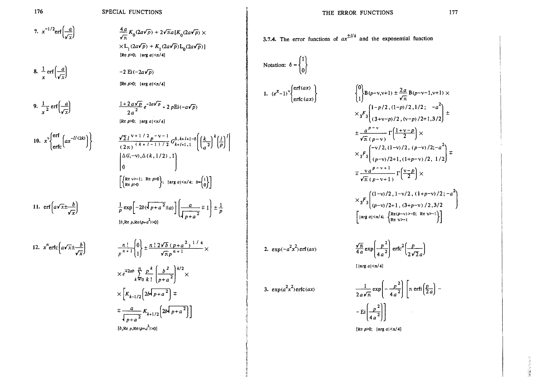
3.7.
3.7.1.
3.7.2.
3.7.3.
3.7.4.
3.7.5.
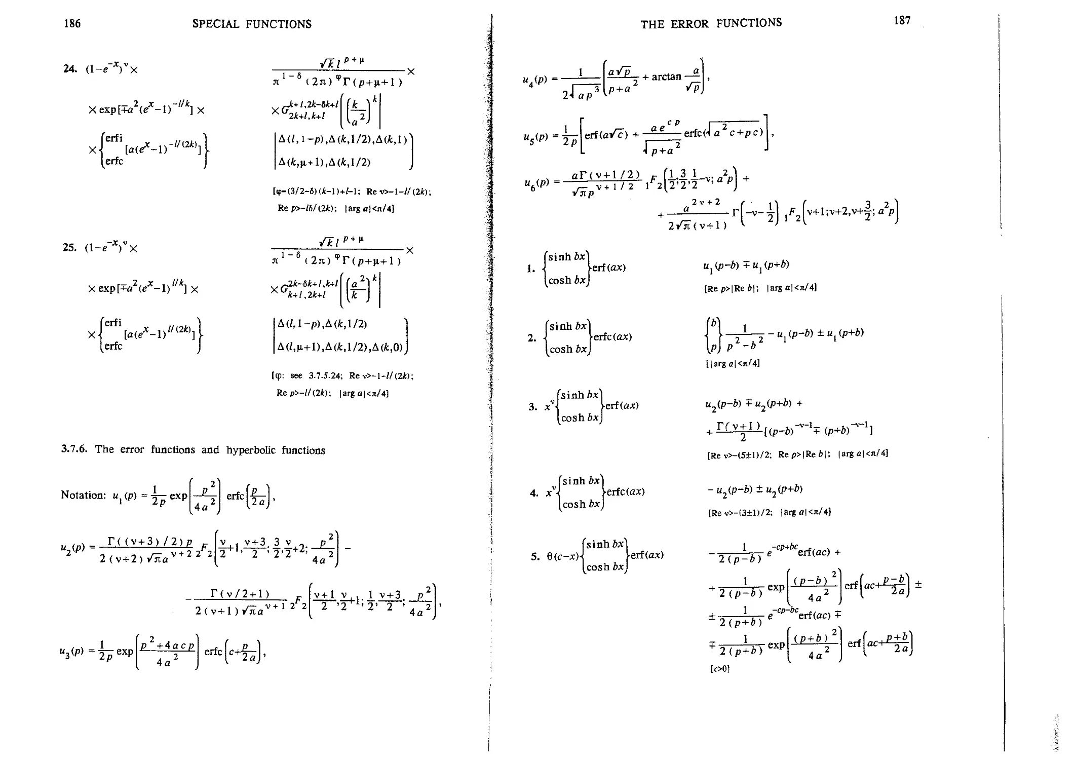
3.7.6.
3.7.7.
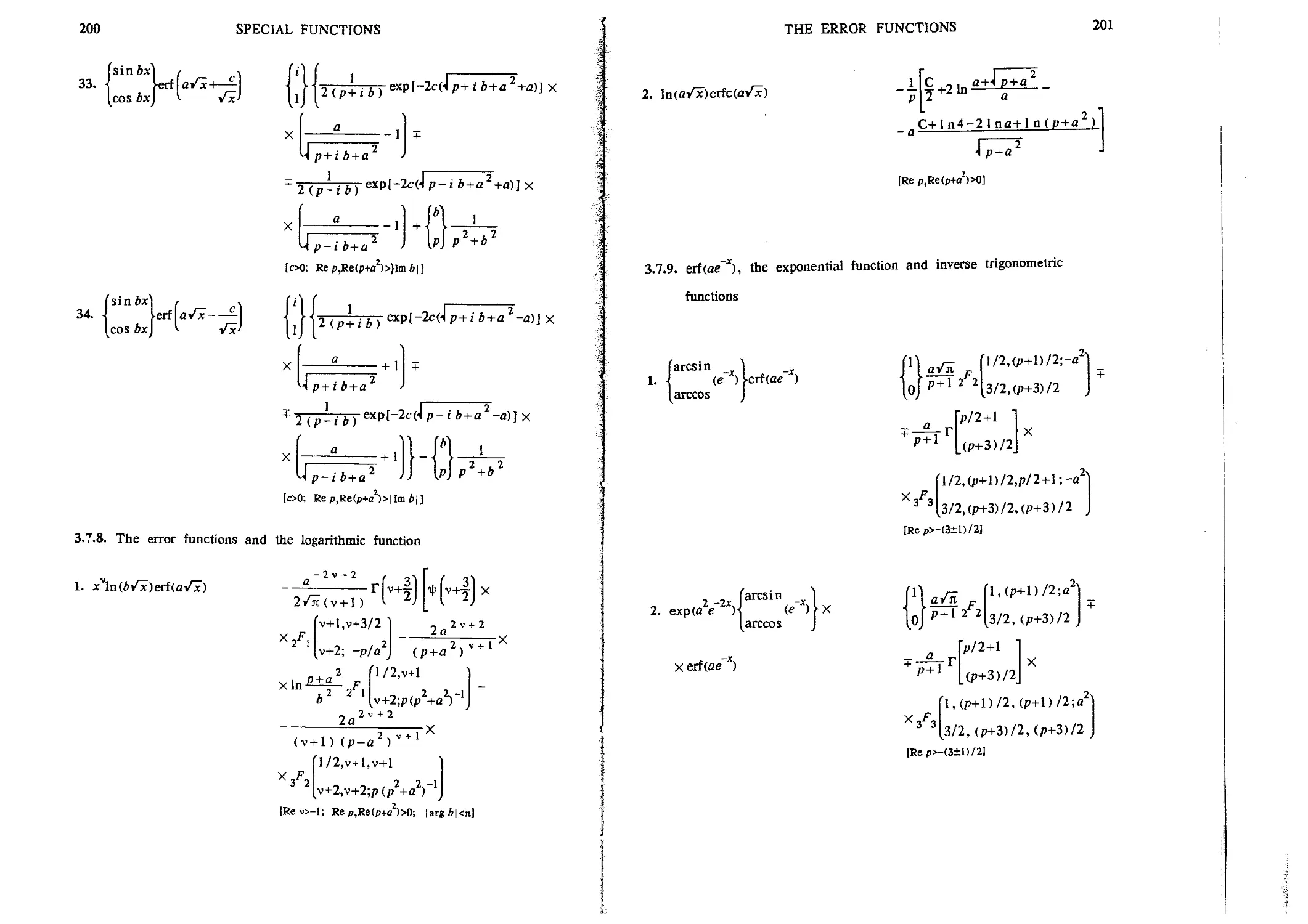
3.7.8.
3.7.9.
3.7.10.
3.7.11.
3.7.12.
3.8.
3.8.1.
3.8.2.
3.8.3.
3.8.4.
3.9.
3.9.1.
3.9.2.
1ЛЛЧТШЧТ!»
si (ax ), Si (их ), the exponential and
trigonometric functions
ci(ax) and the logarithmic function
Products of si(axl/k) and c\(axllk)
THE HYPERBOLIC SINE shi(z) AND COSINE chi(z)
INTEGRALS
Ilk Ilk
shi(ax ), chi(ax ) and the power function
shi(/4e )), chi(/4e )) and the exponential
function
shitax ), chUax ) and hyperbolic functions
shi(ax ), chi(ax ) and trigonometric
functions
chi(ax) and the logarithmic function
THE ERROR FUNCTIONS erf(z), erfc(z), AND erfi(z)
The error functions of ax + b and the power
function
The error functions of ax + b
The error functions of ax or of a/x + b//x
The error functions of ax~ and the
exponential function
The error functions of e x and the exponential
function
The error functions and hyperbolic functions
The error functions and trigonometric functions
The error functions and the logarithmic function
erf(ae ), the exponential function and inverse
trigonometric functions
Products of the error functions of ax1
Products of the error functions of f(e~x)
The error functions and the exponential
integral
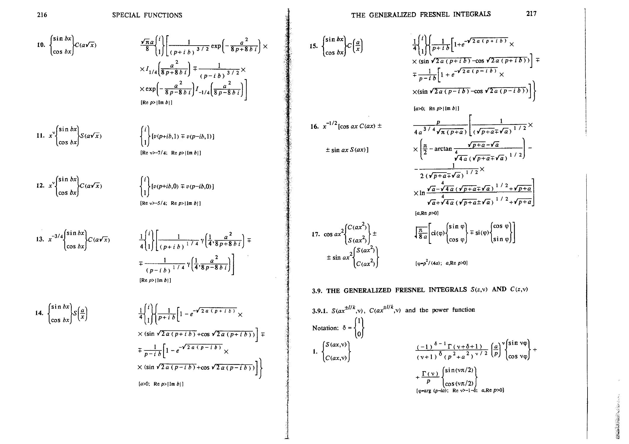
THE FRESNEL INTEGRALS S(z) AND C(z)
S(ax± ), С (ax* ) and the power function
S(f(e )), C(f(e~x)) and the exponential
function
S(ax ), C(ax~ ) and hyperbolic functions
+l/jfc +\lk
S(ax ), С (ax ) and trigonometric functions
THE GENERALIZED FRESNEL INTEGRALS S(z,v)
AND C(z,\)
S(ax± ,v), C(ax± ,v) and the power function
S(f(e~x),\), C(f(e'x),\) and the exponential
function
Ilk
159
160
160
160
160
163
165
167
168
169
169
171
174
177
180
186
193
200
201
202
204
205
205
205
207
209
213
217
217
219
3.9.3.
3.9.4.
3.10.
3.10.1.
3.10.2.
3.10.3.
3.10.4.
3.10.5.
3.10.6.
3.10.7.
3.11.
3.11.1.
3.11.2.
3.11.3.
3.11.4.
3.11.5.
3.11.6.
3.11.7.
3.12.
3.12.1.
3.12.2.
3.12.3.
3.12.4.
3.12.5.
3.12.6.
3.12.7.
3.12.8.
3.12.9.
3.12.10.
and the power function
S(axUk,\), C(axUk,\) and hyperbolic functions
S(axl/k,v), C(axl/k,\) and trigonometric
functions
THE INCOMPLETE GAMMA FUNCTIONS T(v,z)
AND y(\,z)
T(\,ax±l/k),
Г([х]+\,а), y([x]+v,a) and various functions
Г(\,ах±!/к), v(v,ax±'/i) and the exponential
function
r(v, f(e~x)), y(v,f(e~x)) and the exponential
function
T(v,ax±l/k), y(\,ax±1/k) and hyperbolic
functions
T(\,ax±l/k), y(\,ax±llk) and trigonometric
functions
Products of V(\,a^llk) and yiy&x* )
THE PARABOLIC-CYLINDER FUNCTION ?>v(z)
D (a/x) and the power function
D , ,(a) and various functions
V±[X\
D (ax±llk) and the exponential function
D (f(e~x)) and the exponential function
D (a/x) and hyperbolic functions
D (a/x) and trigonometric functions
Products of Dv(a/x)
THE BESSEL FUNCTION .Mz)
/ (ax) and the power function
/ (ax ) and the power function
V Ilk
x
Ilk
J (ax ) and the power function
V Ilk
) and the power function
2 : J and algebraic functions
v -
Jv{a\±b2+x2) and algebraic functions
tblxl (ax*1) and the power function
/ (f(tx)) and the exponential function
/ (ax ) and hyperbolic functions
v +11 к
J (a(sinhx)" ) and hyperbolic functions
223
225
227
228
230
230
231
236
241
246
246
246
248
248
251
253
254
255
256
256
260
261
265
266
268
271
271
274
276

CONTENTS
3.12.11.
3.12.12.
3.12.13.
3.12.14.
3.12.15.
3.12.16.
3.12.17.
3.13.
3.13.1.
3.13.2.
3.13.3.
3.13.4.
3.13.5.
3.13.6.
3.13.7.
3.13.8.
3.13.9.
3.14.
3.14.1.
3.14.2.
3.15.
3.15.1.
3.15.2.
3.15.3.
3.15.4.
3.15.5.
3.15.6.
3.15.7.
3.15.8.
3.15.9.
±11 к
Jv(ax ) and trigonometric functions
/ (ae±x ) and trigonometric functions
, ±hcl к
of e
JQ(f(x)) and the logarithmic function
/ (at ) and inverse trigonometric functions
/ (ax)J (bx) and the power function
/ (ax~ )J^(bx~ ) and the power function
/ (ae~ )J^(at~ ) and the exponential
function
THE NEUMANN FUNCTION ^(z)
Y (ax) and the power function
Y (ax ) and the power function
v -Ilk
Yv(ax ) and the power function
Y (f(x)) and algebraic functions
e Y (ax~ ) and the power function
Y (f(t x)) and the exponential function
Yv(ax) and hyperbolic functions
Yv(ax') and trigonometric functions
,.v. ±11 k. , . ±11 k. ....
Yv(ax ), Jw(ax ) and various functions
THE HANKEL FUNCTIONS
x~
H™(z)
) and the power function
and algebraic functions
THE MODIFIED BESSEL FUNCTION /(z)
/ (ax) and the power function
v ilk
IJax ) and the power function
and algebraic functions
and algebraic functions
ty.p(-bx^)l (ax ) and the power function
Iv(f(t x)) and the exponential function
/ (ax" ) and hyperbolic functions
/ (at ) and hyperbolic functions
I „(ax ) and trigonometric functions
277
280
281
282
283
293
296
298
298
300
301
302
304
304
305
307
309
311
311
312
313
313
317
321
322
324
326
329
331
331
CONTENTS
3.15.10.
3.15.11.
3.15.12.
3.15.13.
3.15.14.
3.15.15.
3.15.16.
3.15.17.
3.15.18.
3.16.
3.16.1.
3.16.2.
3.16.3.
3.16.4.
3.16.5.
3.16.6.
3.16.7.
3.16.8.
3.16.9.
3.16.10.
3.16.11.
3.16.12.
3.16.13.
3.16.14.
3.17.
3.17.1.
3.17.2.
3.17.3.
3.17.4.
3.17.5.
3.17.6.
±lxl k.
I (ae~w/*) and trigonometric functions
of e
1 (f(x)) and the logarithmic function
I (ae'x) and inverse trigonometric functions
J (axr)I (bx ) and the power function
J (f(tx))I (at ) and the exponential function
М- у k v щ
У (ax )Iv(ax ) and the power function
/ (ax) I (bx) and the power function
/ (axl/k)Iv(bxl/k) and the power function
/ (/(e ))Iv(ae ) and the exponential function
THE MacDONALD FUNCTION K^z)
К (ах) and the power function
К (ах ) and the power function
) and the power function
J and algebraic functions
and algebraic functions
(ax ) and the power function
К (/(е x)) and the exponential function
V Ilk
К (ах ) and hyperbolic functions
К (f(x)) and hyperbolic functions
K^(ax) and trigonometric functions
/ (ax"k)K (bxl/k) and the power function
** Ilk v Ilk
Yv(ax )K^(bx ) and the power function
I (ax )K (bx ) and the power function
Iх lit V Юг
К (ax )Kv(bx ) and the power function
THE STRUVE FUNCTIONS Hv(z) AND LJz)
H (ax~ ), L (ax~ ) and the power function
V V
Hv(/(e~x», Lv(f(t~x)) and the exponential
function
Uv(ax ), Lv(ax ) and hyperbolic functions
Hv(axUk), Lv(axUk) and trigonometric
functions
Hv(ax) and the Bessel function / (ax)
Y (ax~ ) - K(ax~ ) and the power function
334
335
336
337
339
340
341
346
349
349
349
352
353
355
356
357
359
363
364
365
366
368
368
370
370
370
375
377
381
383
384

Xll
3.17.7.
3.17.8.
3.17.9.
3.18.
3.18.1.
3.18.2.
3.18.3.
3.19.
3.19.1.
3.19.2.
3.19.3.
3.19.4.
3.19.5.
3.19.6.
3.19.7.
3.19.8.
3.19.9.
3.19.10.
3.20.
3.20.1.
3.20.2.
3.20.3.
CONTENTS
Yv(f(e~x)) -Hv(f(e~x)) and the exponential
function
L (ax~ ) and the modified Bessel function
I±w(f(t ")) -Lv(f(e~x)) and the exponential
function
THE ANGER FUNCTION J(z) AND THE WEBER
FUNCTION E (z)
±l/k v ±11 к
J (ax ), E (ax ) and the power function
J (ax), E (ax) and hyperbolic functions
J (ax), E (ax) and trigonometric functions
THE KELVIN FUNCTIONS beMz), bei^z), kerv(z),
keiv(z)
ber (ax ), bei (ax ) and the power function
ber (ae~rx), bei (ae~rx) and the exponential
function
berv(ax ), bei (ax ) and hyperbolic
functions
ber (ax ), bei (ax ) and trigonometric
functions
Products of the functions beMax1 ),
beiv(ax1M), btr'v(axl/k), ЬеГ(ах1Д)
ker (ax ), kei (ax ) and the power function
ker (ae~rx), keiv(ae~rx) and the exponential
function
ker (ax ), kei (ax ) and hyperbolic
functions
ker (ax ), keiv(ax ) and trigonometric
functions
The Kelvin functions and the logarithmic
function
THE AIRY FUNCTIONS Ai(z) AND Bi(z)
Ai(ax ), Bi(ax ) and the power function
K\(axllk), B\(ax k) and the power function
Ai(f(e'x)
function
M(f(e *)), Bi(f(t x)) and the exponential
384
386
387
390
390
391
392
392
392
394
395
397
398
401
402
404
404
405
405
406
407
408
CONTENTS
3.20.4. Products of the Airy functions and the power
function
3.20.5. Products of the Airy functions and the
exponential function
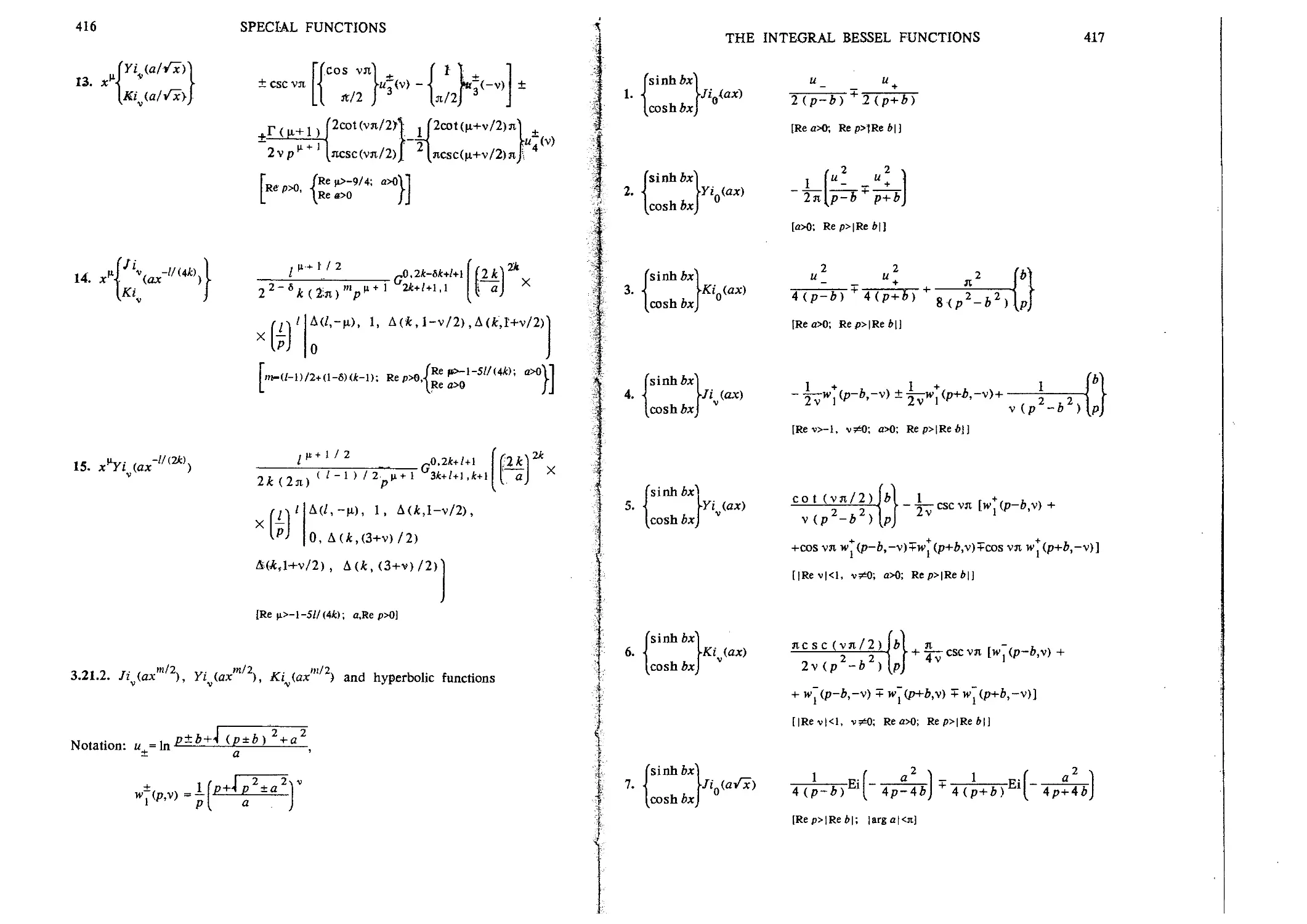
3.21. THE INTEGRAL BESSEL FUNCTIONS Jiv(z),
Kiv(z)
3.21.1. Jiv(ax±l'k), Yiv(ax±l/k), KMax*''*), and the
power function
3.21.2. Jiv(axm/2), Yiv(axm/2), Kijax'2) and
hyperbolic functions
3.21.3. //v(axlM), Yiv(ax), Kiv(ax) and trigonometric
functions
3.22. THE LEGENDRE POLYNOMIALS P (z)
3.22.1. Pn(ax ) and the power function
3.22.2. Pn(f(x)) and algebraic functions
3.22.3. Pn(f(e~x)) and the exponential function
3.22.4. P[x\W and various functions
3.22.5. Pn(cosh ax) and Pn(cos ax)
3.22.6. Products of Pn(f(x)) and the power function
3.23.1. Тп(ах±тП) and algebraic functions
3.23.2. Tn(f(x)) and algebraic functions
3.23.3. Tn(f(e'x)) and the exponential function
3.23.4. Un(ax±m/2) and algebraic functions
3.23.5. Un(f(x)) and algebraic functions
3.23.6. ^„^^e *)) an(* *ke exponential function
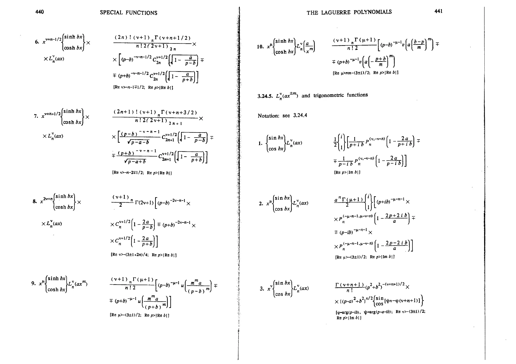
3.24. THE LAGUERRE POLYNOMIALS Lv(z)
3.24.1. Lvn(ax) and the power function
3.24.2. L^ax > an(l Ле power function
3.24.3. L"n(ax~ ) and the exponential function
411
412
413
412
416
416
419
419
420
423
424
425
425
3.23. THE CHEBYSHEV POLYNOMIALS Tn(z) AND Un(z) 425
425
427
428
429
430
431
431
431
435
437

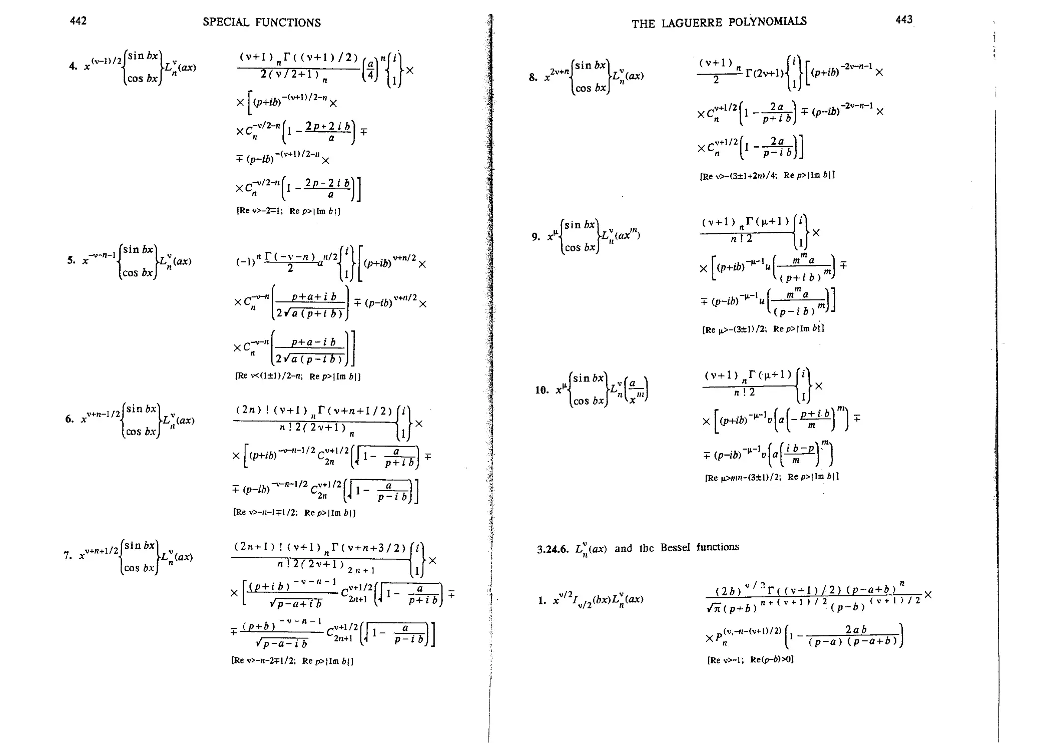
3.24.4.
3.24.5.
3.24.6.
3.24.7.
3.24.8.
3.25.
3.25.1.
3.25.2.
3.25.3.
3.25.4.
3.25.5.
3.25.6.
3.25.7.
3.25.8.
3.25.9.
3.26.
3.26.1.
3.26.2.
3.26.3.
3.26.4.
3.26.5.
3.27.
3.27.1.
3.27.2.
3.28.
3.28.1.
CONTENTS
I? (ax ) and hyperbolic functions
L"U.ax~m) and trigonometric functions
L~"(ax) and Bessel functions
n
Products of L^(ax~m ) and the power function
Ly. . (y) and various functions
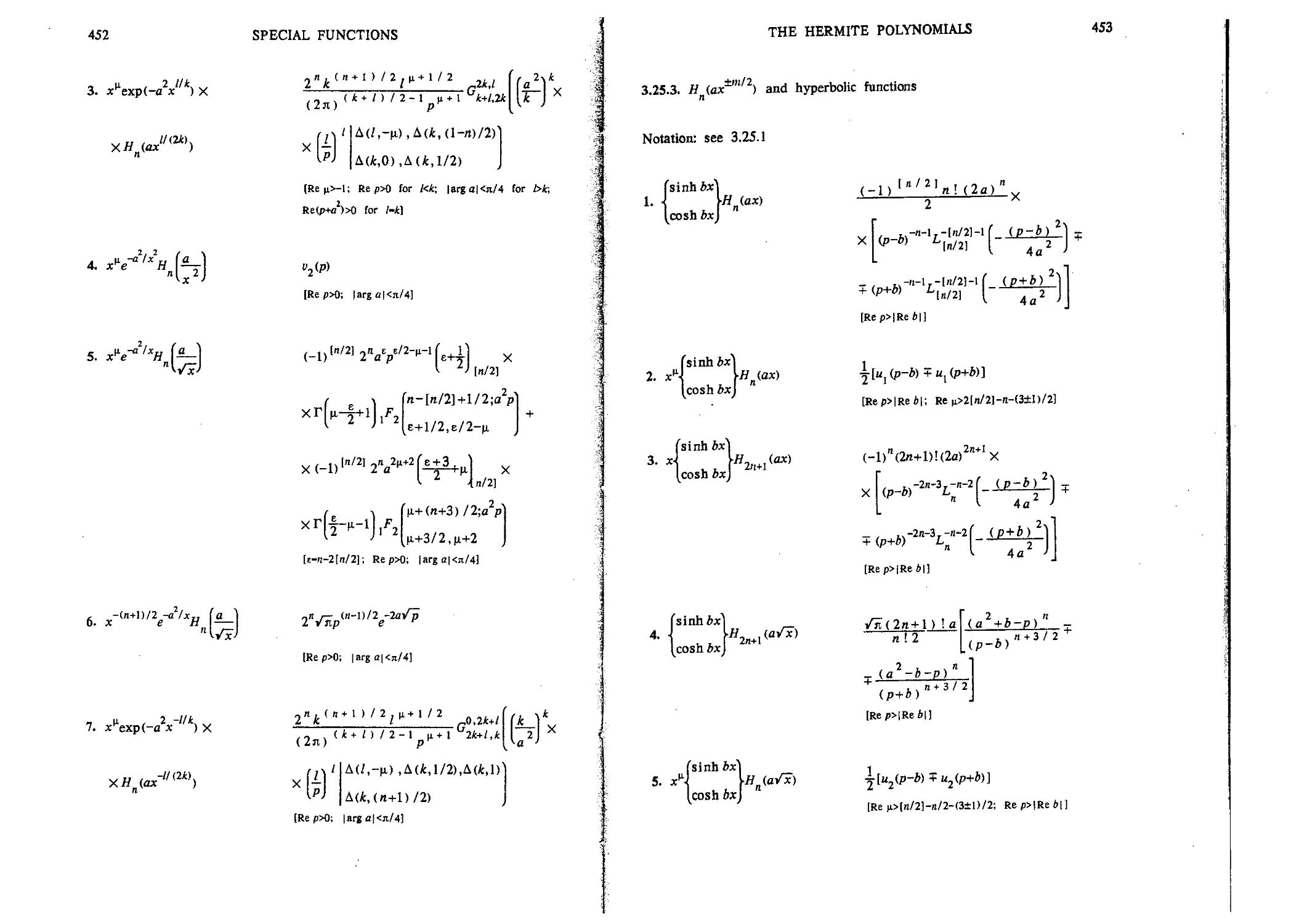
THE HERMITE POLYNOMIALS Я (z)
n
H (ax ) and the power function
±11 к
H (ax ) and the exponential function
1 -f-m/2
Hn(ax~ ) and hyperbolic functions
Hn(ax~m ), the exponential and hyperbolic
functions
H (ax ) and trigonometric functions
Hn(ax~'n ), the exponential and trigonometric
functions
Products of Hn(aV~x) and the power function
H . , (y) and various functions
Products of ^rj.iO') and various functions
THE GEGENBAUER POLYNOMIALS C" (z)
n
Cv(ax±m 2) and the power function
Cv(f(x)) and algebraic functions
C^(/(e *)) and the exponential function
СТ.(y) and various functions
Products of Cvn(f(x))
THE JACOBI POLYNOMIALS P(*'v}(z)
n
P (f(x)) and algebraic functions
"
anc* va"ous functions
THE BERNOULLI Bn(z), EULER ?n(z) AND NEUMANN
On(z) POLYNOMIALS
Bn(ax r), B..(y) and various functions
438
441
443
444
446
448
448
450
453
455
455
458
460
461
461
461
462
465
467
468
468
468
474
476
476
3.28.2.
3.28.3.
3.29.
3.29.1.
3.29.2.
3.29.3.
3.29.4.
3.29.5.
3.29.6.
3.29.7.
3.30.
3.30.1.
3.30.2.
3.30.3.
3.30.4.
3.31.
3.31.1.
3.31.2.
3.31.3.
3.31.4.
3.31.5.
3.32.
3.32.1.
3.32.2.
3.32.3.
3.32.4.
3.32.5.
CONTENTS
En(ax±r), Е.Лу) and various functions
Ore(ax~r) and the power function
THE BATEMAN FUNCTION Mz)
к (ах) and the power function
V II к
к (ах ) and the exponential function
к (ае ) and the exponential function
к (ах) and hyperbolic functions
к (ах) and trigonometric functions
Products of k^(ax) and the power function
Products of kv(ae±x)
THE LAGUERRE FUNCTION Lv(z)
L (ax) and the power function
L (ax~ ) and the exponential function
L (ax) and hyperbolic functions
L (ax) and trigonometric functions
COMPLETE ELLIPTIC INTEGRALS D(z), E(z)
AND K(z)
D(ax±l/k), E(ax±l/k), K(ax±l/k) and the power
function
T)(f(x)), E(f(x)), K(f(x)) and algebraic
functions
T)(f(e~x)), E(f(e~x)), K(f(e~x)) and the
exponential function
D(f(x)), E(f(x)), K(f(x)) and hyperboUc
functions
D(f(x)), E(f(x)), K(f(x)) and trigonometric
functions
THE LEGENDRE FUNCTIONS OF THE FIRST
KIND P*(z)
V
P^(f(x)) and algebraic functions
Рц(/(е~*)) and the exponential function
Pv'(e~x) and various functions
P^coshx), the exponential and hyperbolic
functions
Pi-i..(y) and various functions
477
477
478
478
479
480
481
481
482
483
483
483
484
484
485
485
485
487
489
489
491
492
493
497
499
501
502

3.32.6.
3.33.
3.33.1.
3.33.2.
3.33.3.
3.34.
3.34.1.
3.34.2.
3.34.3.
3.35.
3.35.1.
3.35.2.
3.35.3.
3.35.4.
3.35.5.
3.35.6.
3.35.7.
3.36.
3.36.1.
3.36.2.
3.36.3.
3.36.4.
3.36.5.
CONTENTS
Products of P*(f(x))
THE LEGENDRE FUNCTIONS OF THE SECOND
KIND Q»(z)
Q\fix)) and algebraic functions
Q*ifis~x)) and the exponential function
^ and various functions
THE LOMMEL FUNCTIONS s B) AND S (z)
|i.v |i,v
s (ax±l/k), S (ax±l/k) and the power
H,V |1,V *^
function
s iaxl/k), S jLaxllk) and hyperbolic
functions
s^v(ax' *), S^v(a
functions
and trigonometric
THE KUMMER CONFLUENT HYPERGEOMETRIC
FUNCTION /{(а;Ь;2)
jFj (a;b;wx~ ) and the power function
^F^ia^fix)), the power and exponential
functions
1F1(a±m[x];b±m[x];a>) and various functions
lFl(a;b;a>x±m ) and hyperbolic functions
j.Fx(a;b;wx~m ) and trigonometric functions
^ (a;b;a>x) and various functions
Products of jf j (а;*;шдс)
THE TRICOMI CONFLUENT HYPERGEOMETRIC
FUNCTION V(a,b;z)
W(a,b;a>x~ ) and the power function
^?(а,Ь,/(х)) and the exponential function
.^Ае )) and the exponential function
Домс "") and hyperbolic functions
*, the exponential and hyperbolic
502
502
503
503
504
3.36.7.
3.36.8.
3.36.9.
3.36.10
functions
±m
3.36.6. W(a,b;wx ) and trigonometric functions
504
504
506
507
508
508
512
513
514
515
516
517
517
517
520
522
527
528
529
3-37.
3.37.1.
3.37.2.
3.37.3.
338.
3.38.1.
3.38.2.
3.38.3.
3.39.
3.40.
3.40.1.
3.40.2.
3.40.3.
3.40.4.
3.41.
3.41.1.
3.41.2.
3.42.
3.42.1.
3.42.2.
CONTENTS
W(,a,b-,4>x±m) the exponential and trigonometric
functions
Products {F1(а;Ь;их11к)'?(а,Ъ;-1йхик) and the
power function
Products 1/'1(а;&;-ше±3?)Чг(а,&;ше±3?)
Ilk
Products of ЧГ{а,Ь;е>х ), the power and
exponential functions
Products of
function
and the exponential
THE GAUSS HYPERGEOMETRIC FUNCTION
/ ia,b;c;z)
F (a,b;c;-ax ) and the power function
and algebraic functions
21
F (a,b;c;f(e~x)) and the exponential function
THE GENERALIZED HYPERGEOMETRIC FUNCTION
rht/k
F ((a );(b );шх ) and the power function
щ п т yi
' )} and Ше exP°nentiaI
function
F ((a )±[x]:(b )±[x];a>) and various functions
THE MacROBERT ^-FUNCTION
THE MEIJER G-FUNCTION G™"
«V
G-function and the power function
G-function and the exponential function
G-function with [x] in parameters
Products of G-functions
THETA-FUNCTIONS B.(z,g), e;(z,?)
в.(а/х~,ф, B^v.e)
THE FUNCTIONS viz), v(z,q), ц(гЛ), M'.
Uz,q)
viaxm/2),vit~ax), the power and exponential
functions
viaxm/2,Q), v(e~'",Q) and the power function
xvu
530
530
531
532
532
533
533
535
537
546
546
554
557
558
559
559
560
562
563
564
564
565
566
566
566

xviii
3.42.3.
3.42.4.
3.42.5.
3.43.
3.43.1.
CONTENTS
т/2
т/2
',%) and the power function
\l(ox"" ,X) and the power function
4,q) and the power function
THE CONFLUENT HYPERGEOMETRIC FUNCTIONS
OF TWO VARIABLES
Confluent hypergeometric functions and the power
function
APPENDIX. ELEMENTS OF THE THEORY OF THE LAPLACE
TRANSFORMATION
1. The Laplace transform and its basic properties
2. The application of the Laplace transformation to the
solution of differential and integral equations
3. Some comments and references
BIBLIOGRAPHY
LIST OF NOTATIONS OF FUNCTIONS AND CONSTANTS
LIST OF MATHEMATICAL SYMBOLS
567
568
568
568
568
571
571
584
599
601
607
619
PREFACE
This is Volume 4 of the series Integrals and Series. It contains tables of
direct Laplace transforms
F(p)
and includes results previously published in similar books and journals.
However, many of the results were obtained by the authors and are being
published for the first time.
Volume 5 of this series contains tables of inverse Laplace transforms
and tables of factorization of various integral transforms.
The Laplace transformation is used extensively in various problems of
pure and applied mathematics. Particularly widespread and effective is its
application to problems arising in the theory of operational calculus and in
its applications, embracing the most diverse branches of science and
technology. An important advantage of methods using the Laplace
transformation lies in the possibility of compiling tables of direct and
inverse Laplace transforms of various elementary and special functions
commonly encountered in applications.
In this volume the tables are arranged in two columns. The left-hand
column of each page shows original f(x) and the right-hand column gives the
corresponding image F(p). The main text is introduced by a fairly detailed
list of contents, from which the required formulas can be easily found.
A number of Laplace transforms are expressed in terms of the Meijer
G-function. When combined with the table of special cases of the G-function
[82], these formulas make it possible to obtain Laplace transforms of
various elementary and special functions of mathematical physics. Some other

CONTENTS
3.42.3.
3.42.4.
3.42.5.
3.43.
3.43.1.
ml 2
\к(ах"" ,Х) and the power function
\к(ах ,X) and the power function
,Q) and the power function
THE CONFLUENT HYPERGEOMETRIC FUNCTIONS
OF TWO VARIABLES
Confluent hypergeometric functions and the power
function
APPENDIX. ELEMENTS OF THE THEORY OF THE LAPLACE
TRANSFORMATION
1. The Laplace transform and its basic properties
2. The application of the Laplace transformation to the
solution of differential and integral equations
3. Some comments and references
BIBLIOGRAPHY
LIST OF NOTATIONS OF FUNCTIONS AND CONSTANTS
LIST OF MATHEMATICAL SYMBOLS
567
568
568
568
568
571
571
584
599
601
607
619
PREFACE
This is Volume 4 of the series Integrals and Series. It contains tables of
direct Laplace transforms
F(p)
¦ §f(x)e~pxdx
and includes results previously published in similar books and journals.
However, many of the results were obtained by the authors and are being
published for the first time.
Volume 5 of this series contains tables of inverse Laplace transforms
and tables of factorization of various integral transforms.
The Laplace transformation is used extensively in various problems of
pure and applied mathematics. Particularly widespread and effective is its
application to problems arising in the theory of operational calculus and in
its applications, embracing the most diverse branches of science and
technology. An important advantage of methods using the Laplace
transformation lies in the possibility of compiling tables of direct and
inverse Laplace transforms of various elementary and special functions
commonly encountered in applications.
In this volume the tables are arranged in two columns. The left-hand
column of each page shows original fix) and the right-hand column gives the
corresponding image F(p). The main text is introduced by a fairly detailed
list of contents, from which the required formulas can be easily found.
A number of Laplace transforms are expressed in terms of the Meijer
G-function. When combined with the table of special cases of the G-function
[82], these formulas make it possible to obtain Laplace transforms of
various elementary and special functions of mathematical physics. Some other

PREFACE
xx
formulas, in particular Laplace transforms of general form and those of
piecewise-continuous functions, can be found in [80-82].
For the sake of compactness, abbreviated notation is used. For example,
the formula
ferf(ojc) |
ierfc(ax))
К Re pX); |arga|<ji/4V]
|arg а|<я/4 /J
is a contraction of the two formnlas
erf(ajc) -expl^-yl erfc
[Re p>0; |arga|<jt/4]
(fc)
(in which only the upper sign and the upper expression in the curly brackets
are taken) and
[|arga|<n/4]
(in which only the lower sign and the lower expression in the curly brackets
are taken).
References to formulas written in the form 3.7.1.1. denote Formula 1 of
Subsection 3.7.1.; unless other conditions are indicated, к,1,т,п=0ЛЛ—-
The Appendix contains a short survey of the theory of the Laplace
transformation, and examples of its applications in problems of differential
and integral equations.
The bibliographic sources, notations of functions, constants, and
mathematical symbols are listed at the end of the book.
We would be extremely grateful to any readers who draw our attention to
oversights, which are inevitable in a work of this size.
Chapter 1. FORMULAS OF GENERAL FORM
1.1. TRANSFORMS CONTAINING ARBITRARY FUNCTIONS
1.1.1. Basic formulas
00
F(p) = \e~pxf(x)dx
1. fix)
Y+i'oo
2. 27J J tpxF(p)dp
Y-i'oo
F(p)
1.1.2. f(A(x)) and algebraic functions
1. f(ax)
2. f(x+a)
3. f(ax+b)
4. Q(x-a)fix-a)
[a,bx>]
[a>0]
5.
ГО, х<Ыа
\f(ax+b), x>b/a

PREFACE
xx
formulas, in particular Laplace transforms of general form and those of
piecewise-continuous functions, can be found in [80-82].
For the sake of compactness, abbreviated notation is used. For example,
the formula
ferf(ajc) ]
}erfc(ajc)J
Г/RepM); |arga|<jt/4Y]
|_\|arg a|<jt/4 /J
is a contraction of the two formulas
erf(ajc) -
4a'
erfc
[Rep>0; |arg а|<л/4]
(in which only the upper sign and the upper expression in the curly brackets
are taken) and
erfc(ajc)
t|arga|<jt/4]
(in which only the lower sign and the lower expression in the curly brackets
are taken).
References to formulas written in the form 3.7.1.1. denote Formula 1 of
Subsection 3.7.1.; unless other conditions are indicated, к,1,т,п=0ЛЛ-—
The Appendix contains a short survey of the theory of the Laplace
transformation, and examples of its applications in problems of differential
and integral equations.
The bibliographic sources, notations of functions, constants, and
mathematical symbols are listed at the end of the book.
We would be extremely grateful to any readers who draw our attention to
oversights, which are inevitable in a work of this size.
Chapter 1. FORMULAS OF GENERAL FORM
1.1. TRANSFORMS CONTAINING ARBITRARY FUNCTIONS
1.1.1. Basic formulas
1. f(x) ,
Y+ioo
y-tco
1.1.2. f(A(x)) and algebraic functions
1. f(ax)
2. f(x+a)
3. f(ax+b)
4. Q(x-a)f(x-a)
a
ffl>0]
5.
[0, x<b/a
\f(ax+b), х>Ыа
-1 bp/a
a e
la,bX>]
[c>0]
la,bX))
№)-;¦

FORMULAS OF GENERAL FORM
6. f(x+a)=f<jc)
7. f(x+a)=-f(x)
8.
9. xnf(x)
10. x~'lf(x)
11. Q(a-x)xvf(x-a)
12.
13. xf(x2)
14. x /(x )
15.
16. fix {)
[aX»
A+*-°")
[a>0]
l-e'p
p
(-fc)"
1 \t-pxf(x)dx
у f(k,-kP
/ /we
p p
v+1
(v+l)^t{-aP)'akht
Re v>-l; /(л)-У hxk, \x\<r, r3=aX)
к -о * -I
oo
-4
exp -
OO
Г -3/2 f p2)
u exp -ii—
J >- 4J
p-i/2
17.
TRANSFORMS CONTAININU акшшлм runun
OO
(x4) J70B/pT)F(u)dK
18. xvf(x~1)
[Re v>-2]
И-1 >¦ '
Г *
20. /,(x)/,(x) — f F,WF2<P-*)*
1.1.3. /(ф(х)) and non-algebraic functions
> 2.
3. Q(x-a) X
X (l-e~x
S (P) /^
4. fiat: -a)
Rev>-1; Rep>0;
1
аГ(р+1
[а>о]
^u«
5. /(asinhx) f/ (au)F(u)du
0
[a>0]
"°,a>0
J

6. sinbaxfix)
7. cosh ax fix)
8. sin ax f(x)
9. cos ax f(x)
10. 9(a-x)x|lX
XJJbx)f(x)
FORMULAS OF GENERAL FORM
-a) -F(p+a)]
-j[Fip-a)+Fip+a)]
-Fip+ia)]
(ц+v+l>T(v+l)
v V
2
fill
hk
, \x\<r,
11. 9(x-a)X
ХA-е"Ух
X/ (be~x)f(x)
12. (l-e
(p+v>r(v+l>
x-
л п
[
Re(p+v»0; /(jc)-Y A e"**,
t-o
г[Р'ц+11 у
Re ц>-1; Rep>0;
-x
"°; aX)
oo ^
)-Y А е"*л, |е""|<г, г>е"°; a>0
*»о * J
TRANSFORMS CONTAINING ARBITRARY FUNCTIONS
13. Ыа-х)х* X
X ,F,ib;c;b
(-ар) ; a* (toa)
/ ! Z !
p oo ,
I Re м>-1; /Oc)-Y A jt*, |*|<г, г5чг>0
L t-o J
14. A-е"Ух
X ,F, ib;c;t
[OO -I
Re(i>-1; Rep>0; /Ы-Уле"'*
15.
16. A-е
X 2Fj(a;6;c;coe ) X
X fix)
п.
[OO -.
RepM); /(D-V 4 e"'', | e"* | <r, rSse""; aX)
t-o J
(p) ;^
-1; Rep>0;
1-е'
--**>
t-0
1.1.4. Derivatives of fix)
I. fix) PF(p)-fi0)

2. fin\x)
FORMULAS OF GENERAL FORM
p"F(p) -
• (i
MM,2 n-1
6. xmfn(x)
7. -[x
8. ел4-
if /*'@)-0,
it-0,1,2 »-l
¦-...-/'"""(О)
ОС ОС ОС
Jp J"...pJpF(p)(dp)"
p p p
F(p)}
for
(и-т-2) !
for m<n
for
_ (П-1 ) ! Лп-m-l) n
(n-m-l)l' W)
for m<n
(p-n)F(p-n)
TRANSFORMS CONTAINING ARBITRARY H
9.
1.1.5. Integrals containing fix)
a
1. jf(x,u)du
2.
л x
3. Г...(
о о
5.
fF(p,u)rfu
p~nF(p)
[Re p>0]
p'aF(p)
[Re a,Re p>0]
FAp)F.(p)

n -ax Г su,, . ,
9. e e f(u)du
10.
11.
12.
FORMULAS OF GENERAL FORM
F(p)
p+a
F(p)
13. x ue f(u)du
14.
15.
16. \sinbv(x~u)f(u)du
,- Г -1/2 .
17. и si
о
(P+a)
2F(p)
(P+a)
[Re p>0]
[Re p>0]
Г(у + 1
-у)/2)
2v+1r(l+(p+v)/2)
[-l<Re v<Re p]
г- }
[Re p>0]
TRANSFORMS CONTAINING ARBITRARY FUNCTIONS 9
18. x~1/2 [cosh VTu
00
19. (V1/2sin VTu f(u)du
20.
f(u)du
-f(u)du
аи- 1
, 7 xu f (u)
3* J Г(и+1)
24.
25.
— )
i-ii'
f(u)du
[Re p>0]
[Re p>0]
[Re p>0]
P
[Re p>0]
F(alnp)
[a,Re p>0]
-lnpF(lnp)
[Re p>0]
[Re p>0]
[Rev<l/2; Re(p+a>>0]

10
FORMULAS OF GENERAL FORM
26. jjQ(VTu)f(u)du
27.
28.
29. j (x-u) lJv(a(x-u))f(u)du
0
Hh)
[Re p>0]
[Rev>-1; Rep>0]
2 2
p +a
2
p +a'
F(p)
[Rev>-1; Rep>|Ima|]
I p +a
[RevX); Rep>|lma|]
30. \(x-ufjy(a(x-u))f(u)du
о
«¦
Ba)vr(v+l/2)
[Rev>-l/2; Rep>|lma|]
¦p+1 p +a
X
X / (aV (x-u) (x-u+b)) X X
/2]
f
Xf(u)du
[Rev>-1; Rep>|lma|;
32.
ff]>iexpr «i
[2) и F{ 4p_
F(p>
[Rev>-1; RepX)]
TRANSFORMS CONTAINING ARBITRARY FUNCTIONS 11
33. \jo(a\x2-u2)f(u)du
[Rep>|lm a\)
34.
a'(gV)-'/2nry)
-2 2\ V
(p+4 p
[Re v>-l; Rep>|lm >
35.
—u
-f(u)du F(\p2+a2)
[Re p>|Ima|]
36.
-f(u)du
x
37. \j0QVu(x-u))f(u)du
>2 2
[Rep>|lma|]
[Re p>0]
v/2
38. I l^-^l X
о
X/ (aVu (x-u) )f(u)du
[Re v>-l; Re p>0]
39.
X/
[Rev>-1; Rep>|Im a|/2]

12
FORMULAS OF GENERAL FORM
TRANSFORMS CONTAINING ARBITRARY FUNCTIONS 13
40.
-b,
tx + u
X
XJl(aVxTx+uJ)f(u)du
x
41. U(a(x-u))f(u)du
42. J(X-,
u)"' X
X/ (aVx-u)f(u)du
43.
X/ (a(x-u))f(u)du
X
X/ (aV(x-u) (*-«+*)) X
y,f(u)du
4S.](x-u)v/2:
X/
46. jlo(a\x2-u2)
0
Xf(u)du
X
[Re p> |Ima |/2]
1
F(p)
[Rev>-1; Rep>|Rea|]
p+«lp2-a2
Ftp)
[RevX); Rep>|Rea|]
[Re v>-l/2; Rep>|Re a\]
p -a
[Rev>-1; Rep>|Rea|;
1j [4p
(Rev>-1; Rep>0]
[Rep>|Rea|]
47.
49. /(x)
50.
v/2
X
X/ (aVu(x-u))f(u)du
v/2
л>/2.
52. x I (x+u) X
0
X/ (aVx(x+u))f(u)du
2 2,-1/2
a >
[Rev>-1; Rep>|Rea|]
X/V(dx -u )f(u)du
48. /(x)+ F(Ap*-a")
+ a\ = — f(u)du [Rep>|Rea|]
2 2
I p -a
-f(u)du tRep>|Rea|]
[Re pX)]
[Rev>-1; Re p>0]
ГГ 2 2
i Ap -a -p
2
[Rev>-1; Re p> | Re a |/2]

14
53.
FORMULAS OF GENERAL FORM
-bu
/x+u
54.
55. [<*-"> ° ' X
О
XFx(a\c-Mx-u))f(u)du
«• иы
57. JV«;
(ar)j
f(u)du
-F(b)
[Re p> | Re a |/2]
[Re p>0]
Г(с)р
¦F(p)
[Re cX); Re p>max(O,Re U]
[Re p>0]
\f(u)du
[r«r, 2m+2n^r+q; Re i >-l,
it-l,2,...,m; RepM)]
(-1)*— [coth (lSp)](~vF(p)
V~p
[k-Q,V, Rep>0]
Chapter 2. ELEMENTARY FUNCTIONS
2.1. THE POWER AND ALGEBRAIC FUNCTIONS
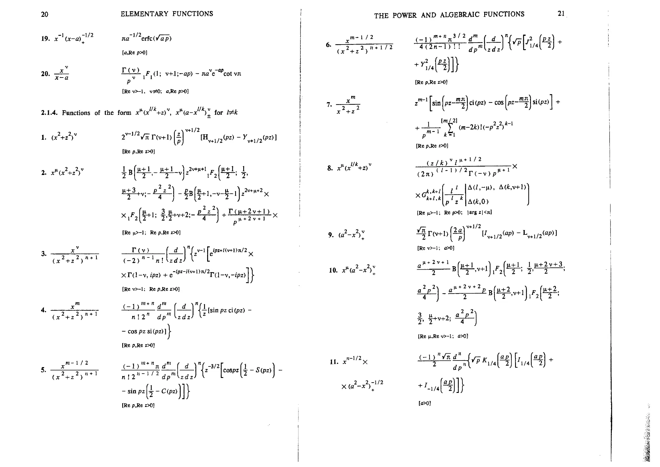
2.1.1. Functions of the form xv, Q(±x + a)xv, [x\n
T(v+1
! 1. X
i
i
|
i 2. x"
I
, n-l/2
3. x
4. 6(a-x)xv
5. b(a-X)xn
v+ 1
p
[Rev>-1;
n!
n+ 1
p
[Re pX>]
Bn-l
Rep>0]
) ! !/я
_« n+1 / 2
2 p
[Re pM»
1 vri
P
[Rev>-1;
n\
n+ 1
P
[a>0]
k'+l ,Up)
a>0]
/I ! -ap
p"+1
6. 9(a-x
n-l/2
~ ap
B/1-1)!!
[a>0]
(ap/2)
2V

14
FORMULAS OF GENERAL FORM
fx+u
X /j (cn/x(x+u))f(u)du
54.
[Rep>|Rea|/2]
[Re p>0]
55. l(x-u)c ' X
Г(с)р'
X jfj (a;c;Ux-u))f(u)du
[Re cX); Re p>max(O,Re X>]
*• Jo'.fH--
^>
[Re p>0)
57. Го'""
J rg
(a)
_1_ Г„т,и+1 ^?
p J r+l,q p
f(u)du
[xq\ Im+ln^r+q; Rei>-1,
/t-1,2 m; Rep>0]
(-1)*—
[
•p
0,l; Rep>0]
Chapter 2. ELEMENTARY FUNCTIONS
2.1. THE POWER AND ALGEBRAIC FUNCTIONS
2.1.1. Functions of the form x", 9(±x + a)xv, [x]
1. x1
2. x"
n-1/2
3. x'
4. 9(a-x
5. 9<a-x)x
6. 9(a-x)x
n-l/2
[Rev>-1; Rep>0]
и!
n+ 1
P
[Re p>01
„n n + 1 /2
2 p
[Re pX)]
1
-¦y(v+l,ap)
[Rev>-1; aX)]
rt ! n ! - ару ( op)
n +l n +l ,Ln к !
p p k-0
laX»
_1) ,,
n-1
[fl>0]
(др/2)
P
-^-!-erf(/a"p)

16
ELEMENTARY FUNCTIONS
THE POWER AND ALGEBRAIC FUNCTIONS
17
7. Q(x-a)xv
8. B(x-a)x
9. %(x-a)x
-n-l/2
10. 8<jt-a)jt
-n-1
П. M
12.
13. M*
1
2. (X+zf
pv+l
[a,Re pX>]
П \ —ар у ( up )
[a,Re p>0]
, . n и- 1 /2
+ Г(П+1/2)
[a.Re p>0]
erfc(v^)
. ,.t. ,4, A-n-1 it
С 1
- ^~Р| Ei(-ap)
[a,Re p>OJ
1
[Re p>0]
ep+l
P(ep-1J
[Re p>OJ
i "
1-е'
к k
i
И
[Re p>0]
2.1.2. Functions of the form (x+z)v, (a-x
1. (x+zf
v+ 1
[Rep>0; | arg г |
3.
4.
5.
6.
7.
1
(x+z)'
'x+z
x+z
1
(x+z)
3/2
1
U+z)
8. (a-*)'
9.
Jt + Z
10. (x-af
11.
e(л-
nl
[Re p>0]
[Rep>0; | arg z | <я]
J|ep2erfc(/pT)
[Rep>0; | arg г | <я]
- ep2Ei(-pz)
[Rep>0; | arg i \ <л]
— - 2Snptpzerfc(.Sp~z~)
V~z
[Rep>0; |argz|<n]
i + peP2Ei(-pz)
[Rep>0; |argz|<n)
-<zp
v + 1
7(v+l,-ap)
[Rev>-1; o>0)
ep2[Ei(-ap-pz)-Ei(-pz)]
[|argz|<n or z>a, a>0]
-ap
[fl.Re p>0]
- t~bpEi(bp-ap)
la>b>0]

18
ELEMENTARY FUNCTIONS
THE POWER AND ALGEBRAIC FUNCTIONS
19
12.
х-а к^0 к\
[a,Re p>0]
2.1.3. Functions of the form xv'(x+zf.
Ыар)
I. x»(x+z)v
2. x\x+zf
V . . • . V
3. x (x±iz)
4.
5.
6.
7.
8.
(x + z)
1/2
(x+z)
¦3/2
X+Z
x+z
n - 1 / 2
ДГ + 2
; pz)
; Rep>0; |argz|<ji]
v+1/2
/i
z)
p)
pi/2
e K
[Re v>-l; Rep>0; |argz|<ji]
H/2 ,
[Rev>-1; Rep>0; -
-v+1/2
2D_2vl (/277)
[Rev>-1; Rep>0; |argz|<n]
pl/2
/7
>
[Re v>-l; Rep>0; |argz|<n]
r<v+l)zvep2r(-v,pz)
[Re v>-l; Rep>0; |argz|<n]
(-D"+1z"ep2Ei(-p2)+ У (к-т(-г)П
k*\ p*
[Re p>0;
(-l)%z'!-1/2epzerfc(/F7)
?TPl
2, к ш 1
[Rep>0; |argz|<n]
9.
10.
11.
,- 1/2, ,
12. x (a-x)
13.
(x+z)
¦fx (x+a)
15. x*(x-a)\
16.
^ _ v , . -v-l/2
17. jc {.x-a)
18. jc (jc-
. -v-3/2
)
[Rep>0; |arg z|<n]
B(n+l,v+l)a|1+v+11/-1(n+l, n+v+2; -ap)
[Re |i,Rev4; a>0]
[Rev>-1; a>0]
[a>0]
[Re ^..Re v>-l; | arg A +e/r) | <л; а>0]
r(v+l)a|1+v+1e"ap4r(v+l, ix+v+2; ap)
[Rev>-1; a,Rep>0]
Г(у + 1)(аУ+и\
[Rev>-1; a,Rep>0]
r(l/2-v)e-ap/2
2v
[Rev<l/2; o,Rep>0]
[Rev<-l/2; a,Rep>0]

20
ELEMENTARY FUNCTIONS
19. x'\x-a)~m
20.
na erfc(v'ap)
[a,Re pX)]
x-a
A;
[Rev>-1, vt^O; a,Re pX)]
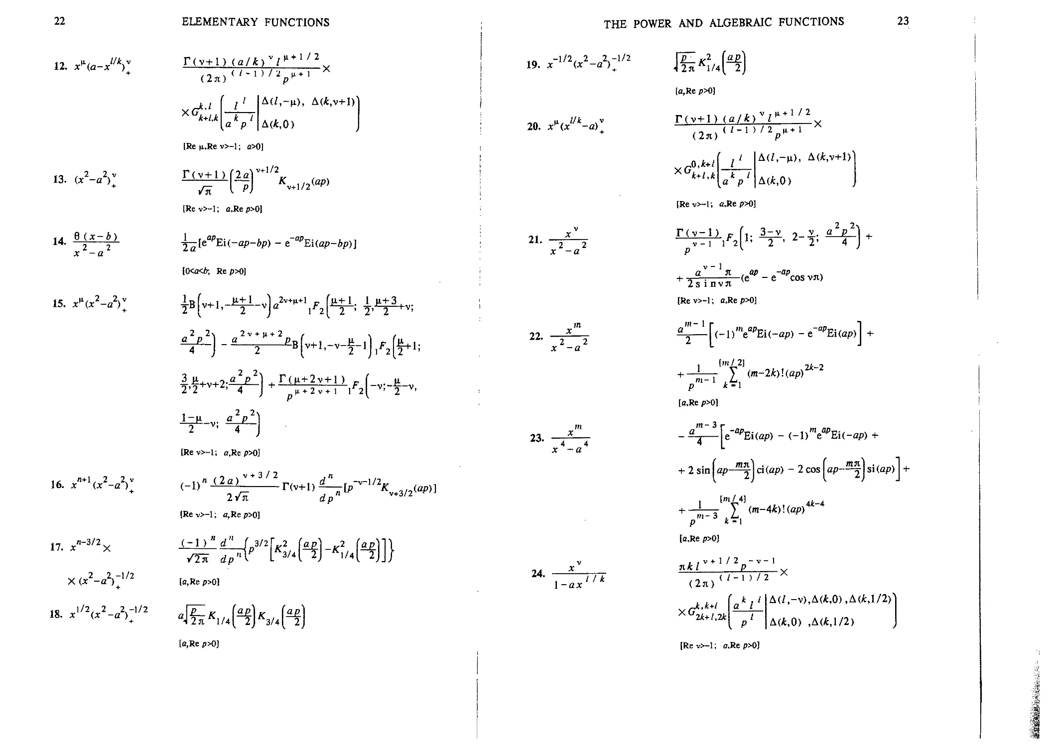
2.1.4. Functions of the form x*(x' +z)v, x*(a-x' )\ for
2.
2 2 . n + 1
+г )
[Hv+1/2(pz)-yv+1/2(pz)]
[Re p,Re г>0]
[Re ц>-1; Re p,Re z>0]
l-v,-ipz)l|
[Re v>-1; Re p,Re z>0]
4.
n ! 2 dp
- cos pz si (pz)] J-
[Re p,Re zXJ]
— [sinpzci(pz) -
5.
'«- 1 / 2
. 2 2 . и + 1
(д: +2 )
n!2" "''dp
- sinpz^-C(pz)jj|
[Re p,Re z>0]
THE POWER AND ALGEBRAIC FUNCTIONS 21
m- 1 / 2
7.
2 2
X +z
8. x»(
9.
10.
11. x"~U2X
1/4
[Re p,Re zXJ]
(**)]}
l[sit
z sin
ci(pz) - cos
\pz-^j si(pz) j
1
+ Ц
[Re p,Re i>0]
(т-2«!(-р2г2)
[Re ц.>-1
I
I k
i 2
; RepX); |argz|<n
1/2
[Rev>-1; aXJ]
ц + 2 v + 1
~ 2 B
2 2
1 ii+v+O- a P
2> 2^ ' 4
[Re p.,Re v>-l; a>0]
(-l)"/j(f"
2 dp*
-X
[a>0]

22
12. x»(a-xl/k)v
13. (*2-a
6 (s-fr)
15.
,, n+l 2 24v
16. x (x -a )
17.
X
18.
ELEMENTARY FUNCTIONS
a p
/,-ц), A(ifc,v+1)
Д<*,0)
[Re |i,Re v>-l; a>0]
Г(у+1
+1/2
[Rev>-1; a,Rep>0]
i(-ap-6p) - e"opEi(ap-6p)]
; Rep>OJ
^-v;
[Re v>-l; a,Re p>0]
v + 3/2
я Bа)
(-1)
[Rev>-1; a,Rep>0]
<-l)"rf"
dp'1
[a,Re p>0]
[a,Re p>0]
JL-H3 ,
THE POWER AND ALGEBRAIC FUNCTIONS
23
19.
20.
Ilk .v
x -a)
21.
2 2
д: -а
22.
2 2
л: -a
23.
4 4
-a
24.
\-ax
ilk
[a,Re p>0]
XG
,0,*+/
I
к I
a p
[Rev>-1; a,Rep>0]
Г(у-1) ,
v-1 I1
P
v- 1
T2sinvJi vc
[Rev>-1; a,Rep>0]
P
[a,Re p>0]
m-3
- <-l)meapEi(-ap) 4
+ 2 sin [ap-^1 d(ap) - 2 cos [ap-^f ] si
p i -1
[a,Re p>0]
nkl p
1/2 -v-1
-X
2Jt+/,2Jt| Z
[Re v>-l; o,Re p>0]

24
25.
ELEMENTARY FUNCTIONS
Ik
УЛ
,A(Jt,(l-v)/2)
[Re ц>-1; Re v<l; a,Re pX)]
2.1.5. Functions containing Vx+z
1
(x+2z) /x+T
2.
4.
5.
7.
x(x+z)
1/2
erf
2/F
[Rep>0; |argz|<n]
[Rep>0; |argz|<n]
Vwz
[Rep>0; |arg w|,|arg
erfc(pn>) erfc <pz)
[Re v>-l; Re pX); |arg z|<л]
v /2 ,
У Z pz/2,,
[Rep>0; | arg i|<n]
[Rev>-1; Rep>0; |arg z|<n]
[Re p>0; |argz|<n]
Sx
THE POWER AND ALGEBRAIC FUNCTIONS 25
2.1.6. Functions containing ix ±z for
2.
3.
)
( Г^
Х+Л X +Z
\x(x2+z2)
4.
[r-0 or 1/2]
5.
<(f
xNl + zx ±<zx '
[r-0 or 1/2]
P PS
[Re p,Re г>0]
nz
_ (pz) -J_ (pz)]
[Re p,Re zX)]
)~
2) x
Xy
(l-2v)/4
N1
[Re p,Re z>0]
Д(*,(у±у)/2)
; Rep>0; |argz|<n]
/ -3 ) / 2
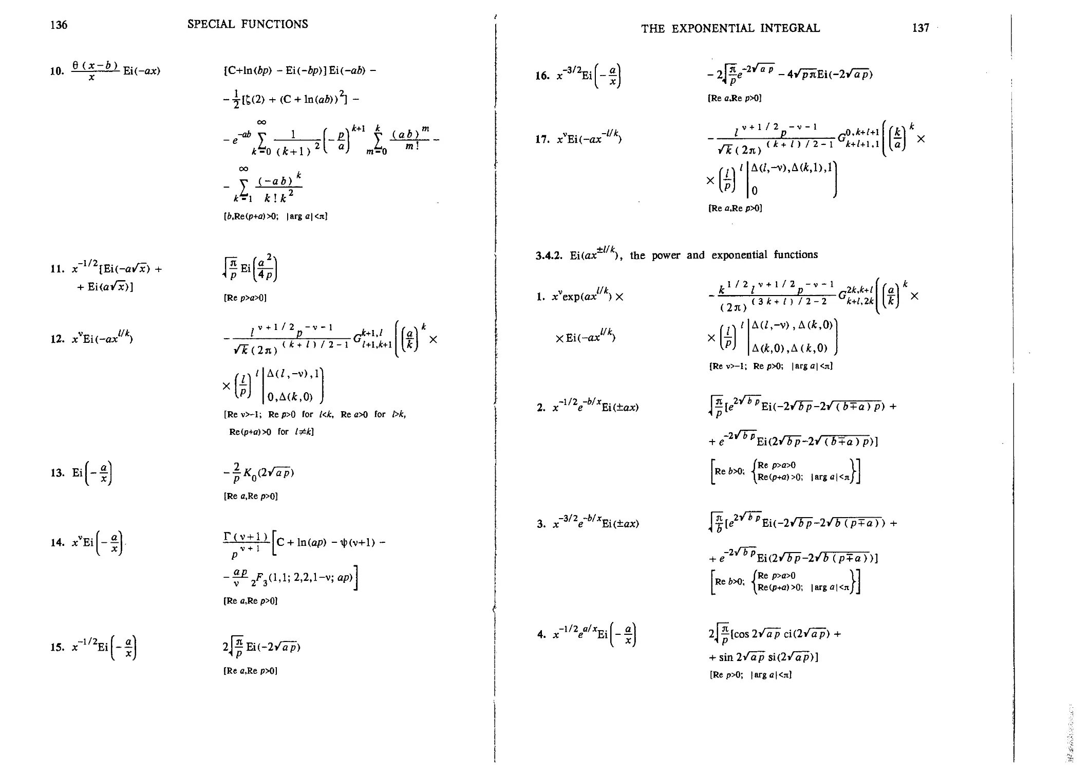
-X
/
A(Jb,l-r±v/2),
Д(*,1/2)
[Re ц>-1; RepX);

26 ELEMENTARY FUNCTIONS
6. <Цх-а)[[х+1х2-а2У- Ц^-К
-\x-\x2-a2 J J [o,Rep>o]
7.
XI \x+ix2-a2) +
8.
Г71
XI \х+Лх2-а2) +
<[(¦
9. /A-Л"гХ
ГГ, П
X | 11-И l-aJ77T)V-
[г-0 or 1/2]
10. *ц(а* -1
2aKv(ap)
[o,Re pX)]
[a,Re p>0]
xG '
lRe(tv+k\j.)>-k; Re ц>-1; а>0]
2k+l,2k\ I
к , I
Д(?,0), Ли, 1/2)
. i42
-(-1)
Г7Т
[a,Re p>0]
THE POWER AND ALGEBRAIC FUNCTIONS 27
2.1.7. Functions of [л:]
1.
2.
3.
4.
5.
1
([*]+!)
(-1)
7.
[r-0 or 1/2]
8.
о
in
1
[*] !
(±1 ) [
B [x]
(±1
X ]
) I
j IX]
[Re p>0]
[Re pX)]
[Re p>0]
[Re p>0]
— sinh ¦§• arctan e
(Re p>0]
[Re p>0]
[Re p>0]
l-e"p fcosh^-i
p \cos
<e-p/2)}

28
11.
12.
13.
14.
ELEMENTARY FUNCTIONS
D
+cos(e-p/4)]
: x]
D
1-е
-p
-cosh
/I J
cos
/i
D
+ sin(e-p/4)]
(-1)
lx]
D [*] + !) !
cp/4 1-е
""
/2p
+ COSh
[г - Р I 4
sinhj
4) ¦ fe"p/4)l
-sin
J I /I JJ
VJ ) \ /I
,. в(п-х)
lx] !
"•
,-p
(n-l) !p exp(e ") Г(п, е
lnd
[Re pX)]
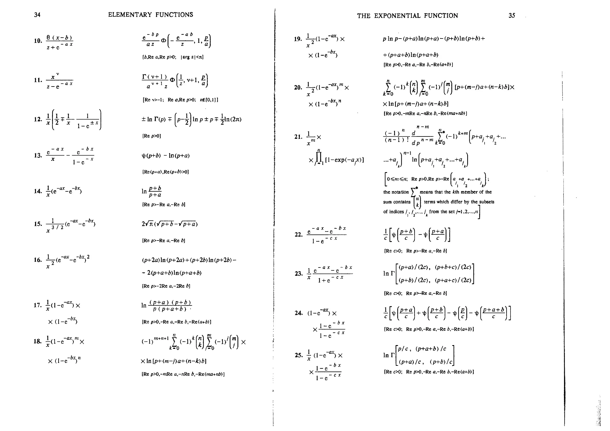
2.2. THE EXPONENTIAL FUNCTION
2.2.1. exp(-ax ) and the power function
1. e
„ v -ax
2. x e
з.
l
p+a
[Re(p+a)>0]
[Re v>-l; Re(p+a)>0]
1
(p+a)
[Rev>-1; b>0]
— y(v+l, ab+bp)
THE EXPONENTIAL FUNCTION
5. exp(-ax )
6.
7. x"exp(-ox2)
I" 8. x exp(-ax
9. x exp(-ax )
10. x exp(-ax )
11. в(х-Ь)ехр(-ах2)
12. (x-b)vtxp(-ax2)
13. ехр(-ал:
1
(P+a) '
[*,Re(p+a)>0]
ab+bp)
[Re a>0]
Ba) (v + 1 ' 7
[Rev>-1; Rea>0]
[Re aX)}
[Re a>0]
[Re <z>0]
[Re a>0]
a>0]
[Re v>-l; A,Re o>0]
19
[Re a>0]

30
14. xvexp(-ax
ELEMENTARY FUNCTIONS
15. ехр{-спЛс)
16.
17.
18. д:1/2ехр(-а/3с)
20.
F2[-l-' 3' t' --its)-
[Rev>-1; Rea>0]
[Re pX>]
B<z)v+1 18PJ -2v-2
[Rev>-1; Rep>0]
( — 1 I I
[Re p>0]
a . a +2i
, 2+ 4
[Re p>0]
[Re p>0]
J|exp(^)
[Re p>0]
erfc
[Re p>0]
THE EXPONENTIAL FUNCTION
31
22.
^ум;у-'
*,/
к , I
a I
к р
Bя) V~T" ' ' '
[Re v>-l; Re pX) for kA, Re a>0 for t>k,
Re(p+a)>0 for l-k]
//jfe
2.2.2. exp(-ax ) and the power function
, v -alx
1. x e
2.
3.
(N IV+U/Z
f] ^v
[Re a,Re p>0]
dp
[Re a,Re p>0]
[Re a,Re p>0]
4.
i FtA +2/сГр)е"
2Jp3
[Re a,Re p>0]
5.
[Re fl.Re p>0]
6.
f1
(v+ 1 ) / 2
aW2 + V
- 2 • 4
2 'J 0^2[2
*• 4 J
[Re a,Re p>0]

32
7.
ELEMENTARY FUNCTIONS
j+v, 2+v;-
[Re a,Re p>0]
-ox )
Bn)(k+l)/2-1
XG°'k.
-X
[Re a.Re p>0]
2.2.3. exp(-ax ) and algebraic functions
2Г(у+1) Га
exP [J
•x
[Rev>-1; 6,Rep>0]
6 F-
¦fx
[A,Re a>0]
6 (x-b)-alx
-a /x
4.
[A.Re px>]
Л pz+a/z
— e er
[Re a.Re pX); | arg z | < л]
5.
1-е
1-е
7.
9.
[Rev>-1; Rea,Rep>0]
THE EXPONENTIAL FUNCTION
2.2.4. Functions of the form f(x, e ax, e , e ,...)
1. (l-e
2.
ч »,i -ax.v
3. д: A-е )
4.
I * <~1>v
[Rev>-m-l; Re a,Re p>0]
a dp'1 ia
[Rev>-n-l; Re a,Re p>0]
[Re v>-2; Re a,Rs p>0]
v + l ' ' a
[Re v,Re a.Re p>0]
[Re a.Re p>0; u-1,2,...]
[Rev>-1; Rea,Rep>0]
[Re a,Re p>0]
[Re a.Re p>0]
33

34
10.
z + e.
11.
- A x
13.
1-е"*
14. i(
5- -ттт
X
16. -L
17. 1A-e
18. l<l-e
X (l-e
1 , -ox -bx.
(е "e >
ELEMENTARY FUNCTIONS
-ab
(-во
, hR
az
[A,Re a,Re pX); | arg 21 < л]
[Rev>-1; Rea,Rep>0; z«S[O,l]]
± In Г(р) + [ P-JI In p ± p + •jlnBn)
[Re pX)]
~ In (p+C)
[Re(p+a),Re(p+A)>0]
ln P+b
(Re p>-Re a,-Re A]
[Re p>-Re a,-Re b]
(p+2a) ln (p+2a)+(p+2i) ln (p+2i) -
[Re p>-2Re a,-2Re b)
,n (P+a) (p+b)
p(p+a+b) ¦
[Re p>0,-Re a,-Re i,-Re(a+A)]
Xln[p+(m-j)a+(n-k)b]
[Re p>0,-'«Re a,-;iRe b,-Re(ttm+nb)]
THE EXPONENTIAL FUNCTION
35
19. ijd-e
20. -4-(l-e
p ln p- (p+a) ln (p+a) - (p+b) ln (p+b)
+ (p+a+b) ln (p+a+b)
[Re pX),-Re a,-Re A,-
У (-
1 lP+(m-f)a+(n-k)b]X
-k)b]
[Re pX),-mRe a,-«Re A,-
x
X
]J1[l-exp(-a
22.
23.
24.
-ax -b x
e -e
X
1-е
-bx
1-е
25.
1-е
-bx
(- 1 ) a V , . k+m |
/—in :;—7, / (~D р+в.+в.+...
ijx)] ...+a.\ In p+a.+a.+...+a.
/ it) { /, /2 /
[0<«i^«; Re p>0,Re p>-Re a +a +...+e ;
1У, У2 V
the notation ) means that the ith member of the
4 -
sum contains I'.' I terms which differ by the subsets
of indices /, / ,..., / from the set /-1,2 n
[Re c>0; Re p>-Re a,-Re b]
'(p+a)/Bc), (p+b+c)/Bc)]
1пГ
(p+b)/Bc), (p+a+c)/Bc)J
[Re cX); Re p>-Re a,-Re b]
1-е
[Re cX); Re p>0,-Re a,-Re 6,-Re(a+A)l
[р/с, (p+a+b) IС
(p+a)/с, (p+b)lc
[ReOO; Rep>O,-Rea,-Re A,-

36
ELEMENTARY FUNCTIONS
1-е
28.
29.
- / X I к , v
(z + e )
30.
31.
[z+(ex-l)-//*]v
32.
q-e"*I1
У (-i)**"*'in
to
[Re cX); Re pX),-HRe с]
p-v4-l; и,»)
[Rev<l; Re oX); |arg(l-u)|,
,p/a) ,
>-1; Reo>0; |arg(l+i
(In)
) v / ц r Гц+ ll
;^"~ГЫ
-k
[Re |
; |argz|<n]
v , - p
:- 1 V
r^ x
Bя)
[Ren>-1; Re p>0; |argz|<n]
/,1-р), A(*,l-v)
[Re m->-1 ; Re p>0; |arg г|<л]
Г(м,+ 1 )пк fJ(,k+l -к
a[V-+l U2k+l,2k+l "
да,0), да,i/2)
ДОМ/2) , Д(/,-р-ц)
[Re ц>-1; a,Re p>0]
да,о>
33.
A-е-*)»1
THE EXPONENTIAL FUNCTION
лк_
37
34.
35.
\a-e |
36.
A-е-'I1
/ / t | v
аГ
Д(А,О),
[Re (x>—1; c,Re
<2я) '-'
Д(/,1-р),
Ji+tMl I _-*
J2*+/,2*+/
, да,i/2)
[Re ц>-1; a,Rep>0]
n(kla)
1 cos(vn/2)
L v J
*,l-v), Да, (l-v
>-1; Rev<l; a,Re pXi]
n(kla)
Zpcos(vn/2) Lv
г x
-*
Да,1-v), A(A,(l-v)/2)
[Re ц>-1; Rev<l; a,Re p>0]

38
37.
38.
X
39. A-е Yx
ELEMENTARY FUNCTIONS
40. A-е
2Bя)
/ - 1.
A«,H+D.
2k+l,2k+l
A(*,0), A(*,(l-v)/2)J
[Re ц>-1; Rev<l; o,Re p>0]
а) УГ(ц+1)Г(у+1)
J X
Ы,к+1^ак д(Л0)) д(/ ^
[Re p>0; Re v>-l for 0<ж1, Re |
o>l, Re(|i+v)>-l for a-1]
а] Г(у+1)Г(р)
for
А(/,-ц), A(/t,v+l)
Mk,Q), Д(/ ,-р-ц.)
[Re ц>-1; Re p>0 for o>l, Re v>-l for
(Ko<l, Re(p+v)>0 for o-l]
v , u. + p
а Г
I
a
[Rev>-1; o.RepX)]
, Д(*,0) J
THE EXPONENTIAL FUNCTION
39
41. (l-e~Vx
X(e
-Ixlk .v
a)
-X
ЭД+/ 1
P
[Re n,Re v>-l;
42. A-е Х)ЦХ
дГГ(у+1)Г(р)
/ p
a* A(*,0),
[Rev>-1; 0<a<l; Re p>0]
43. A-е Х)ЦХ
J_
a
[Re n,Re v>-l; o>0]
, Д(*,0)
44. A-е
/2(+v/2)'~2гГ(ц+1)
X
1 + ze
-Ixlk
X
[r-0 or 1/2]
±1,1
VG*'2*+' z*
Xt72t+/,2Jt+/|Z
A(*,(v±v)/2), Л(/,-р-ц) J
[Re ц>-1; 2/:Re p>-( 1+1) /; | arg z 1 <я]

40
45. A-е Vx
ELEMENTARY FUNCTIONS
/?(+v/2Irr(p)
±i]V
[r-0 or 1/2]
46.
A-е)
)'
X H 1 + ze
- l x / к
[r-0 or 1 ]
47.
[r-0 or 1/2]
48. <l-e~Vx
x[(wi-e'
[r-0 or 1/2]
U+''2k+l> A(*,(vTv)/2),
), A(*,l-2r+v/2)]
A(*,(v±v)/2), Д(/,-р-ц) J
[2tRe n>-(l+l»-2it; Re p>0; |argz|<n]
1 -2 r,
/2(+v/2)'гГ(ц+1)
A(*,0) ,
-X
C2k,k+l L*
A(/t,l-r±v/2),
AOU/2), А(/,-р-ц)
[Ren>-1; Re p>0; |argz|<it]
/2"( + v/2) 'ГГ(р)
X^+/,2*+/|Z ДЛ0)>
A(*,l-r±v/2), A(*,l-r+v/2)'
-1; Re p>0;
P.
-2r
[Re p,Re(p+v)>0]
THE EXPONENTIAL FUNCTION
41
49. (l-e
)v
-
-(-lJr('
[r-0 or 1/2]
l + t~X-A\
^I
50.
-[(ZJ^77)\
1-е
+ lz-^l 1-е~л)"]
51. la-e~x)~+r[[Va+
a-e'x] -(-lJ^-
-<l a-e
[r-0 or 1/2]
52. (Ье
[r-0 or 1/2]
p+v/2+l-2r
[Re p,Re(p+v)>0]
XP
1/2-v
p+v-1/2
г'-l
[Re p>0]
2 r- 1
0,v,-p
[Re p, Re(p+v)>0; 0<а<1 or o>l, Re ц>-1]
A(*,0) ,
A(*,v), A(i.-p-n)
[Re p,Re0fcp+/v)>0; 0<a<l or a-l,
Re ц>2г-3/2 or a>l. Re ц>-1]

42
53.(l-e~Vx
x[a-a-e-x)l/k]-+rx
ELEMENTARY FUNCTIONS
¦(л-
J 7^ -x,
-4 a - ( 1 - e )
[M) or 1/2]
/ / *
А(*,0),
A(*,U+v)/2), A(/t,l-2r+v/2)
A(?,v) , Д(/,-р-и.)
[Re м>-1; Re(*n+/v)>-*; (КЖ1 or
o-l, Re p>2r-l/2 or a>l, Rep>0]
1/2
Г I—г '¦
2.2.5. Functions containing exp[-«x ±b'
I.
,1/2
exp (-
2 ч
[Re o,Re ft,Re(p+W>0]
П 2 1/2
erfc(u )-
,h
2 21
Xexp^-Mx +a J
+a
- — exp [a'J b -p J erfc(«+) J-
[Re c,Re b,Re(p+b)X)]
31 -e^erfcte )erfc(u )
1 / 2
[Re o,Re *,Re(p+W>0]
THE EXPONENTIAL FUNCTION
43
-v- 1 / 2
2+a2)
x2 + a2
'(-
Xexpl-Wx +a
5. (*-a);1/2X
Xexp^-Mx -a
6. (x2-a2>;3/4X
Xexp[-Wx -a J
-1/2
(x-a)
7.
x+a
8. (x+a)v(x2-a2) 4 X
(-
Xexp
9. (x2-a2);l/2X
x-H x 2 - a 2 J X
x[(
Xexp(frJx2-a J +
+ (x-^lx2-a2) X
Xexp[-Mx -a JJ
[Rev<l/2; Re a.Re A,Re(p+A)>0)
-— exp I -en p -b ) erfc (f_) -
[a,ReA,Re(p+W>0]
Jl'
1/4
2
f -1
2
[a,Re *,Re(p
)erfc(»
X exp (-^x2-a2) [o,Re *,Re(p+W>0]
[Rev<l/2; Re o,Re ft,Re(p+A)>0]
2a
[o>0; Rep>O|Reft|]
2.2.6. Functions containing exp(/"(x)>
1. exp(-ae
-p, a)
[Re oX))

44
2. exp(-ae~x)
3. A-е Vexp(-aex)
4. (l-e~Vexp(-ae~x)
ELEMENTARY FUNCTIONS
a~"y(p, a)
[Re p>0]
THE EXPONENTIAL FUNCTION
45
(z+e
6. (l-e-x)vexp(-aeb:/i)
7. (l-e'Vx
X exp(-ae""'x/*)
8. (l-e-x)vx
9. (l-e"x)vx
Xexp[-a(l-e~x) l
[Re v>-l; Re pX>]
B(p,v+lI/!'1(p;p+v+l; -a)
[Rev>-1; RepX)]
^, |p,mp+v+l; - j,el
[Rev>-1; Rep>0, |arg(l+z"
Г(у+1)^1/2/ — '
Bn)(k~l)/2
к
A(Z.-p-v)
[Rev>-1; Rea>0]
< *- 1 ) / 2
* [** Д(*,0),
[Rev>-1; RepX)]
Bя)а-1)/2
/r*+'[/t* A(*,0),
[Re v>-l; Re pX)]
( * - 1 ) / 2 '
[a
[Re a,Re pX)]
10. A-е X)VX
v t/k
xexp[~a(ex-l)(/ ]
11. (l-e"x)vx
Xexp[-a(e*-ir'M]
12. A-eVexpl--
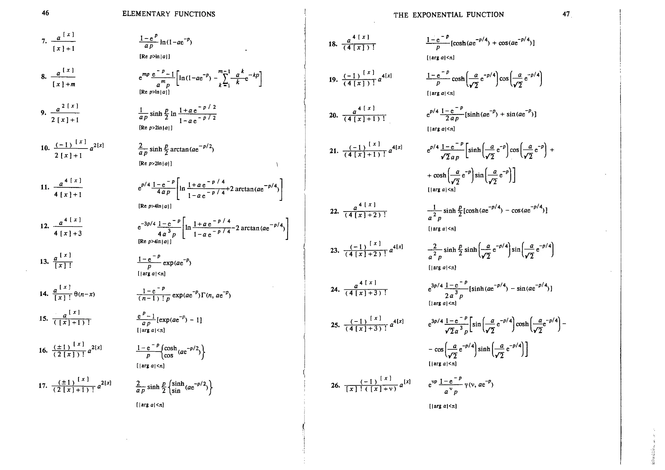
2.2.7. Functions of [x]
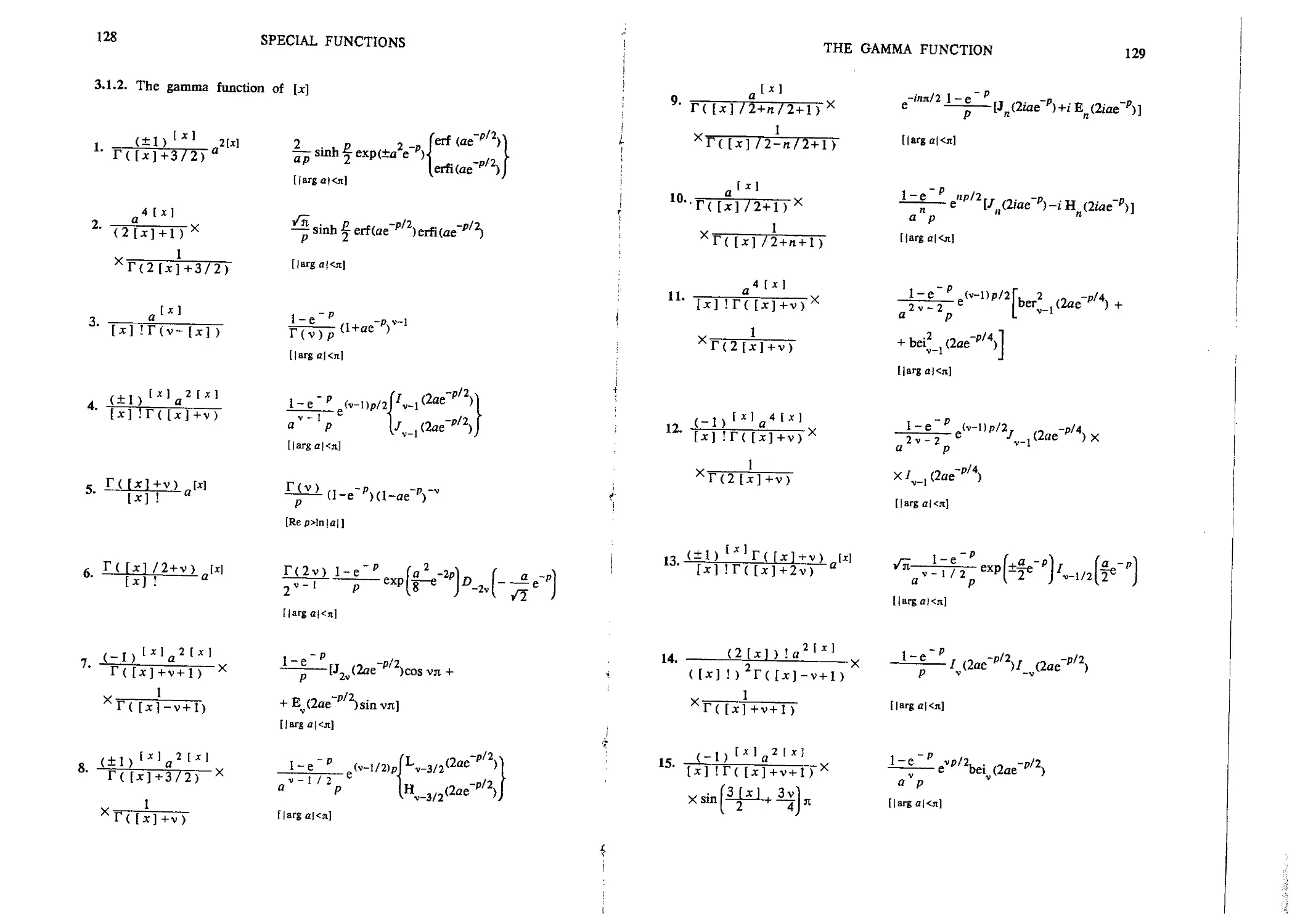
1. a[xl
3. [x]a[xl
4.
5.
( [*]+*)
(lx]+b)s
a[x]
9(n-je)
[Rev>-1; ReaX)]
хСГ1,Ы\
[Re a,Re pX)]
v/2 a/
[Re v>-l; Re pX)]
, A(*,0)
[Rep>ln|o|]
!-e-P l-q"e-"P
p 1-ae p
I4—ae-p(l-ae-p)-2
[Rep>ln|c|]
1-е""
P
[Re p>ln|o|;
ep-l
Ф(ае
Lin(ae"p)
[Rep>ln|e|]

46
7.
[x]
8. S.
'*1
9.
10.
11.
12.
13.
[x] +m
a2[x]
2[x]+l
(-1)"
2[x]+l
a4'*'
4[x] + l
a4'*'
4 [x]+3
Ax]
14. f——Q(n-x)
lx) !
15.
Ax]
([*]+!)!
16. -^
<2[x] ) !
д2[х]
7
- B
ELEMENTARY FUNCTIONS
[Rep>ln|o|]
cmp e - ]
a p
[Rep>ln|o|]
-p/2
[Re p>21n|a|]
[Rep>2ln|a|]
l-ae-p/2
p/2)
[Re p>4ln | a
_-3p/4l-e"p|,.. l + ae"p/4
4a
[Rep>41n|a|]
f^L1 + ge"^4-2 arctan(ae-p/4)l
p [ !-ae p J
i 1 ¦*
. " P
ехр(ае"р)Г(л, ае"р)
ep-l
[exp(ae p) -
[|arge|<n]
l-e"pfcosh,..-i
cos
(ее
[|arg о|<л]
[|arga|<n]
THE EXPONENTIAL FUNCTION
47
18.
4 [*]
D[ж] ) !
9
9' <4[x] ) !
20.
4 [x]
D
1-е
-P
[cosh(ae p/4) + cos<ae"p/4)
P
[|arga|<it]
1-е"
P
[|arga|<it]
ep/4 l~2lp" [sinh(ae'p) + sin(ae"p)]
[|arga|<n]
1
1- D[x]
22.
4 [x]
<4[x]+2)!
Д4[х]
3
• D[x]+2)!
.4 [x]
24.
D[x]+3)!
p/4 1-t
^-/2 I <-/2
[|arg а|<л]
j- sinh^[cosh(ae"p/4) - cos(ae p/4)]
a p
[|arga|<it]
sinh f sinh U e-p/4l sinM e-p/4
2 1 J 1
1/2
[|argo|<n]
3p/4 1 - e
- p
e' —^ [sinh(ae "") - sin(ae
2a p
[|arga|<ai]
4[x] ,3p/4 l-(
5
5' D[x]+3) !
- COS I
1/2
[|arga|<it]
[x] !
[|arga|<n]

48
ELEMENTARY FUNCTIONS
THE EXPONENTIAL FUNCTION
49
27.
28.
(±l)lx]a[x]
( [*]+!) ! ( [*]+!)
a[x]
[x] ! ([x
+ In а - р - Ei(±ae-"p)]
[|arga|<n]
X
['-
n-1 , ..ж x
. [x] 2 [x]
(- I ) g
. [x]
(- I ) g
[ж] !
[|arg о|<л]
30.
31. -г-.
! B[ж]
(±l)[x]a2lx]
+ ехр(±а2е"р) + 11
[|arg о|<л]
B[ж]+2) ! ( [*]+!)
/ 1 Г *. 1 i 1 V t X
(|arg
33.
34.
35.
4'*'
!D
0 ep/4(l -e"p) [erf(ae-p/4)
[|arg
(-1)
(±l)[Xl 2M
! ( [ж]+п)
37. (±DIxl 4M
! }
9 iLLilitx].
< B[ж]) ! L J
• тЩ^ттт^2
42
43.
44.
B
( [
B
(
B
1*1
x] !
[*1
[X]
Г д:1
[x] ! (
) !
J
+ 1
!)
) 1
lx
<2Гх1
)
2
a
}
>
[X]
! M
lx]
+ 1) !
lalx]
([x] !
1-е
- p
" г
12 berBae-p/4)
1 . „Л^"'^-'
Л Sm% beiBae-p/4
-р/4)-/оBае-р/4)
^[-Jf'
-p/2 f. а -p
s exp^t^-e
X1
[|argo|<it]
[Rep>lnD|o|)l
[Rep>lnD|o|)l
[Rep>lnD|o|)]
е"р-
[Rep>lnD|o|)]
-рЛ/2

50
ELEMENTARY FUNCTIONS
HYPERBOLIC FUNCTIONS
51
45. (±D tx] BГл-1 ) ! ^
[x] ! ) 2B [x] + l)
46.
(±B[х М-2НП
Xa
2[x)
[Rep>21nB|a|)]
ep-lfarcsin
77
l -p/2)\2
[Re p>21nB/|a|)]
54.
(.;.)¦
*¦ Uf
Хв(л+1-х)
47. <-l
Л Г*1!
X\B[x]) !
2[x]
2.3. HYPERBOLIC FUNCTIONS
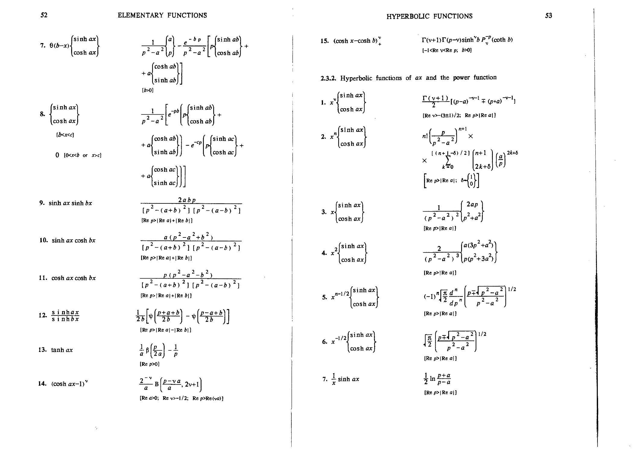
2.3.1. Hyperbolic functions of ax
,, (fxl!)
[|arga|<n]
1.
Tsinhaxl
[cosh ax)
2 2 ,
P -a \p_
[Rep>|Rea|]
49. (-1
2W
B[x1 ) !
51. (-i
Xa
52.
53.
B Где!) !Ги2Ь1
( [x] ! L
2[.x]-1
1-е
- p
expBae
p
|arga|<n]
|argo|<n]
[Rep>21nD|a|)]
2Г'-1
[Rep>21nD|o|)]
2. sinh ax
3. cosh
fsinh ax\
[cosh axj
5.
1
со shax
1
cosh ax
p
\\- l " * " ' )—; Rep>n|Rea|
2a2
[Re p>n|Rea|]
[Rep>2|Rea|]
2aJ
[Rep>-|Reo|]
?_
2
a
1
a) a
[Rep>-2|Re a\]

52
ELEMENTARY FUNCTIONS
HYPERBOLIC FUNCTIONS
53
7.
sinbax)
cosh ax)
8.
[cosh ax)
lb<x<c}
0 [0<x<ft or x>c]
9. sinh ax sinh bx
10. sinh ax cosh 6x
11. cosh ax cosh
12.
s i nhax
s i nhbx
13. tanh ox
14. (coshox-1)
p -a [p
е-Ьр
"~2 :
р —а
cosh ab)
fcosho*)'
¦ai V
[sinh ab)
2 2
p -a
1^1
[sinhaij
(cosh ac]
¦a<
[sinh ac)
( ("sinh ac\
Г
cosh acj
f f
2abp
[p2-(a+b) 2]
[Rep>|Reo
a(p2-a2+b2)
P(p2-a2-b2)
Ip2-(a+bJ] [p2-(a-bJ]
[Rep>|Reo|-|Re*|]
[Re p>0]
-, 2v+l
a | a
[Rea>0; Rev>-l/2; Rep>Re(vo)]
15. (cosh x-cosh6)j
r(v+l)r(p-v)sinhv6PvP(coth b)
[-KRe v<Re p; ft>0]
2.3.2. Hyperbolic functions of ax and the power function
(sinh ax)
1. x
2. x
[coshaxj
fsinhax")
[cosh ax)
3. x
4. ж
sinh ax"|
cosh ax)
2Tsinh ax)
[cosh axj
5. x
n_1/2jsinhax|
[cosh ax)
6.
^1/2(Smhax\
[cosh axj
7. — sinh ax
[Rev>-C±l)/2; Rep>|Rea|]
ЧП+1
n\
X
2 2
p -a
<it+ 1-6) /2] (n+l ) r \2k+6
Rep>|Rea|; 6'
[Rep>|Reo|]
2
(p2-a2K[p(p2+3a2)
aCp2+a2)
[Rep>|Reo|]
-I 2 2I/2
p+ip -a '
2 2
p -a
[Rep>|Rea|]
J!(
«i?±?Z31/2
21 P2~a2 j
[Rep>|Rea|]
[Rep>|Reo|]

54
ELEMENTARY FUNCTIONS
HYPERBOLIC FUNCTIONS
55
8. x~3/2sinhax
9. xv
fsinh ax\n
1
[cosh ax)
10. x sinh ax
¦. 1 . , 2n
11. — sinh ax
12. iSinh2n+1
13. ^si
14.
s'nh
15. ^si
[Rep>|Reo|]
[Rev>-l-(l±l)n/2; Rep>n|Rea|]
(-1)*
m! у
m+ 1
[Rep>n|Reo|]
x
[Rep>2/i|Reo|]
-2„-1 * ы
t-o
. p+Bn-2k+l)a
XU1p-Bn-2k + l)a
[Rep>B/i+l)|Reo|]
[Rep>2|Rea|]
[Rep>2|Reo|]
- -7 arccoth — + 4- arccoth —
[Rep>3|Reo|]
16. —sinh ax
x
17. —г
18.
s i ahax
с oshax
19. x tanh ax
20. — tanh ax
21. x coth ax
22. Q(b-x)x
(sinh алЛ
1
[cosh ax)
23.
24.
sinh ax
Tsinhax"]
[cosh ax)
+ ^arccothj
За1мр2-3а2
1П
[Rep>3|Reo|]
-v- 1
[Rev>0; Rep>-|Reo|]
22v-!a,
[Rev>-1; Rep>-|Reo|
[Re v>-2; Re pX>]
[Re p>0]
[Re v,Re p>0]
~
, bp-ab)
1, bp+ab)]
[Rev>-(l±l)/2; *>0]
1 v,
[4>0]
, bp-ab)
, bp+ab)
[Rep>|Reo|;

56
ELEMENTARY FUNCTIONS
HYPERBOLIC FUNCTIONS
57
25.
sinh ax
cosh ax
26.
1-coshax
27.
28.
29.
30.
31.
32.
1-co shax
ax-sinhax
ax-si nhax
со shax-coshix
cos hax-coshbx
33.
si ahax-axcоshax
- у EH-bp+ab) ± j EH-bp-ab)
[Rep>|Rea|; 6>0]
[Rep>|Rea|]
p\a _ы2±?.
p I p-a
[Rep>|Rea|]
[Rep>|Re a\
1
I1" 2 2
p -a
[Rep>|Rea|,|Re6|]
_2 2
[Rep>|Reo|,|Re 6|]
s inhax-axcoshax 1
[Rep>|Rea|]
2 p-a
[Re p>|Re a|]
sinhax-axcosbax 1 Lp^)inZ±R - 2apj
35.
s inhax-2axcoshax
-
36.1- 1
x xcoshax
37 l a
x s inhax
38. 4 - e coth ax
2
T> 2^ 2
x s i nh ax
40.
41.
sinhaxs i nhbx
s inhaxs i nhbx
42.
43.
s inhaxcoshftx
s i nh ax
xcoshBax)
[Rep>|Re a]]
,2-4a'J
[Rep>|Rea|3
[a,Re p>0]
la)
[a,Re p>03
[a,Re p>0]
4
p -(a+6)
[Rep>|Reo| +
A
(p-ft) -a2
(p-a)-A
4 p-(a-*)
[Rep>|Reo|+|Re/»|]
[Rep>|Re a)-
In Г
[<z,Re p>0]

58
ELEMENTARY FUNCTIONS
HYPERBOLIC FUNCTIONS
59
2.3.3. Hyperbolic functions of ax for b?k and algebraic functions
1. sinh crfx
2. cosh атГх
3. x
(sinh afx\
I cosh атГх I
4. x"sinh a/x
. n-l/2 , i—
5. д: cosh aYx
6. д: sinh a/x
7. д: sinh ai^3c
8. д: cosh
p
[Re p>0]
[Re p>0)
[Re v>-E±l)/4; Re pX>]
. и+ 1 . /
<-') ^
_ 2 я + 1 я + 1
2 p
[Re pX)]
[Re p>0]
4p
Xexp
[Re p>0]
8p7/2
[Re p>0]
P
[Re p>0]
1 a
X
9. xl/25iahafx
10.
11. X
12. д; 1/2sinha/x
13.
14. д;
[cosh a-fx)
15. — sinh a-fx
16. x
_2/3|sinh«
[cosh ад:
-1/3
-1/3
2p'
[Re p>0]
2p+a2
[Re p>0]
icosha^J 2^"J
[Re p>0]
^expl^lerf
[Re pX)]
[Re p>0]
[Re p>0]
[Re p>0]
3_
2a
[u-2p"'/2(a/3K/2; Re p>0]

60
ELEMENTARY FUNCTIONS
„ v/, //<2*L
17. x < (ax )
[cosh
v + 1 / 2 - v - 1
z Bл)
(/ -]
Xl-г
iv>-l-4r: RepX>; 6-|^
18.
л l
2
[Re p,Re
-1/2
19. Xx + Z cosh a/x
^- /r [2 cosh a/7-*/a/7erf
/7 L
2/7
-«""'•erf
[Re p,Re i>0]
20.
(cosh *xj /x
s i nh [ Bn+l ) a/x]
i nhaifx
2(p2-*2I/4
fsinhBj
[cosh B)
4Л j -, 4Д-1П -2-ij -2Aft; Re p> I Re ft I
Lft2-p2 P J
[Re p>0]
lf 1 + 2 У (-1
[Re pX>]
HYPERBOLIC FUNCTIONS
61
23.4. Hyperbolic functions of \x*+xz and algebraic functions
Notation: 2^=2 lz(p±\p2-a2)
az jnliv ill 2 ~2~,
2. — cosh(<M;c2+xz)
[Rep>|Rea|; |argz|<n]
(p2-a2)z
exp(z )
[Rep>)Rea|; |argr|<n]
3.
1
[cosh(aix +xz)j
л A±1)/2
, j-J 2 2, +1/2
(p+-<p -a )
2a
2 2
p -a
- exp(z_)
[Rep>|Rea|;
~2""" 2
[Rep>|Rea|;
3 /2'
x2+xz)"|
+xz)J
, ( 2+1 ) / 2
[Rev>-E+l)/4; Rep>|Rea|;
6.
x+z
/7
[Rep>|Rea|;
_ ГегГ(/7~)")
Л . 1

62
ELEMENTARY FUNCTIONS
7. (x2+xz)~3/*X
(sinhiaix +xz)}
'J . L
i 2 Г
^cosh(aix +xz)J
[Rep>|Rea|; |argr|<n]
: U+4-i;c2+;cz x
fsinh(dx2 + z V
Ч П 2
[cosh(tfix +z )
x*WV
[Rep>|Reo|; |argr|<n]
-1/2
9.
(siahWx +zl)
1 1 ! 2* 2
Icosh(ai x +z )
гA±1)/2г^Г[Л/4(У1
[Re p> | Re a\; Re rX); » -2"'r(-l p 2 - a 2 ±ia) ]
j 2 T
2.3.5. Hyperbolic functions of a\±b +x and algebraic functions
Notation: и =2 '*(-! p 2+a2±a),
"±= 6(p±"l p2 -a2)
-bp/2 ЬГ~2~2]
X cosh(ai bx-x )
HYPERBOLIC FUNCTIONS
63
. , 2 2,-1/2
(b -x ) +
X cosh(i
-X
- 2 [Л
[*>0]
3. e(x-b)x"sinh(J x2 -b2)
a + 1 <r
р
„ 2 2 , ( ff + 1 ) / 2 ff+
(p -a )
[<r-0 or 1; b>0; Rep>|Reo|]
4. (*-*
p -a
[6>0; Rep>|Reo|]
2 2
I p -a
fsinh(ai x -b )
H f—2 2
[cosh(ai д: -i )
Xexp(-Wp -a )
[6>0; Rep>|Rea|]
(x-b)
(x + b)
¦ +3 / 2
X
fsinh(uix -й
,±1
0; Rev>-1; Rep>|Reo|]
-1/2
7.
1
fsinh(aJx2-62)
¦-ft1)
0; Re p>|Rea|]

64
ELEMENTARY FUNCTIONS
o (Г. 2 ,2,-l/2w
8. x (x -* ) X
Xcosh(a<lx2-*2)
(bp)
2 2,,/!^^'»
(p-a)
[(Г-0 or 1; 6X); Rep>|Rea|l
9.
u2-*2>;1/2
Xcosh(aix -4 )
[fc>0; Rep>|Re<z|]
fsinh(aJx -b ]
4
na
\~2-
[b>0; Rep>|Rea|]
Y
2.3.6. Hyperbolic functions of ax, the power and exponential functions
. fsinh ox) .
[cosh ax)
[Rev>-C±I)/2; Rep>|Rea|,|Rea|HRe(M]
2. (l-e
-bx _ -ex
3. cosh ax
-bx -ex
. e -e . .
4. stnh ax
[Rep>|Rea|,|Rea|+Re b]
2 2 2
Z (p+ft) -a2
[Re p>|Re a|-Re 6,|Re a|-Re c]
2 2
[Re p>|Re a|4{e 6,|Re a|HRe c]
HYPERBOLIC FUNCTIONS
65
5.
e'bx-e~cxcoshax
1, (p+cJ-g2
у 1П— г
1 (p+bJ
[Re (p+ft) X); Re (p+c) > | Re a | J
6. д:~ (ae Xsinh сд:
а с ,_ (p+d) 2 -а2 с (p+d)
- се xsinh ax)
~ 2 lnp+*-c
[Re(p+6)>|Rec|; Re(p+d)>|Re <z|]
fsinh ax")
7. exp(-*x2)] \
I cosh axl
[Re
8. x exp(-to')
fsinhax)
[cosh ax)
Г(У+1)
2 . 2
¦)hh
X?>
I; Re v>-C±l)/2)
9. хехр(-йх
[cosh ax)
[Re 6>0]
10. xV*/xJ I
[cosh axj
r. ,-Ь+1)/2„ ,- гх. Гч
[(p-a) Kv+lQVbp-ab)
~W*l)/2
+ (p+a)
[Re6>0; Rep>|Reo|]
Kv+1QVbp+ab)]

66
11.
ELEMENTARY FUNCTIONS
I cosh ax!
ax
12.
l+ax-e
xsi nhax
Vn
2b
<(Г-3)/4 -2
[ir-0 or 1; Rei>0; Rep>|Rea|]
[a,Re pX)]
2.3.7. Hyperbolic functions of ax~ for ft**, the power and algebraic
functions
1. e
[cosh aSx
[Re p>0]
2v ¦
. x e
[cosh атГх)
ГBу+2)
v + 1
Bр)
exp
a2+b2
[ 8р
[Rev>-E±l)/4; Re p>0]
з. _Le
/x [cosh aiTx
[Re p>0]
HYPERBOLIC FUNCTIONS
67
4.
[cosh(a/x)J
[Re*>|Rea|; Re pX)]
_ чг/2-2 -6/Jt
5. x e X
('sinh(a/x)>|
H I
[cosh(a/x)J
/it
2р
п—3)/4 -2Y b p-a p _
- ., . (<r-3)/4 -2/6 p + a p I
+ (ft+a) e
[<r-l or 3; 6>0; Re6>|Rea|;
fsinh(ax+c/x)>|
4 f
[cosh(ax+c/x)J
(sinh d\
[cosh dj
\ , p + t
\d-~ la" Ik, и -rs((*+c)(p+a)/F-<;)(p-<2)) '
4 p-a - ±
±rs (F-c) (p-a) / (b+c) ip+a) )ui\
. 2 2.1/4 .,2 2.1/4
r~(p -a ) ; s-(b -c ) ;-i
Re*>|Rec|; Rep>|Rea(
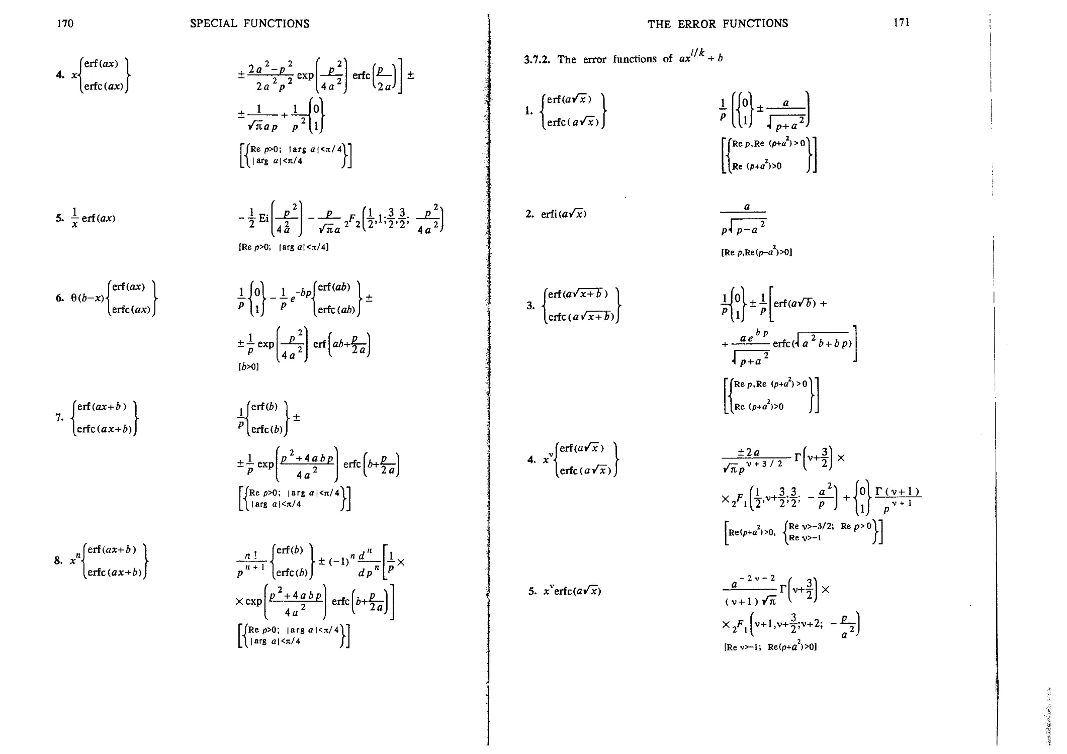
2.3.8. Hyperbolic functions of [x]
1. *Wsinha[x]
1-е
-p
be p sinha
l-2be'pcOsha+b2e-2p
[Re p>ln|A|
2. b Ы cosh a [x]
1-е"" 1-*е "cosha
[Rep>ln|6| + |Rea|]
. [*]
3. , j sinh a [x]
1-е
-p
¦ arctanh
й е рs inha
p
co sha
[Rep>ln|6| + |Rea|]

68
4. i-T-coshaW
ELEMENTARY FUNCTIONS
- In A -26e"pcosh a+b2e'2p)
5.
lx] fsinh(aW+c)|
!lcosh(afx]+c)J
[Rep>In|6| + |Rea|]
—^ exp(*e~pcosh a) X
fsinh(*e"psinh а+сЛ
[cosh(*e sinh a+c))
HYPERBOUC FUNCTIONS
fsinh
5. j [a(l-e )]
cosh
6.
sinh
(a* 1-е x)
cosh
[Re p>0]
[Re p>0]
69
2.3.9. Hyperbolic functions of fie ) and the exponential function
Notation: 6
sinh
cosh
(ae x)
2. A-е
3. (W
sinh
cosh
sinh
(
cosh
аг fp+6. 1 . p+6 . a
Л (V-1+б' 2 +1; —
[Rep>-(l±l)/2]
[Rev>-1; Rep>-(l±l)/2]
г f?+A 1 e P+6 . a21
1^2[ 2 ;2+6' 2 +V+1;4~J
[Rev>-1; Rep>-(l±l)/2]
7. (l-
fsinh
I cosh
S.
. [sinh I
1 ' (ah-e~x)
1-е'
-x I cosh
9. A-е Vx
fSinhr n -x
X-l [a(l-e )
cosh
a6Bf|+v+l,pl
[Re v>-E±l)/4; Re p>0]
/ir(p)ff]1/2"Tp/2<fl)
l2J Vp-l/2<a)
[Re p>0]
[Rev>-l-/6/Bt); Rep>0]
4. A-е x)vx
cosh
ШЛ-р)
[Rev>-l; Rep>-/8/<2*)]
"(f
10. tanh|4Heax-l
22p/,
[Re p>0]

70
ELEMENTARY FUNCTIONS
2.3.10. Functions containing the exponential function of hyperbolic
functions
1. exp(-asinhx)
2. exp(- a cosh д:)
3. —-exp(-acosh /x)
л esc pn [J (a) - / (a) ]
[Re c>0]
csc pn cos(px)txp(a cos x)dx -
-nlp(a)
[Re c>0]
[Re a>0]
4.
1
's i nhx
; exp(-a sinh д:)
5.
1
's i nhx
6. sinhvftx exp(-a coth bx)
л а
8
+ У
[Re oX)]
[Rea>0; Rep>-l/2]
[Rea>0; Rep>Re(vW]
TRIGONOMETRIC FUNCTIONS
71
2.4. TRIGONOMETRIC FUNCTIONS
2.4.1. Trigonometric functions of ax
Notation: X = —^——'—
fsin ax'
1.
[cos
2. | sin ax \
1
+a
[Rep>|Ima|]
p +a
[Re p>|Imo|]
3. j cos ax |
4. sin ад:
[Rep>|Ima|]
2 Я. - 1
[Re p>n\lm a\]
5. cos ax
2" ^0 Wp2+(«-2*Ja2
[Re p>n|Im o|]
6.
[cos ax)
7. | sin ax p
2a
p(p2+4a2) \p2+2a2
[Rep>2|lmo|]
r^ [sinh^X
!v+1(v+l)aL 2a
-1
[Re p>Re v Im a]

72
8. Q(b-x)
sin ax
cos ax
9. 6 T-*|si
10.
11. Q(n-x)
12.
sin x
cos д:
("sin ax)
[cos ax)
[b<x<c]
or x>c]
ELEMENTARY FUNCTIONS
ja\ e~bp
fcos ab~\
±a\ \
[sin abj
[*>0]
1 -ре
P2 + 1
p+e
-pn/ 2
1+e
-ря
P2+1
\
cos ab)
»Usini+
p2+al[ [ [cos ab)
(cos ab
±a\
[sin ab
fcos асП'
4 •
[sin acj
("sin ac)
[cos acj
TRIGONOMETRIC FUNCTIONS
14. 6 ?-.
15.
16. 8(n-x)sinVA:cos д:
17.
18. sin ax sin
/-1
(p2+4X2)(p2+4(X+lJ)...x
X ...(
2V
[Re v>-l]
p2+(v+lJ
[Re v>-l]
n !
-mpn.
—[l-(-l)"" e "'""] X
2abp
[p2+(a+bJ][p2+(a-bJ}
[Re p>|lma|
73
13. 6 -j-x sin x
n !
П
U-l
П [P
X (p2+4(UlJ)...(p2+4(X+/-lJ):
X [B/+2X)!]'
19. sin ax cos йд:
20. cos ax cos bx
а(р2+а2-Ь2)
[p2+(a+*J][
[Rep>|Ima|+|Im *|]
P(p2+a2+b2)
[p2+(a+bJ][p2+(a-bJ\
[Rep>|Ima| + |Im *|]

74
21. sin "ax
ELEMENTARY FUNCTIONS
sinfcc
cos bx
22 2-=-
s inftx
s i nnx
sinx
24. cos[Bn+l)x]tanx
25.
26.
27.
28.
1
со sh6±s i пах
s max
со she±s i пах
1
[+2bcosax+ft'
s max
b+ip+na
2a
rt+1
[<z,6,Re pX)]
-1
±(-1)
ft-tp+na
2a
—1
1 [".ffr + a-z-pl . fft-a-zVH
; a,Re p>0]
[Re p>0]
n-1
p2+Brt+lJ
[Re pX)]
[a,Re p>0]
[a.Re p>0]
l-ft"L P
[|*|<I; a,Rep>0]
f
; a,Rep>0]
TRIGONOMETRIC FUNCTIONS
2.4.2. Trigonometric functions of ax and the power function
[cos ax)
75
fsinax"!
_ n
2. x
[cos axj
3. xl
4.
[cos
2 j sin ax]
[cos axj
5. x
6. x
-l/2p
cos axj
sin ax
cos ax
7. — sin ax
+ (p-ia) ]
2 2 (v+1)/2 ,
(p +a ) [cos и
[«-(v+l)arcten(a/p); Re v>-C±l)/2; Rep>|Ima|]
sin и
n!
p
n+l
x A '""I
l±l)/2; Rep>|Ima|]
lap
U+6
, 2 2,2 2 2
(p +a ) [p -a
[Rep>|Ima|]
(p2+a2K\p(p2-3a2)
[Rep>|Im a\]
а(Ър2-а2)
_ Al ^ ^ Л
(-1) JiTT~2 2
dp [ p +a J
[Rep>]Im a|
2 +a2 +
1/2
[Rep>|Im a\]
arctan —
P
[Re p>|Im a\\

76
8. x~3/2sinax
9. x
sin ax\n
cos ax
10. isi
, , 1 . 2n+l
11. —sin ax
12. isin
13. -Ц-вп
14. isii
ELEMENTARY FUNCTIONS
[Rep>|Im a\]
sin и
[u-(v+l)arctan((fj-2A)a/p); Re v>-l-(l±
Re pxi|Im a|]
(-1)
n + 1 /i - 1
22«
Xln [ "
[Rep>2n|Ima|]
n 2
2 л
lnp
!2n Л 1* i
X arctan
Bn-2*+l)a
[Rep>Bn+l)|Ima|]
[Rep>2|Ima|]
[Rep>2|Ima|]
•| arctan -^ - j arctan —-
[Rep>3|Ima|]
TRIGONOMETRIC FUNCTIONS
77
15. —jsin ax
16.
fsina^i
[cos axj
17.
cos (ax-ab)
18.
sin ox
cos ax
19.
20. 6 be-^U cos л:
21.
1-cosax
- arctan
^ ^
arctan ^
[Rep>3|Ima|]
. ( 1 ± 1 ) / 2
о [(p+ia)" 7(v+l, bp+iab) +
[Rev>-C±l)/2; ЬХ)}
. ( 1±1 ) /2, 2
llo(bp-iab) + I0(bp+iab)]
( 1 ± 1 ) / 2
-[(p+id)~*> r(v+l, bp+iab) +
lT(y+\,bp-iab)}
[Rep>|Ima|;
-p л I 2
[Re p>0]
(P2 + D :
[Re p>0]
[Rep>|Ima|]

78
ELEMENTARY FUNCTIONS
22.
1-cosax
[Rep>|Ima|]
23.
ax-slпах
24.
ax-slnax
25.
cos ax-co s bx
4*4)
+ p arccot -д" - a
[Rep>|imo|]
у ap In 1 +^y + (p +a Jarccot-^ - ap\
L v n ) J
[Rep>|lma|]
I.P^
I1" 2 2
p +a
[Rep>|Ima|,Um
26.
со s ax-co s bx
27.
28.
slnax-axcosax
slnax-axeо sax
2 2 ,
¦?¦ In P .+a . - a arctan — + b arctan —
2 2.2 n p
p +b ^
[Rep>|Ima|,Hm*|l
arccot
?. ap
a 2 2
p +a
[Rep>|Im a\]
a-p arccot'
[Rep>|Ima|]
29.
slnax-ax со sax
yj(p2+a2) arccot ^-
[Re p>|Ima|]
30. si
sinax
X Bax cos ax-sin ax) [Rep>|ima|
TRIGONOMETRIC FUNCTIONS
79
31.
s i naxs i nix
1 in P2+(a+b) 2
4 p2+(a-*J
[Rep>|Imo|+|bn6|]
s i naxs i nfcx
2
-~ arctan ^ ^ -r
1 p+a2-b
2 _, 2
+ 4 p2+(a+*J
[Rep>|ImaH
rarctan 2^p . +
p-a
2 ,2
33.
s i naxсosbx
Cretan 27 -f-^
2 p-a2+*2 4
[Rep>|lma|+|lm6|; ±p2±*2+a2>0]
2.4.3. Trigonometric functions of ax for №k and algebraic functions
1.
fsinox'
[cos ax'
[1-е,.,]
[u-p7Do); a,Rep>0]
COS U
sin и
v I Si nax
I cos ax
iA±I)/2r(v+i)
2Ba)
XD
,.,(¦
I 4 8 cl I I
v. / j
--I}
[Rev>-2+l; a,Rep>0]

80
3. x
sin ax
cos ax
1
Isinax
/3c Icos ax
5. —sin ax
6. sin aiTx
7. cos a-ix
8. tan aiTx
ELEMENTARY FUNCTIONS
i П. ^ Usiau)
2a\0\ ' BaK
cos и
cos uj L
; a,Rep>0]
sin v
[cos v
г
l/4[8aj
+na)/(8a); a,Re pX)]
[a,Re p>01
2J7eXPlp
[Re p>0]
[Re p>0]
[Re pX)]
9. x
fsinaVx
[cos a-fx
TRIGONOMETRIC FUNCTIONS
[secvn
81
10. xnsin
,, n-l/2 i—
11. x cosai'x
12.
13. x sin
14. x cos a/3c
15.
16. x cos a/3c
_v+3/2 v+l|
2 p ^CSC vn
exP" 8^ X
[Re v>-E±l)/4; RepX)]
« i. n ¦*¦ i
[Re pX)]
22V
[Re pX)]
[Re pX)]
8p '
[Re pX)]
P
[Re pX)]
^r + ^
[Re pX)]
[Re p>0]

82
ELEMENTARY FUNCTIONS
TRIGONOMETRIC FUNCTIONS
83
17. x~
[cos ат/~х
18. x sin атГх
19. x 1/2cos afx
20. x~
21. —
22.
( . 1/3'
_2/3sinax
X Usax1'3
'±3/4 [в?]]
[Re p>0]
[Re p>0]
[Re p>0]
[Re p>0]
я erf [-2-1
[Re p>0]
3(A±1)/2| ш/4, , 3.//4 _
" so,i/3<"e )+
-Ш74- . -3n//4
2; Re p>01
24.
-1/2
25.
26.
cos -
bx\ Si
27. x~U2X
s i па
тГх
28.
cost Bn+l ) атГх]
cos a/jF
— e erf
[Re p,Re z>0]
^ 2тГр>
¦fpz S— -2 si
2V~p'
2 sinh fl/ll
2УТ
[Re p,Re i>0]
(sinB
2(p2-62I/4 [cos5
14(,рг+Ьг)А-аг, 2В-агс1апF/р)-Л6;
aX); Rep>|Im6|]
[Re p>0]
[Re p>0]
23.
Sin
cos
Bn)
'7\ /
1/2p-v-'rU [fa V
(i-T,/2 СЦН
A(*,6/2),A(*,(l-6)/2)J
; Re v>-l-/6/B?); a,Re p>0]
-1/2
29.
l-2icosa /3c+6 '
; a,Rep>0]

84
ELEMENTARY FUNCTIONS
-//*
2.4.4. Trigonometric functions of ax'""" and the power function
1. x
(sin(a/x)\
2.
(sin(a/x)}
[cos(a/x)j
3. x
(si
[cos(a//x)J
ЛШ)П(а
(v+l)/2
[Rev>-2; a,Re pX>]
(kerB/Jp)J
[a,Re p>0]
±2r(-2v-2)
sin
1+1)/2
ло'2[~2~' 4 v' 4 J
[Re v>-3/2; a,Re pX)]
TRIGONOMETRIC FUNCTIONS
85
6.
COS
; a,Rep>OJ
2.4.5. Trigonometric functions of ix^+xz and algebraic functions
Notation: z. =2 Iz('lp2+<2 ±p)
2.
+xz)
/
>z/2 f?
*l[2
217^+^
[Rep>|lma|; |argz|<n]
fHp2+.21
\ exp(-z)
(p +a )z
[Rep>|Ima|; |argz|<n]
5. ^-cos-^
2 , A
2"
[a,Re pX>]
[a,Re p>0]
3. (X+z) '/2X
f +xz)\
[COS(B1X +Xz)j
-1/2
4.
(x + z)
1/2
+ 1 /2
i p2 + a'
- exp(-z)
[Rep>|Ime|; |argz|<n]
г*\[
z\ 2 2]
1 p +a '
[Rep>|Ima|; |argz|<n]

86
ELEMENTARY FUNCTIONS
( 2+1 ) /2
5.
(x + z)
/2
(sinicAx |
1 2 Г
[cos(oix +xz)J
6.
X-1/2
X+Z
(sin(
X
[Rev>-E±l)/4; Rep>|Ima|; |argz|<n)
П z [erfi (*^T)
•7 ° Z+{ 1
[Rep>|Ima|; |argz|<n)
TRIGONOMETRIC FUNCTIONS
87
2.4.6. Trigonometric functions of a\±b +x and algebraic functions
Notation: v± = b(\p +a ±p)
Xcos(aibx-x )
-bpl2 .
ле /„
lb>0)
7.
sin(a
X
8. (X2+XZ) 1/2X
[Rep>|Ima|; |argz|<n)
'H
» fsi
sin b'
и/2„ [zl 2 2
*o^ +a'
[cos 6j
[6-v arclan(a/p); Rep>|Ima|; |argz|<n)
-1/2
9.
n
4
X-
-2 + z2'
+Z
I2v+-z(i p г + а г±а); Rep>|Ima|; Re zX)l
XC0S(l2
3. 6(x-6)x X
Xsin^-lx -i )
4. (x-6) 1/2X
Xcos(a4x2 -b )
5.
¦2-62:
2 ,2.
[u -2 '6(o±i a2-p2); *>0!
0* + 1 СГ
ab p %
, 2 2, ( o-+ 1 ) / 2
(p +a )
[cr-0 or 1; *X); Rep>|Ima|]
); Rep>|Ima|]
[*>0; Rep>|Ima|]

88
ELEMENTARY FUNCTIONS
TRIGONOMETRIC FUNCTIONS
89
(х-*)
(sin(Jx2-b2)
2
-* )
7.
(x-b)
-1/2
x+b л
(sin(a«lx2-*2)
• J
[cos(o<lx2-*2)
c a. 1 ,1. -I / 1
8. x (x -b ) + x
Xcos(aix
2-62>
9.
>
•x
X costal x -6 )
fsin(o<lx2-*2)
11.
'X
X [(x+ix2-b2) +
+ (х-\хг-Ъ2) } X
2 ГТ,
(sin(cAx-b)
Xl
2
-b
_± 1 / 2
hfa~
Xli'-v-3/4 1/4tot)
[*X); Re v>-l; Re p> | Im a | ]
'O
VTb T [ 1
lb>0; Rep>|Ima|]
'.(¦
/ 2 2 , o- / 2
(p -a )
[<r-0 or 1; *>0; Rep>|Ima|]
[v \ fy "
0; Rep>|Ima|]
[b>0; Rep>|lma|]
2b"\ \K(b\p2+a2)
sin d)
cos
[rf-v arcten(a/p)\ Re p>|Im a|; b>0\
2.4.7. Trigonometric functions of ax, the power and exponential functions
Sin OX
cos ax]
. ( 1 ± 1 ) / 2
Tb
[Rev>-C±l)/2;
2. (l-e"*x) 'sin
-i x_ -ex
3. — cos ax
-bx _ -ex
4. 7Г- sin ax
Rep>|Ima|]
-*[*?*)]
Rep>|Ima|]
a2+(p+c) 2
-1 г
1 a+(p+b)
[Re p>|lm a|-Re i,|Im а I-Re c]
5.
[Re p>|Im a|-Re i,|Im a|-Re e]
e bx-e cxcosax 1 . (p+c) 2+a2
-In
(P+*)
[Re p>-Re b, I Im a | ч?е с]
6. x~ (аё~ xsin ex -
-dx .
— ce sin ox)
ас
2
c*+(p+b)
p+d
с
[Re p>|Im c|-Re A,|lm a|-Re d]
.A±1) / 2
2 _ a{p+b)arccot 2±t
2 c
7. e
[cos axj
[Re *>0]

90
ELEMENTARY FUNCTIONS
8.
2(sin ax)
\ \
[cos ax)
2B*)
(v+1)/2
xexp
P2-a2
exp
[Re v>-C±l)/2; Re *X)]
i ap
Ab
p+i a
D {P+iA
9. xe
-te2fsi
sin ax
I cos ax
. < 1 + 1 ) / 2
xerfc
Xerfc
[Re bx»
p+i a
+ (p-ia)exp
1 + 1
4*
X
10.
[cos axj
,. -1/2
11. x e
Icos ax
(p+i e))
[Re6>0; Rep>|lma|]
sin u
cos u
[и+- BЙ'/2(J p 2 + a 2±p)'Л; Re *>0; Re p>|Im a] ]
12. x e
-m_-bix\sitiax
cos ax
fsin u
[cos и
[u : see 2.4.7.11; Re *>0; Rep>|Ima|]
TRIGONOMETRIC FUNCTIONS
91
2.4.8. Trigonometric functions of ax for k?k, the power and
exponential functions
1. e
-6/7 fsi
sin avx
[cos <z/x
. ( I±1 ) / 2
Xerfc
Xerfc
i I _j_ ^p
b-i a
[Re p>0]
b+ia)
4p
, /—fsin a/F
- v -bv x
2. x e <
[cos a/x
i('±1)/2rBv+2)
X exp
<2p)
i ab
v+ 1
exp
[4P J
4p J ^-2v-2
[Re v>-E±l)/4; Rep>0]
- 1 -bVl
3. — e
¦fsin a
[cos
. (l±l)/2
+ exp
erfc
[Re p>0)
, 1
4. — e
¦fx [cos a/x
cos
[С(ф) -
cos
4>J
1-С(ф)-5(ф)]
; Rep>0]

92
ELEMENTARY FUNCTIONS
5. xve
[cos(a I x)j
6. xLI e
\cos(a/x))
. (l±l)/2
. (l±l)/2r
(v+n/2 <*+г
[Re 6>|Im a|; Re p>0]
r=- fsiny 1
^ [cos vj
,„.,,/,
[v - I2p)ul {\ a1 + b2 ±b)U1; Re6>|Ima|; Re p>0]
. -3/2-
1 I
lcos(a/x)l
sinw
Icos
(cos v
±V~\ ¦
[v : see 2.4.8.6; Re6>|Ima|; Re p>0]
_ -1/2 -6/л:
8. x e X
^r exp [-2rs cos (Л+?)
sin/?'
[cos D
[2Л-агсшп (a/p), 2B-arctan (c/p),
. 1 2 1/4 2 2 1/4
r^(p +a ) ; s-(b +c ) ;
|; Rep>|Ima|]
9.
(sin(ax+c/x)\
Ч Г
[cos(ax+c/x)\
(sin?"]
[cos E)
[A,B,r,s; see 2.4.8.8;
E-BVlrs sin И+В); Re b> | Im с |; Re p> | Im a | ]
TRIGONOMETRIC FUNCTIONS
93
2.4.9. Trigonometric functions of [x]
1-е
-p
: ps ina
|Rep>ln|*|+|Im a|]
1-е
-p
1-be p cosa
|Im a\]
3.
[x]
-b^arctan ^""sinfl
l-iepcosa
[Rep>ln|6| + |Im
[x]
-ln(l-2*e"pcosa+*2e2p)
[Rep>In|6|+|Ima|]
5.
[x] fsin(e[x]+cI
cos(a[x]+c)l
e exp(*e~pcos a) X
|sin(ie sina+c)|
X
[cos (be sin a+c))
2.4.10. Trigonometric functions of f(e~ > and the exponential function
f1!
Notation: 6=< >
0
sin -x
1. < (ae x)
cos
Г (sin я]
арГ(р)Ы WBa,0) +
I [cos a I p
cos
[sin a
[Re p>-6]

94
ELEMENTARY FUNCTIONS
Jsin
(ae x)
cos
2 г
[Rev>-I;
3.
'
(ae~x)
cos
4. A-е
sin
cos
5. <l-e~Vx
sin
cos
[Re v>-I; Re p>-6]
. v + 1 l,2k+l
[Rev>-I; Rep>-/6/B*)]
„o,*+/1 Bk_)
uat+//H a)
[Rev>-I; a.Re pX)]
Sin -x
6. 1 [a(l-e'x)]
I cos
+2±l
= nP)Up+sBa,0)
[Re p>0]
7. A-e'Vx
sin
cos
a°B(v+6+l,pJF3|
f(v+6+l)/2
6+1/2, (p+v+6+l)/2,
(v+6)/2+l; -a IA
<p+v+6)/2+l
[Rev>-C±l)/2: Rep>0]
TRIGONOMETRIC FUNCTIONS
95
(sin |
8. \ (ail-e x)
cos
1/2-р
[Re p>0]
1 + 1
9. A-e-Vx
fsin . -1
;] {ail-e x)\
[cos J
,P\ X
[Re v>-E±0/4; Re p>0]
sin
cos
ад
l/2-p
p-1/2
(a))
(a)i
[Re p>0]
11. A-c
Sin
[aX
cos
2XJ
A(/fc,6/2),A(/Ul-6)/2),Aa,-p-v)
[Rev>-l-/6/B*); Re p>0]
sin
12. A-е? [ax
Icos
тГШТ(р) ro,k+i \Bk)
2*
; a,Rep>0]
13.
Sin |—r-
X-l (a\e -1)
cos
(sin pit)
(-2p) X
[cos pn)
[Rev>-E±l)/4; Re p>0]

96
ELEMENTARY FUNCTIONS
TRIGONOMETRIC FUNCTIONS
97
14. (l-e
Xsinia'ie x-l)
15. U-<fV1/2X
Xcos(a4e~x-1)
2"
[a,Re p>0]
Г(р+1/2)
[a,Re p>0]
2.4.11. Trigonometric and hyperbolic functions
fsinh ax]
1. i win bx
[cosh axj
2ap
p2+a2+b2
[Rep>|Rea|
-x v sln
16. A-е V-j [aX
COS
17. п-е'У
sin
[
cos
х«Гх-1Г1/2]
[sin
18. A-eV-l lax
cos
[Re v>-l-/6/BJfc); a.Re p>0]
[Rev>-3/2; aX); Re p>-(l±l)/4]
Vnkl
¦¦ ,p + v
Jfc+Л/ (fa
Bя)
'
[Rev>-l-//Bt); aX); Re p>-lS/ Ok) ]
fsinh ax}
2. -I >sinax
I cosh ад; I
fsinh ax\
3. 1 Vcosbx
(cosh ax)
6. — sinh ax sin ax
2ap
[Rep>|Rea|
2 2_, 2
p -a +b
[p2+(ia+bJ][p2+(ia-bJ]\p
[Rep>|Rea| + |Im4|]
4.
i
i
с
J.
fsinh «1
[cosh ax)
fs'n
sinhvax-j
(cos
s ax
bx\
bx)
1 I
[Re p>|Re a\
A±
2V
f Г/
[ \(p~Vi
x г
a(p2-2a2
P3
l)/2r
+ 2
a
J
v + 1)
l+r
L(p+va-i«/<2a)J [<p+va+J6)/Ba)JJ
[Re v>-C±l)/2; Re p>|Re(va)|
^arctan^y
[Rep>|Rea|

98
ELEMENTARY FUNCTIONS
7. — cosh ax sin ax
8. — sinh ax cos ax
9. — A -cosh ax cos ax)
10. —- sinh ax sin ax
x
11. —X
x
X <l-cosh ax cos ax)
12. ^4
s l пах
s i ahbx
fcosh ?/x sin a/3c
13.
[sinh ?/x cos a/x
1 Bа Л 1 f2a Л
~2 arctan —— +1 + -у arctan 1
[Re p>|Re a| + |Im a\)
1, р
4 p-2ap+2a
[Rep>|Rea| + |Ima|]
[Rep>|Re a|
f [arctan fl|+ll + arctan f^-
p-2ap+2a" * p'
[Re p>|Re а|ч
f [arctan (Ц +l] + arctan (Ц -l) -
[Rep>|Re a|
2i,
1 L,(p+b+i
[*{
b+ia) . (p+b-ia)]
2b J *[ 2b Jj
[Rep>|Re й|
.3/2
{
[Re p>0]
TRIGONOMETRIC FUNCTIONS
99
14. *1/2X
Tsinha/x sin a/x"
[cosh a/x cos a/x
3/2
[Re p>0]
sin/
cos1
2 [COS /• 2
15.
X
sinh bVx sin a/3T|
cosh ftVT cos aVT
[Re p>0]
16.
fcosh a/x sin
sinh a/x cos a/x
[Re pX)]
17.
fsinha/x sina/x
[cosh a/3c cos a/3c
cos
+лр)/Dр); Re p>0]
18.
fcosh a-fx sin a/x
I sinh a/x cos a/x
л Га
, 1/4Цр
sin «
[u-(o +яр)/Dр); Re p>0]
19. i
fcosh a/x sin a/3c
I sinh a/x cos a/x
[Re p>0]

100
ELEMENTARY FUNCTIONS
20. x~l/2coshbSxx
(sin ax)
X
cos ax
21. x~3/4X
22. ;T3/4X
X (rosh a/3c±
23. cos (a sinh x)
¦exp -
sinf
Ap +4 a I I cos t»
[v-ab1/ Ырг+Ааг) +2~'arctan (a/p); Re p> | Im a | ]
[а2/<8р)П
X (sinh a/3c±sin a /3c) [Re p>0]
[Re pX>]
¦j cscpn U (w) + J (-ta) -
[a,Re p>0]
24.
Xsinh
cosha-cosx
[Re a,Re p>0]
2.5. THE LOGAMTHMIC FUNCTION
2.5.1. In (ax) and algebraic functions
1. Inx --(C
[Re p>0]
2.
[Re p>0]
THE LOGARITHMIC FUNCTION
101
3. xlnx
>4- 1
-lnp]
. n-l/2,
5. д; In x
[RepX); Re v>-IJ
n ! V 1
UI.±-c-*'
[Re pX)]
iv^ft ,;; 2 > т4—r-c-inDp)
2 я n + 1 / 2 I ,.4, 2 Л - 1 F/1
[Re pX)]
6. —— \nx
-J^[C + lnDp)]
[Re pX)]
7.
J " V 4- 1
dv I p
[RepX); Rev>-1]
8. xv\n2x
9. 6(a-;c)ln x
[Rep>0; Rev>-1]
lrr.-
- e^ln a - In p - C]
10.
11.
[eln
[a,Re p>0]

102
ELEMENTARY FUNCTIONS
12. 6(;c-a)ln-
[a,Re p>0]
-j eap [Ei2(-ap) - 2 In a Ei(-2ap)]
[a,Re p>0]
[a.Re p>0]
15.
B- 1
[Re p>0]
2.5.2. ln"(ax +b) and algebraic functions
1. Ыах+Ь)
3.
4. x lntec+ft)
[a>0;
[a,4,Re p>0]
[a>0; |argi|<n]
eb"Ei(ap-bp)]
[|arg(ax+4) |<л for x>0; Re v>-l for 4тЧ;
Re v>-2 for 6-1; Re p>0]
THE LOGARITHMIC FUNCTION
103
6.
(ax+b)
X Ei(-ap-bp)}
[Re p>0]
(-1)"T(|H
,11 Г
v" \h~
X. „I*
rfv L
[|argto+M
Re ц>-п-1
* 1 Ц-4
|<к for
for ft-1;
X
1 ,, v,*i.^PI
¦1,|A V+^, fljj
x>0; Re ц.>-1 for
Re p>0]
7.
4-[In a - siiap)sia(ap) - ci(ap)cos(ap)]
[Re a.Re p>0]
8.
i[2 In a - eapEi(-ap) - .
[a,Re p>0]
9.
10.
Inl 1-aVl
[Re a,Re p>0]
[a.Re p>0]
11.
_*.2*+/ \_k
(In)
к + ( / - 3 ) / 2 2k+l,2k
akx
Д(/,-у),Д(Л,1),Д(*.1)
[Re v>-l-l/k; |arg a|<л; Re p>0] ]

104
12. xvlaa+ax~'/k)
ELEMENTARY FUNCTIONS
13.
14. xvln|l-a;c
-//4,
<2я)*+
4 + < /-3) /2 u2/t+/,2/t
X |-
д<*,о),да,о)
[Re v>-l; | arg a | <л; Re p>0] ]
( /-3 ) / 2 34+Z.34
i(/,-v) , Д(&, 1), Д(Л
x I-'
l-Z/i; a,Rep>0]]
/2
'ffl'
Д(А,0),Д(Л,0),Д(Л,1/2)
[Rev>-1; a,Re p>0]
15. In
In Г(x + a) (x+b)]
x + a+6
17.
X.la[x(a-x)]
— [cosh(ap)shi(ap) - sinh(ap)chi(ap)]
[a,Re p>0]
e(a+b)p[EH-ab)Ei(-bp) -
XEi(-ap-bp)]
[Rep>0;
[a>0]
i ap
18.
[a>0]
THE LOGARITHMIC FUNCTION
105
2.5.3. Functions of the form In Их* +a+ix+ ) and algebraic
functions
а+т/x-i a)
[Rep>0; | arg 21 <л]
[a,Re p>0]
3.
"apl
i-[AT0(ap) + e"aplnBa)]
(a,Re p>0]
fX + Z
[Rep>0; |argz|<ji]
7.
; +z
[a,Re pX)]
-YQ(pz)] +1 In z
[Re p,Re r>0]
[Re p,Re r>0]
о 1 ,
-Y0(t)]dt
ap
[a,Re p>0]

106
ELEMENTARY FUNCTIONS
9.
In(<lx +z
i X +Z
10. ln(«l x2+2xz+x+z)
11.
<!+«"*>
-X
l+axl/k ±
12.
l+ax
-ilk
±\ax-llk)
13. e(a-x)xvx
Xln I -
14.
-Y0(pz)]
[Re p,Re 2>0]
[Re p>0; |argi|<n]
X | —
Д(Л,1/2),Д(Л,0)
[r-0 or 1/2; Re v>-l-//BA); |arga|<n; Re p>0]
2r-l/2
-v-1
2
/2
-*y
x | —
A(k,r),A(k,r)
[r-0 or 1/2; Re v>-l-r//A; |arga|<n; Re p>0]
, v + 1 / 2 -v-1
a-lX
и1
A(k,0),A(k,0)
[Re v>-l; a>0]
/ / 2-1 i+Z,2i
X
A(k,0),A(k,l/2)
[a,Re p>0]
THE LOGARITHMIC FUNCTION
2.5.4. In"*, the power and exponential functions
107
. v -ax . n
1. x e In x
v±JJ__ ш ( v±i I. e!II
(v + i ) /2 Y[ 2 '2' 4aJJ
r(v+i:
Da)
[Rev>-1; Rea>0] or [Rev>-1;
; Re p>0]
- v -aVT. n
2. x e In x
2 '1'4pl
[Re v>-l; Re p>0]
« v -a/x, n
3. x e )n x
(v+l)/2
4. 1
-l±l/2 -a/x,
5. x e In д;
[Re a,Re p>0]
[Re a,Re p>0]
[Re a,Re p>0]
2.5.5. The logarithmic function of f(e x) and the exponential function
[a>0; Re p>-a]

108
2.
3. il-e
ELEMENTARY FUNCTIONS
[aX); Re p>-2a]
[Re v>-l; a>0; Re p>-a]
[Rev>-I; a>0; Rep>-/ia]
5.
* 2ax+
+...
[a>0; Rep>-o]
7.
8. x
>ln(l + e "J)-ln2
, -ад:
1-е
[aX); Re
[a>0; Re p>-a]
oo
[a,Re v,Re pX)]
9.
[Rev>-1; Rep>0; |arga|<n]
THE LOGARITHMIC FUNCTION
109
10. A-e'Vx
и. (i-<fVx
Xln|l-ae
12. (l-e
Xln|l-ae
-te/i.
13.
14.
15. A-cVx
Xln[l+a(l-e x)t/k]
[Re v>-l; | arg a | <n; Re p>-llk]
I
, + l 3k+t,3k+l
Д<и-р),Д(*,0),Д№,1),Д<*,1/2)
[Rev>-1; a,Rep>0]
лГ(у + 1
v+1 i+/,3W
[Rev>-1; aX); Rep>-l/k]
+ 2^Г Р
2p [p/a+m
[OX); Rep>0]
[aX); Re p>0]
I PT(p) ck,2M \ к

по
16. A-е Vln[l+
ELEMENTARY FUNCTIONS
I PT(p) r,2k,k+l \-к
17. (l-e~Vx
18. (l-e
Xlan+a(ex-l)l/k]
20. A-е Vx
[Re v>-l; | arg a | <n; Re p>0]
пГ(р) -*.2
Aa,l),A(A,0)>A(Jfc,l/2),AU,-p-v)
[Re v>-l-l/k; a.Re p>0]
лГ(р) г.гк.к+1 -к
-аA-е ) 1
1 е"Ух
A(/,-v)
Д(?,0),
Rev>-1;
<2л)*+
,Д<*,0>
a,Re p>0]
lP + V
,да,
3 + V +
1)
/2
1)
,дал/2) 1
„2Ы,*+/ -/t
2*+/2Jfc+/M7
[Re v>-l-l/k; |arga|<n; Re p>0]
.ft»
ГГГГ2 ^
Bn) T(p+v+l)
Д(/,1-р),Д(Л,1),Д(^,1)
[Re v>-l; | arg a | <л; Re p>-l/k)
THE LOGARITHMIC FUNCTION
111
21. (l-e'Vx
nlp + v „2i+/,i+/ I -i
Bл.)
'
[Re v>-l-//?; |arga|<n; Re p>0]
22. (l-e'Vx
[Re v>-l; | arg a | <n; Re p>-l/k]
A+ae )
(TikJr-
Xln(-Jl+ae"/x/i±
[r-0 or 1/2; Re v>-l; Rep>-//B/t); |arga|<n]
XlnHl+ае ±
a. J
2r ' / 2
-*
[r-0 or 1/2; Rev>-1; Rep>-rl/k; |arga|<n]
25. 9(a-x)(l-e x)v X
X In [e'
Ha-x)/Ok)
- i v
+ I
2fc+l ,2s+/
-1] [a>0; Re.

112
26. eOc-a)(l-e~Vx
ELEMENTARY FUNCTIONS
±ГеГ[х~а) /k
-1]
[a, Re p>0]
al
THE LOGARITHMIC FUNCTION
2.5.7. The logarithmic and trigonometric functions
113
1. sin ax In x
pKa1
[Rep>|Ima|]
p arctan — - Ca - -| In (p2+a2)
2.5.6. The logarithmic and hyperbolic functions
fsinhaxl
1. \ Unx
[cosh ax)
1
2. <*2-aV1/2X
Xsinh(Mx -a )x
Xln
хЛхг-аг
s inh(H x2+2xz
Xln-
4. ln(sinhax)
5. In (cosh ax)
Jx2+2xz
i X +2XZ+X + Z
2(p-a)
[Rep>|Rea|]
—-rln(p-a)
[a>0; Re p>|Rei|]
¦In (p+a) -
[Rep>|Re4|;
[a,Re p>0]
2. cos ax In x
(sinax)
3. xvj llnx
^cos ax)
4. — sin ax In x
5.
6. (x2-fl2)-1/2X
I 2 2
x+4x -a
Xln
7. ln|sinax|
^—j a arctan ^ + Cp + ¦?¦ In(p2+a )
+a L " J
[Rep>|Ima|l
, 2 2. ( V+ 1 ) / 2 I ,
(p +a ) [cos b
sin ft
hMv+1) -
fcot A| 1
}• arctan —
[tan ft] PJ
[6-(v+l)arctan(a/p); Re v>-C±l)/2; Rep>|Ima|]
- arctan — С + A In (p2+a )
[Rep>|Im a|J
[a,Re p>0]
arctan
(pH
[a>0; Rep>|Ima|]
[a,Re p>0]
[a,Re p>0]

114
ELEMENTARY FUNCTIONS
8. ln|cosax|
9. la(l-2bcosax+b2)
[a,Re pX)]
• 2 , 2 г ,
г a b \ 1
p
1
A,1,l-ip/a;b
l2,2-ip/fl
1,1,1+ip I a;b
a+i p 3 2 L, _. ,
F [2,2+ip/a
[a,4,Re p>0]
2.6. INVERSE TRIGONOMETRIC FUNCTIONS
Some formulas containing inverse trigonometric functions can be obtained
by means of the relations
arcsin x = arccos il-д: = 7 ~ arccos x, O^x^l;
arctan x = arccot — = 5- - arccot x = arccos = arcsin —-—
X 2. 1 z- 1 ir
2.6.1. Inverse trigonometric functions of algebraic functions
1. Q(a-x)X
farcsin (x/a)
X-l
[arccos (x/a)
IQ(ap) - LQ(ap) -
-ap
[a>0]
farcsin (x/a)}
(v+D/2, v/2+1;
1/2, (v+3)/2,
v/2+1,
Iarccos
2 3
3/2,
2 2,
(v+3)/2; a'
v/2+2, v/2+2
p
y(v+l,ap)
[Re v>-l-(l±l)/2; a>0]
INVERSE TRIGONOMETRIC FUNCTIONS
115
3. 6(a-x)xX
farcsin (x/a)}
X
[arccos (x/a))
2p
f?+ I0(ap)- apl
—QD ~QD
apLx(ap)- 1+ A-е -ape )
4.
I arccos
1 / 2 -v-1
G, ,
2 4Bя)(/-3)/2 МЛ
2/1ТBя)
A №,1/2)
I /2-1 k+MMl
; a>0]
I I
a p
0,
5. 9(x-a)X
farcsin (x/a)
X I
I arccos (x/a)
[a,Re p>0]
6. 9(х-а)д: X
farcsin (x/a)
[arccos (x/a)
r- v + t Г -v/2
. vna r
A I
v/2+l;aV/4
1/2, v/2+1,
-v/2
A/2,
±ap~vr<v) F
(v+3)/2,v/2+2j 3l3/2,
1/2 ;a2p2/4
np
Hv+1)
[a.Re p>0]

116
7. 6(x-a)jcvx
farcsin f\I/Bk)
ELEMENTARY FUNCTIONS
x
I arccos \a'
8. e[x-\a2+b2) x
X arcsin -
9. arccos-
x+ix2+a2
о.м
1 / 2 -v- 1
О I 2/2ТBя)//2'
/
a p
la.Re p>0]
oo
- f [cosh b(p-t)K [Aa2+b
P
P
la,b,p>0]
)dt
[Re a,Re p>0]
2.6.2. Inverse trigonometric functions of the exponential function
farcsin
2. 6(a-x)(l-e Vx
farcsin ;
(arccos
[e
JJ
[a>0; Re p>-
я 1 T(p+v)
of i'*v
-al
1.
/,p), 0
J 2/
Л+/+1.0 -al
1,
да,i/2), о j
[Rev>-1; a>0]
INVERSE TRIGONOMETRIC FUNCTIONS
117
3. 6(x-a)(l-e~Vx
farcsin .
I [e<«-««^j
[arccos
дал),
[а>0;
„1.1 al
G., ... e
0,Д(/,-у-р)
al
Ш,\-р),
о,
±
2.6.3. Trigonometric functions of arccos (ал
Notation: Ь=
, it. 2 2. F-D/2
1. jr(a -x ) X
v arccos
f)}
i M-+ в + 1
Г(ц+1)/2, ц/2+1;
a2p2/4l
^ 3[l/2,(M-y+6)/2+l,(M.-y+6)/2+lJ
6 ц + 6 + 1
яу ar p
Гц+2
ХГ IX
[(ц+у+б+3) /2, (ц-у+6+3) /2J
2 3C/2,(Ц+у+6+3)/2>(ц-у+6+3)/2]
[Re ц>-1; а>0]
2. ;Г1/2(а2-*2Г1/2х
5 v arccos-^-
2)
J-Bv-l)/4[^JJ
[яХ)]

118
, -1/2. 2 2,-1/2
3. jc (a -x ), x
ELEMENTARY FUNCTIONS
П 2n+j\ arccos^j
4.
a
I/Bk)
(-1
2 n[ 2J n+i/2
/F-1)/B*),1/2-в,ц+1/2
-x
, A0fc,F-v+l)/2)
дал/2)
[Re )i>-l; a>0]
5.
; aV/4'
41/2, ц/2+1, (ц+1)/2+б
-ц+1 6 ц+8+1 _
- 2 nv a1^ рГ
-ц.-6-l
X
^3/2, (ц+3)/2, ц/2+6+1
X2f3
, l/2+б
-1) X
2 2
p+v/2-6, l-v/2-б; ap/4
2 3[3/2-б, 1-Ц./2-6, C-ц)/2-6
[a, Re p>0]
INVERSE TRIGONOMETRIC FUNCTIONS
119
6.
. 2 2-1/2
(x -a ) _,_
1/2
X cos v arccos
f)
[a,Re p>0]
7.
M 6- 1 ) / ( 2* ) , 1 / 2-6 ^ |i+ 1 / 2
а р
ла,1/2), ла.б
[a,Re p>0]
2.6.4. Trigonometric functions of arccos f(fx) and the exponential
function
Notation: 6
1. sin(v arccos e )
2p/a+la
[a,Re p>0]
p I a
2a
2. (l-
-ax.
X cos(v arccos e )
~V I
ЛГп fp + av + g p-av + a)"I
2a • 2a j\
-l
[a,Re p>0]
3. e(a-jc)(l-e
«{«•[*
(sin Г /(x-a)/Bi)l\
x|cosLvarccose J;
fv-1 -/яГ
л(;д-р), да,1/2),
AD,v/2), Aa,-v/2),
[Re i

120
4. 6(x-a)(l-e~V X
ELEMENTARY FUNCTIONS
x^tvarccosx
xe
cos
Ha-x)/Bk)
fv NУШ
{2k) /|l +
Aa,F-v+l)/2)
[Re |i>-l; a,Re p>0]
2.6.5. arctan (ax ), arccot(a;c+ ) and the power function
1.
farctan ax]
[arccot ax)
[Re o,Re p>0]
2. jc'J
farctan ал|
(arccot ax)
яГ(у+1) ГП-Г(у) f1'
v+1 W apv 2 3[
+ na~v~ ' vn „ fv + 1.1 v + 3 p2l
~2(v+l)CSC2 Г2 2 '2'T'2
v 4a '
[Rev>-C±l)/2; Rea,Rep>0)
3.
farctan ал)
[arccot ax)
+ -
a
[Re a,Re p>0]
INVERSE TRIGONOMETRIC FUNCTIONS
121
4. arctan
[Re a,Re p>0)
5. arctan(a/3c+l) +
+ sin:
[Re a.Re p>0]
6. xvarctan aVx
яГ(у+1) па t
r. v+i 2 (v+1)cosvn1
ip
Г(у+1/2)
v+l/2 /22' *' 2' 2
ар
[Rev>-3/2; Reo,Rep>0)
7. x arctan [ax ]
- ._ i+(/-3)/2 *+/4
2 Bя)
A(/,-v), ла,1/2),
да,i/2), о
[Re v>-l -// Bi); Re a,Re p>0]
,t+1
a x
8. x arctan —
1/2, 1; -a'pV4
2'31з/2, (l-v)/2, l-v/2
2 2-,
v+l vi r. fv+1 1 v + 3 a p 1
-a cos—2 l 21—2—' ~2'—2 ' 4 I
v
-a
v+2
a P
2 2
p
[Re v>-l; Re a,Re p>0]

122
9. x arctan -
ELEMENTARY FUNCTIONS
n Л1/2'1; а2р
¦Н)л
3/2, 1/2-v
2 v + 2
[Rev>-1; Rea.RepX))
4. A-е Vx
INVERSE TRIGONOMETRIC FUNCTIONS
I
Xarctan[a(e -1)
d1:
2Bn)*+'r(v+p+l) ~
,1-p), Да,1/2), 1 )
, дал/2), о)
[Re v>-l-//Byfc); Rep>0; |arga|<n]
123
-2k
10.
X arctan [ax~'/ak)]
k+l,k+l -2k
2Bя)
k* ( / -3 ) / 2 *+/+!,*+!
I
0,
[Re v>-l; Re a,Re p>0]
2.6.6. arctan/(e ), arccot/(e *) and the exponential function
5. (l-e"x)vX
Xarctan[a(e -1)
/^^-'(p+v+l)^
2Bn)*+/ '
дал-/», дал/2), i
Aa,v+D, дал/2), о
[Re v>-l; Re p>-l/ Bk); | arg a | <л]
2k
[arctan
1. \ It?")
[arccot
2. (l-e
X arctan
3. A-е-Ух
X arctan Г
[Rep>-(l±l)Rea/2]
Г(у+1)г-"'1
дал/2), i
A(/,-v-p), О
[Re v>-t; Re p>-// Bk); | arg а | <л]
Г (v+1 ) /~v ' rk*l,k*l I 2k
,1/2), Ml,p+v+l)
,1/2), 0
[Re v>-l; Re pX); | arg a | <n]
6. A-е
Xarctan[a(l-e
-x I/Bk).
) ]
7. (l-e~Vx
Xarctan[a(l-e
Г(р)
2*n*"'zp
Да,1/2), 1
[Re v>-l -// B*); Re p>0; | arg a | <я]
Да, 1/2),
Г(р)
2 я /
-2*
0,
, 1/2), A(/,-v-p)
[Re v>-l; Re p>0; I arg a | <л]

124
ELEMENTARY FUNCTIONS
INVERSE TRIGONOMETRIC FUNCTIONS
125
2.6.7. Trigonometric functions of arctan (ax )
Notation
ion: 6={J}
X
X
(cos (ap/2) j
>X
[Rev>-C±l)/2; Re a.Re p>0]
_„_„_, fsin(vji/2)]
p ц T(n+v+l)J l
(cos(vji/2)J
, -v/2; -a2p2/4
1/2, -
+ vap ц
[sin(vn/2)J
2; -a2p2/4
3/2, (l-n-v)/2, l-
+ a|1+v+2/>B(-n-v-2,n+2)
X2f3
(cos(ця/2)J
Гц/2+1, (ц+3)/2; -a2p2/4 1
(з/2, 2+(ц+у)/2, C+n+v)/2J
[sin(nji/2)J
Г(ц+1)/2, ц/2+1; -a2p2/4
A/2, C+ц+у)/2
[Re |i>-l-a; Re a,Re p>0]
X2f3
3.
. v. 2 ..v/2
4. JC (JC +1) X
, p., Ilk l/k.W2
5. x (x +a ) x
]}
i 6.
/2
X cos (v arctan
7. arctan
as'mbx
\-acosbx
-V-1.-VH+1/2 v I / Bk)
2k+l,2k
да,в/2),
[Re (t>-l-/8/(it); Re p>O;|arg а|<я*//)
/яГ(у+1)
2pv+wz
fcos(p/2+a)l
±\ к
(sin(p/2+a)J
[Re v>-l; Re p>0; | arg a | <n]
,.1/2B)]
--v- 1 , - v , |i+ 1 / 2 4 I / Bk)
Лк,к*1
Д(А,1/2)
[Re ц>-1: Re p>0; | arg a \ <лк/0
s-a/2D \2p-a
[a,Re p>0]
00
ь У
oo к
a
[a,*,Re pX>]

126
ELEMENTARY FUNCTIONS
2.7. INVERSE HYPERBOUC FUNCTIONS
Laplace transforms of inverse hyperbolic functions see in Sections 2.5 and
2.6 after the following substitutions:
arcsinh z = ln(z-H 2 +1) = -i arcsin(iz),
arccosh z = ± ln(z+<l z - 1) = arccos(iz),
arctanh z = у In -г^г~ ~ ~' arctanto),
г^г
arccoth z = -j In y^y = i arccot (iz).
! Chapter 3. SPECIAL FUNCTIONS
I
f 3.1. THE GAMMA FUNCTION T(z)
3.1.1. T~n(x+a) and the power and exponential functions
1
1.
2.
3.
ru+n
1
V(x+a)
v(e'p)
[p>0]
[p,Re aX)]
m+l)|Me~p,:
[Re k>-l; p>0]
4.
[ReX>-l; p,Rea>0]
5.
TTxTTT
(t+\)
« + Q+D
[Re X>-1; a,p>0]
[Re p>0]
; Rep>0]
[Re X,Ree>-l; Re p>0]

126
ELEMENTARY FUNCTIONS
2.7. INVERSE HYPERBOLIC FUNCTIONS
Laplace transforms of inverse hyperbolic functions see in Sections 2.5 and
2.6 after the following substitutions:
Chapter 3. SPECIAL FUNCTIONS
arcsinh z = ln(z+<l z + 1) = -i arcsin (iz),
arccosh z = ± ln(z+<l z - 1) = arccos(iz),
arctanh z = -* In т~ = ~г arctan (iz),
arccoth z = ^ In jrrj = г arccot(iz).
3.1. THE GAMMA FUNCTION T(z)
3.1.1. Г п(х+а) and the power and exponential functions
1.
1
ru+n
v(e"p)
[p>0]
1
T(x+a)
[p,Re a>0]
Га+1)ц(е'рД)
[Re X>-1; p>0]
4.
[Re »-l; p.Re a>0]
(x-a)
5.
га+1)ц(е"рД,а)
[Re Я>-1; a,p>0]
7.
Г2((+1)
[Re pX)]
[Re X>-1; Re p>0]
[Re X.,Re q>-1; Re pX)]

128
SPECIAL FUNCTIONS
THE GAMMA FUNCTION
129
3.1.2. The gamma function of [x]
1
1- Г([х]+3/2)
2[д]
2.
.4 [x]
1
TB[*]+3/2)
3.
4.
6.
L ¦* J •
7
Г(
Г( [jc]+3/2)
1
|arga|<rt]
erf
[|arga|<n]
1-е
-р
[|arga|<n]
V- 1 "
a p
[|arga|<jt]
[Re р>1п|а|]
ГBу) 1-е"р
2v-1 р
[|arga|<n]
l—j [J2vBae"p/2)cosvn
-p/2.
-p/2,
EvBae"p/2)sinvn]
Г(
1
ЛГ( [jc] /2-Я/2+1)
10-T([x]/2+l) X
1
X^
li.
Г( [х] /¦ 2+n+l)
[jc] !
i- [x] !
X-p
ГB
14.
Bfjcl ) !a
».2^'
[jc] ! ) Г(
Г(
э"
iae"p
[JnBiae"p)+iEnBiae"p)]
[|argfl|<n]
l^c'l »p/2r
е""*[/ CteViH Biae-p)]
[|arga|<n]
l-e
-P
[|ar|a|<n]
l-e
- P
2v-2
a p
[|arga|<it]
[jarga|<n]
I^e-/2beivBae-p/2)
a p
[|arga|<n]

130
SPECIAL FUNCTIONS
,6.
[х]!Г([x]+v+l)
Xcos
[|arga|<ji]
3.2. THE REEMANN ZETA FUNCTION ?(z) AND THE FUNCTION
3.2.1. t,(n[x]+[L) and various functions
1. alxk([x]+2)
2. (±l)WoIxltB[x])
[Rep>ln|a|]
e"p-l
-p/2 .
e я)
coth(/Ie"p/2n)
[Rep>21n|a|
a p
№ ГA-ае"р) -
4-
5-
( M-)
[Re p>ln|a|]
IRep>ln|a|]
6.
tx]
(-1)" 1-е'
(n-1)! p
[Re p>ln|a|]
U-oe")
.~P\
THE POLYLOGARITHM
3.2.2. t,(.[x]+\i, v) and various functions
ep-l
ap
[Rep>ln|a/v|;
(Ц)
1-е
-p
[x] !
n, v-ae
,~P\
.v)
(Re p>ln|a/v|
3.3. THE POLYLOGARITHM Un(z)
3.3.1. Lin(-axr) and the power function
Notation:
2 / - /
_L?_1 f, a
pkL0(n-k)l{m p
[Re p>0;
2. x Li)t(-ax)
(v+1) sinvn lv+l,...,v+l
(-1) Г(у)
V
ар
n+l п+1
1-v, 2,...,2
4
[Re v>-2; Re p>0; |arga|<n]

132
3. ^U2(-a
4. xvUn(-axr)
SPECIAL FUNCTIONS
3 + Зя2С+4!;C) у у (p/a)k
12
12
[RepX); |arga|<n]
[k/2] r 2lA,
l-
(к
-2l)ir
[Re v>-r-l; r,Re p>0; I arg a | <л]
!s in t(v+A+1)я/г]
3.3.2. 1лA(/(е" )) and the exponential function
P l
[Re p>-l
2. ип(-в
3. (l-e
1,!,...,!, p+l;-a
[Rep>-1;
-aB(v+l,p+l) /
(p+v+2,2,...,2
[Rev,Rep>-l; |arga|<it]
THE POLYLOGARITHM
133
4. (l-e
&'~"Г(у+1)
Bn)*-'/v+1
0,0,...,0,A(/,-p-v)J
[Rev>-1; Rep>-l/k; |arga|<jt]
5. A-е x)vUn(-aex)
11+2 '1+1{2-P,2 2
sinpn n*i «
[Re v>-l ;Re p>0; | arg a | <л]
6. A-е Vx
7. (l-e'Vx
xUn(-a(l-e
,k*l I -*
r
[Rev>-1; Re pX); |arga|<n]
к1 "'Tjp) Jt.t*l*n It
[Rev>-1-M; Rep>0; |arga|<n)
8. (l-e"x)vX
xUn(-a(l-e x) Uk)
А'""Г(р) ^t^»J
*-:
[Re v>-l; Re pX); | arg a | <л)
-к

134
9. <l-e~Vx
xUn(-a(ex-l) ')
10. A-е Vx
11. (l-e"Vx
SPECIAL FUNCTIONS
p+l,l,..,l; e
ла
(v+1) s invji
fp+v+l.v+1, ..,v+l;a
[Re v,Re p>-l; I arg a | <it]
~k+l,k+l+n i
- G,., , , _ a
[Re v>-1; Re p>-l/k; | arg a | <л]
G*
+l+n,k+l
, Д(Л,0),0,0,...,0
[Rev>-14//t; Rep>0;
3.4. THE EXPONENTIAL INTEGRAL Ei(z)
3.4.1. Ei(ax~ ) and the power function
[Re(p+a)X);
2. Ei(ax)
[Re p>a>0]
3. x EH-ax)
4.
5. x Ei (±ax)
6.
7.
8. x 1/2Ei(ax)
9.
THE EXPONENTIAL INTEGRAL
-1' "— p+a
135
\
[Rev>-1; Re(p+a)>0; |argz|<n]
r(v+l)cotvJl+ F(v) x
V + 1
a(p-a)
'-1'1 "' a J
[Rev>-1; Rep>a>0]
К Re p>o>0
Re(p+a)>0; |arga|<Jt
¦}]
/n V?t , Vp+a+V~p
ITTln _rz
pvp+a p
[Re(p+a)X>;
[Re(p+a)>0; |arga|<n]
[Re p>a>0]
- In
lbx>)

136
10.
11. x 1/2[Ei(-a/x) +
+ Ei(a/x)]
12. xvm(-axl/k)
14.
SPECIAL FUNCTIONS
-ab v 1
-e
-I,
:-0(fc+l:
(-aft)
_?
[6,Re(p+a) X); | arg a | <л]
[Re p>a>0]
1/2^-v-l
Г + 1"р
(*)'
[Re v>-l; Re p>0 for kit. Re eX) for l>k,
Re(p+e)X) for
[Re a,Re p>0]
V 2
[Re a,Re p>0]
,F3(l,l;2,2,l-v;ep)l
15.
Ei(-f)
[Re a,Re pX>]
THE EXPONENTIAL INTEGRAL
137
16.
^ м V-гч- , —l/к.
17. x Ei(-ax )
[Re e,Re pX»
x -
0
[Re a,Re pX>]
3.4.2. Шах±1 к), the power and exponential functions
m
Ы
1. xvexp(ax ) X
I / ¦
r2k,k+l\ (a
X I
Д(*,0),Л(*,0>
[Re v>-l; Re pX); I arg a | <jt]
2.
p)
-2V (b+a)p)]
JRe p>a>0
' \Re(p+a)>0; | arg а | <л
3.
(p+a))
r2/TpE.(
/Re p>a>0
0; |arga|<:ri
j"J
. -1/2 o/xr
4. л; el
]^[cos
+ sin 2-fap siBiTap)]
[Rep>0; I arg a I <л]

138
5.
SPECIAL FUNCTIONS
¦И)
6. xvexp(ax ) X
X Ei(-ax
+ e
8.
X
X [Ei
^[cos 2т/~ар та
+ sin 2т/ар ciBVap)]
[Rep>0; |arge|<jt]
Bя)
yff
( 3*+ О / 2-2 и2А+;Д [a
| Д (it, 1 >
[Re v>-l -Ilk; Re p>0; | arg a | <jt]
[a,Re p>0]
p>0]
3.4.3. Ei(/(e x) and the exponential function
1. Ei(-ae
2. Ei(-ae
[Re o>0]
y pa
[Rep>0; | arg a | <
THE EXPONENTIAL INTEGRAL
139
3. d(x-b)Ei(-ae
•?-— Ei(-aA +1- Г(-р, ae*)
[*,Re a>0]
4.
- v(P,
5.
7. (l-e
8. exp(a/)Ei(-a/)
[6,Rep>0; I arg a \ <л]
pa
-tip.
"ft ч
-ae )
[b,Rep>0; |argo|<n]
Г(у+1
2ji
( t-1 ) /2 k 1 / 2 "к+(Н,М
0,A(/,-p-v)
[Rev>-1; Rea>0]
, -v - 1
*+l,/ f[oV
[Rev>-1; Ree,Rep>0]
„31 f
23[
[Rep>-1; | arg a | <я]
9. exp(ae х)Ш(-ае х)
1-P.0
0,0,-p
[Rep>0; | arg a | <л]

140
10. 9(x-ft)exp(±ae ) X
хШ(+аех)
SPECIAL FUNCTIONS
_e-bp у
k-0 k
-Ыа + b)]
11.
X exp(aeU/k) x
12. (l-<fVx
Xexp(ae Ы1к) х
13. A-eVx
xEi(-a(l-e x)Uk)
14. (l-e~Yx
XEi(-a(l-e
[..,
Г(у+1
Д«,1-р),Д(?,1),Д(*,1>
[Re v>-l; Re p>-///t; | arg a | <л]
2я
[Re v>-l; Re pX>; | arg a | <it]
ГРГ(р)
*) /2
„2*,*
Uk+l
3 ( k-\ ) /2 Uk+l,2k+l
[Rev>-1; Ree,Rep>0]
Г"Г(р)
O,A(/,-p-v)
[Re a,Re p>0]
THE EXPONENTIAL INTEGRAL
, v + p
141
15. A-е
16. A-eVx
Y —Hie
xEi(-a(c-1) )
17. A-е
Хехр(аA-е~х)М)Х
18. A-е
Xexp(a<l-e~VM)X
xEi(-a(l-ex) l
19. A-е Ух
Хехр(а(ех-1)М)х
ХШ(-а(ех-1)'/к)
[Rev>-1; Re e>0]
[Re aj?e p>0]
k1 /2 1~рГ(р) r2k,k+l \{a\
3 ( к - l ) / 2 ?+;,2?+n [zfcj
[Re v>-l; Re pX>; | arg a|<л]
, 1/2,-pp. , ^ k Г/.у
2ji 3 (?-1 ) / 2 и2/Ы,/Ы[а)
[Re v>-l -l/k; Re p>0; | arg a | <л]
Ski
v + р
BЯ)C*-5)/2+/Г(у+р+1)
[Re v>-l; Re p>-l/k; | arg a | <jt]

142
SPECIAL FUNCTIONS
THE EXPONENTIAL INTEGRAL
143
Vkl
20. <l-<fVx
xW-Л x<;:2-|(f)
хШ(-а(ех-1) Uk)
[RevW/i-l; Rep>0; |arge|<n]
3.4.4. Ei(±ax) and trigonometric functions
-X
3.
[Rev>-1; Re(p+a)X>; |arge|<n]
Г(у+1
^-j [ln(p+a) -i|)(v+l)] X
[Rev>-l; Re(p+o)>0;
(sinbx)
1. 1 YEi(-ax)
[cos 6xJ
fn^
2. I \Ei(ax)
[cos bx)
1 rf»|J<P+qJ+»2
- Г
+ < > arctan
\b\
p+a\
I arg a\ <л]
[b>0; Rep>a>0]
3.4.5. Ei(±ax) and the togarithmic function
1. In x Ei(-ax)
2. In x Ш(ах)
[Re(p+o)>O; | arg а | <л]
-ln2(Ca)+f^
О
[Re p>a>0]
5. x"ln x Ei(-ax)
6. ^[
ln(p+a)
- ? -M
r
(p+a)n+1
[Re(p+a) >0; I arg а | <л]
3.4.6. Products of Ei(±ax) and the power function
1. x
[Rev>-1; Rep>0; |arge|<n]

144
SPECIAL FUNCTIONS
THE SINE AND COSINE INTEGRALS
145
2. Лк-да,-»*, -si^fi - ii2(jrbr) " Ц
+ In a In b - In (p+a+ft) + In (p+a) -
1 I
ftj /
[Re (p+o+6) >0; | arg a |, | arg b | <л]
3.5. THE SINE si(z), Si(z) AND COSINE ci(z) INTEGRALS
3.5.1. si(ax±l/k), Si(ax±l/k), z\(ax±llk) and the power function
Notation: б
lci(ax)J
, Гаге t an (pIa)\
P[\n\\+p2/a2)
[o,Re p>0]
2. Si (ax)
[o,Re p>0]
3. x
1ci(ax)J
4. x si (ax)
5. xci(ax)
6. /xsi(ax)
7. /xci(ax)
8. —si (ax)
( v+2 ) av + i4cos(vji/2)l
v/2+l,v/2+l,(v+3)/2
3/2,v/2+2; -p2/a2
cos(vji/2)
sin(vji/2)l
> + l
3 2(l/2,(v+3)/2; -p2/a2
[Rev>-1; o,Rep>0]
2 2
+a
p(p
[o,Re p>0]
3a'
arctan -
[o,Re p>0]
1/2
2p
3/2
arccos-
[o,Re p>0]
Г-Т—2 11/2
p +a +p i
P[2(p2+a2)\ ~2p:
[o,Re p>0]
I p +a +p
2 2
-Iе
\P
[o,Re p>0]
arccos-
p +a +p

146
9. — aiax)
Sx
10. e(b-x)si(ax)
11. в(Ь-х)сЦах)
12. si (ax2)
13. s
14.
Jsi(a/x)}
\ci(a/x)J
15. —
SPECIAL FUNCTIONS
(a,Re pX>]
- 2e~bpsi(ab) + я - 2 arctan -
a
1
+ Ei(-bp+iab) + Ei(-bp-iab)]
[a,b>0]
a
[a,Re p>0]
-f^erfcf-^;)
[Re p>0]
6 + 2
1 + 26)
l,6/2+l,v+6/2+2;-a/Dp)
2,6/2+2,3/2+6
[Rev>-1; a,Rep>0]
[a,Re p>0]
16.
THE SINE AND COSINE INTEGRALS
, v + 1 / 2 - v - 1
J_ P
147
ci
2/2TBji)
//2-1
0,Д(Л,6/2),Да,A-6)/2)
(Rev>-1; a,Rep>0]
2/t
17.
\d(a/x)j
SI
18. xvi (ax
ci
-I/ilk).
±
p (kerB/ap')J
[o.Re p>0]
r^V"-1
2/2ТBя)
//2-1
X -r
/t; a,Rep>0]
3.5.2. si(/(e x)), Si(/(e x)), ci(/(e *)) and the exponential function
Notation: б
si
_x
(ae x)
-p\ {s\n(pn/2)\
r(p)J t
I p I Icos(pn/2)J
SI
2. J (ее*)
ci
[C(a,p)
[a,Re p>0]
jJsiCa)] ap|S(a,-p)
" lci(a)
[a>0; Re
[C(a,-p)

148
3. (l-<fVx
ci
4. (l-<fVx
5. a-fVx
6. <l-<fVx
ci
7. (l-<fVx
ci
SPECIAL FUNCTIONS
.' [fa I
Д(М-Р),1
[Rev>-1; a,Rep>0]
2VT
[Rev>-1; a>0; Re p>-//Bi)]
2i+;+i.;+i [ a
U
[Revi-1; a,Rep>0]
fp
2vT
0,A(/,-p-v)
; o.Re p>0]
k+l+i T2tV
Ы+1,м\[ а)
p + v
2/2ТBя)'/2r(p+v+l)
2k
A(ifc,l-6/2),A(ifc,(l+6)/2I
[Rev>-1; o>0; Rep>-;/BA)]
THE SINE AND COSINE INTEGRALS
149
8. U-<fx)vX
si
X\ la(e-l)
ci
x ,-t/Qk),
p + v
2/2ТBя)' 3/2r(p + v + l
[Rev>-H/(bt); a,Rep>0]
3.5.3. sii,ax±l/k), d(ax±l/k) and hyperbolic functions
Notation: u(p,6) = - PF(v + 2) ¦ cos
v+2
2(v+2)a
v+2
Tsinh bx)
1. -^ ^si(ax)
[cosh bx)
0; Rep>|Rei|]
fsinhftx")
[cosh bx
)
[o>0;
Tsinh bx\
3. xv\ Шах)
[cosh bx)
u(p~b,l) +u(p+b,\)
(Re v>-C±l) /2; eX>; Re p> | Re * | ]

150
fsinhta]
4. xv\ Yci(ax)
[cosh bx)
fsinhftx")
j
5. x-j
xj W
[cosh bx)
fsinhftx]
6. x\ \a(ax)
[cosh ftxj
fsinhta")
7. /^ Ui(ax)
[cosh ftxj
SPECIAL FUNCTIONS
u(p-b,Q) + u(p+b,0)
[Re v>-C±l) /2; eX); Re p> | Re * | ]
(p-ft)
(p + ft)
J
ч arctan ^— + arctan
3a2l a a J
[a>0; Re p> | Re 61
(p-b) +a (p+b) +a J
[a>0; Rep>|Re6|]
p-b
+a
(p-b) +a -p+b
2 2
(p-b) +a
1/2
x 1 N (p+b) +a -p-b\ I /H
-t- , I - —" I у —
(p+bJ+a2
1/2
1
(p-b)
1
3/2
arccos-
\ (p-b) 2+a2+p-b
3/2
[a>0; Rep>|Re6|]
arccos-
THE SINE AND COSINE INTEGRALS
151
fsinhftx")
8. ifx\ Шах)
[cosh bx)
1
9. ±—l \si(ax)
ifx[cosbbx)
10.
fsinhftx]
\ci(ax)
[coshftxj
11.
fsinhftx")
9(c-x)J ^
[cosh bx)
XsHax)
N (р-йJ+а2+р-г»
z
-b\ , ,. 2 2
(p-b) +a
1/2
_ 1 N(p+bJ+a2+p+b
P + b[ (p + bJ + a''
1/2
1
(p-ft)
1
3/2
arccosh
J2 2
(p-b) +a +p-b -
3/ 2
(p+b)
[a>0; Rep>|Re6|]
arccosh
J2 2 I
(p+b) +a +p+b
¦arccos-
\ (p-bJ
- arccos -
(p-b) +a +p-b
a
[a>0; Rep>|Re*|]
- arccosh -
+ a2+p + b
тГр~+Ъ
[a>0; Rep>|Re*|]
i(ac)
+ 2 arctan —^j + i Ei(-cp+bc+iac) -
- i Ei(-cp+bc-iac)] + -^g he'0?'1* x
X si (ас) + 2 arctan
p + b
i Ei(-cp-bc+iac) - i Ei(-cp-bc-iac) V
[a,b.cXS]

152
SPECIAL FUNCTIONS
THE SINE AND COSINE INTEGRALS
153
fsinhfct
12. Q(c-xU
[cosh bx
Xd(ax)
fsinhfct)
13. I \si(axz)
[cosh bx)
-2e-cp+bcd(ac)
Ei(-cp+bc-iac)
l + {р~Ь2J) 1 +
(ac) - In [
ЕЦ-cp-bc+iac) - Ei(-cp-bc-iac) -
[a>0; Rep>|Re*|]
3.5.4. si (ад: ), z\(ax ) and trigonometric functions
Notation: see 3.5.3
fsinfctl
1. i Vsi(ax)
[cos bxj
p-i b
p+i b
arctan
•3+ i b~\
a J
2lp*-b')
i-arctan -
2ap
[a>0; Rep>|Im*|]
-b)
14. -I Ui(a/x)
[cosh*xj
15. x U2\ \x
[cosh bx)
X ci(a/3c)
16. J
[cosh bx
17.
fsinh ix
[coshftx
rfc
[o>0;
ri c
[a>0; Rep>|Re*|]
i _ i
—^j keiBVap-ab) + —±-тkeiBVap+ab)
la>0; Rep>|Re*|]
- —7TkerB»'ap-ai) ± —WkerBv'ap+ai)
—W
0; Rep>|Re*|]
2.
fsinfct]
J ki
[cos bx)
fsinftx"!
3. xv\ Шах)
[cos bx)
fsinix]
4. xv| УсНах)
[cos fej
p-i b
l + (p-jftJ/a2 -
I ±^ Cretan ¦
2bp
[a>0; Rep>|lmi|l
[u(p+ib,\) +u(p-ib,D]
Г
[Rev>-C±l)/2; a>0; Rep>|lm*|]
i)
\-[u(p+ib,0) +u(p-ib,O)]
lj
[Rev>-C±l)/2; a>0; Rep>|Imi|]

154
fsin&cj
5. x< Ysi(ax)
[cos bx)
SPECIAL FUNCTIONS
II I(p+ib){(p+ibJ+a2]
(p-ib) [(p-ibJ+a2]\ 3a2ll
X arctan p+l + arctan p '
I a a
(p2+b2) (p2+a2-b2J+4b2p2
fsin bx\
6. x\ Va(ax)
[cos bx)
а2Ь-ЪЪ+ЗЬр2\ j Г In С \
2 2 31 21 I
a p-3b p+p ) 3 a [arctan?>J
[C-i
Z)-2ap/(a2-*2-p2); a>0;
' '
II I (p+ib)
1 ЫA+А1±Ш1)
ibJ I a2 J
(p-ib)
f 2b»
[
j Гбр 1пл-(р2-б2)г]
p 2+6 2 ) 2 [ (p2-62) 1 niA+lpbB)
p2+a2-b2J+462p2)/а4, Я-агсшпB6р)/(p'+a-b1);
a>0; Rep>|Imi|]
THE SINE AND COSINE INTEGRALS
155
Tsin bx\
7. Yx< VsHax)
[cos 6xJ
2+a2
1/2
N (p-j
\
ЛИ-
p-i
(p-ibJ+a2
"^ЫЬ+ш3'2'
X arccos•
(p+ibJ+a +p+ib
3/2
•arccos-
f(p-ibJ+a2+p-ib
[a>0; Rep>|Im
8.
sin
cos bx
jlj ' |j 1 N (p+ibJ+a2+p+ib
(p+ibJ+a2
1/2
p-i
¦J (р-г й) 2+а2+р-г 6
(p-ibJ+a2
1
1/2
3 / 2 '
X arccosh
4 (p+ibJ+a2+p+i b_
1 „ _J (p-t6J+a2+p-tfrl
- arccosh-
[a>0;
9.
1
(sinbx)
V~x [cos
•nf'l
-arccos-
- arccos-
[a>0;

156
SPECIAL FUNCTIONS
THE SINE AND COSINE INTEGRALS
157
1
fsin bx\
10. -±-4 \d(ax)
тГх [cos bx)
fsin bx)
11. B(c-x)\ \x
[cos bx)
X si(ax)
fsin bx)
12. 6(c-xW ^
[cos ixj
X ci(ax)
-*
i (p+ibJ+a2+p+ib
—arccosh
laX); Rep>|Im*|]
(p-ibJ+a2+p-ib\
i '" Г i
X si(ac) + 2 arctan f . , +
+ i Ei(-cp+iac-ibc) - i ЕЦ-cp-iac-ibc) +
+ -p±TEhe-cp+ibcsi(ac) + 2 arctan -^ +
+ i ЕЦ-cp+iac+ibc) - i Ei(-cp-iac+ibc) \
la,b,c>0]
Ц-cp+iac-ibc) +
+ EH-cp-iac-ibc) -2e~cp~ibca(ac) -
}_ i A ЕЦ-cp+iac+ibc) + Ei(~cp-iac+ibc) -
[a.6,00)
fsin bx\ ,
13. \ Шах
[cos bx)
14.
(sinbx)
i ^s
[cos bx)
15. x Ш\ \х
[cos bx)
X cHafx)
fsin 6x1 f „
16. si f
[cos&cj Ух
"¦
la
+ l-k
[a>0; Rep>|Im *|]
*/'}[ I
? 1 erfcM—11
[a>0; Rep>|Imi|)
YHV
[a>0; Rep>|Im*|]
]_ib keiBVap-iab)
[a>0; Rep>|Im
[aX>; Rep>|Im6|)

158
SPECIAL FUNCTIONS
THE SINE AND COSINE INTEGRALS
159
v U
[[
cos ax)
fcos ax\
fsi(ax)
sin ax)
1
npr(v + 2)fsec(V3l/2)Kfv,, v + 3.
2av+1 lsec(W2)
/.
fv+1
22.
sin*±^
[RepX); |arga|<n]
5-1) X
19. x/2X
\(sin(ax/2))
ХИ >ci(ax)+
[[cos(oj:/2)J
fcos(ax/2Л
+\ ^Si(ax)
[sin(ax/2)J
20. x/2X
X [cos атГх ci(aV^c) +
+ sina/x si(a
v 3-v
Rev>-1; a,l
Re pX); 6'
,1/2
4p2+a2
[a,Re p>0]
[Rep>0; |arga|<n]
-J4p2+a2
—
+a
23.
cos
cos
(
sin
rj-.v + l /2 -v-l
у к I p
/2Bя)
(I)'
2k-
[Rev>-1; Rep>0; |arga|<n]
3.5.5. si(ax ), Si (ax ), the exponential and trigonometric functions
cos
sinu
cos u
fcos и Л
(sinuj
21. x1/2x
X [COS a/x ci(a/3c) + [Rep>0; |arga|<ji]
fsinu _1
exp(u+)] VEH-2u+)
[cosuj
[u+-i/ b I 2 (-1 4 p 2 + a 2 ±2p; a,Re *>0; Re p>0]

160
2.
SPECIAL FUNCTIONS
|cos v
[sinv
cos
("sin И
exp(t>+H №i(-2»+
(cos »J
/2M a 2 + 4 * 2±2*); a,Re pX); Re
3.5.6. ci(ax) and the logarithmic function
н-й
[a,Re p>0)
3.5.7. Products of si(axl/k) and ci(ax///:)
/2кBя)
2к+1/2~2
Ш {[a_)
-3*+il [2k)
[Re v>-l; Re p>0; | arg a | <л]
U
THE HYPERBOUC SINE AND COSINE INTEGRALS 161
f 2. chi (ал)
3.
4.
5. x
JsbHaxA
{сЪЦах))
In[a2/(p2-a2)]
[Rev>-2; Rep>|Rea|;
v + 2 43C/11 1
^3/2, 2, 2;
[Rev>-1; Rep>|Rea|;
+1
l
3 3. ?
2' 2' p2
(v+l)av+1[s i n2(vJi/2) J
f(v+l>/2,(v+l>/2,v/2+n_ r(v+2)p
, (v+3)/2;
(v+2)av
fsin2
у I 1 С1
(cos2(vji/2)J3 2[3/2, v/2+2;p2/a2 J
[Re v>-C±l)/2; Rep>|Rea|;
3.6. THE HYPERBOLIC SINE shi(z) AND COSINE chi(z) INTEGRALS
3.6.1. shi(axl/k), chUax' *) and the power function
6. x3shi(ax)
p3(p2-a2K
p[\a[(a+p)/(a-p)]
1. shi(oA:)
, Г1п[(р+й)/(р-а)Л
7. x chi (ax)
11р4-

162
SPECIAL FUNCTIONS
THE HYPERBOLIC SINE AND COSINE INTEGRALS 163
8. x2shi(ax)
9. x2cbi(ax)
10. x shi(ax)
11. xchi(ax)
shi(ax)
13.
shi(ax)
2aBp2-a2) , 1 fH(P+«)
p2(p2-a2J р[]пЦа+р)/(а-р)]\
-"-'¦
222 ^
P(p2-a2J
fln[(p+a)/(p-a)]l
р(рг-а2) 2р2\ы[(а+р)/(а-р)}\
2 ^ 2
fln[a2/(p2-a2)]
2,, 2 2.,
[Rep>|Rea|;
[Rep>|Reo|;
14. x1
15.
ch i (afx)
16.
shi
chi
, IIBk).
(ax )
6 + 2
-2 -1 ,
2F+2)A+26
A, 6/2+1, v+6/2+2; aV'/4
Хз 2[б+3/2, 6/2+2
б
Re v>-6/2-l; Re p>0; |arg a\<л;
[RepX); |arga|<n]
x —
['•
*; Rev>-l-/6/B*); Re p>0; |arg a|<п.;
3.6.2. shi(/(e x)), chi(/(e *)) and the exponential function
tion: 6=|J}
Notation:
1.
Jshi(ae *)]
1сЫ(ае"д:I
lr2,i a
?G3,5 4~
l-p/2, 1/2, 1
6/2,6/2, (l-6)/2,(l-6)/2,-p/2
[Rep>-(l±l)/2]

164
SPECIAL FUNCTIONS
THE HYPERBOLIC SINE AND COSINE INTEGRALS 165
2. (l-e'Vx
(shi(ae x)
/ J
" \chi(ae~x)
3. <l-e~Vx
4. <l-e~Vx
chi
6 + 2
4F+2)A+26;
3 4
1, б/2+l, (p+6)/2+l; a21A )
2, 6+3/2, 6/2+2, (p+6)/2+v+2J
[Re v>-l; Re p>-5]
a
A(U-p), A(/t,l/2),
да,б/2>, да,б/2>,
4/IX/p
Л,6/2), Д(?,6/2),
дал)
[Rev>-l-/6/<2*); Rep>0)
[Rev>-1;
(-1)'-гBп)*+1/2Г(Р)с2*,/ U
3.6.3. sid(ax ), chi (ал1 *) and hyperbolic functions
1. sinh bx shi(ax)
2. cosh fcx shi(ax)
3. sinh bx chi (ax)
4. cosh ix chi (ax)
j |in[(p+a-6)/(p-a-6)]
~*W [ (a-b+p) I (a+b-p) ]
[-«-.,.»«.
p-A
p+61ln [ (а+6+р) / (a-b-p) ] J
2a2)
l [jlJ1 (p~* 4
2fl2)
jjln[a2/((p+ftJ-fl2)]
2 2.
ln[fl2/((p+6J-a2)]]

lbb
6. -4 Ш(ах)
x [cosh *xj
1
7. —^-[sinh ax-shi(ax)]
[Re
[Rep>|Rea|]
8. ^-[sinh ax-shi (ex)] ?- \3a\a2~P2 In ?±^ - и {-) +
x 2, p ^ ^
[Rep>|Rea|]
9.
fsinhixi
тГх [cosh bx)
\-chi(a-/x)
_ 1
; |arga|<ji]
10.
sinh a/x
[Re p>0; | arg a |
sinh
M(fl*Gc)
J
THE HYPERBOUC SINE AND COSINK
3.6.4. shi(ax1 /k), chi(axUk) and trigonometric functions
2 2 2
Notation: (p = arg(p -a +b +2abi),
¦ф = arg(p2-a2-b2-2bpi)
1. sinixshi(ax)
2. cas bx shi (ax)
3. sin ix chi(ax)
4. cos ix chi (ax)
4(p2+*2)
(p-aJ+b
4(p+*2)
2(p2+*2)
2(p2+*2)
ю/

168
SPECIAL FUNCTIONS
»• if""
(sinijc)
5. Ц VshHax)
(cos bx)
; Rep>|Rea|
^ if"
[sin bx\
6. -Ц Vshi(ax)
(cos bx)
; Re p>|Re a|
7.
1
(s i n foci
Sx cos йх|
3.6.5. chi(ux) and the logarithmic function
[Rep>|Rea|;
2. -^
[Rep>|Rea|;
THE ERROR FUNCTIONS
3.7. THE ESROR FUNCTIONS erf(z), erfc(z), AND erfi(z)
3.7.1. The error functions of ax+b and the power function
169
1.
(Ы(ах) |
\erfc(ax)J
2. л
r
[erfc(ax)J
3. x1
r |
[erfc(ax)J
2a
К Re p>0; |arga|<n/4\"|
_ Г(у/2+1) .,
v+1
X/.
(v+l)/2,v/2+l; a V/4
l/2,(v+3)/2
хГ(у/2+3/2)рх
(v+2)/Hav+2
v/2+l,(v+3)/2; a'V/4
3/2,v/2+2
Ol p
v+ 1
01я!
L
«L.(/le)*-»x
Xexp
8a'
К Re pX); largo |<я/4У|

168
5.
SPECIAL FUNCTIONS
sin bx\
[cos bx)
Vshi(ax)
[\a\<\p+ib\,\p-ib\; Re/»|Re a|
. [sin их]
6. M Uhi(ax)
(cos bx)
[\a\>\p+tb\,\p-ib\; Rep>|Rea|
cos bx
fp+l,
т/p-i
[Rep>|Im*|; |arga|<ji]
3.6.5. chi(ax) and the logarithmic function
[Rep>|Rea|;
2. ^[chi
[Rep>|Rea|;
THE ERROR FUNCTIONS
3.7. THE ERROR FUNCTIONS erf(z), erfc(z), AND erfi(r)
3.7.1. The error functions of ax + b and the power function
169
1.
(Ы(ах) 
lerfc(ax)]
2. x
[erfc(ax)J
3.
lerfc(a*)J
Иы]
KRepX); |arga|<n/4\"|
|arg а|<л/4 /J
- Г(
(v+
(
Х2Ц
+ T(v
y/2+1) ..
1 )/na
(v+l)/2,v/2+l; ap2/4")
l/2,(v+3)/2 j
/2+3/2)pw
(y+2)/nav+2
xf(
M
W
v/2+l,(v+3)/2; fl"V/4
3/2,v/2+2
T(v+1)
PV + 1
1
*-0 p
Xexp
8c'
D,
I P )
J
KRep>0;
|arga|<*/4

170
4. xi
(erf(a*)
[erfc(ajc)J
5. -^erf(ex)
6. B(b-x)\
(erf(ax) )
H Г
[trfc(ax))
7.
(tif (ax+b) \
[tTtc(ax+b))
8. x
(tTi(ax+b) "I
{tifc(.ax+b)\
SPECIAL FUNCTIONS
2a p1 [4a-
¦/nap p [lj
К Re p>0; |arg а|<я/.
|arg a\<n/4
Ei
[Rep>0; |argal<n/4]
lull.
Ч
p\l) p \trtc(ab)j
lbx>]
Aa'
erfF)
К Re pX); |arg а|<л/4\]
|arg a|<n/4 Jj
p"+1lerfc(A)J'
Xexp
Re p>0; |arga|<n/4
|arg
THE ERROR FUNCTIONS
171
3.7.2. The error functions of ax + b
\erfc(u/*)
2. erfi(u/Jc)
3.
4. x
(erf(a/jc)
lerfc(a/x)
5.
1 0
4 p+a
{Rep,Re (p+a )>0
Re (p+a2)>0
pH p-a
[Re p,Re(p-a2)>0]
p+a
Rep,Re (p+a2)>0
Re (p+a )>0
vrtp v '
_ fl _,_3 3 a2] , fo|r(v+l
X2Fi[l'v+2;2; ~V]+\lj~P^T
fRe(p+a2)>o, {^v^:f2; Rep>0}l
¦^ X
[Rev>-1; Re(p+a2)>0]

172
6. x
[erfc(aVT)/
7. x
8.
[erfc(a/x)J
9.
10. x~
[erfc(a/x)
SPECIAL FUNCTIONS
(-1)%! 0 t ,
Re p,Re (p+a2)>0
Re (p+a )>O
Vn dp
Rep,Re (p+a )>O|
Re (p+a )>0
±i
±-L-f^r +arctan-J +
яр
0
3 (p+a'
2p
3 / 2
Re p,Re (p+a )>0
Re (p+a )>0
з[р-а
1 ,
2 2
I np
[Re p,Re(p-a2>>0]
•?
arctan
Rep.Re (p+a2) >0
Re (p+a2)>0
THE ERROR FUNCTIONS
173
11.
12. i-
13. -erfi(aVT)
14.
(erf(a-Sx+b) ]
4
15. x
16.
Уяр V~p-a
[Re p,Re(p-a2)X)l
In
p+a +a
Ap+a -a
[Re p,Re(p+a2)X)l
2 arcsin —
[Re p,Re(p-a2)X)l
pi p+a
[Rep>0; |arga|<n/4]
, f
lip
«+
1 erf (Ю
pi p+a
[Rep>0; |arga|<n/4]
dp
t2
expl-^—¦^i erfc
2 I p+a
ab
p+a
2a
p2(P+a
M/2[
<p+a2J--f(l-2?2)X
:<p+a2)-Z>2p2]
[Rep>0; |arga|<n/4]
b*V
p+a'

174
17.
SPECIAL FUNCTIONS
2-/лр
3/2
[RepX); |arga|<n/4]
18. ,
erf
erfc
+ / - 1 ) / 2
l.-v), 1
Bл)
Re >-l-6//Bi); Re p>0; |arg а|<л/4;
3.7.3. The error functions of ax or of aifx + b/ifx
°Р^-±^7Г(у)х
1) р гпр
1/2; -а2р2/4
3/2,l-v/2,(l-v)/2
V+ 1
¦И)
X
f(v+l)/2; -в2р2/4]
:if3 *
3(il/2,v/2+l,(v+3)/2j
!|3/2,v/2+2, (v+3)/2J
THE ERROR FUNCTIONS
175
D"
U
2 2
5T**o C/2) k (it!
[Rep>0; |arga|<n/4]
[Re рХУ, |arga|<n/4]
4. x
erf
¦/яр
2v + 2
v+1/2) F f 1.3.1 v. О
v+l/2 lf2[l'I'2"V' aP}±
Г(-у-1/2)
v+ l )
X/2lv+l;v+2,v+4; «2P| +
0|Г(у+1)
v+ 1
>-l; Rep>o\l
>0 |J
5.
e rf
я! IHU2(a2p)'/4
У
*-о к !
[Re p>0; |arga|<n/4]
ferf f
6. xJ H1
p2Llo
[Rep>0; |arga|<n/4]

176
7. ;T^erfU
8. lerfM
10.
ferf
1
[erfc
-и ш
11.
/x
12.
SPECIAL FUNCTIONS
4a
XL, Ba/p) + K} <2a/p)L0Ba/p)]
[Rep>0; |arga|<n/4]
-2 Ei(-2a/p)
[Rep>0; |arga|<n/4]
2a
[Rep>0; |arga|<n/4]
r
( *+ / - 1 ) / 2 k+l+l,l
0
KRev>-l;
Rep>0
[*,Rep,Re(p+aZ)>0]
n+ 1
¦/яр
j[
*-o /t! Ip+a
\p+a'\Z
Kl/2B
i p+a
[*,Re p,Re(p+j ]
THE ERROR FUNCTIONS
3.7.4. The error functions of ax and the exponential function
177
Notation: б
1.
ferf (ax) I
(erfc(aAc)j
2. exp(-a2At2)erf(ax)
3.
«(p-v.v+Dt-2-^]
-a2
C+v-p)/2,(v-p)/2+l,3/2j
I 2 J
Vn (p-v)
f-v/2,U-v)/2, (p-v)/2;-a
2, 1/2
¦/я (p-v+1)
(l-v)/2, l-v/2, (l+p-v)/2;-a'
(p-v)/2+1, C-t-p-v) /2,3/2
-v)>-0; Rev>-l\"l
1 /J
4a r[4a;
[|arga|<n/4]
1
erfc
-exp -
4a'
[4a
[Rep>0; |arga|<n/4]

178
4. xvexp(-bx )arf(ax)
SPECIAL FUNCTIONS
аГ(у
_ v ,.2 2.
5. x exp(+a x )
(erfi(ax)\
\erfc(ax)j
6. exp(-a x )afi(ax)
7. -i
/2) 4r I. 1 ±.1±._ ?_.?
( v + 2) /2 Ti Г'2'2'21 i '4
ap
(v+3)/2
X
v4r v + 3 1.3 3. a2 p2
x Ц 2 '2'2'2' b '4b
[Rev>-2; Re A,Re(a2+A)>0]
r(v) Г1,1/2;±р2/Dа2)
Snap* 2 2ll-v/2,(l-v)/2
1
fcot(vn/2))
v-t-П
v + l 1 С L I—5—
2 a [csc(vn/2)J *¦ >
2"!
ftan(vn/2)"l
2av+ |sec(v;t/2)
4a
[Re v>-C±l)/2; Re p>0; |arga|<a/4]
2a/i
- exp
Aa'
Ei -
[Re p>0; |arga|<n/4]
-21n[l±—-1
[Rep>0; |arga|<n/4l
THE ERROR FUNCTIONS
179
8.
Vnp V
] x
¦/яр
3 1.3 1. a2 b2
¦ T(v+2) X
v + 2
[Re v>-3/2; Re p,Re(p+a2)X)]
9. xvexp(+a x ) X
erfc
S-l/y.v+1/2 -v-1
xC^'Mf1)^
x|-.
:,0) J
[Re v>-l-6//BA); Re p>0; |arga|<n/4]
10. exp<-|-)erfcf—1
2 ferfi ,
11. expfFS_)J (_?
^IH Qa/p)-Y Qap)]
тГр~ тГр
[Rep>0;
v + 1
(v+ 1 ) / 2
sec vn x
[Re v>-3/2; Re p>0; | arg a | <л/4]
12.
у яр
- cosBa/p)siBa/p)]
[Rep>0; |argo|<n/4]

180
SPECIAL FUNCTIONS
13. -exp<-—-)erfc —
[RepX); |arga|<n/4]
14. xvexp(+a2x llk) X
erfi
erfc
(З/2-б) (*-1 ) + ( / - 1 ) / 2
^:;;in x
x —
Д(А,1/2)
; Re p>0; |arg а|<л/4]
3.7.5. The error functions of e and the exponential function
fll
Notation: б =
ferf
1. \ (ae~x)
erfc
2.
erfc
(ее)
(erf
3. \ (aex)
erfc
fefte) | ^
B+1
[Rep>-(l±l)/2]
0 n! , n! la.
il П+1 , ../1+1
11 p (p+1)
p+1.3 р+Ъ р+Ъ.
[erfc(a)J
Г/Re p>0; |arga|<n/4\l
L\|arga|<n/4 /J
THE ERROR FUNCTIONS
4. (l-e
erf
erfc
(ae~x)
5. (l-e
erf
erfc
(ae л)
6.
erf
erfc
[ae
-Ixlak)
erf
erfc
(aex)
181
Г1/2,(р+1)/2,р/2+1; -a2
X/J 1 +
3 3l3/2,(p+v)/2+l,(P+v+3)/2j
[Rev>-1; Rep>-(l±l)/2]
fl/2,(p+l)/2; -a
l3/2,(p+3)/2+v
[Rev>-1; Rep>-A±1)/21
/If
[Rev>-1; Rep>-8//Bi>]
3/2,C-p)/2
±-^Г
1-P
f-v,p/2; -a
2' 2

182
8. A-е
SPECIAL FUNCTIONS
erf
[
erfc
, be/Bk).
[ae ]
9. <1-е~УГ [a(\-e'x)}
erfc
erf
10. A-е V-j (<Al-e~x)
erfc
11. (l-<fV'x
erfc
•I/ v"'
X-
Bji)
1
*/2
2k
0,A(/,-p-v)
; RepX))
B(v+2,p) x
l/2,v/2+l,(v+3)/2; -a
X3f3l 1 +
(i3/2,(P+v)/2+l,(p+v+3)/2j
[Re v>-C±l)/2; Re p>0)
Vn
x/2
l/2,v+3/2; -a
3/2,p+v+3/2
B(v+l,p)
[Re v>-E±l)/4; Rep>0]
V21 рГ(р) „Ы-6,6+/1 f a 2'
/ 2 u/+i,jt+;+i
Aa,l/2),0,A(/,-p-v)
[Re->-!-«//B*); Re p>0]
THE ERROR FUNCTIONS
183
12. A-е
erf
erfc
13. (l-e'Vx
erf
erfc
14. (l-e";ic)vX
erfc
[a(e -1)
15. ехр(+Л 2X)\ (ae x)
erfc
УЫ рТ(р) сб,Ь/-и-б| ffe
0,A(/,-p-v)
KRev>-l;Rep>0\
Re p>0 /'
V2lv+'
A(U-p>,1
к I 2+ /- I
Г (v+p+1)
*1Д(/,1-р
Re v>-l-6l/Bk);
/Re p>0; |arga|W4\l
1|argc|<n/4 /J
р+ 1 3
' 2 ->2
'>+а J
[Rep>-(I±l)/2]

184
SPECIAL FUNCTIONS
2 2x (erfi r
16. exp(+a e Ц (ae)
erfc
17. A-е Vexp(+aV2x) x
(erfi _ )
erfc
18. (l-e
И -x
X-{ (ae л)
erfc
2a
[Rep>-1; |arga|<n/41
3/2,(p+v)/2+l,(p+v+3)/2j
B(v+l,p)x
fp/2,(p+l)/2; a2)
[Rev>-1; Rep>-(l±l)/2]
[Rev>-1; Rep>-(l±l)/2]
19.
erfc
C/2-6) ( * - 1 ) X
[Rev>-1;
THE ERROR FUNCTIONS
185
20. {\-e~xfexp(+a2exlk) X
[erfi
I erfc
r
[ae
1-6 , т_, C / 2-6 ) ( k- 1 )
X
[Rev>-1; Rep>-//Bt); |arga|<n/4ll
21. exp(a2e x)erfi(J \-e'x)
exp(a /2)
p+ 1 /2
Г(р)Х
xM(l-2p)/4,(l+2p)/4(a }
[Re p>0]
22. A-е
erfi
[
erfc
С
[
k+i,2k*l \{k
0U/2),A(/:,0),A(/,-p-v
[Rev>-l-6//BJt); Rep>0]
23. A-е Vx
r_ 2., -x.-l/k
Xexp[+a A-е ) ] X
erfi
[
erfc
•Г/ рГ(р)
д1-6Bп)C/2-6)(*-1)
; Rep>0; |arga|<n/4]]

186
24.
SPECIAL FUNCTIONS
/I/p+l
я1 5 Bл)фГ(р+ц+1
Хехр[+а2<е*-1ГМ]х
erfc
25. (l-e"Vx
Хехр[+а2<е*-1)/Д]х
erfc
[cp-C/2-6)(*-l)+/-l; Re v>-l-//B*);
Re p>-/6/ BA); I arg a | <n/4l
1 -6
Xljk*l,2k+l \[k
[cp: see 3.7.5.24; Re v>-l-//BJt);
); |arga|<n/4]
3.7.6. The error functions and hyperbolic functions
Notation: ы1(р)=-^-ехр -^ erfcf^J,
Г(
v, . v+3 3 v „
Г(у/2 + 1) _ [v + 1 v , , 1 v+3. p2
2 2 '2
"+4acp
4a2 j
erfc
K).
THE ERROR FUNCTIONS
187
J \дл
н.(р) = 4- erf(a/F) + -^-erfc(\ а2с+pc) ,
p[ J
LI
2v + 2
fsinh йдс1
1. i Verf(ax)
(cosh toj
fsinh bx]
2. ^ j-erfc(ajc)
(cosh bx)
fsinh бх")
3. xv\ УетЦах)
[cosh bx)
\ 4.
fsinh йдс"
[cosh i>x
fsinh bx]
5. в(с-х)\ \eTf(ax)
Icoshtaj
[Rep>|Re*|; |arga|<n/4]
J l-^-z--ul(p-b)±ul(p+b)
[p) p -ъ
[|arga|<n/4]
u2(p-b) + u2(p+b)
[Rev>-E±l)/2; Rep>|Re*|;
- u2(p-b) ± u2(p+b)
[Rev>-C±l)/2; |arga|<n/4l
¦e-cp+bcerf(ac)
2(рн
[c>01

188
(sinhbx)
6. в(с-дс)-| S-erfc(ajc)
[cosh bx)
SPECIAL FUNCTIONS
(b)
fsinh bx\
7. -j \erf(ax+c)
[cosh bx)
)
8. i Verfcdzx+c)
[cosh bx)
fsinh fccl
9. < \ed(a-/x)
[cosh faj
1
p -I
1 -cp+bc ,
—rye erfc (ac)
+ 1 „-«P-Ac
erfc(ac) ±
[C>0]
fl^ff 3
[pj p -*
[Rep>|ReA|; |arga|<n/4l
[pj p -ь
[|arga|<n/4]
(p-b)lp-b+a2 (p+b)ip+b+a
[Rep,Re(p+a )>|ReA|]
10.
fsinh bx\
[cosh bx)
(sihbbx\
11. xvJ U
[cosh bx)
1 a
(p+b)ip+b+a
[Re(p+a )>|Re*H
-3/2
[Rev>-2+l/2; Rep,Re(p+a2)>|Re A|]
THE ERROR FUNCTIONS
189
(sinh ft*^
12. xvj Urfc(aV^)
[cosh AacJ
[Re v>-C±l)/2; Re(p+o2)>|Re
13.
. (sinhbx)
[cosh bx)
u4(p-b) + u4(p+b)
[Rep,Re(p+a
14.
(sinhbx)
2] Urfc(aV^)
[cosh йдс]
p-b) ± u
Щ\{р-Ъ)-Л11+(р+Ъ)-
[Re(p+a2)>|ReA|]
_,
x
arctan — +
{p-b)
a
'(p + b)
Vn(p-b)
_ 1
Vn(p+b)
[Rep,Re(p+a2)>|Re АЦ
-arctan
. fsinhb)
16. x W ] Urfc(aV^)
[cosh A.xJ
arctan ±
± arctan +
(p + b)
[Re(p+a )>|Re*H

190
SPECIAL FUNCTIONS
17. x~U2Sinbn bx erf (cr/x~)
18.
sinh bx]
(cosh bx)
19. cosh ЪтГх erf(a-Zx)
20. x" 1/2sinh*VTerf(aVT)
т, -1/2 . ,2A+1, <—
21. x sinh ivx x
X eriiafx)
22.
А Г
(erfc(a/x)J
21-" f f«l <-!)*
X arctan
k-o[kjVp-
a
Vp-nb+2kb
[Re p>n\Re b\; |arga|<n/4]
I 2~ I 2~
ip-b+a -a ip+b+a -a
[Rep,Re(p+a2)>|ReA|]
pi p+fl
xexp 14—1 erf
2p
[Rep,Re(pK!2)>0]
[Rep,Re(p+a )
2n+l
Xexp||n-^| ^-|
[Rep,Re(p+a2):
•7— ±erf
ab
Re p,Re(p+a )>0
Re(p+a )>0
THE ERROR FUNCTIONS
191
fsinh bx\
23. i Verf(aVx+c)
[cosh bx)
fsinh *дс^
24. ^ Verfc(a/xTc)
[cosh ixj
I fsinh
f 25. ^
( (cosh
26. xv\ UrfM
(cosh *xj ^/х-*
27. xvi Verfc
[cosh ixj
28.
fsinh bx
I cosh Jac
us(p-b) + u5(p+b)
[Rep,Re(p+a2)>|ReA|]
- U5(p-b) ± us(p+b)
[Re(p+a )>|ReA|]
2 ,
p -
r
p) p -b
[Rep>|Re*|;
u6(p-b) +u6(p+b)
[Re>-C±l)/2; Rep>|ReA|; |arga|<n/4]
[Rep>|Re*|; |arga|<n/4]
Ip2+*2](P2-*2J
2{p-b)
p(_2
[Rep>|Reft|; |arga|<n/4]

192
SPECIAL FUNCTIONS
A
29. A erfcM
coshfcc {-/x)
30. sinh**erf
(_JL\
, fsinhfccl r ¦>
31. 4 erfcU
x (cosh fccj У-/х~>
, fsinh fccl
32. -U
x [cosh 6xJ
LrfcM
6xJ ^^
33.
[coshfcc
2(p-6)
[Rep>|Re*|; |arga|<n/4]
[Rep>|Re*|; |arga|<n/4]
[Rep>|Re6|; |arga|<n/4]
4a
4a
exp(-2av p+o)
[Rep>|Re*|; |arga|<n/4]
2(p-b)
X
i 2
Ap-b+a
¦-it
-1 +
[c>0; Re p,Re(p+a )>|Re b\]
i
THE ERROR FUNCTIONS
193
34.
[cosh bx
p-b+a2-a)} X
IP
1
Л p-b+a
¦+1
Ap+b+a
[c>0; Re p,Re(p+a'
3.7.7. The error functions and trigonometric functions
Notation: see 3.7.6,
, 1/2
W2 ,2
p -Й
1.
fsinfcc]
-^ ^e
(cos bx}
> [u. (p+ib) + u (p-ib)]
[Rep>|Im*|; |argo|<n/4]
fsin te^
2. -^ Urfc(ax)
(cos ixj
I 2,2
pi p +b
[u^p+ib) + u^p-ib)]
i 3. хЦ Yerf(ax)
cos bx)
[|argo|<n/4]
[u Лр+ib)
fsin[(v+l)tp]l
[cparg(p-iW; Re v>-E±l)/2;
Rep>|lm*|; |arga|<n/4]

194
SPECIAL FUNCTIONS
fsinfcc] fz'l
4. x 1 >eric(ax) -i ШЛр+ib) + uAp-ib)]
[costej [lj 2 2
[Re v>-C±l) /2; | arg a | <л/4]
(sinbx)
5. 8(c-xH Verfiax)
[cos bx)
6. 8(с-д;)-{ terfc(ax)
[cos bx]
(sin bx)
7. \ Verf(ax+c)
[cos bxj
(sinbx)
[cos ixj
("cos 6c] ("sir
r±p1 Mx
[sin be) [cos 6c)
X erf (ас) + -4 }-x
2 1
X
>^ll}erf(ac+^Lt]\
4a2 J 1 2a )\
sin be
cos 6c
p+ii
exp
erfc(ac) -
(p+ib)
2 1
[c>0]
mft|; |arga|<n/41
erfc(c) ['
[pi p~ + b' [l
[|arga|<n/4]
THE ERROR FUNCTIONS
195
9.
fsinta]
i Urf
[cos bx)
bu
a
/I
[Rep,Re(p+a':)>|Imi|]
10.
sin bx\
cos
bx)
bu
2)-J
^ (p+a2)
[Re(p+a2)>|Im *|]
11.
[cos bx)
12.
fsinix")
[cos 6xj
>-ib
[Re v>-2+l/2; Re p,Re(p+aZ)>|Im *|]
-2v -2
а
2 (v+1 )v^
X
2Д1
X
[Rev>-C±l)/2; Re(p+a2)>|Imft|]
13. x lerf(fl/7)
[cos 6xJ
1/2
[Re p,Re(p+a

196
SPECIAL FUNCTIONS
. ,,(sin*x)
14. xU2\ Urfc(a/x")
(cos bx)
15.
_.,, fsin bx)
x l/2i U
[cos *xj
16. x
. fsin bx
[cos *x
17. x sin"*xerf(a/x)
18.
. (sinix"
*[cos ix
krf(a/x)
2/1
.2.,2 3/2J/TT
[Re(p+o2)>|Im*|]
i Г i
arctan a +
'p+ i b Vp+ i b
+ -—3— arctan a
Jp-ib Vp-ib)
[Rep,Re(p+a2)>|Imi|]
1 fj[_l_arctan_^_:
1
:—-arctan a— +
2 . 2.
,1/2
~ 1 - /i . и «
2 t__ у
(-1)
k-°Wip+inb-2kib
X arctan -
1p+inb-2ki b
; |arga|<n/4]
2 II
¦* p+ z
p+ z й+a -a
+a
ip-ib+a -a
[Re p,Re(p+a2)>IIm*|]
THE ERROR FUNCTIONS
197
19. cos bSx erf(
20.
21.
22. x 1/2sin*/xX
C 1
[erfc(a/x)J
23.
fsin^x]
] ^er
[cos *xj
¦exp -
pi p+a
4p+4.2j 2p3/2
Xexp erfi
ab
[Re p,Re(p+o )>0]
?
Xerfi
ab
[Re p,Re(p+aZ»0]
| У ("l)"+f I X
ph*0 [ к J
2n-2k+l
[Re p,Re<p+a
p +а р
+ J 1-erfi
2/p"
[f
Re p, Re(p+o )>0
Re(p+a2)>0
[иЛр+ib) + а Лр-ib)]
[Rep,Re(p+a

198
SPECIAL FUNCTIONS
24. -I Verfc(aVx+c)
(cos bx)
25.
cos bx
(sinbx)
26. xv\ erf
(cos bx)
27.
sinbx
cos bx
V[us(p+ib) + u$(p-i
b)]
[Re(p+a2)>|Im6|]
-rfb exp{-2aVJ^Tb)j
[Rep>|Imi|; |arga|<n/4]
[u
uAp-ib)]
[Re>-C±l)/2; Rep>|Imi|;
|arga|<n/4]
[а
-(v+D/2
(sin[(v+l)cpn
x\ У
[cos[(v+l)v]J
[9-arg(p-/6); Re p> | Im b |;
|arga|<n/4]
(sinbx
28. x\ S-erfl —
I cos bx
THE ERROR FUNCTIONS
2*P
199
29. x] HCb=
cos bx] ^Sx}
30. isinteerf|-^
3i.l|'intaU^
cos
taj
M
1 \sinOX\ _c ( a)
32. -i-rJ Uric MM
x 2 [cos bx) №
lj [ 2(p+ib) "
-exp(-2aVp-i b)
2<,p-ibJ
[Rep>|lm*|; |arga|<n/4]
_1+аУр-г
[Rep>|lm*|; |argo|<n/4]
i Ei(-2a/p+7T) -
a^p-z b)
[Re p> | lm * |; | arg a 1 <n/4]
[Rep>|Im*|; |argo|<n/4]
-i 6)
_ l+2aVp-t
Aa
b)
+ <,p-ib)Ei(-2aVp-ib)
[Rep>|lm*|; |arga|<n/4]

200
33.
Icosfcc
SPECIAL FUNCTIONS
1
j[|2(p+r6)
a
p+ib+a
1
b+a
¦Zjjj exp[-2c{\ p - i b+a2 +a)] x
A p-i b+a
[oO; Re p,Re(p+az)>}lm *| ]
fsinfccj / -. (Of I
^ {cos fccrK-^J {JItTpTTTT exp[-2c(^+77^-a)] x
¦+1
4 p+ z b + a
1
2(p-ib)
a
[oO; Rep,Re(p+a )>|Im 6|]
3.7.8. The error functions and the logarithmic function
-2v -2
1. xvln(bSx)ert(aSx)
ItTR (v+i:
fv+l,v+3/2
X J \
2 '[v+2; -pia2
n^ 2 fl/2,v+l
b2 г
2a
X
2v + 2
2 v + 2
(v+1)(p+a2)v+1
3 2[v+2,v+2;p(p2+a2L
[Rev>-1; Rep,Re(p+a2)X);
THE ERROR FUNCTIONS
201
2.
p|2"" a
C+1n 4-21na+1n
-a-
p+a
[Re p,Re(p+o )X)]
3.7.9. erf(ae"*), the exponential function and inverse trigonometric
functions
fares in
1. i (e )Verf(ae )
larccos j
farcsin
2. exp&eA (e )\X
^arccos
X erf (ae~x)
aVn k
Q[p+1 2 2[3/2((p+3)/2
>/2+l I
l/2,(p+D/2,p/2+l;-a'
F I
3 3[3/2,(p+3)/2,(P+3)/2
[Rep>-C±l)/2]
QJp+l 2 ^3/2, (p+3)/2 J
l+' lx
L(P+3)/2j
fl,(P+D/2,(P+D/2;a2i|
X/,
3 3[з/2,(Р+3)/2,(р+3)/2 J
[Rep>-C±l)/2]

202
SPECIAL FUNCTIONS
3.7.10. Products of the error functions of ax
U к
Notation: Д = 1 p+a2+b2
1 " _?2, .
2. x erf (ax)
3. eric (ax)
4. х"
5. erf(a/x)erf(*/x)
6. л 1/2erf(a/x)erfF/x)
[Rep>0; |arga|<n/4]
dp
n[p
[Rep>0; |arga|<n/4]
+ 2erf[-^r-] -erf2 Г
[|arg а|<л/4]
.. Г
1
dp'1'
[Rep,Re(p+2a2)>0]
—— arctan — +
] 1
- arctan ¦
I p+a J
p+a i p+a
+ ^^ arctan
ip+b ip+b'
[Re p,Re(p+a2+*2)X)]
-*- arctan-^
Vnp
[Re p,Re(p+a2+*2)>0]
THE ERROR FUNCTIONS
203
7. x/2erf(a*Gc)erf(bSx)
8. x 1/2erfc(a/7)erfc(^>
9.
10. x" 1/2erfi(a/x)erf(a/x)
11.
- тГр arctan
[Re p,Re(p+a2+62)>0]
= % - arctan arctan н
l2
/p /p
+ arctan-
ab
Д/р
[Re(p+a2+*2)>0]
4a'
v + 2 4 3
Cl/2,l,v/2+l;a4/p2
13/4,5/4,3/2
[Rev>-2; Re(p-e )>0; |arga|<n/4]
[Re(p-a)>0; |arga|<n/4]
1/2,1,v+3/2; aVL/4
[3/4,5/4,3/2
[Rev>-3/2; Re pX); |arga|<n/4]

204
SPECIAL FUNCTIONS
12. erf(a/x)erfcF/x) x
X erf (cfx)
2
np
- arctan -
p+a
p+a^
- arctan -
ac
\p+b
с
I p+c
— arctan
ab
Д 4 р+с
[A-i p + a2 + b2 + c2;
Re p.Re(p+a2+*2+c2)X)]
3.7.11. Products of the error functions of f(e x)
~х)етЦае~х)
л<р+2) 3'4
[Re р>-2]
/2,l,(P+2)/4; a2/4"|
3/4,5/4, 3/2, (P+6)/4j
2. xerfi(ae~
n(p+2J
fl/2,l,(p+2)/4,(p+2)/4; a2/4l
X4F5
[3/4,5/4,3 /2, (p+6) /4, (p+6) /4j
[Re p>-2]
3. (l-e
X erf (ae x)
X/.
4[3/4,5/4,3/2,(p+6)/4+v
[Re v>-l; Re p>-21
THE FRESNEL INTEGRALS
205
4. A -e~x) verfi (a
^-b(v4p)x
A/2,1,v+3/2; a2/4\
3 4[3/4,5/4,3/2,p+v+3/2j
[Rev>-3/2; Rep>0]
3.7.12. The error functions and the exponential integral
1. Ei(-fcc)erf(a/x)
2 1да+4 p+a +b
p
+•! p+a
p+a +•! p+a
t с
p-J a +*
[Re *,Re p,Re(p+oZ+*)>0]
3.8. THE FRESNEL INTEGRALS S(z) AND С B)
3.8.1. S(ax±l/k), C(ax±l/k) and the power function
Notation: б =
2.
|C(ax)J
CS(ax)"l
C(ax)
+a +
1/2
[o,Re p>0]
v+6+3/2.-» ,.
p B6+1)
[B6+l)/4,Bv+5)/4,Bv+3)/4+5i
3 4(B6+5)/4,6+1/2; -a2/p2j
[Rev>-6-3/2; o,Rep>0]

206
3. x
-m{S{axA
\c(ax)\
4. xS(ax)
5. 6(b-x)
\ I
{C(ax))
6.
(S(ax2))
(
8.
SPECIAL FUNCTIONS
p-a
[a,Re p>0]
гГрК?
p2+a2-p
2 2
> + ¦
[a.Re p>0]
1/2
za)"I/2
X [(p+za)"I/2erf(/Fp+TaT)
+ (p-ia)
la,bX>]
cos
Cl -v fcos cp"J 
[ф-р2/Dа); Rep>0]
Sna
л 3/2
4р
[Re р>0]
^B6+l)pv+B
[Re v>-B6+5)/4; Re p>0]
9. x~3/4C(aVx~)
THE FRESNEL INTEGRALS
JV(±
207
10. хЧ <ox'v~')
с
11.
\c(a/x)j
12.
4
2^
[Re pX)]
2 _-v-
2*
X |-.
Д(*,B±1)/4),Д(*,B+1)/4),0_
[Re v>-l-B±l)Z/Dt); a,Re p>0]
i-fl - e 1'2op(cos /2Tp ± sin
[o.Re p>0]
Mr,^l
.v+1/2 -v-I , , f/_ , ¦. Ikr,-
^ P G4*+' [Ml [I
2Bя)(/)/2 2*+/+1Д[1 а> W
0
[Rev>-1; a,Rep>0]
3.8.2. S(f(e'x)), Cif(e'x)) and the exponential function
[S(ae"x)
lc(ae"x)
23 + i /2 i±i/2
<5±1)/яBр+2±1)
fBp+2±l)/4,B±l)/4;-a2/4
2 3[Bp+6±l)/4,F±l)/4,l±l/2
+l/2; |argo|<n]

208
2.
(S(aex)
\c(aex)
3. A-eVx
(S
X
4. (l-<fVx
5.
x
SPECIAL FUNCTIONS
3 + l /2fll±l /2
X2F3|
fB±I-2p)/4,B±I)/4;-a2/4
F±l-2p)/4,F±l)/4,l±l/2
, av v[\ ) ¦ 2p+2+l
+ ^—^— i -~-р sin —e—-. л
YJKp ^2 > 4
[a,Re p>0]
[Rev>-1; 4*Re v>-B±l)/; |arga|<n]
(v+i) сим \(Щ
I v+ i 2*+/+i,z+i [ aj
Г(у+1
2
Да,1-р),Д(*,<2+1)/4),Д<*,B±1)/4),1
[Re v>-l; Re p>0]
?1
ff_
; Re p>0; |arga|<n]
THE FRESNEL INTEGRALS
209
6. (l
[IK
2k
e ) ]
6.A,-v) ,Д(А,B+1)/4),Д(А,B±1)/4),1
0,A(/,-p-v)
[Rev>-1; a,Rep>0]
7. A-е"
5
С
8. A-е
S
С
v + p
l+Uk+l
2Bn)' 'r(v+p+l)
f-V
1 flJ
[a,Rep>0;
r+i
'
2 Bji) T(v+p+l
[a>0; Rev>-1; 4*Re p>-B±l)fl
3.8.3. S(ax±llk), C(ax±Ulc) and hyperbolic functions
Notation: u(p,6) -
3 / 2'
f26+l 2v+5 2v + 3 ,K 26 + 5 x 1 a
2v + 3,K 26 + 5 c 1 а 1
' Г~^0; 4~'6"^;~ 2 '
n '
v+ ( 2 6 + 5) / 4
f26+1 ,7,64-5 26 + 5 K. 1 a

210
fsinh bx]
1. \ \S(ax)
[cosh bx)
fsinh bx]
2. 1 YC(ax)
[cosh bx)
Isinhbx]
3. xvj is (ax)
[cosh bx)
fsinh Axl
4. хЦ \C(ax)
[cosh ftxj
5.
-1/2
[cosh bx
SPECIAL FUNCTIONS
VI
[¦I (p-b) 2+a2-p+b^
1/2
(p-b)l(p-b) 2+a2
1/2
¦J (p+b) 2+a2-p-b
(p+bL (p+bJ+a2
la>0; Rep>|Re*|]
1/2
(p-ftJ
_ N (p+bJ+a2+p+b)
l/2n
(p+bL (p+b) 2+a2
[a>0; Rep>|Reft|]
u(p-b,l) + u(p+b,l)
[Re v>-5/2; a>0; Re p> | Re * | ]
u(p-bfi) +u(p+b,0)
[Re v>-3/2; a>0; Re p> | Re b | ]
1 ln p+a-b-V2a (p-b) ^
if p-b p+a-b + V2a (p-b)
P+a + b-V2a
Vp+b p+a+b+V2a(p+b)
[a>0, Rep>|Re*|]
THE FRESNEL INTEGRALS
211
, fsinh bx]
6. x~l/2\ \C(ax)
[cosh ixj
.
p+a-b-V2a (p-b)
p+a-b+V2a(p-b)
+ 1 . р+а+Ь-тПа(p+b)
Vp+b p+a+b+V2a(p+b)
[a>0; Rep>|Re6|]
7.
8.
fsinh bx}
[cosh bx)
fsinh bx)
)\ \C(ax)
[cosh bx)
S(ac)\e
b с - с p - b с - с
b-p
b+p
X eri(Vcp-bc+ i ac) -
,-1/2
- (p-b-ia) eri(V с p- b с - i a c)) +
/2 X
X erf(Vcp+bc+ i ac) -
_t /o "^
- (p+b-ia) eri(Vcp+bc- i ac)]>
[a,b,c>0]
C(ac)\e
il
Ь С - С p - Ь С - С p
e
b-p b+p
X erf(Vcp-bc+ iac) +
. 4-l/2
+ (p-b-ia) srf(Vcp-bc-i ac)] +
X erf(Vcp+bc+ iac) +
ia)~[ 2
srf(Vcp + bc-i ac)]
[a,b,cX>]

212
9.
fsinh foe")
i
(cosh bx
)
SPECIAL FUNCTIONS
Vna
(siahbx)
10. i \С(атПс)
[cosh bx)
fsinh bx)
11. xv\ \S(a-/x~)
cosh fa:
fsinh bx |
12. xvi \C{a-/x)
(coshfoj
13.
,,. fsinh bx]
x-3/4 \
(cosh bx)
fsinh Лх) ,,
[cosh for/ V*J
XexP[-i
[Rep>|Re I
VHa
8
X/
-1/4
3/2
X
[Rep>|Re6|]
V(p-b,l) + V(p+b,l)
[Rev>-7/4; Rep>|Re*|]
H(p-*,0) +V(p+b,0)
[Rev>-5/4; Rep>|Re*|]
1 Л
(p-ft)
1
1 /4
(p+i)
tRep>|Re*|]
1/4
+ cos V2a (p-ft))j
X (sin V2a (p + 6) + cos ^2a (p+i)) i
[a>0; Rep>|Re*|]
THE FRESNEL INTEGRALS
213
15.
- cos v'2a(p-*)) +
X (sin /laTp+TT - cos V2a(p+b)) >
[a>0; Rep>|Re6|]
3.8.4. S(ax±Uk), C(ax±l/k) and trigonometric functions
Notation: Л-i (P
cp = arg(p2+a2-i2-2iftp),
?1/2f
и(р,б), w(p,6): see 3.8.3;
m
2cos ^ + p,
y_= Rl/2sin | ± 6;
6 =
fsinixl
\ \S(ax)
(cos bx)
(p+;6J+a2-p-iJ>) 1 /2
(p+i Z»)i (p+i b) +a
+a
(p-
p-
ii
)J
J + a
(P-i
2
6
-p+I
J + a
6)
2
1 /
2
p
*
[a>0; Rep>|Im(>|]

214
(sin bx\
2. i YC(ax)
[cos bx)
(sinbx)
3. xvi YS(ax)
[cos bx)
f si nbx]
4. xv\ \C(ax)
cos bx)
5.
2\ \S(ax)
(cos Z>jcJ
6. x
l
[cos bx)
l
\C(ax)
SPECIAL FUNCTIONS
(-1 (p+ib) 2+a2+p+ib)
2 2
(p+ib)i (p+ib) +a
(p-ibJ+a2+p-tb)
(p-ib)\ (p-i b) 2 + a2
,-1/2 „ _ .,J(b) ф -cp
la>0," Rep>|Im*|]
,1) +u(p-ib,\)]
(Re v>-5/2; a>0; Re p> |lm b\ ]
(Re v>-3/2; a>0; Rep>|ImA|]
1 ,_ p+a+i b-V2a (p+i b) -
+/* p+a+tb+V2a(p+ib)
J ln p+u-tj>-^2a(p-ij))l
Vp-i b p+a-ib+V2a(p+ib)
(a>0; Re p>|Im 6|]
8/n 1
/p+T
1
p-ib-a
, p+a+i' b-V2a(p+ib) +
> p+a+i b+V2a (p+i b )'¦
jn p+a-i b—J2a (p-i b)
Vp-i b p+a-ib+V2a(p-ib)
[a>0; Re p>|Im b\]
THE FRESNEL INTEGRALS
215
fsin bx\
7. Q(c-xH VS(ax)
[cos ixj
— с p - i b с — с p + i b c-i
Xerf(Vcp+i ac-ibc) -
•^-1/2
- (p-ia-ib) erf(Vcp-iac-i be)] +
p+i
\-r[(p+ia+ib)'U2 X
Xed(Vcp+i ac + i be) -
.-1/2
- (p-ia+ib) "''erf(Vcp-iac+ГЪс)]
(sinbx)
8. в(с-х)\ \С(ах)
[cos ixj
Xerffi'cp+iflc + i
+ (p-ia+ib)~U2erf(Vср- i ac+ i be)] +
i -1/2
+ _.bUp+ta-ib) X
X erf(Vcp+ iac-i be) +
ib)'1Пe
+ (p-ia-ib)'1Пerf(Vсp-iac-i be)]
[a,b,c>0]
9.
[cos bx)
\S(aSx)
Г7Техр(-

216
(sin bx\
10. 1 \C(aSx~)
[cos bxj
SPECIAL FUNCTIONS
(sinbx)
11. xvj \S(aVx~)
[cos bxj
fsin bx\
12. xvj \C(aSx~)
[cos bxj
13. x
_,. (sinbx\
3/4J 1
[cos ?xj
14.
cos
0)
-q.
p+1
X/i/4[8p+86ij +
1
(p-ib)
3/ 2 '
[Rep>|Im4|]
(Rev>-7/4; Rep>|Im*|]
[v(p+ib,0) + v(p-ib,O)]
(Rev>-5/4; Rep>|lm*|]
1' 1
4! 11 I(p+ib)
J\ a1 )
1/4 v[4'8p+8*iJ
-ib) l /4 I4'8p-8ft«
(p-ib)
p+i b
, _ -V 2 a ( p + / b )
X (sin Vla(p-i i)+cos Vla(p-ib))
[a>0; Rep>|Im*|]
X (sin V2a (p+i b) +cos V2a (p+ i b)) + f
THE GENERALIZED FRESNEL INTEGRALS 217
15.
(sin bx
I cos bx
16. x 1/2[cosaxC(ax)
± sin ax S(ax)]
17.
,(C(ax2)
± sin ax
1
p+i
-V 2 a ( p + i b )
X
X (sin V2a (p+i b) -cos /2a (p+i b))
-Jin , n-ih\
11 + e
X(sin ^2a (p-i ft)-cos V2a (p -i b))
[a>0; Rep>|Im*|]
r
1
4a тЛГ(р+а) \_(Vp+a+-/a)
p+a-iTa
1 / 2 ¦
X b-arctan-
1
/~4a(Vp+a+Va)
l / 2
Xln-
(a,Re p>0]
1 / 2 '
(т/p+a+Va) +Vp+a
/ 2
+Vp+a
—-Г (sin9|
f^ci(q» +si
[<p-p /Da); a,Rep>0]
3.9. THE GENERALIZED FRESNEL INTEGRALS S(z,\) AND C(z,v)
3.9.1. S(ax±//A,v), C(ax±/M,v) and the power function
Notation: б = ¦
1.
C(ax,v)
vlsin
Г(у) J
p [cos(vn/2)J
((p-arg (p-to); Rev>-l-8; a,Rep>0]

218
(S(ax,\)
\C(ax,\)
3. дф-х)
(S(ax,v)
\c(ax,
v)
4. x11
. II Bk) ч
(ax ,v)
SPECIAL FUNCTIONS
av+6r(n+v+6+l)
lt + V + 6+1. r.
P (v+6)
X
[6+1/2, (v+6)/2+l;
2, 2
-a /p
[Re
[cos(vn/2)J
; a.Re p>0]
r(v) J'sin(vn/2)>|
e-bp (S(ab,
~~MC(<2i,
p [cos(vn/2)J p \C(ab,\)
Y(v, bp+iab)
v, ip-iai)]
(г + 6)р^+^ + 6)/2+1ГГ
f(v+6)/2,n+(v+6)/2+l;-aW4
X/J
[6+1/2,
, Г(ц+1)Г(у) Jsin(vn/2>]
рц+1 [cos(vn/2)J
[Re ц>-1; ReBM.+v)>-2-6; Re p>0]
2v-3 / 2,v-l/2 , ц+l/2
ч/ Д(/,-ц),1
xl-г
1 0,A(fc,F+v)/2),A(i,(l-6+v)/2)
[Ren>-1; ReB*(i+/v)>-2*-6; a.Re p>0]
6. x1
THE GENERALIZED FRESNEL INTEGRALS
v + 6 ( v + а)/2-Ц-
a p
219
7. x^J (ax"
С
v+6
(v+6)/2;
6+1/2, (v+6)/2+1,(v+6)/2-u)
cos(v/2-n)n
X,F
1
\ \
3[n+2,n-v/2+2,n+C-v)/2j
l
cos (vn/2)J
[Re(v-2(i)<4; a,Rep>0]
X -r
[a,Re pX>;
3.9.2. S(f(e~x),\), C(f(e~x),\) and the exponential function
m
Notation: 6 =
(S(ae'x,\)
\c(ae~x,\)
fS(a,p+v)
p[C(a,\)} pap[C(a,p+\)
+ ?i?±vifsin[(p+v)Jl/21l
pap [cos [(p+v)n/2] J
[Rep>0; Re(p+v)>-(l±l)/2]

220
2.
S(aex,\)
C(aex,\
3. A-е
л,
C(ae x,\
4. A-е
SPECIAL FUNCTIONS
t p (S (a,v-j
Пес
a,v-p)|
a,v-p)J
[a>0;
V + 6
(/H-H+v)/2+l
;-a2/4l
(cos(vn/2)J
1; Rep>0; Re(p+v)>-e]
f(v+6)/2, (p+v+6)/2; -a21A
'[6+1/2, (v+6)/2+1, (p+v+6)/2+n+l
1; Re p>0; Re(p+v)>-6]
i
I
4
THE GENERALIZED FRESNEL INTEGRALS
221
S(aeX,v)
C(aex,\)
v + 6
2(v+e:
(v+6)/2,(v+6-p)/2-n; -a /A
6+1/2, (v+6) /2+1, (v+6-p)/2+l
sin[(v-p)n/2)]|
cos[(v-p)n/2)]J
-|i,p/2; -a IA
[c»s(vn/2)J
[Re ц>-1; a>0; Re(v-p)>-2]
0,Д(/,-р-ц)
(Re ц>-1; a>0;
5.
, -hi (Ik) .
(ae ,v)
;+i,2i+;+i| 2 2 a
(Ren>-1; Rep>0; ReBAp+/v)>-6]
8. a-
-;v)>-2;-2i; a.Re p>0]

222
9. A-е
10. A-eVx
11. п-e'Yx
SPECIAL FUNCTIONS
2k
/+1.24+/+1 I „ , ч 2 к
A(/,-p-M,)
Re p>0]
V + 6
V + 6 v + б
X
f(v+6)/2,p+(v+6)/2;
ц + 1
,(v+6)/2-|i
sin(v/2-|i)n
cos(v/2-n)n
a2/4
+ r(v)B(p)M,+l)] I
(cos(vn/2)J
; a,Rep>0; ReBp+v)>-6]
2v-3/2jfev-l I
Bn)
-x
(ReBin-/v)>-2/-2ii a,Re p>0;
THE GENERALIZED FRESNEL INTEGRALS
223
12. A-еУх
2v-3 / 2jfev- 1 / 2 l р + ц
Bn) '/2Г(м,+р+1)
XG,
2 A
/Д+/+1
2*+/+l,/+l| 2 k
[Re ц>-1; ReBi(i+W>-6/-2i; a>0;
ReBip-b)>-2/]
3.9.3. S(axl/k,\), C(axl/k,\) and hyperbolic functions
Notation: иЛр,г) - (-1)' Г( v + e + 1 >
2(v+l)e
Ф = arg (p-ia),
(p,s) = 4
v, cp+iac) + (-l)?(p-ia)vv(v, cp-iac)],
X,
= arg (p+ib)
fx1)
(cosh ixj
(Re v>-E±l)/2; a>0; Rep>|Re6|]

224
(sinhix)
2. 1 >C(ax,v)
[cosh bx)
SPECIAL FUNCTIONS
3.
(sinhbx)
[cosh bx)
YS(ax,v)
(sinhbx]
4. хЦ \C(ax,v)
[cosh bx)
(sinh bx)
5. Q(c-xU >S(ax,v)
[cosh bx)
fsinhijc)
6. Q(c-xU YC(ax)
[cosh bx)
Uj (p-b,O) + u1 (p+b,Q) +
vn
2л rCOS-J
p -b (p)
[Rev>-C+l)/2; aX); Rep>|Re*|]
(Re m>-C±1)/2;
a>0; Rep>|Re6|]
u2(p-b,0) + u2(p+b,0)
[Re ц,
2; a>0; Rep>|Re*|]
I Г(У) Г ¦ Vlt
+ 2 ,21 fSln 2
p -b [pj
e~Cp
2 ,2
p -b
Pi
sinhic)
coshfcl
fcoshicy
[sinh be)
[Rev>-E±l)/2; c>0]
- и (p-6,0) ± U,(p+i,0) +
os-
p2-i2|p
g^ cp Г Tsii
p2-i2[ [coshicj
ГсозЬбс"!]
+ W I C(ac,v)
[sinhicjj
[Rev>-C±l)/2; c>0]
THE GENERAUZED FRESNEL INTEGRALS
225
7.
[sirihbx\
[cosh i
[Re ц>-C±1)/2;
+ 2 X
1; Rep>|Re6|]
8.
[cosh
[Re ц>-C±1)/2; ReBn+v)>-l+l; Rep>|Re6|]
3.9.4. S(ax ,v), C(ax ,v) and trigonometric functions
Notation: ф = arctan -; u.(p,e), /=1,2,3,4: see 3.9.3
fsin bx)
1. -^ YS(ax,v)
[cos toj
ul(p-ib,\)]
2. < lC(ax,v)
[cos i^J
Г(У!
P2 + *2[P
[Re v>-E±l)/2; a>0; Rep>|Im*|]
[Ul{p+ib,0) + u^p-ibfi
P +b 2{p) 2
fsin АдЛ
3. «^ VS(ax,v)
I cos ил)
[Re v>-C+l)/2; а>0; Rep>|Im6|]
[u Ap+lb,\) + uo(p-ib,\)]
Г(ц+1)Г(у)
[Re ц>-C±1)/2;
a>0; Rep>|Im6|]

226
(sin to)
4. xH \C(ax,\)
[cos bx)
SPECIAL FUNCTIONS
fsin&c]
5. Q(c-x)i >S(ax,\)
[cos bx)
(sin foe]
6. Q(c-xH YC(ax)
[cos bx)
fsinixl
7. хЦ \S(aVx,v)
[cos bx)
(sinbx]
(sinbx]
8. ж'М \C(aVx~,v)
[cos &t]
Г(ц+1)Г(у)
(p +b ) (ц+ '
[Re ц>-C±1)/2;
aX); Rep>|ImA|]
vn
2
± u3ip-ib,l)]
, Г(у))-| уя
2 2 1 ISU1 ~2
- с p (b cos be + p sin be]
>S(ac,\)
j
+b
p +b [p cos be - isinicj
(Rev>-E±l)/2; OOJ
r<v),
p +i ip
+ и3(р-И»,0)]
у я
2
- с p (b cos be + p sin icl
k(
in be)
+Z» [pcosic - isinic
tRev>-C±l)/2; e>0]
i
«4(p-i*,I)l
Г(ц+1)Г(у)
Xsin
^f
[Re(t>-C±l)/2;
\cos[(n+l)t|>]J'
; Rep>|Im6|]
Г(м.+ 1
[Re |
V, Rep>|ImA|]
i
THE INCOMPLETE GAMMA FUNCTIONS
227
3.10. THE INCOMPLETE GAMMA FUNCTIONS T(v,r) AND y(\,z)
3.10.1. T(\,ax±l/k), y(\,ax±l/k) and the power function
Notation: б =
y(.\,ax)
2. x1
T(\,ax)
3. Q(b-x)\
[y(\,ax)
4.
Г(\,ах
у (у,ах
[Rev>-1; Rea,Rep>0]
)г(у)Г(ц+1)
i;--r +
oj рц
-1; Re o>0;
Xy(\,ab+bp) +¦
[Rev>-1;
г(у)
Xz 2ll/2,(n+3)/2;ap2/4
Г|г/2+1,ц/2+у+1
221з/2,ц/2+2;а
»)>-!; Reo>0;
1; Rep>0^"]

226
fsin&xl
4. хЧ \С(ах,\)
Icos bx)
SPECIAL FUNCTIONS
5. 6(c-x)J f-S(ox,y)
[cos bx)
(sinbx\
6. в(с~хЦ \С(ах)
Icos bx\
(sin bx]
l^cos bxj
S{a-/x,v)
fsin to")
8. хЧ lC(a-/x~,v)
[cos bx)
[u Лр+ibfi) + u (p-rt,0)] +
2 2
Г(ц+1)Г(у)
[Re ц>-C±1)/2;
о>0; Rep>|Im*l]
Г(у)
~2 m
¦sin-
p~ + b~\p)
e - с p (b cos be + p sin bc\
2 21 I
p + b [p cos be - b sin be]
[Rev>-E±l)/2; e>0]
[- и (р+№,0) + и (p-/*,0)]
Г(у)
Р2 + Ь2\Р
УЯ
2
- с p (b cos ic + p sin be]
k
p +* [pcosic - bsiabc)
[Rev>-C±l)/2; c>0]
Г(ц+1)Г(у)
2,,2.(м+1)/2
|
(p- + b-) -"¦ " " [cosKn+D^lJ
. УЯ
iin —2
(Re ji>-C±l)/2; ReBц+v)>-2+l; Rep>|Im*|]
Xsin^f
Г(ц+1)Г(у)
[Re (i>-C±l)/2; ReBц+v)>-l+l; Rep>|Im*|]
a '
THE INCOMPLETE GAMMA FUNCTIONS 227
3.10. THE INCOMPLETE GAMMA FUNCTIONS T(y,z) AND y(\,z)
3.10.1. T(\,ax±l/k)y y(v,ax±l/ ) and the power function
Notation: б = ¦{
101
I.
y(\,ax)\
2. xl
T(v,ax))
y(v,ax))
3. Q(b-x)
T(v,ax)
y(v,ax)
4. x1
Г(\,ах
у (v,ax )
[Rev>-1; Rea,Rep>0)
^а"Г(м.+У+1) -
vp
\l + V H
(I)
, Г(у)Г(ц+1)
[of P^+I
|r(y
(Rev>-1; *>0]
/2)
С(М.+1)/2,(М-+П/2+У
2
Г(ц/2+у+1)р
-1 2
[3/2, Ц/2+2^-'pV»

228
5.
v,ax )
y(.v,ax
Y (\,a-/x)
7. x'
y(v,a/x")
8.
y(y,axllk)
SPECIAL FUNCTIONS
^ГBу)
[Rev>-l/2; Re a,Re p>0]
т Г(У)а'
2WV':
Г(у>
oj
[Re v>-2; Re a,Re p>0]
x/3
v/2,n+v/2+I
2 -l
l/2,v/2+l;ep 74
±^.p-,-(v+3,..r|ti+_,|x
t3/2,(v+3)/2;a2p '/4
Г(у)Г(ц+1)
[*^»-*»e. >o;{R:s1;Rep>0}]
^v-1 /2/Ц + 1 /2р"Ц-
(гя)'**2
/Re ц>-1; Rep>0\"|
9.
Tiy,alx)
THE INCOMPLETE GAMMA FUNCTIONS
fo
229
10. A \
[y(v,a/x))
11. x
-ill
T(v,a/x)
v,alx)
12. x
13.
y(y,a/x)
T(v,ax Uk)
y(y,ax
-l/k.
)
T(v)
II P
(a.Re p>0]
v v - ц - 1
r(|i-v+l) X
*+1 ,F (\i+l;\L+2,2+\i-v;ap)
|Г(у)Г(ц+1)
Reo>0;
>-1; Rep>0
¦}]
[ReO>0;
; Rep>o
}]
; Rep>o
^v - I / 2 ,[i+l / 2 -ц-1
Bя)(*+П'2-1
7 x
}]
[
Re P>0
>-1; Rep>0
Й

230
SPECIAL FUNCTIONS
3.10.2. Г([х]+\,а), v([x]+v,a) and various functions
1. b[x]y([x]+l,a)
[Rep>In|a*|]
2-
3-
4.
lx
1-е
-P
- y(\,a-abe p)
lx]
1-е
-p
I я
Jl-fte"'
erf(<l a-abe p)
1-е
-p
Ei(aie -a) [Rep>ln|a4|]
3.10.3. T(v,ax+ ), v(v,ax ) and the exponential function
Notation: б =
1. e y(v,e ax )
2.
X
LL
[Rev>-l/2; Re a, Re p>0]
v ( 1 - 8 ) я i /т , ц + 1 / 2
-x
n
V(v,e
k+kt>,kJ(a)k
k+l,2k [kj *
X1p.
L-<W)/2+6(A-l)-l;
RepX); /lar«°l<31
1 Re a>0
THE INCOMPLETE GAMMA FUNCTIONS 231
3. *"exp
(?)rH)
; Re p>0;
4. ЛхрС+лх "к) X
X
-Ilk.
x )
y(y,e ax )
/2
И x
Xr
[,
-x
3.10.4. T(v,/(e л)), 7(v,/(tJ)) and the exponential function
Notation: б =
1. i (v,ae~x)
r(v,a)] fl-pfr(p+v,fl)
г(р+у)
pa
f"/Re(p+v),Rep>o\1
[\Re(p+v)>0 /J
2. ¦( (v,ae
IT
V(v,a)J p U(v-p,a)
Re O>0
a. Re f>O
VI
J J

232
3. A-е )Ч (v,ae )
IT
SPECIAL FUNCTIONS
4.
-ЫК
5. U-fW (у,аеЫк)
6. A-е V-l (у,а-ае'х)
7. (l-e~Vx
[v,a(l
It
ft
f1
(о.
|Re(p+v)>o;
ViP+v;_a Л
v+1,р+ц+v+ll
Re ц>-
*v~1/2ru+i) л<
к - 1 ) / 2 . ц+ 1 /+1./Ы+1
ReUP+/v)>0; /Rep>0; Re
\Re ,!>-!
Bя)(*)/2/ц+1 *+'+1^+l| la
^-!; /Ee ">0; Re
THE INCOMPLETE GAMMA FUNCTIONS 233
8. (l-e"Vx
-X
xu*+/+i,;+i а
[„ f Re pX> \1
Reu>0; \Rep>0-, Re,x>-l}J
9. A-е
[v,e(e -D]
+l+l,l+l [a)
Г , , fRe |i>-l; Re u>o\l
[Re(^+M>-*; \Rep>0 /J
10. A-еУх
[v,fl(e -1)]~
fReu,Rep>o\l
Re(*p+/v)>-<.; |Re ^ |J
11. exp(±ee x) X
X
T(y,ae'x)
V(v,ae
rev"'>(v)l 1f7l^
re(l-v) 2Л
KRe(p+v)>0, Rep>0\l
Re p>0 /J
l-p,v
v,0,-p

234
12. ехр(±а/)х
(Г(\,аех)
X
SPECIAL FUNCTIONS
13. U-ex) x
.ae x)
14. A-е ) ехр(±ае
F(v,ae )
. ш- Ixlk
V(v,ee
\Ti.v,aelxlk)
X-
r6(l-v)
v,p+l
P.v.O
[Re ц>-1; Re p,Re(p+v)>0; |argu|<n]
•1[^л/Г(уI1-6Г(и+1
/Re p>0; Re |
' \Re ц>-1
15. (l-eVexp^Sx W^VjAVA
j2k+lMl\[a
-х
-X
THE INCOMPLETE GAMMA FUNCTIONS 235
16. A-е X) X
7(v,ae A-е ) )
17. (l-e"X) X
-r -//it
e ) ]
X
v(v,ae A-е )
18. A-е X) X
Xexp[±a(/-1) ]X
ni . x
e (e
U(v,ae (e -1) )
Bя)
(*-l)B6+1)/2r6(,_л
р8 A_v)
l; Rep>o
}]
-X
Jc,k+k&+l\ \k
Xexp[±fl(l-e ) ]X XG,
*+*:5+/| (k)k
,M \[a)
, fRe fi>-i\l
>W; \Re«>0|J

236
SPECIAL FUNCTIONS
THE INCOMPLETE GAMMA FUNCTIONS 237
19. A-е"*) x
Хехр[±а(е*-1) l/k] x
Bл)чГ(р+ц+1)
<Gk+l,2M Ml)
<И*-Ш2б
3.10.5. r(v,ax ), v(v>fl* ) and hyperbolic functions
Notation: u(p) = -^Hllt±^±il r [Vi|l+v+1.v+i;_|] ,
2 v pц *¦ PJ
v+ '
flv+ ' -|i-(v+3)/2rf v + 3^) „ fv+1 v+3 3 v+3 a2)
2(v + l)p * ['l' 2 j2/<2( 2 >(i 2 '2' 2 '4pJ
щ
Lel
pr(v+lx/2+l)
2 2 2
z(p) =
V V - [1 -
fsinh b
1.
^ ^r(v,
[cosh bx)
± 1 f a
p+i[p+a+
[Re v>-C±l)/2; Rea>0;
2. J U(v,ax)
[cosh AxJ
3.
fsinhix
[cosh Ax
4. x^ J-T(v,ax)
[cosh bx)
fsinh&tl
5. Q(c-x)\ \Г(\,ах)
[cosh bx)
fsinh
6. 6(c-xH
[cosh
Г(у:
2 Up-*) (p+a-6)
(p+b)(p+a+b)
[Rev>-C±l)/2; Re a>0; Rep>|Re6|]
X [
[Re
Re uX); Re p>|Re6|]
-u(p-b) ±u(p+b)
3±l)/2; Re a>0; Rep>|Re6|]
- с p + bс - ср-Ьс
Г(у , ас) \е
b-p P+b
¦]-
_ (p+a
p+b
cp+ac+bc)]
I I 2 ,2
[p)p -b
[Re v>-C±l)/2; c>0]
7(v , ac)
- сp + bс - с p-b с
\e-cp+
1 ft-P
p+b
p + b
[Re v>-C±l)/2; c>0]
v, cp+ac+bc)]
J

238
(sinhta")
7. i \r(v,ax2)
[cosh bx)
SPECIAL FUNCTIONS
ГBу)
8.
fsinhfc
[cosh bx
fsinhM
9. хЧ УГ(у,ах )
[cosh bx)
10.
11.
fsinhfcc
[cosh bx
fsinhftx
coshftx
Г(у)
¦>2-b'
[Rev>-C±l)/4; ReoX); Rep>|Reft|]
ГBу;
+
[Re v>-C±l)/4; Re a>0; Rep>|Re6|]
w(p-b)
[Re |i>-C±l)/2; Re(|i+2v)>-C±l)/2;
Reu>0; Re/»|Re6|]
- w(p-i) ±
[Re(n+2v»-C±l)/2; Re a>0; Rep>|Re6|]
Г(у)
?^1
[Re v>-3+l; Re a>0; Re p> | Re b | ]
THE INCOMPLETE GAMMA FUNCTIONS
239
(sinhix")
12. хЧ U(\,a/x)
[cosh bx)
13.
fsinhftx)
Ч Vr(v,
[cosh 6xJ
14.
[cosh 6x
15.
(sinhftx)
[cosh*x
l
v,f
16.
Jsinhte] с а
[cosh
fsinh*x)
17. *" Ф
[cosh bx) v
Г(
(Rev>-3T1; Re a>0; Rep>|Re6|]
v(p-b) + v(p+b) +
X [(p-b)'11'1 + (p-
[Re |i>-C±l)/2; Re(
Re a>0; Re p>|Re b\]
-v(p-b) ±v(p+b)
Г(ц+1)Г(у)
2
I-*)1]
2|i+v)>-3+l;
1
(Re |i>-C±l)/2; ReB|i+v)>-3+l;
Re u>0; Rep>IRe6|]
1
v/2~lK B/a
[Rea>0; Rep>|Re6|]
v/2r, ,,v/2-l „
Г(У)
2 ,2
> -A
[Re'oiO; Rep>|Re6|]
- z(p-b) ±z(p+b)
Г(ц+1)Г(у)
[Reu>0; Rep>|Re6|]

240
18. A ¦ L
[coshixj
SPECIAL FUNCTIONS
v,f
19. x
,(sinh bx
[coshixj I. x>
ж
cosh
¦H)
21.
[cosh A
v,
22.
_3/2
f
jcosh6x
z(p-b) +
[Ren>-C±l)/2; Re e>0; Rep>|Re4|]
[Re aX); Rep>|Rei|]
VH
; Re u>0; Rep>|Rei|]
,-l I 2'
(p + b)-1-'11
[Rea>0; Rep>|Rei|]
(p-b))
,-1/2 ?Bv-l,2/fl!
[Rev>+l/2; Rea>0; Rep>|Re6|]
THE INCOMPLETE GAMMA FUNCTIONS
3.10.6. r(v,ax±//*), y(v,ax±Uk) and trigonometric functions
Notation: <p = arctan —, i|) = arctan
241
u(p), v(p), w(p), z(p): see 3.10.5
sin bx
cos bx
r(v,ax)
2. 1 \y(v,ax)
[cos bx)
3. x^ ^r(v,flx)
I cos bx)
4. xf
in bx\
sin
cos bx)
Yy(\,ax)
[{p+aJ+b2]v/2
X
fpsinvi|) + boas vi()^1
[pcos уф - b sin vi|>J J
[Re v>-C±l)/2; Re a>0; Rep>|lm/
Г(у)а"
fp sin \ty + b cos vt|>1
X1 f
[p cos v\]> - b sin vi))J
[Rev>-C±l)/2; Re e>0; Rep>|lm6|]
Mu(p+ii) + u(p-ib)] +
r(v)n,x+l)(A*V(ll+1)/2X
fsi
[Re n,Re(|i+v)>-C±l)/2; Re o>0; Rep>|Im6|]
--^ Uu(p+ib) ± u(pHb)]
[Re(n+v)>-C±l)/2; Re a>0; Rep>|Im4|]

242
SPECIAL FUNCTIONS
(sin bx)
5. Q(c-xH \T(.v,ax)
cos bx)
6. Q(.c-x
sin bx)
cos bx)
fsin bx] ,
7. i к(у,ал- )
[cos ixj
8.
(sin bx)
I cos bx)
"срГ(у, ас) P cos 6c + p sin 6c
p +i [p cos be - b sin be
p+i b
-y(v,cp+ac+ibc) +
-r (p+a-i
1
J
Г(у)
[Re v>-C±l>/2; OQ]
p у (v ас) f * cos *c + p s'n '
p + * [p cos Ac - b sin i
y(,\,cp+ac+ibc)
-(p+a-
p
a_ilbb) y(.v,cp+ac-ibc)]
[Rev>-C±l)/2; 00]
rBv)|''
8a
[Re v>-C+l>/4; Re a>0; Rep>|Imii|]
«a
¦exp
p-ib^\ 8a
(P-
i b) 2)
a J
XD
-2v
p-ib
[Rev>-C±l)/4; Rea>0; Rep>|Im(>|]
THE INCOMPLETE GAMMA FUNCTIONS
243
9.
(sin bx
[cos bx
[w(p+ib) + w(p-ib)] +
[Re |i,Re(|i+2v)>-C±l)/2; Re a>0; Rep>|Im6|]
10.
cos
-\ \[w(p+ib) + w(p-ib)]
UJ
[Re(|i+2v)>-C±l)/2; Re aX)\
11.
(sin A
l
cos bx
[Rev>-3+l; Rea>0; Rep>|Imii|]
(sinixl
12. -^ U(\,a/x)
cos A I
Г(-
Xexp
[Rev>-3+l; Re a>0; Rep>|Imii|]

244
(sinbx)
13. xN \-T(v,a/x)
[cos bx)
SPECIAL FUNCTIONS
14. x»i )v(v,a/x")
[cos bx)
15.
cosix
16.
sinox] , \
17. хЛ Г v,f
cosix *¦ *-*
[Re ц>-C±1)/2;
ReaX); Rep>|lm6|]
[w(p+iW + w(p-zi)]
[1J
[Re ц>-C±1)/2;
Re a>0; Rep>|Im6|]
-{:}
[(p+ib)v/2 lK BVa(p+ib))
+ (p-й) '/^tfVaCp-i*))]
[Rea>0; Rep>|Im6|]
v/2-
и
.>v/2-l.
Г(у)
\р1р2+ь2
[Re a>0; Rep>|Imii|]
(p+ib))
S[(\L+D<p])
[Re a>0; Rep>|Imii|]
THE INCOMPLETE GAMMA FUNCTIONS
245
(sin bx
18. x^ Uv
[cos bx) ^
>
19. xv
T
I cos ix
20. xv
[cos bx
21.
[cos ix
J 22.
_3/2jsin*x
cos
№
[z(p+ib) + z(p-ib)]
[Re |i>-C±l)/2; ReaX); Rep>|Imft|]
xrBv,B/eTpT7TT):
[ReaX); Rep>|Im6|]
.2v
(p-i*)v+
v + 1 / 2
1 /2
X
1
(p-ib)
111'
>-l+l/2; Re u>0; Rep>|Im6|]
X rBv-l,2v'a(p+ii))
1
(p-ib)
(-1/2
; Rep>|Im
,2vtl 1,11, ...v-1/2
2 a[l I I (p+( b)
X
XTBv-l,2/aTp+T5T) +¦
1
(P-ib)
,-1/2
[Rev>+l/2; Re u>0; Rep>|Imii|]

246
SPECIAL FUNCTIONS
3.10.7. Products of Tb,,ax±llk) and y(v,ax±llk)
1. x y(\i,bx)y(\,ax)
цур
Л + u.+ v + 1
>-l; Re a,Re ft.Re p>0]
2. x Г(\,-ах ) X
r(l-v)Bя)
2k+1/2-2
-X
0,A(Jfc,v/2),A(Jfc,(v+l)/2),A(Jfc,v)
3.11. THE PARABOLIC-CYLINDER FUNCTION
3.11.1. D (e/x) and the power function
1. D (a/x)
2-
аГ( C-v)/2)
[ReDp+a2)>0]
2"+5/2fl
Dp+fl2K/2
3 3-v a2-4p
>2' 2 ' 2fl2
+4p
[ReDp+fl2)>0]
3. D (-a/jc)-D (a/jc)
Dp-flVv-')/2
Dp+fl2)v/2+1
[ReDp+a2)>0]
THE PARABOLIC-CYLINDER FUNCTION
4.
5.
6.
8. x'3/4D (art)
[Re |i>-l; ReDp+a2)>0]
(a2-4p)"
22"-1/2n!flv+1
[Re v>2n-l; ReDp+a
4p+a'
[Rev<l; ReDp+fl2)>0]
/n I -I 4p + fl2+/Tfl 1
W
[Re v<-l; ReDp+a
v+1
-X
4p+a
4p-a
X
1/4 I 8p
[ReDp+fl2)>0]
247

248
9. x
SPECIAL FUNCTIONS
!(a2-4p)"
2"-1n!(fl2+4P)n+1/2
[ReDp+a
10. x~U2[D (-
+ D (a/x)]
r<(l-v)/2)DP+fl2)(v+1)/2
[ReDp+a2)>0]
3.11.2. J3 (a) and various functions
V— [X\
3.11.3. D^(ax±llk) and the exponential function
Notation: Л =
6 =
THE PARABOUC-CYLINDER FUNCTION
249
2. -ц
exp
(ах)
3. x exp
(ц+1)/2,ц/2+1;+ар2/2'
l/2,(n±v)/2+E±l)/4
fn/2+l,((i+3)/2;+a"V/2
2 2[3/2,(H±v)/2+G±l)/4 J
-v/2,(l-v)/2;+e"V/2
[.
|аг8а|<B±Оя/4;
-1; Re p>o
-211-1 /- Г2ц+2
-i^r |Х
ii+i
[Re |i>-l; Rep>0; |arga|<3n/4]
-D
v-r . бХР.
а T(-v/2) [2а'
[Rep>0; |arga|<n/4]
г-*-
4.
м-1
[Rev<-1; Rep>0; |arg e|<3n

250
SPECIAL FUNCTIONS
5. Лхр(- V
6.
7.
8.
-(v+3)/2
х
9- M^hfe
n+C-v)/2
№ец.>-1; Rep>0; |arga|<n/4)
[Re v< 1; Re p>0; | arg a | <л/4]
v + 1
2p+aL-a
[Re v<-l; Re p>0; | arg a | <я/4]
v+1
[Re pi>-l; Rep>0; |arg a|<B±I)n/4]
-v/2
Tv,3+l. 1 3 -o
{2 JJ
« :
V
1 u
10. xv/2exp
THE PARABOIJC-CYIJNDER FUNCTION
2A-2v)/4fll/2
( 2v + 3 ) / 4 Sv+l/2.1/2(:
P
[RepX); |arga|<3n/4]
251
11.
-f^) X
12. ^ехр[±-^
[Rep>0; |arga|<n/4]
Al**
XD (ax )
X -
A(Jt,(l-6+v)/2)
Re p>0;ReB*|i-M>-2*;'\1
3.11.4. JD (/(e *)) and the exponential function
Notation: 6=-^ \; A: see 3.11.3.
0
l-p/2,(l+6±v)/2>)
0,l/2,-p/2 J
[Rep>0; |argd|<B±l)n/4]
2. exp ±f->
(aex)
2.3 2
(l+6±v)/2,l+p/2i
p/2,0,1/2
K|argo|<3n/4;
|arga|<3n/4

252
3. (i-e
SPECIAL FUNCTIONS
5. п-е
6.
XD
k+l,2k*l\ \2k
[Re |i>-l; Rep>0)
[,argu,<B±UW4;{R:-Rf^»->]}
Гр
A(/,-|i),A(il,(l+5±v)/2
[Re ji>-l; Re p>0]
Al
rpr. ,r6k,2k+l \Bk)k
THE PARABOIJC-CYUNDER FUNCTION
253
3.11.5. D (атГх) and hyperbolic functions
fsinhix
2-
fsinh ix
[cosh ix
f
3. хЧ
fsinh
[cosh
, fsinh bx
[cosh
X /> (a-fx)
аГ(C-v)/2)
x » fi 3.3-У.а/-4й-4р|
+ ^P' 2 ' 2a2 J
[ReDp+a2)>4|Re*|]
,ч Г ,2
la
, 2 ., . чп+з/:
(а -4й+4р)
(а2-4й-4р)" 1
/ 2 ., . .n+3/2
(а +4й+4р) J
[ReDp+a2)>4|Re*|]
\a^-2x
U13-
-•*•' 2
...3-v
in 2
v a
a
*
2+4й-4р
2a2
-4й-4р|
2a2 |
[Re (i>-C±l)/2; ReDp+a2)>4|Re *|]
4p+a2-4b
(\
4 4p+a +4b
[Rev<2±l; ReDp+a2)>4|Reu|]
5.
[coshfej
(aVx)
[Re v<±l; ReDp+a ) >41 Re * | ]

254
6. x "U X
[cosh bx)
xD2n(cr/x)
SPECIAL FUNCTIONS
n)! Г (a2 + 4Z>-4p)"
2"n! \(а2-4Ь+4р)п+1/2
T (a2-Ab-Ap)n
(a2+4b+4p)n+U2
[ReDp+a2»4|Re*|]
3.11.6. D (ai/~x) and trigonometric functions
(sin bx)
1. \ I
[cos bx)
D(<nTx)
2-
sinix"
cos
sin bx\
cos
их)
ar{C-v)/2)
.3-v.Q -4p-4 г b
2a'
I, 3 3-v Q2-
1 2! 2 ;
2a
[ReDp+a2)>4|Imft|]
,n+3/2 ~(
2 аГ\п+
31141 (a2-4P-4;u)" T
(а2-4р+4гй)"
[ReDp+a2)>4|Imft|]
L|x+C-v)/2
3 3-\.az-4p-4 i b
2a'
3 ,3-v a -4p + 4ib
T> P—T~> 2
2 2 2a2
[Re ц>-C±1)/2; ReDp+a2)>4|Im *|]
THE PARABOLIC-CYLINDER FUNCTION
255
Ь 4.
[cos bx
5.
cos
2 fc
[cos te
3.11.7. Products of D (a/x)
1. D (ax)D(iax)
tt 71
2. x~U2Dn(aifx)Dn(bVx~)
¦J4p+a2+4 г b
(i 4p+a2-4 i b+Vla)
i4p+a -4 i b
[Rev<2+1; ReDp+a2)>4|lmft|]
+ (-I4p+a2-4ii+/2a)v'
[Rev<±l; ReDp+a2»4|Im*|]
V~RBn) ! Г (q2-4p-4iu)"
~n , , 2 . ..,.«+1/2
2 n! I(a +4p+4iй)
(a2-4p+4ib)n
2 . . . . . л + 1 / 2
(a +4p-4io)
[ReDp+a2)>4|Im*|]
.-и , v^TT.
г nlTa -n-i/2
[Re a>0]
2/iin!
2a
X
-16p"
[ReDp+o2+*2»0; |arg a|,

256
3.
SPECIAL FUNCTIONS
n-lnr . 2n-l
[n,Rep>0; |arg<3|<n/4]
Д(*,0>.Д(*,1/4),Д<*,1/2),Д(*,3/4)
[Re (i>-l; Re p>0; | arg a | <л/4]
3.12. THE BESSEL FUNCTION J (z)
V
3.12.1. / (ax) and the power function
Notation: к = 2~1/2| 1 P-
1. / (ax)
2. x*J (ax)
[Rev>-1; Re p> |Ima 1
XP~
I 2 2
ip +a
>-l; Rep>|Imc|]
+v + 2
2 '
3. x / (ax)
Ba)vT(v+l/2)
1— , 2 2 . v + 1 / 2
[Re v>-l/2; Re p>|lm a|]
THE BESSEL FUNCTION
257
4. xv+1/ (ax)
+ Vr(v+3/2)
2 2.V + 3/2
+a )
[Rev>-1; Rep>|Ima|]
5. л; У (ах)
(-\)ndn
[Rev>-n-l; Rep>|Imc|]
6.
+a
) \р2+а2K/2
[Rev>-2; Rep>|lmo|]
7.1.
[Re v>0; Rep>|Ima|]
8.
2v
1
v-1
a
p+i p +a
v-l
1
V+l
[Rev>0; Rep>|Ima|]
p+ip +a
v+b
9.
[Rep>|lm a\\
10. xU2JQ(ax)
яр
[Rep>|lmoi]
-[2E(it)-K(Jt)]

258
11. x3/2J0(ax)
12. x5/2J0(ax)
13.
14. x 1/2/,(ajc)
15. xUlJ1(ax)
16. x3l2Jx(ax)
SPECIAL FUNCTIONS
(l-2fc
2 . 5
2 I Ц^—[8(l-2A2)E(fc)-E-8it2)K(Jt)]
яр
[Re p>|Im a\]
1) [2B3-128fc2+128fc4)E(fc) -
яр
- C1-144fe2+128it4)K(Jt)]
[Re p>|Imo|]
-[(l-k2)K(k) -
(l-2fc")
- (l-2fc2)E(Jt)]
[Re p>|Imo|]
2 Г 1 —2Л: 2
* 4 лр (i ->t2 >
[Rep>|Ima|]
I
П-2/fc2K
- (l-2Jt2)E(Jt)]
[Re p>|Imn|]
-[(l-fc2)(l-8Jt2)K(Jt) -
[Rep>|Im a\]
17. x 3/2J2(ax)
-(l-k2)B-k2)K(k)]
[Re p>|Im a\
THE BESSEL FUNCTION
259
18. x~U2J2(ax)
- 2(l-2Jt2)E(fc)]
[Rep>|Imo|)
19. xU2J2(ax)
it2 (l-it2)-Up3
-(l-Jt2)B-Jt2)K(Jt)]
[Re p>|Im o|]
20.
4/?
2k
I
2Jt2 ( 1-Jt2)-Jrtp5
-2(l-2it2)(l+4*2-4it4)E(Jt)]
[Rep>|Ima|]
21. x5/2J2(ax)
I
4k2 (\-k2)\np1
X(l-fc2)K(Jt)-2(l+7it2-135*4+256it6-128fc8)E(Jt)]
[Rep>|Im a\]
22.
-[(8-15ifc2+3ifc4)X
105it3-ln(l-it2K
X(l-it2)K(Jt)-(8-19it2+9it4-6it6)E(fc)]
[Re p> I Im a I)
23. д: U2J3(ax)
P ( 1-k )
-A ~k2) (8-19it2+15*4)K(Jt)]
[Re p>|Im a\]

260
24. xU2J3(ax)
SPECIAL FUNCTIONS
(I-*2K'
[Rep>|lm a\]
25. ?[1-/„(«)]
-In-
JlL
Г2..Г
p+i p +a
[Rep>|Im a|]
3.12.2. J(axz) and the power function
1. / (ax2)
2.
XD
""Пук J
[Rev>-l/2; a,Re p>0]
.2 f^i V2
i/4l8a J i
[o,Re p>0]
I
¦4
i
\
(ax
¦2)
5.
6. x3/2X
THE BESSEL FUNCTION
2<ii-3)/2 r(M.+2v+l)/4i r(|x-2v+l)/4,
а(^1)/2 r[C+2v-^)/4j2F4l/4, 1/2,
n+2v+l)/4; -ap4/64i -,|W2-1
X
261
(n.+2v+l)/4; -a
3/4
a
2+ l
r(n.+2v+2)/4] f(n.-2v+2)/4,
><r[_B+2v-|l)/4J2 3{l/2, 3/4, 5/4
(M.+2v+2)/4; -ap4/64
(Ц. + 3) /2
'(M.+2v+3)/4l f(M.-2v+3)/4, (|i.+2v+3)/4;
ХГ \f\
A+2v-m.)/4J2 3[3/4, 5/4, 3/2
-a~2p4/64l -ц./2-i з f(M.+2v+4)/4]
1 .A 2—Г X
Ъа»12+2 L<2v-^)/4j
l; -a 2p4/64
z *{5/4, 3/2, 7/4
[o,Re p>0;
[c,Re p>0]
Aa
[a,Re p>0]
3/2
P l"-B+l)/4
3.
1 6-1 2яа
[a,Re p>0]
ii
if
3.12.3. JJax ) and the power function
1. / (aVx)
ат/И
11 '(v-O/2[8p
[Re v>-2; Re p>0; I arg a \ <n]
7(v-l)/2[8pJJ

262
2. JQ(a-/x~)
3.
4. J2(a-/x)
5. Л (a/x)
6. x^/2J (aVx~)
7. x J (avx)
8. хП3
„ H+v/2 r , /—,
9. x J (.aVx)
10. л: 1/2yavGc)
SPECIAL FUNCTIONS
[Rep>0;
4p
[Rep>0;
M-felWt?)-
[Rep>0;
[Re B(i+v)>-2; Re pX);
[Rep>0;
[Re v,Re p>0; | arg о | <я
[Rev>-1; Re p>0;
[Rev>-n-l; Re p>0;
[Rep>0;
12. xJ0(afx)
13.
14. ±[
15. i
16.
n-l/2.
THE BESSEL FUNCTION
263
17. x ll2J{(a-/x)
18.
[Rep>0; |argal<n]
[Rep>0; |arga|<n)
*P}[[* 4p
1 , ,2-, t 2Л
[Rep>0;
4pJ "^ 47
[Rep>0; |argo|<n]
[Rep>0;
[Rep>0; |arga|<ii]
[Rep>0;
2p^
[Re p>0;

264
19.
20.
21.
22. ±
23.
24.
25. xJ2(a-/x)
26. x3/2J2(a-/x)
SPECIAL FUNCTIONS
[Rep>0; |argc|<n]
[Rep>0;
[Rep>0;
[Rep>0;
[Rep>0;
p
[Re p>0;
4 P.
[Rep>0;
exP -TT7
64p
7/2
exP "яТ
4p
2 4
5
[Rep>0;
THE BESSEL FUNCTION
265
27. 6(й-х)Х
[Rev>-1;
28.
х v/2
¦L4A-
X/
29.
//B*L
Bд)
('-1)/2 ^
[ReB/fc(i.+/v)>-2jfc; |argc|<n for /<2*, or a>0 for t>2k,
or Re p> |Ima | for /-2t; Rep>0] or
[l<2k; ReBA|i.+/v+2jfc),Re p>0; |arga|<ji] or
[t>2k; a,Rep>0] or [l~2k; Rep>|Imo|]
3.12.4. /..(ax ) and the power function
'• 'Ox
2.
p
[c.Re p>0]
f)
[(V-M.-D/2
2* + z L<3+M.+v)/2
2 2ч A + 2
16 J 2^+Э
,(i.
t+v + 3 ц-у + 3.
oF3 •>•
x+v
2
[Re (i>-5/2; a,Re p>0]
1+v J
_2n

266
з. ±j \a-
6. x»1/ M
SPECIAL FUNCTIONS
2 J
[a,Re p>0]
[a,Re p>0]
a P
1/3
r ~Z 1X1 -?Z
[e + e e + e
(l±l)/2 -e:.
3, z-3(a2p/4)'/3; <3.Rep>0]
ii-v/2-1
[Re ц>-7/4; a,Rep>0]
,2 .(/-,,/2G/+2*.oN flJ {p\
7
[Re ц.>-1 -311 Di); o,Re p>0]
3.12.5. /Да^ х +xz) and algebraic functions
Notation: z+=2~!z(p
<p2+aV/2exp<z_)
[Rep>|Ima|; |argi|<n
THE BESSEL FUNCTION
267
2.
3. (x2+xz)vl2 X
X J
4.
X
XJ [a4x +xz\
v / 2- 1
5.
X/ [a\x2+xz
•/2
6.
m +xz I
X/ m +xz
-e X
Lit
r(fc+v+l)
a z
41777
k-0
[Re B,i+v) >-2; Re p> |1ш a |; | arg z | <
(а/2)УГ г
Г2 2
\p +a \
H/2
[Rev>-1; Rep>|Ima|;
v + l
XM,-l/2,v/2<Z->
[Re Bm.+v) >0; Re p> | Im a |;
a:
[Rev>0; Rep>|Ima|;
[Rev>-1; Rep>|Ima|;

268
SPECIAL FUNCTIONS
7.
\x2+xz
v/2
Z I IZ
\K
v/2
[ai x +xz J
XJ Ых +xz
[Rev>-1; Rep>|Ima|; |argz|<ji)
Ix2+xz
az
[1 - exp(z >]
x(a\x2+xz)
[Rep>|Ima|; |argz|<ji]
9. x+z'2 X
- exp(z_)
а\рг+а2
[Rep>|Ima|; |argz|<ji]
10. Ax +xz X
2 2,
[Rep>|Imo|;
-7-<p
exp(z_)
3.12.6. J^\a\±b +x J and algebraic functions
Notation: t»+=i[-Jp +a ±p)
1. 6(й-д:>Х
+ 2i UQ [b\ a2 - p2-ibp, ab) - i J0<.ab)]
[b>0]
2. xm(b2-xY/2X
XJn[cAb2-x2)
X [exp^Ma -p I +
+
[*>o]
-р2-гйр,ай) - i JQ(ab)] |
THE BESSEL FUNCTION
269
з.
X/ ЫЬх-х'
4. 6(л:-й>Х
5. B(x-b)xx
XJQ[Jx2-b2)
6.
ab
"v/2+м-, v/2-
v+1, v+1
\/2-\i,v/2
и)Х
+
[u+-2~'b [p±i p 2 - a 2 J; Hie v<2Re
-1/2
1 1 "l/2 ( I—2 Л
(p -кг ) exp[-Wp +a J
[i>0; Rep>|Imo|]
0; Rep>|Imo|]
a) ,
'2 expl~4
ip2+a21
[ReB(i+v)>-2; ft>0; Rep>|Imo|]
7.
X/
8.
/-=-7 V , V +
V2/na b
v + 1 / 2
(P
2 2 Bv+l
+a )
[Rev>-1; Rep>|Ima|; *>0]
tv \ iv
X/
[Rev>-1; Rep>|lmo|; *X>]

270
9.
SPECIAL FUNCTIONS
X/
10.
,, , 2 ,24v/2-l
11. (X -Ъ )+ X
12.
13. (x2-*2)}'2*
14.
X/
JJT2^1)
15.
x/,
(Rev>-1; Rep>|Ima|; *>0]
; Rep>llma|; bX>]
, ,.-v -ftp
(ao) e v(v> ° )
[A,Re v>0; Rep>|Ima|]
[Re v>-l; Re p> | Im a |; fc>0]
a[\+b\p +a J
-47%v
[Rep>|Ima|; *>0]
[Rep>|Ima|;
i^p-
-^-exP(-^p2 + fl2^
p2+a2
[Rep>|Ima|;
THE BESSEL FUNCTION
3.12.7. e blxJ (ax±l) and the power function
1/2
Notation: u+=BiI/2(-l p2+a2±p) ,
271
t;+=BpI/2(b2+a2±i)
1/2
2/ (u )«¦ (u )
V - V +
[Re*X); Rep>|Ima|]
2. -^i
д:
3.
[Reft>0; Rep>|Ima|]
•(f)
[Reft>|Ima|; Rep>0]
2 / (v)K ф )
V V +
[Re6>|lma|; Rep>0]
3.12.8. / (/(e )) and the exponential function
, r , -к (a/2)v
T(v+1)(p+v)
[Re(p+v)>0]
2. J (ae)
fv-p
i[ 2 ;
[Re p>-3/2;
Г (v^)/2 1 , (a/2)

272
3. <l-e~V/ (ее"*)
4. A-е
5. (l-etx/Vx
6. A-е"*)  (ее*)
7. (l-e
X / (ее*)
SPECIAL FUNCTIONS
1 f?iv
J^3l 2 •
p+v+1.
v+,,p+|1+v+1
v+, р+ц+v+l р+ц,+у + 2
' 2 ' 2
[Re м>-1; Re(p+v)>0]
1, (p+v)/2
. a2]
'~J
2V +
[Re |j.>—1; Re(p+v)>0]
x
2 it
2k l*
[Re |i>-l; Re (p+v) X)]
av Г|Х+1, (p-v)/2
- v + 1
2 [v+.
v+1,^+1;
у-2ц-р
2 ;
2P+1
[a>0; Re ц>-1; Re p>-3/2]
All.-V.-lp/12k)) t
[a>0; Ren>-1; Re p>-3/2]
THE BESSEL FUNCTION
8. (l-e~Vx
X exp(±iae X)J (at x)
9. d(x-b)exp(iae~x) X
X/ (at~x)
10. (l-e-x)v/2X
11. (l-e
X/ Ы1-е
12. A-е"х)^Х
х/Ые~*-1.
13. <l-e-V/2X
f г
2v+1, p+n+v+1; ±2ia I
[Re ц>-1; Re(p+v)>0]
(¦vv -4(p + v)
TJ F(v + 1) (p + v) 1
2v+l,p+v+l;±2i'ae~*|
[*,Re(p+v)>0]
[Re v>-l; Re p>0]
r(v) p^'
[Re v>-l; Re p>0]
273
, p+v;
2p
[a>0; ReB(i+v)>-2; Re p>-3/4]
2(a/2)
p + v / 2
*..,, Aa)
r(p+v/2+l ) v/2-pv
[a>0; Rev>-1; Rep>-3/4]

274
14. (l-e~Vx
15. (l-e'Vx
16. (l-e~Vx
X/
17. A-е
x'"
SPECIAL FUNCTIONS
T(p) rk,l
г р Ul.2k
2k
2k
Bk)
Re p>0; |arga|<ji]
Г(р) r0,k+l\BkJk
p 2k+ll\ 2 k
J2k+l.l\-
2 k
[Re n>-l-3//D<t); a.Re p>0]
I P + |i
(In) '"^(p+fi+l )
ДС/.1-Р), A№,l-v/2),
2/t
2*
[aX); ReBjfc|i+/v)>-2it; Re p>-
i Р + Ц
2k
[Re |
: a,ReB/tp+/v)>0]
3.12.9. / (a.x'" ) and hyperbolic functions
Notation: u+=[(p±AJ+a2] 1/2,
v±=a ' [р±й-н1 (p±i)
THE BESSEL FUNCTION
275
[cosh i^J
fsinhix)
(sinh bx\
3. xv\ \J
j^cosh bx)
v+1
-( Kv(
[cosh bx)
5. x"
1
[cosh bx)
(ах)
6. \\ \J..(ax)
[coshfctj
7.
.
fsinh bx
x 1 cosh bx
(ax)
8. j; sinh bxJQ(ax)
[Re v>-C±l)/2; Re p>|Im a| + |Re *|]
[Re(M.+v)>-C±l)/2; Re p>|Im a| + |Re *|]
•H
. _ 2v+U
[Re v>-C±l)/4; Rep>|Im a| + |Re*|]
Ba)
(p+b)u2+v+3]
[Rev>-E±l)/4; Re p>|Im a| + |Re *|]
i-I)" dn , -v_ -v,
1(u v +uv )
dp
[Re v>-C±l)/2-n; Re p>|Im a| + |Re b\]
[Re v>-(l±l)/2; Re p>|Im a| + |Re *|]
v>(l+l)/2; Re p>|Im a| + |Re b\]
[Rep>|Ima| + |Re*|]

276
9. J-y Sinh bxJ^ax)
X
10. j sinh bxJQ(cn/~x)
11.
SPECIAL FUNCTIONS
a(v-2_v-+2) + ah
[Re p>|Ira a| + |Re *|]
[Rep>|Reft|]
4p2-4i
[Rep>|Reft|]
sinh
a2b
4p2-4b2
)
3.12.10. / (a(sinh^) ) and hyperbolic functions
2.
inhx)
[Rev>-1; Rea>0; Re p>-3/2]
"I/2J Hv_
[Rea>0; Rep>-l/2]
3 1 / f g ]
s i nhx v[s i nhxj
л exp (ocothx) .
sinhx x
[Rea>0; Re(p+v)>-l]
a
(p+v+l)/2
v+l
p/2,v/2
X/
а )
v s inhxI
[Re [±W 4 fl 2 + * 2 J >0; ReBp+v)>-lJ |
THE BESSEL FUNCTION
277
±llk.
3.12.11. / (ax ) and trigonometric functions
Notation:
2J ,
„4.2 2 ,2,2 .,2 2
Л =(p +a -b ) +4b p ,
tan 6=A
P
26p cot 2т)=р2+а2-*2,
w±-[(p±jiJ+a2]/2,
(p±i b) 2+a2J ,
Vlb
1/2
(p+ib)
cp=arg(p +a -b -2ibp),
2 b fl1
i|)=v arcsin—, 6=
2.
sinix
cos ox
fsinixi
1 Г
[cos ixj
11 Ч(вд'+«_Г)
[Re v>-C±l)/2; Re p>|Im a| + |lm b\]
[p2+(a+iJ] tp2+(a-iJ]
I r-<2 -p
2
r-*'
3. sin bxJ^ax)
4. cos bx /j (ax)
a 2 2
+ -
[Rep>|Im a| + ]
[Rep>|Ima| +

278
5.
sin bx
cos bx] v
¦/ (ax)
[sin ax\
6. xH \jv(ax)
Icos ax]
(sin fcc)
7. xvi I/
(COS ft
8.
sin bx
(cos bx
XJ (ax)
[sin bx)
(cos А
SPECIAL FUNCTIONS
tRe(|i.+v)>-C±l)/2; Re p>|Im a|
2~vav+6 i"|i+v+6+l
2v + 3 2v+l,- , 1
4 . —4 r6; 6+^, v+6+^, v+1;-
1-6; Rep>2|Ima|]
, v - 1
4a'
1] SZ
С
cos[(v+l/2)<p]J
[Rev>-C±l)/4; Rep>|Ima|
[Re v>-E+l)/4; Re p>|Im o| +
[Re v>-C±l)/2-n; Re p>|Im a|
10.
-vfsin 6
cos 8
[Re v>-(l±l>/2; Re p>|Im a|
THE BESSEL FUNCTION
279
11.
1
fsin bx
x Icos bx
XJv(ax)
4v(v-
a . -1 -v _ -1 -v.I
(v+l)(y+ +V- >J
[Re v>(l+l)/2;Rep>|Ima|
12. л: sin bxJQ(ax)
3w w ipw +bw )-bw -pw_
(lV + +li'_ )
[Rep>|lma| + |lm b\]
13. ^-siniA;/0(aA:)
b
arcsm
/7
[Rep>|Ima|H
14. д: sin bxJ^ax)
2 2
aw_Bw -w_)
2 2 . 3
(w++w_)
[Rep>|Ima| + |Imft|]
15.
sin
-/? sin iq-i-A
Л cos r\-p
[Rep>|Ima| +
16. -*-у sin *л: /j (o-x)
x
lab
a
+ *2sinF-i-Ti)-(p2-i-*2)sin 26|
- arctan
2b
[Rep>|Ima|-i
Rs i
s i n6
+6
CO s6
17.
sin ax
cos ax
2\J0(ax)
1 f
2-, |sin«p|
cos cpl
[ф-р /A6а)-л/4; a,Rep>0]
¦ + Y.

280
18. -isin
19. — sin bxJ, (ai/x)
20.
SPECIAL FUNCTIONS
21 /sin
\cos
[Rep>|Im*|]
[Rep>|Im*|]
X -г
[*
a,Re p>0;
1 / 2
Bя)
X<Ljv\ II Bk) I X LI
sin
4p2+4b2
^,1/4), Д(?,3/4)
[a,Re p>0; 4t Re u>-4ifc-/; 6-< „
1°
3.12.12. / (at ) and trigonometric functions of e
Notation:
1.
v + 6
f(v+p+6)/2,
Bv+26+l)/4,Bv+26+3)/4; -a
, (v+p+6)/2+l
[Re(p+v)>-6]
THE BESSEL FUNCTION
281
2.
(atx)
3. A-е"Ух
X/ (ax )
4. A-е
X/ <«*"«*>
-3f4|
f(v+6-p)/2,
J
(p-v-6)T(v+1)
Bv+26+l)/4,Bv+26+3)/4; -a2
6+1/2, v+1, v+1/2+6
[a>0; Rep>-l/2]
Г(И+1)
Д(/Д-р),
Да, (v+6)/2),
[Re |i>-l; Re(ifcp+/v)>-8/]
дад/4),
Д(*,3/4)
A(t,(v+6)/2),A(Jfc,-v/2),
[Re |i>-l; a>0;
3.12.13. JAf(x)) and the logarithmic function
Notation: r="l p +a'
y[ln(p+r)-21nr-ln2-C]
[Rep>|Ima|]

282
SPECIAL FUNCTIONS
THE BESSEL FUNCTION
283
2. x In x X
3. x In х JQ{crfx)
4.
Inx jia
6.
P
[Re p>0]
[Re p>0]
M Ue^EU-br-bp) - e brEi(br-bp)]
[Rep>|Ima|; fc>0]
+ e
[Rep>|Ima|; |argz|<ji]
3.12.14.
1. (l-e"V/2x
X/
[Rep>|Imc|; |argz|<n]
and inverse trigonometric functions
fp+v
^= Г
2p + 2v Lv+l.(P+M-+v+l)/2,(p-n4-v+l)/2
Xj-Fjp+v; v+1,
[Re<p+v)>0]
JTT7r\ IX
i 3.12.15. / to)/ (.bx) and the power function
Notation: i=sin ср=2/а^[р2+(а+«2]Ч/2,
sin ¦
2 ~l/2
) 1
y=\ р2+(а+Ь) 2+
1. / (ax)J (bx)
V V
.„
(P2+a2+b2)
i[ lab J
2aft
[Rev>-l/2; Re p>\Ыа\
2. J (ax)Jv(ax)
Мц+v Гц+v+l 1 f(|u.+v+l)/2,
p-n-v-lrr M1"
L 4 3[
(M.+v+l)/2,(n+v)/2+l,(n+v)/2+l;-4a2/p2
v+1
)>-l; Rep>2|Ima|]
3. /w(e*)/v+,(flX)
[Re v>-l; Rep>2|Im a\
4.
»
яа *-i
[Rep>2|Ime|]
2a

284
SPECIAL FUNCTIONS
THE BESSEL FUNCTION
285
5-
7. Jn_m(ax) x
8.
9.
10.
11.
a
2n+l,
[Rep>2|Ima|]
Jn-l/2^ X ^
[Rep>2|Im
2n+l,
[Rep>2|Ima|]
к
b\]
pk
2n(ab'
[<Kb\
[Rep>2|Ima|]
nkVab
[Rep>|Ima|
1B-к2)Ка)-2Е(к)]
12.
13.
14.
15.
16. J2(ax)J2(bx)
17.
18.
19.
3/2
[
; Rep>|Ima| + |Imft|]
[Rep>2|Ima|]
2p_
pk
2+b2
KOt)±
й; Re p>|Im a|
[Rep>2|lma|]
1
[Rep>|Ima|
Зла Г
[Rep>2|Im a|
1 -[A28-128-t2+15*4)B-*2)K(/fc) -
I5nk Sal)
[Rep>|Ima| +
•Ц [F144- 12288Л2+8000*4- 1856*б+
+ 105i8)K№)-32B-/k2) (96-96/k2+l 1*
[Rep>|lma|

286
SPECIAL FUNCTIONS
THE BESSEL FUNCTION
287
20. x J (ax)Jv(bx)
21. x J iax)Jviax)
2 ,2
a b
2' ~ 2
P P
; Re p> | Im a | +1 Im b\ ]
a)*
2j
24. *2v+n/
X/ (bx)
4v+1
X
v+l; 1-
j v+
- -COt>
p s in~<p ¦>
[Re v>-(n+I)/4; Rep>!Im a| + |Im b\]
22.
X/ (ax)J (bx)
Ц V
д,+у , , X+n+v+1 X+n+v+2
2 ' 2 '
l; Rep>2|Ima|]
2-»+ ( 3±1 ) / 2
XF Ui+v+1,
i2- 2
2 '
[Re(n+v
22- 2
2
P
; Rep>|Ima| + |ImA|]
, V + l
l, v+l;
25.
27.
26. л"/ (ax)J фх)
V V
4v+l
v+l
v+l; -
4a'
[Re v>-l / 4; Re p>21 Im a | ]
¦ft.
2-k
nVab dp
[Re v>-(h+1)/2; Re p>|Im a| + |Im b\]
1-k'
рк1(аЪ)~Ъ'1 n
I T y
2rt-J 1-k2
[Rev>-l/2; Rep>|Ima| +
23.
-n-1+1/2
x (v2-*
v+
v+l;
2 2 2
у -р -a
.2 2' ,2 2
ft ~y b -y
[Re n>-C±l)/4; Re p>|Im a| + |Im b\]
28. хГ(ах)
29.
2v+l; -
4a'
[Re v>-l; Rep>2|Ima|]
2v+l
[Rev>-3/2; Rep>2|Ima|]

288
SPECIAL FUNCTIONS
THE BESSEL FUNCTION
289
30. xU2J2(ax)
, 2v
1/4
l-l
-1/4
l-l
[Re v>-3/4; Re p>21 Im a\ ]
36. x'U2J (ax)X
XJ lax)
-1/4
[Rep>2|Ima|]
-1/4
1-Z
31. XU2J (OX) X
32. x1/2/ (ax) X
33. * V_v(ax)x
X/ (ox)
34. x'U2J^
XJ (bx)
35.
(ax)
[T v
2) (p2+(a-b) 2)
[Rev>-1; Rep>|lma| + |Im
22* + V
XP
v-1
1
1-Z
•2 Г(у+3/4)
-1/4
1/4 _i -1/4 -1
[Re v>-5/4; Rep>2|Im a|]
1/4
1-Г
-1/4
1-Z
I-/'
-1/4
[Rep>2|Ima|]
; Re p>|Im a| + |Im b\]
ГBу+1/2)
-2v 1/2
2 P
-1/4
[Re v>-l/4; Re p>2|Im a\ ]
37. х/2/0(ол-) X
38.
39. хГ0(ах)
40.
41. i
42. ^
[Rep>|lma| + |Imft|]
4лA-к2)(abK/2
[Rep>|Im a|
E(/fc)
I
¦E(/)
лар
[Re p>2|lm aj
лар
[Rep>2|lma|]
fr, Rep>|Im
[Rep>2|lma|]

290
43. x 1/2JQ(ax) X
XJ{(bx)
44.
45. xJG{ax)Jx(ax)
46. x J0(ax)Jx(bx)
47.
48. ^
49. I
SPECIAL FUNCTIONS
n3y(l-lc2b)
[2E(*a)-K(/ta>] X
X
,2, ,2 2
O-k2)a3l2b512
4аЬп-к
4na
[Rep>2|Ima|]
32лA-*2) W'2!'
[Rep>|Ima| + |Im b\]
4а
ЗлГ
[Rep>2|Ima|]
2л(ab)
\±1
+2Ь) K(/fc) ±
3'2
[a<b; Rep>|lraa| +
[Rep>2|Ima|]
1 >
THE BESSEL FUNCTION
291
50. x~U2Jl(ax)X
51. xJx(ax)JY(bx)
i
52.
53.
54. x U2JQ(ax)
xJ/bx)
55. xJQ(ax)J2(bx)
3*fl*t U3T(l-t*)(l-*J)
[Rep>|Imo|
Pk
4лA-к2)(abK/2
[Rep>|lmo|
16Ж1-Л ) (ab)
X (a2+(
-k2B-k2)p2]K(k)\
[Re p>|lm a\i
[B-/t2)E(/t)-2(l-/t2)K(/t)]
l-k )X
nap
[Rep>2|lma|]
:[8(l-2/t2)E(*a)-E-8/t2)K()fcQ)] X
X Ш-к2) а-Зк2ьШкь)-2п-2к2ь)Е(к)]
[Rep>|lm
pk K ... ?fc
6 2
/>; Rep>|Im a| + |lm b\]
E(/fc)±

292
56. xJQ(ax)J2(ax)
57. ±
58. x~1/2/1(ojc)X
xJ2(bx)
59. ^т
x
60. x U2J2(ax) x
xJ2(bx)
61.
SPECIAL FUNCTIONS
2 3
а ля
[Rep>2|Imo|]
. , , , 2 , 3
4лA-I )a
[Rep>2|Imo|]
\ л
:[(l-/fc2)(l-8/fc2)x
X
X [2(l-*2+*4
[Rep>|Imo|
15лГ
[Rep>2|Imo|]
-a-k2b)B-k2b)K(kb)]
[(W2)D+3/2)K«)-D+/2-6/4)E(/)] -
:[<l-*2)B+5*2-
*
- 8/t^)K(/ta)-2(l-2/t2)(l+4/t2-4/ta)E(/ta)] X
ля р /
[Rep>2|Imo|]
62. ±
THE BESSEL FUNCTION
—Ц[4(И2)(8+Лкй -
15лГ
- C2-12/2-23/4)E(/)] -Ife
[Rep>2|lmo|]
293
63. xll2J_x/A(ax) X
р(р +4<г
[Rep>2|Imo|]
J 2 ~ 2
1p +Aa
64.
a\2np(p +4a
[Rep>2|Imo|]
3.12.16. J (ax±llk)Jv(bx±llk) and the power function
1. xU2J (ax2) X
I л p
X^-v-!/8,
[a.RepX); Rev>-l/2]
2.
Л2)
i\lb
16a
3.
[a,Re p>0]
1 a
J 2 2
[Rev>-1; Rep>|Ima|]
4. J (aJx)J (b/x)
4p
[Rev>-1; RepX)]
ab

294
5. x J (aV~x)Jv(aV~x)
SPECIAL FUNCTIONS
6. x J (a/x) x
7. x 1/2JQ(a-/x~) X
8. x~U2X
X/ («e~""Vl) X
X/
9- К
10.
H+l.v+l J
X
[ReB>.+n+v)>-2; Rep>0]
Ар'
XI
[Re p>0]
iri-/f*l «111
/>; Re p>0]
1-v Г v+1/2
Щ
v+l, v+l I
1/4,-
[Rev>-l/2; Re a,Re p>0]
[Re v,Re p>0]
[Re p>0]
THE BESSEL FUNCTION
295
11.
12.
13.
14. x3/2J0(a-/x) X
15. i/t
16.
17.
2 4
exP 7
[Re p>0]
[Re p>0]
2p2
[Re p>0]
[Re p>0]
1 - exp
[Re p>0]
2pJ
[Re p>0]
2p4""(
[Re p>01

296
18.
19.
X/
SPECIAL FUNCTIONS
r
X —
p
/,-?0, Д<*,0), Д (*, 1/2)
), A<Jfc,-<M.+v)/2),
№е(т+/ц+А>+2*)Х); RepX) for l<2k;
fl.Re p>0 for l>2k]
X —
[Re \>-l-llBk); a.Re p>0]
3.12.17. / (ae )^v(<*e ) and the exponential function
1. / (at X)Jv(at x)
f(H+v+l)/2,
[ ц+1,
(M.+v)/2+l,(P+H+v)/2; -a'
v+1, ti+v+1, (p+jx+v)/2+l
I
2. J (aex)J (aex)
3. A-е Vx
XJ
4. A-е
THE BESSEL FUNCTION
XJ (ae ) X
XJ (ae )
3 4
(H+v+l)/2,(n+v)/2+l; -a
ц+v+l , v+1, ц+1
[o>0; Rep>-1]
го±1)
[Re X>-1; ReB*p+/(i+/v>>0]
Г(Я.+ 1
0; Rep>-//B*)]
297

298
SPECIAL FUNCTIONS
3.13. THE NEUMANN FUNCTION Уv(z)
3.13.1. Y^(ax) and the power function
1/2
1 [ip2+a2
Notation: к - —^
/I (p2+a2I/4
1. У (ах)
2.
3. x*Y (ax)
4.
5. x1/2Y0(ax)
6.
; Rep>|Ima|]
12 2
nip +a
[Rep>|Im a\]
In
P+i P
+g
2Г(ц.+ у+1
[Re n>|Rev|-l; Rep>|Ima|]
[Rep>|Im a|
B/fc2-!K
[Rep>|lmo|]
12 2
i p +a
-lnJ
p +a
[Re p> | lm a | ]
i i
i -
1 i
7.
8. xS/2Y0(ax)
9. xUZY1(ax)
10. xYx(ax)
11.
12.
13.
THE NEUMANN FUNCTION
299
p
яр
[Rep>|Ima|]
p—[8(l-2/t2)E(/t)-E-8/t2)K(/t)]
1 1 B/fc2-!O
Яр
¦p—[2B3-128/t2+128/t4)E(/t)-
- C1-144/t2+l28/t4)K(/t)]
[Re p>|Imo|]
!Ц
[Rep>|Ima|]
[Re p>|Im<2|]
1>
77
- (l-16/fc2+16/fc4)E(/fc)]
[Re p>|Ima|]
J2 7
яр7A-*2)
I яр
- C-134/t2+384/t4-256/t6)E(/t)]
[Re p>|Imo|]
1>
- 2(l-2/t
[Re p>|Im a\]

300
14. xS/2Y2(ax)
SPECIAL FUNCTIONS
I ~2 7~
i2k ~1}
[B+15&2-144&4+128&6)X
Ak2 (\-k2)\npn
X (l-/fc2)K(/fc)-2(l+7/fc2-135/fc4+256/fc6-
-128/t8)E(/t)]
[Rep>|Imo|]
Ilk
3.13.2. YJax: ) and the power function
1. У (a/x)
3.
4. лг^У (а/х)
а/л
[|Rev|<2; v9^,±l; Re p>0]
[Re p>0]
[Re p>0]
(a/2)
+ v / 2 + 1
cos vn T(-v)r
(a/2)
яр'
i-v / 2-
-X
[2Re n>|Re v|-2; Re p>0]
1 6
THE NEUMANN FUNCTION
301
5. Л (а/7)
- cot vn exp -
B/a)
np
¦ T(v) X
[Rev>-1; Rep>0]
. x 1/2У
Rep>0]
7. x'r (ox )
A(/t,-v/2),
[Re ^>-l+/|Re
3.13.3. Yjax tlk) and the power function
1. У„-
; a,Re p>0]
[a,Re p>0]
16
i+v+2
0 3l2'
2 2ч
16 1 2
1-v+ji'
1+v
2 2,
r fv-u. v-ix+1 ,, a p 1
хоГз1 2 ' 2 - v+1; Г6 J
[Re ^>-5/2; a, Re p>0]

302
4.
5. У
SPECIAL FUNCTIONS
2
[a,Re p>0]
[a,Re p>0]
-fc=)
З, г—3(а2р/4)'/3; a
6. x»Y (-*
(!)
2ц+2
2 ч
Р I v+1
[Ren>-7/4; a, Rep>0]
7.
A(*,l-v/2), A(Jk,l+v/2), A(lt,C+v)/2)|
A(i,C+v)/2) J
; a,Re p>0]
3.13.4. Y(f(x)) and algebraic functions
Notation: z+=z [4 p + a ±p),
-exp
[Rep>|lma|; |argr|<n]
m ху
THE NEUMANN FUNCTION
303
(x+z)'
XY [ai x +xz\
X +XZ
4. Q(x-b)X
XYQ[Jx2-b
2 t2
5. (*±
ХУ l^x2-*21
2e
pill
azs in(v/2-n)n
2
; Rep>|Ima|;
ptl 2
ncos <vn/2)
л sin ^-tt У
i V
Re|v|<l; Rep>|Ima|; |arg2|<n]
- exp^W p"+a"
[*>0; Rep>|Ima|]
2i(-«+)]
-Ц- sec-^^-n W. .. .Ли )W_ . .Ли )
ab I ±\Ll2,vl2 + +n/2,v/2 -
ac
r<l+v+n)/2]
л Г
L v+i
Ли
2 -
[|Re v|<l+Re (i; *>0; Rep>|Ima|

304
6.
SPECIAL FUNCTIONS
ХУ Шх2-Ь2}
fofl; Rep>|Ima|]
3.13.5. e~ xYv(ax+l) and the power function
1/2П—2 2 I/2
Notation: t>+=B6) [4 p +a ±p)
2.
3.
<-ь->
Й
1/2
[Rep>|Ima|;
[Re p>|lm a\; Re i>0]
[Re*>|Ima|; Re p>0]
2 У (w )K (w )
v - v +
[Re b>\lma\; Re p>0]
3.13.6. YJf(e~x)) and the exponential function
1. У «ze
2 24[4 |v/2, -v/2, -(v+l)/2, -p/2
[Rep>]Rev|; |arga|<n]
2. У (ае )
3. (l-e-V
ХУ (ae
4. (l-e
XY (at )
5. (l-e
ХУ
THE NEUMANN FUNCTION
lJOfl
T°24 4
-(l+v)/2, l+p/2
p/2, v/2, -v/2, -(v+D/2
[Re p>-3/2; a>0]
Г(Ц,+ 1) G2i./
/(l+l
A(/fc,v/2),
[Re p.>—1; Re p>/1 Re v | / BA) ]
[a>0; Ren.>-1; Re p>-3//D*>]
[Re p>0; Re
3.13.7. yv(ax) and hyperbolic functions
Notation: и+=[(р±6) +a ] ,
p±-e
(p±b) 2+a2\
fsinhix")
1. J Kv(ax>
^cosh bx)
305
esc vn и (у vcos vji - vv) + и (v vcos vn - v")
I - - -++ +j
|Rev|«3±l)/2;
|Re *|

306
fsinhta)
2. \ \Y0(ax)
(cosh bx) u
3. sinh bx Yx (ax)
4. хЦ lx
(cosh bx)
XY
5. x"J x
(cosh bxj
XY (ax)
SPECIAL FUNCTIONS
и
л
и
- л
[Re p>|Ima| + |Re*|]
¦*- и lav - *- U
na - - ля
[Rep>|Ima| + |Re*|]
In V
+
¦ csc vn cos vn-i I -T
1 + V+ 1 Ц.+ У
2 • 2
1; v+1;--
l-V+1
(p+*)v"|l-V1
(p-b)
t-v+1 u-v
[Re n>|Rev|-C±l)/2; Re p>|Im o| + |Re *|]
(-1)" d'1 ., -v_ -u
-1—~-^—cscvn \(u v +uv )cosvn-
1 dp'1 "
- и v ± и v ]
[|Re v|<C±1)/2+k; Re p>|Im a| + |Re b\\
Ш
THE NEUMANN FUNCTION
307
6. jsinh bxYv(ax)
I 7. ^ sinh *x У0(ах)
CSC Vn [(!)_V - 1>+V)COS Vn
); Re p>|Im o| + ]Re *|]
y^(ln »- In У+
[Rep>|Im a| + |Re*|]
3.13.8. У_ (ox") and trigonometric functions
i 2 2~ I 2 2
Notation: rH p +(a+b) + i p +(a-b) ,
u±-[(p±ibJ+a2]'U2,
[p±ib+l (p±ib) 2 + a2
sin bx
cos bx
-=-csc vn
- u+v ± u_v_]
f|Re v|<C±l)/2;
y~v + « у v)cos vn -
. Re p>|Im o|
Tsin bx\
(cos bx)
2. -( VY0(ax)
>(-u In у ± « In v )
- - - -
3.
[Rep>|Ima|
ip-b , ip+b ,
•^-^ и In у е « In у
л<г + + л<г
[Rep>|Imo|

308
4. x»
fsin ax)
1 Г
(cos &xj
(ax)
, (sinbx]
5. jenJ \Y (ax)
(cos fccj v
6. — sin bx Yv(ax)
7. ^si
SPECIAL FUNCTIONS
^
" я cos vn
2v+l
v+6-
V 6 - V
a
- V + 6+ 1
¦¦я—v, 1-v; -
, 6+-s
Re ft>|Re v|-l-6; Rep>2|Ima|;
MA)" d"
cscvn
Jcscvnr[("+"
lj dp
+u v v)cosvn-
v i
- « v ±
[|Re
/i; Re p>|Im a|
CSC vn [(y+V+ W_V)COS vn - VV++ VV] =
1 .
= — sin v arcsin —71 esc vn X
XII1' ^'. 4fl I cosvn-
11 Re v I < 1; V5*O; Re p>|Im a| + |Im *|]
-in
[Rep>|Ira
- arcsin
:a 1
j 'I
I f 3.13.9. У (ax±l/k),
THE NEUMANN FUNCTION
309
8. si
[o,Re p>0]
±11 k.
') and various functions
Notation: к ¦¦
1. :Г1/2Х
X
2 . :
i p +Aa
, \(sin(a/x)) /
\sin(a/x)j v'*
3. JQ(ax)Y0(ax)
4.
5.
i/np [(sin(vn/2)
fsin(vn/2>1
: \ [-kei2v
(cos(vn/2)J
[o,Re p>0]
4 ffcos(vn/2I г 2 2 •]
*|jsin(vn/2)J Lerv( 2<2P) еТ"{ 0P J
fsin(vn/2)l 1
± 2-^ Vker (/2Tp)kei (/Top)
(cos(vn/2)J v V J
[a,Re p>0]
[Rep>2|Ima|]
2/t
np
[Rep>2|Inio|]
np
[Rep>2|Ima|]

310
6. x3J0(ax)Y0(ax)
7. J\(ax)Y
J_v{bx)Yv(ax)
8. JQ(ax)Y0{bx)
J0{bx)Y0(ax)
9. xvJ (aSx)Y (a-fx)
10.
11.
2J0(bx)Y0(aSx~)
12.
SPECIAL FUNCTIONS
T
яр
[Rep>2|Im
1
sec \л P
fp2+a2+*2)
i{ lab J
v-i/2| lab
[|Rev|<l/2; Rep>|Ima|H
К
[Re p>|Im a| + |lra
v - 1
[Rev>-l/2; Rep>0]
[Re p>0]
_2 , .2,
-1/2
(Рг+Ъ2) exp - ?
[Rep>|lra*|]
Bя)"'р
X ¦=•
l+l
[ReB*X+/|i.)>/|Re v\-2k; a,Re p>0]
THE HANKEL FUNCTIONS
311
3.14. THE HANKEL FUNCTIONS
), H<2\z)
.0),
To calculate Laplace transforms of expressions containing Я"'(г) and
B) V
H (z), one can also use the formulas
(-l)yj esc v*
where /-1,2, and the Sections 3.12 and 3.13.
3.14.1. fij (ax~ ) and the power function
1. Нф(ах)
2. H{j\ax)
3.
¦ esc уя
J 2 2
p+Ap +a
[/-1,2; |Rev|<l, vtH); Rep>|lma|]
p2 + a'
[/-1,2; Rep>|Imo|]
2 ~ 2
(p2+a2)
2 i ( - 1 ) '
л{р2+а2)
[/-1,2; Rep>|Imo|]
-
(l+(-l)y^rlnJ
. 2; (-1)Ур
ян
[/-1,2; Rep>|lma|]

312
5.
6.
7.
8.
SPECIAL FUNCTIONS
-11-1/2
na
... ,
-|i-l/2,v/
[/-1,2; Re n>|Re v|/2-l; Re p>0]
[/-1,2; Re ц>-1/2; Re p>0]
na
[/-1,2; Rev<l; Re p>0]
+ n K/2[8^
[/-1,2; |Rev|<l; Re p>0]
[/-1,2; a,Rep>0]
3.14.2. Hv' [aix -b J and algebraic functions
1. H^ialx^)
exp 1-6-1 p +a i
i p +a
[/-1,2; *>0; Rep>|Ima|]
2.
, (/)
2 ГТ1
exp(-bip +a
(_i/ 1L ln
[/-1,2; fc>0; Rep>|Ima|]
x
THE MODIFIED BESSEL FUNCTION
3. \x2-b2x
ехр1-Яр +a
хн'НЛ^Т1}
[/-1,2; ftX>; Rep>|lma|]
3.15. THE MODIFIED BESSEL FUNCTION Iv(z)
3.15.1. / (ax) and the power function
Notation: *=
1. IJax)
л1—(р+[?~а~*)
2.
p -a
[Rev>-1; Rep>|Rea|]
v Гц+V + l]
гП x
i+v+1 a+v + 2.
v)>-l; Rep>|Rea|]
X
3. x I (ax)
Ba)
4. xv+ll (ax)
,—, 2 2. v + 1 / 2
/n(p -a )
[Rev>-l/2; Rep>|Rea|]
2v+1r(v+3/2)qvp
r- . 2 2 v + 3/ 2
Vn(p -a )
[Rev>-1; Rep>|Reo|]
313

314
5. x I (ax)
6. xl (ax)
7. x~U2I (ax)
8. ±
'¦?'
10.
11.
12.
SPECIAL FUNCTIONS
P
[Rev>-n-l; Rep>|Rea|]
2-a2)
[Rev>-2; Rep>|Reo|]
-I я a ^V-i/2 [aj
[Re v>-l/2; Re/»|Re
[Re vX); Rep>|Reo|]
v(v2-l)
[Re v>l; Re p>|Re e|]
[Rep>|Rea|]
— E(/fc)
[Rep>|Rea|]
[Re p>|Reo|]
m
THE MODIFIED BESSEL FUNCTION
315
13. x5/2lo(ax)
14. x Ъ121х(ах)
15.
16.
17. хЗП1х(ах)
18.
19. x~ini2(ax)
32(l-k2K\lna'!
~4(l-/t2)B-/t2)K(«]
[Rep>|Rea|]
-[B3-23/Ь2+8*4)ЕШ-
[Rep>|Rea|]
[Rep>|Rea|]
2(l-/t2)-l2na3
[Re p>|Rea|]
-[B-k2)E(k)-2(l-k2)K(k)]
-[2(l-k2-kA)E(k)-
8(l-/t2J-i2naS
[Rep>|Rea|]
[Rep>|Reo|]
3k3
[Rep>|Rea|]

316
20. x1/2l2(ax)
21. хЪП1г(ах)
22. x5/2l2{ax)
23. x'7/2I3(ax)
24.
SPECIAL FUNCTIONS
:[A6-16/t2+/t4)E(/t)-
-8(l-/t2)B-/t2)K(/t)]
[Rep>|Rea|]
-[A6-16*2-/fc4)(l-/fc2)K(/fc)-
-I
8(l-/t2)
[Rep>|Rea|]
-[4B-2/t2-/t4)B-/t2)x
X(l-/t2)K(/t)-A6-32/t2+9/t4+7/t6-8/t8)E(/t)]
[Rep>|Re<z|]
1A28-256*2+99/fc4+29/fc6+8/fc8)x
XB-/t2)E(/t)- 2(l-/t2)A28-256/t2+
+123/t4+5A6+2/t8)K(/t)]
[Rep>|Rea|]
16
?[A28-128*2-/fc4)(l-/fc2)B-/fc2)K(/fc)-
-2A28-256/t2+135/t4-7/t6-*8)E(/t)]
[Rep>|Re a|]
26.
THE MODIFIED BESSEL FUNCTION
[A28-128/fc2+15/fc4) B-*
317
27. х1/21ъ(ах)
28. х3121ъ(ах)
29. xS/2I3(ax)
30. ^[1-/
15/t
-2A
[Rep>|Rea|]
-2A28-128/t2+23/t4)E(/t)]
-i —— [A28-128/t2+3/t4) Q-k2)x
6/t3 A-к2)$2яа3
xE(/t)-2(l-/t2)A28-128/t2+27/t4)K(/t)]
[Rep>|Rea|]
[Re p>|Rea|]
:[ A28-256/t2+99/t4+29/t6
+ 8/t8)B-/t2)E(/t)-2(l-/t2)A28-256/t2-t
+ 123/t4+5/t6+2/t8)K(/t)]
[Re p> |Rea|]
-ln-
2p
2 2
-a
[Rep>|Rea|]
3.15.2. IJax ) and the power function
25.
-2(l-/t2)A28-128/fc2+27/t4)K(/t)]
[Rep>|Reo|]
1. / (aVx)
aVn
, 3/2
[Re v>-2; Rep>0; |arga|<n]

318
2.
3.
SPECIAL FUNCTIONS
5. x^I (afx)
6. x~~°l2I (a/1)
7. x"l2-lI (а/Л)
8. xv/2l
n n+v/2. i—.
9. x I (a/x)
10. x~U2I (a/7)
ы
[Re p>0;
[Re p>0;
[Re p>0; |arge|<n]
H+v/2+1
(п)
[Re B(i+v)>-2; Re p>0; |arga|<n]
[Re p>0; |arg а|<л]
{lY -nvi f
[Rev,Rep>0; |arga|<i]
(a)v -v-i fa2!
[Re v>-l;
[Re v>-n-l; Re p>0; | arg a | <л]
[Rev>-1; Rep>0;
THE MODIFIED BESSEL FUNCTION
319
11. x~l/2I0(a/x~)
13. xIQ(aVJ)
14.
15. j
16.
17. x1/2l, (a/x)
18.
19.
[Re p>0;
[Rep>0; |arga|<n]
[Rep>0; |arga|<n]
/n
77T
exP \in;
4p
[Re p>0; |argo|<i]
[Re p>0;
[Rep>0; | arg а | <л]
'(b)
—yap |
2p
[Re pX); |arga|<jt]
а/л
[Re p>0; | arg a | <л]
[Re p>0;

320
20. x 3/2I2(a-/l)
21. ±-
X
22.
23.
ТА. xI2(aSx)
25.
26.
X/ (а/х+7)
27.
SPECIAL FUNCTIONS
[Re p>0; |arga|<n]
[Re p>0; |arga|<n]
[Re p>0; |arga|<n]
[Rep>0; |arga|<ji]
64p7/2
[Rep>0;
[Re [i>-l; Re pX>; |arg a|,|arg 1|<л
-vii /2 .ii+l /2 -u.-l
I T L I О /. I A
Bя)(/-1)/2 u/,2^[2/:J
X
(Я1
|
Аг, ReB*n+/v+2/t),Rep>0;
or [l-2k; Rep>|Rea|;
THE MODIFIED BESSEL FUNCTION
3.15.3. / [aix +xz) and algebraic functions
Notation: z+=2 z[р±<1 р -a )
(p2-a2)"I/2exp(z_)
[Rep>|Rea|; |argz|<
(x+z)
X/
X +XZ\
3. (x2+xz)*lX
Ыx2+xz)
v/ 2
(x+z)
XI [c
¦/ 2
X/ lai x +xz \
l
+ XZ
Xl[aix2 + xz)
v+1
Х^./2-^/2B+>
[ReB|i+v)>0; Rep>|Rea|;
[-vv ii+ ( v + 1 ) / 2_ ,
?1 ?_ Г(ц+У
2J /S(p2-a2)B^v +
(-1) (v/2-ц)
2-, Rep>|Rea|;
[Rev>-1; Rep>|Rea|;
(a/2)
z ^
p2-a2J
[Re v>-l; Rep>|Rea|;
epz/27
/2
[Re v>-l; Rep>|Rea|;
321

322
SPECIAL FUNCTIONS
7.
I X + XZ
x/,
8. Ax +xzX
Xl,\a4x +xz
J
fjfexp^J - 1]
[Re p> | Re a |; |argr|<ji]
(P -a )
[Rep>|Rea|; |argz|<ji]
2 ,2
3.15.4. Iv{a*x -b j and algebraic functions
Notation: v+=b[p±% p -a J
1.
v V
X/ alh-*'
2. G(x-b)x
xy^-i'
3. Q(x-b)xx
Xlo{aix2-b2)
4. (x2-bV+x
Х1ч(а\х2-Ъ2)
ХМ (м )
[u+-2"'* \i p 2 + a 2 ±pj ; -Re v<2Re
. 2 2-1/2 f ,1 2 Г)
(p-a ) exp^-Wp -a J
[A>0; Rep>|Rea|]
v+2; A>0]
p(\+b\p2-a2)
[A>0; Rep>|Re a\]
exp [-W p -a J
Bi)l"('t";2r(iifv/2+l
¦X
a2b
2«l p -a
[ReB(i+v)>-2; A>0; Rep>|Rea|]
3 t
I
i
1
THE MODIFIED BESSEL FUNCTION
323
5. (х2-Ь2IПХ
X/
, . 2 ,2.-1/2 ^
6. (X -b ) X
X/ (a\ x
Ъ1)
7.
X/
8.
[а\х2-
2 .2
9.
10. (X2-62I/2X
11.
2 .21
XI [a\x2-b
12. x(x2~b2) I/2X
rn
У2Ь/л(аЬ)
К
[Re v>-l; *X>; Re p> | Re a | ]
(frl^V)
[Rev>-1; *>0; Rep>|Rea|]
224 Bv + 3)/4
(p -a )
[Re v>-l; *>0; Rep>|Reo|]
(l+v+n)/2
; АЮ; Rep>|Rea|]
[a<lx2-&2J [Rev>-1; A>0; Rep>|Reo|]
[b>Q; Rep>|Rea|]
[A>0; Rep>|Rea|]
( J~~2 2] 1 -ftp
[AX); Rep>|Rea|]

324
SPECIAL FUNCTIONS
THE MODIFIED BESSEL FUNCTION
325
±11 k,
3.15.5. exp(-bx~r)l (ax1"*) and the power function
Notation: u+=
1- ^
2.
3.
5. e""* /0(«2)
6.
to2)
1/2 -ax
e
_ 1/2
7. x e
X
2.
I
[Re p,Re(p-2a)>0]
[Rep,Re(p-2a)>0]
[Re *X); Rep>|Re a\]
2a[u~4Q(ujK1 (м+)
[Re *>0; Rep>|Re a\]
[Re a,
[Re v>-l/4; Re a,Re p>0]
[Re a,Re p>0]
8. Лхр(-од:'Д) X
X/ tax"*)
9.
10-ie X
п.
12. xmfalxlA^
13. лцехр(-ал'Д) X
x/
Bл)
( i+ / - 1 ) / 2 i+/,2A
(91
v), Д(*,-
Re e,Re p>0]
I2*)*
v4
[Re*>|Rea|; Re p>0]
[Re *>|Rea|; Re p>0]
+ Г
t-v+ll
,v-"
v-p., 2v+l; 2ap\
[Re ц>-3/2; Re a.Re p>0]
[Re a,Re p>0]
U2
:2я)
[Re |t>-l-//<2*). Re fl,Re p>0]
i-V+2,

326
SPECIAL FUNCTIONS
THE MODIFIED BESSEL FUNCTION
327
3.15.6. I (J(t *)) and the exponential function
(ae~x)
2.
X/ (ae'x)
3.
X/ (at~x)
4. exp(-ae ) x
X/v(ae~x)
j.1 P+M-+V+1 p+n+v+2 a2l
' 2 2 ; 4~J
Re >l R()>0]
[Re p>-l; Re(p+v)>0]
v Гц+l, (p+v)/2
2v+1
[Re p>-l; Re(p+v)X>]
2kl
B*)
ШЛ~1р/Bк))
[Re p.>-l; Re(p+v)>0]
(a/2)v ,(
(p + V ) Г( V+1 ) 2 2 (^
[Re(p+v)>0]
; -la 1
6. 6(x-i) X
X exp(±ae x)I(ae~x)
7. (l-e
Xexp(±oe X)I (at
8. A-е'Ух
-lx/K
Xexp(-ee )X
X/ («
9. A-е
(f)
- i ( p +
(p+v)Г(V+1J 2
2v+l, p+v+1; ±2ae~*|
[*,Re(p+v)>0]
fv-t-j,
Х
X2^2 v+-j, v+p;
[Re (i>-l; Re(p+v)>0]
BЯ)
x-
[Re ц>-1; Re(jfcp+M>0]
Ba)\\V-p'P+l/i
Vk I p+v+1
Xexp(-aex)/v(Qex) p+v+1;- 2a)+ \j
j(-n, p+7; p-
v+1,
v + l,p+M,-v+lJ
[v+i, v-p-ц; 2v+l, 1+v-p; -2al
[Re p>-l; Re a>0; Rep>-1/21
5. exp(-aexO (atx)
(a/2)
(p-v)T(v+l)
X
-j, V~P; 2v+l, v-p+l;-2a
[Re a>0; Re p>-l/2]
10. A-е"х)цХ
Хехр(-ае'хД)Х
Ы.2А+/
B*)U2
j |Д(*,1/2),
[Re ц>-1; ReaX); Re p>-l/Bk))
Ba)* X

328
11. (l-e-V/2x
SPECIAL FUNCTIONS
X/ Ы1-е'
12. Ц-tTYx
X/
13. (l-e
хехр[-аA-е x)t/k]x
X/
14. (l-e~Vx
Хехр[-аA-е""*Г'Я]Х
X/
15. (l-e
X/
[Rev>-1; RepX»
U [(ia)
2/fc
-W2 Г(р)
A{k,-\/2), АA,-^-р
[Rei2kpL+h)>-2k; Re pX); |arga|<n]
тПГрТ(р) Л,к+
Bл)к/г ьш,
да, 1/2)
А(к,-\)у Ш,-\1-р)
¦)>-*; Re pX)}
Ba)
Bп)к/г гш,ы\Aа)к
[Re
Bл)к/г+1-ХГ(р-щ+1)
; Re a.Re p>0]
X
Ba)
, Mk,l/2)
ReaK); Rep>-//Bt)]
THE MODIFIED BESSEL FUNCTION
329
16. (l-e~Vx
хехр[-а(е*-1)~'Д]Х X^j
X/
[Re t
Ml,l-P), Д(*,1/2)
; a,Re(/tp+/v)>0]
x"l/2)
3.15.7. Iv(.ax"l/2) and hyperbolic functions
Notation: u±=[{p±b)-al] ' ,
z+=(p±b)'
fsinh 5x^1
1. i УI ..(ax)
[cosh i
fsinh ix"!
2. xH \x
[cosh ixj
X/ (ax)
(slnhaxi
3. х»\ \x
[cosh axj
(p±b) 2-a2] ,
i+v + 1
[Re v>-C±l)/2;
a| + |Re *|]
[Re(n+v)>-C±l)/2; Re p>|Re a| + |Re b\]
4 3
( >
X/v(ax)
fsinh bx)
4. xv| lx
[cosh bx)
XI (ax)
2v-
4
["
2V
V
[Re
4-3 2v+]
1 4
((i+v)>-l-6;
"lflVrfv
л i
v>-C±l)/4;
Rep>2|Re a\
Rep>|Rea| +
1 X _i_ »> \>-i-
Tk I OTV, V г
= Ki}]
2v+l.
и+ >
¦|Re fr|]
,. 4a2
11 2
P

330
5.
inhbxL
(cosh bx)
Xljax)
Jsinhbx)
6. xn\ x
[cosh AxJ
X/ (ax)
7- L
IcoshAxI
8.
1
(sinn Ax)
x [cosh bx)
XI (ax)
9. ^ sinh Ax/ (ax)
Л U
10. -i^- sinh bxlx (ax)
11. —sinh AxX
X/0(a/3c)
12. jc sinh Ax X
SPECIAL FUNCTIONS
Ba)
-r(v+f) l(p-b)ulv+h (р+ЬУи™)
[Rev>-E±l)/4; Rep>|Re a| + |Re b\]
dp
[Re v>-C±l)/2-n; Rep>|Re a| + |Re *|]
tRev>-(l±[>/2; Rep>|Re a| + |Re *|]
a . l-v- l-v
-i-v_ -
; Re p>|Re o| + |Re *|]
[Rep>|Rea| + |Re*|]
a. -2 -2,
[Rep>|Rea| + |Re*|]
[Rep>|Rei|]
4p -
[Rep>|ReA|]
sinh
a2b
Ap2-Ab2
THE MODIFIED BESSEL FUNCTION
331
3.15.8. / (at ) and hyperbolic functions
)
v + 6
2 (p+v+6)r(v+l
X/.(ae
|Re(p+v»-6;
7+у+б 2v+26+l
2 ' 4
3.15.9. / (ax ) and trigonometric functions
Notation: г -Гр2-а2+А2+ «I (A2+(p+aJ) (А2+(р-аJ)
Л.
R4=(p2-a2-b2J+4b2p2, u±-[(p±ibJ-a2]~Ul,
-if I T~l—
v -a [p±rA-H (p±r A) —c
1/2
z =(p±ib)
±
1 ИГ] 2" 2 ,2,2 772 2 , . 2 2 ,241
1 IJ'- -a -A ) +4A p ±(p-a-A )J ,
+ v+l i;
i .1
1; v+1;
a
(P±ib)
tan 6=-, 2*p cot 2r\=p2-a2-b2, ^=arg(p2-a2-b2-2ibp)
2.
sin Ax
cos i
sin (
cos Ax
¦I0(ax)
-v_ -v
[Rev>-C±l)/2; Re p>|Ira a| + |Ira b\]
(R2Tp2±a2±b2)l/2
VlR2
[b>0; Rep>|Rea|]
3. sin Ax /j (ax)
[Rep>|Rea| +

332
4. cos bx /j (ax)
sinta
cos bx
, fsin bx\
[cos bx)
Xljax)
sin bx
8. x"\ Vljax)
I cos *
SPECIAL FUNCTIONS
[Rep>|Rea| + |Im
[Re(n+v»-C±l)/2; Re p>|Re a| + |Im *|]
6. хЧ VI (ах) i И= — Г
[cosbx) v |l
2v+l 2v+l
+ 4* V]
fsin[(v+l/2)T|)]1
\ \
[cos[(v+1/2)t|)]J
[Rev>-C±l)/4; Rep>|Rea|
* Ba
in[(v+3/2)i|j]
W J
[Rev>-E±l)/4; Re p>|Re a| + |lm ft|]
[Ijdp
[Re v>-C±l) /2-n; Re p> | Re a \ +1 Ira b | ]
sin i
1 9. -H K.(«>
COS ЙХ
THE MODIFIED BESSEL FUNCTION
1
(sinbx\
x cos их)
(ax)
14. j-1 \l [ax)
x [cos bx) l
15. ~ sin &x/j (ax)
W, V+D V)
[Rev>-(l±l)/2; Re p>|Re a| + |Ira
l-v_ l-v4
а , -l-v_ -l-v. 1
v+l)("+ +"- >J
tRev>(l+l)/2; Re p>|Re a| + |Im b\\
3 3
3w w_(pw +bw )~bw -pw
11.
12.
13.
x sin ол лил;
— sin bxIQ(ax)
x sinbxI1(ax)
2 2 3
[Rep>|Rea| + |Im b\]
arcsin —
[Re p>|Reo| + |Ira b\]
aw Bw - w )
tRep>|Rea| + |Im ft|]
-Л cos
[Rep>|Rea| + |Im b\]
2a*'
-j"(p2+*2)sin26-.
333
2sinF+Ti)j-
2b-
¦ arctan
Rs i nr|+<t P +* s i n8
p +* COS 6
[Rep>|Re a|+

334
16. j sin bx 10(a-/x)
17. — sin bx /, (<z/3c)
SPECIAL FUNCTIONS
[Rep>|Im*|]
sin
a2b
{4р2+4Ь2)[4р2+4Ь2\
[Rep>|lm*|]
Bл)
X Mr
,ц+ 1 / 2 j. ,j. , G \2*
//2 ц+1и2Ш,4* \\k] X
p ^V )
(/,-ц.), Да,1/4), Д(Л,3/4)
(*,(v+6)/2), A(/t,-v/2),
o.Re p>0;
s'n
Ш1
B
X
o.Re p>Oi 4* Re ц>-4Ы; б .
3.15.10. / (ae+ ) and trigonometric functions of e±bc/k
Notation:
1. /Sin(ee-
\cos(ae
X/ (ее *)
v + 6
f(v+p+6)/2,
2V (p+v+6)T(v+l ) 3 4l(i+v+6)/2,
Bv+26+l)/4,Bv+26+3)/4; -a
[Re(p+v)>-6]
, (v+p+6)/2+l
1 t
X/ (ее
X/
4.
THE MODIFIED BESSEL FUNCTION
335
v + 6
(v+6-p)/2,
2>(p-v-6)r(v+l) 3 4[l-(p-v-6)/2,
Bv+26+l)/4,Bv+26+3)/4; -а2л
6+1/2, v+1, v+1/2+6
laX); Rep>-l/2]
/Ip^+1
, ДСЛ.З/4)
[Re ц>-1; ReB(tp+/v)>-6fl
дад/4),
Д(Л,3/4)
[Re ц>-1; а>0;
3.15.11. I (f(x)) and the logarithmic function
I 2
Notation: t=A p -a
1. \axIQ(ax)
y[ln(p+O-21n<-ln2-C]
tRep>|Rea|]

336
2.
3. x'll2\axIQ(a-/x)
±*> X
5. lnx/[a\x2
6. ln(x+z)X
SPECIAL FUNCTIONS
[Re р>0]
[Re рХ>]
• - e*rEi(-2*o] +
+ j K-[e"Ei(-to-fy) - t~°Ei(bt-bp)]
[Rep>|Rea|; b>0]
<*/2Гт~
[Rep>|Reo|; |arg2|<n]
[Rep>|Reo|; |argz|<n]
3.15.12. I (at ) and inverse trigonometric functions
1. (l-e"V/2X
X cos (narccos e ) x
X/ (ae x)
2
V F
[Re(p+v)>0]
р+v
i f.
THE MODIFIED BESSEL FUNCTION
337 .
3.15.13. / (axr)Iv(.bxUk) and the power function
Notation: A - —3-fl p2 + a2-b2
¦/2
2. J0(ax)lQ(bx)
3.
4. J2(ax)I2(bx)
5.
6. i/ (ax)Iv(bx)
1/2
(a2+(p+bJ) (a2+(p-b) 2)
-n i ( 2 v + 1 ) / 4 /2 2
^(Hf
1/2
[Rev>-l/2; Re p>|Ira o| + |Re b\]
[Rep>|Irao|
A
nV abk
[Rep>|Irao|
l-/t2) 3/4[(l-/t2)B-3/t2)K(ifc)-
- 2(l-2/t2)Etf)]
[Rep>|Imo|
^
- (l-/t2)(8-19/t2+15/t4)K(/t)]
[Rep>|Irao| + |Re*|]
/tfHtlr(f+l)l^!
/t+v + 1
X2^i \~k' ~k~v; Ц.+1; j
)>-l; Rep>|lmo| + |Re*|]

338
7. x Jv(ax)Iv(ax)
8. x l/2J (ax)x
XI (bx)
9. xJn(ax)In+2(bx)
10. xJ0(ax)IQ(bx)
11. x /j (ax)Ix (bx)
12. xJ2(ax)I2(bx)
SPECIAL FUNCTIONS
(AD,U2v+l);
[
- 4a4/p*\
(v+l)/2 j
[ReU+2v»-l; Rep>|Rea| + |Iraa|]
ц-1/2
Re p>|Ira a| + |Re *|]
1Ч f|^l- [16n(n+2)p2
[Re p>|Im a| +1Re b\\
[Rep>|Ima|
[Re p>|Ira a| +
2p
7i(abK/
- (l-*2>B-
[Re p> | Ira a | +
[2(l-/t2+/t4)E(/t)-
i
i
THE MODIFIED BESSEL FUNCTION
339
13. xJ3(ax)I3(bx)
14.
15.
16. xJ (a/x)X
X/
17. x Jn+2(ai/~x) X
X/,
3.15.14. / (У(е
1. / (ae~Vv(ae
X A -*2)K(/t)-(8-19/t2+9/t4-6/t6)E(/t)]
[Rep>|Ima| + |Re*|]
1
2 ,2
p -*
¦exp -
2
4p -4b[
[Rev>-l/2; Rep>|Re*|]
a2b
a 2 . , 2
4p -4f»
[Rev>-1; Re p>0]
+l)
ХП
I /t+v+1
[ReBX+n+v)>-2; Re p>0]
.23
4а р
exp -3
+ a2Dnp-*2)+a4]/(,ff4)
[Re p>0]
л) and the exponential function
(a/2)
2v
(p+2v)T
v+2 p+2v
2 ' 4
[Re(p+2v)>0]
?+2v
2 '
v+1
•I;--

340
2. (l-e
x/
SPECIAL FUNCTIONS
(p+v)/2
11 + V
Xl(ae~x)
[Re ц>-1; Re(p+v»O)
3.15.15. У (axl/k)I (axllk) and the power function
1 H Г
[Re pX))
2. x^Y (a/x)I (aifx)
+ 12 3
а"Г(ц+2)
aV/l<
C+v)/2
1/2, l-v/2, l+v/2
1з/2, C-
v)/2,
; -aV2/16
3.
l(v+l) /2, v/2+1, v+1
[Re n,Re(n+v)>-l; Re p>0)
U+l
8/f
X/
x -
/,-ц), AU,1/4),
, A(/fc,v/2),
), A(/fc,-v/2)J
[Re ц>-1; ReB*n+/v)>-2*; Re p>0 for /<4*;
Rep>|Re a| + |Ira a\ for
THE MODIFIED BESSEL FUNCTION
3.15.16. / (ax)I (bx) and the power function
Notation: k=2fal[p2-(a-bJ]~1 2,
'¦-(а+ЬJ+\р2-(а-ЬJ
2 _2 , 2
1. / (ax)I (
V V
3. I0(ax)
4. /0(ал)/1 (ал)
5. Ix(ax)Ix(bx)
6.
7.
[Rev>-l/2; Re p>|Re a| + |Re*|]
-K(/fc)
пт/ab
[Rep>|Rea|
[Rep>2|Rea|]
i_
pj 2a
[Rep>2|Rea|]
nkVab
[Rep>|Rea|
-[B-/fc2)K(/fc)-2E(*)]
ла
[Rep>2|Rea|]
2 2
, v+i, —, —
p p
[Re(X+n+v)>-l; Rep>|Re
341

342
8. x I (ax)Iv(ax)
9.
10.
X/ (ax)Iv(bx)
11.
SPECIAL FUNCTIONS
L|x+l,v+lJ
4^3
[Re(X+n+v>>-l; Rep>2|Rea|
av-b-< Г2ц+2г+C±1)/2'
~(i + v 2(i+2v+C±l)/2 . ,
2 p [_|x+1 , v + 1
2 ' l 2
P P
; Re p>|Re a| + |Re b\]
Г|Х+1±1/21
, v-n- ( 1 ±1 ) /2
v+1
ц' ' v' ' X(y2+b2)
-H-l+1/2
V+
4Ц f
*2+72 b +y
[Re (i>-C±l)/4; Re p>|Rea| + |Re b\]
+l/2,2v+l/2
[Rev>-l/4; Rep>2|Rea|]
f
12.
THE MODIFIED BESSEL FUNCTION
r<2v+l/2)L-v ПР2-4а2]Т
,2v 1/2 [ -1/4^ p JJ
343
13.
14. xI2(ax)
15. x~U2I (ax) X
X/ (bx)
16. x1/2/ (ax) X
X/
v
17. xI/2/ (ax) X
2- p
tRev>-l/4; Rep>2|Rea|
-VJli
-v H p -4a
[Rev>-3/4; Rep>2|Reo|]
Ba)
2 v ¦
лр
2v+l;
4- "T
4a'
[Re v>-l; Rep>2|Rea|]
2
v +a
2; Re p>|Re a| + |Re b\]
IT v.v+1/2
hab -.
-2v-1 I 2 2
•< у +a
[Rev>-1; Rep>|Re
- л i ( v + 1 / 2 )
; 2 ] 27
p (p -4a )
¦Hp-
,-v |^_p.
1/4
2 ^
¦< p -4a
„-v-iNp2-4a2
[Rev>-5/4; Rep>2|Rea|]

344
18. x Xl2I_J,ax) X
X/ (ax)
xU2I_v(ax)X
Xljax)
20. xl'iax)
21. x2l2o(ax)
22. x3l2o(ax)
23. xY0(ax)
SPECIAL FUNCTIONS
B
lp -4a
P
-1/4
[Re p>2|Re a\]
Jp(p2-4a2)(
1/4
- H<
2,2
[Re p>2|Re a|]
я(р2-4а2)
[Re p>2|Re a\]
Жр2-4а2) 2
[Rep>2|Re all
22
л(р2-4а2)
4
p2 p
[Re p>2|Re
я(р2-4а2L
_ 192a
P4 p6
^-'-f^f-^n]
[Re p>2|Rea|]
THE MODIFIED BESSEL FUNCTION
345
24. ±
la na'\ p
[Rep>2|Rea|]
25. xl()(ax)l1(ax)
[Rep>2|Rea|]
26.
4a
я(р2-4а2;
[Rep>2|Rea|]
27. x I0(ax)Ix(ax)
4ap
/ 2 2,3
я(p -4a )
-2 1+
14a
[Rep>2|Rea|]
28.
[Re p>2|Rea|]
29. ^
бяа
[Rep>2|Rea|]
[HI-
1 -
4a'
P \ 2
30.
я(p -4a )
[Rep>2|Re a\\
A? _ 2-
4a'
31.
np(p -4a )
[Re p>2|Rea|]

346
SPECIAL FUNCTIONS
THE MODIFIED BESSEL FUNCTION
347
32. x3l2(ax)
33. xl/2l_l/4(ax) x
34. xU2I_3/4(ax) X
Aa
я(р2-4а2K
- 3 +
32a4
P P
[Rep>2|Rea|]
p (p2-4a2)
[Rep>2|Rea|]
\p2-Aa'
a\ 2np{p2-Aa2)
[Rep>2|Rea|]
v X + v + 1
" a,. *
n.—1
Г-1
a2 a2
1 n
p p
[л л "i
Rep>?|ReaJ; v-^v^; Rea+v»-l
t• i *»i J
3. ^
5. xIQ(aSx~)
6.
[Re v,Re p>0]
-exp
[16p2n(/t+2) -
2 2 4
- (Apn-b )a +a
[Re p>0]
2P^
[Re pM>]
[Re p>01
3.15.17. 7 (ax )Iv(bx ) and the power function
2. x I (a/3c)/v(a/3c)
[Rev>-1; Re p>0]
i+v
V'3l 2 ' ~2~
2>
J
>-2; Re p>0]
7. x~1/2/0(e/3o X
X /!
8.
9. x3/2/0(a/3c) x
[Re p>0]
2pz
[Re p>0]
2рЛ
[Re p>0]
tJ)"']

348
10. ^
11.
12.
13.
14.
15. /2v(e/3c)/
SPECIAL FUNCTIONS
-1
[Re p>0]
[Re p>0]
[Re pX>]
Гд+у/2+l)
. v X + vI 2 + 1
Л 7^
-l r(Vjt+l)
2 2
a a
l,...,v +1; -A...,-?-1
n -4p' '4p
v 1
= > v ; ReBX+v)>-2; Re p>Oj
i-1 J
Ji1
Я.+ 1/2 - л M |i + -v ) / 2
e
Bя)
¦Й1
; ReB*X+/(i+/v+2/l:),Re p>0]
a2ft
Гр^Р" I4p2-4ft2j%Dp2-4ft2
[Rev>-l/2; Rep>|Re A|]
i \
1 *
1 :
-1 "
THE MacDONALD FUNCTION
3.15.18. / (f(ex))/ (ae*) and the exponential function
349
•яТ
A(ifc,l/2),
X+l) Л+1,2к I (a)
t X + 1 U2k+lAk+n [к)
XI
[Re X>-1; a>0; Re p>-l/Bk>]
3.16. THE MacDONALD FUNCTION
3.16.1. К (ах) and the power function
1. К (ах)
a2-p2
in varccos-^
- esc vn sin v arccos
0; Re(p+o)>0]
2. KQ(ax)
¦lnJ
J 3. хцХу(ал:)
I 2 2
Ap -a
[Re(p+a>>0]
a v Vn
p -a arccos(pI a)
2 2
-p
l-V+1
2'+V* + 4 ^+3/2 J21[ 2
1. , a'\_l2aL Л1
' 2 . ч V + v+ 1
p j (p+a)^
[|X-V+1 , J4.+V+1
[Ren>|Rev|-l; Re(p+o)>0]

348
10. j
11. xl\(aSx)
12. x2l\(ai/x~)
SPECIAL FUNCTIONS
-1
[Re p>0]
[Re pX>]
[Re pX)]
Г
2
(\ + V
v Я.+
P
/2+1
v / 2 +
)
1
a
и
Г
JJ
2
1 Г
a
a
(v
t
к
k+1\
[v = EVi' ReB;t+v)>'2; RepXlJ
THE MacDONALD FUNCTION
3.15.18. / (f(tx))lvdatx) and the exponential function
(l-e~Vx
rq+i)
/—r- , X + 1
Д<*,0),
-1; a>0; Rep>-//B4)]
3.16. THE MacDONALD FUNCTION JMz)
3.16.1. К (ах) and the power function
1. К (ax) *
2 2
> a
349
—— esc vji sin v arccos -M
 2 v
! a -p
:ev1<l, утЭД; Re(p+a)X)]
,. X. . II'Bk).
14, x I (ax )X
X/ (ax )
15. I2v(aVx)Iv(bx)
- я i ( ц + ¦» ) / 2 , ,,
e „*, 2*+
//2_X.+ 1 аЫ,4*'
X r
Bя) -.р
A(/,-X),
, Д(/Ь, 1/2)
A(ife,(M-v)/2), A(ife,(v-n)/2)J
[l<2k; ReBA>.+/|i+/v+2A),Rep>0]
¦i expl Гр J/
[Rev>-l/2; Rep>|Reft|]
|
3.
1 ,„ p+i p -a arccos (p I a)
in jj -—
1 2 2
«I a -p
[Re(p+a)>0]
j|i+ 1 -Ц- V+ 1
t-v+2 , 3
2 '
ц+3/2 J
2 1
l-V+1
Ba)
ХГ
[Re
p J (p+a)
ц-v+l ,jt+v+l
H+1/2
v|-l; Re(p+a)X))
y. + v + 1
{=§)

350
SPECIAL FUNCTIONS
THE MacDONALD FUNCTION
4. x U2K0(ax)
I p+a
p+a
2a
l(Xp<a]
8. x5/2K0(ax)
4(p -
- B3p:
[0<a<p]
p+a
- (p+a)A5p +8ap+9a
[0<p<a]
5. xU2K0(ax)
л (.p+a)
2 2
p -a
p+a
p+a)\'
[0<a<p]
[0<р<а]
9. xll2Kl(ax)
Vtl (p+a)
a(p -a :
[0<a<p]
[0<p<a]
6. xKQ(ax)
1. x3/2K0(ax)
P2-a2
-In-
p2_fl2
2 2
\p -a
[Re(p+a)>0]
уя(p+a)
2(p2-a2)
[0<a<p]
[0<p<a]
10.
11. хЪ12К1(ах)
а(Р2-а2)"(Р2-а2K/2
[Re(p+a)>0]
lnJ
2 2
p -a
2a(p -i
[0<a<p]
2(p2-a2JS2a~
[0<p<a]

352
12. х5/\(ах)
13. х6 К2(ах)
SPECIAL FUNCTIONS
Уя(Р+а) ГрCр'+29а2)Е[р^
4а(р2-с2K
\р+а\
[0<а<р]
j— , Г(р+о) (Зр2+24ар+5а2) X
4(оZ-p2K/2oL
ХК
[0<р<а]
2а2(р2-<
[0<а<р]
2а(р2-а2JтГП.
Г(р+а)Eа2+3ар-4р2)х
1(Хр<а]
t/k
3.16.2. К (ах ) and the power function
1. К
f2k^^^[b)[^4b)-
-К if
[|Rev|<2, v?^o,±l; Rep>0]
[Re p>0]
1 -'
1 5. x~U2K laVx)
3. x*K (a/x)
THE MacDONALD FUNCTION
-fi-l/2'
4.
6. x*K (axUm)
[2Re|i>|Rev|-2; Re p>0]
T(v+1
Bp)v^
[Re v>-l; Re p>0]
l; Rep>0]
X I —
A(k,v/2), h(k,-y/2)
[Re |i>-l+/|Rev|/Bi); Re a,Re p>0]
3.16.3. К (ax ) and the power function
+ kei(/2lfp) [кег} (Vlap)
[Re a,Re p>0]
353

354
2. х»к \а-
з. ^л:„р
4
5. Л И
SPECIAL FUNCTIONS
L_
г J_
2 ' 16
2
16
1-v,
[Re a,Re p>0]
1-v-
2
v+H. a2p2)
2 ' 16 J
2 KQ(V2iap)K0(V-2iap)
[Re a,Re p>0]
[Re a,Re p>0]
[
¦i-ylX
¦v - v / 2 - ц- 1
[Re c,Re p>0]
THE MacDONALD FUNCTION
2 ]
2я
/I
[Re a,Re p>0]
1/3
-з/2
a/3"
[Re a,Re p>0]
г I 2 ¦* 1
Hv)
8. -r«,.,-?
9.
[Re a,Re p>0]
2Bя)
-К
[Re a,Re p>0]
*+ ( Z-3 )
3.16.4. iC (ai*2+*zj and algebraic functions
f I—2 2]
Notation: z+= z [p±4 p - a J
l\p-a
355
A(/fc,l+v/2)
[Re(p+a)>0;

356
SPECIAL FUNCTIONS
(x+z)
l/2-n,v
[2Re ц> | Re v |; Re(p+a)>0;
v/ 2
3.
(x+z)
XK f
v/2
2 (az) л р -a
[Rev>-1; Re(p+a)>0; |argz|<*]
4.
/ 2
*V2 D^
XK
2 COS (vn/2) v/2
l; Re(p+a)>0;
3.16.5. K^[aix *-Ъ *) and algebraic functions
Notation: u+= b [p±i p - a J
1. Q(x-b)X
2 2
p -a
exp(Wp2-a2JEi(-u+)
-exp[-Hp -a jEi(-u)
[*,Re(p+a)>0]
THE MacDONALD FUNCTION
357
2.
[2Re(i>|Rev|; *,Re(p+a)>0]
+v/2
. ±v г ,
X r(±v,u_) - u+ e:
[+Rev>-1; *,Re(p+a)>0]
u^exp [-от p - a
:±v,u+>]
r(±v
4. (х2-Л X
li *,Re(p+a)>0]
3.16.6. exp(±6x )K^(ax ) and the power function
Notation: u+= VT>(Vp+a±Vp-a),
1.
о
(ax)
1 + H+v,
H+3/2 |Bа)ц +
[Re fi>|Re v|-l; Re a.Re p>0]
2.
l/2-6,it+l/2 -ц-1 б
Л I* P COS VJl
XK (ax1/k)
.2)(*-l)F+l/2)+(/-l)/2
x<u?'(pf]'(a
[Re n>-l+/|Re v|/i; Re a,Re p>0]
TX

358
3. ?
4. i^
5-b/x „ , .
. e KQ(ax)
6.
Lt-b/xK U)
x v{x)
7.
1 а/х„ (а
e К[
9.
10. x-3'V/x
SPECIAL FUNCTIONS
(Re *,Re(p+a)>0]
(Re *.Re(p+a)>0]
[Re a,Re p>0]
[Re a,Re p>0]
[Re a,Re p>0]
a [Yl (VSap)
[Re a,Re p>0]
2a[t>_1K()(t>+)K1(t>_) +
[Re(a+*),Rep>0]
2 К (v )K (V )
v - v +
[Re(a+W,Rep>0]
il
. '..:f
¦¦s
'•$
THE MacDONALX» FUNCTION
11. xXtxp(±ax~'/k) X
X* («Г"*)
A(/fc,l/2)
3.16.7. ЛС (/(e~x>) and the exponential function
Notation: 6=<
1. К (ае~х)
2. К
3. (l-e
1 r2i a
l-p/2
v/2,-v/2,-p/2
[Rep>|Re v|;
1 Jl fl'
4"°13 T
[Rea>0]
l+P/2
p/2, v/2,-v/2
.2*,/ I 2*
B/fc)
2/t
359
A(/fc,v/2),A(?,-v/2),A(Z,-p-|A)
(Re |i>-l; 2*Rep>/|Re v|

360
4.
XK
5. ехр(±ае~х)Х
(ае~х)
6. ехр(±ае )К (ае )
7.
X ехр(±ае'1х/к)х
ХК (аеШ)
8.
X exp(±ae
XK (atM'
SPECIAL FUNCTIONS
2 я"
1
a
[Re fx>—1;
[Rep>|Re
l-p.1/2
v,-v,-p
P,v,-v J
KRep>-l/2; |arga|<n\l
Rea>0 |J
-1; tRep>/|Re v|
) X
Ba)
A(/fc,l/2),
i; Z^
lRe a>0
THE MacDONALD FUNCTION
361
9.
10. A-е
u. a-e
УК
12. <l-e
-v Ilk
Xexp(±a(l-e ) )X
\
apsi
l; v+l, l+p; |-
[Rev<l; Rep>0]
rp
2k
- 1
k(k,-vl2), Д(/,-ц-р
[Re |i>-l+/|Re v|/BJt); Re p>0]
Д(/,-М
fc,v/2),
2 л
го,2Ы
2к+1Л
2k
2k
да.-ix-p)
[Re a,Re p>0]
яГ ( p )
" p
-к: Re
Да,-ц),Д<*,1/2)

362
13. <l-e~Vx
Хехр(±аA-е"х)'/М)х
XK(aU-t~x) Uk)
SPECIAL FUNCTIONS
14. A-е Yx
XK
15. A-е Yx
XK(a(ex-l) "k)x
16. (l-e~Vx
Хехр(±а(ех-1)/Д)х
XKja(ex-l)l/k)
L П > <2я)
r6k,2k+l I (к
2k+t,k+l\
A(/fc,l+v)]
( k-l ) F + 1/2)
AU,-H),A(/fc,l"-v),
A(/fc,l/2),A(i,-n-p)
К2*Кец>-/-2*\
Rea>0 у
Rep>0;
+ ^
, 1 -p),A(U-v/2),A(/U+W2)
2k
[2*Re ц>/| Re v | -2*; Re a>0]
B*)
[Re a,Re p>0]
A(i,H+l),A(/fc,v/2),A(/fc,-v/2)
Я J
A(M-P),
A(/fc,l/2)
Re n>-l+/|Re v| /A, -
Re a>0
I
THE MacDONALD FUNCTION
ЗЬЗ
17. (l-e~Vx
xexp(±a(e -1)
2)
гк+1,ьы\[2а\к
XOk+l,2k+l N /fcj
ДОМ/2)
A(/fc,v), A(fc,-v)
да,1-р),
1-1/12к)\ |arga|<
¦}]
3.16.8. К (ах ) and hyperbolic functions
Notation: u±= \(p±b) -a ]
f±=alp±
(p±*J-a2j ,
l.
fsinhix")
[cosh ftxj
4 esc vre "_(^-f_v) + "+(^~"+?
ЭД+Л 1
^-4; Re(p+a»|Re*|l
2.
sinh
cosh
K0(ax)
¦=— In V + Tf^- In V
[Re(p+a)>|Re b\]
[Re(p+a)>|ReA|]
4. x
sinh
coshftx
v -v. _ .v -v.
-У ) +U(V.-V: )
4sinvn . ra l -v - -
dp
[|Re v|<C±l)/2+n; Re(p+a)>|Re ft|]

364
5. — sinh bx Kv(ax)
6. j^si
SPECIAL FUNCTIONS
-j— CSC VJl (t> + V - V - V )
l, v?sO; Re(p+a)>|Re A|]
4lnt> -|ln«
4 +4
[Re(p+a)>|ReA|]
2.
4.
3.16.9. Kv(f(x)) and hyperbolic functions
2
1. К (a sinh х) 4—
f|Re
J J
0; Re a>0]
f [Ур/2 (f) hJPl2 (f) - 7p/2 (f) fcyp/2 (f) ]
fRe aX)]
дрр/2{2) дадрр/г{2
2
[Re a>0]
(f) fe7P/2(f j -7p/2(f) |^Ур/2 (
[Re a>0; Rep>|Rev|-l]
5.
1
THE MacDONALD FUNCTION
( A-a) /2
s i nhx'
e -1
>[s i nhxj
[Re a,Re b>0; Re p> | Re v | -1 ]
365
6- —Г
Xexp[(a+6)cothx] X
vk [2jL
x v[s i
nhx
1
2-fab
p+v+1
2
,B*)
p/2,v/24
[Rea,ReA>0; Rep>|Rev|-l]
3.16.10. К (ах) and trigonometric functions
Notation: u±= ((p±ib) -a ) ,
v±= -i[p±t*+'J (p±ib) 2-a2\
[sinbx\
1. U
[cos oxj
|Rev|<C±l)/2, j^'*1!; Re(p+a)>|ImA|
fsin bx\
2. \KQ(ax)
[cos bx)
(U In У + U In V )
ll'
1
[Re(p+a)>|lm*|]
3. sin 6* К ((ax)
i— г p , b+ i v i
—=—^ u In f s—^ u In у
2a + + 2a
[Re(p+a)>|lm A|]

366
4. xn\ x
(cos bxj
XKJax)
5. — sinbxK (ax)
SPECIAL FUNCTIONS
— 1
n 11 I . n
л \ a
-v. _ , v -v.
[|Re v|«3±1)/2+h; Re(p+a»|Im
. v -v v -v.
CSC Vrt (У_+ »_ - V+- V+ )
O; Re(p+a)>|Im A|]
6. jsi
3.16.11. / (ax )K (bx ) and the power function
|1 V r
Notation: fc =
J , .2 2
м 1 + b у
\-\1-fl 7
1/2
1/2
Y="
(p2+a2-b2) 2+ 4a2*2
XKQ(bx)
2. X-U2J2(ax) x
[Re(p+A)>|Im a\]
(l-l2)
a\]
3. x U2Jl(ax)x
4. x U2J2(ax) x
5. x~ll2J2(ax) x
XK2(bx)
6.
7.
THE MacDONALX» FUNCTION
367
3klin(l-k2)(I-/2)
-{B-к2)Е(к)-
[Re(p+A)>|Ima|
[Re(p+ft)>|Ima|]
2/y
(I-/2)
X[(l-/2)B+5/2-8/4)K(/)-2(l-2Z2)X
X(l+4/2-4/4)E(/)]
[Re(p+ft)>|Ima|]
4"[2J 4r[
4pJo[2p
[Re pX)]
2-
-Л K^l x
«Й1
[Re |i>-l;
A(/fc,0),A(/fc,l/2),A(/fc,v/2),A(/fc,-v/2)
)>-2il:; Re a,Re p>0]

368
SPECIAL FUNCTIONS
3.16.12. Y (ax!/k)K (bxl/k) and the power function
I.
2k
X* (axlfDk))
Д(*,0),
, A«,v/2),
), A(/t,(l-v)/2)J
[Re n>/|Re v| /B*)-l; a.Re p>0]
3.16.13. / (ах11к)К^Ъх11к) and the power function
Notation: к ¦¦
i-2a
p+la
1. I0(ax)K0(bx)
\p2-(a-bJ
[Rep>|Re(a-*)|]
К
JP2-(а+Ъ
Р2~(а-Ь
3. [lv(ax)+Iv(ax)] x
XK (ax)
4. хЪ1ч(ах)К^(ах)
[Re a,Re pX)]
^ sec vn P
la
[|Rev|<l/2; Re a,Re p>0]
na
-2v-l
4cos%i v~l"-{ la'
[Re v>-l/4; Re a,Re p>0]
P2-2a2
5. х'1/21^(ах) X
XK (bx)
THE MacDONALD FUNCTION
/Zcosun
369
6. x U2I (ax) X
7.
8. x lo(ax)KQ(bx)
9. I0(a-/x')K0(b-/x')
10. xv/ (a/x) x
V
COS(Ц+v)Я
; Re
Re(p-a+6»0]
[2arH 4 a 2 - p 2 ; Re v>-l/4; Re a,Re p>0]
pDa2-p2)
[Re a,Re pX)]
(p-2a)
r[Da2-3p2)E(/fc) +
[Re a.Re pX)]
[Rep>0]
> - l
2 ( 3v + 1 ) /2
[Rev>-l/2; 'Re p>0]

370
11. x\(axUm)X
XKjax1'™)
SPECIAL FUNCTIONS
k+ I I 2- 1 2b
</,-м, да,О).
x -г
Д<*,1/2)
[ReB*X+V)>/|Re v| -2i; Re a,Re p>0]
3.16.14. К (axUk)Kv(bxl/k) and the power function
1. x~U2K (ax) X
(bx)
cos(u.+v) ncos(ц-v)я
f,-v)
; |Re ji| +
2/2ХBя)*+'
k+ I/2-2
X -i-
[2ARe X>/1 Re ^ | +/1 Re v | -2*; Re a,Re p>0]
3.17. THE STRUVE FUNCTIONS Hy(z) AND Lv(z)
ax* ) and the power function
3.17.1. HJax^S,
Notation: A =
+
, A =arcsin^
- p
1.
L (ax)
3.
5.
6.
H3(ax)
THE STRUVE FUNCTIONS
v + l Г v+2 ]
npv + 2r|v+3/2p
fRev>-2;ReP>/|Iina|ll
n+ 1 / 2
2Л,
я«1 р'±а'
p ±a
21 2± a , 2p2±a2
2 [j±4p2± 2a2| T2pDp2±3az)
371
3
1'
i

372
7.
Н (ах)
V
L (ax)
8. х~
И^ах)
L (ах)
9. x1
L (ах)
10. х"Н (ах)
11. Л to)
12. х*+1Н (ах)
SPECIAL FUNCTIONS
>-2; ReP
v + 1 . 2 , 2 - 1
i (p ±a )
Jllmalji
MRe a\)l
v + 1
Ba)v+1
np
[Rev>-1; Rep>|Ima|]
-v- 1 / 2
-Bv+l)/4 v+l/2 (a
[Rev>-1; Rep>|Rea|]
[Rev>-3/2; Rep>|Ima|]
> 2'
THE STRUVE FUNCTIONS
373
13. x^'L (ax)
тПа* со s ее уя „v+3/2 [a\
+ 1/2. 2_ 2. ( 2v + 3 ) / 4 ^-v-3/2 [pj
[Re v>-3/ 2; Re p> | Re a | ]
14.
J1
{\(ax)\
яр(р2±а2)
15. x
L0(ax)
я(р2±а2J ~р2
J_ 2
a\p ±a'
|Ima|"ll
16.
3{H0(ax)
LQ(ax)
Rep:
Jllmalji
MRe a\'l
я(р2±а2KГ P2 P' a\~p~4a~-
17.
m::::;}]
18.
ЛЪг(ах)

374
19. x
L3(ax)
20.
H
L (e/Jc)
21.
v/2(Hv
22. x~v/2H
23.
24.
SPECIAL FUNCTIONS
l\ a2 4p2 T 7 , 4p2±a2
5р2 3a2 + 9 3a3
x
X2F2
A, n+(v+3)/2; +a2p
3/2, v+3/2
[ReB)H-v)>-3; Re p>0]
* CU «&{-*-)
[Rev>-3/2; Re pX)]
(a/2)
v + 1
p3/2T(v+3/2:
[Re p>0]
avT(v+l/2)
[Re p>0]
D/4
-X
Д(Л-Ю,
(A,v/2), A(A,v/2)J
ReB*^+/v)>-2it-/; Re p>0 for /<2jfc.
/Rep>|lma| for l-2k; a.RepX) for
VRep>|Re a] for /-2*
25.
THE STRUVE FUNCTIONS
Bn)
xii
375
.2*
aj
X
[ReB*|i-/v)>-2*-;; Re ji>-1 -3//D*); a,Re p>0]
3.17.2. H.(/(e A)), L,(/(e~*)) and the exponential function
Notation: A_(p) =
+
*2F3 *'
2. H (aeA)
3. A-е Yx
xH
4. (l-e
XH Ы1-е
V + 1
2'0"'napsecf
_ A (_ )
[a>0; Rep>-3/2; Re(v-p)<l]
-v)/2)
aj
№ец>-1; a>0; ReB<fcp-/v)>-/; Re
lv+1/2, p+1/2
p+v,p-v
(a)
[Re pX>]

376
5.
SPECIAL FUNCTIONS
н
X-(LvHl-e-
6. (l-e
7. <l-e-V
XH(a(l-e-V"Bl))
8. (l-e
[Re v>-3/2; Re p>0]
Г(Р)е-л;(у+1)/(
GM+/
О<Ы3<
fc)
2*
[ReBin+/v)>-/-2t; Re pX)]
[P U3k+l,k+l\[ a)
/-2ifc; Re p.>-l-3l/Dk)\ a,Re p>0]
Bя)
ДУ.1-Р), A(*,(v+l)/2)
B/t)
A(/t,-v/2),A(/t,v/2)
[Re ^>-l-3//Di)
a>0; ReBkp+lv)>-[]
I
9. A-е
XH
THE STRUVE FUNCTIONS
I p + h
Bji) '
4. 1
[ReB*(i+/v)>-/-2)t; a>0;
Rep>-3//D*>]
3.17.3. HJax1/k), LJaxl/k) and hyperbolic functions
Notation: A±(p) -
2*2
; f, v+f; ±
t, |t+(v+3)/2; ±e2p"V4'
3/2, v+3/2
u±=«l (p±6)
2, v+=-J (p±6J-a2,
1. l
^cosh oxj
sinh
cosh bx
sinh i
3.
cosh bx
[Rep>|hna| + |Re *|]
[Re p>|Ima| + |Reft|]
377

378
4.
5.
sinh bx
cosh bx
sinh bx
cosh bx
(sinh bx\
6. \ YLAax)
[cosh bx) l
7.
[cosh bx\
xHv(ax)
(sinh bx\
8. xH \x
[cosh bxj
XL (ax)
9.
sinh bx
cosh bx
SPECIAL FUNCTIONS
n(p2-b2)
[Rep>|Rea| + |Re *|]
±J0
r2(p+bJ+a\
+
Зя\p2+b2\ na2
2 2 1
-a _
[Re p>|Rea|
fsinhixi с \v+i, ru+v+21
X f i-гГ UA(p-b)
[coshixj {*) VH LV+3''2J "
>-2; Re p>|Im a| + |Re *|]
+l
я (p 2 -
[A (p-b)
v+3/2j +
2; Rep>|Rea[ + |Re*|]
C6p2+a2i+63
1p3+a2p+362p
_ p+b
[Re p>|Ime| + |Re *|]
THE STRUVE FUNCTIONS
379
Tsinh bx\
10. x-^ \Loiax)
I cosh bxj
11. x'
2fsinh bx\
[cosh 6xJ
H0(ax)
12.
[cosh 6xJ
L0(ax)
-l
sinh bx
13. x '-j \X
[cosh 6xj
X Hj (ax)
(sinhix
14. x \ \X
[cosh Axj
X L, (ax)
15. x
-l
sinh bx
cosh bx
xH2(ax)
2a
[Rep>|Rea| + |Re*|]
5
аи
-
[Re p>|Imo|
a 4
-
5
аи _ at)
[Rep>|Ree| + |Re*|]
MVt + —(" w +и w )
п\\) ла - - + +
[Rep>|Im a| + |Re*|]
4iJ
[Rep>|Rea| + |Re*|]
Ц-[(р-А)и_и'_+ (p+b)u+w+]
па
[Rep>|Imo) + |Re*|]

380
16. x
, fsinh bx
[cosh bx
fsinh bx]
17. хЦ lx
[cosh bx)
XH <a/x)
fsinh bx)
18. хЦ lx
[cosh bx)
XL («Vx)
„fsinhix")
19. xv/2\ lx
[cosh 6xJ
XH (a/x)
,-fsinh 6x)
20. xv/2j lx
[cosh bx)
XL <a/x)
,, fsinh bx]
21. x"v/2j lx
[cosh bx)
XL (a/x)
SPECIAL FUNCTIONS
2a
2 ЛЬ
_z_+ (p+b)v+z+]
па
[Rep>|Ree) + |Re*|]
1 . fn+(v+3)/2]
¦fk [ v+3/2 J "
IReBji+v)>-3; Rep>|Re*|]
>-b) +BJp+b)) Щ
i€'±
[ReBn+v)>-3;
H+(v+3>/2'
v+3/2
2V +
[Rev>-3/2; Rep>|Re/>|]
[Re v>-3/2; Rep>|Re*|]
, v- 1
- (p-6)v~ exp
4p-46
[Rep>|Re*|]
1
-i
I1-
1Г
THE STRUVE FUNCTIONS
3.17.4. Hjax ), L (ox1'*) and trigonometric functions
381
Notation: u^ i r 2± (p2 + aY-b 2 ),
* /2"
.2 2 ,2,2 . 2,2,1/4
r=[(p+a-b)+4pb]
I 2 "T
i (u p+ap+bu ) +(bu +ab-u p)
Л = 1П i ~2 ,2 " '
p +b
В = arg[u+p+ap+bu_+ i(bu++ ab - up)],
v =-t
± /2
, R=Up2-a2-b2J+4p2b2}
C = ln-
I 2~ 2
•» (v +p-ab + bv ) + ( bv + + ap-v p)
2 ,2
p +0
D - arg[u p - ab + bv + i(bv++ ap-v_p)],
A.(P), B.(P): see 3.17.3
1.
sin
cos bx
H0(ax)
[Rep>|Ima|
Bu
fl
2. I L0(ax)
(cos bx)
Dv - Cv
Cv +Dv
i з.
sin bx
cos 6x
na(u2+u2
-X
Apu_+Bpu+-Abu++Bbu_
\Apu+- Bpu_+Abu_+Bbu+
[Re p>|Im Q

382
fsinhixl
4. i У Пах)
[cosh Ъх) '
fsin bx]
5. xH X
[cos 6xJ
XH (ax)
6.
fsin 6x1
[cos 6xJ
XL (ax)
7. x
_, (sin bx\
8.
-i
sin bx
cos bx
x
X L, (ax)
9. x»
sin 6x
[cos bx
XH
10.
sin bx
[cos bx
X L (av'jc)
SPECIAL FUNCTIONS
-X
(v
bCv+-bDv_-Cpv-Dpv+
[Dpv-Cpv -bCv-bDv
[Rep>|Rea|
f ^
v+3/2j[l
-2; Rep>|Ima|
>[A_(p-t
; Re p>|Re a| + |Im
Jsin6x| l/0\+2_К-Ли-1
Icos&cj *W ™[Au++BuJ
Аи + Bu
+
[Re p>|Ima| + |Im*|]
MDv + Cv
Cv_-Dv,
[Rep>|Rea|H
v+3/2 Ml
[Re B^+v) >-3; Re p> | Im * | ]
M-+(v+3)/2l (i
v+3/2 Ml
Rep>|Im*|]
^Г
THE STRUVE FUNCTIONS
383
v/2
sin foe
11. x A \X
Icos 6x1
12.
v/2
sin bx
[cos bx
XL (aVx)
X
21. x
-v/2
sinix
cos bx
XL
2
xerfi
Xerfi
[Rev>-3/2; Rep>|lm*|)
4р+4г'б
X
Xerf
f—^
v2vp+T
Xerf
[Re v>-3/2; Rep>|lm*|]
. v - l
avT(v+l/2)
[Rep>|Im*|]
3.17.5. H (ax) and the Bessel function / (ax)
[Re p>2|Ima|]
2. x[Jv(ax)H'v(ax)-
-/'(ax)H (ax)]
[Rev>-1; Rep>2|Ime|]
X

384
SPECIAL FUNCTIONS
3.17.6. Yv(ax±l/k) - Hv(ax±Uk) and the power function
i2n)
lk+i /-
_
2/t
*(*)'
, A<*,v/2),A<*,-v/2)
[Re )i>/|Re v|/B*)-l; Re pX);
2. ^[У (ах-1П2к)) -
-1П2к))
X
й
[ReB*(i-/v)>-lfc-/; Rep>0;
3.17.7. Y (f(t *)) -H (fit *)) and the exponential function
1. У (ае Х)-Н (ее *)
с о s v я „32 a
^— о,. I -л—
2и
2 44
2. У (ae*)-H (aex)
[Rep>|Rev|]
cos уя ,-41) a
^ "т А ~л
l-p/2, (v+-l)/2
(v+D/2, v/2,-v/2,-p/2
(v+l)/2, l+p/2
p/2, (v+l)/2, v/2,-v/2
THE STRUVE FUNCTIONS
385
3. A-e-Yx
X [У
4. (l-e
X [У
I 5. (l-e'Vx
6. A-е
2*
Bk)
A(/t,{v+D/2), A(/t,v/2)
{Re (i>-l; 2ARe p>
X
A(M-p), A(A,(l-v
>-1; ReBip-/v)>4
4Г.(р)с
BиJ
1
<2*J*
osvn r.U.k+1 \Jk^
k[P ьш,ъш\а x
A(/,-fi), A(^,(v+D/2)
h(k, (v+D/2), AU,v,/2)
|-2i; Жер>0]
4Г(р) cosvn ^,3
2i ,p U3t
X
A(jU-v/2),
(; Rep>-1;

386
7. (l-e'Vx
SPECIAL FUNCTIONS
41 p + tlcosvn
Bл)
2к+1
-x
2k
2k
Ы; 2ARep>Z|Re v|; |arga|<n]
8. (l-e~Vx
X[Y
,гк+1,зы(BкJк
>и3к+1,ы\{ а)
; |arga|<n]
3.17.8. Lv(ax±l/k) and the modified Bessel function / (ax±llk)
1.
[Re p>2|Re
2.
[Re v>-l; Rep>2|Rea|]
-1 '
4.
THE STRUVE FUNCTIONS
/2
387
5.
-L (ax )]
X
Re<2jtn±Zv)>-2it; Re aX),
(Re p>0 1
\^е<2*A+А>)>-2Ы; Re p>OJ J
¦X
U%'l\[ а) [р]
[Re<2jfcn-A>>>-2M; Re a,Re p>0)
3.17.9. /^(/(e ))-Lv(/(e" )) and the exponential function
1. /. (
- L (aex)
V
Ч
(v+l)/2, l+p/2
p/2,(v+D/2,± ^,+ y
3.
[Re p>0; |arga|<n]
- L
[Rev<l; Rep>0]

388
2. (l-e'Vx
X
- L (ae
3. A-е'Ух
4. (l-e
SPECIAL FUNCTIONS
2Г(ц+1)
Bл) /й " (cos-vn
а*х
X-
Bк)
A(*,+v/2), AO,-p-n)J
Г /ReBJtp+/v)>0 \1
[Re ц '•iRetZip-Zv)^; ReBip+Zv»-//J
Bя)'
2k
AU.l-p), A(A
Att,(l-v)/2),
A(A,l+v/2), A(/6,l±v/2)
[Re (t>-l; ReaX); ReB*p-M>-fl
2Г(р)
COS
a x
, A(*,±v/2),
A(it,+v/2>, A(J,-p-
P °
s
5. A-e-Vx
THE STRUVE FUNCTIONS
2Г(р)
389
-е *) """')-
-L
6. (l-e'Vx
-L (a(e -1) )]
7. (l-e~Vx
) -
-L (a(e -1)
)]
Bл) г 1 cos vn
, (l-v>/2),
[Re a,Re p>0;
i + '
A0fc,(v+l)/2) ,
\neBk\i.-h)>-2k-l; Re o>0,
/ReB*p+M>0 \1
\ReB*p-/v)>0; ReBjtp+/v)>-ZjJ
Bn)
2lp + *
Н)
cosvn
*
, A(Jk,l+v/2),Aa,l±v/2)
Rea>0;
[¦
fReBit(i+(v)>-2* Y|
\ReBjfe|i-/v)>-2A:; ReB*|i+W>-2A:-ZjJ

390
SPECIAL FUNCTIONS
3.18. THE ANGER FUNCTION J <z) AND THE WEBER FUNCTION E (z)
v v
3.18.1. J (ax±1/k), EJax±l/k) and the power function
Notation: 6=
fJ tec)
¦ X IE (ax11™)
2
±j
/,-м.), ла,о), да,
д<*,0), да,1/2>,
/2) , Да,1-(б+у)/2)
[Re |i>-l; a,Re p>0]
/2
X -г
[Re |
; a,Re p>0]
Bя)
( / -1 ) / 2
1
f X
J
[Re |1>-1-Д1+1)/B*); a,
THE ANGER AND WEBER FUNCTIONS
391
3.18.2. JJax), Ejax) and hyperbolic functions
Notation: v <p,e) =— sm?vii(l-cos vre) EX
2vrcp
^ fl, 1,Ш;Л2 |
3 2[l+v/2, l-v/2
fl, 1, 3/2; -a2//-2]
3 2[C+v)/2, C-v)/2 J
sinev:rt (i-c
3 2 l+v/2, l-v/2
r(l-cos vk)'"?x
xA+cosvji) ? FA
3 [C
-a2/p2'
C+v)/2, C-v)/2
fsinh&x)
1.
[Rep>|Ima|
2.
[cosh ifjcj
[Rep>|lma|
(sinhtoi
X
coshixj
. (ал)
tJ(p-i,l) +v2(p+b,l)
[Re |i>-C±l)/2; Re p>|Ira a| + |Re 6|]
Isi^
rx
cosh bx)
.. I (ax)
v2ip-b,0) + v2(p+b,0)
[Re |i>-C±l)/2; Re p>|Ira <z| + |Re

392
SPECIAL FUNCTIONS
3.18.3. J (ax), E (ax) and trigonometric functions
Notation: see 3.18.2
(sinbx)
[cos ox)
(ax)
U
[Re p>|Ima|
(sinbx)
2. i Lev(«)
[cos 6xJ
[Re p>|Ira <zH
+ V. (p-i
3.
(sinbx)
[cos bx)
¦J (ax)
[v2(p+ib,l) + u7(p-ib,D]
[Rep>|Ima|
2
; Re
[Rep>|Ima| + |Ira b\; Re |i>-
3.19. THE KELVIN FUNCTIONS ber^z), beiv(z), kerv(z), keiv(z)
3.19.1. btrv(ax1/k), btiv(ax'/k) and the power function
Notation: *=f
1.
ber (ax)
bei (ax)
1/2
p>Re a+|Im a\]
THE KELVIN FUNCTIONS
berv(ax)
bei (ax)
4.
ber
bei (a>
berv(a/3c)
bei (a/3F)
5. л:
v/2
,fberv(a/3c)
Ibei (a/3c)
6.
1 bei (a-/x)
7. -bei(av^c)
8.
1-ber (a/3c)
Г/2 u±=JrJ±p2; r-(Q4+P4)l/4;
3 v я 1 p
<p=—;—1-— arccos —r+v arctan ;
4 2 2 и + p
Re v>-l; /YRe p>Re a+1 Im a |
[Re p>0]
[Re v>-2; Re p>0]
[Rev>-1; Rep>0]
[Re v>-l; Re p>0]
[Re pX)]
C + ln^-dKb
[Re pX)]
393

394
9.
SPECIAL FUNCTIONS
bei
2Bn)
(/-i)/г-к
x
Ш'
A(*,I/2),A(*,A±1)/4)J
*; ReD*(i+vft>-4Jt; Re p>0]
ю.
bei'
x -г
Ц<4к; Re (i>-l-«2±l)/D*); Re pX)]
3.19.2. ber (ae"rjc), bei (ae rx) and the exponential function
1. A-е-Ух
bei
Bn) *Г(ц+1) ^U
x
2/
1
м- +1
D*)"'
ШЛ-р)
[Re ji>-l; Rep>-rtl+l)/D/t)]
THE KELVIN FUNCTIONS
3.19.3. berjax1/k), beiJaxi/k) and hyperbolic functions
395
Notation: <p(*) = 4 ( ap+b }, ^
1.
[cosh bxj
f sinh 6
[cosh bx)
fsinhix;')
3. \ YbtT(ai/l)
[cosh bx)
4. ] \ЪеНатГх~)
[cosh bx)
—-[u (-b) + и (b)]
[/TRe p>Re a+|lra a|+/2"|Re
ujb)]
COSCp(-Z>) -Сф()
2(p-b) + 2(p+b)
[Rep>|Re*|]
s intp (~b ) _ s i пф ( b)
2(p-b) + 2(p+b)
[Rep>|Re*|]

396
(sinh bx\
5. < i-ber (afx)
[ j v
cosh tej
fsinhbx)
6. ¦{ Ibei (aifx)
[cosh focj v
7.
SPECIAL FUNCTIONS
i>j (p-i) + yt (p+b)
[Rev>-3+l; Rep>|Re*|]
v2(p-b) + v2(p+b)
[Re v>-3ll; Re p> | Re 61 ]
av cos[ф(~b)+Зул/41 -
[cosh
Xber
8.
coshZwcl
Xbei
1
(sinhix)
[cosh bx J
10. -t-
[coshtej
X tl-
¦X
2v+,
(p-b)
V + 1
- cos
[Re v>-C±l)/2;
_a s i n fcp (-l>)+3yn/41
I V+ 1 , v+ 1
У s i n ГФ
[Rev>-C±l)/2;
if»
¦ln-
[Rep>|Re<>|]
THE KELVIN FUNCTIONS
3.19.4. berv(aj:1 ), bzijax ) and trigonometric functions
Notation: see 3.19.3
p>Rea+|Im
[u (ib)+U (.-ib)]
397
1. < Yber(ax)
[cos bx)
fsin bx)
2. -I Ibei(ax)
[cos bx)
(sinbx)
3. 4 J-ber(aZx)
[cos bx)
(sinbx]
4. -^ Vbeita/x)
[cos tej
5.
fsinte
[cos ix
[cp? bx)
1
/8[lJ
[/2"Re p>Re a+|Im a\+VJ\lm b\]
C0S
p+b p+b
[Re p>0]
cos
bc
-\ Vcosh-
Ifj P
[Re p>0]
[Rev>-3+l; Rep>||m*H
1
ib) +v2(p-ib)}
[Rev>-3+l; Rep>|Ira*|]

398
SPECIAL FUNCTIONS
7.
v/2(sinbx\
[cos bx)
Xber (a/x)
X
v/2|
8. x < Yx
[cos bxJ
Xbei (e/x)
, fsinix")
9. ^J VoeUaVx)
[cos 6xJ
10- i
x
fsinbx)
i
cos foe
V I
T cos
[Re v>-C±l)/2; Rep>|Im*|]
av Ml s:
2v+1|l
j sin\<p(-ib)+3vn/4]
[Re v>-C+1)/2; Rep>|Im*|]
[Rep>|Im*|]
CI jarg (p-ib)
Cj [1п(ф1р2 + 62/а2)
[Re p>|Im
3.19.5. Products of ber (axUk), bei (axUk), btr'(axUk), bei'(axUk)
1. ber2(ox;)+bei2(ax)
п(р4-4а4)'/4
[Rep>/2"(Rea+|Ima|)]
1/2-
2. x11 [ber (ax) +
+ bei (a/x)
V
4.
5. berv(a/3c)X
X bei (атГх)
V
6.
THE KELVIN FUNCTIONS
399
2v
4 3[ (v + D/2,
(H+2v+2)/4, (n+2v+3)/4,
v/2+1, v+1;
i>)>-1; Re p>/Y(Re a+|lm
4a4/p4
[Rev>-1; Rep>0]
2v
H+v+1
22v/tv+1 Lv+1.
4 2
<H+v)/2+l; a /A6p )
v/2+1, v+1
[Re(|i+v),Rep>-l]
(H+V + D/4,
(v+D/2,
[Rev>-1; Rep>0]
X X
xfber (a.x)ber'(ax) +
+ bei (ax)bei'(ex)]
2v- 1 Г u+2v 1
a Г J
22vp* + 2v [v, v+lj4
(H+2v+3)/4, (n+2v)/4,
(v+D/2, v+1;
[(H+2v+2)/4
г
3[ v/2,
(M.+2v+l)/4]
.4,4
4a /p J
[Re(|i+2v)>0; Re p>/Y(Re a+|lm a\)]

400
7.
SPECIAL FUNCTIONS
л
X [ber (ax) bei'(ax) -
- beiv(ax)ber'tax)]
X [ber (a/x)ber/(a/x)
+ bei
X[ber
V v ...
-beiv (a/x) ber^ (ai/~x) ]
10. x1/?X
li. x/2x
X [berv (a-fx) bei' (
+bei (a/r)ber'(a/3c)]
f(n+2v+2)/4,
2v+l
+ 2v + 2 [v+1,a>+2J4 3( v/2+1,
(H+2v+3)/4, (n+2v+5)/4, (n+2v)/4+l
(v+3)/2, v+1;
[Re(|i+2v)>-2; Re p>/T(Re a+|Im a])]
4a4/p4
2v-l
2v+2
U+v+1/2
[_v, v+1
C, Bn+2v+3)/4 ]
2 3( v/2, (v+n/2, v+1; aV2/16J
-l/2; Re p>0]
2v + 1
[m.+v+3/2]
n+v+3/2
Г
[v+1,
X -F
3
2p
p- ¦ ¦-¦ - [v+l,v+2j
fBM.+2v+3)/4, Bn+2v+5)/4
[v/2+l,(v+3)/2,
¦v)>-3/2; Rep>0]
42p
2
X [berv(a/3c)bei'(aVT)- [Re v>-2; Rep>0]
-bei (a/x)ber'(a/3c)]
[Re v,Re p>0]
THE KELVIN FUNCTIONS
401
12. [ber'(a/B] +
3.19.6. kerv(,
fker (ax))
1.
I kei (ax)
2.
ker (ax)
V
kei (ax)
3.
ker (ax)
v
keiv(ax)
[Re v,Re p>0]
kei (axllk) and the power function
1/2
4p
2±1
E±l)a3±13
[Rep>0; |arga|<a/4]
5±2 _?__
4 ' "a4
„ ,2 2,v/2
-«u -p) +«_)
OTS
sin <p
2 Г .4 4,1/4
± p ; г - (a +p ) ;
[I—
1 p2 3v л.
<p = — arccos —x t v arctan
|Rev|<l; Re p>0; |arga|<n/4]
u ±p
,2|i-5/2
,-.4.41 a
3/2 u+l ,5 4
1/4, 1/2, 3/4, 1,
(H+v+D/4, (n+v+3)/4,
(n+2v+2±l)/4
(H-v+D/4, (|A-v+3)/4, (n+2v+2±l)/4
[Re ji>|Rev|-l; Re p>0; |arga|<n/4]

402
kei
5.
ker,
kei
тГх[kei (a-fx))
7.
kei
SPECIAL FUNCTIONS
(ker (в/хЛ ,
4. I [ - -?-
sinx|
cosy)
- a P /4; Re pX)]
:Gr,
1/2,1, Bm-+2v+3±1)/4
Bh+v+2)/4,1+Bm.+v)/4,
Bn-v+2)/4, l+Bn-v)/4, Bn+2v+3±l)/4
[Re |i>|Re v|/2-l; Re p>0]
3/ 2
sin
cos
COS
[<р-т —t: |Rev|<l; Re p>0
8p 4 J
A(*,0),
X \ —
A(Jk,(l±l)/4)J
[Re |i>/|Re v|/D*)-l; Re p>0;
3.19.7. ker (ae~rx), kei (йе ГА) and the exponential function
Notation:
fker(ae"x)
1.
lkei(ae x)
^16^15
[Re p>OJ
256
l-p/4
0, 1/2, <l-6>/2, 6/2, -p/4
THE KELVIN FUNCTIONS
403
fker(ee )
[keHae*)
3.
kerv(ae x)
kei
4.
kerv(ae )
kei (ее*)
5. A-e-Vx
]ker, -he/Dk).
Xi (ее )
[kei
6. A-е-Ух
kei
. 1 r40
256
l+p/4
p/4, 0, 1/2, A-6)/2, 6/2
[|arga|<n/4]
1 0 2o
(v+6)/2,
Rep>|Re \
4-1 Г50
fc 16iC26
i4
256
-p/4
f И
256
l-p/4, F+v)/2
v/4, (v+2)
F+v)/2,
p/4, v/4,
B-v)/4, (v+6)/2j
[|arga|<n/4]
.. 1
X 4
ц+1) гз*./
t
- 1 ц+ 1 Z,4it+
A(*,0) , Atf.l
/4,-v/4,
l+p/4
(v+2)/4,
{.-«
/2), a a,
B-v)/4
-v/4,
A-6)/2)
[Re ц>-1; 4*Rep>Z|Re
4k
t- 1 ,|i+ 1 4*+U
/,1-p), A(*,l/2)
[Re |i>-l;

404
SPECIAL FUNCTIONS
3.19.8. kerv(ax ), kei^iax ) and hyperbolic functions
Notation: Uj(p,e)
8«lp4+a4
4 Г 2^'^
+a -a J
[cosxj
(sinhbx)
1.
[cosh bx)
fsinhte")
2. -^ Ucei(ax)
[cosh 6^J
fsinhtel
3. 1 ^ker(a/3c)
[cosh taj
[Rep>|Re*|; |arga|<n/4]
4. -^
[cosh
ttj (p-6,0) T Uj (
[Rep>iRe*|; |arga|<n/4]
u2(p-b,l) +u2(p+b,l)
[Rep>|Re*|]
u2(p-b,0) + u2(p+b,0)
[Rep>|Re*|]
3.19.9. ker (ax ), keiv(ax ) and trigonometric functions
Notation: see 3.19.8
fsin bx)
1.
cos bx
|; |arga|<n/4]
THE AIRY FUNCTIONS
fsin bx\
2. -I Vkei(ax)
[cos bx)
3.
fsin bx\
-I ^
[cos bx)
[Rep>|Im*|; |arga|<n/4]
4.
[cos
[u (p+ib,0)+u (p-i
3.19.10. The Kelvin functions and the logarithmic function
1. In
bei
f
Ikei (a/3c)J
sinxj ' I cos %
/4; Rep>0]
405
3.20. THE AIRY FUNCTIONS Ai(z) AND Bi(z)
For calculating Laplace transforms of expressions containing the Airy
functions one can use the relations
and the formulas of the Sections 3.15 and 3.16.

406
SPECIAL FUNCTIONS
3.20.1. Ai(axl/k), 3Haxl/k) and the power function
1. Ai(ax)
2. x^M(ax)
2. x
За
exp -
,1/6
За°\ 2ла'
3 За'
31/64дй3
[|arga|<n/3]
( 4 |i- 3 ) /6
2ла'
Ц.+ 1
f(|x+l)/3, (ц+2)/3 ) -D,1+1 ) /6
, 2/3; -p3/Ca3)
3/Ca3)
, < 4,1 + 5 ) / 6 2
X
2 2
ц./3+l , (ц+4)/3
4/3, 5/3; -p3/Ca3)
3/Ca3)
2' 11 3 * 2й' 
5/3
3|х+5 Зц+8 2. 4аГ
к? 1 6 ' 6 ' 3' „ :
¦и
X
[Re |i>-l; ReCp±2a
4.
//C*).
c )
THE AIRY FUNCTIONS
.l/3,|i+l/2
31/6Bя)*+(/-1)/
-,7k,l
9k'
407
x
X r
A(*,0), A(*,1/3)J
[Ren>-1; RepX) for l<2k, or |arga|<n/3 for
or ReCp+2a3/2)X) for /-2*]
5. x^Biiax )
k11 aV
,1/6
X Г
[Re
,i>-l; Rep>0 for Z<2*, or ReCp-2a3/2)>0 for l-2k]
, |i... -//C*).
6. x M(ax )
4p)
[Re p>0;
A(*,2/3)
3.20.2. AUaxl/k), BUax'/k) and the exponential function
Notation: s = -
L2 3/2 Mlv
±за x x
777ГП-1ГПСЫ,2к
Op
49'
t,0), да,2/3)
[Re^>-1; RepX); |arga|<n/3]
-C—ll^l X

408
2. лгехр
(±§л-"*);
SPECIAL FUNCTIONS
Bл)
3.
xBi(a*2//<3*>)
4. ^exp(-|a3/VW)x
L+1 2*+/-4Ua3/2J
X
ш'
/2
3 / 2ч
Хт
Д«,-ц),Д(*,5/6),Д(*,1/3)
>-I; Rep>0;
1 /3 ;(i+ 1 / 2
fc,2*+/
4а
3/2
X -r
|Д(/,-ц),да,1),Д(*,1/з),да,2/з)]
(л,i/6), да,2/з> J
[Re ц>-1 -// F*); Re p>0; | arg a | <л/31
3.20.3. Ai(/(e x)), Bi(/(e *)) and the exponential function
Notation: б =
Ai(ae
¦ - l / 6
[|arga|<я/31
1+P/3
p/3, 0, 1/3
2. <l-e"Vx
XAi(ae )
3. (l-e
xAi(ae
4. A-е-Ух
xBHae )
5.ap(±|(
xAKae x)
THE AIRY FUNCTIONS
fc1/3r(n+l)
[Re (i>-l; Rep>0]
[Re ц>-1
2t^4yt
[Re м>-1 ;¦
,-2/3 t
3 a , _
рГB/3) 222[6' 3'
-1/3 p+l
3 Д ;
(p+1) Г ( 2 / 3 ) 2r
[Re pX)]
409
, +4 3/21
5 2р+5, 4 3/21
'З'З" ;±3^ J

410
SPECIAL FUNCTIONS
THE AIRY FUNCTIONS
411
6. exp ±-5-
1/3
X
,3,6 4 a
3/ 2
5/6, l+2p/3
2p/Z, 0, 2/3
xAi(ae )
Rep>-l/4; |arg а|<л/3\]
|arg а|<я/3 j"J
7
7.
.-*> 3/2l
e ) J
"'
3V
XBi(ae"
рГ( 2/3)
3; 1' 3
1+4 3/2)
1;± 3е j"
8. exp
(-f(aeV'2);
9.
10. A-е
2p+2 5 2p+5 4 3/2'
' 3 '3' 3 '-3°
(Re p>0]
,1/3
,7/6 r-
3 vji
[Rep>-l/4;
c,.|4a
3/2
5/6, 1/3, l+2p/3
2p/3, 0, 2/3, 1/3
Ш+1 1
XDa3/2)A
[Re ц>-1; Re p>0;]
,5/6)
.„ .*E + I/2),l/6,(i + l *+/,*+/
B я) 6 t
1
Da3/2)
11.
. , t / 2 ,1 / 6 . (i+ 1 2*+/,ЗЫ
Bn) 6 /
Д (М-р), Д(*, 5/6) ,Д<*, 1/3)
,о, Д(*,2/3),
-21/ Ck)
[Re (i>-l; Re p>0]
1 / 3
12. (l-e~Vx
Bл)
?" 3Г(ц.+ 1) Л.2k*I
4/2^1/6^A+1 t+/,2*+
2 3/2W)v
g-a e JX
21/(Зк).
)
, . 3 I 2 .
Dа )
|Re ц>-1;
; |arga|<Ji/3]
3.20.4. Products of the Airy functions and the power function
Notation: б =
, 1 / 6 , (i+ 1 / 2
Ai
. //C*).
(ax )
Bi
k+&k,k-6k+l[[4af\ [I]'
да,2/3), да,i/3)J
[Re (i>-l; Re p>0; |arga|<ji/3]
X

412
SPECIAL FUNCTIONS
/2
Bi
9*'
4a'
,1>, AU, 1/3), Л<*.2/3I
|arga|<ji/3,
/Rep>0
\RepX);Re
3.20.5. Products of the Airy functions and the exponential function
f
4
THE INTEGRAL BBSSEL FUNCTIONS
413
4. A-eY'x
... йс/(ЗИ. w
xAi(ae )X
Bi
/6
Г<и+1>
121/3n1/2-e<2*)V+1
4a'
A(U-p),
A<ifc)l),A(ifc,l/3)>A(ifc,2/^>J
rg <1(<л/3
Лйе p>-Z/F*);|arga|<ji/3
-v -I
J J
Notation: б =
1. Ai(ae *) X
(Ai(ae
lBi(ae
2. Ai(ae)x
X
3. A-rVx
Bi
4a'
12'' /3 „2+6,2-6
, 3/2-j,4
О Л
[Re p>0]
12 ' /3 „з+5,1-б|4а
l-p/3, 5/6
0,2/3,1/3,-p/3
3/2-8 2,4 9
5/6, 1+2/3
p/3,0,2/3,1/3
K|arg а|<я/
Rep>-l/2;
<п/Ъ }J
Д(*,5/6)
Д(А,2/3),
[Re Ц>-1; Re p>0]
4а'
3.21. THE INTEGRAL BESSEL FUNCTIONS Jijz), YUz), Ki (z)
V V
3.21.1. Ji (ax±Uk), Yi (ax±l/k), Ki (ax±ltk), and the power function
Notation:
v v/2-11-1 fu.-v/2+ll
?-2 Г
2 v
v+1 J
,v/2;±aV1/4>l
j
v/2; ±а2р/4
v/2-n,v+l,v/2+l
±а2р/4 I
Л0(ах)
[a,Re p>0]

4H
3. Л (ах)
4.
(YUax)
[Ki (ax)
5. x^Ji (ax)
6- *
U (ах)
SPECIAL FUNCTIONS
vpl
[Rev>-1, v?sO: a,Re p>0]
I 2 2
p +a >
Tcscvn| ! \\\P+ip2±a2V fc0SVl
vp
U/2
X
2±a21
HU
[iRevKl, v^O; ReP>0,
[Re p.,Re(p.+v)>-l; a,Re p>0]
[cos vn
n/2
rcscvji
/2
vl-l; ReP>0,
.
THE INTEGRAL BESSEL FUNCTIONS
415
8. x*Ji (ax)
ГУ[ (а/х)
9. x"J v
10. ЛГ4 (ax 1
11.
[Re ц>-1; ReB[i+v)>-2; Re p>0;
± esc vn
r(u+i)[2cot(V3t/2)|
2vpM'+ [ncsc(vn/2)J
/2-1; Re p>0.
1 / 2
/Ц +
.2-5 m (i+l
2 ЛBл) р
,2*
fR.
\Re
АС1.-Ц), 1
0,
>-l; Rep>0,
>-2t; a>0
)-l; Rea>0
2k>
2 k)
X f
Д(Л-ц), A(ifc,-(v+l)/2), 1
0,
, A(A,-v/2),
[Re ц>-1; a.Rep>0]
7.
[Rep>0; |arga|<Ji]
12.
-^1
[Re |i>-9/4; a,Re p>0]

416
п.
Yi^ahrx)\
AYi
14.
Кг
15.
SPECIAL FUNCTIONS
[cos vn f 1
± csc vji I -i U-(V) - J
Л/2 I 3
A-v) | ±
2урц+1
2cot (vji/2/J , Bcot(n+v/2)n
r Ti
jk:sc(vji/2)J[
и. (v)
[ ^Re e>0 j J
, ц + I' / 2
2 2 - 6 ¦ .* v
к ( in)
2k_)
a)
I
1 / 2
„0.2W+1
x -
0, AU,C+v)/2)
[Re ц>-1-5// D*); a,Re p>0]
3.21.2. fiv(axm'2), Yiv(axm'2), Ki^ax'nl2) and hyperbolic functions
Notation: и =lnP±b+Up±bJ
± a
THE INTEGRAL BESSEL FUNCTIONS
I u- _ "+
[ЛО<ад:) 2(р-6)+2(р+6)
)-, Rep>lReft|]
417
[sinhbx]
2. \ \Yi(ax)
3.
fsinh 6x1
1 Г
(^cosh 6xJ
4. -j Ы(ах)
(cosh tej
5.
fsinh bx\
^cosh bx)
fsinh bx]
6. \ \Ktv(ax)
^cosh bx)
^cosh bx)
2n[p-b p+b
[a>0; Rep>|Reft|]
[Rea>0; Rep>|Reft|]
[Rev>-1, v?4); a>0; Rep>|Re*l]
cot
_^жт[1Г* btV
\(p-b
+cos vn w|(p-6,-v)+w^(p+6,v)+cos vn vf
1, v?4); a>0; Rep>|Reft|]
2v(p 2-b2)[p)
w~(p-6,-v) + w~(p+b,\) + w
|Rev|<l, v?4); Re a>0; Rep>|Reft|]
Eif a2 )T 1 EiL
p-A) [ 4p-46j + 4(p+6)bl(
[Rep>|Reft|;

418
SPECIAL FUNCTIONS
J/K
3.21.3. Лч(йХ ), Yi^iax), Kiv(ax) and trigonometric functions
Notation: A= In4 (u ++p) + (u _ - 6) 2, ф=aгg[p+u++iu_-ib],
(p 2+a 2 - b 2 ), r = I (p2+a2-b2J+4b2p2}
p-ib
C(v)
p-ib+i (p-i b) -t
p- i b
1.
sin bx\
cos bx\
¦Jia(ax)
Г
U-lnaH
[
2.
(sin bx\
J L v;
[cos bx\
Yio(ax)
[aX>; Re p>|lm
\
n (p +b )
- ln2o)
sin bx
cos bx
KiQ(ax)
imB
Re?l 8(p2+62)lp
[a>0; Rep>|Imi|]
4.
[cos
[(p+u >2+(u_-&J]~v/2
, 2 ,2,
v(p +b )
(b cos(vip) -p sin(vq>)]
XflN ^
[p cos(v(p)+6 sin(vq>)J
[Rev>-1; v^O; fl>0; Rep>|lm*|]
THE LEGENDRE POLYNOMIALS
419
5.
cos
\b\ v
v(p
v(p
\jp cos(\q)+b sin(vф)J
[(p+«+J+(u_-6J]W2
v '. ' 2 TIT ^X
a vslnvn(p +b )
); Rep>|Imft|]
fsin bx\
6.
(cos bx)
fIm[C(v)+C(-v)]]
(Re[C(v)+C(-v)]J
; Re a>0;
(sinbx)
1. \
(cos bx)
[Rep>|lm6|; |argo|<ji]
3.22. THE LEGENDRE POLYNOMIALS P (z)
n
3.22.1. Я (ах±т 2) and the power function
1. -!-P {ax)
n \Vn(a/2) n T-n-m(p)T-n-in(
n+i/2 ьЫ1г\ [oj tn/2] (
P
[Re pX>)

420
2. e x-r
SPECIAL FUNCTIONS
<1лар n+l/2 [aj
3. -±
6.
7. в(х-а2)хпПР
И
¦У
(Re p>0)
(-1)"Г(и+1/2) a2nL-2n-\/2
[Re pX)]
P
[Re pX)]
-и, п+е+1/2, Д(/я,ц.+ 1Л
, /~ Ш 2 -Л!
е+1/2; тар J
[е-0 ог 1; Re ц>-1; Re p>0]
n!
2+1
Xm+2F1
-и/2, (
1/2-и;
[Re |1>-1-тл/2; Re p>0]
m - 2 - m
тар
-a 2p
[Re pX)l
3.22.2. P(f(x)) and algebraic functions
1.
ft! (-a/2)" L-2n-l
»i + 1 n
[Re p>0]
2. P a-ax)
П
THE LEGENDRE POLYNOMIALS
•J 2ap
[Re p>0]
421
3. e Hr-
P a-ax)
n
4.
6. ^A+flX™)
7.
«•
9.
\-ax
i+ax
Шг-р1а t
C n+1/2
[Re pX)]
(и!
2n +1 n \4a\ n
\ s
-и, n+1, Д(т,ц+1)
+ 1 nt+2* 11 , m - m / ~
^ 1; - m ap /2
[Re ц>-1; RepX)J
L/Z;« г9я>» Г(ц-аи/2+1)
"Й1 Ufl' ц-тп/2+i x
P
-n, -ft, Д(т,ц.-отп+1)
[Re |i»nu-l; Re p>01
p
[Re p>0]
-mmap-m
[Re ц>-1; RepH»l

422
10. P^Vl+ax)
11.
12. /P, N l+ax
13.
l+ax
14. a+ax)"/2X
XP.
l+ax'
15.
ХЛ
l + ax"
16.
17.
тПс
)" ГГТГ
2n|^a + x
2n+l
SPECIAL FUNCTIONS
n\ (-fl)'' -«-l/2fj
pn + l " I'
[Re p>0]
n! (-a)" -Н-3/2Ы
pn + l » l°J
[Re p>0]
Г<Е+1) F
ц + 1 m+2 1
[Re |i>-l; Re pX)]
-л, л+1/2, Д(от,ц+1)
-mmap-m
r+ 1 m+2 1 ._
m -m
-m ap
XP2n+ j [-1 l + ax"' J [Re м-э—l; Re p>0]
и/2+1 'ii[4a
[Re p>0]
p. + 1 m+2 1 ,
[Re (i>-l; Re pX)I
Г(п+1/2)
„+1/2
m -m
-m ap )
[Re p>0]
1Г7ъ
p
[Re p>0]
THE LEGENDRE POLYNOMIALS
423
18. (a+x)n/2X
XP
2a+x
2i a2+ax
n/2 n+1 n
a p
[Re p>0]
—1/2
n ^
3.22.3. P (fit x)) and the exponential function
tt
n ( A -
(~1} 2((p+e)/2)n+1
[e-0 or 1; Re p>-e]
2((е-р)/2)„+1
[e-0 or 1; RepXt]
3. P Bе"*-1)
П
(-1)
[Re p>0]
4. Я Bе-1)
П
(-D"+1—
[Re p>n]
P}n+1
°a+l J
lJ
i-l; Re p>0]
; Rep>n]
2(n
[Re pX)]

424
SPECIAL FUNCTIONS
8.
In
1-е
[*]
[JC]
7-
2(n!)
[Re p>0]
3.22.4. ^[Х](У) and various functions
([x]!)
1-е
-p
p\ l-2ayt'p+a2t~2p
[oe"'<min|j±J у - 1
In2-ln(l+aye"p+Jl-2aye"p+fl2ep )
[ae"p<mln|y±<l у - 1
± i; v;
[y±-y±A У - 1; Rep>ln|ay+|]
l
2
- 1 ; Rep>ln|av
1-е
THE CHEBYSHEV POLYNOMIALS
425
1-е
3.22.5. P (cosh ax) and -P (cos ax)
n n
l. /ycoshf) г^ар-п)
[Re p>n/
2n+l
p [/cos ax
2п+еЦсо8п ах
2t-l n 2.,-,, ,.2 2
p rr p ±Bft+e-l) a
2 2 e I 1 2 T7
(pZ±fl ) *-l p ±
U-0 or 1; Rep>Bn+e)-|R"°|-
3.22.6. Products of Pnif(x)) and the power function
1,1;
[Re (i>-l; Re p>0)
3.23. THE CHEBYSHEV POLYNOMIALS T (z) AND U (z)
3.23.1. T (.ах±тП) and algebraic functions
1. T._ 4
[Re p>0]
[a.Re p>0]

426
-, -1/2, 2 2.-1/2
3. x (a -x ) X
XT ^
*¦
6. — 7\,
7.
«¦
9. л>Г (ах')
SPECIAL FUNCTIONS
(?)
3/2
Bn+l)/4
2jJ
[a,Re p>0]
[Re p>0]
P
[Re pX)I
)" -2п(
\ [-
р
г
1[l/2;mmaVm
[Re pX)]
Xm+2F1
-л, n-t-1, Д(т,ц+т/2+1)
3/2;
[Re |i>-m/2-l; Re pX)]
|i - m n / 2 + 1
f-n/2, A-я)
1-я;
[Re ц>-мш/2-1; Re p>0]
THE CHEBYSHEV POLYNOMIALS
427
10.
X
.(f)
[fl,Re pH)]
3.23.2. Tn(f(x)) and algebraic functions
1. — T
2.x4/2f|-x| X
3. Г A+ал: )
4.
5.
1/2
W-l)
n ! (-а) "/л .~2nBp~\
n -n+l/2 n { a)
2
[Re pX)]
яе-р/0/
[Re p>0]
[fl,Re p>0]
Пм-l) F [-"• "' A(m^+1>]
pli*l m+2 l^1/2. _m'»ap-m/2j
[Ren>-1; RepX)]
i-1 я
ц - m n + 1
-я, 1/2-rt, Д(от,ц-тл+1)
4 m+2' 1 | , - - m - 1 - m
l-2n; -2m a p
; Re|i>mn-1; Re p>0]
[Re p>0]

428
8.
(l+ax-
nU-axn.
9.
1
VxJT+axT
10.
11.
-X
\ + ax
12.
rf-L
и I n
VV1 + ,
ХГ..1 - I
'\+ax>
13.
SPECIAL FUNCTIONS
Г(ц+1) f~n' 1/2~n' Д(т.Ц+1>]
ц+ I »i+2 1 , .- m -hi |
P { 1/2; m ap j
Re |i>-l; Re pX)]
n!/n(-g)" -2h-1 Ы
n + 1 / 2 n lei
p v у
(Re pX)]
[Re ji>—I; RepX)]
|х+1 )
ц + 1 wi+2 11 , ,~ in —m
p [ 1/2; -m ap
[Re ц>-1; Rep>0]
2
[Re p>0)
<n+ 1 ) /2
Г-л/2,A-л)/2,Д(ш,ц+1)
[Re ц>-1; Re p>0]
3.23.3. ^n(/(e )) and the exponential function
,/,_ _r „ Гр,(р-п+1)/21
1. Cl-e
2" [ (p+i+D/2 J
[Re p>0]
THE CHEBYSHEV POLYNOMIALS
429
2. <l-e
te-0 or 1; Rep>0]
3. (l-e
[e-0 or 1; Rep>«]
4. (l-e
(l/2-p)
[Re p>0]
3.23.4. Un(ax ) and algebraic functions
, . 2 2.1/2.
[a,Re p>0]
2. (л:2+а2)"
-1/2. fix)
(n-1 )л i I 2
2
[Re p>0]
-5n(ap)
3.
n + 3 / 2
[Re p>0]
^ a '
n ! Vna " T-2n-i
[RepX)]
5.
1/2; и a p
; Re pX)]

430
SPECIAL FUNCTIONS
[-л, л+2,
3/2;
[Re ц>-т/'2-1; Re p>0]
[
3/2; map
7.
Bа)"Г(ц,-тл/2+1)
ц-тв/2+l X
-л/2, A-л)/2, Д(т,ц-тп/2+1)
Xm+2F1
-л;
[Re ц>тп/2-1; Re pX))
in -2 -m
map
3.23.5. Un<f(x)) and algebraic functions
I. -/xU (l+ax)
ft
2. xUa+axl)
3.
5. V3c U2n(VT+~ax)
(Л+1) ! (-а) "/л -2и-2С^?
н + 1 л + 3 / 2 я I a
2'1Т 1
р
[Re p>0)
2л+2
[Re p>0)
[Re ц>-1; Re p>0)
(-1)а(п+1)Упп г—
[Re рХ>]
л ! ( 2л+1 ) -/п(-а) " г-2п-1
lp
n+3/2
[Re p>0)
THE LAGUERRE POLYNOMIALS
431
(n+
[Re pX)]
n + 3/2
--г2й
7.
8.
[Re ц>-1; Re p>0]
m -m
a
9. /xd+ax)"
10. хцA+вх У X
ц + 1 т+2' 11 . .„ т
р [ 3/2; т ар
[Re д>-1; Re pX))
гг^п/ 2
„n + l
2
[Re pX»
< n + 3) / 2
"In—
l+ax
-л/2, A-
Xm+2F1
[Re и>-1; Rep>0)
-m
3.23.6. ?/_(/(e *)) and the exponential function
(-1)
п (л+1
n |р+Л+3/2
(Re pX))
3.24. THE LAGUERKE POLYNOMIALS
3.24.1. Lvn(ax ) and the power function
(-л)
Notation:
See also the Section 3.30 for v=n.

432
1. L (ax)
n
3. х\(ах)
4. xn+U\(ax)
5. —l-L (ax)
Vx~ *
6. Ln(ax)
7.
8. xvLvn(ax)
SPECIAL FUNCTIONS
[Re p>0)
Г(и+1/2)
pn+l/2
[Re p>0)
P
[Re p>0)
Г(п+3/2)
л+ 1 ,
P Vp-,
[Re p>0]
P
[Re p>0)
[Re p>0]
(n+I/2) n
^ilJ'-f
2p-g
2 a
u+n+I я
[Re ц>-1; Rep>0]
TCv+n+l)
[Rev>-1; Rep>0]
THE LAGUERRE POLYNOMIALS
r(v/2)
433
10.
11.
12.
н-2 T v, ч
Ln(ax)
13.
(v + я+l ) /2
/2+i I p+a
-C
n-i
2kp-ap
p+a
p-a
X
-ap
[Re v,Re p>0]
(v/2+l)
(v+i
^1
[Rev>-1; Rep>0)
Г(у/2+1) (p-a) "/2Lv/2+i | 2p-a
(v+n)/2+1 I я
2p-a
c
p-a n-i
[Re v>-2; Re p>0]
~ap
24pz-ap
»Г(-у-п-1)а"/2
(-1) -v-n/2-i X
P
X С
[Rev<-n-l;
-n| a+
,нГ(-у-гс)а"/2
' - v - n I 2
P
-v-n| a+p |
n L *
(.2/apJ
Г(-у-п)(у+1)п (p_g)»
p+a
p-a
[Re v<-n; Re p>0]

434
14. x
v+n-l/2-.v
15. x Ln(ax)
16. x L (ax)
x Ln (ax)
18. Ln (ax)
•/x
19.
20. x2vL\ax2)
SPECIAL FUNCTIONS
(In)!(v+1) T(\+n+\/2)
n\ Bv + lJnp
fRev>-n-l/2; Re p>0]
v + n + 1 / 2 In
T(v+n+3/2)
1- s.
n!Bv + lJn+i^ + n+1^^
xc:+1/2
2n+l
[Re v>-n-3/2; Re p>0)
(v + 1) _TBv + l) .,_, „
2a
2 v + n + 1 v
[Rev>-(n+l)/2; Re p>0)
[Re pX)!
.2л ;l / 2 ,
2 на n!
Bn)!ГГ1/2-п)р("+1)/2
[Re p>0)
(-a)"
-«,-v-n;-p'i/DaI
-|x/2-n,(]
[Re |»>-1; RepX)]
x/2
(v+1) TBv+1)Da)"
n ,
2 v + 2 n + 1
P
xZ-v-,-l/2
[Rev>-l/2; Re p>0]
21.
THE LAGUERRE POLYNOMIALS
(v+l)nr<2v+l)Da)
2v+2n+2
xLn { 4a)
[Re v>-l; Re pX>)
435
22. x*Lvn(ax'n)
23.
24.
+ 1
1
n !
[Re ц.>-1; Re p>0]
(v+l)nr(n.+ l
3 3[l/2,v/2+l,(v+l)/2
(v+2)nir(n.+3/2)a
X,F
3 3|3/2,v/2+l,(v+3)/2
[Re (i>-l; RepX)]
'
/4
[Re |x>-I; r,Rep>0]
3.24.2. Lvn(ax~r) and the power function
Г(ц+1)(v+1)
nip
[Re ц>и-1; Re p>0)
¦xF2(-n\-\i,\+\;-ap)

436
з. Л;2-
i 2nT -n-
4. x L
-n-m(a)
[xj
5.
r-2n-i(a)
Jn [xj
6.
n [ xj
1.
n[mj
SPECIAL FUNCTIONS
[Re p>0]
[Re p>0]
[Re p>0]
(-l)nn3/2an+l/2
nJ2
[/2n-./2(
[Re p>0)
(-l)V/2a"tl/2
7n+l/2
[Re p>0)
1 ш+1
[-n,-v-n,A (m-mn+1) ^
m -l -m
-m a p j
[Re (i>«in-l; Re p>0]
n
-n;a(-p/m)""l
THE LAGUERRE POLYNOMIALS
3.24.3. Lvjax ) and the exponential function
437
1.
ni:
[Re ц>-1; Rea>0]
. - n - ( v + 1 ) / 2
г а
n\
И).
¦r(v+n+l)X
[Rev>-1; Rea>0]
(v+1)
n ! p
(
l/2,(v+l)/2,v/2+l;a2/<4p)
a (v + 2)
nip1
[Ц.+3/2, (v+n)/2+1, (v+n+3)/2")
3 3C/2,v/2+l,(v+3)/2;a2/Dp)J
[Re (i>-l; Rep>0]

438
4. *цехр(-олГ ) х
X ?
5.
:(f)
6. л:"
7. хцехр(-ах ) x
SPECIAL FUNCTIONS
x -г
[Re (i>-l; Re pX) for /<i; Re <zX) for t>k;
Re(p+o)X) for l-k)
(v + 1)
(v+n+l;ap
\
_
(\x.+v+n+2; ap
[Re a,Re p>0]
[Re a.Re p>0)
Bn)U +
[Re a,Re p>0)
3.24.4. L (ад: ) and hyperbolic functions
Notation: u(z) = „^-FjC-f, Д(т,ц+1); v+1; z),
v(z) = j^^jC-i; v+1, A(m,-\x.);z)
(coshfctj "
Pn
1[J_
2[p-bPn
T 1
la ^
„(у.-л-п)Г
2а
[Rep>|Re6|]
aJ X
THE LAGUERRE POLYNOMIALS
439
4 h
^cosh bx)
¦Ln(ax)
fsinhfe
v
4.
[cosh *^:J
, (sinhbx)
\ *b\
^cosh bx)
.-Ц-В-1
„(
x »
{
(-ц-в-l.ti-v-B) f. _2p+2»1]
x » I u JJ
[Re (i>-C±l>/2; Re p>|Re b\]
(p-a-b)
_ (p-a+ft)" 1
(p+b) J
[Rev>-C±l)/2; Rep>|Re6|]
(v+l)nr<
2Г v/ 2+-1 )
DJ ;
X Up-b)
хсГ'2-"
,-v/2-n
xc
[Re v>-2+l; Rep>|Re
(-1)"г<-Гп)а"/2
,—v-n p+a — b
v v+n/2 .
xc"
" [2/а(р+6);
[Re v<(l±l)/2-n; Rep>|Re6|)

440
SPECIAL FUNCTIONS
х) Bл)!
 rx
(cosh bxj
X L
7.
[cosh bxj
X L
(cosh их]
2rt
2n
[Re v>-n-l+l/2; Rep>|ReZ>|]
Bn+l)!(v+1) r(v+n+3/2>
n!2r2v+l)
2»+ 1
- V - П - 1
fp-a-l
rv+l/2
[Re v>-n-2+1/2; Re p> | Re ft |)
-rBv+l) (p-,
(v+1)
xcwl
[Re v>-C±l+2n)/4; Re p
THE LAGUERRE POLYNOMIALS
пТ2
[Re M>mn-C±l)/2; Re p>|Re 6|]
3.24.S. Ll(ax±m) and trigonometric functions
Notation: see 3.24.4
(cos 6xJ
2- *4 fc K<«>
[cos o^J
21JLP+'*""
__J (v,-v-ii)f. 2a
+ p-ibrn [L p-ii
[Rep>|Iffl*|l
441
(-(i-n-i.n-v-idf. 2p+2 f
XP,
[Re ц>-C±1)/2; Re p>|lm
9. *
fsinh bx)
[coshfej
[Re ц>-C±1)/2; Rep>|Re6|]
3.
[cos oxj
, 2 ,2.-(v+
(p +0 )
[<p-8rg(p-i6),
Rep>|Im6|)
Re v>-C±l)/2;

442
_ (
/|7
1 . \L
(cos bx)
SPECIAL FUNCTIONS
(v+l)nr((v + l
, fsin bx)
-I lL (ax)
(cos &xj
с ,
«»{"
{Hz.;
, „fsin bx)
7. xv+n+l?2) L_,»(
(cos bx)
2fv/2+l)
[Rev>-2«; Re p> | Im 61 ]
p+a+i b
2Va(p+ib)
«I p+a-ib
(p-ib)v+n/2X
xc"
[Rev<(l±l)/2-n; Rep>|Imi|)
n!2C2v+l)
[Rev>-H-l+l/2; Rep>|Imi|)
2 и + l 1
' p-a+ib
-v-я -l
__rv+l/2fr—
C2n+1 (J1-
+1/2
[Re v>-n-2+l/2; Rep>|Im6|)
g.
«f>iafcV
(cos taj
THE LAGUERRE POLYNOMIALS
(v+1)
443
9.
sin
cos
k<ax'«)
10.
(cos bx
[Rev>-C±l+2n>/4; Rep>|Iffl*|]
X
[Re
< p+ i b )
; Rep>|Iffl*0
+ OH*)1'
[Re м.>»ш-C±1)/2; Rep>|Iffli|]
3.24.6. lZ(ax) and the Bessel functions
{2b)v/2T(
(p-a+b)
— , . ¦ \ / -i л
^(p+*)"t(vtl)/2.(p-i)'<vtl)/2
„(v,-n-(v+l)/2) Г 2й6
x « ( (p-e)(p-a+6!
[Re v>-l; Re(p-6)>0]

444
3.
SPECIAL FUNCTIONS
Aap-Ap'
[Rev>-1; RepX); |arg*|<n]
{ 4pa-2p
[Rev>-l/2; Rep>0]
5. xvLvm(ax)Lvn(bx)
THE LAGUERRE POLYNOMIALS
Г(у+т+1) (p-a) "(p-ft)'".
445
m+ n + v + 1
XP-
Г(у+т+1)(afr)
m+n+v+i
ml p
(m-iu-m-n-v-l)f, (p-a) (P~l
lab
r(v+w+l)(p-b)m~n(p-a-b)n
m + v + 1
x/,<v.m-«)J.
[Rev>-1; Rep>0)
ml p
p - (a+b) p+2ab\
p(p-a-b) J
3.24.7. Products of l/(ax+m ) and the power function
Ln(ax)Ln(bx)
2. Ln(-ax)Ln(ax)
3. Lm(ax)Ln(ax)
(p-a-l
P
[Re p>0)
p ~
p+2ab)
I
«+I "[ p(p-a-b)
p n(
[Re p>0)
m i n (m,n)
i-a) у
ш + n + 1 Zi
A-0
[Re p>0]
6.
7.
8.
n ft
(v+1)
[A2-4abMl-li)~2, B-p+(a+b)h(l-hf{; Re ц>-Г,
RepX))
ГBу+1)Г(у+п+1)
, 2 v + 1
п ! p
(-D
X l-:
Гр) S-
[Re v>-l/2; Re pX))
p + 2ab)
J
p(p-a-b) J
V+n+1 ) n(v,O)f1 2a
7771" » 1 D2
л ! p
[Re v>-l; Re pX)]
4.
Jl «
-1; Rep>0)
9. x^I. (-ax
m/2. rv m/2.
X '"+Л[у , (v+1) /2, v/2+1 ;aVV'"/4
[Re (i>-I; Re р-Ю)

446
SPECIAL FUNCTIONS
in у^тvf- a ) тv\ a
10' * Ln[ m/2JLn{ mi
(-l)"a2n Г(ц-яш+1)
(л!J р"
(-п,п+\/2,-п-\/2,-п-(у+\) 12,
\-2n-\\
A(m, \i-mn+l)
. in —tn . 2
Am p la
[Re |1>шя-1; Re p>0]
3.24.8. Lv. (y) and various functions
2.
[yx>]
b»0; Rep>In|a|)
1-е"'"
-1 f ay 1
«Pi—%\
[Rtv,yX>; Rep>In|a|)
i _»~P r -P\v/2
P (.ay
Гр)
exp(ae~p) x
5.
U)
[Re v>-I;
[Re v>-I; yX); Re p>In | a|)
A/2)
[ ДГ)
[Re v>-1; j»0; Re p>In | a | ]
THE LAGUERRE POLYNOMIALS
447
7. a{
8.
•¦
10.
[л:] !
11.
XL* (y)
T n-2[x]
L
14.
15.
[Rep>ln|aU
p-y) exp(ae )
exp(ac
[Rep>ln|a|)
[Rep>ln|<z|)
l-aye'
2-1 -ae
-P
p(\-ae r)
[Re p>In|a|]
1-е
~ P
- p
-ep/a) °{ \-ae
v/2
¦ " P
p(l-ae p)
ayz
fj+z 1. [2^gyze~p)
Xexp —z / L -—
[Rev>-1; Rep>ln|a|)

448
SPECIAL FUNCTIONS
3.25. THE HERMITE POLYNOMIALS H (z)
3.25.1. Hn(ax ) and the power function
[П/2]
Notation: V
u2(p)
[и/2]„n
(-1)
1+1 } /21я!Г(е/2 + |я+1) сц-п/2+1 (а_
) 1 Ц+1 И
[n/2]
Г(,х-е+1)Х
*lF3
a2p2/4
uAp) =
^1 fe+I]
^ ''¦'[n/
е=и-2 [и/2]
2.
5.
6.
7.
8.
THE HERMITE POLYNOMIALS
г-[л/2]-1(_,
-[п/2]
n+ 1
[Re p>0]
[Re ц>2 [n/2] -n-1; Re pX>]
(-1)
[Re pX)]
4а
2n
!а(а2-р)
П ! p
n + 3 / 2
[Re pX)]
u2(p)
[Re (i> [n/2] -n/2-1; Re pX)]
2(я-1)!т |в_
ри/2 "W-
[Re p>0]
Р
{Re pX)]
Р
[Re pX)]
!(a2-p)
я! p
[Re p>0]
B+ 1 / 2
449

450
10. x U2[H (Ъ-атГх) +
П
+ НпФ+атГх)]
11. х»Н (ахтП)
П
SPECIAL FUNCTIONS
12.
"¦ -'"'Ы
„
[Re pX)]
(-1) [я/2)я! Bд) ЕГ(яге/2+ц+1)
[е-п-2[п/2]; Re р>т[п/2]-тп/2-1; Rep>0)
[Re ц>2г[я/2]-гя-1; r,Rep>0]
[Re р.ж-1; Re p>0]
[8е ц>и/2-1; Re pX)]
[Re ц>т-1; r,Re p>0]
3.25.2. H (ax ) and the exponential function
f(|i+l)/2,M./2+l;e p /4
, (|х-«)/2+1
-(-1)
[11/2] 2
и- 1
,^+2
[n/2]
xr ib+e+i F\
I 2 J 2 2[3/2,(ti-
-2 2,.-
;а р /4
THE HERMITE POLYNOMIALS
451
MP) - (-D
2
(n/2! 2
X
[n/2]
f«-[л/2]+ 1/2;-a
2 2 ,
хг
т-
2р2 /
Г(л+|1)/2+1;-1
J[l/2,(M.+3)/2,^/2+lJ
[я/21
Г(м.+«+3)/2;-а2р2/4")
3l3/2,((i+3)/2,M./2+2j
е=л-2[л/2]
1.
[Ren>2[n/2]-n-l; |ar|a|<n/4]
2.
рЦ ^ Мп/2]
, (л+е+3)/4,
3F3
(х+е/4+1
«V/4
1 '
[п/21
Г(л+е+3)/4, (л+е+5)/4,
X.F \
3 3[5/4,3/2,е+3/4
aV/^
[e-n-2[n/2]; Re (i>[n/2]/2-n/4; Re p>0]

452
SPECIAL FUNCTIONS
5.
*«.ы
6. x-(n+1)/V2/jc« M

7. Лхр(-аУМ) X
( 2 л )
X —
*ы ил\
[Re|i>-1; Re p>0 for l<k; |arga|<n/4 for t>k;
Re(p+o2)X) for 1-k]
[Re p>0; |arga|<n/4]
ХГ
U-|+l \
2 )l
[n/2]
(n-[n/2]+l/2;a2p
\
[t-n-2[nl2\; Rep>0;
Гц+(«+3)/2;а
[Rep>0;
2пк(п
Bя)<
хШ'
[Re p>0;
+ 1 ) / 2 • и.
к*1) 12-
Д«,-ц),
|arga|<n/4]
+ 1 /
V
)/2)
2
+ 1
1/2),/
0,2*+/
2к+1,к
Uk,l)
THE HERMITE POLYNOMIALS
3.25.3. H (ax*12) and hyperbolic functions
Notation: see 3.25.1
fsinhix)
1. J \Bn(ex)
[cosh bx)
453
2. х
(siahbx']
(cosh bx)
cosh ftx
fsinh bx\
[cosh ox)
X
[n/2]
[n/2]
[Rep>|Re*|]
[Rep>|Re *|; Re ц>2[п/2]-п-C±1)/2]
+ (p+b) L
[Rep>|Re*|]
2 1
-я-гГ (р+й) П
'я I „ 2 J
^ 4а > J
л!2
Я + 3 / 2
n+3/ 2
[Re 11>[п/2]-я/2-C±1)/2; Re p>|Re *| 1

454
6.
l\ \H (
(coshtaj "
~(sinhbx\
k(
(cosh bx)
(sinhbx)
2\ \
[cosh bx)
10. ^-si
SPECIAL FUNCTIONS
11. — coshb/xH^ (a-fx)
U
[Rep>|Re*|]
Bn)!/^|(a2+b-p)" _
[Rep>|Re*|]
n+ 1
p
Хй2„+1
[Re p>0]
P
[Re pX)]
i ab
l\p2-a2p
2,n
й ) е
-I 22
2i p -a p
THE HERMITE POLYNOMIALS
455
(sinhta) r \
[coshtaj v ^
[Re ц>п-C±1)/2; Rep>|Reft|]
13.
fsinhijci r
[cosh^J "*
[Re ц>п/2-C±1)/2; Rep>|Reft|]
3.25.4. H (ax ), the exponential and hyperbolic functions
ft
Notation: see 3.25.2
2 2 sinn ox i
1. x^e"^ x \ \Hn<-ax) 1 [wilp~b) ? "i ^ ]
(coshixl
v ; [Re I
(cosh bx)
j[v2(p-b) + v2(p+b)]
[Rep>|Reft|; |arga|<n/4]
з.
IRep>|Re*|; |arga|<n/4]
3.25.5. H (ax+m ) and trigonometric functions
Notation: see 3.25.1
(sin&xl
1. \Hn(ax)
l^cos bx)
4a'

456
SPECIAL FUNCTIONS
2. хЧ
[
fsin bx]
и lax)
n
[cosbxj
fsin bx\
H . K+i
(cos bxj
fsin&x)
4. ] \H Лат/1)
\cosbx) 2n+1
Uinbx]
5. xH \H Лат/1)
I cos bx
„„ , fsin bx)
6. xn/2-l\ \H
(cos bx) '
7.
[cos^J "
[u^p+ib) + ul(p-lb)]
[Re ц>2[/г/2]-н-C±1>/2; Rep>|Im*|]
(-l)"B«+l)!BgJ
Г .,._, ....
X
4g'
4a'
(a2-p)
2 , .2, n/ 2
sin cp
cos cp
[<f>-narg<a -
; Re p>|Im b\]
Ы Hu2(p+ib) + u2(p-ib)]
[Re n>[n/2]-n/2-C±l)/2; Rep>|Im *|]
+
[Rep>|Im*|]
T(p-ib)-in+1)/2Pn
[Rep>|lmi|]
'p-i,
THE HERMITE POLYNOMIALS
457
8.
fsinftj:
cos bx
9.
-1/2JS
[cos
Я2п(д^)
10. -i
11. —^
•—
Vx
111
12.
(cos *xj ^ >
¦ЯМ
[Rep>|ImA|l
(In) \тШ\ (a2-p)
sin i
(cos cpj
[<p-narg(a2-p+i«-(n+l/2)arg(p-f«; Rep>|ImA|]
P
ХЯ2«+1
[Re p>0]
2-lp2-g2p
In
iWp-p2
[Re p>0]
[и (p+lft) +u.(p-fW]
[Re ц>п-C±1)/2; Rep>|Im*|]
[Re

458
SPECIAL FUNCTIONS
3.25.6. Hn(ax " ), the exponential and trigonometric functions
Notation: see 3.25.2
2 2fsin6x1
(cos bxj
2.
4A V[vl(p+ib)+vl(p-ib)]
[Re n>2[;i/2i-n-C±l)/2; |arg a|<n/4]
(cos
|; |arga|<ji/4]
xi k —
(cos bxj ^/xJ
Г I
Г I I 2 2
Xexp\-ail (i p +b +p)
v. ^ (cos
[x-2 '(n-l)arg(p-ift)+2l/2a(-J p 2 + ft 2-p)'/2
; |arga|<n/4]
3.25.7. Products of Н^(атГх) and the power function
2 re! (re+1) !
3/2
-X
[Re p>0]
kl
! (re-/:) [ p
2.
[m/2] ! [re/2] !p^ + e + 1
M fM.+e+l;
[т+я is even; е-н-2[я/2]; Re ц>2[п/2]-п-1;
Re p>0]
3. х/2Я.
4.
7.
THE HERMITE POLYNOMIALS
459
P(p-a2-f>2)
(p-a2)(p-*2)
[т+н is even; e-n-2[n/2); Re p>0]
! Bге) !/л(р-а
2 , n
(m+re)!p
m+n*1/2
(p-a2)(p-*2>
[Re pX)]
(m+rt+1)!
xc;
,-m-n-l
2n+l
+ и + 3 /2
a 6
-X
i(p.-a2) (p-i2)
[Re p>0]
ah
4 p
[Re pX)]
[Re pX)]

460
SPECIAL FUNCTIONS
[
min (m,n)
l
X (p-a2) (m+*)/2(p-c2)(п+*)/2[Ц X
lp
P-a2]
(
H\d
IP
p-c\
[Re pX)]
3.25.8. H.,+n(y) and various functions
2-
3-
2 [x]
(Ux]+\)
B [*]+!) ! Я2[лг]+1{у)
6. Ъ(п+\-х)\ \а[х]Н,,(у)
.-p
,'P
xfl.
"exp {Ц*— | x
[Rep>ln|2a|]
1-е
-p
f ^ sinh f [erf (У+ае-р/2) -
-erf(J.-ae"')/2)]
THE GEGENBAUER POLYNOMIALS
461
3.25.9. Products of
Ax)
and various functions
L
1-е
-p
P
Xexp
(Re p>ln 12a
(l-4aV2p)-1/2X
J4ayze~p-4a2(у2+г2)
e2p-4a2
2.
aWX
3.26. THE GEGENBAUER POLYNOMIALS Cv(z)
3.26.1. C^(ax±m/2) and the power function
Condition:
n ! p ^ +
(-л, л+v, Д(яг,|.
I
1 л m 2 -m \
111; map J
[Re ц>-1; Re p>0]
(-1)
X
( ц+m/2 + 1
-n, л+v+l, Д(яг,|1+яг/2+1I
o/z; map j
1-1; Rep>0]
3. ^
n + 1 / 2
2n
n 7-2rt-v
[Re pX)]

460
SPECIAL FUNCTIONS
[
/x
min (m,n)
2 у
*-0
*! X
P-a2]
r
p-c2
[Re pX)]
3.25.8. # . .+n(y) and various functions
[X]
.2 [X]
B[x]
2 [Xl
2[xJ
expBaye p-a2e'2p)Hn(y-ae~p)
e +4a
X
[Rep>ln|2a|]
e exp(-aVp)coshBaye"p/2)
nh f
erf(y-aep/2)]
THE GEGENBAUER POLYNOMIALS
461
3.25.9. Products of
and various functions
Xexp
|4ayze~/'-4a2 (y 2-
\ *
[Rep>ln|2a|]
2 p . 2
e -4a
2.
aWX
a V2p+1) п
3.26. THE GEGENBAUER POLYNOMIALS
3.26.1. C^(ax±m/2) and the power function
Condition:
l.
ft \ p
(~n, re+v,
I
i/i m 2 -m \
1/2; map )
; Rep>0]
2.
, ц + т/2+l X
n I p
-n, и+v+l, Д(т,ц+т/2+1)
m 2 -m
map
[Re ц>-т/2-1; Rep>0]
3. -J-
/x"
(-1) n/ji:
2n
n+ 1 / 2
r-2n-vf ?_"
1
[Re p>Ol

462
4.
- -n-v_v , -m/2.
5. x C2n(ax )
7.
8.
SPECIAL FUNCTIONS
2 n+ 1
n + 3 / 2
[Re p>0]
BаJпГA-у)
Г-л/2, 1/2-rc, A(m,l-2«-v)
m+2 '[ l-2n-v; mma~2p~m
[Rev<l-2«; Re pX)]
- 2 ti - v
x
Bл+1 ) !p'
Г-л, -1/2-л, A(m,-2rt-v)
[Re v<-2n; Re p>0]
Bn) !/""¦'
[Re v<l-2«; Re pX)]
01 -2 -»
map
[Re v<-2n; Re /»0]
3.26.2. Cn(f(x)) and algebraic functions
Condition:
nip
[Re ц>-1; Re p>0]
1+2
-n, «+2v,
2.
THE GEGENBAUER POLYNOMIALS
Bv)nr(v+l/2) r^n
463
XC^(l-ax)
4.
5.
6.
am-xm)
_ v-1/2, nw
7. л (a-x) X
8.
[Rev>-l/2; Re pX)]
[Rev>-1/2J
v '
ц-mn+l
-n, 1/2-v-n, Д (m, Ц-Я1П+1)
l-2v-2n; 2mma p
[Re |i>nin-l; Re pX)J
[Rev<l/2-n; Re p>01
l Ц + 1
It ! p
[Re ц>-1; Re p>0]
"« «+/l
-и, l/2-«-v, Д(и,
v+1/2; ma p
Bу)дГ(у+1/2)
»+v+1/2 Ln (
[Re ц>-1/2; Re pX)]
Bv)
Г-п, п+v,
- F
hi+2 1 , , ~ /и -m
I v+1/2; m ap
[Re ц>-1; Re pX)]

464
9.
l-ax
10.
v-l /2
11.
12.
xc.
2n
13.
X u-ax"Y+U2X
XC.
2n+l
l-ax'
14.
xc.
2n
SPECIAL FUNCTIONS
BуJд+1Г(ц+1)
X F \
( v+1/2; m ap J
[Re ц>-1; Rep>0]
и!BvJnr(v+l/2)an
B«)!pn+v+1/2 '
[Rev>-l/2; Re p>0]
2и+ ' 1 1_ L~2n-v-l ( 2)
n+l)[ n+v+l/2 n [ aJ
Bл+1 ) !p
[Rev>-l/2; Rep>0]
BvJ(|I
Bn)!pv+1/2 X
Г-л, 1/2-л, А(и, v+1/2)
"i+2 H v+1/2;
[Rev>-l/2; Re p>0]
m -m
m ap
IP
v + 1/2
-л, -1/2-Л, A(m,v+1/2I
m -m
m ap J
v+1/2;
[Re v>-l/2; Re p>0]
BvJnr(v+l/2)an
B«)!22V + v+1/:
[Rev>-l/2; Re p>0]
THE GEGENBAUER POLYNOMIALS
15.
x A-<
16.
,v [ x + a
17.
18.
19.
U+al
nIi x
- и -v- 1 /2
fx+a
n+ 1 / 2
BvJn+1T(v+l/2)a
B«+l)!22n+1pn+v+1
[Rev>-l/2;
(v) ;[r(v-
)a
"/2
j rmn/ 2+ 1
П ! p
[-«, v,
, m -1 -m
l-v-л; map
[Re ц>»ш/2-1; Re p>0]
(-1)
n/2 1-v
a p
[Rev<l-n; Re p>0]
{ ap)
Bл) ! p
[Re v<l-2/i; Re p>0]
[Re v<-2tt; Re p>0]
3.26.3. Cv(/(e *)) and the exponential function
Condition:
XCl (e~*) [Rev>-l/2; Rep>0]
465

466
2. <1-е
4. d-e
5. (l-e
6. (l-e
xc;[<l-2eA)
7. A-е
8. <l-e
^ I
SPECIAL FUNCTIONS
. я 2
2n
4 *' <2л+1
XBJv+2n+|, i±-
[Rev>-l/2; Rep>-1]
<2v)
2 n
v+1/2, p/2-.
In,
2; Rep>n]
4-5-r
2Bn+l )!
[Rev>-l/2; Repwtj
Bv
[Rev>-l/2;
v+p/2
pv+1/2, p 1
4
n \_p+v+n+ 1/2J
[v+1/2, p-n
p+v+1/2
[Rev>-l/2; Rep>0]
[a,Rev>-l/2; Re p>0]
„ <v-p+l/2) fl-2v, p
(-1)" , . , , y-. "Г
n! (v+ 1 /2 ) ^
и [P-2v-n+l
[Re v<l/2-n; Re p>0]
[Re pXi)
THE GEGENBAUER POLYNOMIALS
1-е
11. A-е"
xc;
12. A-е"
XC
2-е'
2-J 1-е
^coshf)
[Re p>OJ
<2v-p)
j -B<1—\
[Rev<l-n; Rep>0]
<p+v-n/2)
n] l
[Rev>0; Rep>«/2]
3.26.4. C.Ay) and various functions
Condition:
1. aWCv[x]iy)
[Rep>ln|a|]
1-е
-p
v, v; ц; aye
[y+-y±i у -l; Rep>ln|ay+|]
3.
<2v)
lx)
•H
- p
467
l/2-v
X
1-е
-р
Bv)
[x]

468
SPECIAL FUNCTIONS
5.
fx] !
Bц)
2 - 2 р . 2 , . 2, ч
о_е (у -1)> z_zl 1
(z-aye~pJ (z-ayt~pJ)
X/.fv,v;2v;
[Rep>ln|a|J
cos,
2at~ рcos(у-z)+a2t~2p
Д X 8
Bv)
2 -2рчл/2
xc
,y| 1-aye
- p
3.26.5. Products of C*(f(x))
It
Bv)
Г(ц+ 1)
(-n, v, 1/2, ц
F
n+3 1 , ,- - m -m
[ v+1/2, 2v; m ap
v;*0; Re ц>-1; Re p>0]
3.27. THE JACOBI POLYNOMIALS />(|i'v)(z)
л
(-n) .(ц+v+n+l) .
ПТТТТ-П L
3.27.1. Pn ' (/(x)) and algebraic functions
Notation: к, (г) ¦
•Г(Х+г/+1) -
THE JACOBI POLYNOMIALS
469
( Я,- 1 ) / 2 + ц
1/2,
(ц+v+n+l
2-v; a2p2/2
-v-n, a+3)/2+fi+n)
-fi-n, -fi-v-n;
ц+л+1, -^-ц-n-l
X/2+1, X/2-v+l; a2p2/2
3/2, Я,/2+ц+п+2, A./2-v-n+l
-n-v, ц+n+l; ap/2
-X-v, ц+1
(ц+1)„Г(-|1-1)р|
|1+1 T-n-v, (i+v+1; ap/2
1, -ц-v-n; ap/2
(ц+v+n+l) e
Ba)"p"+
[a,Re p>0]
2. (X-C
(ц+v+n+l
-ap
n!Ba) p
[-n, -ц-n;
-X-n, -p-v-2
[Re X.>-1; a,Rep>0]

470
з.
SPECIAL FUNCTIONS
(-1) дГ(ц.+п+1)е~ар l-h-v
[Re ц>-1; a,Rep>0]
пар)
4. в(х-а)(х+а) X
5. U-a
7.
[a,Re p>0]
Г(A+у+2п+1 ) e
ap
[Re ц>-1; a,Rep>0)
[Re^-l; Rep>0]
(-1 ) п!Г(ц.+ п+1
ц + 2 п + 1
- {4)
[Ren>-1; Rep>0]
(ц+1) Г(Х+1) f-n, Ц+V+n+l, Д(Я1Д+1I
1 р
X + 1 т+2 1 . т -mlr,\
{ ц*1 ; -w ар II)
п
IP
(ц+v+n+l ) nF(A,+wn+l ) a
,~ n V +mn +1
-X
-n, -ц-п; (-l)"l-lmmap-m/2
~ 2' т+1 -
(_ -n-v-2n;
[Re >.>-!; Re p>0]
THE JACOBI POLYNOMIALS
471
9.
к,(г)
1; Rep>0]
10.
<-2|[•, Rep>0)
11.
[Re ц<-2п; Re p>0]
n ! р
, , m-l -m m /~
-n, ц+v+n+l; (-1) m ap /2
(-1) " (ц+v+n+l
n : 2 p
X ...л^11 _ т - 1 -т
-п, -ц-п,
-'»^l^_v_2n; _2mma-1p
[Re Xxnn-1; Re p>0]
13.
n-l; r,Rep>0]
14.
(-1)
: ц+n+i> ni
1, l-v;
l-v-n, n+n+2j
[Re i
15.
u2(a)
[Re ц>-1; a,]

472
16. x
НУ
17.
18.
X
}(|i,v>fa ,1
n [x l)
19.
20.
21. x1
.(a 1/kV
b~x J.
SPECIAL FUNCTIONS
) -ap/2.vfa
ц + n + 1 e n
[Re ц>-1; a,Rep>0)
[Re (i>—1; a,Re pX))
n !
(*)
Х.+Ц+1
fX-n+1, >.+|x+v+n+2; -ap/2
X2F\
[Х+ц+2, X+n+v+2
[Re^>«-1; Re ц>-1; a>0]
u3(a)
[Re Я.Х1-1; Rep>0; |arga|<n]
; Re(|i+v)<-n-l; Rep>0;
XG.
I - 1 ) / 2 - , X. + 1
n! p
2kll
2k+l,2k
к I
a p
THE JACOBI POLYNOMIALS
473
22.
23.
24. (x-a) X
x n
n [x-a)
25.
26.
27.
x n
[Re >.>-1; Re p>0; I arg a | <л)
/2
v - J. - .
Bл)
I
( /-3) /2
/-,&*¦•
¦G,/..
n!T(-v-n)
2k+l.2k
x-
/
[Re \>nllk-1; Re p>0; | arg a | <я]
(ц+1) Г(Х+1) _ f-n, ц+v+n+l; ар
-ар
, Х+ 1
п ! р
[Re *>н-1; a,Rep>0]
e"ap«3Ba)
[ReX>»-l; a,Rep>0]
2 2
-X, ц+1
-H-l; a.Re p>0)
(X+M. + V + 2)
n!
[Х-л+l, X+n+v+n+2; -ap
Х+ц+2, X+n+v+2
[Re X>/i-l; Re ц>-1; аХН
x/2

474
X X n
29.
30.
31.
[a+x
Ilk
,<H,v) а + дг
,(ц,у)|а2-л:2
а2 + *2
,v)
SPECIAL FUNCTIONS
3.27.2.
1.
H+v+2«+ltX+l/2 -ц-v-n-l
it
a P
Д(*,0),
[Re J>-1; Rep>0; |arga|<Ji]
П I
[Re >.>-!; Rep>0; |arga|<n]
(-1)
n !
+ 2 /i + 1
-X
2 2
[-n, -\i-n; -а'р /4
.
A-М/2-я, -X/2-n, v+1
[Re Х>-1; Re a,Re p>0]
11 [Ren>-1; Re p>0; |arga|<n]
and various functions
[Rep>ln|av|; Ml-2oe 'to e *J
-X
THE JACOBI POLYNOMIALS
((H
4/i
(ц+v+l) f ,
5.
7.
[x]
(*)
[x]
(^v
X ^ [x]
-v-2n, 1;
[Rep>in|ay|]
ae
-pl + 3
"p
(l+ae p)
-р.-ц-v-l
2ae'
ae-p+lJ
[Rep>ln|ay|]
-X
(y-:
/ (
v-D,
ae
-(jh-d)
1-е
-p
~p
, с;
ae
-p
(y+l)
[Rep^la^U
2ер+3а-ау
2ер+а+ау
1-е
-p
- p

476
SPECIAL FUNCTIONS
1-е'
-exp(fle"pIF] ц+v+l; ц+1;
>-P
THE BERNOULLI AND EULER POLYNOMIALS 477
3.28.2. En(ax ),
1.
and various functions
n+1
(ft)
-a ' X
[X]
1-е
-v
X-
±r»Trt±r+|i+l
i+D/2-1; Rep>0)
11.
(-Ц-v)
-X
2.
g
[x]
sech(ae"p)
[Rep>ln|2a/n|]
(-v; -ц-v;
3.28. THE BERNOULLI Biz), EULEE ? (z) AND NEUMANN О (z)
И n Ц
POLYNOMIALS
3.28.1. -Bn(ax ), ^ гл, (y) and various functions
1.
lx)
lx]
4. в(п+1-д
p
-|; Re p>0]
ae
-ехр(ауе~р)[ехр(ае~р) - 1] '
IRep>ln|a/Bn)|]
Wv
— exp(aye p)[exp(ae"p)+ 1] '
3.28.3. О (ax ) and the power function
кг . .¦ / ,
Notation: u(r)
1. x»On(axm/2)
! ги+г-ц-i
II i / (IT/ — J* ¦ 1 A^p, 111. 1 T Ai
7Г+Т~Р ti0 *!(l-n)t
2 r
"'2
n-2[n/2) + l \i.+m [ n/ 2 ) -m< n+ I ) / 2+ 1
a P
f- [n/2], 1 ,n- [n /2]; (-1) m+l4m-mpm/a2
X F
3 т[д(т,т(п+1)/2-я[п/2]-ц)
[Re (i>m(/i+l)/2-l; Re p>0]
U(r)
[Re
11 Re p>0]

478
3. x*0 (ax )
n
SPECIAL FUNCTIONS
п-2[я/2)г
an-2[n/2)+lu-m[n/2)+m(n+l)/2+lX
X m+3Fm I
(-Щ/2), П-Щ/2], 1,
A(m,\x.-m[n/2]+m(n+l)/2)'\
, m -2 -m \
-Am a p J
[Re|i>m[n/2)-JUi(n+l)/2-l; Re p>0)
u(-r)
[Re |i>2r[;t/2)-rrt-r-l; Re p>0)
3.29. THE BATEMAN FUNCTION к (z)
3.29.1. к (ах) and the power function
1. к (ах)
2. Л (ах)
2 ,
[Re(p+a)>01
Оа) Ц '
v/2+1 ,m.-v/2+2J
X2Fl
2 '
->-l; Re(p+a)>0]
- n-3/2, , v
3. X k2n(aX)
22n-3/2n!(P+fl)
[Re(p+a)>0; n-1,2,...]
п 2л-1 Ы р+а I
THE BATEMAN FUNCTION
479
If к
3.29.2. Л (а* ) and the exponential function
Notation: 6 = \ I, s = (k-1) fyt-б!
(-1)
n-l
n-3/2
2<6n+l)/4 Bn-l)/4
>(f^)^-(;
ХехР|Т fi/,J " -C+2n)/4,(l-2n)/4
[Re a,Re p>0)
[Rep>0; h-1,2,...J
3.
(axllk)
v Г
X [
^| 6r2,t,6i+Z f Ba) k
J ЬЫ,2к \[ k) X
Г /Re p;
|arg а|<Зя/2
Re a>0 or
/J
. -l/k.
(ax )
( 1+v ) /2 ,Ц+ 1 / 2 -ц-1
Bn)s+(/-1)/2r(l+v/2)
X
Г
x [
l^lJN'x
A(jfc,+v/2)

480
SPECIAL FUNCTIONS
±lx/k
3.29.3. к (ae ) and the exponential function
exp(±ae~x)k (ae~x)
2. exp(±aex)k (aex)
3. A-е Yexp(±ae Шк) x
Хк
)X
, . lx/k
Хк (ае )
r(
1 f sin(vn/2))8..
l+v/2){ л J x
l-p,l±v/2l
0,1,-p
[Re p>0)
r(l+v/2)[ л
l±v/2,l+p
sin(vn/2n
X<
2,3
P,O,1
i; | arg a | <Зя/2\
,(l+v)/2 / . , ,«
Л I sin(vn/2)
X
Ш,1-р)Л(к,1±\/2)
[Re ц>-1; Re p>0]
A+v)/2
Bя)
)/2 Г sin(yn/2)lS..
Reu>-1
a>0
THE BATEMAN FUNCTION
481
3-29.4. к (ах) and hyperbolic functions
Notation: u^z) = ^j f ц + 1, ц + 2; ц - ^ + 2; zj
fsinh bx\
1. J \kv(ax)
I cosh fe I
fsinh bx
A ,Л
I cosh ox
[Re(p+a»|Re*|]
[Ц+1, U.+2 I
v/2+l,n-v/2+2j
(a + b-p)
2a
+ и
Ц
a-b-p
la
1; Re(p+a»|Re*|]
3.29.5. к (ах) and trigonometric functions
Notation: see 3.29.4
1. U (ax)
\cos bx)
sin(vn/2;
vB-v)ла
(a-p + i b)]
A 2a JJ
[Re(p+a»|lm6|]
2.
\kv(ax)
1
v/2+l,|x-v/2+2j
X
>-1; Re(p+a)>|lm*|]

482
SPECIAL FUNCTIONS
3.29.6. Products of к (ax) and the power function
n
П'
г-1
Л.х^(ах1П2к))Х
Хк (,
m(p+a+b)
4fl2(-p)m+" p ( U-m-n-V
m + « m
[Re(p+2a)>0; ni.n-1,2,...]
2"(-Dm
i'-'~mn;2 2;
[m= 2m, a= 2a; re-1,2,...; Reii>-n-l; Rep>0]
1/2sin(vn/2)
A0fc,l+v/2),A(/t,l-v/2)
[Re ц>-1; Rep>0; a is arbitrary for 2/Ы
or ReaX),
THE LAGUERRE FUNCTION
483
V Bл)
k+ I / 2 ц+ 1
3.29.7. Products of к (ае~ )
2.
[Re p>0; Re a>0 or Re a-0, a^O for
Re ц>-1-5//(8Й]
sin(vn/2)
3/ 2
л v
3,5
[Re p>0]
0,1/2,1, l,-p/2 J
sin(vn/2)
3/ 2
л v
X
p/2,0,1/2,1,1 j
[Re p>0]
3.30. THE LAGUEREE FUNCTION L (z)
3.30.1. L (ax) and the power function
1. L (ax)
(p-a)
[Rep,Re(p-a)>0]

484
2. x*L (ax)
SPECIAL FUNCTIONS
(p-a) * '
[Re ц>-1; Re p,Re(p-a)>0)
±l/k,
3.30.2. L (ax ) and the exponential function
1.
2. x»exp(-axl/k)L (ax'/k)
3 3[ 1,3/2,3/2; ap~XU)
[Rep>0; Ren>-1]
k**l'2I*** ' /2
XGk1l
[Re (i>-l; Re p>OJ
3.30.3. L (ax) and hyperbolic functions
f si nh bx\
2. xN \Lv(ax)
^c
(p-f>-a) " - (p + b-a) v
v+ 1
[Rep,Re(p-a)>|Re*|]
[Ren>-1; Rep,Re(p-a)>|Re6|]
THE COMPLETE ELLIPTIC INTEGRALS
485
3.30.4. L (ax) and trigonometric functions
fsin tai
1. U («)
[cos bx)
2.
fsin bx\
[cos bx)
Lv(ax)
Ф = -arctan—-—H(v+l)arctan —
[Rep,Re(p-a»|Imft|]
\ VlA(p+ib)+A(p-ib))
(A(p): see 3.30.3.2; Re p,Re<p-a»|Im b\; Re ц>-1
3.31. THE COMPLETE ELLIPTIC INTEGRALS D(z), E(z) AND K(z)
3.31.1.
Notation: 6 ;
K(ax±l/k) and the power function
2. E(iav^)
3. K(ia/3c)
[Re p>0]
2p3'2
[Re p>0]
7a2>
[Re p>0]
I
Ц+1 /2
2*
[Re ц.>-1; Re p>0)

486
5. г Е(гах )
6.
D
7.
. -//B*).
шх )
8. (а-х
SPECIAL FUNCTIONS
fcBn)
2k..
(/-3)/2+* ц+1
p*
[Re ц>-1; Rep>0]
-2*
X?
[Re v>-\-llBk)\ Rep>0]
+l,k+l [ -2*
X|t. ,
|A(*,l/2),A(*,-l/2),0
[Re tL>-l+l/Bk); Rep>0]
jx+3/2, ц+6+3/2
; ap)
2 2[|x+3/2,n+6+3/2j
[Re ц>-1; а>0]
THE COMPLETE ELLIPTIC INTEGRALS
487
E(^^)\ яГ(№+1/1).^ Р fl/2,l/2+6;ap
1 / 2
f|x+l,
r-- f
¦ae. . г
21 U+3/2
[Re ц>-1; a,Re p>0]
3.31.2. D(/(x)), E(/-(x)), K(/-(x)) and algebraic functions
я/41гИ'"+6+1
2 [|x+3/2, Ц+6+3/2
f|x+l,H+6+l ;-ap")
X/J
2 2[|x+3/2,|x+6+3/2J
[Re ц.>—1; a>0]
\K(i/\-xla)J
1
6-1
TT^[K[/TT^JJ a11"' Lt^+3/2
xr
lx+3/2, |i+3/2
j4 Cl/2,l/2+6;p/a
,l/2-|i
ц + 1 / 2
ни;:
[Re ц>-1; Re p>0]
3. ^K
1 ПГ ap/2 (ap)
2-1 pe Ko{ 2J
[Re p>0]
4.
(x-aI
'x+a
n e
- 2 a p
X<
23
H+l,1/2,1/2
; a,RepX>]

488
SPECIAL FUNCTIONS
THE COMPLETE ELLIPTIC INTEGRALS
489
5.
VxTx-a
«¦
7.
-К
2 2 II 2 2
Iх +а Ч х +а
8. в(х-»)кЬ!^!
9.
10. B{a-x)xtLX
Се
11.
; RepX)]
1 „2 fa
[a,Re p>0]
[Re p>0]
Ьр+а
2
К Re pX)]
) „ (bp-ap)
J*o[ 2 J
4Bя)('-3)/2Р'1+1
[Re n->—1; a>0]
/2
Д(*,1/2),Д(*,1/2-6)
[a.Re p>0]
J2k+l,2k
[Re ц.>—1; a>0]
/2
12.
[Re
; Rep>0]
3.31.3. D(f(e'x)), E(f{ex)), K(f(e'x)) and the exponential function
fl]
Notation: 6 =
1. D(aex)
l/2,3/2,p/2;a
; Rep>0]
2.
E(ae x)
YL(ae~x)
; Rep>0]
3.31.4. D(f(x)), E(f(x)), К(/Чх)) and hyperbolic functions
(siiihbx\
1. i \D(iafx)
(cosh bx)
-b
1/2,-1/21 2
i-exp(^)
[Rep>|Re*|]

490
f
2. i HE(ia/3c)
[cosbbxj
SPECIAL FUNCTIONS
fsinhfct)
3. J WC(ie/x)
[cosh &c]
4.
x+a ycoshbx
?L?
eXD
P
1
(p+*K/
[Rep>|Re6|]
2|" 1/2,1/2(^2
0,0
P-b
+
[Rep>|Rei|]
_ 1
vp+b
[Rep>|Rei|]
:ехр^
[a>0; Rep>|Rei|]
ap+ab
THE COMPLETE ELLIPTIC INTEGRALS
3.31.5. D(f(x)), E(f(x)), K<f(x)) and trigonometric functions
fll
Notation: 6 :
491
р+6/2,р+6/2-е+1
p+(S+l)/2,p+(S+3)/2-e
Tsin ^
1. i lD(iaSx)
[cos AJ
2.
s in bx
cos bx
a2 1]
;exp
p+t
xexp
na]
1
xw
Xexp
[1
1/2,1/2
p-ib
ib)
+ ib) _
1
(P-ib)
p-ib
3/2-
1/2,1/2
[Rep>|lm i|]
sinh
XK
T6[Jo{ 2 J+yol 2 J
-^(ap+ab) ^„2
[Rep>|Rei|]
ap+ab
is fsin bx]
I 3. \ \K(iainc)
\ [cos bx)
p-ib
w.

492
4.
SPECIAL FUNCTIONS
x+a I cos bx
Yp-ib
[Rep>|Im*|]
cos
XK
1JL°1 2
[aX); Rep>|Im*|]
'(^T1^)]
6.
sin bx
[Rep>|Im*|]
3.32. THE LEGENDRE FUNCTIONS OF THE FIRST KIND P^(z)
Laplace transforms of expressions involving P^(z) can be obtained as
special cases of Laplace transforms of expressions involving the Gauss
hypergeometric function (Section 3.37) and generalized hypergeometric
functions (Section 3.38) by using the relations:
ц/2
1
2Ц
x+l
[x-l
ц/2
"T~;
and similar ones (see [82], Addendum II, 18). Therefore in what
follows only some simplest formulae are given.
THE LEGENDRE FUNCTIONS OF THE FIRST KIND 493
3.32.1. P*(f(.x)) and algebraic functions
2.
3.
5.
-ц/2
231 a Х+ц./2+l, -v, v+1
КеBЯ.-ц)>-2; RepX); |arga|<n]
1; Rep>0;
1 . fa)
Sin VJl 1-я-
л [2)
-ц/2
231 " Л.-И-/2+1, v+1, -v
[ЕеBЯ.-ц)>-2; Re p>0;
г
v+ l [v-|x+l
f 2v; Ы
l 1 [^ a)
; 2p/a
[v+2, 1-V
[Rep>0; |arga|<n]
1; Rep>0]

494
6.
7.
^
9.
a2-*
+ 1
SPECIAL FUNCTIONS
, ц / 2 + v
-viM--v; 2p/a\
j
_ц/ 2-v-1 v-Я
v+l, n+v+1; 2p/u| .
X2F2
2v+2, v-X+l
[X+l, Я,+|х+1; Ipla
k+v+2, X-v+l
[Re A>-1; Re p>0; I arg a | <к]
[Re pX)]
n~"-v4-l/2l^fl
[Re p>0]
¦I 2(a2-^) apj
[2z+-p(a± i 2 * - a ); Re p>0]
THE LEGENDRE FUNCTIONS OF THE FIRST KIND 495
2| 2v+1-J
J
11.
-ц/2
/Hp
2v+
1 2[l/2-v, -2v
-ц/2-v-l 2v+l
I 2
/—
Jl
u/2 + v
; -a p /2")
f 2")
X.FA +
1 2[v+3/2, 2v+2 J
Vn{a/2) ^
H+l/2; -аХр2П
v+3/2, 1/2-v
-ц/2- 1
ГA-Ц) 2F3
2v
[Rep>0; I arg а | <к]
Я.+ 2v +
3/2, v+2, 1-v
-1 2 ,_
-v, ц-v; -a p /2
-2v, (l-X)/2-v, -k/2-v
2-v-l 2V-A.+ 1
fv+1, n+v+1; -a 'p2/2
2 3[2v+2, v-X/2+1, v+C-X)/2
.-(Х.+Ц+П/2
-isinvJl(f)
ХГ
1-Х,)/2-й-

496
SPECIAL FUNCTIONS
12. Рч(ах +2Ьх+\)
x+a v
I (x+a)
14.
15.
16.
.-ц/2
fa+l)/2, a+D/2+ц; -a'p2/2
[1/2, a+l)/2-v, a+3)/2+v
хг
V2+1, v-X/2, -X/2-v-ll
V2+i,
z *|3/2, X/2-v+l, X/2+V+2
[ReX>-l; Re pX);
[2az -р(Ь± i Ь г - a 2 ); Re p>0]
[Re p>0]
[Re pX)]
2,а-1/4рBA-5)/4еар/2и/
[Re ц<1; Re p>0]
-ti -1/4 B|i-3)/4 ap/2H
2u P e H
[Re ц<1; Rep>0]
THE LEGENDRE FUNCTIONS OF THE FIRST KIND 497
17.
x+a
a
[Re ц<1; Rep>0]
18.
__ Ja*b)pl2 D
" Ц+V
:l; a,4,Rep>0]
(x+a) (x+i)
3.32.2. P^(f(t~x)) and the exponential function
1. Pv(e'x) 2"р/НГ
[Re p>0]
, (p+v)/2+lJ
,2ц-1
P/2
, <p-n)/2+l
[Re (i<2; a,Re pX)]
3.
L(p-|x-v+l)/2,(p-|x+v)/2+l
[Ren<l; Rep>0]
4. (l-e
p+m
xr
[(p-v+m+l)/2,(p+v+m)/2+lJ
[ш-1,2,3,...; RepX)]

498
5. A-
6. (l-e
7.
8. P Be *-l)
9. P (ae *-
10.
-ц/2
(ее -e+1)
SPECIAL FUNCTIONS
p/2
1/2, p/2+1; a2
(H-v+D/2, (|x-
3/2, (p+3)/2; a
; Rep>0]
[<p+v+l)/2,(p-v)/2'
Р-И-+1
; Re(p-v)>0; Re(p+v)>-l]
р-|х/2, р+ц/2 "I
[p-|x/2-v,p-|x/2+v+lj
l; 2Rep>|Re|i|]
, p-vj
[Re p>0]
[<K2; Rep>0]
а лр/2 Гр+ix-v.p+ix+v+l] _
>-1; Rea>0; Re(p+fi-v)>0;
THE LEGENDRE FUNCTIONS OF THE FIRST KIND 499
11. (l-e
12. A-
is. ц-
14. A-е x) 1/2X
W-eJl-e"*)]
[Re |i<l; <K2; Rep>0]
p+|x/2, p-|x/2
2, p-v/2J
[2Rep>|Ren|]
(l-|x+v)/2,-(|x+v)/2,p+3/2
X/.
2
p+3/2;
; Rep>0]
X/,
U+l/2;
; Rep>0]
3.32.3.
1. A-е
X
and various functions
Гр+6
ХГ IX
L(p+6-|x-v+l)/2, (p+6-|x+v)/2+lJ

500
2. <1-е-2хГц/2:
3. (l-e
Xexp(*V2x)x
Xerfc(&f
SPECIAL FUNCTIONS
f(p+l)/2, p/2+S
(
б+1/2,
(p+6-|x+v)/2+lJ
I Re ц<1; Rep>-4;
IX
(p-|x-v)/2+l, (p-|x+v+3)/2j
1/2, (p+1)/2, p/2+1; -b2
3/2, (p-|x-v)/2+l, (p-(i+v+3)/2
[RejKl; Rep>-1]
X3F3
, (p+V)/2+l]
X3F3
1/2, (p-v+D/2, (p+v)/2+l;-*2'
3/2, (p-|x)/2+l, (p-|x+3)/2
; Re(p±v)>-C±l)/2]
, (p-|x+v)/2+l
p+1
X3F3
, (p-|x+v+3)/2j
1, (p+1)/2, p/2+1; t2
3/2, (p-|x-v)/2+l, (p-|x+v+3)/2
; RepX); |argi|
THE LEGENDRE FUNCTIONS OF THE FIRST KIND 501
5. (l-e
,p + 2Х-Ц
XJx(be
XT
\p+X
6. A-е
[Re
YHbx+X r[p
Гр/2, (р+1)/2
(p-|x+v)/2+lj4 5[x+l, A,+ l,
[Re |i<l; Re(p+x+A.)>0]
3.32.4. P|J(coshx), the exponential and hyperbolic functions
2. sinh'^P^coshx)
, Г1/2-Ц, (p-v)/2,
—l— Г
2-/K L(P+v)/2-|x+l, (p-v+D/2-ц
2; ReBp-v)X); ReBp+v)>-l]
ri/2-|X,(p+|X-v)/2,
YJL [(p-ix-v+D/2, (p-|x+v)/2+l
2; Re(p+(i-v)X>; Re(p+|x+v)>-l]
3. sinh'"flxP|1(coshx)
f3/2-|X,(p+|X-v-l)/2, (p+|X+v)/2]
[Re(i<3/2;
l; Re(p+(i+v»0]

502
SPECIAL FUNCTIONS
3.32.5. '>rJci+n0') and various functions
1. aWl*_,._<y>
1-е'" B/t-l) !! (l-yV/2
[Rep>ln|a|]
2 «_
(-1)
lx]
3.
3.32.6. Products of
1 exp<uye'p>
a>
.B)
1Л1)
[Re pX)]
3.33. THE LEGENDRE FUNCTIONS OF THE SECOND KIND Q*(z
Laplace transforms of expressions involving Q^(z) can be obtained as
special cases of Laplace transforms of expressions involving the Gauss
hypergeometric function (Section 3.37), generalized hypergeometric
functions (Section 3.38) and the Legendre function of the first kind
Рц(г), by using the relations
2V+1 [v+3/2
¦ Щ
z2-1
and similar ones (see [82], Addendum II, 18).
THE LEGENDRE FUNCTIONS OF THE SECOND KIND 503
3.33.1. Q*(f(x)) and algebraic functions
5.
6.
x+a
fx+a
2V J x J
J.±|i/ 2 + 1
1±H. 1
¦P
Х±ц/2+1, v+1, -v
[2Re Я> | Re |i | -2; Re p>0]
(- l>"n!J j D_n_{ (^HTp)D_n_l i-VTZp)
[Re a,Re p>0]
-v-l/2,0
A
[Rev>-1; Rep>0]
[Re p>0]
/ 2
[Rev>-3/2; Rep>0]
i |ii + a p / 2
[Rev>-3/2; Rep>0]
3.33.2. Bц(/(е~х» and the exponential function
1. Q>ex) e-pil'r(-p)/(a2-l)-p/2Q
[ I arg (a-1) | <л; Re (p+v) >-1 ]

504
2. a-e
SPECIAL FUNCTIONS
1-е
2I
|_2p+v+l
[Rev>-3/2; Rep>|Ren|/2]
3. (l-e
24 1-е'
P+l/2, p+v+1
[Rev>-3/2; Rep>|Ren|]
3.33.3. Q*(f(x)) and various functions
1. (x2+a2)±Bv+1T1)/4x
/я [(v-|x)/2+lJ
+u
x + a
[Re pX)]
2. (l-e
, p+\i/2, p-f
р+ц./2+v+l, р-ц./2+v+l
[Re v>-l; Rep>|Re |
3.34. THE LOMMEL FUNCTIONS s (z) AND S (z)
|i,vv n,vv '
3.34.1. s (ax ), S v(ax+ ) and the power function
Notation:
fl,
J
, (U|x+3)/2;-a2/p2
2 ¦ 2
THE LOMMEL FUNCTIONS
505
J-v2]pX+(|1 + 3)/22 2l(|x-v+3)/2,(|x+v+3)/2
v
a p
Мз=
1. x s (ax)
|1V
2.
4.
5. xXS (a/x)
|1V
6.
L
[_(v-
; a,Re p>0]
26-1
[Re *> | Rev | -1; Rett+ц) >-2; Re p>0; | arg a | <л]
Vap
[Re ц>-7/4; a,Re pX)]
[ReBU|i)>-3; a,Rep>0]
U2+ U2(v) + U2(-V)
[2Re Я.> | Rev | -2; Re BЯ.+Ц) >-3; Re pX); | arg a | <n]
lX+U2u.
Bя)
xfi
/г
A(*,-v/2)J
ReBM.+/|i>-2/fc-/; Re p>0;
(aX>
; |arga|<ji

506
7. x
SPECIAL FUNCTIONS
2ц-1^+1/2й
Bя)(/-1)/2рХ-
k-26kJBk]k
l.k \[ a] X
ReBk\-l\i>-2k-l; Re p>0;
aX); Re X>-l-3//D*I
3.34.2. «^(a* ), S (ax ) and hyperbolic functions
Notation;
fl.
, a+M.+3)/2;-a2/p2
2
[(n-v+3)/2,(n+v+3)/2
2 ' 2
"• I 1 -1 v "
2 |i +v •
N U (
[cosh Ъх) ^
(p-b) + Wj (p+b)
; a>0; Rep>|Re6|]
THE LOMMEL FUNCTIONS
507
fsinhixl
и-j (p-Z>) + wl (p+b) + w} (p-b,v)
v) + и-j (p+b,\) + Wj
[Re X>|Re v|-C±l)/2:
Rep>|Rei>|;
3. VZi
[cosh bx)
¦s ,,Лах
ц.1/4
-rH
x
4.
4.
5.
fsinh bx\
[cosh 4
, fsinh bx]
[aahbxj "
[a>0; Rep>|Re6|; Re
>V2(p-Z>) + )V2(p+Z>)
; аХ); Rep>|Re6|]
)V2(p-Z>) + )V2(p+Z>) + W2(p-b,\)
+ w^(p-b,-\) + w2(p+b,\) + w
[2Re *.>|Rev|-3+l;
Re/»|Re/)|; |arga|<n]
3.34.3. s (axllk), S (ax/k) and trigonometric functions
Notation: see 3.34.2
[a>0; Re p>| lm 6|;
fsin *x1
2. xN W (ax)
(cos bx) ^
[w (p+ib) + Wj (p-ib) + wx (p+ib,\)
x (p-ib,\)
[Re !i>|Re v|-C±l)/2;
|; |arga|<n]

508
SPECIAL FUNCTIONS
THE KUMMER CONFLUENT HYPERGEOMETRIC FUNCTION 509
fsin foe)
3. тГх\ \s ,,Aax)
[cos bxj *AU
X
((p+ibJ} _
Т
(p-ib)
; aX); Rep>|Im6|]
, (sin foe)
[cos fcej ц'
4. x
, fxi
5. xN Is
[cos fa/ ^v
[Re BU|i) >-4+l; a>0; Re p> 11ш b | ]
w2(p-ib)
>{w2(p+ib) +w2y
+ w2(p+ib,-^) + w2(p-ib,\) '¦
+ w2(p-ib,-\)}
[2Re A.>|Re v|-3+l;
Rep>|Im 4|;
3.35. THE KUMMER CONFLUENT HYPERGEOMETRIC FUNCTION
3.35.1. lFx(a;b;ux±llk) and the power function
Notation:
, \b,a-(V
!(l/2,(^+3)/2-a;u~1p2/4
Гц/2+1 ,ц/2-*+2
2а-ц-1
а,а-А+1 ;ш р /4
23/2-a-fc-erBA + e_1) ,^x ,2,
U2W (»-a + 2e-3)/4 6 - a + 1 / 2CXPI 8<0 *-2a-e/2,Bi-2a+e-l)/4l 4@
3
3 рц+1 3 3[1/2,*/2,(*+1)/2;ш2р"/4
1 /2-
Г-ц-1.
; шр"|
(.M.+2,i+M.+lJ
-шр2/4^ ш|!/2+1 Г-м./2-1,а+ц/2+1,*'
-шр /4
¦Г X
*+/,^[(flJ [pj
a/T
-ц,,р+я;-ш
J2 2U+i.p+*

510
SPECIAL FUNCTIONS
THE KUMMER CONFLUENT HYPERGEOMETRIC FUNCTION 511
1. /, (a;b;wx)
a,b+\i+l
2
U+2,
*+ц+1
?л(*'*г)
[Re p,Re(p-Q)>0]
7.
8.
л />-2а-Ц-<р-ш
[Rea>-l/2; Re pJRe(p-Q)>0]
2ш
Г
/2+l
Q \
[Re p,Re(p-u)X)]
2.
3. x ..F.
4.
Г(ц+Г
[Re ц>-1; Rep,Re(p-u)>0]
[Re ft.Re p,Re(p-o)>0]
(p-a)
2p~(fl I
-X
| 9. хц,^, (a;b;tox+z)
»• 10. x^^^afr
12.
13.
>-1: Re p,Re(p-Q)>0]
[Re ц>-1; Re oj!e p>0]
[e-0 or 1; Reu,Rep>0; Re b>(\-t)/2]
[Re ft.Re p,Re(p-o)>0]
УЯШ
[Re u.Re p>0;
[Re ц>-1; Re p>0]
5.
r\-b (р+ш)
ba 'UQJ
14.
[Re ц>-1; Rep>0 for l<k; Re p,Re u>0
for t>k; Rep,Re(p+u)>0 for l-k]
6. x F (a;b;tax)
[Re(a-W>-1; Re p,Re(p-o)>0]
2*Г(а-1/2)Г(»)
( * - 1 ) / 2
a-b I 1 b-
,1-» rnq
ft-2a^i р-ш
[Rea>l/2; Re p,Re(p-<j)>0]
^>h~^
us(a,p)
[Re p,Re uX); Re<n+a) >-l ]
[Re p,Re u>0;

512
SPECIAL FUNCTIONS
THE KUMMER CONFLUENT HYPERGEOMETRIC FUNCTION 513
17.
[Re(<t(n7a)>-i; Re p.Re o»O]
9.
[Re o-,Re o>,Re p>0]
3.35-2. {F{(a;b;f(x)), the power and exponential functions
Notation: see 3.35.1
3.35.3. F (a±m[x];b±m[x];o>) and various functions
e F (a;b;(ox )
Uj (b-a,p)
[Re )i>-l; Re p.Re g»0]
u>
Jx]
Ф2
Ф2(а,а;Ь;а>,ае
. 26-2+e -ых „ . , 2,
2. x e jF (а;Ь;шх )
[г-0 or 1; Rep,Reu>0; Reft>(l-e)/2]
1-е
- p
- ехр«те '
~ 2A-2 -QX2 „ ,„, 3 , 24
3. x e F.(.2b—j;b;u>x )
4.
5.
8.
//*
) x
Ilk
)
ГB»-1)р'
[Rep,Reo»O; Refol/2]
u3(b-a,p)
[Ren>-1; Rep>0]
[Re |i>-l; Re p>0 for kk; Re p,Re u>0
for l>k; Re pJRe(p+o>)>0 for l-k]
[Re p,Re o»O;
[Rep,Reu>0; Re(|i+2*-2e)>-l]
-it; Re p,Re o»O]
3.
[x]!
4.
J. 5.
a[x]x
[x]UbJ[x]
XlFl(a+[x];b+2[x];u»
[^0,-1,-2,...]
[(^0,-1,-2,...; Rep>ln|<r|]
e p^ e
[6^0,-1,-2,...; Rep>ln|<r|]
1-е
-P
<X>2(a,a;b;w,z)
[wz—ae P, ич-z-o; b^O,-
1-е'
[wz—<re~p, ич-z-o; 49^0,-1,-2,...]

514
SPECIAL FUNCTIONS
THE KUMMER CONFLUENT HYPERGEOMETRIC FUNCTION 515
7.
UJ[x]ff
[x]
1-е
-p
X F (a+2 [x] ;Zh-2 [x] ;ш) [h>z~ae~p, w+z-v>\
fsinh crxl
7. хЧ \X
[cosh crxj
a,p-cr) + u6(a,p+cr)]
»е(ц+2а)>-C±1)/2; ReuX); Rep>|Re<r|]
3.35.4. ^(ajAjux '" ) and hyperbolic functions
Notation: see 3.35.1
fsinh crxi
[cosh crx
[¦ .F Ла;Ь;юх)
2.
i
[coshcrxj1 '
fsinh ox)
3. хЧ }¦ FAa;b;ax+z)
[coshcrxj1
fsinh crx^
4. хц^ [F (a;b;~u>x
cosh crx
5.
6. x1
sinh ax
coshcrx
sinh ax
cosh crx
1 '
[Re |i>-C±I)/2; Rep,Re(p-Q)>|Reo-|]
[a-b
+ (p+ff)
" (
; Re p,Re(p-4))>|Re tr|]
[Re |i>-C±l)/2; Re p,Re(p-u)>|Re <r|l
j[u{ (a,p-O) + u, (a,p+ff)]
[Re ц>-C±1)/2: Re u>0; Rep>|Re<r|]
1,
u (a,p-a) + иАа,р+а)]
3 3
; Rep>|Retr|]
[Re<M.+a)>-C±l)/2; Re oX); Rep>|Re<r|
3.35.5. .F (a;b;o>x+m 2) and trigonometric functions
Notation: see 3.35.1
1. *'
sin crx
cos crx
2. x'
b-l
sin crx
cos crx
3. x»-
sin crx
cos crx
4.
sin crx
cos crx
Г(И+1)Ч 1
1 ll||(P+^)'
1
X/, \a,V
(р-гсг)
ц+1
[Re ц>-C±1)/2; Re p,Re(p-u)>|Im a\]
COS q>
I ф-а arctan r-+f ft—a)arctan —;
-(l±l)/2; Re p,Re(p-o)>|Im
a\\
хф, («.^+1;*;г.^7т^) + (p-'ff)1 x
; Re p,Re(p-o)>|lra <r|
Uj (a,p+ia) + Uj (а,р-гсг)]
[Re ц>-C±1)/2; Re o>0; Rep>|Im<r|]

516
SPECIAL FUNCTIONS
5.
sin ax
cos ax
[Re ji>-C±1)/2; Re p>|Ira a\
6. x"
I sin ax]
I cos ax
4е*-*)
us(a,p-ia)]
2; Re o>0; Rep>|Im<r|]
7. x1
sin ax
cos err
1J
[Re(ji+2a)>-C+l)/2; Re uX); Rep>|Im<r|
3.35.6. ;F ^а;Ь;и>х) and various functions
1.
*
3. xML* \ax)lFl(a;b;<ax)
(р+сг2-Ш)а
.3 ff (D
в;75— г
p(p+a -ш)
[Re p,Re(p-o)>0; |arg <г|<л/4]
(all)
exP Т7Г
[Re ft,Re p,Re(p-<j)>0]
Г(Ь)(р-О)"
b-a+n , . b
P (p-ff)
„(Ы,а-6-и) f.
law
[Re ft.Re p,Re(p-Q)>0]
(p-ff) (p-(D)
THE TRICOMI CONFLUENT HYPERGEOMETRIC FUNCTION 517
3.35.7. Products of
2.
, (a ;*';«>/
3. xb'\Fl(a;b;-u>x)X
[Re ji>-1; Re pJRe(p-<r) Jie(p-<j) ,Re(p-tr-o)>0]
[Re A,Re p,Re(p-<r),Re(p-o),Re(p-<r-o)>0]
ft 2
[Re A,Re p,Re(p-Q),Re(p+o)>0]
[Re ц>-1; Rep>0,
I
2 Re o.
3.36. THE TRICOMI CONFLUENT HYPERGEOMETRIC FUNCTION V(a,b;z)
4-I/Jr
3.36.1. ЧЧа.^шх ) and the power function
Notation:
- < U.+ 1 ) / 2

516
SPECIAL FUNCTIONS
5.
6.
7. *'
sin ax
cos ax
sin ax
cos ffx
sin
cos о*
1*1
[u (a,p+jcr) + и (a,p-ia)]
[Re ц>-C±1)/2; Rep>|hn<r|]
[uAa,p+ia) + uAa,p-ia)]
[Re(M.+a)>-C±l)/2; Re a»0; Rep>|Irau|]
[u (a,p+ia) + uAa,p-ia)]
[Re(|z+2a)>-C±0/2; Re u>0; Rep>|Ira<r|
3.35.6. F (a;b;u>x) and various functions
1. x
2.
X ^FAa;b\iax)
3. x*^ (ax) 1F1 (a;b;u>x)
ffM3/4 (P+ff2)g-1/2
ff ш
[Re p.Re(p-u) >0; | arg <r | <я/4]
(ff/2)
ft - 1
ft - a , .a
P (р-ш)
exp hu7 X
[Re A,Re p,Re(p-u)>0]
ГF) (p-ff)
*-a + n , „ b
p (P-ff)
„(ft-l,a-ft-n) {.
2ff(D
[Re ft.Re p,Re(p-<i))>0]
(p-ff)(p
1
-u)J
THE TRICOMI CONFLUENT HYPERGEOMETRIC FUNCTION 517
3.35.7. Products of
2. x
i-l
3.
[Re ц>-1; RepJRe(p-<r),Re(p-Q),Re(p-<r-<j)>0]
[Re i,Re p,Re(p-cr),Re(p-u),Re(p-<r-o)>0]
p v p
[Re 6,Re p,Re(p-u),Re(p+u)>0]
4. x*
*l Vp~ p J
[Re ц>-1; Re pX), max. SReu.
3.36. THE TRICOMI CONFLUENT HYPERGEOMETRIC FUNCTION W(a,b;z)
3.36.1. W(a,b;ax~ ) and the power function
Notation:
„ ,^ Г(ц-2д+1) „
"l^" а ц-2в+ 2^2
со p
- (ц+1 ) / 2

518
SPECIAL FUNCTIONS
ХГ
[a,a-b+l
ЛЦ
\i/2-a+2
[fl-»+l
a-b+l;-tap
[Reft<2; Re pX>]
2.
i+a~b+2
х
3. xb/2'W(a,b;(ox)
[Re jt>-l; Re(,i-6)>-2; Re p>0]
-ft/2
s i n(bn/2)[ p J
[0<Re ft<2; Re p>0]
4.
[Rea>l/2; Re(a-i)>-l/2; Re p>0]
5.
THE TRICOMI CONFLUENT HYPERGEOMETRIC FUNCTION 519
22*~Ь+1/2Г(а+1/2)Г(а-Ь+3/2)
7.
8.
10.
ГЬ-3/2
[Rea>-l/2; Re(a-*)>-3/2; Re p>0]
[Re ц>-1; Re(\x-2b)>-3; Re pX);
|argu|<3n/2]
,а-6+1/2.ц+1/2
1; Re(/t^/*)>-it-/; Re p>0; |arg u|<3n/2]
; Re p>0; |arg ы|<Зп/2]
(l-W/2 a-(»+l)/2
[Rep>0; |argu|<3n/2]
[RepX); |argu|<3n/2]

520
11.
SPECIAL FUNCTIONS
[Re*>l/2; Re pX); |arg u|<3n/2]
п.
( 1 -b) I 2
I
Ы 2
rj-
/up) ~
b-V
[Rep>0; |argu|<3ji/2]
13.
Uk)
a - 6 + 1 / 2 ; |i + 1 / 2
xc;;.
[Re(/t)i+ui)>Ht; Rep>0; |arg u|<3n/2]
3.36.2. W{a,b,f(x)) and the exponential function
Notation:
/2
», (P)
-12,
Г(|х+1)/2,(|х+3)/2-*;ш"'р'/4
X/J
хГ
Г|х/2+1,м./2-*+2'
1х,/2+а-Ь+2 Г i{3/2,]i/2+a-b+2
-i 7
,ц/2-А+2;ш р /4
THE TRICOMI CONFLUENT HYPERGEOMETRIC FUNCTION 521
U-*+i I1 2U,-ix
(\i+b-a+l; up
1 -O — \1l-O-t,
+ A) P V
I 1. x^e X
Ilk.
)X
3.
4.
5.
*— 1, M-*-A"| [\-a; tap
[Re |i>-l;
; Re u,Re p>0]
1 / 2 - a l )i + 1 / 2
B»)"*""-',"*1
A(/t,0),
[Re ц>-1;
[Re u,Re p>0]
-/; Re u,Re p>0]
- <lft)/2
2ш р
[Re u,Re p>0]
[Re u,Re p>0]
( 1 -b) I 2
[Re u,Re p>0]
vft/2-l

522
7. хцехр(-шх ) х
-11 it
)
SPECIAL FUNCTIONS
1 / 2-е , |i+ 1 / 2
8.
«г*
'Jt
[Re o,Re p>0]
D-1)/2
[Re <r,Re u,Re p>0]
3.36.3. VCfl.ij/Ce )) and the exponential function
1. ЧЧя.^ше *)
b,p+l
p-b+l
a J
\2-Ъ,р-Ъ+1
[Rep>0; Re(p-4)>-l]
2.
±r
a-o+1
2^2
a,-p;w\ 1-4
+ -^4—rX
ЬЛ-р
p+*-l
1-*]
ХГ1 P
[a,a-i+l
[Re(p+a)>0; |arg u|<3n/2]
THE TRICOMI CONFLUENT HYPERGEOMETRIC FUNCTION 523
3. A-e-Vx
Гц+1,1-*,Р 1 \a,p;
Г LfJ 1+
w Г
(p-ft+1 ,a-b+l;io
2-b,p+]i-b+2
[Re |i>-l; Rep>0; Re(p-*)>-l]
4. A-еУх
5. A-е"Ух
а-Ы- 1 / 2
Bя)
[Re ц>-1; Re p>0; Re(ip-to)>-/)
Jfc«-»*'/2
t,2i+/
[Re ц>-1; Re(pi+/a)>0]
6. ехр(-ше ) X
I
p
-I
-й
[Rep>0; I
I"
p-i+2
)>-i]
.p;-w]
•i J
,2-b
l -ft
i ш
p-i+i

524
7. exp(-we) X
8. A-е'Ух
X exp(-<i>e~*) x
9. A-е Yx
X ехр(-ше~ ) x
,b;ue lx/k)
10. <l-e~Vx
X ехр(-шех/к) x
SPECIAL FUNCTIONS
1-*
xr
Ь-а,-р;-ш) ш1-*
2F2|,. , _ г p+b-i
Ь-1] A-р-Ь,1-а;-ы
[l-a-b-p
[Re u>0]
[ (p,b-a;-w
a-b+l,p+fx.+ l\2 2[b,p+fi.+ l
; -Ш
[Re (i,Re(p-W>-l; Re pX))
f
+/.2A+/
[Reji>-1; Re pX); Re(/fcp-to)>-/]
0,2А+/ [
[Re ц>-1; Re u>0]
THE TRICOMI CONFLUENT HYPERGEOMETRIC FUNCTION 525
11. <l-e~Vx
+ со Г
Iд,р+ц—6+2
[а-6+1 ,ц-6+2;ш1
2-6,p-6+(i+2 J
[Ren>-1; Re()i-*)>-2; Re p>0]
12. <1-е
Xy?(a,b-Ml-e~x)l/k)
a-b+1 / 2
Bji)
3 ( к- 1 ) /2 , р
a,a-b+l]
Gk+l,2k+l\[l
[Rep>0; Re ц>-Г, Re (Ац-й) >-*-/]
13. A-eYx
X ехр(ше"дг) X
еГ
a-b+\ ,
b-a,\L+l;-ut
+ О)' еТ | X
\а,р+\\.-Ь+2
[
; -ш
-Ь)>-2; Re p>0)
14. <l-e~Vx
Хехр(-шA-е
Х4г(а,»,мA-е
G2
+/,2Ы [Aj
[Re ц>-1; Re (кц-lb) >-*-/; Re p>0)

526
SPECIAL FUNCTIONS
THE TRICOMI CONFLUENT HYPERGEOMETRIC FUNCTION 527
15. A-е'Ух
16. A-eVx
Хехр(-шA-е"дс)"//*)Х
1 12 + a-b
a,a-b+l]
Re pX); |argu|<3n/2]
*1/2-gr(P)
[Re u,Re рЩ
19. <l-e
20. A-eVx
<-
[Re p>0; Re(p-W,ReBc-*)>-l; |arg ы|<Зл/2]
1 / 2
Bя)
( 3*-5) /2+ /
XGk+l2
ff
k+l,2k+l\{j
i; Re(kp-lb)>-l:
|arg ы|<Зя/2]
17. (l-e~Vx
18. A-е Vx
xexp(-to(e -
J'<
Bя)C.-5)!2+/Х
x 1
Г[р+ц,+ 1 ,а , a-b+1
[Re ц>-1; Re(kii-W)>-k-l\ Re(Ap+4z)>0;
|arg ы|<Зя/2]
<2я)
XG.
(к-3)/2+I
xGat+/,wMwJ
[Re ц>-1; Re(A(i-»)>-*-/; Re uX)l
[Reu,Rep>0; Re(p-6)>-l]
21.
xexp j—I X
Х^[а,6;-^-
*¦ e -:
3.36.4. Т^б, шх±т) and hyperbolic functions
Notation: see 3.36.1
[sinh ax]
1. fx
[cosh ax]
2-b
a-b+2
[Re frcE±l)/2; Rep>|Recr|]

528
SPECIAL FUNCTIONS
2. х»\ УХ
fsinh ах
[cosh ах
X W(a,b;a>x)
Ц.+Я-
[Re )i>-C±
-E±l)/2; Rep>|Recr|]
fsinh ax)
з. *"] x
[cosh ax)
[Re ц>-C±1)/2;
Rep>|Recr|; |arg ы|<Зя/2]
fsinh ax)
4. x11] lx
[cosh ax)
[Re(n+fl)X3±l Ml;
Re p>|Re o-| ; |arg ы|<Зя/2]
3.36.5. W(a,b;wx '"), the exponential and hyperbolic functions
Notation: see 3.36.2
1.
fsinh ax)
[cosh ax)
?(а,Ь;шх2)
1,
[Re ц>-C±1)/2;
Re u>0; Re p>|Re a\]
2.
fsinh ax\
(cosh a:
lv^p-a) +v2(p+a)]
[Re u>0; Re p > |Re cr|]
THE TRICOMI CONFLUENT HYPERGEOMETRIC FUNCTION 529
3.
(l-W/2r, .
to [(p-cr)
, Bvtop-D)a)+
fsinh ax)
[cosh ax)
[Re u>0; Rep>|Reo-|]
x±m
3.36.6. W(a,b;ax±m) and trigonometric functions
Notation: see 3.36.1
[sin
1. X
[cos ax)
2.
sin ax
cos
fsin ax)
3. *N \x
cos ax I
sin ax)
cos (tj;I
+ld J p-ld2
p- i a-d
p-ia
[Re*<E±l)/2; Rep>|Ima|]
^И"
ц,+ 1 , fl-b+2
[Re (i>-
Rep>|Ira a\]
[Re n>-C±l)/2; Re( -26)>-G±l)/2;
Rep>|Ira a\; |arg ы|<Зя/2]
Tl 1 Ки
№е(ц+а)>-C±1)/2; Rep>|Imcr|
|arg ы|<Зя/2]

530
SPECIAL FUNCTIONS
3.36.7. 4?(a,b;wx ) the exponential and trigonometric functions
Notation: see 3.36.1
i. Л* x
(sinax|
s ax)
[Re ц>-C±1)/2; Re(|i-2*)>-G±l)/2;
Re6X); Re p>|Im cr|)
2.
(s i n ax|
X X
cos ax)
vAp+ia) л-vAp-ia)]
[Re uX); Rep>|Im cr|]
3.36.8. Products lFx(a;b;axllkL(a,b\-tisxlk) and the power
function
Notation:
ttfi)
-a,
1
' 2
1.
THE TRICOMI CONFLUENT HYPERGEOMETRIC FUNCTION 531
A<0)
[Re ц>-1; ReBn-*)>-3; Rep>0]
2.
/ / BA).
3.36.9. Products
1.
)X
2. jF,^;*,—шеж)Х
Bk)
1/2-6.Ц+1/2
Bn)k+l/2-lP»+l~ia
[Re (i>-l
Re pX) for k2)t; Re p,Re u>0 for
l>2k; Re p,Re(p+u)X) for l-2k]
Vn
3,2
4s 4
[Re p>0; Re(p-W>-1)
4'2
[Re o,Re p>0)

532
SPECIAL FUNCTIONS
3.36.10. Products of 4r(a,6;o»cM), the power and exponential
functions
l.
U(8): see 3.36.8; Re ц>-1;
ReB|i-*)>-3; Re(|i-*)>-2; Re p.Re o>0]
-/; Re(kp.-lb)>-2k-i,
Re p,Re w>0)
±x.
3.36.11. Products of Чг(а,6;шехд:) and the exponential function
1. ехр(-ше~х) х
-fl,»;we )X
2. exp(-toex)X
-а,*;ше )X
4,1 L
0,A-6) /2,1-6/2,
\-b,-pl2 J
[Rep,Re(p-W>-l; Re(p-2*)>-2]
p/2,0, (l-6)/2,
1-6/2,1-6
[Re u>0]
THE GAUSS HYPERGEOMETRIC FUNCTION 533
3.37. THE GAUSS HYPERGEOMETRIC FUNCTION Jx(a,b\c\z)
To reduce functions to a form occuring in this section, one can use the
relations
.c-a-b
)
Condition: a,6^-1,-2,...
3.37.1. 2Fj(a,6;c;-u)x~ ) and the power function
1.
[
X/J
2 2
—M-—1»*—M-—1
2 2
+ ш p 1
\b,c-a
a,a-c+l;
a-b+1 ,a-fi
[a,c-b
6, b-c+1 ;p/d
6-a+l,6-ц
[Re ц>-1; Re p>0;
2. Xе-1 X
Г(с)
с
, (а+б-П/2
(l-a-W/2,(a-6)/2
[Re c,Re p>0; I arg о | <я]
й

534
SPECIAL FUNCTIONS
THE GAUSS HYPERGEOMETRIC FUNCTION
535
3. x 2-Fj (-п,а;с;-ых)
4. xC ' 2Fx(a,\-a;c;-u>x)
5. Xе-1 x
*, Ja,6;i;-o)x2]
7.
Г(ц+1)
M-+ 1
[Re ц>-1; RepX))
1 /2-е
[Re c,Re pX); | arg
i Г(с)
tO c-l/2
[Re c,Re p>0;
to pi
[Re p>0; | arg
a + 6 -2
e + ft ) / 2
[Rep>0; |argu|<n)
,a + b-c, ц+1/2
Г", X
Rep>0; |argo|<n)
9.
3.37.2.
-//*,
,a + b-c. ц+1/2
¦ , , 1. ,. — Г C
A(k,\-b
A(A,l-c)J
[Re(*|i+4z),Re«|i+to)>-/fc; Re p>0;
|argu|<n)
and algebraic functions
,c-l,ц + 1/2
xr:
,2k+l{ k(l
да,0),
[Re n>-l;Re(c-a-ft+/fcn//»-*//;
Re p>0; |arg 6|<я)
2.
Д(*,0).
Д(А,с-а) ,Д(А,с-6)
Д(А,с-а-6)
[a,Re c,Re p>0)

536
SPECIAL FUNCTIONS
THE GAUSS HYPERGEOMETRIC FUNCTION
537
з. х»(ы-хЦк)с;
x Uk)
,с-а) ,A(k,c~b)
A(k,c-a-b)
[Re ц>-1; u,Re c>0;
.С-1.Ц+1/2
[a,b,c-a>C-b\ >
,2k+l,2k\ k(p\l
2*.2W W [fj
ХГ
XG.
Д(*,О) ,Mk,c-a-b)
[Re(/fcц+^a) ,
Re p>0; |arg 8|<я]
7.
(x+2)
х(x+w+z;
c-1
8.
x(x+w+z)
с - 1
9.
a b '
(X+w) (x+z)
X 2FX \a,b;c;
X(X+W+Z) }
(x+w)(x+z)I
(wz )
1/2-a
я
хКа-1/2[Т;}ка-иг
[Rep>0; |argw|,|argz|<n)
„с-1 /2
[Re c,Re p>0; | arg tc |, | arg z | <я)
Г(с)
с - а - b
Р
xV(b,a+b-c+l;pz)
[Re c,Re pX); | arg tc |, | arg z |<я]
5. хЧх11к-ш)с-1 х
i^1—77т)
,Re c,Re p>0]
2A,/ 1_Ш
[u,Re с>0;
a + b-\ I 2
10.
(x+w)"(x+z)
л: (x+w+z )
(дг+w) (x+z ,
2-W*+l/2)
vp v '
X D_ 2 o (VTpw)Dlb(VTpz~)
[Re(a+*)>-l/2; |arg tc|,|arg г|<я)
3.37.3.
and the exponential function
-p,p+a,p+b,c
\a,b,p+c
[Re(p+a),Re(p+W>0; |:

538
SPECIAL FUNCTIONS
2. (l-e~Vx
a + Ь - с
к - 1
a,b
А(к,\-а) ,А(к,1-Ь
Д(/,р) ,Д(*,0),
A(k,\-c) J
№ец>-1; Reikp+la),Re(kp+lb)>0; |argu|<ji]
3. (l-e'Vx
X2F1(a,b;c;l-a>elx/k)
Bп)
- 2
[Re ц>-1;
; |argu|<ji]
4. A-е-Ух
U + b-Cj)L+p r
2я)*+/-2 [«А
| А(/,р) ,
:,1-а) ,А(к,1-Ь)
[Re ц>-1;
|агеш|<л]
5. Q(d-x)(l-ex~d)c'lx
c-b,l,c-a\c+l;\-t ,1-e )
[d.Re сХ>]
THE GAUSS HYPERGEOMETRIC FUNCTION 539
Ух
"i-
¦Г(ц+1)Г(с)х
xGU+l,U+t e
[d,Re c,Re(tp+/a),Re(/fcp+»)>O]
7.
Pd
e P
X(l-e+?X
[v: see 3.37.3.6;
_ , t . Ix/k.
X2Fl(a,b;c;l-e )
8.
X F
,c-b,
[Re p>-l;d,Rec>0]
9.
1 - с
—|-Г(ц,+ 1)Г(с)Х
X[l-eWY'x
2k+t,2kJ
Id
Hx-d)/k.
e )
[Re ц>-1; d.Re c>0)

540
SPECIAL FUNCTIONS
THE GAUSS HYPERGEOMETRIC FUNCTION
541
10. (l-e"Vx
11. (l-e~Vx
X2Fl(a,b;c;-u>(ex-l)-"k)
12. (l-e~Vx
Bя)
2A+/-3
дои-*)
A(k,c-a-b)
№ец>-1; Re(c-a-b+kn/[)>-k/l;
Re ikp+la) ,Re (/fcp+to) >0; | arg u | < л)
Bя)*+/-2
„~k+l,2k+l [ к ЬAЛ~Р
[Re (in+to) ,Re ikp+lb) >-k; Re p>0; | arg w | <л]
Bл)
2 * + / -3
13. /^а.б^-ше Л)
14. (l-e~Vx
15.
16. A-е"дс)е(а+е"дс)ХХ
17. (l-e
Х(а+е"х)ХХ
a,b,p;-a>
[Rep>0; |arg(l+u)|<n]
(а,Ь,р;-ы
[Re ц>-1; Re pX); |arg(l+o)|<n]
(с-р) „ Гб-с+1 ,
1 р
[Rep>0; Re(*-c)>n-l]
[Rec,Rep>0; |arg(l-u)|,|arg(l+o-
I Л
а /2(р,-К
p+c-a-b;p+c-a,p+c-b; )
[Re c,Re p,Re(p+c-a-W>0;
_„2А+/,2* к
ХG2Ы.2Ы Г
[Re (Ац+/а) .Re (кц+lb) >-к;
Re p.Reic-a-Ь+кр/ft>0]
18. <l-e~Vx
ка+Ь-с
<2я)*~
„„2к,2к+1 \,к
Д(А,О) ,
[Re ц>-1; Re p>0; |arg(l+u)|<n]

542
SPECIAL FUNCTIONS
19. A-е Ух
X 2F^a,b;c\toe" -ш)
[
С./М-Ц.+1
[Re ц>-1; RepX); |arg(l+o) |<n]
20. A-е
X .
[Re />,Re cX); | arg A
21. (l-eT'x
l-e x)
Гс,р,/ж
, p+c-a-bl
,p+c-b\
[Re c,Re />,Re(p+c-o-6)X)]
22. A-е
e lx/k)
H1
Bя)
H1
2 * - 2 l Ц + 1
¦,ц,+ 1 "I
i,b , c-a,c-b\
„2k.2k+l I k
ХС2*+/,2*+/'Ш
А(к,1-Ь)
[Re ц>-1; Re рЛе(.с-а-Ь+кр/[)ХУ,
| arg и | < л)
- х . с - 1
а-е
1 \с , р, р+с-а-Ь
— Г\
с-а,р+с-Ь
X3F2
'p+c-a,p+c-b
[cr>l; Re c,Re p,Re(p+c-o-W>0]
THE GAUSS HYPERGEOMETRIC FUNCTION
543
24. (l-eV'x
KV,Rec,Rep,Re(p+c-a-W>0
largo-Кя/' " J
25. (l-e"Vx
Bя)
2 * - 2
; Rep>0;
26.
xF.{p-a+l,c-b,l,a;c+l;l-e ,l-e~ )
[d,Re c>0]

544
SPECIAL FUNCTIONS
THE GAUSS HYPERGEOMETRIC FUNCTION 545
27. (ЬеУх
X/1(a,b;c;-a>a-e~X)t/k)
a + b - с
Bл)
к- :
Д (*,-!*>,
Д(*,0),
/Ik,2к*1 к
*С2к+1,2Ы М
[Re (i>-l; Re pX);|arg(l+u) |<л
31. Q(d-x)a-s'x)ILX
Hd-x)/k
е )
Д(М-р>,
28.
x) X
[c ,p, p+c-a-6
X
p+c-a,p+c-6j
fp,p+c-a-b; -d
X3F2
32. 6(d-x)(l-e Ух
X (l-e'V1 X
X F, (p-a+Ц+1 ,c-6, Ц+1 ,a;c+Ц+1;
[Re c,Re p,Re(p+c-a-i)>0]
[Re (i>-l; Rep>0]
29. Q(x-d)(l~e Ух
1 -c
'е
Д(*,0) ,
33. A-еУх
a,b,p,fi+l; a/4\
[Re ц>-1; Rep>0]
34. A-е~Ух
a + b - с
Bл)
Г\
к - 1 j p [a.
г\рЛ\х
[d.Re c,Re p,Re(c-a-b+kp/[)>0]
30. A-е
pd
e f
: see 3.37.3.31;
d,Re c,Re p,Re(c-a
Rep>O;|argu|<ji]

546
SPECIAL FUNCTIONS
35. (l-efVx
X jF, (a,b;c;
l-Q)(l-e ) )
Bл)
* - 2 l p L \a,b,c-a,c-b\
Д(*,ц,+1),Д(*,0)
; Re pX);
3.38. THE GENERALIZED HYPERGEOMETRIC FUNCTION
3.38.1. mFn«am);(bn);u>x±l/lc) and the power function
Notation:
¦ а,,ап,...,а : (b )
т п
m n
- tfl.-У ь.+
n-m+1
2 '
Д(*,1-(ат» = Д(*,1-а1),...,Д(*,1-а„>.
Гц+1, (ат); -ш/р
[ш+п^О; а 4^0,-1,-2,...; /-I,2,...,m; any of the
following three groups of conditions holds:
1) m-n>0; Re (i>-l; Re uX); Re p>0;
2) m-n>0; Re (i>-l; Re pX); n/2<|arg <л|<Зл/2
and for *-M, the conditions 1O,2°: see 3.38.1.28
3) m^n-1; Re ц>-1; Re p>0; о is arbitrary]
2-
THE GENERALIZED HYPERGEOMETRIC FUNCTION 547
р-"-Г
%x~ai а
X
Xn*lFn+l\ _ . . , ,
а.-ц,,«
p/<A
x г
^п+Г п+1
[а,?ЭД,-1,-2,...; /-1.2,...,ш; Re|i>-1; Re p>0;
| arg u | <я]
x
3.
(bj;-ax)
[Re (i>-l; Rep>0; u is arbitrary]
4.
Q) p
[Re c,Re p>0]
c-1
X
P
[Re c,Re p>0]
cosBVu)/p) I

548
SPECIAL FUNCTIONS
THE GENERALIZED HYPERGEOMETRIC FUNCTION 549
c-l
7. x jF2(-n;c,<f;-M*)
8. xc'lxF2(a;c,2a;ax)
(a,b;®x
0- X 2Fl\
2 2[2a+l/2(c j
.., -л
12. xc~\
c-l
-п,а; ах
U(a+l-n)/2
-n,b;<ax
c.d
-n,n+\ ;asx
\,d
(d-l)T(c)a> p е fY
[Re c,Re p>0]
Ы)прс
[Re c,Re p>0]
» \.P)
[Re c,Re p>0]
Tic)
с 2
',(•**!]
[Re c,Re p,Re(p-o»0]
?2o а-с Г2а+1/2,с
2 p p
Лв |_ 2a
[Re c,Re p,Re(p-o)>0]
дГ(с)В(д,a-n)
[Re c,Re p>0]
nlT(c) r(d-Ub-d
, с n
[Re c,Re p>0]
Г(С) ,
_ 2ы)
[Re c,Re p>0]
14.
-n,n+(l±l)/2;o)x
1+1/2, с
p [cos 2nq>
(cp-arcsln/unrp"; Re c.Re p>0]
(Ъх+\)П,...ЛЬп+\)П
^^Д'Й,*]
шГ(ц+3/2)
P
-l
л2т+1 2п+1
; 4m"nM2/p'|
[m+n^O; a ^0,-1,-2,..., /-1,2 m;
Reji>-1; Re p>0; u Is arbitrary]
'•"'°n „2,2/1+3 @
1 2и+3,2и+2 р
¦aV">an+l
0,1/2, (l-ft,)
ь^/г.-.л-^/г
Г "
\\-2,Ла~Ь)+а -1; й ?ЭД,-1,-2
[ l-i I I »+| /
/-1,2 п+1; Re (i>-l; Re p>0; |argu|<n

550
SPECIAL FUNCTIONS
+2 "
*,.
; a 5*0,-1,-2 /-1,2 m; any of
the following two groups of conditions holds:
1) ffl-n-1; Reji>-1; u,Re pX);
2) пкл-l; Re (i>-l; Re pX); о is arbitrary]
2!L_r[*If ••"
O; Re ц>-1; Re p>0;
19.
20.
1 4l3/2,c,c+l/2,J
21. ^'^(^-.b2]
22.
B
[Re
2d
A
i-^d-l
»(¦>) P
c,Re p>0]
•it Г (d ) Г
+ 1/2шB
[Re c,Re p>0]
Г(
X/
[Re
с)Г(с/2
(C-I) /2 [ 2j
c,Re p>0]
2 c-d+ 1
Bc)
d- 1 ) /4
!m1
+ l/2)cx
P
Jd-.^p
d-2c-I/2
f 2«]
[o,Re c,Re P>0]
THE GENERALIZED HYPERGEOMETRIC FUNCTION 551
23.
2c-l
а*Ь-2с„
5
[Re c,Re p>0; I arg ы | <л
«¦
c.c+1/2
\a,b,z-a,
e-l/2,c,
e-6;-(ox
c+1/2
[Re c,Re p>0]
лГ<
8p
2 c-:
-1) A-6)-1
Jb-t/2)m
?-1
x
¦<~1>
[e-1 or 2; Re c,Re pX); |argu|<n]
26. x3c-' X
l;
,c+l/2,c+2/3J
rCC)(oa~c(p2- 27ш)-°
[o>,Re c,Re p>0]
-tox )
xrl» *¦]
Д(*,0),
x —
П-1 .*.

552
SPECIAL FUNCTIONS
THE GENERALIZED HYPERGEOMETRIC FUNCTION 553
; a ?*0,-l,-2,...,/-l,2,...,m; any of the following nine groups of
conditions holds:
1) m-n+l; Re (i>-l; RepX); |argu|<n;
2) m-n>0; lot, Ren>-1; Rep>0; o is arbitrary;
3) m-nX); Re(i>-1; Re uX); RepX);
4) т-п>0; k-l; Ren>-1; RepX); n/2<|arg ы|<Зя/2; 1°,2° (for m-n);
5) m-n-1; Re ji>-1; u,Re pX);
6) m-n-l; 2k-l; Ren>-1; Rep>0; 0< | arg u | <2я; 1°,2° (for m-n-l);
7) m-n-l; 2Ы; Ren>-1; RepX); о is arbitrary;
8) m<n-l; *(n-m+l)>/; Re ц>-1; Re pX); о is arbitrary;
9) m<n-l; *(n-m+l)-/; Re (i>—1; RepX); |argu|<2n; 1°,2°;
1°: If /-*(n-m+l>, then |arg(l-z (ирт'"~')*>|<л, where
о
z -(n-m+1) " e and for Re(fi+v)<-l/2 the following value
should hold (p"'"MV)*-z .
о
о
2 : Any of the following three conditions holds:
XX);
С
Я-0, Я ;*0, Re(a+v)<l/2;
A.-J.-O, Re((i+v)<-l/2;
С S
where
a гвы '
"-'n) "
Л — /?| + 1
П - ttl + 1
|p|cos(argp),
+|p|Sin(arg p),
if arg p arg ы ^0;
If argp-O, arg u^O, then X -X X ,
If arg р?ЭД, arg оЧ), then X -X+J.~,
1 S S
If arg p-arg u-0, then Я. -Я. X ,
where X~- lim X , X~- lim
, J.+±- lim
lim
argw-*+0
argp-?±O
28.
XT
*, ,...,*„, 1 + n+a,
a, , ...,
X
XmFn+\
; <ap
[2+\L;l+\L+b
a 7^0,-1,-2,...; /-1,2 m; any of the following four groups of
conditions holds:
1) m-n+l; Re((i+a)>-l, /-1,2 n+1; Rep>0; |argu|<n;
2) m-n; Re((i+a)>-l, /-1,2 n; Re u.Re pX);
3) m-n; Re((i+a)>-l, /-1,2 n; Re Li+ 2j(ft -a ) >-2; Re p>0; |argu|-n/2;
( "~1 ) 1
4) m-n-l; Re((i+fl)>-l, /-1,2 n-1; 2Re 2(i+.2 (ft-a )+ft >-5; u,Re pX)\
I \ /-» / / "J J
29.
X F \-k,(a );(ft);-— I [Re ц>*-1; RepX); о is arbitrary]
m л I m-1 n xj
30.
(YJK)/+<
ХГ
,m-n-l
X \-b
,!-(«„))
, Д(*,0),
; й ^0,-1,-2,...; /-1,2,...,m; any of the following four groups
I
to,)>-*, /-l,2,...,n+l; Re p>0; |argu|<n;
of conditions holds:
1) m-n+l;
2) m-n;
to )>-k, /-l,2,...,n; Re u.Re p>0;
3) m-n; Re(*(i+to )>-*, /-1,2 n;
| arg u|-n/2;
4) m-n-l; Re(ifc|i+/a)>Hfc, /-l,2,...,n-l;
Re 2b+/2 (*-a)+/ft >-2*-//2; u.RepX)
[ ^ /-1 / / «J J
p;
Zi^ft -a) >-*-t
Rep>0;

554
SPECIAL FUNCTIONS
3.38.2. F ((a );(b );/(e )) and the exponential function
IK tt ttl tt
Notation:
: 3.38.1
р. (а~>; ~<А
1 F
[Re pX); |arg(l+u)|<ji for m-n+1]
2. (l-e"Vx
<«и>, р; м
[Re м>-1; Re pX); |arg(l-u)|<n for m-n+1]
3- «-«
-2
хг
t-
Д«,-р-ц)
[a?4),-l,-2 /-1,2,...,т: Re (i>-l; Re p>0;
|arg(l+u)|<jt for m-n+1]
4. F ((a );(* );
1 Г"- а1'"-ат; "м
P"l+i n+1 1-„* A
ц
й ?ЗД,-1,-2,...; /-1.2 m; Re(p+fl)>-l, /-1,2 m;
any of the following four groups of conditions holds:
1) m-n+1: |arg<j|<n;
2) m-n; Re u>0;
n
3) m-n; Rep+2 (A-fl)>-l; |argu|-]t/2;
/-1 / /
4) m-n-1; g>X); Re 2p+ 2 Ф-а)+Ь |>-1/2
THE GENERAUZED HYPERGEOMETRIC FUNCTION 555
5. A-е
BЛ)и-1)(т-"+1)/2/1
ХГ
ai '•
Д(*,1-(а
\а 7*0.-1,-2,...; /-l,2,....m;
, /-1,2 т;
\а 70.,2,; /l,2,...; R(p)
any of the following four groups of conditions holds:
1) m-n+1; Re (i>-l; |argu|<n;
2) m-n; Re (i>-l; Re o»O:
[n t
ifcp+zY (*-й) >-/; |аг8ы|-л/2;
M ' <i
[n-1 -I-]
2кр+1 У (Ь-а)+1Ь >-'/2
, m-n-1 ,k
(*я);-шA-е
fn+l.
(ат); to
[Re ц>-1; Re p>0; |arg(I-w)[<n for m-n+I]
„
(t-l)(m-n+l)/2
M
••••«
XCJ.. , ,.... L.Afc to)
[Re (i>-l; Re p>0; |arg(l+u)|<]t for m-n+1]

556
SPECIAL FUNCTIONS
THE GENERALIZED HYPERGEOMETRIC FUNCTION 557
Bл)
ХГ
'*"' ' <m~ n+ '
й ?4),-l,-2,...; /-l,2,...,m; Re(*|i+fo >>-*, /-1,2 m;
any of the following four groups of conditions holds:
1) m-n+1; RepX); |argu|<n;
2) m-n; Re pX); Re uX);
3) m-n; RepX); ReLfc|i+/.2 (ft -a ) >-*-/; |arg о|-it/2;
г n-1 , -,
4) m-n-1; u.RepX); Re2(fcu.+/.Z,(ft-u )+й> \>-l/2-2k\
L l I ' "J J
Bл)
(к-1){т-п+I)/2+1-1
'¦
•l,km+l I .,m-n-1
U s*0,-l,-2,...; /-1,2 m; p+(i?t-l,-2,-3,...; Reikp+la )X), /-1,2 m;
Reji>-1; any of the following four groups of conditions holds:
1) m-n+1; |argu|<n;
2) m-n; Re uX);
3) m-n; Re *p+/.2 (ft -a ) >-Z; | arg u | -л/2;
4) m-n-1; uX); Re 2*л+/2 (*-й)+й >-//2
L '"' / / "J J
10. <l-e
Bл)
ХГ
(*-!)(m-n+l)/2+/-l
,a. , . . . ,a
X
[
,m-n-1 .Jfc
,1-р), Д(*,1-(вт»
й 5*0,-1,-2,...; /-1,2 hi; р+A5*-1,-2,-3 Re(*|i+fo >>-*, /-1,2 т;
Re pX); any of the following four groups of conditions holds:
1) m-n+1; |arg (*|<л;
2) m-n; Re uX);
3) m-n; ReU|i+/.2 (ft-a) \>-k-l; |argu|-n/2;
4) m-n-1; ыХ); Re 2*ц+/ Sfft-а)+й> |>-2Ы/2
11. (l-e"Vx
A-p+Y)
л !
(%), p, p-y;
~m+2 n+2
[Re n>-l; Re p>0]
3.38.3. F ((a )±[x]:(b )±Ы;ш) and various functions
Ttl И ftl H
Notation: (am) + [x]= flj + [x] ,a2+ [x] ,...,«,„
1— exp(cre~") x
u)
, p-v-n
[Re pX)]

558
SPECIAL FUNCTIONS
2.
X]
[x] !
[x] !
(flm-i>;<V=w>
1-е"
-A-ere") ux
e -a-
[Rep>ln|(r|]
[msjn+l; Rep>In|<r|; |arg(l-u) |<л for m-n+1]
*-[*];(*„.,);»)
nlx] f(a ) + [*]
5-TxTTr\ lx
[m<H+l; Rep>ln|a|; |arg(l-u) |<л for m-n+1]
l; Rep>ln|a/u|;
for m-n+1]
6. Ш+1-Х)
к
lx)
3.39. THE MacROBERT ^-FUNCTION E(u;arv;b :z)
The Laplace transforms of the ^-functions can be obtained from the
Section 3.38 using the relation
THE MEIJER G-FUNCTION
559
Eiu;a-v;b-.z)
Р '
[u<v, |z|>0] or lu-v+l; |z|>l]
- > Г
where the prime ' means that the term ak~ak is dropped, or from the
Section 3.40 using the relation
i, (V
3.40. THE MEUER G-FUNCTION Gmn\z
3.40.1. G-function.and the power function
Notation: *.= j *.- J
с = m + n - ¦
u+v
, u.~mn Ilk
1. jTG ax
(Тя)
I, I
A) /
, *(u-v) I
\a-b ?il,2 /-1,2 n, j-\
, /-1,2 m;
any of the following ten groups of conditions holds:
1) c-O; u-v; uX); Re pX); Re Я.<1;
2) c>0; u>w; Re pX); 2Re[i(:(u-v)(
3) cX); u<v; RepX); |argu|-at;
ku+l'kv'

560
SPECIAL FUNCTIONS
,2;
; 1,2;
4) k(v-u»l; RepX); о Is arbitrary;
5) c>0; mX); n-O; k(v-u)<l\ | arg g> | <cn; p is arbitrary;
6) cX); Re pX); |argu|<cn;
7) c<0; m+n>u; k(v-u)-i, Re p>0; |arg ы|<(т+п-и+1)я;
8) cX); и-»-I; k-l; RepX); cn<|arg o>|<(c+l)n; 1°,2°;
9) cX); wcp-l; *(!/-и)-Л RepX); «t<|arg о|<(т+л-ц+1
10) cX); mX); n-O; k(v-u)-l\ n/2<|argp|<3n/2; |argu|<cn; 1°,2°
1°. If 2*с*Й, then |arg(l-zop"'o>*)|<ji, where z-l-r-j exp -|у+Ас|яЛ and
for Re(\+(i)<-l/2 the following value can hold: pu -z
2 . Any of the following three groups of conditions holds;
Я X);
e
J. -0, X *
where X-Rep--Hu| sin-r-(|arg ы|-сл),
— |со| sgntarg u)cos-^(|arg и|-сл); here sgn 0-11
1, .*/'
3.40.2. (/-function and the exponential function
Notation: see 3.40.1
, „mn -x
1. С? ше
uv'
(V
(bv), -p
la-b ^1,2,..., i'-l,2 n, /-1,2 m; Re(p+ft )X), /-1,2 m;
' / /
any of the following five groups of conditions holds:
1) c>0; |argu|<cn;
2) c-O; u-v; Re Я.<1; ыХ);
3) cX); u>w; 2Re[(u-w)p-\] >-3; |argu|-cn;
4) с 50; u<o; | arg o> | -от;
5) c<0; m+n^u; u is arbiirary]
2. C?m0|e"J:
mm
'р+ь,
[т, ReH (a-i)X); Re(p+ft) Re(p+i )X)
/"' / / i m J
THE MEIJER G-FUNCTION
561
3. G0-*
Г
nX);
L
; Re(p-a
1
)>-l
4. (l-e
-lxl к
(а..)
X-
(w-
[a-i 5^1,2,..., /-1,2 n, /-l,2,...,m; Re(kp+lb )X), /-l,2,...
any of the following six groups of conditions holds:
1) cX); Re (i>-l; |argu|<cn;
2) c4>; и-w; Re (i>-l; Re X<1; oX), o^l;
3) c-O; u-v; Re(>.-(i)<r, u-1;
4) c^O; u>v; Re (i>-l; 2Relkfa-v)p-lk]>-3l; |argo|-en;
5) c>0; n<v; Reu>-1; |argu|^cn;
6) c<0; /n+n>u; Re (i>-l; о is arbitrary]
cm,kn+l
X
5. (l-
e'Yx
к.КГ(р)
(In)
[
• /
any of
1) cX)
2) сЧ>
3) c4>
4)
5)
6) c<0
1,2 г-1,2,...,п, /-1,2 m;
к i v- и)
, /-1,2 m;
the following six groups of conditions holds:
RepX); |argu|<cn;
и-к RepX); ReX<l; oX), u^l;
и-w; Re(p-X)X); u-1;
>w; RepX); 2Re[t(u-w)(i-/>.]>-3Z-2jKu-ti); |argo>|-cu;
<о; Re p>0; |argu|^cn;
+Hztu; RepX); u is arbitrary]
k
Д(*,(а

562
SPECIAL FUNCTIONS
THE MEIJER G-FUNCTION
563
6. A-е"Ух
kxl**p Г(u+p+1)
Bл)
с ( к-I ) + / -1 Uku+l,ku+l\a X
-//*
1
к(v-u)
д«,и+о,
[е-*.5*1,2,.... /-1,2 л, /-1,2 m; р+и.;*-1,-2,-3,...;
Re(*p+to)X), /-1,2 m; Re(A(x-to)>-Ar-/, f-l,2,...,n;
any of the following four groups of conditions holds:
1) cX); |arg ю|<сл;
2) c-O; u-v, u>0; ReX<l;
3) cX); u>v; |argu|-cn; 2Re[Hu-v)p-lk] >-3l;
4) 00; u<v; |argu|-cn: 2Re[k(.u-v)fi.+lX]<3U2k(,v-u)]
3.40.3. G-function with [x] in parameters
1-е
-A-cre-Vx
; Re p>ln | a |; | arg о | <сл]
2.
XG ш
I»
XGmn
l-cre"p
; Re p>ln | a |; | arg
3.
-n>l; Rep>'n|(r|;
; Rep>ln|<r|; |arg
i 3.40.4. Products of G-functions
Notation: see 3.40.1; C= У (c.-d.)
1. (f°
X
Bя)
„km, kn+ Is
G,
с ( *- 1 ) ku+ls,kv+l s
-Ix/k
(о-и)
1а-й?Я,2 /-1,2 л, /-1,2 т; Шкр+Ы+1Ь)>0, ?—1,2 1,
/-1,2,...,»i; any of the following six groups of conditions holds:
1) c>0; Re q>0; |argu|<cn;
2) сЧ); u-w; Re qX); Re \<l; o>0, o?M;
3) сЧ); u-ir, Re(Q-X)>0; u-l;
4) cX); u>ir, ReQ>0; |argu|-cn; /
5) cX>; u<v; Re e>0; |argo|-CT;
6) c<0; m+n >u; Re e>0; u is arbitrary]
2. G- e*
Bл)
с ( *-
,kn+lt
(v-u)
Д«,(с,)-р>,Д(*,(ви>>
Д(*,(*„)) ,b(l,(dt)-p)
[a-b 5^1,2 /-l,2,...,n, /-1,2 m; Re(,kp-kc+lb )>-k, /-1,2 f,
' / ' /
/-1,2 m; any of the following six groups of conditions holds:

564
SPECIAL FUNCTIONS
THE THETA-FUNCTIONS
565
1) c>0; Re e>0; |argo>|<cjt;
2) c-O; u-v; Re e>0; ReX<l; uX), qt^I;
3) c-0; u-v; Re<e-A.)X>; u-I;
4) cSsO; u>v; Ree>0; |argu|-cn; Re[k(u-v)(p-c)-lX]>-3l/2-k(u-u),
1-1,2 ft
5) cX); u<v. Re e>0; |argu|-cn;
6) ciO; m+n^u; Re e>0; о is arbitrary]
6. 64(v,e"x)
7. 62(ля,е х)
ncoshB/pv)
Sps i nh (/р"я)
'^n/2; Re p>0]
i
— tanh(/p"n)
[Re p>0]
3.41. THE THETA-FUNCTIONS 6 <z,?), 6 (z,?)
3.41.1. %.{ai/x,q), B.(v,e~x)
1.
2.
/3c
J|e.@)?e-
[Re a,Re ?,Re(?e * /p)>0]
x-0
8. в3(пя,е x)
9. 64(пя,е"х)
3.41.2. e.(v,ax)
[RepX)]
— CSCh(SpTt)
V~p
[Re p>0]
1 coshBvVp/c)
Гар coshVp/ a
RepX)]
3. 6,(v,e
ns i nhB/pv)
/pcosh (i/~pn)
W2; Rep>0]
2. 62(v,ax)
1 cosh Г(l-2v)Vp/a]
~ap coshVp/ a
O^v^l; Rep>0)
4. 62(v,e x)
5. e,(v,e"x)
ns inh \2fp(n-2v) 1
/p^cosh
n; Rep>0]
ncosh[/р(я-2у)
iTps i nh (Spn)
n; RepX)!
3. 63(v,ax)
4. 64(v,ax)
1 sinhf (l-2v)i/JTa]
~ap s i nhVp / a
0«v^l; Rep>0]
s i nhVp / a
; Rep>0]

566
SPECIAL FUNCTIONS
THE FUNCTIONS v(z), v(z,q), цЧгД), X(z,q)
567
3.42. THE FUNCTIONS v(z), v(z,q), ц.(гД), цЧгД.р.), X(z,q
3.42.1. v(axm ),v(e ax), the power and exponential functions
1. \(ax)
2. xv (ax)
[Re p>a>0]
-*-l
Г " Л
Rep>flX); (s+l) -2ii
2. X v(OJC,Q)
3.
4. —
-*-l
[n -i
(s+e+1) -I c/; Ree>-1; Rep>a>0
[Ree>-1; a,Rep>0]
[Ree>-1; fl.Re p>0)
3. —
e -1
5. v(e )
6. vd-e"")
v(ax)
[a,Re p>0)
0
[a,Re pX))
[fl.Re p>0)
[a,Re p>0]
3.42.2. v(axm ,q), v(e~ax,Q) and the power function
v(ax,Q)
-1
[Re q>-1; Rep>fl>0)
5.
6.
3.42.3.
1. \i(ax,X)
2. x%.(ax,X)
3. —
[Ree>-1; fl,Re(p+e)>0]
[ReQ>-l; fl.Re pX))
and the power function
Г(Х+1) I, p
a
-x-i
[ReX>-l; Rep>flX)]
[П
(J+1) -.2 *t$*; Re
1; Rep>a>0
лА^1 I tfv I U
[Re X>-1; fl.Re p>0]

568
SPECIAL FUNCTIONS
3.42.4. ц(а/х,X,q), цA-е ""Я.о) and the power function
2
1. — \i.(aSx,m,2n)
Vx
2. цA-е *">!,(
2m J^i
[a,Re p>0]
[Re e>-l; a,Re pX))
3.42.5. X(ax~ ,q) and the power function
1. V3FX f,
te.a,Re p>0]
2. -^M!.
[e,a,Re pX)]
3.43. THE CONFLUENT HYPERGEOMETRIC FUNCTIONS OF TWO
VARIABLES
3.43.1. The confluent hypergeometric functions and the power function
(a,b; c; i,
2. д:цФ (Ь,Ъ'\ с; t,x,w)
3. хцФ ф,Ь'; с; &,
ГО
[Re ц>-1; Re p,Re(p-o)X))
Г(|
[Re ц>-1; Re p,Re(p-y>0)
Г(ц+1;
tRen>-l; Re p,Re(p-?),Re(p-u)>0)
THE HYPERGEOMETRIC FUNCTIONS OF TWO VARIABLES 569
,Ъ'\ с; tx,a>x)
5. ^Ojtft; c; t,,a>x)
6. x Ф.ф; с; ^>:,с
з
7. л^Ф^*; с; ^д:,
8. xc~l<b3(b; c; t,x,a>x)
9. х*Ф3Ф; c;t,,v>xl)
10. xIL4rl(a,b;c,c;t,,v>x)
11. «^(e; c,c'; U,
12. Л2(а; с,с';
Г(
[Re |i>-l; Re p,Re(p-u)>0]
[Re ц>-1; Re p,Re(p-5)>0)
1; Re p
p
[Re c,
[Re ц>1 /2; Re р>21 Re/п | J
Г(|
[Re ц>-1; Re p.Re(p-u) >0)
1; Rep,Re(p-5)>0]
[Rec>-1; Re p,Re(p-J)>0)

570
SPECIAL FUNCTIONS
13. x'V.ta; c,c; Zx,a>x)
14. x^E^(a,a ,b; с; %,
15. л:^Е2(а,й; с; ?,
16. х*Е (а,Ь;с-Л,
Г(|
; Rep,Re(p~G»X)]
[Re ц>-г, Rep,Re(p-o)>0]
Г(ц+1) ,
р
№ец>1/2; Re p>2|Re-/ZT| J
APPENDIX. ELEMENTS OF THE THEORY OF THE
LAPLACE TRANSFORMATION
1. THE LAPLACE TRANSFORM AND ITS BASIC PROPERTIES
Let fix) denote a function of the real variable x, 0 < x<+°°, Lebesgue
integrable over any interval iO,A). Let p = a+n be a complex number. The
expression
F(p)
-I-
A)
is called a Laplace integral, whilst the function F(p) is the Laplace
transform of f(x) . The basic properties of the Laplace integral are as
follows.
1°. If integral A) is convergent at a point pQ, it is convergent at all
points p for which Re(p-pQ)>0.
Three cases are possible for the Laplace integral:
A) The integral is divergent everywhere.
B) The integral is convergent everywhere.
C) There exists a number ac such that the integral is convergent for
Rep>ac, and divergent for Rep<exc.
The straight line Re p= ac on the complex plane is called the axis of
convergence, whilst the number <xc is the abscissa of convergence of
integral A).
2°. If integral A) is absolutely convergent at the point p = сго+гто, it
is absolutely and uniformly convergent in the half-plane Rep^cr .
Definitions similar to the above can be given of the axis of absolute
convergence Re p=ea and the abscissa of absolute convergence <jfl. Obviously,
afl>CTc and it is easy to adduce examples when ctq>ctc.
3°. If integral A) is convergent at the point p - cr + гх and if Q>0
and к > 1 are given constants, the integral is uniformly convergent in the
domain Д given by the inequalities

570
SPECIAL FUNCTIONS
13. х^Ла; с,с'; 1х,
14. л^Е
15. дс11' (в,6;с;?,(вдс)
16. дс^Е (e,i;c; ?,шдс)
[Re
Г(ц-1
[Re |i>—I; Re p,Re(p-o)>0]
[Re ц>-1; Rep,Re(p-o)>0]
Г(ц+1 ) F f,
2 ^
. 4йЛ
Rep>2|Re/o'|]
APPENDIX. ELEMENTS OF THE THEORY OF THE
LAPLACE TRANSFORMATION
1. THE LAPLACE TRANSFORM AND ITS BASIC PROPERTIES
Let fix) denote a function of the real variable x, 0 < x<+°°, Lebesgue
integrable over any interval @,A). Let p = ст+ix be a complex number. The
expression
F(p) - J(
e "/(*)</* = L[/<*)]
A)
is called a Laplace integral, whilst the function F(p) is the Laplace
transform of /(*) . The basic properties of the Laplace integral are as
follows.
1°. If integral A) is convergent at a point pQ, it is convergent at all
points p for which Re(p-p0)>0.
Three cases are possible for the Laplace integral:
A) The integral is divergent everywhere.
B) The integral is convergent everywhere.
C) There exists a number oc such that the integral is convergent for
Re p>a , and divergent for Re p<a .
The straight line Re p- a on the complex plane is called the axis of
convergence, whilst the number a^ is the abscissa of convergence of
integral A).
2°. If integral A) is absolutely convergent at the point p0 = сго+гто, it
is absolutely and uniformly convergent in the half-plane Rep>aQ.
Definitions similar to the above can be given of the axis of absolute
convergence Rep=afl and the abscissa of absolute convergence <rfl. Obviously,
aa>ac and it is easy to adduce examples when aa>ec-
3. If integral A) is convergent at the point pQ= aQ+ix. and if Q>0
and к > 1 are given constants, the integral is uniformly convergent in the
domain Д given by the inequalities

572
ELEMENTS OF THE THEORY
THE PROPERTIES OF THE LAPLACE TRANSFORMS
573
B)
4°. If ec<°°, integral A) represents an analytic function of the variable
p at all points of the half-plane Rep>a? and
dp'
C)
5°. Let F^p), F2(p) be the Laplace transforms of functions f1(x), f2(x).
If both Laplace integrals are convergent at the point p. and
1o2o D)
where the constant 1>Q and n=0,l,2,..., then f{(x)=f2(x) almost everywhere.
It follows from this property that the Laplace transform F(p) uniquely
defines the function fix) apart from a set of zero measure.
6°. If integral A) is convergent at the point ро=сто+гто, exo>O, then
lime'V ff(u)du.= 0,
E)
i.e. j j
as
7°. If: (a) f(x) is bounded from below, i.e. there exists a positive
number С such that f(x)> -C for all x^O, (b) one of the limits
e со
imi \f(x)dx, or 1 im a ff(x)e~axdx = lim oF(o),
»0 ' <r-»°° ", ff-»°°
0 0
exists, then the other limit also exists, and
F)
lim- \f(x)dx= limcf(ij). G)
E-»0 J (Г->оо
8 . If: (a) f(x) is bounded from below, (b) one of the limits
E 00
lim±-\f(x)dx, or lima \f(x)t~axdx (8)
exists, then the other exists, and
lim- \f(x)dx= limcxF(cx).
(9)
The last two properties of the Laplace integral follow from the general
theory of Tauberian theorems [103,104].
The necessary and sufficient condition for convergence of integral A)
is that, for some ctq>0 and *¦*»,
i.e.
lime~V {f(u)du = 0.
A0)
A1)
As already mentioned, the Laplace transform uniquely defines f(x)
(apart from a set of a zero measure). Let us now turn to the question of
finding f(x) if F(p) is known.
Theorem 1 (Inversion theorem). If integral A) has an abscissa of convergence
A2)
a <°°,
where
we have
i •
11
Q->
<Ле limit
y+ftj
_ 1 Г P,r
™2«f J F('
y-fu
0.
i) p dp ¦
0 for x<0,
f/(u)du fc
0
Hence, for almost all x,
A3)
y-100
where the Integral is understood in the sense of the principal value.
Note. It follows from property 6° that
/~(p)
p
A4)

574
ELEMENTS OF THE THEORY
THE PROPERTIES OF THE LAPLACE TRANSFORMS
575
where fx(x) = \f(u)du, a>ac, o>0 and p=o+ii. A constant Q exists such
о
that |/j(*)|<QeV (ст>стс) for all x. Hence
F(p)
o-o,
A5)
Thus, if
F(p) - \f(x)e'pxdx, a>oe and f{(x) = \f(u)du, A6)
о о
the Laplace transform of fx(x) will be F(p)/p, the Laplace integral being
absolutely convergent for o>oc. Consequently, if
then
and
F(i
I
P
y+/oo
A8)
A9)
y-JOO
It follows from inequality A5) that the integral in A9) is absolutely
and uniformly convergent in any segment а^л^й when n=3. Obviously, the
greater the value of n the better is the convergence of this integral.
Evaluation of the integral in A3) and A9) is performed in the majority
of cases by means of a suitable deformation of the path of integration.
Theorem 2. // integral A) is absolutely convergent, then lim F(o+h)=0
T-»± oo
and the convergence is uniform for all о (CT>CTj>crfl).
Theorem 3. // integral A) is absolutely convergent, H(z) is an analytic
function in the neighbourhood of every point z=F(p) and Я@)=0, the function
O(p) - H[F(p)] is expressible in the half-plane Rep>crfl by an absolutely
convergent Laplace integral.
Importance is attached to the criteria which decide whether a given
function (analytic in the half-plane Rep>-y) is a Laplace transform. In a
number of cases, Theorem 3 enables us to answer this question. For instance,
oo
\t~pxdx=\lp is absolutely convergent forRep>0. By using Theorem 3, we
о
can conclude that A/Vp+l)- 1 is also expressible in the half-plane Rep>0
by an absolutely convergent Laplace integral. Hence the function
l(\/V p+l) - l]e P + l ~l js similarly expressible, and so on. These
arguments imply, in particular
Theorem 4. An analytic function, regular in the neighbourhood of an
infinitely remote point and equal to zero at it, is expressible by an
absolutely convergent Laplace integral.
We shall state several theorems of a similar kind.
Theorem 5. Let F(p), analytic in the half-plane Rep>y, satisfy the
conditions:
— = 0, o>y, B0)
and the convergence in the half-plane o~^-aQ>y is uniform.
2°. For all x, -«кдк+оо, the limit
CT+/(i>
lir » Г FA
B1)
exists.
3°. The function Ф(х) is absolutely continuous and the integral:
G(p) = |ф'(х)е pxdx
B2)
exists.
Then F(p)=G(p), so that F(p) is a Laplace transform.
Theorem 6. // F(p) is analytic in the half-plane Rep>y, is bounded in
every half-plane Rep>a(>y, and if, for o>y, the integral
{\F(o+ii)\rdT<
B3)
exists, then F(p) is expressible in the half-plane Re p>y by a Laplace
integral.

576
ELEMENTS OF THE THEORY
THE PROPERTIES OF THE LAPLACE TRANSFORMS
577
Theorem 7. // F(p), analytic in the half-plane Rep>y, satisfies the
condition
sup f | F(a+h) | rdx < °°,
B4)
0>y
where Kr<2, F(p) is expressible by a Laplace integral in this half-plane.
Theorem 8. The condition
OO
sup {\F(o+n)\2d-c<°° B5)
cr>Y
r -oo
is necessary and sufficient for a function F(p), analytic in the half-plane
Rep>y, to be the Laplace transform of the function f(x), for which
B6)
Theorem 9. Let:
1°. F(p) be a regular function in any finite part of the plane of the
complex variable p, excluding the set of points p , p , p,,..., Pn,—
(\p{ I < \p21 < \p3\ <•••*? \pn\ <•-> (the poles of /"(p)) wAere Re Pn^<Tc for all n.
2 . The limit:
y+i'u
+ joo
B7)
y-JU
7-/0
exists for y>ct , v>0.
3°. There exists a sequence of simple contours С , supported on the
straight line Rep=y at the points y+i"p , V~'Pn- (These contours lie in the
half-plane Rep<y, and do not pass through the poles p ). Each contour
Cn encloses the origin and the first n poles p , p2, p,,..., p .
4 . For all xX),
B8)
Then the integral is equal to the sum of the convergent series
+ joo
B9)
-1,
where rn(x) is the residue of p~ F(p)e at the point p=pn (n-1,2,...) and
rAx) is the residue at zero.
Remark. If p~lF(p) satisfies the conditions of Lemmas of Jordan [20,23],
we naturally choose as С arcs of circles with centres at the origin.
If there exist a number Q>0 and sequences of positive numbers Pn and
б >0 such that
П
lim Pn = °°.
Hm6n= 0,
F(a±i$ )
П
C0)
<r±f
and |т|<ри, C1)
we can take for Cn rectangular contours of the type:
Rep = V[ (~P,,^Imp^Pn); Imp = -р"и (у ^ Rep^rf);
Rep = v, (-Pn^Imp^P ); Imp = p (
Theorem 10 (Titohmarsh). // the convolution of functions a(x) and b(x),
continuous for 0^д:<+°°, is identically zero, at least one of these functions
is identically zero.
This result was proved by Titchmarsh in 1924. Several proofs of this
theorem were later proposed.
Theorem 11 (Convolution theorem). // the integrals
xdx and F2(
F{(p)
0
\f2(x)t~pxdx
C2)
are absolutely convergent for Rep>CTQ, F{p) = F (p)F (p) is the Laplace
(p)F (
transform of
and the integral
C3)

578
ELEMENTS OF THE THEORY
THE PROPERTIES OF THE LAPLACE TRANSFORMS
579
F(p) = J7(*)e pxdx
C4)
is absolutely convergent for Rep>CTfl.
This theorem may also be stated as follows:
Theorem 11'. If~f(p)lp,~g{p)lp and 7(PO(P>/p are the Laplace integrals
of fix), g(x) and h(x) respectively, then
x
C5)
holds almost everywhere.
A remark must also be made about the above theorem. Let
and
We now obtain:
where
j(p) = 1 t~pxfx(x)dx,
e'"xf2(x)dx,
Р,+Д
Fx(p)F2(p)= I e pxf(x)dx,
min(|3 ;x-a )
/(«) = J
C6)
C7)
C8)
C9)
max (a ; x-B )
I 2
The proof of C8) and C9) follows from the hypotesis of the absolute
integrability of C6) and C7).
Theorem 12. Let f(x) and g(x) be two given functions with growth indices
and s2, i.e.
, \g(x)\<Me2 .
Then the Laplace transform of the product f(x)g(x) is
o+ioo
j^y J" F(z)G(p-z)dz,
D0)
D1)
where a>sx and Rep>s2+a,
oo cx>
F(p) = je~pxf(x)dx, G(p) = ^e~pxg(x)dx. D2)
0 0
The following generalized multiplication theorem, proved in 1935 by
A.M.Efros, is of great importance.
oo
Theorem 13. Let P(p) - Гe~pxf(x)dx and let the analytic functions G(p)
and q(p) be such that
G(p)e-|9(p> = \t-pxg(x,\)dx.
Then
OO OO
F[q(p)]G(p) =
D3)
D4)
0 0
In particular, on putting q(p)=p, Гt~pxg(x,\)dx = e~"^G(p), i.e. g(x,%)-
=g(x-%), we have (when %>x, g(x-%)=0):
oo oo
D5)
0 0 0 0
We shall give a number of simple propositions that are the basis of
the operational method. We shall in future always use the notation
F(p) = Je pXf(x)dx = L[f(x)],
f(p) =p|e v f(x)dx = C[f(x)].
0
1 . Property of linearity. Let
л
fix) = У с/ (x),
where c. are arbitrary (complex) constants. Then
Y
?
ckFk(p)=F(p)
D6)
D7)
D8)
D9)

580
ELEMENTS OF THE THEORY
We have formally, from D9):
F(p,X+dX)-F(p,X) d
dX -Ж
I r2 I r2 r2
L\ f(x,X)dX\ = L[f(x,X»dK~ F(p,X)dX.
J •* J
1-Х J X X
i i I
Similar properties hold for the Laplace-Carson transform D7).
2 . The property of similitude. We have, for any constant a:
E0)
E1)
E2>
Щ pJ p E3)
0 0
3. Laplace transformation of derivatives. We easily obtain, with the
aid of integration by parts:
oo oo
С [/ (f) ] = p\f Щ tpxdx= apJ7(l)e-a/'lrfl= 7(ap).
0
L U(n) (x)] = p"F(p) -p""V(O) -p"/' @) -Л3/" @) -...
С [/(л) (х)] = p" 7(P)-p"/@) -p""V'@) -p"~2/" @)-...
E4)
E5)
where n is a positive integer.
The dual of property 3° is
4°. Differentiation of Laplace transforms. We have, for a positive
integer n:
LEl = (-1)" \xnf(x)t-pxdx= (-l)"L[x7(x)],
</"/<Р)-(-1)"с[х7(х)- fi
E6)
E7)
n:
THE PROPERTIES OF THE LAPLACE TRANSFORMS 581
5°. Laplace transformation of integrals. We have, for a positive integer
E8)
oo о
6°. Integration of Laplace transforms. If ГF(q)dq is convergent, it is
the Laplace transform of f(x)/x, i.e. we have
У (x)
Obviously, we have for any positive integer n:
oo oo oo
\dq\dqv..\
P Q Q
We shall mention several other formulae of a similar type.
integrating the expression
±f\±\e-pxdx
with respect to a from 0 to 1, we get formally
1 oo 1 r!
о oo
On putting ap=g, x=a\, we have
Similarly,
Hence
E9)
F0)
On
F1)
F2)
F3)
F4)
F5)

582
ELEMENTS OF THE THEORY
THE PROPERTIES OF THE LAPLACE TRANSFORMS
583
7°. Given any positive |, assuming that f(x-%)=0 for x<l, we easily
obtain:
i.e.
e~pV(p).
F6)
F7)
8 . We have for any complex q:
oo oo
F(p-q) = ^f(x)fT{p~4)xdx= J [f(x)e9x]e'pxdx= L\f(x)eqx} F8)
О о
OO
7(P-<7)=(P-?)J
J и(х)е"х] e'pxdx -
Г 1
U(x)f?xWpxdx = С /We'1- ?J/(E)ertrfE . F9)
0 L о J
We must mention here two important theorems that enable a very
large number of practical problems to be solved.
Theorem 14 (First expansion theorem). // the function F(p) is regular
at an infinitely remote point and has in its neighbourhood the Laurent
expansion
? ck
F^ = 1.-1'
then
Here
is an entire function.
f(X) = У
oo с
k-\
(k-l) !
к к-]
x
G0)
G1)
G2)
Theorem 15. (Second expansion theorem). Let the function F(p) satisfy
the following conditions:
1 . F(p) is meromorphic and regular in a half-plane Rep>sQ.
2°. There exists a system of concentric circles:
cn. |p|=*n, VV- V00'
on which F(p) tend to zero uniformly with respect to argp.
3 . Given any a>s , the integral
a+i oo
G3)
Г F(p)dp
G4)
is absolutely convergent.
Then
F(p) = L i ?.res F(p)epx) , G5)
*¦ p к '
where the sum of the residues is taken with respect to all the singular
points p, of F(p) in order of dec
Corollary. The rational function
points pk of F(p) in order of decreasing modulus.
m m-1
Ft ^ M<P> a'nP +a»-'P +---+aiP+a
P N(P) A „'!^A n"^ ^
is the Laplace transform of the function
, m<n, G6)
G7)
where p, are the poles of F(p), whilst n, (fc=0,l,...,s) are their multiplicities,
and the sum is taken over all the poles.
In particular, if all the poles of F(p) are simple, using the formula
for calculating the residues at simple poles we find
n M (p , )
fix)' У eV.
k-\ N' (pk)
If the polynomials M(p) and N(p) have real coefficients, then
G8)
where the first sum is over all real roots of N(p), and the second over
all the complex roots with positive imaginary parts.

584
ELEMENTS OF THE THEORY
Notice that each term of G7) corresponding to a complex root pk
=ak+iik is expressible in the form
M(Pk)
N'(Pk)
e * (cos \kx + i sin ¦
G9)
2. THE APPLICATION OF THE LAPLACE TRANSFORMATION TO THE
SOLUTION OF DIFFERENTIAL AND INTEGRAL EQUATIONS
1. Suppose we have a differential equation of the form
anuM(x)+ a^^'^(x)+...+ a{u (x)+ aQu(x)= f(x), (80)
where u(x) is the required function of the independent variable д:, f(x) is
the prescribed "disturbing" function, and a. (i - 0,1,2,...,n) are constant
coefficients. We multiply the equation by e~px and integrate with respect to
x from zero to infinity; this gives us
A(p)UQ» -B(p)=F(p),
where
A(p) =
B(p)
,p+V
-+ bi p+ V
and
(81)
On solving (81) for U(p), we get the formula:
We introduce the notation
THE APPLICATIONS OF THE LAPLACE TRANSFORMATION 585
Now,
U(p) =F(p)R(p)
The quantities R(p) and S(p) are rational fractions, which can be split by
familiar methods into elementary fractions. We obtain with the aid of the
convolution theorem
X
u(x) = U(%)r(x-l)dl + s(x). (82)
о
We have obtained the general solution of equation (80), containing n
arbitrary constants, the values of which are determined by the initial
values of the required function u(x) and its n-\ derivatives. The actual
form of the solution will depend on what soft of roots the characteristic
equation
A(p)=Q (83)
has.
1 . When all the roots of (83) are real and distinct, we have
A(p) =an(p-pl)(p-p2)...(p-pn).
Thus
R(p)
Г2 Гп
•+...H —
P-P,
P-Px P~P2 P~Pл
where the constant coefficients r and s. are given by
Therefore,
A'(p.) A'(p.)
B(p)=u(Q) У а.р'+и'Ф) У а. р. +.
...+ и @)
l+uvl-u@)a
2j
l-n-l

586
ELEMENTS OF THE THEORY
THE APPUCATIONS OF THE LAPLACE TRANSFORMATION 587
It M.
r(x) = У reV, six) = У s.eV.
k-\ k-\
On substituting (84) in (82), we get
нСх>-
2 . When all the roots of (83) are zero, we have
so that
R(p) =-
Now,
2 — a t
n p n p
n- 1
, . 1 д:
r(x) = ^7—
(„-!)!•
six)
n-i
„.
n p
b. n- 1
О д:
! ¦1">""t" en (n-2) !
In this case, equation (82) takes the form
tt> пп
3 . When all the roots of (83) are real and equal, we have
A(p)=an(p-Pl)",
and now,
R(p)
S(p) =-
B(p)
n '
n-1
"- 1 P-l
(84)
(85)
where ck are linear homogeneous functions of the initial data, determined
by the familiar methods of splitting rational into elementary fractions. We
find that
Formula (82) can be written as
2. We now consider a system of linear differential equations with
constant coefficients a^ and with auxiliary terms /;(x) which are given
functions of time:
du
1И1+ ai2°2+-+ el,,B«+ Л
2°2+-+ a2«V f2(x)>
du
(87)
We multiply each equation of the system by e px and integrate with respect
to x from zero to infinity. We now have:
(au-P)Vl(P)+al2U2(p)+...+alnUn(p)=-[Fl(p)+ul@)],)
(88)
On solving this system, we get
U. =
к А(р)
(89)
where
Д(р)
la22-p)
an\ an2
is the principal determinant of system (88),

588
ELEMENTS OF THE THEORY
THE APPLICATIONS OF THE LAPLACE TRANSFORMATION 589
Ьк—JL™ '«**<">-,
J+k
and
(an-p) ai2 ... axk_{ a{k+{
a2l (e22-p)... а2Д_, а2М
а.
ai-l ,2-ai-i.k-iai-l,M-ai-l .n
,2'"
,n
an\ %г - an,k-i
is the minor of the principal determinant, obtained by striking out the zth
row and &th column. Formula (89) can therefore be written as follows:
(90)
l
l
where
are rational fractions in p, the degree of the numerator &ЛР) being not j
less than unity less than the degree of the denominator Д(р), equal to n. '
To expand Djk(p) into elementary fractions, we need to know the roots of
the equation Д(р)=0. After finding the functions VAp) from (90) and
subsequently finding uk(x), we have
n . n
uk(x) = ? jf.(t)dtk(x-l)dl + ? и.Ш.к(х).
(91)
3. For a certain class of differential equations, the solution can be
written in the form of Laplace integrals, where the independent variable
appears under the integral sign as a parameter. We introduce the equation
(a +b x)un\x)+(a .+b .x)uin l
П tl il~ I H~ 1
...+ (an+bnx)u(x)=0.
(92)
Let
u(x) = \tpxv(p)dp,
no assumptions being made as yet regarding the interval of integration. Now,
и (x) = e p v(p)dp,
x uk)(x) = §xepxpkv(p)dp - [e"*pk J
On substituting these expressions in (92), we obtain
t atPk»W ~ I bk^-[pkv(P)]]dp + У Ыер
-0 k-0 P > k-0
(93)
This equation is satisfied if the expression in the curly brackets of (93)
vanishes, which yields a differential equation of the first order for the
function v(p). The second term must also be zero; this condition can be
satisfied by making a suitable choice for the interval of integration. Let
xu"(x)+(a+b+x)u (x)+au(x) = 0.
The Laplace transform u(x)= \epxv(p)dp gives the equation for v(p):
v'(p) (p2+p)- v(p) [p(a+b-2)+a-l] =0.
It follows from this that
У(р) = (р+1)*~У''.
We have from the second condition:
=0, (94)
where a and p are the beginning and the end of the interval of integration.
We shall assume for definiteness that a>0, b>0. In this case (94) is satisfied
if a = -l, p = 0. Consequently, the first integral of equation (92) has the
form
0
u{(x) = J e^ (p+1) p dp.
-l
On putting p = 0 and a = -°°, we obtain the second integral (at least for
0
u2(x) = J
-
V
In many cases it is a question of choosing the path of integration in
the complex plane.
Let us take the equation
xu"(x)+ 2nu'(x)+ xu(x) =0.

590
ELEMENTS OF THE THEORY
THE APPLICATIONS OF THE LAPLACE TRANSFORMATION 591
We find, as before, that
The condition
v(p)
gives us a= -i, |3= +z. Thus
On putting p=i%, we get
рх, 2 ,чл-
(P +1)
+1) dp.
-i
U, (X) = I
-1
After separating real and imaginary parts, we find
l l
-l
-l
The second integral contains an odd function, so that it is zero.
Consequently,
— 1
The second integral is obtained if we put a=-°° and E=+i or -i (x>0).
On integrating from -°° to 0, then from 0 to i, we obtain
u2(x)
The imaginary part is therefore equal to -^ «j (x); consequently, the real
part must also be a solution, i.e.
u2(x)
4. A method similar to the above can also be used in the solution of
partial differential equations, encountered in various branches of mathematical
physics.
Suppose we have the equation
d2u
a(x,y,z) ^ + b(x,y,z) -Л + c(x,y,z)u = f(x,y,z,t)
dl1 at
(95)
r\ r\ 2 7 2 7 ?
where V и = д и/дх + д и/ду + д uldz is the Laplace operator, (x,y,z) is
a point of some domain, and t, which usually denotes time, is positive. The
boundary condition has the form
a(x,y,z)u + P(x,y,z) |f = if(x,y,z,t),
(96)
where ди/дп denotes the normal derivative. In addition, initial conditions
are also given inside the domain, e.g.,
lim u(x,y,z,t)
lim jju(x,y,z,t) =u](x,y,z).
(97)
(98)
We multiply the initial equation (95) by e p and integrate with respect to
t from zero to infinity. We asssume that the integrals
oo oo
[fTptu(x,y,z,t)dt, [e~ptjju(x,y,z,t)dt, etc
0
exist. In addition,
о о
Given these assumptions about the properties of the unknown function
u(x,y,z,t), we obtain from (95), (97), (98) the equation
V2U(p)+[a(x,y,z)p2 + b(x,y,z)p + c(x,y,z)]U(p) = (99)
= a(x,y,z) \puQ(x,y,z)-ux(x,y,z)]+b(x,y,z)uQ(x,y,z)+F(x,y,z,p).
Boundary condition (96) transforms to the following:
a(x,y,z)U(p) + p(x,y,z) 311Я(„Р) = Ф(х,у,г,р). A00)

592
ELEMENTS OF THE THEORY
After finding U(p) from equations (99), A00), the problem reduces to finding
u(x,y,z,t) from the equation
U(x,y,z,p) = Г e~"'u(x,y,z,t)dt.
If U(x,y,z,p) can be found from a table of formulae already compiled, the
required solution may be evaluated directly. Otherwise, the solution can be
found with the aid of the inversion theorem
y+/oo
uU,y,z,0 = 2^j J tUU(x,y,z,%)d%.
y-ioo
This last integral is often evaluated with the aid of a transformation to
the corresponding closed contour and application of the residue theorem. It
should be noted that a number of definite assumptions are made about the
properties of the function u(x,y,z,t), when forming the auxiliary equation
and its boundary conditions, and when obtaining the function u(x,y,z,t) from
U(x,y,z,p) with the aid of the inversion theorem. All similar assumptions
about the possibility of interchanging the operation of Laplace transformation,
on the one hand, and the operations of differentiation and passage to the
limit, on the other, assumptions that the solution must have a definite form,
can be expanded as a series, etc., are in many cases not restrictive from
the physical point of view. On the other hand, the method of solution
indicated can be applied formally, if the result obtained satisfies the
equation, as also the initial and boundary conditions.
We shall quote the solution of some actual problems.
1 . We take the one-dimensional heat conduction equation
ди _д_ и
dt=ffx2
A01)
and suppose that a boundary value problem is posed for the segment 0<x</,
with the boundary conditions
and the homogeneous initial condition
"U=°-
A02)
A03)
THE APPLICATIONS OF THE LAPLACE TRANSFORMATION 593
transform:
oo
U(x,p)=\e~ptu(x,t)dt. (Ю4)
0
On applying the Laplace transformation to both sides of A01) and assuming
that we can differentiate with respect to x under the integral sign in A04),
we get
dx
-pU(x,p).
On also applying the Laplace transformation to the equations A02), we have
where
We find:
A05)
where
°k(P) = I6""' Vk
0
U (x,p) = Ф1 (p) Q ((X,p) + Ф2 (p) Q2 (X,p),
sinhl-fp
sinhl-fp
The functions Q,U,p) and Q2(x,p) are the Laplace transforms of the
functions
« respectively, where
2ninv-n2n2t
) I2-- oo
i
• is a theta-function. On determining u(x,t) from A05) with the aid of the
'-[ convolution theorem, we find that
Instead of u(x,t), we introduce as the required function its Laplace
Let us now take the non-homogeneous equation

594
ELEMENTS OF THE THEORY
THE APPLICATIONS OF THE LAPLACE TRANSFORMATION 595
-
with homogeneous initial and homogeneous boundary conditions:
A06)
A07)
Let
F(x,p) =|e ptf(x,t)dt.
On applying the Laplace transformations to A06) and A07), we obtain
d2U
pU-F(x,p),
A08)
A09)
dx
U@,p)=*U(l,p) =0.
It is easily verified that Green's function for the equation A08) with boundary
conditions A09) has the form
sinh(/-E)/psinhx/p
inhlSp
s inh(/-x)/p~sinhl/p
for
for
i i nh//p
and the solution of equation A08), satisfying conditions A09), can be written
as
A10)
The function Г(х,|;р) is the Laplace transform of
Hence it follows from A10) that
/ t
u(x,t) =\d%{
0 0
(Ш)
2 . Suppose we want to find a function satisfying equation A01) and
the conditions
u(x,0) =0 (x>0), u@,0 =/(<).
A12)
As before, after applying the Laplace transformation to the original equation
A01) and taking into account conditions A12), we obtain
d2U(x p)
dx2
We write U(x,p) in the form
Since U(x,p) is bounded as x->°°, we get
U(x,p)
=pF(p)
We find from this, with the aid of the convolution theorem,
. 2
u(x,t
7= I
2/7
It may easily be seen that
u(x,0) =0, u@,t) =/
^— Ге rf
Ге
J
3 . Let us also consider the following problem for the heat conduction
equation A01). Let 0<x<°°,
u(x,0) =uQ, u'@,O =hu@,t) (ft=const).
A13)
On applying the Laplace transformation, the original equation A01) and
condition A13) reduce to the form
d2U
dU
hU.
x-0
As above, from the fact that the solution U(x,p) is bounded as x->°o, we
find that

596
ELEMENTS OF THE THEORY
THE APPLICATIONS OF THE LAPLACE TRANSFORMATION 597
x-0
Hence
U(x,p)=y-\l-
Since
12/7-
where the integration is taken from x to °°, we find on using the relationship
-A(t-jc)- -
¦лет
that
oo
!T *
5. Let us now discuss an equation which is widely encountered in
various fields of science, namely the Volterra integral equation of the
second kind with difference kernel:
f(x)
A14)
We shall assume that all the functions appearing in the equation have
Laplace transforms:
], F(p)=L[f(x)], K(p)=L[k(x)].
We obtain with the aid of convolution:
<t>(p)=F(p)+K(p)O(p).
Hence
-J <u(p)epxdp.
All the iterated kernels for equation A14) depend on the difference x-%,
so that the resolvent similarly depends on x, \.
The Volterra equation of the first kind
x
fix) = jk(x-tL>(l)dl
0
can be solved similarly. Furthermore, the present method is applicable to a
system of Volterra integral equations, of the form
x
cp.(x) = /.(x) + ? J kA(x-l)vk(%)dl (i-l,2,...,n).
*"' 0
On applying the Laplace transformation to both sides, we get
Ф.(р) = F.(p)
?
(i=l,2 n).
We can find Ф.(р) by solving this system of first degree equations, and
the solution of the original system takes the form
We shall give some examples.
1 . Abel's equation. The first integral equation in the history of
mathematics (i.e. the first equation in which the unknown function cp(x)
appeared under the integral sign) was obtained by Abel in 1826, when solving
the so-called tautochrone problem
Let Ф(р) =L[cp(x)], F(p) =L[f(x)]. On applying the usual Laplace
transformation method, A15) now reduces to
and

598
ELEMENTS OF THE THEORY
SOME COMMENTS AND REFERENCES
599
Hence
pl~aF(p) /@)
pf(p)-/@)
ГA-а)ра
We now easily find that
1
@) , f/'(l)dt
ГA-а)Г(а)| vi-a J _ i-o
0 l * e '
On recalling that r(l-a)r(a)=n/sin an, we have
•' (l)dt
2 . Let us take the integral equation with logarithmic kernel:
Jq>(g)ln (*-?)</? =/<*),
A16)
where фф is the unknown function. Let O(p)=L[<p(x)]t F(p)=L[f(x)]. We
make use of the equation
¦dk\ =
1
p Aпр+аГ
A17)
Bearing in mind the relationship
С is Eiler's constant, we obtain
Hence
ф(„) = _ PF(P) = _ p2F(p)-f @) _ f (Q)
yy> lnp+C p(lnp+C) p(lnp+C
On taking A17) into account, we find that
3 . Finally, we consider the equation
A18)
On applying the Laplace transformation to both sides, we get
Ф(р),
We have, in accordance with the last formula,
sin x =
о
Notice that what has been said in this section may be generalized at
once to an integro-differential equation of the form
x
фl= f(x)
ao<pin)(х)+ауп~1\х)+...+апц>(х)
J
and to a system of such equations.
3. SOME COMMENTS AND REFERENCES
The integral
F(p) = Je pxf(x)dx
A19)
appeared for the first time in Euler's investigation A737). The regular use
of the transformation of the form A19) began after the publication of
Laplace's book [54]. At the present time the Laplace transformation A19)
is the most usable integral transformation. An extensive list of integral
transforms and tables of their factorizations in terms of Laplace transforms
will be given in the handbook "Integrals and Series. Vol.5. Inverse Laplace
transforms".
A complete account or elements of the theory of Laplace transformation
can be found in numerous books on Laplace transformation, on operational
calculus or on integral transformations. Among them we mention the
monographs [104, 75, 24, 100, 63, 94, 11, 25, 48, 96,46,66,10,67,98,19,

600
ELEMENTS OF THE THEORY
90, 50, 52, 102, 58,12]. Here and later on we arrange references in accordance
with dates of publication. Rather complete surveys of publications are contained
in [18, 90, 20, 13, 12] (see also [5, 43] ). Various forms of inversion
formulas for Laplace transform and conditions of their applicability were
obtained in [77,49,8,78,9, 24, 100, 79, 17, 95, 87, 48, 86, 88, 76, 10,
1, 34, 102, 2].
Numerous applications of the Laplace transformation are described in
books [24, 45, 101, 64, 41, 26, 90, 20, 51, 89, 30, 22, 23, 16, 2, 92]
and others. Information on multidimensional Laplace transformations can be
found in [97, 18, 20, 74, 14] (for corresponding references see [14]).
Tables of Laplace transforms are contained in handbooks [31, 64, 17,
37, 96, 65, 71, 19, 84, 21, 29, 70, 73, 74, 12] and in tables of integrals
where such formulas are often given in a different form [ 7, 44, 56, 69, 72,
73, 40, 42, 3, 80-82]. The most complete tables are those in [80-82] and
the present handbook. They are constructed on the basis of a general
method of calculating the integrals with elementary and special functions
of hypergeometric type [57, 58, 82, 83]. These functions are special cases
of the Meijer G-function. The theory of this function can be found in [62,
36,61,57,58]. The most complete tables of special cases of the G-function
are given in [82]. The most complete bibliography on evaluation of integrals
and various integral transforms is given in [83].
BIBLIOGRAPHY
1. N. I. Akhiezer, Lectures in the Theory of Approximation, Nauka, Moscow,
1965.
2. N. I. Akhiezer, Lectures on the Integral Transforms, Vishcha Shkola,
Kharkov, 1984.
3. A. Apelblat, Table of Definite and Infinite Integrals, Elsevier, Amsterdam,
1983.
4. G. Ascoli, Transformazione de Laplace, Gheroni, Torino, 1951.
5. H. Bateman, Report on the history and present state of the theory of
integral equations, in: Report of the British Association, A910),
354-424.
6. L. Berg, Introduction to the Operational Calculus, North Holland,
Amsterdam, 1967.
7. D. Bierens de Haan, Nouvelles tables d'integrales definies, Hafner, New
York, 1957.
8. R. P. Boas, Jr., and D. V. Widder, The iterated Stieltjes transform,
Trans. Amer. Math. Soc. 45A939), no. 1, 1-72.
9. R. P. Boas, Jr., and D. V. Widder, An inversion formula for the Laplace
integral, Math. Duke J., 6A940), 1-26.
10. S. Bochner, Lectures on Fourier integrals, Princeton Univ. Press, Princeton,
N. J., 1959.
11. S. Bochner and К. С Chandrasekharan, Fourier transforms, Princeton
Univ. Press, Princeton, N. J., 1949.
12. Yu. A. Brychkov and A. P. Prudnikov, Integral transforms of generalized
functions, Gordon and Breach, New York, 1989.
13. Yu. A. Brychkov, A. P. Prudnikov and V. S. Shishov, Operational calculus,
ItogiNauki i Tekhniki. Mat. Anal., VINITI AN SSSR 16A979), 99-148.
14. Yu. A. Brychkov, H.-J. Glaeske, A. P. Prudnikov and Vu Kim Tuan,
Multidimensional Integral Transforms, Gordon and Breach, New York, 1991.

600
ELEMENTS OF THE THEORY
90,50,52,102,58,12]. Here and later on we arrange references in accordance
with dates of publication. Rather complete surveys of publications are contained
in [18, 90, 20, 13, 12] (see also [5, 43]). Various forms of inversion
formulas for Laplace transform and conditions of their applicability were
obtained in [ 77,49, 8, 78,9, 24, 100, 79, 17, 95, 87, 48, 86, 88, 76, 10,
1, 34, 102, 2].
Numerous applications of the Laplace transformation are described in
books [24, 45, 101, 64, 41, 26, 90, 20, 51, 89, 30, 22, 23, 16, 2, 92]
and others. Information on multidimensional Laplace transformations can be
found in [97, 18, 20, 74, 14] (for corresponding references see [14]).
Tables of Laplace transforms are contained in handbooks [31, 64, 17,
37, 96, 65, 71, 19, 84, 21, 29, 70, 73, 74, 12] and in tables of integrals
where such formulas are often given in a different form [ 7, 44, 56, 69, 72,
73, 40, 42, 3, 80-82 ]. The most complete tables are those in [80-82] and
the present handbook. They are constructed on the basis of a general
method of calculating the integrals with elementary and special functions
of hypergeometric type [57, 58, 82, 83]. These functions are special cases
of the Meijer (/-function. The theory of this function can be found in [62,
36,61,57,58]. The most complete tables of special cases of the G-function
are given in [82]. The most complete bibliography on evaluation of integrals
and various integral transforms is given in [83].
BIBLIOGRAPHY
1. N. I. Akhiezer, Lectures in the Theory of Approximation, Nauka, Moscow,
1965.
2. N. I. Akhiezer, Lectures on the Integral Transforms, Vishcha Shkola,
Kharkov, 1984.
3. A. Apelblat, Table of Definite and Infinite Integrals, Elsevier, Amsterdam,
1983.
4. G. Ascoli, Transformazione de Laplace, Gheroni, Torino, 1951.
5. H. Bateman, Report on the history and present state of the theory of
integral equations, in: Report of the British Association, A910),
354-424.
6. L. Berg, Introduction to the Operational Calculus, North Holland,
Amsterdam, 1967.
7. D. Bierens de Haan, Nouvelles tables d'integrales definies, Hafner, New
York, 1957.
8. R. P. Boas, Jr., and D. V. Widder, The iterated Stieltjes transform,
Trans. Amer. Math. Soc. 45A939), no. I, 1-72.
9. R. P. Boas, Jr., and D. V. Widder, An inversion formula for the Laplace
integral, Math. Duke J., 6A940), 1-26.
10. S. Bochner, Lectures on Fourier integrals, Princeton Univ. Press, Princeton,
N. J., 1959.
11. S. Bochner and К. С Chandrasekharan, Fourier transforms, Princeton
Univ. Press, Princeton, N. J., 1949.
12. Yu. A. Brychkov and A. P. Prudnikov, Integral transforms of generalized
functions, Gordon and Breach, New York, 1989.
13. Yu. A. Brychkov, A. P. Prudnikov and V. S. Shishov, Operational calculus,
Itogi Nauki i Tekhniki. Mat. Anal., VINITI AN SSSR 16A979), 99-148.
14. Yu. A. Brychkov, H.-J. Glaeske, A. P. Prudnikov and Vu Kim Tuan,
Multidimensional Integral Transforms, Gordon and Breach, New York, 1991.

602
BIBLIOGRAPHY
BIBLIOGRAPHY
603
15. J. Cossar and A. Erdelyi, Dictionary of Laplace transforms, Admiralty
Computing Service, London, 1944-1946.
16. B. Davies, Integral Transforms and Their Applications, Springer-Verlag,
Berlin, 1978.
17. V. A. Ditkin and P. I. Kuznetsov, Handbook of Operational Calculus,
Gostehizdat, Moscow, Leningrad, 1951.
18. V. A. Ditkin and A. P. Prudnikov, Operational Calculus, Itogi Nauki i
Tekhniki. Mat. Anal. 1964, VINITI AN SSSR, 1966, 7-75.
19. V. A. Ditkin and A. P. Prudnikov, Integral Transforms and Operational
Calculus, Pergamon Press, Oxford, 1966.
20. V. A. Ditkin and A. P. Prudnikov, Integral Transforms, Itogi Nauki i
Tekhniki. Mat. Anal. 1966, VINITI AN SSSR, 1967, 7-82.
21. V. A. Ditkin, A. P. Prudnikov, Formulaire pour Ie calcul operationnel,
Masson, Paris, 1967.
22. V. A. Ditkin and A. P. Prudnikov, Integral Transforms and Operational
Calculus, Nauka, Moscow, 1974.
23. V. A. Ditkin and A. P. Prudnikov, Operational Calculus, Vysshaya
Shkola, Moscow, 1975.
24. G. Doetsch, Theorie und Anwendung der Laplace-Transformation,
Springer-Verlag, Berlin, 1937 Bnd ed. in New York A944)).
25. G. Doetsch, Handbuch der Laplace-Transformation, Birkhauser-Verlag,
Basel, Stuttgart, Bd.l, 1950, Bd.2, Abt. 1, 1955, Bd. 3, Abt. 2, 1956.
26. G. Doetsch, Einfuhrung in Theorie und Anwendung der Laplace-
Transformation. Ein Lehrbuch fur Studieren de der Mathematik,
Physik und Ingenieurwissenschaft, Birkhauser-Verlag, Basel, 1958.
27. G. Doetsch, Introduction a I'utilisation pratique de la transformation
de Laplace, Gauthier-Villars, Paris, 1959.
28. G. Doetsch, Anleitung zum praktischen Gebrauch der Laplace-
Transformation und der Z-Transformation, Dritte Aufl., Oldenbourg,
Munchen, 1967.
29. G. Doetsch, Guide to the Applications of the Laplace and Z-Transforms,
2nd ed., Van Nostrand-Reinhold, London, 1971.
30. G. Doetsch, Introduction to the Theory and Application of the Laplace
Transformation, Springer-Verlag, Berlin, 1974.
31. G. Doetsch, H. Kniess, und D. Voelker, Tabellen zur Laplace-
Transformation, Springer-Verlag, Berlin, 1947.
32. F. Dymek and J. F. Dymek, О pewnych transformatach Laplace'a i
pewnych nieskonczonych szeregach potegowych, Mat. Stos. Rosz.
PTMO) 26A985), 49-78.
33. F. Dymek and J. F. Dymek, On selected Laplace transforms, Zesz. nauk
AGH. Opusc. math., A987), no. 3, 9-28.
34. M. M. Dzhrbashian, Integral Transforms and Representation of Functions
in the Complex Domain, Nauka, Moscow, 1966.
35. A. M. Efros and A. M. Danilevskii, Operational Calculus and Contour
Integrals, GNTIU, Kharkov, 1937.
36. A. Erdelyi (ed.), Higher Transcendental Functions, Vols. 1-3, [Bateman
Manuscript Project], McGraw-Hill, New York, 1953-1955.
37. A. Erdelyi (ed.), Tables of Integral transforms, Vols. 1-2, [Bateman
Manuscript Project], McGraw-Hill, New York, 1954.
38. A. Erdelyi, Operational Calculus and Generalized Functions, Holt,
Rinehart and Winston, New York, 1962.
39. H. Exton, Multiple Hypergeometric Functions and Applications, Ellis
Horwood, Chichester, 1976.
40. H. Exton, Handbook of Hypergeometric Integrals: Theory, Applications,
Tables, Computer Programs, Ellis Horwood, Chichester, 1978.
41. P. Funk, H. Sagan and F. Selig, Die Laplace-Transformation und ihre
Anwendung, F. Deuticke, Wien, 1953.
42. I. S. Gradshtein and I. M. Ryzhik, Table of Integrals, Series and
Products, Academic Press, New York, 1980.
43. J. L. Griffith, On some aspects of integral transforms, /. and Proc.
Roy. Soc, N.S., Wales 93A959), no. 1-2, 1-9.
44. W. Grobner und N. Hofreiter, Integraltafel, Teil II, Bestimmte
Integrale, Springer-Verlag, Wien, Innsbruck, 1958.
45. P. Herreng, Les applications du calcul operationnel, Courcier, Paris,
1944.
46. E. Hille and R. S. Phillips, Functional Analysis and Semi-Groups,
Amer. Math. Soc, Providence, 1957.
47. I. I. Hirschman, Jr., A new representation and inversion theory for the
Laplace integral, Duke Math. J. 15A948), no. 2, 473-494.
48. I. I. Hirschman, Jr. and D. V. Widder, The Convolution Transform,
Princeton Univ. Press, Princeton, N. J., 1955.
49. P. Humbert, Le calcul symbolique, Hermann, Paris, 1934.
I

604
BIBLIOGRAPHY
50. К. S. Kolbig, Laplace transform, Lectures given in the Acad. Training
Programme of CERN 1968-1969, gen., 1969, 1-160.
51. G. A. Korn and Т. М. Korn, Mathematical Handbook for Scientists
and Engineers. Definitions, theorems and formulas for reference
and review, McGraw-Hill, New York, 1968.
52. G. Krabbe, Operational Calculus, Springer-Verlag, Berlin, 1970.
53. E. Labin, Calcul operationnel, Masson et Cie, Paris, 1949.
54. P. S. Laplace, Theorie analytique des probabilites, Courtier, Paris, 1812.
55. C. F. Iindman, Examen des nouvelles tables d'integrales definies de
M. Bierens de Haan, Hafner, New York, 1944.
56. Y. L. Luke, The Special Functions and Their Approximations, Vol. 1,
Academic Press, New York, 1969.
57. 0. I. Marichev, A method for calculating integrals of hypergeometic
functions, Dokl. Akad. Navuk BSSR 25A981), no. 7, 590-593.
58. O. I. Marichev, Handbook of Integral Transforms of Higher
Transcendental Functions. Theory and Algoritmic Tables, Ellis
Horwood, Chichester, 1982.
59. O. I. Marichev, Asymptotic behavior of functions of hypergeometric type,
Vestsi Akad. Navuk BSSR. Ser. Fis.-mat. navuk A983), no. 4, 18-25.
60. A. M. Mathai and R. K. Saxena, Generalized Hypergeometric Functions
with Applications in Statistics and Physical Sciences, Lect. Notes
Math., Vol. 348, Springer-Verlag, Berlin, 1973.
61. A. M. Mathai and R. K. Saxena, The Я-function with Applications in
Statistics and other Disciplines, Halsted Press Book, New York, 1978.
62. N. W. McLachlan, Complex Variable and Operational Calculus with
Technical Applications, Macmillan, New York, 1946.
63. N. W. McLachlan, Modern Operational Calculus with Applications in
Technical Mathematics, Macmillan, London, 1948.
64. N. W. McLachlan and P. Humbert, Formulaire pour Ie calcul Symbolique,
2nd ed., Gauthier-Villars, Paris, 1950.
65. N. W. McLachlan, P. Humbert and L. Poli, Supplement au Ie calcul
symbolique, Mem. sci. math., Gauthier-Villars, Paris, 1959.
66. J. Mikusinski, Operational Calculus, Pergamon Press, London, 1957.
67. F. D. Murnaghan, The Laplace Transform, Spartan Books, Washington, 1962.
68. F. Oberhettinger, Tabellen zur Fourier Transformation, Springer-Verlag,
Berlin, 1957.
BIBLIOGRAPHY
605
69. F. Oberhettinger, Tables of Bessel Transforms, Springer-Verlag, New
York, 1972.
70. F. Oberhettinger and L. Badii, Tables of Laplace Transforms, Springer-
Verlag, Berlin, 1973.
71. F. Oberhettinger and T. P. Higgins, Tables of Lebedev, Mehler and
generalized Mehler transforms, Math. Note no. 246, Boeing Sci. Res.
Lab., Seattle, Washington, 1961, 1-48.
72. Sh. Okui, Complete elliptic integrals resulting from infinite integrals of
Bessel functions, I, Res. Nat. Bur. Stand. B78U974), no. 3, 113-135.
73. Sh. Okui, Complete elliptic integrals resulting from infinite integrals of
Bessel functions, II, Res. Nat. Bur. Stand. В79Ц975), no. 3-4, 137-170.
74. Sh. Okui, Tables of one- and two-dimensional inverse Laplace transforms of
complete elliptic integrals, Res. Nat. Bur. Stand. B8K1977), no. 1-2, 5-39.
75. E. A. C. Paley and N. Wiener, Fourier Transforms in the Complex
Domain, Amer. Math. Soc., New York, 1934.
76. R. S. Pinkham, An inversion of the Laplace and Stieltjes transforms
utilizing difference operators, Trans. Amer. Math. Soc. 83A956), no. 1, 1-18.
77. M. Plancherel, Integraldarstellungen willkurlicher Funktionen, Math.
Ann. 67A909), 519-534.
78. H. Pollard, Real inversion formulas for Laplace integrals, Duke Math.
J. 7A940), 445-452.
79. H. Pollard, Integral transforms, Duke Math. J. 13A946), 307-330.
80. A. P. Pmdnikov, Yu. A. Brychkov and O. I. Marichev, Integrals and Series.
Vol. 1: Elementary Functions, Gordon and Breach, New York, 1986.
81. A. P. Prudnikov, Yu. A. Brychkov and O. I. Marichev, Integrals and
Series. Vol. 2: Special Functions, Gordon and Breach, New York, 1986.
82. A. P. Prudnikov, Yu. A. Brychkov and O. I. Marichev, Integrals and Series.
Vol. 3: More Special Functions, Gordon and Breach, New York, 1990.
83. A. P. Prudnikov, Yu. A. Brychkov and O. I. Marichev, Calculation of
integrals and Mellin transformation, Itogi Nauki i Tekhniki. Mat. Anal.,
VINITI AN SSSR 27A989), 3-146.
84. G. E. Roberts and H. Kaufman, Table of Laplace Transforms, McAinsh,
Toronto, 1966.
85. P. G. Rooney, A generalisation of the complex inversion formula for
Laplace transformation, Proc. Amer. Math. Soc. 5A954), no. 3, 385-391.
86. P. G. Rooney, On an inversion formula for the Laplace transformation,
Canad. J. Math. 7A955), no. 1, 101-115.

606
BIBLIOGRAPHY
87. F. Runs, Eine Umkehrformel zur Laplace-Transformation, Wiss. Z.
Univ. Rostock. Math.-naturwiss. Reihe 4A954-1955), no. 1, 23-26.
88. E. J. Scott, Transform calculus with an introduction to complex
variables, Harper and Brothers, New York, 1955.
89. I. Z. Shtokalo, Operational Calculus: Generalization and Applications,
Naukova Dumka, Kiev, 1972.
90. M. G. Smith, Laplace Transform Theory, D. Van Nostrand, London, 1966.
91. I. N. Sneddon, Fourier Transforms, McGraw-Hill, New York, 1951.
92. H. M. Srivastava and P. W. Karlsson, Multiple Gaussian Hypergeometric
Series, Ellis Horwood, Chichester, 19S5.
93. W. T. Thompson, Laplace Transformation, Prentice-Hall, New York, 1950.
94. E. C. Titchmarsh, An Introduction to the Theory of Fourier Integrals,
2nd. ed., Oxford Univ. Press, 1948.
95. L. Toscano, Sul complemento della funzione gamma incomplete nel
calcolo simbolico, Boll. Unione mat. ital. 10A955), no. 4, 484-488.
96. B. Van der Pol and H. Bremmer, Operational Calculus Based on the
Two-sided Laplace Transform, Cambridge Univ. Press, Cambridge,
1955.
97. D. Voelker und G. Doetsch, Die Zweidimensonale Laplace-Transformation,
Birkhauser-Verlag, Basel, 1950.
98. K. W. Wagner, Operatorenrechnung und Laplacesche Transfonnationen
nebst Anwendungen in Physik und Technik, 3. verb. Auft. Bearb.
Thoma Alfred, Leipzig, 1962.
99. D. V. Widder, The inversion of the Laplace integral and the related
moment problem, Trans. Amer. Math. Soc. 36A934), no. 1, 107-201.
100. D. V. Widder, The Laplace Transform, Princeton Univ. Press, Princeton,
N. J., 1946.
101. D. V. Widder, A symbolic form of an inversion formula for a Laplace
transform, Amer. Math. Monthly 55A948), no. 8, 489-491.
102. D. V. Widder, An Introduction to Transform Theory, Academic Press,
New York, 1971.
103. N. Wiener, The operational calculus, Math. Ann. 95A926), 557-584.
104. N. Wiener, The Fourier integral and certain of its applications,
Cambridge University Press, 1933.
LIST OF NOTATIONS
OF FUNCTIONS AND CONSTANTS
z I is
the
function
arccos z, arcsin z, arccot z, arctan z are the inverse trigonometric functions,
arccosh z, arcsinh z, arccoth z, arctanh z are the hyperbolic functions,
argz is the argument of the complex number z (z= I z I e'arg z)
В are the Bernoulli numbers.
n
В (z) are the Bernoulli polinomials.
beiv(z), berv(z), bei(z)=beio(z), ber(z)=berQ(z), (berv(z)+ibeiv(z) =
=/ (e *' z)) are the Kelvin functions.
Bi(z)=j|r/_1/3f|z3/2]+/l/3f-2fz3/2]l is the Airy function.
C=-i|)(l)=0.5772156649... is the Euler-Masceroni constant.
OO
C(x)= —— Г Г1 2castdt is the Fresnel cosine integral.
V2n Q
oo
C(x, v)= i"~ cos t dt [Rev<l] is the generalized Fresnel cosine integral.
x
к {2%) n ( 1 1-z^l
Cn(z)= j—2Fl -n, n+2X; K+-~; ~ are the Gegenbauer polynomials.
x
chi(x)=C+ln x+\ t (casbt-l)dt is the hyperbolic cosine integral.
0
oo
ci(x)=- t cos t dt is the cosine integral.
i z - i z
cos z=cosh(z'0=-
is the trigonometric function.

606
BIBLIOGRAPHY
87. F. Runs, Eine Umkehrformel zur Laplace-Transformation, Wiss. Z.
Univ. Rostock. Math.-natunviss. Reihe 4A954-1955), no. 1, 23-26.
88. E. J. Scott, Transform calculus with an introduction to complex
variables, Harper and Brothers, New York, 1955.
89. I. Z. Shtokalo, Operational Calculus: Generalization and Applications,
Naukova Dumka, Kiev, 1972.
90. M. G. Smith, Laplace Transform Theory, D. Van Nostrand, London, 1966.
91. I. N. Sneddon, Fourier Transforms, McGraw-Hill, New York, 1951.
92. H. M. Srivastava and P. W. Karlsson, Multiple Gaussian Hypergeometric
Series, Ellis Horwood, Chichester, 19S5.
93. W. T. Thompson, Laplace Transformation, Prentice-Hall, New York, 1950.
94. E. С Titchmarsh, An Introduction to the Theory of Fourier Integrals,
2nd. ed., Oxford Univ. Press, 1948.
95. L. Toscano, Sul complemento della funzione gamma incompieta nel
calcolo simbolico, Boll Unione mat. Hal. 10A955), no. 4, 484-488.
96. B. Van der Pol and H. Bremmer, Operational Calculus Based on the
Two-sided Laplace Transform, Cambridge Univ. Press, Cambridge,
1955.
97. D. Voelkerund G. Doetsch, Die Zweidimensonale Laplace-Transformation,
Birkhauser-Verlag, Basel, 1950.
98. K. W. Wagner, Operatorenrechnung und Laplacesche Transformationen
nebst Anwendungen in Physik und Technik, 3. verb. Auft. Bearb.
Thoma Alfred, Leipzig, 1962.
99. D. V. Widder, The inversion of the Laplace integral and the related
moment problem, Trans. Amer. Math. Soc. 36A934), no. 1, 107-201.
100. D. V. Widder, The Laplace Transform, Princeton Univ. Press, Princeton,
N. J., 1946.
101. D. V. Widder, A symbolic form of an inversion formula for a Laplace
transform, Amer. Math. Monthly 55A948), no. 8, 489-491.
102. D. V. Widder, An Introduction to Transform Theory, Academic Press,
New York, 1971.
103. N. Wiener, The operational calculus, Math. Ann. 95A926), 557-584.
104. N. Wiener, The Fourier integral and certain of its applications,
Cambridge University Press, 1933.
LIST OF NOTATIONS
OF FUNCTIONS AND CONSTANTS
^"aiJf *1/зг12 j is
the ^^ function
arccos z, arcsin z, arccot z, arctan z are the inverse trigonometric functions,
arccosh z, arcsinh z, arccoth z, arctanh z are the hyperbolic functions,
argz is the argument of the complex number z (z= | z | e arg z)
В are the Bernoulli numbers.
n
В (z) are the Bernoulli polinomials.
beiv(z), berv(z), bei(z)=beiQ(z), ber(z)=berQ(z), (berv(z)+zbeiv(z) =
=/v(e3m/4z)) are the Kelvin functions.
В1B)=Я|/-1/зA z3/2)+/i/3(fz3/2)] is the Afcy hncxion-
C=-ifi(l)=0.5772I56649... is the Euler-Masceroni constant.
oo
C(x)=—— С cos t dt is the Fresnel cosine integral.
oo
C(x, v)= Г tv'lcostdt [Rev<i] is the generalized Fresnel cosine integral.
X
Ckn(z)= p^- F \-n, n+2X; X+ A; —i^-\ are the Gegenbauer polynomials.
X
chi(x)=C+Inx+\ t (cosh t-I) dt is the hyperbolic cosine integral,
о
oo
ci(x)=- t cos i dt is the cosine integral.
i г - i г
cos z=cosh(z'O=-
is the trigonometric function.

608
LIST OF NOTATIONS
z - z
cosh z= e te is the hyperbolic function.
cot z= c . s—=z coth (zz) is the trigonometric function.
S 1 П Z
. z - z
coth z= c?s. z = —z—-—- is the hyperbolic function,
esc z= —: is the trigonometric function.
я/2
. 2
Г s in idi- is the complete elliptic integral.
J I 7 T"
0 4 l-k sin t
Z>v(z)=2v/Vz/V[-y,-i;-|] is the parabolic-cylinder function.
я/2
Г I 2" 2"
Щк)= М1-Л sin t dt is the complete elliptic integral of the second kind.
A = Nl-i sin t dt is the elliptic integral of the second kind.
E are the Euler numbers.
re
E (z) are the Euler polynomials.
л
Ev(z)=— sin(v*-zsin t) dt is the Weber function.
0
x
Ei(x)= fle dt is the exponential integral.
is the MacRobert ?-function.
e=2.7I828I828459...
ez=expz is the exponential function.
LIST OF NOTATIONS
609
2 Г -t1
- e dt i
1
2 Г -t
erf(x)=—- e dt is the error function.
^1
сНс(х)»1-егКх)я— e dt is the complementary error function.
2 Г t*
erfi(x)= — e dt is the error function of an imaginary argument.
оЛ l-*2sin:
is the elliptic integral of the first kind.
fc-0
1v-]J'
[ReoReiX); |arg(l-z) |<я]
is the Gauss hypergeometric function.
°°(fl ) (fl ) . . . ( U ) jfe
= ^ (h* )—Th—) ( bP )—T^~ ^s ^e generalized hypergeometric
function.
(a)kz
FAa;b;z)= У . < .—т-у is the Kummer confluent hypergeometric
1 t - 0 * " ' к K ¦
function.
n'zi z«>=
(Л1
I
n 1
n 1 n
1 re
is the Lauricella function.

610
LIST OF NOTATIONS
F'cm(a,b;Cl,..., ce; z,, ...,*„)-
I
1 в
1
1 n
is the Lauricella function.
F.(...;z, 5) [/-1,2,3,4] are the Appell functions.
Fj(a, b, b'\ c;z, i
(c)
'Л! П
~ (a) .(*>,(*') , *,'
F.(a, b, b'\ c, c'; z, О- У — ; ^yf, [ИМ6КП
2 *,T-0 (с) (с ) , •
LIST OF NOTATIONS
2 dn - 2
H (z)=(-l)"ez e z are the Hermite polynomials.
" dz"
611
modified Bessel function of the first kind (Bessel function of an imaginary
argument).
Im z is the imaginary part of the complex number z=x+iy (Im z=y).
i ( \ v ( ^\
¦^v(z)=7T^—ГТ T 0^1 V+I'~f] is the BesseI function of the first
kind.
Jv(z)=— cos(v*-z sin 0 df is the Anger function,
о
OO
/z'v(jc)= Г r'/v(O d* is the integral Bessel function of the first kind.
X
oo
F3ia,a,b,b';c;z,Q- У
(a) (a') .(*),(*') , к
*^^ LfT7
л +
fT7
V
4
TYT<i]
t
с) (с )
у _LJJ—- = 0.9159655942... is the Catalan constant.
я/2
dt
К
0 ^ l-/t2sin2<
nt/_v(z)-/v(z)]
'dt
is the complete elliptic integral of the first kind.
(z)
2sinvi lv^"J' лв^
is the MacDonald function (modified Bessel function of the third kind).
а , ..., as
, Л is the MeiJer ^-function.
f,v+j;-^) is the Struve function.
A)()J (z)+iY (z)H^\
the third kind (Hankel functions of the first and second kinds).
HA)(z)=J (z)+iY (z),H^\z)=J4(z)-iY4(z) are the Bessel functions of
I
r (v / 2+ 1 )
is the Bateman function.
keiv(z), kerv(z), kei(z)=kei (z), ker(z)=ker (z)
(kerv(z)+tkeiv(z)=e"VJl'V2^v(eJl'/4z)) are the Kelvin functions.
OO
Kiv(x)= \ t~lKvU) dt is the integral Bessel function of the third kind.

612
LIST OF NOTATIONS
Lv(z)=e"(v+1):i;/2Hv(eIl'/2z) is the modified Struve function.
Ln(z)=L°n(z) are the Laguerre polynomials.
- \ 1 , П
Ln(z)=- f (zn+ e'z) are the generalized Laguerre polynomials.
' dz
г ГГ' dt
r(v)J e«_z
[Rev>0; |arg(l-z)|<n]
is the polylogarithm of order v.
x
li(z)=Ei(ln z), li(x)= -s—j is the logarithmic integral.
0
lnz=In |z|+zargz is the natural logarithm [z-|r|e""e**'2JU), Ы),±1,±2,...]
Mx (z)=zfl+1/Vz/21i:'1((i-x+i;2(i+l;z) is the Whittaker confluent
hypergeometric function.
°-w-U
[n/2]
71 V G1-*-
! "I
2Л-П-1
are the Neumann polynomials.
P (z)= ; (z -1)" are the Legendre polynomials.
n n\ dzn
Pv(z)=P^(z)=2F1(-v, l+v;l;-
function of the first kind.
[|argd+z)|<n] is the Legendre
z + l
z-1
ц/2
Ц/2
[|arg(z±l)|<n]
T»
is the associated Legendre function of the first kind.
LIST OF NOTATIONS
613
(-1)"
2"n!
are Ше Jacobi
polynomials.
Q (z)=Q (z) is the Legendre function of the second kind.
Паг8(х±1)|.|аг8г|<л]
is the
associated Legendre function of the second kind.
Re z is the real part of the complex number z=x+iy (Re z=x).
x
S(x)=-^— \finsintdt is the Fresnel sine integral.
S(x, v)= \tv~ sin tdt [Rev<l] is the generalized Fresnel sine integral.
x
[n/ 2] . , _ . r \2k-n
S (z)= У Kn~7.. ' 4 , 5.(z)=l are the Schlafli polynomials.
" к -о k • \ L i
+ 2Ц 'г
Lommel function.
Ц. vV ' ((i-V+1 ) (U.+ V+1 ) 1 2[1'
Lommel function.
. z2)
' 4 J 1S
the

614
LIST OF NOTATIONS
sec x= is the trigonometric function.
со s z
sech z= L— is the hyperbolic function.
X
shi(x)= f sinh t dt= -i SHix) is the hyperbolic sine integral.
i(x)= f sin t dt is the sine integral,
о
oo
i(x)=Si(jc)-^=- fr'suWd* is the sine integral.
t z _ - i z
sin z= -i sinh(iz)=- =4 is the trigonometric function.
z_ - z
sinh z= ——2^ is the hyperbolic function.
Г 1, x>0,
sgn x= \ 0, x=0,
[-1, x<0
rn(z)=cos(n arccos z)= [(z-nl z -l)"+(z—\z -1)"] are the Chebyshev
polynomials of the first kind.
tan z= ff?4= -itanh(iz) is the tangent function.
tanh z=
С О S
h
s ' n z
—
cosnz
U (z)
e + e
sin[U+I)arccosz]
is the hyperbolic tangent function.
^ Cheb hev poIynomials of
I 1-г ¦
the second kind.
L-x+i, 2|x+l; z| is the Whittaker confluent
г. )
hypergeometric function.
UST OF NOTATIONS
615
cosvn/ (z)-/ (z)
Y(z) =
У (г)=НтУ (z) [n-0, ±1, ±2,...] is the Neumann function
n v
(Bessel function of the second kind).
yn(z)~2^Q\~n' rt+^'' ~ ¦§ are ^e Bessel polynomials.
oo
y/v(x)= Г r'yv@ dt is the integral Bessel function of the second kind.
B(a,
«s the beta function.
o
F(z)= Hz~ e~'d< [Rez>o] is the gamma function,
о
oo
F(v, x)= <v e dt is the complementary incomplete gamma function,
x
x
•y(v, x)= r(v)-F(v, x)= \t"~ e~'dt is the incomplete gamma function.
-
Л0,
nt ^ n, .
m = n
is the Kronecker symbol.

616
LIST OF NOTATIONS
IJST OF NOTATIONS
617
?(z)= У — [Rez>i] is the Riemann zeta function.
k-i kz
1
t,(z,v) = У —=¦ [Rez>l; v^O, -1, -2, ...] is the
k-0(v+k)
generalized Riemann zeta function.
e.(z, q) are the elliptic theta functions.
(-1) q cos 2kz
J 1(r+l) r Ji
'd<
OjU, <?)=2
2
*+1/2) sinB*+l)z
OO 2
QAz, q)=2 У ^( +I 2) cosB^+l)z
*-0
к)
о A-vs in'
S (a, a, b; c; w, z)= У
6.(z, ^)=9 (z, i
e = Ц-Г
*-0
(д:+<:+1/2)
Q
S <e,6;c;w,z)- У -т-г ^jyT
Пи-1<Н
«. *
ФB, S, l>)=
[|z|<l;v?iO, -1, -2, ...]
oo ^a'Jt+/^O''Jtw*
I
^ (+1) exp -
u+ii
Ф2F, 6 ; с; w,
: ! / I
a, c; z)=r[[^_J ^(a; c; z)+r[c1]21-c1F1(l+a-C; 2-е; z)
is the Tricomi confluent hypergeometnc function.

61S
LIST OF NOTATIONS
k+Ikwz'
Tjte, b; c; e; w, z)=J.o (c)j(c1),*!/
^(a; с; с'; w, z)= Y —r
2 *,T-o *¦
k+ I w z
'= i
jjy is the psi function.
LIST OF MATHEMATICAL SYMBOLS
(a )=ej> a2, ... , a is the special vector.
{a-bp)=al-bva2-b2,...,ap-bp
(a
ia/-araraf , ... , a.^-a., a^-a, a-a,
(a)k=a(a+l) ... (a+i-1) [*-i, 2, 2,...],
n!=l-2-3... (n-l)n, 0!=l!=l
Bn)!!=2-4-6... Qn-2Jn=2nn\
is the Pochhammer symbol.
... Bи+1)
. (
Bk) !!,
ak+W, «-
n) _ n (n-l ) . . . (n-k+l )
k\~ k\ ~ k\ (n-i) !
n I
(-1)
Fi
are the binomial coefficients.
Re a, Re *>c means Re a>c and Re *>c.
[x]=n [ii<x</ki, «-0, ±1, ±2,...] is the integral part of x.
z=a:-i'ji [z=x+iy]
xX),
x<0
k-m
Uaktx)-\im П ajfctz)
1 [n<m]
л
,1 ak=am+am+l+"+an
*"w =0
°° ;i
Y a (z)=lim Y e,(z)