/


Текст
Undergraduate Texts in Mathematics
Editors
S. Axler
F.W. Gehring
K.A. Ribet
Springer
New York
Berlin
Heidelberg
Barcelona
Hong Kong
London
Milan
Paris
Singapore
Tokyo
Undergraduate Texts in Mathematics
Anglin: Mathematics: A Concise History
and Philosophy.
Readings in Mathematics.
Anglin/Lambek: The Heritage of
Thales.
Readings in Mathematics.
Apostol: Introduction to Analytic
Number Theory. Second edition.
Armstrong: Basic Topology.
Armstrong: Groups and Symmetry.
Axler: Linear Algebra Done Right.
Second edition.
Beardon: Limits: A New Approach to
Real Analysis.
Bak/Newman: Complex Analysis.
Second edition.
BanchoflTWermer: Linear Algebra
Through Geometry. Second edition.
Berberian: A First Course in Real
Analysis.
Bix: Conies and Cubics: A
Concrete Introduction to Algebraic
Curves.
Bremaud: An Introduction to
Probabilistic Modeling.
Bressoud: Factorization and Primality
Testing.
Bressoud: Second Year Calculus.
Readings in Mathematics.
Brickman: Mathematical Introduction
to Linear Programming and Game
Theory.
Browder: Mathematical Analysis:
An Introduction.
Buskes/van Rooij: Topological Spaces:
From Distance to Neighborhood.
Callahan: The Geometry of Spacetime:
An Introduction to Special and General
Relavitity.
Carter/van Brunt: The Lebesgue-
Stieltjes Integral: A Practical
Introduction
Cederberg: A Course in Modern
Geometries.
Childs: A Concrete Introduction to
Higher Algebra. Second edition.
Chung: Elementary Probability Theory
with Stochastic Processes. Third
edition.
Cox/Little/O'Shea: Ideals, Varieties,
and Algorithms. Second edition.
Croom: Basic Concepts of Algebraic
Topology.
Curtis: Linear Algebra: An Introductory
Approach. Fourth edition.
Devlin: The Joy of Sets: Fundamentals
of Contemporary Set Theory.
Second edition.
Dixmier: General Topology.
Driver: Why Math?
Ebbinghaus/Flum/Thomas:
Mathematical Logic. Second edition.
Edgar: Measure, Topology, and Fractal
Geometry.
Elaydi: An Introduction to Difference
Equations. Second edition.
Exner: An Accompaniment to Higher
Mathematics.
Exner: Inside Calculus.
Fine/Rosenberger: The Fundamental
Theory of Algebra.
Fischer: Intermediate Real Analysis.
Flanigan/Kazdan: Calculus Two: Linear
and Nonlinear Functions. Second
edition.
Fleming: Functions of Several Variables.
Second edition.
Foulds: Combinatorial Optimization for
Undergraduates.
Foulds: Optimization Techniques: An
Introduction.
Franklin: Methods of Mathematical
Economics.
Frazier: An Introduction to Wavelets
Through Linear Algebra.
Gordon: Discrete Probability.
Hairer/Wanner: Analysis by Its History.
Readings in Mathematics.
Halmos: Finite-Dimensional Vector
Spaces. Second edition.
Halmos: Naive Set Theory.
Hammerlin/Hoffmann: Numerical
Mathematics.
Readings in Mathematics.
Harris/Hirst/Mossinghoff:
Combinatorics and Graph Theory.
Hartshorne: Geometry: Euclid and
Beyond.
Hijab: Introduction to Calculus and
Classical Analysis.
(continued after index)
. 's—
M. Carter B. van Brunt
The Lebesgue-
Stieltjes Integral
A Practical Introduction
With 45 Illustrations
Springer
M. Carter
B. van Brunt
Institute of Fundamental Sciences
Palmerston North Campus
Private Bag 11222
Massey University
Palmerston North 5301
New Zealand
Editorial Board
S. Axler F.W. Gehring K.A. Ribet
Mathematics Department Mathematics Department Mathematics Department
San Francisco State East Hall University of California
University University of Michigan at Berkeley
San Francisco, CA 94132 Ann Arbor, MI 48109 Berkeley, CA 94720-3840
USA USA USA
Mathematics Subject Classification B000): 28-01
Library of Congress Cataloging-in-Publication Data
Carter, M. (Michael), 1940-
The Lebesgue-Stieltjes integral: a practical introduction / M. Carter, B. van Brunt.
p. cm. - (Undergraduate texts in mathematics)
Includes bibliographical references and index.
ISBN 0-387-95012-5 (alk. paper)
1. Lebesgue integral. I. van Brunt, B. (Bruce) II. Title. III. Series.
QA312.C37 2000
515'.43-dc21 00-020065
Printed on acid-free paper.
© 2000 Springer-Verlag New York, Inc.
All rights reserved. This work may not be translated or copied in whole or in part without the
written permission of the publisher (Springer-Verlag New York, Inc., 175 Fifth Avenue, New
York, NY 10010, USA), except for brief excerpts in connection with reviews or scholarly analysis.
Use. in connection with any form of information storage and retrieval, electronic adaptation,
computer software, or by similar or dissimilar methodology now known or hereafter developed is
forbidden.
The use of general descriptive names, trade names, trademarks, etc., in this publication, even
if the former are not especially identified, is not to be taken as a sign that such names, as
understood by the Trade Marks and Merchandise Marks Act, may accordingly be used freely
by anyone.
Production managed by Timothy Taylor; manufacturing supervised by Jerome Basma.
Typeset by The Bartlett Press Inc., Marietta, GA.
Printed and bound by R.R. Donnelley and Sons, Harrisonburg, VA.
Printed in the United States of America.
9876 5 4321
ISBN 0-387-95012-5 Springer-Verlag New York Berlin Heidelberg SPIN 10756530
Preface
It is safe to say that for every student of calculus the first encounter
with integration involves the idea of approximating an area by sum-
summing rectangular strips, then using some kind of limit process to
obtain the exact area required. Later the details are made more
precise, and the formal theory of the Riemann integral is introduced.
The budding pure mathematician will in due course top this off
with a course on measure and integration, discovering in the process
that the Riemann integral, natural though it is, has been superseded
by the Lebesgue integral and other more recent theories of integra-
integration. However, those whose interests lie more in the direction of
applied mathematics will in all probability find themselves needing
to use the Lebesgue or Lebesgue-Stieltjes integral without having
the necessary theoretical background. Those who try to fill this gap
by doing some reading are all too often put off by having to plough
through many pages of preliminary measure theory.
It is to such readers that this book is addressed. Our aim is to
introduce the Lebesgue-Stieltjes integral on the real line in a nat-
natural way as an extension of the Riemann integral. We have tried
to make the treatment as practical as possible. The evaluation of
Lebesgue-Stieltjes integrals is discussed in detail, as are the key the-
theorems of integral calculus such as integration by parts and change of
Preface
variable, as well as the standard convergence theorems. Multivariate
integrals are discussed briefly, and practical results such as Fubini's
theorem are highlighted. The final chapters of the book are devoted
to the Lebesgue integral and its role in analysis. Specifically, func-
function spaces based on the Lebesgue integral are discussed along with
some elementary results.
While we have developed the theory rigorously, we have not
striven for completeness. Where a rigorous proof would require
lengthy preparation, we have not hesitated to state important theo-
theorems without proof in order to keep the book reasonably brief and
accessible. There are many excellent treatises on integration that
provide complete treatments for those who are interested.
The book could also be used as a textbook for a course on in-
integration for nonspecialists. Indeed, it began life as a set of notes
for just such a course. We have included a number of exercises that
extend and illustrate the theory and provide practice in the tech-
techniques. Hints and answers to these problems are given at the end of
the book.
We have assumed that the reader has a reasonable knowledge of
calculus techniques and some acquaintance with basic real analy-
analysis. The early chapters deal with the additional specialized concepts
from analysis that we need. The later chapters discuss results from
functional analysis. It is intended that these chapters be essen-
essentially self-contained; no attempt is made to be comprehensive, and
numerous references are given for specific results.
Michael Carter
Bruce van Brunt
Palmerston North, New Zealand
Contents
Preface v
1 Real Numbers 1
1.1 Rational and Irrational Numbers 1
1.2 The Extended Real Number System 6
1.3 Bounds 8
2 Some Analytic Preliminaries 11
2.1 Monotone Sequences 11
2.2 Double Series 13
2.3 One-Sided Limits 16
2.4 Monotone Functions 20
2.5 Step Functions 24
2.6 Positive and Negative Parts of a Function 28
2.7 Bounded Variation and Absolute Continuity 29
3 The Riemann Integral 39
3.1 Definition of the Integral 39
3.2 Improper Integrals 44
3.3 A Nonintegrable Function 46
Vll
Contents
4 The Lebesgue-Stieltjes Integral 49
4.1 The Measure of an Interval 49
4.2 Probability Measures 52
4.3 Simple Sets 55
4.4 Step Functions Revisited 56
4.5 Definition of the Integral 60
4.6 The Lebesgue Integral 67
5 Properties of the Integral 71
5.1 Basic Properties 71
5.2 Null Functions and Null Sets 75
5.3 Convergence Theorems 79
5.4 Extensions of the Theory 81
6 Integral Calculus 87
6.1 Evaluation of Integrals 87
6.2 Two Theorems of Integral Calculus 97
6.3 Integration and Differentiation 102
7 Double and Repeated Integrals 113
7.1 Measure of a Rectangle 113
7.2 Simple Sets and Simple Functions in
Two Dimensions 114
7.3 The Lebesgue-Stieltjes Double Integral 115
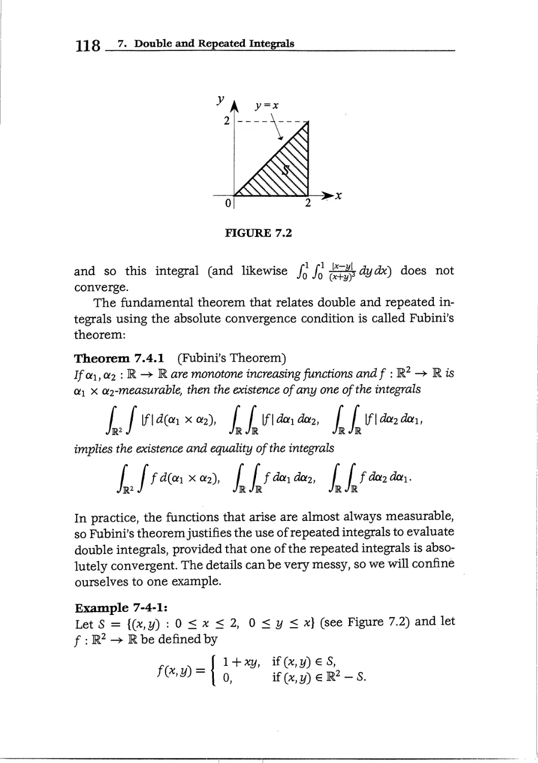
7.4 Repeated Integrals and Fubini's Theorem 115
8 The Lebesgue Spaces LP 123
8.1 Normed Spaces * 124
8.2 Banach Spaces 131
8.3 Completion of Spaces 135
8.4 The Space L1 138
8.5 The Lebesgue IP 142
8.6 Separable Spaces 150
8.7 Complexly Spaces 152
8.8 The Hardy Spaces Hp 154
8.9 Sobolev Spaces Wk>? 161
Contents
IX
9 Hilbert Spaces and L2 165
9.1 Hilbert Spaces 165
9.2 Orthogonal Sets 172
9.3 Classical Fourier Series 180
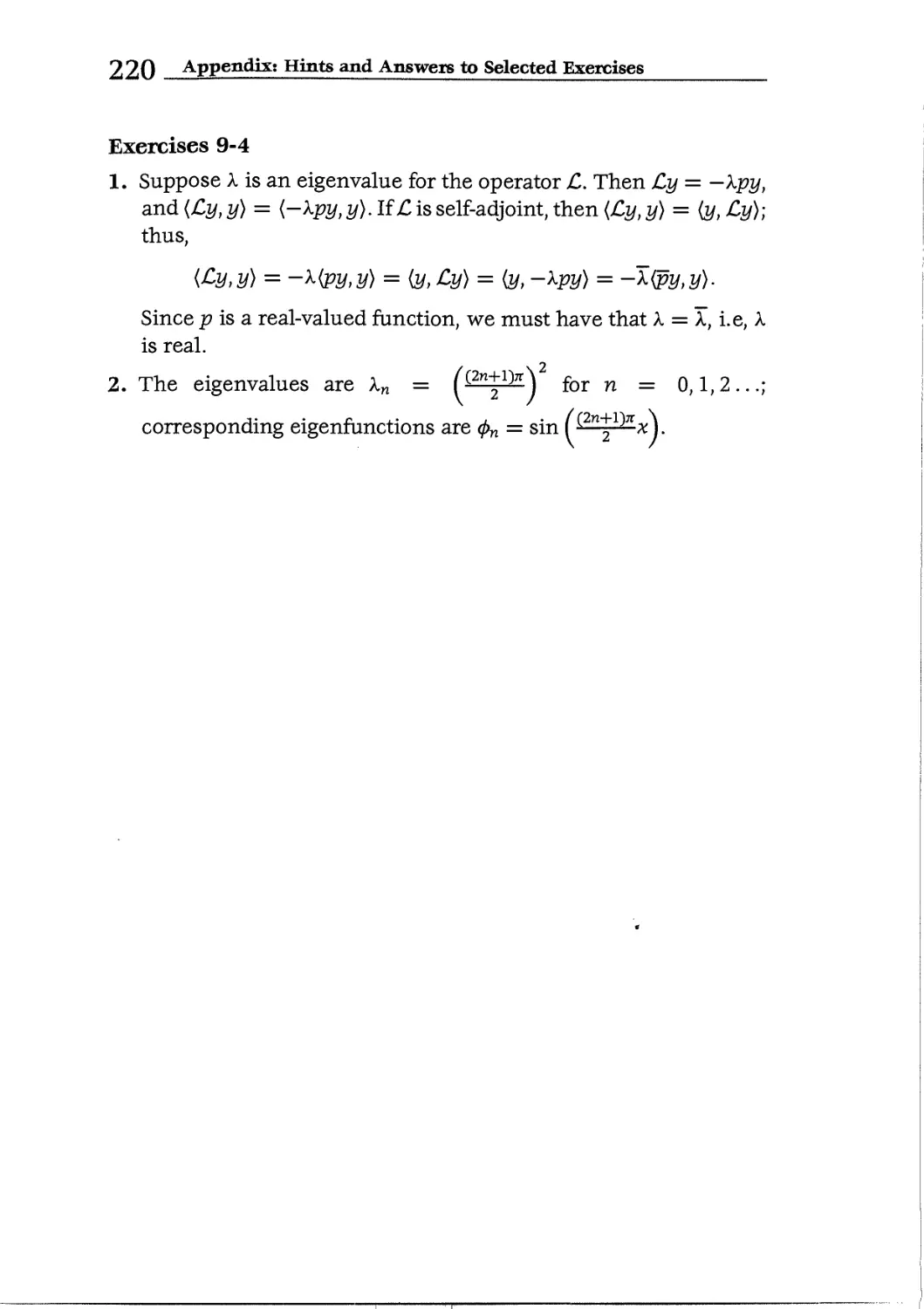
9.4 The Sturm-Liouville Problem 188
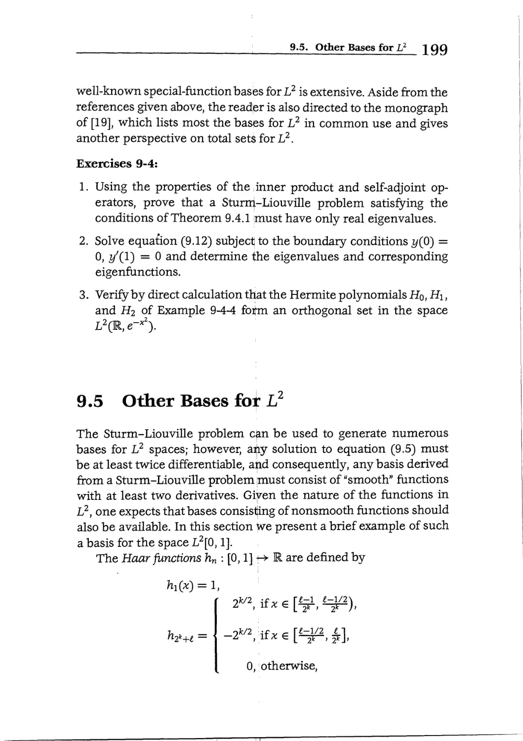
9.5 Other Bases for L2 199
10 Epilogue 203
10.1 Generalizations of the Lebesgue Integral 203
10.2 Riemann Strikes Back 205
10.3 Further Reading 207
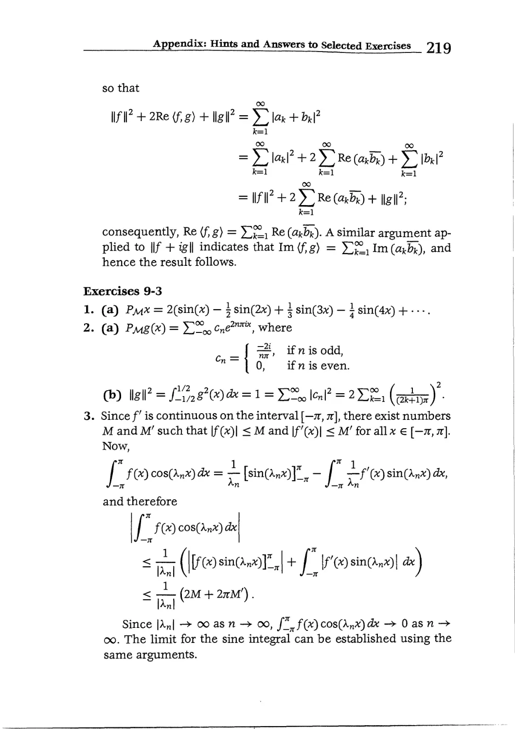
Appendix: Hints and Answers to Selected Exercises 209
References 221
Index 225
CHAPTER
Real Numbers
The field of mathematics known as analysis, of which integration is
a part, is characterized by the frequent appeal to limiting processes.
The properties of real numbers play a fundamental role in analysis.
Indeed, it is through a limiting process that the real number system
is formally constructed. It is beyond the scope of this book to recount
this construction. We shall, however, discuss some of the properties
of real numbers that are of immediate importance to the material
that will follow in later chapters.
1.1 Rational and Irrational Numbers
The number systems of importance in real analysis include the nat-
natural numbers (N), the integers (Z), the rational numbers (Q), and
the real numbers (R). The reader is assumed to have some famil-
familiarity with these number systems. In this section we highlight some
of the properties of the rational and irrational numbers that will be
used later.
The set of real numbers can be partitioned into the subsets of
rational and irrational numbers. Recall that rational numbers are
1. Real Numbers
numbers that can be expressed in the form m/n, where m and n
are integers with n ^ 0 (for example f, y, -f(= ^), 15(= y),
0(= f )). Irrational numbers are characterized by the property that
they cannot be expressed as the quotient of two integers. Numbers
such as e, n, and */2 are familiar examples of irrational numbers.
It follows at once from the ordinary arithmetic of fractions that
if r\ and r2 are rational numbers, then so are r\ + r2, n — r2, rir2,
and r\/r2 (in the last case, provided that r2 =? 0). Using these facts
we can prove the following theorem:
Theorem 1.1.1
If r is a rational number and xisan irrational number, then
(i) r + x is irrational;
(ii) rx is irrational, provided that r =? 0.
Proof See Exercises 1-1, No. 1. ?
A fundamental property of irrational and rational numbers is that
they are both "dense" on the real line. The precise meaning of this
is given by the following theorem:
Theorem 1.1.2
If a and b are real numbers with a < b, then there exist both a rational
number and an irrational number between a and b.
Proof Let a and b be real numbers such that a < b. Then b — a > 0,
so \/2/(Z? — a) > 0. Let k be an integer less than a, and let n be an
integer such that n > <j2/(b — a). Then
1 >/2 ,
0 < — < — < b — a,
n n
and so the succesive terms of each of the sequences
12 3
?c + -, ?c + -, k+-,...
n n n
n n n
differ by less than the distance between a and b. Thus at least one
term of each sequence must lie beween a and b. But the terms of
the first sequence are all rational, while (by Theorem 1.1.1) those of
the second are all irrational, so the theorem is proved. ?
1.1. Rational and Irrational Numbers
1
1
1
—L
i
[
f 1
H
3
f
>
1
-2
f
FIGURE
-1
1
1.1
I 1
o -> i 2 :
; i
Counting the integers
i
\ i \
Corollary 1.1.3
If a and b are real numbers with a < b, then between a and b there
exist infinitely many rational numbers and infinitely many irrational
numbers.
Proof This follows immediately by repeated application of Theo-
Theorem 1.1.2. ?
An infinite set S is said to be countable if there is a one-to-one
correspondence between the elements of S and the natural num-
numbers. In other words, S is countable if its elements can be listed as a
sequence
5 = {alf a2, a3,...}.
For example, the set Z is countable because its elements can be listed
as a sequence {a1; a2, a3,...} by using the rule
an = •
0 if n = 1
m if n = 2m, m > 0
-m ifn = 2m + l,ra>0
so that ai = 0, a2 = 1, a3 = -1, aA = 2, and so on. The process of
listing the elements of Z as a sequence can be visualizedby following
the arrows in Figure 1.1 starting at 0. Much less obvious is the fact
that the set Q is also countable. Figure 1.2 depicts a scheme for
counting the rationals. To list the rationals as a sequence we can
just follow the arrowed path in Figure 1.2 starting at 0/1 = 0, and
omitting any rational number that has already been listed. The set
1. Real Numbers
-3/3 -2/3 < 1/3 <— 0/3 4r—1/3 < 2/3 3/3
i t r
-3/2 -2/2 -1/2 <— 0/2 <— 1/2 2/2 3/2
11 T T t
-3/1 -2/1 -1/1 0/1 —> 1/1 2/1 3/1
11 t t
1 t
— -3/-2 -2I-2-+ -1/-2—*0/-2 -M/-2 —> 2/-2 -» 3/-2 —
... _3/_3 _2/_3 _i/_3 o/-3 1/-3 2/-3 3/-3 —
¦ ¦ ¦ ¦ ¦ ¦¦
¦ ¦ ¦ ¦ ¦ ¦¦
¦ ¦ ¦ ¦ ¦ ¦¦
FIGURE 1.2 Counting the rationals
Q can thus be written as
^ f 11 2 112 3 1
Q=|0'1'2'-2'-1'-2'2'3'3'-3'-3'-2'-3'3-l
The infinite sets N, Z, and Q are all countable, and one may won-
wonder whether in fact there are any infinite sets that are not countable.
The next theorem settles that question:
Theorem 1.1.4
The set S of all real numbers x such that 0 < x < 1 is not countable.
Proof We use without proof here the well-known fact that any real
number can be represented in decimal form. This representation
is not unique, because N.nin2n3 ... n^9999... and N.nin2n3 ... (n^ +
1H000 ... are the same number (e.g. 2.349999... = 2.35); likewise
N.999... and N + 1 are the same number. We can make the repre-
representation unique by choosing the second of these representations in
all such cases, so that none of our decimal expressions will end with
recurring 9's.
We will use a proof by contradiction to establish the theorem.
Suppose S is countable, so that we can list all the elements of 5 as a
sequence:
S = {ai,a2la3,...}.
1.1. Rational and Irrational Numbers
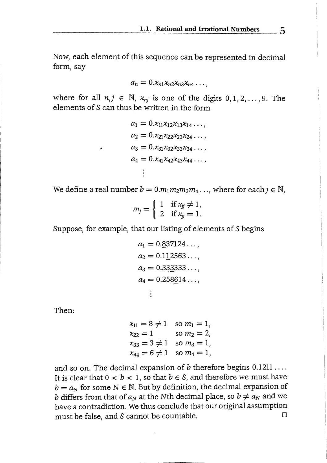
Now, each element of this sequence can be represented in decimal
form, say
an = O.xnixn2xn3xn4...,
where for all nj e N, xnj is one of the digits 0,1,2,...,9. The
elements of S can thus be written in the form
U2 = 0.#21 #22*23*24 • • • ,
U3 = 0.#3i#32#33*34 • • • ,
#4 = 0.#4i#42#43#44 . . . ,
We define a real number b = O.mim2m3m4..., where for each; € N,
mi — \
Suppose, for example, that our listing of elements of 5 begins
ai = 0.837124...,
a2 = 0.112563 ...,
a3 = 0.333333 ...,
a4 = 0.258614
Then:
*n = 8 j
x22 = 1
*33 = 3 7
*44 = 6 5
?1
?1
?1
SO
SO
SO
so
mi
ra2
m3
m4
— 1,
= 1,
= 1,
and so on. The decimal expansion of b therefore begins 0.1211 —
It is clear that 0 < b < 1, so that b e S, and therefore we must have
b = aN for some N € N. But by definition, the decimal expansion of
b differs from that of aN at the Nth decimal place, so b ^ aN and we
have a contradiction. We thus conclude that our original assumption
must be false, and S cannot be countable. ?
1. Real Numbers
It follows at once from this theorem that the set R is not count-
countable. In fact, it is also not hard to deduce that the set of all real
numbers belonging to any interval of nonzero length (however
small) is not countable.
Exercises 1-1:
1. Use the method of proof by contradiction to prove Theorem 1.1.1.
2. Give examples to show that if x\ and x2 are irrational numbers,
then x\ + #2 and Xix2 may be rational or irrational.
3. Since the set of all rational numbers is countable, it follows easily
that the set 5* = {x : 0 < x < 1 and x rational} is countable. Thus,
if we apply the argument used in the proof of Theorem 1.1.4 to
5* instead of 5, something must go wrong with the argument.
What goes wrong?
4. (a) Prove that the union of two countable sets is countable.
(b) Use a proof by contradiction to prove that the set of all
irrational numbers is not countable.
1.2 The Extended Real Number System
It is convenient to introduce at this point a notation that is useful in
many parts of analysis; care, however, should be taken not to read
too much into it.
The extended real number system is defined to be the set Re
consisting of all the real numbers together with the symbols oo and
—cx), in which the operations of addition, subtraction, multiplication,
and division between real numbers are as in the real number system,
and the symbols oo and — oo have the following properties for any
XGR:
(i) -oo < x < oo;
(ii) oo + x = x + oo = oo and -oo + x = x+ (—oo) = -oo;
(iii) oo + oo = oo and -oo + (-oo) = -oo;
(iv) oo • x = x • oo = oo and (-oo) -x = x- (-oo) = -oo for any
x > 0;
1.2. The Extended Real Number System
(v) oo • x = x ¦ oo = -oo and (-oo) -x = x- (-oo) = oo for any
x < 0;
(vi) oo • oo = oo, oo • (-oo) = (-oo) • oo = -oo, and (-oo) • (-oo) =
oo.
The reader is warned that the new symbols oo and —oo are defined
only in terms of the above properties and cannot be used except as
prescribed by these conventions. In particular, expressions such as
oo + (-oo), ('-oo) + oo, oo • 0, 0 • oo, 0 • (-oo), and (-oo) • 0 are
meaningless.
A number a e Re is said to be finite if a € R, i.e. if a is an ordinary
real number.
In all that follows, when we say that I is an interval with endpoints
a, b we mean that a and b are elements of Re (unless specifically
restricted to finite values) with a <b, and I is one of the following
subsets of R:
(i) the open interval {x e R : a < x < b}, denoted by (a, by,
(ii) the closed interval {x e R : a < x < b}, denoted by [a, b],
where a and b must be finite;
(iii) the closed-open interval {x e R : a < x < b}, denoted by
[a, b), where a must be finite;
(iv) the open-closed interval {x e R : a < x < b}, denoted by
(a, b], where b must be finite.
Note that although the endpoints of an interval may not be finite,
the actual elements of the interval are finite. Note also that for any
a € R, the set [a, a] consists of the single point a, whereas the sets
[a, a) and (a, a] are both empty. The interval (a, a) is empty for all
aeRe.
The only change from standard interval notation is that intervals
such as (-oo, -3], (-oo, oo), (-2, oo), etc. are defined. (Intervals
such as [-oo, 3], [-oo, oo], (-2, oo], etc. are not.)
Q 1. Real Numbers
1.3 Bounds
Let S be any nonempty subset of Re. A number c € Re is called an
upper bound of S if x < c for all x e S. Similarly, a number d € Re
is called a lower bound of S if x > d for all x e S.
Evidently, oo is an upper bound and — oo is a lower bound for
any nonempty subset of Re. In general, most subsets will have many
upper and lower bounds. For example, consider the set Si = (-3,2].
Any number c e Re such that c > 2 is an upper bound of Si, and any
number d e Re such that d < — 3 is a lower bound of Si. Note that
there is a least upper bound for Si (namely 2) and that in fact it is
also an element of Si. Note also that there is a greatest lower bound
(namely —3), which is not a member of Si.
As another example, consider the set
Here any c > 1 is an upper bound of S2, while any d < 0 is a
lower bound. Note that no positive number can be a lower bound of
S2, because for any d > 0 we can always find a positive integer n
sufficiently large so that 1/n < d, and therefore d cannot be a lower
bound of S2. Thus S2 has a least upper bound 1 and a greatest lower
bound 0.
As a final example, let S3 = Q. Then 00 is the only upper bound
of S3 and — ex) is the only lower bound. Thus S3 has a least upper
bound 00 and a greatest lower bound —00.
The following result (often taken as an axiom), which we state
without proof, expresses a fundamental property of the extended
real number system:
Theorem 1.3.1
Any nonempty subset ofRe has both a least upper bound and a greatest
lower bound in Re.
The least upper bound of a nonempty set S c Re is often called
the supremum of S and is denoted by sup S; the greatest lower
bound of S is often called the infimum of S and denoted by inf S.
The examples given above indicate that sup S and inf S may or may
not be elements of S; however, in the case where sup S or inf S is
1.3. Bounds Q
finite, although sup 5 and inf S need not be in 5, they must at any
rate be "close" to 5 in a sense that is made precise by the following
theorem:
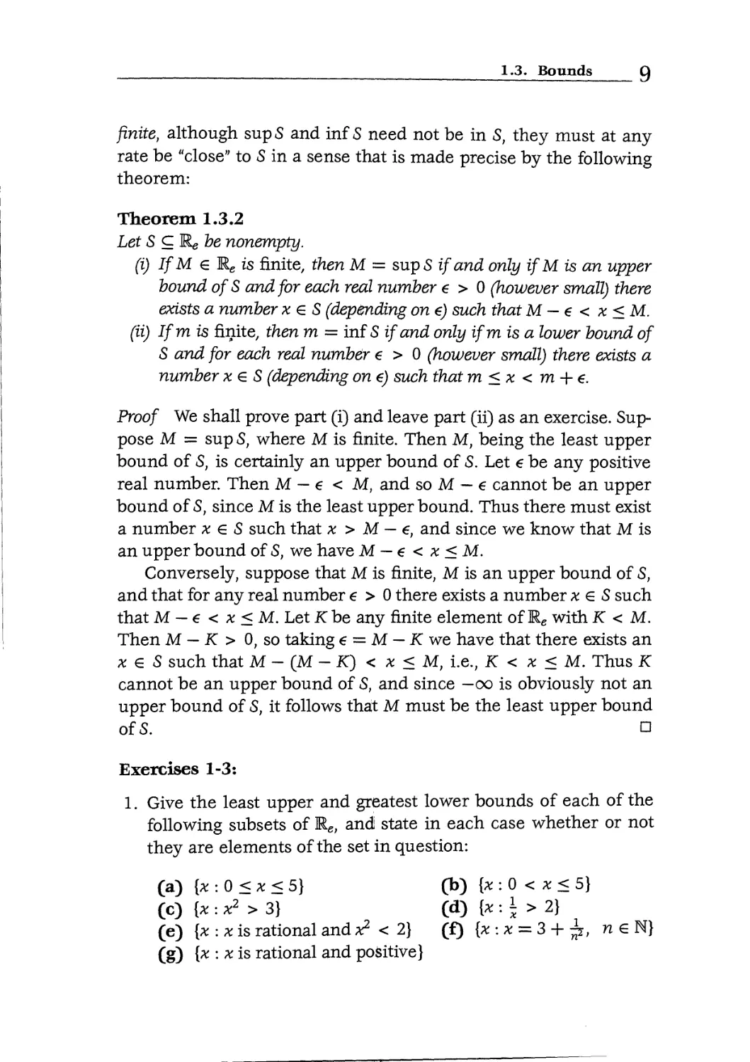
Theorem 1.3.2
Let S C Rg be nonempty.
(i) IfM € Re is finite, then M = sup 5 if and only if M is an upper
hound of S and for each real number e > 0 (however small) there
exists a number x € S (depending on e) such that M — e < x < M.
(ii) If mis finite, then m = inf 5 if and only if mis a lower bound of
S and for each real number € > 0 (however small) there exists a
number xe S (depending on e) such that m < x < m + e.
Proof We shall prove part (i) and leave part (ii) as an exercise. Sup-
Suppose M = sup 5, where M is finite. Then M, being the least upper
bound of 5, is certainly an upper bound of S. Let e be any positive
real number. Then M — e < M, and so M — e cannot be an upper
bound of 5, since M is the least upper bound. Thus there must exist
a number x e S such that x > M — e, and since we know that M is
an upper bound of 5, we have M — e < x < M.
Conversely, suppose that M is finite, M is an upper bound of 5,
and that for any real number e > 0 there exists a number xe S such
that M — € < x < M. Let K be any finite element of Re with K < M.
Then M — K > 0, so taking e = M — K we have that there exists an
x € S such that M - (M - K) < x < M, i.e., K < x < M. Thus K
cannot be an upper bound of 5, and since — oo is obviously not an
upper bound of 5, it follows that M must be the least upper bound
of 5. ?
Exercises 1-3:
1. Give the least upper and greatest lower bounds of each of the
following subsets of Re, and state in each case whether or not
they are elements of the set in question:
(a) {x : 0 < x < 5} (b) {x : 0 < x < 5}
(c) {x : x2 > 3} (d) {x : \ > 2}
(e) {x : x is rational and x2 < 2} (f) {x:x = 3 + ^, n e N}
(g) {x : x is rational and positive}
10 1. Real Numbers
2. If S c Re has only finitely many elements, say S = {xi, x2,..., xn},
then clearly S has both a greatest element and a least element, de-
denoted by max{*i ,X2,...,xn} and min{*i, x2,..., xn}, respectively.
Prove:
lx2)...,xn} = max{*i tx2,...,xn},
inf{a:i,x2,...,xn} = min^i, a:2, ..., A:n}.
3. Prove that if 5i and S2 are nonempty subsets of Re such that
5i C 52, then sup Si < sup52 and inf 5i > inf 52.
4. Let 5 be a nonempty subset of Re, and c a nonzero real number.
Define 5* by 5* = {ex : x e S}.
(a) Prove that if c is positive, then sup 5* = c(supS) and
inf(S*) = c(infS).
(b) Prove that if c is negative, then sup 5* = c(inf 5) and
inf(S*) = c(supS).
5. Prove part (ii) of Theorem 1.3.2.
CHAPTER
Some Analytic
Preliminaries
Before we can develop the theory of integration, we need to re-
revisit the concept of a sequence and deal with a number of topics
in analysis involving sequences, series, and functions.
2.1 Monotone Sequences
Convergence of a sequence on Re can be defined in a manner anal-
analogous to the usual definition for sequences on R. Specifically, a
sequence {an} on Re is said to converge to a finite limit if there
is a finite number a e Re having the property that given any posi-
positive real number e (however small) there is a number N e N such
that \an — a\ < e whenever n > N. This relationship is expressed
by an -»¦ a as n -»¦ oo, or simply an -»¦ a. The number a is called the
limit of the sequence.
If for any finite number M € Re there exists an N € N such
that an > M whenever n > N, then we write an -» oo as n -» oo
or simply an -» oo, and the limit of the sequence is said to be oo;
similarly, if for any finite number M € Re there exists an N € N such
11
19 2. Some Analytic Preliminaries
that an < M whenever n > N, then we write c^ -> — oo as n -> oo
or simply an -> — oo, and the limit of the sequence is said to be — oo.
Let {an} be a sequence of real numbers. The sequence {an} is said
to be monotone increasing if an < an+i for all n e N, and mono-
monotone decreasing if #„ > an+\ for all n e N. For example:
The sequence 1,2,3,4,... is monotone increasing.
The sequence 1, \, |, \,... is monotone decreasing.
The sequence 1,1,2,2,3,3,... is monotone increasing.
The sequence 1,1,1,1,... is monotone increasing and monotone
decreasing.
The sequence 1,0,1,0,... is neither monotone increasing nor
monotone decreasing.
If a sequence {an} is monotone increasing with limit I e Re, we
write an 11 (read "an increases to ?"~). If the sequence is monotone
decreasing with limit I e Re, we write an 11 (read "On decreases to
We shall frequently be studying sequences of functions. Let {fn}
denote a sequence of functions fn : I -> R denned on some interval
I C. R. The sequence {fn} is said to converge on I to a function f
if for each x e I the sequence {fn(x)} converges to f(x), i.e., if the
sequence is pointwise convergent. The notation used for sequences
of functions is similar to that used for sequences of numbers: specif-
specifically,
fn -»- f on I means that for each x e I, fn(x) -> f(x).
fn t f on I means that for each x e I, /„(*:) t f (*)•
/n j f on I means that for each x€l, fn(x) I /(*)•
The fundamental theorem concerning monotone sequences is
the following:
Theorem 2.1.1
Let {an} be a sequence on R.
(i) If the sequence {an} is monotone increasing, then an t sup{an}.
(ii) If the sequence {an} is monotone decreasing, then an ^ inf{an}.
2.2. Double Series
Proof We shall prove part (i) of the theorem, leaving the second
part as an exercise. Let M = sup{^}. The proof of part (i) can be
partitioned into two cases depending on whether or not M is finite.
Case 1: If M = 00, then for any positive real number K, we know
thatK cannot be an upper bound of {an}, so there exists a positive
integer N such that aN > K. Since the sequence is monotone
increasing, it follows that cin > aN > K for all n > N, and thus
an t oo(= M) by definition.
Case 2: Suppose M finite and let ebe any positive real number. Then
by Theorem 1.3.2 there exists a positive integer N such that
M — € < aN <M.
Since the sequence is monotone increasing and has M as an
upper bound, it follows that
M — € < aN <an <M < M + e
for all n>N. This implies that for all n>N,
\an-M\ < e
and. consequently an -> M by definition. Since the sequence is
monotone increasing, this means that an f M as required. ?
Exercises 2-1:
1. Let S be a nonempty subset of R, with sup S = M and inf S = m.
Show that there exist sequences {an} and {bn} of elements of S
such that an\M and bn I m.
2. Prove part (ii) of Theorem 2.1.1.
2.2 Double Series
Let {an} be a sequence on Re. Recall that the infinite series ?m=i am
is said to converge if the sequence of partial sums {sn}, where sn =
5Zm=i am> converges to a finite number. If sn -> 00, then the series
is said to diverge to 00; if sn -> —00, then the series is said to diverge
to —00. Often, questions concerning the convergence of an infinite
\A 2. Some Analytic Preliminaries
#11 -* #12 #13 -> #14
#21
#31
#41
#11
#21
#31
#41
#22
#32
#42
•
#23
#33
#43
j
FIGURE 2.1
-* #12
<~ #22
-* #32
<- a42
#13 ~
t
#23
t
-* #33
<- #43 <
#24
#34
#44
•
* #14
#24
#34
- a44
FIGURE 2.2
series involve considering sequences {#„} of nonnegative terms (e.g.,
absolute convergence). If the terms of the sequence {#„} consist of
nonnegative numbers, then the resulting sequence of partial sums is
monotone increasing. Theorem 2.1.1 thus implies that sn t sup{sn}
and therefore that either the series Ylm=i am converges or it diverges
to oo, according as sup{sn} is finite or oo.
Consider the array of real numbers depicted in Figure 2.1. This
array can be written as a (single) sequence in many ways. One way
is to follow the arrowed path in the diagram. This gives the sequence
{#11, #12, #21, #31, #22, #13, #14, #23, • • •},
but this is obviously not the only way. Another scheme for
constructing a sequence is given in Figure 2.2.
2.2. Double Series
For any way of writing this array as a single sequence Ai, A2,
A3,... we can form the corresponding infinite series Yl°li Aj- We
know from Riemann's theorem on the derangement of series [6]
that in general, the convergence and limit of the series depends on
the particular sequence {An} used, but there are some situations in
which every possible sequence leads to the same answer. When this
is the case, it is sensible to introduce the notion of a "double series"
Ylm,n=i amn and consider questions such as convergence. This leads
us to the following definition: If for all possible ways of writing the
array {awj as a single sequence the corresponding series has the
finite sum ?, then the double series Ylmn=i amri is said to converge to
I. If for all possible ways of writing the array as a single sequence the
corresponding series either always diverges to 00 or always diverges
to —00, then the double series is said to be properly divergent (to
00 or —00 as the case maybe). In all other circumstances the double
series is simply said to be divergent, and its sum does not exist as an
element of Re.
As well as "summing" the array by writing it as a single sequence,
we can "sum" it by first summing the rows and then adding the sums
of the rows, giving the repeated series 5Im=i(?nLi amn)- Alterna-
Alternatively, we can first sum the columns and then add the sums of the
columns, giving the repeated series Yl™=iGLm=i amn)-
The relationship between convergence for a double series
Hmn=i amn and for the two related repeated series is, in general,
complicated. For our purposes, however, we can focus on the par-
particularly simple case where all of the entries in the array are
nonnegative, i.e., tfWi > 0 for all n,m e N. In this case we have
the following result, which is stated without proof:
Theorem 2.2.1
Suppose that for all n, m e Nwehaveamn > 0, where a^n e Re. Then the
double series Y,m,n=ia™ and the two repeated series J2n=i(I2m=i amn)
ana> Em=i Q2n=i amn) e^ier <*% converge to the same finite sum or are
all properly divergent to 00.
More details on double series can be found in [6].
2. Some Analytic Preliminaries
Ax)
t-8
fix) lies between ?-e and
?+? for all x e (t-8, t)
x
FIGURE 2.3
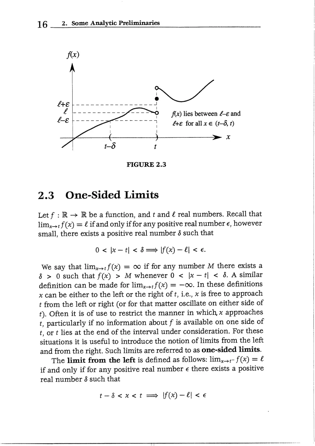
2.3 One-Sided Limits
Let f : R -> R be a function, and t and I real numbers. Recall that
lmvH>f/(X) = € if and only if for any positive real number e, however
small, there exists a positive real number 8 such that
0 < \x - t\ < 8 =$> |f (X) -i\< €.
We say that limx^f f(x) = oo if for any number M there exists a
8 > 0 such that f(x) > M whenever 0 < \x - t\ < 8. A similar
definition can be made for Hmx^,tf(x) = —oo. In these definitions
x can be either to the left or the right oft, i.e., x is free to approach
t from the left or right (or for that matter oscillate on either side of
t). Often it is of use to restrict the manner in which., x approaches
t, particularly if no information about f is available on one side of
t, or t lies at the end of the interval under consideration. For these
situations it is useful to introduce the notion of limits from the left
and from the right. Such limits are referred to as one-sided limits.
The limit from the left is defined as follows: limx_K- f(x) = Z
if and only if for any positive real number e there exists a positive
real number 8 such that
t-8 < x < t
\f(x)-i\ <€
2.3. One-Sided Limits
17
/+?
fix) lies between ?-? and
?+? for all x e it, t+S)
t+8
FIGURE 2.4
(cf. Figure 2.3). In this case we say that f(x) tends to ? as x tends
to t from the left. Similarly, the limit from the right is defined as
limx_yt+f (*) = ? if and only if for any positive real number e there
exists a positive real number 8 such that
(cf. Figure 2.4). In this case we say that f(x) tends to ? as x tends to
t from the right.
We can easily extend these definitions for cases where the limit
is not finite, e.g., lmv+t- f(x) = oo if and only if for any positive real
number M there exists a positive real number 8 such that
t-8<x<t
f(x) > M.
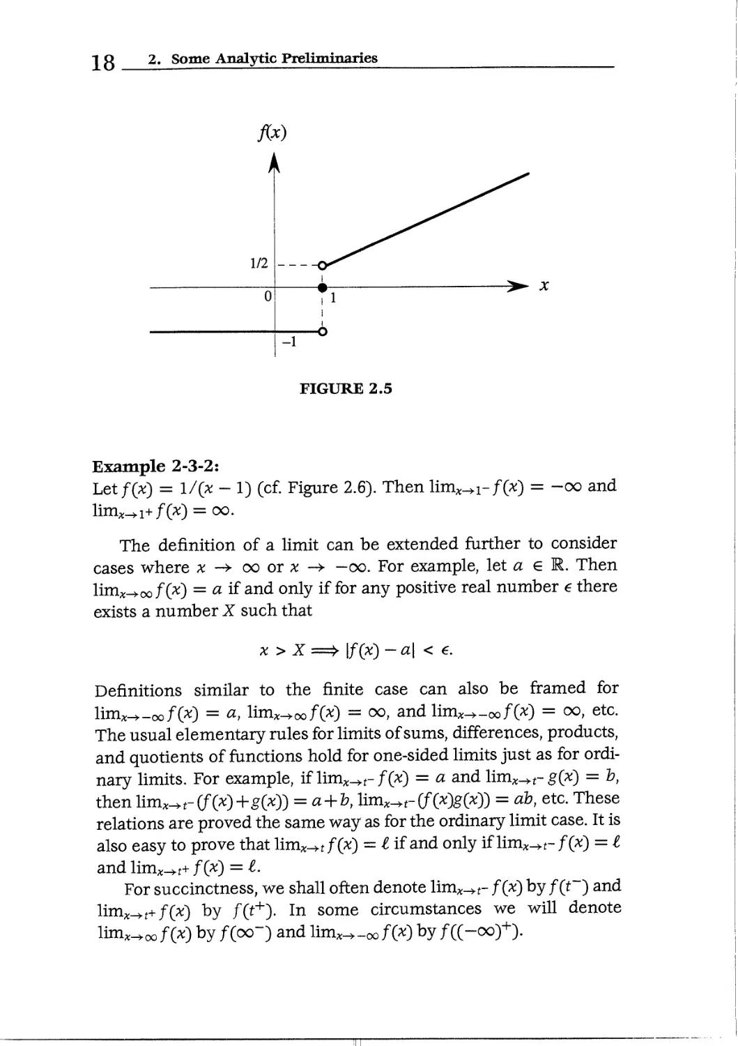
Example 2-3-1:
Let/ : R -> R be defined as
/(*) =
-1 if x < 1,
0 ifx = l,
x/2 if x > 1.
Then \imx^i-f(x) = -
depicted in Figure 2.5.
¦1 and linv+i+/(x) = 1/2. This function is
1 Q 2. Some Analytic Preliminaries
Ax)
X
FIGURE 2.5
Example 2-3-2:
Let f(x) = l/(x - 1) (cf. Figure 2.6). Then limx_>i-f(x) =
-oo and
The definition of a limit can be extended further to consider
cases where x -> oo orx -> —oo. For example, let a e R. Then
lim^oo/CX) = a if and only if for any positive real number e there
exists a number X such that
x
\f(x)-a\
Definitions similar to the finite case can also be framed for
lim^-oo/OO = a> linWoo/OO — °°» andlimx^_oo/(A:) = oo, etc.
The usual elementary rules for limits of sums, differences, products,
and quotients of functions hold for one-sided limits just as for ordi-
ordinary limits. For example, if limx_^t- /(*) = a and \imx^.t- g(x) = b,
then limx.+f-(f(X)+g(X)) = a + b, lim^-(f(X)g(X)) = ab, etc. These
relations are proved the same way as for the ordinary limit case. It is
also easy to prove that lim^tf (*) = I if and only if \\n\x-*t- f(x) = I
and limx.^t+ f(>0 = I-
For succinctness, we shall often denote limx_^f- f(x) by f(t~~) and
\imx^t+f(x) by f(t+~). In some circumstances we will denote
oo f(x) by f (oo~) and limx_».-oo ffr) by f ((-oo)+).
2.3. One-Sided Limits
19
FIGURE 2.6
One-sided continuity for a function f at finite points t is defined
in terms of one-sided limits in the obvious way. We say that f is
continuous on the left at t if f(t) is defined and finite, f(t~) exists,
and f(t~) = f(f), and continuous on the right at t if f(t) is defined
and finite, f(t+) exists, and/(t+) = f(t). Evidently, f is continuous
at t if and only if it is both continuous on the left and continuous on
the right at t, i.e., if and only if f(t~) = f(t) = f(t+).
There are several different ways in which a function can fail to
be continuous at a point. If f(t~),f(f),f{t+) all exist but are not all
equal, then f is said to have a jump discontinuity at t. Thus, the
function in Example 2-3-1 has a jump discontinuity at 1. A function
may fail to be continuous at a point because the limit is not finite.
The function of Example 2-3-2 is discontinuous at 1 not only because
the limit is not finite but also because /(I ~) ^ /(I+) and f(t) has not
been defined. Yet another way in which a function can fail to be
continuous at a point is when the right or left limits fail to exist. The
next example illustrates this.
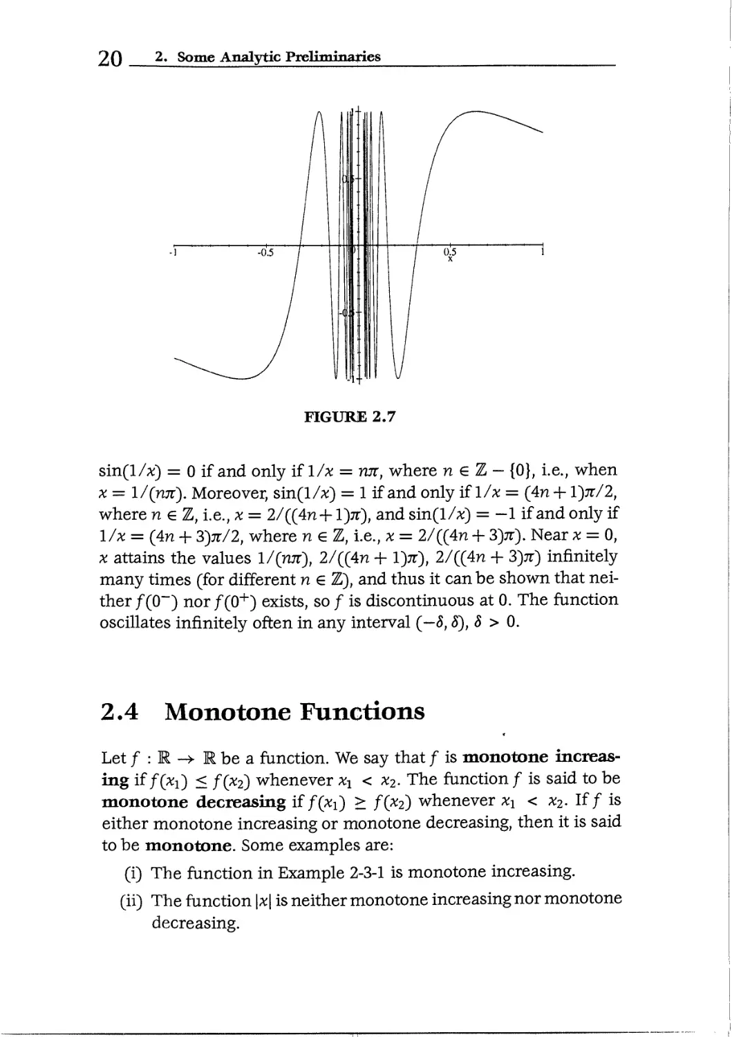
Example 2-3-3:
Consider the function / :
}^J~ [ 0, ifx = 0.
Figure 2.7 illustrates this function. Now, |sin(l/x)l <
defined by
1 and
20 2. Some Analytic Preliminaries
0.5
x
FIGURE 2.7
sin(l/A:) = 0 if and only if 1/x = rut, where n € Z — {0}, i.e., when
x = l/(njr). Moreover, sin(l/x) = 1 if and only if 1/x = {An + Y)n/2,
where n e Z, i.e., x = 2/(Dn + lOr), and sin(l/x) = —1 if and only if
1/x = (An + 3)jt/2, where n e Z, i.e., x = 2/(Dn + 3>r). Near x = 0,
x attains the values l/(rur), 2/(Dn + 1», 2/(Dn + 3);r) infinitely
many times (for different n e Z), and thus it can be shown that nei-
neither f@~) nor f@+) exists, so f is discontinuous at 0. The function
oscillates infinitely often in any interval (—5,5), 8 > 0.
2.4 Monotone Functions
Let f : R -> R be a function. We say that f is monotone increas-
increasing if f(xi) < f(x2) whenever x\ < x2. The function f is said to be
monotone decreasing if f{x{) > f(x2) whenever xx < x2. If f is
either monotone increasing or monotone decreasing, then it is said
to be monotone. Some examples are:
(i) The function in Example 2-3-1 is monotone increasing.
(ii) The function |x| is neither monotone increasing nor monotone
decreasing.
2.4. Monotone Functions 21
(iii) Constant functions are both monotone increasing and mono-
monotone decreasing.
One can also speak of functions being monotone increasing or
monotone decreasing on a particular interval rather than the en-
entire real line. For example, the function \x\ is monotone decreasing
on (—00,0] and monotone increasing on the interval [0, oo). In this
section, however, we will restrict the discussion to functions that are
monotone on the entire real line. The general case will be discussed
in Section 2.7.
The most important theorem on monotone functions is the
following:
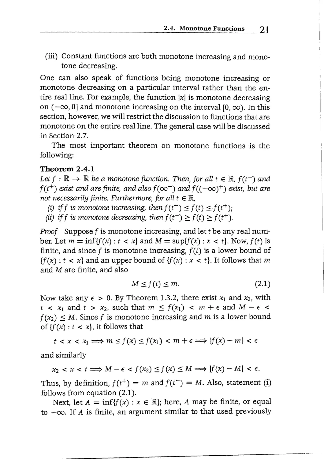
Theorem 2.4.1
Let f : E -> E be a monotone function. Then, for all tel, f(t~) and
f(t+) exist and are finite, and also /(oo~) and /((—oo)+) exist, but are
not necessarily finite. Furthermore, for all t e R,
(i) iff is monotone increasing, then f(t~~) < f(t) <f(t+~);
(ii) iff is monotone decreasing, then f(t~~) > f(f) > f(t+~)-
Proof Suppose f is monotone increasing, and let t be any real num-
number. Let m = inf {f (x) : t < x} and M = sup{f (x) : x < t}. Now, f(t) is
finite, and since / is monotone increasing, f(t) is a lower bound of
{f(x) : t < x} and an upper bound of {f(x) : x < t}.lt follows that m
and M are finite, and also
M < f(t) < m. B.1)
Now take any e > 0. By Theorem 1.3.2, there exist x\ and X2, with
t < xi and t > x2, such that m < f(x{) < m + e and M — e <
f(x2) < M. Since f is monotone increasing and m is a lower bound
of {f(x) : t < x}, it follows that
t < x < xi =» m < f(x) < f(xi) < m + € => \f(x) -m\ < €
and similarly
x2 < x <t=>M-€ < f(x2) <f(x) <M=> \f(x)-M\ < e.
Thus, by definition, f(t+) = m and f(t~) = M. Also, statement (i)
follows from equation B.1).
Next, let A = inf {f(x) : x e E}; here, A may be finite, or equal
to —oo. If A is finite, an argument similar to that used previously
22 2. Some Analytic Preliminaries
shows that /((-oo)+) = A. If A is -oo, let K be any negative real
number. Then K is not a lower bound of {f(x) : x € R}, so there exists
a.nx\ € R such that f(x{) < K. Since / is monotone increasing, it
follows that
x < xi => f(x) < /(*!) < K,
and so /((—oo)+) = — oo = A in this case also. A similar argument
shows that/(oo") = sup{/(x) : x € R}.
The case where / is monotone decreasing can be proved in a
similar way, or by considering the function —/ (see Exercises 2-4,
No. 1). ?
Corollary 2.4.2
(i) Iff is monotone increasing, and a, b are elements ofRe with a < b,
then f(a+) < f(b~).
(ii) Iff is monotone decreasing, and a, b are elements ofRe with a < b,
thenf{a+)>f(p-y
Proof We will prove part (i) of this theorem and leave the other
part as an exercise. Let/ be monotone increasing. From the proof of
Theorem 2.4.1 we know that/(a+) = m?{f{x) : a < x) and/G?~) =
sup(f (x) : x < b). Since a < b, there exists a y € R such that a <
y <b, and so /O+) < f(y) and f{y) < f(b~), whence f(a+) < f(b~)
as required. ?
Iff is monotone, then for any real t we have by Theorem 2.4.1
that /(t"),/(t), and /(?+) all exist. It follows at once that the
only discontinuities that a monotone function can-have are jump
discontinuities.
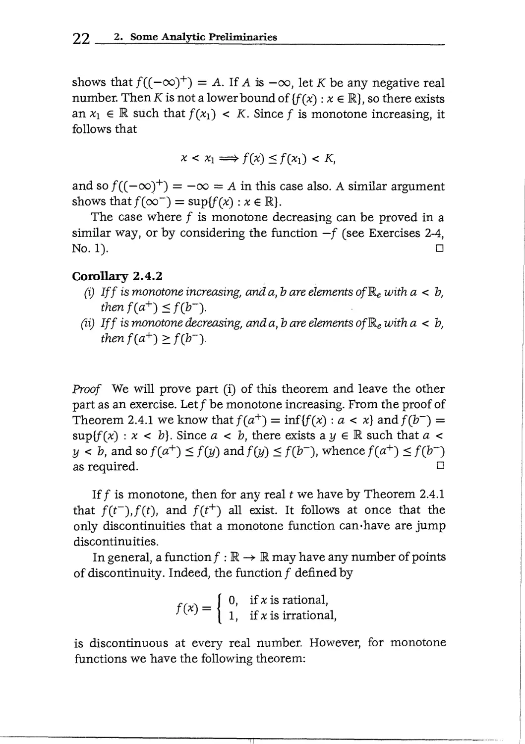
In general, a function/ : R ->• R may have any number of points
of discontinuity. Indeed, the function / defined by
f | 0, if x is rational,
^~ { 1, ifx is irrational,
is discontinuous at every real number. However, for monotone
functions we have the following theorem:
2.4. Monotone Functions 23
Theorem 2.4.3
If f : R -> R is monotone, then the set of points at which f is
discontinuous is either empty, finite, or countably infinite.
Proof Iff is monotone decreasing, then —/ is monotone increasing
(see Exercises 2-4, No. 1)) and has the same points of discontinuity
as /, so it is sufficient to prove the theorem for the case where / is
monotone increasing.
Let E be the set of points at which/ is discontinuous, and suppose
E is not empty .'Then for each x $ Ewe have/(x~) < f(x+), and so by
Theorem 1.1.2 there exists a rational number rx such that f(x~) <
rx < f(x+). Now by Corollary 2.4.2 we have xx < x2 =» f(xf) —
/(*D> and it follows that if xi,#2 € E are such that x\ < x2} then
rXl < rX2; thus, we have associated with each x € E a distinct rational
number.
Since the set of all rational numbers can be listed as a sequence,
it follows that the set {rx : x € E} can also be listed as a (finite or
infinite) sequence. We can then list the elements of E in the same
order as their associated rational numbers. Thus E (if not empty) is
either finite or countably infinite. ?
Although Theorem 2.4.3 places restrictions on the possible set of
discontinuities of a monotone function, this set can nevertheless be
quite complicated, and one must be careful not to make unjustified
assumptions about it. For example, one might guess that the discon-
discontinuities of a monotone function must be some minimum distance
apart, but the following example shows that this need not be so.
Example 2-4-1:
Let/ : R -> Rbe defined as follows:
/(*) =
0, if* < 0,
l/(n + l), ifl/(n +
1, if* > 1.
Figure 2.8 illustrates this function. Clearly, / is monotone increas-
increasing. It can be shown that /@+) j= 0 (see Exercises 2-4, No. 3), so
/ has jump discontinuities at the countably infinite set of points
{l,i,|,i,...} and is continuous at all other points. In fact, unlikely
24 2. Some Analytic Preliminaries
1/2 —
1/3 —
1/4 —
0
i i
i i
- - 1/4 1/3 1/2
FIGURE 2.8
as it may seem, it is possible to construct a monotone increasing
function that is discontinuous at every rational number!
Exercises 2-4:
1. Prove part (ii) of Theorem 2.4,1, by showing that iff is monotone
decreasing, then —/ is monotone increasing, and then applying
part (i).
2. Prove part (ii) of Corollary 2.4.2.
3. Prove that/(O+) = 0 in Example 2-4-1.
2.5 Step Functions
Let I be any interval. A function 0 : I -> R is called a step func-
function if there is a finite collection {Ji, J2, • • •, Jn} of pairwise disjoint
intervals such that S = h U J2 U • • • U In c. I and a set {c\, c2,..., cn}
2.5. Step Functions 25
6(x)
I = (-oo, oo)
4 ^
Q.
c\
/2
c\=C4
I=[a,b)
= sum of hatched areas with
appropriate signs
b
a
K-
/2 /3
FIGURE 2.9
of finite, nonzero real numbers Such that
eW-[ 0, ifxel-S.
In other words, 6 is constant and nonzero on each interval J;-, and zero
elsewhere in J. The set S on which 0 is nonzero is called the support
of 0. Note that S maybe empty, so that the zero function on I is also
a step function. Figure 2.9 illustrates some possible step-function
configurations.
O O V s v r
26 2. Some Analytic
If the support of a step functioifi 0 has finite total length, then we
associate with 0 the area A@) between the graph of 0 and the x-axis,
with the usual convention that areas below the x-axis have negative
sign (we often refer to A@) as the "area under the graph" of 0). Thus
A@) exists for the step function 0 in Figure 2.9-2, but not for that in
Figure 2.9-1.
If 0i, 02,..., 0m are step functions on the same interval I, all with
supports of finite total length, and if alf a2,..., am axe. finite real
numbers, then the function 0 defined by
m
for x € I is also a step function on J. The support of 0 has finite
length, and
m
The fact that 0 is also a step function is a rather tedious and messy
thing to prove in detail, but an example should be sufficient to
indicate why it is true.
Example 2-5-1:
Let 0i, 02 : [0, 3) -> R be defined by
<x <2, n r f -1, ifO <x<l,
<-x < 3. 2U~ 1, if 1 < x < 3
(cf. Figure 2.10). Let 0 = 26>i - 02. Then
3, ifO<*<l,
1, if 1 < x < 2,
3, if 2 <x < 3.
(cf. Figure 2.11). Clearly, 0 is a step function. Note also that
A@2) = -!(!) +2A) = 1,
2.5. Step Functions 27
Oi(x)
FIGURE 2.10
2d\(x)-
3
2
1
1
0
i
i
i
lj
i
2
9
i
i
3 >
0
-9
i
9—?
¦>-x
FIGURE 2.11
A@) = lC) + l(l) + lC) = 7
as expected.
If f,g : I -> R are such that/(x) < g(x) for all x € I, we write
simply"/ <gon J." The following properties of areas under graphs
of step functions are geometrically obvious and straightforward to
prove:
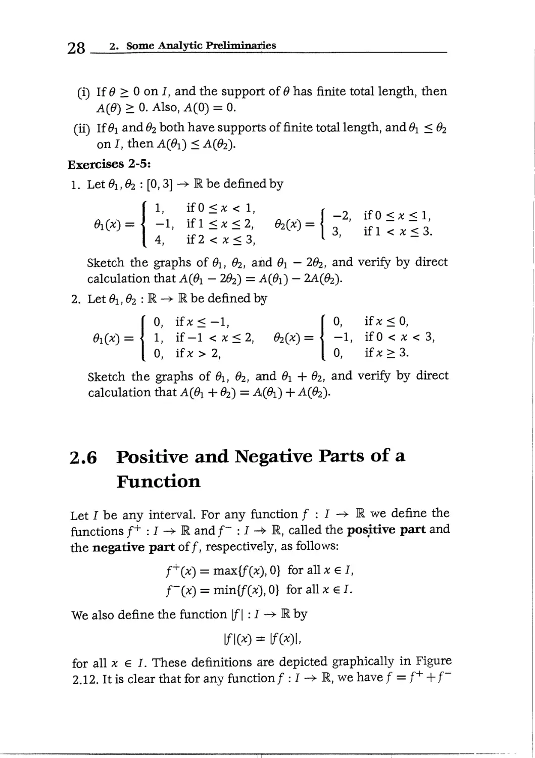
28 2. Some Analytic
(i) If 0 > 0 on I, and the support of 0 has finite total length, then
A@) > 0. Also, A@) = 0.
(ii) If 0i and 62 both have supports of finite total length, and B\ < 02
on I, then A{0{) < A@2).
Exercises 2-5:
1. Let 0i, 62 : [0,3] -> R be defined by
0i(*) =
1, ifO<x < 1,
Sketch the graphs of 0i, 02, and B\ - 202, and verify by direct
calculation that A@X - 202) = A@i) - 2A@2).
2. Let 0i, 02 : R -> R be defined by
0, ifx<0,
-1, if 0 < x < 3,
0, ifx>3.
0, ifx<-l,
1, if —1 < x<2, 02(x) =
0, if x > 2,
Sketch the graphs of 0i, 02, and 0X + 02, and verify by direct
calculation that A@X + 02) = A@i) + A@2).
2.6 Positive and Negative Parts of a
Function
Let I be any interval. For any function / : I -> R we define the
functions /+ : J -» R and /" : J -4- R, called the positive part and
the negative part of/, respectively, as follows:
f+{x) = max{f O), 0} for all x € J,
/"(x) = min{f (x), 0} for all x € J.
We also define the function |/| : I -» Rby
1/100 * If WL
for all x € J. These definitions are depicted graphically in Figure
2.12. It is clear that for any function/ : I -» R, we have /=/++/"
2.7. Bounded Variation and Absolute Continuity 29
Graph of/
Graph of /*•
Graph of 1/1
v\
Graph o
FIGURE 2.12
and |/| = /+ -/". It is also clear that 0 < /+ < |/| and -|/| < /" < 0
on J.
Exercises 2-6: If f,g : J -» R, prove the following inequalities:
2.
3.
2.7 Bounded Variation and Absolute
Continuity
For any (nonempty) interval I, a partial subdivision of J is a
collection S = {h, h,.. •, In} of clpsed intervals such that:
30 2« Some Analytic
(i) JlUJ2U---UJnCJ;
(ii) for any j,k = 1,2,..., n with ; =? k, either Ik n Ij is empty or
Ik n J;- consists of a single point that is an endpoint of both J;-
and Ifc.
For example, if I = [0, 3), then S = {[0,1], [1, §], [2, f ]} is a partial
subdivision of J.
Let / : I -> R be a function, and let S = {ii, I2,..., !„} be a partial
subdivision of I. For each; = 1, 2,..., n, let J;- have endpoints Oj, ty.
We can associate with /, I, and S the quantity Vs(f, I) defined by
Consider now the set A(f, I) = {Vs(f, J): S is a partial subdivision
of J}. Obviously Vs(f,I) cannot be negative, so 0 is a lower bound of
A(f,I). The least upper bound of A(f, J) is called the total variation
off over J, and denoted by V(f, I}; and we have 0 < V(f, I) < oo for
any/ and J.
Example 2-7-1:
Let / : I -» R be any step function. If / is constant on J, then
evidently V(f, J) = 0. If not, then as x increases through J, f(x) has
a finite number of changes in value. Let the absolute magnitudes of
these changes be fclf k2,..., km.
Now take any closed interval J;- = [a,-, b;] c j. if none of the
changes in the value of f(x) occur! within J;-, then/(x) is constant on
Ij and \f(bj) —f(aj)\ = 0. If the changes numbered r\, r2,..., rp occur
within Ij, then |/(b;) - /(^)| < J%^i K-
If S is a partial subdivision of I, then since a given change in the
value off (x) can occur within at most one of the intervals I\, h,..., In
that make up S, it follows that Vs(f, J) < J^Li ^- Furthermore, if we
choose S such that each change in the value of f(x) occurs within
one of the intervals comprising S, and no interval has more than one
change occurring within it, then Vs(f, J) = J^Li ^-lt f°U°ws tnat /
has finite total variation given by
m
r=l
2.7. Bounded Variation and Absolute Continuity
6(x)
3
2-
ttt
9"
i
"ft
k4
0
-1-
FIGURlE 2.13
i
i
i
-o
where YT=i *V is the sum of absolute values of all changes in the
value of f(x).
For instance, let 6 : [0,4) -> Kbe defined by
1, ifO <x < 1,
f, ifl<x<2,
3, if* = 2,
1, if 2 < x< 3,
-1. if 3 < x < 4.
(cf. Figure 2.13). Numbering the changes in value of 6(x) from left
to right, their absolute magnitudes are /ci = \, fo = §, fo = 2,
7c4 = 2, respectively, and the sum of the absolute magnitudes of all
the changes is therefore YLt=\ ^ *= 6-
, [0,4)) = |0c|) - 0(i
32
* Some Analytic Preliminaries
and so Vs(#, [0,4)) = Yli=i^r- Note that exactly one of the four
changes in the value of 0(x) occurs within each of the four intervals
making up S.
Example 2-7-2:
Let / : @,1) -+ R be denned by f(x) = sin(l/x) for all x € @,1).
(The graph of this function is depicted in Figure 2.7.) For each; =
1,2, ...,n, let
Then S = {h, h,..., In} is a partial subdivision of @,1), and we have
Vs(f, @,1)) =
Now, if; is even, then
sin
sm I —
V 2
— sm
while if; is odd,
y\
Therefore,
Vs(f, @,1)) * T1 = n,
and so for S of this form we have Vs(f, @,1)) ->¦ oo as n ->- oo. It
follows that V(f, @,1)) = oo.
If V(f, I) is finite for a particular function f : I ->¦ R, we say that f
has bounded variation (or is a flanction of bounded variation)
on I. Example 2-7-1 shows that all step functions on I have bounded
variation on I, while Example 2-7-2 is an example of a function that
does not have bounded variation.
2.7. Bounded Variation and Absolute Continuity 33
There is a very important connection between functions of
bounded variation and monotone functions, which we must now
discuss. Recall first that / : I *-> R is monotone increasing on / if
/(*i) < ftyi) whenever x\ < x% (x\,x2 € /), and monotone decreas-
decreasing on I if f(x{) > f(x2) whenever x\ < x2 (x\,x2 € I); in either
case we say that / is monotone on I. A very slight modification of
the appropriate part of the proof of Theorem 2.4.1 shows that if/ is
monotone on I, where/ is an interval with endpoints a, b, then/(t~)
and f(t+) exist and are finite for all t such that a < t < b, and also
/(a+) and f(b~~) exist (but are not necessarily finite). Furthermore,
/(a+) and f(b~) are both finite if and only if sup{/(x) : x e 1} and
inf {/(*) : x e 1} are both finite.
Lemma 2.7.1
Let I be an interval, andf : I —> JR a function of bounded variation on
I. For any x el, denote by Ix the interval {t :t el,t <x} c /. Then
(i) 0 < V(f,Ix) < V(f,l)forallxel;
(ii) the function g : I ->- R defined by g(x) = V(f, Ix) for allx e I is
monotone increasing on I.
Proof Part (i) follows at once ftom the result proved in Exercises
1-3, No. 3, and the fact that any partial subdivision of Ix is also a
partial subdivision of I. To prove part (ii), let #i,#2 e / be such that
x\ < x2. Then IXl c iXl> so any; partial subdivision of IXl is also a
partial subdivision of IXl. Thus V(f,IXl) < V(f,IX2), which proves that
g is monotone increasing on I. ?
Theorem 2.7.2
Let I be any interval. Then a function /:/->¦ R has bounded variation
on I if and only iff can be expressed as a difference
where the functions hi,h2 : I ->¦ R are both monotone increasing on
I, and suip{hi(x) : x e I}, inf {hi (x) : x e I), sup{fr2(x) :*€/},
inf [h2(x) : x e 1} are all finite.
Proof We prove first that if/ has bounded variation on I, then it can
be represented by the difference hi —h2) where the hk are as claimed
. Some Analytic Preliminaries
in the theorem. Suppose / has bounded variation on I. For each x e I,
define Ix as in Lemma 2.7.1. Define hi, h2 :1 ->¦ Rby hi(x) — V(f, Ix)
and h2{x) = V(f, Ix) -/(*) for eachxel. Then certainly/ = hi - h2,
and Lemma 2.7.1 shows that hi has all the required properties.
Also, \fxi,x2 el are such that x\ < x2, then
M*2) " M*!) = V(f, IX2) - V(f, IXl) - [/(x2) -f(xi)]. B.2)
Now, if S is any partial subdivision of IXl, then S* = S U {[*i, x2]} is a
partial subdivision of IX2, and
Vsff.ItJ + 1/(^2) -/(^i)| = Vs*(f,IX2) < V(f,IX2l
Thus, ys(f, IXl) < V(f, IX2) - \f(x2) -/(a:i)| for all partial subdivisions
S ofl^, and so
V(f,IXl) = sup{Vs(f,/Xl) : S a partial subdivision of IXl}
Hence V(f,IX2) - V(f,IXl} > |/(x2) -/(*i)| > f(x2) -/(*i), and it
follows from equation B.2) that h2(x2)—h2(xi') > 0, so h2 is monotone
increasing on I.
Finally, it can be shown (see Exercises 2-7, No. 1) that M =
sup{/(#) : x e 1} and m = inf {/(#) : x e 1} are finite, and so by
virtue of Lemma 2.7. l(i) we have that for any x e I,m < f(x) < M
and 0 < V(f,Ix) < V(f,I), i.e., -M < -f(x) < -m and 0 <
V(f, Ix) < V(f,I), and therefore -M < V(f,Ix) - f(x) < V(f,I) - m,
i.e., -M < h2(x) < V(f, T)-m, where -M and V(f, T) - m are both
finite. It follows that sup{h2(#) : x e 1} and inf {h2(^) : x e 1} are both
finite as required.
It remains to show that if/ = h\—h2, where hi and h2 satisfy the
conditions prescribed in the theorem, then/ has bounded variation
on I. We leave the proof of this as an exercise. ?
Corollary 2.7.3
If I is an interval with endpoints a, b and f : I -> R has bounded
variation on I, then f(t~) andf(t+) exist and are finite for all t such that
a < t < b, and also f(a+) andf(b~") exist and are finite.
Proof This follows at once from Theorem 2.7.2, the corresponding
properties of monotone functions, and the basic rules for limits. ?
2.7. Bounded Variation and Absolute Continuity 35
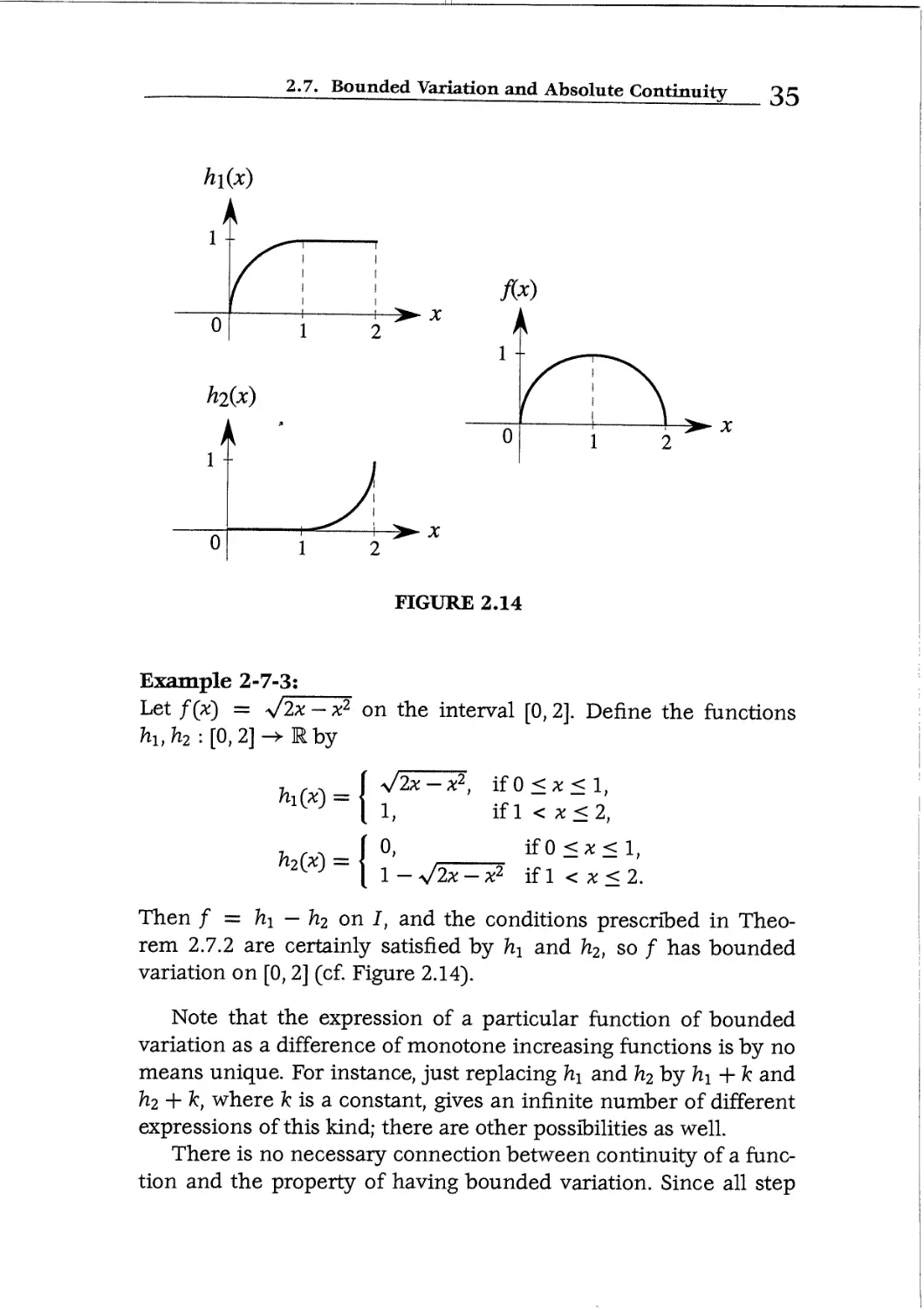
FIGURE 2.14
Example 2-7-3:
Let f(x) = s/2x - x2 on the interval [0,2]. Define the functions
-x2, ifO<x<l,
if 1 < x < 2,
ifO <x< 1,
-x2 ifl < x<2.
Then f — h\ — h.2 on I, and the conditions prescribed in Theo-
Theorem 2.7.2 are certainly satisfied by hi and h2, so / has bounded
variation on [0,2] (cf. Figure 2.14).
Note that the expression of a particular function of bounded
variation as a difference of monotone increasing functions is by no
means unique. For instance, just replacing hi and h2 by hi + k and
fo2 _j_ -fc, where k is a constant, gives an infinite number of different
expressions of this kind; there are other possibilities as well.
There is no necessary connection between continuity of a func-
function and the property of having bounded variation. Since all step
36 2. Some Analytic Preliminaries
functions have bounded variation (see Example 2-7-1), functions of
bounded variation need notbe continuous. Conversely, a continuous
function need not have bounded variation. For instance, the function
tan(x) is monotone increasing and continuous on (—tc/2, tt/2), but
since its set of values does not have finite upper and lower bounds,
it does not have bounded variation on this interval (See Exercises
2-7, No. 3). Indeed, Example 2-7-2 shows that even if the set of val-
values of a continuous function has finite upper and lower bounds, the
function need not have bounded variation (see also Exercises 2-7,
No. 5).
We say that a function / :-> R is absolutely continuous on I
if given any e > 0, there exists a 8 > 0 (depending on e) such that
Vs(f,r) < € for all partial subdivisions S of I for which the sum of
the lengths of all the constituent intervals is less than 8. It follows
easily, by considering only partial subdivisions consisting of a single
interval, that if a function is absolutely continuous on I, it is also
continuous on I. We have also the following theorem:
Theorem 2.7.4
If I is an interval with finite endpoints a, b andf : I —> Ris absolutely
continuous on I, then f has bounded variation on I.
Proof Let S = {h, h, ¦ ¦ •, In} be any partial subdivision of I such that
Ij — [Oj, bj] for ; = 1, 2,..., n. Let e = 1 in the definition of absolute
continuity. Then there exists a 8\ > 0 such that Vs*(f, I) < 1 for all
partial subdivisions S* of I for which the sum of the lengths of all the
constituent intervals is less than 8\. Let N be the smallest positive
integer greater than (b - a)/Si. Then 1/N < Si/(b - a).
Now take any; = 1, 2,..., n. Divide Ij into N subintervals of equal
length,
Ijl = [«;(= Xj6), Xjl], Ij2 = [Xjl,Xj2], ¦ ¦ ¦ , IjN = [^(N-l), ty(= XjN)],
and denote the length of J;r by ?,> 0' = 1, 2,..., n; r = 1,2,..., N).
Then
Civ
N b-a
For each r = 1, 2,..., N, let Sr = {hr, I2r, ¦¦-, W- Then Sr is a partial
subdivision of I, and the sum of the lengths of all its constituent
2.7. Bounded Variation and Absolute Continuity r>n
intervals is
since ?;n=1(fy ~ aj) is the sum of the lengths of all the intervals that
make up the partial subdivision S of/, and is therefore no greater
than the length b - a of I. Therefore, VSr(f,I) < 1 for each r =
Now
n N
?? l/C^O -/(^-i))| (by the triangle inequality)
;=1 r=l
N n
r=l ;=1
N N
r=l r=\
Since N is finite and independent of S, it follows that V(f, I) <N and
/ has bounded variation on I. ?
Note that the converse of this theorem does not hold; as we have seen
earlier, a function of bounded variation need not even be continuous,
let alone absolutely continuous.
Note also that we have seen examples of continuous functions on
finite intervals that do not have bounded variation, and therefore (by
Theorem 2.7.4) are not absolutely continuous. Thus absolute conti-
continuity, as the name suggests, is a stronger condition than continuity,
in the sense that the set of absolutely continuous functions on an
interval is a proper subset of the set of continuous functions on that
33 2. Some Analytic Preliminaries
interval. Some examples of functions that are absolutely continuous
are given in Exercises 2-7, No. 6.
Exercises 2-7:
1. Prove that if/ : I ->- R has bounded variation on I, then sup {f (x) :
x e 1} and inf {f {x) :xe 1} are both finite.
2. Prove that if /, g : I ->- R have bounded variation on I, then so do
kf (where k is a real number), f + g, and fg.
3. Prove that a function /:/->- R that is monotone on I has
bounded variation on I if and only if sup(f (x) : x e 1} and
inf {/ (x) : x e 1} are both finite. Use this, together with the
results proved in the preceding exercise, to prove part (b) of
Theorem 2.7.2.
4. Express the step function 9 defined in Example 2-7-1 as a dif-
difference of two monotone increasing functions, and sketch the
graphs of the two functions.
5. Let/ : [-7r/2,7r/2] -> Rbe defined by
J^~\ 0, if x = 0.
(a) Prove that/ is continuous on [—jc/2, tc/2]; you may assume
that #sin(l/#) is continuous for all x ^ 0, so all that has to
be proved is that/ is continuous at x = 0.
(b) Use a method similar to that used in Example 2-7-2 to show
that/ does not have bounded variation on [—jc/2, it/2\
6. A function/ : I ->- R is said to be a Lipschitz function on I if there
exists a real number L such that \f(x{) —f(x2)\ <L\xi—x2\ for all
(a) Prove that any Lipschitz function on I is absolutely
continuous on I.
(b) Use this result to show that any linear function is abso-
absolutely continuous on any interval and that the function x2 is
absolutely continuous on any interval with finite endpoints.
(c) Use a proof by contradiction to show that x2 is not absolutely
continuous on (—oo, oo).
CHAPTER
The Riemann
Integral
The development of a rigorous theory of the definite integral in
the nineteenth century is associated particularly with the work of
Augustin-Louis Cauchy A789-1857) in France, and Bernhard Rie-
Riemann A826-1866) in Germany. In order to give some background
to the modern theory, we will describe briefly a definition of an inte-
integral equivalent to that introduced by Riemann in 1854, and discuss
some of the weaknesses in this definition that suggest the need for
a more general theory.
3.1 Definition of the Integral
Let [a, b]loe any closed interval. A function/ : [a, b] ->- R is said to be
Riemann integrable over [a, b] if and only if for any number e > 0,
there exist step functions g€,G€: [a, b] ->- R such that
(i) g€<f<G<;
(ii) A(G^ - A(ge) < e
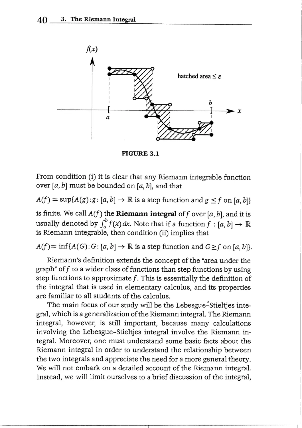
(cf. Figure 3.1). A function/ : I -+ R for which the set {/(*) : x e 1}
has finite upper and lower bounds will be called bounded on I.
39
40 3. The Riemann Integral
hatched area < e
FIGURE 3.1
From condition (i) it is clear that any Riemann integrable function
over [a, b] must be bounded on [a, b], and that
A(f) — sup{A(g) :g: [a, b] ->- R is a step function and g < f on [a, b]}
is finite. We call A(f) the Riemann integral of/ over [a, b], and it is
usually denoted by Xf/OO dx. Note that if a function / : [a, b] ->- R
is Riemann integrable, then condition (ii) implies that
A(fi — inf {A(G): G: [a, 2?] ->- R is a step function and G>f on [a, b]}.
Riemann's definition extends the concept of the "area under the
graph" of/ to a wider class of functions than step functions by using
step functions to approximate /. This is essentially the definition of
the integral that is used in elementary calculus, and its properties
are familiar to all students of the calculus.
The main focus of our study will be the Lebesgue-Stieltjes inte-
integral, which is a generalization of the Riemann integral. The Riemann
integral, however, is still important, because many calculations
involving the Lebesgue-Stieltjes integral involve the Riemann in-
integral. Moreover, one must understand some basic facts about the
Riemann integral in order to understand the relationship between
the two integrals and appreciate the need for a more general theory.
We will not embark on a detailed account of the Riemann integral.
Instead, we will limit ourselves to a brief discussion of the integral,
3.1. Definition of the Integral
highlighting any properties that are of use later in establishing the
relationship between the Riemann and Lebesgue-Stieltjes integrals.
Given abounded function/ : I —> R, candidates for the step func-
functions g€, G€ in the above definition can be constuctedby partitioning
the interval and defining step functions based on the maximum and
minimum values the functions assume in the subintervals. By a par-
partition P of an interval I = [a, b] we mean a finite set of numbers
Xn, where
,Xn,
< x\ < • • • < xn = b.
*
Let I\ — [xo, x\], and for 1 < k < n let Ik — (xk-i, xk] denote the kth.
subinterval of I associated with the partition P. Let Ak = xk — xk-\
denote the length of the subinterval. If/ : I —> R is bounded on I,
then given any partition P of I, step functions gp,GP : I ->- R such
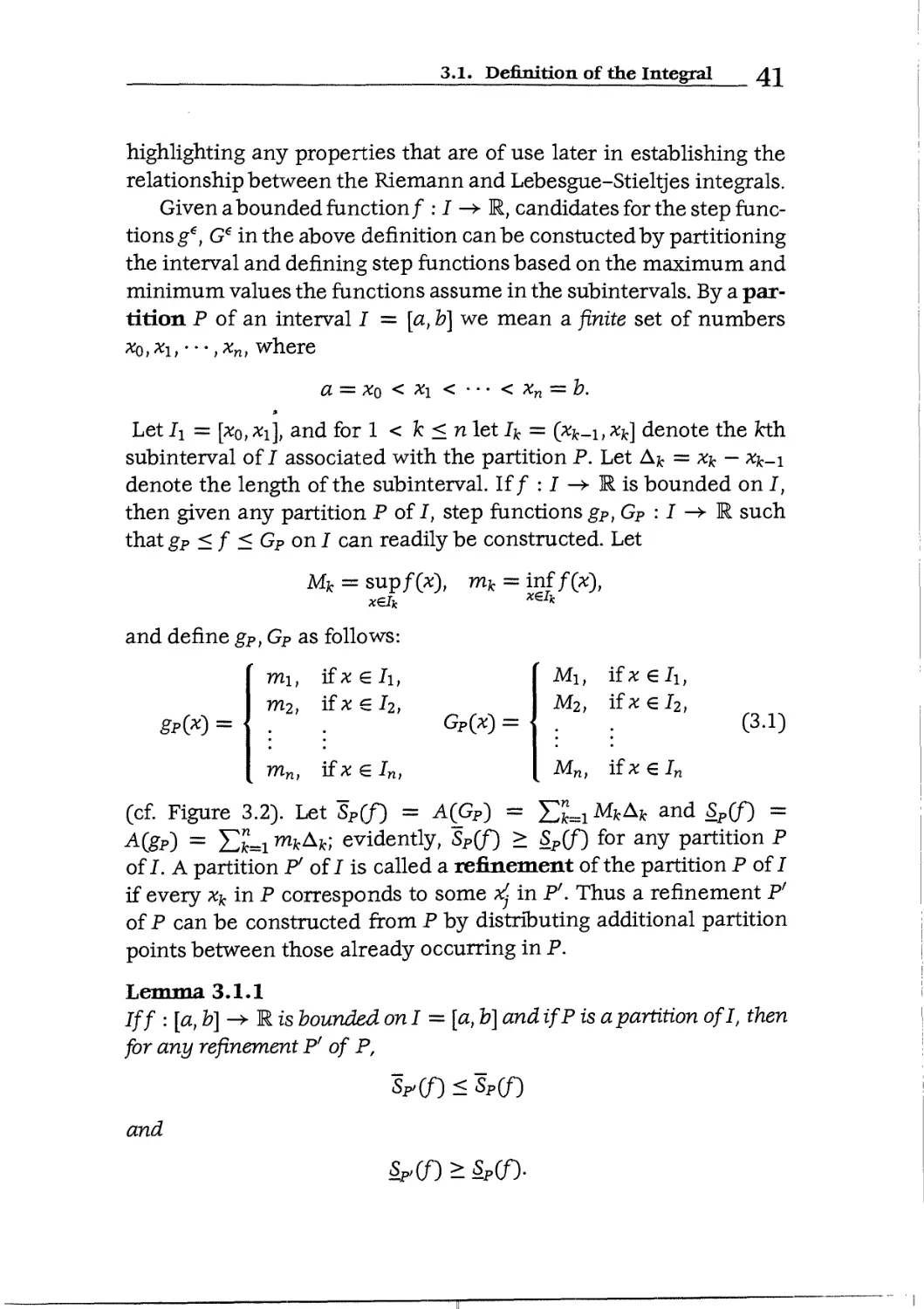
that gP <f <GP on I can readily be constructed. Let
Mk = sup/OO, mk
and define gp, GP as follows:
mi, if x e Ji,
m2, ifxel2,
m
n>
ifx
ln>
Mi, if^e/i,
M2, if^€/2,
Gp(*) = { . . C-1)
Mn, if xe In
(cf. Figure 3.2). Let SP(f) = A(GP) = ELi M^A)t and Sp(/) =
a(Bp) = ELi m^A^" evidently, SP(f) > Sp(f) for any partition P
of I. A partition P1 of I is called a refinement of the partition P of I
if every xk in P corresponds to some #J in P'. Thus a refinement P'
of P can be constructed from P by distributing additional partition
points between those already occurring in P.
Lemma 3.1.1
Iff : [a, 2?] ->¦ R is bounded on I
for any refinement P' of P,
[a, b] and ifP is a partition of I, then
SP'(f) < SP(f)
and
42 3. The Riemann Integral
Ax)
A
A(gp)
X
A(GP)
X
FIGURE 3.2
Lemma 3.1.2
Suppose that f : [a, b] ->¦ R is bounded on I
are any two partitions of I. Then
= [a, b] and that P and P'
Let n denote the set of all partitions of I = [a, b]. From Lem-
Lemmas 3.1.1 and 3.1.2 the set 5 = (SP(f) : P ? U) is bounded below by
Sj(f), where I is the partition corresponding to x0 = a, x\ = b. The
set 5 must therefore have a finite lower bound iff is bounded on-J.
Similarly, iff is bounded on I, then the set 5 = {Sp(f) : P e U} must
have a finite upper bound, because it is bounded above by 5j(f). The
quantities infPen ~Sp(f) and supP6n SP(f) are finite and are called the
upper and lower Riemann-Darboux integrals of / over I, respec-
respectively. If, in addition, it is assumed that/ is Riemann integrable over
3.1. Definition of the Integral
I, then it can be shown that
PeU Pen
Indeed, the condition infPen SP(f) = supPen Sp(f) is commonly used
in the definition of a Riemann integrable function.
Iff : [a, b] -> R is Riemann integrable on I = [a, b], then there is
a sequence of partitions {Pj}, Pj € n, such that lim,.^ S-?(f) = A(f)
and a sequence {PjJ, Pk € n, such that lim^oo ?&(/") = A(f)- Now>
for any two partitions P and P', the set PUP' yields a partition Q. that is
the common refinement of P andP'. Lemma 3.1.1 and the definitions
of infimum and supremum thus indicate that we can always find a
sequence {Pk} such that lim^^ S^tf) = lim^oo S^Cf) = A(f), and
moreover, we can assume thatP^+i is a refinement ofP*.,fc = 1,2,
Theorem 3.1.3
Iff : [a, i>] -» R is Riemann integrable over I = [a, b], then there exists
a sequence of partitions {P^}, P^ € n, such that P^+i is a refinement of
Pkf k = l,2,..., and
k-±oo
Let P = {xo, ^i, • • •, *n} be a partition of the interval I = [a, b]. The
norm of P, denoted by ||P||, is defined as
||P|| = max A*.
fc=l,2,...,n
The norm of P is thus the maximum of all the lengths of all the
subintervals formed by the partition P. It can be shown that if / :
I -» R is Riemann integrable over I, then any sequence of partitions
{Pj} such that ||P;-1| -» 0 as; -» oo will produce the Riemann integral
off over/, i.e.,
In general, it is not particularly convenient to prove that a given
function is Riemann integrable directly from the definition. The
following theorems are thus useful in this regard:
The Riemann Integral
Theorem 3.1.4
Iff .- [a, b] -> R is monotone on I = [a, b], then it is Riemann integrable
over I.
Theorem 3.1.5
Iff : [a, b] -» R is continuous on I = [a, b\ then it is Riemann integrable
over I.
Exercises 3-1:
1. Let / : [a, b] -> R be a bounded function on I = [a, b] and let P'
be a refinement of the partition P of I. Prove that gP < gp> and
Gp > Gp>, where the step functions g and G are as defined in
equation C.1).
2. Use Lemma 3.1.1 and the fact that Q. = P U P' is a com-
common refinement for any two partitions P and P' of I to prove
Lemma 3.1.2.
3.2 Improper Integrals
The Riemann integral as defined in Section 3-1 is over closed inter-
intervals. The defintion of the integral can be extended to other intervals
by using a limiting process leading to the theory of what are usu-
usually called "improper integrals." We eschew a detailed account of
improper integrals; instead, we give a brief description of the basic
idea with examples.
Suppose that / is a continuous function on the interval (a, b].
By Theorem 3.1.5 the function / is Riemann integrable over any
interval of the form [c, b], where a < c < b, and we can enquire
about the existence of limc_>a+ f^f(x)dx. If this limit'is finite, then
we say that it defines the improper integral off from a to b. The im-
improper integral is denoted in the same way as the Riemann integral,
i.e., by f*f(x)dx- If an improper integral exists, we also say that it
converges. Improper integrals over other intervals such as [a, b),
[a, oo), (—oo, b], etc. are defined in a similar way.
Example 3-2-1:
The function/ defined by f(x) = 1/y/x is continuous for all x € @,1].
By Theorem 3.1.5 / is Riemann integrable in any closed subset of
3.2. Improper Integrals
@,1]. In fact, for any 0 < c < 1,
/ /(*)<& = [2V*]*= 2A-
Now, limc_>0+ jc f(x)dx = 2A - limc_>0+ ^/c) = 2, and therefore the
improper integral /* f(x) dx exists.
Example 3-2-2:
The function / defined by f(x) = 1/x2 does not have an improper
integral from 0 to 1. The function / is Riemann integrable over any
interval [c, 1], 0 < c < 1, because it is continuous there, but
1
c
and thus limc_>0+ fc f(x) dx is n°t finite.
Example 3-2-3:
Let / be the function defined in Example 3-2-2 and consider the in-
interval [1,00). The function/ is Riemann integrable over any interval
of the form [1, c], where 1 < c < 00, and since
fc 1
Km / —• dx = lim
= lim (l --) =1,
1 c-»oo
the improper integral f™ l/x2dx converges.
Example 3-2-4:
Let / : [1, oo) -> R be defined by f(x) = 1/x. In any closed interval
[1, c], c > 1, we have that
/'
-dx = [logx]!^ = logc.
Since logc -» 00 as c -» 00, the improper integral f™ 1/xdx does
not exist, i.e., it diverges.
Although the definition of the Riemann integral can be extended
to open or semiopen intervals, many of the results concerning the
Riemann integral over a closed interval do not carry over in the
extension. Example 3-2-2 indicates that continuity on a semiopen
interval does not guarantee the existence of the improper integral.
46 3. The Riemann Integral
Examples 3-2-2 and 3-2-4 show that monotonicity does not imply
Riemann integrability when the interval is not closed.
If / : [a, b] -» R is Riemann integrable over [a, b], then it can
be shown that |/| is also Riemann integrable over [a, b]. For im-
improper integrals, this is no longer true, i.e., f%f(x)dx may converge
but fa \f(x)\ dx may diverge. If f^f(x)dx and f°a \f{x)\ dx both con-
converge, then the improper integral is called absolutely convergent.
If fa f(x) dx converges but fa \f(x)\ dx diverges, then the improper
integral is called conditionally convergent. The integral in Exam-
Example 3-2-3 is absolutely convergent. The next example requires more
familiarity with improper integrals than assumed heretofore, but it
provides a specific example of a conditionally convergent integral.
Example 3-2-5:
Let/ : [it, oo) -» JRbe defined by f(x) = (sinx)/x. Over any closed in-
interval of the form [it, c], c > it, the function/ is Riemann integrable,
and (anticipating integration by parts) we have
/
Jn
c sinx ., r cosanc fc cosx
d \/
n
2| < 1/x2
Now, |cosx/x2| < 1/x2 for all x € [it, c], and it can be shown
that lim^oo f° cos x/x2 dx exists, since lim^oo f° 1/x2 dx exists (the
comparison test). On the other hand, it can be shown that
f° \sinx/x\dx does not exist.
The definition of the Riemann integral can thus be extended to
intervals of integration other than closed intervals by using improper
integrals. The modern approach, to be described in the next chapter,
works with arbitrary intervals from the start, leading to a tidier the-
theory, but this is a relatively minor improvement. A mofe fundamental
weakness of Riemann's approach is revealed in the next section.
3.3 A Nonintegrable Function
Theorems 3.1.4 and 3.1.5 indicate that the class of Riemann in-
integrable functions is a large one. In fact, it can be proved that if
/ : [a, b] -» M is bounded on [a, b) and the set of all points of dis-
3.3. A Nonintegrable Function AH
continuity off in [a, b] is either empty, finite, or countably infinite,
then/ is Riemann integrable over [a, b]. However, if the set of points
of discontinuity off is infinite but not countable, then / may not be
Riemann integrable, as the following example illustrates.
Example 3-3-1:
Let/ : [0,1] -+ JRbe defined by
frx-\ _ f 1> ifxis rational, x ^ 0,1,
. [ 0, if a; is irrational or x = 0 or x = 1.
Suppose that / were Riemann integrable over [0,1]. Then taking
€ = \ in the definition of Riemann integrability, there must exist
step functions g, G : [0,1] -* R such that g < f < G on [0,1] and
A(G)-A(g)<\.
Now, we have seen that any interval of nonzero length contains
infinitely many rational numbers and infinitely many irrational
numbers. Thus we must have g{x) < 0 and G{x) > 1 for all but a
finite number (possibly zero) of points x € [0,1]. The values of g{x)
and G(x) at a finite number of values of x do not affect the values of
the areas A(g) and A{G), so we must have A{g) < 0 and A{G) > 1.
Thus A(G) - A(g) > 1, which contradicts A(G) - A(g) < \, and so /
cannotbe Riemann integrable over [0,1]. Note that/ is discontinuous
at every point in the interval [0,1].
The reader might rightly ask why we should be concerned that
this rather peculiar function does not have an integral in the Rie-
Riemann sense. The reason is connected with the following concern:
Suppose the functions /„ : [a, b] -» R are Riemann integrable over
[a, b] for all n = 1,2,..., and /„ -» / on [a, b]. It is natural to hope
that the property of integrability "carries over to the limit," so that we
can be sure that/ is also Riemann integrable over [a, b] (and that the
integral of/„ tends to the integral off as n tends to oo), but this may
not be the case. This concern is important, because the solutions to
many problems in the calculus such as differential equations are of-
often obtained as the limit of a sequence of successive approximations.
Unfortunately, there are sequences of functions that are Riemann
integrable but that converge to a function that is not. It is necessary
to find only one counterexample to destroy our hopes.
48 3. The Riemann Integral
We will now show that the nonintegrable function defined in
the previous example is the limit of a sequence of Riemann inte-
grable functions. We know that the rational numbers in @,1) form
a countably infinite set, so we can write the set of rationals in @,1)
as {r\, r2, r3,...}. For each; = 1,2,... we subdivide [0,1] into three
subintervals: J;1 = [0, rj), Ij2 = [r;-, rj\, and Ij3 = (rjt 1]. We then define
0;:[O,1]-+Rby
*;(*) =
Now, 0j is a step function for each; = 1,2, Define /„ : [0,1]
by
0, ii
1, if X € Ij2,
0, ii
Now, each /„ is also a step function, and is therefore Riemann
integrable over [0,1]. Furthermore, it is evident that
ff0, if a: is irrational or x e {0,1, rn+1, rn+2 ...},
~~ i 1, if ^ € {n, r2,..., rn} .
Thus if x € [0,1] is irrational or x = 0 or x = 1, then/n(x) = 0 = /(x)
for all n = 1,2,..., and so fn(x) -» /(x) as n -> oo. If x € [0,1]
is rational, say x = rN(N = 1,2,...), then fn(x) = 1 = f(x) for
all n > N, so again /n(x) -> /(^) as n -» oo. We have therefore
established that the Riemann integrable sequence of functions /„
converges to the nonintegrable function/ on [0,1].
This example shows that integrability in the Riemann sense does
not always carry over in the limit. It can be shown that it does under
certain conditions, but these conditions are rather complicated. Be-
Because the modern theory (as we shall see) allows for a wider class of
integrable functions, the conditions under which integrability car-
carries over to the limit are much simpler and easier to use. This is
one of the most important ways in which the modern theory is an
improvement over the older one.
CHAPTER
The Lebesgue-
Stieltjes
Integral
We now proceed to formulate the definition of the integral that we
are going to study. It results from combining the ideas of two people.
The French mathematician Henri Lebesgue A875-1941), building
on earlier work by Emile Borel A871-1956) on the measure of a set,
succeeded in defining an integral (the Lebesgue integral) that ap-
applied to a wider class of functions than did the Riemann integral, and
for which the convergence theorems were much simpler. The Dutch
mathematician Thomas Stieltjes A856-1894) was responsible for the
notion of integrating one function with respect to another function.
His ideas were originally developed as an extension of the Riemann
integral, known as the Riemann-Stieltjes integral. The subsequent
combination of his ideas with the measure-theoretic approach of
Lebesgue has resulted in a very powerful and flexible concept of
integration.
4.1 The Measure of an Interval
Let a : R —> R be a monotone increasing function, and let I be an
interval with endpoints a, b. We define the a-measure of I, denoted
49
cQ 4. The Lebesgue-Stieltjes Integral
by /xa(I), as follows:
tia([a, b]) = a(b+) - a{a~),
Ha({a, bj) = a(b+) - a(a+),
Vctda, b)) = a(b~) - a(a~),
and if a < b,
ixa{{a, by) = a(b~) - a(a+).
The "open interval" (a, a) is of course the empty set, and we
define ?ta((a, a)) to be zero for any a € Re. The intervals {a, a] and
[a, a) are also empty, but in those cases the fact that their a-measure
is zero follows from the general definition, and need not be specified
separately.
It follows easily from Theorem 2.4.l(i) and Corollary 2.4.2(i) that
Ma(-0 >: 0 fc>r any interval I, and that if I and/ are intervals with I QJ,
then Ma(I) < fia(J).
If a and b are finite, and a is continuous at both a and b, then
we have a(a~) = a(a+) = a{a) and a(b~) = a(b+) = u(b), and so
/xa(T) = a(b) — a(a) in all four cases. In particular, if a{x) = x for
all xeR, then na{I) = b — a is the ordinary length of the interval
I. In general, the a-measure of an interval is just the change in the
value of a over the interval in question; it can be thought of as a
generalization of the notion of length.
Example 4-1-1:
Let a : R -> R be defined by
a(x) =
0, if* < 1,
x2 - 2x + 2, if 1 < x < 2,
3, if x = 2,
x + 2, if x > 2
(cf. Figure 4.1). Then:
, 2]) = aB+) - a(l") = 4-0 = 4,
, 2]) = aB+) - a(l+) = 4-1 = 3,
, 2)) = aB") - a(l") = 2-0 = 2,
4.1. The Measure of an Interval
51
FIGURE 4.1
3])
3))
2])
aB~) - a(l+) = 2 - 1 = 1,
aC+) - aB") = 5-2 = 3,
:aC")-aB+) = 5-4 = l,
: aB+) - aB") = 4-2 = 2,
: aC") - a(-l+) = 5-0 = 5,
: a(|+) - a(-8") = 0-0 = 0.
It can be seen from these examples that the a-measure of an interval
takes account of a jump in the value of a at an endpoint if and only
if that endpoint is included in the interval. Note also that it is the
left- and right-hand limits of a at the endpoints that determine the
measure, not the value of a at the endpoints. Note finally that, as
the following examples illustrate, an interval that has one or both
endpoints infinite may have, but does not necessarily have, infinite
measure:
oo)) = a(oo~) - aB ) = oo - 2 = oo,
-oo, oo)) = a(oo~) - a((-oo)+) = oo - 0 = oo,
;-oo, 2]) = aB+) - a((-oo)+) = 4-0 = 4.
52 4. The Lebesgae-Stieltjes Integral
1.
Exercises
Let a : R -
4-1:
> Rbe
defined by
a(x) = ¦
x,
l',
3-
ifx
if*
c *¦ if v
C/ . 11 /I
<o,
= o,
> 0.
(a) Sketch the graph of or.
(b) Find /za(@, 1)), /za([0, 1]), /za((-l,1)), /xa([0, 0]),
jtt«((-OO, 1)), /Za(@, 00), /*a([0, 00)).
2. Let a : R -> R be defined by
a(x) =
0,
1, if 0 < x < 1,
4, if 1 <x < 2,
6, ifx>2.
(a) Sketch the graph of or.
(b) Find /xa([-l; 2)), /za((l, oo)), /xa((-oo; 4)), /za(@,2]);
/xa((l/2; 3/2)), /xa([l; 3D, /za((l, 3)).
4.2 Probability Measures
A particularly important type of measure arises when the function
or is a probability distribution function. In this case, the variable x is
referred to as a random variable, and for each real number X, the
value a(X) is the probability that the random variable x has a value
no greater than X:
a(X) = P(x < X).
The corresponding or-measure is then called a probability measure,
and has the property that for any interval J,
/xa(J) = P(x e I).
Any probability distribution function must necessarily satisfy the
conditions a((—oo)+) = 0 and or(oo~) = 1, and it follows from this
4.2. Probability Measures
FIGURE 4.2
that if/xa is a probability measure, then /xa(J) < 1 for any interval I.
Example 4-2-1:
The uniform distribution on the interval [A,B] (A and B finite,
A < .B) is the probability distribution a denned by
0, if x < A,
§Ei, ifA<*<?,
1, if x > B
(cf. Figure 4.2). Since a is continuous, we can say that if I is an
interval with finite endpoints a, h, then /xa(J) = a(b) — or(a), so that
if A <a<b<B, then
b — A a —A b — a length of I
., rp. -j. _ 2 .
^ J B-A B-A B-A length of [A,B]
Since the only changes in the value of a occur within the interval
[A, B], it follows that for any interval /,
length of ID [A, B]
length of [A, B] '
In this case /xa(J) can be interpreted as the probability that a random
number generator, programmed to select a random number in the
interval [A, B], will in fact select a number in I.
Example 4-2-2:
A discrete distribution is a probability distribution that is con-
constant except for jump discontinuities at a finite or countably infinite
54 4. The Lebesgae-Stieltjes Integral
1"
-1 0
1/2
FIGURE 4.3
number of points. An example is the function a defined by
a(x) =
0, if x < -1,
\, if — 1 <x < 1,
1, ifx>l
(cf. Figure 4.3). In this case we have
0, if I contains neither 1 nor — 1,
\, if I contains 1 or —1 but not both,
1, if I contains both 1 and — 1.
This corresponds to a random variable x such that
_ _ 1
2
For example, x might be the outcome of tossing a coin if "heads" is
scored as 1 and "tails" as —1.
Exercises 4-2:
1. If x is a random variable that can take only one value X (with
probability 1), what is the corresponding probability distribution
function or?
2. If x is a random variable that can take exactly n values
X1,X2,...>Xn (where X1 < X2 < ¦ • • < Xn), each with a probability
1 /n, what is the corresponding probability distribution function
<*?
4.3. Simple Sets 55
4.3 Simple Sets
A simple set is a subset of R that can be expressed as the union
of a finite collection of disjoint intervals. If 5 is a simple set, say
S = Uj^I; where h, I2,..., Im are disjoint intervals, and if a : R -> R
is a monotone increasing function, then the or-measure of 5 is denned
by
m
A given simple set can, of course, be subdivided into disjoint in-
intervals in many different ways, but the value of its or-measure is
independent of the way in which it is subdivided. Note also that
(i) /za(<S) > 0 for any simple set S;
(ii) if 5 and T are simple sets such that S c T, then /za(S) < /za(T).
Some other elementary properties of simple sets are explored in the
exercises. Note finally that a simple set is said to be or-finite if it has
finite or-measure.
Exercises 4-3:
1. It is true (though rather tedious and unenlightening to prove in
general) that if S and T are simple sets, so are S U T, S 0 T, and
S — T = {x:xeS and x & T}. Verify this for each of the following
cases:
(a) S = [1, 3) U D, 8), T = B, 5] U F, 7];
(b) S = B, 3) U [5, 7], T = [1, 4] U [6, 8);
(c) S = A, 2] U [5, 6), T = [2, 4] U E, 7).
2. Prove that if S and T are disjoint simple sets, then /xaE UT) =
A<<a<(>>) + HciCn for any monotone increasing function a : R ->
R. Give examples to show that if S and T are not disjoint, then
/xaE U T) may or may not equal /xaE) + /xa(T).
3. Use what was proved in the preceding exercise to show that if
S and T are simple sets such that T Q S and T is a-finite, then
/xaE — T) = /xaE) — fia(T) f°r anY monotone increasing function
a : R -» R. (Note that T is required to be or-finite in order to avoid
Lebesgue-Stieltjes Integral
having the meaningless expression oo — oo on the right-hand
side.)
4. Give examples to show that if T is not a subset of 5, then /u,a(S—T)
may or may not equal fia(S) — /xa(T).
4.4 Step Functions Revisited
Let a : R -> R be a monotone increasing function. Let I be any
interval, and let 6 : I -» R be a step function. It is clear from the
relevant definitions that the support of 0 is a simple set. We say
that 0 is a-summable if the support of $ is a-finite. In that case we
associate with 6 a real number Aa{6) denned by
using the notation introduced in Section 2-5.
If a(x) = x for all x € R, so that fia(Ij) is just the ordinary length
of the interval Ij, then Aa{6) is just the area AF) under the graph of
6, as denned in Section 2.5. In general, AaF) can be thought of as a
generalized "area" for which "lengths" along the x-axis are measured
by or-measure rather than by ordinary length.
Note that if the endpoints of I are both finite, then any step func-
function 9 :1 -* R is or-summable for all monotone increasing functions
a : R -> R.
Example 4-4-1:
Let a be denned as in Example 4-1-1, and let 0Y :< [0,3] -> R be
denned by
^-{2, ifl<*<3
(cf. Figure 4.4). Then
/^([0,1)) = a(l") - a(O") = 0-0 = 0,
fiaQl, 3]) = aC+) - of(l-) = 5 - 0 = 5,
4.4. Step Functions Revisited
1
0\(x)
FIGURE 4.4
2 --
1 -
02(x)
o1- i
FIGURE 4.5
and so
Suppose we modify the definition of 01 very slightly, to give
\
-\2, ifl<x<3
(cf. Figure 4.5). In this case
HaQO, 1]) = «A+) ~ «@") = 1-0
Ha(.(l, 3]) = «C+) - «A+) = 5-1
1,
4,
and so
«(fc) = (-l)l+2D) = 7.
58 4. The Lebesgae-Stjeltjes Integral
0
FIGURE 4.6
Note that while the area A{&) under the graph is the same for
these two functions, the values of Aa(G{) and Aa(G2) are different.
This is because at the single point where #i and 02 have different
values, a has a discontinuity, and so the interval consisting of that
single point has positive or-measure. Clearly, discontinuities in a
complicate matters!
Example 4-4-2:
Let a be the discrete distribution function denned in Example 4-2-2,
and let 9 : R -> R be denned by
2, if a: > 0
(cf. Figure 4.6). Then
/xa((-oo, 0])
c<0+)-<(-oo)+) = --0 = -,
/xa(@, oo)) = a(oo-) - ex@+) = 1 - - = -,
and so
We conclude this section by listing a number of basic properties
that are straightforward to prove and intuitively reasonable, so we
will omit the proofs.
(i) If G is a nonnegative a-summable step function, then Aa{&) > 0;
also, Aa@) = 0.
4.4. Step Functions Revisited
FIGURE 4.7
(ii) If 0i and 02 are or-summable step functions on the same interval
I such that 0i < 02 on I, then Aa@i) < Aa@2).
(iii) If 0 is an or-summable step function, then so are |0|, 0+, and 0~,
and we have Aa@) = Aa@+) + Aa@") and Aa(|0|) = Aa@+) -
Aa@").
(iv) If 0i, 02,..., 0m are a-summable step functions on the same in-
interval J, a\, a.2,..., dm are finite real numbers, and 0 : J -> E is
defined by
m
for all a: € I (i.e., 0 = J^ a;0;), then 0 is also an a-summable
step function on J, and
m
Exercises 4-4:
Let a : M. -> R be denned by
\x, if ^ < 0,
l, if*>0
(cf. Figure 4.7). For each of the following step functions 0:
(a) sketch the graph of 0;
(b) determine whether or not 0 is a-summable, and if it is, find
Aa@).
60 4. The Lebesgue-Stieltjes Integral
1.0: (-2,1) -» E defined by
Br^-l 3> if~2<*< -1,
*(*)-| _i; if-i<x<i.
2. 0 : [-1,1] -» E defined by
()~il, ifO<*<l.
3. 0 : [-1, oo) -» E defined by
GW-\ 1, ifx>3.
4. 0 : (-oo; 0) -» E defined by
5. 0:E-» E defined by
4.5 Definition of the Integral
We are now in a position to set up the necessary machinery for
defining the Lebesgue-Stieltjes integral. Throughout this section we
take I to be a given interval with endpoints a, b, and a : E -» E to
be a given monotone increasing function.
Let / : I -» E be a function that is nonnegative on I. A se-
sequence 0i, 02, #3, • • • is said to be admissible for / if it satisfies all
the following conditions:
(a) 0;- is an or-summable step function on J, for each; = 1,2,3,.. .;
(b) Oj(x) > 0 for each x € I and each; = 1, 2, 3,...;
(c) 0 < /(a:) < J2™i ej(*) for eacn * € L
Theorem 4.5.1
An admissible sequence exists for any nonnegative function f : I -» E.
Proof There are two cases to consider.
4.5. Definition of the Integral gi
Case 1. The endpoints a, b of I are finite. In this case we define the
function 0;- : I -» R by 0;(x) = 1 for all x € I (j = 1,2, 3...). Then 0;-
is nonnegative, and since the endpoints of J are finite, 0;- is certainly
a-summable for each; = 1, 2, 3.... Since J2™i &.O0 = H;2i 1 = oo,
condition (c) above is also satisfied for any nonnegative function
f : I -> R, and so the sequence 0i; 02,93,... is admissible for /.
Case 2. Either a = -ooorb = ooor both. In this case we define the
subinterval J;- of J as follows:
If J is (—oo, b), b finite, then I; is (b —j, b).
If/ is (—oo* b], b finite, then I;- is (b —j, b].
If J is (a, oo), a finite, then J;- is (a, a + j).
If J is [a, oo), a finite, then J;- is [a, a+j).
If J is (—oo, oo), then J;- is (—;,;").
For each; = 1, 2, 3,... we then define Oj: J -» R by
Then 0;- is nonnegative on I and is or-summable, since its support
Ij is an interval with finite endpoints. Further, for each x e I we
have that 0;(x) = 1 for all sufficiently large values of;, and so again
J2^i fyOO = °° f°r eacn x & I. Thus the sequence 9\, 02,03,... is
admissible for any nonnegative function / : I -> R. D
We associate with any nonnegative function / : I -» R an
extended real number La(f) denned by
00
.7=1
where the greatest lower bound is taken over all sequences
0i, #2, #3, • • • that are admissible for /. Since the set of all such sums
]??i ^o<@;) is non-empty (by Theorem 4.5.1) and has 0 as a lower
bound, it follows by Theorem 1.3.1 that La(f) exists and La(f) > 0
for any nonnegative function / : I -> R. Note that La(f) = oo is a
possibility. Note also that it follows easily from the definition that
La@) = 0.
Example 4-5-1:
Let/ : [0,1] -» R be the function discussed in Section 3.3, and let the
functions 0;- be as denned in that section. For each; = 1,2,3,..., 0;- is
62 4. The Lebesgae-Stieltjes Integral
a nonnegative a-summable step function on [0,1], and Yl^i fy(.x) =
f(x) for each x e I, so the sequence 01; 02,03,... is admissible for /.
In particular, let a* be denned by a*(x) = x for all x € R. Then for
each; = 1,2,3,... we have
A«*@;) = /za*([r;-, r;]) = r,- - r,- = 0,
and so Y?i -<V@;) = 0. It follows that La*(f) = 0.
Note that although each 0j is a step function, / = J2*jli fy *s not a
step function, since it is not possible to describe it by taking constant
values on any finite set of subintervals of [0,1].
Theorem 4.5.2
For any function f : I —> ~Rwe have:
(i) La(f+-) < LaQf\) andLa(-f-) < La(|/|);
(ii) La(\af\) = |<2|La(|/|) for any finite nonzero real number a (and for
a = 0, provided that La(|/|) is finite).
Proof (i) Clearly, any sequence 61,02,03,... that is admissible for
I/I is also admissible for /+ and —f~. Thus the set of admissible
sequences for \f\ is a subset of the set of admissible sequences for
/+ and of the set of admissible sequences for —/~. Part (i) follows at
once from Exercises 1-3, No. 3. ?
(ii) It is obvious that both sides are zero if a = 0 andLa([f|) is finite,
so suppose fl^O. Let 0\, 02,0^,... be an admissible sequence for \f\,
so that for all x € I,
0 < If(*)I <?>(*)•
7=1
Then
00 00
0<\af(x)\<\a\Y/9i(x) = Y.
7=1 7=1
for all x € I, and also
00 00 00
7=1 7=1 7=1
and so \a\0\, \a\02, \a\O3,... is an admissible sequence for \af\.
4.5. Definition of the Integral
Conversely, if 9l,e2, 03,... is an admissible sequence for \af\,
then (l/\a\Nlr (l/\a\H2, (l/\a\H3,... is an admissible sequence for
\f\. Thus, if S is the set of admissible sequences for \f\. Then from
above and Exercises 1-3, No. 4(a), we have
L*Qaf\) = inf ¦
oc
)
J^ActQalOj)
7=1
= \a\ inf <
00
• = inf ¦
5
00
E
.7=1
D
Theorem 4.5.3
If fg : J -> R are such that 0 < f(x) < g(x) for all x € I, then
La(f) < La(g).
Proof This result follows at once, since any sequence 6\, d2,03,...
that is admissible for g is also admissible for /. ?
Theorem 4.5.4
Iffi,f2,f3,---isa sequence of functions such that fj-.I-^M. for each
j = 1,2,3,... and X^i fj(.x) converges for each x el, then
7=1
00
7=1
[Note that is it possible to have J^i ^aCI^D = °° under the condi-
conditions of the theorem. Note also that when the sequence f\,f2)h,--'
is such that fj¦ = 0 for all; > n, we obtain the important special case
Proof The result is evidently true if J^i -^aCI^I) = °°> s0 assume
that Yl'jliLcedfjl) is finite. Then certainly La(|/y|) is finite for each
j = 1,2,3, Take any e > 0. By part (ii) of Theorem 1.3.2 and the
definition of La(|/y|), we have that for each; = 1,2,3,... there is a
sequence 6>;i, 6>;2,0,3,... admissible for \fj\ and such that
m=l
64 4. The Lebesgue-Stieltjes Integral
It follows from the properties of double series of positive terms
(Section 2-2) that
00
00 / 00
j,m=\
7=1 \m=l
oo
7=1
oo
oo
oo
7=1
But since 0 < \fi(x)\ < Em=i ^mOO for all x € I and each; =
1, 2, 3,..., we have
0<
00
7=1
00
00/00
00
;=1 ;=1 \m=l / 7,m=l
If we write the double sequence Ojm (j,m = 1,2,3,...) as a sin-
single sequence (in any way we choose), the result is a sequence
t/t1; t/t2, t/^3, ... that is admissible for | Yl'jli fj\> an?^ so
oo
7=1
00
00
= E
7,m=l
00
thus, La(| E^
that
~ Ef^i ^a(l^l) — e f°r anY ^ > ; and it follows
00
E
7=1
oo
7=1
i.e.,
oo
E©
00
7=1
as required.
?
4.5. Definition of the Integral
Theorem 4.5.5
tf hJiJz, • • • is a sequence of functions such that fn : I -> R and
LaQfn\) is finite for each n = 1, 2, 3,..., and if f : I -> R is such
that LaQf —fn\)-> 0 (asn-^- oo) then:
(i) L«(|/|), La(f+) and La(-/") are all finite;
(ii) LaQf+ -f+\) -* 0,LaQT ~fn\) ~+ 0 andLaQ\f\ - \fn\\) -> 0;
(in) La(|fn|) -> La(|/|);LaCf+) -> La(f+-) andLa{-f~) -> La(-/-).
Proof (i) Since La(|f -/n|) -»- 0, there certainly exists a positive
integer N such that La(]f - fN\) is finite. Then
La{\f\) = La(]fN +/ -/nI) < WnI) +W -/nI),
by Theorem 4.5.4, and so LaQf\) is finite, since LaQfN\) and La(|/ -
/N|) areboth finite. The fact thatLffi(f+) andLa(-/~) are finite follows
at once from Theorem 4.5.2(i).
(ii) From Exercises 2-6 we have that on J,
\f+ -f+\ < \f-fnl \r ~fn\ < \f-fnl
and
\\f\-\fn\\<\f-fnl
Since La(]f — fn\) —> 0 by hypothesis, part (ii) follows at once using
Theorem 4.5.3.
(iii) We have, using Theorem 4.5.4:
Wnl) = W +/» "/I) <^«(lfl)+A,(lfn "/I)
= La(|/|)+La(|f-/n|). D.1)
Also,
X-orCLTD = W "/n +/nl) < LaQf - fn\) + La(|/n|),
and so
Wnl) > ^(l/l) -!>«(!/ -fnl). D-2)
From equations ( 4.1) and ( 4.2) we have
~fn\) < La(\fn[) < I*
i.e.,
-fn\) < LaQfn\) -La{\f\) < LaQf-fn\l
66 4. The Lebesgue-Stieltjes Integral
i.e.,
Since LaQf - fn\) -> 0 by hypothesis, it follows that L«(|/n|)
have also
/+) and f+ = (f+-
-fn = -r + c-/r - c-D) and -r = (-/- - (-o+(-/-),
and since LaQf+ - /+|) -* 0 and La(\ - f~ - (-/")!) -* 0 by part
(ii), the rest of part (iii) can be proved by an argument similar to the
preceding one. ?
Now let a : R -> R be a monotone increasing function, and let
f : I —> R be a function with the property that there is a sequence
0i,02,03t... of a-summable step functions defined on I such that
LaQf-9n\) -> 0. It follows from part (i) of Theorem 4.5.5 thatLa(|/|),
La(f+) and La(—/") are all finite. Under these conditions we write
and call this quantity the (Lebesgue-Stieltjes) integral of / over I
with respect to a. If a(x) = x for all x € R, we write fjf dx instead of
fjfda; this special case is called the Lebesgue integral off over I.
It is important to be sure that J: 6 da = Aa(9) for any a-summable
step function 6 :1 —> R, because only then can the integral justifi-
justifiably be regarded as an extension of the concept of the "area under
a graph" as defined for step functions. This is, in fact, true, but the
proof is surprisingly hard, so we shall just state the result without
proof:
Theorem 4.5.6
For any a-summable step function 0 :1 —> R, we have fjOda = Aa@).
Exercises 4-5:
1. Complete the proof of part (iii) of Theorem 4.5.5by showing that
La(f+) -> L*(f+) and La(-/") -> La(-f-).
2. Let/ be the function discussed in Section 3.3 and Example 4-5-1,
and let a* be defined by a*(x) = x for all x € R. Since f+=f and
/~ = 0, and we have shown in Example 4-5-1 that La*(f) = 0,
4.6. The Lebesgue Integral
it follows that La*(f+) - La*(-/~) = 0. Complete the proof of
the fact that f[01]fdx = 0, by showing that there is a sequence
#i, #2, #3, • • • of a*-summable step functions on [0,1] such that
La*(]f-On |) -^ 0. (This example shows that fj dx may exist in the
Lebesgue-Stieltjes sense in some cases where / is not Riemann
integrable over I).
3. Use Theorem 4.5.6 to show that if 0 : I -> R is a nonnegative
a-summable step function, then Aa{6) = LaF).
4.6 The Lebesgue Integral
The mathematical machinery required to define the Lebesgue-
Stieltjes integral is notably more complex than that needed for the
Riemann integral. Here, we pause to discuss informally the defini-
definition of the Lebesgue integral and contrast it with that of the Riemann
integral.
Let J be an interval and / : J —* R be some function, which for
simplicity we assume to be nonnegative. Iff is Lebesgue integrable
over J, then Lx(f) < oo and
= i*Cf)
Recall that
Lx(f) = i
;=0
where the greatest lower bound is taken over all the sequences {#,}
that are admissible for /. If {0;-} is an admissible sequence, then in
particular, 0 < f(x) < J2^i fy(.x)-For a given admissible sequence {0;}
the quantity ?°!0 A@;) is thus an upper bound for the "area under
the graph off" and the quantity Lx(f) plays a role in the Lebesgue
theory analogous to that of the upper Riemann-Darboux integral in
the Riemann theory. Suppose now we consider sequences {<f>j} that
satisfy conditions (a) and (b) for an admissible sequence (see p. 60),
but satisfy the inequality
68 4. The Lebesgae-Stieltjes Integral
(c*) 0 < ??
for all x € I instead of condition (c). Let
00
where the least upper bound is taken over all sequences satisfying
conditions (a), (b), and (c*). If 4(f) < oo, we could define another
integral by
The quantity 4(f) is analogous to the lower Riemann-Darboux
integral. Note that in the Riemann theory the upper and lower
Riemann-Darboux integrals are always finite even if / is not
Riemann integrable. This is because the definition of Riemann in-
tegrability is framed in terms of closed intervals on which / must
be bounded. In the Lebesgue theory, no restrictions are placed on
I, and/ need not be bounded; consequently, neither lx(f) nor Lx(f)
need be finite.
If / is Riemann integrable, then condition (ii) of the definition
requires that the upper and lower Riemann-Darboux integrals be
equal. There is no analogue to this condition in the Lebesgue theory:
It is not required that lx(f) = Lx(f) for the Lebesgue integral to exist,
only that Lx(f) < oo. Prima facie, this may seem a weakness in the
theory, as there is no particular reason to choose Lx(f) over lx(f) to
define an integral, but it can be shown that the relationship lx(f) =
Lx(f) is in fact a consequence of the condition Lx(f) < oo together
with measurability of / (see p. 82). In other words, if Lx(f) < oo
and / is measurable, then ?x(f) < oo and ?x(f) = Lx(f). A similar
statement can be made if lx(f) < oo, and in this sense lx and Lx axe
always on the same mathematical "footing" in the Lebesgue theory.
The definitions of the Riemann and Lebesgue integrals differ
fundamentally in the functions used to approximate the "area under
the graph," and it is this difference that affords greater generality for
the Lebesgue integral. Recall that a function/ is Riemann integrable
on a closed interval I if for any € > 0 there are step functions g€, G€
such that g€ <f < G€ and A(G€) - A(g€) < €. The definition of the
4.6. The Lebesgue Integral
Lebesgue integral also uses step functions but in a different way. For
example, if {0;} is an admissible sequence, then the inequality in the
Lebesgue definition analogous to the inequality / < G€ in the Rie-
mann definition is / < ?°^i ty- Although each 0; is a step function,
the sum J^jSi fy need not be a step function. A more general class
of functions is thus allowed into the "approximation." Coupled with
this increased generality is the notion of measure, which is in itself a
generalization of length. The generality is enough to make functions
such as that described in Section 3.3 integrable under the Lebesgue
definition (c? Exercises 4-5, No. 2). The real value of the general-
generalization, however, lies in results such as the dominated convergence
theorem (Theorem 5.3.3), which resolve some of the problems with
the Riemann integral discussed at the end of Section 3.3.
The Lebesgue integral is a generalization of the Riemann
integral. We state the following result without proof:
Theorem 4.6.1
If a function f : [a, b] —> M is Riemann integrable over the interval
I = [a, b), then it is also Lebesgue integrable over I, and the two integrals
are equal
The above result is used frequently to calculate Lebesgue in-
integrals. Note that the generalization breaks down if the integral is
improper. For example, the conditionally convergent integral in Ex-
Example 3-2-5 is not Lebesgue integrable. (In fact, Theorem 5.1.1 in
the next chapter indicates that if a Lebesgue integral exists, it is al-
always absolutely convergent.) If an improper integral is absolutely
convergent, however, then it can be shown that it is also Lebesgue
integrable and the integrals are equal.
Exercise 4-6:
Let/ : [0, oo) -> Rbe defined by
n =
(Figure 4.8).
70
4-
Lebesgae-Stieltjes Integral
0
11
1
1 | ~~T
1 | 1
1 | 1
' il '
1 | , 1
1 1 '
i , m
i i
i i
]
. t
! 13 >
4 6
FIGURE 4.8
(a) Evaluate L c. / dx for c a positive real number. (Since / is a step
function on [0, c), this integral exists in both the Riemann and
Lebesgue senses.)
(b) Show that /0°° / dx exists in the Riemann sense, as lim^oo /oc fdx.
(c) Show that \imc.+oo f° \f\dx does not exist; this shows that
L^fdx does not exist in the Lebesgue sense (cf. Theorem
5.1.1).
CHAPTER
Properties of
the Integral
In this chapter we will examine some of the essential properties of
the Lebesgue-Stieltjes integral, culminating in the convergence the-
theorems that (as remarked in Chapter 3) are among the most important
features of the Lebesgue-Stieltjes theory.
5.1 Basic Properties
Theorem 5.1.1
Iff : I -> R is integrable over I with respect to a, then so are f+, f~,
and \f\, and we have
[fdct = ff+doc + ff-doc and f\f\dce= ff+dec - ff~doc.
Ji Ji Ji Ji Ji Ji
Proof Since / is integrable over I with respect to a, there is a se-
sequence d\, 62, #3,... of a-summable functions on I such that LaQf —
&n\) -* 0. Since 0n is a-summable for each; = 1, 2, 3,..., so is \9n\,
and it follows from Exercises 4-5, No. 3, that La(|0n|) is finite for each
; = 1,2, 3, It then follows from part (ii) of Theorem 4.5.5 that
71
72 5. Properties ot the Integral
- 0~\) -> 0 and LB(||f I - l^ll) -> 0, so by
definition f+,f~, and |/| are all integrable over I with respect to a.
By definition, fTf+da = La(f+) and fIf~da = -La(-f~), and so
y/ da = La(f+) - La(-O = jf+da + ff~ da.
Also, we have by property (iii) (at the end of Section 5-4) that
Thus La(|0n|) = LaF>+) + La{-e~) by Exercises 4-5, No. 3. Letting n
tend to oo, we have by Theorem 4.5.5 part (iii) that
WO = La(f+) + !*(-/-) = jj+da- Jf~ da.
But since |/|+ = |/|, we have fT \f\da = La(|/|), which proves the
last part of the theorem. D
Theorem 5.1.2
If for each n = 1, 2,3,..., fn : I —> Ris integrable over I with respect to
a, and iff : I -> Ris such that La(\f — fn\) -> 0, then f is integrable
over I with respect to a, and we have
[fnda-+ \f da, (f+da-+ f f+da,
Ji Ji Ji Ji
[f~da-+ ff-da, [\fn\da-+ [\f\da.
Ji Ji Ji Ji
Proof Take any positive integer n. We know that fn is integrable,
so by definition there is a sequence Vi, fa, • • • of a-summable step
functions such that La(|/n - ^y|) -> 0 as; -^ oo. Thus, for some
k = 1,2, 3,... we must have La(\fn — Vod) < 1/n. Chpose such a k
and denote fa by 6n. In this way we obtain a sequence $i, 62,... of
a-summable step functions such that
K(\fn-0n\)< K E-1)
for each n = 1,2, Now take any e > 0. Since La(|/ - fn\) -> 0,
there exists a positive integer N(e) such that
/n|)< |. E.2)
5.1. Basic Properties
Also, from equation E.1), we have that
e n ~ 2 ' ~"v"" nU 2 l J
By Theorem 4.5.4 we have that for each n = 1,2,...,
LaOf ~ 0n\) = LaQf-fn + fn ~ &n\) < La(\f -/n|) + LaQfn - 0n\).
Thus, if n > max{NF), 2/e} then equations E.2) and E.3) imply that
and so La(\f — 6n\) -> 0, and/ is integrable over I with respect to a
by definition.
The rest of the theorem follows from Theorem 5.1.1, Theo-
Theorem 4.5.5(iii), and the definition of the integral (see Exercises 5-1,
No. 1). D
Theorem 5.1.3
Iff .-1 -> Ris integrable over I with respect to a, then
I ffda\< [\f\da.
Ji Ji
Proof By definition,
ffda
Ji
thus,
fda
< La(f+)
= Jf+da-j
f-da =
by Theorem 5.1.1.
D
Theorem 5.1.4 (Linearity of the Integral)
If for each) = 1, 2,..., m, fj: I -> R is integrable over I with respect to
a, and Oj is a finite real number, then Y1JL\ tyf)is integrable over I with
74 5. Jtrropera.es oi we
respect to a, and
m
m
Proof For each; = 1,2,... ,mwe know that there exists a sequence
6ji, 6j2,.. ¦ of a-summable step functions such that LaQfj — 0;-n|) -> 0
as n -> oo. By Theorem 4.5.6 we have that for each n = 1,2,...,
/
m
m
^
m m a
;=1 ;=1 JI
E.4)
Now for each n = 1,2,...
0 <La
m
m
= La
m
m
by Theorems 4.5.4 and 4.5.2(ii). Since La(}fj — 6>;n|) -> 0 for each
j = l,2,...,m,it follows that
m
m
La
and so Y%Li aifi ^s integrable over I with respect to a«by definition.
It follows also, by Theorem 5.1.2, that fjOjnda -> fjfi da as n -> oo,
for each; = 1,2,..., m, and that ^(E^i afipd <** -> /j(E;=i «jfi) ^«-
Letting n tend to oo in equation E.4) gives the result. ?
Theorem 5.1.5
Let f,g:I->M.be functions integrable over I with respect to a.
(i) Iff > 0 on I, then fjda>Q.
(ii) Ifg <f on I, then fjgdu < fjfda.
5.2. Null Functions and Null Sets
Proof Part (i) follows at once, since if/ > 0 on I, then f f da =
¦LaCO > 0- For part (ii) we need only observe that
j
(f-g)da,
by Theorem 5.1.4. Part (i) implies that ftf-g) da > 0, and therefore
ff D
Exercises 5-1:
1. Complete the proof of Theorem 5.1.2.
2. For any functions/g : I -> R we define the functions max{/ g} :
I -> R and min[f, g} : I -> R by
(max[f, g}H0 = max[f (x), g(x)} for each x € I,
(min{/ g})(^) = min{/(^), g(^)} for each x el.
Prove that max[f, g} = / + (g - f)+ and min[f, g}=f + (g-f)~,
and deduce that if/ andg are both integrable over I with respect
to a, then so are maxf/g} and minf/g}.
3. Prove the "first mean value theorem for integrals": If / : I —> R
is integrable over I with respect to a, and if /xa(I) is finite, and if
Ci and C2 are finite real numbers such that C\ < f < C2 on I, then
< I
4. Prove that if for each ; = 1,2,..., m the function fi : I -> R is
integrable over I with respect to a, then
fAda
m
)\da).
5.2 Null Functions and Null Sets
If / : I -> R is such that La(|/|) = 0, we call/ a null function (with
respect to a).
76 5. Properties of the Integral
Theorem 5.2.1
Iff : I —> R is a null function with respect to a, then f is integrable over
I with respect to a and
= f\f\da = O.
Proof The sequence 0i,62)... denned by 0n = 0 for all n = 1,2,...
is a sequence of a-summable functions such that La(|f — 0n\) =
LaQf I) = 0 for all n = 1,2,..., and so f is integrable. By Theo-
Theorem 4.5.3(i) we have La(f+) = La(-f~) = 0, and therefore fjfda =
fj |f | da = 0 by definition of these integrals. ?
Corollary 5.2.2
A function f : I —> M. is null with respect to a if and only iff is integrable
over I with respect to a, and fj\f\da = 0.
Now let S be any subset of R. We define the characteristic
function of S to be the function xs(*) : R —> R defined by
, . f 1, if x € 5,
*s« = | 0, if* 4 S. E-5)
We say that 5 is a null set (with respect to a) if xs is a null
function (with respect to a). Since xs is nonnegative, it follows at
once from Corollary 5.2.2 that xs is null if and only if/R xs da = 0. It
also follows from Theorem 4.5.3 and the definition of a null function
that any subset of a null set is a null set.
Iff : I -> R. is a function, and P is some property off that holds
everywhere in I except possibly on some null subset of I, we say that
P holds almost everywhere on I (abbreviated to a.e.). For example,
iffn (n = 1, 2,...) andf are functions defined on I, then % -> f a.e."
means that fn(x) -> f (x) for all x e I except possibly for values of x
belonging to some null subset of I.
Theorem 5.2.3
(i) Iff : I -+ R is null, then f = 0 a.e.
(ii) Iff : I -> R is such thatf = 0 a.e., then f is null.
(Hi) Iff, g : I -+ Rare such thatf = g a.e., and iff is integrable over
I, then g is also integrable over I, and fIfda = fIgda.
5.2. Null Functions and Null Sets
Proof (i) Assume that / : I -> R is null, so that La(\f\) — 0. We
define the sequence of sets A1; A2,... as follows:
A1 = {x:xel, \f(x)\ > 1},
An=L:xel,^<\f(x)\
for n = 2, 3,.... Clearly, x e An => 1 < n|/(x)| (n = 1,2,...), and so
for each n = 1,2,... we have 0 < /An < n\f\ on I, and therefore
0 < La(xAn) < La(n\f\) by Theorem 4.5.3
= nLa(|/|) by Theorem 4.5.2(ii).
Since / is null, it follows that La{xAn) = 0 for all n = 1, 2,
Now let S = {x : x € I,f(x) ^ 0}. For any x e S there exists a
unique positive integer N such that x € Aw, and therefore
1, ifn = N,
0, ifn^N.
Thus Xs(X) = 1 = HS=i XAnW for each x e S. On the other hand,
if x <? S, then x & An for each n = 1,2,..., and so Xs(X) = 0 =
ES=i /An(X). Therefore, xs = ES=i XAn, and so by Theorem 4.5.4 we
have
00 OO
0 < LaUs) < EL«^«) = E ° = °'
n=\ n=\
and so xs is null, which proves part (i).
(ii) Assume that/ = 0 a.e. Let S = [x : x e I,f(x) ^ 0}. Then 5 is a
null set. For each n = 1,2,... define Bn = {x : x e I, n - 1 < \f(x)\ <
n}. Since Bn c 5, it follows that Bn is null for each n = 1, 2, Now
define fn = nxBn for each n = 1,2, For any x e S there is a unique
positive integer N such that x e Bn, and therefore
N> ]fn = N>
{ 0, ifn^N.
Hence ??Li/n(X) = N > \f(x)\ (since x e BN), and so we can
say that ]f(x)\ < ?S=i/nO0 for all x e S. On the other hand, if
x e I - S, then x I Bn for each n = 1,2,..., and so Y^=\fnix) —
0 = /(*). Thus ES=i/n converges on I, and |/| < T^=Jn on I. By
5. Properties of the Integral
Theorems 4.5.2(ii), 4.5.3, and 4.5.4 we then have
00
n=l
oo
n=l
oo oo
n=l n=l
oo
n=l
since Bn is null for each n = l,2, Thus, La(\f\) = 0, and/ is null
as required.
(iii) Since / = g a.e., we have g — f = 0 a.e., so by part (ii),
g — f is null. By Theorem 5.2.1 it follows that g — f is integrable and
Ji(? ~ f) d® = 0< But ^ = / + fe ~ f) on ^^ so by Theorem 5.1.4, g is
integrable and
fgda= Sfda+ f(g-f)da= ffda,
Ji Ji Ji Ji
as required. ?
Part (iii) of the preceding theorem is particularly important. It shows
that changing the values of a function on a null set does not affect
the integral of the function. Two functions that are equal almost
everywhere can be regarded as identical in the context of integration
theory.
Exercises 5-2:
1. Let a* : R -> R be defined by a*(x) = x for all xeR. Prove that
any finite or countably infinite subset of R is null with respect
to a*.
2. Give an example of a finite subset 5CR and a monotone in-
increasing function a : R -> R such that S is not null with respect
to a.
5.3. Convergence Theorems
3. Let g : [0,1] -> R be denned by
or*) = { °' if * is rational> * t^ °» !»
} 1, if x is irrational or x = 0 or x = 1.
Find fp^gdx, explaining your reasoning in full.
4. Generalize Theorem 5.1.5(ii) by proving that if fg : I -> R are
integrable over I with respect to a, andg < / a.e., then fjgda <
fjda.
5. Prove that the union of two null sets is a null set.
5.3 Convergence Theorems
We now state the main convergence theorems for the Lebesgue-
Stieltjes integral. The proofs are, regrettably, too long and technically
difficult to include here. The reader is referred to [31], [32], or [38]
for the details.
Theorem 5.3.1 (Monotone Convergence Theorem)
Letfi,f2,.. .be a monotone sequence of functions that are all integrable
over I with respect to a, and are such that\imn^00(fIfn da) is finite. Let
f : I —> R be such thatfn -^ f a.e. Then f is also integrable over I with
respect to a, and fj.fnda -+ jTf da.
Suppose that {<%„} is a sequence of real numbers bounded below.
Let kn = infm>n Om. Then by Exercises 1-3, No. 3, the sequence {kn}
is monotone increasing, and so by Theorem 2.1.1,
lim kn = lim (inf Om)
±oo n±oo m>n
m>n
exists in Re. A consequence of the monotone convergence theorem
is the following technical result, which we shall use in Chapter 8:
Lemma. 5.3.2 (Fatou's Lemma)
Letfi, f2,... be a sequence of nonnegative functions that are all integrable
over the interval I with respect to a and suppose that fn(x) —> f(x) for
allx € I except perhaps in a null set of I. Then f is integrable over I with
respect to a if and only if limn_).oo (infm>n fifm(x) da) is finite, and in
80 5. Properties of the Integral
that case
ffda< lim (inf [fm(x)da
Jl n->oo^m>nt/J
Theorem 5.3.3 (Dominated Convergence Theorem)
Letfi,f2, ...be a monotone sequence of functions that are all integrdble
over I with respect to a and are such that for each n = 1, 2,..., \fn\ < A.
on I, where A. : I -+ Ris integrable over I with respect to a. Letf : I -> R
be such that fn —> / a.e. Then f is also integrable over I with respect to
a, and we have
/fnda -+ I fda and I \fn—f\da-+ 0.
Ji Ji
As immediate consequences of Theorems 5.3.1 and 5.3.3, obtained
by applying these theorems to the sequence of partial sums of a
series (see Exercises 5-3, No. 1), we obtain the following important
results on the integration of series term by term.
Theorem 5.3.4
Let a\, <%2,... be a sequence of functions that are all integrable over I with
respect to a, all have the same sign (i.e., either Oj > 0 for allj = 1, 2,...
or aj < 0 for allj = 1,2,...), and are such that J^ (j^. Oj da) converges.
Let s : I —> M. be such that Y^li ty = s a-e- Then s is also integrable over
I with respect to a, and
I sda = Y^( / ajda).
Theorem 5.3.5
Let a\, <%2,... be a sequence of functions that are all integrable over I
with respect to a, and are such that for each n = 1,2,...,
on I, where X : I —> R is integrable over I with respect to a. Let s : I —> R
be such that ]T\-^i #; = sa.e. Then s is also integrable over I with respect
5.4.
t
1
0
FIGURE
Extensions of the
?
i
—. -rt
5.1
?
i
i
n+l >
Theory ^"|
to a, and
Exercises 5-3:
1. (a) Deduce Theorem 5.3.4 from Theorem 5.3.1.
(b) Deduce Theorem 5.3.5 from Theorem 5.3.3.
2. For each n = 1,2,... let /„ : R -> R be defined by
=(
1, ifn <x < n + l,
0, otherwise
(Figure 5.1).
(a) Find the function f = limn_»oo/n-
(b) Show that limn_>oo(Jii/n ^) t^ /
(c) State which hypothesis of the monotone convergence theo-
theorem is not satisfied in this case, and explain in detail why it
is not satisfied. Do the same for the dominated convergence
theorem.
5.4 Extensions of the Theory
In this section we describe briefly two important ways in which the
definition of fjdct can be extended: A) by allowing integration over
sets other than intervals, and B) by allowing a to be a function of
bounded variation.
82 5. Properties of the Integral
A) We say that a function / : I -> R is a-measurable if there
is a sequence 6i,62t... of a-summable step functions on I such that
limn_»oo 0n = f a.e. Any a-summable step function is obviously a-
measurable, and so is the unit function 1, which takes the value 1
for each x e R (see Exercises 5-4, No. 1). From the properties of step
functions and the elementary rules for limits, it follows easily that:
(i) the modulus and the positive and negative parts of an
a-measurable function are a-measurable;
(ii) iff, g : I -> R are a-measurable, then so are f ±g,fg, max{f, g},
and mm\f,g}. It is also true that f/g is a-measurable, provided
that g ^ 0 a.e., but this is a little harder to prove.
It can be proved that a function / : I -> R is integrable over I with
respect to a if and only if it is a-measurable and La([f|) is finite.
A set JCRis said to be a-measurable if its characteristic func-
function Xx is a-measurable. If X is a-measurable and La(xx) is finite,
then xx is integrable over R with respect to a, and we define the
a-measure Ata(X) ofXby
/ID
t/ IK
If X is a-measurable and La(xx) = oo, we say that X has infinite
a-measure and write fia(X) = oo.
This definition of measure is easily seen to be consistent with
our previous definition of measure for simple sets. Note also that
a set is null with respect to a if and only if it has a-measure zero.
The concept of the measure of a set is of considerable importance
in itself, quite apart from its connection with integration.
If a function / : R -> R is integrable over R witli respect to a,
and X c R is a-measurable, then fxx is a-measurable, and since
\fxx\ < \f\ on ^> we can say that La(|/xxl) is finite and so fxx is
integrable over R with respect to a. We can then define the integral
of/ over X with respect to a by
ffda= f
Jx Jr
fxxda.
5.4. Extensions of the Theory
a(x)
A
a(x)
a
I
a
ael
FIGURE 5.2
FIGURE 5.3
B) Suppose a : I -> R is a function of bounded variation. If I is
a proper subset of R with endpoints a, b, then we have by Corollary
2.7.3 that a(a+) and a(b~) exist and are finite. We extend a to a
function of bounded variation on E in the following way. (i) If a is
finite, then define a(x) to be equal to oc(a+) for all x < a in the case
where a 4 I, and equal to a(ci) for all x < a in the case where a el
(Figure 5.2). (ii) If b is finite, then define oc(x) to be equal to oc(b~)
for allx>b in the case where b ?1, and equal to a(lo) for allx > b in
the case b € I (Figure 5.3). By Theorem 2.7.4, we can then express
a as a difference
a = a\ —
where <*i, oc2 : R -> R are both monotone increasing.
Now let / be any subinterval of I. If a function / : / -> R is
integrable over / with respect to both <*i and a2, we say that / is
84 5. Properties of the Integral
integrable over / with respect to a, and make the natural definition
ffda= ffdct!- ffda2.
Jj Jj Jj
It can be proved that the value of Lj da does not depend on the
particular way in which a is expressed as a difference of monotone
increasing functions.
In the same spirit, we define the a-measure of an interval /cj
to be
= M«i CD-M
From the elementary rules for limits, it is easy to see that (ia(J) can
be described in terms of the one-sided limits of a at the endpoints of
/ in precisely the same way as was done for monotone increasing a
(Section 4-1). Of course, when a is a function of bounded variation,
we must allow for the possibility that intervals may have negative
a-measure. Note also (and particularly) that the theory of null sets
and null functions, as developed in Section 5-2, is no longer valid in
this more general setting.
For the most part we will continue to restrict ourselves to integra-
integration with respect to monotone increasing functions, but we will need
the extension to functions of bounded variation when we discuss
integration by parts in the next chapter.
Exercises 5-4:
1. Prove that the unit function 1 : R -> R is a-measurable for any
monotone increasing function a : R -> R.
2. Define the functions /, a : [0,2) -> R as follows:
1,
—
1-
ifO <
1, ifl<
ifO
-x, if 1
\x
<
<
<
<
x :
X
1,
2,
<1,
< 2
(Figure 5.4).
(a) Extend a to a function on R as specified in Section 5-4. Show
that a, so extended, is a function of bounded variation on R,
5.4. Extensions of the Theory
-1
T
by expressing a as a difference of two monotone increasing
functions a\, oc2 : K. -> R that satisfy the hypotheses of
Theorem 2.7.2.
(b) Find (A,a([0, 2)), fiaQO, 1]), ^([1,1]) and ^(A, 2)).
(c) Evaluate f[02-\fda-
CHAPTER
Integral
Calculus
Having worked through the basic theory of the integral, we now
turn to the actual techniques of integral calculus, that is, the practi-
practicalities of evaluating and manipulating Lebesgue-Stieltjes integrals.
The emphasis here will be on understanding and applying the re-
results. For this reason, the proofs of most the results stated in this
chapter will be suppressed. The results are standard to the theory,
and their proofs can be found in most texts on integration (e.g., [31],
[32], [38]). It should be noted, however, that many of these proofs
pose a technical demand on the reader greater than what has been
expected so far in this text.
6.1 Evaluation of Integrals
The actual evaluation of Lebesgue-Stieltjes integrals takes as its
starting point the fact that for a closed interval [a, b] the ordinary
Riemann integral Jlf{x)cbc (if it exists) has the same value as the
Lebesgue integral f[ab]fdx (cf. Theorem 4.6.1). The same holds for
improper Riemann integrals, provided that they are absolutely con-
87
88 6. Integral Calculus
vergent (as discussed at the end of Chapter 4). Lebesgue integrals
that correspond to Riemann integrals can therefore be evaluated
using all the elementary techniques with which you are presumed
familiar. More general Lebesgue-Stieltjes integrals can usually be
dealt with by reducing them to combinations of integrals that either
are equivalent to Riemann integrals or are easy to evaluate. The
theorems that follow provide the necessary tools. In all of them, we
assume that a : R -> R is a monotone increasing function.
Theorem 6.1.1
If the interval lisa union of a finite number ofpairwise disjoint intervals
I = I1UI2U.-.UIm
then
~~ (fda
in the sense that if one side exists, then so does the other, and the two are
equal.
Theorem 6.1.2
Let a = Ej=i ciai> where for eachj = 1,2,..., a;: R -> R is a monotone
increasing function and c;- is a nonnegative finite real number. If a func-
function f : I -> R is integrable over I with respect to each ofoci,a2,...,oc-
then it is integrable over I with respect to a, and
m,
;=1
Theorem 6.1.3
(i) If a is continuous at a, then
I fda= I fda and I fda= I fda
J[a,b] J{a,b\ J[a,b) J\a,V)
in the sense that if one side of the equation exists, then so does the
other, and the two are equal,
(ii) If a is continuous at b, then
f fda= f fda and j fda = I fda
J[a,b] J[a,b) J(a,b] J(a,b)
6.1. Evaluation of Integrals
in the sense that if one side of the equation exists, then so does the
other, and the two are equal.
Theorem 6.1.4
For any interval I, fIlda = na(I).
Theorem 6.1.5
If a. is constant on an open interval I, then frf da = 0.
Theorem 6.1.6
For any function f defined at a, La]fda = f(a)[a(a+) - a(a~)].
Theorem 6.1.7
If a is differentiable at all points in an open interval I, then
ffda= (fa'
Ji Ji
dx
in the sense that if one side exists, then so does the other, and the two are
equal.
Theorem 6.1.8
Let I be an open interval, and let ft : I -> Rbe a monotone increasing
junction on I such that a(x) = fi(x) for all x el. Then
ffda= f
Ji Ji
fdfi
(note that since I is open, the integral on the right is defined even if the
domain ofj3 does not extend beyond I).
A few examples should be sufficient to show how these theorems
are applied. The most important thing to note is that points of dis-
discontinuity of a must be dealt with separately, by treating them as
single-point closed intervals and using Theorem 6.1.6.
Example 6-1-1:
Let a : R -> Rbe defined by
. f 0, if x < 2,
v J [ 1, if x > 2
(cf. Figure 6.1).
90 6. Integral Calculus
>
0
a(x)
a i.
f
i
i
1 2
FIGURE 6.1
Then L 3]x2da = /„ 2]x2da+ L 3] x2 da by Theorem 6.1.1 (note
that a is discontinuous at 2). Now, Theorem 6.1.6 implies that
f x2da = 22(<xB+) - aB")) = 4A - 0) = 4,
J[2,2]
and Theorem 6.1.3(ii) implies that
f f
I x2 da = / x2 da.
.7B,3] .7B,3)
The above equation and Theorem 6.1.5 indicate that
/ x2 da = 0,
•7B,3]
and thus
/•
x2 da = 4 + 0 = 4.
/
•>[2,3]
Note that Theorem 6.1.5 requires the interval to be open, and we
used Theorem 6.1.3(ii) to change the interval of integration to the
open interval B,3). The main feature to note from this example is
that although a is constant on the closed interval [2,3], we cannot
conclude that L 3]x2da = 0, because of the discontinuity in a.
Example 6-1-2:
Let a : R -> R be denned by
0, if x < 0,
3-e-2*, ifx>0
(Figure 6.2).
6.1. Evaluation of Integrals
FIGURE 6.2
e~2x)
Then,
/ exda= I exda + e? da (by Theorem 6.1.1)
«/[0,oo) «/[0,0] •'(O.oo)
= e°(a@+) - <*@~)) + f e?dC-
./@,oo)
(by Theorems 6.1.6 and 6.1.8).
Applying Theorem 6.1.7 to the second integral gives
f e? da = 1B-0)+ I e*^'2*) dx
«/[0,oo) «7@,oo)
= 2 + / 2e~xdx (by Theorem 6.1.3(i))
J[0,oo)
/•OO
= 2+/ 2e~^ dx (an improper Riemann integral)
Jo
= 2 + lim
Note again that although a(x) = 3 — e ^ for all x e [0, oo), we cannot
conclude that L o^ ?* ^fo = ./[o oo) ^ ^C^ ~~ e~2^)- Again, the disconti-
discontinuity in a at the endpoint of the interval is crucial; the condition in
Theorem 6.1.8 that I must be open cannot be disregarded.
92 6. Integral Calculus
>¦ x
FIGURE 6.3
FIGURE 6.4
Example 6-1-3:
Let a : R -> R be denned by
if X < 0,
(Figure 6.3).
Let/1,/2:
R be defined by
(Figure 6.4). Now, the set {2} has zero a-measure, and Theorem 5.2.3
implies that /[13]/i da = f[l3]xda. Thus,
/ f1da= I xd(x+r) (by Theorems 6.1.3 and 6.1.8)
Jp. ,3] ->A,3)
6.1. Evaluation of Integrals
i
L
A,3)
3
x(l)dx (by Theorem 6.1.7)
x dx (a Riemann integral) by Theorem 6.1.3
x2
However, we cannot say that f,x ^2 da — f ^xda, because the
set {0} does not have zero a-measure. Instead, we proceed thus:
f hda= I f2da + f f2da+[ f2da
J[-i,i] J[-i,o) J[o,o] ./(o,i]
(by Theorem 6.1.1)
= xdx + /2@)(a@+) - a@")) + / x
J-\ Jo
(by Theorem 6.1.6)
dx
(using reasoning similar to that used in the first part to deal with the
first and third integrals). Therefore,
r [VI0
= - +1A-0) +
/V 1
.2"Jo = 1'
Note that in contrast, Jlj „ xda = 0, the calculation being the same
as the preceding one except that f2@) is replaced by 0, the value of
the integrand at 0.
Example 6-1-4:
Let a : R -+ R be defined by
0, if* < 1,
*2 - 2* + 2, if 1 < * < 2,
3, if* = 2,
* + 2, if * > 2
a(x) = •
(Figure 6.5). Then,
/ x2da= x2da+ x2da+ \ x2 da
J[Q,S) J[0,l) J\l,l] •7A,2)
+ / x2da+ x2da (by Theorem 6.1.1)
J[2,2] .7B,3)
6. Integral Calculus
3--
2-
1 -
I I
I I
0
FIGURE 6.5
= f x2da
.7(o,i)
/
B,3)
2)
* + 2)
(by Theorems 6.1.3 (i), 6.1.6, and 6.1.8)
0 + 1A - 0) + / *2Bx -2)dx + 4D- 2)
.7A ,2)
+ / x2ldx (by Theorems 6.1.5 and 6.1.7)
•7B,3)
r , , Co-,
•7[1,2] •7[2,3]
(by Theorem 6.1.3)
Bx3 - 2x2) dx + / x2 dk (Riemann integrals)
f
12
109
6.1. Evaluation of Integrals 95
FIGURE 6.6
Exercises 6-1:
1. Let a : R -+ R be defined by
e3x, if x < 0,
2, if 0 < x < 1,
2*+l, if*>l
(cf. Figure 6.6).
Let/ : R -» Rbe defined by
/(*)
= I e~2*>
if x < 1,
if x > 1
(cf. Figure 6.7). Evaluate Jjda for each of the following intervals
I:
(i) (-1,0) (ii) [-1,0] (iii)(-l,l)
(iv) (-1,1] (v) [1,3] (vi) (-oo,0)
2. Let [x] denote the integer part of*, i.e., the largest integer n such
that n < *; for example, [2.71] = 2, [3] = 3, [-1.82] = -2.
(a) Sketch the graph of the function [*]: R -* R.
(b) Evaluate the following integrals:
6. Integral Calculus
FIGURE 6.7
/
[0,5]
/[l/4,5/4][*]42*] (iV)
3. Let a : R -» R be a probability distribution function correspond-
corresponding to a random variable x. We define the mean of x (also called
the expectation or the expected value') to be
E(x) =
xda.
(—00,00)
(a) Calculate the mean of the uniformly distributed random
variable defined in Example 4-2-1.
(b) Calculate the means of the random variables defined in
Example 4-2-2 and Exercises 4-2, No. 2.
(c) If x is a random variable that can take exactly n values
M, *2, • • •, K (where Xi < X2 < • • ¦ < K ) with probabil-
probabilities p\,p2, ¦¦¦ ,pn, respectively (where Y!j=\Vj = 1)> find
the corresponding probability distribution function a, and
the mean of this random variable.
6.2. Two Theorems of Integral Calculus Q7
6.2 Two Theorems of Integral Calculus
In this section we will look at the form taken in the Lebesgue-
Stieltjes theory by two theorems that are familiar to you in the
context of elementary integral calculus.
An important aid in evaluating elementary integrals is the
"change of variable" theorem
f f[u{f)]u\f)dt= fU f(x)cbc,
Ja Ju(a)
where we have made the substitution x = u(f) in order to simplify
the integral on the left. The same thing can be done within the
Lebesgue-Stieltjes theory.
First we need a definition. We say that a function u : R -» R is
strictly increasing on an interval I if u(x\) < u{x-i) for all x\, X2 e I
such that X\ < xj. Suppose now that u : R -» R is continuous and
strictly increasing on I, and write
u(I) = {u(x) :*€/}.
Then it is easy to see that w(I) is an interval. For example, if u(x) =
x3 + 1 for all x (=R, then w((-2,1)) = (-7,2), w([3, oo)) = [28, oo),
w((—oo, —1)) = (—oo, 0), and so on.
We can now state the "change of variable" theorem for the
Lebesgue-Stieltjes integral.
Theorem 6.2.1 (Change of Variable)
Let I be any interval, and u : R -* R he a function that is continuous
and strictly increasing on the interval I. Then
f(fou)du= f fdx,
Jl Ju(T)
where fou denotes the composition off and u, defined by (f o u)(x) =
f\u(x)] for all x € I. If, in addition, u is differentiable on I, then this
result can be written in the form
f(fou)ufdx= I fax.
Jl Ju(I)
98 6. Integral Calculus
Finally, if a : R -» R is monotone increasing, then
(fou)d(aou)= / fda.
Jl Ju(I)
All three results hold in the sense that if one side e?dsts, then so does the
other, and the two are equal.
The condition that u should be strictly increasing on I is not really
a restriction in practice. If u is not strictly increasing, the interval
of integration can usually be split up into subintervals on which u
is either strictly increasing or strictly decreasing, or constant, and
each of these can be dealt with separately (note that if u is strictly
decreasing then — u is strictly increasing, so the theorem can still be
used with the obvious modifications). When evaluating integrals in
practice, therefore, one is usually safe, provided that u is continuous
(and for the most part u is also differentiable).
The second matter we will consider here is integration by parts.
Recall that for the Riemann integral, the technique of integration by
parts centers on the formula
f fg'dx + f
Ja Ja
For the Lebesgue-Stieltjes integral, this result takes the basic form
where / and g can be allowed to be functions of bounded variation,
using the approach outlined in Chapter 5. However, a correction
term is needed in order to take account of cases where / and g have
points of discontinuity in common.
In order to understand the need for a correction term, it is suf-
sufficient to consider the simplest case, where I is the closed interval
[a, a] = {a} consisting of a single point. We then have
f fdg=f{d)[g(a+)-g{a-
J{a}
I gdf = g{cC)[f{a+) - f(a~
J\a\
0+) - CfeXO = /O
6.2. Two Theorems of Integral Calculus
Thus,
(f
\J{a
[
{a} J{a}
= CfO) 1/C«+)K({«}) + fe(«) -g(O)Mf({«}) = A(pQ, say.
Then also
A{d) = [fda)-f^-) +f(a-)-f(a+)}vLg(\a})
= \f(a) -f{a-)]ng(\a\) -
(fi - g(a+)]nf({a})
-f(a-)]ng(\a\) + [g(a) - g(a+)]nf(\a}).
Adding gives
2A(a) = [2/(a)-/(a+)
and so finally,
A(a) = [no) - \(f(a+)
We then have
f fdg+ f
J{a] J{a]
Note first that iff is continuous at a, then/(a) = \(f (a+
and iXf{{a}) = 0, and so A(a) = 0; similarly if g is continuous at
a. Thus it is possible for A to be nonzero only if both / and g axe
discontinuous at a. Three important special cases are:
(i) Iff {a) = \(f(a+) +f(oC)) axidg(a) = \(g(a+) + g(a.-)), then
^ = 0.
100 6. Integral Calculus
(ii) Iff and g are both continuous on the right at a, so that/(a+)
f(a) and g(a+) = g(a), then
(iii) If/ and g are both continuous on the left at a, so that f(a~) =
f(a) and g(a") = g(a), then
It is now easy to see why the general theorem for integration by
parts takes the form given below. Note that iff andg are functions of
bounded variation, thenby Theorems 2.7.2 and 2.4.3 the set of points
of discontinuity off and g is either empty or countably infinite.
Theorem 6.2.2 (Integration by Parts)
Let fg:I-*Rbe functions of bounded variation, and let S denote the
set of points at which f and g are both discontinuous. Then
J1 J1 aes
where
Ada) = [f(a) - i(f(a
In particular,
mpty or iff (a) = \
(i) If Sis empty, or iff (a) = \(f(a+)+f(crj)andg(a)
#00) for °^ a € ?/
(ii) Iff and g are continuous on the right at all points of S, then
[fdg+
Ji J
6.2. Two Theorems of Integral Calculus
(Hi) Iff and g are continuous on the left at all points ofS, then
ffdg + fgdf =
Jl Jl
Example 6-2-1:
Consider the integral L 3. x2 da that was discussed in Example 6-1-4.
Using integration by parts, bearing in mind that x2 has no points of
discontinuity, we have
/ x2 da-\- I ad(x2) =/j,x2a([0,3y)
J[Q,3) J[0,3)
= 9aC") - 0 = 9E) = 45.
Thus,
x2da = A5
'[0,3)
- f ad(x2)
J[0,3)
= 45-/ ad(x*) by Theorem 6.1.3
.7@,3)
= 45-1 aBx) dx by Theorem 6.1.7
•/@.3)
r3
= 45—1 2*a ^ by Theorem 6.1.3 (a Riemann integral)
^o
r f2 7 z*3 ,1
= 45 — / 2x(x2 -2x-\-2)dx+ I 2x(x + 2)dx\
U\ h J
45-
= 45-
x4 4X3
2 r2x3 --13
H2a:2
3
4 \1
109
If'
as before.
102 6. Integral Calculus
FIGURE 6.8
2.
Exercises 6-2:
1. Use integration by parts to evaluate the integrals in Example 6-1-1
and Exercises 6-1, No. 2(b)(i).
(a) Investigate what happens when integration by parts is tried
as a method for evaluating the integral in Example 6-1-2.
Which hypothesis of Theorem 6.2.2 does not hold in this
case?
(b) Use integration by parts to evaluate L ^ e~x da, where
a is as defined in Example 6-1-2. Check your answer by
evaluating the integral directly.
6.3 Integration and Differentiation
We now examine some connections between differentiation and in-
integration. Here we restrict ourselves to the Lebesgue rather than the
Lebesgue-Stieltjes integral; that is to say, integration is with respect
to x throughout.
For the first theorem, we need some notation. Let / be any in-
interval with endpoints a, b and let t be any real number such that
a < t < 2?. We denote by ItJt the intervals defined by It = {x : x e
I)X< t), Jt = {x:xGl,t<x} (cf. Figure 6.8).
Theorem 6.3.1 (Fundamental Theorem of Calculus)
(i)Iff:I-+Ris integrable over I, then both F(f) = fItfdx and
G(t) = f fdx are absolutely continuous on I and differentiable
a.e. on I, andFf(t) = f(f), G'(f) = -/@ ae- onL *f> in addfaon,
f is continuous on I, then "a.e." can be replaced by "everywhere" in
the preceding statement.
6.3. Integration and Differentiation 1Q3
(ii) IfF :I ->Ris absolutely continuous on I, then it is differentiable
a.e. on I, F' is integrable over I, and F(f) = ft F' dx + C for all
t € I, where C is constant on I.
Example 6-3-1:
The error function erf(f) is denned as an ordinary Riemann integral
erf(f) = —¦= / e~x dx
f(f) = -?= f e-*
Vn Jo
for allt > 0. It is important in statistics (in connection with the nor-
normal distribution), and it also arises in the context of certain partial
differential equations connected with heat flow. The complementary
error function erfc(f) is denned by
• oo
erfc(f) = — / e~xl dx
y/TC Jt
for all t > 0. It follows at once from Theorem 6.3.1 (a) that for all
and J
Example 6-3-2:
Let a:R-> Ebea probability distribution function. If there exists
a function f : R -> E such that f > 0 on E and a(t) = f(_oo t]f dx
for all t € E, then f is call a density of a. From Theorem 6.3.1, we
know that this happens if and only if a is absolutely continuous, and
that in this case o/ = f a.e. on E. Clearly, discrete distributions, as
denned in Section 4-2, do not have densities, since their distribution
functions are discontinuous.
If the functions/ and g are both densities of a, then/ = g a.e., so
in this sense we can say that the density of oc, if it exists, is unique.
As an example, take the case of the uniform distribution denned
in Example 4-2-1:
a(x) = ¦
0,
1, if* > B
(Figure 6.9). Here we can take the density f of a to be the derivative
of a where it exists (which is everwhere except at A and J3), and
104
Calculus
FIGURE 6.9
-9
i
0
FIGURE 6.10
define f (arbitrarily) to be zero at A and B, giving
- A or x > B.
if A < x< B
(Figure 6.10).
The previous theorem dealt with differentiation of an integral
that has a variable interval of integration. It is also important to be
able to differentiate functions of the form
J
= Jf(t,x)dx,
where the variable t appears in the integrand, not in the interval of
integration. It is natural to ask whether we can find g'(f) by inter-
interchanging the order of the differentiation and integration operations.
Thus
6.3. Integration and Differentiation
where in the right-hand integral, x is held constant while differenti-
differentiation is carried out with respect to t. Simple examples suggest that
this is correct. Consider, for example,
= / sinBt + 3x)dx =
x=l
^ Jx=O
1 1
= -- cosBt + 3) + - cos 2t.
o 3
By direct differentiation, g'(t) = f sinBt + 3) -1 sin 2t. On the other
hand,
r1 d
I — si
Jo ot
sinBt + 3x) dx
r1
= I
Jo
2 cosBt + 3x~)dx
9
- sinBt
2 2
= - sinBt + 3) sin 2t,
as expected. The general theorem, which tells us that this process,
called "differentiation under the integral," is legitimate, is as follows:
Theorem 6.3.2 (Differentiation Under the Integral)
Let I and J he any intervals. Let the real-valued function f(t, x) he such
that
(i) f(t, x) is defined for allt € /, x € I;
(ii) f(t, x) is integrahle with respect to x over I;
(Hi) For each t &J, jtf(t} x) exists a.e. on I;
(iv) For each closed subinterval J* c jt there exists a function X : J ->
R such that X is integrahle over I, and \^f(t,x)\ < X(x) for all
x el and t e /*.
Then for each t &J, d/dtf(t, x) is integrahle with respect to x over I, and
Example 6-3-3:
Consider the function g(f) = /07rln(l+1 cos x) dx, where -1 < t < 1.
Note that since | cosx| < 1 for all x, we have that |tcosx| < \t\ < 1
106 6. Integral Calculus
for all t € (-1,1). Thus 1 + tcosx > 0 for all x and all t € (-1,1),
and so both ln(l +1 cos a:) and
3 . r cosa:
l(l t)
are continuous for all x and all t € (—1,1).
Take any closed subinterval [a, b] c (-1,1), and let k =
max{|a|, \b\}. We have that for all x and all t € [a, b], \t cosx\ < k < 1,
and so
Thus
cosa:
1+tcos*
1-k
f* cos a:
= / dx
Jo l+tCOSAt
for all x and all t € [a, b\ Hence all the conditions of Theorem 6.3.2
are satisfied in this case, where f(t,x) = ln(l + tcosx), I = [0,tt],
J = (-1,1), and k(x) = 1/A - k) for each /¦ = [a,b] c /. By
Theorem 6.3.2 we have therefore
/ _ ra
Jo 9t
for all t € (-1,1). Note first that
= f
Jo
If t € (—1,1) is not zero, then
/1 + t cos a: — 1
t \
'A -t)tan(At/2)x
= 0.
*
=i r r i l_
Wo \ 1+tcosx
arctan
*=o.
(The final equality is not obvious, but it can be verified using any
reasonably comprehensive table of integrals.) Now, as a: —> 7t~,
tan(At/2) -> oo, and so
(l-f)tan(x/2)
J
oo
6.3. Integration and Differentiation 1Q7
as x -> n , and thus
'A-f)tan(x/2)\ n
arctan
as x —> n~. Also, arctan(O) = 0, and so
for t ^ 0, t e (-1,1). Thus we have finally
2A - :j=), if t € (-1,1) and t ^ 0,
0, if t = 0.
Since g@) = /^(ln 1)^ = ^0^ = 0, we have that for allt € (-1,1)
8® = g® - g@) = f ^{x)dx
Jo
by the fundamental theorem of calculus; thus,
g(f) = I - A . 1 ) doc.
V) Jo * \ VT^J
Now (using a table of integrals) we have that
f ( ~
= \n\x\+\n
vT-
xL
x
c
= ln
x(l + VI - x2)
x
+ C
C
(note that 1 + Vl -*2 > 0 for |*| < 1). Hence,
g(t) = 7r[ln(l + y/l - x% = n (ln(l + Vl -12) - In 2) ,
and so finally
r
Jo
= 7rln
for-l < t < 1.
108 6» Integral Calculus
In the most general case, a function denned by an integral may
have the variable appearing both in the limits of integration and in
the integrand, for example
r2
Such a function can be differentiated by using a combination of
the fundamental theorem of calculus and differentiation under the
integral.
Consider an integral of the form
g(t)= f f(w(t-),x)dx,
Ji(t)
where I(t) is the closed interval [u(t), v(t)]. Here we assume that for
some interval Jo, u, v, w : Jo -* R are differentiable functions of t
such that for some interval Ii we have w(t) € Ij for all t e Io. We
assume also that for each t € Jo, f(u>,x) satisfies the conditions of
Theorem 6.3.2 for w € l\ and a: € I(t). Let h(u, v, w) = f<uv]f(w>x) ^x-
Then g(t) = h(u(t), v(t), w(t)), so by the chain rule
dh dw
I \ dw
where the fundamental theorem of calculus has been used to find
dh/du and dh/dv, and differentiation under the integral to find dh/Bw.
In particular, if we take w(t) = t for t € Jo, then dw/dt = 1, and we
obtain the following result, often referred to as Leibniz's rule:
d r f i du dv
- / f(t, x)dx\ = -f(t, u(t))— + f(t, v(t))-
dtlJ[u(f))V(t-)} J at at
J[u
F.1)
'KOXO] Ol
Iff happens to be independent oft, then we obtain the important
special case
±[f /w*] = -/c
6.3. Integration and Differentiation
Consider the function g(f) = ft eu dx for t > 1. Here Jo = [1, oo),
and since w(t) = t, we have also h=[l, oo). Take any t>l, and let
[a, b] be any subinterval of [1, oo). Then
-WX
dw
= xe
wx
xehx
for all w € [a, b] and x € [t, t2], so we can apply Leibniz's rule to
obtain
= — e* +2te +\\_ ]t — I —dx\ integrating by parts
= -e" + 2t/ +
2t/
tf-S-
' t3 i2'
_2/ -I {/-/).
In this particular case we can check by evaluating g(t) directly:
otX.'
\-\if-f)..
thus,
-2/-
±
as before.
Example 6-3-4:
Consider the differential equation
dt2
110 6. Integral Calculus
with initial conditions y@) = ch i/@) = c2. Assume that g is
continuous on the interval [0, oo). For all t > 0, define
y(t) = cj + c2t + I (t- x)g(x) dx.
Jo
Clearly, y@) = Ci. The function f (w, x) = (w - x)g(x) certainly
satisfies conditions (i) and (ii) of Theorem 6.3.2, for w € [0, oo) and
x € [0, t] (t > 0). Further, for each t € [0, oo) we have that
dw
¦f(w, x)
= \g(*)\
(independent of w) is continuous and therefore integrable over [0, t].
It follows by Leibniz's rule that
2/@ = C2 + (t- t)g(t) + f
Jo
- t)g(t) + f g(x) dx
J
= C2+ g(x) dx.
Jo
Thus yf(Q) = c2; also, we have by the fundamental theorem of
calculus that
and so the function y(t) denned above is the solution of the given
initial value problem.
As a final comment on the relationship between the integral and
the derivative, we point out a serious gap in the Lebesgue theory.
Recall that an antiderivative (sometimes called an indefinite inte-
integral) of a function f is a function F such that F' = f. It turns out that
there exist functions that are "integrable" in the sense of having an
antiderivative at all points of a certain interval but are not Lebesgue
integrable on that interval. An example of such a function is given
in Section 10.1, where we revisit this matter.
Exercises 6-3:
1. Use L'Hospital's rule to find
(a) lim fEJQ. and Co) lim t erfc(f).
6.3. Integration and Differentiation
2. By writing erf(*) as 1 x erf (x) and integrating by parts, show that
/ erf(x) dx = t erf (f) -
3. Use a table of integrals to show that
F
Jo
dx =
Jo t-cosx y/t2 -1
for all t > 1. By differentiating both sides of this equation with
respect to t, evaluate
r i
Jo (t-cosxJ
4. Given that g(f) = f? sin(A: - f) dx, findg'(f) by using Leibniz's rule.
Check by evaluating g(t) directly and then differentiating.
5.
g(t)
= / -sin(tx-)dx,
Jt x
where t > 1.
6. Assuming that g is continuous on the interval [0, oo), show that
the function
1 1 ff
y(f) = -c2 sin(fa) + c\ cos(kt) + - / g(x) sin [k(t - x)\ dx,
*¦ k Jo
for t > 0, satisfies the differential equation
where /c > 0, together with the initial conditions y@) = Ci,
7. Assuming that g is continuous on the interval [0, oo), show that
the function
satisfies the differential equation
together with the initial conditions
2/@) = 0, i/A)@) = 0,...,i/^@) = 0.
CHAPTER
Double and
Repeated
Integrals
Lebesgue-Stieltjes integrals of functions of more than one variable
canbe denned using the same approach as was used in Section 4.5 for
functions of one variable. For the sake of simplicity we will discuss
only functions of two variables. The process for functions of more
than two variables is completely analogous.
7.1 Measure of a Rectangle
We define a rectangle to be a set of the form JixJ2 c R2, where Ij and
I2 are intervals. For monotone increasing functions u\, a2 : M -> K
we define the ocj x a2-measure of Ij x I2, denoted by /xaiXa2(Ii x I2),
by
X h) =
For example, if a.\ and a2 are the functions denned in Exercises 4-1,
problems 1 and 2, respectively, then
/V((°> 1)) = 1 - e-\ fi^QO, 1)) = 3 - e~\
0, /xa2([0,l)) = l,
113
114 7. Double and Repeated Integrals
and therefore
,1) X @.1)) = 0, Ataix«2(@,1) x [0,1)) = I - e~\
7.2 Simple Sets and Simple Functions
in TWo Dimensions
A simple set in R2 is a subset of R2 that can be expressed as the union
of a finite collection of disjoint rectangles. Just as for simple sets in
R, we can define the measure of a simple set in R2. If ol\, olj : R —> R
are monotone increasing functions and S is a simple set of the form
m
S = (J(Ilj X I2jl
where Ilti x h,\, h,2 x h,2,---,h,m x I2,m are pairwise disjoint
rectangles, then the a\ x ^-measure of S is denned by
m
X
The properties of simple sets in R and their measures are the same
as those described in Section 5-3 for simple sets in R.
We can now define simple functions of two variables by analogy
with step functions of one variable (see Sections 2-5 and 4-4). We
could continue to use the term "step functions," but customary usage
restricts this term to functions of one variable.
A function 0 : R2 ->¦ R is a simple function if there is a simple
set
S = U(Iij x I2JO
7=1
and a list {c\, c2,..., cn) of finite, nonzero real numbers such that
Cj, if (x, y) € hj x I2j, (j = 1,2,..., n),
0(x, y) = \
0, if(x,y)€R2-S.
7.4. Repeated Integrals and Fubini's Theorem H5
The set S is called the support of 0. The properties of step functions
given in Section 2-5 carry over without difficulty to simple functions.
If ai, a2 : R ->¦ R are monotone increasing functions, we define the
generalized "volume" AaiXa2@) in a way exactly analogous to the
definition of Aa@) in Section 4-4.
7.3 The Lebesgue-Stieltjes Double
Integral
Let S be a subset of R2 and let / : S ->¦ R be a function. We extend
the definition of / to R2 by defining f(x, y) to be zero if (x, y) €
R2 — S. Let ai, Q-i '• R —> R be monotone increasing functions. The
Lebesgue-Stieltjes double integral of/, denoted by
/
x a2),
is denned by a process that is almost word-for-word the same as
that used for the single-variable integral in Section 4-5. The only
change is that a-summable step functions on I are replaced by a?i x a2-
summable simple functions on M2. All the elementary properties
analogous to those proved in Sections 5-1 and 5-2 carry over and
are proved in the same way, and the same goes for the convergence
theorems of Section 5-3 and the definitions of measurable functions
and measurable sets given in Section 5-4.
In practice, the evaluation of double integrals is invariably done,
as in elementary calculus, by converting them to repeated integrals.
7.4 Repeated Integrals and Fubini's
Theorem
Let / : R2 -> R be a function. For any y € R we define the single-
variable function /(•, y):x-> f(x, y), and for any xelwe likewise
define the function /(x, •) : U -*¦ f(*,y)- Let ai>a2 be monotone
7. Double and Repeated Integrals
increasing functions. If for each y e M, fRf(-,y)dai exists, then this
defines a function f2 : y -+ fRf(:,y)dal. If fRf2da2 exists, we call
this a repeated integral of/ and write it as fRfRfdai d«2- If for
each x € R, /R/(xf -)^2 exists, we define fi : x -* fRf(x, •)da2,
and if/M/i da.\ exists, it gives us the repeated integral off with the
opposite order of integration, written fRfRfdct2dcti. In most cases
calculation shows that fRfRfdaida2 and fRfRfda2dal have the
same value, but this is not always the case. Consider, for example,
the improper Riemann repeated integrals
f1 f1 x
Jo Jo (x
dx dy and
fl f1 *-V
Jo Jo (x+y):
dydx.
We have
Jo Jo
x-y
dxdy
x + yJ (* + yf.
i y
dxdy
However,
Jo Jo (x
dydx =
fl rl y — x
I I ? dx dy (interchanging x and y)
Jo Jo (x + yK
Jo Jo (x + ;
dxdy
1
2'
and so the two repeated integrals have different values.
It turns out, though we shall not prove it, that this cannot hap-
happen if either repeated integral is absolutely convergent. We can
easily verify that this condition does not hold in our example. We
7.4. Repeated Integrals and Fubini's Theorem H7
investigate
Jo Jo {%
\x-y\
dxdy
by splitting the region of integration into two parts, one where y < x
and one where y > x (cf. Figure 7.1). Then,
/•I /»1 \y
Jo Jo (.x
^Wdxdy+
~ Jo Jy &
= f|f7_! 3t
Jo \Jy \(*+yJ fr+l
-fy(—
Jo \(*+yJ fr
= /-1fL_2_ + _A__l
Jo L *+y (x+yJl
Jo Jo (x + yf
dxdy
x=l
x=y
_ x + y
ty \ 2y Ay y y)\
118 7. Double and Repeated Integrals
y=x
and so this integral (and likewise flfl^Adydx) does not
converge.
The fundamental theorem that relates double and repeated in-
integrals using the absolute convergence condition is called Fubini's
theorem:
Theorem 7.4.1 (Fubini's Theorem)
If (Xi,oi2 : R -> ^ are monotone increasing functions andf :
is
x o>2-measurable, then the existence of any one of the integrals
f f
Jm? J
implies the existence and equality of the integrals
f f2da1.
|f | dal da2, f f \f\ da2
Jr Jr
f ff d(pn x a2), f f fdalda2) f ffda2
Jr2 J Jr Jr Jr Jr
In practice, the functions that arise are almost always measurable,
so Fubini's theorem justifies the use of repeated integrals to evaluate
double integrals, provided that one of the repeated integrals is abso-
absolutely convergent. The details can be very messy, so we will confine
ourselves to one example.
Example 7-4-1:
Let S = {(x,y) : 0 < x < 2, 0 < y < x) (see Figure 7.2) and let
f : R2 -+ Rbe denned by
f( > _ f i + xu> if (*> y)€ s>
0, it {x, y) €
7.4. Repeated Integrals and Fubini's Theorem ]J.9
Let a?! and a2 be the functions denned in Exercises 4-1, problems
1 and 2, respectively. We will evaluate fR2 f f d(u\ x a2) by evalu-
evaluating the repeated integral fR fRfdcti doc2, and check by evaluating
fRfRfda2dai. Since the integrand is nonnegative, our procedure
will be justified (by Fubini's theorem) if one of the repeated integrals
exists.
Evaluation of fR fR f dcti doc2:
We have that
, ifO <y <x<2,
0, otherwise;
hence,
f[y2](l+xy)dalt ifO<z/<2,
0,
otherwise
1C " e~x) dx,
- e-*)dx, ify = 0,
if 0 < y < 2,
otherwise
0,
3 - e
t, ifO<z/<2,
otherwise
~2
-e~2 - 3ye~2 + e"» + y2e~y + z/e
if 0 < y <2,
otherwise.
120 7. Double and Repeated Integrals
Therefore,
/ / fdocida2 = f2da2
JR JR JR
/
Jo
-e - 3ye~2 + e~y + y2e
~y
d
dy
/•2
/ C-e -
J\
3ye
~2
dy
{A)dy
= C-
Evaluation of L Lfdcti doc2:
We have that
/(*, 00/) =
ifO<y<x<2,
0, otherwise;
hence,
x)= f f(x,-)da2
= { W1+^)^2, ifO<^<2,
\ 0, otherwise
7.4. Repeated Integrals and Fubini's Theorem
ifO<*< 1,
l(a2@+) -
^{A) dy,
if 1 < x < 2 ,
if x = 2,
0, otherwise
1, ifO <a: < 1,
4 + 3x, ifl <x < 2,
6 + 7x, ifx = 2,
otherwise.
Therefore,
/
JrJr
= f
Jr
fida1
r1 d
/ l—C-
e-x)dx
d
= 2+
= 3 + 9c - 13e =
122 7. Double and Repeated Integrals
Exercise 7-4:
Let S = {(x, y) : 0 < x < 2, 0 < y < 2 - x] and let / : R2 ->- R be
denned by
7A a TCP 2 C
,l/J tK — o.
Let ol\ and a2 be the functions defined in Exercises 4-1, problems 1
and 2, respectively. Verify that
/ / fdaida2 = fda2dal.
Jr Jr Jr Jr
CHAPTER
The Lebesgue
Spaces J7
There are many mathematical problems for which the solution is a
function of some kind, and it is often both possible and convenient
to specify in advance the set of functions within which the solution
is to be sought. For example, the solution to a first-order differential
equation might be specified as being differentiable on the whole real
line. The set of functions differentiable on the whole real line has
the useful property that sums and constant multiples of functions
in the set are also in the set. In fact, this set of functions has the
structure of a vector space, where the "vectors" are functions.
Beyond the algebraic properties associated with vector spaces,
many problems are solved by use of series or sequences of functions,
and it is desirable that any "limits" also be in the set. Some of the most
useful sets of functions have this property. We have seen in Section
3-3 that the limit of a sequence of Riemann integrable functions does
not necessarily yield a Riemann integrable function, and this signals
that the sets defined using the Riemann integral may not be suitable
for many applications. In contrast, sets defined using the Lebesgue
integral have the desirable "limit properties."
There are a number of sets of functions that are vector spaces
that are of importance in subjects such as differential and integral
equations, real and complex function theory, and probability theory,
123
124 8. The Lebesgue Spaces U
along with the fields of applied mathematics where these subjects
play a significant role. Some of the most important of these function
sets make use of the Lebesgue integral in their definitions, and so it
is appropriate to discuss them here.
In this chapter we aim to give the reader an overview of some of
these function sets. We neither go into all the technical details nor
attempt a comprehensive survey. References are given where more
detail can be found if desired.
8.1 Normed Spaces
The reader has probably encountered the concept of a finite-
dimensional vector space. These spaces are modeled after the set
of vectors in Rn. Vector spaces, however, can be defined more gen-
generally and need not be finite-dimensional. Indeed, most the vector
spaces of interest in analysis are not finite-dimensional. Recall that
a vector space is a nonempty set X equipped with the operations of
addition '+' and scalar multiplication. For any elements f g, h in X
and any scalars a, ft these operations have the following properties:
(iii) f+(g + K) = (
(iv) there is a unique element 0 (called zero) inX such that/+0 =
/ for all/ eX;
(v) for each element / e X there is a unique element (—/) e X
such that f + (-f) = O;
(vi) af e X;
(vii) a(f + g) = af + ag;
(viii) (a + ftf = af + ft;
(ix) (aftf = atff):
(x) l-f=f.
For our purposes, the scalars will be either real or complex numbers.
We shall use the term complex vector space if the scalars are complex
numbers when there is some danger of confusion.
8.1. Normed Spaces
Example 8-1-1:
The set of vectors {fa ,x2,..., xn) : xk e R, k = 1,2,..., n) is denoted
by Rn. Let x = fa,x2, •.. ,*n) and y = (yi,y2t ...,#„) be vectors in
Rn. If addition is defined by
x + y = fa + y1, x2 + y2,..., xn + yn)
and scalar multiplication by
ax = (axl,ax2,...,cxxn)
for any a e R,.then Rn is a vector space.
Similarly, the set Cn = {(zi, z2,..., zn) : zk e C, k = 1,2,..., n} of
complex vectors is a complex vector space when addition is defined
by
for any vectors z = (z\, z2,..., zn), w = (u>i, w2,..., u>n), and scalar
multiplication by
cxx = (axi)ax2,...,axn),
where a e C. The vector spaces Rn and Cn are essentially the
prototypes for more abstract vector spaces.
Example 8-1-2:
Let C[a, b] denote the set of all functions / : [a, b] -> R that are
continuous on the interval [a, b\ If for any f,g e C[a, b], addition is
defined by
and scalar multiplication by
(af)(x) = ocf{x)
for a g R, then it is not difficult to see that C[a, b] is a vector space.
Example 8-1-3:
Let tx denote the set of sequences {an} in R such that the series
HSLi \an\ is convergent, and define addition so that for any two
elements A = {an}, B = {bn},
226 8« The Lebesgue Spaces U
and scalar multiplication so that
a. A = {aan}.
Then ?l is also a vector space.
The above examples show that the elements in different vector
spaces can be very different in nature. More importantly, however,
there is a significant difference between a vector space such as Rn
and one such as C[a, b] having to do with "dimension." The space Rn
has a basis: Any set of n linearly independent vectors in Rn such
as ei = A,0,..., 0), e2 = @,1,..., 0)..., en = @,0,..., 1) forms a
basis. The concept of dimension is tied to the number of elements
in a basis for spaces such as Rn, but what would be a basis for a
space like C[a, b]? In order to make some progress on this question
we need first to define what is meant by a linearly independent set
when the set itself might contain an infinite number of elements.
We say that a set is linearly independent if every finite subset is
linearly independent; otherwise, it is called linearly dependent.
If there exists a positive integer n such that a vector space X has n
linearly independent vectors but any set of n + 1 vectors is linearly
dependent, then X is called finite-dimensional. If no such integer
exists, then X is called infinite-dimensional. We will return to the
question of bases for certain infinite-dimensional vector spaces in
Chapter 9.
A subspace of a vector space X is a subset of X that is itself
a vector space under the same operations of addition and scalar
multiplication. For example, the set of functions / : [a, b] -> R such
that / is differentiable on [a, b] is a subspace of C[a, b\ Given any
vectors x\, X2,..., xn in a vector space X, a subspace can always be
formed by generating all the linear combinations involving the x*,
i.e., all the vectors of the form a\X\ + a2*2 + h otnxn, where the
a*.'s are scalars. Given any finite set S C X the subspace of X formed
in this manner is called the span of S and denoted by [S]. If S C X
has an infinite number of elements, then the span of S is defined to
be the set of all finite linear combinations of elements of S.
Vector spaces of functions such as C[a, b] are often referred
to simply as function spaces. After the next section we shall be
concerned almost exclusively with function spaces, and to avoid rep-
8.1. Normed Spaces 127
etition we shall agree here that for any function space the operations
of addition and scalar multiplication will be defined pointwise as was
done for the space C[a, b] in Example 8-1-2.
Vector spaces are purely algebraic objects, and in order to do
any analysis we need to further specialize. In particular, basic con-
concepts such as convergence require some means of measuring the
"distance" between objects in the vector space. This leads us to the
concept of a norm. A norm on a vector space X is a real-valued func-
function on X whose value at / e X is denoted by ||/|| and that has the
following properties:
(i) 11/11 > 0;
(ii) Il/H = 0 if and only iff = 0,
(iii) ||a/|| = |a|||/||;
(iv) 11/ +g\\ < ll/ll + ||g|| (the triangle inequality).
Here, / and g are arbitrary elements in X, and a is any scalar. A
vector space X equipped with a norm || • || is called a normed vector
space.
Example 8-1-4:
For any x € Rn let || • ||e be defined by
Then || • ||e is a norm on Rn. This function is called the Euclidean
norm on Rn. Another norm on Rn is given by
Example 8-1-5:
The function || • ||oo given by
ll/lloo = sup
is well-defined for any / e C[a, b], and it can be shown that || • ||oo is
a norm for C[a, b\ Alternatively, since any function / in this vector
space is continuous, the function |/| is Riemann integrable, and thus
128 8« The Lebesgue Spaces U
a
FIGURE 8.1
b
the function || • \\R given by
11/11* = / \f(x)\cbc
is well-defined on C[a, b\ It is left as an exercise to show that || • \\r
is a norm on C[a, b\
The above examples indicate that a given vector space may have
several norms leading to different normed vector spaces. For this
reason, the notation (X, || • ||) is often used to denote the vector space
X equipped with the norm || • ||.
Once a vector space is equipped with a norm || • ||, a generalized
distance function (called the metric induced by the norm || • ||) can
be readily defined. The distance d(f, g) of an element f e X from
another element g e X is defined to be
The distance function for the normed vector space (Rn, || • ||e) cor-
corresponds to the ordinary notion of Euclidean distance. The distance
function for the normed vector space (C[a, b], || • ||oo) measures the
maximum vertical separation of the graph off from the graph of g
(Figure 8.1).
Convergence can be defined for sequences in a normed vector
space in a manner that mimics the familiar definition in real anal-
8.1. Normed Spaces 129
ysis. Let (X, || • ||) be a normed vector space and let {/„} denote an
infinite sequence inX. The sequence {/*„} is said to converge in the
norm if there exists an/ e X such that for every e > 0 an integer N
can be found with the property that \\fn -f\\ < e whenever n > N.
The element / is called the limit of the sequence {/„}, and the re-
relationship is denoted by limn^oo/n = / or simply /„ -> /. Note that
convergence depends on the choice of norm: A sequence may con-
converge in one norm and diverge in another. Note also that the limit /
must also be an element in X.
In a similar spirit, we can define Cauchy sequences for a normed
vector space. A sequence {fn} in X is a Cauchy sequence (in the
norm || • ||) if for any e > 0 there is an integer N such that
Wfm-fnW <€
whenever m > N and n > N. Cauchy sequences play a vital role
in the theory of normed vector spaces. As with convergence, a se-
sequence {/„} inX maybe a Cauchy sequence for one choice of norm
but not a Cauchy sequence for another choice.
It may be possible to define any number of norms on a given
vector space X. Two different norms, however, may yield exactly the
same results concerning convergence and Cauchy sequences. Two
norms || • ||fl and || • ||& on a vector space X are said to be equivalent
if there exists positive numbers a and /? such that for all f eX,
a||/||fl < Wfh < 011/lla.
If the norms || • ||a and || • ||z, are equivalent, then it is straightforward
to show that convergence in one norm implies convergence in the
other, and that the set of Cauchy sequences in (X, \\ ¦ ||fl) is the same
as the set of Cauchy sequences in (X, || • ||&). Equivalent norms lead
to the same analytical results.
Identifying norms as equivalent can be an involved process. In
finite-dimensional vector spaces, however, the situation is simple:
All norms defined on a finite-dimensional vector space are equiva-
equivalent. Thus the two norms defined in Example 8-1-4 are equivalent.
The situation is different for infinite-dimensional spaces. For exam-
example, the norms || • \\R and || - ||oo defined on the space C[a, b] in Example
8-1-5 are not equivalent. We elucidate further this comment in the
next section, when we discuss completeness.
130 8. The Lebesgue Spaces U
Exercises 8-1:
1. Let Q denote the set of rational numbers. Show that Q is a vector
space, provided that the scalar field is the rational numbers.
2. (a) Prove that the function || • ||R defined on C[a, b] in Example
8-1-5 satisfies the conditions of a norm.
(b) Suppose that the set C[a, b] is extended to R[a, b], the set
of all functions / : [a, b] -> R such that |/| is Riemann
integrable. Show that || • \\R is not a norm on R[a, b\
3. Let Cn[a, b] denote the set of functions/ : [a, b] -> R with at least
n continuous derivatives on [a, b\ Show that the functions || • II 1,00
and || • || i,i defined by
i|00 = sup \f(x)\ + sup
xe[a,b] xe[a,b]
1,1 =
are norms on the space C1 [a, b\
4. The number V2 can be approximated by a sequence {an} of ra-
rational numbers. Let So = {1,2,..., 9} and choose Oq as the largest
element of So such that Oq < 2. Since I2 = 1 < 22 = 4, we
have Oo = 1. Let Si = {1.1,1.2,..., 1.9} and choose a.\ as the
largest element of Si such that a\ < 2. Thus, a\ = 1.4. Let
S2 = {1.41,1.42,..., 1.49} and choose a2 as the largest element
in S2 such that a2. < 2. This gives a2 = 1.41. Following this pro-
procedure for the general n show that the resulting sequence {#„}
must be a Cauchy sequence.
5. Suppose that || • ||fl and \\-\\b are equivalent norms for the vector
space X. Prove that the condition
aWfWa < ll/b < j8||/||fll
where a and /? are positive numbers, implies that there exist
positive numbers y and 8 such that
8.2. Banach Spaces
8.2 Banach Spaces
The definitions for convergence and Cauchy sequences for the
normed vector space (Rn, || • ||e) correspond to the familiar defini-
definitions given in real analysis. Various results such as the uniqueness
of the limit can be proved in general normed vector spaces by essen-
essentially the same techniques used to prove analogous results in real
analysis. The space (Rn, || • ||e), however, has a special property not
inherent in the definition of a normed vector space. It is well known
that a sequenge in (R, || • ||e) converges if and only if it is a Cauchy
sequence. This result does not extend to the general normed vector
space. It is left as an exercise to show that every convergent sequence
in a normed vector space must be a Cauchy sequence. The converse
is not true. The following examples illustrate the problem for finite-
and infinite-dimensional spaces.
Example 8-2-1:
The set Q of rational numbers, equipped with the Euclidean norm
|| • ||g restricted to the rational numbers, is a normed vector space,
provided that the scalar field is the rational numbers (Exercises 8-1,
No. 1). It is well known that the number V2 is not a rational number.
The sequence {an} defined in Exercises 8-1, No. 4, is a Cauchy se-
sequence, which in the normed vector space (R, || • ||e) can be shown to
converge to the limit \fl. This sequence is also a Cauchy sequence
in Q, but it cannot converge to an element in Q and is therefore not
convergent in Q.
Example 8-2-2:
Consider the normed vector space (C[—1,1], || • |U) and the sequence
of functions {/„} defined by
/*(*) =
l-2nx, if 0 < x<l/2n,
0, ifl/2n<x<l.
The function fn is depicted in Figure 8.2, and it is clear that fn e
C[-l, 1] for all positive integers n.
232 8>
Lebesgue Spaces U
fn{x)
-1 0 1/2" 1
FIGURE 8.2
Now, \fn\ =fn, and
therefore, for any m > N,n > N,we have that
1
\\fm-fn\\R =
Given any € > 0, any positive integer N such that N > — log2 e
suffices to ensure that \\fm -fnIU < € whenever n > N and m > N.
The sequence is thus a Cauchy sequence.
It is clear geometrically thatfn approaches the function/ defined
by
fM=U if-l<*<0,
n J \ 0, ifO < x<l.
Indeed, for any fixed x0 e [-1,1] the sequence of real numbers
{fn(x0)} converges to f(xo~) (in the || • ||e norm), i.e., {fn} is point-
wise convergent to /. The function /, however, cannot be a limit
in C[-l, 1] for {fn} because / ^ C[-l, 1].
Although the pointwise limit function / cannot be a limit in
C[-l, 1] for {fn}, this does not extinguish the possibility that there
is some other function g e C[-l,l] that is the limit. We will
show now that no such g exists. Suppose, for a contradiction, that
fn _> g e C[-l, 1] in the || • |U norm. Then
I = J \f(x) - g(x)\ dx = j \(f(x) - fn(x)) + (fn(x) - g(x))\ dx
8.2. Banach Spaces 133
< f \fn(X)-f(x)\dx+ f \fn{x)-g(x)\dx
J-\ J-l
= 1/ + Ig.
The quantity If can be made arbitrarily small by choosing n suffi-
sufficiently large. By hypothesis /„ -> g in the || • ||R norm, so that Ig can
be made arbitrarily small for n large. Now, I < If + Ig, and I does
not depend on n. This implies that 1 = 0. Since g e C[-l, 1] and
/ is continuous on the intervals [-1,0), @,1], the condition 1 = 0
implies that / = g for all x e [-1, 0) and x e @,1]. Therefore,
limx^0- g(X) = 1 and limx^Q+g(x) = 0, so that \imx^Qg(x) does not
exist, contradicting the assumption that g is continuous on the inter-
interval [—1,1]. The Cauchy sequence {/*„} therefore does not converge
in the || • \\R norm.
Suppose that the space C[—1,1] is equipped with the || • lloo norm
defined in Example 8-1-5 instead of the || • \\R norm. If {hn} is a Cauchy
sequence in the || - lloo norm, then {hn} converges pointwise to some
limit function h. The difference here is that because {hn} is a Cauchy
sequence in the || • ||oo norm, it can be shown that {hn} in fact con-
converges uniformly to h, and a standard result in real analysis implies
that a uniformly convergent sequence of continuous functions con-
converges to a continuous function. In other words, the limit function
h must be in C[—1,1]. It is left as an exercise to verify that the se-
sequence {/*„} defined in this example is not a Cauchy sequence in the
|| • lloo norm.
A normed vector space is called complete if every Cauchy
sequence in the vector space converges. Complete normed vec-
vector spaces are called Banach spaces. In finite-dimensional vector
spaces, completeness in one norm implies completeness in any
norm, since all norms are equivalent. Thus, spaces such as (Rn, || • ||e)
and (Rn, || • ||t) are Banach spaces. On the other hand, Example 8-
2-1 shows that no norm on the vector space Q can be defined so
that the resulting space is a Banach space. For finite-dimensional
vector spaces, completeness depends entirely on tjie vector space;
for infinite-dimensional vector spaces Example 8.-2-2 shows that
134 8. The Lebesgue Spaces U
completeness depends also on the choice of norm. The space
(C[-l, 1], || -Hoo)is a Banach space, whereas, the space (C[-l, 1], ||-||R)
is not. If the norms || • ||a and || • \\b are equivalent, then the correspond-
corresponding normed vector spaces are either both Banach or both incomplete,
since the set of Cauchy sequences is the same for each space and
convergence in one norm implies convergence in the other. The two
norms || • \\R and || • ||oo on C[—1,1] are evidently not equivalent.
Given a set 5 c X, if (X, || • ||) is a normed vector space, a new
subset S called the closure can be formed by requiring that / e "S if
and only if there is a sequence {fn} of vectors in S (not necessarily
distinct) such that fn -> / (in the norm || • ||). If S = 5, then S is
called a closed set. The subset S is called complete if every Cauchy
sequence in S converges to a vector in S. For Banach spaces the
concepts of completeness and closure are linked by the following
fundamental result:
Theorem 8.2.1
Let (X, || • \\)be a Banach space and S c X. The set S is closed if and
only ifS is complete.
In particular, if 5 is a subspace, then it forms a normed vector space
E, || • ||) in its own right, and if it is closed, the above theorem indicates
that E, || • ||) is a Banach space. This observation leads to the following
corollary:
Corollary 8.2.2
Let (X, || • ||) be a Banach space and KI Then ([S], || • ||) is also
Banach space.
a
Exercises 8-2:
1. Let (X, || • ||) be a normed vector space and suppose that {an} is
a sequence in X that converges in the norm to some element
a e X. Prove that {an} must be a Cauchy sequence.
2. Let {/„} be the sequence defined in Example 8-2-2. Prove that
{fn} is not a Cauchy sequence in the normed vector space
8.3. Completion of Spaces 135
8.3 Completion of Spaces
If a normed vector space is not complete, it is possible to "expand"
the vector space and suitably redefine the norm so that the resulting
space is complete. In this section we discuss this process, and in the
next section we apply the result to get a Banach space with a norm
defined by the Lebesgue integral. Before we discuss the main result,
however, we need to introduce a few terms.
In functional analysis, a function T : X -> Y that maps a normed
vector space X to a normed vector space Y is called an operator.
Example 8-3-1:
Let the set Cl[a, b] and the norm || • ||ii00 be as defined in Exercises
8-1, No. 3. Every function in Cl[a, b] has a continuous derivative. If T
is the operator corresponding to differentiation d/dx, then T maps
every element in Cl[a,b] to a unique function continuous on the
interval [a, b]. Thus T maps Cl[a, b] into C[a, b]. The definition of an
operator is not norm dependent, but for illustration, we can regard T
as mapping the space (Cl[a, b], \\ • ||ii00) into the space (C[a, b], \\ • ||oo).
Much of functional analysis is concerned with the study of oper-
operators. For a general discussion the reader can consult [25]. Here, we
limit ourselves to a special type of operator that preserves norm. An
operator T from the normed vector space (X, || • \\x) into the normed
vector space (Y, || • ||y) is called an isometry if for all x\, x2 ? X
ll*i -*2|U= \\Txl-Tx2\\Y.
In essence, an isometry preserves the distance between points in
X when they are mapped to Y. An isometry must be one-to-one.
If there exists an isometry T : X -» Y such that T is onto (so the
inverse T~l : Y -» X exists), then the normed spaces (X, \\ • \\x) 3nd
(Y, || • || y) are called isometric. If two spaces are isometric, then
completeness in one space implies completeness in the other.
Example 8-3-2:
The differentiation operator of Example 8-3-1 is clearly not an isom-
isometry from (Cl[a, b], \\ • ||i@0) into the space (C[a, b], \\ • ||oo), since in
136 8. The Lebesgue Spaces II
general,
ll/-?lli,oo= sup \f(x)-g(x)\+ sup l/'OO-g'OO
xe[a,b] xe[a,b]
> SUp
xe[a,b)
Example 8-3-3:
Let H(p(c; rj) denote the set of all functions holomorphic (analytic)
in the closed disk D(c; r) = {z e C : \z — c\ <r},r > 0. This set forms
a complex vector space, and the function || • ||c defined by
\\f\\c= sup |/(z)|
zeD(c;r)
provides a norm for the space. In fact, it can be shown that
(H(D(c; r)), || • |jc) is a Banach space. Let T^& be the operator mapping
H(D(a; rj) to H(p(a - b; r)) defined by
= i*f{z - b),
where (f> e R is a constant. The operator T^& is a one-to-one and
onto mapping from (H(p(a; r)), || • ||fl) to (H(D{a - b;rj), || • \\a-b),
and since
a-h = sup \tPf(z - fe) - tPg(z - V) |
zeb(a-b;r)
= sup
= SUp \f{z)-g{z)\=\\f-g\\a,
zeD(a;r)
the operator is also an isometry. The two normed spaces are thus
isometric.
Given an incomplete normed vector space (X, || • ||), it is natural to
enquire whether the space can be made complete by enlarging the
vector space and extending the definition of the norm to cope with
the new elements. The paradigm for this process is the completion
of the rational number system Q to form the real number system
R. This example has two features, which, loosely speaking, are as
follows:
8.3. Completion of Spaces
(i) the completion does not change the value of the norm where
it was originally defined, i.e., ||r||g = ||r||e, for any rational
number r;
(ii) the set Q is dense in the set R (cf. Section 1-1).
The first feature is obviously desirable: We wish to preserve as much
as possible the original normed vector space, and any extended defi-
definition of the norm should not change the value of the norm at points
in the original space. The second feature expresses the fact that the
extension of the set Q to the set R is a "minimal" one: Every el-
element added to Q is required for the completion. We could have
"completed" Q by including all the complex numbers to form the
complex plane C, which is complete, but this is overkill.
The completion of the rational numbers serves as a model for the
general completion process. Feature (i) can be framed for general
normed vector spaces in terms of isometries. In order to discuss
feature (ii) in a general context, however, we need to introduce a
general definition of density. Let (X, || • ||) be a normed vector space
and W c X. The set W is dense in X if every element of X is the
limit of some sequence in W. Density is an important property from
a practical viewpoint. If W is dense in X, then any element in X
can be approximated by a sequence in W to any degree of accuracy.
For example, the sequence {an} of Example 8-2-1 consists purely of
rational numbers and can be used to approximate >/2 to within any
given (nonzero) error.
A fundamental result in the theory of normed vector spaces is
that any normed vector space can be completed. Specifically, we
have the following result:
Theorem 8.3.1
Given a normed vector space (X, || • ||x), there exists a Banach space
(Y, || • || Y) containing a subspace (W, || • || y) with the following properties:
(i) (W, || • || Y) is isometric with (X, \\ ¦ \\x);
(ii) W is dense in Y.
The space (Y, || • ||y) is unique except for isometries. In other words if
(Y, || • || y) is also a Banach space with a subspace (W, \\ • ||y) having
properties (i) and (ii), then (Y, || • ||y) is isometric with (Y, || • ||Y).
138 8. The Lebesgae Spaces II
The space (Y, || • ||y) is called the completion of the space (X, || • \\x).
The proof of this result would lead us too far astray from our main
subject, integration. We refer the reader to [25] for the details.
Exercises 8-3:
1. (a) Suppose that Z is dense in W, and W is dense in Y. Prove
that Z is dense in Y.
(b) Suppose that the completion of (X, || • ||x) is (Y, || • || y) and that
P is dense in X. Prove that (Y, || • ||y) is also the completion
of (P, Mix).
2. Let P[a, b] denote the set of polynomials on the interval [a, b], and
let Pq[ci, b] denote the set of polynomials on [a, b] with rational
coefficients. Prove that Pq\ol, b] is dense in P[a, b\
3. Weierstrass's theorem asserts that any function in C[a,b] can
be approximated uniformly by a sequence of polynomials, i.e.,
P[a, b] is dense in C[a, b] with repect to the || - Moo norm. Use Ex-
Exercises 8-3, No. 2, to deduce that any function in C[a, b] can be
approximated uniformly by a sequence in Pq\ci, b].
8.4 The Space L1
Having made our brief foray into functional analysis, we are now
ready to return to matters directly involved with integration. Ex-
Example 8-2-2 shows that the normed vector space {C[a, b], || • \\r) is
not complete. We know, however, that this space can be completed,
but it is not clear exactly what kinds of functions are required to
complete it. In this regard, the norm itself can be used as a rough
guide. Clearly, a function / need not be in C[a, b] for the Riemann
integral of \f\ to be defined. This observation suggests that perhaps
the appropriate vector space would be R[a, b], the set of all functions
/ : [a, b] -» M. such that \f\ is Riemann integrable. This "expansion" of
C[a, b] to R[a, b] solves the immediate problem, since the sequence
{fn} in Example 8-2-2 would converge to a function / e R[a, b], but
it opens the floodgates to sequences such as that defined in Section
8.4. The Space L1 139
3-3-1 that do not converge to functions in R[a, b]. Although || • ||R is
not a norm on R[a, b] (Exercises 8-2, No. 2(b)); this problem can be
overcome. Any hopes of using R[a, b] to complete the space, how-
however, are dashed by Example 3-3-1, because this example indicates
that (R[a, b], || • \\R) is not complete.
Recall that Example 4-3-1 motivated us initially to seek a more
general integral to accommodate functions such as
is rational, x ^ 0,1,
0, if x is irrational or x = 0,1.
Eventually, we arrived at the Lebesgue integral. The function/ plays
a role in the completion of (R[a, b], || • \\R) analogous to that played
by the number V2 in the completion of (Q, || • ||g). The Lebesgue
integral essentially leads us to the appropriate space and isometry
for the completion of (R[a, b), || • ||R) (and (C[a, b], \\ • \\R)).
Let A1 [a, b] denote the space of all functions / : [a, b] -> R that
are (Lebesgue) integrable on the interval [a, b] and let \\ - \\i be the
function defined by
\\fh= f \f(x)\cbc.
The set A1 [a, b] forms a vector space, but || • ||i is not a norm on it
because there are nonzero functions g in A1 [a, b] such that ||g||i = 0,
i.e., if g = 0 a.e. then ||g||i = 0. Functions that fail to be norms solely
because they cannot satisfy this condition are called seminorms,
and the resulting spaces are called seminormed vector spaces.
Notions such as convergence and Cauchy sequences are defined for
seminormed vector spaces in the same way they are defined for
normed vector spaces.
The problem with the seminorm on A1 [a, b] is not insurmount-
insurmountable. The essence of the problem is that ||g|| = ||/|| whenever/ = g
a.e. (Theorem 5.2.3 (iii)). The set Al[a,b], however, can be parti-
partitioned into equivalence classes based on equality a.e. Let Ll[a, b]
denote the set of equivalence classes of A1 [a, b]. An element F of
L1 [a, b] is thus a set of functions such that if/i, f2 e F, tr^en/i = f2 a.e.
Since any element f of F can be used to represent the equivalence
140 8» The Lebesgae Spaces II
class, we use the notation F = [f].1 Addition is defined as
and scalar multiplication as
a[f] = [af].
The set Ll[a, b] forms a vector space, and if || • Id is defined by
W\f]W= f \f(x)\*<,
J[a,b)
then (Ll[a, b], || • ||i) is a normed vector space.
The candidate for the completion of the space (C[a, b], || • \\R) (and
the space (R[a,b], \\ • ||R)) is the space (Ll[a,b], \\ • ||i). In the nota-
notation of the previous section, we have X = C[a, b], \\ • \\x = || • \\r,
Y = Ll[a,b), and || • ||y = || • ||j. Let W = {[/] € Ll[a,b] :
[f] contains a function in C[a, b]}, and let T be the operator that
maps a function / e C[a, b] to the element [f] e W. Now, every
element of C[a, b] has a corresponding element in W, and no equiv-
equivalence class in W contains two distinct functions in C[a, b]; therefore,
T is a one-to-one, onto operator from C[a, b] to W. Moreover,
Theorem 4.6.1 implies that
= \\[f)h = f \f(x)\dx
J[a,b)
so that T is an isometry. The space W is thus isometric with C[a, b].
To establish that (Ll[a, b], \\ ¦ ||i) is the completion of (C[a, b], \\ ¦ \\R) it
remains to show that W is dense in Ll[a, b] and that (l}[a, b], \\ • ||i)
is a Banach space. We will not prove that W is dense in L\a, b]. The
reader is referred to [37] for this result. We will, however, sketch a
proof that (L}[a, b], \\ • ||i) is complete.
Theorem 8.4.1
The normed vector space (Ll[a, b], \\ ¦ ||i) is a Banach space.
Although this is standard notation, there is some danger of confusion with the
notation used for the span that takes sets as arguments
8.4. The Space L1
Proof We prove that the seminormed space (Al[a,b],\\ ¦ \\{) is
complete. The completeness of (Ll[a, b), || • Id) then follows upon
identification of the functions with their equivalence classes in
Ll[a, b\ Let {/„} be a Cauchy sequence in (A1^, b], \\ ¦ Id). Given any
€ > 0 there is thus an integer N such that \\fn - fm\\ < € whenever
m > N and n > N. In particular, there is a subsequence {/nJ of {fn}
with the property that
Let
and let g = limm_^oo gm denote the pointwise limit function. Note
thatg(x) need not be finite for all x e [a, b]. Let [a, b] = Jx UI2, where
Ji denotes the set of all points such thatg(x) < oo. We will show that
h must be a null set.
Now, gm € A1 [a, b] and
llgmlll = f lgm(x)\ dx < J^ f \fnk+l(x) -/n,(*)| dx
J[a,b] k=1 J[a,b]
m m
Jt=l
The sequence {gm} is a monotone sequence of functions in A1 [a, b],
and the above inequalities indicate that limm-xx) ||gm||i < 1. The
monotone convergence theorem (Theorem 5.3.1) implies that g e
A\a,b] and ||gm||i -> ||g||i; hence, ||g||i < 1. Since ||g||i is finite,
g(x) < oo a.e., and so the set J2 must be null. The series
00
Jt=l
must therefore be absolutely convergent for almost all x. This series
thus defines a function /, the pointwise limit, almost everywhere.
Eventually, / will be identified with an equivalence class in Ll[a, lo],
so the fact that/ is defined only a.e. is not a real concern.
142 8. The Lebesgue Spaces II
We have shown that/nfc -> /; we need to show that/n -> / in the
|| • ||i seminorm and that/ e A\a, b\ Since {/„} is a Cauchy sequence,
for any e > 0 there is an integer N such that
ll/n "/mill = /" |/n(*) -/m(*)l<k < *
for any m > N,n > N. Let /c be sufficiently large so that rib > N and
let m = rifc. Then for n > N,
0 < lim inf
oo
and so Fatou's lemma (Lemma 5.3.2) implies that for n > N, \fn —f\ is
integrable over [a,b] and f.ab, \fn(x) —f(x)\dx < e. Therefore, fn—fe
A1 [a, b], and so / e A1 [a, b\ Moreover, ||/n —/||i -> 0 as n -> oo,
so that the sequence {fn} converges to/ in the || • ||i seminorm. The
space (Al[a,b], \\ • ||i) is thus complete. The completeness of this
space implies the completeness of the space (l}[a,h\, || • ||i), since
each Cauchy sequence in Ll[a, b] can be represented by a Cauchy
sequence in A1 [a, b\ ?
8.5 The Lebesgue Spaces If
The norm denned for the space L\a, b] is a "natural" choice in appli-
applications where the average magnitude of a function is of conspicuous
importance. The function
ll/lli= f \f(x)\dx
J[a,b)
is the continuous analogue of the norm || • ||T denned in Example 8-
1-4 for Rn. If we seek a continuous analogue for the Euclidean norm
in Rn we are led to the function || • ||2 denned by
2=
1/2
8.5. The Lebesgue II 143
and more generally, if we seek a continuous analogue to a general
mean norm for Rn,
for p > 1, we are led to a function || • \\p denned by
/
J[a
[a,b]
In this manner, vector spaces for which these functions define norms
or seminorms* come into prominence.
The space (L1 [a, b], |HI 1) serves as a prototype for all the Lebesgue
spaces. Let Ap[a, b], 1 < p < oo, denote the set of measurable
functions / such that
J[a,b]
\f(x)\pdx< oo.
Now, \\f\\p = \\g\\p for any/g e Ap[a,b] such that/ = g a.e., so
we know that || • \\p is at best a seminorm for Ap[a, b]. This problem
can be easily remedied by using equivalence classes. A more serious
concern is that Ap[a, b] may not even be a vector space. In partic-
particular, if /g e Ap[a, b], it is not clear that/ + g e Ap[a, b]. Moreover,
it is not obvious that || • \\p will satisfy the triangle inequality. As it
turns out, the sets Ap[a, b] are vector spaces and || • \\p is a seminorm
on them for 1 < p < oo. This follows from Minkowski's inequal-
inequality, which is derived from another inequality of importance called
Holder's inequality (versions of these results are given below for the
corresponding LP spaces).
Let W\a} b] denote the set of the equivalence classes of Ap[a, b]
modulo equivalence a.e., and for [f] e If[a, b] define the function
II • II* by
i/p
\\[f]\\P=
/
J[a,b]
Theorem 8.5.1 (Holder's Inequality)
LetF e LP[a, b] and G e Lq[a, b\ where 1 < p < oo and l/p+l/q
Then FG e L\a, b] and
\\FG\\i < \\F\\p\\G\\q.
= 1.
144 8. The Lebesgae Spaces II
Theorem 8.5.2 (Minkowski's Inequality)
Let 1 < p < oo and suppose that F,Ge LP[a, b]. Then F+G e LP[a} b]
and
\\F + G\\p<\\F\\p + \\G\\p.
The proofs of these inequalities can be found in most texts on
functional analysis, e.g., [38]. In the Holder inequality, the product
is the pointwise product of functions, i.e., if F = [f], G = [g], then
FG = [fg], where (fg)(x) = f(x)g(x). That L?[a, b) is a vector space
and || • \\p defines a norm on it follows from Minkowski's inequality.
As with the space (Ll[a, b], || • ||i), the normed vector spaces
{LP\a} b], || • \\p) axe complete. This result is a generalized version
of the classical Riesz-Fischer theorem.
Theorem 8.5.3
The normed vector spaces (IP [a, b], \\ • \\p) are Banach spaces for 1 <
p < oo.
A detailed proof of this result can be found in [17] and [18]. The
proof for the case 1 < p < oo is similar to that for the case p =
1. Essentially, the civilized behavior of the Lebesgue integral (as
manifested in the monotone convergence theorem) is responsible
for completeness. The Lebesgue integral thus yields an entire family
of Banach spaces.
To simplify notation, we shall refer to the Banach space
(IP[a, b],\\ • \\p) simply as LP[a, b] unless there is some ambiguity re-
regarding the norm. These Banach spaces are collectively referred to
as the Lebesgue or IP spaces. We also follow the common (and con-
convenient) practice of blurring the distinction between Ap[a, b] and
LP[a, b] by treating elements of LP[a, b] as functions. We trust the
reader to make the correct technical interpretation and to remember
in this context that"/ = g" means / = g a.e.
Suppose that / € L2[a, b]. The constant function g = 1 is also in
L2[a, b], and therefore Holder's inequality implies that the function
/ • 1 = / is in Ll[a, b]. In addition, we have that
This observation shows that L2[a,b] c Ll[a,b\ The calculation
"works" because p — q = 2 in Holder's inequality and g — 1 is
8.5. The Lebesgue IP 145
integrable on any interval of finite length. We can repeat this argu-
argument for the general p > 1 because g e Lq[a, b] for any q. Thus,
LP[a,V\ c l}[a,b] for allp > 1. The next result indicates that if
1 <Pi <Pi, then U2[a, b] c i/i[a, b\
Theorem 8.5.4
Let 1 < p\ <p2 and suppose thatf e LP2[a, b\ Then
and consequently f eLP1 [a, b\
Proof lip\ =P2, the result is trivial. Suppose that 1 < p\ < p2, and
let k =p2/plt m = k/(k — 1). Now,
f \\m\pitdx^ (
J[a,b] J[a,
)P ax < oo,
since / e LP2[a,b], and therefore \f(x)\Pl e Lk[a,b\ Holder's in-
inequality with p = k, q = m, and g = 1 € Lm[a, b] yields the
inequality
But
= f
[a,b]
\/k
k
J[a,b]
dx
ii IS \_ y i •••¦» | y •• v. y • y
and
Consequently,
and the inequality follows. ?
Two positive numbers p and q are called conjugate exponents
ifl/p+l/q = l. Holder's inequality suggests that the Banach spaces
If [a, b] and Lq[a, b] axe related if p and q axe conjugate exponents.
In fact, the spaces are intimately related. A linear functional is an
146 8. The Lebesgue Spaces II
operator / from a normed vector space (X, || • ||) to the scalar field
or C) of the vector space such that for any /i,/2 e X
and for any scalar a
/(a/0 =
The functional / is bounded if there is a number c > 0 such that
I7(f)l S. c\\f\\ for all f e X. The norm of a bounded functional / is
defined as the smallest number c such that \J(f)\ < c\\f\\ for all/ € X
and denoted by ||/||. Since a = 0 is a legitimate choice for a scalar,
we see that
7@ • /i) = 7@) = o/cfo = o,
i.e., /(O) = 0. The norm of/ is thus given by
(any choice of c > 0 satisfies |0| < c||0||).
Example 8-5-1:
Let
7@= f Kx)f(x)*x,
J[a,b]
where k e L2[a, b], and let X = L2[a, b]. Now, / is evidently a linear
functional, and Holder's inequality implies that for any/ € L2[a, fr],
I7C0I < / \k(x)f(x)\dx= \\kfh < WI2II/II2;
thus,
In fact, 11/11 = ||fc||2. To see this, note first that if ||fc||2 = 0, then k = 0
a.e., and therefore kf = 0 a.e. for any/ e L2[a, b]; hence, /(/) = 0 for
all/ € L2[a, b] and ||/|| = 0. If ||fc||2 # 0, choose/ = fc/||fc||2 € L2[a, b].
8.5. The Lebesgue If
Now,
1/0I =
l[a,b]
Since ||/||2 = 1 for this choice, we see that ||/|| = ||fc||2.
The above example is typical of bounded linear functionals on
the LP[a, b] spaces for 1 < p < oo. The following representation
theorem expresses the situation:
Theorem 8.5.5
Let p and q be conjugate exponents with I < p < oo, and suppose that
J : LP[a, b] -* R is a bounded linear functional. Then there exists a
unique element g e Lq[a, b] such that
f
/0)= / /00&00^
J[a,b]
for all f € LP[a,b\ Moreover,
11/II = 11*11*.
The proof of this fundamental result can be found in [37]. In the
more general context of functional analysis, the dual space of a
normed space (X, || • ||) is denned to be the set of all bounded linear
functionals on X. The above theorem indicates that Lq[a, b] is the
dual space of LP[a, b] when p and q are conjugate exponents with
1 < p < oo.
Conjugate exponents and dual spaces bring to the fore two ex-
exceptional cases. Each Banach space LP[a, b] is paired with its dual
space Lq[a,b], where 1/p + l/q = 1, 1 < p < oo. The conjugate
exponent of p = 2 is q = 2, and so L2[a, b] is its own dual space. The
space L2[a, b] is clearly the only member of the If [a, b] spaces with
this property, and it turns out that L2[a, b] has several other special
properties not shared by the other LP[a, b] spaces. The space L2[a, b]
is special because it forms what is known as a Hilbert space. We
postpone farther discussion about the special properties of L2[a, b]
until the next chapter.
148 **' r^ie Lebesgue Spaces If
The other exceptional case is the space Ll[a, b]. There is no
conjugate exponent for p = 1, yet there are certainly bounded lin-
linear functionals defined on l}\a, b\ What then is the dual space of
L\a, b]? If |fc(x)| < M < oo for all x e [a, b], then the functional /
denned by
/CO = / *0
J[a,b]
is a bounded linear functional, since
I/COI <M f
J[a,b]
In fact, the condition that \k(x)\ < M < oo for all a: € [a, b] can be
relaxed to \k(x)\ <M< oo a.e. in view of the Lebesgue integral. This
example serves as a guide to what might be expected as a dual space
for L\a, b\.
Let / : [a, b] -> R be a measurable function. A number \x is an
essential upper bound for |/| if |/(x)| < \i a.e. If |/| has an essential
upper bound, then it can be shown that there exists a least such
bound. This leastbound is denotedby ess sup |/|. Let A00[a, b] denote
the set of all measurable functions on [a, b] such that ess sup |/| < oo
and define the function [[ - Hoo
= ess sup|/|.
As with the Ap[a, b] spaces, A00[a, b] is a vector space and || • ||oo is a
seminorm on it. Let L°°[a, b] denote the set of equivalence classes of
A°°[a, b] modulo equality a.e. Then (L°°[a, b], || • ||oo) is a normed vec-
vector space. The following theorem summarizes some of the properties
of L°°[a, 2?]:
Theorem 8.5.6
(i) (L°°[a, b], || • ||oo) is a Banach space,
(ii) The dual space ofLl[a, b] is L°°[a, b\
(Hi) Iff e L\a, b] andg e L°°[a, b], then fg e Ll[a, b] and
00
(an extension of the Holder inequality),
(iv) Iff e L°°[a, b\ then f e Uf>\a, b] for all I < p < oo.
8.5. The Lebesgue U J49
The proofs of parts (i) and (ii) can be found in [33]. The proofs of
parts (iii) and (iv) are left as exercises.
If p and q axe, conjugate exponents withp > 1, then the dual space
of LP[a, b] is Lq[a, b] and vice versa. In the language of functional
analysis, the IP spaces are reflexive for j? > 1. In contrast, the dual
space of L°°[a, b] is not Ll[a, b\ The dual space of L°°[a, b] turns out
to be a space of measures. More details concerning the dual space
of L°°[a, b] can be found in [34]. The space Ll[a, b] is thus unusual
among the LP[a, b] spaces in that it is not reflexive.
We have trjus far been concerned with LP spaces where the inter-
interval of integration is bounded. The definitions for LP spaces can be
extended to include unbounded intervals of integration. If I c R is
any interval, the space LP(T) consists of the set of functions/ : I -> R
(i.e., equivalence classes) such that
All the results stated for the LP[a, b] spaces carry over to the general
LP(J) spaces with the notable exception of the inclusion results. The
proof of Theorem 8.5.4 relies crucially on the fact that the interval is
bounded. If the interval is not bounded, then results such as L2(T) c
L1 (I) are not valid. For example, consider the functions f\ and f2
denned by
ifO < x< 1,
Now, /i € L^O, oo), but/2 <? 1^@,00); alternatively, /i ? L2@, oo)
but f2 e L2@, oo). Hence L2@, oo) does not contain L!@, oo), and
L!@, oo) does not contain L2@, oo).
Exercises 8-5:
1. Suppose that the function r : [0,1] -> R is continuous and
positive on the interval [a, b].
150 8< The -Lefresfflie Spaces U
(a) Prove that for 1 <p the function r|| • \\p denned by
Af\\P=[ I r(x)]f(x)F-
\J[a,b]
is a norm on If [a, b\
(b) Prove that the norm r|| • \\p is equivalent to the norm || • \\p.
2. Let 1 < p\ < P2 and let I be a bounded interval. Prove that
11/IU < 1 + 11/IU and from this deduce that If2(I) c LP (I).
3. The Fredholm integral operator K is denned by
J[0,l]
where k : [0,1] x [0,1] -> R is a given function. Suppose that k
is bounded in the square [0,1] x [0,1]. Prove that the operator K
maps functions in L2[0,1] to functions in L2[0,1].
4. Prove parts (iii) and (iv) of Theorem 8.5.6.
5. Iff e L°°[0,1], prove that
ll/lll < ll/lb < < ll/lln < H/lln+1 < < ll/lloo.
8.6 Separable Spaces
A Banach space (X, \\ • ||) is separable if X contains a countable set
that is dense in X in the || • || norm. The Banach space (R, || • ||e), for
example, is a separable space. To establish this claim we note that
the rational numbers form a countable set that is dense in the real
numbers.
Separability is a desirable property, because the existence of a
countable dense set simplifies problems concerning the represen-
representation of functions (e.g., bases for spaces) and the approximation
of functions. In the Hilbert space theory discussed in Chapter 9,
separability is a key ingredient in establishing the existence of an
orthonormal basis (cf. Theorem 9.2.4). Fortunately, the IP spaces
are separable.
8.6. Separable Spaces
Theorem 8.6.1
The IP spaces are separable for 1 <p < oo.
The proof of this result can be found in [17]. We limit ourselves here
to a brief informal discussion of the ideas underlying the proof and
focus on sets that are dense in the IP spaces. These sets are of interest
in their own right for the purpose of approximation.
The construction of the Lebesgue-Stieltjes integral in Chapter
4 brings to the fore one class of functions that must be dense in
any IP space, viz. the set of functions consisting of x-summable step
functions (Section 4.5). This density relationship is used to prove the
Riemann-Lebesgue theorem (Theorem 9.3.4) in the next chapter.
Unfortunately, this set is not countable. There are, of course, other
sets dense in the V spaces. The next result (which we state without
proof) provides a sample of such a set.
Theorem 8.6.2
Let C?°(E) denote the set of functions f : E -» E with derivatives of all
orders and with supports of finite length. The set C?°(R) is dense in each
IP(E) space for I < p < oo.
Similar results are available for the 1P(J) spaces where I is an
interval.
The set C?°(E) is not countable, but if the above theorem is cou-
coupled with Weierstrass's theorem concerning the approximation of
continuous functions by polynomials (Exercises 8-3, No. 3), a count-
countable dense set can be derived. Suppose that/ e Cq°(E) and choose
some € > 0. Now, f has a support of finite length, and hence there
is some number p > 0 such that / = 0 outside the interval [—p, p\
Certainly / (restricted to the interval [—p, P]) is in the space C[—P, P],
and thus there is a polynomial p€ such that
sup |p€(*) _/(*)| <_-!_. (8.1)
BPJ /v
Moreover, we know from Exercises 8-3-2 that the set Pq[—P, P] of
polynomials with rational coefficients is dense in P[—p, P], and
hence we can find a polynomial with rational coefficients satisfying
inequality (8.1). In fact, we can find a polynomial q€ with rational co-
coefficients such that inequality (8.1) is satisfied and q€(-P) = q€(_P~) =
0. Now the polynomial q€ canbe extended to a function g€ = q€- X[-p,p\
152 8» The Lebesgae Spaces II
defined on R. Here X[-p,p\ is the characteristic function defined by
0; other4ispe
Thus,
= \g€(x) -
\g€() f()f dx
Now, the set of rational numbers is countable, and this can be used
to establish that the set Pq[—P, P\ is also countable. If we define the
set T = {g : g = q • X[-/?,0 ^or some q € Pq[—A )S] and some p =
1,2,...}, then it can be shown that T is a countable set in C?°(R).
The above inequality indicates that T is dense in Cg°(R), and hence
it is dense in 2/(R). Thus, If(R) contains a countable dense set.
8.7 Complex U Spaces
In this section we pause to make a modest generalization of IP spaces
to include complex-valued functions of a real variable. A fuller treat-
treatment of these spaces can be found in [17]. Let I clbe some interval
and let / : I -> C be a complex-valued function defined on I. The
function/ can always be decomposed into the form/ = Re/+ilm/,
where Re/ and Im/ are real-valued functions. If Re/ and Im/ are
integrable functions, then the Lebesgue integral of/ is defined as
lf(t) dt= I Re/(t) dt + i I Im/(t) dt.
Ji Ji Ji
We wish to construct spaces analogous to Ap(T) and 1/A). The natu-
natural generalization of the norm function is the function || • \\p defined
by
\\nP =
8.7. Complex U Spaces 153
where for / = Re/ - ilmf (the complex conjugate), |/|2 = //.
The next theorem shows that \f\p is integrable if and only if \Ref\p
and \lmf\p are both integrable. The proof rests on the inequalities
[Re/| < |/|, |Im/| < |/|, and |/| < |Re/| + |Im/|, and is left as an
exercise.
Theorem 8.7.1
Letf : I -> C be a complex-valued function defined on an interval I c R
and suppose f = Re/ + ilmf, where Re/ and Im/ are real-valued
measurable functions. Then, for 1 <p < oo,
j\f(t-)\pdt< oo
if and only if
I \Refm\p dt < oo and I \lmf(f)\pdt < oo.
Ji Ji
Let A^.(I) denote the set of functions / : I -> C such that \\f\\p < oo.
The above result asserts that / e A?(I) if and only if Re/ € A^(I)
and Im/ € A^(I).
For 1 < p < oo it can be shown that the function || • \\p satis-
satisfies the Holder and Minkowski inequalities. In particular, the sets
A^.(T) are complex vector spaces and || • \\p is a seminorm. As with
the AP(T) sets, we can form a normed vector space by partitioning
A^.(I) into equivalence classes. Two functions belong to the same
equivalence class if \f — g\ =0 a.e. Let L^(I) denote the resulting set
of equivalence classes. The spaces L^(I) share the same properties
as the LP(J) spaces. For example, if 1 < p < oo, the complex vector
space LPC(T) is a Banach space. If p and q are conjugate exponents
andp > 1, then the dual space of LPC(T) is the space L^(I). If/ is a
bounded linear functional from LPC(I) to C, then there is a unique
g e Lqc(I) such that
for all / € L^(I). The space Lg^I) can be denned in a manner anal-
analogous to that used to define L00^), and this space is the dual of
8. The Lebesgue Spaces U
The 1^A) spaces often arise in applications involving line in-
integrals in the complex plane. Recall that if y is some curve in
C represented parametrically by some piecewise smooth function
z(f) — x(f) + iy(t) for t € [t0; ti], then the line integral of a function F
denned on y is given by
The definition of a line integral can be extended using the Lebesgue
integral in an obvious way, and thus line integrals can be denned
for a more general class of functions. Note that a curve y may be
parametrized any number of ways. For example, the variable t may
be replaced by any smooth function g : [so,Si] —> [to, ti] to give a
new parametrization z(s) = z(g(s)), provided that g'(s) ^ 0 for all
s € [so,si]. If g'(s) > 0 in the interval [so,si] then the parametriza-
parametrization is orientation preserving, and it is well known that the value of
the line integral in the Riemann setting is invariant under smooth
orientation preserving reparametrizations. In the Lebesgue setting,
Theorem 6.2.1 ensures that this is also the case. Thus, provided that
the orientation of y is specified, we can use the notation / F(z)dz
without ambiguity. In this context we may also use the notation
L^(y) unless a specific parametrization of y is required.
A particularly interesting case is that in which y is a simple
closed curve (no self-intersections) and F(z) is holomorphic (ana-
(analytic) in the region enclosed by y but not necessarily on y itself. In
the next section, we investigate a class of spaces known as Hardy
spaces and show that the I%*(I) spaces are closely related to spaces
of holomorphic functions.
8.8 The Hardy Spaces Hp
Hardy spaces are complex normed vector spaces of functions holo-
holomorphic on a region of the complex plane. These spaces are closely
related to the Lebesgue spaces and share the same properties. The
functions in a Hardy space are quite different in nature from ele-
elements in an L^(I) space. Aside from the fact that elements in the
8.8. The Hardy Spaces Hp
latter set are equivalence classes, the underlying functions in an
I?C(I) space need not be continuous. In contrast, the functions in a
Hardy space are infinitely differentiable. That these spaces should
be so closely linked is remarkable. Hardy spaces play an impor-
important role in complex function theory and harmonic analysis. These
spaces also arise in applications such as control theory. The discus-
discussion in this section presumes some knowledge of complex analysis,
but it is primarily a descriptive account and no proofs are given. For
a basic reference on complex analysis the reader is directed to [2],
[10], or [39]. A much fuller discussion of Hardy spaces along with
the proofs of various results in this section can be found in [20], [21],
and [37].
Let ficC denote a region (ie., a nonempty, connected open
set) and let A(Q) denote the set of functions holomorphic on Q. It
is clear from the elementary properties of holomorphic functions
that A(Q) is a vector space. A candidate for a norm on A(Q) is the
function jj - jjcx^ defined by
o = sup|f(z)|.
Although this function satisfies the conditions for a norm such as
the triangle inequality, it is not finite for all f € A(Q). There are
functions in A(Q) with singularities on the boundary 8Q of Q. If the
set A(Q) is restricted to the functions / for which ||/||oo < 00, then
the resulting space is a normed vector space. Let
Hoo(Q) = {feA(ti):\\f\\oo < 00}.
The set H°°(?2) is still a vector space, and now || • H^, is a norm on it.
In fact, the space (H°°(?2), || • ||oo) is a Banach space.
The value of \\f\\oo for a given / € H°°(^) is less tractable than
the analogous function defined fot C[a, b] (Example 8-1-5) owing to
the two-dimensional nature of the region Q and the fact that Q is
an open set. A fundamental result in complex analysis known as
the maximum modulus principle, however, mitigates these problems.
Let ficCbea bounded region with boundary dQ and suppose that
f € A(Q) and also that f is continuous in the set Q = Q U dQ. Under
these conditions, the maximum modulus theorem implies that the
function \f\ assumes its maximum value on the boundary dQ and
8. The Lebesgue Spaces U
that a nonconstant function in A(Q) cannot have local maxima for
|/| in Q.
The maximum modulus principle cannot be applied directly to
all the functions in H°°(?2), since functions in this set need not be
continuous on Q U dQ. Nonetheless, the norm HfHoo of a function in
jFi°°(?2) reflects the values of |/(i)| as z approaches the boundary of
the region, and this suggests that the norm can be calculated using
a limiting argument.
The Riemann mapping theorem implies that arbitrary regions such
as S can be conformally mapped to a unit disk in the complex plane.
We can thus limit our investigations mostly to the study of functions
holomorphic on the unit disk centred at the origin. Let D@; r) =
{z € C : \z\ < r), D@;r) = {z € C : \z\ < r), 8Dr = {z € C : \z\ =
r}, and for simplicity, denote D@; 1), D@; 1), dD\ by D, D, and 3D,
respectively. If 0 < r < 1, then, taking Q = D@; r), the maximum
modulus principle implies that
sup |/(z)| = sup |/(z)|.
z€D@;r) z€dDr
The function Moo is denned by
M00(r,/)= sup *
and it is evident from the maximum modulus principle that for a
fixed f € H°°(X>) the function Mbo is monotonic increasing in r and
that
sup |/(z)|=Moo(r,f).
z€D@;r)
We thus expect that for any f € JFJ°°(D),
limMoo(r,/)= Il/H oo,
r—»-l~
and in fact, this relationship can be proved formally.
The function Moo suggests a generalization for norms analogous
to the IP norms. Let Mp be the function denned by
1i/p
8.8. The Hardy Spaces Hp
and let HP{U) be defined as
Hp(D) = {f € A(P) : sup M^(r,f) < oo}.
r<\
It can be shown that for 1 < p < oo the Mp functions satisfy Holder-
and Minkowski-type inequalities. Specifically, if p and q are con-
conjugate exponents with p > 1, then for any functions f € HP(D),
g € H4(B),
rjg) <Mp(r,f)Mq(r,g),
andifhe HP(p), then
Mp(r,f + h) < M^r,/} + M^(r, h).
If p > 1, the function || • \\p denned by
is therefore a norm on HP(D). (TSTote that we need not form equiva-
equivalence classes because the functions involved are holomorphic, and
thus iff = g a.e., then f = g.) As with Moo(r, f), it can be shown that
for all feHP(D),
Urn Mp(r,f) = ||f H,.
r-*-l~
The normed vector spaces (Hp(p), || • ||^) are called Haidy or Hp
spaces. As with the Lebesgue spaces, we refer to the normed vector
space (HP(P), || • ||^) as HP(D). The Hardy spaces share the same
properties as the Lebesgue spaces. The next theorem gives a sample
of some of these properties.
Theorem 8.8.1
(i) Holder's Inequality: If I < p < oo and q is the conjugate
exponent ofp, then for any f € HP(P), g € Hq(D) we have that
\\fg\\v<\\f\\P\\g\\q.
(ii) Minkowski's Inequality: For any f,g e HP{U) with p>l,
(Hi) Completeness: The normed vector spaces (HP(D), || • ||^) are
Banach spaces.
158 8» The Lebesgue Spaces U
(iv) Inclusion: For any 1 < pi < p2 < oo,
c HP2(D) c HP\D).
The two inequalities in the above theorem are direct consequences
of the corresponding inequalities involving the Mp functions. A proof
of completeness can be found in [21]. The inclusion result is estab-
established using the same approach as used to prove a similar result in
Theorem 8.5.4.
It is not a coincidence that the Hp spaces mimic the IP spaces.
These spaces are closely related through the "boundary values" of the
functions in HP(D). Cauchy's integral formula is a remarkable mani-
manifestation that a holomorphic function is determined by its boundary
values. Recall that for any/ € A(?)@; r)), r > 0, the Cauchy integral
formula states that
2m ./an W — Z
for any z € D@;r). Here, the circle dDr is oriented anticlockwise.
The value of/ on the boundary dpr thus determines the function /
uniquely in the interior D@; r). We cannot apply Cauchy's integral
formula directly on the boundary of D because / need not be holo-
holomorphic on 3D, but we can still apply the formula on any boundary
dDr when 0 < r < 1. This suggests that any function / € HP(P) can
be "identified" with a function f defined on 3D a.e. by some limiting
process as r -> 1~.
Let
_ *
If 0 < r < 1, then/r(z) is holomorphic on D and the Cauchy integral
formula implies that
Intuitively, we should be able to define a function / : 3D -» C by
considering the function limr_^i- fr. The next result shows that this
approach does lead to an isometry from the HP(D) spaces to the
spaces. The notation for the norms for these spaces is the
8.8. The Hardy Spaces Hp
same by convention. Here, we shall use the notation || • \\HPf and
|| • ||lp to distinguish the norm for W(P) from the norm for Lpc{dU).
Theorem 8.8.2
Let 1 < p < 00 and suppose thatf € HP(D). Then there is an element
[f] € Lpc(dD) such that:
(i) \\f\y = \\f\\HP.
(ii) linw!- ||f -fr 11^ = 0.
(Hi)
The above result indicates that there is an isometry from HP(D)
to Lpc(dD). These spaces are not isometric, since the set Lpc{dD)
contains elements with no corresponding members in HP(D). Let
Hp(dD) c Lpc(dD) denote the set of elements [f] € Lpc(dD) such that
f corresponds to some function / € HP{D). The complex normed
vector spaces (W(dD), \\ • H^) and (HP(D), \\ • ||hp) are isometric.
Now, it can be shown that the space (W(dD), || • ||lp) is a closed
subspace of the Banach space {Lpc(dU)} \\ • ]]&), and this means that
(Hp(dD), || • ||lp) is also a Banach space. Since (W(dD), \\ • ||lp) is iso-
isometric to (iF(D), II • \\HP), the latter space must also be a Banach
space. Properties of the HP(D) spaces such as completeness are gen-
generally proved by establishing the analogous results for the 7ip(dD)
spaces, and in this sense the Hardy spaces "inherit" the qualities of
the IP spaces.
The HP(D) spaces can be generalized to sets of functions holo-
morphic in arbitrary regions ot the complex plane via conformal
transformations. Perhaps the most frequently encountered Hardy
spaces aside from the Jf^(D) spaces are the spaces of functions holo-
morphic on a half-plane. Specifically, the Hardy spaces of functions
analytic on the right half-plane n0 = {z € C : Rez > 0} are of
interest owing to (among othef things) their connection with the
Laplace transform. The Hardy Spaces in the half-plane share most
of the properties of the HP(D) spaces. Indeed these properties are
sometimes established by using a Mobius transformation such as
z =
w
160 8. The Lebesgue Spaces LP
This transformation maps points z € D to points w € n0; the circle
3D is mapped to the imaginary axis. If g € A(D), then the function
f defined by
is in .A(rio), and in this manner we can "transport" some of the
properties of the HP(D) spaces. We return to this comment at the
end of the section.
Let
and define the function || • ||^ by
\\f\\v = sup Mp(x,f).
The Hardy spaces Hp(Jlo) are defined as
= {f € A(U0) : Hfll, < oo}.
In contrast with the set D, the set Ho is not bounded in the complex
plane, and this complicates matters because along any line Ix = {z €
C : Re z = x, x > 0} the function fx defined by
f*Qfl = f& + iy)
must be in LP^Ix). Moreover, we cannot appeal directly to the max-
maximum modulus principle to evaluate \\f\\p because the region is
unbounded and the function may have a singularity at the point
at infinity. The bound for Mp(x, f) for large x is as important as that
for small x for the general f € .A(rio). It turns out, however, that the
requirement that \\f\\p < oo forces f to tend uniformly to zero as
z tends toward the point at infinity along any path inside any fixed
half-plane of the form Us = {z G C : Rez > 8 > 0}. It can thus be
shown that Mp(x,f) is a decreasing function of x and that
\imMp(x,f)=\\f\\p.
x-*0+
As with the HP{D) spaces, the boundary values of functions
in Hp(Jlo) can be mapped to elements in an I? space. The
8.9. Sobolev Spaces W**
Lebesgue space associated with H^(n0) is the space l?(R), and the
corresponding Cauchy (Poisson) integral for this case is
x
For each x > 0 the function fx is in L^(R), and
as x -» 0+. Moreover, we have that \\f\\Hp = \\f\\ij>-
As remarked earlier, the sets D and n0 are related by a Mobius
transformation, and we can expect that the sets of functions in one
space can be used to generate the functions in the other space. If g €
HP(D), then the function f as denned in equation (8.2) is certainly
in .A(n0), but it is not clear whether/ € Hp(Jlo) and whether all the
functions in Hp(Jlo) can be generated by functions in HP{D). The
final result of this section gives a concrete connection between the
two spaces (cf. [21]).
Theorem 8.8.3
Letg € A(U) and define f as in equation (8.2). Ifp > 1, thenf € fF(n0)
if and only if there is a function G € HP(D) such that
g{z) = A - zf/pG{z).
Equivalently, the function g is in HP(D) if and only if there is a function
F € H^(llo) such that
f(w) = A + wJ/pF(w).
8.9 Sobolev Spaces Wkp
Sobolev spaces are another class of function spaces based on the
Lebesgue integral. These function spaces have found widespread
applications in differential equations and feature norms that not
only "measure" the modulus of a function but also the modulus of
its derivatives in an V setting. In this section we give a brief glimpse
162 8- The Lebesgue Spaces If
of these important spaces and hopefully whet the reader's appetite
for a more serious study. A detailed account of the theory can be
found in [1].
Let C1 (I) denote the set of functions f mapping the interval ICR
to R such that f exists and is continuous for all x € I. The set C1 (T)
forms a vector space, and the function || • ||1|00 defined by
X€l
is a norm. The space (Cl(T), || • ||l00) can be shown to be complete.
More generally, we can define functions || • ||i^ by
and investigate the corresponding normed vector spaces (C1 (f), \\f || 1<p).
For 1 < p < oo we know that (C(Z), || • \\p) is not complete. The com-
completion of this space essentially led us to use the Lebesgue integral
instead of the Riemann integral and "expand" the vector space to
11A). Now we know that the normed vector space {Cl(T), ||/||ijO has
a completion, but it is not clear what new concepts will be involved in
finding it. Evidently, we need to enlarge our vector space to include
functions that have a first derivative in 1/A), but is this adequate?
That / must have a derivative in the classical sense requires f to
be continuous, and this seems a strong restriction in the Lebesgue
setting.
The completion of spaces such as {Cl(J), || • ||ij,) leads to the
concept of distributions (generalized functions) a.p.6. generalized
derivatives. A discussion about these functions would lead us far
astray. Suffice it to say that spaces like {Cl(I), || • \\\iP) can be com-
completed, but the "cost" is the introduction of an entire new class of
objects that are not functions in the classical sense. Once again, the
completion of a space yields a new mathematical concept.
The Sobolev spaces are the completions of spaces like
(C\l), HfHij,). The completion of (C1^), || • ||ij,) is denoted by
(W^Cf), || •' Ilij,) or simply Wl*(I). If C\l) denotes the set of func-
functions with fcth-order continuous derivatives, and || • ||^ is denned
8.9. Sobolev Spaces W**
;=o
then the Sobolev space (Wkp(r), || • ||^) is defined as the completion
of the space (Ck(T), || • ||^).
CHAPTER
Hilbert Spaces
andL2
9.1 Hilbert Spaces
Hilbert spaces are a special class of Banach spaces. Hilbert spaces are
simpler than Banach spaces owing to an additional structure called
an inner product. These spaces play a significant role in functional
analysis and have found widespread use in applied mathematics. We
shall see at the end of this section that the Lebesgue space I? (and its
complex relative H2) is a Hilbert space. In this and the next section,
we introduce some basic definitions and facts concerning Hilbert
spaces of immediate interest to our discussion of the space L2. Fur-
Further details and proofs of the results presented in these sections can
be found in most books on functional analysis, e.g., [25].
Let X be a real or complex vector space. An inner product is a
scalar-valued function (•, •) on X x X such that for any/, g,h € X and
any scalar a the following conditions hold:
(i) <f,f)>0;
(ii) (f, /) = 0 if and only if/ = 0;
(iii) (f+g>fe) = (f>fe> + <g,fe>;
(iv) (f,g)=!gj);
165
166 9» Hilbert Spaces and L2
A vector space X equipped with an inner product (•, •) is called an
inner product space and denoted by (X, (•,•))• Note that in general,
(f,g) is a complex number; however, condition (i) indicates that (f,/>
is always a real nonnegative number. Note also that conditions (iii)
and (iv) imply that
In general, (f, fig) = P(f,g) ^ 0{f,g), and consequently the inner
product is not in general a bilinear function. The special case arises
frequently in applications that X is a real vector space and (•, •) is real-
valued. These spaces are referred to as real inner product spaces,
and for these spaces the inner product is a bilinear function.
Example 9-1-1: Cn and W1
Let X = Cn and for any z = (zlt z2,..., zn), w = (Wi, W2,..., u>n) €
Cn define (-,-)by
Then it is straightforward to verify that (•, •) is an inner product
on C\ Similarly, if X = W1 and for any x = (xi,X2,... ,Xn),y =
Q/iil/21 • • • ,yn) € Rn the function (•, •) is defined by
then (•, •) defines an inner product on W1. The definition of the inner
product is modeled after the familiar inner product (dot product)
defined for W1.
Example 9-1-2: ?2
Let I2 denote the set of complex sequences {#„} such that the series
Y^=\ \an\2 is convergent. If addition and scalar multiplication are
denned the same way as for the space ?l in Example 9-1-3, then ?2
is a vector space. Suppose that a = {an},~b = {bn} € ?2, and let cn =
max(an, bn). Then the series J^=1 \cn\2 is convergent, and hence the
series J2T=i an^n is absolutely convergent. An inner product on this
9.1. Hilbert Spaces 167
vector space is defined by
00
n=\
Let (X, (•, •)) be an inner product space and let || • || : X -> R be
the function defined by
We will show that || • || as defined above is a norm hence justifying our
notation. The,conditions for the inner product ensure that || • || meets
the requirements for a norm except perhaps the triangle inequality.
In order to establish the triangle inequality we need the following
result, which is of interest in its own right:
Theorem 9.1.1 (Schwarz's Inequality)
Let (X, (•,•)) be an inner product space. Iff, g € X, then
\(f,g)\<\\f\\\\gl
The proof of this inequality is left as an exercise. Now,
<
and Schwarz's inequality implies that
ll/ + gl|2<
= A1/11 + llgllJ.
Thus,
and hence || • || defines a norm on X.
Given any inner product space (X, (•, •)) we can construct a
normed vector space (X, || • ||). The function || • || is called the norm
induced by the inner product. The normed vector space may or
may not be complete. If (X, \\ • ||) is a Banach space, then the inner
168 9- Hilbert Spaces and L2
product space (X, (•,•)) is called a Hilbert space. A Hilbert space is
thus an inner product space that is complete in the norm induced by
the inner product. The inner product spaces (Rn, (•, •)) and (Cn, (•, •))
are examples of finite-dimensional Hilbert spaces. Although we do
not show it here, the inner product space (i2, (•, •)) of Example 9-1-2
is an infinite-dimensional Hilbert space.
It is of interest to enquire whether a given normed space (X, || •
||) can be identified with an inner product space (X, (•, •)). In other
words, given a norm || • || on X can an inner product (•, •) be defined on
X such that || • || corresponds to the norm induced by (•,•)? Suppose
that the norm || • || can be obtained from some inner product (•, •).
Then for any f,g € X,
= 2 (H/ll2 +
thus, if a norm || • || can be obtained by some inner product, then it
must satisfy the equation
This condition is also sufficient. This equation is called the paral-
parallelogram equality. The name comes from an elementary relation
in plane geometry. If x and y are two vectors in R2 that are not
parallel, then they can be used to define a parallelogram. Here, the
quantities ||x|| and ||y|| correspond to the lengths of the vectors x
and y respectively and hence the lengths of the sides of the parallel-
parallelogram. The quantities ||x+y|| and ||x--i/|| correspond to the lengths
of the diagonals. The parallelogram equality is useful for (among
other things) showing that certain norms cannot be obtained from
an inner product.
Example 9-1-3:
Consider the normed vector space (C[a, b], || • ||oo) defined in Example
8-1-5. We shall use the parallelogram equality to show that the norm
|| • || oo on C[a, b] cannot be obtained by an inner product. Suppose,
for contradiction, that the norm || • ||oo can be obtained by an inner
product. Then the parallelogram equality must be satisfied for any
9.1. Hilbert Spaces 169
choice of /, g € C[a, b\ Let / and g be the functions denned by
NOW,
= l, ||g||oo = l,
and
*?[«,&]
' 11/-g II oo = SUp
xe[a,b]
1 +
1 -
x ~~ a
b — a
x — a
b — a
x — a
b — a
= 2.
= 1;
consequently,
and
As the parallelogram equality is not satisfied for these functions,
the normed vector space (C[a, b], \\ ¦ ||oo) cannot be obtained from an
inner product space.
The parallelogram equality can be used to show that the only LP
space that might arise from an inner product space is I?.
Theorem 9.1.2
The only Lebesgue norm || • \\p that can be obtained from an inner product
is the L2 norm || • H2.
Proof We first establish the result for LP[—1,1] spaces. A modest
change of the proof leads to the result for general LP[a, b] spaces and
LP(J) spaces where I is an unbounded interval.
Suppose that the norm || • \\p on LP[—1,1] can be obtained from
an inner product. Then the parallelogram equality indicates that
for all/,g € LP[~l, 1]. Consider the functions / and g defined by
/(*) = !+*, g(x) = \-x.
9.1. Hilbert Spaces \J\
Now,
HI) < 0,
and thus 5 is a monotonic strictly decreasing function of p. Since
S(l) = 1 - 2log2 < 0, it follows that S{p) < 0 for all]? > 1 and
consequently that Q'(j?) < 0 for all p > 1. This means that Q. is
a monotonic strictly decreasing function of p, and therefore the
equation Q_(p) = 0 can have at most one solution. Therefore, the
parallelogram equality is satisfied only if p = 2.
A slight modification of the functions / g for the general interval
[a, b] leads to the proof of the result for the U^a, b] spaces. If I is
not a bounded interval, then a suitable restriction of the functions
can be used to establish the result for the 1/A) spaces. For example,
suppose that I = (-oo, oo). Then we can choose the functions
fM=i !+*. if* €[-1,1],
J^ J I 0, otherwise,
Hi
-X, if* €[-1,1],
otherwise,
and the proof then is exactly the same. ?
It is not difficult to see that for any interval I, L2(J) is a Hilbert space.
We know from Chapter 8 that this space is complete with respect to
the || • H2 norm, and the inner product (•, •) defined by
for all/, g € L2(I) induces this norm. The complex space Lj.(/) is also
a Hilbert space with an inner product (•, •) defined by
The conjugate exponent]? = q = 2 is special throughout the function
spaces based on the Lebesgue integral. One can show, for example,
that the only Hilbert space among the Hardy spaces is H2, and a sim-
similar statement can be made about the Sobolev spaces. These spaces
have found widespread use and have many special properties not
enjoyed by the other UP (HP, Wk-?) spaces, p ^ 2, because they
170 9. Hilbert Spaces and L2
These functions are (in equivalence classes) in IP[— 1,1] for all]? > 1.
Now,
r rl 2p+l
11/11?=/ \l+x?dx= (\+xfdx = -,
J{-\,\] J-\ P + 1
r rl 2P+l
= \l-xfdx= (i-xfdx=—rT,
•q-i,i] J-i P+±
\\8\\PP
and
= f \l+x + (l-x)pdx= f
J[-i,i] J-\
\\f-g\\pp= f \l+x-(l-x)?dx= f \2xfdx
J[-\,i] J-\
r1
_ 9P+1 /
h
p + 1
The parallelogram equality implies that
i.e.,
2/p / op+1 \ 2/p'
?p+1 \2/p [ / ?p+1 \2/p / 2P+1 \
Note that ]9 = 2 is a solution to this equation. We will show that this
is the only solution for p > 1. Let
Q.CP) = CP + iJ/i? - 3.
Then
where
272 9. Hilbert Spaces and L2
are Hilbert spaces. In the next section we investigate some special
properties of Hilbert spaces.
For the remainder of this chapter we shall denote an inner prod-
product space (X, {-, •)) simply by X, unless there is some danger of
confusion, and the norm || • || on X will always be the norm induced
by the inner product unless otherwise stipulated.
Exercises 9-1:
1. Verify that the function (•, •) defined in Example 9-1-2 satisfies
the conditions for an inner product.
2. LetX be an inner product space and suppose f,g € X withg ^ 0.
Prove that |(f,g/||g||>| < ||/|| and use this to prove the Schwarz
inequality.
3. Let X be an inner product space. Prove that for any elements
\\hf\\ + \\hg\\ \\fg\\ + 2\\h
This relation is known as the Appolonius identity.
9.2 Orthogonal Sets
The paradigm for a finite-dimensional inner product space is the
space W1 discussed in Example 9-1-1. In this space, the inner prod-
product can be used to measure the angle between two vectors, i.e.,
(x, y) = ||x|| ||y|| cos0, where (f> is the angle between the vectors x
and y. This geometrical idea can be extended to infinite-dimensional
real inner product spaces, but there is no satisfactory extension to
general inner product spaces. It turns out, however, that the mag-
magnitude of the angle between elements in an infinite-dimensional
real vector space is of limited interest in the general theory with
one important exception. Recall that for x, y € W1 the relationship
(x, y) = 0 means geometrically that the vector x is orthogonal to
the vector y. This concept of orthogonality can be readily extended
to general inner product spaces. Let (X, (•, •)) be any inner product
space. Two elements f,g e X are said to be orthogonal if (f, g) = 0.
9.2. Orthogonal Sets 173
This relationship is denoted by / _L g. As we shall see, orthogonality
plays an important part in Hilbert space theory.
Example 9-2-1:
Consider the inner product space L2[—jt, it], and let /„ denote the
functions denned by /„ (x) = sin(nx) for n = 1,2, Now,
(fn,fm) = / fn(*)/m(*) dx
J[-x,it]
r
= / sin(n#) sm(mx) dx.
J—7T
Integration by parts indicates that
ifnjm) =
m
cos(mx)
*
— I cos(nx) cos(mx) dx
n
= — / cos(nx~)cos(mx)dx,
and integration again by parts yields
1
ifnjm) = -
m
m
+ — / si
sin(n^) sin(m^) dx
= (-JifnJm).
If n ^ m, then 1 - (n/raJ ^ 0, and consequently (fn,fm) = 0-
n = m, then
= 7V.
ifnjm) = \\fn\\2 = f Si
J—it
We therefore have that /„ L fm unless m = n.
Suppose that / and g are elements in the inner product space X.
Then
— W-F l|2
= if + g,
If / ± g then if,g) = 0, and we thus have an extension of
Pythagoras's theorem:
174 9» Hilbert Spaces and L2
We pause here to introduce two terms applicable to a general
vector space. Let X be a vector space, and let Y and Z be subspaces
of X. If for each f € X there exist elements g € Y and h € Z such
that f = g + h, then we say that X is the vector sum of Y and Z, and
denote this relationship by X = Y + Z. If, in addition, the elements
g € Y and h € Z are determined uniquely for every f € X, then we
say that X is the direct sum of Y and Z, and write X = Y © Z.
Given a set S C X, where (X, (•, •)) is an inner product space,
another set S1- can be formed by taking all the elements of X that
are orthogonal to every element of S, i.e., the set S1 = [f € X : (? g) =
0 for all g € S}. The set S1- is called the orthogonal complement
ofS.
Example 9-2-2:
Let ei, e2, e3 be three linearly independent vectors in R3 such that
(e;-, ek) = 0 for;, k = 1,2,3 unless; = h If S = {v € R3 : v = aei +Z?e2
for some a, b € R} (i.e., the span of {ei, e2}), then S1 = {w € E3 :
w = ce3 for some c € E}. Since the set {ei, e2,63} forms a basis for
we have that R3 = S © S1-.
Example 9-2-3:
Let I2 be the inner product space denned in Example 9-1-2, and let
ei € I2 be the sequence {1,0, 0,...}. Let S be the subspace denned
by S = {a € I2 : a = aei for some a € C}, and define the set B
by B = {h = {bn} € I2 : h = 0}. Then (a,b) = 0 for all a € S and
all b € B, and consequently B c 51. In fact, B = S1, for if there is
a sequence c = {cn} with C\ ^ 0, then (a, c) = ac\, and ac\ is not
zero for all a € C. Since any sequence d = {^4} can be written as
{d\, 0, 0,...} + {0, d2, d3,...}, and this representation is unique, we
have that I2 =S®S±.
The inner product space M3 and the set S of Example 9-2-2 demon-
demonstrate two geometrical properties both of which extend to any finite
dimensional inner product space. First, given any vector x € R3
there is a unique vector v € S at a minimum distance from x, i.e.,
||x - v|| < || x - v|| for all v € S \ {v}. Second, any vector x € R3 can
be represented in the form x = v + w, where v € S and w € S1 are
uniquely determined, i.e., R3 — St&S1. Any subspace of R3 has these
properties, and one can enquire whether these properties persist in
9.2. Orthogonal Sets ^75
the infinite-dimensional case. The space I2 in Example 9-2-3 demon-
demonstrates the second property, and it is straightforward to show that
the set 5 in this example also has the "minimum distance" property.
Unfortunately, these properties do not carry over to the general in-
inner product space. Under the crucial assumption of completeness,
however, these properties do extend to infinite-dimensional inner
product spaces.
Theorem 9.2.1
Let She a closed subspace of the Hilbert space X and let f e X. Then
there exists a unique g e S at a minimum distance from f.
Note that if 5 is a closed subspace, then 5 is a Hilbert space in its
own right.
Theorem 9.2.2 (Projection Theorem)
Let Sbea closed subspace of the Hilbert space X. Then S-1 is also a closed
subspace in X, andX = S © S2-. Moreover, iff eX is decomposed into
the form f =g+h, where g e S and h € S-1, then g is the unique element
in S closest to f.
The projection theorem provides a key to understanding bases
in Hilbert spaces. The study of bases in general Banach spaces is
of limited value, but there is a rich and useful theory for bases in
Hilbert spaces. As our main focus will eventually be on the space
L2, which is separable, we limit our general discussion to bases for
separable Hilbert spaces.
In Example 9-2-2, consider the set K = {ei,e2,e3}. The set K-1
consists of all the vectors x € M3 such that (x, ejt) = 0 for k = 1,2,3,
but the only vector with this property is x = 0; thus K-1 = 0. Now, the
set K forms a basis for M.3, and this is characterized by the condition
K1- = 0. Motivated by this observation, we can extend the concept
of an orthogonal basis to general (separable) Hilbert spaces. Let M
be a set of elements in the Hilbert space X. lfNL = 0, then J\f is
called a total set1 in X. If M is a countable set in X and (a, b) = 0 for
all a, b € M, a ^ b, then M is called an orthogonal set in X. If, in
addition, ||a|| = 1 for all a € M, then M is called an orthonormal
lrThese sets are also called "complete" in the literature. We avoid this term, since
"complete" in this context has no connection with "complete" as used in Banach
space theory.
\JQ 9. Hflbert Spaces and L2
set in X. For our purposes, we are interested primarily in the case
where M. has an infinite number of elements but is countable.
Let M. = {<f>n} be an orthonormal set in the Hilbert space X, and
let / € X. The numbers if, <f>n) are called the Fourier coefficients
off with respect to M, and the series X!S=i(Z0"H" *S called the
Fourier series off (with respect to M). Now, for any m € M,
m m m
0 < ||/ — /\f) tynj^PnII = (/ — / (/; *fin)(fin>f — /
71=1 71=1 71=1
m m
= if,f) ~ <f,Y,<f,4>nL>n) ~ (?,<f,4>nL>n,f)
71=1 71=1
m m
= ll/ll
m m
2
m m
71=1 71=1
and Pythagoras's equation implies that
m m
m
m
71=1
and therefore we have
m
71=1
m
J^\(f,<l>n)\2.
71=1
9.2. Orthogonal Sets ^77
m
Hence,
?i(/;^>i2<ii/ii2,
71=1
and since the sequence {am} = {]T)™=1 \(f,4>n)\2} is a monotonic in-
increasing sequence bounded above, we have that {am} converges to
some a € R and Bessel's inequality holds:
00
Bessel's inequality indicates that the Fourier series off with re-
respect to M is absolutely convergent (in the norm). This means that
the Fourier series is convergent (in the norm) and that its sum is
independent of the order in which terms are added. Thus, the series
HSU if, <l>nL>n converges to some function Pj^f € X. Now, iff e [M\L
(= M.L>), all the Fourier coefficients of/ are zero, and thus Pj^f = 0.
Alternatively, iff € [M], then it can be shown that Pm/ = f. For the
general f € X, the set [M] is a closed subspace in the Hilbert space
X, and the projection theorem indicates that / = Pj^f + h, where
e [Afj and h_e[M]L. The function PMf is thus the "closest"
approximation in [M] to f.
An orthonormal set M = {<f>n} in the separable Hilbert space X
is called an orthonormal basis of X if for every / € X,
00
/ = ?(/: <t>n)<f>n-
If M is an orthonormal basis, then
m
lim Vtf (/>n)<t>n = f
m-^-oo
71=1
and using the derivation of Bessel's inequality (and continuity of the
norm function) we have that
lim I \\f ||2 - Y \{f,4>n)\2 = lim 11/ - J]{f, <l>n)<t>n\\2
m^oo , n=1 . n=1
178 9- Hflbert Spaces and L2
We thus arrive at Parseval's formula
00
n=l
Suppose now that/ € M1. Since M is an orthonormal basis of
X, f = 5ZS=i(fi 4>n)$n an^ if, <j>n) = 0 for all <pn € M; consequently,
by Parseval's formula we have that \\f\\ = 0, and the definition of
a norm implies that f = 0. In this manner we see that if M is an
orthonormal basis, then M1- = 0, i.e., M is a total orthonormal set.
Yet another implication of M being an orthonormal basis is that
[M] = X. This follows from the projection theorem, since [M] c
ML = 0, and so
x = [M] e [.M] = [M] e o = [M\
It is interesting that the above implications actually work the
other way as well. For example, if M is an orthonormal set in X
such that Parseval's formula is satisfied for all f e X, then it can be
shown that M. is an orthonormal basis. In summary we have the
following result:
Theorem 9.2.3
Let X be a separable Hilbert space and suppose that M. = {<t>n} is an
orthonormal set in X. Then the following conditions are equivalent:
(i) M. is an orthonormal basis;
(H) \\f II2 = XT=i I if, 4>n) I2 for all f € X;
(Hi) M is a total set;
)
(iv) \M] = X.
It can be shown that every separable Hilbert space has an
orthonormal basis. Formally, we have the following result:
Theorem 9.2.4
Let X be a separable Hilbert space. Then there exists an orthonormal
basis for X.
The proof of this result is based on a Gram-Schmidt process anal-
analogous to that used in linear algebra to derive orthonormal bases.
Parseval's formula is remarkable in this context because it essentially
identifies all separable Hilbert spaces with the space I2. Now, I2 is a
separable Hilbert space, and given an orthonormal basis M. = {<j>n}
9.2. Orthogonal Sets 179
on a general separable Hilbert space X there is a mapping T : X -> I2
denned by the Fourier coefficients (f, <?„). In other words, T maps
/ € X to the sequence {{f, <?„)} el2. Parse val's formula shows that T
is an isometry from X to ?2. On the other hand, given any sequence
{an} € ?2, the function denned by JZS=i aA is in -^ since X is a
Hilbert space and the series is convergent. We thus have that any
separable Hilbert space is isometric to the Hilbert space I2. In fact, an
even stronger result is available, viz., all separable complex Hilbert
spaces are isomorphic to I2. This means that at an "algebraic level" a
complex separable Hilbert space is indistinguishable from the space
I2, i.e., at this level there is only one distinct space. A similar state-
statement is true for real Hilbert spaces, where the space I2 is replaced
by its real analogue.
In passing we note that any Hilbert space X possesses an "or-
"orthogonal basis," though it may not be countable. The cardinality of
the set is called the Hilbert dimension of the space. If X and X are two
Hilbert spaces both real or both complex with the same Hilbert di-
dimension, then it can be shown that X and X are isomorphic. This is
a generalization of the situation in finite-dimensional spaces, where,
for example, all n-dimensional real Hilbert spaces are isomorphic to
Exercises 9-2:
1. Show that for any integers m, n
f r ^ r aJ f °i #m ?" n,
I cos(mx) cos(nx) ax = \ .f _
J[-n,n] I TC> " m — n>
and
/ sin(m#) cos(m:) dx = 0.
J\—1ZJl\
2. The first three Legendre polynomials are denned by Po(x) = 1,
PiOO = x, and P2(x) = \Bx2 - 1).
(a) Show that the set P = {P0,Pi,P2} forms an orthogonal set
onL2[-l,l].
(b) Construct an orthonormal set M from the set P and find
the Fourier coefficients for the function/(X) = e*.
180 9- Hflbert Spaces and L2
3. The Rademacher functions are denned by
rn(x) = sgn(sinBrx))
for n = 1,2,..., where sgn denotes the signum function
, A f -1, if* < 0,
Sgn« = | 1, if x > 0.
(a) Show that the set M = {rn} is an orthogonal set on L2[0,1].
(b) Iff is definedby/Xx) = cosBjtx), show that/ _L rn for alln =
1,2,... and deduce that .M cannot form a total orthogonal
set.
4. Let X be an inner product space and let M. = {<f>n} be an
orthonormal basis of X. Show that for any fg eX,
00
k=l
9.3 Classical Fourier Series
We saw in Section 9-1 that L2 is a Hilbert space, and we know from
Theorem 8.6.1 that all IP spaces are separable. Theorem 9.2.4 thus
implies that the space L2 must have an orthonormal basis. It turns
out that the classical Fourier series (i.e., trigonometric series) lead
to an orthonormal basis for L2[a, b]. In this section we study classical
Fourier series and present some basic results with little detail. There
are many specialized texts on the subject of Fourier series such as [15]
and [45], and we refer the reader to these works for most the details.
A particularly lively account of the theory, history, and applications
of Fourier series can be found in [24]. For convenience we focus
primarily on the space L2[—7t, 7t] and note here that the results can
be extended mutatis mutandis to the general closed interval.
A classical Fourier series is a series of the form
-«o + Yl (Un cos(m:) + bn sin(m:)), (9.1)
2 n=l
9.3. Classical Fourier Series
where the an's and bn's are constants. We know from Example 9-2-1
that for any nonzero integers m,n,
[
J[
- r -x • r > j [ 0, if ra ^ n,
smfmx) sm(nx) ax = { . _ 7
[ ic, if m = n.
We also know from Exercises 9-2, No. 1, that for all integers m, n,
f
/
J[-
^-n^-xj fO, ifm #n,
cosfrra:) cos(nx) ax = \ . _ 7
I t, if m = n,
L
and
r
vc)dx = O.
In addition, it is evident that for any integer n,
f f
/r_ I .A— 1
Let <I> = {<t>n} and ^ = {i/f^} denote the sets of functions denned by
cosfnx)
4>n(x) = —^=—, fn(x) =
for n = 1,2,... . Then the above relationships indicate that the set
S = {l/-\/27r} U <I> U *l> forms an orthonormal set in L2[~7t, jc]. The
Fourier coefficients of a function f € L2[—7t, jc] with respect to 5 are
given by
f
TI J [-71,71]
{f, (/>„) = -— f(x) cosQvc) dx,
V^ J[-JT,JT]
{f,fn) = -— f(x)sin(nx)dx,
V^ J[-x,x]
and the Fourier series is
/ i \ i oo
Psf = [f, -7= -7= + T ((f, <t>n)<Pn + (f, tn)tn) , (9-2)
182 9- HiLbert Spaces and L2
which is equivalent to expression (9.1) with the familiar coefficient
relations
0o = - / /(
TT I r _ i
1 /
dm = — I f(x) cos(nx) dx,
I. l f ^ • r W
TT* /r i
Fourier series can be expressed in a tidier, more symmetric, form
using the relation einx = cos(m:) + i sin(nx). Using this relation, the
series (9.1) can be written in the form
00
—00
where the cn are complex numbers denned by
/ f{x)eiroidx.
The set of functions JB = {f$n}, where
einx
forms an orthonormal set for L^[—n, tc\ and for any / € L^[—tv, it]
(and consequently for any/ € L2[—7t, 7t]) the corresponding Fourier
series is
oo
PBf = VVf j8n)Ai. * (9.4)
—00
Now, for any / € L2[-jt, jt], Bessel's inequality guarantees that
the Fourier series (9.2) (and (9.3)) converges in the || • ||2 norm to
some function Psf € L2[—7t, jt\. The central question here is whether
the set S forms an orthonormal basis for L2[—7t, it], so that Psf = f
a.e. In fact, it can be shown that S forms an orthonormal basis for
L2[-7t, jt]. If we combine this fact with Theorem 9.2.3, we have the
following result:
9.3. Classical Fourier Series 183
Theorem 9.3.1
Let f € L2[-7t, jc] and let
Sy, =
Then:
(i) \\Sn ~ fh -* 0 as n -* oo;
(^i) Parseval's relation is satisfied:
00
2 _
2 —
oo
00 00
—00 —00
From the last section we know that all separable Hilbert spaces
are isomorphic to the Hilbert space I2, and Parseval's relation is
a manifestation of this relationship. This observation leads to the
following result:
Theorem 9.3.2 (Riesz-Fischer)
Let {cn} € t2. Then there is a unique function f € L2[—7t, Jt] such that
the cn are the Fourier coefficients for f.
Note that "unique" in the above theorem means that the sequence
{cn} determines an equivalence class of functions modulo equality
a.e.
An immediate consequence of Theorem 9.3.1 and the projection
theorem (Theorem 9.2.2 ) is the following result:
Theorem 9.3.3
Let f € L2[—7t, jt]. Then for any € > 0 there exists a positive integer n
and a trigonometric polynomial of degree n, say Qn = Ylk=-n €*& suc^1
that || Qn - / II2 < €. Moreover, among the trigonometric polynomials of
184 9. Hflbert Spaces and L2
degree n, the closest approximation to f in the \\ • ||2 norm is that for
which the q* correspond to the Fourier coefficients.
In other words, trigonometric polynomials can be used to approxi-
approximate any function in L2[-tv, jc], and the Fourier coefficients provide
the best approximation among such polynomials in the || • H2 norm.
Theorem 9.3.1 guarantees that the Fourier series will converge
in the || • ||2 norm, but this is not the same as pointwise convergence,
and an immediate question is whether or not a Fourier series for
a function f e L2[-7t, 7t] converges pointwise to f. More explicitly,
for a fixed x € [—jt, jt] does the sequence of numbers {sn(x)} con-
converge, and if so does sn(x) -> f(x) as n -> 00? The answer to this
question is complicated, and much of the research on Fourier series
revolved around pointwise convergence. Some simple observations
can be made. First, the orthonormal basis defining the Fourier series
is manifestly periodic, so that if sn(x) converges for x = —it, it also
converges for x = it, and s(—it) = s(it). The existence of a Fourier
series does not require that/(—it) = f(it), so pointwise convergence
will fail at an endpoint unless / satisfies this condition. More gen-
generally, we see that any two integrable functions f and g such that
f = g a.e. produce the same Fourier coefficients, so that for a spe-
specific function f, we expect that the best generic situation would be
that sn(x) -> f(x) a.e. We shall not "plumb the depths" of the vast re-
results concerning pointwise convergence of Fourier series; however,
we will discuss two results of interest in their own right that make
crucial use of the Lebesgue integral.
Prima facie, it is not obvious that the coefficients an and bn in the
Fourier series have limit zero as n -> 00. Given that arguments such
as x = 0 lead to series such as J2™=q an> tn^s *s clearly a concern. An
elegant result called the Riemann-Lebesgue theorem resolves this
concern and is of interest in its own right. We state the result here
in a form more general than is required for the question at hand.
Theorem 9.3.4 (Riemann-Lebesgue)
Let I c R he some interval andf e Ll(I). If{kn) is a sequence of real
numbers such that Xn -> 00 as n -> oo, then
I f(x) cos(^x) dx -> 0 and I f(x) sin(^x) dx -> 0
as n —> 00.
9.3. Classical Fourier Series
185
Proof The proof of this result is of particular interest because the
convergence theorems of Chapter 5 are of little help, and we must
return to the definition of the integral itself. We sketch here the proof
for the cosine integral.
Suppose first that I = [a, b] and that f : I -> R is bounded on I.
If M denotes an upper bound for |/|, then
I f(x) cos(Anx) dx
J[a,b]
<M
= M
M
J[a,
I.
[a,b]
b
x)dx
y\(ht
Yi<+-j W^v
- sin(Xnd)\
1M
Since kn -> oo, as n -> oo, we have that J. b. f(x) cos(AnA:) dx -> 0.
This calculation shows in particular that the theorem holds for any
step function having a support of finite length. Now, the Lebesgue
integral is defined in terms of a sequence of a-summable functions,
with a = x, and by definition these functions have supports of finite
length. If f € Ll(I), then we know that there is a sequence 0;- of
#-summable functions such that
as j -> oo. Choose any e > 0, and select a j sufficiently large so that
Now,
/f{x) cos(Anx) dx
_
\{J{x) - 6j(x
Ji
f
Ji }
/ Oj(x) cos(Anx) dx
186 9. Hilbert Spaces and L2
Ji
f,r f
< / \f(x) - Oj(x)\ dx+ I Oj(x) costynX) dx
Ji Ji
)j(x) cos(knx) dx .
From the above discussion we know that
/ Oj(x) cos(Anx) dx -> 0
as n -> oo for any;, so that there is an integer N such that
_
2
whenever n > N. Therefore,
r
ffv\ rn<ifl v\ sJ-y
whenever n > N, and by definition this means that
/*
as n -> oo.
D
The Riemann-Lebesgue theorem with I = [-^, it\ and An = n
shows that the Fourier coefficients tend to zero as n -> oo. This
theorem is also crucial in proving another notable result known as
the Riemann localization theorem, which we shall not prove.
Theorem 9.3.5 (Riemann Localization)
Letf € L-^-jt, jt] andx € [—it, it]. Then for any fixed 8 with 0 < 8 < it,
sn(x) -> f(x) if and only if
lim
Here it is assumed that / has been extended periodically to a func-
function on R so that f is denned for arguments x±t that may not be in
[-jt, it]. What is interesting in the above theorem is that the number
8 can be arbitrarily small, and this means that the pointwise con-
convergence of the Fourier series depends only on the values that /
9.3. Classical Fourier Series
assumes in a small neighborhood of x. Given that the Fourier coef-
coefficients in the series denning sn depend on the values f assumes in
the entire interval [—jc, jc], this result is remarkable.
We can study Fourier series outside the comfortable space
L2[~7t, jc]. Naturally, we lose the results that rely on L2[-jt, jc] being
a Hilbert space such as Parseval's relation, but in the larger space
Ll[-7t,7t] the Fourier coefficients are still well-defined, and results
such as the Riemann-Lebesgue theorem are still valid. We even have
the following uniqueness result:
Theorem 9.3.6
Iff, g € L1 [—jc, it] have the same Fourier coefficients, then f = g a.e.
What is needed, however, is some result that shows that the partial
sums of the Fourier series for a function f € L1[—jc, n] converge in
the || • ||i norm to f, but this is where things go wrong. Iff € L1[—jc, jc],
then in general we do not have that ||sn — f ||i -> 0 as n -* oo. It can
be shown, however, that for
n k=i
\Wn - fill -+ 0 as n -> oo for any f € L1[—jc,jc]. The quantity an
is called the Cesaro mean of the partial sum sequence {sn}. This is
a weaker convergence result, since an effectively measures an av-
averaged partial sum. The sequence {an} may converge even if {sn}
diverges, and if {sn} converges to some s, then {an} also converges
to some function s € I}[—jc,jc\ In the space L1[—jc, jc] this is the
sharpest result we can get. In fact, it can be shown that there are
functions in Ll[~Jt,jt] such that {sn(x)} diverges a.e. Though most
of the above results concerning pointwise convergence were estab-
established by the early twentieth century, it was not until the 1960's that
Carleson [7] proved that is f € L2[-jt, jc] then [sn(x)} -> f(x) a.e.
From this perspective, the space L2[—7t,7t] is the natural space in
which to study Fourier series.
Exercises 9-3:
1. Let f (x) = x on the interval [—jc, jc].
(a) Determine the Fourier series for f.
188 9. Hilbert Spaces and L2
(b) Show that the series obtained by differentiating term by
term the Fourier series in part l(a) is a divergent series.
2. The complex Fourier series for a function/ € L2[-A,A], A > 0,
is given by
00
—oo
where
for n = 0, ±1, ±2,..., and it can be shown that the set M =
{eimrx/A} suitably normalized forms an orthonormal basis for
L2[-A,A].
(a) Find the complex Fourier series for the function g :
[~2>\] -* R defined by
(b) Use Parseval's relation and the Fourier series in 2(a) to prove
that
^1 _it2
?-Bn + lJ" 8"
3. Suppose that f has a continuous derivative on the interval [—tc, jt],
and let an, bn denote the Fourier coefficients off. Use integration
by parts to prove the Riemann-Lebesgue theorem for this special
case.
9.4 The Sturm-LiouviHe Problem
Theorem 9.2.4 indicates that for any interval I the Hilbert space
L2(I) must have an orthonormal basis. If I is bounded, then the
trigonometric functions provide such a basis. Theorem 9.2.4 does
not, however, preclude the existence of other orthonormal bases,
and there are, in fact, any number of orthonormal bases available. If
9.4. The Sturm-Liouville Problem
I is not bounded, then the trigonometric functions are not even in
the space L2(I), and the classical Fourier expansions are no longer
valid. Nonetheless, Theorem 9.2.4 guarantees the existence of an
orthonormal basis for any interval I.
In practice, many of the orthonormal bases for L2(I) arise as
solutions to boundary value problems of the Sturm-Liouville type.
A regular Sturm-Liouville problem consists in determining a solution
y to a differential equation of the form
0 (9.5)
on some interval [a, b], satisfying boundary conditions of the form
hy(a) + hy'ia) = 0, hy(b) + l2y'(b) = 0. (9.6)
Here, r, q, andp are given functions, k is a complex parameter, and
the k/s and 2/s are constants such that k2 + k2, ^ 0, I2 -\-l2 ^ 0. In
addition, it is assumed for the regular Sturm-Liouville problem that
the functions r andp are nonzero in the interval [a, b\
Sturm-Liouville problems are important in theory and appli-
applications of differential equations. As a consequence, this class of
boundary value problems has been studied exhaustively for some
150 years. Relatively accessible accounts of the theory can be found
in [5], [9], [11], [23], and [40]. In addition, many applications-oriented
texts such as [3], [8], and [26] contain short summaries of the the-
theory and various applications. We do not attempt here to replicate
the general theory in any detail or depth, but merely focus on the
Sturm-Liouville problem as a "machine" for producing orthogonal
sets inL2.
Equation (9.5) is often written in the abbreviated form
Cy = -\p{x)y, (9.7)
where the linear operator C is denned by
(9-8)
If y € C2[a, b], r € C'[a, b], and q € C[a, b] then Ly € C[a, b], and in
particular Cy € L2[a, b]. For linear operators such as C there exists
another operator C* called the (Hilbert) adjoint. The adjoint operator
190 9. Hilbert Spaces and Lz
satisfies the relation
(?yity2)=*{yi,?*y2) (9.9)
for all yi,y2 € L2[a, b], which also satisfy the boundary conditions
(9.6). The peculiar form of the operator C for the Sturm-Liouville
problem ensures that the operator is self-adjoint, i.e., C = C*. This
can be verified directly as follows:
-yi(x)—y2(x)
r / d
= \r(x) [yiWrg
= 0.
The final equality follows from the condition that z/i and yi satisfy the
same boundary conditions (9.6). (The specific details can be found
in [26]). As we shall see shortly, the self-adjointness of C is the key
to obtaining orthogonal sets.
For any value k € C, the Sturm-Liouville problem always has
one obvious solution, viz., the trivial solution y = 0. Generically,
this is the only solution available for a given value of k, but there
may be some values of A for which nontrivial solutions exist. These
values are called eigenvalues, and the associated nontrivial solu-
solutions are called eigenfunctions. The set of all eigenvalues for the
problem is called the spectrum2 of the problem. The theory of the
existence and distribution of eigenvalues to problems such as the
Sturm-Liouville problem forms a significant component of linear
functional analysis known as spectral analysis. Most introductory
texts on functional analysis such as [25] devote a few chapters to
the general theory. A comprehensive and detailed discussion of the
subject can be found in [12].
2More generally, the spectrum is the set of points where the inverse operator (the
resolvent) (X - A.J) is not well-defined.
9.4. The Sturm-Liouvffle Problem
The regular Sturm-Liouville problem has fairly tractable spectral
properties, as the next theorem illustrates.
Theorem 9.4.1
Suppose that r € Cl[a,h\p,q € C[a, b\ andthatr(x) > OandpQc) > 0
for all x € [a, b\ Then:
(i) the spectrum for the Sturm-Liouville problem is an infinite but
countable set;
(ii) the eigenvalues are all real;
(Hi) to each eigenvalue there corresponds precisely one eigenfunction
(up to a'constant factor), i.e., the eigenvalues are simple;
(iv) the spectrum contains no finite accumulation points.
Thus, under the conditions of the above theorem, the Sturm-
Liouville problem always has an infinite (but countable) number
of eigenfunctions. The spectrum is a countable set, so we can regard
it as a sequence {kn} and impose the condition |An| < |An+i | for all n.
Since there are no finite accumulation points, we see that \kn\ -> oo
as n -> oo.
Suppose that the conditions of Theorem 9.4.1 are satisfied,
and that Xm and Xn are distinct eigenvalues with corresponding
eigenfunctions ym)yn, respectively. Then,
Cym = -
Cyn =
and therefore
ymCyn - ynCym = (*m -
The above equation indicates that
(ym(x)Cyn(x)-yn(x)Cym(x)) dx
J\a,
[a,b]
- (ym, Cyn) ~ fan,
= (Xm - ln) / p(x)ym(x)yn(x)dx.
J[aib]
Now, the eigenfunctions are real, so that (ym, Cyn) = {Cyn,ym), and
since C is self-adjoint,
Om - *n) / P(x)ym(x)yn(xydx = {?yn, ym) - (yn, Cym) = 0.
J[a,b]
192 9. Hilbert Spaces and L2
By hypothesis, the eigenvalues are distinct (km ^ A,n), and the above
calculation shows that
/ P(x)ym(.x)yn(x') dx = 0. (9.10)
J[a,b]
Ifp = 1, the above equation implies that ym _L yn for m ^ n, and
thus the eigenfunctions are orthogonal. By hypothesis we have that
p{x) > 0, so that in any event the set of functions {+Jpyn} is orthogo-
orthogonal. As the eigenfunctions are by definition nontrivial solutions, we
know that \\pyn ||2 =fi 0, so that this set of functions can always be nor-
normalized to form an orthonormal set in L2[a, b]. The Sturm-Liouville
problem thus produces eigenfuncttions from which orthonormal sets
can be derived.
Given a continuous function p positive on the interval [a, b], it is
always possible to define another norm for L2[a, b], viz.,
P\\yh =
J[a,b]
1/2
(9.11)
Since p is positive and continuous on [a, b], there exist numbers pm
and pM such that 0 < pm < p(x) < pM for all x € [a, b]. This implies
that
Pmllyh < pWyh <PM\\y\\2,
so that thep\\ • H2 norm is equivaletnt to the || • H2 norm. Consequently,
the vector space L2[a, b] equipped with the ^H • H2 norm is a Banach
space, and any convergence results valid in (L2[a, b],p \\ ¦ H2) are still
valid in (L2[a, b], || • H2) (and vice versa). If we define (•, -)p by
= /
then it is readily verified that (-, -)p is an inner product and that^ || • H2
is the norm induced by this inner product. Thus the inner product
space (L2[a, b],{-, •)]7) is a Hilbert space. We use the (standard) nota-
notation L2([a, b\p) to denote this Hilbert space, with the abbreviation
L2[a, b] for the space L2([a, b],l).
If equation (9.5) satisfies the conditions of Theorem 9.4.1,
the above arguments indicate that the normalized eigenfunctions
9.4< The Stunn-Liouville Problem
{yn/P \\yn Ib} form an orthonormal set in the Hilbert space L2 ([a, b], p).
In fact, this set forms an orthonormal basis for L2([a, b\p).
Theorem 9.4.2
Suppose that equation (9.5) satisfies the conditions of Theorem 9.4.1.
Then the collection of normalized dgenfunctions forms an orthonormal
basis for the Hilbert space L2([a, b\,p).
Example 9-4-1: Fourier Sine Series
Consider the differential equation
y"(x) + ky = 0, (9.12)
with boundary conditions
z/@) = 0, 2/00 = 0. (9.13)
If k < 0, then the general solution to the differential equation (9.12)
is
y(x) =
where A and B are constants. The boundary conditions (9.13), how-
however, indicate that A = B = 0, so that only the trivial solution is
available in this case. Thus, this problem does not have any negative
eigenvalues. If k = 0, then the general solution is
Y(x) =*= Ax2 + B,
where A and B are constants. A^ain, the boundary conditions imply
that A = B = 0, so that k = 0 cannot be an eigenvalue. If k > 0,
then the general solution is
y(x) = A cos(\/Tx) + B sin(Vkx),
where A and B are constants. Tfhe condition z/@) = 0 implies that
A = 0, and the condition z/(jt) =t 0 implies that
J3sin(\/Lr) = 0. (9.14)
Equation (9.14) is satisfied for B ^ 0 only if k = n2 for some integer
n, and in this case equation (9.12) has the nontrivial solution
yn(x) = sinOi*). (9-15)
194 9. Hilbert Spaces and L2
The set {n2} corresponds to the spectrum. Hence from Theorem 9.4.2
we know that the set {yn/\\lln\\2\ =* {z/nV27jr} forms an orthonormal
basis for L2[0, it].
Example 9-4-2: Maihieu Functions
Consider the differential equation
y" + (A - 29 cosBx))z/ = 0, (9.16)
along with the boundary conditions (9.13). Equation (9.16) is called
Mathieu's equation, and 9 is some fixed number. Here, r(x) = p(x) =
1 and q{x) = -20cosBx). Note that when 0 = 0 equation (9.16)
reduces to equation (9.12). Now, unlike the previous example, we
cannot solve equation (9.16) in closed form, and it is clear that the
eigenvalues will depend on the parameter 9. Nonetheless, the above
results indicate that for any 9, there is a set {^.n(#)} of eigenvalues
with corresponding eigenfunctions that when normalized will yield
an orthonormal basis for L2[0, it], ithe solutions to equation (9.16) are
well-known special functions called (appropriately enough) Mathieu
functions. The intricate details concerning these functions can be
found in [28] or [41]. Suffice it h^re to say that corresponding to
the spectrum {An@)}, Mathieu's equation has eigenfunctions sen(x, 9)
that are periodic with period 2n arid reduce to sine functions3 when
9 = 0. The Mathieu functions [sen(x, 9)} thus form an orthogonal
basis for L2[0,jt].
The Sturm-Liouville problem can be posed under more gen-
general conditions. These generalizations lead to bases for L2 that are
widely used in applied mathematics and numerical analysis. The
generalizations commonly made Correspond to either:
(i) relaxing the conditions onp and r at the endpoints so that these
functions may vanish (or even be discontinuous) at x = a or
x = b (or both); or
(ii) posing the problem on an unbounded interval.
The general solutions to the differential equations with these
modifications are usually unbounded on the interval, and the homo-
3The notation sen comes from Whitjtaker and Watson [41] and denotes
"sine-elliptic." There are "cosine-elliptic" functions cen with analogous properties.
9.4; The Stunn-LiouviHe Problem 195
geneous boundary conditions @.6) are often replaced by conditions
that ensure that the solution is bounded, or that limit the rate of
growth of the function as x approaches a boundary point of the inter-
interval. These generalized versions of the Sturm-Liouville problem are
called singular Sturm-Liouville problems. The theory underlying sin-
singular Sturm-Liouville problems and the corresponding results are
more complicated than those fdr the regular Sturm-Liouville prob-
problems. For example, the spectruijn may consist of isolated points or a
continuum, and not every point in the spectrum need correspond
to an eigenvalue.
The singular Sturm-LiouviHe problem is studied in some depth
in [9] and [40]. More general references such as [5] and [11] give less
detailed but clear, succinct accounts of the basic theory. We content
ourselves here with a few exanjiples that lead to well-known bases
for L2. The special functions arising in these examples have been
studied in great detail by numerous authors, and we direct the reader
to the aforementioned references as a starting point.
Example 9-4-3: Legendre Polynomials
Consider the Legendre differential equation
= 0 (9.17)
on the interval (-1,1). Note that r(x) = 1 - x2 is zero at x = ±1, so
that this equation leads to a singular Sturm-Liouville problem. The
general solution to equation (9.17) can be found by using a power
series method, which seeks solutions of the form
oo
n=0
where the an's are constants (cti [5] for details of the method). Sub-
Substituting power series (9.18) intd the Legendre differential equation
and equating the coefficients of';*" to zero for n = 1,2,... yields the
recursive relation
- ^(n + 1) -
Un+2 ~ (n
Once ao and a\ are specified, the [above relation determines the other
an's uniquely. Specifically, the recursive relation defines two linearly
196 9- Hilbert Spaces and L2
independent solutions ye and y0 corresponding to the choices a® =
l,ai = 0 and ao = 0, a\ = 1, respectively. Here ye is an even solution
and y0 is an odd solution. Supposb now that we require the solution
to be bounded as x -» ±1. If X =fi n(n + 1), we can apply the ratio
test to the series defining ye (or #0) to establish that the radius of
convergence is 1, and it can be shc-wn that ye (and#0) are unbounded
in the interval (—1,1). We thus n?ed X = n(n + 1) for some positive
integer n to get bounded solutions. The eigenvalues for the problem
are thus Xn = n(n + 1). The corriesponding eigenfunctions are the
polynomials formed by the truncated series for ye and y0 (modulo a
scaling factor). Specifically, the eigenfunctions Pn corresponding to
Xn are defined by
iW IBnm)!-"-2m
2nm\(n - my.(n - 2m)!
where M = n/2, or (n — l)/2, whichever is an integer. For example,
P2(x) = \{3x2 - 1), P3(x) = \{Sx* - 3x).
The peculiar form of the polynomial coefficients is standard: The
polynomials have been scaled so that Pn(l) = 1 for all n. This cor-
corresponds to choosing the last coefficient cn in the polynomial Pn to
be
c =
2n(n\J
and using the recursive relation to get the lower-order coefficients.
The functions Pn are called the L$gendre polynomials. Note that the
proof of orthogonality follows immediately from the self-adjointness
of the operator. The boundary values for the P* do not matter,
because r(l) = r(-l) = 0. Tr4 Legendre polynomials, suitably
normalized, form an orthonormall basis for L2[—1,1].
Example 9-4-4: Hermite Polynomials
The Hermite differential equation is
(9.19)
9.4. The Sturm-Liouville Problem 197
This equation is not in the self-adjoint form of equation (9.5), but
since
dx
and e~*2 / 0 for all xeR, equation (9.19) is equivalent to
The singular Sturm-Liouville pitoblem consists in finding solutions
y to equation (9.20) on the interval (—oo, oo) such that \y(x)\ does not
grow exponentially as x -» dboo. Substituting the power series (9.18)
into the equivalent equation (9.19) yields the recursive relation
2n-X
As with the Legendre equation, this recursive relation defines an
even and an odd solution. If X ^ 2n, then the ratio test indicates
that the series converges for all x e R. The solutions in this case will
have exponential growth. In or«^er to meet the growth condition,
we must therefore have that X .= In for some n = 0,1,2, If
X = 2n, then the series (9.18) reduces to a polynomial of degree n.
The eigenfunctions are commonly given in the form
and called Hermite polynomials. The first few Hermite polynomials
are
H3(x) = Qx3 - llx, H4(k) = 16x4 - 48x2 + 12.
Note that for the self-adjoint equation (9.20), we have that p(x) =
e~*2, and therefore for mj^n,
/.
—00,00)
198 9- Hilbert Spaces and L2
It can be shown that the Hermits polynomials form an orthogonal
basis for L2(R, e"*2). If en is defined by
en{x) =
then it can be shown that the s$t {en} is an orthonormal basis for
AK., 6 j.
Example 9-4-5: Laguerre Polynomials
A basis for L2@, oo) can be derived from the Laguerre differential
equation
which in self-adjoint form is
4- (xe~x
dx \ )
The singular Sturm-Liouville problem consists in solving equation
(9.22) on the interval @, oo) subject to the conditions limx_^o+ y(x) <
oo, lim^-^oo e~xy{x) = 0. As with the Hermite equation, the growth
conditions lead to a restriction oiji the values of A.. For the Laguerre
differential equation, the eigenvalues are kn = n for n = 1,2, —
The standard representation for fhese eigenfunctions is
LO(X) = 1,
Ln(x) = nx
The functions Ln are polynomials of degree n; they are called
Laguerre polynomials. The first few Laguerre polynomials are
1 O
L^-/\ 1 v J u/y*\ 1 Oy -I- —V
a:j — i zx-t tjX 6x , i-^*J — j. ^^-r o* 3/t 24^ .
The Laguerre polynomials foitm an orthogonal basis for the space
L2(@,oo),e-*)
The above examples are a small sample of the many "special
functions" in mathematics that correspond to bases for L2. The list of
9.5. Other Bases for L2
well-known special-function bases for L2 is extensive. Aside from the
references given above, the reader is also directed to the monograph
of [19], which lists most the bases for L2 in common use and gives
another perspective on total sets for L2.
Exercises 9-4:
1. Using the properties of the inner product and self-adjoint op-
operators, prove that a Sturm-Liouville problem satisfying the
conditions of Theorem 9.4.1 must have only real eigenvalues.
2. Solve equation (9.12) subject to the boundary conditions y@) =
0, y'(Y) = 0 and determine the eigenvalues and corresponding
eigenfunctions.
3. Verify by direct calculation that the Hermite polynomials Ho, Hi,
and H2 of Example 9-4-4 foifm an orthogonal set in the space
9.5 Other Bases fof L2
The Sturm-Liouville problem c?n be used to generate numerous
bases for L2 spaces; however, aijry solution to equation (9.5) must
be at least twice differentiable, aftd consequently, any basis derived
from a Sturm-Liouville problem must consist of "smooth" functions
with at least two derivatives. Gif en the nature of the functions in
L2, one expects that bases consisting of nonsmooth functions should
also be available. In this section we present a brief example of such
a basis for the space L2[0,1].
The Haar functions hn : [0,1] f* R are denned by
-2
k/2
0, otherwise,
200 9- Hilbert Spaces and L2
where I = 1, 2,..., 2k and k = 0,1,.... For example, if n = 2, then
k = 0and? = 1, so that
1, if ^ € [0, I),
-1, if*€[|,l].
If n = 3, then k = 1 and ? = 1, and thus
2^2, if x € [0, i),
= U' 2J'
D,if*€(i,l].
If n = 4, then k = l,? = 2, and
0, if*
ol/2 :r pi 3-,
Z , II X 6 [j, 4J,
The support of the Haar function h2k+t is the interval [(? -
l)/2fc, ^/2fc]. Figure 9.1 depicts the^ functions h5 through h8.
The set of Haar functions H =^ {hn} forms an orthonormal basis
for L2[0, l]r The proof that H is a tj)tal set can be found in [19]. Here,
we show that H is an orthonormal set in L2[0,1]. The normality of
the Haar functions is simple to establish. Evidently, \\hi\\2 = 1; if
n = 2k + ?, then
ii^^iii
=/
J[O,1]
-r
Je-i
-f
2kdx
= 1.
Hence \\hn\h = 1 for all n = 1,2,. t.. To establish orthogonality note
first that hi J_ hn for all n = 2,3, Suppose that ft: is fixed, and
9.5. Other Bases for L2
201
hs(x)
1
0
-2
1/4
hi(x)
0
-2
3/4
1/2!
i i
i i
i i
i i
x
0
-2
1/4
1/2
0
-2
FIGURE 9.1
3/4
i i
i i
i i
i i
consider the functions h2k+l for ? = 1,2,..., 2*. The support of h2k+t
is the interval IM = [(€ - l)/2*f ?/2*]f and if lY ^i2)the set 1^^ fl4i4
contains at most one point. Therefore, h2^+i1(x) ln2k+l2{x) = 0 a.e., so
that
J[0,l]
Consequently, we have that fr^+fr -L ^2fc+^2 f°r a^ ^i ?" ^2- Suppose
now that /q > k2 and consider; the functions h2k1+tl, ln2h1+i1 with
supports Ifc!,^, h2ti2, respectively. Since \ > k2) the length of 1^ is
at most half that of J^2>tl1 and sinpe any endpoint in a support for a
Haar function must be of the forija. m/2n for m, n = 0,1,2..., the set
hxfr ni^2 will be one of the following:
(i) the empty set;
(ii) a set consisting of a single 0ndpoint of I*^;
(iii) the set 1^^.
202 9. Hflbert Spaces and L2
Cases (i) and (ii) indicate that 7*2*1 f^OO^+^OO = 0 a.e. and there-
therefore 7i2*i+*i -L hi^+tz- For case (p)> note ^at in hlttl} the function
does not cnange sign; hence,
00 dx *= ±2*2/2 / h2^ +il (x) dx
4=0.
Thus, for case (iii), 7i2*i+*i -L ^2^+^- T^e above arguments indicate
that hm Jl hn for m^n, and the set H is consequently orthonormal.
Series of Haar functions may "be used to represent measurable
functions. If/ : [0,1] -» Re is finite a.e. on the interval [0,1] and
measurable, then there exists a series of the form Yl™=i anhn(x) that
converges a.e. on the interval [0,1) to/.
In passing we note that the Rademacher functions rn of Exercises
9-2-3 do not form abasis for L2[0, l];i however, another set of functions
called the Walsh functions wn cari be formed from the products of
Rademacher functions. The set of iValsh functions {wn} forms abasis
for L2[0,1], and these functions haVe applications in probability and
communication theory. For a short discussion of these functions the
reader is referred to [19].
Epilogue
CHAPTER
10.1 Generalizations of the Lebesgue
Integral
The Lebesgue-Stieltjes integral may be generalized in any number
of ways to accommodate, for example, higher dimensions. Rather
than pursue extensions of this nature, we choose to describe infor-
informally and briefly a generalization of the Lebesgue integral whose
origins go back to Newton.
Newton regarded the integral of a function as being the an-
tiderivative of that function. Formally, a function / : [a, b] -» R
is said to be Newton integrable on the interval [a, b] if there exists a
differentiate function F denned on [a, b] such that F'{x) = f(x) for
all x €. [a, b\ The definition of the Newton integral is evidently very
limiting: not even step functions, strictly speaking, have Newton in-
integrals. On the other hand, there are functions that have Newton
integrals but are not Lebesgue integrable. Consider, for example, the
function F denned by
_| *2sin(l/x2) if*#0,
~ \ 0 ifx = O.
203
204 10- Epilogue
Now, F is evidently differentiate at every point in the interval @,1].
At x = 0 the definition of the derivative can be used to establish
that F is differentiate there as well. Consequently, the function /
defined by f(x) = F'(x) is Newton integrable in the interval [0,1]. It
can be shown, however, that this function is not Lebesgue integrable
on [0,1]. It is interesting to note that the improper Riemann integral
also exists for/ on the interval @,1].
The essence of the problem with the Lebesgue integral is that the
theory is restricted to absolutely convergent integrals. Recall that if
a function / is Lebesgue integrable, then the function |/| must also
be Lebesgue integrable. This seems quite a harsh restriction, and
it filters out conditionally convergent Riemann integrals as well as
certain Newton integrals.
Newton's definition of an integral is very natural to the student
of elementary calculus and useful, particularly in fields such as dif-
differential equations. The class of Newton integrable functions is not
contained by the class of Lebesgue integrable functions, and this
awkward situation was soon realized by mathematicians. Within
fifteen years of Lebesgue's pioneering work two mathematicians ar-
arrived independently at a generalization of the Lebesgue integral that
would mend the awkward gaps in the definition where improper
Riemann integrals and/or Newton integrals exist, but the Lebesgue
integral does not. In 1912, A. Denjoy made a generalization directly
from the Lebesgue integral. The definition of the Denjoy integral
proved a complicated affair, and as a result, some of its potential for
applications and generalizations was lost. In 1914, O. Perron devised
another integral that would also remedy the problem. Rather than
start with the Lebesgue integral, Perron devised a definition based
on upper and lower integrals defined by functions whose deriva-
derivatives are respectively greater than and less than the given function.
Roughly, a function A is said to be a major function off on the inter-
interval [a, b] if its derivative A' satisfies A'{x) > f(x) for every x e [a, b\
A function B is said to be a minor function for/ if — B is a major func-
function for —/. A function/ is said to be Perron integrable on the interval
[a, &>] if / has both major and minor functions, and
-oo < inf {A(b) - A{d)} = sup{B(fc) - B(d)} < oo.
10.2. Riemann Strikes Back 205
Here, the infimum is taken over all major functions of / on [a, b],
and the supremum is taken over all minor functions off on [a, b].
The common value of the infimum and supremum is defined to
be the Perron integral off on [a,b]. Note that Perron's extension
immediately includes the class of Newton integrable functions. This
is because the primitive F of a Newton integrable function / is at
the same time a major and a minor function. Although the Perron
integral patched up the gaps with the Lebesgue integral, it suffered
from the same problems as the Denjoy integral.
The Perron integral and the Denjoy integral are defined very
differently, and for a time it was thought that they characterized
different functions as "integrable." As it turns out, however, these
integrals are equal, i.e., / is Denjoy integrable if and only if it is
Perron integrable. The integral is now commonly referred to as the
Denjoy-Perron integral.
10.2 Riemann Strikes Back
The reader who has followed these chapters on the Lebesgue-
Stieltjes integral is doubtless convinced of the vast superiority of
the Lebesgue integral over the humble Riemann integral. Indeed,
the Riemann integral is denigrated by many authors as merely a
mathematical object of "historical" interest. At best, the integral is
used as a pedagogical tool to introduce a "rigorous definition" of
the integral in an elementary course in analysis. For example, in
the 1930s Norbert Wiener [42] wrote in the introduction to his book
on the Fourier integral/'However, the Riemann integral is of rela-
relatively little importance in the theory of Fourier series and integrals,
save as the classical definition applying to continuous and 'step-wise
continuous' functions." It is certainly true that the Lebesgue integral
has won many resounding victories over the Riemann iritegral in
fields such as Fourier analysis; it is also true that the Riemann inte-
integral surfers analytical deficiencies that are absent with the Lebesgue
integral, but the victory is not complete, and good ideas (once ac-
accepted) are difficult to extinguish completely in mathematics. There
is still an important realm where the Riemann integral reigns, viz.,
206 10- Epilogue
conditionally convergent integrals. The (improper) Riemann inte-
integral does not suffer the same restrictions as the Lebesgue integral
regarding absolute convergence, and this annoying fact perhaps mo-
motivated Lebesgue and some of his contemporaries (e.g., Denjoy and
Perron) to search for a more all-embracing definition of an integral.
It is interesting to note that though many mathematicians have
joined in the funeral chorus for the Riemann integral, the study
of the Riemann integral has never really left the curriculum of
mathematicians, owing to certain pedagogical advantages it has over
the Lebesgue integral, and the need for conditionally convergent
integrals in applications.
Riemann's approach to integration was as revolutionary as
Lebesgue's; Riemann effectively divorced the integral from differ-
differentiation and brought the geometrical properties of the integral into
focus. In the late 1950s, the Riemann approach was vindicated by
R. Henstock and J. Kurzweil. Working separately, these mathemati-
mathematicians extended the Riemann integral to include Lebesgue integrable
functions. Even more impressive, their Riemann-based definition
of an integral also captured the more general Denjoy-Perron in-
integral. The resulting integral is now called the Henstock-Kurzweil
integral, and it has since been shown to be equivalent to the Denjoy-
Perron integral,1 i.e., / is Denjoy-Perron integrable if and only if it
is Henstock-Kurzweil integrable. The key to their success in the
extension was replacing Riemann's uniformly fine partitions of the
integration interval with locally fine partitions. The use of locally
fine partitions can be readily motivated by numerical examples. Con-
Consider, for example, the function f defined by f(x) = x~l sin(l/x) in
some interval [e, 100], where e is some small positive number. The
graph of f shows that the function oscillates rapidly in the inter-
interval [e, 1], but it then decreases steadily to 0 in the interval [1,100].
If we wished to approximate efficiently and accurately the integral
JIt is tempting now to refer to the common integral as the Denjoy-Perron-
Henstock-Kurzweil integral, but one needs some patience in reading and typing
such an appellation, and thus we eschew it. Often, if some proof requires the
integral, then it is referred to as the Denjoy-Perron integral or the Henstock-
Kurzweil integral, depending on which definition is to be used for the purposes
of the proof.
10.3. Further Reading 207
off over the interval [e, 100], we would be inclined to use a much
finer partition of the interval [e, 1] than in the interval [1,100]. In-
Indeed, given some freedom, we would probably devise even more
refined partitions for subintervals near the endpoint at x = e. The
Henstock-Kurzweil approach allows the partition refinements in
the integration interval to be nonuniform in the limit and thus "ex-
"extra fine" where needed. Although the Henstock-Kurzweil integral is
equivalent to the Denjoy-Perron integral, the Riemann-type defini-
definition of the former makes it a more tractable concept and thus more
amenable to applications and generalizations.
In passing we note that these general integrals do not lead imme-
immediately to complete function spaces. The extension of the Lebesgue
integral to include conditionally convergent integrals (the Denjoy-
Perron integral) or the generalization of the Riemann integral to
include the Lebesgue integral (the Henstock-Kurzweil integral)
opens floodgates that neither Riemann nor Lebesgue can close
without help.
10.3 Further Reading
Our approach to the Lebesgue-Stieltjes integral in this book has been
pragmatic and arguably ostrich-like. Major results such as the mono-
monotone convergence theorem were stated without proof, and we seldom
entertained generalizations or abstractions. The purist might right-
rightfully claim that this approach is demeaning to the subject; however,
there is little harm in viewing some of the cornucopia before a sub-
substantial investment in further study is made (if desired). Moreover,
the Lebesgue-Stieltjes integral is no longer the exclusive preserve of
mathematicians: It is an important tool in any subject that uses inte-
integrals. At any rate, there are numerous excellent texts that cover the
Lebesgue-Stieltjes integral in depth resplendent with proofs and ab-
abstractions. Some elementary texts pitched approximately at the same
level as this book include those by Pitt [30], [31], Priestley [32], and
Weir [43], among others. These books develop the Lebesgue integral
from the central concept of measure (which we did not emphasize).
Pitt's books also cover applications of the Lebesgue-Stieltjes integral
7,0ft 10- Epilogue
to geometry, harmonic analysis, and probability theory. Priestley's
book is a particularly lively account of the integral2 with many
practical comments and examples.
There are several advanced accounts of integration theory avail-
available. Classic specialist references include Halmos [14] and Taylor
[38], but many advanced analysis books such as Royden [36] and
Rudin [37] also cover integration in depth. In addition, since the IP
spaces loom large in functional analysis, most books on this subject
devote some time to the Lebesgue integral. Riesz and Nagy [35], for
example, devote nearly a quarter of their book to the Lebesgue and
Stieltjes integrals; other authors such as Hutson and Pym [22] and
Yosida [44] give concentrated but general accounts of the theory. The
reader is encouraged to explore these references as curiosity or the
need for more refined details dictates.
Some of the reference cited above discuss the "post Lebesgue"
integrals of Denjoy et al. These integrals have formed a nucleus
of specialist literature somewhat apart from the normal texts on
integration. Lee [27] and Pfeffer [29] provide a quite accessible
reference on the Henstock-Kurzweil integral and its equivalence
to the Denjoy-Perron integral. Gordon [13] also provides a basic
self-contained account of these integrals along with the Lebesgue
integral. The reader is also directed to the article by Bartle [4] for an
introductory account.
Finally, the history of integration is interesting in its own right.
Most accounts (such as ours) contain fleeting glimpses of the de-
development of the integral. Hawkins [16] traces the history of the
Riemann and Lebesgue integrals along with some early applications
of the Lebesgue integral.
2Where else would you find yetis and nonmeasurable functions discussed in the
same paragraph?
Appendix: Hints
and Answers to
Selected Exercises
Exercises 1-1
2. For example, V2+(l -V2) = 1 is rational, while V2+V2 = 2V2 is
irrational; (V2)(V2) = 2 is rational, while (V2)(l +\/2) = V2~+2
is irrational.
3. Hint: Can you be sure that b is an element of 5*?
4.
(a) Hint: Look at the proof that the set of all integers is countable.
(fa) Hint: If the set of all irrational numbers were countable, what
would that imply about the union of the set of all irrational
numbers and the set of all rational numbers?
Exercises 1-3
1. Let lub and gib denote the least upper bound and the greatest
lower bound respectively.
(a) lub = 5, gib = 0, both are in the set.
(fa) lub = 5, gib =0, 5 is in the set but 0 is not.
(c) lub = +00, gib = —00, neither is in the set.
(d) lub = \} gib =0, neither is in the set.
209
210 Appendix; Hints and Answers to Selected Exercises
(e) lub = V2, gib = - <Jl, neither is in the set.
(f) lub = 4, gib =3, 4 is in the set but 3 is not.
(g) lub = +oo, gib = 0, neither is in the set.
3. Hint: Show that sup S2 is an upper bound of Si, and that inf S2 is
a lower bound of Si.
4. Hint: For (a), show that c(sup S) satisfies the definition of sup S*,
in other words, show that c(sup S) is an upper bound of S* and
that c(sup S) < B for any upper bound B of S*. Follow a similar
strategy to show that c(inf S) = inf S*, and also for part (b).
Exercises 2-1
1. Hint: To choose a sequence {an} such that ^fM, consider sep-
separately (i) M finite, (ii) M = oo. For (i), choose a\ € S such
that M - 1 < #i < M (using Theorem 1.3.2). Then choose
a2 e S such that max{M - \,a{\ < a2 < M, a3 e S such that
max{M - |, a2} < a3 < M, and so on. For (ii), choose a\ e S such
that a\ > 1. (Why is this always possible?) Then choose a2 e S
such that a2 > max{2, a\}} a3 e S such that a3 > max{3, a2}, and
so on. Use a similar approach to choose a sequence bn such that
bn 4, m.
Exercises 2-4
3. Hint: Given e > 0, choose n such that l/(n+l) < e. It follows from
the definition of/ that 0 < x < l/n=»0< f(x) < l/(n +1) < e.
Exercises 2-6
1. Hint: Prove that \f+(x) - g+(x)\ < \f(x) - g(x)\ for all x e I by
considering the four cases /(*) > 0 and g(x) > 0, /(*) > 0 and
g(x) < 0, f(x) < 0 andg(x) > 0, f(x) < 0 andg(x) < 0.
2. Similar to 1.
3. Hint: For eachx e I, |/(x)| = \f(x) -g(x)+g(x)\ < \f(x) -g(x)\ +
|g(x)|, therefore 1/(^-^(^I > |/(x)| - |g(x)|. Interchanging/ and
g gives |f(x) -g(x)| > teMI - If (*) |. since I If Ml " I^MH must
equal either |f (x)| - \g(x)\ or |g(x)| - \f(x)\, the result follows.
Appendix; Hints and Answers to Selected Exercises 211
Exercises 2-7
1. Hint: Suppose f has bounded variation on I. Choose a point a el,
and let x be any point in I. Denote by Ix the closed interval with
endpoints a and x. Use the fact that {Ix} is a partial subdivision
of I, together with the definition of bounded variation, to obtain
the required result.
2. Hint: For fg, use
E irateto) -/(«te(«OI = E
n
and then use the result of Exercise 1 to obtain bounds for \f(bj)\
and \g(af)\ that are independent of;.
3. Hint: In view of Exercise 1, for the first part you need prove only
that if sup{f(X) : x e 1} and inf \f(x) : x e 1} are both finite (and
/ is monotone on I), then / has bounded variation on I. Using
the notation for partial subdivisions introduced earlier, you can
assume without loss of generality that
cl\ < 2?i < a2 < b2 < • • ¦ < an < bn.
Iff is monotone increasing on I, then
/OO < f(b{) < f(U2) < f(b2) < < f{an) < f(bn),
and therefore for any partial subdivision of I we have
ft
n
n
0) +
j=2
< s\xp{f(x) :xel}- inf{f(x) :
212 Appendix; Hints and Answers to Selected Exercises
A similar argument shows that if/ is monotone decreasing, then
< sup[f (x) : x e 1} - inf [f (x) : x e I}.
The first part then follows easily, and the second part is a
straightforward application of the results already proved.
4. Hint: Use the construction described in the proof of Theorem
2.7.2.
5. (a) Hint: Use the fact that \x sin(l/x)| < \x\ for all x ^ 0.
6. (hi) Hint: If an interval I has finite endpoints a, b, then for
any Xi,x2 e I we have \x\ - x\\ = \xi + x2\\xi - x2\ <
Bmax{|a|, |fr|})|xi —x2\.
(c) Hint: Let/(x) = x2, and assume that/ is absolutely continu-
continuous on I = (-oo, oo). Then by definition (choosing e = 1 in
the definition), there exists a 5 > 0 such that Vs(/, I) < 1 for
all partial subdivisions S of I for which the sum of the lengths
of all the constituent intervals is less than 5. Considering in
particular partial subdivisions consisting of a single interval
[n, n + 5/2] (where n is a positive integer) leads to the desired
contradiction.
Exercises 3-1
1. Suppose that x e [a, b\ Then x e h for some Ik e P and x e fy for
some JV g P'. Now, P' is a refinement of P, so that JV c Jfc. The
result follows from the general inequalities inf {fix) : x
inf[f (x) :x elk} and sup[f (x) : x e 1^} < sup[f (x) : x e
2. Since the partition Q. = P U P' is a refinement of both P and P',
Lemma 3.1.2 implies that 5P(f) > Sa(f) and ^(f) > 5p,(f). Since
> 5Q(f) for any partition Q, we have that
and the lemma thus follows.
Appendix; Hints and Answers to Selected Exercises 213
Exercises 4-1
1. (b) A*«(@f 1)) = 1 - e~\ fia([0,l]) = 3 - e-\ ^((-1,1)) =
4 - e~\ Ma([0,0]) = 2, Ata((-oo,l)) = oo, ^(@, oo)) = 1,
Ata([0,oo)) = 3.
2. (b) ^a([-l,2)) = 4, a*«(A,oo)) = 2, A*«CC-oo,4)) = 6,
MaCCO, 2]) = 5, ^(A, §)) = 3, ^a([l, 3]) = 5, A*a((lf 3)) = 2.
Exercises 4-2
2.
0, if x < Xi,
i/n, ifXi<x< Xi+i (i = 1, 2,..., n - 1),
1, if* > Xn.
Exercises 4-3
1. (a) SUT = [1,8). SO T = B,3) U D, 5] U F, 7].
S-T = [1,2]UE,6]UG,8).
(b) SUT = [1,4]U[S,8). 5nT = B,3)U[6,7]. 5 - T = [5, 6).
(c) S U T = A, 4] U [5, 7). 5 fl T = [2, 2] U E, 6). S - T =
Exercises
1. Aa(9) =
2. Aa@) =
4. Aa(&) =
5. 0 is not
Exercises
4-4
0.
0.
:3.
. 1
¦ 2"
a-summable.
4-5
2. Hint: The difficulty with this one is that it is too easy! Since
La*(\f\) =La*(f) = 0, you can just take 9n to be the zero function
on [0,1], for each n = 1,2, —
214 Appendix: Hints and Answers to Selected Exercises
Exercise 4-6
(a) Let n be the integer part of c, i.e., the largest integer not
exceeding c. Then
f fdx-[ St. if«<c<n+i,
W I 1Sf?. ifn + l/2<c<n+l.'
(b) ffint: Following on part (a), show that
1
fdx
' 2(n + l)'
where n is the integer part of c.
(c) Hint: Show that if n is the integer part of c and c > 1, then
Jo 2 3 n n + 1
Exercises 5-1
2. Jfint: Tb prove that max{f(x),g(x)} = f(x) + (g - f)+(x) for all
x e I, consider separately the cases f(x) > g(x) and f(x) < g(x);
similarly, for mm{f(x),g(x)}.
3. Hint: Use Theorem 5.1.5(ii) and Theorem 4.5.6.
4. Hint: Use Theorem 5.1.4 and Theorem 5.1.3.
Exercises 5-2
1. Hint: Use the same approach as was used in Example 4-5-2.
3. Hint: Use the fact thatg = 1 -/, where/ is the function defined in
Section 3.2, or use the fact thatg = 1 a.e. to show that L ^
1.
4. Hint: Define g* on I by
p*rv-\ —
W { /(*), if g(*) > f(x), '
so that g = g* a.e. and g* < f on I.
5. Hint: Show that xsut < Xs + Xt on R.
Exercises 5-3
2. (a) / = 0.
Appendix; Hints and Answers to Selected Exercises
215
Exercises 5-4
1. Hint: To obtain a sequence #i, #2, • • • of a-summable step functions
on R such that lim^oo 0n = 1 on R, define
0, otherwise.
2. (b) ^([0,2)) = -1, Ma([0, 1]) = 0, At«C[l, 1]) = -1, ^(A, 2)) =
-1.
(c) 3.
Exercises 6-1
1. (i) 3A - e~l), (iiL-3e, (iiiL-3e, (iv) 4 - 3e~l + e~2,
2. (b) (i) 61, (ii) e + e2+ e3+ e4 + 2e5, (iii) 1, (ivJ.
3. (a) ±
(c) «(x) =
0, if a: < A.i,
} = 1,2,..., n - 1),
1, if a: > A.n.
Exercises 6-3
1. lim^o+ erf(t)/t = 2/y/jt. lim^oo terfc(t) = 0.
5. f sin(t3) - f sin(t2).
Exercise 7-4 Each repeated integral has the value 9 sin 1+4 sin 2.
Exercises 8-1
1. (a) Properties (i), (iii), and (iv) are straightforward to establish.
The real problem is showing that property (ii) is satisfied. Ev-
Evidently, iff = 0, then \\f\\R = 0. Suppose now that ||/|U = 0
but that/ ^ 0. Since / is not identically zero on the interval
[a, b], there is some number c e [a, b] such that |/(c)| > 0.
Since / is continuous on [a, b] this means there is some in-
interval [a,p\ c [a,b] containing c such that \f(x)\ > 0 for all
216 Appendix; Hints and Answers to Selected Exercises
x € [a, fl. Now \\f\\R = fha \f(x)\ dx > fi \f(x)\ dx > 0, which
contradicts the hypothesis that ||/||a = 0. Therefore, || • \\R
satisfies property (ii).
(b) Hint: Let c be any number in the interval [a, b] and let / be
the function defined by f(x) = 0 if x ^ c and/(c) = 1. What
is the norm of this function?
3. Hint: Properties (i) and (ii) follow from the inequalities ||/||i|Oo >:
H/ll oo and Il/H ii > ||/Ha. Property (iv) follows from the inequality
SUVx€[aib] \f(?Q+g(x)\ < SWpx€[ab] \f(x)\ + SWpx€[a>b] \g(x)\.
4. Hint: \Sn+i - Sn\ < l/10n, and if n > m, then |5n - Sm\ = |En -
5n-l) + (Sn-l ~ $n-2) H 1" (Sm+i ~ Sm)\.
5. Since ||/||& < fi\\f\\a we can choose y = 1/yS. Similarly, we can
choose 8 = 1/a.
Exercises 8-2
1. Suppose that an ->- a as n ->- oo. Then, for any e > 0 there is an
N such that \\am — a\\ < e/2 whenever m > N. Now, H^ — a\\ =
II(«m - On) + («n ~ «)ll > ll«m ~ «nll ~ IK ~ «ll, and thus
ll Il ll || ll
so that if n > N, then
ll«m-««ll -- < -•
Thus, for any e > 0 there is an N such that \\cim — an\\ < e
whenevern,m > N.
2. Let n be any positive integer. Note that sup^.^j \fn(x) —
fn+i(x)\ is achieved at x = l/2n+1, where fn+\{x) = 0 and
fn(x) = 1 - 2™-C™+1) = I. Thus 11/nC*) -/n+l(*)||oo = 3 f°r ^ U>
and {/„} cannot be a Cauchy sequence.
Exercises 8-3
1. (a) Let y be any element in Y and choose any e > 0. Since W
is dense in Y, there is a w e W such that ||u> - y\\ < e/2.
Similarly, since Z is dense in W, there is a z € Z such that
Appendix: Hints and Answers to Selected Exercises 217
IIz - it'll < e/2. Consequently, for any y ? Y and any e > 0
there is a z € Z such that ||z - y\\ < e, i.e., Z is dense in Y.
(b) Use part (a) and the definition of completion.
2. Hint: Use the fact that the set of rational numbers is dense in the
set of real numbers.
Exercises 8-5
1. (a) Mnt:Ibshowthetriangleinequalityr||/+g||J,<r||/||J,+r||g||J,
apply tjie Minkowski inequality with F = r1/pf and G = r1/pg.
(b) See the discussion after equation (9.11).
3. Since / € L2[0,1], we have that / e Ll[0,1]; since k is bounded,
there is an M < oo such that \k(x, z/)| < M for all (x, y) e [0,1] x
[0,1]. Hence,
KKf)(x)\<f
J[0,l]
and consequently
\\Kff2< f
J[0
4. Part(iii): Suppose that/ € Ll[a, b] and thatg e L°°[a, lo\ Then
f l/(*M*)l^<ll?lloo f \f(x)\*X
J[a,b] J[a,b]
= llglUI/lli? < oo,
and therefore fg € Ll[a, b].
Part(iv): Hint: First establish the inequality
f \f(x)f & < WfKoQ> - *)¦
J[a,b]
5. Hint: Note that
218 Appendix; Hints and Answers to Selected Exercises
Exercises 9-1
1. Leth=g/\\g\\.Then
0<\\f-(f,h)h\\2 = {f -Jfih)Kf ~ if,h)h)
= Wf\\2-\{fM2;
thus, \{f, h)\ < H/ll, andhence \{f,g)\ < \\f\\\\g\\ forg ^ 0. (Ifg = 0,
then the inequality follows immediately.)
3. Hint: Use the parallelogram equality, or verify by direct calcula-
calculation.
Exercises 9-2
2. (a) For example,
/ Pl(x)P2(x)dx= / x-Cx2-l)dx
J-\ J-\ 2
_!
(b) Tb normalize P0(x), note that ||P0||2 = /^ l2dx = 2; thus,
let 0o(*) = ^PoC^) = ^- Similarly, H^H2 = f, ||P2||2 = §,
so let 0i(x) = y§Pi(x), 02(^) = J\P2{x)- The Fourier co-
coefficients are given by {e?,<j>n) for n = 0,1,2. For example,
4. Since M. is a total orthonormal set, Parseval's formula is valid.
Using the notation a\ = (f, 0;t), ibfc = (g, (j>k) we thus have that
ll/ll2 = E?i Iflfcl2 and HSU2 = E?i l^l2- In addition, we also
have that
00 00
k=l fc=l
Now,
11/ + ^II2 = ll/ll2 + 2Re {f,g) + \\g\\2,
Appendix; Hints and Answers to Selected Exercises 219
so that
Il/H2 + 2Re <f,g) + \\g\\2 =
00
*=1
00
h\2
+•2 VRe(;
00
00
consequently, Re (f, g) = YT=i Re («Jt5t)- A similar argument ap-
applied to ||/ + ig\\ indicates that Im (f,g) = ?~ x lm (ajfa), and
hence the result follows.
Exercises 9-3
1. (a) PMx = 2(sin(x) - \ sinBx) + \ sinC^) - \ si
2. (a) PMgQc) = E-oo cne2mrix, where
n~ 1 0, ifni
00
is odd,
is even.
" I2 — ?
¦1I •"
3. Since /' is continuous on the interval [—tt, tt], there exist numbers
M and M' such that \f(x)\ < M and \f'(x)\ < M' for all x e [-tt, tt].
Now,
C71 1 /*7r 1
/ f(x) cos(A.nAf) <ix = — jsinrA.nA:)l — I —f Ya:') sinfA.n;
and therefore
/•7T
/ f(x) cos(AnA:) ^
¦ (x) sm(An;
j (
< BM
Since |A.n| -> oo as n —>• oo, J^fix^cosQ-n^dx -> 0 as n —>
oo. The limit for the sine integral can be established using the
same arguments.
220 Appendix; Hints and Answers to Selected Exercises
Exercises 9-4
1. Suppose k is an eigenvalue for the operator C Then Cy = —kpy,
and (?y,y) = {-kpy, y). If ? is self-adjoint, then (Cy,y) = (y,?y);
thus,
(?y,y) = -*-{py,y) = (y, ?y) = in, -tyy) = -%<py,y)-
Since p is a real-valued function, we must have that k = k, i.e, k
is real.
2. The eigenvalues are kn = A2n+1Or) for n = 0,1,2...;
corresponding eigenfunctions are <pn = sin ( s;*)-
References
[1] Adams, R.A., Sobolev Spaces, Academic Press, 1975.
[2] Ahlfors, L., Complex Analysis, 2nd edition, McGraw-Hill Book
Co., 1966.
[3] Arfken, G., Mathematical Methods for Physicists, 2nd edition,
Academic Press, 1970.
[4] Bartle, R.G., "A return to the Riemann integral", Amer. Math.
Monthly, 103 A996) pp. 625-632
[5] Birkhoff, G. and Rota, G., Ordinary Differential Equations, 4th
edition, John Wiley and Sons, 1989.
[6] Bromwich, T.A., An Introduction to the Theory of Infinite Series,
Macmillan and Co., 1926.
[7] Carleson, L. "Convergence and growth of partial sums of
Fourier Series" Acta Math., 116, A966) pp. 135-157
[8] Churchill, R.V., Fourier Series and Boundary Value Problems, 2nd
edition, McGraw-Hill Book Co., 1963.
[9] Coddington, E.A. and Levinson, N., Theory of Ordinary
Differential Equations, McGraw-Hill Book Co., 1955.
[10] Conway, J.B., Functions of One Complex Variable I, 2nd edition,
Springer-Verlag, 1978.
221
222 References
[11] Courant, R. and Hilbert, D., Methods of Mathematical Physics,
volume 1, John Wiley and Sons, 1953.
[12] Dunford, N. and Schwartz, J.T., Linear Operators, parts I, II, III,
John Wiley and Sons, 1971.
[13] Gordon, R.A., The Integrals ofLebesgue, Denjoy, Perron, and
Henstock, American Math Soc, 1994
[14] Halmos, P.R., Measure Theory, Springer-Verlag, 1974.
[15] Hardy, G.H. and Rogosinski, WW, Fourier Series, 3rd edition,
Cambridge University Press, 1956
[16] Hawkins, T., Lebesgue's Theory of Integration, Its Origins and
Development, The University of Wisconsin Press, 1970.
[17] Heider, L.J. and Simpson, J.E., Theoretical Analysis, W.B.
Saunders Co., 1967.
[18] Hewitt, E. and Stromberg, K., Real and Abstract Analysis,
Springer-Verlag, 1969.
[19] Higgins, J.R., Completeness and Basis Properties of Sets of Special
Functions, Cambridge University Press, 1977.
[20] Hille, E., Analytic Function Theory, volume II, Ginn and Co.,
1959.
[21] Hoffman, K., Banach Spaces of Analytic Functions,
Prentice-Hall, 1962.
[22] Hutson, V. and Pym, J.S., Applications of Functional Analysis
and Operator Theory, Academic Press, 1980.
[23] Ince, E.L., Ordinary Differential Equations, Longmans, Green
and Co., 1927.
[24] Korner, T.W, Fourier Analysis, Cambridge University Press,
1988.
[25] Kreyszig, E., Introductory Functional Analysis with Applications,
John Wiley and Sons, 1978.
[26] Kreyszig, E., Advanced Engineering Mathematics, 4th edition,
John Wiley and Sons, 1979.
[27] Lee, P., Lanzhou Lectures on Henstock Integration, World
Scientific, 1989.
[28] McLachlan, N.W., Theory and Application of Mathieu Functions,
Oxford University Press, 1947.
References 223
[29] Pfeffer, W.F., the Riemann Approach to Integration: Local
Geometric Theory, Cambridge University Press, 1993.
[30] Pitt, H.R., Integration, Measure and Probability, Oliver and
Boyd, 1963.
[31] Pitt, H.R., Measure and Integration for Use, Oxford University
Press, 1985.
[32] Priestley, H.A., Introduction to Integration, Oxford University
Press, 1997.
[33] Pryce, J.D. Basic Methods of Linear Functional Analysis,
Hutchinson and Co., 1973.
[34] Richtmyer, R.D. Principles of Advanced Mathematical Physics,
volume I, Springer-Verlag, 1978.
[35] Riesz, F. and Nagy, B., Functional Analysis, Frederick Ungar
Publishing Co., 1955.
[36] Royden, H.L., Real Analysis, Macmillan and Co., 1963.
[37] Rudin, W., Real and Complex Analysis, 2nd edition, McGraw-Hill
Book Co., 1974.
[38] Taylor, A.E., General Theory of Functions and Integration,
Blaisdell Publishing Co., 1965.
[39] Titchmarsh, E.C., The Theory of Functions, 2nd edition, Oxford
University Press, 1939.
[40] Titchmarsh, E.C., Eigenfunction Expansions, Part I, 2nd edition,
Oxford University Press, 1962.
[41] Whittaker, E.T. and Watson, G.N., A Course of Modern Analysis,
4th edition, Cambridge University Press, 1952.
[42] Wiener, N., The Fourier Integral and Certain of Its Applications,
Cambridge University Press, 1933.
[43] Weir, A.J., Lebesgue Integration and Measure, Cambridge
University Press, 1973.
[44] Yosida, K. Functional Analysis, 6th edition, Springer-Verlag,
1980.
[45] Zygmund, A., Trigonometric Series, volumes I and II, Cambridge
University Press, 1959.
Index
almost everywhere (a.e.),
76
anti-derivative, 110
Appolonius identity, 172
Banach space, 133
Lebesgue, 144
separable, 150
Sobolev, 162
Hp spaces, 157
Bessel's inequality, 177
bound
essential upper, 148
greatest lower, 8
least upper, 8
Cauchy
integral formula, 158
Cesaro mean, 187
characteristic function, 76, 152
conjugate exponents, 145
continuity
one-sided, 19
continuous
absolutely, 36
convergence
in the norm, 129
of a double series, 15
of a sequence, 11
of a series, 13
of an improper integral, 44
pointwise, 12
uniform, 133
Denjoy integral, 204
dense, 2
density of distribution, 103
divergence
of a series, 13
proper, 15
dominated convergence
theorem, 80
225
226
Index
dual space, 147
eigenfunctions, 190
eigenvalues, 190
error function, 102
complementary, 103
extended real number system, 6
Fatou's Lemma, 80
Fourier
coefficients, 176
complex series, 182
series, 176
series, classical, 181
sine series, 193
Fredholm integral operator, 150
Fubini's theorem, 118
function
a-measurable, 82
characteristic, 76, 152
error, 102
Lipschitz, 38
major, 204
monotone, 20
negative part, 28
null, 75
positive part, 28
simple, 115
step, 24
strictly increasing, 97
function spaces, 126
functional
bounded, 146
linear, 145
norm, 146
fundamental theorem of
calculus, 102
Holder's inequality, 143
HP spaces, 158
Haar functions, 199
Hardy spaces, 157
Henstock-Kurzweil integral, 206
Hermite
differential equation, 197
polynomials, 197
Hilbert
adjoint operator, 190
dimension, 179
Hilbert space, 168
improper integral, 44
absolutely convergent, 46
conditionally convergent, 46
convergence of, 44
infimum, 8
inner product, 165
inner product space, 166
real, 166
integral
Denjoy, 204
Henstock-Kurzweil, 206
improper, 44
indefinite, 110
Newton, 203
Perron, 205
Riemann, 39
Riemann-Darboux, 42
interval
closed, 7
open, 7
irrational numbers, 2
jump discontinuity, 19
Laguerre
differential equation, 198
polynomials, 198
Lebesgue integral
definition, 66
Index
227
generalization of Riemann, 69
Lebesgue-Stieltjes integral
change of variable, 97
definition, 66
differentiation under the
integral, 105
double, 115
first mean value theorem, 75
integration by parts, 100
linearity of, 74
repeated, 116
Legendre
differential equation, 195
polynomials, 179, 196
Leibniz's rule, 108
limit
asx ->• ±oo, 18
for a function, 16
of a sequence, 11
one-sided, 16
Lipschitz function, 38
Mathieu
equation, 194
functions, 194
maximum modulus principle,
155
measure
of a rectangle, 113
of an interval, 50
probability, 52
Minkowski's inequality, 144
HP spaces, 158
monotone convergence
theorem, 79
Newton integral, 203
norm
definition, 127
equivalent, 129, 130
Euclidean, 127
induced by inner product, 167
of a partition, 43
normed vector space
closed subset of, 134
complete, 133
complete subset of, 134
completion of, 137
definition, 127
dual space, 147
isometric, 135
nul
function, 75
set, 76
operator
adjoint, 190
definition, 135
Fredholm integral, 150
isometry, 135
resolvant, 190
self-adjoint, 190
orthogonal
complement, 174
definition, 172
set, 175
orthonormal
basis, 177
set, 176
ostrich, 207
parallelogram equality, 168
Parseval's formula, 178
partial subdivision, 30
partition
locally fine, 206
norm of, 43
of an interval, 41
refinement of, 41
Perron integral, 205
228
Index
probability
density, 103
discrete distribution, 54
distribution function, 52
measure, 52
uniform distribution, 53
Pythagoras's theorem, 173
Rademacher functions, 180
random variable, 52
mean, 96
rational numbers, 1
rectangle, 113
Riemann
-Lebesgue theorem, 184
localization theorem, 186
Mapping Theorem, 156
theorem on derangement of
series, 15
Riemann integral
definition, 39
Schwarz's inequality, 167
seminorm, 139
separable, 150
sequence
admissible, 60
Cauchy, 129
convergence, 11
monotone, 12
series
term by term integration, 80
set
a-finite, 55
a-measurable, 82
closure of, 134
complete, 175
countable, 3
dense, 137
nul, 76
orthogonal, 175
orthonormal, 176
simple, 55, 114
total, 175
signum function, 180
simple function, 115
Sobolev space, 162
span, 126
spectrum, 190
step function, 24
a-summable, 56
Sturm-Liouville problem
regular, 189
singular, 195
sum
direct, 174
vector, 174
support
of a Haar function, 201
of a step function, 25
of simple function, 115
supremum, 8
variation
functions of bounded, 32
total, 30
vector space
complex, 124
definition, 124
finite-dimensional, 126
infinite-dimensional, 126
normed, 127
subspace, 126
vector spaces
seminormed, 139
Walsh functions, 202
Weierstrass, 138
yeti, 208
Undergraduate Texts in Mathematics
(continued from page ii)
Hilton/Holton/Pedersen: Mathematical
Reflections: In a Room with Many
Mirrors.
Iooss/Joseph: Elementary Stability
and Bifurcation Theory. Second
edition.
Isaac: The Pleasures of Probability.
Readings in Mathematics.
James: Topological and Uniform
Spaces.
Janich: Linear Algebra.
Janich: Topology.
Kemeny/Snell: Finite Markov Chains.
Kinsey: Topology of Surfaces.
Klambauer: Aspects of Calculus.
Lang: A First Course in Calculus. Fifth
edition.
Lang: Calculus of Several Variables.
Third edition.
Lang: Introduction to Linear Algebra.
Second edition.
Lang: Linear Algebra. Third edition.
Lang: Undergraduate Algebra. Second
edition.
Lang: Undergraduate Analysis.
Lax/Burstein/Lax: Calculus with
Applications and Computing.
Volume 1.
LeCuyer: College Mathematics with
APL.
Lidl/Pilz: Applied Abstract Algebra.
Second edition.
Logan: Applied Partial Differential
Equations.
Macki-Strauss: Introduction to Optimal
Control Theory.
Malitz: Introduction to Mathematical
Logic.
Marsden/Weinstein: Calculus I, II, III.
Second edition.
Martin: The Foundations of Geometry
and the Non-Euclidean Plane.
Martin: Geometric Constructions.
Martin: Transformation Geometry: An
Introduction to Symmetry.
Millman/Parker: Geometry: A Metric
Approach with Models. Second
edition.
Moschovakis: Notes on Set Theory.
Owen: A First Course in the
Mathematical Foundations of
Thermodynamics.
Palka: An Introduction to Complex
Function Theory.
Pedrick: A First Course in Analysis.
Peressini/SuIIivan/Uhl: The Mathematics
of Nonlinear Programming.
Prenowitz/Jantosciak: Join Geometries.
Priestley: Calculus: A Liberal Art.
Second edition.
Protter/Morrey: A First Course in Real
Analysis. Second edition.
Protter/Morrey: Intermediate Calculus.
Second edition.
Roman: An Introduction to Coding and
Information Theory.
Ross: Elementary Analysis: The Theory
of Calculus.
Samuel: Projective Geometry.
Readings in Mathematics.
Scharlau/Opolka: From Fermat to
Minkowski.
Schiff: The Laplace Transform: Theory
and Applications.
Sethuraman: Rings, Fields, and Vector
Spaces: An Approach to Geometric
Constructability.
Sigler: Algebra.
Silverman/Tate: Rational Points on
Elliptic Curves.
Simmonds: A Brief on Tensor Analysis.
Second edition.
Singer: Geometry. Plane and Fancy.
Singer/Thorpe: Lecture Notes on
Elementary Topology and
Geometry.
Smith: Linear Algebra. Third edition.
Smith: Primer of Modem Analysis.
Second edition.
Stanton/White: Constructive
Combinatorics.
Stillwell: Elements of Algebra:
Geometry, Numbers, Equations.
Stillwell: Mathematics and Its History.
Stillwell: Numbers and Geometry.
Readings in Mathematics.
Strayer: Linear Programming and Its
Applications.
Undergraduate Texts in Mathematics
Thorpe: Elementary Topics in Differential
Geometry.
Toth: Glimpses of Algebra and Geometry.
Readings in Mathematics.
Troutman: Variational Calculus and
Optimal Control. Second edition.
Valenza: Linear Algebra: An Introduction
to Abstract Mathematics.
Whyburn/Duda: Dynamic Topology.
Wilson: Much Ado About Calculus.