Igor Evgenyevich Irodov, Candidate of Sciences (Physics and
Mathematics), Professor of General Physics, has published over 100
scientific papers and books, among which are several manuals: The
Fundamental Laws of Mechanics, Problems of General Physics, A
Laboratory Course on Optics.
His Problem Book on Atomic and Nuclear Physics appeared in six
Russian editions, and was published in Great Britain, USA, Romania,
and twice in Poland.
A Problem Book on General Physics (with I. V. Savelyev and
0. I. Zamsha as co-authors) was printed three times in Russian
and published in Poland. MIR Publishers have translated in into
French; its publication in Arabic and Vietnamese is expected.
Mir Publishers of Moscow publish Soviet scientific and technical
literature in sixteen languages—English, German, French, Italian,
Spanish, Portuguese, Czech, Slovak, Finnish, Hungarian, Mongolian,
Arabic Persian*, Hindi, Vietnamese and Tamil. Titles include
textbooks for higher technical schools and vocational schools, literature
on the natural sciences and medMine, including textbooks for
medical schools, popular science and science fiction.
The contributors to Mir Publishers' list are leading Soviet scientists
and engineers in all fields of science and technology and include
more than 40 Members and Corresponding Members of the USSR
Academy of Sciences.
Skilled translators provide a high standard of translation from the
original Russian.
Many of the titles already issued by Mir Publishers have been
adopted as textbooks and manuals at educational establishments in
France, Switzerland, Cuba, Egypt, India, and many other
countries.
Mir Publishers' books in foreign languages are exported by
V/O "Mezhdunarodnaya Kniga" and can be purchased or ordered
through booksellers in your country dealing with V/O
"Mezhdunarodnaya Kniga".

M. E. HpoaoB
OCHOBHblE
3AKOHBI
MEXAHHKH
H3flaTeni>CTBo «Bucmafl mKOna»
MocKBa

is. wmmm
Translated from the Russian
by YURI ATANOV
Mir
Publishers
Moscow

First published 1980
Revised from the 1978 Russian edition
Ha amjiuucKOM astute
© H3flaTejii>CTBO «BMCmaji mKona», 1978
© English translation, Mir Publishers, 1980

CONTENTS
Preface 7
Notation 9
Introduction 11
PART ONE
CLASSICAL MECHANICS
Chapter 1. Essentials of Kinematics 14
§ 1.1. Kinematics of a Point 14
§ 1.2. Kinematics of a Solid 21
§ 1.3. Transformation of Velocity and Acceleration on
Transition to Another Reference Frame 30
Problems to Chapter 1 . 34
Chapter 2. The Basic Equation of Dynamics 41
§ 2.1. Inertial Reference Frames 41
§ 2.2. The Fundamental Laws of Newtonian Dynamics 44
§ 2.3. Laws of Forces 50
§ 2.4. The Fundamental Equation of Dynamics .... 52
§ 2.5. Non-inertial Reference Frames. Inertial Forces 56
Problems to Chapter 2 61
Chapter 3. Energy Conservation Law 72
§ 3.1. On Conservation Laws 72
§ 3.2. Work and Power 74
§ 3.3. Potential Field of Forces 79
§ 3.4. Mechanical Energy of a Particle in a Field ... 90
§ 3.5. The Energy Conservation Law for a System ... 94
Problems to Chapter 3 104
Chapter 4. The Law of Conservation of Momentum .... 114
§ 4.1. Momentum. The Law of Its Conservation 114
§ 4.2. Centre of Inertia. The C Frame 120
§ 4.3. Collision of Two Particles 126
§ 4.4. Motion of a Body with Variable Mass 136
Problems to Chapter 4 139
Chapter 5. The Law of Conservation of Angular Momentum 147
§ 5.1. Angular Momentum of a Particle. Moment of Force 147
§ 5.2. The Law of j Conservation of Angular Momentum 154
§ 5.3. Internal Angular Momentum 160
§ 5.4. Dynamics of a Solid 164
Problems to Chapter 5 . , 178

6
Contents
PART TWO
RELATIVISTIG MECHANICS
Chapter 6. Kinematics in the Special Theory of Relativity . 189
§ 6.1. Introduction 189
§ 6.2. Einstein's Postulates 194
§ 6.3. Dilation of Time and Contraction of Length 198
§ 6.4. Lorentz Transformation 207
§ 6.5. Consequences of Lorentz Transformation .... 210
§ 6.6. Geometric Description of Lorentz Transformation 217
Problems to Chapter 6 221
Chapter 7. Relativistic Dynamics 227
§ 7.1. Relativistic Momentum 227
§ 7.2. Fundamental Equation of Relativistic Dynamics 231
§ 7.3. Mass-Energy Relation 233
§ 7.4. Relation Between Energy and Momentum of a
Particle 238
§ 7.5. System of Relativistic Particles 242
Problems to Chapter 7 249
Appendices 257
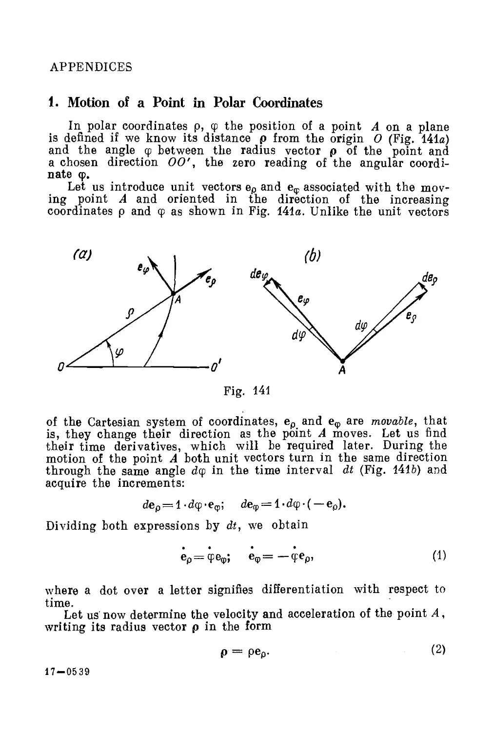
1. Motion of a Point in Polar Coordinates 257
2. On Keplerian Motion 258
3. Demonstration of Steiner's Theorem 260
4. Greek Alphabet 262
5. Some Formulae of Algebra and Trigonometry . . . 262
6. Table of Derivatives and Integrals ... 263
7. Some Facts About Vectors 264
8. Units of Mechanical Quantities in the SI and CGS
Systems 266
9. Decimal Prefixes for the Names of Units 266
10. Some Extrasystem Units 267
11. Astronomic Quantities 267
12. Fundamental Constants 267
Index
269

PREFACE
The objective of the book is to draw the readers'
attention to the basic laws of mechanics, that is, to the laws of
motion and to the laws of conservation of energy,
momentum and angular momentum, as well as to show how these
laws are to be applied in solving various specific problems.
At the same time the author has excluded all things of
minor importance in order to concentrate on the questions
which are the hardest to comprehend.
The book consists of two parts: (1) classical mechanics
and (2) relativistic mechanics. In the first part the laws of
mechanics are treated in the Newtonian approximation, i.e.
when motion velocities are much less than the velocity of
light, while in the second part of the book velocities
comparable to that of light are considered.
Each chapter opens with a theoretical essay followed by
a number of the most instructive and interesting examples
and problems, with solutions provided. There are about
80 problems altogether; being closely associated with the
introductory text, they develop and supplement it and
therefore their examination is of equal importance.
A few corrections and refinements have been made in the
present edition to stress the physical essence of the
problems studied. This holds true primarily for Newton's second
law and the conservation laws. Some new examples and
problems have been provided.
The book is intended for first-year students of physics
but can also be useful to senior students and lecturers.
/. E, Irodov

NOTATION
Vectors are designated by roman bold-face type (e.g. r, F);
the same italicized letters (r, F) designate the norm of a
vector.
Mean values are indicated by crotchets ( ), e.g. (v),
(N).
The symbols A, d, 5 (when put in front of a quantity)
signify:
A, a finite increment of a quantity, i.e. a difference between
its final and initial values, e.g. Ar = r2— t1: AU = £/2 — Ui;
d, a differential (an infinitesimal increment), e.g. dr, dU;
5, an elementary value of a quantity, e.g. £>A is an
elementary work.
Unit vectors:
i, j, k are unit vectors of the Cartesian coordinates x, y, z;
eP, e^, ez are unit vectors of the cylindrical coordinates
p, cp, z;
n, t are unit vectors of a normal and a tangent to a path.
Reference frames are denoted by the italic letters K, K'
and C.
The C frame is a reference frame fixed to the centre of
inertia and translating relative to inertial frames. All
quantities in the C frame are marked with a tilde, e.g. p, E.
A, work,
c, velocity of light in vacuo,
E, total mechanical energy, the total energy,
E, electric field strength,
e, elementary electric charge,
F, force,
G, field strength,
g, free fall acceleration,
/, moment of inertia,
L, angular momentum with respect to a point,
Lz, angular momentum with respect to an axis,

10
Notation
I, arc coordinate, the arm of a vector,
M, moment of a force with respect to a point,
Mz, moment of a force with respect to an axis,
m, mass, relativistic mass, m0 rest mass,
N, power,
p, momentum,
q, electric charge,
r, radius vector,
s, path, interval,
t, time,
T, kinetic energy,
U, potential energy,
v, velocity of a point or a particle,
w, acceleration of a point or a particle,
P, angular acceleration,
p, velocity expressed in units of the velocity of light,
Y, gravitational constant, the Lorentz factor,
e, energy of a photon,
x, elastic (quasi-elastic) force constant,
[x, reduced mass,
p, curvature radius, radius vector of the shortest distance
to an axis, density,
cp, azimuth angle, potential,
to, angular velocity,
Q, solid angle.

INTRODUCTION
Mechanics is a branch of physics treating the simplest
form of motion of matter, mechanical motion, that is, the
motion of bodies in space and time. The occurrence of
mechanical phenomena in space and time can be seen in any
mechanical law involving, explicitly or implicitly, space-time
relations, i.e. distances and time intervals.
The position of a body in space can be determined only
with respect to other bodies. The same is true for the motion
of a body, i.e. for the change in its position over time. The
body (or the system of mutually immobile bodies) serving
to define the position of a particular body is identified as
the reference body.
For practical purposes, a certain coordinate system, e.g.
the Cartesian system, is fixed to the reference body
whenever motion is described. The coordinates of a body permit
its position in space to be established. Next, motion occurs
not only in space but also in time, and therefore the
description of the motion presupposes time measurements as well.
This is done by means of a clock of one or another type.
A reference body to which coordinates are fixed and
mutually synchronized clocks form the so-called reference frame.
The notion of a reference frame is fundamental in physics.
A space-time description of motion based on distances and
time intervals is possible only when a definite reference
frame is chosen.
Space and time by themselves are also physical objects,
just as any others, even though immeasurably more impor-

12
Introduction
tant. The properties of space and time can be investigated
by observing bodies moving in them. By studying the
character of the motion of bodies we determine the properties
of space and time.
Experience shows that as long as the velocities of bodies
are small in comparison with the velocity of light, linear
scales and time intervals remain invariable on transition
from one reference frame to another, i.e. they do not depend
on the choice of a reference frame. This fact finds
expression in the Newtonian concepts of absolute space and time.
Mechanics treating the motion of bodies in such cases is
referred to as classical.
When we pass to velocities comparable to that of light, it
becomes obvious that the character of the motion of bodies
changes radically. Linear scales and time intervals become
dependent on the choice of a reference frame and are
different in different reference frames. Mechanics based on these
concepts is referred to as relativistic. Naturally, relativistic
mechanics is more general and becomes classical in the case
of small velocities.
The actual motion characteristics of bodies are so complex
that to investigate them we have to neglect all insignificant
factors, otherwise the problem would get so complicated as
to render it practically insoluble. For this purpose notions
(or abstractions) are employed whose application depends
on the specific nature of the problem in question and on the
accuracy of the result that we expect to get. A particularly
important role is played by the notions of a mass point and
of a perfectly rigid body.
A mass point, or, briefly, a particle, is a body whose
dimensions can be neglected under the conditions of a given
problem. It is clear that the same body can be treated*as a mass
point in some cases and as an extended'object in"others.
A perfectly rigid body, or, briefly, a solid, is a system of
mass points separated by distances which do not vary
during its motion. A real body can be treated as a perfectly
rigid^one provided its deformations are negligible under
the conditions of the problem considered.
Mechanics tackles two fundamental problems:
1. The investigation of various motions and the
generalization of the results obtained in the form of laws of mo-

introduction
13
tion, i.e. laws that can be employed in predicting the
character of motion in each specific case.
2. The search for general properties that are typical of
any system regardless of the specific interactions between
the bodies of the system.
The solution of the first problem ended up with the so-
called dynamic laws established by Newton and Einstein,
while the solution of the second problem resulted in the
discovery of the laws of conservation for such fundamental
quantities as energy, momentum and angular momentum.
The dynamic laws and the laws of conservation of energy,
momentum and angular momentum represent the basic laws
of mechanics. The investigation of these laws constitutes
the subject matter of this book.

PART ONE
CLASSICAL MECHANICS
CHAPTER 1
ESSENTIALS OF KINEMATICS
Kinematics is the subdivision of mechanics treating ways
of describing motion regardless of the causes inducing it.
Three problems will be considered in this chapter: kinematics
of a point, kinematics of a solid, and the transformation of
velocity and acceleration on transition from one reference
frame to another.
§ 1.1. Kinematics of a Point
There are three ways to describe the motion of a point:
the first employs vectors, the second coordinates, and the
third is referred to as natural. Let us examine them in
order.
The vector method. With this method the location of a
given point A is defined by a radius vector r drawn from
a certain stationary point 0 of a chosen reference frame to
that point A. The motion of the point A makes its radius
vector vary in the general case both in magnitude and in
direction, i.e. the radius vector r depends on time t. The locus
of the end points of the radius vector r is referred to as the
path of the point A.
Let us introduce the notion of the velocity of a point.
Suppose the point A travels from point 1 to point 2 in the
time interval At (Fig. 1). It is seen from the figure that
the displacement vector Ar of the point A represents the
increment of the radius vector r in the time At: Ar = r2 —

Essentials of kinematics
15
— r1. The ratio Ar/Att is called the mean velocity vector (v)
during the time interval At. The direction of the vector
(v) coincides with that of Ar. Now let us define the
velocity vector v of the point at a given moment of time as the
limit of the ratio Ar/At as At ->0, i.e.
&t-+o ai ai
This means that the velocity vector v of the point at a given
moment of time is equal to the derivative of the radius
vector r with respect to time, and its direction, like that of
Fig. 1
the vector dr, along the tangent to the path at a given point
coincides with the direction of motion of the point A. The
modulus of the vector v is equal to*
v = | v | = | dr/dt |.
The motion of a point is also characterized by acceleration.
The acceleration vector w defines the rate at which the
velocity vector of a point varies with time:
w = dv/dt, (1.2)
i.e. it is equal to the derivative of the velocity vector with
respect to time. The direction of the vector w coincides with
the direction of the vector d\ which is the increment of the
vector v during the time interval dt. The modulus of the
* Note that in the general case | dr | =£ dr, where r is the modulus
of the radius vector r, and v =£ dr/dt. For example, when r changes
only in direction, that is the point moves in a circle, then r = const,
dr = 0, but | dr \ =£ 0.

16
Classical Mechanics
vector w is defined in much the same way as that of the
vector v.
Example. The radius vector of a point depends on time t as
r = a* + b«a/2,
where a and b are constant vectors. Let us find the velocity v of the
point and its acceleration w:
v = dr/dt = a + bt, w = dsldt = b = const.
The modulus of the velocity vector
v= ]/"v»= /a2 + 2ab« + 62«a.
Thus, knowing the function r (t), one can find the velocity
v of a point and its acceleration w at any moment of time.
Here the reverse problem arises: can we find v (t) and
r (t) if the time dependence of the acceleration w (t) is
known?
It turns out that the dependence w(t) is not sufficient to
get a single-valued solution of this problem; one needs also
to know the so-called initial conditions, namely, the
velocity v0 of the point and its radius vector r0 at a certain
initial moment t = 0. To make sure, let us examine the
simple case when the acceleration of the point remains
constant in the course of time.
First, let us determine the velocity v (t) of the point. In
accordance with Eq. (1.2) the elementary velocity
increment during the time interval dt is equal to dv = wdt.
Integrating this relation with respect to time between
t = 0 and t, we obtain the velocity vector increment
during this interval:
t
Av= \ -wdt^wt.
o
However, the quantity Av is not the required velocity v.
To find v, we must know the velocity v0 at the initial
moment of time. Then v = v0 + Av, or
v = v0 + wt.
The radius vector r (t) of the point is found in a similar
manner. According to Eq. (1.1) the elementary increment of
the radius vector during the time interval dt is dv = vdt.

Essentials of Kinematics
17
Integrating this relation with respect to the function v (t),
we obtain the increment of the radius vector during the
interval from t = 0 to t:
Ar = j v{t)dt = v0t + wt2/2.
To find the radius vector r (t), the location r0 of the point
at the initial moment of time must be known. Then r =
= r0 + Ar, or
r = r0 + v0i + wi2/2.
Let us consider, for example, the motion of a stone thrown
with the initial velocity v0 at an angle to the horizontal.
Assuming the stone to move with the constant acceleration
w = g, its location relative
to the point r0 = 0 from which
the stone was thrown is ^
defined by the radius vector
i.e. in this case r represents
the sum of two vectors as ^/;/////m////M///////////////mm
shown in Fig. 2.
Thus, the ^complete solu- Fig. 2
tion of the problem of a moving
point, that is, the determination of its vcleoity v and its
location r as functions of time, requires knowing not only
the dependence w (t), but also the initial conditions, i.e. the
velocity v0 and the location r0 of the point at the initial
moment of time.
The method of coordinates. In this method a certain
coordinate system (Cartesian, oblique-angled or curvilinear)
is fixed to a chosen reference body. The choice of a coordinate
system is stipulated by various considerations: the
character or] the symmetry of the problem, the formulation of
the problem, the quest for a simpler solution. We shall
confine ourselves here* to Cartesian coordinates x, y, z.
* The motion of a point in polar coordinates is considered
in Appendix 1.
2-0539

18
Classical Mechanics
Let us write the projections of the radius vector r (t)
on the axes x, y, z to characterize the position of the point
in question relative to the origin 0 at the moment t:
x = x (0; y = y (t); z = z (0-
Knowing the dependence of these coordinates on time, that
is, the law of motion of the point, we can find the position
of the point at any moment of time, as well as its velocity
and acceleration. Indeed, from Eqs. (1.1) and (1.2) we can
easily obtain the formulae defining the projections of the
velocity vector and the acceleration vector on the x axis:
vx = dxldt, (1.3)
where dx is the projection of the displacement vector dr on
the x axis;
wx = dvxfdt^=d2x/dt2, (1.4)
where dvx is the projection of the velocity increment vector
d\ on the x axis. Similar relations are obtained for y and z
projections of the respective vectors. It is seen from these
formulae that the velocity and acceleration vector
projections are equal respectively to the first and second time
derivatives of the coordinates.
Thus, the functions x (t), y (t), z (t), in essence,
completely define the motion of a point. Knowing them, one can
find not only the position of a point, but also the projections
of its velocity and acceleration, and, consequently, the
magnitude and direction of vectors v and w at any moment
of time. For example, the modulus of the velocity vector
v = Vvx + vl + vj;
the direction of the vector v is defined by the directional
cosines as follows:
cos a = vjv; cos P = vjv; cos v = vjv,
where a, p, v are the angles formed by the vector v with the
axes x, y, z respectively. Similar formulae define the
magnitude and direction of the acceleration vector.
. Besides, some more questions can be solved: one can
determine the path of a point, the dependence of the distance

Essentials of Kinematics
19
covered on time, the dependence of the velocity on the
position of a point etc.
The reverse problem, that is, the determination of the
velocity and the law of motion of a point from a given
acceleration, is solved, as in the vector method, by integration
(in this case, integration of acceleration projections with
respect to time); this problem also has a single-valued
solution provided that in addition to the acceleration the initial
conditions are also available, i.e. velocity projections and
the coordinates of a point at the initial moment.
The "natural" method. This method is employed when
the path of a point is known in advance. The location of
a point A is defined by the arc
coordinate Z, that is, the distance from the
chosen origin 0 measured along the
path (Fig. 3). In so doing, the
positive] direction of the coordinate
Z is adopted at will (e.g. as shown
by an arrow in the figure).
The motion of a point is
determined provided we know its path,
the origin 0, the positive direction of the arc coordinate Zand
the law of motion of the point, i.e. the function I (t).
Velocity of a point. Let us introduce the unit vector x
fixed to the moving point A and oriented along a tangent to
the path in the direction of growing values of the arc
coordinate I (Fig. 3). It is obvious that x is a variable vector since
it depends on I. The velocity vector v of the point A is
oriented along a tangent to the path and therefore can be
represented as follows:
Fig. 3
■■VXT,
(1.5)
where vx = dlldt is the projection of the vector v on the
direction of the vector t, with vx being an algebraic
quantity. Besides, it is obvious that
|»x| = |v|=l7.
Acceleration of a point. Let us differentiate Eq. (1.5)
with respect to time:
d\ dvx _ . dx ,. „.
Vf=-d7=-drx+v*nr- (!-6)
2*

20
Classical Mechanics
Then transform the last term of this expression:
dx dx dl 2 dx n dx
~dT==Vx1T~dT = Vx~dT = v ~dT'•
v*
(1.7)
Let us determine the increment of the vector x in the
interval dl (Fig. 4). It can be strictly shown that when point 2
approaches point 1, the segment of the path between them
tends to turn into an arc of a circle with centre at some
Fig. 4
point 0. The point 0 is referred to as the centre of curvature
of the path at the given point, and the radius p of the
corresponding circle as the radius of curvature of the path at
the same point.
It is seen from Fig. 4 that the angle 5a = | dl |/p =
= | dr |/1, whence
| dx/dl | = 1/p;
at the same time, if dl -v 0, then dr J_ x. Introducing a unit
vector n of the normal to the path at point 1 directed toward
the centre of curvature, we write the last equality in a
vector form:
dx/dl = n/p. (1.8)
Now let us substitute Eq. (1.8) into Eq. (1.7) and then
the expression obtained into Eq. (1.6). Finally we get
w =
dvr , va
irx+Tn-
(1.9)

Essentials of Kinematics
21
Here the first term is called the tangential acceleration wx
and the second one, the normal (centripetal) acceleration wn:
wx = (dvx/dt)x; w„ = (i;2/p)n. (1.10)
Thus, the total acceleration w of a point can be
represented as the sum of the
tangential wT and normal wn
accelerations.
The magnitude of the total
acceleration of a point is
w = Yw% + wl =
= V(dv/dt)2 + (v2/p)2.
X
/
U/f
Y«i\
itfi" \uf
if
?
I
0
Fig. 5
Example. Points travels along
an arc of a circle of radius p
(Fig. 5). Its velocity depends on
the arc coordinate I as v = a Y~l
where a is a constant. Let us calculate the angle a between the
vectors of the total acceleration and of the velocity of the point as a
function of the coordinate I.
It is seen from Fig. 5 that the angle a can be found by means of
the formula tan a = wn/wx. Let us find wn and u>T:
v2 aH dvx dvx dl a r-z a2
p p dt dl dt 2 / I 2
Whence tan a = 2Z/p.
§ 1.2. Kinematics of a Solid
Being important by itself, the theory of motion of a solid
is also essential in another respect. It is well known that
a reference frame used for describing various kinds of
motion in space and time can be fixed to a solid. Therefore,
the study of motion of solids is actually equivalent to the
study of motion of corresponding reference frames. The
results to be obtained in this section will be repeatedly used
hereafter.
Five kinds of motion of a solid are identified: (1)
translation, (2) rotation about a stationary axis, (3) plane motion,
(4) motion about a stationary point, and (5) free motion.
The first two kinds of motion, that is, translation and
rotation about a stationary axis, are the basic kinds of motion

22
Classical Mechanics
of a solid. All the other kinds of motion of a solid prove to be
reducible to one of the basic motions or to their
combination. This will be shown by the example of plane motion.
In this section we shall deal with the first three kinds of
motion and with the problem of summing angular
velocities.
Translation. In this kind of motion of a solid any straight
line fixed to it remains parallel to its initial orientation
all the time. Examples: a car
travelling along a straight
section of a road, a Ferris wheel
cage, etc.
When moving translationa-
ry, all points of a solid
traverse equal distances in the
same time interval. Therefore
velocities, as well as
accelerations, are of the same value
at all points of the body at the
given moment of time. This
fact allows the study of
translation of a solid to be reduced
to the study of motion of an
individual point belonging to
that solid, i.e. to the problem of kinematics of a point.
Thus, the translation of a solid can be comprehensively
described provided the dependence of the radius vector on
time r (t) for any point of that body is available as well as
the position of that body at the initial moment.
Rotation about a stationary axis. Suppose a solid, while
rotating about an axis 00' which is stationary in a given
reference frame, accomplishes an infinitesimal rotation
during the time interval dt. We shall describe [the
corresponding rotation angle by the vector dtp whose modulus is
equal to the rotation angle and whose direction coincides
with the axis 00', with the rotation direction obeying the
right-hand screw rule with respect to the direction of the
vector dtp (Fig. 6).
Now let us find the elementary displacement of any point
A of the solid resulting from such a rotation. The location
of the point A is specified by the radius vector r drawn from
Fig. 6

Essentials of Kinematics
23
a certain point 0 on the rotation axis. Then the linear
displacement of the end point of the radius vector r is
associated with the rotation angle dq> by the relation (Fig. 6)
| dr | = r sin 0 dcp,
or in a vector form
dT = [d<p, r]. (1.11)
Note that this equality holds only for an infinitesimal
rotation dq>. In other words, only infinitesimal rotations
can be treated as vectors.*
Moreover, the vector introduced (d<p) can be shown to
satisfy the basic property of vectors, that is, vector addition.
Indeed, imagined solid performing two elementary
rotations, d^ and d<p2, about different axes crossing at a
stationary point 0. Then the- resultant displacement dr of
an arbitrary point A of the body, whose radius vector with
respect to the point 0 is equal to r, can be represented as
follows:
dr = rfrx + dr2 = [d<Pi, r] + [d<p2, r] = [dq>, r ,
where
d<p = d<pxF+ d<p2, (1.12)
i.e. the two given rotations, dcpx and d<p2, are equivalent to
one rotation through the angle d<p = d<px + d<p2 about the
axis coinciding with the vector d<p and passing through
the point 0.
Note that in treating such quantities as radius vector r,
velocity v, acceleration w we did not hesitate over the choree
of their direction: it naturally followed from the properties
of the quantities themselves. Such vectors are referred to
as polar. As distinct from them, such vectors as dq> whose
* In the case of a finite rotation through the anglejAcp the linear
displacement of the point A can be found from Fig. 6:
I Ar | = rsin9-2sin(Acp/2).
Whence it is immediately seen that the displacement Ar cannot
be represented as a vector cross product of A(p and r. It is only
possible in the case of an infinitesimal rotation d<p when the radius
vector r can be regarded invariable.

24
Classical Mechanics
direction is specified by the rotation direction are called
axial. „
Now let us introduce the vectors of angular velocity arid
angular acceleration. The angular velocity vector & is
defined as
a> = dufldt, (1.13)
where dt is the time interval during which a body performs
the rotation d((. The vector to is axial and its direction
coincides with that of the vector d((.
The time variation of the vector u\ is defined by the
angular acceleration vector p.*
P = datldt. (1.14)
The direction of the vector p coincides with the direction of
do, the increment of the vector o>. Both vectors, p and to,
are axial.
The representation of angular velocity/and angular
acceleration in a vector1 form proves to be very beneficial,
especially in the study of more complicated kinds
H of motion'of a solid. In many cases this makes
a problem more explicit, drastically simplifies
the analysis of motion and the corresponding
r ~**\ calculations.
^-J^^V Let us write the expressions for angular
velocity and angular acceleration via projec-
Fig. 7 tions on the rotation axis z whose positive
direction is associated with the positive
direction of the coordinate cp, the rotation angle, in accordance
with the right-hand screw rule (Fig. 7). Then the projections
coz and |JZ of the vectors o> and P on the z axis are defined by
the following formulae:
coz = dq>/dt, (1.15)
pz = dajdt. (1.16)
Here coz and |3Z are algebraic quantities. Their sign specifies
the direction of the corresponding vector. For example, if
co2 > 0, then the direction'of the vector at coincides with
the positive direction of the z axis; and if to z < 0, then the
vector to has the opposite direction. The same is true for
angular acceleration.
M

Essentials of Kinematics
25
Thus, knowing the function cp (t), the law of rotation of
a body, we can find the angular velocity and angular
acceleration at each moment of time by means of Eqs. (1.15) and
(1.16) On the other hand, knowing the time dependence of
angular acceleration and the initial conditions, i.e. the
angular velocity co0 and the angle cp0 at the initial moment of
time, we can find cor(0 and cp (t).
Example. A solid rotates about a stationary axis in accordance
with the law <p = at — bt2/2 where a and b are positive constants.
Let us determine the motion characteristics of this body.
In accordance with Eqs. (1.15) and (1.16)
coz = a — bt; Pz = —b = const.
Whence it is seen that the body performs a uniformly decelerated
rotation (Pz < 0), comes to a standstill at the moment t0 = alb
and then reverses its rotation direction (due to ©^changing its sign
to the opposite).
Note that the solution of'all problems on rotation of a solid
about a stationary axis is similar in form to that oFprob-
lems on rectilinear motion of a
point. It is sufficient to replace the
linear quantities x, vx and wx by the
corresponding angular quantities cp,
coz and pz in order to obtain all
characteristics and relationships for
the case of a rotating body.
Relationship between linear and
angular quantities. Let us find the
velocity v of an arbitrary point A of
a solid rotating about a stationary
axis 00' at an angular velocity a>.
Let the location of the point A
relative to some point Oof the
rotation axis be defined by the radius
vector r (Fig. 8). Dividing both
sides of Eq.r(l.H) by the
corresponding] time interval! dt and taking
dtldt = v and d<p/dt = to, we obtain
into account that
:[cor],
(1-17)
i.e. the velocity v of any point A of a solid rotating about
some axis at an angular velocity to is equal to the cross

26
Classical Mechanics
product ofj© and the'radius vector r of the points relative to
an arbitrary point 0 of the rotation axis (Fig. 8).
The modulus of the vector (1.17) is v = cor sin 0, or
V = dtp,
where p is the radius of the circle which the point A
circumscribes. Having differentiated Eq. (1.17) with respect to
Fig. 9
Fig. 10
time, we find the acceleration w of the point A:
w = [d&ldt, r] + [©, dr/dt]
or
w = [Pr] + [o[©r]].
(1.18)
In this case (when the rotation axis is stationary) 0 || a,
and therefore the vector [0r] represents the'tangential
acceleration wT. The vector [© [tor]] is the normal acceleration
wn. The moduli of these vectors are
|Wt|=PpJ B?B = ©»p,
whence the modulus of the total acceleration w is equal to
w-
G>»
Plane motion of a solid. In this kind of motion each point
of a solid moves in a plane which is parallel to a certain
stationary (in a given reference frame) plane. In this case
the plane figure d> formed as a result of cutting the solid by
that stationary plane P (Fig. 9) remains in that plane all

Essentials of Kinematics
27
the time during the motion. Example: a cylinder rolling
along a plane without slipping (in a similar case a cone
performs a much more complicated motion).
It is easy to infer that the position of a solid in plane
motion is unambiguously determined by the position of the
plane figure O within the stationary plane P. The study of
the plane motion of a solid thus reduces to the study of
motion of a plane figure within its plane.
Let the plane figure O move within its plane P, which
is stationary in the K reference frame (Fig. 10). The
position of the figure O in the plane can be defined by
specifying the radius vector r0 of an arbitrary point 0' of the figure
and the angle <p between the radius vector r' rigidly fixed
to the figure and a certain selected direction in the K
reference frame. The plane motion of the solid is then described
by the two equations
r0 = To (*); V = V (*)•
It is clear that if the radius vector r' of the point A
(Fig. 10) turns through the angle dq> during the time
interval dt, then any segment fixed to the figure will turn through
the same angle. In other words, the rotation of the figure
through the angle dq> does not depend on the choice of the
point 0'. This means that the angular velocity o> of the
figure does not depend on the choice of the point 0', and
we have the right to call o> the angular velocity of the solid
per se.
Now let us find the velocity v of an arbitrary point A
of a solid in plane motion. Let us introduce the auxiliary
reference frame K' which is rigidly fixed to the point 0'
of the solid and translates relative to the K frame (Fig. 10).
Then the elementary displacement dr of the point A in the K
frame can be written in the following form:
dr = dr0-{-dr',
where dr0 is the displacement of the K' frame, or the point
0', and dr' is the displacement of the point A relative to
the K' frame. The translation dr' is caused by the rotation
of the solid about the axis which is at rest in the K' frame
and passes through the point 0'\ according to Eq. (1.11)
dr' = [dq>, r']. Substituting this relation into the previous

28
Classical Mechanics
one and dividing both sides of the expression obtained by
dt, we get
v = v0 + [o)r'], (1.19)
i.e. the velocity of any point A of a solid in plane motion*
comprises the velocity v0 of an arbitrary point 0' of that
solid and the velocity v' = [ow'] caused by rotation of the
solid about the axis passing through the point 0'. Once
again we would like to stress that v' is the velocity of the
point A relative to the translating reference frame K' which
is rigidly fixed to the point 0'.
In other words, plane motion
of a solid can 'be represented as
a combination of two basic kinds
of motion: translation (together
with an arbitrary point 0' of the
solid) and rotation (around an
axis jpassing through the point
0').
Now we shall demonstrate
that plane motion can be
reduced to a purely rotational
motion. Indeed, in plane motion
the velocity v0 of the arbitrary point 0' rof the solid
is normal to the vector © which means that we can always
find a certain point M which is rigidly fixed to the solid**
and whose velocity v = 0 at a given moment. The location
of the point M, i.e. its radius vector r'M relative to the
point 0' (Fig. 11), can be found from the condition 0 =
= v0 + [fitr^f]. The vector r'M is perpendicular to © and
v0, its direction corresponding to the vector cross product
v0 = — [fitr^f] and its magnitude r'M = v0/a.
The point M defines the position of another important
axis (coinciding with the direction of the vector ©). At
a given moment of time the motion of a solid represents
a pure rotation about this axis. Such an axis is referred to as
an instantaneous rotation axis.
Fig. 11
* Note that Eq. (1.19) also holds for any complex motion of
a solid.
** The point M may turn out to be outside the solid.

Essentials of Kinematics
29
Generally speaking, the position of the instantaneous axis
varies with time. For example, in the case of a cylinder
rolling over a plane surface the instantaneous axis coincides at
any moment with the line of contact between the cylinder
and the plane.
Angular velocity summation. Let us analyse the motion
of a solid rotating simultaneously about two intersecting
axes. We shall set into rotation a
certain solid at the angular velocity ti>'
about the axis OA (Fig. 12), and then
we shall set this axis into rotation
with the angular velocity ci)0 about
the axis OB which is stationary in the
K reference frame. Let us find the
resultant motion in the K frame.
We shall introduce an auxiliary
reference frame K' fixed rigidly to the
axes OA and OB. It is clear that this
frame rotates with the angular velocity ci)0 while the
solid rotates relative to this frame with the angular
velocity o'.
During the time interval dt the solid will turn through
an angle dq>' about the axis OA in the K' frame and
simultaneously through d<p0 about the axis OB together with the
K' frame. The cumulative rotation follows from Eq. (1.12):
dip = d<jp0 -f- d<p'. Dividing both sides of this equality by
dt, we obtain
a> = a)0 + a>'. (1.20)
Thus, the resultant motion of the solid in the K frame is
a pure rotation with the angular velocity ti> about an axis
coinciding at each moment with the vector ti> and passing
through the point 0 (Fig. 12). This axis is displaced relative
to the K frame: it rotates together with the OA axis about
the axis OB at the angular velocity ti>0.
It is not difficult to infer that even when the angular
velocities w' and ci)0 do not change their magnitudes, the
body in the K frame will possess the angular acceleration
P directed, according to Eq. (1.14), beyond the plane
(Fig. 12). The angular acceleration of a solid is analysed in
detail in Problem 1.10.
Fig. 12

30
Classical Mechanics
And here is one more remark. Since the angular velocity
vector a satisfies the basic property of vectors, vector
summation, a can be expanded into a sum of vector components
projected on definite directions, i.e. (a = ^ ■}- <o2 + ...,
where all vectors belong to the same reference frame. This
convenient and beneficial routine is frequently employed
to analyse complex motions of a solid.
§ 1.3. Transformation of Velocity and Acceleration
on Transition to Another Reference Frame
Prior to entering upon the study of this problem we should
recall that within the bounds of classical mechanics the
length of scales and time are considered absolute. A scale
is the same in different reference frames, i.e. it does not
change during motion. This is also true of time running
uniformly throughout all frames.
Formulation of the problem. There are two arbitrary
reference frames K and K' moving relative to each other
in a definite manner. The velocity v and the acceleration w
of a point A in the K frame are
known. What are the
corresponding values v' and w' of this
A point in the K' frame?
We shall examine the three
most significant cases of relative
motion of two reference frames
in succession.
1. The K' frame translates
— relative to the K frame.
Suppose the origin of the
Fig. 13 K' frame is determined by the
radius vector r0 in the K frame,
and its velocity and
acceleration by the vectors v0 and w0. If the location of the point
A in the K frame is determined by the radius vector r and
in the K' frame by the radius vector r', then apparently
r = r0 + r' (Fig. 13). Next, let during the time interval dt
the point A accomplish the elementary displacement dt
in the K frame. This displacement is made up of the
displacement dr0 (together with the K' frame) and the displace-

Essentials of Kinematics
31
ment dr' relative to the K' frame: dr = dr0 + dr'. Dividing
this expression by dt, we obtain the following formula for
the velocity transformation:
v = v0 + v'.
(1.21)
Differentiating Eq. (1.21) with respect to time, we
immediately get the acceleration transformation formula:
w = w0 + w'.
(1.22)
Whence it is seen, specifically, that if w0 = 0 and w = w',
i.e. when the K' frame moves without acceleration, the
acceleration of the point A relative to the K frame will be
the same in both frames.
2. The K' frame rotates at the constant
angular velocity a about an axis] which is
stationary in the K frame.
Let us assume the origins of the reference frames K and K'
to be located at an arbitrary point 0 on the rotation axis
Fig. 14
(Fig. 14a). Then the radius vector of the point A will be
the same in both reference frames: r = r'.
If the point A is at rest in the K' frame, this means that
its displacement dr in the K frame during the time interval
dt is caused only by the rotation of the radius vector r
through the angle dq> (together with the K' frame) and in

32
Classical Mechanics
accordance with Eq. (1.11) is equalj.;to the vector cross
product [dq>, r].
If the point A moves at the velocity v' relative to the K'
frame, it will cover an additional distance v' dt during the
time interval dt (Fig. 14a), so that
dx = v'dt + [dtp, r]. (1.23)
Dividing this expression by dt, we obtain the velocity
transformation formula as follows:
v = v' + [<ar],
(1.24)
where v and v' are the velocity values which characterize
the motion of the point A in the K and K' frames
respectively.
Now let us pass over to acceleration. In accordance with
Eq. (1.24) the increment d\ of the vector v during the time
interval dt in the K frame must comprise the sum of the
increments of the vectors v' and [cor], i.e.
dv = dv' + [w, dt]. (1.25)
Let us find dw'. If the point A moves in the K' frame with
a constant velocity (v' = const), the increment of this
vector in the K frame is caused only by this vector turning
through the angle dq> (together with the K' frame) and is
equal, as in the case of r, to thed"vector cross product [dtp, v'].
To make sure of this, let us position the beginning of the
vector v' on the rotation axis (Fig. 146). But if the point A
moves with the acceleration w' in the K' frame, the vector
v' will get an additional increment -w'dt during the time
interval dt, and consequently
dv' = w'dt + [dip, v']. (1.26)
Now let us substitute Eqs. (1.26) and (1.23) into Eq. (1.25)
and then divide the expression obtained by dt. Thus we
shall get the acceleration transformation formula:
w = w' + 2[<bv'] + [©[jar]], (1.27)
where w and w' are the acceleration values of the point A
observed in the K and K' frames. The second term on the
right-hand side of this formula is referred to as the Coriolis

Essentials of Kinematics
33
acceleration wCor and the third term is the axipetal
acceleration wap directed toward the axis*
wCor = 2[fi>v'], wop = [©[««]]. (1.28)
Thus, the acceleration w of the point relative to the K
frame is equal to the sum of three accelerations: the
acceleration w' relative.to the K' frame, the Coriolis acceleration
wCor and the axipetal acceleration wap.
The axipetal acceleration can be represented in the form
wap = —co2p where p is the radius vector which is normal
to the rotation axis and describes the position of the point A
relative to this axis. Then Eq. (1.27) can be written as
follows:
w = w' + 2[(ov'} —w2p. (1.29)
3. The K' frame rotates with the constant
angular velocity © about the axis translating
with the velocity v0 and acceleration w0
relative to the K frame.
This case combines the two previous ones. Let us
introduce an auxiliary S frame which is rigidly fixed to the
rotation axis of the K' frame and translates in the K frame.
Suppose v and vs are the velocity values of the point A in
the K and S frames; then in accordance with Eq. (1.21)
v = v0 + vs. Replacing vs in accordance with Eq. (1.24)
by vs = v' + [or], where r is the radius vector of the
point A relative to the arbitrary point on the rotation axis
of the R' frame, we obtain the following velocity
transformation formula:
v = v'+v0 + [«or].
(1.30)
* This axipetal acceleration should not be confused with
conventional (centripetal) acceleration.
3-0539

34
Classical Mechanics
In a similar fashion, using Eqs. (1.22) and (1.29), we obtain
the acceleration transformation formula*:
w = w' + w0 + 2[(ov'] —co2p. (1.31)
Recall that in the last two formulae v, v' and w, w' are the
velocities and accelerations of the point A in the K and K'
frames respectively, v0 and w0 are the velocity and
acceleration of the rotation axis of the K' frame in the K frame, r
is the radius vector of the point A relative to an arbitrary
point on the rotation axis of the K' frame, and p is the
radius vector perpendicular to the rotation axis and
describing the location of the point A relative to this axis.
In conclusion, let us examine the following example.
Example. A disc*rotates with a^constant'angular^ velocity © about
an axis fixed to "the table. Point A moves along the disc with
the constant velocity v relative to the table. Find the velocity v'
and acceleration w' of the point A relative to the disc at the moment
when the radius vector describing its position relative to the
rotation axis is equal to p.
In accordance with Eq. (1.24) the velocity v' of the point A is
equal to
v' = v — [©p].
The acceleration w' can be found from Eq. (1.29), taking into account
that in this case w = 0 since v = const. Then w' = —2 [cov'] +
+ ©2p. Substituting the expression for v' into this formula we obtain
w' = 2 [va>] — co2p.
Problems to Chapter 1
• 1.1. The radius vector describing the position of the particle A
relative to the stationary point 0 changes with time according to the
following law:
r = a sin o)J + b cos ait,
where a and b are constant vectors, with a j_b; o) is a positive constant.
Find the acceleration w of the particle and the equation of its path
y (x), assuming the x and y axes to coincide with the directions of
the vectors a and b respectively and to have the origin at the point 0.
* Note that in the_most general case when o> =^ const, the right-
hand side of Eq. (1.31) will feature one more term, namely [(Jrj,
where p" is the angular acceleration of the K' frame, r is the radius
vector describing the position of the point located on the rotation
axis and taken for the origin in the K frame.

Essentials of Kinematics
35
Solution. Differentiating r with respect to time twice, we obtain
w = —to2 (a sin to* + b cos (ot) = — co2r,
i.e. the vector w is always oriented toward the point O while its
magnitude is proportional to the distance between the particle and the
point O.
Now let us determine the trajectory equation. Projecting r on the
x and y axes, we obtain
x = a sin <s>t, y = b cos at.
Eliminating at from these two equations, we get
xVa2 + i/2/62 = 1.
This is the equation of an ellipse, and a and b are its semi-axes (see
Fig. 15; the arrow shows the direction of motion of the particle A).
Fig. 15 " ' Fig. 16
#1.2. J Displacement and| distance. At the moment t= 0 a,
particle is set in motion at the velocity v0 whereupon its velocity begins
changing with time in accordance with the law
v = v„ (1 - tlx),
where x is a positive constant. Find:
(1) the displacement vector Ar of the particle, and
(2) the distance s covered by it in the first t seconds of motion.
Solution. 1. In accordance with Eq. (1.1) dv = v dt = v0 (1 —
— tlx) dt. Integrating this equation with respect to time between O
and t, we obtain
Ar = \0t (1 — t/2x).
2. The distance s covered by the particle in the time t is
determined by
t
s= \ v dt,
0
3*

36
Classical Mechanics
where v is the modulus of the vector v. In this case
01 \ v0(t/x — 1), if <> 1.
From this it follows that if t > t^the integral for calculating the
distance should be subdivided into two parts: between 0 and x and
between x and t. Integrating in the two cases (t < x and t > x),
we obtain
_ f v0t(l — t/2x), if <<x.
s~\ i;0T[l + (l-t/i)2]/2, if <>x.
Fig. 16 illustrates the plots v (t) and s (t). The dotted lines show
the time dependences of the projections vx and Ax of the vectors v
and Ar on the x axis oriented along the vector v0.
• 1.3. A street car moves rectilinearly from station As to the next
stop B with an acceleration varying according to the law w = a — bx
where a and b are positive constants and x is its distance from
station A. Find the distance between these stations and the maximum
velocity of the street car.
Solution. First we shall find how the velocity depends on x. During
the time interval dt the velocity increment dv = w dt. Making use
of the equation dt = dx/v, we reduce the last expression to the form
which is convenient to integrate:
v dv = (a — bx) dx.
Integrating this equation (the left-hand side between 0 and v and
the right-hand side between 0 and x), we get
v2/2 = ax — bx2/2 or v = yr(2a — bx) x.
From this equation it can be immediately seen that the distance
between the stations, that is, the value x0 corresponding to v = 0
is equal to x0 = 2a/b. The maximum velocity can be found from the
condition dv/dx = 0, or, simply, from the condition for the maximum
value of the radicand. The value xm corresponding to vmax is equal
to xm = alb and vmax = al~\/b.
• 1.4. A particle moves in the x, y plane from the point x = y = 0
with the velocity v = a\ + bxj, where a and b are constants and i
and j are the unit vectors of the x and y axes. Find the equation of
its path y (x).
Solution. Let us write the increments of the x and y coordinates
of the particle in the time interval dt: dy = vy dt, dx = vx dt, where
Vy — bx, vx= a. Taking their ratio, we get
dy = (b/a) x dx.

Essentials of Kinematics
37
Integrating this expression, we obtain the following equation:
x
2/= \ (bid) x dx = (b/2a) x2,
0
i.e. the path of the point is a parabola.
• 1.5. The motion law for the point A of the rim of a wheel rolling
uniformly along a horizontal path (the x axis) has the form
x = a (a>t — sin <£>t); y = a (1 — cos co*),
where a and co are positive constants. Find the velocity v of the point
A, the distance s which it traverses between two successive contacts
with the roadbed, as well as the magnitude and the direction of the
acceleration w of the point A.
Solution. The velocity v of the point A and the distance s it covers
are determined by the formulae
v = yv2-\-v2 = a<£> Y2 (1 —cos cfl«) = 2aco sin (at/2),
s= \ v(t)dt = ia [1 — cos(co«1/2)],
j
0
where ix is the time interval between two successive contacts. From
y (t) we find that y (tj) =0 at a^ = 2n. Therefore, s = 8a.
The acceleration of the point A
w= y~w%.-\-w2 = a(i>2.
Let us show that the vector w, constant in its magnitude, is always
directed toward the centre of the wheel, the point C. In fact, in the
K' frame fixed to the point C and translating uniformly relative
to the roadbed the point A moves uniformly along a circle about the
point C. Consequently, its acceleration in the K' frame is directed
toward the centre of the wheel. And since the K' frame moves
uniformly, the vector w is the same relative to the roadbed.
#1.6. A point moves along a circle of radius r with deceleration;
at any moment the magnitudes of its tangential and normal
accelerations are equal. The point was set in motion with the velocity v0.
Find the velocity v and the magnitude of the total acceleration w
of the point as a function of the distance s covered by it.
Solution. By the hypothesis, dv/dt = —v2/r. Replacing dt by ds/v,
we reduce the initial equation to the form
dvlv = —dslr.
The integration of this expression with regard to the initial velocity
yields the following result:
v = v0e's/r.

38
Classical Mechanics
In this case | wx | = wn, and therefore the total acceleration
w = ]/2" wn = \f2vVr, or
jy=]/2ug/re2Vr.
#1.7. A point moves along a plane path so that its tangential
acceleration wx = a and the normal acceleration wn = bt*, where
a and 6 are positive constants and t is time. The point started moving
at the moment t = 0. Find the curvature radius p of its path and its
total acceleration w as a function of the distance s covered by the point.
Solution. The elementary velocity increment of the point dv =
= wx dt. Integrating this equation, we get v = at. The distance
covered s = at2l2.
In accordance with Eq. (1.10) the curvature radius of the path
can he represented as p = v2lwn = a2/bt2, or
p = a3/26s.
The total acceleration
w= fi»;+^ = a|/ l + (46s2/a3)2.
#1.8. A particle moves uniformly with the velocity v along a
parabolic path y = ax2, where a is a positive constant. Find the
acceleration w of the particle at the point x = 0.
Solution. Let us differentiate twice the path equation with respect
to time:
dy „ dx d2y „ r / dx \2 d2x 1
dt dt dt2 L \ dt 1 dt2 J
Since the particle moves uniformly, its acceleration at all points
of the path is purely normal and at the point x = 0 it coincides with
the derivative d2yldt2 at that point. Keeping in mind that at the
point x = 0 | dx/dt | = v, we get
w=(d2y/dl2)x=0 = 2av2.
Note that in this solution method we have avoided calculating the
curvature radius of the path at the point x = 0, which is usually
needed to determine the normal acceleration (wn = v2/p).
• 1.9. Rotation of a solid. A solid starts rotating about a
stationary axis with the angular acceleration P = Po cos (p, where po is
a constant vector and w is the angle of rotation of the solid from the
initial position. Find the angular velocity coz of the solid as a
function of (p.
Solution. Let us choose the positive direction of the z axis along
the vector p0. In accordance with Eq. (1.16) dmz = Pz dt. Using
Eq. (1.15) to replace dt by dcp/mz, we reduce the previous equation
to the following form:
coz d(o2 = p0 cos (p d(f.

Essentials of Kinematics
39
The integration of this expression with regard to the initial condition
(co2 = 0 at cp = 0) yields co|/2 = p0 sin cp. From this it follows that
co2 = + y^Po sin cp.
The plot con (cp) is shown in Fig. 17. It can be seen that as the angle cp
grows, the vector co first increases, coinciding with the direction of
the vector p0 (®z > °)> reaches the maximum at cp = n/2, then starts
decreasing and finally turns into zero at cp = n. After that the body
starts rotating in the opposite direction in a similar fashion (co, < 0).
As a result, the body will oscillateraboutQthefposition cp = n/2,|with
an amplitude equal lo n/2.
CI .10. A round cone having the height h and the base'radius r
rolls without..slipping"along^the table surface as shown in Fig. 18.
Fig. 17 Fig. 18
The cone apex is hinged at the point 0 which is exactly level with
the point C, the cone base centre. The point C moves at the constant
velocity v. Find:
(1) the angular velocity co and
(2) the angular acceleration p of the cone relative to the table.
Solution. 1. In accordance with Eq. (1.20) co = co0 + »', where
©o and w' are the angular velocities of rotation about the axes OO'
and OC respectively. The magnitudes of the vectors w0 and ©' can be
easily found from Fig. 18:
<x>0 = v/h, <s>' = vlr.
Their ratio co0/co' = rlh. It follows that the] vector (0 coincides at
any moment with the cone generatrix which passes through the
contact point A. V5
The magnitude of the vector w is equal to
co = /cog + co'2= (v/r) Yl + {rlh)\
2. In accordance with Eq. (1.14) the angular acceleration p of the
cone is represented by the derivative of the vector © with respect
to time. Since a>0 = const, then
P = dmldt — dm'ldt.

40
Classical Mechanics
The vector ©' rotating about the 00' axis with the angular velocity
co0 retains its magnitude. Its increment in the time interval dt is
equal to I dm' | = co'-co0 dt , or in vector form to dm'=[m0m'] dt. Thus,
P = [fi>o<o']-
The magnitude of this vector P is equal to P = v2/rh.
• 1.11. Velocity and acceleration transformation. A horizontal
bar rotates with the constant angular velocity <o about a vertical
axis which is fixed to a table and passes through one of the ends of
that bar. A small coupling moves along the bar. Its velocity relative
to the bar obeys the law v' = at where a is a constant and r is the
radius vector determining the distance between the coupling and the
rotation axis. Find:
(1) the velocity v and the acceleration w of the coupling relative
to the table and depending on r;
(2) the angle between the vectors v and w in the process of motion.
Solution. 1. In accordance with Eq. (1.24)
v = at + [<or].
The magnitude of this vector v = r j/a2 + co2.
The acceleration w is found from Eq. (1.29) where in this case
w' = dx'ldt = a?T. Then
w = (a2 _ o)2) r + 2a [or].
The magnitude of this vector w = (a2 + a>2) r.
2. To calculate the angle a between the vectors v and w, we shall
make use of their scalar product, from which it follows that cos a =
= \w/vw. After the requisite transformations we obtain
cosa = l/j/l + (co/a)2.
It is seen from this formula that in this case the angle a remains
constant during the motion.

CHAPTER 2
THE BASIC EQUATION OF DYNAMICS
§2.1. Inertial Reference Frames
The law of inertia.'Kinematics, being concerned with
describing motion irrespective of its causes, makes no essential
difference between various roference frames and regards
them as equivalent. It is quite different with dynamics,
which deals with laws of motion. Here we detect the
intrinsic difference between various reference frames and identify
the advantages of one class of frames over others.
Basically, we can use any one of the infinite number
of reference frames. But the laws of mechanics have,
generally speaking,5 a different form in different reference frames;
it may then happen that in an arbitrary reference frame the
laws governing simple phenomena prove to be very
complicated. Thus, we face the problem of choosing a reference frame
in which the laws of mechanics take the simplest form. Such
a reference frame is obviously most suitable for describing
mechanical phenomena.
With this aim in view let us consider acceleration of a
mass point relative to an arbitrary reference frame. What
causes the acceleration? Experience shows that it can be
due to some definite bodies acting on this point, as well as
to the properties of the reference frame itsels (in fact, in the
general case the acceleration is different relative to
different reference frames).
We can, however, assume that there is a reference frame
in which acceleration of a mass point arises solely due to its
interaction with other bodies. Then a free mass point
experiencing no action from any other bodies moves rectili-
nearly and uniformly, relative to such a frame, or, in other
words, due to inertia. Such a reference frame is called inertial.
The statement of the existence of inertial reference
frames formulates the content of the first law of classical
mechanics, the law of inertia of Galileo and Newton.
The existence of inertial frames is corroborated by
experiments. By early tests it was established that the Earth
represents such a frame. Subsequently, the more accurate

42
Classical Mechanics
experiments (Foucault's experiment and the like) argued
that this reference frame is not totally inertial*, viz., some
kinds of acceleration were detected whose occurrence
cannot be explained by any definite bodies acting in this frame.
At the same time the observation of acceleration of planets
proved the inertial character of the heliocentric reference
frame fixed to the centre of the sun and "stationary" stars.
At the present time the inertial character of the heliocentric
reference frame is confirmed by the whole totality of
experimental facts.
Any other reference frame moving rectilinearly and
uniformly relative to the heliocentric frame is also inertial.
In fact, if the acceleration of a body is equal to zero in
the heliocentric reference frame, it will be equal to zero
in any other of these reference frames.
Thus, there is a vast number of inertial reference frames
moving relative to one another rectilinearly and uniformly.
Reference frames executing accelerated motion relative to
inertial ones are called non-inertial.
On symmetry properties of time and space. An important
feature of inertial frames consists in the fact that time and
space possess definite symmetry properties with respect to
them. Specifically, experience shows that in such frames
time is uniform while space is both uniform and isotropic.
The uniformity of time signifies that physical phenomena
proceed identically at different moments when observed
under the same conditions. In other words, different moments
of time are equivalent in terms of their physical properties.
The uniformity and isotropy of space mean that the
properties of space are identical at all points (uniformity)
and in all directions at each point (isotropy).
Note that space is non-uniform and anisotropic with
respect to non-inertial reference frames. This means that if
a certain body does not interact with any other bodies, its
different orientations are still not equivalent in mechanical
terms. In the general case this is also true for time which is
non-uniform, i.e. different moments of time are not equiva-
* It should be pointed out that in many cases the reference frame
fixed to the Earth can be regarded practically inertial.

The Basic Equation of Dynamics
43
lent. It is clear that such properties of space and time would
complicate the description of mechanical phenomena very
much. For example, a body experiencing no action from
other bodies could not be at rest: even though its velocity
is equal to zero at an initial moment of time, the next
moment the body would start moving in a definite direction.
Galilean relativity. In inertial reference frames the
following principle of relativity is valid: all inertial frames
are equivalent in their mechanical properties. This means
that no mechanical tests performed "inside" a given inertial
frame can detect whether that frame moves or not.
Throughout all inertial reference
frames the properties of
space and time, as well as
all laws of mechanics, are
identical.
This statement
formulates the content of the
Galilean principle of
relativity, one of the most
important principles of classical
mechanics. This principle 2/
is a generalization of
practice and is confirmed by
all multiform applications
of classical mechanics to motion
ity is considerably less than that of light.
Everything that was said above clearly demonstrates the
exceptional nature of inertial reference frames, which as a
rule makes them indispensable in studies of mechanical
phenomena.
i'he Galilean transformation. Let us find the coordinate
transformation formulae describing a transition from one
inertial frame to another. Suppose the inertial frame K'
moves relative to the inertial frame K with the velocity V.
Let us take the x', y', z coordinate axes of the K' frame
parallel to the respective x, y, z axes of the K frame, so
that the axes x and x coincide and are directed along the
vector V (Fig. 19). The moment when the origins O' and O
coincide is to be taken for the initial reading of time. Let
us write the relation between the radius vectors r' and r
Fig. 19
of bodies whose veloc-

44
Classical Mechanics
of the same point A in the K' and K frames:
r' = r — V* (2.1)
and, besides,
f = t. (2.2)
The length of rods and time rate are assumed to be
independent of motion here and, consequently, are identical in the
two reference frames. The assumption that space and time
are absolute underlies the concepts of classical mechanics,
which are based on extensive experimental data pertaining
to the study of motion whose velocity is substantially less
than that of light.
The relations (2.1) and (2.2) are referred to as the Galilean
transformations. These transformations can be written in
a coordinate form as follows:
x' = x — Vt, y' — y, z' = z, t' = t. (2.3)
Differentiating Eq. (2.1) with respect to time, we get the
classical law of velocity transformation for a point on
transition from one inertial reference frame to another:
= v—V.
(2.4)
Differentiating this expression with respect to time and
taking into acocunt that V = const, we obtain w' = w,
i.e. the point accelerates equally in all inertial reference
frames.
§ 2.2. The Fundamental Laws of Newtonian
Dynamics
Investigating various kinds of motion in practice, we
discover that in inertial reference frames any acceleration
of a body is caused by some other bodies acting on it. The
degree of influence (action) of each of the surrounding bodies
on the state of motion of the body A in question is a
problem whose solution in a concrete case can be obtained through
experiment.

The Basic Equation of Dynamics
45
The influence of another body (or bodies) causing the
acceleration of the body A is referred to as a force. Therefore,
a body accelerates due to a force acting on it.
One of the most significant features of a force is its
material origin. When speaking of a force, we always implicitly
assume that in the absence of extraneous bodies the force
acting on the body in question is equal to zero. If it
becomes evident that a force is present, we try to identify its
origin as one or another concrete body or bodies.
All the forces which are treated in mechanics are usually
subdivided into the forces emerging due to the direct
contact between bodies (forces of pressure, friction) and the
forces arising due to the fields generated by interacting bodies
(gravitational and electromagnetic forces). We should point
out, however, that such a classification of forces is
conditional: the interacting forces in a direct contact are essentially
produced by some kind of field generated by molecules and
atoms of bodies. Consequently, in the final analysis all
forces of interaction between bodies are caused by fields. The
analysis of the nature of interaction forces lies outside the
scope of mechanics and is considered in other divisions of
physics.
Mass. Experience shows that every body "resists" any
effort to change its velocity, both in magnitude and
direction. This property expressing the degree of unsusceptibili-
ty of a body to any change in its velocity is called inertness.
Different bodies reveal this property in different degrees.
A measure of inertness is provided by the quantity called
mass. A body possessing a greater mass is more inert, and
vice versa.
Let us introduce the notion of mass m by defining the
ratio of masses of two different bodies via the inverse ratio
of accelerations imparted to them by equal forces:
mjm^ = wjwy. (2-5)
Note that this definition does not require any preliminary
measurements of the forces. It is sufficient to meet the
criterion of equality of forces. For example, if two different bodies
lying on a smooth horizontal surface are pulled in
succession by the same spring oriented horizontally and stretched
to the same length, the influence of the spring on the bodies

46
Classical Mechanics
is equal in both cases, i.e. the force is identical in both
cases.
Consequently, a comparison of the masses of two bodies
experiencing the action of the same force reduces to the
comparison of accelerations of these bodies. Having adopted
a certain body for a mass standard, we may compare the
mass of any body against the standard.
Experience shows that in terms of Newtonian mechanics
a mass determined that way possesses the following two
important properties:
(1) mass is an additive quantity, i.e. the mass of a
composite body is equal to the sum of the masses of its constituents;
(2) the mass of a body proper is a constant quantity,
remaining invariable in the process of motion.
Force. Let us get back to the experiment in which
we compared the accelerations of two different bodies
subjected to the action of an equally stretched spring. The fact
that the spring was stretched equally in both cases
permitted us to claim an identical force exerted by the
spring.
On the other hand, a force makes a body accelerate. The
accelerations of different bodies under the action of the same
equally stretched spring are different. Our task is to define
a force in such a way as to make it the same despite the
difference in accelerations of different bodies in the case
considered.
To do this, we have to clear up the following thing first:
what quantity is the same in this experiment? The answer
is obvious: it is the product mw. It is then natural to adopt
this quantity for a definition of force. Besides, taking into
account that acceleration is a vectorial quantity, we shall
also assume a force to be a vector coinciding in its direction
with the acceleration vector w.
Thus, in Newtonian mechanics a force acting on a body of
mass m is defined as a product mw. Apart from the maximum
simplicity and convenience, this definition of a force is
of course justified only by the subsequent analysis of all
consequences following from it.
Newton's second law. Examining in practice the
interaction of various mass points with surrounding bodies, we
observe that mw depends on the quantities characterizing

The Basic Equation of Dynamics
47
both the state of the mass point itself and the state of
surrounding bodies.
This significant physical fact underlies one of the most
fundamental generalizations of Newtonian mechanics,
Newton's second law:
the product of the mass of a mass point by its acceleration
is a function of the position of this point relative to
surrounding bodies, and sometimes a function of its velocity as well.
This function is denoted by F and is called a force.
This is exactly what constitutes the actual content of
Newton's second law, which is usually formulated in a brief
form as follows:
the product of the mass of a mass point by its acceleration
is equal to the force acting on it, i.e.
mw = F.
(2.6)
This equation is referred to as the motion equation of a
mass point.
It should be immediately emphasized that Newton's
second law and Eq. (2.6) acquire specific meaning only after
the function F is established, that is, its dependence on the
quantities involved, or the law of force, is known.
Determining the law of force in each specific case is one of the basic
problems of physical mechanics.
The definition of a force as mw (Eq. (2.6)) has the
remarkable merit of presenting the laws of force in a very simple
form. The study of motions at relativistic
velocities, however, showed that the laws of force should be
modified to make the forces dependent on the velocity of a
mass point in an intricate way. The theory would thus turn
out to be cumbersome and confusing.
However, there is an easy way to dispose of the problem;
the definition of a force should be slightly modified as
follows: a force is a derivative of the momentum p of a mass point
with respect to time, that is, dp/dt; Eq. (2.6) should then be
rewritten as dp/dt = F.
In Newtonian mechanics this definition of a force is
identical to mvf since p = mv, m = const and dp/dt = mw,
while in relativistic mechanics, as we shall see, momentum
depends on the velocity of a mass point in a more complicat-

48
Classical Mechanics
ed way. But something different is important here. When
force is defined as dp/dt, the laws of forces prove to remain
the same in the relativistic case as well. Thus, the simple
expression of a given force via the physical surrounding
should not be changed on transition to relativistic
mechanics. This fact will be employed later.
On summation of forces. Under the given specific
conditions any mass point experiences, strictly speaking, only
one force F whose magnitude and direction are specified
by the position of that point relative to all surrounding
bodies, and sometimes by its velocity as well. And still
very often it is convenient to depict this force F as a
cumulative action of individual bodies, or a sum of the forces Flt
F2, .... Experience shows that if the bodies acting as
sources of force exert no influence on each other and so do
not change their state in the presence of other bodies, then
F = Fx + F, + . . .,
where Fj is the force which the ith body exerts on the given
mass point in the absence of other bodies.
If that is the case, the forces Flf F2). . . are said to obey
the principle of superposition.This statement should be
regarded as a generalization of experimental data.
Newton's third law. In all experiments involving only
two bodies A and B, body A imparting acceleration to B, it
turns out that B imparts acceleration to A. Hence, we come
to the conclusion that the action of bodies on one another
is of an interactive nature.
Newton postulated the following general property of all
interaction forces, Newton s third law:
two mass points act on each other with forces which are always
equal in magnitude and oppositely directed along a straight
line connecting these points, i.e.
F12=-F21. (2.7)
This implies that interaction forces always appear in pairs.
The two forces are applied to different mass points; besides,
they are the forces of the same nature.
The law (2.7) holds true for systems comprising any
number of mass points. We proceed from the assumption that

the Basic Equation of Dynamics
49
in this case as well the interaction reduces to the forces
of paired interaction between mass points.
In Newton's third law both forces are assumed to be equal
in magnitude at any moment of time regardless of the motion
of the points. This statement corresponds to the Newtonian
idea about the instantaneous propagation of interactions,
an assumption which is identified in classical mechanics as
the principle of long-range action. In accordance with this
principle the interaction between bodies propagates in space
at an infinite velocity. In other words, having changed
the position (state) of one body, we can immediately detect
at least a slight variation in the other bodies interacting
with it, however far they may be located.
Now we know that this is actually not the case: there does
exist a finite maximum velocity of interaction propagation,
being equal to the velocity of light in vacuo. Accordingly,
Newton's third law (as well as the second one) is valid only
within certain bounds. However, in classical mechanics,
treating bodies moving with velocities substantially lower
than the velocity of light, both laws hold true with a very
high accuracy. This is evidenced, for example, by orbits of
planets and artificial satellites computed with an
"astronomical" accuracy by the use of Newton's laws.
Newton's laws are the fundamental laws of classical
mechanics. They make it possible, at least in principle, to
solve any mechanical problem. Besides, all the other laws
of classical mechanics can be derived from Newton's
laws.
In accordance with the Galilean principle of relativity
the laws of mechanics are identical throughout all inertial
reference frames. This means, specifically, that Eq. (2.6)
will have the same form in any inertial reference frame. In
fact, the mass m of a mass point per se does not depend on
velocity, i.e. is the same in all reference frames. Moreover,
in all inertial reference frames the acceleration w of a point
is also identical. The force F is also independent of the
choice of a reference frame since it is determined only by
the position and velocity of a mass point relative to surr
rounding bodies, and in accordance with non-relativistic
kinematics these quantities are equal in different inertial
reference frames.
4-0539

50
Classical Mechanics
Thus, the three quantities m, w and F appearing in
Eq. (2.6) do not change on transition from one inertial
reference frame to another, and therefore Eq. (2.6) does not
change either. In other words, the equation mvt = F is
invariant with respect to the Galilean transformation.
§ 2.3. Laws of Forces
In accordance with Eq. (2.6) the motion laws of a particle
can be determined in strictly mathematical terms provided
we know the laws of forces acting on this particle, that is,
the dependence of the force on the quantities determining it.
In the final analysis, each law of this kind is obtained from
the processing of experimental data, and, basically, always
rests on Eq. (2.6) as a definition of force.
Gravitational and electrical forces are the most
fundamental forces underlying all mechanical phenomena. Let us
describe briefly these forces in the simplest form when
interacting masses (charges) are at rest or move with a low
(non-relativistic) velocity.
The gravitational force acting between two mass points.
In accordance with the law of universal gravitation this force
is proportional to the product of the masses of points m1 and
m2, inversely proportional to the square of the distance r
between them and directed along the straight line
connecting these points:
F = yJ^, (2-8)
where y is the gravitation constant.
The masses involved in this law are called gravitational
in distinction to inert masses entering Newton's second law.
It was established from experience, however, that a
gravitational mass and an inert mass of any body are strictly
proportional to each other. Consequently, we can regard
them equal (i.e. to take the same standard for measuring
the two masses) and speak just of mass, whether it appears
as a measure of inertness of a body or as a measure of
gravitational attraction.

The Basic Equation of Dynamics
51
The Coulomb force acting between two point charges
1x and q2i
F = k^-, (2.9)
where r is the distance between the charges and k is a
proportionality constant dependent on the choice of a system
of units. As distinct from the gravitational force Coulomb's
force can be both attractive and repulsive.
It should be pointed out that Coulomb's law (2.9) does not
hold precisely when the charges move. The electrical
interaction of moving charges turns out to be dependent on
their motion in a complicated way. One part of that
interaction which is caused by motion is referred to as magnetic
force (hence, another name of this interaction: the
electromagnetic one). At low (non-relativistic) velocities the
magnetic force constitutes a negligible part of an electric
interaction, which is described by the law (2.9) with a high degree
of accuracy.
In spite of the fact that gravitational and electrical
interactions underlie all innumerable mechanical phenomena,
the analysis of these phenomena, especially macroscopic
ones, would prove to be very complicated if we proceeded
in all cases from these fundamental interactions. Therefore,
it is convenient to introduce some other, approximate, laws
of forces which can in principle be obtained from the
fundamental forces. This way we can simplify the problem in
mathematical terms and to turn it into a practically soluble one.
With this in mind, the following forces can be, for example,
introduced.
The uniform force of gravity
F = mg, (2.10)
where m is the mass of a body and g is gravity acceleration.*
The elastic force is proportional to a displacement of a
mass point from the equilibrium position and directed to-
* Note that in contrast to the force of gravity the weight P is
the force which a body exerts on a support or a suspension which is
motionless relative to this body. For example, if a body with its
support (suspension) is at rest with respect to the Earth, the weight P
coincides with the gravity force. Otherwise, P = m (g — w), where w
is the acceleration of the body (with the support) relative to the Earth.
4*

52
Classical Mechanics
ward the equilibrium position:
F = — xr, (2.11)
where r is the radius vector describing the displacement of
a particle from the equilibrium position; and x is a positive
constant characterizing the "elastic" properties of a
particular force. An example of such a force is that of elastic
deformation arising from an extension (constriction) of a spring
or a bar. In accordance with Hooke's law this force is denned
as F = kAI, where AZ is the magnitude of elastic
deformation.
The sliding friction force, emerging when a given body
slides over the surface of another body
F = kRn, (2.12)
where k is the sliding friction coefficient depending on the
nature and condition of the contacting surfaces (specifically,
their roughness), and Rn is the force of the normal pressure
squeezing the rubbing surfaces together. The force F is
directed oppositely to the motion of a given body relative
to another body.
The resistance force acting on a body during its
translation through fluid. This force depends on the velocity v of
a body relative to a medium and is directed oppositely
to the v vector:
F = — kv, (2.13)
where A: is a positive coefficient intrinsic to a given body
and a given medium. Generally speaking, this coefficient
depends on the velocity v, but in many cases at low
velocities it can be regarded practically constant.
§ 2.4. The Fundamental Equation of Dynamics
The fundamental equation of dynamics of a mass point
is nothing but a mathematical expression of Newton's
second law:
dv „
m-r- = F.
at
(2.14)

The Basic Equation of Dynamics
53
Basically, Eq. (2.14) is a differential equation of motion
of a point in vector form. Its solution constitutes the basic
problem of dynamics of a mass point. Two antithetic
formulations of the problem are possible here:
(1) to find the force F acting on a point if the mass m of
the point and the time dependence of its radius vector
r (t) are known, and
(2) to find the motion law of a point, i.e. the time
dependence of its radius vector r (t), if the mass m of the point
and the force F (or the forces F*) are known together with
the initial conditions, the velocity v0 and the position r0
of the point at the initial moment of time.
In the first case the problem reduces to differentiating
r (t) with respect to time and in the second to integrating
Eq. (2.14). The mathematical aspects of this problem were
discussed at length when we treated kinematics of a point.
Depending on the nature and formulation of a specific
problem Eq. (2.14) is solved either in vector form or in
coordinates or in projections on the tangent and on the
normal to the trajectory at a given point. Let us see how
Eq. (2.14) is written in the last two cases.
In projections on the Cartesian coordinate axes. Projecting
both sides of Eq. (2.14) on the x, y, z axes, we get three
differential equations
(2.15)
dVy-
dt
~FX,
m dt ~ y'
dv7
m dt -
= FZ,
where Fx, F y, Fx are the projections of the vector F on the
x, y, z axes. It should be borne in mind that these
projections are algebraic quantities: depending on the orientation
of the vector F they may be both positive and negative. The
sign of the projection of the resultant force F also defines
the sign of the projection of the acceleration vector.
Let us show a concrete example of the standard method
of solving problems through the use of Eq. (2.15).
Example. A small bar of mass m slides down an inclined plane
forming an angle a with the horizontal. The friction coefficient is
equal to k. Find the acceleration of the bar relative to the plane. (This
reference frame is assumed to be inertial.)
First of all we should depict all the forces acting on the bar: the
force of gravity mg, the normal force of reaction R of the plane and

54
Classical Mechanics
the friction force F^r (Fig. 20) directed oppositely to the motion of
the bar.
After that let us fix the coordinate system x, y, z to the "inclined-
plane" reference frame. Generally speaking, a coordinate system can
be oriented at will, but in many cases (and in this one, in particular)
the direction of the'axes is specified by the character of motion. In this
case, for example,* the direction in which the bar moves is known
in advance, and therefore the coordinate axes should be so laid out
that one of them coincides with the motion direction. Then the
problem reduces to the solution of only one of the equations (2.15). Thus,
let us choose the x axis as shown
in Fig. 20, and indicate its
positive direction by an arrow.
And only now we can set about
working out Eq. (2.15): the left-
hand side contains the product of
the mass m of the bar by the
projection of its acceleration wx, and
the right-hand side the projections
of all forces on the x axis:
mwx = mgx + Rx + Ffrx.
In this case gx = g sin a, Rx =
=0 and Fjr x= — Ffr, and therefore
F1?- 20 mwx = mg sin a — Ffr.
Since the bar moves only along the
x axis, ■ the sum of projections of
all forces on any direction perpendicular to the x axis is equal to zero
in accordance with Newton's second law. Taking the y axis as such
a direction (Fig. 20), we obtain
i? = mucosa and Ffr = kR = kmg cos a.
And finally,
mwx = mg sin a — kmg cos a.
If the right-hand side of this equation is positive, then also wx > 0,
and consequently the vector w is directed down along the inclined
plane, and vice versa.
In projections on the tangent and the normal to the
trajectory at a given point. Projecting both sides of Eq. (2.14)
on the travelling unit vectors x and n (Fig. 21) and making
use of the tangential and normal accelerations appearing
in Eq. (1.10), we can write
dvx n V2 r,
dt T' p "'
(2.16)

The Basic Equation of Dynamics
55
where Fx and Fn are the projections of the vector F on the
unit vectors x and n. In Fig. 21 both projections are
positive. The vectors FT and Fn are referred to as the tangential
and normal components of the force F.
Recall that the unit vector x is oriented in the direction
of growing arc coordinate I while the unit vector n is directed
to the centre of curvature of the trajectory at a given point.
Eqs. (2.16) are convenient to use provided the trajectory
of a mass point is known.
Example. A small body A slides oft the top of a smooth sphere
of radius r. Find the velocity of the body at the momeDt it loses
contact with the surface of the sphere if its initial velocity is negligible.
Fig. 21 Fig. 22
Let us depict the forces acting on the body A (which are the force
of gravity mg and the normal force of reaction R) and write Eqs. (2.16)
via projections on the unit vectors t and n (Fig. 22):
mdvldt = mg sin 0,
mv2/r = mg cos 0 — if;
since the subindex t is inessential here, it has been omitted.
The first equation should be transformed to make it more
convenient to integrate. Taking into consideration that dt = dl/v = r dQ/v
where dl is an elementary path the body A covers during the time
interval dt, we shall write the first equation in the following form:
v dv = gr sin 0 dQ.
Integrating the left-hand side of this expression between the limits 0
and v and the right-hand side between 0 and 0, we find
v2 = 2gr (1 — cos 0).
Next, at the moment the body loses contact with the surface R = 0,
and therefore the second initial equation takes the form
v2 = #r cos 0,

56
Classical Mechanics
where v and 0 correspond to the moment when the body loses contact
with the surface. Eliminating cos 6 from the last two equalities, we
obtain v = ]/2gr/3.
§ 2.5. Non-inertial Reference Frames.
Inertial Forces
The fundamental equation of dynamics in a non-inertia!
frame. As mentioned above, the fundamental equation of
dynamics holds true only in inertial reference frames. Still
there are many cases when a specific problem needs to be
solved in a non-inertial reference frame (e.g. motion of a
simple pendulum in a carriage moving with an
acceleration, motion of a satellite relative to the Earth surface etc.).
Hence, the following question arises: how to modify the
fundamental equation of dynamics to make it valid in non-
inertial reference frames?
With this in mind let us consider two reference frames:
the inertial frame K and non-inertial frame K'. Suppose
that we know the mass m of a particle, the force F exerted
on this particle by surrounding bodies and the character
of motion of the K' frame relative to the K frame.
Let us examine a sufficiently general case when the K'
frame rotates with a constant angular velocity o> about an
axis which translates relative to the K frame with the
acceleration w0. We shall employ the acceleration
transformation formula (1.31), from which it follows that the
acceleration of the particle in the K' frame is
w' = w —w0 + (o2p + 2[v'o)J, (2.17)
where v' is the velocity of the particle relative to the K'
frame and p is the radius vector perpendicular to the
rotation axis and describing the position of^this particle with
respect to this axis.
Multiplying both sides of Eq. (2.17) by the mass m of
the particle and taking into account that in an inertial
reference frame mw = F, we obtain
mw'=F-mw04-m(o2p + 2m[v'(D]. (2.18)
This is the fundamental equation of dynamics in a non-inertial
reference frame rotating with a constant angular velocity o>

The Basic Equation of Dynamics
57
about an axis translating with the acceleration w0. It
indicates that even if F = 0, the particle will move in this
frame with an acceleration (which in the general case
differs from zero), as if under the influence of certain forces
corresponding to the last three terms of Eq. (2.18). These
forces are referred to as inertial.
Eq. (2.18) shows that the introduction of inertial forces
makes it possible to keep the format of the fundamental
equation of dynamics in non-inertial reference frames as
well: the left-hand side is the product of the mass of the
particle by its acceleration (but this time relative to the
non-inertial reference frame), and the right-hand side
contains the forces. However, apart from the force F caused by
the influence of surrounding bodies (interaction forces), it
is necessary to take into account inertial forces (the
remaining terms on the right-hand side of Eq. (2.18)).
Inertial forces. Let us write Eq. (2.18) in the following
form :
mw' = F + FfB + Fc/ + FCor, (2.19)
where
Ffn= ~»o
(2.20)
is the inertial force caused by the translation of the non~
inertial reference frame;
Fc/ = ma)2p
(2.21)
is the centrifugal force of inertia;
FCOr = 27n[v'o)] (2.22)
is the Coriolis force. The last two forces emerge due to
rotation of the reference frame.
Thus, we see that the inertial forces depend on the
characteristics of the non-inertial reference frame (w0, o) as well
as on the distance p and the velocity v' of a particle in that
reference frame.
For example, if a non-inertial reference frame translates
relative to an inertial one, a free particle in that frame
experiences only the force (2.20) whose direction is opposite

58
Classical Mechanics
to the acceleration w0 of the given reference frame. Recall
how a sudden braking of the carriage we travel in makes us
swing forward, that is, in the direction opposite to w0.
Here is another example: a reference frame rotates about
a stationary axis with the angular velocity w, and the body
A is at rest in that frame (e.g. you are on a rotating
platform in an amusement park). Apart from the forces of
interaction with surrounding bodies, the body A experiences
the centrifugal force of inertia (2.21) directed along the
radius vector p from the rotation axis. As long as the body A
is at rest relative to the rotating platform (v' = 0), this
force makes up for the interaction force. But as soon as the
body begins to move, i.e. the velocity v' appears, there
originates the Coriolis force (2.22) whose direction is
determined by the vector cross product [v'w]. Note that the
Coriolis force crops up to supplement the centrifugal force of
inertia appearing irrespective of whether the body is at rest
or moves with respect to the rotating reference frame.
It was pointed out that the reference frame fixed to the
Earth's surface can be regarded in many cases as practically
inertial. However, there are some phenomena whose
interpretation in this reference frame is impossible unless its
non-inertial nature is taken into account.
For instance, free-fall acceleration is the greatest
at the Earth's poles. Approaching the equator, one observes
a decrease in this acceleration caused not only by the
deviations of the Earth from a spherical shape, but also by the
growing action of the centrifugal force of inertia. There are
also such phenomena as a deviation of free-falling bodies to
the East, a wash-out of right banks of rivers in the Northern
Hemisphere and left banks in the Southern Hemisphere,
a rotation of the Foucault pendulum oscillation plane, etc.
Phenomena of this kind are associated with the motion of
bodies relative to the Earth's surface and can be explained
by the Coriolis force.
Example. A train of mass m moves along a meridian at the
latitude cp with the velocity v'. Find the lateral force which the train
exerts on the rails.
In the reference frame fixed to the Earth (rotating at the angular
velocity w) the train's acceleration component normal to the
meridian plane is equal to zero. Therefore, the sum of the projections
of forces acting on the train in this direction is also equal to zero. And

The Basic Equation of Dynamics
59
this means that the Coriolis force FCor (Fig. 23) must be
counterbalanced by the lateral force R exerted by the right rail on the train,
i.e. FCo7. = —R. In accordance with Newton's third law the train
acts on that rail in the horizontal direction with the force R' = —R.
(i)
Fig. 23
m
mill I I I I ITTTTTTT1
(a) fff
m Fcf
-&—»-
(b)
/ if'
Fig. 24
Consequently, R' = Fcor = 2 m [v'o]. The magnitude of the vector
R' is equal to R' = 2mv' o) sin cp.
The following simple example illustrates how the inertial
forces "appear" on transition from an inertial reference
frame to a non-inertial one.
Example. A horizontal disc D freely rotates over the surface of
a table about a vertical axis with a constant angular velocity o>.
A sphere possessing mass m is suspended over the disc as shown in
Fig. 24a. Let us consider the behaviour of that sphere in the K frame
fixed to the table and assumed inertial, and in the K' frame fixed to
the rotating disc.
In the inertial K frame the sphere is subjected to two forces, the
gravity force and the stretching force of the thread. These forces
equalize each other so that the sphere is at rest in the K frame.
In the non-inertial K' frame the sphere moves uniformly along
a circle with the normal acceleration (o2p, where p is the distance
between the sphere and the rotation axis. One can easily see that this
acceleration is due to inertial forces. Indeed, in the K' frame, apart
from the two counterbalancing forces mentioned above, there are
also the centripetal force of inertia and the Coriolis force (Fig. 246).
Taking the projections of these forces on the normal n to the path at

60
Classical Mechanics
the point where the sphere is located, we write:
mw'n = Fcor — Fcf = 2mv'co — mco2p = mco2p,
where it is taken into consideration that in this case v' = cop. Hence,
w'n = w2P-
Properties of inertial forces. To summarize, we shal1
list the most significant properties of these forces in order to
discriminate them from interaction forces:
1. Inertial forces are caused not by the interaction of
bodies, but by the properties of non-inertial reference frames
themselves. Therefore inertial forces do not obey Newton's
third law.
2. To avoid misunderstandings is should be firmly borne
in mind that these forces exist only in non-inertial reference
frames. In inertial reference frames there are no inertial
forces at all, and the notion of force is employed in these
frames only in the Newtonian sense, that is, as a measure of
interaction of bodies.
3. Just as gravitational forces, all inertial forces are
proportional to the mass of a body. Consequently, in a
uniform field of inertial forces, as in the field of gravitational
forces, all bodies move with the same acceleration regardless
of their masses. This highly important fact has far-reaching
consequences.
The principle of equivalence. Since inertial forces, just
as gravitational ones, are proportional to the masses of
bodies, the following important conclusion can be made.
Suppose we are in a certain closed laboratory and are deprived
of observing the external world. Moreover, let us assume
that we are not aware of the whereabouts of our laboratory:
outer space or, e.g. the Earth. Observing the bodies falling
with an equal acceleration regardless of their masses, we
cannot determine the cause of this acceleration from only
this fact. The acceleration can be brought about by a
gravitational field, by an accelerated translation of the laboratory
itself, or by both causes. In such a laboratory no experiment
whatsoever on free fall of bodies can distinguish the uniform
field of gravitation from the uniform field of inertial forces.
Einstein argued that no physical experiments of any kind
can be of use to distinguish the uniform field of gravitation
from the uniform field of inertial forces. This suggestion;

The Basic Equation of Dynamics
61
raised to a postulate, provides a basis for the so-called
principle of equivalence of gravitational and inertial forces:
all physical phenomena proceed in the uniform field of
gravitation in exactly the same way as in the corresponding uniform
field of inertial forces.
This far-reaching analogy between gravitational and
inertial forces was used by Einstein as a starting point in his
development of the general theory of relativity, or the
relativists theory of gravitation.
In conclusion it should be pointed out that any mechanical
problem can be solved in both inertial and non-inertial
reference frames. Usually the choice of one or another reference
frame is determined by the formulation of the problem or by
the desire to solve it in as straightforward a manner as
possible. In so doing, we quite often find that non-inertial
reference frames are most convenient to apply (see
Problems 2.9-2.11).
Problems to Chapter 2
• 2.1. A bar of mass m1 is placed on a plank of mass m2, which
rests on a smooth horizontal plane (Fig. 25). The coefficient of
friction between the surfaces of the bar and the plank is equal to k. The
'///
m,
Ffr
-*-
Ffr mz
/////////////////////;/,
F
Fig. 25
plank is subjected to the horizontal force F depending on time t as
F = at (a is a constant). Find:
(1) the moment of time t0 at which the plank starts sliding from
under the bar;
(2) the accelerations of the bar w1 and of the plank w2\m the
process of their motion.
Solution. 1. Let us write the fundamental equation of dynamics
for the plank and the bar, having taken the positive direction of the x
axis as shown in the figure:
m1w1 = Ffr, m2w2 = F — Ffr. (1)
As the force F grows, so does the friction force Ffr (at the initial
moment it represents the friction of rest). However, the friction force

62
Classical Mechanics
Ffr has the ultimate value /''/,. max = km^. Unless this value is
reached, both bodies move as a single whole with equal accelerations.
But as soon as the force Ffr reaches the limit, the plank starts sliding
from under the bar, i.e.
Substituting here the values of w% and w2 taken from Eq. (1) and
taking into account that Ffr = km-^g, we obtain
(at — fcm1g,)/m2 ^ kg,
where the sign "=" corresponds to the moment t = t0. Hence,
'o = (mi + mi) kg/a.
2. If t < i0, then
w1 = w2 = at/ (m1 + m2);
and if t > t0, then
w1 = kg = const, w2 = (at — fcm1g)/m2.
The plots w1 (t) and w2 (t) are shown in Fig. 26.
#2.2. In the arrangement of Fig. 27 the inclined plane forms the
angle a = 30° with the horizontal. The ratio of the masses shown is
r] = mjm2 = 2/3. The coefficient of friction between the plane and
Fig. 26 Fig. 27
the body m2 is k = 0.10. The masses of the pulley block and the
threads are negligible. Find the magnitude^and direction of the
acceleration of the body m1 if the system is set into motion from an initial
state of rest.
Solution. First we should tackle the problem associated with the
direction of the friction force acting on the body m2. Otherwise, we
cannot write the fundamental equation of dynamics for the body m2
in terms of projections, and the problem proves to be uncertain.
We shall argue as follows: suppose that in the absence of friction
forces the body m2 starts sliding, say, upward along the inclined
plane. "Switching on" the friction forces, we obviously cannot reverse

The Basic Equation of Dynamics
63
the motion direction, but only decrease the acceleration. Thus, the
direction of the friction force acting on the body m2 is determined if
we find the acceleration direction of this body in the absence of
friction (k = 0). Accordingly, we shall begin with that.
Let us write the fundamental equation of dynamics for both
bodies in terms of projections, having taken the positive directions of
the x1 and x2 axes as shown in Fig. 27:
m,]Wx = mxg — T, m2wx = T — m2g sin a,
where T is the tensile force of the thread. Summing up termwise the
left- and right-hand sides of these equations, we obtain
T|+l
After the substitution r\ = 2/3 and a = 30° this expression yields
wx > 0, i.e. the body m2 moves up the inclined plane. Consequently,
the friction force acting on this body is directed oppositely. Taking
this into account, we again write the equations of motion:
miw'x = miS — T', m2w'x = T' — m2g sin a — km2g cos a.
Hence,
ti—sina — k cos a . ._
w* = - ^+1 g~0.05 g.
• 2.3. A non-stretchable thread with masses m1 and m2 attached
to its ends (m1 > m2) is thrown over a pulley block (Fig. 28). We
begin to lift the pulley block with the acceleration w0 relative to the
Earth. Assuming the thread to slide over the pulley block without
friction, find the acceleration w1 of the mass m1 relative to the Earth.
Solution. Let us designate the positive direction of the x axis
as shown in Fig. 28 and write the fundamental equation of dynamics
for the two masses in terms of projections on this axis:
m1wlx = T — m1g, (1)
m2w2X = T — m2g. (2)
These two equations contain three unknown quantities: wlx, w^,
and T. The third equation is provided by the kinematic relationship
between the accelerations:
w1 = w0 + W, w2 = w0 — w',
where w' is the acceleration of the mass m1 with respect to the pulley
block. Summing up termwise the left-hand and the right-hand sides
of these equations, we get
Wi + w2 = 2w0,
or in terms of projections on the x axis
u>lx + w2x=--2wn. (3)

64 Classical Mechanics
The simultaneous solution of Eqs. (1), (2) and (3) yields
wlx=[2m2w0+{m2 — m1)g\l{m1 + m2).
Whence it is seen that for a given w0 the sign of wlx depends on the
ratio of the masses m1 and m2.
f»2.4. A small disc moves along an inclined plane whose friction
coefficient k = tan a, where a is the angle which the plane form?
1*0
Fig. 28 Fig. 29
with the horizontal. Find how the velocity v of the disc depends on
the angle q> between the vector v and the x axis (Fig. 29) if at the
initial moment v = v0 and (p = it/2.
Solution. The acceleration of the disc along the plane is determined
by the projection of the force of gravity on this plane Fx = mg sin a
and the friction force Ffl. = kmg cos a. In our case k = tan a and
therefore
FIt = Fx = mg sin a.
Let us find the projections of the acceleration on the direction of the
tangent to the trajectory and on the x axis:
mwx = Fx cos (f — FjT — mg sin a (cosq) — 1),
mwx = Fx — FfT cos (f = mg sin a (1 —cos q>).
It is seen from this that wx = —wx, which means that the velocity v
and its projection vx differ only by a constant value C which does
not change with time, i.e.
v ~ —vx + C,
where vx = v cos <p. The constant C is found from the initial
condition v = v0, whence C = v0. Finally we obtain
v = v0/(i -\- cos (f).
In the course of time q> ->- 0 and v -»- vQ/2.

The Basic Equation of Dynamics
65
f) 2.5. A thin uniform elastic cord of mass m and length l0 (in
a non-stretched state) has a coefficient of elasticity x. After having
the ends of the cord spliced, it was placed on a smooth horizontal
plane, shaped as a circle and set into rotation with the angular
velocity a> about the vertical] axis passing through the centre of the circle.
Find the tension of the cord in this state.
Solution. Let us single out a small element of the cord of mass
6m as shown in Fig. 30a. This element moves along the circle due
Fig. 30 Fig. 31
to a force which is a geometric sum of two vectors each of which has
the magnitude of the tension sought T (Fig. 306). Consequently,
in accordance with Newton's second law
dm-tfr = r-5a. (1)
Since 6m — (ml2n) 8a and r = l/2n (where I is the length of the cord
in the state of rotation), Eq. (1) takes the form
mo>2W/4na = T. (2)
On the other hand, in accordance with Hooke's law
T = x (J - J,). (3)
Eliminating I from Eqs. (2) and (3), we obtain
T_ Kip
4jtax/ma>2 — 1'
Note that in the case of a non-stretchable cord (x = <x>) T — maH0/in2.
£> 2.6. Integration of motion equations. A particle of mass m moves
due to the action of the force F. The initial conditions, that is, its
radius vector r (0) and velocity v (0) at the moment t = 0, are known.
Find the position of the particle as a function of time if
(1) F = F0smat, r(0) = 0, v(0) = 0;
(2)F=-fcv, r(0) = 0, v(0) = v0;
(3)F=— xr, r(0) = r0, v(0) = v„, with v0||r0.
Here F0 is a constant vector, and a>, k, x are positive constants.
5-0539

66
Classical Mechanics
Solution. 1. In accordance with the fundamental equation of
dynamics the acceleration is
d\/dt = (F0/ot) sin at.
We obtain the elementary increment of the velocity vector dv during
the time dt and then the increment of this vector during the time from
0 to t:
t
v(t) — v(0) = (F0/ot) i sin cot dt.
0
Taking into account that v (0) = 0, we obtain after integration
\(t) = (F0/ma) (1 — cos utt).
Now let us find the elementary displacement dx, or the increment
of the radius vector r of the particle during the interval dt: dx =
= v (t) dt. The increment of the radius vector during the time from 0
to t is equal to
t
x(t)— x(0) = (F0/ma) t (1 — cos utt) dt.
0
Integrating this expression and taking into account that r (0) = 0,
we get
r (t) = (F0/ma2) (at—sin at).
Fig. 31 illustrates the plots vx (t) and x (t), the time dependences
of projections of the vectors v and r on the x axis chosen in the
particle motion direction, i.e. in the direction of the F0 vector.
2. In this case the acceleration is
d\/dt = — (klm) v.
To integrate this equation we must pass to the scalar form, that is,
to the modulus of the vector v:
dv/v= — (klm) dt.
Integration of this equation with allowance made for the initial
conditions yields: In (v/v0) = — (klm) t. After taking antilogarithms
we return to the vector form:
v=v0e-*"m.
Integrating the last equation once more (and again taking into account
the initial conditions), we obtain
t
r=J vdt = (m\0/k)(l—e-M'm).
a

The Basic Equation of Dynamics
67
Fig. 32 shows the plots of the velocity v and the path covered s
as functions of time t (in our case s = r).
3. In this case the particle moves along the straight line coinciding
with the radius vector r. Choosing the x axis in this direction, we can
immediately write the fundamental equation of dynamics in terms
of the projection on this axis:
y+co2x = 0, (1)
where x is the second derivative of the coordinate with respect to
time, i.e. the projection of the acceleration vector, co? = %/m. Eq. (1)
is referred to as the equation of harmonic vibrations.
Fig. 32 Fig. 33
It can be shown mathematically that the general solution of this
equation takes the form
x (t) = A cos at + B sin at, (2)
where A and B are arbitrary constants. The restrictions imposed
on these constants are usually determined from the initial conditions.
For instance, in our case at the moment t = 0
xl(0) = x0 &ndjzj>x(0) = v0x, (3)
where x0 and v0x are the projections of the r0 and v0 vectors on the x
axis. After substituting Eq. (2) into Eq. (3) we get: A = x0, B =
= vox/a. All the rest is obvious.
• 2.7. A particle of mass m moves in a certain plane due to the
force F whose magnitude is constant and whose direction rotates with
the constant angular velocity co in that plane. At the moment t = 0
the velocity of the particle is equal to zero. Find the magnitude of the
velocity of the particle as a function of time and the distance that the
particle covers between two consecutive stops.
Solution. Let us fix the x, y coordinate system to the given plane
(Fig. 33), taking the x axis in the direction along which the force
vector was oriented at the moment t = 0. Then the fundamental
equation of dynamics expressed via the projections on the x and y
5*

68
Classical Mechanics
axes takes the form
m dvjdt = F cos at, m dvjdt = F sin at.
Integrating these equations with respect to time with allowance
made for the initial condition v (0) = 0, we obtain
vx = (F/ma) sin at, vy = (F/ma) (1 — cos at).
The magnitude of the velocity vector is equal to
v = y y> + ya = (2FI ma) sin (at 12).
It is seen from this that the velocity v turns into zero after the time
interval hi, which can be found from the relation co Ai/2 = n.
Consequently, the sought distance is
s= \ v dt = 8F/ma2.
0
• 2.8. An automobile moves with the constant tangential
acceleration wx along the horizontal plane circumscribing a circle of radius R.
The coefficient of friction between the wheels of the automobile and
the surface is equal to k. What distance s will be covered by the
automobile without slipping in the case of zero initial velocity?
Solution. As the velocity increases, so do both the normal and
the total acceleration of the automobile. There is no slipping as long
as the total acceleration required is provided by the friction force.
The maximum possible value of that force Fmax = kmg, where m
is the mass of the automobile. Therefore, in accordance with the
fundamental equation of dynamics, mw = F, the maximum value
of the total acceleration is
, , %«! = kg. (1)
On the other hand,
«W = ]/«>|+(t>W, (2)
where v is the velocity of the automobile at the moment its
acceleration reaches the maximum value. This velocity and the sought
distance s are interrelated by the following formula:
v2 = 2wxs. (3)
Eliminating v and wmax from Eqs. (1), (2) and (3), we obtain
s=(Rl2)Y(kglwx)*-l.
It is not difficult to see that the solution is meaningful only if the
radicand is positive, i.e. if wx < kg.
9 2.9. Non-inertial reference frames. A satellite moves in the
Earth's equatorial plane along a circular orbit of radius r in the west-
east direction. Disregarding the acceleration due to the Earth's motion

The Basic Equation of Dynamics
69
cor
around the Sun, find the acceleration w' of the satellite in the
reference frame fixed to the Earth.
Solution. Suppose K is an inertial reference frame in which the
Earth's rotation axis is motionless, and K' is a non-inertial reference
frame fixed to the Earth and rotating with the angular velocity <b
with respect to the K frame.
To derive the acceleration w' of the satellite in the K' frame we
must first of all depict all the forces acting on the satellite in that
reference frame: the gravity F, the
Coriolis force FCor and the
centrifugal forced ¥ct (Fig. 34, the view
from the Earth's North Pole).
Now let us make use of Eq.
(2.18), assuming w0 = 0 (in
accordance with the conditions of the
problem). Since in the K' frame
the satellite travels along a circle,
Eq. (2.18) can be immediately
written via projections on the
trajectory's normal n:
mw' = F — 2mi/a> — m<B?r, (1) Fig 34
where F = ymM/r?, and m and
M are the masses of the satellite
and the Earth respectively. Now we have only to find the velocity «'
of the satellite in the K' frame. To do this, we shall make use of the
kinematic relation (1.24) in scalar form
1/ = v — cor, (2)
where v is the velocity of the satellite in the K frame (Fig. 34), and
of the equation of motion of the satellite in the K frame
mv?/r = ymMlr?,
(3)
from which v is found. Solving simultaneously Eqs. (1), (2) and (3),
we obtain
w' = (l — cor YrjyM)2 yM/r*.
Specifically, w' = 0 when r = -fyMlafi = 4.2-103 km. Such
a satellite is called stationary, it is motionless relative to the Earth's
surface.
C 2.10. A small sleeve of mass m slides freely along a smooth
horizontal shaft which rotates with the constant angular velocity <b
about a fixed vertical axis passing through one of the shaft's ends.
Find the horizontal component of the force which the shaft exerts
on the sleeve when it is at the distance r from the axis. At the initial
moment the sleeve was next to the axis and possessed a negligible
velocity.
Solution. Let us examine the motion of the sleeve in a rotating
reference frame fixed to the shaft. In this reference frame the sleeve
moves rectilinearly. This means that the sought force is balanced

70
Classical Mechanics
out by the Coriolis force (Fig. 35):
R=-FCor = 2m[fflv']. (1)
Thus, the problem reduces to determining the velocity v' of the sleeve
relative to the shaft. In accordance with Eq. (2.19)
dv'/dt^Fcf/m = a2r.
Taking into account that dt = dr/v', the last equation can be trans-
formedj[to
i/ dv/ = <a2r dr.
Integrating this equation with allowance made for the initial
conditions (i/ = 0, r = 0), we find v' = cor, or in a vector form
v' = cor. (2)
Substituting Eq. (2) into Eq. (1), we get
R = 2m.co [<»r].
• 2.11. The stability of motion. A wire ring of radius r rotates
with the constant angular velocity co about the vertical axis 00'
Fig. 35 Fig. 36
passing through its diameter. A small sleeve A can slide along the
ring without friction. Find the angle 6 (Fig. 36) corresponding to the
stable position of the sleeve.
Solution. Let us examine the behaviour of the sleeve in a reference
frame fixed to the rotating ring. Its motion along the ring is
characterized by the resultant force projection Fx on the unit vector x
at the point A. It is seen from Fig. 36 that
Fx = Fcf cos 6— mg sin 6.

The Basic Equation of Dynamics
71
The right-hand side of this equation contains the projections of the
centrifugal force and gravity. Taking into account1 that Fcf =
= rcico2r sin 0, we rewrite the foregoing expression as follows:
FT~sin0(cos0-g/co2r). ., (1)
From the equilibrium condition (.Ft = 0) we can find the two values
of the angle 0O ensuring that equilibrium: sin 0O = 0 and cos 0g =
= g/co2r. The first condition can be satisfied for any value of co, while
the second one only if g/co2r < 1. Thus, in the case of low co values
there is only one equilibrium position, at the bottom point (0O = 0);
but in the case of large co values (co > Y sir) another equilibrium
position, defined by the second condition, is possible.
A certain equilibrium position is stable provided the force Fx
appearing on withdrawal of the sleeve from that position (in any
direction) is directed back, to the equilibrium position, that is, the
sign of Fx must be opposite tojthat of the deflection A0 from the
equilibrium angle 0O.
At low deflections <20 from the 0O angle the appearing force bFx
may be found as a differential of expression (1):
bFx ~ [cos 0O (cos 0O — g/co2r)— sin2 0O] dQ.
At the bottom equilibrium position (0O = 0)
6FT~(l-g/co2r)d0. (2)
This equilibrium position is stable provided the expression put in
parentheses is negative, i.e. when co < Yg/r.
At the other equilibrium position (cos 0O = g/co2r)
6i?T sin20o<Z0.
It is seen that this equilibrium position (if it exists) is always stable,
Thus, as long as there is only the bottom equilibrium position
(with co < Yg/r), it is always stable. However, on the appearance
of the other equilibrium position (when co > Yg/r) the bottom
position becomes unstable (see Bq. (2)), and the sleeve immediately passes
from the lower to the upper position, which is always stable.

CHAPTER 3
ENERGY CONSERVATION LAW
§ 3.1. On Conservation Laws
Any body (or an assembly of bodies) represents, in fact,
a system of mass points, or particles. If a system changes in
the course of time, it is said that its state varies. The state
of a system^ is defined by specifying the concurrent
coordinates and velocities of all constituent particles.
Experience shows that if the laws of forces acting on a
system's particles and the state of the system at a certain
initial moment are known, the motion equations can help
predict the subsequent behaviour of the system, i.e. find its
state at any moment of time. That is how, for example, the
problem of planetary motion in the solar system has been
solved.
However, an analysis of a system's behaviour by the use of
the motion equations requires so much effort (e.g. due to
the complexity of the system itself), that a comprehensive
solution seems to be practically impossible. Moreover, such
an approach is absolutely out of the question if the laws of
acting forces are not known. Besides, there are some
problems in which the accurate consideration of motion of
individual particles is meaningless (e.g. gas).
Under these circumstances the following question
naturally comes up: are there any general principles following from
Newton's laws that would help avoid these difficulties by
opening up some new approaches to the solution of the
problem.
It appears that such principles exist. They are called
conservation laws.
As it was mentioned, the state of a system varies in the
course of time as that system moves. However, there are
some quantities, state functions, which possess the very
important and remarkable property of retaining their values
constant with time. Among these constant quantities,
energy, momentum and angular momentum play the most
significant role. These three quantities have the important
general property of additivity: their value for a system
composed of parts whose interaction is negligible is equal to

Energy Conservation Law
73
the sum of the corresponding values for the individual
constituent parts (incidentally, in the case of momentum and
angular momentum additivity holds true even in the
presence of interaction). It is additivity that makes these three
quantities extremely important.
Later on it became known that the laws of conservation
of energy, momentum and angular momentum intrinsically
originate from the fundamental properties of time and space,
uniformity and isotropy. By way of explanation, the
energy conservation law is associated with uniformity of
time, while the laws of conservation of momentum and
angular momentum with uniformity and isotropy of space
respectively. This implies that the conservation laws listed
above can be derived from Newton's second law
supplemented with1 the corresponding properties of time and space
symmetry. We shall not, however, discuss this problem in
more detail.
The laws of conservation of energy, momentum and
angular momentum fall into the category of the most fundamental
principles of physics, whose significance cannot be
overestimated. These laws have become even more significant since
it was discovered that they go beyond the scope of mechanics
and represent universal laws of nature. In any case, no
phenomena have been observed so far which do not obey
these laws. They "work" reliably in all quarters: in the field
of elementary particles, in outer space, in atomic physics
and in solid state physics. They are among the few most
general laws underlying contemporary physics.
Having made possible a new approach to treating various
mechanical phenomena, the conservation laws turned into
a powerful and efficient instrument of research used by
physicists. The importance of the conservation principles
as a research instrument is due to several reasons.
1. The conservation laws do not depend on either the paths
of particles or the nature of acting forces. Consequently, they
allow us to draw some general and essential conclusions
about the properties of various mechanical processes without
resorting to their detailed analysis by means of motion
equations. For example, as soon as it turns out that a
certain process is in conflict with the conservation laws, one
can be sure that such a process is impossible and it is no

74
Classical Mechanics
use trying to accomplish it.
2. Since the conservation laws do not depend on acting
forces, they may be employed even when the forces are not
known. In these cases the conservation laws are the only
and indispensable instrument of research. This is the
present trend in the physics of elementary particles.
3. Even when the forces are known precisely, the
conservation laws can help substantially to solve many problems
of motion of particles. Although all these problems can be
solved with the use of motion equations (and the
conservation laws provide no additional information in this case), the
utilization of the conservation laws very often allows the
solution to be obtained in the most straightforward and
elegant fashion, obviating cumbersome and tedious
calculations. Therefore, whenever new problems are ventured, the
following order of priorities should be established: first,
one after another conservation laws are applied and only
having made sure that they are inadequate, the solution is
sought through the use of motion equations.
We shall begin examining the conservation laws with the
energy conservation law, having introduced the notion of
energy via the notion of work.
§ 3.2. Work and Power
Work. Let a particle travel along a path 1-2 (Fig. 37)
under the action of the force F. In the general case the
force F may vary during the
motion, both in magnitude and
direction. Let us consider the
elementary displacement dv,
during which the force F can be
assumed constant.
The action of the force F
over the displacement dr is
characterized by a quantity
equal to the scalar product Fdr
and called the elementary work of the force F over the
displacement dr. It can also be presented in another form:
Fdr = F cos ads = Fsds,
Fig. 37

Energy Conservation Law
75
where a is the angle between the vectors F and dr, ds =
= | dr | is the elementary path, and Fs is the projection of
the vector F on the vector dr (Fig. 37).
Thus, the elementary work of the force F over the
displacement dr is
8A = Fir = Fsds. (3.1)
The quantity 8^4 is algebraic: depending on the angle between
the vectors F and dr, or on the sign of the projection Fs of
the vector F on the vector dr, it can be either positive
or negative, or, in particular, equal to zero (when F J_ dr,
i.e. Fs = 0).
Summing up (integrating) the expression (3.1) over all
elementary sections of the path from point 1 to point 2, we
find the work of the force F over the given path:
(3.2)
The expression (3.2) can be graphically illustrated. Let
us plot Fs as a function of the particle position along the
path. Suppose, for example, that this plot has the shape
shown in Fig. 38. From this figure the elementary work 8^4
is seen to be numerically equal to the area of the shaded
strip, and the work A over the path from point 1 to point 2
is equal to the area of the figure enclosed by the curved line,
ordinates 1 and 2, and the s axis. Here the area of the figure
lying over the s axis is taken with the plus sign (it
corresponds to positive work) while the area of the figure lying
under the s axis is taken with the minus sign (it corresponds
to negative work).
Let us consider a few examples involving calculations
of work.
The work of the elastic force F = —%r, where r is the radius
vector of the particle A relative to the point 0 (Fig. 39).
Let us displace the particle A experiencing the action of
that force along an arbitrary path from point 1 to point 2.
We shall first find the elementary work performed by the
force F over the elementary displacement dr:
6A = F dr = — %r dr.

76
Classical Mechanics
The scalar product rdr = r (dr)r, where (dr)T is the
projection of dr on the vector r. This projection is equal to dr, the
increment of the magnitude of the vector r. Therefore r dv =
= r dr and
8A = — nrdr = — d (xr2/2).
Now, to calculate the work performed by the given force over
the whole path, we should integrate the last expression
between point 1 and point 2:
2
A = — J d (xr2/2) = xr*/2 - xr*/2. (3.3)
l
The work of a gravitational (or Coulomb's) force. Let
a stationary point mass (charge) be positioned at the point 0
Fig. 38 Fig. 39
of the vector r (Fig. 39). We shall find the work of the
gravitational (Coulomb's) force performed during the
displacement of the particle A along an arbitrary path from
point 1 to point 2. The force acting on the particle A may be
represented as follows:
F = (a/r3) r,
, f—7?nj?n2, the gravitational interaction,
_ 1 &<h<72! the Coulomb interaction.
Let us first calculate the elementary work performed by
this force over the displacement dr:
8A = Fdr = (a/r3) r dr.

Energy Conservation Law
77
As in the previous case, the scalar product rdr = rdr,
so that
6.4 = adr/r2 = — d {air).
The total work performed by this force over the whole path
from point 1 to point 2 is
A= — \ d (a/r) = a/rj — a/r2.
(3.4)
The work of the uniform force of gravity F = mg. Let
us write this force as F =— mgk, where k is the unit vector of
the vertical z axis whose positive direction is chosen upward
(Fig. 40). The elementary work of gravity over the
displacement dv is
6.4 = F dr = — mgkdr.
The scalar product k dr = (dr)*, where (dr)* is the projection
of dr on the unit vector k and is equal to dz, the z coordinate
increment. Therefore, kdr = dz
and n
bA = — mgdz = — d (mgz).
The total work of this force
performed over the whole path from
point 1 to point 2 is
2
A= — J d(mgz) = mg(z1 — z2).
(3.5)
*,,
The forces considered are £Fig.S40
interesting in that the work
performed by them between points 1 |and 2 does not depend
on the shape of the path and is determined only by their
positions (see Eqs. (3.3)-(3.5)). However, this very significant
peculiarity of the forces considered is by no means a
property of all forces. For example, the friction force does not
possess this property: the work performed by this force
depends not only on the positions of the initial and final
points but also on the shape of the path connecting them.

78
Classical Mechanics
So far we have discussed the work performed by a single
force. But if during its motion a particle experiences several
forces whose resultant is F = Ft + F2 + . . ., it can be
easily shown that the work performed by the resultant force F
over a certain displacement is equal to the algebraic sum
of the works performed by all the forces over the same
displacement. In fact,
A= j(F1 + F2+...)dr=JF1dr+JF2dr+...=
= Al + Ai+... . (3.6)
Power. To characterize intensity of the work performed,
the quantity called power is introduced. Power is denned as
the work performed by a force per unit time. If the force F
performs the work F dr during the time interval dt, the power
developed by that force at a given moment of time is equal
to N = F dr/dt; taking into account that dxldt = v, we obtain
N^Fv.
(3.7)
Thus, the power developed by the force F is equal to the
scalar product of the force vector by the vector of velocity
with which the point moves under the action of the given
force. Just like work, power is an algebraic quantity.
Knowing the power of the force F, we can also find the
work which that force performs during the time interval t.
Indeed, expressing the integrand in formula (3.2) as F dr =
= Fvdt = N'dt, we get
t
A= [ Ndt.
-J
As an example, see Problem 3.1.
Finally, one very essential circumstance should be pointed
out. When dealing with work (or power), in each specific case
one should indicate precisely what force (or forces) performs
that work. Otherwise, misinterpretations are, as a rule,
inevitable.

Energy Conservation Law
79
§ 3.3. Potential Field of Forces
A field of force is a region of space at whose each point
a particle experiences a force varying regularly from point
to point, e.g. the Earth's gravitational field, or the field of
the resistance forces in a fluid stream. If the force at each
point of a field of forces does not vary in the course of time,
such a field is referred to as stationary. Obviously, a
stationary field of forces may turn into a non-stationary field on
transition from one reference frame to another. In a
stationary field of forces the force is determined only by the
position of a particle.
Generally speaking, the work performed by the forces of
the field during the displacement of a particle from point
1 to point 2 depends on the* path. However, there are some
stationary fields of forces in which that work does not depend
on the path between points 1 and 2. This class of fields
possesses a number of the most important properties in physics.
Now we shall proceed to these properties.
The definition: a stationary field of forces in which the work
performed by these forces between any two points does not
depend on the shape of the path but only on the positions of
these points, is referred to as potential, while the forces
themselves are called conservative.
If this condition is not satisfied, the field of forces is not
potential and the forces of the field are called
non-conservative. Among them are, for example, friction forces (the work
performed by these forces depends on the path in the general
case).
An example of two stationary fields of forces, one of which
is potential and the other is not, is examined in Problem 3.2.
Let us demonstrate that in a potential field the work
performed by the field forces over any closed path is equal to zero.
In fact, any closed path (Fig. 41) may be arbitrarily
subdivided into two parts: la2 and 2bl. Since the field is
potential, then by the hypothesis^' = A^>. On the other hand,
it is obvious that A<$ = —A$. Therefore,
^12 + ^21 =^12 — Ai2 =U,
which was to be proved.

80
Classical Mechanics
Conversely, if the workjperformed by the field forces over
any closed path is equal to zero, the work of the same forces
performed between arbitrary points 1 and 2 does not depend
on the path, i.e. the field is potential. To prove this, let us
take two arbitrary paths: la2 and lb2 (Fig. 41). We can
connect them to make closed path la2bl. The work performed
over this closed path is equal to zero by the hypothesis,
i.e. A[%>+A&> = 0. Hence, . A[<$ = — Aft. But A%> =
= —A[f and therefore
aW— a^
Thus, when the work of the field forces performed over
any closed path is equal to zero, we obtain the necessary
and sufficient condition for the
-^ \ work to be independent of the shape
j^ y of the path, a fact that can be
f J regarded as a distinctive attribute
A ^y/ of any potential field of forces.
^- ""* The field of central forces. Any
field of forces is brought about by
Fig. 41 the action of definite bodies. In
that field the particle A
experiences a force arising due to the interaction of this
particle with the given bodies. Forces depending only on
the distance between interacting particles and directed
along the straight line connecting them are referred to as
central. An example of this kind of forces is provided by
gravitational, Coulomb's and elastic forces.
The central force which the particle B exerts on the
particle A can be presented in general form as follows:
F = / (r) er, (3.8)
where / (r) is a function depending for the given type of
interaction only on r, the distance between the particles;
and er is a unit vector defining the direction of the radius
vector of the particle A with respect to the particle B
(Fig. 42).
Let us demonstrate that any stationary field of central
forces is potential.
To do this, we shall first find the work performed by the
central forces in the case when the field of forces is brought

Energy Conservation Law
81
about by one motionless particle B. The elementary work
performed by tne force (3.8) over the displacement dr is
equal to &A = F dr = f (r) er dr. Since er dr is equal to dr,
the projection of the vector dr on the vector er or on the
corresponding radius vector r (Fig. 42), then 6A = / (r) dr.
The work performed by this force over an arbitrary path
from point 1 to point 2 is
2
A12=^f(r)dr.
l
This expression obviously depends only on the appearance
of the function / (r), i.e. on the type of interaction, and on
the values of r1 and r2, the
initial andj final distances
between the particles A and B. It
does not^depend on the shape
of the path in any way. This
means that the given field§of
forces is potential.
Let us generalize the
result obtained to a stationary
field of forces induced by a set
of motionless particles exert- B
ing on the particle A the forces Fig. 42
Fx, F2, . . ., each of which
is central. In this case the work performed by the resultant
force during the displacement of the particle A from one
point to another is equal to the algebraic sum of the works
performed by individual forces. But since the work
performed by each of these forces does not depend on the shape
of the path, the work performed by the resultant force does
not depend on it either.
Thus, any stationary field of central forces is indeed
potential.
Potential energy of a particle in a field. Due to^the fact
that the work performed by potential field forces depends
only on the initial and final positions of a particle we can
introduce the extremely important concept of potential
energy.
6-0539

82
Classical Mechanics
Suppose we displace a particle from various points P:
of a potential field of forces to a fixed point 0. Since the
work performed by the field forces does not depend on the
shape of the path, it is only the position of the point P
that determines this work, provided the point 0 is fixed.
This means that a given work is a certain function of the
radius vector r of the point P.
Designating this function as U (r), we write
o
AP0= j Fdr = U(x). (3.9)
p
The function U (r) is referred to as the potential energy of
the particle in a given field.
Now let us find the work performed by the field forces
during the displacement of the particle from point 1 to
point 2 (Fig. 43). The work being independent of the shape
of the path, we can choose one passing through the point 0.
Then the work performed over the path 102 can be
represented in the form
or, taking into account Eq. (3.9),
Aa =
2
1
Fdv =
= ux-
-u2.
The expression ort the right-hand side of this equation is
the diminution* of the potential energy, i.e. the difference
* The variation of some quantity X can be characterized either
by its increment, or its diminution. The increment of the X quantity
is the difference between its final (Xz) and initial (Xx) values:
the increment AX = X2 — X±.
The diminution of the quantity X is taken to be the difference between
its initial (X^ and final (X2) values:
the diminution X1 — X2 = —AX,
i.e. the diminution of the quantity X is equal to its increment in
magnitude but is opposite in sign.
The diminution and increment are algebraic quantities: if X2 >
> Xx, then the increment is positive while the diminution is negative,
and vice versa.

Energy Conservation Law
83
between the values of the potential energy at the initial
and final points of the path.
Thus, the work of the field forces performed over the path 1-2
is equal to the decrease in the potential energy of the particle
in a given field.
Obviously, any potential energy value can be chosen in
advance and assigned to a particle positioned at the point 0
of the field. Therefore, measuring the work makes it possible
to determine only the difference of the potential energies at
two points but not the absolute
value of thej potential energy.
However, as soon as the potential energy
at some point is specified, its values
are uniquely determined at all other
points of the field by means of Eq.
(3.10).
Eq. (3.10) makes it possible to find
the expression U (r) for any potential Fig. 43
field of forces. It is sufficient to
calculate the work performed by the field forces over any path
between two points and to represent it as the diminution of
a certain function which is the potential energy U (r).
This is exactly how the work was calculated in the cases
of the fields of elastic and gravitational (Coulomb's) forces,
as well as in the uniform field of gravity (see Eqs. (3.3)-
(3.5)). It is immediately seen from these formulae that the
potential energy of a particle in such fields of forces takes
the following form:
(1) in the field of elastic forces
U (r) = xr2/2; (3.11)
(2) in the field of a point mass (charge)
U (r) = air, (3.12)
, _ I —ym1m2, gravitational interaction,
_ 1 k?i?2> Coulomb's interaction;
(3) in the uniform field of gravity
U (z) = mgz. (3.13)
It should be pointed out once again that the potential
energy U is a function determined with an accuracy of a
6*

84
Classical Mechanics
certain arbitrary addendum. This vagueness, however, is
quite immaterial as all equations deal only with the
difference of the values of U at two positions of a particle.
Therefore, the arbitrary addendum, being equal at all points of
the field, gets eliminated. Accordingly, it is usually omitted
as it is done in the three previous expressions.
There is another important point. Potential energy should
not be assigned to a particle but to a system consisting of
this particle interacting with the bodies generating a
field of force. For a given type of interaction the potential
energy of interaction of a particle with given bodies
depends only on the position of the particle relative to
these bodies.
Potential energy and force of a field. The interaction of
a particle with surrounding bodies can be described in two
ways: by means of forces or through the use of the notion of
potential energy. In classical mechanics both ways are
extensively used. The first approach, however, is more general
because of its applicability to forces in the case of which
the potential energy is impossible to introduce (e.g.
friction forces). As to the second method, it can be utilized
only in the case of conservative forces.
Our objective is to establish the relationship between
potential energy and the force of the field, or putting it
more precisely, to define the field of forces F (r) from a given
potential energy U (r) as a function of a position of a
particle in the field.
We have learned by now that the work performed by field
forces during the displacement of a particle from one point
of i potential field to another may be described as the
diminution of the potential energy of the particle, that is,
A12 = U1 — U2 = —AZ7. The same can be said about the
elementary displacement dv as well: bA = —dU, or
F dv = —dU. (3.14)
Recalling (see Eq. (3.1)) that F dx = Fs ds, where ds =
= | dv | is the elementary path and Fs is the projection of
the vector F on the displacement dr, we shall rewrite
Eq. (3.14) as
Fsds = —dU,

Energy Conservation Law
85
where —dU is the diminution of the potential energy in the
dr displacement direction. Hence,
Fs = —dU/ds, (3.15)
i.e. the projection of the field force, the vector F, at a given
point in the direction of the displacement dr equals the
derivative of the potential energy U with respect to a given
direction, taken with the opposite sign. The designation of
a partial derivative dlds emphasizes the fact of deriving with
respect to a definite direction.
The displacement dr can be accomplished along any
direction and, specifically, along the x, y, z coordinate axes. For
example, if the displacement dr is parallel to the x axis, it
may be described as dr = i dx, where i is the unit vector of
the x axis and dx is the x coordinate increment. Then the
work performed by the force F over the displacement dr
parallel to the x axis is
F dr = Fi dx = Fx dx,\
where Fx is the projection of the vector F on the unit vector i
(but not on the dr displacement as in the case of Fs).
Substituting the last expression into Eq. (3.14), we get
Fx = —dUldx,
where the partial derivative symbol implies that in the
process of differentiation U (x, y, z) should be considered as
a function of only one variable, x, while all other variables
are assumed constant. It is obvious that the equations for
the Fy and Fz projections are similar to that for Fx.
So, having reversed the sign of the partial derivatives of
the function U with respect to x, y, z, we obtain the
projections Fx, Fy and Fz of the vector F on the unit vectors i, j
and k. Hence, one can readily find the vector itself: F —
= Fx\ + Fy] + FX or
The quantity in parentheses is referred to as the scalar
gradient of the function U and is denoted by grad U orV/7.
We shall use the second, more convenient, designation where

8G
Classical Mechanics
V ("nabla") signifies the symbolic vector or operator
Therefore V U may be formally regarded as the product of
a symbolic vector V by a scalar U.
Consequently, the relationship between the force of a
field and the potential energy, expressed as a function of
coordinates, can be written in the following compact form:
F= —VU,
(3.16)
i.e. the field force F is equal to the potential energy gradient,
taken with the minus sign, for a particle at a given point of
the field. Put simply, the field force F is equal to the anti-
gradient of potential energy. The last equation permits the
field of forces F (r) to be derived from the function U (r).
Example. The potential energy of a particle in a certain field
has the following form:
(a) U (x, y) = —axy, where a is a constant;
(b) U (r) — ar, where a is a constant vector and r is the radius
vector of a point of the field.
Let us find the field of force corresponding to each of these cases:
« *—(-£-' + -£ i)=° <" + *»'
(b) first, let us transform the function U to the following form:
U = axx -\- ayy -f- azz; then
The meaning of a gradient becomes more obvious and
descriptive as soon as we introduce the concept of an equipo-
tential surface at all of whose points the potential energy U
has the same magnitude. It is clear that each value of U
has a corresponding equipotential surface.
It follows from Eq. (3.15) that the projection of the
vector F on any direction tangential to the equipotential surface
at a given point is equal to zero. This means that the vector
F is normal to the equipotential surface at a given point.
Next, let us consider the displacement ds in the direction
of decreasing U values; then dU < 0 and in accordance with

Energy Conservation Law
87
Eq. (3.15) Fs > 0, i.e. the vector F is oriented in the
direction of decreasing U values. As F is directed oppositely to
the vector V U, we may conclude that the gradient of U is
a vector oriented along a normal to an equipotential surface
in the direction of increasing values of potential energy U.
Fig. 44 illustrating a two-dimensional case clarifies what
was said above. It shows a system of equipotentials (Ux <
< U2 < U.6 < £/4), a gradient of the potential energy V U
and the corresponding vector of the force F at the point A
of the field. It pays to consider how
these two vectors are directed, for
example, at the point B of the "given
field.
In conclusion it should be pointed
out that a gradient can be calculated
not only from the function U but from
any other scalar function of
coordinates. The concept of a gradient
permeates various divisions of physics.
Concept of a field. Experience shows
that in the case of gravitational and
electrostatic interactions the force F that surrounding bodies
(the system B) exert on a particle A is proportional to the
mass (or the charge) of that particle. In other words, the
force F may be represented as the product of two
quantities:
F = m6, (3.17)
where m is the mass (or the charge) of the particle A, and G
is a certain vector depending both on the position of the
particle A and on the properties of surrounding bodies, that
is, the system B.
This opens up the possibility for another physical
interpretation of interaction which is based on the concept of a
field. In this case the system B is assumed to induce a spatial
field characterized by the vector G (r). Expressed otherwise:
the system B, the origin of a field, is assumed to provide
such conditions (the vector G) at all points of space that
a particle positioned at any point experiences the force
(3.17). Moreover, the field (the vector G) is supposed to exist
Fig. 44

88
Classical Mechanics
irrespective of whether the particle A is] actually in the
field or not*.
The vector G is referred to as the field strength.
One of the most important properties of a field is that
the field induced by several sources is equal to the sum of
the fields induced by all of them. Putting it more precisely,
the strength G of the resultant field at an arbitrary point
G = ^ GM (3.18)
where G; is the field strength of the ith source at the same
point. This formula expresses the so-called principle of
superposition of fields.
Now let us direct our attention to the potential energy of
a particle. In accordance with Eq. (3.17) we can rewrite
Eq. (3.14) as mG dv = —dU. Dividing both sides by m
and denoting Ulm = qp, we get
G dv = —dtp (3.19)
or
2
f Gdr = q>i —<p,. (3.20)
i
The function qp (r) is called the field potential at the point
whose radius vector is equal to r.
Eq. (3.20) allows the potential of any gravitational or
electrostatic field to be found. To do this, it is sufficient to
calculate the integral I G dv over an arbitrary path between
points 1 and 2 and then to present the expression obtained
as a diminution of a certain function, the potential qp (r).
For instance, the potentials of the gravitational field of a
point mass m and of the Coulomb field of a point charge q
are determined, in accordance with Eq. (3.12), as follows:
<V = — ym/r, ' qpCou, = kqlr. (3.21)
* While we confine ourselves to statics, the concept of a field
may be treated as a mere formality simplifying the description of
phenomena. However, when we pass to variable fields, the concept
of a field acquires a profound physical meaning: a field is a physical
reality.

Energy Conservation Law
89
Note that the potential cp, as well as the potential energy,
can be determined only with an accuracy of some
addendum, whose magnitude is of no importance. Accordingly,
it is usually omitted.]
Thus, a field can be described either in vector form G (r)
or in scalar form cp (r). Both methods are adequate.
However, for all practical purposes the second method of
describing a field (by means of the potential cp) turns out to be
far more convenient in most cases. Here is why this is so.
1. If q? (r) is known, the potential energy U and the work
A performed by the field forces can be immediately obtained:
U=*mq>, Ai2 = m((fi — cp2). (3.22)
2. Instead of the three components of the vectorial
function G (r) it is simpler to specify the scalar function cp (r).
3. When a field is produced by many sources, the potential
cp is more easily calculated than the vector G: potentials are
scalars, so that they can be summed up disregarding the
force directions. In fact, in accordance with Eqs. (3.18)
and'(3.19) Gdr= JJ (Gf dt) = — 2 dVi =— d 2 <P« = — *P
i.e.
cp (r) = 2 <pf (r), (3.23)
where cp* is the potential produced by the ith particle at a
given point of the field.
4. And finally, when the function cp (r) is known, one can
readily obtain the field G**(r) as the antigradient of the
potential cp:!
G<"= — V cp. (3.24)
This formula follows directly from Eq. (3.16).
In conclusion let us examine an example involving the
determination of the field potential of centrifugal forces
of inertia.
Example. Let us find the field strength G and the potential cp„^
of centrifugal forces of inertia in a reference frame rotating with
a constant angular velocity about a stationary axis.
The field strength G= Ffffm"= o>2p, where p isTthe radius vector
of a point of the field relative to the rotation axis.

90
Classical Mechanics
Now, utilizing Bq. (3.20), we integrate G over a path from point 1
to point 2:
6 6 6
\ Gdr = co2 \ pdr=co2 f p dp = co2(p2
-PS/2.
It is evident that this integral does not depend on the shape of the
path between points 1 and 2 and is defined by the positions of the
given points. This means that the considered field of forces is
potential.
Comparing the result obtained with Bq. (3.20), we get
(pc/=— co2p2/2.
(3.25)
Fig. 45 shows qw vs the distance p to the rotation axis. For the sake
of comparison also shown is the
potential q>g/. (p) of the gravitational
field produced by a point mass
placed at the point p = 0.
Fig. 45
§ 3.4. Mechanical Energy
of a Particle in a Field
Kinetic energy. Suppose a
particle of mass m moves under the
action of a eertain force F,
which in the general case may
be a resultant of several forces. Let us determine the
elementary work performed by this force over an elementary
displacement dr. Taking into account that F = m dyldt
and dt — v dt, we may write
8A = F dr — m\ d\.
The scalar product v d\ = v (dv)v, where (dv)v is the
projection of the vector d\ on the direction of the vector v. This
projection is equal to dv, the increment of the velocity
vector magnitude. Consequently, v d\ = v dv and the
elementary work
6\A = mv dv = d (mv2l2).
It is seen from this that the work of the resultant force F
contributes to an increase in a certain quantity (enclosed

Energy Conservation Law
91
in parentheses) referred to as kinetic energy;
T = mv2/2.
(3.26)
Thus, the increment of the kinetic energy of a particle during
its elementary displacement is equal to
dT = 8A, (3.27)
and during the finite displacement from point 1 to point 2
■Ti = A1
(3.28)
i.e. the Increment of the kinetic energy gained by a particle
over a certain displacement Is equal to the algebraic sum of
the works performed by all forces acting on the particle over
the same displacement. If A12 > 0, then T2 > Tlt i.e. the
kinetic energy of a particle grows; but if A12 < 0, the
kinetic energy decreases.
Eq. (3.27) may be written in another form, having divided
its both sides by the corresponding time interval dt:
dTldt = Fv = N.
(3.29)
This means that the derivative of the kinetic energy of a
particle with respect to time is equal to the power N
developed by the resultant force F acting on the particle.
Eqs. (3.28) and (3.29) hold true both in inertial and in
non-inertial reference frames. In the latter frames, apart
from the forces exerted on the considered particle by other
bodies (interaction forces), we must also take into account
inertial forces. That is why in these equations work (power)
should be conceived as an algebraic sum of the works (powers)
performed both by interaction forces and by inertial forces.
Total mechanical energy of a particle. In accordance
with Eq. (3.27) the increment of the kinetic energy of a
particle is equal to the elementary work performed by the
resultant F of all forces acting on the particle. What kind of
forces are they? If the particle is located in a potential field,
this field exerts a conservative force Fc on it. Besides, the

92
Classical Mechanics
particle may experience other forces of different origin.
We shall call them outside forces Fout.
Thus, the resultant F of all forces acting on the particle
may be presented in the form F = Fc + Foui. The work
performed by all these forces results in an increment of the
kinetic energy of the particle:
dT = dAc + 8A0Ut.
In accordance with Eq. (3.14) the work performed by the
field forces is equal to the decrease in the potential energy
of the particle, i.e. 8AC = —dU. Substituting this
expression into the previous one and transposing the term dU
to the left-hand side, we obtain
dT + dU = d(T + U) = 8Aoui.
It is seen from this that the work performed by the outside
forces results in an increment of the quantity T ~\- U. This
quantity, the sum of the kinetic and potential energies, is
referred to as the total mechanical energy of a particle in
a field:
E = T + U.
(3.30)
Note that the total mechanical energy E, just as the
potential energy, is denned with an accuracy up to an arbitrary
constant.
So, the increment of the total mechanical energy acquired
by a particle over an elementary displacement is equal to
dE = dA0Ut (3.31)
and over the finite displacement from point 1 to point 2
Es-E^A
outi
(3.32)
i.e. the increment of the total mechanical energy acquired by
a particle over a certain path is equal to the algebraic sum of
works performed by all outside forces acting on the particle
over the same path. When Aout > 0, the total mechanical
energy of a particle increases, and when Aout < 0, it
decreases.

Energy Conservation Law
93
Example. From a cliff rising to the height h over a lake surface
a stone of mass m is thrown with the velocity v0. Find the work
performed by air resistance forces if the stone falls on the lake surface
with the velocity v.
When the motion of the body is considered in the Earth's
gravitational field, the air resistance forces should be treated as outside
ones, and in accordance with Eq. (3.32) the sought work Ares —
= E2 — Ex= mu2/2 — {mv$/2 + mgh), or
Ares = m(v*~ v%)!2 — mgh.
The obtained value may turn out to be not only negative but positive
as well (this depends, for example, on the character of wind during
the fall of the body).
Eq. (3.31) may be presented in another form if its both
sides are divided by the corresponding time interval dt.
Then
dEldt = F0Ulv.
(3.33)
This implies that the derivative of the total mechanical
energy of a particle with respect to time is equal to the
power developed by the resultant of all outside forces acting
on the particle.
We have thus established that the total mechanical energy
of a particle can change only due to outside forces. Hence,
the law of conservation of the total mechanical energy of a
particle in an external field follows directly:
when outside forces are absent or such that the algebraic sum
of powers developed by them during the time interval considered
is equal to zero, the total mechanical energy of a particle
remains constant during that interval. In other words,
E = T + U = const,
or
mv2l2 + U (r) = const.
(3.34)
Even when written in such a simple form this conservation
law permits some significant solutions to be obtained quite
easily without resorting to equations of motion associated
with cumbersome and tedious calculations. That is why
the conservation laws prove to be a very efficient instrument
of research.

94
Classical Mechanics
The following example illustrates the capabilities and
advantages provided by the application of the conservation
law (3.34).
Example. Suppose a particle moves In the unidimensional
potential field U (x) shown in Fig. 46. In the absence of outside forces the
total mechanical energy of a particle in this field, i.e. E, does not
vary during the motion, and we can easily solve, for example, the
following problems.
1. To find v (x), the velocity of the particle as|a function of its
coordinate, without solving the fundamental equation of dynamics.
In accordance with Eq. (3.34), this
can he done provided the specific
appearance of the potential '[curve
U (x) and the total energy value
E (the right-hand side of that
equation) are precisely known.
2. To establish the variation
range of the x coordinate of the
particle within which it can be
located when the total energy value E
is fixed. It is clear that the
particle cannot get in the region where
U > E since the potential energy
U of the particle cannot exceed its
total energy. From this it
immediately follows that when E = Et
(Fig. 46), the|particle|can move either in the region confined by the xx
and x2 coordinates (oscillation) or to the right of the x3 coordinate.
The particle cannot however pass from the first region to the second
one (or vice versa) due to the potential barrier dividing these regions.
Note that the particle moving in a confined region of a field is referred
to as being locked in a potential well (in our case, between a:, and x%).
The particle behaves differently when E — E2 (Fig. 46): the whole
region lying to the right of x0 becomes accessible to it. If at an initial
moment the particle was located at the point x0, it travels to the
right. The reader is advised to find how the kinetic energy of the
particle varies depending on its coordinate x.
§ 3.5. The Energy Conservation Law
for a System
Until now we confined ourselves to treating the behaviour
of a single particle in terms of its energy. Now we shall pass
over to a system of particles. That may be any object, gas,
any device, the solar system, etc.
In the general case particles of a system interact both with
one another and with other bodies which do not belong to
jFig. 46

Energy Conservation Law
95
that system. The system of particles experiencing negligible
(or no) action from external bodies is called closed (or
isolated). The concept of a closed system is the natural
generalization of the concept of an isolated mass point and plays
a significant part in physics.
Potential energy of a system. Let us consider a closed
system whose particles interact only through central forces,
i.e. the forces depending (for a given type of interaction)
only on a distance between the particles and directed along
the straight line that connects them.
We shall show that in any reference frame the work
performed by all these forces during the transition of the system
of particles from one position to another may be represented
as a decrease of a certain function depending (for a given
type of interaction) only on the configuration of the system,
that is, on the relative positions of its particles. We shall
call this function an internal potential energy of the system
(in distinction to a potential energy characterizing the
interaction of a given system with other bodies).
First we shall examine a system consisting of two particles.
Let us calculate the elementary work performed by the force
of interaction between the particles. Suppose that in an
arbitrary reference frame the positions of the particles at
a certain moment of time are denned by the radius vectors
rj and r2. If during the time dt the particles shift through
dv1 and dr2 respectively, the work performed by the
interaction forces F12 and F2] is equal to
8AU2 = Fi2dri + F21dr2.
Taking into account that in accordance with Newton's third
law F2i = —F12, the previous expression may be rewritten
in the following form:
8Ali2 = F12(dri — dr2).
Let us introduce the vector r12 = I1! — r2 describing the
position of the first particle with respect to the second
particle. Then dr12 = drx — dr2, substituted into the
expression for the work, it yields
6Ali2 = Fi2dri2.
F12 is a centra] force, and therefore the work performed
by this force is equal to the decrease in the potential energy

96
Classical Mechanics
of interaction of a given pair of particles, i.e.
S^i,2= —dUi2.
Since the function U12 depends only on the distance r12
between the particles, the work §Alf2 obviously is not affected
by the choice of a reference frame.
Now let us direct our attention to a system comprising
three particles (in this case the results obtained can readily
be generalized for a system consisting of an arbitrary number
of particles). The elementary work performed by all
interaction forces during elementary displacements of all
particles may be presented as the sum of the elementary works
performed by all three pairs of interactions, i.e. 8A =
= 54li2 + 8^1,3 + 84 2,3- It was shown, however, that
for each pair of interactions 84jft = —dUik, and
therefore
8A = - d (U12 + U13 + U23) =-dU,
where the function U is the internal potential energy of the
given system of particles:
U = Ui2 + Ul3 + U23.
Since each term of this sum depends on the distance between
the corresponding particles, the internal potential energy U
of the given system obviously depends on the relative
positions of particles (at the same moment of time), or in other
words, on the configuration of the system.
Naturally, similar arguments hold true for a system
comprising any number of particles. Consequently, it can be
claimed that every configuration of an arbitrary system of
particles is characterized by its internal potential energy U,
and the work performed by all internal central forces, while
that configuration varies, is equal to the decrease of the internal
potential energy of the system, i.e.
SA = — dU; (3.35)
during the finite displacement of all particles of the system
A = Ux — U2, (3.36)
where Uy and U2 are the values of the potential energy of
the system in the initial and final states.

Energy Conservation Law
97
The internal potential energy U of the system is a non-
additive quantity, that is, in the general case it is not equal
to the sum of the internal potential energies of the
constituent parts. The potential energy of interaction V'ia
between the individual parts of the system should be also
taken into account:
U = %Un + Uta, (3.37)
where Un is the internal potential energy of the rcth part
of the- system.
It should be also borne in mind that the internal potential
energy of a system, just as the potential energy of
interaction for each pair of particles, is defined with an accuracy
up to an arbitrary constant which is quite insignificant,
though.
In conclusion, we shall quote some useful formulae for
calculation of the internal potential energy of a system.
First of all, we shall demonstrate that that energy may be
represented as
t/=42^
(3.38)
where Ui is the potential energy of interaction of the ith
particle with all remaining particles of the system. Here
the summation is performed over all particles of the system.
First, let us make sure that this formula is valid for a
system of three particles. It was shown earlier that the
internal potential energy of the given system is U = U12 +
+ U13 + U23. This sum can be transformed as follows. Let
us depict each term Uih in a symmetrical form: Uik =
= (Uih + Ukj)/2, for it is obvious that Ulh = Uhi- Then
U = y (Ua + Uu + Ua + U31 + U23 + U32),
Grouping together the terms with identical first subindex,
we get
U = \ [(Ui2 + Ua) + (Uu + U23) + (U3l + U32)].
Each sum in parentheses represents the potential energy Ui
of interaction of the ith particle with the remaining two.
7-0539

98
Classical Mechanics
Consequently, the last expression can be rewritten as
identically with Eq. (3.38).
The result obtained can be evidently applied to an
arbitrary system since these arguments by no means depend on
the number of particles constituting the system.
Making use of the concept of potential, Eq. (3.38) can be
transformed in the case of a system with the gravitational
or Coulomb interaction between particles. Replacing the
potential energy of the ith particle in Eq. (3.38) by Ut =
= wijcpj, where mt is the mass (charge) of the ith particle
and cpj is the potential produced by all remaining particles
of the system at the site of the ith particle, we obtain
V = ±^mm. (3.39)
When the masses (charges) are continuously distributed
throughout the system, summation is reduced to integration:
tf = l j <pdro = i-jq>pd7, (3.40)
where p is the volume density of the mass (charge), and dV is
the volume element. Here integration is performed over the
whole volume occupied by the masses (charges).
The application of the last formula may be illustrated by
Problem 3.11 in which the internal potential energy of
gravitational interaction of masses distributed over the surface
and volume of a sphere is calculated.
Kinetic energy of a system. Let us examine an arbitrary
system of particles in a certain reference frame. Suppose the
ith particle of the system has the kinetic energy Tt at a
given moment. In accordance with Eq. (3.26) the increment
of the kinetic energy of each particle is equal to the work
performed by all forces acting on this particle: dTt = 6\4,-.
Let us find the elementary work performed by all forces
acting on all particles of the system:
dA = ,ZdAi = ^dTi = d^1Ti = dT,

Energy Conservation Law
99
where T = 2 Tt is the total kinetic energy of the system.
Note that the kinetic energy of a system is an additive
quantity: it is equal to the sum of the kin«tic energies of
individual parts of a system irrespective of whether they
interact with one another or not.
So, the increment of the kinetic energy of a system is equal
to the work performed by all the forces acting on all the
particles of that system. During an elementary displacement of
all particles
dT = 8A, (3.41)
and in the case of a finite displacement
T^-T^A. (3.42)
Eq. (3.41) may be represented in another form, having
divided its both sides by the corresponding time interval dt.
Making allowance for 5^4* = Ftvt dt, we obtain
dT/dt^FtVt,
(3.43)
i.e. the time derivative of the kinetic energy of a system is equal
to the cumulative power of all the forces acting on all the
particles of the system.
Eqs. (3.41)-(3.43) hold true both in inertial and in non-
inertial reference frames. It should be recognized that in
non-inertial frames the work performed by interaction forces
is to be supplemented- by that of inertial forces.
Classification of forces. The particles of the considered
system are known to be able to interact both with one another
and with bodies outside the given system. Accordingly, the
forces of interaction between the particles of the system are
referred to as internal while the forces caused by the action
of other bodies outside the given system are called external.
In a non-inertial reference frame the latter forces include
also inertial ones.
Furthermore, all forces are subdivided into potential
and non-potential ones. The forces are referred to as potential
if, for a given type of interaction, they depend only on
7*

100
Classical Mechanics
the configuration of a mechanical system. The work
performed by these forces was shown to be equal to the decrease
of the potential energy of the system.
To non-potential forces we refer the so-called dissipative
forces, the friction and resistance forces. The significant
feature of these forces is that the total work performed by
internal dissipative forces of the considered system is
negative in any reference frame. Let us demonstrate that.
Any dissipative force may be represented in the form
F = — k {v) v, (3.44)
where v is the velocity of a given body relative to another
body (or medium) with which it interacts and k (v) is the
positive coefficient depending in the general case on the
velocity v. The force F is always directed oppositely to the
vector v. Depending on the choice of a reference frame the
work performed by that force can be either positive or
negative. However, the total work performed by all internal
dissipative forces is always a negative quantity.
To prove this, we should point out first of all that the
internal dissipative forces in a given system appear in
pairs. In accordance with Newton's third law the forces
of each pair are equal in magnitude and opposite in
direction. Let us find the elementary work performed by an
arbitrary pair of dissipative forces of interaction between bodies
1 and 2 in the reference frame where the velocities of these
bodies at a given moment are equal to vx and v2:
.6i4di» = Flav1df + F21vad«.
Making allowance for F2i = —F12, Vj. — v2 = v (the
velocity of body] 1 relative to body 2) and F12 = —k (v) v, we
may transform the expression for work as follows:
8Adis = F12 (vx—va) dt=—k(v)\ydt=—k (v) v* dt.
It is seen from this that the work performed by an arbitrary
pair of internal dissipative forces of interaction is always
negative, and hence the total work performed by all pairs
of internal dissipative forces is always negative. Consequently
(3.45)
4»?<o.

Energy Conservation Law
101
Energy conservation law. It was shown above that the
increment of the kinetic energy of a system is equal to the
work performed by all forces acting on all particles of the
system. Classifying these forces into external and internal
ones, and the internal forces, in their turn, into potential
and dissipative ones, we write the foregoing statement in
the following form:
dT = bAext + §Aint = §Aext + dAfX + §A?n\.
Then we take into account that the work performed by
internal potential forces is equal to the decrease of the
internal potential energy of the system, i.e. SAVf* = —dU.
The foregoing expression then takes the form
dT + dU = bAext+bA\%. (3.46)
Let us introduce the concept of the total mechanical energy
of a system, or, briefly, mechanical energy, as the sum of the
kinetic and potential energies of the system:
E = T + U.
(3.47)
Obviously, the energy E depends on the velocities of the
particles of the system, the type of interaction between them
and the configuration of the system. Besides, the energy E,
just as the potential energy U, is denned with an accuracy
up to an arbitrary constant, and is a non-additive quantity,
i.e. the energy E of a system is not equal in the general case
to the sum of energies of its individual parts. In accordance
with Eq. (3.37)
E=l]En + Uia, (3.48)
where En is the mechanical energy of the nih part of the
system and Uia is the potential energy of interactions of
its individual parts.
Let us return to Eq. (3.46). We shall rewrite it with an
allowance made for Eq. (3.47) in the following form:
dE = 6Aext+6Ait (3.49)
The last expression is valid for an infinitesimal variation
of the configuration of the system. In the case of a finite

102
Classical Mechanics
change
E2 — E1-.
■ A J_ Adis
(3.50)
i.e. the increment of the mechanical energy of a system is equal
to the algebraic sum of the works performed by all external
forces and all internal dissipative forces.
Eq. (3.49) may be presented in another form, having
divided both its sides by the corresponding time interval dt.
Then
dis
dE/dt = Next + JVtst,
(3.51)
i.e. the time derivative of the mechanical energy of a system
is equal to the algebraic sum of powers developed by all external
forces and all internal dissipative forces.
Eqs. (3.49)-(3.51) are valid both in inertial and in non-
inertial reference frames. It should be borne in mind that in
a non-inertial reference frame one has also to take into
account the work (power) of inertial forces acting as external
forces, i.e. Aext has to be treated as an algebraic sum of the
works performed by the external interaction forces A\axt
and the work performed by the inertial forces Ain. To
emphasize this fact, we rewrite Eq. (3.50) in the form
dis
E2 — Ex = Ain -\- Alit + Mnt-
(3.52)
Thus, we have arrived at a significant conclusion: the
mechanical energy of a system may vary both due to external
forces and! due to internal dissipative forces (or, more
precisely, due to the algebraic sum of the works performed by all
these forces). From this another important conclusion follows
directly, the law of conservation of mechanical energy:
in an inertial reference frame the mechanical energy of a
closed system of particles, in which there are no dissipative
forces, remains constant in the process of motion, i.e.
E = T + U = const.
(3.53)

Energy Conservation Law
103
Such a system is called conservative*. Note that during the
motion of a closed conservative system it is the total
mechanical energy that remains constant while the kinetic
and potential energies vary in the generalfcase. These
variations, however, always happen so that the increase of
one of them is exactly equal to the decrease in the other,
i.e. AT = —At/. It is obvious that this is valid only in
inertial reference frames.
Furthermore, it follows from Eq. (3.50) that when a closed
system is non-conservative, i.e. when there are dissipative
forces in it, the mechanical energy of such a system decreases,
in accordance with Eq. (3.45):
E2-E1 = Att<0. (3.54)
It may be stated that the decrease of the mechanical energy
is caused by the work performed against the dissipative forces
acting in the system. Yet this explanation is formal since it
does not reveal the physical nature of dissipative forces.
A more profound examination of the problem has led to
the fundamental conclusion about the existence of the
universal law of energy conservation in nature:
energy is never generated or eliminated, it may only pass
from one form into another or b° exchanged between individual
parts of matter. The concept of energy had to be expanded
by introducing some new forms (in addition to mechanical):
energy of an electromagnetic field, chemical and nuclear
energies, etc.
The universal law of energy conservation thus
encompasses even those phenomena for which Newton's laws are not
valid. Therefore, it cannot be derived from these laws, but
should be treated as an independent law, one of the most
extensive generalizations of experimental data.
Returning to Eq. (3.54), we can state the following: every
decrease in mechanical energy of a closed system always
implies the appearance of the equivalent amount of energy
of different kinds which are not associated with visible
motion. In this respect Eqs. (3.49)-(3.51) can be considered
as a more general formulation of the energy conservation
* The solar system can be regarded as a closed conservative system
with an adequate degree of accuracy.

104
Classical Mechanics
law in which the cause of the mechanical energy variation
for a non-closed system is indicated.
Specifically, the mechanical energy of a non-closed
system may remain constant, but this happens only in those
cases when, in accordance with Eq. (3.50), the decrease
in the energy due to the work performed to overcome
internal dissipative forces is equalized by the inflow of energy
at the expense of the work performed by external forces.
Finally, we should point out that most problems usually
require the energy conservation law to be applied together
with the momentum conservation law, or the angular
momentum conservation law; sometimes all three laws are
used simultaneously. The way this is done will be illustrated
in the next two chapters.
Problems to Chapter 3
• 3.1. A stone of mass m is thrown from the Earth's surface at the
angle a to the horizontal with the initial velocity v0. Ignoring the
air drag, find the power developed by the gravity force t seconds after
the beginning of the motion, and also the work performed by that
force during the first t seconds of the motion.
Solution. The velocity of the stone t seconds after the beginning
of the motion is v = v0 + gt. The power developed by the gravity
force mg at that moment is
N = mgv = m (gv0 + gH).
In our case gv0 = gvQ cos (ji/2 + a) = — gv0 sin a, therefore,
N = mg {gt — y„ sin a).
It is seen from this that if t < t0 = y0 sin alg, then N < 0 while if
t > t0, then N > 0.
The work performed by the gravity force during the first t seconds
is
(
A= \ N dt = mg (gt212 —v0 sin a-1),
o
The N (t) and A (t) plots are shown in Fig. 47.
• 3.2. There are two stationary fields of force:
(1) F = ayi;
(2) F = axi + by],
where i, j are the unit vectors of the x and y axes, and a and b are
constants. Are these fields of force potential?

Energy Conservation Law
105
Solution. Let us find the work performed by the force of each field
over the path from a certain point 1 (xlt y±) to a certain point 2 (x2, y2):
(1) 8A = F dr = ayi dr= ay dx; A = a\ y dx;
(2) 64 = F dr = (axi-{-by}) dr = ax dx-\-by dy;
A = a \ xdx-\-b \ y dy.
In the first case the integral depends on the type of the y (x)
function, that is, on the shape of the path. Consequently, the first field
of force is not potential. In the second case both integrals do not
y
Pfx,y)
Mfx,0) x
Fig. 47
Fig. 48
depend on the shape of the path: they are defined only by the
coordinates of the initial and final points of the path; therefore, the second
field of force is potential.
• 3.3. In a certain potential field a particle experiences the force
F = a (yi + xj),
where a is a constant, and i and j are the unit vectors of the x and y
axes respectively. Find the potential energy U (x, y) of the particle
in this field.
Solution. Let us calculate the work performed by the force F
over the distance from the point 0 (Fig. 48) to an arbitrary point
P (x, y). Taking advantage of this work being independent of the
shape of the path, we choose one passing through the points OMP
and consisting of two rectilinear sections. Then
m p
*op--
0 M
Fdr.
The first integral is equal to zero since at all points of the OM section
y = 0 and F J_ dr. Along the section MP x = const, F dr = Fj dy =

106
Classical Mechanics
= Fy dy = ax dy and therefore,
p
Aop = 0-\-ax \ dy = axy.
M
In accordance with Eq. (3.10) this work must be equal to the decrease
in the potential energy, i.e. A0P = Uq — Up. Assuming Uq = 0,
we obtain UP = —A 0P, or
U (x, y) = —axy.
Another way of finding U (x, y) is to resort to the total differential
of that function:
dU = (dUldx) dx + (dU/dy) dy.
Taking into account that dUldx = — Fx = —ay and dUldy = —Fy =
= —ax, we get
dU = —a (y dx + x dy) = d (—axy).
Whence U (x, y) = —axy.
f) 3.4. A ball of mass m is suspended on a weightless elastic thread
whose stiffness factor is equal to x. Then the ball is lifted so that the
thread is not stretched, and let fall with the zero initial velocity.
Find the maximum stretch xm of the thread in the process of the ball's
motion.
Solution. Let us consider several solution methods based on the
energy conservation law.
1. According to Eq. (3.28) the increment of the kinetic energy of
the ball is equal to the algebraic sum of the works performed by all
forces acting on it. In our case those are the gravity force mg and
the elastic force Fel = %x of the thread (Fig. 49a). In the initial
and final positions of the ball its kinetic energy is equal to zero for
when the maximum stretch occurs the ball stops moving. Therefore,
in accordance with Eq. (3.28) the sum of the works Agr + Aei = 0,
or
mgxm + I (— kx) dx = mgxm — xzg, /2 = 0.
0
Whence %= 2mg/x.
2. The ball may be considered in the Earth's gravity field. This
approach requires the total mechanical energy of the ball in the Earth's
gravity field to be analysed. In accordance with Eq. (3.32) the
increment of this energy is equal to the work performed by the external
forces. In this case it is the elastic force that should be treated as an
external force while the increment of the total mechanical energy of
the ball is equal to that of only its potential energy in the Earth's

Energy Conservation Law
107
gravity field. Therefore,
m
0 — mgxm= I ( — %x) dx = — xxfn/2.
0
Whence we get the same result for xm.
Note that we could proceed in the opposite way, examining the
ball in the field of the elastic force and treating the gravity force
as an external one. It pays to make sure that the result obtained in
that approach is the same.
3. And finally, we can consider the ball in the field generated by
the joint action of both the gravity force and the elastic force. Then
external forces are absent, and the total mechanical energy of the
vmx
0
m
mg
77777777777777/.
Fig. 49
Fig. 50
ball in such a field remains constant in the process of motion, i.e.
kE — kT + At/ = 0. During the transition of the ball from the
initial to the final (lower) position AT = 0, and therefore kU =
= kUgT + kUel = 0, or
— mgxm-fxzy 2 = 0.
Again we get the same result.
Fig. 496 shows the plots Ugr (x) and Uel (x), whose origins are
assumed to be located at the point x = 0 (which is not mandatory,
of course). The same figure illustrates the plot of the total potential
energy U (x) = Ugr + Uel. For a given choice of the potential energy
reference value the total mechanical energy of the ball E = 0.
• 3.5. A body of mass m ascends from the Earth's surface with
zero initial velocity due to the action of the two forces (Fig. 50): the
force F varying with the height y as F = —2mg (1 — ay), where a
is a positive constant, and the gravity mg. Find the work performed
by the force F over the first half of the ascent and the corresponding
increment of the potential energy of the body in the Earth's gravity
field, which is assumed to be uniform.
Solution. First, let us find the total height of ascent. At the
beginning and the end of the path the velocity of the body is equal to zero,

108
Classical Mechanics
and therefore the increment of the kinetic energy of the body is also
equal to zero. On the other hand, in accordance with Eq. (3.28) AT
is equal to the algebraic sum of the works A performed by all the
forces, i.e. by the force F and gravity, over this path. However, since
KT = 0, then A = 0. Taking into account that the upward direction
is assumed to coincide with the positive direction of the y axis, we
can write
h h
A= j (F + mg)dr= j (Fy-mg)dy =
0 0
h
= mg \ (l — 2ay)dy=mgh(l — ah) = 0.
0
Whence h = ila.
The work performed by the force F over the first half of the ascent is
ft/2 Ji/2
AF= \ Fydy = 2mg \ (1 — ay) dy = 3mg/ia.
0 0
The corresponding increment of the potential energy is
MJ = mgh/2 = mg/2a.
• 3.6. A disc slides without friction up a hill of height h whose
profile depends only on the x coordinate (Fig. 51a). At the bottom

Energy Conservation Law
109
the disc has the velocity vr whose direction forms the angle <xx with
the x axis (see Fig. 516, top view). Find the motion direction of the
disc after it reaches the top, i.e. find the angle a2.
Solution. First of all we shall note that this problem cannot be
solved by the use of the fundamental equation of dynamics since the
force F acting on the disc in the region x1 < x < x2 is not specified.
All we know about this force is that it is perpendicular to the y axis.
We shall make use of the energy conservation law: mv\ = mv\ -\-
+ 2mgh, whence
v\ = v\-2gh. (1)
This expression can be rewritten as follows:
»lx + vh = ulx + "ly — 2gh.
Since the force of the field is perpendicular to the y axis, it does not
affect the vy projection of the velocity; hence, v2y = vly. Therefore,
the previous expression may be reduced to v\x — v\x — 2gh, or
v2cos<x2=\rvlcos2a1 — 2gh, (2)
where v2 is defined from Eq. (1). As a result
cos a2= Y{v{ cos2 (*! — 2gh)l(v\ — 2gh).
Note that this expression holds if the radicand in Eq. (2) is not
negative, i:e. when vx cos ax > Y2gh. Otherwise the disc cannot
overcome the hill, that is, it is "reflected" from the potential barrier.
• 3.7. A plane spiral made of stiff smooth wire is rotated with
a constant angular velocity co in a horizontal plane about the fixed
vertical axis O (Fig. 52). A small sleeve
M slides along that spiral without
friction. Find its velocity v' relative to
the spiral as a function of the distance
■p from the rotation axis O if the initial
velocity of the sleeve is equal to v'Q.
Solution. It is advisable to solve l,this
problem in a reference frame fixed to the
spiral. We know that the increment of
the kinetic energy of the sleeve must be
equal to the algebraic sum of the works
performed by all the forces acting on it.
It can easily be reasoned that of all forces work is performed only
by the centrifugal force of [inertia. The remaining forces, gravity,
the force of reaction of the spiral, the Coriolis force, are
perpendicular to the v' velocity of the sleeve and do not perform any work.
In accordance with Eq. (3.28),
m(u'2 — v'02)/2= f m(02pdr,
where m is the mass of the sleeve and di is its elementary
displacement relative to the spiral. Since p dr = p (dr)p = p dp, the integral

110
Classical Mechanics
proves to be equal to mco2p2/2. Hence, the sought velocity
v'= ]/^2 + co2p2.
• 3.8. Find the strength and the potential of the gravitational
field generated by a uniform sphere of mass M and radius R as a
function of the distance r from its centre.
Solution. First of all we shall demonstrate that the potential
produced by a thin uniform spherical layer of substance outside the
layer is such as if the whole mass of the layer were concentrated at
its centre, while the potential within the layer is the same at all
its points.
Suppose the thin spherical layer has the mass m and radius a.
Let us start with calculating the potential dtp at the point P (r > a)
forming the elementary band dS of the given layer (Fig. 53a). If the
Fig. 53
mass of this band is equal to dm and all its points are located at the
distance x from the point P, then dq> = —y dm/x. Allowing for dm =
= (m/2) sin 6 dQ, we obtain
dip = — (ym/2x) sin 6 dQ. (1)
Next, from the cosine theorem (for the triangle OAP) it follows that
x2 — a2 + r2 — 2ar cos 0. Taking the differential of this expression,
we get
x dx = ar sin 0 dQ. (2)
Using Eq. (2) we reduce Eq. (1) to the form dip = — (yml2ar) dx;
then we integrate this equation over the whole layer. Then
r+a
<Poutside = — (ym/2ar) \ dx= —ym/r. (3)
r—a
Thus, the potential at the point P outside the thin uniform spherical
layer is indeed such as if the whole mass of that layer were
concentrated at its centre.
When the point P is located inside the layer (r < a), the foregoing
calculations remain valid till the integration. In this case the integra-

Energy Conservation Law
111
tion with respect to x is to be carried out from a — r to a + r. As
a result,
<9inside=— ym/a, (4)
that is, the potential inside the layer does not depend on the position
of the point P, and consequently it will be the same at all points
inside the layer.
In accordance with Eq. (3.24) the field strength at the point P
is equal to
_ Sep ( —ym/r2 outside the layer,
r— dr ~ \ 0 inside the layer.
The plots cp (r) and G (r) for a thin spherical layer are illustrated
in Fig. 536.
Now let us generalize the results obtained to a uniform sphere of
mass M and radius R. If the point P lies outside the sphere (r > R),
then from Eq. (3) it immediately follows that
(PoiUsid,e=— VM/r. (5)
But if the point P lies inside the sphere (r < R), the potential cp
at that point may be represented as a sum:
<P = <Pi + cp2-
where cpx is the potential of a sphere having the radius r, and cp2 is
the potential of the layer of radii r and R. In accordance with Eq. (5),
M (r/R)3 M .
The potential cp, produced by the layer is the same at all points inside
it. The potential cp2 is easiest to calculate for the point positioned at
the layer's centre:
R
f dM 3 yM /D,
r
where dM = (3M/R3) r2 dr is the mass of a thin layer between the
radii r and r + dr. Thus,
yinside = Vi + V2=-(yM/2R)(3-r2!R2). (6)
The field strength at the point P follows from Eqs. (5) and (6):
_ _JKP__ f — yM/r2 with r>R,
r~ dr ~~ \ — yMr/R3 with r < R.
The plots cp (r) and G (r) for a uniform sphere of radius R are
shown in Fig. 54.
• 3.9. Demonstrate that the kinetic energy T2 which a body
requires to escape the Earth's gravitational pull is twice as high as the
energy Tt required to launch that body into a circular orbit around

112
Classical Mechanics
the Earth (close to its surface). The air drag and the Earth's rotation
are to ;be ignored.
Solution. Let us find the velocity v1 of a body travelling along
a circular orbit. In accordance with the fundamental equation of
dynamics
mv\lR = mg,
where m is the mass of the body, and/? is the orbit radius equal
approximately to the Earth's radius.
Hence,
vx = YlR = 7-9 km/s.
This is the so-called first cosmic
velocity.
To overcome the Earth's
gravitational pull, the body has to reach
the second cosmic velocity v2. Its
magnitude can be found from the
energy conservation law: the
kinetic energy of the body close to the
Earth's surface must be equal to
Fig. 54 the height of the potential barrier
that the body must overcome.
The height of the barrier is equal to the increment of the potential
energy of the body between the points r = R and r = oo. Thus,
mvl/2 = ymMlR,
where M is the Earth's mass. Hence,
v2 = Y2yM/R = Y~2gR = 11 km/s.
Consequently, v2 = j/2 vx and T2 = 2TX.
9 3.10. Three identical charged particles, each possessing the
mass m and charge +g, are placed at the corners of an equilateral
triangle with the side r0. Then the particles are simultaneously set
free and start flying apart symmetrically due to Coulomb's repulsion
forces. Find:
(1) the velocity of each particle as a function of the distance r
between them;
(2) the work A1 performed by Coulomb's forces acting onfeach
particle until the particles fly from one another to a very large distance.
Solution. 1. Since the given system is closed, the increment of
its kinetic energy is equal to the decrease in the potential energy, i.e.
3mv2/2 = 2kq*lr0 — Zkq^lr.
Hence,
v= ]/2fcg2 (r — r0)/mrr0.
It is seen that asr->oo the velocity of each particle approaches the
limiting value vma^ = mrn.

Energy Conservation Law
118
2. The work performed by the interaction forces during the
variation of the system's configuration is equal to the decrease in the
potential energy of the system:
A = U1-Uz = 3kq2/r0,
where allowance is made for the fact that at the final position U2 =
= 0. Hence, the sought work is
A1 = A/3 = kq*/r0. (1)
Note. Here attention should be drawn to a frequent mistake made
when solving this kind of problem. In particular, one may often
hear the following argument: at the initial position the potential
energy of each particle is equal to 2kq2/r0 while at the final position
to zero. Hence, the sought work A± = 2kq2/r0. This result is twice
as great as the one of Eq. (1). Why is this so?
The mistake is made because the field in which each particle
travels is non-stationary and, consequently, non-potential (since
the two other particles also displace relative to each other), and
therefore the work in such a field cannot be represented as a decrease in
the potential energy of the particle.
© 3.11. Making use of the results obtained in solving Problem 3.8,
find the internal potential energy of gravitational interaction of
masses distributed uniformly:
(1) over the surface of a sphere;
(2) throughout the volume of a sphere.
The mass of the sphere is equal to M and its radius to R.
Solution. 1. Since the potential at each point of a spherical surface
is <p = —yM/R, we obtain, in accordance with Eq. (3.40):
U = (tp/2) I dm = —yM2l2R.
2. In this case the potential inside the sphere depends only on r
(see Problem 3.8):
<p = — (3yMl2R) (1 — r2/3i?2).
Substituting this expression into Eq. (3.40) and integrating, we
get
TT 1 f , 3 vA/2
r=0
where dm is the mass of an elementary spherical layer confined between
the radii r and r + dr; dm = (3M/RS) r2 dr.
8-0539

CHAPTER 4
THE LAW OF CONSERVATION OF MOMENTUM
§ 4.1. Momentum. The Law of Its Conservation
The momentum* of a particle. Practical knowledge and
analysis of mechanical phenomena indicate that apart from
the kinetic energy T = mv2/2 one needs to introduce one
more quantity, momentum (p = mv), in order to describe
the mechanical motion of bodies. These quantities provide
the basic measures of mechanical motion of bodies, the
former being scalar and the latter vectorial. Both of them
play a most significant part in the construction of
mechanics.
Let us proceed to a more detailed analysis of momentum.
First of all we shall write the fundamental equation of
Newtonian dynamics (2.6) in another form, by the use of
momentum:
dp/dt = F,
(4.1)
i.e. the time derivative of the momentum of a mass point is
equal to the force acting on that point. Specifically, if F = 0,
then p = const.
Note that in a non-inertial reference frame the force F
comprises not only the forces of interaction between a given
particle and other bodies, but also inertial forces.
Eq. (4.1) allows the increment of the momentum of a
particle to be found for any time interval provided the time
dependence of the force F is known. In fact, it follows from
Eq. (4.1) that the elementary momentum increment that
the particle acquires during the time interval dt is equal
to dp = F dt. Integrating this expression with respect to
time, we find the momentum increment of a particle during
the finite time interval t:
P2
— Pl=JFd*. (4.2)
* It is sometimes called the quantity of motion.

The Law of Conservation of Momentum
115
When the force F = const, the vector F can be removed from
the integrand and then p2 — Pi = Fit. The quantity on the
right-hand side of this equation is referred to as the power
impulse. Thus, the momentum increment acquired by a
particle during any time interval is equal to the power
impulse over the same time interval.
Example. A particle which at the initial moment t = 0 possesses
the momentum p0 is subjected to the force F = a* (1 — t/x) during
the time interval t, a being a constant vector. Find the momentum p
of the particle at the moment when the action of the force comes to
an end.
T
In accordance with Eq. (4.2) we get p = p0 + \ F dt = p0 +
o
+ at2/6 (Fig. 55).
The momentum of a system. Let us consider an arbitrary
system of particles and introduce the concept of the
momentum of a system as a vector sum of
the momenta of its constituent
particles:
where p; is the momentum of the
ith particle. Note that the
momentum of a system is an additive
quantity, that is, the momentum of
a system is equal to the sum of the momenta of its
individual parts irrespective of whether or not they interact.
Let us find the physical quantity which defines the
system's momentum change. For this purpose we shall
differentiate Eq. (4.3) with respect to time:
dp/dt = 2 dj>i/dt.
In accordance with Eq. (4.1)
dPi/dt = J\Fik + Fh
k
where Fik are the forces which the other particles of the
system exert on the ith particle, i.e. internal forces; F; is
the force which other bodies outside the system under con-
Fig. 55
8*

116
Classical Mechanics
si deration exert on the same particle (external forces).
Substituting the last expression into the previous one, we get
i ft i
The double summation symbol on the right-hand side
denotes the sum of all internal forces. In accordance with
Newton's third law the interaction forces between the
system's particles are pairwise identical in magnitude and
opposite in direction. Consequently, the resultant force of
each interacting pair is equal to zero, and therefore the
vector sum of all internal forces is also equal to zero. As a
result, the last equation takes the following form:
dp/dt = F,
(4.4)
where F is the resultant of all external forces, F = ^ ^V
Eq. (4.4) implies that the time derivative of the momentum
of a system is equal to the vector sum of all external forces
acting on the particles of the system.
As in the case of a single particle, it follows from Eq. (4.4)
that the increment of momentum which the system acquires
during the finite time interval t is equal to
(4.5)
i.e. the increment of momentum of the system is equal to
the momentum of the resultant of all external forces over
the corresponding time interval. Here F is the resultant of
all the external forces.
Eqs. (4.4) and (4.5) hold true both in inertial and in
non-inertial reference frames. It should be borne in mind,
however, that in non-inertial reference frames one needs
to take into account the inertial forces, which act as external
forces, i.e. in these equations F should be regarded as the
sum Fia + Fjn, where Fia is the resultant of all external
interaction forces, and F;n is the resultant of all inertial
forces.

The Law of Conservation of Momentum
117
The law of momentum conservation. We have drawn an
important conclusion: in accordance with Eq. (4.4) the
momentum of a system may vary only due to external forces.
Internal forces cannot change the momentum, of a system.
Hence, another important conclusion immediately follows
from this, the law of momentum conservation: in an inertial
reference frame the momentum of a closed system of particles
remains constant, i.e. does not change in the course of time:
p = S Pi (f) = const.
(4.6)
Here the momenta of individual particles or parts of a
closed system may change with time, a fact emphasized in
the last expression. These changes, however, always happen
so that the momentum increment of one part of the system
is equal to the momentum decrease of another part of the
system. In other words, the individual parts of a closed
system can only interchange momenta. Having detected
a momentum increment in a certain system, we can state
that this increment originated at the expense of a momentum
decrease in surrounding bodies.
In this regard Eqs. (4.4) and (4.5) should be treated as
a more general formulation of the momentum conservation
law. This formulation indicates that the momentum change
of a non-closed system is caused by the action of other bodies
(external forces). What was said is of course valid only in
reference to inertial reference frames.
The momentum of a non-closed system can remain constant
provided the resultant of all external forces is equal to zero.
This follows immediately from Eqs. (4.4) and (4.5). In these
cases the conservation of momentum is of practical interest,
for it permits the system to be studied in a sufficiently
simple fashion without going into a detailed analysis of
the process.
One more thing. Sometimes in a non-closed system it is
not the momentum p itself that remains constant, but its
px projection on a certain x direction. This happens when
the projection of the resultant F of the external forces on
the x direction is equal to zero, i.e. the vector F is
perpendicular to that direction. In fact, projecting Eq. (4.4),

118
Classical Mechanics
we get
dpjdt = Fx, (4.7)
whence it follows that if Fx^ 0, then px = const. For
example, when a system moves in a uniform field of gravity,
the projection of its momentum on any horizontal direction
remains constant whatever happens inside the system.
Let us consider examples involving constant and varying
momenta.
Example 1. A cannon of mass m slides down a smooth inclined
plane forming the angle a with the horizontal. At the moment when
the velocity of the cannon reaches v, it
fires a shell in a horizontal direction
with the result that the cannon stops
and the shell "carries away" the
momentum p. Suppose that the firing duration
is equal to t. What is the reaction force
R of the inclined plane averaged over
the time t?
Here the system "cannon-shell" is
non-closed. During the time interval t
this system acquires a momentum in-
Fig. 56 crement equal to p — my. The change
of the system's momentum is caused
by two external forces: the reaction force R (which is
perpendicular to the inclined plane) and gravity mg. Therefore, we can write:
p — my = (R) t + mgt,
where (R) is the vector R averaged over the time t. It is helpful to
depict this relationship graphically (Fig. 56). It can be immediately
seen from the figure that the sought value (R) is defined by the
formula (B) t = p sin a + mgt cos a.
Example 2. A man of mass m1 is located on a narrow raft of mass m2
afloat on the surface of a lake. The man travels through the distance
Ar' with respect to the raft and then stops. The resistance of the water
is negligible. We shall find the corresponding displacement Ar2 of
the raft relative to the shore.
In this case the resultant of all external forces acting on the "man-
raft" system is equal to zero, and, therefore, the momentum of that
system does not change, remaining equal to zero in the process of
motion:
m1y1 + m2v2 = 0,
where yt and v2 are the velocities of the man and the raft with respect
to the shore. But the velocity of the man relative to the shore may be
represented in the form y1 = v2 + v', where v' is the velocity of the
man relative to the raft. Eliminating vt from these two equations,

The Law of Conservation of Momentum
119
we obtain
mi ,
v2= r—v'.
m1 + mz
Multiplying hoth sides hy dt, we find the relationship between the
elementary displacements of the raft dr2 and the man di' relative
to the raft. Obviously, the same relationship also holds in the case
of finite displacements:
It is seen from this that the displacement Ar2 of the raft does not
depend on the character of the man's motion, i.e. on the law v' (t).
We emphasize once again that the momentum
conservation law holds only in inertial frames. This statement,
however, does not rule out the momentum of a system remaining
constant in non-inertial reference frames as well. This
happens when in Eq. (4.4), which is also valid in non-inertial
reference frames, the external force F (including inertial
forces) is equal to zero. Clearly this situation occurs only
under special conditions. Such special cases are fairly rare.
Let us now demonstrate that if the momentum of a system
remains constant in one inertial reference frame K, it also
does so in any other inertial frame K'. Suppose in the K
frame
2 m{Vi = const.
If the K' frame moves relative to the K frame with the
velocity V, the velocity of the ith particle in the K frame
may be written as v; = Vi + V, where y\ is the velocity
of that particle in the K' frame. Then the expression for
the momentum of the system may be transformed as follows:
2 77i;Vi + 2 mi^ ~ const- The second term here does not
depend on time. This implies that the first term, the
momentum of the system in the K' reference frame, does not depend
on time either, i.e.
2] mt\i = const'.
The result obtained is in complete agreement with the
Galilean relativity principle, according to which the laws of
mechanics are identical in all inertial reference frames.

120
Classical Mechanics
The validity of Newton's laws underlies the reasoning
that led us to the momentum conservation law. Specifically,
the mass points of a closed system were assumed to interact
in pairs and to obey Newton's third law. Now, what happens
in systems which do not obey Newton's laws, e.g. in systems
involving electromagnetic radiation?
Experience shows convincingly enough that the
momentum conservation law is valid for such systems as well.
However, in these cases one has to take into account in the
general equilibrium of momenta not only the momenta of
particles, but also the momentum which, as electrodynamics
confirms, the radiation field itself possesses.
Thus, experience shows that the momentum conservation-
law, when appropriately correlated, constitutes a fundamental
law of nature which is valid without exceptions. But in this
broad sense, this law is no longer a consequence of Newton's
laws, and should be regarded as an independent general
principle inferred from experimental data.
§ 4.2. Centre of Inertia.
The C Frame.
The centre of inertia. Any system of particles possesses
one remarkable point C, the centre of inertia, or the centre
of mass, displaying a number of interesting and significant
properties. Its position relative to the origin 0 of a given
reference frame is described by the
radius vector rc defined by the following
formula:
where mt and rt are the mass and the
radius vector of the iih particle, and
m is the mass of the whole system
Fig. 57 (Fig. 57).
It should be pointed out that the
centre of inertia of a system coincides
with its centre of gravity. However, this statement is
valid only when the gravitational field can be assumed
uniform within the limits of a given system.

The Law of Conservation of Momentum
121
Let us find the velocity of the centre of inertia in a given
reference frame. Differentiating Eq. (4.8) with respect to
time, we get
vc4s^4sp1- (4-9)
If the velocity of the centre of inertia is equal to zero, the
system is said to be at rest as a whole. This provides a
natural generalization of the concept of a motionless particle.
Accordingly, the velocity Vc acquires the meaning of the
velocity of the system moving as a whole.
With allowance made for Eq. (4.3) we obtain from Eq. (4.9)
P = mVc, (4.10)
i.e. the momentum of a system is equal to the product of the
mass of the system by the velocity of its centre of inertia.
The equation of motion for the centre of inertia. The
concept of a centre of inertia allows Eq. (4.4) to be rewritten
in a more convenient form. To do this, we have to
substitute Eq. (4.10) into Eq. (4.4) and take into account that
the mass of a system per se has a constant value. Then we
obtain
(4.11)
where F is the resultant of all external forces acting on the
system. This is the equation of motion for the centre of inertia
of a system, one of the most important equations of
mechanics. According to this equation, during the motion of any
system of particles its centre of inertia moves as if all the mass
of the system were concentrated at that point, and all external
forces acting on the system were applied to it. In this case
the acceleration of the centre of inertia is quite independent
of the points to which the external forces are applied.
Next, it follows from Eq. (4.11) that if F = 0, then
d\c/dt = 0, and therefore Vc = const. In particular, this
case is realized in a closed system (in an inertial reference
frame). Furthermore, if Vc = const, then in accordance
with Eq. (4.10) the momentum of the system p = const.
Thus, if the centre of inertia of a system moves uniformly
and rectilinearly, the momentum of the system remains con-

122
Classical Mechanics
stant in the process of motion. Obviously, the reverse
statement is also true.
Eq. (4.11) coincides in its form with the fundamental
equation of dynamics of a mass point and is its natural
generalization to a system of particles: the acceleration of
a system as a whole is proportional to the resultant of all
external forces and inversely proportional to the total
mass of the system. Recall that in non-inertial reference
frames the resultant of all external forces includes both
forces of interaction with surrounding bodies and inertial
forces.
Let us consider three examples associated with motion
of a system's centre of inertia.
Example 1. We shall show how the problem of a man on a raft
(see Example 2 on p. 118) can be solved by resorting to the notion
of the centre of inertia.
Since the resistance of water is negligibly small, the resultant
of all external forces acting on the system "a man and a raft" is equal
to zero. This means that the position of the centre of inertia of the
given system does not change in the process of motion of the man
(and the raft), i.e.
7%^ -f- m2r2 = const,
where r1 and r2 are the radius vectors describing the positions of the
centres of inertia of the man and the raft relative to a certain point
on the shore. From this equality we find the relationship between
the increments of the vectors rx and r2:
m1 Arx -f- m2 Ar2 = 0.
Taking into account that the increments Arx and Ar2 represent the
displacements of the man and the raft with respect to the shore and
that Arx = Ar2 -f- Ar', we find the displacement of the raft:
Example 2. A man jumps down from a tower into water. In the
general case his motion is quite complicated. However, if the air
drag is negligible, it can be immediately stated that the centre of
inertia of the jumper moves along a parabola, just as a mass point
experiencing the constant force mg, where m is the man's mass.
Example 3. A closed chain connected by a thread to a rotating
shaft revolves around a vertical axis with the uniform angular
velocity o) (Fig. 58), the thread forming the angle 6 with the vertical.
How does the centre of inertia of the chain move?
First of all, it is clear that it does not move in the vertical
direction during the uniform rotation of the chain. This means that the
vertical component of the tensile strength T of the thread counter-

The Law of Conservation of Momentum
123
mcvy
Fig. 58
balances gravity (Fig. 58, right). As for the horizontal component
of the tensile strength, it is constant in magnitude and permanently
directed toward the rotation axis. It follows from this that the centre
of inertia of the chain, the point C, travels along the horizontal circle
whose radius p is easy to find via
Eq. (4.11), writing it as
mco2p = mg tan 0,
where m is the mass of the chain.
In this case the point C is
permanently located between the
rotation axis and the thread, as shown
in Fig. 58.
The C frame. In many cases
when we examine only the
relative motion of particles
within a system, but not the
motion of this system as a
whole, it is most advisable to
resort to the reference frame in which the centre of inertia
is at rest. Then we can significantly simplify both the
analysis of phenomena and the calculations.
The reference frame rigidly fixed to the centre of inertia
of a given system of particles and translating with respect
to inertial frames is referred to as the frame of the centre of
Inertia, or, briefly, the C frame. The distinctive feature of
the C frame is that the total momentum of the system of
particles is equal to zero; this immediately follows from
Eq. (4.10). In other words, any system of particles as a
whole is at rest in its C frame.
The C frame of a closed system of particles is inertial, while
that of a non-closed system is non-inertial in the general case.
Let an find the relationship between the values of the
mechanical energy of a system in the K and C reference
frames. Let us begin with the kinetic energy T of the system.
The velocity of the ith particle in the K frame may be
represented as V; = V; + Vc, where v; is the velocity of that
particle in the C frame and Vc is the velocity of the C
frame with respect to the K reference frame. Now we can
write
T = 2 mtvV2= £ mt (vi + Vc)=»/2 =
= 2 mtvV2 + \c 2 mtv 4 + 2 m4V&/2.

124
Classical Mechanics
Since in the C frame 2 mixi = 0> the previous expression
takes the form
(4.12)
where T = 2 miv\l2 is the total kinetic energy of the
particles in the C frame, m is the mass of all the system, and p
is its total momentum in the K frame.
Thus, the kinetic energy of a system of particles comprises
the total kinetic energy T in the C frame and the kinetic energy
associated with the motion of the system of particles as a whole.
This important conclusion will be repeatedly utilized
hereafter (specifically, in studies of dynamics of a solid).
It follows from Eq. (4.12) that the kinetic energy of a
system of particles is minimal in the C frame, another
distinctive feature of that frame. Indeed, in the C frame Vc =
= 0, and Eq. (4.12) yields T = f.
Now let us pass over to the total mechanical energy E.
Since the internal potential energy U of a system depends
only on its configuration, the magnitude U is the same in
all reference frames. Adding U to the left- and right-hand
sides of Eq. (4.12), we obtain the formula for transformation
of the total mechanical energy on transition from the K
to the C frame:
(4.13)
The energy E = T + U is referred to as the internal
mechanical energy of the system.
Example. Two small discs, each of mass m, lying on a smooth
horizontal plane, are interconnected by a weightless spring. One
of the discs is set in motion with the velocity i>0, as shown in Fig. 59.
What is the internal mechanical energy E of this system in the process
of motion?
Since the surface is smooth, the system in the process of motion
behaves as a closed one. Therefore, its total mechanical energy E
and total momentum p remain constant and equal to the initial
values, i.e. E = mi>§/2 and p = mv0. Substituting these values into

The Law of Conservation of Momentum
125
Eq. (4.13), we obtain
l=E — p*l{2-2m) = mvllit.
It is easy to realize that the internal energy E is associated with the
rotation and oscillation of the given system, while at the initial
moment E was equal only to the rotational motion energy.
If the processes associated with a change in the total
mechanical energy take place in a closed system of particles,
from Eq. (4.13) it follows that AE = AE, i.e. the increment
of the total mechanical energy relative
to an arbitrary inertial reference frame
is equal to the increment of the internal
mechanical energy. In this case the kinetic
energy resulting from the motion of the
system of particles as a whole does not
change because in a closed system p =
= const.
Specifically, if a closed system is
conservative, its total mechanical energy re- Fig. 59
mains constant in all inertial reference
frames. This conclusion completely agrees with the Galilean
relativity principle.
A system of two particles. Suppose the masses of the
particles are equal to ml and m% and their velocities in the K
reference frame to vx and v2, respectively. Let us find the
expressions defining their momenta and the total kinetic
energy in the C frame.
The momentum of the first particle in the C system is
Pi = wi1v1 = /n1(v1 —Vc),
where Vc is the velocity of the centre of inertia (of the C
system) in the K reference frame. Substituting in this
formula expression (4.9) for Vc, we obtain
Pi = l*(vi —va),
where jx is the so-called reduced mass of the system
(x = m1m2/(m1 + m2).
(4.14)

126
Classical Mechanics
Similarly, the momentum of the second particle in the
C frame is
Thus, the momenta of the two particles in the C frame
are equal in magnitude and opposite in direction; the
modulus of the momentum of each particle is
p-=\wreu
(4.15)
where vTei = | vx — v2 | is the velocity of one particle
relative to another.
Finally, let us consider kinetic energy. The total kinetic
energy of the two particles in the C frame is
T = f1 + f 2 = p*l2m1 + p2/2m2.
Since in accordance with Eq. (4.14) Um1 + l/m2 = 1/u.,
then
T = p*/2\L = \wUi/2.
(4.16)
If the particles interact, their total mechanical energy
in the C frame is
E = f + U, (4.17)
where U is the potential energy of interaction of the given
particles.
The formulae obtained play an important part in studies
of particle collisions.
§ 4.3. Collision of Two Particles
In this section we shall examine various cases of
collisions of two particles, using only the momentum and energy
conservation laws as an investigatory tool. Here we shall
see that the conservation laws enable us to draw some general
and essential conclusioi s concerning the properties of a
given process irrespective of a specific law of particle
interaction.
At the same time we shall illustrate the advantages of the
C frame, whose utilization considerably simplifies analysis
of a process and many calculations.

The Law of Conservation of Momentum
127
Although we shall discuss collisions of particles, it should
be mentioned at once that all subsequent arguments and
conclusions relate to collisions of any bodies. One only has
to substitute the velocity of the centre of inertia of each
body for the velocity of a particle, and to replace the kinetic
energy of a particle by that part of the kinetic energy of
each body that characterizes its motion as a whole.
In what follows we shall assume that
(1) the initial reference frame K is inertial,
(2) the system of two particles is closed,
(3) the momenta (and the velocities) of the particles
before and after a collision correspond to sufficiently large
distances between them; at the same time the potential
energy of interaction can be neglected.
In addition, the quantities relating to the system after
a collision will be marked with a prime, while those in the
C frame with a tilde.
Now let us pass to the essence of the problem. Particle
collisions are classified into three types: completely
inelastic, perfectly elastic, and inelastic (the intermediate
case).
Completely inelastic collision results in two particles
"sticking together", after which they move as a single unit.
Suppose two particles with masses m1 and m2 move with
the velocities \1 and v2 before collision (in the K frame).
After the collision a particle with mass m1 + m% is formed
because of additivity of mass in Newtonian mechanics. The
velocity v' of the formed particle can be immediately found
from the momentum conservation law:
{mx + m^ v' = m1\1 + m2v2.
The velocity v' is obviously equal to that of the system's
centre of inertia.
In the C frame this process is the most simple: prior to
the collision both particles move toward each other
carrying equal momenta p, while after the collision the formed
particle turns out to be stationary. In this case the total
kinetic energy T of the particles completely turns into the
internal energy Q of the formed particle, i.e. T = Q. Whence,

128
Classical Mechanics
with allowance made for Eq. (4.16), we obtain
Q _ Kri _ 1 mimt , .„
V~ 2 ~ 2 mi + m2 ^Vl V^ •
Thus the value of Q for a given pair of particles depends only
on their relative velocity.
Perfectly elastic collision does not lead to any change
in the internal energy of the particles, so that the kinetic
energy of the system does not change either. We shall
consider two particular cases: central (head-on) and non-central
elastic collisions.
1. A head-on collision. Both particles move along the
same straight line before and after collision. Suppose that
prior to collision the particles move with the velocities v2
£ ^ -* h before
~*——, =; *- after
Pi Pz
Fig. 60
and v2 in the K reference frame (the particles either move
toward each other or one particle overtakes another). What
are the velocities of these particles after the collision?
Let us first consider this process in the C frame, where
the particles before and after the collision possess momenta
equal in magnitude and opposite in direction (Fig. 60).
Moreover, since the total kinetic energy of the particles is
the same before and after the collision, as well as their
reduced mass, then in accordance with Eq. (4.16) the
momentum of each particle only reverses its direction as a
result of the collision, its magnitude remaining unchanged,
i.e. pj = —pz-, where i = 1, 2. The same can be said about
the velocity of each particle in the C frame:
Now let us find the velocity of each particle after the
collision in the K reference frame. For this purpose we shall
make use of the velocity transformation formulae for the
transition from the C to the K frame and also the foregoing

The Law of Conservation of Momentunt
129
equality. Then
vi = Vc + vi = Vc-v, = Vc^(vl-Vc) = 2Vc-v„
where Vc is the velocity of the centre of inertia (of the C
frame) in the K frame; this velocity is determined by
Eq. (4.9). Hence, the velocity of the ith particle in the K
frame after the collision is
vi = 2Vc-v„ (4.18)
where i = 1, 2. In terms of the projections on an arbitrary
x axis the last equality takes the form
v'ix = 2VCx-vtx. (4.19)
Specifically, when the particle masses are identical, it is
easy to see that the particles exchange their velocities as
a result of the collision, i.e. v[ = v2 and v^ = vx.
2. A non-central collision. We shall limit ourselves to
the case when one of the particles is motionless before the
collision. Suppose a particle possessing the mass mx and
momentum pj experiences in the K frame a non-central
elastic collision with a motionless particle of mass m2.
What are the possible momenta of these particles after the
collision?
First, let us examine this process in the C frame. Here,
as in the previous case, the particles possess momenta equal
in magnitude and opposite in direction at any moment of
time before and after the collision. Besides, the momentum
of each particle does not change in magnitude following the
collision, i.e.
p'=p.
However, the particles' rebound direction is different in this
case. It forms a certain angle 6 with the initial motion
direction (Fig. 61), depending on the particle interaction law
and the mutual positions of the particles in the process of
collision.
Now let us calculate the momentum of each particle
after the collision in the K reference frame. Making use
of the velocity transformation formulae for the transition
9-0539

130
Classical Mechanics
from the C to the K frame, we obtain:
Pi = "Hvl = mx (Vc + v;) =m1Vc + Pi-
P; = ™2v; = m2 (Vc -f y't) = m2\c + p;, (4.20)
where Vc is the velocity of the C frame relative to the K
reference frame.
Summing up separately the left- and right-hand sides of
these equalities and taking into account that p^ = —p^,
we get
Pi + P2 = (mi + mz) Vc = Pi,
just as it should be in accordance with the momentum
conservation law.
Now let us draw the so-called vector diagram of momenta.
First we depict the vector pj as the section AB (Fig. 62),
Fig. 61
and then the vectors p^ and p'2, each of which represents,
according to Eq. (4.20), a sum of two vectors.
Note that this drawing is valid regardless of the angle 9.
The point C, therefore, can be located only on the circle of
radius p having its centre at the point 0, which divides the
section AB into two parts in the ratio AO : OB = m^ : m2.
Moreover, in the considered case (when the particle of mass
m2 rests prior to the collision) this circle passes through the
point B, the end point of the vector pn since the section
OB = p. Indeed,
OB = m2Vc = m2 m]Vl ,

the Law of Conservation of Momentum
131
where vx is the velocity of the bombarding particle. But
inasmuch as in our case vx = vrei,
OB = [Wrel = p
in accordance with Eqs. (4.14) and (4.15). Thus, in order
to draw a vector diagram of momenta corresponding to an
Eig. 62
elastic collision of two particles (one of which rests initially)
it is necessary:
(1) first to depict the section AB equal to the momentum
Pi of the bombarding particle;
(2) then through the point B, the end point of the vector
px, to trace a circle of radius
p = iwnl= m^ Pl,
whose centre (point 0) divides the section AB into two parts
in the ratio AO : OB = m1 : m2.
This circle is the locus of all possible locations of the
apex C of the momenta triangle ABC whose sides AC and
CB represent the possible momenta of the particles after
the collision (in the K reference frame).
Depending on the particle mass ratio the point A, the
beginning of the vector p1; can be located inside the given
circle,_on it, or outside it (Fig. 63). In all three cases the
angle 6 can assume all the values from 0 to n. The possible
values of the angle Q1 of scattering of the bombarding particle
and the angle 0 of rebounding particles are as follows:
(a) mi<m2 O<01<n 6>n/2
(b) m1 = m2 O<01^n/2 9 = n/2
(c) ml>m2 0< 0X< 0imax 6< jt/2
9*

132
Classical Mechanics
Here 9, max is the limiting angle. It is defined by the formula
sinQimax = m2/m1, (4.21)
which directly follows from Fig. 63c: sin 8lmaa: == OC'IAO =
= OB/AO = mjm^
In addition, here is another interesting fact. In the last
case {m1 >m 2) the particle m1 can be scattered by the same
m^/rij mt=m2 mt>irii
Fig. 63
angle dx whether it possesses the momentum AC or AD
(Fig. 63c), i.e. the solution is ambiguous. The same is true
for the particle m2.
And finally, from the same vector diagram of momenta
we can determine the relation between the angles dx and 6
tan 94 = J™® . (4.22)
cos 0 + m1lmi
With this we have exhausted any information on the
given process which can be derived through the use of only
the momentum and energy conservation laws.
Thus, we see that the momentum and energy conservation
laws by themselves permit us to draw a number of significant
conclusions about the properties of a given process. Most
essential here is the fact that these properties are universal
in their nature, that is, they do not depend on the type of
interaction between particles.
One fundamental fact, however, should be pointed out.
The vector diagram of momenta based on the momentum
and energy conservation laws provides us with a complete
pattern of all possible cases of rebounding particles; but
this very significant result cannot indicate the concrete case
that is actually realized. To answer that question, we must

The Law of Conservation of Momentum
133
analyse the collision process in more detail by means of the
motion equations. In the process it becomes clear that the
scattering angle 9X of a bombarding particle depends on the
type of the interaction of colliding particles and on the
so-called aiming parameter*, while the ambiguity of a
solution in the case m1 > m2 is due to the fact that the same
scattering angle 6X can occur with two different values of
the aiming parameter irrespective of the law of particle
interaction.
The circumstance discussed here represents an inherent,
fundamental property of all conservation laws in general.
The conservation laws can never provide an unambiguous
picture of what is actually going to happen. But if, on the
basis of some other considerations, it becomes possible to
infer what exactly is going to happen, the conservation laws
can contribute information on how it must happen.
Inelastic collision. After this kind of collision the
internal energy of rebounding particles (or one of them) changes,
and therefore the total kinetic energy of the system changes
as well. It is customary to denote the corresponding
increment of the kinetic energy of the system by Q. Depending
on the sign of Q an inelastic collision is referred to as exoergic
(Q > 0) or endoergic (<?<C 0). In the former case the kinetic
energy of the system increases while in the latter it decreases.
In an elastic collision Q = 0, of course.
Our task is to determine possible momenta of particles
after a collision.
This problem is easiest when solved in terms of the C
frame. By the hypothesis, the increment of the total kinetic
energy of the system in the given process is equal to
f' — f = Q. (4.23)
Since in this case T' =/= T, this means, in accordance with
Eq. (4.16), that the momenta of particles change their
magnitude after the collision. The momentum of each
particle p' after the collision can be easily found if we replace
* The aiming parameter is the distance between the straight line
along which the momentum of a bombarding particle is directed, and
the particle exposed to a "collision".

134
Classical Mechanics
7" in Eq. (4.23) by its expression J" = p'2/2p:
p'^V2li(f + Q). (4.24)
Now let us consider the same problem in the K reference
frame, where a particle of mass m1 with the momentum pt
collides with a stationary particle of mass m2. To determine
the possible cases of particle rebounding after the collision,
it is helpful to resort to theTvector diagram of momenta. It
is drawn similarly to the case of an elastic collision. The
momentum of a bombarding
particle pt = AB (Fig. 64)
is divided by the point 0 into
two parts proportional to the
masses of the particles
■b (AO : OB = m1: m2). Then
from the point 0 _a circle is
Fig. 64 drawn with radius p' specified
byEq. (4.24). This circle is the
locus of all possible positions of the vertex C of the triangle
ABC whose sides AC and CB are equal to the momenta of
the corresponding particles after the collision.
Note that in contrast to the case of an elastic collision
the point B, the end point of the vector px, does not lie on
the circle any more; in fact, when <?>0, this point is
located inside the circle, and when Q < 0 outside it. Fig. 64
illustrates the latter case, an endoergic collision.
Threshold. There are many inelastic collisions in which
the internal energy of particles is capable of changing by
a quite definite value, depending on the properties of the
particles themselves (e.g. inelastic collisions of atoms and
molecules). Nevertheless, exoergic collisions (Q > 0) can
occur for an arbitrarily low kinetic energy of a bombarding
particle. In similar cases endoergic processes (Q < 0)
possess a threshold. A threshold is the minimal kinetic energy
of a bombarding particle just sufficient to make a given
process possible in terms of energy.
So, suppose we need to carry out an endoergic collision
in which the internal energy of the particles is capable of
acquiring an increment not less than a certain value | Q \.

The Law of Conservation of Momentum
135
Under what condition does such a process become
possible?
Again, the problem is easiest when solved in the C frame,
where it is obvious that the total kinetic energy T of the
particles before the collision must in any case be not less
than | Q |, i.e. f > |(?J. Whence it follows that there
exists the minimal value Tmtn = | Q |, such that the kinetic
energy of the system entirely turns into an increment of the
internal energy of the particles, and so the particles come
to a standstill in the C frame.
Let us consider the same problem in the K reference frame,
where a particle of mass m1 collides with a stationary
particle of mass m2. Since at T^^the particles come to a
standstill after the collision in the C frame, this signifies that
in the K frame, provided the kinetic energy of the
bombarding particle is equal to the requisite threshold value TuhT,
both particles move after the collision as a single unit whose
total momentum is equal to the momentum px of the
bombarding particle and the kinetic energy p\l2 (m1 -\- m2)-
Therefore
7uhr=l<?|+P?/2K + m2).
Taking into account that Tlthr = p^/2mj and eliminating p\
from these two equations, we obtain
Tithr= mi + ma |<?1- (4.25)
This is the threshold kinetic energy of the bombarding
particle sufficient to make the given endoergic process possible
in terms of energy.
It should be pointed out that Eq. (4.25) plays an
important part in atomic and nuclear physics. It is used to
determine both the thresholds of various endoergic processes and
their corresponding energies | Q \.
In conclusion we shall consider an example which, in
essence, provides a model of an endoergic collision (see
also Problems 4.5 and 4.8).
Example. A small disc of mass m and a smooth hillock of mass M
and height h are located on a smooth horizontal plane (Fig. 65). What

136
Classical Mechanics
minimal velocity should be imparted to the disc to make it capable
of overcoming the hillock?
It is clear that the velocity of the disc must be at least sufficient
for it to climb the hillock and then to move together with it as a single
unit. In the process, part of the system's kinetic energy turns into
Fig. 65
an increment of potential energy At/ = mgh. We shall regard this
process as endoergic in which \ Q \ = At/. Then in accordance with
Eq. (4.25).
mv\hTl2 = mgh (m + M)/M,
whence
vthr=Y2(i + m/M)gh.
§ 4.4. Motion of a Body with Variable Mass
There are many cases when the mass of a body varies in
the process of motion due to the continuous separation or
addition of matter (a missile, a jet, a flatcar being loaded
in motion, etc.).
Our task is to derive the equation of motion of such a
body.
Let us consider the solution of this problem for a mass
point, calling it a body for the sake of brevity. Suppose
that at a certain moment of time t the mass of a moving body
A is equal to m and the mass being added (or separated) has
the velocity u relative to the given body.
Let us introduce an auxiliary inertial reference frame K
whose velocity is equal to that of the body A at a given
moment t. This means that at the moment t the body A
is at rest in the K frame.
Now suppose that during the time interval from t to
t -f- dt the body A acquires the momentum m dv in the
K frame. The momentum is gathered due to (1) the addition
(separation) of the mass 8m bringing (carrying away) the
momentum 8m u, and (2) surrounding bodies exerting the
force F, or the action of a field of force. Thus, it can be

The Law of Conservation of Momentum
137
written that
m dv = F dt + 8m u,
where the plus sign denotes the addition of mass and the
minus sign denotes the separation. These cases can be
combined, designating +8m as the mass increment dm of the body
A (in fact, in the case of mass addition dm = -\-8m, and in
the case of mass separation dm = —8m). Then the
foregoing equation takes the form
m dv = F dt -\- dm u.
Dividing this expression by dt, we obtain
d\ -r, , dm
dt ' dt ' (4 26)
where u is the velocity of the added (separated) matter with
respect to the considered body.
This is the fundamental equation of dynamics of a mass
point with variable mass. It is referred to as the Meshchersky
equation. Obtained in one inertial reference frame, this
equation is also valid, due to the relativity principle, in
any other inertial frame. It should be pointed out that in
a non-inertial reference frame the force F is interpreted as
the resultant of both inertial forces and the forces of
interaction of a given body with surrounding bodies.
The last term in Eq. (4.26) is referred to as the reactive
force: R = (dmldt) u. This force appears as a result of the
action that the added (separated) mass exerts on a given
body. If mass is added, then dmldt > 0 and the vector R
coincides in direction with the vector u; if mass is separated,
dmldt < 0 and the vector R is directed oppositely to the
vector u.
The Meshchersky equation coincides in form with the
fundamental equation of dynamics for a permanent mass
point: the left-hand side contains the product of the mass
of a body by acceleration, and the right-hand side contains
the forces acting on it, including the reactive force. In
the case of variable mass, however, we cannot include the
mass m under the differential sign and present the left-
hand side of the equation as the time derivative of the
momentum, since m dvldt =/= d (mv)/dt,.

138
Classical Mechanics
Let us discuss two special cases.
1. When u = 0, i.e. mass is added or separated with zero
velocity relative to the body, R = 0 and Eq. (4.26) takes
the form
m(t)4f = F. (4.27)
where m (t) is the mass of the body at a given moment of
time. This equation describes, for example, the motion of
a flatcar with sand pouring out freely from it (see
Problem 4.10, Item 1).
2. If u = —v, i.e. the added mass is stationary in the
chosen reference frame, or the separated mass becomes
stationary in that frame, Eq. (4.26) takes another form,
m (dv/dt) + (dm/dt) v = F,
or
d (rm)ldt = F. (4.28)
In other words, in this case (and only in this one) the action
of the force F determines the change of momentum of a body
with variable mass. This is realized, for example, during
the motion of a flatcar being loaded with sand from a
stationary hopper (see Problem 4.10, Item 2).
Let us consider an example in which the Meshchersky
equation is utilized.
Example. A rocket moves in the inertial reference frame K in the
absence of an external field of force, the gaseous jet escaping with
the constant velocity u relative to the rocket. Find how the rocket
velocity depends on its mass m if at the moment of launching the mass
is equal to m0.
In this case F = 0 and Eq. (4.26) yields
dv = u dm/m.
Integrating this expression with allowance made for the initial
conditions, we get
v = — u In (m0/m), (1)
where the minus sign shows that the vector v (the rocket velocity)
is directed oppositely to the vector u. It is seen that in this case (u =
= const) the rocket velocity does not depend on the fuel combustion
time: v is determined only by the ratio of the initial rocket mass m0
to the remaining mass m.
Note that if the whole fuel mass were momentarily ejected with
the velocity u relative to the rocket, the rocket velocity would be
different. In fact, if the rocket initially is at rest in the chosen inertial

The Law of Conservation of Momentum
139
reference frame and after the fuel ejection gathers the velocity v,
the momentum conservation law for the system "rocket-and-fuel"
yields
0 = m\ + (m0 — m) (u + v),
where u + v is the velocity of the fuel relative to the given reference
frame. Hence
v = — u (1 — m/m0). (2)
In this case the rocket velocity v turns out to be less than in the
previous case (for equal values of the mjm ratio). This is easy to
demonstrate, having compared the dependence of v on m0/m in both cases.
In the first case (when matter separates continuously) the rocket
velocity v grows infinitely with increasing mjm as Eq. (1) shows,
while in the second case (when matter separates momentarily) the
velocity v tends to the limiting value — u (see Eq. (2)).
Problems to Chapter 4
• 4.1. A particle moves with the momentum p (t) due to the force
F (£)• Let a and b be constant vectors, with alb. Assuming that
(1) p (t) = a + t (1 — at) b, where a is a positive constant, find
the vector F at the moments of time when F J_ p;
(2) F (t) = a + 2t b and p (0) = p0, where p0 is a vector directed
oppositely to the vector a, find the vector p at the moment t0 when
it is turned through 90° with respect to the vector p0.
Solution. 1. The force F = dp/dt = (1 — 2at) b, i.e. the vector F
is always perpendicular to the vector a. Consequently, the vector F
is perpendicular to the vector p at those moments when the coefficient
of d in the expression for p (t) turns into zero. Hence, ^=0 and i2.=
= 1/a; the respective values of the vector F are equal to
Fx = b, F2 = - b.
2. The increment of the vector p during the time interval dt is
dp — F dt. Integrating this equation with allowance made for the
initial conditions, we obtain
t
p—p0= I F* = ai+bi2,
o
where by the hypothesis p0 is directed oppositely to the vector a.
The vector p turns out to bo perpendicular to the vector p0 at the
moment tQ when at0 = p0. At this moment p = {pja)* b.
• 4.2. A rope thrown over a pulley (Fig. 66) has a ladder with
a man A on one of its ends and a counterbalancing mass M on its
other end. The man, whoso mass is m, climbs upward by Ar' relative
to the ladder and then stops. Ignoring the masses of the pulley and
the rope, as well as the friction in the pulley axis, find the
displacement of the centre of inertia of this system,

140
Classical Mechanics
Solution. All the bodies of the system are initially at rest, and
therefore the increments of momenta of the bodies in their motion
are equal to the momenta themselves. The rope tension is the same
both on the left- and on the right-hand side, and consequently the
momenta of the counterbalancing mass (p{) and the ladder with the
man (p2) are equal at any moment of time, i.e. pt = p2, or
AfVx = m\ -\- (M — m) v2,
where v^ v, and v2 are the velocities of the mass, the man, and the
ladder, respectively. Taking into account that v2 = —Vj and v =
= v2 + v', where v' is the man's velocity relative
to the ladder, we obtain
\l — (ml2M)\'. (1)
On the other hand, the momentum of the whole
system
P
where Vc is the velocity of the centre of inertia
of the system. With allowance made for Eq. (1)
we get
Vc = v1 = (77i/2ikf)v'.
'////maw////.
Pi + p2 = 2Pi, or 2M Vc = 2M\1,
M-m
And finally,
:=JVC
AiY
the sought displacement is
(m/2M) [ v' it = (m/2M)Ar'.
dt
Fig.
Another method of solution is based on a
property of the centre of inertia. In the reference
frame fixed to the pulley axis the location of the centre of inertia'of
the given system is described by the radius vector
rc = [M^ + (M - m) r2 + mr3\l2M,
where rx, r2, and r3 are the radius vectors of the centres of inertia
of the mass M, the ladder, and the man relative to some point O
of the given reference frame. Hence, the displacement of the centre
of inertia Arc is equal to
Arc = [M A^ -f (M — m) Ar2 -f m Ar3]/2Af,
where Ar^ Ar2, and Ar3 are the displacements of the mass M, the
ladder, and the man relative to the given reference frame. Since
Arx = —Ar2 and Ar3 = Ar2 -f Ar', we obtain
Arc = (m/2M) Ar'.
C4.3. A system comprises two small spheres with masses ;% and m2
interconnected by a weightless spring. The spheres are set in motion
at the velocities Vj and v2, as shown in Fig. 67, whereupon the system
starts moving in the uniform gravitational field of the Earth. Ignoring
the air drag and assuming that the spring is non-deformed at the
initial moment of time, find;

The Law of Conservation of Momentuiti
Hi
(1) the velocity Vc (t) of the centre of inertia of this system as
a function of time;
(2) the internal mechanical energy of the system in the process of
motion.
Solution. 1. In accordance with Eq. (4.11) the velocity vector
increment of the centre of inertia is d Vc = g At. Integrating this
equation, we get Vc (t) — Vc (0) = gt, where Vc (0) is the initial
velocity of the centre of inertia. Hence
Vc (t) = (tojV! + mjjVaJ/fm! + m2) + gt.
2. The internal mechanical energy of a system is its energy E in
the C frame. In this case the C frame moves with the acceleration g,
so that each sphere experiences two external forces in that frame:
gravity mtg and the inertial force —mtg. The total work performed
Fig. 67 Fig. 68
by the external forces is thus equal to zero (in the C frame), and
therefore the energy E does not change. To find the energy, it is sufficient
to consider the initial moment of time, when the spring is not yet
deformed and the energy E is equal to the kinetic energy T0 in the C
frame. Making use of Eq. (4.16), we get
^?o = i(v1-v2)2 = JT^^(yf + yi).
• 4.4. A ball possessing the kinetic energy T collides head-on with
an initially stationary elastic dumbbell (Fig. 68) and rebounds in the
opposite direction with the kinetic energy T'. The masses of all three
balls are the same. Find the energy of the dumbbell oscillations after
the collision.
Solution. Suppose p and p' are the momenta of the striking ball
before and after the collision, p'c and T'c are the momentum and the
kinetic energy of the dumbbell as a whole after the collision, and E
is the oscillation energy. In accordance with the momentum and
energy conservation laws
P=-P' + P'c, T = T' + T'C+E.
that T = p2l2m, we obtain
£ = (r_37" —2 YW')l2.
Taking into account that T = p2/2m, we obtain from these two
equations:

142
Classical Mechanics
#4.5. In the K frame particle 1 of mass m1 strikes a stationary
particle 2 of mass m2. The charge of each particle is equal to -\-q.
Find the minimal distance separating the particles during a head-on
collision if the kinetic energy of particle 1 is equal to Z\ when it is
far removed from particle 2.
Solution.Lei us consider this process both in the K frame and in the C
frame.
1. In the K frame the particles move at the moment of the closest
approach as a single unit with the velocity v, which can be determined
from the momentum conservation law:
Pi = (% + m2) v,
where px is the momentum of the striking particle, px =]/' 2m1T1.
On the other hand, it follows from the energy conservation law
that
T1 = (m1 + m2)v2/2+AU,
where the increment of the system's potential energy AU = kq2lrmin.
Eliminating v from these two equations, we get
rmin = (kq2/T1)(l-{-m1/m2).
2. The solution is simplest in the C frame: here the total kinetic
energy of the particles turns entirely into an increment of the
potential energy of the system at the moment of the closest approach:
?=AC/,
where in accordance with Eq. (4.16) T = \iv\l2 — T1m2/(m1 + m2)
AU = kq2/rmin.From this it is easy to find rmin.
• 4.6. A particle of mass tox and momentum p1 collides elastically
with a stationary particle of mass m2. Find the momentum p[ of the
first particle after its collision and scattering through the angle 0
relative to the initial motion direction.
Solution. From the momentum conservation law we find (Fig. 69)
P? = Pi + Pi2 -2p1p'1cobB, (1)
where p2 is the momentum of the second particle after the collision.
On the other hand, from the energy conservation law it follows
that Tx = T[ + T2, where T[ and T'2 are the kinetic energies of the
first and second particles after the collision. Using the relation T =
= p2/2m, we can reduce Eq. (1) to the following form:
Pi* = (Pl-Pit)m^m1. (2)
Eliminating p'22 from Eqs. (1) and (2), we obtain
,_ cos9± Vcos2 Q+(ml/ml — 1)
When m1 < m2, only the plus sign (in front of the radical sign) has
physical meaning. This follows from the fact that under this condi-

The Law of Conservation of Momentum
143
tion the radical is greater than cos 9 and that p[ is the vector's
modulus, which cannot be negative.
But when m1 > m2, both signs haye physical meaning; the solution
is ambiguous in this case: the momentum of the particle scattered
through the angle 9 may have one of two values (depending on the
relative positioning of the particles at the moment of collision). The
latter case is illustrated by the vector diagram shown in Fig. 63c.
• 4.7. What fraction t) of its kinetic energy does a particle of mass
m1 lose when it scatters, after an elastic collision, through the
threshold angle on a stationary particle of mass m2 (m1 > m2)?
Solution. Suppose Tu p1, T{, and p[ are the values of the kinetic
energy and momentum of the striking particle before and after the
scattering, respectively; then
^ = (T1-Ti)/T1 = l-T'1/T1 = i-(pi/Pl)\ (1)
i.e. tbe problem reduces to the determination of p[lpi.
Let us make use of the vector diagram of momenta corresponding
to the threshold angle Qthr (Fig. 70). From the right triangle A CO
it follows that
Pi2 = (Pi-lp)2-lp2 = Pl-2Pi!p,
whence
(Pilp1)2 = l-2p/p1=l-2m2/(ml + m2). (2)
Substituting Eq. (2) into Eq. (1), we obtain
•n = 2m2/(m1 + m2).
• 4.8. An atom of mass m1 collides inelastically with a stationary
molecule of mass m2. After the collision the particles rebound at
the angle 0 between them with kinetic energies T[ and T2
respectively. In the process the molecule is excited, that is, its internal energy
increases by the definite value Q. Find Q and the threshold kinetic
energy of the atom enabling the molecule to pass into the given excited
state.
Solution. From the energy and momentum conservation laws
in this process we can write
Ti = Ti + Ti + Q,
. Pi = Pi2 + P22 + 2.PJ.P2 cos ©,

144
Classical Mechanics
where the primes mark the after-collision values. The second relation
1'ollows immediately from the momenta triangle according to the
cosine theorem. Making use of the formula p2 = 2m T, we eliminate Tt
from these equations and get
(? = (mS!/m1-l) T'2 + 2 Y(m2/mi) T'XT2 cos 0
and
Ti thr= I Q I (mj + m^/ntg.
• 4.9. A particle with the momentum p0 (in the K frame) disintegrates
into two particles with masses m1 and m2. The disintegration
energy Q turns into kinetic energy. Draw the vector diagram of momenta
for this process to find all possible momenta px and p2 of the generated
particles.
Solution. This process appears to be the simplest in the C frame:
here the disintegrating particle is at rest while the generated particles
Fig. 71
move in opposite directions with momenta equal in magnitude pi =
— Pz = P- Since the disintegration energy Q turns entirely into the
total kinetic energy T of the generated particles,
p=Y'2ixT=y"2^Q,
where \x is the reduced mass of the generated particles.
Now let us find the momenta of these particles in the K frame.
Making use of the velocity transformation formula for the transition
from the C to the K frame, we can write:
Pi = "hVj = mj (Vc + Vj) = m{Vc + px,
p2 = m2v2 = m2 (Vc + v2) = m2Vc + p2
with Pi + p2 = Po in accordance with the momentum conservation
law.
Using these formulae, we can draw the vector diagram of momenta
(Fig. 71). First, we draw the segment AB equal to the momentum p0.
Then we draw a circle of radiusp from the point 0 to divide the
segment AB into two parts in the ratio m1 : m2. This circle is the locus
of all possible positions of the vertex Cof the momenta triangle ABC±

The Law of Conservation of Momentum
145
• 4.10. A flatcar starts rolling at the moment t = 0 due to the
permanent; force F. Ignoring friction in the axes, find the time
dependence of the velocity of the flatcar if
(1) it is loaded with sand which pours out through a hole in the
bottom at the constant rate |x kg/s, and the initial mass of the flatcar
with sand at the moment t = 0 is equal to m0;
(2) the sand is loaded on it from a stationary hopper at the
permanent rate |x kg/s, starting from the moment t = 0, when it nad
the mass m0.
Solution. 1. In this case the reactive force is equal to zero and the
Meshchersky equation (4.26) takes the form (m0 — jxf) d\/dt = F,
whence
d\ = F dtl(m0 — jxf).
Integrating this expression with allowance made for the initial
conditions, we get
v = (F/|x) In [mj(m0 — |x«)].
2. In this case the horizontal component of the reactive force
(which is the only one of interest here) is R = |x (—v), where v is
the velocity of the flatcar. That is why the Meshchersky equation
should be taken in the form (4.28), or
d (mv) = F dt.
Integrating this equation with allowance made for the initial
conditions, we obtain
mv = Ft,
where m = m0 -f- fii. Hence,
v = Ft/(m0 + lit).
Needless to say, the expressions obtained in both cases are valid
only in the process of unloading (or loading) a flatcar.
• 4.11. A spaceship of mass m0 moves with the constant velocity
v0 in the absence of a field of force. To change the direction of motion,
a reactive engine is started whose jet moves with the constant
velocity u with respect to the spaceship and is directed perpendicular
to the spaceship's direction of motion. The engine stops when the
spaceship's mass is equal to m. Find how much the course of the
spaceship changes during the operation of the engine.
Solution. Let us find the increment of the spaceship's velocity
vector during the time interval dt. Multiplying both sides of the
Meshchersky equation (4.26) by dt and taking into account that
F = 0, we get
d\ = u dmlm.
10-0539

146
Classical Mechanics
Here dm < 0. Since the vector u is always perpendicular to the
vector v (the spaceship's velocity), the modulus of the vector v does not
change and retains its original magnitude: | v | = | v0 | = v0.
It follows from this that the rotation angle da of the vector v that
occurs during the time interval dt is equal to
da = \ dv \/v0 = (u/v0) | dmlm \.
Integrating this equation, we obtain
a = (u/v0) In {mjm).

CHAPTER 5
THE LAW OF CONSERVATION OF ANGULAR MOMENTUM
§ 5.1. Angular Momentum of a Particle.
Moment of Force
The analysis of the behaviour of systems indicates that
apart from energy and momentum there is still another
mechanical quantity also associated with a conservation law,
the so-called angular momentum*. What is this quantity
and what are its properties?
First, let us consider one particle. Suppose r is the radius
vector describing its position relative to some point 0 of
a chosen reference frame and p is its momentum in that
frame. The angular momentum of the particle A relative
to the point 0 (Fig. 72) is the vector L equal to the vector
product of the vectors r and p:
L = [rp].
(5.1)
It follows from this definition that L is an axial vector.
Its direction is chosen so that the rotation about the point 0
toward the vector p and the vector L correspond to a right-
handed screw. The modulus of the vector L is equal to
L = rp sin a = Ip, (5.2)
where a is the angle between r and p, and I = r sin a is the
arm of the vector p relative to the point 0 (Fig. 72).
The equation of moments. Let us determine what
mechanical quantity is responsible for the variation of the vector
L in a given reference frame. For this purpose we
differentiate Eq. (5.1) with respect to time:
dL/dt = [dvldt, pi + [r, dp/dt].
Since the point 0 is stationary, the vector dvldt is equal to
the velocity v of the particle, i.e. coincides in its direction
with the vector p; therefore
[dvldt, p] = 0.
* The following names are also used: moment of momentum,
moment of quantity of motion, rotational moment, or simply moment.
10*

148
Classical Mechanics
Next, in accordance with Newton's second law dp/dt = F,
where F is the resultant of all the forces applied to the
particle. Consequently,
dh/dt = [rFL
The quantity on the right-hand side of this equation is
referred to as the moment of force, or torque, of F relative
La
Mk
~s*S
Fig. 72
Fig. 73
to the point 0 (Fig. 73). Denoting it by the letter M, we
write
M = [rF].
(5.3)
The vector M, like the vector L, is axial. Similarly to (5.2)
the modulus of this vector is equal to
M = IF, (5.4)
where I is the arm of the vector F relative to the point 0
(Fig. 73).
Thus, the time derivative of the angular momentum L
of the particle relative to some point 0 of the chosen reference
frame is equal to the moment M of the resultant force F
relative to the same point 0:
dUdt = M.
(5.5)
This equation is referred to as the equation of moments.
Note that in the case of a noninertial reference frame the
moment of the force M includes both the moment of the
interaction forces and the moment of inertial forces (relative
to the same point 0).
Among other things, from the equation of moments (5.5)
it follows that if M = 0, then L = const. In other words,

The Law of Conservation of Angular Momentum
149
if the moment of all the forces acting on a particle relative
to a certain point 0 of a chosen reference frame is equal to
zero during the time interval of interest to us, the angular
momentum of the particle relative to this point remains
constant during that time.
Example 1. A planet A moves in the gravitational field of the
Sun S (Fig. 74). Find the point in the heliocentric reference frame
relative to which the angular momentum of that planet does not
change in the course of time.
First of all, let us define what forces act on the planet A. In the
given case it is only the gravitational force F of the Sun. Since during
the motion of the planet the direction of this force passes through
Fig. 74 Fig. 75
the centre of the Sun, that point is the one relative to which the
moment of the force is equal to zeroa nd the angular momentum of the
planet remains constant. The momentum p of the planet changes
in the process.
Example 2. A disc A moving on a smooth horizontal plane rebounds
elastically from a smooth vertical wall (Fig. 75, top view). Find the
point relative to which the angular momentum of the disc remains
constant in this process.
The disc experiences gravity, the force of reaction of the horizontal
surface, and the force R of reaction of the wall at the moment of the
impact against it. The first two forces counterbalance each other,
leaving only the force R. Its moment relative to any point of the
line along which the vector R acts is equal to zero, and therefore
the angular momentum of the disc relative to any of these points
does not change in the given process.
Example 3. On a horizontal smooth plane there are a motionless
vertical cylinder and a disc A connected to the cylinder by a thread AB
(Fig. 76, top view). The disc is set in motion with the initial velocity v
as shown in the figure. Is there any point here relative to which the
angular momentum of the disc is invariable in the process of motion?

150
Classical Mechanics
The only uncompensated force acting on the disc A in this case
is the tension F of the thread. It is easy to see that there is no point
here relative to which the moment of the force F is invariable in
the process of motion. Therefore, there is no point relative to which
the angular momentum of the
tdisc would vary.
This example illustrates that
. sometimes a point relative to which
, the angular momentum of a particle
F is constant cannot be found at all.
-* kA
The equation of momenta
Fig. 76 (5.5) makes it possible to solve
the following two problems:
(1) find the force moment M relative to a certain point 0
at any moment of time t if the time dependence of the
angular momentum L (t) of a particle relative to the same
point is known;
(2) determine the increment of the angular momentum of
a particle relative to a point 0 at any moment of time if
the time dependence of the force moment M (t) acting on
this particle (relative to the same point) is known.
The solution of the first problem reduces to the
calculation of the time derivative of the angular momentum, that
is, dh/dt, which is equal, in accordance with Eq. (5.5),
to the sought force moment M.
The second problem is solved by integrating Eq. (5.5).
Multiplying both sides of this equation by dt, we obtain
the expression dh = M dt determining the increment of the
vector L. Integrating this expression with respect to time,
we get the increment of the vector L over the finite time
interval t:
t
L2-L1=fM^. (5.6)
o
The quantity on the right-hand side of this equation is
referred to as the momentum of the force moment, or the
torque momentum. Thus, the increment of the angular
momentum of a particle during any time interval is equal to
the momentum of the force moment during the same time.
Let us consider two examples,
o

The Law of Conservation of Angular Momentum
151
Example 1. The angular momentum of a particle relative to a
certain point varies in the course of time t as L {t) = a + b«2, where
a and b are certain constant vectors, with a _|_ b. Find the force
moment M acting on the particle when the angle between the vectors M
and L is equal to 45°.
In accordance with Eq. (5.5) M = dL/dt = Zbt, i.e. the vector M
coincides in its direction with the vector b. Let'us depict the vectors M
0 /V/////////////////////////////////A
Fig. 78
and L at some moment t (Fig. 77). It is seen from the figure that the
angle a = 45° at the moment t0, when a = bt%. Hence, t0 = '\f~afh
and M = 2 -\falb b.
Example 2. A stone A of mass m is thrown at an angle to the
horizontal with the initial velocity v0. Ignoring the air drag, find
the time dependence L (t) of the angular momentum of the stone
relative to the point O from which the stone was thrown (Fig. 78).
During the time interval dt the angular momentum of the stone
relative to the point O increases by dL = M dt = [r, mg] dt. Since
r = v0* + g«2/2 (see p. 17), dL = [v0, mg] t dt. Integrating this
expression with allowance made for the initial condition (L (0) = 0
at t = 0), we get L (t) = [v0, mg] t2/2. It is seen from this that the
direction of the vector L remains constant in the process of motion
(the vector L is directed beyond the plane of Fig. 78).
The angular momentum and the force moment relative
to an axis. Let us choose an arbitrary motionless'axis z
in a given reference frame. Suppose the angular momentum
of the particle A relative to a certain point 0 of the z axis
is equal to L and the force moment acting on the particle
is equal to M.
The angular momentum relative to the z axis is the
projection of the vector L, denned with respect to an arbitrary
point 0 of the given axis, on that axis (Fig. 79). The
concept of a force moment relative to an axis is introduced in
a similar fashion. They are denoted by Lz and Mz re-

152
Classical Mechanics
spectively. We shall see later that Lz and Mz do not depend
on the choice of the point 0 on the z axis.
Let us examine the properties of these quantities.
Projecting Eq. (5.5) on the z axis, we obtain
dLjdt = Mz, (5.7)
i.e. the time derivative of the angular momentum of the
particle relative to the z axis is equal to the force moment
Fig. 79
relative to the same axis. In particular, if Mz = 0, then
Lz = const. In other words, when the force moment relative
to a fixed axis z is equal to zero, the angular momentum
of the particle relative to that axis remains constant. The
vector L can, however, vary in the process.
Example. A small body of mass m suspended on a thread moves
uniformly along a horizontal circle (Fig. 80) due to gravity mg and
the tension T of the thread. The angular momentum ofC the body
relative to the point O, the vector L, is located in the same plane
as the z axis and the thread. During the motion of the body the vector
L rotates continuously under the action of the moment M of gravity,
i.e. it varies. As for the projection Lz, it remains constant since the
vector M is perpendicularjto'the.^z axis and Mz = 0.
Now let us find analytical expressions for Lz and Mz.
It is easy to see that this problem reduces to the
determination of the projections of the vector products [rp] and [rF]
on the z axis.
We shall make use of the cylindrical coordinate system
p, <p, z, fixing the unit vectors ep, e^, ez, oriented in the

The Law of Conservation of Angular Momentum
153
direction of increasing coordinates, to the particle A (Fig. 81).
In this coordinate system the radius vector r and momentum
p of the particle are written in the form '•
r = pep + ze, p = ppep +p(fe<f +pzez,
where pp, p^, pz are the projections of the vector p on the
corresponding unit vectors. It is known from vector algebra
Fig. 80
Fig. 81
that the vector product [rp] can be represented via the
following determinant:
ep e^ e.,
[rp] =
P
Pp
0
Pv
z
Pz
From this it is immediately seen that the angular momentum
of the particle relative to the z axis is
Lz = pp<p, (5.8)
where p is the distance of the particle from the z axis. Let
us reduce this expression to a form more suitable for
practical applications. Taking into account that pv = mvif =
= mpoiz, we get
Lz = /np2coz, (5.9)
where co2 is the projection of the angular velocity at with
which the radius vector of the particle rotates.

154
Classical Mechanics
The force moment relative to the z axis is written similarly
to Eq. (5.8):
Mz = pFv, (5.10)
where F^ is the projection of the force vector F on the unit
vector eq,.
Note that the projections Lz and M z are indeed
independent of the choice of the point 0 on the z axis, relative to
which the vectors L and M are defined. Besides, it is seen
that Lz and Mz are algebraic quantities, their 'signs
corresponding to those of the projections p<p and F^.
§ 5.2. The Law of Conservation
of Angular Momentum
Let us choose an arbitrary system of particles and
introduce the notion of the angular momentum of that system
as the vector sum of angular momenta of its individual
particles:
L = 2 U, (5.H)
where all vectors are determined relative to the same point 0
of a given reference frame. Note that the angular momentum
of the system is an additive quantity: the angular momentum
of a system is equal to the sum of the angular momenta of
its individual parts, irrespective of whether they interact
or not.
Let us clarify what quantity defines the change of the
angular momentum of the system. For this purpose we
differentiate Eq. (5.11) with respect to time: dh/dt =
= 2 dLi/dt. In the previous section it was shown that the
derivative dLjdt is equal to the moment of all forces acting
on the jth particle. We represent this moment as the sum of
the moments of internal and external forces, i.e. M\ + M;.
Then
Here the first sum is the total moment of all internal forces
relative to the point 0 and the second sum is the total moment
of all external forces relative to the same point,

The Law of Conservation of Angular Momentum
155
Let us demonstrate that the total moment of all internal
forces relative to any point is equal to zero. Indeed, the
internal forces are the forces of interaction between the
particles of the given system. In accordance with Newton's
third law these forces are pairwise equal in magnitude, are
opposite in direction and lie on the same straight line, that
is, have the same arm. Consequently, the force moments of
each pair of interaction are equal in magnitude and opposite
in direction, i.e. they counterbalance each other, and hence
the total moment of all internal forces always equals zero.
As a result, the last equation takes the form
dL/dt = M,
(5.12)
where M is the total moment of all external forces, M =
Eq. (5.12) thus asserts that the time derivative of the angular
momentum of a system is equal to the total moment of all
external forces. It is understood that both quantities, L and M,
are determined relative to the same point 0 of a given
reference frame.
As in the case of a single particle, from Eq. (5.12) it
follows that the increment of the angular momentum of a
system during the finite time interval t is
(5.13)
i.e. the increment of the angular momentum of a system is
equal to the momentum of the total moment of all external
forces during the corresponding time interval. Of course,
the two quantities, L and M, are also determined here
relative to the same point 0 of a chosen reference frame.
Eqs. (5.12) and (5.13) are valid both in inertial and non-
inertial reference frames. However, in a non-inertial
reference frame one has to take into account the inertial forces
acting as external forces, i.e. in these equations M should
be regarded as the sum Mia + Mjn, where Mia is the total
moment of all external forces of interaction and Min is the

156
Classical Mechanics
total moment of inertial forces (relative to the same point 0
of the reference frame).
Thus, we have reached the following significant
conclusion: in accordance with Eq. (5.12) the angular momentum
of a system can change only due to the total moment of all
external forces. From this immediately follows another
important conclusion, the law of conservation of angular
momentum:
in an Inertial reference frame the angular momentum of
a closed system of particles remains constant, i.e. does not
change with time. This statement is valid for an angular
momentum determined relative to any point of the inertial
reference frame.
Thus, in an inertial reference frame the angular
momentum of a closed system of particles is
L = 2 Lj (t) = const.
(5.14)
At the same time the angular momenta of individual parts
or particles of a closed system can vary with time, a fact
emphasized in the last expression. These variations,
however, occur in such a way that the increment of the angular
momentum in one part of the system is equal to the angular
momentum decrease in another part (of course, relative to
the same point of the reference frame).
In this respect Eqs. (5.12) and (5.13) can be regarded as
a more general formulation of the angular momentum
conservation law, a formulation specifying the cause of
variation of the angular momentum of a system, which is the
influence of other bodies (via the moment of external forces
of interaction). All this, of course, is valid only in inertial
reference frames.
Once again we shall point out the following: the law of
conservation of angular momentum is valid only in inertial
reference frames. This, however, does not rule out cases
when the angular momentum of a system remains constant
in non-inertial reference frames as well. For this, it is
sufficient that, in accordance with Eq. (5.12), which holds
true also in non-inertial reference frames, the total moment
of all external forces (including inertial forces) be equal to

The Law of Conservation of Angular Momentum 157
zero. Such circumstances are realized very seldom, and the
corresponding cases are exceptional.
The law of conservation of angular momentum is just
as important as the energy and momentum conservation
laws. In many cases this law by itself enables us to draw
important inferences about the essential aspects of particular
processes without going into their detailed analysis. We shall
illustrate this by the following example.
Example. Two identical spheres are mounted on a smooth
horizontal bar along which they can slide (Fig. 82). Initially the spheres are
brought together and connected by a thread. Then the whole assembly
0%
J Fig. 82
is set into rotation about a vertical axis. After a period of free
rotation, the thread is burned up. Naturally, the spheres fly apart toward
the ends of the bar. At the same time, the angular velocity of the
assembly drops drastically.
The observed phenomenon is a direct consequence of the law of
conservation of angular momentum, for this assembly behaves as
a closed system (the external forces counterbalance one another and
the friction forces in the axis are small). To assess quantitatively the
angular velocity change, let us assume the mass of the whole assembly
to be concentrated in the spheres and their size to be negligible.
Then, from the equality of the angular momenta of the spheres relative
to the point C in the initial and final states of the system 2m [r^j] =
= 2m [r2v2] it follows that
rl®i = rlw2.
It is seen that as the distance r from the spheres to the rotation axis
grows, the angular momentum of the assembly decreases (as 1/r2).
And vice versa, if the distance between the spheres decreases (due
to some internal forces), the angular velocity of the assembly increases.
This general phenomenon is widely used by, for example, figure
skaters and gymnasts.
Note that the final result is quite independent of the nature of
internal forces (here the friction forces between the spheres and the
bar).
Thread

158
Classical Mechanics
Of special interest are cases in which the angular
momentum L remains constant in non-closed systems in which the
momentum p is known to change with time. If the total
moment of external forces relative to a point 0 of the chosen
reference frame M = 0 during the time interval considered,
then in accordance with Eq. (5.12) the angular momentum
of the system relative to the point 0 remains constant during
this time interval. Generally speaking, such a point may
not exist in non-closed systems, so that the fact of its
existence should be established in every concrete case.
Example 1. The Earth-Moon system moving in the gravitational
field of the Sun is non-closed. Its momentum continuously varies
due to gravitational forces. However, there is one point here relative
to which the moment of the gravitational forces acting on this system
is always equal to zero. This point is the centre of the Sun. Therefore,
it can be immediately claimed
that the angular momentum of the
Earth-Moon system relative to the
Sun's centre remains constant.
Example 2. A rod OB lying on
a smooth horizontal plane can
rotate freely about a stationary;ver-
A /, tical axis passing through the rod's
// end 0 (Fig. 83). A disc A moving
_// along the plane hits the rod's end B
and gets stuck there, whereupon
the whole system starts rotating
Fig. 83 as a single unit about the point 0.
It is clear that the di'sc and the
rod compose a non-closed system:
apart from the forces counterbalancing each other in the vertical
direction, a horizontal force exerted by the axis is generated during
the impact, while during the rotation the axis exerts a force impelling
the centre of inertia of the system to move along the circle. But both
of these forces pass through the point 0, and therefore the moment
of these external forces is always equal to zero (relative to the point 0).
Hence, the following conclusion can be drawn: the angular momentum
of this system remains constant relative to the point 0.
Infrequently in non-closed systems it is not the angular
momentum L itself that remains constant, but its
projection on a stationary axis z. This happens when the
projection of the total moment M of all external forces on that
axis z is equal to zero. In fact, projecting Eq. (5.12) on
the z axis, we obtain
dLJdt = Mz.
(5.15)

The Law of Conservation of Angular Momentum
159
Here Lz and M z are the angular momentum and the total
moment of external forces relative to the z axis:
Lz = ^Liz, Mz = %Miz, (5.16)
where Ltz and Miz are the angular momentum and the
moment of external forces relative to the z axis for the ith
particle of the system.
It follows from Eq. (5.15) that if Mz == 0 relative to some
stationary axis z in a given reference frame, the angular
momentum of the system relative to that axis does not
change:
Lz = TiLiz(t) = const. (5.17)
At the same time the vector L, defined relative to an
arbitrary point 0 on that axis, may vary. For example, when
a system moves in a uniform gravitational field, the total
moment of all gravitational forces relative to any stationary
point 0 is perpendicular to the vertical, and therefore
Mz = 0 and Lz = const relative to any vertical axis. This
cannot be said about the vector L itself.
The reasoning leading to the law of conservation of
angular momentum is based entirely on the validity of Newton's
laws. But what about systems that do not obey those laws,
e.g. the systems with electromagnetic radiation, atoms,
nuclei, etc.?
Because of the immense role that the law of conservation
of angular momentum plays in mechanics, the concept
of angular momentum is extended in physics to
non-mechanical systems (which do not obey Newton's law) and the law
of conservation of angular momentum is postulated for all
physical processes.
The law of conservation of angular momentum thus extended
is no longer a consequence of Newton's laws; it represents
an independent general principle generalized from experimental
facts. Together with the energy and momentum
conservation laws the law of conservation of angular momentum is
one of the most important, fundamental laws of nature.

160
Classical Mechanics
§ 5.3. Internal Angular Momentum
It was established in the foregoing section that the angular
momentum L of a system changes only due to the total
moment M of all external forces; it is the vector M that
defines the behaviour of the vector L. Now we shall examine
the most essential properties of these quantities together
with the significant conclusions
following from those properties.
The total moment of external
forces. Just as the moment of an
individual force, the total moment of
forces depends, generally speaking,
on the choice of a point relative to
which the moment is determined.
Let M be the total moment of
forces relative to the point 0 and M'
relative to the point 0' whose
radius vector is equal to r0 (Fig. 84).
Let us find the relationship between M and M'.
The radius vectors r, and t\ of the point at which the force
F, is applied are related as r, = t\ + r0 (Fig. 84).
Consequently, M may be written in the following form:
M = 2[riFi] = 2[riFi] + 2[r0Fi]
or
M = M' + [r0F], (5.18)
where F = 2 Fi is the resultant of all external forces.
Eq. (5.18) shows that when F = 0, the total moment of
external forces does not depend on the choice of the point
relative to which it is determined. In particular, such is
the case when a couple acts on a system.
In this respect the C frame possesses one interesting and
important characteristic (recall that this reference frame
is rigidly fixed to the centre of inertia of a system of particles
and translates with respect to inertial frames). Since in
the general case the C frame is non-inertial, the resultant of
all external forces must include not only the external forces
of interaction Fia but also the inertial forces F,n. On the
other hand, the system of particles as a whole is at rest in

The Law of Conservation of Angular Momentum
161
the C frame, and therefore in accordance with Eq. (4.14)
F = Fia + Fin = 0. Taking into account Eq. (5.18), we
reach the following significant conclusion: in the C frame
the total moment of all external forces, including inertial
forces, does not depend on the choice of the point 0.
And here is another important conclusion: in the C frame
the total moment of inertial forces relative to the centre of
inertia is always equal to zero:
Mfcn = 0.
(5.19)
Indeed, the inertial force acting on each particle of the
system F; = —wijW0, where w0 is the acceleration of the
C frame. Consequently, the total moment of all these forces
relative to the centre of inertia C is
M{T=S[rt, -mivr0]=-[(2miri), w0l.
In accordance with Eq. (4.8) 2 miri = mTc, and as in
our case rc = 0, then M" = 0.
Internal angular momentum. Generally speaking,
angular momentum, just as the force moment, depends on the
choice of the point 0 relative to which it is determined.
When that point is transferred by the distance r0 (Fig. 84),
the new radius vectors r^ of the particles are related to the
old ones r, by means of the formula r, = rj -f r0.
Consequently, the angular momentum of the system relative
to the point 0 can be written as follows:
L=2[r«Ps] = 2[riP*] + 2[roP«],
or
L = L' + [roP], (5.20)
where L' is the angular momentum of the system relative
to the point 0', and p = S Pi 1S the total momentum of
the system.
From Eq. (5.20) it follows that if the total momentum of
the system p = 0, then its angular momentum does not
depend on the choice of the point O. This distinguishes the
C frame, in which the system of particles as a whole is at
rest. Hence, we reach the third important conclusion: in the
C frame the angular momentum of a system of particles is
11-0539

162
Classical Mechanics
independent of the choice of the point relative to which it is
determined. We shall refer to this quantity as the internal
angular momentum of a system and denote it by L.
Relation between L and L. Suppose L is the angular
momentum of a system of particles relative to the point 0
of the K reference frame. Since the internal angular
momentum L in the C frame does not depend on the choice of the
point 0', this point may be taken coincident with the point
0 of the K frame at a given moment of time. Then at that
moment the radius vectors of all the particles in both
reference frames are equal (r* = r*) and the velocities are related
by the formula
v*=v* + Vc, (5.21)
where Vc is the velocity of the C frame relative to the K
frame. Consequently, we may write
L = 2 mt [r,v,] = 2 mt [r»v,] +^i [r,Vc]. (5.22)
The first sum on the right-hand side of this equality is the
internal angular momentum L. The second sum may be
written in accordance with Eq. (4.8) as m [rcVcl, or [rcp],
where m is the mass of the whole system, rc is the radius
vector of its centre of inertia in the K frame and p is the
total momentum of the system. Finally, we obtain
L = L + [rcP],
(5.23)
i.e. the angular momentum L of a system of particles comprises
its internal angular momentum L and the momentum [rcp],
associated with the motion of the system of particles as a single
unit.
Let us consider, for example, a uniform sphere rolling
down an inclined plane. Its angular momentum relative to
some point of that plane is composed of the angular
momentum associated with the motion of the centre of inertia of
the sphere and the internal angular momentum associated
with the rotation of the sphere about its axis.
Specifically, it follows from Eq. (5.23) that if the centre
of inertia of a system is at rest (the momentum of the system
p = 0), then its angular momentum L represents the inter-

The Law of Conservation of Angular Momentum
163
nal angular momentum. We are already familiar with that
case. In another extreme case, when L = 0, the angular
momentum of a system relative to some point is determined
only via the momentum associated with the motion of the
system as a single unit, i.e. by tfre second term of Eq. (5.23).
This is how, for example, the angular momentum of any
solid behaves during its translation.
Equation of moments in the C frame. We pointed out
in the previous section that Eq. (5.12) holds true in any
reference frame. Consequently, it is valid in the C frame as
well, and we can immediately write: dh/dt = M, where M
is the total moment of external forces in the C frame.
Since the C frame is non-inertial in the general case, M
includes not only the moments of external forces of
interaction, but also the moment of inertial forces. On the other
hand, at the beginning of this section (see p. 161) the force
moment M in the C frame was shown to be independent of
the choice of the point relative to which it is determined.
Usually, the point C, the centre of inertia of the system, is
taken as such a point. The choice of this point is advantageous
because the total moment of inertial forces relative to it
is equal to zero, so that one must take into account only
the total moment Mc of external forces of interaction.
Thus,
dh/dt = MC,\ (5.24)
i.e. the time derivative of the internal angular momentum
of a system is equal to the total moment of all external forces
of interaction relative to the centre of inertia of that system.
In particular, when Mc == 0, then L = const, i.e. the
internal angular momentum of a system does not vary.
When written in projections on the z axis passing through
the centre of inertia of a system, Eq. (5.24) takes the form
dLJdt = MCz (5.25)
where M Cz is the total moment of external forces of
interaction relative to the z axis fixed in the C frame and passing
through the centre of inertia. Here again, if MCz = 0,
then Lz = const.
n*

164
Classical Mechanics
§ 5.4. Dynamics of a Solid
In the general case the motion of a solid is defined by two
vector equations. One of them is the equation of motion of
the centre of inertia (4.11), and the other the equation
relating momenta and moments in the C frame, Eq. (5.24):
mdVc/dt=F; dl/dt = Mc. (5.26)
If the laws of acting external forces, the points of their
application and the initial conditions are known, these
equations provide the velocity and the position of each
point of a solid at any moment of time, i.e. make it
possible to solve the problem of motion of a solid completely.
However, despite the apparent simple form of Eqs. (5.26),
their solution in the general case is far from easy. First of
all this is because the relationship between the internal
angular momentum L and the velocities of individual points
of a solid in the C frame turns out to be complicated, except
for a few special cases. We shall not consider this problem
in the general case (it is solved in the general theory) and
shall limit ourselves hereafter to only several special cases.
But first we shall quote some considerations which follow
directly from the very appearance of Eqs. (5.26). Clearly,
translation of forces along the direction of their action does
not affect either the resultant F or the total moment Mc.
Eqs. (5.26) do not vary either, and therefore the motion of
a solid remains the same. Consequently, the points of
application of external forces can be transferred along the
direction of their action, a technique used very extensively.
Equivalent force. In those cases when the total moment of
all external forces turns out to be perpendicular to the
resultant force, i.e. M _J_ F, all external forces may be reduced
to one force F acting along a certain straight line. In fact,
if the total moment relative to some point 0 M J_ F, then
we can always find a vector r0 J_ M (Fig. 85), such that
with the given M and F
M = [r0Fl.
Here the choice of r0 is not unambiguous: adding any vector
r parallel to F, we do not violate the last equality. This
means that this equality defines not a point of "application"

The Law of Conservation of Angular Momentum
165
of the force F, but a line along which it acts. Knowing the
moduli M and F of the corresponding vectors, we can find
the arm Z of the force F (Fig. 85): I = M/F'.■
Thus, if M J_ F, then the system of forces acting on various
points of a solid may be replaced by one equivalent force
which is equal to the resultant force F and produces a moment
equal to the total moment M
of all external forces.
A uniform field of force, e.g.
the gravitational field, can
serve as an example. In such a
field each particle experiences
the force F; = mtg. In this
case the total moment of
gravitational forces relative to
any point 0 is equal to
M = 2[ri,roig] = [(2roir,)g].
In accordance with Eq. (4.8)
the sum in parentheses is equal
to mrc, where m is the mass of a body and rc is the radius
vector of its centre of inertia relative to the point 0.
Therefore,
M = [mrc, g] = [rc, rag].
This implies that the equivalent force mg of the gravitational
forces passes through the centre of inertia of the body. It is
customary to say that the equivalent force of gravity is
"applied" to the centre of inertia of a body, or to its centre
of gravity. Clearly, the moment of this force relative to the
centre of inertia of a body is equal to zero.
Now we shall move on to an examination of the four
specific cases of motion of a solid: (1) rotation about a
stationary axis, (2) plane (two-dimensional) motion, (3)
rotation about free axes, (4) the special case of motion when a
body has only one motionless point (gyroscopes).
1. Rotation about a stationary axis. First let us find the
expression for the angular momentum of a solid body relative
to the rotation axis 00' (Fig. 86). Making use of Eq. (5.9),
we write

166
Classical Mechanics
where m; and p; are the mass of the ith particle of a solid
and its distance from the rotation axis, and co z is its angular
velocity. Denoting the quantity in parentheses by I, we get
L, = /co,
(5.27)
where I is the so-called moment of inertia of a solid relative
to the 00' axis:
I = H,miPl (5.28)
It is easy to see that the moment of inertia of a solid depends
on the distribution of masses relative to the axis in question,
and is an additive quantity. ^
The moment of inertia of a
body is calculated by means of
the following formula:
7= f r2rfm= \pr*dV,
where dm and dV are the mass
and the volume of an element of
the body located at the distance
r from the z axis chosen, and p
is the density"'of the 'body at a
given point.
The 'moments of inertia of
some uniform^ solids relative
to the zc axis passing through their centres of inertia are
listed in the following table (here m is the mass of the body):
Fig. 86
[Solid body
A thin rod of
length I
A uniform cylinder
of radius R
A thin disc of
radius R
A sphere of radius R
zc axis
Is perpendicular to
the rod
Coincides with the axis
of the cylinder
Coincides with the
diameter of the disc
Passes through the
centre of the sphere
Moment of inertia
rc
LmR>
~mR^
4
0

The Law of Conservation of Angular Momentum
167
In terms of mathematics the calculation of the moment of
inertia of a solid body of an arbitrary shape relative to one
or another axis presents, generally speaking, a painstaking
task. In certain cases, however, the moment of inertia can
be calculated much more easily if one resorts to the Steiner
theorem: the moment of inertia / relative to an arbitrary z
axis is equal to the moment of inertia I c relative to the zc
axis which is parallel to the z axis and passes through the
centre of inertia C of the body, plus the product of the mass
m of the body by the square of the distance a between the
axes:
I = Ic + ma2. (5.29)
The theorem is proved in Appendix 3.
Thus, when the moment of inertia Ic is known, the
moment of inertia / is calculated with no effort. For example,
the moment of inertia of a thin rod (of mass m and length I)
relative to an axis perpendicular to the rod and passing
through its end is equal to
I-l2ml2 + m{-YY = T
ml2.
The fundamental equation of rotation dynamics of a solid
body (stationary axis of rotation). This equation can be
easily obtained as a consequence of Eq. (5.15) by
differentiating Eq. (5.27) with respect to time. Then
I$Z = MZ,
(5.30)
where M z is the total moment of all external forces relative
to the rotation axis. Specifically, from this equation the
moment of inertia / is seen to determine the inertial
properties of a solid body during its rotation: the same moment
of forces Mz induces a smaller angular acceleration fSz
in bodies possessing greater moments of inertia.
Recall that force moments relative to an axis are algebraic
quantities: their signs depend on both the choice of the
positive direction of the z axis (coinciding with the rotation
axis) and the "rotation" direction of the corresponding force
moment. For example, choosing the positive direction of the
z axis as shown in Fig. 87, we thereby specify the positive

168
Classical Mechanics
direction of reading the angle cp (both of these directions
are associated with the right-hand screw rule). Next, if a
certain moment Miz "rotates" a body in the positive
direction of the angle cp, that moment is regarded as positive,
and vice versa. In its turn, the sign of the total moment Mz
determines the sign of |3Z, the projection of the angular
acceleration vector on the z axis.
By integrating Eq. (5.30) with allowance made for the
initial conditions, the val ues CDoz and cpo at the initial
moment of time, we can obtain a compre-
M? hensive solution of the problem of a
solid body rotating about a stationary
^- -^, axis, i.e. obtain the time dependence of
C^ ^^ y> the angular velocity co z (t) and the rota-
— tion angle cp (t).
„. g7 Note that Eq. (5.30) is valid in any
reference frame fixed rigidly to the
rotation axis. However, if the reference frame
is non-inertial, it should'be borne in mind that the force
moment Mz consists not only of moments of forces of
interaction with other bodies, but also moments of inertial
forces.
Kinetic energy of a rotating solid body (stationary axis
of rotation). Since the velocity of the tth particle of a
rotating solid body is vt = p^co, we may write
T = 2 w,yf/2 = (2 m,pf) co2/2
or briefly,
(5.31)
T = Ia>*/2,
where / is the moment of inertia of the body relative to the
rotation axis and co is its angular velocity.
Example. Disc 1 (Fig. 88) rotates about a smooth vertical axis
with the angular velocity©!. Disc 2 rotating with the angular
velocity o)2 falls oil disc 1. Due to friction between them the discs soon
start rotating as a single unit. Find the increment of the rotational
kinetic energy of that system provided that the moments of Inertia
of the discs relative to the rotation axis are equal to Ix and I2
respectively.
First let-.'us find the steady-state angular velocity of rotation.
From the law of conservation of the'angular momentum of a system
relative to the z axis it follows that 71colz + /3co2z = (Ix + 72) a>2,

The Law of Conservation of Angular Momentum
169
whence
g>z = (h®iz + h®*z)l(Ii + h) ■
(1)
Note that col2, co2z and coz are algebraic quantities. If coz > 0, the
corresponding vector co coincides with the positive direction of the z
axis, and vice versa.
The increment of the kinetic energy of 1^
rotation for this system is
AT = (Jx + /,) caJ/2 - (7,<d|2/2 + J2co|z/2).
Replacing coz by its expression (1), we get
AT =
2(/: + /2)
(colz — C02z)2.
(2)
Fig. 88
The minus sign shows that the kinetic
energy of the system decreases.
Note that the results (1) and (2) are quite similar in form and
meaning to the case of absolutely inelastic collision (see p. 127).
The work performed by external forces during the rota"
tion of a solid body about a stationary axis. In accordance
with the law of variation of mechanical energy of a system
the elementary work of all external forces acting on a solid
body is equal only to the increment of kinetic energy of the
body, as its internal potential energy remains constant, i.e.
8A = dT. Making use of Eq. (5.31), we may write 8A =
= d (7co2/2). Since the z axis coincides with the rotation
axis, co
2
co, and
8 A = /co , du>.
But in accordance with Eq. (5.30), Id<Dz = Mzdt.
Substituting this expression into the last equation for 8A
and taking into account that co2 dt = dcp, we obtain
6,4 = Mz dy. (5.32)
The work 8^4 is an algebraic quantity: if Mz and dcp have
identical signs, then 8,4 > 0; if the signs are opposite, then
8A< 0.
The work performed by external forces during the rotation
of a solid through an angle cp is equal to
(5.33)

170
Classical Mechanics
When M z = const, the last expression takes a simple form:
A = Mzy.
Thus, the work performed by external forces during the
rotation of a solid around a stationary axis is determined by
the action of the moment Mz of these forces relative to that
axis. If the forces are such that their moment Mz = 0,
then they perform no work.
2. Plane motion of a solid body (see p. 26). During plane
motion the centre of inertia C of a solid body moves in a
certain plane stationary in a given reference frame K while
the angular velocity vector © of the body remains
permanently perpendicular to that plane. This signifies that the
body in the C frame performs a purely rotational motion
about the stationary (in that frame) axis passing through
the centre of inertia of the body. At the same time, the
rotation of a solid is denned by Eq. (5.30), which was shown
to be valid in any reference frame.
Thus, we have the following two equations describing
plane motion of a solid body:
mwc = F; /cpz = MCz, (5.34)
where m is the mass of the body, F is the resultant of all
external forces, Ic and MCz are the moment of inertia and
the total moment of all external forces, both moments being
determined relative to the axis passing through the centre
of inertia of the body.
It should be borne in mind that the moment MCz includes
only external forces of interaction in spite of the fact that
in the general case the C frame is non-inertial. This is because
the total moment of inertial forces is equal to zero both
relative to the centre of inertia and relative to any axis
passing through that point. Therefore it can be disregarded
altogether (see p. 163).
Note also that the angular acceleration |3Z, as well as coz
and 9, are equal in both reference frames since the C frame
translates relative to the inertial reference frame K.
Integrating Eqs. (5.34) with allowance made for the
initial conditions, we can find the relationships rc (t) and
9 (t) denning the position of a solid body at any moment t.
When finding the motion of a non-free solid body one has

The Law of Conservation of Angular Momentum
171
to use still another, additional condition specifying the
restrictions that existing bonds impose on the motion. This
condition provides a kinematic relationship between the
linear and angular accelerations.
Example. A uniform cylinder of mass m and radius r rolls without
slipping down an inclined plane forming the angle a with the
horizontal (Fig. 89). Find the motion
equation of the cylinder.
The standard ''approach to the
solution of problems of this type
consists in'the following. First of
all, one should identify the forces
acting on""a given body and the
points of their application (in this
case the acting^forces include mg,
gravity, R, 'the normal component
of the force 'of reaction of the
inclined plane and F^r, the static fric
tion force). ,'Then it is necessary to
choose the positive directions of
the x axis and of the rotation angle
(p (these directions should be
consistent so that the accelerations wCx and |32 have the identical signs),
e.g. as shown in Fig. 89, right. And only after that can the equations
of motion (5.34) be written in terms of projections on the chosen
positive directions of x and (p:
m!5Cl.= mgsina — Ffr, Ic$z = rFfr.
In addition, the absence of slipping provides the kinematic
relationship between the accelerations:
mg
Fig. 89
The simultaneous solution of all three equations allows the
accelerations wc and"P,'as well as'the F^r force,'to'be found.
Kinetic energy in the plane motion of a solid body.
Suppose a body performs a plane motion in a certain inertial
reference frame K. To find its kinetic energy T in this frame,
we shall resort to Eq. (4.12). The quantity f entering into
this equation represents in this case the kinetic energy of
rotation of the body in the C frame about an axis passing
through the body's centre of inertia. In accordance with
Eq. (5.31) f = 7cco2/2, therefore we may immediately

172
Classical Mechanics
write
JC0)8
mVl
(5.35)
where Ic is the moment of inertia of the body relative to
the rotation axis passing through its centre of inertia, co
is the angular velocity of the body, m is its mass, and Vc
is the velocity of the body's centre of inertia in the K
reference frame.
Thus, the kinetic energy of a solid body in a plane motion
comprises the rotation energy in the C frame and the energy
associated with the motion of
the centre of inertia.
3. Free axes. Principal axes
of inertia. When a solid body
is set in rotation and then
left free, the direction of the
rotation axis changes in space,
generally speaking. To make
the body's arbitrary rotation
axis keep its direction
constant, some forces need to be
applied to that axis.
Let us consider this problem
in detail using the following
example. Suppose the middle
Fig. 90 point C of a uniform rod is
rigidly fixed to a rotation axis
so that the angle between
the axis and the rod is equal to 8 (Fig. 90). Let us find the
moment M of the external forces which should be applied
to the rotation axis to keep its direction constant during
the rod's rotation with the angular velocity to. In accordance
with Eq. (5.12) this moment M = dL/dt. Thus, to determine
M, one should first find the angular momentum L of the
rod and then its time derivative.
The angular momentum L can be determined most easily
relative to the point C. Let us isolate mentally the rod's
element of mass 8m located at the distance r from the point
C- Its angular momentum relative to that point SL=lr, 577iv],

The Law of Conservation of Angular Momentum
m
where v is the velocity of the element. It can be easily seen
from Fig. 90 that the vector 6L is perpendicular to the rod
and its direction is independent of the choice of the element
8m. Consequently, the total angular momentum L of the
rod coincides with the vector 6L in direction.
Note that in this case the vector L does not coincide in
its direction with the vector to!
During the rotation of the rod the vector L also rotates
with the angular velocity to. In the time interval dt the
vector L acquires the increment dL, whose magnitude is
seen from Fig. 90 to be equal to
| dL | = L sin (jt/2 — 9) a> dt,
or, in a vector form, dL = [toL] dt. Dividing both sides of
the last expression by dt, we obtain
M = [toL].
Thus, to maintain the rotation axis in a fixed direction, it
should be subjected to the moment M of some external forces
F (shown in Fig. 90). However, it is easy to see^that when
0 = jt/2, the vector L coincides in its direction with the
vector to, and in this case M = 0, i.e. the direction of the
rotation axis remains invariable in the absence of external
influence.
A rotation axis whose direction in space remains invariable
in the absence of any external forces is referred to as a free
axis of a body.
It is proved in the general theory that for any solid body
there are three mutually perpendicular axes which pass
through the centre of inertia of a body and can serve as free
axes. They are called the principal axes of inertia of a body.
The determination of the principal axes of inertia of a
body of an arbitrary form is a complex mathematical
problem. It is much simpler, however, for bodies possessing
some kind of symmetry, since the position of the centre of
inertia and the direction of the principal axes of inertia
possess in this case the same kind of symmetry.
For example, a uniform rectangular parallelepiped has
principal axes passing through the centres of opposite faces.
When a body possesses a symmetry axis (e.g. a uniform
cylinder), one of its principal axes of inertia may be repre-

174
Classical Mechanics'
sented by that symmetry axis while any two mutually
perpendicular axes lying in the plane perpendicular to the
symmetry axis and passing through the body's centre of
inertia can be chosen as the other axes. Thus, in a body
possessing axial symmetry only one of the principal axes of
inertia is fixed. In a body possessing central symmetry (e.g.
in a uniform sphere) any three mutually perpendicular axes
passing through the body's centre can be chosen as the
principal axes of inertia, that is, not a single principal axis of
inertia is fixed with respect to the body.
The important characteristic property of the principal
axes of inertia of a body is the fact that during the rotation
of the body about any of them the angular momentum L of
the body coincides in its direction with the angular velocity
to of the body and is determined by the formula
L = /to, (5.36)
where 7 is the moment of inertia of the body relative to the
given principal axis of inertia. Here L does not depend on
the choice of the point relative to which it is determined
(assuming the rotation axis to be stationary).
The validity of Eq. (5.36) may be easily demonstrated for
the case of a uniform body possessing axial symmetry.
Indeed, in accordance with Eq. (5.27) the angular
momentum of a solid body relative to the rotation axis Lz = 7coz
(recall that Lz is the projection of the vector L determined
relative to any point on that axis). But when a body is
symmetric relative to the rotation axis, it immediately
follows from the condition of symmetry that the vector L
coincides in its direction with the vector to, and therefore,
L = /to.
Once again, it should be pointed out that in the general
case (when the rotation axis does not coincide with any of
the principal axes of inertia though it passes through the
centre of inertia of a body) the direction of the vector L
does not coincide with that of the vector to, and the
relationship between these vectors is very complex. This fact
accounts for the complicated behaviour of rotating solids.
4. Gyroscopes. A gyroscope is a massive symmetric body
rotating about its symmetry axis with a high angular
velocity. Let us examine the behaviour of a gyroscope using a

The Law of Conservation of Angular Momentum
175
top as an example. It is known from experience that if the
axis of a spinning top is tilted from the vertical, the top does
not fall, but performs so-called precession, with its axis
circumscribing a cone about the vertical with a certain
angular velocity »'. It turns out that with an increase in
the angular velocity o) of spinning of the top, the angular
velocity »' of precession decreases.
Such behaviour of a gyroscope can be readily explained
using the equation of momenta (5.12), assuming co ^> co'.
This condition, by the way,
elucidates what is meant by the
rapid spinning of a gyroscope. In
fact, the angular momentum L
of a precessing gyroscope
relative to the supporting point 0
(Fig. 91) may be represented as
the sum of the angular
momentum Lm associated with gthe
gyroscope spinning about its axis
and some additional angular
momentum L' caused by the
gyroscope precession about the
vertical axis, i.e.
777777777777777777?,
Fig. 91
Since the gyroscope "axis
coincides with one of the principal
axes of inertia, then]* in
accordance with Eq. (5.36) Lm = /o),
where / is the moment of
inertia of a gyroscope with respect
to that axis. Moreover, it is clear that as the precession gets
slower, the corresponding angular momentum L' diminishes.
If co ^> co', then in all practical cases La ^> L , and therefore
the resultant angular momentum L essentially coincides
with Lm both in magnitude and direction. We can thus
assume that
L = la.
Knowing the behaviour of the vector L, we can find the
motion characteristics of a gyroscope axis.

176
Classical Mechanics
But the behaviour of the vector L is described by the
equation of moments (5.12). In accordance with that
equation the angular momentum L relative to the point 0
(Fig. 91) acquires during the time interval dt the increment
dh = M dt, (5.37)
coinciding in direction with the vector M, the moment of
external forces relative to the same point 0 (in this case
that is the moment of the gravitational force m.g). From
Fig. 91 it is seen that dh J_ L. As a result, the vector L
(and, consequently, the gyroscope axis) spins together with
the vector M about the vertical, circumscribing a circular
cone with the half-aperture angle 0. The gyroscope precesses
about the vertical axis with some angular velocity co'.
Let us find how the vectors M, L and co' are interrelated.
From the figure the modulus increment of the vector L during
the time interval dt is seen to be equal to | dh | =
= L sin Qa'dl, or in vector form dh = [co'Ll dt.
Substituting this expression into Eq. (5.37), we obtain
[co'L] =M. (5.38)
It is seen from this equation that the moment of force M
defines the angular precession velocity co' (but not
acceleration!). Therefore, an instantaneous elimination of the
moment M entails an instantaneous disappearance of precession.
In this respect, one may say that precession possesses no
inertia.
Note that the force moment M acting on a gyroscope may
be very different in nature. Continuous precession, i.e. the
constant angular velocity co', is maintained provided the
vector M remains constant in magnitude and spins together
with the gyroscope axis.
Example. Find the angular velocity of precession of a tilted
gyroscope of mass m spinning with a high angular velocity co about its
symmetry axis with respect to which the moment of inertia of the
gyroscope is equal to /. The gyroscope's centre of inertia is located at
a distance I from the supporting point.
In accordance with Eq. (5.38) a'la sin 6 = mgl sin 6, where 6
is the angle between the vertical and the gyroscope axis (Fig. 91).
Hence,
co' = mglllm.

The Law of Conservation of Angular Momentum
ill
It is interesting to note that^the quantity (o' is independent of the
inclination angle 0 of the gyroscope axis. In addition, the result
obtained shows that w' is inversely proportional to co, i.e. the higher
the angular velocity of a gyroscope, the lower the angular velocity
of its precession.
Gyroscopic couple. Now let us examine a phenomenon
appearing with the forced rotation of a gyroscope axis.
Suppose, for example, a gyroscope axis is mounted in a U-
shaped support, which we rotate about the 00' axis as
Fig. 92 Fig.|93
shown in Fig. 92. If the angular momentum L of the
gyroscope is directed to the right, then during the time interval
dt in the process of that rotation the vector L gets an
increment dh, a vector directed beyond the plane of the figure.
In accordance with Eq. (5.37) this implies that the gyroscope
experiences the force moment M coinciding with the dh
vector in direction. The moment M is due to the appearance
of the couple F that the support exerts on the gyroscope axis.
In accordance with Newton's third law, on the other hand,
the support itself experiences the forces F' developed by the
gyroscope axis (Fig. 92). These forces are referred to as
gyroscopic; they form the gyroscopic couple M' = —M. Note
that in this case the gyroscope is not capable of resisting
the variation of its rotation axis direction.
12-0539

178
Classical Mechanics
^ The^appearance of gyroscopic forces is referred to as
gyrostatic action, or gyroeffect. A gyroeffect associated with
the appearance of gyroscopic stresses in bearings is observed,
for example, in turbine rotors of ships at the time of turning,
rolling or pitching, in propeller-driven planes during
turning, etc. i
Let us examine gyrostatic action in a gyroscope whose
axis together with a bearing frame (Fig. 93) can rotate freely
about the horizontal axis 00' of a U-shaped mount. When
the mount is set into a forced rotation about the vertical
axis as shown in the figure by the ©' vector, the angular
momentum L of the gyroscope receives during the time
interval dt an increment JL1; a vector directed beyond the
plane of the figure. That increment is induced by the moment
Mt of a couple exerted on the gyroscope axis by the frame.
The corresponding gyroscopic forces exerted by the gyroscope
axis on the frame make the frame turn about the horizontal
axis 00'. In the process the vector L acquires an additional
increment dL2 which is in its turn caused by the moment M2
of the couple which the frame exerts on the gyroscope axis.
Consequently, the gyroscope axis turns so that the vector L
tends to coincide in its direction with the vector ©'.
Thus, during the time interval dt the angular momentum L
of the gyroscope acquires an increment dL = dLy + dh2 =
= (Mj -j- M2) dt. As this takes place, the frame experiences
the gyroscopic couple
M'=-(M1 + M2).
The component of that couple M^= —M1 makes the frame
turn about the horizontal axis 00', while the other
component Mj = —M2 opposes the turning of the whole system
about the vertical axis (in contrast to the previous case).
The gyroeffect underlies various applications of
gyroscopes: the gyrocompass, gyroscopic stabilizers, the gyro-
sextant, etc.
Problems to Chapter 5
• 5.1. Find the maximum and minimum distances of the planet
A from the Sun S if at a certain moment of time it was at the distance
r0 and travelled with the velocity v0, with the angle between the
radius vector r0 and the vector v0 being equal to <p (Fig. 94).

The Law of Conservation of Angular Momentum
179
Solution. Let us make use of the laws of conservation of angular
momentum and energy. The centre of the Sun is the point relative
to which the angular momentum of the planet remains constant.
Therefore,
ramva sin (f = rmv,
where m is the mass of the planet. The angular momentum of the
planet at a given moment of time enters into the left-hand side of
Fig. 94 Fig. 95
that equality, while the right-hand side contains its angular
momentum at the maximum (minimum) distance r when r j_ v.
From the energy conservation law it follows that
mvl/2 — ymM/r0 = mv*/2 — ymM/r,
where M is the mass of the Sun and y is the gravitational constant.
Eliminating v from these two equations, we get
r= 2^° (l ± /l — a(2-a)sin2~cp),
where a = r0v%/yM. The plus sign in front of the radical sign
corresponds to rmax and the minus sign to rmin.
©5.2. Particle 1 located far from particle 2 and possessing the
kinetic energy T0 and mass m1 strikes particle 2 of mass m2 through
the aiming parameter I, the arm of the momentum vector relative
to particle 2 (Fig. 95). Each particle carries a charge -\-q. Find the
smallest distance between the particles when
(1) m1 « m2;
(2) m^ is comparable to m2.
Solution. 1. The condition m1 « m2 means that in the process
of interaction particle 2 is practically motionless. The vector of the
force acting on particle 1 passes continuously through the point at
which particle 2 is located. Consequently, the angular momentum
of particle 1 relative to motionless particle 2 is conserved. Hence,
where the left-hand side represents the angular momentum of
particle 1 located far from particle 2 and the right-hand side is the
angular momentum of particle 1 at the moment of the closest approach,
12*

180
Classical Mechanics
when r J_ p (Fig. 95.) Next, from the energy conservation law it
follows that
where T is the kinetic energy of particle 1 at the moment of the closest
approach. Having solved these two equations (and taking into account
the relationship between p0 and r0), we obtain
rmin = -^f- (l + /l + (2lZ\,/fcg»)») •
(1)
2. In this case one cannot assume that particle 2 is at rest in the
process of interaction. It is advisable to seek the solution here in the
C frame, in which the "collision" occurs the way it is shown in Fig. 96.
This system of two particles is assumed closed, and therefore its
internal angular momentum is
conserved:
^Pio — rminPlt
(2)
where account is_ taken of the
fact that r12 J_ pj at the
moment of the closest approach
(see Fig. 95). Moreover, in
accordance with the energy
conservation law
T9 = T + kq*lrmn,
(3)
Fig. 96
where r0 and T are the total
kinetic energies of the particles
in the C frame, respectively, at
the moment when they are far
from each other and at the moment of their closest approach. From
Eqs. (2) and (3) we get expression (1), only with Ta substituted for
T0. What is more, in this case (particle 2 is originally at rest)
T m2 m
1 o ~—r~z— L o>
in accordance with Eq. (4.16). Note that if mt < m2, then Ta « Ta
and the expression for rmin is completely identical to Eq. (1).
£ 5.3. A small sphere is suspended at the point O by means of
a light non-stretchable thread of length I. Then the sphere is swung
through an angle 9 from the vertical and imparted an initial velocity
v0 perpendicular to the vertical plane in which the thread is located.
At what velocity f0 is the maximum swinging angle equal to n/2?
Solution. The swinging sphere experiences two forces: the
gravitational force and the tension of the thread. It is not difficult to see
that the moment of these forces Mz = 0 relative to the vertical axis z
passing through the point O. Consequently, the angular momentum
Lz of the sphere relative to the given axis is constant, or
I sin 9 -rnvQ = l-mv, (1)

The Law of Conservation of Angular Momentum
181
where m is the mass of the sphere, and v is its velocity in the position
when the thread forms the angle jt/2 with the vertical.
The sphere moves in the Earth's gravitational field under the
influence of an external force, the tension of the-thread. That force
is always perpendicular to the velocity vector of the sphere and
therefore does not perform any work. It follows that in accordance with
Eq. (3.32) the mechanical energy of the sphere in the Earth's
gravitational field remains constant:
mvg/2=mv*/2-{-mgl cos 6, (2)
where the right-hand side of the
equality corresponds to the
horizontal position of the thread.
The simultaneous solution of
Eqs. (1) and (2) yields
v0 = ]/2gJ/cos 6.
• 5.4. Two identical small
couplings are positioned on a rigid
wire ring of radius r0 which can
freely rotate about the vertical axis
AB (Fig. 97). They are joined
together by a thread and set in the
position m-m. Then the whole
assembly is set into rotation with the
angular velocity w0, whereupon the
thread is burnt at the point A.
Assuming the mass of the assembly to be concentrated mainly in the
couplings, find its angular velocity at the moment when the couplings
have slid down (without friction) to the extreme lower position m'-m'.
Solution. Suppose that in the lower position the couplings are
located at the distance r from the rotation axis and the angular
velocity of the assembly is w. Then, from the laws of conservation of
energy and angular momentum relative to the rotation axis, it
follows that
r2(02-r2(02 = 2gfc; r2(o = r2(o0,
where h is the difference in the height of the couplings in the upper
and lower positions. Besides, from Fig. 97 it is seen that
r2 = r2 + fc2.
These three equations, when solved simultaneously, yield
(o = (l + /l+(4g/r0co2)2)(o0/2.
•> 5.5. A smooth rod rotates freely in a horizontal plane with the
angular velocity w0 about a stationary vertical axis O (Fig. 98)
relative to which the rod's moment of inertia is equal to /. A small coupling
of mass m is located on the rod close to the rotation axis and is tied
to it by a thread. When the thread is burned, the coupling starts

182
Classical Mechanics
sliding along the rod. Find the velocity v' of the coupling relative
to the rod as a function of its distance r from the rotation axis.
Solution. In the process of motion of the given system the kinetic
energy and the angular momentum relative to the rotation axis do
not vary. Hence, it follows that
7cog = 7co2+my2; 7co0 = (7 + mr2) co,
where v2 = v'2 -\- co2r2 (Fig. 98). From these equations we obtain
i/ = CD0r/|/l+ mr2/7.
• 5.6. A bullet A flying horizontally hits and remains in a vertical
uniform rod of mass m and length Z0 hinged by its upper end at the
■////(///////,
Fig. 98
Fig. 99
point O (Fig. 99). The bullet has the momentum p and hits the rod
at a point lying at the distance I from the point O. Disregarding the
mass of the bullet, find
(1) the momentum increment of the bullet-rod system during the
time of motion of the bullet in the rod;
(2) the angular velocity acquired by the rod with regard to the
internal angular momentum of the bullet, which is equal to L and
coincides in direction with the vector p (the bullet spins about its
motion direction).
Solution. 1. The bullet-rod system is non-closed: apart from the
counterbalancing forces a horizontal component of the reaction force
appears in the process of motion of the bullet at the point O of the
rod. That component brings about the momentum increment of the
system:
Ap = mvc — p,
where vc is the velocity of the centre of inertia of the rod after the
bullet has hit.
Since all external forces in this process pass through the point O,
the angular momentum of the system remains constant relative to
any axis passing through that point as long as the bullet moves in the
rod. Choosing the axis that is at right angles to the figure plane, we

The Law of Conservation of Angular Momentum
183
write
Ip = J CO,
where J is the moment of inertia of the rod relative to the axis thus
chosen, and co is the angular velocity of the rod immediately after
the bullet has stopped in it.
With allowance made for vc = cor, where r is the distance from
the point 0 to the centre of inertia of the rod, these two equations
yield
Ap = (Sl/2l0 — 1) p.
It is seen that the sign of the increment hp depends on the ratio l/l0.
Specifically, when l/l0 = 2/3, hp = 0, i.e. the momentum of the
V//////,
Fig. 100
Fig. 101
system does not vary as long as the bullet keeps moving in the rod.
This signifies that in this case the horizontal component of the reaction
force at the point 0 is absent.
2. In this case the angular momentum of the system with respect
to the point 0 also remains constant as long as the bullet moves in
the rod, and consequently in accordance with Eq. (5.23)
L+[lp]=L.
Here the angular momentum of the bullet relative to the point 0
is written on the left-hand side and on the right-hand side we wrote
the angular momentum of the rod (together with the bullet stuck
in it) immediately after the bullet stopped (see Fig. 100 where all
three vectors are located in the horizontal plane).
Let us calculate the vector L when the rod (with the bullet) acquires
the angular velocity co. We shall consider a small element of the rod
of mass dm located at the distance r from the point O. Its angular
momentum relative to the point O is equal to
dL = [r, dmv] = dm-r2<i> = (m<i>/l0) r2 dr,

184
Classical Mechanics
where v is the velocity of the given element. Integrating this
expression over all elements, we obtain
Thus,
L+[lp] = mZ§(D/3.
Using this formula, we obtain in accordance with Fig. 100
«> = 3VL* + l*p*/ml*.
From the same figure one can find also the direction of the vector w
(the angle a).
• 5.7. A uniform solid cylinder of mass m0 and radius R can rotate
without friction about a stationary horizontal axis 0 (Fig. 101).
A thin non-stretchable cord of length I and mass m is wound in one
layer over the cylinder. Find the angular acceleration of the cylinder
as a function of the length x of the overhanging piece of cord. Slipping
is assumed absent and the centre of gravity of the wound portion of
cord is supposed to be located at the cylinder's axis.
Solution. Let us make use of the equation of moments (5.15)
relative to the 0 axis. For this purpose we find the angular momentum
of the system Lz relative to the given axis and the corresponding force
moment Mz. The angular momentum is
Lz = I(£>z-\-Rmv = (m0/2-\-m) Rza>z,
where allowance is made for the moment of inertia of the cylinder
/ = m0R2/2 and v = a>zR (no cord slipping). The moment of the
external gravitational forces relativejto'the 0 axis is
Mz = Rmgxll.
Differentiating Lz with respect to time and substituting dLjdt
and Mz into the equation of moments, we obtain
Pz = 2mgx/lR (m0 + 2m).
• 5.8. A uniform disc of radius r0lies on a smooth horizontal plane.
A similar disc spinning with the angular velocity co0 is carefully
lowered onto the first disc. How soon do both discs spin with the
same angular velocity if the friction coefficient between them is equal
to ft?
Solution. First, let us find the.'steady-state rotation angular
velocity w. From the law of conservation of angular momentum it follows
that 7co0 = 2/co, where / is the moment of inertia of each disc relative
to the common rotation axis. Hence,
(O = co0/2.
Now let us examine the behaviour of one of the discs, for example,
the lower one. Its angular velocity varies due to the moment M
of the friction forces. To calculate M, we single out on the upper
surface plane of the disc an elementary] ring with radii r and r + dr.

The Law of Conservation of Angular Momentum
185
The moment of the friction forces acting on the given ring is equal to
dM = rk (mg/nr%) 2nr dr = {2kmgl4) r2 dr,
where m is the mass of each disc. Integrating thi'S' expression with
respect to r between 0 and r0, we get
M = (2/3) kmgr0.
In accordance with Eq. (5.30), the angular velocity of the lower disc
increases by dw over the time interval
dt = (IlM) dm = (3r0/4 kg) da.
Integrating this equation with respect to co between 0 and co0/2,
we find the sought time
t = 3r0(o0/8kg.
• 5.9. A uniform cylinderis placed on a horizontal board (Fig. 102).
The coefficient of friction between them is equal to k. The board is
V/////////////M///M//A>y;///////////////
Fig. 102
imparted a constant acceleration win a horizontal direction at right
angles to the cylinder's axis. Find
(1) the acceleration of the cylinder axis in the absence of slipping;
(2) the limiting value wlim for which there is no slipping.
Solution. 1. Choosing the positive directions for x and (p as shown
in Fig. 102, we write the equation of motion of the cylinder axis and
the equation of moments in the C frame relative to that axis:
mwc = Ffr; If> = rFfT,
where m and / are the mass and the moment of inertia of the cylinder
relative to its axis. In addition, the condition for the absence of
slipping of the cylinder yields the kinematic relation of the
accelerations:
w — wq = Pr.
From these three equations we obtain wc = w/3.
2. Let us find from the previous equations the magnitude of the
friction force F*T ensuring that the cylinder rolls without slipping:
FtT = mw/3. The maximum possible value of that force is equal

186
Classical Mechanics
to kmg. Hence,
C 5.10. A uniform sphere of radius r starts rolling down without
slipping from the top of another sphere of radius R (Fig. 103). Find
the angular velocity of the sphere after it leaves the surface of the
other sphere.
Solution. First of all note that the angular velocity of the sphere
after it leaves does not change. Therefore the problem reduces to the
determination of its magnitude at the moment of breaking-off.
Let us write the equation of motion for the centre of the spnere at
the moment of breaking-off:
mvzl(R -f- r) = mg COS 0,
where v is the velocity of the centre of the sphere at that moment,
and 0 is the corresponding angle (Fig. 103). The velocity v can be
found from the energy conservation law:
mgh = mvi/2 + 7co2/2,
where / is the moment of inertia of the
sphere relative to the axis passing through
the sphere's centre. In addition,
v = cor; h = (R + r) (1 — cos 0).
From these four equations we obtain
a>=-|/"l0g(i? + r)/17r».
• 5.11. A thin uniform rod of mass
m and length I rotates with the constant
angular velocity w about the vertical axis
passing through the rod's suspension
point 0 (Fig. 104)."In so doing, the rod
describes a conical surface with a half-
aperture angle 0. Find the angle 0 as
well as the magnitude and direction of
the reaction force R at the point 0.
Solution. Let us consider the frame
rotating about the vertical axis
together with the rod. In this reference frame the rod experiences
not only the gravity mg and the reaction force R but also the
centrifugal force of inertia Fc^. As the rod rests in the given reference frame,
that is, stays in the equilibrium position, the resultant moment
of all forces relative to any point and the resultant of all forces are
equal to zero.
It is only gravity and the centrifugal forces of inertia that produce
a moment relative to the point 0. From the equality of the moments
of these forces it follows that
(mgl/2) sin 0 = Mc{. (l)
Let us calculate Mcf. The elementary moment of the force of inertia
that acts on the rod element dx located at the distance x from the
Fig. 104

The Law of Conservation of Angular Momentum
187
point Olis equal to
dMCf = (mapII) sin 8 cos Qx2 dx.
Integrating this expression over the whole length of the rod, we get
Afc/ = (mco2Z2/3) sin9 cos 9. (2)
It follows from Eqs. (1) and (2) that
cos 9 = 3g/2aH. (3)
Now let us determine the magnitude and direction of the vector R.
In the reference frame where the rod rotates with the angular velocity
© its centre of inertia, the point C, moves along a horizontal circle.
Consequently, from the law of motion of a centre of inertia, that is,
Eq. (4.11), it immediately follows that
the vertical component of the vector R
is R\\ = mg, while the horizontal
component R , is determined from the equation
mwn = R±, where wn is the normal
acceleration of the centre of inertia C.
Hence
i?± = (mco2Z/2)sine. (4;
The magnitude of the vector R is
equal to
R=Y(mW+Rl =
= (mco2Z/2) /l + 7g2/(4w4Z2),
and its direction, specified by the angle
8' between the vector R and the
vertical, is determined from the formula cos 8' = mglR. It is
interesting to note that 8' ^= 8, i.e. the vector R does not coincide
with the rod in direction. One can easily make sure of this by
expressing cos 8' via cos 8:
cos 8' = 4 cos 9/1^9 + 7 cos2 8-
It is seen from this that cos 8' > cos 9, i.e. 8' < 8, as it is in fact
shown in Fig. 104.
Note that the equivalent of the forces of inertia Fc/ passes not
through the point C but below it. Indeed, Fcf = R± and is determined
by Eq. (4), whereas the resultant moment Mcf is determined by Eq. (2).
It follows from these formulae that the arm of the vector Fcf relative
to the point 0 is equal to (21/3) cos 8 (Fig. 104).
• 5.12. A spinning top of mass m whose axis forms an angle 8
with the vertical precesses about the vertical axis passing through
the point of support 0. The angular momentum of the top is equal
to L, and its centre of inertia is located at the distance I from the
point 0. Find the magnitude and direction of the vector F which is
the horizontal component of the reaction force at the point 0.
Fig. 105

188
Classical Mechanics
Solution. In accordance with Eq. (5.38) the angular velocity of
precession is
co' = mgl/L.
Since the centre of inertia of the top moves along the circle, the
vector F is oriented as illustrated in Fig. 105 (this vector precesses
together with the axis of the top).
From the motion equation for the centre of inertia we obtain
ma'HsmQ = F.
And finally,
F = (m3gH3/L2) sin 6.
It should be pointed out that if the point of support of the top were
located on an ideally smooth plane, the top would precess with the
same angular velocity but about the vertical axis passing through
the centre of the top, the point C in Fig. 105.

PART TWO
RELATIVISTIC MECHANICS
CHAPTER 6
KINEMATICS IN THE SPECIAL THEORY
OF RELATIVITY
§6.1. Introduction
The special theory of relativity proposed by Einstein
in 1905 called for a review of all concepts of classical physics
and primarily the concepts of time and space. Therefore,
this theory, in accordance with its basic contents, can be
referred to as a physical study of time and space. The study
is called physical because the properties of space and time
are analysed in this theory in close connection with the
laws governing physical phenomena. The term "special"
implies that this theory considers phenomena only in
inertia! reference frames.
We shall begin this section with a brief review of pre-
relativistic physics, dwelling in particular on the problems
that led to the appearance of the theory of relativity.
Basic notions of prerelativistic physics. First, we shall
recall those notions of space and time that are associated
with Newton's laws, i.e. that underlie classical mechanics.
1. Space, which has three dimensions, obeys Euclidean
geometry.
2. Together with three-dimensional space and
independent of it, there exists time. Time is independent in the
same sense that the three dimensions are independent of
each other. But for all that, time relates to space through
the laws of motion. Specifically, time is measured by a clock,
which is basically an instrument utilizing one or another
periodic process providing a time scale. Therefore, it is
.impossible to determine time irrespective of some periodic
process, i.e. irrespective of motion.

190
Relativistic Mechanics
3. Dimensions of solid bodies (scales) and time intervals
between given events are identical in different reference
frames. This corresponds to the Newtonian concept of
absolute space and time, according to which their properties are
assumed to be independent of the reference frame, that is,
space and time are the same for all reference frames.
4. The Galileo-Newton law of inertia is assumed to be
valid, according to which a body experiencing no influence
from other bodies moves rec-
K kK y tilinearly and uniformly.
i *~ This law maintains the ex-
y
y\ "T^ istence of inertial reference
1 frames in which!Newton's laws
hold true (as well as the
Galilean principle of relativity).
\P. L*g._,_ » 5. From the above notions
" x the Galilean transformation
follows, expressing the space-
lg' time relation of any event in
different inertial reference
frames. If the reference frame K' moves relative to the K
frame with the velocity V (Fig. 106) and the zero time
reading corresponds to the moment when the origins 0' and
0 of the two frames coincide, then*
x' = x — Vt; y' = y; t' = t. (6.1)
From this it follows that the coordinates of any event are
relative, i.e. have different values in different reference
frames; the moment of time at which an event occurs is
however the same in different frames. This testifies to the
fact that time flows identically in different reference frames.
That seemed to be so obvious that it was not even stated as
a special postulate.
From Eq. (6.1) the classical law of velocity
transformation (composition) follows immediately:
v' = v - V, (6.2)
where v' and v are the velocities of a point (particle) in
the K' and K frames respectively.
* Hereafter we shall limit ourselves to only two spatial
coordinates x and y. The z coordinate behaves as y in all respects.

Kinematics in the Special Theory of Relativity
191
6. The Galilean principle of relativity holds: all inertial
reference frames are equivalent in terms of mechanics,
all laws of mechanics are identical in these reference
frames, or, in other words, are invariant relative to the
Galilean transformation.
7. The principle of long-range action is valid: interactions
between bodies propagate instantaneously, i.e. with an
infinitely high velocity.
These notions of classical mechanics were in complete
accord with the totality of experimental data available at
that time (it should be noted, though, that those data
related to the study of bodies moving with velocities much lower
than the velocity of light). The validity of these notions
was confirmed by the very successful development of
mechanics itself. Therefore, the, notions of classical mechanics
about the properties of space and time were thought to be
so fundamental as not to raise any doubts about their truth.
The first to be put to the test was the Galilean principle
of relativity, which is known to be applicable only in
mechanics, the only division of physics advanced sufficiently
by that time. As other branches of physics, in particular,
optics and electrodynamics, were developing, the natural
question arose: does the principle of relativity cover other
phenomena as well? If not, then using these
(non-mechanical) phenomena one can in principle distinguish inertial
reference frames and try to find a primary, or absolute,
reference frame.
One of such phenomena that was expected to occur
differently in different reference frames is the propagation of
light. In accordance with the predominant wave theory of
that time waves of light must propagate with a certain
velocity relative to a certain hypothetical medium ("luminifer-
ous ether") whose nature, however, was debated among
scientists. Still, whatever the nature of that medium, it
surely cannot rest in all inertial reference frames at once.
Consequently, one can distinguish one inertial frame, the
absolute frame, which is stationary with respect to the
"luminiferous ether". It was supposed that in that (and
only in that) reference frame light propagates with the equal
velocity c in all directions. If a certain inertial reference
frame moves with the velocity V relative to the ether, the

192
Relativistic Mechanics
velocity of light c' in that reference frame must obey the
conventional law of velocity composition (6.2), i.e. c' =
= c — V. This assumption was tested experimentally by
Michelson (together with Morley).
Michelson's experiment. The purpose of this experiment
was to detect the "true" motion of the Earth relative to
the ether. Michelson in his experiment took advantage of
the motion of the Earth along its orbit with the velocity
30 km/s. The idea of the experiment was the following.
The light from the source S (Fig. 107) was emitted in
two mutually perpendicular directions, reflected from the
mirrors A and B [located at
*T^ the same distance I from the
source S and finally returned
to the point S. In this
experiment a comparison was made
I between the time taken by
light to cover the path SAS
and the time taken to cover
the path SBS.
c Let us suppose that at the
c+l/
• v moment of the experiment the
set-up moves together with
Fig. 107 the Earth so that its velocity
V relative to the ether is
directed along SA. If the velocity
of light obeys the conventional law of velocity composition
(6.2), light moves along the path SA with the velocity
c — V relative to the set-up (the Earth) and in the reverse
direction with the velocity c + V. Then the time spent by
light to traverse the path SAS is equal to
_ I I _ % 1
tH— C_V + c + y — c i__(y/c)2 •
Along the path SBS the velocity of light relative to the
set-up is equal to c = "|/c2 — V2 (Fig. 107) and the time
taken to cover that path is equal to

Kinematics in the Special Theory of Relativity
193
Comparing the expressions for t^ and t±, we see that light
must take different time periods to cover these paths. By
measuring the time difference i|| — t± the velocity of the
set-up (the Earth) relative to the ether can be determined.
Despite the fact that the time difference was expected
to be extremely small, the set-up was capable of observing
that difference using a very sensitive interferometer
technique.
For all that, the result of the experiment proved to be
negative: a time difference was not detected. Surely, by
sheer accident, the Earth could happen to be motionless
relative to the ether at the time when the experiment was
conducted. But then hi half a year, for example, the Earth's
velocity would have reached 60 km/s. The repetition of the
experiment in half a year, however, did not bring the result
expected.
More accurate experiments of the same kind performed
later corroborated the original result.
The negative result of Michelson's experiment
contradicted what was expected from the Galilean transformation
(velocity composition). It also showed that motion relative
to the ether cannot be detected and the velocity of light
is independent of the motion of a light source since its
motion with respect to the ether is different at different
seasons of the year.
Some astronomical observations (e.g. of double stars)
also point to the fact that the velocity of light does not
depend on the velocity of a source. A number of special
experiments carried out later gave the same evidence.
By the beginning of the twentieth century theoretical
and experimental physics faced a serious challenge. On
the one hand, the theory predicted various effects
permitting the principal (absolute) reference frame to be
distinguished from the great number of inertial frames. On
the other hand, persistent attempts to detect these effects
experimentally inevitably terminated in failure. The
experiment perfectly confirmed the validity of the principle of
relativity for all phenomena, including those which were
thought incompatible with that principle.
A few attempts were ventured to explain the negative
outcome of the Michelson experiment and some other simi-
13-0539

194
ttelativistic Mechanics
lar experiments in terms of classical mechanics. However,
all of them turned out to be unsatisfactory in the final
analysis. The cardinal solution of this problem was
provided only in Einstein's theory of relativity.
§ 6.2. Einstein's Postulates
A profound analysis of all experimental and theoretical
data accumulated by the beginning of the twentieth century
led Einstein to review the initial notions of classical physics
and primarily the concepts of space and time. As a result,
he created the special theory of relativity, which proved to
be a logical completion of classical physics.
This theory adopts unaltered such concepts of classical
mechanics as Euclidean space and the Galileo-Newton law
of inertia. As to the statement concerning the constancy of
size of solid bodies' and of time intervals in different
reference frames, Einstein noticed that these representations
emerged from the observations of bodies moving with low
velocities, and therefore their extrapolation to higher
velocities is unwarranted and, for this reason, incorrect. Only
experiment can give evidence concerning the true
properties of space and time. The same can be said about the
Galilean transformation and the principle of long-range action.
Einstein proposed two postulates, or principles as the
foundation of the special theory of relativity, which were
backed up by experimental data (and primarily by the
Michelson experiment):
(1) the principle of relativity,
(2) independence of the velocity of light of the velocity
of a source.
The first postulate is a generalization of the Galilean
principle of relativity to cover all physical processes: all
physical phenomena proceed identically in all inertial
reference frames; all laws of nature and the equations describing
them are invariant, i.e. keep their form on transition from one
inertial reference frame to another. In other words, all
inertial reference frames are equivalent (indiscernible) in their
physical properties; basically, no experiment whatever
can distinguish one of the frames as preferable.

kinematics in the Special Theory of Relativity
195
J^The second postulate states that the velocity of light
in vacuo is independent of the motion of a light source and
is the same in all directions. This means that the velocity of
light in vacuo is the same in all inertial reference frames.
Thus, the velocity of light holds a most unique position.
In contrast to all other velocities, which change on
transition from one reference frame to another, the velocity of
light in vacuo is an invariant quantity. As we shall see
later, the existence of such a velocity essentially
modifies the notions of space and time.
It also follows from Einstein's postulates that light
propagates in vacuo at the ultimate velocity: no other signal,
no interaction between any two bodies can propagate with
a velocity exceeding that of light in vacuo. It is precisely
due to its limiting nature that the velocity of light is the
same in all reference frames. Indeed, in accordance with
the principle of relativity the laws of nature must be
identical in all inertial reference frames. The fact that the
velocity of any signal cannot exceed the ultimate value is also
a law of nature. Consequently, the ultimate velocity value,
the velocity of light in vacuo, must be the same in all
inertial reference frames.
Specifically, the existence of an ultimate velocity
presupposes the limiting of velocities of moving particles by
the value c. If otherwise, particles could transmit signals
(or interactions between bodies) with a velocity exceeding
the ultimate one. Thus, in accordance with Einstein's
postulates all possible velocities of moving bodies and of
interaction propagation are limited by the value c. Thus,
the principle of long-range action of classical mechanics
does not hold any more.
The whole content of the special theory of relativity
follows from these two postulates. By the present time,
both Einstein's postulates, as well as all of their
consequences, have been convincingly confirmed by the totality of
experimental data accumulated so far.
Clock synchronization. Prior to drawing any conclusions
from these postulates Einstein carefully analysed the
methods of measuring space and time. First of all, he noticed
that neither a point of space nor a time moment at which
a certain event occurs possesses a physical reality; it is
13*

196
tietativistic Mechanics
the event itself that does. To describe an event in a given
reference frame, one must indicate the point and the
moment of time at which it occurs.
The location of the point at which the event occurs can
be determined in terms of Euclidean geometry by means of
rigid scales and expressed in Cartesian coordinates. In
this case classical mechanics resorted to quite workable
methods of comparing quantities being measured against
reference standards.
The corresponding moment of time can be determined by
means of a clock placed at the point of the reference frame
where the given event occurs. This method, however, is
not satisfactory any more when we have to compare events
occurring at different points, or, which is the same, to inter-
compare the moments of time of events happening at points
removed from the clock.
Indeed, to compare the moments of time (time readings)
at different points of a reference frame one has to define
first what is the universal time for all points of the reference
frame. In other words, we have to ensure a synchronous
rate of all clocks of the given reference frame.
It is clear that the synchronization of clocks positioned
at different points of the reference frame can be
accomplished only by means of some signals. The fastest signals
suitable for the purpose are light and radio signals propagating
with the known velocity c. The choice of these signals is also
stipulated by the fact that their velocity is independent of
the direction in space and is the same in all inertial
reference frames.
Next, we can do as follows. An observer located, for
example, at the origin 0 of a given reference frame broadcasts
a time signal at the moment t0 by his clock. At the moment
when this signal reaches the clock located at the known
distance r from the point 0 the clock is set so that it
registers t = t0 -f- rlc, i.e. the signal delay is taken into
account. The repetition of signals after definite time intervals
permits all observers to synchronize the rate of their clocks
with that of the clock at the point 0. This operation having
been performed, one can claim that all the clocks of the
given reference frame register the same time at each
moment.

Kinematics in the Special Theory of Relativity
197
It is essential to point out that time denned that way
refers only to the reference frame relative to which the
synchronized clocks are motionless.
Relationships between events. Let us investigate the
spatial and temporal relationships between given events in
different inertial reference frames.
Even in classical mechanics the spatial relationships
between different events depend on the reference frame to
which they belong. For example, two consecutive flashes
in a moving train occur at the same point of a reference
frame fixed to the train but at different points of a reference
K
Fig. 108
frame fixed to the railroad bed. The statement that
alternative events occur at the same point or at a certain distance
between them makes sense only if the reference frame to
which that statement refers is indicated.
By contrast, in classical mechanics temporal
relationships between events are assumed independent of the
reference frame. This means tbat if two events occur
simultaneously in one reference frame they are simultaneous in all
other frames. Generally, the time interval between the
given events is assumed to be the same in all frames.
However, it is easy to see that this is not actually the
case: simultaneity (and therefore the rate of time flow) is
a relative notion that makes sense only when the reference
frame to which that notion relates is indicated. By means
of simple reasoning we shall illustrate how two events
simultaneous in one reference frame prove to occur at
different time moments in another reference frame.
Imagine a rod AB moving with a constant velocity V
relative to the reference frame K. A flashbulb is located
at the middle point O of the rod, and photodetectors at the
ends A and B (Fig. 108). Suppose that at a certain moment
the bulb O flashes. Since the velocity with which light
propagates in the reference frame fixed to the rod (as in any

198
Relativistic Mechanics
inertial reference frame) is equal to c in both directions,
the light pulses reach the equidistant photodetectors A
and B at the same moment of time (in the reference frame
"rod") and both photodetectors respond simultaneously.
Things are different in the K frame. In that reference
frame the velocity of light pulses propagating in both
directions is also equal to c, whereas the paths traversed
by them are different. In fact, as the light signals propagate
toward the points A and B, the latter shift to the right,
and therefore the photodetector A responds earlier than the
photodetector B.
Thus, events that are simultaneous in one reference frame
are not simultaneous in another one, i.e. in contrast to
classical mechanics simultaneity here is a relative notion.
This, in turn, means that time flows differently in different
reference frames.
If we had at our disposal signals that propagate
instantaneously, events simultaneous in one reference frame would
also be simultaneous in any other reference frame. This
directly follows from the example just considered. In this
case the rate of time flow would be independent of the
reference frame, and we could talk about the existence of the
absolute time that appears in the Galilean transformation.
Thus, the Galilean transformation is, in fact, based on the
assumption that clock synchronization is accomplished by
means of signals propagating instantaneously. However,
such signals do not exist.
§ 6.3. Dilation of Time and Contraction
of Length
In this section we shall examine three important
consequences of Einstein's postulates: the equality of transverse
dimensions of bodies in different reference frames, the
dilation of the rate of moving clocks, and the contraction
of longitudinal dimensions of moving bodies. In § 6.4 we
shall generalize the results obtained in the form of the
pertinent formulae for transformation of coordinates and time.
Prior to solving these problems we recall that a reference
frame is understood as a reference body to which a
coordinate grid is fixed together with a number of identical synchro-

Kinematics in the Special Theory of Relativity
199
nized stationary clocks. Next, the coordinate grids and
clocks are assumed to be calibrated in a like manner in all
inertial reference frames. Clearly, this can be accomplished
only by means of length and time standards also similarly
realized in all reference frames.
For this purpose we can utilize some natural periodic
process providing a natural scale for both length and time
measurements, e.g. monochromatic waves emitted by
individual atoms resting in a given reference frame. Then in
that reference frame the wavelength can serve as a length
standard and the corresponding period of oscillation as a
time standard. Using these standards we can construct a
standard representing one metre as a definite number of the
given wavelengths and a standard representing one second
as a definite number of periods of the given oscillations
(it should be pointed out that this method has been
realized).
A similar technique can be utilized in every inertial
reference frame, using the same monochromatic wave
emitted by the same atoms resting in each of these reference
frames. The method is justified, for in accordance with the
principle of relativity physical properties of stationary atoms
are independent of the inertial reference frame in which
these atoms rest.
Having effected length and time standards in each
reference frame, we can move on to solving the fundamental
problem of comparing these standards in different
reference frames, or, in other words, the comparison of dimensions
of bodies and rates of time flow in these frames.
Equality of transverse dimensions of bodies. Let us begin
with the comparison of transverse dimensions of bodies
in different inertial reference frames. Imagine two inertial
reference frames K and K' whose y and y' axes are parallel
to each other and perpendicular to the direction of motion
of one frame relative to the other (Fig. 109), with the
origin 0' of the K' frame moving along the straight line
passing through the origin 0 of the K frame. Let us position
the rods OA and O'A', which are the metre standards in
each of these frames, along the y and y' axes. Next,
imagine that at the moment when the y and y' axes coincide the
upper end of the left rod makes a marking on the y axis of

200
Relativisttc Mechanics
the K frame. Does that marking coincide with the point
A, the upper end of the right rod?
The principle of relativity makes it possible to answer
that question: yes, it does. Were it not so, one of the rods
would be, for example, shorter than the other from the
viewpoint of both reference frames, and therefore there
would appear an experimental opportunity to distinguish
B m B'
"/' % ' 2
/
/
/
/
/
St
0>/
/
/
/
?
\
\
\
\
\
I
/ Vat/2
7fo 7/P.
w
\
\
\
\
\
\
\
—k
0' 0 X.X' A A' A"
Fig. 109 Fig. 110
one inertial reference frame from another by shorter
transverse dimensions. This, however, contradicts the principle
of relativity.
From this it follows that the transverse dimensions of
bodies are the same in all inertial reference frames. This
also means that if the origins of the K and K' frames are
chosen as indicated, the y' and y coordinates of any point
or event coincide, i.e.
v = y- (6.3)
This relation represents one of the sought transformations
of coordinates.
Dilation of time. Our next task is to compare the
rate of time flow in different inertial reference frames.
As we already mentioned, time is measured by a clock,
which may be any device in which one or another periodic
process is used. Accordingly, the theory of relativity
customarily deals with the comparison of rates of identical clocks
in different inertial reference frames.
i
i
A'

Kinematics in the Special Theory of Relativity
201
The task is easiest when solved by means of the following
thought (i.e. basically feasible) experiment. Let us make
use of a so-called light clock, a rod with mirrors at the ends
between which a short light pulse travels back and forth.
The period of such a clock is equal to the time interval
between two consecutive arrivals of a light pulse at a
given end of the rod.
Next, imagine two inertial reference frames K' and K
moving relative to each other with the velocity V. Let the
light clock AB be at rest in the K' frame and oriented
perpendicular to the direction of its motion with respect
to the K frame (Fig. 110). Let us see what the rate of the
clock is in each respective reference frame K' and K.
In the K' frame the clock is at rest, and its period is
At0 = 21/c,
where I is the distance between the mirrors.
In the K frame, relative to which the clock moves, the
distance between the mirrors is also equal to I, for the
transverse dimensions of bodies are the same in different
inertial reference frames. However, the path of the light
pulse in that reference frame is different (the zigzag of
Fig. 110): as the light pulse travels from the bottom mirror
toward the upper one, the latter shifts somewhat to the
right, etc. Consequently, to get back to the bottom mirror,
the light pulse has to cover a longer distance in the K
frame while travelling with the same velocity c. Therefore,
the light pulse takes a longer time to cover that distance as
compared to the case when the clock is motionless.
Accordingly, the period of the moving clock is longer, i.e. in
terms of the K reference frame the clock's rate is slower.
Let us designate the period of the moving clock in the
K frame by At. It follows from the right triangle AB'A'
(Fig. 110) that P + (VAt/2f = (cAt/2)2, whence
At = (2Z/c)/|/l —(Wc)*.
But since 21/; — At0, then

202
Relativisttc Mechanics
where |3 = Vic and V is the velocity of the clock in the
K frame.
This formula shows that At > Aif0, i.e. the same clock has
different rates in different inertial frames: the rate is slower
in a reference frame relative to which the clock moves, as
compared to the reference frame in which the clock is at
rest. In other words, a moving clock goes slower than a
stationary one. This phenomenon is referred to as the
dilation of time.
The time measured by the clock moving together with
the body in which a certain process takes place is called the
proper time of that body. It
is denoted by At0. As it
follows from Eq. (6.4) the proper
time interval is the shortest.
The time duration At of the
same process in another
reference frame depends on the
velocity V of that frame with
respect to the body in which
the process takes place. This
dependence is quite
appreciable
&t„
h0
3.0
2.0
1.0
y
J
/
'
0.1 0.2 0.3 0.4 0.5 0.6 0.7 0.8 0.91.0
J3=v/c
Fig. Ill
ble at velocities V comparable
to that of light (Fig. 111).
Thus, as distinct from
classical mechanics the rate of
time flow actually depends on
the state of motion. There is
no such thing as universal time, and the notion of the "time
interval between two given events" proves to be relative.
The statement that a certain number of seconds has passed
between two given events is meaningful only when the
reference frame, relative to which it is valid, is indicated.
The absolute time of classical mechanics is an approximate
notion in the theory of relativity holding only for low
(compared to the velocity of light) relative velocities of reference
frames. This follows directly from Eq. (6.4) and is seen
from Fig. Ill: At = At0 at V < c.
So, we reach a fundamental conclusion: in a reference
frame moving together with a clock, time flows slower
(from the standpoint of the observer with respect to whom

Kinematics in the Special Theory of Relativity
203
the given clock moves). The same is true for all processes
proceeding in reference frames moving with respect to an
observer.
Naturally, one may ask whether an observer in the K'
frame, which moves relative to the K frame, realizes that
his clock goes slower compared to the clock of the K frame.
Obviously, he does not. This immediately follows from the
principle of relativity. If the K' observer also noticed the
dilation of time in his reference frame, that would
mean that for both observers K' and K time flows more
slowly in one of the inertial reference frames. From that
fact the observers might have inferred that one of the
inertial reference frames differed from another, which is in
contradiction with the principle of relativity.
From this it follows that the dilation of time is
reciprocal and symmetric relative to both inertial reference
frames K and K'. In other words, if in terms of the K frame
the clock of the K' frame goes slower, then in terms of the
K' frame it is the clock of the K frame that goes slower
(and with the same deceleration factor). This circumstance
is evidence that the dilation of time is a purely
kinematic phenomenon. It is an obligatory consequence of the
velocity of light being invariant and cannot be attributed
to some variation of clock properties caused by motion.
Eq. (6.4) has been experimentally confirmed by
explaining the seemingly mysterious behaviour of muons
traversing the Earth's atmosphere. Muons are unstable elementary
particles whose average lifetime is 2 -10~6 s, this time being
measured when the particles are at rest or moving with
low velocities. Muons are generated in the upper layers of
the atmosphere at a height of 20 to 30 km. Were the
lifetime of muons independent of velocity, they would travel,
even moving with the velocity of light, only about cAt =
= 3-108-2-10~6 m = 600 m. Observations indicate,
however, that a substantial number of muons nevertheless reach
the Earth's surface.
The explanation is that the interval 2-10-"6 s is the
proper lifetime At0 of muons, time measured by a clock moving
together with them. Since the velocity of these particles
approaches that of light a time interval measured by a clock

204
Relativistic Mechanics
on Earth is much longer (see Eq. (6.4)) and turns out to
be sufficient for muons to reach the Earth's surface.
In conclusion a few words about the so-called "clock
paradox", or "twin paradox". Suppose there are two identical
clocks A and B, with clock A resting in some inertial
reference frame and clock B first moving away from clock A
and then returning to it. The clocks are assumed to show
the same time at the original moment, when they are
located side by side.
In terms of clock A clock B moves, and therefore its
rate is slower and during its travel it will lag behind clock
A. But in terms of clock B it is clock A that moves and
therefore on its return it will turn out to be slow. This
evident incongruity constitutes the substance of the
"paradox".
Actually, we made a fundamental mistake when we
argued in terms of clock B since the reference frame fixed to
that clock is non-inertial (it first moves away with
acceleration and then comes back), and we cannot in this case use
results related only to inertial reference frames. A detailed
calculation lying outside the special theory of relativity
indicates that the clock moving with acceleration (in our
case clock B) goes slower, and therefore it is this clock that
is behind when it returns to its initial point.
Lorentz contraction. Suppose rod AB moves relative to
the K reference frame with the constant velocity V (Fig. 112)
and the length of the rod in the reference frame K' fixed
to the rod is equal to la. Our task is to determine the length
I of that rod in the K frame.
K
K'
A
B v
iM
©
Fig. 112
For this purpose let us conduct the following imaginary
experiment. Let us mark a point M on the x axis of the
K frame and place a clock at that point. Using that clock
we can measure the time of flight At0 of the rod past the

Kinematics in the Special Theory of Relativity
205
point M. Then we may state the sought length of the rod
in the K frame to be equal to
Z = VAt0.
An observer fixed to the rod registers a different time
of flight. In fact, from his point of view the clock which
registered the time of flight &t0 moves with the velocity
K
0
1
1
J
4
5m
,
V
>
0 1 2 3m
Fig. 113
V and therefore registers "someone else's" time. In accordance
with Eq. (6.4) the observer's "own" time of flight is longer:
Z0 = VM.
From these two equations and Eq. (6.4) we get
Z/Z0 = A*0/A* = yi — P2
or
Z = Z0fl-P2,
(6.5)
where (3 = Vic. The length Z0 measured in the reference
frame where the rod is at rest is referred to as the proper
length.
Thus, the longitudinal length of a moving rod turns out
to be shorter than its proper length, i.e. Z< Z0. This
phenomenon is called the Lorentz contraction. Note that this
contraction occurs only in longitudinal dimensions of
bodies, that is, dimensions along the motion direction,
whereas the transverse dimensions do not vary, as it was shown
above. As compared to the shape of a body in the reference
frame where it is at rest, its shape in the moving reference
frame may be characterized as oblate in the motion
direction.
The length contraction of a moving rod is illustrated
in Fig. 113, in which it is seen that in the reference frame

206
Retativistic Mechanics
fixed to the rod its length l0 = 5 m, whereas in the K
frame relative to which the rod moves with the velocity V =
= 4/5 c its length I = 3 m.
It follows from Eq. (6.5) that the degree of contraction
depends on the velocity V. This dependence becomes
especially pronounced at velocities V comparable with the
velocity of light (Fig. 114).
So, in different inertial reference frames the length of
the same rod turns out to be different. In other words,
length is a relative notion which is meaningful only with
respect to one or another reference frame. A statement about
the length of a body being
equal to some number of
metres has no sense unless the
reference frame relative to
which the length is measured
is indicated.
As it follows from Eq. (6.5)
and is seen in Fig. 114 I «
Z0 at low velocities (V <C
to
0.9
0.8
0.7
0,6
0.5
0A
0.3
0.2
0.1
0
0.1 0.2 03 O.k 0.5 0.6 0.7 0.6 0.9 1.0
Fig. 114
c), so that the length of a
body acquires an almost
absolute meaning.
It should be pointed out
that the Lorentz contraction,
just as the dilation of time,
must be reciprocal. This
means that if we compare two rods moving relative to each
other and having equal proper lengths, in terms of each of
the rods the length of the other one is shorter in the same
proportion. Were it not so, there would have appeared an
experimental possibility to distinguish between the inertial
reference frames fixed to the rods, which, however,
contradicts the principle of relativity.
This points to the fact that the Lorentz contraction is
also a purely kinematic phenomenon: no stresses causing
deformations appear in a body.
It should be emphasized that the Lorentz contraction
of bodies in the direction of their motion as well as the
dilation of time are real and objective facts by no means
associated with any illusions of an observer. All the values

Kinematics in the Special Theory of Relativity
207
of dimensions of a given body and of time intervals
obtained in different reference frames are equivalent, that is,
all of them are "true". These statements are difficult to
comprehend only because of our habit, based on routine
experience, to regard length and time intervals as absolute
notions while actually this is not so. The notions of length
and time interval are as relative as those of motion and rest.
§ 6.4. Lorentz Transformation
Now we have to solve the fundamental problem of trans-
formation of coordinates and time. Here we mean the
formulae relating the coordinates and time moments of the
same event in different reference frames.
Could the Galilean transformation possibly serve the
purpose? Recall that this transformation is based on the
assumption that the length of bodies is invariable and time
flows at the same rate in different reference frames. In the
previous section, however, we found out that in fact this
is not so: the rate of time flow and the length of bodies
depend on the reference frame. These are inevitable
consequences of Einstein's postulates. Therefore, we are
compelled to reject the Galilean transformation, or, more
precisely, to recognize it as a special case of some more general
transformation.
Thus, we have to obtain the transformation formulae
which (i) take into account the dilation of time and
the Lorentz contraction (i.e. are, in the final analysis,
consequences of Einstein's postulates), and (ii) reduce to
the Galilean transformation formulae in the limiting case
of low velocities. Let us proceed to the solution of this
problem.
We shall consider two inertial reference frames K and
K'. Suppose the K' frame moves with the velocity V
relative to the K frame. Let us orient the coordinate axes of
the two frames as shown in Fig. 115: the x and x axes
coincide and are directed in parallel with the vector V, and
the y and y' axes are parallel to each other. Let us position
at various points of the two reference frames identical clocks
and synchronize them, separately the clocks of the K frame
and the clocks of the K' frame. And finally, let us adopt

208
Relativistic Mechanics
the moment when the origins 0 and 0' coincide as the zero
time reading in both frames (t = t' = 0).
Suppose now that at the moment t at the point with the
coordinates x, y in the K frame a certain event A takes
place, e.g. a bulb flashes. Our task is to determine the
coordinates x , y' and the time moment t' of that event in the
K' frame.
The problem concerning the y' coordinate was solved at
the beginning of this section, where it was shown (see Eq.
(6.3)) that y' = y. Therefore, we immediately pass to
searching the x coordinate of the event. The x coordinate
describes the proper length of the segment O'P resting in
the K' frame (Fig. 115). The length of the same segment in
the K frame where the
measurement is taken at the moment
t is equal to a; — Vt. The
relationship between these lengths
is specified by Eq. (6.5), from
which it follows that x —
- Vt = x'VT^F . Whence
K
y
H i
—-I ^
i i
i i
Fig. 115
x' = (x— Vt)l)/i — p2.
(6.6)
On the other hand, the x
coordinate describes the proper
length of the segment OP at rest in the K frame. The length
of the same segment in the K' frame where the measurement
is taken at the moment t' is equal to x + Vt'. Taking into
account Eq. (6.5) once again, we obtain x' + Vt' =
== xYI — (J2, whence
x = {x' + Vt')lViZ:$L- (6.6')
The obtained formulae make it possible to determine the
relationship between the time moments t and t' of the event
A in both reference frames. For this purpose it is sufficient
to eliminate x or x from Eqs. (6.6) and (6.6'), whereupon
we get:
t' = (t-xVlc^)lVi:zW\ t = {f + x'Vl6>)iyi=fP. (6.7)
Eqs. (6.3), (6.6), (6.6') and (6.7) are referred to as the
Lorentz transformation. They play a key part in the theory

Kinematics in the Special Theory of Relativity
209
of relativity. Using these formulae, the coordinates and time
of any event can be transformed on transition from one iner-
tial reference frame to another.
Thus, the Lorentz transformation on transition from the K
frame to the K' frame takes the form
, x — Vt , M, t — xV/c*
x = r—__ ; y =y; t
/i-U2
/i-p2 '
(6.8)
and for the reverse transition from the K' frame to the K
frame
x'-\-Vt'
/l —P2
y = y;
t' + x'V/c*
(6.9)
where p = Vic and V is the velocity of the K' frame relative
to the K frame.
It should be immediately emphasized that the symmetry
(a similar form) of Eqs. (6.8) and (6.9) is the consequence
of the complete equivalence of both reference frames (the
different sign of V in these formulae is only due to the
opposite motion direction of the K and K' frames relative to
each other).
The Lorentz transformation differs drastically from the
Galilean transformation (6.1), but the latter can be obtained
from Eqs. (6.8) and (6.9) if the formal substitution c = oo is
made in them. What does this mean?
At the end of the foregoing section it was mentioned
that the Galilean transformation is based on the
assumption of clocks synchronized by means of signals propagating
instantaneously. From this fact it follows that the quantity
c plays in the Lorentz transformation the part of the
velocity of the signals utilized for clock synchronization. When
this velocity is infinitely great, we get the Galilean
transformation; when it is equal to the velocity of light, the
Lorentz transformation. Thus, the Lorentz transformation
is based on the assumption of clock synchronization by
means of light signals possessing ultimate velocity.
The remarkable feature of the Lorentz transformation
14-0539

2id
Relativistic Mechanics
is the fact that at V <C c it reduces* to the Galilean
transformation (6.1). Thus, in the limiting case F<c the
transformation laws of the theory of relativity and classical
mechanics coincide. This means that the theory of
relativity does not reject the Galilean transformation as incorrect
but includes it into the true transformation laws as a
special case that is valid at V <C c. In what follows we shall
see that this reflects the general relationship between the
theory of relativity and classical mechanics: the laws and
relations of the theory of relativity turn into the laws of
classical mechanics in the limiting case of low velocities.
Next, from the Lorentz transformation it is seen that
at V > c the radicands become negative and the formulae
lose physical meaning. This corresponds to the fact that
bodies cannot move with a velocity exceeding that of light
in vacuo. It is even impossible to use a reference frame
moving with the velocity V = c; in this case the radicands
turn into zero and the formulae lose physical meaning. This
means that no reference frame can in principle be fixed,
for example, to a photon moving with the velocity c.
Expressed otherwise, there is no reference frame in which a
photon is at rest.
And finally, it should be noted that the time
transformation formulae contain a spatial coordinate. This significant
circumstance reveals the inseparable relationship between
space and time. In other words, we should not speak
separately of space and time but of unified space-time in which
all physical phenomena take place.
§ 6.5. Consequences of Lorentz
Transformation
Concept of simultaneity. Suppose two events Ai (xi7 yi,
tj) and A% (x%, y%, t%) occur in the reference frame K. Let
us find the time interval separating these events in the
K' frame moving with the velocity V along the x axis as
* Strictly speaking, it is also required that xlc <^ t, i.e. the
times of propagation of light signals over the distances typical for
the problems considered (xlc) should be less than the time intervals
we discuss here. When this condition is satisfied, the signals may be
regarded as propagating instantaneously.

Kinematics in the Special Theory of Relativity
211
shown in Fig. 115. In accordance with the time
transformation formula (6.8) the sought time interval is equal to
From this it follows that events which are simultaneous in
the K frame (t2 = ^) are not simultaneous in the K' frame
(t'2 — t[ =£■ 0). The only exception is the case when the two
events occur in the K frame simultaneously at points with
the same values of the x coordinate (the y coordinate may
have any value).
Simultaneity is thus a relative concept; events which
are simultaneous in one reference frame are not
simultaneous in the general case in another reference frame. When
discussing simultaneity of,events, one has to specify the
reference frame relative to which simultaneity occurs.
Otherwise, the concept of simultaneity loses its meaning.
It follows from relativity of simultaneity that clocks
positioned along the x axis in the K' frame and
synchronized together^in that reference frame show different time
in the K frame. Indeed, for the sake of simplicity let us
consider the moment when the origins 0 and 0' of the two
reference frames coincide and the clocks at those points
show the same time: t = t' = 0. Then in the K frame the
clock at a point with the coordinate x shows at that moment
the time t = 0, while the clock of the K' frame at the same
point shows a different time, t'. Indeed, in accordance with
the time transformation formula (6.8)
t' = -xV/c2\/l — $2.
It is seen from this that at the moment t = 0 (in the K
frame) the clock of the K' frame shows a different time
depending on the x coordinate (the so-called local time).
This is shown in Fig. 116a. In terms of the K' frame the
situation is reciprocal (Fig. 116&), as it in fact should be
due to the equivalence of both inertial reference frames.
Next, it is seen from Eq. (6.10) that for events
simultaneous in the K frame the sign of the difference t'% — t[ is
defined by the sign of the expression —(x2 — x^) V.
Consequently, in different reference frames (with different values
of the velocity V) the difference t'2 — t\ is different not only
14*

Hi
Relativlstic Mechanics
in magnitude but also in sign. This fact signifies that the
sequence of the events A1 and A2 may be either direct or
reverse.
This, however, does not apply to events obeying the
causality principle. The sequence of such events (cause ->■
—*- effect) is the same throughout all reference frames. This
can be easily demonstrated through the following
reasoning. Let us consider, for example, a firing, event A1 (x1,
t-y), and a hitting of a target with a bullet, event A2 (x2 ,
assuming that both events occur on the x axis. In the K
frame Z2>£i, the velocity of the bullet is v, and assuming,
%KZKD--®-<S>
(b)
Fig. 116
for definiteness, x2 >> xlt we may write x2 — x-y = v (t2 —
— ty). Substituting this equality into Eq. (6.10), we get
The quantity in the second parentheses of the numerator is
always positive as V <z c (even at v = c when the cause-
and-effect relationship is determined by signals or
interactions propagating with the highest possible velocity).
It follows that if t2 >> tx, then t'2 >> t\, i.e. the sequence of
the cause-and-effect events is the same in all inertial
reference frames.
Lorentz contraction. Let us orient a rod resting in the
K' frame along the x axis, i.e. along the motion direction
of this reference frame relative to the K frame. Suppose
the length of the rod in the K' frame is equal to Z0 = x'2 —
— x\ (the proper length).

Kinematics in the Special Theory of Relativity
213
In the K frame, relative to which the rod moves, its
length is defined as the distance I between the coordinates
x2 and xx of its ends taken at the same moment of time (t2 =
= tx). Making use of the Lorentz transformation (6.8)
for the x and x coordinates, we get
l0 = x'2 — x\ = (x2 - xJlVl — p =ny 1-p2,
whence
l=.l0Y~\=f-. (6.11)
Thus, the length I of the moving rod proves to be less than
its proper length ln, and in each reference frame it has its
own value. This result is in a complete agreement with the
result obtained in Eq. (6.5).
It follows from the definition of the length that the
relativity of the length of the given rod is a consequence of the
relativity of simultaneity. The same pertains to the form
of any body: its dimensions in the motion direction are
also different in different inertial reference frames.
Duration of processes. Suppose that at the point with
the coordinate x of the reference frame K' a certain process
takes place whose duration in that frame is equal to Atn =
= t\ — t[ (the proper time of the process). Let us
determine the duration of the given process At — t2 — tx in the
K frame relative to which the K' frame moves. r'
For this purpose we shall resort to the Lorentz
transformation of time. As the process takes place at the point with
the fixed coordinate x of the K' frame, it is more
convenient to use Eq. (6.9):
or
At = At0lV1T^. (6-12)
It is seen that the duration of the same process is different
in different inertial reference frames. In the K frame its
duration is longer (At > Atn), and therefore in that
reference frame it proceeds slower than in the K' frame. This
fact is in a complete agreement with the result concerning
the rate of the same clock in different inertial reference
frames, that is, Eq. (6.4).

214
Relativistic Mechanics
Interval. The relativity of spatial and time intervals
by no means implies that the theory of relativity denies
the existence of any absolute quantities. In fact, the
opposite is true. The theory of relativity tackles the problem
of finding such quantities (and laws) which are
independent of the choice of the inertial reference frame.
The first of these quantities is the universal velocity with
which interactions propagate; it is equal to the velocity
of light in vacuo. The second invariant value, just as
important, is the so-called interval s12 between events 1 and 2,
whose square is defined as
= CHl - l\t = illV.
(6.13)
where t12 is the time interval between the events and l12
is the distance between the two points at which the given
events occur (f12 = x% + y\2 + z212).
We can easily see that the interval is invariant,
calculating it directly in the reference frames K and K'. Making
use of the Lorentz transformation (6.8) and taking into
account that y'12 = y12 and z[2 = z12, we can write:
r2f'2 ~'2 -?, (t12~^12^/ca)2 (3l2~ Vh2)2 -2/2 „2
<- t12 x12 u I H2 1 02 u l12 X12"
Thus, it is clear that the interval is really invariant. In
other words, the statement "two events are separated by a
certain interval s" has an absolute meaning for it is valid
in all inertial reference frames. The invariant interval
plays a fundamental role in the theory of relativity and
provides an efficient instrument of analysis and solution
of many problems (see, e.g., Problem 6.4).
Types of intervals. Depending on what component,
spatial or temporal, prevails, an interval is referred to as either
space-like (l12 > ct12), or
time-like (ct12 > l12).
In addition to these two types of intervals there is another
type, light-like (ct12 = l12). '
If the interval between two events is space-like, a
reference frame K' can always be found in which these events
occur simultaneously (t'12 — 0):
C ^12 ^12 = hi-

Kinematics in the Special Theory of Relativity
215
If the interval is time-like, one can always find a reference
frame K' in which both events occur at the same point
(*» = 0): a,_,_a.,
In the case of space-like intervals Z12 > ct12, i.e. the
events cannot influence each other in any reference frame,
even if communication between the events is carried out
at the ultimate velocity c. This is not the case with
timelike and light-like intervals, for which Z12 -^ ct12.
Consequently, events separated by such intervals may be in a
cause-and-effect relationship with each other.
Transformation of velocity. Suppose in the x, y plane
of the K frame a particle moves with the velocity v, whose
projections are equal to vx and vy. Using the Lorentz
transformation (6.8), we find the velocity projections vx and
Vy of that particle in the K' frame moving with the velocity
V as shown in Fig. 115:
Ax' Ax' 1 vx — V
Vx =
At' At At'I At 1 — vxVk* '
Ay' =Ay' 1 = vy /l^
At' At At'I At l — vxVc* '
(6.14)
where |3 = Vic. Hence, the velocity of the particle in the
K' frame is
These formulae yield the so-called relativistic law of
transformation of velocity. At low velocities (F<c and v <C c)
they reduce, as one can easily see, to the classical formulae
of transformation of velocity:
V'X---=VX—V\ V'y = Vy,
or in a vector form
v' = v — V.
Note that the last formula is valid only in the Newtonian
approximation; in the relativistic case it has no meaning,
for the simple law of velocity composition cannot be
applied here. This can easily be demonstrated by the
following example. Suppose the velocity vector v of a particle

216
Relativistic Mechanics
in the K frame is perpendicular to the x axis, i.e. has the
projections vx = 0 and vy — v. Then in accordance with
Eq. (6.14) the velocity projections of the same particle in
the K' frame are
(6.16)
v'x=-V; vl = VyYl-p.
This means that in the given case (v J_ x axis) the v'v
projection diminishes on transition to the K' frame and clearly
v' ^v — V (Fig. 117).
Let us now examine the case when two particles move
toward each other with the same velocity v in the K
reference frame. What is the
yiK y'{K' , i* velocity v' of one particle
with respect to the other?
In the non-relativistic
approximation the obvious
answer is 2v. In the case of
high velocities we have to
apply the first formula of
(6.14), assuming the
particles to move along the x
'[Q'_ > „ axis. Let us fix the K' ref-
x z' erence frame to one of the
particles, e.g. to the one
moving in the positive
direction of the x axis. Then
the problem reduces to finding the velocity of the other
particle in that reference frame. Substituting vx = — v and
V = v into Eq. (6.14), we obtain
y;=-2y/[l + (y/c)2].
The minus sign means that in the given case the second
particle moves in the negative direction of the x axis of
the K' reference frame. It should be pointed out that even
when both particles move almost with the highest possible
velocity v ^ c, the velocity v cannot exceed c (which is
immediately seen from the last formula).
And finally, let us check directly whether the relativistic
formulae of velocity transformation correspond to Einstein's
second postulate concerning the constancy of the velocity
of light c in all inertial reference frames. Suppose vector
Fig. 117

Kinematics in the Special Tlieury of Relativity
217
c has the projections cx and cy in the K frame, i.e. c2 =
= cl + c\. Now let us transform the radicand in Eq.
(6.15) as follows:
cl-2cxV + Vz + (c*-cl)[\-^)=,[c-^f )2.
After this it is not difficult to get v' = c. Of course, in the
general case vector c' is oriented differently in the K' frame.
§ 6.6. Geometric Description
of Lorentz Transformation
Let us now consider the relativistic concepts of space-
time using the geometric approach developed by Minkowski,
which helps to describe the substance of the Lorentz
transformation in a different
light.
Minkowski diagrams.
Suppose there are two inertial
reference frames K and K', the
latter moving relative to the
former with the velocity V.
First, let us draw the so-called
space-time diagram for the
K frame, confining ourselves
to the more simple and
graphic unidimensional case
(Fig. 118). In this diagram the
ordinate axis usually marks
not the time t itself but the
quantity x = ct (where c is the
velocity of light). We may thus calibrate both axes, Ox
and Ox, in metres using the same scale.
Each point of the diagram, referred to as a world point,
describes a certain event A (x, x). Each particle (even a
stationary one) has a corresponding world line in this
diagram. For example, "the Ox axis is the world line of a
particle resting at the point x = 0. The Ox axis depicts the
totality of events simultaneous with the event 0 irrespective
pf the x coordinate.
The world line corresponding to light propagating from
the point 0 in the positive direction of the x axis is the
T=ct 4x'
1
/
1
1
1
xJ /
^ / _--'
/ /
^
/
/
/
s*
^
^
/r>
/o
-#
Fig. 118

218
Relativistic Mechanics
bisector OC of the right angle (the dotted line in Fig. 118).
Let us plot the %' and x axes of the K' frame in this
diagram. Assuming x = 0 in the Lorentz transformation
(6.8), we obtain the world line of the origin of the K' frame.
Then x = Vt = fix, where fi == Vic. This is the equation
of the straight line forming the angle 9 with the % axis,
which can be determined from the formula tan 9 = p.
The straight line obtained is the world line depicting the
totality of events occurring at the origin of the K' frame,
i.e. it is the %' axis.
The x axis of the K'
frame is a straight line
depicting all the events which
are simultaneous with the
event 0 in the K' frame.
Assuming t' = 0 in the
Lorentz transformation
(6.8), we get ct = xVlc,
or t = fix. From this it
follows that the x axis forms
the same angle 9 (tan 9 =
= fi) with the x axis.
Thus, the %' and x axes
of the K' frame are
arranged symmetrically with
respect to the world line
OC of light, and the coordinate grid {%', x) of the K' frame
proves to be oblique-angled. The higher the velocity V of
the K' frame, the more "oblate" its coordinate grid is. As
V ->■ c it degenerates into the world line of light.
The last thing left to be done in the diagram is to scale
the x, x, %', x axes of both reference frames. The easiest way
to do this is to utilize the invariance of the interval:
x=1
Fig. 119
S2 = T2_.r2 = T'2_.c'2-
Let us mark on the % axis of the K frame the point
corresponding to a time unit in the K frame (% = 1, Fig. 119)
and then draw through that point the hyperbola
x2 — x2 = 1,

Kinematics in the Special Theory of Relativity
219
t
hff
-//.-
r
1 ■
/
V
1
1
! *
L^ /
^
-,-'
/£
/
/
/ ?
^*<j
^ x
•*»-
^"
^-
/.->-
<*'--
whose points conform to the invariant interval s = 1
(since when x = 0, x = 1 and s = 1). Its asymptote is the
world line of light. The hyperbola crosses the x axis at the
point corresponding to a time unit in the AT' frame. Indeed,
T'» _ x'2 = 1 and if x = 0, then t' = 1.
The x and x axes are calibrated in much the same way:
a hyperbola x2 — t2 = 1 is drawn through the point x =
— 1, t = 0 of the K frame; then the point at which the
hyperbola crosses the x axis, and where x = 0, marks a
unit of length (x = 1) in the
K' frame (since x'2 — x'2 = 1
and if x = 0, then x = 1).
The Minkowski diagram thus
plotted illustrates the transition
from the K to K' frame and
conforms to the Lorentz
transformation (6.8). In accordance with
the principle of relativity the
reverse transition from the K'
to K frame is illustrated by a
diagram of a quite symmetric x
form: the coordinate grid of the Fi„ 12o
K' frame is rectangular and the
K frame is oblique-angled. We suggest that the readers
themselves should demonstrate this.
Now we shall show how the Minkowski diagram assists
in interpreting simply and graphically such relativistic
effects as, for example, the relativity of simultaneity, the
dilation of time, and the Lorentz contraction.
Relativity of simultaneity follows immediately from
Fig. 120. In fact, events A and B simultaneous in the K
frame turn out to occur at different moments in the K'
frame. The event A occurs later than event B by the time
At'.
Dilation of time. Let us consider two clocks K and K'
which show the same time x = x = 0 at the moment when
they are at the same point in space (x = x = 0). The
clock K is assumed to be at rest in the K frame and the
clock K' in the K' frame.
Suppose that according to the clock K a time unit elapses
(t = 1); this corresponds to the event A in the diagram

20
Relativistic Mechanics
(Fig. 121). Let us draw a hyperbola t2 — x2 = 1 through
the point A and also a straight line AB' describing all the
events which are simultaneous with the event A in the K
frame. The intersection of the x' axis, i.e. the world line
of the clock K', with the hyperbola gives the point A' {%' =
= 1) and with the straight line OB' the point B' {x < 1).
This means that in the K' frame a time unit has not yet
Fig. 121 Fig. 122
elapsed according to the moving clock K' when the clock
K registers the passing of a time unit. This fact signifies
that the clock K' goes slower.
Let us utilize the diagram to make sure that the effect of
the dilation of time is reversible. Draw a straight line BA'
parallel to the x' axis which describes all the events which
are simultaneous with the event A' in the K' frame (t' =
= 1). The point B at which this straight line intersects the
world line of the clock K, the x axis, shows that t< 1,
i.e. it is the clock K whose rate is now slower with respect
to the K' frame.
Lorentz contraction. Suppose a one-metre rod is at rest
in the K frame (the segment OA in Fig. 122). The straight
lines Ox and AD are the world lines of its ends. To measure
the length of that rod in the K' frame, we have to determine
the coordinates of its ends simultaneously in that frame.

Kinematics in the Special Theory of Relativity
m
But in the K' frame the event 0 (the determination of the
left end of the rod) is simultaneous with the event B'
represented by the point of intersection of the world line of the
right end of the rod with the simultaneity line Ox'. It
is seen from the diagram that in the K' frame OB' < OA',
i.e. the rod moving relative to the K' frame is shorter than
one metre.
It can be demonstrated just as easily that the Lorentz
contraction is reversible as well. If a one-metre rod is at
rest in the K' frame (segment OA'), then, drawing the world
lines of its ends in that frame (Ox' and A'B), we see that
in the K frame OB < OA
provided the coordinates of the ...
rod's ends are determined si- "
multaneously, i.e. the K' rod
experiences the Lorentz
contraction with respect to the
K frame.
M*
—&!
Problems to Chapter 6 0 0'
• 6.1. A stationary rod of FiS- 123
length I = 1.00 m is oriented at the
angle 6 = 45° to the x axis of the K frame (Fig. 123). Find its length V
and the corresponding angle 6' In the K' frame moving relative to
the K frame with the velocity V = c/2 along the x axis.
Solution. The rod's length in the K' frame is
V = )/(Ax')2+ (Ay')2 = ]/(Ax)2 (1 _p») + (Ay)*.
Taking into account that Ax = I cos 6 and Ay = I sin 0, we get
l' = l ]/l —pa cos2 6 = 0.94 m.
The angle 6' in the K' frame is found from its tangent:
tane'=4<- = A* = ^^L-; 6' = 49°.
Ax Ax ]/l —P2 ]/l — P2
It should be pointed out that the results obtained are independent
of the direction of the velocity of the K' frame.
V 6.2. A rod moves along a ruler with a certain constant velocity.
When the positions of both ends of the rod are determined
simultaneously in the reference frame fixed to the ruler, the length of the
rod lt = 4.0 m. However, when the positions of the ends of the rod
are determined simultaneously in the reference frame fixed to the rod,

222
Relaiivistic Mechanics
the difference of readings made by the ruler is equal to l2 = 9.0 m.
Find:
(1) the proper length of the rod;
(2) the velocity of the rod relative to the ruler.
Solution. The proper length of the rod l0 is related to lx and l2
via the following formulae:
h = io /r^F; Zo = h Y^J^
where P is the velocity of the rod expressed in units of the velocity
of light. From these formulae we obtain:
(1) i0 = Yhk = 6 m; (2)0 = Yi — ljl2 = 5/3 « 0.75 or v= 0.75 c.
• 6.3. Rod-and-tube "paradox". A tube AB of length 1.0 m is
at rest in the K frame. Let us take a rod A'B' of length 2.0 m and
accelerate it to such a velocity that its length in the K frame becomes
equal to 1.0 m. Then at a certain moment the rod, flying through the
Fig. 124
tube, fits in it completely. However, "in terms of" the rod it is the
tube that becomes reduced by half, and consequently the rod (2.0 m)
does not fit in the tube (0.5 m). Is there a contradiction here?
Solution. "In terms of" the tube the ends of the flying rod coincide
with the ends of the tube simultaneously. "In terms of' the rod the
ends do not coincide simultaneously: first, the ends B and B' coincide
(Fig. 124), and after the time interval kt, the ends A and A'. The
time interval At may be calculated as follows:
At = (L0 — l)/V = &-10~s s,
where L0 = 2.0 m is the proper length of the rod, I = 0.5 m is the
length of the tube moving relative to the rod, and V is its velocity.
The latter is found from Eq. (6.11): V = c /3/2.
• 6.4. Find the distance which an unstable particle traverses
in the K frame from the moment of its generation till decay, provided
its lifetime in that reference frame is Kt = 3.0-10-6 s and its proper
lifetime is Af0 = 2.2-IO"6 s.
Solution. Using Eq. (6.12), we determine the velocity V of the
particle and then the distance sought:
l = At-V = At-c Yi — (Af0/Af)2 = 0.6 km.
Another method of solution is based on the invariance of the
interval:
c2(Af0)2 = c2(Af)2 — I2,

Kinematics in the Special Theory of Relativity
223
where on the left-hand side we write the squared interval in the frame
fixed to the particle and on the right-hand side the squared interval
in the K frame. From this we
obtain the same value of I.
• 6.5. Doppler effect. A
stationary detector P of light signals is
located in the K frame (Fig. 125).
A source 5 of light signals
approaches the detector with the velocity
V. In the reference frame fixed to
the source the signals are emitted
K IK
Si—
I
L
»l
0
0'
X'
with the frequency v0. With what
Fig. 125
frequency v does the detector
receive these signals?
Solution. The time interval between two consecutive signals
(pulses) in the K' frame fixed to the source is equal to T„ = l/v0. As this
frame moves with the velocity V, the corresponding time interval
in the K frame is, in accordance
with Eq. (6.12), longer:
7,= 7,0//l^P», p = V/e.
The distance between two
consecutive pulses in the K frame is equal
to
X = cT-VT = (c — V) r=
= (c-V)—fi=. (1)
Therefore, the frequency
received by the detector is equal to
tVo
f T
10
1
1
1
-10-OS-Of-»-02
Receding
0 02 M OS
Approach
P'V/c or
To(e-V) V°y
1 + P
1-P
Fig. 126
:V0
/1-P!
,2
1-P
When the source approaches
(as in our case), then v > v0, but
when it moves away, v < v0 (in this case the sign of P changes to the
opposite, Fig. 126). The formula obtained for the frequency v
expresses the so-called radial Doppler effect.
Note that in classical physics T = T0 since time is absolute.
Therefore, the classical formula for the Doppler effect does not contain
the factor Y1 — P2, which is replaced by unity:
v = v0/(l - P) « v„ (1 + Vic).
At the same time let us consider a more general case: in the K
frame the velocity V of the source forms the angle a with the line of
observation (Fig. 127). In this case it is sufficient to replace V in

224
Relativistic Mechanics
Eq. (1) by V cos a. Then
= v0
1 —(5 cos a
In particular, at o = n/2 the so-called transverse Doppler effect is
observed:
v = v0 /I=p\
in which the observed frequency always proves to be lower than the
proper one v0. Incidentally, the last expression is just a consequence
VCOSOL
Fig. 127
of the dilation of time in a moving reference frame; it may also
be obtained directly from Eq. (6.12):
T 7V/1-P2
:V0 /1-P2.
• 6.6. Relationships between events. Fig. 128 illustrates a space-
time diagram. Each point of that diagram (a world point) describes
T=ct,m
6
A
8)
C
1 I 3
5 6 7 x,m
K'\
>■
1/2
X'
Fig. 128
Fig. 129
a certain event, that is, a coordinate and a time moment at which
that event happens. Let us examine three events corresponding to the
world points A, B, and C. Prove that the following relationships exist
between these events:

Kinematics in the Special Theory of Relativity
225
Pair of
events
AB
AC
BC
Type of interval
Time-like
Space-like]
Light-like1
Proper time
c- Ato, m
4
0
Proper
distance
Axo, m
4
0
Possible cause-
and-effect
relation
A-+B
None
C-+B
Hint: use invariance of the interval.
m 6.7. Two particles move in the K frame at right angles to each
other: the first one with the velocity v1 and the second one with v2.
Find the velocity of one particle with respect to the other.
Solution. Let us choose the coordinate axes of the K frame as
illustrated in Fig. 129. When the K' frame is fixed to particle 1,
the velocity of particle 2 in that reference frame is the value sought.
Introducing V = v1 and vx = 0
in Eq. (6.15), we get
K.
Note that in accordance with the
classical law of vector composition
Fig. 130
© 6.8. Velocity direction
transformation. A particle moves in the K
frame with the velocity v at the angle 6 to the x axis. Find the
corresponding angle 6' in the K' frame, which moves with the velocity V
as illustrated in Fig. 130.
Solution. Suppose the projections of the vector v in the K frame
are equal to vx and vy. Then the following relation is true:
tan 0' = Vy/vx.
Taking into account Eqs. (6.14) we obtain in the K' frame
After
tan 6' =v'y/v'x = vy Yi-^/(Vx-V).
the substitution vx = v cos 6 and vy = v sin 6 we find
sin6-/r
tan8' = -
-P2
cosO — V/v
As the last equation shows, the angle transformation law for velocity
differs from that for segments (see Problem 6.1).
€> 6.9. A rod oriented parallel to the £ axis of the K reference frame
moves in that frame with the velocity v in the positive direction of
the y axis. Find the angle 6' between the rod and the x' axis of the
K' frame travelling with the velocity V relative to the K frame in
15-0539

226
Relativistic Mechanics
the positive direction of its x axis. The x and x' axes coincide, the y
and y' axes are parallel to each other.
Solution. Suppose that at a certain moment the ends of the rod
coincide with the x axis in the K frame. These two events, which
are simultaneous in the K frame, are not so in the K' frame; in
accordance with Eq. (6.10) they are separated by the time interval
At' = AxV/c*yT^Jz,
where Ax is the proper length of the rod. In that time the right end
of the rod shifts "higher" than the left one by Ay' = v' At', where
Vy = v |/"l — pa (see Eq. (6.16)). Thus, in the K' frame the rod is
turned counterclockwise through the angle 9', which may be
determined using the formula
tan 9' = Ay'I Ax' = py/c ]/"l — P2,
where Ax' = Azj/l — p2 is the projection of the rod on the x' axis
of the K' frame, and P = Vic.
• 6.10. Relativistic transformation of acceleration. A particle
moves with the velocity v and the acceleration w in the K frame.
Find the acceleration of that particle in the K' frame, which shifts
with the velocity V in the positive direction of the x axis of the K
frame. Examine the cases when the particle moves along the following
axes of the K frame: (1) x, (2) y.
Solution. 1. Let us write each projection of the acceleration of
the particle in the K' frame as follows:
m_dvx__dv'x 1
W*~ At' — At ' At'lit '
Making use of the first of formulae (6.14) and the last one of (6.8),
we get after differentiation:
(l_P2)3/2
2. Similar calculations yield the following results:
w'x = 0; u>'=(l-p2)!v
In these formulae P = Vic.

CHAPTER 7
RELATIVISTIC DYNAMICS
§7.1. Relativistic Momentum
Let us first recall two basic assumptions of Newtonian
mechanics concerning momentum:
(1) the momentum of a particle is defined as p = m\,
and the mass m of the particle is supposed to be
independent of its velocity;
(2) the momentum of a closed system of particles does
not vary with time in any inertial reference frame.
Now we shall turn to relativistic dynamics. It is found
here that the conservation law for Newtonian momentum
is not valid in the case of a closed system of relativistic
particles. (We shall illustrate this later by a simple
example.) Thus we face the following choice: either to reject the
Newtonian definition of momentum, or to discard the law
of conservation of that quantity.
Considering the immense significance of the conservation
laws, in the theory of relativity the momentum
conservation law is regarded as fundamental and the momentum
itself is expressed accordingly*.
First of all we shall demonstrate that the requirement
for the momentum conservation law to hold in any inertial
reference frame together with the relativistic
transformation of velocities on transition from one inertial reference
frame to another leads to the conclusion that the particle's
mass must depend on the velocity of the particle (in contrast
* The following question arises: how can the momentum
conservation law be of any value if momentum is defined so as to keep it
constant? To answer the question, let us imagine a particle colliding
with other particles in the process of its motion. Having considered
the first collision, we define momentum so that it obeys the
conservation law in that collision. In the following collisions, however, the
situation is different: we know the momenta of the particles involved
in those collisions, and the momentum conservation law (if it really
exists) is valid not according to definition but due to underlying
laws of nature.
Experience shows that momentum thus defined really obeys the
conservation law. At least, not a single phenomenon has been
observed up to now in which that law fails.
15*

228
Relativistic Mechanics
to Newtonian mechanics). For this purpose let us examine
a completely inelastic collision of two particles, where the
system is assumed closed.
Suppose two identical particles 1 and 2 move toward
each other in an inertial reference frame K with the same
velocity v0 at an angle a to the x axis (Fig. 131a). In that
reference frame the total momentum of both particles
apparently remains constant: it equals zero both before and after
the collision (and the formed particle turns out to be
motionless, as follows from symmetry considerations).
Now let us see what happens in another inertial reference
frame. First, we choose two reference frames: the Kx frame
In K frame in A", frame
Fig. 131
moving to the right with the velocity vlx and the K2 frame
moving to the left with the velocity v2x (Fig. 131a). Clearly,
particle 1 in the Kx frame and particle 2 in the K2 frame
move only along the y axis with velocities whose equal
moduli we denote by u.
Let us consider the collision in the Kx frame (Fig. 1316)
in which particle 1 has the velocity u. We find the y
component of the velocity of particle 2 in that reference frame,
denoting it by u'. As we mentioned, that particle moves
with the velocity u along the y axis in the K2 frame and at
the same time translates together with the K2 frame to the
left with the velocity V relative to the Kx frame. Therefore,
in accordance with Eq. (6.16), the y component of the
velocity of particle 2 in the Kx frame is equal to

Relativistic Dynamics
229
Now the y components of momenta of both particles may
be written in the Kx frame as mxu and m2u'. In accordance
with Eq. (7.1) u' <C u, and therefore it is easy to see that
the momentum conservation law does not hold true in its
conventional (Newtonian) statement. Indeed, in our case
m1 = m2 (the particles being identical) and therefore the
y component of the total momentum of the particles before
the collision differs from zero while after the collision it is
equal to zero, since the
particle formed moves only
along the x axis.
The momentum
conservation law becomes valid in
the Kx frame if we assume
mxu = m^u'. Then from
Eq. (7.1) we get
m2 = m/Kl — (F/c)2.
When a^O (Fig. 131),
u-*-Q and m1 is the mass
of the motionless particle;
it is denoted by m0 and is
referred to as the rest
mass. In that case the velocity V proves to be equal
to v, the velocity of particle 2 with respect to particle
1. Consequently, the last formula can be rewritten as
Fig. 132
m = m0//l-(i;/c)2, (7.2)
where m is the mass of the moving particle (recall that the
two particles are identical). The mass m is referred to as
relativistic. As it is seen from Eq. (7.2), the latter is greater
than the rest mass and depends on the particle's velocity
(Fig. 132).
Thus, we have reached an important conclusion: the
relativistic mass of a particle depends on its velocity. In other
words, the mass of the same particle is different in different
inertial reference frames.
In contrast to the relativistic mass the particle's rest mass
m0 is an invariant quantity, i.e. is the same in all reference
frames. For this reason we can claim that rest mass is a
characteristic property of a particle. But later on we shall

230
Relativistic Mechanics
frequently use the relativiritic mass m to simplify some
conclusions, reasonings, and calculations.
Now we shall take the last step. Using Eq. (7.2) we write
the momentum of a relativistic particle in the following
form:
ji = m\ ■
TO0V
Yl-(v/c)*
(7.3)
This is the so-called relativistic momentum of a particle.
Experience confirms that the momentum thus defined does
obey the conservation law
regardless of the inertial
reference frame chosen.
Note that if v < c Eq.
(7.3) yields the Newtonian
definition of momentum:
p = m0\, where m0 is
independent of the velocity
v. The velocity dependences
of the relativistic and
the Newtonian momentum
of a particle are compared
in Fig. 133. The difference
between the momenta is
seen to grow substantially as the velocity of a particle
approaches that of light.
Let us consider two examples illustrating how Eqs. (7.2)
and (7.3) are applied.
Example 1. In modern giant accelerators protons can he
accelerated up to a velocity"differing from that of light by 0.01 per cent.
How many times does the relativistic mass of such protons exceed
their restYmass?
In accordance with Eq. (7.2) m/m0 = l/|Al — p2, where p = vie.
Since p slightly differs from unity, the radicand should be
transformed as follows:
Fig. 133
Then
1 —
52 = (1
m/m0
P) (1 - P)
: 1/ YHJ
2 (1 - p).
P) « 70.
turn
Example 2. At what velocity does a particle's Newtonian mornen-
a differ from its relativistic one by one per cent? by ten per cent?

Relativistic Dynamics
231
From the condition r\ = (p — pcj)lp = 1 — j/1 — {vie)2 we get
vie = j/t] (2 — r\).
Whence
JL— / °-14 at Tl = 0-01>
c — \ 0.45 at t] = 0.10.
Thus, the classical formula for momentum provides an accuracy Letter
than one per cent at vie < 0.14 and better than ten per cent at vie <
<0.45.
§ 7.2. Fundamental Equation of Relativistic
Dynamics
According to Einstein's principle of relativity all laws
of nature must be invariant with respect to inertial
reference frames. In other words, the mathematical formulations
of laws must be identical in all these reference frames.
In particular, this is true for the laws of dynamics.
However, detailed analysis shows that the fundamental
equation of dynamics of Newton mw = F does not satisfy
Einstein's principle of relativity. The Lorentz
transformation totally changes the form of the equation on transition
to another inertial frame.
To satisfy the requirements of the principle of relativity,
the fundamental equation of dynamics must have another
form and only in the case of v <c c turn into the Newtonian
equation. It is shown in the theory of relativity that these
requirements are met by the equation
dp/dt = F, (7.4)
where F is the force acting on the particle. This equation
completely coincides in form with the fundamental equation
of Newtonian dynamics (4.1). But the physical meaning is
different here: the left-hand side of the equation contains
the time derivative of a relativistic momentum denned by
formula (7.3). Substituting Eq. (7.3) into Eq. (7.4), we
obtain
-LI m°y )=F. (7.5)
This is the fundamental equation of relativistic dynamics.

232
Relativistic Mechanics
It can be easily seen that the equation written in this
form ensures the invariance of momentum for a free particle
and turns into the fundamental equation of Newtonian
dynamics (mvt = F) at low velocities (v <C c).
Moreover, the fundamental equation of dynamics, when
written in this form, proves to be invariant relative to the
Lorentz transformation and, consequently, satisfies
Einstein's principle of relativity. We shall not prove this here,
but shall only note that on
transition from one inertial reference
frame to another the force F is
transformed in accordance with
definite rules. In other words, the
force F is not an invariant in the
theory of relativity and its rmag-
nitude and direction vary*.
A surprising conclusion follows
from the fundamental equation of
relativistic dynamics: the
acceleration vector w of a particle does not coincide in the
general case with the direction of the force vector F. To
demonstrate this, we write Eq. (7.5) in the following form:
d (mv)ldt = F,
where m is the relativistic mass of the particle.
Differentiating with respect to time, we obtain
(dm/dt) v + m (dvldt) = F. (7.6)
This expression is graphically illustrated in Fig. 134. Thus,
the acceleration vector w is indeed not collinear with the
force vector F in the general case.
The acceleration w coincides in direction with the vector
F only in two cases:
(1) Fj_v (transverse force); in this case the magnitude of
the vector v does not vary, i.e. v = const, and Eq. (7.5)
* As distinct from Newtonian mechanics where forces are absolute,
in the theory of relativity the force projections perpendicular to'the
direction of the relative velocity vector of the reference frames are
different in these frames. The^projections have'maximum values
in the reference frame'where theTparticle*is at rest at a given moment:
F'9 = FX, F'v==FyYT=<UW,
mw
Fig. 134

Relativistic Dynamics
233
takes the form
m0w/]A - {vfcf = F,
whence the acceleration
w = (F/m0)l/l-(y/c)2;
(2) F 11 v (longitudinal force). In this case Eq. (7.5) may
be written in scalar form; performing differentiation with
respect to time on the left-hand side of the equation, we
obtain
/ m0 | mpi^/c8 \ dv __ „
V/l-(»/«)» +[l-Wc)2P/a/ dt _jr'
whence the acceleration written in vector form is
w = (F/m0)I[l-(y/C)2]3/2.
It is not difficult to see that if the force F and the velocity
v have the same values in both cases, the transverse force
imparts to the particle a greater acceleration than the
longitudinal force.
The fundamental equation of relativistic dynamics makes
it possible to find the law relating to the force F acting
on a particle provided the time dependence of the
relativistic momentum p(t) is known, and on the other hand, to
find the equation of motion of the particle r (t) if the acting
force and the initial conditions, the velocity v0 and the
position r0 at the initial moment of time, are known.
The application of Eq. (7.5) is illustrated by problems
7.1-7.3.
§ 7.3. Mass-Energy Relation
Kinetic energy of a relativistic particle. We shall
define this quantity in the same fashion as we did in classical
mechanics, i.e. as a quantity whose increment is equal to
the work performed by the force acting on a particle. First
we find the increment of the particle's kinetic energy dT
due to the force F acting over the elementary path dv =
— xdt:
df = Fwdt,

234
Relativistic Mechanics
In accordance with the fundamental equation of relativistic
dynamics (7.4) Fdt = d (mv) = dm-x ~\- md\, where m is
the relativistic mass. Therefore,
dT = v (dm -v -\- mdx) — v2dm + mvdv,
where the relation xdx = vdv is taken into account (see
p. 90). This expression can be simplified by allowing for
the dependence of mass on velocity (Eq. (7.2)). Squaring
the equation, we get
m2c2 — mh)2 + m\c2.
Let us find the differential of this expression, bearing in
mind that m0 and c are constants:
2mc2dm = 2mv2dm ~\- 2m2vdv.
The right-hand side of this equality, when divided by 2m,
coincides with the expression for dT. Hence, it follows that
dT = c2dm. (7.7)
Thus, the increment of the kinetic energy of a particle
is proportional to the increment of its relativistic mass.
The kinetic energy of a motionless particle is equal to zero
and its mass is equal to the rest mass m0. Consequently,
integrating Eq. (7.7), we obtain
T = (m — m0)c2, (7.8)
or
■m0c2
(_! l)
(7.9)
where P = vie. This is the expression for the relativistic
kinetic energy of a particle. It can be seen how conspicuously
it differs from the classical m0v2/2. Let us make sure,
however, that at low velocities (P <C 1) expression (7.9) turns
into the classical one. For this purpose we employ the
binomial theorem, according to which
=(i—p2)-i/2=i+i-p2+4p*+....
/I —P8 2

Relativistic Dynamics
235
T,m0cl
to
At p <C 1 we can confine ourselves to the first two terms of
the series, and then
T = m0c2$2/2 = m0v2f2.
Thus, at high velocities the kinetic energy of a particle
is given by the relativistic formula (7.9), which is different
fromm0z;2/2. It should be
pointed out here that expression
(7.9) cannot be represented
as mz;2/2, where m is the
relativistic mass.
The relativistic TTel and
classical Tci kinetic energies to
plotted as functions of p are
compared in Fig. 135. Their
difference becomes very
pronounced at velocities compara-
ble to that of light. o „ oz g3 u gj. u gj u ag w
Example 1. A particle of mass m0 fi~ V/c
moves with the velocity at which
its relativistic kinetic energy T ex- ^'S- lci5
ceeds by n times the kinetic energy
calculated by means of the classical formula. Find T.
For the sake of simplicity we introduce the designation t = T/m0c2.
Then the given condition T = n-m0v2l2 may be written as
t = BpV2,
where P = vie. From Eq. (7.9) [5 can be expressed as
P2 = 1 — 1/(1 + T)2.
Eliminating P2 from these two equations, we get
2t2 + (4 - n) % — 2 (n — 1) = 0.
The root of this equation is
i
j
/
f
\
1
Tret
Td^
%=[n-i+Yn(n+ 8)]/4.
The minus sign in front of the radicand has no physical meaning
(t cannot be negative) and thus can be omitted.
Here are the four values of t calculated from the last formula for
the following n:
n=T/Tcl: 1.01 1.1 1.5 2.0
T = 7,/m0c2: 0.0067 0.065 0.32 0.62

236
Relativistic Mechanics
It is seen that, for example, at T/m0c2 < 0.0067 the application of the
classical formula permits the kinetic energy to be determined with
an accuracy better than one per cent.
Example 2. What amount of work must be performed to increase
the velocity of a particle of rest mass m0 from 0.6 c to 0.8 c? Compare
the result obtained with that calculated from the classical formula.
In accordance with Eq. (7.9) the work sought is equal to
A = T„—T1 = m0c* ( , 1 * )=0.42m0c2.
The classical formula yields the following value:
A = m0 (y| — y|)/2 = 0.14moca.
The difference between the two results is seen to be substantial.
Relation between mass and energy. It follows from Eq.(7.7)
that the increment of kinetic energy of a particle is
accompanied by a proportional increment of its relativistic mass.
It is known, however, that various processes taking place
in nature are connected with the transformation of one kind
of energy into another. For example, the kinetic energy of
colliding particles can be transformed into the internal
energy of a new particle formed after the collision. Therefore,
it is natural to expect that the mass of a body grows not
only due to additional kinetic energy but also due to any
increase in the total energy stored in the body, irrespective
of what specific kind of energy is responsible for that
increase.
Owing to this Einstein reached the following
fundamental conclusion: the total energy of a body (or a system of
bodies), whatever kinds of energy it comprises (kinetic,
electric, chemical, etc.), is related to the mass of that body
by the equation
E = mc2.
(7.10)
This formula expresses one of the most fundamental laws
of nature, the relationship (proportionality) of the mass m
and the total energy E of a body. To avoid
misunderstanding, we should point out that the total energy E does not
include the potential energy of a body in an external field,
provided such a field acts on the body.

Relativistic Dynamics
237
Relation (7.10) may be written in another form if Eq.
(7.8) is taken into account. Then the total energy of a body
is
E = m0c2 + T,
where m0 is the rest mass of a body and T is its kinetic
energy. From this it follows directly that a motionless body
(T = 0) also possesses the energy
E0 = m0c*. (7.11)
This energy is referred to as the rest energy or the proper
energy.
We see that the mass of a body which in non-relativistic
mechanics manifested itself as a measure of inertness (in
Newton's second law), or as a measure of gravitational
action (in the law of universal gravitation), emerges now
as a measure of the energy content of a body. In accordance
with the theory of relativity even a body at rest has a
certain amount of stored-up energy, the rest energy.
A change in the total energy of a body (a system) is
accompanied by an equivalent change in its mass Am =
= AE/c2 and vice versa. In conventional macroscopic
processes the change of mass of bodies turns out to be
extremely small, so that its experimental detection is impossible.
This can be demonstrated by the following examples.
Examples. A. A satellite of mass m = 100 kg is launched into
the Earth's orbit by accelerating it to the velocity v — 8 km/s. This
means that its energy increases by AE = mv%l2 (allowing for v « c).
The corresponding increase in the satellite's mass is equal to
Am = A£/c2 = mt>2/2c2 = 3.5-10-8 kg.
B. Heating one litre of water from 0 to 100 °C requires the energy
AE = mcp At, where cp =[4.2 J/(g-K) is the specific heat of water
and At is the temperature difference. The corresponding increase
in the mass of the water is
Am = A£/c2 = 0.47-10-1o kg.
C. A spring of stiffness factor % = 103 N/cm is compressed by
Al = 1 cm. In the process the spring acquires the energy AE =
= x (AZ)2/2. The equivalent increment in its mass is equal to
Am = A£/c2 = 0.5-10-16 kg.
It is easy to see that in all three cases the mass changes
lie far outside the capabilities of experimental technique.

23S
Relativistic Mechanics
In astronomical phenomena, however, associated, for
example, with exploration of stars mass can change by an
appreciable amount. One may ascertain this by the example
of solar radiation.
Example. According to astronomical observations the amount
of energy carried by solar radiation each second to an area of 1 m2
of the Earth's surface oriented at right angles to the solar rays comes
to about 1.4-103 J/(s-m2). This makes it possible to calculate the
total energy radiated by the Sun per second:
A£ = 1.4-103-4jti?2 = 4-1026 J/s,
where R is the distance between the Earth and the Sun. Consequently
every second the Sun loses the mass
Am = A£/c2 = 4.4-10° kg/s!
This value is stupendous on the Earth's scale, but when compared
to the mass of the Sun this loss is negligible: Am/m = 2-10-2* s-1.
Things are quite different in nuclear physics. Here it
became possible for the first time to experimentally check
and confirm the law relating mass and energy. This is
because nuclear processes and transformations of elementary
particles are associated with very large changes of energy
comparable with the rest energy of the particles themselves.
We shall return to this problem in § 7.5.
§ 7.4. Relation Between Energy and Momentum
of a Particle
It is clear that both the energy E and the momentum p
of a particle have different Values in different reference
frames. There is, however, a quantity, a certain combination
of E and p, that is invariant, i.e. has the same value in
different reference frames. Such a quantity is E2 — p2c2.
Let us make sure that this is so.
Making use of the formulae E = mc% and p = mv, we
may write
£2 _ p2c2 = m2c4 _ m2y2c2 = j^j£^ {1 — (v/c)2]
or after cancelling
E2 — p2c2 = m\ck.
(7.12)

Relativistic Dynamics
239
The cancellation of the velocity v on the right-hand side
means that the value of E2 — p2c2 is independent of the
velocity of the particle, and consequently, of the reference
frame. In other words, the quantity E2 — p2c2 is indeed
an invariant with the value m20c* in all inertial reference
frames:
£2 _ p2c2 = inv (713)
This conclusion is of great importance since it allows,
as it will be shown later, the analysis and solution of
various problems to be drastically simplified in many cases.
Here are two more relations which are very often useful.
The first one is
p = my = Ex/c2
(7.14)
and the second one relates the momentum and the kinetic
energy T of a particle; it can be easily obtained by
substituting E = m0c2 + T into Eq. (7.12):
pc =
=v
T(T + 2m0c2).
(7.15)
At T <C m0c2 the last relation turns into the classical one,
p = Y2m0T, and when T > m0c2, it takes the form p =
= Tic.
Example. Assuming the rest energy of an electron to be equal
to 0.51 MeV, calculate:
(1) the momentum* of an electron possessing a kinetic energy
equal to its rest energy;
(2) the kinetic energy of an electron possessing the momentum
0.51 MeV/c, where c is the velocity of light.
1. If T = m0c2, we obtain from Eq. (7.15) p — j/3 m0c =
= 0.9 MeV/c.
2. This problem may also be solved by resorting to Eq. (7.15).
A simpler way, though, is to utilize Eq. (7.12):
T=E—maci = ypW+ m§c*— m0c2 = 0.21 MeV.
* Note that now momenta of relativistic particles are expressed
in the units"energy/c", where c is the velocity of light. E.g., if energy
is expressed in MeV units (1 MeV = 1.6-10-6 erg), then momentum
is in MeV/c. The introduction of such a unit for momentum simplifies
many kinds of calculations quite noticeably.

240
Relativistic Mechanics
In passing, let us examine the interesting possibility of
the existence of particles with zero rest mass (m0 = 0).
From the equations
E = m0c2/yi — (vie)2 and p = m0v/\/ 1 — (v/c)2
it follows that a particle whose rest mass m0 = 0 may
possess energy and momentum only when it moves with the
velocity of light c. Then the last two formulae turn into the
indeterminate ratio 0/0. This fact does not signify,
however, the indeterminacy of energy and momentum of such
a particle. The point is that both these quantities prove to
be independent of velocity. Moreover, the relationship
between the momentum p and the energy E is specified
by Eq. (7.14), where v = c, i.e.
p = Eh. (7.16)
Thus, in accordance with the theory of relativity the
existence of particles with zero rest mass is possible,
provided they move with the velocity c. This motion is not a
result of preceding acceleration but this is the only state
in which such particles can ever exist. The stoppage of such
a particle is equivalent to its absorption (disappearance).
At the present time there are two such particles known:
the photon and the neutrino.
The Lorentz]transformationTof momentum andjenergy. Let a
particle move with the^velocity v = dZ/dt.in^the K reference frame. From
Eq. (6.13) it follows that the elementary interval is
ds = Y°2 (dt)2 — (dl)2 =c dt /I—(y/c)2-
Bearing that expression in mind, we present the projections of the
momentum and the energy of the particle in the following form:
dx dx dy
— mnc-r- ; pv = mnc-
_, "^nc2 dt , dt c2 dt
E = — " — -T- = mnc3 — "■
Yi — (v/c)* dt ds ds
From the invariance of the interval ds it immediately follows that
on transition to another inertial reference frame px and py are
transformed as dx and dy, i.e. as x and y, whereas the energy E is
transformed as c2 dt, i.e. as the time t. Thus, the following correlations

Relativistic Dynamics
241
may be pointed out:
Px ~ *. Py — V, EJc2 ~ t.
Replacing the indicated quantities in the Lorentz transformation (6.8),
we immediately obtain the transformation of momentum and energy
sought:
P RW E,= B-pJ_
x yi-(v/c)* y " /i_(F/C)2
where V is the velocity of the K' frame relative toJhe^K frame.
These formulae express the transformation law for thtT momentum
and energy projections of a particle on transition from the K to K'
frame.
More compact notation. At present all formulae of
relativistic mechanics are customarily written in a more
compact form using the following abbreviations:
(1) the quantities mc2 and pc are denoted simply by m and
p and expressed accordingly in energy units (e.g., in MeV
units);
(2) all velocities are expressed in units of the velocity
of light and denoted by [J:
P = vie; (7.18)
(3) the frequently occurring factor 1/]/ 1 — p2 is denoted
by y, the so-called Lorentz factor:
7 = 1/K1-P2. (7.19)
These designations dramatically simplify not only the
appearance of the formulae but all transformations and
calculations as well. The basic formulae of relativistic dynamics
in the new notation are given below:
relativistic momentum (7.3)
^T^^0*1, (7-20)
kinetic (7.9) and total (7.10) energies
r = mo(-j7=--l)=™o.(V-l). (7.21)
E = m = m0 + T = ym0; (7.22)
16-0539

242
Relativistic Mechanics
relations between energy and momentum (7.12)-(7.15):
£a—pa = m* = inv, (7.23)
P = £P, (7-24)
p = YT (T + 2m0); (7.25)
the Lorentz transformation of momentum and energy
(7.17):
Pi = fft|=f = Y(P.-Ptf),l
Pv=Py,
(7.26)
E'= EZ^l- = y(E-$Px).
§ 7.5. System of Relativistic Particles
About the energy and momentum of a system. Up to now
we restricted ourselves to consideration of the behaviour
of a single particle. In contrast to the dynamics of a single
particle, the development of the dynamics of a system of
particles proves to be a much more complicated task in
the theory of relativity. Nevertheless, a number of
important general laws can be established in this case as well.
If we wish to examine the motion of a system as a whole,
then, neglecting the internal processes in the system and
ignoring its spatial dimensions, that system can be
regarded as a mass point (a particle). Accordingly, a system of
relativistic particles can be described by the total energy
E, momentum p, and rest mass M0, and the relations
derived earlier can be considered valid for the system of
particles as a whole.
We have to establish now how to interpret the total
energy E, the momentum p, and the rest mass M0 of a
system as a whole. In the general case, if the system consists
of interacting relativistic particles, its total energy is
E='%mtc2 + W, (7.27)
where m^c2 is the total energy of the ith particle (recall
that this quantity does not include the energy of interaction

Relativistic Dynamics
243
with other particles), and W is the total energy of
interaction of all particles of the system.
In classical mechanics W is the potential energy of
interaction of a system's particles, a quantity depending only
on the configuration of the system (for a given character
of interaction). It turns out that in relativistic dynamics
there is no such concept as the potential energy of
interaction of particles. This is due to the fact that the very
concept of potential energy is closely connected with the
concept of long-range action (instantaneous interaction
transmission). Being a function of the system's configuration,
potential energy is denned at every moment of time by the
relative disposition of the system's particles. A change in
the configuration of a system must immediately induce a
change in potential energy. Since there is no such thing in
reality (interactions are transmitted with a finite velocity),
the concept of potential energy of interaction cannot be
introduced for a system of relativistic particles.
An expression for the interaction energy W, and therefore
the total energy E, of a system of interacting relativistic
particles cannot be written in the general case. The same
can be said about the system's momentum since in
relativistic dynamics momentum is not a quantity independent
of the energy E. Things are as complicated in the case of
the rest mass M0 of the system. In the general case it is
known to be the mass in a reference frame where the given
mechanical system is stationary as a whole (i.e. in the
C frame).
Owing to the complications mentioned above the
development of the dynamics of a system of relativistic particles
is restricted to a few simple cases, two of which will be
examined here: a system of non-interacting relativistic
particles and the case of two colliding particles, which is
important from a practical point of view.
System of non-interacting particles. In this case the total
energy E and momentum p possess additive properties
which can be given as
E = V,m,c*, P=SPm (7-28)
where mt and p; are the relativistic mass and the momentum
16*

244
Relativistic Mechanics
of the rth particle of the system. Since there is no
interaction in this case, the velocities of all particles are constant
and consequently the total energy and the momentum
of the whole system do not change with time.
Let us introduce the rest energy E0 for a system of
particles as its total energy in the C frame, where the total
momentum is p = 2 Pi = 0 and the system as a whole is
at rest. Thus,
E0=%Et, (7.29)
where Et is the total energy of the ith particle in the C
frame. This means that the rest energy includes not only the
rest energies of all particles but also their kinetic energies
Ti in the C frame: Et = moic2 + ft.
Obviously, the same is true for the rest mass of the
system:
M0 = E0/c2. (7.30)
In particular, it follows from this that the rest mass of
the system is not equal to the sum of the rest masses of
its constituent particles:
M0\> 2 moi.
The introduction of the rest energy and the rest mass of
a system, E0 and M0, makes it possible to regard a system
of non-interacting relativistic particles as one particle with
the total energy E = 2 "^c2, the momentum p = 2jPm
the rest mass M0 = E0/c2, and to claim Eqs. (7.12) and
(7.14) to be valid for the system of particles as well:
£2_/,2c2 = Af2c4 = inV) (7.31)
p = £V/c2, (7.32)
where V is the velocity of the system as a whole, i.e. the
velocity of the C frame. In accordance with Eq. (7.32) this
velocity may be represented in the following form:
V = (2Pi)/(2roO. (7.33)
where m-i is the relativistic mass of the iW particle of the
system. Note that Eq. (7.33) coincides in form with the
corresponding non-relativistic expression (4.9) for the

Relativistic Dynamics
245
velocity of the system's centre of inertia.
Collision of two particles. We shall consider the
collision process as proceeding in two stages: first, the formation
of a compound particle A* and then its decay into two
particles that, in the general case, may differ from the initial
ones:
Ai + A2^A*^A3 + Ai+... .
In the process of the convergence of particles Ax and A2
the interaction between them may not remain weak, and
Eq. (7.28) becomes inapplicable. However, after the
resulting particles have separated far from each other, Eq. (7.28)
becomes applicable again.
In the given case the sum of the total energies of the two
initial particles (when they are so far from each other that
their interaction is negligible) can be shown to equal the
total energy of the compound particle. The same is true
for the second stage of the process, that is, the decay. In
other words, it may be shown
that the total energy
conservation law proves to hold
true for this process in the
following form:
Ei + E, = E*=E3 + Ei+... .
(7.34)
We shall demonstrate that
this is really so by the
following simple example.
Let us imagine a collision Fig. 136
of two identical particles 1
and 2 that results in the formation of a certain compound
particle. Suppose the particles move toward each other in
the K frame before the collision with the same velocity
v as shown in Fig. 136. Let us consider this process in the
K' frame moving to the left with the velocity V relative
to the K frame. Since in the K frame the velocity of each
particle is perpendicular to the vector V, the two particles
in the K' frame, in accordance with Eq. (6.14), have x
component equal to V. The compound particle formed,
whose relativistic mass is denoted by M, has the same
K
1
if
'

24G
Relativistic Mechanics
velocity in the K' frame. Applying the momentum
conservation law before and after the collision (to the x component
of the momentum), we obtain 2m (v') V = M-V, where
v' is the velocity of each initial particle in the K' frame.
Hence,
2m (v) = M,
i.e. the sum of the relativistic masses of the initial particles
is equal to the relativistic mass of the formed particle.The
situation is similar in the K frame. Indeed, if the value of
V is small, the velocity v' is practically equal to v, and the
mass M to the rest mass M0 of the formed particle, so that
in the K frame
2m (v) = M0.
It is seen that the rest mass of the formed particle is greater
than the sum of the rest masses of the initial particles.
The kinetic energy of the initial particles experiences a
transformation which causes the rest mass of the formed
particle to exceed the sum of the rest masses of the initial
particles.
Thus, we have shown that due to the system's momentum
conservation the sum of the relativistic masses of the initial
particles equals the relativistic mass of the formed particle.
The same is obviously true for the total energy. Therefore,
we can assert that the conservation of the total energy in
the form described by Eq. (7.34) indeed occurs in the
considered stages of that process.
As we already mentioned at the end of § 7.3, the energy
conservation law, when applied to nuclear processes, made
it possible to experimentally verify the validity of one of
the fundamental laws of the theory of relativity, the mass-
energy relationship. Let us consider some examples.
Example 1. Energy yield of nuclear reactions. Let us consider
a nuclear reaction of the type
Ax + A2-+ A3 + At,
where the initial nuclei are on the left-hand side and the reaction
product nuclei on the right-hand side. We apply the law of
conservation of total energy to this reaction:
Ei + E2 = ES + Ei-

Relativistic Dynamics
247
Recalling that the total energy of each particle may be given as E =
— m0c2 -j- T, where m0 is the rest mass of a nucleus and T is its
kinetic energy, we rewrite the preceding equality as
(m1+m2)C2 + 7'12=(m3+m4)C2 + 7'34)
where T12 and T3i are the total kinetic energies of nuclei before and
after the reaction. Hence,
r34 — T12=(m1+ma)ci — (m3 + m4)c2.
The left-hand side of this equality is the increment of the overall
kinetic energy of the nuclei of the given system. It is referred to as
the energy yield of a nuclear reaction and is denoted by the letter Q.
Thus,
<?=[("ii+m2) — (™3+m4)] c2-
This quantity may have either sign depending on the nature of the
nuclear reaction. Thus, the energy yield of a nuclear reaction is
determined by the difference of the cumulative rest masses of nuclei before
and after the reaction. All the quantities involved in this relation
can be experimentally measured with a sufficiently high accuracy,
verifying thereby the equality itself.
Let us consider the specific nuclear reaction
'Li + 1H^24He.
The rest masses of these nuclei measured in atomic mass units (amu)
are equal to 7.0160, 1.0078, and 4.0024 amu respectively. From this
it is not difficult to calculate that the sum of rest masses of the nuclei
decreases by 0.019 amu as a result of the reaction. Since one amu
corresponds to an energy of 931.4 MeV, we find Q — 0.019 -931.4 MeV =
= 17.7 MeV. This value agrees very accurately with experimental
data.
Example 2. Decay of a particle. Suppose a stationary particle A±
spontaneously decays producing two particles A2 and A3: Ax -*■ A% +
-f- A3. In accordance with the law of conservation of total energy,
Ei = E2 + E3.
As the total energy of each particle is E = m0c* -+- T, the preceding
equality takes the form
mjc2 = (m2 -f m3) c2 + Ti3,
where T23 is the overall kinetic energy of the resulting particles.
This energy is referred to as the decay energy Q. Thus,
Q=[m1 — (m2+m3)]c2.
Since Q is essentially a positive quantity, the spontaneous decay
of a particle is possible only if
m1 > m2 + m3,
that is, if the rest mass of the initial particle exceeds the sum of the

248
Relativistic Mechanics
rest masses of the formed particles. Otherwise, spontaneous decay
is impossible. Experimental evidence fully confirms this conclusion.
Let us consider, for example, the~decay of a pi-meson. It is an
experimental fact that charged pi-mesons disintegrate into a mu-meson
and a neutrino v: n -»■ ft + v."1 Thel tabulated data give the rest
masses of these particles (in electron rest mass units) as 273.2, 206.8
and 0 respectively. It follows that the rest mass decreases by 66.4 emu
as a result of the decay. Since one emu corresponds to an energy of
0.51 MeV, the energy of this decay Q = 66.4-0.51 MeV = 34 MeV,
which accurately agrees with experimental data.
Since the collision of particles and the subsequent decay
of the compound particle do not involve any change in
the total energy of the system (and consequently, its
momentum), another important conclusion can be inferred: for
a system, the quantity E2 — p2c2 is invariant not only
with respect to different inertial reference frames but also
with respect to the above-mentioned stages of a collision
process.
Imagine, for example, two relativistic particles to
experience a collision which leads to the generation of a new
particle with rest mass M0. If in the K frame of reference
the total energies of the particles are equal to Ex and E2
before the collision (and their momenta to px and p2
respectively), we may write immediately that on transition from
the K frame (prior to the collision) to the C frame (after
the collision) the following equality holds:
(g1 + g«)»-(Pi+P>)»c» = M}?, (7-35)
K frame C frame
in which it is taken into account that the formed particle
is at rest in the C frame.
The invariance of the quantity E2 — p2c2 provides us
with a means to investigate the various processes of decay
and collision of relativistic particles. Its application
simplifies drastically both the analysis of the processes
themselves and the appropriate calculations.
Example. In the K reference frame a particle possessing a rest
mass m0 and a kinetic energy T strikes a stationary particle with the
same rest mass. Let us find the rest mass M0 and the velocity V of the
compound particle formed as a result of the collision.

Relativistic Dynamics
249
Making use of the invariance of the quantity E2 — p2c2, we write
£2 — p2c2=M%ci,
where the left-hand side of the equality relates to the K frame (prior
to the collision) and the right-hand side to the C frame (after the
collision). In this case, E = T + 2m0cz; besides, in accordance with
Eq. (7.15), p*c2 = T (T + 2/n0c2), and therefore,
(T + 2m0c2)2 — T (T+ 2m0c2) = Mlc*.
Whence,
M0 = Y 2m0(r + 2m0c2)/c.
The velocity of the formed particle is the velocity of the C frame.
In accordance with Eq. (7.32),
V = pc*/E = c YT (T + 2m0c2)/(T+ 2m0c2) = c//1 + 2m0c2/T.
Problems to Chapter 7
Attention! In problems 7.4 through 7.11 we employ the abbreviated
notation described at the end of § 7.4. (e.g., p and m0 are the
abbreviated forms of the quantities pc and m0c2).
• 7.1. Motion due to a longitudinal force. A particle of rest mass m0
begins moving under the action of a constant force F. Find the time
dependence of the particle's velocity.
Solution. Multiply both sides of Eq. (7.5) by dt. Then
d (m0v/ "j/l — (vie)2) = F dt.
Integrating this expression and taking into account that v = 0 at the
initial moment, we obtain m0i;/'j/'l — (v/c)2 = Ft. Whence
v (t) = (Ftlm0)/Yl+(Ft/m0c)*.
Let us compare the expression thus obtained with the classical one.
According to Newton's second law, w = F/m0 and the velocity vcl =
= Ft/m0, and that is why the preceding expression for the velocity
v (t) may be presented as
v(t) = vcilYT+{vcllc)\
From this it is seen that v < vel, i.e. the actual velocity v of the
particle grows more slowly with time as compared to vcl, and the
velocity y->-c as t -»- oo (Fig. 137).
It is interesting to note that the momentum of the particle grows
linearly with time: from the equation d\>ldt = F it follows that
p = Ft. This is a characteristic property of relativistic motion: while
the velocity of a particle approaches a certain limit (i.e. becomes
practically constant), the momentum of that particle keeps growing.
• 7.2. Motion due to a transverse force. A relativistic particle
of rest mass m0 and charge q moves in a stationary uniform magnetic

250
Relativistic Mechanics
field whose induction is equal to B. The particle circumscribes a
circle of radius p in a plane perpendicular to the vector B. Find the
momentum and the angular rotation frequency of the particle.
Solution. In this case the particle moves due to the Lorentz force
F = q [vB], where v is the velocity of the particle. Since F _L v,
the magnitude of the velocity of the particle v = const and Eq. (7.5)
takes the form
tow = q [vB],
where m is the relativistic mass of the particle. Recalling that w
is a normal acceleration whose magnitude is equal to v2/p, we rewrite
the preceding equation as mv^/p = qvB. Hence, the momentum of
the particle is
p = mv = qpB. (1)
Thus, the product pB may serve as a measure of the relativistic
momentum of the given particle.
With allowance made for Eq. (1) the angular frequency of the
particle is
CO = v/p = pimp = qB/m.
It follows that the angular frequency co depends on the velocity of
the particle: the greater the velocity of the particle, and therefore,
Fig. 137
the relativistic mass m, the lower the angular frequency co. However,
at low velocities (v <t c) m -»- ra0, and
co = qB/m0 = const,
i.e. in this velocity range the frequency co is practically independent
of the velocity.

Relativistic Dynamics
251
© 7.3. At the moment (= Oa relativistic proton with momentum p0
flies into a region where there is a transverse uniform electric field
of strength E, with p0 J_ E. Find the time dependence of the angle 0
at which the proton is deflected from the initial direction of its motion.
Solution. Taking the x coordinate along the vector p0 and the y
coordinate along E, we write Eq. (7.4) in projections on these axes:
dpjdt = 0, dpy/dt = eE,
where e is the proton charge. From these equations it follows that
Px = Po, Py = eEt,
or
m0i>jyi — (v/c)2 = p0, m0Vy/-\fl — (i>/c)2 = eEt. (1)
From the ratio of the last two equalities we get
tan 9 = vylvx = eEt/p0.
It is interesting to point out that in contrast to the non-relativistic
case vx decreases with an increase in time here. To make sure of
this, let us square both equalities (1) and then add separately their
left-hand and right-hand sides:
Recalling that v| + vt = y2> we obtain
\cl I. ^ Pl + UEt)* \ ■
Pl + {eEt)*
Substituting this expression into the first equality of (1), we get
vx=clY\ + (moC/p0)2 + (eEtlp^,
i.e. vx really decreases in the course of time t.
• 7.4. Symmetric elastic scattering. A relativistic proton possessing
kinetic energy T collides elastically with a stationary proton with
the result that both protons move apart symmetrically relative to the
initial motion direction. Find the angle between the motion
directions of the protons after the collision.
Solution. In symmetric scattering of the protons their momenta
and energies must be equal in magnitude. This is immediately seen
from the triangle of momenta (Fig. 138), which expresses the
momentum conservation law. From that triangle we can write, in accordance
with the cosine theorem,
p2 = 2p'2 + 2p'2cos9,
whence
cos9 = p2/2p'2 —1.
Using Eq. (7.25) and taking into account that T = 22", where T'

252
Relativistic Mechanics
is the kinetic energy of each proton after the collision, we find
ps T(T+2mts) T + 2m0
p't T'(T' + 2m0) T+im0 '
where m0 is the rest mass of a proton. Substituting this expression
into the formula for cos 0, we obtain
cos 0 = Tl(T + 4m0).
Note that as distinct from the non-relativistic case when 6 = n/2,
hare © < n/2.
• 7.5. A photon of energy e is scattered by a stationary free
electron. Find the energy e' of the scattered photon if the angle between
the motion directions of the incoming photon and the scattered one
is equal to 0.
Solution. Let us apply the momentum and energy conservation
laws to the given process:
Te = e — e', Pe = p — p',
where Te and pe are the kinetic energy and the momentum of the
recoiled election, andjp and p' are the momenta of the incoming
Fig. 138 Fig. 139
and scattered photons. According to the cosine theorem it follows
from the triangle of momenta (Fig. 139) that
Pl = p* + p'* — 2pp' cos &.
Substituting here p = e, p' — e' and pe = Y Te (Te + 2m.c) =
= Y(e ~ B') (8 — 8' + 2me) , where me is the rest mass of the
electron, \vd obtain after simple transformations
l + (2e/me)sin2(6/2) '
#7.6. Two protons move toward each other with equal kinetic
energies T (in the K reference frame). Find the kinetic energy T'
of one proton with respect to the other.
Solution. Let us take advantage of the invariance of the quantity
E% — p2, writing it in the K frame (which is also the C frame here)

Relativistic Dynamics
253
and in the reference frame fixed to one of the protons
[2(r+i»p)]» = (r+2i»„)»-r(r+2mp),
where mp is the rest mass of a proton. From this it follows that
T' = 2T(T+2mp)/mp.
For example, in the case of protons (mp s; 1 GeV), if T = 50 GeV),
then T' = 5-103 GeV. The possibility of such a large energy "gain"
underlies the method of head-on collision beams.
♦ 7.7. Energy diagram of a nuclear reaction. A particle At with
kinetic energy T1 strikes a stationary nucleus A2 (in the K frame).
As a result of the reaction the nuclei A3 and At are formed:
At+ A2-+ A3 + Av
The rest masses of the particles are equal to my, m2, ms, and ra4
respectively. Illustrate the energy level diagram of the nuclear reaction
for two cases: (a) mx + m2 > m3 + m., and (b) m-y + m2 < m3 + ra4.
For the second case find the threshold kinetic energy Tlthr of the
incoming particle in the K frame.
Solution. From the law of conservation of the total energy it
follows that in the C frame;
Tl2 + mi + ^2 = fg4 + m3 + m4,
where T12 and TSi are the overall kinetic energies of the particles
raj
;kt
?^"
m3+m^
(b)
CM
Jh-T
■
V
C3T
/773H
L/774
ft)i+mz
Fig. 140
before and after the reaction. Denoting the increment of the kinetic
energy T3i— T12 by Q, we may write the preceding expression as
Q = ("h + m2) — (m3 + mt),
where <? is the energy yield of the nuclear reaction. The energy diagram
of the reaction is illustrated in Fig. 140 for both cases. In case (a) the
effect is positive, Q > 0: the overall kinetic energy increases at the

254
Relativistic Mechanics
expense of a decrease in the sum of the rest masses of the system's
particles; in case (b) the opposite is true.
In the latter case, as it is seen from Fig. 140ft, the nuclear reaction
is possible only if T12 ^ | Q |. Here the equality sign corresponds
to the threshold value of the energy T12. In accordance with Eq. (4.16),
at low velocities,
^I2tftr-—2—- mi+rrl2 ~2—- mi+mt lthr ~ ' QU
whence
Tithr= I Q I (m^mj)/™,.
• 7.8. Threshold energy (the minimum energy required to activate
a given process).
1. A relativistic particle of rest mass m0 strikes a stationary
particle of rest mass M0. As a result of the impact, particles of rest
masses m^ m2, . . . are generated according to the scheme
mo + M0 -*■ m1 + m2 + ... .
Find the threshold kinetic energy Tthr of the incoming particle.
2. Find the threshold energy of a photon for electron-positron pair
production in the field of a stationary proton.
Solution. 1. First of all, it is clear that threshold energy is
meaningful only when the sum of the rest masses of the initial particles is less
than that of the particles produced. To find Tthr, let us make use of
the invariance of the quantity E2 — p2. Let us write this quantity
prior to the collision for T = Tthr in the reference frame where the
particle M0 is at rest, and after the collision in the C frame:
£2 — p2 = E2,
or
(Tthr + mo + M0)*-Tthr(Tthr + 2m0) = (m1+m2+..,)\
Here we have taken into account that in the C frame the kinetic
energy of the formed particles is equal to zero at the threshold of the
reaction, and therefore their total energy equals the sum of the rest
masses of the individual particles. From the latter equation we get
J'(jr=[('»i+'«2+--)2-('",+ M0)2]/2M0.
2. Let us write E2 — p2 before the interaction in the reference
frame where the proton is at rest and after the interaction in the C
frame. At the threshold value of the energy s of the incoming photon
(Ethr + M0y-s*thr = (M(1 + 2m0)z,
where M0 is the rest mass of a proton, and m0 is the rest mass of an
electron (positron). Hence,
sthr = 2m0 (l + m0/M0).

Retativistic Dynamics
255
It is seen that pair production requires the photon energy to exceed
• 7.9. Decay of a moving particle. A relativistic n° meson of
rest mass m0 disintegrates during its motion into tvyo gamma photons
with energies et and e2 (in the K reference frame). Find the angle 6
of divergence of the gamma photons.
Solution. Using the invariance of the expression E2 — p2, we
write it in the C frame before the decay and in the K frame after the
decay:
mg=(e1 + e2)2-(p1 + p2)2,
where pj and p2 are the momenta of the gamma photons. We
transform the right-hand side of this equation taking into account that
Px = Ej and p2 = e2; then
m§ = 2e1e2 —2p!P2, or ml = 2z1z2 (1 — cos G).
Hence
sin (0/2)= m0/2yre1e2.
• 7.10. The total momentum and energy of a system of two non-
interacting particles are p = Pt + p2 and E = Et-\- E2. Demonstrate
explicitly that the Lorentz transformation for the total momentum p
and energy E is consistent with the invariance of the quantity E2 — p2
for the given system.
Solution. Using the Lorentz transformation for momentum and
energy (7.26), we find the projections of the total momentum and
energy in another (primed) reference frame possessing the velocity P
and the corresponding Lorentz factor v:
p'x=Pix+P2x=y(Pix+Psx)—v$(Ei+E2) = y(px—$E);
Py = P'iy + P'ly = Ply + Piy = Py\
£' = £J + £i = Y(£i+£i)-Yfl(Pw + Pi*) = Y(£-Pftc)-
Hence
E'2-p'2 = E'2-{p'x2 + p'y2) = E2-p2.
C> 7.11. In the laboratory reference frame a photon with energy e
strikes a stationary particle A of rest mass m0. Find:
(1) the velocity of the C frame for these two particles;
(2) the energies of the photon and the particle in the C frame.
Solution. 1. In accordance with Eq. (7.32) the velocity of the C
frame is
P = plE = e/(e + m0).
2. From the Lorentz transformation for energy (7.26) it follows
that the photon energy in the C frame is
e = V (e - M = Y (e-N = ey^= = e ]/T^ ■
Substituting the expression for (5 from the previous part, we obtain
e = e ]/ m0/(2s + ma).

256
Relativistic Mechanics
The energy of the particle A in the C frame is
EA = mjY\ — (52 = (e + m) Ymj{2e + m0).
The correctness of the formulae obtained may be checked by making
use of the invariance of the expression E2 — p2 on transition from
the laboratory reference frame to the C frame:
(e+m0)»-s» = £+EA)8.

APPENDICES
1. Motion of a Point in Polar Coordinates
In polar coordinates p, <p the position of a point A on a plane
is defined if we know its distance p from the origin O (Fig. 141a)
and the angle <p between the radius vector p of the point and
a chosen direction 00', the zero reading of the angular
coordinate cp.
Let us introduce unit vectors ep and e^ associated with the
moving point A and oriented in the direction of the increasing
coordinates p and cp as shown in Fig. 141a. Unlike the unit vectors
Fig. 141
of the Cartesian system of coordinates, ep and e,p are movable, that
is, they change their direction as the point A moves. Let us find
their time derivatives, which will be required later. During the
motion of the point A both unit vectors turn in the same direction
through the same angle dtp in the time interval dt (Fig. 1416) and
acquire the increments:
dep = l-Ap-e<p; de,p = l-dcp-( — ep).
Dividing both expressions by dt, we obtain
ep=tPe<p; e<p=—<Fep' (i)
where a dot over a letter signifies differentiation with respect to
time.
Let us now determine the velocity and acceleration of the point A,
writing its radius vector p in the form
P = pep- (2)
17-0539

258
Appendices
The velocity v of a point. Let us differentiate Eq. (2) with respect
to time, allowing for Eq. (1):
v=pep+pcpe(p, (3)
i.e. the projections of the vector v on the movable unit vectors ep
and e^ are equal to
vP = p; % = p<J>, (4)
and the magnitude of the velocity vector is v = "1/ As _j_ pO,
The acceleration w of a point. Differentiating Eq. (3) with respect
to time once again, we get
d\ "" " d * ""
w =-^-= pep + pep +-^-(p(p) e<p + p(pe<p.
After simple transformations we find, taking into account Eq. (1):
w = (p'-p<p2)ep + (2p9+p*(p)e(p, (5)
i.e. the projections of the vector w on the unit vectors ep and e^, are
equal to
">p=p—Pep2. (6)
Id
w(p = 2p(p + p(p = — — (p«<p).
The fundamental equation of dynamics in polar coordinates. The
fundamental equation of dynamics mw = F in projections on the
movable unit vectors ep and e<p is easy to obtain at once, making use
of Eqs. (6):
m(p-p(p2) = Fp
LA ■ > (7)
p dt
m — — (P2<P) = ^cp,
where Fp and Fq, are the projections of the vector F on the unit
vectors ep and e^ (Fig. 142). In that figure Fp < 0 and Fv > 0.
2. On Keplerian Motion
The motion of a particle in a central field of forces that are
inversely proportional to the square of the distance from the field centre
is called Keplerian. The Newtonian attraction forces between mass
points (or bodies possessing spherical symmetry) and Coulomb forces
between point charges are forces of this kind.
In such a field the potential energy of a particle is U = —a/p,
where a is a constant and p is the distance from the field centre. Let
us examine the case when a > 0, i.e. the force acting on a particle
of mass m is directed toward the field centre (attraction). What shape

Appendices
259
does the trajectory of the particle have in polar coordinates p (q>)
if p (0) = p0 at q> = 0 and its velocity is perpendicular to the radius
vector and is equal to v0 (Fig. 143)?
To solve this problem, the laws of conservation of energy and
angular momentum are usually utilized. In polar coordinates these
laws yield
-f-(P2 + PV)-y=^; m9\ = L,
where E and L are the total mechanical energy and the angular
momentum of the particle relative to the point 0, the field centre. Both
of these quantities are easy to find from the initial conditions.
These equations are solved as follows. Initially, in the first
equation differentiation with respect to time is replaced by differentiation
Fig. 142 Fig. 143
with respect to q>; this can be done by using the second equation:
dt = (mp2/L) dtp. Then the variables p, q> are separated, i.e. the
obtained expression is reduced to the form dtp = f (p) dp. And finally,
that equation is integrated, with account taken of the initial
conditions. The result of integration yields the sought solution p (q>).
We shall not describe the rather cumbersome procedure for solving
these equations here. If necessary, it may be found in almost any
textbook on theoretical physics or mechanics. We shall restrict
ourselves to an analysis of the solution obtained, which has the form
P (<P) = PoA« + (1 — a) cos q>], (1)
where a = a/mp0vl.
It is known from mathematics that Eq. (1) describes a curve of
the second order. Depending on the value of the parameter a this
may be an ellipse (circle), a parabola, or a hyperbola.
1. It is immediately seen that at a = 1 p does not depend on q>,
i.e. the trajectory is a circle. A particle has such a trajectory at a
velocity v0 equal to
vi = ya/mp0. (2)
17*

260
Appendices
2. For all values of the parameter a at which p is finite up to <p =
= it, the trajectory has the form of an ellipse. At <p = it, as it follows
from Eq. (1),
p (it) = p0/(2a — 1).
It is seen from this that p (it) is finite only when 2a > 1, i.e. when
the velocity v0 < vu, where
i>n = "|/2a/mp0. (3)
3. If 2a = 1, i.e. v0 = vu, the ellipse degenerates into a parabola,
which means that the particle does not come back again.
4. At v0 > vu the trajectory has the shape of a hyperbola.
All of these cases are illustrated in Fig. 144. It should be pointed
out that in elliptical orbits the field centre coincides with one of the
Fig. 144
ellipse's focal points: namely, with the back focus if v0 < vj, and
with the front focus if v0 > vj.
Note that Eq. (1) describes, for example, the trajectories of the
planets of the solar system, with a = ymM, where M is the mass of
the Sun. As applied to the motion of space vehicles, vj and vu are
the orbital and escape velocities respectively. Obviously, their
magnitudes depend on the mass of the body that is the source of the field.
3. Demonstration of Steiner's Theorem
Theorem: the moment of inertia / of a solid body relative to an
arbitrary axis z equals the moment of inertia Ic of that body relative
to the axis zc parallel to the given one and passing through the body's
centre of inertia, plus the product of the mass m of the body and the
square of the distance a between the axes:
/ = Ic-\- ma2.

Appendices
261
Proof. Let us draw through the jth element of the body a plane
perpendicular to the z axis, and in this plane, three vectors pt, pj
and a (Fig. 145). The first two vectors describe the position of the ith
element of the body relative to the z and zq axes while the vector a
specifies the position of the zc axis relative to the z axis. Taking
Fig. 145
advantage of the relationship between these vectors (p( = p: + a),
we transform the expression for the moment of inertia of the body
relative to the z axis:
1 = 2 miPi =T,mt (Pi + a)2 = S mi9? + 2a H mip'i + JJ rrncP.
The first term on the right-hand side of that equality is the moment
of inertia Iq of the body relative to the zc axis, and the last term is
equal to ma2. What is left is to show that the middle term equals zero.
Suppose r^ is the radius vector of the ith element of the body
relative to the centre of inertia; then the vector y] n^ri = 0 relative
to that centre. But p^ is the vector projection of the vector r' on the
plane perpendicular to the z axis. Hence it is clear that if the composite
vector is equal to zero, the sum of its vector projections on any plane
is also equal to zero, i.e. yj, mtpi = 0. The theorem is thus proved.

262
Appendices
4. Greek Alphabet
A, a—Alpha
B, p—Beta
T, y—Gamma
A, 6 —Delta
E, e —Epsilon
Z, £—Zeta
H, T] — Eta
0, e.fl— Theta
I, i —Iota
K, x — Kappa
A, %—Lambda
M, (x — Mu
N, v —Nu
3, |-Xi
0, o —Omicron
n, ix—Pi
P, p —Rho
2, a—Sigma
T, t—Tau
T, v—Upsilon
0>, cp—Phi
X, X —Chi
¥, i|j—Psi
Q, co—Omega
5. Some Formulae of Algebra and Trigonometry
The roots of the quadratic equation az2 + &z + c = 0
_ —h± yb2 — 4ac
x™ 2a •
Some approximate formulae. If a<l, then
(l+a)n = l+rca sina = a
cosa = l —a2/2
e"=l + a
ln(l + «.) = a
The basic formulae of trigonometry
tan a = a
sin2 a + cos2 a=l
sec2 a—tan2 a= 1
esc2 a—cot2 a = l
sin a-sec a= 1
cos a-csca=l
tan a-cot a= 1
1
cos a =
Y l + cot2a
1
Y l + tan2a
sin (a±P) =
--= sin a cos P+cos a sin P
cos (a+P) =
= cos a cos P+sin a sin p
* / _urn tan a+tan P
tan(a±P)= lTtana,tanp
cot a-cot P+l
cot p+cot a
cot(a±P) =
sina+sinP =
. . a + p a—p
= 2 sin—^-!- cos —jH-
sin a—sin p =
. a+P • a—P
= 2 cos —±-*- sin —7r-L-

Appendices
263
Concluded
sin 2a = 2 sin a • cos a
cos 2a = cos2 a—sin2 a
tan 2a =
cot 2a =
2tana
1 — tan2 a
cot2 a — 1
2cot a
'■f-/
1 — cos a
a , /" 1-1-cos a
C0S —V 2
cos a + cos p =
a + P a—p
= 2 cos —fr-1- cos —tH-
cos a — cos p
= —2s
tan a+tan PJ
„. a+P . a-P
= —2sin—^p-sin—^-
sin (a±P)
cot a+cot p =;
cos a ■ cos p
sin (a±P)
sin a-sin p
2 sin a ■ sin p = cos (a—P) —
— cos (a + P)
2 cos a ■ cos P = cos (a — P) +
+ cos (a + P)
2 sin a-cos p = sin (a—P) +
+ sin (a+P)
6. Table o! Derivatives and Integrals
Function
xn
1
X
1
xn
Y~x
ex
enx
ax
Derivative
nxn~1
1
z2
n
xn+i
1
2 Y~x
ex
nenx
axlna
Function
sin x
cos X
tan x
cot X
arcsin x
arccos x
Derivative
COS X
— sin a;
1
COS2 a;
1
sin2 x
1
y i~x*
i
V l — x*

264
Appendices
Concluded
Function
In x
Y~u
In u
u
V
Derivative
1
X
u'
2/17
u'
u
vu'—v'u
V2
3 Function
arctan x
arccot x
sinh x
cosh x
tanh x
coth x
Derivative
1
1-fz2
1
1+z2
cosh x
— sinhz
1
cosh2 x
1
sinh2 x
\xn
dx
n + i
, »=£-!
\ sin x dx= ■
I cos r i
-cos x
■ <fe = sin x
\ tan x dx = — In cos z
\ cot z dz = lnsin z
da:
tan 2:
— cot x
u
COS2 X
dx _
sin2 2:
dz
+ z2
dz
= arc tanz
/T
- = arcsinz
dz
Y z2 —1
ln(z+/z2—1)
7. Some Facts About Vectors
Scalar product:
Cross product:
ab = ba = a& cos a;
a(b + c) = ab + ac.
[ab] = —[ba]; | [ab] \ = ab sin a;
[a, b + c] = [ab] + [ac].

Appendices
265
Concluded
Mixed, or vector-scalar, product of three vectors is a scalar
equal numerically to the volume of the parallelepiped
constructed from these vectors:
a [bc] = b [ca] = c [ab];
a [bc]=—b [ac]=—a[cb].
Double vector product:
[a[bc]] = b(ac) — c (ab).
Products of vectors in coordinate form. If
a=ffijej + a2e2 + a3e3,
b = 6ie1 + 52e2 + 63e3,
where et, e2, e3 are coordinate unit vectors which are mutually
perpendicular and form a right triad, then
ab = a1b1 + atb2 + asb3;
el e2 e3
H a2 H = (a263 - a3&2) el + (°3&1 ~ <*1&3) eS + (°1&2 ~ a26l) 63-
b-L b2 63
[ab] =
The rules for differentiating vectors depending on a certain
scalar variable t:
d , ,, da . db
d . , da , da
— (aa)=^-a + a — ;
4 "•"-[#>]+[■■£]•
Gradient of the scalar function cp:
Vq> =
d* '"*" % '"
dtp
dz
where i, j, k are the coordinate unit vectors of the x, y, z axes.

266
Appendices
8. Units of Mechanical Quantities in the SI and CGS Systems
Quantity
Length
Time
Angle
Area
Volume
Velocity
Acceleration
Frequency
Angular frequency
Angular velocity
Angular acceleration
Mass
Density
Force
Pressure
Work, energy
Power
Momentum
Power impulse
Force moment (torque)
Angular momentum
Moment of inertia
Torque momentum
Energy flux
Energy flux density
Unit
SI
m
s
rad
m2
m3
m/s
m/s2
Hz
rad/s
rad/s
rad/s2
kg
kg/m3
N
Pa
J
W
kg-m/s
N-s
N-m
kg-m2/s
kg-m2
N-m-s
W
W/m2
CGS
cm
s
rad
cm2
cm3
cm/s
cm/s2
Hz
rad/s
rad/s
rad/s2
g
g/cm3
dyn
dyn/cm2
erg
erg's
g • cm/s
dyn-s
dyn-cm
g-cm2/s
g-cm2
dyn-cms
erg/s
erg/(s-cm2)
Conversion
factor, 1 SI
unit/1 C&S
unit
102
1
1
10*
106
102
102
1
1
1
1
103
10"3
105
10
107
107
105
105
107
107
107
107
107
10'
9. Decimal Prefixes for the Names of Units
T tera (1012)
G giga (109)
M mega (106)
k kilo (103)
h hecto (102)
da deca (101)
d deci (10"1)
c centi (10"2)
m milli (10"3)
\i micro (10"6)
n nano (10-9)
p pico (10-12)
f femto(10"15)
a atto (10"18)
Examples: nm nanometer (10-9 m)
kN kilonewton (103 N)
MeV megaelectronvolt (106 eV)
fiW microwatt (10"6 W)

Appendices
267
10. Some Extrasystem Units
Length
Time . .
Mass
Force . .
Pressure .
Energy .
Power . .
. 1
1
1
1
1
1
1
. 1
1
1
1
. 1
1
. 1
1
1
1
1
. 1
1
. 1
A (angstrom) = 10-10 m
AU (astronomical unit) = 1.496 -1011 m
light-year = 0.946-1016 m
parsec = 3.086-1016 m
in (inch) = 0.0254 m ;
ft (foot) = 0.3048 m; 1 yd (yard) = 0.9144
mile = 1609 m
day = 86400 s
year = 3.11-10' s
amu = 1.66-10-2'kg; 1 oz (avdp) = 0.028
ton=103 kg; 1 lb (avdp) = 0.454
kgf (kilogram-force) = 9.81 N
tf (ton-force) = 9.81-103 N
bar = 105 Pa (precisely)
atm (atmosphere) = 1.01-105 Pa
mm Hg (Torr) = 133 Pa
in Hg = 3386 Pa
psi (pounds per square inch) = 6895 Pa
eV = 1.60-10-19 J
Wh (Watt-hour) = 3.6-103 J
hp (horsepower) =736 W
m
kg
kg
11. Astronomic Quantities
Sun
Earth ....
Moon
Mass, kg
1.97-1030
5.96-1024
7.34-1022
Mean radius,
m
6.95-108
6.37.10°
1.74-106
Mean orbit
radius, m
1.50-10"
3.84-108
12. Fundamental Constants
Velocity of light in vacuo
Gravitational constant
Standard free
fall acceleration
c =
V =
g =
■{
■{
•{
2.998-108 m/s
2.998-1010 cm/s
6.67-10"11 m3/(kg-s2)
6.67.10"8 cm3/(g-s2)
9.807 m/s2
980.7 cm/s2

268
Appendices
Avogadro constant
Elementary charge
Electron rest mass
Electron charge to mass ratio
Proton rest mass
Atomic mass unit
Concluded
w _ / 6.025-1026 kmol-1
• lyA-^ 6.025-1023 mol-1
_ f 1.602-10-" C
e~\ 4.80-10-10 esu
f 0.911 -10-3° kg
. me= \ 0.911-10"27 g
1 0.511 Mev
e/m _ / 1.76-10" C/kg
• e/m«- \ 5.27.10" esu/g
_ _ / 1.672-10-" kg
• mP~ \ 1.672-10-2* g
( 1.660-10-2' kg
. lamu= \ 1.660-10"24 g
I 931.4 MeV

INDEX
Acceleration 15
angular 24
centripetal (normal) 21
Coriolis 32
free fall 58
of a point in polar
coordinates 298
relativistic transformation of
226
tangential 21
transformation of 31
Aiming parameter 133
Angular momentum 147
conservation of 156
internal 161
relative to an axis 15
Angular velocity 24
summation of 29
Arc coordinate 19, 55
Axes, free 173
of inertia, principal 173
Centre of mass (inertia) 120
motion equation of 121
C frame 9, 123
Clock synchronization 195
Coefficient of friction 52
Collision 126
completely inelastic 127
endoergic 133
exoergic 133
head-on 128
inelastic 133
non-central 129
perfectly elastic 128
of two particles 126
of two relativistic particles
245
Conservative system 125
Contraction of length 204
Coordinates
arc 9, 55
Cartesian 17
polar 257
Coordinate system 5, 54
Couple 160
Decay of a stationary particle
247
of a moving particle 254
Diagram of momenta, vector 130
Dilation of time 200, 219
Diminution 82
Direction cosines 18
Doppler effect 223
radial 223
transverse 224
Einstein's postulates 194
principle of relativity 194
Energy
conservation of 93, 101
decay 247
internal 124
internal potential, of a
system 96
kinetic 90
kinetic, of a solid body 171
kinetic, of a system 98
mechanical 90
potential 81, 95
potential, of a system 95
of a relativistic particle 234
of a rotating solid body 167
threshold 254
total mechanical 91
Energy conservation law 93, 101
Energy content 237
Energy diagram of nuclear
reactions 252
Energy-momentum relationship
238
Energy yield of nuclear reactions
246
Equation
of dynamics, fundamental
52
of harmonic vibrations 67
of moments 147
of moments in the C frame
163
of relativistic dynamics,
fundamental 231

270
Index
Equipotential surface 86
Equivalence principle 60
Event 195
Field
of central forces 80
of elastic forces 83
of force 79
of gravity 83
of a point mass (charge) 83
potential 79
stationary 79
Field potential 88
Field strength 88
Force 46
central 80
centrifugal 57
conservative 79
Coriolis 57
Coulomb 51
dissipative 100
elastic 51
equivalent 164
external 99
of a field 84
friction 52
gravitational 50
inertial 57, 60
internal 99
longitudinal 233
Lorentz 249
magnetic 51
non-potential 99
normal 55
potential 99
of reaction 48
reactive 137
resistance 52
of sliding friction 52
tangential 55
transverse 232
Fundamental equation of
dynamics 52
in polar coordinates 298
of variable mass 136
Fundamental equation of rela-
tivistic dynamics 231
Galilean relativity 43
Galilean transformation 34
General theory of relativity 61
Gradient 86
Gyroeffect 178
Gyroscope 174
precession of 175
Gyroscopic couple (moment) 177
Gyrostatic action 178
Hooke's law 52
Increment 82
Inertness 45
Initial conditions 16
Instantaneous rotation axis 28
Interval 214
light-like 214
space-like 214
time-like 214
Isotropy of space 42
Keplerian motion 298
Kinematics of a point 14
of a solid body 21
Kinetic energy 90
relativistic 234
of a solid body 171
Law
of acceleration
transformation, relativistic 226
of conservation of angular
momentum 156
of conservation of energy
93, 101
of conservation of momentum
117
of inertia 41
Newton's first 41
Newton's second 46
Newton's third 48
of universal gravitation 50
of velocity transformation,
relativistic 215
Laws of forces 50
Light clock 201
Local time 211
Long-range action 49
Lorentz contraction 205

Index
271
Lorentz factor 241
Lorentz transformation 208
of momentum and energy
240
Mass 45
gravitational 50
reduced 125
relativistic 229
rest 229
Mass-energy relation 236
Meshchersky equation 137
Michelson's experiment 192
Minkowski diagram 217
Moment of force 148
relative to an axis 151
Moment of inertia 166
Momentum 47, 114
conservation of 117
relativistic 227, 230
of a system 115
total, of external forces 160
Path 14
Perfectly rigid body 12
Plane motion 26
of a solid body 170
Potential 88
Power 78
Precession 175
Principle of equivalence 60
Proper length 205
Proper time 202
Reference frame 11
heliocentric 42
inertial 41
non-inertial 42
Relativistic mechanics 12
Rod-and-tube "paradox" 222
Rotation 22
of a solid body 38
about a stationary axis 22,
165
Rotation axis, instantaneous 28
Simultaneity 197, 210
relativity of 219
Space-time diagram 224
Steiner's theorem 301, 167
Superposition of fields 88
Symmetric elastic scattering 251
Symmetry of space-time 42
Time dilation 200, 219
Torque 148
Transformation
of acceleration 31
of velocity 31
of velocity direction 225
Translation 22, 57
Uniformity of space 42
of time 42
Vector
axial 24
displacement 14, 35
mean velocity 15
polar 23
Vector diagram of momenta 130
Velocity
of a centre of mass (inertia)
120
of light 49
of a point 14
Weight 51
Work 74
of Coulomb force 76
of elastic force 75
of gravitational force 77
World line 217
World point 217

ALSO OF INTEREST
MECHANICS
BY S. P. STRELKOV
Prof. S.P. Strelkov (1905-1974) taught for many years
at the Physics Department of the State University of
Moscow and was a distinguished research worker in the
field of physics of vibration. In his versatile works an
important role was played by the study of some problems
concerning the vibration of elastic constructions placed in
an air stream.
S.P. Strelkov was a] talented teacher and wrote very
good textbooks in mechanics and vibration theory and
also a collection of problems in the general course of
physics.
A characteristic feature of his scientific and pedagogical
work was the thorough physical analysis of the
phenomena in question. The general course of Mechanics is meant
for students of Physical and Mathematical Departments
of universities and pedagogical colleges. It is based on
the material of the seminars and lectures given by the
author for many years at the State University of Moscow.
It includes many important and instructive examples
covering a wide range of mechanical phenomena. The book
can serve as an introduction to applied and theoretical
physics.
MIR PUBLISHERS
Moscow
Printed in Union of Soviet Socialist Republics