AD-780 999
ENGINEERING DESIGN HANDBOOK
ENVIRONMENTAL SERIES, PART ONE
BASIC ENVIRONMENTAL CONCEPTS
Army Materiel Command
31 July 1974
DISTRIBUTED BY:
GW
National TtthMcal tafonutitt Sonic*
U. S. DEPARTMENT OF COMMERCE
AMC PAMPHLET
АМСГ 706И5
(
ENGINEERING DESIGN
HANDBOOK
ENVIRONMENTAL SERIES
PART ONE D D c
ES^nW2Efn'
EP 20 1974
зыпгыШ
ENVIRONMENTAL CONCEPTS
HEADQUARTERS, U S ARMY MATERIEL COMMAND JULY 1974
АМСР 706-115
DEPARTMENT OF THE ARMY
4? QUARTERS US ARMY MATERIEL COMMAND
SS01 EISENHOWER AVE., ALEXANDRIA, VA 22333
AMC PAMPHLET
NO. 706-115	31 July 1974
ENGINEERING DESIGN HANDBOOK
ENVIRONMENTAL SERIES, PART ONE
BASIC ENVIRONMENTAL CONCEI-TS
TABLE OF CONTENTS
Paragraph	Page
LIST OF ILLUSTRATIONS .......................... v
LIST OF TABLES .............................. viii
PREFACE ........................................ x
CHAPTER I. THE ENVIRONMENT FACED
BY THE MILITARY
1-1	Introduction ................................  1-1
1-2	The Environment Defined ................. 1 — 1
1-3	Environmental Factors ........................ 1-2
1-4	Gassification Systems......................... 1-2
References .................................. 1--7
CHAPTER 2. IMPORTANCE OF ENVIRONMENT
2-1	Introduction ................................. 2-1
2-2	Performance Deterioration and Required
Maintenance ................................ 2-2
2-2.1	Effects on Surface Finishes .................. 2-2
2-2.2	Erosion....................................... 2-2
2-2.3	Rot and Decay ................................ 2-2
2-2.4	Corrosion .................................... 2-3
2-2.5	Electrical Properties ........................ 2-3
2 -3	Reduction in Useful Life ..................... 2—3
2-4	Special Materiel Requirements ................ 2-4
Military Specifications....................... 2-4
2-6	Mbas^sof Operations........................... 2-4
2-7	Factor Importance ............................ 2-5
References ................................... 2-7
АМСР 706115
TABLE OF CONTENTS (Con't.)
Paragraph	Page
CHARIER 3. NATURAL ENVIRONMENTAL FACTORS
3-1	Introduction .................................... 3-1
3-2	Terrain..................................... 3-1
3-T	Temperature ..................................... 3-3
3 4	Humidity......................................... 3-4
3-5	Pressure ........................................ 3-7
3-6	Solar Radiation ................................. 3-7
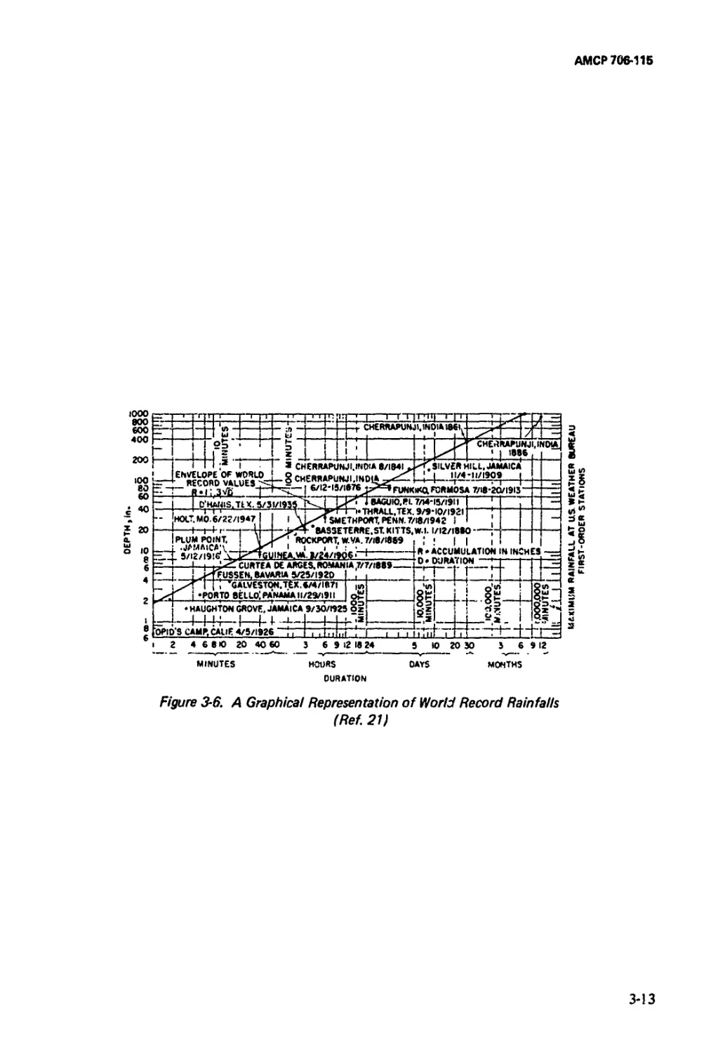
3-7	Rain............................................ 3-10
3-8	Solid Precipitation ............................ 3-12
3-9	Fog and Whiteout ............................... 3-18
3-10	Wind ........................................... 3-19
3-11	Sait, Sait Fog, and Salt Water ................. 3-19
3-12	Ozone........................................... 3-21
3-13	Macrobiological Organisms....................... 3-23
3-14	Microbiological Organisms ...................... 3-31
References ..................................... 3-33
CHAPTER 4.	INDUCED ENVIRONMENTAL FACTORS
4-1	Introduction .................................... 4-1
4-2	Atmospheric Pollutants .......................... 4-1
4-	3	Sand and Dust.................................... 4-4
4-4	Vibration, Shock, and Acceleration............... 4-9
4-	5	Acoustics....................................... 4-11
4-6	Electromagnetic Radiation ...................... 4-11
4-7	Nuclear Radiation .............................. 4-18
References ..................................... 4-20
CHAPTER 5.	COMBINED ENVIRONMENTAL
FACTORS-CLIMATES
5-1	Introduction .................................... 5-1
5-	2	Multifactor Combinations ........................ 5-2
5-2.1	Environmental Factor Descriptors............... 5-2
5-2.2	Two-Factor Combinations........................ 5-3
5-2.3	Functional Combinations........................ 5-3
5-3	Gimates .......................................   5-3
5-3.1	Hot-Dry Climate ................................. 5-7
5-3.1.1	Temperature .................................. 5-11
5-3.1.2	Solar Radiation .............................. 5-12
5-3.1.3	Precipitation and Moisture ................... 5-12
5-3.1.4	Wind.......................................... 5-14
5-3.1.5 Terrain.......................................... 5-16
5-3.1.6	Materiel Effects ............................. 5-17
5-3.2	Hot-Wet Climate ................................ 5-18
ii
АМСР 706-115
TABLE OF CONTENTS (Con't.)
Paragraph	Psge
5-3.2. i	Temperature..................................... 5-20
5-3.2.2	Solar Radiation ................. 5—21
5-3.2.3	Rainfall ....................................... 5-25
5-3.2.4	Humidity........................................ 5-29
5 3.2.5	Wind .... .................................. 5 30
5-3.2.6	Terrain......................................... 5-30
5-3.2.6.1	Topography ..................................... 5-30
5-3.2.6.2	Soil............................................ 5-32
5-3.2.6.3	Vegetation.................................. 5 32
5-3.2.7	Materiel Effects................................ 5-36
5-3.3 Cold Climate..................................... 5 36
5-3.3.1	Temperature................................. 5 37
5-3.3.2	Snow............................................ 5-43
5 - 3.3 2.1	Snow Cover..................................... 5-45
5-3.3.2.2	Snow Load....................................... 5-48
5-3.3.3	Glaze, Rime, and Hoarfrost...................... 5-48
5-3.3.4	Solar Radiation................................. 5-54
5-3.3.5	Obscurants ..................................... 5-60
5-3.3.6	Terrain......................................... 5-62
5-3.3.6.1	Glaciers........................................ 5-62
5-3.3.6.2	lee Cover....................................... 5-67
5-3.3.6.3	Frozen Ground ........................	5-69
5-3.3.7	Materiel Effects................................ 5-73
References....................................... 5-75
CHAPTER 6.	QUANTITATIVE ENVIRONMENTAL
CONCEPTS
6-1	General............................................ 6-1
6-2	Quantitative Factor Parameters..................... 6-2
6-2.1	Terrain .................................... 6-2
6-	2.2	Temperature................................. 6 5
6-2.3	Humidity ................................... 6 -7
6-2.4	Pressure.................................... 6-7
6-2.5	Solar Radiation............................. 6-9
6-	2.6	Rain ............................................ 6-9
6-2.7	Solid Precipitants ......................... 6 9
6-2.8	Fog and Whiteout............................ 6- 12
6-2.9	Wind............................................ 6-12
6-	2.10	Salt. Salt Fog. and Salt Water.................. 6-12
6-2.11	Ozone....................................... 6 12
6-2.12	Macrobiological Organisms......................... 6-18
6-2.13	Microbiological Organisms ....................... t>-18
6-2.14	Atmospheric Pollutants............................ 6-18
6-2.15	Sand and Dust..................................... 6-18
6-2.16	Vibration, Shock, and Acceleration..........	6-20
АМСР 706-11Б
TABLE OF CONTENTS (Con't)
Paragraph	Page
6-2.17 Radiation: Acoustics, Electromagnetic,
and Nuclear............................................... 6-20
6-3	Data Quality...................................... 6-20
6-4	Data Sources...................................... 6-24
References ...................................... 6-25
CHAPTER 7.	TESTING AND SIMULATION
7-1	Environmental Factors and Their Effects.......	7—2
7 -2	Simulating the Conditions ......................... 7-8
7-3	Accelerated Testing................................ 7-9
7-4	Testing in the Operational Environment........	7--11
7-5	Applications of Testing in Hardware Programs ...	7-11
7-6	Test Classifications and Planning................. 7-12
References ...................................... 7-17
CHAPTER 8.	MATERIEL CATEGORIZATION
8-1	Supply System Categorization....................... 8-1
8-2	Evolution of Army Materiel Categorization.....	8-6
8-3	Environmental Effects and Materiel
Categorization.................................. 8-13
References ...................................... 8-17
Index........................................ 1-1
АМО» 706-115
LIST OF ILLUSTRATIONS
Fig. No	Title	Page
J --1 Areas of Occurrence of Indicated Climatic
Categories................................................... 1-5
3-1 Coastal Plain in Arctic Showing Summer
Surface Conditions With Numerous Thaw
Lakesand Stream Channels..................................... 3-2
3 -2 Daily Diurnal Range of Standard Surface
Temperature at Various Stations for 1943.......... 3-5
3-3 Composite of Five Daily Cycles of High
Temperature and Dewpoint for Abadan, Iran....	3-6
3-4	Spectral Distribution of'Solar Radiation.......	3-9
3-5	Estimated Mean Global Energy Flow.................. 3-11
3-6 A Graphical Representation of World Record
Rainfalls........................................ 3-13
3-7 Age-hardened Snow Produced by Sintering in an
Undisturbed Winter Snow Pack................................ 3-15
3-8 Estimate of Probability P That in a Given
Hailstorm, the Maximum Hailstone Diameter
Will Not Exceed a Certain Value h................ 3-16
3-9 Rime on a Windvane Showing the Windward
Development of This Form of Solid
Precipitation.................................... 3-17
3—10 Results of Seeding Ground Fog.......................... 3-20
3-11 Diurnal Variation of Ozone Concentration (and
That of Nitrogen Dioxide) in a Rural
Environment...................................... 3-22
3-12 Tire Showing Ozone Effect on Unprotected
Section Labeled “Control"................................... 3-24
3-13	Termite Attack on Structural Lumber................ 3-28
3--I4	Piling Destroyed by Marine Borers.................. 3-30
.3—-15—	Fungous Attack on Lumber........................... 3-32
4-yl	Material Attack by Air Pollutants................... 4-5
4-2 Truck at 15 mph Velocity on Typical Well-
maintained Unpaved Road Illustrating Dust
Problem........................................... 4-8
4-3 Testing Shipping Containers on <' Flat-bed
Trailer..................................................... 4-12
4-4 vibration Testing of Tracked Vehicle.................... 4-13
4-5 Sound Pressure Level Contours During Static
Test of Large Rocket Motor....................... 4-14
4-6 Mobile Tropospheric Scatter Antenna..................... 4-16
4-7 Octopuslike Array of Electromagnetic Emission
Sources.......................................... 4-17
4-8 Low Altitude Nuclear Detonation Showing
Toroidal Fireball and Dirt Cloud.................. 4—19
5-1 Diurnal Temperature Cycles for Various Climatic
Categories......................................... 5-9
АМСР 706-11S
LIST OF ILLUSTRATIONS (Con't.)
Fig. No.	Title	Page
5-2 Diurnal Variations of Relative Humidity for
Various Climatic Categories....................... 5-10
5-3 Core and Transitional Wet-Tropical Regions..........	5-19
5 -4 Measured Moisture Content of Soil in Tropical
Forest ........................................... 5-27
5 5 Measured Moisture Content of Soil in Tropical
Grasslands........................................ 5-28
5-6 Relative Humidity Above and Belov/ the Canopy
of a Tropical Rain Forest......................... 5-3<
5-7 Tropical Rain Forest, Ft. Sherman, C. Z.............	5-33
5 -8 Mean Annual Air Temperature on the Greenland
Ice Cap (°C)....................................... 5-40
5 -9 Percent Frequency of Temperatures Below-25°F
During January in the Northern Hemisphere ....	5-41
5-10 Windchill Index and Related Levels of Human
Discomfort........................................ 5-42
5-11 Temperature inversions Observed at Arctic
Weather Stations.................................. 5-44
5 -12 World Distribution and Duration of Seasonal
Snow Cover................................................... 5-46
5-13 Maximum Annual Snow Cover in the Northern
Hemisphere..................................................   5-47
5-14 Windblown Snow From High Elevations Increasing
the Snow Burden at Lower	Levels.................   5-49
5 — 15 Annual Accumulation of Snow Cover in
Greenland......................................... 5-50
5 -16 Maximum Probable Snow Load on a Horizontal
Surface........................................... 5-51
5 -17	Snow Load With a P^stie-crcep Cornice..........	5-52
5-18	Snow Load With Wind Cornice on End-eaves.......	5-53
5-19	Rime Formation on Tree Branches...................... 5-55
5 20 Idealized Air Temperature Profile Associated
With Precipitation Fallingas Snow,
Rain, or Glaze or Sleet........................... 5-56
5 -21 Glaze Belts of the Northern Hemisphere............ 5-57
5 -22 Whiteout Development on the Greenland
IceCap....................................... 5-59
5 -23 Attenuation of Visibility by Fog.................. 5-61
5-24 Attenuation of Visibility by Blowing Snow..........	5-63
5 -25 Mountain-valley Glacier Debouching Onto a
Coastal Plain, Ellesmere Island................... 5-64
5 -26 Ice-cliff Front of a Continental Glacier With
Terminus on Land. North Greenland............ 5—65
5-27 Tabular Icebergs Calved at the Sea Terminus of the
Humboldt Glacier. North Greenland............ 5-66
5-28 Average Number of Days Per Year in Which Water
is [Innavigable.............................. 5-68
vi
АМСР 706-115
	LIST OF ILLUSTRATIONS (Con't.)
Fig. No.	Title	Page
5-29	Distribution ol Frozen Ground in the Northern Hemisphere	 5-70
5-30	Determination of Freezing index by Cumulative Degree Days	 5-71
7-1	Environmental Testing in Hardware Development	 7-13
8-i:	Typical Entries From Federal Supply Classification (FSC)	 8-7
vii
АМСР70в-1'и
LIST OF TABLES
Table No.	Title	Page
1 -1	Major Environmental Factors.......................... 1-3
1 -2	Climatic Classification System....................... 1-4
1 -3 Summary of Temperature, Solar Radiation, and
Relative Humidity Diurnal Extremes............................ 1-6
2-1 Association of Factor Importance With Region
of Environment................................................ 2-6
3-1	Heat-absorbing Capacity of Air....................... 3-8
3 -2	Important Pests at Military Installations.......	3-25
4- J	Classification of Induced Environmental	Factors..	4-2
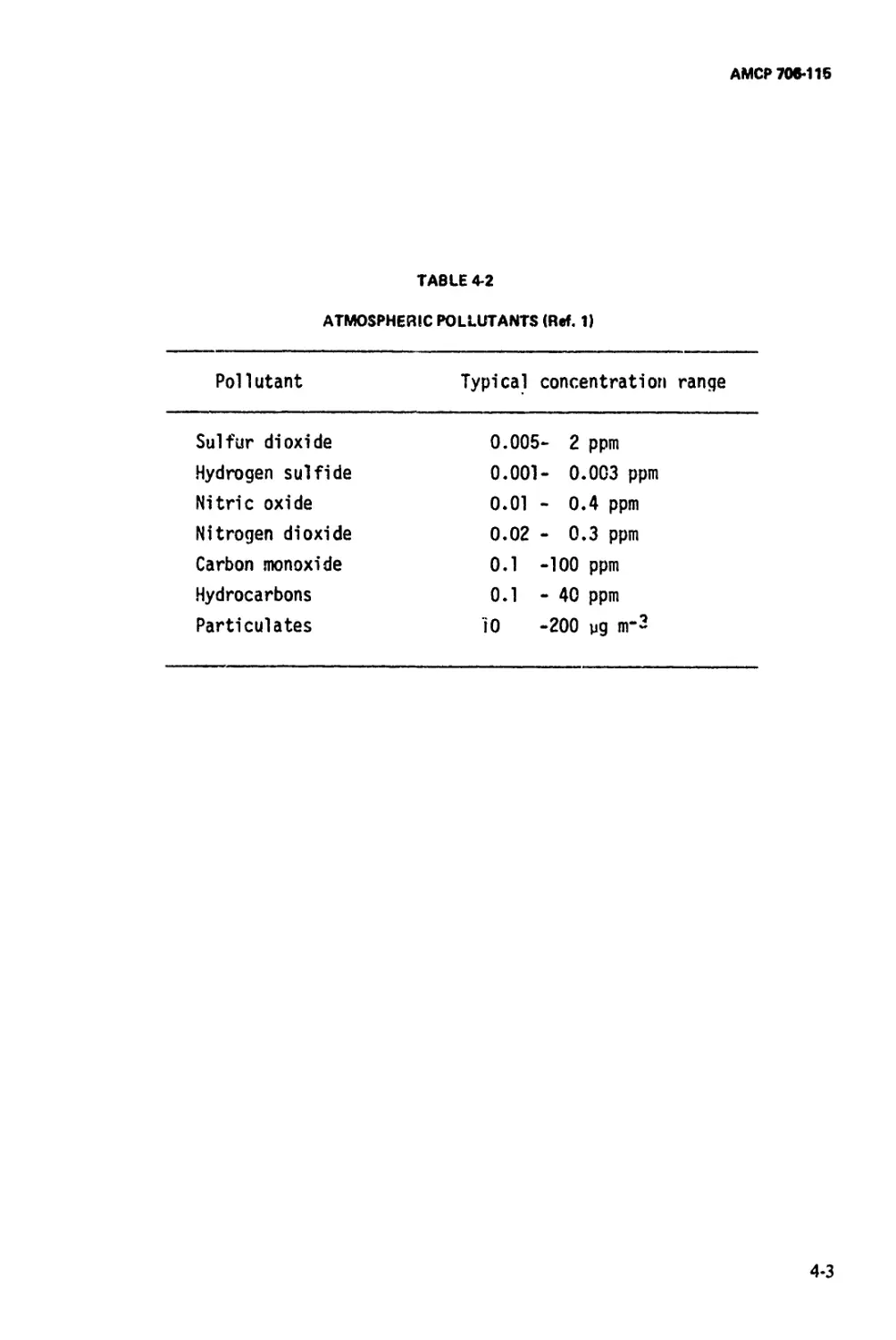
4-2	Atmospheric Pollutants............................... 4-3
5-1	Environmental Factor Descriptors..................... 5-4
5-2	Two-factor Combinations of Importance	to
Materiel........................................... 5-5
j- 3	Combinations of Environmental Factors As-
sociated With Various Activities.............................. 5-6
Association of Natural Environmental Factors
With Climatic Categories............................ 5-8
5-5	Computed Annual Average Solar Radiation at
Ground Surface.................................... 5-13
5-6	Average Relative Humidities in Hot-Dry
Locations......................................... 5-15
5-7	Temperature Changes With A.liituae (in
Netherlands East Indies).......................... 5-22
5-8	Temperatures at Different Heights in Wet-Tropical
Forests.........................................   5-23
5-9	Solar Radiation (ly d^y T’ a. Surface of Earth
With Normal Cioud Cove»........................... 5-24
5—10	Monthly Averap? Rainfall............................ 5-26
5-11	Comparative Temperatures for the Cold Climatic
Categories........................................ 5-38
5-12	Frost Depths (for Duluth, Minn.).................... 5-72
6-1	Terrain Parameters................................... 6-3
6-2	Temperature Parameters............................... 6-6
6-3	Humidity Parameters.................................. 6-8
6-4	Solar Radiation Parameters.......................... 6-10
6-5	Rain Parameters .................................... 6-11
6-6	Snow Parameters..................................... 6-13
6-7	Fog Parameters...................................... 6-14
6-8	Beaufort Scale of Wind.............................. 6-15
6-9	Wind Parameters..................................... 6-16
6-10	Salt Parameters..................................... 6-17
6-11	Sand and Dust Parameters............................ 6-19
6-12	Vibration Parameters................................ 6-21
6-13	Acoustical Parameters............................... 6-22
6-14	Electromagnetic Radiation Parameters................ 6-23
7-1	Relationships Subject to Testing..................... 7-4
viii
АМСР 706115
LIST OF TABLES (Con't.)
Table No.	Title	Page
7-2	Environmental Test Classifications........................ 7—14
7-3	Practical Factors Related to Testing...................... 7-16
8-1 Materiel Categorization Based on Nature and
Importance of Items.................................................. 8-2
8-2 Materiel Categorization Based on Method of
Handling Items in Logistic System.................................... 8-3
8-3 Federal Supply Classification Major Groups
(excluding space vehicles)........................................... 8-4
8-4	Supply Classification (December 1917)...................... 8-8
8-5	Supply Classification (December 1940)...................... 8-9
8-6	Supply Classification (November 1943)..................... 8-10
8-7	Supply Classification, QM Recommendations
(November 1945)......................................... 8-11
8-8	Supply Classification (September 19<9).................... 8-12
8-9	Supply Classification (February 1963)..................... 8-14
8-10	Material Classes.......................................... 8-15
8-11	Materiel Categorization by Type........................... 8-16
ix
A МСР 708-115
PREFACE
lliis handbook, Basic Environmental Concepts, is the first in a series on
the nature and effects of the environmental phenomena.
Part One introduces the importance of the environment; i.e., its effects,
the factors of the environment, the complex combinations of the environ-
ment that occur, quantitative environmental concepts, and the testing of
materiel and simulation of the environment. The categorization of materiel
as it exists and relates to environmental effects also is discussed.
Part One introduces in a general and qualitative manner those factors that
are to be treated quantitatively in the succeeding volumes. The revision
augments the treatment of those factors and climates, which are a
combination of the factors that were discussed only briefly in the original
handbook. The chapter on materiel categorization also is added by the
revision.
The majority of the handbook content was obtained from various
individual contributors, reports, and other publications. Accordingly, it is
impractical to acknowledge the assistance cf each individual or even each
organization which has contributed materially to the preparation of this
volume. Appreciation is extended, however, in a general way io the
following US Army Materiel Command organizations and through them to
the individuals concerned: Frankford Arsenal, Waterways Experiment
Station, Army Tank-Automotive Command, Cold Regions Research and
Engineering Laboratories, Electronics Command, Harry Diamond Labora-
tories. Natick Laboratories, Picaunny Arsenal, and Test and Evaluation
Command.
The original Part One was prepared by the Southwest Research Institute;
the revision was prepared by the Research Triangle Institute, Research
Triangle Park, NC-for the Engineering Handbook Office of Duke University,
prime contractor to the US Army Materiel Command-under the general
direction of Dr. Robert M. Burger. Technical guidance and coordination
were provided by a committee under the direction of Mr. Richard C.
Navarin, Hq. US Army Materiel Command.
The Engineering Design Handbooks fall into two basic categories, those
approved for release and sale, and those classified for security reasons. The
US Army Materiel Command policy is to release these Engineering Design
Handbooks to other DOD activities and their contractors and other
Government agencies in accordance with current Army Regulation 70-31,
dated 9 September 1966. It will be noted that the majority of these
Handbooks can be obtained from the National Technical Information
Service (NTIS). Procedures for acquiring these Handbooks follow:
x
АМСР 706-115
a.	Activities within АМС, DOD agencies, and Government agencies other
than DOD having need for the. Handbooks should direct their request on an
official form to:
Commander
Letterkenny Army Depot
ATTN: AMXLE-ATD
.’’hambersburg, PA 17261
b.	Contractors and universities must forward their requests to:
National Technical Information Service
Department of Commerce
Springfield, VA 22151
(Requests for classified documents must be sent, with appropriate “Need to
Know” justification, to Letterkenny Army Depot.)
Comments and suggestions on this Handbook are welcome and should be
addressed to:
Commander
US Army Materiel Command
ATTN: AMCRD-TV
Alexandria, VA 22333
«and. Blank Forms,
(DA Forms 2028, Recommended Changes to Publications/ which are
available through normal publications supply channels, may’be used for
comments/suggestions.)
АМСР 706-115
CHAF £R 1
THE ENVIRONMENT FACED BY THE MILITARY
1-1 INTRODUCTION
This handbook-the first of the Environ-
mental Series of Engineering Design Hand-
books-is cn introduction to the environment
faced by the military. Emphasis is on informa-
tion that relates to environmental effects on
materiel or materiel requirements. The ob-
jectives are to describe the characteristics of
the environment, to set forth the situations in
which such environmental conditions are en-
countered, and to identify the adverse effects
of the environment on materiel.
In this introductory part of the Environ-
mental Series of Engineering Design Hand-
books, the importance of the environment is
discussed and the 21 natural and induced
environmental factors that produce significant
effects on military materiel are identified and
individually described. In addition, the nature
of the real environment in which various
combinations of factors act in concert is
discussed. Quantitative concepts relative to
the environment, simulation of the environ-
ment and materiel testing, and materiel cate-
gorization are also included in this introduc-
tory part.
1-2 THE ENVIRONMENT DEFINED
Environment is defined in MIL-STD-1165
(Ref. 1) as “the totality of natural and
induced conditions occurring or encountered
at anv one time and place”	An
alternative definition states that environment
is the complex of climatic, edaphic, biotic,
and topographic factors that describes a given
place.
The description of the environment is
tailored for particular considerations. Thus,
one may view the environment as having (n +
4) parameters where the three spatial coordi-
nates and time comprise four of these para-
meters, plus» (« ~ 21 in this handbook series)
factors that comprise the climatic, cdaphic,
oiotic, and topographic description. If, how-
ever, one is interested in a particular materiel
type, many of the environmental factors are
of little importance and a more limited set
will comprise a sufficient description.
One environment at one location has differ-
ent factor values than that at another location
and, for a given location, the description of
the environment at a given time is different
from that at another time. In different
environments, the environmental factors vary
in importance. For example, solid precipitants
comprise an important factor in Alaska, but
this factor is absent in the Panama Canal
Zone. In similar fashion, rain is an important
factor in the outdoor environment in the
temperate zone but is unimportant inside a
warehouse. The interior of the warehouse,
however, is an important region of the envi-
ronment for military materiel. An attempt is
made in Chap. 2 to identify those environ-
mental factors that are important for specific
regions of the environment.
In addition to obtaining an accurate defini-
tion of environment, it is important to under-
stand the meaning of terminology that in-
clude? the word “environmental” as an adjec-
tive. Thus, environmental control implies
modifying the effects of certain environment-
al factors to reduce stresses on materiel or
personnel. Environmental design criteria are
environmental factors representing a given
degree of stress severity with regard to equip-
ment, and environmental engineering is that
branch of engineering concerned with the
1-1
АМСР 706-115
control of environmental factors and the
design of materiel to function adequately
under various environmental conditions. En-
vironmental protection is provided to people
or equipment and evaluated performance will
be obtained under various environmental op-
erating conditions.
1-3 ENVIRONMENTAL FACTORS
The components or descriptors of the
environment are termed “environmental fac-
tors". Table l-l lists the 21 environmental
factors that are discussed in the Environmen-
tal Series of Engineering Design Handbooks.
These factors are believed to provide a com-
plete description of the environment for the
use of design engineers. Additional factors
could have been included, or some of tne
factors that are included could have been
either subdivided into several factors or com-
bined with other factors to provide a more
comprehensive factor. For example, terrain is
included as a factor but could have been
readily divided into hydrography, topog-
raphy, and soiis. Sand and dust could have
been combined with atmospheric pollutants;
vibration, shock, and acceleration could have
been made a single factor; and other modifica-
tions are equally possible. Consideration of
environmental effects on materiel and mili-
tary operations resulted in the list given in
Table 1-1 as being deemed most appropriate.
Most environmental factors are neither
static nor universal. The occurrence or ab-
sence of environmental factors, or ranges of
factor characteristics normally arc used as a
basis for defining terrestrial regions such as
arctic, tropic, or temperate. The wet tropics,
foi example, are characterized by heavy rain-
fall, high atmospheric humidity levels, moder-
ately high ambient temperatures, abundant
vegetation, and a large population of both
micro- and macrobiological organisms. The
wet tropics, however, arc void of sand or dust,
solid precipitants, and fog. In particular, all of
the environmental factors characterized as
induced factors are produced primarily by
man's activities. In all cases, caution must be
employed in the assignment of specific
environmental factors to a given area, since
these may change radically with seasons of
the year or with climatic conditions. It is well
known that some region' of the earth pre-
viously covered with vegVation are now
almost desert in character, tr^j? rainfall pat-
terns arc continuing to change, a^Lthat man's
activities sometimes have large effe^j on local
environmental factors.	4
1-4 CLASSIFICATION SYSTEMS
Classification of the different tvpes of
environment is useful since unique sets of
factors are associated with various places,
conditions, or functions. Fe. example, the
“operational environment’’ ; nd the “logistics
environment’’ are important runctional classi-
fications that arc employee to categorize
those environmental condit ons associated
with military operations or with the logistic
system. In similar fashion, one may use
“warehouse environment” »»; categorize en-
vironmental conditions found within ware-
houses; other examples are “laboratory envi-
ronment”, “aircraft environment”, “open-
storage environment”, or “battlefield environ-
ment”.
Important classification systems are associ-
ated with terrain and are employed in topo-
graphic mapping. Descriptors such as moun-
tains, plains, marshlands, and rivers have
definite and important meanings. A system
for more precise classification of topographic
features is described in Chap. 2, Part Two, as
arc various classification systems for soils.
Probably the most important classification
systems arc those associated with climate.
While a variety of climatic classification sys-
tems exist, the one defined in AR 70-38 is
applicable to Army materiel considerations
(Ref. 2). Eight climatic categories are grouped
into four types of climate as given in Table
1-2. The ranges of environmental factors
associated with each of these climatic cate-
gories is given in Table i-3; their geographic
extent is given in the map of Fig. 1-1 and
1-2
АМСР 706*115
TABLE 1-1
MAJOR ENVIRONMENTAL FACTORS
Type	Class	Factor
Natural	Terrain*	Topography Hydrology Soils Vegetation
	Climatic	Temperature Humidity Pressure Solar radiation Rain Solid precipitants Fog Hind Salt Ozone
	Biological	Macrobiological organisms Microbiological organisms
Induced	Airborne	Sand and dust Pollutants
	Mechanical	Vibration Shock Acceleration
	Nqergy 		Acoustics Electromagnetic radiation Nuclear radiation
*In this handbook seri&s, terrain is considered to be one factor.
AMCF 709-111
TABLE 1'2
CLIMATIC CLASSIFICATION SYSTEM
Climatic type	Climatic category
( 1. A. Hot-wet 	 {2. (з.	Wet-warm Wet-hot Humid-hot coastal desert
B. Hot-dry 	 4.	Hot-dry
(5 C. Intermediate 	 <g‘	Intermediate hot-dry Intermediate cold
D. Cold 	 ( o«	Cold Extreme cold
1-4
АМСР 706-1 IB
Figure 7-1. Areas of Occurrence of Indicated Climatic Categories
1-5 4
AMCP706-I15
TABLE 1-3
SUMMARY OF TEMPERATURE, SOLAR RADIATION. AND RELATIVE HUMIDITY
DIURNAL EXTREMES (Ref. 2)
Climatic category	Operational conditions			Storage and transit conditions	
	Ambient air temperature, °F	Solar radiation, Btu/ft2/hr	Ambient relative humidity, percent	Induced air temperature, °F	Induced relative humidity, percent
1 Wet-warm	Nearly constant 75	Negligible	95 to 100	Nearly constant 80	95 to 100
2 Wet-hot	78 to 95	0 to 360	74 to 100	90 to 160	10 to 85
3 Humid-hot coastal desert	85 to 100	0 to 360	63 to 90	90 to 160	10 to 85
4 Hot-cry	90 to 1Z5	0 to 360	5 to 20	90 to 160	2 to 50
5 Inter- mediate hot-dry	70 to 110	0 to 360	20 to 85	70 to 145	5 to 50
6 Inter- mediate cold	-5 to -25	Negligible	Tending toward saturation	-10 to -30	Tending toward saturation
7 Cold	-35 to -50	Negligible	Tending toward saturation	-35 to -50	Tending Joward saturation
8 Extreme cold	-60 to -70	Negligible	Tending toward saturation	-60 to -70	Tending toward saturation
1-6
''МСР 706-115
additional details concerning each climatic
category are given in AR 70-38.
Terminology such as shock and vibration
environment, temperature environment, or
nuclear radiation environment often is used in
the literature. This usage is misleading-shock
and vibration are important in some environ-
ments and unimportant in others; the temper-
ature range of a given environment always can
be given special consideration; and a signifi-
cant level of radiation can be used to distin-
guish certain environments from others. To
avoid ambiguity, however, it is best not to
classify environments on the basis of single
environmental factors.
REFERENCES
I.	MIL-STD-1165, Glossary of Environment-
al Terms.
2.	AR 70-38, Research, Development, Test,
and Evaluation of Materiel for Extreme
Climatic Conditions.
I-7/1-8
АМСР 706-115
CHAPTER 2
IMPORTANCE OF ENVIRONMENT
2-1 INTRODUCTION
The importance of environment to materiel
may be categorized as follows:
(1)	Environmental effects result in perfor-
mance deterioration, thereby creating a main-
tenance burden.
(2)	Environmental effects shorten the use-
ful life of many materiel items, thereby
affecting the procurement and logistic func-
tions.
(3)	Environmental ...Teets create a require-
ment for many specialized materiel items in
order to insure operational capabilities.
(4)	Environmental effects place demands
on materiel performance u'.?f greatly increase
the costs of development and production of
all materiel subject to Military Specifications.
(5)	Environmental effects on materiel
sometimes have major impact on the success
or failure of military operations.
The importance of environment is estab-
lished by the large magnitude of these mainte-
nance, procurement and logistic, operational,
and performance burdens. This chapter pro-
vides information on these environmentally
imposed burdens in order to substantiate the
pervasive importance of environment in all
materiel considerations. It also seeks to iden-
tify those factors of most concern in the more
important regions of the environment.
In discussing the importance of enviion-
ment to materiel, it is essential to recognize
that both effects of environment on materiel
and requirements for materiel resulting from
environment are important; e.g., it is equally
as important for the design engineer to know
that airborne sand can rapidly destioy a truck
engine as it is to know that operations in
regions where blowing sand is common re-
quire the placement of additional filters on
engine-air intakes. Solutions to problems as-
sociated with vehicular mobility on snow
cover may be better solved by use of special
vehicles than by design changes in convention-
al transport. Examples such as these are found
throughout the discussion of environmental
factors in subsequent parts of this Environ-
mental Series.
Material deterioration assumes a variety of
forms, depending on the particular item of
materiel being considered. That such deterio-
ration occurs is neither surprising nor without
benefits. In fact, manmade materials that are
not biodegradable have generated consider-
able concern since, after their useful purpose
has been realized, they become problems in
the waste stream. Deterioration is just a form
of natural change that is more obvious in
those material forms that man has created.
Given sufficient time, nature would restore all
manmade materials to their natural forms.
Maintenance is the effort to counteract the
effects of materiel deterioration, whether the
deterioration is induced by environmental
factors or results from normal wear during
use. It takes the form of cleaning, parts
replacement, repainting, lubrication, perfor-
mance testing, and similar functions. Mainte-
nance required by environmental effects .s
costly and every effort is made to design
materiel that is impervious to environmental
effects.
2-1
AMCF706-11S
In this discussion wc arc concerned with
those forces associated with environmental
factors that tend to degrade the useful func-
tion that man has built into materials and
structures.
2-2 PERFORMANCE DETERIORATION
AND REQUIRED MAINTENANCE
In order to gain perspective on the impor-
tance of environment, it is useful to examine
the spectrum of environmental effects that
result in materiel deterioration. In the para-
graphs that follow, this is accomplished by
giving examples of deteriorative effects. The
list of examples is not exhaustive; additional
examples are given in subsequent parts of this
Environmental Series of Engineering Design
Handbooks. The examples given, however, are
sufficient to indicate the importance of such
effects.
2-2.1 EFFECTS ON SURFACE FINISHES
A majority of the materials used in struc-
tures, mechanisms, and devices are chosen for
useful functions, not necessarily for their
stability in the natural environment. For this
leason a majority of these materials arc
furnished with a surface protective coating of
some type. It may be a plating on metal,
paint, or a chemical treatment of the surface.
In the complete spectrum of environmental
factors, these surface finishes deteriorate with
time. Sometimes the deterioration process is
more rapid than at other times. Experience of
the Army with the deterioration of surface
finishes covers many areas. It has been noted,
for example, that trucks received in specific
operational areas during World War 11 often
required painting upon arrival before being
put into service. This resulted from the severe
stress of the tropical environment on the then
available surface finishes.
Surface finishes may be deteriorated by
temperature, humidity, solar radiation, rain,
solid precipitants, fog, wind, salt, ozone,
macrobiological organisms, microbiological
organisms (microbes), pollutants, and sand.
Often, these factors act in synergism, or one
of them is supportive of the action of
another. Microbes, for example, are inactive
without sufficient humidity and a sufficiently
high temperature. Sand requires wind to
damage a surface. It has been noted that a
sandstorm can strip the paint from a vehicle
and thus expose the bare metal to corrosion.
Humidity, rain, solid precipitants, and fog are
very similar in their effec's. Often the specific
deteriorative factor cannot be identified, but
a combined effect of several factors with
unknown relative impacts is assumed. Too
often, surface deterioration results from dam-
age that compromises the protective coating
and allows corrosion, rot, or abrasion to start.
2-2.2 EROSION
Erosion is employed here to describe gross
removal of materiel from a structure. This
occurs, for example, when windblown sand
actually cuts away wood from telephone
poles, often reducing their diameter by 50
percent in less than 1 yr. Erosion is produced
by natural forces such as windblown sand,
water, or the action of wind by itself, its
primary effects in military operations are the
erosion of roadways and other topological
features by water, erosion of exposed surfaces
by blowing sand and dust, and the induced
erosion of sand. Another commonly observed
example of erosion is that of pilings in
saltwater that are so weakened by molluscan
borers that the wood is carried away by the
wave action.
2-2.3 ROT AND DECAY
Rot and decay are products of deteriorative
processes associated primarily with microbes.
Common evidences such processes include
the spoiling of foodstuffs, loss of strength in
wood and other cellulosic materials, and the
weakening and disintegration of textile pro-
ducts. A large proportion of the consumables
used by society eventually are subjected to
conditions wherein rot and decay are encour-
aged. The final result is the eventual mineral-
ization and disposal of the product.
2-2
АМСР 706-116
Rot and decay are useful processes con-
tributing much to the economy as well as to
the esthetics of modem life. The problem
with respect to military materiel is to recog-
nize those materials that are subject to this
environmental factor and to provide tech-
niques for avoiding deterioration during the
useful life of the materiel item. This is
accomplished with protective barriers, chemi-
cal treatment, dehumidification, and cold
storage.
2-2.4 CORROSION
Corrosion is a form of deterioration that is
associated primarily with metals. It is an
extremely important form of deterioration
and is influenced by a variety of environment-
al factors. For example, a type of corrosion
closely associated with vibration and shock is
known as stress-corrosion, which is very im-
portant in vehicles as well as other meial
structures. It results from the combined effect
of strain on the metal and subsequent corro-
sion induced at the strain point through
microscopic cracks. The rusty nail, however,
is the most common evidence of the corrosion
processes that are most evident in areas where
atmospheric salt or pollutants support the
corrosion processes. Although the corrosion
of metals is one of the most costly and
prevalent material deterioration processes, it
can be avoided by adequate surface protec-
tion and good practices.
2-2.5 ELECTRICAL PROPERTIES
Environmental effects on electrical and
electronic components are related primarily
to temperature and humidity, although other
factors produce less important effects. Clas-
sifications of electrical failures include insula-
tion breakdown, nonconducting switch con-
tacts, changing resistance values, physically
broken components, and the change in param-
eters of active devices such as tubes and
transistors. Dirt and other atmospheric con-
taminants contribute to problems with switch
contacts and the deterioration of insulation.
Heat, however, is the most important deterio-
rative factor for electrical properties, causing
reduced tube or transistor life, breakdown of
insulation, and other similar processes. Shock
and vibration, acting in synergism with tempe-
rature, result in most physical breakage. Ex-
amples of this include broken wires, cracked
insulators, and malfunctioning electromechan-
ical mechanisms.
Much effort is expended in the design of
electrical and electronic apparatus to provide
protection from environmental effects. This
includes provision for cooling and dehumidifi-
cation, shock mounts, derating of compo-
nents, filtering of cooling air, and extensive
use of protective coatings.
2-3 REDUCTION IN USEFUL LIFE
A large quantity of military materiel is lost
tiirough the effect of environmental factors
without ever being used because of the
conditions under which it is transported and
stored. An even larger quantity of materiel
has a reduced useful life because of environ-
mental effects. This is most obvious in opera-
tional situations where materiel is more ex-
posed to environmental stresses. Rust, mil-
dew, and rot are common effects that ^ause
various items to be discarded. Rubber hoses
attacked by ozone, wood damaged by ter-
mites, pilings eroded by marine borers, tex-
tiles damaged by moths, aircraft antennas
corroded by salt, and vehicle brake linings
prematurely worn by sand are other exam-
ples.
Many forms of attack by environmental
factors can be alleviated or obviated by
proper design and procurement. Much pro-
gress has been made in preventing the com-
mon forms of deterioration. The effects of
shock and vibration during off-the-road opera-
tion of vehicles, the peculiar problems of
oversnow transport, the severe corrosion and
microbiological attack of the wet-tropics, and
the erosion of blowing sand and dust, how-
ever, are examples of environmental stresses
for which complete protection is too cosily.
The military accepts, then, the resultant
2-3
АМСР 706-115
deterioration and pays the cost in reduced
useful life of materiel until more cost-
effective protective measures are found.
Much environmental damage is triggered by
misuse and other types of damage. Corrosion
may start with a scratch in a painted surface;
rot may follow damaged packaging; erosion of
roads follows inadequate maintenance; and
termite damage may result from poor con-
struction practices. If the designer uses the
best materials and provides the known protec-
tive measures, and if the materiel is used
properly and carefully, then much of the
concern with environmental darnage would be
unnecessary and the useful life of Army
materiel would be little affected by the
environment.
2-4 SPECIAL MATERIEL REQUIREMENTS
The identification of special materiel re-
quirements with environmental effects is not
necessarily clear. For example, the effect of
terrain on mobility may call for tracked
vehicles, but tracked vehicles are also required
to provide operational capabilities not other-
wise available. Is this a requirement imposed
by the environment or by operations? The
same ambiguity applies to such materiel re-
quirements as oversnow transport vehicles,
fog dissipation systems, warehouse dehumid-
ifiers, nuclear-radiation-hardened equipment,
and amphibious vehicles. In each case, an
operational requirement exists fo»- operating
in an environment that has adverse effects on
materiel. Without the operational require-
ment, special equipment would not be re-
quired; because of the requirement, special
equipment must be provided because of the
various environmental factors to be faced.
It ь thus clear that, while the environment
imposes a need for much special equipment,
the provision of such equipment directly
determines the operational capability of the
Army, fne analysis of the costs and benefits
of such requirements is beyond the scope of
this handbook. The provision of such equip-
ment, hovever, does constitute a major ele-
ment of co»v in materiel procurement.
Examples of special materiel requirements,
in addition to those cited previously, include
raincoats, snowshoes, foghorns, pontoon
bridges, air conditioners, and cushioning ma-
terials for packing. This list could have in-
cluded a very large number of supply items.
2-5 MILITARY SPECIFICATIONS
Aside from the costs asso • i;. h special
materiel items but closely и mainte-
nance costs and the limitations on useful life
of Army materiel are the costs associated with
procurement of materiel to Military Specifica-
tions. including stringent environmental re-
quirements. The requirement that an item not
only survive undarnaged but also operate
normally in a full range of environmental
factors is sometimes very difficult to meet.
The testing to prove that the requirements
are met is an additional cost factor. That
these requiiements are placed on large quanti-
ties of materiel jiems. the majority of which
are never exposed to environmental extremes,
is adequate testimony to the importance
placed on such requirements. The sometimes
large cost escalation associated with meeting
the environmental requirements in Military
Specifications is deemed fully justified by the
assurance of performance obtained for those
few items that are exposed to severe environ-
mental stresses. The added reliability achieved
under normal conditions of such materiel is a
bonus.
2-6 SUCCESS OF OPERATIONS
Environmental effects on materiel have a
large impact on military operations-at times
determining the success or failure of a mis-
sion. It is well known, for example, that the
inoperability of German vehicles in the severe
Russian winter was a factor in the defeat of
the German Army in Russia during World War
II. Even aircraft engines could not be started
in the extreme cold. Another example of
environment affecting large military opera-
tions is the delay of the Normandy landings
by adverse environmental conditions—the
storm in the Engli-h Channel. However, a
majority of environmental effects on opera-
АМСР 706-116
tions are found in the smaller day to day
operations, e.g., (Ref. 1):
“ ... meanwhile the tanks had charged
down the road to perform the second
part of the mission, but just short of this
goal, they ran into a stretch of boggy
land that proved to be a veritable tank
trap. This area of wet ground limited the
area of maneuverability to the road and
a stretch immediately south of the road.
In this unfavorable position, the tanks
were hit by 88:s with such deadly fire
that after losing nine vehicles the attack
was forced to withdraw.”
This example was obtained from the opera-
tional report of an infantry regiment in
Tunisia in 1943. The success or failure of
military operations is compounded from a
multitude of such small events. Such events as
mud inhibiting mobility, inclement weather
preventing aircraft operations, personnel per-
formance being restricted by extreme cold,
and artillery fire being inhibited by poor
visibility can be vitally important tactical
effects. In some cases, the effects result from
a lack of capability of available materiel,
while in others they result from deterioration
of materiel performance or from unavail-
ability of suitable materiel.
There is insufficient information available
to document the direct effects of materiel
deteiioration on mission failure or success.
The failure of a piece of electronic equip-
ment, gun, tank, or other materiel item due to
cumulative deterioration resulting from en-
vironmental stresses is not documented as an
environment effect. Often such data only
appear as a statistic describing the useful
lifetime of a particular item. The total of such
effects, however, is one of the more impor-
tant environmental effects and, through its
cumulative impact on logistics, maintenance,
and operations, contributes importantly to
the probability of mission success.
2-7 FACTOR IMPORTANCE
The relative importance of the various
environmental factois varies with circum-
stances. If one considers that the materiel life
cycle consists of storage, transportation, and
operational use, then this variation may be
examined. In the storage environment, ma-
teriel is protected by both the warehouse and
its packaging from factors such as rain and
solar radiation. On the other hand, because of
the possible long duration of such storage,
slow-acting factors such as ozone and salt are
more important than would otherwise be
true. In transportation, the mechanical factors
are important but the slow-acting factors have
little or no effects. In operations, the pack-
aging that protects materiel is discarded, and
full exposure to the natural and induced
factors occurs. Not only are more factors
active, but their seventy is greater. Materiel
with an expected lengthy operational life
receives more exposure to the environmental
factors and thus is susceptible to greater
effects.
The importance of environmental factors is
tabulated in Table 2-1 for the various regions
of the environment.
REFERENCES
1. С. E. Hesaltine, Military Operations As
Characterized by the Effects c,f
Environment, George Washington
University, Washington, D.C., September
1957.
2-5
TABLE 2-1
ASSOCIATION Or FACTOR IMPORTANCE WITH REGION OF ENVIRONMENT
Environmental factor
Region of the environment	I Terrain	Temperature
Storage	0	A
Transportation		
Highway	A	В
Rail	A	В
Ship	0	С
Air	0	В
Operational use		
Cold regions	A	А
Hot-wet	A	А
Hot-dry	A	А
Temperate	A	А
Indoor use	0	8
Operational storage	0	А
ACOOOOOCC В
в сссвооо о
BGCB3BCOO 0
BOCCBCCOO 0
B0CC0BC80 c
CCOCCA6OO 0
AOBAABBCO C
ACBACOBBO C
OOAOOOBBO 0
С В А в в в в с с
800000000 С
AOBBBOCBC В
О	0	С	А	А	С	0	0	0
О	О	С	А	Л	С	О	О	О
о	О	О	В	С	С	О	О	о
о ОСВВВОО О
о	ССВВОСВ	с
А	ООВВОСВ	С
О	ОАВВОСВ	С
в	свввосв	с
с	свсооов	с
в	ссосоос	с
А - Major importance
В - Important
С - Minor
О - Absent
AM СР 706-115
CHAPTER 3
NATURAL ENVIRONMENTAL FACTORS
3-1 INTRODUCTION
Thirteen natural environmental factors are
discussed at length in this series of handbooks
and also are described briefly in the following
paragraphs. These factors and the induced
environmental factors discussed in Chap. 4 are
associated with climatic categories in Chap. 5.
When the effects of factors are considered
individually as in this chapter and in Parts
Two and Three of the Environmental Series
of handbooks, the process is referred to as
single-factor analysis and offers the most
direct means for assessing environmental ef-
fects. Such analysis is limited, however, in its
applicability since it docs not describe the
actual circumstances encountered in the en-
vironment. Multifactor combinations are
discussed in Chap. 5 and, at length, in Part
Four, Life Cycle Environments, of the
Environmental Series of handbooks. Detailed
data on natural environmental factors are
presented in Part Two of this handbook series
which serves as the prime reference for all of
this chapter. The information in this chapter
is intended only to identify and introduce
each factor.
3-2 TERRAIN
By definition, terrain comprises the phys-
ical features of land and thi s includes topo-
graphy-the geometric contours of the land-
scape; hydrography-the lakes, streams, and
other water bodies on the land; vegetation-
forest, grasslands, or thickets: and soils-the
composition and strength propeities of the
underlying earth. In describing terrain, there-
fore, it is necessary to discuss each of these
major parts of the terrain separately since
each is a major field of knowledge and
activity.
The topography of land normally is indi-
cated on maps by contour lines of equal
elevation above a reference level, i.e., sea
level. The spacings between contour lines thus
provide information on slope. Additional in-
formation is provided by indicating the land
areas that consist of mountains, plateau re-
gions, hilly areas, or plains. More quantitative
descriptions of topography are obtained by
classifications based on slope angles or ob-
stacle dimensions (Ref. 1).
Qualitatively, the vegetation portion of
terrain is described as dense forrests, wooded
areas, thickets, underbrush, grasslands, marsh-
lands, oi cultivated agricultural areas. For
military purposes, where mobility is of major
concern, quantitative vegetation descriptors
include parameters such as stem diameter,
stem spacing, and recognition distance. Such
descriptions are not concerned directly with
the type of vegetation present nor with the
coexistence of different types (Ref. 1).
Hydrologic descriptions of terrain are con-
cerned primarily with rivers because of their
varying nature although the presence of lakes
and marshlands is important. The presence
and course of rivers arc indicated on maps.
Additional quantitative information that is
employed for military purposes includes pa-
rameters such as differential bank height, gap
side slopes, water depth, water width, and
water velocity, which would indicate the
fordability of a stream. Quantitative informa-
tion is usually unavailable on seasonal vari-
ability in water flow parameters which are
sometimes the most important element of
hydrography for military considerations. An
example of a hydrologically complex terrain
is shown in Fig. 3-1.
3-1
АМСР 706-115
Figure j- 7. Coastal Plain in Arctic Showing Summer Surface Conditions
With Numerous Thaw Lakes and Stream Channels (Ref, 4)
3-2
АМСР 706-11Б
The composition and physical properties of
soils are very important to mobility and
construction considerations. This has led to
the evolution of a number of classification
systems based on soil type (e.g., clay, loam, or
sand), on the physical nature of the soils (e.g.,
rock content, plasticity, or grain size), or on
macroscopic mechanical properties (e.g., trac-
tive and bearing capabilities). One of the more
important of these classification systems is
known as the Unified Soil Classification
System which is widely employed by engi-
neers for construction purposes (Ref. 2).
Information on terrain is available in a
variety of forms including tabulated engineer-
ing data and maps which display a variety of
terrain information in a wide range of detail
and of accuracy. Efforts are underway to
obtain a greater amount of usable information
in terrain descriptions. An example of this is
the generation of areal terrain-factor complex
maps which include classifications based upon
21 terrain parameters (Ref. 1). Another at-
tempt to enhance the data base for terrain
uses power spectrum density curves to de-
scribe the roughness of terrain on a local level.
Terrain information is being expanded rapidly
by the increased use of a variety of remote
sensing techniques, bo?h aircraft and satellite
borne, which provide a very large amount of
terrain data (Ref. 3).
The effects of terrain .ary in their nature
and importance. Mobility is often the prime
element of success in military operations and
terrain determines land mobility. It is not
surprising, therefore, to find much emphasis
on trafficability, off-road mobility, and river
crossing problems. In any theater of opera-
tions in which ground forces play a najor
role, mobility will continue to be of major
importance, and this importance has many
effects both on materiel and on materiel
requirements. Materiel is exposed to all modes
of transport across terrain; materiel require-
ments are determined by the nature of the
terrain; and much special materiel is required
for achieving an effective ground mobility
(Ref. 5).
Terrain has other effects of lesser impor-
tance on materiel. For example, all types of
construction are affected by the terrain,
particularly soil strength properties. The ap-
proach to the consideration of such effects,
however, Is simila- to that employed in
nonmilitary construction and, as a result, a
large body of information and techniques as
well as materiel is available and is used.
Another important effect of terrain relates to
concealment and visibility. For example,
mountains affect artillery effectiveness, pro-
vide concealment, and degrade detectability.
The same is true of many types of terrain
features and, because of these effects, new
materiel requirements are created to lessen
their impact.
3-3 TEMPERATURE
No environmental factor is more pervasive
than temperature. The temperature of the
earth as determined by its thermal energy
balance is the prime determinant of human
existence. It also controls and determines the
nature of other environmental processes. All
natural environmental factors are affected by
temperature, and most induced environmental
factors are influenced greatly by temperature.
The measurement and study of temperature
processes have received more attention than
almost any other subject, and the considera-
tion of environmental effects on materiel has,
at times, consisted exclusively of temperature
studies.
The average temperature of the earth, of
course, is determined primarily by the
amount of solar radiation that impinges on
the earth. Variations in temperature in various
regions of the earth thus depend to a large
extent on the variability of insolation levels,
although other factors play important roles.
Regional and local temperatures are subject to
various thermal energy controls and circula-
tion patterns involving ocean and air currents,
terran features, and even the gross effects of
civilization. Thus, the descriptions of the
temperature of the environment involve de-
tails of these thermal energy controls.
3-3
АМСР706-11Т
Temperature patterns in forests, soils, urban-
ized areas, mountains, and other regions of
the environment must be specified so that the
effects of temperature in such circumstances
can be defined. Much data have been assem-
bled on temperature phenomena, and both
gross and detailed patterns are known. The
extremes of temperature, both high and low,
for Giese different regions and for the differ-
ent components of the environment are docu-
mented. An example of data is shown in Fig.
3-2 where the diurnal temperature cycies of
six locations are shown fora l-yrspan. These
studies extend into those portions of the
environment in which the tempeiature is
controlled or affected by man’s activities
(Ref.6).
The internal temperatures of structures and
vehicles are equally important. These are
subject to control but are often uncontrolled,
being determined by combinations of natural
and induced processes.
The effects of temperature on materials is a
complex subject. All deteriorative processes
are affected by temperature. Usually, the
extremes of temperature are most important.
Most material changes are accelerated by
increases in temperature and are slowed by
decreases in temperature. Any extreme of
temperature or rapid change in temperature
has adverse effects on some materials.
34 HUMIDITY
Humidity closely follows temperature in
importance as an environmental factor. At-
mospheric water vapor is essential to life and
is a determinant of the importance of the
effects of a number of other environmental
factors.
The exchange processes between the var-
ious physical states of water arc weli known
so that the 'water vapor content of the
atmosphere can be correlated closely with
other environmental conditions. Terminology
such as vapor pressure, relative humidity,
mixing ratio, absolute humidity, mole frac-
tion, saturation, dewpoint, and latent heat is
employed to describe various properties or
processes involving atmospheric water vapor
(Ref. 8). With such descriptions, reasonably
valid descriptions can be obtained of the
geographic distribution of atmospheric water
vapor without actual measurement data. Prox-
imity to bodies of water, rainfall, snow cover,
atmospheric circulation patterns, and, above
all, temperature determine the wetness of the
air. The importance of temperature is indi-
cated by the observation that a larger quan-
tity of water is found in the desert air of the
Southwestern United States than in the
winter air over Alaskan snow cover.
The variation in the concentration of at-
mospheric water vapor closely follows that of
temperature. With increasing altitude, for
example, both the temperature and the water
vapor content of the air decrease. Diurnal
variations in water vapor content follow the
daily march of temperature. When the tem-
perature decreases to the extent that air
becomes saturated with water vapor, precipi-
tation is likely to occur. Because of their
important effects on materiel, the conjunc-
tion of high temperatures and high dewpoints
has received particular attention. Places where
high temperature air is almost saturated with
water vapor arc limited to seacoasts bordering
on warm bodies of water (Ref. 9). An
example of a high, fluctuating dewpoint cycle
and its associated very hot temperature cycle
is given in Fig. 3-3.
Porous materials and the surfaces of mate-
rials maintain a moisture level that is in
equilibrium with the water vapor in the
surrounding air. This moisture level is deter-
mined, of course, by the temperatures of both
the air and materials. In normal diurnal
variations of temperature, it is common for
material temperatures to be sufficiently below
air temperatures to induce frequent condensa-
tion of water onto surfaces.
It is important to note that, while the
presence of humidity-particularly when in
exccss-is a deteriorating factor with respect
34
AMCP705-11S
KEY WEST *F	ST. LOUIS *F	ICE ISLAND *F
50
30
Ю
-Ю
-30
-50
1Ю
90
70
50
30
10
JAN FEB MAR
APR
MAY
JUN
OCT
DEC
NOV
JUL AUG SEP
DAWSON, YUKON TER.
6«.l*N, 139. SfW.
ICE ISLAND T-3
86*N. 85*W.
n.iiib mi
мшит.''
iww.
Jit
шоп
И1Г" IV'ITT'I
1st.LOUIS, MISSOURI	:

SB.T'N, 90/w.

90
70
50
30
10
-Ю
-30
-50
110
90
70
50
30
90
70
50
Figure 3-2. Daily Diurnal Range of Standard Surface Temperature at Various Stations
BATAVIA *F	PHOENIX *F	DAWSON *F
for 1943 (Batavia}; 1953 (Key West, Phoenix, St. Louis, Ice Island T-3);
and November-December 1952, January-October 1953
(Dawson, Canada) (Ref. 7)
3-5
АМСР 706-115
Figure 3-3. Composite of^ive Daily Cycles of High
Temperatures and Dewpoint for Abadan, Iran
(Ref. 11)
3-6
АМСР 706-1 IS
to many materials, in some cases low water
vapor content of the atmosphere constitutes
an equally deteriorating factor. Rations, cellu-
losic products, and textiles are affected di-
rectly by low water vapor content and the
static electricity that results from extreme
dryness can produce undesirable effects.
The primary effects of high humidity are to
promote corrosion and microbiological attack
on material. The most common form of
corrosion is the rust that appears on ferrous
metals, but other forms of chemical and
electrochemical corrosion are common. Hu-
midity affects in subtle ways the performance
of electrical and electronic equipment by
deterioration of the properties of compo-
nents. Microbiological deterioration as ev-
idenced by fungal attack, mildew, and rot
requires certain minimum levels of humidity
to be active. This is observed most commonly
in textiles stored in damp environments where
mildew growth rapidly ensues but is found
also with corrugated packing materials, many
types of rations, wood products, and certain
types of corrosion. In almost all of these
instances, humidity is working in combination
with another environmental factor to create
the undesirable effect (Ref. 10).
3-5 PRESSURE
The effects of pressure are not sufficiently
common to make it one cf the more impor-
tant environmental factors. Pressure variations
due to meteorological processes range from
lows of about 880 mb to an upper extreme of
1,083 mb. The low pressures arc associated
with the eyes of tropical storms while the
high pressures are associated with wintertime
continental high pressure systems (Ref. 12).
Pressure variations also are associated with
changes m altitude. As altitude increases, the
mass of the air above a given point decreases
and, consequently, the pressure decreases. At
about 18,000 ft altitude, the atmospheric
pressure is reduced to about one-half of its sea
level value while at 53,000 ft the pressure is
about one-tenth of the sea level value (Ref.
13).
The effects of pressure result primarily
from the rapid changes that occur with
moving storm systems or with the transport
or flight of material to high altitudes. Such
variations in pressure can cause the rupture of
seals, distort containers, or move objects. In
moving storm systems, pressure differentials
may actually cause the explosion of buildings
or the breakage of windows. Pressure changes
cause leakage of fluids from containers and
control systems, the condensation of trapped
water vapor, a..d equivalent effects. Other
effects of pressure include those phenomena
associated with the availability of a certain
amount of air. Combustion processes are less
efficient at lower pressures, the lubrication
capability of oils and greases decreases, elec-
trical breakdown occurs more frequently,
heat transfer is less efficient, and liquids
vaporize more readily. The heat-absorbing
capacity of air, for example, varies as shown
in Table 3-1. Design engineers should be alert
to these effects of pressure on materiel that
will or may be exposed to reduced pressures
of high altitude, eithei in shipment or in use,
as well as to the effects of rapid pressure
changes associated with storm systems.
3-6 SOLAR RADIATION
Although the radiation that impinges on
the earth from the sun is essential to life on
earth, it would be lethal to life without the
filtering effect cf the atmosphere. The quan-
tity and specular distribution of solar radia-
tion that is absorbed at the surface of the
earth is dependent upon the motion and
orientation of the earth with respect to the
sun, atmospheric absorption processes, and
the nature of the surface on which solar
radiation impinges (Ref. 15). The effect of
atmospheric absorption is seen in the solar
irradiance curves of Fig. 3-4.
Diurnal and seasonal changes in insolation
arc dependent on the rotation of the earth
about its axis and its orbit about the sun.
These predictable changes vary only slightly
over longer time periods (Ref. 6).
3-7
АМСР 706-11Б
TABLE 3-1
HEAT-ABSORBING CAPACITY OF AIR (Rtf. 14)
Altitude , ft	Percent heat-absorbing capacity of given volume of air to that at sea level
0	100
20,000	50
40,000	25
60,000	10
80,000	3
100,000	1
3-8
АМСР 706-116
SPECTRAL IRRADIANCE
2.5
2.0
1.5
1.0
0.5
3.0 3.2
as
WAVELENGTH ,
Figure 3-4. Spectral Distribution of Solar Radiation (Ref 14)
3-9
АМСР 706-115
Atmospheric processes contribute a large
amount of variability to the solar radiation at
the surface of the earth due to the changes in
atmospheric absorption and reflection proc-
esses as evidenced, for example, by cloud
cover. These changes are less predictable on
any but a short-term basis but do occur in
certain regular patterns.
At the surface of the earth, as little as 5
percent (fresh snow) to as much as 95 percent
(coniferous forest) of the incident energy is
absorbed. The remainder is reflected. In most
cases the energy is absorbed in a thin layer on
the surface, but in the case of clear water, it
may penetrate for large distances below the
surface. The most significant part of this
absorbed energy is reradiated at a different
wavelength into the atmosphere and provides
the bulk of the atmospheric thermal energy.
The remainder of the absorbed energy serves
to heat the oceans or soil and participates in
various forms of energy circulation or storage
before- it ultimately is reradiated into the
atmosphere (Ref. 6). Estimates of mean glob-
al energy-flow patterns are given in Fig. 3-5.
Since solar radiation incident on the sur-
face of the earth is highly dependent on
atmospheric conditions (primarily cloud cov-
er), intuitive concepts with regard to those
geographic regions receiving the maximum
solar radiation are sometimes erroneous. Data
on solar radiation also are affected by the
period of time for which average solar radia-
tion is being reported. For example, the
maximum and the minimum average monthly
solar radiation levels are found in the Arctic
and Antarctic where, during the long winter
nights, the average monthly solar radiation is
zero and, during the summer with 24 hr of
solar radiation each day, the monthly averages
are the largest observed on earth. On an
annual basis, however, the subtropics with
their long periods of clear skies receive more
solar radiation than elsewhere on earth. Nev-
ertheless, when considering the effects of
solar radiation, one must be aware that 1 mo
of exposure in an arctic summer can exceed
exposure levels anywhere else on earth (Refs.
17,18).
3-10
The effects of solar radiation on materiel
are often similar to those of high temperature
since solar radiation elevates the temperature
of many materials quite rapidly. Nonthermal
effects, however, are important. The high-
energy short-wavelength components of solar
radiation induce reactions in materials that
often deteriorate their functional properties.
Textiles, paper, plastics, rubber, and various
surface coatings are susceptible to solar radia-
tion induced changes. A commonly observed
effect is that of bleaching of colors from
textiles through the action of sunlight. This is
brought about through chemical changes in
the dyes induced by the ultraviolet portion of
the solar radiation.
Solar radiation is an environmental factor
for which special material requirements are
established that may be as costly as the
deteriorating effects that solar radiation has
on materials. Requirements for air condi-
tioning, shade, special clothing, sunglasses,
and other protection from the direct effects
of solar radiation are important to the mate-
riel design engineer. But for all of these
adverse effects of solar radiation, its beneficial
effects, although not discussed here, are much
greater.
3-7 RAIN
Rain is a familiar natural environmental
factor but this familiarity does not result in
simplicity in the consideration of rain proper-
ties. The frequency with which rain falls and
the magnitude of its effects have led to the
definition and study of a variety of rain
properties that are derived in large part from
the effects of rain on materials and opera-
tions.
Properties of rain that are of interest to
design engineers include the following (Ref.
19):
(1)	Raindrop shape, size distribution, mass
velocity, and impact energy and pressure
(2)	Liquid water content
АМСР 706-115
Note: A solar constant of 1395 W m and a global albedo value of
0.34 are assumed. The average total incoming radiation to
the glebe is 1/4 of the solar constant, e denotes an average
rate of less than 0.5 W m~2.
t
Figure 3-5. Estimated Mean Global Energy Flow (Ref. 16)
3-11
АМСР 706-115
(3)	Rainfall intensity.
(4)	Physical and chemical properties of
water in rain.
In addition to these properties of rain, the
nature of rainfall throughout the earth is of
interest, including characteristic intensity pat-
terns, durations, and variations in the listed
properties as they occur with geographical
positions. With respect to geography, the
heaviest rains arc found in the tropical lati-
tudes, and belts of frequent rainfall are found
in the middle latitudes. Longitudinal varia-
tions in rainfall patterns are controlled almost
completely by topography and prevailing
wind directions over large water bodies. Thus,
rainfall is more abundant at higher altitudes
and near seacoasts. Different types of rain are
derived from these topographic and meteoro-
logic dependencies; e.g., convective rain.,
cyclonic rain, and orographic rain.
Data have been obtained on rainfall rates,
frequency of occurrence of rainfall, the hours
per year in which rain occurred, the fre-
quency of rainfall occurrence in days per
year, and other data bases for reporting
rainfall. Extremes of rainfall are also available
and arc dependent upon the length of the
time period employed. Thus, a rainfall of
about 3.18 cm (1.25 in.)has been observed to
occur in I min; for a 20-min interval, the
record is a little over 20.3 cm (8 in.); for a
12-hr period, the record is 135 cm (53 in.);
for I day, the record is 188 cm (74 in.); and
for 1 yr, the highest recorded rainfall is 2,647
cm (1,042 in.) (Ref. 20). A graphical repre-
sentation of record rainfalls, based on other
data, is given in Fig. 3-6.
The effects of rain fail into three cate-
gories; those that occur while the rain is in the
atmosphere, those occurring on impact, and
those occurring after deposition of the rain on
the surface of the earth. Rain while falling
deteriorates radio communications, limits ra-
dar effectiveness, limits aircraft operations
due to visibility restrictions, damages aircraft
in flight, affects weapon accuracies, degrades
or negates optical surveillance, and decreases
the effectiveness of personnel in exposed
activities. The impact of rain on surfaces
causes erosion of surfaces, particularly ex-
posed earth, and also imposes very large
forces on structures. After deposition, rain
has the essential properties of water in its
deteriorative effects. Thus, it degrades the
strength of materials, promotes corrosion,
deteriorates surface coatings, decreases off-
road mobility capabilities, causes destructive
flooding, directly destroys certain types of
exposed material, and can render electrical
and electronic apparatus inoperative. Some of
these effects of rainfall are common (i.e., the
erosive effects of rainfall on exposed earth)
while other effects are less well known (i.e.,
radar attenuation). All, however, have been
subjects of many investigations and much
data are available to aid the design engineer in
his efforts to avoid these adverr ffects of
rain on Army materiel.
3-8 SOLID PRECIPITATION
This environmental factor includes all
forms of ice that are derived from atmos-
pheric moisture. Although snow is the most
important of these precipitants, graupel, ice
pellets (sleet), ice crystals, hail, glaze, rime,
and hoa"frost also are included and are at
times important environmental factors. Be-
cause those regions of the earth that are
exposed to solid precipitants arc also mili-
tarily important, the effects thereby have
been developed for operating in snow-covered
regions. Emphasis on this aspect of solid
precipitants should not detract from the
devastating effects of solid precipitants in the
temperate zones. The disabling consequences
of major snowstorms, widespread glaze, or
intense hailstorms must not be overlooked,
although they are transient in nati. .
While both precipitant snow and deposited
snow as well as other solid precipitants arc of
interest in this discussion, the deposited ice
forms arc more important because of their
longer lasting effects. Snow in the atmosphere
is characterized by its density, crystalline
3-12
АМСР 706-115
1000
800
600
400
<n
ы
т-ггпчг
DEPTH, In.
200 f
100
80
60 ;
40 :
I 1,1
ENVELOPE OF WORLD j
20
10
8
6
2
8
8
[—Ё-ПЛ'Б
| D'HAIIIS, ТЕ X. 5/31/1931
HOLT. MO. 6/22/1947	I
Я CHERRAPUNJI.INDIA 8/1841
g CHERRAPUNJI.INDIA
:5— 6/12-15/1676
4 CHERRAPUNJI, INDIA 1861
4ч-----------1_4------к
FUNKlKg FORMOSA 7/18-20/1913
CHEdRAPUNJI, INDIA
; । шве
.SILVERHILL,JAMAICA '
] [	II/4-II/I909	|
BAGUIO.PI. 7/14-15/1911 I
P-Ti—!• THRALL.TEX. 9/9-Ю/1921 |
SMETHPORT, PENN. 7/18/1942 I •
_ .	BASSETERRE.ST. KITTS,W.l. I/I2/I88O -
ROCKPORT. W.VA. 7/18/1889
________________6ШИ£АЖУ&4й :~hT~
.4-1 ,-^CURTEA DE ARGES.ROMANIA,7/7/1889
I J-fFUSSEN, BAVARIA 5/25/1920
>T I T; “GALVESTON.TEX.8/471871
j «PORTO BELLO;PANAMAII/29/I9II
«HAUGHTON GROVE. JAMAICA 9/30/1925 Sz
PLUM POINT,
; .JAMAICA'!
XL 5/I2/I9I61
l_E____I__. . ‘^ru

-OPID'S CAMP,CAUE 4/5/1926' Г
2	4 6 8 Ю 20 40 60	3	6 9 12 18 24
M&XIMIJM RAINFALL AT US. WEATHER BUREAU
FIRST-ORDER STATIONS
R • ACCUMULATION IN INCHES —
0. DURATION
6 9 12
5	10 20 30
DAYS	MONTHS
MINUTES
HOURS
DURATION
Figure 3-6. A Graphical Representation of World Record Rainfalls
(Ref 21}
3-13
АМСР 706-115
structure, and its occurrence. Deposited snow,
because of its diverse uses and effects, is
subject to more intensive analysis (Ref. 22).
Data are available on mechanical properties of
snow such as density, poiosity, permeability,
hardness, grain size, elastic properties, creep,
and sliding friction. The strength of age-
hardened snow is illustrated in Fig. 3-7.
Because snow is an excellent thermal insula-
tor, its thermal properties also have been
examined. Data are available on thermal
conductivity, the latent heat of fusion, and
thermal ел-oansion. Electrical properties of
snow are ot interest with respect to electro-
magnetic propagation. This has led to ac-
cumulation of information on conductivity
and dielectric properties. In similar fashion
the optical reflectivity of snow is important
with respect to its electromagnetic properties
as well as its effect on the energy transfer and
visibility in the cold regions.
The other solid precipitants have not been
studied as intensely as has snow, but the
properties that are important with respect to
effects are documented. The important pro-
perties of hail, for example, are size, weight,
and falling velocity. The largest hailstones
reported in the United States, for example,
are 13.7 cm in diameter and have a mass of
about 450 g. Only one hailstorm in 100,000
would be expected to have hailstones this
large, as indicated by extrapolation of the
probability data in Fig. 3-8. Glaze, rime, and
hoarfrost are forms of ice derived from
atmospheric moisture under different meteor-
ological circumstances, thus having distinct
characteristics. Hoarfrost is a light, feathery
deposit of ice consisting of interlocking ice
crystals; rime is a white, opaque, granular
deposit formed by rapid freezing of super-
cooled water drops as they impinge on a
surface; and glaze is a hard transparent coat-
ing of ice formed by the freezing of super-
cooled rain or drizzle. .An example of rime is
shown in Fig. 3-9.
The annual snowfall in various regions of
the world is well documented and, in addition
to its latitudinal dependence, is affected by
3->4
topological features such as mountains and
water bodies. Annual accumulations in the
Northern Hemisphere range from about 3.8
cm to u -er 3 m but this is not necessarily
directly related to the thickness cf the snow
blanket on the ground. Metamorphic changes,
thawing and freezing cycles, and the nature of
the snowfall all affect the accumulated depth.
A seasonal snowfall of 60 to 75 «.m in rhe
extreme cold regions may produce a maxi-
mum snow cover of 25 io 50 cm during the
month of maximum depth. In the cold
regions of the Northern Hemisphere, the
greatest accumulation of seasonal snow occurs
between 40 and 60 deg latitude. For construc-
tion purposes, snow accumulation is also
reported in terms of maximum expected snow
load on a horizontal surface. In those regions
of the e’ reme cold climate where little or no
summer melting occurs, the annual load accu-
mulates from year to year (Ref. 24).
While hailstorms occur in those regions of
the earth from the Equator to the 65 th
parallel, hail occurs sufficiently frequently in
certain regions to characterize them as hail
belts. These are in midlatitude continental
regions. In similar fashions, in other regions
the probability' of occurrence of the other
solid precipitants is large compared to the
remainder of the globe (Ref. 25).
The effects of solid precipitants are listed:
(1)	Transportation systems are slowed or
completely dismpted.
(2)	Personnel movements are slowed or
stopped.
(3)	Snow loading of exposed structures
can result in damage.
(4)	Obscuration of the terrain makes navi-
gation and position location difficult.
(5)	Camouflage is made difficult.
(6)	Mechanical apparatus can be jammed
or otherwise rendered inoperative.
AIWCF 7vS-n&
Figure 3-7. Age-hardened Snow Produced by Sintering in an Undisturbed
Winter Snow Pack (Snow is about 30 in. deep) (Photo in late
January at Goose Bay, Canada - provided by R. W. Gerde!)
3-15
АМСР 706-115
Figure 3-8. Estimate of Probability P That in a Given Hailstorm,
the Maximum Hailstone Diameter Will Not Exceed a
Certain Value h (Ref. 23)
3-16
АМСР 706-11Б
Figure 3-9. Rime on a Windvane Showing the Windward Development
of This Form of Solid Precipitation (Photographed at
Donner Summit, Calif., by R. W. Gerde!)
3-1?
АМСР 706-115
(7)	The probability of personnel injuries
increases.
(8)	Electromagnetic propagation is affect-
ed by precipitating snow or by deposits on
antennas.
(9)	Weapon performance may be degraded;
i.e.. contact fuzes can fail on a snow cover.
The damaging effects of hailstorms-
particularly from the larger hailstones-are
apparent. Effects of the deposited forms of
ice-glaze, rime, and hoarfrost-are related
primarily to the weight that they impose on
various materiel items. The most important
example of such damage is that occurring to
suspended wires associated with power distri-
bution or communication. Ice loadings on
vegetation at times create a hazard and
impede movements as a result of fallen limbs
and trees. It is not uncommon for a large tree
to be coated with 50 tons of ice in a glaze
storm (Ref. 26).
The largest costs resulting from solid pre-
cipitants are associated with snow removal,
oversnow transport, and control of drifting
snow. A variety of snow removal equipment
has been specifically developed and applied to
road and airport clearance. Although much of
this equipment receives only periodic usage,
nevertheless it is required in order to maintain
operating capabilities. In similar fashion much
effort has been directed toward the develop-
ment of specialized equipment for oversnow
transport in the form of vehicles with tracks
or runners. Drifting snow often creates major
problems, thus stimulating continuing efforts
to control it through use of suitable barriers.
In studies directed towards acclimatization
of military operations to the snow-covered
environment, the Army extensively has inves-
tigated the use of snow as a construction
material, including not only snow pavements
for aircraft runways and roads but also the
use of snow to build structures. One of the
more unique examples of snow construction
was created at Camp Century in Greenland
where the utility of living and working quar-
ters built within the snow cover were demon-
strated.
3-9 FOG AND WHITEOUT
Fog and whiteo’it constitute an environ-
mental factor, their most important effect
being the reductio t of visibility. Other effects
of these phenomena are almost identical to
those produced by high humidity or rain and
thus will not be discussed in this paragraph.
Fog is essentially a cloud whose base
touches the surface of the earth. It consists of
a visible aggregate of minute water droplets
suspended in the atmosphere. Another form
of fog, icefog, is composed of suspended ice
particles. Whiteout is a weather condition
occurring in extreme cold climates over a
snow cover in which the combined effect of
the snow cover and fog is such that light is
completely diffused. In a whiteout no object
casts a shadow, the horizon is not discernible,
and light-colored objects are difficult to see
(Ref. 27).
Some knowledge of fogs is derived fiom
their formative processes. Thus, there are
evaporation fogs, mixing fogs, and cooling
fogs. The latter category is subdivided into
radiation fogs, advection fogs, and upslope
fogs. The small water droplets in fog range in
size from I to 60 pm, although in most cases
the largest diameter is closer to 20 pm (Ref.
28). Ice crystals in icefogs fall within the same
range of diameters. The liquid water content
of fogs ranges between 0.01 and l.O g“3, and
the droplet concentration ranges from about
10 to 600 cm-3.
The visibility or visible range in a fog is one
of the prime methods for parameterizing the
fog and may range from essentially zero in a
thick fog to I km in a light fog. If the
visibility is greater, then the atmospheric
moisture is not called a fog (Ref. 8).
Since fogs result from atmospheric conden-
sation of water vapor on nuclei, the presence
3-18
АМСР 706-115
of small suspended particles or nuclei in the
atmosphere is conducive to fog formation,
and the nuclei constitute an important impu-
rity source in fog. Condensation nuclei result
from combustion processes, chemical reac-
tions in the atmosphere, and entrainment of
liquid and solid particles in die atmosphere by
wind action.
Large regions of the earth are free from
fog. Fog occurs most frequently along coastal
regions of large land masses and frequently is
associated with ocean currents, both hot and
’cold. Ice fog results primarily from injection
of water vapor into a cold atmosphere by
combustion or other processes associated with
man's activities and, therefore, is observed
most frequently around habitation in the
extreme cold regions (Ref. 29).
As mentioned, the primary effect of fog is
on visibility. Efforts to alleviate its effects
concentrate on more accurate prediction of
fog and the various fog dissipation techniques
that have been employed. A successful seed-
ing operation is shown in Fig. 3-10. While
land transportation systems are affected by
fog, the main effect is on air transport.
3-10 WIND
Wind is another well-known and commonly
observed environmental factor. The extreme
winds associated with cyclones, thunder-
storms, tornadoes, and similar violent meteor-
ological disturbances produce the primary
adverse effects. Lighter winds interact with
military materiel to some extent, such as to
enhance evaporation processes or to carry
suspended sand and dust, but these effects are
less important in themselves. Airborne sand
and dust, being an important induced environ-
mental factor, is discussed separately.
Since wind is a primary factor in meteor-
ology, a large body of information has been
compiled on it. The complexities of atmos-
pheric motion as produced by energy ex-
change processes and as affected by the earth
are well known. In discussing the distribution
of wind, it is convenient to treat separately
the surface byer closest to the earth-a
planetary boundary layer-and the free atmos-
phere in which the jet stream is found. The
horizontal distribution of wind is associated
with so-called global wind systems and is also
well known. Localized phenomena such as sea
breezes, the urban heat island effect, and
mountain wind systems play important roles
in certain regions.
In most regions of the earth, the effects of
normal winds on materiel are unimportant. In
fact, the beneficial effects of wind in dis-
persing pollutants and in cooling the environ-
ment are very helpful. The adverse effects of
extreme winds, however, are important and
include the following:
(1)	Damage to buildings, bridges, and
other structures.
(2)	Flooding by wind-driven water-,
(3)	Damage to power distribution and
communication systems.
(4)	Damage to aircraft-
(5)	Interference with ground-vehicle opera-
tions.
(6)	Injuries and damage by windblown
objects.
(7)	Damage to vegetation and terrain-
(8)	Restriction of visibility.
3-11 SALT, SALT FOG, AND SALT
WATER
The widespread presence of salt in the
environment and the acceleration of corrosion
by salt are the reasons for focusing attention
on salt as an important environmental factor.
Salt, although relatively inactive chemically, is
a strong promoter of electrochemical re-
actions in the presence of water. This pro-
perty of salt has led to its strong association
with corrosion and to the use of salt-spray,
salt-water immersion, and salt-fog testing as
3-19
3-20
Time: 3 min
Looking SW
AMCP706-11S
Time: 0	Looking NE
Initial circular swath
»700 ft D.
Time: 5 min
Looking NE
Cleared hole «1600 ft 0.
Time: 6 min
Looking SW
Cleared hole «2100 ft D,
Cleared hole «2500 ft D.
Figure 3-10. Results of Seeding Ground Fog (Ref. 28}
АМСР 706-115
standard methods for determining corrosion
resistance of materials.
Salt is used generically to identify sodium,
chloride, sulfate, and magnesium ions such as
occur naturally and as are entrained in the
atmosphere as particles, condensation nuclei,
salt fog, and saltwater droplets. In such
circumstances, the airborne salt is measured as
pounds of salt per cubic mile of air and, in
particulate form, its size distribution is given
in terms of diameter or weight. Another
measurement parameter is saltfall, which is
the amount of atmospheric salt deposited on
land from the air, usually in units of pounds
per acre per year.
Almost all airborne salt results from bub-
bles produced on the ocean surface or from
the breaking of waves on the beach. This
results in entrainment of the salt in the
atmosphere. Salt is removed from the atmos-
phere by means of precipitation washout or
by dry fallout. In unusual circumstances, sea
salt particles from the air impinge on struc-
tures such that encrustment occurs (Ref. 30).
Most atmospheric salt is found in the
vicinity of oceans or seas. Normal sea winds
can carry from IO to 100 lb of salt per cubic
mile of air onto the land. This may increase to
1,000 lb in a storm. The amount of salt
entrained in the air depends markedly upon
the salinity and temperature of sea water in
the particular region.
Salt fallout may be as high as 400 lb acre-’
yf1 in the immediate coastal region but drops
off rapidly with distance from the seacoast.
However, farther inland the salt fallout
reaches a constant minimum value at about 2
lb acre-1 yf ’, which is characteristic of inland
continental areas (Ref. 31).
Almost all of the effects of salt are the
result of metal corrosion. Thus, even when
paint blistering is observed or when electrical
or mechanical equipment is affected by salt,
the prime cause of damage is corrosion. A
different but related mechanism occurs in salt
attack on concrete structures in which vulner-
able components of the cement are chemical-
ly converted, resulting in scaling and some-
times disintegration (Ref. 10).
3-12 OZONE
Ozone is a gas that occurs in the lower
atmosphere in varying, usually low, concen-
trations coming from both natural and man-
made sources. Since it is highly reactive and
can be harmful to both people and materiel,
its presence as an environmental factor is a
concern to design engineers who are charged
with providing protection for both materiel
and personnel.
Ozone is classified as a natural environ-
mental factor because the largest amount of
observed ozone originates in the stratosphere
and is transported to the surface of the earth
by atmospheric circulation. These natural
concentrations are unlikely to exceed 6
pphm. Ozone is produced in the stratosphere
by absorption of solar ultraviolet radiation by
oxygen molecules. In the troposphere, ozone
is produced b, photochemical reactions, usu-
ally involving pollutants. Ozone also can be
produced by photochemical reactions with
nat nil organic vapors and by electrical dis-
ch _-.es. ultraviolet radiation, and nuclear
radiation.
Only limited data are available on world-
wide ozone concentrations. These data are
insufficient to allow any general conclusions
other than that higher altitudes, pollution,
and active vertical airflow are conducive to
high ozone concentrations. The diurnal varia-
tion in ozone concentration is illustrated in
Fig. 3-11.
The effects of ozone un materials are those
of a strong chemical oxidant. The most
obvious of these effects is that on rubber,
which is highly sensitive to ozone attack. This
degradation of rubber is observed commonly
as ozone-cracking wherein a large number of
small cracks appear in the rubber, degiading
its strength and ultimately causing it to fail.
3-21
АМСР 706-116
(A) Clear skies
(B) Overcast skies
Figure 3-11. Diurnal Variation of Ozone Concentration (and
That of Nitrogen Dioxide) in a Rural Environment
(Ref. 33)
АМСР 706-115
Ozone attack on an automobile tire is shown
in Fig. 3-12. Ozone also attacks cellulose,
such as is found in fabrics, and dyes, pro-
ducing rapid deterioration in these materials
(Ref. 32).
Design engineers also must be aware of the
ozone-generating potential of some materiel.
Electrical and electronic equipment in which
high voltages are employed can serve as ozone
generators when high voltage discharges oc-
cur. The sweetish smell of ozone is not
uncommon in electronic equipment environ-
ments. Ultraviolet lamps used for germicidal
or other purposes also generate ozone and can
produce harmful amounts.
The health effects of ozone are important
since as little as 1 ppm produces readily
discernible effects, and exposure to 9 ppm
can produce severe illness.
3-13 MACROBIOLOG I CAL ORGANISMS
Macrobiological organisms include all those
living things that individually can be seen with
the unaided eye. In the animal kingdom this
includes all of the insects, marine borers,
rodents, reptiles, mammals, and birds. It also
includes vegetation. That these types of living
organisms do affect Army materiel is obvious.
The effects range from materiel destruction
by rats and mice to destruction of buildings
by termites and damage to aircraft by birds.
Macrobiological organisms that are important
pests at military installations arc listed in
Table 3-2. Each type has its individual habits
and produces individual effects. The more
important macrobiological organisms and
their effects are described in the discussion
that follows.
The identification and brief discussion of
the various najor types of macrobiological
organisms that affect military materiel and
operations do not exhaust the cataloging of
effects of this environmental factor. In a given
location at a given time, other organisms not
mentioned here may create important effects.
In some regions of Africa, for example, it is
possible that the large mammals may cause
problems or that the reptiles may have a
significant effect on military operations in
some tegions. Because such instances are
isolated products of particular circumstances
and because of the great diversity of macro-
biological organisms, it is neither possible nor
desirable to discuss all such possible effects.
(I)	Termites are the mosf destructive of
the biological agents, damaging wood and
other cellulosc-containing products. Once a
wooden building or other wooden product
becomes infested with termites, the damage
they cause may be extensive before it is
discovered. Fig. 3-13 shows an example. Of
the two primary types of termites, the subter-
ranean termites are found in both tropic and
temperate areas in large colonies. They fre-
quent warm, moist ground containing abun-
dant food. Nonsubterranean termites do not
require a ground contact and are less com-
mon. They are found in warm coastal areas in
the tropics and subtropics. Termites infest
structural timbers, furniture, utility poles,
lumber, paper, cloth, fiber insulation panels,
and numerous other items (Ref. 35).
(2)	Powder-post beetles comprise several
families of wood borers that honeycomb hard
woods and softwoods. Their name is derived
from the excreted flourlike powder deposited
mainly in burrows formed by their larvae. At
least some species of *his insect can be found
in all parts of the world and cause consider-
able damage to wood products (Ref. 36).
(3)	Gothcs moths damage unprotected
animal fibers including wool, mohair, fur, hair
bristles, feathers, and down. Damage consists
of holes eaten into the materials, which often
make an article unsuitable for further use.
Gothes moths are distributed widely except
in the tropics and are found throughout the
United States. In order to flourish, they need
an ample supply of suitable food, a temper-
ature of about 27°C, and relative humidities
in the 60- to 80-percent range (Ref. 37).
3-23
АМСР 706-115
Figure 3-12. Tire Showing Ozone Effect on Unprotected
Section Labeled "Control" (Ref. 34)
3-24
АМСР 706-115
TABLE 3-2
IMPORTANT PESTS AT MILITARY INSTALLATIONS (Ref. 36)
Peet	Common name	Scientific name
Mosquitoes		. Anopheline mosquito	 Culicine mosquito		. Anopheles spp . Aedes spp Cvlex spp Mantonia spp
Flies		. House fly	 Greenbottle fly	 Bluebottle fly	 Stable fly or dog fly	 Deer fly	 Horse fly	 Latrine fly	 Cluster fly	 Fruit flies		. Musca domeslica . Lucilia spp . Calliphora spp . Slomoxys calcitrant . Chrysops spp . Tabanus spp . Fannia spp . Pollenia rvdis . Drosophila melanogasfer
Gnats and Other Diptera....	. Sandfly	 Plunkie		 Black fly	 Eye gnat	 Nonbiting midge		. Phelebotomus spp . Culicoides spp . Simulium spp . Hippelades spp . Chironomus spp
Bed Bup		. Bed bug			. Cimex lectularius Cimex hemipterus
Lice		. Bjdy louse	 Head louse	 Crab louse		. Pediculus humanus corporis . Pediculus humanus humanus . Phthirvs pubis
Fleas		. Human flea	 Dog flea	 Cat flea						 Oriental rat flea		. Pulex irrilans . Clenocephalides canis . Clenocephalides felis . Xenopsylla cheopie
Ticks		. Rocky Mountain spotted fever tick or wood tick	 American dog tick	 Brown dog tick	 Relapsing fever tick	 Pacific tick				 Rabbit tick	 Henns soft tick		. Dermacenior andersoni . Dermacenior variobilis . Rhipicephalus sanguineus . Omilhodorus luricala . Ixodes pacificus . Haemaphysalis leporis-palustris . Omithodorus hermsi
Mites and Spiders		. Chigger	 ItchMite	 Black widow spider	 Food infesting mite	 Clover mite	 Chicken mite		. Trombiculidae . Sarcoptes scabiei . LatrodeciuB maclans . Tyroglyphus spp . Bryobia praeliosa . Dermanyssus gallinae
Termites and Wood Borers..	. Subterranean termite	 Dry-wood termite	 Old house borer	 Flat oak borer	 fvory-rnarked beetle	 Cyctus beetles	 Furniture beetles	 Death watch beetle	 Wharf borer	 Rot fungi	 Building poria fungi		. Reticvlitermes spp . Kalotermes spp . Hylotrupes bajulus . Smodicum cucujiformae . Eburia quadrigeminala . Lyclus spp . Anobium punclalum . Xeslobiutn rvfovillosum . Nacerda melanura . Merulius spp . Poria incrassala
3-25
АМСР 706-115
TABLE 3-2 (continued). IMPORTANT PESTS AT MILITARY INSTALLATIONS (Ref. 36)
Scientific name
Pest
Common name
Cockroaches			 German	cockroach	 American cockroach	 Oriental cockroach			 Blallela germanica 	Periplaneta americana 	Blalta orientalia
	Brown-banded roach			tiupella	aupelleclilium
	Brown cockroach			 Periplaneta	brunnea
	Wood roach			 ParcoblaUa	app
Ants			 Argentine	ant	 Red harvester ant	 Carpenter ant	 Odorous house ant	 Pharaoh ant	 Thief ant	 Fire ant			 Iridomyrmex humilia 	 Pogonomyrmex barbatus 	 Camponotva app 	 Tapinoma sessile 	 Monomorivm pharaonia 	 Solenopsis moleata 	Solenopsis aaeinaaima
Stinging Insects			 Yellow jackets			 Veapula	app
	Polistes wasps			 Polisles	app
Stored-Product Insecto....... Cadelle............................
Black carpet beetle................
Confused flour beetle..............
Red flour beetle...................
Saw-toothed grain beetle...........
Indian meal moth...................
Mediterranean flour moth...........
Casemaking clothes moth............
Webbing clothes moth...............
Silverfish.........................
Broadbean weevil...................
Pea weevil.........................
Rice weevil........................
Larder beetle......................
Hide beetle........................
Red-legged ham beetle..............
Cabinet beetle.....................
Cheese skipper.....................
Powder-post beetle.................
Carpet beetle......................
House cricket......................
Fire brat..........................
Book louse.........................
Grain mite.........................
Spider beetles.....................
Cigarette beetle...................
Pests of Turf and Grasses
Japanese beetle..................
Green June beetle................
Carolina grasshopper.............
Differential grasshopper.........
Red-legged grasshopper...........
Long-winged grasshopper..........
Southern mole cricket............
Armyworm.........................
Chinch bug.......................
Nematodes........................
Rhodes grass scale...............
Tenebroides mavrilanicua
AUagenus picevs
Tribolivm confvsvm
Tribolium castaneum
Oryzaephilus surinamenrie
Plodia ‘nterpunctella
Epheatia kuhnieUa
Tinea pellionella
Tinecla bisselliella
Lepisma caccharina
Bruchus rufimanus
Bruchus pieorum
Silophilus oryza
Dermestes lardariua
Dermesles maculatva
Necrobia rufipea
Trogodenna incluaum
Piophila caaei
Lyctua planicollia
AUagenus piceua
Achela domeslica
Thermobia domestica
Liposcelis divinatoriua
Acarus tiro
Ptinus app
Lasioderma serricome
Popillia japonica
Colinua nitida
Dieaosteria Carolina
Alelanoplua differentialia
Melanoplua femur-rubrum
Dissosleira longipennia
Scapteriscus acletua
Paeudaletia unipvncia
ВНааиа app
Heterodera app
Antonina graminia
3-26
АМСР 706-115
TABLE 3-2 (continued). IMPORTANT PESTS AT MILITARY INSTALLATIONS (Ref. 36)
Common name
Scientific name
Insects Damaging Schrube,
Shade Trees, and
Forested Areas............. Plant louse.....................
Locust borer....................
Twig borer......................
Twiggirdier.....................
Elm bark beetle.................
Bagworm.........................
Tent caterpillar................
San Jose Scale..................
Euonymue scale..................
Box wood leaf miner.............
Pine shoot moth.................
Thrips..........................
Plant bugs......................
Oak kermes......................
Oyster shell scale..............
Mealy bugs......................
Red spider......................
White fly.......................
Leafhopper......................
Nematodes.......................
fu'te, Mice, Held Rodents
and Predatory Animals...... Norway rat......................
Roof rat........................
Meadow mouse....................
House mouse.....................
Ground squirrel.................
White-footed mouse..............
Pine mouse......................
Prairie dog.....................
Pocket gopher...................
Western mole....................
Eastern mole....................
Bate............................
Skunks..........................
Coyote..........................
Woodchucks......................
Cotton rate.....................
Pack rate.......................
Kangaroo rate...................
Pocket mice.....................
Jack rabbit.....................
Aphis spp
Megacyllene robiniae
Saperda spp
Oncidtres spp
Scolylvs spp
Thyridopitryx ephemeraeformis
Malacosoma spp
Aipidiolus pemiciosvs
U^Mspis svonymi
Nonarlhropaipvs bust
Rhyacionia buoliana
Liothrips umbripennis
Leptocoris spp
Kermes spp
Lepidosaphes ulmi
Pseudococcus spp
Tetranychus spp
Trialeurodes spp
Rhopalosiphum spp
Xiphinema spp
Rattus noroegievs
Rattut ra.,us rattus,
Rattus rattus alexandrinvs
Microtvs spp
Mvs spp
Citellvs spp
Pcromyscvs spp
Pityms spp
Cynomys spp
Geomvs spp
Craiogeomys spp
Thomomys spp
Scapanvs spp
Sctuopvs spp
Lasivrus spp
Mephitis spp
Cunis latrans
Marmota spp
Sigmodon spp
Neotoma spp
Dipodomys spp
Psrognathvs spp
Lepus spp
3-27
АМСР 706-115
Figure 3-13. Те> mite Attack on Structural Lumber (Ref. 36}
3-28
АМСР 706-115
(4)	Carpet beetles attack materials contain-
ing animal products including fur, silk, wood,
ieathei, feathers, meet, and milk solids. The
larvae of these insects do the damage. They
arc common pests in dwellings, industrial
plants, and warehouses (Ref. 36).
(5)	Silverfish and fire brats, primitive in-
sects flourishing at high ambient temperatures
and relative humidities, travel a considerable
distance to find their food, carbohydrates and
protein. These insects are particularly destruc-
tive of paper products and often destroy
books. They also attack cotton and arc fond
of linen and rayon, particularly those con-
taining starch (Ref. 38).
(6)	Ants are the most abundant of living
creatures and a variety of species exists. Ants
have a varied diet but are particularly fond of
most of the same foods that man eats. The
presence of ants on exposed rations often
renders them unfit for human consumption.
Ants also create a health problem, and their
presence in buildings and equipment often
causes difficulties. Argentine ants, found in
the Southern United States, will bite people
and cause much discomfort. Harvester ants
have vicious stings and often cause indirect
damage to roads and airplane runways by
destroying soil-binding vegetation. Carpenter
ants invade wooden buildings and can ulti-
mately cause much destruction of the struc-
ture (Ref. 36).
(7)	Marine borers глые tremendous dam-
age throughout the world by attacking the
timbers of unprotected piers (see Fig. 3-14)
and vessels in immense numbers and riddiing
them to such an extent that they become
worthless in a surprisingly short time. Some
marine structures have been destroyed by
marine borers in le.ss than 1 yr. Marine borers
consist of two distinct groups: »he molliiscan
and the crustacean borers. The former, some-
times called shipworm?, are more destructive
(Ref.. 39).
(8)	Rats, mice, and other members of the
redent family constitute an environmental
factor that, at times, has played an important
role in world history and military operations.
The mqjor harmful effect of rodents has been
the transmission of disease, but large quanti-
ties of materiel have been destroyed by their
activities. The Norway or ground rat is the
most common rodent species, but black rats,
mice, and other rodents dominate in some
localities. The importance of the rodents
results from their prodigious appetites and
their never-ending search for food to satisfy'
these appetites. This search usually leads them
to inhabited areas and, when adequate food
supplies are found, their population increases
rapidly. Evidences of rat and mouse infesta-
tion are droppings, runways, tracks, and
gnawings. Their population is greatest in
eastern and southeastern Asia where they
originated, but they have spread throughout
the world from the tropics to the arctic
regions and no doubt have the widest distribn-
on of any mammal except man. In their
efforts to obtain food, rats chew their way
through packing cases, plastic containers, and
other barriers, ruining stored materials in
addition to the food that they seek. Plague is
the bacterial dsease most commonly associ-
ated with ral ., but other diseases are carried
with equal facility. Direct attack on human
beings is fairly common (Ref. 36).
(9)	Birds are attractive and useful contrib-
utors to the environment in which man lives,
but they carry diseases and insects, create
hazards for aircraft, create dirt and noise
nuisances, contaminate food, deteriorate
equipment, and destroy crops. Militarily, their
most important effect is probably their haz-
ard for aircraft. Airliners have crashed after
passing through flocks of starlings, and the
pilot of a jet trainer was killed as a result cf a
collision with a snow goose. Each year a large
number of aircraft-bird mishaps are recorded
with much costly damage resulting. The solu-
tion to bird problems has often been to
3-29
АМСР 706-115
Figure 3-14. Piling Destroyed by Marine Borers (Ref. 36)
3-30
АМСР 706-115
remove the particular attraction that an area
has for the birds. Other more direct methods
of removing bird populations have been only
partially successful (Ref. 40).
(IO)	Vegetation is included in discussion
of both terrain and macrobiological orga-
nisms. With respect to terrain, vegetation is
considered as a physical feature of the land-
scape. inhibiting mobility and. at times, pro-
viding concealment or impeding visibility.
Vegetation, as a macro-organism, creates ef-
fects on materiel through its harboring of
microbiological organisms, its altering of me-
teorological conditions, its direct damage by
thorns and spines, its contribution to fire
hazards, and, at times, by its toxicity.
The distribution of the various classes of
vegetation over the earth is determined by
temperatures, soils, and rainfall. These factors
have created reasonably well-defined forests,
grasslands, tundra, and other regions charac-
terized by some specific type of vegetation
(Ref. 6).
3-14 MICROBIOLOGICAL ORGANISMS
Microbiological organisms (or microbes)
constitute a more important environmental
factor relative to material degradation than is
recognized by the average design engineer.
The design engineer may accept rot. decay,
corrosion, and other microbiological deterio-
ration processes without recognizing their
causes or adopting optimal preventive mea-
sures. The degradativc mechanisms associated
with microbes are related closely to-often
indistinguishable trom-similar mechanrms
discussed in other chapters of this handbook.
Humidity, temperature, salt, solar radiation,
and macrobiological organisms are factors
that influence, accompany, or contribute to
microbiological degradation processes (Ref.
IO).
Microbes include bacteria, fungi, and other
species. Bacteria are without chlorophyll and
are present in soil, water, air. animals, and
plants. Bacteria can survive wide extrem s in
the environment including boiling water, com-
plete desiccation, or a vacuum. Fungi are
plants without leaves, stems, or roots and
include such well-known species as mush-
rooms, yeast, and molds. Fungi reproduce
through generation of spores that are readily
disseminated in nature and are present in
virtually all environments. The growth and
nourishment of microbes, since they are
universally present, depend upon the avail-
ability of moisture and food under suitable
environmental conditions rather than on the
confirmed presence of a species.
The products of living microbial, plant, or
animal cells do not accumulate on earth due
to the ability of microbes to biodegrade and
mineralize all components of living cells. The
fact that the biological productivity of the
oceans-about 30 billion metric tors per
year is biodegraded without any significant
accumulation gives some idea of th<* numbers
and biodegradative capacities of microbes.
These organisms constitute an estimated 50
percent of all of the living material on the
earth. Every gram of fertile soil contains
between IO6 and IO9 microbes (Ref. 41).
The ubiquity of microbes and their me-
tabolic versatility suggest that lew materials
are resistant to some form of attack or
alteration by microbes. Examples of such
attack include damage to concrete, bricks,
electrical materials, glass, optical equipment,
photographic products, fats. oils, waxes,
minerals, metals, paints, petroleum fuels, oils,
greases, asphalt, plastics, rubber, resins, sew-
age sludge, wool, linen, cotton, synthetic
te (tiles, wood pulp, paper, and cork. The
general types of microbial damage to trate-
rials are as follows (Refs. 42.43):
(I)	Corrosion of metal surfaces, destruc-
tion of insulation on electrical wires, and
deterioration of some lubricants result from
microbial action.
(2)	Microbes eat cellulosic materials and
decompose foodstuffs. Fungal growth on lum-
ber is shown in Fig. 3-15.
3-31
АМСР 706-115
Figure 3-15. Fungous Attack on Lumber (Ref. 36)
3-32
АМСР 706-115
(3)	Excretory products including organic
and inorganic acids produced by microbes
corrode iron and attack many other materials.
(4)	Mechanical mechanisms and pipes arc
clogged by growth of bacterial colonies; a
specific example is the blocking of fuel lines
by hydrocarbon-utilizing microbes in fuel
tanks.
The destructive effects that microbes have
on materiel is the composite result of a great
number of environmental factors. Materiel
degradation is dependent on the accessibility
of the material to attack and on the environ-
mental and nutritional factors that exist. The
prime factors necessary for microbes include;
(I)	A compatible temperature. Various mi-
crobes grow and fiourish in fairly narrow
temperature ranges although they survive ex-
tremes.
(2)	Light. Light is necessary for some
microbes to grow and nourish but ultraviolet
light is lethal to all such microbes; however,
fungi do not require light.
(3)	Oxygen. Oxygen is very necessary for
the growth of fungi, and most other microbes
grow better with oxygen, although it will kill
some species.
(4)	Water. If the moisture content of a
material is less than IO percent and no
moisture is available from other sources, little
growth of microbes will occur.
(5)	Acceptable acidity. Some microbes
grow over a relatively wide range of acidity,
although optimal levels of acidity or alkalinity
prevail for particular species.
(6)	Nutritional factors. Like all living or-
ganisms, microbes require copious supplies of
the basic building block elements such as
carbon, hydrogen, oxygen, and others as well
as trace amounts of a variety of other
chemicals in order to survive.
REFERENCES
1.	The AMC '71 Mobility Model, Mobility
and Environmental Division, U.S. Army
Engineer Waterways Experiment Station,
Vicksburg, Miss., and Surface Mobility
Division, U.S. Army Tank-Automotive
Command, Warren. Mich.
2.	S. M. Needleman and С. E. Molineux,
Earth Science Applied to Military Use of
Natural Terrain, AFCRL-69-O364, Air
Force Cambridge Research Laboratories,
L. G. Hanscom Field, Bedford, Mass.,
August 1969.
3.	M. Abdel-Gawad, Geologic Exploration
and Mapping From Space, North Amer-
ican Aviation Science Center, Anaheim,
Calif., 1967.
4.	SEI' Arctic Environment Dal Package.
U.S. Army Cold Regions Research and
Engineering Laboratory, Hanover, N.H.,
November 1970.
5.	M. G. Bekkcr. Introduction to Terrain-
Vehicle Systems, Univ, of Michigan Press,
Ann Arbor, 1969.
6.	R. Geiger. The Climate Near the Ground,
Revised Edition, Harvard University
Press. Cambridge, 1965.
7.	Handbook of Geophysics for Air Force
Designers. Geophysics Research Director-
ate. Air Force Cambridge Research Cen-
ter. Air Research and Development Com-
mand. L. G. Hanscom Field, Bedford,
Mass.. 1957.
8.	R. E. Huschke. Ed.. Glossary of Meteo-
rology, American Meteorogical Society,
Boston. 1959.
9.	A. V. Dodd. Simultaneous Occurrence of
High Temperatures and High Dew Points.
Tech. Report 66-55-ES, U.S. Army
Natick Laboratories. Natick. Mass., 1966.
3-33
АМСР 708-115
10.	G. A. Greathouse and C. J. Wessel,
Deterioration of Materials, Reinhold Pub-
lishing Corp., N.Y., 1954.
11.	H. A. Salmela and D. D. Grantham,
Diurnal Cycles of High Absolute Humid-
ity at the Earth’s Surface, AFCRL-
72-0587, Air Force Cambridge Research
Laboratories, L G. Hanscom Field, Bed-
ford, Mass., October 1972.
12.	О. M. Ludlam, Ed., Weatherwise, 24, 3
(1971), P- 131.
13.	U.S, Standard Atmosphere, 1962, U.S.
Government Printing Office, Washington,
D.C., 1962.
14.	AFSC DH 1-5, Environmental Engineer-
ing, Wright-Patterson Air Force Base,
Ohio, 10 March 1971.
15.	W. D. Sellers, Physical Climatology, Univ,
of Chicago Press, Chicago, 1965.
16.	S. L. Valley, Ed., Handbook of Geo-
physics and Space Environments,
McGraw-Hill Book Co., Inc., N.Y., April
1965.
17.	D. Ashbel, New World Maps of Global
Solar Radiation During I. G. Y., The
Hebrew University, Jerusalem, Israel,
1961.
18.	G. O. G. Lof, et al., World Distribution of
Solar Radiation, Report No. 21, Engi-
neering Experiment Station, Solar Energy
Laboratory, Univ, of Wisconsin, Madison,
1966.
19.	B. J. Mason, Physics of Qouds,
Second Ed., Clarenau.'. Press, Oxford,
1971.
20.	P. Riordan, Weather Extremes Around
the World, TR 70-45-ES, U.S. Army
Natick Laboratories, Natick, Mass., 1970.
21.	A. E. Cole, et al.. Precipitation and
Clouds: A Revision of Chaste» 'I Hand-
book of Geophysics and Space Environ-
ments, AFCRL-69-0487, Air Force Cam-
bridge Research Laboratories, L. G.
Hanscom Field, Bedford, Mass.,
November 1969.
22.	M. Mellor, Properties of Snow, Mono-
graph III-A1, U.S. Army Cold Regie .is
Research and Engineering Laboratory,
Hanover, N.H., 1964.
23.	I. I. Gringorten, Hailstone Extremes for
Design, AFCRL-72-OO81, Air Force Cam-
bridge Research Laboratories, L- G.
Hanscom Field, Bedford, Mass.,
December 1971.
24.	R. W. Gerdel, Characteristics of the Cold
Regions, Monograph 1-A, U.S. Army
Cold Regions Research and Engineering
Laboratory, Hanover. N.H., August 1969.
25.	В. B. Hull, Hail Size and Distribution,
Technical Report EP-83, U.S. Army
Quartermaster Research and Engineering
Center, Natick, Mass., 1958.
26.	1. Bennett, Glaze: Its Meteorology and
Climatology. Geographical Distribution,
and Economic Effects, Technical Report
EP-105, Quartermaster Research and En-
gineering Center, Natick, Mass., March
1959.
27.	H. Reiquam and M. Diamond, Investiga-
tions of Fog Whiteout, Research Report
52, U.S. Army Cold Regions Research
and Engineering Laboratory, Hanover,
N.H., 1959.
23. R. J. Pilie, “A Review of Project Fog
Drops”, Progress of NASA Research on
Warm Fog Properties and Modification
Concepts, NASA SP-212, February 1969,
p. 1.
3-34
АМСР 706-11Б
29.	С. S. Benson, Ice Fogs: Low Temperature
Air Pollution, Geographical Institute '
the University of Alaska, 1965.
30.	A. H. Woodcock, “Salt and Rain’’, Sci-
entific America: . October 1957, pp.
42-7.
31.	С. E. Junge and P. E. Gustafson, “On the
Distribution of Sea-Salt Over the United
States and Removal by Precipitation”.
Tcllus, 9, 2 (1957) pp. 164-74.
32.	A-63, Air Quality Criteria for Photo-
chemical Oxidants, U.S. Department of
Health, Education, and Welfare,
Washington, D.C., March 1970.
33.	L A. Ripperton and J. J. B. Worth,
Chemical and Environmental Factors Af-
fecting Ozone Concentrations in the
Lower Troposphere, E.S.E. Publication
254 (NSF Grant GA-1022) Univ, of
North Carolina, Chapel Hill, N.C., 1969.
34.	AMCP 706-121. Engineering Design
Handbook, Packaging and Pack Engineer-
ing.
35.	C. A. Kofoid, Ed., Termites and Termite
Control, Univ, of California Press.
Berkeley, 1934 (available from Johnson
Reprint Corp., N.Y.).
36.	Military Entomology Operational Hand-
book, NAVFAC MO-ЗЮ, ARMY TM
5-632, AIR FORCE AFM 91-16. Depart-
ments of the Navy, the Army, and the
Air Force, Washington. D.C., December
1971.
37.	E. A. Back, Clothes Moths and Their
Control, Farmers’ Bulletin, U.S. Depart-
ment of Agriculture, Washington, D.C.,
1953.
38.	R. Lasker “Silverfish, a Paper-Eating In-
sect”. Scientific Monthly, 84, No. 3
(1957), pp. 123-7.
39.	Marine Fouling and Its Prevention,
Oceanographic Institution, Woods Hole,
Mass., for U.S. Naval Institute,
Annapolis. Md., 1952.
40.	A. Stefferod, Ed., Birds in Our Lives,
Department of Interior, Washington,
D.C.. 1966.
41.	M. P. Starr, Global Impacts of Applied
Microbiology, John Wiley and Sons, Inc.,
N.Y., 1964.
42.	A. H. Walters and J. J. Elphick, Eds.,
Biodeterioration of Materials, Elsevier,
London, 1968.
43.	F. Langlois, International Directory of
Biological Deterioration Research,
O.E.C.D., Paris.
3-35/3-36
АМСР 706-115
CHAPTER 4
INDUCED ENVIRONMENTAL FACTORS
4-1 INTRODUCTION
Induced environmental factors include
those for which man’s activities constitute the
major contribution insofar as their effects on
materiel are concerned. It is notable that the
importance of every one of the natural
environmental factors may be altered by man
and, in fact, often is when protection is
provided. Those regions of the environment
within modem buildings are almost com-
pletely controlled by man, for example. In
similar fashion, tne induced environmental
factors are influenced and, at times, domi-
nated by natural forces.
The environmental factors discussed in
Chap. 3, “Natural Environmental Factors",
include those of primarily natural origin. The
induced factors discussed in this chapter
complete the compilation of factors that are
required io describe the environment. They
are tabulated in Table 4-1.
Since these induced factors are derived
from man’s activities, they may be controlled
to any extent deemed necessary and practical.
The following discussion is intended to pro-
vide a perspective on th? induced factors.
Detailed information is proviil?d in Part Three
of the Environmental Series of Engineering
Design Handbooks. In addition, an attempt is
made to relate each factor to other environ-
mental factors with which it has a strong
interaction, to assess its importance, and to
ascertain areas where the factor is of impor-
tance.
4-2 ATMOSPHERIC POLLUTANTS
Atmospheric pollutants are an induced
environmental factor that is receiving in-
creased attention because of the growth in
pollutant concentrations and because of their
adverse effects upon the overall quality of the
environment. These adverse effects are related
more closely to human health and environ-
mental quelity than to effects on materiel.
However, it is well documented that the
effects of air pollutants on materiel are of
considerable economic importance to the
civilian economy (Refs. 1,2). These effects are
more pronounced if materiel is in the prox-
imity of industrial activity or dense popula-
tion centers. Certain military operations are
also sources of air pollutants and the environ-
ment in the vicinity of such sources exhibits
those same characteristics found in urban
areas.
The important pollutants arc listed in Table
4-2 along with their approximate concentra-
tion ranges. The lowest concentrations are
found in regions remote from habitation
while the higher extremes are associated with
a high level of human activity.
The atmospheric pollutants of most im-
portance include sulfur dioxide, carbon mon-
oxide, hydrocarbons, and particulates. Sulfur
pollutants, which arc primarily derived from
the combustion of fossil fuels, are responsible
for a significant fraction of air pollution
problems because of the chemical activity of
these compounds in the atmosphere. Carbon
r> onoxide is more abundant and more widely
distributed than any other air pollutant and is
the most important effluent from the internal
combustion engine. Hydrocarbon gases in the
atmosphere are important because of their
high concentrations and because they are
precursors of photochemical oxidants that
<1 .•
АМСР 706-115
TABLE 4-1
CLASSIFICATION OF INDUCED ENVIRONMENTAL FACTORS
Contaminants
Air pollutants
Sand and dust
Mechanical factors
Vibration
Shock
Accel eration
Radiated energy
Acoustics
Electromagnetic radiation
Nuclear radiation
4-2
АМСР 706-115
TABLE 4-2
ATMOSPHERIC POLLUTANTS (Ref. 1)
Pollutant	Typical concentration range
Sulfur dioxide	0.005- 2 ppm
Hydrogen sulfide	0.001- 0.003 ppm
Nitric oxide	0.01 - 0.4 ppm
Nitrogen dioxide	0.02 - 0.3 ppm
Carbon monoxide	0.1 -100 ppm
Hydrocarbons	0.1 - 40 ppm
Particulates	10	-200 ug nr2
4-3
АМСР 706-115
produce damaging effects. Atmospheric par-
ticulates arc the most obvious of the atmo-
spheric pollutants and include both inert
particles with only a soiling effect and partic-
ulates with active chemical properties.
The effects of air pollutants on materials
are observed primarily on surfaces where they
may cause corrosion, discoloration, leaching,
and similar effects. Pollutants also contribute
to the deterioration of textiles, paper, dyes,
and rubber products. Often, the effects of
atmospheric pollutants are such as to acceler-
ate deterioration processes that are associated
with natural environmental factors such as
solar radiation, humidity, temperature, micro-
biologies. organisms, and ozone. Patterns of
deterioration have been associated with in-
creased concentrations of pollutants in the
vicinity of specific sources and with specific
air pollution incidents. Several examples of air
pollution damage to materials are shown in
Fig. 4-1.
4-3 SAND AND DUST
An airborne sand and dust environment is
associated most often with the hot-dry re-
gions of the earth but also occurs seasonally
in other regions. Naturally occurring sand and
dust storms are эп important factor but, with
the increased mechanization of military oper-
ations, these cause less of a problem than does
sand and dust associated with man's activities.
Thus, the most important impact of sand and
dust on materiel is as an induced environ-
mental factor rather than as a naturally
occurring factor (Refs. 3,4).
The parameters of sand and dust environ-
ments of interest to materiel designers include
the concentration, particle size, size distribu-
tion. particie shape, and the composition and
hardness of the particles. The normal concen-
tration range of sand and dust particles is
from micrograms to milligrams per cubic foot
and the particle diameters are on the order of
1 to 150 pm. Larger size particles settle
rapidly from the air while smaller diameter
particles comprise a small percentage by
weight of the total dust in the atmosphere.
Shapes of sand and dust particles may vary
from irregular jagged shapes to well-rounded
smooth spheres. Silica comprises by far the
bulk of the constituents of dust although
smaller quantities of aluminum oxide and
other metallic oxides are present in varying
amounts depending upon the origin of the
airborne particles (Refs. 5,6).
The adverse effects of sand and dust
depend considerably upon the nature of the
materiel they contact. When carried by the
wind, sand and dust will abrade metallic
surfaces, penetrate seals, and cause a variety
of damage to equipment. Chemically, sand
and dust particles may cause either acid or
alkaline reactions in the presence of moisture,
thus producing corrosion. All such damage
can be classified as either abrasion, clogging
and blocking, or corrosion. Readily apparent
effects of sand and dust may be observed in
the erosion of telephone poles in desert areas,
the pitting of automobile windsliields, the
pitting of the surfaces of electrical insulators,
and the soiling of exposed materiel. For
example, it has been observed that helicopter
rotorblades with wooden leading edges are
severely worn after 20 min of hovering in
dust-laden air (Ref. 7). Gas turbine engines
have oeen destroyed by 15 hr of operation in
dusty areas (Ref. 8).
The importance of airborne sand and dust
as a detrimental, induced environmental fac-
tor varies considerably with circumstances.
Off-road operations in dry regions are most
damaging. Fig. 4-2 shows a typical vehicle-
created dust cloud on an unpaved road. In
urbanized areas, where the roads are paved,
airborne sand and dust are more of a nuisance
than a hazard for materiel. Materiel designers
therefore must be alert to those circumstances
in which sand and dust will be an important
factor in the performance of materiel and
take such precautions as are necessary when
exposure would be expected to create prob-
lems.
4-4
АМСР 706-115
(Al Glass window
Figure 4-1. Materia! Attack by Air Pollutants (Photograph
courtesy of Environmental Protection Agency)
4-5
АМСР 706-115
(В) Electrical insulator
Figure 4-1 (continued). Material Attack by Air Pollutants (Photograph
courtesy of Environmental Protection Agency)
4-6
АМСР 706-115
(С) Automobile doorhandle
Figure 4-1 (continued). Material Attack by Air Pollutants (Photograph
courtesy o' Environmental Protection Agency)
4-7
АМСР7СЮ-П»
Figure 4-2. Truck at 15 mph Velocity on Typical Well-maintained
Unpaved Road Illustrating Dust Problem (Ref. 3)
4-8
АМСР 706-115
4-4 VIBRATION, SHOCK, AND ACCEL-
ERATION
Vibration, shock, and acceleration are in-
duced environmental factors that interact
with materiel through application of various
types of mechanical forces. These factors have
many similarities but are sufficiently unique
in their characteristics and effects to warrant
the separate consideration given them in Part
Three of this handbook series. Vibration is a
quasi-continuous oscillatory motion or force;
shock is a short duration impact type of force
or motion; and acceleration, while defined as
the rate of change of velocity, is used to
describe those forces acting on materiel as a
result of a changing velocity and slowly'
varying with respect to time when compared
to vibration or shock. These three induced
environmental factors are described most of-
ten in terms of their motion parameters; i.e.,
the time dependencies of their velocity or
acceleration (Ref. 9).
Natural manifestations of vibration, shock,
and acceleration are sometimes important.
Earthquakes, glacial activity, rock slides, and
severe windstorms produce vibration and
shock. The wave motion of the ocean pro-
duces a common form of low frequency
vibratory motion. Hailstorms constitute an-
other form of natural shock phenomena, and
the almost constant force exerted by gravity
is the most prevalent form of acceleration.
However, these various natural mechanical
forces are relatively unimportant in their
effects on materiel when compared to similar
forces that result from man’s activities. Only
in the rarely occurring catastrophic natural
phenomenon is this situation reversed.
In considering the effects of vibration,
shock, and acceleration on materiel, exposure
may be categorized into two distinct cate-
gories. The first category is exposure to
sometimes severe vibration, shock, and accel-
eration forces during normal operational use
while the second category of exposure is that
incidental to normal application of the mate-
riel. In the first category, materiel usually is
designed to survive the environmental stresses
adequately. This applies to materiel employed
in close proximity to guns, that used in the
severe environment of tracked vehicles, or
materiel that is a component of any vehicle.
The mechanical forces associated with the
transportation and handling environment con-
stitute the greatest stress on materiel in
incidental exposure. All materiel, whether
designed to survive a severe vibration, shock,
or acceleration environment or not, must
survive the transportation and handling en-
vironment. This environment produces the
most materiel damage that can be associated
with the mechanically induced environmental
factors.
Rational design and test of material and
equipment to insure survival in transit require
that the salient shock and vibration condi-
tions be identified and expressed in suitable
engineering parameters. Where design require-
ments thus imposed are incompatible eco-
nomically or technically with end function,
protective packaging must be employed to
bridge the differential between environment
severity and equipment or material strength
(Ref. 1C).
Subjectively, it would not appear .ficult
to identify specific sources of vi*-- iron,
shock, and acceleration in the environment;
however, the shock and vibration aspect of
transportation differs substantially from other
environmental factors in that loads encoun-
tered by equipment in transit are not prede-
termined uniquely but result from interaction
of the shipped item and the transportation
equipment. An additional consideration is
that, while shock and vibration may seem
significantly different phenomena, in practice
their separation may be difficult and may
require arbitrary criteria for differentiation.
At other times, classification of the different
mechanical stresses is accomplished readily.
Thus, when a truck traverses a generally
smooth road and strikes an isolated chuck-
hole, the truck and its contents are obviously
4-9
АМСР 706-115
subject to shock. The disturbance is transient,
and the free vibrations of the truck and its
cargo decay as the shock energy is dissipated.
An accident?1 drop of a container or package
onto an unyielding surface is a similarly
discontinuous phenomenon, inducing severe
transient vibration of the packaged item in
the absence of protective cushioning. Addi-
tional typical examples of shock in trans-
portation are the humping (forcible coupling)
of rail cars, airdropping, and hard landing of
aircraft. In-transit disturbances obviously sat-
isfying the “continuous” criteria for vibration
are the pulsating forces transmitted to air-
frame and cargo by aircraft engines, both
turbojet (compressor and turbine) and recip-
rocating (crankshaft and propeller). Vibration
induced in a truck traveling a coarse gravel
road, while clearly continuous, would not be
periodically repetitive, however, since the
roadbed discontinuities generally would be of
unequal size and spacing. If the road had
developed a “washboard” surface, a periodic
vibration may be introduced (Ref. 11).
Application of engineering disciplines to
design of shock- and vibration-resistant equip-
ment and packaging requires that the specific
hazards be not only identified and classified
but also quantified. Extensive measurement
programs have accordingly been conducted
under Government and industry sponsorship
to quantify typical shock and vibration ex-
citation.
Transportation shocks most frequently are
described in the literature in terms of acceler-
ation versus time or a specific total velocity
change, while vibration conditions normally
are reported in terms of motion amplitudes
(usually acceleration or displacement) versus
frequency, although measurement is made
against a time base, as in the case of shock.
Thus, an additional step in data reduction
that is rarely performed for shock is routinely
performed for vibration. The unfortunate
inference is created that shock is intrinsically
“different” and more simple. Actually, shock
transients may be equally and aptly expressed
in terms of an acceleration versus frequency
spectrum, although the transposition is gen-
erally more tedious and requires more elab-
orate equipment for instrumental analysis.
Expression of both shock and vibration in
terms of amplitude versus frequency spectra is
advantageous, p. imarily because of resonance
phenomena, a universal aspect of dynamic
structural response. Briefly, the resonance
phenomena are associated with an extremely
wide variation in structural response as a
function of the frequency of the forcing
function. At forcing frequencies, where iner-
tial and elastic forces cancel each other, the
structural response is exaggerated and its
damage susceptibility is high.
These aspects of shock excitation some-
times are combined in a single presentation
because shock transients can be defined in
terms of a continuous frequency spectrum,
and structural response is frequency related.
Shock transients thus are expressed in terms
of the maximum motion response of an
idealized resonator to the pulse as its fre-
quency of resonance is varied across the
frequency range of interest.
The wide variation in structural response to
dynamic forces as a function of frequency is
also reflected in the manner in which struc-
tures load the source of dynamic energy. The
“motional impedance” of the structure al the
point of loading similarly varies widely with
frequency. The common specification of
dynamic excitation in motional parameters
alone effectively implies that the “sources” of
the dynamic loading have “infinite” material
impedance; i.e., that their motion while im-
parting energy is totally unaffected by the
loading structure itself. The limited validity of
this convention in many applications is recog-
nized increasingly in efforts to define shock
and vibration in terms of force parameters, or
to supplement motion data with motional
impedance measurement.
A common form of shock phenomenon
associated with military operations is the
shrek wave that accompanies the detonation
4-10
АМСР 706-115
of either chemical or nuclear explosives. The
shock wave associated with nuclear weapons
is most important, of course, because the
magnitude of all of the shock parameters are
much greater than for other detonations. A
shock or blast wave produces large transient
forces on materiel in its path. Analysis of
effects normally is accomplished by treating
Hiateriel structures as rigid bodies in de-
scribing the shock wave in terms of the peak
overpressure, the overpressure impulse, shock
velocity, its rise time, its decay characteristics,
and its duration. All of these depend upon the
particular type of detonation producing the
shock wave. Most effects depend on the
magnitude of the peak overpressure. If this
exceeds 0.5 lb in.-2, a majority of structures
will suffer damage.
Vibration, shock, and acceleration are very
important induced environmental factors con-
stituting one of the mqor threats to the
proper operation of materiel. Much effort has
gone into designing materiel that will survive
these stresses and into protecting materiel
through packaging. In Fig. 4-3, the protection
offered by one type of packing container is
being subjected to a rougn ride on a trailer. In
Fig. 4-4, the complexity of the equations of
motion of a tracked vehicle are illustrated,
and the vehicle is shown undergoing a test to
check the validity of the model. Improve-
ments in transportation vehicles and handling
procedures also are major contributions to the
mitigation of such effects. All of these efforts,
however, only serve to reduce the incidents of
materiel failures attributed to vibration,
shock, or acceleration. These still constitute
major environmental stresses and warrant
continued emphasis by design engineers.
4-5 ACOUSTICS
Inclusion of acoustics ac an important
induced environmental factor results from an
increasing awareness of its importance to
materiel design engineers. Hie acoustical as-
pects of the environment arc related closely
to vibration out, in this case, the concern is
only wi»!< those vibratory excitations trans-
mitted through the atmosphere. Acoustical
energy can interact with materiel so as to
cause deterioration; more importantly, acous-
tical energy-as noise-interferes with com-
munications and also constitutes a hazard to
personnel. The primary concerns of the design
engineer with respect to the acoustical factor
in the environment are to minimize the
generation of noise or sound by materiel and
to provide for the protection of personnel
from the effects of noise (Ref. 14).
The most severe sources of acoustical ener-
gy are gunfire and other explosive detona-
tions. Machinery of various types-particu-
larly vehicular propulsion equipment-also
constitutes an important source of noise. The
sound pressure levels in the vicinity of a
rocket test site are shown in Fig. 4-5. The
effects of noise and blast on personnel are
quantified in terms of temporary and per-
manent threshold shifts in hearing ability.
Measurements have indicated that such deteri-
oration in hearing ability is common in
personnel exposed severe noise envirc"
ments. Personnel exhibiting hearing impair-
ment are less able to detect low level sounds
and are less efficient in their speech reception
capabilities (Ref. 15).
Data on noise exposure limits, speech
interference criteria, and workspace noise
criteria are available for application to design,
and methods for hearing protection are avail-
able. The constantly changing magnitude and
spectrum of acoustical energy produced by
modern materiel warrants increased emphasis
on the acoustical factor in the environment
by design engineers.
4-6 ELECTROMAGNETIC RADIATION
Electromagnetic radiation, a form of ener-
gy present everywhere in the environment, is
an increasingly important environmental fac-
tor. This energy is in the form of varying
electromagnetic fields propagating throughout
the environment. The frequency of these
variations-the complete set being referred to
as the electromagnetic spectrum ranges over
4-11
Figure 4-3. Testing Shipping Containers on a Fiat-bed Trailer (Ref. 12)
AMCP 706-115
АМСР 706-11Б
(A) The model
(В) The test
Figure 4-4. Vibration Testing of Tracked Vehicle (Ref. 13)
4-13
£
-f*.
Figure 4-5. Sound Pressure Level Contours During Static Test of
Large Rocket Motor (Ref. 16)
AMCP 706-115
AMP 706-115
25 orders of magnitude (Ref. 17). The ampli-
tude of these radiations and their char-
acteristics vary considerably within this fre-
quency ranje.
The most prevalent form of natural electro-
magnetic radiation is that associated with
lightning (Ref. 18). It is estimated that
lightning strikes the earth about * *>0 times
each second, each stroke releasing 'ur,cs
of electromagnetic energy which encirch the
globe. Most of this energy is concentrated at
the low frequency end of the electromagnetic
spectrum with the maximum power level
being concentrated at about 3 kHz. Addi-
tional natural electromagnetic energy reaches
the earth from the sun '.nd is found at the
very high frequency region of the spectrum.
The importance of solar energy is sufficient to
warrant consideration as a separate natural
environmental t> ctor.
Although natural electromagnetic energy
dominates all other sources in the vicinity of a
lightning stroke, manmade electromagnetic
energy is of far greater importance when solar
energy is excluded. This results not only from
a low probability of being in the immediate
vicinity of a lightning discharge but also to
the complex and sophisticated use to which
man is putting electromagnetic radiation. In
Figs. 4-6 and 4-7, electromagnetic radiation
sources of the modern Army are shown.
Artificial electromagnetic radiators include
power distribution systems, a multitude of
uses in communications, and specialized de-
tection and analytical applications. The devel-
opment of lasers has introduced another
intense source of electromagnetic radiation
and, in military applications, t>.e electro-
magnetic pulse associated with nuclear weap-
on detonation?, is of considerable importance.
The characterization of the electromagnetic
radiation factor in the environment is diffi-
cult. Empirical measurement of the radiation
is a complex task even for one point in space
And is almost impossible on a synoptic basis.
Calculation of the electromagnetic radiation
at a point is also difficult unless one or two
well-characterzed sources are dominant. In
most cases, the practical approach is to be
aware of the nearby energy sources that will
contribute significant power levels.
The production of a strong pulse of electro-
magnetic energy by я nuclear weapon is not
surprising since even small detonations of
chemical explosives produce electromagnetic
signals. The two mechanisms by which elec-
tromagnetic pulses are produced in nuclear
explosions are:
(1) The creation of an asymmetrical charge
distribution in the detonation (the “Comp-
ton-dectron model”)
(2) The rapid expansion of the conducting
plasma created by the explosion within the
magnetic field of the earth (the field displace-
ment model) (Ref. 20).
The first of these is the mechanism by
which electromagnetic pulse (EMP) is gener-
ated by nuclear detonations on or slightly
above the surface of the earth. In this model,
Kgh energy protons resulting from the explo-
sion dislodge electrons from the atoms and
molecules of the surrounding air. A large
quantity of these Compton electrons move
rapidly away from the center of the burst in a
symmetrical fashion unless some obstacle
exists. When the charge symmetry is de-
stroyed by the presence of a boundary such as
that of the earth, the net effect is to produce
an instantaneous pulse of current in one
direction which radiates electromagnetic en-
ergy just as it would if it were flowing in an
antenna. Because the charge plasma of the
nuclear fireball undergoes oscillations at char-
acteristic frequencies, the radiated electro-
magnetic energy similarly oscillates.
The second mechanism, characteristic of
underground or very high altituce explosions
where spherical symmetry is maintained, de-
pends on the immediate interaction of the
charged plasma created by the explosion with
the geomagnetic field of the earth.
4-15
АМС₽70в-И&
Figure 4-6. Mobile Tropospheric Scatter Antenna (Ref. 19}
4-16
ЛМСР 705-115
Figure 4-7. Octopuslike Array of Electromagnetic Emission
Sources (Ref. 19}
4-17
АМСР 706-115
The EMP spectrum is similar to that
created by lightning with a maximum energy
appearing at about 10 kHz but distributed
with smaller amplitudes throughout a broad
region of the frequency spectrum. EMP ener-
gy is of considerably greater magnitude than
that observed in lightning and extends over a
much larger area of the earth. Despite the
similarities among EMP and lightning and
other strong sources of electromagnetic ener-
gy, it cannot be assumed that protective
measures consistent with these other electro-
magnetic radiation sources will protect ma-
teriel from the effects of EMP. The rapid rise
time of the pulse associated with a nuclear
detonation and the strength of the resulting
pulse arc unique (Ref. 21).
A variety of effects of electromagnetic
radiation on materiel are known, probably a
number of effects are still unrecognized, and
there are some poorly understood effects on
man. Of course, one of the most important
effects of electromagnetic radiation in the
environment is the interference it produces
for the use of the electromagnetic spectrum
(Ref. 22). Well-known examples are called
radio interference and radar clutter. Another
important effect in the military is the inter-
action of electromagnetic radiation with elec-
troexplosive devices used as detonators (Ref.
23). Military as well as civilian explosives arc
provided with detonators that often depend
on heating a small bridge wire to initiate the
explosion. Absorbed electromagnetic radia-
tion can accidentally activate such fuzes.
Most electromagnetic effects on material
occur in close proximity to sources of large
energy. In such cases, overheating and dielec-
tric breakdown can occur. Devices partic-
ularly semiconductor devices can be dam-
aged permanently by relatively small electro-
magnetic fields. Direct effects of electro-
magnetic radiation on human beings are not
fully understood. It is accepted that certain
thermal effects resulting from absorption of
energy can be harmful, particularly to organs
such as the eyes. Some investigators believe
that additional effects result from direct
interaction of electromagnetic waves with the
nervous system.
Protection against the effects of electro-
magnetic radiation has become a sophisticated
engineering field. The most direct approach to
protection is, in most cases, to avoid the
limited region in which high radiation levels
are found. When exposure cannot be avoided,
shielding and filtering are important pro-
tective measures. Li other cases materiel
design changes or operating procedural
changes must be instituted in order to provide
protection.
4-7 NUCLEAR RADIATION
Although a natural background level of
nuclear radiation exists, the only nuclear
radiation that is of interest to design engineers
is that associated with manmade sources such
as reactors, isotope power sources, and nu-
clear weapons. The most important of these
sources is nuclear weapons, the effects of
which can produce both transient and per-
manent damaging effects in a variety of
materiel. A nuclear detonation is shown in
Fig. 4-8.
X rays, gamma rays, and neutrons are the
types of nuclear radiation of most concern.
As opposed to charged nuclear particles,
which also emanate from nuclear reactions,
those forms of radiation listed have long
ranges in the atmosphere; thus, they can
irradiate and damage a variety of military
materiel.
Among the nuclear effects that have been
of most concern arc those called “transient
radiation effects on electronics”, often
referred to as TREE. These transient effects
are due primarily to the nonequilibrium-free
charged condition induced in materials pri-
marily by the ionization effects of gamma
rays and X rays. The separation of transient
and permanent effects is made on the basis of
the primary importance of the radiation
effects. For example, a large current pulse
may be produced by ionizing radiation, and
4-18
АМСР 706-115
Figure 4-8. Low Altitude Nuclear Detonation Showing Toroidal
Fireball and Dirt Cloud (Ref. 24)

4-19
АМСР 706-115
this current pulse may result in permanent
damage to a device by overheating. This is a
transient effect because the permanent dam-
age results from overheating due to excess
current rather than to direct-radiation-in-
duced materiel property change. A large
amount of information is available on specific
electronic components, circuits, and hard-
ening methods.
It is impossible to completely protect
materiel items from nuclear radiation as can
be accomplished for some other environ-
mental factors. The variety of effects pro-
duced by nuclear radiation for different ma-
terials and components makes protective de-
sign difficult. The procedure employed is to
define a radiation hardness level in a given
materiel item and to design and test the item
to that level.
Nuclear radiation hardening is a large and
complex field with a variety of specialists
required to deal with different aspects of the
problem. This subject is treated extensively in
the Design Engineers ’ Nuclear Effects Manuel
(Refs. 25-28) and only briefly in this Environ-
mental Series of Engineering Design Hand-
books.
REFERENCES
L R. L. Salmon, Systems Analysis of the
Effects of Air Pollution on Materials,
APT1C Report No. 19169, Midwest Re-
search Institute, Kansas City, Mo., 1970.
2.	J. E. Yocom and R. O. McCaldin, “Ef-
fects of Air Pollution on Materials and
the Economy”, Air Pollution, Second
Edition, Vol. I, A. C. Stem, Ed., Academ-
ic Press, Inc., N.Y., 1968, pp. 617-54.
3.	Edward Kulelz and Howard C. Schafer,
Survey and Study on Sand and Dust,
NWC-TP-5170, Naval Weapons Center,
China Lake, Calif., 1971.
4.	Robert E. Engelhardt and George W.
Knebel, Characteristics of the Dust Envi-
ronment in the Vicinity of Military Ac-
tivities, Southwest Research institute,
San Antonio, Tex., 1968 (AD-665 439).
5.	G. B. Hoidale, et al., A Study of Atmos-
pheric Dust, Atmospheric Sciences Labo-
ratory, White Sands, N. Mex., March
1967 (AD-654 990).
6.	T. Clements, et al., A Study of Windborne
Sand and Dust in Desert Areas, Tech.
Report ES-8, U.S. Army Natick Labora-
tories, Natick, Mass., 1963 (AD-417
036).
7.	Sheridan J. Rodgers, Evaluation of the
Dust Cloud Generated by Helicopter
Rotor Downwash, MSA Research Corp.,
Evans City, Pa., 1968 (AD-669 676).
8.	Charles D. Wood, “Erosion of Metals by
the High Speed Impact of Dust Parti-
cles”, 1966 Annual Technical Meeting
Proceedings, Institute of Environmental
Sciences, Mt. Prospect, Ill., pp. 55-63.
9.	R. H. Wallace, Understanding and Mea-
suring Vibrations, Wykeham Publications,
London, 1970.
10.	AMCP 706-121, Engineering Design
Handbook, Packaging and Pack Engi-
neering.
11.	F. E. Ostrerr ;-,nd B. Libovicz. A Survey
of Environmental Conditions Incident to
the Transportation of Materials, Final
Report, General American Research Divi-
sion, General American Transportation
Corp., Niles, HL, GARD Project No.
1512-1, Contract No. DOT-05-00038
(Phase 1), October 1971.
12.	C. Masten. Semi-Bulk Shipment of Haz-
ardous Materials, Report of Tenth Joint
Industry-Miiitary-Govemment Packaging,
Handling, Facilitation Symposium and
4-20
Exposition, American Ordnance Associa-
tion, Washington.. D. C.. January 1971.
13.	R. Eustace, "Track-Vehicle Missile System
Dynamic Environment Data Acquisition
and Application”, Shock and Vibration
Bulletin. No. 33 (March 1964), pp.
83-94.
' V D. C. Hodge and G. R. Garinther, “Noise
and Blast”, Bioastronaulics Data Book,
Bio-Technology. Inc.. Falls Church, Va.,
1972.
15.	ТВ MED 251, Noise end Consideration of
Hearing, Washington, D. C., March i972.
16.	S. H. Guest and R. M. Slone. Jr.. Struc-
tural Damage Claims Resulting front
Acoustic Environments Developed
During Static Test Hiring of Rocket
Engines, in .V/15/1 Space Shuttle Tech-
nology Conference, NASA TM X-2570.
National Aeronautics and Space Adminis-
tration, Washington. D.C.. Juiy 1972. pp.
45-69.
17.	Electromagnetic Spectrum Chart. Doc.
SPP-F-1000. Spectrum Plans and Program
Branch. Frequency Management Division.
Federal Aviation Administration. Wash-
ington, D.C.. February 1969.
18.	Lightning. NG’AAzPl 70005, National
Oceanic and Atmospheric Adminis-
tration. Washington. D.C.. 1970.
19.	MG T. M. Rienzi. Como.imications-Elec-
fronics 1962-1970 Department of the
Army. Washington. I). C.. 1972
20.	J. G. Hays. “Protecting Communications
Systems From EMP Effects of Nuclear
Explosions”. IEEE Spectrum. May 1964.
pp. 115-22.
21.	DASa EMP Handbook, DASA 2114-1
and Classified Supplement 2114-2, De-
fense Atomic Support Agency (now De-
fense Nuclear Agency), Washington, D.C.,
1968.
22.	Handbook on Radio Frequency Inter-
ference' Vol. 1, Fundamentals of Electro-
magnetic Interference: Vol. 2, Electro-
nagnetic interference Prediction and
Measurement; and Vol. 3, Methods of
Electromagnetic Interference-Free De-
sign and Interference Suppression; Fred-
erick Research Corporation, Wheaton,
Md., 1962.
23.	AMCP 706-235, Engineering Design
Handbook, Hardening Weapon Systems
Against RF Energy.
24.	S. Gladstone, Ей., The Effects of Nuclear
Weapons. Revised Edition, U.S. Atomic
Energy Commission, Washington, D.C.,
1964.
25.	AMCP 706-335(SRD). Engineering De-
sign Handbook, Design Engineers’ Nu-
clear Effects Manual, Vol. J, Munitions
and Weapon Systems (U).
26.	AMCP 706-336(SRD), Engineering De-
sign Handbook, Design Engineers’ Nu-
clear Effects Manual, Vol II, Electronic
Systems and Logistical Systems (U).
27.	AMCP 706-336(SRn), Engineering De-
sign Handbook. Design Engineers' Nu-
clear Effects Manual, Vol. Ill, Nuclear
Environment (U).
28.	AMCP 706-338(SRD), Engineering De-
sign Handbook. Design Engineers’ Nu-
clear Effects Manual. Vol IV, Nuclear
Effects (U).
4-21/4-22
АМСР 706-115
CHAPTER 5
COMBINED ENVIRONMENTAL FACTORS-CLIMATES
5-1 INTRODUCTION
The discussion of natural and induced
environmental factors in Chaps. 3 and 4 is an
example of single-factor analysis wherein each
of the environmental factors is considered
independently. The advantage of single-factor
analysis is that it allows attention to be
focused on compartmented sets of informa-
tion and thus avoids the almost intractable
problem of considering all environmental
stresses on materiel simultaneously. In the
actual materiel environment, however, many
of the factors do cooccur. This chapter is
concerned with identifying combinations of
environmental factors that frequently are
observed and that are associated by natural
coupling.
The fact that, in a given region of the
environment, a number of environmental fac-
tors are working together to affect materiel
does not necessarily imply that all sue;;
factors must be considered in every case In
the natural environment, for example, a set of
environmental factors is associated with each
major t/pe of climate. The environmental
factors associated with climates arc discussed
in subsequent paragraphs of this chapter In
those regions of the environment Inal are
subject to control inside structures the
number of enviromr- al factors that must be
considered is very much reduced from that
found in most natural environments. Ihus. in
spite of the fact that the consideration of
actual materiel environments may at first
seem Io be overly complex because of the
multiplicity of factors involved, in actual
circumstances the number of environmental
factors that are active is very much reduced
and may be discussed in a logical fashion. This
is jot to say that the environment is not
complex the interactions between factors
take many forms and exert complex stresses
on materiel and exert large influences on
materiel requirements.
'n their effects on materiel, many environ-
mental factors act in conjunction or in syn-
ergism. In the former case are found examples
of factors in pairs or in multiple combinations
that are characteristic ot geographic regions or
other circumstances. Ihus. high temperature
and high humidity often cooccur as do high
temperature and airborne sand and dust.
Synergisms create factor combinations of
importance to materiel designers Two or
more factors that act together to produce
effects that are more important than the
separate effects of either constitute a synergis-
tic action. An example of a synergism is that
obtained with low temperatures and vibra-
tion. With this combination of factors, rubber
shock mounts that can survive either the
extreme cold or severe vibrations readily are
destroyed by the combined action of these
two factors. fr similar fashion the appearance
of ore environmental factor may inhibit the
tction of another. High temperature inhibits
.»ohd precipitants and low temperature inhib-
its attack by microbiological organisms
lime is extremely important in the con-
sideration of the effects of environmental
factors on materiel. Some factors produce
effects rapidly and others require long periods
of exposure The various combinations of
factors to which materiel is exposed change
with the seasons and with the time of day.
Some items of materiel are designed for
repetitive use over lor.g periods of time while
others are consumed in use and thus have a
short life cycle. Time is included in the
ionsideration of environmental effects by
calculat.on of duration of effect or duration
ol exposuie. by probability of occurrence of a
5-1
АМСР 706-115
given effect, or by other time integration or
.summation procedures.
The life cycle of a given item of materiel
includes time periods in which the item is in a
storage environment, a transportation envi-
ronment. or an operational environment.
These time periods determine the degree of
exposure to which the materiel item is sub-
jected to the environmental factors that are
active in those particular regions of the
environment.
In this chapter two categories of informa-
tion are introduced. The first of these involves
the cooccurrence and combined effects of
various natural and induced environmental
factors, and the second is concerned with
those combinations of environmental factors
characterizing specific climatic ujious Be-
cause climates represent a long-term concern
foi which much information has been accu-
mulated. the preponderance ot this chapter is
a catalog of climatic data based on the
classifications established in AR 7O-3X (Ref
I).
5-2 MULTIFACTOR COMBINATIONS
Probable combinations of climatic, ter-
rain. and induced factors have received much
attention from climatologists, meteorologists,
geographers, and materiel design engineers
Combinations of factors are based on climatic
categories effects on materials, and syn-
ergisms. and on functional conditions eg.
transportation, storage, or operational envi-
ronments.
It is difficult to quantity objective!} the
effects that all combinations ol environmental
factors may have on every Hem Depending
upon the detail with winch it is desired to
analyze both the епмюптсги am! I unction of
an Hem. h.crally hundreds ol thousands ol
possible combinations exist between the ef-
fects of the environment and the reaction of
an item under exposure to this environment
Therefore, it is necessary that some iclation-
ships be established between logical lombma-
tiuns and the effect of these combinations on
common properties of materials. As an exam-
ple. it is well recognized that many materials
exhibit increased rigidity and become more
brittle as temperature is reduced. It is logical
to assume that they will become more sus-
ceptible to failure by shock and by vibration
under these conditions. Hence, the combina-
tion of the environmental factors of low
temperature, shock, and vibration is signifi-
cant Similar examples could be presented
describing many such distinct phenomena
related to rhe probability of occurrence of
various environmental factors. Studies have
been made which have attempted to general-
ize such pheromena. It is emphasized, how-
ever. that these are generalizations and do not
apply necessarily to every equipment item.
The occurrence of environmental factors in
combination with each other is not as impor-
tant as their probable intensities and fre-
quencies. Certain obvious conclusions can be
drawn from climatic data which serve to
identify normal combinations of environ-
mental factors occurring in various regions of
the earth. I he purpose of considering com-
bined factors, however, goes beyond estab-
lishing frequency of occurrence of combina-
tioib and levels of intensity of individual
factors. I he primary purpose is to establish
whether or net these conditions will have an
effect on a given piece of equipment.
5-2.1 ENVIRONMENTAL FACTOR DE-
SCRIPTORS
All of tne enviionmental factors aie
capable of piodi.cing adverse effects on mate-
riel but m most regions of the environment,
only a limited number of factors actually
produce eilects because many factors either
arc absent from that particular region of the
enviioiimcnt or are piesent in an intermediate
range where they have no significant effects.
Associated with each of the factors are fsetors
that indicate the possible severity of materiel
eflei ts As applied to a natural environmental
factor e.g. temperature the descriptors
employe 1 are low. high, or intermediate. The
AMCP 706-115
first two descriptors would describe circum-
stances wherein materiel ef’eets are important
but intermediate temperatures would be less
important. The descriptors employed with
vibiation, as an example of an induced factor,
would most likely be severe, moderate, or
none. With a number of factors, it is sufficient
to note whether they are pres« • r absent. In
Table 5-1. descriptors are H o- -a ch of
the environmental factors.
5-2.2 TWO-FACTOR COMBINATIONS
Because of the frequency of their evoccur
rence or because they have been found to
affect adversely many items and materiel, a
number of important two-factor combina-
tions have been identified. One list of such
combinations, which resulted from a study of
combined effects on materiel, is given in
Table 5-2. 11 may be noted that two environ-
mental lactots. free moisture and explosive
atmospheres, are identified but are not in-
cluded in those discussed in this handbook.
A number of naturally occurring two-factor
combinations are not included in the tabu-
lated list, including wind and sand and dus'..
wind and salt spray, vibration and acoustics,
and high temperature and microbiological
orgamsms This probably resulted from the
nature of the materiel effects included in that
specific study. At the same time, some envi-
ronmental factors are independent of other
factors. Strong acoustic, electromagnetic. or
nuclear radiations are induced bv nan’s activi-
ties and thus, are relatively independent of
the other environmental factors although
their efleets may be either enhanced or
reduced through the action cf another factor.
5-2.3 FUNCTIONAL COMBINATIONS
The lactor combinations cited In the pre-
ceding paragraph are those frequently ob-
served to cooccur. In par. 5-3, the various
factor combination', comprising natural cli-
mates are described In this paragraph, brief
attention is given !• -.ctor combinations that
occur as a result cl the task or function being
performed. The factor combinations listed do
not include all such combinations or all
conceivable functions but are deemed to
represent adequately the types of such combi-
nations possible.
From the examples of combinations of
environmental factors by activities given in
Table 5-3, it is apparent tha'. no more than 10
of the 21 environmental 'actors are of impor-
tance in any given circumstance. During troop
movement by foot, for example, acceleration
is not present, and .dow-acting factors such as
'•zone and microbiological organisms are insig-
nificant. From the operational perspective,
environmental effects may be limited to a few
of the mo.e important factors. The design
engineer must consider all factors, however,
so that the materiel he is designing will not
have ondue limitations on its applicability.
5-3 CLIMATES
The natural environment is composed of a
large number of individual factors which
occur in multitudinous combinations in vari-
ous parts of the world. A number of environ-
mental factors are completely absent in some
regions and may occur only seasonally in
others. Awareness and recognition of the
common groups of natural environmental
factors, where they are likely to occur, and
their probai ‘e quantitative hmits are neces-
sary for materiel design engineers. The classifi-
cation of climates into four broad types
which are farther subdivided into eight cli-
matic categories is defined in AR 7O-3X (Ref.
1). The basis for this subdivision is the range
of temperatures and humidities typical of
different regions. The four major climatic
types are hot-dry. hot-wet. cold, and interme-
diate. The intermediate type of climate char-
acterizes most of the land regions of the earth
which do not experience extreme conditions.
However, since the most important effects of
environmental factors on materiel relate to
extreme conditions. emphasis has been on the
hot-dry. hot-wet. and cold climatic types.
These often are referred to as desert, tropical
and arctic environments. The characteristics
5-3
АМСР 706-115
	TABLE 5-1
ENVIRONMENTAL FACTOR DESCRIPTORS
Factors	Descriptors
Terrain
Topography Hydrography Vegetation	Mountainous, hilly, flat Tundra or swamp, lakes, rivers, arid Mature forests, mixed, brush, grasslands, none
Temperature Humidity Pressure	High, low, intermediate, changing, range High, low, intermediate High, low, intermediate, changing
So1.ar radiation	Intense, weak, intermediate, none
Rain	Intense/frequent, moderate/occasional, light, rare
Solid precipitation	Permanent snowcover, seasonal snowcover, seasonal occurrence, none
Fog Wind	Heavy/frequent, light/occasional, none Severe, niuucfuvcj l^ght, none
Salt	Heavy, light
Ozone	High, normal
Macrobiological organisms Microbiological organisms Atmospheric pollutants Sand and dust (airborne) Vibration	Present, absent Quiescent, active Present (type), absent Heavy, light, none Severe, moderate, none
Shock	Strong, weak, none
Acceleration Acoustics (radiation) Electromagnetic radiation Nuclear radiation	Strong, weak, none Loud, annoying, weak, or none Strong, moderate, weak Strong, moderate, background
5-4
АМСР 706-1 IS
TABLE 5-?.
TWO-FACTOR COMBINATIONS OF IMPORTANCE
TO MATERIEL (Rif. 2)
High temperature with
Humid*ty
Free moisture
Low pressure
Salt spray
Sunshine
Sand and dust
Vibration
Shock
Acceleration
Low temperature	with	Humidity Free moisture Low pressure Sand and dust Vibration Shock
Humidity	with	Low pressure Sunshine Vibration Ozone
Low pressure	with	Vibration Explosive atmospheres
Sunshine	with	Sand and dust Vibration Ozone
Sand and dust	with	Vibration
Vibration	with	Acceleration
5-5
АМСР 706-115
	TABLE 5-3
COMBINATIONS OF ENVIRONMENTAL FACTORS ASSOCIATED
WITH VARIOUS ACTIVITIES
Function	Significant factors
Troop movement on foot	Terrain, temperature, humidity, solar ra- diation, rain, solid precipitants, fog, wind, sand and dust
Air transport of men and materiel	Pressure, fog, wind, vibration, shock, acceleration
Long-term storage of materiel in warehouse	Temperature, humidity,, salt, ozone, macro- biological organisms, microbiological organisms, pollutants
Arctic ba^e operations	Terrain, temperature, solar radiation, solid precipitants, fog, wind, pollu- tants, vibration
Tropical air opera- tions	Temperature, humidity, solar radiation, rain, wind, salt, microbiological organisms, vibration
5-6
АМСР 706-115
of the intermediate climate are not considered
here because the factors operative in it are less
severe but are otherwise similar to those of
the extreme climates.
The diurnal extremes of temperature, solar
radiation, and relative humidity for both
operational and storage/transit conditions are
tabulated for all eight climatic categories in
Table 1-3 of Chap. 1. “The Environment
Faced by the Military”. The subdivision of
climatic types into climatic categories is tabu-
lated in Table 1-2. In Table 5-4, the relation-
ship between the 13 natural environmental
factor:, and the eight climatic categories is
indicated. This table serves io identify the
importance of each factor for each category.
In Fig. 1 -1 the areas of occurrence of the eight
climatic categories are given. In this same
figure are plotted diurnal temperature and
humidity cycles defined by AR 70-38 as
climatic requirements for design purposes.
The diurnal variations in temperatun* for
both operational and storage/transit condi-
tions are plotted for all eight climatic cate
gories in Fig. 5-1. It is important to no’ that
these data represent a I-percent risk policy.
Ma'eriel is not designed, developed, and
tested to withstand such climatic conditions
that more severe conditions are expected to
occur only I-percent of the time (hr) in the
most extreme month in the most extreme
parts of the appropriate areas. This 1-percent
risk policy is established to avoid the cost and
complexity of designing for the absolute
extreme conditions that might occur in an
area. Thus, the temperature data given in Fig.
5-! and the humidity data given in Fig. 5-2 do
not represent averages, norms, or typical
diurnal cycles for the defined climatic cate-
gories but an extreme diurnal cycle based on a
I-percent risk policy.
The paragraphs that follow describe the
principal climatic types.
F3.1 HOT-DRY CLIMATE
Desert is often employed as a synonym for
hot-dry climate although this is not com-
pletely accurate. (A desert is defined as a
region that is generally vegetationless, rainless,
and desolate ) Since desert regions are defined
by a low precipitation level, the climate can
be cold. The hot-dry climate is characterized
by simultaneous occurrence of very high air
I. "Dentures, very low relative humidities,
and intense solar radiation. There is no
necessity for subdividing this climatic type
into two categories; thus, hot-dry is also a
c.v ic category. The hot-dry* climate is
fo<. *4 in ]oW latitude deserts which, as indi-
cated in Fig. 1-1, are found in northern
Africa, West Pakistan, anc India, a region on
the Arabian peninsula around the Red Sea,
north central interior of Australia, and a small
region in the southwestern United States and
northern Mexico. Many other regions of the
earth arc dry and are classified as deserts but
these do not meet the combined criteria of
high temperature and low precipitation that
defines the hot-dry climatic type.
The hot desert climate is characterized by
high incoming solar radiation, high outgoing
ground radiation, clear skies, low relative
humidity, large ranges of diurnal temperature,
and infrequent and irregular rainfall. Visibility
is generally good although it can be very
restricted during sandstorms or duststorms
and atmospheric shimmer. Mirages are not
unusual. These climatic conditions are unique
to the desert only in that they occur over long
periods of time; it is not uncommon for high
temperatures, radiation, etc.-characteristic of
it deserts-to occur in the more humid
«.ones for a few days during the summer
months. Vegetation in the desert is sparse
although certainly not completely lacking.
Woody shrubs exist in almost all areas with
perhaps the singular exception of sand dunes
which cover a relatively small percentage of
the total desert area. The terrain of the desert
vanes widely from loose dune sands to stone-
and rock-strewn surfaces, and from playas and
flats to precipitous slopes and mountains.
Playas are dry lake beds which may fill after a
rainstorm. Flash floods occasionally occur, so
that occupancy of dry washes should be
avoided.
5-7
tzi
de
TABLE 5-4
ASSOCIATION OF NATURAL ENVIRONMENTAL FACTORS WITH CLIMATIC CATEGORIES
Factor	Climatic category						
	Wet-warm	Wet-hot	Humid-hot coastal desert	Intermediate hot-dry	Intermediate cold	Cold	Extreme cold
Terrain	2	2	2	2	2	2	2
Temperature	2	2	2	2	2	2	2
Humidity	2	2	2	2	2	2	2
Pressure	2	2	2	2	2	2	2
Solar radiation	2	3	2	2	2	2	2
Rain	2	2	2	1	2	2	0
Solid precipitation	0	0	0	1	2	3	3
Fog	1	1	1	0	2	2	2
Wind	2	2	2	2	2	2	2
Salt	2	2	3	2	2	2	1
Ozone	2	2	2	2	2	2	2
Macrobiological organisms	2	2	2	2	2	1	0
Microbiological organisms	3	3	3	1	2	1	1
AMCP 706-1 IS
0 Absent
1 Occasional
2 Common
3 Frequent or permanent
TEMPERA Г'. RE
I - WF -WARM
2- WET-HOT
3-HUMID-HOT COASTAL DFSFRT
4-HOT-DRY
5-INTERMEDIATE KOT-DRY
6-INTERMEDIATE COLD
Figure 5-1, Diurnal Temperature Cycles for Various Climatic Categories I Ref 1!
AMCP 706-115
KEY
I- WET-WARM
.......... AMBIENT
2- WET-HOT
3- HUMID-HOT COASTAL DESERT
4-HOT-DRY
5-INTERMEDIATE HOT-DRY
INDUCED IN TRANSIT
AND STORAGE
6-INTERMEDIATE COLD
7-CvLD
8-EXTREME COLD
RELATIVE HUMIDITY.
(FOR CATEGORIES 6, 7, AND 8,
THE RELATIVE HUMIDITY
TENDS TOWARDS SATURATION;
0	2	4	6	8 Ю 12 M 16	19 20 К 24
TIME, 24-hr clock
Figure 5-2, Diurnal Variations of Relative Humid^'f for Various Climatic Categories (Ref. V
5-10
АМСР 706-11Б
The desert of the Yuma, Ariz., area is of
particular interest to the Army because this is
the locale in which the majority of Army
materiel is field tested and evaluated. A series
of reports comparing the Yuma climate with
other desert areas of the world has been
prepared and is very useful in evaluating or
estimating probable deleterious effects to be
expected in other deserts (Ref. 3).
5-3.1.1 TEMPERATURE
The highest ambient temperatures in the
world are experienced in the hot deserts. The
upper limit of high temperature defined in
AR 70-38 for operations in hot desert areas is
53°C (125°F). One source has estimated that
this temperature is exceeded approximately 2
percent of the time based on composite
temperature data from stations located in
Libya (Libyan Desert), Pakistan (Indian Des-
ert), Death Valley (Mojave Desert) (Ref. 4),
and Mali (Sahara Desert) (Ref. 5).
Temperatures of the hot desert commonly
exceed 38°C (100°F) daily. During the warm-
est month, large portions of northern Africa
and Saudi Arabia, for example, have a mean
daily maximum temperature exceeding 38°C
(100°F) on 95 percent of the days. Almost all
of northern Africa, the eastern part of Saudi
Arabia, the Mojave Desert, and the Gibson
Desert in Western Australia have a mean daily
maximum temperature of 38°C (100°F) on at
least one-half of the days during the warmest
month
Insofar as extremes are concerned, only
Death Valley in the United States* and an
area in northwestern Africa between latitudes
20 and 30 deg N. have temperatures equal or
greater than 49°C (120°F) from 2 to 8 days
•Because Death Valley t< below sea level, -86 m (-282 ft),
there is an additional temperature rise due to the adiabatic
heating of th. air as a result of the normal lapse rate with a
change in elevation. As compared to the nearby Moja-e
Desert with an elevation of 610 to 915 m (2.000 io 3.000
ft), the temperature in Death Valley, with equal insolation,
could be expect.d to range 4 to 6 deg C (7 to 10 deg Fl
higher as a result cf the tower elevation.
during (heir warmest month. Southwestern
Algeria is the only area in the world reporting
temperatures above 38°C (100°F) more than
50 percent of the total hours during the
warmest summer month. Conversely, stations
within this so-called hot spot-such as Reggart.
Bou-Bernous, and Aoulef, Algeria-reported
January average daily maximum and mini-
mum temperatures of approximately 22cC
(72°F) and 6°C (43°F), respectively. Tem-
peratures at Yuma Proving Ground, Ariz.,
exceed 49°C (120°) on less than 1 percent of
the days; however. 29.9 days during July will
have a maximum temperature of greater than
38°C (100°F). The mean maximum and mini-
mum temperatures for Yuma during De-
cember and January are approximately 20°C
(68°F) and 6°C (43°F). respectively, which
compare quite closely with the temperatures
cited in Algeria.
It may be seen that rather extreme seasonal
variations exist between the summer and
winter tern per-tures of the desert regions. The
extreme high temperatures in tjie Northern
Hemisphere generally occur in the season
from May through September. Some stations
in Libya and Algeria experience temperatures
exceeding 38°C (100°F) during some portion
of all months between April and October, and
a few stations in Egypt (e.g., Aswan) report
average daily maximum temperatures in ex-
cess of 38°C (100°F) from March through
November. Therefore, temperatures in excess
of 38°C (i00°F) can be expected most of the
year in many parts of northern Africa, during
the summer months in Yuma, and for approx-
imately 6 to 7 mo in the hotter portions of
Arabia along the eastern boundary.
The clear, cloudless skies characteristic of
the desert result in rapid nighttime radiation
and often a wide diurnal temperature range-
extremely wide in rare instances. Daily tem-
perature excursions average 14 to 25 deg C
(25 to 45 deg F), even 35 to 40 deg C (60 to
70 deg F). During the hot season, the lower
nighttime temperatures are a distinct relief by
contrast with the day. although ihey may not
be cool by any means. For example, daily
5-11
АМСР 706-115
maximum temperatures of over 38°C (!00°F)
at Phoenix, Ariz., ate followed by minimum
nighttime temperatures of 24°C (75°F),
which may be considered typical temperature
variations for hot desert areas. Wider ex-
tremes have been experienced, however, espe-
cially during low sun seasons. At Bir Milrha in
the Sahara, a minimum of ~O.56°C (31°F)
and a maximum of 37.2°C (99°F) have been
recoided on the same day in December.
During this season, days are still warm but
nights are distinctly chilly. Daily maximum
temperatures may average 16° to 21°C(60°
to 70°F). occasionally reaching 27°C (80°F).
Average minimum temperatures :n the area
are about 4°C (40°F) (Ref. 6).
5-3.1.2 SOLAR RADIATION
Solar radiation at a locality is influenced
primarily by sun position (latitude and hour),
cloud coven and atmospheric particulate mat-
ter. With clear skies the computed average
daily solar energy reaching the surface of the
earth is a maximum of 570 ly* (2,100 Btu
ft’2 day'1) at 0 deg latitude, decreasing less
than 10 percent at latitude 30 deg N. (Ref. 7).
Between latitude 30 and 70 deg N., however,
it decreases roughly 10 percent for each
10-deg latitudinal interval. At Yuma during
the months of July and August at 5:.’0 a.m.
and at 8:30 p.m., total radiation including
both solar and зку radiation is about 25
percent of maximum, which is almost 135 ly
(500 Btu ft'2 day1) (Ref. 8). Between the
hours of approximately 11 a.m. and 3 p.m..
radiation remains within 5 percent of maxi-
mum. the actual maximum occurring about
1:30 p.m. Cloud cover in desert areas is of
little consequence, ranging between 0.1 and
0.3. somewhat gieatei in winter than in
summer. Atmospheric moisture attenuates
radiation but usually not significantly in hot
dry regions. Atmospheric sand and dust cause
scattering and reflection, their occurrence and
effects varying considerably with air move-
ment and sand and dust storm characteristics
of the area. Table 5-5 portrays computed
*1 langlcy - 1 cat cm'1.
annual average solar radiation at the ground
surface with normal cloud cover in various
latitudinal zones of the Northern Hemisphere.
Insolation, or solar radiation received, in
hot-dry regions has severe indirect as well as
direct thermal effects. To those effects on
personnel and materiel of simply high am-
bient air temperature must be added heat
absorption by direct exposure to solar radia-
tion. Similarly, because of solar radiation
effects, ground surface temperatures and air
temperatures near the surface are consider-
ably h’gher than ambient temperatures nor-
mally reported, measured at 200 cm above
the ground. Ground surface temperatures as
much as 20.5 deg C (37 deg F) above those at
200-cm level are reported in studies at Yuma
(Ref. 8), and Tre.,artha (Ref. 6) mentions
that temperatures may reach 90°C (194°F)
for dry ground in desert regions.
5-3.1.3 PRECIPITATION AND MOISTURE
The most notable comment on precipita-
tion is that stated by Trewartha: “It is a
general rule, worthy of memorization, that
dependability of precipitation usually de-
creases with decreasing amount” (Ref. 6). АП
areas of the hot desert will receive precipita-
tion during some time period but n is highly
unreliable and occurs in a most sporadic man-
ner. While most hot desert weather stations
record average annual rainfalls from a few
miilimeters to as much as 30 cm, 8 to 10 cm
is a more common figure. Average annual
precipitation figures have little meaning in the
desert except that they do give some indica-
tion cf the frequency of rainstorms. If precip-
itation is at the rate of 3 to 4 cm hr'1 or
greater, storms of the order of I to 3 cm of
rainfall can cause severe damage in the desert
because of the rapid runoff. Stories of solid
wal.s of rock and water rushing down dry
stream beds are common and can be verified
by surveying resulting damage to roads and
bridges.
Average relative humiditv in het-dry re-
gions is quite low although there is usually a
AMCP 706-115
TABLE 5-5
COMPUTED ANNUAL AVERAGE SOLAR RADIATION AT GROUND SURFACE (Ref. 7)
Latitude, °N:	0-10	10-20	20-30 30-40 40-50 50-60	60-70
Solar radiation, oer day, ly	385	445	438	396	332	243 kBtu ft-2):	(1420)	(1641)	(1615)	(1457)	(1224)	(896)	195 (719)
5-13
AMCP 706-115
moderate amount of moisture in th? atmo-
sphere. For example, the air at Yuma, Ariz.,
contains nearly as much moisture as that at
Madison, Wis., in July and twice as much in
January. Relative humidity at Yuma during
these months, however, is only one-half to
two-thirds that in Madison. In spite of the iow
relative humidity in desert areas, surface
cooling during late evening and early morning
hours is often sufficient to produce valley
fogs and dew. Relative humidity may be quite
high in morning hours, becoming extremely
low during the heat of the day, as indicated in
Table 5-6 for randomly selected hot-dry
locations.
Monthly average morning relative humid-
ities for Yuma are consistently fairly high,
ranging from 56 to 68 percent Baghdad
and Timbuktu, average highs are considerably
above those at Yuma, and average lows are
considerably below. Similarly, average mid-
afternoon highs at Yuma are appreciably
lower than those at the other locations.
Generally, midaftemoon lows-the relative
humidity levels commonly associated with
hot-dry regions-are below 20 percent.
5-3.1.4 WIND
In general, an average windspeed of 6 to 11
km hr'1 (3. / to 6 8 mph) would be represen-
tative of the majority of desert locations.
However, some desert areas characteristically
have strong winds; an example is the “wind of
40 days” in southwestern Iran. Storms having
higher winds occur in the desert which are
serious for man and machine. In some interior
regions in northeastern Africa the air is
normally almost calm, with only occasional
sandstorm disturbances particularly during
the summer season. Coastal portions of north-
western Africa have prevailing winds with a
mean speed of 25 km hr"’ (15.5 mph) during
July, but winds in interior regions range from
calm up to only 11 or 12 km hr"1 (6.8 or 7.5
mph). Personnel stationed in North Africa
during World War II reported that in spite of
low speeds the persistent wind had little
cooling effect and often carried a sufficient
amount of sand and dust to cau<w severe eye,
nose, and throat irritations.
The dominant effect of wind in an arid
region is the ’’(ting of surface dust particles
into air. or surface migration of sand particles.
Porter et al. cite live types of duststorms and
sandstorms distingu htd in central Africa
(Ref. 10):
(1)	Dust devil. A small vortex of 3 to 15
m (10 to 49 ft) in diameter rotating rapidly.
It occurs quite often and may upset light
structures such as tents and scaffolding, but is
generally of little importance and not likely
to be recorded as a sandstorm.
(2)	Local rising sand. A highly localized
phenomenon of rising sand, resulting from
wind velocity exceeding a critical level that
varies widely according to locality.
(3)	Haboob. A rainy season sandstorm or
duststorm with strong wind occurring with
thunderstorms. (Most frequent from May
through September, but haboobs have occur-
red in every month except November (Ref.
ID.)
(4)	Rainy season cold-front-type sand-
storm. A sandstorm followed almost invari-
ably within a day or two by general rains.
(5)	Harmattan haze. An intensified haze
occuning when the dust content of the
“harmattan”, or northeast trade wind, is
increased behind cold air invasions during
winter. The harmattan blows consistently in
the center of northwestern Africa and is
normally dust laden at all seasons. Behind
widespread coid fronts, its dust content is
greatly increased, and "harmattan” haze per-
sists for days. The same harmattan-type haze
predominates over wide areas in French Equa-
torial Africa except during summer months.
Clements states that a windspeed of ap-
proximately 48 km hr"* (30 mph) is required
to produce a sandstorm (Ref. 12). He further
states that perhaps not more than three or
5-14
TABLE 5-6
AVERAGE RELATIVE HUMIDITIES IN HOT-DRY LOCATIONS (Ref. 9)
Location (Cour try)	E1-, ft	Annual precip,, in.	Time, hr	RH, Hiqhest		RH, Lowest	
				% ’	Month	X	Month
Yuma	141	3.4	0530	68	Aug	53	June
(U.S.)			120C	34	Dec	18	May-June
Baghdad	111	5.5	0J00	84	J^n-Dec	32	July
(Iraq)			1500	52	Dec	12	July
Khartoum	1.279	6.2	0800	67	Aug	18	Apr
(Sudan)			1400	41	Aug	10	Apr
Timbuktu	988	9.1	0600	83	Aug	27	Apr
(Mali)			1200	57	Aue	15	Apr
AMCP70S-I15
АМСР >у6-1?5
four siornis occur per year in most localities
in the American deserts. This number of
storms, particularly those1 of a violent nature,
probably holds true for most of the African
deserts. These storms rarely exceed two or
three days in duration and are most likely to
occur during the spring. Contrasted v ith these
data arc reports by some observers who have
noted as many as 20 duststo’ms pec year in
Africa. Data show as many as i 00 sandstorms
in a year in the area of southern Algeria (Ref.
10).
5-3.1.5 TERRAIN
Elevations of the desert are quite varied,
ranging from below sea level to around 1,000
m (3,000 ft). High mountain- found in some
desert regions generally are /o< considered
true desert areas because of the low tempera-
tures associated with their elevations. If they
receive no appreciable rainfall, however, ihey
take on aspects characteristic of dry regions.
Clements has divided the desert surfaces of
the southwestern United States into IO types
(Ref. 12):
(>) Playas. Dry lake beds occupying the
lowermost portions of interior basins, perhaps
the flattest physiological feature that can be
found.
(2)	Desert flats. Areas of very low relief
varying widely in size and, except for playas,
the flattest surfaces to be found in the desert.
(3)	Bedrock fields. Smooth rock surfaces
of varying size which may be of very low
relief (hammadas), slightly inclined (pedi-
ments). or domed (desert domes).
(4)	Regions bordering through-flowing
streams. Rive/ bottc.ns and terraced areas
adjoining streams in which the total relief
from the river bottom to the highest terrace
may be well over 3u m (100 ft).
(5)	Alluvial fans and bajadas. Areas
formed by the deposited materials washed out
from higher elevations.
5-J(
(6)	Dunes. Mounds or hills of windblown
materials ranging in size from clay to coarse
sand, usually sand. They occupy from I
percent of th: American deserts up to 25
percent of the Sahara.
(7)	Dry washes. Stream courses that con-
tain water shortly after heavy rainstorms but
are dry the remainder of the time.
(8)	Badlands. Extremely rough terrain
formed by the intricate dissection of soft rock
by torrential run-off characteristic of desert
areas.
(9)	Volcanic cones and fields. Cones of
loose volcanic material having slopes of about
30 deg, varying in height but recognizable
above the surrounding desert. Fields consist
of loosely packed cinder surfaces. Lava flows
commonly have irregular surfaces consisting
of basaltic blocks a.id tubes, and large pits
resulting from collapse of tubes-
(!0> Desert mountains. Mountains whose
outstanding features are abundant reck out-
crops and abrupt change from mountain slope
to valley, as contrasted with rounded smooth
slopes of mountains of more humid regions.
Surface materials may be mineral salts,
hrne, clay, silt, sand, gravel, boulders, or bare
rocks. Occurrence of these surface conditions
is highly irregular and requires extremely
detailed mapping to indicate their locations.
It is sufficient to state that desert surfaces can
be negotiated relatively easily by man and
machine, or almost impossible, depending
upon location. It is only through detailed
maps that locations of the “good and bad”
areas can be established firmly.
There are occasional trails through almost
all desert areas; camel routes, where used,
normally follow the more sandy areas whereas
stony surfaces most often are used by vehi-
cles. Precise surface conditions thb’t have a
critical effect on movement are difficult to
discuss in a genera! manner. Few areas in the
hot deserts of the world cannot be traversed
AMCP 706-115
by man on foot provided that he has suffi-
cient food and water. Vehicles, however, will
be hampered almost continuously by steep-
sided washes, boulder-strewn surfaces, and
other impediments of the surface microrelief.
M.1.« MATERIEL EFFECTS
The most important materiel effects ob-
served in the hot-dry climatic regions result
from the extremely high daytime tempera-
ture. Effects that closely follow this in impor-
tance are derived from the extreme ultraviolet
radiation, the airborne sand and dust pro-
duced by sudden violent winds or by human
activity, :ind the large daily temperature
fluctuation is.
A rule of thumb that often is employed is
that the rate of chemical change doubles for
each rise of 1C deg C in the temperature.
Thus, at 50°C (312°F) chemical reactions
occur 16 times as rapidly as they do at 10°C
(50°F). Hitfi temperatures can have impor-
tant effects on electronic apparatus in which
such components as condensers and batteries
deteriorate rapidly. The black finish often
employed on electronic apparatus because of
its excellent thermal radiation properties has
the inverse effect in a hot climate. By
efficiently absorbing direct sunlight, tempera-
tures of black-finished objects may rise 50
percent above the outside temperatures and,
with the added effect of heat generated
within the equipment, surface temperatures
may rise to 200°F, a temperature that will
damage many types of equipment.
The sand and dust of the hot-dry environ-
ment will damage electromechanical equip-
ment such as relays and switching gear;
gasoline engines; any fine, lubricated moving
parts of li*ht and heavy equipment; and other
materiel. The most injurious effects of sand
and dust result from their adherence to
oil-bearing surfaces, but all polished surfaces
including glass and plastic window areas are
etched by sand particles driven by high wind.
Tires wear out rapidly in desert areas, and
surface finishes of all types crack, craze, and
blister. Sunlight causes chemical changes in
textiles, plastics, and rubber products.
The primary effects of sandstorms and
duststorms are those of abrasion or erosion,
visibility reduction, particle penetration
through small apertures, and alteration or
obliteration of surface landmarks. Less widely
publicized and encountered but otten spec-
tacular are electrostatic effects (Ref. 10).
Sandblasted paint and chrome, and frosted or
pitted glass occur commonly with vehicles
used in the desert. Sculptured effects are seen
on wood posts and rocks projecting from the
ground.
Although visibility often is reported as zero
by desert inhabitants it is probably rarely lecs
than 3 m (10 ft). Where the surface is alluvial
with little or nc sand, the dust rises in dense
clouds to heights of several thousand feet
(Ref. 13). In an erosion desert in which the
only free dust consists of fine rock particles,
the wind produces first a mist of both sand
and dust. Later the mist disappears leaving
only a low-flying cloud of sand. Where the
ground consists of coarse grains, pebbles, or
large stones, the top of the cloud may be as
much as 2 m (6 ft) above the ground surface
but is usually less. When the surface consists
of fine sand, the height of the sand cloud is
noticeably lower (Ref. 13).
Although 13 m s’! (30 mph) is often used
as the windspeed threshold for sandstorms,
sand-sized particles will migrate at windspeeds
as low as 5 m s*1 (11 mph) (Ref. 13). Within
this range of speeds, particle movement may
cause formation of ripples, ridges, and whale-
backs; movement of considerable masses of
sand; dune growth; and drifts of sufficient
magnitude to cover small structures or ob-
jects.
The impact of windblown sand particles on
metallic electrical conductors produces elec-
trostatic charges of sometimes serious propor-
tions. During the Dust Bowl conditions in the
United States in the middle 1930’s, some auto
5-17
АМСР 706-115
ignition systems failed to function unless the
auto frame was grounded by means ot a wire
or chain to the ground. Breakdowns of
insulators, transformers, and lightning ar-
restors in electric power systems have been
reported during sandstorms even when no
lightning discharges occurred. During con-
struction of a telephone line in a sandstorm in
the Imperial Valley of California, electrostatic
voltages high enough to knock a man down
were reportedly built up on a bare wire being
laid. In Saudi Arabia, charges as high as
I $0.000 V have made telephone and tele-
graph communications of a railroad impossi-
ble during a sandstorm (Ref. 12).
In many ways the hot-dry environment is
benign. Such natural environmental factors as
solid precipitants, rain, and fog are com-
pletely absent and deterioration by micro-
biological organisms does not occur because
of the lack of the moisture required for
growth of such organisms. Macrobiological
organisms such as insects exist in small num-
bers but do not create significant problems.
While saltfall occurs in quantities from 0.05
to 0.5 g m*2 yr'1 . the lack of moisture
prevents the occurrence of a significant corro-
sion problem. Equipment that was recovered
from years of exposure to the hot-dry climate
has been found to operate well.
5-3.2 HOT-WET CLIMATE
This climat>c type often is described as
tropical and j« characterized by lush vegera-
tion along with high temperature and humid-
ity. Generally. .Topical climates may be as-
sumed to be those lying roughly between
latitudes 25 deg N. and 25 deg S. Areas within
this zone, however, may be hot or cold, wet
or dry. and may have much or little vegeta-
tion. Major deserts occupy a considerable
portion of the landmass in these regions and
might be classed as tropical deserts. They are
categorized more correctly and usefully as
hot-dry regions, however, and are treated as
such in this handbook. Much of the remainder
of the lands in tropic latitudes are those areas
considered truly tropic; i.e.. wet-humid, wet-
tropic, characterized by abundant moisture
and relatively high temperatures, continu-
ously or at least for some portion of the year.
In order to fully characterize the hot-wet
climatic type, three climatic categories are
identified in AR 70-38-the wet-warm, wet-
hot, and humid-hot coastal desert (Kef. 1).
Wet-tropic climates cover approximately 15
percent of the land area of the earth and are
found in all continents except Europe and
Antarctica. The largest continuous areas are in
the Amazon and Congo Basins. Asian and
Australian wet-tropics are small by compari-
son and are mostly on tropical islands lying
between the two continents (Ref. 14). Limits
of the wet-tropics vary greatly, but several
authorities agree on the location of sizable
core areas in tropical latitudes (shown in Fig.
5-3), which constitute less than one-third of
the total wet-tropic area. Moisture and tem-
perature are constantly high, and tropical rain
forest vegetation and lateritic soils predomi-
nate in these areas. Surrounding the core areas
are broad transitional zones whose character-
istics gradually change from core to pe-
riphery. Transitional areas characteristically
have a dry season of some extent increasing in
duration as the perimeter is approached. As
aridity increases outward from the core area,
the tropical rain forest yields to patches of
scattered trees and grass and, finally, to
expanses of tropical grassland and low shrubs.
Outstanding features of wet-tropical re-
gions are heavy precipitation distributed
throughout its year, a relatively small diurnal
annual ter. "aturc variation, and over-
abundance of vegetation. The latter forms a
closed canopy of leaves and branches above
ground level and results in a microclimate
below the canopy significantly different from
ambient conditions above it. Although reli-
able data are scarce, approximate differences
between the microclimate below the closed
canopy of a mature wet-tropical forest and
the climate measured, in extensive clearings
are outlined where pertinent in the paragraphs
that follow It may be assumed that the
5-18
АМСР 706-115
-igure 5 3. Core and Transitional Wet-Tropica! Regions
5-I9
АМСР 706-115
climatic conditions measured immediately
above the canopy are equivalent to those that
would occur in extensive clearings.
Within the regions identified as wet-tropics,
subregions may be differentiated on the basis
of climate, vegetation, and soil. Chambers ct
al. treat wet-tropic areas in terms of interior
plains mountains, and coastal lowlands (Ref.
14). Trewartha, classifying subregions on the
basis of climate, identifies the tropical wet or
tropical rain forest climate, the monsoon-rain
forest climate, and the tropical wet and dry
climate (Ref. 6). Similarly descriptive, and
combining aspects of each of these systems,
are the categories of tropical rain forest,
tropical marine and tropical monsoon, de-
scribed briefly in the subparagraphs that
follow.
Tropica! rain forests are constantly wet,
with average monthly temperatures for the
warmest and coolest months varying only
about 2 to 4 deg C (4 to 8 deg F). They are
typified by high rainfall, but the wettest
month of the wettest season varies greatly
from place to place. Moisture-laden prevailing
winds forced to higher elevations by moun-
tain ranges can create a situation of high
rainfall, and hence, rain forests. On the lee
side of the mountains, drought conditions
may exist during part of the year so that the
dry aieas may be considered marginal to the
true tropical rain forest. Disrinct differences
are observed between the environment be-
neath the forest canopy and in clearings and
that above the canopy.
Although a tropical rain forest region usu-
ally is located on relatively large landmasses
between latitudes 10 deg S. and 2 deg N.,
similar tropical conditions are found on iso-
lated Pacific islands as far north as latitude 20
deg N. The islands exhibit a temperature
range greater than the rain forests between
the hot and cool months, but diurnal temper-
ature variations are less than in the rain forest
Decause of the surrounding ocean.
The tropical monsoon climate, which in-
cludes most of India and Southeast Asia, is
entirely seasonal. Temperature extremes are
high. Cloudless skies L-etween mid-April and
June are accompanied by afternoon tem-
peratures averaging 40°C (103°F) with ex-
tremes to 45°C (113°F). With the clear skies
and strong earth radiation of this period, the
night air may cool to 27°C (80°F). Following
rrins in June until late September, cooling dry
winds from the northeast result in daily
temperatures from 9° to 21 °C (48° to 70°F).
Precipitation is concentrated in the months of
June to September. During these months, the
southwest monsoons bring in continual rain,
drizzle, and clouuioess. Rainfall is light from
September to April with less than 25 percent
of the yearly precipitation occurring during
this period. Aside from the seasonal variation,
total rainfall varies widely between coastal or
mountainous areas receiving about 250 cm
(100 in.) annually and interior plains receiving
only about 75 cm (30 in.).
5-3.2.1 TEMPERATURE
Mean annual temperatures of about 27°C
(80°F) are common for continuously wet
tropical areas. Seasonality is marked by a
change in precipitation accompanied by a
change in temperature of 6 to 8 deg C (10 to
15 deg F). Slightly lower temperatures are
associated with the wetter months. The dif-
ference in average temperature between the
hottest and coldest months for areas near the
Equator is usually less than 5 deg C (9 deg F).
In some areas mean monthly temperatures
vary less than 1 deg C (1.8 deg F).
Although monthly variations in tempera-
ture are small in tile wet-tropics, diurnal
variations may be considered relatively large.
Mean daily ranges of 3 to 14 deg C (5 to 25
deg F) can be expected for different areas.
Mean monthly minimum temperatures are
usually near 2ГС (70°F) and mean monthly
maximum temperatures are generally in the
vicinity of 30°C (85°F). Maximum tempera-
tures rarely exceed 35°C (95°F) in continu-
ously wet regions.
5-20
AMCP 706-116
Although insufficiently supported by data,
a mean temp.'rature of !8°C (64°F) for the
coldest month has been used by many author-
ities as the minimum temperature for the
megathermic type of vegetation* characteris-
tic of the wet-tropics (Refs. 6, 15). Lower
temperatures are found primarily in moun-
tainous regions as indicated :n Table 5-7,
which also indicates a lapse rate (temperature
decrease with altitude incr-'ase) of approxi-
mately 0.4 to 0.7 deg С/100 m (2.2 to 3.8 deg
F/1,000 ft).
The closed canopy formed by leaves and
branches effectively reduces the total amount
of solar radiation reaching the forest floor.
Mixing of the air above the canopy with air
below also is impeded by the vegetation.
These two influences result in lower maxi-
mum temperatures in tropical forests than in
clearings. Table 5-8 provides data on tempera-
tures within wet tropica) forests. The maxi-
mum daily temperature is approximately 4
deg C (7 deg F) lo’vei in the undergrowth of a
mature tropical forest than above the main
tree canopy. Minimum duly temperatures are
not affected appreciaoly by the vegetation.
Contributory factors are climatic; extensive
cloud cover, high humidity, and frequent rain
tend to reduce outgoing radiation and night-
time cooling.
5-3.2.2 SOLAR RADIATION
The belt of maximum solar radiation
crosses the Equator twice during the year as
seasons change (Ref. 6). Totd daily solar
radiation received by the surface of the earth
at any given point depends upon a number of
factors-the angle of solar rays, length of day,
selective scattering of short wavelength blue
light by molecules of air and fine dust, diffuse
reflection of all wavelengths by large dust
particles and cloud droplets, and absorption
of principally the longer wavelength by water
vapor. It is estimated that 35 percent of the
total solar radiation entering the atmosphere
’A type of vegetation that requires high temperature and
abundant moisture.
of the earth is reflected back into space by
scattering and reflection from the various
components of the atmosphere and the sur-
face of the earth. Two percent is refl ted
from the surface, 6 percent is reflected by the
atmosphere; and the remaining 27 percent is
reflected from clouds. Fourteen percent of
the total radiation is absorbed by the atmos-
phere and only 51 percent of the total
incoming radiation finally reaches the surface
of the earth and is absorbed by it. " ’•"’'-four
percent of this 51 percent is in u» ..n of
direct sunlight and the remaining 17 percent
is diffused radiation or sky radiation (Ref. 6).
Landmasses at or near the Equator receive
the greatest total annual solar radiation but
do not necessarily receive the maximum daily
radiation. Latitude 40 deg N., at the time of
summer soL..' з, receives approximately 28
percent more radiation than the Equator
(Ref. 17). This radiation level is 6 percent
higher than the maximum at the Equator at
the time of the vernal and autumnal equi-
noxes when incoming radiation is incident at
90 deg on the atmosphere at the Equator.
Because of the greater amount of water vapor
in the atmosphere over the wet-tropics, a
larger amount of incoming radiation is ab-
sorbed annually by the atmosphere than in
the higher latitudes or at higher elevations in
the low latitudes. Consequently, the total
solar radiation reaching the earth is reduced
correspondingly.
The modifying effect of normal .cloud
cover on the amount of solar radiation re-
ceived at the land surface is shown in Tabic
5-9 which represents only average annual
conditions since the actual amount of solar
radiation absorbed by the ground depends
upon the geographical location, season of the
year, type of soil and vegetation, and weather
conditions. In comparing solar radiation for
two specific sites-the Canal Zone (latitude 9
deg N.) and Amarillo, Tex. (latitude 35 deg
N.)-it is interesting to note that the Canal
Zone received 381 ly day"1 and Amarillo 471
ly day"1 (Refs. 18. 19). On a typical hot
sunny day in May, a maximum of 615 ly
5-21
АМСР 706-116
TABLE 5-7
TEMPERATURE CHANGES WITH ALTITUDE (IN NETHERLANDS
EAST INDIES) (Ref. 16)
L nation	Altitude, m (ft)	Av. temp., °C ('»F)
Lowland;	0- 200 (	0- 656)	25-27 (77-81)
Foothill belt	200-1000 ( 656-3280)	19-24 (66-75)
Mountain belt	1000-1800 (3280-5900)	13-18 (55-64)
5-22
TABLE 5-8
TEMPERATURES (°C) AT DIF» cRENT HEIGHTS IN WET-TROPICAL t '/RESTS (Ref. 1Si
Location	Temperature	Dry season		Pet	season
Rain forest		(0.7 m) Undergrowth	(24 m) В Story*	(0.7 m) Undergrowth	(24 m) В Story*
in southern Nigeria	Mean daily max	29.7	33.9	26-8	30.9
	Mean daily min	23.9	24.0	23.3	21.8
			(35-40 m)		(35-40 m)
Forest at 300 m on Mt. Maquiling in Philippines		Undergrowth	Top of tall tree	Undergrowth	Top of tall tree
	Mean daily max	27.5	32.5	26.9	31.3
	Mean daily min	19.9	19.6	21.0	20.6
*Tiu«e terms "A", '’B", and "C" Stories are used to describe different tree strata in a tropical
forest. "A" is the highest and "C" the lowest. A profile of this particular forest showed
that the "B" Story formed the closed portion of the canopy and the trees of the "A" Story did
not form a closed canopy.
АМСР 706-115
АМСР 706*115
TABLE 5-9
SOLAR RADIATION (ly day'11 AT SURFACE OF EARTH WITH NORMAL CLOUD COVER (Rtf. 7)
Conditions	Latitude			
	0°-10°N	10°-20°N	20°-30‘N	30®-40®N
Solar radiation at surface with clear sky	567	556	534	494
Mean cloudiness	0.52	0.40	0.34	0.40
Solar radiation absorbed at ground surface	308	365	346	31Ю
5-24
АМСР 706-116
day'1 was recorded in the Canal Zone while
the monthly average in Amarillo for the
month of May was 617 ly day"1. The peak
monthly average at Amarillo occurred in June
with 654 ly day"1.
Measurements of solar radiation in Java
(Ref. 16) indicate a total radiation level
considerably lower than Washington, D.C.,
during the time that the incidence of solar
rays was at the same angle for the two
locations. A study of radiation in the Congo
Basin (Ref. 7) revealed that the maximum and
mean total radiation levels in this area are
approximately equivalent to those in temper-
ate zones during summer. A marked defi-
ciency in blue and ultraviolet wavelengths was
also reported. It is suggested that the low
total radiation for this part of the Congo is
due to large quantities of water vapor and
contaminants such as volcanic dust in the
atmosphere.
5-3.2.3 RAINFALL
Depending on the seasonal distribution,
high total annual rainfall can be associated
with either continuously wet conditions or
with alternating periods of heavy rainfall and
prolonged drought. Table 5-10 presents rain-
fall data for two locations in the Tropics-
Conakry. Guinea, and Padang, Sumatra. Both
have approximately the same annual total
precipitation of about 4.3 m (170 jn.), but
that for Padang is distributed more or less
evenly throughout the year while rain falls
predominantly from June through October at
Conakry. Obviously, high annual rainfall does
not always mean a continuously wet-hot
condition.
A large portion of the total rainfall in the
Tropics occurs as cloudbursts, a cloudburst
being defined as a shower of rain intensity
greater than 0.1 cm min'1 (0.04 in. min'1) for
not less titan 5 min. Although a greater
percentage of precipitation in the Tropic»
occurs as cloudbursts, intensity appears to be
approximately the same as cloudbursts in
temperate climates, 0.2 to 0.3 cm min'1.
Variations in amount of rainfall appear due to
shorter or longer durations of showers rather
than to any significant change in intensity
(Ref. 20).
!t is desirable to ascertain the total amount
and distribution of rainfall necessary for
continuously wet conditions, la this context a
“wet” soil is defined as one receiving a net
surplus of moisture; i.e.. more than the
amount thjt will evaporate from the soil and
transpire through vegetation, a process
t< rmed “evapotranspiration”. Under wet
conditions, the soil cannot hold additonal
water against gravity, and any excess runs
off or percolates through the soil. Because
of difficulties of measuring actual evapo-
transpiration, Thornthwaite developed meth-
ods of calculating it from mean monthly
temperature (Ref. 21), leading to a method of
calculating mean monthly precipitation neces-
sary for wet conditions at various tempera-
tuies. According to this method, rainfall of at
leist 10 cm mo'1 is necessary to maintain
wet-tropical conditions at 30°C (86°F) and
above, and at least 7.5 cm mo'1 between 20°
and 30°C and 86°F) (Ref. 19)
The U.S. Army Corps of Engineer; has
measured soil moisture and lainfall in an
effort to pred’c* moisture content from cli-
matic data (Ref. 22). Figs. 5-4 and 5-5 show
the monthly variation of soil moisture con-
tent for two diffeient sites in the Canal Zone.
Both are in the sane general area, but the
vegetation on one site consisted of a spotty
growth of tall grass while vegetation on the
other was a dense semideciduous jungle for-
est. The denser vegetation resulted in less
variation and higher moisture content during
the dry season. Soil moisture content at both
sites, however, remained remarkably constant
from June through January. Absence of ap-
preciable variation in soi1 moisture over a
period of 9 mo, even though the recorded
precipitation varied from 5.6 to 37 cm (2.2 to
14.5 in.) in that time, indicates that excess
water either percolated down through the soil
or ran off. It can be assumed that the soil was
continuously wet from June through January,
5-25
AMCP 700-115
TABLE 5-10
MONTHLY AVERAGE RAINFALL (in.) (Ref.
Month	Padang, Sumatra	Conakry, Guinea
January	13.8	0.1
February	10.2	0.1
March	12.1	0.4
April	14.3	0Л
May	12.4	6.2
June	12.1	22.0
July	10.9	51.U
August	13.7	41.5
September	6.0	26.9
October	19.5	H.6
Member	20.4	4.8
December	J8.9	0.4
	Total 174.3	169.0
5-26
MOISTURE CONTENT, in. water/6 in. soil
(0-6 in. layer)
RAINFALL, in.
Fig:tre 5-6. Measured Moisture Content of Soil in Tropica! Forest (Hef. 22)
AMCP 706-115
I
Ю
00
MOISTURE CONTENT, iu.^water/6 in. soil
RAINFALL, Ln.
Figure 5-5. Measured Moisture Content of Soil in Ttopical Grasslands (Ref. 22)
AMCP 606-116
АМСР 706-115
during which time monthly rainfall never fell
below 5.6 cm (2.2 in.).
Koppen used vegetation for his criterion
and concluded that a minimum of 6 cm (2.4
in.) of rainfall each month is required for
continuously wet conditions in the Tropics
(Ref. 15). Other investigations have reported
higher values. It has been found that 10 cm (4
in.) is the minimum monthly precipitation
requirement for rain forests to grow in the
West Indies (Ref. 23).
It generally is agreed that high annual
rainfall is not a guarantee of continuously wet
condiCons. Most authorities on plant ecology
believe that with a minimum annual rainfall
of approximately 165 to 180 cm (65 to 70
in.) the type of vegetative climax is influenced
Score by seasonal distribution than total
гайц^П. Exceptionally high totals do appear
able delay the effects of short drought
periods; ^<th high total rainfall, it is possible
to have at TlSsSt I mo with little or no rain
before soils starb^Vbecome noticeably dry.
Few consistent data are available for deter-
mining rainfall requirements for continuously
wet conditions in the Tropics. Several differ-
ent approaches to the determination include
an empirical equation expressing evapo-
transpiration, field measurements by the
Corps of Engineers of soil moisture content in
the Canal Zone, and several attempts to use
ve?. * 'lion as an indication of moisture con-
tent. ’ i spite of somewhat diverse results, a
range of 5.5 to 10 cm (2.2 to 4 in.) appears to
represent a monthly rainfall considered mini-
mum for continuously wet conditions. The
lower figure is probably applicable for a
period of 1 to 2 mo preceded by considerably
higher rainfall.
The canopy formed by the leaves an-,
branches of mature wet tropical forests acts as
a huge umbrella that prevents a considerable
portion of each rainfall from reaching the
ground. Th? amount of moisture intercepted
appears to be dependent on the density and
type of vegetation, and on the intensity and
duration of the- rainfall. The amount of
moisture needed to wet the surface of the
vegetation would represent a greater percent-
age of the total rainfall when the total is low
(0.2 to 0.5 cm) than when it is high (2 to 5
cm). Frequent light showers should allow
greater opportunity for evaporation from the
foliage than would one deluge of the same
total precipitation. It is difficult to reconcile
the findings of different investigators in this
respect because many of the pertinvnt vari-
ables are usually not reported. Also, several
investigators have obtained divergent results
concerning effects of intensity and duration
of rainfall on this phenomenon. One author
states that a greater percentage of rainfall was
retained by the vegetation when the rain fell
as thundershowers than when it fell as a long
continued fine rain. Another group “found
that relatively more rain reached the forest
floor during the season of heavy downpours
than during the season when rain is less
heavy”. These comments typify the informa-
tion available. Data indicate that under a
cover of dense forest roughly 70 to 80
percent of the precipitation falling on the
forest canopy reaches the soil (Refs. 20, 24.
25); however, reliance on the judgment of
experts in the fields of plant ecology and
pedology is suggested for a more realistic
estimate under specific conditions
S-2.2.4 HUMIDITY
High relative humidity is a characteristic
phenomenor: of the wet Tropics. The daily
range varies considerably, with highest humid-
ity occurring du»-' hours of minimum tem-
peratures. In general, the air is near saturation
(100 percent RH) during most of the night
and early morning hours. Conversely, mini-
mum relative humidities occur during the
highest daily temperatures (usually around
noon) and often may be as low as 60 to 65
percent in open areas, even during the rainy
season.
Seasonal variations in relative humidity
correspond to seasonal precipitation, in part
because months with high precipitation are
5-29
АЮСР ;0611Б
usually cooler than months with lower rain-
fall. Corrective action usually is occurring,
and since the adiabatic rate of cooling usually
exceeds the temperature lapse rate, condensa-
tion occurs.
Relative humidities as low as 60 to 65
percent during the rainy season may be
experienced in such open areas as airfields and
other similar locations for meteorological
stations, but do nnt occur usually in the
interior of a wet tropical forest. Fig. 5-6 is a
replot of data for a rain forest in Southern
Nigeria. Although the minimum relative hu-
midity above the canopy was as low as 60
percent and stayed below 70 percent for an
appreciable length of time, the air near the
forest floor remained very close to saturation.
Why 100-percent relative humidity was never
reached at the lower level but was at the
uppei is not easily explained, but these results
b"v<" been substantiated by other investiga-
tors.
5-3.2.5 WIND
Winds in most of the areas near the
Equator are very light and variable. This is the
area often called the doldrums or intertropical
convergence zone. Average windspeeds are
generally less than 5 km hr*’ (3 mph) and
seldom exceed 13 km hr*1 (8 mph). Farther
north or south of the Equator, winds are more
brisk but, oxcept fo» the hurricane zone of
the West Indies, prevailing breezes are nor-
mally 16 to 24 km hr*1 (10 to 15 mph)
during the day and somewhat less at night.
Thundershowers in both of these areas usually
are accompanied by high winds and occasion-
al tornadoes.
In addition to the West Indies, other
coastal regions of the Tropics experience
cyclones. In the Western Hemisphere, they
normally are referred to as hurricanes but in
the vicinity of the Philippines Republic and
the China Sea they a.te called typhoons. These
storms may be as large as 800 km (1,500 mi)
in diameter and have maximum windspeeds in
the vicinity of 240 km hr*1 (150 mph). In the
West Indies they occur at the end of late
summer and early fall. Windspeed decreases
quite rapidly as soon as the storms pass over
appreciable landmasses although very heavy
rainfall may occur many miles inland for
several duys after their passage.
Since the closed canopy of a mature wet
tropical forest greatly impedes the movement
of air, windspeeds are noticeably lower than
above the canopy. Air circulation at night
appears to be dependent primarily upon
convection currents set up by thermal gradi-
ents due to radiation from the surface of the
canopy.
Air movement within the forest is often so
light that smoke appears to stand still. Mea-
surement of airspeed under these conditions
requires extremely sensitive instrumentation
or the use of special techniques. As a result,
reliable data on air velocities in wet tropical
forests are almost nonexistent. Data of one
investigator show that for an airspeed of 8 km
hr*1 (5 mph) measured 150 m (500 ft)
outside a forest in Brazil, it was 1.6 km hr"1
(1 mph) at a distance of 100 m (328 ft) inside
the forest. Al a distance of 1,100 m (3,600 ft)
inside the forest, the windspeeo was too low
to be measured with an anemometer (Ref.
>6).
5-3.2.6 TERRAIN
5-3.2.6.1 TOPOGRAPHY.. In general, the to-
pography of the wet-tropics is not much
different from that in other parts of the
world. Landforms vary from extensive flai-
lands-such as the Amazon Basin in Brazil-to
high mountains. By far the most outstanding
topographic feature is the large number of
rivers, creeks, gullies, and ditches formed by
the heavy runoff cf tropical rains. These
drainage ways vary in size and shape but
usually are characterized by very steep and
slippery banks. Flash floods arc a constant
danger in many areas. Rivers may rise many
feet in a matter of horns or even minutes.
Generally, there is no warning of such flash
floods because they may be caused by heavy
5-30
TREE 73 ft ABOVE GROUND
in UNDERGROWTH 2,2 ft ABOVE GROUND
Figure 5-6. Relative Humidity Above and Below the Canopy of a Tropica) Rain Forest (Ref. 16>
АМСР7ММ1Б
АМС9 706-115
rains that have fallen a considerable distance
upstream.
5-3.2.6.2 SOIL. Soils in the wet tropics vary as
much in structure and physical and chemical
properties as do in situ soils of temperate
regions Many of the wet tropical soils are red
or red<- sh brown due to high iron content
and con ain sufficient clay minerals to create
mobility problems when wet. In general, the
principal soil of wet tropicai areas is a highly
leached, claylike material, and the soil stra-
tum of interest usually is confined to the
vicinity of flood plains.
Sms'll difference in moisture content cat-
cause drastic changes >n the mcchanicai prop-
erties of soil-. Surfaces of soils with excess
water are firm but very slippery. With a
slightly lower moisture content, the soil be-
comes sticky and may ball-up on shoes,
wheels, and tracks.
Soils on steep slopes are usually quite
shallow due to erosion a.id are often not more
than a few inches deep. In many instances the
parent material, which is usually partially
weathered rock, may outcrop on steep slopes.
Soil conditions are also dependent on the
type of natural vegetative cover. There is
relatively little undergrowth in a mature
tropical rain forest and-due to rapid decom-
position of organic matter by fungi and
bacteria-there is only a light covering of
leaves and humus on the forest floor, which is
easily removed to expose firm but often
slippery soil. In a forest with more open
canopy-such as deciduous or semideciduous
forests-undergrowth is slightly heavier and
forms a porous mat of fine roots and organic
matter which is temporarily effective in in-
creasing traction. Savannas (grasslands) are
found often on poorer sandy soil, and are
accompanied usually by hardpan. During the
wet season, unsurfaced rot.is and trails in
savannas become quagmires often impassable
even io trucks with large tires and high
grouno clearances. In the dry season, the
ground surface is reasonably firm, with ruts,
5-32
chuckhoies, and washboard surfaces if motor
vehicle traffic is moderately heavy. Depth of
mud usually does not increase, however,
because of the hardpan characteristic of many
wet tropical soils.“Bottomless” mud (more
than 1 or 2 m deep) rarely exists except in
peat swamps which are sometimes encoun-
tered between mangrove swamps and higher
land. Peat swamps are not extensive though,
and many swamp soils are very firm even
though they may be covered by 30 to 60 cm
(12 to 24 in.) of water. Some soils formed by
yearly deposits of silt may become “bottom-
less” but are the exception rather than the
rule.
5-3.2.6.3 VEGETATION. Continually most
soils and moderately high temperatures have
been shown as representative of (he wet-trop-
ics. These climatic factors are necessary re-
quirements for the luxurious, evergreen-type
of vegetation that is probably the most
outstanding feature of wet tropical regions. A
detailed desorption op the various types of
vegetation iour.d in the wet-honics is not
warranted in this publication, and only the
outstanding vegetative characteristics th *
may have military importance are disc:
The tropic, rain forest (sec Fig. 5-7) is the
predominant vegetative climax in the wet-
tropics, but adverse soil conditions or topog-
raphy may result in slightly different forest
types. Although deciduous forests are found
more often in drier regions of the Tropics
having a prolonged dry season (3 mo or
more), poor soil may result in a semidecid-
uous-type forest even though the soil is
continuously wet. Swamp forests are a result
of poorly drained soils; montane (mountain)
forest characteristics reflect the influence of
lower temperatures at higher altitudes.
The principal differences between the four
types of forest (rain forest, semideciduous
forest, swamp fert.t, and montane forest)
appear to be in Height of the trees and
structure of the canopy, the dosed torл of
the forest formed by the crowns of its trees.
Three strata of trees exist in a mature rain
АМСР 706-115
(А)
(В)
Figure 5'7. Tropica! Rain Forest, Ft. Sherman, C.Z.
5-33
AMCP 706-115
forest (see footnote, Table 5-8). While it is
quite possible for each strata to form a
continuous canopy, the highest and middle
stories more ofter. ;ombine to form a single
canopy the height of which may vary from 15
to 45 ni (49 to 1^7 ft) above the forest floor
(Ref. 17). Tailer trees are by no means
uncommon, but are usually well scattered and
do not form a continuous canopy.
Due to the closed canopy, the floor of a
mature rain forest receives only a small
fraction of available sunlight and, therefore, is
relatively free of undergrowth. Lateral visibil-
ity at eye level is limited more by the spacing
than foliage, and a person usually can be <ecn
at a distance 25 to 50 m (82 to 164 ft).
Trees of the semideciduous and montane
forest are somewhat lower in height than
those of the rain forest, and their canopy is
slightly more open. This allo-vs more light to
penetrate to the forest floor which often
results in heavier undergrowth. However, the
increased cloudiness usually accompanying
the montane forest counterbalances the slight-
ly more open canopy so that it is relatively
free of undergrowth. The swamp forest han a
greater number of trees per unit area than
does the rain forest canopy, ..nd heavy under-
growth is common.
Except for occasional openings in the
canopy caused by Jatlen trees, ground-to-air
visibility in a rain forest, usually is limited to
the height of the closed canopy. In swamp
forest and semideciduous forests, the canopy
is often sufficiently open to allow low-flying
aircraft to be seen if they are directly over-
head. The converse of this is not true since
the forest floor is only occasionally visible
from the air.
Large trees often have enormous, but-
tressed root systems that may extend laterally
6 to 9 m (20 to 30 ft) along the ground, but
most of the trees in the wet-tropics are
shallow rooted.
The term “jungle” connotes a dense growth
of vines, grasses, shrubs, and trees that form
an almost impenetrable barrier. The term
often is applied to any and all types of
tropical vegetation and, as can be seen from
the previous discussion, *s certainly erroneous
for mature forests. In reality, “jungle” or
“bush” is second growth vegetation m the
process of replacing a matin ; fores? that has
been destroyed.
Although destruction of the forest ira; b-
due to natural phenomena such as lightning-
caused ."’res or windstorms, the mo::t impor-
tant cause is the widespread “slasli-and-lurn”
agricultural practices common in the majority
of wet tropicai countries. This practice usual-
ly consists of fcllin.vn J burning a majority of
trees tn an aret- C?cps are then grown for a
period of i to 3 yr, but rapid leaching of
humus and nutrients soon makes the soil
infertile and it is abandoned. If the 'and is
allowed to lie fallow, development of second
growth wd! begin tapidly and, although 75 to
100 yi may be required, a mature climax
closely resembling the original forest will be
formed.
Second growth usually is initiated by rapid
growth ot weeds and grasses. A period of at
least 2 to 3 yr is required before seedling trees
can establish themselves. The first weedlike
trees are characteristic of earl) secondary
forests; they grow very rapidly and many
species attain a height of 4 to 8 m (13 to 26
ft) in a period of 2 to 3 yr. Because of their
rapid growth, these trees are very soft tex-
tured and of low density.
After the first 10 yr of its development,
the “jungle” is perhaps at its densest. The
numerous small trees are closely spaced and
interlaced with vines and climbers. Razor
grass ai.J bamboo may add to the chaotic
jumble to form an almost impenetrable barri-
er. Laterai visibility is often only a few feet,
but vertical visibility is usually much better
than in a mature forest because of the absence
of a clos’d canopy. The fast-growing trees
soon reach maturity and die. The time to
reach maturity varies with the species, but a.
-34
АМСР 706-11Б
period of 15 to 20 yr seems to be a reasonable
estimate for many. Because of their relatively
short lifespan, such trees do not attain the
she and proportions of the larger trees in the
original fore*?. The largest trees of a young
secondary forest rarely attain a height greater
than 22 m (72 ft) and a diameter greater than
30 cm (1 ft), measurements which are consid-
erably smaller than f’ees of a mature rain
forest that often average 50 m (164 ft) in
height and 1 m (3.2 ft) or so in diameter. By
the latter stages of their maturity, these
second growth trees have succeeded in shad-
ing out a considerable portion of the under-
growth, and m.**ny of the earlier aspects of the
jungle have disappeared.
The original climax consists of numerous
species of trees, possibly over several hundred,
and crowns of indiv dual trees can be readily
distinguished from the air. In contrast, the
secondary forest is made up of trees chiefly of
a few dominant species, of which many may
reach maturity simultaneously. From the air
these even stands of secondary forest may
resemble a well-cut lawn except for gaps left
by trees fallen as ". resuit of disease or
windstorm. Such gaps admit sunlight and
encourage dense coverage of the forest floor
by heavy undergrowih until the next suc-
cession cf slower growing trees fills them and
closes the canopy. For the succeeding 10 to
20 yr, the secondary forest still retains many
aspects of a jungle; the trees are polelike and
closely spaced, and vine and climbers abound.
After the forest has reached the age of 50 to
100 yr, it is usually indistinguishable from the
original.
Savannas are essentially grassy plains with
random tiees and shrubs. They are often
assumed to be an indication of a relatively dry
tropical climate, but it is also theorized that
the savanna climax is due prim-drily to adverse
soil conditions or repealed turnings rather
than climatic conditions (Ref. 16). It is
generally recognized that, although various
theories have been propounded to explain the
nature and distribution of savanna vegetation,
no singif. and convincing viewpoint has met
with universal acceptance (Ref. 26).
In the preceding discussion of second
growth, it was assumed that, after the forest
had once been cleared, it was left undisturbed
until it reached its final stage of maturity. If,
instead, the process of slash and bum is
repeated, a totally different or “deflected”
climax usually results. For this reason, exten-
sive savanna grasslands are often found in
areas that previously have supported a trop-
ical rain forest
Savannas usually are dominated by grasses.
Although trees <£ 4 bushes are seldom totally
absent, the canopy typical of most wet
tropical forests never is formed. The climate
of the savannas is usually quite similar to the
macroclimate reported by meteorological or
weather stations. The majority of savannas
formed by slash-a.id-bum agricultural prac-
tices are found on flat or gently rolling
terrain, but they are by no means limited to
flatlands because local economies often re-
quire the cultivation of very steep slopes.
In lowland savannas the soil usually be-
comes saturated during the wet season but
dries out very rapidly and invariably shows
the first signs of drought. It is this characteris-
tic that leads to repeated burnings of savannas
in many areas where the original vegetation
rarely becomes dry enough to bum.
Laieral visibility is usually dependent on
height of the grass and in many savannas is
almost unlimited. If bushes and trees are
numerous, an observer may be req’tired to
climb a vantage point such as c tree for an
unobstructed view. Ground-to-air and air-to-
ground visibilities usually are limited only by
fog or !ow clouds.
Although coastal vegetation represents only
a small percentage of the vegetation in the
wet-tropics, the mangrove swamp is a formi-
dable obstacle to movement of men and
materiel. Mangroves are found mostly on tidal
mud fiats, bays, and inlets, and occasionally
on sandy beaches and coral reefs. Depending
5-35
AMO 706-116
ол the topography, they may extend inland a
few hundred feet to a few hundred у aids and
often may change abruptly into swamp forest
or rain forest. They may vary in height fiom
low shrubs to trees almost 30 m (98 ft) tall.
Aerial roots, their most outstanding character-
istic. extend as much as a meter or so above
the surface at low tide and may seriously
impede foot travel in addition to very effi-
ciently catching debris and soil-forming mate-
rials.
5-3.2.7 MATERIEL EFFECTS
In the Tropics, the effects of high tempera-
ture, high humidity, and the accompanying
microbes produce the primary effects on
materiel. Metallic corrosion, wood rot, and
fabric deterioration оссь - rapidly and may
cause major problems. Reports from the
Tropics are replete with examples of rapid
deterioration-canvas tents having a lifetime
of 6 mo, a complete issue of clothing being
required every 2 weeks, and aircraft antenna
wire being replaced every week.
If any feature dominates the hot-wet envi-
ronment, it is the necessity for protecting
materiel from moisture. Once materiel is wet,
wthcr fungous or corrosive deterioration oc
curs. Materiel protected from moisture by
packaging, surface coatings, or shelter does
not deteriorate so rapidly.
Other effects in the Tropics are well
known. The tropical vegetation restricts visi-
bility and mobility; macrobiological orga-
nisms such as termites, wood borers, rodents,
and mosquitoes cause materiel problems; and
the often oppressive high temperature-high
humidity combination reduces the ability of
personnel to counter or correct environmental
effects.
5-3.3 COLD CLIMATE
The cold or arctic climate is separated into
two climate categories-the cold and the
extreme cold. These are differentiated by the
minimum temperatures of -50° and -70°F,
respectively.
The cold regions of the Southern Hemi-
sphere are tempered by the influence of large
ocean areas so that, with the exception of
Antarctica, severe cold is not found there to
any great extent. Accordingly, emphasis is on
the climatic factors and related phenomena
peculiar to the cold regions of the Northern
Hemisphere. The stresses imposed by a cold
environment influence engineering design, fa-
cility maintenance and operations, transporta-
tion, and human performance. Snow, ice,
frozen ground, and low temperature during
the cold months, and ice jams, floods caused
by melting snow, mud, and thawed muskeg
during the warmer months are characteristic
phenomena with which man and his equip-
ment must contend in the cold regions.
With minor exceptions, the 4Cth parallel is
the southern limit of the cold regions in the
Northern Hemisphere. Major ocean current?
such as the Gulf Stream may ameliorate the
climate of adjacent landmasses, accounting
for the relatively mild climate of Great Britain
and Ireland and the northwest coast of
Europe. The warm ocean currents can create
an anomalous situation, however; when the
Gulf Stream is warmer than ruual, the low
atmospheric pressure associated with tue large
mass of warm water forces the major storm
tracks to the south, bringing abnormally cold
winters with much snow and ice to o:herwise
mild climates. Thus, large areas, which nor-
mally are included in the intesmediate cli-
matic categories of the Temperate Zone,
frequently fall within the criteria for the cold
climatic category during winter periods.
Elevation also has a marked effect on the
climate. Vertical temperature gradients up
mountain slopes are much steeper than lati-
tudinal temperature gradients at sea level. The
worldwide lapse rate (change of temperature
with elevation) varies from 1 deg C/100 m
(5.4 deg F/ 1,000 ft) for dry air to 0.5 deg
C/100 m (2.8 deg F/1,000 ft) for saturated
air. The latter rate commonly is used by
climatologists when transferring temperature
information from low elevations to higher
elevations. The extension of the cold regions
5-36
AMCP 706*116
of the Northern Hemisphere south of the
40th parallel in Southeast Asia and in ths
mountain regions of North America is due
mainly to the high elevation of these areas.
A high elevation regime in the Temperate
Zone has certain similarities and many anom-
alies when compared with a high latitude
regime. Annual temperature extremes may be
similar in both regimes but the great dif-
ference in insolation has a marked influence
on the diurnal temperature cycle. Snowfall
volume and distribution patterns also are
much different at high elevations. The orog-
raphic influence on precipitation may result
in winter sncw depths of tens of feet on the
windward side and only a few inches on the
lee or precipitation shadow side of ?. moun-
tain.
5-3.3.1 TEMPERATURE
The basic concept of a cold region requires
acceptance of the temperature as the domi-
nant climatological factor. The cold climatic
categories in AR 70-38 (Ref. I) are defined
by a 1 -percent probability of occurrence of 6
continuous hours with a maximum ambient
temperature (4 to 6 ft above the ground) of
-25°, -50°, and -70°F for the intermediate
cold, cold, and extreme cold categories, re-
spectively.
Each of the three categories-intermediate
cold, cold, and extreme cold-may be further
subdivided into lowlands and highlands. The
latter is typified by the Cordillera of western
North America, the mountains of Europe, the
Asian Highlands, and the Greenland ice dome.
Latitudinal variation in temperature range and
in average temperature for some typical low-
land locations and comparative records for
several highland sites are shown in Table 5-11.
The difference in range of average annual
temperature (mean maximum for the highest
month minus mean minimum for the lowest
month) increases progressively as latitude
increases from the intermediate cold zone to
the extreme, cold zone. Although seasonal
temperature is lower at high elevations than at
low elevations within the same latitude, the
annual temperature range, as shown in Table
5-11, is little affected by change in elevation.
The seasonal change in the temperature re-
gime with latitude is influenced by the sea-
sonal change in length of day and the avail-
able amount of ?л1аг radiation. At a given
latitude, there is little change in the length of
day or the anouut of available solar radiation
with change in equation. Climatically, the
highland (or Alpine'- regions of the intermedi-
ate cold zone 'ui-, not analogous to lowland
regimes in the cold zone or the extremciy
cold zone although they frequently ate con-
sidered as such ')r lest and evaluation of
equipment and staging cf winter maneuvers.
Any assumption tnat an Alpine climate is
analogous to an arctic or subarctic climate
ignores the difference in stresses created by
length of daylight, diurnal temperature cycle?,
and diurnal differences in both solar and
' longwave radiation.
The average annual temperature range
shown in Table 5-11 is far from the extreme
range that may be expected in the cold areas.
At Verkhoyansk, Siberia, the difference be-
tween the maximum and minimum of record
is 87 deg C (157 deg F). At Snag. Yukon
Territory, it is 77 deg C (139 deg F) and at
Camp Century, Greenland, it is 41 deg C (74
deg F).
Both latitude and elevation temperature
gradients must be taken into consideration
when comparing climatic information from
one part of the cold regions to another. The
abundance of meteorological data available
from the more populated regions of several
cold zones permits extrapolation to analogous
areas where records are lacking. In the higher
latitudes and elevations, sparse or nonexistent
meteorological records make identification of
zonal boundaries and evaluation of elevation-
temperature regimes difficult. It is sometimes
possible to use low elevation weather records
to estimate temperatures for higher eleva-
 tions.
5-37
5-38
AM.CP 706-115
TABLE 5- И
COMPARATIVE TEMPERATURES FOR THE COLD CLIMATIC CATEGORIES
Climatic category	Station	Mean temperature, °F		
Lowland regime		Coldest month	Year	Annual range
Intermediate cold	Peoria, Illinois	24	51	5«?
	Bucharest, Romania	26	51	
	Peking, China	24	53	5$
Cold	Harbin, China	-2	38	74
	Moose Factory, China	-4	30	66
Extremely cold	Yakutsk, Siberia	-35	12	112
	Ft. Yukon, Alaska	-21	20	99
	Eureka, Canada	-38	-3	St
Highland regime				
Intermediate cold	Lake Moraine, Colo.	20	38	57
	10,000 feet			
Extremely cold	Camo Century,	-44	-14	75
	Greenland 6,000 feet (1961)					
АМСР 706-115
On th«? high Greenland lee Cap where no
melting occurs in most years, the amplitude
of the annual temperature cycle approaches
zero at 8 to 10 m (26 to 33 ft) below the
surface (Refs. 27, 28). Comparison of the
snow temperature at this nepth with available
synoptic data from a few stations on the Ice
Cap that have been manned for a period of at
least 12 mo shows that it is very close to the
mean annual temperature as measured in a
weather instrument shelter. By use of this and
snow profile temperature data, a lapse rate of
0.7 >leg 'J/iOO m (3.84 deg F/ 1,000 ft) is
found. I? is was used to construct the m?p of
Fig. 5 -8 showing the mean annual air tempera-
ture distribution on the Greenland Ice Cap.
Tivi frequency at which a potentially dele-
terious temperatuie may occur b an impor-
tant factor in operations in the cold regions.
Th-' percentage frequency of times that the
temperature is below - 31 °C (- 23.8°F) for the
month of January in the Northern Hemi-
sphere is shown in Fi’. 5-9 (Refs. 29,30). The
need for a rational interpretation of such
maps is emphasized by the recorded occur-
rence of several consecutive days with temper-
atures above -1°C (?0cF) accompanied by
some rainfall in January 1958 at weather
stations in the Canadian Arctic north of
latitude 75 deg. At the same general latitude
in north Greenland, as many as seven consecu-
the days with maximum temperatures of
-л5.6°С (-50°F) or lower have been recorded
during winter. At Snag, Yukon Territory, a
minimum of -48.4°C (-55°F) or lov'er has
occurred on an average of 6 days yr’1 fo» the
more tnan 5Э yr of record.
The temperat vre-frequency map presented
in Fig. 5-3 permits n reasonable evaluation of
operational limitations. Where the ambient
temperature remains below -3L6°C (-25°F)
for several days, most operational capabilities
are reduced by 50 percent. Several additional
days can result in almost total immobiliza-
tion. At that temperature so much time must
be devoted to protection of facilities and
equipment and to survival efforts that gainful
activities are reduced to ineffectual levels.
Windchill adds to operational problems in a
cold area. Low air temperature accompanied
by wind increases the cooling effect of the
atmosphere which increases human discom-
fort. Siple and Passel developed a windchill
formula which has become widely accepted as
the most satisfactory measure of potential
human discomfort in the cold regions (Ref.
31):
Ko = (100F+ 10.45- И) (33- Ta) (6-1)
where
= windchill, the cooling effect of the at-
mosphere, kcal пГ2 hr-2
V = windspeed, m s’’
Ta= air Km»'?«-ature, °C
From experiments it was determined that
windchill values could be associated with a
subjective sense of cold by the human body
but windchill has no meaning when used to
indicate the cooling rate of inanimat-' equip-
ment since it does not include all avenues of
heat transfer that may be active during a test
(Ref. 32).
The U.S. Air Force, recognizing that the
subjective approach has some value in icnnec-
tion with survival of aircraft crews, prepared
the windchiil chatt presented in Fig. 5-10.
This chart in one form or another generally is
used by the Armed Forces in planning arctic
activities
Frequent and persistent temperature inver-
sions are a characteristic of the cold regions.
Normally, .'he temperature of the lower level
of the atmosphere (troposphere) decreases
with height. The lighter warm air ner.r the
ground rises through the dense cooler air,
setting up convection^ processes which in-
duce a thorough mixing of die air. When the
ground surface is chilled by radiation neat
losses or evaporative cooling, or when there is
inflow or intrusion of a low temperature layer
of air near the surface, an inversion develops.
5-39
АМСР 706-11Б
Figure 5-8. Mean Annual Air Temperature on the Greenland
lee Cap (°C) (.Ref. 27»
540
AMCP 706-115
Figure 5-9. Percent Frequency of Temperatures Below-31.6°C (-25° F) During
January in the Northern Hemisphere (Refs. 29,30)
5-41
911-909
WINDSPBED, soph
И COMFORTABLE «1 «и
NMMAl PRECAUTIONS
* « ' coua
ИЧ BECOMES UNCOMFORTABLE
ON OVERCAST OAVS
£*238 BITTERLY COLO TRAVEL
BECOMES UNCOMFORTABLE
EVEN ON CLEAN SUNNY OATS.
__ • FREFJfNS OF HUMAN FLESH
И ’ BE3INS, OE°EPOlNB U»ON
.. OCONEE OF ACTIVITY,
AMOUNT OF SOLAR RAOIATION,
ANO CHARACTER OF SKIN
ANO CIRCULATION TRAVEL
AMO LIFE IN TEMPORARY
SHELTER BECOMES DIS-
AGREEABLE
SURVIVAL EFFORTS ARE
REQUIRED EXPOSCO FLESH
WILL FREEZE IN LESS
thaw one minute
TEMPERATURE, °F
Figure 5-10. Windchill Index end Related Levels of Human Discomfort
AMGP 706-116
The coo! air in contact with the ground, being
heavier and denser than the warm air above,
establishes a stagnant condition which may
prevail for days. With radiational or convec-
tional warming of the ground surface at a
minimum, the air temperature may be low-
ered to the dewpoint tempeiatv.e and fog
may form.
If the ground is warmed by soiar radiation
dr ;ig an inversion without sufficient energy
being developed to establish normal convec-
tive processes, the inversion may lift a few
teas of feet above the ground. If the ground is
covered by snow, diffused sunlight pene-
trating the overcast and reflected between the
snow surface and the fog or cloud base
produces the classic whiteout.
Typical temperature inversions measured at
several stations in the Arctic ar? shown in Fig.
5-11. Steeper gradients than illustrated in this
figure are not uncommon. A statistical survey
of inversions at a number of stations located
in the extreme cold zone showed that inver-
sion thickness-i.e., height above ground at
which normal lapse rates are reestablished—is
much greater during cold months of the year
than during warm months (Ref. 33). Inver-
sions with their bases at ground surface occur
more frequently during the cold months, and
whiteouts with the fog or cloud base at some
elevation above the snow surface occur most
frequently during warm months. The steep-
ness of inversions is greater during the cold
months than in the warm season. Winter
inversions of more than 9.1 deg C/100 m (50
deg F/1,000 ft) have teen measured in Green-
land and at the South Pole. These steep
inversions were associated with a surface
temperature of-55°C (~67°F) in the Arctic
and -74.5°C (-I02°F) in the Antarctic. Such
steep gradients do not occur where inversions
and fogs are associated with temperature
differences between land or extensive ice
sheets and open water, nor where a maritime,
albeit low-temperature, climate dominates the
environment.
5-3.3.2 SNOW
Solid precipitation, primarily in the form
of snow, is an important environmental factor
in the cold regions. Often, activities are
stopped completely by snow. Materiel can be
ineffective or damaged when operated in
snow.
Annual snowfall in fhe cold regions of the
Northern Hemisphere varies from as little as
25.4 cm (10 in.) to more than 20.3 m (800
in.). In water equivalent terms, this is equal to
about r.8 ern to 3.05 m (1.5 to 120 in.) of
precipitation. Orography plays an important
part in distribution of snowfall. The north-
south axis of the Western Cordillera imposes a
barrier to inflow of warm moist air from the
Pacific Ocean into the continental area of
North America. Some of the largest sne-w
storms of record are reported from locations
along the west slope of the Sierra Nevada,
Cascades, and mountains of Alaska. The single
storm snowfall in this highland regime prob-
ably is not exceeded anywhere else in the
world. At Donner Pass in the High Sierra. 2.1
m (83 in.) of snow fell in 24 hr, the highest
snowfall rate on record. At Tamarack, Calif.
also on the west slope of the Sierra, 9.9 m
(390 in.) of snow fell in 1 mo. At Thompson
Pass, Alaska, on the Richardson Highway,
24.8 m (975 in.) of snow fell in one winter.
All of these events occurred in recent times.
The Himalayas, with their east-west axis,
intercept the northward flow of warm moist
air from the Indian Ocean. Since the Hima-
layas are located close to the Tropics, moist
air must be lifted to a greater elevation before
snowfall occurs. Here the winter snowline is
located at approximately 2,130 m (7,000 ft),
while on the west slope of the Sierra Nevada,
it is about 1,220 m (3,900 ft). The orographic
influence on snowfall also may be observed in
the Alps, the Appalachians, the mountains of
central Quebec, and on the Greenland Ice
Cap.
5-43
AMCP 706-115
ELEVATION, m and ft
Figure 5-11. Temperature Inversions Observed at Arctic Weather Stations
544
АМСР 706-115
Lesser annual precipitation in the form of
snow during winter in midcontincntal areas of
both the Eastern and Western Hemispheres
may be due to the precipitation shadow effect
of mountains, to the low initial moisture
capacity of the airmasses associated with the
major winter storms, or to the long trajectory
of storm paths over dry continental areas with
little opportunity for moisture pickup.
5-3.3.2.1 SNOW COVER. Accumulation of
seasonal snow cover is a function of the
seasonal volume of precipitation and tempera-
ture cycles. In the extreme cold zone, the
mean snow depth during the month of maxi-
mum depth on the ground may equal or
exceed the mean depth for the corresponding
period in the intermediate cold zone in spite
of much greater annual snowfall in the latter
zone. Frequent winter thaws in the intermedi-
ate cold zone may reduce the seasonal snow-
fall of 102 to 152 cm (40 to 60 in.) or more
to an actual maximum seasonal cover of 30.5
to 45.8 cm (12 to 18 in.) in undisturbed
areas. In the extreme cold zone where no
melting occurs for 4 to 8 mo. a seasonal
snowfaii of 61 to 76.3 cm (24 to 30 in.)
produced a maximum snow cover of 25.4 to
50.8 crn (10 to 20 in.) during the month of
maximum depth. The difference between
recorded annual snowfall and actual depth of
snow on the ground in the extreme cold zone
is due to settling, consolidation, and meta-
morphosis of the snow grains, not to melting
as in other zones of the cold regions.
World distribution and duration of seasonal
snow cover are shown in Fig. 5-12. This shows
that the major snow-caused piobiem areas of
the world are in the northern cold regions.
The location of the zero-duration snow cover
isoline in this figure does not identify the
southern limit of snowfall. Snowstorms of
sufficient magnitude to create traffic and
communication problems do occur occasion-
ally south of this line.
The average seasonal maximum snow depth
on the ground in the cold regions of the
Northern Hemisphere is shown in Fig. 5-13.
This shows the maximum depth on the
ground as recorded at the end of the month
with maximum snow on the ground. Data
used in the preparation of this map were
derived from climatological records covering
periods up to 30 yr.
The largest menthend depth of snow as
reported for the winter season is usually less
than winter maximum since the heaviest
snowfall producing the maximum winter
depth may have occurred early in the month
(Ref 34). Settling and possibly some melting
with no subsequent snowfall during the
month may reduce the record monthend
depth to less than winter maximum.
In Canada, a factor of 1.236 must be used
to convert monthend maxima to annual
maxima where such information is needed for
operational or design purposes (Ref. 34). This
conversion factor appears to be particularly
applicable where the only available records of
snow depth are tho.se obtained from periodic
snow surveys made for hydrologic purposes.
Although the maps in Figs. 5-12 and 5-13
give some idea of the world distribution of
depth and duration of snow cover, they fail to
illustrate adequately snow accumulation in
the higlilands of the cold regions. In the
mountains, seasonal snowfall may accumulate
to as much as 9.3 m (30 ft) or more and
persist for 4 to 5 mo. Keeping highways,
railroads, and airports open and maintaining
communication services in these areas is a
costly process suitable only to a high level of
industrial economy or military necessity.
In the cold regions of the Northern Hemi-
sphere, the greatest accumulation of seasonal
snow occurs between latitudes 40 and 60 deg
N. The decrease in accumulation northward is
due to lesser annual precipitation and south-
ward to intermittent melting during the win-
ter. Seasonal accumulation also decreases with
altitude above some elevation determined by
the orographic and meteorological features of
the region. The decrease in depth of snow on
the ground at higher elections may be
5-45
5-46
Figure 5-12. World Distribution and Duration of Seasonal Snu;' Ccuer iRef. 34)
su-SMdomv
ЛМО'70»11Б
Figure 5-13. Maximum Annual Snow Cc ir in the Northern Hen-isphere (Ref. 35)
5-47
AMCP 706-11S
masked by the effects of topography and
exposure. High w;nds may sweep exposed
areas char of snow and deposit it in protected
areas to depths several times the normal
snowfall for the locality. Fig. 5-14 shows how
exposed peaks at high elevations may be
denuded of snow by frequent periods of high
winds.
An excellent illustration of the effect of
elevation, latitude, and exposure to prevailing
storm Lacks on seasonal snow accumulation
is shown in Fig. 5-15. It is apparent from this
map that there is an increase in the annual
accumulation of snow from about 30 cm
(11.8 in.) of witter equivalent пвьг sea Invel to
60 cm (23.6 in.) water equivalent at an
elevation of about 2,500 m (8,200 ft) and
then a decrease to 20 cm (7.9 in.) water
equivalent snow about 3,000 m (9.850 ft)
across central Greenland. This change in
annual accumulation of snow with elevation
along the westward face of the Ice Cap
exhibits a uniform pattern that is illustrative
of the orographic influence of the Ice Cap on
the prevailing westerly storms that pick up
large supplies of moisture as they cross th?
open waters of the Labrador Sea and Davis
Strait. The effect of latitude .4 illustrated by
the change in accumulation from ab<ut 90 cm
(35.4 in.) water equivalent south of latitude
60 deg N. to 30 cm (11.8 in.) near 70 deg N.
and 10 cm (3.9 in.) along the crest of the Ice
Cap.
5-33.2.2 SNOW LOAD. Although depth of
snow on the ground imposes a physical barrier
to mobility, it ic the weight of the snow, or
the snow load, that must be taken into con-
sideration for design criteria in the cold
regions. Conversion of depth of snow on the
ground to weight from which snnw-load
values may be computed is difficult. Nuwfall-
en snow may have a density of less than 0.01
g cm*1, and older snow density may exceed
0.05 g cm*1. The map of Fig. 5-16'shows the
maximum probable snow load to be expected
in Canada and the United States.
The isopleths in Fig. >16 are indicative
only of the probable maximum snow load in
5-48
any locality. Rain on snow can add appreci-
ably to the load, particularly if the snow is
cold enough tc cause freezing of the rain in
the snow cover. High winds may clear the
snow load from some structures, or transfer
and even increase the load on portions of
other structures. Where the snow load is not
removed by wind, the increased surface area
created by accumulated snow may result in
the snow load being augmented by wind
pressure. Figs. .-17 and 5-18 are photographs
of snow-Ir^.eG roofs with creep-type and
wind-type co’rices, both of which caused
damage be^.i the end of the winter to the
eaves, sidewalls, and windows of the building
shown.
In the extreme zone, the annual snow
load may accumulate year after year. On the
Greeiand Ice Cap, above the firn line where
these is little or no summer melting, the snow
load increases at rates of 146 to 489 kg
m^yr*1 (30 to ICO lb ff2yr*:). Similar load
accumulation problems are encountered at
higher elevations in Alaska, Canada, and in
the Antarctic.
Most available records on snow cover that
may be used for computing regional snow
loads are for snow depth only. Density or
water equivalent values essential to satisfac-
tory evaluation of potential snow loads are
seldom measured or reported in standard
climatological summaries. To compute snow
loads from the regular weather station reports
of depth on the ground, Boyd (Ref. 34)
assumed that 2.5 cm (1 in.) of snow corre-
sponds to л pressure of 4.88 kg m*1 (1 lb
ft*2).
Snow load specifications in AR 70-38 for
the intermediate cold, cold, and extreme cold
climatic categories are 195 kgm*2 (40 lb ft'2)
for semipermanent installations. As shown io
Fig. 5-16, this value may be far too low for
many parts of the cold categories.
Б-З..ЧЗ GLAZE, RIME, AND HOARFROST
Surface deposits of ice in the form of glaze,
АМСР 706-115
Figure 5-14. Windblown. Snow From High Elevations Increasing the Snow Hurden
at Lower Lewis (The "snowsheds" shown in this photograph protect the
transcontinental railroad crossing Donner Summit, Calif., from the
20- to 60-ft drifts which often block the parallel
interstate highway.)
(Photo by R. W. Garde!)
5-49
АМСР 706-115
Figure 5-15. Annua! Accumulation of Snow Cover ;n Greenland (Ref. 37)
5-50
АМСР 706-1 VS
Figure 5-16. Maximum Probable Snow Load on a Horizontal Surface (ib "f2) (Refs. 36,38)
5-5!
АМСР 706-115
Fijure 5-17. Snow Load With a Plast/осгаяр Cornice (Heated
building with wood shingle roof)
(Photo by R. W. GertM)
5-52
АМСР 706-115
Figure 5-18. Snow Load With Wind Cornice on End-eaves
(Heated building with sheet-metil roof)
(Staff Photo, Central Siam Snow Laboratory)
5-53
rime, and hoarfrost are characteristic of the
cold regions. A coating of glaze ice develops
when rain falls on a surface that is below
freezing. Rime is produced by cloud particles
freezing to cold surfaces and is usually distin-
guishable from glaze by the opacity and lower
density of the dcoosit. Rime commonly forms
on the windward side of an object. This
windward development of rime on a tree is
shown in Fig. 5-19. Similar and frequently
much more massive forms of rime develop on
all types of exposed structures in maritime
climates and at high elevations in cold regions.
Hoarfrost is a sublimational product charac-
terized by a feathery network of fragile
crystals with a very low mass density. It is
deposited commonly on cold surfaces in clear,
calm air. It may be considered the winter
equivalent of a heavy' dew.
Glaze !? jiua- ransparent to translucent
and has a siens iroaching that of pure ice
(0.9 g em'-’j. »  j is translucent to opaque
and the density ».sually falls within the range
of 0.1 to 0.6 g cm’3 (6.2 to 37.5 lb ft"3). The
mass density of hoarfrost is almost impossible
to measure, but it is probably less than 0.2 g
cm'3 although the sing’e “blades” or “cups”
that give hoarfrost its striking patterns will
have a density approaching that of pure ice.
Some idealized temperature curves asso-
ciated with formation of precipitation as
snow, glaze or sleet, and rain are shown in
F ;g. 5-20. Too little is known about tempera-
ture stratification in the lower atmosphere
during formation of glaze and sleet to identify
the actual conditions contributing to deposi-
tion of one or the other of these forms of
precipitation.
Probably the must comprehensive treat-
ment of glaze, rime, and hoarfrost from the
standpoint of meteorological occurrence, geo-
graphical distribution, economic damage, and
control practices is presented by Bennett
(Ref. 39). Fig. 5-21 is a map of the Northern
Hemisphere showing the “glaze belt” of the
cold regions. It has been prepared largely
from n.aps and other information presented
by Bennett and supporting material from many
quasi-technical sources and news articles.
Lack of satisfactory meteorological records
prevents extension of the glaze belt on this
map through Asia, but probably much of
interior Asia is relatively free of ice storms.
Rime may be expected frequently in the
southern Asian Highlands. Although data are
sparse and inconclusive, it appears that heavy
ice storms are frequent in Japan and along the
Asian coast.
The frequency of occurrence of ice storms
and extent of damage produced by them is
difficult to evaluate from official weather
records. Conditions in urban areas where
weather stations usually are located may not
indicate the extensive coverage of freezing
rain in the open country during a major ice
storm.
5-3.3.4 SOLAR RADIATION
Solar radiation in the cold regions has
several unique characteristics. In winter, the
long winter night with zero solar radiation
lasts for longer than 2 mo at a latitude of 70
deg N. In contrast, the solar radiation of the
long summer day provides the polar regions
with a higher level of daily solar radiation
than occurs elsewhere on the earth. In addi-
tion to this wide range of solar radiation
levels, other phenomena such as the “green-
house effect”, whiteout, and atmospheric
refraction contribute to a diverse solar radia-
tion environment.
The “greenhouse effect”, which is most
pronounced in the cold regions, results from
the confinement of radiation to the surface of
the earth by atmospheric absorption and
reflection. Incident solar radiation penetrates
the atmosphere and is absorbed at the surface
of the earth. Long wavelength radiation from
the surface provides thermal energy to heat
the atmosphere, and some portion of it is
radiated into space. The arctic cloud cover,
primarily in the summer, reduces the amount
of long wavelength radiation that escapes to
space to under 3 percent (Ref. 40). Tais
5-54
□act Available Copy
АМСР 706-115
Figure 5-19. Rime Formation on Tree Branches
(Photo by R. W. Gerdel)
5-55
АМСР706-П5
Figure 520. Idealized Air Temperature Profile Associated With
Precipitation Falling as Snow, Rain, or Glaze or Sleet
5-56
АМСР 796-115
Figure 5 21. Glaze Belts of the Northern Hemisphere (Ref. 391
5-57
AMCP 706-116
causes rapid melting of the snow cover and
arctic ice sheet and produces a wet, often
impassable, terrain during the spring thaw and
ice breakup period.
The strong, persistent inversions that are
characteristic of higher latitudes produce ex-
traordinary' atmospheric refraction phenom-
ena. Mirage' are common, sharply defined,
and frequently so extensive, particularly in
coastal areas, that explorers have reported
large 'crum~%tfs where none exist. In the
presence of two or more inversion layers,
which is not uncommon in the Arctic, a
mirage may corsi.;! of multiple or vertically
elongate 1 images which give a false impression
of the height of coastline features and moun-
tains. The term “ice blink” has been applied
to mirages produced by refraction of snow-
covered landforms or massive ice features.
Atmospheric refraction phenomena (vari-
ously referred to as “terrestrial scintillation”,
“atmospheric boil”, and “shimmer”) may
influence object recognition and surveillance
capabilities in cold regions. Image distortion
and apparent, though not real, image moticn
are caused by propagated turbulence and
fluctuations in atmospheric density along the
line of sight. Optical shimmer in a horizontal
path above snow cover mny be greater than
over any other type of surface (Ref. 41). The
optical perturbations that cause deterioration
in visual resolution are the product of incom-
plete turbulent mixing of thermally stratified
layers of air near the ground. Visual resolu-
tion deteriorates systematically as the vertical
temperature gradient increases. Under clear
skies, deterioration of resolution increases as
windspeeds increase up to 8 km hr’1 (5 mph)
and then improves with further increases in
windspeed. Optical shimmer is at a minimum
and visual resolution at an optimum under
low overcast. However, low overcast above an
unbroken snow surface also creates the opti-
mum condition for whiteout with the ac-
companying lack of contrast and depth per-
ception.
When sunlight is diffused through an over-
cist with multiple reflection between the
cloud base and a continuous snow cover, the
environment becomes almost uniformly
“whitened”, a condition :n which there are no
shadows and visual orientation is difficult.
This is the characteristic cold region phenom-
enon called “whiteout”. In a typical, full-scale
whiteout, under c ontinuous overcast, there is
to.al lack of con rast between the sky and the
snow surface. Si ice there is no horizon usable
for reference, perspective involving judgment
of distance is limited to a few feet although
actual horizontal visibility of dark objects is
not materially reduced. The uniform, spatial
albedo or reflectance of snow surface for
diffused light obliterates all surface features
so that drifts, wind etchings, footprints, and
tracks produced by sleds or vehicles are not
visible. Reduction in visual contrast may be
sufficient to cause a man to stumble over a
5-cm (2-in.) “mountain" or into a 5-cm (2-in.)
“gully”, as one polar explorer is reported to
have remarked in describing a whiteout. Fig.
5-22 illustrates the conditions typical of a
whiteout on polar ice sheets. A similar condi-
tion occurs on ice-covered lakes or ?eas when
there is an unbroken expanse of snow cover.
Contrary to a somewhat common assump-
tion, the color of an object doe* not affect its
visual range in whiteout. The color contrast
between an object and its background falls
below the chromaticity threshold when the
distance between the observer and object
approaches 'he visual range limit (Ref. 42)
Colored trail markers, colored paints, and
color-tinted glasses are ineffective as aids to
improvement in visibility during whiteouts.
As distance increases, colored objects appear
gray long before they merge into the back-
ground and become invisible.
The high albedo of snow-und-ice-covered
areas produces a background of very high
luminance under clear skies. The high lumi-
nance may contribute to an increase in
contrast between an observable object and the
background with some improvement in visual
range and recognition. Atmospheric boil or
scintillation may attenuate details, however,
5-58
АМСР 706-115
•W
(A) Exempt» of typically clear day. Note pretence of horizon, high
contrast of surface features, tractor swing elements, and all parts
of the aircraft
(B) Onset of whiteout with light diffusion and loss of shadow effects
(C) Complete whiteout with no horizon and all surface features
obliterated by full spatial diffusion of light
Figure 5-22 Whiteout Development on the Greenland Ice Cap
(Photograph by R. W. Gerdel)
5-59
АМСР 706-115
so that any improvement in contrast may be
more than offset by loss in resolution. In
nonturbu.ent, clear .air, the absolute visual
range maximum is attained with a black
object against a white background. In nature,
there is no whiter background than a new
snow surface. Any dark, nonrefleciive object
that does not lose its “blackness” by re-
flecting light from the surroundings will be
highly visible with a snow background. A
dark, olive-colored tent and a vehicle painted
the usual olive or dark green color are
examples of objects that are essentially black
when viewed against a snow background.
Very white or bright objects with high albedo
will reflect light and blend into a snow-
covered background. Moving, light-colored
objects are more readily detectable than
stationary ones. When the sun is behind the
observer, the object may be less readily
detected than when the sun is behind the
object being viewed. This is due, in part, to
the mixed contrast effect produced by the
lower reflectance of the snow surface in the
shadow created on the snow surface by the
object. Over snow or Ice, from the air or from
the ground, under conditions of high surface
albedo and high luminance, improvements in
visual acuity may be achieved by making
observations over the widest possible angle.
5-3.3.5 OBSCURANTS
Water fogs, ice fogs, and blowing snow are
the n-.cct common Gbscurarus that reciuce
visibility in cold regions. Steam fogs occur
over open leads on the Arctic Sea at all
seasons but are most prevalent during summer
and often create a navigational hazard. Sea
fogs and low stratus inflowing over coastal
areas impede both air and ground transporta-
tion in the Arctic during summer months. At
high elevations, radiational and advectional
fogs may persist for several days, immobi-
lizing all surface and air movements; as low
fogs, they are additive in their effect on
reduction of visibility and target recognition
during whiteouts. Fig. 5-23 shows the effect
on visibility of fog over a snow surface. It
should be compared with Fig. 5-22 which
shows visual conditions in a typical overcast
whiteout.
Ice fogs may form at temperatures below
-3C°C (-22°F) and probably will form at
temperatures below -40°C (-40°F) when
atmospheric moisture is provided by combus-
tive or explosive processes, lliey are most
common during the dark period of the arctic
winter when the essential extreme low tem-
perature conditions prevail for several days.
Ice fogs may vary from a light fallout of
minute ice crystals called diamond dust to a
dense manmade fog caused by pollution of
the atmosphere with water vapor .from auto-
mobile exhaust and residential and industrial
effluence. A dense ice fog over Fairbanks,
Alaska, during a period when the air tempera-
ture was about -40’C (~40°F) was sustained
by a water supply of 600 kg min'1 (1,300 lb
min"1), delivered to the atmosphere from
local residential and industrial heating plants,
cooling ponds of thermal generating stations,
and automobile exhausts (Ref. 43).
Visibility during an ice fog may be reduced
to as little as 3 m (10 ft). The slowly falling
particles may consist of well-formed ice
crystals or spherical crystals with only rudi-
mentary faces. When wei’-formed hexagonal
or columnar ice crystals predominate, there is
a spectacular scattering of light in an ice fog.
Vertical and horizontal rays extend from
automobile headlights and street lights, and
the scattering of light by the crystals makes
judgment of distance almost impossible.
Because of their small (2 to 20 pm) average
diameter, ice crystals fall very slowly. With an
increasingly available supply of water vapors
and nuclei as products of combusion in
densely inhabited areas during extremely cold
weather, there is a continuing concentration
and increase in density of ice fog, which
usually will not dissipate fully until the
atmospheric temperature rises above -18°C
(0°F). The crystals nvsy sublime into warmer
air or they may aggregate, growing into snow
crystals with sufficient mass to fall out.
5-60
AMCP 706-115
Figure 523. Attenuation of Visit '4ty by Fog
(in this photograph, the fog is a physical obscwant,
additive to an optical whiteout
illustrated ir Fig. 5-22.)
(Photograph by R. W. Gerdt!)
5 “61
АМСР 706-115
At hi/$h elevations, a form of ice fog
develops at comparatively high temperatures.
It usually is associated with hoarfrost or rime
formation at a few degrees below freezing.
Crystals suspended in the air appear to have
been formed originally as frost or rime on
trees or other objects exposed to supersatu-
rated or supercooled saturated air, and cooled
by longwave radiational heat loss. Some of
the crystals appear to be attached so lightly
that only a light breeze is required to scatter
them through the air, creating a condition
similar to the diamond dust fallout of the
high Arctic. The small crystals frequently
adhere to the windshields of automobiles
traveling over a mountain pass, creating a
visibility problem far greater than their actual
mass in the atmosphere would imply. Fre-
quently these high temperature ice fog crys-
tals are sufficiently tenacious to cause icing
similar to that occurring during a freezing
rain.
Blowing snow is an atmosphere-borne ob-
scurant common to all parts of cold regions.
-Reduction in visibility by blowing snow may
occur during a snowstorm, or when recently
deposited, unconsolidated snow is lifted from
the surface by high winds. The reduction in
contrast and visual acuity during a blowing
snowstorm is shown in Fig. 5-24. As shown in
this photograph, the presence of objects that
may channel the wind and increase its veloc-
ity aggravate the condition. The usual combi-
nation of blowing snow and low temperature
with extremely high winds results in almost
total immobilization of all forms of transpor-
tation. Heavily populated metropolitan areas
are as susceptible to traffic delays caused by
blowing snow as are the highways through
mountain passes. Tractor trains carrying sup-
plies to industrial and iiiihlary facilities in the
far north may be stalled for days, waiting for
the end of a blowing snowstorm and improve-
ments in visibility.
5-3.3.6 TERRAIN
Terrain in the cold regions i< characterized
by snow cover and ice. Vegetation varies from
forests to barren, permanently snow-covered
soil. Tundra and muskeg are unique terrain
features of the cold regions. While overall
precipitation is not large, the spring thaw, the
huge glaciers, and the permafrost create a land
of lakes, streams, and swamps that creates a
formidable mobility problem.
5-3.3.6J GLACIERS. Geologists and physi-
cal geographers recognize two basic types of
glaciers-mountain glaciers and continental ice
sheets. Mountain glaciers occur throughout
the cold regions. In the extreme cold zone,
glaciers may extend from the highest peaks
down to sea level. In the southern highlands
of the intermediate cold zone, they may be
limited to inactive, cirque-confined ice rem-
nants. Where they flow out of valleys and
spread out on plains at the foot of mountains,
piedmont glaciers often proride trafficable
access routes to high elevation sites that may
have strategic importance. An example of a
mountain glacier discharging onto a coastal
plain is shown in Fig. 5-25. High mountain
glaciers are the major source of water for
many of the northern rivers that provide
navigable access to inland regions in summer,
and ice-covered natural highways in winter.
Continental glaciers cover the Antarctic,
Greenland, and a part of Ellesmere Island in
Canada. They are dome- or shield-shaped
masses of ice which in the Antarctic and in
Greenland are more than 3,000 m (10,000 ft)
thick near their center. The Greenland ice
sheet occupies more than 1,800,000 km2
(700,000 mi2) of the total 2,200,000 km3
(850,000 m2) of land area, ,’t reaches the sea
or coastal plain in the form of valley glaciers,
high, steep ice cliffs (Fig. 5-26), and floating
ice shelves. The Humboldt Glacier in North
Greenland (Fig. 5-27) is an ice shelf 20 km
(50 ini) wide and 90 m (300 ft) above sea
level where it reales the rea. Tabular icebergs
or small ice islands, 90 m (300 ft) thick and
up to several square miles in area, constantly
break off the ice shelf during the summer and
float southward into the sea lanes of the
Atlantic.
5-62
АМСР 706-11Б
Figure 5-24. Attenuation of Visibility by Blowing Snow
(In this photograph the diffusion of sunlight is additive
to the obscuration caused by the blowing snow.)
(Photo'ysph by R. W. Gerdel)
5-63
AMCP 706-115
Figure 5-25. Mountain Valley Glacier Debouching Onto a Coastal Plain
(Photograph on Ellesmere Island by R. W. Gertiel)
5-64
AMCP 706-115
Figure 5-26. Ice-cliff Front of a Continental Glacier With Terminus on Land
(Photograph in North Greenland by R. W. Gerdel)
5-65
АМСР 706- Л 5
Figure 5-27. Tabular Icebergs Calved at the Sea Terminus
(Photograph of Humboldt Glacier, North Greenland by H. W. Gerdel)
3-66
AMCP 706-115
In contrast to mountain glaciers which may
mo<e downslope at rates of a meter to several
meters (several feet to several yards) per day,
the continental ice sheets are relatively stable.
Movement at higher elevations in the interior
regions is on the order of several centimeters
per year. The slow horizontal movement
permits the establishment of leasonably per-
manent facilities on or within the ice such as
Camp Century in Greenland. Such facilities
will be destroyed by the pressure of accu-
mulative snow loads as they become sub-
merged in the ice long before any appreciable
damage develops from horizontal shifting of
the continental ice sheet.
5-3.3 6.2 ICE COVER. In most cold regions,
an ice cover forms ar. open water during
winter month' sufficiently to interfere with,
or totally halt, navigation for 2 to 4 mo each
year. Ice does not form on the open sea in the
intermediate cold zone, but coastal harbors
may become icebound and require special
efforts to maintain navigation. A notable
example of heavy ice cover on a major harbor
occurred in 1844 when hand labor was
required to cut a channel about 7 mi long
through the ice in Boston Harbor to release
outbound and inbound ships. In 1852 an ice
cover at the headwaters of Chesapeake Bay
was so thick and persistent that it interfered
with navigation for 2 mo.
Ice jams, formed when heavy rains and
rapid melting break up ice cover in upper
reaches of a stream, cause development of ice
Hoes larger than the channel can contend
v'ith. Such floes can have material effect on
navigation p.-.d hydroelectric installations. The
Mississippi River was totally blocked by ice
jams at New Orleans in 1899.
Ice-related damage to property and inter-
ference with transportation probably cause
greater annual economic loss in southern parts
of the cold regions of the Northern Hemi-
sphere than all of the ice cover-several orders
of magnitude greater in thickness and vol-
ume-that is formed during a single winter
season in the cold and extremely cold zones.
Since the freezing point of sea water is
approximately -2°C (28°F), extensive ice
cover develops on ocean water only in cold
and extreme cold zones. In the extreme cold
zone, sea ice cover reaches a thickness of 1 to
3 m (3 to 10 ft) annually. In summer the
continuous cover breaks up into floes which
drift wiih wind and current.
Fig. 5-28 shows the area of ice cover ana its
duration in terms of navigability for the cold
regions of the Northern Hemisphere (Ref.
36). Navigability occasionally may be affected
by ice jams and ice covers produced by
abnormally low temperatures some 10 deg of
latitude south of the 100-day isoline on this
map.
By taking advantage of open leads that
develop in tiie arctic pack ice for several
weeks each summer and with the assistance of
large icebreaker ships, strategically located
stations around the perimeter of the Polar
Basin are receiving annual logistic support by
sea. With under-ice navigation by nuclear-
powered submarines having been proved feasi-
ble and with continuing improvement in
aircraft operational capabilities in the extreme
cold zone, routine support and maintenance
of Arctic- and Antarctic-based establishments,
including those on floating island’ '.re now
feasible.
When ice cover develops on calm Л’а'ег in
lakes, pools, and the quiescent reaches of a
stream, crystallization usually starts from the
shore or solid objects projecting above the
water surface. If the watei Surface is not
greatly disturbed, a stable ice sheet rapidly
forms by outward growth from the initial
region of crystallization.
In turbulent streams and on Jakes and the
sea where the water surface is disturbed by
wind and wave action and kept in contact
with cold air, a layer of water several inches
to several feet in thickness may be super-
cooled before freezing takes place. Under
suitable conditions of turbulence and rate of
supercooling, the morphological form of ice
5-67
АМСР 706-115
Figure 5-28. Average Number of Days Per Year in Which Water is Unnavigabie (Ref. 3G)
5-68
АМСР 706-115
particles called “frazil ice” develops through-
out the supercooled layer. Frazil particles arc
initially disc shaped with a lobate perimeter
and are usually less ill an 1.0 mm (0.04 in.) in
diameter. They continue to form and grow
with some transition toward crystal shape if
the rate of supercooling remains fairly con-
stant.
Frazil ice particles are very buoyant, and,
under turbulent action of stream flow or
waves, they remain in suspension below the
surface or even to the bottom of streams and
shallow lakes.
When frazil ice forms in rivers, it clogs
water intakes and leads to formation of ice
jams which may cause heavy upstream dam-
age by flooding, and downstream damage to
bridges, piers, levees, and jetties.
Since the water in which frazil ice is
forming or in which it is being transported m
suspension remains slightly supercooled,
wood, metal, stone, and other objects in the
water will have a surface temperature at o:
slightly below freezing. This leads to ad-
herence and eventual buildup of frazil ice into
a cohesive mass oi coating of ice on under-
water objects and on rocks in the riverbed.
This form of submerged ice is called “anchor
ice”.
5-ЗЛ6.3 FROZEN GROUND. An arbitrar-
ily selected depth of seasonal frost penetra-
tion into the ground is an engineering crite-
rion for identification of the cold regions. Fig.
5-2,9 shows the southern boundary cf the cold
regions of the Norther1 Hemisph.eiv as de-
t'.r.cO by a 0.3-m (l-ft) depth of frost penetra-
tion. A criteria of 100-degvee days of freezing
temperature was used as an equivalent for
frost ncnetration of 0.3 m (1 ft) and a
recurrence of at least once in 10 yr to identify
this southern boundary of the northern cold
regions.
Since the actual depth of frost penetration
is not observed regularly, cumulative degree
days* frequently are used as a measure of
potential frost penetration into the ground.
Several other methods have been used to
derive the cumulative degree-day value for
computing a freezing index. Some are de-
scribed in the Corps of Engineers publication,
Freezing Index in the Uniter States (Ref. 44).
Fig. 5-30 shows how the cumulative degree
day curve is used to derive the freezing index
for Caribou, Maine. Maps showing the distri-
bution of mean freezing indexes for Canada
Alaska, Greenland, and northern Eurasia are
presented in TM 5-852-1 (Ref. 45).
Application of the freezing index to estima-
tion of frost penetration into the ground is
complicated by many other factors that affect
surface heat losses and thermal conductivity.
Moisture content, and structural and textural
composition of soil have a marked influence
on penetration of the freezing isotherm and
on actual freezing of water in the soil. The
insulating effect of vegetation and snow cover
reduces depth of frost penetration. Under
pavement from which snow has been removed
dating winter months, freezing may penetrate
to a depth twice as great as in adjacent brush
or snow-covered fields. The average depth of
frost penetration under different types of
surfaces and ground cover at Duluth, Minn.,
which has a freezing index of about 2,900, is
shown in Table 5-12. In that area, frost
penetrated to 1.75 m (69 in.) under a
concrete pavement but to only 0.75 m <30
in.) where approximately I m (3 ft) of snow
cover insulated the ground.
In general, for soil ot uniform texture and
moderate moisture content, frost will pene-
trate about 0.3 m (? ft) for a freezing index
of 100 and 1.8 to 2.4 m (6 to 8 ft) where the
•/«I accun.utatioi) of ICO degree day» of freezing tempera-
lure i» nbtaiixd when the turn of the differences between
the freeiin- temperature end the mean daily temperature
/'.aches 100 tn i given season. Thus, a mean daily
temperature of 27° F has a value of 5 F degree davs and a
mean dtfly tcmpetaiu • of 34’F has a value of -2 F degree
day». Ths curr.id’tlrc total for there 2 days would be 3 F
degree day. of freezing temperature. It requires 20 consecu-
tive days of 27°p mean temperatures to accumulate 100
degree days of freezing temperatures.
5-69
АМСР 706-116
Figure 5-29. Distribution of Frozen Ground in the Northern Hemisphere {Ref. 43)
5-70
AMCP 706-115
600
TIVE DEGREE DAYS
200
200
600
>1000
1400
1800
2200
						
					i	
						
						
					\ \ C	л о 0 'J si’
					zing Indej	
T#»rr	^vg.	I	Jegree C Па«-в	г	umulative q		F rec	
	.8	520.8	520.8 .8	-36.0	484.8 1.2	-582.8	-98.0 Л	-762.6	-860.6					
О	4c N	30 D	13 J	7						
> 	 irt -a bh	t. » .9 >. 6	1 и*», *» 437.1 108.0	- 1 О4.Э. U -2062»1 -2054.1			
OCT	NOV	DEC	JAN	FES	MAR	APRIL						
MONTH
Figure 5-30. Determination of Fteezing Index by Cumulative Degree Dayt (Ref. 44)
5-71
AMCP 706-115
TABLE 5-12
FROST DEPTHS (FOR DULUTH, MINN.) (Ref. 46)
Condition	Frost depth, in.
Bare concrete on sandy soil	69
Bare asphalt on sandy soil	68
Bare sandy soil	68
Grass on sandy soil	66
1 ft of snow on grass and sandy soil	47
Brush cover on sand, ro snow	47
Brush and 1 ft of snow on sand	36
2 ft of snow on sandy soil	37
3 ft of snow on sandy soil	30
5-72
AMCP 706-115
freezing index is 5,000. Frequently, ampli-
tude a..d duration of freeze-thaw cycles,
capacity of the surface for absorbing and
retaining solar radiation, and infiltration of
rain and melt water are factors that influence
the depth of seasonal frost penetration. Use
of the freezing index in the development of
design criteria for road construction, utilities
installation, or foundations in the region of
seasonal freezing requires a thorough under-
standing of the local environment.
Permafrost is defined as a thickness of soil
or other superficial deposit or even of bed-
rock, at a variable depth beneath the surface
of the earth in which a temperature below
freezing has existed continuously for a long
time (from two to tens of thousands of years)
(Ref. 11). The definition is based exclusively
on temperature, irrespective of texture, de-
gree of induration, water content, or litho-
logic character. A readily drained soil, rock,
or boulder mantle may be frozen with little or
no ice present in the voids. Such permafrost
will not have the hardness that develops in an
ice-cemented material and can be excavated
readily. Wateriines buried in such dry perma-
frost will freeze as quickly as those installed
in ice-bonded permafrost of the same temper-
ature. Any construction or operational prac-
tice that will permit infiltration of water into
dry frozen ground will produce the character-
istic ice-bonded permafrost.
An organic form of dry', nonindurated
permafrost may be produced if an area of
muskeg is drained artificially or if the water
table is lowered th.ough some change in the
natural hydrology of the ugion.
Permafrost is universal throughout the ex-
treme cold zone of the Northern Hemisphere.
It is prevalent, although really discontinuous,
in the northern part of the cold zone. It is
present, below the seasonal freeze-thaw layer,
at a depth of several inches to 8 or 10 ft and
extends from a few feet to several thousand
feet below the bottom of the seasonally
frozen ground. Fig. 5-29 shows the distribu-
tion of the frozen ground zones in the
Northern Hemisphere.
Thickness, distribution, and temperature of
permafrost are not consonant with present
day climate in many areas. In the region
where permafrost is discontinuous, it often
does not re-form if disturbed. In the region of
continuous permafrost, it may not re-form to
the original depth or acquire the same temper-
ature following large-scale disturbance. Since
permafrost is predominantly a relic of the Ice
Age, its distribution cannot be defined readily
by the freezing index. It does appear that a
freezing index of at least 7,000 degree days is
required to maintain a continuous permafrost
regime.
Permafrost underlies about one-fifth of ail
the land surface of the earth with most of it
in the Noithem Hemisphere (Ref. 47). Three-
fourths of Asiatic Russia and 45 percent of all
the U.S.S.R. is underlain by permafrost (Ref.
48). The permafrost region of northeastern
European Russia has the most severe climate
in Europe with not more than 100 frost-free
days in the year and a mean annual low
temperature of -50°C (-58°F). Lack of pre-
cipitation in summer and rapid evaporation of
the small amount of moisture in the thin
seasonally thawed layer inhibits plant growth.
A mean maximum temperature of 36°C
(96.8°F) in this barren, water-deficient region
makes the summer climate less endurable than
the cold winteis.
Most of Alaska and at least one-half the
land area of Canada lie within the continuous
and discontinuous permafrost zones (Fig.
5-29). In Alaska, the Brooks Range is the
approximate dividing line between the region
of continuous permafrost which extends
northward to the Arctic Ocean, and the
region of discontinuous permafrost extending
southward almost to the Gulf of Alaska.
5-3.3.7 MATERIEL EFFECTS
In the cold climates, the mos? important
5-73
АМСР 706-116
effects of the environment are immediate.
When a heavy snow occurs, surface mobility is
immediately degraded and with sufficient
accumulation becomes zero; if the tempera-
ture drops below -25°F for several days,
operational capabilities are reduced 50 per-
cent. if the low temperatures persist for
several additional days, then all effort is spent
on survival and operational capabilities are
zero. Field operations in much of the cold
regions are difficult, even in the summer
months, because of the wet, unstable terrain.
When the temperature drops below -40°F, ice
fog forms due to combustion products ema-
nating from vehicles, power stations, and
heating facilities. The result is an obscured
atmosphere which persists until the tempera-
ture rises or the wind blows. These examples,
however, represent only the extreme. In the
densely inhabited intermediate cold regions,
incursions of the cold climate impede activi-
ties, cause great expense, and do much dam-
age.
Low temperatures, by themselves, are not
damaging to materiel. Items that had been
exposed to severe cold for years have been
found to operate well. In fact, man creates
the arcticlike conditions to preserve perish-
able food for future consumption. Most direct
materie’ damage results from changing tem-
peratures or from cold temperatures com-
bined with other environmental factors. Plas-
tics, rubbers, and metals are embrittled at low
temperatures. If they are subjected to shock
or vibration, they may fail. Melting and
refreezing of ice often causes mechanical
linkages to be jammed. Freezing of the
ground can cause accumulation of water and
can lead to displacement of structures and
roadways. The properties of fluids change
with low temperature; lubricants can become
ineffective and batteries will cease to store
electrical power.
In summary, the cold climate has little
deteriorative effect on materiel, but when the
materiel is used at low temperatures, its
performance may be degraded. Operationally,
the combined effect of the many environ-
mental factors associated with a cold climate
present formidable problems, restricting capa-
bilities and creating a requirement for much
specialized equipment or for modifications of
operational procedures.
REFERENCES
1.	AR 70-38, Research. Development, Test
and Evaluation of Material for Extreme
Climatic Conditions
2.	P. H. Monsanat, Development of Com-
bined Environment Qualification Test Pro-
grams fur Air Force Equipment, WADC
Technical Report 60-440, Wright Air De-
velopment Division, Wright-Patterson Air
Force Base, Ohio, 1960.
3.	Analogs of Yuma Climate /-.¥/, U. S.
Army Natick Laboratories, Natick, Mass.
1958-60.
4.	Aridity and Man, American Association
for the Advancement of Science, Wash-
ington, D.C. 1963.
5.	E. 1. Tinkham, “A Proposed Time Depen-
dent Ambient Temperature Environment
for Open Storage”, 13th Annual Tech.
Meeting Proceedings. Institute of Envi-
ronmental Sciences, Mt. Prospect, 111.,
1967.
6.	G. T. Trewartha, An Introduction to
Climate. McGraw-Hill Book Co., Inc.,
N.Y., i954.
7.	Jen-Hu-Chang, Ground Temperature.
Vol. I, Harvard University, Milton, Mass.,
1958.
8.	A. V. Dodd and H. S. McPhilimy, Yuma
Summer Microclimate, U. S. Army Na-
tick Laboratories, Natick, Mass., 1959.
5-74
АМСР 706-115
9.	Tables of Temperature, Relative Humid-
ity and Precipitation for the World, Parts
1, IV. and V. Her Majesty: Stationery
Office, London, 1958.
10.	W. L. Porter, et al., Analogs of Yuma
Climate in Northwest Africa, U. S. Arrny
Natick Laboratories, Natick. Mass., 1955.
11.	R E. Huschke, Ed.. Glossary of Meteo-
rology, American Meteorological Society,
Boston, Mass., 1959.
12.	T. Gements, et al., A Study of Wind-
borne Sand and Dust in Desert Areas,
U.S. Army Nytick Laboratories, Natick,
Mass., 1963.
13.	R. A. Bagnold, The Physics of Blown
Sand and Dust, Methuen & Co., Ltd.,
London, 1941. repiinted 1954.
14.	J. V. Chambers, et al.. Wet Tropics:
Limits and Characteristics, Tech. Report
No. EP-63, U.S. Army Natick Labora-
tories, Natick, Mass., 1957.
15.	W. Koppen, Klassifikation der Klima
nach Temperatur, Niederschlag und
Jahreslauf, Petermanr.s, Mitt. 64, 1918.
16.	P. W. Richards, The Tropical Rain Forest,
Cambridge University Press, N.Y., 1957.
17.	M. Milankovitch, “Mathematische Klima-
iehre in Koppen-Geiger”, Handbuch der
Klimatologie, Band 1, Teil A, Berlin, 1930.
18.	I. Bennett, “Monthly Maps of Mean Daily
Insolation for the United States”, Solar
Energy, IX. No. 3 (July-September
1965).
19.	J. V. Chambers, Representative Tropical
Days, Special Report S-5 Earth Sciences
Division, U.S. Army Natick Laboratories.
Natick, Mass., November 1964.
20.	E. C. J. Mohr and F. A. Van Barren,
Tropical Soils, Interscience Publications,
Inc., N.Y., 1959.
21.	C. W. Thomthwaite, “An Approach
Toward a Rational Classification of Cli-
mate”, Geographical Review, 38, (194o),
pp. 55-94.
22.	A. A. Rula and E. S. Rush, Trafficability
Predictions in Tropical Soils: Four Soils
in the Panama Canal Zone, Misc. Paper
No. 4-355, U.S. Army Engineer Water-
ways Experiment Station, Vicksburg,
Miss., 1959.
23.	J. S. Beard, “The Natural Vegetation of
the Island of Tobago, British 'Vest In-
dies", Ecological Monographs, 14,
(1944), pp. 135-63.
24.	С. E. P. Brooks, “The Influence of
Forests on Rainfall and Run-Off’, Quar-
terly Journal of the Royal Meteorological
Society. 54 (1928).
25.	C. L. Wicht, “An Approach to the Study
of Rainfall Interception by Forest Cano-
pies”, Journal of the South African For-
estry Association, No. 6 (1941).
26.	Savanna-Tropical Forest Boundary
Symposium: Venezuela, Tech. Report 1,
Humid Tropics Commission, T. L. Hill,
Chairman, International Geographic
Union, July 1966.
27.	M. Diamond. Air Temperature and Pre-
cipitation on the Greenland Ice Cap,
Research Report 43, U.S. Army Terres-
trial Sciences Center, Hanover. N.H.,
1958.
28.	C. S. Benson, Stratographic Studies in the
Snow and Firn of the Greenland Ice
Sheet, Research Report 70, U.S. Army
Terrestrial Sciences Center, Hanover,
N.H.., 1962.
29.	J. N. Rayner, Atlas of Surface Tempera-
ture Frequencies for North America and
Greenlan : Publication No. 3. Arctic
Meteorology Research Group, McGill
University. Montreal, Quebec, 1961.
30.	J. N. Rayner, A this of Surface Tempera-
5-75
АМСР 706-116
ture Frequencies for Eurasia, Publication
No. 39, Arctic Meteorology Research
Group, McGill University, Montreal, Que-
bec, 1961.
31.	P. A. Siple and C. F. Passel, “Measure-
ments uf Dry Atmospheric Cooling in
Subfreezing Temperatures", Proceedings
of the American Philosophical Society,
89, No. 1 (1945), p. 22.
32.	W. K. Morris, The Significance of Wind-
chill as a Criterion of Arctic Atmospheric
Cooling, Report, Contract No. DA-23-
072-ORD-1210, Southv/est Research In-
stitute, San Antonio, Tex., 1958.
33.	M. Biiello, A Statistical Survey of Arctic
and Subarctic Inversions, Tech. Report
161, U.S. Army Terrestrial Sciences Cen-
ter, Hanover, N.H., 1964.
34.	D. W. Boyd, “Maximum Snow Depths
and Snow Loads on Roofs in Canada”,
Proceedings Western Snow Conference
Spokane, Wash., 1961.
35.	G. D. Rikhter, Geografia Snezhnogo
Pokrova, (Geography of the Snow Cov-
er), Izd-vo Akad., Nauk, U.S.S.R., Mos-
cow, 1960.
36.	R. E. Bates and M. A. Biiello, Defining
the Cold Regions of the Northern Hemi-
sphere, Tech. Report 178, U.S. Army
Terrestrial Sciences Center, Hanover,
N.H., 1966.
37	H. Bader, The Greenland Ice Sheet, Sci-
ence and Engineering Monograph I-B2,
U.S. Army Terrestrial Sciences Center,
Hanover, N.H., 1961.
38.	Snow Load Studies, Housing Research Pa-
per No. 19, Housing and Finance Agency,
U.S. Government Printing Office, Wash-
ington, D.C., 1952.
39.	!. Bennett, Glaze, Its Meteorology and
Climatology, Geographical Distribution,
and Economic Effects, Tech. Report EP-
’05, U.S. Army Natick Laboratories,
.xatick, Mass., 1959.
40.	E. Vowinckel, The Greenhouse Effect of
the Arctic Atmosphere, Scientific Report
AFCRL-64-495, No. 11, Mr Force Cam-
bridge Laboratories, Bedford, Mass.,
1964.
41.	D. J. Portman, et al., Visual Resolution
and Optical Scintillation Over Snow, Ice,
and Frozen Ground, Research Report
111, Part I (and Part II, 1965), U.S.
Army Terrestrial Sciences Center, Han-
over, N.H., 1964.
42.	W. E. K. Middleton, Vision Through the
Atmosphere, University of Toronto Press,
Toronto, 1952.
43.	M. Kumai, A Study of Ice Fog and Ice
Fog Nuclei at Fairbanks, Alaska. Re-
search Report 150, Part 1, U.S. Army
Terrestrial Sciences Center, Hanover,
N.H., 1964.
44.	Freezing Index in the United States, U.S.
Army Corps of Engineers, Prepared by
Arctic Construction and Frost Effects
Laboratory. U.S. Army Terrestrial Sci-
ences Center, Hanover, N.H., October
1954.
45.	TM 5-852-1, Arctic and Subarctic Con-
struction
46.	D. W. Evans, “Frost Estimation", The
Military Engineer, No. 377 (May-June
1965), pp. 176-7.
47.	S. W. Muller, Permafrost or Permanently
Frozen Ground and Related Engineering
Problems, J. W. Edwards, Inc., Ann Ar-
bor, Mich., 1947.
48.	A. A. Borisov. Climates of the U.S.S.R.,
Second Edition, C. D. Harris, Transl.,
Univ, of Chicago, Aldine Publishing Co.,
Chicago, 1965.
5-76
AMCP 706-115
CHAPTER 6
QUANTITATIVE ENVIRONMENTAL CONCEPTS
6-1 GENERAL
The description of the environment of
Army materiel, if it is to be useful to design
engineers, must be in quantitative terms. It is
difficult to design and test materiel for a hot,
humid region unless temperature and humid-
ity aata tor the region are available in
understandable terms. The need for quantifi-
cation extends to all environmental factors
but the success in doing so is limited for many
factors. Macrobiological and microbiological
organisms, for example, are not readily
parameterized.
Equally important to the quantitative de-
scription of environmental factors is the
quantitative description of the effects of these
factors on materiel. Thus, voluminous data
have been collected on the relationships be-
tween operating temperature and the time-de-
pendent properties of electronic components,
on corrosion rates of various materials as a
function of time and environmental condi-
tions, and on deteriorative effects of various
forms of radiated energy.
Both types of data-ihat on environmental
factors and that on their effects-require
measurements that in turn depend on the
availability of standardized measurement pro-
cedure instrumentation, calibration stan-
dards, and data processing techniques in order
that th. measurements yield useful data.
Without ait ntion to these matters and their
careful recording, erroneous use may be made
of the data.
Examples of the pitfalls in data collection
and interpretation are not difficult to find. In
one such case, a decrease in skin cancer
incidence was attributed to decreased solar
radiation which in turn was attributed to
increased air pollution (Ref. 1). The decreased
solar radiation was based on pyranometer
data over a 20-yr period for which regression
analysis showed a 20-percent decrease in the
annual average of daily incoming solar radia-
tion. The analysis, however, failed to account
for deterioration of the absorbing surface in
the pyranometer and the fact that the pyra-
nometer had been relocated twice during the
period of the record. These factors introduced
uncertainties in the data sufficient to invali-
date the analysis and conclusions.
Time is an important parameter in data on
environmental factors and their effects.
Steady-state conditions rarely exist in the
natural environment. Changes may occur in
seconds-such as when a cloud passes the sun;
or in hours-such as when a weather front
passes through; or in days-as when the
synoptic weather pattern changes. The effect
of an environmental factor may depend on
the intensity of the factor and the time of
exposure in a highly nonlinear relationship.
The nature of the environment and its
effects may be embodied in models that
provide logical relationships between the oc-
currence of environmental factors or relate
effects to factor values. Although such models
are often poor approximations to the actual
occurrences, they serve very useful functions
in environmental analyses. Examples of mod-
els would include:
(1)	The quantitative descriptions of cli-
matic categories given in AR 70-38, which
provide temperature and humidity ranges and
cycles as well as limits on other factors (Ref.
2)
6-1
АМСР 706-115
(2)	Descriptions of typical days based on
accumulations of weatner records (Ref. 3)
(3)	A mathematical relationship between
raindrop size and rainfall intensity (Ref. 4)
(4)	The Arrhenius equation for the tem-
perature dependence of reaction rates, which
serves as a model for the temperature-depen-
dent changes in materials (Ref. 5)
(5)	The U.S. Standard Atmosphere, which
serves as a model for atmospheric parameters
(Ref. 6).
There are many such models for many
purposes. Some are purely conceptual, while
others are based on a large quantity of data.
They are necessary for quantitative analysis of
the environmeat and its effects.
6-2 QUANTITATIVE FACTOR PARAM-
ETERS
In order that measurements can be made,
the measurable parameters associated with
each environmental factor must be identified.
In some instances, one factor may have a
number of such parameters and those of
greatest usefulness must be identified. In
other instances, it is difficult to identify even
one measurable parameter. In the subpara-
graphs that follow, quantifiable parameters
are discussed for each of the 21 environ-
mental factors. The general references for
these descriptions are AMCP 706-116 and
AMCP 706-117 (Refs. 7,8).
6-2.1 TERRAIN
Terrain, for quantitative study, is subdivid-
ed into four elements--soil, lydrographic fea-
tures, vegetation, and topography. Table 6-1
lists the measurable parameters associated
with each of these elements. Soils being of
greater engineering importance have been
studied more intensely and have a larger
number of measurable pan meters identified,
16 contrasted with 4 for vegetation.
Topography or surface geometry includes
the macrorelief and microrelief of the land
surface. Techniques for presenting surface
geometry vary widely and are largely a func-
tion of the use to be made of the data. Relief
maps drawn to various scales commonly are
used to express surface geometry but have
little value in depicting surface irregularities
♦hat, for example, a vehicle suspension design-
er may require. Therefore, microrelief and
macrorelief normally are not presented in the
same terms or units because of scalar differ-
ences. Microrelief commonly is reported in
terms of frequency per unit length of several
hundred feet or yards and amplitude in inches
since this basically describes surface rough-
ness. Data reduction techniques often are
applied to make such information tr.jre use-
ful. Macrorelief is concerned with the gross
land features and refers to slopes in percent,
elevation, or altitude, and the frequency of
occurrence of these in terms of miles.
Surface composition or soil factors are
considered here to be the characteristics of
the surface of the eart'n which determine its
load-bearing capacity, relative negotiability,
stability, and workability. While the scientist
is concerned with soil type or geologic forma-
tion, the engineer has more need of physical
characteristic data that will determine, for
example, the load-carrying ability of the
surface. Soil characteristics regarding strength
under static loads are reasonably well defined,
nd several systems for classifying soils have
been developed. The Unified Soil Qassifica-
tion System developed by the U.S. Army
Corps of Engineers is one of the more widely
used systems and classifies soils on the basis
of grain size and distribution, liquid limit, and
plastic limit.
For purposes of mobility assessment, it
generally is accepted that the soil reaction to
dynamic loading must oe determined. Many
methods of measuring soil dynamic strength
have been proposed and evaluated but as yet
the development of a group of soil measure-
ments that will positively determine the
6-2
АМСР 706-115
	TABLE 6-1 TERRAIN PARAMETERS
Terrait: element	Parameters
Soil	Particle size	Density Allowable pressure	Deformation modulus Permeability	Cohesive strength Chemical composition	Cone index Layer thickness	Grain size distribution Water content	Atterberg limits Plasticity	Penetration resistance Shear strength	Bearing capacity
Hydrographic features	Water depth	Lake aree Stream width	Stream flow velocity Bank height	Differential bank height Bank slope
Vegetation	Height	Stem spacing Stem diameter	Recognition distance
Topography	Slope	Obstacle width	and length Obstacle approach	angle.	Power spectral	density Obstacle vertical	dimension	Elevation Obstacle spacing
6-3
АМСР 706-115
mobility of current vehicles has not been
perfected.
Hydrological factors are the characteristics
that define the nature of landmass surface
water and the surface underlying it. An
important hydrological factor is simply the
location of rivers, streams, lakes, swamps, or
other bodies of water. Others are the charac-
teristics of a body of water such as its
velocity, temperature, impurity content,
amount of flow, depth, and width, and the
seasonal variation of each. Descriptions of
water basins sometimes include bottom and
shoreline characteristics as well as obstacles
that may hinder navigation.
Locations of bodies of water normally are
presented on maps drawn to suitable scale.
Characteristics of the water and flow are
usually obvious from these maps but seasonal
variations are often important enough to be
noted specifically. Stream bed and bank
geometry are presented in a manner similar to
that of terrain relief; i.e., frequency and
height of obstacles as well as slopes. Charac-
teristics of the bed of a stream or river and
bank conditions should be reported in terms
a will allow an estimate to be made of
;f;icular and personnel mobility in crossing.
Vegetation factors comprise the physical
 haracteristics of earth surface plants, trees,
brush, and undergrowth. Characteristics of
vegetation are of importance to the environ-
mental engineer when considering the design
of earth-moving equipment «л special vehicle
design. Obviously, vegetation characteristics
are of utmost importance in activities that
require a vegetated area. Thus, characteristics
that define the physical geometry rather than
the botanical specifics are important to the
environmental engineer. One system for ex-
pressing these physical characteristics has
been developed by the U.S, Army Engineer
Waterways Experiment Station. The terms
used in this system are:
(1)	Crown shape
(2)	Height
(3)	Stem diameter
(4j Stem habit
(5)	Branch habit
(6)	Root habit
(7)	Stem hardness
(8)	Stem succulence
(9)	Special properties (spines, cutting
edges, etc.)
(10)	Leaf size
(11)	Leaf shape
(12)	Leaf texture
(13)	Leaf presence
(14)	Leaf activity
(15)	Plant distribution characteristics.
Each of the preceding major characteristics
is broken down into subcharacteristics, and a
symbological system is developed whereby
presentation can be made in chart form
(vegatation structure diagrams).
Each of the separate terrain parameters is
of importance to some activity. Cross-country
mobility, construction, communication, and
other activities require different types of
information on soils and topography. In some
cases, the parameter is of interest to the field
engineer, and for other cases, the design
engineer or scientist.
Obviously, the parameterization of terrain
as given in Table 6-1 is incomplete. Variations
in hydrography with the seasons is often of
overriding importance. Terrain parameters are
difficult to associate in analytical expressions
6-4
AMCP 706-115
and a complete description of a complex
terrain would require excessive data.
6-2.2 T^iPERATURE
Temperature b a measure of the thermal
state of a solid, liquid, or £as. It is expressed
in units that are related to absolute zero or to
the freezing and boiling points of pure water.
The four scales or units used to 'ndicate
temperature are rankine (°P.) and fahrenb?’'
(°F) in the British system of measurement,
and kelvin (K) and Celsius or centigrade (°C)
in the metric systems. The absolute scales,
rankine ana kelvin, a:c used primarily when
dealing with thermodynamic expressions.
Fahrenheit and Celsius or centigrade cjmmon-
ly are used to express relative thermal condi-
tions. The relationships among these scales
can be expressed by the following:
°R = °F + 459.69
К = °C+ 273.16
°F = (9/5)°C + 32
°C = (5/9)(°F - 32)
(6-1)
The climatic temperature in which the
environmental engineer is most interested is
the ambient or surrounding air temperature in
degrees fahrenheit or Celsius (centigrade). The
ambient temperature in no way completely
defines the thermal regime, but is a strong
index of its general magnitude. Ambient air
temperature normally is measured in a venti-
lated enclosure approximately 4 ft above the
soil surface, shielded to minimize heat trans-
fer to the measuring instrument from solar
and surface radiation. Ambient temperature
will vary considerably depending upon local
terrain features and height above th? surface,
which is the case whether macvoclimatic or
microclimatic conditions are of interest. One
of the пс-re useful techniques in estimating
tempera» ures for locales not in the immediate
vicinity of measuring instruments is the ap-
plication of lapse rate, or the variation of
temperature with altitude, usually stated in
terms of degrees per unit change in elevation.
Generalized lapse rates have been computed
for the major climatic zones of the world.
There is no fixed or standard manner in
which ambient temperature data «re present-
ed. Since temperature is an instantaneous
measurement, many types of data reduction
are sed to provide more iseful forms for its
expression. Thc^e include frequency, average,
mean, extreme, probability, deviations, etc.
Table 6-2 lists quantifiable temperature pa-
rameters
Temperature data are extremely sensitive
to measurement technique and the instru-
mentation employed. Temperatures as mea-
sured in a standard weather instrument shelter
differ from temperatures measured in exposed
locations, at different heights, or with a
different sensor. A lo v thermal mass ther-
mistor exposed to air currents will record
rapid temperature fluctuations while a large
thermal mass bimetallic thermometer will not
respond to fluctuations but will indicate some
average value of temperature.
Recorded temperature data are subject to
variations related to the location of the
measurement instruments, their care and use,
as well as less obvious factors (Ref. 1). The
network of climatological stat’Pus of the
National Weather Service includes 13,000
stations operated by cooperating observers
who record daily maximum and minimum
temperatures. One observer, whose observing
record was continuous for 25 yr without a
missed day, carried her instruments with her
on з trip in order to preserve the record. It
was noticed that her reported data were not
consistent for the station location and, after
investigation, the cause was found and the
data were corrected. However, weather re-
cords throughout the world are subject to
similar variability.
In the space of less than 10 mi, tempera-
ture variations in excess of 20 deg F have
been observed and, at a given location, fluo-
6-5
AMCP 706-115
TABLE 6-2
TEMPERATURE PARAMETERS
Air temperature
Soil temperature
Average temperature
Temperature lapse rate
Temperature range
Extreme temperatures
Exceedance probabilities
Diurnal temperature cycle
Annual temperature cycle

AMCP 706-115
tnations over a 2-dcg-F range are readily
observed in a iO-min tine span. These obser-
vations make it dear that reading and record-
ing atmospheric temperatures to an accuracy
exceeding i deg F is not worthwhile. This is
not to imply, however, that temperature
variations even less than 1 deg F are not
important ut many atmospheric phenomena.
6-2.3 HUMIDITY
Humidiiy is a general expression referring
to the amount of water vapor present in the
air. In its several forms, humidity is either
defined or its extent established by the
quantifiable ..arameters listed in Table 6-3.
Humidity data can be presented in numer-
ous ways, providing the proper identification
is used; i.e., relative humidity as a percentage,
dewpoint in degrees fahrenheit or celsius
(centigrade), etc. Some care must be taken
when averaging data because relative humidi-
ty, dewpoint, and wet-bulb temperature are
not linear functions of specific humidity and
vapor pressure. Since dewpoint and wet-bulb
temperature generally are regarded as the
better indicators of the amount of water
vapor in the air, the averaging of relative
humidity, dewpoint, and wet-bulb tempera-
ture data per se may be considered to be in
error.
Tire most common expression of humidity
is relative humidity. This term is much
maligned by the scientific community but
remains popular nevertheless. It is an admit-
tedly poor indicator of the absolute amount
of water vapor in the air unless it is associated
with a dry-bulb temperature, but it is one of
the most simple and practical expressions
regarding the likelinood that an object will
give up or absorb moisture from the atmos-
phere. Wet- and dry-bulb thermometers are
ths most common devices for measuring
humidity; through the use of semiempirical
psychrometric charts or slide rales, wet- and
dry-bulb temperatures can be converted into
relative humidity or most of the other humid-
ity indices. Other devices for measuring
humidity include (1) dewpoint hygrometers,
which determine the temperature at which
the water vapor will condense on a solid
surface. (2) instruments for determining the
amount of water vapor based on infrared
absorption, and (3) several types of hygrome-
ters using physical changes in, or the
hygroscopicity of, salts to detect moisture.
As with other meteorological factors,
humidity data are dependent on the proce-
dures, instrumentation, and locations used in
their collection. Rapid changes in atmospheric
water content result from transient showets,
wind direction changes, and solar radiation
variation. Instruments for measuring humidity
are not as accurate as could be desired and, in
general, humidity measurements can be great-
Ij • "-proved.
6-2.4 PRESSURE
Atmospheric pressure is the pressure exert-
'ed by the atmosphere due to the gravitational
attraction of the earth at the point of interest,
or the pressure of the “column” of atmos-
phere above the point of interest, in engine-
ering terms, pressure is force per unit area;
e.g., psi or dyn cm'2. Atmospheric pressure or
barometric pressure often are measured and
recorded in terms of the height of a column
of mercury which the atmosphere will sup-
port. 1Ъе following units and values are
commonly used to define standard atmos-
pheric pressure:
Standard atmospheric pressure
Millimeters of mercury	760
Inches of mercury	29.92
Pounds per square inch	14.696
Millibars	1,013.2
Standard atmcsnheric pressure also is known
as sea-level pressure, and pressure sometimes
is noted as “corrected to sea level”. Station
pressure or pressure measurements made at
elevations different from sea level or zero-feet
elevation are corrected by means of standard
atmospheric charts which arc tables listing the
variation of standard pressure with elevation.
6-7
АМСР 706-115
TABLE 6-3
HUMIDITY PARAMETERS
Vapor pressure
Relative humidity
Mixing ratio
Absolute humidity
Mole fraction
Dewpoint temperature
Wet-bulb temperature
Diurnal cycle
Altitudinal variations
Humidity extremes
Cooccurrence with high temperature
6-8
АМСР 706-115
Absolute pre'uure is pressure measured
from a base of zero pressure, while gage ,
pressure is measured (and corrected) from a
base of standard pressure. Thus, gage pressure
equals absolute pressure minus 14.696 psi at
standard atmospheric pressure.
Parameters associated with this factor in-
clude only pressure and its extreme values,
averages, and distribution.
The largest errors in pressure data result
from the effects of wind and a lack of
knowledge of the temperature of the measur-
ing instrument.
6-2.5 SOLAR RADIATION
Solar radiation is commonly restricted to
the radiation *hat is received at the surface of
the earth. This generally is reported in terms
of heat energy per unit area per unit t:me.
These units may be presented as langley (cal
cm-2) per unit of time or Btu ff2 per unit
time, or W per unit time. The data appear in
totalized form o*'er time units of hours, days,
months, or even years. Solar radiation is a
spectrum of wavelengths with different
energy levels at each wavelength. Instruments
or radiometers for measuring solar radiation
have different spectral responses which are
reflected in the data. Fortunately, the differ-
ences are very small and can be ignored for
most design and operational purposes.
One important aspect of solar radiation is
the amount of radiation reflected back to
space by the earth, which is a function of the
albedo of the earth, estimated to be about 35
percent. A number of factors such as time of
year, latitude, elevation, and atmospheric dust
and moisture determine the amount of solar
radiation that reaches the surface of the earth
at any particular location. Therefore, solar
radiation data should contain references to
the conditions of measurement to be mean-
ingful. Generalized values of solar radiation
versus latitude and climatic zones are avail
able. The quantitative parameters listed in
Table 6-4 are commonly used.
6-2.6 RAIN
When water vapoi condenses in the atmos-
phere, the drops or droplets large enough to
overcome convection fall from the formation
and are observed as rain. The American
Meteorological Society defines a raindrop as
having a diameter above 0.5 mm (0.02 in.).
Falling drops having diameters of 0.2 to 0.5
mm are referred to as drizzie (Ref. 9). Wcter
vapor that condenses but does not form Urge
enough droplets to precipitate remains sus-
pended as fog, mist, or haze.
Rain is measured most commonly in rate of
accumulation, as inches of water per unit
time. It very often is averaged or totaled into
monthly, seasonal, or yearly rates. Important
climatic data are amount, intensity, duration,
and number of days on which rainfall occurs.
The amount of rainfall required for a bona
fide rainfall to be recorded is arbitrary; (he
National Weather Service records amounts less
than 0.01 in. as a trace. Rain parameters are
listed in Table 6-5.
When rain is collected in a rain gage, the
quantity collected is subject to various instru-
mental errors. However, these errors are smJl
compared to those resulting from the way in
which the data are used. One 8-in. diameter
gage, exposed to a 0.5-mi diameter local
shower, may be used to indicate the average
rainfall for a 1,000 mi2 land area. In such
cases, the data are useful only as averages over
large areas and long time intervals which
decrease the impact of the many short range
variations.
6-2.7 SOLID PRECIPITANTS
Snow is measured in rate of f-'.i', w
accumulation per <(ni- time, sucn as inches per
hour or inches per year. Accumulation in
terms of inchv.; of witer equivalent per unit
time is also important in calculating resultant
runoff. Amount, in'jnsity, duration, and
number of days on which snowfall occurs are
important climatic parameters. Although an
effect rather than a measure of the intensity
6-9
AMCP 706-115
TABLE 64
SOLAR RADIATION PARAMETERS
Sunshine intensity
Mean daily solar radiation
Maximum solar radiation
Mean monthly solar radiation
Spectral distribution
Sunshine duration
Cloud cover
6-10
AMCP 706-115
TABLE 9-5
RAIN PARAMETERS
Raindrop size
Raindrop mass
Raindrop size distribution
Raindrop velocity
Liquid water content
Intensity
Chemical composition
Frequency
Average: monthly, annual
Probability
Extremes
Number of days with measurable precipitation
Amount
Duration
Radar reflectivity
Raindrop impact energy
Electrical conductivity
6-1!
AMCP 706*111
of the factor itself, an important aspect of
snowfall is the accumulation or snowload on
surface objects, reported in pounds per square
inch or grams per cubic centimeter.
Parameters associated with snow are given in
Table 6-6.
Hail, like snow, is reported in terms of
depth of accumulation. An obviously impor-
tant characteristic of hail is the diameter of
the individual hailstones. Because of the
damage h? д can do, the frequency of occur-
rence of hail is important, and maps indicat-
ing areas commonly experiencing hail have
been prepared. The other solid precipitants
are less subject to quantitative data collection,
their occurrence is the primary record obtain-
ed.
6-2.8 FOG AND WHITEOUT
Visibility is the most common measure of
the intensity of fog or whiteout. Fog is
characterized by its constituents and by its
occurrence and effect on visibility using pa-
rameters such ac those given in Table 6-7.
Whiteout is less definitively measurable since
effects are more subjective than objective,
although limits of horizontal visibility dis-
tance, h« ’zontal extent, frequency of occur-
rence, •' duration may be reported. Atmos-
pheric pressure, dry-bulb and dewpoint tem-
peratures, and wind velocities are pertinent to
studies of fog and whiteout but are not
measures of their intensity.
6-2.9 WIND
Wind is movement of the atmospheric
airmass in relation to the surface of the earth,
most often horizontally. Frc-гл an engineering
standpoint, the most useful description of
wind is in terms of velocity and duration.
Usually either miles per hour or knots are
used to indicate speed. Observers may in some
cases use qualitative terms such as hurricane
foree, strong, light, etc., which are identified
in tne Beaufort Scale of Table 6-8. The
meaning of the word “force" as used in this
scale is indicative of gross windspeed. The
figures tabulated in the fourth column,
“Force", indicate the unit pressures exerted
on a surface transverse to «the wind direction
for the various Beaufort numbers and cor-
responding windspeeds. Although they are
measures of effects rather than the intensity
of the facfor itself, they are useful for
engineering applications. Often when wind-
speeds are high, maximum speeds reached in
gusts as well as maximum sustained speeds are
reported or predicted. Wind direction is also
important and is recorded in terms of com-
pass points or as degrees of azimuth. Many
operations make use of data describing the
frequency with which the wind blows from
the several points of the compass on a
seasonal or yearly basis. Wind parameters are
listed in Table 6-9.
A useful means for showing the prevailing
wind direction is the “wind-rose", a diagram
designed to show the distribution of wind
direction experienced at a given location over
a considerable period of time. The most
common form consists of a circle from which
8 or 16 lines emanate, one for each compass
point. The length of each line is proportional
to the frequency of wind from that direction;
the frequency of calm conditions is entered in
the center (Ref. 9).
6-2.10 SALT, SALT FOG, AND SALT
WATER
Salt as dry fallout from the atmosphere, as
contained in water droplets in salt form, or in
water constitutes an important environmental
factor because of ifs effects on materials.
Parameters employed to characterize salt in
its various forms are given in Table 6-10.
6-2.11 OZONE
Ozone is a naturally occurring as well as
induced atmospheric constituent Ft is mea-
sured in terms of a mixing ratio; i.e., an
expression of the amount of ozone in a given
amount of air where both are expressed in the
same units; e.g., parts per million (ppm) or
micrograms per gram (pg g"*) of air. Altema-
6-12
АМСР ИМИ 15
TABLE 6-6
SNOW PARAMETERS*
Snowfall rate	Young's modulus
Snowflake mass	Poisson's ratio
Snowflake falling velocity	Strength
Grain size	Creep rate
Density	Sliding friction coefficient
Poros i ty	Viscosity
Permeability	Thermal conductivity
Hardness	Dielectric constant
Annual snowfall	Reflectance
Mean snow depth	Extinction coefficient
Snowcover duration	Snow load
*With the exception of the first three entries» these parameters
apply to snow on the surface of the earth.
6-13
АМСР 706-115
TABLE 6-7
FOG PARAMETERS
Droplet size
Droplet size spectra
Liquid water content
Droplet concentration
Visible range
Chemical composition
Vertical depth
Duration
Frequency
6-14
АМСР 706-116
TABLE 6-8
BEAUFORT SCALE OF WIND (Ref. 10)
Beaufort number	Beaufort descriptive term	Velocity, mph	Force, psf
0	Calm	Less than 1	0.00
1	Light air	1 to 3	0.01
2	Light breeze	4 to 7	0.08
3	Gentle breeze	8 to 12	0.28
4	Moderate breeze	13 to 18	0.67
5	Fresh breeze	19 to 24	1.31
6	Strong breeze	25 to 31	2.30
7	Moderate gale	32 to 38	3.60
8	Fresh gale	39 to 46	5.40
9	Strong gale	47 to 54	7.70
10	Whole gale	55 to 63	10.50
11	Storm	64 to 75	14.CO
12	Hurricane	Above 75	17.00+
6-15
АМСР 706-115
	TABLE 8-8. WIND PARAMETERS
Windspeed	Vertical distribution
Wind direction	Extreme windspeeds
Gustiness	Average windspeed
Wind trajectory	Storm frequency
6-16
АМСР 706-115
TABLE 6-10
SALT PARAMETERS
In water	Atmospheri c
Salinity	Saltfall
Specific gravity	Particle size
Electrical conductivity	Particle weight
Chemical composition	Distribution
Freezing temperature	Transport
6-17
AMCP 706-115
tively, ozone may be measured as concentra-
tion per unit volume, which is the absolute
quantity of ozone in a given spatial veiume;
e.g., 1СГ6 moles of ozone per liter or 10’3 g of
ozone per cubic meter.
6-2.12 MACROBIOLOGICAL ORGANISMS
Quantitative descriptors of macrobiological
species are difficult to define and data are
difficult to obtain. Since vegetation as well as
all forms of animal life is included, the most
obvious p<. zameters are population density in
a given area of a given species. Additional
capabilities and other parameters are required
only in special circumstances and then only
for one or several species.
6-2.13 MICROBIOLOGICAL organisms
The population of microbiological organ-
isms (microbes) is not important. The spores
which lead to rapid growth under favorable
conditions are always available. Although few
data are available, those of potential value to
design engineers concerned with microbes are
the temperature, humidity, and chemical con-
ditions favoring rapid growth.
6-2.14 ATMOSPHERIC POLLUTANTS
Atmospheric pollutants are manmade solid,
gas. or liquid contaminants of the atmos
phere. Pollutants usually are confined to
deleterious contaminants and may inch'd?
nitrates, nitrites, oxides, sulfates, and other
metal salts, oils and tars; sulfur dioxide and
trioxide; hydrogen sulfide; oxides of nitrogen;
hydrocarbons; and fly ash (Refs. 11, 12).
For the most part, pollutants exist at
relatively low concentrations. Gases may be
reported in parts per million, parts per hun-
dred million, or parts per billion. Particulate
matter may be reported in milligrams per
cubic foot (mg ff3), micrograms per cubic
meter (/zg m"3), -or grams per cubic foot (g
fT3) (Ref. 13). Fallout may or. occasion be
reported in such cases micrograms per
square meter per unit of time. Opacity effects
6-18
usually are reported in terms of some visual
measurement. The Ringelmann numbering
system is used but is subjective and yields
inconsistent results. Various light-obscunng
smokemeters are more precise measuring !*i-
vices but, nevertheless, yield an arbitrary
number that must be converted to qualitative
units to be usable in many applications.
Chemical identification of pollutant is essen-
tial, and other climatic data often are report-
ed with concentration when found to be
determining factors in their presence or trans-
port. Frequency of occurrence and duration
are of major interest.
6-2.15 SAND AND DUST
Although the definition of sand and dust is
highly arbitrary, some authorities define dust
as particles emanating from the surface of the
earth and having diameters between 1 pm and
150 pm (Ref. 14). The coarser sand particles
range from 150 pm up to 5,000 pm (0.0906
to 0.2 in.).
As with other atmospheric particulates,
identification of the particles is mandatory.
Concentration in terms of weight per unit
volume of air, wind velocity, and particle
shape are important characteristics of air-
borne sand and dust. Concentration is normal-
ly reported in grams per cubic foot (g ff3),
although some references can be found to the
number of particles per cubic foot; particle
shape is reported in qualitative terms such as
round, subround, and angular; velocity is
most often in feet per second or miles per
hour. Blowing sand and dust may be reported
in terms of weight passing a unit area, such as
grams per square centimeter per minute (g
cm-2 min'1). Further definitions of the parti-
cles may include hardness based on Mohs’
scale. Size of the particle is commonly a
measure of diameter in micrometers where
the diameter is Stokes’ equivalent diameter;
i.e„ diameter of sphere that would settle at
the same rate as the particle. The parameters
are listed in Table 6-11.
AMCP 706-11Б
TABLE в-11
SAND AND DUST PARAMETERS
Particle size	Concentration
Size distribution	Vertical distribution
Particle shape	Pickup speed
Composition	Settling velocity
Hardness	Frequency
6-19
АМСР 706-116
6-2.16 VIBRATION, SHOCK, AND AC-
CELERATION
These environmental factors are discusse ’
together since their parametric descriptions
are very similar. Parameters for vibration are
given in Table 6-12. The time-dependence of
the phenomena associated with each factor is
the most im; ortant basis for their differentia-
tion
The characteristics describing mechanical
factors may be presented in any of several
different ways. Basically, vibration is defined
in terms of repeated displacement versus time;
shock is defined in the same units but is not
repetitive; and acceleration is presented in
gravitational units.
There are many characteristics of con-
ditions producing shock and vibration that are
difficult, if not impossible, to list in a simple
comprehensive form. They are concerned
largely with the form of ths wave versus a
time function and conditions under which
measurement is made or data gathered. Much
time and effort have been devoted to deter-
mine characteristics such as the shock and
vibration associated with transportation. Be-
cause of the many factors involved, however,
there is often much disagreement between
investigators regarding application and relia-
bility of the data. Further, limitations of
instrumentation and data analyst ‘echniqucs
tend to introduce new factors into the data
that are subject to question.
6-2.17 RADIATION: ACOUSTICS, ELEC-
TROMAGNETIC, AND NUCLEAR
These three environmental factors comprise
various forms of en.cigy flow through the
atmosphere that are induced primarily by the
activiti-s or people. Acoustical radiation con-
sists ci movement of ,:r ."-•Jecules and is
aes'-ribed by the parameters given in Table
6-13. One parameter, hea .ng threshold shift,
is an example of a measurement based on an
effect; i.e it is the integrated acoustics
power require, to shift the hearing Threshold
by the amount given.
Electromagnetic radiation normally is re-
ported in units of wavelength (pm) or of
frequency (Hz). The energy of radiation is
indicated by the amplitude of the wave, and
may be measured in W cm'2, erg s'* cm-2, or
cal min-' cm-2. One important aspect of
electromagnetic radiation is attenuation of
the signal (or radiation) by absorption and
scattering in the propagation medium. Quanti-
fiable electromagnetic radiation parameters
are given in Table 6-14.
Nuclear radiation is either pure energy such
as X rays or gammi- i »ys. or particulate energy
such as alpha or beta particles, or neutrons.
Nuclear radiation intensity is expressed as
unit energy per unit time, such as erg s-’ or
eV s'*. Radiati»'n received usually is measured
in rads where г rad is a unit of absorbed dose
equal to 100 ergs g-: of absorbing material
(Ref. 14). Ionization and electromagnetic
wave inierference are measured in terms of
electron density; i.e.. electrons per cm3.
Neutrons are measured in number of neutrons
per cm2 (flux) or net’ •'*-ns per cm2 per unit
of time (tiuence). There are many other units
of measurement essential to this very broad
subject. Identification of the type of radia-
tion, intensity, duration (half-life), and dose
rate are all of primary importance.
6-3 DATA QUALITY
There is a tendency to ascribe the ultimate
in precision to printed data. The less that is
known about the data source, the more
confidence is given to it This tendency is not
supported by t. perience. An example is given
wherein the Eckman Spiral theory was ex-
amined (Ref. I). This theory postulates that
the horizontal wind vector turns with increas-
ing height due to a decre<>«e in the effect of
surface friction. Since the effects a.e studied
best ov r oceans to avoid terrain effects, data
from ocean station vessels were employed to
t.-st the theory and it was found to be valid.
The data, however, had been collected using
measurement techniques incapable of suffi-
cient resolution r-t the lower wind levels.
Observers had compensated for this lack of
resolution by using the Eckman Spiral theoiy
6-..
AMCP 706-115
TABLE 5-12
VIBRATION PARAMETERS
Spectra	Acceleration
Displacement	Nature1 frequencies
Velocity	Duration
6-21
АМСГ70в-115
TABLE В-13
ACOUSTICAL PARAMETERS
Sound-pressure level	Peak pressure level
Duration	Attenuation
Frequency spectra	Hearing threshold shifts
6-22
АМСР7М-11В
TABLE в-U
ELECTROMAGNETIC!' АОИ TION PARAMETERS
Spectrum
Intensity
Duration
Energy
Radiation
Patterns
Lightning frequency
Pulse shape
Power
6-23
АМСЯ70в-И5
to correct low level data, unbeknown to the
theoretician, it is not surprising that the
theory was validated; such a result could not
be avoided.
For quantitative manipulations, it is neces-
sary to know something about the instrumen-
tation and measuring process. The resolution
(the smallest change in the quantity being
measured that will produce a detectable
change in the indication of the instrument) of
a resistance thermometer, for example, is
readily degraded by that of the recorder with
which it is used. For example, if the resistance
thermometer has a span of 100 К and the
recorder potentiometer has 1,000 turns, the
^solution of the two is ± 0.1 К corresponding
tv one tum of ths potentiometer. However,
when the sliding contact of the potentiometer
becomes worn, the resolution might decrease
to ± i К (Ref. 15). Other attributes of the
instrumentation are equally important-ac-
curacy, sensitivity, speed of response,
linearity, repotting increment, repeatability,
and reliability are among these. The sensor
itself may be subject to hysteresis effects, a
dead band, и time constant, a delay distance,
or other factor that will affect the nature of
the data. Modem instrumentation storage
me.. .. can introduce biases of various types in
data which must be guarded against. When
properly employed, complex data acquisition
systems provide much higher quality data
than is possible with manual collection.
It is seldom difficult to obtain accuracy in
laboratory measurements of meteorological
parameters or to obtain accuracy in the open
air with new instruments. The problem is in
ma’ntaining that accuracy over long periods
of time.
It was pointed out in par. 6-2.2 that
accuracy of atmospheric temperature data in
excess of I deg F is of little use in aonlysis. In
similar fashion, there are limits on the useful
accuracy of measurements for each of the
environmental factors. These limits are deter-
mined by the environment and the use to be
made of the data.
M DAIASCURCCS
Cu .usim: environmental data are avail-
2ble in з variety of forms and from a variety
of sources. Specific source's are identified in
the discussions of individual factors in Parts
Two and Three of the Environmental Series
(Refs, 7,8). Some of th< more important
sources of data are listed :
(1)	U. S. A rmy- en vironmental data sources:
(a)	U.S. Army Engineer Topographic
Laboratories, Fort Belvoir, Va. 22060
(b)	Atmospheric Sciences Laboratory,
U.S. Army Electronics Command, White
Sands Missile Range, N. Mex. 88002
(c)	U.S. Army Waterways Experiment
Station, Vicksburg, Miss. 39180
(d)	U.S. Army Cold Regions Research
and Engineering Laboratory, Hanover, N. H.
03755
(e)	Frankford Arsenal, Philadelphia, Pa.
19137
(f)	U.S. Army Natick Laboratories,
Natick, Mass. 01760
(g)	Land Locomotion Research Labora-
tories, U.S. Anny Tank-Automotive Com-
mand, Warren, Mich. 48090
(k, Army Materials and Mechanics Re-
search Center, Watertown, Mass. 02172
(i)	U.S. Army Human Engjneerihb
Laboratories. Aberdeen Proving Ground,
Aberdeen, Md. 21005
(j)	U.S. Army Transportation Engineer-
ing Agency, Newport News, Va. 23606
(2)	Other organizations
(a)	Air Force Cambridge Research
Laboratories, Bedford. Mass.
6-24
AMCP 700*115
(b)	Naval Ship Research and Develop-
ments Center, Carderock, Md.
(c)	U.S. Naval Oceanographic Office,
Suitland, Md.
(d)	Smithsonian Institution, Washing-
ton, D.C.
(e)	Environmental Data Service, Ashe-
ville, N.C.
(f)	Environmental Protection Agency,
Washington, D.C.
(g)	Davidson laboratory, Stevens In-
stitute of Technology, Castle Point Station,
N.J.
(h)	National Research Council of
Canada, Ottawa, Ontario, Canada
(i)	Highway Research Board, National
Academy of Sciences, Washington, D.C.
(j)	Muskeg Research institute, Univer-
sity of New Brunswick, Fredericton, New
Brunswick, Canada
(k)' Arctic Meteorology Research Group,
McGill University, Montreal, Quebec. Canada.
REFERENCES
1.	J. Giraytys, “Introductory' Remarks’’ (To
Special Issue, Meteorological Equipment
Test and Evaluation), IEEE Trans, of
Geoscience Electronics, GE-li. No. 2
(April 1973), pp. 81-2.
2.	AR 70-38, Research, Development, Test,
and Evaluation of Materiel for Extreme
Climatic Conditions.
3.	J. V. Chambers, Representative Tropical
Days, Special Report 5-5, U.S. Army
Natick Laboratories, Natick, Mass., Nov-
ember 1964.
4.	"Rain”, Chap. 7 in AMCP 706-116,
Engineering Design Handbook, Environ-
mental Series, Part Two. Natural Environ-
mental Factors.
5.	Practical Reliability, Vol. Ill, Testing,
NASA CR-1128, National Aeronautics
and Space Administration, Washington,
D.C., 1968.
6.	U.S. Standard Atmosphere, i962, U.S.
Government Printing Office, Washington,
D.C., 1962.
7.	AMCP 706-116, Engineering Design
Handbook, Environmental Seiies, Pari
Two. Natural Environmental Factor:
8.	AMCP 706-117 Engineering Design Hand-
book, Environmental Series, Part Three,
Induced Environmental Factors.
9.	R. E. Huschke, Ed., Glossary of Meteo-
rology, American Meteorological Society,
Boston, Mass., 1959.
10.	Glenn R. Trewartha, An Introduction to
Climate, McGraw-Hill Book Co., Inc.,
N.Y., 1954.
11.	Morton L. Barad, et al., Addresses on Air
Pollution, Interdisciplinary Conference
on Atmospheric Pollution at Santa
Barbara, Cdif., N itional Institute of Re-
search, National Science Foundation,
June 1969.
12.	Walter S. Smith, Atmospheric Emissions
From Fuel Oil Combustion: An Invento-
ry Guide, PHA Publication No. 999-AP-2.
U.S. Dept, of Health, Education and
Welfare. Cincinnati, Ohio, November
1962.
13.	Air Pollution Manual, Part I, Evaluation,
American Industrial Hygiene Association,
Detroit, Mich., 1960.
1*. H. Heywood, Filter Efficiency and Stan-
dardization of Test Dust, Proceedings of
6-25
ДМСР70в-115
the Institution nf Mechanical Engineers,
London (1952-1953).
15. G. C. Gill and P. L. Hexter, "Some
Instrumentation Definitions for Use by
meteorologists and Engineers", IEEE
Trans, on Geoscience Electronics, GE-11,
No. 2 (April 1973), pp. 83-9.
6-26
АМСР 706-115
CHAPTER 7
TESTING AND SIMULATION
This chapter is concerned with environ-
mental tests and the simulation of the en-
vironment required to carry cut such tests.*
To some extent, any test is an environmental
test si.’ce some type of environment is always
present As discussed herein, however, en-
vironmental testing pertains to selecting and
simulating the various environmental condi-
tions of temperature, vibration, radiation,
humidity, etc., for the express purpose of
determining or verifying the capability of an
item to operate satisfactorily when subjected
to them. As such, it is not a basic test method
itself but it is a way of implementing basic
testing approaches. Strength, life, and perfor-
mance tests as well as other basic test types
may all involve environmental testing. Some
hardware development programs desi de a
particular phuse of their testing program
formally as environmental testing. In this
chapter the basic problems and considerations
for testing and simulating environmental test
conditions am- considered
The effect of environmental conditions,
eirher natural or induced, on equipment is an
important aspect of reliability. Environmental
testing provides a method of investigating
the«c effects. It is emphasized that environ-
mental testing is done not because of the
uncertainty of the environment but because
of the un.ertainty in the effects of the
environment. The uncertainty of the environ-
ment can only be accounted for by conserva-
tive design practices to render it unimportant,
by field testing to verify the success of the
conservative design, or by increasing knowl-
edge of the environment.
•Thh ditiuuwn employs a /cnerd -efc.vnoc Practice!
Reliability, VoL til, Getting (Ref. I) md Phiotophy
Environmental Teaing (Ref 2?.
In environmental testing, conditions such
as ambient temperature, vibration, and elec-
tromagnetic radiation are generated and con-
trolled. In some cases there is a deliberate
attempt to simulate as closely as possible the
environmental profile during intended equip-
ment operation. This occasionally is done, for
example, in reliability demonstration with
samples of prototype hardware. More fre-
quently the emphasis is on simulating certain
critical features of the total operational en-
vironment at specific severity levels. This is
typically the approach in design qualification
and acceptance testing of components and
systems, and serves the useful purpose of
uncovering design and material weaknesses
and workmanship errors. In still other cases
{such as development tests), the operational
environment may not be known ana test
conditions consequently cover a wide range to
explore the capabilities of an item.
All uses of environmental testing have as
common objectives either determining the
effect of the environmental conditio.is on an
item or verifying that the item is capable of
•V •’islanding environmental stresses. It is em-
] /cd in all phases of hardware programs
from the parts and materials level of item
complexity to fairly large sys‘ems. In pro-
giams that rely primarily on a “build and
test” approach, it provides the major source
of confidence in operational hardware. It also
remains a necessity in a complementary role
in programs where greater emphasis is placed
on analytical design procedures.
A logical alternative to environmental test-
ing is testing under field conditions. This
alternative can provide the desued confidence
but usually costs more (especially in the case
7-1
AMCP 70*115
of complex expensive items) and often delays
the desired information. In field or flight
testing, test conditions generally are not
controlled as well as environmental testing
permits; hence, cause and effect relationships
may be more obscure.
Environmental testing ranges in sopliistica-
tion from very crude methods such as using
an improvised temperature chamber to testing
in very elaborate facilities that enable switch-
ing between many combinations of condi-
tions. Tests may be purposely destructive (as
in strength and life testing), or nondestructive
(such as proof tests and bum-in).
Selection of the appropriate test conditions
is the major problem associated with environ-
mental testing. Basic factors that affect this
selection are:
(I)	The possible environmental conditions
during intended use of the equipment.
(2)	The sublets of these that need to be
treated by a testing approach.
(3)	The capability for generating and con-
trolling them.
The crux of the problem lies in determining
which environmental features can affect the
behavior of the item during intended use and
in employing environmental simulation to
investigate these features to the extent feasi-
ble within the constraints of cost, sche’uie.
and testing capability. Not all environmental
conditions that affect behavior can be simu-
lated readily, and very randy can all be
generated simultaneously to account for inter-
action effects. Trade-offs are thus necessary in
selecting the test conditions to make the best
us*, of available capability in obtaining envi-
ronmental performance information.
7-1 ENVIRONMENTAL FACTORS AND
THEIR EFFECTS
Environmental conditions may be natural,
induced, or combinations of these. Natural
environments are those that exist in nature
such as the weather, solar radiation, and low
pressure iti deep space. Induced environments
are manmade and include such things as
mechanical slock during transportation and
handling, air conditioned rooms for com-
puters, and electromagnetic radiation. An
example of a combined natural ai.d induced
environment is the set of conditions sur-
rounding a tracked vehicle operating under
two sources of vibration-that induced by the
vehicle and that resulting from the terrain.
Tlie set of environmental conditions in
proper sequence and combination that an
item encounters during its lifetime is its
environmental profile. The total profile begins
during item fabrication and continues
throughout iis life. Therefore, environmental
testing must consider the environments en-
countered in manufacturing, storage, trans-
portation. and handling, as well as those
experienced during operational use.
Descriptions of the environmental condi-
tions are not always available in explicit form.
Nc one knows precisely, for example, the
environmental profile that a helicopter will
experience throughout its life including all
typo of environmental factors and their
severity levels. Through various sources of
data on environments.* it is often possible to
select representative characteristics, such as
avenges or maximum levels of major factors,
for adequately describing conditions for a
test.
Environmental conditions of greatest inter-
est iron, the reliability viewpoint are those
that have detrimental effects (i.e., those that
cause drift, degradation, failure, wear, etc.) on
equipment operation. Some conditions have
no significant effect; some even may be
beneficial.
•AR 70-38 defines cbm»tic criteria for Army materiel (Ref.
3), and MIL-STD-810 describes standard environmental test
methods (Ref. 4).
7-7
АМСР/06-116
Table 7-l lists detrimental effects of several
environmental factors. In many cases, effects
•rot detectable when the factors are en-
countered singly show up when two or more
are present simultaneously. For example,
some electronic components function prop-
erly in either a low temperature or a vibra-
tional environment, but when the environ-
ments arc combined, component leads may
break.
Some conditions cause cumulative nonre-
versible changes in equipment; therefore,
when considering equipment behavior at any
point during its useful life, the history of
environmental exposures should not be ig-
nored. For example, heating from welding
and soldering can cause permanent shifts in
device characteristics; mechanical shock can
result in permanent dislocation of a lead or a
part; and nuclear radiation can cause perma-
nent delects in semiconductor devices. The
possible need for conditioning items prior to
environmental testing <o simulate the histor-
ical effects should not be ignored. This
conditioning is sometimes necessary to assure
that the response, during the test is representa-
tive of that in operational use. Knowing the
environmental history is not important when
the effects were reversible, but knowing
whether all pertinent responses are reversible
can be determined only through careful con-
sideration. Ignoring the nonreversible effects
that have occurred in previous testing and
operations can lead to very misleading envi-
ronmental test results. Admittedly, they are
not always easy to assess or to simulate, but
just knowing of their possibility often can be
informative in testing.
In selecting the environmental factors, the
severity levels, and combinations of them to
be treated, experience is usually the most
reliable guide. For instance, a designer of a
vehicle component may know that the com-
bination of vibration and high temperature is
far more likely to harm his component than
low pressure and high ozone content. He may
also know that the most severe conditions to
consider for testing are determined by the
operation environment rather than by the
transportation and handling environment.
Such prior knowledge and experience can
help reduce the number of environmental
tests needed to insure the successful operation
of the item.
The problems associated with common
environmental factors such as temperature,
vibration, and thermal shock nearly always
receive attention. Less familiar factors some-
times can be equally or even more important.
Effects of ice fog, for example, are mere
likely to be strange to most engineers than the
effects of high temperature. For arctic opera-
tions, the employment of artillery may be
considerably influcced by creation of ice fog
during firing. The characteristics of ice fog for
environmental testing purposes, however, are
the same as for other atmospheric obscurants.
Factors for which tests are less common, such
as hail or insects, if they are to receive
attention in testing, require the determination
of test characteristics and intensity levels that
are representative of the test objectives. With
hail, for example, if mechanical impact
damage is the major effect of interest, then
the size, shape, velocity, and number per unit
area of the simulated hailstones are the
characteristics of concern. On the other hand,
the vibration induced by the incident hail
may be the most significant factoi. Insects
can cause both mechanical and chemical
damage, and both characteristics demand con-
sideration when insects reasonably can be
expected in large numbers.
When there is little available knowledge
about tiie operational environment o’ its
effect on an item, it is often simpler and more
economical to test and sec what happens
instead of spending a great deal of time and
money on an independent study. This is
essentially the "build-and-test" approach but
it has its limitations for large and expensive
items. When used with discretion, it can be
applicable especially to certain new designs or
new applications of old designs.
7-3
AMCP 706-115
	TABLE 7-1
RELATIONSHIPS SUBJECT TO TESTING (Ref. 1)
Environment	Effects
Winds: gust and turbulence	Applies overloads to structures causing weakening or collapse; interferes with function such as aircraf. control; convectively cools surfaces and compon- ents at .ow velocities and generates heat through friction at high veloci- ties; delivers and deposits foreign materials which interfere with func- tions
P.eclpitation: sleet, ’ow, rain, hail, dew, trust	Applies overloads to structures caus- ing weakening or collapse; removes heat from structures and items; aids corrosion; causes electrical failures; causes surface deterioration; damages protective coating
Sar^ and dust	Finely finished surfaces are scratched and abraded; friction between surfaces may be increased; lubricants can be contaminated; clogging of orifices, etc.; materials may be worn, cracked, or chipped
Salt atmosphere and sorry	Salt combined with water is a good con- ductor which C'.n lower insulation re- sistance; causes galvanic corrosion cf metals; chemical corrosion of metals is accelerated.
Humidity	Penetrates porous substances and causes leakage paths between electrical con- ductors; causes oxidation which leads to corrosion; moisture causes swelling in materials such as gaskets; excessive loss of humidity causes embrittlement and granulation
Sunshine	Causes colors to fade; affects elastici- ty of certain rubber compounds and plartics; increases temperatures with- in enc"'sures; can cause thermal aging; can cause ozone formation
7-4
АМСР 706 115
TABLE 7-1 (continued).
RELATIONSHIPS SUBJECT TO TESTING (RH. 1)
Environment	Effects
High temperature	Parameters of resistance, inductance, capacitance, power factor, dielectric constant, etc., will vary; insulation may soften; moving parts may jam due to expansion; finishes may blister; devices suffer thermal aging; oxida- tion and other chemical reactions are enhanced; viscosity reduction and evaporation of lubricants are problems; structural overloads may occur due to physical expansions.
Low temperature	Plastics and rubber lose flexibility and become brittle; electrical constants vary; ice formation occurs when mois- ture is present; lubricants gel and increase viscosity; high heat losses; finishes may crack; structures may be overloaded due to physical contraction.
Thermal shock	Materials may be instantaneously over- stressed causing cracks and mechanical failure; electrical properties may be permanently altered.
High or low pressure	Structures such as containers, storage tanks, and buildings may collapse, explode, or rupture; seals may leak, air bubbles may form in materials causing damage; the Hight characteristics of shells, aircraft, or missies may be altered; some instrument? such as altimeters may give erroneous data; electrical characteristics may change.
Gases	Corrosion of metals may be enhanced; di- electric strength may be reduced; an explosive environment can be created; heat transfer properties may be altered; oxidation may be accelerated.
Acceleration	Mechanical overloading of structures; items may be deformed or displaced; mechanical functions may be impaired.
7-5
AMCP 70 С-115
	TABLE 7-1 (continued).
RELATIONSHIPS SUBJECT TO TESTING (R«f. 1)
Environment	Effects
Vibration	Mechanical strength may deteriorate due to fatigue or overstress; electrical signals may be mechanically and erroneously mod- ulated; materials and structures may be cracked, displaced, or shaken loose from mounts; mechanical Functions may be im- paired; finishes may be scoured by other surfaces; wear may be increased.
Shock	Mechanical structures may be overloaded causing weakening or collapse; items may be ripped from their mounts; mechanical functions may be impaired.
Nuclear/cosmic radiation	Causes heating and thermal aging; can alter chemical, physical, and electrical proper- ties of materials; can produce gases and secondary radiation;, can cause oxidation and discoloration of surfaces, damages electrical and electronic components, especially semiconductors
Yharmal radiation	Causes heating and possible thermal aging- surface deterioration, structural weak- ening, oxidation, acceleration of chemi- cal reactions, and alteration of physical and electrical properties.
RFI	Causes spurious and erroneous signals from rlectrical and electronic equipment and components; may cause complete disrup- tion of normal electrical and electronic equipment such as communication and mea- suring systems.
Solar radiation	Effects similar to those for sunshine, nu- clear/cosmic radiation, and thenral ra- diation
Albedo radiation	Albedo radiation is reflected electromag- netic (EM) radiation; amount depends on the reflective capabilities of illumi- nated object such as a planet or the moon; effects are the same as for other EM radiation.
7-6
АМС? 706-115
TABLE 7-1 (continued)
RELATIONSHIPS SUBJECT TO TESTING (Ref. 1)
Environment	Effects
Zero gravity	Disrupts gravity-dependent functions; aggra- vates high-temperature effects
Magnetic fields	False signals are induced in electrical and electronic equipment; interferes with certain functions; can induce heating; can alter electrical properties
Insects	Can cause surface damage and chemical reac- tions; can causa clogging and interference with function; can cause contamination of lubricants and other substances
juds, fog, smog, smoke, haze, etc.	Can interfere with optical and visual mea- surements; deposition of moisture, pre- cipitation, etc.; enhances contamination; can act as an insulator cr attenuator of radiated energy
Acoustic noise	Vibration applied with sound waves rather than with a mechanical couple; can cause the same damage and results as vibrational environment, i.e., the sound energy ex- cites structures to vibrate.
7-7
АМСР 708-115
7-2 SIMULATING THE CONDITIONS
The emphasis on environmental testing has
led to the development of elaborate facilities;
e.g., t;ie huge NASA dynam:- 4st facility
which can accommodate a	pound
replica of the complete Apollo-Saturn V
vehicle in tests involving six degrees of motion
(Ref. 5). Other facilities have even more
versatility in terms of the number of different
conditions that can be generated simulta-
neously. Detailed descriptions of methods for
simulating various environmental conditions
are given by Peeler (Ref. 6). The most
frequently cited standard for methods in
military procurement is M IL-STD-810 (Ref.
4). A tabulation of Government-operated
environmental testing facilities is available
(Ref. 7).
Given that certain environmental condi-
tions need to be treated by a resting
proach, it is not always possible to generate
similar conditions even with the most elabo-
rate facilities. No single facility, for example,
can generate at once all of the types, energies,
and intensities of Van Allen radiation for the
space environment. Air turbulence, gases, and
insects typically can present similar problems
for environmental conditions not related to
space. Many facilities are limited even in their
capability to generate complex temperature
profiles.
The realization of such problems has been
the motivation for creating more sophisti-
cated simulation capability. But there are
often other ways of resolving the question at
hand. It is the effect of the environmental
conditions that is of interest, not just the
conditions themselves. Thus, is there a suit-
able substitute? For example, pebbles might
substitute for hailstones if mechanical damage
from impact is the effect of interest. Or if
vibration induced by hailstones is of interest,
then a vibration test already scheduled may
be adequate.
Some effects often are investigated more
easily from a more fundamental level. The
effect of ionizing radiation is studied most
often at a materials or parts level than at the
level of assembled equipment. Also, the envi-
ronment^ conditions themselves sometimes
may be separated into more fundamental
components. TypicJly, a temperature profile
is simulated by high and low levels and
thermal shock; cosnuc radiation may be sepa-
rated into components composed separately
of protons and beta particles. In such cases,
one rnuji be alert that there is proper ac-
counting for nonreversibility, interactions,
and aging.
Elaborate environmental res: facilities not
always are needed to resolve certain problems.
Simply heating individual electronic circuit
components with a soldering iron may in
some cases be more informative than testing
the entire circuit or assembly in an oven. In
the absence of certain capabilities, an answer
from an improvised test may be better than
no answer at all; e.g., when concerned about
mechanical shock testing, simply dropping
from a prescribed height is better than ig-
noring the effects of shock altogether.
With the increased emphasis on generating
conditions for different factors simulta-
neously, a very important question concerns
whether to use single or combined environ-
ments. When facilities do not exist for gener-
ating combined environments, there is, of
course, no choice but to generate single
environments. Multiple environmental factors
must then be treated as single environments in
sequence. If the severity levels of the environ-
ments are not purposely damaging, as in a
sequence of screening tests, the order of
application is determined by whatever is most
convenient. Tests that are purposely dam-
aging, as in certain qualification tests and
acceptance sampling, demand careful con-
sideration of order of environments, especial-
ly where only one or just a few test specimens
are available. The basic criterion to employ in
this case is to apply first the conditions that
are least likely to damage the specimen. Thus
for a mechanical part, humidity and salt-spray
tests logically would be applied before vibra-
7-8
АМСР ЛИМ 16
lion or a mechanical load test. An electronic
part more likely would be tested by applying
vibration before high temperature. Such test
sequencing allows the maximum amount of
information to be obtained before damage
occurs.
Ordering of environments for items com-
posed of both mechanical and electrical parts
is not as clear cut. Although the same basic
criteria still apply, ability to repair the item
can greatly influence the ordering.
When capability exists for generating both
single and combined environmental condi-
tions, it does not follow necessarily that
combined environmental testing is preferable.
The decision depends main.'y on what is to be
accomplished with the test and is influenced
strongly by factors such as time, cost, skills,
and instrumentation.
Combined environmental testing has two
significant advantages over single environ-
mental testing. First and most significant is
the ability to investigate the synergistic ef-
fects of multiple conditions; i.c., combined
testing in most instances more closely ap-
proximates the real environment. Second,
several conditions usually can be applied
simultaneously in a shorter time than in
sequence due to savings in set-up time. There-
fore, combined testing often saves money.
The major disadvantage is that the initial cost
of the equipment for combined testing is
higher.
In qualification and acceptance tests, com-
bined environmental testing is preferable to
testing with single environments. The in-
creased confidence derived from the knowl-
edge that synergistic effects arc accounted for
usually allows use of smaller safety factors in
application.
In testing to relate cause and effect, the
combined environmental test is used as an
extension of single environment testing (Ref.
8). Testing during development usually em-
phasizes learning the effects of single environ-
ments. Combined environments are. employed
after single environment effects have been
determined and synergistic effects become of
interest. Employing combined environments
first can be impractical. Single environment
testing also can be preferable in long duration
tests due to the impracticality of committing
combined environmental test facilities for
long periods of time.
7-3 ACCELERATED TESTING
In accelerated testing, items are subjected
to conditions more severe than those en-
countered in normal use in an attempt to
speed up aging and hence obtain degradation
and failures in less time. It is thus a technique
to shorten test time but applicable only to
those tests in which aging is important. It is a
very loosely defined concept; attempts to
make it rigorous generally run into problems.
Accelerated testing means roughly, “i-et’s
treat it worse than we expect it to be treated
in ordinary practice and then see what hap-
pens”. One difficulty is that “treating it
worse” is not always clearly defined. For
example, electrical contacts behave better as
voltage and current are increased (up to a
point) and some heating may improve the
performance of electronic equipment by driv-
ing off moisture.
Because there is a reasonably firm qualita-
tive foundation for much of accelerated test-
ing, accelerated testing often is used benefi-
cially and without too much difficulty in
qualitative roles such as failure mode investi-
gation. It is in the quantitative interpretation
and application such as predicting perfor-
mance and life of items under normal oper-
ating conditions that it begins to run into the
greatest difficulty.
The most familiar ways of programming
the conditions for accelerated testing are
constant-stress and step-stress. Another ap-
proach frequently recognized is the progie*-
sive-stress method; however, this is no dif-
7-9
AMCP 706-11Б
ferent from the slep-^ress approach when the
steps are small.
Temperature is the most popular and prob-
ably the most important environmental factor
for accelerated testing. Hie equations used in
the literature to describe the accelerated
behavior are a matter of some controversy.
There are many experimental situations
wherein temperature is changed, the results
are recorded at each level, then the logarithms
of the results are plotted versus 1/(ЛТ) (or
against 1/7). This is often done because the
conceptual model being used to describe the
process suggests that the resulting line will be
nearly straight (neglecting random variations).
Many of these situations have nothing to do
with the Arrhenius or Eyring equations. For
example, the product of the electron and hole
concentrations (n and p, respectively) in a
semiconductor is given by:
n/> = 7Y77XexpbEx/(*7)J <7-l)
where
P(T) = a polynomial in T (or similar
expression containing fractional exponents)
Eg = the bandgap energy
k. = Boltzmann’s constant
T - temperature.
The form of this equation has its. routs in the
Maxwell-Boltzmann distribution. There are
thermodynamic equations which have been
put in the form
y = expf-E/(A7)|	(7-2)
where E is some thermodynamic energy. One
of the reasons this form is preferred is that it
turns up in the rether tractable analysis for
perfect gases.
The Arrhenius equation often is cited as
the classic example for temperature depen-
dence of reaction rates and can be written*
rr-A expt-Wnj	(7-3)
While we do not have access to the personal
thoughts of Arrhenius, undoubtedly he was
influenced for the form of the equation by
the thermodynamic forms mentioned pre-
viously. The Arrhenius equation has enjoyed
au appreciable amount ot success for both
interpolation and extrapolation.
The Eyring equation oi, as it is more often
known in physical chemistry, the equation for
absolute reaction rates, seems to have is-
sumed a strong image in some of the reli-
a bility-physics/acceleraterl-testing literature.
The specific reaction rate may be written as
KkT
h
exP\— J
where
A(7t = the Gibbs free energy of the acti-
vated complex
к	= a transmission coefficient (usually
virtually unity)
h	= Planck’s constant.
This equation has been developed for an
elementary' reaction and should be applied
only to such a reaction. It is equally useful in
considering the rates of the very rapid reac-
tions that occur in a flame as well as the rates
of reactions that under ordinary conditions
icquirc geologic ages.
•Sometimes an R is used in place of the t R is the universal
jas constant; к is Boltzmann's constant. Chemists tend to use
the former and physicists the latter, the difference being per
mole or per molecule, respectively. When R is U'fcd. £ is
usually given in kioolnries per mole, whereas when к is
used, E is usually given in electron -*olts per molecule. Very
often the per molecule or per mole ts dropped. A is often
called the frequency factor because the earliest reactions
considered were of the first order. This name does not apply
to reactions cf other orders. The specific reaction rate is also
called the reaction rate constant
7-10
АМСР 706-115
Electronic components arc complex engi-
neering systems from the point of view of
theoretical chemistry-physics and, for practi-
f'ai purposes, use of absolute reaction rate
theory will offer little if anything over the
Arrhenius equation. One of the biggest obsta-
cles to its use is she tremendous ^ca'ter in the
data. Another is that the specific reaction rate
is not observed, but some complicated func-
tion of it is. 8y the time one is discussing
failure rales, he is 2 long, long way from a
specific reaction rate.
7-4 TESTING IN THE OPERATIONAL
ENVIRONMENT
It often is said that the only way really to
determine whether an item will function as
intended in its operational environment is to
put it there and see. This is basically true, but
it is not always possible nor necessarily
desirable to do this prior to the real mission.
One significant shortcoming of this approach,
for example, is that certain cause and effect
relationships may be obscured because of lack
of knowledge about operating conditions.
Field tests, flight tests, commercial market-
ing tests, and in-service evaluation tests are all
examples of testing in the operational envi-
ronment. Typical reasons for wanting to test
in this manner are.
(I)	Increase confidence in the ability of
the item to perform in actual operational
environment
(2)	Inability to simulate particular environ-
mental conditions in the laboratory
(3)	Obtain response data as a basis for
future laboratory tests
(4)	The item is too large and complex for
environmental conditions in the laboratory.
Sometimes, it may be simply less expensive
or easier than simulating conditions. However,
if the capability to simulate conditions al-
ready exists, it is usually less expensive to use
environmental simulation. As illustrated by
the sejond and fourth reasons, there is often
no choice but to resort to the operational
environment.
There are often certain shortcomings in the
approach. A simple test of a vehicle, for
exampie, gives response to only a particular
set of conditions, and the behavior is not
known to be representative of the population
of operational items. The extent of other
shortcomings depends considerably upon how
much control is maintained over the tests. If
the items are merely put in the hands of
customers to operate and are checked from
time to time, the results may only indicate
how well they survived this environment.
Items may be used for purposes other than
those intended or operated under conditions
not included in the design criteria. Unless
these are known, the results can have only
limited utility. An even worse situation occurs
when the reporting of behavior is left to the
customer. Usually, he considers it the least
important of his jobs and it often gets done
poorly if at all.
Even when more control is maintained by
the manuiacturer. there can be disadvantages.
Some cause and effect relationships may be
obscured because of lack of detailed knowl-
edge of the conditions. Measurements are
often not as thotough or as accurate. Typical-
ly. there-are delays in reporting results.
When the individual items are simple and
inexpensive, such as hand tools, turning them
over to the customer for testing in his
environment can be a good way of evaluating
the product. When they are as expensive as
tanks, the controlled approach is usually
better. Basic procedures for planning such
tests are no different than others. The rewards
must be evaluated with respect to costs in
time, money, and effort.
7-5 APPLICATIONS OF TESTING IN
HARDWARE PROGRAMS
As a design evolves from its initial concept
ч-ll
AMCP 706-115
through design and production to final opera-
tional form, numerous tests are required The
tests at a particular stage usually can be
associated with some general problem area
such as development, design qualification, and
verification of the final product. Whether the
program is concerned with developing a
piece-part, an equipment, or a large system,
the types of problem areas to be treated are
basically the same.
An illustration of how these applications
relate to product evolution is presented in
Fig. 7-1. The designations such as feasibility,
development, and qualification are common
terminology found in most progtams. but
meanings used here generally are based on
concepts defined or implied by a number of
sources (Refs. 8-JO).
Note that in this representation the cycle
of evolution ends following production; the
testing and operation following production
are associated with either the evolution cycle
of a higher level of assembly or the opera-
tional use of the end item. For example,
installation and checkout are simply in-pro-
cess activities during fabrication of higher
levels of assembly. Even though the manu-
facturer’s major attention to a product may
terminate with customer acceptance, the
post-production test" and operations often
can provide good feedback information for
improving other items in production or in
aiding new or modified designs. Some pro-
grams even provide for field personnel in
support of this.
7-6 TEST CLASSIFICATIONS AND
PLANNING
A significant barrier to the understanding
of testing is the plethora of test names in
common use. A given test name often means
different things to different people, and two
tests with the same objectives sometimes have
different names.
Any form of classification is simply a way
of viewing testing, and a variety of classifica-
tions are shown in Table 7-2.
Sound planning is critical to efficient test-
ing. Facilities, personnel skills, instrumenta-
tion, and methods of reducing and analyzing
data are typical of things considered, but has
anyone considered, for example, what ht.p
pens if the power fails during the test?
Test planning involves the prior considera-
tion of as many of the practical test factors as
possible. There are many of these and Table
7-3 illustrates the magnitude and complexity
of them.
A basic question concerns the proportion
of total test effort to devote to planning. The
answer depends on schedules, experience,
cost, and complexity of test specimens. It
often is stated in testing literature that more
test planning is needed, but clear justification
for such statements usually is missing. Never-
theless. situations have arisen when it became
•obvious that more thought to test planning
could have provided significant benefits.
A satellite once toppled several feet from
its mount onto a concrete floor during a high
temperature test of a flight acceptance test
series because someone had failed to consider
the effect of high temperature on the mount.
This illustrates just one of many practical
aspects of proper design for a test.
7-12
RELIABILITY
QUALITY
----------------->
PRODUCTION
DESIGN ENGINEERING
ACCEPTANCE,
QUALIFICATION	I
LN-PROCESS	।
SPECIAL
(RELIABILITY DEMO.,
SAFETY MARGIN, ETC.)
POST ACCEPTANCE
TESTINC AND
OPERATION “
INSTALLATION AND
CHECKOUT
SYSTEMS TESTING
IN-SERVICE EVALUATION
END-OF-SERVICE EVALUATION
DEVELOPMENT
FEASIBILITY
PLANNING AND DEFINITION	DESIGN AND DEVELOPMENT	PRODUCTION	POST PRODUCTION
CYCLE OF EVOLUTION			
Figure 7-1. Environmental Testing in Hardware Development

AMCF 706-115
TABLE 7-2
ENVIRONMENTAL TEST CLASSIFICATIONS (ПИ. 1)
Basis of classification
Types of tests
AMCP 706-115
Classification by specific
purpose
Severity of test conditions
Test design
Method of analysis
Proportion of population
tested
Level of assembly
Degree of formality
Degree of destruction
proof
life
strength
overstress
peripheral
low voltage
nonsequential
up-and-down method
Robbins-MOnroe design
linear discriminant
sequential analysis
Dixon-Mood analysis
sampling
100-percent screening
screening (title alone implies 100 percent)
material	part
subassembly	assembly
system
component
subsystem
formal
informal
exploratory (indicates informality)
probe (informal)
search (informal)
destructive
nondestructive (general sense)
nondestructive (special methods to circumvent destruction)
go, no-go	burn-in
run-in	functional check
failure mode	performance check
accelerated	normal stress
understress	high temperature
random balance design	matrix
20 zil design	factorial	design
Langlie design	Alexander	design
split-the-difference	probit design
design
probit method
hypothesis testing
maximum likelihood analysis
TABLE 7-2 (continued).
ENVIRONMENTAL TEST CLASSIFICATIONS (Rtf. 1)
Basis of classification
Types of tests
Type of hardware function
Method of terminating test
electrical
structural
mechanical
time-truncated
failure-truncated
sequential (implies that termination depends upon cumulative results)
stress-to-fai1ure (test-to-fai1ure)
Type of measurement
Item maturity
Method of applying test
conditions
Program applications
variables
attributes
breadboard
engineering model
production model
constant stress
step-stress
progressive stress
profile
feasibility
development
qualification
acceptance
parameter
go, no-go
boiler-plate model
prototype
reliability
quality control
systems
preoperational
programmed stress
random stress
stress-to-failure
(test-to-failure)
in-service
end-of-service
AMCP 70e-H5
TABLE 7-3
91-4
PRACTICAL FACTORS RELATED TO TESTING

Responses
Use of results
Measurements
Reversible vs nonreversible
Aging Important vs aging not
important
Single vs multiple
Correlation of responses
Duration
Continuity (discrete, inter-
mittent, or continuous)
Degree of destruction
Mature of items
Interruptable response » non-
interruptable response
One-shot vs repeated shot
Repairable vs nonrepairable
Hardware type (electronic, elec-
tromechanical, structural, etc.)
Level of assembly (material, piece-
part, system, etc.)
Level of design maturity (bread-
board, experimental model, pro-
duction item, etc.)
Stage of life cycle (during fabri-
cation, pre-application,
during application, etc.)
Estimation vs hypothesis testing
Basic use (measure strength, perform-
ance check, burn-in, etc.)
Program related application (develop-
ment, reliability, acceptance
testing, etc.)
Proportion of items tested
Degree of formality
Test conditions
Stress vs nonstressing condition
Effect of stress
Severity of stress
Relation to conditions during normal
use
Single vs multiple factors
Importance of control or measurement
Control or measurement at test ter-
mination
Control or measurement precision
Attributes vs variables
Duration
Continuity (discrete vs
continuous)
Single vs multiple
Precision
Accuracy
Frequency
Variability and uncertainty
instrumentation and capa-
bility
Calibration of instruments
Resources
Time
Cost
Personnel skills
Test facilities
Item availability
Analysis of Data
Measurement accuracy
Measurement precision
Importance of variability
Statistical model (normal distribution,
constant hazard, ’’white" noise, etc.)
Statistical confidence
Engineering confidence
Necessity of replications
Other
Safety
Equipment dependability
AMCP 706-115
REFERENCES
1.	Practice Reliability. Vol HI, Testing,
NASA v.t-1128, National Aeronautics
and Space Administration, Washington,
D.C., August 1968 (Чу Research Triangle
Institute, Research Triangle Park, N.C.)
2.	D. Askin, Philosophy of Environmental
Testing, Report M66-21-1 Frankford
Arsenal, Pliiladelphia, Pa., April 1966
(AD-633 577).
3.	AR 7C-38, Л "search, Development, Test,
and Eva'vatiun of Materiel for Extreme
Climatic (r editions.
4.	iV'?L-STD-8i ?, Environmental Test Meth-
ods.
5.	W. Kramer, “Computerized Shake Facil-
ity Tests Sat urn Moon Rocket”, Control
Engineering. 14, No. 5 (May 1967), p.
87.
6.	F. C. Peeler, "Environmental Testing'’,
Chap. 8 of Reliability Engineering for
Electronic Systnms, R. H. Meyers, st al.,
Eds., John Wiley and Sons, Inc., N.Y.,
1964.
7.	Index of Environmental Test Equipment
in Government Establishments, Third
Edition, The Shock and Vibration In-
formation Center, Naval Research Lab-
oratory, Washington, D.C., 1967
(AD-828 072,.
8.	Martin-Marietta Corporation, Investiga-
tion of the Requirements for Com-
bined-Environmental Testing of Air
Force Material, Vol. 1, AFFDL-1R-
65-126, Contract AF 33(615)-1313,
Denver, Colo., December 1965.
9.	MIL-STD-785, Requirements for Reli-
ability Program (For Systems and Equip-
ments).
10.	R. W. Smiley, “Testing Programs”, Sect. 8
of Reliability Handbook, W. G. Ireson,
Ed., McGraw-Hill Book Co., N.Y., 1966.
11.	S. A. MacCarley, Testing for Reliability,
Part II of Reliability Control in Aero-
space Equipment Development, SAE
Technical Progress Series, Vol. 4, The
Macmillan Co., N.Y., 1963.
7-17/7-18
АМСР 706-116
CHAPTER 8
MATERIEL CATEGORIZATION
Effects of the environment on materiel and
materiel requirements are the basis of the
Environmental Series of Engineering Design
Handbooks. Previous chapters in this hand-
book introduce the importance of the en-
vironment; e.g., its effects, the factors of the
environment, the complex combinations of
environmental factors that cooccur, quantita-
tive environmental concepts, and the testing
of materiel and simulation of the environ-
ment. In this chapter, materiel is discussed.
Emphasis is on the categorization of materiel
as it exists and relates to environmental
effects.
A variety of materiel categorization sys-
tems are employed, each tailored to a particu-
lar purpose. In discussions of the effects of
environmental factors, material type is a
commonly used basis for categorization. In
other cases, the level of complexity of the
item is used as a categorization basis. How-
ever, the most common materiel categoriza-
tion is that used by the supply system. This
will be examined in order to discern the
information available ir< it that relates to
environmental effects.
8-1 SUPPLY SYSTEM CATEGORIZATION
The purpose of materiel categorization
based on the ways in which items are handled
in the logistic system is to aid in the procure-
ment and supply cycle. The existence of a
uniform item classification system that is
understood by both the suppliers and users of
the items allows the total logistic system to
function effectively and efficiently.
Materiel categorization systems are usually
of little interest to the user but are necessary
for the management and operations of the
logistic system. The majority of materiel
categorization systems used by the Army have
originated with procurement and supply or-
ganizations.
One way to categorize materiel is based on
the nature and importance of the individual
items (Ref. 1). Ar. examnle of this is given in
Table 8-1. Another, more often used type of
materiel categorization is based on the nature
of the acquisition and distribution functions.
An example of this type of materiel catego-
rization is given in the Army Field Manual on
logistic management and is shown in Table
8-2 (Ref. 2).
The most widely use.; materiel categoriza-
tion system is the Federal Supply Classifica-
tion (FSC) (Ref. 3). This system has been
adopted by the DOD for use in classifying
items of supply. The FSC is a commodity
classification system designed to serve the
functions of supply and is sufficiently com-
prehensive to permit classification of all items
of personal property. In order to accomplish
this, groups and classes have been established
for the numerous commodity items with
emphasis on the items known to be in the
supply system of the Federal Government.
The Federal Supply Classification System
consists of 76 groups which are divided into
590 classes. A group is a bread category such
as engines, turbines and components, or weap-
ons. Table 8-3 contains a list of FSC groups
arranged in alphabetical order. Each materiel
class covers a relatively homogeneous area of
commodities that are related with respect to
their physical or performance characteristics
or to otherwise related factors for supply
management purposes.
The Federal Catalog System is designed to
8-1
АМСР 706-116
	TABLE 8-1
MATERIEL CATEGORIZATION BASED ON NATURE
AND IMPORTANCE OF ITEMS (Ref. 1)
Principal items	Table of equipment items, the supply of which is, or is about to be, increasingly active, a high value item, or an item whose procurement will be difficult due to long lead time, shortage of strategic materials, or difficulty of manu- facturing. Principal items represent less than one percent of the items stocked by the Army yet account for 60 percent of the procurement funds.
Secondary items	All other supplies except repair parts, clothing, and subsistence. They are categorized by short lead times, low value, and ease nf procurement.
Repair Items	All essential elements, materials, components, assemblies or subassemblies required for the maintenance and repair of an end item
Off-the-shelf items	Items regularly stocked by coninercial organizations to supply normal demands; either principal, sec- ondary, or repair items
Bulk procurement items	Items normally shipped in bulk form, and not sent through depot facilities; usually secondary items
8-2
AMCP 709-115
TABLE 8-2
MATERIEL CATEGORIZATION BASED ON METHOD OF
HANDLING ITEMS IN LOGISTIC SYSTEM (R«f. 2)
Class	Description
I	Subsistence
Il	Clothing, individual equipment, tentage, organizational tool
sets and tool Kits, hand tools, administrative and house
keeping supplies and equipment
III POU petroleum fuels, lubricants, hydraulic and insulation
oils; preservatives; liquid and compressed gases; bulk
chemical products; coolants; deicing and antifreeze compon-
ents arid additives of such products; and coal
IV Construction; construction materials to include all installed
equipment and ail fortification/barrier materials
V Ammunition: ammunit’.on of all types including chemical,
radiological, and nuclear ordnance; bomhs; explosives;
mines; fuzes; detonators; pyrotechnics; missiles; rockets;
propellants; and other associated items
VI	Personal demand items (nonmilitary sale items)
VII	Major end items; a final combination of and products which is
ready for its intended use; e.g., launchers, tanks,
whole machines, and vehicles
VIII	Medical materiel; including medical peculiar repair parts
IX Repair parts (less medical peculiar repair parts); all repair
parts and components to include kits, subassemblies and assem-
blies, repairable and nonrepairable, required for maintenance
support of all equipment
X Materiel to support nonmilitary programs; agricultural and eco-
nomical development
8-3
AMCP 706-115
	TABLE 8-3 FEDERAL SUPPLY CLASSIFICATION MAJOR GROUPS (•xdading spec» vehicles) (Ref. 3)
FSC group number	Class
37 87 15 16 17 63 13 31 76 80 68 79 84 58 38 56 81 61 59 28 29 12 42 73 91 44	Agricultural machinery and equipment Agricultural supplies Aircraft and airframe structural components Aircraft components and accessories Aircraft launching, landing, and ground handling equipment Alarm and signal systems Ammunition and explosives Bearings Books, maps, and other publications Brushes, paints, sealers, and adhesives Chemicals and chemical products Cleaning equipment and supplies Clothing and individual equipment Communication equipment Construction, mining, excavating, and highway maintenance Construction and building materials Containers, packaging, and packing supplies Electric wire and power and distribution equipment Electric and electronic equipment components Engines, turbinest and components Engine accessories Fire control equipment Firefighting, rescue, and safety equipment Food preparation and serving equipment Fuels, lubricants, oils, and waxes Furnace, steam plant, «nd drying equipment; and nuclear reactors
71 14 51 53 72 66 62 88 55 49 39 52 39 65	Furniture Guided missiles Hand tools Hardware and abrasives Household and c&miercial furnishings and appliances Instruments and laboratory equipment Lignting fixtures and lamps Live animals Lumber, millwork, plywood, and veneer Maintenance and repair shop equipment Materials handling equipment Measuring tools Mechanical power transmission equipmei.t Medical, dental, and veterinary supplies and equipment
8-4
АМСР 766-1IS
	TABLE 8-3 (continued) FEDERAL SL?PLY CLASSIFICATION MAJOR GROUPS (excluding spec* vahicta) (Ref. 3)
FSC group number	Class
95 34 99 23 77 94 93 11 74	Metal bars, sheets, and shapes Metal working machinery Miscellaneous Motor vehicles, trailers, and cycles Musical instruments, phonographs, and home-type radios Nonmetal lie crude materials Nonmetallic fabricated materials Nuclear ordnance Office machines, visible record equipment, and data process- ing equipment
75 96 67 47 45 54 43 22 78 41 40 35 19 20 36 89 83 26 85 24 69 48 25 46 10	Office supplies and devices Ores, minerals, and their primary products Photographic equipment Pipe, tubing, hose, and fittings Plumbing, heating, and sanitation equipment Prefabricated structures and scaffolding Pumps and compressors Railway equipment Recreational and athletic equipment Refrigeration and air conditioning equipment Rope, cable, chain, and fittings Service and trade equipment Ships, small craft, pontoons, and floating docks Ship and marine equipment Special industry machinery Subsistence Textiles, leather, and furs Tires and tubes Toiletries Tractors Training aids and devices Valves Vehicular equipment components Water purification and treatment equipment Weapons
32	Woodworking machinery and equipment
8-5
AMCP 706-115
classify, describe, and assign one, and only
one, Federal Stock Number to each item of
supply. The listing of classifications and de-
scriptions is too extensive to include here.
However, it is useful to describe the nature of
the catalog number.
The Federal Stock Number (F-SN) is com-
posed uniformly of 11 digits and b always
written in a 4-3-4 digit format with a dash
after the fourth and seventh digits to facilitate
reading; e.g., 8105-290-0345. The first four
digits (8105) are the Federal Supply Classifi-
cation code and the last seven digits
(2904)345) are the Federal Item Identifica-
tion Number (FUN). The whole Federal
Stock Number never is separated to run into a
second line. Ir. the Federal Supply Classicea-
tion code (8105), the i'rst two digits identify
the broad group of material; Le., group 81
covers containers, packaging, and packing
supplies, and the last two digits identify a
particular class within the group. Class 05
covers bag:; and sacks.
As an example of groups and classes, the
first page of cataloging handbooks H2-1 is
shown in Fig. 8-1. This includes the entries
under Group 10, Weapons, and part of those
under Group 11, Nuclear Ordrance. Descrip-
tions of the other groups and classes are
included in the reference.
The Federal Item id'ntification Number
(290-0345) serves to diiierentiate each item
of supply from all others within its class. In
the example being used, the number identifies
a 9-1/2- X 14-1/2-in. paper, cushioned ship-
ping sack. Each Federal Item Identification
Number applies to one, and only one, item of
supply. They are assigned serially without
regard to the name or the item, its descrip-
tion, or its classification.
8-2 EVOLUTION OF ARMY MATERIEL
CATEGORIZATION
In order to understand materiel categoriza-
tion and classification systems, it is instructive
to examine the evolution of supply classifica-
tion systems (Ref. 4). In World War I, supply
was grouped into the tour classes shown in
Table 8-4. Prior to then, the Quartermaster
Corps (established in 1775 to furnish supplies
to sustain the individual soldier) and the
Ordnance Corps (established in 1812 to fur-
nish munitions) constituted the only military
supply agencies and the only recognized
supply classes. Before World War II, the
classification offici By was expanded to the
five classes defined in Table 8-5 (Ref. 5).
During World War II the Army Air Corps
required the addition of two more classes
requiring the redefinition of classes as given in
Table 8-6 (Refs. 6,7). The Quartermaster
General was concerned with the lack of
flexibility in this clarification system. Parts
associated with a baric item were in a differ-
ent class from that of the basic item. Some
items could be in two different classes
(notably П and IV); an item could be classifi-
ed as equipage or regular supply and require
different handling; and Army exchange items
were not separated from the general classifica-
tions. The Quartermaster General desired clas-
sification by use rather than classification by
the nature of the item and recommended that
the classifications be changed to those shown
in Table 8-7. Apparently, no action was taken
on this recommendation and at the end of
World War П the official supply classification
remained as shewn in Table 8-6.
When the Air Force was established as a
separate branch, it bad the effect of increasing
the number of supply classes that were
recognized officially to nine as defined by the
1949 issue of FM 100-10 and as shown in
Table 8-8. The 1954 issue of FM 100-10,
however, reverted to the original five classes
of 1940 (Ref. 11). However, the 1958 Dictio-
nary of United States Army Terms, AR
320-5 again defined, the nine classifications
essentially as given in Table 8-8 (Ref. 12). In
fact, the nine classes never had dropped out
of common usage and officially were confirm-
ed in a number of documents (Refs. 13-16).
The reasons for this vacillation are unclear. In
every case the classification was influenced by
8-6
AMCP 706-115
FEDERAL SUPPLY CLASSIFICATION—Part 1
Groups and Classes
GROUP 10
Wsafau
Ne*. —Tito Grvu» iMtadee both •Cnuhw e*4 Мишка •« » b-
ritaMu -ш tM« Gawp are Bee central end altM riaica darieM *ЬмМаЫ«
la Cfcwya 12eeH.
IM* Gum, through 30 mm
Include» Machine Guns; Bayonets; Brushes, Ma-
chine Gu'i end Pistol.
Exclude» Turrets. Aircraft.
J910 Guns, aver 30 mm up to 75 mm
Include» Breech Mechanis’ne; Mounts.
1015 Guns, 75 mm through 123 mm
Include» Breech Mechanisms; Mounts; Rcntmen.
1020 Guns, over 125 mm through J5C ntm
Include» Breech Mechanisms; Power Drives; Gun
Shields.
1625 Guns, over 150 mm through 200 mm
Include» Firing Platforms; Mounts; Gun Shields.
lt?30 Guns, over 200 mm through 300 mm
Include» Gun Yokes; Rammers; Reflectors.
1035 Gutta, over 30C mm
Include» Breed. Mechanisms; Training Gears;
Power Drivee.
1040 Chemical Weapons and Equipmen*
Include» Flame Throwers; Smoke Generators.
1045 Launchers, Torpedo and Depth Charge
Includes Depth Charge Tracks; Torpedo Tubes.
1055 Launchers, Rocket and Pyrotechnir
Includes Airborne Rocket Launchers adaptable to
guided missile use.
•Excludes Specifically designed Airborne Guided
Missile Launchers; Jettisonable Rocket Launchers:
Launcher Fairings designed for specific airframes.
1070 Nets and Rooms. Ordnance
Non — This class Includes nets end txoms for harbor defense only.
1075 Degaussing and Mine Sweeping Equipment
1080 Cacaovflage and Deception Equipment
Includes Dummy Artillery, Aircraft and Vehicles;
Garnished Nets.
1090 Assemblies Interchangeable Between Weapon* ia
Two or More Classes
Includes Components and Accessories used on or
with weapons falling in two or more classes of
Group 10.
10Э5 MtocelUseeus Weapons
Includes Line Throwing Guns; Catapult Guns;
Saluting Guns; Signal Guns; Flare Guns; Barrage
Bailee: >; Accessories, not elsewhere classifiable, for
Weapons in this group; Expendable Bomb
Dispensers.
GROUP 11
Nucfar Ordnance
Nate.-ТЫе 0ГМФ l»da4ee. in ynrUnl». aadnw eedaaaee traialef
ПОИГ practice Wttadc aaka, 1H aB compeneata eteOsUf <Mjtaa4
tkenfar, when Mt epeeiBcaBr ctaaaiBed eleewliere. Abo iadaded ir- lb»
(reap are ppedaBy .aaifnrd aimalaiara and mockapa, rhkh era udcxral
И»*» *t lb* abeee. Errladod r>»« iMe (rasp are семга! рагрем мео
семе, east еесиом. Bare aectieae or coater ooclioM deeixaed to eawy par-
toedo ай».- tkaa aedear aa4/or for aae on a adanile. rocket. ar rsx-itrr
rohtete to attain the neceeaary aerMlyaantr configamlon.
1105 Nuclear Bombs
Note.—Tula class Includes nuclear weapon» (Including bomba),
which are designed to be dropped from an aircraft.
Includes Ballistic cases, tail assemblies, retarda-
tion devices, and other peculiar components
which are not classifiable ?lsewhere.
Excludes Parachute canopies and canopy hardware.
1110 Nuclear Projectiles
Non.—This class Includes nuclear weapons which are designed
to be piopeikd from a recoilless rine, cun. howitzer, or the like,
and which we not designed to be self-propelled.
Includes Ogive sections, body sections, bases, and
other peculiar components which are not classifi-
able elsewhere.
1115 Nuclear Warheads and Warhead Sections
Non.—This class includes nuclear warheads (without or assem-
bled with case sections, adaption kits, and/or futlnc and Briny
comfionentsl which are to be wed In or with bombs, rockets, pro-
jectiles. missiles, demolition churces, or the like. Also Include)
case sections, nose cones, flare sections, center sections, and aux-
iliary structure! components of missiles, rockets, and reentry vehi-
cles which are designed or constructed for exclusive use with or
for bouslnt of nuclear warheads and/or warhead secllcjs.
Includes Components and p ;rts peculiar to the
warhead or warhead section, which are not classi-
fiable in more specific classes.
Excludes Such components as fuzing and firing
devices, nuclear components, high explosive com-
ponents, classifiable in more specific classes, and
items such as projectiles and bombs which inctude
the entire outer case of a weapon.
1125 Nuclear Demolition Charge*
Non.—This elaas includes nuclear weapons which an designed
to be emplaned In or near a structure, area, or the like, which is to
be destroyed. The weapons may include асмеоеШ.
Includes Outer coses, case section*, and other
peculiar components, which are not classifiable
elsewhere.
1
Figure 8-1. Typical Entries From Federal
Supply Classification (FSC} (Ref. 3)
8-7
АМСР 706-115
	TABLE 8-4 SUPPLY CLASSIFICATION (DECEMBER 1917}	8 °;
Class	Description
I	Food, forage, and other articles of automatic supply
II	Shoes, clothing, and similar equipment neces- sary for a soldier
III	Trucks, tarpaulins, axes, shovels, and other equipment authorized for individuals or organizations
IV	Items depending on tha character of operations; exceptional items not part of the equipment of troops
8-8
АМСР 706-115
TABLE ДО
SUPPLY CLASSIFICATION (DECEMBER IMO) (Ref. 4)
Giers
Descfiction
I	Articles consuned at an approximately uniform daily rate, such as rations and forage
II	Authorized allowances, such as clothing, gas masks, arms, trucks, radio sets, tools, and instruments
III	Engine fuels and lubricants, such as gasoline for all vehicles and aircraft, diesel oil, fuel oil, and coal
IV	Supply related to operations in hand (except for articles in classes III and V), such a> fortification materials, construction mate- rials, and machinery
V	Ammunition, pyrotechnics, antitank mines, and chemicals
&-9
АМСР 700-116
TABLE М.
SUPPLY CLASSIFICATION (NOVEMBER 1043) <R*f. 0)
Class
Description
I	Supplies consumed at an approximately uniform daily rate under all conditions and issued automatically, such as rations and forage
II	Supplies for which allowances are fixed, such as clothing, weapons, and vehicles
III	Supplies of fuel and lubricants for all pur- poses except aviation
Ш (A)	Aviation fuel snd lubricants
IV	Supplies for which allowances are not prescribed or which require special measures of control, such as fortification materials, construction materials, and articles of similar nature
IV(E)	Complete airplanes and all spare parts and supplies required to maintain the complete airplane in commission
V	Ammunition, pyrotechnics, antitank mines, and chemical warfare agents
8’50
АМСР70е11Б
TABLS8-7
SUPPLY CLASSIFICATION, QM RECOMMENDATIONS
(NOVEMBER 1945) (Ref. 10)
Class
Description
I	Rations and ration accessories, and items used exclusively in
the handling of rations, such as bread sacks, solidified
alcohol heating units, and coffee bags
11(A) Individual or organizational clothing and equipment with au-
thorized allowances
11(B) Expendables such as cleaning and preserving material, and
office supplies
11(C) Spare parts such as field range parts and tools that would be
in excess of authorized allowances
Ш Gasoline, oil, lubricants, and solid fuels and items used ex-
clusively in the handling of these items, such as gasoline
cans ano hose
IV(A) Distinctive items of clothing and accessories
IV(B) Items specifically for supernumerary personnel, such as Red
Cross personnel and war correspondents
IV(C) Special supplies of a nonrecurring nature, such as American
flag armbands and nausea bags
IV(D)	Medals and decorations
IV(E)	Materials-handling equipment not contained in allowance
PX items Items procured by the QM and turned over in wholesale lots to
the Amy Exchange Service, Navy, and Red Cross
8-11
АМСР 706-1 IS
TABLE M.
SUPPLY CLASSIFICATION (SEPTEMBER 1949) (ritf. IT)
Class	Description
I Supplies consumed at an approximately uniform daily
rate under all conditions and issued automatically
II	Supplies	for which allowances are	fixed	for	the	Amy
11(A)	Supplies	for which all allowances	are	fixed	for	the
Ai r Force
III	Fuel and	lubricants for the Amy
III(A)	Fuel and	lubricants for aviation
IV Supplies, except Air Force supplies, for which allow-
ances were not prescribed. Classes I, II, III, and V
may be subject to class IV issue when issued in ex-
cess of prescribed allowances or for purposes not
regularly authorized
IV(A) Air Force supplies for which allowances were not pre-
scribed
V	Ammunition, pyrotechnics, antitank mines, and chemical
warfare agents
V(A)	Aviation ammunition
8-12
АМСР 706-115
the method of distribution and issue, the as-
signment of supply responsibilities, the storage
and use of the item, and, to some extent, by the
user of the item and its anticipated consump-
tion and life. The classification system appar-
ently took no appreciable cognizance of pro-
curement, source vf issue, cost, and obsoles-
cence. In 1966, the supply classification was
that given in Table 8-9 but has now been super-
seded by those given in Table 8-2.
8-3 ENVIRONMENTAL EFFECTSAND MA-
TERIEL CATEGORIZATION
The current supply classification (Table 8-2)
as defined in FM 38-1 (Ref. 2) includes all ma-
teriel that is supplied to the Army. Its interface
with the Federal Supply Classification is mix-
ed. For example, Class 1 materiel that is subsis-
tence corresponds to FSC Group 89, but Class
VII materiel, major end items, includes at least
10 FSC groups. The 10 materiel classes defined
in Table 8-2 have an equally complicated rela-
tion to environmental effects as discussed by
materiel class in the subparagraphs that follow.
Subsistence, Class I, is characterized by
foodstuffs, many types of which are perishable.
Fresh foodstuffs require controlled environ-
ments. whiie dried, canned, or prepared items
have various degrees of environmental suscepti-
bility that generahy require special considera-
tion. One unusual incident relates to a quantity
of canned goods stockpiled in a humid location
wherein their packaging materials and labels
deteriorated so that the cans could not be han-
dled without repacking and the individual
items could not be identified. They were a total
loss.
Generally Class I materiel is most susceptible
to temperature, humidity, solar radiation, rain,
macrobiological organisms, and microbiologi-
cal organisms. The more slowly acting factors
such as ozone, salt, and atmospheric pollutants;
the mechanical factors; the various forms of
radiated energy; and factors such as fog, wind,
and pressure ha/e little or no direct effect on
subsistence.
Class E materiel includes clothing and a vari-
ety of small items such as tools, office supplies,
and housekeeping equipment. Because of this
variety, little coherence can be obtained in du-
cussion of environmental effects. Generally,
such materiel is packaged for normal handling
and protected warehousing; hence little deteri-
oration is observed. If packaging is compro-
mised, open storage employed, or if long-term
storage is required, the materiel is degraded by
various natural environmental factors.
Class HI materiel is largely petroleum pro-
ducts which require special handling both in
transportation and storage. Characteristic envi-
ronmental problems include evaporative losses
at high temperature, moisture contamination
caused by condensation, and microbiological
attack.
Construction materials, which are Gass JV
supplies, interact directly with the natural envi-
ronmental factors. Because engineering person-
nel consider environmental effects as major fac-
tors in any construction activity-a large
amount of attention is given to such effects-
littie can be added here. However, engineering
personnel must be alerted to those peculiarities
of specific operating areas that call for special
procedures or materials.
Gass V includes all types of ammunition and
explosives. Because of the nature of their use,
these items are designed to resist environmental
effects.
Materiel in Classes V) through X is
insufficiently homogeneous in type, use pat-
tern, or construction to allow any discussion of
environmental effects by class.
It can be seen that the major materiel catego-
rization systems in use relate poorly to classifi-
cation of environmental effects.
In consideration of environmental effects,
there is considerable emphasis on classes of ma-
terials as listed in Table 8-10. The advantages of
this, approach are that it is tractable in a one-
8-13
АМСР 708-115
TABLE 8*9
SUPPLY CLASSIFICATION (FEBRUARY 1963) (Ref. 18)
Class
Descripti on
I Supplies such as rations, forage, and PX supplies that are
consumed a', ar. approximately uniform daily rate under all
conditions
II Clothing, organizational equipment, and vehicles, including
spare parts for which allowances, tables of organization
and equipment, or other appropriate lists or tablas, and
which are not included in classes 11(A), IV, or IV(A)
11(A) Aviation supplies and equipment for which allowances for ini-
tial issue to organizations are prescribed by appropriate
tables-of-allowance lists
III Fuels and lubricants for ell purposes except for operating
aircraft or for use as ammunition in weapons such as flams
throwers
III(A) Aviation fuels and lubricants
IV Items not otherwise classified and for which initial issue
allowances are not prescribed by approved issue tables.
Noriiially such supplies include fortification and construc-
tion materials, special machinery and equipment, and other
special supplies, as well as additional quantities of items
identical to those authorized for initial issue (class II),
such as additional vehicles
IV(A) Aviation supplies and equipment for which allowances for ini-
tial issue to organizations are not prescribed by appropri-
ate tables-of-allowance lists, or which require special
measures of control
V Ammunition of all types (including chemical), explosives,
antitank and antipersonnel mines, fuzes, detonators, and
pyrotechnics
v(A) Aviation ammunition, bombs, rockets, pyrotechnics, and similar
expendable accessories
8-14
AMCP 706-115
TABLES-W
MATERIAL CLASSES
Plastics and rubber
Metals
Ceramics
Transparent materials
Textiles
Casting materials
Adhesives and_«~i’i>ig compounds
Magnetic materials
Gasket materials
Hydraulic fluids
Chemicals
Hydrocarbon fuels and lubricants
Wood and wood products
Explosives
Paint and other surface-protective coatings
8-15
АМСР 706-115
TABLE 8-11
MATERIEL CATEGORIZATION BY TYPE
Mechanical assemblies
Electrical and electronic equipment
Optical equipment
Construction materials and equipment
Bulk materials
Weapons
Personal subsistence, clothing, and supplies
Small Items
8-16
AMCP 706-115
factor, one-material-class-type of analysis and
that ir provides information that is useful in
design. Its disadvantage is that, since mosi end
items include a variety of such materials, it is
not always apparent which will be affected
most in a given complex environment.
An alternative categorization system is given
in Table 8-11 based on the type of materiel.
This is also commonly employed because the
interactions of electrical and electronic equip-
ments with environmental factors, for ex-
ample, differ from interactions of mechanical
assemblies. Most of the data available on effects
on end items is presented in these categories.
Each category provides a distinct set of envi-
ronmental effects which is observed, tested,
and analyzed independently of the other
categories.
REFERENCES
I.	AMCP 706-121, Engineering Design
Handbook, Packaging and Pack Engineer-
ing.
2.	FM 38-1, Logistic Supply Management.
3.	Federal Supply Classification, Part I,
Groups and Classes, Cataloging Hand-
book H2-1, Defense Supply Agency, Bat-
tle Creek, Mich., January 1970.
4.	R. A. Hafner and B. R. Baldwin, Supply
Categories Under a Functionalized Sup-
ply System, Research Analysis Corpora-
tion, McLean, Va., November 1966
(AD-813 541).
5.	FM 100-10, Field Service Regulations
Administration, 9 December 1940.
6.	FM i 00-10, Field Service Regulations
Administration, Reissue, 15 November
1943.
7.	TM 20-205, Dictionary of United States
Army Terms, Department of the Army,
18 January 1944.
8.	General Order 73, General Headquarters,
American Expeditionary Forces, 12 Dec-
ember 1917.
9.	SR 32D-5-1, Dictionary of United States
Army Terms, Department of the Army,
24 November 1953.
10.	Definitions of Quartermaster Supplies,
Operational Study 1, Office of Theater.
Chief Quartermaster, European Theater,
1 November 1945.
11.	FM 100-10, Field Service Regulations
Administration, Reissue, October 1954.
12.	AR 320-5, Dictionary of United States
Army Terms, 28 November 1958.
13.	JCS Pub. 1, Dictionary of United States
Army Terms for Joint Usage. July 1959.
14.	JCS Pub. 1, Dictionary of United States
Army Terms for Joint Usage, Reissue,
July 1962.
15.	FM 101-10, Staff Officer’s Field Manual:
Organization, Technical, and Logistical
Data, Parts I and П.
It. AR 320-5, Dictionary of United States
Army Terms, Reissue, January 1961.
17. FM 100-10, Field Service Regulations
Administration, Reissue, September
1949.
1?. AR 320-5. Dictionary of United States
Army Terms, Reissue, February 1963.
8-17/8-18
АМСР 706-115
INDEX
А
accelerated testing, 7-9
acceleration, 4-9,6-20
acceptance tests, 7-9
acoustics, 4-11, 6-20
air, heat absorption, 3-8
air temperature, 5-56
albedo, 5-58
alluvial, 5-16
Alpine climate, 5-37
altitude, 3-7
ants, 3-29
Arrhemus equation, 7-10
atmospheric pollutants, 4-1,6-18
В
bacteria, 3-31
badlands, 5-16
bajadas, 5-16
Beaufort scale, 6-15
bedrock fields, 5-25
beetles, 3-29
birds, 3-29
blowing snow, 5-62
C
canopy, 5-21,5-29
carbon monoxide, 4-1
climate, cold, 5-36
climate, hot-dry, 5-7
climate, hot-wet, 5-18
climates, 5-1,5-3
climatic categories, 1-2
cold climate, 5-36
cold regions, 5-36
combined environmental factors, 5-1
corrosion, 2-3
cyclones, 5-30
D
data, 6-20
data sources, 6-24
decay, 2-2
desert climate, 5-7
desert flats, 5-16
dewpoint, 6-7
diurnal extremes, 1-5, 5-7
doldrums, 5-30
dry washes, 5-16
dunes, 5-16
dust, 4-4, 5-15,6-18
dust devil, 5-14
E
electromagnetic radiation, 4-11,6-20
electromagnetic pulse, 4-15
electronic components, effects on, 2-3
EMP, 4-15
environment, classification, 1-2
environment, definition, 1-1
environment, importance, 2-1
environmental contiol, 1-1
environmental design criteria, 1-1
environmental effects, 8-13
environmental engineering, 1-1
environmental factors, 1-1,1-2,3-1,4-1,6-1,
7-2
environmental factors, importance, 2-5
environmental protection, 1-2
environmental tests, 7-i
erosion, 2-2
Eyring equation, 7-10
F
factor combinations. 5-2
factor descriptors, 5-2
factor parameters, 6-2
Federal Catalog System, 8-1
Federal Stock Number, 8-6
Federal Supply Classification, 8-1
field tests, 7-11
fog, 3-18, 5-60, 6-12
frazil ice, 5-69
freezing index, 5-69
frozen ground, 5-69
functional combinations, 5-3
fungi, 3-31
1-1
AMCP 706-115
G
glacier, 5-62
glaze, 5-48
global energy flow, 3-l 1
greenhouse effect, 5-54
Greenland Ice Cap, 5-39
H
hail, 3-14, 6-12
haboob, 5-14
handling, 4-9
harmattan haze, 5-14
hoarfrost, 5-48
hot-dry climate, 5-7
hot-wet climate, 5-18
humidity, 3-4, 5-29, 6-7
hurricanes, 5-30
hydrocarbons, 4-1
hydrology, 3-1,6-3
I
ice, 3-12, 5-48
ice cover, 5-67
ice fogs, 5-60
icebergs, 5-66
induced environmental factors, 4-1
insolation, 3-7
instrumentation, 6-5
J
jungle, 5-34
L
life cycle, 5-2
lightning, 4-15
M
macrobiological organisms, 3-23, 6-18
maintenance, 2-1
marine borers, 3-2?
material deterioration, 2-1
materiel categorization, 8-13,8-6, 8-1
materiel effects, 5-17,5-36, 5-73
materiel requirements, 2-4
mechanical forces, 4-9
microbes, 3-31
microbiological organisms, 3-31,6-18
military specifications, 2-4
mobility, 3-3, 6-2
moisture, 5-12
monsoon climate, 5-20
moths, 3-23
mountains, 5-16
muskeg, 5-62
N
natural environment, 5-1
natural environmental factors, 3-1
noise, 4-9
nuclear radiation, 4-15, 6-20
О
obscurants, 5-60
operational environment, 7-3, 7-11
ozone, 3-21,6-12
P
particulates, 4-1
performance deterioration, 2-2
permafrost, 5-73, 5-62
playas, 5-16
precipitation, 3-10, 5-12, 5-25
pressure, 3-7, 6-7
Q
qualification, 7-9
quantitative environmental concepts, 6-1
R
radiation, 6-20
rain, 3-10, 6-9
rain forests, 5-20, 5-32
rainfall, 5-25
rainfall records, 3-13
refraction phenomena, 5-58
relative humidity. 5-12, 5-29, 6-7
reliability, 7-2
rime, 5-48
rodents, 3-29
rot, 2-2
S
salt, 3-19, 6-12
salt fog, 3-19, 6-12
salt water, 3-19, 6-12
sand, 4-4, 5-14, 6-17
sauannas. 5-35
shock, 4-9, 6-20
1-2
дплии те нь
silverfish, 3-29
simulation, 7-1,7-8
single-factor analysis, 3-1
snow, 3-12, 5-43, 6-9
snow cover, 5-45
snow depth, 5-45
snow load, 5-48
snowfall, 3-14, 5-43
soil, 3-3, 5-32,6-3
soil moisture, 5-25
solar radiation, 3-3, 3-7, 5-12, 5-21,5-54,6-9
solar spectrum, 3-9
solid precipitants, 6-9
solid precipitation, 3-12, 5-43
sound pressure level, 4-14
sulfur dioxide, 4-1
surface finishes, effects on, 2-2
synergism, 5-1
T
temperature, 3-3, 5-11,5-20, 5-37, 6-5,7-10
temperature cycles, 3-4
temperature-dewpoint cycles, 3-6
temperature, effects. 3-4
temperature inversions, 5-39
termites, 3-25
terrain, 3-1.3-3,5-62, 5-16, 5-30
test classifications, 7-12
testing, 7-1,7-4, 7-11
thermal energy controls, 3-3
time, 6-1
topography, 3-1,5-30, 6-2
transportation, 4-9
tree, 4-18, 5-34,6-4
tropica! climates, 5-18
tundra, 5-62
two-factor combinations, 5-3
V
vegetation, 3-1,3-31,5-32, 6-3
vibration, 4-9, 6-20
visibility, 5-17, 5-35, 5-60,6-12
volcanic cones, 5-16
W
water vapor, 3-4
whiteout, 3-18, 5-58,6-12
wind, 3-19,5-14, 5-30,6-12
wind-rose, 6-12
windchill, 5-39
wood borers, 3-23
I-3/I-4
§ ? :i s s ЕЕЕЕЕ ;	; EEEEE 5 EJ’iSs ё j ss j it ё?5? Ек ESSE 5EEE5 EEEEEE.iEEEEIss I?g |?s
---;--	'	5г«Е
•	3 •> s
:
ENGINEERING DESIGN HANDBOOKS