/


Теги: military affairs engineering design handbook
Год: 1974
Похожие


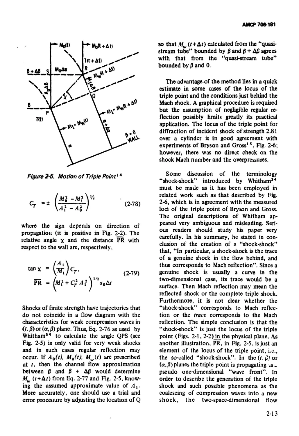
Текст
AMC PAMPHLET
АМСР 706-181
ENGINEERING DESIGN
HANDBOOK
EXPLOSIONS IN AIR
PART ONE
D D C
D
Reproduced by
NATIONAL TECHNICAL
INFORMATION SERVICE
US Deoertmen* of Commorc*
SpriW, VA. 22151
HEADQUARTERS, U S ARMY MATERIEL COMMAND
DEPARTMENT OF THE ARMY
HEADQUARTERS UNITED STATES ARMY MATERIEL COMMAND
5001 Eisenhower Ave, Alexandria, VA 22333
AMC PAMPHLET
No. 706-181
ENGINEERING DESIGN HANDBOOK
EXPLOSIONSJNr?tfR, PART ONE
TABLE OF CONTENTS
Paragraph
Page
15 July 1974
LIST OF ILLUSTRATIONS............... viii
LIST OF TABLES ..................... xv
PREFACE............................. xvii
CHAPTER 1. GENERAL PHENOMENOLOGY
1-0 List of Symbols ...................................... 1-1
1-1 Definition of Explosion............................... 1—2
1-2 Blast Wave Characteristics............................ 1—2
1-3 “Ideal” Blast Waves in Free Air....................... 1-2
1-3.1 Measured Primary Shock Characteristics................ 1-2
1-3.2 Functional Forms of Primary Shock
Characteristics................................................ 1-3
1-3.2.1 Pressure-Time History................................... 1—3
1-3.2.1.1 Positive Phase ....................................... 1—3
1—3.2.1.2 Negative Phase ....................................... 1-4
1—3.2.2 Particle Velocity and Other Parameters......... 1-5
1—3.3 Secondary and Tertiary Shock Characteristics.... 1—5
l-£ “Nonideal” Blast Waves ............................... 1-5
1-4.1 In Free Air........................................... 1-5
1—4.2 Ground Effects........................................ 1-6
1 —5 Reflection and Diffraction of Blast Waves.............. 1—7
1—5.1 Reflection of a Plane Wave............................ 1-7
1-5.1.1 Types of Reflection..................................... 1-7
1-5.1.1.1 Normal Reflection ................................. 1-7
I-5.1.1.2 Regular Oblique Reflection......................... 1-8
1-5.1.1.3 Mach Reflection ................................... 1-9
1-5.1.2 Reflection Process................................ 1-10
1-5.1.2.1 Strong Shock Waves ............................... 1-10
1-5.1.2.2 Weak Shock Waves.................................. 1—11
i
АМСР 706*181
TABLE OF CONTENTS (Con't.)
Paragraph Page
1-5.2 Diffraction of a Plane Wave........................... 1-11
1—5.2.1 Two-dimensional Rigid Thick Wall ............... 1-12
1-5.2.2 Three-dimensional Block......................... 1-13
1-5.2.3 Circular Cylinder............................... 1-14
1-6 Effects on Blast Waves............................. 1-16
1—6.1 Shape or Asymmetry of Source on Blast Waves ... 1-16
1-6.1.1 Common Shapes................................... 1-16
1-6.1.1.1 Straight Line Charge.............................. 1-17
1-6.1.1.2 Muzzle Blast...................................... 1-17
1 --u.1.1.3 Large Plane Charge.............................. 1-17
1-6.1.2 Distance Effect................................. 1-17
1-6.2 Long-range Focusing............................. 1-18
1-6.2.1 Homogeneous Medium ............................. 1-18
1-6.2.2 Inhomogeneous Medium............................ 1-18
1- 6.2.2.1 Theory........................................... 1-19
1-6.2.2.2 Practice.......................................... 1-20
1-6.3 Variation of Types of Energy Source.............. 1-21
1-6.3.1 Chemical Explosives ................................ 1—21
1-6.3.2 Nuclear Explosives .............................. 1-22
1-6.3.3 Other Sources ................................... 1-23
References..................................... 1 -24
CHAPTER 2. AIR BLAST THEORY
2-0 List of Symbols..................................... 2-1
2—1 General........................................... . 2—2
2—2 Basic Equations..................................... 2—3
2-2.1 Coordinate Systems............................... 2-3
2-2.2 Forms of Equations............................... 2-3
2-2.2.1 Lagrangian....................................... 2-3
2-2.2.2 Eulerian......................................... 2-4
2-2.3 Rankine-Hugoniot Conditions ..................... 2-4
2-2.4 Single Spatial Variable Cases.......................... 2-5
2-2.4.1 Linear Flow...................................... 2-5
2-2.4.2 Spherically Symmetric Flow....................... 2-5
2-2.4.3 Cylindrically Symmetric Flow..................... 2-5
2-2.4.4 Application...................................... 2-6
2-3 Analytic Solutions to Equations..................... 2-6
2-3.1 Taylor’s Similarity Solution for Spherically
Symmetric Blast Waves.....................t . 2-6
2-3.2 Initial Conditions for Solutions................. 2-9
2-3.2.1 Initial Isothermal Spherical Detonation Front.. . 2-9
2-3.2.2 Other Initial Conditions ....................... 2—10
2-3.3 Mach Shock Reflection........................... 2-10
2-3.4 Some Recent Theories............................ 2—14
2-3.4.1 Weak Shock Regime of a Blast Wave............... 2-14
2-3.4.2 Intermediate and Strong Shock Strengths...... 2-16
АМСР 708-181
TABLE OF CONTENTS (Ccn't.)
Paragraph
2—3.5 Theilheimer’s Solution for the “Time Constant"
of an Air Blast Wave....................................... 2-19
2—4 Summary of Pertinent Equations........................ 2-20
2—4.1 Basic Equations of Motion....................... 2-21
2—4.2 Rankinc-Hugoniot Conditions .................... 2-21
2-4.3 Basic Equations for Spherically Symmetric Flow.. 2-21
2-4.4 Taylor’s Similarity Solution ................... 2-21
2—4.5 Theilheimer’s Solution for Initial Decay of
a Shock................................................. 2-21
References...................................... 2-22
CHAPTERS. BLAST SCALING
3-0 List of Symbols.................................. 3-1
3-1 Introduction..................................... 3-2
3-2 Scaling Laws for Blast Parameters................ 3-2
3-2.1 Hopkinsor. Scaling............................... 3-2
3-2.1.1 Definition......................................... 3-2
3-2.1.2 Experimental Verification........................ 3-3
3-2.1.3 Implications ................................... 3-5
3-2.1.4 Model Analysis................................... 3-7
3-2.2 Sachs’ Scaling .................................. 3-9
3-2.2.1 Assumptions..................................... 3-11
3-2.2.2 Model Analysis.................................. 3-11
3-2.2.3 Experimental Verification....................... 3-13
3-2.2.4 Application................................... 3-13
3-2.3 Other Scaling Law", for Blast Pi rameters..... 3-15
3-2.3.1 Additional Blast Source Pararleter.............. 3-15
3-2.3.2 Small Scaled Distances......................... 3-17
3-2.3.3 Wecken’s Law?..................................... 3-18
3-3 Scaling Laws for Interaction With Structures.. 3-20
3-3.1 “Replica” Scaling ....................... 3-20
3-3.2 Scaling for Impulsive Loading................... 3-21
3-3.3 Missile Response to Air Blast .................. 3-23
3—4 Limitations of Scaling Laws..................... 3-23
References...................................... 3-24
CHAPTER 4. COMPUTATIONAL METHODS
4-0 List of Symbols.................................. 4-1
4—1 General.......................................... 4—2
4-2 Methods With Discontinuous Shock Fronts ...... 4 -2
4-2.1 Kirkwood and Brinkley Method .................... 4-2
4-2.2 Granstrom Method................................. 4-5
4-2.3 Method of Characteristics........................ 4-6
4-3 Methods With Fictitious Viscosity................ 4-8
iii
АМСР 706-181
TABLE OF CONTENTS (Con't.)
Paragraph Page
4-3.1 Brode’s Method.................................... 4-9
4-3.2 WUNDY Code (NOL) and LSZK Equation
of State....................................... 4-13
4-4 Particle and Force (PAF) Method....................... 4-16
4-4.1 Governing Equations.............................. 4-17
4-4.2 The Finite Difference Forms 4-18
4-4.2.1 Neighbors .................................... 4-18
4-4.2.2 Forces........................................ 4—19
4-4.2.2.1 Nondissipative................................ 4-19
4-4.2.2.2 Dissipative................................... 4-21
4—4.3 Test Cases ......................................... 4—22
4—4.3.1 Flow Past a Wedge............................. 4-22
4—4.3.2 Flow Past a Blunt Cylinder.................... 4-23
4—4.3.3 Flow Past a Cone.............................. 4—23
4-5 Particle-in-cell (PIC) Method......................... 4-24
4-5.1 State Equations.................................. 4-24
4—5.2 Two-dimensionai Demonstration Problem.......... 4—25
4-5.2.1 Phase 1 of Calculation............................ 4—25
4-5.2.2 Phase 2 of Calculation (The Transport of
Material) ................................... 4—27
4—5.2.3 Phase 3 of Calculation (Functionals of Motion). . 4—27
4—5.3 Other Boundary Conditions ....................... 4—27
4—6 Fluid-in-ce)’ (FLIC) Method .......................... 4-29
4-6.1 Computing Mesh................................... 4—29
4—6.2 The Difference Equations......................... 4—30
4-6.2.1 Step 1 ........................................... 4-30
4-6.2.2 Step 2 ......................................... 4-31
4-6.2.3 Boundary Conditions and Stability............... 4—33
4—7 Comparisons of Various Methods................. 4- 34
References ...................................... 4—35
CHAPTER 5. AIR BLAST EXPERIMENTATION
5—0 List of Symbols................................ 5 — 1
5-1 General........................................... 5-1
5-2 Units and Dimensions for Blast Data............... 5-2
5-3 “Free Air” Measurements........................... 5-2
5-4 Measurements for Blast Sources on the Ground . . . 5-5
5-5 Measurements of Mach Waves and Other Obliquely
Reflected Waves........................................... 5-10
5—6 Measurements of Normally Reflected Waves....... 5-12
5—7 Measurements Under Real and Simulated Altitude
Conditions.................................... 5 — 13
5-8 Measurements for Sequential Explosions......... 5-16
5-9 Accuracy of Measurement of Blast Parameters.... 5- -18
References....................................... 5-19
iv
АМСР 706-181
TABLE OF CONTENTS (Ccn't)
Paragraph Page
CHAPTER 6. COMPILED AIR BLAST PARAMETERS
6-0 List of Symbols............................... 6-1
6-1 General........................................... 6-2
6-2 Sources of Compiled Data on Air Blast............. 6-2
6-3 Generation of Tables and Graphs of Air Blast Wave
Properties ...................................... 6-3
6-3.1 Shock-front Parameters............................ 6 -4
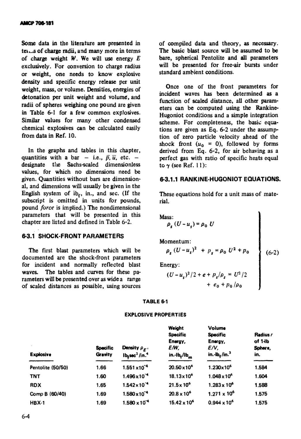
6-3.1.1 Rankine-Hugoniot Equations.......................... 6-4
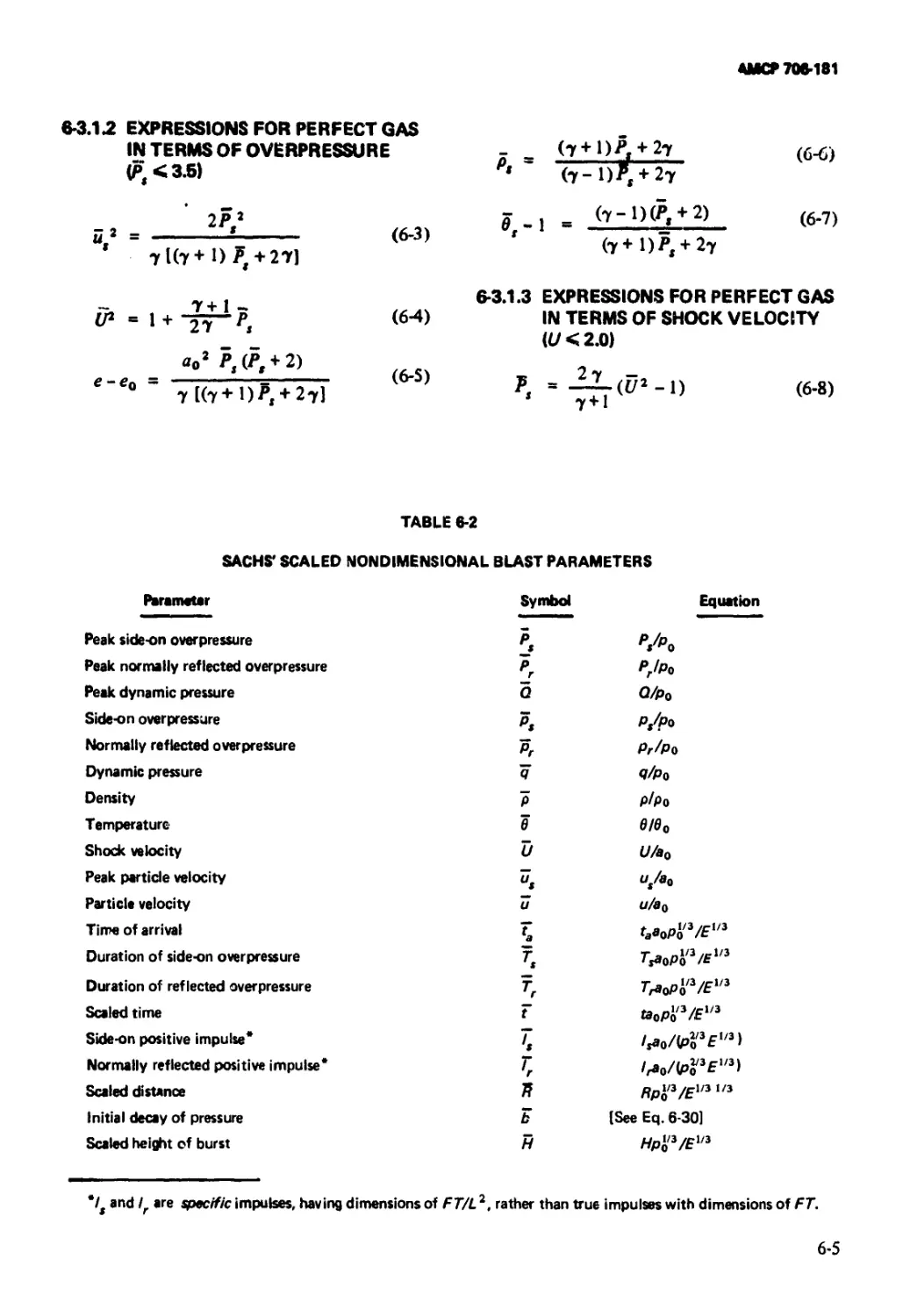
6—3.1.2 Expressions for Perfect Gas in Terms of
Overpressure (Ps < 3.5) ......... 6-5
6—3.1.3 Expressions for Perfect Gas in Terms of Shock
Velocity (U < 2.0)........................................ 6-5
6—3.2 Impulses and Durations............................ 6-9
6—3.3 Time Constant and Initial Decay Rate............. 6-11
6—3.4 Oblique Reflection Data........................... 6—12
6 -3.5 Conversion Factors............................... 6—15
6—4 Example Calculations ............................ 6-17
References ...................................... 6-21
CHAPTER?. AIR BLAST TRANSDUCERS
7-0 List of Symbols................................... 7-1
7-1 General........................................... 7-1
7-2 Pressure Transducers.............................. 7-1
7—2.1 Side-on Gages .................................... 7-1
7—2.1.1 BRL Side-on Gages.................................. 7—2
7-2.1.2 Southwest Research Institute Side-on Gages .... 7-2
7-2.1.3 Atlantic Research Corporation Side-on Gages . . . 7-4
7—2.1.4 British Side on Gages ............................. 7-4
7-2.1.5 Other Side-on Gages ............................... 7-6
7-2.2 Reflected Pressure Gages.......................... 7-6
7-2.3 Miniature Pressure Gages............................. 7-7
7-2.3.1 BRL Miniature Transducers.......................... 7-8
7-2.3.2 Langley Research Center Miniature Transducers . 7-8
7-2.3.3 Other Minature Transducers ........................ 7-10
7-3 Arrival-time Gages and Zero-time Markers ........ 7-14
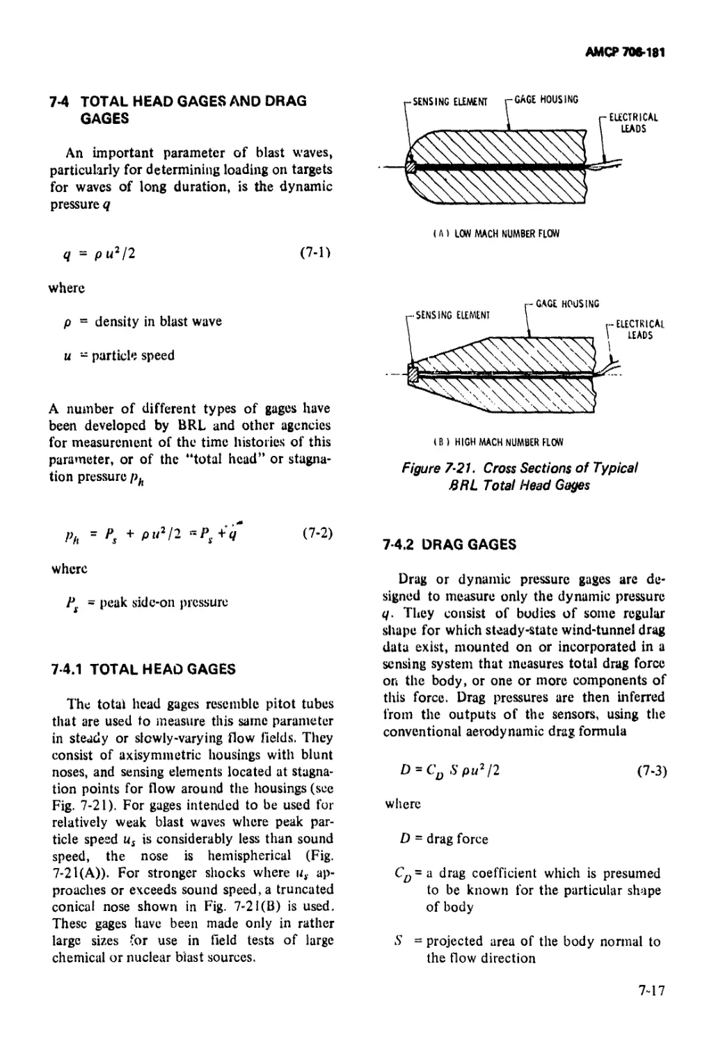
7—4 Total Head Gages and Drag Gages....................... 7-17
7—4.1 Total Head Gages ............................... 7—17
7-4.2 Drag Gages................................... 7-17
7—4.2.1 Drag Gage of Johnson and Ewing ................... 7-18
7-4.2.2 NOL Drag Force Gages......................... 7-18
7-4.2.3 SRI Drag Probes................................ 7-18
7—4.2.4 BRL Biaxial Drag Gage......................... 7-19
7—5 Density Gage ......................... 7-19
7-6 Impulse Transducers......................... 7-20
v
АМСР 706-181
TABLE OF CONTENTS (Con't.)
Paragraph Page
«
7-6.1 Free Plug Transducer............................ 7-20
7-6.2 Sliding Piston Gage............................. 7-21
7-6.3 Spring Piston Gage.............................. 7-21
7-7 Various Mechanical Gages........................ 7-21
7-7.1 Deformation Gages............................... 7-21
7-7.2 Peak Pressure Gages............................. 7-22
7-8 Summary......................................... 7-26
References....................................... 7-33
CHAPTER 8. INSTRUMENTATION SYSTEMS
8-1 General.......................................... 8-1
8-2 Ground-based Instrumentation Systems............. 8-1
8-2.1 Cathode-ray-tube Systems......................... 8-1
8-2.1.1 The BRL CRT Systems.............................. 8-2
8-2.1.2 The CEC Type 5-140 CRT System.................... 8-4
8-2.1.3 British CRT Systems.............................. 8-4
8-2.1.4 The Denver Research Institute CRT System ... 8-4
8—2.1.5 The Langley Research Center CRT System........ 8—6
8-2J .6 Other CRT Systems ............................... 8-6
8-2.2 Magnetic Tape Systems............................ 8-6
8-2.3 Galvanometer Oscillograph Systems................ 8-9
8-2.4 Transient Recorders ............................ 8-10
8-2.5 Instrumentation Problems Associated With Nuclear
Blast Tests................................... 8—10
8-2.5.1 TREE.......................................... 8-11
8-2.5.2 EMP............................................. 8-11
8—2.5.2.1 EMP Generation ............................... 8—11
8-2.5.2.2 Near Surface Burst............................ 8-11
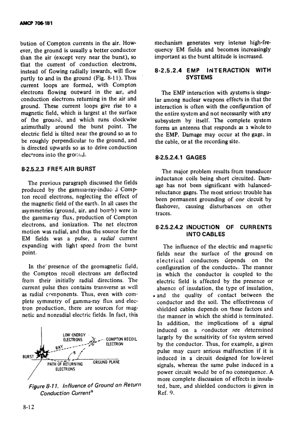
8-2.5.2.3 Free Air Burst................................ 8-12
8—2.5.2.4 EMP Interaction With Systems ................. 8-12
8-2.5.2.4.1 Gages......................................... 8-12
8-2.5.2.4.2 Induction of Currents into Cables............. 8-12
8-2.5.2.4.3 Recording Systems ............................ 8-13
8-3 Portable Systems...................................... 8-13
8-3.1 Galvanometer Oscillograph Systems............... 8-13
8-3.2 Magnetic Tape Recorder Systems ................. 8-14
8-3.2.1 The Leach MTP.-l 200 Recorder................... 8-14
8-3.2.2 The Genisco Г ata 10-110 Recorder............... 8—14
8-3 2.3 Typical Portable Magnetic Tape Recorder
Systems...................................... 8-15
8-3 3 Self-recording Gages ........................... 8-17
8-3.3.1 Blast Pressure Sensors.......................... 8-19
8-3.3.2 Time Base....................................... 8-19
8-3.3.3 Initiation Methods.............................. 8-20
8-3.3.4 Acceleration Methods............................ 8-20
vi
АМСР 706-181
TABLE OF CONTENTS (Con't.)
Paragraph Page
8-4 Calibration Techniques................................ 8-20
References................................... 8—25
CHAPTER 9. PHOTOGRAPHY OF BLAST WAVES
9—1 General........................................... 9-1
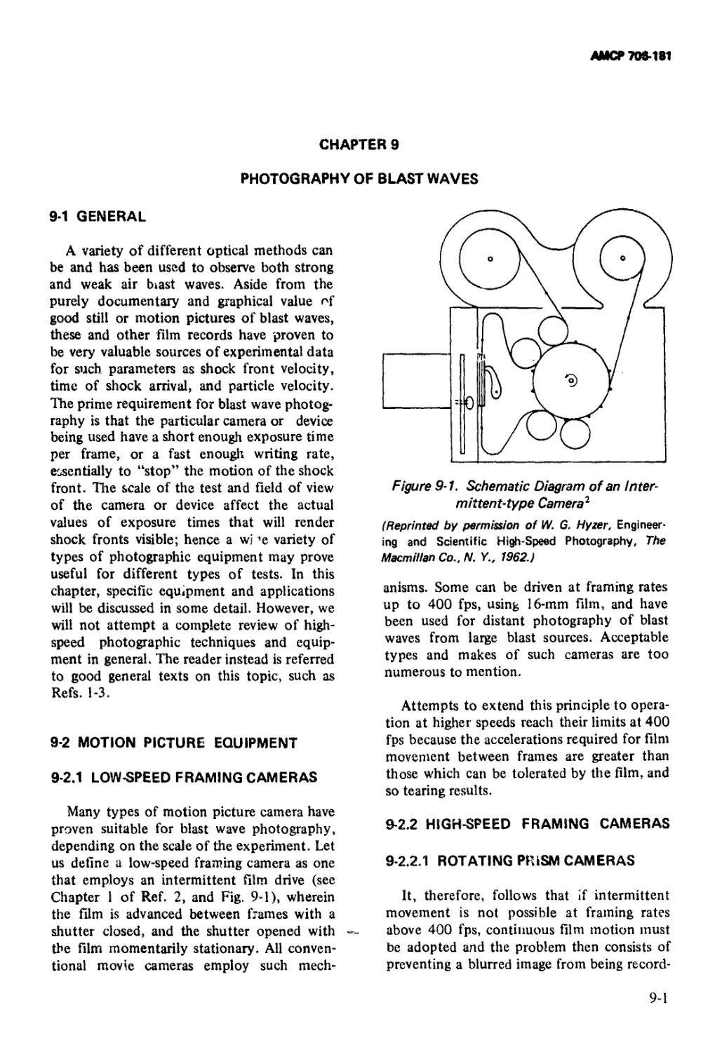
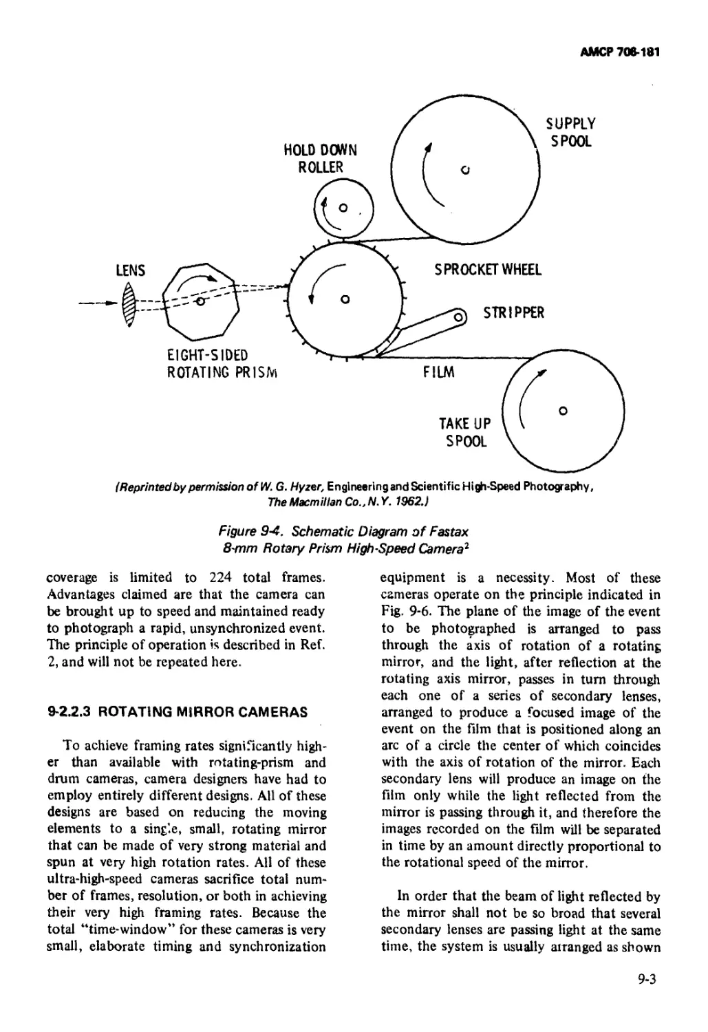
9-2 Motion Picture Equipment ......................... 9-1
9-2.1 Low-speed Framing Cameras ........................ 9-1
9-2.2 High-speed Framing Cameras........................ 9-1
9-2.2.1 Rotating Prism Cameras............................ 9-1
9-2.2.2 Rotating Drum Cameras............................. 9-2
9-2.2.3 Rotating Mirror Cameras........................... 9-3
9-2.2.4 Image Dissector Cameras........................... 9-4
9—3 Streak Photography Equipment ..................... 9-6
9-4 Still Photography Equipment....................... 9-7
9-4.1 Conventional Cameras.............................. 9-7
9-4.2 Fast Shutter Cameras.............................. 9-7
9-4.3 Image Converter Cameras........................... 9-9
9-5 Shadowgraph and Schlieren Equipment.............. 9-13
9-5.1 Shadowgraph Equipment............................ 9-13
9-5.2 Schlieren Equipment.............................. 9-14
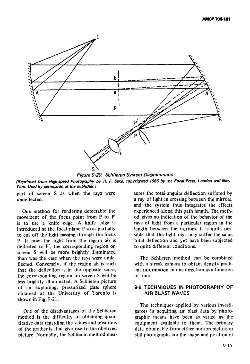
9-6 Techniques in Photography of Air Blast Waves .... 9-15
References ...................................... 9-22
CHAPTER 10. DATA REDUCTION METHODS
10-0 List of Symbols.................................. 10-1
10—1 General.......................................... 10—1
10—2 Reduction of Film and Paper Traces................... 10-1
10—2.1 Types of Rec rds ................................ 10-1
10-2.2 Reading of Records............................... 10-3
10—2.3 Record Correction for Gage Size and Flow
Effects........................................ 10—4
10-2.4 Reduction of Dynamic Pressure Data ................ 10-5
10-2.5 Determination of Positive Phase Duration .......... 10-7
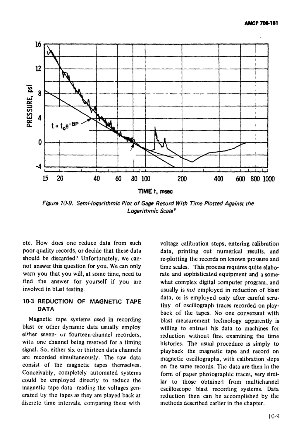
10-3 Reduction of Magnetic Tape Data ................. 10-9
10-4 Reduction of Data from Self-recording Gages.. 10-10
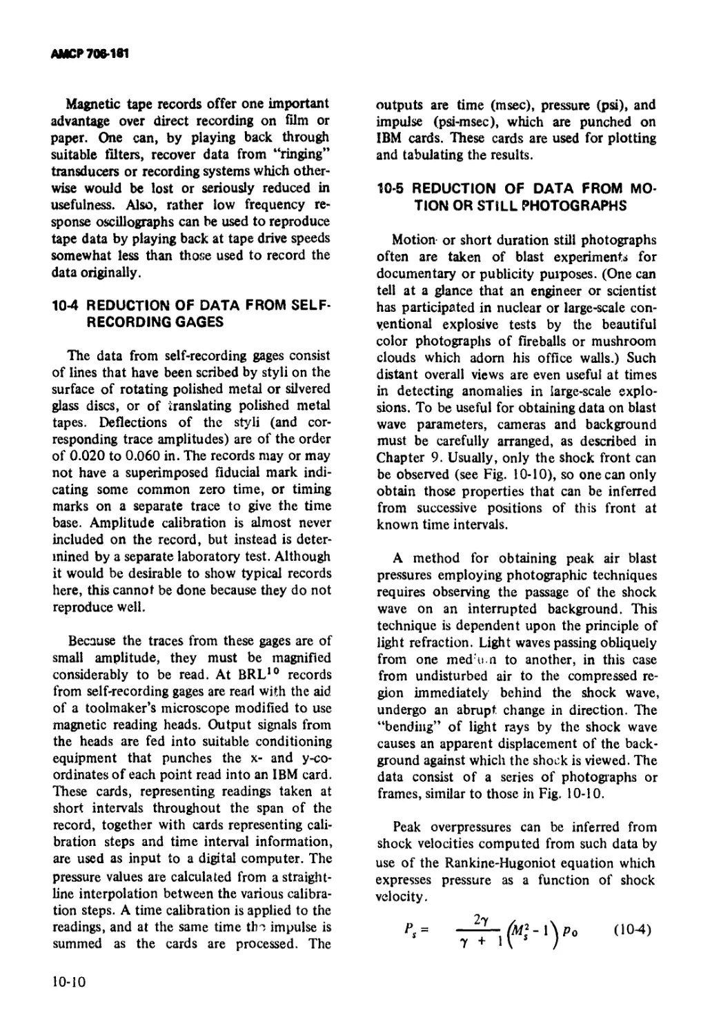
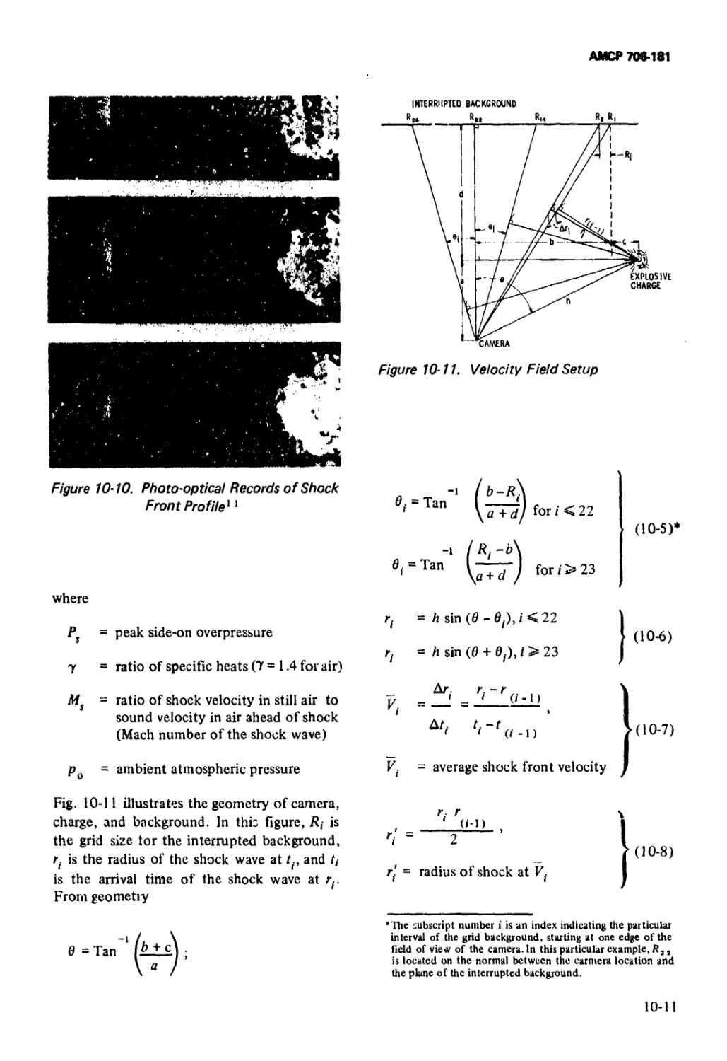
10-5 Reduction of Data from Motion or Still
Photographs.................................... 10-10
10-6 Other Data Reduction............................ 10-12
References ..................................... 10-13
BIBLIOGRAPHY...................................... B-l
INDEX............................................. 1-1
vii
АМСР 706-181
LIST OF ILLUSTRATIONS
Fig. No. Title Page
I-1 Ideal Blast Wave ........................................ 1-3
1-2 Recorded Pressure-Time Histories of Actual Blast
Waves from l-lbm Pentolite Explosive Spheres ... 1-6
1-3 P-T Curves Produced by a Cased Charge ................... 1-7
1-4 Typical Nonideal Pressure Traces Showing
Precursor......................................... 1-8
1-5 Normal Reflection of a Plane Shock from a Rigid
Wall.............................................. 1-8
1—6 Regular Oblique Reflection of a Plane Shock from a
Rigid Wall........................................ 1-9
1—7 Mach Reflections from a Rigid Wall............... 1 — 10
1 -8 Reflection of Strong Shock Waves................. 1-11
1—9 Geometry of Mach Reflection...................... 1-12
1-10 Reflection of Weak Shock Waves................... 1 — 12
1 — 11 Diffraction of a Shock Front Over a Wall .......... 1—13
1-12 Diffraction of a Shock Front Over a Three-dimen-
sional Block Structure (Plan View) .............. 1-14
1 — 13 Pressures on a Three-dimensional Block Structure
During Diffraction............................... 1-14
1 — 14 Tracings of Shadowgraphs Showing the Interaction
of a Shock Front With a Cylinder................. 1-15
1-15 Tracings of Shadowgraphs Showing the Interaction
of a Shock Front With a Cylinder................. 1-16
1-16 The Blast Wave from a 7.62 mm,'Riflc at Three
Stages of Expansion.............................. 1-17
1-17 Incident Shock Overpressure Ratio vs Scaled
Distance......................................... 1-18
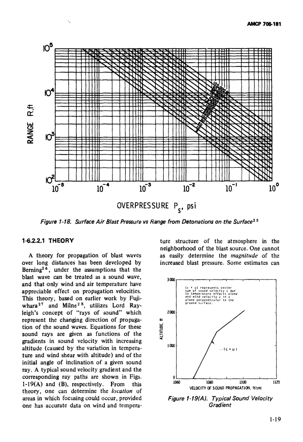
1-18 Surface Air Blast Pressur. vs Range from
Detonations on the Surface.................................. 1-19
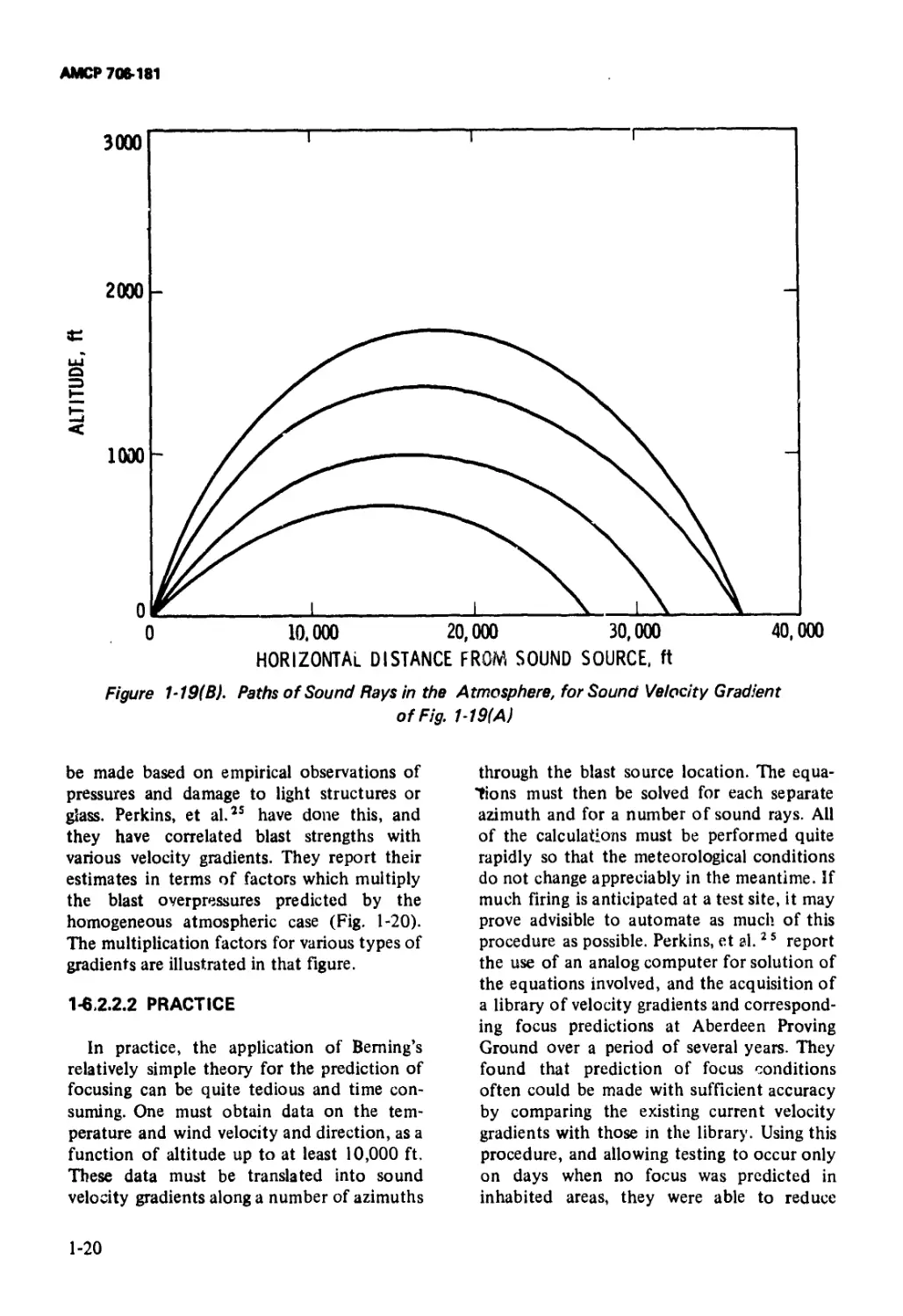
I-19(A) Typical Sound Velocity Gradient................... 1 — 19
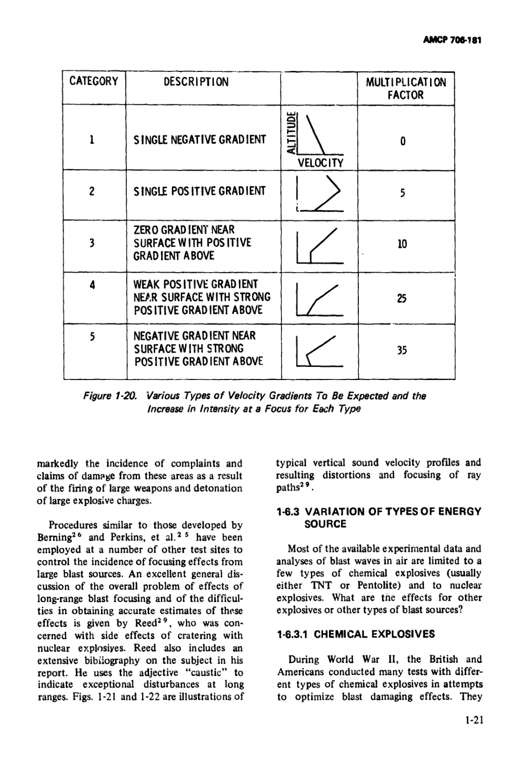
1 - 19(B) Paths of Sound Rays in the Atmosphere, for Sound
Velocity Gradient of Fig. 1-19(A)................ 1-20
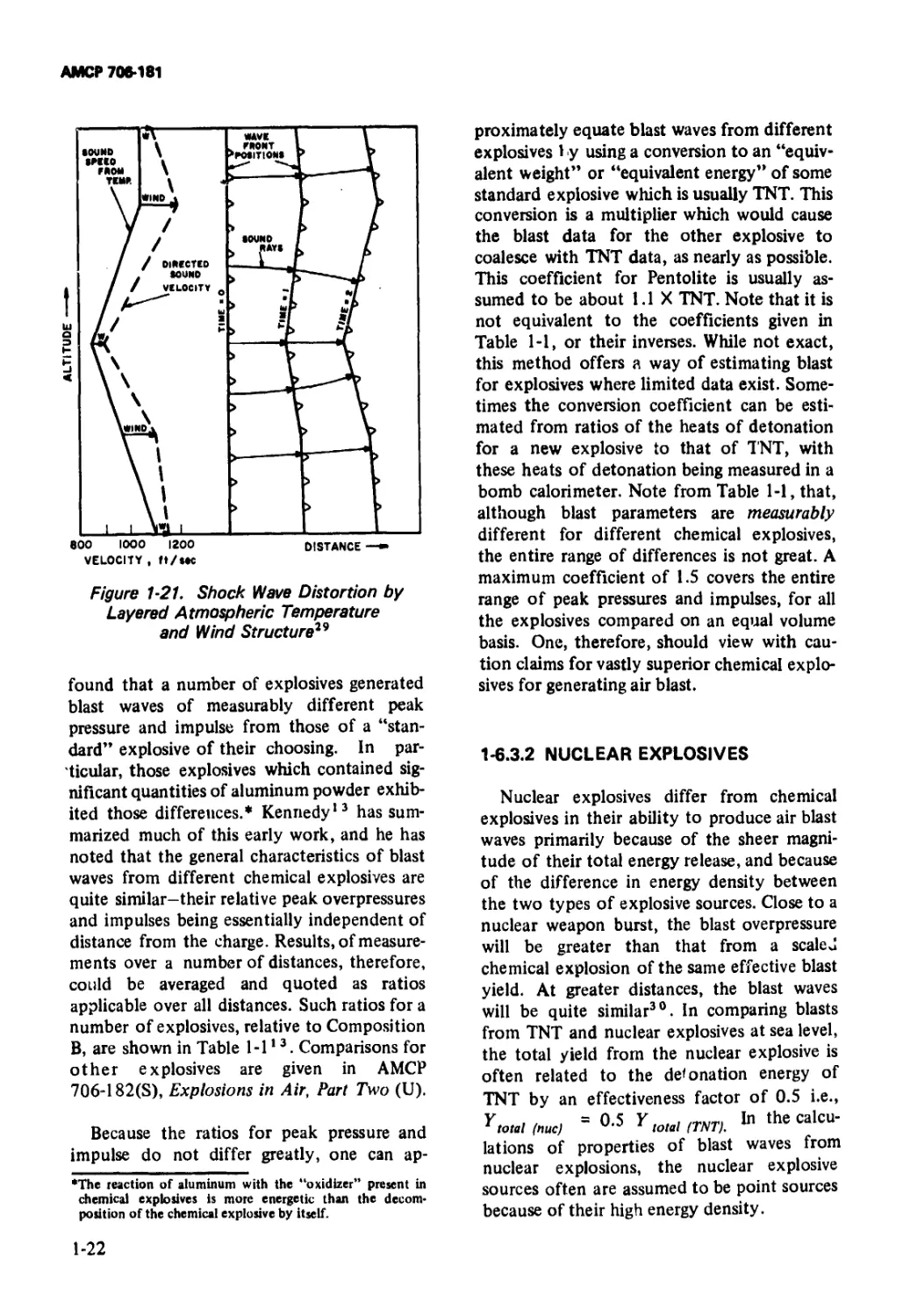
1-20 Various Types of Velocity Gradients To Be Expected
and the Increase in Intensity at a Focus for Each
Type........................................... 1-21
1-21 Shock Wave Distortion by Layered Atmospheric
Temperature and Wind Structure................. 1 -22
1-22 Typical Explosion Ray Paths.......................... 1 -23
1-23 Variation of Peak Overpressure Ratios P With
Shock Radius Xs for Various Explosions......... 1—24
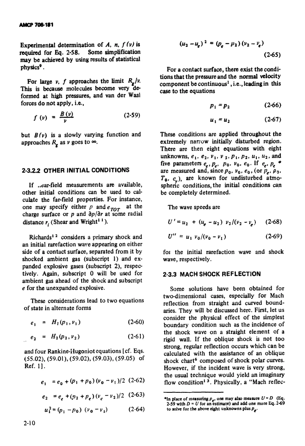
2-1 Mach Shock Reflection.............................. 2-11
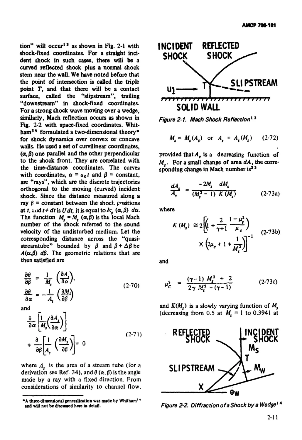
2—2 Diffraction of a Shock by a Wedge ................. 2-11
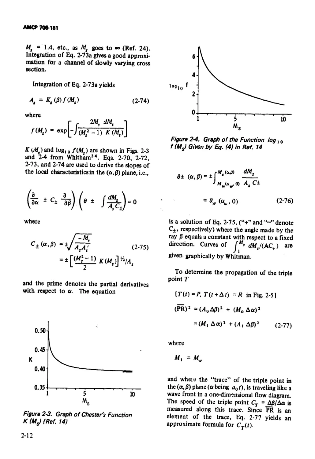
2-3 Graph of Chester’s Function K(MS) ................. 2-12
2-4 Graph of the Function loe i 0 f(Ms) Given by Eq. (4)
in Ref. 14.................................................. 2-12
2-5 Motion of Triple Point ............................ 2-13
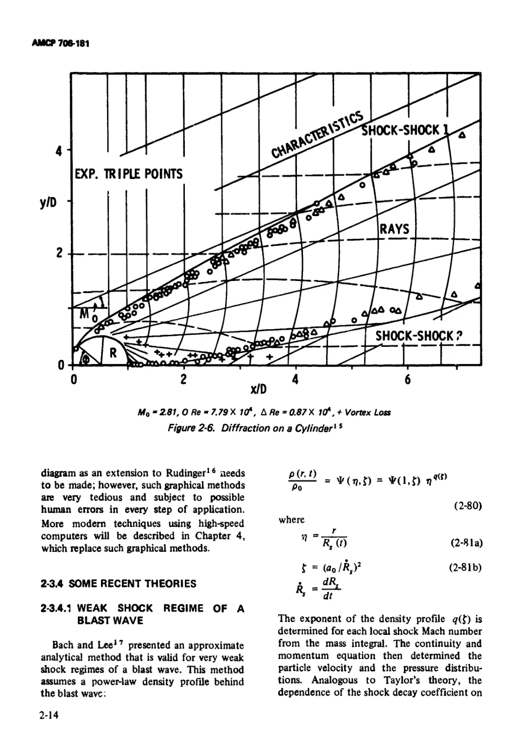
2-6 Diflrautio: on a Cylinder.......................... 2-14
viii
АМСР 706-181
LIST OF ILLUSTRATIONS (Con't.)
Fig. No. Title Page
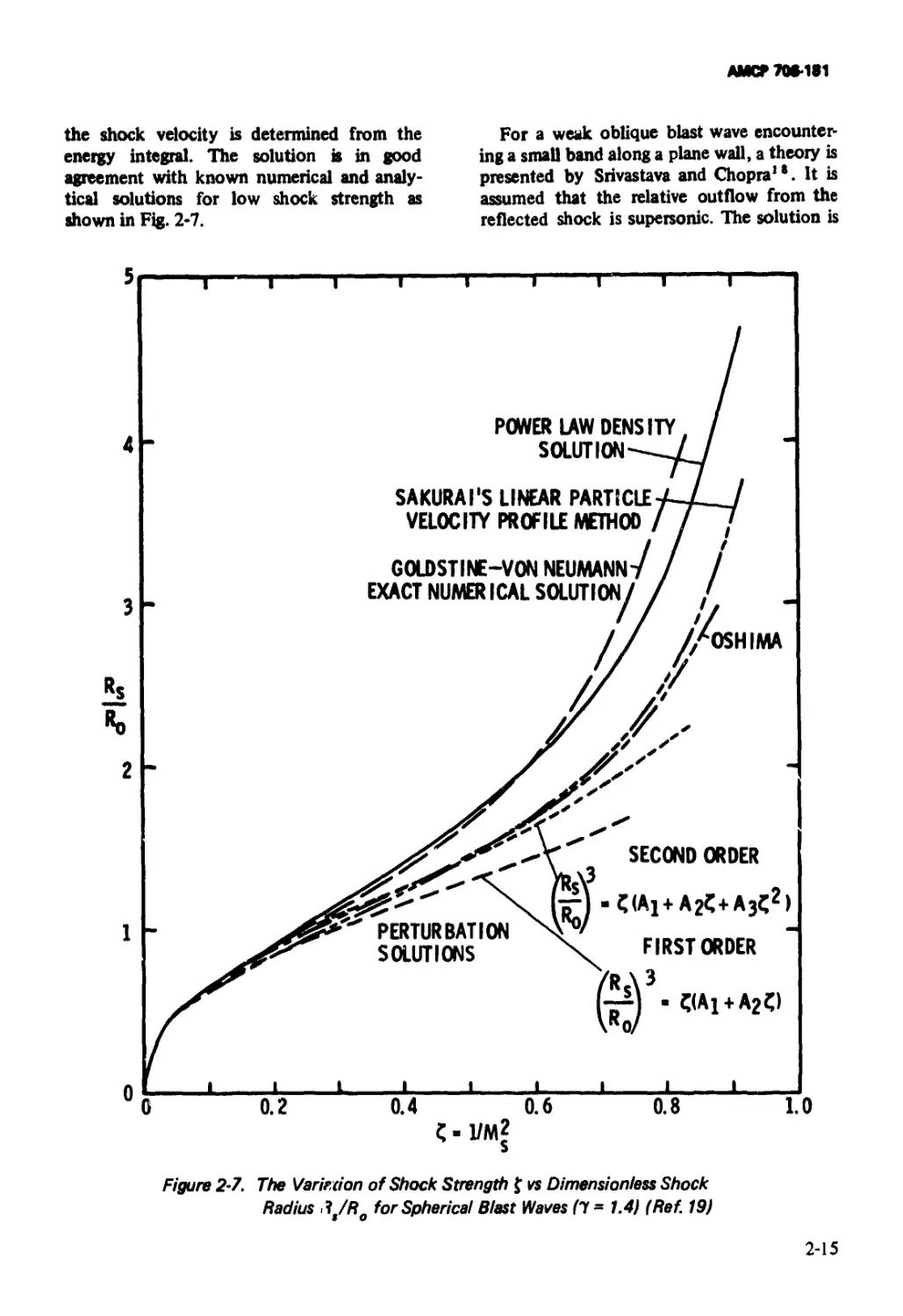
2-7 Variation of Shock Strength f vs Dimensionless
Shock Radius RjRo for Spherical Blast Waves,
7=1.4 ...................................................... 2-15
2—8 Spherical Blast Wave............................... 2—18
2-9 Cylindrical Blast Wave............................. 2-18
2-10 Plane Blast Wave .................................. 2-19
3—1 Hopkinson Blast Wave Scaling ....................... 3-4
3—2 Pressure-distance Curves for Ground-burst Blast of
Bare Charges................................................. 3-4
3—3 Experimental Positive Impulses vs Distance Curves
(on ground) from Various Sources ........................... 3-5
3-4 Comparisons of Peak Particle Velocities for Surface
Burst TNT Charges ........................................... 3-6
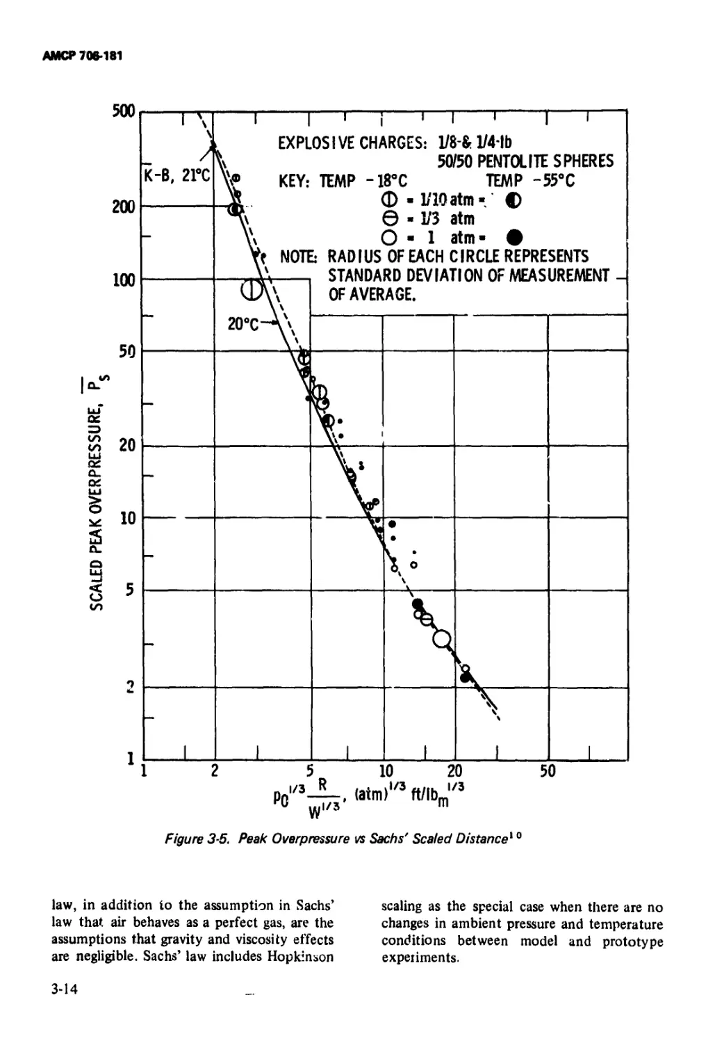
3—5 P. ,iк Overpressure vs Sachs’ Scaled Distance.... 3-14
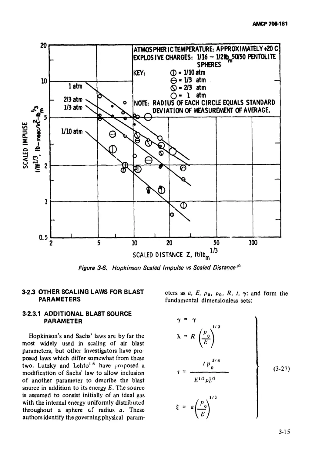
3—6 Hopkinson Scaled Impulse vs Scaled Distance...... 3-15
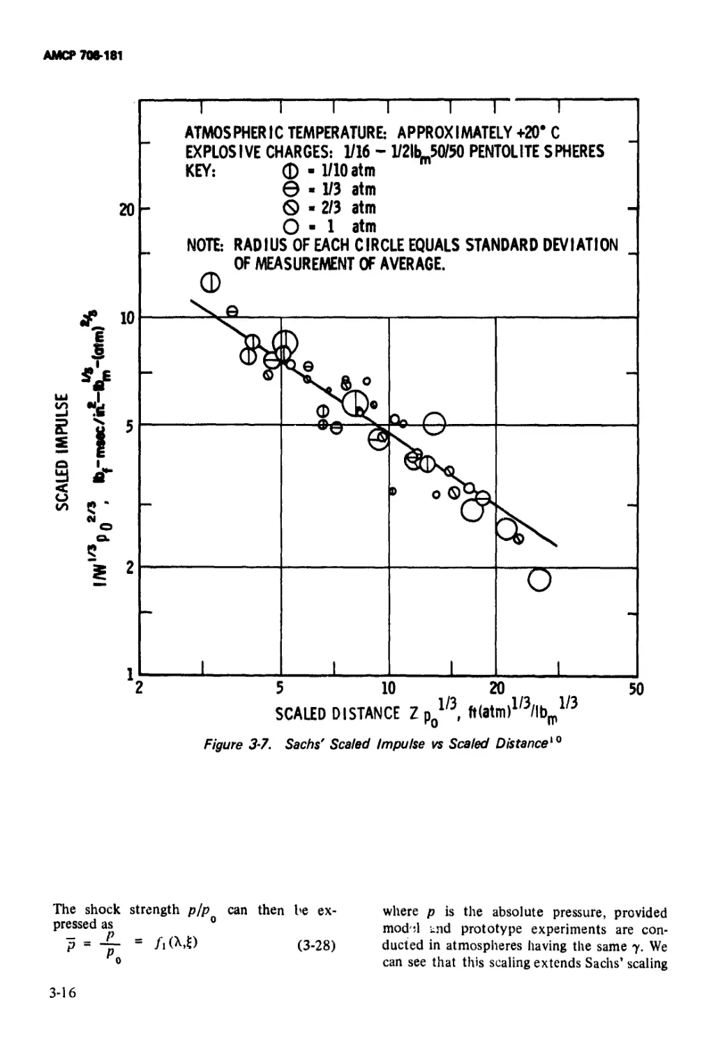
3-7 Sachs’Scaled Impulse vs Scaled Distance............ 3-16
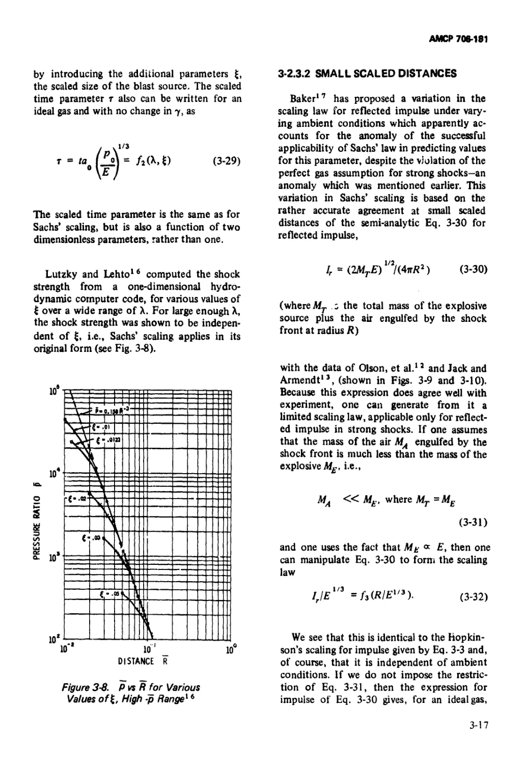
3-8 p vs Л for Various Values of £, High-p Range ...... 3-17
3-9 Comparison of Predicted and Measured Reflected
Impulse /r-Sea Level Conditions............................. 3-18
3-10 Comparison of Predicted and Measured Reflected
Impulse Ir-Reduced Pressure Ambient Conditions 3-19
3-11 “Replica” Scaling of Response of Structures to
Blast Loading............................................... 3-21
3-12 “Replica” Scaling of Elastic Response of Aluminum
Cantilevers io Air Blast Waves.............................. 3-22
3-13 “Replica” Scaling of Permanent Deformation of
Aluminum Cantilevers Under Air Blast Loading. . . 3-22
3—14 Peak Overpressure Ratio vs Scaled Distance........... 3-24
4—1 Peak Excess Pressure Ratio vs Distance in Charge
Radii for Pentolite at a Loading Density of
1,65 g/cm3........................................ 4-5
4-2 Initial Singularity in Method of Characteristics .... 4-6
4-3 Schematic of Region of Numerical Solution for
Method of Characteristics.................................... 4-8
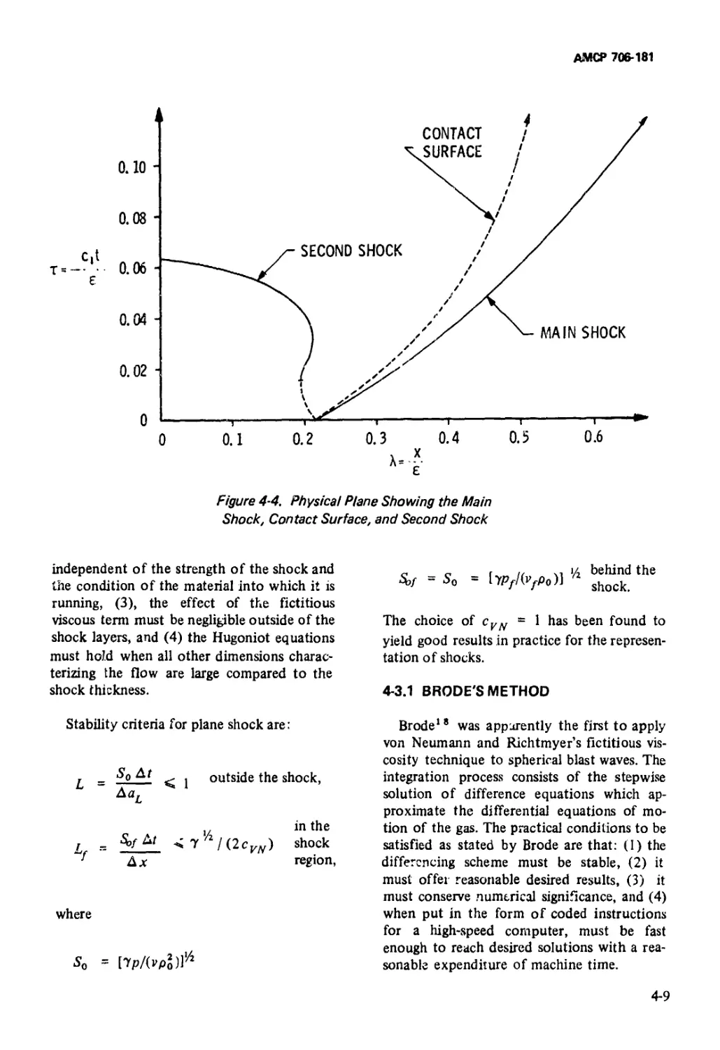
4-4 Physical Plane Showing the Main Shock, Contact
Surface, and Second Shock.................................... 4-9
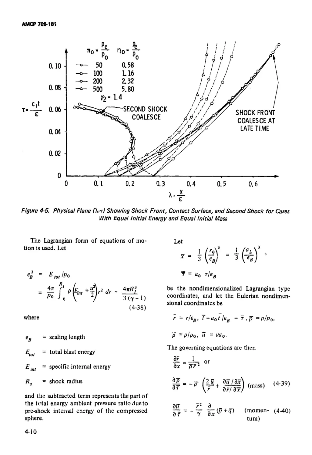
4-5 Physical Plane (X-т) Showing Shock Front, Contact
Surface, and Second Shock for Cases With Equal
Initial Energy and Equal Initial Mass ........... 4-10
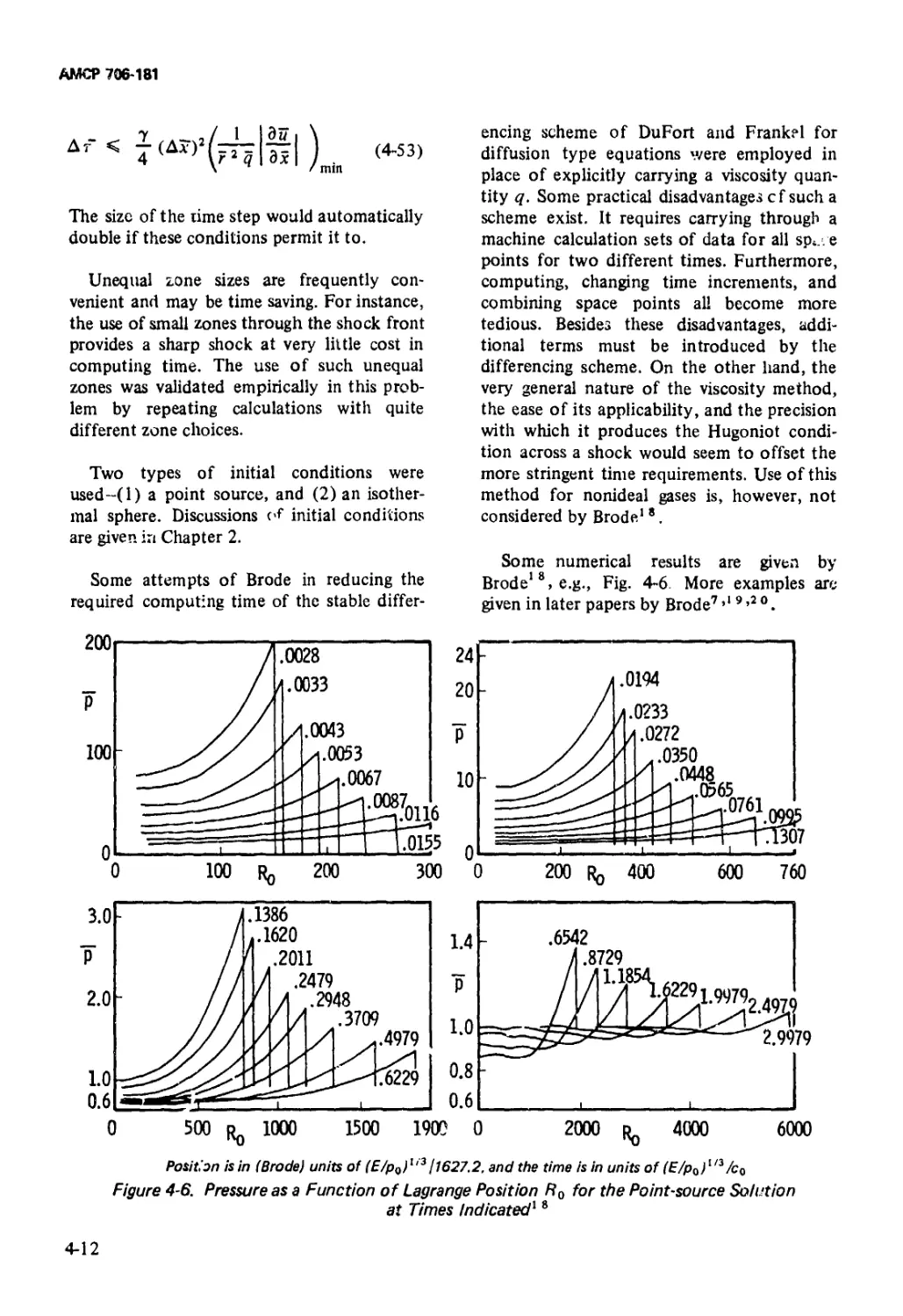
4-6 Pressure as a Function of Lagrange Position Ro for
the Point-source Solution at Times Indicated ... 4-12
4-7 A Comparison of the ?AF Detached Bow Wave
Positions (Dashed Lines) After Impact With Those
Observed in a Shock Tube Experiment Involving
a Mach 1.35 Flow Past a Wedge.................. 4 22
4-8 The Steady-state Detached Shock Front Position
in a Mach 1.58 Flow Past a Blunt Cylinder...... 4-23
ix
АМСР 706-181
Fig. No.
4-9
4-10
4-11
4-12
4-13
5-1
5-2
5-3
5-4(A)
5-4(B)
5-5
5-6
5 -7
5-8
5-9
5-10
5-11
5-12
5-13
5-14
J5-15
5-16
LIST OF ILLUSTRATIONS (Con't.)
Title Page
A Comparison of Steady-state PAF Pressures (the
Dots) Along the Cone Face With Experimental
Values Observed in a Mach 1.41 Flow Past a
75-degCone ........................................ 4-23
A Late-time PAF Particle Plot (the Dots) Compared
to an Experimental Steady-state Bow Wave........ 4-23
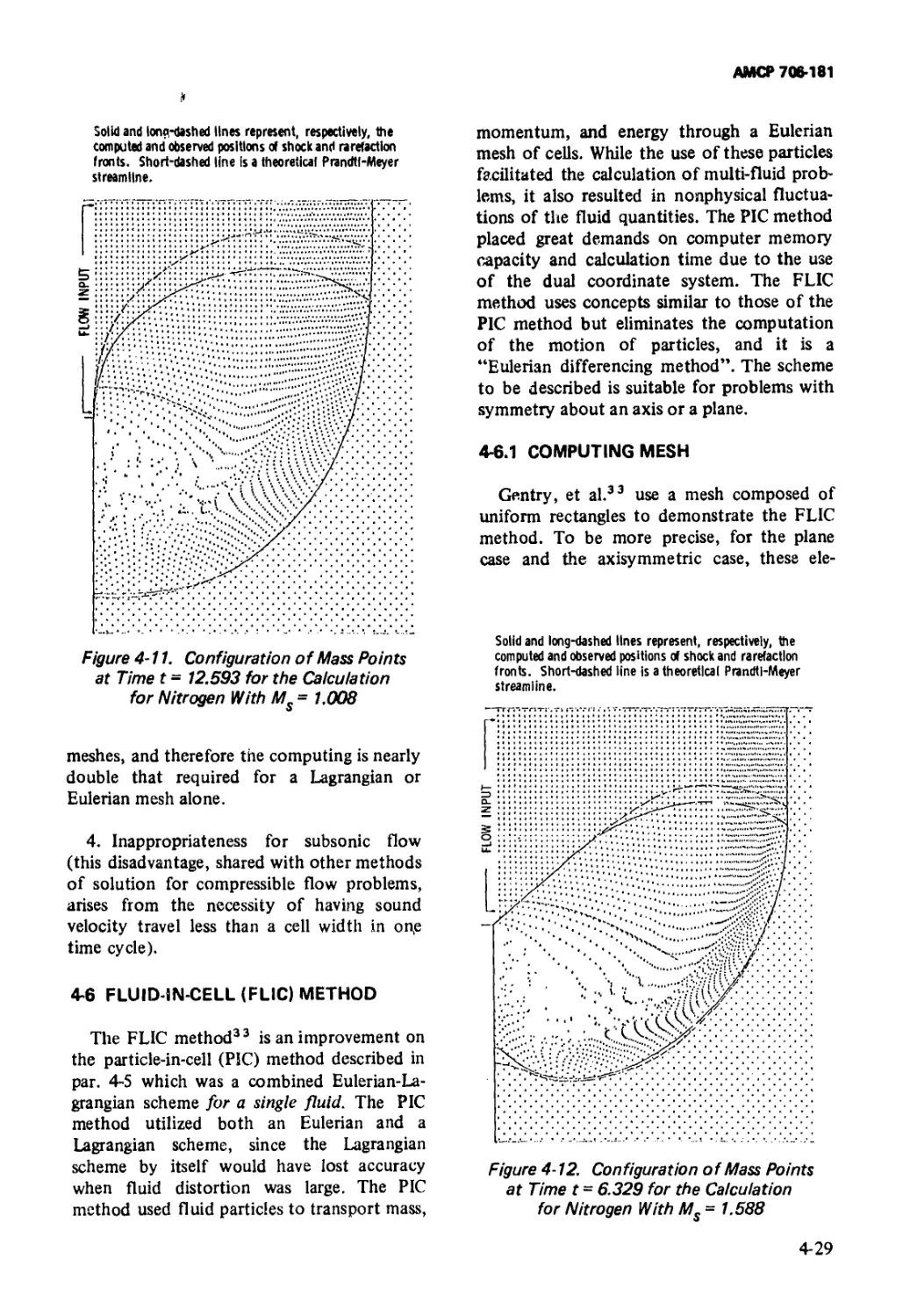
Configuration of Mass Points at Time t = 12.593
for the Calculation for Nitrogen With Ms -
1.008 ............................................. 4-29
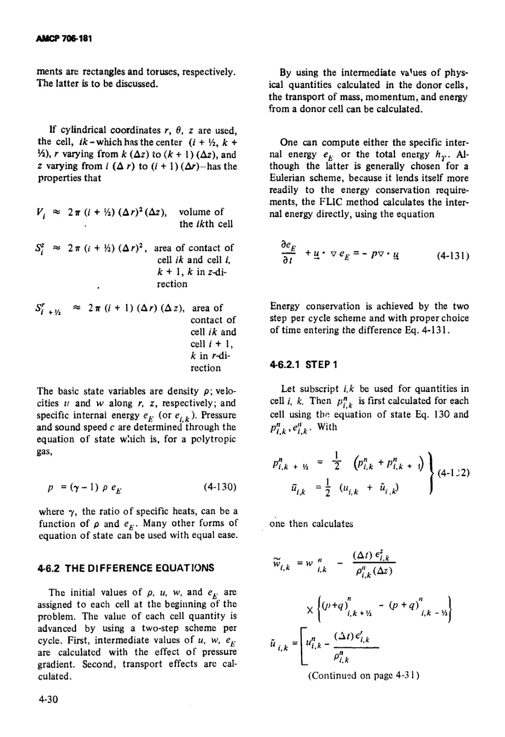
Configuration of Mass Points at Time t = 6.329 for
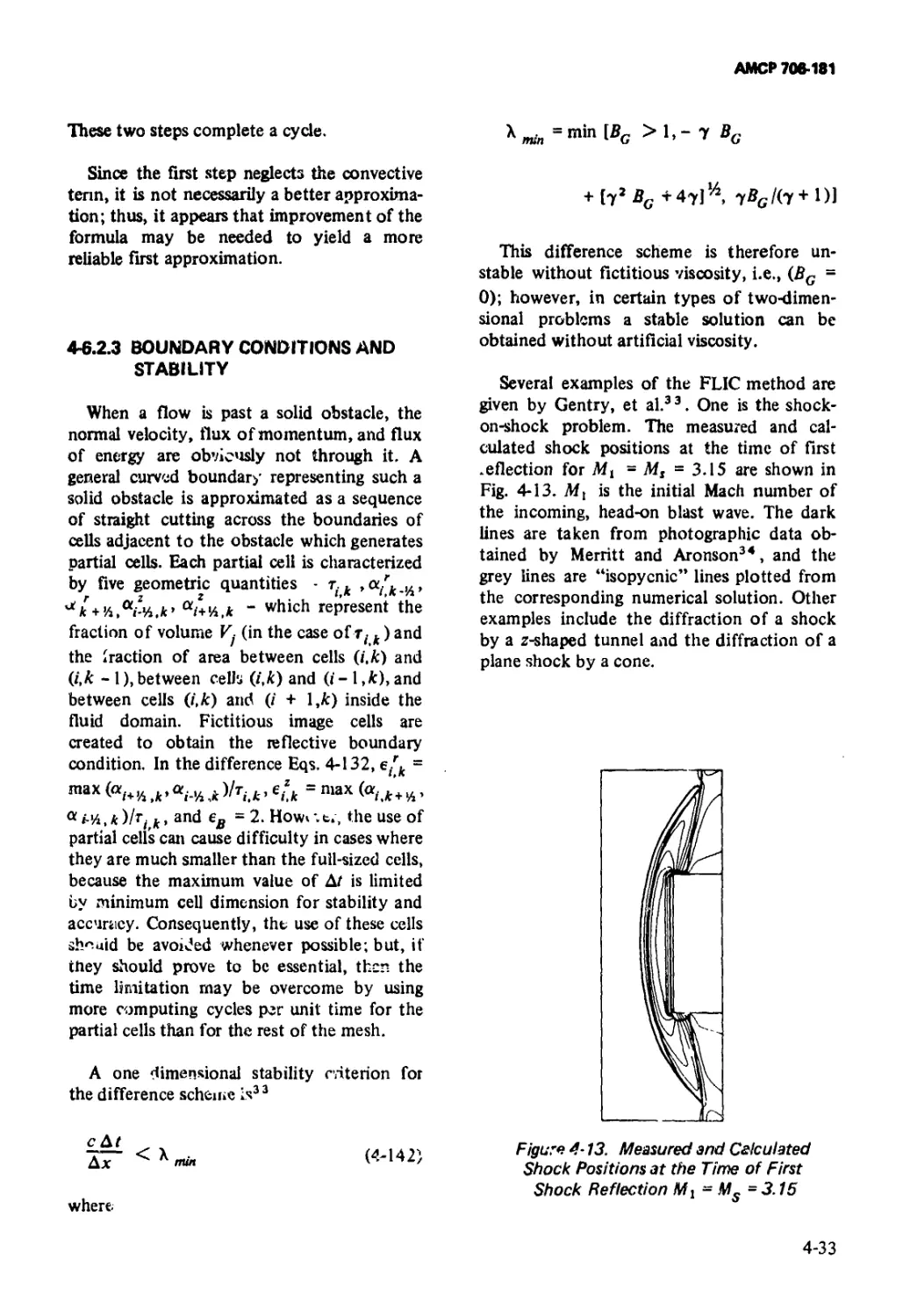
the Calculation for Nitrogen With Ms = 1.588 . . . . 4 -29
Measured and Calculated Shock Positions at the
Time of First Shock Reflection M t = Ms = 3.15. . . 4-33
Logarithmic Plot of Free-air Pressure vs Scaled
Distance for Cast TNT........................... 5 -3
Logarithmic Plot of Positive Impulse vs Scaled
Distance in Free Air for Cast TNT................... 5-3
Experimental Pressure vs Scaled Distance for Four
Types of Charges...................................... 3
Side-on and Normally Reflected Pressure vs
Scaled Distance..................................... 5-4
Side-on and Normally Reflected Pressure vs Scaled
Distance............................................ 5—5
Side-on and Normally Reflected Pressure vs Scaled
Distance............................................ 5-5
Side-on and Normally Reflected Duration vs Scaled
Distance............................................ 5-5
Radius-time Curves for I -lbm Sphere of TNT at Sea
Level Conditions.................................... 5-6
Pressure-Distance Curves for Ground Burst Blast of
Bare Charges........................................ 5-7
Experimental Positive Impulses vs Distance Curves
(on ground) from Various Sources.................... 5-7
Scaled Arrival Time vs Ground Range ................ 5-8
Scaled Peak Overpressure vs Ground Range ........... 5-8
Scaled Positive Duration vs Ground Range ....... 5 -8
Scaled Positive Overpressure Impulse vs Ground
Range........................................... 5 9
Comparisons of Peak Particle Velocities for Surface
Burst TNT Charges of Various Weights from
60 lbm to 20,000 lbm ........................... 5 10
Comparison of the Time Variation of Velocity at a
Specific Scaled Distance from Surface Burst TNT
Charges from 60 lbm to 20,000 lbnl ............. 5 26
x-t Diagram from Particle Velocity and Shock
Front Data...................................... 5 10
x
АМСР 706-181
LIST OF ILLUSTRATIONS (Con't.)
Fig. No. Title Page
5-17 Measured Arrival Times for Flat Top 1, II, and III
Compared With Prediction...................................... 5-10
5-18 Measured Positive Duration for Flat Top I, II, and
III Compared With Prediction.................................. 5-11
5-19 Measured Overpressure for Flat Top I, II, and III
Compared With Prediction...................................... 5-11
5-20 Measured Positive Overpressure Impulse for Flat
Top I, II and III Compared With Prediction......... 5-11
5-21 Measured Dynamic Pressure for Flat Top 1, II, and
III Compared With Prediction.................................. 5-11
5-22 Paths of Triple Point................................ 5-12
5-23 Typical Time Histories in Mach Reflection Region.. 5-12
5-24 Triple Point Loci Over Reflecting Surfaces of Hard-
packed Dirt and Dry Sand...................................... 5-13
5-25 Typical Complex Shock Waves Observed in
Reflection Studies............................................ 5-13
5-26 Normally Reflected Peak Overpressure vs Scaled
Distance...................................................... 5-14
5-27 Scaled Normally Reflected Positive Impulse vs Scaled
Distance...................................................... 5—14
5-28 Geometrically Scaled Reflected Impulse vs Scaled
Distance at Different Atmospheric Pressures ....... 5-15
5-29 Normally Reflected Positive Impulse as a Function
of Scaled Distance (72/И*1 /3) and Ambient Pressure
Po ........................................................... 5-16
5-30 Normally Reflected Pressure-Time History, Scaled
Distance - 0.10 ft/lb^3,0.1 mm Hg (approx.
210,000-ft altitude).......................................... 5-17
5-31 Phenomenon of Blast Wave Coalescence for Two
Charges Detonated With Time Delay................. 5 . /
5-32 Scaled Delays Between Shock Fronts from Sequential
Explosions........................................ S —18
6 - 1 Compiled Shock-front Parameters for Incident Air
Blast Waves.................................................... 6-9
6-2 Compiled Shock-front Parameters for Normally
Reflected Air Blast Waves..................................... 6-11
6-3 Compiled Impulses and Durations...................... 6-13
6-4 Geometry for Regular Reflection...................... 6-14
6-5 Reflected Overpressure Ratio as a Function of Angle
of Incidence for Various Side-on Overpressures ... 6-14
6-6 Typical Reflected Overpressure vs Horizontal Dis-
tance for Selected Heights of Burst, 1 lbm
Pentolite at Sea Level............................. 6-17
6-7 Typical Dynamic Pressure vs Distance for Selected
Heights of Burst, 1 lbm Pentolite at Sea Levei.. 6-17
7 ’ Schematic of BRL Piezoelectric Side-on Blast
Gage .......................................................... 7-3
xi
АМСР 706*181
LISTS OF ILLUSTRATIONS (Con't.)
Fig. No. Title Page
7-2 SwRI Side-on Blast Gage................................... 7-3
7-3 Atlantic Research Corp. Pencil Blast Gage, Type
LC-13......................................................... 7-4
7-4 The British H3 Side-on Gage........................ 7-5
7-5 The British H3B Blast Gage......................... 7—5
7-6 The British H3C Blast Gage......................... 7-6
7-7 Side-on Blast Gage Using Small, Flush-diaphragm
Transducers......................................... 7-6
7-8 Reflected Pressure Gage of Granath and Coulter . . . 7-7
7-9 Exploded View of Half-inch Gage of Granath and
Coulter ............................................ 7-8
7-10 Sectional View of Gage of Baker and Ewing............ 7—9
7-11 Sectional View of NASA Miniature Transducer of
Morton and Patterson............................... 7-10
7-12 Atlantic Research Corp. Miniature Pressure
Transducers........................................ 7 11
7-13 Kistler Model 603 A Quartz Miniature Pressure
Transducer ........................................ 7-12
7-14 Internal Schematic of Kistler Model 603A Pressure
Transducer Showing Scheme for Acceleration
Compensation................................................. 7-12
7-15 Basic Single Coil Variable Impedance Pressure
Transducer, Kaman Nuclear.................................... 7-12
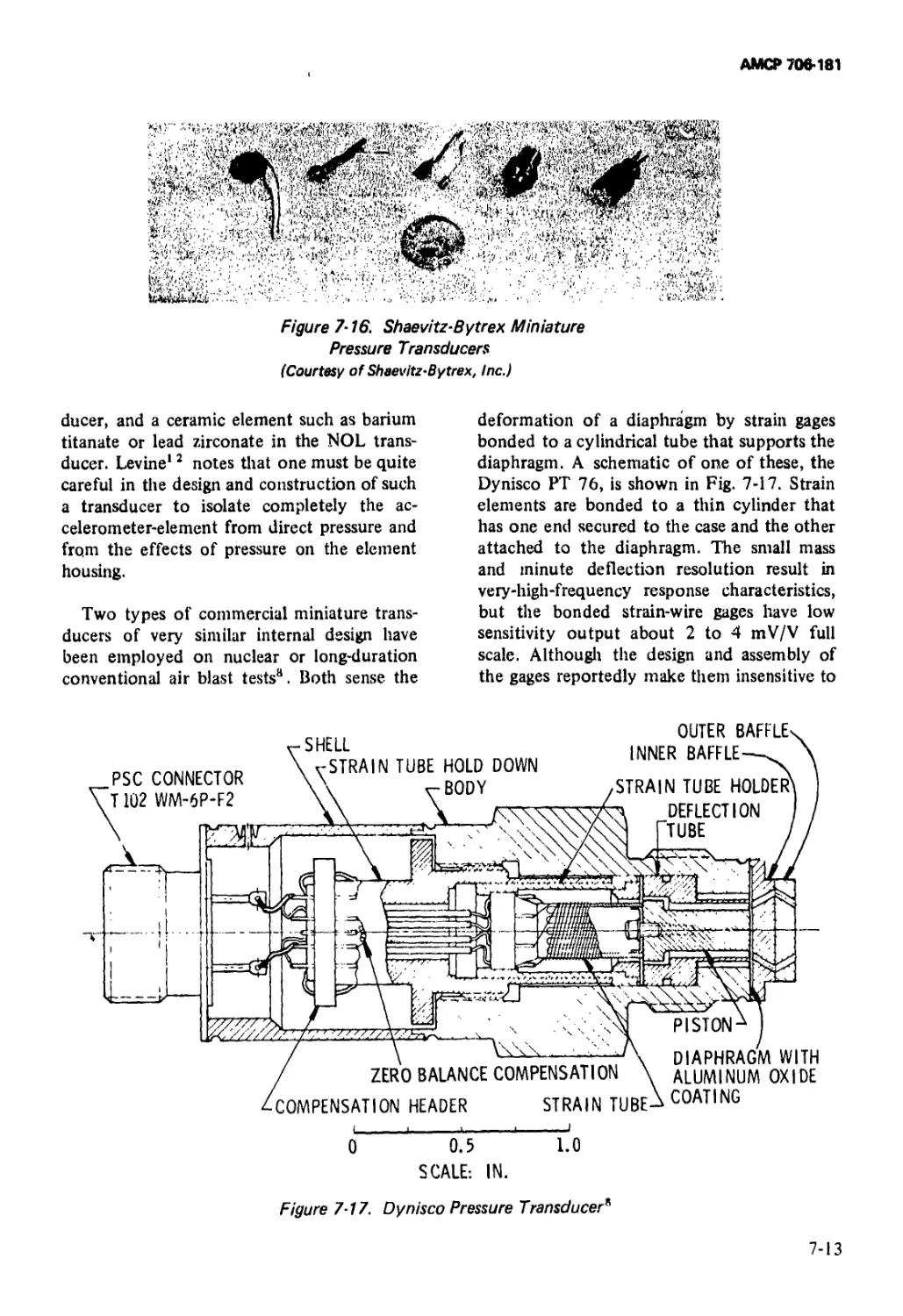
7-16 Shaevitz-Bytrex Miniature Pressure Transducers ... 7-13
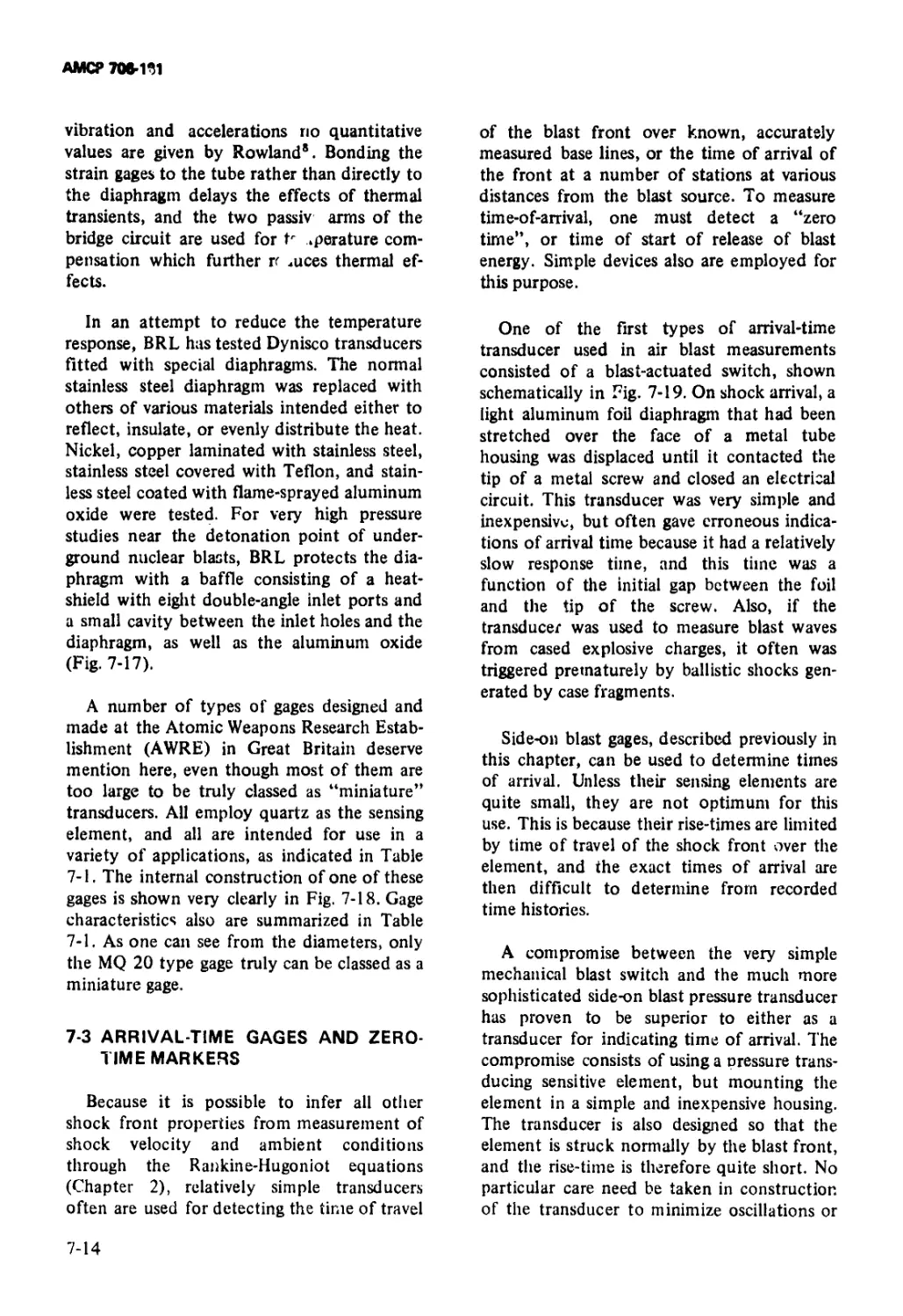
7-17 Dynisco Pressure Transducer................. 7-13
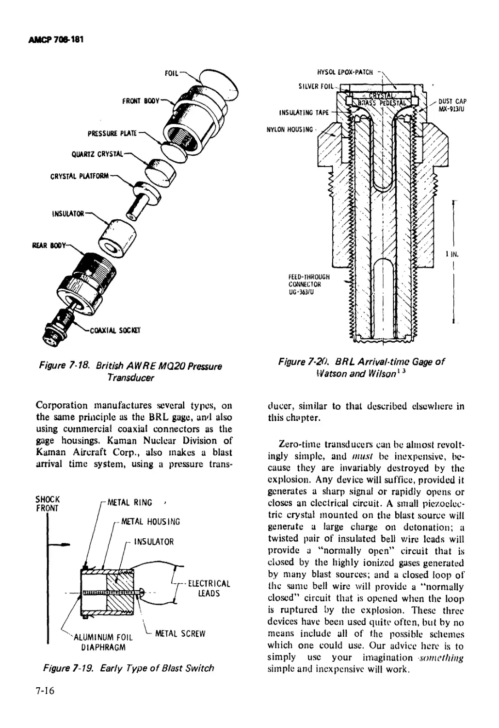
7-18 British AWRE MQ20 Pressure Transducer............. 7—16
7-19 Early Type of Blast Switch.................. 7-16
7-20 BRL Arrival-time Gage of Watson and Wilson........ 7-16
7—21 Cross Sections of Typical BRL Total Head Gages . . 7—17
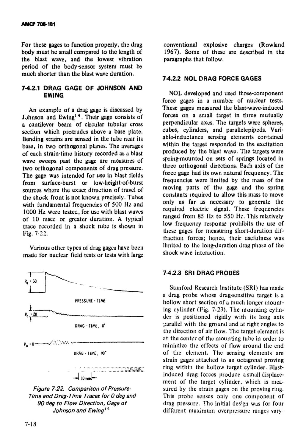
7—22 Comparison of Pressure-Time and Drag-Time Traces
for 0 deg and 90 deg to Flow Direction, Gage
of Johnson and Ewing............................... 7-18
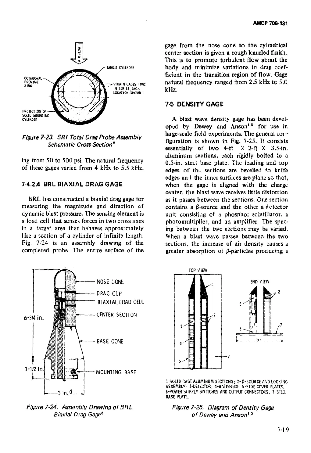
7-23 SRI Total Drag Probe Assembly, Schematic Cross
Section ........................................... 7-19
7-24 Assembly Drawing of BRL Biaxial Drag Gage............ 7-19
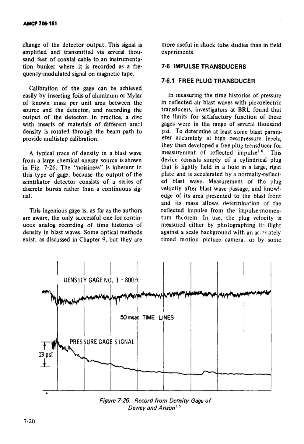
7-25 Diagram of Density Gage of Dewey and Anson .... 7-19
7—26 Record from Density Gage of Dewey and Anson .. . 7-20
7-27 Permanent Tip Deflection of 0.051-in. 6061
Aluminum Alloy Beam vs Distance for Spherical
Pentolite or TNT................................... 7-23
7—28 Surface Tension Blast Pressure Gage of Muirhead and
McMurtry ........................................ 7-24
7-29 Squirt Blast Pressure Gage of Palmer and
Muirhead........................................... 7-25
8 - 1 Block Diagram of CRT Oscilloscope Recording
System..................................................... 8- i
8 -2 BRL Four-channel Recording Equipment................. 8-2
xii
АМСР 706-181
LIST OF ILLUSTRATION (Con't.)
Fig. No. Title Page
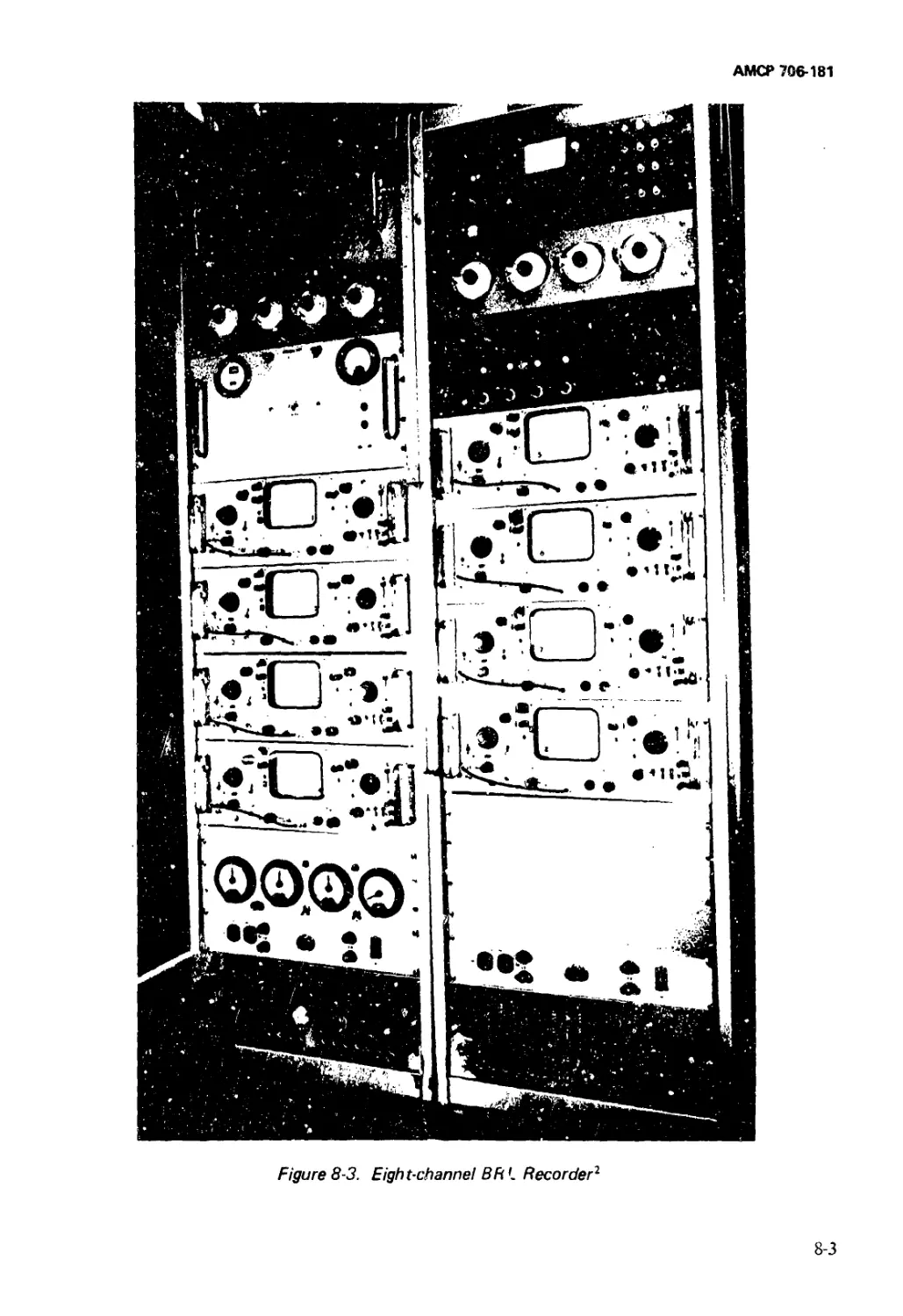
8-3 Eight-channel BRL Recorder.................... 8-3
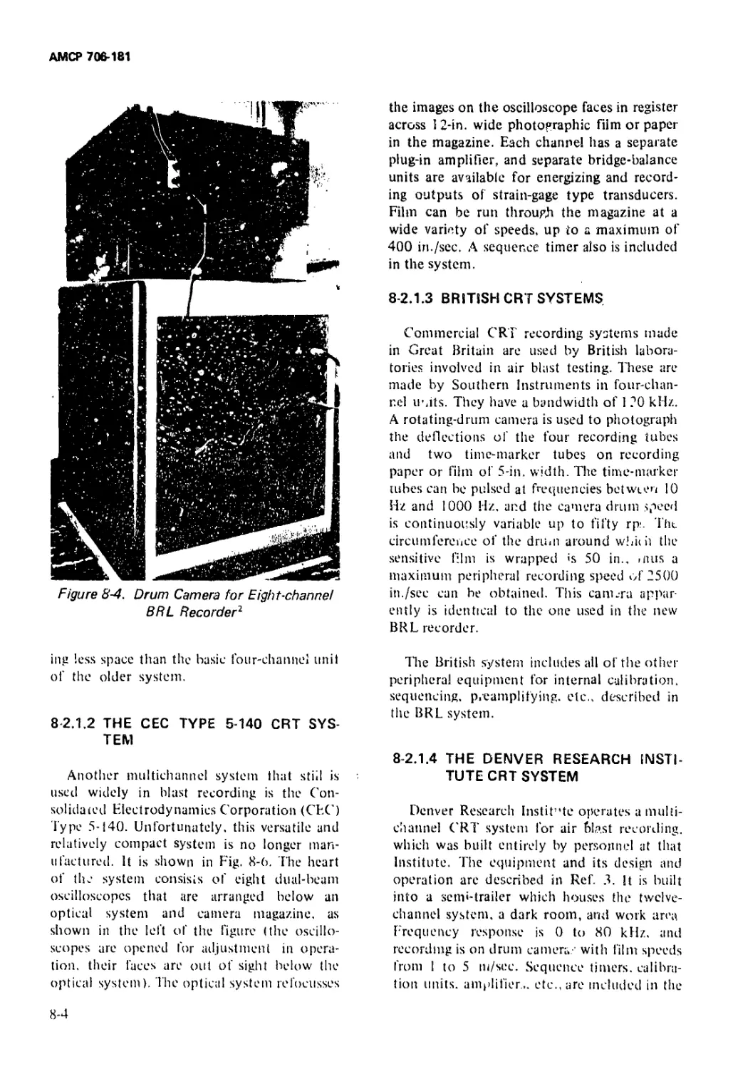
8-4 Drum Camera for Eight-channel BRL Recorder .. . 8-4
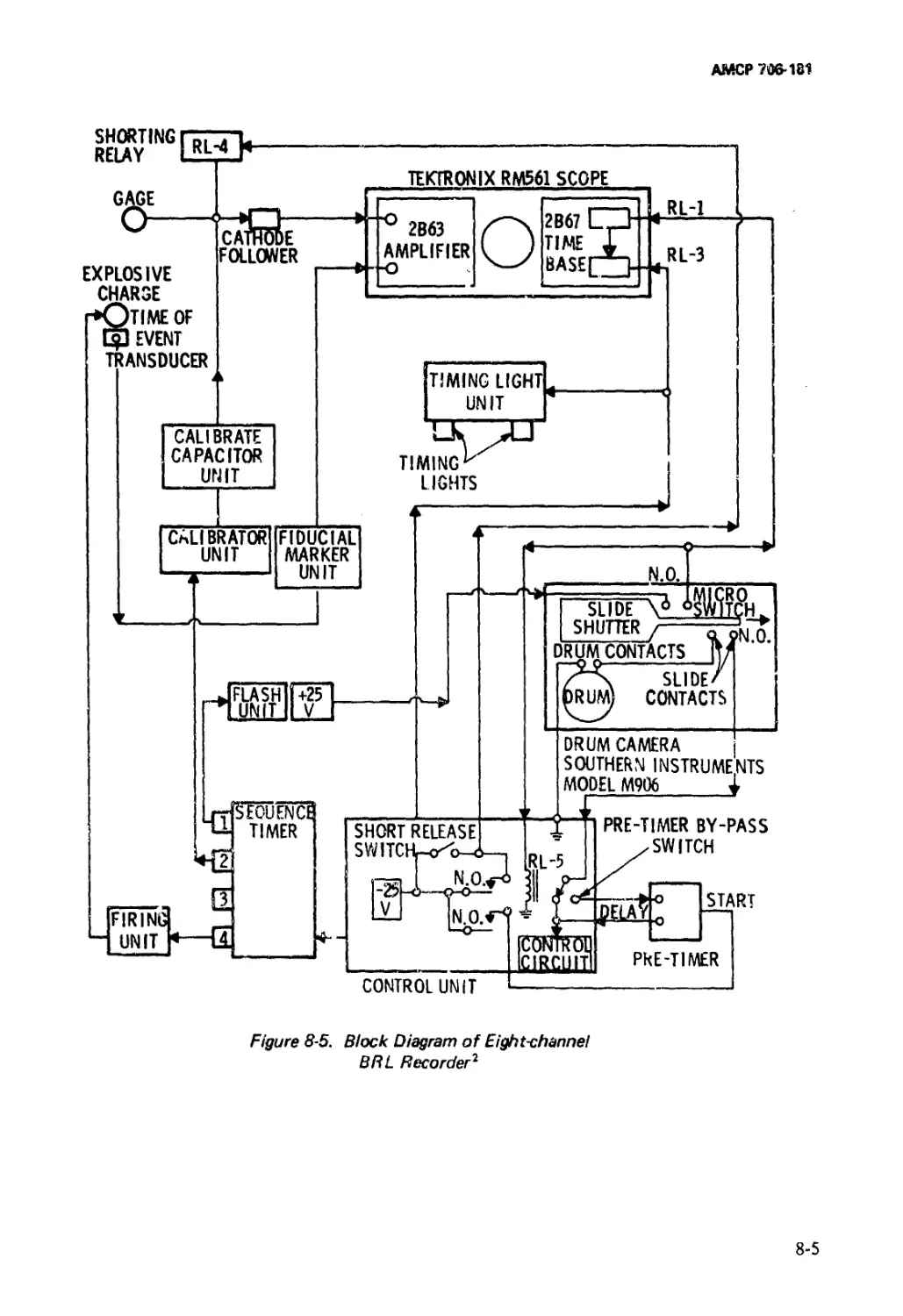
8-5 Block Diagram of Eight-channel BRL Recorder.... 8-5
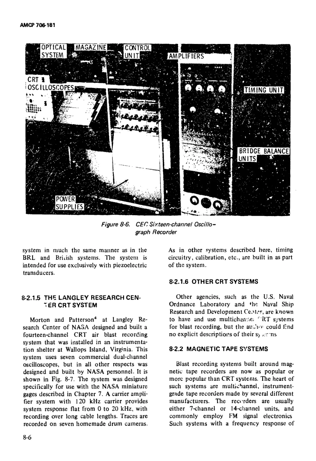
8-6 CEC Sixteen-channel Oscillograph Recorder.......... 8-6
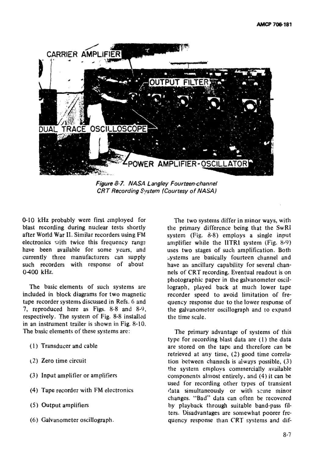
8-7 NASA Langley Fourteen-channel CRT Recording
System....................................................... 8-7
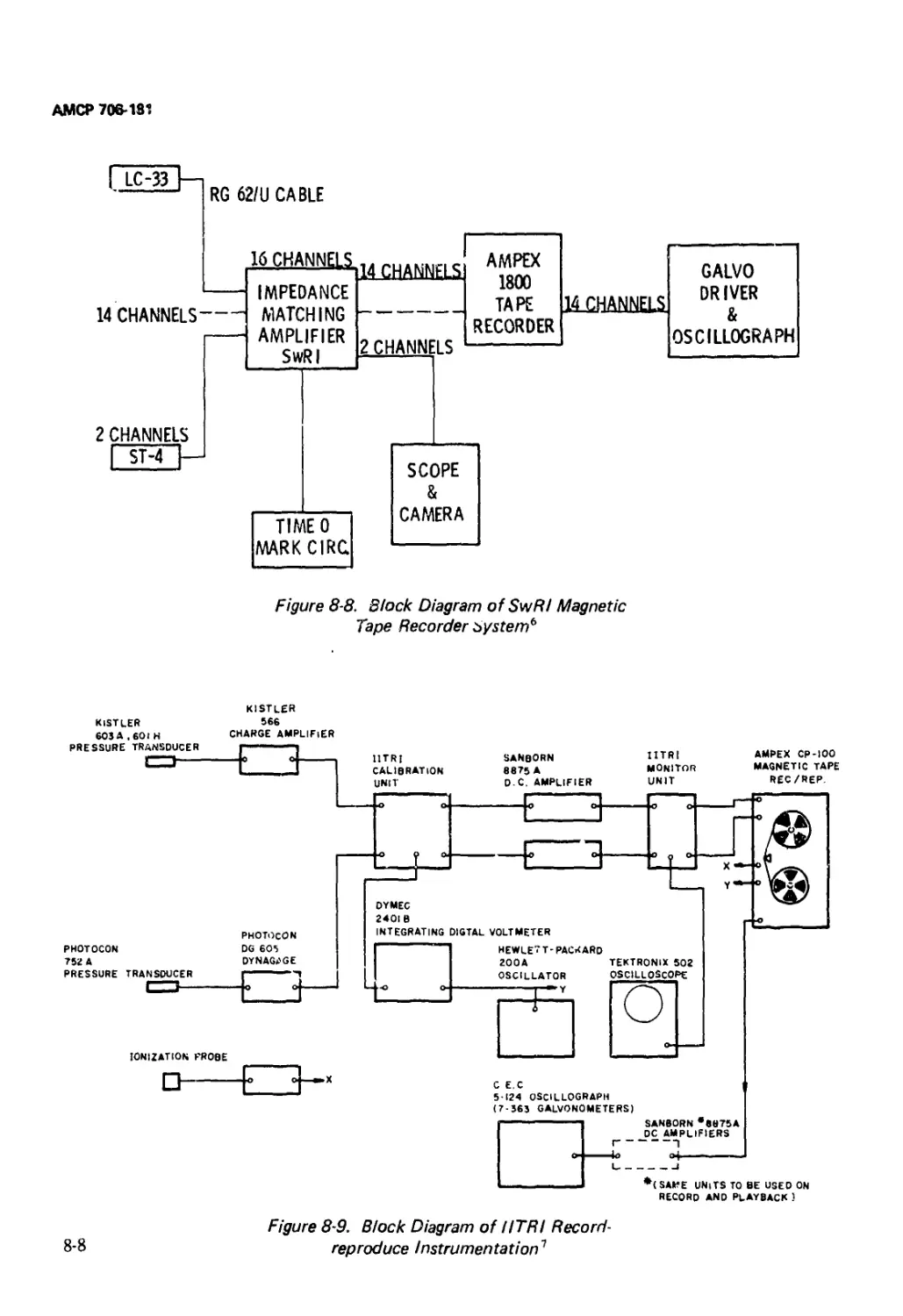
8-8 Block Diagram of SwRI Magnetic Tape Recorder
System..................................................... 8—8
8-9 Block Diagram of IITRI Record-reproduce
Instrumentation.............................................. 8-8
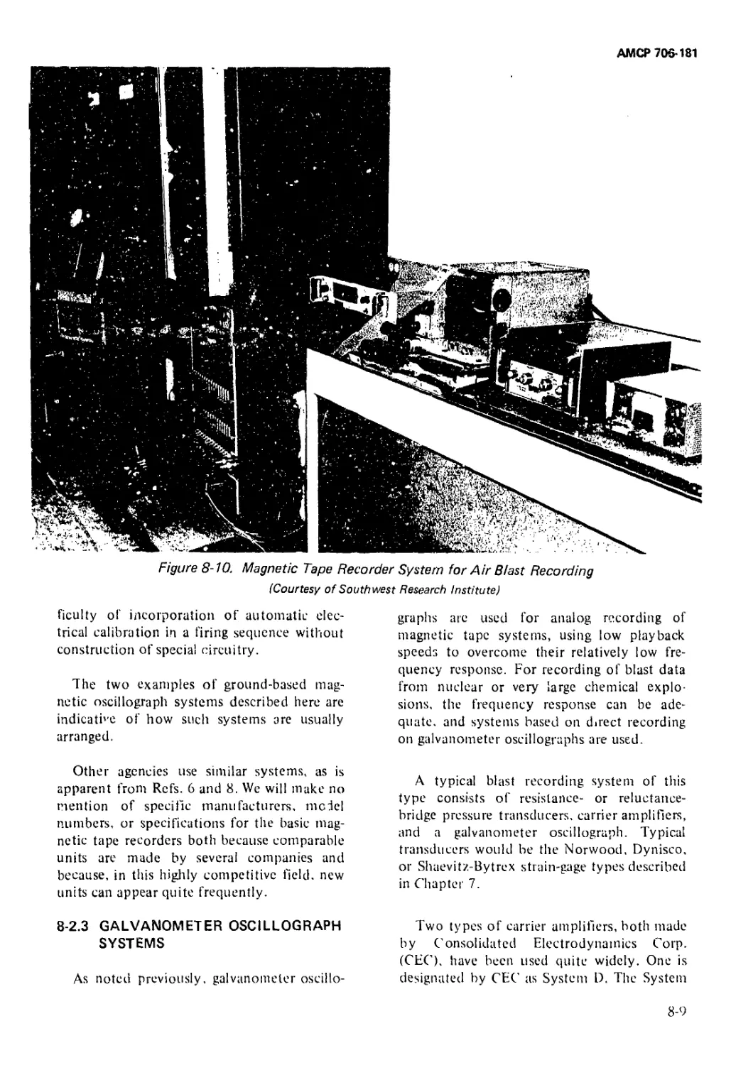
8-10 Magnetic Tape Recorder System for Air Blast
Recording ................................................... 8-9
8-11 Influence of Ground on Return Conduction
Current..................................................... 8-12
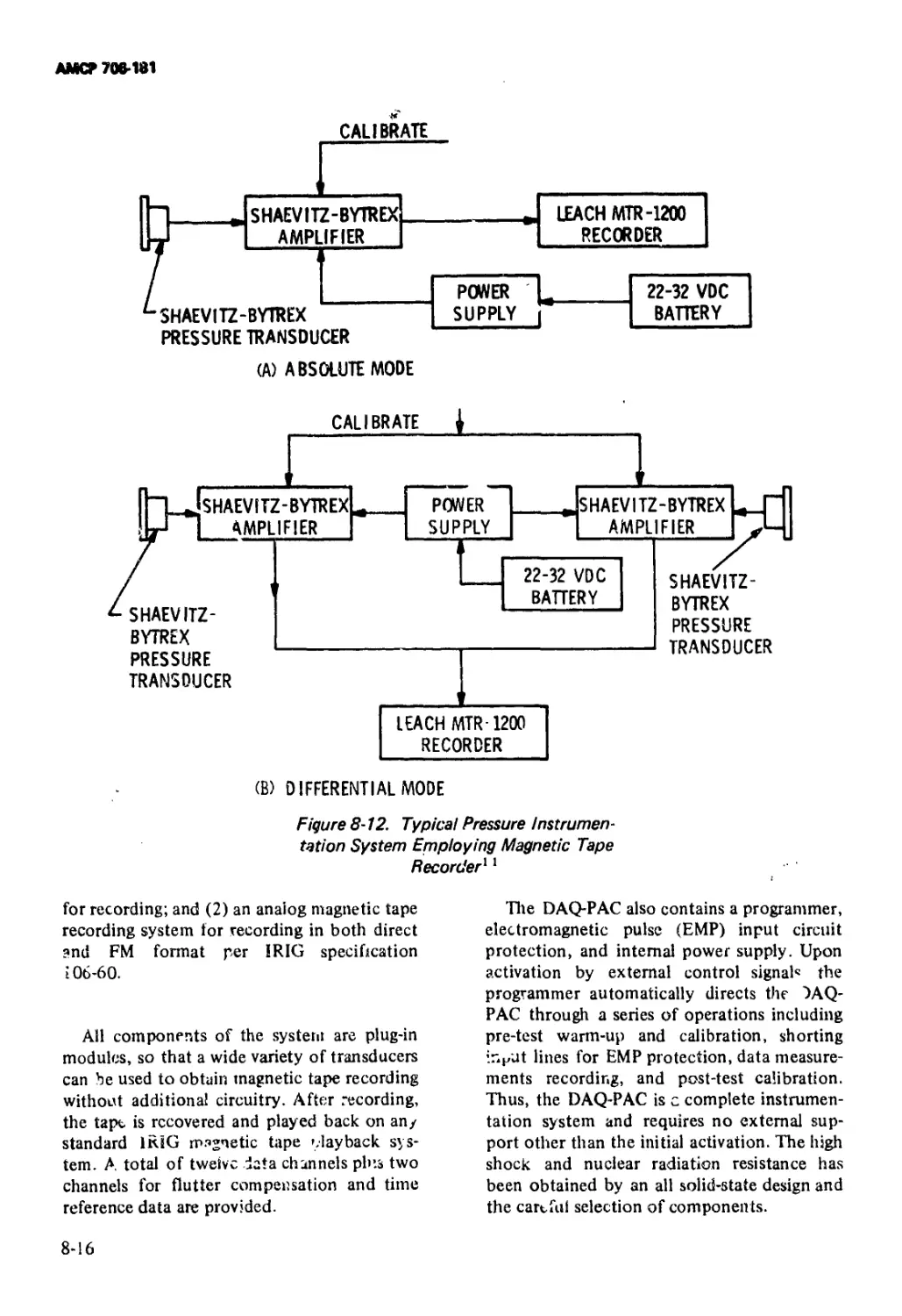
8-12 Typical Pressure Instrumentation System Employing
Magnetic Tape Recorder...................................... 8-16
8-13 Schematic Diagram of Quasi-static Gage Calibration
Apparatus........................................ 8-24
8-14 Quasi-static Pressure Calibrator for Field Use .... 8-24
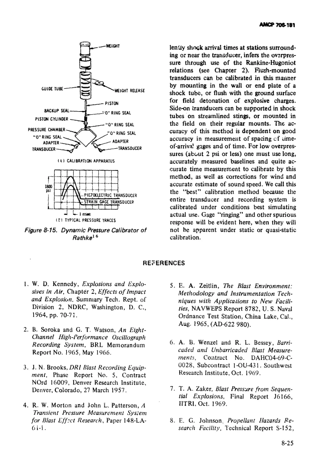
8-15 Dynamic Pressure Calibrator of Rathke.............. 8-25
9-1 Schematic Diagram of an Intermittent-type Camera. 9-1
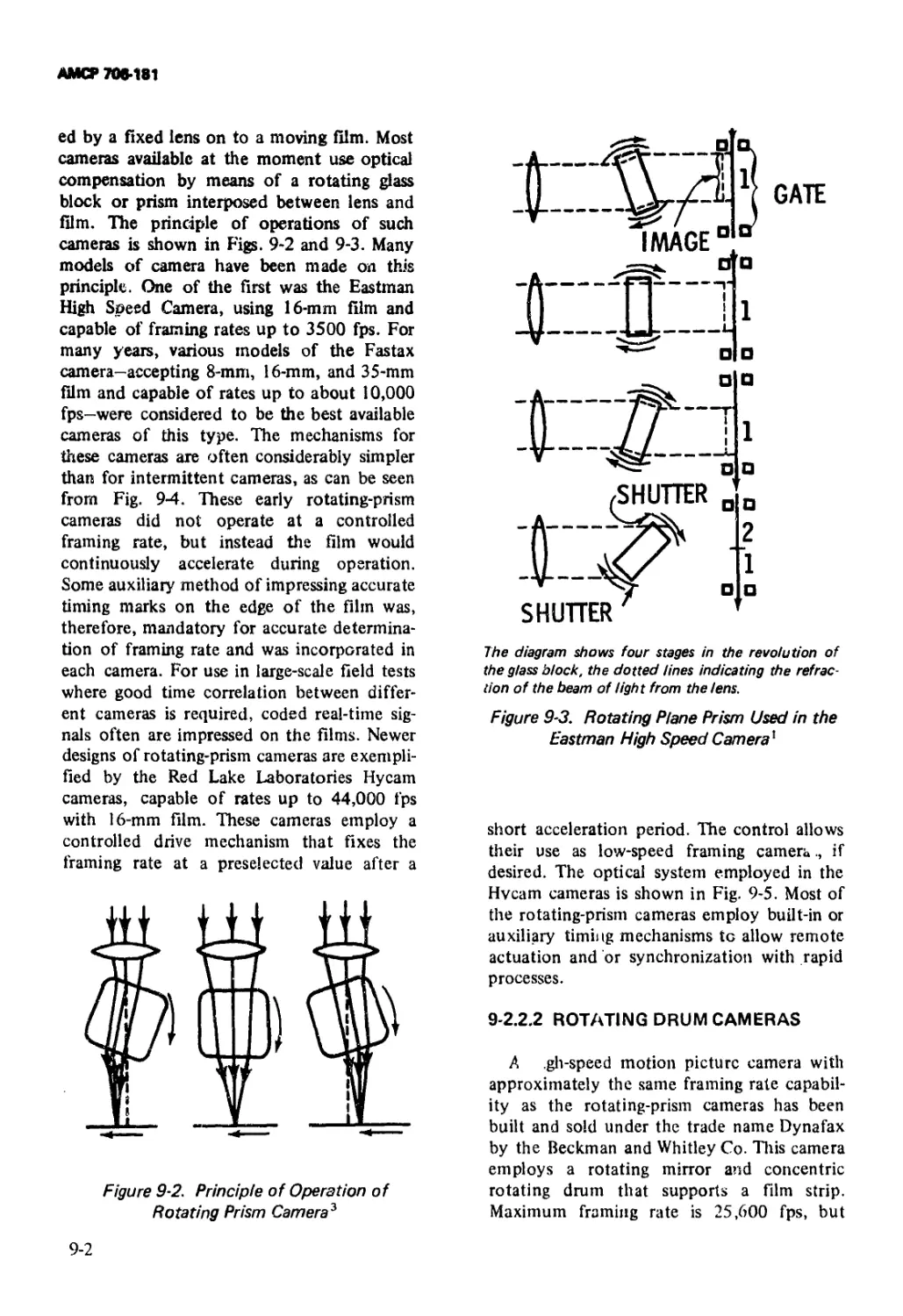
9-2 Principle of Operation of Rotating Prism Camera. . . 9—2
9-3 Rotating Plane Prism Used in the Eastman High
Speed Camera................................................. 9-2
9-4 Schematic Diagram of Fastax 8-mm Rotary Prism
High-speed Camera ........................................... 9-3
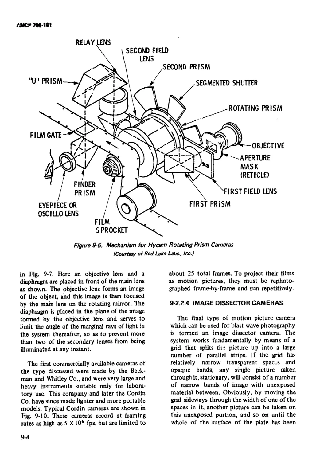
9-5 Mechanism for Hycam Rotating Prism Cameras. . . . 9-4
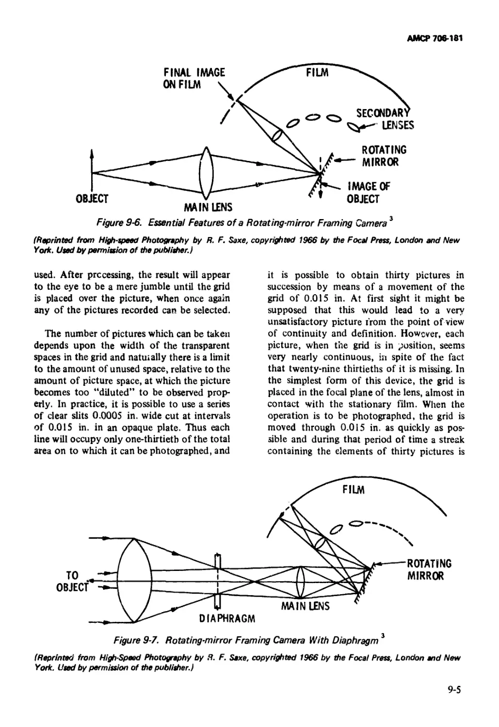
9-6 Essential Features of a Rotating-mirror Framing
Camera....................................................... 9-5
9-7 Rotating-mirror Framing Camera With Diaphragm. . 9—5
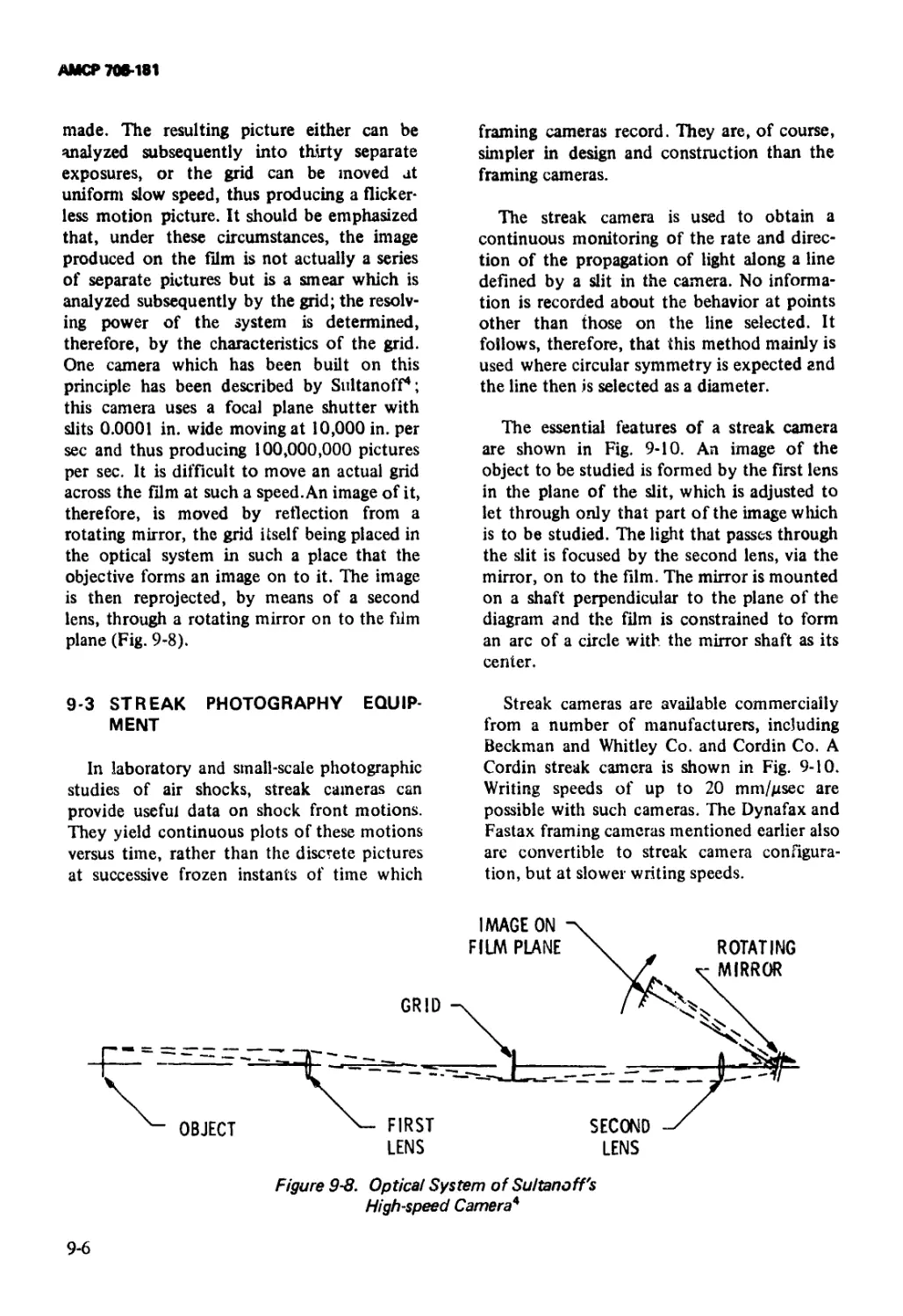
9—8 Optical System of Sultanoff’s High-speed Camera . . 9-6
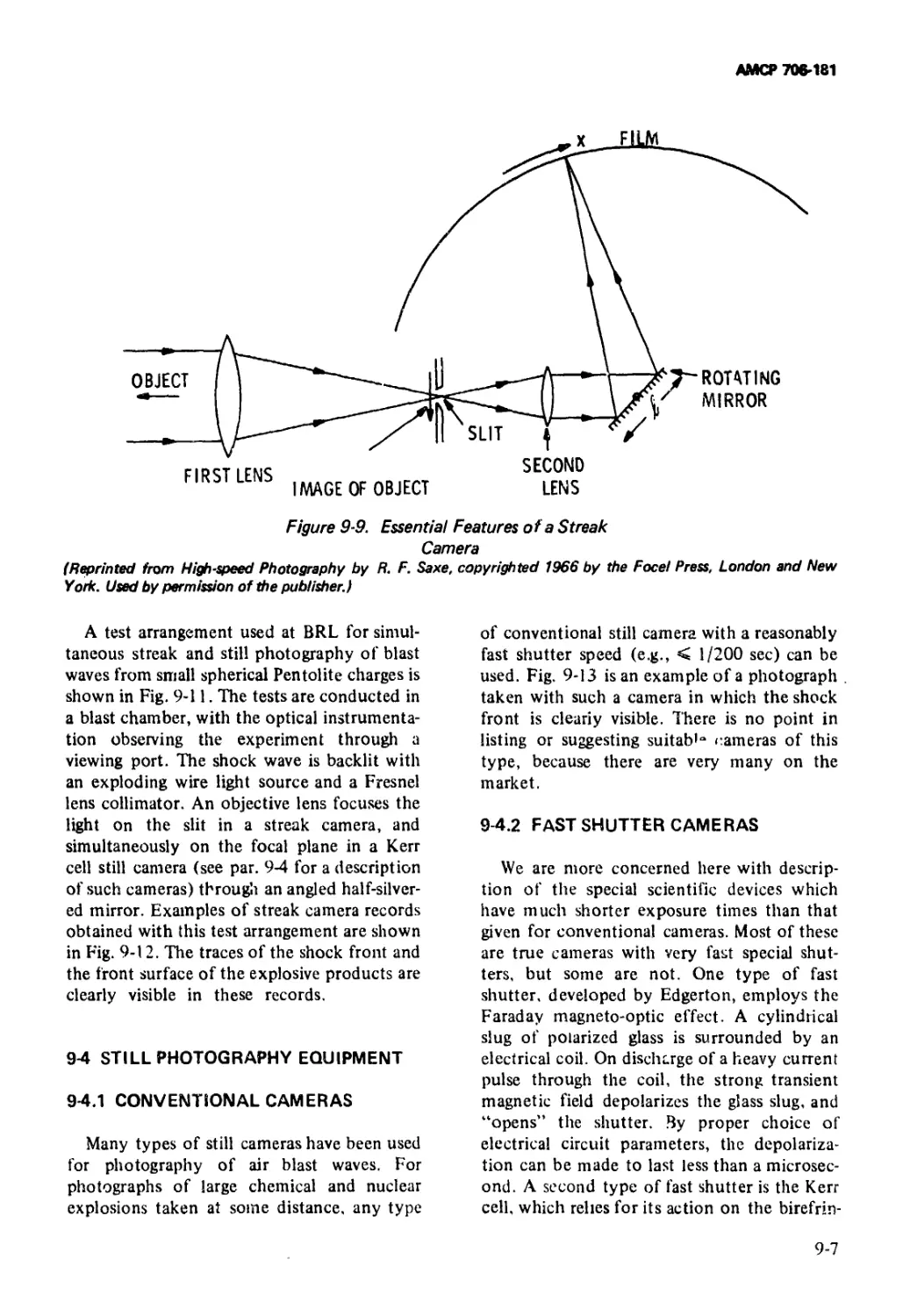
9-9 Essential Features of a Streak Camera......... 9—7
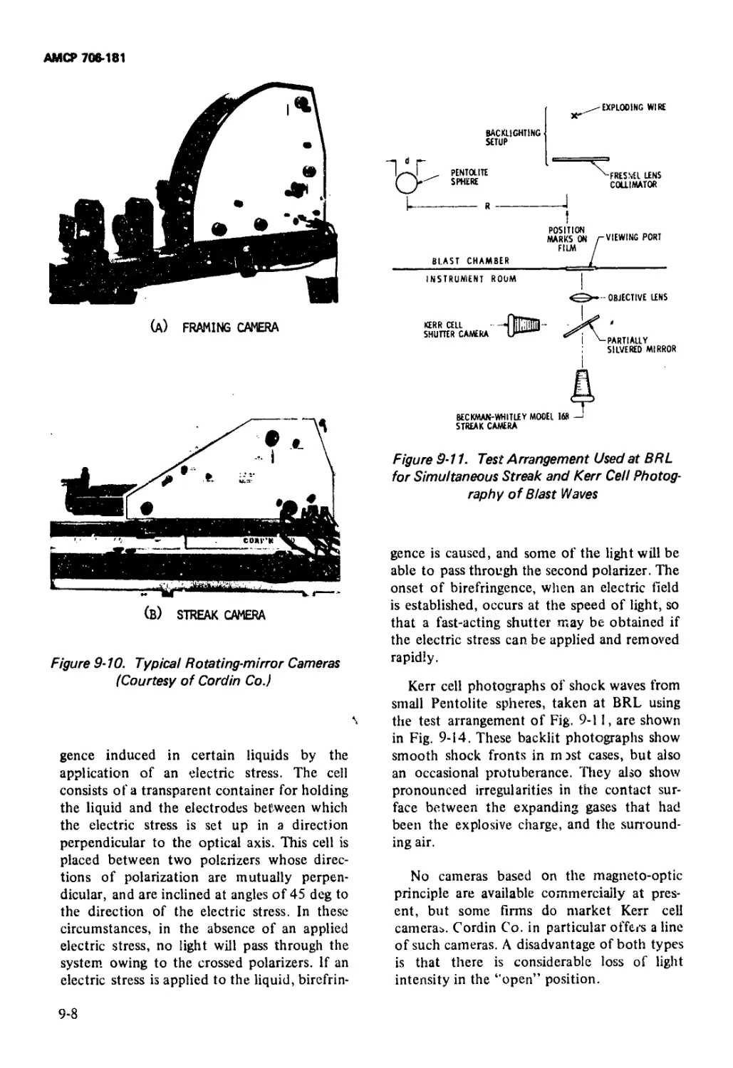
9-10 Typical Rotating-mirror Cameras............... 9-8
9-11 Test Arrangement Used at BRL for Simultaneous
Streak and Kerr Cell Photography of Blast Waves. . 9-8
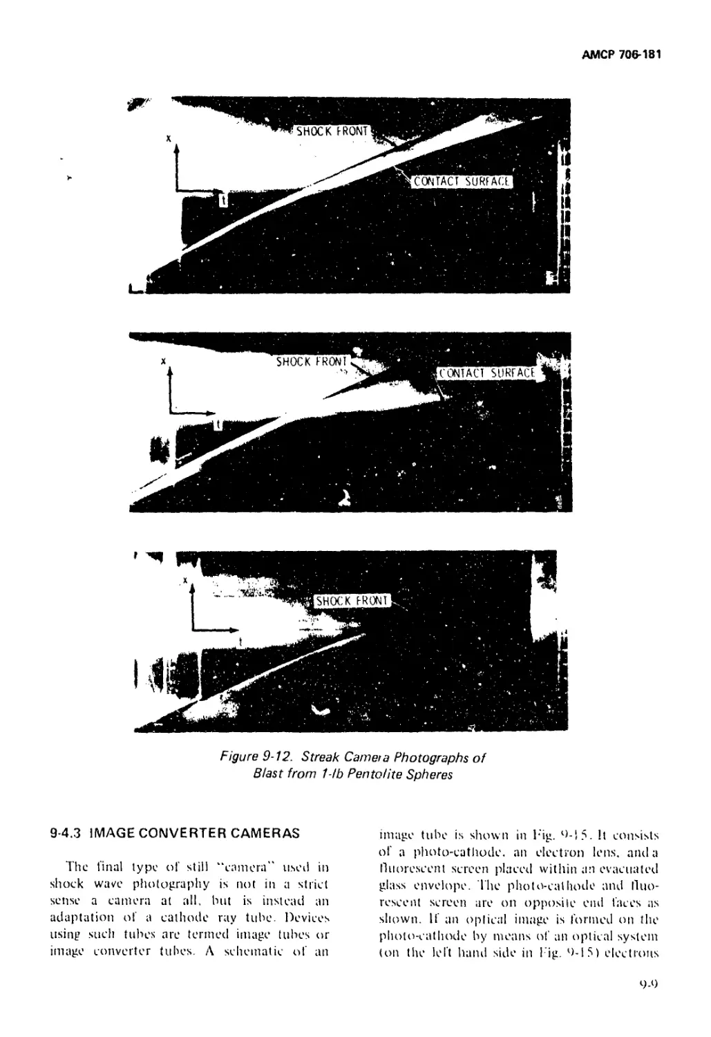
9-12 Streak Camera Photographs of Blast from 1-lb
Pentolite Spheres............................................ 9-9
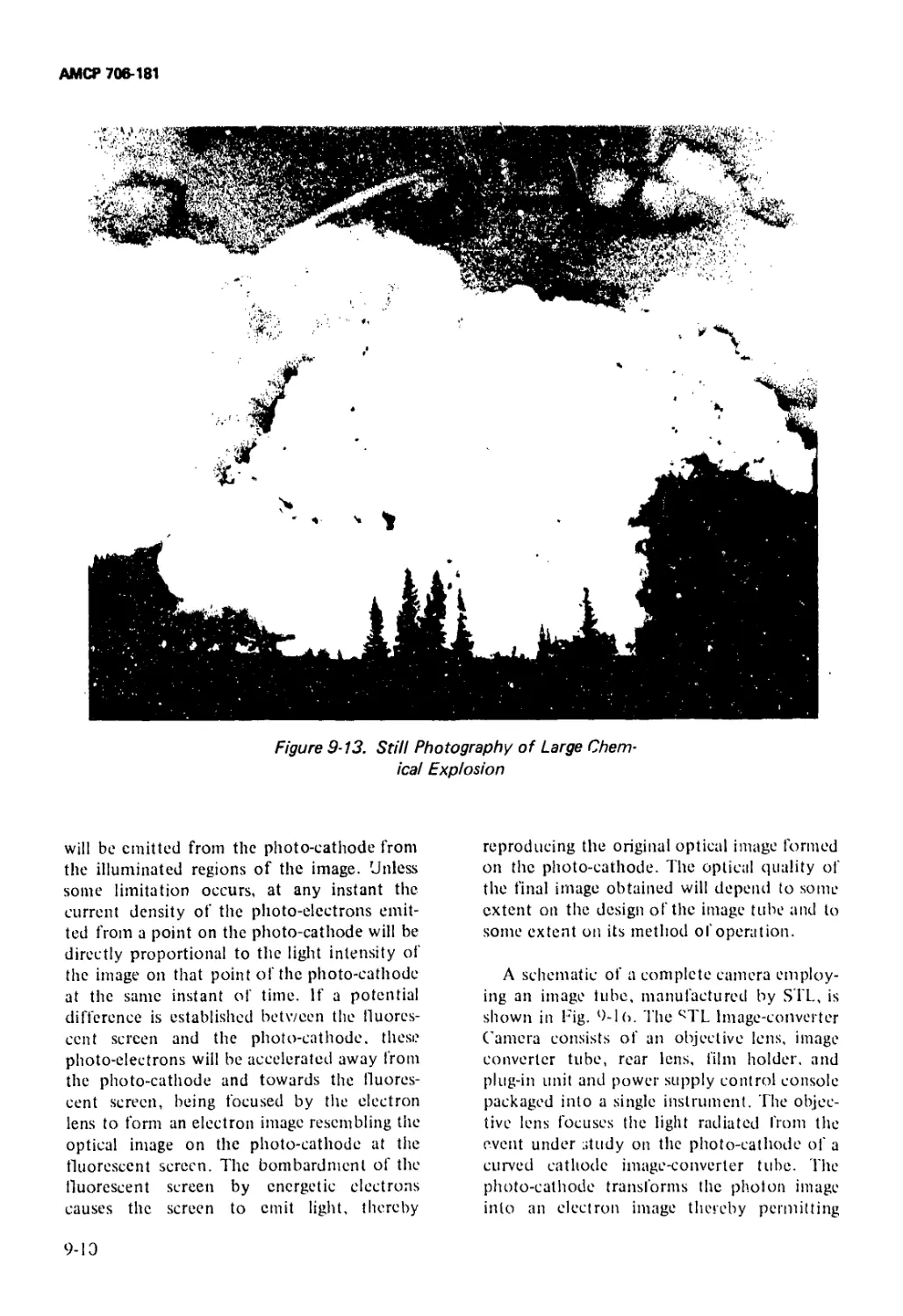
9-13 Still Photograph of Large Chemical Explosion ... 9-10
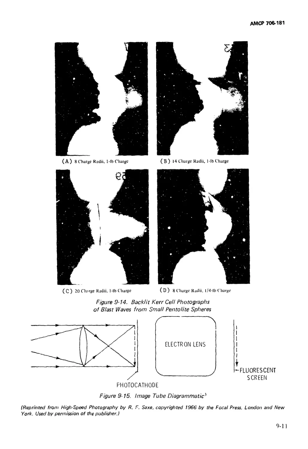
9-14 Backlit Kerr Cell Photographs of Blast Waves from
Small Pentolite Spheres..................................... 9-11
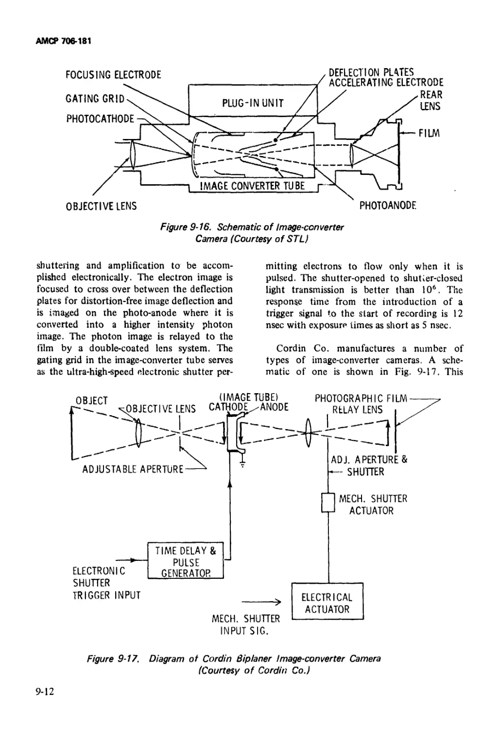
9-15 Image Tube Diagrammatic............................ 9-11
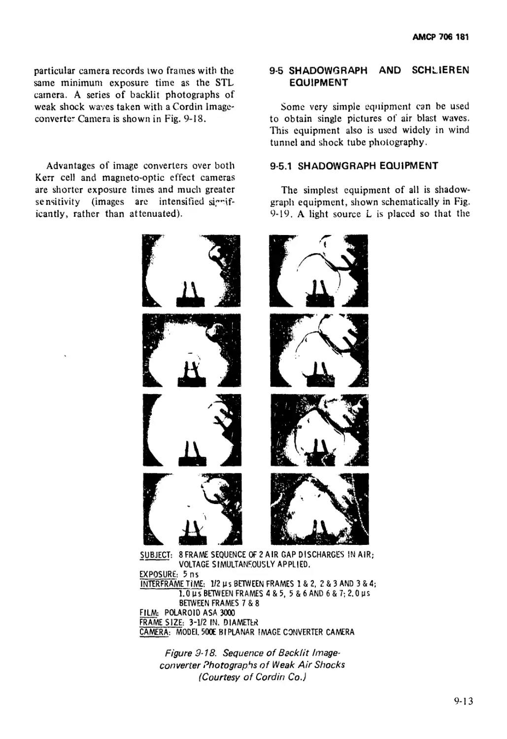
9-16 Schematic of Image-converter Camera................ 9-12
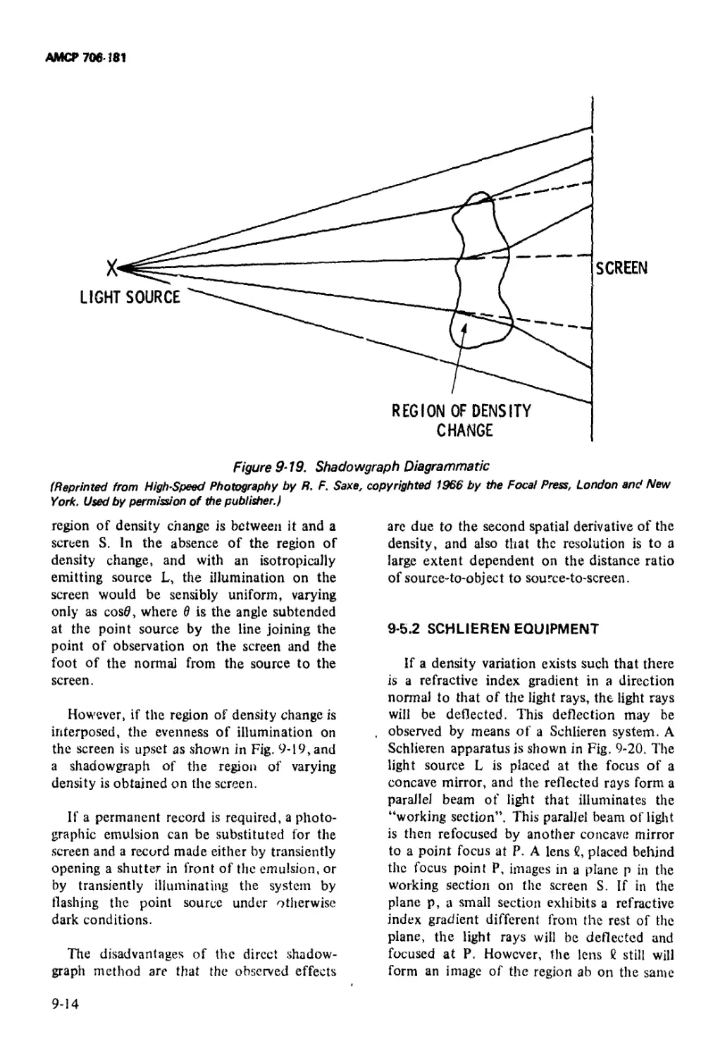
9-17 Diagram of Cordin Biplanar Image-converter
Camera ..................................................... 9-12
9 — 18 Sequence of Backlit Image-converter Photographs
of Weak Air Shocks............................ 9 -13
9-19 Shadowgraph Diagrammatic........................... 9-14
xiii
АМСР 706-181
LIST OF ILLUSTRATIONS (Con't.)
Fig. No. Title Page
9-20 Schlieren System Diagrammatic ........................ 9-15
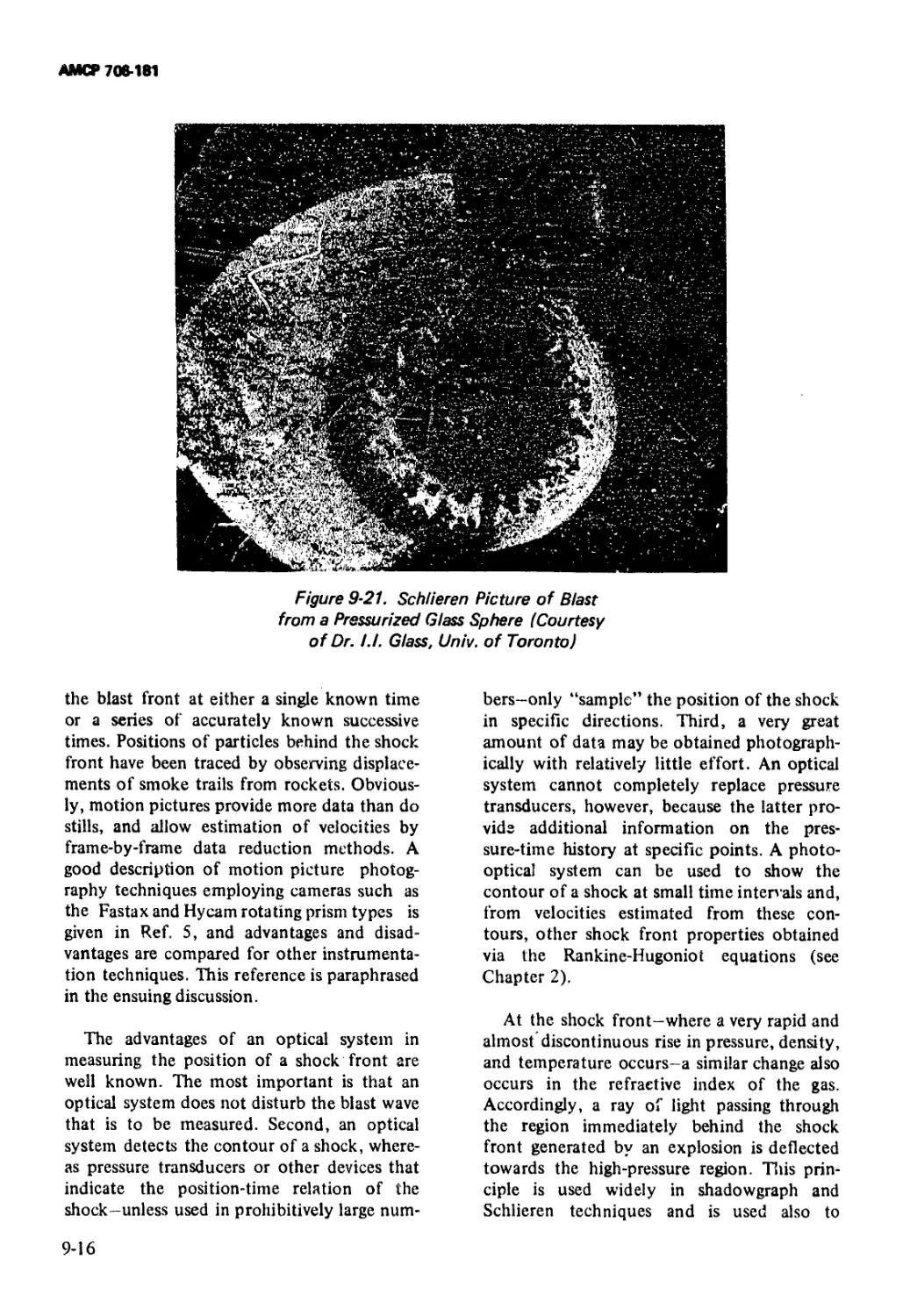
9-21 Schlieren Picture of Blast from a Pressurized Glass
Sphere........................................... 9-16
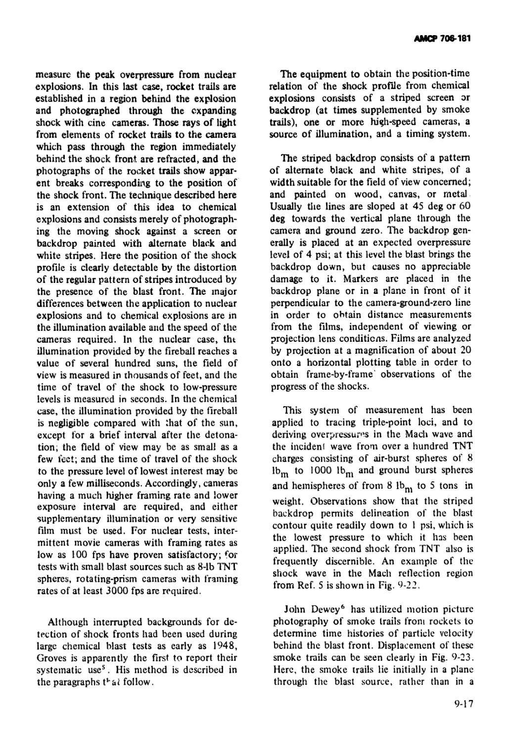
9-22 Views of Shock Waves from 8-lbm TNT Spheres
Detonated 8 ft Above Concrete.................... 9-18
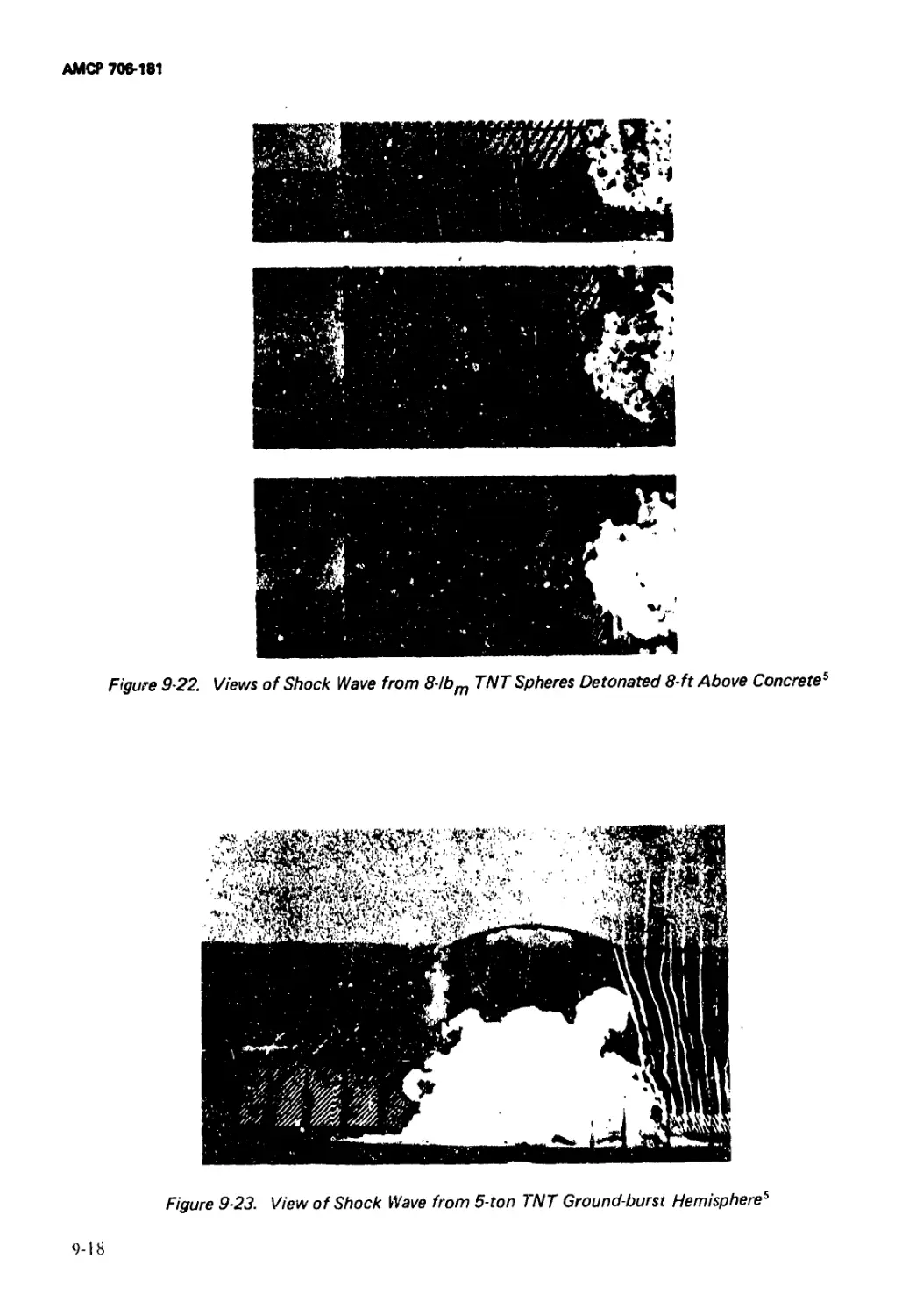
9-23 View of Shock Wave from 5-ton TNT Ground-
turst Hemisphere................................. 9-18
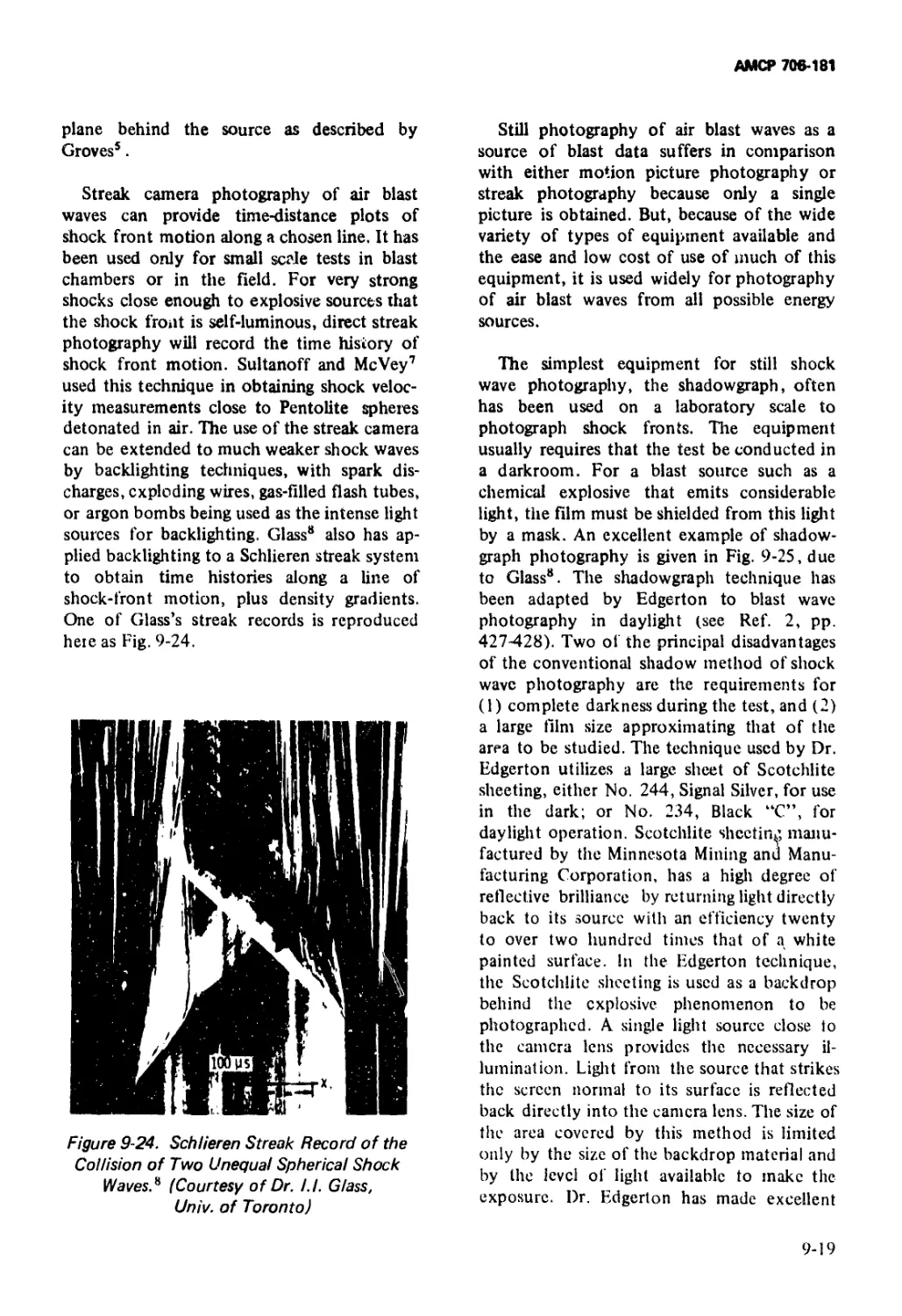
9-24 Schlieren Streak Record of the Collision of Two
Unequal Spherical Shock Waves.................... 9-19
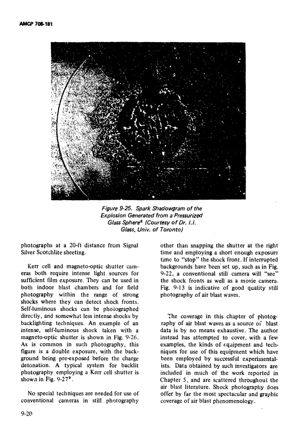
9-25 Spark Shadowgraph of the Explosion Generated
from a Pressurized Glass Sphere ................. 9-20
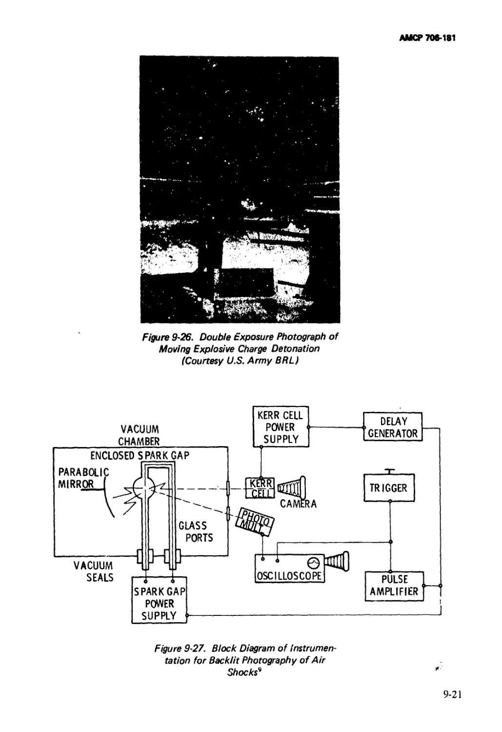
9-26 Do ible Exposure Photograph of Moving Explosive
Charge Detonation ............................... 9-21
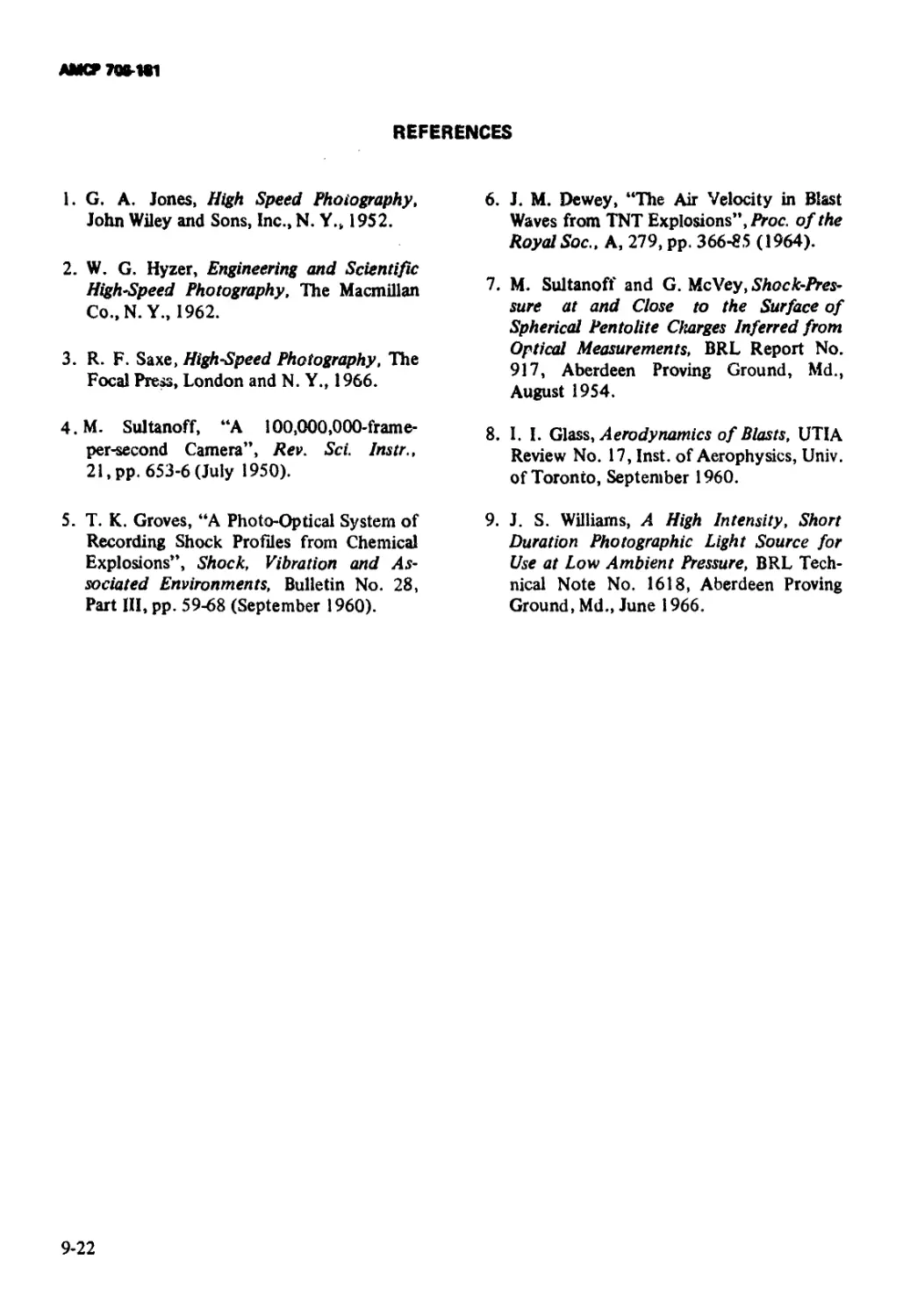
9-27 Block Diagram of Instrumentation for Backlit
Photography of Air Shocks........................ 9-21
10-1 Typical Traces from Oscillograph Record Cameras. 10-2
10—2 Typical Traces from Four-channel Blast Recorders. 10-3
10-3 Typical Trace from Eight-channel BRL
Blast Recorder .................................. 10-4
10—4 Calculated Response of a Gage of Finite Diameter
to Linearly Decaying Pressure ................... 10-5
10-5 Method of Extrapolation of
Experimental Records ............................ 10-5
10—6 Recorded Side-on and Total Head Pressure-Time
Histories and Calculated Dynamic Pressure-Time . 10-7
History ......................................... 10—7
10 -7 Linear Plot of BRL Self-recording Gage Record
Obtained at a Ground Range of 334 ft from the
1961 Canadian 100-ton HE Test ................... 10-8
10-8 Semi-logarithmic Plot of Gage Record With
Pressure Plotted Against the Logarithmic Scale .. 10-8
10—9 Semi-logarithmic Plot of Gage Record With Time
Plotted Against the Logarithmic Scale ........... 10-9
10-10 Phoio-optical Records of Shock Front Profile . . 10-11
10—11 Velocity Field Setup ............................... 10-11
xiv
АМСР 706-181
LIST OF TABLES
Table No. Title Page
1-1 Peak Pressure and Positive Impulse Relative to
Composition В (The Comparison Being on an
Equal Volume Basis).......................................... 1-23
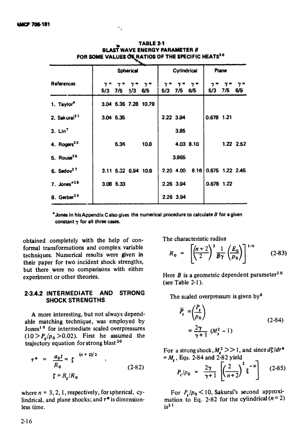
2-1 Blast Wave Energy Parameter В for Some Values
of Ratios of the Specific Heats ............................. 2-16
3-1 List of Physical Parameters for Hopkinson
Blast Scaling ................................................ 3-8
3-2 Sach’s Scaling Parameters .......................... 3—11
3 -3 Blast Scaling Laws Proposed by Wecken............... 3-19
3-4 Additional Parameters in Wecken’s Analysis ......... 3-19
3-5 Dimensionless Products Corresponding to Wecken’s
Scaling ........................................... 3-20
3-6 Primary Buckingham it Terms. Blast Loading and
Response of High-speed Structure................... 3-23
4-1 Coefficients of Partial Derivatives in
Kirkwood-Brinkley Method ...................... 4-5
4-2 Comparison of Detonation Velocities D Calculated
for LSZK Substance With Detonation Velocities
Determined at Bruceton ...................................... 4-16
4-3 Input Data for Flow Past a Wedge-PAF Method .. . 4-22
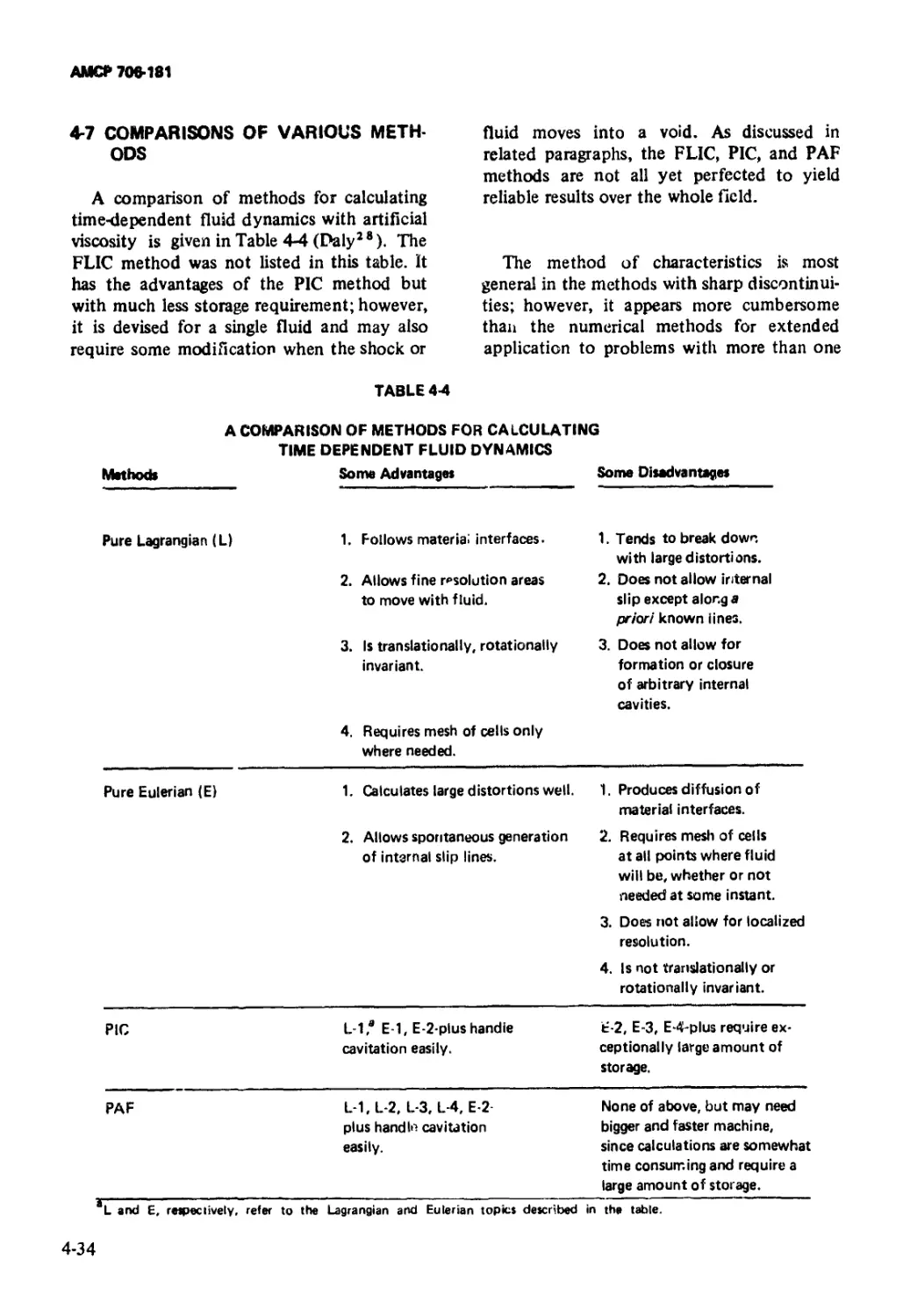
4-4 A Comparison of Methods for Calculating Time
Dependent Fluid Dynamics .......................... 4-34
6-1 Explosive Properties ..................................... 6-4
6-2 Sachs’ Scaled Non '-imensional Blasi
Parameters ................................................... 6-5
6-3 Scaled Shock-front Parameters for Incident
Blast Waves ................................................ 6-8
6 -4 Scaled Shock-front Parameters for Reflected
Blast Waves ....................................... 6-10
6-5 Scaled Impulses and Durations of Overpressure ... 6-12
6-6 Time Constant and Initial Decay Rate of ps 6-14
6-7 Typical Compiled Data for Strong,
Obliquely Reflected Shocks......................... 6-15
6-8 Limit of Regular Reflection a vs Shock
„ extreme
Strength .......................................... 6-16
6-9 Conversion Factors for Scaled Blast Wave
Properties ........................................ 6-18
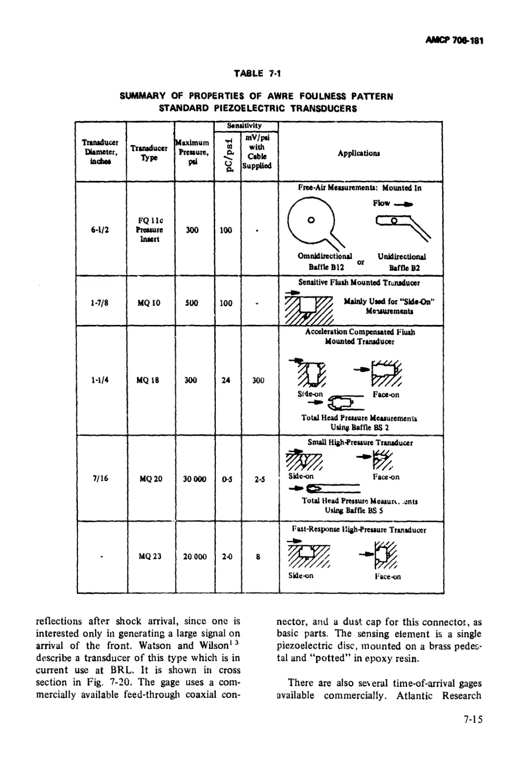
7-1 Summary of Properties of AWRE Foulness Pattern
Standard Piezoelectric Transducers ................ 7-15
7-2 Characteristics of Side-on Pressure Transducers ... 7-26
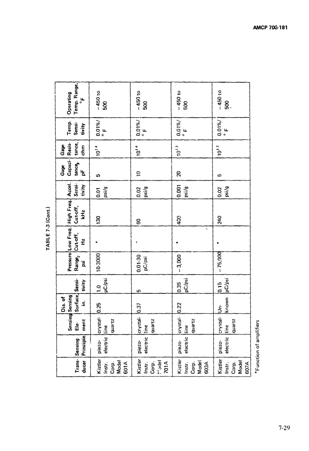
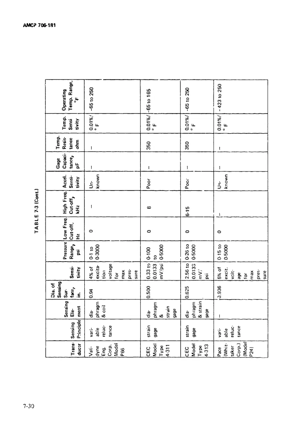
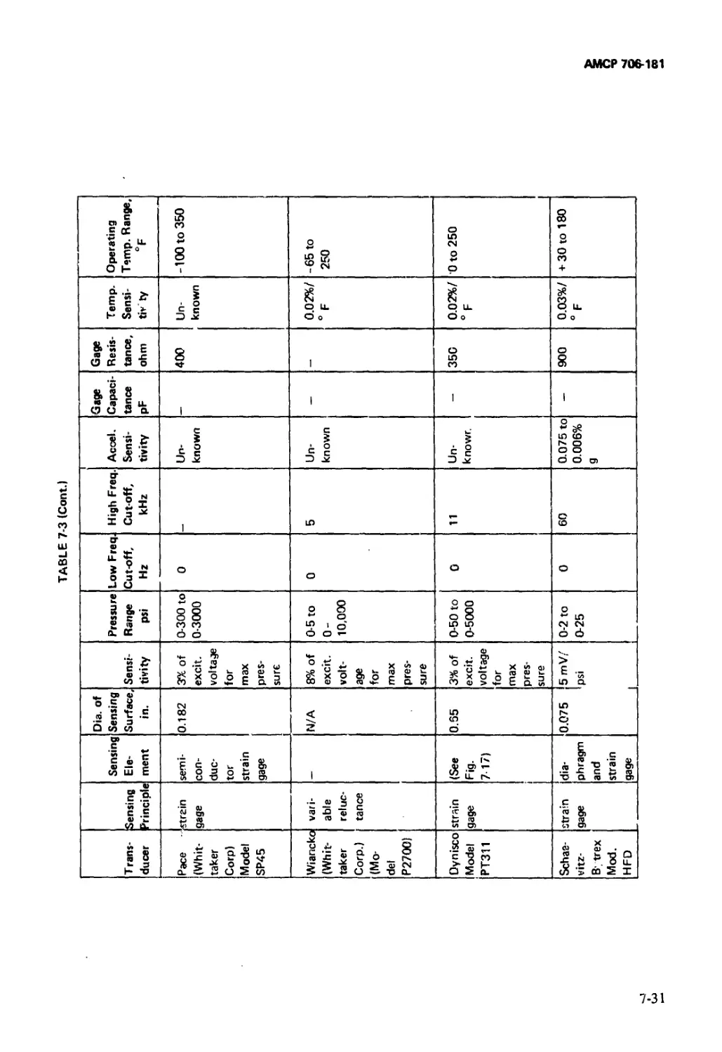
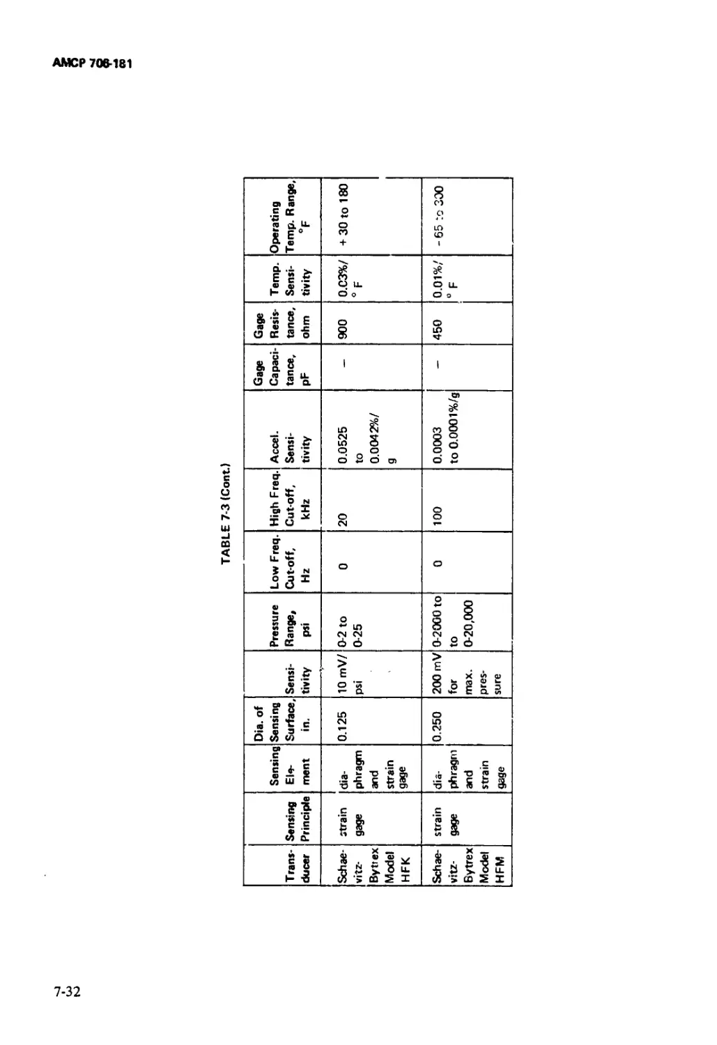
7-3 Characteristics of Flush-mounted Pressure
Transducers ....................................... 7-27
xv
АМСР 706-181
LIST OF TABLES (Con’t.)
Table No. Title Page
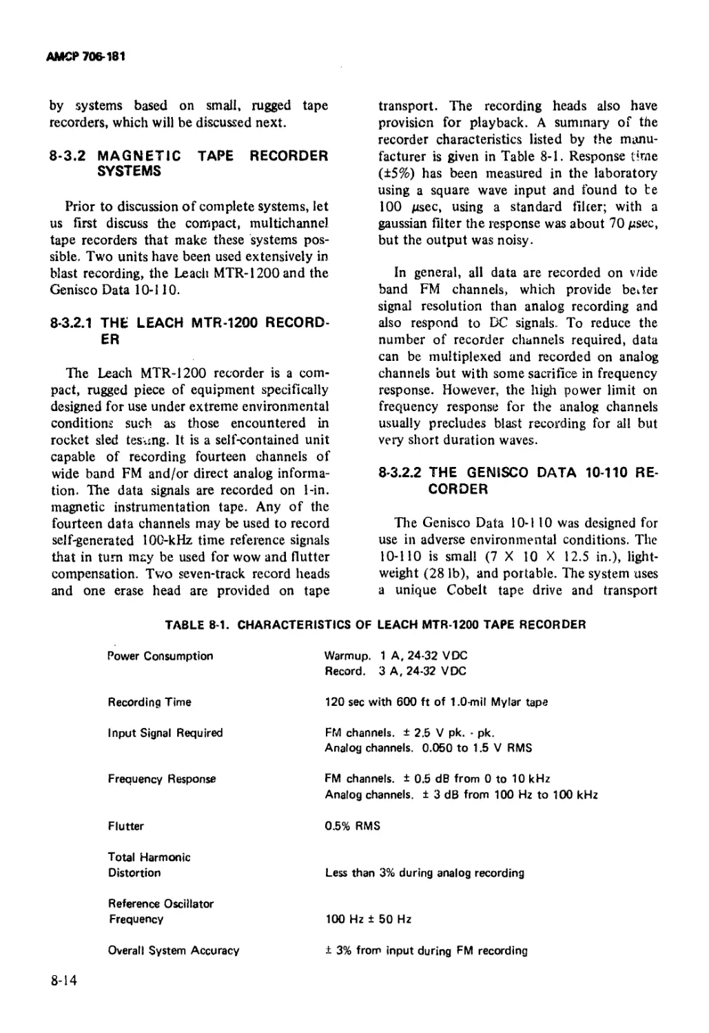
8-1 Characteristics of Leach MTR-l 200
Tape Recorder ................................ 8—14
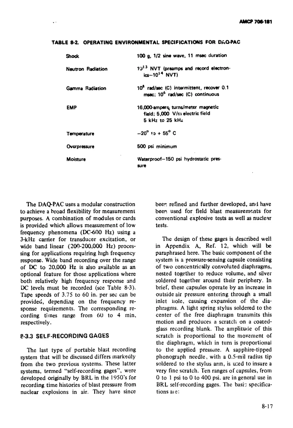
8-2 Operating Environmental Specifications
forDAQ-PAC ................................... 8-17
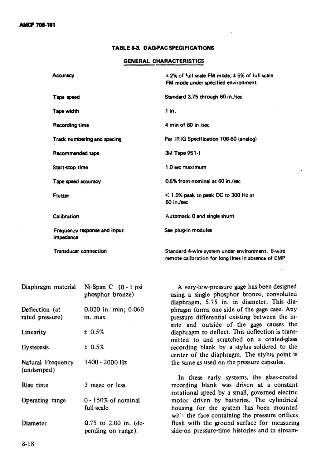
8-3 DAQ-PAC Specifications.......................... 8-18
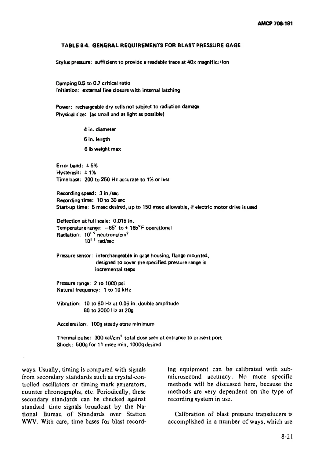
8-4 General Requirements for Blast Pressure Gage . . 8-21
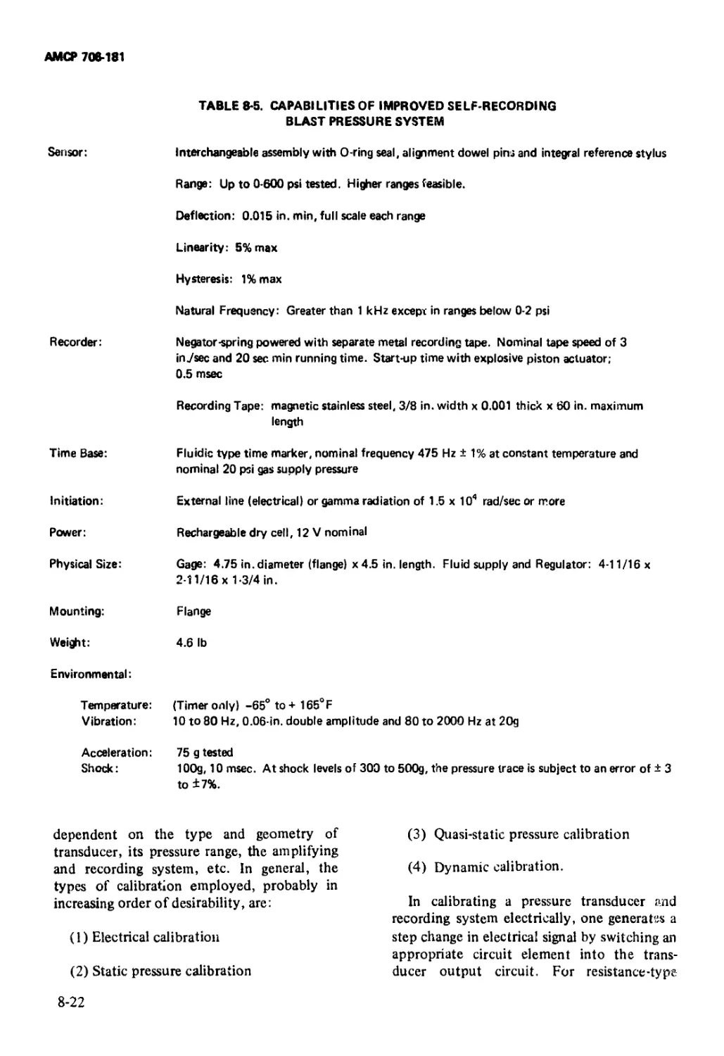
8-5 Capabilities of Improved Self-recording Blast
Pressure System .............................................. 8-22
xvi
АМСР 706-181
PREFACE
Scientific interest in the processes of generation and transmission through
the air of blast waves from explosive sources dates back at least to the latter
part of the nineteenth century. The number of reported experimental and
analytic studies of air blast phenomenology increased materially during
World War II. In spite of the voluminous literature on the subject, there has
been no single reference work comprehensive enough to cover both
theoretical and experimental aspects of air blast technology. This handbook
attempts to remedy diis problem.
Explosions in Air, Part One is a general reference handbook on the topic,
intended for use by both casual and experienced investigators in air blast
theory and experiment. A special feature of the handbook is the inclusion of
large-scale graphs of scaled air blast parameters. Tire literature relating to air
blast technology is reviewed thoroughly and an extensive list of reference is
included.
This handbook includes chapters on general phenomenology, air blast
theory, blast scaling, computational methods, air blast experimentation,
compiled blast data, air blast transducers, instrumentation systems, photog-
raphy of air blast waves, and data reduction methods. It is illustrated by
many figures and graphs. Specifically excluded from this handbook are
classified aspects of air blast technology, laboratory applications such as
shock tubes, and response of structures to blast loading. These topics are
presented in Explosions in Air, Part Two, AMCP 7O6-182(S).
This handbook was prepared by the Southwest Research Institute, San
Antonio, Texas, for the Engineering Handbook Office of Duke University,
prime contractor to the U. S. Army Materiel Command. Dr. Wilfred E. Baker
was the author. Technical guidance and coordination were provided by a
committee with representatives from the Ballistic Research Laboratories,
Picatinny Arsenal, and the U. S. Army Electronics Command. Members of
this committee were Charles N. Kingery, Chairman; William J. Taylor;
Richard W. Collett; and Charles Goldy.
The Engineering Design Handbooks fall into two basic categories, those
approved for release and sale, and those classified for security reasons. The
Army Materiel 'ommand policy is to release these Engineering Design
Handbooks to other DOD activities and their contractors and other
Government agencies in accordance with current Army Regulation 70-31,
dated 9 September 1966. It will be noted that the majority of these
Handbooks can be obtained from the National Technical Information
Service (NTIS). Procedures for acquiring these Handbooks follow:
xvii
АМСР 706-181
‘ a. Activities within АМС, DOD agencies, and Government agencies other
than DOD having need for the handbooks should direct their request on an
official form to:
Commander
Letterkenny Army Depot
ATTN: AMXLE-ATD
Chambersburg, PA 17201
b. Contractors and universities must forward their requests to:
National Technical Information Service
Department of Commerce
Springfield, VA22151
(Requests for classified documents must be sent, with appropriate “Need to
Know” justification, to Letterkenny Army Depot./
Comments and suggestions on this Handbook are welcome and should be
addressed to:
Commander
US Army Materiel Command
ATTN: AMCRD-TV
5001 Eisenhower Avenue
Alexandria, VA 22333
DA Forms 2028 (Recommended Changes to Publications), which are
available through normal publications supply channels, may be used for
comments/suggestions.
xviii
АМСР 708-181
CHAPTER 1
GENERAL PHENOMENOLOGY
ro
1-0 LIST OF SYMBOLS
A - path of triple point S Sf •—
a,b,c,f,£,h C.C' E I = constants = charge center; image center = total explosive energy = incident wave front T T*. T- t =
= positive impulse fa
4 = negative impulse U =
L = largest characteristic dimen- Ur =
M M*. M" Pr sion of blast source = locus of Mach stem front = side-on overpressure of re- и =
P , P' 0 , 0 p Po 4 R r flected wave - d/fracted Mach stems = side-on overpressure of in- cident wave, overpressure of positive phase, overpressure of negative phase = dimensionless pressure ratio = absolute pressure = ambient pressure = dynamic pressure = reflected wave front, or dis- tance from blest center = re jial cylindrical coordinate 0 ur V V,,V2 И' z аД» 7 <w=
characteristic dimension of
blast source
slipstream locus
reflecting surface locus
triple point
positive phase duration, nega-
tive phase duration
time
blast wave arrival time
velocity of incident wave
velocity of reflected wave
particle velocity at time f,
wind velocity
particle velocity in ambient air
particle velocity at time t = 0
particle velocity of reflected
wave
total volume
locus of vortices
explosive charge mass
axial cylindrical coordinate
constants
various angles describing geom-
etry of obliquely reflected
shocks
ratio of specific heats
l-l
АМСР 706-181
0, 0s, 0г, 0O = temperature, temperature of
incident wave, temperature of
reflected wave, temperature of
ambient air
= shock radius
p,ps,pf>p0 density, density of incident
wave, density of reflected
wave, density of ambient air
ф angle of inclination of A to Sf
11 DEFINITION OF EXPLOSION
The word “explosion” is defined by
Webster as: “explosion: a large-scale, rapid
and spectacular expansion, outbreak, or other
upheaval”. We will use the word in a some-
what more restrictive context in this hand-
book, implying a process by which a pressure
wave of finite amplitude is generated in air by
a rapid release of energy. Some widely differ-
ent types of energy sources can produce such
pressure waves, and thus be classified as
“explosives” according to our definition. The
stored energy in a compressed gas or vapor,
either hot or cold, can be such a source. The
failure of a high pressure gas storage vessel or
steam boiler, or the muzzle blast from a gun,
are, therefore, examples of explosions. Re-
lease of electrical energy by discharge in a
spark gap, or the rapid vaporization of a fine
wire or thin metal film, can produce strong
pressure waves in air, and thus can be clas-
sified as an explosion source. The more usual
energy sources for explosions in air are,
however, either chemical or nuclear materials,
which are capable of violent reactions when
properly initiated.
1-2 BLAST WAVE CHARACTERISTICS
Regardless of the source of the initial finite
pressure disturbance, the properties of air as a
compressible gas will cause the front of this
disturbance to steepen as it passes through the
air (colloquially, to “shock-up”) until it ex-
hibits nearly discontinuous increases in pres-
sure, density, and temperature. The resulting
shock front moves supersonically, i.e., faster
than sound speed in the air ahead of it. The
air particles are accelerated also by the pas-
sage of the shock front, producing a net
particle velocity in the direction of travel of
the front. These characteristics of the shock
or blast wave differ quite markedly from an
acoustic wave - the latter involves only
infinitesimal pressure changes, produces no
finite change in particle velocity, moves at
sonic velocity, and does not “shock-up”. We
can emphasize the differences in other ways.
The transmission of blast waves in air is
inherently a nonlinear process involving non-
linear equations of motion, while acoustic
wave propagation can be handled quite ade-
quately by linear theory. The processes of
reflection and diffraction occur for either
type of wave on encountering obstacles, but
these processes are markedly different for
blast waves and sound waves.
1-3 "IDEAL" BLAST WAVES IN FREE AIR
1-3.1 MEASURED PRIMARY SHOCK
CHARACTERISTICS
Let us consider the characteristics of ideal,
or classical, blast waves formed m air by one
of the sources mentioned in par. 1-2. We will
assume that an explosion occurs in a stili,
homogeneous atmosphere and that the source
is spherically symmetric, ’o that the char-
acteristics of the blast wave are functions only
of distance R from the cent * of the source
and time t. Let us further ass«’.mv that an 'deal
pressure transducer, which of • rr no resis-
tance to flow behind the shock .-ont and
follows perfectly all variations in press.:.-л
records the time history of absolute pressure
at some given fixed distance R. The record
that such a gage would produce is shown in
Fig. 1-1. For some time after the explosion,
the gage records ambient pressure p0- '-A
arrival time ta, the pressure rises quite abrupt-
ly (discontinuously, in an ideal wave) to a
peak value p0 + /*. The pressure then decays
to ambient in total time ta + T*, drops to a
partial vacuum of amplitude Ps’ and eventually
returns to pQ in total time ta + T* + T\ The
1-2
АМСР 706-181
quantity /J” usually is termed the peak side-on
overpressure or merely the peak overpressure.
The portion of the time history above initial
ambient pressure p0 is called the positive
phase, of duration T*. That portion below p0,
of amplitude P' and duration T', is called the
negative phase. Positive and negative impulses,
which are defined by the equations
of the pressure-time history of the “ideal”
blast wave, one should specify its form a? a
function of time. A number of different
authors have recommended or used such
functional forms, which are based on empir-
ical fitting to measured or theoretically pre-
dicted time histories. Primary emphasis has
been given to fitting the positive phase.
1-3.2.1.1 POSITIVE PHASE
1. Two Parameter Form:
The simplest of these “blast wave shapes”
involve only two parameters. Flynn1 *, in
considering blast loading of structures, as-
sumed a linear decay of pressure, given by the
equation**
p(t)=p0 +P; (1 -t/T*) (1-3)
where
f tP(O - Po I dt
‘a
(Ы)
< '.*T'
(1-2)
are also significant blast wave parameters.
Under well-controlled experimental con-
ditions, it is possible to observe the ideal blast
wave characteristics*.
1-3.2 FUNCTIONAL FORMS Or PRIMARY
SHOCK CHARACTERISTICS
1-3.2.1 PRESSURE-TIME HISTORY
To describe completely the characteristics
In fitting this form to data, the true value for
P* usually is preserved, and the positive phase
duration T+ is adjusted to maintain true
positive impulse I*. One also could adjust the
positive phase duration to match the initial
decay rate of Eq. 1-3 with that of experi-
mental data, but this would result in an
underestimate of the positive impulse. This
form is admittedly oversimplified, but it is
often adequate for response calculations. Eth-
ridge2 has shown that a form of the equation
рю = P0+p; e~cl
where
'a <t <fa +T<
•Where the symbols designating pe?k pressures, durations,
and impulses appear without superscript plus or minus signs
later in this handbook, the plus sign indicating positive
phase will be implied.
•Superscript numbers refer to References at the end of each
chapter.
••In the following equations tg can be set equal to zero or
any other convenient number.
1-3
АМСР 706-181
will accurately fit many gage records over
meet of the positive phase. With this form one
also can match the amplitude P* and the
initial decay rate or the amplitude and the
positive impulse* with experimental results.
Eq. 1-4 is undoubtedly a better representation
than the purely linear decay predicted by Eq.
1-3.
2. Three or More Parameter Form:
The next more complex formulation in-
volves three parameters. This form, usually
termed the “modified Friedlander equation”,
is
P(') =P0 +P;(A~tlT*)e
where
t., < t < t+ T*
a a
The additional parameter allows freedom in
matching any three of the four blast char-
acteristics P* T*, I* and initial decay rate
I
dt |/ = O
Ethridge2 noted that rate of exponential
decay in experimental records appeared to
decrease with time and he proposed a four-
parameter equation to allow still more free-
dom in matching. This equation is
P(t)=p0 (1-6)
+ P*S (1 -t/T^e ~b (1" л/Г)'/7'+
All four of the previously mentioned char-
acteristics could then be fitted, or some
additional characteristic introduced in place
of one of these four. Brode3 also has pro-
posed a four-parameter model given by the
equation
p(t) = Pb d-7)
+ ?♦ (1 - t/T*)e ~b l1 +к/(1 +ЛГ/Т*) I
♦Even though the pressure never returns to ambient with this
form, P is finite.
to match time histories of positive phase
overpressure which he predicted from theoret-
ical calculations of blast waves generated from
a point source. The most complex formula to
date which has been proposed for fitting
positive phase time history data is also due to
Brode*. This equation, involving five param-
eters, is
p(t)=Pb+Ps4l-t/T')
+ 0-аУ J (1-8)
Ethridge2 shows that a very excellent fit of
experimental data can be made with this
equation.
One can ask the question, “In defining
overpressure, which of the Eqs. 1-3 through
1-8 should I use?” No unique answer can be
given to this question. All of the equations are
strictly empirical. Eqs. 1-3 and 1-4 are simple,
but both deviate considerably from some of
the observed characteristics of ideal blast
waves. The linear decay Eq. 1-3 is. inaccurate,
and the failure of Eq. 1-4 to return to
ambient pressure is inaccurate. Eq. 1-5 is still
reasonably simple and allows more accurate
matching with observed parameters. Eqs. 1-6
through 1-8 are increasingly complex, but
they also allow increasing accuracy in adjust-
ing to experiment or theory. The author feels
that one should use the simplest form com-
mensurate with the accuracy he desires for
any given analysis. Probably the best com-
promise is the “modified Friedlander equa-
tion”, Eq. 1-5, since it does allow adjustment
to conform to the most important blast wave
properties, and yet it is not too complex.
1-3.2.1.2 NEGATIVE PHASE
The characteristics of the negative phase of
the pressure-time history have been ignored
almost totally. Probably this is the case
because most investigators have felt that the
negative phase is relatively unimportant com-
pared to the positive phase, or because they
have experienced considerable difficulty in
accurately measuring or computing its char-
I-4
АМСР 705-181
acteristics. The only proposed functional
form for this phase which the author could
locate is one due to Brode3, given by the
equation
/,«>₽»-?; [«/г-) (19)
(1 -r/T-)e ’4,/r]
where
+ T* < t < t + T* + T'
a a
This form is based on Brode’s point-source
theoretical solution.
1-3.2.2 PARTICLE VELOCITY AND
OTHER PARAMETERS
The blast front in its passage through the
air not only increases the pressure, but also
increases density p and temperature 0, and
accelerates the air particles to produce a
particle velocity и in the direction of travel. If
we were to plot time histories of these
physical quantities, they would be similar to
Fig. 1-1 with the exception that the durations
would not necessarily be the same as for
pressure-time history.
)hn Dewey5 has proposed an empirical
equation to fit time histories of particle
velocity u for blast waves generated by TNT
explosions. This equation, involving four
parameters, is
u(t) = us (1 -0Г)е~“' + а Cn (1 + pt) (1-10)
Dewey notes that the last term in this
equation does not agree with theoretical
predictions from Brode’s theory, but is re-
quired to fit experimental data. He attributes
the discrepancy to the contribution of after-
burning which is not accounted for in Brode’s
theory.
1-3.3 SECONDARY AND TERTIARY
SHOCK CHARACTERISTICS
For any finite explosion source our ideal
blast wave also can exhibit numerous repeated
shocks of small amplitude occurring at various
times after tg. These are caused by the
successive implosion toward the center of
rarefaction waves from the contact surface
between explosion products and air.* Sec-
ondary and tertiary shocks of this nature,
sometimes facetiously called “pete” and
“repete”, have indeed been observed, as can
be seen in Fig. 1 -2. These later waves have
little effect on any of the characteristics of
th ?. positive phase of the blast wave with the
exception of positive duration T*. This param-
eter can be changed quite markedly if a
secondary shock happens to arrive just prior
to the initial decay reaching Po- On the other
hand, secondary and repeated shocks can
markedly affect the negative phase, causing it
to be abruptly terminated, or markedly reduc-
ing the negative impulse /,* or amplitude P~.
The only reasonably complete discussion of
secondary shocks appears to be that of
Rudlin6 who points out differences in scaled
arrival times and overpressures for secondary
shocks with type of explosive source and
presence or absence of a ground reflecting
plane.
1-4 “NONIDEAL" BLAST WAVES
1-4.1 IN FREE AIR
Quite often, the observed characteristics of
air blast waves differ in one or more respects
from the “ideal” waves which we have just
discussed. If the blast source is of low specific
energy content, such as a relatively low
pressure mass of expanding gas, then the
finite pressure pulse generated in the sur-
rounding air may progress some distance
before “shocking-up”. This phenomenon has
been observed by Larson and Olson7 in
measurements of the waves generated by
bursting air-filled pressure vessels. The pres-
sure-time histories of waves close to such
vessels exhibit rise-times to maximum pres-
sure which are of the same order of magni-
tude as times for decay back to atmospheric
pressure. If the blast source is a cased explo-
•These later shocks for explosions in free air should not be
confused with reflected shocks occurring when reflecting
boundaries are present.
1-5
АМСР 706-181
Figure 1-2. Recorded Pressure-Time Histories
of Actual Blast Waves from 1-lbm
Pentolite Explosive Spheres
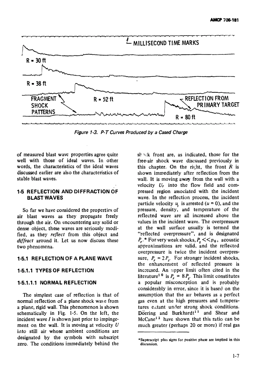
sive charge, recorded time histories of pres-
sure may be quite “trashy” in appearance,
that is to say, many small pressure distur-
bances superimposed on the primary pressure
variation of the blast wave. An example is
shown in Fig. l-3. These disturbances are the
ballistic shocks generated by fragments of the
casing moving at supersonic speed through the
air. Because fragment velocities decay less
rapidly than blast wave velocity, these frag-
ments outrun the blast wave for some time,
and they produce disturbances prior to blast
wave arrival*. This effect is shown quite
clearly in Fig. l-3.
Blast waves from sources of shapes other
than spherical are affected by the shape of the
source. These deviations are, however, quite
different from the nonideal effects discussed
here. Characteristics of waves from effectively
infinite line or plane sources are discussed in
par. 1-6 of this handbook, while character-
istics of waves from finite sources of various
shapes are covered in Chapter 3 of AMCP
706-182, Explosions in Air, Part Two36.
* Eventually the blast wave will catch up to and pass the
fragments, because the lower limit for blast wave velocity is
sound speed while the lower limit for the velocity of the
fragments, which are decelerated by drag, is zero.
14.2 GROUND EFFECTS
The character of blast waves from large
energy sources detonated near the ground can
be modified considerably by certain “ground
effects”, quite independ. ">tly of the effects of
shock reflection from a relatively rigid sur-
face, which we will discuss later. Thermal
radiation from a nuclear weapon may preheat
the air near the ground, which causes a severe
enough inhomogeneity m the atmosphere
near the ground that the subsequent passage
of a blast wave is affected seriously. Pressure
gages located near the ground then will record
decidedly nonidval time histories, as indicated
by some typical data reproduced here as Fig.
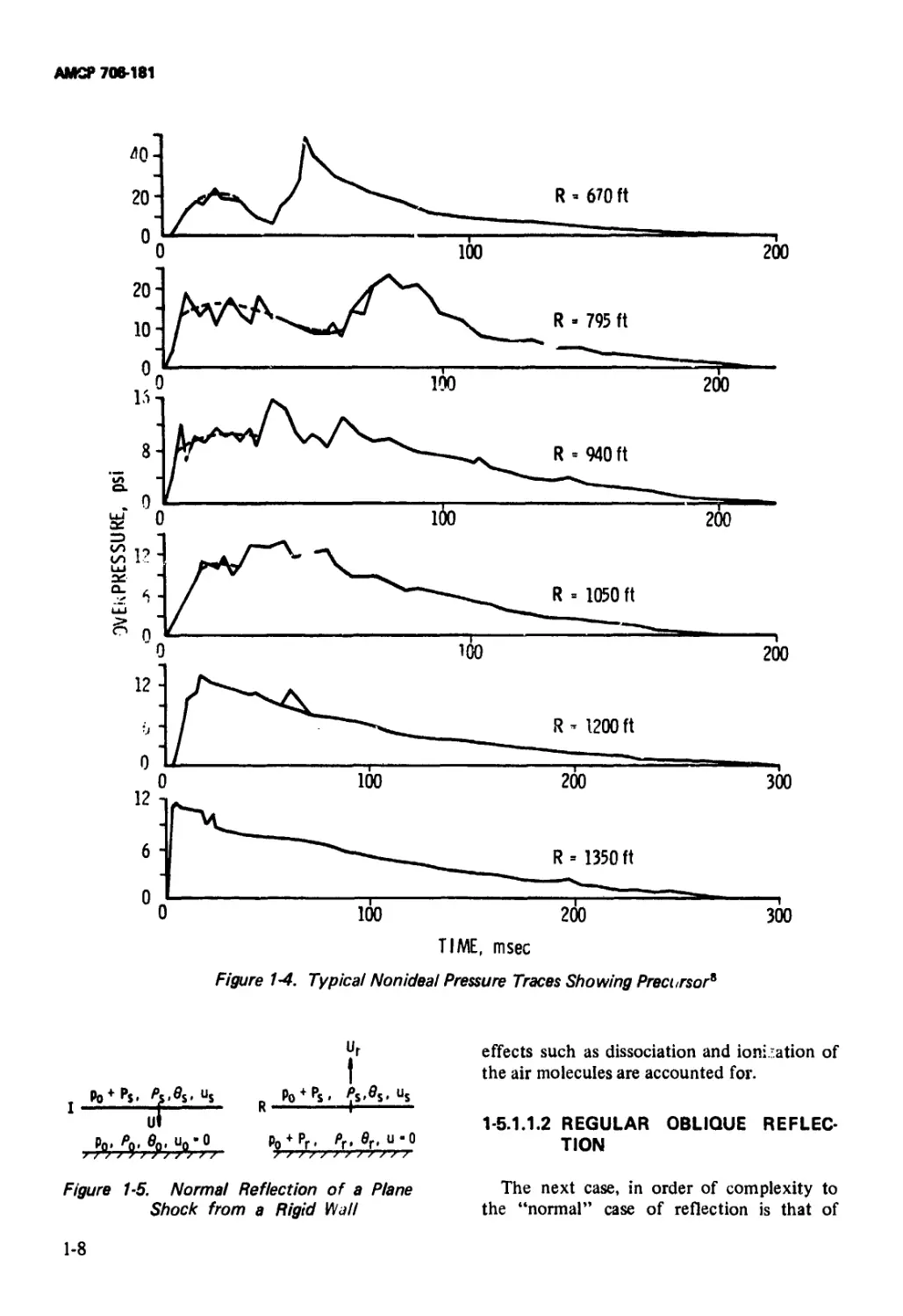
l-48. The disturbance arriving ahead of the
main shock is usually termed a “precursor”.
In the precursor regime, dynamic pressures** * is
may be much greater than in a region where
ideal waves occur. As can be seen from Fig.
I-4, precursor effects tend to disappear, and
the blast wave to return to its classical (ot
ideal) form as the wave moves farther from
the blast source. These effects are more
pronounced over dusty or heat-absorbing sur-
faces than over dust-free or heat-reflecting
surfaces.
Precursors from a large chemical explosion
on the surface of a prairie have been observed
by John Dewey9 to occur along roads com-
pacted in the prairie. He attributed the
precursors to strong ground waves, which
would have propagated along the compacted
roads at greater velocity than through the
uncompacted prairie.
The deviations from ideal blast wave char-
acteristics which have been noted are only a
few examples of such deviations which can
occur. But, small variations in initial spheric-
ity of a shock front, or other small aberra-
tion from ideal conditions, usually “smooth
out” quite quickly on passage of the blast
wave through the air, resulting in relatively
ideal blast waves everywhere except close to
the blast source. A surprisingly large majority
**Dynanic pressure q - (l/2)p и’ where p is density and и
is a particle velocity.
I-6
АМСР 706-181
Figure 1-3. Р-Т Curves Produced by a Cased Charge
of measured blast wave properties agree quite
well with those of ideal waves. In other
words, the characteristics of the ideal waves
discussed earlier are also the characteristics of
stable blast waves.
1-5 REFLECTION AND DIFFRACTION OF
BLAST WAVES So
So far we have considered the properties of
air blast waves as they propagate freely
through the air. On encountering any solid or
dense object, these waves are seriously modi-
fied, as they reflect from this object and
diffract around it. Let us now discuss these
two phenomena.
1-5.1 REFLECTIONOF A PLANE WAVE
1-5.1.1 TYPES OF REFLECTION
1-5.1.1.1 NORMAL REFLECTION
The simplest case of reflection is that of
normal reflection of a plane shock wave from
a plane, rigid wall. This phenomenon is shown
schematically in Fig. 1-5. On the left, the
incident wave I is shown just prior to impinge-
ment on the wall. It is moving at velocity U
into still air whose ambient conditions are
designated by the symbols with subscript
zero. The conditions immediately behind the
sb K'k front are, as indicated, those for the
free-air shock wave discussed previously in
this chapter. On the rirht, the front R is
shown immediately after reflection from the
wall. It is moving away from the wall with a
velocity Ur into the flow field and com-
pressed region associated with the incident
wave. In the reflection process, the incident
particle velocity us is arrested (u = 0), and the
pressure, density, and temperature of the
reflected wave are all increased above the
values in the incident wave. The overpressure
at the wall surface usually is termed the
“reflected overpressure”, and is designated
Pr* For very weak shocks, «p0, acoustic
approximations are valid, and the reflected
overpressure is twice the incident overpres-
sure, Pr = 2PS. For stronger incident shocks,
the enhancement of reflected pressure is
increased. An upper limit often cited in the
literature10 is Pr = 8Pr This limit constitutes
a popular misconception and is probably
considerably in error, since it is based on the
assumption that the air behaves as a perfect
gas even at the high pressures and tempera-
tures extant under strong shock conditions.
Doering and Burkhardt11 and Shear and
McCane12 have shown that this ratio can be
much greater (perhaps 20 or more) if real gas
♦Superscript plus signs Гог positive phase are implied in this
discussion.
1-7
АМСР 706-181
TIME, msec
Figure 1-4. Typical Nonideal Pressure Traces Showing Precursor*
Po + P$ > us
ut
Г
Po + Ps. ftA.us
Pg+Pr, Pf, в,-, U-0
777ГГП 7T>77
Figure 1-5. Normal Reflection of a Plane
Shock from a Rigid Wall
effects such as dissociation and ionization of
the air molecules are accounted for.
1-5.1.1.2 REGULAR OBLIQUE REFLEC-
TION
The next case, in order of complexity to
the “normal” case of reflection is that of
1-8
АМСР 706-181
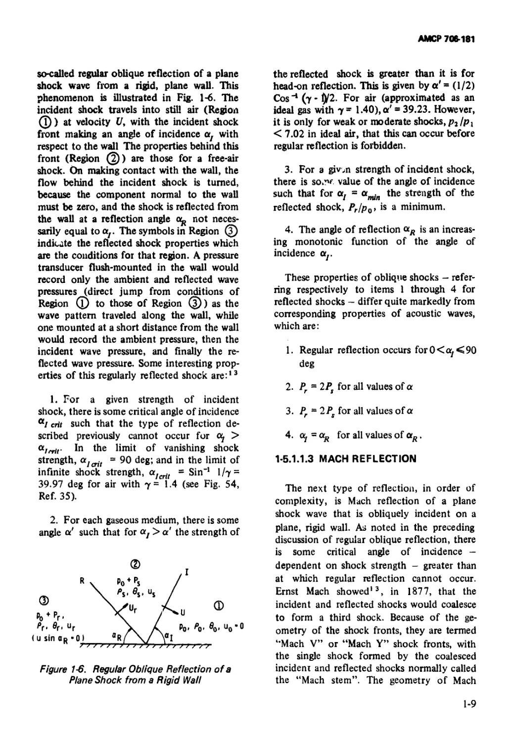
so-called regular oblique reflection of a plane
shock wave from a rigid, plane wall. This
phenomenon is illustrated in Fig. 1-6. The
incident shock travels into still air (Region
Q) at velocity U, with the incident shock
front making an angle of incidence with
respect to the wall The properties behind this
front (Region (2)) are those for a free-air
shock. On making contact with the wall, the
flow behind the incident shock is turned,
because the component normal to the wall
must be zero, and the shock is reflected from
the wall at a reflection angle 0^ not neces-
sarily equal to otr The symbols in Region (T)
indicate the reflected shock properties which
are the conditions for that region. A pressure
transducer flush-mounted in the wall would
record only the ambient and reflected wave
pressures (direct jump from conditions of
Region (T) to those of Region (5)) as the
wave pattern traveled along the wall, while
one mounted at a short distance from the wall
would record the ambient pressure, then the
incident wave pressure, and finally the re-
flected wave pressure. Some interesting prop-
erties of this regularly reflected shock are:13
1. For a given strength of incident
shock, there is some critical angle of incidence
ai crit such that the type of reflection de-
scribed previously cannot occur for 0^ >
a/rrif. In the limit of vanishing shock
strength, = 90 deg; and in the limit of
infinite shock strength, a/crlt - Sin-1 1/7 =
39.97 deg for air with 7= 1.4 (see Fig. 54,
Ref. 35).
2. For each gaseous medium, there is some
angle a' such that for 07 > a' the strength of
Figure 1-6. Regular Oblique Reflection of a
Plane Shock from a Rigid Wall
the reflected shock is greater than it is for
head-on reflection. This is given by a' = (1/2)
Cos “* (7 - ty2. For air (approximated as an
ideal gas with 7= 1.40), a' = 39.23. However,
it is only for weak or moderate shocks, p2 lpx
< 7.02 in ideal air, that this can occur before
regular reflection is forbidden.
3. For a givm strength of incident shock,
there is so,r>e value of the angle of incidence
such that for az = the strength of the
reflected shock, Prlp0, is a minimum.
4. The angle of reflection <xR is an increas-
ing monotonic function of the angle of
incidence
These properties of oblique shocks - refer-
ring respectively to items 1 through 4 for
reflected shocks - differ quite markedly from
corresponding properties of acoustic waves,
which are:
1. Regular reflection occurs for0<a;<90
deg
2. Pr - 2PS for all values of a
3. Pr = 2Pf for all values of a
4. a; = aR for all values of aR.
1-5.1.1.3 MACH REFLECTION
The next type of reflection, in order of
complexity, is Mach reflection of a plane
shock wave that is obliquely incident on a
plane, rigid wall. As noted in the preceding
discussion of regular oblique reflection, there
is some critical angle of incidence -
dependent on shock strength - greater than
at which regular reflection cannot occur.
Ernst Mach showed13, in 1877, that the
incident and reflected shocks would coalesce
to form a third shock. Because of the ge-
ometry of the shock fronts, they are termed
‘"Mach V” or “Mach Y” shock fronts, with
the single shock formed by the coalesced
incident and reflected shocks normally called
the “Mach stem”. The geometry of Mach
1-9
АМСР 706-181
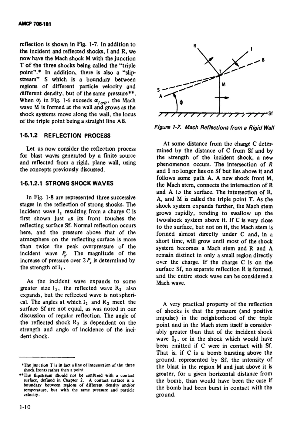
reflection is shown in Fig. 1-7. In addition to
the incident and reflected shocks, I and R, we
now have the Mach shock M with the junction
T of the three shocks being called the “triple
point”.* In addition, there is also a “slip-
stream” S which is a boundary between
regions of different particle velocity and
different density, but of the same pressure**.
When at; in Fig. 1-6 exceeds the Mach
wave M is formed at the wall and grows as the
shock systems move along the wall, the locus
of the triple point being a straight line AB.
1-5.1.2 REFLECTION PROCESS
Let us now consider the reflection process
for blast waves generated by a finite source
and reflected from a rigid, plane wall, using
the concepts previously discussed.
1-5.1.2.1 STRONG SHOCK WAVES
In Fig. 1-8 are represented three successive
stages in the reflection of strong shocks. The
incident wave lt resulting from a charge C is
first shown just as its front touches the
reflecting surface Sf. Normal reflection occurs
here, and the pressure above that of the
atmosphere on the reflecting surface is more
than twice the peak overpressure of the
incident wave Ps. The magnitude of the
increase of pressure over 2PS is determined by
the strength of It.
As the incident wave expands to some
greater size 12, the reflected wave R2 also
expands, but the reflected wave is not spheri-
cal. The angles at which I2 and R2 meet the
surface Sf are not equal, as was noted in our
discussion of regular reflection. The angle of
the reflected shock R2 is dependent on the
strength and angle of incidence of the inci-
dent shock.
♦The junction T is in fact a line of intersection of the three
shock fronts rather than a point.
**The slipstream should not be confused with a contact
surface, defined in Chapter 2. A contact surface is a
boundary between regions of different density and/or
temperature, but with the same pressure and particle
velocity.
At some distance from the charge C deter-
mined by the distance of C from Sf and by
the strength of the incident shock, a new
phenomenon occurs. The intersection of R
and I no longer lies on Sf but lies above it and
follows some path A. A new shock front M,
the Mach stem, connects the intersection of R
and A to the surface. The intersection of R,
A, and M is called the triple point T. As the
shock system expands further, the Mach stem
grows rapidly, tending to swallow up the
two-shock system above it. If C is very close
to the surface, but not on it, the Mach stem is
formed almost directly under C and, in a
short time, will grow until most of the shock
system becomes a Mach stem and R and A
remain distinct in only a small region directly
over the charge. If the charge C is on the
surface Sf, no separate reflection R is formed,
and the entire stock wave can be considered a
Mach wave.
A very practical property of the reflection
of shocks is that the pressure (and positive
impulse) in the neighborhood of the triple
point and in the Mach stem itself is consider-
ably greater than that of the incident shock
wave I3, or in the shock which would have
been emitted if C were in contact with Sf.
That is, if C is a bomb bursting above the
ground, represented by Sf, the intensity of
the blast in the region M and just above it is
greater, for a given horizontal distance from
the bomb, than would have been the case if
the bomb had been burst in contact with the
ground.
1-10
АМСР 706-181
Figure 1-F. Reflection of Strong Shock Waves
In Fig. 1-9 the geometry of the Mach
reflection process can be seen in more detail.
By comparison with Fig. 1-7, one can see that
incident and reflected shocks are both curved,
and that the path of the triple point is no
longer a straight line. Although the Mach stem
is shown as a vertical straight line in Fig. 1-9,
this is not always the case in realitv.
1 5.1.2.2 WEAK SHOCK WAVES
Very weak shock waves, i.e., those of
nearly acoustic strength, are reflected from
plane surfaces in such a way that a geomet-
rical construction of the wave system can be
made very simply. Consider a point source of
the shock C (Fig. 1-10) and, some distance
from it, a plane reflecting surface Sf. The
incident wave I, striking the surface, will be
reflected from it in such a way that the
reflected wave R may be considered to arise
from a second image source C' which is on the
opposite side of the reflecting surface, on a
line perpendicular to Sf through the true
source, and at a distance from Sf equal to the
distance of C from the surface.
Fig. 1-10 shows two successive stages of
this reflection process. In the first stage the
incident wave h is just tangent to the
surface. The excess pressure over that of the
atmosphere at the reflecting surface is just
double (for very weak shock waves) that of
the incident wave where it is not in contact
with the surface. At a later stage, the incident
wave is represented at I2 and the reflected
wave at R2, which is imagined to arise from
the image source C'. Again, the pressure at the
line of contact of 12, R2, and the surface Sf is
just double that at I2 where it is not in
contact with the surface. The angles at which
the shocks I2 and R2 meet the surface Sf are
equal, and no Mach stein is formed. For most
practical cases of interest in air blast tech-
nology, shocks are too strong for this acoustic
approximation to be applicable, and this
simplified geometry cannot be used.
1-5.2 DIFFRACTION OF A PLANE WAVE
When a blast wave encounters a solid object
of finite extent, very complicated processes
1-11
АМСР 706-181
Y - height of Mach stem do - horizontal distance for start of formation of
hc “ height of charge above reflecting surface Mach stem
d = any horizontal distance > do
Figure 1-9. Geometry of Mach Reflection
Figure 1-10. Rtf lection of Weak Shock Waves
1-12
ensue. The interaction of the shock front with
such obstacles is termed diffraction.
The phenomenology to be described indi-
cates the complexity of the diffraction pro-
cess for even the very simple case of passage
of a plane shock wave over obstacles of very
regular geometry. For more complex shapes,
or for different blast orientations, or for
curved shock waves, the processes are even
more complicated. Many shock-tube experi-
ments have been conducted to determine
diffracted shock configurations and pressures
(in fact, the discussion that follows is based
on the results of such experiments). The
reader is referred to Refs. 15 through 23 for
comprehensive studies of the diffraction pro-
cess.
1*5.2.1 TWO-DIMENSIONAL RIGID THICK
WALL
The diffraction process can perhaps best be
illustrated by describing the sequence of
АМСР 706-181
events occurring when a plane blast wave
traveling over a rigid plane encounters a rigid,
thick wall protruding from the plane, as
illustrated in Fig. 1-11(A). The geometry is
shown in the first sketch of this figure, 'vith
the blast front being normally incident on the
front face of the wall, and the pressure on all
faces on the wall being at ambient pressure
p0. As the incident wave 1 first encounters the
wall, reflection of the portion of the wave
striking the front face of the wall occurs; the
reflected wave R moves to the left, and the
pressure on the front face jumps to p0 + Pr.
Above the wall, the incident waves continue
on relatively undisturbed.
As the reflected wave moves to the left
away from the front face of the wall, a
rarefaction front moves down the front face,
as shown in Fig. 1-11 (B). A vortex is shed
from the upper lefthand comer at the wall. A
vortex is a region of air spinning about an axis
at a high speed. Low overpressures exist at its
center because of the Venturi effect. At the
instant depicted in Fig. 1-11 (B), the lower
portion of the front face still feels the
reflected pressure pQ + Pr, while the upper
portion feels a lower pressure quite near the
pressure p9 + Ps in the incident wave. The
portion of the top face behind the incident
shock I is subjected to pressure p0 +PS, with
the pressure perhaps somewhat reduced below
(A)
VORTEX
RAREFACTION \
WAVE ;
.U
SHOCK FRONT
DIFFRACTED
SHOCK
FRONT
IB)
Uf*|
frm
R
Figure 7-7 7. Diffraction of a Shock Front Over
a Wall16
(Reprinted by permission ofC. H. Norris, R. J. Han-
sen, M. J. Holiey, Jr., J. M. Biggs, S. Namyet, and
J. K. Minami, Structural Design for Dynamic Loads,
McGraw-Hill Book Co., N.Y., 1959.)
this value in the vicinity of the vortex. Ahead
of the incident shock, the pressure on the top
face and on the rear face of the wall is still p0.
As the incident shock front passes beyond
the rear face of the wall, it diffracts around
this face, as shown in Fig. 1-11(C). A second
vortex is formed at the upper righthand
comer of the wall. At the instant shown in
Fig. 1-11 (C), the reflected wave from the
front face of the wall has been completely
attenuated by the rarefaction wave, and the
pressure on the front face is p0 + q, where q is
dynamic pressure. On the top face the pres-
sure is still nearly equal to p0 + Ps. Behind the
diffracted incident wave on the rear face,
pressure is somewhat less than p0 + Ps. Ahead
of the front 1, the pressure is p0. The
maximum back wall pressure develops slowly
as a result of vortex phenomena and the time
required for the back wall to be enveloped by
the blast. In the final strge, the incident wave
has passed beyond the wall, the diffraction
process is over, and the wall is immersed in
the flow field behind the front. For a long-
duration blast wave, pressures are nearly
those which would be measured in steady-
state wind tunnel experiments.
1-5.2.2 THREE-DIMENSIONAL BLOCK
For a three-dimensional block structure,
the phenomena described in par. 1-5.2.1 also
occur along the sides of the block, so that the
preceding discussion also applies to diffrac-
tion about the sides of such structures. This
process is illustrated in Fig. 1-12. Fig. 1-13
gives recorded pressure-time histories for the
front, top, and back faces of a model three-
dimensional block structure, as recorded in
shock tube at BRL33. The pressure-time
history for the front face of the block shows
reflected pressure (initially Pr) and the effect
of the rarefaction wave produced at the front
face which causes rapid reduction in reflected
pressure. The pressure recorded on the top
face of the block shows an initial peak of
side-on pressure Ps and a less rapid pressure
decay. The pressure recorded at the back face
of the block shows a slow rise time of
pressure with no real “shocking-up”. Detailed
1-13
АМСР 706-181
,SH0CK FRONT
loading of another three-dimensional struc-
ture is given in a report by Janus and
Kingery34.
1-5.2.3 CIRCULAR CYLINDER
In Figs. 1-14 and 1-15 are shown the
sequence of events involved in diffraction of a
blast wave about a circular cylinder15. In
these figures the shock fronts are shown as
thick lines and their direction of movement
by arrows normal to the shock front. In Fig.
1-14(A), the incident shock has collided with
the cylinder giving rise to a curved, expand-
ing, reflected shock R. In Fig. 1-14(B), the
incident shock I and reflected shock R are
now joined to the cylinder surface by a Mach
stem M. R is now much weaker than in Fig.
1-14(A) and is omitted in the succeeding parts
of the figure.
In this shock configuration a slipstream S
has been formed. This slipstream is a line
dividing flows of differing densities, but of
the same pressure. When a Mach stem is
formed on a plane surface the slipstream
Figure 1-12. Diffraction of a Shock Front
Over a Three-dimensional Block Structure
(Plan View)16
(Reprinted by permission of С. H. Norris, R. J. Han-
sen, M. J. Holley, Jr., J. M. Biggs, S. Namyet, and
J. K. Minami, Structural Design for Dynamic Loads,
McGraw-Hill Book Co., N.Y., 1959.)
Figure 1-13. Pressures on a Three-dimensional Block Structure During Diffraction33
1-14
АМСР 706-181
Figure 1-14. Tracings of Shadowgraphs Showing the interaction of a Shock Front With a Cylinder
extends upstream, slanting down to meet the
surface. In the present case, however, the
increased flow near the cylinder surface has
caused the foot of the slipstream to move
nearer to the foot of M. The slipstream,
therefore, presents a curved appearance. In
Fig. I-14(C), the feet of the Mach stems have
reflected from each other and are now moving
on a second circuit of the cylinder. The
slipstreams have been swept nearer the rear of
the cylinder and now intersect with the
diffracted parts of the Mach stems X and Y.
The commencement of two vortices is indi-
cated at Vt and V2. These are probably
induced by the back pressure behind the
shocks X and Y interacting with the boundary
layer flow at the surface of the cylinder. The
shaded portion is due to a localized region of
supersonic flow. In Fig. 1-14(D), the Mach
stems, M and M', have moved some way
downstream of the cylinder. A Mach stem M "
joins the free air parts of M and M' with the
diffracted parts PD and P 'D which terminate
on the cylinder surface. The growth of the
vortices is apparent in this figure. In Figs.
1-15(A) and (B), the foot of PD has moved
further round the cylinder upstream. Notice
that the point of flow separation has followed
this shock. In Fig. 1-15(C), the vortices, Vj
and V2, are breaking away from the cylinder;
while in Fig. 1-15(D), the vortices are being
swept downstream, and the point of flow
separation has moved toward the rear of the
cylinder again.
The phenomenology described indicates
the complexity of the diffraction process for
even the very simple case of passage of a plane
1-15
АМСР 706-181
Figure 1-15. Tracings of Shadowgraphs Showing the Interaction of the Shock Front With a
Cylinder
shock wave over obstacles of very regular
geometry. For more complex shapes, or for
different blast orientations, or for curved
shock waves, the processes are even more
complicated. Many shock-tube experiments
have been conducted to determine diffracted
shock configurations and pr jsures (in fact,
the discussion is based on the results of such
experiments). The reader is referred to Refs.
16 through 23 for comprehensive studies of
the diffraction process.
1-6 EFFECTS ON BLAST WAVES
1-6.1 SHAPE OR ASYMMETRY OF
SOURCE ON BLAST WAVES
1-6.1.1 COMMON SHAPES
In most air blast theoretical work, the
source of blast energy is assumed to be a
point or a sphere, so that the blast wave
characteristics are a function of one space
dimension only, i.e., the radial distance from
the center of the source. Similarly, in most air
blast experimentation, great pains are taken
to make the source as spherical as possible so
that comparisons can be made with one-
dimensional theory, or to eliminate the ef-
fects of shape of source. Many real blast
sources, however, are distributed or highly
directional. Detonating cord is widely used in
explosive operations, and it is essentially a
line source rather than spherical. Explosive in
the form of thin sheets is also now widely
used, and it represents a plane source. The
gases released from gun muzzles after exit of ;
projectiles are important sources for blast 1
waves, and they represent axisymmetric but
highly directional sources. Let us now discuss
some of the effects of shape or asymmetry of
the source on blast wave characteristics.
1-16
АМСР 706-181
1-6.1.1.1 STRAIGHT LINE CHARGE
For straight line charges which are very
long compared to their diameters, Kennedy*3
reports that both theoretical and experi-
mental studies indicate blast waves that are
similar in their general characteristics to the
waves from spherical or “blocky” sources but
which have much less rapid decay of pressure
and impulse with distance. In fact, for such
line charges, a different scaling law usually is
applied than the commonly used Hopkinson
blast scaling (see Chapter 3). The peak over-
pressure Pt is a function of R/CW/LP12 rather
than R/W* '3 where distance L is measured
normal to the charge axis. Similarly, the
scaled positive side-on impulse IJ (W/L)1'2 is
a function of R/fW/L)1'2, rather than the
scaled impulse ISW3 being a function of
R/WVi. To explain, the shock front expands
cylindrically rather than spherically, but it is
still a function of only one space coordinate,
provided one considers distances which are
short compared with length of the line source,
i.e., R <<L - where R is the distance from
the blast center and L is the larger character-
istic dimension of the blast source.
1-6.1.1.2 MUZZLE BLAST
Muzzle blast waves from guns are axisym-
metric but not spherically symmetric. They
usually consist of a single shock front (see
Fig. 1-16), but one which has highly direc-
tional properties near the muzzle. The general
characteristics at any point in the blast field
are nearly similar to those of spherical
sources, but the difference is that the muzzle
blast field characteristics are a function of
two spatial cylindrical coordinates, (r, z)
rather than one spherical coordinate R. Diver-
gence is more nearly spherical than for line
charges, but it is definitely a function of the
two cylindrical coordinates r and z.
1-6.1.1.3 LARGE PLANE CHARGE
Blast waves generated by a iaige, plane
source, such as a thin sheet of explosive or a
blanket of woven detonating chord, decay
even more slowly with distance from the
Figure 1-16. The Blast Wave from a 7.62 mm
Rifle at Three Stages of Expansion
(Courtesy of Roy»! Armament Research and Develop-
ment Establishment)
source than do waves from line sources.
Lindberg and Firth24 have compared theoret-
ically predicted variations in peak overpres-
sure with distance for spherical, infinite cylin-
drical (line), and infinite plane blast sources
(see Fig. 1-17). The scaled distance parameter
R/ro in their plot is based on characteristic
dimension r which is defined as
О
ro^E/[p0L^]l/v (1-11)
where
v = 1,2,3, respectively, for plane, cylindri-
cal, and spherical blasts
E = total explosive energy.
1-6.1.2 DISTANCE EFFECT
Any real blast source is, of course, finite in
extent, so that the idealization of infinite line
1-17
АМСР 706*181
Figure 1-17. Incident Shock Overpressure
Ratio ks Scaled Distance2 *
or plane sources only can give reasonable
approximations for small distances from the
sources. As one moves further from a real,
nonspherical source, i.e., for/? >>£, the blast
front tends to more closely approximate that
of one which would have emanated from a
spherical blast source. All effects of asym-
metry of the new spherical source disappear
and, for R > > L, waves from two sources
having the same total energy but very dif-
ferent shapes become indistinguishable.
1-6.2 LONG-RANGE FOCUSING
1-6.2.1 HOMOGENEOUS MEDIUM
As a blast wave is propagated through the
air to great distances from its source, it
weakens and decreases in shock velocity until
it is propagating at essentially the speed of
sound. If the air were a homogeneous, still
medium, then acoustical laws still apply; the
velocity of propagation would be constant,
and the pressure in the front would decrease
as the inverse of the distance. Because the
head of the wave would now be moving at
nearly the same velocity as the tail, the
duration of the very low magnitude positive
overpressure eventually should reach some
nearly constant value. In fact, the entire time
history should approach essentially a constant
functional form, changing only in amplitude
1-18
as it advances. Such acoustic asymptotes for
overpressure, duration, and positive phase
impulse are given in Chapter 6.
1-6.2.2 INHOMOGENEOUS MEDIUM
If the orderly behavior described in par.
1-6.2.1 were indeed always observed in the
transmission of air blast waves over long
distances, then long range focusing of blast
waves would be of minor interest. The shock
wave characteristics from even very large
energy blast sources would decrease rapidly to
their acoustic asymptotes; and the amplitudes
and durations of the resulting weak pressure
waves could be estimated by extrapolation
from measured time histories, using the acous-
tic law for inverse decrease in pressure with
increase in distance from the blast source.
Such a procedure has been followed by
Perkins, et al.2 5 in estimating the side-on
overpressures at large distances from TNT
explosive charges detonated on or near the
ground (see Fig. 1-18). Unfortunately, the
atmosphere cannot be considered a homo-
geneous, still medium over any appreciable
distance from a given location on the ground;
and the variations in meteorological condi-
tions-such as wind velocity, temperature, and
perhaps relative humidity-seriously can af-
fect the propagation of air shocks at long
distances.
Berning2 6 points out that the phenomenon
of unusual sound or blast propagation has
been known for many years, dating back even
to the era prior to the Civil War. Successive
zones of audibility and silence along radial
lines from the blast centers of severe explo-
sions or artillery fire have been noted by
many observers. Complaints of damage from
blast waves at long distances from the source
have emphasized the fact that some kind of
''constructive" or "destructive" focusing of
blast waves can occur at long distances. It is
termed “constructive” from f..e point of view
of the blast physicist, who notes that the blast
pressure is enhanced; it is termed “destruc-
tive” from the point of view of the home-
owner, whose windows are shattered or walls
are cracked.
АМСР 706-181
OVERPRESSURE Р psi
Figure 1-18. Surface Air Blast Pressure vs Range from Detonations on the Surface15
1-6.2.2.1 THEORY
A theory for propagation of blast waves
over long distances has been developed by
Berning26, under the assumptions that the
blast wave can be treated as a sound wave,
and that only wind and air temperature have
appreciable effect on propagation velocities.
This theory, based on earlier work by Fryi-
whara27 and Milne28, utilizes Lord Ray-
leigh’s concept of “rays of sound” which
represent the changing direction of propaga-
tion of the sound waves. Equations for these
sound rays are given as functions of the
gradients in sound velocity with increasing
altitude (caused by the variation in tempera-
ture and wind shear with altitude) and of the
initial angle of inclination of a given sound
ray. A typical sound velocity gradient and the
corresponding ray paths are shown in Figs.
1-19(A) and (B), respectively. From this
theory, one can determine the location of
areas in which focusing could occur, provided
one has accurate data on wind and tempera-
ture structure of the atmosphere in the
neighborhood of the blast source. One cannot
as easily determine the magnitude of the
increased blast pressure. Some estimates can
Figure 1-19(A). Typical Sound Velocity
Gradient
1-19
АМСР 706-181
HORIZONTAL DISTANCE FROM SOUND SOURCE, ft
Figure 1-19(B). Paths of Sound Rays in the Atmosphere, for Sound Velocity Gradient
of Fig. 1-19(A)
be made based on empirical observations of
pressures and damage to light structures or
glass. Perkins, et al.25 have done this, and
they have correlated blast strengths with
various velocity gradients. They report their
estimates in terms of factors which multiply
the blast overpressures predicted by the
homogeneous atmospheric case (Fig. 1-20).
The multiplication factors for various types of
gradients are illustrated in that figure.
1-6.2.2.2 PRACTICE
In practice, the application of Berning’s
relatively simple theory for the prediction of
focusing can be quite tedious and time con-
suming. One must obtain data on the tem-
perature and wind velocity and direction, as a
function of altitude up to at least 10,000 ft.
These data must be translated into sound
velocity gradients along a number of azimuths
through the blast source location. The equa-
tions must then be solved for each separate
azimuth and for a number of sound rays. All
of the calculations must be performed quite
rapidly so that the meteorological conditions
do not change appreciably in the meantime. If
much firing is anticipated at a test site, it may
prove advisible to automate as much of this
procedure as possible. Perkins, et al.2 5 report
the use of an analog computer for solution of
the equations involved, and the acquisition of
a library of velocity gradients and correspond-
ing focus predictions at Aberdeen Proving
Ground over a period of several years. They
found that prediction of focus conditions
often could be made with sufficient accuracy
by comparing the existing current velocity
gradients with those in the library. Using this
procedure, and allowing testing to occur only
on days when no focus was predicted in
inhabited areas, they were able to reduce
1-20
АМСР 706-181
CATEGORY DESCRIPTION MULTIPLICATION FACTOR
1 SINGLE NEGATIVE GRADIENT ALTITUDE VELOCITY 0
2 SINGLE POSITIVE GRADIENT 5
3 ZERO GRADIENT NEAR SURFACE WITH POSITIVE GRADIENT ABOVE 10
4 WEAK POSITIVE GRADIENT NEAR SURFACE WITH STRONG POSITIVE GRADIENT ABOVE ,. - ... 25
5 NEGATIVE GRADIENT NEAR SURFACE WITH STRONG POSITIVE GRADIENT ABOVE 35
Figure 1-20. Various Types of Velocity Gradients To Be Expected and the
Increase in Intensity at a Focus for Each Type
markedly the incidence of complaints and
claims of damage from these areas as a result
of the firing of large weapons and detonation
of large explosive charges.
Procedures similar to those developed by
Berning26 and Perkins, et al.2 5 have been
employed at a number of other test sites to
control the incidence of focusing effects from
large blast sources. An excellent general dis-
cussion of the overall problem of effects of
long-range blast focusing and of the difficul-
ties in obtaining accurate estimates of these
effects is given by Reed29, who was con-
cerned with side effects of cratering with
nuclear explosives. Reed also includes an
extensive bibliography on the subject in his
report. He uses the adjective “caustic” to
indicate exceptional disturbances at long
ranges. Figs. 1-21 and 1-22 are illustrations of
typical vertical sound velocity profiles and
resulting distortions and focusing of ray
paths2 ’.
1-6.3 VARIATION OF TYPES OF ENERGY
SOURCE
Most of the available experimental data and
analyses of blast waves in air are limited to a
few types of chemical explosives (usually
either TNT or Pentolite) and to nuclear
explosives. What are the effects for other
explosives or other types of blast sources?
1-6.3.1 CHEMICAL EXPLOSIVES
During World War II, the British and
Americans conducted many tests with differ-
ent types of chemical explosives in attempts
to optimize blast damaging effects. They
1-21
АМСР 706-181
ALTITUDE
BOO IOOO 1200 DISTANCE —•»
VELOCITY , ft/wc
Figure 1-21. Shock Wave Distortion by
Layered Atmospheric Temperature
and Wind Structure29
found that a number of explosives generated
blast waves of measurably different peak
pressure and impulse from those of a “stan-
dard” explosive of their choosing. In par-
ticular, those explosives which contained sig-
nificant quantities of aluminum powder exhib-
ited those differences.* Kennedy’3 has sum-
marized much of this early work, and he has
noted that the general characteristics of blast
waves from different chemical explosives are
quite similar-their relative peak overpressures
and impulses being essentially independent of
distance from the charge. Results, of measure-
ments over a number of distances, therefore,
could be averaged and quoted as ratios
applicable over all distances. Such ratios for a
number of explosives, relative to Composition
B, are shown in Table 1-113. Comparisons for
other explosives are given in AMCP
706-182(S), Explosions in Air, Part Two (U).
Because the ratios for peak pressure and
impulse do not differ greatly, one can ap-
‘The reaction of aluminum with the “oxidizer” present in
chemical explosives is more energetic than the decom-
position of the chemical explosive by itself.
proximately equate blast waves from different
explosives I у using a conversion to an “equiv-
alent weight” or “equivalent energy” of some
standard explosive which is usually TNT. This
conversion is a multiplier which would cause
the blast data for the other explosive to
coalesce with TNT data, as nearly as possible.
This coefficient for Pentolite is usually as-
sumed to be about 1.1 X TNT. Note that it is
not equivalent to the coefficients given in
Table 1-1, or their inverses. While not exact,
this method offers a way of estimating blast
for explosives where limited data exist. Some-
times the conversion coefficient can be esti-
mated from ratios of the heats of detonation
for a new explosive to that of TNT, with
these heats of detonation being measured in a
bomb calorimeter. Note from Table 1-1, that,
although blast parameters are measurably
different for different chemical explosives,
the entire range of differences is not great. A
maximum coefficient of 1.5 covers the entire
range of peak pressures and impulses, for all
the explosives compared on an equal volume
basis. One, therefore, should view with cau-
tion claims for vastly superior chemical explo-
sives for generating air blast.
1-6.3.2 NUCLEAR EXPLOSIVES
Nuclear explosives differ from chemical
explosives in their ability to produce air blast
waves primarily because of the sheer magni-
tude of their total energy release, and because
of the difference in energy density between
the two types of explosive sources. Close to a
nuclear weapon burst, the blast overpressure
will be greater than that from a scaled
chemical explosion of the same effective blast
yield. At greater distances, the blast waves
will be quite similar30. In comparing blasts
from TNT and nuclear explosives at sea level,
the total yield from the nuclear explosive is
often related to the detonation energy of
TNT by an effectiveness factor of 0.5 i.e.,
Y. . . , , = 0.5 Y, , , In the calcu-
total (nuc) total (TNT).
lations of properties of blast waves from
nuclear explosions, the nuclear explosive
sources often are assumed to be point sources
because of their high energy density.
1-22
МКГ 706-181
Figure 1-22. Typical Explosion Ray Paths29
1-6.3.3 OTHER SOURCES
Other types of blast sources often have
smaller energy densities than condensed
TABLE 1-1
PEAK PRESSURE AND POSITIVE IMPULSE
RELATIVE TO COMPOSITION В
(THE COMPARISON BEING ON AN EQUAL
VOLUME BASIS)
Explosive Relative peak pressure Relative positive impulse
Torpex (30% Al) 1.13 1.21
Torpex-2 1.12 1.1Б
Minol-3 1.09 1.13
DBX 1.07 1.11
HBX 1.06 1.11
Tritonal 7Б/25 1.04 1.10
Minol-2 1.06 1.09
Tritonal 80/20 1.04 1.08
T rialen 1.02 1.06
Baronal 1.00 1.02
Comp. В (1.00) (1.00)
Pentolite 0.98 0.97
Ednatol 0.94 0.9Б
TNT 0.92 0.94
Picratol 0.90 0.90
Amatex 0.88 0.8Б
Amatol 0.86 0.B0
chemical explosives. Such sources include
bursting pressure vessels, the muzzle and
breech blasts from guns and recoilless weap-
ons, detonable gas mixture, etc. Air blasts
generated by such sources will have peak
overpressures that are initially less than those
from solid chemical explosives, but again,
these waves will become essentially similar to
those of approximately scaled TNT blasts at
sufficiently great distances from the blast
center. Larson and Olson3 * show such data
for light pressure vessels burst by burning
propellant. Brode3 presents results of calcula-
tions showing the differences in peak over-
pressures for various types of blast sources
(see Fig. 1-23). Again, an approximate “TNT
equivalent” can be estimated by comparing
the ratio of energies available to drive the
blast wave from these more diffuse sources to
that of the detonation energy of TNT. A
method used by Baker, et al.32, for a com-
pressed gas source, is to estimate blast energy
by assuming an isentropic expansion from gas
conditions at the instant of pressure release to
ambient atmospheric pressure. The change in
internal energy of the gas then is assumed to
be the relevant input energy for blast. The
equation for computing this energy E is
P*V
(1-12)
1-23
AMSP 706-181
Point Source, Air, (----------) Perfect, f------J
Imperfect; Hot Sphere 2 x 10* atm and 3.86 x
10 s °K(----------);TNT(------------)
Figure 1-23. Variation of Peak Overpressure
Ratios P With Shock Radius \
for Various Explosions3
helium at a pressure of 3500 psia. The NASA
Manned Spacecraft Center was concerned
about the possible blast effects of rupture of
this vessel during vibration testing in their
laboratory. What is the TNT equivalent of
burst of this vessel?
Input values for Eq. 1-12 are
p0 - 14.7 psia (ambient pressure at
Houston, Texas)
p - 3500 psia
F= 7x10* in.2 3
7 = 5/3 (Helium is a monatomic gas.)
where
p = initial absolute pressure
V = total volume
p0 = ambient pressure
у = ratio of specific heats for the expanding
gas
By comparing this energy to the detonation
energy of TNT (1000 cal/g = 18.3 X 10⁶
in.-lbf/lb ), a “TNT equivalent” can be esti-
mated. A sample calculation follows.
Sample Calculation
In the Apollo Service Module, there is a
pressure vessel which stores 7 X 10* in.3 of
From Eq. 1-12,
1.546X 10⁶ [238 - (238)3/s]
E = 3.27 X Ю8 in.-lbf
Using the detonation energy of TNT, we have
3.27 X 10⁸
Wtnt ~ 18.13X .06
= 18.02 lbm of TNT
ffl
REFERENCES
1. P.D. Flynn, Elastic Response of Simple
Structures to Pulse Loading, BRL Memo.
Report No. 525, Aberdeen Proving
Ground, Md., November 1950.
2. N. H. Ethridge, A Procedure for Reading
and Smoothing Pressure-Time Date from
H. E. and Nuclear Explosions, BRL
Memo. Report 1691, Aberdeen Proving
Ground, Md., September 1965.
3. H. L. Brode, “Numerical Solutions of
Spherical Blast Waves”, Jour, of Appl.
Phys. 26, 6, 766-775 (June 1955).
1-24
AMCF 70M81
4. H. L. Brode, The Blast Wave in Air
Resulting from a High Temperature, High
Pressure Sphere of Air, RM-1825-AEC,
The Rand Corp., Santa Monica, Cali-
fornia, December 1956.
5. John M. Dewey, “The Air Velocity in
Blast Waves from TNT Explosions”, Proc,
of the Royal Soc. A, 279, 366-385
(1964).
6. L. Rudlin, Private communication regard-
ing second and secondary airshocks from
HE explosions.
7. R. J. Larson and W. Olson, Measurements
of Air Blast Effects from Simulated
Nuclear Reactor Core Excursions, BRL
Memorandum Report No. 1102, Aber-
deen Proving Ground, Md., September
1957.
8. E. J. Bryant, N. H. Ethridge, and J. H.
Keefer, Operation TEAPOT, Project
1.14b, Measurements of Air-Blast Phe-
nomena with Self-Recording Gages,
WT-1155, July 1965 (AD-617 170).
9. John M. Dewey, “Precursor Shocks Pro-
duced by a Large Yield Chemical Explo-
sion”, Nature, 205, p. 1306.
10. S. Glasstone (Ed.), The Effects of Nu-
clear Weapons, U. S. Government Print-
ing Office, Washington, D. C., p. 124,
1962.
11. W. Doering and G. Burkhardt, Contribu-
tions to the Theory of Detonation, TR
No. F-TS-1227-1A, Wright-Patterson
AFB, Ohio, p. 306, May 1949.
12. R. Shear and P. McCane, Normally Re-
flected Shock Front Parameters, BRL
Memorandum Report No. 1273, Aber-
deen Proving Ground, Maryland, May
1960.
13. W. D. Kennedy, Effects of Impact and
Explosion, Report of Div. 2, NDRC,
Washington, D.C.
Vol. I: Explosions and Explosives in Air,
Chapter 2, Part II, p. 84,1946.
14. E. Mach and J. Sommer, “Uber die
Fortpflanzungsgeschwindigkeit von Ex-
plosionsschailwellen”, Akadetnie der Vis-
senschafter, Sitzangberichte der Wiener,
Vol. 74,1877.
15. V. J. Bishop, R. D. Rowe, The Inter-
action of a Long Duration Friedlander
Shaped Blast Wave with an Infinitely
Long Right Circular Cylinder. Incident
Blast Wave 20.7 psi. Positive Duration 50
ms and a 16 cm Diameter Cylinder,
AWRE Report No. 0-38/67, Atomic
Weapons Research Establishment, Alder-
waston, Berkshire, England, April 1967.
16. С. H. Norris, R. J. Hansen, M. J. Holley,
Jr., J. M. Briggs, S. Namyet, and J. K.
Minami, Structural Design for Dynamic
Loads. McGraw-Hill Book Co., New
York, 1959, pp. 249-252.
17. W. Bleakney, Shock Loading of Rec-
tangular Structures, Tech. Rept. 11-11,
Princeton Univ. Dept, of Physics, Prince-
ton, N. J., January 10, 1952.
18. W. Bleakney, Rectangular Block, Dif-
fraction of a Shock Wave Around an
Obstacle, Princeton Univ. Dept, of
Physics, Princeton, N. J., December 17,
1949.
19. W. Bleakney, The Diffraction of Shock
Waves Around Obstacles and the Tran-
sient Loading of Structures, Tech. Rept.
11-3, Princeton Univ. Dept, of Physics,
Princeton, N. J., March 16, 1950.
20. D. R. White, D. K. Weimer, and W.
Bleakney, The Diffraction of Shock
Waves Around Obstacles and the Tran-
sient Loading of Structures, Tech. Rept.
II-6, Princeton Univ. Dept, of Physics,
Princeton, N. J., Aug. 1, 1950.
21. R. E. Duff and R. N. Hollyer, The Effects
of Wall Boundary Layer on the Diffrac-
1-25
АМСР 706-181
tion of Shock Waves Around Cylindrical
and Rectangular Obstacles, University of
Michigan, Ann Arbor, Mich., June 21,
1950.
22. G. Uhlenbeck, Diffraction of Shock
Waves Around Various Obstacles. Univer-
sity of Michigan, Engineering Research
Institute, Ann Arbor, Mich., March 21,
1950.
23. W. Bleakney, D. R. White and W. C.
Griffith, “Measurements of Diffraction of
Shock Waves and Resulting Loading of
Structures”, Jour, of Appl. Meeh. 17, 1,
439-445 (March 1950).
24. H. E. Lindberg and R. D. Firth, Struc-
tural Response of SPINE Vehicles, Vol.
II, Simulation of Transient Surface Loads
by Explosive Blast Waves, Tech. Rept.
AFWL-TR 66-163, Vol. II Air Force
Weapons Lab., Kirtland AFB, N. Mex.,
May 1967.
25. B. Perkins, Jr., P. H. Lorrain and W. H.
Townsend, Forecasting the Focus of Air
Blasts due to Meteorological Conditions
in the Lower Atmosphere, BRL Report
No. 1118, Aberdeen Proving Ground,
Maryland, October 1960.
26. W. W. Berning, Investigations of the
Propagation of Blast Waves Over Rela-
tively Large Distances and the Damaging
Possibilities of such Propagation. BRL
Report No. 675, Aberdeen Proving
Ground, Maryland, November 1948.
27. S. Fujiwhara, Bull. Cent. Meteor. Obs.
Japan 2, 1, 1912; and 2, 2, 1916.
28. E. A. M'lne, Phil. Mag. and Jour, of
Science, 42, 96-114 (1921).
29. J. W. Reed, Acoustic Wave Effects
Project: AirM^t Prediction Techniques,
SC-M-69-332, Sandia Laboratories,
Albuquerque, N. Mex., May 1969.
30. C. N. Kingery, Parametric Analysis of
Sub-Kiloton Nuclear and High Explosive
Blast Report No. 1393, February
1968 (AD-833 698).
31. R. J. Larson and W. Olson, Measurements
of Air Blast Effects from Simulated
Nuclear Reactor Core Excursions, BRL
Memorandum Report No. 1102, Sep-
tember 1957.
32. W. E. Baker, S. Silverman, and T. D.
Dunham, Study of Explosions in the
NASA-MSC Vibration and Acoustic Test
Facility (VATF), Final Report on Con-
tract NAS 9-7749, March 1968.
33. G. Beichler, Records of Air Shock Load-
ing on a Three-Dimensional Model, BRL
Mechanical Note No. 842, APG Mary-
land, Jan. 1954.
34. R. J. Janus and C. N. Kingery, Air Blast
Loading on a Three-Dimensional Model
of a Gabled Shelter, AFSWP 1054, Jan.
1958.
35. R. Courant and К. O. Friedrichs, Super-
sonic Flow And Shock Waves, Inter-
scid^ce Publishers, New York, N.Y., 1948.
36. AMCP 706-182(S), Engineering Design
Handbook, Explosions in Air, Part Two
(U).
1-26
АМСР 706-181
CHAPTER 2
AIR BLAST THEORY
20 LIST OF SYMBOLS
F,
ai = Lagrangian coordinates, i =
1,2,3 HE
aj,bj,Cj, dj,ej,hj, 4j>Qj - parameters in fits to shock trajectories J К
«0 - sound velocity in ambient air KE
A = a constant in Taylor’s solution
4o = a constant P>Pi<P max
= area of a “stream tube”
В = a function of y, a geometric dependent parameter - Ps * Po P =-£ s Po
C± = slopes of characteristics in the (a,0) plane Л
cT = velocity of triple point Po
CP = specific heat at constant pres- sure </(n)
= specific heat at constant vol- ume r R
D = detonation velocity Rg
e.e. = internal energy, internal energy at location i
et0t - total energy
= energy per unit length in a blast source S
f = a functional form t
functions in G.I. Taylor’s sim-
ilarity solution
internal (heat) energy
the Jacobian
a constant
kinetic energy
U/a0 = Mach number of a
shock front
absolute pressure, absolute
pressure at location i, maxi-
mum pressure in shock front
scaled peak overpressure
Ps - Po, peak overpressure
ambient pressure
exponent in a power law
radial distance
radius of shock front
universal gas constant for air
a characteristic length defined
by Jones (Ref. 19)
shock radius
entropy
time
7-1
АМСР 706-181
te = shock front arrival time
T = absolute temperature
= triple point
u. - particle velocities
U,Ut - shock velocity
v=l/p = specific volume
xt = Eulerian coordinates, i = 1,2,3
a,(3 - curvilinear coordinates
T = Cn/cv - ratio of specific heats
for air
6, - displacements
f = 1/AfJ = shock strength
ij = r/R = dimensionless radial
position
в = a function of a and 0, also a
time constant
X = an angle
Xj = a parameter in Sakurai's ap-
proximation
pc = a function of shock Mach
number
£ = RjRo = dimensionless shock
radius
p, p{ = density, density at location i
Pj = initial density
p0 = ambient density
т = time in Lagrangian system
r* dimensionless time
X relative angle
2-2
2-1 GENERAL
In this chapter, basic equations which
describe the transmission of blast waves
through air will be presented together with
certain special solutions that can be obtained
analytically. The equations are complex
enough that only a few “exact” solutions for
limiting cases and restricted geometries are
possible. One usually must resort to numerical
solution by electronic computer to obtain
predictions which can be compared with
experiment. Computer methods, for nu-
merical solution of the basic equations pre-
sented here, will be deferred to Chapter 4.
For anyone involved in theoretical study of
b'ast waves, one particular text is required
reading. This text is Supersonic Flow and
Shock Waves, by R. Courant and К. O.
Friedrichs1. All of the basic equations for
shock transmission through air are presented
there with lucid descriptions and with con-
siderable insight into the physics of shock
waves and accompanying flow fields. Much of
the material in this chapter is based on a
study of this excellent book. Another good
reference on this topic is a voluminous report
by Doering and Burkhardt2.
In studying air blast theory, one's first step
should be to discard any notion that acoustic
theory is adequate to describe air blast in all
but a limited class of problems. In fact, one
should include a state of mind in which one
considers an acoustic wave as a degenerate
shock wave, rather than the state of mind
which considers a shock wave as a strong
acoustic wave. One should become ac-
customed to thinking of waves which move
faster than sound (sometimes much faster);
which have finite (sometimes large) pressure,
density, and temperature changes and finite
particle velocities associated with them; and
which have fronts across which changes in
these various parameters are so rapid that
they are usually described by discontinuous
“jump”. None of these notions are consistent
with acoustic theory.
АМСР 708-181
2-2 BASIC EQUATIONS
2-2.1 COORDINATE SYSTEMS
In writing fluid dynamic equations in-
volving large motions and changes in prop-
erties, one can employ one of two different
forms of these equations, which are named
for Lagrange and Euler, respectively. The
equations in Lagrangian form are fixed con-
ceptually to particles in the fluid, and de-
scribe motion of particles as functions of time
and other parameters characterizing each indi-
vidual particle. In a Cartesian coordinate
system,
+ 6» (в1,в2,вз>0,< =1,1' О*
where
xt - Eulerian coordinates
at - Lagrangian coordinates of the partide
at some specified initial time
8. = displacements
t - time
In the Eulerian form, attention is directed to
points fixed in an inertial frame of reference
and to what happens at these points in course
of time t. A rigidly mounted side-on blast
gage would record variation of pressure in an
Eulerian system fixed with respect to the
ground, for example. Motion in the Eulerian
system is described by giving velocity com-
ponents ut as a function of x(. and t. Trans-
formation from Eulerian to Lagrangian co-
ordinates is effected by solving the system of
ordinary differential equations
Ox. . t
"3r = xz - u/Xj л2pc3,f) (2-2)
where
Xj = Xt (ai,a2,a3tr)
t = т
'Subscript i will indicate three components throughout this
discussion.
and the dot here denotes differentiation with
respect to time in a Lagrangian system.
Constants of integration can be taken as
parameters ar
2-2-2 FORMS OF EQUATIONS
2-2.2Л LAGRANGIAN -
In Lagrangian form, considerations of con-
servation of momentum of moving fluid
elements lead to the set of equations
(2-3)
where
p = fluid density
p = absolute pressure*
From considerations of conservation of mass,
one obtains the equation
J = — (2-4)
P
where
/ - (2-5)
o(fli,a2 ,a3)
is the Jacobian.
In shock theory, viscosity and heat conduc-
tion effects are usually assumed negligible
everywhere but in shock fronts. This is
expressed by the equation
2? _ n (2-6)
Dt ' u
where 5 is entropy of a fluid element.
Finally, an equation of state is required to
complete the set of equations. A possible
form for such an equation is
P = f(p,S) (2-7)
'Gravity and other body forces are «stunted negligible.
2-3
АМСР 706-181
As noted by Courant and Friedrichs*, Eqs.
2-3 through 2-7 are deceptively simple, but
their expression in terms of the initial Lagran-
gian coordinates a(. will lead to a number of
complicated nonlinear terms. Only when
treating special cases involving a single space
coordinate can one use this representation
with any facility. ♦
22.2.2 EULER IAN
In Eulerian coordinates, the Eqs. 2-3, 2-4,
2-6, and 2-7 take the form:
(conservation of momentum)
з
+ z
i - 1
dp
bt
d(pUj)
= 0
(conservation of mass)
as 3 zas\ n
JT + 2 u,. ( 3^) =0 (2-10)
i = 1 ' ’ •'
2-2.3 RANKINE-HUGONIOT CONDITIONS
In the steep gradients within shock fronts,
the previously given equations are not valid,
because viscosity and heat conduction effects
become important. In blast theory, the even
more complex equations that take these
effects into account are seldom used, but
instead they are replaced by a set of equations
or “jump” conditions that were first com-
pletely formulated by Hugoniot3, and usually
are called the Rankine-Hugoniot conditions.
These equations*, for a coordinate system
moving with a discontinuity, are given by
Uj pj = u2 Pi (conservation of mass)
Pi + P1 “i = Pt +Pi ul
(conservation of momentum)
(2-9)
(conservation of energy)
Here, subscripts 1 and 2 denote one side or
the other of the discontinuity.
An alternative form of Eqs. 2-14 for an
inertial system with the discontinuity moving
with velocity U is given by equations
(adiabatic change of state)
Pi (u1-C/) = p2 (u2-U)
where
P~f(.P,S) (2-11)
is the form of the equation of state.
An alternative form of Eq. 2-10 is*
з dfpx,)
Рв/О/ + Л " ° (2-12)
where total energy
1 3
and e is internal energy.
•See Ref. l,pp. 15-16.
2-4
P\ + Pi (Ui -U)2 ~ Pt
+ Pi (u2-02
Pt (u]/2 + e!)(ut - t/)+p, ut
= p2 (u2/2 + e2)
(w2 - U) + p2 u2
(2-15)
As noted by Doering and Burkhardt2, the
Rankine-Hugoniot equations apply for shock
fronts of any curvature. A comment by G. I.
Taylor32 with regard to these equations and
their usefulness in blast technology is quite
apropos to a study of air blast, and is quoted
♦Sec Ref. 2, p. 11.
АМСР 706-181
here: “They are so certainly correct in their
application to real gases that the only possible
explanation of any set of measurements
which appears to contradict them is that the
observations are wrong.”
2-2.4 SINGLE SPATIAL VARIABLE CASES
The general equations for air blast trans-
mission which have been previously given are
very difficult to solve, either analytically or
numerically, in arbitrary three-dimensional
cases. Most of the available solutions are
limited to one of the three “one-dimensional”
cases, i.e., cases in which the shock and flow
fields can be described in terms of a single
spatial variable and time. The equations for
these three special cases are presented in a
number of standard works in fluid dynam-
ics* »a, but will be repeated here for complete-
ness.
2-2.4.1 LINEAR FLOW
In linear flow, all quantities depend oniy
on time t and one Cartesian coordinate x. The
governing equations in Eulerian form are then
du
dt
(2-16)
(conservation of momentum)
distance r from the origin of coordinates. All
flows are radial, with a single velocity com-
ponent u. The fundamental equations are
du
d7 + «
(2-19)
(conservation of momentum)
Эр /Эр\ (ди\ 2up _
'Tt p\Tr) + ~T ' 0 (2‘20)
(conservation of mass)
3S /dS\ n (2-21)
+ 0
(adiabatic changes of state)
where
r = (X? + xl + Xj) 1/2
In this case again, an equation of state is
needed to complete the set of equations.
2-2.4.3 CYLINDRICALLY SYMMETRIC
FLOW
The third special case consists of cylindrical-
ly symmetric flow. The radial distance from
the axis of symmetry is the single spatial
coordinate for this system. Here, the basic
equations are:
Эр /Эр\ /du\
э7 + ЧэГЛ W
= о
(2-17)
(conservation of mass)
(conservation of momentum)
(2-18)
(adiabatic changes of state)
(conservation of mass)
The equation of state, Eq. 2-11, is needed
to complete the set of equations.
dS fdS \
Э7 + wVd7/l= 0
(2-24)
2-2,4.2 SPHERICALLY SYMMETRIC
FLOW
If the flow is spherically symmetric, then
all quantities depend only on time t and the
(adiabatic changes of state)
where
r = (xj + xj) 1/2
2-5
АМСР 706-181
2-2.4.4 APPLICATION
Of these three cases, the one most applica-
ble to blast waves in air is the second,
spherically symmetric. This case applies to
either a spherical source far from any reflec-
ting surface or to a hemispherical source
located on a perfectly rigid reflector, both of
which approximate a number of real blast
sources. The first (plane wave) case is quite
useful for prediction of performance of shock
tubes, but shock tubes are not a topic of
discussion in this handbook.
2-3 ANALYTIC SOLUTIONS TO EQUA-
TIONS
Eqs. 2-1 through 2-15 constitute all of the
general equations that usually are used in air
blast theory. To solve specific problems, one
must add initial and boundary conditions and
must choose specific equations of state. Once
equations of state are chosen, Eqs. 2-14 or
2-15 also yield a number of additional inter-
relations between shock front properties. The
remainder of this chapter will be devoted to
specific problems and to those analytical
solutions which are available in the literature.
Some specific or partial analytic solutions
are available for one-dimensional cases. Sev-
eral of these solutions are used to generate
initial conditions for computer code nu-
merical calculations. We will now discuss in
some detail a few of these solutions.
2-3.1 TAYLOR'S SIMILARITY SOLUTION
FOR SPHERICALLY SYMMETRIC
BLAST WAVES
A famous blast wave solution for strong
shocks is due to G. I. Tavlor4 and usually
termed “Taylor’s similarity solution”. It will
be given here.
The similarity assumptions* made by
Taylor are for pressure
*A more general similarity transformation has been em-
ployed by Garg and Siekman* which contains Taylor’s law
but also requires the strong shock assumption.
2-6
P/Po - R'3 F(f?) (2-25»)
for density
P/Po = * (П) (2-25b)
and for radial velocity
и = д-з/з ф(ч) (2-25c)
In Eqs. 2-25, R is the radius of the shock
wave forming the outer edge of the disturb-
ance and is a function of time, r is any radial
distance from the blast center, and 17 = r/R.
Also, Po and p0 are the pressure and density,
respectively, of the ambient air. Eq. 2-19 can
now be satisfied. This problem is solved most
conveniently by the inverse method of mak-
ing appropriate choices for velocity of propa-
gation and shock radius. If the velocities U of
propagation and shock radius R are given by
(2-26a)
(2-26b)
then from Eq. 2-19, the conservation of
momentum constraint,
-a ф +1?ф') + фф'+^J 4 = 0
(2-27)
where A is a constant; the primes denote
partial derivatives with respect to r? = r/R; and
Ф, F, Ф are functions in Taylor’s similarity
solution. The continuity equation (Eq. 2-20)
yields
-А пФ' + Ф ' Ф
/ , 2 \ <2-28)
+ Ф(Ф ’+ Ф) =°
Further, if a perfect gas is assumed, Eq.
2-11 takes the form
P = P Rg T (2-29)
АМСР 706-181
For constant specific heats the entropy6 is
given by
By elimination of ф' and ф' from Eq. 2-38
using Eqs. 2-36 and 2-37, one obtains the
equation for calculating/' when/, Ф, Ф, and r)
are knowns. This equation is
/’[о?-Ф)2-(//*)]= /[-зт?+ф(з+£)
К ft / .
(pp
7) - fin (p0 Po "7
(2-30)
-(2уф2М)] (2-39)
where
у = the ratio of specific heats of air
R = gas constant of air.
Substitution of Eq. 2-30 in Eq. 2-21 yields
<Э
0
(2-31)
and thus using the similarity laws (Eqs. 2-25)
and Eqs. 2-26, Eq. 2-31 becomes
Similarly, ф', Ф' can then be expressed in
terms of /, ф, Ф,г) for simultaneous numerical
integrations. A forward spatial method of
integration can be used to integrate for/Ф ,and
ф at a given layer 17 if an initial condition is
given. In Taylor’s solution, a backward spatial
integration scheme was used to integrate from
the shock front (r? = 1) to the interior.
The Rankine-Hugoniot relations for the
case where tj = 1, which is at the shock wave
front, can be reduced to the equations (see
Ref. 6, Eqs. 4.2, 4.3, 4.5, and 4.6)
A(3F+r]F') +-ф- Ф' (-Aij + Ф)
-Ф^' =0
(2-32)
Pi _ 7-1 +(7+ l)Pi/Po
Po “ 7 + 1 + (7—OPi/Po
(2-40)
Eqs. 2-27, 2-28, and 2-32 can be reduced to
nondimensional form by substitution of
f=FallA^ F= "jr f
(2-33)
ф = Ф/А Ф = Аф (2-34)
where the velocity of sound in air is given by
= l7Po/Pol 1/2
(2-35)
The results of this substitution are the equa-
tions
Ф’О?~Ф) = ф
7 \ф / 2
Ф* sx ф' + (2ф/т?)
Ф Л-ф
(2-36)
(2-37)
of = 2^" H7-1) + (7+l)Pi/PoJ
(2-41)
H = .2>»/P.o>7..lL. (2-42)
" 7-1 +(7+»Pi/Po (2 2)
(It is noted that in Liepmann and Puckett6,
the spatial coordinate is shock-fixed; in the
case given here the shock is propagating into a
stationary medium; therefore, u2-ui, p2,
Pi (Ref. 6) may be writtenU, ut, Pi,andp0
here.)
However, Eqs. 2-40 to 2-42 cannot be
satisfied consistent with the similarity as-
sumptions represented by Eqs. 2-25. How-
ever, when the shock is strong (Pi» p0)
Eqs. 2-40 through 2-42 become
3/ + rtf' + f (~г)^ф)
-ФГ =0
(2-38)
Po 7-1
(2-43 a)
9-7
АМСР 706-181
Ш <7+0 Pi
ао 2у р0 (2-43Ь)
и । 2
~U~ ~ ТП (2-43с)
and they are now consistent with the similar-
ity assumptions.
The total energy in terms off, ф, Ф, andq is
obtained by Eqs. 2-45 and 2-46 and using
Eqs. 2-25, 2-33, and 2-34; one obtains
E = 4ir A2
1
(’/2)Po / *Ф2г)24п
о
At q = 1, Eqs. 2-25, 2 26, 2-33, 2-34, and
2-43 yield
Ф = (2-44a)
7- 1
f = 2t_ (2-44b)
J 7+1
ф = ___ (2-44c)
7+ 1
where p ~Pi and u = Uj. Eq. 2-39 and similar
equations for Ф' and ф' derived from Eqs. 2-36,
2-37, and 2-38 can now be integrated to yield
values of f, ф, Ф behind the shock front, i.e.,
fori? < 1.
To complete the solution one must deter-
mine the constant A in Eq. 2-26. To do this
we add an additional condition by assuming
an instantaneous energy release of amount E,
which remains nearly constant for some
period of time. This condition is especially
well met if Taylor’s solution is used only for
the brief initial stage of shock expansion to
start numerical integrations.
In general, the kinetic energy of the dis-
turbances within a sphere of radius R is
R
KE = 4ir f (‘/2)pu2 r2 dr (2-45)
о
The integral energy (or heat energy is
R
HE = 47Г J (pc^r^di
о
K . 24
. 4, f dr <M6>
J \7~1/
0 '
Using Eq. 2-35 to eliminate po/ao, one finds
from Eq. 2-47
A2 ~~ (!-]— (2-48)
\B/ Po
where
В = 2n J 'Фф2 dr?
0 i
+ —f
7(7 - 1) J
(2-49)
which is a function of 7 only.
Eq. 2-49 can be integrated by quadrature
formulas, and discrete values of ф, Ф, and f
determined through numerical integration of
the three simultaneous ordinary differential
Eqs. 2-36, 2-37, 2-39, and the ones for ф' and
Ф' derived from Eqs. 2-34, 2-36, and 2-38.
The time history and space distribution of p,
p, and и as well as the location and velocity of
the shock, R, U, have now been determined at
discrete points. The particle velocity, the
pressure, and the density just behind the
shock (t/i,Pi. and P]) may be determined
from Eqs. 2-26 and 2-43.
For air at not too high a temperature, 7 =
1.4. In this case, Taylor4 gives the integrated
value of В as 5.36; i.e.,
E = 5.36 Po /I2 (2-50)
Also at the shock front
2-8
АМСР 705-181
Ртах = Pl = 0.155 Л -3 Е
U = R'3/a £1/2 (Яр0)‘,/2
(2-51)
4 = 0.926 R 3/2 рЪ/2 Е’2'2
where te is the arrival time of the shock front
at distance R, while and Ui can be easily
calculated by Eqs. 2-43.
mates do exist which can be of value to
engineers and physicists. Landau and Stan-
yukovich (Chapter VII, p. 540, of Ref. 9)
have deduced the parameters of the detona-
tion front from the equations of state for
highly compressed explosive products*. The
basic relations derived for detonation waves
are
- 1 n2
Pi = 7 Po D2
For a given time t, Eqs. 2-48 and 2-26b
yield
It is noted that an equally important
analogous solution for a cylindrical blast wave
was derived by S. C. Lin 7.
Sakurai21 has extended G.I. Taylor’s solu-
tion by expanding an expression for the shock
radius in an infinite power series of terms in
A/,. He considers plane, cylindrical, and
spherical waves by including a multiplier of
the form (R0/Rs)a+ 1 , where a = 0, 1, 2, in
the expansion. The basic approach is similar
to Taylor’s, but higher order approximations
can be made and plane and cylindrical shocks
are handled in addition to the spherical
shocks of Taylor’s solution.
2-3.2 INITIAL CONDITIONS FOR SOLU-
TIONS
2-3.2.1 INITIAL ISOTHERMAL SPHERI-
CAL DETONATION FRONT
A modification to initial conditions is given
by Br< ’e8. However, the complex physical-
chemical processes in an explosion are such
that accurate theoretical predictions are a
very difficult task, see Oppenheim9. Brode’s
initial condition was either a point source or
an isothermal sphere. Some theoretical esti-
_ 4
Pi ~ 3 Po
which are in agreement with Zeldovich and
Kompaneets results10 derived from minimiz-
ing the propagation velocity D of the detona-
tion front. Furthermore, Landau and Stan-
yukovich derived the equation
D = ADp0 (2-54)
where, for most secondary explosives,
Ad a4.5 (km/sec)/ (g/cm3) (2-55)
However, the “suitable” general equation
of state assumed by Landau and Stanyukovich
takes the form
P = Ф(г)+/'(v)T
(2-56)
v here v is the specific volume, instead of
the ideal gas form assumed by Taylor. Other
equations of state will be given later in Chapter
4.
If the forces of repulsion and attraction
between molecules are represented by
Ф(у) = av -bvm (2-57)
and since, for highly heated explosion prod-
ucts, the forces of attraction can be neglected,
this equation of state reduces to
p=Avn + f(v)T (2-58)
♦Mo.c complete discussions of equations of state appear in
Chapter 4.
2-9
АМСР 706-181
Experimental determination of Л, n, f (v) is
required for Eq. 2*58. Some simplification
may be achieved by using results of statistical
physics’.
For large v. f approaches the limit Rg/v.
This is because molecules become very de-
formed at high pressures, and van der Waal
forces do not apply, i.e.,
f (v) = “
(2-59)
but B(v) is a slowly varying function and
approaches Rg as v goes to <».
2-3.2.2 OTHER INITIAL CONDITIONS
If ..ear-field measurements are available,
other initial conditions can be used to cal-
culate the far-field properties. For instance,
one may specify either p ^ieTOT at the
charge surface or p and др/dr at some radial
distance r{ (Shear and Wright11).
Richards*2 considers a primary shock and
an initial rarefaction wave appearing on either
side of a contact surface, separated from it by
shocked ambient gas (subscript 1) and ex-
panded explosive gases (subscript 2), respec-
tively. Again, subscript 0 will be used for
ambient gas ahead of the shock and subscript
e for the unexpanded explosive.
These considerations lead to two equations
of state in alternate forms
e, = (2-60)
e2 = H2(p2,v2) (2-61)
and four Rankine-Hugoniot equations [cf. Eqs.
(55.02), (59.01), (59.02), (59.03), (59.05) of
Ref. 1 ].
e, =e0+(Pi +Po)0'o-И)/2 (2-62)
e2 = ee + (p2 + pe)(ve ~v2')/l (2-63)
Ui-<Pi ~Po) (*'o~Vj) (2-64)
(u3 -ue) 2 « (pt - p2) (v2 - vt)
(2-65)
For a contact surface, there exist the condi-
tions that the pressure and the normal velocity
component be continuous*, i.e., leading in this
case to the equations
Pi =p2 (2-66)
U] = u2 (2-67)
These conditions are applied throughout the
extremely narrow initially disturbed region.
There are then eight equations with eight
unknowns, et, e2, vt, v 2, plt p2, ult u2, and
five parameters ee,pe, p0, v0, e0. If ee pe *
are measured and, since p0, v0, e0, (or pe, p^,
To, cv), are known for undisturbed atmo-
spheric conditions, the initial conditions can
be completely determined.
The wave speeds are
U’ = u2 + (ue -u2) v2/(v2 -v.) (2-68)
U" = Ui v0/(v0-i>i) (2-69)
for the initial rarefaction wave and shock
wave, respectively.
2-3.3 MACH SHOCK REFLECTION
Some solutions have been obtained for
two-dimensional cases, especially for Mach
reflection from straight and curved bound-
aries. They will be discussed here. First, let us
consider the physical effect of the simplest
boundary condition such as the incidence of
the shock wave on a straight element of a
rigid wall. If the oblique shock is not too
strong, regular reflection occurs which can be
calculated with the assistance of an oblique
shock chart6 composed of shock polar curves.
However, if the incident wave is very strong,
the usual technique would yield an imaginary
flow condition* 3. Physically, a “Mach reflec-
*ln place of measuring pe, one may also measure U = D (Eq.
2-59 with D = U for an estimate) and add one more Eq. 2-69
to solve for the above eight unknowns plus pe-
2-10
АМСР 706-181
tion” will occur13 as shown in Fig. 2-1 with
shock-fixed coordinates. For a straight inci-
dent shock in such cases, there will be a
curved reflected shock plus a normal shock
stem near the wall. We have noted before that
the point of intersection is called the triple
point T, and that there will be a contact
surface, called the “slipstream”, trailing
“downstream” in shock-fixed coordinates.
For a strong shock wave moving over a wedge,
similarly, Mach reflection occurs as shown in
Fig. 2-2 with space-fixed coordinates. Whit-
ham34 formulated a two-dimensional theory*
for shock dynamics over convex or concave
walls. He used a set of curvilinear coordinates,
(a,0) one parallel and the other perpendicular
to the shock front. They are correlated with
the time-distance coordinates. The curves
with coordinates, a = aot and p = constant,
are “rays”, which are the discrete trajectories
orthogonal to the moving (curved) incident
shock. Since the distance measured along a
ray P = constant between the shock positions
at t, and r+ dt is U dt, it is equal to (a, 0) dot.
The function Mt - Mt (a,0) is the local Mach
number of the shock referred to the sound
velocity of the undisturbed medium. Let the
corresponding distance across the “quasi-
streamtube” bounded by P and P + ДД be
Л(а,0) dp. The geometric relations that are
then satisfied are
(2-70)
(2-71)
where is the area of a stream tube (for a
derivation see Ref. 34), and в (a, p) is the angle
made by a ray with a fixed direction. From
considerations of similarity to channel flow.
•A three-dimensional generalization was made by Whitham1 *
and will not be discussed here in detail.
INCIDENT REFLECTED
SOLID WALL
Figure 2-1. Mach Shock Reflection*3
4 = Af/Л,) or As = АгЩ) (2-72)
provided thatX, is a decreasing function of
Mf. For a small change of area dA, the corre-
sponding change in Mach number is3 3
dA, Щ
A = (Af/- o
(2-73a)
where
K(Mt) S2
[7 2 1-дЛ
(2-73b)
and
(7-DAf/ * 2
2 у A'2 - (у - 1)
(2-73c)
and K(MS) is a slowly varying function of Mt
(decreasing from 0.5 at Ms = 1 to 0.3941 at
Figure2-2. DiffractionofaShockbya Wedge1 A
2-11
АМСР 706-181
Мг = 1.4, etc., as Mf goes to <» (Ref. 24).
Integration of Eq. 2-73a gives a good approxi-
mation for a channel of slowly varying cross
section.
Integration of Eq. 2-73a yields
At = (2-74)
where
= exp
г f 2MS dMt -
_-J(M2-l) К (MJ.
Figure 2-4. Graph of the Function log j 0
f (MJ Given by Eq. (4) in Ref. 14
К (Af ) and log! о f(M ) are shown in Figs. 2-3
and 2-4 from Whitham34. Eqs. 2-70, 2-72,
2-73, and 2-74 are used to derive the slopes of
the local characteristics in the (a,0) plane, i.e.,
MJatf dMf
= К 4,0)
(2-76)
where
/-Ч
C± (#,0) = '
(2-75)
= ± рЧ*-*) K(MX)] l/2IAt
and the prime denotes the partial derivatives
with respect to a. The equation
Figure 2-3. Graph of Chester's Function
К (MJ (Ref. 14)
is a solution of Eq. 2-75, (“+” and denote
C±, respectively) where the angle made by the
ray /3 equals a constant with respect to a fixed
direction. Curves of dWJ/(AC+) are
given graphically by Whitman.
To determine the propagation uf the triple
point T
[T(0 =P, T(t + At) =R in Fig. 2-5]
(PR)2 = (АйЩ)2 + (Af0Aa)2
= (Mi Да)2 +(A, Д0)2 (2-77)
where
Afi = Mw
and where the “trace” of the triple point in
the (а, Д) plane (a being a0 Г), is traveling like a
wave front in a one-dimensional flow diagram.
The speed of the triple point CT » Д0/Да is
measured along this trace. Since PR is an
element of the trace, Eq. 2-77 yields an
approximate formula for CT(t).
2-12
АМСР 706-181
, _± (mi -м? р
г " \л? - Al I
(2-78)
where the sign depends on direction of
propagation (it is positive in Fig. 2-2). The
relative angle x and the distance PR with
respect to the wall are, respectively,
tanX = \^)ст>
PR = ImI + C} Al)a0&
(2-79)
Shocks of finite strength have trajectories that
do not coincide in a flow diagram with the
characteristics for weak compression waves in
(t, 0) or (a, 0) plane. Thus, Eq. 2-76 as used by
Whitham3* to calculate the angle QPS (see
Fig. 2-5) is only valid for very weak shocks
and in such cases regular reflection may
occur. If Aa(t), Mw(t) are prescribed
at t, then the channel flow approximation
between 0 and 0 + Д0 would determine
Mw (t+At) from Eq. 2-77 and Fig. 2-5, know-
ing the assumed approximate value of Л t.
More accurately, one should use a trial and
error procedure by adjusting the location of Q
so that Mw (t+ДО calculated from the “quasi-
stream tube” bounded by 0 and 0 + Д0 agrees
with that from the “quasi-stream tube”
bounded by 0 and 0.
The advantage of the method lies in a quick
estimate in some cases of the locus of the
triple point and the conditions just behind the
Mach shock. A graphical procedure is required
but the assumption of negligible regular re-
flection possibly limits greatly its practical
application. The locus of the triple point for
diffraction of incident shock of strength 2.81
over a cylinder is in good agreement with
experiments of Bryson and Gross*5, Fig. 2-6;
however, there was no direct check on the
shock Mach number and the overpressures.
Some discussion of the terminology
“shock-shock” introduced by Whitham3*
must be made as it has been employed in
related work such as that described by Fig.
2-6, which is in agreement with the measured
loci of the triple point of Bryson and Gross.
The original descriptions of Whitham ap-
peared very ambiguous and misleading. Seri-
ous readers should study his paper very
carefully. In his summary, he stated in con-
clusion of the creation of a “shock-shock”
that, “In particular, a shock-shock is the trace
of a genuine shock in the flow behind, and
thus corresponds to Mach reflection”. Since a
genuine shock is usually a curve in the
two-dimensional case, its trace would be a
surface. Then Mach reflection may mean the
reflected shock or the complete triple shock.
Furthermore, it is not clear whether the
“shock-shock” corresponds to Mach reflec-
tion or the trace corresponds to the Mach
reflection. The simple conclusion is that the
“shock-shock” is just the locus of the triple
point (Figs. 2-1,2-2) in the physical plane. As
another illustration, PR, in Fig. 2-5, is just an
element of the locus of the triple point, i.e.,
the so-called “shock-shock”. In the (t, 0) or
(a,0) planes the triple point is propagating is i.
pseudo one-dimensional “wave front”. In
order to describe the generation of the triple
shock and such possible phenomena as the
coalescing of compression waves into a new
shock, the two-space-dimensional flow
2-13
АМСР 706-181
Mo w 2.81, 0 Re- 7.79 X 10/*, ЬНе- 0.87 X 70*, + Vortex Loss
Figure 2-6. Diffraction on a Cylinder1 s
diagram as an extension to Rudinger16 needs
to be made; however, such graphical methods
are very tedious and subject to possible
human errors in every step of application.
More modem techniques using high-speed
computers will be described in Chapter 4,
which replace such graphical methods.
2-3.4 SOME RECENT THEORIES
2-3.4.1 WEAK SHOCK REGIME OF A
BLAST WAVE
Bach and Lee17 presented an approximate
analytical method that is valid for very weak
shock regimes of a blast wave. This method
assumes a power-law density profile behind
the blast wave;
2-14
= Ф(1,Г)
Po
where
Г = (a0IRs)2
R =
dt
(2-80)
(2-8 la)
(2-8 lb)
The exponent of the density profile is
determined for each local shock Mach number
from the mass integral. The continuity and
momentum equation then determined the
particle velocity and the pressure distribu-
tions. Analogous to Taylor’s theory, the
dependence of the shock decay coefficient on
АМСР 708-181
the shock velocity is determined from the
energy integral. The solution is in good
agreement with known numerical and analy-
tical solutions for low shock strength as
shown in Fig. 2-7.
For a weak oblique blast wave encounter-
ing a small band along a plane wall, a theory is
presented by Srivastava and Chopra18. It is
assumed that the relative outflow from the
reflected shock is supersonic. The solution is
Figure 2-7. The Variraon of Shock Strength J ks Dimensionless Shock
Radius 1,/RO for Spherical Blast Waves (T = 1.4) (Ref. 19)
2-15
UUCP 706-181
TABLE 2-1
BLAST WAVE ENERGY PARAMETER В
FOR SOME VALUES OK RATIOS OF THE SPECIFIC HEATS30
Spherical Cylindrical Plane
References 7 = 7 = 7“ 7“ 7» 7= 7- 7" 7" 7=
5/3 7/5 1/3 6/5 5/3 7/5 6/5 5/3 7/5 6/5
1. Taylor* 3.04 5.36 7.28 10.79
2. Sakurai21 3.04 5.35 2.22 3.94 0.678 1.21
3. Un’ 3.85
4. Rogers25 5.36 10.8 4.03 8.10 1.22 2.52
5. Rouse26 3.965
6. Sedov27 3.11 5.32 6.94 10.9 2.20 4.00 8.16 0.675 1.22 2.45
7. Jones*28 3.08 5.33 2.26 3.94 0.678 1.22
8. Gerber29 2.26 3.94
* Jones in his Appendix C also gives the numerical procedure to calculate В for a given
constant 7 for all three cases.
obtained completely with the help of con-
formal transformations and complex variable
techniques. Numerical results were given in
their paper for two incident shock strengths,
but there were no comparisons with either
experiment or other theories.
2-3.4.2 INTERMEDIATE AND STRONG
SHOCK STRENGTHS
A more interesting, but not always depend-
able matching technique, was employed by
Jones19 for intermediate scaled overpressures
(10 >Pt/p0 >0.02). First he assumed the
trajectory equation for strong blast20
д » 01+ 2)/2
т* = = f
(2-82)
Г = Л,//?о
The characteristic radius
=
(2-83)
Here В is a geometric dependent parameter20
(see Table 2-1).
The scaled overpressure is given by6
(2-84)
For a strong shock,>> 1, and since df/dr*
= Ms, Eqs. 2-84 and 2-82 yield
- n
£
(2-85)
where п = 3, 2, ^respectively, for spherical, cy-
lindrical, and plane shocks; and r* is dimension-
less time.
For Pj/Po < 10, Sakurai’s second approxi-
mation to Eq. 2-82 for the cylindrical (n = 2)
is21
2-16
АМСР 706-181
(2-86а)
Solving Eqs. 2-90 and 2-91, one obtains in Eq.
2-89
neglecting terms of order (a0/(/,)* and higher.
In Eq. 2-86a
(2-92)
(2-86b)
Integration* of Eq. 2-86a yields
r* = 4- fl -d -4X, Г)1/г (2-87)
2Л| | |
where ал is 0.543, 0.500, and 0.444 and b} is
4.61, 4.00, and 3.38 for spherical, cylindrical,
and plane shocks (n = 3,2,1), respectively.
Recalling that - Ms, (the derivative of
Eq. 2-89, being the derivative of a second-
order approximation, is not as accurate as the
Eq. 2-82 itself), substitution of the derivative
from Eq. 2-89 into Eq. 2-84 predicts fast
decay (for instance, in the case of cylindrical
where Xj = - 1.989
Eq. 2-87 has the proper limiting value r*->
£2 as -* 0 (strong shock). But r* * (£/] Xj l^2)
instead of the acoustic limit r* = $ as $ -* <*.
Vlases and Jones22 found that Eq. 2-87 is a
poor fit to intermediate shock trajectory data
from an inverse pinch discharge. However, if
one sets Xj =- 1, Eq. 2-87 becomes
t* = [(1 + 4O,/2 - l]/2 (2-88)
which yields the correct weak limit as £ * <x>.
To match both limits for spherical, cylin-
drical, and plane blast, Jones assumed “the
generalized correct limit trajectory equation”,
t* = aj [(1+6, eJ -1] (2-89)
To check the strong blast limit, Eq. 2-82, one
has as £ -> 0
wave it leads to exactly Eq. 2-85), but in the
weak limit Ps/Po is (Cn/?^)1^] *, R'™, and
R^ for spherical, cylindrical, and plane
shocks, respectively (Bethe 2 3). So one has to
return to the correct limit approach. Re-
writing Eq. 2-85 in the form
in the strong limit, m = n.
In the weak limit, one may assume
— proportional to £ qj
Po
(2-93)
(2-94)
a7 bj ej = 1 and dj = (n + 2)/2 (2-90)
To check the weak limit, Eq. 2-88, one has as
^->oo
where
2n- 1
q, - —z------ = m
v 2n
(2-95)
=1,
eJ = VdJ “ nT2
(2-91)
which yields the correct value qj = + % and
+ Vi for cylindrical (n = 2) and plane (« = 1)
shock, respectively. However,£ '5/6 was used
to approximate (Cnfc)1^2 1 ~l for spherical
*ajUs = llMs = dr*ld( and Eq. 2-86a is therefore a differen-
tial equation which can be integrated.
*This limit for weak spherical shock can also be derived from
Eqs. (41) and (34) of Whitham’ *.
2-17
АМСР 706-181
shocks, which decay faster than the approxi-
mate “limit equation” Eq. 2-93, with m given
by Eq. 2-95. As before, to match the solution,
assume
Qj (2-96)
The strong shock limit ($ * 0) yields
= 1 and fj = n (2-97)
The weak shock limit (£ -* <*) yields
Qfy $ = 1 and
(2-98)
<?7 = (2л-1)/ (2лг)
Eqs. 2-97 and 2-98 can then be solved for Cj
(2-99)
and
й = [2п2/(2л-1)12л,/(2л,’2л+1)
(2-100)
Th» solid curves are calculated from Eqs. 2-89 and
2-101 n - 3 for т and respectively. The data
points are the calculated velues of Brode.
The general equation for scaled peak over-
pressure is then
(2-101)
where Cj >s 0.611,0.555, and 0.500 and hj is
5.89,4.80, and 4.00 for spherical, cylindrical,
and plane blast, respectively.
Results from Eqs. 2-89 and 2-101 have
been compared with Brode’s numerical solu-
tions’ for spherical shocks, Fig. 2-8. The
trajectory is in excellent agreement while the
overpressure did not agree too well near the
weak limit, as may be expected; but, in the
range shown, the worst error is less than 22%.
Results from Eqs. 2-89 and 2-101 for cylin-
2-18
Figure 2-8. Spherical Blast Wave*
The solid curves are calculated from Eqs. 2-89 and
2-101 n • 2 for т and Pt, respectively. The data
points on the r curve are from the measurements of
Vlases and Jones2 3. On the Pt curve the data points
represent the work of Piooster.
Figure 2-9. Cylindrical Blast Wane
AMCP706-1S1
The solid curves ere calculated from Eqs. 2-89 end
2-101 (n • 1) for r end Pt, respectively.
Figure 2-10. Plane Blast Wave*
then overpressure at all points as we>! as the
trajectory may be calculated.
Jones19 gave possible applications of these
equations such as thermonuclear explosions,
solar flares, lightning discharges and the like
which may possess strength in the inter-
mediate range. Nevertheless, the information
obtained on shock trajectory and overpressure
is insufficient in many applications, and ad-
ditional (time-dependent) information behind
the shock front needs to be calculated or
supplemented by a numerical procedure.
2-3.5 THEILHEIMER’S SOLUTION FOR
THE "TIME CONSTANT" OF AN
AIR BLAST WAVE
A useful partial solution in blast wave
theory has been generated by Theilheimer30.
He defines a “time constant” from the
empirical definition of time history of pres-
sure*
drical waves were in very good agreement
with available experimental results, as seen in
Fig. 2-9. Results for the plane shock wave are
shown in Fig. 2-10.
It is noted that if the shock trajectory Rt(t)
is measured at one or more points, Eq. 2-89
will give Ro and thus Eo from Eq. 2-83 by
successive approximations, although for cylin-
drical cases this is unnecessary as
Rypo ( R2 ~ Ф2 \
£» =— )
where в is the time constant. From this
definition, one can see immediately that 6 is
given by the equation
_ (P-Po)
° " ЪрТдГ~ (2-105)
If this latter formula is assumed to define 0,
then 6 defines the initial pressure decay
behind the shock front when evaluated at t -
0*.
then all points on the trajectory as well as
overpressure may be calculated.
Similarly, if the overpressure is known,
Eqs. 2-101 and 2-83 yield
Eo = (Po E7[2/(n + 2)]2Rt"
(2'103)
2л’/(2л-1)
+ I - 1
(9p/9r)|t = 0+ (2-106)
Theilheimer3 ° derived formulas for 0 from
the basic equations for spherical shock waves,
Eqs. 2-7 and 2-19 through 2-21. He used one
additional definition for sound velocity
behind the shock front,
(2-107)
•This definition is identical to Eq. 1-4 in Chapter 1, with c
replaced by 1/0.
2-1?
МКГ 706-181
By taking total derivatives and by manip-
ulating the basic equations, Theilheimer
arrived at four equations
A} + ?£.= о
\9r dr / dr
Eq. 2-109 can be further reduced using the
Rankine-Hugoniot Eq. 2-15, and an explicit
equation of state for air. Theilheimer makes
this reduction using the perfect gas law with
ratio of specific heat у = 1.4. When this is
done, Eq. 2-111 becomes
(bPs + 7
7(Pf+l)
3PS/?
du _ du 1 /du\
dR dr U \dt)
dPs / 7 7 2 \|
+ —+—=_+------\
dR \3P2 2P p+i)
• 4 J —
(2-112)
These equations were combined to yield a
single equation for $2,
do 2pua2
= Ul—------(U-u)
dt I R
+ —L2 +u (t/-u)"l+^-a2 P u
dRL J dR
X [a2-(IZ-u)2]’1 (2-109)
If the various shock parameters and their
spatial derivatives are known immediately
behind the shock front, Eq. 2-109 permits
calculation of the initial decay of the pres-
sure-time history. By introducing the non-
dimensional overpressure
This equation is explicit in dimensionless
overpressure P , shock front radius Л, and the
first derivative of Ps with respect to shock
front radius R. So, if the “shock line” of Ps
versus R is known from theory or experiment,
then Eq. 2-112 allows determination of the
time constant. Theilheimer30 computes 0
from this equation using an empirical fit to
the shock line for Pentolite spheres obtained
by Stoner and Bleakney31 (see also Chapter
5).
This particular partial solution is potential-
ly useful for comparison with overpressure
gage records, because it allows an independent
check of the initial decay rate of these
records.
Ps = Ps/Po = (P-P^IPo (2-1Ю)
Eq. 2-109 can be rewritten as
dA
<c/-U)+7;
X ( r, [o’ -(U-u)1] ] (2-111)
2-4 SUMMARY OF PERTINENT EQUA-
TIONS
In a chapter with over one hundred num-
be-ed equations, it is sometimes difficult for
the reader to assess which equations are the
important ones, and which are merely used in
exposition or development of other equa-
tions. We will attempt to list here those
equations most likely to be used by a blast
analyst, under brief descriptive subheadings.
The numbers used in earlier paragraphs in this
chapter will be retained.
2-20
АМСР 706-181
24.1 BASIC EQUATIONS OF MOTION
Momentum
Energy
Э I- Z /- 1 but ut + / bx} 1 p Эр Эх, = 0 (2-8)
Mass
ie dr 3 + S i - 1 Э (pup Эх, = 0 (2-9)
Energy
bt + 3 Z i= 1 /3S\ 0 (2-10?
State
State
P = f(P,S)
(2-21)
(2-11)
24.4 TAYLOR'S SIMILARITY SOLUTION
Energy
E = 5.36 p0A2 (2-50)
Maximum Pressure
P=/(P.S) (2-11)
24.2 RANKINE-HUGONIOT CONDITIONS
Pi (Ui- U) = p2 (ut-U)
Pi + Pi («1 - О2 = P2 + p2 (u2 ~
(2-15)
Pl (u?/2 + ei) (u । ~(Z) + P1 «1
~ Pi (u2/2 + e2) (u2 -C/) + p2 u2
Ртах = Pi = 0.155R-3E
Shock Velocity
U = R'3>2Eit2 (Ep0)',/2
Arrival Time
ta = 0.926 R^p^/22- /2
Shock Radius
24.3 BASIC EQUATIONS FOR SPHERI-
CALLY SYMMETRIC FLOW
Momentum
24.5 THEILHEIMER'S SOLUTION FOR
INITIAL DECAY OF A SHOCK
Initial Decay of Pressure
Maw
Эр /Эр\ /Эи\ 2up
э7 + u Va7/ + p \э7/ + ~ - 0
(2-20)
(2pua2 ... . . dp r
~ (U'u) Hr?+“(L u
du , )
+ PUfr2 -((/-M)2]-1
aR •
(2-109)
2-21
АМСР 706-181
Inverse of Time Constant
Inverse of Time Constant, у = 1.4
- U
2p ua2
(U-iT) +
dP,
dR
/ , \ du ta2 p U\
(aJ + и (U-u)) +
X Iе’ ' (2-1И)
i. /Ч*7УЛ + <r,
° ~ "a°\ 7 / 3P R dR
•
(2-112)
REFERENCES
1. R. Courant and К. O. Friedrichs, Super-
sonic Flow and Shock Waves, Inter-
science Pub., Inc., New York, 1948.
2. W. Doering and G. Burkhardt, Contribu-
tions to the Theory of Detonation, TR
No. F-TS-1227-1 A, Wright-Patterson
AFB, Ohio, May 1949.
3. H. Hugoniot, “Memoire sur la propaga-
tion du mouvement dans les corps et
specialement dans lesgaz parfaits’,J. del
I’icole Poly tech. Paris, 57 (1887), and 58
(1889).
4. G. I. Taylor, “The Formation of a Blast
Wave by a Very Intense Explosion, Proc.
Roy. Soc., A201, 159(1950).
5. S. K. Garg and J. Siekmann, “Approxi-
mate Solution of the Propagation of an
Axisymmetric Blast Wave Generated by a
Finite Spherical Charge”, ZAMP, 17, 1,
108-121 (1966).
6. H. W. Liepmann and A. E. Puckett,
Introduction to Aerodynamics of a Com-
pressible Fluid, John Wiley & Sons, New
York, 1947.
7. Shao-Chi Lin, “Cylindrical Shock Waves
Produced by an Instantaneous Energy
Release”, Jour. Appl. Phys., 25, 1
(1954).
2-22
8. H. L. Brode, “Numerical Solutions of
Spherical Blast Waves”, Jour. Appl.
Phys., 26, 6, 766-775 (1955).
9. A. K. Oppenheim, The No-man's Land of
Gas Dynamics of Explosions, AIAA
Paper No. 66-517, AIAA 6th Aerospace
Sciences Meeting, Los Angeles, Cali-
fornia, June 1966.
10. La. B. Zeldovich and A. S. Kompaneets,
Theory of Detonation, Academic Press,
New York, 1960.
11. R. E. Shear and E. Q. Wright, Calculated
Peak Pressure-Distance Curves for Pento-
lite and TNT, BRL Mer* orandum Report
No. 1423, Aberdeen jving Ground,
Maryland, August 1962.
12. P. 1. Richards, Sharp Shock Lagrcigian
Hydrodynamic Code, Rept. No. TO-B
66-74, Ballistic Research Labs., Aberdeen
Proving Ground, Maryland, October
1966.
13. S. I. Pai, Introduction to Theory of
Compressible Flow, D. Van Nostrand
Co., Inc., New York, 1959.
14. G. B. Whitham, “A New Approach to
Problems of Shock Dynamics, Part II,
Three-Dimensional Problems”, Jour.
Fluid Mechanics, 5, Part 3, 369-386
(1959).
АМСР 706-181
15. А. Е. Bryson and R. W. F. Gross,
“Diffraction of Strong Shocks by Cones,
Cylinders and Spheres”, Jour. Fluid
Mechanics, 10, Part I, 1-16, (1961).
16. G. Rudinger, Wave Diagrams for Non-
steady Flow in Ducts, D. Van Nostrand
Co., Inc., New York, 1955.
17. G. G. Bach and J. H. S. Lee, “An
Analytic Solution for Blast Waves”,
AIAA Journal, 8,2 (1970).
18. R. S. Srivastava and M. G. Chopra,
“Diffraction of Blast Wave for the
Oblique Case”, Jour. Fluid Mechanics,
40, Part 4,821-831 (1970).
19. D. L. Jones, “Intermediate Strength Blast
Wave”, Phys, of Fluids, 11,8 (1968).
20. D. L. Jones, Energy Parameter В for
Strong Blast Waves, National Bureau
Standards Tech. Note 155, 1962.
21. A. Sakurai, “On the Propagation of
Structures of the Blast Wave, Part I”,
Jour, of Phys. Soc. of Japan, 8, 5,
662-669 (1953). Also, “Part 11 , Jour, of
Phys. Soc. of Japan. 9, 2, 256-266
(1954).
22. G. C. Vlases and D. L. Jones, “Blast
Waves from an Inverse Pinch Machine”,
Phys, of Fluids, 9, 3, 478-484 (1966).
23. H. A. Bethe, Shock Hydrodynamics and
Blast Waves, Los Alamos Scientific Lab.,
Univ, of Calif. Report AECD-2860, 1944.
24. G. B. Whitham, “The Propagation of
Weak Spherical Shocks in Stars”, Comm.
Pure and Appl. Math., VI, 397-414
(1953).
25. M. H. Rogers, “Similarity Flows Behind
Strong Shock Waves”, Quart, Jour. Meeh.
Appl. Math., 11,411 (1958).
26. C. A. Rouse, “Theoretical Analysis of the
Hydrodynamic Flow in Exploding Wire
Phenomena”, Exploding Wires, p. 227,
Plenum Press, New York, 1959.
27. L. I. Sedov, Similarity and Dimensional
Methods in Mechanics, p. 210, Academic
Press, New York 1959.
28. D. L. Jones, “Strong Blast Waves in
Spherical, Cylindrical and Plane Shocks”,
Phys. Fluids, 4, 1183 (1961). (Also see
Erratum, Phys. Fluids, 5, 637. May
1962).
29. N. Gerber and J. M. Bartos, Tables of
Cylindrical Blast Functions, BRL Memo-
randum Report 1376, Aberdeen Proving
Ground, Maryland, 1961.
30. F. Theilheimer, The Determination of the
Time Constant of a Blast Wave from the
Pressure-Distance Relation, NAVORD
Report 1734, U. S. Naval Ordnance Lab.,
December 1950.
31. R. G. Stoner and W. Bleakney, “The
Attenuation of Spherical Shock Waves in
Air”, Jour, of Appl. Phys., .19, 670-678,
(1948).
32. G. I. Taylor, “The Propagation and
Decay of Blast Waves”, Paper 20 in The
Scientific Papers of Sir Geoffrey Ingram
Taylor, Vol. Ill, Cambridge Univ. Press,
1963, pp. 221-235.
33. W. Chester, Phil. Mag., 45, pp.
1293-1301, 1954.
34. G. B. Whitham, “A New Approach to
Problems of Shock Dynamics, Part I,
Two Dimensional Problems”, Jour. Fluid
Mechanics, pp. 145-171,(1957).
2-23/2-24
АМСР 706*181
CHAPTER 3
BLAST SCALING
34) LIST OF SYMBOLS 9 length ratios
= radius of perfect gas sphere L 9 length dimension
a
simulating a blast source ini- tially M 9 molar mass of gas
во 9 sound velocity in ambient air m, ME, M.,MT A 1 9 masses of gas, explosive, etc.
b = acceleration p 9 absolute pressure
- angular moments Po 9 ambient pressure
CP 9 specific heat at constant pres- pr 9 reflected pressure
sure
= specific heat at constant vol- p. 9 side-on overpressure
cv
ume p(f) = functional form of overpres-
sure
C. 9 plastic moduli = diameter or characteristic di- p 9 shock strength; pressure ratio
d
mension of blast source p 9 peak overpressure
e 9 specific energy Л 9 peak side-on overpressure
E 9 total energy of explosive = modulus of elasticity or plas- P, R, etc. = nondimensional pressure, dis- tance, etc.
E«
ticity of structural material 4 9 dynamic pressure
4 9 functions r 9 radius of blast source
F 9 force dimension ri 9 nondimensional length ratios
H = enthalpy r 9 initial radius of spherical ex-
9 impulse (integral of pressure- I plosive charge
I
time history) R 9 distance from center of blast
source
4 = reflected impulse s 9 specific entropy
к = a scale factor S 9 scaling factor used by John
К 9 a scale factor, a force Dewey
3-1
АМСР 708-181
t = time
/ - arrival time of blast wave
a
T = duration of positive phase of
blast wave, also time dimen-
sion
и = flow or particle velocity
U = shock wave velocity
V = flight velocity
W = weight or mass of explosive
1/3
Z = R/E = scaled distance
a = a power
= angles
6 = maximum permanent deflec-
tion in beam
7 = ratio of specific heats
e, = strains
1/3
f = I/E = scaled impulse
в = absolute temperature
X = a scale factor, also Sachs’
scaled distance
д = viscosity
£ = scaled size of blast source
= a dimensionless product or
group
p = density
pu = density of structural material
at = stresses
, 1/Э
г = t/E = s< Jed time
3-2
3-1 INTRODUCTION
Experimental studies of blast wave phe-
nomenology are often quite difficult and
expensive, particularly when conducted on a
large scale, and, as we will see in Chapter 4,
methods of cor ation of blast wave charac-
teristics are oi .so involved that one cannot
repeat these computations economically while
varying in a systematic manner all of the
physical parameters tnat may affect the blast
wave. Thus, almost from the outset of scien-
tific and engineering studies of air blast,
various investigators have attempted to gen-
erate model of scaling laws which would
widen the applicability of their experiments
or analyses.
3-2 SCALING LAWS FOR BLAST PARAM-
ETERS
3-2.1 HOPKINSON SCALING
3-2.1.1 DEFINITION
The most common form of scaling (familiar
to anyone who has ha^i even a rudimentary
introduction to blast) is Hopkinson or “cube-
root” scaling. This law, first formulated by B.
Hopkinson1, states that self-similar blast
(shock) waves are produced at identical scaled
distances when two explosive charges of
similar geometry and the same explosive
composition, but of different size, are deto-
nated in the same atmosphere. It is customary
to use as the scaled distance a dimensional
parameter, but this dimensional parameter
uniquely determines a corresponding non-
dimensional parameter, as we will show later.
The customary dimensional scaled distance Z
is either
R
or
(3-la)
(3-lb)
АМСР 706-1*1
where
R - distance from the center of the
explosive source
E - energy of the explosive
W = weight of the explosive.
The use of £ instead of W is preferred, for the
reasons that follow.
In much of the reported work on air blast
technology, W is given in pounds weight or
pounds mass of the explosive, or in “TNT
equivalent” (kilotons or megatons), which is
common in reporting of blast data from
nuclear weapon tests. But, any study of the
physics of generation of blast waves demon-
strates that the important parameters of the
explosive source are its total energy £ and its
energy density, i.e., energy per unit volume or
mass. This is apparent from simply con-
sidering the differences in nuclear and chem-
ical explosives, for example; and the process
which one must use in calculating a TNT
equivalence for a nuclear weapon. It is obvi-
ous that the total weight or mass of explosive
in a large TNT-filled bomb can be much
greater than the mass of nuclear explosive in a.
nuclear weapon. Yet, even the smallest yield
nuclear weapon has much more potential
energy per unit mass than the largest TNT
bomb because the total energy capable of
being released is much greater for the nuclear
weapon. Calculation of TNT equivalence for
the nuclear weapon is, therefore, always based
on a comparison of energies available in the
two types of blast sources instead of explosive
weights. Usually, the heat of detonation of
about 1000 cal/g or 1.4 X 106 ft-lbf/lbm is
used as the specific energy for TNT in such
computations*.
The heat of detonation can be measured
easily for chemical explosives in the labora-
tory by burning or detonating small quantities
of the explosive in a bomb calorimeter that
has been purged and pressurized with an inert
*Onc pound mass of TNT (И* = 1 lb ) therefore has a total
energy E of 1.4 X 10‘ ft-lbf m
gas. Procedures for measuring heats of ex-
plosion have been thoroughly described2, and
numerical values for many explosives have
been reported3. Examples of the use of heats
of explosion to estimate “TNT equivalents”
and values for these equivalents for a number
of common explosives will be given in
Chapter 6.
The implications of Hopkinson scaling can
perhaps be best described by the example
illustrated in Fig. 3-1. An observer located a
distance R from the center of an explosive
source of characteristic dimension d will be
subjected to a blast wave with an amplitude
(peak overpressure) P, a duration T, and a
characteristic pressure-time history p(t). The
positive impulse I in the blast wave is defined
by
f ta ♦ T
I = p(t)dt (3-2)
fa
where tg is arrival time of the shock front and
p(f) is the functional form of the time-varying
overpressure. The positive impulse also is used
often to characterize the blast wave. The
Hopkinson scaling law states that an observer
stationed a distance KR from the center of a
similar explosive source of characteristic di-
mension Kd detonated in the same atmo-
sphere will feel a blast wave of a similar form,
the same amplitude P, but a duration KT and
impulse KI. All characteristic times, such as
arrival time tg, are scaled by the same factor
as the length scale factor K. In Hopkinson
scaling, scaled blast wave pressures and velo-
cities are unchanged at homologous* times.
3-2.1.2 EXPERIMENTAL VERIFICATION
Hopkinson scaling has been shown by
many investigators to apply over a very wide
range of distances and for a wide range of
explosive source energies. One of the earliest
confirmations of this law is reported by
Kennedy* for blast measurements about a
variety of bombs and explosive charges, which
only crudely satisfied the requirements of
* "Homologous” means "similar, but not necessarily equal”.
3-3
АМСР 708-181
KR
Figure 3-1. Hopkinson Blast Wave Scaling
geometrical similarity*. The charge masses
used in these experiments ranged from a few
pounds of explosive up to several thousand
pounds. Comparisons of the peak overpres-
sure and scaled positive impulse data from
this World War II work are shown in Figs. 3-2
and 3-3. It can be seen in these figures that
the “Hopkinson-scaled” curves for the data
from various sources show the same general
functional forms, but they differ in amplitude
at some scaled distances by factors of as much
as two.
Another example of early published work
reporting Hopkinson-scaled blast wave data is
that of Stoner and Bleakney5, which demon-
strated Hopkinson scaling for a limited range
of distances and source energies. The validity
of Hopkinson scaling of peak particle velocity
has been well demonstrated for a much larger
range of explosive charge weights by John
Dewey6, who measured such velocities in
blast waves from TNT explosions. Fig. 3-4
shows the close agreement that Dewey found
in his scaled data for various charge
Figure 3-2. Pressure-distance Curve for
Ground-burst Blast of Bare Charges*
♦In reporting experimental data in this handbook, dimen-
sions used in the original references usually will be retained.
3-4
АМСР 706-181
svmio. type of charge
A BOMBS, ALL ЯРУ*
В 3 560-fcm BARE CHARGES
D «TISH BOMBS,
P OVMECT bucks
V o'
U Ю-MARE CHARGES
T TWICE CHARGE WEIGHT IN FREE AIR ITHEORY)
-J
в
SCALED DISTANCE R/W1'5 , ft/lb"’
m
Figure 3-3. Experimental Positive
Impulses vs Distance Curves (on ground)
from Various Sources*
weights*. The list of other investigations
corroborating this law is too long io include
here, but in a recent report by Kingery7 very
good agreement was shown between blast
data obtained during field tests with 5-, 20-,
100-, and 500-ton TNT detonations when
scaled to a 1 -lb TNT charge.
3-2.1.3 IMPLICATIONS
Hopkinson’s scaling law, in fact, has be-
come so universally used that blast data are
almost always presented in terms of Hopkin-
son-scaled parameters
Z = R/E 1/3 or R/W
(scaled distance)
, 1/3 , 1'3
r = t/E or t/W
(scaled time)
t = l/Eit3 orl/w'**
(scaled impulse)
(3-3)
•The quantity S used for scaling distance in Fig. 3-4 is given
byS B (lfye) where IV is in units of lbm andPt in sea
level atmospheres. *
Tliis law implies that all quantities with
dimension of pressure and velocity are un-
changed in the scaling. Thus, side-on pressure
рг, dynamic pressure q, and reflected pressure
pr all remain identical at homologous times as
well as both the shock velocity U and time
histories of the particle velocity u. The law
can be stated in another way
P = P(Z)
r = r(Z)
(3-4)
U- U(Z)
r = m
i.e., each specific pressure, time, velocity, or
scaled impulse is given by a unique function
of scaled distance Z.
As an example of an application of Hopkin-
son’s scaling, let us assume that a l-lbm
hemispherical TNT charge (W = l-lbm) de-
tonated on the ground surface produces a
peak side-on overpressure Pt of 10 psi at a
distance Я of 9 ft. The positive duration Tof
this wave is 1.8 msec and the positive impulse
/ is 9 psi-msec. Hopkinson’s law allows
immediate prediction of the properties of the
blast wave from any other hemispherical TNT
charge at a certain specific distance defined
by the law. The calculations are as follows:
h'i = i-i*rt, (И',)1/3 =(i-ibm),/3
Rt = 9 ft
Tj =1.8 msec
it =9 psi-msec
i
Pt = 10 psi
i
Zi = R,WJ/3 ) = 9 ft/l-lbm ),/3
= 9 ft/lb^
£i “A,/ fW'l73 ) =9psi-rnsec/(l-lbm)1/3
1/3
= 9 psi-msec/lbm
3-5
AMCF706-1S1
SCALED PEAK PARTICLE VELOCITY
The line shows the particle velocity calculated from the shock velocity.
Figure 3-4. Comparisons of Peak Particle Velocities for Surface Burst TNT Charges6
3-6
АМСР 706-181
т, = Т,/( И/р )= 1.8msec/(l-lbm),/3
» 1.8 msec/lb"3
Now let W2 = 1000 lbm of TNT. ForZ, =
Z2, Hopkinson’s law requires that Pf = Ps 2,
= fj. and Tj = t2 , i.e., all scaled parameters
are unchanged by the scaling. Because Z2=R2l
H'P, and Щ'3 “(10001bm),/3 = 101b"3 ,
Z, = Z2 = 9 ft/lb"3= R2 IW\>3 = Rt ft/lOlt^3,
and R2 = 9 X 10 = 90 ft.
Similarly, ISi = 9 X 10 = 90 psi-msec and
T2 = 1.8 X 10 = 18 msec. So, a l000-lbm
charge produces a blast wave with peak
pressure Ps = 10 psi, having an impulse /s of
90 psi-msec and lasting 18 msec at a distance
R of 90 ft.
3-2.1.4 MODEL ANALYSIS
It is not immediately apparent that Hop-
kinson scaling is dimensionless modeling, be-
cause the parameters shown in Eq. 3-3 are not
dimensionless. A model analysis will show,
however, that the parameters indeed are
defined uniquely by dimensionless groups. We
will demonstrate this by listing a possible set
of physical parameters that should govern
blast waves in air under any given ambient
conditions, together with their dimensions in
a force-length-time (FLT) system, and then
construct the dimensionless groups.
The source of blast energy is defined by its
local energy E, a characteristic length r
indicating the size of the source, and a group
of nondimensional length ratios rt that fix the
entire geometry of the source and experi-
ment. The latter term introduces the conven-
tion or shortand notation of a subscript i to
denote a number of similar nondimensional
parameters. Here we imply that there are
enough such terms to completely describe the
geometry of the entire experiment.
The distance R from the center of the blast
source is an important parameter. We wish to
observe or measure a number of physical
properties of the blast wave at the location R.
A primary one is the ovarpressure p as a
function of time t. These two quantities
should then be included in our list of param-
eters. Furthermore, we add to the list the
shock front velocity Ut the particle velocity
(or flow velocity) u, and the density p in the
air behind the shock front-all of which can
be measured or predicted. We could also
include temperature 9 behind the shock front,
but this can be determined from a separate
physical relationship, an equation of state for
air, if p and p are known.
Finally, we know from both theory and
experiment in gas dynamics that the transmis-
sion of blast waves through a compressible
fluid is affected by the ambient conditions in
the fluid ahead of the shock front. Two such
parameters will suffice to define these condi-
tions, again under the presumption that an
equation of state for the fluid is known*. Let
us choose ambient pressure p0 and sound
velocity a0. Although these parameters will
not be varied between model and prototype
in Hopkinson scaling, they are included be-
cause they are important in the physics of the
problem-shock strengths and velocities are,
indeed, functions of these two parameters.
The eleven physical parameters that have
been described are listed in Table 3-1, togeth-
er with their dimensions in a force-length-
time (FLT} system**. Because we wish to
emphasize the physical aspects of this prob-
lem rather than the mechanism of generation
of a model law, we will simply present a
possible set of Buckingham ir terms which is
consistent with the parameters of Table 3-1.
We note that the eleven physical parameters,
less three fundamental dimensions, dictate
that there should be eight ir terms. These
eight terms are:
‘Actually, three quantities are required to fully describe an
, equation of state for air, but one of these can be assumed
to be the ratio of specific heats 7,. It is omitted because it is
already dimensionless and doos not affect the model
analysis.
“Any consistent set of units can oe used. We would assume
the English system and let the units for force F be pounds
force, for length L be feet, and for time T be seconds. An
equally valid set would result from use of the cgs system
where the units of F are dynes, I. are centimeters, and T
are seconds.
3-7
АМСР 706-181
TABLE 3-1
LIST OF PHYSICAL PARAMETERS FOR
HOPKINSON BLAST SCALING
Symbol Description Units*
e Total energy in blast source FL
r Size of source L
ri Shape of source, geometry of experi- ment —
R Distance from source L
P Pressure in blast wave F/L2
U Shock velocity L/T
и Particle velocity in blast wave L/T
P Density of gas in blast wave ft2/l*
t Time T
Po Ambient pressure ahead of blast front F/L2
«0 Sound velocity in ambient air L/T
*F = force, L = length, and T time.
=r/ tra =R/r it3 = U/aQ *5 = P/po -pr3lE it1 =pu2/p (3-5)
tr4 = U/u tr8 = tu/r
The set of Eqs. 3-5 constitute the model
law. For strict adherence to the law, all eight
dimensionless groups should remain invariant
between model and prototype. This requires
the following relationship between scale
factors*:
irt -* geometric similarity of
blast sources
-*ХЯ =Xr
”3 "*^1/ =
^4 "* X^ = \
*5 -* Xp = Xp
яб "* XpX’ = X£
я7 - XpX’ = xp
^8 •* \хи = xr
(3-6
‘The symbol X with a subscript defines the ratio of model t
prototype for the particular physical quantity indicated b
the subscript.
3-8
АМСР 706-181
The model law, Eq. 3-5, is quite general
until additional restrictions are imposed.
First, recall that Hopkinson scaling is limited
to model and prototype experiments con-
ducted under identical atmospheric condi-
tions. Scale factors for p0 and a0, relating the
model and prototype, are, therefore, unity for
this type of scaling, i.e.,
W1
(3-7)
This restriction drastically reduces the gen-
erality of Eqs. 3-6, as follows:
irt -* geometric similarity of
blast sources
тг2 -* XK = Xr, geometric similarity
of entire experiment
ir3 -* Xy = l, equivalence of shock
velocity
*3, <4 -♦ X s 1, equivalence of
particle velocity
ir5 -*• X = 1, equivalence of blast
pressure
irs,ir6 -* X£ = X£, scaling of blast
energy
тг4, its, sr7 * \p = 1, equivalence of
density
тг4, “* Xf =Xr, equivalence of
time and
space scaling
(3-8)
Eq. "-8 is, indeed, Hopkinson’s law. If one
drops from Eq. 3-5 all terms which are
identically satisfied by the assumptions*, Eq.
3-5 can then be rewritten as
or3
-j- = ftr^R/r, tao/r, . . .) (3-9)
which states that a scaled pressure parameter
is a function of scaled geometry and time.
Had this form been used in reporting scaled
blast data, then the Hopkinson-scaled data
would have been dimensionless. Introduction
of dimensions in the usual sense of Eqs. 3-1
•By “identically satisfied”, we mean that all scale factors on
both sides of one of the Eq. 3-8 are unity.
and 3-3 occurs if one applies to Eq. 3-9 the
relations Xe =1, Xr3 =X£, and the cube root
of this latter0 expression, Xr = Then Eq.
3-9 becomes
p=f(rlt R/El'\ ЦЕ™ > - -) (3-10)
We have now seen how dimensionless prod-
ucts uniquely determine functional forms for
certain dimensional groups, given specific
restrictions on a model-prototype com-
parison.
3-2.2 SACHS' SCALING
In an attempt to account for the effects of
altitude or other changes in ambient condi-
tions on air blast waves, Sachs’ proposed a
more general blast scaling law than that of
Hopkinson. Sachs' scaling law states that
dimensionless groups can be formed which
involve pressure, time, impulse, and certain
parameters for the ambient air; and that these
groups are unique functions of a dimension-
less distance parameter. Specifically the
groups
P Iao Юо Po3
Po ’ Eia pl13 ' E1/3
are stated to be unique functions of
(Я^/Е1'3).
Sample Calculation
An experiment conducted under sea level
atmospheric conditions yields a prediction of
blast parameters under any other ambient
conditions. A TNT sphere weighing 2 lbm is
detonated in free air at sea level ambient
conditions given by p0 = 14.7 psi and a0 ~
1100 ft/sec. At a distance R = 9 ft from the
center of the charge, the measured overpres-
sure is Ps = 10 psi, positive duration is T - 1.8
msec, and positive impulse is If = 9 psi-msec.
We wish to know how this measurement
scales according to Sachs’ law at an altitude of
40,000 ft where p0 ~ 2.73 psi and a0 ~ 968
ft/sec, with the same explosive source.
3-9
АМСР 706-181
Sachs’scaled distance is RpV3 IEl/3. The
total energy E is obtained by multiplying the
charge mass W by the specific energy for TNT
of 1.4 XI06 ft-lbf/lbm.
£= 2 X 1.4 X 106
= 2.8 X 106 ft-Ibf
Then,
(\ 1/3
14.7 lbf x 144jn? 1
' in? ft2 /
1/3
(2.8 X106 ft-lbf)
It = 0.0615
Г - Га°Ро1/3
1 1/3
E
, T = 0.230
- 9X12.8
140.9
R = 0.821
Note that this parameter is rendered dimen-
sionless by suitable choice of units. Similarly,
the three other groups in Sachs’ law can be
made dimensionless, as follows:
I's ~ Ps/Po = 10 psi/14.7 psi = 0.680
Is<h
4= £l/3p2/3
These values scale to the specified altitude
conditions as follows:
0.821 =
*(ft)X
1/3
140.9 (ft-lbr)
ж 140.9 X0.821
7.31
0.680 = Ps (psi)/ 2.73 psi
Ps = 2.73 X0.680 = 1.79 psi
I sec
0.0615 - I (psi-msec) X |IO"3 —
\ msec
’/3
322 (in.-lb) X
2/3”|'l
(2.73 psi)
0.0615X322X1.955
10'3 X 968 X 12
= 3.34 psi-msec
3-10
АМСР 706-181
0.230X322
Т ----------------------- = 4.57 msec
10’3 X 968X 12X 1.397
3-2.2.1 ASSUMPTIONS
Sperrazza9 has presented a careful deriva-
tion of Sachs* scaling law, using dimensional
analysis techniques. Let us follow this deriva-
tion to show the manner in which such a law
is determined and to indicate the simplifying
assumptions that are inherent in the law.
Stating the principles of similitude in the
usual way, that a relation expressed in all
relevant dimensionless variables must be in-
variant to changes in dimensional variables, it
is only possible to obtain a definite scaling
law for shock propagation by making certain
assumptions. It is assumed that the only
relevant parameter of the explosive charge is
its total energy of detonation. This assump-
tion restricts the scaling law to distances large
in comparison with some characteristic di-
mension of the explosive charge. Thus, the
initial formation of the shock, which depends
to some extent on charge density (or radius),
is assumed not to affect the blast parameters
at large distances from the charge. It also is
assumed that peak overpressure P is a func-
tion of the parameters: p0 the density of the
undisturbed air, aQ the velocity of sound in
the undisturbed air, E the detonation energy,
and R the distance from the blast source
center,
P = P(R, р0,ай, E) (3-11)
3-2.2.2 MODEL ANALYSIS
According to the я-theorem of dimensional
analysis, the product
(3-12)
must be dimensionless. Substituting the di-
mensions of each parameter from Table 3-2,
into Eq. 3-12, results in the equation
к =(M)P p b
X (Т)”а?’"в’,в£ (3-13)
TABLE 3-2
SACHS’ SCALING PARAMETERS
Parameter Dimension
p ML'1 Г'
R L
-3
Po ML
a0 LT'1
E ML2^
Since ir is dimensionless, the exponents of M,
L, and T must vanish. Hence
aE " ~ap ~aP
“a = 2“p
“л = 3aP +
(3-14)
Substituting Eq. 3-14 into Eq. 3-12 results in
a„ / \ a
PR3\ IP^R3} p
~—J \-------/
E / \ E /
(3-15)
3-11
AMCP706-1S1
Each term in parentheses of Eq. 3-1S is
dimensionless. Furthermore, each term is in-
dependent since each contains a parameter
not existing in the other. The general solution
relating the five parameters now can be
written in the form
= 0. (3-16)
We now apply the theory of modeling to
Eq. 3-16. The parameters at sea-level and at
some altitude h above sea-level are specified
by the subscript (0) and superscript (h),
respectively. We substitute the scaling factors
pUt) p (Ю
kp ~ pToj’ kR ~ Л (o)
kp = 1° , % =
40)
kE = -------
E E
(3-17)
These equations establish a relationship
among the five scaling factors, three of which
are arbitrary. Suppose kp, ka, and kE are
specified. Then from Eq. 3-19
• kP “ kpka (3-20)
kR
If we are dealing with shock pressures less
than several hundred psi, then air can be
assumed to act as an ideal gas and therefore
б(Л)
о _
0(0) -
о
(3-21)
where d0 is the absolute temperature, p0 is
the ambient pressure, and у is the ratio of
specific heats of the ambient air. When we
substitute Eqs. 3-17 and 3-21 into Eq. 3-20,
the scaling factors for pressure and distance
become
into Eq. 3-16 to obtain
kE
kpkR
p(h)p(h')3
д(А)в(М2л(А)3
p <*>
£0—
к k2k 3
*p*aKR
(3-18)
In order that the general solution be
invariant, i.e., the form of the solution be the
same for both the unsealed model (at sea-
level) and the scaled model (at altitude h) it is
necessary that each dimensionless product in
Eq. 3-18 remain invariant, therefore,
/oA) J
p0(o) 1
p0(°)
» J
|£(0)
p0(0)
(0)
0
(3-22)
By equating the pressure and distance scaling
factors of Eq. 3-17 with those of Eq. 3-22 one
obtains Sachs’ general scaling law for peak
overpressure
kE kE
Гк* = 1, = I. (3-19)
KPKR pa *R
p (h) p (0)
p<»
о 0
3-12
АМСР 706*181
(А)
Я(0)
(3-23)
Making use of the fact that the time scaling
factor is defined as
(3-24)
and that the definition of positive impulse is
given by Eq. 3-2, we obtain the equation
/(0)
у (A)
(3-25)
By substitution of Eqs. 3-17, 3-20, and 3-21
into Eq. 3-25, one obtains Sachs’ general
scaling law for positive impulse
a (A)
о
1/3
£(A)
у (A) =
(3-26)
a0
г(0),/3 (0)2'3
у (°)
3-2.2.3 EXPERIMENTAL VERIFICATION
Sachs’ law has been confirmed by experi-
ments of Jane Dewey and Spenazza1 °, Erics-
son and Edin*1, and Olson, et al.12 The most
extensive series of model-prototype compari-
sons by far were the experiments of Dewey
and Sperrazza. Dewey and Sperrazza con-
ducted their tests with several sizes of bare
Pentolite spheres in an altitude-simulating
chamber in which both the ambient pressure
and temperature could be varied. Arrays of
side-on blast pressure transducers were
mounted at various distances from the ex-
plosive spheres, and time histories of pressure
were recorded. The two primary blast param-
eters reported were peak overpressure P and
positive impulse /. A number of repeat tests
were conducted for any given condition and
distance. Fig. 3-5 shows their data for peak
overpressure which has been scaled according
to Sachs’ law. Their data for impulse with
Hopkinson scaling applied are shown in Fig.
3-6, and with Sachs’ scaling applied, in Fig.
3-7. One can see that, within the limits of
scaled distance covered by Dewey and Sper-
razza 10, Sachs’ law is indeed verified by their
tests.*
Experiments performed at scaled distances
close to explosive sources and under very low
ambient pressure conditions (simulating high
altitudes above ^ea-level) by Jack and Ar-
mendt13 showed that the entire character of
the blast wave changes at such distances and
ambient conditions and that Sachs’ scaling for
pressures does not apply. The reason for this
is that the assumption that air behaves like a
perfect gas is untrue for tests close to the
blast source, and Sachs’ scaling is based on
this assumption. An anomaly observed by
both Olson, et al.12 and Jack and Armendt13
is that this law apparently does apply for the
reflected impulse parameter, even very close
to the explosive source. We note here that this
agreement is strictly fortuitous, and an ex-
planation is given later in par. 3-2.3.2.
3-2.2.4 APPLICATION
Sachs’ law is used almost universally to
predict effects of change in ambient tempera-
ture and pressure on blast parameters. Most
authors correctly identify the law as due to
Sachs, but some, such as Brode14 and Glas-
stone1 s, simply use it with no mention of its
author.
Inherent in both Hopkinson’s and Sachs’
*A» in other experiment! reported in this chapter for
conoboration of scaling laws the units used by the original
authors are retained. Dewey and Spenazza use p, in lea
level atmosphere, and charge weight W of PentoUte rather
than energy E.
3-13
АМСР 706-181
500
50
О 20
Рп1/3—, (atm)'/3 ft/lbml/3
Figure 3-5. Peak Overpressure vs Sachs' Scaled Distance1 °
law, in addition io the assumption in Sachs’
law that air behaves as a perfect gas, are the
assumptions that gravity and viscosity effects
are negligible. Sachs’ law includes Hopkinson
3-14
scaling as the special case when there are no
changes in ambient pressure and temperature
conditions between model and prototype
experiments.
АМСР 706-181
Figure 3-6. Hopkinson Scaled Impulse vs Scaled Distance10
3-2.3 OTHER SCALING LAWS FOR BLAST
PARAMETERS
3-2.3.1 ADDITIONAL BLAST SOURCE
PARAMETER
Hopkinson’s and Sachs’ laws are by far the
most widely used in scaling of air blast
parameters, but other investigators have pro-
posed laws which differ somewhat from these
two. Lutzky and Lehto1 6 have proposed a
modification of Sachs’ law to allow inclusion
of another parameter to describe the blast
source in addition to its energy E. The source
is assumed to consist initially of an ideal gas
with the internal energy uniformly distributed
throughout a sphere cf radius a. These
authors identify the governing physical param-
eters as a, E, p0, p0, R, t, 7; and form the
fundamental dimensionless sets:
(3-27)
3-15
АМСР 706-181
SCALED IMPULSE
The shock strength p/p can then be ex-
pressed as 0
P = ~ = (3-28)
where p is the absolute pressure, provided
mod ;l knd prototype experiments are con-
ducted in atmospheres having the same 7. We
can see that this scaling extends Sachs’ scaling
3-16
АМСР 706-181
by introducing the additional parameters £,
the scaled size of the blast source. The scaled
time parameter т also can be written for an
ideal gas and with no change in 7, as
(.1/3
= /j(^» £)
E /
(3-29)
The scaled time parameter is the same as for
Sachs’ scaling, but is also a function of two
dimensionless parameters, rather than one.
Lutzky and Lehto16 computed the shock
strength from a one-dimensional hydro-
dynamic computer code, for various values of
$ over a wide range of X. For large enough X,
the shock strength was shown to be indepen-
dent of (, i.e., Sachs’ scaling applies in its
original form (see Fig. 3-8).
Figure 3-8. Pvs R for Various
Values oft, High -p Range16
3-23.2 SMALL SCALED DISTANCES
Baker17 has proposed a variation in the
scaling law for reflected impulse under vary-
ing ambient conditions which apparently ac-
counts for the anomaly of the successful
applicability of Sachs’ law in predicting values
for this parameter, despite the violation of the
perfect gas assumption for strong shocks—an
anomaly which was mentioned earlier. This
variation in Sachs’ scaling is based on the
rather accurate agreement at small scaled
distances of the semi-analytic Eq. 3-30 for
reflected impulse,
Ir = (2MTE)U2K4irR2) (3-30)
(where Мт .5 the total mass of the explosive
source plus the air engulfed by the shock
front at radius R)
with the data of Olson, et al.13 and Jack and
Armendt13, (shown in Figs. 3-9 and 3-10).
Because this expression does agree well with
experiment, one can generate from it a
limited scaling law, applicable only for reflect-
ed impulse in strong shocks. If one assumes
that the mass of the air MA engulfed by the
shock front is much less than the mass of the
explosive ME, i.e.,
MA « Me, where MT =ME
(3-31)
and one uses the fact that Мц « E, then one
can manipulate Eq. 3-30 to form the scaling
law
IrlE1'3 =f3(RlEU3). (3-32)
We see that this is identical to the Hopkin-
son’s scaling for impulse given by Eq. 3-3 and,
of course, that it is independent of ambient
conditions. If we do not impose the restric-
tion of Eq. 3-31, then the expression for
impulse of Eq. 3-30 gives, for an ideal gas,
3-17
АМСР 706-181
DISTANCE R , ft
DISTANCE R , ft
Figure 3-9. Comparison of Predicted and Measured Reflected Impulse lf- Sea Level Condition!,
MA « K3P0/ao (3-33)
and
Ir a a(£//?2) + E1'2l(aR'/2 )
(3-34)
If we make Eq. 3-34 nondimensional, then we
obtain the scaling law
/^/tf1'3^'3) = А(а0,р"3Я/Е‘'3) =
/4(ао,*) (3-35)
The scaled impulse parameter here is the same
as for Sachs’ scaling, but it is a function of
ambient sound velocity as well as of scaled
distance. To test this scaling law, one would
have to conduct experiments with significant
variation in aQ, at intermediate distances from
the blast center, where shocks are still strong
and the mass of air engulfed by the shock
front is an appreciable fraction of the mass of
explosive. Since this was not done in the work
reported by Olson, et al.12 and Jack and
Armendt* 3, one can see from Eq. 3-35 why
Sachs’ scaling appears to apply well to the
data of those two references-the dependence
on aQ could not be determined because a0
was not varied.
3-2.3.3 WECKEN'S LAWS
Several blast scaling laws have been pro-
posed for spherically symmetric explosions by
Wecken18, who also discusses the history of
blast scaling, and who attributes the Hopkin-
son law to Cranz* 9 (even though he notes
that Hopkinson apparently first derived it
during World War I). Wecken18 gives no
derivations of his proposed laws, but he does
indicate that they were obtained by use of the
3-18
REFLECTED IMPULSE lr, pti-auec
Figure 3-10. Comparison of Predicted and
Measured Reflected Impulse /_ -
Reduced Pressure Ambient Conditions
TABLE 3-3
BLAST SCALING LAWS PROPOSED BY WECKEN1 *
Parameter Dimensions Law 1 Law 2 Law 3 Law 4
r L X 1 1 1
t T X x-‘ 1 1
m M X3 1 X 1
0 0 1 X’ 1 X
и LT'1 1 X 1 1
p ML'3 1 1 X 1
p ML'iT'i 1 X1 X 1
b LT'2 X’1 X1 1 1
к MLT'3 X’ X’ X 1
w ML1 T"2 X3 X3 X 1
• l2t'2 1 XJ 1 1
L2 Т'3О2 1 1 1 X'1
M L'3T'O 1 1 1 X
TABLE 3-4
ADDITIONAL PARAMETERS IN WECKEN'S
ANALYSIS
Buckingham it Theorem. He includes a num-
ber of parameters not considered in most
other laws. In his presentation he first lists the
significant physical parameters, and then he
immediately drops all but one of any group
which have identical dimensions (analogous to
the technique of using nondimensional dis-
tance ratios, pressure ratios, etc.). He lists
remaining parameters in a table with their
dimensions in an M, L, T, 0 system (0 being
temperature), and enumerates four separate
laws, simply by stating powers to which a
basic scale factor must be raised to satisfy the
particular law. The scale factor X may or may
not be the conventional geometric scale factor
for any particular law. These laws are sum-
marized in Table 3-3. In this table, parameters
not included in other laws discussed in this
chapter are mass of gas m, temperature 0,
acceleration b, force K, specific energy e,
specific heat at constant volume and molar
mass of gas M. Other parameters included as
ratios of those in Table 3-3, or already
nondimensional, are given in Table 3-4.
Parameter
Dimensions
R (distance from blast source center) L
a 0 (ambient sound veloc- ity! LT'1
U (shock wave velocity) LT'*
H (enthalpy) ML2T'2
cp (specific heat at con- stant pressure) L2 T~2 0~
s (specific entropy) L2r2Q-'
7 (ratio of specific heats) —
Wecken speaks of the four laws in Table
3-3 as laws of similitude of length, velocity,
density, and molar mass, respectively. That is,
in each of these laws, one of the quantities r,
и. p, M is varied (i.e., is assigned the scaling
parameter X), while the remainder are held
constant (i.e., are assigned a scaling parameter
of unity). The law of length (Law 1) is
Hopkinson’s law. The remaining three laws
are special ones differing from any previous
laws known by the authors. They all imply
3-19
АМСР 706-181
model and prototype testing to the same
geometrical scale, rather than a reduced scale
for the model tests. The second law requires
“model” testing at greatly reduced tempera-
ture (Xe = X2) from the prototype to achieve
the necessary reduced velocity scaling (Xu =
X). The third law requires testing at reduced
pressure and energy to achieve results at
reduced density. The fourth law requires the
use of a “model” gas with a different cv (but
with the same y) at different temperatures
from the prototype. Whether Laws 2 through
4 in Table 3-3 are useful scaling laws is
doubtful. The paper by Wecken is an interest-
ing one, however, and well worth reading for
its other aspects, since it includes discussions
of past theoretical work and of the history of
blast scaling. For completeness, we include
here in Table 3-S a list of dimensionless
parameters from which Wecken’s analysis can
be derived, even though he omitted this
intermediate step in his paper.
3-3 SCALING LAWS FOR INTERACTION
WITH STRUCTURES
Originally, we planned to limit the scope of
this handbook to air blast phenomenology
and specifically to exclude any detailed treat-
ment of response of structures to air blast
loading. We will now depart somewhat from
this philosophy by discussing scaling laws for
interaction of blast waves with structures,
because we feel that (1) a modeling discussion
TABLE 3-5
DIMENSIONLESS PRODUCTS CORRESPONDING
TO WECKEN'S SCALING
*i = ut/r *9 “ CVM
*2 - риЧр *1 о = U/u
*з - pr*/W *n = a /и 0
*4 = bt/u *1 2 = H/W
я s = K/pr1 *13 = s/cv
ч = mu2/W *14 = R/r
я. = et2/-1 *15 - у = с /с * ''v'
*8 = cy6/u2
would be incomplete without some indication
of response scaling, and (2) the response
model laws may prove quite useful to the
reader.
3-3.1 “REPLICA” SCALING
Model laws for elastic and plastic structural
response to blast loading are of much more
recent origin than the majority of the blast
loading laws discussed previously in this
chapter, and they usually receive scant at-
tention in any bl?;t scaling discussion. As far
as we can determine, the first statement of a
blast scaling law which included structural or
solid material response is the law discussed by
Doering and Burkhardt20. Their similarity
theorem relates to the transmission of strong
shocks into a solid from an explosive source
located in a fluid of any type, and essentially
is an extension of Hopkinson’s size-scaling law
to include shock properties in the solid. Their
proof was based on the scaling of linear
hydrodynamic equations, and on considera-
tions of boundary conditions at the interface
between fluid and solid media. They noted
that viscosity, strain-rate, and gravity effects
must be neglected, in both fluid and solid
media, for their law to be applicable.
In a much more systematic treatment, H.
N. Brown21 considered the interaction of
blast waves with elastic structures and in-
ferred the same model law as that of Doering
and Burkhardt from equations of motion. He
limited his treatmem vi equations for small
deformations and strains and assumed that
pressures, stresses, and densities should be
unchanged between model and prototype.
Baker, et al.22, later extended Brown’s anal-
ysis to show that the same law could be used
for prediction of large elastic and plastic
deformations of structures, and conducted a
series of experiments on the blast response of
aluminum alloy cantilevers which verified the
law. For want of a better name, this response
scaling law is usually termed “replica scaling”,
since geometrical similarity must be main-
tained, and material and fluid media prop-
erties must be identical in model '-nd proto-
3-20
АМСР 7М-181
type experiments. The law is shown conceptu-
ally in Fig. 3-11, and the experimental ver-
ification for appropriately scaled response
parameters from the paper by Baker, et al.3 3
given in Figs. 3-12 and 3-13. In Fig. 3-13,
maximum permanent deflection 5 divided by
original beam length £ is the nondimensional
measure of beam response. As in Hopkinson’s
scaling, all quantities with dimensions of
pressure and velocity are unchanged in replica
response scaling. So, all stress components at
scaled locations in the structure are un-
changed. All response times (such as natural
vibration periods and times for transmission
of elastic or plastic waves) and displacements
are scaled by the same factor as the length
scale factor K. Strains, being dimensionless,
are identical at homologous times in the
model and prototype.
3-3.2 SCALING FOR IMPULSIVE LOAD-
ING
Although the replica response law can be
quite useful, it also imposes severe restrictions
on model testing. Other laws have been
generated to allow greater flexibility in such
testing. Nevill33 proposed a limited model
law for structural response which applies only
for those structures whose characteristic
response times are long enough for the blast
loading to be considered impulsive. In his law,
scale factors for length, time, and density are
independent, so that these scales can be
selected arbitrarily within limits imposed by
available materials and fabrication techniques.
Thus, he introduced the concept of “dis-
similar material modeling”, wherein structural
response to impulsive loading can be modeled
Figure 3-11. "Replica" Scaling of Response of Structures to Blast Loading
3-21
МНЮ» 706-181
Figure 3-12. "Replica" Scaling of Elastic Response of Aluminum Cantilevers to Air Blast Waves
Figure 3-13. "Replica" Scaling of Permanent Deformation of Aluminum
Cantilevers Under Air Blast Loading
3-22
АМСР 706-181
accurately by the use of construction mate-
rials in the model structure which may be
quite different from those in the prototype
structure. He also reports experimental ver-
ification of this law in a limited series of tests
of simple structures. In this law, geometric
similarity is maintained, and strains in the
model are unchanged from those in the
prototype. The stress-strain r rve for the
model material must be sinr . to that of the
prototype, but the elastic t.td plastic moduli
can be quite different. The most important
dimensionless parameter in this modeling law
is
structural materials for the model which
differ in material characteristics from the
prototype and for model experiments which
are conducted under ambient conditions dif-
fering from those of the prototype. The
neglect of gravity and strain-rate effects is also
inherent in this law. The law implies geo-
metrical similarity, and reduces to replica
response modeling when ambient conditions
are assumed identical to model and proto-
type-
3-4 LIMITATIONS OF SCALING LAWS
In discussing the various blast scaling laws
in this chapter, we have attempted to note the
assumptions made in derivation of the laws
and, therefore, some of the limitations of
where is either the elastic or plastic
modulus.
3-3.3 MISSILE RESPONSE TO AIR BLAST
In considering the complex problem of
modeling of the structural response of a
missile in flight to air blast loading, Baker, et
al.24, have generated a law whLh incor-
porates the concept of dissimilar materials.
This law also allows for blast wave transmis-
sion through a different gaseous medium in
the modeled situation than that of the proto-
type situation, and a difference in ambient
conditions (po, Po, and a0) between the
model and prototype situations. A total of
eighteen physical parameters were identified
as significant in the derivation of this law, and
fifteen controlling primary dimensionless
groups were formed in its derivation. These
terms are listed in Table 3-6- If one does not
attempt to maintain Reynolds number, term
ir2, invariant (i.e., neglects viscosity effects),
then a useful model law for a structure
moving with a high velocity and deforming
both elastically and plastically in response to
air blast loading results. This general law
includes the Hopkinson’s and Sachs’ scaling
laws for blast loading, and dictates the use of
TABLE 3-6
PRIMARY BUCKINGHAM я TERMS.
BLAST LOADING AND RESPONSE OF
HIGH-SPEED STRUCTURE
Term Description
*1 = Vla0 Vehicle Mach number
*2 = р0 ИД/р Reynolds number
*3 = PiHOo V2) Pressure ratios
я4 = 7 Ratio of specific heats
*5 = Prt/Po Density ratio
*6 = R/L Hopkinson's scaling
Я, = E/lp^R3} Sachs' scaling
я» B Ejlaj | Stress ratios
"9 " Cjl of |
я10 a <7 Strains
*11 = ii/L Length ratios
= “/ Angles
= Bi/lPoL*} Angular momentum parameter
Я| 4 = mj'M Mass ratios
*15 = MKp^L3} Linear momentum parameter
3-23
АМСР 706-181
these laws. A common feature of all of the
laws is that rate-dependent effects (viscosity in
fluids and strain-rate in solids) and gravity
effects are assumed negligible. Thus, the laws
may not accurately predict scaling of the
details of loading and response where such
effects are important. Examples of this limita-
tion include the inability of these laws to
predict the trajectories of missiles generated
by blast loading, the rise of a fireball or
heated air in the atmosphere, strains or
stresses in heavily rate-dependent solid mate-
rials such as viscoelastics, etc.
Hopkinson’s scaling, and the corresponding
replica response scaling for structures, applies
over a remarkably large range of length and
energy scale factors. In the limit of small
scale, one primarily is restricted by the
practical considerations of one’s ability to
detonate tiny explosive charges and to fabri-
cate accurate uniform structural models from
very thin gages of material. Also, one is
restricted by the lower limits of the size of
transducers for measuring the loading and
response of the structure. In the large scale
limit, sheer size and expense of a single test
usually provides the practical restriction.
is not, however, restricted in shock strength,
amplitude of displacements, or strains, etc.
A limitation of the Sachs' law, the Lutzky
and Lehto modification of this law, and the
corresponding dissimilar materials response
law is that shock strengths must be low
enough for the gaseous medium transmitting
the blast wave to behave as an ideal gas. For
Figure 3-14. Peak Overpressure Ratio vs
Scaled Distance2 5
sufficiently strong shocks, at distances close
to the blast source, the ideal gas assumption is
violated and these laws no longer apply. This
has been demonstrated experimentally by
Jack and Armendt13 and analytically by
Shear25. Fig. 3-14 shows some of the results
of Shear’s calculations where the deviations
between the three curves indicate the degree
of departure from Sachs’ scaling due to
violation of the ideal gas assumption for these
conditions, /? — /-1 where rt is the charge
radius.
REFERENCES
1. B. Hopkinson, British Ordnance Board
Minutes 13565, 1915.
2. Oxygen Bomb Calorimetry and Combus-
tion Methods, Technical Manual No. 130,
Parr Instrument Co., Illinois, I960.
3. AMCP 706-177, Engineering Design
Handbook, Properties of Explosives of
Military Interest, AD-814 964.
4. W. D. Kennedy, “Explosions and Explo-
sives in Air’’, Chapter 2, Part II, Vol. 1,
Effects of Impact and Explosions, Sum-
mary Tech. Report of Div. 2, NDRC,
Washington D.C., 1946, AD-221 586.
5. R. G. Stoner and W. Bleakney, “The
Attenuation of Spherical Shock Waves in
Air”, Journal of Appl. Physics, 19, 7,
670-678(1948).
3-24
АМСР 706-181
6. John М. Dewey, “The Air Velocity in
Blast Waves from TNT Explosions”, Proc,
of the Royal Soc., A, 279, 1964, pp.
366-385.
7. C. N. Kingery, Air Blasi Parameters
versus Distance for Hemispherical TNT
Surface Bursts, BRL Report 1344, Aber-
deen Proving Ground, September 1966.
8. R. G. Sachs, The Dependence of Blast on
Ambient Pressure and Temperature, BRL
Report No. 466, Aberdeen Proving
Ground, Md., 1944.
9. J. Sperrazza, “Modeling of Air Blast”,
Use of Models and Scaling in Shock and
Vibration (W. E. Baker, Ed.), ASME,
New York, November 1963, pp. 65-78.
10. Jane M. Dewey and J. Sperrazza, The
Effect of Atmospheric Pressure and Tem-
perature on Air Shock. BRL Report No.
721, Aberdeen Proving Ground, Md.,
1950.
11. V. Ericsson and K. Edin, “On Complete
Blast Scaling”, Jour, of the Physics of
Fluids, 3, 5, pp. 893-895 (September-
October 1960).
12. W. C. Olson, Jr., J. D. Patterson, II, and
J. S. Williams, The Effect of Atmospheric
Pressure on the Reflected Impulse From
Blast Waves BRL Memo Report No.
1421, Aberdeen Proving Ground, Md.,
January I960.
13. W. H. Jack, Jr., and B. F. Armendt, Jr.,
Measurements of Normally Reflected
Shock Parameters From Explosive
Charges Under Simulated High Altitude
Conditions. BRL Report No. 1280, Aber-
deen Proving Ground, Md., April 1965.
14. H. L. Brode, “Numerical Solutions of
Spherical Blast Waves”, Jour, of Appl.
Physics, 26, 6, pp. 766-775 (June 1955).
15. S. Glasstone, ' 1., The Effects of Nuclear
Weapons. U. Atomic Energy Com-
mission, Rev. Ed., April 1962, pp.
128-129.
16. M. Lutzky and D. Lento, On the Scaling
of Pressures from Nuclear Explosions
with Some Observations on the Validity
of the Point-Source Solution. NOLTR
65-74, U.S. Naval Ordnance Laboratory,
White Oak, Md., September 1965.
17. W. E. Baker, “Production and Scaling of
Reflected Impulse from Strong Blast
Waves”, Int. Jour, of Meeh. Sci., 9, pp.
45-51 (1967).
18. F. Wecken, “Les Lois de Similitude dans
les Explosions a Symetric Spherique”,
Memorial de i’Artillerie Francaise, Sci-
ences et Technique de £’ Armement, 35,
136, pp. 438-459(1961).
19. C. Cranz, Lehrbuch der Ballistik, 2, Ber-
lin, 1926, p. 181.
20. W. Doering and G. Burkhardt. “Beitrage
zur Theoric Jcr Detonation”, Technische
Akademie der Luftwaffe, Berlin-Gatow,
April 1944, (translated from the German
as Contributions to the Theory of De-
tonation. Tech. Report No.
F-TS-1227-1 A, by Brown Univ., May
1949).
21. H. N. Brown, Effects of Scaling on the
Interaction Between Shock Waves and
Structures, Appendix 1 to BRL Report
No. 1011, Aberdeen Proving Ground,
Md., March 1957.
22. W. E. Baker, W. O. Ewing, Jr., and J. W.
Hanna, Laws for Large Elastic Response
and Permanent Deformation of Model
Structures Subjected to Blast Loading,
BRL Report No. 1060, Aberdeen Proving
Ground, Md., December 1958.
23. G. E. Nevill, Jr., Similitude Studies of
Re-Entry Vehicle Response to Impulsive
Loading. AFWL TDR 63-1, Vol. 1, Kirt-
land Air Force Base, New Mexico, 1963.
3-25
АМСР 708-181
24. W. E. Baker, P. S. Westine, and S.
Silverman, Feasibility Study on Simu-
lating the Structural Response of High
Altitude Missiles to Blast Loading, Final
Tech. Rept., Contract No. DA-18-
001-AMC-794(X), Southwest Research
Institute. Texas, January 1966.
25. R. E. Shear, Incident and Reflected Blast
Pressures for Pentolite, BRL Report No.
1262, Aberdeen Proving Ground, Md.,
September 1964.
3-26
AMCF70fr1S1
CHAPTER 4
COMPUTATIONAL METHODS
40 LIST OF SYMBOLS
Pt
a. = Lagrangian space coordinate
Po
Ли.Лц. .. = quantities in Kirkwood-Brink- _
etc. ley method /»
Л", FJ. t/J - areas of interfaces, volumes of P, Q
zones in WUNDY code
c = sound speed Q
CVN = dimensionless constant in fic- titious viscosity coefficient R
cv, Cy t D = specific heats in WUNDY code = detonation velocity
e eE = internal energy s energy density in WUNDY code s S
E = energy t
^int = internal energy of explosive source T
= total energy of explosive source и и, c. r, etc
L,Lj = quantities in Kirkwood-Brink- ley method = quantities in equations for stability criteria for plane shocks и" x?+1, etc. U
О = number of grid zones in shock front V
p = pressure X, r
initial pressure in explosives or
high pressure sphere
ambient pressure
scaled peak overpressure
Reimann variables in method
of characteristics
chemical energy released per
unit mass of exp'osive
shock front distance, or search
radius
charge radius
shock radius
= subscript denoting shock front
= entropy
= Eulerian time coordinate
= absolute temperature
= particle or flow velocity
= convergence of velocity, etc.,
between two points
= finite-difference forms of velo-
city, radius, etc.
= shock speed
= specific volume
= quantity in Brode’s method
= Eulerian space coordinates
4-1
АМС? 706-181
х, т = dimensionless radius, time,
etc. etc., in Brode’s method
У[ = specific partial derivatives
a, В = constant in WUNDY code
7 = ratio of specific heats; a poly-
tropic index associated with
intermolecular forces
4 Г, Д x, = an increment in time, space,
etc. etc.
e, €B = characteristic length in Brode’s
method
rj = constant ratio of specific heats
p = density
pe - initial density in explosives or
high pressure sphere
= density of ambient air
a - fictitious viscosity coefficient,
radial function in PAF method
т = Langrangian time coordinate
- constant
4-1 GENERAL
The governing equations for transmission of
shock waves in air are given in Chapter 2,
togeth л with a few analytical solutions,
which exist for limiting cases, and some
special partial solutions. But, in general, the
governing equations are too complex and too
highly nonlinear to admit of analytical solu-
tions. Only with the advent of large digital
computers has prediction of air blast wave
characteristics from the governing equations
become possible. We differentiate in this
hanc look between such predictions and ana-
lytic solutions, because the former are not
truly mathematical solutions, ihey are, in-
stead, numerical computations that essentially
satisfy a variety of conditions and restrictions,
4,2
which are imposed by both the nature of the
governing equations and the capabilities of,
the computing machines. In this chapter, we
will discuss computational methods geared to
digital computers.
As in most facets of air blast technology,
little work in computation of blast wave
properties was accomplished prior to World
War II, and the initial impetus for such work
was tne result of research conducted during
World War II. The best known of the early
efforts are those of Kirkwood and Brink-
ley1’2 and von Neumann and Richtmyer3,
the latter paper being a classic one on which
many following computer programs have been
based. More recent investigators who have
contributed mcu heavily to advancements in
computational methods have been Shear at
BRL, Lutzky and co-workers at NOL, Brode
at Rand Corp., and Chou and co-workers at
Drexel University. Specific references to con-
tributions of these and other individuals will
be given with descriptions of their different
methods of computation.
These computational methods can be di-
vided into two basic classes: (1) methods
with discontinuous shock fronts, and (2)
methods which “smear” properties over shock
fronts of finite thickness so that no discon-
tinuities are permitted. In this chapter we will
discuss a variety of methods falling within
these two basic classes.
4-2 METHODS WITH DISCONTINUOUS
SHOCK FRONTS
4-2.1 KIRKWOOD AND BRINKLEY METH-
OD
The method of Kirkwood and Brink-
ley1’2’4’5 predicts the shock-front pressure-
time history where the pressure p and energy
E at the charge surface are given, or where the
pressure p and slope of the pressure-distance
curve dpIdR, at some fixed value of the shock
front distance R, are given. The essentials of
this method are reproduced here.
Let (aL, r) be the Lagrangian space and
time coordinates, respectively, corresponding
АМСР 706-181
to the Eulerian* space and time, (r,t) in
undisturbed air:
aL = aiSr’t) (4-l)
т = t
Pl
Po
2ut
V
_J__/др/
PiC? \ dr
(4-9)**
aL(Rs,t ) = R atr = R ,t = t (4-2)
The conservation of mass in a spherical-shell
element (a£, daL) and (r, dr) yields
4npQaldaL = 4itpr2dr (4-3)
Wx.ere p0 is the Lagrangian density and p is
the Eulerian density.
For a traveling shock, conservation of mass
yields
Pi - Po ~ Po Uui
(4-10)
where U is the shock speed.
The Stokes-type derivative of Eq. 4-10 (in the
direction of the shock path) multiplied by
dtiildpi, gives a third relation in addition to
Eqs. 4-8 and 4-9
Thus
Pof/
pr2
2
POal
or
< Ъг \
^aL )T
pr2 (4-4)
Eqs. 2-19 and 2-20 are, in Lagrangian coordi-
nates,
/ du \ 1 / dp \ pr2
I--- — I — ) ------j = 0
\d7/ p \daJ pQaL (4-5)
Is t
(Ьр\ + + 0
\Эг/ад Р\Ч/роа/ r
(4-6)
where
& = c2 (4-7)
dp
du ।
dr
dpi
dr
duA
+ U--- 1+
d/?J
♦ №
4
Po
0
dU
Wi —
dpt
1
(4-11)
Eq. 4-11 agrees with Eq. 4.28 of Ref. 5. while
Eq. 3 of Shear and Wright4 is an id> ntity
contrary to their statement derived as a third
relation from Eq. 4-10.
A fourth relation, along with Eqs. 4-8,4-9,
and 4-11, is required to solve these equations
for duj/dr, dui/d/?I; dpj/ dr, and dpi/bRs.
This relation is supplied by equating the
remaining energy E of the energy source at
time ts to the work that remains to be done
on air by the blast wave as time goes to
infinity.
oo
E(RS) = ft r* (Q “i
and c is the speed of sound. Just behind the
shock front, (subscript 1) Eqs. 4-2, 4-5, 4-6,
and 4-7 yield
oo
= /r RS <Pi ~ Po) «I dRslu
s
9wA + = о
9r ’ as V9V
(4-8)**
oo
= /rs R^Po dRs
(4-12)
*We usually use the symbols Io represent sound speed in this
handbook, but we have given this symbol another meaning
here.
‘‘Subscript Rs indicates that the quantity is evaluated for r =
4-3
АМСР 706-181
An empirical equation describing the energy
time curves is
i = _ L.
/"о ~ I3’’
£л (r2 pu)
(4-13)
4
2 А„У, =bi for 2 = Ь^.ЗД (4-19)
/=1 v • 1
where the coefficients 4^ and b{ are given in
Table 41.
where is a constant.
From the Hugoniot equations, Cole5 gives
Let
U =
* = G _ff) / •
then Eqs. 4-12 and 4-13 give
E(Rt) =
(4-14)
Pi
Po
Pi -Po
Pl ~Po
(4-20)
where
oo
vkb ~ 1 kb (Rs > t) dt
as the solution of the conservation of mass
and momentum equations for a shock wave
moving into an undisturbed medium. This
expresses U and as functions of pressure
and density only. Eqs. 4-20 may be derived
from Eqs. 2-15 where p2 = p0, u2 = u0 = 0,
Fq. 2-63 on solution of Eqs. 4-20 yields
(4-15)
1 _ 1
Pl Po Pl ~Po
(4-21)
fKB -
r2 (0 [Pl (^)-Pol Ul(t)
Rs tPi Uf)-Pol«i(t,)
(4-16)
From the equation of state,
.2 -
U! "Vp/,
(4-22)
An approximate formula that depends on the
snape of decay curve was derived by Kirk-
wood and Brinkley for blast in air as
VKB * {>-<»/3) e'((P* "Po)/Po1 | (4-17)
Eqs, 4-13 and 4-14 yield
(4.i8)
E(R,)
where ^д(/?г) and E(Rs) are given in Eqs.
4-17 and 4-12. Letting у, = Эи./Эт, dui/dRs,
Spj/Sr, dp i / dRs fori = 1,2,3,4, respectively,
we see that Eqs. 4-8, 4-9, 4-11, and 4-18 are
in the form
The coefficients in Eq. 4-19 (Table 4-1) are all
functions of Pi, Rs, and E, since p0 is a
constant and iq and U can be found as in Eq.
4-20. Inversion of Eq 4-19 yields
4 -i
y. = 2 Ai} bj , /= 1,2,3,4 (4-23)
/ = 1
wherezl"1 is the //-element of the inverse
matrix of A.
From Eq. 4-23 and the coefficients Aif one
could find in particular
У.Р..Л,.я
0Ks ai<s
= (4-24)
where f can be obtained by algebraic elimina-
tion of иi and U from j\. The derivative of
4-4
АМСР 706-181
TABLE 4-1
COEFFICIENTS OF PARTIAL DERIVATIVES
KIRKWOOD-BRINKLEY METHOD
A4
Ail ~ 1 A31
Au =0 Аза
A,3 “ 0 Азз
Д14 “ 1/Po A34
Aa i ~ 0 Д41
Aji = Pi/Po А42
Д23 - 1/(Pic’) Д4 з
A24 =0 Д44
" Po^
= Poi/a
= [(po^t dUldp/i - 11
- [[poWid^Pil-U U
= 1/t/j
= 0
= 1/pi
= 0
52
bi “ 0
b2= -,24l/Rt
by ~ 0
Й4 = - [Я,2Р! ut vKB
Eq. 4-12 with respect to/2^ gives
dE , 2
(4-25)
In principle, Eqs. 4-24 and 4-25 can be solved
simultaneously — given E and pt, or given pt
and 9pi ldRs - at the charge surface R, or at
a fixed value of Rs. Details nii.y be best found
in the original paper by Kirkwood and Brink-
ley* . Some misprints are suspected in the
group of equations quoted by Shear and
Wright4.
With measured initial values of p i and E at
the charge surface, Shear6 obtained a pres-
sure distance curve (see Fig. 4-1). Calculations
based on measured pi and dpildRs at 20
charge radii made by Shear and Wright4 are
compared with experimental data in Fig. 4-1.
Agreement seems to be good, except at early
stages where R ^Rj. It appears in this case
that the initial conditions near the charge
radius, i.e., R * Rj, are suspect just as they
also were in the results of Brode7. With good
initial conditions, the Kirkwood-Brinkley
theory appears to be valid as long as the
approximation Eq. 4-17 holds. Discussions on
initial conditions are given in Chapter 2.
4-2.2 GRANSTROM METHOD
One of the few blast wave computations
made by other than U. S. investigators is that
reported by Granstrom8. He uses a semi-
empirical approach. The pressure-time history
at a fixed distance r is measured; or, instead,
if the shock front and general shape of the
blast wave are measured, the physical quan-
DI STANCE IN CHARGE RADII, R/R,
Figure 4-1. Peak Excess Pressure Ratio vs
Distance in Charge Radii for Pentolite ata
Loading Density of 1.65g/cm3
4-5
/uvrioi
tities just after passing of the shock are
known from the Rankine-Hugoniot relations
and are then waned adiabatically with known
equations of state of the hot gas. A curve
E/(RT0) versus p0/p is obtained. Its slope is
equal to —plpo. No additional relations were
shown by Granstrcm8 to yield time histories
at a fixed point, although the peak pressure-
distance history would have been known.
Granstrom further calculated the momentum
in space between the front and tail of the
shock at specific times. No sophisticated
theory was given. This paper is briefed mainly
because it is the only Swedish paper available.
It does, however, contain an excellent discus-
sion of blast wave phenomenology in general.
4-2.3 METHOD OF CHARACTERISTICS
Chou9’10’11 and his associates extended
Hartree’s method of characteristics12»13, for
a given time interval, to a spherical explosion
with a shock front, while constant entropy is
assumed as in the previous investigations by
Unwin1 * and Fox and Ralston15.
In Rudinger’s16 terminology for one-dim-
ensional unsteady flow, there are Riemann’s P
waves and Q waves, and entropy S waves for
which
dx
- и+c, u-c, u, respectively.
(4-26)
In Lagrangian coordinates the respective prop-
erties of the P, Q, and S waves are (Rudinger,
Ref. 16, p. 37)
(4-28)
The notation I, II, III is used by Chou, et
al.11, for P, Q, and S waves, respectively.
Along with the notation I, II, III, one has, for
the P, Q, and S waves in Eulerian coordinates
respectively,
а±х/а±/ = й±с, ах/ar = a (4-29)
a±u = + (c/p) (A±p/y) + 2 (й с/f) a±r,
p/po = 27/(7 ° (4-30)
where the tilde means convergence between
two point®.
Eqs. 4-29 are obtained from Eqs. 4-27 with
the perfect gas Jaw assumption. The waves as
singularities, starting from the origin t{ = 0, r
= r0, arc shown in Fig. 4-2. In Fig. 4-2, r0 is
the initial radius of the sphere of high
pressure gas.
Rudinger16 uses a table for the conditions
behind the shock, which is not suitable for
comjuter calculation. For the right-traveling
shock (Fig. 4-2), at t = Chou, et al.11,
derived from the Rankine-Hugoniot equations
and the constant surface conditions p3 = p4,
u3 = u4 that
Д + Р = - £ (сиЛ+т)
a _ Q = (cub_ r)
(4-27)
5 = constant or p/p0 = (p/p0)7
where n = 0,1,2 for one-dimensional plane,
cylindrical, and spherical waves, respectively.
The well-known Riemann variables are de-
fined as
Figure 4-2. Initial Singularity in Method
о f Characteristics
4-6
АМСР 706-1Я1
Pi
Рг
Pi L /7г ~ 1\ ££
P4 | \ 2 71 } C2
(Ptlpi)- 1
2?,
У1 -1
(4-31)
five waves, Ia, Ig, II, IIIe, III^; there are 12
physical and state characteristic equations, 3
shock relations, and 3 contact surface condi-
tions (u5 = u6,p5 =P«>^ a^)-
Wave Ia introduces J/7 which can be
eliminated by the shock slope condition
where subscripts are related to points shown
in Fig. 4-2. It is noted that Point 1 is the
undisturbed ambient state and Point 2 is the
unexpended explosive. Point 3 is ahead of the
“tail” of the rarefaction waves behind the
contact surface, while Point 4 is just behind
the shock (ahead of the contact surface).
J;.-.,:e 1 artd 2 are known states, the only
unknown in Eq. 4-31 is p4. The Newton-
Raphscn iterative process was used to solve
P4 from this equation without encountering
any difficulty. Uo, u4, and <?4, are then given
from the same set of equations (Eqs. 4-2C
through 4-31) by
U4 = U0 = c> {[(7, + l)/(27j)]
x [(p4/pi)’1] +1}1/2
«4 = [201/(7! + 1)]
X [(^o/c,) - (C1/(/0)l
(4-33)
c4 =сд{1 + [2(71 - 1)/(7i + D2]
*/2! 4 34
X [7((/o/ci)-(Oi/(/o)-(7i-I)]
The computation is not straightforward. Dif-
ferent cases must be tested and branched
properly. The details of the iteration pro-
cedures are given by Huang and Chou10. For
example, the solutions, for p, г. и, c at points
5,6,7 in Fig. 4-2, consisting of 12 unknowns,
are related to points A,B,C through physical
and state characteristic equations and shock
relations. The solutions p, и, c at points
A,B,C, depending on their location (r, t),
require nine interpolation formulas. There are
In addition, (r. t) at A,B,C are related io xN,
x7,x6, At by three slope conditions:
rN~ro _ rA ~r° ri ~r° - rB~r<>
Д/ " tA ' Д/ tB ’
,f> ~r° = rc~r° (4-36)
Д t tc
Hence there are a total of 9 + 12 + 3 + 3 + 1= 28
equations for the 28 unknowns ps, rs, us, cs,
Рб, Л;. w6. cb, p7, r7, u7, c7, pA.uA, ca, PB ,
ub< CB’Pc. uc, cc, U7, ta, tb,tc, rA,rB,rc. If
one eliminates three variables by the three
simple contact surface conditions, there are
25 equations governing 25 unknowns to be
solved simultaneously10. The near-
initial-stage numeiical solution of Chou and
Huang agreed within 0.25% of McFadden’s17
short time power series solution at a time
when the head of the rarefaction wave travel-
ed a distance of 5% of the initial radius of the
sphere.
The schematic of the region of numerical
solution is shown in Fig. t-3. AD was chosen
so that its slope is smaller than that of the
local P-characteristics; thus the second shock
does not affect the regions to the right of it.
The second shock, main shock, and the
contact surface in the physical plane are
shown in Fig. 4-4. In this figure, dimension-
less time т and dimensionless distance X ere
used as ordinate and abscissa, respectively.
The quantity e is a length expressing energy
and pressure scaling, e3 = Eolp\- This is
similar to Brode’s quantity e0.
4-7
АМСР 706*181
In addition, the likelihood of late-stage
equivalence with equal initial energy , eleased
£0 > but different pressure and density ratios
(Pc/Po, PciPo)> is demonstrated by the four
examples shown in Fig. 4-5. Here, the quan-
tities pt, pt are the initial values of pressure
and density in the explosives or high pressure
sphere; p0> Po are those aheei of the main
shock (Point 1), while the totul energy £0 is
given by
£n = — (Pf-jPpl гз (4-37)
3 (V -1) 0
4-3 METHODS WITH FICTITIOUS VIS-
COSITY
As noted before, the idea of introducing
fictitious viscosity into the governing equa-
tion and the corresponding finite difference
equation was originated by von Neumann and
Richtmyer3 for plane shock waves. Instead of
approximating the thin but continuous shock
layer by a mathematical discontinuity, it is
approximated by a layer of the order of the
thickness of one mesh size, von Neumann and
Richtmyer’s work3 is very well known, and
only the fictitious viscosity term and stability
criterion will be summarized.
Fictitious viscosity coefficient,
a - -----------------
»Po
where cVN is a dimensionless constant nearly
unity, which satisfies the requirements that
(1) the governing equations must possess
solutions without discontinuities, (2) the
thickness of the shock layers must be every-
where of the same order as the interval length
Да£ used in the numerical computation,
du
^7
4-8
АМСР 706-181
Figure 4-4. Physical Plane Showing the Main
Shock, Contact Surface, and Second Shock
independent of the strength of the shock and
the condition of the material into which it is
running, (3), the effect of the fictitious
viscous term must be negligible outside of the
shock layers, and (4) the Hugoniot equations
must hold when all other dimensions charac-
terizing the flow are large compared to the
shock thickness.
Stability criteria for plane shock are:
_ So At outside the shock,
’ 4 1
in the
- ' /(2crjv) shock
Дх region,
where
So = [yp/(vp20)]i/2
с о r // м */2 behind the
Sof - So - [ypfl(vfp0)] shock
The choice of cVN = 1 has been found to
yield good results in practice for the represen-
tation of shocks.
4-3.1 BRODE'S METHOD
Brode18 was apparently the first to apply
von Neumann and Richtmyer’s fictitious vis-
cosity technique to spherical blast waves. The
integration process consists of the stepwise
solution of difference equations which ap-
proximate the differential equations of mo-
tion of the gas. The practical conditions to be
satisfied as stated by Brode are that: (1) the
differencing scheme must be stable, (2) it
must offer reasonable desired results, (3) it
must conserve numerical significance, and (4)
when put in the form of coded instructions
for a high-speed computer, must be fast
enough to reach desired solutions with a rea-
sonable expenditure of machine time.
4-9
АМСР 708-181
Figure 4-5. Physical Plane (\-т) Showing Shock Front, Contact Surface, and Second Shock for Cases
With Equal Initial Energy and Equal Initial Mass
The Lagrangian form of equations of mo-
tion is used. Let
€B & tot
_ f* d(e. , + dr -
- po Jo V"' 4
4itR*
3(7-1)
(4-38)
Let
1 /'oV _ 1/M3 ,
* = 3 = 3 VV
? = a0 t/cb
be the nondimensionalized Lagrangian type
coordinates, and let the Eulerian nondimen-
sional coordinates be
where
r = r/eB, t=aotleB = r,p = p/p9,
eB = scaling length
Etol = total blast energy
E jnt = specific internal energy
Rs = shock radius
and the subtracted term represents the part of
the total energy ambient pressure ratio due to
pre-shock internal energy of the compressed
sphere.
P = P/Po, u = ua0.
The governing equations are then
ax pr i
^P. = _ g- /2 й du /9x\ . . (4-39)
Эт P T + (mass) ( }
°' \r or/ ax/
(momen- (440)
turn)
4-10
АМСР 706-181
^г= [7p+(7-D?],
Эт р дт
(energy) (4-41)
й ~ (velocity) (4-42)
where an ideal gas has been assumed for
which the internal energy is
p n + 1 = pn
И Я-'A fg->A
1-^
1+^
where C indicates the 2th node, etc.
(447)
E _ P /Po\
p(7-l)\pj
2 (“ Г'л +
у Л + 1 -I- p n у n + 1 +ул
_ a a g -1 2-i
(4-43)
and the entropy is given by Eq 2-30. Here q is
nondimensional fictitious viscous pressures.
5Л+>/2 _ у Л + И
fi 2 -1
+ ’ - —----------------------
+ ft n
tt e fi-1 fi-1
An appropriate viscosity for the case of an
outward moving spherical shock wave is,
according to Brode18,
97(7+1) /МЛ 2
4 = -----------(-7* р(Дх)2
4 \37г/
(448)
97(7+1)
2 \ 3 ir
/ Эи
\dx~
Эй
Эх
(4-44)
x - “П
where Ax is the grid size and MB i; number of
grid zones in the shock front. In this form q
vanishes in the regions of expansion where Эй/
Эх > 0 and is nonzero only in the compres-
sion phase of shock, where Эй/Эх is largeand
negative.
The difference equations are approximated
by
for и " + Vt > и n +1/2
a -i e
qn + ,/i = 0 for йя + ’/2 < йп + ,/2
a -14 a -1 a
Й-Л+ 1
a - vs
(449)
(4-50)
й"+й
a
= йп-‘л
a
- ТТЛ _ йЛ
(Дх)87 + P й-'/i
_л-И
+ ?«+-/2 -
_л-'Л
(4-45)
The stability conditions are
r”+1 = + й« + 'л Ar
(4-46) д'т~ < Дх/ Гг2 (pp)"| (4-52)
u J max
4-11
АМСР 706-181
ДГ < -у (Дх)2/г“Г
4 \г 2 q
ди I \
Э? ) . (4-53)
/ mm
The size of the time step would automatically
double if these conditions permit it to.
Unequal zone sizes are frequently con-
venient and may be time saving. For instance,
the use of small zones through the shock front
provides a sharp shock at very little cost in
computing time. The use of such unequal
zones was validated empirically in this prob-
lem by repeating calculations with quite
different zone choices.
Two types of initial conditions were
used-(l) a point source, and (2) an isother-
mal sphere. Discussions of initial conditions
are given in Chapter 2.
Some attempts of Brode in reducing the
required computing time of the stable differ-
encing scheme of DuFort and Frankel for
diffusion type equations were employed in
place of explicitly carrying a viscosity quan-
tity q. Some practical disadvantages cf such a
scheme exist. It requires carrying through a
machine calculation sets of data for all spt.. e
points for two different times. Furthermore,
computing, changing time increments, and
combining space points all become more
tedious. Besides these disadvantages, addi-
tional terms must be introduced by the
differencing scheme. On the other hand, the
very general nature of the viscosity method,
the ease of its applicability, and the precision
with which it produces the Hugoniot condi-
tion across a shock would seem to offset the
more stringent time requirements. Use of this
method for nonideal gases is, however, not
considered by Brode1 8.
Some numerical results are given by
Brode1 8, e.g., Fig. 4-6 More examples arc
given in later papers by Brode7 >* 9,2 0.
Position is in (Brode) units of (E/p9)I>3/1627.2, and the time is in units of (E/p0)1'3 /c0
Figure 4-6. Pressure as a Function of Lagrange Position Ro for the Point-source Solution
at Times indicated* 8
4-12
АМСР 706-181
4-3.2 WUNDY CODE (NOL) AND LSZK
EQUATION OF STATE
The von Neumann-Richtmyer method has
been further developed by Lutzky and co-
workers. Their computer code for one-di-
mensional blast waves are identified by the
acronym WUNDY.
The first FORTRAN version of WUNDY
written by Walker, et al.21, was based on the
KO-Code of the University of California
Radiation Lab, Wilkins, et al.22. Several
versions of the WUNDY Code now exist at
NOL. The one to be described has been used
in the calculation of some of the hydro-
dynamic aspects of nuclear explosions in
air23 ’24. This is a one-dimensional code and
is basically simple but with many options
such as the inclusion of plane, axisymmetric,
and spherical symmetries all in the same code.
Complex equations of state can be included.
The input and output routine usually requires
considerable machine time.
The finite-difference equations for this
program are
(4-57)
(4-58)
The derivation of Eq. 4-57 is less obvious but
it can be derived from
d e
Э т
and
+ (P + <7) 77 = 0
pv
C 7-1
(4-59)
Using a second-order finite difference ap-
proximation to the differential Eq. 4-59 with
en + 1 as obtained from Eq. 4-59, one finds
- en + (p n + 1 + p ") /2 +
X ( p” + 1 - p") « 0
(4-60)
n p
i-'A i
u. + m
(4-54)
~Q
provided that q ” 4 1/2 or (q " + 1 + q“ )/2 is
used. However, as q is artificial, qn is usually
used. Simple algebraic manipulation of Eq.
4-60 yields
(momentum)
where m is the mass of a zone.
X
л + 1
i
n +1
Pj-'A
n + 1 + 1
n , A n
“i + Д/,
n
-Ai
x" + Д/7 + 1/2
X и / +1/1
(velocity)
p'.' 7 = vn; 4m . ,,
I - 'A i - !4 / / - 'A
(specific volume of a zone)
(4-55)
(4-56)
from which Eq. 4-57 follows at the point / - ‘/г.
In Eqs. 4-54 through 4-61
x = distance from origin
и - velocity of intciface
p - specific volume of zone
p = pressure in zone
4-13
АМСР 700-181
q = artificial viscosity in zone*
P = p + q
g = acceleration of gravity component
A" = area of interface /at time n\ = 4tt
X (x^ )* 2 for sphere
= volume of zone/-‘Л, = у К*/1)3
- (x” )31 for sphere
Дг;м = time step = (Д/? + ’/г + Дг? ’ 1/г)/2
m = mass of zone
Appropriate modifications hav<; to be made
for other equations of slate. Other details
such as initialization, rezoning, summary rou-
tines, equation for , will not be given here.
Although calculations of the air shock
motion produced by a spherical TNT explo-
sion with the reaction considered gaseous
have given satisfactory agreement with experi-
mental results, the experimental motion of
the explosive interface and of the second
shock have not agreed with theoretical cal-
culations. Initial attempts to improve the
theory were made by Lutzky24 using the
Landau-Stanyqkovich equation of state that
was derived by drawing an analogy between
the state of the detonation products of a
condensed explosive and the crystal lattice of
the solid. It is well known that the enemy of a
solid body has a iwo-fold origin; it is made up
of an elastic energy arising from the binding
forces between the atoms and molecules, and
a thermal energy associated with oscillation of
the atoms or molecules about their positions
of stable equilibrium. Landau and Stanyu-
kovich25 have attempted to describe the
behavior of the detonation products by con-
sidering them as a solid with the property that
•Lehto and Lutzky gave no expressions for q; however, in
the KO-code there were two expressions, one linear and one
quadratic. They arc 1
2 4 4 ‘no V 'iv
(ДХ)’ with < = 2. Presumably some expres-
sion similar to Eq. 4-44 was used.
4-14
the elastic energy and the elastic part of the
pressure are predominant. Their theory has
been described and expanded bv Zeldovich
and Kompaneets16 so that it is referred to as
the LSZK equation of state, which is
e£, = energy density (per unit mass)
v = specific volume
T = temperature
and B, Cy , Cy, and 7 are constants defined
as follows: 7 is a dimensionless constant
serving as a polytropic index connected with
the intermolecular forces, C, is the specific
heat at constant volume, Cy i is a specific heat
associated with the appropriate lattice vibra-
tions, and В is a dimensional constant. The
elastic part of the pressure is B/vy aniifl/fCy-l)
v (7’! !]js the elastic part of the energy. Elim-
inating T from Eqs. 4-62 and 4-63 one has
(4-64)
„ = eE В П ------------5-----1
p -------- + — ” tt (7 - 1)
(П j,7 L
Or, one may use
В
— (1 +y)
I'7
“ + CyT
(7- 1) v (7"')
where
АМСР 706-181
С Т
у = v у*?'1)
<х.В
For an isentropic process, it can be shown
that
ay +
P = Kp
+ Bpy
(4-66)
where
2(«! -Q)
if Po, «o^O
К = constant of integration
= (po - В pj\ РБ1^ , for example.
(4-67)
From Eqs. 4 64 and 4-66
eE =аКр"“+±-----.....
c (7- 1) (4-68)
from Eqs. 4-65 and 4-68,
a К p 1/a (4-69)
and From Eq. 4-66,
+ £7p(7-,)
The corresponding Chr.pman-Jouguet condi-
tions* are summarized as follows:
* these are the Rankine-Hugoniot relations for a reacting me-
dium with heat release, e.g., Williams17using the LSZK equa-
tion of state.
where all quantities behind the detonation
wave are related implicitly to the specific
volume v0 of the undetonated explosives
ahead of the shock, and Q is the chemical
energy released per unit mass of explosives.
The three undetermined parameters 7, a,
and B/Q which appear in the LSZK equation
of state can be evaluated by using experi-
mental data. It is noted that if 1 + a/a<7 in
the isentropic pressure Eq. 4-66, then p~* К
X pd+o,)/a as p -> 0; and if it is assumed that in
the limit of low pressure the detonation
4-15
АМСР 706-181
products behave as idea! gases with a constant
ratio of specific heats t? then one must set a =
1/(17 _ l).The remaining constants may be
evaluated by referring to experimental results
for the dependence of the detonation velocity
on the density. After a particular value is
assigned to у (where у > т?) a series of values
of B/Q may be obtained by carrying out a
point by point comparison of the theoretical
plot, obtained from Eqs. 4-71, of in D vs in
Jp0 + in (B/Q)}with the experimental
plot of in D vs in pQ. Since B/Q must be a
constant, the accuracy of the fit is determined
by the amount of variation in the values of
B/Q obtained, and у may be adjusted to make
this variation a minimum.
For TNT, the experiments of Explosive
Research Laboratory at Bruceton, yielded D =
0 1785 + 0.3225 p0, where D is in cm/psec
and Po is in g/cc. Using 7? = 1.34, with Q =
1,018 cal/g, 7 = 2.78, B/Q = 0.53562, and a -
2.9412, results based on Eqs. 4-71 were in
good agreement with experimental data (see
Table 4-2).
4-4 PARTICLE AND FORCE (PAF) METH-
OD28
This method is based on the concept of
“particle” dynamic theory which is modified
to take into account the dissipative effects in
a fluid28. The particles are not molecules
whose internal energy is carried by velocity
fluctuations, but instead they are (fictitious)
effective mean particles whose velocity repre-
sents the mean velocity of small finite masses
of fluid. The macroscopic kinetic energy of
the fluid is required to be exactly the sum of
the kinetic energy of all the particles, so the
internal energy must be represented by an
additional variable. If this variable is ex-
pressed as a function of the particle position
alone, only adiabatic motion can be repre-
sented. Compression and subsequent expan-
sion would then return the set to their initial
configurations with no dissipation; therefore,
a special description is needed to describe the
variations of particle internal energy.
4-16
TABLE 4-2
COMPARISON OF DETONATION VELOCITIES D
CALCULATED FOR LSZK SUBSTANCE WITH
DETONATION VELOCITIES DETERMINED AT
BRUCETON
Po.S/cc D, ст/дмс; LSZK D, ст/дмс; (Bruceton)
1.7935 0.7572 0.7569
1.6620 0.7146 0.7145
1.5535 0.6795 0.6795
1.4412 0.6433 0.6433
1.3655 0.6189 0.6189
1.2995 0.5977 0.5976
1.2412 0.5791 0.5788
1.1773 0.5588 0.5582
1.1320 0.5444 0.5436
1.1009 0.5345 0.5335
1.0034 0.5039 0.5021
0.9590 0.4900 0.4878
0.9256 0.4797 0.4770
0.9010 0.4720 0.4691
0.8565 0.4584 0.4547
0.8082 0.4437 0.4391
0.7703 0.4322 0.4269
0.7331 0.4211 0.4149
Symbols
eE = specific internal energy
Ej = internal energy of the /th particle
f Z;- = force associated in form with
equation of state
F = force exerted by /th particle on
/th particle
g (.. = fictitious dissipative force, cor-
responding effectively to the
fictitious viscosity
Я = total energy
/, / = indexes describing particle number
Kj = kinetic energy of /th particle,
w.u.-u./2
m = particle mass (assumed constant)
АМСР 706-181
= mass of /th particle
= nij u^, momentum of /th particle
n = number density of particle (par-
ticles per unit area)
pD = pressure (“force per unit dis-
tance”, if two physical dimen-
sions, i.e., force per unit distance
per unit thickness)
<./ = space coordinate of /th particle
the following considerations must be made:
1. Conservation of mass holds.
2. Conservation of momentum holds
where F = - F is the same as in classical
particle dynamics, so that momentum change
of any subset of particles arises only through
external forces; the contributions of any
particular pair of particles in the subset to the
momentum of the subset is F + Ffj (/, / in
the subset) which must vanish. Thus, the
restrictions imposed are
r = M
- a
tn = Cy / C«/ » a unit vector Point-
ing from /th particle to /th par-
ticle
= velocity of/th particle
XD ~ rij
SZ = summation over i over certain
neighbors of / (not including
i = /)
4-4.1 GOVERNING EQUATIONS
One has
<4‘72)
- «,
dt (4-73)
Sy £ + Ki/ " f ij Si/ + £. ц
where
4 =/(r./,£,.,£.) (4-75)
In order to correspond to fiuid mechanics,
(4-76)
3. Conservation of energy holds where the
rate of change of energy of a particle should
be given by the rate at which the other
particles do work on it. However, a departure
from particle dynamics is made by using (Ц/
+ 10/2 instead of#; for the proper systematic
property. Thus we have the equation
S'
+“P (4-77)
Since the total energy of an isolated system
is conserved, summing Eq. 4-77 over all the /
particles in such a system, yields
dH
dt
= Щ F(. • (u . + u .) = 0 (4-78)
in which the contribution for each pair of
particles vanishes since F = - F . By defini-
tion К, = гп/Ц,/ • и/ /2 therefore, from Eq.
4-72 ‘
4-17
АМСР 706-181
dK du
= т/4г/,зг- <4-79>
di 11 dt * ' -41
r n + 1 _ r J>
= u« + 1
—37-----
(backward formula)* (4-82)
Subtraction of Eq. 4-79 from Eq. 4-77 yields
dE.
-ТГ = C/z)S> F '(и, -и)
dt ‘ ->ij -4 -4
Therefore, using Eq. 4-74
dEi
dt
(*) SMAy
dr r
—+C/2)S<
dt
4. y
£ ” + 1 _ еп
J.-----------L = e/2) s/ f n
Д/ ' ~*‘i
(4-83)
where
П + 'A In n + I \ /
и = (un + u ) 2 (4-84)
и ,), where r ..
-*/ -y
»ves
dE,
-t -WWffy
dt
----+r..
dt
v
dr ..
-*i/
dt .
К" + 1 - K“
At
= F" u’!*Vi (4-85)
+ C/2)SZ • (u. -
(4-86)
= -C/i) 2 / f [^LiL + r ..
' Jii\dt -4
di
-ij
dt
+ ('A) 2^(/«(u.-u.)
(4-80)
It isqu .tionable in general that dr^/dt is zero
since tiie direction of r,/ may be changing
with time. This term was not present and has
not been discussed by Daly, et al.28. How-
ever, for “one-dimensional flow”, this term
may vanish.
4-4.2 THE FINITE DIFFERENCE FORMS
The finite difference forms used by Daly,
et al.28 are:
Since F = -F , this would imply energy
-и/ - H
transfer from I to j is equal in magnitude to
but opposite in sign from that transferred
from j to z, thus one property of energy
conservation is implied.
The choice of form Eq. 4-83 is based on
monotonic dissipation. The use of this equa-
tion with the proper choice of g from Eq.
-»/
4-74 will not result in decreased entropy,
while most of the other alternatives examined
can produce such decrease under certain
circumstances.
4-4.2.1 NEIGHBORS
I n +1 n\
I и - U I
™/ ~z -*7 e;
(forwa.'d formula)
(4-81)
The neighbors are not clearly defined as
neighboring .fluid elements. A search radius R
* This is used in preference to a forward formula based on the
argument of a stability requirement, Harlow and Meisner*’.
4-18
АМСР 706-181
and a maximum number of neighbors TV* are
predetermined for each problem, as described
later. Among all of the particles in the system
which lie within the search radius of the /th
particle, the N* closest particles are tenta-
tively chosen to be neighbors; any of these
which do not similarly find / as one of their
N* closest neighbors are then subtracted
from the list. Good results have been attained
by choosing N* to be twice the number of the
physical dimensions of the problem. An alter-
native method of achieving neighbor recip-
rocity is to add rather than subtract neigh-
bors, but the subtractive method has the
distinct programming advantage that a lower
upper limit can be put on the storage require-
ments for inter-particle relations. Tests indi-
cate that the two methods produce equally
good results. However, physically, due to the
selection of N*, adding may be more realistic
than subtracting.
The success of the PAF method depends to
such a large extent upon the proper statistical
averaging of inter-particle fluctuations that it
seems necessary to search for neighbors every
time cycle. It would be preferable to avoid
this because it is by far the most time-con-
suming phase of the calculation, requiring
50% or more of the calculation time. Experi-
ments “are” being performed to see under
what circumstances the neighbor search can
be conducted less often. In addition, an
attempt has been made by Daly, et al., to
speed up this part of the calculation as
described in the paragraphs which follow.
The first step is to overlay the computa-
tional systems with a guide of square cells,
each cell having a side of length R, the search
radius. The particles are then classified ac-
cording to the cells in which they fall and the
actual search for neighbors begins. For any
given particle /, the distances to all other
particles within its own or a neighboring cell
are computed and compared with R. If any
such distance rti is less than R, then / is listed
as a neighbor of j and / is listed as a neighbor
of i, unless either i or / already has a full
quota of neighbors. Then гц would be com-
pared to distances of the other neighbors and
the most distant particle would be dropped as
a neighbor.
In order to achieve the greatest possible
speed with this method, it is imperative to
choose R as small as accuracy will permit. The
customary choice is about one and a half
times the anticipated particle separation in
the least compressed region.
If one starts at the lower left corner of the
cell mesh and works from left to right and
upward through the cells, it is possible to
restrict somewhat the number of cells which
must be searched for any given particle. For
instance, if the/th. particle lies in cell (k, £)
then it is necessary only to search through
cells (k, £), (M+ 1), (k + 1, £- !),(£+ 1, £),
and (k + 1, £ + 1) for neighbors of /. If j had
additional neighbors in other cells bordering
(к, £) this fact would have already been
determined in searching for neighbc of
those particles.
After these tentative neighbor determina-
tions have been made, a second pass is made
through the particles dropping neighbors as
necessary for reciprocity.
Ф4.2.2 FORCES
The formulation is not yet complete until
the forces are defined.
Ф4.2.2.1 NONDISSIPATIVE
The nondissipative part of the force func-
tion/}/ should be associated with the equation
of state of the fluid through an integral
equation which in dimensional Cartesian
space has the form30
(4-87)
PD (mn,eE) =
where a is a radial function describing the
4-19
АМСР 708-181
density of neighbors as defined in par. 4-4.2.1
and is restricted in form by the equation
From Eqs. 4-87 and 4-90 it can be seen that a
term Ф* in the series of integrals is given by
» / a(£)d£=N*
Jo
(4-88)
where the change in variable £ = nxD .
Harlow30 solves Eq. 4-87 by approximating a
by a step function. This formulation has
proven satisfactory when applied to a poly-
tropic equation of state, but for more com-
plicated equations of state it may lead to a
force function that does not vanish at normal
density and zero internal energy. The dif-
ficulty can be avoided if a is chosen to satisfy
these requirements. Daly, et al.28, thus as-
sume the equation of state can be expanded
in powers of compression minus unity
0
X ( -1\ a(n^)dxD
ir
4
(1 +«n)/2
BK
►(4-92)
Ak(eE)
//ЯЛ \*
X 1-----1]
Vo /
(4-89)
where pq is ambient density.
The nondissipative part of the force function
takes a similar form
. X z ч о
f (XD > eE^ '<XD ) Jt )
(4-90)
The right hand side of Eq. 4-87 will consist of
a series of integralsФ*, summed over k. If we
let p = mn = po and since
(4-91)
from Eq. 4-89, then a must take a form so
that the rest of the integrals vanish atp ~ Po-
4-20
The form of the integral suggests that
a = a6(t- 1)
(4-93)
Eqs. 4-88 and 4-93 yield
/V*
0 = ~
(4-94)
Substituting Eqs. 4-93 and 4-94 into Eq. 4-87
yields
BD
= /4 /uo.e£)
О
X 5 (nxl - l)JxD
N*n* 7 .54
4 Л «
X 8(£-D^
= f(b/T7^
4
In plane coordinates, at £ = 1,
(4-95)
АМСР 706-181
1
2
XD
(4-96)
Thus, from Eqs. 4-95 and 4-96
and the second term vanishes at p = mn =
mfr2 ~ Po» norm£d density. If a step
function is assumed for a, the bracketed term
in Eq. 4-101 would be (1 ~ Jrpo rij21 (3m) ]
which does not vanish at the normal density.
MrU’eE>
eE
(4-97)
For a polytropic equation of state,
=(7- 1) peE
Ф4.2.2.2 DISSIPATIVE
For practical application, the “main” re-
quirement of a dissipative mechanism in the
PAF is to prevent the growth of instability for
finite difference methods which are not in-
herently stable. In all the numerical experi-
ments carried out, the minimum amount of
the “artificial viscosity” required for stability
has been employed.
Dissipation is only required in those por-
tions of the fluid which are undergoing
compression; thus g = 0 for (^. -f }
* (Ц — И/) " tj ’ (U / _ <{/) < 0, otherwise,
Eqs. 4-96 and 4-98 yield
4 (7- 1) meE
f(rif,eE) -------------------(4-99)
rH
£,Г (4-1C2)
where <0 is a constant with dimensions T ’’
Eqs. 4-97 and 4-99 according to Daly, et at.28
can be shown to hold for any о satisfying Eq.
4-88. For a “stiffened” gas equation of state
Pp = (7-l)pe£.+aD(p-p0) (4-100)
The corresponding result from Eqs. 4-96,
4-97, and 4-100 is, analogously,
The form ofg =mu(u ,-u ,)used by Harlow
and Meixner2« was inferior to Eq. 4-102
because it did not rigorously conserve angular
momentum. Further, the new alternative
form gives a measure of the compression
between particles i and ;;thus, it is consistent
with the one-dimensional stability analysis
which assumes that all compression is head-
on. Eq. 4-102 is also less likely to lead to
inter-penetration for a large value of co. Both
forms, however, have the drawback of being
independent of the inter-particle spacing.
Therefore, further modifications used employ
either
(4-101)
(4-103)
4-21
АМСР 706-181
or
(4-104)
where co' is now a dimensionless constant,
and u0 is chosen to be a typical sound speed
for the problem. The first of these two forms
has been in the most common usage; the
second one is reserved mainly for problems
whose initial conditions require the material
to be cold. The form of Eq. 4-103 was
patterned after a form suggested by Land-
shoff; the square root factor is simply propor-
tional to local sound speed in a polytropic gas
and closely related to it for many other
materials.
The discussions on boundary conditions
and the use of images for rigid wall reflection
will not be detailed here.
4-4.3 TEST CASES
Let subscripts 1 and 0 be used for input
data related to shocked air and ambient air,
respectively.
TABLE 4-3
INPUT DATA FOR FLOW PAST A WEDGE -
PAF METHOD
Variable Value Units
«1 0.0755 cm/psec
u0 0 cm/psec
И * 0 cm/psec
0 cm/psec
1.0403 x 10’2 joule
e0 0.3932 x 10’2 joule
Axi 0.0635 cm
ДИ1 0.0635 cm
Ax0 0.1243 cm
А Ио 0.1243 cm (particle spacings)
m 1.86! x 10‘5 g (particle mass)
At 0.1 psec
GJ* 0.07 - (using Eq. 4-102)
‘here v is y- component of velocity.
Griffith’s value of Ms = 1.35, however, may
be subject to an experimental error as much
as 5%; thus, the qualitative agreement be-
tween the two curves is as much as could be
expected and demonstrates that PAF calcu-
lates early bow wave development correctly
(at least qualitatively).
4-4.3.1 FLOW PAST A WEDGE
One ci the test cases for the. PAF meth-
od20 was the rate of growth of a detached
bow wave produced by the passage of a shock
over a two-dimensional wedge of 90 deg
“apex” angle suspended in air. The input data
are given in Table 4-3. The locations of the
detached bow wave at times of 18 and 46
Msec after impact are compared ir. Fig. 4-7
with shock tube experiment'd results given by
Griffith31. The PAF results are the dashed
lines while the experiments are solid lines.
The shapes at the first observation time (18
Msec) are somewhat different but essentially
the same at the second time, (46 psec) except
for the reflection on the PAF curve which was
_aused by interaction with the top reflected
boundary.
Figure 4-7. A Comparison of the PAF De-
tached Bow Wave Positions (Dashed Lines}
After Impact With Those Observed in a
Shock Tube Experiment Invoicing a Mach
1.35 Flow Past a Wedge2 8
4-22
АМСР 706-181
44.3.2 FLOW PAST A BLUNT CYLINDER
The detached shock front observed experi-
mentally in a Mach number 1.58 flow past a
blunt, axially symmetric cylinder is plotted
□n a late time PAF particle configuration
from the calculation of the same problem in
Fig. 4"8. In the figure, the dots siipw particle
locations which originally constituted an
equally spaced grid in nondimensional radial
and axial positions. /
44.3.3 FLOW PAST A CONE
For a shock ofAf = 1.41 passing a 75 deg
cone, the steady-state pressure along the
obstacle face and the final bow wave shape
were compared with those observed experi-
mentally by Marschner32 in Figs. 4-9 and
4-10. The nondimensional free stream condi-
tions are: u0 = 1.41, v0, = 0; c0 = 1.0; Az0 =
0.1, A r0 = 0.1; Ar = 0.01; ui = 1.0 (using Eq.
Figure 4-9. A Comparison of Steady-state
PAF Pressures (the Dots} Along the Cone
Face With Experimental Values Observed in
a Mach 1.41 Flow Past a 75-deg Cone
NONDIMENSIONAL AXIAL
DISTANCE
Figure 4-8. The Steady-state Detached
Shock Front Position in a Mach 1.58 Flow
Past a Blunt Cylinder
4-103).* In Fig. 4-9, X is measured as the
distance along the cone force from the nose,
and S is the short length of the cone face to
the shoulder. For PAF prediction, ps is the
DISTANCE
Figure 4-10. A Late-time PAF Particle Plot
(the Dots) Compared to an Experimental
Steady-state Bow Wave
*/. is axial distance.
4-23
АМСР 706-181
on the blunt cone subject to the given free
stream conditions, while Marschner’s pt is a
measured value.
The agreement of the calculated p/ps with
experiment was considered to be good,
although there is less variation in PAF pres-
sure across the cone face than was observed.
This was attributed to the PAF strategy of
destroying light particles as they move up the
cone face a. d distributing their mass, momen-
tum, and energy among their heavier neigh-
bors as described in the discussion of bound-
ary conditions2 8. However, the good agree-
ment near the nose conforms with the results
in the other two test cases.
uii' VU ~ x ~ У~ comP°nent °f velocity,
respectively
= mass of £th material in C{,\ £
1,2,...
V (g)
Mif = “ M Z/. , total mass in Cif
specific internal energy of £th
material in C.. о
Pif = pressure *n Cq
«if fictitious viscosity pressure in
c;i
4-5 PARTICLE-IN-CELL (PIC) METHOD
This technique35 *36 is a finite-difference
method of expressing the equations of motion
of a compressible fluid. The computational
framework is achieved by dividing the system
into an Eulerian mesh of cells and super-
imposing a mesh of particles whose distribu-
tion and mass are such as to describe the
initial configuration of the fluid. The differen-
tial equations of motion with transport terms
neglected are written in finite difference form
relative to the system of cells. The transport
effect is obtained by allowing particles to
communicate between neighboring cells ac-
cording to their velocities. This transport
mechanism produces a “nonlinear dissipative
force” which is effective in reducing the
fluctuations that arise as a result of the
differencing technique. This dissipative term
is of the form of a “true” viscosity in the
sense that it is proportional to the velocity
gradient. However, artificial viscosity (of
linear form) must be introduced for stability
in the low speed region. Artificial viscosity
might be eliminated, according to Daly31, by
proper choice of the parameters of the system
to obtain a tolerable maximum error, which is
bounded due to the transport mechanism.
Details in the paragraphs which follow are
mainly based on those of Harlow38. The
variables relating to the z/th cell, Сц, are
defined:
4-24
Д Qq = Phase-I change in total internal
energy
(B)
E = total energy of £th material in
Xy, Y.. = .otal x, у momentum in C\-
Superscript £ for quantities related to £th mate-
rial, £=1,2, ...
4-5.1 STATE EQUATIONS
Some remarks on pressure must be
made. Let the equation of state for the £th
material be p(B> =Ife=l,2,
and if the fraction of a cell occupied by the
first material isa^\then the condition of
pressure continuity across an interface yields
(4И05)
where
___ H______I/'(в)
O\p bxby J ‘I
(4-106)
£ = 1,2
АМСР 706-181
я(2) = | )
(4-107)
Eqs. 4-105 and 4-106 determine oj11, thus
also If there is no interface but rather a
cell consisting of mixtures, then the total
pressure is related to the partial pressure by
4-5.2 TWO-DIMENSIONAL DEMONSTRA-
TION PROBLEM
The computations in the PIC method are
divided into three phases which are demon-
strated by the foilowing two-dimensional
problem, the dynamics of £ materials con-
fined to a two-dimensional rectangular box
with rigid walls that allow perfect slippage.
4-5.2.1 PHASE 1 OF CALCULATION
(4-108)
Eq. 4-108 may be sufficiently accurate
even if the equations of state are complicated,
but it is “strictly valid if pressure is propor-
tional to the density for both materials”.38
Thus, in some cases, Eq. 4-108 may yield
results far from reasonable and the following
approximation to Eq. 4-106 was found useful
on several occasions:
In the first step of calculation, the particles
are assumed to be “not moved” and the
transport terms are neglected leading to the
finite-difference equations
The assumption here is that the volume
fraction of material 1 in cell ij is
(I)
* о
4“
4” +
--'-°;'
(4-110)
(where subscript 0 means ambient condition
and RM is the ratio of the initial densities,*
p<2> I p(1 and that the compression of eachof
the two materials is in the same ratio as their
initial compressions. It is easily seen from Eq.
4-110 that ifPo2) =0, then сФ -+ 1, and if
= 0.
where Py = py +fly Based on experience, the
effects of py and qlf are best treated separa-
tely. Cell boundary velocities are averaged
from adjacent cells. The reason that Py and
<7y are treated in different fashion is that Py is
basically a cell-centered quantity, while the
fictitious viscous pressure q^ depends on
velocity differences, and is basically a cell-
boundary quantity (in the PIC method). The
transport terms are again neglected in the
finite-difference energy equation
и\эГ/ = V \ Дх
♦In Harlow*! paper,** the dot material u material 1 and the
x material is material 2; however, his Я is wrong in the
limiting care ofp^*l-*Oand O.
p ©
equation continued on page 4-26
4-25
АМСР 706-181
КЯ“)/ + И,/
<• -А - W'iJ -*А 1
&У
+ м,/ ft * К’/
\ Ах /
The tentative new velocities—the tilde
indicates tentative new values—computed
from those at the beginning of the calculation
cycle are
/ЭгД
“.7 * UH + (Д'ЛэгЛ/
+ At ( -3 ) (4-116)
1 1 \ Э t /
(where the tilde means tentative new values)
but, instead, with
й = (и + u)/2,v = (v + v)/2 (4-117)
the proper form to use is
Д£- _ ч
_2L = -pit [Ду^ + 1/Jt/ -«.--A,?
+ ДН\/+А /,)’•
- Ду Кг/ы), + ./2i/ -(^(•-•/2 ,/
"»// Ч + >AJ
- Дл- l((lv)iJ + V1 -(<?%-. 1/2
- ‘«и --/JI
(4-118)
The total energy of the cell is given by
+1,*)й (4'I19)
For an unmixed cell of £th material only,
(4-114)
/ Эу \
17 « P..+ (ДО ( —
ч ч \ at /ч
л l- (v)
- (в) («) &E..
e.. « e.. + _______ч
11 4
Mu
(4-120)
То define the specific internal energy for a
mixed cell, set
„ /4) . 1 /Ч,\
w ^bt (Дх)(Ду)\ Э// (4-115)
where Ец is the total internal energy of the
cell.
For rigorous energy conservation, one may
not use the similar approximation
4-26
If the cell is mixed, then at least three
possible procedures for distributing energy
changes to the general materials may be used.
(1) The materials could be treated as
though each had been compressed or ex-
panded adiabatically through the same pres-
sure change.
(2) Each could be given the same change in
total internal energy.
(3) Each could be given the same change in
specific internal energy.
АМСР 706-181
The first and second were proven to be
satisfactory in several trials, while the third
inhibited the flow of energy across an inter-
face in a test problem.
Ф5.2.2 PHASE 2 OF CALCULATION (THE
TRANSPORT OF MATERIAL)
First, there is a calculation of cell-wise
energies and momenta from quaiVu.es ob-
tained in Phase 1 through the equations
H <«> = M (B) { E(S) +-4- [(w <c>)2
+ C = 1,2 (4-121)
X=ZM^u (4-122)
e
(4-123)
Next, the particles are moved, the coordi-
nates of each mass point become
x ' = x +
У' = У + veff^t
(4-124)
!n this step, for better accuracy, the uc^
are calculated by a process called “velocity
weighting” which is much more time-con-
suming than just using the cell value of» and
v, but this increase in accuracy could not be
achieved by increasing the mesh fineness,
which would consume equal machine time.
Finally, the final velocities for the cycle are
computed from the equations
X
S1W (8)
f
и =
/
У
<4-|25)
and from these the final specific energies for
the cycle are computed from the equation
eE
e
n' (Я) 1
= £--------J-[(u')2 + O'')2],
M'<B> 2
= 1,2,
(4-126)
4-5.2.3 PHASE 3 OF CALCULATION
(FUNCTIONALS OF MOTION)
To allow immediate ent-y into Phase I of
the next cycle, various functionals for each
material — such as the total kinetic energy
and internal energy, the components of total
momentum, positions of centers of mass,
entropy, and numerous other quantities - are
computed. In some cases, total boundary
fluxes may be used as a check on the changes
of these quantities. For rigid walls the total
energy should be rigorously conserved within
bounds of round-off-error. Likewise, some of
the boundary forces can be used to check
changes in momentum components. Such
checks were found valuable to indicate ma-
chine or coding error.
4-5.3 OTHER BOUNDARY CONDITIONS
For other boundary conditions, besides
those of the example of par. 4-5.2, the
momentum of the system can easily be shown
to be conserved. Some slight manipulation is
required to show that the energy equation is
also conservative. The flux of physical quan-
tities across a boundary of a rectangular cell is
illustrated for the specific case of the energy
flux
(energy flow) + 1/г _ . = | (P, + i,, »,7
+ Pij + (4-127)
If the boundary is adjacent to an empty cell
say, i+l, then the properties of cell i + 1 used
in computation of the properties of cell i are
determined by vanishing of energy flux, which
is attained by setting
4-27
АМСР 706-181
PU + 1 = - PiJ
^< + 1,/ Ui.j
«i+K.i = 0
(4-128)
If the boundary had been a perfectly rigid
wall, then the fictitious cell, i + 1, beyond the
wall, must be assigned the following prop-
erties in the computations for cell i:
P.j* i = pid
ni + i,i = ~uiJ
“i + K, / = 0
(4-129)
These properties are assigned such that the
interpolated velocity at the wall between i
and i + 1 is zero. Calculation of the boundary
value of q. + . uses appropriate reflected
quantities.
In the velocity weighting procedure, a
rectangle of cell size is imagined to be located
about each particle, ths particle being at the
center. Such a rectangle then overlaps four
adjacent cells and the effective velocity for
moving the particle is taken as the weighted
average of the four cell-wise tilde velocities,
the weighting being proportional to the over-
lap areas. If the surrounding rectangle lies
partly in an empty cell, then that cell may be
assumed to have the same velocity as does the
cell with the particle. If it lies partly outside
the walls of the computation region, assumed
rigid, then the fictitious outside cells may be
given either reflected velocity or the same
velocity as in the adjacent interior cells. In the
former case, (partly in an open cell) no
particle will be lost but may lead to “bound-
ary catastrophe” discussed by Harlow, et
al.35. In the latter case (partly outside), it is
necessary to reflect the particle back in; the
particle then carries a change in momentum as
though entering from a cell with reflected
velocity, and the boundary catastrophe is
avoided.
If the particle remains in the same cell from
which it started, there is no modification to
the cell-wise quantities. Some of the particles
may end up in new cells; then the mass,
momentum, and energy of the particles
should be subtracted from the original cell
and added into those of the new cells where
they are now located.
For curved obstacles oblique to the cells,
partial cells must be employed as in the FLIC
method; similar difficulties may be encounter-
ed and treated with locally smaller time steps
and more cycles, etc.
Several examples are given even though
they do not directly relate to air blast. The
result of a shock in nitrogen passing around a
90-deg comer was given by Harlow, et al.*35
and is reproduced in Fig. 4-11 for t =
12.593**, Ms = 1.008; and in Eg. 4-12 for t =
6.32>’, Ms = 1.588. The rarefaction front in
both cases is not in too good agreement with
experiment, thus suggesting tnat refinements
may be required for accurate prediction of
flow behind the shock< Some discrepancy in
the shock front is also seen, which would
possibly worsen as time increases. As will be
commented in the FLIC method, Phase 1 of
the PIC method may also need improvement.
Harlow1 states that the strong advantage of
the PIC method is its applicability to flow
w>th large distortions or in which voids may
open or close. Its disadvantages are:
1. Lack of rotational and translational
invariance; (not a serious disadvantage in most
cases)
2. Lack of resolution of the fine detail of a
large system
3. A relatively great consumption of com-
puter storage space (both the Lagrangian and
the Eulerian meshes requiie storage) which
also leads to somewhat greater computation
time. Computation must be made for both
*Harlow, el al.” use first and second ordinary viscosity
coefficient while Harlow”, uses
, du.
**The unit was not given, nor is t nondimensionalized;
perhaps it is in seconds.
4-28
АМСР 706-181
Solid and Iona-dashed lines represent, respectively, the
computed and observed positions of shock and rarefaction
fronts. Short-dashed line Is a theoretical Prandtl-Meyer
streamline.
Figure 4-11. Configuration о f Mass Points
at Time t = 12.593 for the Calculation
for Nitrogen With M. = 1.008
О
meshes, and therefore the computing is nearly
double that required for a Lagrangian or
Eulerian mesh alone.
4. Inappropriateness for subsonic flow
(this disadvantage, shared with other methods
of solution for compressible flow problems,
arises from the necessity of having sound
velocity travel less than a cell width in on,e
time cycle).
4-6 FLUID-IN-CELL (FLIC) METHOD
The FLIC method33 is an improvement on
the particle-in-cell (PIC) method described in
par. 4-5 which was a combined Eulerian-La-
grangian scheme for a single fluid. The PIC
method utilized both an Eulerian and a
Lagrangian scheme, since the Lagrangian
scheme by itself would have lost accuracy
when fluid distortion was large. The PIC
method used fluid particles to transport mass,
momentum, and energy through a Eulerian
mesh of cells. While the use of these particles
facilitated the calculation of multi-fluid prob-
lems, it also resulted in nonphysical fluctua-
tions of tire fluid quantities. The PIC method
placed great demands on computer memory
capacity and calculation time due to the use
of the dual coordinate system. The FLIC
method uses concepts similar to those of the
PIC method but eliminates the computation
of the motion of particles, and it is a
“Eulerian differencing method”. The scheme
to be described is suitable for problems with
symmetry about an axis or a plane.
4-6.1 COMPUTING MESH
Gentry, et al.33 use a mesh composed of
uniform rectangles to demonstrate the FLIC
method. To be more precise, for the plane
case and the axisymmetric case, these ele-
Solid and long-dashed lines represent, respectively, the
computed and observed positions of shock and rarefaction
fronts. Short-dashed line is a theoretical Prandtl-Meyer
streamline.
Figure 4-12. Configuration of Mass Points
at Time t = 6.329 for the Calculation
for Nitrogen With Ms = 1.588
4-29
АМСР 706-181
ments are rectangles and toruses, respectively.
The latter is to be discussed.
If cylindrical coordinates r, 6, z are used,
the cell, ik- which has the center (z + ¥2, к +
Mt), r varying from к (Az) to (Ar + 1) (Az), and
z varying from z (Д r) to (z + 1) (Ar)-has the
properties that
V. * 2ir (z + /2) (Дг)2(Дг), volume of
the z'Arth cell
SJ « 2tt (i + ¥2) (Ar)2, area of contact of
cell ik and cell z,
к + 1, к in z-di-
, rection
Sj +I/j « 2 it (z + 1) (Ar) (Az), area of
contact of
cell ik and
cell z + 1,
к in r-di-
rection
The basic state variables are density p; velo-
cities it and w along r, z, respectively; and
specific internal energy eE (or e(. fc). Pressure
and sound speed c are determined through the
equation of state which is, for a polytropic
gas,
P =(7-Dpe£. (4-130)
where 7, the ratio of specific heats, can be a
function of p and eE. Many other forms of
equation of state can be used with equal ease.
4-6.2 THE DIFFERENCE EQUATIONS
The initial values of p, u, w, and eE are
assigned to each cell at the beginning of the
problem. The value of each cell quantity is
advanced by using a two-step scheme per
cycle. First, intermediate values of u, w, eE
are calculated with the effect of pressure
gradient. Second, transport effects are cal-
culated.
4-30
By using the intermediate va’ues of phys-
ical quantities calculated in the donor cells,
the transport of mass, momentum, and energy
from a donor cell can be calculated.
One can compute either the specific inter-
nal energy eE or the total energy hr. Al-
though the latter is generally chosen for a
Eulerian scheme, because it lends itself more
readily to the energy conservation require-
ments, the FLIC method calculates the inter-
nal energy directly, using the equation
— +zz-v<?£ = -pvH (4-131)
Energy conservation is achieved by the two
step per cycle scheme and with proper choice
of time entering the difference Eq. 4-131.
4-6.2.1 STEP1
Let subscript i,k be used for quantities in
cell z. k. Then p?k is first calculated for each
cell using the equation of state Eq. 130 and
Pt,k + >л = T (Pi.k + P”,k + <)
“i,k ~2 (l/U + “iJ
one then calculates
wt,k
“i.k =
(AQ ei.k
Pi.k^
(Л , n
(p+q) - (p+q)
i.k + 'A i.k-Yi
n (^e'i.k
ui,k - ______
P«.
(Continued on page 4-3 1)
AMO* 706-181
X | 2K + % + 1 • k P"-k >
+ Si-'A^,k -P/-1,*) 1
+ •£<<*?+‘4,к (4-133)
e i.k =ei,k ~ 7Г77 (ei,k W.k (Si + ’Л
f*i,kV I '
X Ui,k ~Si- ‘A “”k )
~“U Si ^'A.k -Ч"-Уг.О 1
+<k tWU + V4
”,k - % (P/>* + "k - 'А Я
-^-.k Si ^niik + V1 ~ Qnt,k _ .л)))
where er( k and e| k are unity for a full cell.
For partial cells, these quantities will be de-
fined later in this paragraph.
This step is a first approximation, neglect-
ing convective terms in the Eulerian equa-
tions, to get first estimates of u, w, eE. In the
next step the effect of convective terms is
calculated by taking mass, momentum, and
energy transport into the cell into considera-
tion. A fictitious viscosity term is introduced
in Eqs. 4-132 “to enhance the stability
properties of the difference equations in
regions where the fluid velocity is small
compared to the local sound speed”,33 and
this term is given by
? i.k + 4 “ eB BG С",к + У1 Рцк-кл + 4
X (<k“ <k+ 1) (4-134)
if
^G(«2+H-2)?,k + 1/1 < (c2)^*
w ”k > * I.k + i ’ and
<k-4 = 0
Otherwise
^"+ %, к =eB B(fni + 'Л, к P?+ '4, к
x (<k-“/"i,k) (4*135)
if
KG{u2 + w2)i + Vltk <(c2)?+./2,k
n
U i + 1, к
и
i.k
и
, and
4 i+'A.k °’
where eB is fraction of cell filled, and is unity
for a full cell, and c is the local speed of
sound. KG is a constant determining the
maximum value of the Mach number at a ceil
interface for which the fictitious viscosity will
be applied. BG is also a constant which
determines the magnitude of the viscous
pressure term, which should be large enough
to insure stability but small enough to avoid
obscuring important details of the solution.
Generally, BG need not exceed a value of 0.5.
4-Б.2.2 STEP 2
The transport effects are calculated in this
step. The mass flows from cell to cell are
4-31
АМСР 706-181
taken as being directly proportional to the
density of the donor cell, which precludes the
possibility of developing negative density in a
cell, and whish results in good stability
properties for the far subsonic regions of the
mesh. This is known as “donor cell, mass flow
differencing” method.
be the mass flowing acoss
the area S* during time Д/, and ДЛ/"+ *be
that across the area Srj+Vi, respectively, then
the mass flow from the “right” side* of the
cell i,k is given by
AMi.k + 'A ~°^i,k + 'A + H
if w"* + 14 > 0 (flow cut)
= °\k + ’А5! р",к + 1 w.,k + <A
if wi k + ,л < 0 (flow in)
(4-136)
and similarly, the mass flow for the upper side
of cell i,k is given by
=a/+^,fc Sj+tt P" * “/ + %,* Д/»
if “/+%,* > 0 (flow out)
“ ai + 'A ,k ’4 + W P" + 1 ,k + 14 ,fc
if + < 0 (flow in) (4-137)
where otk + ,A and are unity for a full
cell. The new value of p k can be obtained by
consideration of the conservation of mass
«?;= <>;.» + 7Нг<дм?.и.»
T i.k yi
(4-138)
*z-axis is in the "horizontal” direction pointing “to the
right".
4-32
where Tt k is unity for a full cell.
To determine the momentum and energy
transport, if j = 1,2,3,4 be the left, lower,
right, and upper boundaries of the /fcth cell,
respectively, with an axis z pointing to the
right and axis r pointing upward, and if a Tt k
(j) is defined such that
(/) = 1, if fluid flow into cell
i,k across side/
= 0, if fluid flows ont
of ceil i, к across side /
(4-139)
then the transport equations are given by
pi,k ,K 1 X
Р"к + 1 AMf.k + 'A
-TitkM F^itk ^i^A,k
<• ?;.*I p?.* v,
+ и1 ди;.й.,
-Il-ту, (.11
-11-Т/ л(4)] ДЛ/;+й>. (4-140)*
where Fi k is wik, uj k, hi k, respectively, and
*The introduction of Ту it to conform with the “donor cell
mass flow differentia” idea.
АМСР 706-181
These two steps complete a cycle.
Since the first step neglects the convective
term, it is not necessarily a better approxima-
tion; thus, it appears that improvement of the
formula may be needed to yield a more
reliable first approximation.
4-6.2.3 BOUNDARY CONDITIONS AND
STABILITY
When a flow is past a solid obstacle, the
normal velocity, flux of momentum, and flux
of energy are obvic’isly not through it. A
general curved boundary representing such a
solid obstacle is approximated as a sequence
of straight cutting across the boundaries of
cells adjacent to the obstacle which generates
partial cells. Each partial cell is characterized
by five geometric quantities - Tik
к +'A,aiZ-Vi,k’ ai+<A,k ~ which represent the
fraction of volume Vj (in the case of r, t) and
the iraction of area between cells (i,k) and
(i,k - I), between cells (i,k) and (i - I ,k), and
between cells (i,k) and (i + l,k) inside the
fluid domain. Fictitious image cells are
created to obtain the reflective boundary
condition. In the difference Eqs. 4-132, =
max (а/+й „a.* k Vri k, efk = max Ц *,
a i-'A., к k, and eB = 2. Howi -.t., the use of
partial cell's can cause difficulty in cases where
they are much smaller than the full-sized cells,
because the maximum value of ДГ is limited
by minimum cell dimension for stability and
accuracy. Consequently, the use of these cells
should be avoided whenever possible; but, if
they should prove to be essential, then the
time limitation may be overcome by using
more computing cycles per unit time for the
partial cells than for the rest of the mesh.
A one dimensional stability criterion for
the difference scheme is33
cД.1
дГ <4'142'
where.
*min =min >1»“ T BG
+ (72 BG +47]*A 7#c/(7+ 1)]
This difference scheme is therefore un-
stable without fictitious viscosity, i.e., (BG =
0); however, in certain types of two-dimen-
sional problems a stable solution can be
obtained without artificial viscosity.
Several examples of the FLIC method are
given by Gentry, et al.3 3. One is the shock-
on-shock problem. The measured and cal-
culated shock positions at the time of first
.eflection for = Mt = 3.15 are shown in
Fig. 4-13. is the initial Mach number of
the incoming, head-on blast wave. The dark
lines are taken from photographic data ob-
tained by Merritt and Aronson34, and the
grey lines are “isopycnic” lines plotted from
the corresponding numerical solution. Other
examples include the diffraction of a shock
by a z-shaped tunnel and the diffraction of a
plane shock by a cone.
Figure 4-13. Measured and Calculated
Shock Positions at the Time of First
Shock Reflection Mt - Ms =3.15
4-33
АМСР 706-181
4-7 COMPARISONS OF VARIOUS METH-
ODS
A comparison of methods for calculating
time-dependent fluid dynamics with artificial
viscosity is given in Table 4-4 (Daly28). The
FLIC method was not listed in this table. It
has the advantages of the PIC method but
with much less storage requirement; however,
it is devised for a single fluid and may also
require some modification when the shock or
TABLE 4-4
fluid moves into a void. As discussed in
related paragraphs, the FLIC, PIC, and PAF
methods are not all yet perfected to yield
reliable results over the whole field.
The method of characteristics is most
general in the methods with sharp discontinui-
ties; however, it appears more cumbersome
than the numerical methods for extended
application to problems with more than one
A COMPARISON OF METHODS FOR CALCULATING
TIME DEPENDENT FLUID DYNAMICS
Methods Some Advantages Some Disadvantages
Pure Lagrangian (L) 1. Follows materiai interfaces. 2. Allows fine resolution areas to move with fluid. 3. Is translationally, rotationally invariant. 4. Requires mesh of cells only where needed. 1. Tends to break down with large distortions. 2. Does not allow internal slip except along a priori known lines. 3. Does not allow for formation or closure of arbitrary internal cavities.
Pure Eulerian (E) 1. Calculates large distortions well. 2. Allows spontaneous generation of internal slip lines. 1. Produces diffusion of material interfaces. 2. Requires mesh of cells at all points where fluid will be, whether or not needed at some instant. 3. Does not allow for localized resolution. 4. Is not translationally or rotationally invariant.
PIC L-1,e E-1, Е-2-plus handle cavitation easily. t-2, E-3, Е-4-plus require ex- ceptionally large amount of storage.
PAF L-1, L-2, L-3, L-4, E-2 plus handle cavitation easily. None of above, but may need bigger and faster machine, since calculations are somewhat time consuming and require a large amount of storage.
3 I— I— — I ' . ...---------------------—------------------—- —
L and E, reflectively, refer to the Lagrangian and Eulerian topics described in the table.
4-34
АМСР 706-181
space dimension. For complex situations such
as strong Mach reflection, the usefulness and
accuracy of all these methods remain to be
shown. However, if one shares the optimism
of von Neumann and Richtmyer3 that the
method of artificial viscosity would be able to
treat “all shocks correctly and automatically
whenever and wherever they may arise”, this
approach seems to be more powerful than the
method of characteristics. The statement of
von Neumann and Richtmyer could be true if
appropriate inesh and artificial viscosity con-
stants were used and if needed refinements
and/or modifications are introduced. Never-
theless, the method of artificial viscosity
would be unable to obtain more refined
information such as the effect of true vis-
cosity and energy dissipation.
REFERENCES
I. J. G. Kirkwood and S. R. Brinkley, Jr.,
Theory of the Propagation of Shock
Waves from Explosive Sources in Air and
Water, OSRD Report 4814, 1945.
2. S. R. Brinkley, Jr., and J. G. Kirkwood,
“Theory of the Propagation of Shock
Waves”, Phys. Лек, 71, p. 606 (1947).
3. J. von Neumann and R. D. Richtmyer,
“A Method for the Numerical Calculation
of Hydrodynamic Shocks”,/. AppL Phys.,
21, pp. 223-237 (1950).
4. R. E. Shear and E. Q. Wright, Calculated
Peak Pressure Distance Curves for Pen-
tolite and TNT, BRL MR-1423, Ballistic
Research Lab., Aberdeen Proving
Ground, Md., August 1962.
5. R. H. Cole, Underwater Explosions,
Dover Publications, Inc., New York,
1965.
6. R. E. Shear, Detonation Properties of
Pentolite, BRL Rept. No. 1159, 1961.
7. H. L. Brode, A Calculation of the Blast
Wave from a Spherical Charge of TNT,
The Rand Corp., RM-1965, August 1957,
AD 144 302.
8. S. A. Granstrom, “Loading Character-
istics of Air Blasts from Detonating
Charges”, Acta Polytechnica, 196 (1956).
Also, Trans, of the Royal Institute of
Technology, Stockholm, Sweden, No.
100, 1956.
9. P. C. Chou and R. R. Karpp, Solution of
the Blast Wave by the Method of Charac-
teristics, DIT Rept. No. 125-7, Contract
No. DA-36-034-ORD-3672RD, Drexel
Inst, of Tech., September 1965.
10. S. L. Huang and P. C. Chou, Solution of
Blast Waves by a Constant Time Scheme
in the Method of Characteristics, Rept.
No. 125-9, Contract No. DA-
18001-AMC876(X), Drexel Inst, of Tech.,
August 1966.
11. P. C. Chou, R. R. Karpp, and S. L.
Huang, “Numerical Calculation of Blast
Waves by the Method of Characteristics”,
AIAA Journal, 5, 4, pp. 618-623 (April
1967).
12. A. Raison and H. S. Wilf, Mathematical
Methods for Digital Computers, John
Wiley & Sons, Inc., New York, 1960.
13. D. R. Hartree, Some Practical Methods of
Using Method of Characteristics in the
Calculation of Non-Steady Compressible
Flows, Los Alamos Report LA-HU-1,
1952.
14. J. J. Unwin, The Production of Wave by
the Sudden Release of a Spherical Dis-
tribution of Compressed Air in the
Atmosphere, Proc. Roy. Soc., A 178,
1941.
15. P. Fox and A. Ralston, “On the Solution
oi Equations for Spherical Waves of
Finite Amplitude”, J. Math, and Phys.,
36,4 (Jan. 1958).
4-35
АМСР 706-181
16. G. Rudinger, Wave Diagrams for Non-
Steady Flow in Ducts, D. Van Nostrand
Co., Inc., 1955.
17. J. A. McFadden, “Initial Behavior of a
Spherical Blast", J. Appl. Phys. (1952).
18. H. L. Brode, “Numerical Solution of
Spherical Blast Waves”, J. Appl. Phys.,
26, 6 (June 1955).
19. H. L. Brode, Point Source Explosion in
Air, The Rand Corp., RM-1824-AEC,
December 3, 1956.
20. H. L. Brode, Theoretical Solutions of
Spherical Shock Tube Blast, RM-1974,
The Rand Corp., September 1957,
AD-206 491.
21. W. A. Walker, D. Piacesi, and H. M.
Sternberg, A Fortran Program for the
Numerical Solution of Explosion and
Shock Hydro-Dynamic Problems in One-
Space Dimensions, U.S. Naval Ordnance
Lab., NOLTR 64-114.
22. M. Wilkins et al., A Computer Program
for Calculating One-Dimensional Hydro-
dynamic Flow - KO Code, Univ, of Calif.
Radiation Lab., UCRL 6919, July 1962.
23. D. Lehto and M. Lutzky, One-Dimen-
sional Hydrodynamic Code for Nuclear
Explosion Calculations, NOLTR 62-168,
DASA-1518, U.S. Naval Ordnance Lab.,
White Oak, Silver Spring, Md., March
1965.
24. M. Lutzky, The Flow Field Behind a
Spherical Detonation in TNT Using Lan-
dau-Stanyukovich Equation of State for
Detonation Products, NOLTR-64-40,
U. S. Naval Ordnance Lab., White Oak,
Md., December 1964.
25. L. D. Landau and К. P. Stanyukovich,
“On the Study of Detonation in Con-
densed Explosive”,Doklady Akad., Nuuk
SSSR, 46, 399 (1945).
4-36
26. la. B. Zeldovich and A. S. Kompaneets,
Theory of Detonation, Academic Press,
Chapter 14,1960.
27. F. A. Williams, Combustion Theory, Ad-
dison-Wesley Publishing Co., Inc., 1965.
28. B. J. D?iy, F. H. Harlow, J. E. Welch, et
al., Numerical Fluid Dynamics Using the
Particle-and-Force Method, Los Alamos
Sci. Lab., LA 3144, September 1964.
29. F. H. Harlow and B. D. Meixner, The
Particle-and-Force Computing Method in
Fluid Dynamics. Los Alamos Scientific
Lab., Report LAMS-2567, June 1961.
30. F. H. Harlow, Theory of Correspondence
Between Fluid Dynamics and Particle and
Force Models, Los Alamos Scientific
Lab., Report LA 2806, November 1962.
31. W. Griffith, “Shock Tube Studies of
Transonic Flow Over Wedge Profiles”, J.
Aero. Sci., 19,249(1949).
32. B. W. Marschner, “An Investigation of
Detached Shock Waves”, M. S. Thesis,
California Inst, of Tech., 1948.
33. R. A. Gentry^ R. E. Martin, and B. J.
Daly, “An Eulerian Differencing Method
for Unsteady Compressible Flow Prob-
lems", J, of Computational Physics, 1,
pp. 87-118 (1966).
34. D. L. Merritt and P. M. Aronson, “Study
of Blast-Bow Wave Intersections in a
Wind Tunnel”, AIAA Paper No. 65-5
presented at the AIAA Second Aerospace
Science Meeting, New York, January
1965. (Also, private communication with
Gentry, et al.),
35. F. H. Harlow, et al., Two-Dimensional
Hydrodynamic Calculations, LA-2301,
Los Alamos Scientific Lab., Los Alamos,
New Mexico, September 1959.
36. F. H. Harlow, “Hydrodynamic Problems
АМСР 706-181
Involving Large Fluid Distortion”, J.
Assn. Comp. Machinery 4,2 (April 1957).
37. B. J. Daly, The Bounding of Instabilities
of the PIC Difference Equations, Rept.
No. LA 2414, Appendix I, Los Alamos
Scientific Lab., 1962.
38. F. H. Harlow, “The Particle-in-Celi Meth-
od for Numerical Solution of Problems in
Fluid Dynamics”, Symposia in Appl.
Math., Proc., Vol. XV, 1963.
4-37/4-38
АМСР 706-191
CHAPTER 5
AIR BLAST EXPERIMENTATION
5-0 LIST OF SYMBOLS
d = horizontal distance from
“ground zero” for charge
burst above a surface
E = total energy in explosive
charge
h = height of charge
H = height of gage
Hy = height of triple point
If = positive phase impulse of nor-
mally reflected blast wave
Is = positive phase impulse of side-
on blast wave
kT = yield of nuclear weapon, kilo-
tons of TNT
p0 = ambient pressure
P = normally reflected (face-on)
peak overpressure
Pt = side-on peak overpressure
P = scaled peak side-on overpres-
sure
Q = peak dynamic pressure
R = distance from center of blast
source
S = parameter (Dewey) propor-
tional to (h'/po)1'3
t = time
t = arrival time
T = positive phase duration
и = particle velocity
U - shock front velocity
W = mass of explosive
X = distance in charge radii
Y = scaled height of Mach stem
Z = scaled distance
p = specific gravity of explosive
source (Stoner and Bleakney)
7 = volume of explosive source
(Stoner and Bleakney)
5-1 GENERAL
Before one can perform air blast experi-
ments, he must have an intimate knowledge
of one or more techniques and/or systems for
measuring various properties of the blast
waves. As in all systems for measuring phys-
ical quantities, one cannot make good mea-
surements with inferior equipment or equip-
ment whose capabilities and limitations he
does not understand. But, because some
readers may be interested in results of blast
experiments and not in the nuances of acquir-
ing valid data, we will defer until later
chapters our discussion of blast measurement
hardware and give here the results of experi-
ments by competent investigators. The reader
is warned, however, that the figures in this
chapter are not intended for use in calculating
or predicting blast parameters, and grids are
often deliberately omitted. Predictions should
5-1
АМСР 706-181
instead be made from tables and graphs in
Chapter 6.
5-2 UNITS AND DIMENSIONS FOR BLAST
DATA
Blast data are reported by various investiga-
tors in a variety of different units and
combinations of units, and dimensions are
given in the English or metric system, and
combinations of units, and dimensions are
given in the English or metric system, and
sometimes in a combination of these systems.
We will not attempt in this chapter to convert
reported data to a single system of measure-
ment, but will instead present data in the
most commonly used system in the U.S. and
U.K. is the English system, and the most
commonly used units are an unfortunate
mixture of English units. For explosions of
chemical sources, these units are:
Pressures, Pf, Pf, pQ, etc.: pounds force per
square inch (psi or lbf/in.2)
Times, te, T, etc.: milliseconds (msec)
Impulses, lft Ir: pounds force times milli-
seconds per square inch (psi-msec or lbf
msec/in.2)
Distances, R: feet
Velocities, U, и: feet per second
Blast energy, W: pounds mass of TNT or
other explosive.
For nuclear explosives, similar units are
usually used, with the exception that blast
energy is usually given in units of “kilotons of
TNT (kT)”, and times are sometimes quoted
in seconds. By “kilotons of TNT” one does
not mean that the nuclear explosive source
has a mass equal to the specified mass of
TNT. Instead, he implies an energy released
by the nuclear explosive which produces a
blast wave which matches in intensities and
durations, over some range of distances, the
blast wave from the specified mass of TNT
The use of these mixed units can sometimes
lead to confusion, particularly if pounds mass
of an explosive are assumed incorrectly to be
pounds force. Such confusion can be elimi-
nated by use of true energy units of force
times length, rather than mass of an explosive
which simply happens to be proportional to
energy.
Most blast experimentalists are familiar
with Hopkinson’s scaling law of Chapter 3
(even though they may not know it by that
name) and report their data in Hopkinson-
scaled units. These scaled units will, therefore,
appear often in this chapter. Some investiga-
tors simply state that their data are scaled to
one pound (mass) of TNT, or one kiloton of
nuclear yield, and do not enter the units
associated with the Hopkinson scaling. We do
not condone this practice—we merely report
it.
5-3 "FREE-AIR" MEASUREMENTS
Many small-charge blast experiments have
been conducted with the explosive charges
and the blast transducers far enough from the
nearest reflecting surface (usually the ground)
that the entire time history of the blast wave
can be recorded prior to arrival of any
reflected waves. Such measurements are
usually termed “free-air” measurements, and
form much of the empirical data base for
prediction of air blast parameters and for
comparison with theory.
The original free air blast measurements
were made by various groups in the U.S. and
the U.K. during World War II. In the earliest
work, the investigators failed to recognize
that shape of the explosive charge could have
a significant effect on the blast wave and that
the geometry of the blast transducers could
affect pressure by altering flow behind 'he
shock front1. In spite of these failings, results
of a number of experiments ere averaged
and are reported in Ref. 1 as smooth curves.
These curves for peak overpressure and posi-
tive impulse from TNT are reproduced here as
Figs. 5-1 and 5-2. No detailed data are given
in Ref. 1, so the curves in Figs. 5-1 ar-d 5-2
should be used only as indications of the
5-2
АМСР 706-181
Figure 5-1. L ogarithmic Plot о f Free-А ir
Pressure us Scaled Distance for Cast TNT1
5000
SCALED DISTANCE RAN*'3ft/lbml/3
Figure 5-2. Logarithmic Plot of Positive
Impulse v® Scaled Distance in Free Air for
Cast TNT1
ranges of parameters over which measure-
ments were taken, and the specific parameters
which were reported.
Stoner and Bleakney2 were early investiga-
tors who reported the results of free-air
experiments conducted with small TNT and
Pentolite charges of various shapes. Because
of uncertainties of flow effects about the
side-on blast pressure transducers available at
that time, these investigators chose to report
only peak overpressures which were inferred
from measurements of shock velocities
through the Rankine-Hugoniot relations.
Their data are shown graphically in Fig. 5-3.
They also obtained empirical fits to their
data, as quoted from Ref. 2:
1000
100
Ps
10
1
0.1
0.05
10 20 40 60 80 100 120
Z-R/lpr)'"
Figure 5-3. Experimental Pressure vs
Scaled Distance for Four Types of
Charges2
5-3
АМСР 706-181
“The pressure-distance relations for the
four principal charge types are given by the
following fitted equations, in which Ps
represents excess peak pressure in atmo-
spheres, and the distance, scaled according
to charge weight, is given by the nondi-
mensional variable Z = 7?/(рт)1/3 where R
is the distance from a charge of volume r
and specific gravity p:
’/z-lb rectangular blocks, TNT,
= 13.50/Z-769.9/Z2 + 36280/Z3;
8-lb_cylinders, Pentolite,
P1A = 10.49/Z - 135.5/Z2 + 21070/Z3;
4-lb cylinders, TNT,
PlB = 11.34/Z- 185.9/Z2 + 19210/Z3;
3.75-lb spheres, Pentolite,
PjC = 8.63/Z + 295.1/Z2 + 7823/Z3.
These equations are valid for values of Z
between approximately 18 and 110. The
indicated probable error of the fitted
curves is of the order of one percent for
intermediate distances, increasing to from
two to seven percent at the extremes of the
distance range covered.”
After World War II, the majority of the
free-field blast measurements in the U.S. were
made by various investigators at the U. S.
Army Ballistic Research Laboratories and at
the U. S. Naval Ordnance Laboratory. Pento-
lite was established as a standard in most of
these experiments because it gave repro-
ducible data when detonated in small quan-
tities. On the other hand, the more familiar
explosive TNT proved difficult to detonate
reproducibly in quantities of one pound mass
and less3. To avoid effects of charge shape,
cast spheres were used exclusively. Rather
than list the numerous reported and unreport-
ed efforts of these two laboratories, we will
instead cite two reports which condense and
compile free-field blast data*. The first, by
Goodman at BRL4, has become more or less a
‘The many BRL and NOL reports summarized here are listed
in the Bibliography.
“bible” for air blast technologists. It compiles
measurements of peak overpressure, positive
impulse and positive durations from bare,
spherical Pentolite which were taken from
1945 to 1960. Spreads in each set of reported
data are given, both graphically and numeri-
cally. Empirical fits are made to the data for
side-on peak overpressure and positive im-
pulse. Goodman also compiled data for nor-
mally-reflected blast waves in Ref. 4. Figs. 5-4
through 5-6 are graphs reproduced from this
reference. The second report, by Lutzky at
NOL5, is primarily a comparison of theory
with experiment, but also reports free-air
blast parameters which are seldom reported,
such as first and second shock arrival times
and the time history of motion of the contact
surface (the boundary between the hot explo-
sion products and the surrounding air). Such
data are shown in Fig. 5-7, taken from Ref. 5.
We know that the British have also con-
ducted free-air blast experiments, but we
Figure 5-4(A). Side-on and Normally
Reflected Pressure vs Scaled Distance*
5-4
АМСР 706-181
SCALED OVERPRESSURE
Figure 5-4(B). Side-on and Normally
Reflected Pressure vs Scaled Distance*
Figure 5-5. Side-on and Normally Reflected
Impulse vs Scaled Distance*
cannot report their data in this volume
because, unlike their American counterparts,
the British consider much of their blast data
to be classified.
Finally, let us note those free-air blast
parameters which have apparently not been
measured. There are no reported data for
dynamic pressure; essentially none for nega-
tive phase pressure durations, impulses, ’.nd
amplitudes; and essentially no measurements
of density or temperature in either positive or
negative phase. Usually, no data exist because
there are no suitable transducers or measure-
ment techniques for obtaining the data. But,
for negative phase data, we suspect that no
data are available primarily because this phase
of the blast wave was considered unimportant
relative to the positive phase which has much
greater amplitude and impulse.
5-4 MEASUREMENTS FOR BLAST
SOURCES ON THE GROUND
If a blast source is placed on or near a
reflecting surface such as the ground, then the
initial shock is very quickly reflected, and the
Figure 5-6. Side-on and Normally Reflected
Duration vs Scaled Distance*
5-5
АМСР 706-181
Figure 5-7. Radius-time Curves for 1-ibm Sphere of TNT at Sea Level Conditions5
reflected wave merges with the incident wave
so rapidly that a single, strengthened blast
wave is formed. The characteristics of this
single wave are often almost identical with the
characteristics of blast waves in free-air ex-
periments, with the exception that the blast
source appears to have greater energy than for
free-air tests. The proportion of energy re-
flected from the ground is a function of how
perfect a reflector it is, i.e., how little energy
is imparted to the ground in cratering, ground
shock, etc. If the ground were a perfectly
rigid surface, then the equivalent “free-air”
energy driving the air blast wave would be E*
= 2E. The other extreme case is that of a
perfect absorber, for which E' = E. All actual
tests will have equivalent free-air energies
lying between these limits.
There have been very few large scale
free-air experiments because of practical
limits on height above ground at which the
experiments must be conducted to avoid
ground reflection effects. For ground burst
experiments, this limit is removed, and the
scale of the blast test is limited only by
available real estate or, for nuclear weapons,
treaties which prohibit testing. So, there is a
considerable body of experimental data for
large-scale ground bursts of conventional and
nuclear weapons, as well as data for small-
scale experiments. An advantage of the large-
scale experiments is that it is often possible to
use transducers, recording equipment and
measurement techniques with relatively low
frequency response or time resolution, and
therefore obtain measurements which cannot
be made during very small scale tests. An
offsetting disadvantage of the large-scale tests
is the great cost in money, time, and man-
power.
Measurements of air blast from ground-
burst explosive sources date from the same
initial effoas in World War II as do free-air
blast data. In the early test i esults reported in
Ref. 1, it is noted that there is more scatter in
the data than for free-air measurements. Data
reported are peak overpressures and positive
impulses, and blast sources range from 8 lb of
bare explosives such as Composition В and
TNT to bombs with steel casings containing
5-6
АМСР 706-181
up to several thousand pounds of explosives.
Typical curves from Ref. 1 are reproduced
here as Figs. 5-8 and 5-9. In these plots,
Kennedy has attempted to eliminate differ-
ences due to use of different explosives and of
bomb casings by use of suitable conversion
factors. This early work is more of interest for
its historical value rather than for its ac-
curacy, because it has been largely superseded
by later experiments done with better equip-
ment and at a more leisurely pace.
It is apparent that a number of measure-
ments of blast wave properties have been
made during nuclear tests, but until recently,
these data were classified. Some are now
available in Refs. 6, 7, and 8. Measurements
reported are times of shock arrival, peak
overpressures, positive impulses, and positive
durations. Kingery7’9 reports data from
ground bursts of hemispherical TNT charges
ranging in weight from 5 tons to 500 tons and
of nuclear devices ranging in yield from 20
Figure 5-9. Experimental Positive Impulses vs
Distance Curves (on ground) from Various
Sources'
Figure 5-8. Pressure-distance Curves (Ex-
perimental and Theoretical) for Ground
Burst Blast of Bare Charges2
tons to 1.8 kT, while Haskel, et al.8 report
blast data for nuclear devices detonated at
several heights of burst. Smooth curves fitted
to the TNT data and data points for nuclear
test data are shown for various blast param-
eters in Figs. 5-10 through 5-13. Note that
the blast yield of the nuclear devices is
assumed to be only half the blast yield of
TNT in these comparisons. Kingery also
notes7 that multi-kiloton nuclear tests also
produce essentially the same scaled data at
scaled distances greater than 200ft/(kT) l/3.
The majority of the experimental data
from large explosive sources detonated on the
ground have been accumulated during recent
years for TNT hemispheres ranging up to 500
tons in weight at the Suffield Experiment
Station in Canada. There are a number of
reports for results from individual tests, such
as Ref. 10. The smooth curves in Figs. 5-10
through 5-13 are fits to Hopkinson-scaled
data from a number of these tests. In addition
to the usual blast parameters, other para-
meters which have been seldom measured in
other tests were „are fully measured during
5-7
АМСР 706-181
Figure 5-10. Scaled Arrival Time vs
Ground Range"1
Figure 5-11. Scaled Peak Overpressure vs
Ground Range"1
1000
g
100
TNT SCALED TO l/2kT
40
100
I
II
X
о
NUCLEAR
DATA
SCALED TO
IkT
1000 10000
GROUND RANGE R, ft
Figure 5-12. Scaled Positive Duration vs Ground Range1
SUGAR
FIG
LITTLE FELLER
LITTLE FELLER
JOHNIE BOY
SMALL BOY
---HE, STANDAi
---500-TON SNOWBALL
STANDARD TNT SCALED TO l/2kT
100000
5-8
АМСР 706-181
GROUND RANGE R, ft
Figure 5-13. Scaled Positive Overpressure Impulse us Ground Range’’
many of the Canadian experiments. (These
tests were also the first to demonstrate the
“wavy” shape of the curves of scaled impulse
and scaled duration at relatively small scaled
distances.) These include time histories of
particle velocity and density. John M.
Dewey11 reports data foi particle velocity for
a range of TNT charges from 30 to 200,000
lb. Typical data from Ref. 11 taken from high
speed motion picture photography of smoke
trails displaced by flow behind the shock
front, are shown in Figs. 5-14 through 5-16.
Dewey has also made an empirical fit (see Eq.
1-10, Ref. 11) to an equation for time history
of decay of velocity in a blast wave. (Dewey’s
parameter S' is proportional to(H,/p0)1/3.)
Anson and Dewey12 also report some meas-
urements of time history of density, but they
are insufficient in number to establish the
variation of this parameter with scaled dis-
tance. The final set of large-scale ground-burst
tests which we will note here were conducted
at Nevada Proving Ground with 20-ton spher-
ical TNT charges half-buried in the ground1 3.
The purpose of these tests (Code name Flat
Top I, II and III) was to obtain airblast data
in the high overpressure region of 10 to
10,000 psi, and to compare with previous
data from the Canadian tests. Three tests were
conducted and data collected on arrival times,
side-on overpressures and impulses, and
dynamic pressures. Overpressures were
slightly lower than predicted for Ps > 10 psi,
presumably because the charge was half-
buried. In the same range, durations were
longer than predicted. Typical plots of data
5-9
АМСР 706-181
Figure 5-14. Comparisons of Peak Particle
Velocities for Surface Burst TNT Charges
of Various Weights from 60 lbm to
20,000 ibm"
are shown in Figs. 5-17 through 5-21. In this
report, the authors note that a reflection
factor of 1.7 gave reasonably good correlation
with free-air data, but that pressures were
higher over a rock surface than over alluvium.
Figure 5-15. Comparison of the Time Varition
of Velocity at a Specific Scaled Distance
from Surface Burst TNT Charges from 60
lbm to 200,000lbmli
jcaled radial distance, tvs
Figure 5-16. x-t Diagram from Particle
Velocity and Shock Front Data'1
5-5 MEASUREMENTS OF MACH WAVES
AND OTHER OBLIQUELY REFLECT-
ED WAVES
The formation of Mach waves for explosive
sources located in finite distance above a
reflecting surface is discussed in Chapter 1.
The initial impetus for experimental studies
of these waves and waves in the region of
regular reflection came from suggestions early
in World War II that blast damage from
bombs and warheads could be increased by
GROUND RANGE R,ft
Figure 5-17. Measured Arrival Times for
Fiat Top i, //, and III Compared With
Prediction13
5-10
АМСР 706-181
Figure 5-18. Measured Positive Duration
for Fiat Top /, //, and III Compared
With Prediction13
Figure 5-20. Measured Positive Ove~-
pressure Impulse for Flat Top I, II,
and III Compared With Prediction13
bursting in air rather than on the ground1. It
was first thought that such an increase in
damage would be due to a reduction in the
screening of one building by another. However,
early experiments reported in Ref. 1 showed
that screening had little effect; instead, peak
pressures and impulses both increased over
large areas as charges were elevated off the
ground, up to some optimum height of burst.
Figure 5-19. Measured Overpressure for
Flat Top I, //, and III Compared With
Prediction13
findings were aimed primarily at determining
these optimum heights for use by weapon
designers. Loci of the triple point were
determined experimentally, as shown in Fig.
5-22.
Few additional experiments have been per-
formed since the early work summarized in
Figure 5-21. Measured Dynamic Pressure
for Flat Top I, II, and III Compared
With Prediction1 3
5-11
АМСР 705-181
SCALED HORIZONTAL DISTANCE dM1'3, It'lb^,1 '3
Figure 5-22. Paths of Triple Point1
only two references reporting such experi-
ments. The first of these is an investigation by
Bryant, et al.14 of tripie-point loci for Pento-
lite spheres detonated over hard packed dirt
and dry sand surfaces. Typical gage records
recorded during this program are shown in
Fig. 5-23. These authors reported that the
incident and reflected shocks coalesced more
rapidly than indicated in Fig. 5-22. Plots of
triple-point loci from Ref. 14 are reproduced
here as Fig. 5-24. The second reference
consists of more recent experiments by
Schleuter, et al.IS, wherein the primary pur-
pose of the tests was to determine the
detailed time histories of the blast waves in
the region of regular reflection at various
scaled heights over an essentially rigid (con-
crete) surface. These authors also used Pento-
lite spheres. Typical time histories of data
obtained by these investigators are shown in
REFLECTED WAVE
INCIDENT
WAVE
INCIDENT
WAVE
MOO Нт TjMING MARKS ;
HEIGHT OF GAGE45.75 IN.
HORIZONTAL DISTANCE TFT ,
REFLECTED WAVE------HEIGHT OF GAGE X IN.
S. I ; HORIZONTAL OlSWjff
HEIGHT OF GAGE 10 IN.
~ HORIZONTAL DISTANCE 7 FT
INCIDENT
WAVE
MACH REGION
. REFLECTED WAVE
REFLECTION TIME
HEIGHT OF GAGE 42.5 IN.
HORIZONTAL DISTANCE S FT
500 Hl TIMING MARKS
Figure 5-23. Typical Time Histories in Mach
Reflection Region14
Fig. 5-25. Note that secondary shocks in the
incident wave are quite apparent, and that
they occur at various times relative to arrival
of the obliquely reflected wave. In both Refs.
14 and 15, detailed data are reported ac-
curately, and the reader should obtain them if
he is interested in detailed measurements of
obliquely reflected shocks.
5-6 MEASUREMENTS OF NORMALLY RE-
FLECTED WAVES
When an air blast wave is reflected nor-
mally from a large, rigid surface, then the
pressures and impulses are considerably en-
hanced. The physics of normal reflection is
discussed in Chapter 1. Because the normally
reflected parameters represent upper bounds
to blast loading of structures, a number of
investigators have measured them. Most of
these experiments have been conducted using
small Pentolite spheres.
The first comprehensive set of measure-
ments was accomplished by Hoffman and
Mills16, with piezoelectric gages of their own
design (see Chapter 7) which were flush-
mounted in a reinforced concrete wall. Re-
flected peak pressures and impulses were
reported in Ref. 16, over the range in which
the authors felt that gage response was reli-
able (up to about 1500 psi overpressure). The
curves in Figs. 5-4(A) and 5-4(B) for normally
reflected pressure are based on this reference.
Next, Johnson, et al.17 devised a simple
mechanical means for measurement of im-
pulse in normally reflected blast waves (see
Chapter 7) which allowed measurement of
this specific blast parameter with excellent
accuracy to very small scaled distances. These
measurements, conducted for a range of
charge weights, agreed with Hopkinson’s scal-
ing law and considerably extended the range
of the previous measurements. In 1961, Olson
and Wenig*8 employed a different experi-
mental technique to extend the range of
measurements of reflected pressure-time his-
tories. Their technique consisted of simulta-
neously detonating two equal charges placed
equidistant from a suitable oriented side-on
blast transducer, and measuring the time
5-12
АМСР 706-181
Figure 5-24. Triple Point Loci Over Reflecting Surfaces of Hard-packed Dirt and Dry Sand14
PRESSURE
TIME
Figure 5-25. Typical Complex Shock Waves
Observed in Reflection Studies15
histories of the colliding waves. With good
experimental control, this technique produces
the same reflected blast wave characteriestics
as reflection from a rigid wall. Measurements
were made to overpressures as great as 3600
psi. The development of improved gages for
recording short-duration pressures up to much
higher pressures allowed Jack19 in 1963 to
further extend the range of measurement of
time histories of reflected pressure. The tech-
nique used in these experiments was es-
sentially identical to that employed earlier
by Hoffman and Mills1 *, but quite small
Pentolite spheres (1/8 1Б) were used. Data
were obtained for peak reflected overpres-
sures up to nearly 30,000 psi. Comparisons of
data from Refs. 16 through 19 are shown in
Figs. 5-26 and 5-27, taken from Ref. 19.
5-7 MEASUREMENTS UNDER REAL AND
SIMULATED ALTITUDE CONDITIONS
When a blast source releases energy at high
altitude, the characteristics of the resulting
blast wave are affected significantly by the
5-13
АМСР 706-181
Figure 5-26. Normally Reflected Peak Over-
pressure vs Scaled Distance19
change in ambient pressure and temperature
from sea level conditions. Probable magni-
tudes ."or these effects were predicted by
Sachs2 ° when he generated his scaling law for
effect of ambient conditions on air blast (see
Chapter 3 for a more complete discussion and
derivation of Sachs’ Law). These predictions
predated any measurements under altitude
conditions. Kennedy1 reports that limited
series of tests were conducted late in World
War II with side-on peak pressures and im-
pulses being measured at altitudes of 650,
6600, and 14,000 ft above sea level. These
results did not disagree with predictions based
on scaling sea-level data using Sachs’ law.
There are apparently no other reported meas-
urements of blast parameters measured at
high altitudes. Instead, most measurements
5-14
Figure 5-27. Scaled Normally Reflected
Positive Impulse vs Scaled Distance'9
have been made in altitude simulating cham-
bers under conditions of reduced pressure and
temperature or both. Because such chambers
are necessarily limited in size, most of these
measurements have been made using relatively
small explosive charges. The first series of
tests under simulated altitude conditions is
reported by Dewey and Sperrazza21. In these
experiments, side-on pressures and impulses
were measured for a limited range of spherical
Pentolite charge weights and a limited range
of scaled distances under conditions simula-
ting several altitudes up to 55,OGO ft. These
measurements confirmed t ie adequacy of
Sachs’ scaling law over the range of altitudes
and scaled distances possible in the test
chamber.
After the work of Dewey and Sperrazza21,
most of the tests under simulated altitude
conditions involved measurement of normally
reflected blast parameters. Olson, et al.22,
measured reflected impulse for bare, spherical
Pentolite in an altitude-simulating chamber in
which ambient pressure could be varied (but
not temperature), using the “flying-plug”
technique described in Chapter 7. Ambient
pressures as low as 8 mm Hg, simulating an
АМСР 706-181
altitude of 100,000 ft, were utilized. Tests
were conducted at quite small scaled dis-
tances, for a limited range of small explosive
charge weights. Results for these tests are
shown graphically in Fig. 5-28. These inves-
tigators noted that the data appeared to be
consistent with Sachs' scaling law, even
though a basic assumption in Sachs’ law is
violated for such strong shock waves. Dewey,
et al.23, followed this work with additional
experiments using the same technique, to
investigate further the apparent agreement of
reflected impulse data with Sachs’ law. Their
results are shown graphically in Fig. 5-29.
They discovered that ambient pressure had no
effect on impulse at “small enough” scaled
distances. They noted that agreement with
Sachs’ law was strictly fortuitous, and de-
pendent on the functional relationship of
reflected impulse with distance close to the
explosive source. They also noted that Hop-
kinson’s Law is more appropriate for this
particular blast parameter close to explosive
sources. The most recent set of measurements
is that of Jack and Armendt24, wherein
parameters of reflected blast waves were
measured with pressure transducers flush-
mounted in the wall of a test chamber. These
authors report peak reflected overpressures,
reflected impulses, arrival times, and positive
durations at ambient pressures down to 0.1
mm Hg (approximately equivalent to
210,000-ft altitude). Pentolite spheres of
nominal 1/8-lb weight were used, with a range
KEY
SEA LEVEL
200 rr.ni HG (32,000 ft)
40 mm HG (66,000 ft)
8 mm HG (100,000 ft)
О
700
*6
500
400
8.
300
20G
100
СП
50
.5
0.50 0.75 1.0 1.5 2.0
SCALED DISTANCE R/W1/3 , ft/lb
m
Figure 5-28. Geometrically Scaled Reflected Impulse vs Seeled
Distance at Different Atmospheric Pressures2 2
□
о
NOTE:
VERTICAL DISTANCE ON EACH GEOMETRIC
FIGURE REPRESENTS ±1-<tLIMITS (STANDARD
DEVIATION OF THE INDIVIDUAL)
5-15
АМСР 706-181
Figure 5-29. Normally Reflected Positive Impulse as a Function of
Scaled Distance (R/W}'3) and Ambient Pressure p021
of scaled distances similar to that reported in
Refs. 22 and 23. These investigators noted
that the entire time history of the reflected
blast wave changed character below about 8
mm Hg ambient pressure, with the usual sharp
shock front being almost indistinguishable
below about 0.5 mm Hg. A typical time
history at 0.1 mm Hg is shown in Fig. 5-30.
Impulses obtained by integrating the pressure
traces agreed well with data from Refs. 22
and 23, although the experimental scatter was
greater than for the moving plug method.
Reflected pressures in excess of 4500 psi are
reported in this reference. These authors also
noted that Sachs’ scaling law cannot be used
for scaling all blast parameters close to explo-
sive sources.
Indicative of the small amount of data
obtained under actual high altitude condi-
tions, and of the difficulties of obtaining such
data, are Refs. 8 and 25. These references add
little to the data obtained in altitude-simula-
ting chambers, with the exception of a few
data points for very large scaled distances.
5-8 MEASUREMENTS FOR SEQUENTIAL
EXPLOSIONS
When high explosives are stored in large
quantities, an important consideration in
determining safe distances from these storage
areas is the physics of interaction of the blast
waves from closely-spaced, sequentially
initiated piles of explosive. Accidental detona-
tion of one storage pile often will cause
detonation of an adjacent pile with a signifi-
cant time lag between the two detonations.
Such questions as, “Do the two blast waves
coalesce?” “Where and at what time do they
coalesce?” are important in determining pos-
sible blast loading of structures.
To obtain answers to these questions, some
blast measurements have been made on both
small and large scale. All have involved deton-
5-16
АМСР 706-181
Figure 5-30. Normally Reflected Pressure-Time History, Scaled
Distance - 0.10 ft/lblL3 0.1 mm Hg (approx. 210,000-ft altitude)2 4
ation of bare explosive charges on the ground,
and measurements of the side-on blast
parameters with gages flush-mounted in the
ground or located a few feet above the
ground. Some initial exploratory measure-
ments were made by Wilton and Kaplan26,
using pairs of 0.25-lb hemispherical charges
located close to each other on a steel' plate
with a steel separating wall, and various
programmed delays between times of detona-
tion. Measurements of blast pressures ortho-
gonal to the line of centers of the two charges
indicated that blast waves from the two
charges would coalesce, even for appreciable
delays in detonation time. A series of pressure
records showing this phenomenon is re-
produced in Fig. 5-31. A limited series of
larger scale tests was conducted at the Naval
Weapons Center following this initial study2 7.
Following the few experiments reported in
Refs. 26 and 27, a much more comprehensive
study was undertaken by Zaker28. This work
included both analysis and experiments, with
the experiments consisting of detonation of a
number of pairs of small hemispherical C-4
TIME t, msec
1 D I APPROXIMATELY 331.9 ft FROM CHARGE
Figure 5-31. Phenomenon of Blast Wave Coa1
escence for Two Charges Detonated With
Time Delay2 8
5-17
АМСР 706-181
explosive chaises of varying weight ratios and
delay times. Time histories of the blast waves
were measured along two orthogonal gage
lines. Delays were varied over я large enough
range to determine the limits for scaled time
for which the waves did not coalesce. Shock
coalescence was found to be a strong function
of orientation as well as delay time, as can be
seen from Fig. 5-32. In this figure, “axial”
refers to the gage line orthogonal to the line
of centers of the two charges, and “lateral”
refers to the gage line containing the line of
centers. This excellent report28 should be
considered the basic reference in any study of
sequential explosions.
5-9 ACCURACY OF MEASUREMENT OF
BLAST PARAMETERS
We will close this chapter with a brief
discussion of the accuracy with which one can
expect to measure various air blast wave
parameters, using present experimental equip-
Figure 5-32. Scaled Delays Between Shock
Fronts from Sequential Explosions2 8
ment and techniques. Accuracy of measure-
ment of course, is, affected by many factors
such as repeatability and linearity of trans-
ducers, amplifiers, and recorders; changes in
gage sensitivity with changing ambient condi-
tions; spurious response of transducers to
thermal pulses, electromagnetic pulses, etc.;
cable noise due to triboelectric effect; suf-
ficient high and/or low frequency response of
recording system; gage size and shape effects;
reading errors in data reduction. If factors
such as those cited have not been considered
by an experimental investigator, then it is
quite possible that totally meaningless data
can be collected and reported, and a discus-
sion of possible accuracy in measuring blast
parameters is as meaningless as the data. We
must also differentiate between accuracy and
precision, with the former term indicating
correspondence between measurements and
physical reality, and the latter term indicating
the number of significant figures (or “least
count”) of any given measurement. Good
precision is not necessarily a sign of good
accuracy. In discussing accuracy, we then
presume that one will employ as nearly an
optimum system as he can for conducting his
blast experiments. In presenting estimates of
accuracy, we employ the common statistical
measure of ± I o, or ± one standard deviation
of the mean, expressed as a percent of the
mean.
Many of the measurements reported in
figures in this chapter show their accuracy
graphically by scatter in individual data
points, or by symbols oi bars indicating
standard deviations of individual sets of meas-
urements. By surveying these and other data
reports, by personal experience, and by dis-
cussion with active investigators in blast ex-
perimentation we have ascribed approximate
error bounds for various blast parameters.
Of all of the air blast wave parameters, the
ones which can be measured most accurately
are those based on measurements of time of
travel over known distances in a fixed phys-
ical frame of reference. This is so because
times can be measured to sub-microsecond
precision (and accuracy) with counter chrono-
5-18
АМСР 706-181
graphs or from precise timing marks im-
pressed on high-speed film, and detector
locations relative to a fixed blast source and
to each other can also be surveyed quite
accurately. Such parameters as time of shock
arrival and time of travel of a shock front over
a known short baseline (and consequently
shock velocity) then can be measured in the
field over a large range of blast wave strengths
to about ± 2%. Somewhat better accuracy
may be possible in controlled “laboratory”
experiments in blast chambers.
The accuracy of various parameters ex-
tracted from recordings of pressure-time his-
tories of either face-on or side-on blast pres-
sure transducers varies. Face-on peak over-
pressures Pr car. be measured, up to levels of
several thousand psi, with an accuracy of
about ± 5%. This same accuracy can be
quoted for side-on peak overpressures Ps
below shock strengths at which flow effects
around the transducer head are important. No
specific upper bound for overpressures can be
cited here because the aerodynamic shape of
the transducer is all-important. For gages
mounted flush in a level surface, however, the
± 5% accuracy is possible up to several
thousand psi. For impulses integrated from
both reflected and side-on pressure-time his-
tories, Ir and s, accuracy is poorer, say about
± 10%, than for peak overpressures. Lastly,
one can expect even poorer accuracy in
duration of positive overpressure T, say ±
20%. This last parameter is inaccurate because
the approximately exponential decay of pres-
sure approaches ambient pressure nearly
asymptotically, and the exact time at which
pressure returns to ambient therefore cannot
be measured with good accuracy. For blast
parameters such as dynamic pressure which
cannot be measured by a single transducer but
must be synthesized by subtracting signals
either electrically or by data reduction from
separate transducers, the accuracy is some-
what reduced. Peak dynamic overpressures are
probably not accurate to better than ± 10%;
dynamic pressurs impulses, to better than ±
20%. So few reliable measurements have been
made of duration of dynamic overpressure
that no accuracy can be quoted. Similarly,
not enough direct measurements have been
made of time histories of density to quote a
probable accuracy.
Finally, one of the simplest of measure-
ment techniques for a blast parameter yield
data with excellent accuracy and repeat-
ability. The “flying plug” technique15 for
measurement of reflected impulse Ir has been
shown to be capable of an accuracy of about
± 2%.
The numerical accuracies stated in pre-
ceding paragraphs should by no means be
considered as “gospel truth”. They represent
the author’s opinion of what one can expect
to achieve in blast experiments, with four to
five replications of any measurement. Much
larger spreads in test results probably indicate
that something is amiss, and that one should
carefully review his entire procedure. Sig-
nificantly smaller spreads are probably a sign of
either quite careful work or of enough replica-
tion of tests to insure small statistical scatter
because of large sample size.
REFERENCES
1. W. D. Kennedy, “Explosions and Explo-
sives in Air”, Chapter 2, Part 11, Vol. 1,
Effects of Impact and Explosions, Sum-
mary Tech. Report of Div. 2, NDRC,
Washington, D.C., 1946.
2. R. G. Stoner and W. Bleakney, “The
Attenuation of Spherical Shock Waves in
Air”, Journal of Applied Physics, 19, pp.
670-678 (July 1948).
3. E. M. Fisher and J. F. Pittman, Air Blast
Resulting from the Detonation of Small
TNT Charges, NAVORD Report 2890,
U.S. Naval Ordnance Laboratory, White
Oak, Maryland, July 1953. AD- 208 580.
4. H. J. Goodman, Compiled Free-Air Blast
Data on Bare Spherical Pentolite, BRL
Report No. 1092, Feb. 1960, AD-235
278.
5-19
АМСР 706-181
5. М. Lutzky, Theoretical Versus Experi-
mental Results for Air Blast from One-
Pound Spherical TNT and Pentolite
Charges at Sea Level Conditions, NOLR
65-57, July 1765. AD-619 438.
6. E. J. Bryant, N. H. Ethridge, and J. H.
Keefer, Measurements of Air-Blast
Phenomena with Self-Recording Gages,
WT-1155, Feb.-May 1955, AD-617 170.
7. C. N. Kingery, Parametric Analysis of
Sub-Kiloton Nuclear and High Explosive
Air Blast, BRL Report No. 1393, Feb.
1968, AD-833 698.
8. N. A. Haskell, J. A. Fava, and R. M.
Brubaker, Measurement of Free Air
Atomic Blast Pressures, WT-1101, Opera-
tion TEAPOT-Projcct 1.1, Headquarters
Fiel ‘ Command, Armed Forces Special
Weapons Project, Sandia Base, Albuquer-
que, New Mexico, Feb. 1958, AD-460
280.
9. C. N. Kingery, Air Blast Parameters Ver-
sus Distance for Hemispherical TNT Sur-
face Bursts, BRL Report No. 1344, Sept.
1966.
10. R. E. Reisler, J. H. Keefer, and L.
Giglio-Tos, Basic Air Blast Measurements
from a 500-ton TNT Detonation Project
1.1 Operation Snowball, BRL Memor-
andum Report No. 1818, Dec. 1966.
11. J. M. Dewey, “The Air Velocity in Blast
Waves from TNT Explosions’’, Proc, of
the Royal Soc., A, 279, pp. 366-385
(1964).
12. W. A. Anson and J. M. Dewey, Density
Measurements in the Blast Wave from a
Surface Burst 500-ton TNT Hemispher-
ical Charge, Suffield Technical Paper No.
305, S.E.S., Ralston, Alberta, Canada,
Aug. 1965.
13. R. E. Reisler, L. Giglio-Tos, and R. C.
Kellner, Ferris Wheel Series, Flat Top
Event, Proje>: Officers Report - Project
5-20
1.1, Airblast Phenomena, POR-3001,
Oct. 1966, AD-801 665.
14. E. J. Bryant, R. A. Eberhard, and C. N.
Kingery, Mach Reflection Over Hard
Packed Dirt and Dry Sand, BRL Report
No. 809, July 1952.
15. S. D. Schleuter, R. G. Hippensteel, and B.
F. Armendt, Measurements of Air Blast
Parameters Above a Reflecting Surface,
BRL Memorandum Report No. 1645,
April 1965.
16. A. J. Hoffman and S. N. Mills, Jr., Air
Blast Measurements About Explosive
Charges at Side-On and Normal Inci-
dence, BRL Report No. 988, July 1956.
17. О. T. Johnson, J. D. Patterson, 11, and W.
C. Olson, A Simple Mechanical Method
for Measuring the Reflected Impulse of
Air Blast Waves, BRL Memorandum
Report No. 1088, July 1957, (also, Proc,
of 3rd U. S. Nat. Cong, of Appl. Meeh.,
ASME, New York, pp. 203-207, June
1958).
18. W. 01s<m and J. Wenig, A Double-Charge
Technique to Measure Face-On Blast,
BRL Memorandum Report No. 1347,
May 1966.
19. W. H. Jack, Jr., Measurements of Nor-
mally Reflected Shock Waves from Ex-
plosive Charges, BRL Memorandum Re-
port No. 1499, July 1963, AD-422 866.
20. R. G. Sachs, The Dependence of Blast on
Ambient Pressure and Temperature, BRL
Report No. 466, May 1944.
21. J. Dewey and J. Sperrazza, The Effect of
Atmospheric Pressure and Temperature
on Air Shock, BRL Report No. 721, May
1950.
22. W. C. Olson, J. D. Patterson 11, and J. S.
Williams, The Effect of Atmospheric
Pressure on the Reflected Impulse from
Air Blast Waves, BRL Memorandum Re-
port No. 1241, Jan. 1960.
АМСР 706-181
23. J. М. Dewey, О. Т. Johnson, and J. D.
Patterson II, Mechanical Impulse Mea-
surements Close to Explosive Charges,
BRL Report No. 1182, November 1962.
24. W. H. Jack, Jr., and B. F. Armendt, Jr.,
Measurements of Normally Reflected
Shock Parameters from Explosive
Charges Under Simulated High Altitude
Conditions, BRL Report No. 1280, April
1965.
25. J. G. Schmidt, Interim Report, Phase /
and II, Project BANSHEE, BRL Memo-
randum Report No. 1413, DASA Report
No. 1293, Aberdeen Proving Ground,
Md., June 1962,. AD-287 140.
26. C. Wilton and K. Kaplan, Preliminary
Investigation of Pulse Shapes from a
Near-Simultaneous Detonation of Two
High-Explosive Charges in a Barricaded
Enclosure, Final Report URS 649A-l,
URS, Burlingame, Cal., April 1966.
27. URS Research Company, Evaluation of
Explosives Simultaneity Tests, NWC TP
4720, Naval Weapons Center, China
Lake, Cal., May 1969.
28. T. A. Zaker, Blast Pressures from Sequen-
tial Explosions, Final Report J6166,
I1TRI, October 1969.
5-21/5-22
АМСР 708*181
CHAPTER 6
COMPILED AIR BLAST PARAMETERS
6-0 LIST OF SYMBOLS R - distance
- sound velocity in ambient air Я, Г Pt, = dimensionless quantities as-
Pr, etc. sociated with corresponding
b = constant related to initial decay dimensional quantities (see
of side-on overpressure Table 6-2)
В = a constant jn an asymptotic t = time
relation for P,
= arrival time
d = horizontal distance for oblique
shocks Tr = duration of positive phase of
reflected overpressure
e = specific internal energy in air T, = duration of positive phase of
*0 - specific internal energy in side-on overpressure
ambient air и = particle velocity
E = explosive chaige energy «0 = particle velocity ahead of
go = acceleration of gravity at sea shock front
level = peak particle velocity
H = height of burst U = shock velocity
lr = reflected specific positive im-
pulse V = volume
= side-on specific positive im- W = explosive charge weight (mass)
pulse z = Hopkinson-scaled distance
Po = ambient atmospheric pressure «2 = angle of reflection of oblique
Pr = reflected overpressure shock
Ps = side-on overpressure “ex = extreme angle for regular re-
flection
Pr = peak reflected overpressure
“/ = angle of incidence of oblique
P, = peak side-on overpressure shock
4 = dynamic pressure 7 = ratio of specific heats
Q = peak dynamic pressure n = scaled time
6-1
АМСР 708-181
6 = temperature
О о - temperature in ambient air
0r = peak temperature in reflected
wave
Ot = peak temperature in side-on
blast wave
p - density
PE = density of explosive
Po = density of ambient atmo-
sphere
pr = peak density in reflected wave
ps = peak density in side-on blast
wave
r - modified scaled time
6-1 GENERAL
In previous chapters, we have discussed
both air blast theory and experimentation,
with descriptions of results obtained by a
number of investigators. The actual values of
parameters which characterize air blast waves,
of course, differ from one set of computa-
tions or experimental results to another, so
th?. one can obtain considerably different
predictions of peak overpressures, impulses,
durations, etc. from different sources of
original work. We feel that a more or less
“standard” set of parameters - defined over
as wide a range as possible of source energies,
distances, and times - would prove very
helpful to scientists and engineers engaged in
air blast studies. These parameters should be
presented in both tabular and graphical form,
in much the same manner as the properties of
steam are presented in steam tables and
Mollier diagrams. This chapter will be devoted
to a discussion of the limitations of current
references which present compiled blast pa-
rameters, the manner in which we have gen-
erated such “standard” parameters, and tables
and both small-scale and large-scale graphs
presenting the data. Particular emphasis has
been given to making the data as internally
consistent as possible, and to coverage of a
very wide range of input parameters.
6-2 SOURCES OF COMPILED DATA ON
AIRBLAST
The most widely used sources for air blast
properties are probably Goodman’s compiled
data for Pentolite1, Brode’s theoretical pre-
dictions for point and distributed sources2>3,
and The Effects of Nuclear Weapons*. Good-
man reports primarily experimental data on
bare spherical Pentolite charges, giving prop-
erties for both free air and normally reflected
blast waves. He does supplement the experi-
mental results with values for shock velocity
and arrival time, derived from application of
the Rankine-Hugoniot conditions to the ex-
perimental curve for peak side-on overpres-
sure versus distance. He reports his data in
both tabular and graphical form. For many of
the parameters presented by Goodman1, the
range of distances or energies is somewhat
limited, in accord with the limits of the
original experiments which he has compiled.
Brode,2’3 gives his results in purely graphical
form, on plots which are reproduced on such
a small scale that accurate reading is quite
difficult. His curves do cover a rather large
range of scaled distances, and he presents
some parameters which Goodman does not,
because they are more easily computed than
measured. All of Brode’s data represent the
blast waves from free-air sources. The blast
data in Effects of Nuclear Weapons* also are
given in purely graphical form, on small plots
which obviate accurate reading. Because origi-
nal work is not properly referenced in that
publication, it is impossible to ascertain
whether the curves are based on theory, or
experiment, or a combination of both. The
data in Ref. 4 are given for ground burst of
nuclear blast sources.
In an attempt to generate air blast data in a
form which would allow relatively rapid
6-2
АМСР 706-181
estimation of various blast wave parameters
for a moving target, Baker and Schuman5
generated graphical plots of both blast front
parameters and time histories of overpressure,
density, and particle velocity, based partly on
Goodman’s compiled experimental data1, and
partly'on Brode’s theoretical calculations3.
These authors noted that their data were not
internally consistent, because the properties
at the front were based on experimental data
alone and the time histories were based
primarily on adjusted theoretical calculations.
They also noted that there were internal
inconsistencies in Brode’s work. Mills, et al.6
generated similar graphical plots of blast
parameters for TNT, by “marrying” experi-
mental data from a variety of sources with a
set of theoretical calculations performed by
Lehto and Lutzky7. Their curves cover a
considerably wider range of scaled distances
than does Ref. 5, and the data are internally
consistent from plot to plot and agree with
the Rankine-Hugoniot conditions at the shock
front. Finally, Ruetenik and Lewis8 have
proposed an interesting method of graphical
presentation of blast data which is a modifica-
tion of the more usual presentations of the
scaled distance-time plots of Refs. 5 and 6, by
introducing a modified scaled time т defined
by
т = n~Z (6-1)
where
t? = t/Wi/3
Z = R/W*'3
t =time
W = explosive charge weight
R - distance
These authors claim better reading accuracy
from plots made on a (Z, t) coordinate
system than from conventional plots on a (Z,
17) system.
6-3 GENERATION OF TABLES AND
GRAPHS OF AIR BLAST WAVE PROP-
ERTIES
The air blast parameters which we will
present in tables in this chapter and in the
large graphs in the envelope in the back cover
have been generated in much the same man-
ner as in Ref. 6, i.e., by combination of
experiment with theory, and iterative adjust-
ment of the two. They differ from the data of
Ref. 6 primarily in the inclusion of additional
parameters, in coverage of a wider range of
scaled distances, and in omission of time-dis-
tance plots. First, we will present the pa-
rameters associated with the shock front, in-
cluding shock velocity and peak values of
side-on and reflected overpressure, dynamic
pressure, density, and temperature. Next, we
will give data for durations of both side-on
and reflected overpressure, and the integrated
quantities side-on and reflected impulse.
Initial decay of side-on overpressure also is
presented as a parameter.
Because we wish to present the blast
parameters in dimensionless form, we will use
the Sachs-scaled parameters for many plots
even though this scaling law does not apply
for strong shocks (see Chapter 3). It is
possible to present Hopkinson-scaled param-
eters in dimensionless form (see also Chap-
ter 3), but this form would be unfamiliar to
the majority of air blast investigators. The
basic blast sources for all data are bare
Pentolite spheres detonated under standard
sea level ambient conditions. Standard condi-
tions taken from Ref. 9, are:
Density p0 = 1.146277 X 10 7 lbysec2/in.4
Gravitational acceleration g0 = 386.08859
in./sec2
Pressure po = 14.695951 lbf/in.2
Sound speed a0 = 13397.324 in./sec
Temperature 0o = 518.688°R= 59.0°F
6-3
АМСР 706-181
Some data in the literature are presented in
teu.iS of charge radii, and many more in terms
of charge weight W. We will use energy E
exclusively. For conversion to charge radius
or weight, one needs to know explosive
density and specific energy release per unit
weight, mass, or volume. Densities, energies of
detonation per unit weight and volume, and
radii of spheres weighing one pound are given
in Table 6-1 for a few common explosives.
Similar values for many other condensed
chemical explosives can be calculated easily
from data in Ref. 10.
In the graphs and tables in this chapter,
quantities with a bar - i.e., p, u, etc. -
designate tlie Sachs-scaled dimensionless
values, for which no dimensions need be
given. Quantities without bars are dimension-
al, and dimensions will usually be given in the
English system of ibf, in., and sec. (If the
subscript is omitted in units for pounds,
pound force is implied.) The nondimensional
parameters that will be presented in this
chapter are listed and defined in Table 6-2.
6-3.1 SHOCK-FRONT PARAMETERS
The first blast parameters which will be
documented are the shock-front parameters
for incident and normally reflected blast
waves. The tables and curves for these pa-
rameters will be presented over as wide a range
of scaled distances as possible, using sources
of compiled data and theory, as necessary.
The basic blast source will be assumed to be
bare, spherical Pentolite and all parameters
will be presented for free-air bursts under
standard ambient conditions.
Once one of the front parameters for
incident waves has been determined as a
function of scaled distance, all other param-
eters can be computed using the Rankine-
Hugoniot conditions and a simple integration
scheme. For completeness, the basic equa-
tions are given as Eq. 6-2 under the assump-
tion of zero particle velocity ahead of the
shock front (u0 = 0), followed by forms
derived from Eq. 6-2, for air behaving as a
perfect gas with ratio of specific heats equal
to 7 (see Ref. 11):
6-3.1.1 RANKINE-HUGONIOT EQUATIONS.
These equations hold for a unit mass of mate-
rial.
Mass:
Pt (U~us) = p0 U
Momentum:
Ps (U-uJ* + Ps =Po U2+p0
Energy:
(U-us)2/2 + e+ ps/ps = (T'/2
+ e0 + po /Po
(6-2)
TABLE 6-1
EXPLOSIVE PROPERTIES
Explosive Specific Gravity Density p£, lbjsec2/in.4 Weight Specific Energy, EM, in.-lbJIb, T m Volume Specific Energy, £/v, in.-Ibf/in.3 Radius r of 14b Sphere, in.
Pentolite (50/50) 1.66 1.551 x10'4 20.50 x10⁶ 1.230x10* 1.584
TNT 1.60 1.496x10"* 18.13x10* 1.048x10* 1.604
RDX 1.65 1.542x10* 21.5x10* 1.283x10* 1.588
Comp В (60/40) 1.69 1.580x1 O'4 20.8x10* 1.271 x 10* 1.575
HBX-1 1.69 1.580x10"* 15.42x10* 0.944x10* 1.575
6-4
4MCF 706-181
6-3.12 EXPRESSIONS FOR PERFECT GAS
IN TERMS OF OVERPRESSURE
(P, <3.5)
2P ’
й 2 = --------!------ (6-3)
7 1(7 + 1)?,+ 27]
</* = 1 + -УГ1?, <64>
a02 PAP, + 2)
e-e 0 = ---------------- (6-5)
° 7 [(7+ VP, + 271
z = (7+DA + 27 (6-6)
' (7-l)Jt + 27
0 - 1 = + V (6-7)
(7+1)?,+ 27
6-3.1.3 EXPRESSIONS FOR PERFECT GAS
IN TERMS OF SHOCK VELOCITY
U/<2.0)
= (6-8)
7 + I
TABLE 6-2
SACHS' SCALED NONDIMENSIONAL BLAST PARAMETERS
Parameter Symbol Equation
Peak side-on overpressure Pt p/p0
Peak normally reflected overpressure Pr Pr/Po
Peak dynamic pressure Q Q/Po
Side-on overpressure p/po
Normally reflected overpressure Pr/Po
Dynamic pressure - 4 Q/Po
Density P p/po
Temperature в eie0
Shock velocity u U/Bq
Peak particle velocity u/a0
Particle velocity й u/a0
Time of arrival Ta tAPtW'1
Duration of side-on overpressure I
Duration of reflected overpressure T_r Л-аоРо73/£173
Scaled time t teopJ/3/£,/3
Side-on positive impulse* /,ао/(р2о/3£,/3)
Normally reflected positive impulse* ~r /^o/^3^73»
Scaled distance «pi/3/£1/3 1/3
Initial decay of pressure b (See Eq. 6-30]
Scaled height of burst H Mp473/£1/3
*/, and lr are specific impulses, having dimensions of FT/L1, rather than true impulses with dimensions of FT.
6-5
АМСР 706-181
о, "7Гг[г'-(,да)] <6'9>
(7-l)t72 +2
ё _ j = (7£72 +1)
1 (т+1)2£72 (6-11)
Shear and Day in Ref. 11 present tables of
shock-front Hugoniots for air, for both strong
and weak shocks. “Real” air properties, in-
cluding effects of dissociation and ionization
at high pressures and temperatures, were
considered in use of Eqs. 6-2 to obtain these
properties for values of Ps > 3.5. We will use
data of Ref. 11 to obtain all properties except
P, and extend the data in that reference by
Eqs. 6-3 through 6-11. For weak shocks,
acoustic approximations developed from
these latter equations will be used. Somewhat
arbitrarily, we will assumejhat the acoustic
approximations hold for Ps < 10‘3. These
asymptotes are:
0.1153
(6-12)*
0.0824
R
(6-13)
0.0824
(6-14)
♦Note: The constant is determined empirically.
(6-15)
(6-16)
The basic front parameter will be assumed
to be scaled peak side-on overpressure Pt,
because most experimental data and theo-
retical predictions center on this parameter.
There are many measurements of Ft for bare,
spherical Pentolite detonated in free air from
the surface of the explosive out to values R of
about 4. The majority of these are reported,
and a curve fitted to them, by Goodman in
Ref. 1. This could be used to describe
completely the functional dependence of Ps
with R. But unfortunately, Goodman adjusts
his curve to fit an asymptotic relationship at
large R of a form
P = Л/{ R[fbi(R/B)]'A ] (6-17)
The author feels that this form is physically
incorrect because it does not agree with the
acoustic approximation of Eq. 6-12.
An alternative curve for Ps versus R,
extending over a very large range of the
dependent variable, is generated by Lehto and
Larson12 for TNT spheres detonated in air.
This curve is based entirely on numerical
computations using the von Neumann-
Richtmyer artificial viscosity method, which
is discussed in Chapter 4. When curves from
Refs. 1 and 12 are compared, the pressures
are seen to be greater for Goodman’s curve
for small R, to agree almost exactly over an
intermediate range, and then to be signifi-
cantly greater again for Goodman’s curve for
R > 0.6. The curve from Ref. 12 approaches
the asymptote of Eq. 6-1 2. The very limited
data for R > 3 agree much better with the
Lehto and Larson curve.
The relationship which we use to defin? the
variation of Ps with R is a combination of
those given in Refs. 1 and 12, designed to fit
available experimental data as well as possible
over the entire range, and to approach acous-
tic asymptotes for very large R. The range of
definition is from R = 0.01423 (surface of
explosive) to R = 1004, with Ref. 1 control-
ling over the inner range. For R > 1004, Eqs.
6-6
АМСР 706-181
6-12 through 6-16 define the acoustic wave.
As noted previously, all other front param-
eters for the incident wave can be deter-
mined once Pt is defined. For values of R
from 0.01423 to 1.2, the parameters «i, U, p,
and 0s are determined from the Hugoniot
tables in Ref. 11. For larger R, Eqs. 6-3
through 6-7 are used, with 7 = 1.4. Peak
dynamic pressure Q is obtained from rT and
pt using the definition
ё= fprf <6-18>
Scaled arrival time for the shock front, based
on a zero of shock arrival at the explosive
surface, can be obtained directly from Ref. 1
out to R = 0.244. For larger scaled distances,
this parameter is obtained by integrating the
incremental relationship
дг = <6-19)
and adding the increments in arrival time to
the value at R = 0.244. All front parameters
are given numerically in Table 6-3 and graphi-
cally in Fig. 6-1. This figure is reproduced in
small scale in the text, and also in large-scale
graphs which can be read to three significant
figures, in a pocket inside the back cover of
this Handbook.
Parameters immediately behind the shock
fronts which are normally reflected from a
rigid wall can be determined from knowledge
of the incident front parameters and from the
boundary condition that и = 0 during reflec-
tion. Measurements have been made of peak
reflected overpressure Pr up to 27,000 psi by
Jack13; and Shear and McCane14 have used
the tables of Ref. 11 plus thermodynamic
properties of real air to calculate pressures,
densities, and temperatures behind reflected
shocks. In Ref. 14, Pr is limited to values of
less than 1000 because no real air data exist
above this pressure at temperatures existing in
reflected shocks. For values of Pr < 3.5,
equations for normally reflected shock front
parameters in a perfect gas will hold. These
are1 s:
(T+1)P3
р - 2P + ------------=--------
(7 “ 1 + 2y
(6-20)
7(?s + l) [(7+1)/; +271
Pr ’ [(7-1)?,+7] 17-0^ + 27]
(6-21)
1(7-1)?, + 7] [(37-1)? + 27
e , ---------------------------------
7 [(7 + 1) Ps + 27]
(6-22)
The acoustic asymptotes for these parameters
are:
0.2306
P = 2P - —=—
R
Pr = 1 + 2Pf/7
0.1648
= 1 + —-------
R
or = 1 + 2(7- DPsh
0.0660
= 1 +-------
(6-23)
(6-24)
(6-25)
Front parameters for normally reflected
waves are given in functions of R in Table 6-4,
and graphically in Fig. 6-2, based on Jack’s
data13 for Pr for high pressures, Shear and
McCane’s calculations14 for intermediate
pressures, and Eqs. 6-20 through 6-25 at low
pressures.
6-7
Ch
00
TABLE 6-3 SCALED SHOCK-FRONT PARAMETERS FOR INCIDENT BLAST WAVES
R /> it U r p Q e.
t 9 4 rt
0.01423 819 23.2 25.2 0 12.18 4570 39.9
0.016 703 31.5 23.6 7.16-5* 11.9 3850 36.7
0.018 605 19.8 21.9 1.66-4 11.6 3240 34.7
0.020 531 18.6 20.6 2.58-4 11.3 2760 33.1
0.030 324 14.4 16.1 8.05-4 10.1 1450 26.0
0.040 225 12.0 13.5 1.48-3 9.28 935 21.1
0.050 170 10.4 11.7 2.27-3 8.88 670 17.7
0.100 67.9 6.47 7.50 7.62-3 7.02 205 9.85
0.150 37.2 4.61 5.55 1.54-2 5.91 87.2 6.20
0200 20.4 3.50 4.27 2.55-2 4.92 44.1 4.31
0.250 11.9 2.69 3.33 3.82-2 4.20 20.8 3.21
0.300 7.28 1.95 2.66 5.41-2 3.59 9.45 2.48
0.400 3.46 1.25 2.00 9.90-2 2.66 2.79 1.68
0.500 2.05 0.888 1.67 0.157 2.09 1.08 1.43
0.600 1.38 0.672 1.48 0.218 1.81 0.570 1.30
0.800 0.772 0.427 1.28 0.340 1.49 0.212 1.18
1.00 0.506 0.302 1.19 0.466 1.33 9.40-2* 1.12
1.50 0.254 0.165 1.11 0.830 1.17 1.96-2 1.07
2.00 0.161 0.107 1.0733 1.26 1.11 7.58-3 1.0436
2.50 0.115 0.0797 1.0481 1.71 1.0809 4.23-3 1.0306
3.00 0.0889 0.0631 1.0374 2.20 1.0628 2.70-^ 1.0247
4.00 0.0616 0.0441 1.0257 3.21 1.0436 1.37-3 1.0172
5.00 0.0468 0.0336 1.0198 4.21 1.3332 8.20-4 1.0134
6.00 0.0374 0.0268 1.0159 5.19 1.0266 5.15-4 1.0107
8.00 0.0261 0.0190 1.0111 7.15 1.0186 2.50-4 1.00745
10.0 0.0198 0.0144 1.00850 9.10 1.0141 1.43-4 1.00565
20.0 8.70-3* 6.21-3* 1.00372 18.9 1.00620 2.76-5 1.00248
30.0 5.43-3 3.90-3 1.00232 28.8 1.00387 1.07-5 1.00155
40.0 3.91-3 2.79-3 1.00167 38.9 1.00279 5.52-6 1.00112
50.0 3.04-3 2.17-3 1.00130 48.9 1.00217 3.31-6 1.000870
60.0 2.48-3 1.77-3 1.00106 58.8 1.00177 2.19-6 1.000709
80.0 1.81-3 1.28-3 1.000618 78.5 1.00103 1.15-6 1.000413
100 1.41-3 1.00-3 1.000494 98.5 1.000824 6.95-7 1.000330
500 2.42-4 1.73-4 1.0000988 499 1.000173 2.03-8 1.0000660
1000 1.153-4 8.20-5 1.0000494 1000 1.0000824 4.71-9 1.0000330
Digits preceded by minus sign indicate negative powers of 10.
AMCP706-1B1
АМСР 706-181
This chart is reproduced to a larger scale located in the rear of the handbook.
Figure 6-1. Compiled Shock-front Parameters for Incident Air Blast Waves
6-3.2 IMPULSES AND DURATIONS
The second class of blast parameters to be
presented includes some of the quantities that
can be abstracted from experimental data and
theoretical predictions behind incident and
normally reflected shock fronts. Theoreti-
cally, one could present data for durations of
positive phases of overpressure, density in
excess of ambient, particle velocity, tempera-
ture in excess of ambient, etc., in addition to
integrated quantities over these durations.
Also, it is theoretically possible to report
negative phase amplitudes and durations of
various quantities. We will, however, limit our
| presentation to those quantities for which
' sufficient experimental data exist to assure
reasonably good correlation with theory.
Theoretical estimates will only be used to
extend data to acoustic asymptotes at large R.
The parameters reported are scaled im-
pulses and durations for positive phases of
side-on and normally reflected blast waves.
They are given numerically in Table 6-5 and
graphically in Fig. 6-3 for a large range of R.
Two sources of data ajre used for side-on
duration and impulse, Ts and these are
Goodman* and Kingery*6. The former in-
cludes scaled data for Pentolite spheres de-
tonated in free air, and the latter gives data
from large, hemispherical charges of TNT
detonated on the ground. To convert to
“equivalent” free-air Pentolite data, the data
of Ref. 16 are converted by multiplying blast
energies by appropriate ratios of weight
specific energy from Table 6-1 and by a
ground reflectivity factor of 1.8.
Data for I from Refs. 1 and 16 agree quite
closely, with the data from Ref. 16 extending
6-9
АМСР 706-181
to much greater R. These data are extended
to merge smoothly with a straight line of
slope minus one on a logarithmic plot of J
versus/? beyondR = 500. This^orresponds to
an acoustic asymptote at large /?, given by
2.88 X 1(T2
Л = ——
R
(6-26)
Although side-on impulse data from the
two references agree quite well, side-on dura-
tion data do not. These are large differences
for values of R < 0.8, with Goodman’s data
lying well below that of Kingery. The reasons
for these discrepancies are not clear, but a
possible explanation is a difference in ac-
counting for the effect of second shocks in
lengthening the positive phase when they
arrive before pressure has decreased to
ambient. Perhaps these were ignored in Ref. 1
and accounted for in Ref. 16. The data that
we will present here are essentially those of
Kingery16, because they represent later mea-
surements and because they cover a much
wider range of R. At large R, the experi-
mental curve for Ts has been extended by a
smooth curve fitted by eye to a horizontal
asymptote at/? = 1000.
Reflected impulses and durations have been
measured by a number of investigators at
TABLE 6-4. SCALED SHOCK-FRONT PARAMETERS FOR REFLECTED BLASTWAVES
R Pr P' °r
0.0538 1840 —
0.070 1110 — —
0.080 860 37.8 20.7
0.100 585 33.2 16.8
0.150 277 24.4 12.1
0.200 146 18.1 7.46
0.250 80.3 13.5 5.15
0.300 37.7 10.0 3.71
0.400 15.3 6.10 2.42
0.500 9.40 4.16 1.90
0.600 6.05 3.14 1.65
0.800 2.63 2.12 1.39
1.00 1.31 1.66 1.26
1.50 0.580 1.32 1.13
2.00 0.358 1.22 1.088
2.50 0.250 1.16 1.0612
3.00 0.188 1.12 1.0594
4.00 0.126 1.087 1.0344
5.00 9.48-2* 1.0664 1.0268
6.00 7.65-2 1.0532 1.0214
8.00 5.36-2 1.0392 1.0149
10.0 4.01-2 1.0282 1.0113
20.0 1.76-2 1.0124 1.00496
30.0 1.10-2 1.00774 1.00310
40.0 7.88-3 1.00558 1.00224
50.0 6.12-3 1.00434 1.00174
60.0 4.96-3 1.00354 1.00142
80.0 3.58-3 1.00206 1.000825
100 2.80-3 1.00165 1.000660
500 4.86-4 1.000330 1.000132
1000 2.31-4 1.000165 1.0000660
‘Digits preceded by minus sign indicate negative powers of 10.
6-10
АМСР 706-181
This chart is reproduced to a larger scale located in the rear of the handbook.
Figure 6-2. Compiled Shock — front Parameters for Normally Reflected Air Bia- Vaves
BRL (see Chapter 5). These data are gathered
in Ref. 13, and this reference has been used to
generate the curves and numerical values of Ir
and Tr. No extension has been made for the
latterj)arameter, but Ir has been extended to
large R by using the approximate relation
Tr = Ts y- (6-27)
‘ s
over the range of 0.6 < 100. Beyond this
range, the acoustic approximation
Tr = 2 4 (6-28)
is sufficiently accurate and has been used.
Although no data exist for Tr beyond R =
0.7, Hoffman and Mills’17 experiments indi-
cate that durations are not greatly different
from durations of side-on waves. One can,
therefore, use Hie curves and tabular data for
Ts to estimate Tr for R > 0.7.
6-3.3 TIME CONSTANT AND INITIAL DE-
CAY RATE
Refs. 5 and 6 present compiled blast
parameters in graphical plots, in the scaled
distance R versus scaled time t domain, of
scaled physical quantities such as side-on
overpressure ps, particle ^velocity и , dynamic
pressure q, temperature в , and density p. The
curves in Ref. 6 are consistent with the shock
front parameters in that reference, but not
necessarily with the parameters presented in
Figs. 6-1 through 6-3. Rather than present
scaled R - t plots here, we instead calculate
an additional parameter which will allow the
reader to generate his own time histories for
the positive phase of side-on overpressure.
6-11
АМСР 706-181
The empirical Friedlander equation of Chap-
ter 1,
. (6-29)
Xexp [-6(7-/J/rJ j
is integrated over the positive phase, 0 <
(t -t a) < Tt> to obtain impulse /jand, the decay
constant b is determined from the resulting
transcendental equation
(l-e*) (6-30)
The initial (dimensionless) slope of the pres-
sure-time curve can also be determined by
differentiating Eq. 6-29, and is given by
dp
dt~
-P. 0 + 1)
(6-31)
T
1 s
(t-la)=0
Values of b and initial decay rate are given in
Table 6-6, together with intermediate quan-
tities used in the calculation. The parameter b
is also plotted graphically in Fig. 6-3.
If the reader desires time-distance curves
for blast parameters, it is suggested that he
obtain Ref. 6.
6-3.4 OBLIQUE REFLECTION DATA
All of the scaled blast parameters presented
numerically and graphically in previous para-
graphs of this chapter represent the two
limiting cases of waves freely transmitted
TABLE 6-5. SCALED IMPULSES AND DURATIONS <. OVERPRESSURE
R Ir rs Tr
0.0400 — 2.06-2*
0.0500 — — 1.84-2 —
0.0600 — 3.08 1.75-2 1.40-2
0.0800 — 1.86 1.75-2 1.80-2
0.100 7.85-2* 1.27 1.91-2 2.19-2
П.150 7 88-2 0.677 3.41-2 3.15-2
0.200 1.06-1 0.456 8.85-2 4.25-2
0.250 1.03-1 0.355 0.157 5.42-2
0.300 8.85-2 0.294 0.171 6.84-2
0.400 6.95-2 0.222 0.158 0.103
0.500 5.70-2 0.178 0.162 0.147
0 600 4.82-2 0.150 0.181 0.195
0.800 3.71-2 0.112 0.232 --
1.00 3.02-2 8.85-2* 0.268 —
2.00 1.58-2 3.77-2 0.362 —
4.00 8.12-3 1.73-2 0.445 —
6.00 5.46-3 1.12-2 0.495 —
8.00 4.10-3 8.40-3 0.532 —
10.0 3.25-3 6.58-3 0.564 M-
20.0 1.58-3 3.20-3 0.666 —
40.0 7.64-4 1.54-3 0.781 —
60.0 4.98-4 9.96-4 0.856 —
100 2.93-4 5.86-4 0.960 —
500 5.75-5 1.15-4 1.24 —
1000 2.88-5 5.76-5 1.25
‘Digits preceded by minus sign indicate negative powers of 10.
6-12
АМСР 706-181
This chart Is reproduced to a larger scale located In the rear of the handbook.
Figure 6-3. Compiled Impulses and Durations
through the aii and waves normally reflected
from an infinite rigid wall. The intermediate
case of oblique reflection of waves from
spherical blast sources located at various
heights of burst above a rigid, plane surface is
also of considerable interest (see Chapter 1).
It is much more difficult to present compiled
blast parameters in concise form foi this case
because an additional geometric parameter,
height of burst II or angle of incidence a;, is
required to define the geometry of the shock
reflection. Fig. 6-4 shows this geometry in the
region of regular reflection, i.e., for at small
enough that the Mach stem has not been
formed (see Chapter 1). Because the reflecting
surface of most interest is the ground, data
for oblique reflections seldom are presented
in Sachs-scaled parameters, but instead are
given for either Hopkinson-scaled or unsealed
quantities for standard sea level ambient
conditions4’18 . These data can, however, be
easily converted to the Sachs-scaled param-
eters of Table 6-2.
Data for overpressure ratios for relatively
weak shocks at all angles of incidence up to
grazing (ptj = 90 deg) are reproduced graphic-
ally here in Fig. 6-5 from a set of curves in
Ref. 4. Although the measurements on which
these curves are based are not described in
Ref. 4, it is likely that they date from World
War II or shortly thereafter, and consist of
tests using small TNT or Pentolite charges.
Recent work at BRL indicates that these old
curves may still be reasonably accurate over
the indicated range of shock strengths.
Kingery and Panill*8 have generated a
comprehensive set of tables and graphs for
prediction of a number of shock-front param-
6-13
АМСР 706-181
Figure 6-4. Geometry for Regular Reflection
eters for obliquely reflected strong air blasts
in the region of regular reflection. Their data
are based on Goodman’s1 curve for side-on
overpressure, and use variable ratios of spec-
Figure 6-5. Reflected Overpressure Ratio as
Function of Angie of incidence for
Various Side-on Overpressures*
ific heat у for strong shocks to compute peak
reflected overpressure Prt peak dynamic pres-
sure Q, and angle of reflected shock ot2 for
various heights of burst H and horizontal
distances d. The value of a2 at which regular
reflection ceases and the Mach stem starts to
TABLE 6-6
TIME CONSTANT AND INITIAL DECAY RATE OF pf
>t dp
я r. ~T. \ ~т, »
0.100 67.9 7.85-2* 1.91-2* 6.07-2* 15.5 •5.86+4
0.150 37.2 7.88-2 3.4 1-2 6.21-2 15.0 -1.64+4
0.200 20.4 1.06-1 Г 5-2 5.88-2 16.0 -3.91+3
0.250 11.9 1.03-1 и. .57 5.52-2 17.0 -1.37+3
0.300 7.28 8.85-2 0.171 7.11-2 12.9 -5.91+2
0.400 3.46 6.95-2 0.158 0.127 6.76 -1.70+2
0.500 2.05 5.70-2 0.162 0.172 4.56 •7.02+1
0.600 1.38 4.82-2 0.181 0.193 3.87 •3.72+1
0.800 0.772 3.71-2 0.232 0.207 3.48 •1.49+1
1.00 0.506 3.02-2 0.268 0.223 3.08 -7.70
2.00 0.161 1.58-2 0.362 0.271 2.19 -1.42
4.0П 6.16-2* 8.12-3 0.445 0.297 1.81 -3.89-1
6.00 3.74-2 5.46-3 0.495 0.295 1.84 -2.15-1
8.00 2.61-2 4.10-3 0.532 0.296 1.83 -1.39-1
10.0 1.98-2 3.25-3 0.564 0.292 1.87 •1.01-1
20.0 8.70-3 1.58-3 0.666 0.273 2.17 •4.14-2
40.0 3.91-3 7.64-4 0.781 0.250 2.55 -1.78-2
60.0 2.48-3 4.98-4 0.856 0.234 2.87 -1.12-2
100 1.41-3 2.93-4 0.960 0.217 3.25 -6.24-3
500 2.42-4 5.75-5 1.24 0.192 3.90 -9.55-4
1000 1.153-4 2.88-5 1.25 0.200 3.67 4.31-4
* Digits preceded by minus (plus) sign indicate negative (positive) powers of 10.
6-14
АМСР 706-181
form is also given as a function of shock
strength. The data in Ref. 18 are all given in
dimensional units for one pound of spherical
Pentolite at standard sea level ambient condi-
tions. They are much too voluminous to
reproduce here, but some typical data are
shown in Tables 6-7 and 6-8, and Figs. 6-6
and 6-7. It is suggested that the reader obtain
Ref. 18 if he wishes to predict front param-
eters for obliquely reflected strong shocks.
6-3.5 CONVERSION FACTORS
The nondimensional presentation of blast
parameters used here has the great advantage
of being independent of systems of units. It
TABLE 6-7
COMPILED DATA FOR STRONG, OBLIQUELY REFLECTED
SHOCKS14*
Height of Burst H - 2.5 ft
— Horizontal Distance d, ft Peak Overpressure Peak Dynamic Pressure Q, psi Incident Angle a/( deg Reflected Angie 0^2, deg
Incident Pt, P»i Reflected Pr, P»l
0.000 169.47 982.55 0.00 0.00 0.00
0.158 168.73 974.81 6.09 3.62 1.41
0.388 165.11 937.61 34.92 8.83 3.51
0.527 161.60 902.32 61.19 11.91 4.84
0.637 158.18 868.83 85.12 14.31 5.95
0.732 154.86 837.05 106.92 16.32 6.94
0.817 151.62 806.86 126.78 18.09 7.87
0.894 148.48 778.20 144.88 19.67 8.76
0.966 145.42 750.99 161.38 21.12 9.62
1.033 142.44 725.15 176.42 22.45 10.46
1.097 139.55 700.59 190.16 23.69 11.30
1.158 136.73 677.26 202.71 24.85 12.13
1.216 133.98 655.10 214.20 25.94 12.97
1.272 131.30 634.05 224.76 26.97 13.81
1.326 128.70 614.07 234.48 27.95 14.66
1.379 126.16 595.10 243.47 28.88 15.53
1.430 123.68 577.11 251.84 29.77 16.41
1.480 121.27 560.06 259.69 30.62 17.32
1.528 118.92 543.94 267.13 31.43 18.24
1.575 116.63 528.72 274.26 32.22 19.20
1.622 114.40 514.38 281.21 32.97 20.19
1.667 112.22 500.92 288.11 33.70 21.22
1.712 110.09 488.33 295.09 34.40 22.30
1.756 108.02 476.65 302.37 35.08 23.44
1.799 106.00 465.93 310.17 35.74 24.65
1.841 104.03 456.26 318.86 36.38 25.95
1.883 102.10 447.81 328.95 36.99 27.38
1.925 100.22 440.89 341.36 37.59 28.98
1.965 98.39 436.18 357.90 38.17 30.85
2.005 96.61 435.57 383.48 38.74 33.25
2.045 94.87 39.29
*AII data for 11b Pentolite spheres detonated at sea level.
6-15
АМСР 708-181
TABLE 6-8
LIMIT OF REGULAR REFLECTION aaKtraMa VS
ejLuvnW * ** ***
SHOCK STRENGTH 18”
«••• ^extreme aex, deg Peak Side- on Over- pressure P.psi Slant Range fl.ft Height of Burst W.ft Horizontal Distance d, ft
0.002 0.4657 + 2* 0.7335 + 4* 0.1969 0.1353 0.1430
.003 .4552 + 2 .4885 + 4 .2734 .1915 .'.951
.004 .4502 + 2 .3660 + 4 .3452 .2440 .2442
.005 .4480 + 2 .2925 + 4 .4134 .2933 .2913
.006 .4450 + 2 .2435 + 4 .4779 .3408 .3350
.007 .4416+2 .2085 + 4 .5397 .3871 .3760
.008 .4379 + 2 .1822 + 4 .5989 .4323 .4145
.009 ,4345 + 2 .1618 + 4 .6556 .4759 .4509
.01 .4315 + 2 .1455 + 4 .7099 .5179 .4855
.02 .4151+2 .7203 + 3 .1154+1* .8642 .7650
.03 .4072 + 2 .4753 + 3 .1482 + 1 .1123+1* .9674
.04 .4032 + 2 .3528 + 3 .1745 +1 .1330 + 1 .1129 + 1*
.05 .4004 + 2 .2793 + 3 .1968 + 1 .1507 + 1 .1266 + 1
.06 .3983 + 2 .2303 + 3 .2165 + 1 .1662 +1 .1386+1
.07 .3967 + 2 .1953 + 3 .2340 + 1 .1801 + 1 .1494 + 1
.08 .3956 + 2 .1690 + 3 .2502 + 1 .1929+1 .1594 + 1
.09 .3948 + 2 .1486 + 3 .2653 + 1 .2048+ 1 .1687 + 1
.10 .3942 + 2 .1323 + 3 .2795 + 1 .2159+1 .1775 + 1
.15 .3926 + 2 .8330 + 2 .3414 + 1 .2643 + 1 .2160 + 1
.20 .3932 + 2 .5880 +2 .3955 + 1 .3059 + 1 .2506 +1
.25 .3953 + 2 .4410 + 2 .4462 + 1 .3441 + 1 .2840 +1
.30 .3988 + 2 .3430 + 2 .4960 +1 .3806+1 .3180+1
.35 .4034 + 2 .2730 + 2 .5467 + 1 .4167 + 1 .3539 +1
.40 .4093 + 2 .2205 + 2 .5997 + 1 .4530 + 1 .3929 +1
.45 .4165 + 2 .1796 + 2 .6567 + 1 .4906 + 1 .4365 + 1
.50 .4252 + 2 .1470 + 2 .7158 + 1 .5275 + 1 .4838 + 1
.55 .4355 + 2 .1202 +2 .7914 + 1 .5735 + 1 .5453 +1
.60 .4477 + 2 .9800 +1 .8731 + 1 .6198+1 .6150 + 1
.65 .4622 + 2 .7915 + 1 .9734 + 1 .6734 + 1 .7029 + 1
.70 .4797 + 2 .6300 +1 .1099 + 2 .7363 + 1 .8169 + 1
.75 .5009 + 2 .4900 + 1 .1269 + 2 .8146 + 1 .9740 +1
.80 .5273 + 2 .3675 +1 .1516 + 2 .9179+1 .1206+2
.85 .5615+2 .2594 +1 .1916+2 .1067 + 2 .1592 +2
.90 .6082 + 2 .1633 + 1 .2713 + 2 .1322 + 2 .2369 + 2
.95 .6802 + 2 .7736 .5088 + 2 .1903 + 2 .4718 + 2
“Digits preceded by plus sign indicate positive powers of 10.
**AII data for 1-lb Pentolite spheres detonated at sea level
***The parameter £ = P0/(P, +pQ)
6-16
АМСР 706-181
Figure 6-6. Typical Reflected Overpressure vs
Horizontal Distance for Selected Heights of
Burst, 1 lbm Pentolite at Sea Level* 8
Figure 6-7. Typical Dynamic Pressure vs
Distance for Selected Heights of Burst
1 lb Pentolite at Sea Level18
m
does, however, have the disadvantage of dif-
fering from the presentation in most other
sources of blast properties, with the exception
of Brode2’3. Some conversion factors are
listed in Table 6-9 for those who wish to
convert the nondimensional parameters of
Table 6-2 to dimensional ones, or vice versa.
The standard atmospheric conditions given
previously are assumed in calculating these
conversion factors.
6-4 EXAMPLE CALCULATIONS
To demonstrate the use of figures and
tables in this chapter, we will present here
some example calculations.
Example I. We wish to predict blast param-
eters in free air at 10 ft from the center of a
l-lbm Pentolite sphere detonated under sea
level ambient conditions, R = 120 in., W = 1
From Table 6-1, weight specific energy for
Pentolite is
E/W- 'J.50X106 in.-lbf/lbm
So,
E = IPX 20.50 X106
= 1 X 20.50 X106
= 20.50 X106 in.-lbf
Standard sea level ambient conditions are:
pQ = 14.70 lbf/in.2
~ 1.146 X 10‘7 ibf-sec2/in.4
ao ~ 13,400 in./sec
90 = 519°R
6-17
АМСР 706-181
TABLE 6-9
CONVERSION FACTORS FOR SCALED BLAST WAVE PROPERTIES
Multiply in unit* of from by to obtain
ОС / \1/3 / atm \ ft / 1. I lbm 1 \ m / Goodman1, Mills, et al.6, 8aker & Schuman® 0.1075 Я
Po Po atm Goodman1, Mills, et al6 1 1 a? lu?
X charge radii Goodman1 0.01428 R
yv/j \и'"3 / msec lb»'3 m Goodman1, Mills, et al.6, Baker 8t Schuman® 0.120 1 «J* Ik
/ж/(p0a/3iv1/3>, //./(Рог/эИ',/3) psi-msec atm2/3 lb!'3 m Goodman1, Mills, etal.6 4.92 X 10"3
Pt'Pr Psi Lehto& Larson12, Goodman, etc. 0.0681 1 -Si
R meters Lehto & Larson12 0.353 я
R - Brode2,3 1.13 я
Г, Г - Brode2'3 1.18
Scaled distance J? = RpQl/3/Eif3 (Table 6-2)
write down all of the side-on scaled param-
eters we can find. These are:
- = 120 X 14.701/3 . I lb‘/3 \
20.50 1/3 X 102 \in'2 3 /
J--------\ = .l 20 X2-45 __1 072*
in.1'3 lb"3 ) 2.74 X Ю2
We enter Tables 6-3 and 6-5, or Figs. 6-1
and 6-3, for the calculated value of R and
♦Note that all dimensions cancel,_as they should in calcula-
ting the dimensionless parameter R
ps = 0.450 Q = 7.20 X IO*2
us = 0.276 = 1.12
и = 1.17 = 2.85 X 10’2
ta = 0.520 Ts = 0.280
Ps = 1 30
6-18
АМСР 708-181
We next convert these dimensionless quan-
tities to dimensional ones, using Table 6-2, as
follows:
Pt =Pf X p0 = 0.450 X 14.70 psi = 6.61 psi
u = и. X a = 0.276 X 13,400 in./sec
= 3700 in ./sec
U= 7j Xa0 = 1.17X 13,400 in./sec
= 15,700 in./sec
— 1/3
~ - ta'AE - °-520 X 2-74 X 102
* e0Xp0>'3 1.34 X 104 X 2.45
= 4.33 X 10"3 sec = 4.33 msec
ps = pt X p0 = 1.30 X 1.146 X IO'7
= 1.490 X 10"7 lb-sec2/
in.4
Q = Q X pQ = 7.20 X 10‘2 X 14.70 psi
= 1.06 psi
X Go = 1-12 X 519°R = 581°R
/ = Л X p02'3 X E,/3
До
2.85 X 10~2 X(14.70)2 3 X 2.74 X 102
1.34 X 10⁴
(lbf/in.2)2'3 X (in.-lbf)1/3
(in./sec)
= 3.49 X IO 3 lb-sec/in.2
= 3.49 psi-msec
T X £ 1/3 _ 0.280 X 2.74 X 102
T = —£ ... -— “---------------------------
a X p 1/3 1.34 X 104 X 2.45
о о
= 2.33 X 10'3 sec
= 2.33 msec
Note that the choice of units was arbitrary.
We could have used metric units, or English
units with feet as the length unit rather than
inches. The basic tables and graphs are inde-
pendent of choice of system of units.
Example 2. We wish to predict properties
of a blast wave normally reflected from a rigid
wall located R = 15 ft from the center of a W
= 10 lbm RDX sphere, in an altitude chamber
which is at sea level temperature, but at
reduced pressure and density which are 1/10
of sea level values.
From Table 6-1, weight specific energy for
RDX is
E/W = 21.5 X 106 in.-lbf/lbm
So,
E = W X 21.5 X IO6
= 10 X 21.5 X IO6
= 2.15 X 108 in.-lbf
Ambient conditions are:
p0 = 0.1 X 14.70= 1.470 lbf/in?
pQ = 0.1 X 1.146 X 10’7 = 1.146 X
10'8 lbf-sec2/in?
aQ = 13,400 in./sec*
e0 = 519°R
‘Sound velocity a is a function only of ambient tempera-
ture в . It is therefore the same as for Example 1, since
temperature is the same.
6-19
AMCF 70*181
Scaled distance R = RPo1,3IE1/3
IS X 12 X (1.47)1/3
(0.215 X 10’)1,3
15X 12X 1.137 _niA1
600
We now enter Tables 6-4 and 6-5, or_Figs.
6-2 and 6-3, for the calculated value of R and
write down all of the reflected scaled pa-
rameters we can find. These are:
Pf = 23.5
pr = 8.05
вг= 3.03
( = 0.258
Tr= 8.20 X 10’2
We next convert these dimensionless quan-
tities to dimensional ones, as follows:
pr = Pr X Po = 23-5 X L470 Psi
= 34.6 psi
pr = pr X p0 = 8.05 X 1.146 X IO'»
= 9.20 X 10'8 lbf-sec2/inf
0r = 0rX0o =3.03 X 5 19° R = 1570° R
/’ Xp02'3 X£,/3
a0
2/3
0.258 X (1.47) X 600
1.34 X 104
= 15.00 X 10 3 lbf-sec/in?
= 15.00 psi-msec
TXE*'3 8.20 X 10'2 X 600
Tf = -------------= —----------------------
a X n 1/3 1.34 X 104 X 1.137
ao A₽o
= 3.23 X 10‘3 sec
= 3.23 msec
Example 3. We wish to estimate the over-
pressure which the charge of Example 1
would apply to a plane surface at a slant range
R equal to the standoff distance of Example
1, but at an angle of incidence otz = 50 deg.
From Example 1, Ps =0.450. Entering Fig.
6-5 at a{ = 50 deg, and interpolating for P =
0.45, we get Pf/Ps = 2.8. Then,
Pr = 2.8 X Ps
= 2.8X0.45 = 1.26
pr = ~pr x Po
= 1.26 X 14.7 psi = 18.5 psi
Example 4. For the situation described in
Example 3, is the oblique reflection within
the region of regular reflection or not? The
incident overpressure is (see Example 1) Ps =
6.61 psi. Comparing with the third column in
Table 6-8, we find that this lies between
7.915 psi and 6.300 psi. By interpolating in
the second column, we get:
= 47 97 (47.97-46.22 ) (6.61-6.30)
(7.915-6.300)
= 47.97- 0.34
= 47.63 deg
The angle of incidence = 50 deg and a ex
<ar Therefore, the reflection is out of the
region of regular reflection, and the Mach
stem has begun to form.
6-20
АМСР 706-181
REFERENCES
1. Н. J. Goodman, Compiled Free-Air Blast
Data on Bare Spherical Pentolite, Ballistic
Research Laboratories Report No. 1092,
February 1960.
2. H. L. Brode, “Numerical Solutions of
Spherical Blast Waves”, Jour, of Appl
Physics, 26, 6, pp. 766-775 (June 1955).
3. H. L. Brode, A Calculation of the Blast
Wave from a Spherical Charge of TNT,
Rand Corp., Report RM-1965, August
1957.
к
4. S. Glasstone, Ed., The Effects of Nuclear
Weapons, U. S. Atomic Energy Commis-
sion, Rev. Ed., April 1962.
5. W. E. Baker and W. J. Schuman, Jr., Air
Blast Data for Correlation with Moving
Airfoil Tests, Ballistic Research Labora-
tories Technical Note No. 1421, August
1961.
6. R. R. Mills, Jr., F. J. Fisch, B. W. Jezek,
and W. E. Baker, Self-Consistent Blast
Wave Parameters, DASA-1559, October
1965.
7. D. Lehto and M. Lutzky, One Dimen-
sional Hydrodvnamic Code for Nuclear-
Explosion Calculations, NOLTR 62-168,
U. S. Naval Ordnance Laboratory, Mary-
land.
8. J. R. Ruetenik and S. D. Lewis, Com-
putation of Blast Properties for Spherical
TNT or Pentolite from Measured Pressure
Histories, AFFDL-TR-66-47, October
1966, AD-807 756.
9. R. A. Minzner, K. S. W. Champion and H.
L. Pond, The ARDC Model Atmosphere,
1959, AFCRC-TR-59-267, August 1969,
AD-229 482.
10. AMCP 706-177, Engineering Design
Handbook, Explosives Series, Properties
of Explosives of Military Interest.
11. R. E. Shear and B. D. Day, Tables of
Thermodynamic and Shock Front Param-
eters for Air, BRL Memo Report No.
1206, May 1959.
12. D. L. Lehto and R. A. Larson, Long
Range Propagation of Spherical Shock-
waves from Explosions in Air, NOLTR
69-88, U.S. Naval Ord. Lab., White Oak,
Md., July 1969.
13. W. H. Jack, Jr., Measurements of Nor-
mally Reflected Shock Waves from Ex-
plosive Charges, BRL Memo Report No.
1499, July 1963.
14. R. E. Shear and P. McCane, Normally
Reflected Shock Front Parameters, BRL
Memo Report No. 1273, May 1960.
15. W. Doering and G. Burkhardt, Contribu-
tions to the Theory of Detonation, TR
No. F-TS-1227-1A, Wright-Patterson
AFB, Ohio, May 1949, Table 6.
16. C. N. Kingery, Air Blast Parameters Ver-
sus Distance for Hemispherical TNT Sur-
face Bursts, BRL Report No. 1344, Sept.
1966.
17. A. J. Hoffman and S. N. Mills, Jr., A<r
Blast Measurements About Explosive
Charges at Side-On and Normal Inci-
dence, BRL Report No. 988, Aberdeen
Proving Ground, Maryland, July 1956.
18. C. N. Kingery and B. F. Panill, Parametric
Analysis of the Regular Reflection of Air
Blast, BRL Report No. 1249, Aberdeen
Proving Ground, Maryland, June 1964.
6-21/6-22
АМСР 706-181
CHAPTER 7
AIR BLAST TRANSDUCERS
7-0 LIST OF SYMBOLS
CD = drag coefficient
D = drag force
ph = “total head” or stagnation
pressure
P = peak side-on overpressure
Py = peak drag pressure
q = dynamic pressure
S = projected area
и = particle speed
us = peak side-on particle speed
Pf = scaled side-on peak overpres-
sure
p = density in blast wave
7-1 GENERAL
In this chapter, we will discuss the various
types of transducers that have been used to
sense the physical properties of air blast
waves, and to convert these properties into
signals that can be recorded by some type of
instrumentation system. Strictly speaking,
transducers are only elements of blast instru-
mentation systems, but they are so critical in
the proper functioning of these systems that
we feel they deserve special treatment. In
many experimental air blast programs, the
investigator is indeed restricted to measuring
those blast parameters that can be properly
sensed, or for which proper sensors can be
easily built, rather than the parameters that
he would like to measure but cannot because
no suitable sensor exists or can be made. In
his dreams, the blast experimentalist can
imagine perfect transducers-for sensing the
rapidly varying pressure, density, tempera-
ture, particle velocity, and shock velocity—
which have (1) infinite frequency response to
faithfully follow all variations in these param-
eters, (2) infinitesimal size to offer no
disturbance to the transient flow field associ-
ated with the blast wave, (3) sensitivity to
only the desired physical property, (4) great
output signal for small changes in input, (5)
linear response for either very small or very
large input signals, and (6) excellent stability
so that they need be calibrated only once. In
reality, he must accept many compromises
between these desired characteristics. He will
find many types of more or less suitable
pressure transducers, one type of density
transducer, some devices which sense impulse,
essentially no suitable temperature trans-
ducers, and limited techniques for measuring
shock or particle velocity at discrete loca-
tions. We will discuss in this chapter many of
the past and present air blast transducers,
both commercial and those developed in
Government laboratories.
7-2 PRESSURE TRANSDUCERS
7-2.1 SIDE-ON GAGES
If one wishes to record the free-field
history of the pressure in the blast wave at
various distances from the blast source, then
it is essential that he employ transducers that
do not seriously interfere with the flow
behind the shock front. The geometry of the
transducer housing and mounting is then very
important. A number of different types of
such “side-on” blast gages have been devel-
oped, primarily by U. S. and British govern-
ment laboratories. They all have the common
characteristic that the sensing elements are
mounted in the side of some type of rather
7-1
АМСР 706-181
slender, streamlined housing. They are all
directional, in the sense that they will read
properly the free field blast properties only
when properly oriented with respect to the
direction of shock travel. No suitable omnidi-
rectional blast transducer of this type has as
yet been developed.
Many of the different types of side-on blast
gage employ either natural or synthetic piezo-
electric materials as sensing elements. The
natural crystals are usually either tourmaline
or quartz, while the synthetic materials may
be barium titanate, lead zirconate, lead meta-
niobate, or other materials of compositions
which are considered as proprietary by their
manufacturers. Natural crystals only can be
used in the form of flat plates or discs cut
along certain crystal planes, while the syn-
thetic materials can be made and polarized in
a wide variety of different geometries. The
synthetic materials are usually much more
sensitive than the natural, but are apt to
exhibit appreciable changes in sensitivity with
change in ambient temperature, while the
natural materials do not. Advantages to use of
piezoelectric pressure sensing elements are (1)
the elements are self-generating and very
linear over extremely wide ranges in applied
pressure, (2) very high frequency response is
possible, and (3) most of the piezoelectric
materials are quite strong mechanically and
therefore can survive high pressures and much
rough handling. Disadvantages are (1) they do
not respond to static pressure and so are
difficult to calibrate, (2) they are brittle, (3)
they are without exception also pyroelectric
so that one must guard against direct heating
of the elements during passage of a blast
wave, (4) they are sensitive to acceleration,
and (5) they only can be employed properly
with recording equipment of very high input
impedance to minimize leakage of the elec-
trical charge generated under application of
pressure.
7-2.1.1 BRL SIDE-ON GAGES
Much of the development of side-on blast
pressure gages in the U. S. has been done at
the Ballistic Research Laboratories (BRL) or
under their supervision. Some of the early
difficulties in attempting to use gages that
were not streamlined are mentioned by
Stoner and Bleakney1. The design which has
evolved at BRL is shown schematically in Fig.
7-1. Gages of this general design often are
called colloquially “pancake” or “lollipop”
gages because of the flat disc shape of the
housing. The sensing elements consist of
stacks of even numbers of piezoelectric discs
placed in a cavity in the housing as shown,
and interleaved with metal foil discs and tabs.
The individual piezoelectric discs are alter-
nated in polarity in the stack, with all tabs of
one polarity being connected to an insulated
electrical lead in the stem, and the others
being grounded to the metal housing. Elec-
trical connection is made to a coaxial con-
nector at the end of the stem.
The elements must be made of a material
that is sensitive to hydrostatic pressure for
this gage to function properly-usually either
tourmaline or a synthetic pizeoelectric
ceramic*. The head of this gage is made in a
variety of sizes, depending on desired sensi-
tivity and scale of experiment, but the ratio
of diameter to thickness always is kept greater
than 10:1 to minimize flow effects. In use it
normally is mounted at the end of a long tube
with the stem parallel to the direction of
travel of the blast front. It can be employed,
however, for measurement of any blast wave
whose direction of propagation lies in the
plane of the gage head, and has been used to
measure the characteristics of two blast waves
striking head-on2. As far as we know, there is
no presently available commercial counterpart
to this type of gage.
7-2.1.2 SOUTHWEST RESEARCH INSTI-
TUTE SIDE-ON GAGES
A gage similar in basic design to the BRL
gage has been developed at Southwest Re-
search Institute (SwRI). The basic com-
ponents of this gage are shown in Fig. 7-2(A),
and completed gages in Fig. 7-2(B). The
sensing element is a two-crystal piezoelectric
*Quartz is insensitive Io hydros) itic pressure.
7-2
АМСР 706-181
GAGE
HOUSING
Figure 7-1. Schematic of BRL Piezoelectric
Side-on Blast Gage
(a) gage components
(b) assembled gage
(Courtesy of Southwest Research institute)
Figure 7-2. SwRI Side-on Gage
7-3
АМСР 706*181
stack of lead zirconate, 0.060-in. thick, and
0.125-in. in diameter. The gage components
are assembled in a mold, and the housing cast
from an epoxy resin. The sensing element is
isolated mechanically from the housing by a
thin layer of silicone rubber painted on before
casting. It is considerably smaller than the
smallest BRL gage, being intended for use in
quite miniature-scale experiments. Possible
advantages over the BRL gage in addition to
the small size are a superior aerodynamic
shape with very high diameter-to-thickness
ratio of the “pancake” head and smooth
transition of head into stem, fast rise-time
because of small sensor diameter, and relative
ease of manufacture. These particular gages
are designed for mounting in the end of a
0.5-in. diameter tube. In spite of their small
size, they have good sensitivity and can be
used to measure low overpressures with long
lines in the Held.
7-2.1.3 ATLANTIC RESEARCH CORPORA-
TION SIDE-ON GAGES
Cylindrical side-on blast gages (“pencil”
gages) employing synthetic piezoelectric ele-
ments are made commercially by Atlantic
Research Corp. These gages originally were
developed under contract to BRL. One is
shown in Fig. 7-3. The sensing element is a
small hollow cylinder of barium titanate or
lead zirconate which has been polarized radi-
ally. This element is shock isolated from the
Figure 7-3. Atlantic Research Corp. Pencil
Blast Gage, Type LC-13
(Courtesy of Atlantic Research Corp.)
housing by mounting on corprene rings, and is
covered by an outer neoprene sheath that
provides electrical and heat insulation. Elec-
trical connections are made to an integral
coaxial connector at the rear of the housing.
In use, this type of transducer is mounted in
much the same manner as the BRL “pancake”
gage, with the exception that its axis always
must be closely aligned with the direction of
blast wave travel if it is to record side-on
pressures.
7-2.1.4 BRITISH SIDE-ON GAGES
At several British laboratories, side-on
piezoelectric gages have been developed and
used for air blast measurements. Several ver-
sions of a more or less standard basic design
have been evolved at Royal Armanent Re-
search and Development Establishment
(RARDE). The basic design is the standard
H3 gage illustrated in Fig. 7-4. The sensitive
element consists of twelve X-cut quartz
crystals sandwiched between a pair of one-
inch diameter pistons that serve to com-
municate the pressure to the crystal pile. The
whole pile is suspended between neoprene
rubber diaphragms that are clamped around
their periphery to the gage body and provide
a radially compliant mounting. This feature
helps to reduce the response of the crystal
pile to axial acceleration forces when the gage
is struck by a blast wave. The gage housing is
made of stainless steel, with a molded plastic
rear section. The gage has a nominal sensi-
tivity of approximately 100 *pC/psi, but the
actual sensitivity of individual gages is deter-
mined, in the laboratory, by a quasi-static
calibration system. These calibrations are re-
peated at regular intervals and in practice the
sensitivity constant of a well-made gage, used
normally, changes very little even over a
period of years. The undamped natural fre-
quency of the crystal pile has been calculated
to be about 200 kHz. Field experiments have
shown that only if the gage is subjected to
high shock strengths do marked oscillations
appear in the decay curve and that these die
out very rapidly. The measured frequency of
*pC = picocoulomb
7-4
АМСР 706-181
Figure 7-4. British H3 Side-on Gage
(British Crown copyright reserved. Reproduced with the permission of the Controller, Her Brittanic Majesty's
Stationery Office.)
the damped oscillations is approximately 130
kHz, and it is concluded that the crystal pile
is very nearly critically damped.
In use at high overpressures <Ps >3), the
rear portion of the H3 gage was found to be
too weak. A stronger design was evolved,
using the same hatchet-shaped front position,
but a streamlined brass rear section that was
threaded to mate with a 1.25-in. O.D. tube.
This gajjc, designated H3B, is shown in Fig.
7-5. The British report use of this gage in
free-field and Mach stem measurements of
pressures up to and exceeding Ps = 20, The
H3B gage has been calibrated under the
conditions of use, i.e., using explosively gen-
erated blast waves of widely differing inten-
sities and hence flow velocities. The peak
overpressures indicated by the H3B gages
were compared with those given by a com-
pletely independent system, and excellent
agreement was obtained.
A third version of the basic H3 gage is
designated H3C, and is illustrated in Fig. 7-6.
The sensing element is identical to that in the
other two designs, but the housing is similar
to the BRL pancake design. The disc-slnped
head of the gage is made of aluminum alloy,
and has an aspect ratio of greater than 12/1.
The head is attached to a streamlined brass
rear section that is threaded to mate with
1.25-in. O. D. tubing, as is the H3B gage. The
British report that the use of this gage is
similar to use of the ИЗВ, but with omnidirec-
tional properties in one plane.
Figure 7-5. The British H3B Blast Gage
(British Crown copyright reserved. Reproduced with the permission of the Controller, Her Brittanic Majesty's
Stationery Office.)
7-5
АМСР 706-181
Figure 7-6. The British H3C Blast Gage
(British Crown copyright reserved. Reproduced with the permission of the Controller, Her Brlttanic Majesty's
Stationery Office.)
7-2.1.6 OTHER SIDE-ON GAGES
Many types of miniature pressure trans-
ducers can also be employed as sidc-on gages,
provided they arc small enough to be
mounted in one or both sides oi‘ a pancake
head or other suitable streamlined housing.
Ruetenik and Lewis3 report of the use of
small, commercial transducers in this inamicr.
The design, showfti schematically in big. 7-7, is
nearly identical in geometry to the BRL
side-on gages. Pierce and Manning4 also have
used very small flush-diaphragm gages of
NASA design in a similar manner. Whiteside7
discussed the use of a number of different
types of piezoelectric elements made in the
British Atomic Weapons Rese.iuli Establish-
ment (AWRE), Foulness, in side-on trans-
ducers. We will defer until later in this chapter
the discussion of the characteristics of these
and other miniature transducers which could
be used in suitable housings as side-on gages,
because their use as blast transducers is not
limited to this application. We merely note
7-6
here that some types may be preferable to
piezoelectric gages for long duration blast
waves, because they have DC' response and arc
less sensitive to temperature or acceleration.
7-22 REFLECTED PRESSURE GAGES
In the measurement of blast pressures
Figure 7-7. Side-on Blast Gage Using Small
Flush-diaphragm Transducers
АМСР 706*181
reflected at normal or oblique incidence from
a rigid plane surface, flow and diffraction
effects are no longer important, provided that
the pressure transducer is capable of being
mounted with its sensing element or dia-
phragm flush with the reflecting surface.
Many more types of transducers thus can be
satisfactorily used for measurement of re-
flected pressures than can be used for side-on
pressures. We will confine our discussion here
io those gages that either have been designed
specifically for reflected pressure measure-
ments, or are too large to be classified as
miniature transducers.
The majority of the data reported to date
on reflected blast waves from small explosive
charges were obtained using a reflected pres-
sure gage designed by Hoffman and Mills at
BRL*. This gage used tourmaline or synthetic
piezoelectric sensing elements mounted in a
cavity in (he face of a massive metal housing.
The length of the gage housing effectively
determined the lower limit on response time,
i.e., several times greater than the transit time
of an elastic dilatational wave along the length
of the housing. This gage produced acceptable
time histories for reflected pressures up to
about 1500 psi. Granath and Coulter6 later
improved somewhat on this design, develop-
ing the gage shown in Fig. 7-8. This gage has
been used successfully for reflected pressure
measurements up to 4500 psi. It is also sold
commercially.
Finally, the British at RARDE have de-
veloped a gage for reflected pressure measure-
ments using the basic quartz sensing element
of their H3 side-on gages. No data are
available regarding the upper limit of pressure
at which it is considered usable.
7-2.3 MINIATURE PRESSURE GAGES
Many types of miniature pressure trans-
ducers have been found to be suitable as air
blast gages, either for mounting in small
models or structures to measure details of
diffracted pressure loading, for mounting in a
large flat surface to measure reflected pres-
sures, or for mounting in streamlined housings
to record side-on blast wave pressures. Aside
from their small size, the transducers that
perform well under blast loading all appear to
1 METAL GROUNDING WIRE
2 PIEZOELECTRIC ELEMENT
3 BRASS ACOUSTIC WAVE GUIDE
4 NYLON OR TEFLON INSERT
5 STAINLESS STEEL GAGE CASE
6 CONTACT SPRING
7 COAXIAL CONNECTOR
Figure 7-8. Reflected Pressure Gage of Granath and Coulter**
7-7
АМСР 706*181
have several characteristics in common. They
all have a sensing surface that can be mounted
flush with the surface of some housing or
structure. This surface may be a diaphragm
whose displacement under applied pressure is
sensed, a diaphragm or piston transmitting
pressure to an interior piezoelectric sensor, or
a surface containing one or more ports leading
to a very small interior chamber containing an
interior sensor. They all employ quite simple
and rugged construction. Most have been
developed specifically for measurement of
blast pressures, and are designed to minimize
spurious signals from acceleration and heat.
Some also are designed to minimize effects of
nuclear radiation on output or sensitivity.
Those transducers which are of complex
internal construction, particularly those em-
ploying unbonded wire strain gages, have
generally proven to be quite unsuitable for air
blast measurements.
In paragraphs that follow we will limit our
discussion to I hose transducers that have been
tested thoroughly and have been proven
adequate as air blast transducers.
7-2.3.1. BRL MINIATURE TRANSDUCERS
Let us first discuss the miniature trans-
1 NYLON CAP
2 METAL FOIL GROUNDING TAB
3 CERAMIC PIEZOELECTRIC ELEMENT
4 NYLON INSERT
5 CONTACT SPRING
6 STAINLESS STEEL GAGE CASE
7 COAXIAL CONNECTOR
Figure 7-9. Exploded View of Half-inch
Gage of Granath and Coulter6
1-8
ducers that have been developed at Govern-
ment laboratories. Several types of gage em-
ploying piezoelectric elements have been de-
veloped at BRL. Two types, designed and
made by Granath and Coulter6 for mounting
in small models, are shown in sectional view
in Fig. 7-9. The smaller of thest gages is 0.31
in. :n diameter and 0.31 in. long. Somewhat
similar gages were designed by Baker and
Ewing9 for flush-mounting in the surfaces of
airfoils subjected to blast loading. These latter
gages, about 0.5 in. in diameter and 0.5 in.
long, were designed to minimize acceleration
and transient temperature sensitivity. One
type is shown in sectional view in Fig. 7-10.
From sinusoidal vibration tests, the signals
generated under accelerations of one “g”
normal to the gage face were determined to
be less than that which would be generated by
0.004 psi blast pressure, over a wide range of
excitation frequencies. The frequency re-
sponse of these gages is dependent on the
diameter of the piezoelectric discs that con-
stitute the sensing element and the velocity of
the shock front passing over the gage, rather
than on the inherent frequency response of
the sensing element. For weak shock fronts
moving at near sonic velocity, rise times are in
the order of 10-12 microsec. The lower limit
on frequency is dependent on the input
impedance of the associated amplifiers, as is
true for any capacitive device.
Ewing at BRL also has designed and built
several other types of miniature gages employ-
ing natural and synthetic piezoelectric ele-
ments as sensors which are about the same
size and external configuration as gages of
Granath and Coulter. These are similar to the
previous transducers of Ewing and Baker in
internal construction, except that a different
matrix material is employed in the cavity
containing the sensing elements.
7-2.3.2 LANGLEY RESEARCH CENTER
MINIATURE TRANSDUCERS
At the Langley Research Center of NASA,
several types of small transducers have been
developed for measurement of blast waves
interacting with model airfoils and for mea-
surement of free air blast wave pressures. All
АМСР 706-181
SILVER FOIL
SOLDERED
CONNECTIONS
TEFLON
TUBING
EPOXY —
RESIN
COPPER .
WIRE
0.50 in.
STAINLESS STEEL
HOUSING
Figure 7-10. Sectional View of Gage of Bakerand Ewing9
CERAMIC DISCS
-BRASS
PIN
TEFLON
INSULATOR
METAL CON-
NECTOR BODY
employ the principle of sensing of deflection
of a ferromagnetic diaphragm under pressure
by measurement of change in inductance of
small electrical coils placed adjacent to the
diaphragm. The first NASA design was
evolved by Patterson10. The basic size of the
transducer was 7/16-in. in diameter by 1/4-in.
thick. A rather novel characteristic of this
transducer is that it can be used for differ-
ential pressure measurement between two
sides of an airfoil or other model, as well as
absolute pressure measurement at one surface.
When used with a suitable carrier amplifier
system, this gage has frequency response from
DC to an upper frequency which is dependent
on the acoustic resonance of the cavities
within the gage housing and on the funda-
mental vibration frequency of the diaphragm.
Usually the acoustical resonance controls,
yielding a flat response up to about 1000 Hz.
Various pressure ranges are achieved by em-
ploying diaphragms of different thickness.
Possible nonlinear response of thin dia-
phragms is minimized by pre-tensioning. Two
very attractive features of this gage are its
very low sensitivity to temperature and ac-
celeration effects. Patterson reports, over a
temperature range of-50°to 200°F, zero drift
of less than 0.02 percent of full scale per
degree and change in sensitivity of less than
0.02 percent of full scale per degree. For a
gage whose full-scale pressure range was 8 psi,
vibration tests conducted normal to the dia-
phragm showed an acceleration response of
0.001 psi/g. Accelerations in the plane of the
diaphragm produce negligible gage response.
The first design was later modified and
decreased in size, as reported by Morton and
Patterson11. resulting in one of the smallest
of miniature blast trar. iducers. This tiny gage,
shown schematically in Fig. 7-11, employs a
single coil to sense displacement of a flush
diaphragm. Its basic dimensions are 3/16-in.
in diameter by 1/10-in. thick. Frequency
response is flat from DC to 20 kHz for gages
of full-scale range of 30 psi or greater, and is
7-9
АМСР 706*181
TUBING
Figure 7-11. Sectional View of NASA Miniature Transducer of Morton and Patterson1!
slightly less for more sensitive gages. As for
the earlier design, this gage exhibits quite low
sensitivity to temperature and acceleration.
7-2.3.3 OTHER MINIATURE TRANS-
DUCERS
Several commercial firms manufacture min-
iature pressure transducers that employ piezo-
electric materials as sensors. Atlantic Research
Corp, produces several types. Photographs of
several of these gages are reproduced in Fig.
7-12. The smallest (Type LD-80) is 0.14 in. in
diameter and 0.5 in. long. All employ syn-
thetic piezoelectric materials as sensors. The
manufacturer does not report sensitivity to
temperature or accelerations. The Type
LD-80 transducer is claimed to be usable for
shock pressures as high as 10,000 psi and to
have face-on rise times of less than one
microsecond.
The Kistler Instrument Corp, makes several
types of pressure transducers employing
quartz as the piezoelectric sensing element.
One type in particular, Model 603A, has been
employed as a miniature blast pressure trans-
ducer. This gage, shown in Fig. 7-13, is 0.22
in. in diameter by 0.45 in. long. A novel
feature is the inclusion of additional quartz
discs to compensate for acceleration, as
shown schematically in Fig. 7-14. Accelera-
tion sensitivity of 0.001 psi/g and tempera-
ture sensitivity of 0.01 percent of full scale
per one degree Fahrenheit are claimed by the
manufacturer, rendering this transducer much
less sensitive to these effects than are most
other piezoelectric transducers. Response
time to reflected shock waves has been
demonstrated to be about one microsecond.
The Kaman Nuclear Division of Kaman
Aircraft Corp, manufactures a line of variable
reluctance blast pressure transducers which
act on an eddy-current loss principle. Mag-
netic flux lines, emanating from a coil, pass
into a diaphragm and produce eddy currents
in the conductive diaphragm circuit. As the
diaphragm is brought closer to the coil, more
flux lines are intercepted and the losses
become greater; and, as the diaphragm is
moved away from the coil, the losses become
less. When the coil is connected as an arm of a
conventional AC bridge circuit, the coil im-
pedance will change with applied pressure;
and this in turn will result in a change of the
AC output signal from the bridge circuit. The
electrical output of the bridge can be made
linear with respect to the applied pressure by
proper selection of the diaphragm thickness,
active diaphragm area, diaphragm material,
and diaphragm-to-coil spacing. The basic ele-
ment is shown in Fig. 7-i5. The smallest gage
is somewhat larger than the other miniature
gages discussed previously, but all of ;he
Kaman Nuclear gages are shielded from nu-
7-10
АМСР 706-181
Figure 7-12. Atlantic Research Corp. Miniature Pressure Transducers
(Courtesy of Atlantic Research Corp.)
clear radiation effects, as well as being de-
signed to minimize temperature and accelera-
tion sensitivity. Acceleration sensitivity of the
Model K-1200 gage is stated as 0.01 percent
of full scale per “g”, depending on pressure
range and output sensitivity. The Kaman
Nuclear gages all have response, when used
with suitable carrier systems.
One of the few types of miniature strain
gage pressure transducer that has pre '-n
useful for blast wave measurements has > <•
АМСР 706-181
Figure 7-13. Kistler Model 603A Quartz
Miniature Pressure Transducer
(Courtesy of Kistler Inst. Corp.)
developed by Shaevitz-Bytrex, Inc. These
gages employ semiconductor strain gages on
minute columns supporting flush-mounted
diaphragms as pressure sensors. Several
models are shown in Fig. 7-16. The smallest
of these is 1/8 in. in diameter by 5/8 in. long.
Certain models have been proven by test to
have quite low temperature and acceleration
sensitivity. One model has a thermal drift of
less than 0.01 percent of full scale per degree
Fahrenheit, and thermal effect on sensitivity
of less than 0.01 percent of reading per degree
Fahrenheit. Acceleration sensitivity for mo-
tion normal to the diaphragm (the most
sensitive direction) is 0.006 psi/g for a 0-15
psi range gage, and 0.001 psi/g for a 0-1000
psi range gage. Frequency response is flat
from zero to at least 20 kHz. for all gages in
this series.
<+)
QUARTZ CRYSTALS
PRESSURE ELEMENT
ACCELEROMETER MASS
Figure 7-14. Internal Schematic of Kistler
Model 603A Pressure Transducer Showing
Scheme for Acceleration Compensation
Miniature piezoelectric transducers with
acceleration compensating elements, siir t
to the Kistler Model 603A gages but some-
what smaller, have been developed by Levine
at the Naval Ordnance Laboratory12. The
internal construction and principle of opera-
tion seem similar to Kistler gages. The prima-
ry difference is the use of quartz as the
piezoelectric element in the Kistler trans-
I - FLAT COIL
2- DIAPHRAGM
3 - CASE HOUSING
4 - CASE COVER
5 - COIL FORM
6 - ELECTRICAL TERMINAL
1 - MAIN PRESSURE INLET PORE
8 - REFERENCE PRESSURE PORT
9 GAGE ASSEMBLY SCREW HOLE
Figure 7-15. Basic Single Coil Variable
Impedance Pressure Transducer, Kaman
Nuclear
(Courtesy of Kaman Nuclear Corp.)
7-12
АМСР 706-181
Figure 7-16. Shaevitz-Bytrex Miniature
Pressure Transducers
(Courtesy of Shaevltz-Bytrex, Inc.)
ducer, and a ceramic element such as barium
titanate or lead zirconate in the NOL trans-
ducer. Levine*2 notes that one must be quite
careful in the design and construction of such
a transducer to isolate completely the ac-
celerometer-element from direct pressure and
from the effects of pressure on the element
housing.
Two types of commercial miniature trans-
ducers of very similar internal design have
been employed on nuclear or long-duration
conventional air blast tests8. Both sense the
deformation of a diaphragm by strain gages
bonded to a cylindrical tube that supports the
diaphragm. A schematic of one of these, the
Dynisco PT 76, is shown in Fig. 7-17. Strain
elements are bonded to a thin cylinder that
has one end secured to the case and the other
attached to the diaphragm. The small mass
and minute deflection resolution result in
very-high-frequency response characteristics,
but the bonded strain-wire gages have low
sensitivity output about 2 to 4 mV/V full
scale. Although the design and assembly of
the gages reportedly make them insensitive to
SCALE: IN.
Figure 7-17. Dynisco Pressure Transducer*
7-13
АМСР 706-1*51
vibration and accelerations no quantitative
values are given by Rowland8. Bonding the
strain gages to the tube rather than directly to
the diaphragm delays the effects of thermal
transients, and the two passiv arms of the
bridge circuit are used for tr .perature com-
pensation which further rr rnces thermal ef-
fects.
In an attempt to reduce the temperature
response, BRL has tested Dynisco transducers
fitted with special diaphragms. The normal
stainless steel diaphragm was replaced with
others of various materials intended either to
reflect, insulate, or evenly distribute the heat.
Nickel, copper laminated with stainless steel,
stainless steel covered with Teflon, and stain-
less steel coated with flame-sprayed aluminum
oxide were tested. For very high pressure
studies near the detonation point of under-
ground nuclear blasts, BRL protects the dia-
phragm with a baffle consisting of a heat-
shield with eight double-angle inlet ports and
a small cavity between the inlet holes and the
diaphragm, as well as the aluminum oxide
(Fig. 7-17).
A number of types of gages designed and
made at the Atomic Weapons Research Estab-
lishment (AWRE) in Great Britain deserve
mention here, even though most of them are
too large to be truly classed as “miniature”
transducers. All employ quartz as the sensing
element, and all are intended for use in a
variety of applications, as indicated in Table
7-1. The internal construction of one of these
gages is shown very clearly in Fig. 7-18. Gage
characteristics also are summarized in Table
7-1. As one can see from the diameters, only
the MQ 20 type gage truly can be classed as a
miniature gage.
7-3 ARRIVAL-TIME GAGES AND ZERO-
TIME MARKERS
Because it is possible to infer all other
shock front properties from measurement of
shock velocity and ambient conditions
through the Rankine-Hugoniot equations
(Chapter 2), relatively simple transducers
often are used for detecting the time of travel
of the blast front over known, accurately
measured base lines, or the time of arrival of
the front at a number of stations at various
distances from the blast source. To measure
time-of-arrival, one must detect a “zero
time”, or time of start of release of blast
energy. Simple devices also are employed for
this purpose.
One of the first types of arrival-time
transducer used in air blast measurements
consisted of a blast-actuated switch, shown
schematically in Fig. 7-19. On shock arrival, a
light aluminum foil diaphragm that had been
stretched over the face of a metal tube
housing was displaced until it contacted the
tip of a metal screw and closed an electrical
circuit. This transducer was very simple and
inexpensive, but often gave erroneous indica-
tions of arrival time because it had a relatively
slow response time, and this time was a
function of the initial gap between the foil
and the tip of the screw. Also, if the
transducer was used to measure blast waves
from cased explosive charges, it often was
triggered prematurely by ballistic shocks gen-
erated by case fragments.
Side-on blast gages, described previously in
this chapter, can be used to determine times
of arrival. Unless their sensing elements are
quite small, they are not optimum for this
use. This is because their rise-times are limited
by time of travel of the shock front over the
element, and the exact times of arrival are
then difficult to determine from recorded
time histories.
A compromise between the very simple
mechanical blast switch and the much more
sophisticated side-on blast pressure transducer
has proven to be superior to either as a
transducer for indicating time of arrival. The
compromise consists of using a pressure trans-
ducing sensitive element, but mounting the
element in a simple and inexpensive housing.
The transducer is also designed so that the
element is struck normally by the blast front,
and the rise-time is therefore quite short. No
particular care need be taken in construction
of the transducer to minimize oscillations or
7-14
АМСР 706-181
TABLE 7-1
SUMMARY OF PROPERTIES OF AWRE FOULNESS PATTERN
STANDARD PIEZOELECTRIC TRANSDUCERS
Transducer Diameter, inches Transducer type Maximum Prcuure, P*» Sensitivity Applications
pC/psl mV/psi with Cable Supplied
6-1/2 FQ 11c Pressure Insert 300 100 • Free-Air Measurements: Mounted In Z" \ Flow _* ° \ f ° Omnidirectional Unidirectional Baffle B12 “ Baffle B2
1-7/8 MQ 10 500 100 - Sensitive Flush Mounted Transducer ’/Z f/Л Mainly Used for “Side-On" ZZj ’Trv/y Measurements
1-1/4 MQ 18 300 24 300 Acceleration Compensated Flush Mounted Transducer Stde-on p . Face-on Total Head Preuure Measurements Using Baffle BS 2
7/16 MQ 20 30 000 65 2-5 Small High-Pressure Transducer Side-on Face-on Total Head Pressure Measun. .cnts Using Baffle BS 5
- MQ 23 20 000 2-0 8 Fast-Response High-Pressure Transducer z'Tzzzz, wz Side-on Face-on - - - - - - -
reflections after shock arrival, since one is
interested only in generating a large signal on
arrival of the front. Watson and Wilson13
describe a transducer of this type which is in
current use at BRL. It is shown in cross
section in Fig. 7-20. The gage uses a com-
mercially available feed-through coaxial con-
nector, and a dust cap for this connector, as
basic parts. The sensing element is a single
piezoelectric disc, mounted on a brass pedes-
tal and “potted” in epoxy resin.
There are also several time-of-arrival gages
available commercially. Atlantic Research
7-15
АМСР 706-181
Figure 7-18. British AW RE MQ2Q Pressure
Transducer
Figure 7-20. BRL Arrival-time Gage of
Watson and Wilson13
Corporation manufactures several types, on
the same principle as the BRL gage, and also
using commercial coaxial connectors as the
gage housings. Kaman Nuclear Division of
Kaman Aircraft Corp., also makes a blast
arrival time system, using a pressure trans-
DIAPHRAGM
Figure 7-19. Early Type of Blast Switch
ducer, similar to that described elsewhere in
this chapter.
Zero-time transducers can be almost revolt-
ingly simple, and must be inexpensive, be-
cause they are invariably destroyed by the
explosion. Any device will suffice, provided it
generates a sharp signal or rapidly opens or
closes an electrical circuit. A small piezoelec-
tric crystal mounted on the blast source will
generate a large charge on detonation; a
twisted pair of insulated bell wire leads will
provide a “normally open’’ circuit that is
closed by the highly ionized gases generated
by many blast sources; and a closed loop of
the same bell wire will provide a “normally
closed’’ circuit that is opened when the loop
is ruptured by the explosion. These three
devices have been used quite often, but by no
means include all of the possible schemes
which one could use. Our advice here is to
simply use your imagination something
simple and inexpensive will work.
7-16
АМСР 706-181
7-4 TOTAL HEAD GAGES AND DRAG
GAGES
An important parameter of blast waves,
particularly for determining loading on targets
for waves of long duration, is the dynamic
pressure q
SENSING ELEMENT r-GAGE HOUSING
ELECTRICAL
LEADS
(Л I LOW MACH NUMBER FLOW
q = pu2/2
where
p = density in blast wave
и - particle speed
(7-1)
A number of different types of gages have
been developed by BRL and other agencies
for measurement of the time histories of this
parameter, or of the ‘‘total head” or stagna-
tion pressure ph
<B) HIGH MACH NUMBER FLOW
Figure 7-21. Cross Sections of Typical
BRL Total Head Gages
Ph = ps + р“2/2 (7’2)
where
P = peak side-on pressure
7-4.1 TOTAL HEAD GAGES
The total head gages resemble pitot tubes
that are used to measure this same parameter
in steady or slowly-varying flow fields. They
consist of axisymmetric housings with blunt
noses, and sensing elements located at stagna-
tion points for flow around the housings (see
Fig. 7-21). For gages intended to be used for
relatively weak blast waves where peak par-
ticle speed us is considerably less than sound
speed, the nose is hemispherical (Fig.
7-21(A)). For stronger shocks where u4- ap-
proaches or exceeds sound speed, a truncated
conical nose shown in Fig. 7-21(B) is used.
These gages have been made only in rather
large sizes for use in field tests of large
chemical or nuclear blast sources.
7-4.2 DRAG GAGES
Drag or dynamic pressure gages are de-
signed to measure only the dynamic pressure
q. They consist of bodies of some regular
shape for which steady-state wind-tunnel drag
data exist, mounted on or incorporated in a
sensing system that measures total drag force
on the body, or one or more components of
this force. Drag pressures are then inferred
from the outputs of the sensors, using the
conventional aerodynamic drag formula
D = CD S pu2/2
where
(7-3)
D = drag force
Со~ л drag coefficient which is presumed
to be known for the particular shape
of body
5 = projected area of the body normal to
the flow direction
7-17
АМСР 706-181
For these gages to function properly, the drag
body must be small compared to the length of
the blast wave, and the lowest vibration
period of the body-sensor system must be
much shorter than the blast wave duration.
7-4.2.1 DRAG GAGE OF JOHNSON AND
EWING
An example of a drag gage is discussed by
Johnson and Ewing14. Their gage consists of
a cantilever beam of circular tubular cross
section which protrudes above a base plate.
Bending strains are sensed in the tube near its
base, in two orthogonal planes. The averages
of each strain-time history recorded as a blast
wave sweeps past the gage are measures of
two orthogonal components of drag pressure.
The gage was intended for use in blast fields
from surface-burst or low-height-of-burst
sources where the exact direction of travel of
the shock front is not known precisely. Tubes
with fundamental frequencies of 500 Hz and
1000 Hz were tested, for use with blast waves
of 10 msec or greater duration. A typical
trace recorded in a shock tube is shown in
Fig. 7-22.
Various other types of drag gages have been
made for nuclear field tests or tests with large
conventional explosive charges (Rowland
1967). Some of these are described in the
paragraphs that follow.
7-Д.2.2 NOL DRAG FORCE GAGES
NOL developed and used three-component
force gages in a number of nuclear tests.
These gages measured the blast-wave-induced
forces on a small target in three mutually
perpendicular axes. The targets were spheres,
cubes, cylinders, and parallelepipeds. Vari-
able-inductance sensing elements contained
within the target responded to the excitation
produced by the blast wave. The targets were
spring-mounted on sets of springs located in
three orthogonal directions. Each axis of the
force gage had its own natural frequency. The
frequencies were limited by the mass of the
moving parts of the gage and the spring
constants required to allow this mass to move
only as far as necessary to generate the
required electric signal. These frequencies
ranged from 85 Hz to 550 Hz. This relatively
low frequency response prohibits the use of
these gages for measuring short-duration dif-
fraction forces; hence, their usefulness was
limited to the long-duration drag phase of the
shock wave interaction.
PRESSURE - TIME
DRAG-TIME. 0*
DRAG-TIME, 90*
Figure 7-22. Comparison of Pressure-
Time and Drag-Time Traces for 0 deg and
90 deg to Flow Direction, Gage of
Johnson and Ewing14
7-4.2.3 SRI DRAG PROBES
Stanford Research Institute (SRI) has made
a drag probe whose drag-sensitive target is a
hollow short section of a much longer mount-
ing cylinder (Fig. 7-23). The mounting cylin-
der is positioned rigidly with its long axis
parallel with the ground and at right angles to
the direction of air flow. The target element is
at the center of the mounting tube in order to
minimize the effects of flow around the end
of the clement. The sensing elements are
strain gages attached to an octagonal proving
ring within the hollow target cylinder. Blast-
induced drag forces produce a small displace-
ment of the target cylinder, which is mea-
sured by the strain gages on the proving ring.
This probe senses only one component of
drag pressure. The initial design was for four
different maximum overpressure ranges vary-
7-18
АМСР 706-181
OCTAGONAL
PROVING
RING
PROJECTION Of
SOLID MOUNTING
CYLINDER
- TARGET CYLINDER
STRAIN GAGES I TWO
IN SERiES, EACH
LOCATION SHOWN I
Figure 7-23. SRI Total Drag Probe Assembly
Schematic Cross Section*
ing from SO to 500 psi. The natural frequency
of these gages varied from 4 kHz to 5.5 kHz.
7-42.4 BRL BIAXIAL DRAG GAGE
BRL has constructed a biaxial drag gage for
measuring the magnitude and direction of
dynamic blast pressure. The sensing element is
a load cell that senses forces in two cross axes
in a target area that behaves approximately
like a section of a cylinder of infinite length.
Fig. 7-24 is an assembly drawing of the
completed probe. The entire surface of the
gage from the nose cone to the cylindrical
center section is given a rough knurled finish.
This is to promote turbulent flow about the
body and minimize variations in drag coef-
ficient in the transition region of flow. Gage
natural frequency ranged from 2.5 kHz tc 5.0
kHz.
7-5 DENSITY GAGE
A blast wave density gage has been devel-
oped by Dewey and Anson15 for use in
large-scale field experiments. The general cor-
figuration is shown in Fig. 7-25. It consists
essentially of two 4-ft X 2-ft X 3.5-in.
aluminum sections, each rigidly bolted to a
0.5-in. steel base plate. The leading and top
edges of thv sections are bevelled to knife
edges ami the inner surfaces are plane sg that,
when the gage is aligned with the charge
center, the blast wave receives little distortion
as it passes between the sections. One section
contains a 0-source and the other a detector
unit consisting of a phosphor scintillator, a
photomultiplier, and an amplifier. The spac-
ing between the two sections may be varied.
When a blast wave passes between the two
sections, the increase of air density causes a
greater absorption of Д-particles producing a
------3 in.d —-
NOSE CONE
DRAG CUP
BIAXIAL LOAD CELL
CENTER SECTION
BASE CONE
MOUNTING BASE
Figure 7-24. Assembly Drawing of BRL
Biaxial Drag Gage*
1-SOLID CAST ALUMINUM SECTIONS; 2-3-SOURCE AND LOCKING
ASSEMBLY- 3-DETECTOR; 4-BATTERIES; 5-SIDE COVER PLATES;
6-POWER SUPPLY SWITCHES AND OUTPUT CONNECTORS; 7-STEEL
BASE PLATE.
Figure 7-25. Diagram of Density Gage
of Dewey and Anson15
7-19
АМСР 706-181
change of the detector output. This signal is
amplified and transmitted via several thou-
sand feet of coaxial cable to an instrumenta-
tion bunker where it is recorded as a fre-
quency-modulated signal on magnetic tape.
Calibration of the gage can be achieved
easily by inserting foils of aluminum or Mylar
of known mass per unit area between the
source and the detector, and recording the
output of the detector. In practice, a disc
with inserts of materials of different are.!
density is rotated through the beam path to
provide multistep calibration.
A typical trace of density in a blast wave
from a large chemical energy source is shown
in Fig. 7-26. The “noisiness” is inherent in
this type of gage, because the output of the
scintillator detector consists of a series of
discrete bursts rather than a continuous sig-
nal.
This ingenious gage is, as far as the authors
are aware, the only successful one for contin-
uous analog recording of time histories of
density in blast waves. Some optical methods
exist, as discussed in Chapter 9, but they are
more useful in shock tube studies than in field
experiments.
7-6 IMPULSE TRANSDUCERS
7-6.1 FREE PLUG TRANSDUCER
In measuring the time histories of pressure
in reflected air blast waves with piezoelectric
transducers, investigators at BRL found that
the limits for satisfactory function of these
gages were in the range of several thousand
psi. To determine at least some blast param-
eter accurately at high overpressure levels,
they then developed a free plug transducer for
measurement of reflected impulse16. This
device consists simply of a cylindrical plug
that is lightly held in a hole in a large, rigid
plate and is accelerated by a normally-reflect-
ed blast wave. Measurement of the plug
velocity after blast wave passage, and knowl-
edge of its area presented to the blast front
and its mass allows determination of the
reflected impulse from the impulse-momen-
tum theorem. In use, the plug velocity is
measured either by photographing its flight
against a scale background with an ac '.irately
timed motion picture camera, or by some
Figure 7-26. Record from Density Gage of
Dewey and Anson15
7-20
АМСР 706-181
otner means of accurately measuring time of
travel over a known base line. The “flying
plug’’ has been used under simulated altitude
conditions17 as well as sea level conditions.
This simple method is quite accurate and
precise, provided one adjusts the plug mass so
that little motion occurs during the total
duration of the blast wave. Measurements are
made routinely at very small scaled distances
(down to 6 in. from the center of 1-lb
explosive charges of Pentolite), where piezo-
electric transducers have been either erratic or
useless.
7-6.2 SLIDING PISTON GAGE
In theory, a modification of the technique
described in par. 7-6.1 for measuring reflected
impulse should prove adaptable for measure-
ment of side-on impulse. One such device is
described by Kennedy18 as being used at
Underwater Explosions Research Laboratory
during World War II. The gage was described
as having a freely-sliding piston, and being
provided with a rotating drum carrying re-
coiding paper on which a stylus attached to
the piston writes. The resulting record is a
plot of the integral of impulse versus time.
Thus, the impulse at any time is proportional
to the slope of the curve at that tim-г, and the
positive impulse is proportional to the maxi-
mum (positive) slope of the curve. The gage
records the negative impulse as well. In
practice, this device apparently was much less
accurate than integration of time histories
from side-on pressure transducers, since no
appreciable amount of data appears to have
been generated with it. Other attempts at
BRL for measurement of side-on impulse
using relatively simple transducers that would
mechanically integrate the pressure-time his-
tory also has proven abortive.
7-6.3 SPRING PISTON GAGE
For measuiement of blast intensities from
charges of moderate size for which the posi-
tive durations encountered are not extremely
long, Kennedy18 claims that a spring piston
gage is capable of precise measurement of
positive impulse. For this purpose, the piston
mass and spring strength are adjusted so that
the natural period of the mass is about four
times the positive duration of the blast. Under
these conditions, the maximum compression
of the spring is a measure of the positive
impulse. Again, no data are given, so the
usefulness of such an impulse transducer is
questionable.
7-7 VARIOUS MECHANICAL GAGES
Throughout the history of air blast testing,
there have been sporadic efforts to replace the
complex instrumentation usually required to
measure Ы .st parameters with simple mechan-
ical gages requiring either no or very unsophis-
ticated recording equipment. One must sacri-
fice exact knowledge of the complete time
history of pressure, etc., with such simple
devices, and be content with estimates of
peak overpressure alone, or peak drag pres-
sure, or drag impulse, or perhaps only an
Tfective equivalent explosive charge energy.
Balancing this disadvantage is the extreme
simplicity and relative cheapness of mechan-
ical devices-one can easily emplace dozens or
hundreds of properly calibrated mechanical
gages during a field test.
7-7.1 DEFORMATION GAGES
Tne simplest possible gages are those per-
manently deformed by the blast wave. Many
such devices have been used by both U.S. and
British investigators. Ref. 18 includes descrip-
tions of a number of such devices used prior
to and during World War II. Examples of this
group are two types of gage used by the
Research Department, Woolwich, England, up
to the beginning of World War II, both of
which gave an empirical estimate of blast.
They were the “foil gage” and the “cylinder
gage”. In both the deformation of copper
discs under the action of the blast wavf was
measured.
The foil gage consisted of thin annealed
copper discs rigidly clamped round their
periphery over holes in a steel plate. The gages
were calibrated by clamping simple discs over
the open end of a cylinder connected to an air
A'МСР 706-181
supply and measuring the deflection as the air
pressure was increased progressively. In the
field the discs were exposed face-on to the
blast, and from their deformation the so-
called “equivalent static pressure” in the
blast was measured by reference to the
calibration curve.
The larger and much thicker discs of the
cylinder gage were clamped on to form the
opposite airtight ends of a steel cylinder some
6 in. in diameter and IO in. long. These gages
were placed with the axes of the cylinders at
right angles to the direction of the blast wave;
the discs were therefore exposed approxi-
mately side-on to the blast. Their deformation
was used as a comparative measure of the
blast from different charges.
Another simple blast merer of the deforma-
tion type used in England consists of a
number of aluminum strips, of different
thicknesses, clamped at their centers to a steel
post to form a series of double cantilever
beams. These blast “flags” have been used to
determine the high-explosive equivalent of
propellant explosions. They are calibrated by
exposing sample strips to the blast from
known weights of explosive and determining
the relation, for each thickness, among the
charge weight, the distance from the charge to
the cantilever in question, and the angle of
deflection of the cantilever. The deflection of
a given strip decreases rapidly with distance
from a charge and the device is also reported
to be subject to a scale effect; as the charge
weight was increased a disproportionate in-
crease in deflection was observed. Wind velo-
city can also affect the deflection of the strip.
The calibration requires care, and the use of
blast “flags” must be restricted to the range
of charge weights for which they are cali-
brated. Their main virtue, as with many
simple mechanical gages, is that their com-
parative cheapness permits them to be used in
sufficiently large numbers for the results to be
treated statistically and so to yield significant
answers. A U. S. variant of this same type of
blast gage19 employs single aluminum canti-
lever beams clamped in simple vises that are
mounted on relatively massive base plates.
Calibration was achieved in the same manner
as for the British “flags”. Typical calibration
curves from Ref. 20 are shown in Fig. 7-27.
Exposing a series of stiff vertical wires,
mounted as cantilevers, has also been tried by
the British. Under blast loading a given wire
will be bent through an angle whicn at any
particular distance is a function of die drag
force experienced and therefore of the weight
or energy of explosive detonated. This func-
tion can be determined by experiment. The
circular cross section of the wires makes gages
of this type omnidirectional, thus they can be
used to indicate asymmetry of the blast wave.
They also have been used in atomic weapon
tests to measure the dynamic pressure in the
blast wave.
Another use of very sim; le gages occurred
during an early atomic weapon iest at Bikini.
Sir William Penney, who was present as an
observer, deployed around the test site a large
number of empty gasoline tins; these tins
deformed to various degrees by the blast
wave. He was able to estimate the peak
pressure to which the tins had been subjected
by measuring the change in internal volume
which each had sustained. In this way
considerable amount of data was gained at a
trial in which some of the more sophisticated
methods of measurement failed. One-gallon
empty varnish cans were later used in the
same manner by other investigators21 to
compare the relative blast effectiveness of
conventional explosives. The advent of atomic
weapons in fact renewed interest in mechan-
ical gages. There were two main reasons for
this. Firstly, the duration of an atomic blast
wave was so long that the use of mechanical
systems for accurate measurements became
feasible, despite their inherent low frequency
response. Secondly, the electromagnetic radia-
tion emitted by nuclear devices interfered
with the use of piezoelectric systems.
7-7.2 PEAK PRESSURE GAGES
Peak-pressure gages have been devised to
operate on the principle that a thin dia-
phragm, stretched over a hole in a rigid plate,
7-22
АМСР 706-181
will rupture at a certain pressure when the
diaphragm is subjected to a blast wave. If
several such diaphragms are provided, cover-
ing holes of various sizes, the pressure re-
quired to rupture a diaphragm over a given
hole will depend on the hole size. Hence,
given a calibration of the device, the peak
pressure of a blast wave is established as less
than that required to break the diaphragm of
the largest hole unbroken, and greater than,
or equal to, the pressure required to break the
diaphragm over the smallest hole broken. In
theory, the pressure in thus bracketed quite
closely, simply by having a sufficient number
of holes of graduated sizes.
The first device of this type was apparently
a “paper blast meter’’. It consisted of two
boards clamped together with a sheet of paper
held tightly between them. Holes cf about ten
Figure 727. Permanent Tip Deflection
of 0.051-in. 6061 Aluminum Alloy Beam
us Distance for Spherical
Pentolite or TNT
7-23
АМСР 706-181
different sizes ’were bored through both
boards, in register. The gage was mounted
with the plane of the diaphragm face-on to
the wave.
A later modification of this gage was the
foilmeter, or “Bikini gage”, which consisted
of a wooden or metal box with one open end
over which was clamped an assembly similar
to the paper blast meter but with aluminum
foil instead of paper. Foil was used because it
is much less sensitive than paper to changes in
atmospheric conditions such as temperature
and humidity. The box gage could be oriented
either face-on or side-on to the direction of
propagation of the blast, since the box pre-
vented blast from acting on the reverse side of
the diaphragm. The great advantage of this
type of peak-pressure gage was its simplicity.
Tne operation and the interpretation of re-
sults were simple, and no elaborate machine
work was involved. Its great limitation was
that the precision of results was not high, and
the limits within which the pressure covld be
bracketed with a reasonable number of holes
were rather wide. Such gages have been used
on both conventional and nuclear explosion
tests.
Two types of simple peak pressure gages
that employ liquids have been developed at
Suffieid Experiment Station, Canada. One is
termed a “surface tension gage”, and employs
the principle that the pressure required to
break a surface film of a liquid over an orifice
is directly proportional to the surface tension
of the liquid and inversely proportional to the
diameter of the orifice. As reported in Ref. 23
and shown in Fig. 7-29, the gage developed on
this principle consisted of a can filled with a
very dilute acid to a level above that of a
series of orifices of different diameters. On
application of pressure to the surface of the
liquid, surface film., over some orifices would
break, ejecting the liquid. Detection was
recorded by litmus paper located beneath
each orifice. Thus, the peak pressure could be
bracketed in the same manner as for paper
blast meters or Bikini gages. The authors
claim a response time of 3 msec and accuracy
to within ± 0.01 psi in the range of 0.015 to
0.15 psi, using orifices ranging from 8 to 60
mils diameter. They also state that a modified
version using mercury as a liquid and catching
trays beneath each orifice could be used to
measure peak pressures in the range 0.1 to 1.2
psi, with a response time of 10 msec. The
second type of gage was termed a “squirt
gage”. It is shown schematically in Fig. 7-29,
and described in Ref. 24. This gage functions
on the principles that the velocity of stream
line flow in a tube is directly proportional to
(A) Schematic of Surface Tension
Pressure Gage
< B) Use of Litmus Paper to Record Ejection
of Acidified Liquid
Figure 7-28. Surface Tension Blast
Pressure Gage of Muirhead and McMurtry2 3
7-24
АМСР 706-181
the pressure causing the flow, and that the
distance which a horizontally-ejected jet
travels before falling to earth is a unique
function of its velocity. In practice, the device
consisted of an ink reservoir, a nozzle ar-
ranged for horizontal ejection of ink, and a
“catching” material located on a horizontal
plane below the nozzle. Everything but the
upper surface ot the ink reservoir was pro-
tected from the overpressure in a blast wave.
A typical calibration curve is shown in Fig.
7-29. The authors claim a response time of
less than 4 msec. They also note that the
device is temperature-dependent, because of
change in viscosity of the ink. Both of the
devices described are limited in use to
measurement of peak pressures for relatively
long-duration blast waves, i.e., those whose
positive phases are several times as long as the
quoted gage response times.
The ranges of some of the mechanical
devices can be extended by use of relatively
simple instrumentation of low frequency re-
sponse. Peak bending strains of slender canti-
lever ceams have been recorded in this man-
ner, on direct writing oscillograph systems
with frequency response limited to about 100
Hz, and correlated with blast source en-
ergy19’20 Because the beams only are de-
formed elastically, they can be reused for
many tests, rather than being replaced as must
all devices that are permanently deformed.
For this simple devise, it is possible to predict
analytically the dynamic response under blast
loading20 so that the specific blast parameters
that affect the gage response can be iden-
tified.
One or more of the types of mechanical
gages described here can prove to be quite
useful, particularly in large-scale field tests,
but should be used always with caution and
the knowledge that they yield only partial
and sometimes misleading information about
the blast wave characteristics.
INK
NOZZLE
JSzaZZZ2Z22Z22
"CATCHING
MATERIAL1
ZZZ2ZZZZZZ1
INK RESERVOIR
AIR-TIGHT CONTAINER
(A) DIAGRAM OF THE SQUIRT GAGE
(B) COMPOS I ТЕ RECORD OF TEN GAGE READ INGS
Figure 729. Squirt Blest Pressure Gage
of Palmer and Muirhead2 4
7-25
АМСР 706-181
7-8 SUMMARY
Most of the air blast transducers discussed
in this chapter, and all of those illustrated,
have been proven in use and carefully cali-
brated. Some are large and have inherent low
frequency response so that they can only b<-
used for sensing properties of long duration
waves from large chemical or nuclear blast
sources. Others are designed primarily for the
short durations of small charge experiments.
These limitations have been noted in the
discussions of specific transducers in this
chapter.
Two tables have been prepared to sum-
marize the characteristics of some of the
transducers discussed in this chapter, plus
some additional commercial transducers. Ta-
ble 7-2 lists data for side-on transducers, and
Table 7-3 similar data for flush-mounted
transducers. Model numbers or types are given
together with manufacturer's names, sensing
principle, and physical dimensions which we
felt were important. Useful ranges of pressure
are given, and upper and lower cut-off fre-
quencies. Electrical characteristics are listed.
Lastly, responses to other stimuli than pres-
sure (temperature and acceleration) are given
if they are known. These tables are by no
means exhaustive, but do represent a sample
of the transducers available to the blast
experimenter.
The subject of air blast transducers is given
special treatment in this handbook because
TABLE 7-2
CHARACTERISTICS OF SIDE-ON PRESSURE TRANSDUCERS
1 Trans- ducer Sensing Prin- ciple Type of Element Shape Aspect Ratio of Hous- ing Overall Length, in. Sensing Element Length, in. Sensi- tivity pC/psi Pressure Range, psi High Freq* Cutoff, к Ha Accel. Sensi- tivity Temp. Sensi- tivity. %/°F Gage Resis- tance, ohm Gage Capaci- tance, pF
Susque hanna Instr. Model ST-7 piezo- electric lead metanio- bate pencil 0.055 16.0 0.188 20.0 0.1-500 250 Unknown 0.1 T0‘" 150
Celesco (Atlan- tic Res. Corp.) LC-13 piezo* electric read zirconate titanate pencil 0.072 5.20 0.125 610 0.1-r00 >120 UnKnown Un- known 10" 1750
Celeicc (Atlai tic Res. Corp.) LC-35 piezo- electric lead zirconate titanate pencil 0.063 10.0 0.25 3156 0.01-500 >67 Unknown 0.25 2.5 x 10⁹ 4500
BRL Pan- cake piezo* electric tour- maline, lead zircona*c, eic. pancake 0.Ю 0.2u 18 0.25 1.00 Varies 5-5G0 12-70 Unknown Varies with type of ele- ment 10" Varies
SwRI Pan- cake piezo- electee Ip;.d zirconate pancake 0.063 4.2 0.125 20 0.01-50 120 Unknown Un- known 10" 350
British H-3 piezo- electric quartz hatchet 0.082 12 | 1.00 100 0.1-300 60 Unknown Un- known 10"’ Unknown
*The low frequency cut off for all gages in this table is a function of the input characteristics of the first amplifier seen by the gage, be-
cause all gages are capactive devices.
7-26
TABLE 7-3
CHARACTERISTICS OF FLUSH-MOUNTED PRESSURE TRANSDUCERS
Trans- ducer Sensing Principle Sensing Ele- ment Dia. of Sensing Surface, in. Sensi- tivity Pressure Range, psi Low Freq. Cut-off, Hz High Freq. Cut-off, kHz Accel. Sensi- tivity Gage Capci- tance, pF Gage Resis- tance ohm Temp. Sensi- tivity Operating Temp. Range, °F
Sus- que- hanna Instr. Model ST-2 piezo- electric lead metan- iobate 0.210 20.0 pC/psi 0.1-500 ♦ 250 150 10'° 1%/10°C Unknov.n
Sus- que- hanna Instr. Model ST-3 piezo- electric lead zircon- ate 0.375 100.0 pC/psi 0.1-100 « 100 Un- known Un- known 10'0 Unknown Unknown
Sus- que- hanna instr. Mo- de! ST-4, 2000 piezo- electric tour- maline 0 210 0.05 10-2000 ♦ 1500 Un- known 10 1010 Unknown Unknown
Mo- del ST-4 10000 piezo- electric tour- maline 0.210 0.01 pC/psi 10-10,000 «» 1500 Un- known 10 10'° Unknown Unknown
* Function of amplifiers
AMCP 706-18
7-28
TABLE 7-3 (Cont.)
Trans- ducer Sensing Principle Sensing Ele- ment Dia. of Sensing Surface, in. Sensi- tivity Pressure Range, psi Low Freq. Cut-off, Hz High Freq. Cut-off, kHz Accel. Sensi- tivity Gage Capaci- tance, pF Gage Resis- tance, ohm Temp. Sensi- tivity Operating Temp. Range, °F
Celesco (Atlan- tic Res. Corp.) Model LD-25 piezo- electric lead zircon- ate tita- nate 0.375 35 pC/psi t - 3000 * 350 Un- known 240 5x 10⁸ Unknown -40 to 225
Celesco (Atlan- tic Res. Corp.) Model LC-60 & LC- 65 piezo- electric lead zircon- ate tita- nate 0.375 1200 pC/psi - 200 * 50 0.012- 0.019 psi/g 4700 2.5x10’ 0.26%/° F - 40 to 225
Celesco (Atlan- tic Res. Corp.) Model LC-70 & LC- 71 piezo- electric lead zircon- ate tita- nate 0.208 120 pC/psi -300 150 0.013- 0.013 psi/g 800 2.5 x 10’ 0.14%/ °F - 40 to 225
-Function of amplifiers
AMCP 706-181
t Lower value unknown; not given by manufacturer
TABLE 7-3 (Cont.)
Trans- ducer Sensing Principle Sensing Ele- ment Dia. of Sensing Surface, in. Sensi- tivity Pressure Range, Psi Low Freq. Cut-off, Hz High Freq. Cut-off, kHz Accel. Sensi- tivity Gage Capaci- tance, pF Gage Resis- tance, ohm Temp. Sensi- tivity Operating Temp. Range, °F
Kistler Instr. Corp. Model 601A piezo- electric crystal- line quartz 0.25 1.0 pC/psi 10-3000 • 130 0.01 psi/g 5 10!4 0.01%/ ° F - 450 to 500
Kistler Instr. Corp, f'odel 701A piezo- electric crystal- line quartz 0.37 5 0.01-30 pC/psi 60 0.02 psi/g 10 1014 0.01%/ c F - 450 to 500
Kistler Instr. Corp. Model 603A piezo- electric crystal- line quartz 0.22 0.35 pC/psi -3,000 ♦ 400 0.001 psi/g 20 10’3 0.01%/ ° F - 450 to 500
Kistler Instr. Corp. Model 607A piezo- electric crystal- line quartz Un- known 0.15 pC/psi - 75,000 240 0.02 psi/g 5 1013 0.01%/ ° F -450 to 500
* Function of amplifiers
sO
AMCP 706-181
C£-L
TABLE 7-3 (Cont.)
Trans- ducer Sensing Principle Sensing Ele- ment □ia. of Sensing Sur- face, in. Sensi- tivity Pressure Range, psi Low Freq. Cut-off, Hz High Freq. Cut-off, kHz Accel. Sensi- tivity Gage Capaci- tance, pF Temp. Resis- tance ohm Temp. Sensi tivity Operating Temp. Range, °F
Vali- dyne Eng. Corp. Model P66 vari- able reluc- tance dia- phragm & coil 0.94 4% of excita- tion voltage for max pres- sure 0-1 to 0-3000 0 Un- known 0.01%/ 0 F -65 to 250
CEC Model Type 4-311 strain gage dia- phragm & strain gage 0.500 0.33 to 0.0133 mV/psi 0-100 to 0-5000 0 8 Poor - 350 0.01%/ ° F -65 to 165
CEC Model Type 4-313 strain gage dia- phragm & strain gage 0.625 2.56 to 0.0133 mV/ psi 0-26 to 0-5000 0 6-15 Poor — 350 0.01%/ ° F -65 to 250
Pace (Whit- taker Corp.) (Model P24) vari- able reluc- tance 0.936 5% of excit. volt- age for max pres- sure 0-15 to 0-5000 0 Un- known 0.01%/ ° F -423 to 250
AMCP 706-181
<л>
TABLE 7-3 (Cont.)
T rans- ducer Sensing Principle Sensing Ele- ment Dia. of Sensing Surface, in. Sensi- tivity Pressure Range Psi Low Freq. Cut-off, Hz High Freq. Cut-off, kHz — Accel. Sensi- tivity Gage Capaci- tance pF Gage Resis- tance, ohm Temp. Sensi- ti< ty Operating Temp. Range, °F
Pace (Whit- taker Corp) Model SP45 strein gags semi- con- duc- tor strain gage 0.182 3% of excit. voltage for max pres- sure 0-300 to 0-3000 0 — Un- known — 400 Un- known -100 to 350
Wiancko (Whit- taker Corp.) (Mo- del P27OO) vari- able reluc- tance N/A 8% of excit. volt- age for max pres- sure 0-5 to 0- 10,000 0 5 Un- known — 0.02%/ ° F -65 to 250
Dynisco Model PT311 strain gage (See Fig- 7 17) 0.S5 3% of excit. voltage for max pres- sure 0-50 to 0-5000 0 11 Un- known — 35G 0.02%/ °F 0 to 250
Schas- vitz- B'. trex Mod. HFD strain gage dia- phragm and strain gage 0.075 5 mV/ psi 0-2 to 0-25 0 60 0.075 to 0.006% g — 900 0.03%/ ° F + 30 to 180
АМСР 706-18
АМСР 706-181
TABLE 7-3 (Cont.)
Trans- ducer Sensing Principle Sensing Ele- ment Dia. of Sensing Surface, in. Sensi- tivity Pressure Range, psi Low Freq. Cut-off, Hz High Freq. Cut-off, kHz Accel. Sensi- tivity Gage Capaci- tance, pF Gage Resis- tance, ohm Temp. Sensi- tivity Operating Temp. Range, °F
Schae- vitz- Byttex Model HFK strain gage dia- phragm and strain gage 0.125 10 mV/ psi 0-2 to 0-25 0 20 0.0525 to 0.0042%/ g — 900 0.03%/ ° F + 30 to 180
Schae- vitz- Bytrex Model HFM strain gage dia- phragm and strain gage 0.250 200 mV for max. pres- sure 0-2000 to to 0-20,000 0 100 0.0003 to 0.0001%/g — 450 0.01%,' ° F - 65 to 300
AMCP 706-181
suitable transducers are critical to success in
blast instrumentation. An investigator who is
new to this field should view with caution
manufacturers’ claims of transducer perfor-
mance. Their use in sensing blast wave prop-
erties is a special application that requires
special attention to method of mounting,
effects of simultaneous pressure, temperature
and acceleration transients, etc. The designs
presented in this chapter have without ex-
ception required considerable development,
calibration, and test before they were ac-
cepted as suitable blast transducers.
REFERENCES
1. R. G. Stoner and W. Bleakney, “The
Attenuation of Spherical Shock Waves in
Air”, Jour. Appl. Physics, 19, pp.
670-678 (July 1948).
2. W. Olson and J. Wenig, A Double-Charge
Technique to Measure Face-On Blast,
BRL Memorandum Report No. 1347,
Aberdeen Proving Ground, Md., May
*961.
3. J. R. Ruetenik and S. D. Lewis, Pressure
Probe and System for Measuring Large
Blast Waves, Tech. Rept. AFFDL-
TDR-65-35, A. F. Flight Dynamics Lab.,
Wright-Patterson AFB, Ohio, June 1965.
4. H. B. Pierce and J. C. Manning, Exper-
imental Investigation of Blast Loading on
an Airfoil in Mach Number 0.7 Airflow
With Initial Angle-of-Attack Change of
20°, NASA TN D-1603, February 1963.
5. A. J. Hoffman and S. N. Mills, Jr., Air
Blast Measurements About Explosive
Charges at Side-On and Normal Inci-
dence, BRL Report No. 988, Aberdeen
Proving Ground, Maryland, July 1956.
6. B. A. Granath and G. A. Coulter, BRL
Shock Tube Piezo-Electric Blast Gages,
BRL Technical Note No. 1478, Aberdeen
Proving Ground, Maryland, August 1962.
7. T. Whiteside, instrument Development
Section Notes, U.K.A.E.A., Atomic
Weapons Research Establishment,
A.W.R.E., Foulness, Jan. 1967.
8. R. H. Rowland, Blast and Shock Measure-
ment, State-of-the-Art Review, DASA
1986, Nov. 1967 (AD-824 160).
9. W. E. Baker and W. O. Ewing, Jr.,
Miniature Piezoelectric Gages for Measur-
ing Transient Pressures on Airfoils, BRL
Memorandum Report No. 1329, Aber-
deen Proving Ground, Maryland, March
1961.
10. J. L. Patterson, A Miniature Electrical
Pressure Gage Utilizing a Stretched Flat
Diaphragm, NACA TN 2659, April 1962.
11. R. W. Morton and J. L. Patterson, A
Transient Pressure Measurement System
for Blast Effect Research, Paper 148-
LA-61-1, Los Angeles, California, Sep-
tember 1961.
12. David Levine, Acceleration-Compensating
Pressure Transducers for Surface-Pressure
Measurements, NAVORD Report 6834,
18 January 1961.
13. G. T. Watson and R. D. Wilson, BRL
Time-of-Arrival Blast Gage, BRL Tech-
nical Note No. 1476, August 1962.
14. О. T. Johnson and W. O. Ewing, Jr., An
Omnidirectional Gage for Measuring the
Dynamic Pressure Behind a Shock Front,
BRL Memorandum Report No. 1324,
March 1962.
15. J. M. Dewey and W. A. Anson, “A Blast
Wave Density Gage Using Beta-Radia-
tion’’,/. Sci. Instrum., Vol.40.
7-33
АМСР 706-181
16. О. Т. Johnson, W. С. Olson, and J. D.
Patterson, II, Л Simple Mechanical
Method for Measuring the Reflected Im-
pulse of Air Blast Waves, Proc, of 3rd U.S.
National Congress of Appl. Meeh.,
ASME, New York, 1958, pp. 203-207.
17. W. C. Olson, J. D. Patterson, II, and J. S.
Williams, The Effect of Atmospheric
Pressure on the Reflected Impulse from
Blast Waves, BRL Memo. Report No.
1241, Aberdeen Proving Ground, Md.,
January 1960.
18. W. I). Kennedy, “Explosions and Explo-
sives in Air”, Chapter 2, Vol. 1 Effects of
Impact and Explosion, Summary Tech.
Repi. of Division 2, NDRC, Washington,
D.C., 1946 (AD-221 586).
19. W. C. Ewing, Jr. and J. W. Hanna, A
Cantilever for Measuring Air Blast, BRL
Tech. Note No. 1139, August 1957.
20. W. E. Вакег, W. O. Ewii,o, Jr., J. W.
Hanna, and G. W. Eunnewith, The Elastic
and Plastic Response of Cantilevers to Air
Blast Loading, Proc, of the Fourth U. S.
Natl. Congress of Appl. Meeh., ASME,
New York, 1962, pp. 853-866.
21. W. E. Baker and О. T. Johnson, Some
Crude Comparative Tests of Damage with
Explosive Charges of Pentolite and Me-
talized Tetranitromethane, BRL Tech.
Note No. 287, September 1950.
22. R. G. Sachs, The Calibration of Paper
Blast Meters, BRL Report No. 472, Aber-
deen Proving Ground, Md., June 1944.
23. J. C. Muirhead and W. M. McMurtry,
“Surface Tension Gauges for the Mea-
surement of Low Transient Pressures”,
Review of Sci. Inst., 33, 12, pp.
1473-1474 (December 1962).
24. W. O. Palmer and J. C. Muirhead, “A
Squin. Gauge for Peak Blast Pressure
Indication”, Review of Sci. Inst., 40, 12,
pp. 1637-1638 (December 1969).
7-34
АМСР 706-181
CHAPTER 8
INSTRUMENTATION SYSTEMS
8-1 GENERAL
Although the various types of transducers
discussed in Chapter 7 are critical to the
measurement of air blast wave parameters,
they are only one element in the entire
instrumentation system that is required to
record the data. The signal from the trans-
ducer must be transmitted over cables or by
telemetry to a recording instrument. The
signal usually is amplified or conditioned in
some manner before being recorded, often
with several stages of amplification. Other
types of ancillary equipment often are in-
cluded in recording systems to calibrate elec-
trically each channel, to provide accurate
timing marks, etc. Blast instrumentation
systems can differ radically in the type and
size of equipment, depending on whether
they are intended for use in fixed or semi-
fixed installations, or in portable installations
such as airborne or missile-borne systems. The
elements of a system are also quite dependent
on the type of recorder used. First we will
discuss ground-based systems in this chapter,
followed by a discussion of airborne or other
portable systems.
8-2 GROUND-BASED INSTRUMENTA-
TION SYSTEMS
8-2.1 CATHODE-RAY-TUBE SYSTEMS
The earliest type of ground-based blast
recording system, and still one of the most
popular and versatile, is a system based on
cathode-ray-tube (CRT) oscilloscopes. A
simplified block diagram of such a system is
shown in Fig. 8-l. Multichannel CRT oscillo-
scope systems were built specifically for
SEQUENCE
TIMER
ELECTRICAL
CALIBRATOR
CRT
l-V OSCILLOSCOPE
Figure 8-1. Block Diagram of CRT Oscillo-
scope Recording System
8-1
AMCP 706-181
recording the outputs of piezoelectric blast
gages in World War II research1 because no
adequate commercially available systems or
components were available at that time. These
early systems employed tourmaline or quartz
crystal transducers; did not use a preamplifier;
employed relatively wide-band (0 to 100 kHz)
vacuum-tube amplifiers; and used moving-film
oscillograph cameras to provide the time axis
for the recording. Several cathode-ray tubes
were in the field of view of each camera so
that several channels of information could be
recorded on each film strip. Ancillary equip-
ment included an electrical calibrator to
display one or more calibration steps on each
trace, timing circuitry and one or more timing
lamps in the field of view of each camera to
calibrate the time axis, and a sequence timer
to sequence all events in a test. Current CRT
systems in use for multichannel blast record-
ing are remarkably similar to the early sys-
tems used in the 1940’s. They may employ
commercial components for many of the
subsystems and may have superior frequency
response, linearity, etc., and be much more
compact, but the system is essentially the
same.
8-2.1.1 THE BRL CRT SYSTEMS
A CRT recording system that has been in
use for a number of years at the Ballistic
Research Laboratories (BRL) consists of four-
channel units incorporating all of the ele-
ments shown in Fig 8-2. Frequency response
of the system is somewhat dependent on
amplifier gain, but is at least flat from 0-100
kHz. Film speed of the 35-mm camera is
adjustable up to a maximum of 100 ft/sec,
providing a resolution of up to 1.2 in./msec.
All circuits are switched on and off in proper
sequence, including imposition of four-step
calibrations prior to charge detonation, by the
sequence timer. The system is designed for
use with piezoelectric transducers and cannot
be used with other types. The only commerci-
ally available component in the system is the
oscillograph camera.
Although a number of the units of the type
described are still in use, they are being
8-2
Figure 8-2. BRL Four-channel Recording
Equipment
replaced by another CRT system that is
assembled in eight-channel units. This system
was designed by B. Soroka and G. T. Wat-
son2 . It is built around commercially available
oscilloscopes and drum cameras and is shown
in Figs. 8-3 and 8-4, and in block diagram in
Fig. 8-5. Frequency response for the system is
0.03 Hz to 250 kHz. The drum camera can be
operated at film speeds ranging from 0.024 to
2.5 in./msec, recording all eight channels on a
12-cm wide film strip. The system also can be
used as an eight-channel, single-sweep record-
ing system using Polaroid cameras. It is much
more versatile than the earlier BRL system
because it can accept signals from a variety of
types of transducers including piezoelectric,
potentiometer, thermocouples, and strain
gages. As in the older system, an integral part
is a sequence timer that automatically se-
quences all events once the timer is started. It
is much more compact per channel, occupy-
АМСР 706-181
Figure 8-3. Eight-channel BR L Recorder1
8-3
АМСР 706-181
Figure 8-4. Drum Camera for Eight-channel
BRL Recorder1
ing less space than the basic four-channel unit
of the older system.
8 2.1.2 THE CEC TYPE 5-140 CRT SYS-
TEM
Another multichannel system that still is
used widely in blast recording is the Con-
solidated Electrodynamics Corporation (CEC)
Type 5-I40. Unfortunately, this versatile and
relatively compact system is no longer man-
ufactured. It is shown in Fig. 8-6. The heart
of the system consists of eight dual-beam
oscilloscopes that are arranged below an
optical system and camera magazine, as
shown in the left of the figure (the oscillo-
scopes are opened for adjustment in opera-
tion. their faces are out of sight below the
optical system). The optical system refocusses
8-4
the images on the oscilloscope faces in register
across 1 2-in. wide photographic film or paper
in the magazine. Each channel has a separate
plug-in amplifier, and separate bridge-balance
units are available for energizing and record-
ing outputs of strain-gage type transducers.
Film can be run through the magazine at a
wide variety of speeds, up io a maximum of
400 in./sec. A sequence timer also is included
in the system.
8-2.1.3 BRITISH CRT SYSTEMS
Commercial CRT recording systems made
in Great Britain are used by British labora-
tories involved in air blast testing. These are
made by Southern Instruments in four-chan-
nel units. They have a bandwidth of I ?0 kHz.
A rotating-drum camera is used to photograph
the deflections of the four recording tubes
and two time-marker tubes on recording
paper or film of 5-in. width. The time-marker
tubes can be pulsed at frequencies between IO
Hz and 1000 Hz. and the camera drum speed
is continuously variable up to fifty rp.'. The
circumference of the drum around whit it the
sensitive film is wrapped is 50 in., mus a
maximum peripheral recording speed of 2500
in./sec can be obtained. This camera appar-
ently is identical to the one used in the new
BRL recorder.
The British system includes all of the other
peripheral equipment for internal calibration,
sequencing, p.eamplifying, etc., described in
the BRL system.
8-2.1.4 THE DENVER RESEARCH INSTI-
TUTE CRT SYSTEM
Denver Research Institute operates a multi-
channel CRT system for air blast recording,
which was built entirely by personnel at that
Institute. The equipment and its design and
operation are described in Ref. 3. It is built
into a semi-trailer which houses the twelve-
channel system, a dark room, and work area
Frequency response is 0 to 80 kHz, and
recording is on drum camera.-- with film speeds
from I to 5 m/see. Sequence timers, calibra-
tion units, amplifier.,, etc., are included in the
AMCP 706-181
SHORTING
RELAY
RL-4 H
FOLLOWER
EXPLOSIVE
CHARGE
TIME OF
EVENT
TRANSDUCER
CALIBRATE
CAPACITOR
UNIT
CALIBRATOR
UNIT
TEKTRONIX RM561 SCOPE
TIMING LIGHT
UNIT
TIMING
LIGHTS
FIDUCIAL
MARKER
UNIT
----Y
N.O.
FLASH +25
UNIT II V
SLIDE
SHUTTER /---
DRUM CONTACTS IV
SLIDE/
CONTACTS
RUM
DRUM CAMERA
SOUTHERN INSTRUMENTS
MODEL M906 j
CONTROL UNIT
Figure 8-5. Block Diagram of Eight-channel
BRL Recorder2
8-5
АМСР 706-181
Figure 8-6. СЕС Sir, teen-channel Oscillo-
graph Recorder
system in much the same manner as in the
BRL and British systems. The system is
intended for use exclusively with piezoelectric
transducers.
As in other systems described here, timing
circuitry, calibration, etc., are built in as part
of the system.
8-2.1.6 OTHER CRT SYSTEMS
8-2.1.5 THE LANGLEY RESEARCH CEN-
TER CRT SYSTEM
Morton and Patterson4 at Langley Re-
search Center of NASA designed and built a
fourteen-channel CRT air blast recording
system that was installed in an instrumenta-
tion shelter at Wallops Island, Virginia. This
system uses seven commercial dual-channel
oscilloscopes, but in all other respects was
designed and built by NASA personnel. It is
shown in Fig. 8-7. The system was designed
specifically for use with the NASA miniature
gages described in Chapter 7. A carrier ampli-
fier system with 120 kHz carrier provides
system response flat from 0 to 20 kHz, with
recording over long cable lengths. Traces are
recorded on seven homemade drum cameras.
Other agencies, such as the U.S. Naval
Ordnance Laboratory and *he Naval Ship
Research and Development Center, are known
to have and use multichan.'ie, ' RT systems
for blast recording, but the au.’v»! could find
no explicit descriptions of their s> >.r ns
8-2.2 MAGNETIC TAPE SYSTEMS
Blast recording systems built around mag-
netic tape recorders are now as popular or
more popular than CRT systems. The heart of
such systems are multichannel, instrument-
grade tape recorders made by several different
manufacturers. The recorders are usually
either 7-channel or 14-channel units, and
commonly employ FM signal electronics
Such systems with a frequency response of
8-6
АМСР 706-181
Figure 8-7. NASA Langley Fourteen-channei
CRT Recording System (Courtesy of NASA)
0-10 kHz probably were first employed for
blast recording during nuclear tests shortly
after World War II. Similar recorders using FM
electronics with twice this frequency range
have been available for some years, and
currently three manufacturers can supply
such recorders with response of about
0-400 kHz.
The basic elements of such systems are
included in block diagrams for two magnetic
tape recorder systems discussed in Refs. 6 and
7, reproduced here as Figs. 8-8 and 8-9,
respectively. The system of Fig. 8-8 installed
in an instrument trailer is shown in Fig. 8-Ю.
lite basic elements of these systems are:
(I) Transducer and cable
(2) Zero time circuit
(3) Input amplifier or amplifiers
(4) Tape recorder with FM electronics
(5) Output amplifiers
(6) Galvanometer oscillograph.
Tire two systems differ in minor ways, with
the primary difference being that the SwRi
system (Fig. 8-8) employs a single input
amplifier while the IlTRl system (Fig. 8-9)
uses two stages of such amplification. Both
systems are basically fourteen channel and
have an ancillary capability for several chan-
nels of CRT recording. Eventual readout is on
photographic paper in the galvanometer oscil-
lograph, played back at much lower tape
recorder speed to avoid limitation of fre-
quency response due to the lower response of
the galvanometer oscillograph and to expand
the time scale.
The primary advantage of systems of this
type for recording blast data are (I) the data
are stored on the tape and therefore can be
retrieved at any time, (2) good time correla-
tion between channels is always possible, (3)
the system employs commercially available
components almost entirely, and (4) it can be
used for recording other types of transient
data simultaneously or with seme minor
changes. "Bad” data can often be recovered
by playback through suitable band-pass fil-
ters. Disadvantages are somewhat poorer fre-
quency response than CRT systems and dif-
8-7
АМСР 706-18?
RG 62/U CABLE
14 CHANNELS—
2 CHANNELS
| ST-4 -
IMPEDANCE
MATCHING
AMPLIFIER
SwRI
2 CHANNELS
TIME 0
MARK CIRC
SCOPE
&
CAMERA
AMPEX
1800
TAPE
RECORDER
Г
GALVO
DRIVER
&
OSCILLOGRAPH
Figure 8-8. Block Diagram of SwRI Magnetic
Tape Recorder System6
KISTLER
kistler see
BOSA.eOlH CHARGE AMPLIFIER
RECORD AND PLAYBACK !
Figure 8-9. Block Diagram of HTR! Record-
reproduce Instrumentation1
8-8
AMCP 706-181
Figure 8-10. Magnetic Tape Recorder System for Air В fast Recording
(Courtesy of Southwest Research Institute)
ficulty of incorporation of automatic elec-
trical calibration in a firing sequence without
construction of special circuitry.
The two examples of ground-based mag-
netic oscillograph systems described here are
indicatb'e of how such systems are usually
arranged.
Other agencies use similar systems, as is
apparent from Refs. 6 and 8. We will make no
mention of specific manufacturers, model
numbers, or specifications for the basic mag-
netic tape recorders both because comparable
units are made by several companies and
because, in this highly competitive field, new
units can appear quite frequently.
8-2.3 GALVANOMETER OSCILLOGRAPH
SYSTEMS
As noted previously, galvanometer oscillo-
graphs are used for analog recording of
magnetic tape systems, using low playback
speeds to overcome their relatively low fre-
quency response. For recording of blast data
from nuclear or very large chemical explo-
sions, the frequency response can be ade-
quate, and systems based on direct recording
on galvanometer oscillographs are used.
A typical blast recording system of this
type consists of resistance- or reluctance-
bridge pressure transducers, carrier amplifiers,
and a galvanometer oscillograph. Typical
transducers would be the Norwood, Dynisco,
or Shaevitz-Bytrex strain-gage types described
in Chapter 7.
Two types of carrier amplifiers, both made
by Consolidated Electrodynamics Corp.
(CEC), have been used quite widely. One is
designated by CEC as System D. The System
8-9
АМСР 706-181
D will record static and dynamic outputs
between 0 and 600 Hz. It uses an amplitude-
modulated, suppressed-carrier signal, with the
amplified gage signal transmitted to an oscillo-
graphic recorder. The system may be used
with any type of two- or four-arm bridge
transducers operating on the resistance change
or variable reluctance principle. A signal of ±
1 mV will cause a full-scale deflection. At-
tenuators enable the system to operate with
input signals in the range of + 1 V to-1 V. The
system includes an oscillator power supply for
sensor excitation with an output of 10 V at 3
kHz, an attenuator to vary th;, nput signa!
levels, an amplifier to boost low-signal levels,
and a phase-sensitive demodulator to provide
correct polarity to the signal output. Under
the condition of zero stress on the sensor, the
output signal amplitude is zero. The signal is
amplified, transmitted, and admitted to the
demodulator, where the carrier is decoded
and the proper sign and magnitude given to
the signal. The basic “building blocks” of this
system are groups of four carrier amplifiers
and an oscillator-power supply capable of
energizing up to twelve amplifiers. A compact
twelve-channel unit can be mounted on a
single shock-mount base.
The second CEC carrier amplifier system is
their Type 1-127, sometimes called “System
E”. The CEC System E, like the System D,
operates on the AM-suppressed carrier princi-
ple and functions in essentially the same way
as the System D; however, the System E uses
a earner frequency of 20,000 Hz, with a
bandpass of 0 to 3000 Hz, which permits
recording of a much higher frequency from
the gage. The basic building block for this
system contains four channels cf carrier am-
plifiers, and the necessary power supply and
oscillator in a single compact unit.
8-2.4 TRANSIENT RECORDERS
For some blast experimentation, such as
“cook-off’ tests of ordnance items, the time
at which the explosion occurs may vary by
minutes from test to 'est. Many of the
blast-recording systems discussed earlier in
this chapter have short total recording times
and can be used only if the time of explosion
is known and controlled within milliseconds.
Even magnetic tape recorders ah ’ oscillograph
recorders, which have relatively long record-
ing times, cannot be used efficiently if they
must run for many minutes to record an event
lasting milliseconds.
A recent (1970) addition to instrumenta-
tion systems designed to solve this problem is
a line of transient recorders manufactured by
Biomation. These devices accept signals from
transducers when initiated by external trig-
gers, or when triggered by rhe transient signal
itself, with no loss of the initial portion of a
record. They store the signal digitally in an
internal memory bank. The signal can be
played back later in analog form on a CRT
oscilloscope, tape recorder, or oscillograph
recorder; or in digital form to a digital
recorder or directly to a computer for proces-
sing. Amplitudes and time scales can be
adjusted at will during playback. Recording
times can be adjusted over wide ranges, 20 sec
to 5 hr, depending on the expected event and
the particular recorder model. These recorders
have pioven to be quite versatile and useful in
blast recording, and undoubtedly will be used
more widely in the future.
8-2.5 INSTRUMENTATION PROBLEMS
ASSOCIATED WITH NUCLEAR
BLAST TESTS
Ground-based systems have been used to
record air blast data during many nuclear
weapon tests, and these systems are basically
the same as those discussed previously in this
chapter. There are some special problems
associated with such testing which are caused
by nuclear radiation and electromagnetic
pulse effects associated with the nuclear
detonation, and by the necessity of using long
recording cables, remote-operated recorders,
etc. Many of these problems are reviewed in
Ref. 9, and much of the discussion that
follows is taken from that reference.
8-10
AMCP 706-181
When attempting any measurement in an
intense nuclear radiation environment, an
investigator is faced with severe restrictions
with respect to the choice and deployment of
his instrumentation. Two radiation manifesta-
tions are noted: first, an effect on electronics
due to transient radiation (TREE) caused by
the direct interaction of the ionizing radiation
with the measuring system, and second, elec-
tromagnetic pulse (EMP) effects whereby the
measuring system acts as an antenna to
receive a transient EM signal produced by the
burst*.
For many systems, the problem of the
effects of nuclear detonations cannot be
segregated clearly into EMP problems, TREE
problems, thermal problems, blast problems,
etc. Rather, these effects can interact in a way
such that the combined effect is much more
serious than is any particular effect taken
alone. A related design problem is that while
it is often comparatively simple to protect a
system from one particular effect, the protec-
tion can actually soften the system to some
other effect. Thus, the system designer must
always keep in mind the necessity of obtain-
ing a realistic balanced system hardness.
8-2.5.1 TREE
The TREE effects on electronic measuring
systems can be both transient and permanent
in nature. The permanent effects usually are
due to displacement of atoms located in
crystalline lattices and are produced by close
collisions between incident nuclear particles
and the crystal atoms. These permanent ef-
fects are normally of little concern in blast
and shock measurements, for they degrade
only such semiconductors (and quartz crys-
tals) which depend upon a very high degree of
crystal regularity for proper function.
Most transient effects result from the gen-
eration of ion pairs in the system by the
incident radiation. These ion pairs ultimately
cause either photocurrents in transistors or
diodes, or leakage currents in dielectrics.
*This EM signal is not unique to a nuclear detonation, but
can also be observed in large chemical explosions.
82.5.2 EMP
The EMP signal is characterized by high
power but low energy, a consequence of its
highly transient nature. Low-frequency com-
ponents of the pulse may propogate both
electric and magnetic fields to considerable
distances from the burst and to considerable
depths below the surface of the earth. The
signal peaks at about 10'8 sec and lasts about
5 to 10 gsec, but the effective fields are
reduced to 1/10 peak magnitude within one
msec.
8-2.5.2.1 EMP GENERATION
The chief agent for the production of
electromagnetic fields from nuclear explo-
sions is the gamma radiation. The gamma rays
produce a current of Compton recoil elec-
trons that acts as a source of fields and, by
ionization processes, makes the air a conduc-
ting medium. However, most of the detona-
tion energy is ordinarily emitted in the form
of X rays. By Compton scattering and photo-
electric absorption in the air, these also
produce electric currents and lead to effects
similar to the gamma-ray-induced effects,
especially at high altitudes. The fields pro-
duced by these effects are generally smaller
than those produced by gamma rays.
The electron current that initiates the
nuclear electromagnetic pulse (EMP) and the
conductivity that shapes the EMP pu’se are
products of Compton collisions of prompt
gamma rays. The Compton current and the
ionization rate are complicated functions of
time at any point. These functions reflect the
arrival times, angles, and energies of gamma
rays.
S-2.5.2.2 NEAR SURFACE BURST
The gamma rays that enter the ground (er
ocean) from a detonation slightly above the
surface are absorbed in a very short distance,
a few meters at the most. Thus, over most of
the distances where there are sizable Compton
currents in the air, there are none in the
ground. We thus have a hemispherical distri-
8-11
АМСР 706-181
bution of Compton currents in the air. How-
ever, the ground is usually a better conductor
than the air (except very near the burst), so
that the current of conduction electrons,
instead of flowing radially inwards, will flow
partly to and in the ground (Fig. 8-11). Thus
current loops are formed, with Compton
electrons flowing outward in the air, and
conduction electrons returning in the air and
ground. These current loops give rise to a
magnetic field, which is largest at the surface
of the ground, and which runs clockwise
azimuthally around the burst point. The
electric field is tilted near the ground so as to
be roughly perpendicular to the ground, and
is directed upwards so as to drive conduction
electrons into the gror.iid.
8 2.5.2.3 FREE AIR BURST
The previous paragraph discussed the fields
produced by the gamma-ray-induc> J Comp-
ton recoil electrons, neglecting the effect of
the magnetic field of the earth. In all cases the
asymmetries (ground, air, and bomb) were in
the gamma-ray flux, production of Compton
electrons, and ionization. The net electron
motion was radial, and thus the source for the
EM fields was a pulse, a radial current
expanding with light speed from the burst
point.
In the presence of the geomagnetic field,
the Compton recoil electrons are deflected
from their initially radial directions. The
current pulse then contains transverse as well
as radial components. Thus, even with com-
plete symmetry of gamma-ray flux and elec-
tron production, there are sources for mag-
netic and nonradial electric fields. In fact, this
Figure 8-11. Influence of Ground on Return
Conduction Current?
mechanism generates very intense high-fre-
quency EM fields and becomes increasingly
important as the burst altitude is increased.
8-2.5.2.4 EMP INTERACTION WITH
SYSTEMS
The EMP interaction with systems is singu-
lar among nuclear weapons effects in that the
interaction is often with the configuration pf
the entire system and not necessarily with any
subsystem by itself. The complete system
forms an antenna that responds as a whole to
the EMP. Damage may occur at the gage, in
the cable, or at the recording site.
8-2.5.2.4.1 GAGES
The major problem results from transducer
inductance coils being short circuited. Dam-
age has not been significant with balanced-
reluctance gages. The most serious trouble has
been permanent grounding of one circuit by
flashover, causing disturbances on other
traces.
8 2.5.2.4.2 INDUCTION OF CURRENTS
INTO CABLES
The influence of the electric and magnetic
fields near the surface of the ground on
electrical conductors depends on the
configuration of the conductoi. The manner
in which the conductor is coupled to the
electric field is affected by the presence or
absence of insulation, the type of insulation,
• and the quality of contact between the
conductor and the soil. The effectiveness of
shielded cables depends on these factors and
the manner in which the shield is terminated.
In addition, the implications of a signal
induced on a conductor are determined
largely by the sensitivity of the system served
by the conductor. Thus, for example, a given
pulse may cause serious malfunction if it is
induced in a circuit designed for low-level
signals, whereas the same pulse induced in a
power circuit would be of no consequence. A
more complete discussion of effects in insula-
ted, bare, and shielded conductors is given in
Ref. 9.
8-12
АМСР 706-181
8-2.5.2.4.3. RECORDING SYSTEMS
Whereas in the case of long cable systems
the EMP coupling was principally through the
electric field, the EMP coupling into compact
recording systems is principally a magnetic
field interaction. Time-varying magnetic fields
induce circulating currents in conducting
loops found in compact systems. Associated
with these circulating currents are voltages
determined by a characteristic impedance of
the loops. These voltage differences appear to
systems as signals and may cause severe
disruption in system operation.
Magnetic cores, tapes, and tape heads have
been found relatively insensitive to pulsed
magnetic fields. In experiments, typical selec-
tions of these components have withstood
pulsed fields of over 10 gauss with no
detrimental effect to either the component or
the system. Thin-film memory devices, how-
ever, are expected to be more sensitive to
transient magnetic fields.
The importance of the EMP interaction
with a recording system is determined by the
magnitude of the induced signal, the normal
signal levels in the system, and the filtering
and noise rejection properties of the system.
Methods for minimizing the EMP interaction
with recording systems are discussed in Ref.
9.
Some specific problems which one should
consider in instrumenting nuclear blast tests
include:
(!) High susceptibility to radiation damage
of transducers employing semi-conductor
strain gage sensors
(2) Fogging of film or paper photographic
records by gamma radiation
(3) Burnout of galvanometers in galvo
oscillographs due to EMP.
8-3 PORTABLE SYSTEMS
In the early days of blast experimentation,
no compact blast-recording systems existed
which were capable of being carried in air-
craft, missiles, or rocket sleds, or of func-
tioning in a severe blast, ground shock, or
radiation environment. With the development
of solid-state electronic components to re-
place electron tubes and with the develop-
ment of compact recorders specifically de-
signed to function in severe environments,
complete blast recording systems that were
essentially portable and self-contained could
be and were developed. These systems often
contain the same elements as the ground-
based systems discussed earlier in this chapter,
with the addition of a bank of batteries for
power. They have been carried in aircraft,
missiles, rocket sleds, balloon-borne canisters,
etc., and have been used for field measure-
ments to circumvent problems of recording
over long cable lengths. Typical systems will
now be described.
8-3.1 GALVANOMETER OSCILLOGRAPH
SYSTEMS
The first “portable” systems were probably
identical to those described under this same
heading for ground-based systems, with the
possible exception of substitution of a battery
power supply for external power. The CEC
Systems D and E are designed to function
under moderate shock and vibration environ-
ments, and easily can be adapted for remote
operation. An example of their use for blast
recording is given in Ref. 10, with the
equipment being housed in a light shelter that
is subjected to blast at standoffs of about 500
ft from 640-lb HBX explosive charges. NASA
49 TP pressure transducers (see Chapter 7)
were used successfully un this program. The
same system functioned inadequately when
mounted on a rocket sled for recording of
blast pressures on moving airfoils1 0 because
of malfunction caused by the severe accelera-
tion and vibration environment in the instru-
mentation compartment on the sled. Another
limitation of this system is the maximum
frequency response of 0-3 kHz, which is
inadequate for recording blast waves from
small blast sources. The galvanometer oscillo-
graph systems have been supplanted largely
8-13
AMCP 706-181
by systems based on small, rugged tape
recorders, which will be discussed next.
8-3.2 MAGNETIC TAPE RECORDER
SYSTEMS
Prior to discussion of complete systems, let
us first discuss the compact, multichannel
tape recorders that make these systems pos-
sible. Two units have been used extensively in
blast recording, the Leach MTR-1200 and the
Genisco Data 10-110.
8-3.2.1 THE LEACH MTR-1200 RECORD-
ER
The Leach MTR-1200 recorder is a com-
pact, rugged piece of equipment specifically
designed for use under extreme environmental
conditions such as those encountered in
rocket sled testing. It is a self-contained unit
capable of recording fourteen channels of
wide band FM and/or direct analog informa-
tion. The data signals are recorded on 1-in.
magnetic instrumentation tape. Any of the
fourteen data channels may be used to record
self-generated 100-kHz time reference signals
that in turn may be used for wow and flutter
compensation. Two seven-track record heads
and one erase head are provided on tape
transport. The recording heads also have
provision for playback. A summary of the
recorder characteristics listed by the manu-
facturer is given in Table 8-1. Response time
(±5%) has been measured in the laboratory
using a square wave input and found to te
100 gsec, using a standard filter; with a
gaussian filter the response was about 70 psec,
but the output was noisy.
In general, all data are recorded on wide
band FM channels, which provide ЬеЛег
signal resolution than analog recording and
also respond to DC signals. To reduce the
number of recorder channels required, data
can be multiplexed and recorded on analog
channels but with some sacrifice in frequency
response. However, the high power limit on
frequency response for the analog channels
usually precludes blast recording for all but
very short duration waves.
8-3.2.2 THE GENISCO DATA 10-110 RE-
CORDER
The Genisco Data Ю-l IO was designed for
use in adverse environmental conditions. The
10-110 is small (7 X 10 X 12.5 in.), light-
weight (28 lb), and portable. The system uses
a unique Cobelt tape drive and transport
TABLE 8-1. CHARACTERISTICS OF LEACH MTR-1200 TAPE RECORDER
Power Consumption Warmup. 1 A, 24-32 VDC Record. 3 A, 24-32 VDC
Recording Time 120 sec with 600 ft of 1.0-mil Mylar tape
Input Signal Required FM channels. ± 2.5 V pk. - pk. Analog channels. 0.050 to 1.5 V RMS
Frequency Response FM channels. ± 0.5 dB from 0 to 10 kHz Analog channels. ± 3 dB from 100 Hz to 100 kHz
Flutter 0.5% RMS
Total Harmonic Distortion Less than 3% during analog recording
Reference Oscillator Frequency 100 Hz ± 50 Hz
Overall System Accuracy ± 3% from input during FM recording
8-14
АМСР 706-181
which is claimed by the manufacturer to
eliminate many problems inherent in tape
transports using reels and pinch rollers.
The Cobelt drive scheme was first ap-
plied to the Genisco recorder designed for use
on a rocket sled. This recorder has several
features designed to permit it to operate
satisfactorily under heavy vibration and ac-
celerations up to several hundred g. In th;
recorder, no conventional reels are used.
Instead the recorder is constructed very rigid-
ly on both sides of precision spaces only
0.0001-in. thicker than the tape width. The
tape, instead of being supported between reel
sides, is handled by the blocks of metal which
form the body of the recorder. When the
recorder is assembled, the entire tape guide
function is carried out by these side plates.
For withstanding shock, this constn :tion is
claimed to be much superior to one using a
reel of any kind since a reel side necessarily
must be relatively flimsy.
The data channels are wide-band FM (±40%
deviation) with 54-kHz center frequency, thus
giving a frequency response of 0 to 10 kHz.
The minimum input to the voltage-controlled
oscillator (VCO) for full-scale deviation is ±
250 mV. Thus, a high output transducer may
be used directly into the VCO and give
full-scale deviation without the use of a
preamplifier. These characteristics are similar
to the Leach recorder, and other spec-
ifications are probably also similar to those in
Table 8-1.
An advantage of this recorder is its ability
to operate with the center frequency shifted,
thus giving a much higher signal-to-noise ratio
when using the extended frequency band.
With commercial DC amplifiers, a signal of 2
mV will drive the system to full-scale devia-
tion.
8-3.2.3 TYPICAL PORTABLE MAGNETIC
TAPE RECORDER SYSTEMS
In Ref. 11, successful use is reported of a
portable system using the Leach MTR-1200
recorders for recording many channels of
blast data on a moving airfoil subjected to
blast loading. The system employed up to
seven 14-channel recorders, as many as 100
absolute or differential pressure transducers,
amplifiers for each transducer, battery power
supplies, and ancillary equipment for remote
stop and start. A schematic of the system is
shown in Fig. 8-12. Note that the system is
capable of recording either absolute pressure
from a single flush-mounted transducer or
differential pressure between a pair of match-
ed transducers. Transducers employed in this
system were Shaevitz-Bytrex Model HF (see
Chapter 7), and the amplifiers were small,
solid-state units made by the iame manu-
facturer. As indicated in Fig. 8-12, electrical
calibration signals can be applied to each
channel.
A similar, but smaller, system was employ-
ed for blast line instrumentation on the came
program. The elements of the system vere
identical to those used on the rocket sled, but
it consisted of a single Leach MTR recorder
and associated electronics installed in a steel
box near the rocket track. The adaptation of
the Bytrex gages for free-field measurement
on this program has been described in Chapter
7.
Another complete system using a magnetic
tape recorder has been developed for record-
ing of nuclear blast data. This system bears
the acronym “DAQ-PAC”. It is described in
Ref. 9, from which the discussion that follows
was taken.
The DAQ-PAC system, developed by the
MRD Division of General American Transpor-
tation Corporation for AFWL, is a self-con-
tained portable package to obtain measure-
ment under severe shock, pressure, radiation,
and EMP environments. Table 8-2 lists the
operating environmental specifications.
The DAQ-PAC consists basically of two
parts: (1) a signal conditioning section that
provides excitation voltages for transducers,
automatic calibration, bridge balance, and
bridge completion and a balanced differential
preamplifier to provide adequate signal levels
8-15
АМСР 706*181
CALIBRATE
(A) ABSOLUTE MODE
(В) DIFFERENTIAL MODE
Figure 8-12. Typical Pressure Instrumen-
tation System Employing Magnetic Tape
Recorder1 1
for recording; and (2) an analog magnetic tape
recording system for recording in both direct
and FM format per IRIG specification
i 06-60.
All components of the system are plug-in
modules, so that a wide variety of transducers
can be used to obtain magnetic tape recording
without additional circuitry. After recording,
the tape is recovered and played back on an/
standard IRiG magnetic tape ’.layback sys-
tem. A total of twelve data channels plus two
channels for flutter compensation and time
reference data are provided.
Tlte DAQ-PAC also contains a programmer,
electromagnetic pulse (EMP) input circuit
protection, and internal power supply. Upon
activation by external control signal4 the
programmer automatically directs the )AQ-
PAC through a series of operations including
pre-test warm-up and calibration, shorting
inHut lines for EMP protection, data measure-
ments recording, and post-test calibration.
Thus, the DAQ-PAC is c complete instrumen-
tation system and requires no external sup-
port other than the initial activation. The high
shock and nuclear radiation resistance has
been obtained by an all solid-state design and
the careful selection of components.
8-16
AMCP 706-181
TABLE 8-2. OPERATING ENVIRONMENTAL SPECIFICATIONS FOR DAQ-PAC
Shock 100 g, 1/2 sine wave, 11 msec duration
Neutron Radiation 10*3 NVT (preamps and record electron- ics-1014 NVT)
Gamma Radiation 10s rad/sec (C) intermittent, recover 0.1 msec: 106 rad/sec (C) continuous
EMP 16,000-amper^ turns/meter magnetic field; 5,000 V/m electric field 5 kHz to 25 kHz
Temperature -20° to + 55° C
Overpressure 500 psi minimum
Moisture Waterproof-150 psi hydrostatic pres- sure
The DAQ-PAC uses a modular construction
to achieve a broad flexibility for measurement
purposes. A combination of modules or cards
is provided which allows measurement of low
frequency phenomena (DC-600 Hz) using a
3-kHz carrier for transducer excitation, or
wide band linear (200-200,000 Hz) proces-
sing for applications requiring high frequency
response. Wide band recording over the range
of DC to 20,000 Hz is also available as an
optional feature for those applications where
both relatively high frequency response and
DC levels must be recorded (see Table 8-3).
Tape speeds of 3.75 to 60 in. per sec can be
provided, depending on the frequency re-
sponse requirements. The corresponding re-
cording times range from 6U to 4 min,
respectively.
8-3.3 SELF-RECORDING GAGES
The last type of portable blast recording
system that will be discussed differs markedly
from the two previous systems. These latter
systems, termed “self-recording gages’’, were
developed originally by BRL in the 1950’s for
recording time histories of blast pressure from
nuclear explosions in air. They have since
beer, refined and further developed, and have
been used for field blast measurements for
conventional explosive tests as well as nuclear
tests.
The design of these gages is described well
in Appendix A, Ref. 12, which will be
paraphrased here. The basic component of the
system is a pressure-sensing capsule consisting
of two concentrically convoluted diaphragms,
nested together to reduce volume, and silver
soldered together around their periphery. In
brief, these capsules operate by an increase in
outside air pressure entering through a small
inlet hole, causing expansion of the dia-
phragms. A light spring stylus soldered to the
center of the free diaphragm transmits this
motion and produces a scratch on a coated-
glass recording blank. Die amplitude of this
scratch is proportional to the movement of
the diaphragm, which in turn is proportional
to the applied pressure. A sapphire-tipped
phonograph needle, with a 0.5-mil radius tip
soldered to the stylus arm, is used to insure a
very fine scratch. Ten ranges of capsules, from
0 to 1 psi to 0 to 400 psi. are in general use in
BRL self-recording gages. The basic specifica-
tions aie:
8-17
АМСР 706-181
TABLE 8-3. DAQ-PAC SPECIFICATIONS
GENERAL CHARACTERISTICS
Accuracy ± 2% of full scale FM mode; ± 5% of full scale FM mode under specified environment
Tape speed Standard 3.75 through 60 in./sec
Tape width 1 in.
Recording time 4 min of 60 in./sec
Track numbering and spacing Per IRIG Specification 106-60 (analog)
Recommended tape 3M Tape 951-1
Start-stop time 1.0 sec maximum
Tape speed accuracy 0.5% from nominal at 60 in Jsec
Flutter < 1.0% peak to peak DC to 300 Hz at 60 in Лес
Calibration Automatic 0 and single shunt
Frequency response and input impedance See plug-in modules
Transducer connection Standard 4-wire system under environment. 6-wirs remote calibration for long lines in absence of EMP
Diaphragm material
Deflection (at
rated pressure)
Linearity
Hysteresis
Natural Frequency
(undamped)
Rise time
Operating range
Diameter
Ni-Span C (0-1 psi
phosphor bronze)
0.020 in. min; 0.060
in. max
+ 0.5%
± 0.5%
1400-2000 Hz
3 msec or less
0 - 150% of nominal
full-scale
0.75 to 2.00 in. (de-
pending on range).
A very-low-pressure gage has been designed
using a single phosphor bronze, convoluted
diaphragm, 5.75 in. in diameter. This dia-
phragm forms one side of the gage case. Any
pressure differential existing between the in-
side and outside of the gage causes the
diaphragm to deflect. This deflection is trans-
mitted to and scratched on a coated-glass
recording blank by a stylus soldered to the
center of the diaphragm. The stylus point is
the same as used on the pressure capsules.
In these early systems, the glass-coated
recording blank was driven at a constant
rotational speed by a small, governed electric
motor driven by batteries. The cylindrical
housing for the system has been mounted
wit’> the face containing the pressure orifices
flush with the ground surface for measuring
side-on pressure-time histories and in stream-
8-18
АМСР 706-181
lined housings to record dynamic pressure or
total pressure. The gage also incorporates a
simple system for remote actuation. Data
recorded with these gages are shown in Ref.
12.
The design of the original BRL self-record-
ing gages formed the basis for an improved
design by Bendix Corp., under contract to
BRL. The development of the improved
design is described by Wells13. This reference
also contains a good history of improvements
in the original BRL design for the 1953-1963
period that is presented her j.
8-3.3.1 BLAST PRESSURE SENSORS
The basic element in blast pressure sensors
has been the metal diaphragm. 7116 diaphragm
has been defined as a pressure responsive
element that is movable in a direction sub-
stantially perpendicular to its flexible surface.
The sensor of an early blast pressure ^age
consisted of a capsule formed by two nested
corrugated diaphragm discs joined by a brazed
circumferential seam. A mounting block,
brazed to the center of one of the dia-
phragms, provided support for the sensor and,
by means of a through hole, connected the
small sensing volume of the capsule with the
atmosphere. A stylus was mounted on a flat
spring brazed to the center of the opposite
diaphragm. Thus, the stylus motion was con-
trolled directly by the motion of the dia-
phragm in response to changes in sensed
pressure. While this sensor performed fairly
well, the principal faults were the relatively
slow rate of response and the tendency for
the unguided stylus to wander from a straight
line motion. During 1960 and 1961, shock
tube tests at BRL indicated that single-dia-
phragm sensors would provide higher rates of
response to pressure changes. The motion of
the original single diaphragms (1-5/8 in. dia-
meter) was about one-half that of the capsule
design; but, in general, the response time was
less than 1 msec. In 1962, a new design blast
sensor based on the single diaphragm was
introduced. This design used a similar 1.25-in.
O.D. Ni-Span C diaphragm, spot welded to a
formed Ni-Span C support. The stylus motion
was restricted to a single axis by a Teflon
bushing in the support member. Refinements
followed rapidly. For example, a stainless
steel flange was added to the assembly to
facilitate sealing the sensor to the gage hou-
sing with an Oring. Later, alignment pins
were placed in the flange to orient the stylus
in proper relation to the recorder when
installed in the gage housing. Still later, the
separate support and flange were replaced
with a single stainless steel support disc
incorporating an Oring groove, alignment
pins, and a jewel bearing to guide the stylus.
Some typical performance specifications
for a series of 1963 model blast pressure
sensors were:
Pressure range: 0-1000 psi (in steps such as
0-1;0-2;0-5;... .0-100;etc.)
Motion for each range: 0.015 to 0.031 in.
with a mean value of about 0.022 in.
Response time: 1 msec or less except in the
lowest pressure range
Linearity: 0.5 to 5%
Hysteresis: up to 1.1%
Another aspect of sensor development con-
cerns the techniques used to provide damping.
The damper used in the early gages consisted
of an outer screen over a tabular cavity
leading to the sensing volume of the capsule.
Later, interchangeable aperture plates made it
possible to provide multiple holes of various
diameters for optimum damping in specific
environments.
8-3.3.2 TIME BASE
A reliable time base is an essential require-
ment for analyzing the recoided data obtain-
ed from the self-recording instruments. At
least two methods have been used to measure
time intervals on the recordings. One method,
used on the earlier gages, employed a constant
speed electric motor to drive a disc on which
the test data were recorded. The time base
8-19
AMCP 706-181
was governed chronometrically to about 5%.
Power for the motor was supplied by self-con-
tained batteries. A second method, a time
marker, was developed for metal tape record-
ing systems where there is an inherent varia-
tion in the linear speed of the tape due to the
change in radius as the tape unwinds from a
constant speed spool. The early time markers
consisted of a solenoid-operated oscillator.
The stylus scribed an oscillating timing trace
on *he moving recording tape simultaneously
with the test data traces. The nominal fre-
quency of the timer trace was 50 Hz. The
principal faults in this time marker were its
low frequency and its sensitivity to shock.
8-3.3.3 INITIATION METHODS
Since the self-recording instruments have a
limited operating period (about 20 sec), initia-
tion of the recorder must precede arrival of
the event to be measured by as short a time
interval as possible, consistent with accelera-
ting the recording medium (tape or disc) to
normal speed. A number of methods have
been used by BRL to accomplish initiation,
such as:
(I) The visible light output from the
monitored detonation operated a self-record-
ing instrument photocell that closed a relay
and started the recorder motor.
(2) The thermal radiation from a large-scale
detonation melted low temperature solder in
a thermal link on the self-recording instru-
ment. The link supported a spring-loaded
plunger that, when released by the melting
solder, closed a switch that started the record-
er motor.
(3) Closure of an electrical switch in an
external circuit attached by wire to the
self-recording instrument closed a relay that
started the recorder motor.
8-3.3.4 ACCELERATION METHODS
Closely associated with initiation methods
are means for rapidly accelerating the record-
ing medium to normal speed following the
initiation signal. The negator-spring powered
recorders accelerate more rapidly then electric
motor driven turntable models. Nevertheless,
the following special techniques have been
developed to further reduce the spring-drawn
recorder acceleration time to very short inter-
vals:
(I) Closure of the relay (by any of the
initiating methods previously given) com-
pletes a circuit to a solenoid that releases a
kick spring and accelerates the recorder to
operating speed in an average of 18.4 msec.
(2) When the solenoid in (1) was replaced
by an explosive piston actuator and fired
electrically by the relay closure, acceleration
time was reduced to an estimated 10 to 15
msec.
(3) The acceleration time of the recorder
was reduced to 5 msec or less by means of a
rack and pinion starter, driven by an explosive
piston actuator, fired directly from the initia-
tion line.
Based on the BRL developments up to
1963, requirements for an improved system
were developed and used as guidelines by
Bendix Corp, in their contract. These require-
ments are listed in Table 8-4. Bendix develop-
ed a number of prototype units based on
these requirements. These units were sub-
jected to a number of laboratory tests, as well
as field testing with a 500-ton TNT blast
source1 3 4. Based on their work, an improved
self-recording system emerged with capabili-
ties as listed in Table 8-5. Whether the
improved system has been produced in suf-
ficient quantity for wide field use is not
known.
8-4 CALIBRATION TECHNIQUES
In air blast experimentation, some type of
calibration of transducers and/or recording
systems usually is employed. Most blast test-
ing involves measurement of times and pres-
sures. Calibration of time bases for oscillo-
scope sweeps, timing marks for moving film
records, etc., is accomplished in a variety of
8-20
АМСР 706-181
TABLE 8-4. GENERAL REQUIREMENTS FOR BLAST PRESSURE GAGE
Stylus pressure: sufficient to provide a readable trace at 40x magnifies ’ion
Damping 05 to 0.7 critical ratio
Initiation: external line closure with internal latching
Power: rechargeable dry cells not subject to radiation damage
Physical size: (as small and as light as possible)
4 in. diameter
6 in. length
6 lb weight max
Error band: ± 5%
Hysteresis: ± 1%
Time base: 200 to 250 Hz accurate to 1% or less
Recording speed: 3 in ./sec
Recording time: 10 to 30 sec
Start-up time: 5 msec desired, up to 150 msec allowable, if electric motor drive is used
Deflection at full scale: 0.015 in.
Temperature range: -65° to+ 165°F operational
Radiation: 10*s neutrons/cm2
1011 rad/sec
Pressure sensor: interchangeable in gage housing, flange mounted,
designed to cover the specified pressure range in
incremental steps
Pressure range: 2 to 1000 psi
Natural frequency: 1 to 10 kHz
Vibration: 10 to 80 Hz at 0.06 in. double amplitude
80 to 2000 Hz at 20g
Acceleration: 100g steady-state minimum
Thermal pulse: 300 cal/cm2 total dose seen at entrance to present port
Shock: 500g for 11 msec min, 1000g desired
ways. Usually, timing is compared with signals
from secondary standards such as crystal-con-
trolled oscillators or timing mark generators,
counter chronographs, etc. Periodically, these
secondary standards can be checked against
standard time signals broadcast by the Na-
tional Bureau of Standards over Station
WWV. With care, time bases for blast record-
ing equipment can be calibrated with sub-
microsecond accuracy. No more specific
methods will be discussed here, because the
methods are very dependent on the type of
recording system in use.
Calibration of blast pressure transducers is
accomplished in a number of ways, which are
8-21
АМСР 706-181
TABLE 8-5. CAPABILITIES OF IMPROVED SELF-RECORDING BLAST PRESSURE SYSTEM
Sensor: Interchangeable assembly with О-ring seal, alignment dowel pins and integral reference stylus Range: Up to 0-600 psi tested. Higher ranges feasible. Deflection: 0.015 in. min, full scale each range Linearity: 5% max Hysteresis: 1%max Natural Frequency: Greater than 1 kHz except in ranges below 0-2 psi
Recorder: Negator-spring powered with separate metal recording tape. Nominal tape speed of 3 in У sec and 20 sec min running time. Start-up time with explosive piston actuator; 0.5 msec Recording Tape: magnetic stainless steel, 3/8 in. width x 0.001 thick x 60 in. maximum length
Time Base: Fluidic type time marker, nominal frequency 475 Hz ± 1% at constant temperature and nominal 20 psi gas supply pressure
Initiation: External line (electrical) or gamma radiation of 1.5 x 10⁴ rad/sec or more
Power: Rechargeable dry cell, 12 V nominal
Physical Size: Gage: 4.75 in. diameter (flange) x 4.5 in. length. Fluid supply and Regulator: 4-11/16x 2-11/16 x 1-3/4 in.
Mounting: Flange
Weight: 4.6 lb
Environmental:
Temperature: (Timer only) -65° to+ 165°F
Vibration: 10 to 80 Hz, 0.06-in. double amplitude and 80 to 2000 Hz at 20g
Acceleration: 75 g tested
Shock: 100g, 10 msec. At shock levels of 300 to 500g, the pressure trace is subject to an error of ± 3 to ±7%.
dependent on the type and geometry of
transducer, its pressure range, the amplifying
and recording system, etc. In general, the
types of calibration employed, probably in
increasing order of desirability, are:
(1) Electrical calibration
(2) Static pressure calibration
8-22
(3) Quasi-static pressure calibration
(4) Dynamic calibration.
In calibrating a pressure transducer and
recording system electrically, one generates a
step change in electrical signal by switching an
appropriate circuit element into the trans-
ducer output circuit. For resistance-type
AMCP 706-181
transducers, a fixed resistor usually is parallel-
ed with the resistive gage element to generate
a voltage change. For piezoelectric trans-
ducers, a step in electrical charge is generated
by switching into the gage circuit a known
capacitance applied to a standard voltage.
Often, electrical calibration will be accom-
plished in an automatic sequence in blast
recording equipment prior to charge detona-
tion. Calibration steps of several different
amplitudes usually are impressed on records
in this manner. The accuracy of purely
electrical calibrations of this type is totally
dependent on separate static or dynamic
calibration of the transducers, so that the step
changes in voltage can be correlated with
equivalent pressure changes. For the electrical
calibration method to be useful, the pressure
transducers must be stable and preferably
linear in their outputs.
Static pressure calibration can be accom-
plished with any means of applying static
pressure to a transducer and a number of
methods of recording output. The applied
pressure is measured by manometer, precision
bourdon gage, or any of a number of other
means. Transducer output can be measured
by digital or analog voltmeter, galvanometer
oscillograph, etc. With suitable equipment for
accurate measurement of pressure and trans-
ducer output, those types of blast pressure
transducers that have IX? response often can
be calibrated accurately by static methods. In
a static pressure calibration, one, of course,
obtains no information on shock response of
a transducer. This method is useless for
calibration of piezoelectric transducers be-
cause they have no DC response.
By quasi-static pressure calibration we
imply calibration by application of a pressure
increase or decrease to a transducer in a
relatively long time (i.e., a number of millisec-
onds) but a time short enough for adequate
response of a transducer and associated re-
cording system having a finite electrical time
constant. Calibration systems of this type,
commonly used for piezoelectric transducers,
are pneumatic and usually employ solenoid
valves to rapidly fill (from a much larger
reservoir) a small chamber containing the
transducer, or rapidly dump pressure from the
small chamber. A schematic of one such
system used for laboratory calibration25 is
shown in Fig. 8-13. This particular system
includes a means of superimposing an elec-
trical calibration step on the pressure calibra-
tion record. Recording is accomplished by a
CRT oscilloscope. By multiple exposure of
film in an oscillograph record camera and
adjustment of initial oscilloscope sweep posi-
tion, multiple calibrations can be obtained
easily on one piece of film, as shown in an
inset in Fig. 8-13. A similar system for field
calibration is shown in Fig. 8-14. Here, an
Atlantic Model LC-33 transducer is shown in
the calibration chamber. This particular sys-
tem is light and portable, and can be taken
into the field to calibrate an entire blast
pressure recording system. Quasi-static pneu-
matic systems can be used for calibration up
to several hundred psi.
Dynamic calibration of pressure trans-
ducers has been accomplished in several ways.
Rathke26 reports a clever adaptation of a
simple drop test device for applying a known
half-sine pulse at very high pressure ampli-
tudes (up to 20,000 psi). The pressure cham-
ber and contained liquid deform elastically
under impact of the drop weight, acting
amazingly like a linear spring. By varying drop
height and mass of the impacting weight, the
amplitude and duration of the pressure pulse
easily can be varied over wide ranges. A
schematic of Rathke’s apparatus and typical
pressure traces are shown in Fig. 8-15. This
system is suitable for calibration of all types
of flush-mounted blast pressure transducers.
Rathke used a common calibration technique
here of comparison with a reference or
standard transducer, which presumably had
been calibrated separately by some other
means.
The best method of dynamic calibration of
air blast transducers is essentially a “boot-
strap” method. One subjects the transducer to
a blast or shock wave itself and, by indepen-
dently measuring shock velocity or equiva-
8-23
АМСР 706-181
ELECTROM- CRT
ETER AMPLI- OSCILLOSCOPE
PRECISION BOURDON
PRESSURE GAGE
ELEC.
CAL.
STEP
CALIBRATION
CHAMBER
VO-WAY, SOLENOID
ACTUATED VALVE
FROM HIGH-PRESSURE
HELIUM CYLINDER
LOW-PRESSURE
RESERVOIR
WITH REGULATOR
Figure 8-13. Schematic Diagram of Quasi-
static Gage Calibration Apparatus
Figure 8-14. Quasi-static Pressure Cali-
brator for Field Use (Courtesy of South-
west Research Institute)
8-24
АМСР 706-181
Figure 8-15. Dynamic Pressure Calibrator of
Rathke16
lently shock arrival times at stations surround-
ing or near the transducer, infers the overpres-
sure through use of the Rankine-Hugoniot
relations (see Chapter 2). Flush-mounted
transducers can be calibrated in this manner
by mounting in the wall or end plate of a
shock tube, or flush with the ground surface
for field detonation of explosive charges.
Side-on transducers can be supported in shock
tubes on streamlined stings, or mounted in
the field on their regular mounts. The ac-
curacy of this method is dependent on good
accuracy in measurement of spacing cf iime-
of-arriva! gages and of time. For low overpres-
sures (about 2 psi or less) one must use long,
accurately measured baselines and quite ac-
curate time measurement to calibrate by this
method, as well as corrections for wind and
accurate estimate of sound speed. We call this
the “best” calibration method because the
entire transducer and recording system is
calibrated under conditions best simulating
actual use. Gage “ringing” and other spurious
response will be evident here, when they will
not be apparent under static or quasi-static
calibration.
REFERENCES
1. W. D. Kennedy, Explosions and Explo-
sives in Air, Chapter 2, Effects of Impact
and Explosion. Summary Tech. Rept. of
Division 2, NDRC, Washington, D. C.,
1964, pp. 70-71,
2. B. Soroka and G. T. Watson, An Eight-
Channel High-Performance Oscillograph
Recording System, BRL Memorandum
Report No. 1965, May 1966.
3. J. N. Brooks, DRl Blast Recording Equip-
ment, Phase Report No. 5, Contract
NOrd 16009, Denver Research Institute,
Denver, Colorado, 27 March 1957.
4. R. W. Morton and John L. Patterson, A
Transient Pressure Measurement System
for Blast Effect Research, Paper 148-LA-
61-1.
5. E. A. Zeitlin, The Blast Environment:
Methodology and Instrumentation Tech-
niques with Applications to New Facili-
ties, NAVWEPS Report 8782, U. S. Naval
Ordnance Test Station, China Lake, Cal.,
Aug. 1965, (AD-622 980).
6. A. B. Wenzel and R. L. Bessey, Barri-
caded and Unbarricaded Blast Measure-
ments, Contract No. DAHC04-69-C-
0028, Subcontract I-OU-431. Southwest
Research Institute, Oct. 1969.
7. T. A. Zaker, Blast Pressure from Sequen-
tial Explosions, Final Report J6166,
I1TR1, Oct. 1969.
8. E. G. Johnson.. Propellant Hazards Re-
search Facility, Technical Report S-152,
8-25
АМСР70Г181
Rohm & Haas Co., Huntsville, Ala., Oct.
1967, (AD-822 133).
9. R. H. Rowland, Blast and Shock Measure-
ments, State-of-the-Art Review, DASA
1986, DAS/AC Special Report 45, Aug.
1967, (AD-824 160).
10. R. L. Jarvis, et al., A Program to Induce
High Blast-Induced Airloads and Struc-
tural Response of Lifting Surfaces, ASD-
TDR-63-764, Vol. II, July 1964, (AD-605
407).
11. I. O. Wolf, et al., An Experimental
Investigation of Blast-Induced Airloads
and Response of Lifting Surfaces,
AFFDL-TR-64-176, March 1965, (AD-
465 721).
12. E. J. Bryant, N. H. Ethridge and J. H.
Keefer, Measurements of Air-Blast Phe-
nomena with Self-Recording Gages
WT-1155 Operation TEAPOT - Project
1.14b, Feb.-May 1955, (AD-617 170).
13. H. S. Wells, Development and Test of
Prototype Miniature, Rugged Self-
Recording Air-Blast Instrumentation, Re-
port No. E.I.R. 700, The Bendix Corp.,
Baltimore, Md., Nov. 1966.
14. D. P. LeFevre, Evaluation of New Self-
Recording Air Blast Instrumentation:
Project 1:36 Operation SNOWBALL,
BRL Memorandum Report No. 1815,
Jan. 1967.
15. W. E. Baker and W. O. Ewing, Jr.,
Miniature Piezoelectric Gages for Measur-
ing Transient Pressures on Airfoils, BRL
Memorandum Report No. 1329, March
1966.
16. T. S. Rathke, A System for Dynamic
Calibration of Pressure Transducers, Inst.
Soc. of Am. Preprint No.
P19-2-PHYMMID-67, 22nd ISA Confer-
ence and Exhibit, Chicago, III., Sept.
1967.
8-26
АМСР 706-181
CHAPTER 9
PHOTOGRAPHY OF BLAST WAVES
9-1 GENERAL
A variety of different optical methods can
be and has been used to observe both strong
and weak air bast waves. Aside from the
purely documentary and graphical value of
good still or motion pictures of blast waves,
these and other film records have proven to
be very valuable sources of experimental data
for such parameters as shock front velocity,
time of shock arrival, and particle velocity.
The prime requirement for blast wave photog-
raphy is that the particular camera or device
being used have a short enough exposure time
per frame, or a fast enough writing rate,
essentially to “stop” the motion of the shock
front. The scale of the test and field of view
of the camera or device affect the actual
values of exposure times that will render
shock fronts visible; hence a wi’e variety of
types of photographic equipment may prove
useful for different types of tests. In this
chapter, specific equipment and applications
will be discussed in some detail. However, we
will not attempt a complete review of high-
speed photographic techniques and equip-
ment in general. The reader instead is referred
to good general texts on this topic, such as
Refs. l-3.
9-2 MOTION PICTURE EQUIPMENT
9-2.1 LOW-SPEED FRAMING CAMERAS
Many types of motion picture camera have
proven suitable for blast wave photography,
depending on the scale of the experiment. Let
us define a low-speed framing camera as one
that employs an intermittent film drive (see
Chapter I of Ref. 2, and Fig. 9-l), wherein
the film is advanced between frames with a
shutter closed, and the shutter opened with —
the film momentarily stationary. All conven-
tional movie cameras employ such mech-
Figure 9-1. Schematic Diagram of an Inter-
mittent-type Camera2
(Reprinted by permission of W. G. Hyzer, Engineer-
ing and Scientific High-Speed Photography, The
Macmillan Co., N. Y., 1962.)
anisms. Some can be driven at framing rates
up to 400 fps, using 16-mm film, and have
been used for distant photography of blast
waves from large blast sources. Acceptable
types and makes of such cameras are too
numerous to mention.
Attempts to extend this principle to opera-
tion at higher speeds reach their limits at 400
fps because the accelerations required for film
movement between frames are greater than
those which can be tolerated by the film, and
so tearing results.
9-2.2 HIGH-SPEED FRAMING CAMERAS
9-2.2.1 ROTATING PRISM CAMERAS
It, therefore, follows that if intermittent
movement is not possible at framing rates
above 400 fps, continuous film motion must
be adopted and the problem then consists of
preventing a blurred image from being record-
9-1
АМСР 700-181
ed by a fixed lens on to a moving film. Most
cameras available at the moment use optical
compensation by means of a rotating glass
block or prism interposed between lens and
film. The principle of operations of such
cameras is shown in Figs. 9-2 and 9-3. Many
models of camera have been made on this
principle. One of the first was the Eastman
High Speed Camera, using 16-mm film and
capable of framing rates up to 3500 fps. For
many years, various models of the Fastax
camera—accepting 8-mm, 16-mm, and 35-mm
film and capable of rates up to about 10,000
fps—were considered to be the best available
cameras of this type. The mechanisms for
these cameras are often considerably simpler
than for intermittent cameras, as can be seen
from Fig. 9-4. These early rotating-prism
cameras did not operate at a controlled
framing rate, but instead the film would
continuously accelerate during operation.
Some auxiliary method of impressing accurate
timing marks on the edge of the film was,
therefore, mandatory for accurate determina-
tion of framing rate and was incorporated in
each camera. For use in large-scale field tests
where good time correlation between differ-
ent cameras is required, coded real-time sig-
nals often are impressed on the films. Newer
designs of rotating-prism cameras are exempli-
fied by the Red Lake Laboratories Hycam
cameras, capable of rates up to 44,000 fps
with 16-mm film. These cameras employ a
controlled drive mechanism that fixes the
framing rate at a preselected value after a
Figure 9-2. Principle of Operation of
Rotating Prism Camera3
bHUIItK
The diagram shows four stages in the revolution of
the glass block, the dotted lines indicating the refrac-
tion of the beam of light from the lens.
Figure 9-3. Rotating Plane Prism Used in the
Eastman High Speed Camera'
short acceleration period. The control allows
their use as low-speed framing camera., if
desired. The optical system employed in the
Hvcam cameras is shown in Fig. 9-5. Most of
the rotating-prism cameras employ built-in or
auxiliary timing mechanisms to allow remote
actuation and or synchronization with rapid
processes.
Э-2.2.2 ROTATING DRUM CAMERAS
A .gh-speed motion picture camera with
approximately the same framing rate capabil-
ity as the rotating-prism cameras has been
built and sold under the trade name Dynafax
by the Beckman and Whitley Co. This camera
employs a rotating mirror and concentric
rotating drum that supports a film strip.
Maximum framing rate is 25,600 fps, but
9-2
AMCP 706-181
(Reprinted by permission of W. G. Hyzer, Engineering and Scientific High-Speed Photography,
The Macmillan Co., N. Y. 1962.)
Figure 9-4. Schematic Diagram of Fastax
8-mm Rotary Prism High-Speed Camera2
coverage is limited to 224 total frames.
Advantages claimed are that the camera can
be brought up to speed and maintained ready
to photograph a rapid, unsynchronized event.
The principle of operation is described in Ref.
2, and will not be repeated here.
9-2.2.3 ROTATING MIRROR CAMERAS
To achieve framing rates significantly high-
er than available with rotating-prism and
drum cameras, camera designers have had to
employ entirely different designs. All of these
designs are based on reducing the moving
elements to a single, small, rotating mirror
that can be made of very strong material and
spun at very high rotation rates. All of these
ultra-high-speed cameras sacrifice total num-
ber of frames, resolution, or both in achieving
their very high framing rates. Because the
total “time-window" for these cameras is very
small, elaborate timing and synchronization
equipment is a necessity. Most of these
cameras operate on the principle indicated in
Fig. 9-6. The plane of the image of the event
to be photographed is arranged to pass
through the axis of rotation of a rotating
mirror, and the light, after reflection at the
rotating axis mirror, passes in turn through
each one of a series of secondary lenses,
arranged to produce a focused image of the
event on the film that is positioned along an
arc of a circle the center of which coincides
with the axis of rotation of the mirror. Each
secondary lens will produce an image on the
film only while the light reflected from the
minor is passing through it, and therefore the
images recorded on the film will be separated
in time by an amount directly proportional to
the rotational speed of the mirror.
In order that the beam of light reflected by
the mirror shall not be so broad that several
secondary lenses are passing light at the same
time, the system is usually arranged as shown
9-3
ЛМСР 706481
U" PRISM
SEGMENTED SHUTTER
RELAY LENS
SECOND FIELD
LENS
SECOND PRISM
ROTATING PRISM
OBJECTIVE
FIRST FIELD LENS
FIRST PRISM
FINDER
PRISM
"^APERTURE
MASK
(RETICLE)
EYEPIECE OR
OSCILLO LENS
FILM
SPROCKET
Figure 9-5. Mechanism for Hycam Rotating Prism Cameras
(Courtesy of Red Lake Labs., Ire.)
in Fig. 9-7. Here an objective lens and a
diaphragm are placed in front of the main lens
as shown. The objective lens forms an image
of the object, and this image is then focused
by the main lens on the rotating mirror. The
diaphragm is placed in the plane of the image
formed by the objective lens and serves to
limit the angle of the marginal rays of light in
the system thereafter, so as to prevent more
than two of the secondary lenses from being
illuminated at any instant.
The first commercially available cameras of
the type discussed were made by the Beck-
man and Whitley Co., and were very large and
heavy instruments suitable only for labora-
tory use. This company and later the Cordin
Co. have since made lighter and more portable
models. Typical Cordin cameras are shown in
Fig. 9-10. These cameras record at framing
rates as high as 5 X IO6 fps, but are limited to
about 25 total frames. To project their films
as motion pictures, they must be rephoto-
graphed frame-by-frame and run repetitively.
Э-2.2.4 IMAGE DISSECTOR CAMERAS
The final type of motion picture camera
which can be used for blast wave photography
is termed an image dissector camera. The
system works fundamentally by means of a
grid that splits th? picture up into a large
number of parallel strips. If the grid has
relatively narrow transparent spaces and
opaque bands, any single picture taken
through it, stationary, will consist of a number
of narrow bands of image with unexposed
material between. Obviously, by moving the
grid sideways through the width of one of the
spaces in it, another picture can be taken on
this unexposed portion, and so on until the
whole of the surface of the plate has been
9-4
АМСР 706-181
Figure 9-6. Essentia! Features of a Rotating-mirror Framing Camera3
(Reprinted from High-speed Photography by R. F. Saxe, copyrighted 1966 by the Focal Press, London and New
York. Used by permission of the publisher.)
used. After precessing, the result will appear
to the eye to be a mere jumble until the grid
is placed over the picture, when once again
any of the pictures recorded can be selected.
The number of pictures which can be taken
depends upon the width of the transparent
spaces in the grid and natuially there is a limit
to the amount of unused space, relative to the
amount of picture space, at which the picture
becomes too “diluted” to be observed prop-
erly. In practice, it is possible to use a series
of clear slits 0.0005 in. wide cut at intervals
of 0.015 in. in an opaque plate. Thus each
line will occupy only one-thirtieth of the total
area on to which it can be photographed, and
it is possible to obtain thirty pictures in
succession by means of a movement of the
grid of 0.015 in. At first sight it might be
supposed that this would lead to a very
unsatisfactory picture from the point of view
of continuity and definition. However, each
picture, when the grid is in position, seems
very nearly continuous, in spite of the fact
that twenty-nine thirtieths of it is missing. In
the simplest form of this device, the grid is
placed in the focal plane of the lens, almost in
contact with the stationary film. When the
operation is to be photographed, the grid is
moved through 0.015 in. as quickly as pos-
sible and during that period of time a streak
containing the elements of thirty pictures is
Figure 9-7. Rotating-mirror Framing Camera With Diaphragm 3
(Reprinted from High-Speed Photography by R. F. Saxe, copyrighted 1966 by the Focal Press, London and New
York. Used by permission of the publisher.)
9-5
AMCP 706-181
made. The resulting picture either can be
analyzed subsequently into thirty separate
exposures, or the grid can be moved at
uniform slow speed, thus producing a flicker-
less motion picture. It should be emphasized
that, under these circumstances, the image
produced on the film is not actually a series
of separate pictures but is a smear which is
analyzed subsequently by the grid; the resolv-
ing power of the system is determined,
therefore, by the characteristics of the grid.
One camera which has been built on this
principle has been described by Sultanoff4;
this camera uses a focal plane shutter with
slits 0.0001 in. wide moving at 10,000 in. per
sec and thus producing 100,000,000 pictures
per sec. It is difficult to move an actual grid
across the film at such a speed. An image of it,
therefore, is moved by reflection from a
rotating mirror, the grid itself being placed in
the optical system in such a place that the
objective forms an image on to it. The image
is then reprojected, by means of a second
lens, through a rotating mirror on to the film
plane (Fig. 9-8).
9-3 STREAK PHOTOGRAPHY EQUIP-
MENT
In laboratory and small-scale photographic
studies of air shocks, streak cameras can
provide useful data on shock front motions.
They yield continuous plots of these motions
versus time, rather than the discrete pictures
at successive frozen instants of time which
framing cameras record. They are, of course,
simpler in design and construction than the
framing cameras.
The streak camera is used to obtain a
continuous monitoring of the rate and direc-
tion of the propagation of light along a line
defined by a slit in the camera. No informa-
tion is recorded about the behavior at points
other than those on the line selected. It
follows, therefore, that this method mainly is
used where circular symmetry is expected and
the line then is selected as a diameter.
The essential features of a streak camera
are shown in Fig. 9-10. An image of the
object to be studied is formed by the first lens
in the plane of the slit, which is adjusted to
let through only that part of the image which
is to be studied. The light that passes through
the slit is focused by the second lens, via the
mirror, on to the film. The mirror is mounted
on a shaft perpendicular to the plane of the
diagram and the film is constrained to form
an arc of a circle with the mirror shaft as its
center.
Streak cameras are available commercially
from a number of manufacturers, including
Beckman and Whitley Co. and Cordin Co. A
Cordin streak camera is shown in Fig. 9-10.
Writing speeds of up to 20 mm/gsec are
possible with such cameras. The Dynafax and
Fastax framing cameras mentioned earlier also
are convertible to streak camera configura-
tion, but at slower writing speeds.
Figure 9-3. Op tical Sys tern о f Su/tano ff's
High-speed Camera*
9-6
АМСР 706-181
Figure 9-9. Essential Features of a Streak
Camera
(Reprinted from High-speed Photography by R. F. Saxe, copyrighted 1966 by the Focet Press, London and New
York. Used by permission of the publisher.!
A test arrangement used at BRL for simul-
taneous streak and still photography of blast
waves from small spherical Pentolite charges is
shown in Fig. 9-11. The tests are conducted in
a blast chamber, with the optical instrumenta-
tion observing the experiment through a
viewing port. The shock wave is backlit with
an exploding wire light source and a Fresnel
lens collimator. An objective lens focuses the
light on the slit in a streak camera, and
simultaneously on the focal plane in a Kerr
cell still camera (see par. 9-4 for a description
of such cameras) through an angled half-silver-
ed mirror. Examples of streak camera records
obtained with this test arrangement are shown
in Fig. 9-12. The traces of the shock front and
the front surface of the explosive products are
clearly visible in these records.
94 STILL PHOTOGRAPHY EQUIPMENT
94.1 CONVENTIONAL CAMERAS
Many types of still cameras have been used
for photography of air blast waves. For
photographs of large chemical and nuclear
explosions taken at some distance, any type
of conventional still camera with a reasonably
fast shutter speed (e.g., < I/200 sec) can be
used. Fig. 9-13 is an example of a photograph
taken with such a camera in which the shock
front is cleariy visible. There is no point in
listing or suggesting suitab<“ cameras of this
type, because there are very many on the
market.
94.2 FAST SHUTTER CAMERAS
We are more concerned here with descrip-
tion of the special scientific devices which
have much shorter exposure times than that
given for conventional cameras. Most of these
are true cameras with very fast special shut-
ters, but some are not. One type of fast
shutter, developed by Edgerton, employs the
Faraday magneto-optic effect. A cylindrical
slug of polarized glass is surrounded by an
electrical coil. On discharge of a heavy current
pulse through the coil, the strong transient
magnetic field depolarizes the glass slug, and
“opens” the shutter. By proper choice of
electrical circuit parameters, the depolariza-
tion can be made to last less than a microsec-
ond. A second type of fast shutter is the Kerr
cell, which relies for its action on the birefrin-
9-7
АМСР 706-181
BACKLIGHTING
SETUP
BLAST CHAMBER
INSTRUMENT ROOM
EXPLODING WIRE
FRESXEL LENS
COLLIMATOR
(a) framing camera
POSITION
MARKS ON
FILM
VIEWING PORT
KERR CELL
SHUTTER CAMERA
OBJECTIVE LENS
SILVERED MIRROR
(в) STREAK CAMERA
Figure 9-10. Typical Rotating-mirror Cameras
(Courtesy of Cordin Co.)
gence induced in certain liquids by the
application of an electric stress. The cell
consists of a transparent container for holding
the liquid and the electrodes between which
the electric stress is set up in a direction
perpendicular to the optical axis. This cell is
placed between two polarizers whose direc-
tions of polarization are mutually perpen-
dicular, and are inclined at angles of 45 deg to
the direction of the electric stress. In these
circumstances, in the absence of an applied
electric stress, no light will pass through the
system owing to the crossed polarizers. If an
electric stress is applied to the liquid, birefrin-
BECKMAN-WHITLEY MODEL 168
STREAK CAMERA
Figure 9-11. Test Arrangement Used at BRL
for Simultaneous Streak and Kerr Cell Photog-
raphy of Blast Waves
gence is caused, and some of the light will be
able to pass through the second polarizer. The
onset of birefringence, when an electric field
is established, occurs at the speed of light, so
that a fast-acting shutter may be obtained if
the electric stress can be applied and removed
rapidly.
Kerr cell photographs of shock waves from
small Pentolite spheres, taken at BRL using
the test arrangement of Fig. 9-1 I, are shown
in Fig. 9-14. These backlit photographs show
smooth shock fronts in rn jst cases, but also
an occasional protuberance. They also show
pronounced irregularities in the contact sur-
face between the expanding gases that had
been the explosive charge, and the surround-
ing air.
No cameras based on the magneto-optic
principle are available commercially at pres-
ent, but some firms do market Kerr cell
cameras. Cordin Co. in particular offers a line
of such cameras. A disadvantage of both types
is that there is considerable loss of light
intensity in the “open” position.
9-8
AMCP 706-181
Figure 9-12. Streak Camera Photographs of
Blast from 1-/b Pentolite Spheres
9-4.3 IMAGE CONVERTER CAMERAS
The final type of still “camera" used in
shock wave photography is not in a strict
sense a camera at all. but is instead an
adaptation of a cathode ray tube. Devices
using such tubes are termed image tubes or
image converter tubes. Л schematic of an
image tube is shown in Tig. 9-!5. It consists
of a photo-cathode. an electron lens, and a
fluorescent screen placed within an evacuated
glass envelope. The photo-cathode and fluo-
rescent screen are on opposite end faces as
shown. If an optical image is formed on the
photo-cathode by means of an optical system
(on the left hand side in Tig. 9-I5) electrons
9-‘)
АМСР 706-181
Figure 9-13. Still Photography of Large Chem-
ical Explosion
will be emitted from the photo-cathode from
the illuminated regions of the image. Unless
some limitation occurs, at any instant the
current density of the photo-electrons emit-
ted from a point on the photo-cathode will be
directly proportional to the light intensity of
the image on that point of the photo-cathode
at the same instant of time. If a potential
difference is established between the fluores-
cent screen and the photo-cathode, these
photo-electrons will be accelerated away from
the photo-cathode and towards the fluores-
cent screen, being focused by the electron
lens to form an electron image resembling the
optical image on the photo-cathode at the
fluorescent screen. The bombardment of the
fluorescent screen by energetic electrons
causes the screen to emit light, thereby
reproducing the original optical image formed
on the photo-cathode. The optical quality of
the final image obtained will depend to some
extent on the design of the image tube and to
some extent on its method of operation.
A schematic of a complete camera employ-
ing an image tube, manufactured by S'l’L, is
shown in Fig. 9-l(>. The 4TL Image-converter
Camera consists of an objective lens, image
converter tube, rear lens, film holder, and
plug-in unit and power supply control console
packaged into a single instrument. The objec-
tive lens focuses the light radiated from the
event under study on the photo-cathode of a
curved cathode image-converter tube. The
photo-cathode transforms the photon image
into an electron image thereby permitting
9-Ю
АМСР 706-181
(С) 20 Charge Radii. 1 -lb Charge (D) 8 Charge Radii, I/4-lb Charge
Figure 9-14. Backlit Kerr Cell Photographs
of Blast Waves from Small Pentolite Spheres
I
I
I
I
I
I
i
-FLUORESCENT
SCREEN
(Reprinted from High-Speed Photography by R. F. Saxe, copyrighted 1966 by the Focal Press. London and New
York. Used by permission of the publisher.)
9-1 I
AMCP 706-181
Figure 9-16. Schematic of image-converter
Camera (Courtesy of STL}
shuttering and amplification to be accom-
plished electronically. The electron image is
focused to cross over between the deflection
plates for distortion-free image deflection and
is imaged on the photo-anode where it is
converted into a higher intensity photon
image. The photon image is relayed to the
film by a double-coated lens system. The
gating grid in the image-converter tube serves
as the ultra-high-speed electronic shutter per-
mitting electrons to flow only when it is
pulsed. The shutter-opened to shutter-closed
light transmission is better than IO6. The
response time from the introduction of a
trigger signal to the start of recording is 12
nsec with exposure times as short as 5 nsec.
Cordin Co. manufactures a number of
types of image-converter cameras. A sche-
matic of one is shown in Fig. 9-17. This
Figure 9-17. Diagram of Cordin Biplaner image-converter Camera
(Courtesy of Cordin Co.}
9-12
AMCP 706 181
particular camera records two frames with the
same minimum exposure time as the STL
camera. A series of backlit photographs of
weak shock waves taken with a Cordin Image-
converter Camera is shown in Fig. 9-18.
Advantages of image converters over both
Kerr cell and magneto-optic effect cameras
are shorter exposure times and much greater
sensitivity (images are intensified signif-
icantly, rather than attenuated).
9-5 SHADOWGRAPH AND SCHLIEREN
EQUIPMENT
Some very simple equipment can be used
to obtain single pictures of air blast waves.
This equipment also is used widely in wind
tunnel and shock tube photography.
9-5.1 SHADOWGRAPH EQUIPMENT
The simplest equipment of all is shadow-
graph equipment, shown schematically in Fig.
9-19. A light source L is placed so that the
SUBJECT: 8 FRAME SEQUENCE OF 2 AIR GAP DISCHARGES IN AIR;
VOLTAGE SIMULTANEOUSLY APPLIED.
EXPOSURE: 5 ns
INTERFRAME TIME: 1/2 us BETWEEN FRAMES 1 & 2, 2 & 3 AND 3 & 4;
1.0 Us BETWEEN FRAMES 4 & 5, 5 & 6 AND 6 & 7; 2.0 US
BETWEEN FRAMES 7 & 8
FILM: POLAROID ASA 3000
FRAME SIZE: 3-1/2 IN. DIAMETER
CAMERA: MODEL 500E Bl PLANAR IMAGE CONVERTER CAMERA
Figure 9-18. Sequence of Back fit hn age-
converter Photographs of Weak Air Shocks
(Courtesy of Cordin Co.)
9-13
АМСР 706 181
SCREEN
Figure 9-19. Shadowgraph Diagrammatic
(Reprinted from High-Speed Photography by R. F. Saxe, copyrighted 1966 by the Focal Press, London and New
York. Used by permission of the publisher.)
region of density change is between it and a
screen S. In the absence of the region of
density change, and with an isotropically
emitting source L, the illumination on the
screen would be sensibly uniform, varying
only as cos0, where 0 is the angle subtended
at the point source by the line joining the
point of observation on the screen and the
foot of the normal from the source to the
screen.
However, if the region of density change is
interposed, the evenness of illumination on
the screen is upset as shown in Fig. 9-19, and
a shadowgraph of the region of varying
density is obtained on the screen.
If a permanent record is required, a photo-
graphic emulsion can be substituted for the
screen and a record made either by transiently
opening a shutter in front of the emulsion, or
by transiently illuminating the system by
flashing the point source under otherwise
dark conditions.
The disadvantages of the direct shadow-
graph method are that the observed effects
are due to the second spatial derivative of the
density, and also that the resolution is to a
large extent dependent on the distance ratio
of source-to-object to source-to-screen.
9-5.2 SCHLIEREN EQUIPMENT
If a density variation exists such that there
is a refractive index gradient in a direction
normal to that of the light rays, the light rays
will be deflected. This deflection may be
observed by means of a Schlieren system. A
Schlieren apparatus is shown in Fig. 9-20. The
light source L is placed at the focus of a
concave mirror, and the reflected rays form a
parallel beam of light that illuminates the
“working section”. This parallel beam of light
is then refocused by another concave mirror
to a point focus at P. A lens C, placed behind
the focus point P, images in a plane p in the
working section on the screen S. If in the
plane p, a small section exhibits a refractive
index gradient different from the rest of the
plane, the light rays will be deflected and
focused at P. However, the lens 2 still will
form an image of the region ab on the same
9-14
АМСР 708*181
Figure 9-20. Schlieren System Diagrammatic
(Reprinted from High-speed Photography by R. F. Saxe, copyrighted 1966 by the Focal Press, London and New
York. Used by permission of the publisher.)
part of screen S as when the rays were
undeflected.
One method for rendering detectable the
movement of the focus point from P to P'
is to use a knife edge. A knife edge is
introduced at the focal plane P so as partially
to cut off the light passing through the focus
P. If now the light from the region ab is
deflected to P', the corresponding region on
screen S will be more brightly illuminated
than was the case when‘the rays were unde-
flected. Conversely, if the region ab is such
that the deflection is in the opposite sense,
the corresponding region on screen S will be
less brightly illuminated. A Schlieren picture
of an exploding, pressurized glass sphere
obtained at the University of Toronto is
shown in Fig. 9-21.
One of the disadvantages of the Schlieren
method is the difficulty of obtaining quan-
titative data regarding the values and positions
of the gradients that give rise to the observed
picture. Normally, the Schlieren method mea-
sures the total angular deflection suffered by
a ray of light in crossing between the mirrors,
and the system thus integrates the effects
experienced along this path length. The meth-
od gives no indication of the behavior of the
rays of light from a particular region in the
length between the mirrors. It is quite pos-
sible that the light rays may suffer the same
total deflection and yet have been subjected
to quite different conditions.
The Schlieren method can be combined
with a streak camera to obtain density gradi-
ent information in one direction as a function
of time.
9-6 TECHNIQUES IN PHOTOGRAPHY OF
AIR BLAST WAVES
The techniques applied by various investi-
gators in acquiring air blast data by photo-
graphic means have been as varied as the
equipment available to them. The primary
data obtainable from either motion picture or
still photographs are the shape and position of
9-15
AMCP 706-181
Figure 9-21. Schlieren Picture of Blast
from a Pressurized Glass Sphere (Courtesy
of Dr. 1.1. Glass, Univ, of Toronto)
the blast front at either a single known time
or a series of accurately known successive
times. Positions of particles behind the shock
front have been traced by observing displace-
ments of smoke trails from rockets. Obvious-
ly, motion pictures provide more data than do
stills, and allow estimation of velocities by
frame-by-frame data reduction methods. A
good description of motion picture photog-
raphy techniques employing cameras such as
the Fastax and Hycam rotating prism types is
given in Ref. 5, and advantages and disad-
vantages are compared for other instrumenta-
tion techniques. This reference is paraphrased
in the ensuing discussion.
The advantages of an optical system in
measuring the position of a shock front are
well known. The most important is that an
optical system does not disturb the blast wave
that is to be measured. Second, an optical
system detects the contour of a shock, where-
as pressure transducers or other devices that
indicate the position-time relation of the
shock-unless used in prohibitively large num-
9-16
bers—only “sample” the position of the shock
in specific directions. Third, a very great
amount of data may be obtained photograph-
ically with relatively little effort. An optical
system cannot completely replace pressure
transducers, however, because the latter pro-
vide additional information on the pres-
sure-time history at specific points. A photo-
optical system can be used to show the
contour of a shock at small time intervals and,
from velocities estimated from these con-
tours, other shock front properties obtained
via the Rankine-Hugoniot equations (see
Chapter 2).
At the shock front-where a very rapid and
almost discontinuous rise in pressure, density,
and temperature occurs-а similar change also
occurs in the refractive index of the gas.
Accordingly, a ray of light passing through
the region immediately behind the shock
front generated by an explosion is deflected
towards the high-pressure region. This prin-
ciple is used widely in shadowgraph and
Schlieren techniques and is used also to
АМСР 706-181
measure the peak overpressure from nuclear
explosions. In this last case, rocket trails are
established in a region behind the explosion
and photographed through the expanding
shock with cine cameras. Those rays of light
from elements of rocket trails to the camera
which pass through the region immediately
behind the shock front are refracted, and the
photographs of the rocket trails show appar-
ent breaks corresponding to the position of
the shock front. The technique described here
is an extension of this idea to chemical
explosions and consists merely of photograph-
ing the moving shock against a screen or
backdrop painted with alternate black and
white stripes. Here the position of the shock
profile is clearly detectable by the distortion
of the regular pattern of stripes introduced by
the presence of the blast front. The major
differences between the application to nuclear
explosions and to chemical explosions are in
the illumination available and the speed of the
cameras required. In the nuclear case, tht
illumination provided by the fireball reaches a
value of several hundred suns, the field of
view is measured in thousands of feet, and the
time of travel of the shock to low-pressure
levels is measured in seconds. In the chemical
case, the illumination provided by the fireball
is negligible compared with that of the sun,
except for a brief interval after the detona-
tion; the field of view may be as small as a
few feet; and the time of travel of the shock
to the pressure level of lowest interest may be
only a few milliseconds. Accordingly, cameras
having a much higher framing rate and lower
exposure interval are required, and either
supplementary illumination or very sensitive
film must be used. For nuclear tests, inter-
mittent movie cameras with framing rates as
low as 100 fps have proven satisfactory; for
tests with small blast sources such as 8-lb TNT
spheres, rotating-prism cameras with framing
rates of at least 3000 fps are required.
Although interrupted backgrounds for de-
tection of shock fronts had been used during
large chemical blast tests as early as 1948,
Groves is apparently the first to report their
systematic use5. His method is described in
the paragraphs tba< follow.
The equipment to obtain the position-time
relation of the shock profile from chemical
explosions consists of a striped screen or
backdrop (at times supplemented by smoke
trails), one or more high-speed cameras, a
source of illumination, and a timing system.
The striped backdrop consists of a pattern
of alternate black and white stripes, of a
width suitable for the field of view concerned;
and painted on wood, canvas, or metal
Usually the lines are sloped at 45 deg or 60
deg towards the vertical plane through the
camera and ground zero. The backdrop gen-
erally is placed at an expected overpressure
level of 4 psi; at this level the blast brings the
backdrop down, but causes no appreciable
damage to it. Markers arc placed in the
backdrop plane or in a plane in front of it
perpendicular to the camera-ground-zero line
in order to obtain distance measurements
from the films, independent of viewing or
projection lens conditions. Films are analyzed
by projection at a magnification of about 20
onto a horizontal plotting table in order to
obtain frame-by-frame' observations of the
progress of the shocks.
This system of measurement has been
applied to tracing triple-point loci, and to
deriving overpressures in the Mach wave and
the incident wave from over a hundred TNT
charges consisting of air-burst spheres of 8
lbm to 1000 lbm and ground burst spheres
and hemispheres of from 8 lbm to 5 tons in
weight. Observations show that the striped
backdrop permits delineation of the blast
contour quite readily down to I psi, which is
the lowest pressure to which it has been
applied. The second shock from TNT also is
frequently discernible. An example of the
shock wave in the Mach reflection region
from Ref. 5 is shown in Fig. 9-22.
John Dewey6 has utilized motion picture
photography of smoke trails from rockets to
determine time histories of particle velocity
behind the blast front. Displacement of these
smoke trails can be seen clearly in Fig. 9-23.
Here, the smoke trails lie initially in a plane
through the blast source, rather than in a
9-17
АМСР 706-181
Figure 9-22. Views of Shock Wave from 8-lbm TNT Spheres Detonated 8-ft Above Concrete5
Figure 9-23. View of Shock Wave from 5-ton TNT Ground-burst Hemisphere5
9-18
АМСР 706-181
plane behind the source as described by
Groves5.
Streak camera photography of air blast
waves can provide time-distance plots of
shock front motion along a chosen line. It has
been used only for small scale tests in blast
chambers or in the field. For very strong
shocks close enough to explosive sources that
the shock front is self-luminous, direct streak
photography will record the time history of
shock front motion. Sultanoff and McVey7
used this technique in obtaining shock veloc-
ity measurements close to Pentolite spheres
detonated in air. The use of the streak camera
can be extended to much weaker shock waves
by backlighting techniques, with spark dis-
charges, exploding wires, gas-filled flash tubes,
or argon bombs being used as the intense light
sources for backlighting. Glass8 also has ap-
plied backlighting to a Schlieren streak system
to obtain time histories along a line of
shock-front motion, plus density gradients.
One of Glass’s streak records is reproduced
here as Fig. 9-24.
Figure 9-24. Schlieren Streak Record of the
Collision of Two Unequal Spherical Shock
Waves* (Courtesy of Dr. 1.1. Glass,
Univ, of Toronto)
Still photography of air blast waves as a
source of blast data suffers in comparison
with either motion picture photography or
streak photography because only a single
picture is obtained. But, because of the wide
variety of types of equipment available and
the ease and low cost of use of much of this
equipment, it is used widely for photography
of air blast waves from all possible energy
sources.
The simplest equipment for still shock
wave photography, the shadowgraph, often
has been used on a laboratory scale to
photograph shock fronts. The equipment
usually requires that the test be conducted in
a darkroom. For a blast source such as a
chemical explosive that emits considerable
light, tiie film must be shielded from this light
by a mask. An excellent example of shadow-
graph photography is given in Fig. 9-25, due
to Glass8. The shadowgraph technique has
been adapted by Edgerton to blast wave
photography in daylight (see Ref. 2, pp.
427-428). Two of the principal disadvantages
of the conventional shadow method of shock
wave photography are the requirements for
(1) complete darkness during the test, and (2)
a large film size approximating that of the
area to be studied. The technique used by Dr.
Edgerton utilizes a large sheet of Scotchlite
sheeting, either No. 244, Signal Silver, for use
in the dark; or No. 234, Black “C”, for
daylight operation. Scotchlite sheeting manu-
factured by the Minnesota Mining and Manu-
facturing Corporation, has a high degree of
reflective brilliance by returning light directly
back to its source with an efficiency twenty
to over two hundred times that of a white
painted surface. In the Edgerton technique,
the Scotchlite sheeting is used as a backdrop
behind the explosive phenomenon to be
photographed. A single light source close io
the camera lens provides the necessary il-
lumination. Light from the source that strikes
the screen normal to its surface is reflected
back directly into the camera lens. The size of
the area covered by this method is limited
only by the size of the backdrop material and
by the level of light available to make the
exposure. Dr. Edgerton has made excellent
9-19
AMCP 706-181
Figure 9-25. Spark Shadowgram of the
Explosion Generated from a Pressurized
Glass Sphere* (Courtesy of Dr. 1.1.
Glass, Univ, of Toronto)
photographs at a 20-ft distance from Signal
Silver Scotchlite sheeting.
Kerr cell and magneto-optic shutter cam-
eras both require intense light sources for
sufficient film exposure. They can be used in
both indoor blast chambers and for field
photography within the range of strong
shocks where they can detect shock fronts.
Self-luminous shocks can be photographed
directly, and somewhat less intense shocks by
backlighting techniques. An example of an
intense, self-luminous shock taken with a
magneto-optic shutter is shown in Fig. 9-26.
As is common in such photography, this
figure is a double exposure, with the back-
ground being pre-exposed before the charge
detonation. A typical system for backlit
photography employing a Kerr cell shutter is
shown in Fig. 9-27’.
No special techniques are needed for use of
conventional cameras in still photography
9-20
other than snapping the shutter at the right
time and employing a short enough exposure
time to “stop” the shock front. If interrupted
backgrounds have been set up, such as in Fig.
9-22, a conventional still camera will “see”
the shock fronts as well as a movie camera.
Fig. 9-13 is indicative of good quality still
photography of air blast waves.
The coverage in this chapter of photog-
raphy of air blast waves as a source of blast
data is by no means exhaustive. The author
instead has attempted to cover, with a few
examples, the kinds of equipment and tech-
niques for use of this equipment which have
been employed by successful experimental-
ists. Data obtained by such investigators are
included in much of the work reported in
Chapter 5, and are scattered throughout the
air blast literature. Shock photography does
offer by far the most spectacular and graphic
coverage of air blast phenomenology.
АМСР 706-181
Figure 9-26. Double Exposure Photograph of
Moving Explosive Charge Detonation
(Courtesy U.S. Army BRL)
Figure 9-27. Block Diagram of Instrumen-
tation for Backlit Photography of Air
Shocks9
9-21
АМСР 70S-W1
REFERENCES
1. G. A. Jones, High Speed Photography,
John Wiley and Sons, Inc., N. Y., 1952.
2. W. G. Hyzer, Engineering and Scientific
High-Speed Photography, The Macmillan
Co., N. Y., 1962.
3. R. F. Saxe, High-Speed Photography, The
Focal Press, London and N. Y., 1966.
4. M. Sultanoff, “A 100,000,000-frame-
per-second Camera”, Rev. Sci. Instr.,
21, pp. 653-6 (July 1950).
5. T. K. Groves, “A Photo-Optical System of
Recording Shock Profiles from Chemical
Explosions”, Shock, Vibration and As-
sociated Environments, Bulletin No. 28,
Part III, pp. 59-68 (September 1960).
6. J. M. Dewey, “The Air Velocity in Blast
Waves from TNT Explosions”, Proc, of the
RoyalSoc., A, 279, pp. 366-85 (1964).
7. M. Sultanoff and G. McVey, Shock-Pres-
sure at and Close to the Surface of
Spherical Pentolite Charges Inferred from
Optical Measurements, BRL Report No.
917, Aberdeen Proving Ground, Md.,
August 1954.
8. I. I. Glass, Aerodynamics of Blasts, UTIA
Review No. 17, Inst, of Aerophysics, Univ,
of Toronto, September 1960.
9. J. S. Williams, A High Intensity, Short
Duration Photographic Light Source for
Use at Low Ambient Pressure, BRL Tech-
nical Note No. 1618, Aberdeen Proving
Ground, Md., June 1966.
9-22
АМСР 706-181
CHAPTER 10
DATA REDUCTION METHODS
10-0 LIST OF SYMBOLS
a,b,c,d - distances associated with ge-
ometry of camera, charge, and
background (see Fig. lO-l I)
M = Mach number
= ratio of shock velocity in still
air to sound velocity in air
ahead of shock (Mach number
of the shock wave)
Po ~ ambient atmospheric pressure
Pp = total head pressure M > I
Ps = free stream side-on overpres-
sure; peak side-on overpressure
P = free stream total pressure
' M < I
q - dynamic pressure
r ~ shock radius
r' = shock radius at velocity V
R - grid size
t = time
V = average shock front velocity
7 = ratio of specific heats
в = angle
10-1 GENERAL
An essential step in any experimental air
blast program is the reduction of the raw
data, either for simple reporting of the test
results or for comparison with theory. These
data may exist in many forms. The most
common are multiple photographic traces
recorded on moving film or paper or on fixed
film in oscillograph record cameras, and
multichannel magnetic tapes. Some
self-recording gages generate either polar or
rectilinear traces on metal discs or tapes, or
on glass discs. All of the preceding types of
raw data represent continuous time histories
of some blast wave property, recorded at a
specific location. Other types of data may
include motion and still pictures of shock
fronts passing some regular background,
recorded times from electronic counters for
shock fronts to pass stations known distances
apart, or “blips” recorded on moving
photographic film or paper by time-of-arrival
gages. Data from simple mechanical gages may
consist of measurements of permanent
deformation or peak strain of simple
structures such as cantilever beams, or change
in volume of cans, or determination of smallest
size of a series of diaphragms which are
ruptured by the blast wave. In this chapter,
we will discuss methods of reduction of these
various types of raw data, and problems
encountered and corrections that can or must
be made during such reduction.
10-2 REDUCTION OF FILM AND PAPER
TRACES
10-2.1 TYPES OF RECORDS
In reduction of photographic film or paper
traces, one may be faced with a wide variety
of sizes and types of record. The simplest
type is that recorded by an oscillograph
record camera that has photographed an
oscilloscope face through a graticule. Usually,
a single trace is represented on one record,
with a separate calibration signal (perhaps
doubly exposed on the same record) to
establish the scale for the blast parameter, and
the time scale is given by the calibrated sweep
rate for the oscilloscope. Two, examples of
blast pressure records of this type, from Refs.
1 and 2, are shown in Fig. 10-1. Fig. 10-1 (A)
10-1
AMCP 706-181
is a record from a side-on gage, and Fig.
10-!(B) from a face-on gage. Because dual-
and four-beam scopes are now in common
usage, records of this type may include as
many as four traces, recorded simultaneously.
More common in blast measurement are
multichannel traces recorded on moving film
or paper. In Fig. 10-2(A) we see traces from a
four-channel system impressed on 35-mm
film3,while in Fig. 10-2(B) are traces from a
similar system1 on 5-in. wide paper. Fig. 10-3
shows a typical record from an eight-channel
recorder*. As many as sixteen data traces may
be recorded on a single record up to 12 in.
wide by certain types of blast recorders.
In addition to being of various widths and
being either transparent or opaque, the blast
records may contain either much or little
additional data. Any time history worth
reducing must of course have an accurate time
1 1 1 i I j Г I 1 II Illi -Illi Illi
lit 11 t l_ 1 t rf 1 1 II 1 1 It lilt
— — — - — -35*" J -
TIME, 200/Xsec/division
(A ) SIDE-ON PRESSURE-TIME TRACE
Figure 10-1. Typical Traces from Oscillo-
graph Record Cameras
10-2
АМСР 706-181
( В ) MOVING PAPER PRESSURE-TIME TRACES
Figure 10-2. Typical Traces from Four-channel Blast Recorders
base superimposed. In fixed-film records such
as those in Fig. 10-1 this time base is provided
by the graticule lines and accurate internal
sweep circuits in the oscilloscope. In
moving-film records such as Figs. 10-2 and
10-3 the time base is provided by periodic
voltage deflection of continuous traces, or by
flashing of neon lights on and off at
controlled rates. These systems can be
adapted to provide a real-time base for
accurate time correlation with other events in
a complex test by applying binary-coded
signals received from some central timing
source. Usually, electrical calibration signals
in one or more steps precede the blast record
on each trace. Because the traces from
multichannel recorders are not necessarily “in
register" across the record, some common
zero time mark (or fiducial mark) usually is
superimposed on all traces.
10-2.2 READING OF RECORDS
The data that one usually wishes to obtain
from film or paper records include amplitudes
(peak pressures), characteristic times (shock
arrival at various transducer locations,
duration of positive overpressure, duration '
negative pressure), positive or negative
impulses, and other details of the
tiine-histories such as initial decay rates, etc.
Regardless of the equipment used to reduce
the film or paper records, certain operations
must be performed. The records must first be
“read”, i.e., various distances and areas must
be measured and tabulated. These include
heights of calibration steps, amplitudes of
vertical deflections of traces (perhaps at a
number of closely-spaced intervals), distances
between timing marks, distances representing
10-3
АМСР 706-181
Figure 10-3. Typical Trace from Eight-chan-
nel BRL Blast Recorder
characteristic times on traces, etc. The
equipment used to read records can be as
simple as a transparent scale with a fine grid
and a magnifying glass, or as complex as a
semi-automatic data reduction system with
projection screen, digital readout and card
punch, and associated digital computer. The
choice of the system to be used is very much
dependent on the equipment available, the
number of records to be reduced, and one’s
budget for the test program. When each
record is read, certain operations must be
performed to convert the distances measured
on the record to the desired blast parameters.
If the designers of the instrumentation
systems and the transducers have done their
jobs well, the ordinates on the records will be
simply proportional to some physical
parameter, and the abscissas will be simply
proportional to time. The operations
performed after record reading will then be
quite simple, consisting merely of multiplying
trace ordinates and abscissas by appropriate
constants to obtain pressures, etc., and times.
Only the more complex operations involve
the determination of areas (positive and
negative impulses) and slopes (decay rates,
rise times). These can be done graphically
from enlargements of the traces themselves,
or numerically by relatively simple
mathematical operations on the readings from
the traces. If either the transducer or some
part of the instrumentation system has
nonlinear response so that the ordinates are
not proportional to a physical parameter, or
the time base is not linear because film or
sweep speed is varying, then the record is
distorted and reduction of data is
considerably complicated. One must then
obtain a careful calibration curve for the
transducer and recorder so that each
measured ordinate can be converted
individually into the appropriate physical
parameter, and individual times must be read
accurately from the nonlinear time base. Final
data reduction from distorted records usually
is accomplished most expeditiously using
digital data reduction systems and simple
computer programs which contain the
nonlinear calibrations.
10-2.3 RECORD CORRECTION FOR
GAGE SIZE AND FLOW EFFECTS
Certain corrections sometimes must be
applied to blast gage records to account for
failure of a transducer or recording system to
faithfully transduce or respond to the rapid
variations in pressure, etc., during blast
traversal. Finite high frequency response of
any part of the transducing and recording
system usually will limit the recorded
rise-time of a measured blast parameter, and
low-frequency cutoff v'ill affect the long
duration portions of a record. These problems
have been prevalent in blast measurement for
many years, and much effort 's been
devoted in design of blast recorders to
minimize such errors. One, therefore, usually
can assume that no corrections need be made
for inadequate frequency response. But, for
side-on blast pressure gages, one may have to
correct for two types of transducer error in
data reduction. The first of these is termed
“gage-size error” or “transit-time error”. It is
introduced because the sensitive element of
the gage is of finite size relative to the
thickness of the shock front, so that the front
requires a finite time to traverse the element.
Again, this error long has been recognized, as
evidenced from Fig. 10-4s. If the gage-size
error is not too great, corrections can be
made, as indicated in Fig. 10-5. The technique
illustrated in Fig. 10-5 is used both in
England* and in tne United States6. The
second type of transducer error is that due to
10-4
AMCP /06-181
REDUCED TIME (t/W
Figure 10-4. Calculated Response of a Gage of Finite Diameter tn Linearly Decaying Pressure5
flow effects. Accurate corrections for errors
in pressure due to flow effects can be deter-
mined only for a particular gage geometry by
carefully conducted shock tube or wind tun-
nel tests. Ruetenik and Lewis7 report calibra-
tions and a correction method for a pancake
side-on gage, and Goodman8 reports the
results of an extensive wind tunnel investiga-
tion on flow effects around side-on gages of
several different geometries. Correction for
flow effects about even well-streamlined gagvs
are indicated by these authors to be as great
as 10-20 percent for shocks which are strong
enough for flows to be of sonic or greater
Mach number. For relatively weak shocks
(flow of small Mach number), flow effect
corrections are negligible provided the gage
housing is well streamlined.
10-2.4 REDUCTION OF DYNAMIC
PRESSURE DATA
A special case in data reduction occurs in
determination of an important blast wave
parameter, i.e., the dynamic pressure, from
measured pressures. This parameter is usually
not measured directly, but must instead be
inferred from separate measurements of
“total head” and side-on pressure, with
several intermediate calculations. In these
calculations pressure as a function of time is
obtained from the individual total head and
side-on record The difference between the
measured and the true free stream total head
pressuu in the absence of the probe has been
TIME
Figure 10-5. Method of Extrapolation of
Experimental Records
10-5
АМСР 708*181
determined by wind tunnel tests. These cor-
rection factors, which are a function of the
Mach number M of the particle flow behind
the shock wave, must be applied to the
uncorrccted data. The Mach number of the
flow is found by the use of the following two
equations:
where
Pf = free stream total pressure M < 1
Pp = total head pressure M > 1
= free stream side-on overpressure
7 = ratio of specific heats = 1.4 for
air
The dynamic pressure q is related to the
side-on pressure and the flow Mach number
by the following relationship:
correction is applied to the data by use of a
Mach number versus percent of error curve
obtained from wind tunnel calibration data
for the probe used.
Step 3. The first step then is repeated
using the corrected total head pressure to
calculate a new Mach number. This process is
repeated until sufficient accuracy of the Mach
number is obtained.
Step 4. The adjusted Mach number ob-
tained by this iteration process and the
free-stream side-on pressure finally is used in
Eq. 10-3 to calculate the dynamic pressure as
a function of time.
Typical dynamic pressure-time histories ob-
tained from the calculations are plotted in
Fig. 10-6, along with total head and side-on
pressure records.
EXAMPLE CALCULA TION
At a given time after shock arrival, Pf = 25
psi and Ps = 17 psi. From Eq. 10-1,
1.470= (1 + 0.2Л/2) 7/2
7 PSM2
(Ю-3)
2/7
M2 = (1.470 - l)/0.2
Using the total head and side-on pressure-time
histories, one employs the following steps to
obtain corrected dynamic pressure:
Step 1. The ratio of the total head pressure
to the side-on pressure is used in Eq. 10-1 or
Eq. 10-2, depending on velocity of the par-
ticle flow, to calculate a free stream Mach
number.
Step 2. The gage corrections then are
applied to the total head pressure data. This
1/2
= 0.758
This is less than one, so we have used the
correct choice of equations for calculating
Mach number. From Eq. 10-3,
1.4 X 17 X (0.758)2
4 = ---------------------
q = 6.83 psi
10-6
АМСР 70*181
&40-|
£30-V
“ 20- X SIDE-0N
<П \
<п 10”
ш л --- Г'-^
ог U 1 I' । '" i^“ । ^яа=п । ~ |—г*” । се=п- • 1 г । । ~~ 1
0 10 20 30 40 50 60 70 80 90 100 ПО 120 130 140 150
</)
DYNAMIC
£ 20
= 10
О III |- "7 — I I I I I" 1 I I -----Г--"(— '"1
О 10 20 30 40 50 60 70 80 90 100 ПО 120 130 140 150
TIME, msec
ш
Figure 10-6. Recorded Side-on and Total Head Pressure-Time Histories and Calculated
Dynamic Pressure-Time History
Had M been greater than one, recalculation
using Eq. 10-2 would have bven required
before substitution in Eq. 10-3.
10-2.5 DETERMINATION OF POSITIVE
PHASE DURATION
In addition io correction of peak pressure
for gage size error, a recurring problem in
blast data reduction is that of accurate deter-
mination of the duration of the positive phase
of a pressure-time history. Relatively large
variations in this blast parameter are almost
unavoidable because of the more or less
exponential character of the pressure decay
and consequent nearly horizontal slopes of
blast pressure records on return to ambient
pressure. Ethridge’ has proposed graphical
?r hods for reading and smoothing pressure-
data which allow correction for gage size
and frequency response errors in peak pres-
sure, and better estimation of positive phase
duration than by direct reading of records.
His procedure consists of replotting the stan-
dard linear records such as shown in Figs.
10-1 through 10-3 on semi-logarithmic plots,
and fitting straight lines to these plots to
obtain estimates of peak pressure and dura-
tion. A linear plot such as Fig. 10-7 is
transformed into a semi-logarithmic plot
(pressure on the logarithmic scale) as in Fig.
10-8 to obtain an estimate of the true peak
pressure and initial decay rate. Because the
initial decay rate is nearly exponential, a
straight line can be accurately fitted to the
initial portion of the record. For estimating
10-7
AMCP 706-181
Figure 10-7. Linear Plot of BRL Self-Recording Gage Record Obtained at a Ground Range of
334 ft from the 1961 Canadian 100-ton HE Test9
positive phase duration, time is plotted loga-
rithmically as in Fig. 10-9, and a curve fitted
to the new plot.
Although no limiting exponential is ap-
proached at the end of the positive phase, Fig.
10-9 does allow more accurate determination
of the end of the positive phase and the final
slope of the positive phase, as is apparent in
the figure. Ethridge also claims that the
semi-logarithmic plots are useful for manually
developing a smoothed waveform.
We have discussed so far the reduction of
data under the assumption that the traces are
“clean” and easily read. But, unfortunately,
in blast research, one often must attempt to
recover data from records of poor quality.
The particular test may be an expensive
“one-shot” affair that cannot be repeated; a
transducer may be knowingly or unknowingly
subjected to blast waves that are too strong
for it and generate erratic or ringing response;
Figure 10-8. Semi-logarithmic Plot of Gage Re-
cord With Pressure Plotted Against the Loga-
rithmic Scale9
10-8
АМСР 706*181
TIME t, msec
Figure 10-9. Semi-logarithmic Plot of Gage Record With Time Plotted Against the
Logarithmic Scale9
etc. How does one reduce data from such
poor quality records, or decide that these data
should be discarded? Unfortunately, we can-
not answer this question for you. We can only
warn you that you will, at some time, need to
find the answer for yourself if you are
involved in blast testing.
10-3 REDUCTION OF MAGNETIC TAPE
DATA
Magnetic tape systems used in recording
blast or other dynamic data usually employ
either seven- ur fourteen-channel recorders,
witn one channel being reserved for a timing
signal. So, either six or thirteen data channels
are recorded simultaneously. The raw data
consist of the magnetic tapes themselves.
Conceivably, completely automated systems
could be employed directly to reduce the
magnetic tape data-reading the voltages gen-
erated by the tapes as they are played back at
discrete time intervals, comparing these with
voltage calibration steps, entering calibration
data, printing out numerical results, and
re-plotting the records on known pressure and
time scales. This process requires quite elabo-
rate and sophisticated equipment and a some-
what complex digital computer program, and
usually is not employed in reduction of blast
data, or is employed only after careful scru-
tiny of oscillograph traces recorded on play-
back of the tapes. No one conversant with
blast measurement technology apparently is
willing to entrust his data to machines for
reduction without first examining the time
histories. The usual procedure is simply to
playback the magnetic tape and record on
magnetic oscillographs, with calibration steps
on the same records. The data are then in the
form of paper photographic traces, very simi-
lar to those obtained from multichannel
oscilloscope blast recording systems. Data
reduction then can be accomplished by the
methods described earlier in the chapter.
10-9
AMCP 706*181
Magnetic tape records offer one important
advantage over direct recording on Шт or
paper. One can, by playing back through
suitable filters, recover data from “ringing”
transducers or recording systems which other-
wise would be lost or seriously reduced in
usefulness. Also, rather low frequency re-
sponse oscillographs can be used to reproduce
tape data by playing back at tape drive speeds
somewhat less than those used to record the
data originally.
10-4 REDUCTION OF DATA FROM SELF-
RECORDING GAGES
The data from self-recording gages consist
of lines that have been scribed by styli on the
surface of rotating polished metal or silvered
glass discs, or of translating polished metal
tapes. Deflections of the styli (and cor-
responding trace amplitudes) are of the order
of 0.020 to 0.060 in. The records may or may
not have a superimposed fiducial mark indi-
cating some common zero time, or timing
marks on a separate trace to give the time
base. Amplitude calibration is almost never
included on the record, but instead is deter-
mined by a separate laboratory test. Although
it would be desirable to show typical records
here, this cannot be done because they do not
reproduce well.
Because the traces from these gages are of
small amplitude, they must be magnified
considerably to be read. At BRL10 records
from self-recording gages are read with the aid
of a toolmaker’s microscope modified to use
magnetic reading heads. Output signals from
the heads are fed into suitable conditioning
equipment that punches the x- and y-co-
ordinates of each point read into an IBM card.
These cards, representing readings taken at
short intervals throughout the span of the
record, together with cards representing cali-
bration steps and time interval information,
are used as input to a digital computer. The
pressure values are calculated from a straight-
line interpolation between the various calibra-
tion steps. A time calibration is applied to the
readings, and at the same time tin impulse is
summed as the cards are processed. The
outputs are time (msec), pressure (psi), and
impulse (psi-msec), which are punched on
IBM cards. These cards are used for plotting
and tabulating the results.
10-5 REDUCTION OF DATA FROM MO-
TION OR STILL PHOTOGRAPHS
Motion or short duration still photographs
often are taken of blast experiments for
documentary or publicity purposes. (One can
tell at a glance that an engineer or scientist
has participated in nuclear or large-scale con-
ventional explosive tests by the beautiful
color photographs of fireballs or mushroom
clouds which adorn his office walls.) Such
distant overall views are even useful at times
in detecting anomalies in large-scale explo-
sions. To be useful for obtaining data on blast
wave parameters, cameras and background
must be carefully arranged, as described in
Chapter 9. Usually, only the shock front can
be observed (see Fig. Ю-Ю), so one can only
obtain those properties that can be inferred
from successive positions of this front at
known time intervals.
A method for obtaining peak air blast
pressures employing photographic techniques
requires observing the passage of the shock
wave on an interrupted background. This
technique is dependent upon the principle of
light refraction. Light waves passing obliquely
from one med'u.n to another, in this case
from undisturbed air to the compressed re-
gion immediately behind the shock wave,
undergo an abrupt change in direction. The
“bending” of light rays by the shock wave
causes an apparent displacement of the back-
ground against which the shock is viewed. The
data consist of a series of photographs or
frames, similar to those in Fig. 10-10.
Peak overpressures can be inferred from
shock velocities computed from such data by
use of the Rankine-Hugoniot equation which
expresses pressure as a function of shock
velocity.
(l04)
7 + Ц /
Ю-Ю
АМСР 70S-181
Figure 10-10. Photo-optical Records of Shock
Front Profile11
INTERRUPTED BACKGROUND
Figure 10-11. Velocity Field Setup
(10-5)*
where
P = peak side-on overpressure
7 = ratio of specific heats (7 = 1.4 for air)
Ms - ratio of shock velocity in still air to
sound velocity in air ahead of shock
(Mach number of the shock wave)
p0 = ambient atmospheric pressure
Fig. 10-11 illustrates the geometry of camera,
charge, and background. In this figure, R, is
the grid size tor the interrupted background,
r. is the radius of the shock wave at Л, and tj
is the arrival time of the shock wave at r..
From geometiy
b-RX
a +d) for i < 22
- A
а + d / fori>23
r. - h sin (Q - 6(), i < 22
r. - h sin (0 + Op, i > 23
K. = average shock front velocity
, b-D
ri = 2
r'f = radius of shock at V.
(Ю-6)
>(10-7)
’ (10-8)
0 - Tan ' (£_+ £) ;
\ а /
‘The subscript number i is an index indicating the particular
interval of the grid background, starting at one edge of the
field of view of the camera. In this particular example,
is located on the normal between the carmera location and
the plane of the interrupted background.
10-11
fM№ 706-181
The velocity component of the prevailing
winds parallel to the interrupted background
at the time of the test should be stripped
from all velocity measurements before ap-
plication of these data to the Rankine-
Hugoniot equation. This is necessary as the
wind effectively increases or decreases the
velocity of the shock front, depending upon
the direction of the wind vector in relation to
shock wave propagation. A wind vector tan-
gent to the shock front will have no effect on
shock velocity measurements.
10-6 OTHER DATA REDUCTION
Data obtained from air blast transducers
such as the mechanical transducers described
in Chapter 7 usually can be reduced quite
simply, once the devices are “calibrated”.
Only limited information, such as effective
energy yield of the explosive usually is
obtained, rather than estimates or measures of
specific blast wave parameters. The relatively
simple measures of damage (such as per-
manent tip deflection of a metal cantilever
beam) can be used to estimate effective
energy yield from calibration curves such as
shown in Chapter 7, provided only that the
distance from explosive energy source to the
mechanical gage is known.
Data from the simple “plug” gage for
measurement of reflected impulse which has
been so widely used by BRL (see also Chapter
7) consist of either motion picture films of
the plug in flight, or of times recorded on an
electronic counter for the plug to travel a
known distance. The apparatus is usually
oriented so that the plug is accelerated by
gravity as well as by the blast wave.
If the time origin is known, as for comput-
ing the impulse from counter data, impulse is
calculated directly from Eq. 10-9 by measur-
ing the time taken for the plug to travel a
known distance.
/ = z(f’i//2) (10’9)
where
/ = impulse, psi-msec
m - mass of plug, lb-msec2/in.
A - area of plug, in.2
X = distance plug travels between top
and bottom plate, in.
g = acceleration due to gravity, in./msec2
t = time of travel, msec
For the optical measurements, where the
time origin is not known but the time interval
over a predetermined distance is known, ve-
locity at distance Xi is given in terms of a
known time interval by
= л—-g(G~G)/2 (10-10)
‘2 ~ ‘ 1
where
X2 -Xt = predetermined distance for op-
tical methods
t2 - 11 = time interval to travel (X2 - Xt)
interval, msec
X] = velocity of plug at X j
The initial velocity X0 velocity of plug at
Xo (top plate) - or impulse/is then computed
from
Xo =— I
m
ZgXi
(10-11)
10-12
AMCP 706-181
REFERENCES
1. К. J. Jarvis, The Measurement of Air
Blast, Armament Research and Develop-
ment Establishment, Ft. Halstead, Kent,
England.
2. W. H. Jack, Jr., Measurements of Normal-
ly Reflected Shock Waves from Explosive
Charges, BRL Memorandum Report No.
1499, Aberdeen Proving Ground, Mary-
land, July 1963.
3. W. C. Olson and H. Goldstein, Air Blast
Measurements Around Water-Filled Sim-
ulated Nuclear Research Core Vessels,
BRL Memorandum Report No. 1219,
Aberdeen Proving Ground, Maryland,
July 1959.
4. B. Soroka and G. T. Watson, An Eight-
Channel ifigh-Performance Oscillograph
Recording System, BRL Memorandum
Report No. 1765, Aberdeen Proving
Ground, Maryland, May 1966.
5. R. H. Cole, Underwater Explosions,
Dover Pub., Inc., New York, 1965, pp.
200-204.
6. B. F. Armendt, R. Smith and R.C.Wise,
The Initial Decay of Pressure Behind
Shock Front: Comparison of Experi-
mental and Calculated Results, BRL
Memorandum Report No. 997, Aberdeen
Proving Ground, Maryland, April 1956.
7. J. R. Ruetenik and S. D. Lewis, Pressure
Probe and System for Measuring Blast
Waves, AFFDL-TDR-65-35, Air Force
Flight Dynamics Lab., Wright-Patterson
Air Force Base, Ohio, June 1965.
8. H. J. Goodman, Aerodynamic and Fre-
quency Dependent Errors in an Air Blast
Gage, BRL Report No. 1345, October
1966.
9. N. H. Ethridge, A Procedure for Reading
and Smoothing Pressure-Time Data from
H. E. and Nuclear Explosions, BRI,
Memorandum Report No. 1691, Sep-
tember 1965.
10. R. E. Reisler, J. H. Keefer, and L.
Giglio-Tos, Basic Air Blast Measurements
from a 500-ton TNT Detonation Project
1.1 Operation Snowball, BRL Memoran-
dum Report No. 1818, December 1966.
10-13/10-14
АМСР 706-181
BIBLIOGRAPHY
V. V. Adushkin and A. I. Korotkov, “Param-
eters of a Shock Wave Near an Explosive
Charge in an Explosion in Air”, Zhurnal
Prikiadnoi Mekhaniki i Tekh Nicheskoi Fiziki
(Journal of Applied Mechanics and Technical
Physics), 5, 119-23, 1961.
A. A. Arnsden, The Particle-ln-Cell Method
for the Calculation of the Dynamics of
Compressible Fluids, LA-3466, June 1966.
W. A. Anson, A Portable Shock Tube for
Calibration of Piezoelectric Pressure Trans-
ducers in Situ, Suffield Tech. Note No. 191,
Dec. 1967.
W. A. Anson and J. M. Dewey, Density
Measurements in the Blast Wave from a
Surface Burst 500-Ton TNT Hemispherical
Charge, Suffield Technical Paper No. 305,
SES, Ralston, Alberta, Canada, August 1966.
B. F. Armendt, R. Smith and R.C. Wise, The
Initial Decay of Pressure Behind a Shock
Front: Comparison of Experimental and Cal-
culated Results, BRL Memo Report No. 997,
April 1956.
G. G. Bach and J. H. S. Lee, “An Analytic
Solution for Blast Waves”, AIAA Journal,%, 2
(Feb 1970)
W. E. Baker, “Prediction and Scaling of
Reflected Impulse from Strong Blast Waves”,
Int. Jour, of Meeh. Sci., 9,45-51 (1967).
W. E. Baker and W. O. Ewing, Jr., Miniature
Piezoelectric Gauges for Measuring Transient
Pressures on Airfoils, BRL Memo Report No.
1329, Aberdeen Proving Ground, Md., March
1961.
W. E. Baker, W. O. Ewing, Jr., and J. W.
Hanna, Laws for Large Elastic Response and
Permanent Deformation of Model Structures
Subjected to Blast Loading, BRL Report No.
1080, Aberdeen Proving Ground, Md., De-
cember 1958.
W. E. Baker, W. O. Ewing, Jr., J. W. Hanna
and G. W. Bunnewith, “The Elastic and
Plastic Response of Cantilevers to Air Blast
Loading”, Proc, of the Fourth U. S. Natl.
Congress of Appl. Meeh., ASME, N.Y.
853-866(1962).
W. E. Baker, and О. T. Johnson, Some Crude
Comparative Tests of Damage with Explosive
Charges of Pentolite and Metalized Tetranitro-
methane, BRL Tech. Note No. 287, Sep-
tember 1950.
W. E. Baker, S. Silverman, and T. D. Dunham,
Study of Explosions in the NASA-MSC Vibra-
tion and Acoustic Test Facility (VA TF), Final
Report on Contract NAS9-7749, March 1968.
W. E. Baker, P. S. Westine and S. Silverman,
Feasibility Study on Simulating the Structural
Response of High Altitude Missiles to Blast
Loading, Final Tech. Report, Contract No.
DA-18-001-AMC-749(X). Southwest Research
Institute, Texas, January 1966.
F. A. Baum, К. P. Stanyukovich, and В. I.
Shekter, Physics of Explosion (Russ. Book
FIZMATGIZ, Moscow, 1959, Translated by
Research Information Service. 122 E. 55th
St., N. Y.).
W. W. Berning, Investigation of the Propaga-
tion of Blast Waves Over Relatively Large
Distances and the Damaging Possibilities of
Such Propagation, BRL Report No. 675,
Aberdeen Proving Ground, Md., November
1948.
H. A. Bethe, Shock Hydrodynamics and Blast
Waves, Report AECD-2860, Los Alamos
Scientific Lab., Univ, of Calif., 1944.
H. A. Bethe, K. Fuchs, J. von Neumann, R.
Peierls, and W. G. Penney, Shock Hydro-
dynamics and Blast Waves, Report AECD-
2860, Los Alamos Scientific Laboratory,
1944.
B-l
АМСР 706-1Г
V. J. Bishop, R. D. Rowe, The Interaction of
a Long Duration Friedlander Shaped Blast
Wave with an Infinitely Long Right Circular
Cylinder. Incident Blast Wave 20.7 psi; Posi-
tive Duration 50 ms and a 16 cm Diameter
Cylinder. AWRE Report No. 0-38/67, Atomic
Weapons Research Establishment, Alder-
mast on, Berkshire, England, April 1967.
W. Bleakney, The Diffraction of Shock Waves
Around Obstacles and the Transient Loading
of Structures, Tech. Report П-3, Princeton
University, Dept, of Physics, March 16, 1950.
W. Bleakney, Rectangular Block, Diffraction
of a Shock Wave Around an Obstacle, Prince-
ton Univ., Dept, of Physics, December 17,
19^9.
W. Bieakney, Shock Loading of Rectangular
Structures, Tech. Report 11-1’., Princeton
Univ., Dept, of Physics, January 10, 1952.
W. Bleakney and A. H. Taub, “Interaction of
Shock Waves”, Rev. Mod. Physics, 21, 584
(1949).
W. Bleakney, D. R. White and W. C. Griffith,
“Measurements of Diffraction of Shock Waves
and Resulting Loading of Structures”, Journal
of Appl. Meeh., 17, 1.439-445 (March 1950).
D. W. Boyer, Spherical Implosions and Explo-
sions, UTIA Report No. 58, 1959.
D. W. Boyer, H. L. Brode, 1.1. Glass, and J. G.
Hall, Blast from a Pressurized Sphere, UTIA
Report No. 48, 1958.
V. M. Boyle, R. L. Jameson, and F. E.
Allison, Shock Hugoniot for Composition B,
BRL Report No. 1250, May 1964.
S. R. Brinkley, Jr., and J. G. Kirkwood,
“Theory of the Propagation of Shock Wr*.-es”,
The Physical Review, 71,9 (May 1947).
S. R. Brinkley, Jr., J G. Kirkwood, and J. M.
Richardson, Tables of Properties of Air Along
the Hugoniot Curve and the Adiabatics and
Terminating in the Hugoniot Curve, ASRD
Report No. 3550, April 1944.
B-2
H. L. Brode, “Blast Waves from a Spherical
Charge”, Phys, of Fluids, 2, 2, 217 (1959).
H. L. Brode, The Blast Wave in Air Resulting
from a High Temperature, High Pressure
Sphere of Air, RM-I825-AEC, The Rand
Corp., Santa Monica, Calif., December 1956.
H. L. Brode, “A Calculation of the Blast Wave
from a Spherical Charge of TNT”, The Rand
Corp., RM-1965, August 1957, AD-144 302.
H. L. Brode, “Numerical Solutions of Spher-
ical Blast Waves”, Jour, of Appl. Phys., 26,6,
766-775 (June 1955).
H. L. Brode, Point Source Explosion in Air,
RM-1824-AEC, The Rand Corp., December 3,
1956.
H. L. Brode, Theoretical Solutions of Spher-
ical Shock Tube Blast, RM-1974, The Rand
Corp., September 1957.
J. N. Brooks, DRI Blast Recording Equip-
ment, Phase Report No. 5, Contract N ORD
16009, Denver Research Institute, Denver,
Colorado, March 27, 1957.
H. N. Brown, Effects of Scaling on the
Interaction Between Shock Waves and Struc-
tures, Appendix I to BRL Report No. 1011,
Aberdeen Proving Ground, Md., March 1957.
P. L. Browne and M. S. Hoyt, HASTI, a
Numerical Calculation of Two-Dimensional
Lagrangian Hydrodynamics Utilizing the Con-
cept of Space-Dependent Time Steps, LA-
3324-MS, May 1965.
E. J. Bryant, R. A. Eberhard, and C. N.
Kingery, Mach Reflection Over Hard Packed
Dirt and Dry Sand, BRL Report No. 809,
July 1952.
E. J. Bryant, N. H. Ethridge, and J. H. Keefer,
Operation TEAPOT Project 1.14b, Measure-
ments of Air-Blast Phenomena with Self-Re-
cording Gauges, WT-11 55, July 1965.
A. E. Bryson and R. W. F. Gross, “Diffraction
of Strong Shocks by Cones, Cylinders and
ANKUr /ио-io a
Spheres”, J. Fluid Meeh., 10, I, 1-16 (Feb.
1961).
T. D. Butler, “Numerical Calculations of the
Transient Loading of Blunt Obstacles by
Shocks in Air”, AIAA Jou*., 4, 3, 460-467
(March 1966).
S. Chandrasekhar, The Normal Reflection of d
Blast Wave, BRL Report No. 439, Aberdeen
Proving Ground, Md., December 1943.
T. S. Chang and O. Laporte, “Reflection of
Strong Blast Waves”, Physics of Fluids, 7, 8,
1225-1232 (Aug. 1964).
P. C. Chou and S. L. Huang, “Late-Stage
Equivalence in Spherical Blasts as Calculated
by the Method of Characteristics”, Jour, of
Appl. Physics, 40, 2, 752-759 (Feb. 1969).
P. C. Chou and R. R. Karpp, Solution of the
Blast Wave by the Method of Characteristics,
DIT Report No. 125-7, Contract No. DA-
36-034-ORD-3672RD, Drexel Institute of
Tech., September 1965.
P. C. Chou, R. R. Karpp, and S. L. Huang,
“Numerical Calculation of Blast Waves by the
Method of Characteristics”, AIAA Journal, 5,
4,618-623 (April 1967).
W. H. Chu and W. E. Baker, Performance
Analysis of a Helium-Air Shock Tube, Final
Report, SwRI Project 02-1974, Southwest
Research Institute, San Antonio, Texas, De-
cember 1966.
R. H. Cole, Underwater Explosions, Dover
Publications, Inc., N.Y., 1965.
M. Collins, Use of the HYDRO 1 Code in the
Analysis of Transient Axisymmetric Shock
Hydrodynamics Problems, Tech. Report
3251, Picatinny Arsenal, July 1965.
M. A. Cook, The Science of High Explosives,
Reinhold, N.Y., 1958.
R. Courant and К. O. Friedrichs, Supersonic
Flow and Shock Waves, Interscience Pub.,
Inc., N.Y., 1948.
В. K. Crowley, A Comparison of Analytical
and Numerical Solutions for the Shock Tube
Problem, UCRL-14198 preprint, Lawrence
Radiation Lab., Univ, of Calif., Livermore,
Calif., May 1965.
В. K. Crowley, PUFL, An Almost-Lagrangian
Gasdynamic Calculation for Pipe Flows With
Mass Entrainment, UCRL-14556, Lawrence
Radiation Lab., Livermore, Calif., May 1966.
W. Curtis, Free Air Blast Measurements on
Spherical Pentolite, BRL Memo Report No.
544, Aberdeen Proving Ground, Md., July
1951.
B. J. Daly, The Bounding of Instabilities of
the PIC Difference Equations, Report No.
LA 2414, Appendix I, Los Alamos Scientific
Lab., 1962.
B. J. Daly, F. H. Harlow, J. E. Welch, et al.,
Numerical Fluid Dynamics Using the Particle-
and-Force Method, LA 3144, Los Alamos
Scientific Lab., September 1964.
C. W. Davis, Jr., The AFWL ROC-VTS Com-
puter Code, AFWL-TR-65-74, July 1965.
V. D. D. Dawson, Pressure-Gauge Design for
the Measurement of Pressures in Shocktube
Wind Tunnels, Shocktubes, and Guns.
Navweps Report 7326, U. S. Naval Ord. Lab.,
January 1961.
R. DeBar, One Dimensional Eulerian Hydro-
dynamics Difference Equations, UCRL-
12238-T, Lawrence Radiation Lab., Liver-
more, Calif., October 1965.
J. H. deLeeuw, 1. 1. Glass and L. E. Heuck-
roth, A High-Speed Multi-Source Spark
Camera, UTIA Tech. Note No. 26, 1960.
Jane M. Dewey, О. T. Johnson, and J. D.
Patterson II, Mechanical Impulse Measure-
ments Close to Explosive Charges BRL Re-
port.
Jane Dewey and J. Sperrazza, The Effect of
Atmospheric Pressure and Temperature on
Air Shock, Ballistic Research Labs. Report
B-3
АМСР 706-181
No. 721, Aberdeen Proving Ground, Md.,
1950.
John M. Dewey, “The Air Velocity in Blast
Waves from TNT Explosion”, Proc, of the
Royal Soc., A 279, 366-385 (1964).
John M. Dewey, “Precursor Shocks Produced
by a Large Field Chemical Explosion”, Na-
ture, 205,1306.
John M. Dewey and W. A. Anson, “A Blast
Wave Density Gage Using Beta-Radiation”, J.
Sci. Instrum. 46, 568-572 (1963).
W. Doering and G. Burkhardt, Contributions
to the Theory of Detonation, TR No.
F-TS-1227-1 A, Wright-Patterson AFB, Ohio,
May 1949,p.307.
R. E. Duff, and R. N. Hollyer, The Effect of
Wall Boundary Layer on the Diffraction of
Shock Waves Around Cylindrical and Rectan-
gular Obstacles, Univ, of Michigan, Ann
Arbor, Michigan, June 21,1950.
V. Ericsson and K. Edin, “On Complete
Blast Scaling”, Jour, of the Physics of Fluids,
3, 5, 893-895 (Sep - Oct 1960).
N. H. Ethridge, A Procedure for Reading and
Smoothing Pressure-Time Data from H. E.
and Nuclear Explosions, BRL Memo Report
1691, Aberdeen Proving Ground, Md., Sep-
tember 1965.
W. O. Ewing, Jr., and J. W. Hanna, A
Cantilever for Measuring Air Blast, BRL Tech.
Note No. 1139, August 1957.
W. J. Fader, Amplifier Frequency Response
Requirements for Recording Short Duration
Air Blast Pressure Pulses, BRL Memo Report
No. 569, October 1951.
E. Fisher, Air Blast Resulting From the
Detonation of Small TNT Cnarges, Report
NAVORD 2890, U. S. Naval Ordnance Labo-
ratory, July 27, 1953.
E. Fisher, Spherical Cast TNT Charges: Air
Blast Measurements on, Report NOLM
B-4
10780, U. S. Naval Ordnance Laboratory,
January 23,1950.
J. W. Fitzgerald, Design Considerations for
Pencil Type Air Blast Gauges, Contract No.
DA-36-034-ORD-1860, Prepared for BRL by
Atlantic Research Corporation, Alexandria,
Va., November 1, 1955.
P. D. Flynn, Elastic Response of Simple
Structures to Pulse Loading, BRL Memo
Report No. 525, Aberdeen Proving Ground,
Md., November 1950.
P. Fox and A. Ralston, “On the Solution of
Equations for Spherical Waves of Finite Am-
plitude”, J. Math, and Phys., 36, 4 (Jan.
1958).
S. Fujiwhara, Bull. Cent. Meteor, Obs. Japan,
2, 1 (1912),and 2,2(1916).
W. R. Gage and C. L. Mader, Three-Dimen-
sional Cartesian Particle-In-Cell Calculations,
LA-3422, January 1966.
S. K. Garg and J. Siekman, “Approximate
Solution of the Propagation of an Axisym-
metric Blast Wave Generated by a Finite
Spherical Charge”, ZAMP, 17, 1, 108-121
(1966).
R. A. Gentry, R. E. Martin, and B. J. Daly,
“An Eulerian Differencing Method for Un-
steady Compressible Flow Problems”, J. of
Computational Physics, 1,87-118 (1966).
N. Gerber and J. M. Bartos, Tables of Cylin-
drical Blast Functions, BRL Memo Report
1376, Aberdeen Proving Ground, Md., 1961.
L. Giglio-Tos and R. E. Reisler, Air Blast
Studies of Large Ammonium Nitrate/Fuel Oil
Explosions, BRL Memo Report No. 2057,
August 1970.
I. I. Glass, Aerodynamics of Blasts, UTIA
Review No. 17, Institute of Aerophysics,
Univ, of Toronto, September 1960.
1. I. Glass, “Spherical Flows and Shock
АМСР 706-181
Waves”, UTIA Decennial Symposium, 3, 233
(1959).
I. I. Glass and J. H. Hall, “Shock Sphere - An
Apparatus for Generating Spherical Flows”,
Jour. Appl. Phys., 28,424 (1957).
I. I. Glass and L. E. Heuckroth, “Head-on
Collision of Spherical Shock Waves”, Phys, of
Fluids,2,5, 542 (1959).
S. Glasstone, Ed., The Effects of Nuclear
Weapons, U. S. Atomic Energy Commission,
Rev. Ed., April 1962.
H. Goldstein and A. Hoffman, Preliminary
Face-On Air Blast Measurements BRL Tech-
nical Note No. 788, Aberdeen Proving
Ground, Md., April 1953.
H. Goldstein and J. von Neumann, Blast Wave
Calculation, Collected Work of J. von Neu-
mann, Vol. VI, Pergamon Press, Oxford,
England, 1963, pp. 386-412 (also McMillan,
N.Y.).
H. J. Goodman, Aerodynamic and Frequency
Dependent Errors in an Air Blast Gauge, BRL
Report No. 1345, October 1966.
H. J. Goodman, Compiled Free-Air Blast Data
on Bare Spherical Pentolite, BRL Report No.
1092, Feb.1960.
H. J. Goodman and R. E. Shear, Pressure,
Density and Internal Energy of Pentolite
Explosion Products, BRL Report No. 1212.
J. W. Goresh and R. G. Dunn, Tables of Blast
Wave Parameters-!. Spherical Explosions,
ARL 69-0011, Aero Research Lab., Office of
Aerospace Res., USAF, Jan. 1969.
B. A. Granath and G. A. Coulter, BRL Shock
Tube Piezo-Electric Blast Gauges, BRL Tech-
nical Note No. 1478, Aberdeen Proving
Ground, Md., August 1962
S. A. Granstrom, “Loading Characteristics of
Air Blasts from Detonating Charges”, Acta
Polytechnics, 196, (1956); also, Trans, of the
Royal Institute of Technology, Stockholm,
Sweden, No. 100(1956).
W. Griffith, “Shock Tube Studies of Tran-
sonic Flow Over Wedge Profiles”, J. Aero.
Sci., 19,249(1949).
T. K. Groves, “A Photo-Optical System of
Recording Shock Profiles from Chemical Ex-
plosives”, Shock, Vibration, and Associated
Environments, Bulletin No. 28, Part III, 59-67
(Sept. 1960).
F H. Ha; low, “Hydrodynamic Problems In-
volving Large Fluid Dynamics”, J. Assn.
Comp. Machinery, 4, 2 (April 1957).
F. H. Harlow, ‘The Particle-ln-Cell Method
for Numerical Solution of Problems in Fluid
Dynamics”, Symposia in Appl. Math., Proc.,
XV (1963).
F. H. Harlow, Theory of Correspondence
Between Fluid Dynamics and Particle and
Force Models, Report LA 2806, Los Alamos
Scientific Lab., November 1962.
F. H. Harlow, et al., Two-Dimensional Hydro-
dynamic Calculations, LA-2301, Los Alamos
Scientific Lab., Los Alamos, New Mexico,
September 1959.
F. H. Harlow and B. D. Meixner, The Particle-
and-Force Computing Method in Fluid Dy-
namics, Report I.AMS-2567, Los Alamos
Scientific Lab., June 1961.
D. R. Hartree, Some Practical Methods of
Using Method of Characteristics in the Cal-
culation of Non-Steady Compressible Flows,
Report LA-HU-1, Los Alamos, 1952.
D. Hicks, ilydrocode Test Problems, AWL-TR-
67-127. Air Force Weapons Laboratory, Feb-
ruary 1968.
D. Hicks and R. Pelzl, Comparison Between a
von Neumann-Rich tmyer Hy drocode
(AFWL’s PUFF) and a Lax-Wendroff Hydro-
code, AFWL-TR-68-112, Air Force Weapons
Laboratory, October 1968.
B-5
AMCP 706-181
J. Hilsenrath and M. Klein, Tables of Thermo-
dynamic Properties of Air in Chemical Eqvi-
ibrium Including 2nd Virial Corrections from
1500°К to 15,000°K, TDR-63-161, Arnold
Engineering Dev. Center, 1963.
J. Hilsenrath, et al., Thermodynamic Prop-
erties of Highly Ionized Air, Air Force Special
Weapons Center, AFSWC-TR-56-35, April
1957.
D. V. Ho, Notes on Shock Propagation in a
Non-Uniform Duct, Tech. Report No. 4,
Contract DA-19-020-ORD-5126, Div. of
Appl. Math, Brown Univ., Providence, R. I.,
Nov. 1960.
A. J. Hoffman and S. N. Mills, Jr., Air Blast
Measurements About Explosive Charges at
Side-On and Normal Incidence, BRL Report
No. 988, Aberdeen Proving Ground, Md., July
1956.
M. Holt, Basic Developments in Fluid Dy-
namics, Vol. I, Academic Press, N.Y., 1965.
M. Holt, “The Initial Behaviour of a Spherical
Explosion”, Proc. Roy. Soc. (London), A234,
(1956).
B. Hopkinson, British Ordnance Board Min-
utes 13565,1915.
S. L. Huang and P. C. Chou, Calculations of
Expanding Shock Waves and Late-Stage
Equivalence, Report 125-12, Contract DA-
18-001-AMC-8K(x), Drexel Institute of Tech.,
Philadelphia, Penn., April 1968.
S. L. Huang and P. C. Chou., Solution of Blast
Waves by a Constant Time Scheme in the
Method of Characteristics. Report No. 125-9,
Contract No. DA-18001-AMC-876(X), Drexel
Institute of Tech., August 1966.
H. Hugoniot, “M6moire sur la propagation du
mouvement dans les Corps et specialement
dans les gaz parfaits”, J. de I'ecole polytech.
Paris, 57 (1887), and 58 (1889).
W. G. Hyzer, Engineering and Scientific High-
B-6
Speed Photography, The Macmillan Co., N.Y.
1962.
W. H. Jack, Jr., Measurements of Normally
Reflected Shock Waves from Explosive
Charges, BRL Memo Report No. 1499, July
1963.
W. IL Jack, Jr., and B. F. Armendt, Jr.,
Measurements of Normally Reflected Shock
Parameters from Explosive Charges Under
Simulated High Altitude Conditions, BRL
Report No. 1280, Aberdeen Proving Ground,
Md., April 1965.
K. J. Jarvis, The Measurement of Air Blast,
Armament Research and Development Estab-
lishment, Ft. Halstead, Kent, England (un-
dated).
R. L. Jarvis, et al., A Program to Induce High
Blast-Induced Airloads and Structural Re-
sponse of Lifting Surfaces, ASD-TDR-63-764,
Vol. II, July 1964.
E. G. Johnson, Propellant Hazards Research
Facility, Technical Report S-152, Rohm &
Haas Co., Huntsville, Ala., Oct. 1967.
О. T. Johnson and W. O. Ewing, Jr., An
Omni-Directional Gauge for Measuring the
Dynamic Pressure Behind a Shock Front,
BRL Memo Report No. 1324, March 1962.
О. T. Johnson, J. D. Patterson, 11, and W. C.
Olson, A Simple Mechanical Method for
Measuring the Reflected Impulse of Air Blast
Waves, BRL Memo Report No. 1088, July
1957, Also, Proc, of 3rd U. S. Mat. Cong, of
Appl. Meeh., ASME, N. Y., 203-207 (June
1958).
W. E. Johnson, OIL -a Continuous Two-
Dimensional Euierian Hydrodynamic Code,
GAMD-5580, October 1964.
D. L. Jones, “Blast Waves and Scaling Laws”,
Physics of Fluids, 13, 5, 1398-1399 (May
1970).
D. L. Jones, Energy Parameter В for Strong
АМСР 706-181
Blast Waves, National Bureau Std. Tech. Note
155,1962.
D. L. Jones, “Intermediate Strength Blast
Wave”, The Physics of Fluids, 11, 1664-1667
(Aug. 8, 1968).
D. L. Jones, “Strong Blast Waves in Spherical,
Cylindrical and Plane Shocks”, Phys. Fluids,
4, 1183 (Sept. 1961). Also see Erratum, Phys.
Fluids, 5, 637 (May 1962).
D. M. Jones, P. M. Martin, and С. K.
Thornhill, “A Note on the Pseudo-Stationary
Flow Behind A Strong Shock Diffracted or Re-
flected at a Comer”, Proc. Royal Soc., A209
238 (1951).
G. A. Jones, High Speed Photography, John
Wiley and Sons, Inc., N. Y., 1952.
M. A. Kaplan and R. A. Papetti, An Analysis
of the Two Dimensional Particle-In-Cell Meth-
od, RM-4876-PR, September 1966.
W. D. Kennedy, “Explosions and Explosives
in Air”, Chapter 2, Vol. I, Effects of Impact
and Explosion, Summary Tech Report of
Division 2, NDRC, Washington, D. C., 1946.
C. N. Kingery, Air Blast Parameters Versus
Distance for Hemispherical TNT Surface
Bursts, BRL Report No. 1344, September
1966.
C. N. Kingery, Parametric Analysis of Sub-
Kiloton Nuclear and High Explosive Blast,
BRL Report No. 1393, February 1968.
C. N. Kingery, et al., Surface Air Blast
Measurements from a 100-Ton TNT Detona-
tion, BRL Memo Report No. 1410, Aberdeen
Proving Ground, Md., June 1952.
G. F. Kinney, Explosive Shocks in Air, The
MacMillan Co., N.Y., 1962.
J. G. Kirkwood and S. R. Brinkley, Jr.,
Theory of the Propagation of Shock Waves
from Explosive Sources in Air and Water,
OSRD Report 4814, 1945.
A. R. Kiwan, Self Similar Flows Outside an
Expanding Sphere, BRL Report No. 1495,
September 1970.
H. G. Kolsky, A Method for the Numerical
Solution of Transient Hydro-dynamic Shock
Problems in Two Space Dimensions, Report
LA-1867, Los Alamos Scientific Lab., March
1955.
L. D. Landau and К. P. Stanyukovich, “On
the Study of Detonation in Condensed Explo-
sives”, Doklady Akad., Nauk SSSR, 46, 399
(1945).
R. J. Larson and W. Olson, Measurements of
Air Blast Effects from Simulated Nuclear
Reactor Core Excursions, BRL Memo Report
No. 11G2, Aberdeen Proving Ground, Md.,
September 1957.
С. K. Law, Diffraction of Strong Shock Waves
by a Sharp Compressive Corner, UTIAS Tech.
Note No. 150, APOSR 70-0767TR, July
1970.
P. D. Lax and R. D. Ricktmyer, “Survey of
Stability of Linear Finite Difference Equa-
tions”, Comm. Pure and Appl. Math., 9,
267-293 (1956)
J. H. Lee, R. Knystautas, and G. G. Glen,
Theory of Explosions, Report No. MERL-
69-10, McGill Univ., Montreal, Canada, Nov.
1969.
D. P. LeFevre, Evaluation of New Self-Re-
cording Air Blast Instrumentation: Project
1:36 Operation SNOWBALL, BRL Memo
Report No. 1815, January 1967.
D. L. Lehto and L. J. Belliveau, The Treat-
ment of Airblast Radius-Time and Pressure
Distance Data by Use of Polynominal Ap-
proximations, with Applications to Pentolite
Data, NOLTR 62-85, DASA-1352, U.S. Naval
Ord. Lab., White Oak, Md., March 1962.
D. L. Lehto and R. A. Larson, Long Range
Propagation of Spherical Shockwaves from
Explosions in Air, NOLTR 69-88, U. S. Naval
Ord. Lab., White Oak, Md., July 1969.
B-7
АМСР 706-181
D. Lehto and M. Lutzky. One Dimensional
Hydrodynamic Code for Nuclear Explosion
Calculations. NOLTR 62-168, DASA-1518,
"J. S. Naval Ordnance Lab., White Oak, Silver
Spring, Md., March 1965.
D. Levine, Acceleration-Compensating Pres-
sure Transducers for Surface-Pressure Meas-
urements, NAVORD Report 6834, January
18,1961.
P. Lieberman, Ferris Wheel Series, Flat Top
Event. Project Officers Report-Project 1.36.
Close-In Pressure-Time Histories, POR-3004,
(W Г-3004), IIT Research Institute Tech-
nology Center, Chicago, Ill., October 1966.
H. W. Liepmann and A. E. Puckett, Introduc-
tion to Aerodynamics of a Compressible
Fluid, John Wiley & Sons, N. Y., 1947.
M. J. Lighthill, “On the Diffraction of Blast
I”, Proc. Royal Soc., A 198, 454 (1949).
M. J. Lighthill, “On the Diffraction of Blast
II”,Proc. Royal Soc., A 200, 554 (1950).
S. C. Lin, “Cylindrical Shock Waves Produced
by an Instantaneous Energy Release”, J.
Appl. Phys., 25, 1 (Jan. 1954).
H. E. Lindberg and R. D. Firth, Structural
Response of SPINE Vehicles, Vol. II, Simula-
tion of Transient Surface Loads by Explosive
Blast Waves, Tech. Report AFWL-TR-66-163,
Vol. II, Air Force Weapons Lab., Kirtland
AFB, New Mexico, May 1967.
G. Ludford and R. J. Seeger, “An Unsteady
Flow of Compressible Viscous Flow”. J.
Appl. Phys., 24, 4, 490-495 (April 1953).
M. Lutzky, Explosions in Vacuum, NOLTR
62-19, U. S. Naval Ord. Lab., White Oak, Md.,
January 1962.
M. Lutzky, The Flow Field Behind a Spher-
ical Detonation in TNT Using the Landau-
Stanyukovich Equation of State for Detona-
tion Products, NOLTR 64-40, U. S. Naval
Ord. Lab., White Oak, Md., December 1964.
B-8
M. Lutzky, Theoretical Versus Experimental
Results for Air Blast from One-Pound Spher-
ical TNT and Pentolite Charges at Sea Level
Conditions, NOLR 65-57, July 1965.
M. Lutzky and D. Lehto, On the Scaling of
Pressures from Nuclear Explosions with Some
Observations on the Validity of the Point-
Source Solution, NOLTR 65-74, U. S. Naval
Ordnance Laboratory, White Oak, Md., Sep-
tember 1965.
M. Lutzky and D. L. Lehto, “Scaling of
Spherical Blast”, Jour. Appl. Physics, 41, 2,
844-846 (Feb. 1970).
M. Lutzky and D. Lehto, Shock Propagation
in Nonhomogeneous Atmospheres and Modi-
fied Sachs Scaling. Part 1: Exponential Ideal-
Gas Atmospheres, NOLTR 67-20, U. S. Naval
Ord. Lab., White Oak, Md., June 1967.
M. Lutzky and D. Lehto, Transformations for
Scaling of Close-in Pressures from Nuclear
Explosions, NOLTR66-12, U. S. Naval Ord.
Lab., March 1966.
E. Mach and J. Sommer,“Uber die Fortpilanz-
ungsgeschwindigkeit von Explosion-
sschallwellen”, Akademie de Wisycnschafter,
Sitzangberichte der Wiener, 74 (1877).
R. C. Makino, The Kirkwood-Brinkley Theory
of the Propagation of Spherical Shock Waves,
and Its Comparison with Experiment, BRL
Report No. 750, Aberdeen Proving Ground,
Maryland, April 1951.
R. C. Makino and R. E. Shear, Estimation of
Normally Reflected Impulse of Blast Waves,
BRL Technical Note No. 1010, Aberdeen
Proving Ground, Maryland, May 1955.
R. C. Makino and R. E. Shear, Unsteady
Spherical Flow Behind a Known Shock Line,
BRL Report No. 1154, November 1961.
B. W. Marshner, An Investigation of Detached
Shock Waves, M. S. Thesis, California Insti-
tute of Tech., 1948.
AMCP 706-181
V. C. Martin, К. F. Mead, and J. E. Uppard,
Blast Loading of a Right Circular Cylinder,
AWRE Report No. 0-93/65, Atomic Weapons
Research Establishment, Aldermaston, Berk-
shire, England, November 1965.
D. L. Merritt and P. M. Aronson, Study of
Blast-Bow Wave Intersections in a Wind Tun-
nel, AIAA Paper No. 65-5 presented at the
AIAA Second Aerospace Science Meeting,
New York, Januaiy 1965. (Also, private
communications with Gentry, et al.).
R. R. Mills, Jr., F. J. Fisch, B. W. Jezek and
W. E. Baker, Self-Consistent Blast Wave Pa-
rameters, DASA-1559, Aircraft Armaments,
Inc., Cockeysville, Md., October 1964.
E. A. Milne, Phil. Mag. and Jour, of Science,
42,96-114(1921).
R. A. Minzer, K. S. W. Champion, and H. L.
Pond, The ARDC Model Atmosphere, 1959,
AFCRC-TR-5 9-267, August 1969.
R. W. Morton and J. L. Patterson, A Transient
Pressure Measurement System for Blast Effect
Research, Paper 148-LA 61-1, Presented at
16th Annual ISA Instrument-Automation
Conf., Los Angeles, California, September
1961.
J. C. Muirhead and W. M. McMurtry, “Surface
Tension Gauges for the Measurement of Low
Transient Pressures”, Review of Sci. Inst., 33,
12, 1473,1474 (Dec. 1962).
J. A. McFadden, Initial Behavior of a Spher-
ical Blast, NAVORD Report No. 2378, 1952.
J. A. McFadden, “Initial Behavior of a Spher-
ical Blast”, J. Appl. Phys., 1952.
G. E. Nevill, Jr., Similitude Studies of Re-
Entry Vehicle Response to Impulsive Load-
ing, AFWL TDR 63-1, Vol. 1, Kirtland Air
Force Base, New Mexico, 1963.
С. H. Norris, R. J. Hansen, M. J. Holley, Jr., J.
M. Biggs, S. Namyet, and J. K. Minami,
Structural Design for Dynamic Loads, Mc-
Graw-Hill Book Co., N. Y., 1959, pp. 249-52.
W. C. Olson and H. Goldstein, Air Blast
Measurements Around Water-Filled Simulated
Nuclear Reactor Core Vessels, BRL Memoran-
dum Report No. 1219, Aberdeen Proving
Ground, Maryland, July 1959.
W. C. Olson, J. D. Patterson, II, and J. S.
Williams, The Effect of A tmospheric Pressure
on the Reflected Impulse from Blast Waves,
BRL Memo Report No. 1241, Aberdeen
Proving Ground, Md., January 1960.
W. Olson and J. Wenig, A Double-Charge
Technique to Measure Face-On Blast, BRL
Memo Report No. 1347, APG, Md., May
1961.
A. K. Oppenheim, The No-Man’s Land of Gas
Dynamics of Explosions, AIAA Paper No.
66-517, AIAA 6th Aerospace Sciences Meet-
ing, Los Angeles, Calif., June 1966.
T. Orlow, et al., A Computer Program for the
Analysis of Transient Axially Symmetric Ex-
plosion and Shock Dynamics Problems,
USNOL Report NAVWEPS 7265, 1960.
K. Oshima, Blast Waves Produced by Explo-
sive Waves, Report 358, Aeronautical Re-
search Institute, Univ, of Tokyo, Tokyo,
Japan, July 1960.
D. C. Pack, “The Reflection and Diffraction
of Shock Waves”, J. Fluid Meeh., 18, 549
(1964).
S. I. Pai, Introduction to Theory of Compres-
sible Plow, D. Van Nostrand Co., N. Y. 1959.
W. O. Palmer and J. C. Muirhead, “A Squirt
Gauge for Peak Blast Pressure Indication”,
Review of Sci. Inst., 40, 12, 1637-1638 (Dec.
1969).
J. L. Patterson, A Miniature Electrical Pres-
sure Gage Utilizing a Stretched Flat Dia-
phragm, NACA TN 2659, April 1962.
B-9
АМСР 706-181
В. Perkins, Jr., Р. Н. Lorrain and W. H.
Townsend, Forecasting the Focus of Air Blasts
due to Meteorological Conditions in the Lower
Atmosphere, BRL Report No. 1118, Aber-
deen Proving Ground, Md., October 1960.
R. Piacesi, Numerical Hydrodynamic Calcula-
tion of the Flow of the Detonation Products
from a Point-Initiated Explosive Cylinder,
NOLTR 66-150, U. S. Naval Ordnance Lab.,
White Oak, Md., January 1967.
R. Piacesi, et al., A Computer Analysis of the
Two Stage Hypervelocity Model Launchers,
NOLTR-62-87, U. S. Naval Ordnance Lab.,
Feb. 1963.
H. B. Pierce and J. C. Manning, Experimental
Investigate. of Blast Loading on an Airfoil in
Mach Number 0.7 Airflow With Initial Angle-
of-Attack Change of 20°, NASA TN D-1603,
February 1963.
K. D. Pyatt, HECTIC-a Two-Dimensional
Interaction Code, AFWL-TR-65-90, Vol. II,
Addendum, October 1965.
A. Raison and H. S. Wilf, Mathematical
Methods for Digital Computers, John Wiley &
Sons, N. Y., 1960.
T. S. Rathke, A System for Dynamic Calibra-
tion of Pressure Transducers Inst. Soc. of Am.
Preprint No. P19-2-PHYMMID-67, 22nd ISA
Conference and Exhibit, Chicago, Ill., Sept.
1967.
R. E. Reisler, “The Mechanical Self-Recording
Pressure-Time Gage - A Useful Instrument for
the Acquisition of Air Blast Data from Nu-
clear and Large HE Detonations", Shock,
Vibration and Associated Environments, Bul-
letin No. 28, Part III, 99-112 (Sept. I960).
R. E. Reisler, J. H. Keefer, and L. Giglio-Tos,
Basic Air Blast Measurements from a 500-Ton
TNT Detonation Project 1.1 Operation Snow-
B-10
ball, BRL Memo Report No. 818, December
1966.
R. E. Reisler, L. Giglio-Tos, and R. C. Kellner,
Ferris Wheel Series, Flat Top Event, Project
Officers Report - Project 1.1, Airblast
Phenomena, POR-3001, October 1966.
R. E. Reisler, L. Giglio-Tos, G. D. Teel, and
D. P. LeFevre, Air Blast Parameters from
Summer and Winter 20-Ton TNT Explosions,
Operation Distant Plain, Events 3and 5, BRL
Memo Report No. 1894, November 1967.
R. E. Reisler, N. H. Ethridge, D. P. LeFevre,
and L. Giglio-Tos, Air Blast Measurements
From the Detonation of an Explosive Gas
Contained in Hemispherical Balloon (Opera-
tion Distant Plain Event 2A), Ballistic Re-
search Laboratories, Aberdeen Proving
Ground, Maryland, July 1971.
M. Rich. A Method for Eulerian Fluid
Dynamics Report No. LAMS-2826, Los
Alamos Scientific Lab., 1963.
P. I. Richards, Sharp Shock Lagrangian
Hydrodynamics Code, Report No. TO-B
66-74, BRL, Aberdeen Proving Ground, Md.,
October J 966.
E. H. Rogers, Two-Numerical Methods for
Calculating Axisymmetric Flow, BRL MR
1745, Ballistic Research Lab., Aberdeen Prov-
ing Ground, Md., May 1966.
M. H. Rogers, “Similarity Flows Behind
Strong Shock Waves”, Quart. J. Meeh. Appl.
8,337-367 (1960).
J. Rosciszewski, “Calculations of the Motion
of Non-Uniform Shock Waves”, J. Fluid
Meeh., 8,337-367 (1960).
C. A. Rouse, “Theoretical Analysis of the
Hydrodynamic Flow in Exploding Wire Phe-
nomena”, Exploding Wires, 227. Plenum Press,
N.Y. (1959).
АМСР 708-181
R. Н. Rowland, Blast and Shock Measure-
ment, State-of-the-Art Review, DASA 1986,
November 1967.
G. Rudinger, Wave Diagrams for Nonsteady
Flow in Ducts, D. Van Nostrand, Co., N. Y.,
1955.
L. Rudlin, On the Origin of Shockwaves from
Condensed Explosions in Air. Part 2, Measure-
ments of Airshock Pressures from 8-lb TNT
Spheres of Various densities at Ambient
Pressures, NOLTR 63-16, DASA-1360, ’J. S.
Naval Ordnance Lab., October 1963.
L. Rudlin , On the Origin of Shockwaves from
Spherical Condensed Explosions in Air. Part I,
Results of Photographic Observations of Pen-
tolite Hemispheres at Ambient Conditions,
NOLTR 62-182, DASA-1360, U. S. Naval
Ord. Lab., August 1963.
J. R. Ruetenik and S. D. Lewis. Computation
of Blast Properties for Spherical TNT or
Pentolite from Measured Presstire Histories,
AFFDL-TR-66-47, October 1966.
J. R. Ruetenik and S. D. Lewis, Pressure
Probe and System for Measuring Large Blast
Waves. Tech. Report AFFDL-TR-65-35, A. F.
Flight Dynamics Lab., Wright-Patterson AFB,
Ohio, June 1965.
R. G. Sachs, The Calibration of Paper Blast
Meters, BRL Report No. 472, Aberdeen
Proving Ground, Md., June 1944.
R. G. Sachs, The Dependence of Blast on
Ambient Pressure and Temperature, BRL
Report No. 466, Aberdeen Proving Ground,
Md., May 1944.
A. Sakurai, “On the Propagation of Structures
of the Blast Wave, Pari I”, J. of Phys. Soc. of
Japan, 8, 5, 662-669 (1953), also “Part 11”,
Jour. Phys. Soc. of Japan, 9, 2, 256-266
(1954).
R. F. Saxe, High-Speed Photography, The
Focal Press, London and N. Y., 1966.
H. Schardin, “Measurement of Spherical
Waves”, Corn mu ns. Pure and Appl. Math., 7,
1,223 (1954).
W. J. Schenck, “Kerr Cells for Ultrahighspeed
Photography”, ISA Transactions, 5, 1, 14-27
(1966).
S. D. Schieuter, R. G. Hippensteel, and B. F.
Armendt, Measurements of Air Blast Param-
eters Above a Reflecting Surface, BRL Memo
Report No. 1645, April 1965.
L. I. Sedov, Similarity and Dimensional Meth-
ods in Mechanics, Academic Press, N. Y.,
1959,p.210.
R. E. Shear, Detonation Properties of Pento-
lite, BRL Report No. 1159, December 1961.
R. E. Shear, Incident and Reflected Blast
Pressures for Pentolite, BRL Report No.
1262, Aberdeen Proving Ground, Md., Sep-
tember 1964.
R. E. Shear and B. D. Day, Tables of
Thermodynamic and Shock Front Parameters
for Air, BRI, Memo Report No. 1206, May
1959.
R. E. Shear and R. C. Makino, Unsteady
Spherical Flow Behind a Known Shock Line,
BRL Report No. 1154, BRL, Aberdeen Prov-
ing Ground, Md., November 1961.
R. E. Shear and P. McCane, Normally Re-
flected Shock Front Parameters, BRL Memo
Report No. 1273, Aberdeen Proving Ground,
Md.., May 1960.
R. E. Shear and E. Q. Wright, Calculated Peak
Pressure-Distance Curves for Pentolite and
TNT, BRL Memo Report No. 1423, August
1962.
B. Soroka and G. T. Watson, An Eight-Chan-
nel High-Performance Oscillograph Recording
B-ll
AMCP 706 181
System, BRL Memo Report No. 1765, May
1966.
B. Soroka and J. Wenig, High impedance
Cathode Followers for Piezoelectric Gage
Recording in Air Blast Research, BRL Memo
Report No. 1474, April 1963.
J. Sperrazza, “Modeling of Air Blast”, in Use
of Models and Seeding in Shock and Vibra-
ticn, W. E. Baker, Ed., ASME, N. Y., Nov.
1963, 65-78.
R.^S. Srivastava, and M. G. Chopra, “Diffrac-
tion of Blast Wave for the Oblique Case”, J.
Fluid Meeh., 40, Part 4, 821-831 (1970).
К. P. Stanukovich, Unsteady Motion of Con-
tinuous Media, Pergamon Press, N.Y., 1960.
R. G. Stoner and W. Bleakney, “The Attenua-
tion of Spherical Shock Waves in Air”, Jour-
nal of Appl. Physics, 19, 7, 670-678 (July
1948).
M. Sultanoff, “A 100,000,000-frame-per-sec-
ond Camera”, Rev. Sci. Instr., 21,653-656
(July 1950).
M. Sultanoff and G. McVey, Observations
from Spherical Pentolite Charges, BRL Re-
port No. 984, Aberdeen Proving Ground, Md.,
July 1956.
M. Sultanoff and G. McVey, Shock-Pressure
at and Close to the Surface of Spherical
Pentolite Charges Inferred from Optical Meas-
urements. BRL Report No. 917, Aberdeen
Proving Ground, Md., August 1954.
M. Sultanoff and R. L. Jameson, “New
Observations of Explosive Phenomena by
Submicrosecond Color Photography”, J.
SMPTE, 69, (Teb. I960)..
A. H. Taub, “Refraction of Plane Shock
Waves”, Phys. Rev., 72, 51 П947).
G. I. Taylor, “The Air Wave Surrounding an
Expanding Sphere”, Proc. Royal Soc., A, 186,
273-292 (1936).
G. 1. Taylor, “The Formation of a Blast Wave
by a Very Intense Explosion: II The Atomic
Explosion of 1945”, Proc. Royal Soc., 201,
175-186(1950).
G. 1. Taylor, “The Formation of a Blast Wave
by a Very Intense Explosion: I Theoretical
Discussion”, Proc. Royal Soc., 201, 159-174
(1950).
G. 1. Taylor, “The Propagation and Decay of
Blast Waves”, Paper 20 in The Scientific
Papers of Sir Geoffrey Ingram Taylor, III,
Cambridge Univ. Press, 221-235 (1963).
G. I. Taylor, “The Propagation of Blast Waves
Over the Ground”, Paper 29 in The Scientific
Papers of Sir Geoffrey Ingram Taylor, III,
Cambridge Univ. Press, 274-276 (1963).
G. I. Taylor, “Notes on the Dynamics of
Shockwaves from Bare Explosive Charges”,
Paper 26 in The Scientific Papers of Sir
Geoffrey Ingram Taylor, 1И Cambridge Univ.
Press, 255-259 (1963).
G. I. Taylor, “Pressures on Solid Bodies Near
an Explosion”, Paper 27 in The Scientific
Papers of Sir Geoffrey Ingram Taylor, III,
Cambridge Univ. Press, 260-267 (1963).
G. I. Taylor and H. Jones, “Blast Impulse and
Fragment Velocities from Cased Charges”,
Paper 40 in The Scientific Papers of Sir
Geoffrey Ingram Taylor, III, Cambridge Univ.
Press, 363-369 (1963).
G. I. Taylor and H. Jones, “~he Bursting of
Cylindrical Cased Charges”, Paper 42 in The
Scientific Papers of Sir Geoffrey Ingram
Taylor, III, Cambridge Univ. Press, 379-382
(1963).
F. Theilheimer, The Determination of the
Time Constant of a Blast Wave from the
Pressure-Distance Relation, NAVORD Report
1734, U. S. Naval Ordnance Lab., December
1950.
L. Ting and H. F. Ludloff, “Aerodynamics of
Blasts ’, J. Aero Sci., 18 139 (1951).
B-12
АМСР 706-181
G. Uhlenbeck, Diffraction of Shock Waves
Around Various Obstacles, University of
Michigan, Engineering Research Institute,
Ann Arbor, Michigan, March 21, 1950.
J. J. Unwin, “The Production of Wave by the
Sudden Release of a Spherical Distribution of
Compressed Air in the Atmosphere”, Proc.
Roy. Soc., A 178(1941).
G. C. Vlases, and D. L. Jones, “Blast Waves
from an Inverse Pinch Machine”, Phys, of
Fluid,t 9,3, 478484 (March 1966).
J. von Neumann and R. D. Richtmyer, “A
Method for the Numerical Calculation of
Hydrodynamic Shocks”, J. Appl. Phys., 21,
233-237 (1950).
W. A. Walker, D. Piacesi, and H. M. Sternberg,
A Fortran Program for the Numerical
Solution of Explosion and Shock Hydro-
dynamic Problems in One-Space Dimension,
NOLTR 64-114, U. S. Naval Ordnance Lab.
G. T. Watson and R. D. Wilson, BRL Time-of-
Arrival Blast Gage, BRL Technical Note No.
1476, Aberdeen Proving Ground, Md., August
1962.
F. Wecken, “Les Lois de Similitude Dans Les
Explosions A Symetrie Sphfirique”, Memorial
De L’Artillerie Francaise Sciences et Tech-
niques de TArmement, 35,136 (1961).
W. Weibull, Explosion of Spherical Charges in
Air: Travel Time, Velocity of Front, and
Duration of Shock Waves, Report No. X-127,
BRL, Aberdeen Proving Ground, Md., Feb-
ruary 1950.
H. S. Wells, Development and Test of Proto-
type Miniature. Rugged, Self-Recording Air
Blast Instrumentation, Report No. EIR 700,
The Bendix Corp., Baltimore, Md., November
1966.
A. B. Wenzel and R. L. Bessey, Barricaded and
Unbarricaded Blast Measurements, Contract
No. DAHC04-69-C-0028, Subcontract
l-OU-431, Southwest Research Institute,
October 1969.
W. A. Whitaker, E. A. Nawrocki, С. E.
Needham, and W. W. Troutman, Theoretical
Calculations of the Phenomenology of De-
tonations, Vol. 1 and 2, AFWL-TR 66-141,
Vol. I, Air Force Weapons Lab., Res. and
Tech. Div., Air Force Systems Command,
Kirtland Air Force Base, New Mexico, No-
vember 1966.
D. R. White, D. K. Weimer, and W. Bleakney,
The Diffraction of Shock Waves Around
Obstacles and the Transient Loading of Struc-
tures, Tech. Report II-6 Princeton University,
Dept, of Physics, August 1, 1950.
T. Whiteside, Instrument Development Sec-
tion Notes, UKAEA, Atomic Weapons Re-
search Establishment, AWRE, Foulness, Jan-
uary 1967.
G. B. Whitham, “A New Approach to Prob-
lems of Shock Dynamics, Part II, Three-Di-
mensional Problems”, J. Fluid Mechanics, 5,
Part 3, 369-386 (April 1959).
G. B. Whithain, “The Propagation of Weak
Sphericai Shocks in Stars”, Comm. Pure and
Appl. Math.,V\, 397414 (1953).
M. Wilkins, et al., A Computer Program for
Calculating One-Dimensional Hydrodynamic
Flow-Ko Code, UCRL 6919, Univ, of Calif.
Radiation Lab., July 1962.
F. A. Williams, Combustion Theory, Addison-
Wesley Publishing Co., Inc., Reading, Mass.,
1965.
J. S. Williams, A High Intensity, Short Dura-
tion Photographic Light Source for Use at
Low Ambient Pressure, BRL Technical Note
No. 1618, Aberdeen Proving Ground, Md.,
June 1966.
R. D. Wilson, The Application of an Opera-
tional Amplifier to the Use of Piezoelectric
Transducers, BRL Memo Report No. 1646,
April 1965.
C. Wilton and K. Kaplan, Preliminary Inves-
tigation of Pulse Shapes from a Near-Sitnul-
B-13
АМСР 708-181
taneous Detonation of Two High-Explosive
Charges in a Barricaded Enclosure, Final Re-
port URS 649A-1, URS, Burlingame, Calif.,
April 1966.
I. 0. Wolf, et al., An Experimental Investiga-
tion of Blast-Induced Airloads and Response
of Lifting Surfaces, AFFDL-TR-64-176,
March 1965.
Yu. S. Yakovlev, The Hydrodynamics of an
Explosion, FTD-TT-63-381/1 + 2, Wright-Pat-
terson Air Force Base, Dayton, Ohio, Sep*
tember 1963.
T. A. Zaker, Blast Pressures from Sequential
Explosions, Final Report J6166, IITRI, Octo-
ber 1969.
E. A. Zeitlin. The Blast Environment: Meth-
odology and Instrumentation Techniques
with Applications to New Facilities,
NAVWEPS Report 8782, U. S. Naval Ord-
nance Test Station, China Lake, Calif., August
1965.
la. B. Zeldovich and S. A. Kompaneets,
Theory of Detonation, Academic Press, N. Y.,
1960.
B-14
AMCP 706-181
INDEX
A
Accuracy of measurement of blast waves,
5-18 through 5-19
Acoustic approximations
for asymptotes for blast wave r /perties,
6-6, 6-9
in long-range focusing, I-L. through 1-21
in reflection of weak shocks, 1-7,1-9, 1-11,
1-12
Analytic solutions to blast wave equations
for strong shocks, 2-6 through 2-9
for weak shocks, 2-14 through 2-16
time constant, 2-19 through 2-20
Arrival-time gages (See: Gages)
В
Basic equations (See: Equations)
Blast parameters, nondimensional
arrival time, 6-5,6-7, 6-8, 6-9
density, 6-5 through 6-11
durations, 6-5, 6-9 through 6-11
impulses, 6-5, 69 through 6-11
initial rate of decay of pressure, 6-5,6-11,
6-13
pressures, 6-5, 6-6, through 6-11
scaled distance, t>-5, 6-8 through 6-14
shock-front parameters, 6-5 through 6-11
temperature, 6-5 through 6-11
time constant, 6-5, 6-11
velocities, 6-5 through 6-6, 6-8 through
6-9
Blast sources, 1 -2
Blast wave
diffraction
about cylinders, 1-14 through 1-16
about rectangular blocks, 1-12 through
1-14
measurement
accuracy (See: Accuracy of measurement
of blast waves)
dynamic pressures, 5-9, 5-11
“free-air” waves, 5-2 through 5-6
from sequential explosions, 5-16
Mach waves, 5-10 through 5-12
normally reflected waves, 5-4 through
5-5, 5-12 through 5-14, 5-17
obliquely reflected waves, 5-10 through
5-12
sources on or near the ground, 5-5,
through 5-11
under real and simulated altitude con-
ditions, 5-13 through 5-17
physical properties (See: Blast param-
eters, nondimensional)
arrival time, 1-2, 1-3, 5-6, 5-8, 5-10
duration of positive phase, 5-5, 5-8,5-11
negative impulse, 1-3
particle velocity, 5-10
positive impulse, 1-3, 5-3, 5-7, 5-9,5-11,
5-14, 5-15,5-16
pressure (See: Blast wave, pressure),
1-2, 1-3, 5-3, 5-4, 5-5,5-7,5-8,5-11,
5-14
shock velocity, 5-10
pressure
dynamic pressure, 6-5, 6-7, 6-8, 6-14
through 6-16
effect of ambient conditions, 3-13
through 3-14, 5-13 through 5-16
overpressure, 1-3 through 1-4, 2-16,
2-8, 2-20, 5-2 through 5-10
peak pressures, 1-2,1-3, 6-6, 6-8
reflected pressures, 1-7 through 1-11,
5-12, 5-13,6-7, 610
side-on pressure, 1-3, 2-19, 6-11,6-12
scaling
Hopkinson scaling
definition and implications, 3-2
through 3-7
experimental verification, 3-3 through
3-5
proof, 3-7 through 3-9
limitations of, 3-23 through 3-24
I • tzky and Lehto scaling, 3-15
through 3-17
Sachs' scaling
definition, 3-9
experimental verification, 3-13
through 3-16
proof, 3-11 through 3-13
sample calculation, 3-9 through 3-11
scaling of reflected impulse, through
3-18
Wecken’s laws, 3-18 through 3-20
I-i
АМСР 708-181
С
D-E
Calibration techniques
dynamic calibration, 8-21,8-24, 8-25
static calibration, 8-23 through 8-25
Cameras
fast-shutter still cameras
Kerr cell, 9-7, 9-8, 9-11
magneto-optic effect, 9-7
framing motion picture cameras
Beckman and Whitley, 9-4
Cordin, 9-4, 9-8
drum, 9-2
Dynafax, 9-2
Eastman, 9-2
Fastax, 9-2, 9-3
Hycam, 9-2, 9-4
intermittent, 9-1
rotating mirror, 9-3 through 9-8
rotating prism, 9-2 through 9-5
image-converter cameras, 9-9 through 9-13
image-dissector cameras, 9-4, 9-5, 9-6
streak cameras, 9-6, 9-7, 9-8, 9-9
Cathode-ray tube (CRT) blast recorders,
8-1 through 8-6
Charts of compiled blast parameters, 6-9,
6-11,6-13
Computational methods
comparison of methods, 4-34, 4-35
fluid in cell (FLIC) method, 4-29 through
4-33
Granstrom method, 4-5,4-6
Kirkwood and Brinkley method, 4-2
through 4-5
methods of characteristics, 4-6 through
4-8
particle and force (PAF) method, 4-16
through 4-24
particle-in-cell (PIC) method, 4-24 through
4-29
with fictitious viscosity
Brode’s method, 4-9 through 4-1 2
von Neumann and Ric’.dmyer method,
4-8,4-9
WUNDY code, 4-13 through 4-16
Corrections for gage size errors, 10-4
through 10-5
Density gage (See: Gages)
Diffraction (See: Blast wave, diffraction)
Effects of explosive composition, 1-21
through 1-23
Equations
basic
definitions of impulse, 1-3, 3-3
in Eulerian form, 2-4, 2-5, 2-20, 2-21
in Lagrangian form, 2-3, 24
Rankine-Hugoniot equations, 24, 2-7
2-10, 2-21
one-dimensional blast waves
cylindrically symmetric flow, 2-5
linear flow, 2-5
spheric-illy symmetric flow, 2-5, 2-21
time histories of blast parameters, 1-3
through 1-5
Explosives, properties of, 64
F
Fluid m cell (FLIC) computational methods
(See: Computational methods)
Focusing, long range, 1-18 through 1-22
G
Gages
arrival-time
blast switch, 7-14, 7-16
piezoelectric, 7-15, 7-16
density, 7-19 through 7-20
mechanical
burst diaphragm, 7-21 through 7-24
cantilever beam, 7-22 through 7-23
deformed disc, 7-22
squirt, 7-24, 7-25
surface tension, 7-24
tin can, 7-22
self-recording blast, 8-17 through 8-21
Galvanometer oscillograph instrumentation
systems, 8-9 through 8-10
Granstrom method (See: Computational
methods)
1-2
АМСР 706-181
H-L
Hopkinson’s scaling law (See: Blast wave,
scaling)
Image converter cameras (See: Cameras)
Image-dissector cameras (See: Cameras)
Impulse transducers (See: Transducers)
Instrumentation systems
effect of nuclear weapons on, 8-10
through 8-13
magnetic tape, 8-6
hardened, 8-15 through 8-17
laboratory, 8-6 through 8-9
portable, 8-14 through 8-15
Kirkwood and Brinkley (See: Computational
methods)
Lutzky and Lehto scaling (See: Biast wave,
scaling)
M
Magnetic tape instrumentation systems (See:
Instrumentation systems, magnetic tape)
Measurements of blast waves (See: Blast
wave, measurement)
Mechanical gages (See: Gages)
Methods for accurate estimation of positive
duration, 10-7 through 10-9
Methods of characteristics (See: Computation-
al methods)
T-Z
Transducers
impulse, 7-20
pressure
Atlantic Research Corp., 7-4, 7-10, 7-i 1,
7-26 through 7-28
British, 7-4 through 7-6, 7-14 through
7-16
BRL, 7-2, 7-3, 7-7 through 7-9
drag, 7-17 through 7-19
dynamic, 7-17 through 7-19
Dynisco, 7-13, 7-14
Kaman Nuclear, 7-10 through 7-12
Kistler, 7-10, 7-12,7-26 through 7-28
miniature, 7-7 through 7-14
NASA, 7-8 through 7-10
zero-time, 7-14, 7-16
Wecken’s laws (See: Blast wave, scaling)
Zero-time transducers (See: Transducers)
1-3
ENGINEERING DESIGN HANDBOOKS
Available to ANC ectivitiss, MD and Government agaaclea Став Lectarheriny Акву Depot» Chambersburg, PA 17201.
Uaclssaiflad dueumsuts available to coacraccors and vaivareltlM free Motional Technical lafanMtlM Service (1ГТ19),
Dapartwat of Сомегсе, Sprl^fleld. VA 22151.
»o.
АМСР 706-
Tit:
100
104
106
107
100
100
110
ill
112
113
114
115
116
117
116
119
120
121
12?
124
125
126 (S)
127
126(5)
129
150
152
133
134
1)5
1)6
132
IM
139
140
130
160(S)
161(5)
:62(SAS)
165
170(6)
175
176(0
177
179(C)
179
160
161
182(5)
195
196
167
189
189
190
191
192
195
196
197
198
199
200
Do* 14ft Guidance for Producibility
Value Engineering
EXemsnta of Armament Entlaetrln»» Pert 0м»
Sources of Knotty
Elements of Amaut 1а<1маг1м» Parc Two»
Ballistics
Element* of AreMeet Eagineeriag. Fart Three»
Weapon Systems and Coapoaants
Tablee of the Cwmulstiva Biaoaia)
Probabilities
Experinental Statistics, Section 1» Male
Concept* and Analysis of Measurement Data
Experimental Statistics. Section 2, Analyaia
of Knumerative and Claaaificatory Data
Kaperiaental Statistics, Section 3» Planning
and Analysis of Cooperative Experiments
Кареriaeical Statistics» Section 4» Special
Topics
taper inane*1 Statistics, Section 5. Tables
««Kavirosmental Series, Port One, Ionic Ea-
viroMantai Concepts
«Environmental Serios» Part Two, Mature!
Environmental Vectors
«Environmental Series, Port Three» Induced
Environmental Factors
*lnviro«n*a«ital Serios» Port Four, Life Cyclo
Inviroeetanto
«Eavirosmental Serios, Parc Five» Glossary
of Environmental Tons
Criteria (or Envireameatal Control o(
Kvlll» Salens
Packaging and Pack Eagiaeerlug
Kydraulic Fluids
♦Reliable Military Electronica
Electrical Wire and Cable
•’.’ulnorabillty of CoMMOieacioe-Electroaic
(C-E) Syatena co Electronic СоиаСог-
Manures (U)
Infrared Military Sy st мм, Pert One
Infrarod Military Syetemo. Part Two (U)
«ElecCromagaaf. Ic Co^aclbility (INC)
Design (or Alt Transport and Airdrop of
Materiel
«Maintenance tMineorii* Techniques (MKT)
«Maintainability EngiaaariM Theory and
Practice (MKTAP)
Keintalasbilltу Guida fur Design
ФInventions, Patent*, and related Matter*
**Servr.4ochaaleno, Section 1. Theory
««Servomechanisms, Section 2. Maecuraneat
and S14A*1 Convertors
««Servomechanism*. Sercion 5. Anpiif.catiea
««hervcmechauisme. Section 4. Power Elements
and System Design
Trajectories, Different 1*1 Effect*, and
Det* for ProjoctUse
Interior Ballistics of Gun*
Element* of Terminal Ballistic*. Parc One»
Kill Mac harden* and Vulnerebir ty (U)
llosMat* of Те rain*1 Ballistics. Part Гwo.
Collection and Analysis ol Dot* Concern*
i*t Target* (U)
Eleewnt* of 1emin*l Ballistics. Pert Three,
Application to Mleail* and Space Tsrgete(U)
Llquld-Fiil*d Projectile Design
Armor and Its Appllcatloao <U)
Solid Propellant*. Part One
«^Solld Propellant*. Part Two (U)
Properties of Eaploslve* ol Military
*Prcfr'ertles of Exploalv** of Military
Interest, Section 2 (U) by
• T)
Evploelvr Train*
Principle* of Explosive AelMvior
Eaploaioa* In Air, Part One
‘Explosion*, tn Air, Pact /wo (U)
Military Fyrotectalca, Part One, Theory and
Appllest Ion
Military Pyrotechnic*, Part Two. Safety,
procedure* erd Closaerv
Military Pyrotechnic*, Part Three, Properties
of Material* U*ed tn P^rote'hi'lc Composition*
Military Pyrotechnic*, Pert Fout, Design of
Ammunition for Pytotechnlc Effect*
Military Pyrotechnic*, Part Five, Bibliography
«Army Weapon Svetem Analyst*
System Analysis and Coat‘Effecttveneea
Computer Aided Design ol Mechanic*! Sye’em*
*Dev«loptM,nt Guide tor Reliability, Part One,
Introduction. tackgro’ind. and Planniug for
Arny Materiel Requirement*
«Development Guide for Reliability, Part Two,
Design for Reliability
*Daveiopa«nt Guide for Reliability. Part Three,
Reliability Prediction
«Development Guide for Reliability. Part Four,
Reliability Kesturemcnt
«Development Guide for Reliability, Part Five,
Contracting for Reliability
«Development Guide for Reliability, Part Sla.
MatIxsat leal Appendix and Glossary
K*
AMCP 706-
201
202
203
204
205
210
211(C)
212(S)
213(S)
214(g)
215(0
235
238
239
2400
242
244
245(0
246
247
24g
249
250
251
252
253
255
260
270
280
26HS6D)
292
263
284(C)
2*5
286
290(C)
291
292
29)
294(5)
295(S)
296
297(S)
500
327
329
3)1
3)5(515)
336(580)
3)7(580)
138(580)
3*0
34 I
342
34>
)44
3*5
346
34?
350
155
356
357
MO
361
445
Title
«Helicopter Engineering» Port Ом» РгеГжАмку
Design
«Helicopter Engineering, Pert Two, Detail Design
Helicopter Et<ii>eerlM> ₽«rt Three, Qualification
Assurance
Helicopter Performance Testing
•Tining Systems and Components
Puses
Fuses, Proximity, Else trical, Pert One (U)
Fusee, Proximity» Electrical, Part Two (u)
Рима. Proximity, Electrical, Part Three (U)
Puses, Proximity, Electrical, Part Four (U)
Рима, Proximity» Electrical. Fart Five (U)
Herdenii< Weapon Systems Against V Tnargy
«Eacoilles* Rifle Weapon Syeteme
•See11 Arma Weapon Systems
Grenade* (U)
Deuign for Control of Projectile Flight Char-
actsriacice (Лар1ао*е -hl)
Ameunition, Section 1. Artillery Ammuaitloa--
Generel. with Tabla of Conta>’«, Glaeaary,
and Index for Serine
Ameunition, Section 2, Design (or Tii*1m1
Effects (U)
♦Ammunition, Section 3, Design for Control of
Flight Characteristics (/Uptacwd by -243}
Ammunition, Section 4, Design for projection
♦Ammunition» Section 5» Inspect Ac* Aspects of
Artillery Ammunition Design
Ameunition. Section 6, Manufacture of Metallic
Components of Artlllary Амии it ion
Guns—Getters!
tarsi* Devices
««Cum Tubes
«reech Mechanism Design
Spectral Characteristics of MusSis Flash
Automatic Weapon*
•«Propellent Actuated Devices
Design Aeredynsmicnlly Stabilised Fees
Rockets
Weapon System Effectiveneea (U)
«Propulaion and Propellonts (ffspUoed by -IIS)
Aerodynamic*
Trajectories (U)
Element* of Aircraft sad Missile Propulsion
(Avphi-.«ea *211)
Structures
Uerheoil*—General (U)
Surface-to-Alr Missiles, Part Osa» System
Intagrat ion
t$urfsce-to-Air Missile*, Part Two, Weapon
Control
фSurfece-to-Alr Missiles. Part Three. Computers
Г-jrface-to-Alr Mlsallea. Part Four. Ml**l)*
Armament (U)
Surfacs-to-Alr Missiles, Part Five, Cooater-
moeauro* (U)
фSurface-to-Alr Mianllas, Part Sla, Structures
and Power Sourcee
фСигface-to*Air Missiles, Pert Sevan, Semple
Problem (U)
Fabrlc Design
Fire Control Sy*I am*--General
Fire Control Computing System*
Component Ing Elements
«Design Engineer*' Nuclear Effect* Manual (DEMIN).
Volume I. 4millon» ard Weapon Systems (U)
«Design Engineers' Nuclear Effect* Meatal (DENEN).
Volume II, Electronic Systems end Log lit leal
Syataws (U)
«De«lR* Engineers' Nuclear Effect* Manuel (DEMEN),
Volumt Hl, Nuclear Trrvlrceeeni (V)
«De-igo Engineers* buciear Effect* Manual iLEMEM).
Volume IV, Puclrar Effect* (U)
Cjrilage* aod Nuuats--Gv<ural
Cradle*
Recoil System*
Top Carriage*
tattoo Carriage*
Equl I Ibra tor*
Elevating Mechanlams
Traversing Mechaniams
Wheeled Anphlblanu
The Automotive Assembly
Automotive Suspension*
Automotive todies snd Hulls
Military Vehicle Electrical S e**s
•Military Vehicle Power Plant Cooling
Sabot Technology Engineering
•IhTOER PREPARATlOH--not available
««REVISION UNDER PREPARATION
+OD50LnE--out of stock
AMCP 706-181
(AMCRD-TV)
FOR THE COMMANDER:
JOHN LYCAS
Colonel, GS
Chief, HQ Admin Mgt Ofc
JOSEPH W. PEZDIRTZ
Major General, USA
Chief of Staff
DISTRIBUTION:
Special
* U.S. GOVERNMENT PRINTING OFFICE: 1974 О 55S-S3I