Introduction to
Shape Optimization
Theory» Approximation.
and! Computation
J. Hast in ger
R. A. E. Makinen
Introduction to
Shape Optimization
Advances in Design and Control
SIAM'S Advances in Design and Control series consists of texts and monographs dealing with
all areas of design and control and their applications. Topics of interest include shape
optimization, multidisciplinary design, trajectory optimization, feedback, and optimal control.
The series focuses on the mathematical and computational aspects of engineering design and
control that are usable in a wide variety of scientific and engineering disciplines.
Editor-in-Chief
John A. Burns, Virginia Polytechnic Institute and State University
Editorial Board
H. Thomas Banks, North Carolina State University
Stephen L. Campbell, North Carolina State University
Eugene M. Cliff, Virginia Polytechnic Institute and State University
Ruth Curtain, University of Groningen
Michel C. Delfour, University of Montreal
John Doyle, California Institute of Technology
Max D. Gunzburger, Iowa State University
Rafael Haftka, University of Florida
Jaroslav Haslinger, Charles University
J. William Helton, University of California at San Diego
Art Krener, University of California at Davis
Alan Laub, University of California at Davis
Steven I. Marcus, University of Maryland
Harris McClamroch, University of Michigan
Richard Murray, California Institute of Technology
Anthony Patera, Massachusetts Institute of Technology
H. Mete Soner, K05 University
Jason Speyer, University of California at Los Angeles
Hector Sussmann, Rutgers University
Allen Tannenbaum, University of Minnesota
Virginia Torczon, William and Mary University
Series Volumes
Haslinger, J. and Makinen, R. A. E., Introduction to Shape Optimization: Theory,
Approximation, and Computation
Antoulas, A. C., Lectures on the Approximation of Linear Dynamical Systems
Gunzburger, Max D., Perspectives in Flow Control and Optimization
Delfour, M. C. and Zolesio, J.-P., Shapes and Geometries: Analysis, Differential Calculus, and
Optimization
Betts, John T., Practical Methods for Optimal Control Using Nonlinear Programming
El Ghaoui, Laurent and Niculescu, Silviu-lulian, eds., Advances in Linear Matrix Inequality
Methods in Control
Helton, J. William and James, Matthew R., Extending H°°Control to Nonlinear Systems:
Control of Nonlinear Systems to Achieve Performance Objectives
Introduction to
Shape Optimization
Theory, Approximation,
and Computation
J. Haslinger
Charles University
Prague, Czech Republic
R. A. E. Makinen
University of Jyvaskyla
Jyvaskyla, Finland
Society for Industrial and Applied Mathematics
Philadelphia
Copyright © 2003 by the Society for Industrial and Applied Mathematics.
109 8 7 6 54 3 2 1
All rights reserved. Printed in the United States of America. No part of this book may
be reproduced, stored, or transmitted in any manner without the written permission
of the publisher. For information, write to the Society for Industrial and Applied
Mathematics, 3600 University City Science Center, Philadelphia, PA 19104-2688.
Library of Congress Cataloging-in-Publication Data
Haslinger, J.
Introduction to shape optimization : theory, approximation, and computation / J.
Haslinger, R.A.E. Makinen.
p. cm. — (Advances in design and control)
Includes bibliographical references and index.
ISBN 0-89871-536-9
1. Structural optimization—Mathematics. I. Makinen, R.A.E. II. Title. III. Series.
TA658.8.H35 2003
624.1 '7713—dc21	2003041589
NAG is a registered trademark of The Numerical Algorithms Group Ltd., Oxford, U.K.
IMSL is a registered trademark of Visual Numerics, Inc., Houston, Texas.
Siam, is a registered trademark.
Contents
Preface	ix
Notation	xiii
Introduction	xvii
Part I Mathematical Aspects of Sizing and Shape Optimization	1
1	Why the Mathematical Analysis Is Important	3
Problems................................................................ 12
2	A Mathematical Introduction to Sizing and Shape Optimization	13
2.1	Thickness optimization of an elastic beam: Existence and
convergence analysis ................................................... 13
2.2	A model optimal shape design problem............................. 24
2.3	Abstract setting of sizing optimization problems: Existence and
convergence results..................................................... 38
2.4	Abstract setting of optimal shape design problems and then-
approximations ..........................................................45
2.5	Applications of the abstract results............................. 50
2.5.1 Thickness optimization of an elastic unilaterally
supported beam.................................................. 50
2.5.2 Shape optimization with Neumann boundary value
state problems.................................................. 53
2.5.3 Shape optimization for state problems involving mixed
boundary conditions............................................. 61
2.5.4 Shape optimization of systems governed by
variational inequalities........................................ 64
2.5.5 Shape optimization in linear elasticity and contact
problems.........................................................71
2.5.6 Shape optimization in fluid mechanics ..................... 83
Problems.................................................................93
v
vi	Contents
Part II Computational Aspects of Sizing and Shape Optimization	97
3	Sensitivity Analysis	99
3.1	Algebraic sensitivity analysis......................................99
3.2	Sensitivity analysis in thickness optimization.....................107
3.3	Sensitivity analysis in shape optimization.........................109
3.3.1	The material derivative approach in the continuous setting 109
3.3.2	Isoparametric approach for discrete problems...........119
Problems..................................................................125
4	Numerical Minimization Methods	129
4.1	Gradient methods for unconstrained optimization ...................129
4.1.1	Newton’s method .......................................131
4.1.2	Quasi-Newton methods...................................131
4.1.3	Ensuring convergence...................................133
4.2	Methods for constrained optimization...............................134
4.2.1	Sequential quadratic programming methods ..............136
4.2.2	Available sequential quadratic programming software . . 138
4.3	On optimization methods using function values only.................139
4.3.1	Modified controlled random search algorithm............140
4.3.2	Genetic algorithms.....................................141
4.4	On multiobjective optimization methods.............................144
4.4.1	Setting of the problem.................................145
4.4.2	Solving multiobjective optimization problems by
scalarization.........................................146
4.4.3	On interactive methods for multiobjective optimization . 147
4.4.4	Genetic algorithms for multiobjective optimization
problems..............................................148
Problems..................................................................150
5	On Automatic Differentiation of Computer Programs	153
5.1	Introduction to automatic differentiation of programs .............153
5.1.1	Evaluation of the gradient using the forward and
reverse methods.......................................156
5.2	Implementation of automatic differentiation........................160
5.3	Application to sizing and shape optimization.......................165
Problems..................................................................167
6	Fictitious Domain Methods in Shape Optimization	169
6.1	Fictitious domain formulations based on boundary and distributed
Lagrange multipliers......................................................170
6.2	Fictitious domain formulations of state problems in shape optimization 181
Problems..................................................................197
Contents
vii
Part Ш Applications	199
7	Applications in Elasticity	201
7.1	Multicriteria optimization of a beam.............................201
7.1.1	Setting of the problem...............................201
7.1.2	Approximation and numerical realization	of (Pw).......204
7.2	Shape optimization of elasto-plastic bodies in contact...........211
7.2.1	Setting of the problem...............................211
7.2.2	Approximation and numerical realization	of (P).......213
Problems................................................................219
8	Fluid Mechanical and Multidisciplinary Applications	223
8.1	Shape optimization of a dividing tube............................223
8.1.1	Introduction.........................................223
8.1.2	Setting of the problem...............................224
8.1.3	Approximation and numerical realization of (Pe).......227
8.1.4	Numerical example ...................................230
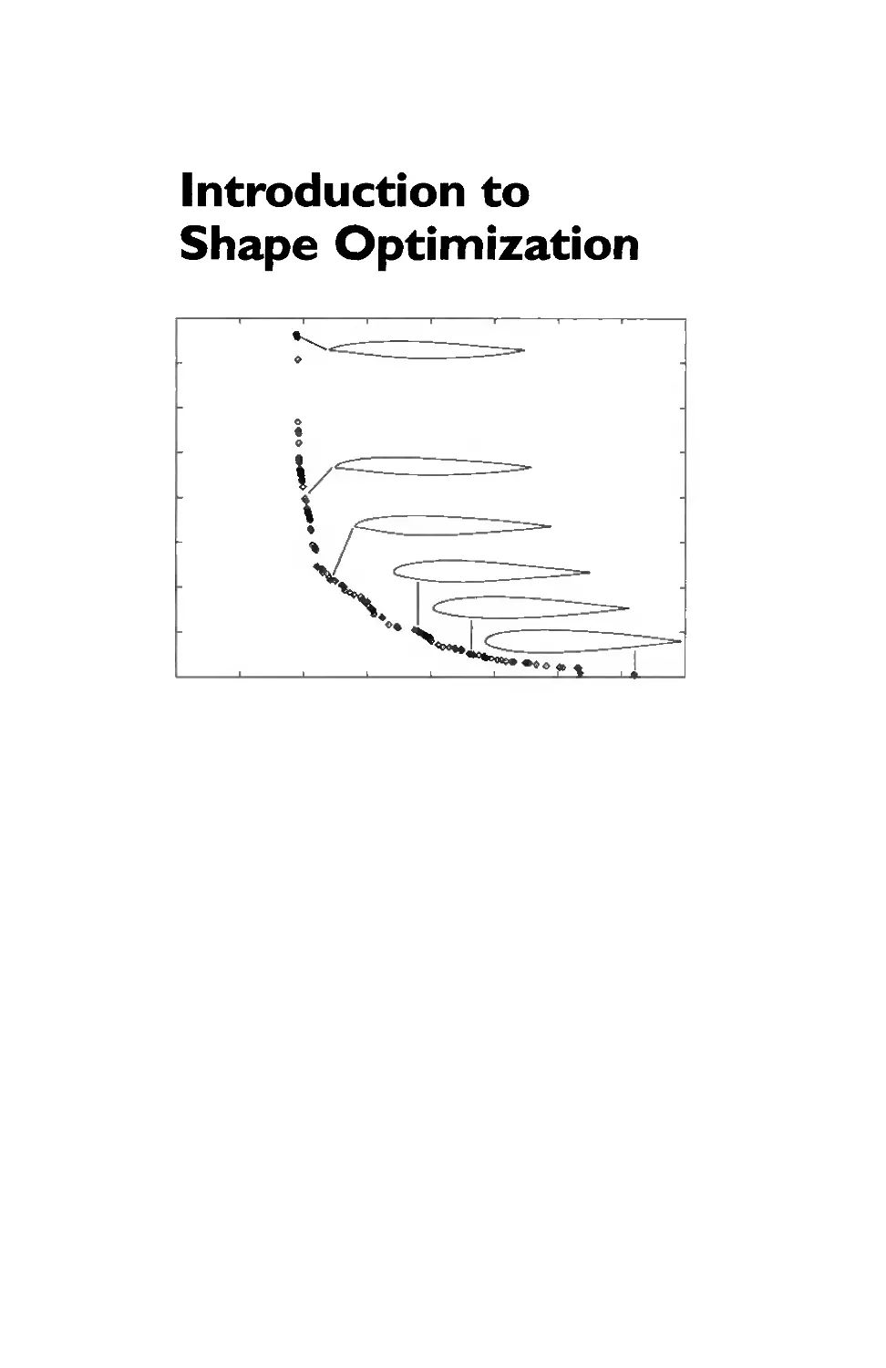
8.2	Multidisciplinary optimization of an airfoil profile using genetic
algorithms...............................................................230
8.2.1	Setting of the problem...............................232
8.2.2	Approximation and numerical realization..............236
8.2.3	Numerical example ...................................239
Problems................................................................243
Appendix A Weak Formulations and Approximations of Elliptic
Equations and Inequalities	245
Appendix В On	Parametrizations of Shapes and Mesh Generation	257
B.l	Parametrization of shapes........................................257
B.2	Mesh generation in shape optimization............................260
Bibliography	263
Index	271
This page intentionally left blank
Preface
Before we explain our motivation for writing this book, let us place its subject in a more
general context. Shape optimization can be viewed as a part of the important branch of
computational mechanics called structural optimization. In structural optimization prob-
lems one tries to set up some data of the mathematical model that describe the behavior of a
structure in order to find a situation in which the structure exhibits a priori given properties.
In other words, some of the data are considered to be parameters (control variables) by
means of which one fine tunes the structure until optimal (desired) properties are achieved.
The nature of these parameters can vary. They may reflect material properties of the struc-
ture. In this case, the control variables enter into coefficients of differential equations. If one
optimizes a distribution of loads applied to the structure, then the control variables appear on
the right-hand side of equations. In shape optimization, as the term indicates, optimization
of the geometry is of primary interest.
From our daily experience we know that the efficiency and reliability of manufactured
products depend on geometrical aspects, among others. Therefore, it is not surprising that
optimal shape design problems have attracted the interest of many applied mathematicians
and engineers. Nowadays shape optimization represents a vast scientific discipline involving
all problems in which the geometry (in a broad sense) is subject to optimization. For a finer
classification, we distinguish the following three branches of shape optimization:
(i)	sizing optimization: a typical size of a structure is optimized (for example, a thickness
distribution of a beam or a plate);
(ii)	shape optimization itself: the shape of a structure is optimized without changing the
topology;
(iii)	topology optimization: the topology of a structure, as well as the shape, is optimized
by, for example, creating holes.
To keep the book self-contained we focus on (i) and (ii). Topology optimization needs
deeper mathematical tools, which are beyond the scope of basic courses in mathematics, to
be presented rigorously.
One important feature of shape optimization is its interdisciplinary character. First,
the problem has to be well posed from the mechanical point of view, requiring a good
understanding of the physical background. Then one has to find an appropriate mathe-
matical model that can be used for the numerical realization. In this stage no less than
three mathematical disciplines interfere: the theory of partial differential equations (PDEs),
approximation of PDEs (usually by finite element methods), and the theory of nonlinear
X
Preface
mathematical programming. The complex character of optimal shape design problems
makes the presentation of the topic in some respects difficult.
Nowadays, there exist quite a lot of books of different levels on shape optimization.
But what is common to all of them is the fact that they are usually focused on some of
the above-mentioned aspects, while other aspects are completely omitted. Thus one can
find books dealing solely with sensitivity analysis (see [HCK86], [SZ92]) but omitting
approximation and computational aspects. We can find excellent textbooks for graduate
students ([Aro89], [HGK90], [HA79]) in which great attention is paid to the presentation of
basic numerical minimization methods and their applications to simple sizing problems for
trusses, for example. But, on the other hand, practically no problems from (ii) (as above)
are discussed there. Finally, one can find books devoted only to approximation theory in
optimal shape design problems [HN96].
This book is directed at students of applied mathematics, scientific computing, and
engineering (civil, structural, mechanical, aeronautical, and electrical). It was our aim to
write a self-contained book, including both mathematical and computational aspects of
sizing and shape optimization (SSO), enabling the reader to enter the field rapidly, giving
more complex information than can be found in other books on the subject. Part of the
material is suitable for senior undergraduate work, while most of it is intended to be used
in postgraduate work. It is assumed that the reader has some preliminary knowledge of
PDEs and their numerical solution, although some review of these topics is provided in
Appendix A. Moreover, knowledge of modem programming languages, such as C++ or
Fortran 90,1 is needed to understand some of the technical sections in Chapter 5.
The book has three parts. Part I presents an elementary mathematical introduction
to SSO problems. Topics such as the existence of solutions, appropriate discretizations of
problems, and convergence properties of discrete models are studied. Results are presented
in an abstract, unified way permitting their application not only in problems of solid me-
chanics (standard in existing books) but also in other areas of mathematical physics (fluid
mechanics, electromagnetism, etc.). Part II deals with modem computational aspects in
shape optimization. The reader can find results on sensitivity analysis and on gradient, evo-
lutionary, and stochastic type minimization methods, including methods of multiobjective
optimization. Special chapters are devoted to new trends, such as automatic differentiation
of computer programs and the use of fictitious domain techniques in shape optimization.
All these results are then used in Part III, where nontrivial applications in various areas
of industry, such as contact stress minimization for elasto-plastic bodies, multidisciplinary
optimization of an airfoil, and shape optimization of a dividing tube, are presented.
Acknowledgments. The authors wish to express their gratitude to the following
people for their help during the writing of this book: Tomas Kozubek from the Technical
University of Ostrava, who computed some of examples in Chapters 1 and 6 and produced
most of the figures; Ladislav Luksan from the Czech Academy of Sciences in Prague and
Kaisa Miettinen from the University of Jyvaskyla for their valuable comments concerning
Chapter 4; and Jari Toivanen from the University of Jyvaskyla, who computed the numerical
example in Section 8.2.
'The code in this book can be used with Fortran 90 and its later variants.
Preface
xi
This work was supported by grant IAA1075005 of the Czech Academy of Science,
grant 101/01/0538 of the Grant Agency of the Czech Republic, grants 44568 and 48464 of
the Academy of Finland, and by the Department of Mathematical Information Technology,
University of Jyvaskyla.
The motto of our effort when writing this book could be formulated as follows: An
understanding of the problem in all its complexity makes practical realization easier and
obtained results more reliable. We believe that our book will assist its readers to accomplish
this goal.
J.H. and R.A.E.M.
This page intentionally left blank
Notation
Banach and Hilbert spaces
Ck(A, B)	functions defined in A, taking values in B, continuously differentiable in the Frechet sense up to order it e {0} UN (Ck(A) Ck(A, R));
Ck(Q)	functions whose derivatives up to order к are continuous in Q, к e {0} U N U {00} (С(Й) := С°(Й));
Ck(Q) c0’1^) Z^(Q) L°°(Q) Я*(П)	functions from C*(fi) vanishing in the vicinity of 3Q; Lipschitz continuous functions in Q; Lebesgue integrable functions in Q, p e [1, oo[; bounded, measurable functions in Q; functions whose generalized derivatives up to order к e {0} U N are square integrable in Q (Я°(Ю) := L2(Q));
^(Q)	functions from Hk(Q), к e N, whose derivatives up to order (к — 1) in the sense of traces are equal to zero on
	functions from L°°(Q) whose derivatives up to order к e {0} U N belong to Z,00 (Q)	:= L°°(Q));
V(Q) V(Q) H~k(Q) H^2(T) Я-!/2(Г)	subspace of Hk(£l)\ Cartesian product of V (Q); dual space of Нк(£1~), к e N; traces on Г c of functions from dual space of Я1/2(Г);
Convergences
-> inX in X in Q	convergence in the norm of a normed space X (strong convergence); weak convergence in a normed space X; uniform convergence of a sequence of continuous functions in Q\
Differential calculus
f,f	material and shape derivatives, respectively, of f;
xiii
xiv
Notation
э/(х) э2/(^) дх, ’ dxidxj Da 	J	 j 3x“’ • • • dXn’ f\«; P) 4f Df (also J) Д/ df/dv, df/ds curl/ div/	first and second order generalized derivatives, respectively, of / : R" -> R, n > 2; - ath generalized derivative of / : R" -> R, |a| = 22"=1а(-, a, e ’ {0} U N; directional derivative of / at a point a and in a direction ft; gradient of /; partial gradient of / with respect to x; Jacobian of /; Laplacian of /; normal and tangential derivatives, respectively, of / on Г c 9Q; rotation of a function / : R2 —> R; divergence of /;
Domains and related notions	
R C R" N Q Q intQ, extQ 3Q Г BdQ) conv Q	set of all real numbers; set of all complex numbers; Euclidean space of dimension n; set of all positive integers; bounded domain in R"; closure of Q; interior and exterior of Q, respectively; boundary of Q; part of the boundary 3Q; 3-neighborhood of a set Q c R"; closed convex hull of Q \
Finite elements	
T R Pk(T) Qi(R) h Th, R-h T(h, jx)	triangle; convex quadrilateral; polynomials of degree < к in T; four-noded isoparametric element in R\ norm of a partition of Q into finite elements; uniform triangulation and rectangulation of Q, respectively, whose norm is Л; triangulation of Q^), e U°d, whose norm is h; partition of	s^_ e U^, into convex quadrilaterals whose norm is /г; domain Q(sM) with a given partition T(h, sM), 1Z{h, sM), s.„_ e Uad\
Notation
xv
Vh(s^) VA(s«) Uh	finite element space in QA(rM), e U°d; Cartesian product of Vh (гж); finite element solution;
Fluid mechanics
r	stress tensor (components ту, i, j = 1,..., d; d = 2, 3);
£	strain rate tensor (components £y, i, j = 1,..., d; d = 2,3);
P P Q	static pressure; viscosity of a fluid; density of a fluid;
Linear algebra
x, y, a xT A, В A-1 AT |A| trA I	column vectors in R"; transpose ofx; matrices A, B; inverse of A; transpose of A; determinant of A; trace of A; identity matrix;
Linear elasticity
T	stress tensor (components ту, i, j = 1,..., d; d = 2, 3);
£	linearized strain tensor (components £y, i, j = 1,..., d; d = 2, 3);
/С, /Z f p	elasticity coefficients defining a Hooke’s law; bulk and shear moduli, respectively; density of body forces; density of surface tractions;
Mappings A : X -+ Y A~l £(X, Y) fog (also /(g))	A maps X into Y; inverse of A; space of all linear continuous mappings from X into Y; composite function;
xvi	Notation
Miscellaneous
Sij V	Kronecker symbol; unit outward normal vector to 3Q;
c	generic positive constant;
X	characteristic function of a set;
Norms and scalar products
II • II (also || • ||x) 1 • 1 (also |  |x) (•, ) (also (•, -)x)	norm in a normed space X; seminorm in a normed space X; scalar product in X;
Norms and scalar products in particular spaces
IWIp	p-norm in R"; i.e., ||x||p :=	lx/lp, P e [l,oo[, ЦхН», := maxi=i„..,„ |x, |;
xTy f-g	scalar product of x, у e R"; scalar product of two vector-valued functions f, g : Q -► R"; i.e., (/ • g)M = £"=1 /(x)g, (x);
(/, g)*,0 IMli.Q, Hfc.Q	scalar product of f, g in Hk(Q,~), к e {0} U N; norm and seminorm, respectively, of v in the Sobolev space Hk(£2), к e {0} U N;
II||&,oo,£2? I^l&,oo,£2	norm amd seminorm, respectively, of v in the Sobolev space 77*’°°(Q), к e {0} U N;
IIv llc*(S2)	norm of v in the space C*(Q), к e {0} U N.
Introduction
As we have already mentioned in the preface, this book consists of three parts and two
appendices.
Part I is devoted to mathematical aspects of sizing and shape optimization (SSO).
Our aim is to convince the reader that thorough mathematical analysis is an important part
of the solution process. In Chapter 1 we present simple optimization problems that at
first glance seem to be quite standard. A closer look, however, reveals defects such as the
nonexistence of solutions in the classical sense or the nondifferentiability of the solution to
a state problem with respect to design variables. These circumstances certainly affect the
numerical realization. Further, we present one simple example whose exact solution can be
found by hand. We shall see that this is an exceptional situation. Unfortunately, in real-life
problems, which are more complex, such a situation occurs very rarely and an appropriate
discretization is necessary. By a discretization we mean a transformation of the original
problem into a new one, characterized by a finite number of degrees of freedom, which
can be realized using tools of numerical mathematics. Then a natural question immediately
arises: Is the discretized problem a good approximation of the original one? If yes, in what
sense? And is it possible to establish some rules on how to define a good discretization?
All these questions are studied in the next chapters.
Chapter 2 starts with two simple SSO problems. We show in detail how to prove
the existence of solutions and analyze convergence properties of the discretized problems
(Sections 2.1,2.2). The reason we start with the particular problems is very simple: the main
ideas of the proofs remain the same in all SSO problems. This approach facilitates reading
the next two sections, in which the existence and convergence results are established in an
abstract framework. These results are then applied to particular shape optimization problems
governed by various state problems (Section 2.5) of solid and fluid mechanics. To keep
our presentation as elementary as possible we confine ourselves to 2D shape optimization
problems in which a part of the boundary to be determined is described by the graph of
a function. This certainly makes mathematical analysis and numerical realization much
easier. Let us mention, however, that the same ideas can be used in the existence analysis
of problems in 3D, but the proof will be more technical. Since most industrial applications
deal with domains with Lipschitz boundaries, we restrict ourselves to domains satisfying
the so-called uniform cone property. For readers who would like to be familiar with the
use of more general classes of domains we refer to the recent monograph by Delfour and
Zolesio [DZ01] published in the same SIAM series as our book.
Part II is devoted to computational aspects in SSO. Chapter 3 deals with sensitivity
analysis or how to differentiate functionals with respect to design variables. Sensitivity
xvii
xviii
Introduction
analysis is an integral part of any optimization process. Gradient information is important
from the theoretical as well as the practical point of view, especially when gradient type
minimization methods are used.
We start with sensitivity analysis in algebraic formulations of discretized problems,
which is based on the use of the classical implicit function theorem. Then the material
derivative approach, a very useful tool in shape derivative calculus, will be introduced. Spe-
cial attention is paid to sensitivity analysis in problems governed by variational inequalities.
In Chapter 4 we briefly recall both gradient type (local) and gradient free (global)
algorithms for the numerical minimization of functions. Gradient type methods include
Newton’s method, the quasi-Newton method, and the sequential quadratic programming
method. Gradient free methods are represented by genetic and random search algorithms.
In addition, some methods of multiobjective optimization are presented.
In Chapter 5 we discuss a rather new technique for calculating derivatives, namely
automatic differentiation (AD) of computer programs. AD enables us to get accurate deriva-
tives up to the machine precision without any human intervention. We describe in detail
how to apply this technique in shape optimization.
Chapter 6 presents a new approach to the realization of optimal shape design problems,
based on the use of fictitious domain solvers at the inner optimization level. The classic
boundary variation technique requires a lot of computational effort: after any change in the
shape, one has to remesh the new configuration, then recompute all data, such as stiffness
matrices and load vectors. Fictitious domain methods make it possible to efficiently solve
state problems on a uniform grid that does not change during the optimization process. Just
this fact considerably increases the efficiency of the inner optimization level. This approach
is used for the numerical realization of a class of free boundary value problems.
Part III is devoted to industrial applications. In Chapter 7 we present two problems of
SSO of stressed structures, namely multiobjective optimal sizing of a beam under multiple
load cases and contact stress minimization of an elasto-plastic body in contact with a rigid
foundation. In Chapter 8 we first solve a problem arising in the paper machine industry: to
find the shape of the header of a paper machine in order to get an appropriate distribution
of a fiber suspension. Next a multidisciplinary and multiobjective problem is solved: we
want to optimize an airfoil taking into account aerodynamics and electromagnetics aspects.
For the convenience of the reader two appendices complete the text. In Appendix A
some elementary results of the theory of linear elliptic equations, Sobolev spaces, and
finite element approximations are collected. Appendix В deals with 2D parametrization of
shapes. A good shape parametrization is a key point in a successful and efficient optimization
process. Basic properties of Bezier curves are revisited.
Part I
Mathematical Aspects of Sizing
and Shape Optimization
This page intentionally left blank
Chapter 1
Why the Mathematical
Analysis Is Important
In this chapter we illustrate by using simple model examples which types of problems are
solved in sizing and shape optimization (SSO). Further, we present some difficulties one may
meet in their practical realization. Finally we try to convince the reader of the helpfulness
of a thorough mathematical analysis of the problems to be solved.
We start this chapter with a simple sizing optimization problem whose exact solution
can be found by hand. Let us consider a simply supported beam of variable thickness e
represented by the interval I = [0, 1]. The beam is under a uniform vertical load fy. One
wants to find a thickness distribution to maximize the stiffness of the beam. The deflection
и := u(e) of the beam solves the following fourth order boundary value problem:
| (^Зи"(х))" = /о in [0, 1],
| w(0) = u(l) = (0е3и")(О) = (/le3u")(l) =0,	6
where is a given positive constant. The stiffness of the beam is characterized by the
compliance functional J defined by
f1
J(u(e)) = I fou(e)dx,
Jo
where u(e) solves fP'(e)). The stiffer the construction is, the lower the value J attains.
Therefore the stiffness maximization is equivalent to the compliance minimization. We
formulate the following sizing optimization problem:
( Find e* e Uad such that
1	и	(pi)
l J(«(e*)) < J(«(e)) Ve e Uad,
where Uad is the set of admissible thicknesses defined as follows:
{f1	1
e : [0, 1] —> R+ | I e(x) dx = у >, у > 0 given.
Jo	J
The integral constraint appearing in the definition of Uad says that the volume of the beam
is preserved. Next we show how to find a solution to (Pi).
3
4
Chapter 1. Why the Mathematical Analysis Is Important
For the sake of simplicity we set ft = fo = 1 in [0, 1]. Instead of the classical
formulation CP'(e)) we use its weak form:
Find и := u(e) e V such that
e3u"v" dx =
Vv e V,

where
V = {v e H2(I) | v(0) = v(l) = 0}
is the Sobolev space of functions vanishing at the endpoints of I (for the definition of
Sobolev spaces we refer to Appendix A). In order to release the constraints in (Pi) that are
represented by the state problem (P(e)) and the constant volume constraint we introduce
the following Lagrangian:
£(e, u,p,k)= I udx+ I e3u"p"dx — I pdx
Jo Jo	Jo
Of1	\
' edx - у I, ее Uad, (и, p) e V x V, A e R.
о	/
We now seek stationary points of £, i.e„ all points (e, u, p, A) satisfying
8£(e, u, p, A) = 0,
(1.1)
where the symbol 8 stands for the variation of £ with respect to all mutually independent
variables without any subsidiary constraints. From the definition of £ it easily follows that
3£(e, u, p, A) = f (Зе2и"p" + k)8edx + [ 8udx+ f e3(8u)"p"dx
Jo	Jo Jo
+ f e3и"(8p)"dx — f 8pdx + 8k( f edx — y\ , (1.2)
Jo	Jo	\Jo /
where 8e, 8u, 8p, and ЗА denote the variation of the respective independent variable. From
(1.1) and (1.2) we obtain the following optimality conditions satisfied by any stationary
point (e, u, p, A) of £:
3e2w"p" + A = 0 in ]0, 1[;	(1.3)
(е3и")" = 1 in ]0,1 [, w(0) = u(l) = (е3и")(0) = (е3и")(1) = 0;	(1.4)
(е3р"У = -1 in]0,1[, р(0) = р(1) = (е3р")(О) = (е3р")(1) = 0;	(1.5)
/ edx — у.	(1.6)
Jo
Equation (1.4) is the classical form of the state equation while (1.5) represents the so-called
adjoint state equation. Comparing (1.4) with (1.5) we see that p = —u so that (1.3) becomes
-Зе2(и")2 + A = 0 in]0,1[.
(1.7)
Chapter 1. Why the Mathematical Analysis Is Important
5
Figure 1.1. Optimal thickness distribution.
From this it follows that
e\u"| = c = const. > 0.
(1.8)
Convention: Here and in what follows the letter c stands for a generic positive constant
attaining different values at different places.
The bending moment M := M(x) — (e3 w") (x) satisfies the following boundary value
problem:
|M"(x)=l in]0,1[,
| M(0) = M(l) = 0,
whose solution is M(x) = ^x(x — 1). Therefore
e(x)w"(x) =	- 0
в \X)
implying together with (1.8) that
e(x) = J-------- — cJxfl — x), x e]0,1[.	(1.9)
V c
The value of the constant c on the right side of (1.9) can be fixed from the volume constraint.
If у = 1, then e(x) = (8/tt)a/x (1 — x) (see Figure 1.1).
Remark i.i. It is worth noticing that the stiffest simply supported beam has zero thickness
at the endpoints x = 0, 1 and, besides the constant volume constraint, no other assumptions
on admissible thicknesses are present. As we shall see later on this is an exceptional situation.
Usually some additional constraints are needed to get a physically relevant solution.
6
Chapter 1. Why the Mathematical Analysis Is Important
The fact that we were able to find the exact solution of the previous optimization
problem is exceptional and due to the simplicity of the state problem and the particular
form of the cost functional (compliance). Unfortunately most optimization problems we
meet in practice are far from being so simple and an approximation is necessary. We
proceed as follows: first we decide on an appropriate discretization of the state prob-
lem (by using finite elements, for example) and of design parameters (instead of com-
plicated shapes we use spline approximations, for example). Computed solutions to the
discrete state problems are now considered to be a function of a finite number of dis-
crete design variables a — (at,..., ad) fully characterizing discretized shapes or thick-
nesses. After being inserted into cost functionals, these become functions of a. In this
way we arrive at a constrained optimization problem in whose solutions we shall
look for.
There are two ways to realize this step. The first is based on the numerical solu-
tion of the respective optimality conditions, as in the previous example. This approach,
however, has serious drawbacks. First of all one has to derive the optimality conditions.
This is usually a difficult task especially in problems whose state relations are given by
variational inequalities or even by more complicated mathematical objects. But even if the
optimality conditions are at our disposal they are usually so complex that their numerical
treatment is not easy at all. For this reason the structural optimization community prefers
a more universal approach based on the numerical minimization of functions by means of
mathematical programming methods. But also in this case one should pay attention to a
thorough mathematical analysis in order to obtain additional information on the problem
that can be useful in computations. A typical feature is that minimized functions are usually
nonconvex. This gives rise to some difficulties: nonconvex functions may have several local
minima; further, the minimization method used may be divergent or the result obtained may
depend on the choice of the initial guess. Below we present very simple SSO problems in
one dimension (i.e., d = 1) with states described by equations and inequalities involving
ordinary differential operators. The dependence of cost functions on the design parameter
will be illustrated by the graphs.
Example i.i. Let
U = {e € R | Cmin — C — Стах},
where 0 < еть < emax are given, and consider the optimal sizing problem
min J(e) = I (ue — I)2 dx,
eeUad Jo
where ue solves the following boundary value problem:
-eu'; = 2 in]0,l[, eeUad,
ue(0) = ue(l) = 0.
It is readily seen that ue(x) = (x — хг)/е and
J(e) = 1 + i-3? e^ad-
Chapter 1. Why the Mathematical Analysis Is Important
7
Figure 1.2. Graph of the cost functional.
The graph of J is plotted in Figure 1.2. We see that J is unimodal (i.e., for any choice
of ^min, бщах it has only one local minimum) but not convex. If one tries to minimize J
numerically using a simple quadratic approximation of J, the method will not converge
provided the initial guess e0 is large enough, say eo > 1 /2.
Example 1.2. (See [Сёа81].) Let us consider the following simple prototype of the shape
optimization problem:
min J (a) = I (ua — l)2dx,
aeUad	Jo
where
t7 — {tt € 1R I 0 < «min < Ot < «max) ,
«min < «max is given, and ua solves the boundary value problem
-u" = 2 in]0, a[,
u'a(0) = ua(a) = 0.
(1.11)
In contrast to the previous two sizing optimization problems the differential equation here
is posed on an unknown domain that is to be determined. The solution of this problem is
ua(x) - a2 — x2 and
8 ,	4 ,	j
J (a) = —a5 ~ з“3 + «>	“ e Uad.
The graph of J is shown in Figure 1.3. We see that J is nonconvex and it may have one or
two local minima depending on the choice of qmin. «max-
8
Chapter 1. Why the Mathematical Analysis Is Important
Figure 1.3. Graph of the cost functional.
In the previous two examples the resulting functions are continuously differentiable.
But this is not always so. With an inequality instead of a state equation the situation may
be completely different, as will be seen from the following example.
Example 1.3. (State variational inequality.) Consider the optimal shape design problem
with the same J and Uad as in Example 1.2 but with ua solving the following variational
inequality:
ua e K(a) :	[ u'a(y'— u'a) dx > f 2(v — ua)dx Vv e K(a),	(1-12)
Jo	Jo
where
K(a) = {ve Я’ОО, a[) I v(0) = 0, v(a) < 1}, a e Uad.
It is well known that the solution ua to (1.12) exists and is unique as follows from Lemma A. 1
in Appendix A. Integrating by parts on the left-hand side of (1.12) it is easy to show that
ua satisfies the following set of conditions:
-u"(x) = 2 Vx e]0, a[,
u„(0) = 0, ua(a) < 1, u'a(a) < 0, (u„(a) - l)u„(a) = 0.
(1.13)
It is readily seen that the function
ua(x) =
—x2 + 2ax,
2 , “2 + 1
—x -|------X,
a
a < 1,
a > 1,
(1.14)
Chapter 1. Why the Mathematical Analysis Is Important
9
Figure 1.4. Graph of the cost functional.
satisfies (1.13) and its substitution into J yields the following analytic expression of J as a
function of the design parameter a:
J (a) =
8 5	4 з
---Ct----Ct + Ct.
15	3	’
1 5	1 з 1
30“ ’ 6“ + 3“’
a < 1,
a > 1.
A direct computation shows that JL(1) = —1/3 and J^_(l) = 0;i.e., J is not differentiable at
a — 1 (see Figure 1.4). Let us comment on this fact in more detail. The external functional
I	[ (y - l)2dx,
Jo
у e	a e U^,
is continuously differentiable with respect to both variables, while the composite function
/ (w„ — l)2dx = I (a, ua), a e Uad,
о
is not. From this it immediately follows that the inner control state mapping a h> ua cannot
be continuously differentiable. Indeed, ua being a solution to the variational inequality
(1.12) can be expressed as the projection of an appropriate function from H!(]0, a[) onto
the convex set К (a). A well-known result (see [Сёа71 ]) says that the (nonlinear) projection
operator of a Hilbert space on its closed convex subset is Lipschitz continuous. This in short
explains the source of the possible nondifferentiability of the control state mappings in the
case of state variational inequalities (for more detail on this subject we refer to [SZ92]).
10
Chapter 1. Why the Mathematical Analysis Is Important
Figure 1.5. Graph of the cost functional.
The fact that a minimized function is not differentiable at some points may have
practical consequences. A common way of minimizing J is to use classical gradient type
methods that require gradient information on the minimized function. The absence of
such information at some points may give unsatisfactory or unreliable numerical results.
Fortunately there is a class of generalized gradient methods for which the nondifferentiability
does not present a serious difficulty and that were developed just to treat this type of problem.
This is a nice illustration of how a thorough analysis and understanding of the problem may
help with the choice of an appropriate minimization algorithm.
The fact that the control state mapping is not differentiable, however, does not mean
that the composite function is automatically nondifferentiable as well. Indeed, let us choose
the new cost functional
। pa	pa
J(a) = - I (u'a)2 dx — / 2uadx, a e Uad,
2 Jo	Jo
(1.15)
where ua e К (a) solves (1.12). Substituting (1.14) into (1.15) we obtain
J(a) =
2 з
3“ ’
1 з 1
--a + -----a,
6 2a
a < 1,
a > 1
(1.16)
(see Figure 1.5). One can easily check that J is a once (but not twice!) continuously differ-
entiable function in Uad. Therefore, for a special choice of cost functionals it may happen
that the composite function is continuously differentiable despite a possible nondifferentia-
bility of the inner mapping. We shall meet the same situation several times in this textbook
(see Chapters 2, 3, 7).
We end this chapter with one shape optimization problem that has no solution, showing
how this fact manifests itself during computations.
Chapter 1. Why the Mathematical Analysis Is Important
11
Let Q(a) = {(xi,x2~) e R2 | 0 <	< a(x2), x2 e]0,1[} be a “curved rectangle”
(see Figure 2.2) with the curved side Г (a) being the graph of a function a e Uad, where
t/arf = {a e C([0,1]) | 0 < amin < a < «max in [0, 1], [ a(x2)dx2 = у I,	(1.17)
I	Jo	J
with 0 < amin < «max and у > 0 given. Further denote by О — {Q(a) | a e Uad} the
set of all admissible domains; i.e., О is realized by domains whose curved part Г (a) of the
boundary lies within the strip bounded by amin, «max and have the same area equal to у. On
any Q(a), a e Uad, we shall consider the following Dirichlet-Neumann state problem:
—Ди(а) = C
du(a) _
3v
и(а) = 0
in Q(a),
on Ti = ЭП(а)\Г(а),
on Г (a),
(1.18)
where C > 0 is a given constant. We define the following optimal shape design problem:
Find a* e Uad such that
J{a*, u(a*)) < J{a, u{a))
where
J («, y) =
Va e Uad,
(P2)
(1.19)
{dx = dx\dx2) and и (a) solves (1.18) in Q (a).
Problem (P2) was solved with the following values of the parameters: C = 2, amin =
0.1, «max = 0.9, and у = 0.5. Shapes were discretized by piecewise quadratic Bezier
functions. The number of segments is d = 10, 18. Computed results are shown in Figure 1.6.
We see that the designed part Г (a) oscillates and the oscillation becomes faster and faster
for increasing values of d. Now a question arises: What does the optimal shape look like?
It is difficult to imagine such a domain on the basis of the obtained results since there is no
“understandable” domain from О that can be deduced from them. In fact the oscillatory
pattern is a consequence of the nonexistence of solutions to (P2) • The rigorous mathematical
analysis of this problem is far from easy and goes beyond the scope of this textbook. Let us
try, however, to give a naive “explanation.” Boundary value problem (1.18) describes the
stationary temperature distribution in the body represented by Q(a), which is isolated on
Ti and cooled along Г(а). The right-hand side C characterizes the heat source. Since the
area of all Q (a) is the same, the only way to decrease the temperature in Q (a) is to increase
the length of the cooling part Г (a). This is just what the solution found mimics: Г (a)
begins to oscillate. The constant volume constraint is added to avoid the trivial solution
O!* = «min-
12
Chapter 1. Why the Mathematical Analysis Is Important
Figure 1.6. Oscillating boundaries.
A possible way to ensure the solvability of (P2) is to impose additional constraints,
keeping the length of Г (a) bounded. Thus instead of (1.17) one can consider another
(narrower) system of admissible domains defined by
Uad = e Co,1([0,1]) I 0 < «m,n < a < amax in [0,1];
|a'| < Co almost everywhere in ]0,1[; / а(хг)^2 = Y 1, 0-20)
Jo	J
where Co > 0 is given. As we shall see later on, problem (P2) with Uad defined by (1.20)
already has a solution.
Since shape optimization problems are generally nonconvex they may have more than
one solution (see Problem 1.2).
Problems
Problem i.i. Prove that u(<z) solves the variational inequality (1.12) iff it satisfies (1.13).
Problem 1.2. [BG75] Consider the optimal shape design problem (P2) with the state
problem (1.18) and the cost functional (1.19). Prove that if Q(a*) solving (P2) (a* € Uad
given by (1.17)) is not symmetric with respect to the line xi = 1/2, then Q(a**), where
а**(хг) := (composite function) a*(l — X2), X2 e]0, 1[, is a solution of (P2), too.
Chapter 2
A Mathematical Introduction to
Sizing and Shape Optimization
The aim of this chapter is to present ideas that are used in existence and convergence analysis
in sizing and shape optimization (SSO). As we shall see, the basic ideas are more or less
the same: we first prove that solutions of state problems depend continuously on design
variables (and we shall specify in which sense). Then, imposing appropriate continuity (or
better lower semicontinuity) assumptions on a cost functional, we immediately arrive at an
existence result. The same scheme remains more or less true when doing the convergence
analysis. Before we give an abstract setting for optimal sizing and shape design problems
and prove abstract existence and convergence results, we show how to proceed in particular
model examples. The same ideas will be used later on in the abstract form.
2.1 Thickness optimization of an elastic beam:
Existence and convergence analysis
Let us consider a clamped elastic beam of variable thickness e subject to a vertical load f.
The beam is represented by an interval I = [0, €], t > 0. We want to find the thickness
distribution in I minimizing the compliance of the beam, given by the value J(u(e)), where
(2.1)
and u(e) is the solution of the following boundary value problem:
(0e3w")"U) = f(x) Ух <=]0, £[,
w(0) = и'(0) = u(i) = u'(t) = 0.
(2.2)
Here ft e L°°(I), ft > Д) = const. > 0, is a function depending on material properties and
on the shape of the cross-sectional area of the beam. The solution of (2.2) is assumed to be
a function of e, playing the role of a control variable. To define an optimization problem,
one has to specify a class Uad of admissible thicknesses. As we already know, the result of
the optimization process depends on, among other factors, how large Uad is.
13
14
Chapter 2. A Mathematical Introduction to SSO
Let Uad be given by
Uad= ее С°л(1) \0<emia<e<emarnI,
|e(%i) — e(%2)l < L0|xi — X2I Vxi,X2Gl, je(x)dx = y^; (2.3)
i.e., Uad consists of functions that are uniformly bounded and uniformly Lipschitz continuous
in I and preserve the beam volume. The positive constants Cmin, emax, Lq, and у are chosen
in such a way that Uad / 0.
Remark 2.1. The uniform Lipschitz constraint
|e(xi) - e(%2)l < Lolxi - X2I Vxi, X2 e I
appearing in the definition of Uad prevents thickness oscillations and plays an important
role in the forthcoming mathematical analysis.
We are now ready to formulate the following thickness optimization problem:
Г Find e* e Uad such that
I J(u(e*)) = min J(w(e)),
eelM
where J is the cost functional (2.1) and u(e) is the displacement, solving (2.2). In what
follows we shall prove that (IP) has at least one solution e*. The key point of the existence
analysis is to show that the solution и of (2.2) depends continuously on the control variable
e. But first we have to specify what the word continuous means. This notion differs for и
and e.
Convention: For the sake of simplicity of our notation throughout the book we shall use
the same symbol for subsequences and the respective original sequences.
Our analysis starts with a weak formulation of (2.2). Let Hq (/) be the Sobolev space
of functions v whose derivatives up to the second order are square integrable in I and satisfy
the boundary conditions v(0) = v'(0) = v(£) = v'(£) = 0 (see Appendix A). The weak
formulation of (2.2) reads as follows:
Find и и(ё) e Hq(I) such that
I Pe3u"v"dx= I fvdx Vv e T/02(f),
(P(e))
where e e Uad and f e L2(/) are given. We adopt the notation (Р(е)), w(e),... to stress
the dependence on e e Uad. The continuous dependence of и on e mentioned above will
be understood in the sense of the following lemma.
Lemma 2.1. Let en, e e Uad, be such that en =4 e (uniformly) in I and let un := u(en) be
solutions to (P(en)), n = 1, 2,... . Then
un -> u(e) in
and u(e) is the solution of(P(e)).
2.1. Thickness optimization of an elastic beam
15
Proof. Let un e Hq (I) solve (P(en)); i.e.,

Vv e H3(I).
(2.4)
Inserting v := u„ into (2.4) and using the definition of Uad we obtain
< ||/||о,г||ил||2,г VneN.
From this and the Friedrichs inequality we see that the sequence {un} is bounded:
ll«n||2,/<c VneN.
(2.5)
Thus one can pass to a subsequence such that
un и (weakly) in Hq (/),
(2.6)
where и is an element of Hq(I). It remains to show that и solves (P(e)). But this follows
from (2.4) by letting n -> oo. It is readily seen that

•3u"v"dx, n -+ oo.
(2.7)
Indeed,

•3u"v" dx
(2.8)
3	3
e„ -e
- u”)v"dx
0 as n —> oo,
taking into account that en =f e in I and (2.6). From (2.7) it follows that и solves (P(e)).
Since (P(e)) has a unique solution, not only this subsequence but the whole sequence {un}
tends weakly to и in Hq (/). To prove strong convergence, it is sufficient to show that
where ||| • ||| is a norm with respect to which Hq (/) is complete. Clearly the energy norm
(2.9)
with e being the limit of {en} possesses this property. Then
£(e3 - е„)(и")2 dx +
'3 ~ e3n)(-un)2dx +
as follows from the definition of (P(e„)), (P(e)), (2.6), and uniform convergence of {en}
to e in I proving strong convergence of {un} to w(e) := и in the Hq (/)-norm.	□
16
Chapter 2. A Mathematical Introduction to SSO
Having this result at our disposal we easily arrive at the following existence result
for (P).
Theorem 2.1. Let Uad be as in (2.3). Then (P) has a solution.
Proof. Denote
q := inf J(w(e)) = lim J(w(en)),	(2.10)
e^U'‘d	n-*oo
where {e„}, en e Uad, is a minimizing sequence. Since Uad is a compact subset of C(Z),
as follows from the Arzel^-Ascoli theorem, one can pass to a subsequence of {e„} such that
en =4 e* e Uad in I, n -+ 00,
for an element e* e Uad. At the same time
u(en) u(e*~) in Н$(Г),	(2.11)
as follows from Lemma 2.1. From (2.10), (2.11), and continuity of J in Hfi (Z) we see that
q = J(«(e*));
i.e., e* e Uad solves (P).	□
Definition 2.1. A pair (e*, u(e*)), where e* solves (P) and u(e*) is a solution of the
respective state problem (Р(е*У), is called an optimal pair of (P).
Convention: The wording “optimal pair” will be used in the same sense in all other
optimization problems.
Comments 2.1.
(i)	There are three substantial properties used in the previous existence proof: the contin-
uous dependence of u(e) on the control variable e; the compactness of Uad, enabling
us to pass to a convergent subsequence of any minimizing sequence; and continuity
of J.
(ii)	Some extensions in the setting of (P) are possible: instead of the load f e L2{I) we
can take any f e (the dual of H02(Z)), enabling us to consider concentrated
loads f — 8Xo, e.g., where the Dirac distribution 8^ at a point x0 e I is defined by
Mv) = vUo) Vv e {I).
The functional J given by (2.1) depends on the state variable у e V (V =	(I)
in our example) but not explicitly on the control variable e e Uad. It becomes
a function of e only through the composition of J with the control state mapping
и : e i-> u(e). In many situations, however, cost functionals depend on both variables
of (e,y) e Uad x V. For this reason the abstract setting of these problems considers
2.1. Thickness optimization of an elastic beam
17
cost functionals defined on Uad x V, i.e., depending explicitly on both variables.
From the proof of Theorem 2.1 we see that, for a general J : Uad x -> R, the
existence of solutions to (P) is guaranteed provided that J is lower semicontinuous
in the following sense:
en =i e in I
yn-+ у in H02(/)
=> lim inf J(en, yn) > J(e, y).
n->oo
(2.12)
(iii)	The admissible set Uad defined by (2.3) is quite narrow. It would be possible to extend
it by omitting the uniform Lipschitz constraint, i.e., to take Uad as
Uad = e e C(/) | 0 < Cmin < e < emax in l, У e(x)dx =	.	(2.13)
Unfortunately, Uad is not a compact subset of C(/). But one can still extend Uad as
follows:
Uad = |e e L°°(/) 10 < emin < e < emax almost everywhere (a.e.) in I, e(x) dx = у |
(2.14)
Then is a compact subset of with respect to L00* weak convergence. On
the other hand the mapping и : e i-> u(e), e e Uad, is not continuous with respect to
this convergence. More precisely, if ё„, ё e Uad are such that
en e	* weakly, n —> oo,
then the sequence {и(ё„)} tends weakly to an element u in (/), but not necessarily
u = и(ё); i.e., the limit element и is not a solution of (Р(ё)). In order to analyze
(P) with Uad defined by (2.14), deeper mathematical tools, going beyond the scope
of this book, have to be used.
(iv)	Let us again consider (P) with the cost functional (2.1). Since (73(e)) is the problem
with a symmetric bilinear form, its solution can be equivalently characterized as a
minimizer of the total potential energy functional E,
E(e,u(e)) = min E(e,v),
VSHO2(I)
where
E(e,v) = У fie\v")2 dx — 2 j fvdx.
It is easy to verify that
E(e, u(e)) = - У /и(е) dx = -J(u{e)) Ve e Uad.
Consequently
min J(u(e)) = min — min E(e, v)
eeUad	eeUad veH2(T)
= — max min E(e, v).
e&Uad veH2(T)
18
Chapter 2. A Mathematical Introduction to SSO
Thus the original, minimum compliance problem can be reformulated as a max-min
problem for the functional E : Uad x (/) -► R. This form of (P) is closely related
to a saddle-point type problem for E on the Cartesian product Uad x (Z) enabling
us to extend Uad even more than has been done so far. Indeed, instead of Uad, Uad,
given by (2.3), (2.14), respectively, one can also consider
U£d = le e | 0 < e < emax
a.e. in I,
e(x) dx = у
i.e., we allow zero thickness of the beam. The problem of finding a saddle point of E on
U#d x Hq(T) still has good mathematical meaning, regardless of the fact that elements
of U#d may vanish in subsets of I, implying the degeneracy of (P(e)). The explanation
is very simple: in the saddle-point formulation (P(e)) is not solved explicitly. This
approach is used in the so-called free topology optimization of structures, whose goal
is, roughly speaking, to find an optimal distribution of the material permitting the
presence of voids, i.e., the absence of any material in some parts of structures.
We now pass to a discretization of (P), i.e., to its transformation into a new problem,
defined by a finite number of parameters.
We start with a discretization of Uad. Let d e N be given and Дл : 0 = ao <
ai < • •  < ад — I be an equidistant partition of I with the step h — l/d, a, = ih, i =
0,...,d. Instead of general functions from Uad we shall consider only those that are
continuous and piecewise linear on А/,; i.e., we define
U%d = {eh e C(T) | ehnai_uai] e Pi([a,_!, a;]), i = 1,..., d(h)} П Uad. (2.15)
For a discretization of (P(e)) we use a finite element approach. Let Vh be the finite dimen-
sional subspace of Hq (/) defined as follows:
Vh = {ил e C\l) | vA|[e._lwei] € Р3([а;_1,а,]), i = l,...,d(h),
.	.	(Z.lO)
Vft(O) = vh(0) = vh(t) -- vh(t) = 0};
i.e., Vh contains all piecewise cubic polynomials that are continuous together with their first
derivatives in I and that satisfy the same boundary conditions as functions from Hq (/).
Let eh e U£d be given. Then the discretized state problem (P^fy/,)) reads as follows:
Find uh := ил(ел) e Vh such that
Pe^u'hVl dx = fvh dx Yvh e Vh.

We now define the discretization of (P) as follows:
Find e% e U£d such that
J(uh(e*h)) - min J(uh(eh)),
(П)
where uh(eh) e Vh solves (Рл(ел)).
2.1. Thickness optimization of an elastic beam
19
It is left as an easy exercise to prove the following theorem.
Theorem 2.2. Problem (IP/,) has a solution for any h > 0.
In what follows we shall show how problem (PA), characterized by a finite number of
degrees of freedom, can be realized numerically. To this end we derive its algebraic form.
Let h > 0 be fixed. Any function eh e U^d can be identified with a vector e =
(eo,... ,ed) e U whose components are the nodal values of eh; i.e., e, = eh(at), i =
0,..., d. It is easy to see that
U = e Rrf+1 | emin < e, < e^, i = 0,...,d;
d-i
h+i - e;| < Loh, i = 0,..., d - 1; h ^(e; + e,+i) = 2y
1=0
(2.17)
The discrete state problem (PA(eA)) transforms into a system of linear algebraic equa-
tions,
K(e)q(e) = f,
(2.18)
where KAe) = (fcij(e))"y=1 is the (symmetric) stiffness matrix, f = (/i)"=1 is the force
vector, q(e) e R" is the nodal vector representing the finite element solution иА(еА) e VA
of (P/be/,)), and n := n(h) = dim VA. Any function vA e VA is uniquely defined by the
vector v of nodal values vA(a/), иА(а(), i = 1,..., d — 1, so thatn = 2(d — 1). Thus the
components of q (e) are the values of uA and wA at the nodal points a, e Aa , i = 1,..., d—1,
which will be arranged as follows:
q{e) = (wA(ai), u'h(a\), иА(а2), u'h{a2),..., uh(aa_i), u'h{ad-i)).	(2.19)
The elements of К (e) and f are computed in the standard way:
ktj(e) =	ft = ^f<Pidx, i,j = l,...,n,	(2.20)
where {<pj }"=1 are the basis functions of VA. The one-to-one correspondences eh -e- e and
vh ++ v between elements of U£d and U and Vh and R", respectively, defines the following
isomorphisms 7b and Ts-
TD : Uahd U; TD(eh) =e, eh e Uahd-,
7s : Vh -* R"; 7s(va) = v, vA e VA,
(2.21)
(2.22)
enabling us to identify U^d with U and Vh with R". In a similar way one can identify the
cost functional J restricted to Vh with a function J7 : R" —> R:

20
Chapter 2. A Mathematical Introduction to SSO
where Ts 1 denotes the inverse of T$ (if J : Uad x Hq(I) -> R depends explicitly on both
variables, then J : U x R" -► R, where J(e, v) :=	Tf~\vyf). Therefore the
discrete thickness optimization problem (PA) leads to the following nonlinear mathematical
programming problem:
I Find e* e U such that
Л«(Л) < Ve e U,	(Prf)
where q(e) e Rn solves (2.18). Problem (Pj) can be solved using nonlinear mathematical
programming methods. Some of them will be presented in brief in Chapter 4.
Until now, the mesh parameter h > 0 has been fixed. A natural question arises: What
happens if h -+ 0+, meaning that finer and finer meshes are used for the discretization of
Uad and (P(e))? Is there any relation between solutions to (P) and (PA) as h -+ 0+? This
is what we shall study now.
Let {ДА}, h -> 0+, be a family of equidistant partitions of I whose norms tend to
zero and consider the respective families {U£d}, {VA}, h -> 0+. The next lemma, which is
a counterpart of Lemma 2.1 in the continuous setting, plays a major role in the convergence
analysis.
Lemma 2.2. Let {eA}, eA e U^d, be such that eh e in I and let {wA(eA)J be the sequence
of solutions to (Ph(eh), h —> 0+). Then
uh(eh) -> u(e) in	h -> 0+,
and u(e) solves (P(e)).
Proof. As in Lemma 2.1 one can prove that {wA(eA)J is bounded:
3 c > 0 : ||иА(еА)||2,/ < c Vh > 0.
Passing to a subsequence, there exists и e Hq (/) such that
wA(eA) и in Hq (I), h -> 0 + .	(2.23)
Next, we show that и solves (P(e)). Let v e (/) be arbitrary but fixed. Then there is a
sequence {vA}, vA e VA, such that
Vh -+ v in	h -+ 0 + .	(2.24)
From the definition of (PA(eA)) it follows that
^e3hu'^ dx	= fvh dx.	(2.25)
Passing to the limit with h -+ 0+ in (2.25) we obtain
У fe^u'fv'^dxУ Pe3u"v"dx,	(2.26)
У fvh dx	^fvdx.	(2.27)
2.1. Thickness optimization of an elastic beam
21
Indeed,
,ehuhvh ~ fe3u"v") dx
|eA — e3| |uAvA| dx 4-
I /8e3(u^v'^ — u"v")dx
< c\\e% — e3||c(Z)ll«ftIh.zIIVhHz.z +
(u'ffi - u"v”) dx
-> 0,
making use of (2.23), (2.24), and uniform convergence of eh to e in I. The limit passage
(2.27) is trivial. From (2.25), (2.26), and (2.27) it follows that
•3u"v"dx =
is satisfied for any v e Hq (/); i.e., u solves (P(e)). Due to its uniqueness, the whole
sequence {Uh(eh)} tends weakly to u(e) := u in Hq (I). Strong convergence of {uA(eA)J to
и (e) can be established in the same way as was done in Lemma 2.1.	□
A direct consequence of the previous lemma is the following convergence result.
Theorem 2.3. Let {(e*f uA(eA))} be a sequence of optimal pairs of (Ph), h -> 0+- Then
one can find a subsequence of{(e^, Uh(e^))} such that
el =t e* in I,
(2.28)
Uh(^h) -* и(е*) in Hq(I), h ->• 0+,
where (e*, u(e*)) is an optimal pair of (P). In addition, any accumulation point of
{(e£, uh(eh))}In sense of (2.28) possesses this property.
Proof. Let {e%} be a sequence of solutions to (PA), h -> 0+ (if (PA) had more than one
solution, we would choose one of them). Since U^d c Uad V/г > 0 and Uad is compact in
C(I), one can pass to a subsequence of {e%} such that
e* =4 e* e Uad in I, h -+ 0 + .
At the same time
uh(e*h) -+ u(e*) in Hfrj),	(2.29)
as follows from Lemma 2.2.
Let e e Uad be given. Then one can find a sequence {ёА}, eh e U^d, such that (see
Problem 2.2)
eh e in I, h 0+,	(2.30)
and
Uhf^h) -> ufe) in Hq(I), h ->• 0+,
(2.31)
22
Chapter 2. A Mathematical Introduction to SSO
using Lemma 2.2 once again. From the definition of (IP/,) it follows that
J(uh(e*h)) < J(uh(eh)).
Letting h -+ 0+ in this inequality, using continuity of J, (2.29), and (2.31), we arrive at
J(w(e*)) < 7(и(ё));
i.e., (e*, w(e*)) is an optimal pair of (P). From the proof we also see that any other accu-
mulation point of {(e£, Uh (<?^))} is also an optimal pair of (P).	□
Comments 2.2.
(i)	Theorem 2.3 says that (Рл), h -> 0+, and (P) are close in the sense of subsequences
only. This is due to the fact that (P) may have more than one solution. This theorem,
however, ensures the existence of at least one subsequence of {(e£, и/,(е^))} tending
to an optimal pair of (P). In addition, any convergent subsequence of {(e^, uA(e£))}
in the sense of (2.28) tends only to an optimal pair of (P).
(ii)	Besides the continuous dependence (established in Lemma 2.2) and the compactness
of {U^d} in Uad, yet another property plays a role in the convergence analysis: one
needs the density of {U£d} and {Vh} in Uad, Н$(Г), respectively.
(iii)	Since functions from Ufid are continuous, their C(I)- and L°°(/)-norms coincide.
Nevertheless the assertion of Lemma 2.2 remains true even if U£d C but
uniform convergence of {ен} in I has to be replaced by convergence in the
norm. This elementary result will be used below.
Besides the mathematical aspects, practical aspects should also be taken into account.
The set U^d defined by (2.15) is very simple from a mathematical point of view but usually
not acceptable for practical purposes. Rather than a piecewise linear thickness distribution,
engineers prefer stepped beams, which are characterized by a piecewise constant thickness
distribution. In what follows we shall consider this case by changing the definition of U£d.
Let Д/, be the partition of I as before. The new set Ufid of discrete thickness distri-
butions is defined as follows:
U£d = \eh e I e), <= P0([a.-i,«/]), i = l,...,d,
Cmin —	— ^max in I,
|^+1-е11<АЛ j =	, (2.32)
where ej, := eh^[a._i<ai] £see Figure 2.1).
This means that U^d consists of all piecewise constant functions on А/, satisfying the
same uniform boundedness and volume constraints as functions from the original set Uad.
The uniform Lipschitz constraint is satisfied by the discrete values e'h, i = 1,... ,d(h).
2.1. Thickness optimization of an elastic beam
23
-----5©-----
„ - "	4 ч	----—e-z----
Q-----\	' '	" "
x	'	------ "O----О
X. /	_____ ~
------e------	eh
~ & - eh
в------e-----a-------e-----s-----©-----в------©-------в---©--------a
«о «1/2 «1	«3/2 «2	«</-1/2 a<i
Figure 2.1. Piecewise constant approximation ofUad.
This time, however, U£d is not a subset of Uad since it contains discontinuous functions.
Next, we shall study the following discrete thickness optimization problem:
( Find e? e U?d such that	~
I	л л	Zjp \
I J(uh(e*hy) < J(uh(eh)) Veh e U°d,	h
with uh(eh) e Vh being the solution to (Ph(eh)), eh e U£d, and J given by (2.1).
It is not surprising that a convergence result similar to Theorem 2.3 also remains valid
for (PA) with a minor change concerning convergence of {e%} to e*.
Theorem 2.4. Let {(e^, Uh(e^))} be a sequence of optimal pairs of(J?f), h —> 0+. Then
from any sequence {(e^, Uh(e^))} one can pass to its subsequence such that
fet-+e* inL°°(I),
J "	(2 33)
[ uh(e*h) -> и(е*) in H^(I), h -> 0+,
where (e*,u(e*)) is an optimal pair of (P). In addition, any accumulation point of
{(e^, Uh(ef))} in the sense of (2.33) possesses this property.
Proof. In view of Comments 2.2(iii) we know that Lemma 2.2 remains true if we change
“eA =5 e in I” to “eA —> e in L°°(/)”. We only have to verify the compactness of any
sequence {eh}, eh e U£d, and the density type result for {U^d} (see Comments 2.2(H)).
Let {e'h}, h -+ 0+, eA e U£d, be an arbitrary sequence. With any eA, the following
continuous, piecewise linear function ёА defined on the partition ДА : 0 = «о < «1/2 <
«з/2 < • • • < а</-1/2 < ad = I will be associated (see Figure 2.1):
ёА(а,+1/2) = e1^1, i = 0.....d - 1,
ёА(а0) = еА, eh(ad)=edh,
where a, —1/2 denotes the midpoint of the interval [a,_i, a,], i = 1,..., d. From the con-
struction of ёА we see that
emin < eA < бщах in I
and
|eAl < Lo a.e. in/.
24
Chapter 2. A Mathematical Introduction to SSO
Thus (eh] is compact in C(I) so that there exists a subsequence of {eh} and an element
ё e C(I) such that
ёл 3 ё in I, h -+ 0+,	(2.34)
satisfying emin < ё < emax in I, |ё'| < Lq a.e. in I. The function can be viewed as the
piecewise constant interpolant of eh e I¥l oo(/) implying that
1кл — ёл||/,оо(/) < с/г|ё/г|1у1.0о(/) < ch,
as follows from the well-known approximation properties and the fact that the sequence
{П^л II wi.°°(z)} is bounded. This, (2.34), and the triangle inequality yield
W^h — ё|к°°(/) < \\eh — ёл|к°°(/) + №h —	-* 0
as h -+ 0+. At the same time f, ё dx = у so that ё e Uad.
The density of {U£d} in Uad in the L°°(/)-norm is easy to prove. Indeed, let e e Uad
be given and define e* as follows:
v—» /1 fa‘ \
=	ed*JXi’	(2.35)
where x, is the characteristic function of [a,_i, a,], i = 1..d. Clearly e U^d and
eh einL°°(/), h -> 0 + .	□
2.2 A model optimal shape design problem
In this section we present the main ideas that will be used in the existence analysis of opti-
mal shape design problems. One of the main difficulties we face in any shape optimization
problem is that functions are defined in variable domains whose shapes are the object of
optimization. One of the possible ways to handle this difficulty is to extend functions from
their domain of definition to a larger (fixed) set containing all admissible domains. This ex-
tension is straightforward for homogeneous Dirichlet boundary value problems formulated
in Яо* (Q), since any function from (Q) can be extended by zero outside of Q, preserving
its norm. For this reason our analysis starts with just this type of state problem. For the sake
of simplicity we restrict ourselves to the case when only a part of the boundary is subject
to optimization and, in addition, this part is represented by the graph of a function.
Let
O = {Q(a) | a e Uad]
be a family of admissible domains, where
Uad = {a e C01 ([0, 1]) | 0 < amin < a < «max in [0,1],
|a'| < Lo a.e. in ]0,1[,	/ a(x2)dx2 = y>
Jo	J
2.2. A model optimal shape design problem
25
X2 *
and
Q(a) = {(Х1,хг) e R2 | 0 < xj < afe), X2 e]0, ![}, as Uad
(see Figure 2.2). Here Co,1([O,1]) is the set of all Lipschitz continuous functions in [0,1]
and the parameters а„цп> amax, Lo, and у are such that Uad / 0.
The family О consists of all “curved rectangles” whose curved sides Г (a), represented
by the graph of a e Uad, will be the object of optimization. Since the shape of any Q (a) e О
is characterized solely by a e Uad, there exists a one-to-one correspondence between О and
Uad: Q(a) e О <-> a e Uad. Elements of Uad will be called design variables, determining
the shape of Q e О in a unique way.
Remark 2.2. From the definition of Uad it follows that all Q (a) e О are domains with
Lipschitz boundaries (see Appendix A), with the same area equal to y, and such that all
Г(а) remain in the strip bounded by amjn, amax (see Figure 2.2). In addition, the uniform
Lipschitz constraint prevents oscillations of Г(а) (see also Remark 2.1).
Remark 2.3. The admissible domains depicted in Figure 2.2 are parametrized in a very
simple way. In real-life problems, however, the parametrization of the geometry may
represent a difficult task.
On any Q(a), a & Uad, we shall consider the following state problem:
-Au(a) = f
u(a) = 0
in Q(a),
on 3Q(a),
(P(a))
where f e L2OC(R2). To emphasize that u depends on Q(a) (and hence on a), we shall
write a in the argument of u.
26
Chapter 2. A Mathematical Introduction to SSO
Let D be a “target set” that is a part of any Q (a) e O, say D — ]0, amin/2[x]0, 1[. We
want to find Q(a*) e О such that the respective solution u(a*) of (P(a*)) is “as close as
possible” to a given function Zd in D. Assuming Zd e L2(Z>), the problem can be formulated
as follows:
Find a* e Uad such that
(P)
J(u(a*)) < J(«(a)) Va e Uad,
where w(a) e Я^Ща)) solves (P(a)) and
j(y) = jlly -Zd\\lD, yeL2(D).
Remark 2.4. Since D is the same for all a e Uad, the cost functional J depends explicitly
only on the state variable у and becomes a function of a e Uad only through its composition
with the inner control state mapping и : a i-> u(a). Cost functionals, however, may depend
explicitly on both control and state variables. For this reason, the abstract formulation of
optimal shape design problems presented in Section 2.4 uses functionals depending on both
variables.
We start our analysis by introducing convergence in O.
Definition 2.2. 2>r{Q(an)}, Щ«п) e O, be a sequence of domains. We say that {£1(ап)}
tends to Q(a) e О (and write £l(an) ->• Q(a)) iff
a„ =ta in [0, 1], n —> 00.
In other words, taking an arbitrary 8-neighborhood В^(Г(а)) of Г (a), there exists no :=
n0(8) e N such that Г(а„) с Вз(Г(а)) Vn > n0.
From the definition of Uad we have the following result.
Lemma 2.3. Thefamily О is compactforthe convergence of sets introduced inDefinition 2.2.
Proof. The proof follows from the Ascoli-Arzela theorem. □
Lemma 2.4. Let Sl(an) —> Q(a), n -+ 00,	Q(a) e O, and Xn, X be the
characteristic functions of Q (a n), Q(a), respectively. Then
Xn -> X inLp(Q) Vpe[l,oo[,
where Q is such that Q Э Q(a) Va e Uad. In what follows we shall take Q =
]0, 2amax[x]0, 1[.
Another point has yet to be clarified, namely, how to define convergence of functions
belonging to H01(Q(a)) for different a e Uad. Let Q be the same as in Lemma 2.4.
2.2. A model optimal shape design problem
27
If v e Hq (Q (a)) for some a e Uad, then the function v defined by
v inQ(a),
0 inQ\Q(a)
belongs to and ||v||= || v||i,n(a).
(2.36)
Convention: In the rest of this section the symbol ~ above a function stands for its
extension by zero to Q.
Definition 2.3. Letvn e Нц(£1(апУ), v e Нд(П(а)), an,a e Uad, n -+ 00. We say
that
vn
vn
iff vn -* v in HjCQ),
iff vn v in Hq(Q),
00.
(2.37)
(2.38)
—> v
v
n
The symbols -> and on the right of (2.37) and (2.38) denote classical strong and weak
convergence, respectively, in //J (Q).
As in the previous section, the following continuous dependence type result plays a
key role in the forthcoming analysis.
Lemma 2.5. Let £i(an), Q(a) e О be such that S2(an) -* ^(a) and let un := u(an) be
the respective solution to (P(an)), n -+ 00. Then
un и in	n -+ 00,
and u(a) := U|Q(„) solves (Р(аУ).
Proof. The function un e Н0'(^(ап)) being the solution of (P(an)) satisfies
I Pun  Pcpdx = I f(pdx Y<p e Нц(£2(апу),	(2.39)
J £2n	J
where Q„ := Q(a„) and dx := dxidx2. Inserting <p := un into (2.39) and using (2.36) we
see that {un} is bounded in Но!(^). Indeed,
- ll/llo,oll“„ 111,0-
From this and the Friedrichs inequality in the existence of a constant c > 0 such
that
||ип||1,о < C Vn e N	(2.40)
follows. One can pass to a subsequence of {wn} such that
un u in Hq^Q).	(2.41)
We first prove that = 0, implying that И|П(а) e Я0*(Ща))-
28
Chapter 2. A Mathematical Introduction to SSO
Let x € Q \ Q (a) be arbitrary. Since Q \ Q (a) is open, there exists a 3-neighborhood
Bs(x) of x such that Bs(x) C B2s(Y) C □ \ Q(a) and at the same time Г(а„) C Bj(T(a))
for n e N large enough, as follows from Definition 2.2. Therefore un = 0 in Bs(x) so that
u = 0 in Bg(x), as follows from (2.41). Since x e Q \ Q(a) is arbitrary we have и = 0 in
Q \ Q(a). To prove that U|Q(a> solves (P(a)) we rewrite (2.39) as follows:
/ xnVu„ • Vpdx = / Xnf<pdx Vp e H0’(S2(an)),	(2.42)
Jn	Jn
where x„ is the characteristic function of Q(an). Let | e C£°(Q(a)) be fixed. Then |
vanishes in a neighborhood of (a) so that e C£°(Q(an)) for n e N large enough
and ||Q(a„) can be used as a test function in (2.42):
f Xn^Un-^dx = f Xnf^dx.	(2.43)
Jfi	Jn
Passing to the limit with n —> oo, using (2.41) and Lemma 2.4, we easily obtain
IX^u^dx= [xfldx,
J Q	J Q
where x is the characteristic function of Q(a). This is equivalent to
I	VuV|dx=/	f^dx.	(2.44)
Jn(a)	lata)
From the density of C£°(Q(a)) in //^(Qta)), it follows that (2.44) holds for any | e
Hq (Q (a)); i.e., U|Q(a) solves (P(a)). Thus we proved that any accumulation point u of the
weakly convergent sequence {un} is such that = 0 and И|п(а> solves (T’(a)). Such
a function is unique so that not only a subsequence but the whole sequence tends weakly to
u in Hj (Q). Let us prove strong convergence. From the definition of (P(a„)) and (2.41) it
follows that
|MnliQ -- / Xn|Vun|2dx= lxnfundx-> xfudx= x|Vu|2dx = |u|2
v a	v a	v a	Jq
Indeed,
/ Xnfun dx - I xfu dx = Xnf(un - u) dx
J Q	J Q	J Q
+ / (x„ - X)fudx -> 0, n -> oo. (2.45)
Jn
The first and second integrals on the right of (2.45) tend to zero because of (2.41) implying
un -> и in L2(Q) and the Lebesgue-dominated convergence theorem, respectively. □
Remark 2.5. Sinceu = 0inQ\Q(a) andu(a) := И|П(а) solves fP(a)), we have и = u(a)
in Q. Thus the statement of Lemma 2.5 can be written in the form
un -* и(«) in Hq^Q).
2.2. A model optimal shape design problem
29
From Lemma 2.5 the existence of a solution to problem (P) easily follows.
Theorem 2.5. Problem (P) has a solution.
Proof. Denote
q := inf J(u(a)) = lim J(u(an)),
a^Uad	n-+oo
where {an}, otn e Uad, is a minimizing sequence. Since Uad is compact in C([0, 1]), one
can pass to a subsequence such that
an a* in [0,1]
and a* e Uad. At the same time
u(an) —> u(a*) in
as follows from Lemma 2.5. This and continuity of J yield
q = lim J(u(an)) = J(u(a*)) = J(u(a*));
n-+oo
i.e., a* is a solution of (P).	□
Comments 2.3.
(i) The family О = {fi(a)|ae Uad) is a special case of domains satisfying the so-
called uniform cone property. This class of domains possesses a very important
uniform extension property (see Appendix A). Since most of the domains that we meet
in real-life problems belong to this class, we restrict ourselves to them throughout the
book.
(ii) The continuity assumption on J used in the proof of Theorem 2.5 is too strong and
can be weakened. Consider a cost functional J depending on both variables a and
y. The existence of solutions to (P) will be guaranteed provided that J is lower
semicontinuous as follows:
an a in [0,1], an, a e
Уп У in Яо1 (^)> Уп,У Но(П)
=> lim inf J(a„, уп)П(ал)) > 7(а, У|П(а>)- (2-46)
We now pass to an approximation of (P); i.e., we shall discretize both the admissible
family О and state problem fP(a)), a e Uad. We start with the former. The simplest
way would be to take piecewise linear approximations of searched boundaries. This type of
approximation has, however, serious drawbacks, as mentioned in Appendix B. Engineers
prefer to discretize admissible domains by domains that are smooth enough and at the same
30
Chapter 2. A Mathematical Introduction to SSO
time are defined by a finite number of parameters. For this reason piecewise spline approx-
imations of Г (a) locally realized by quadratic Bezier functions will be used throughout this
book. For more detail we refer to Appendix B.
Let d e N be given; Аж : 0 = «о < «1 <•••<«</ = 1 be an equidistant partition of
[0,1], a,- = ix, x = 1/d, i = 0,...,d-, and a,+1/2 be the midpoint of [a,, a,+i]. Further
let A, = (a,, ix), a,- e R,i = 0,..., d, be design nodes and A,+i/2 = |(A,- + A,+l) be the
midpoint of the segment А,- A/+b i = 0,..., d — 1. In addition let <2-1/2 = — у, a</+i/2 =
1 + y, A-i/2 = (|»o +	Я-1/2), Ad(jK)+1/2 = (|ad-i + \ad, ad+i/2) (see Figure 2.3).
Introduce the sets
= Is'fc e C*([-y, 1 + у]) I ^и|[а,_1/2,«1+1/2] is a quadratic Bezier function
determined by {A,-1/2, A,-, A,+1/2}, i =0,...,d
Ux — t/хцо,ц — {sx e C'([0,1]) I 3s,,: e : s^ = $x|[o,i]} •
Remark 2.6. The triple {A(_i/2, A,-, Ai+y2} is termed the control points of the Bezier
function (see Appendix B).
In order to define a family of admissible shapes locally realized by Bezier functions, it
is necessary to specify a,- € R defining the position of A(-, i = 0,..., d. With the partition
Ax we associate the set Qad C Uad of continuous, piecewise linear functions over Ax:
Sx = {ax 6 C([0,1]) I	e Pi([a,_i, a,]) Vi = 1,..., d} П Uad. (2.47)
2.2. A model optimal shape design problem
31
From the previous section we already know that <2^ can be identified with the convex,
compact subset U C R<i+1:
U = | a = (ao,..., ad) e Rrf+1 | amin < a,- < «max, i — 0,...,d;
।	_ ।	rf-i
———— < Lq, i’ = 0,..., d — 1;	xY^(a,-+ ai+i) = 2y
X	i=0
(2.48)
where a,- — a^(ai), i =0,... ,d; aM e QaJ.
The family of admissible discretized design domains is now represented by
Ox = {Q(s„) | e Ua„d},	(2.49)
where
Uf? = {sx e U„ | the design nodes A, = (a,-, ix), i = 0......d,
are such that a = (ao,..., ad) e W}. (2.50)
We now turn to an approximation of (P(a)). We use the finite element method with
continuous, piecewise linear polynomials over a triangulation of the so-called computational
domain, an appropriate approximation of Q(sM) e О*. We now describe its construction.
To this end we introduce another family of regular partitions {Ал}, h -+ 0+, of [0,1],
Ал : 0 = bo < bi < • •  < bd(h) = 1 (not necessarily equidistant), whose norm will be
denoted by h. Next we shall suppose that h -+ 0+ iff x -► 0+. Let rhs„ be the piecewise
linear Lagrange interpolant of on Aft:
rhS^bt) = s^ibi) Vi = 0,..., d(h)‘,
e A([^-1, M Vi = 1,..., d(h).
The computational domain related to Q (sx) will be represented by Q (rAsx); i.e., the
curved side Г($х), the graph of s„ e Uf*, is replaced by its piecewise linear Lagrange
approximation r^s^ on Aa. The system of all Q (rAsx), s^ e U^, will be denoted by Oxh
in what follows:
=	(2.51)
Since Q(rftSM) is already polygonal, one can construct its triangulation T(h, s^) with the
norm h > 0 (the same as above) and depending on sx e U“f.
Convention: The domain Q.(rhSy,) with a given triangulation T(h, s^) will be denoted
by £lh (sx) in what follows.
With any Qft(5M) the space of continuous, piecewise linear functions over T(h, s„)
will be associated:
Vft(^) = {vft e C(Qft(sx)) | Vft|r e Pi(T), TeT(h, sM); vh = 0 on 3QA(sM)}.
32
Chapter 2. A Mathematical Introduction to SSO
/ f<Phdx У(ph € VA(s«).
The state problem is discretized in a standard way. For any	fixed, we define
it as follows:
Find uh := uA(sM) e Vh(sM) such that
/ \7uh  V<ph dx —
• jQh(s><)
Finally, the discretization of (P) reads as follows:
Find s* e U°d such that
(Рйм)
•/(«*«)) < J(uM) Vs„ e U“d,
where uA (sM) is the solution of (Ph (sM)). The approximate optimal shape is given by Q (s*).
Next, we shall analyze
•	the existence of solutions to (РАж),
•	the relation between solutions of(f?) and (РАж) as h, x -► 0+.
In order to establish these results, we have to impose additional assumptions on the family
of triangulations {T(h, s^)}, h, x -► 0+, which are listed below.
We shall suppose that, for any h, x > 0 fixed, the system \T(h, sM)}, sx e
consists of topologically equivalent triangulations, meaning that
(7” 1) the triangulation T(h, syj has the same number of nodes and the nodes still have
the same neighbors for any e U^d,
(T2) the positions of the nodes of T(h, syj depend solely and continuously on variations
of the design nodes {A,}^=0.
For /г, x —> 0+ we suppose that
(T3) the family {T(h, s^)} is uniformly regular with respect to h, x, and s„ e U^d:
there is i?o > 0 such that d(h, s„) > &0 Vfi, x > 0, VsM e U^, where is
the minimal interior angle of all triangles from T(h, sM).
In general boundary value problems, boundaries of designed domains usually consist of
several nonoverlapping parts where different types of boundary conditions are prescribed.
In this case we suppose that
(T4) the family [T(h, s>f)} is consistent with the respective decomposition of bound-
aries (see Appendix A) for any s^_ e U^d and for any x, h > 0.
Convention: Throughout the book we shall consider only such families {T (h, sj] that
satisfy (T1)-(T4).
As in the previous section one can show that (РАж) leads to the following nonlinear
mathematical programming problem-.
Find a* e U such that
J{q(«*)) < J(q(a)) Va e U,	(Prf)
2.2. A model optimal shape design problem
33
where q(a) e R" is the unique solution of a linear algebraic system
К (a) q (a) = f (a),	(P(a))
U is defined by (2.48), and J is the algebraic representation of J.
Remark 2.7. From (7*1) it follows that n = dim Vh (s^) does not depend on e U“d or
equivalently on a e U. The elements ktj (a) and fi (a) of the stiffness matrix К (a) and the
force vector f(a), respectively, are given by
kij(a)= I Уф, dx, fi(a) = I f(ptdx, i,j = l,...,n,
where {<pi }"=1 is the Courant basis of Ул(5ж).
A simple but important consequence of assumptions (Tl) and (T2) is the following.
Lemma 2.6. Let (Tl) and (T2) be satisfied. Then the mapping
К : a i-> K(a), a elA,
is continuous.
Proof. Let {2Vy}"=1 be the set of all the interior nodes of T(h, sx), Nj = (xi(j), X2(j))-
Then from (Tl) and (T2) it follows that
Nj = Ф7-(a),	j = 1,... ,n, Va iU,	(2.52)
where Ф7 : if —> R2 are continuous functions. Let <pi e Vh (s„) be the Courant basis
function associated with the node Nt, i.e., (pt(Nj) = 8^, where 8^ denotes the Kronecker
symbol. Finally, let T e T(h, s*) be a triangle sharing N, as one of its vertices and let
Nj, Nk be the remaining vertices. It is known that
Й|Т —
xi(j)
X2<j)
х\(к) _ 1
X2(k)	1
*2 O')
x2(fc)
X[ +
xi(j)
xi(k)
X2
1
1
2 meas T
and
1
meas T = -
2
1 *i(0 *2(0
1 *i(.O *2(y)
1 Xl(fc) X2(k)
From this and (2.52) we see that
<pi |Г = at (a)xi + bi (a)x2 + ct (a),	(2.53)
where the coefficients a,(a), b,(a), and c,(a) are continuous functions of a in U. Thus
#>;|Г and Vx#>,|r are continuous functions of a e U. Since meas T depends continuously on
a, we easily deduce that
kij : a h* кц(а), a eU,
is a continuous mapping for any i, j = 1,..., n. □
34
Chapter 2. A Mathematical Introduction to SSO
Suppose now that the right-hand side f is continuous in Q. The elements of the force
vector f will be computed using the following simple quadrature formula:
f<pi dx * meas Tf(QT)Vi(QT),	(2.54)
where Qt is the center of gravity of T. Then one has the following result.
Lemma 2.7. Let (Tl) and (T2) be satisfied, f e C(Q), and the force vector f(a) be
computed by means of (2.54). Then the mapping f : a i-> /(a), azU, is continuous.
Remark 2.8. If /(a) were computed exactly, i.e., no numerical integration were used, then
the assertion of Lemma 2.7 would be true even if f C(Q). From the analysis presented
above we also see that if the mappings Ф(, i = 1,..., n, from (2.52) belonged to the class
Ce for an integer t, then the respective coefficients a, (a), b, (a), and c, (a) in (2.53) would
share the same smoothness property and the mapping К : a i-> К (a) would preserve the
Cl-regularity. The same holds for the mapping f : a /(a) provided that f is smooth
enough in Q.
From Lemmas 2.6 and 2.7 we easily get the following continuity type result.
Lemma 2.8. Let all the assumptions of Lemmas 2.6 and 2.7 be satisfied. Then there exists
a constant c > 0 such that
119(a) - 9(18)11 < c{||X(a) - K(fi)|| + ||/(a) - f(f)||}	(2.55)
holds for any a, fieU, where 9(a), q(ft) are solutions of(P(ot')), (P(fi)), respectively.
An easy consequence of Lemma 2.8 is the following.
Theorem 2.6. Problem (Pj) has at least one solution.
Proof. Since the composite mapping a i-> q(a) i-> J (q(a)) is continuous in U, as follows
from (2.55) and continuity of J, and U is the compact subset of Rrf+1, the existence of a
minimizer follows from the classical result of the calculus of variations. □
Next we shall pay attention to the convergence analysis. We start with two auxiliary
lemmas, which will be used in subsequent parts.
Lemma 2.9. Let s^ e Then s^ e W2’°°([0,1]) and
(i)	amin — S^ixf) < amax V%2 ё [0, l]j
(ii)	K(%2)l < Lo Vx2 e [0,1];
(iii)	the segment A, A,+i is tangent to the graph ofs^ at А;+1/2, i — 0,..., d — 1;
2.2. A model optimal shape design problem
35
(iv)	the graph of := sX|[ei_1/2,ai+1/2] € conv{A,_i/2, А,-, АЖ/2} := the convex hull
of {A;—1/2, A>, Ai+1/2} for i = 1,... ,d — 1 with the following modifications for
i = 0, d:
4 := ^|[oo,a1/2] € conv{A-i/2j Ao, Ai/2},
,:=	COnv{Aj-i/2, Aj, A^+i/2},
(v)	there exists a constant c > 0 that does not depend on x, h, and s* e such that
Ik/i^ ~ Mc([o,i]) S oh, h -> 0+;
(vi)	there exists a constant c > 0 that does not depend on x and s* e UaJ such that
sx(x2)dx2 - у
< см, м —> 0+,
where amin, «max, Lo, and у are the same as in the definition ofUad.
Proof. The fact that sx e W2'°°([0,1]) is straightforward, as are (i)-(iv), which follow from
the basic properties of Bezier functions (see Appendix B). The error estimate (v) follows
from (ii) and
llr/tS^ — s^||c([o,id < chUsmIIc1 ao.id — ch.
It remains to prove (vi). Let e <2^ be the piecewise linear function determined by the
design nodes A,, i = 0,..., d. Then
||Sx ®м|1с([а,-,а,+1]) — ^-^11 IIC1 ]) — cm, i — 0,..., d 1,	(2.56)
as follows from (ii) and the fact that аЖ|[а,.а1+1] is tangent to s„ at Ai+i/2. From this, (vi)
easily follows. Indeed,
\Sx(x2) - ax(x2)\ dx2
\s^(X2) - ax(x2)l dx2 <CM, X -> 0 + .
The next lemma collects the basic properties of the system {Ож}, x -> 0+. Recall
thatO^ = {Q(s„) | sx e U“d}.
Lemma 2.10. It holds that
(i)	there exists a system О of domains, compact with respect to convergence, introduced
in Definition 2.2 such that
Ох С О Чм>&,
36
Chapter 2. A Mathematical Introduction to SSO
(ii)	for any sequence {Q (sM)}, Q(sM) e O*, x -> 0+, there exist its subsequence and
an element Q (a) e О such that
Q(Sm) -► S2(a), x -* 0+;
(iii)	for any Q(a) e О there exists a sequence {Q(sM)}, Q(sM) e such that
-> ^(a), x->0+;
(iv)	ifQ^) —> Q(a), x -► 0+, then
^(.rhsx) -+ Q(a), h, x—>0+.
Proof. Since the constant area constraint is slightly violated by functions s^_ e as
follows from Lemma 2.9(vi), we see that <£. O. On the other hand, omitting this
constraint in the definition of О and keeping all the remaining parameters unchanged,
we obtain a new family О possessing the compactness property as stated in (i). From
Lemma 2.9(i)-(ii) it follows that с О 'in > 0.
Let {Q(Sjf)}, Q(s„)~e Оbe given. Then from (i) it follows that there exists its
subsequence and Q (a) e О such that
Q(sM) —> Q(a), x—>0+.
From Lemma 2.9(vi) we see that а(хг) dx2 — y, meaning that Q (a) e O; i.e., (ii) holds.
Let a e Uad be given. Then there exists a sequence {аж}, e Qfd (see Problem
2.2), such that
ax a in [0, 1],	x —> 0 + .	(2.57)
With any a ж we associate a unique	e Undefined by the design points A, = (aM(a,), ix),
i = 0,..., d. Then
11^ — “IIc([o,id — II^m — «мllc([o,i]) + II«m — a||c([o,ij) -* 0,
as follows from (2.56) and (2.57), proving (iii).
Finally, (iv) is a direct consequence of Lemma 2.9(v).	□
The following continuity type result for approximate solutions is important in the
forthcoming convergence analysis.
Lemma 2.11. Lets* =} a in [0, 1], x -► 0+, sx e U°d, a e Uad, anduh := uh{sx) be
a solution to (Ph(Sx)), h —> 0+- Then
Uh(s^) ->• u in	h, n -+ 0+,
andu(a) := U|Q(„) solves
Proof. Using the same approach as in Lemma 2.5 one can show that {|| uh ||	is bounded
so that
uh и in Hq (Q)	(2.58)
2.2. A model optimal shape design problem
37
holds for an appropriate subsequence and и e Яо* (Q). Since rAsx =4 a in [0,1] as h, x ->
0+ we easily get that и = 0 in Q \ Q(a) so that u(a) := И|ща) e ЯдСЩа)). This can be
proved just as in Lemma 2.5. We now show that w(a) solves (P(a)). Let | e C^°(Q(a))
be given and |A be the piecewise linear Lagrange interpolant of |on T(h, sx). For
h, x > 0 small enough, the graph of rAsx has an empty intersection with supp|. This
means that |A e VA(sx) and it can be used as a test function in (77/i(jx)). In addition,
111л ~ 111и'1“(Я) = 111л — III и,1'“(Пл(5Х)) — eh HI Ilc2(£2),	(2.59)
where c > 0 is a constant that does not depend on h, x, and sx, as follows from the well-
known approximation results and the uniform regularity assumption (7*3) on {T(h, sx)}.
Finally,
ХлмX in LP(Q) 'ip e [1, oo[, h, x -> 0+,	(2.60)
where хл« and x are the characteristic functions of Q(sx) and Q(a), respectively. The
definition of (PA (sx)) yields
/ Хлх^ил • V|A dx = I XhxfUh dx.
J Q	J Q
Passing here to the limit with x, h 0+ and using (2.58), (2.59), and (2.60) we obtain
fx^u^dx= fxf^dx-,
J Q	J Q
i.e., W|Q(„) is the solution of (P(a)). Since (P(a)) has aunique solution, the whole sequence
{w/i(sx)} tends weakly to и in Яо!(^). Arguing as in Lemma 2.5, one can prove strong
convergence. □
On the basis of this lemma we have the following result.
Theorem 2.7. Let {($£, Uh(st))} be a sequence of optimal pairs of(Phu), h -> 0+. Then
one can find a subsequence of [(st, Uf,(s^))} such that
st =$ a* in [0, 1],	(2.61)
ma(s*)->«* inHol(£2), h, x->0+,	(2.62)
where (а*, и*|я(в»)) is an optimal pair of (P). In addition, any accumulation point of
{(st, uh(st))}IW the sense of (2.61), (2.62) possesses this property.
Proof. Let a e Uad be arbitrary. Then there exists a sequence {?x}, ?x e U^, such that
(see Lemma 2.10(iii))
Sx =t a in [0, 1], x -> 0+,
and
иА(?х) —> й inHg^Q), h,x-+0+,
(2.63)
38
Chapter 2. A Mathematical Introduction to SSO
where u(a) := solves (P(a)), as follows from Lemma 2.11. From Lemma 2.10(ii)
it follows that one can pass to a subsequence of {$*} such that
s* =} a* in [0,1], x -► 0+,
and
uh(s^) -> u* in	h,x -+ 0+,	(2.64)
where u(a*) := и*|п(„.> solves (73(a*)), applying Lemma 2.11 once again. Using the
definition of (Р/,ж) we have
(Uft(s^)) < J(Uh(sm)).
Letting /г, x —> 0+, using (2.63), (2.64), and continuity of J, we arrive at
J(«(a*)) < J(u(a)) Va e Uad. □
2.3 Abstract setting of sizing optimization problems:
Existence and convergence results
The aim of this section is to give an abstract formulation of a large class of sizing optimization
problems and their approximations. We present sufficient conditions under which they have
at least one solution and discretized problems are close in the sense of subsequences to the
respective continuous setting. We shall follow ideas used in the particular sizing optimization
problem studied in Section 2.1. However, in view of other possible applications, we shall
consider a more general class of state problems given by variational inequalities.
Let V be a real Hilbert space, || • || its norm, V the dual space of V with the norm
|| • ||*, (•, •) the duality between V and V, and К с V a nonempty, closed, and convex set.
Let U be another Banach space and Uad c U be its compact subset, representing the set of
all admissible controls. With any e e Uad we associate a bilinear form ae : V x V -+ R.
Next we shall suppose that the system {ae}, ее Uad, satisfies the following assumptions:
(Л1) uniform boundedness with respect to Uad:
3M > 0 : |ae(y, v)| < M||y|| ||v|| Vy, v e V, Ve e Uad;
(Л2) uniform V-ellipticity with respect to Uad:
3a >0: ae(v, v) > a||v||2 Vv e V, Ve e Uad;
(ЛЗ) symmetry condition:
ae(y, v) = ae(v, y) Vy, v e V, Ve e Uad.
For any e e Uad we shall consider the following state problem:
Find и :— u(e) e К such that
ae(u, v — u) > (f,v — u) Vv e K,
2.3. Abstract setting of sizing optimization problems	39
where f e V is given. From (41) and (42) it follows that (P(e)) has a unique solution
u(e) for any e e Uad (see Appendix A). Finally, let J : Uad x V -> R be a cost functional.
An abstract sizing optimization problem reads as follows:
Find e* e Uad such that
(P)
J(e*, u(e*)) < J(e, и(е)) Ve e Uad,
where и(е) solves (P(e)).
In order to guarantee the existence of solutions to (P), we need additional continuity
assumptions on the mappings a : e ae, J : (e, у) J(e, y), e e Uad, у e V. Next we
suppose that
(44)	en -+ e in U, en, e e Uad
=> sup |ae„(y, v) - ae(y, v) | —> 0, n -> oo;
llyll < 1
||v|| < 1
(45)	yn -+ у in V, en e in U, en, e e Uad
=> liminf J(e„, y„) > J(e, y).
n—>oo
Remark 2.9. Assumption (43) is not necessary but it simplifies our presentation. As-
sumption (44) can be equivalently expressed in a more explicit form. Let A(e) e £(V, V)
be the mapping defined by
(A(e)y, v) = ae(y, v) Vy, v e V, 'ie e Uad.
Then (44) is equivalent to saying that
(46)	en -> e in U, en, e e Uad => A(e„) -> A(e) in £{V, V).
This form of the continuous dependence of ae on e will be used in what follows.
We start our analysis by proving that the mapping и : e н> и(е), where e e Uad and
и(е) solves (P(e)), is continuous. As we already know, this property plays a major role in
the existence analysis.
Lemma 2.12. Suppose that (41)-(44) are satisfied. Let en e in U, en,e e Uad, and
u„ := u(e„) e К be a solution of (P(en)), n 00. Then
un u(e) in V, n -+ 00,
and и(е) solves {P(e)).
Proof. Let us fix v e К. Then, from the definition of (P(en)), (41), and (42), it follows
that
a||w„||2 < ае„(и„, un) < aen(un,v) + {f,un - v)
<M||Mn||||v|| + ||/||,(ll«n|| + ||v||),
40
Chapter 2. A Mathematical Introduction to SSO
implying the boundedness of {un}:
3c = const. >0: ||un|| <c VneN.	(2.65)
One can pass to a subsequence of {un} such that
un и in V, n -> oo.	(2.66)
Let us show that u solves (P(e)). The convex set K, being closed, is weakly closed, so that
и e K, as follows from (2.66). From the definition of CP(en)) we have that
lim ae„(un, v - un) > lim (/, v — un) Vv e К	(2.67)
И->ОО	fl—>00
provided that both limits exist. From (2.66) we see that
lim (/, v - un) = (/, v - u).	(2.68)
n—>oo
The evaluation of the limit on the left of (2.67) is not so straightforward. We first prove that
lim ae(un, v) = ae(u, v)	(2.69)
fl—>00
holds for any v e K. Indeed,
|ае„(ил, v) — ae(u, v)| = |(A(e„)u„, v) - (A(e)u, v>|
<	|(A(e„)u„, v) - {A(e)un, v)| + |(A(e)u„, v) - (A(e)u, v)|
<	||A(e„) - A(e)||£(V>W)||un||||v|| + |(u„ - u, A(e)v)| -> 0, n -> oo,
making use of (АЗ), (A6), (2.65), and (2.66).
Next we show that
lim {A(en)un, un — u) = 0.	(2.70)
n—>oo
Inserting v := и into (P(en)) we obtain
lim sup(A(e„)un, u„ - u) < lim sup(/, un - u) — 0.	(2.71)
fl—>00	n—>00
On the other hand,
liminf(A(en)Mn> un—u)> lim inf (A(e„)u, un — u)
fl—>OO	n—>00
— liminf {(u, A(en)un) — (u, A(en)u)}
h->oo
= (u, A(e)u) — (u, A(e)u) = 0,
taking into account (АЗ), (A6), and (2.69). From this and (2.71) we arrive at (2.70). Using
(2.69) and (2.70) we see that
lim (A(en)un, un) = (A(e)u, u).
n ->00
2.3. Abstract setting of sizing optimization problems
41
From this, (2.67), (2.68), and (2.69) it follows that the limit element и e К satisfies
ae(u, v — u) > {f,v — u) Vv e K\
i.e., и solves (P(e)). Since и is unique, the whole sequence {и„} tends weakly to и in V.
Strong convergence of {u„} to u(e) := и now easily follows:
а||и„ - w||2 < (A(e„)(w„ - w), w„ - w)
= {A(en)un, un — w) — {A(en)u, un — и) —> 0, n —> oo,
taking into account (Л6), (2.66), and (2.70).	□
We are now ready to prove the following existence result.
Theorem 2.8. Let Uad be a compact subset of U and let (Л1)-(Л5) be satisfied. Then
(P) has a solution.
Proof. Let {en}, en e Uad, be a minimizing sequence of (P):
q := inf J(e, и(е)) = lim 7(еп,и(еп)).	(2.72)
eeUad	n-+oo
Since Uad is compact, one can find a subsequence of {en} and an element e* e Uad such
that
en -> e* in U, n -+ oo.
From the previous lemma we know that
u(en) -> w(e*) in V, n -+ oo,
where u(en), u(e*) are solutions of (P(en)), (Pfe*)), respectively. This, (2.72), and lower
semicontinuity of J yield
q = liminf J(en, u(enf) > J(e*, u(e*)) > q;
i.e., e* is a solution of (P).	□
We now pass to an approximation of (P). Let h > 0 be a discretization parameter
tending to zero (for example, a mesh norm in finite element methods). With any h > 0 finite
dimensional spaces Vh с V, Uh c U will be associated. The symbol U stands for another
Banach space such that U c U. The reason for introducing U is simple: sometimes it
is more convenient to work with approximations of Uad that do not belong to the original
space U (cf. U^d given by (2.32), which is a subset of U = but not of U — C(I)).
The nonempty, closed, convex set К will be approximated by nonempty, closed, convex
subsets Kh C Vh, not necessarily being a part of K, i.e., Kh К in general. Similarly,
the set of admissible controls Uad will be replaced by compact subsets U£d C Uh- Again,
we do not require that U£d C Uad\ Next we shall suppose that the bilinear forms ae are
also defined for any e e Ua>o Uhd- The state problem will be approximated by means of
42
Chapter 2. A Mathematical Introduction to SSO
a Galerkin type method on Kh, using elements of U^d as controls. Thus, for any eA e Ufid
we define the following problem:
I Find Uh '= uh(eh) e Kh such that
/	\ - / r	\	V	(Ph(^h))
Vh ^й) — (jt Vh	U-h) *Vh € Kh*
The approximation of (P) is now stated as follows:
| Find e*h e U^d such that
{ J(e*h, uh(e*h)) < J(eh, uh(eh)) Veh e Uahd,	(П)
where Uh(eh) solves (Ph(eh)). In what follows we present an abstract convergence theory;
i.e., we shall study the mutual relation between solutions of (P) and (PA) as h -+ 0+.
To this end we shall need the following additional assumptions:
(41)ft 3M>0: |ae„(y,v)| <M||y||||v|| Vy, v e V, VeA e J С/***;
h>0
(Д2)АЗа>0: aeh(v, v) > a||v||2 Vv e V, Vehe\Ju£d-,
h>0
(A3)h aeh(y,v)-aeh(v,y) Vy, v e V, VeAe^Jt/Aarf;
h>0
(A4)h eh -+ e in U, eh e U“d, e e Uad
=> A(eh) -> A(e) in £(V, V');
(45)A Vv e К 3{vA}, vh e Kh- vh -+ v in V;
(A6)h vh v in V, vh e Kh => v e K;
(A7)h Ve e Uad 3{eA}, eh e U“d: eh -+ e in
(48)a for any sequence {eA}, eA e U^d, there exists its subsequence and an element
e e t/arf such that e/, —> e in C;
(A9)h eh e in U, yA -► у in V, where eh e U^d, e e Uad, yh e VA, у e V
=> lim J(eh, yh) = J{e, y).
й->0+
Comments 2.4.
(i)	If U — U and U^d ~c Uad \h > 0, then assumptions (41)A-(44)A follow
from (41)-(44) and M = M, a — a;
(ii)	(A5)h and (Л7)л are standard density assumptions;
(iii)	If Kh С К yh -+ 0+, i.e., Kh is the so-called inner approximation of K, then (Л6)л
is automatically satisfied;
(iv)	(48)a is a compactness type assumption.
2.3. Abstract setting of sizing optimization problems
43
The convergence analysis starts with the following auxiliary result.
Lemma 2.13. Let (A1)a-(A6)a be satisfied and {eh}, e/, e U£d, be a sequence such that
eh -> e e Uad, h —> 0+, in U. Then
uA(eA) -> u(e) in V, h 0+,
where Uh(eh), u(e) are the solutions of(Ph(eh)), (P(e)), respectively.
Proof. We first prove that the sequence {uA}, Uh := Uh(eh) e Kh, is bounded in V. Let
v e К be a fixed element. From (A5)h the existence of {vh}, vh e Kh, such that
Vh -* v in V, h -+ 0+,	(2.73)
follows. From the definition of (Phlch)), (Л1 )A, and (A2)h we have
а||иА||2 < aeil(uh, uh) < aeii(uh,Vh) + (/, uh - vh)
< M\\uh||||vA|| + ||/||*(||иА|| + ||vhII),
implying the boundedness of {uA}. Therefore one can pass to a subsequence of [uh} such
that
uh и in V, h -+ 0 + .	(2.74)
From (Д6)А it follows that и e К. Next we show that u solves the limit problem (P(e)).
Letv e К be an arbitrary element and {vA}, vh e /CA, be a sequence satisfying (2.73).
Then from the definition of (PA(eA)) it follows that
aei,(Uh,Vh - uh) > {f,vh - uh).	(2.75)
Passing to the limit with h -+ 0+ and using (2.73) and (2.74) we obtain
(/, Vh -Uh) -> (/, v-u), h-+0 + .	(2.76)
We now pass to the limit on the left of (2.75) by modifying the approach used in the proof
of Lemma 2.12. It is easy to show that
lim aeh (uh, vh) = ae (u, v).	(2.77)
Л-+0+
Indeed,
\aek(Uh,Vh) - ae(u,v)\ < \{A(eh)uh, vh) - {A(e)uh,vh)\
+ \{A(e)Uh,Vh) - {A(e)u, v)| -► 0, h -+ 0+,
as follows from (Д4)А, (2.73), and (2.74). Also the analogy with (2.70) remains true:
lim (A(eA)uA, uA — uA) = 0	(2.78)
Л->0+
44
Chapter 2. A Mathematical Introduction to SSO
holds for any sequence {Uh}, иА e Kh, such that	—> u, /г —> 0+, whose existence
follows from (A5)h, implying that
lim aeAUh, Uh) = ae(u, u)
Л->0+
and consequently
lim ae>i(uh,Vh — Uh) = ae(u, v — u).
Л—>0+
From this and (2.76) we conclude that
ae(u, v — u) > {f, v — u) Vv e K;
i.e., u(e) := u solves (P(e)). Since u(e) is unique, the whole sequence {Uh} tends weakly
to u(e) in V. It remains to show strong convergence. Let {uh}, uh e Kh, be a sequence
such that
uh -* u(e) in V, h -+ 0 + .	(2.79)
Then
а||иА — йл||2 <aeh(uh ~uh, uh ~uh)
< (/, uh - uh) - aeh(uh, Uh - Uh) -> o, h -+ 0+,
as follows from the definition of (PA(eA)), (2.74), (2.77), and (2.79). From this and the
triangle inequality we arrive at the assertion. □
On the basis of the previous lemma, we prove the following convergence result.
Theorem 2.9. Let (Д1)А-(Д9)А be satisfied. Then for any sequence {(e^, uA(ej*))} of
optimal pairs of(jPh), h —> 0+, there exists its subsequence such that
e*h -> e* in U,
s	(2.80)
uA.(eA ) —> u(e*) in V, j -> 00.
In addition, (e*, u(e*)) is an optimal pair of(^). Furthermore, any accumulation point of
{(eh> Uhl^h))}In sense °f (2.80) possesses this property.
Proof. Let ё e Uad be an arbitrary element. From (Л7)л the existence of a sequence
{ёА}, eh e U£d, such that	~
ёА -► ё in U, h -+ 0+,
follows. Using (Д8)а one can find a subsequence } of {e^} such that
e*h. -> e* e Uad in U, j -> 00.
At the same time
мл,(ер-> u(e*), uh}(ehj) и(ё) in V, j-> 00,
2.4. Abstract setting of optimal shape design problems
45
where u(e*), u(e) are solutions of (P(e*)), (Р(ё)), respectively, as follows from
Lemma 2.13. The definition of (PAj) yields
J(e*h.,uhj(e*h.)) < J(ehj,uhj(ehj)) Vj e N.	(2.81)
Lettinghj -> 0+in(2.81),usingpreviousconvergencesof{(e£ , uA/(e£.))}, {(ёАр uAj.(eA>))},
and (A9)h, we may conclude that J(e*, u(e*)) < J(e, u(e)) Ye e Uad. □
Remark 2.10. It would be possible to consider more general approximations of (P) in
which the bilinear form a, the linear term f, and the cost functional J are replaced by
suitable approximations aA, fh, and Jh, respectively. Such approximations in practical
applications occur when a numerical integration is used for the evaluation of integrals
defining a, f, and J. In this case one can also formulate sufficient conditions on the
families {aA}, {fh}, and {JA} under which the continuous and discrete problems are close
in the sense of subsequences.
2.4 Abstract setting of optimal shape design problems
and their approximations
In contrast to sizing optimization, when control variables appear in coefficients of differential
operators, the situation in shape optimization is different and more involved: this time
domains themselves, in which state problems are solved, are the object of optimization.
Two basic questions immediately appear, namely how to define convergence of sets and
convergence of functions with variable domains of their definition. We have already met
and solved these problems for the particular example in Section 2.2. Convergences of sets
and of functions defined in variable domains, however, can be introduced in many different
ways, depending on the type of state problems we consider. For this reason we shall not
specify any particular choice of these convergences in the abstract setting.
Any formulation of the problem starts with introducing a family О of admissible
domains', i.e., О contains all possible candidates among which an optimal one is sought.
The choice of О depends on the particular problems that we solve. It should reflect all
technological constraints characterizing the problem. Further, let О be a larger system
containing O. The reason for introducing О will be explained later on in this section.
Let {Qn}, e O, be a sequence and Q e O. We first define a rule that enables us
to say that {Qn} tends to Q. This fact will be denoted by
Q„ -Я Q, n -> 00.	(2.82)
6
Next we shall suppose that the convergence -► satisfies the following (very natural) as-
sumption:
For any subsequence {QnJ of{Qn} satisfying (2.82) it holds that
Q, k -> 00;	(2.83)
i.e., any subsequence of the convergent sequence tends to the same element as the original
one.
46
Chapter 2. A Mathematical Introduction to SSO
With any Q e О we associate a function space V(Q) of real functions defined in Q.
Next we introduce convergence of functions belonging to V (Q) for^different Q e O. In
particular, if {y„}, yn e V(Q„), e O, and у e V(Q), Q e O, we have to specify
convergence of {yn}t0 y:
y„ y.	(2.84)
We use the notation in order to distinguish this convergence from standard ones in the
space V(Q) with Q e О being fixed. Again we suppose that abstract convergence (2.84)
satisfies an assumption similar to (2.83):
For any subsequence {y„t} of {yn} satisfying (2.84) it holds that
ynt у, к oo.	(2.85)
In any Q e О we solve a state problem. In this way we define a mapping и that with
any Q e О associates an element u(Q) e V (Q) that is the solution of a partial differential
equation (PDE), inequality, etc., describing the behavior of a physical system represented
by Q:
и : Q i—> u(Q) e V(Q), Q e 6.	(P(Q))
Convention: Throughout this book we suppose that (P(Q)) has a unique solution for any
Q e 6.
Let Q be the graph of the mapping (u(-)) restricted to O; i.e.,
5 = {(Я>В(Й))|ЯбО}.
Finally, let J : (Q, y) i-> J(Q, y) e R, Q e О, у e V(Q), be a cost functional.
An abstract optimal shape design problem reads as follows:
Find Q* e О such that
(P)
J(Q*, m(Q*)) < J(Q, и(П)) VQ e O,
where u(Q) e V(Q) solves (P(Q)).
The existence of solutions to (P) will be ensured by an appropriate compactness
property of Q and lower semicontinuity of J. Next we shall suppose that
(Bl) {compactness ofQ)
for any sequence {(Qn, M(Qn))}, (Qn,M(Q„)) e Q, there exists its subsequence
{(Qnt, u(Q„t))} and an element (Q, u(Q)) e Q such that
о
£1Пк —► Q,
u(Q„t) u(£l), к oo;
(132) (lower semicontinuity of J)
Q„ -Я Q, Qn, S2 e О
Уп у, y„ e V(Q„), у e V(Q)
=> liminf J(Qn, Уп) > J(^, У)-
n-+OQ
2.4. Abstract setting of optimal shape design problems
47
Remark 2.11. Convergences of sets and functions in (Bl), (B2) are understood in the
sense introduced above. The usual way of verifying (Bl) is as follows: we first prove that
О is compact in O; i.e., for any sequence {Q„}, Q„ e O, there is a subsequence {QnJ and
an element Q e О such that
4 Й, k -+ 00.	(2.86)
Next we show that solutions u(Q) of (P(Q)) depend continuously on variations of Q e O:
Q„ Д Q, Qn, e О => u(Qn) u(Q).
This together with (2.86) implies (Bl).
We are now ready to prove the following result.
Theorem 2.10. Let (Bl), (B2) be satisfied. Then (P) has at least one solution.
Proof. Denote
q := inf J(Q,u(Q)) = lim J(£ln,u(£ln)),
ПёО	п-юо
where {QnJ, e O, is a minimizing sequence of (P). From (Bl) the existence of
{(Q„t, u(Q„J)} c {(Qn, u(Q„))} and (Q*, u(Q*)) e Q such that
-Я Q*,
u(Qnt) u(Q*), к oo,
follows. From this and (B2) we arrive at
q = lim J(Qn, u(£ln)) = liminf J(Q„4, u(£int)) > J(Q*, u(Q*));
П-ЮО	fc->OO
i.e., (Q*, u(Q*)) is an optimal pair of (P).	□
We now turn to an abstract formulation of approximations of (P). We shall follow
the same ideas used in Section 2.2 when approximating the particular problem. Two types
of discretized domains will be introduced: discrete design and computational domains.
The boundaries of discrete design domains are usually realized by smooth piecewise spline
functions (for example, Bezier curves). The optimal discrete design domain is the main
output of the computational process on the basis of which a designer makes decisions.
On the other hand, computational domains represent an auxiliary tool that simplifies the
numerical realization of state problems. If, for example, standard straight finite elements for
the approximation of (P(Q)) are used, computational domains are represented by polygonal
approximations of discrete design domains where all computations will be performed.
Let x > 0 be a discretization parameter and n(x) be the number of parameters
defining the shape of discrete design domains Qx. For x > 0 fixed, the set of all admissible
discrete design domains will be denoted by Ox. We shall suppose that the number n(x) is
the same for all	e x > 0 fixed, and Ox С О for any x > 0 but not necessarily
O.CO.
48
Chapter 2. A Mathematical Introduction to SSO
Figure 2.4. Design and computational domains with triangulation.
Remark 2.12. Due to the presence of complicated constraints appearing in the definition
of O, it is sometimes difficult to construct (% as a subset of O. Some constraints for x > 0
given might be violated. For this reason we introduced a larger system O. AnyOM, x > 0,
can be viewed as an external approximation of O. We shall formulate assumptions under
which the gap between О and disappears when x —> 0+.
With any £2^ e we associate in a unique way a computational domain (£2M)A,
where h := й(х) > 0 is another discretization parameter such that there exists a one-to-one
relation between h and x such that
h -> 0+ <=> x -* 0 + .
In other words, from the knowledge of £2X one can construct (£2X)* and vice versa. To
clarify—if computational domains (£2x)ft are realized by polygonal approximations of £2M,
then h is related to the number of sides of the respective polygonal domain approximating
£2^ and also to the norm of a triangulation T(h, x) of (£2x)ft used for the construction of
finite element spaces (see Figure 2.4). Instead of (£2X)* we shall write £2мЛ in brief. The
set of all computational domains corresponding to O* will be denoted by In what
follows we shall also suppose that O^h С О for any x > 0, A(x) > 0.
With any £2Хй e O^h a finite dimensional space Уй(^хл) c V(£2^) will be associ-
ated. We shall suppose that dim ¥^(£2^) is the same for all £2X& e €>xh, h, x > 0 fixed.
Since both Ож and O^h belong to O, the same convergences of sets and functions as before
can be used. Finally we define a mapping
Uh - £^хй u/I(£2x/I) 6 1^л(£2хл)	(T>/i(£2>f/t))
associating with any £2хЛ € O^h a unique element ил(£2хЛ) from Ул(^хл) and defining an
approximation of the state problem.
Thus, starting from £2X e C7X, we have the following chain of mappings:
£2X 1—> Quit u/i(£2x/i) h—► J(£2X*, K/I(£2>r/i)).
The approximation of (IP) reads as follows:
Find £2^a e O^h such that
•/(£2^, U^(£2X^)) < Jlfiftht Uhifluhf)	Otth-
OV)
2.4. Abstract setting of optimal shape design problems
49
The set Q^A will be called the optimal computational domain, while Q^., which can be
reconstructed from Q£.A, is termed the optimal discrete design domain.
Solutions to discrete state problems are available only on computational domains so
that only these can be used when evaluating J. From what has been said before, however, it
follows that not the optimal computational but the respective optimal discrete design domain
is of primary interest.
Convention: By a solution of(Phx) we understand corresponding to £1*^- An optimal
pair of (PAx) will be denoted by (Q^, uA(Q^A)) in what follows.
Next we shall analyze convergence properties of (Рлх) as x, h -+ 0+. To this end
we introduce the following assumptions on approximated data:
(Ш)ж VQ e О 3{QX}, e such that
8	8
—> Q and —> fi,	h, и —> 0+;
(В2)ж for any sequence {QM}, e there exists a subsequence } and an
element Q e О such that
£2	£2 and £2	£2,
M(Q), j -> oo;
(<B3)	~ё Й ё О
Uh(^xh) w(Q)
=>• кл(^мЛ))J(Q, w(Q)), х, h-+0 + .
Comments 2.5.
(i)	(<Bl)x is the density type assumption for the systems {Ож}, {С^л} in O. In addition
it says that if {Qx} tends to Q e O, then tends to the same element.
(ii)	(B2)x is the compactness type assumption saying that the limit pair (Q, u(Q)) e Q.
(iii)	(133) x is the continuity property of J.
We conclude this section with the following result.
Theorem 2.11. Let (Bl) ^-(B3) ж be satisfied. Then for any sequence {(Q£., uA(Q^.A))}
of optimal pairs of(^hx), h —> 0+, there exists its subsequence such that
4 Q*.
«Лу(^уА,) -
00.
(2.87)
Inaddition, (Q*, w(Q*)) is an optimal pair of (V). Any accumulation point of {(Q*,, ma(Q^a))}
in the sense of (2.87) possesses this property.
50
Chapter 2. A Mathematical Introduction to SSO
Proof. From (B2)M it follows that there exists a subsequence {Q£. } of {Q^} and an element
Q* e О such that
Q* -Я Q*, Q* -Я Q*,
xy ““ » Xjhj	’
Uhjt^jh/)u(Q*), j -> oo.
(2.88)
Let Q e О be arbitrary and {QM}, e be a sequence such that
-Я Q.
The existence of such a sequence follows from Applying (B2)M once again to the
sequence {(QmA, ua(QmA))} we have a similar result to (2.88) with £2^ instead of
., £2^ л > respectively. (Observe that due to (2.83) and (2.85) we can take the common
filter of indices {xy, hj] for which all these convergences hold true.) The rest of the proof
now easily follows from the definition of (PA .MJ):
^^•*Kjhj ’ Uhj	Uhjifixjhj))-
Passing to the limit with hj, x) -► 0+ and using (B3)M we arrive at
J(Q*,u(Q*)) < J(Q, u(Q)).
Since Q e О is an arbitrary element we see that (Q*, u(Q*)) is an optimal pair of (P). From
the proof it is also readily seen that any accumulation point possesses such a property. □
Remark 2.13. It would be possible to consider the case in which both the computational
and discrete design domains coincide.
2.5 Applications of the abstract results
2.5.1 Thickness optimization of an elastic unilaterally
supported beam
This section presents an example of sizing optimization with a state variational inequality.
We shall prove the existence of a solution to this problem and analyze its approximation by
using the abstract results of Section 2.3.
Let us consider the same elastic beam of variable thickness e, subject to a vertical
load f, as in Section 2.1, with the following minor change: the deflection u of the beam is
now restricted from below by a rigid obstacle described by a function у e C(I) (we use the
notation of Section 2.1). We want again to find the thickness distribution e e Uad, with Uad
defined by (2.3), minimizing the compliance (2.1). The state problem is now represented
by the following elliptic inequality:
Find и := u(e) 6 К such that
Vv e K,
(P(e))
2.5. Applications of the abstract results
51
where
К = {v e H2(/) | v > <p in I].
Next we shall suppose that <p(0) < 0, <p(t) < 0, implying that К is nonempty. It is readily
seen that К is a closed, convex subset of (/). Furthermore Uad is a compact subset of
U = C(I), as follows from the Ascoli-ArzeU theorem.
The thickness optimization problem reads as follows:
Find e* e Uad such that
J(u(e*)) = min J(u(e)),
eeUad
where u(e) e К solves (P(e)).
We prove the following result.
Theorem 2.12. Problem (P) has a solution.
Proof. We use Theorem 2.8. Clearly (Л1), (A2), (ЛЗ), and (.45) are satisfied. Let us
check (.44):
sup
hll2,/<i
I|V||2,/<1
e3)y"v" dx
< НЖ»(/)1К3 - e3||C(Z) -> 0
as n —> 00, provided en e in I, en, e e Uad. The existence of a solution to (P) now
follows from Theorem 2.8.	□
Let us pass to the approximation of (P). The convex set К will be replaced by
Kh = {vA e Vh I vA(a,) > ^(a;), i = 1,..., d - 1},
with Vh as in (2.16); i.e., Kh contains all functions from Vh satisfying the unilateral con-
straints at all the interior nodes of ДА. Observe that Kh is not a subset of K, in general. As
far as the approximation of Uad is concerned, we shall distinguish two cases:
(i) U“d given by (2.15). Then U = U = C(T).
(ii) uf = U“dVh>0 defined by (2.32). In this case U = C(I), U =
For ей e U£d fixed, we define the following discrete state problem:
Find ин := Uh(eh) e Kh such that
Pe3hUh(.Vh-u'^dx > f (.Vh -uh)dx VvA e Kh.	<Ph(. h))
The approximation of (P) is given as follows:
Find e*h e U^d such that
J(Uh(e*hY) = min J(uA(eA)),
with uA(eA) e Kh being the solution of (PA(eA)).
52
Chapter 2. A Mathematical Introduction to SSO
Next we shall prove that (P) and (Р/,), h -+ 0+, are close in the sense of subsequences
as follows from Theorem 2.9. To this end we shall verify assumptions (Л1)/,-(Л9)/, of
Section 2.3. It is readily seen that (Л1)/,-(Л4)л, (Л9)л are satisfied as well as (A7)h and
(Л8)л for U£d given by (2.15) (see Problem 2.2); for U£d = U£d defined by (2.32) we refer
to the proof of Theorem 2.4 and Problem 2.5. It remains to verify (A5)h and (AL)h- These
assumptions follow from a lemma.
Lemma 2.14. Let v e К be given. Then there exists a sequence {v/J, Vh e Kh, such that
vh v in	h -+ 0 + .
If{vh}, e Kh, is such that
Vh v in	h —> 0+,
then v e K.
Proof. We shall show that the set К П C“(/) is dense in К in the (/)-norm. To simplify
our presentation we suppose that the function <p describing the obstacle is such that
<p(0) < 0 and p(£) < 0.	(2.89)
The case for which the value of <p at one of the endpoints of I is equal to zero is left as an
exercise (see Problem 2.10).
Choose a function Ф e Hq (/) such that Ф(х) > 0 Vx e]0, £[. Let v e K. For any
e > 0 we define
ve := v + еФ.
It is easy to see that ve e Hq(I),
ve v in	e -> 0+,	(2.90)
and
vs > <p in I for any £ > 0.	(2.91)
The last property is a consequence of (2.89). Fix £ > 0. Since C“(/) is dense in (/)
there exists a sequence {vsn}, ven e C^°(/), such that
ven -* ve in Hq(I) as n -+ 00	(2.92)
and consequently
Ven =S Ve in / as n —> OO,
making use of the embedding of (/) in C(/). From this and (2.91) we also have that
Ven > <P in I for n sufficiently large; i.e., ven e К П Cq°(/). Finally, the triangle inequality
IIV - Ven||2,Z < IIV - Ve ||2,z + II Ve ~ V£n ||2,Z
2.5. Applications of the abstract results
53
together with (2.90) and (2.92) proves the existence of a sequence {vm}, vm e К П C£°(/),
such that
vm -> v in Hq (/), m -+ oo.	(2.93)
Let r) > 0 be an arbitrary number. From (2.93) it follows that there exists m0 e N such that
llvm„ - vfot < %	(2.94)
Let rh : C^°(/) -► Vh be the piecewise Hermite interpolation operator of functions by
means of piecewise cubic polynomials on A/,. Then
l|vmo -rhvmo\\2,i <	(2.95)
for h > 0 sufficiently small, as follows from the classical approximation theory. From the
definition of rh we see that rhvmo e Kh. From (2.94), (2.95), and the triangle inequality we
conclude that
IIV - rhVmo\\2,l < II v - vmo ||2,Z + II Vmo - rhVmo\\2tl < Г},
meaning that any function v e К can be approximated by functions from {Kh}, h -+ 0+,
as indicated in the assertion of this lemma.
Let {vh}, vh e Kh, be such that vh v in Hq (/). Then
vh =3 v in I
by virtue of the compact embedding of Hq (Z) into C(/). It is easy to show that v > у in I;
i.e., v e К (see Problem 2.11).	□
Since all the assumptions of Theorem 2.9 are satisfied we arrive at the following result.
Theorem 2.13. Problems (IP) and (IP/,), h —> 0+, are close in the sense of Theorem 2.9.
Remark 2.14. The quality of convergence of {e£} to e* depends on the choice of U^d:
e^ =3 e* in I, h -> 0+, for U^d given by (2.15);
e*h -* e* in L°°(/), h -» 0+, for U£d = U£d defined by (2.32).
2.5.2 Shape optimization with Neumann boundary value
state problems
The next few sections will be devoted to shape optimization with state problems involving
other types of boundary conditions than the one studied in Section 2.2. The existence and
convergence analysis will be based on the abstract theory of Section 2.4.
54
Chapter 2. A Mathematical Introduction to SSO
To simplify our presentation we restrict ourselves in all examples to a class of domains
whose shapes are as in Figure 2.2; i.e., the designed part Г (a) of the boundary will be
parametrized by functions a : [0, 1] -► R. More precisely, we define
Uad = {a e C0J([0,1]) | 0 < amin < a < «max in [0, 1],
|a'| <Loa.e.in]0,1[}, (2.96)
where «min. “max, £o are given and
Uad = {a eUad \gi(a)<0 Vi eTi, g,(a) = 0 Vi e Z2}.	(2.97)
Ti, Ti are index sets (possibly empty) and g,-, i e Ti UI2, are given continuous functions
of a. With Uad and Uad two families of domains will be associated:
6= {Q(a) | a e Uad], O = {Q(a)|a eUad],
where
Q(a) = {(xi, x2) e R2 | 0 < xi < a(x2), x2 e]0, 1 [}.
Remark 2.15. The functions gt, i e Ti UI2, define additional technological constraints in
O, such as meas Q (a) = у or у < meas Q (a) < 8, where y, 8 are given positive numbers.
The reason for introducing a larger family О has already been explained in Section 2.4.
Next we shall suppose that the data characterizing Uad and Uad are such that Uad /
0, Uad / 0. Convergence of domains from О will be defined as in Section 2.2:
Q(an) Щ“), Й(“п), Щ“) e О <==> an =i a in [0, 1], an,a e Uad.
The definition of Uad contains the minimum of assumptions under which О is compact
with respect to the above-mentioned convergence of domains. Owing to the continuity of
the functions g,, i e Ii UI2, the family О is closed in О and hence compact as well. Basic
assumptions, such as the continuous dependence of solutions on domain variations, will be
verified on O.
The convergence of a sequence {yn}, where yn e V(Qn) c Hl(Qn) (Qn := Q(an)),
will be defined as strong or weak convergence in V(Q) c Hl (Q) of appropriate extensions
of yn from Q„ to Q, where Q D Q(a) Va e Uad. In our particular case we may take, for
example, Q =]0, 2ащах[х]0, 1[. Such an extension is straightforward for homogeneous
Dirichlet boundary value problems formulated in Нц(£1(аУ): indeed, any function from
Hq (Q (a)) can be extended by zero outside of Q (a) to a function from Hq (Q), preserving its
norm (see (2.36)). For other boundary conditions such a trivial approach is not possible and
one has to use more sophisticated extensions pci(a) e £(V(Q(a)), V(Q)) whose operator
norm can be bounded independently of a e Uad. Since О consists of domains possessing the
uniform e-cone property for some £ := c(Lq) > 0, such extensions exist (see Appendix A):
Эе = const. > 0 : 11ра(а)11.с(у(п(а)),у(п)) — c Va e Uad.	(2.98)
2.5. Applications of the abstract results
55
Thus we define
Уп У, Уп € V(Q(a„)), у e V(Q(a)) <=>
РП(а„)Уп РП(а)У in V(^)
or
РпмУп -> Рп(а)У in V(Q).
Convention: If у e V (a), then its extension pn(a)yfrom Q (a) to Q with рсци) satisfying
(2.98) will be denoted by у in what follows. Exceptions to this rule will be quoted explicitly.
(P)
This section deals with shape optimization involving Neumann state problems. On
any Q(a), a e Uad, we consider the Neumann boundary value problem
—\u(a) + u(a) = f inQ(a),
Эи(а) _
—-— =0 on 3Q(a),
or, in the weak form:
Findu := u(a) e //’(^(ce)) such that
f	f	1	(P(a))
/ (Vu • Vv + uv)dx = / fvdx v e Hfflia)),
*/s2(a)	*/Q(a)
where f e L2(Q).
Let D c Q(a) Va e Uad be a target set (for example, D =]0, amin/2[x]0, 1[)
and Zd e L2(L>) be a given function. We shall study the following optimal shape design
problem:
Find a* e Uad such that
J(u(a*)) < J(u(a)) Va e Uad,
where
J(y) = ^lly-Zrfllo,D’
u(a) e /^(Qta)) solves (P(a)), and Uad is given by (2.97).
To prove the existence of solutions to (P) we shall verify assumptions (Bl) and (B2)
of Section 2.4.
Lemma 2.15. (Verification of (Bl).) For any sequence {(an, u„)}, where an e Uad and
un := u(an) e Hl(£i(an)) is a solution of('P(an)), n -+ 00, there exist its subsequence
and elements a e Uad, и e №(Q) such that
an =i a in [0,1],	(2.100)
un и in H1^), n 00.	(2.101)
In addition, u(a) U|Q(„) solves (P(a)).
(2.99)
56
Chapter 2. A Mathematical Introduction to SSO
Proof. One can pass to a subsequence of {an} such that (2.100) holds for some a e Uad.
Inserting v := un into the definition of (P(an)) we obtain
= СЛип)о,я„ < ll/llo.fill"»llo,£2„ (S2n := ^ (<*„)),
implying the boundedness of {«„}:
3c = const. > 0 :	< c VneN
and also
ll«n lll.fi < C
for another positive constant c independent of n by virtue of (2.98).
Thus one can pass to a subsequence of {ип} such that (2.101) holds for an element
и e Hl(Q). It remains to show that w(a) W|Q(„j^solves (P(a)).
Let v e ff*(Q(a)) be given and v e H!(Q) be its extension to Q. Since e
Hl(£2n) Vn e N, it can be used as a test function in (P(an)) written now in the following
form:
/ Xn(Vw„ • Vv + unv)dx = / xnfvdx,
Jn	Jn
(2.102)
where Xn is the characteristic function of Qn- Letting n —> oo in (2.102) we arrive at
• V v + uv) dx
(2.103)
where x is the characteristic function of the limit domain Q (a). To see that, let us compute
the limit of the first term in (2.102) (and similarly for the remaining ones). The triangle
inequality yields
X Vu • Vvdx
Хп(Уип — Vw) • Vvdx
(X„ - x)v« • Vvdx
-► 0
as n —> oo
since Vwn — Vw 0 and XnVv —> x^v in (L2(fi))2. Because v e	is an
arbitrary function, it follows from (2.103) that w(a) solves (73(a)).	□
We leave as an easy exercise the proof of the following lemma.
Lemma 2.16. (Verification of (132).) The cost functional J given by (2.99) is continuous in
the following sense:
an =5 a in [0, 1], a„, a e
Уп У in Hr(Q), yn, у e Hl(£2)
=> lim J(y„) = J(y).
n—>00
From Theorem 2.10 and Lemmas 2.15 and 2.16 the existence of solutions to (P)
follows.
2.5. Applications of the abstract results
57
The assertion of Lemma 2.15 can be written in the following form: for an appropriate
subsequence of {un} it holds that
V«„	Vи in (L2(Q))2,
un и in L2(Q) asn —> oo.
(2.104)
At the same time -> X in L2(Q) (see Lemma 2.4), implying that
XnVu„ xVu in (L2(Q))2,
XnUn XU in L2(fi).
(2.105)
Substitution of v := un into (P(an)) yields
^X„ (|Vu„|2+ |u„|2) dx = j^Xnfundx ^xfudx = j~X (IVu|2 + |u|2) dx.
Therefore weak convergence in (2.105) can be replaced by strong. Thus one can expect that
the assertion of Lemma 2.15 can be improved. Indeed, we have the following lemma.
Lemma 2.17. Let {(an, un)}, « e Uad, and и e Hl(£2) be the same as in Lemma 2.15.
Then
un\Q -* “ie (strongly) in Hl(Q), n 00,
(2.106)
in any domain Q CC Q(a) (i.e., Q C Q(a)).
Proof. Let Q CC Q(a) be given. For any me Nwe define
Gm(a) =
x e Q(a) I dist(x, Г(а)) >
(2.107)
1
m
Let m e N be fixed and such that Gm(a) D Q (i.e., m is large enough). Then there exists
«0 := n0(m) such that Q(an) 2) Gm(a) Vn > «о- Since un = un in Gm(a) for n > n0 we
have
||Un U||2 e < ||U„	Mlll,G„(a) —Нил111,П„	2(un, u)l,G„(a) + ||и||2 cm(a)
= / XnfUndx ~ 2(un, U)1,G„(K) + ll«|ll,G„(a)
JQ
using the definition of (P(an)). Therefore
0 < limsup ||u„ — u||2 g < [ xfudx - ||и||? Ст(„) = ||u||f n(a) - ||u||?,g„(«) (2.108)
n->oo	JQ
holds for any m e N sufficiently large. Letting m -+ 00 on the right-hand side of (2.108)
we arrive at (2.106).	□
58
Chapter 2. A Mathematical Introduction to SSO
Remark 2.16. The statement of Lemma 2.17 can be equivalently expressed as follows:
un -► u(a) in T/jJx/Q(a)), n —> 00.
Remark 2.17. Let us now consider a nonhomogeneous Neumann boundary condition
Эи/dv = g on 3Q(a), where g e L2(3Q(a)) for any a e Uad. The weak formulation of
this problem reads as follows:
Findu := u(a) e Я!(^(“)) such that
/ (Vu • Vv + uv) dx = / fvdx+ I gvds
Jn(a)	Jsi(a)	Jia(a)

Vv e Н1(й(а)).
The presence of the curvilinear integral on the right-hand side of (P(a)) complicates the
existence analysis of the respective optimal shape design problem. Uniform convergence
of boundaries, ensured by the definition of O, is not sufficient to claim that	ds ->
fan(a) ds so that assumption (Bl) may not be satisfied. To overcome this difficulty one
can either increase the regularity of a or reformulate the Neumann boundary condition
avoiding the integrals over 3Q(a). We shall describe in brief the latter approach. Suppose
that the function g is of the form g = dG/ds, where G e H2(Q) is a given function and
Э/Э$ stands for the derivative along 3Q(a). From Green’s formula it follows that
[	f	dG	f
I	curlGVvdx= I	-~—vds= I	gvds
JQ(a)	JdQ(a) °s	JdS2(a)
holds for any v e Н^Ща)), where curl G := (3G/dx2, —dG/dxi). Thus, the nonhomo-
geneous Neumann boundary value problem takes the following form:
(Find u := u(a) e Я*(й(а)) such that
f (Vu-Vv + uv)dx = f fvdx+ fcurlG-Vvdx VveB1(Q(a)).
Al (a)	Jn(a) JQ(a)
Since this formulation contains only integrals over Q(a), assumption (Bl) can be verified
without changing the system O.
We now pass to an approximation of (P). First we specify constraints, defining Uad
(see (2.97)).
Convention: In all examples here and in the next subsections only the volume of Q (a)
will be prescribed:
Uad = {a e Uad I measQ(a) = y],
where у > 0 is a given constant.
The family О characterized by Uad will be approximated by the same discrete systems
{OM} and {Омл} as in Section 2.2 (see (2.49), (2.51)). Also all the other symbols introduced
2.5. Applications of the abstract results
59
there keep the same meaning with the following minor change concerning the definition of
Vh (^), e UaJ-
V/M = {vA e C(Q^J) | vA|r e ACT) VT e T(h, s„)} ,
where {T (h, s^)}, s* e U°d, is a family of triangulations of Q (rAsM) satisfying (T1)-(T3)
of Section 2.2. Recall that QA (sM) stands for Q (rAsM) with the given triangulation T (h, sx).
For any	we define the following:
Find Uh := uA(sM) e Vh(s„) such that
( ZV7 V7 i \J f f J	TZ/'i	С^йС^м))
/ (yuh • Vvh + uhvh)dx = / fvhdx VvA e VA(sM).
For h, x > 0 fixed, the approximation of (P) reads as follows:
f Finds* e Uad such that
I	J	(Pftx)
[ 7(ИЛ«)) < J(uh{s^ e U^,
where uh (s^) e VA (sx) solves (PA (sM)). Arguing just as in Theorem 2.6 of Section 2.2 one
can prove that (PAx) has at least one solution s* for any h, x > 0.
The convergence analysis will be based again on the abstract convergence theory
presented in Section 2.4. As in Section 2.4 we shall consider the mesh parameter h to be a
function of x; i.e., h := fi(x) such that
h —> 0+ Ч У % —> 0 И-.
We shall verify assumptions (B1)M and (132) ж of Section 2.4. Assumption (В1)„
follows from (iii) and (iv) of Lemma 2.10.
Lemma 2.18. (Verification of(B2)^.) For any sequence {(sM, uA(sM))}, where s„ e U^d
and uh (s„) e VA (sM) solves (Ph Ы)> h -> 0+, there exist its subsequence and elements
a e Uad, и e Hr(£2) such that
Sx =$ a, rhS^ =3 a in [0, 1];	(2.109)
Uh(sx) и inHr(^l), h, x—>0 + .	(2.110)
In addition, u(a) := U|q(c() solves (Via)).
Proof. The existence of [s*], {rAsM}, /г, x —> 0+, satisfying (2.109) for some a e Uad
follows from (ii) and (iv) of Lemma 2.10. Since the system {OxA}, x, h > 0, possesses
the uniform c-cone property with the same £ > 0 as О (i.e., independent of h, x > 0) we
know that
3c = const. >0: ||uA (jm) || 1 q < c Vh,x>G.	(2.111)
Therefore (2.110) holds for an appropriate subsequence of {uA(sM)} and for an element
и e //’(Q). Let us prove that и is such that w(a) := W|Q(a) solves (P(a)).
60
Chapter 2. A Mathematical Introduction to SSO
Let 5(^5^) = Q\Q(rhs^) and construct another family {T(h, s„)] of triangulations
of S(rftSx) satisfying (Ti)-(T3) of Section 2.2. The union of T(h, syj and T(h, sx)
defines a regular triangulation of Q. Let v e C°°(Q) be given and nhv be the piecewise
linear Lagrange interpolant of v on T(h, syj UT(h, sM). From the classical approximation
results and the regularity assumptions on {T(h, sM)} and (T(h, $„)} it follows that
||v — nhv||t< ch -+ 0, h -+ 0+,	(2.112)
with a constant c > 0 that does not depend on h, x > 0.
The definition of (Ph(s^)) yields
/ Xh*(Nuh • Vttav + uhnhv)dx = / Xhxfnhvdx,	(2.113)
Jn	Jn
where хлм is the characteristic function of QA(sM). Letting /г, x —> 0+ in (2.113) and
using (2.110), (2.112), and the fact that Xh* -* X in L2(&), x,h -+ 0+, where x is the
characteristic function of Q (a), we arrive at
I х(Уи • Vv + uv) dx — Ixfvdx.	(2.114)
J Q
Since C°°(Q) is dense in (2.114) holds for any v e	i.e., и (a) solves
(P(a)). □
Remark 2.18. Using the same approach as in Lemma 2.17 one can show that
uA(«M) -> и(а) in H,;,c(Q(a!)), h, x->0 + .
Since assumption (233) ж is also satisfied for J given by (2.99), Theorem 2.11 applies.
We obtain the following result.
Theorem 2.14. For any sequence {($*, wA(s*))} ofoptimal pairs of (РАж), h ->• 0+, there
exists its subsequence such that
si =} a* in [0, 1],
uA(s*) u* in H!(Q),
(2.115)
h, x —> 0 + .
In addition, (a*, u*|Q(a.)) is an optimal pair of (P). Any accumulation point of
{(.si, uh(sl))} in the sense of (2.115) possesses this property.
Remark 2.19. We also have that
uh(sl) u(a*) in^c(Q(a*)), Л,х->0+,
where u(a*) := u*|Q(a.) solves (73(a*)).
2.5. Applications of the abstract results
61
2.5.3 Shape optimization for state problems involving mixed
boundary conditions
We have so far confined ourselves to state problems with boundary conditions of one type,
prescribed on the whole boundary. In this section we shall analyze a more general situation,
when different types of boundary conditions are considered on boundaries of designed
domains. In addition, differential operators, defining PDEs, will not contain an absolute
term. We pay special attention to this case because the proof of the uniform boundedness
of solutions with respect to domains, which is a key point of the existence analysis, is no
longer so straightforward.
Let Uad, Uad, O, and О be the same as in Subsection 2.5.2; i.e., the shape of any
Q(a) e O, a e Uad, is illustrated in Figure 2.2. In any Q(a) e О we shall consider the
following Dirichlet-Neumann boundary value problem:
— Au(a) = / inQ(a),
u(a)=0 onTifa),	(P'(a))
du (a)	------
—^=0 on Г2 = 3Q(a) \ Tifa),
where f e L2(Q) and Г1(а) = {(%i, 0) | xi e]0, a(0)0 is the bottom of Q(a).
The weak formulation of (P'fa)) is defined as follows:
Find u := u(a) e V(a) such that
f Vu Vvdx = f fvdx VveV(a),	(^(“))
 */Q(a)	jQ(a)
where
V(a) = {v e ff’fQfa)) | v = 0опГ1(а)}.	(2.116)
Let the cost functional be given by (2.99) and consider the respective optimal shape
design problem (P) on О with the mixed Dirichlet-Neumann boundary value problem
(P(a)) as the state equation.
The first step of the existence analysis consists of proving that the solutions u(a) to
(P(a)) are bounded uniformly with respect to a e Uad:
3 c = const. > 0 :	||u(a)||ijQ(a) < c VaeUai.
Inserting v := u(a) into (Via)) we obtain
l«(“) 11.12(a) = / fu(a)dx < ||/|lo,fil|M(«)lll,12(a)-
J £2 (a)
From the generalized Friedrichs inequality in V (a) we have
№(«<Я(«) < |И(“)11,П(«) < ll/llo,fill«(«)lll.Q(a),	(2.117)
where ft is a positive constant. From this, however, one cannot claim that {||u(a) || i,n<aj) is
bounded! The reason is very simple: the constant ft in (2.117) might depend on a e Uad.
Therefore we first prove the following lemma.
62
Chapter 2. A Mathematical Introduction to SSO
Lemma 2.19. There exists a constant ft > 0 such that
|v|i,Q(K) > Яv||i,n(a) Vv e V(a), Va e Uad,	(2.118)
where Uad, V(a) are given by (2.96), (2.116), respectively.
Proof. (By contradiction.) Let, for any к e N, there exist vk e V(ak), ak e Uad, such that
Q(„t) < у||(2.119)
к
We may assume that || vk || i,n(at> = 1 Vie N and, in addition, passing to a subsequence of
{a^} if necessary, that
ak =i a in [0,1], к oo,	(2.120)
for some a e Uad. Let vk be the uniform extension of vk from Q(ak~) to Q. Since the
sequence {v*} is bounded in H'(Q) we may also assume that
vk -* v т№(£2), к -> oo.	(2.121)
Next we shall show that
|v|i,£2(«) < liminf	= 0.	(2.122)
k—>00
Indeed, for any m e N we define the set Gm(a) by (2.107). From (2.121) we also have that
vk v in H1(Gm(a)), к oo,
for any m e N fixed so that
Iv|i,G„(«) < liminf Ivk|i>Gm(K) < liminf |vk|itn(at),	(2.123)
k-+oo	к ->oo
making use of weak lower semicontinuity of the seminorm | • |i,G„(a)- Letting m —> 00 in
(2.123) and using (2.119) we arrive at (2.122). From (2.122) it follows that v is constant in
Q (a) and, since v = 0 on Г1 (a), we have v = 0 in Q (a). On the other hand,
llv*lll,Q(at) = II l,£2(cet) + II vk llo,Q(at) = 1 VI € N.
From (2.119) we see that for k0 e N large enough,
Iloilo, Q(at) — 2’
But at the same time
1
IIV||o,£2(ce) = Um ||Vjt||o,£2(a*) >
Л->оо	2
which contradicts v = 0 in Q(a).	□
2.5. Applications of the abstract results
63
Remark 2.20. A similar approach can be used to prove the uniform property of other
equivalent norms with respect to a class of domains satisfying the uniform e-cone property
(see [Has02]).
With this result at our disposal it is now easy to prove the following result.
Lemma 2.20. (Verification of (Bl).) For any sequence {(an, un)}, where an e Uad and
un := u(an) e V(an) is a solution of(P(an)), n -+ 00, there exist its subsequence and
elements a e Uad, и e Hl(Q) such that
a„ =$ a in [0,1],
un и in H’fQ), n 00.
In addition, u(a) := И|ща) solves (P(a)).
Proof. We may assume that a„ =4 a in [0, 1] and a e Uad. From Lemma 2.19 and (2.117)
it follows that {||un || i,o(a„)} is bounded. Passing again to a new subsequence if necessary
we have that
un u in №(Q).
Let us show that u(a) := И|«(а) solves (P(a)). It is readily seen that и = 0 on Г1(а) so
that u(a) e V(a). Let v e V(a) be given and v be its uniform extension to Q. Then one
can find a sequence {v7}, Vj e C°°(Q), such that
8(j) := dist(supp Vj, Г1(а)) >0 Vj e N
and
vj v in H^Q), j -> 00.	(2.124)
In other words, any function v e Hl(£l) such that V|n(a> e V(a) can be approximated by
functions from C°°(Q) vanishing in the vicinity of Г1(а).
Let j e N be fixed. Since an =4 a in [0, 1] we see that e V(an), provided
that n is large enough. This restriction can be used as a test function in (P(an)) written in
the form
/ XnVun-Vvjdx = / Xnfvjdx,	(2.125)
Jn	Jn
where is the characteristic function of Q(an)- Passing to the limit first with n —> 00,
then with j —> 00, in (2.125) (using (2.124)), we obtain
Ix'Vu’Vfidx = Ixfvdx,
Jq	Jq
where x is the characteristic function of the limit domain Q(a). Thus, u(a) solves
(P(a)).	□
64
Chapter 2. A Mathematical Introduction to SSO
Remark 2.21. Using the same approach as in Lemma 2.17 one can show that
un -> u(a) in Hioc(Sl(a)), n -+ 00,
where un, u(a) solve (P(a„)), (P(a)), respectively.
Since the cost functional J is also continuous, as follows from Lemma 2.16, the
statement of Theorem 2.10 applies: problem (P) has a solution.
The discretization and convergence analysis for (P) follow the same steps as the
Neumann state problems in the last subsection with appropriate modifications reflecting
the mixed Dirichlet-Neumann boundary conditions prescribed on 3Q(a). It is left as an
exercise to verify that assumptions (В1)Ж-(ВЗ)Ж of Section 2.4 are satisfied. Therefore
solutions to discrete optimal shape design problems are close in the sense of subsequences
to solutions of the original, continuous setting in the sense of Theorem 2.11.
Remark 2.22. If the boundary 3Q(a) were decomposed into Г1(а) and IVa) in a more
general way than considered here, yet another assumption would be necessary: the de-
composition of 3Q(a) into Ti(a) and Гг(а) has to depend continuously on a e Uad, and
the triangulations used for the construction of Vj(sx) have to satisfy assumption (7*4) of
Section 2.2.
2.5.4 Shape optimization of systems governed by
variational inequalities
In the mechanics of solids we often meet problems whose mathematical models lead to
variational inequalities. Contact problems of deformable bodies are examples of this type.
Shape optimization of structures governed by variational inequalities is an important part
of the topic. It turns out that there is yet another feature making these problems more
involved: namely, the mapping that associates with any shape Q a solution of the respective
state inequality is not differentiable in general. This fact considerably restricts the use of
classical, gradient type minimization methods. This subsection treats the case of scalar
variational inequalities used as state problems. Shape optimization in contact problems will
be briefly mentioned in the next section.	~
Let Uad, Uad be defined by (2.96), (2.97), respectively, and the families О, О be the
same as before; i.e., shapes Q (a) e O, a e Uad, are as in Figure 2.2. The boundary 3Q (a)
consists of two parts: Г(а) is the graph of a function a e Uad and Г1(а) = 3Q(a) \ Г(а).
In any Q(a), a e Uad, we define the following unilateral boundary value problem:
—Au(a) = f in Q(a),
u(a) = 0 опГ1(а),
„(«,,0. ^>0.»(«)^=0 on Г(«).
3v	ov
(?(«)')
where f e L2(Q).
To give a weak form of we introduce the space
V(a) = {иё №(Q(a)) | v = 0 on Г1(а)}
2.5. Applications of the abstract results
65
and its closed, convex subset
K(a) — {v e V(a) | v > 0 on Г(а)}.
The weak form of fP(a)') reads as follows:
Find и u(a) e К (a) such that
f Vu  V(y — u)dx > f f(v — u)dx Vv e К (a).
. JO (a)	Jo (a)
It is well known that (P(a)) has a unique solution u(a) for any a e Uad (see Appendix A).
Remark 2.23. Since the bilinear form a(u, v) — /n(a) Vw • Vv dx is symmetric, problem
(P(a)) can be equivalently formulated as the following minimization problem:
IFindw(a) e К (a) such that	~
(Р(а))
Ea(u(a)) < Ea(v) Vv e К (a),
where
Ea(y) = - / Vv-Vvdx— / fvdx.
Jsi(a)	Jsi(a)
In other words, u(a) solves (P(a)) iff и(а) is a solution of (P(a)). Formulation (P(a)) is
important from a computational point of view.
We shall analyze the following optimal shape design problem:
( Find a* e Uad such that
1	(p)
[ J(u(a*)) < J(u(a)) Va e Uad,
where J is given by (2.99) and и (a) solves (P(a)) (or (P(a))).
To prove the existence of solutions to (P) we need the following continuity type result
for the trace mapping.
Lemma 2.21. Let {(an, yn)}, e Uad, yn e HfSl), be such that
an =3 a in [0, 1],
yn у in //’(Q),	и —> 00,
for some a e Uad and у e //'(Q). Then
zn-+z in L2(]0, 1[), n —> 00,	(2.126)
where zn = Уп\гМ ° otn and z := У|Г(а) о a.
Proof. It holds that
/ lzn - z\2dx2 < 2 I / |ynoa„ - ynoa\2dx2 + |ynoa - yoa\2dx21.	(2.127)
Jo	{Jo	Jo	J
66
Chapter 2. A Mathematical Introduction to SSO
Since |a'| < Lo a.e. in ]0, 1[ for any a e Uad, the second integral on the right of (2.127)
can be bounded from above by the curvilinear integral over Г (a):
/ |yn О a ~y oa\2dx2 < / |yn - y\2 ds -+ 0, n -> oo,
0	JV(a)
(2.128)
making use of the compactness of the embedding of H1(Q(a)) into £2(Г(а)) (see Ap-
pendix A) and weak convergence of {yn} to у in Hl (Q). Further,
|yn - Уп o«l2 =
/*атах
< max \an(x2) — a(x2)\ I
X26[0,1]	Jo
dyn
Э%1
2
dx\.
Integrating this inequality over [0,1] we obtain
[ \ynoan -yn oa\2dx2 < ||an - allc([0,i]) 11упII? a -> 0+
Jo
by virtue of our assumptions. From this and (2.128) we arrive at the assertion of the
lemma. □
Corollary 2.1. Let {(an, yn)} be a sequence from Lemma 2.21 and, in addition, let
уП|п(„„) e /C(an)- Then the limit у of {yn} is such that уe K(a). Indeed, from (2.126)
it follows that there is a subsequence of{zn} tending to z a.e. in ]0,1[. Ifyn e K(an), then
all zn are nonnegative in ]0,1[ and so is the limit z. Hence У|П(а) e К (a).
We shall now verify assumptions (Bl) and (B2) of Section 2.4, guaranteeing the
existence of solutions to (P).
Lemma 2.22. (Verification of (Bl).) For any sequence {(an. un)}, where an e Uad and
un := u(an) e K(an) is a solution of(P(an)), n -+ 00, there exist its subsequence and
elements a e Uad, и e Hl(Q) such that
an =i a in [0, 1],
un и in H*(Q),	n —> 00.
In addition, u(a) := W|Q(a) solves (P(a)).
Proof. As usual we may suppose that
an =4 a in [0, 1]	(2.129)
and a e Uad. Inserting v := 0 e K(an) Vn e N into (P(an)) we obtain
1И»11,Г2(а„) — (/’ ип)о,Я(а„) < |1У?11о,£2Нм«111,£2(«п)-
This and the generalized Friedrichs inequality with a constant^ > 0 independent of a e Uad
(see (2.118)) imply the boundedness of {||и„ II i,«<«„)} and hence also of {||«nlli,n}- One can
pass to a subsequence of {un} weakly converging to an element и e H] (Q):
un^u inH1^).	(2.130)
2.5. Applications of the abstract results
67
We want to prove that u(a) := U]n(a) solves (P(a)). First of all u(a) e K(a), as follows
from (2.129), (2.130), and Corollary 2.1.
Let v e К (a) be given. It is easy to show that there exists an extension v* of v from
Q(a) to Q such that v* e Hq(Q). Since the trace of v* on U Г (a) is nonnegative,
one can construct a nonnegative extension <p of v* from U Г(а) into Q; i.e., a function
<p e Но!(^) exists such that <p > 0 a.e. in Q and ^|аииг(К) = v*ianur(K) (see [Nec67,
p. 103]). This makes it possible to express v* as the sum
V* = <p + w,
where w e ^(Q) and w = 0 on Г(а) or, equivalently, Ш|П(а) e HjlQla)), W|S(a> e
Hj (E (a)), where E (a) := Q \ Q (a). The function w can be approximated by a sequence
{Wj], Wj e C£°(Q), such that
Wj -> w in HjlQ), j -> oo,
™j|n(„) e С§°(Й(а)), w7|B(a) e Cg°(E(a)) for any j e N.
Let Vj <p + Wj. Then
Vj -> v* in Hq(£2), j -> oo,
(2.131)
(2.132)
(2.133)
by virtue of (2.131). Let j e N be fixed. Then from (2.129), (2.132), and the definition of
Vj we see that
VJ|r(«„) = ^|Г(а„)	0
holds for any n large enough (say n > «о := »o (У)) meaning that	) e K(an) 'in > no.
This enables us to substitute Vj into (P(an)), n > n0:
I Xn^Un -V(vj - Un) dx > I Xnf(Vj - Un) dx,
J Q	J Q
where xn is the characteristic function of Q(an)- Hence
lim sup / XnVwn • V(v; — un) dx > lim sup / Xnf(vj — un) dx. П-+0О Jq	П-+ОО Jq	(2.134)
It has already been proven that
lim / Xnf(vj -un)dx = / xf(vj-u)dx, n->00 Jn	Jn	(2.135)
lim / XnVwn • Vv, dx = / x^u -Vv/dx, п-*°°7п	Jn	(2.136)
liminf / XnVwn  Vun dx > / х^и 'Vudx, Jn	Jn	(2.137)
where x stands for the characteristic function of Q(a) (for the proof of (2.137) see the
inequality in (2.122)). Using (2.135)-(2.137) in (2.134) we obtain that
/ x Vw • V(v7 — u) dx > / xf(Vj — “) dx
J Q	J Q
68
Chapter 2. A Mathematical Introduction to SSO
holds for any j e N. The limit passage for j —> oo gives
/ xVu  V(v* — u) dx > I xf(v*~u)^x,
Jn	Jn
taking into account (2.133). Since v := v*|Q(„) e К (a) is arbitrary, we may conclude that
и (a) solves (P(a!)).	□
Remark 2.24. Adapting the proof of Lemma 2.17 one can show that
un -> u(a) in H/oc(Q(a)), n —> 00.
Since the cost functional J satisfies (Й2) we have proved the following result.
Theorem 2.15. Problem (P) has a solution.
We now turn to an approximation of (P). As in the previous subsections we shall
consider the constant area constraint in the definition of O.
We first introduce two discrete systems {О*} and {CU}, x, h -+ 0+, by (2.49)
and (2.51), respectively, keeping the meaning of the other notation of Section 2.2. Let
{T(h, sM)}, s„ e U^d, be a family of triangulations of Q^s^) satisfying assumptions
(7'l)-(7'3) of Section 2.2. Recall that QfcU) is a polygonal approximation of Q(sM), s^ e
U^d, with the given triangulation T(h, sM). The curved part Г($ж) of the boundary of
Q (sM) is locally represented by piecewise quadratic Bezier functions, while the moving part
r(r^^x) of the boundary of Q^U) is given by the graph of the piecewise linear Lagrange
interpolant rhsx of s^. On any Q^U) we define the following finite element space:
VA(^) = {vh e С(£Ш) Ivh|Г e А(Г) VT e T(h, sx),
vh - 0 on Ti(sM) = SQ^U) \ r(rhs^}
and its closed, convex subset
Kh(s„) = {vfc e Vh(s„) I vh(A) > 0 VA e AU
where A/j, is the set of all vertices of T eT(h, s^) from the interior of Пг^).
Remark 2.25. Since rhs^ is piecewise linear in [0, 1], any vh e Kh(sx) satisfies the
unilateral boundary condition not only at all A e Afh but also along the whole Г(гл^ж),
meaning that Kh{sx) C KtrhS^).
On any Slh (sM) e O^h we define the discretization of the state problem as follows:
Find uh := ил(жж) e Kh{s^) such that
[ V7 Г7/	\ j . f f /	\ 1 w V < \	(^л(^м))
/ Vuh • V(vA - uh)dx > / f(yh-uh)dx Vv* e Kh(s„).
J £2^ x )	(-S x )
2.5. Applications of the abstract results
69
Finally, the approximation of (P) reads as follows:
Find s* e Uad such that
,	(Рйм)
ДиА«)) < Дил(*„)) e Uad,
with uA(sM) e Kh(s„) solving (Pa(sm))-
By virtue of assumptions (7“1)—(7”3) it is easy to prove that (РАж) has a solution
for any h, и > 0. Next we show that solutions to (РАж) and (P) are close in the sense of
subsequences in the sense of Theorem 2.11. To this end we shall verify assumptions (Ш)ж-
(B3)x of Section 2.4. The validity of (Ш)х and (B3)x has been already established so that
it remains to prove a lemma.
Lemma 2.23. (Verification of(B2)x.) For any sequence {(s^, Uh(s>c)')}, where s„ e U^d
and Uh (sM) e Kh (ы solves (Ph fc)), h —> 0+, there exist its subsequence and elements
a e Uad, и e H'(Q) such that
sx =$ a, rhSx =$ a in [0, 1],	(2.138)
uh(si() и inHr(Q), /г,х—>0+.	(2.139)
In addition, u(a) := solves (P(a)).
Proof. Equation (2.138) follows from (ii) and (iv) of Lemma 2.10. The boundedness of
{НилЫII 1,я»(5ж)} implying the boundedness of {||ил(«х)Н1,п} can be proven just as in
Lemma 2.22. Thus one can pass to a subsequence of {иА(5ж)} such that (2.139) holds
for some и e T/^Q). From (2.138), (2.139), Corollary 2.1, and the fact that кл(5ж) e
Kh(s^) С /С(глжж) we have that u(a) := и^а) e К (a). Next we show that u(a) solves
(P(a)).
Let v* e HjfQ) be such that v := v*|Q(„) e К (a). From thegroof of Lemma 2.22
we know that v* can be approximated by a sequence {v7}, Vj e Hq (Q), of the form
Vj =<p + Wj,
where <p e HjfQ), <P > 0 a.e. in Q, and {w7} satisfies (2.131) and (2.132). The function <p
also can be approached by another sequence {<pj} such that <pj e Cq°(Q), <p}> 0 in Q, for
any j e N:
<pj (p in T/JfQ), j -> 00.	(2.140)
Define v* := <pj + Wj. Then v* e Cq°(Q) for any j e N and
v* -> v* in	j -> 00,	(2.141)
as follows from (2.131) and (2.140).	_______
Let S (rhs^) := Q \ Q (rhS^) and {T (h, s„)} be a family of triangulations of S (rhS^)
satisfying (T1)-(T3). The union of T(h, s^) and T(h, s^) defines a regular triangulation
70
Chapter 2. A Mathematical Introduction to SSO
of Q. Since v* e Cg°(Q), one can construct its piecewise linear Lagrange interpolant я* v*
on T(h, s^) UT(h, s^). The classical approximation result says that
II v* - тгА v*||	< ch II v*||2.a Vj e N,	(2.142)
where c is a positive constant that does not depend on j and h.
Fix j e N. Then in view of (2.132), (2.138), and the nonnegativeness of <pj in Q we
see that ) e K{rhs^) and consequently tthV*^s } e Kh(s„) provided that h, и are
small enough. Thus one can use 7rAvt as a test function in (Pft(sx)):
У |&2/|(5де)
Xh^uh  V(nhv* -uh)dx > / Xh^f^hV* -uh)dx (2.143)
Jn
holds for any h, и > 0 sufficiently small and any j e N. Here xAx stands for the char-
acteristic function of QA(sM). We now proceed as in the proof of Lemma 2.22. Applying
lim supA ^0+ to both sides of (2.143) we arrive at
X^u • V(v* — и)dx > Lxf(.v*~ u)dx Vj e N, (2.144)
J £2
where x is the characteristic function of Q(a), taking into account (2.139) and (2.142).
Letting j —> oo in (2.144) and using (2.141) we finally obtain
f x^u -V(v* — u)dx > f xf(v*~ u)dx.
Jn	Ja
In other words, и(а) solves (P(a)).	□
Remark 2.26. It can be shown again that
Uhls*) -+ u(a) in Н'ос(£1(аУ), /г,х->0+.
Since (В1)Ж-(ВЗ)Ж of Section 2.4 are satisfied we arrive at the following.
Theorem 2.16. For any sequence {($*, wA(s*))} ofoptimal pairs of (РАж), h ->• 0+, there
exists its subsequence such that
s*„ =3 a* in [0,1],
Ил«)^и*
(2.145)
h, x —> 0 + .
Inaddition, (a*, и*|ща»)) is an optimal pair of (P). Any accumulation point of {($£, И/Ля*))}
in the sense of (2.145) possesses this property.
In the remainder of this subsection we present the algebraic form of (PAx) for h, x >
0 fixed. Let 7Ь and T$ be the isomorphisms between Ufd and U (the set of discrete
design variables defined by (2.48)) and Vh (sM) andR" (n = dim Vh(s^)'), respectively (see
2.5. Applications of the abstract results
71
(2.21), (2.22)). As in Remark 2.23 the approximate solution иА(^) of (PfctSz)) can be
characterized as a minimizer of ErhS>t over Kh{s^):
Find Uh(sx) e Khis^) such that
(Ий (®>с)) —	VvA € KhCs^),
(Ph^Y)
where
^„(v/.) = - / VvA • VvA dx - / fvh dx.
JClh(sx)
The algebraic form of (РА (sx)) leads to the following quadratic programming prob-
lem'.
Find 9(a) e /С such that
8(a, q(a)) < £(a, q) V9 e K,,
(?(.«))
where
£(a. 9) = ^qJK(a)q - q7f(a)
is the quadratic function defined by the stiffness matrix К (a) and the force vector /(a)
both depending on the discrete design variable a & U and
/С = {x e R" | T~lx e Kh(s„)}.
It is readily seen that /С is a closed, convex subset of R" defined by
K, = {x e R" I Xj. > О V ji e I},
where I contains the indices of the constrained components of x corresponding to the nodal
values of uA (sx) at the points of Л/"А:
ji v r 3 Л/ 6 Д/"А I Xjt ~ Uk(Sx)(.Ai).
Observe that /С does not depend explicitly on a e U. Optimization problem (PAx) leads to
the following nonlinear mathematical programming problem'.
Find a* eU such that
J (Я («*)) < J(q (a)) VaeW,	( rf)
where q(a) e /С solves (P(a)) and J is the algebraic representation of J. As we have
already mentioned at the beginning of this subsection, problem (Pj) is more involved than
the ones analyzed up to now due to the fact that the state problem is given by the variational
inequality (P(a)).
2.5.5 Shape optimization in linear elasticity and contact problems
The previous subsections were devoted to shape optimization of structures governed by
scalar state problems. We saw that the way to prove the existence and convergence results
depends on the type of boundary conditions in the state problem. We discussed in detail
72
Chapter 2. A Mathematical Introduction to SSO
four typical cases: the Dirichlet and Neumann boundary conditions prescribed on the whole
boundary, the mixed Dirichlet-Neumann boundary condition, and finally the unilateral
boundary conditions on the designed part of the boundary. These techniques can be used
(eventually and with minor modifications) in more general state problems.
This subsection deals with shape optimization in the mechanics of solids. We restrict
ourselves to the case of linearly elastic structures. Before we formulate the problem, recall
in brief the basic notions of linear elasticity that will be used (for details we refer to [NH81]).
Convention: In what follows Einstein’s summation convention is used: any term in which
the same index appears twice indicates summation with respect to this index over the range
from 1 to the spatial dimension (2 or 3). For example,
Let a body occupying a bounded domain й C R3 be loaded by body forces of density
f = (.fi, fi, /з) and surface tractions of density P — (P\, P2, P3) on a portion Гр of
the boundary of Q. On the remaining part Гм =	\ Гр, the body is fixed. We want
to find an equilibrium state of Q. This state is characterized by a symmetric stress tensor
(tiffi j=i, ttj = tji, defined in Q, in equilibrium with f and P, i.e., satisfying
^- + ft=O inQ, i = 1,2,3;	(2.146)
Эх;
TijVj^Pi on Гр, i = 1,2,3.	(2.147)
The deformation of Q is characterized by a displacement vector и — (и 1, U2, И3) and the re-
spective linearized strain tensor e(u) = (£у(и))’?=1, where£y(«) = | (Эи,/Эху + Эиу/Эх,).
The stress-strain relation is given by a linear Hooke’s law.
Tij — CijklSkl, i, j, к, I — 1, 2, 3,
(2.148)
with Cijki e L°°(Q) Vi, j, к, I satisfying the following symmetry and ellipticity conditions:
cijki(x) = Cjiki(x) = Ckitj(x) for almost all (a.a.) x e Q,	(2.149)
Bq = const. > 0 : с17и(х)|у&/ > qfyfy for a.a. x e Q,	(2.150)
where (£iy)??=1 is an arbitrary 3x3 symmetric matrix.
We seek a displacement vector и such that (2.146) and (2.147) are satisfied with
r := r(u), where r(u) is related to £(и) through (2.148). In addition, the displacement
vector и has to satisfy the homogeneous boundary condition on Гм:
u, =0 on Гм, i = 1, 2, 3.
(2.151)
To derive the weak formulation of this problem we use the following Green’s formula:
/ Tijeij(v)dx - - /
Jn	Jn
Эт,-,- f
Vi dx + I г,j Vj Vids,
OXj
(2.152)
which is valid for any r and v smooth enough.
2.5. Applications of the abstract results
73
Let V(Q) be the space of admissible displacements
V(Q) = {v e (H!(fi))3 | v = 0 on Гм}.	(2.153)
From (2.146), (2.147), and the definition of V(Q) it is readily seen that a solution u (if any)
can be characterized as an element of V(Q) satisfying the following integral identity:
I Tij(u)Sij(y)dx = I ftVidx+ I PjVids Vv e V(Q),	(2.154)
J П	JП	J Гр
which will be used as a basis for the weak formulation of our problem.
Thus the weak formulation of the linear elasticity problem reads as follows:
I Find u e V(Q) such that
(Pi)
afu, v) = L(v) Vv e V(Q),
where the bilinear form a and the linear form L are defined by the left and right sides of
(2.154), respectively.
Next we shall suppose that f e (L2(Q))3, P e (£2(Гр))3, and Ги is nonempty and
open in 3Q. From (2.148) and (2.150) we see that
a(y, v) > q f eij(y)eij(.v)dx = ?||e(v)||§n Vv e V(Q).	(2.155)
Jn
The most important assumption of the Lax-Milgram lemma, namely the V(Q)-ellipticity
of the bilinear form a, follows from Korn’s inequality:
= const. > 0 :	||e(v)||2n > 0||v||2n,	(2.156)
which holds for any v e V(Q). Therefore (Pi) has a unique solution.
We now turn to shape optimization. To simplify our presentation we restrict ourselves
to plane elasticity problems in what follows (due to symmetry conditions that are frequently
present, such a dimensional reduction is possible).
Shapes of admissible domains will again be parametrized by means of Lipschitz
continuous functions from Uad, defined by (2.96) (see also Figure 2.2). On any Q (a), a e
[7arf, we consider the following linear elasticity problem:
I Find и := и (a) e V(a) such that
, X r / X W	xxr/ x	(P1(“))
aa(u, v) = La(y) VveV(a),
where
a„(u, v) = / Ty(«)ey(v)dx,	(2.157)
Jn(a')
La(y) = j fvidx+ I Pi Vi ds,	(2.158)
Jq(o)	*/Гр(а)
and V(a) is the space of admissible displacements defined by (2.153) on Q(a). As in
Remark 2.22 we shall suppose that Гм (a), Гр (a) depend continuously on a e Uad and, in
74
Chapter 2. A Mathematical Introduction to SSO
addition, there exists 3 > 0 such that the one-dimensional Lebesgue measure meas 1ГМ (a) >
8 > 0 for any a e Uad. Finally, let
f e (L2(Q))2,	(2.159)
3c = const. >0:	||P||o,rP(«) <c Va e Uad,	(2.160)
and (2.149), (2.150) be satisfied in Q □ Q(a) Va e Uad.
One of the most typical problems we meet in shape optimization of deformable struc-
tures can be formulated as follows: Determine the shape of the structure of a prescribed
volume exhibiting the highest stiffness. The mathematical formulation of this problem is
as follows:
Find a* e Uad such that
J{a*, u(a*)) < J(a, u(a))
Va e Uad,
where
J(a,y)= / f,yidx+ / Piy,ds
*/Гр(а)
(Pi)
(2.161)
is the compliance functional, w(a) e V(a) solves (Pi (a)), and Uad is defined by (2.97)
involving the constant volume constraint.
Before we prove the existence of solutions to (Pi) we shall specify the location of
Гм(а) and Гр (a). In what follows we shall suppose that Гм(а) is represented by the graph
of a e Uad; i.e., Гм(а) — Г(а) and Гр (a) = 3Q(a) \ Г(а). We shall verify assumptions
(Bl) and (B2) of Section 2.4.
Lemma 2.24. {Verification of(BV).) Let Гм(а), Гр(а) be as above and {(a„, w„)} be an
arbitrary sequence, where an e Uad and u„ u{an) € V(an) solves {V\{an)), n -+ 00.
Then one can find its subsequence and elements a e Uad, и e (H1 (Q))2 such that
an =i a
un и
in [0,1],
in (№(Q))2,
(2.162)
n —> 00,
where un denotes the extension of un from Q (an) to Q by zero. In addition, u(a) := и|ща)
solves (Pi (a)).
Proof. From the definition of (Pi(an)), (2.155), (2.159), and (2.160) we see that
9 ll®(Mn) Но,Г2(а) — ®«л(“лЗл) = ^-a„fyn) — C||Un || 1 ,Q(K„)	(2.163)
holds for any n e N with a positive constant c that does not depend on a e Uad. Next
we use a nontrivial result saying that the constant 0 of Korn’s inequality (2.156) is uniform
with respect to a class of domains possessing the uniform e-cone property (see [Nit81]). In
particular, this constant can be chosen independently of a e Uad. From this and (2.163)
we see that there exists a positive constant c such that
||ип||1,Жа„) < c VneN.
(2.164)
2.5. Applications of the abstract results
75
The rest of the proof is now obvious. Since un = 0 on Г(аи),one can use its zero extension
un from fi (a„) to fi, satisfying (2.164), as well. Thus there exists a subsequence of {(an, un)}
satisfying (2.162)i for some a e Uad and converging weakly to an element и in (H1 (fi))2.
The fact that и = 0 in fi \ fi(a), implying that w(a) := W|Q(„) e V(a), can be verified just
as in Lemma 2.5. To show that u(a) solves (Pi (a)), fix v e V(a). Then one can find a
sequence {Vj} with Vj e (C°°(fi))2 vanishing in a vicinity of Г (a) and such that
Vj -+ v in (//’(fi))2, j -> oo.
(2.165)
For j e N fixed, the function belongs to V(an) for n large enough. This means that
it can be used as a test function in (Pi (a„)). Passing to the limit first with n —> oo, then
with j -> oo, we obtain
lim ( lim a„„(w„, v,)J = aa(u(a), v),
j-+oo \n->oo	' /
lim ( lim Lait(vj)} = La(y),
j-too \n->00	/
making use of (2.162)i, (2.165), and weak convergence of {un} tow. From this we conclude
that u(a) solves (Pi(a)). Strong convergence in (2.162)2 can be shown in the standard
way. □
Remark 2.27. The linear term La also involves the integral over Гр (a). We have men-
tioned in Subsection 2.5.2 that uniform convergence of {an} to a generally does not ensure
convergence of the respective sequence of the curvilinear integrals. In our particular case,
however, the situation is simpler, since the integration over Гр (a) is carried out on the
straight line segments and only the integrals along the top and bottom of fi (a) depend on
a. These integrals are of the form
PiVi dx\,
PiVidxi,
and clearly uniform convergence of {an} to a is more than enough to pass to the limit with
n —> 00. If the surface tractions P were prescribed on a curved part, it would be possible
to proceed as in Remark 2.17, avoiding the use of more regular design variables a.
It is left as an easy exercise to show that J is continuous in the following sense:
an =4 a in [0, 1], an, a e Uad
Уп^У in (H’(fi))2, y„, у e (//’(fi))2
=> Um J(an, уИ|я(а„)) = (а, У\а(«))-
(2.166)
From this and Lemma 2.24 we arrive at the following result.
Theorem 2.17. Problem (Pi) has a solution.
We now describe very briefly the discretization of (Pi). The discrete families of
admissible domains O^h will be defined as in Section 2.2. The space of admissible
76
Chapter 2. A Mathematical Introduction to SSO
displacements will be discretized by continuous, piecewise linear vector functions on a
triangulation T(h, s„) of Q(rAsM), e U^-.
Nh(s„) = {vA e (C(W))2 |vA|r e (P1(T))2 VT e T(h, s„),
vh-0 on rM(rAsM)}.	(2.167)
Recall that Гм(гЛ5ж) = Г(гАжж) is the graph of the piecewise linear interpolant of s.„_.
In any Qa (sm) e we define the following discrete linear elasticity problem:
Find Uh := uA(sM) e VA(sM) such that
Vh) =	VV/, ё ^/г(^х),
(Vih(^))
where
arhS„(Uh, Vh) - / Tij(uh)eij(Vh)dx,
J Q/t (л )
— / fi^hi dx + / Pi^hi ds	=	\ V utyhS *сУ) •
jQh(Sit)	JrptrhStc)
For /z, x > 0 fixed, the discretization of (Pi) is as follows:
( Find s* e Uad such that	.
I	(P1 )
[ J«, Ил(О) <	uh(s„)) Vs„ e U“d,	h”
where
J(s><,yh)= I f,yhidx+ Ptyhids, yh eVh(s„).
JClh(sx)	Jrp(rhs^)
The convergence analysis for this problem can be done in a similar fashion as in the
previous parts of the book (see Problem 2.18).
We now turn to an important class of problems called contact shape optimization, i.e.,
optimization of structures assembling several deformable bodies in mutual contact. For the
sake of simplicity, we restrict ourselves to contact problems between one elastic body and
a rigid foundation—the case known in literature as the Signorini problem.
Consider a body Q loaded by body forces of density f and surface tractions of density
Pon a part Гр c 3Q and fixed along Г„, respectively. In addition, the body will be supported
along a portion Гс of the boundary by a rigid foundation S, limiting its deformation (see
Figure 2.5).
The body deforms in such a way that it still remains in the complement of S. Why
is this problem more complicated than the classical elasticity problem discussed above?
The deformation of Q depends not only on the given forces but also on contact pressures
occurring on Гс. Unfortunately, these pressures are not known a priori; they are unknowns
of the problem. To make the form of contact conditions simpler, we confine ourselves to
a two-dimensional case and, in addition, shapes of bodies will be as shown in Figure 2.6:
the rigid foundation supporting Q(a) is represented by the half-plane S = {x = (%i, хг) e
R2 | X2 < 0} and the contact part Гс, usually the main object of optimization by the bottom
of Q (a). We shall suppose that Гс is represented by the graph of functions a e Uad, where
Uad = {a e C^GO, 1]) | 0 < a < amax in [0,1], |a'| < Lo a.e. in ]0,1 [}	(2.168)
2.5. Applications of the abstract results
77
Figure 2.5. Deformable body on a rigid support.
Figure 2.6. Shape of admissible domains.
for some positive constants amax, Lq. The family (Э consists of domains
Q(a) = {(xi, X2) e R2 I a(xi) < X2 < y, 0 < xi < 1), у > 0 given, (2.169)
where a e t/od and amax < у/2.
The contact conditions on Гс := Гс(а), a e Uad, are expressed as follows:
иг{х) > —a(xi),	?2(x) >0 Vx = (xi,a(xi)), xi e]0,1[,
(иг(х) + a(xi)) 7г(х) = 0, Vx = (xi,a(xi)), xi e]0,1[,
7i(x) = 0, VxeTc(a),
(2.170)
(2.171)
(2.172)
where 7}(x) = rIJ(w(x))vJ, x e 0Q(a), stands for the ith component (i = 1, 2) of the
stress vector T.
Condition (2.170) says that Q(a) cannot penetrate into S and only pressures may
occur on Гс(а). If there is no contact at a point x e Гс(а), then Тг(х) = 0 (no pressure).
78
Chapter 2. A Mathematical Introduction to SSO
This is expressed by (2.171). Assuming perfectly smooth surfaces of Q(a) and S, the
influence of friction can be neglected (see (2.172)).
By a classical solution of the Signorini problem we mean any displacement field
и — (mi, и2) satisfying the analogy of (2.146), (2.147) for plane problems with r := т(и),
where т(и) is related to the strain tensor e(u) by means of the linear Hooke’s law, as well
as the homogeneous conditions on Гм(а) and the contact conditions (2.170)-(2.172) on
Гс(а). As before we shall suppose that both Гм(а) and Гр(“) depend continuously on
a e Uad and meas i Гн(а) > 8 > 0 for some 8 > 0 and all a e Uad.
The weak form of the Signorini problem in Q(a) leads to an elliptic variational
inequality. We first introduce the closed, convex, and nonempty subset of V(a):
K(a) = {v = (vi, v2) e V(a) | v2(%i, a(xi)) > — a(%i) for а.а. xi e]0, 1[}. (2.173)
By a weak solution of the Signorini problem we mean any function и that is the solution of
the following:
Find и := и (a) e K(a) such that
aa(u, v — u) > La(v — u) Vv e K(a),

where aa, La are defined by (2.157), (2.158), respectively. It is well known that (P2(a))
has a unique solution и (a) for any a e Uad (see [HHN96]). It is left as an exercise to show
that the weak and classical formulations are formally equivalent. Since the bilinear form aa
is symmetric, (^(a)) is equivalent to the following minimization problem:
Find и := u(a) e K(a) such that
Е„(и(а)) < Ea(v) Vv e K(a),
(P2(«))
where
Ea(v) = -aa{v, v) - La(v)
is the total potential energy functional.
Next we shall analyze the following optimal shape design problem:
( Find a* e Uad such that
1	л	(P2)
[ J (a*, u(a*)) < J (a, u(a)) Va e Uad,
where
t/a</= !a e t7arf given by (2.168) I [ a(xi)dxi = y|, у > 0 given, (2.174)
l	Jo	J
and
J(a, w(a)) := Е„(и(а)) Va e Uad\	(2.175)
i.e., the value of the cost functional equals the value of the total potential energy in the
equilibrium state u(a) e K(a), the solution of (P2(a)). As we shall see in Chapter 3, shape
2.5. Applications of the abstract results
79
optimization with such a choice of J has an important feature: namely the resulting contact
stresses are evenly distributed along the optimal contact part.
The existence analysis for (P2) is based on the following auxiliary result, whose proof
can be found in [HN96] (see also Problem 2.19).
Lemma 2.25. Let an =4 a in [0,1], an, a e Uad, and v e K(a) be given. Then there
exists a sequence {Vj}, vj e (H^Q))2, such that
I viin<a ) e K(“«) Vj g NVn > n0(j) e N,
1 1 ( n) ,	„	(2.176)
[ Vj -+ v in (H^Q))2, j -> 00,
where v — pn^v is the uniform extension of v from Q(a) to Q.
With this lemma in hand one can easily prove the following one.
Lemma 2.26. (Verification of (Bl).) For any sequence {(an, “«)}> where an e Uad and
un u(an) e K(an) is a solution of (P2(an)), n -+ 00, there exist its subsequence and
elements a e Uad, и e (H!(Q))2 such that
Ian=ia in [0,1],
1 - ,	(2-177)
un и in (H (£2)) , n —> 00,
where un = Pci(a„)Un- In addition, u(a) := u\a(a) solves (Pi(a)).
Proof. (Sketch.) Inserting v := 0 into (P2(an)) we obtain
ttan(ttn. Wn) < Lan(Un) < c||w„ || 1,^(0;^) Vn € ГЧ,	(2.178)
making use of (2.159) and (2.160). Exactly as in the linear elasticity problem one obtains
the boundedness of {||wn||i,n(«„)} and hence of {||wn lli.fi}-
We may assume that (2.177) holds for an appropriate subsequence and elements
a e Uad, и e (//’(Q))2. Setw(a) := W|Q(„). To prove that и (a) e K(a), it is sufficient
to verify that «2(^1, a(xi)) > — a(xi) a.e. in ]0, 1[. Indeed, let zn := un2 oan + an,
z := U2 ° a + a be the functions belonging to L2(]0,1 [). As in Lemma 2.21 one can show
that
zn -► z in L2(]0, 1 [), n -> 00.
Since zn are nonnegative for any n e N, so is the limit z, implying that u(a) e K(a). It
remains to prove that u(a) solves (P2(«)). Fix v e K(a). From Lemma 2.25 the existence
of {V;} satisfying (2.176) follows. In particular, for j e N fixed, can be used as a
test function in (P2(otn)) provided that n > no(j):
aa„(un, vj - un) > Lan(vj - un).
It is now easy to show that the limit passage for n —> 00 and then for j -> 00 in the previous
inequality yields
aa(u(a), v — u(a)) > La(v — u(a)),
making use of (2.176) and (2.177). From this we conclude that u(a) solves (P2(«)).	□
80
Chapter 2. A Mathematical Introduction to SSO
We now prove the following.
Lemma 2.27. (Verification of(B2).) The cost functional J, defined by (2.175), is lower
semicontinuous in the following sense:
an =4 a in [0, 1], an, a e Uad
Уп У in (//’(fi))2, yn, у e (Я1^))2
Proof. From the definition of J it follows that
J (а, У) = Ea(y) = ^aa(y, y) - La(y).
Since the bilinear form ao is symmetric for any a e Uad, it holds that the mapping у н>
у), У e V(a), is a norm in V(a). Arguing as in the proof of Lemma 2.19 one can
show that
a“»(3'n|Q(a„), Ул|П(а„)) > Яа(У|О(а), У|П(К))-
Since also
Jirn^ LOr(yn |П(ал)) = Ьк(У|ща)),
we arrive at the assertion. □
As a consequence of Lemmas 2.26 and 2.27 we obtain the following existence result.
Theorem 2.18. Problem (P2) has a solution.
In the remainder of this subsection we briefly describe the discretization of (P2).
Recall that the geometry of admissible domains is now given by Figure 2.6. The only
difference in contact shape optimization is the fact that the state problem is given by a
variational inequality. Let А/, : 0 = bo < b\ < • • • < b^ = 1 be a partition of [0, 1]
and, as before, denote by the piecewise linear interpolant of s„ e (given by
(2.50)) on А/, defining the computational domain Q^s^). Let T(h, sM) be a triangulation
of Q^s^) and Mh = {A{}d^o’ Л = (^i, ^^(h,)) = (bi, sM(bi)), be the system of all
nodes of T(h, s*) lying on Гс (rhS^). By Nh c Мн we denote the system of all the contact
nodes-, i.e., А,- € ffh iff А,- € Гс(г/,5Х) \ Гм(гй5ж) (observe that A/j, is a proper subset of
Mh provided Vc(rhs^) П Гм(глжж) / 0). We set
КЛ(5Ж) = {v* = (Vhi, vh2) e ¥л(«ж) I vh2(Ai) > -s^th,) VAte^}, (2.179)
where ¥л(жж) is defined by (2.167).
Remark 2.28. As in Remark 2.25 one can show that Кл(яж) с К(глжж); i.e., functions
from (sM) satisfy the unilateral condition not only at the contact nodes but also along the
whole piecewise linear contact boundary Гс(гЛ5ж).
=> Hminf J(an, yn^^ > J(a, У|Ща)).
2.5. Applications of the abstract results
81
On any £2h (sM) e we define the discrete state inequality as follows:
Find Uh ил(жж) e Кл(жж) such that
QrhSxfahf Vh Wft) — Lr>lSlt(Vh Uh) VVh €
(Ы^))
Remark 2.29. In analogy to the continuous setting the solution uh(s^) of (РглС^)) can
be characterized as follows:
Find uh (sM) e ($ж) such that
(Ил(s«)) <	Vv/; € ]Кй(>Ум),
(Р2Л(^))
where
^fhS^(.Vh) —	Vh) Lri'S^Vh').
The discretization of (P2) is now obvious. For h, x > 0 fixed we define the following:
Find 17^ such that
J (si, uh(sD) < J(s„, uh(sx)) Vs„ e Uad,	h*
where uh(sx) e KA(sM) solves C^W-s^)) and
J (^>r, ^/г(-^х)) •— (Uh (S'x)).
To establish a relation between (P2) and (P^) for h, x -► 0+ we have to verify the
assumptions of Theorem 2.11.
Lemma 2.28. (Verification of (132)^.) For any sequence {(sM, u^fs^))}, where sx e Ufd
anduh(sx) e solves (РглС^х)), h —> 0+, there exist its subsequence and elements
a e Uad, и e (№(Q))2 such that
sx =} a, rhs„ =} a in [0, 1],
i-2	(2-180)
Uh(s><) и in(№(Q)) , h, x—> 0+,
where M/,(Sx) = Pn(rhsx)Uh(s>f) is the uniform extension of Uh(sM) from Q(rhS^) to Q. In
addition, u(a) := И|ща) solves (lPi(a)).
Proof. (Sketch.) The existence of a subsequence and of elements a e Uad, и e (H '(Q))2
satisfying (2.180) is obvious. Also, the fact that и (a) := u;n(u) e K(a) can be shown as
in Lemma 2.26. Next we prove that u(a) solves (^(a))- From Lemma 2.25 we know
that any function v e K(a) can be approximated by a sequence {vj, Vj e (H!(Q))2,
satisfying (2.176) with instead of {an}- It is possible to show (see [HNT86]) that
the functions Vj can be chosen even more regular, namely vj e (C°°(Q))2 VJ e N and
vt |t2(rfcj ) e ^(r^x) provided that h, x are small enough, still preserving (2.176)2. Let
{T(h, s^)} be a system of triangulations of Q \ Q (r^s^) satisfying (T1)-(T3) and let tth Vj
82
Chapter 2. A Mathematical Introduction to SSO
be the piecewise linear Lagrange interpolant of Vj on T(h, s^) U T(h, s*). Fix j e N.
Then
TthVj -> Vj in (H'(Q))2, h -> 0+,
and trhVj^s j e for h, x small enough. Therefore irhVj can be used as a test
function in (Ал(^м))- The rest of the proof proceeds in the standard way: we pass to the
limit in (Piftfc)) first with h —> 0+, then with / —> oo. □
Lemma 2.29. {Verification of{B3)^.) Let {{s^, Uh{s^_))}, where e and Uhls*) e
Кл(«ж) solves (J^hls„У), h -> 0+, be such that (2.180) holds for some a e Uad and
и e (H*(Q))2. Then
lim UhlSyff) — J{^-. W|£2(a))'
Л.Х—>0+
Proof. From the proof of the previous lemma we know that any function from K(a), in
particular the solution u{a) of (P2 (<*)), can be approximated by a sequence {u7}, u7 e
(C°°(Q))2, Uj^fhS j e К(глжж), h, x small enough, such that (2.176)г holds with v :=
u{a). LetTthUj be the piecewise linear Lagrange interpolant of Uj constructed in the previous
lemma. We know that for any j e N fixed
tthUj -> u,- in (H'(Q))2, h ->• 0+,
ттл/	(2.181)
for h, x small enough. From the definition of J, Remark 2.29, and (2.181) it follows that
d{s>c. Mh {s yff) = E,,^ {Ufo {s^ef) < E^s^iTthUj).
From this and (2.181) we easily obtain
lim sup J(s„, uh{s^)) < lim sup (lim sup ErhSx {tthUj)
Л,х->0+	j—>oo \Л,х—>0+
= lim ( lim E^frthuf) ) = Ea(u(a))
j-+<X) уЛ,№>0+	у
(for the sake of simplicity of notation we write instead of tthUj^^s^). On the other
hand, from Lemma 2.27, it follows that
liminf J(sM, uh(s„)) > J(a, u(af) = Ea(u(af).
Л,м->0+
Combining this and (2.182) we see that
lim J(jM, uh(s„)) = J (a, u(a)).	□
й,х->0+
Since all the convergence assumptions are satisfied, we have proved that (P2) and
«Д h -> 0+, are close in the sense of subsequences in the sense of Theorem 2.11.
The matrix formulation of {Vzhls^)) for h, x > 0 fixed leads again to a quadratic
programming problem similar to the one presented in the previous subsection. However,
there is one distinction in comparison with the scalar case: the closed, convex subset of
]R" (n = dimV/!(sM)), which is isomorphic with К/,($ж), now depends explicitly on the
(2.182)
2.5. Applications of the abstract results
83
discrete design variable a e U. Indeed, the function sx defining the shape of Q (sM)
is uniquely determined by a discrete design variable a eU (see (2.48) and (2.50)). To stress
this fact let us write sM(a) instead of sx. Then
ОД = {хбГ|ху,>-5х(М) Vjf ё Z},	(2.183)
where I is the set of indices of all (constrained) x2 components of Uhat the nodes of A/j,:
jt e Z <=> ЗА,- <= Mh : xjt = uh2(Ai), At = (bi, s„(bi, a)).
2.5.6 Shape optimization in fluid mechanics
In the third part of this book we shall present several examples of shape optimization in
the field of fluid mechanics with applications in practice. The aim of this subsection is to
show how the techniques developed so far can be used in such problems. For the sake of
simplicity we restrict ourselves to two-dimensional stationary problems governed by the
Stokes equations and to a cost functional J depending only on the velocity. For more details
on the formulation and the numerical realization of problems in fluid mechanics we refer to
[GR79],
We first introduce the state problem. Let an incompressible Newtonian fluid occupy
a domain Q c RI 2. We want to find the velocity field и — (ui, u2) and the pressure p of the
fluid satisfying the Stokes equations
Эр
—p,Aui + -— = fi in Q, i = 1, 2,
Эх,-
я- n o	(2.184)
div и = 0 in Q,
ui =0 on i = 1, 2,
where p > 0 is a viscosity parameter and f e (L2OC(R2))2 is the density of external forces.
For simplicity let p = 1. To get a weak form of (2.184) we introduce the space
V(Q) = (v e (^(Q))2 I div v = 0 in Q}.	(2.185)
We start with the so-called velocity formulation. A velocity u is said to be a weak solution
of the Stokes problem iff
u e V(Q) :
f Vu:Vvdx — I f-vdx VveV(Q),
Q	J Q
(P)
where Vu : Vv := Vu, -Vv; and/-v := fv, using again the summation convention. The
pressure p disappears from this formulation owing to the definition of the space V(Q) in
which the incompressibility constraint div v = 0 in Q is satisfied a priori. On the other hand
this condition can be viewed to be an additional constraint that can be released by means of
a Lagrange multiplier technique. In this way we arrive at the velocity-pressure formulation,
frequently used in computations.
A couple (u, p) e (//J (Q))2 x Zg (Q) is called a weak solution of the velocity-pressure
formulation of the Stokes equations iff
/ Vu:Vvdx — / pdivvdx— I f-vdx
J Q	v £2
I qdivudx=0 Vq e
Jn
Vv e (Hg1^))2,
(P)
84
Chapter 2. A Mathematical Introduction to SSO
where Lg(Q) is the subspace of functions from L2(Q) that are orthogonal to Po, i.e., to all
constants. The pressure p can be interpreted as the Lagrange multiplier associated with the
constraint div и = 0 in Q. It is well known that (P) and (P) are equivalent in the following
sense: if и e V(Q) solves (P), then there exists p e Lq(Q) such that the pair (и, p) solves
(P). On the contrary, if (и, p) solves (P) then the first component и solves (P). In addition,
(P) and (P) have unique solutions и and (и, p), respectively.
In what follows we shall consider an optimal design problem with the Stokes equations
as the state problem. As before we restrict ourselves to domains depicted in Figure 2.2;
i.e., the designed part is again parametrized by functions a e Uad given by (2.96). On any
Q (a), a e Uad, the Stokes problem will be defined. One of the typical shape optimization
problems in fluid mechanics consists of finding a profile of the structure that minimizes the
dissipated energy. The mathematical formulation of this problem is as follows:
Find a* e Uad such that
J{а*, w(a*)) < J{а, u{a))
Va e Uad,
(P)
where
8ij(v) = |
J(a, v) =
1
2
eij(v)eij(v) dx,
Sv, dv;
—L 4----
dxj dx.
(2.186)
w(a) solves the Stokes equations in Q(a); and Uad is defined by (2.97). Below we prove
the existence of a solution to (P). To this end we shall verify assumptions (Bl) and (B2)
of Section 2.4. Since the cost functional J involves only the velocity field и, we shall use
the weak velocity formulation of the Stokes problem in Q(a):
Find и := u{a) e V(a) such that
 vdx
Vv e V(a),
(P(a))
where V(a) is the space defined by (2.185) in Q := Q(a), a e Uad.
Convention: Throughout this subsection, the symbol ~ above the function stands for its
extension by zero outside of the domain of its definition.
Lemma 2.30. {Verification of {Bl).) For any sequence {(an, wn)}, where an e Uad and
un u{an) e V(an) solves {P{an)), n co, there exist its subsequence and elements
a e Uad, и e (/^(Q))2 such that
an =i a
un и
in [0,1],
in (HjfQ))2,
(2.187)
n -+ 00.
In addition, u{a) := u^(a> solves {P{a)).
Proof. The proof proceeds in the same way as the proof of Lemma 2.5 using that V(a) П
(C^°(Q (a)))2 is dense in V(a) for any a e Uad (for the proof see [Tem77]) and the fact that
2.5. Applications of the abstract results
85
if v e V(a), then its zero extension v belongs to V(Q) = {<p e (Hq (fi))2 | div <p — 0 in Q}.
Only one more step has to be proven, namely that u(a) is divergence free in Q(a), or
f u(a)-V<pdx=Q V<p eC0°°(Q(a)).	(2.188)
Jn(a)
Let <p e Cff(Q(a)) be fixed. Then ^|П(а„) e C“(Q(an)) for any n > no, where no e N is
large enough. Since un e V(a„) we have that
/ un • Vtpdx — 0 Vn > no.
Passing to the limit with n -> oo and using (2.187) we arrive at (2.188).	□
It is readily seen that assumption (232) is also satisfied for the cost functional J defined
by (2.186). Therefore from Theorem 2.10 we obtain the following.
Theorem 2.19	. Problem (IP) has a solution.
Let us pass to an approximation of (P). As far as the approximation of the geometry
is concerned, we use the same systems Ox and O„h as in Section 2.2. We will focus on the
discretization of the state problem. The incompressibility condition is the main difficulty
we face in the numerical realization of the Stokes equations. There are several ways to treat
this condition. Here we briefly mention three of them: (i) the stream function formulation,
(ii) mixed finite element formulations, and (iii) penalization techniques.
The stream function formulation relies on the fact that any function v e V(a) in
(simply connected) Q(a) can be written in the form v = curli/г, where the so-called
stream function Vf belongs to Hq (Q(a)). Inserting и curl <p, v := curl into (73(a)),
(p, Vr e Hq (Q(a)), we derive the stream function formulation of the Stokes problem:
Find <p tp(a) e Hq (Q(a)) such that
I /!s<p\^rdx— I f-cutl^rdx V^eflg(fi(a)),
J Я (a)	J Я (a)
CPstr(a))
which will be the basis of a finite element approximation.
Remark 2.30. In the derivation of (Pstr(a)) we used the fact that
f Э2у Э2^	_ f
Я(а) 9x2 Э%2 Уя(а)
д2<р d2fi
ЭХ1Э%2 ЭХ1Э%2
V<p, Vf е H02(Q(a)).
Let Whls^f) С Но(^(глжж)) be a finite element space constructed by means of C1-
finite elements over a triangulation Tih.s^) of Qfr^s^), e U°d (we may use, for
example, polynomials of the fifth degree on triangles with 21 degrees of freedom; for
details we refer to [Cia02]).
86
Chapter 2. A Mathematical Introduction to SSO
(rstt,h {Suf)
e Wh{s^.
The discretization of the stream function formulation is now defined in the standard
way:
Find <ph := <ph(s„) e W^fs^) such that
/ \<ph^h dx =
With <ph (s^) at hand, the function uh (s^) := curl (ph (sx) approximates the velocity field.
Observe that the incompressibility condition divu^fs^) = 0 is satisfied exactly in fi^fs^)
in this case.
The discretization of (P) now reads as follows:
Find s* e Uad such that
(РЛж)
curl^(sX)) < curl^(sM)) e UaJ,
with (ph(s„) e W/fis^) being the solution of (Pstr,*(««)).
We want to prove that (P) and (P/,^) are close as h, x -> 0+ in the sense of Theo-
rem 2.11. We first shall verify assumption (B2)M of Section 2.4.
Lemma 2.31. {Verification of(B2)>c.) For any sequence {(sM, (ph{s^))], where e Ua^
and (ph := (ph{s*) e ^(Jx) is the solution of (Pia h(s^)), h -> 0+, there exist its
subsequence and elements a e Uad, (p e (fi) such that
s„ =5 a in [0, 1],
, ~	(2.189)
(Ph{s„) -► (p in Я^(fi), /г,х->0 + .
In addition, (p(a) := <P\n(a) solves (Pstr(aO)-
Proof. Inserting := <ph into (Pstr,ft(s»)) we obtain (see Remark 2.30)
l9>/i^2,nk(sx) — II llo,nA(j^) — ll/llo.filWI^).	(2.190)
Since the extended function (ph belongs to Я^ (fi), (2.190) and the Friedrichs inequality in
Hq (fi) yield
с||^л|1г,Q < Ifol2.fi = l^kw H/Ho.fillfo Il2.fi,
where c > 0 does not depend on h, x > 0, implying the boundedness of {||^ ||2,fi}- Thus
one can pass to a subsequence of {(sM, &)} satisfying (2.189)i for some a e Uad and
converging weakly to an element (p e Яд (fi). To prove that (p{a) := belongs to
Hq (fi (a)) we have to show that (p (a) = 3#>(a)/3v = 0опГ(а). But this follows from the
fact that (p — 0 in fi \ fi(a) (see the proof of Lemma 2.5). It remains to prove that (p{a)
solves (PstXa))-	_________
Let {T{h, sM)} be a regular family of triangulations of fi \ fi (rh sx) satisfying {T1 )-
(7*3) of Section 2.2 and Wh (fi) be the finite element space over T(h, s^) UT(h: sx) using
the same type of C1-finite elements as above. Let e Co°(fi(«)) be given and denote by
tthfi e Wfc(fi) the piecewise Hermite interpolant of fi. Then
Tthfi fi inffg(fi), h -> 0 + .	(2.191)
2.5. Applications of the abstract results
87
In addition,the restriction	belongs to Wh(s^) as follows from (2.189)i for h, x >
0 small enough. Thus it can be used as a test function in (Psu.h(s^))-
I	dx — I f • curl (тгьф) dx
or, equivalently,
I Xh><&<Ph&(7th&)dx = Xhxf  curl (л>1Д) dx,
J £2	v Q
where Xh* is the characteristic function of Letting h, x -► 0+ we arrive at
I xAipA^rdx — I xf • curl 1Д dx,	(2.192)
J Q	Jq(o)
where x is the characteristic function of Q(a), making use of (2.189)i, (2.191), and weak
convergence of a subsequence of {^(sx)} to <p. Since C£°(Q(a)) is dense in Hq(Q(a)),
(2.192) holds for any if e H02(Q(a)); i.e., ^|П(а> solves (Psa(a)). The proof of strong
convergence of {^(s^)} to <p in the Hq (Q)-norm is obvious:
curl^(^))o.f2 -* (/- eurl^)o,Q = l40|2,£2-	°
Since assumption (B3)M is also satisfied for the cost functional J, we arrive at the
following result.
Theorem 2.20	. Let {(i*, ^(s*))} be a sequence of optimal pairs of (Р/,ж), h -> 0+.
Then one can find its subsequence such that
( s* a* in [0, 1],
(2-193)
[&«) -> 4>* mH^Qf, /1, x—>0 + .
In addition, (a*, ?>*|Q(a*)) is an optimal pair of (P). Any accumulation point of
{($*, (Ph{s*^))} in the sense of (2.193) possesses this property.
Due to their complexity, C1-finite elements used for the approximation of the stream
function formulation represent the main drawback of the previous approach. For this reason,
mixed finite element techniques based on the velocity-pressure formulation are nowadays
more popular. For more^details on mixed variational formulations see also Chapter 6.
On any Q (a) e О we shall consider the velocity-pressure formulation of the Stokes
problem:
Find (u(a), p(a~)) e (Нд(£2(а)))2 x Lo(Q(a)) such that
/ Vw(a):Vvdx — / p(a)divvdx
Jci(a)	jQ(a)
Г	1	,	(P(a))
= / f-vdx Vv e (^(Ща)))2,
I qdivu(a) dx —0 \q e Lo(Q(a)).
jQ(a)
88
Chapter 2. A Mathematical Introduction to SSO
As we have already mentioned we are not now restricted to divergence free velocities.
LetXft(sM) с (^(Щгл^)))2, МЛ(5Ж) С	be finite element spaces
constructed by means of triangular elements in Q/,^). By a mixed finite element approx-
imation of the Stokes equations we mean a problem of finding a pair {uh{s^), Ph(s^}) e
x Mh(s^) satisfying
/ Vuh(s^) : Vvh dx — I ph{s^)dxNVhdx
= / f-Vhdx VvbeXt(sx), (Рл(^м))
JQh(S;x)
/ qhdivuh(si()dx =0 Vqh e Mh(s„).
The existence and uniqueness of a solution to (Ph (s^)) is ensured provided that the following
condition is satisfied:
I qhdivvhdx = 0 Vi'/,eXj(sx) => qh = 0 inQ/,0^).	(2.194)
J Qht5*')
This condition restricts the choice of X/, (sM) and Mh (s*) used in (Рл (sx)). For pairs satis-
fying (2.194) we refer to [GR79] and [BF91]. Contrary to the stream function formulation,
the divergence free constraint in (Pj(sx)) is satisfied only in the following approximate
sense'.
/	qhdiv vh dx = 0 e Mh(s„).
v (s )
On the other hand, mixed finite element methods enable us to approximate simultane-
ously and independently the velocity и and the pressure p. The convergence analysis for
(Р/,ж), h, x -> 0+, using mixed finite element formulations of the Stokes state equations
can again be carried out by adapting the abstract theory of Section 2.4.
A penalty technique is another way to treat the incompressibility condition. We shall
illustrate this approach in the continuous setting of the Stokes equations.
It is known that the velocity formulation (P(a)) is equivalent to the following mini-
mization problem:
Find w(a) e V(a) such that
Ea(w(a)) < Ea(v) Vv e V(a),
(Г(«))
where
E„(v) = | [ Vv.Vvdx- f f-vdx, a e C7arf, v e (7/01(Q(a)))2.
2 Jq(o)	*/Q(a)
The divergence free condition appearing in the definition of V(a) represents a constraint
that can be involved in the problem by means of a suitable penalty term.
Let e > 0 be a penalty parameter destined to tend to zero and define the augmented
functional E„,e:
Ea,e(v) := Ea(v) +	[ (divv)2dx, a e Uad, v e (^(Ща)))2.
2.5. Applications of the abstract results
89
The penalized form of the Stokes equations in Q(a) is defined as follows:
Find uE(a) e (//JfQfa)))2 such that
MMa)) < Vv e (tfj (Q(a)))2
or, equivalently:
Findwe := uE(a) e (HjfQfa)))2 such that
I YuE:Yvdx + -
Jn(a)	e
I divuedivvdx = I f-vdx Vv e (T/JfQfa)))2.
Jn(a)	Jn(a)
(W)
(.Vela))
Notice that (P' (a)) is already the unconstrained minimization problem, which approximates
(P(a)) in the following sense (see [Lio69]):
и£(а) -> u(a) in (tfJfQfa)))2, £ -> 0 + .	(2.195)
For any e > 0 fixed, we shall define the following optimal shape design problem:
( Find a* e Uad such that
i	и
[ J(a*, иЕ(а*У) < J(a, uE(a)) Ya e Uad,
where uE(a) e (Hq (Q (a)))2 is the solution to (Pe(a)) and J is defined by (2.186). Instead
of the original state problem (P(a)) we use its penalty approximation (Pe (a)) whose quality
depends on, among other factors, the magnitude of e. The optimal shape in (Pe) depends
on e. This is why we use the notation a*. A natural question arises: What happens when
£ -> 0+? Are solutions to (P) and (Pe) close for £ -> 0+ and, if yes, in which sense? We
shall study this in more detail.
First of all, using the abstract theory of Section 2.4, one can easily show that (Pe) has
at least one solution a* for any £ > 0.
The following lemma plays a crucial role in the convergence analysis.
LEMMA2.32. For any sequence {(aE, uE(aE))],whereaE e Uad anduE(aE) e (//JfQfag)))2
is the solution of(Pe(ae)), e -> 0+, there exist its subsequence and elements a e Uad,
и e (//pfQ))2 such that
IaE a in [0,1],
, - ,	(2-196)
uE(aE) —> и in (//JfQ))2, £ —> 0 + .
In addition, u(a) := И|ща) solves (P(a)).
Proof. The definition of (Pe(ae)) yields
f Yue :YuEdx + - f (divuE)2 dx = f f-uEdx. (2.197)
Jn(ac)	£
From this and the Friedrichs inequality in (^(Q))2 it easily follows that {||we Hi q} is
bounded. Therefore (2.196) holds for an appropriate subsequence of {(ae, we(ae))} and for
90
Chapter 2. A Mathematical Introduction to SSO
some a e Uad and и e (Hj (Q))2. It is easy to prove that и = 0 in Q \ Q (a), meaning that
w(a) := И|П(а) e (/^(Qfa)))2.
Next we prove that u(a) is divergence free in Q(a); i.e., u(a) e V(a). To this end it
will be sufficient to show that
I qdivu(a)dx=0 Vq e L(a)	(2.198)
J £2 (a)
for a dense subset L(a) of Lq(Q(o!)). Indeed, if (2.198) were satisfied for q e L(a), then
it also would be satisfied for any q belonging to the direct sum Po ® L(a), which is dense
in L2(Q(a)), since
I divvdx = 0 Vv e (ЯоЧЩя)))2,
Jo (a)
implying div и (a) = 0 in Q (a). Below we show that
L(a) = {q e L§(Q(a)) | 3v e (C£=(Q(a)))2 : q = div v} (2.199)
possesses this property. We first prove that such an L(a) is dense in Lq(Q(cu)).
Let# e Lo(Q(a)) and# > Obe given. Then there exists a function v e (//^(Qta)))2
(see [GR79]) such that
divv = # inQ(a).	(2.200)
From the density of (C“(Q(a)))2 in (//^(Qta)))2, the existence of w e (C“(Q(a)))2
such that
l|i> - w||i,n(a) < q
follows. From this and (2.200) we see that
II? - ?||0,Я(а) < q,
where q = div w in Q (a), proving the required density result.
Let w e (C£°(Q(a)))2 be given. Then W|n<as) e (C£°(Q(ae)))2 for any e < £0
where £o > 0 is small enough. The definition of (PE(ae)), e < £o, yields
/ div и £ divwdx = £ I / f-wdx— I	VuE :Vwdx].	(2.201)
Letting £ —> 0+ in (2.201) and using the boundedness of {||ue||i,□<«,)} we obtain
lim / divwedivuldx = 0.
e-*°+ Jn(as)
On the other hand it is easy to show that
0— lim / divwediv wdx = / divw(a)#dx,	(2.202)
е_>0+2Я(ае)	Jn(a)
proving (2.198) for any element q = div w e L(a) given by (2.199). It remains to show
that и (a) solves (73(a)).
2.5. Applications of the abstract results
91
Let w e (C“(Q(a)))2, div w = 0 in Q(a), be given. Then W|n(at> e V(ae) for any
e < £o with £o > 0 small enough. From the definition of (Pe(ae)) it follows that
I Vue:Vwdx = I f-wdx	(2.203)
•/Г2(ае)	JCila,)
holds for any £ < £0. The limit passage £ -> 0+ in (2.203) yields
I \7u(a) :Vwdx = f f-wdx.	(2.204)
This equality holds for any w e V(a) П (C£°(Q(a)))2 that is dense in V(a). Therefore
(2.204) holds for any w e V(a); i.e., u(a) solves (P(a)). Let us show now that {ue(ae)J
tends strongly to и in (//^(Q))2. From the definition of (Pe(ae)) it follows that
|ue|2^ < f Vue :'VuEdx + - f (divue)2dx = f f-uEdx
so that
limsup |ue|2 < lim / f-uEdx = I f-u(a)dx
e_>0+	'	e-*°+Jn(a£)	Jn(a)	(2 205)
= / Vu(a) : Vu(a)dx = |u|2^,
J £2 (a)
making use of the fact that и(а) = U|Q(a) solves (P(a)). On the other hand,
liminf |и£|2 g > |и|2й,
as follows from the weak convergence of {ue} to u. From this and (2.205) we see that
lim |ue|i □ = Iwlr.n,
implying strong convergence, taking into account that | • |j g is a norm in T/J (Q).	□
On the basis of the previous lemma we are ready to analyze the relation between
solutions to (P) and (Pe) as £ —> 0+.
Theorem 2.21	. Let {(a*, ue(a*))} be a sequence of optimal pairs of(PE), e ->• 0+. Then
one can find its subsequence such that
a* =4 a* in [0,1],
, - ,	(2.206)
uE(a*) -> u* in (Яо(«)) > £ -> 0 + .
In addition, (a*, и*|я(а«)) is an optimal pair of(f?~). Furthermore, any accumulation point
of {(a*, ue(a*))} in the sense of (2.206) possesses this property.
Proof. From Lemma 2.32 we already know that (2.206) holds for an appropriate subse-
quence of {(a*, ue(a*))J and that u(a*~) := u*|Q(a.) solves (P(a*)). We shall show that a*
92
Chapter 2. A Mathematical Introduction to SSO
solves (P). Let a e Uad be given and и (a) e V(a) be the respective solution to the Stokes
problem in Q(a). From (2.195) we know that и (a) can be approximated by the solutions
of the penalized problems fPe(a)) (keeping a fixed):
w£(a) -» u(a) in (Н^ЭДи)))2, £—> 0+.	(2.207)
From the definition of (P£),
J{a*, u£(a*)) < J(a, ue(a)).
Passing to the limit with £ -> 0+, using (2.206), (2.207), and continuity of J, we arrive at
J(a*, u(a*)) < J(a, u(a)).
Since a e Uad is arbitrary, a* solves (P).	□
Remark 2.31. Instead of the penalty functional j£(v) = (1/e) /Q(a)(div v)2dx, which is
the simplest one, more sophisticated penalizations of the Stokes problem (see [GR79]) are
usually used.
We now briefly describe the discretization of (P) using the penalized form of the
Stokes equations. Let e U^d be given and Va(sm) be a finite element subspace of
(Hq (Q (гА£ж)))2 made of continuous, piecewise linear vector functions over T(h, s^). Fi-
nally, let the penalty parameter e := e(h) be a function of h such that eQi) -> 0+ iff
h 0+. We first discretize the penalized Stokes problem as follows:
Find u£h := uEh(sx) e VA(iM) such that
f Vueh :Vvhdx +[ div weAdiv vh dx
JshM	eQi) Jnh(s„)	QPeh{s^))
= f -vhdx Yvh e VA(s«),
and then we define the following discrete optimization problem:
Find s* e Uad such that
(Р£Лм)
7(«*ж, u£h(s*„)) < J(s„, u£h(s^)) e UaJ,
where u£h(sx) solves (P£h(s*))- One can show again that problems (P) and (Р£Лж) are
close in the sense of Theorem 2.11 as h, и 0+.
Remark 2.32. The penalty technique can be used with success in any optimization prob-
lem involving constraints. In particular, it can be used in the optimization of structures
whose behavior is governed by variational inequalities. As we have already mentioned,
these problems are not generally differentiable due to the fact that the state is represented
by a variational inequality. An appropriate penalization of constraints makes it possible
to approximate state inequalities by a sequence of equations and therefore to replace an
originally nonsmooth problem with a sequence of smooth ones. This approach has been
used, for example, in contact shape optimization (see [HN96]).
Problems
93
Problems
Problem 2.1. Prove Theorem 2.2.
Problem 2.2. [BG75] Prove that for any e e Uad there exists {ел}, eh e U^d, such that
eh =S einl,h 0+, where Uad, U£d are defined by (2.3), (2.15), respectively.
Hint: For any h > 0 define the continuous, piecewise linear function eh on Ah as
follows:
1 rai+1/2
eh(ai) — - I edx, i=0,...,d,
where e is the even extension of e from [0, t] to [—h/2, t + h/2} and a1+i/2 stands for the
midpoint of [ai,ai+1] (a-1/2 = —Л/2, ал-1/2 = £ + Л/2). Show that eh e U£d and {eh}
has the required convergence property.
Problem 2.3. Prove the formal equivalence between the classical formulation (2.2) of the
state problem and its weak formulation (P(e)).
Problem 2.4. Prove that the cost functionals (e e Uad (see (2.3)), у e (I))
J(e,y) = |||y - уЛ2/ + I f e
2	2 Ji
1 dk	2
J(e, y) = -	y(*o) - ck +
e2 dx, ya e given, j = 0, 1, 2;
- I e2dx, Ck e R and xq e]0, t[ given, к = 0,1,
2 Ji
satisfy (2.12).
Problem 2.5. Prove that the function eh defined by (2.35) belongs to U£d given by (2.32)
and
eh -► e inL°°(/), h -+ 0+,
for any e e Uad.
Problem 2.6. Prove Lemma 2.4. (Hint: use the Lebesgue-dominated convergence
theorem.)
Problem 2.7. Prove Lemma 2.7.
Problem 2.8. Prove Lemma 2.8.
Problem 2.9. Prove that the following cost functionals satisfy (2.46) (a e Uad (see
Section 2.2), у e H^(£2)):
J (a, y) = i ||y — Zrf|lo,£2(«). e L2(Q) given;
Да.у) = IIVy-Zrfllo, 12(a), Zd e (L2(fi))2 given;
1	2
У) =	,Q(a)	(/’ У)о,12(a)-
94
Chapter 2. A Mathematical Introduction to SSO
Problem 2.10. Prove Lemma 2.14 under the conditions that
^(0) < 0, #>(£) < 0,
where <p is the function appearing in the definition of К.
Problem 2.11. Let Kh and К be the same as in Subsection 2.5.1. Let {vh}, vh e Kh, be
such that
-► v(x), h -> 0+, for all x e I,
where v e C(/). Prove that v e K.
Problem 2.12. Prove that (P(e)) from Subsection 2.5.1 has a unique solution u. Using
integration by parts shows that и satisfies the following set of conditions:
А(е)и > f in ]0, t[,
w(0) = и'(0) — u(i) = w'(£) = 0, и > <p, in [0, £],
(A(e)u - f)(u - <p) = 0 in]0, £[,
where A(e)u := (/Зе3и")" provided и is smooth enough.
Problem 2.13. Give the algebraic formulation of the discrete state inequality (^(e/,))
from Subsection 2.5.1.
Problem 2.14. Prove Lemma 2.16.
Problem 2.15. Consider problem (P) with nonhomogeneous Neumann state problems
whose weak formulation is defined by (PG(a)) (see Remark 2.17) and with the cost func-
tional J:
J(.a,y)= I Vy-Vydx, у еЯ^Ща)), a e Uad,
J £2 (a)
where Uad is given by (2.97). Prove the existence of solutions to (P).
Problem 2.16. Define the approximation of (P) with the Dirichlet-Neumann boundary
state problems and verify that assumptions (В1)Ж-(ВЗ)Ж of Section 2.4 are satisfied.
Problem 2.17. Prove (2.166).
Problem 2.18. Complete the convergence analysis for optimal shape design problem (Pi)
from Subsection 2.5.5.
Problem 2.19. Prove Lemma 2.25.
Hint: let^v = (vi.vi) e K(a), v pn(a)V = (vi.vi) be the extension of v
from Q(a) to Q. Define ^2(^1,X2) := max{v2(*i, *2), —*2}, (xi,x2) e G, and set
i/r = (vb ^2). Prove that Vf 1 q(„) e K(a). Decomposer : v = Vf+Ф, where Ф = (Фь Ф2)
is such that Ф^г^(«) = Ф2|г„(«) = Ф2|гс(«) — 0- Approximate Ф by a sequence {Ф? }, Ф7 =
Problems
95
(Ф7ь Ф7г) € (C°°(Q))2, with Ф71, Фу-2 vanishing in the vicinity of Ги (a), F„(a)Urc(a),
respectively, and show that {Vj}, where Vj :=	+ Ф7, satisfies (2.176) using the fact that
^2(^1, *2) > —X2 in Q.
Problem 2.20. Let Uad be given bjf (2.96) and consider the respective family О of
admissible domains. On any Q(a) e O, a e Uad, we shall consider the linear elasticity
problem (Pi (a)) as in Subsection 2.5.5 with the following minor change: the surface traction
P is now applied on Гр(а) = Г(а), i.e., on the designed part of the structure, while the
zero displacements are prescribed on Гм(а) = 3Q(a) \ Гр (a). Formulate the traction
conditions on Гр (a) by using the technique of Remark 2.17.
Problem 2.21. Prove the formal equivalence between the classical and weak formulations
of the Signorini problem without friction.
Problem 2.22. Prove that optimal shape design problem (Pe) from Subsection 2.5.6 using
the penalized Stokes equations (Pe(a)) has a solution for any e > 0.
Problem 2.23. Consider an approximation (Рл«) of (P) using a mixed finite element ap-
proximation (Ph fy«)) of the Stokes problem with finite element spaces Хл ($ж) and Mh fyM)
satisfying (2.194). Prove that (P) and (Р/,ж) are close in the sense of Theorem 2.11 for
/г, x —> 0+ provided that the systems {Хл ($ж)}, {Mh (sx)) satisfy the following conditions:
Va e Uad V(v, p) e (TTjfQfa)))2 x L^(Q(a)) 3{(sM, vh, Ph)}, s* e UaJ, vh e ХА(«Ж),
ph e Mh(sfe),
IIv -	-* 0,
IIP -Рл11о,яА(8«) -* о as h, x -> 0 + .
Problem 2.24. Consider the approximation (РеАж) of (P) defined in Subsection 2.5.6
using the discretization (РЕь($*:У) of the penalized form of the Stokes problem. Let the
penalty parameter e := e(h) satisfy e(h) -+ 0+ iff h -> 0+. Prove that (P) and (PeA>r) are
close in the sense of Theorem 2.11 for /г, x -> 0+ provided the family {T(h, sM)} satisfies
assumptions (TV)-(T3) of Section 2.2.
This page intentionally left blank
Part II
Computational Aspects of Sizing
and Shape Optimization
This page intentionally left blank
Chapter 3
Sensitivity Analysis
From the previous chapter we already know that a continuous dependence of solutions
to state problems on design variations is a fundamental property ensuring the existence of
optimal solutions. Continuity is important but not enough. To better understand the problem,
other properties are needed. Differentiability is one of the most important of these. The
need to deal with such information gave rise to a special discipline in optimization called
sensitivity analysis. Sensitivity analysis develops appropriate tools and concepts enabling
us to analyze the differentiability of various objects, such as solutions to state problems,
cost and constraint functionals, etc., with respect to control variables, and in particular
with respect to design variables in sizing and shape optimization (SSO). On the basis of
these results one can derive necessary optimality conditions satisfied by solutions to optimal
control problems. The interpretation of optimality conditions reveals important properties of
optimal solutions that are not usually directly seen from the original setting of the problem.
Sensitivity analysis also plays an important role in computations: it provides us with gradient
information required by the gradient type methods most frequently used for the numerical
minimization of discretized problems.
This chapter deals with sensitivity analysis in SSO. The basic ideas are the same. Each
branch of structural optimization, however, develops its own techniques, taking into account
its features. This will be seen, in particular, in the case of shape optimization, for which
appropriate tools enabling us to describe the change in geometry have to be introduced.
This chapter starts with sensitivity analysis in the algebraic setting of problems because of
its simplicity. Here we explain common ideas. These results will then be adapted following
the specific needs of SSO.
3.1 Algebraic sensitivity analysis
Let us consider a system of linear algebraic equations depending on a parameter a:
A(a)x(a) = /(a), A(a) e Rnxn, /(a) e R",	(P(a))
in which A and f are matrix and vector functions, respectively, of a, which belongs to an
open set U c Rrf. Further, let J : U x R" -> R be a real function and define J : U -> R
99
100
Chapter 3. Sensitivity Analysis
by
J(a,x(a))	(3.1)
with x(a) ё R" a solution of (P(a)).
Remark 3.1. In the framework of SSO, (P(a)) represents a finite element approximation
of a linear elliptic equation, a is a vector of discrete design variables, U is isometrically
isomorphic with U^d, and J is an algebraic representation of a cost functional.
In what follows we shall analyze the differentiability of the mappings x : U -+ R"
and J : U -> R defined by (P(a)) and (3.1), respectively. To this end we shall suppose
that
(i)	A(a) is regular for any a e U;
(ii)	A, f are Cl-mappings inU: A e Cl(U; Rnxn), f e Cfll; R");
(iii)	J e C\U x R").
Remark 3.2. From (ii) it follows that the directional derivatives of A and f exist at any
point a ell and in any direction j8 e Rrf:
A’(a. „ := ,im A<« + <№-A(a) 6 g».,
t—>0+	t
П := iim /<« + »№-/(«> 6B.
t—>0+	t
The elements of A'(a; j8) and f'lpr, p) can be computed in the standard way:
а'и(a; j8) = (Vaa!7 (a))Tj8 Vi, j = 1,..., n,
fl(cr, p) = (Va filet))1 p Vi = l,...,n,
where Va is the gradient of a function with respect to a.
Convention: To simplify notation we shall sometimes use the symbols A'(a), f'(ot), etc.,
instead of A' (a; /?), f'(cr, p), etc. The direction of differentiation will be seen from the
context.
From (i)-(iii) continuous differentiability of the mappings x and J in U easily follows.
Indeed, let a e U, p e Rrf be given and x(ct + tP) e R" be a solution to (P(a + tp)):
A(a + tP)x(a + tP) — f(a + tp), t > 0.
The classical implicit function theorem ensures the existence of the directional derivative
x'(a) := x'(a; j8) for any P e Rrf:
x'(a) = A(a)-1 (/'(a) - A'(a)x(a)).	(3.2)
3.1. Algebraic sensitivity analysis
101
Remark 3.3. If A is symmetric for any a e U, then the directional derivative x'(a) can be
equivalently characterized as the solution of the following minimization problem:
I Find x'(a) e Rn such that
Qa,p(x'(a)) < ga,fi(y) Vy e R",
where
g«,p(y) = ^yTA(a)y + yTA'(a)x(a) - yT/'(a).	(3.3)
By virtue of (ii) the mapping x' : a i-> x'(a; •) is also continuous in U so that
x e Cl(U, R"). From this and (iii) we may conclude that J e CX(U) and, in addition,
the directional derivative J'(or, P) can be computed by using the classical chain rule of
differentiation:
J'{a-, p) = (Va J(a, x(a)))Tj8 + (Vx J(a, x(a)))Tx'(a, j9),	(3.4)
where Va, Vx denote the partial gradients of J with respect to a e It, x e R", respectively.
To get full information on the gradient of J, d linearly independent directions j8 e Rrf are
needed. If (3.4) were directly used for its computation, it would be necessary to solve (3.2)
d times for each direction separately to get Vax (a). Fortunately there is a way to overcome
this difficulty. We first introduce the so-called adjoint state system
A(a)Tp(a) = Vx J (a, x(a)).	(3.5)
The vector p(a) is termed the adjoint state. Multiplying (3.5) by x'(a) we obtain
^(«)T (/'(«) - A'(a)x(a)) = />(a)TA(a)x'(a) = (Vx J(a, x(a)))Tx'(a),	(3.6)
making use of (3.2). From (3.4) and (3.6) we arrive at the final expression for J'(or, P):
J'(or, P) = (VaJ(a, x(a)))Tj8 + p(a)T (/'(a) - A'(a)x(a)) .	(3.7)
The previous results are summarized below.
Theorem 3.1. Let (i)-(iii) be satisjied. Then the solution of(P(aj) and the junction J
defined by (3.1) are continuously differentiable in U with respect to a. The directional
derivatives x!(a; P), and J'(or, p) are given by (3.2) and (3.7), respectively. The adjoint
state p(a) appearing in (3.7) is defined by (3.5).
The same result can be achieved by using a duality approach: state equation (P(a))
will be treated as a constraint by means of a Lagrange multiplier technique. Indeed, it is
readily seen that the value J (a, x(a)), where x(a) e R" solves (T’(a)), can be expressed
as follows:
J(a, x(a)) = inf sup C(a, x, p),	(3.8)
xeR" peR"
102
Chapter 3. Sensitivity Analysis
where £ : Z7 x R" x R" —> R is the Lagrangian defined by
£(a, x, p) = J{a, x) + pT (/(a) - A(a)x).	(3.9)
Let (x, p) e R" x R" be such that
J(a,x(a)) = inf sup £(a, x, p) = £{a, x, p).
peR"
Then necessarily
Vp£(a, x, p) = 0 <=> A(a)x = /(a)
and
Vx£(a, x, p) = 0 <=> A(a)Tp = Vx J(a, x);
i.e., x = x(a) solves (P(a)) and p = p(a) is the respective adjoint state. From this, (3.1),
and (3.9) we have
J(a) = J(a, x(a)) + p(a)T (/(a) - A(a)x(a)).
Assuming that the adjoint state is directionally differentiable in U, the classical chain rule
of differentiation applies to the right-hand side of the previous expression:
J'{a, fi) = pT\7aJ(a, x(a)) + (Vx J(a, x(a)))Tx'(a)
+ (p'(a))T(/(a) - A(a)x(a))	(З.Ю)
+ p(a)T(/'(a) - A'(a)x(a) - A(a)x'(a)).
The third term on the right of (3.10) disappears since x(a) solves (P(a)). The second and
fourth terms can be rearranged as follows:
x'(a)T(Vx J(a, x(a)) - A(a)Tp(a)) + p(a)T(/'(a) - A'(a)x(a))
= p(a)T(/'(a) - A'(a)x(a)) ,
taking into account (3.5). We have recovered (3.7).
Remark 3.4. It would be possible to consider nonlinear state equations of the form
A(a,x(a)) = /(a),
where A e Cl(U x R",R"), f e CX(U, R") are two vector functions. The previous
sensitivity analysis extends straightforwardly to this case (see Problem 3.1).
We shall now pay attention to the case when (P(a)) is given by the following algebraic
inequality, depending on a parameter a e U:
Find x(a) e /C(a) such that
(y - x(a))TA(a)x(a) > (y - x(a))T/(a) Vy e /C(a),
(Pm (a))
3.1. Algebraic sensitivity analysis
103
where
K.(a) — {y e R" | У]! > —a, Vfi e Z}, a — (ai,..., ад) e U c Rrf, (3.11)
and I is a set of indices of the constrained components of у e R". As we have already
mentioned, optimization of systems governed by variational inequalities deserves special
attention. In contrast to state equations, this time the control state mapping need not be
continuously differentiable. The remainder of this section will be devoted to the sensitivity
analysis of solutions to (Pin (a)).
In addition to (i)-(iii), two more assumptions are supposed to be satisfied:
(iv) A (a) is symmetric for any a e U;
(v) Вт = const. > 0 : yTA(a)y > m||y||2 VyeR", Va e U.
Remark 3.5. Assumption (iv) is not needed. It helps us to interpret the next results in а
variational way. Also (v) can be weakened. It is sufficient to assume that
(v') yTA(a)y >0 VyeR", VaeW
(see Problem 3.2).
It is left as an exercise to show that the control state mapping defined by (Pin(a)) is
Lipschitz continuous in U. This results from (ii) and the following.
Lemma 3.1. Let (v) be satisfied. Then, for any two solutions x(a), x(j8) o/(P,„(a)),
(P;n(j8)), respectively, where a, P e U,
||x(a) - x(j9)|| < c{||A(a) - A(j8)|| + ||/(a) - /(j8)|| + ||a - j8||},	(3.12)
where c > 0 does not depend on a, p ell.
Proof. See Problem 3.3.	□
Remark 3.6. If (v') were satisfied then the control state mapping would be only locally
Lipschitz continuous in U, having no influence on the sensitivity analysis.
From the previous lemma and the Rademacher theorem it follows that the mapping
x : a i-> x(a) e /C(a) is differentiable almost everywhere in U. Next we prove that x is
in fact directionally differentiable at any a eU and in any direction p e Rrf and we show
how to compute x'(a; /?).
We start with an equivalent formulation of (P(a)). It is well known that x (a) e /C(a)
solves (P(a)) iff there exists a vector
A := A(a) = (Xi(a),..., Am(a)) e Rm, m = cardZ,
104
Chapter 3. Sensitivity Analysis
such that the pair (x (a), 1(a)) satisfies the following conditions (the summation convention
is used):
aij (a)Xj (a) = ft (a) Vi 0I,
ajik(a)xk(a) = fjt (a) +1,-(a) Vy, e I,
l,(a) > 0 Vi, Xj;(a) +a; > 0 Vy, e I,
ki(a)(xjt(a) + a,) = 0 (no sum) Vy) e I,
(KKT(a))
known as the Karush-Kuhn-Tucker (KKT) optimality conditions for (Pin(a)) (see [Fle87]).
From Lemma 3.1 and (KKT(a)) we see that the mapping X : a i-> 1(a) is Lipschitz
continuous in U, as well.
Let (x(a + tj8), l(a + ij8)) be the solution of (KKT(a + ij8)), where a e U, 0 e Rd,
and t > 0. In view of Lipschitz continuity, the difference quotients
x(a + tj8) — x(a) l(a + tj8) — 1(a)
t	’	t
are bounded for t > 0. Thus one can find a sequence {rn}, tn -> 0+, and vectors x :=
x({rn}), 1 '= i({M) such that
x(a + rnj8)-x(a)	. l(a + t„j8) - 1(a)	.
	> x,	> 1, tn—>0 +
in----------------------------in
We do not yet know if x and 1 depend on a particular choice of {tn}. This is why we used
the symbol {rn} in the argument of the previous limits. From (ii) it follows that
i, ax г A(a + tnj9) - A(a)
A(a; j8) := lim ---------------------------= A (a; j8),
► 0+	tfl
ax r /(a + t„j8) -/(a)	o,
f(a; 0) := lim ----------------------------= /'(a; j8)
(3.14)
in
and these limits are independent of {?„}, tn -* 0+. The operation “  ” can be viewed as a
kind of “directional derivative” that coincides with the classical one for smooth functions.
Applying “ • ” to the first two equations in the KKT conditions we obtain
аи (a)Xj (a) = //(a; j8) - a^ (a; j8)xj (a) Vi 0I,
ajik(a)xk(a) = f-. (a; j8) - а\к(а; j9)x*(a) + if VJ, e Z,
making use of (3.14). The constrained components of x(a) determine the following de-
composition of T: I = Z+(a) U To (a) U Z_(a), where
Z+(a) = {ft e T | Xjfta) > -a, }
2b(a) = {ft e Z1 Xjfta) = -a,, ki(a) = 0}
Z_(a) - {ft e 11 Xjfta) = -a., ki(a) > 0}
(set of nonactive constraints),
(set of semiactive constraints),
(set of strongly active constraints).
Next we shall analyze the behavior of the constrained components of x(a) and of the vector
1(a) for small parameter perturbations of the form a + tj8, t -> 0+.
3.1. Algebraic sensitivity analysis
105
Let ji e Z+(a). Then owing to the continuity of the mapping x : a i-> x(a) the
index j, belongs to Z+(a + tj8) for any |t| < 8, where 8 > 0 is small enough. From the
last condition in the KKT system we have that A, (a + tj8) = 0 = A, (a) for any |t| < 8,
implying A, (a) = 0.
If ji e Z_(a), then A, (a) > 0 and also A,(a + tP) > 0 for |t| < 8 using the
continuity of the mapping X : a i-> A(a). The last condition in the KKT system yields
Xjt (a + rj8) = —a, — tPi so that x(a) = — Д.
Finally, let ji e io(a). Then for all t > 0,
A, (a + tj8) > A, (a) = 0,
(a + rj8) > —a, - tPi = Xj. (a) - tfa
and consequently A, (a) > 0, x7i(a) > —fr.
We now show that
'ki(a)(xj:(a) +	— 0 (no sum)	(3.15)
This is certainly true for j) e Z+(a) U 21(a) since either A, (a) = 0 or x7i.(a) = —Д. Let
ji e 7b(a). If A,(a) = 0, then (3.15) holds true. On the other hand if A,(a) > 0, then
necessarily A,(a + tP) > 0 so that x7 (a + tfi) = —at — tfr for any t > 0 small enough.
Hence x7 (a) = —Д, and we may conclude that (3.15) holds for any ji e I.
With the decomposition of I into 2b(a), 21(a), and Z+(a) the following convex set
/C(a, /?) will be associated:
lC(a,ft = {yeR"|^=-AVjieZ-(a)> yjt > -0t V7ie2o(a)}.	(3.16)
From the previous analysis it follows that x({rn}) belongs to /C(a, /?) and, in addition, the
pair (x({t„}), A({rn})) satisfies the following KKT type system:
a,7(a)x7(a) = f-{a) - aLtajxffa) \i 2o(a) U 21(a),
ajik(<x)xk(<x) = /J. (a) - a!jik(<x)xk(fx) + А,- Vy) e 2b(a) U21(a),
A, (a) > 0, x7/(a) >-ft 'ijielo(<x),xjl(<x) = -pi 'ijtel-la),
A, (a)(xy, (a) + 0i) = 0 Vj, e Io(a) U Z_(a).
We are now able to formulate and prove the following theorem.
Theorem 3.2. Let (i), (ii), (iv), and (v) be satisfied. Then the solution x(a) of(Pin (a))
is directionally differentiable at any a eU and in any direction p e In addition the
directional derivative x'(a) := x'(a; p) can be equivalently characterized as the unique
solution of the following minimization problem:
I Find x'(a) e /C(a, P) such that
,	(3.18)
Ga.fiix (a)) < Qa^(y) Vy e /C(a, P),
where Ga,p, £(«> P) are defined by (3.3), (3.16), respectively.
106
Chapter 3. Sensitivity Analysis
Proof. We have already shown that x := x({tn}) belongs to /C(a, j8), and in view of (3.17)
the vector x minimizes Qa^ on /C(a, /?). It is seen from the previous analysis that any
accumulation point of {t-1(x(a + t/J) — x(a))}, t -> 0+, possesses this property. But
Gap being strictly convex admits a unique minimizer on /C(a, jS). Therefore the limit of
the previous difference quotient for t —> 0+ exists and x({t„}) = x'(a; /?).	□
Let us comment on the previous results. For the linear state problem (P(a)), sensi-
tivity analysis leads to a linear algebraic problem (3.2) or, equivalently, to an unconstrained
minimization problem for the quadratic function Qa,p provided that A(a) is symmetric for
any a eU (see Remark 3.3). In the case of a variational inequality (Ptn (a)), the sensitivity
analysis is more involved. This time the directional derivative of x is obtained as the solution
of the constrained minimization problem. Despite the fact that the control state mapping
is directionally differentiable in any direction, it need not be continuously differentiable in
U. Indeed, the directional derivative x'(a; j8) being the solution of the quadratic program-
ming problem (3.18) does not satisfy x'(a; —j8) = —x'(a, j8) in general; i.e., approaching
a from the opposite direction, the respective directional derivative may have a jump. At
the same time, Theorem 3.2 indicates the source of possible nondifferentiability: it is due
to the presence of semiactive constraints or, equivalently, the nonemptiness of Iq(a). If
7b(a) = 0, the respective control state mapping would be continuously differentiable (see
Problem 3.4).
Let J : U x R" -> R be a function satisfying (iii) and J : U -+ R be defined by
(3.1) with x(a) solving (^„(a)). Then J as a composition of J and x is directionally
differentiable at any a eU and in any direction p e Rrf but generally not continuously
differentiable. For some special choices of J, however, it may happen that J is once
continuously differentiable. Take, for example,
J(a, y) = ^yTA(a)y - yT/(a).
Then
J{a) = i(x(a))TA(a)x(a) - (x(a))T/(a)
is а C1 -function. To see that, we first compute the directional derivative J'(or, p):
J'(a- p) = (xl(a))TA(a)x(a)
+ i(x(a))TA'(a)x(a) - (x'(a))T/(a) - (x(a))T/'(a),
making use of (iv). From (KKT(a)) and the definition of /C(a, j8) we see that
(x'(a))T(A(a)x(a) - /(a)) = -0,1; (a)
and consequently
J"(a; P) = i(x(a))TA'(a)x(a) - (x(a))T/'(a) - ftl,(a). (3.19)
From (ii) and the continuity of X : a i-> 1(a) it follows that the mapping a	J'(a, •) is
also continuous in U so that J e CX(U).
3.2. Sensitivity analysis in thickness optimization
107
Directional derivatives of solutions x(a) to algebraic inequalities, which are a finite
element discretization of the scalar variational inequalities studied in Subsection 2.5.4, can
be computed directly from Theorem 3.2 by setting
/C(a, j8) = {y e R" | yy. = 0 Vy, <= Z_(a), yjt > 0 Vy,- <= 2b(a)},
where
Z_(a) - {j, e T | xy.(a) = 0, A,(a) > 0},
2o(a) = {jt e Z I x7i(a) = 0, A, (a) = 0}.
Observe that /C(a, /?) does not depend on /?; information on p is encoded in the func-
tional Qa,p- Sensitivity analysis in contact problems (see Subsection 2.5.5) is slightly more
complicated since the closed, convex set /C(a) is of the following type:
K(a) = {x еГ |хл > el),	(3.20)
where ; : U R, i e I, are continuously differentiable functions in U (see (2.183) with
<pt(a) = -s^bi, a)). If its proof is adapted, Theorem 3.2 extends to this case, too. This is
left as an exercise.
3.2 Sensitivity analysis in thickness optimization
This section deals with sensitivity analysis in sizing optimization. We shall show how to
compute the derivatives of stiffness matrices and of right-hand sides with respect to discrete
sizing variables. Knowledge of these derivatives is indispensable to obtain sensitivities of
solutions and cost functionals.
To illustrate how to proceed let us consider thickness optimization of the elastic beam
studied in Section 2.1. Instead of the compliance of the beam, we take the following cost
functional (see Problem 2.4):
1	If1
J(e,y) = -I (y — yd)2dx + - I e2dx,	(3.21)
Jo	Jo
where yj e C([0, £]) is given such that yj(0) = yd(£) — 0. The set V^d and the space
Vh used for the discretization of (2.2) are defined by (2.15) and (2.16), respectively. The
discrete state problem leads to the following system of 2(d — 1) algebraic equations (see
(2.18)):
K(e)q(e) = f(e),	(3.22)
where e = (e0, • • •, ed) e Rrf+1 is the discrete sizing variable. (To make the presentation
more general, we allow here the force vector to depend on e, too. One could consider the
loads caused by the weight of the beam, for example.) Recall that e,, i = 0,..., d, are the
nodal values of eh e U^d. Using a numerical integration formula for the evaluation of J
we obtain its algebraic representation in the form
1 d—1	j d
3(e) := J(e, q(e)) = (Otiqa-iie) - yd(at))2 + -	а(е2,	(3.23)
i=l	i=0
108
Chapter 3. Sensitivity Analysis
where {<W; }f=0 are the weights of the selected numerical integration scheme and q{e) solves
(3.22) (the components of q(e) are arranged as in (2.19)).
Let e e U and e e Rrf+1. Then arguing as in Section 3.1 we obtain the following
expressions for the directional derivatives of q and J\
q'(e- ё) = K{e)~r ё) - K'(e- e)q(e)},	(3.24)
J\e- ё) = (yeJ{e, «(е)))Тё + р(е)т (/'(e; ё) - К'(е; ё)9(е)),	(3.25)
where р(е) е R2W lf is the adjoint state:
K(e)p(e) = VqJ(e, q(e)),
(3.26)
making use of the symmetry of K(e). Choosing ё as the fcth canonical basis vector in
we obtain the partial derivatives dq/dek, dj/dek from (3.24) and (3.25). The partial
gradients of J needed in (3.25) and (3.26) are easy to compute:
and
dj(e,g)
dek
— a>kek, k — 0,..., d,
(3.27)
dj(e,q)
dq2k-i
dj(e,q)
dq2k
— &k(q2k-l - yd{dk)),
= 0,
(3.28)
(3.29)
k — 1,..., d — 1. To determine
ЭК(е) _ (дкц(ё)\п
дек \ дек /,•
n = 2(d — 1), k = 0,..., d,
we use (see (2.20))
i, j = 1,   •, n,
(3.30)
where eh e Ukd and {уэ7}"=1 is the basis of Vh. Since U^d is realized by piecewise linear
functions, any eh e U^d can be expressed in the form
d
ел(х) = J2e, Vfi(x), e — (e0, • • •, ed) e U,
i=0
where {tyi}di=Q is the Courant basis associated with the equidistant partition Дл of [0, €]; i.e.,
^(x) =
h х{х-ак_1), xefo-bflt],
1 — Л-1(л: — a*), xe[ak,ak+i],
0	otherwise,
3.3. Sensitivity analysis in shape optimization
109
к = 1, ...,d — 1, with the appropriate modifications for к = 0, d. From this and (3.30),
-ak-^efo-tp'-dx
dek Ja^	1
+ Г*’ 3/3(1 - h~\x - a^e^^dx, (3.31)
J at
i, j = 1,... ,n and к = 1,..., d — 1, again with the modifications for к = 0, d.
If f does not depend on the thickness, then
-i-	= 0, k = Q,...,d.
oek
Remark 3.7.
(i)	Taking the compliance J(y) = f у dx as the cost functional and using the same
integration formulas for the evaluation of both J and the right side of (2.2), we obtain
J(q) = fq,
so that q(e) = p(e), as follows from (3.26), and no adjoint state is needed.
(ii)	In multicriteria optimization or in problems involving a number of state constraints,
sensitivities for several functions Ji, i = 1,..., M, are needed. If the number M is
bigger than the number of design variables d, the adjoint equation technique is not
any more advantageous since M adjoint equations have to be solved. In this case we
compute the derivatives from (3.24) and substitute them directly into
dj(.e) dJi(e,q(e))	^q{e)	.
—-----=---------------h (yqJt(e, q(e))y——,	k = 0, ...,d, i =
oek	oek	dek
where J(e) = J(e, q(e)).
3.3 Sensitivity analysis in shape optimization
Sensitivity analysis in shape optimization deals with computations of derivatives of solutions
to state problems as well as control and cost functionals with respect to shape variations.
But first, basic questions such as how to describe changes in the geometry and how to
differentiate functions with varying domain of their definition have to be clarified. We
present the approach based on the material derivative idea of continuum mechanics. This
presentation will be formal, meaning that it is correct provided that all data we need are
sufficiently smooth. For a rigorous mathematical treatment of this topic going beyond the
scope of this textbook we refer to [SZ92].
3.3.1 The material derivative approach in the continuous setting
A bounded domain Q c Rn with Lipschitz boundary is thought to be a collection of
material particles changing their position in time. A space occupied by them at time t will
110
Chapter 3. Sensitivity Analysis
determine a new configuration Qt. The change in the geometry of Q will be given by an
evolutionary process deforming the initial configuration Q. To formalize this idea mathe-
matically, we introduce a one-parameter family of mappings {F,}, t e [0, tol, Ft : S2 -► R",
defining the motion of each material particle x e Q and such that Fo = identity (id). At
time t the particle x e Q will occupy a new position xt:
x, = Ft(x), x e Q, t e [0, to]-	(3.32)
The new configuration of Q at time г is given by
S2, = Fr(Q);	(3.33)
i.e., Qt is the image of Q with respect to Ft. The set Q C R"+1, where Q = Ut6[o,ro]{t] x Qt,
determines the evolution of Q in space and time г e [0, Го]. To keep the shape of all Qt
“reasonable,” each Ft, t e [0, Го], has to be a one-to-one transformation of Q onto Q, such
that
Ft (int Q) = int Qt, Ft(3Q) = 9Qt.	(3.34)
In the rest of this textbook we shall consider a special class of mappings Ft being a pertur-
bation of the identity, namely
Ft = id +rV, г > 0,	(3.35)
where V e (2/100(Q))" is the so-called velocity field. It can be shown that for to small
enough Ft of the form (3.35) is a one-to-one mapping of Q onto Qr satisfying (3.34) and
preserving the Lipschitz continuity of 3Qt.
Remark 3.8. The form of the velocity field V realizing shape variations depends on
how shapes of admissible domains are parametrized. Consider, for example, the family of
domains shown in Figure 2.2, whose moving parts Г (a) of the boundaries are parametrized
by functions a e Uad, Uad as in (2.96). Then it is natural to take У in the form
Xi
V = (Vlt0), Vi(x) -——t/f(x2), x = (xbx2) e Q(a),	(3.36)
a(x2)
where a e Uad and : [0, 1] -► R is a Lipschitz continuous function. It is readily seen
that for this choice of V we have
Qt(a) = {(xi, x2) e R2 | 0 < xi < a(x2) + пД(х2), x2 e]0, 1 [}.
In computations we use shapes described by functions belonging to a finite dimensional
space x > 0, spanned by functions |i,..., <Цх) = dim2\.. Then the coeffi-
cients of the linear combination of form a vector of the discrete design variables.
Let DFt be the Jacobian of Ft and denote It = det DFt. Important formulas con-
cerning their differentiation are listed in the next lemma.
3.3. Sensitivity analysis in shape optimization
111
Lemma 3.2.
(i)	DFt |I=o — id,		
	d	/ЭРА"	
(iii)	-df, dt	t=0	= DV = \9xy/,-J=1
(v)	d	, Tt(DFt-1) dt		= -DV, t=0
	d		
(ii)	— Ft dt	t—0	-v,
(iv)	U	rr tAdf^ at		= DVT r=o
(vi)	—It dt	f—0	divP.
Proof. The proof is left as an easy exercise. □
Let us consider state problem (P) in a domain Q c Rn. Let (Pf), t e]0, to], be
a family of problems related to (P) but solved in Qr = Ft($l) with Ft given by (3.35).
Solutions of (Pt) will be denoted by ut : Qt -» Rm. The function ut can be viewed as the
restriction of another function и : Q —> Rm to {t} x Qr:
ut{xt) = u(t,x + rP(x)), x e Q, t e [0, to].	(3.37)
Suppose that и is smooth enough in a 8-neighborhood Qs of Q. Then the classical chain
rule of differentiation applies:
d	d
w(0, x)	—u(t, x + tV(x)) =—w(0, x) + Vx«(0, x) • P(x).	(3.38)
dt	t=0 dt
Convention: (Pt)for t = 0 coincides with (P), and uo(xo) = u(0, x) := u(x), x e Q,
solves (P~). The symbol и now has two meanings: it designates the function и defined by
(3.37) and designates u’s restriction to the time level t = 0.
Using this convention, (3.38) can be written in the following abbreviated form:
du
u = — + Vxu-P inQ.	(3.39)
at
The total derivative й is termed the pointwise material derivative of и. It characterizes
the behavior of и at x e Q in the velocity direction P(x). To be precise we should write
й(х, P(x)). The partial derivative du/dt will be denoted by u' in what follows and it will
be called the pointwise shape derivative of u. Under certain smoothness assumptions the
shape and spatial derivatives commute:
/Эи\' Э , ,
7-	= Т-(И').
у vXj у uJCj
(3.40)
The material derivative concept can be extended to less regular functions belonging to
Sobolev spaces. For example, let ut о Ft e Hk(£l) for any t e [0, to]- Then the material
derivative й can be defined as an element of Hk(£l) that is the limit of the finite difference
quotient in the norm of Hk(fl):
ut о Ft — и
----------------и
t
t —> 0 +.
Hk(Q)
0,
112
Chapter 3. Sensitivity Analysis
With u in hand one also can define the shape derivative u' for less regular functions by
u' := й — Vu  V in Q,
(3.41)
which is inspired by (3.39).
Next we shall explain how to compute the shape and material derivatives of u. It is
clear that knowledge of only one of them is needed to determine the other one in view of
(3.41) (the term Vu • V results from u, a solution to (73)). Relations satisfied by u' and й
will be obtained by differentiating (Pf) with respect to t at t = 0. Since state problems are
defined in a weak form, i.e., a form involving integrals, we first show how to compute the
derivative of integrals in which both the integrands and the domains of integration depend
on the parameter t > 0.
Let
Jt=	Ct= f(t,xt)dst,
Jn,	Jan,
where Qt = F,(Q) and = Ft(3Q), and let f : Qs -+ R be a sufficiently smooth
function, where Qs is a 8-neighborhood of Q. Denote
j := j(Q; V) =
C := C(3S2; V) =
These derivatives can be viewed as directional type derivatives characterizing the behavior
of J and C when Q “moves” in the direction V defining Ft. They can be computed as
follows.
Lemma 3.3.
j= I f dx + / /divVdx,
Jn Jn
j — [ f dx + [ fV-vds,
Jn	Jan
C=[ f'ds+ [ (^ + fH\v-vds,
Jan	Jan \ov /
(3.42)
(3.43)
(3.44)
where f := /(0, x) and f' := f'(0, x) are the material and shape derivatives, respectively,
of f at t = 0 and H denotes the mean curvature of
Proof. For the proof of (3.44), which is quite technical, we refer to [НСК86]. Expres-
sion (3.43) follows from (3.41), (3.42), and Green’s formula. Thus it remains to prove
(3.42). Using the theorem of substitution for integrals and applying the classical result of
differentiation of integrals with respect to parameters, we obtain
d	d ( Г	\ f d
—Jt - — ( / f(t,x + tV(xY)Itdx I = / — [/(r,x+ tV(x))/t] dx.
dt I=o+ dt	) I=o+ Jq dt	t=0+
From this and (vi) of Lemma 3.2 we arrive at (3.42).	□
3.3. Sensitivity analysis in shape optimization
113
We shall illustrate how to get sensitivities in particular boundary value problems.
Example3.1. (NonhomogeneousDirichletboundaryvalueproblem.) Let/ e Ljoc(R.n), g e
be given and consider
-&ut = f inQt = Ft(Q),
ut=g on — Ft(3Q)
or, in the weak form:
Find ut e H1 (Qr), ur = g on such that
/ Vut-Vvtdxt = I fvtdxt Vv( e Hq/GJ.
J	J
(P)
(P)
Let v e be arbitrary and take vt in the form vt = v о Ft 1 e Hq/Q,). Since vt is
constant along each streamline x + tV(x), x e Q, we have v — 0 in Q so that
i/ = -Vv-V inQ.	(3.45)
From this, (3.40), and (3.43) it follows that
d ( f	\	f
— ( / Vwt Vvtdxtl = / Vw -Vvdx
at \Jn,	) t=0+	Jn
- / Vw • V(Vv • V) dx + / (Vh • Vv)(V • v) ds. (3.46)
Jn	Jan
Applying Green’s formula to the second integral on the right of (3.46), we obtain
f Vu • V(Vv -V)dx = - f AuVv-Vdx + f ^Vv-Vds
Jq	Jq	J3Q °V
= [ Auv'dx + [ ^Vv -Vds,	(3.47)
Jn	Jan 9v
making use of (3.45) again.
We now arrange the curvilinear integrals in (3.46) and (3.47). It holds that
Эи dv „.
3v 9vz’
= rr(V'v)’
dv dv
„ „ ,	, /Эи dv du dv\ , du dv,
(Vu  Vv)(V • v) = I —— + —— I (V • v) - — — (У • v),
\3v 3v ds ds }
du	du ГЭг	dv
(Vv.V)=	-(V-v) + —(V-5)
3v	3v 3v	ds
du
dv
since v e Hq(Q,~), yielding dv/ds = 0 on 3Q, where d/ds stands for the derivative along
9Q. From this, (3.46), and (3.47) we obtain the following expression for the derivative of
the first integral in (P):
d
dt
:t • Vvtdxt
t=o+
I Auv'dx.
n
(3.48)
114
Chapter 3. Sensitivity Analysis
Differentiation of the second integral in (Pr) is easy. Since f does not depend on t, we have
f' = 0 in Q so that
(3.49)
as follows from (3.43) using also that v = 0 on 3Q. From (3.48), (3.49), and the fact that
—Aw = f in Q, we finally obtain
I Vu' Vvdx = 0 Vv e HjtQ);
(3.50)
i.e., u' is harmonic: Aw' = 0 in Q. To specify the boundary condition satisfied by w' we
use (3.41):
w' = w — Vu • V — g — Vu  V = Vg • V — Vu • V
d
=-x~(g-u)(V-v) on
since g' = 0 in Q and g — и e Hq(£1). In summary, we proved that the shape derivative w'
satisfies the nonhomogeneous Dirichlet boundary value problem
—Aw' = 0 in Q,
, d
и =—(g — u)(V  v) on3Q.
3v
(3.51)
Example 3.2. (Nonhomogeneous Neumann boundary value problem.) Let f e L2OC(R")
and g : R" -> R be such that e L2(3Qr) Vt e [0, to]- Consider the problem
-Aut+ut-f inQt-Fr(Q),
^=g on 3Qt = Fr(3Q)
(Л')
or, in the weak form:
Findwr e H'(Qr) such that
/ (VufVvt + utvt)dxt= / fv,dx,+ / gv,ds,
Jn,	Jn,	Jan,
Vv, e
(Pt)
Since any function vt e H1 (Qr) can be obtained as the restriction of an appropriate function
v e Hl (Rn) to Qt, one can use V|q, as a test function in (P,). Differentiating both sides of
with respect to t at t = 0+, we obtain the following equation satisfied by the shape
derivative of w:
I (Vu' Vv + u'v) dx + I (Vu-Vv+ uv)(V  v)ds = I fv(V-v)ds
Jn	Jan	Jan
+ [ (^-(8v) + (gvH)}(V-v)ds Vvetf^Q),
Jan\dv	J
(3.52)
3.3. Sensitivity analysis in shape optimization
115
making use of (3.43), (3.44), and the fact that v, f, and g do not depend on t, implying
v' = f = g' - OinR". □
We now show how to differentiate functionals depending on solutions ut to state
problems fPr). To this end let us consider two sufficiently smooth functions L : (t, у) h>
L(t, y) 6 R, re [0, Го], у e Rm, and f : Qs -> Rm (recall that Qs is a ^-neighborhood
of Q and Q = Ut6[o,to]{r} x Qt) and denote
Et — f L(t, ft)dxt, Qt —	ft — f |(Г}хп,-
J n,
Arguing as in the proof of (3.42) and (3.43), one can easily show that
d
E := E(Q; V) = — Et
at
t=0+
and
= [ riz,(0,/) + VyL(0,/)-./ dx +
Jq Iе"
f L(0, /jdivVdx
Jn
E=[ ^L(0,f) + VyL(P,f)-f dx+ f L(0, f)(V  v)ds,
Jn	J Jan
(3.53)
(3.54)
where f := /(0, x) and f and f' stand for the material and shape derivatives, respectively,
of f at t = 0. If L does not depend on t explicitly, then
E = [ VyL(J)-fdx + f L(f)divV dx,	(3.55)
Jn	Jn
E = [ VyL(J)-fdx + f L(f)(V  v)ds.	(3.56)
Jn	Jan
Remark 3.9. From (3.53) and (3.54) we see that the same derivative Ё can be equivalently
expressed in two different ways.
Example 3.3. Let L : R -► R be a sufficiently smooth function and ut e Hq (Qr) be the
solution of the homogeneous Dirichlet boundary value problem from Example 3.1 (g = 0).
Denote
Et =
L(ut)dxt.
Then (3.56) yields
E = [ L y(u)u'dx + [ L(u)(V  v) ds,	Ly .— —L.	(3.57)
Jn	Jan	dy
To get rid of u' from (3.57) we use the adjoint state technique again. Let p be the solution
to the following adjoint state problem:
f-Лр = £.,(«) i-П.	(358)
I p = 0 on 3Q.
116
Chapter 3. Sensitivity Analysis
Then Green’s formula and (3.58) yield
0 = f Vp • Vu' dx = — f kpu' dx + [ ^u' ds
Jn	Jn	Jan ov
= [ L y(u)u'dx + I —u' ds.	(3.59)
Jn	Jan ov
The first integral in (3.59) vanishes since p e 2/01(Q)andu' e H*(Q) satisfies (3.50). From
this, (3.57), (3.59), and (3.51)2 with g = 0 we obtain the final expression for Ё:
E=f ^-^(V-v)ds+ f L(u)(V -v)ds.	(3.60)
Jan ov ov	Jan
Take, for example, the compliance functional
Et = / futdxt,
Jnt
where f is the right-hand side in (P,). Then from (3.58) we see that p = и in Q and, since
L(u) := fu = 0 on 3Q, expression (3.60) becomes
E= f (—(V-v)ds. □	(3.61)
Jan \9v/
The same sensitivity results for functionals can be obtained by using a duality tech-
nique. To illustrate how one can proceed, consider Example 3.3. We have
Et — I L(ut)dxt = inf sup £t(vt,qt),
Jn,	v,eH'(n,) 9,SHO1(Q,)
where the Lagrangian £t : #o(^r) x Hq (Qr) —> R is defined by
£t(vt,qt) = L(vt) + / (fqt - Vqt  ^vt)dxt.
Jn,
Let (vr,?r) e HjfQr) x HjfQJ be such that Et = £t(vt, qt). Then necessarily vt = ut
solves (Pr) and
8v,£t(vt,q,) = 0 •<=>• / Vq,  Vv, dx, = I Lty(yt)vtdxt Yvt e HjfQ,), (3.62)
where 8Vt stands for the partial variation of £t with respect to vt. From (3.62) we recover
the adjoint state (3.58) at time t so that (vt, qt) = (ut, pt). Hence
Et= L(ut)dxt + / (fpt - Yut  Vpt)dxt.
Jn,	Jn,
3.3. Sensitivity analysis in shape optimization
117
From this, (3.43), and (3.56),
Q	J	J £2
- f Vu' Vpdx- [ Vu Vp'dx- [ (Vu-Vp)(V  v)ds, (3.63)
Jn	Jn	Jan
using also that f = 0 in Q and p = 0 on 3Q. Green’s formula, (3.58), and the definition
of (P) yield
Vu' Vpdx =
[ L v(u)u'dx + [ u'^-ds
Jn	Jan 9v
and
f , f , f du , f , f du .
I Vu  Vp dx = — I Aup dx + I —p ds = I fp dx + I —p ds.
Jn	Jn	Jan ov Jn Jan
Inserting these expressions into (3.63) we obtain
Ё = f L(u)(V  v)ds — f u'^-ds-f p'^ds-f ^~(V-v)ds.
Jan	Jan dv	dv	dv dv
Finally using (3.51)2 for both u' and p' we find (3.60).
From the previous examples we see that only the normal component of V and the
normal derivatives of states and adjoint states on the boundaries appear in integrands defining
Ё. The fact that sensitivities depend only on boundary data is not accidental. This is
a general result that can be rigorously justified (see [SZ92]). In computations, however,
the boundary integral form of sensitivities turns out not to be convenient. Indeed, classical
variational formulations of state problems together with low order finite elements give a poor
approximation of the normal fluxes. To overcome this difficulty we may use the alternative
formula (3.53), which involves only volume integrals (see Problems 3.11 and 3.12).
On the basis of the previous results one can formulate necessary optimality conditions
satisfied by optimal solutions. Their interpretation may reveal some important properties
that are usually hidden in the original setting.
Consider, for example, a shape optimization problem with the homogeneous Dirichlet
boundary value state problem
—Au(Q) = f in Q e O,
u(£l) = 0 on 3Q
(Р(Й))
with the compliance J(Q) = fu(Q) dx as the cost and
йсГ |
where c is a positive constant. To release the constant volume constraint, we introduce the
Lagrangian С : О x R -► К as follows:
£(Й,Л) = J(Q) + A
118
Chapter 3. Sensitivity Analysis
Suppose that Q* e О is an optimal shape and denote Q* = F,(Q*). Then there exists
A e R such that
Z(Q*,A;y) :=
d
-£(q;,a) =o
r=o+
(3.64)
holds for any regular velocity field V. From the definition of (3.43), and (3.61) we see
that (3.64) is equivalent to
2
+ Л (y-v)ds = 0 vy,
implying that the absolute value of the normal flux 3w(Q*)/3v across the boundary of the
optimal domain Q* is constant.
The next example interprets the optimality conditions in the contact shape optimization
problem studied in Subsection 2.5.5, where we claimed that shape optimization with respect
to the cost functional J given by (2.175) results in an appropriate distribution of contact
stresses along the optimal contact part. In what follows we shall clarify the meaning of this
statement.
LetQ(a) e О be given. In view of the special parametrization of shapes of admissible
domains (see Figure 2.6), the velocity field У e (7/l oo(Q(a)))2 will be chosen as follows:
У = (0,У2), У2 = 0 опГ„(а)иГР(«),
(3.65)
meaning that only the contact part Гс(а) varies. It can be shown (see [HN96, p. 153]) that
Ё := E(Q(a); У) = - I r!j(w)£(j(u)y2v26fr -
2 7rc(a)
- / T2;(w)viy2ds
Jrc(a)
/ f,u,V2v2ds
'Гс(«)
Г	ди2
I	r2i(u)Vi^—V2ds,
Jrc(a)	°X2
(3.66)
where u := u(a) e К (a) solves (P(a)). We now make several simplifications in (3.66).
The right-hand side of (3.66) contains one dominating term, namely the third one, while the
remaining ones represent lower order terms. This claim can be justified by using one of the
axioms of linear elasticity, which says that the deformation gradients are small compared to
unity. The same holds for the displacement field u since Гм (a)	0. Neglecting the lower
order terms in (3.66) we have
Ё «
Гс(а)
T2i(w)viy2ds.
(3.67)
The second simplification results from the fact that the contact surfaces can be identified
with the shape of a rigid support. Thus v « (0, — 1) in our particular case, implying
Ё* f T22(u)V2ds.	(3.68)
7rc(a)
Suppose that domains belonging to О are subject only to the constant volume constraint and
no other constraints are present. As in the previous example, the volume constraint will be
3.3. Sensitivity analysis in shape optimization
119
released by using the Lagrange multiplier technique. Let Q (a*) e О be an optimal shape.
Then there exists Л e R such that
-d ( f
E(Q(a*);V) + A— (/ dx - c
= 0
r=0+
(3.69)
for any V of the form (3.65). Further,
r=0+
V2V2 ds
I V2ds
Гс(“‘)
in consideration of v ~ (0, —1). Thus, from (3.68) and (3.69),
f (Г22(и(а*)) -k)V2ds «0
for any У2 satisfying (3.65). Therefore Т22(и(а*)) « Л = const, on Гс(а*). Since
Т22(и(а*)) represents the contact (normal) stress on Гс(а*) we may conclude that the
contact stress along the optimal contact part is almost constant. This is certainly a very im-
portant property from a practical point of view. Shape optimization with the cost functional
J given by (2.175) avoids stress concentrations between bodies in contact.
Remark 3.10. It is worth noticing that from (3.66) it follows that the cost functional J,
which is equal to the value of the total potential energy in the equilibrium state, is once
continuously differentiable. Compare with (3.19) where the same property has been proved
for solutions of (P,„(a)).
3.3.2 Isoparametric approach for discrete problems
This subsection deals with sensitivity analysis of discretized optimal shape design problems.
We describe how to differentiate stiffness and mass matrices and force vectors with respect
to discrete design variables. Our approach will be based on the isoparametric technique,
enabling us to compute these derivatives by using elementary matrix operations. We start
with a scalar elliptic problem in 2D. The reader will find that after minor modifications the
formulas are also valid in the three-dimensional case.
Consider the following state problem:
— isu{a) + u(a) = f inQ(a)cR2,
onan<«).
9v
(P(«))
Using a finite element discretization of (P(a)) and an appropriate parametrization of Q (a)
by a finite number of discrete design variables a\,...,ad forming the vector a, we obtain
the following system of linear algebraic equations:
K(a) q(a) + M (a) q(a) = /(a),
where К (a) and M(a) are the stiffness and mass matrices, respectively, and /(a) is the
force vector.
120
Chapter 3. Sensitivity analysis
Our aim is to find sensitivities of К(a), M(a), and f(a) with respect to the design
parameter ak, к = 1,... ,d, i.e., tofind3AT(a)/3a!^, ЭЛ/(а)/Эа^, and3 f(a)/dak. In what
follows we denote (•)' := Э(-)/Эа*. For the sake of simplicity of notation the argument а
will be omitted.
The global vector q of nodal values, arranged relative to the global numbering of
nodes, is related to the element (or local) nodal value vector qe by
qe = Peq,	(3.70)
where Pe are Boolean matrices whose elements are only ones and zeros. These matrices are
used only for notational convenience and are not explicitly formed in actual computations.
The global stiffness and mass matrices and the force vector can be assembled with
the aid of the local ones as follows:
К = '^(Pe')'YKePe, M = ^(Ре)тМеРе, f = '£(Pe)Yfe, (3.71)
e	e	e
where the summation is carried out over all elements of a given partition T of Q. The
elements of Ke, Me, and fe are given by
кеи = У ^<pf^<pjdx, теи = / <pt<pjdx, = f fcpidx, (3.72)
respectively. Here tpi, i = 1,..., p, are the shape functions associated with the element
Te e T. In practical computations the integrals in (3.72) are usually evaluated by using a
numerical integration formula. Therefore, the integrals are transformed to a fixed “parent
element” T. Let Fe\T be a one-to-one mapping of T onto Te. Further, let
:	and	"	(3.73)
фр/
be matrices whose elements are the shape functions and their derivatives associated with
the element Te. Then the local matrices and vectors can be written in a compact form as
follows:
Ke = f GTG\J\d^ Me = [ NNT\J\d$, fe = [ fN\J\d^, (3.74)
Jf	Jf	Jf
where | J | denotes the determinant of the (transposed) Jacobian J of the mapping Fe : T -+
Te. To simplify our notation, the superscript e by the matrices behind the sign of the integrals
here and in what follows will be omitted.
Remark 3.1 i. To be more precise we should write
Ke =f(G’rG)(Fe^))\J (t)|
and similarly for the other integrals. However, the abbreviated form of (3.74) is commonly
accepted. For this reason we shall also omit letters denoting the arguments of functions.
3.3. Sensitivity analysis in shape optimization
121
The derivatives of the global matrices К and M and the vector f now can be computed
element by element using (3.71) and (3.74). Since the domain of integration in (3.74) is
fixed, we obtain
(КУ =	+ GTG'| J| + GTG| J|')	(3.75)
(МУ = (ЛГЛГТ| J| + 2V(2V')T| J| + AWT| J|')	(3.76)
(Г)'= f ((^-x'l + ^-X^N\J\ + fN'\J\ + fN\jAd^ (3.77)
Jf\\dx\ 9x2 J	)
Thus it suffices to find expressions for N', G', x', and | J|'. A naive way to do this would
be to express the integrands as explicit functions of the design variable a and to perform
the differentiation. This, however, will result in very specific expressions of daunting
complexity.
Instead we use the chain rule of differentiation. Let (Хи, X12), i — I,..., p, be the
nodal coordinates of Te = Fe(T). The integrands in (3.75)-(3.77) are completely defined
by the nodal points of Te. Thus,
and	" 9^p/9^
anU ° “	••• Э^,/Э|2
In practical computations, elements are implemented by using the isoparametric tech-
nique. Let
(£i
<Pp
be the matrices made of the shape functions and their derivatives for the standard p-noded
Lagrangian finite element of a chosen parent element T. The one-to-one mapping Fe
between T and Te is defined by means of the shape functions on T and the nodal coordinates
of Te as follows:
(Ге)у(|) = ^Й(|)Х,7,	J = l,2.
i=l
For a general element Te the shape functions are given by
<pt(x) = tpi(Fe ’(%)), x <= Te,
(3.78)
(3.79)
so that
V^,(x) = J-’V^/Ff^x)).
(3.80)
122
Chapter 3. Sensitivity analysis
From this we see that the matrices G and G are related by
G = J G.
(3.81)
and the (transposed) Jacobian of the mapping Fe is given by
J = GX,
(3.82)
where
Xi2\
X22
\Xpi Xp2/
is the matrix containing the nodal coordinates of Te. For curved elements, the shape functions
of a general element are usually represented by rational functions.
Before giving simple formulas for N', G', x', and | J |', we need the following classical
result.
Lemma 3.4. (Jacobi’s formula for the derivative of a determinant.) Let A be a nonsingular
m x m matrix function. Then
|A|' = |A|tr(A-1A').	(3.83)
Proof. Let A* = (a? )”.=1 be the adjugate of A, i.e., a matrix with the elements
a*j = (— 1)'—7 det (A without its jth row and ith column).
With the aid of A* one can represent the determinant and the inverse of A as follows:
m	.
|A| =	for any i = 1,..., m, A-1 — —— A*.
k=i	|A|
From this we get the desired result. Indeed,
w' = E E = EEflX== iai □
,=1	,=1 j=1
Theorem 3.3. For isoparametric finite elements,
G' =	—GX'G,	(3.84)
N' =	0,	(3.85)
x' =	(X')T7V,	(3.86)
|J|' =	IJItr(GX').	(3.87)
3.3. Sensitivity analysis in shape optimization
123
Proof. Since G does not depend on a we obtain, from (3.81),
(JG)' = JG + JG' = G' = 0,
so that
G' =-J 'J'G = -J 'GX'G = —GX'G,
making use of (3.81) and (3.82). Let| e T. From (3.79) it follows that #>,(x(£)) = ^(|);
i.e., N is independent of the nodal coordinates of Te, and therefore of design, too. This
yields (3.85).
Equation (3.86) now immediately follows from the relation x = XTN. Finally, ap-
plying Lemma 3.4 to | J\ and using (3.81) and (3.82), we get the derivative of | J\:
I J|' = IlltrC/-1 J') = IJItrU-’GX') = |J|tr(GX').	□
Example 3.4. Let us consider the very simple situation shown in Figure 3.1. We have four
design variables cq,..., a4 and nine quadrilateral elements (each horizontal line is divided
into three segments of the same length). The nodal coordinate matrix corresponding to the
four-noded element T5 is given by
«2/З
l/3\
2a3/3
<a3/3
(5) _ 2a2/3 1/3
- 2/3 
2/3/
The derivatives of the matrix X(5) with respect to the design variables are readily obtained:
			/1/3	0\	/ 0		o\
эх(5)	-^-0	ЭХ(5) _	2/3	0	эх(5) _	0	0
dai	Эа4	Эа2	0	0	Эаз	2/3	0
			^0			V/з	0/
124
Chapter 3. Sensitivity analysis
The benefit of the chain rule technique is obvious: all we need are the derivatives of Xе.
The calculation of (Xе)' can be done completely independently. On the other hand, the
parametrization of the shape is not explicitly visible from formulas (3.84)-(3.87). This is
important in practical implementation: if one changes the parametrization of shapes, only
the “mesh module” that calculates X and X' needs modifications. On the other hand, the
same mesh module can be used without any modification for different state problems.
Consider now a plane linear elasticity problem:
dTij(u)/dxj + fi = 0 inQcR2, i = 1,2;	(3.88)
Uj = 0 on3Q, i = l,2;	(3.89)
Tij(u) = cijkieki(u), i, j,k,l = 1,2;	(3.90)
£y(u) — ^(dui/dxj + duj/dxi), i, j = 1, 2.	(3.91)
We assume, for simplicity, that the elasticity coefficients Сун and the body forces f =
(fi, /2) are constant.
Applying the isoparametric element technique in the same way as in the scalar case,
we get similar expressions for the local stiffness matrix Ke and the local force vector fe.
The matrix Ke can be written in the following compact form:
Ke = j BTDB\J\d^,
where
(d<P\/dx\
0
Э?>1/ЭХ2
0
d<pi/dx2
dcpi/dxi
d<f>2/dxi 0
0	d<P2/SX2
d((>2/dx2 d<p2/d<pi
d<pp/dXi
0
d<Pp/dx2
0
d<Pp/dx2
dtpp/dXi
(3.92)
and tp,, i = 1,..., p, are the shape functions of Te given by (3.79). The symmetric matrix
D contains the elasticity coefficients of the linear Hooke’s law (3.90) expressed in matrix
form as follows:
(nA	dn ^1з\ / £ii \
T22 1 = I ^12 ^22 ^23 I I £22 I •
£12/	V13 ^23 ^33/ \2fil2/
The local force vector corresponding to the body force f = (fi, /2)T is given by
fe = f\J\dii,
where
ф =	0	<p2	0	• • •	<Pp	0 \
у 0 <pi	0	<P2	  •	0	<pp)	’
Taking into account that D' = f' = Ф' — 0, we obtain the following formulas for the
derivatives of the local stiffness matrix and the force vector:
(Ke)' = f~[(B')TDB\J\ + BTDB'\J\ +	J|) d$,
= j &f\J\'
Problems
125
The nonzero elements of В can be assembled from those of the matrix G. Similarly, B' can
be obtained from G' using (3.84).
Remark 3.12. Suppose now that boundary tractions P = (Pi, P2) act on a part Гр (a) and
that the respective boundary conditions are of the form
Tij(u)ViVj = Pv := P • v
ту(и)У;Г, = Pt := P • t
on Гр(а).
(3.93)
Let TJ с ЭТе be a side of Te placed on Гр(а), Г/ = Fe(T’), where V — {(xi, *2) I e
(—1, 1), %2 = 0}- Then the local contribution corresponding to (3.93) can be written in the
form (see [HO77])
pe = Д ФТ(ЛЛ1 - P„J12, PVJ11 + PtJ12)Tds,
(3.94)
where Ф is as above and denotes the elements of J. Assuming P to be constant on
Гр (a), we easily obtain from (3.94)
(pe)’ = У’ ФТ(Р,71'1 - PVJ[2, PvJ[i + P'J^ds.	(3.95)
Problems
Problem 3.1. Perform sensitivity analysis for a nonlinear state equation from Remark 3.4.
Problem 3.2. Suppose that the matrix function A : U R"x" satisfies (iv) and (v') of
Remark 3.5. Prove that there exists a continuous function m := m(a) > 0 for any aeU
such that
yTA(a)y > m(a) ||у||2 Vy e Rn, Va e U.
Problem 3.3. Prove Lemma 3.1.
Problem 3.4. Prove that the mapping x : a h> x(a) e /C(a), where x(a) solves
(^in(a)) from Section 3.1, is continuously differentiable provided that the set of semiactive
constraints To (a) is empty.
Problem 3.5. Let A e Сг(Ь( x ®"; R"x") be a generally nonlinear matrix function once
continuously differentiable with respect to both variables, f eCl(U, R"), and consider the
following variational inequality:
Find x (a) e )C(a) such that
(y - x(a))TA(a, x(a)) x(a) > (y - x(a))T/(a) Vy <= £(a),
(3.96)
126
Chapter 3. Sensitivity analysis
where /C(a) is as in (3.11). Suppose that A is strictly monotone uniformly with respect to
U\ i.e., 3/n = const. > 0 :
(y-x)T(A(a, y)y - A(a,x)x) > m||y — x||2 Vy,xeR" Va e U.
Then(3.96)hasauniquesolutionx(a)foranya e U. Prove that the mapping x : a x(a)
is Lipschitz continuous in U and directionally differentiable at any aeU and in any direction
j8. Prove the counterpart of Theorem 3.2.
Problem 3.6. Let x (a) be a solution of (Pin (a)) with /C(a) defined by (3.20). Show that
Theorem 3.2 holds true with /C(a, j8) given by
AS (a, j8) = {y e R" | yjt = tf(a; p) Vj, e 2L(a), ул > $(a; p) Vj, e Io(a)},
where (p-(a, p) is the directional derivative of <pi at a and in the direction p and
Z_(a) = {ji e 1 I x7j(a) = ^(a), A,(a) > 0},
2b(a) = {ji e % I х^(а) - p,(a), A,(a) = 0}.
Problem 3.7. Consider the same thickness optimization problem as in Section 3.2 but with
the set Ufid defined by (2.32). Calculate the derivatives of the respective stiffness matrix
K(e).
Problem 3.8. Consider the thickness optimization problem for an elastic unilaterally
supported beam and its discretization studied in Subsection 2.5.1. Compute the directional
derivatives of q : e i-> q(e), where q(e) solves the algebraic inequality resulting from the
finite element approximation of (P(e)).
Problem 3.9. Prove Lemma 3.2.
Problem 3.10. Denote At = (DF^where Ft : R" -> R" is given by (3.35).
Compute A := At | by using Lemma 3.2.
Problem 3.11. Let L : [0, to] x Rm R and f : Qs -+ Rm be two sufficiently smooth
functions, where Qs is a 8-neighborhood of Q and Q = Ut6[o,to]{t} x Qt, Qt = Ft(£i), with
Ft given by (3.35). Compute
d ( (	\
Е(ЭЯ;У):=- / L(t,ft)dst\ , Л =/|{г}х8П(.
at \Jsn,	/	r=0+
Problem 3.12. Consider the homogeneous Dirichlet boundary value problem
{—Au(Q) = f in Q,
(P(Q))
w(Q) = 0 on3Q,
Problems
127
where f e Z,2OC(R"). Prove that the material derivative й satisfies
I— Дй = div (fV + AVu) inQ,
й = 0 on 3Q,
where A is the same as in Problem 3.10.
Problem 3.13. Consider the following optimization problems:
(i) min I J(Q, u(Q)) = / (u(Q) - uad)2 dx I, uad e
«с»" I	Jn	J
(ii) min I J(Q,u(Q)) — f |Vu(Q) - zad\2dx I, zad e (L2oc(R"))2,
^cR" I	Jn	J
where u(Q) solves
-Ди(Й) = f in Q, f e L? (Rn),
,	(P(Q))
M(Q) = g on 3Q, geC(R’).
Express j(Q; V) by using both the shape and material derivatives of u.
Problem 3.14. Consider the following optimal shape design problem:
min 1 J(3Q, u(Q)) = / (u(Q) - uad)2 ds I,
£2cR" I	J
where u(Q) solves
—Au(Q) + u(Q) = / inQ,
3«(Q)	(P(Q))
-------= g on 3Q,
f e L2oc(1R"), uad, g : R" -> R are such that uad\sn and g|3n belong to L2(3Q) for any
admissible Q. Compute j(3Q; V) by using both the adjoint state and duality techniques.
This page intentionally left blank
Chapter 4
Numerical Minimization
Methods
Unlike authors of many other books on structural and shape optimization, we discuss basic
nonlinear programming algorithms only very briefly. Nonlinear programming is central to
operations research and a vast literature is available. The reader not familiar with the subject
should consult [DS96], [He87], [GMW81], and [BSS93], for example.
We will focus on methods that we will use for the numerical realization of the “upper”
optimization level in examples presented in Chapters 7 and 8. We do not consider methods,
such as preconditioned conjugate gradients, intended for solving very large and sparse
quadratic (or almost quadratic) programming problems with very simple constraints (or
without constraints) arising from the discretization of state problems.
As we have seen previously, the algebraic form of all discrete sizing and optimal shape
design problems leads to a minimization problem of the following type:
min/(x),	(P)
where / : Z7 —> R is a continuous function and U c R" is a nonempty set representing
constraints. In this chapter we briefly discuss typical gradient type and global optimization
methods based on function evaluations, which will be used for the realization of (P). In the
second part of this chapter we shall also mention methods of multiobjective optimization.
4.1 Gradient methods for unconstrained optimization
We start with gradient type methods for unconstrained optimization when U — R".
Suppose that f is once continuously differentiable in R". Then the necessary condition
for x* to solve (P) is to be a stationary point of /; i.e., x* satisfies the system of n generally
nonlinear equations
V/(x*) = 0.	(4.1)
Therefore any minimizer of f in R" is a stationary point at the same time. The opposite
is true for convex functions. Gradient-based methods realize a sequence {x^}, x* e R",
129
130
Chapter 4. Numerical Minimization Methods
к = 0,1,..., starting from an initial point xo following the formula
Xk+1 =Xk + pkdk,	(4.2)
where pk > 0 is a given number and dk e R" are chosen in such a way that f(xk+i) <
f(xk)V к = 0,1,.... From the Taylor expansion of f around xk it follows that a decrease
in f is locally achieved when dk is the so-called descent direction of f at xk'.
dk^ftxk) < 0.	(4.3)
The simplest and oldest method is steepest descent, in which dk = — V/(x*) Yk =
0, 1,... and pk is defined from the condition
f(xk + Pkdk) = min f(xk + pdk).	(4.4)
p>0
The one-dimensional minimization of f in (4.4) is called a line search. The steepest descent
method corresponds to a linear approximation of f. Due to its simplicity it is not surprising
that the method is not too efficient. It can be shown that if f e C2(R") is convex, then
convergence is linear, i.e.,
/	_ jx к
limsup||x*-x*|| < ( ^—- ) ||x0 — x*||,	(4.5)
k—>oo	\^+l/
where x > 0 is the spectral condition number of the Hessian of f at the minimum point x*.
A better result is obtained for conjugate gradient methods. In this case the descent direction
dk at Xk is computed by using the gradient of f at xk and the previous descent direction
dk-i-
= -go,
dk = -gk+akdk-i, k>l,
where gk = Yf(xk~) anda* = ||gt ||2/||^*_i II2. It is known that under appropriate assump-
tions on f and with an appropriate choice of pk the ratio on the right-hand side of (4.5)
can be replaced by a much more favorable one, namely (л/х - 1)/(л/х -I- 1), where x
has the same meaning as in (4.5). Let us mention that this method with exact line searches
(4.4), when applied to a quadratic function, terminates at its stationary point xk after к < n
iterations.
The speed of convergence can be improved by using methods based on quadratic
approximations of f. As a typical representative of such a class of methods we briefly discuss
the sequential quadratic programming (SQP) method. Before that, however, Newton’s and
quasi-Newton methods are presented to help the reader understand the SQP algorithm. The
reasons for selecting the SQP method are the following:
•	It is widely accepted that the SQP method is very efficient and reliable for general
nonlinear programming problems provided that accurate derivatives of objective and
constraint functions are available.
•	Well-tested and reliable implementations of the SQP method are available either free
of charge or at nominal cost for academic research.*
*More information on nonlinear programming software packages (properties, commercial status, contact in-
formation, etc.) can be found at www-fp.mcs.anl.gov/otc/guide/softwareguide/ or www.ici.ro/camo. URLs were
current as of January 2003.
4.1. Gradient methods for unconstrained optimization
131
Comparison of several gradient-based methods in structural optimization problems
has been done in [SZZ94].
4.1.1 Newton's method
Let us consider an unconstrained nonlinear optimization problem (P) with / : R" -► R
that is at least twice continuously differentiable in R". Let xo e R" be an initial guess for the
solution of (P). Then f can be approximated near xo by its second order Taylor expansion
f(x0 + d) к /(x0) + gixofd + ^drH(x0)d, d e R",	(4.6)
whereg(x) = V/(x) and H(x) = {32/(x)/axi3xj}"j=1 are thegradient and the Hessian
matrix of f at x e R", respectively. If H(xq) is positive definite, the (unique) minimum
of the quadratic approximation on the right of (4.6) with respect to d is obtained as the
solution of the linear system of equations H(x0)d = —g(xo). A new approximation for
the minimum in (P) is obtained by setting xi = xo + d.
Suppose that Я(х) is regular for all x e R". Repeating the previous approach we
obtain the following algorithm.
Algorithm 4.1. (Basic Newton’s method for unconstrained optimization.)
1.	Choose an initial guess x0 e R" and a tolerance parameter £ > 0 for the stopping
criterion. Set к := 0.
2.	Calculate the gradient g(xk) and the Hessian matrix H(xk) of f at x*.
3.	Calculate the search direction dk by solving the linear system of equations
H(xk)dk = -g(xt).
4.	Update the approximated minimum by
xk+l := xk+dk.	(4.7)
5.	If ||g(xt+i) || < £, then stop. Otherwise set к к + 1 and go to step 2.
Thus Newton’s method corresponds to the choice dk = — [H(xJt)]~1g(xJi) andpt = 1
for alU e N in (4.2) (notice that dk is a descent direction only if H(xk) is positive definite).
It can be shown (see, e.g., Problem 4.1 and [GMSW89, p. 11]) that if xo is sufficiently
close to x* and f satisfies certain (quite restrictive) assumptions, then the sequence {x^}
generated by Algorithm 4.1 converges quadratically to x*; i.e.,
r	* r ||xt+i-x*||
lim xk = x , Inn sup —-------------5- = const. > 0.
^*11
4.1.2 Quasi-Newton methods
The calculation of the Hessian matrix requires the evaluation of n(n + 1)/2 partial deriva-
tives. Hand coding of the second derivatives is very error prone and tedious. Therefore
132
Chapter 4. Numerical Minimization Methods
their computation is recommended only if automatic differentiation techniques described
in Chapter 5 are available. A finite difference approximation of the Hessian is usually very
expensive. If the gradient g := V/ is available analytically, a simple finite difference
approximation of the Hessian Hix) requires n additional evaluations of g(x). Another
serious drawback of the classical Newton method is that the Hessian H(xk) may not be
positive definite; i.e., dk — —[H(xk)]~ig(xk) is not generally a descent direction.
To overcome these disadvantages the so-called quasi-Newton methods have been
developed. Instead of the Hessian they use its approximation by a symmetric, positive
definite matrix. Let f be three times continuously differentiable in R". Using the Taylor
expansion for the gradient g(x + d) = g(x) + H(x)d + O(||d||2) one can obtain an
approximation of the second order derivative of f in the direction d without explicitly
forming approximations of the individual elements of the Hessian:
f"(x-d, d) = drH(x)d « dT(g(x + d) - g(x)).
Therefore we replace the Hessians in Newton’s method with a sequence of symmetric
matrices satisfying the so-called quasi-Newton condition
В*+1(х*+1 - xk) = g(xk+\) ~ g&k)-
(4.8)
If n = 1, then the numbers В к are unique and the method is just the secant method for the
single nonlinear equation f'(x) — 0.
If n > 1, then relation (4.8) does not determine Bk in a unique way. The identity
matrix may be chosen as the initial guess Bq. After that a new Hessian approximation
at xi is formed by updating Bq, taking into account the additional curvature information
obtained during the step xi = x0 + d. It is believed that the most efficient update is the
Broyden-Fletcher-Goldfarb-Shanno (BFGS) rank-two update given by
Bk+i = Bk -
Btst(gtst)T Ук(Ук)Г
sjBkSk (Ук^Зк
(4.9)
Here we write in shorthand sk — xk+l — Xk and yk = g(xt+i) — g(xt). If the natural step
length is used, i.e., x*+i = xk + dk, then sk = dk in (4.9).
It can be proved that if Bk is positive definite, then Bk+i is also positive definite
provided that
(ykfdk > 0.
Replacing the Hessian in Newton’s method with the BFGS approximation, we obtain
the following algorithm.
Algorithm 4.2. (Quasi-Newton method with BFGS update.)
1.	Choose an initial guess xq e R" and a tolerance parameter £ > 0 for the stopping
criterion. Set Bq := I and к := 0.
2.	Calculate the search direction dk by solving the linear system of equations
Bkdk = -g(xk).
3.	Update the approximated minimum by
xt+i :=xk + dk.
(4.10)
4.1. Gradient methods for unconstrained optimization
133
4.	If ||g(x,t+i) || < £, then stop.
5.	Update the Hessian approximation by
R . R Bksk(Bksk)r yk(.yk)r
skBksk (yk) sk
where sk = xk+i - xk, gk = Vf(xk), and yk = gk+1 - gk.
Remark 4.1. The solution of the linear system in step 2 requires O(n3) arithmetic op-
erations. It would be possible to formulate the BFGS quasi-Newton method yielding an
approximation to the inverse Hessian matrix. In that case, step 2 would be replaced by
a matrix-vector product requiring only O(n2) arithmetic operations. The preferred way
is to update the Cholesky factors LkDkL^ of Bk instead. The factors Lk+i and Dk+i of
the updated matrix Bk+i can be formed using O(n2) operations. If the Cholesky factors
are available, then the linear system in step 2 can be solved using О (n2) operations. This
approach is more numerically stable and in addition allows one to estimate the condition
number of the Hessian matrix very easily. The latter is very useful in practice.
4.1.3 Ensuring convergence
From elementary numerical analysis it is well known that Newton’s method for solving a
nonlinear equation converges to a single root only if an initial guess is sufficiently close
to the root. Unfortunately the same holds true in the case of Algorithms 4.1 and 4.2,
even if f is convex. One cannot, of course, tolerate this in practice. The methods should
be globally convergent, meaning that the sequence {x*} generated by (4.2) is such that
lim inft-юо II g (xO || = 0 for any choice of xq el". One way to achieve this goal is to add
a line search technique and to ensure that dk, к = 0,1,..., are uniform descent directions:
3e0 > 0 : -dJkg(xk) > llg(**)ll VkeN,	(4.11)
meaning that the angle between dk and g (xk) is uniformly bounded away from orthogonality.
Assume that the search direction dk satisfies (4.11). Instead of (4.7) or (4.10), the
new approximation for solving (P) is calculated as
xt+i =xk + pkdk,	(4.12)
where pk is defined by (4.4).
In practice the exact minimization to determine pk is not usually used. Convergence
can be guaranteed if a sufficient decrease in f is obtained. Moreover, pk = 1 is used
whenever possible so that the good convergence rates of Newton’s method or the quasi-
Newton method near the optimum can be exploited. A sufficient decrease in f can be
attained if pk satisfies the following Wolfe conditions:
f(xk+i) - f(xk) < fpkd[g{xk),	(4.13)
dlg(xk+i) > ydjg(xk),	(4.14)
where 0 < f < and f < у < 1. It can be shown that under (4.11), (4.13), and (4.14) the
descent direction method (4.2) is globally convergent provided f is bounded from below
and the gradient of f is Lipschitz continuous in R" (see [He87]).
134
Chapter 4. Numerical Minimization Methods
Unfortunately, the line search variant of Newton’s method is globally convergent only
if the minimized function is uniformly convex in R"; i.e.,
3a = const. >0: yTH(x)y > a||y||2, x,yeR".
To ensure global convergence for nonconvex functions, the so-called trust region concept
has to be used. Let us describe it in brief. Denote by
Qk(.s) = ^syH(xk)s + g(xkfs, s e R",
the quadratic approximation of the difference f (xk + s) — f(xk) in a vicinity of xk and let
,, f(*k + s) - f(xk)
0>k(s) = -----——---------
Qk(s)
be the ratio of the real and expected decreases in f at xk. We realize the sequence {x*} by
Xk+1 = Xk + sk, x0 e R" given,	(4.15)
with sk e Bk = {s e R" | ||s|| < Д*} being the solution of
Qk(sk) = min Qk(s).
scBt
The sequence {Д t} defining the radius of Bk is defined as follows:
< pthen£||s*|| < Д*+1 < jSllstll;
otherwise Д* < Д^+1 < у Д*,
where 0<f<f<l<y and 0 < p < 1. It can be shown that, if f is bounded from
below, if it has a bounded Hessian in R”, and if the level sets
L7 = {x e R" | /(x) < /}
are compact for any f e R, then for any xq e R" there is an accumulation point x* of {x^}
defined by (4.15) such that g(x*) = 0 and H(x*) is positive semidefinite. If, in addition,
H(x*) is positive definite, the whole sequence {x^} tends to x*, a local minimizer of f.
4.2 Methods for constrained optimization
The numerical realization of sizing or shape optimization problems usually leads to a non-
linear programming problem with constraints. Let us consider problem (P) with equality
constraints defining Id:
U — {x e R" | c(x) = (ci(x),..., cm(x))T — 0},	(4.16)
where / : R" —> R and c : R" —> Rm are twice continuously differentiable functions in R”.
In what follows we denote by A(x) e Rmx" the Jacobian of the vector-valued function c at
x e R".
4.2. Methods for constrained optimization
135
A nonlinear programming problem with U given by inequality constraints c, (x) < 0
for г = 1,..., m can be converted to a problem with equality constraints by using an
active set strategy: if it is known a priori which constraints are active at the optimum (i.e.,
a (x*) — 0, i e T), the rest of the constraints can be removed from the problem and a new
one with only equality constraints is obtained. In practice the set I is not known a priori but
it can be treated as an additional unknown of the problem and adjusted iteratively during
the numerical optimization process. Next we shall consider problem (IP) with the equality
constraints (4.16).
The basic principle invoked in solving a constrained optimization problem is that of
replacing the original problem with a sequence of simpler subproblems that are related in a
known way to the original problem (IP).
The classical penalty method is an example of the above-mentioned principle. The
original constrained problem (IP) is replaced with a sequence of unconstrained ones:
min |/i(x) :=/(x) + —||c(x)||2|,	(PeJ
хеЖ" [	8k	J
where -> 0+ as X -> oo. Then each convergent subsequence of {x£} of solutions to
(Pet) tends to a solution of (IP) (see Problem 4.2). Each problem (Pet) can now be solved by
using Newton’s method or the quasi-Newton method, for example. Unfortunately, when 8 k
is very small, the Hessian Hk of Д becomes ill conditioned at the solution x* of (IP) since
Hk(x*) = H(x*) + —A(x*)TA(x*)
Sk
is dominated by the singular matrix A(x*)TA(x*). To avoid ill-conditioning of (Pet) caused
by small 8k the so-called augmented Lagrangian methods have been developed (see [Fle87]).
The most efficient and numerically stable methods are based on seeking a point sat-
isfying the sufficient optimality conditions for constrained optimization that are mentioned
below. Before doing that let us recall the following basic notion: a point x e U is said to
be regular if the gradient vectors of the constraint functions c,, i = 1,..., m, are linearly
independent at x; i.e., the Jacobian matrix A(x) has full rank equal to m.
Let £ : R" x Rm -> R be the Lagrangian corresponding to (IP):
£(x, X) = /(x) - XTc(x).	(4.17)
Theorem 4.1	. (Karush-Kuhn-Tucker (KKT) first order necessary optimality condition.)
Let the objective and constraint functions of problem (IP) be continuously differentiable at
a regular point x* &1Л. A necessary condition for x* to be a local minimizer in (P) is that
there exists a vector X* e Rm such that
Vf(x*) - A(x*)TX* = 0.	(4.18)
Since x* is regular, then X* (called the vector of Lagrange multipliers) is unique.
Theorem 4.2	. (KKT second order sufficient optimality conditions.) Let the objective
function and constraint functions of problem (P) be twice continuously differentiable at a
136
Chapter 4. Numerical Minimization Methods
regular point x* e 1Л. A sufficient condition for x* to be a local minimizer in (P) is that
there exists a vector X* e Rm such that
(i) V/(x*) - A(x*)TX* = 0,
(ii) dTV|£(x*, X*)d > Ofor any satisfying A(x*)d — 0, where stands for
the partial Hessian of £ with respect to x.
Remark 4.2. Denote by Z(x*) an n x (n — m) matrix whose columns form a basis of
the null space A/"(x*) of A(x*). Then condition (ii) in Theorem 4.2 can be equivalently
expressed as follows:
(ii’) The reduced Hessian Z(x*)TV2£(x*, X*)Z(x*) is positive definite.
4.2.1 Sequential quadratic programming methods
Instead of quadratic approximations of f, we now use quadratic approximations of the
Lagrangian £. Since (x*, X*) is a saddle point of £ we have to add some constraints into the
quadratic programming subproblem to ensure its solvability. Condition (ii) in Theorem 4.2
suggests that a set of linear constraints might be appropriate.
Let (xk, X^) e R" x Rm be a current approximation of (x*, X*). A point x* + dk is
intended to be a better approximation for x*. Therefore xk + dk should also be feasible;
i.e., c(xk + dk) 0. Making use of the Taylor expansion of c at xk we get
c(xk + dk) = c(xk) + A(xk)dk + О (M, ||2) = 0.	(4.19)
Ignoring the higher order terms in (4.19), the search direction dk should satisfy
A{xk)dk = -c(xk).
We are now able to formulate a quadratic programming subproblem with equality constraints
whose solution determines dk.
mia^-d1 Bkd + g(xt)Td
deK" 2
subject to	(IP*)
A(xk)d = -c(xk),
where g(xk) := V f(xk) and the matrix Bk is the exact Hessian (or its approximation) with
respect to x of £ at (xk, Xt).
Let Zk e and Yk &'Rnxm denote matrices whose columns form the basis of
the null space Af(xk) of A(xk) and the range space И(хк) of A(xk) , respectively. If the
reduced Hessian (Z^)TBjtZjl. is positive definite, subproblem (P^) has a unique solution dk-
Indeed, the vector dk can be decomposed as follows:
dt = Zkd? + Y kdy, dz, £ R" m, dy £ Rm,
making use of the fact that R" = Afxk) Ф И(хк). The range space component of dy is
given by the unique solution of the linear system
A(xk)Ykdy = -c(xk),
4.2. Methods for constrained optimization
137
while the null space component dz solves
(Z^ BkZkdz = ~(Zk)Tg(xk) - (Zt)TBkYkdy.	(4.20)
The Lagrange multiplier p,k e Rm corresponding to the set of linear constraints in
(Pt) satisfies the compatible overdetermined system
А(хк)гр,к = Bkdk + g(xk).	(4.21)
The reason for using g(xk) instead of VxC(xjt, X*) in (Pt) is the following: First, the
solution dk of (Pt) is the same if g(xk) is replaced by S7x£(xk, X*) in (4.20) because
(Zt)TVx£(xt, Xt) = (Zt)Tg(xt) - (Zt)TA(xt)TXt = (Zt)Tg(xt),
employing the fact that A(xk)Zk = 0. Second, when dk -> 0 then (4.21) leads to the
optimality condition for problem (P):
A(x*)V - g(x*).
Therefore the vector of the Lagrange multipliers in (Pt) can be taken as an approximation
of the Lagrange multipliers in the original problem (P).
Algorithm 4.3. (Simple SQP algorithm.)
1.	Choose an initial guess (x0, Xo) e R" x Rm and a tolerance parameter s > 0 for the
stopping criterion. Set к := 0.
2.	If ||g(xt) - A(xt)TXt|| < £ and ||c(x)|| < £, then stop.
3.	Let (dk, /ik) be the solution and the vector of Lagrange multipliers, respectively, of
the quadratic programming subproblem
min|dTBt^ + gtxk^d
. . . ♦	(4-22)
subject to
A(xk)d = -c(xk).
4.	Set
Xji+i .— xk + dk, X/.-I-] .= p,k.
5.	Calculate a new Hessian Bk+i (exact or its BFGS approximation).
6.	Set к := к + 1 and go to step 2.
It can be shown (see [GMW81, p. 239]) that, if Bk is the exact Hessian (with respect
to x) of £ and the initial guess (xo, Xo) is sufficiently close to (x‘, X*), the sequences
{x^}, {Xjt} defined by Algorithm 4.3 converge quadratically to x* and X*, respectively,
satisfying the first order KKT condition (4.18).
As in Newton’s method, the convergence properties of Algorithm 4.3 will be improved
if a line search is added to step 4. In contrast to unconstrained optimization the decrease in
138
Chapter 4. Numerical Minimization Methods
f itself is not a measure of progress in constrained nonlinear programming. Usually step 4
is replaced by the following step:
4'. Set
xk+i
/jt+1
хЛ .	( dk \
i ) + Pk I „ - i I ’
(4.23)
where pk > 0 is chosen in such a way that a “sufficient decrease” in the augmented La-
grangian merit function
Фг(х, X) := £(x, X) + ^||c(x)||2	(4.24)
is achieved. Here r > 0 is a penalty parameter. It can be shown that under additional
assumptions the sequence {(xb kk)} defined by (4.23) converges to (x‘, X*) satisfying the
KKT first order necessary optimality conditions. Furthermore, there exists finite ro such that
x* is the unconstrained minimizer of Фг(х, X*) Vr > r0- For details we refer to [Sch82].
4.2.2 Available sequential quadratic programming software
There are several SQP implementations available. Most of the implementations assume that
the size of the optimization problem is moderate because the matrices are stored as dense
ones. The following subroutines are widely used and easily accessible:
•	NLPQL, by K. Schittkowski, University of Bayreuth, Germany. NLPQL solves the
following nonlinear programming problem:
min fix')
хеЖ"
subject to
c, (x) = 0, i — 1,..., «о;
c,(x) >0, i — mo + 1,..., m;
x‘ow < Xi < x“pp, i = l,...,n.
For details on the availability of NLPQL contact the author at klaus.schittkowski@
uni-bayreuth.de. NLPQL is also included in the commercial IMSL subroutine library
[IMS94],
•	DONLP2, by P. Spellucci, Technical University of Darmstad, Germany. DONLP2
solves the following nonlinear programming problem:
min/(x)
xeR"
subject to
a (x) — 0,
cfx) > 0,
i — 1,..., mo',
i = mo + 1,..., m.
The code is available online free of charge for research purposes from ftp://plato.la.
asu.edu/pub/donlp2/.
4.3. On optimization methods using function values only
139
•	E04UCF, included in the commercial NAG subroutine library [NAG97]. E04UCF
solves the following nonlinear programming problem:
min/(x)
хеЖ"
subject to
x]™ <X. <x“PP, i = l,...,n-,
n
if <	1=1,..., mA',
j=l
i? < Ci(x) <uCj, i = 1,..., mc.
In E04UCF the linear constraints, defined by a matrix A = (atj) e Rm4X", and
general nonlinear constraints are described separately. All constraints have both lower and
upper bounds. If some bound is not present one can use ±M instead, where M > 0 is a
“large” number. Equality constraints are obtained if the upper and lower bounds coincide.
NLPQL allows the use of reverse communication', i.e., the values of objective and
constraint functions and their derivatives can be evaluated in the (sub)program from which
the optimizer is called. This is useful especially in sizing and shape optimization (SSO)
since the calculation of function values of f, a and of their derivatives is difficult to separate
into different subroutines.
4.3 On optimization methods using function values only
In this section we shall present two types of optimization methods that do not use any
gradient information and have a potential to reveal global minima of functions with several
local minima. One of the main reasons for their popularity is that they are very simple
to implement. A structural analyst with some experience in finite element analysis but no
knowledge of nonlinear programming is able to implement these methods in a few hours.
Since they do not use gradients, one can use them for minimization of nondifferentiable
functions. However, they need considerable fine tuning to perform well. Moreover, they
should not be used when the problem is “too simple.” In this case gradient-based methods
with a finite difference approximation of derivatives together with some global strategy
(several initial guesses, for example) are usually much more efficient than methods based
on function evaluations only.
Solutions of (P), i.e., global minimizers of f with respect to U, representing solutions
of discretized problems may hardly be detected by gradient methods. This happens, for
example, if the objective function f is multimodal; i.e., many local minima exist in the fea-
sible region. If a global minimizerx* of f is needed, global optimization methods represent
an appropriate tool to find it. Due to the limited accuracy of floating-point representations
of real numbers by computers, the global optimization problem is considered as solved if
an element of the level set
Lf(x.)+e = {x 6 U I /(x) < /(x*) + £}, £ > 0,
has been found by using an appropriate algorithm. Unfortunately, the theoretical results
indicate that, in general, the global optimization problem is NP-complete; i.e., there is no
140
Chapter 4. Numerical Minimization Methods
efficient (i.e., polynomial time) approximation algorithm capable of solving an arbitrary
global optimization problem. For details see, e.g., [Bac96, pp. 35-62].
In many applications the feasible region U is usually defined by simple box constraints;
i.e., U — n?=i[xi0W’x-ow,x“pp g R, i = 1,2, Specialized stochastic
algorithms have been developed especially for such problems in the past decades. Some of
them imitate the evolutionary process in organic populations [BS93, Gol89, Mic92]; some
of them are based on the physical process of annealing [MRR+53, Ing93]. Empirical results
confirm that objective functions appearing in industrial applications are such that stochastic
algorithms yield a good approximation of global minima.
4.3.1 Modified controlled random search algorithm
Random search belongs to the class of stochastic algorithms of global optimization. Random
search algorithms are reviewed in [TZ89]. The controlled random search (CRS) algorithm
was proposed by Price [Pri76] in 1976. The CRS algorithm is based on ideas of the Nelder-
Mead simplex method [NM64]. It starts with a population T7 of N points (<V » n) taken at
random in the feasible region U. A new trial point x is generated from a simplex S' in R",
whose n + 1 vertices belong to the population P in Z7, using the relation
x = g - Y(z -g),
where z is one vertex of S, g the center of gravity of the face defined by the remaining
vertices of S, and Y a multiplicative factor. The point x may be considered as resulting
from the reflection of z with respect to g. Let xmax be the point with the largest objective
function value among N points currently stored. If f(x) < f(xmax), then xmax := x;
i.e., the worst point in P is replaced by the new trial point. The process continues until a
stopping condition is fulfilled.
The modified CRS (MCRS) algorithm is described in [КТ95]. The principal modifi-
cation of the CRS algorithm consists of randomizing the factor Y when searching for a new
trial point. Consider the procedure Reflection formally written as follows.
procedure Reflection(in: P, out: x )
repeat
set S' := set of (n + 1) points selected from P at random;
setx :=g — F(z-g);
until x g U-,
The multiplication factor У is a random variable. Then the MCRS algorithm can be written
very simply.
Algorithm 4.4. (MCRS.)
P population of N points in U generated at random;
repeat
Reflection)?7, x);
if /(x) < f(xmax) then xmax := x;
until stopping criterion is true;
4.3. On optimization methods using function values only
141
Several distributions of Y have been tested. It was found that good results are obtained
with Y distributed uniformly in [0, a[ with a ranging from 4 to 8 [КТ95]. The MCRS
algorithm has been successfully applied to parameter estimation in nonlinear regression
models [KTK00] and in shape optimization [HJKT00] (see also Chapter 6).
No particular stopping criterion is defined. However, in most optimization problems
the stopping criterion is expressed as
f(xmax) - f(xmin) < e,	(4.25)
where xmin is the point with the smallest value of the objective function among all the N
points of P held in the memory and £ > 0 is an input parameter. The MCRS algorithm is
very easy to implement. It has three input tuning parameters:
•	the number N of points in P,
•	the value of a defining the range of Y,
•	the value of £ for the stopping condition.
A correct setup of the tuning parameters depends on the nature of the optimization
problem to be solved. The higher the values of N and a the more thorough the search
for global minima is. Empirical observations indicate that the values a = 8 and N =
max(5n, n2) are acceptable in many applications.
Some other modifications of the CRS algorithms can be found in [ATV97] and in
several references therein.
4.3.2 Genetic algorithms
Genetic algorithms (GAs) are stochastic methods that can be used to solve problems ap-
proximately in search, optimization, and machine learning. GAs can be presented using the
concept of natural evolution: a randomly initialized population of individuals (approximate
solutions to a mathematical problem) evolves, mimicking Darwin’s principle of survival of
the fittest. In a GA a new generation of individuals is produced using the simulated genetic
operations crossover and mutation. The probability of survival of the generated individuals
depends on their fitness: the best ones survive with a high probability, the worst die rapidly.
For more detailed treatment of the topic see [Hol75], [Gol89], for example.
In what follows we shall apply the general idea of GAs to the problem of finding
an approximate solution to a shape optimization problem, for example. Let us consider a
population of admissible shapes. Every shape is uniquely defined by a set of floating-point
numbers (design parameters), which can be represented as a single finite bit string (“digital
chromosome”). We assume that it is possible to evaluate the fitness of each shape, where
the fitness is a real number indicating how “good” a shape is compared with the others in
the population. To simulate the process of breeding a new generation of shapes from the
current one, the following steps are used:
•	Reproduction according to fitness: the more fit the shape is, the more likely it is to be
chosen as a parent.
•	Recombination: the bit strings of the parents are paired, crossed, and mutated to
produce offspring bit strings. Every new bit string uniquely determines a new shape.
•	Replacement: the new population of shapes replaces the old one.
142
Chapter 4. Numerical Minimization Methods
Let us now consider a discrete shape optimization problem reduced to the solution
of the nonlinear programming problem (P) with U given by simple box constraints. In the
traditional GA the chromosome string is an array of bits (zeros and ones) and the genetic
operations are performed bitwise. Instead of this we use the so-called real coding. The real-
coded GA processes a population P of vectors {x(,)}, xw e R”, i = 1,..., N, where N is
the population size. The genetic operations to vectors are now performed componentwise
using standard arithmetic operations. Next we shall give a specific meaning to the general
concepts mentioned above in our specific context.
Genetic type algorithms are used for the maximization of a fitness function F char-
acterizing the state of a population. Therefore if one can use GAs in SSO formulated as
minimization problems for a cost functional f, one has to set F = — f, using the well-known
fact that maxt/(—f) — — min^ f. For multiobjective optimization problems, which will
be discussed later, a completely different choice is useful. Therefore we define the fitness
evaluation phase as the following procedure:
procedure Evaluate_fitness( in: N, P, f, out: P)
set JF = {Fb ..., Fjv} := {-/(x(1)),.... -/(x^)};
To select individuals to become a parent in breeding we can use, for example, the so-
called tournament selection rule. For each “tournament” a fixed number nT of individuals is
selected randomly from P. The individual with the highest fitness value wins the tournament,
i.e., is selected to be a parent. If there are several such individuals, then the first one to enter
the tournament wins. This selection rule is conveniently written as the following procedure:
procedure Choose_parent(in: P, P, N, nT, out: x )
select к & {1,..., N} at random;
do i = 2,..., пт
select m e {1,..., N} at random;
if Fm > Fk then set к := m;
end do
setx := x№);
parent xa
parent xb
offspring ya
offspring yb
Figure 4.1. An example of one-site crossover.
4.3. On optimization methods using function values only
143
In the breeding process the offspring can be implemented by using, e.g., the following
one-site crossover. With a given probability Pco the components of xa, xb are crossed in
the following way:
Ук = xak, ybk = xbk, k = l,...,m
Ук=хк’Ук=хк, k = m + l,...,n,
where 1 < m < n are again randomly chosen. Otherwise, the values of the parents xa, xb
are copied to ya, yb. Figure 4.1 shows an example of this type of one-site crossover. The
crossover operation can be written as the following procedure:
procedure Crossoverfin: Pco, xa, xb, out: ya, yb)
select r e [0, 1] at random;
if r < Pco then
select m e {1,..., n} at random;
ya :=(Xf,...,X“,Xb+1,...,Xb)
yb := (x?,...,x*,x“+1,...,x“)
else
ya xa-,
yb := xb;
end if;
The mutation can be understood as a way to escape from local minima. Mating two
“locally” good parents may produce a better offspring but only locally. A random variation
of the properties of the offspring may produce a design that would be impossible to get
using just crossover operations to selected parents. The mutation of a single floating-point
string x can be done, e.g., in the following way, which uses a special distribution promoting
small mutations [MNP+97]. The components of the individual under consideration are gone
through one by one and mutated with a given probability Pm. We denote the component x,
after the mutation by x”. It is computed in three steps:
procedure Mutatefin: ЛГ, xlaw, xupp, p, Pm, in/out: P)
do к = 1,..., N
setx := x(t);
do i = 1,..., n
select r e [0, 1] at random;
if r < Pm then
set t - (x,- - x'ow)/(x“pp - X‘ow),
ОЧ/V .---- p
(r — t v
t -I- (1 - t) I ---- I , r > t;
setx, := (1 - tm)X[0W +tmx"pp-,
end if
end do
replace xw by x in P;
end do;
144
Chapter 4. Numerical Minimization Methods
The input parameter p > 1 (“mutation exponent”) defines the distribution of mutations and
xlow and xupp e R" are the vectors defining the lower and upper bounds for <7, respectively.
If p — 1, then the mutation is uniform. The probability of small mutations grows if the
value of p grows.
Because we have already defined all of the necessary genetic operations, we can
present the following simple GA for solving the nonlinear programming problem (P) with
box constraints.
Algorithm 4.5. (Simple GA.)
procedure GA( in: N, nT, Pco, Pm, p, xlow, xupp, f, out: P )
P := population of N points xlow < x(,) < xupp, i — 1,..., N, generated at random;
Evaluate_fitness( N, P, f, P);
repeat
setP"'’” := 0;
dok = 1,..., N/2
Choose_parent( P, (F, N, nT, xa );
Choose_parent( P, F, N, пт, xb );
Crossover( Pco, xa, xb, ya, yb );
set Pnew := Pnew U {yfl, /};
end do
Mutate( N, xlow, xupp, p, Pm, Pnew );
setp
Evaluate_fitness( N, P, f, F);
until stopping criterion is true;
There is no natural stopping criterion for Algorithm 4.5. Usually the iteration process
is terminated after a given number of generations has been produced or there is no improve-
ment in the fitness of the best individual in the population. As a result the algorithm gives
the final population, i.e., a set of approximate solutions to (P). Unlike in the optimization
methods discussed before, the best individual in the offspring population may be worse than
the best one in the parent population. This fact further complicates the choice of a stopping
criterion. A remedy to this is to add an elitism mechanism to Algorithm 4.5; i.e., a few best
parents are always copied into the new population. In this way the best individuals are not
lost in the reproduction and a decrease in the value of the objective function corresponding
to the best individual in each generation becomes monotonic.
In practical shape optimization applications GAs require quite a lot of cost function
evaluations. However, the inherent parallelism in GAs makes them attractive. In GAs,
the objective functions can be evaluated at each generation independently. In a parallel
implementation based on the master-slave prototype, the master process computes the ge-
netic operations and the slave processes compute the object function values. Therefore the
amount of communication between the master and the slave processes is rather small and a
network of low cost workstations can be used to execute the different processes.
4.4 On multiobjective optimization methods
In classical optimal shape design problems only one objective function based on one sci-
entific discipline is minimized. Real-life problems are rarely so simple. Often there exist
4.4. On multiobjective optimization methods
145
Figure 4.2. Pareto and weakly Pareto optimal set.
several (conflicting) objective functions that should be simultaneously optimized. For ex-
ample, in aerospace engineering one wants to design the shape of an airfoil to minimize
its drag and at the same time maximize its lift. Such multiobjective optimization prob-
lems (also known in the literature as multicriteria or vector optimization problems) require
tools different from the standard optimization techniques for single (or scalar) objective
optimization; see, for example, [Mie99].
4.4.1 Setting of the problem
Consider a multiobjective optimization problem of the form
min {/i (x), f2(x),..., fk(x)}
(4.ZO)
subject to x e 1Л,
where fi : R" -> R, i = 1,... ,k, are objective functions and 0 ^4 U C R" is a set of
feasible design variables. We do not specify constraint functions defining U. Let Z be the
image of U under the mapping f = (/j,..., fk): U -> R*. The elements z of Z are called
criterion vectors.
The components of an ideal criterion vector z* = (z,,..., zf) 6 R* are optima of the
individual objective functions; i.e., z* = minxeW fi(x), i = 1, ...,k. Unfortunately, z* is
usually infeasible; i.e., it is not possible to minimize all the objective functions at the same
point fromZV because of the conflicting character of fi, i = 1,..., k. Instead we introduce
the concept of (weak) Pareto optimality.
Definition 4.1. A design variable x* &1Я and the corresponding criterion vector f(x*)
are Pareto optimal if there does not exist another design variable x & U such that fi (x) <
fi(x*) Yi = 1,..., к and fj(x) < fj(x*) for at least one objective function fj. Weak
Pareto optimality is defined by employing к strict inequalities.
We call the set of all Pareto optimal solutions the Pareto optimal set. This set can be
nonconvex and nonconnected. The geometrical interpretation of Pareto optimal and weakly
Pareto optimal points in fif2 space is shown in Figure 4.2.
There are usually many Pareto optimal solutions. From a mathematical point of
view, every design in the Pareto optimal set would make an equally good solution of the
146
Chapter 4. Numerical Minimization Methods
multiobjective optimization problem. However, in practical design problems one has to
choose just one design as the solution. Selecting one design from the Pareto optimal set
requires extra information that is not contained in the objective functions. The selection is
done by a decision maker. A decision maker is a person who is supposed to have some extra
information on the optimization problem not contained in the mathematical formulation,
enabling the selection of a particular solution.
4.4.2 Solving multiobjective optimization problems by scalarization
In general, multiobjective optimization problems are solved by scalarization: converting
the problem into one or several scalar optimization problems with a real-valued objective
function depending possibly on some parameters. Thus standard methods of constrained
nonlinear optimization can be used.
One has to keep in mind that descent methods for scalar optimization may find only a
local minimizer. In addition, it is important to scale the problem properly; i.e., the values of
the cost functions have to be of the same order of magnitude. The following two methods are
examples of scalarizing functions. For more methods and further information see [Mie99].
Method of global criterion
In the method of global criterion, the decision maker is not involved. The distance between
some reference point in R* and the set Z is minimized. A natural choice for the reference
point is the ideal criterion vector z*. Thus the original vector optimization problem is
replaced by the following standard scalar nonlinear programming problem:
min ||/(x) — z*||p,	(4.27)
where || • ||p denotes the norm in R* defined as follows: ||x ||p = (£*=1 |x,- |p)1/p if 1 < p <
oo and ||xHoo — maX|=i,...,t |x,-1, x = (xi,..., xj. It can be shown that any solution of
(4.27) is Pareto optimal if 1 < p < oo. If p = oo, the solution of (4.27) is weakly Pareto
optimal (see [Mie99] and also Problem 4.3 for 1 < p < oo).
Corollary 4.1. If U is a nonempty compact subset and all f, i — 1,... ,k, are
continuous in IA, the problem (4.27) has a solution. Consequently, the Pareto optimal
set for problem (4.26) is nonempty.
Let p = 00, /(x) > 0, and z* = 0. Then (4.27) reduces to the following min-max
problem:
min max {/, (x)},	(4.28)
xcU l<i<k
which can be transformed into a smooth one as follows:
min xn+i,	(4.29)
xeVt, x„+ieR
fi(x) -Xn+i < 0, i = l,...,k.
4.4. On multiobjective optimization methods
147
A weak point in the previous approach is that it requires the knowledge of an ideal
objective vector z*  In practical optimization problems it can be quite difficult to find global
minima of individual objective functions. To overcome this practical difficulty one may
use the so-called achievement scalarizing function approach (for further details we refer to
[Mie99] and references therein).
Weighting method
The idea of the weighting method is to associate with each objective function ft a weighting
factor Wj > 0 and to minimize the weighted sum of the objective functions. We further
suppose that the weights are normalized:	w, = 1. The multiobjective optimization
problem is then replaced by the following scalar nonlinear programming problem:
к
min У* Wifi(x)
(4.30)
subject to x e U.
If w, > 0 Vi = 1,..., k, then any solution x* of (4.30) is Pareto optimal (see Problem 4.4).
Here either the decision maker specifies the weights or the weights are varied and the decision
maker must select the best of the solutions obtained.
4.4.3 On interactive methods for multiobjective optimization
In interactive methods the decision maker works with an interactive computer program.
The basic idea is that the computer program tries to determine the preference structure
of the decision maker iteratively in an interactive way. After each iteration the program
presents a new (weakly) Pareto optimal solution and the decision maker is asked to provide
some information. After a finite number of steps the method should give a solution that
the decision maker is satisfied with. For a survey on interactive multiobjective methods we
refer to [Mie99].
We will briefly discuss the NIMBUS method (Nondifferentiable Interactive Multiob-
jective BUndle-based optimization System) of Miettinen and МакеШ [MM95], [ММ00].
In this method the decision maker examines the values of the objective functions calculated
at a current point xc and divides the set T =	into up to five subsets denoted by
/<, I-, I=, I>, 1° as follows:
1.	ie/< <=> the value of/; should be decreased;
2.	i e I- 4=> the value of f should be decreased to the given aspiration level L,;
3.	i e I= <=> ft is satisfactory at the moment;
4.	i e /> <=► is allowed to increase to a given upper bound U, > fi (xe);
5.	i e /° <=> fi is allowed to change freely.
This means that the decision maker wishes to improve the values of the functions in /< and
I- from their current level at the expense of the functions in and 1°.
148
Chapter 4. Numerical Minimization Methods
According to this classification and to the values Lt, If given by the decision maker,
we form an auxiliary problem:
minimize max {/(*) — z*, max (x) — Lj, 0]}
subject to fi(x) < fi(xe), ?6/<U/-U7=,	(4 31)
f(x) < Ui, i G />,
X G U.
This is a scalar and nonsmooth problem regardless of the smoothness of the original problem.
It can be solved by a proximal bundle method designed for nondifferentiable optimization
[MN92]. It is known [MM00] that if /< /= 0, then the solution of problem (4.31) is a
weakly Pareto optimal solution of (4.26).
It is clear that the decision maker must be ready to allow the values of some objective
functions to increase in order to achieve improvement for some other objective functions
when moving around the weakly Pareto optimal set. The search procedure stops when the
decision maker does not want to improve the value of any objective function.
The NIMBUS method has been successfully applied to problems of optimal control
and design (see [Mie94], [MMM96], [MMM98]). Moreover, a Web-based implementation
of the method is available online at http://nimbus.mit.jyu.fi/.
4.4.4 Genetic algorithms for multiobjective optimization problems
We could, of course, transform the multiobjective optimization problem into a scalar one
using the techniques presented in Subsection 4.4.2, and after that apply scalar GAs. One
approach in multiobjective problems is to give as many as possible of the Pareto optimal
solutions to the decision maker for the selection of the most suitable one. For this reason
we shall modify the basic GAs to handle multiple objective functions directly without any
scalarization and to let GAs generate a population whose individuals are all approximations
of different Pareto optimal points.
There are several variants of GAs for multiobjective optimization problems. In what
follows we describe a modification of the nondominated sorting GA (NSGA) of Srinivas
and Deb [SD95J. The NSGA differs from a scalar GA only in the way the fitness of an
individual is defined and the parents are chosen. The crossover and mutation operations
remain the same as in the scalar GA.
A point x(1) is said to dominate another point x(2) if the following conditions hold:
•	Л(х(1>) < Л(х<2>) Vj = l,...,k;
•	/)(х(1)) < /)(х(2)) for at least one 1 < I < k.
Let P = {x(i)}£Lj be a population of N points. A subset of all points in P that is not
dominated by any other point of P is called the set of nondominated points. If a point
X(O 6 p is Pareto optimal, it is also a nondominated point.
If x(1) and x(2) are two Pareto optimal points, then they are considered to be equally
good and it is natural to assign the same fitness value to both of them. Therefore it is
natural to assign the largest fitness value to the nondominated points and smaller values to
4.4. On multiobjective optimization methods
149
0= 18
0= 19
0 = 20
0 = 21
0 = 22
Figure 4.3. Fitness values 0 assigned to a population of 22 random pairs (fi, ff)
of objective function values.
the remaining ones. In an NSGA the fitness values of individuals are set using the following
nondominated sorting procedure:
procedure Evaluate_fitness( in: N, P, out: P)
set 0 := A;
repeat
Mark all individuals whose fitness value is not set as “nondominated”;
do i = 1,..., N, fitness value of x(,) not set
do j — 1,..., N; j f i, fitness value of x(j) not set
ifx(j) dominates x(,) then markx(!) as “dominated”;
end do
end do
set the fitness P of all individuals not marked “dominated” equal to 0;
set 0 := 0 — 1;
until fitness value of all individuals is set;
An example of the fitness values obtained by using the previous procedure is shown in
Figure 4.3.
To select individuals becoming a parent in breeding we could again use the tourna-
ment selection rule. Unfortunately, if there are no modifications of the standard tournament
selection, the population may converge toward one point on the set of Pareto optimal solu-
tions. Since our aim is to obtain several points from the Pareto set a mechanism is needed
in order to maintain diversity in the population.
In [MTP99] the following tournament slot sharing approach was employed to preserve
the diversity of the population. A sharing function is defined by
Sh(Jy) =
0
if d(j < d$
otherwise,
150
Chapter 4. Numerical Minimization Methods
where is the genotypic distance between the individuals x(l> and x(j\ the Euclidean one
in our case. The parameter ds > 0 is the maximum sharing distance for a tournament slot.
The same sharing function Sh(dy) is also used in the original NSGA. The probability of the
individual x(l) entering a tournament is now computed using the formula
1/1X1 ShWj)
Pi~ Lf=i(i/L7=iSh(^))-
(4.32)
Each individual’s probability of entering the tournament is proportional to the inverse of the
sum of all sharing functions associated with this individual. Therefore the probability of a
point located in a “cluster” of points becoming a parent is small.
The parent selection process can be summarized as the following procedure:
procedure Choose_parent( in: P, P, N, nT, out: x )
select к e {1,..., A} at random using probabilities in (4.32);
do i = 2,..., пт
select m e {1,..., N} at random using probabilities in (4.32);
if Fm > Fk then set к := m\
end do
set x := xw;
A modification of the scalar GA to the multiobjective case now consists of replacing the
procedures Evaluate_fitness and Choose_parent in Algorithm 4.5 by the modified versions
presented above.
Again an elitism mechanism can be added to the algorithm. One possibility is to copy
from the old population to the new all individuals that would be nondominated in the new
population. In this way the number of copied individuals will vary from one generation to
another.
Problems
Problem 4.1. Let x* e R" be a local minimizer of a function f e C2(R"). Further, let
(i) the Hessian H(x*) be positive definite;
(ii) H be Lipschitz continuous in a neighborhood of x*; i.e., 3 q > 0 :
||Я(х)-Н(у)|| <?||x-y|| Vx,yeBa(x*), 8 > 0.
Show that, if the fcth iteration x* is sufficiently close to x*, Newton’s method is well defined
for any к and converges quadratically.
Hint: denote hk = xk — x*, g(x) = V/(x). From the Taylor expansion
0 = g(r*) = g(xk) - H(xk)hk + 6>(||ftd|2)
it follows that hk+i = О(||й^||) provided that xk is close enough to x*.
Problem 4.2. Let x*k be a solution to penalized problem (PeJ, -> 0+ as й -> oo.
Show that any convergent subsequence of {x£} tends to a solution of (P).
Problems
151
Problem 4.3. Consider the minimization problem
min||/(x) -z*||p,
xel/
(4.33)
where 1 < p < oo, /(x) = (/i(x),..., Д(х)), and z* e R* is an ideal criterion vector.
Prove (by contradiction) that every solution of (4.33) is Pareto optimal.
Problem 4.4. Consider minimization of the weighted sum of к continuous objective
functions
к
(4.34)
Assume that w, > 0 Vi = 1,..., k. Show (by contradiction) that if x* is a solution of
(4.34), then x* is a Pareto optimal point of the corresponding multiobjective optimization
problem.
This page intentionally left blank
Chapter 5
On Automatic Differentiation
of Computer Programs
Using the techniques presented in Chapter 3, one can program the algebraic sensitivity
analysis in optimal sizing and shape design problems with a reasonable amount of work. In
the papers [HM92], [MT94], and [TMH98], algebraic sensitivity analysis was performed
by hand for quite complicated shape optimization problems. However, full hand coding
of derivatives requires a lot of time. This is not acceptable when solving industrial design
problems.
Automatic differentiation (AD) is a technique for augmenting computer programs
with derivative computations [Gri89]. It exploits the fact that every computer program
executes a sequence of elementary arithmetic operations. By applying the chain rule of
differential calculus repeatedly to these operations, accurate derivatives of arbitrary order
can be computed automatically.
AD is now under active study and is used in many applications in engineering
[BCG+92], [MMRS96] and mathematical physics [KL91], [IGOO].
5.1 Introduction to automatic differentiation of programs
AD of computer programs is still sometimes confused with finite difference approxima-
tions of derivatives or symbolic differentiation of a single expression using packages like
Mathematica [Wol99].
It is always possible to approximate partial derivatives of a smooth function f :
R" -> R by using simple divided difference approximations such as the forward difference
approximation
Wo) ~ f(x0 + 3g(,)) - /(x0)
Эх;	8	’	1 ‘ '
Here e(l) is the г th unit vector and 8 > 0 is the step length. It is well known that this
approach leads to the first order approximation of the partial derivatives. Computation of
approximate derivatives in this way has the advantage that one needs f only as a “black
box.” There are, however, two disadvantages to this approach: first, the accuracy of this
approximation is difficult to estimate. Second, difference approximations are expensive
153
154
Chapter 5. On Automatic Differentiation of Computer Programs
when the evaluation of f needs a solution of a (possibly nonlinear) state problem. A small
step size 8 is needed to minimize the truncation error due to neglect of higher order terms
in the Taylor expansion of f in (5.1). On the other hand, if 8 is too small, the subtraction of
nearly equal floating-point numbers may lead to a significant cancellation error. Therefore
very conservative (large) values of 8 have to be used. As a rule of thumb one can say that if
f is calculated with d-digit precision, then the partial derivative calculated using (5.1) has
only d/2-digit precision. More accurate higher order approximations are practically useless
in sizing and shape optimization because they require too many function evaluations.
Symbolic manipulation packages are, in general, unable to deal with whole computer
programs containing subroutines, loops, and branches. It takes a lot of human effort to
differentiate a large computer program in small pieces using a symbolic manipulator and
to reassemble the resulting pieces of the derivative code into a new program. Because the
Fortran code generated by the manipulators is usually unreadable, the process is also very
error prone.
Most problems of numerical analysis (approximate solutions of a nonlinear system
of algebraic equations, numerical integration, etc.) can be viewed as the evaluation of a
nonlinear vector function Ф : R" -> Rm. A computer program evaluating Ф at | 6 R" can
be viewed as a sequence of К scalar assignment statements:
Xk — ^k, Л = 1,..., n;
do i = n + 1,..., К
(5.2)
end do.
The computer program has К variables xj, xz,..., xk- The first n of them are called input
or independent variables. The last m variables are output variables. The rest of the variables
are temporary variables. The elementary functions (p, may depend on all known variables
xi,..., Xj-i. If (pi is a function of n, variables xilt, к = 1,..., nt, only, then we define
It = {/1,..., ini} and denote xit = {%,,,..., x,}. In practice, each (pt is a unary or binary
arithmetic operation (±, *, /) or a univariate transcendental function (sin, exp, etc). In this
case the length | < 2.
The dependencies among variables in the computer program can be visualized using
a directed acyclic graph. The nodes of the graph represent the variables xi,... ,xk and
the edges represent the dependencies. An arc (xj, x,) exists iff j e I,, i.e., the variable x,
depends directly on Xj. If a node corresponds to an independent variable, no arc enters it.
Similarly no arc leaves a node corresponding to an output variable.
Example 5.1. Let us consider the evaluation of the simple function
/(*1,x2) = *1*2 + sin(%i - x2)	(5.3)
at a point (|i, |2). In this case n = 2 and m = 1. The corresponding computer program and
the associated graph are shown in Figure 5.1. We have used several temporary variables to
make the right-hand side of each assignment statement contain a binary arithmetic operation
or evaluation of a univariate standard function.
5.1. Introduction to automatic differentiation of programs
155
xi =|i
*2 = |2
X3 = Xi • %2
Хд = Xl — %2
%5 = sin(jc4)
Хб = X3 + X5
f =X6
Figure 5.1. Computer programfor the evaluation off and the associated acyclic
directed graph.
Our aim is to differentiate the output variables with respect to the independent ones.
A variable x( , i > n, is said to become active when an independent or an active one is
assigned to it. Let <pi,... ,<pn denote the functions corresponding to the first n assignment
statements in (5.2). Application of the chain rule to both sides of the composite functions
in (5.2) yields
dx,
dxj
дер, dxk
dxk dxj ’
(5.4)
Defining the matrices
/ ° \
0
д(рз/дх1 д<рз/дх2 0	• • • >
к :	/
/ 1	0	\
Эхг/Эх]	1
Эхз/Эх1 дхз/дх2 1	• • • ’
к :	/
(5.4) can be written in the compact matrix form
Dx = I + (D<p)(Dx).
This can be further expressed in the form
(I — D<p) Dx = 1.
(5.5)
156
Chapter 5. On Automatic Differentiation of Computer Programs
Using standard manipulations (5.5) can be expressed as follows:
Dx = (J — D<p)~r,
Dx(I - Dtp) = I,
(I - Zty)T(Dr)T = I.	(5.6)
From the lower triangular system (5.5), dxt/dxj, i j, can be computed by using the
forward substitutions
do i = 2,..., К
do j — 1,..., ii - 1
Эх,- _ Эу,- Эх^
дх,-	“ дх/с дх/
J	k—j	J
end do
end do
Similarly the upper triangular system (5.6) can be solved by using the backward substitutions
do j = К - 1, К - 2,..., 1
do i = К, К - 1,..., j + 1
Эх,- _ ул Эх,-
dxi ~ k=]ti dxJ dXk
end do
end do
Equations (5.5) and (5.6) represent the forward and reverse methods, respectively, of
AD. In practice, because К n and \Ii | < 2, it follows that the matrix Dip is very sparse.
Therefore the practical implementation of AD is not based on the direct application of (5.5),
(5.6).
5.1.1 Evaluation of the gradient using the forward and
reverse methods
Consider now the program shown on the left in Figure 5.2 evaluating a real-valued function
/ : R" -> Rat£ e R". Let us complete this program by gradient computations applying the
forward method (5.7). In this case we need to store only the partial derivatives of variables
x, with respect to the input variables. The augmented program is shown on the right in
Figure 5.2.
Following [Gri89] we briefly mention the complexity of the straightforward imple-
mentation of the forward and reverse modes in terms of arithmetic operations and memory
usage. For more detailed analysis and more sophisticated implementations we refer to
[GriOO], Let work(/) and work(/, V f) denote the work (in terms of arithmetic operations)
done in the original and augmented codes (5.2), respectively. Similarly, let mem(/) and
5.1. Introduction to automatic differentiation of programs
157
do i = 1,..., n
Xi = Si
end do
do i = n + 1,..., К
х, = $0,(xz,.)
end do
f = XK
do i = 1,..., n
Xi == Si
Vx,- = e(i)
end do
do i = n + 1,..., К
Xi = <Р(Х!^
= E
jeh J
end do
V/ = W
Figure 5.2. Original program (left) and augmented program using the forward
mode of AD (right).
mem(/, V/) denote the number of memory locations used in the original and augmented
programs, respectively.
Suppose that every function cpt is restricted to the elementary arithmetic operations
and standard univariate library functions. Moreover, suppose that every (pt requires at most
сщ arithmetic operations, where c is a fixed positive constant and n( = [I,J. Then one can
show (see [Gri89]) that
(n\
1 + -J • work(/),
mem(/, Vf) = (1+ n) • mem(/);
i.e., the computational work and memory requirement both grow linearly in n.
Example 5.2. Let us evaluate the gradient of the function f defined in (5.3) at a point
(Ii, S2) using the forward method:
xi=|i, Vxi = (l,0)T,
X2 = S2, Vx2 = (0,1)T,
X3 = $0з(Х1,Х2) = Xi -x2,
Vx3 =	+ lx?=*2^X1 +XlVx2 = (x2,Xl)T,
X4 = 0>4(xi, X2) = XI — X2,
Vx4=^Vx1 + ^Vx2 = (l,-l)T,
x5 = (p5 (jC4) = SinX4,
V%5 = |^Vx4 = (COSX4, — cosx4)T,
X6 = $0б(хз, x5) = X3 + x5,
Vx6 =	+ f^Vx5 = (x2 + COSX4, Xi - cosx4)T,
V f = V%6 = (Х2 + COSX4, Xi — COSX4)T.
158
Chapter 5. On Automatic Differentiation of Computer Programs
Consider now the reverse method. Instead of (5.6) it is interesting to present an
alternative way of deriving the reverse method for calculating V/. One may interpret
the input variables %i,..., x„ as “control variables” and x„+i,... ,xK as “state variables”
and treat the assignment statements involving state variables on the left-hand side as state
constraints (“state equation”). Then the problem of adding gradient computations to the
program can be written in a form that is already familiar to us from Chapter 3, i.e., to evaluate
the gradient of the function
f(xn+i, ...,xK) =xK	(5.9)
subject to the constraints
Гп+1(х) — -Гп+1	(-Г) — 0,
rK(x) := xK - <рк(х1к) = 0.
(5.10)
The partial derivatives of f with respect to the control variables jq,..., xn are given by
Э/ = Л drj(x)
dx;	Pj QXj
j=n+l
(5.И)
where p := (p„+i, • • •, Рк)Г is the solution of the “adjoint equation”
Here
J(x) =
/ 1
3r„+2
(j(x))Tp =
1
(5.12)
\
/
is the Jacobian corresponding to the nonlinear system (5.10). As J is a lower triangular
matrix with ones at the diagonal, the upper diagonal system (5.12) is readily solved. Due
to this analogy with optimal control the reverse method is often termed the adjoint mode of
AD.
The previous calculations can be compactly augmented into the program shown on
the left of Figure 5.3, resulting in the program shown on the right of the same figure.
For the reverse mode one may derive a quite surprising result:
work(/, V/) < 5  work(/),
(5.13)
mem(/, V/) < К + mem(f).
(5.14)
Because the program flow must be reversed in the reverse mode, one has to store the call
graph (the index sets in practice) and the partial derivatives dtp,/dxj, j e 1,, during the
execution of the program. This implies that the memory required in the worst case may be
equal to the number of assignment statements К in the program.
5.1. Introduction to automatic differentiation of programs
159
do i = 1,..., n
Xi = t=i
end do
do i = n + 1,..., К
Xi = <Pi(xTi)
end do
f =xK
do i = 1,..., n
Xi = ^i
end do
do i = n + 1,..., К
Xi = <Pi(X!.)
end do
f = xK
do i =
Xi = 0
end do
xK = 1
do i = К, К - 1,..., n + 1
—	— d<Pi —
x7:=x- + — Xi	V j el,
dxj
end do
V/ = {x.}?=1
Figure 5.3. Original program (left) and augmented program using the reverse
mode of AD (right).
Although the reverse mode seems to be superior in terms of computational work, it
is more difficult to implement it efficiently. Moreover, storing and retrieving the call graph
take time that is not included in (5.13).
If one wishes to calculate the gradient of several dependent variables xK-m+\-.
хк-т+г, - ,хк, then the forward mode is more efficient in terms of computational work
provided m > n.
Example 5.3. Let us evaluate the gradient of the function f in (5.3) at a point (|i, |2) using
the reverse method:
X3 = 0>3(X1,X2) =%1 -X2,
X4 = 0>4(X1, X2) = Xl - X2,
X5 = 0>s(X4) — sinx4,
x6 = $0б(*з, X5) — X3 + x5,
f = *6,
Xi = 0, i = 1,..., 5,
x6 = 1,
x3 := x3 + х6Э^б/Эхз = 1,
x5 := x5 +х6Э^б/Эх5 = 1,
X4 := X4 +Х5Э^5/ЭХ4 = COSX4,
Xl :=X1 +X43^4/3xi =COSX4,
X2 := X2 + Х4Э^4/Эх2 = — COSX4,
xi := xi +х3Э$о3/Эх1 = x2 + C0SX4,
x2 := x2 + хзд<?з/дх2 = xi — COSX4,
V/ = (Xl, X2)T = (x2 + COSX4, Xl — COSX4)T.
160
Chapter 5. On Automatic Differentiation of Computer Programs
5.2 Implementation of automatic differentiation
In this section we describe very briefly the main steps needed to implement AD. The pieces
of computer code are in Fortran 90 with keywords typed in uppercase letters. A reader not
familiar with Fortran 90 should consult [MR96], for example.
In the forward method, the gradient Vx, of each variable x, with respect to the n
independent variables xi,..., x„ is stored after being calculated. Therefore we may define
a new data type dvar_t for storing the pair (z, Vz) as follows:
INTEGER, PARAMETER:: nmax=10
INTEGER:: n
TYPE dvar_t
REAL:: val, der(nmax)
END type dvar_t
Here n and nmax are the actual number and maximum allowed number of independent
variables, respectively.
If z is the i th independent variable, then its gradient must be initialized by Vz = e(,).
Next we will implement simple routines to declare some variables to be independent and to
extract the value or the gradient as normal floating-point numbers:
! x will be the nth independent variable with an initial
! value x=val.
! grad(x) is set equal to the nth unit vector.
I
SUBROUTINE ad_declare_indep_var( x, val )
REAL, INTENT(IN):: val
TYPE(dvar_t):: x
IF ( n < nmax ) THEN
n = n + 1
ELSE
CALL error()
END IF
x%val = val
x%der(1:nmax) = 0.0
x%der(n) = 1.0
END SUBROUTINE ad_declare_indep_var
FUNCTION ad_value( x ) RESULT ( v )
TYPE(dvar_t), INTENT(IN):: X
REAL:: V
v = x%val
END FUNCTION ad_value
FUNCTION ad_gradient( f ) RESULT ( df )
TYPE(dvar_t), INTENT(IN):: f
REAL:: df(n)
df = f%der(l:n)
n = 0
END FUNCTION ad_gradient
5.2. Implementation of automatic differentiation
161
Finally we must define the standard arithmetic operations and library functions for the
new data type dvar_t using the standard rules of differential calculus. For example, the
operators	and the library function s in for the new data type could be implemented
as the following Fortran 90 functions:
FUNCTION add_dvar( a, b ) RESULT( c )
TYPE(dvar_t), INTENT(in):: a, b
TYPE(dvar_t):: c
c%val = a%val + b%val
c%der(l:n) = a%der(l:n) + b%der(l:n)
END FUNCTION add_dvar
FUNCTION sub_dvar( a, b ) RESULT( c )
TYPE(dvar_t), INTENT(in):: a, b
TYPE(dvar_t):: c
c%val = a%val - b%val
c%der(l:n) = a%der(l:n) - b%der(l:n)
END FUNCTION sub_dvar
FUNCTION mul_dvar( a, b ) RESULT( c )
TYPE(dvar_t), INTENT(in):: a, b
TYPE(dvar_t):: C
c%val = a%val * b%val
c%der(l:n) = a%der(l:n) * b%val + a%val * b%der(l:n)
END FUNCTION mul_dvar
FUNCTION div_dvar( a, b ) RESULT( c )
TYPE(dvar_t), INTENT(in):: a, b
TYPE(dvar_t):: C
c%val = a%val / b%val
c%der(l:n) = ( a%der(l:n)*b%val - a%val*b%der(1:n) ) /
(b%val*b%val)
END FUNCTION div_dvar
FUNCTION sin_dvar( a ) RESULT( c )
TYPE(dvar_t), INTENT(in):: a
TYPE(dvar_t):: c
c%val = SIN( a%val )
c%der(l:n) = COS( a%val ) * a%der(l:n)
END FUNCTION sin_dvar
Let us consider once again the evaluation of the simple function of Example 5.1. The
corresponding Fortran 90 subroutine is shown below:
SUBROUTINE myfunc( xi, f )
REAL xi(2), f
REAL xl, x2, хЗ, x4, x5, x6
xl = xi(1)
x2 = xi(2)
x3 = xl*x2
x4 = xl - x2
x5 = SIN(x4)
162
Chapter 5. On Automatic Differentiation of Computer Programs
x6 = x3 + x5
f = x6
END SUBROUTINE myfunc
Let us augment this code with the gradient computations. Now xl and x2 are the
independent variables and f is the output variable. We define all variables except xi and
f to be of type dvar_t. Then the arithmetic operations and the call to library function
sin must be replaced by calls to appropriate functions introduced above. In addition,
the values of the independent variables and their derivatives are initialized using subrou-
tine declare_indep_var. After computations, the values of f and V f as ordinary
floating-point numbers are recovered by functions ad_value and ad_gradient. Let
the definitions of new AD-related data types and subroutines be encapsulated in a Fortran 90
module ad_m. Then the augmented subroutine reads as follows:
SUBROUTINE myfunc2( xi, f, df )
USE ad_m
REAL xi (2) , f, df (2)
TYPE(dvar_t) xl, x2, хЗ, x4, x5, x6
CALL declare_indep_var( xl, xi(l) )
CALL declare_indep_var( x2, xi(2) )
x3 = mul_dvar( xl, x2 )
x4 = sub_dvar( xl, x2 )
x5 = sin_dvar( x4 )
x6 = add_dvar( x3, x5 )
f = ad_value( x6 )
df = ad_gradient( x6 )
END SUBROUTINE myfunc2
The transformation of the subroutine myfunc into myfunc2 was done by hand. To
justify the term automatic differentiation, the transformation should be done by the computer
without any human intervention. This can be achieved in two different ways either by using
the source transformation (done by a preprocessor) or the operator overloading.
Automatic differentiation using a preprocessor
If a preprocessor like ADIFOR or Odyssee (see [RS93], [BCKM96]) is used, the source
transformation is usually done in three steps:
1.	In the code canonicalization step long right-hand sides of assignment statements
are broken up into smaller pieces of code; expressions appearing as arguments of function
calls are written as separate assignment statements using temporary variables. For example,
the following piece of code:
у = SlN(a*b+c) + d*a
is transformed into, e.g., the following form:
tl = a*b
t2 = tl + c
t3 = SIN(t2)
t4 = d*a
у = t3 + t4
5.2. Implementation of automatic differentiation
163
2.	In the variable nomination step a derivative object is associated with every active
variable whose value has an effect on the output variables. Savings in storage and computing
time can be achieved by identifying those active variables that have no effect on the output
variables.
3.	After the code canonicalization and variable nomination steps the augmented
source code is generated by allocating storage for additional derivative information and
replacing the original assignment statements with the appropriate subroutine calls (or their
inline counterparts). The user then compiles the augmented code using a standard Fortran
or C compiler instead of the original one. We do not enter into further detail on the use of
precompilers in AD.
Automatic differentiation using operator overloading
Modem programming languages such as Fortran 90, C++, and Ada make it possible to
extend the meaning of an intrinsic operator or function to additional user-defined data types.
For each elementary operation and a standard function (+, *, sin (),...) we can
define the meaning of the operation for variables of the new data type dvar_t introduced
before. In Fortran 90 this requires special interface blocks to be added into the module
containing AD-related definitions and subroutines. The compiler then replaces the operator
by a call to a subroutine specified in the interface block. This step, however, is totally
invisible to the user.
Finally, we can encapsulate all previous declarations and subroutines needed to im-
plement AD into a single Fortran 90 module that can be used where needed:
MODULE ad_m
INTEGER, PRIVATE:: n
INTEGER, PRIVATE, PARAMETER:: nmax=10
! -- declaration of a new data type --
TYPE dvar_t
REAL:: val, der(nmax)
END TYPE dvar_t
! -- interface blocks for overloaded operators
INTERFACE OPERATOR!*)
MODULE PROCEDURE mult_dvar
END INTERFACE
INTERFACE sin
MODULE PROCEDURE sin_dvar
END INTERFACE
CONTAINS
! -- code of subroutines needed for declaring input and output
variables
SUBROUTINE ad_declare_indep_var( x, val )
. . . ( code not shown )
164
Chapter 5. On Automatic Differentiation of Computer Programs
FUNCTION ad_value( x ) RESULT ( v )
. . . ( code not shown )
FUNCTION ad_gradient( f ) RESULT ( df )
. . . ( code not shown )
! -- code implementing overloaded operators
FUNCTION mul_dvar( a, b ) RESULT( c )
. . . ( code not shown )
FUNCTION sin_dvar( a ) RESULT( c )
. . . ( code not shown )
END MODULE ad_m
The advantage of the operator overloading is that it almost completely hides the AD
tool from the user. The code used for the evaluation of f itself and the code used for
the evaluation of both f and V/ are identical except for the variable declaration and the
identification of input and output variables. If the implementation of the AD tool is changed,
the user-written source code needs no modifications.
Example 5.4. Consider again the code we are familiar with:
SUBROUTINE myfunc( xi, f )
REAL xi(2), f
REAL xl, x2, хЗ, x4, x5, x6
xl = xi(1)
x2 = xi(2)
x3 = xl * x2
x4 = xl - x2
x5 = SIN(x4)
x6 = x3 + x5
f = x6
END SUBROUTINE myfunc
Let us assume that the module ad_m implementing AD using operator overloading
is available. Then the augmented code reads as follows:
SUBROUTINE myfunc2( xi, f, df )
USE ad_m
REAL xi (2) , f, df (2)
TYPE(dvar_t) xl, x2, хЗ, x4, x5, x6
CALL declare_indep_var( xl, xi(l) )
CALL declare_indep_var( x2, xi(2) )
x3 = xl * x2
x4 = xl - x2
x5 = SIN( x4 )
хб = x3 + x5
f = ad_value( x6 )
df = ad_gradient( x6 )
END SUBROUTINE myfunc2
5.3. Application to sizing and shape optimization	165
Of course, this simple example does not fully show the advantage of operator over-
loading. If, however, the body of the original code had, e.g., 100 lines of Fortran 90 code,
then there would still be only 5 additional lines and 1 modified line in the augmented code.
Note that there is no need to canonicalize the code by hand. The Fortran 90 compiler
will introduce additional temporary variables of type dvar_t corresponding, e.g., to the
statement x5 = sin( xl - x2 ).
5.3 Application to sizing and shape optimization
In standard software used for numerical minimization the evaluation of an objective function
and its gradient is done in a separate program unit. Usually, the user of the minimization
software is responsible for writing a subroutine that evaluates the value of the objective
function J and its gradient at a point a e given by the (sub)program calling the
user-written subroutine.
Consider the numerical solution of a simple shape optimization problem. Let us first
assume that a computer program solves the direct problem on a domain described by the
discrete design vector a = (cq,..., ad). Moreover, the program also evaluates a cost
function (the compliance in our case) depending on the solution of the state problem. This
program can be written as a Fortran subroutine as follows:
subroutine costfun( a, J)
real a,J
Generate a finite element mesh corresponding to a.
Assemble the stiffness matrix К := К (a) and the force vector f /(a).
Solve the linear system Kq — f.
J = fq.
end
This subroutine executes a finite sequence of basic arithmetic operations. Therefore
any of the AD techniques presented in the previous sections could be directly applied to add
gradient computations to this subroutine. However, the efficient use (in terms of memory
and computing time) of AD for large-scale industrial shape optimization problems is not
often so straightforward.
A direct application of AD can be too expensive due to the complexity of the state
equation. If the forward mode of AD is used, the required computing time and the memory
of one combined cost and gradient evaluation is approximately d times as expensive as
the evaluation of the cost function only. Note that in costfun all entries of the stiffness
matrix and all statements of the linear system solver are differentiated with respect to design
variables.
For AD to be useful it is important that the problem structure be understood and used.
In what follows we describe a “hybrid approach” in which both hand coding of derivatives
and AD are used to produce a subroutine augmented with gradient computations.
Let us consider a system of (non)linear algebraic equations depending on a parameter
a e U c Rd:
К (a, q(a))q(a) = /(a, ?(a)),
(5.15)
166
Chapter 5. On Automatic Differentiation of Computer Programs
in which К e C*(Z7 xR";R"x")and f e C*(Z7 x R"; R") are a (non)linear matrix and a
vector function, respectively. Let J : U x R" R be a real function and define J : U R
by
J (a) = J(a, q(a))	(5.16)
with q(a) e R" the solution of (5.15).
Equation (5.15) can be equivalently stated as
r(a,q(a)) := K{a-,q{a))q(a) - /(a; q(a)) = 0,	(5.17)
where r (a, q) is the residual vector. Following the steps of Section 3.1 (see also Problem 3.1)
we obtain
r'(a,9(a);j8) + J(a, 9(a))9'(a; 0) = 0, e Rd,	(5.18)
where r'(a, q; j8) denotes the (partial) directional derivative of r at (a, q) with respect to
a in the direction j8, J (a, q) is the (partial) Jacobian of r with respect to q at (a, q), and
q'(a; fi) is the directional derivative of q. Introducing the adjoint state system
(J(a, ?(a)))T p(a) = V, J (a, q (a))	(5.19)
one can express the directional derivative of J as follows:
J"(a; j8) = (V« J(a, ?(a)))Tj8 - p(a)Tr'(a, q(a); ft),	(5.20)
making use of (5.18) and (5.19).
Assume now that the system (5.15) arises from a finite element discretization of a
quasi-linear partial differential equation. In addition to the previous application of the chain
rule of differential calculus we exploit the sparsity of the partial gradient and Jacobian
with respect to q. Let every finite element have p degrees of freedom. The residual vector
r(a, q) e R" is obtained by using the standard assembly process:
r(a,9) = ]T(Pe)V(a,9e),	(5.21)
e
where
r\a,qe) = Kfa,qe)qe - ffa,qe),
qe e Rp is the vector of element degrees of freedom, and Pe are Boolean matrices (see
(3.70)). Finally, let the objective function J be separable in the following sense:
J(a,q) = YlJe(«,qe).	(5.22)
e
This assumption is true for most cost functions of practical interest.
In many practical shape optimization problems the order of magnitude of d and p
is 10. On the other hand the number of global degrees of freedom n even in simple two-
dimensional state problems may be over 10,000.
Problems
167
To obtain the partial derivatives needed in (5.19) and (5.20) we use AD. Taking
into account (5.21) and (5.22) it is obvious that one needs to apply AD only to the local
contributions re, Je in (5.21), (5.22), respectively, to get the partial derivatives with respect
to a and q. Thus, one has to differentiate only scalars Je and small vectors re with respect
to a small number of independent variables ai,... ,aj,ql,... ,qep. The global terms in
(5.19), (5.20) are then obtained using the standard assembly process, which involves no
differentiation.
In shape optimization, differentiation with respect to a requires differentiation of the
mesh produced by the mesh generator. This is not a time-consuming task if the topology of
the mesh is shape independent and the position of each node is given by a simple algebraic
formula. This was the case presented in Section 2.2. More complicated mesh generation
methods, such as advancing front and Voronoi methods (see [Geo91]), are iterative and the
dependence of the nodal positions on design variables is highly implicit. In this case the
differentiation of the mesh generation process can be the most time-consuming step.
The proposed hybrid method for shape design sensitivity analysis is both easy to
program and efficient in terms of computing time and memory. It is efficient because the
(non)linear state solver is not differentiated and thus the standard floating-point arithmetic
can be used in solving (5.15), (5.19). This makes it possible to use standard software
(LAPACK [ABB+99], for example) to solve the linear(ized) state problem. Computed sen-
sitivities are very accurate provided that the mesh topology remains fixed and the (non)linear
state equation is solved with sufficiently high accuracy. Our approach is general because it
can also be applied in multidisciplinary shape optimization problems and it is not restricted
to some specific type (such as linear triangular) of finite element.
Problems
Problem 5.1. Consider the function / : R3 -> R,
fix) = У1 + xl +	- *2*3-
(i) Write a subroutine for evaluating f using the elementary functions <pt of (5.2) and
draw the associated directed graph.
(ii) Count the number of arithmetic operations needed to evaluate V f with the algorithms
that use the forward and reverse modes shown on the right of Figures 5.2 and 5.3.
Problem 5.2. Complete the simple implementation of the forward mode discussed in Sec-
tion 5.2 to handle the basic arithmetic operations ±, •, / and the following library routines:
sin, cos, exp, sqrt. If it is more convenient, C++ may be used instead of Fortran 90.
This page intentionally left blank
Chapter 6
Fictitious Domain Methods
in Shape Optimization
Sizing and shape optimization problems are typical bilevel problems. The upper level
consists of minimizing a cost functional by using appropriate mathematical programming
methods. Some of these have been presented in Chapter 4. The lower level provides
solutions of discretized state problems needed to evaluate cost and constraint functions and
their derivatives at the upper level. Typically, discrete state problems are given by large-scale
systems of algebraic equations arising from finite element approximations of state relations.
Usually the lower level is run many times. Thus it is not surprising that the efficiency of
solving discrete state problems is one of the decisive factors of the whole computational
process. This chapter deals with a type of method for the numerical realization of linear
elliptic state equations that is based on the so-called fictitious domain formulation. A
common feature of all these methods is that all computations are carried out in an auxiliary
simply shaped domain Q (called fictitious) in which the original domain Q representing the
shape of a structure is embedded. There are different ways to link the solution of the original
problem to the solution of the problem solved in the fictitious domain. Here we present a
class of methods based on the use of boundary Lagrange (BL) and distributed Lagrange (DL)
multipliers. Just the fact that the new problem is solved in a domain with a simple shape
(e.g., a rectangle) enables us to use uniform or “almost” uniform meshes for constructing
finite element spaces yielding a special structure of the resulting stiffness matrix. Systems
with such matrices can be solved by special fast algorithms and special preconditioning
techniques. In this chapter we confine ourselves to fictitious domain solvers that use the
so-called nonfitted meshes, i.e., meshes not respecting the geometry of Q. Besides the
advantages we have already mentioned there is yet another one, which makes this type
of state solver interesting: programming shape optimization problems is easier and “user
friendly.” To see this let us recall the classical approach based on the so-called boundary
variation technique widely used in practice. Suppose that a gradient type minimization
method at the upper level and a classical finite element approach at the lower level are used.
The program realizes a minimizing sequence {Qfi|} of domains, i.e., a sequence decreasing
the value of a cost functional. Each new term Q(*+1) of this sequence is obtained from
by an appropriate change in If the classical finite element method is used and the
state problem is linear we have to
169
170
Chapter 6. Fictitious Domain Methods in Shape Optimization
(i)	remesh the new domain,
(ii)	assemble the new stiffness matrix and the right-hand side of the system,
(iii)	solve the new system of linear equations.
As we have already mentioned, all these steps are repeated many times. Fictitious domain
methods with nonfitted meshes completely avoid step (i) and partially avoid step (ii) since
the stiffness matrix remains the same for any admissible shape.
6.1 Fictitious domain formulations based on boundary
and distributed Lagrange multipliers
Let us consider a homogeneous Dirichlet boundary value problem in a bounded domain
Q C R" with the Lipschitz boundary 3Q:
—Au = f inQ, f e L2(Q),
и = 0 on 3Q
(П
or, in a weak form:
Find и e Я0*(й) such that
I Vu-Vvdx = I fvdx
Jn	Jn
Vv G H0‘(Q).
(P)
Let Q c R" be another domain with a simple shape, containing Q in its interior; see
Figure 6.1.
On Q we shall formulate the following boundary value problem:
Find и G Hj(Q, 3Q) such that
I Vu-S7vdx= I fvdx Vv G/f0*(Q, 3Q),
Jn	Jn
(P)
Figure 6.1. Fictitious domain method.
6.1. Fictitious domain formulations based on Lagrange multipliers
171
where Hq(£2, 9Q) is the subspace of containing all functions vanishing on
H04Q, ЭЙ) = {иеЯ01(£2)|и = ОопЭЯ},	(6.1)
and f e L2(Q) is an extension of f from Q to £2.
It is left as an easy exercise to show that (P) has a unique solution и (see Problem 6.1).
In addition, и := «jp solves the original problem (P). Next we reformulate problem (P)
by using a mixed variational formulation.
Before doing that we introduce more notation and recall well-known facts that will
be used later on. Denote by #5 (9Q) the space of all traces on of functions belonging
to
H^(dQ) = &G L2(dQ) | Sv e Я\2) : v = ^on9Q}.
It can be shown (see [GR79]) that Hi (3Q) endowed with the norm
kill an = inf М1,й
2 veHl(O)
v=(p on ЭП
(6.2)
is a Banach space. It is easy to show that the infimum in (6.2) is realized by a function
u(<p) e № (Q) that is the unique solution of
—Ди(^) + u(<p) = 0 in Q,
u(<p) = <p on
(6.3)
i.e.,
М11.8Й = ll«k)lll,n-
(6.4)
Further, let H ? (9Q) be the dual of Hi (9Q) equipped with the standard dual norm
llpll-i.an
sup -------- ,
peHZ(3Q) 2’3n
where (•, •) is the duality pairing between Я“5(ЭО) and fH(3Q). One can show again
that the previous supremum is attained at w(/z) e № (Q) solving the nonhomogeneous
Neumann problem
—Дм(м) + и(м) = 0 in Q,
9«(m) ao
—-— = м on 3S2;
3v
i.e.,
IIpII-i.bq = Ци(д)||1,п
(6.6)
(see [GR79]).
172
Chapter 6. Fictitious Domain Methods in Shape Optimization
The fact that a function v belongs to Hq(£1, 3Q) can be equivalently expressed as
follows:
v e 3Q) <==> v e tfJfQ) and (p., v) = 0 Vp, e Н~'цдП). (6.7)
For simplicity of notation we use the same symbol for functions and their traces.
Instead of (P) we shall consider the following problem also formulated in Q:
Find (w, А) e Ho(^) x 4 * (9Q) such that
[ Viv-Vvdx = [ fvdx + {k,v) Vv e Hq(Q),
Jn	Jn
(jx, w) = 0 Vp. e H“5(9f2).
(At)
The relation between (P) and (At) is established in the following lemma.
Lemma 6.1. Problem (At) has a unique solution (iv, A). Inaddition, (w,X) = (и, [Эи/Эр]),
where ii solves (P); [3w/3v] is the jump of the normal derivative ofu across and v is
oriented as shown in Figure 6.1.
Proof. Suppose that the solution и" of (P) is sufficiently smooth (for a general case see
Remark 6.1). From Green’s theorem it follows that
Эи"'
9v
vds
n
Q
Q
Jan
f Г Эи'1	,
I — vds Vv e Hq
an l_9v J
r0W
making use of the fact that — Ди" — f in Q. From this we see that (At)i is satisfied with
w = и and A = [Эи/Эг]. Since и = 0 on 3Q, (А1)г is satisfied as well. Therefore
(u, [3m/3v]) solves (At). On the contrary if (w, A) is a solution to (At), then using a
similar approach one can show that (w, A) = (u, [31?/3v]) with и the solution to (P). The
uniqueness of (w, A) follows from the uniqueness of и-.	□
Remark 6.i. The proof of Lemma 6.1 can be done without any smoothness assumption
on u. We only need that f e L2(Q). Then the jump [Эй/Эг] has to be interpreted as an
element of Н~г (3Q) and the integrals over have to be replaced with the corresponding
duality pairing (•, ).
Convention: In view of Lemma 6.1, the solution to (Л4) will be denoted by (u, A) in what
follows.
Remark 6.2. The couple (u, A) being the solution to (At) can be equivalently characterized
as a unique saddle point of the Lagrange function £ : HJ (Q) x H~? (3Q) —> R:
(u, A) e Hq (Q) x H ЦЭ2) such that
£(m, m) < £(u, A) < £(v, X) V(v, m) 6 x Я“ЧЭ2),
6.1. Fictitious domain formulations based on Lagrange multipliers
173
where
£(v,/л) = - / |Vv|2dx— / fvdx — {ц, v).
2 Jn	Jn
The second component X of the saddle point represents the Lagrange multiplier associated
with the constraint v = 0 on satisfied by v e f/[(S2, 3Q).
Remark 6.3. (Very important.) The function f on the right-hand side of (P) and CM)_is
an arbitrary L2(Q)-extension of f. It turns out that the zero extension of f to E := £2 \ Q,
i.e.,
f in Q,
0 in E,
is of particular importance. Indeed, for such a special extension it holds that и = 0 in E,
implying that A = [du~/dv] = du/dv on Since и := u\n solves (P), the Lagrange
multiplier A is equal to the normal derivative of и on
Problem (Л1) is a fictitious domain formulation of (P) based on the BL multiplier
technique. As we have already mentioned, (Л1) is a particular example of a mixed variational
formulation. Since such formulations are frequently used for the numerical realization of
partial differential equations and will be employed for introducing another type of fictitious
domain method, let us recall their abstract setting and main existence, uniqueness, and
convergence results (for a detailed analysis we refer to [BF91]).
Let V, Q be two real Hilbert spaces equipped with norms denoted by ||  ||v, II • lie,
respectively; V, Q' be the corresponding dual spaces; and (•, -)v'xv, [•, -Iq'xQ be the
duality pairings on V' x V, Q' x Q, respectively. Let a : V x V -> R, & : V x 2 -> R
be two bounded bilinear forms:
3M = const. > 0 :	|u(«, v)| < Л1||м||у||г||у Vm,vgV;	(6.8)
3m = const. > 0 : |Z>(v, q)\ < w II f II v 11^ lie V(v, q)eV*Q. (6.9)
Finally, let / G V', g g Q be given. By a mixed variational formulation determined by
{V, Q, a, b, f, g} we mean the following problem:
Find (и, X) е V x Q such that
a(u, v) + b(v, X) = (/, v)vrxv Vv £ V,
b(u,q) = [g,q]Q'xQ Vq&Q.
(Pm)
To guarantee the existence and uniqueness of (и, X) solving (Pm) for any (/, g) G V x Q'
the following two assumptions are needed (in fact, (6.10) can be weakened):
3 a = const. > 0 :
3 к = const. > 0 :
u(v, v) > a||v||2 Vv G V;
Z>(v, q)
sup>ф||е Vq&Q.
veV llwll V
v^O
(6.10)
(6.И)
Then we have the following result.
174
Chapter 6. Fictitious Domain Methods in Shape Optimization
Theorem 6.1. Let (6.8)—(6.11) be satisfied. Then CPm) has a unique solution (и, X) for
any (J, g) 6 V x Q'.
Proof. See[BF91]. □
Our problem (Л4) is a special case of (Pm) with the following choice of data:
V = tfJ(Q), 2 =	a(u,v) = [ Vu-Vvdx,
b(v,q) = ~{q,v), u,veHg(Q), q e H~^(dS2),
{f,v)vxv= [ fvdx, g = 0
Jn
(recall that (•, •) stands for the duality pairing on H_?(3Q) x #5(3Q)). The existence
and uniqueness of a solution to (Л4) can be obtained directly from Theorem 6.1 (see Prob-
lem 6.3).
For a discretization of (Pm) we use a Galerkin type method. Let {V/,} and {Qh},
h	04-, be two systems of finite dimensional subspaces of V and Q, respectively. The
discretization of (Pm) on Vh x Qh reads as follows:
Find (и*, Лй) e Vh x Qh such that
a(uh, vh) -ЬЬ(илДл) = (/, vh)v*v Vvh e Vh,	(P%)
b(uh, qh) = [#, 4h]Q'xQ Vqh 6 Qh.
To ensure the existence and uniqueness of (ил, Лл) solving (P^) the following assumption
will be needed:
b(yh,qh)=0 Vvh e Vh => ?л=0.	(6.12)
From (6.12) we see that there is a constant kh > 0, generally depending on the discretization
parameter h, such that
b(vh,qh) . и и w	1O\
sup -г—j;— > MMe V<lh 6 Qh-	(6.13)
vheVk IlVftllv
WO
To get convergence of approximate solutions one needs a stronger assumption, namely the
so-called Ladyzhenskaya-B abuska-Brezzi (LBB) condition: there exists a positive constant
к such that
sup	>к||?л11й Vqh 6 Qh Vh 0+;	(6.14)
17, eV* llUftllv
W
i.e., the constant kh in (6.13) can be bounded from below by a positive constant к independent
of h.
6.1. Fictitious domain formulations based on Lagrange multipliers
175
The convergence result follows from Theorem 6.2.
Theorem 6.2. Let (6.8)—(6.11) and (6.14) be satisfied. In addition, suppose that systems
{Vh}, {Qh}, h 0+, are dense in V, Q, respectively. Then the sequence {(jih, kh)} of
approximate solutions to (P^), h 0+, tends to the unique solution (u, k) of(Pm):
Uh и in V,
kh —> к in Q, h —> 0 + .
We now give an algebraic form of (РД) for a fixed value of the discretization pa-
rameter h. We first choose bases of Vh and Qh'. Vh = {^i, • • •, ^n}, Qh — {^i,
n — dim Vh, m = dim Qh- Then (P^) leads to the following system of linear algebraic
equations:
4” + BlX = /’	(6.15)
Bu = g,
where u,k are the coordinates of Uh,kh with respect to {^}"=1, {iM/Lp respectively.
Furthermore A g Rnxn, В e Rmx" are matrices whose elements are given by
atj = a((pj, (fi), bki = b(q>i, tk), i,j,l = l,...,n; к =),...,m,
respectively, and f g R", g g Rm are vectors with the coordinates
ft ~ (f<Pi}v*v, i - 1, •••,«, gj = [g,^j]Q'xQ, j = ),..., m,
respectively.
After this short excursion to mixed variational formulations and their approximations
let us return to the homogeneous Dirichlet boundary value problem formulated at the begin-
ning of this section. We now present another fictitious domain formulation of this problem
using DL multipliers.
Denote by V(E) the space of restrictions to E := fi \ fi of all functions belonging to
^(fi):
V(E) = {w e Я*(Е) | 3v e Hj(fi) : w = V|S}.
Further, let V'(E) be the dual of V(E) with the duality pairing denoted by «-, •)). Next we
shall consider the following mixed type variational formulation:
Find (u, k) g Яо* (fi) x V'(E) such that
[ Vu-Vvdx = f fvdx + {{k,v}} Vv G H0*(fi),	(J?)
,(M) = 0 VMeV'(B).
Again, f denotes an L2(fi)-extension of f to fi. Before proving the existence and unique-
ness of (u, k) solving (A/) let us show that и := «(q solves (P). Indeed, from (Л/‘)2 it
176
Chapter 6. Fictitious Domain Methods in Shape Optimization
follows that и — 0 in 3 and, consequently, и e Hj (Q). Restricting to functions v e Hj (Q)
with supp v c Q in we have
I Vu • Vvdx — I fvdx',
Jn	Jn
i.e., —Дм = f in Q, implying that и solves (P).
To prove the existence and uniqueness of a solution to (A/) we use Theorem 6.1.
Lemma 6.2. Problem has a unique solution (и, A).
Proof. Setting V = H0'(Q), Q = V'(3), b(y, g) = ~{{g,v)) in abstract formulation
(Pm) we see that (6.8)-(6.10) are satisfied. It remains to verify (6.11). Let w e V(3) be
arbitrary. Then the trace of w on can be continuously extended from into Q; i.e.,
one can construct a function w e Hq(S2) such that W|E = w in 8 and
30 = const. >0: ||ш||1яй < j8||w||i.B,	(6.16)
where f does not depend on w. Denote by V(3) the subset of йд(^) whose elements
are the continuous extensions of all v e V(3) from 8 to Q constructed above. Then from
(6.16) it follows that
«М, v))	«д, ffi)) 1	«д, w))	1
SUP ....II II '	- SUP	H~|| Д SUP	|| ||	'= дНмН*.
t-0	weV(3)	Hwll	1.Я & wev(S)	11*^11	1,3 f
„#)	w#0	w#)
where || • || * stands for the dual norm of p, e V'(3).	□
Remark 6.4. Denote
ЯоЧй, 8) = {v 6 Hq(Q) I v = 0 in S}.
From Lemma 6.2 it follows that the first component и of the solution to (A/") belongs to
Ho’(^, E). The second component A is the Lagrange multiplier releasing the constraint
v = 0 in 3 satisfied by elements of Hq(Q, 3).
Let us now pass to discretizations of both fictitious domain formulations of the homo-
geneous Dirichlet boundary value problem. For the sake of simplicity of our presentation
we shall consider Q to be a plane, polygonal domain. We start with a discretization of the
BL multiplier approach.
Let Q be a rectangular domain containing Q in its interior and {Th}, h 0+, be
a family of uniform triangulations of Q constructed as follows: we first subdivide Q by a
uniform square mesh of size h and then divide each square into two triangles along the same
diagonal. With any such Th the following space of continuous piecewise linear functions
will be associated:
Vh = {e C(Q) I пл|Г e Pi(T) VT e Th, vh = 0 on 3Q}.	(6.17)
6.1. Fictitious domain formulations based on Lagrange multipliers
177
Next we discretize the space (9Q) of the Lagrange multipliers on Let {77/}, H ->
0+, be another regular system of partitions of into a finite number m := m(H) of
straight segments S' of length not exceeding H. On any Th we construct the space AH of
piecewise constant functions:
= {mh 6 L2(9Q) | ph\s 6 Po(S) VS 6 Th}-
The discretization of (Л1) is as follows:
Find (uh, кн) e Ул x AH such that
I Vuh-S7vhdx= I fvhdx+ I knVhds Yvh e Vh,
Jti	Jq Jan
I 'uhliHds=0 6 Ад.
Jan
(MH)
As we already know, the LBB condition (6.14) is the fundamental property in the conver-
gence analysis. In [GG95] it has been shown that the LBB condition is satisfied provided
the ratio Н/ h is sufficiently large, i.e., the partition Th is coarser than the triangulation Th 
More precisely Lemma 6.3 holds.
Lemma 6.3. Let the ratio H/h satisfy
3 < H/h < L,
where L > 0 is a fixed positive number. Then there exists a positive constant к independent
ofh,H such that
vheVh НглН1,й
WO
> к\\цнII-Эй-
With this result at hand and from abstract error estimates (see [BF91]) we arrive at
the following result.
Theorem 6.3. Let the mesh sizes h, H satisfy the assumptions of Lemma 6.3 and let (и, Л)
be a solution to (Л4). Then there exists a unique solution (иь,}-н) to (At^) and
IIй — “fclli.n + 11^- — ^н11-1,эй — O(hi e), /1-> 0+,
(6.18)
holds for any e > 0 provided that the restrictions of и to£l,a belong to Я2(Я), №(S),
respectively.
For the proof we refer to [GG95].
Remark 6.5. We see that the error estimate (6.18) is not optimal in view of the fact that
the solution и~ is not generally smooth in the whole domain Q. What one can expect is that
и e 7f5-6 (Q) for any e > 0, explaining the rate of convergence in (6.18). (For the definition
of Sobolev spaces with noninteger exponents we refer to [Nec67], [LM68].) The normal
178
Chapter 6. Fictitious Domain Methods in Shape Optimization
derivative of и may have a nonzero jump across 3Q. From (6.18) we also see that both
components of (и, X) are approximated. In particular if f = 0 in E, then approximates
du/dvond£l, where и e (Q) solves the homogeneous Dirichlet boundary value problem
(P) (see Remark 6.3).
Let h and H be fixed. Then (Af^) leads to a linear system of algebraic equations of
type (6.15) with A e Rnx", В e Rmx" given by
atj = I Yip,  V<pj dx, i, j = 1,..., n; n = dim Vh,	(6.19)
bu = — / <Pids, Sk e Th, к = 1,..., m, I = 1,..., n, m = dim Лд, (6.20)
where are the Courant basis functions of Vh.
Remark 6.6. From the second equation in (Af ^) it follows that the homogeneous Dirichlet
boundary condition on is satisfied by Uh in an integral average sense:
Uh ds = 0 YS 6 Th-
Next we briefly describe how to discretize the second formulation based on the DL
multipliers. As before, we divide Q into a square mesh of size h. Then each square will be
divided by its diagonals into four isoceles right triangles (for reasons see Remark 6.7). The
system of all such triangles creates a uniform “union jack” mesh of Q denoted by Th - Let Vh
be defined by (6.17) using the triangulation Th- The space V'(E) of the DL multipliers will
be discretized by the finite dimensional space ЛА realized by the restrictions of all Vh e Vh
to E; i.e.,
Л/, = V*|E.
The discretization of (AZ) now reads as follows:
Find (uh, X/,) e V/, x Л/, such that
/ Vuh -Vvhdx — / fvhdx+ / khVhdx Yvh e Vh,
(6.21)
(Д)
It is readily seen that condition (6.12) is automatically satisfied in this case owing to the
definition of Ah', i.e.,
j IXh^h dx = 0 Vvh e Vh => Uh = 0 in
Therefore problem (A7“a) has a unique solution (и"А, XA). From the last equation in (A/,) we
also see that и), — 0 in E. Since и/, is piecewise linear on Th it vanishes not only in E but in
6.1. Fictitious domain formulations based on Lagrange multipliers
179
Figure 6.2. Polygonal domain £2 and its inner approximation £2A.
a larger set EA э E that is the union of all triangles from Th having a nonempty intersection
with the interior of E (see Figure 6.2). This phenomenon is known as a locking effect.
Denote £2A := £2 \ EA. Then the restriction uh := «л|ой belongs to Hq(£2a), and
from the first equation in (Лл) it follows that uh solves the following discrete homogeneous
Dirichlet boundary value problem in £2A:
uh g УЛ(£2Л): j Vuh-Vvhdx — I fvhdx vA G VA(£2A),	(6.22)
where
Vh(Qh) = VA|nft П Я0!(£2а).	(6.23)
Unlike with the BL multiplier approach, this time the homogeneous Dirichlet boundary
condition is satisfied exactly on Э£2.
Remark 6.7. The assumption that 7л is a uniform “union jack” mesh is needed in the error
analysis. In [HMT01] it has been shown that for such 7л the following error estimate holds:
llw - WA||1,Q, < c/ibs, h->o+,
provided that £2 is convex; f G L₽(£2) with p > 2, where £ > 0 is an arbitrary number; c
is a positive constant that does not depend on h\ and и g Hq (£2) is the solution to (P).
Remark 6.8. The space ЛА defined by (6.21) uses the same triangulation 7л as VA- But this
is not necessary. Suppose that Th is another triangulation of £2 such that 7л is its refinement;
i.e., each К g Th is a union of a finite number of triangles from 7л- Denote by Vh and Ад
the following finite dimensional spaces:
Уя = g C(£2) I vh|t- g Pi(T) VT g Th, vh = Oon Э£21,
Ля - V#|E.
180
Chapter 6. Fictitious Domain Methods in Shape Optimization
Since Ан С V*।b we see that condition (6.12) remains valid:
Uh e AH :	/ unVh dx = 0 Vvh e Vh => Р-н = 0 in S.
Therefore the following problem:
Find (мл, Xh) e Vh x Ay such that
j^Vuh-Vvhdx = j^fvhdx + j\Hvhdx Vvh e Vh,
^UhfxHdx = 0 УцуСАу
still has a unique solution (и/,, XH). In this way one can reduce the dimension of the space
of Lagrange multipliers. On the other hand the homogeneous Dirichlet boundary condition
is satisfied only in the following integral sense:
Uhlia dx = 0 Уцн e Ay.
From this it does not follow that и), = 0 in S and, consequently, by using a coarser partition
Th one can avoid the locking effect.
The algebraic form of (Л/л) leads again to the linear system (6.15). This time the
elements of the matrix В are given by
bki = — j<Pk<Pidx, Z = l,...,n; n = dim Vy, k&I, (6.24)
where {<pi }"=1 are the Courant basis functions of Vh and 1 is the set containing indices of all
<Pi whose support has a nonempty intersection with the interior of S. Let us observe that the
system {<pi }ieI forms a basis of Ah- If two different partitions Th, Th are used, appropriate
modifications are necessary.
In the next section we use the previous fictitious domain techniques for the numerical
realization of state problems in shape optimization. To this end let us check how data
of the linear system (6.15) depend on the geometry of the original domain Q. Since the
previous discretizations use the so-called nonfitted meshes, meaning that the partitions Th
of Q are constructed independently of Q, the stiffness matrix A does not depend on Q.
The information on the geometry of Q appears solely in matrix В (see (6.20), (6.24)) and
eventually in the right-hand side vectors f and g. The fact that A is independent of Q is of
practical significance: it can be computed once and stored forever. In addition, due to the
particular construction of Th, the matrix A possesses a special structure enabling us to use
fast direct solvers for large and sparse systems of linear algebraic equations.
Remark 6.9. There is another class of finite element discretizations of the fictitious domain
formulations using partitions Th that take into account the geometry of Q (locally fitted
meshes) and at the same time still preserve the good properties of A. In this case the
stiffness matrix A depends on the shape of Q so that the main advantage of the previous
6.2. Fictitious domain formulations of state problems in shape optimization
181
approach is lost. For this reason we shall confine ourselves to finite element discretizations
with nonfitted meshes in the rest of this chapter.
Remark 6.10. Consider now a nonhomogeneous Dirichlet boundary condition и = g on
g e №(9Q). Then the second equations in the mixed finite element formulation
(Atf), (Л/л) have to be replaced by
/ uhfiHds=l g/j,f]ds УцнеАн,
JaQ	J9Q
j uhvh dx = /_ gvh dx VvA e Ah,
respectively, where g is an extension of g from to S. Fictitious domain approaches can
be used not only for solving Dirichlet boundary value problems, but also for the case of
Neumann boundary conditions analyzed in [HMT01], [НК00].
6.2 Fictitious domain formulations of state problems in
shape optimization
As we already know, a discretization of any shape optimization problem consists of two steps:
First, a family of admissible domains is replaced by another one containing domains whose
shapes are fully characterized by a finite number of parameters. Second, a state problem
is discretized by using an appropriate numerical method. We have used a classical finite
element method in all examples presented up to now. To overcome some of the drawbacks
of this approach, which have been mentioned in the introduction to this chapter, we now use
fictitious domain methods for the numerical realization of state problems. Special attention
will be paid to sensitivity analysis. It turns out that fictitious domain solvers with nonfitted
meshes reduce the smoothness of the respective control state mapping and consequently
may lead to nondifferentiable optimization problems.
To illustrate the whole matter let us consider the optimal shape design problem with the
family О consisting of domains Q (a) whose shapes, captured in Figure 2.2, are described
by functions a from Uad defined by
Uad = {a 6 C01 ([0, 1]) |0 < amin < a < amax in [0,1],
|a'| < Lo almost everywhere in ]0,1 [},	(6.25)
where «min. «max. and Lo are given positive parameters (this time the constant volume
constraint in the definition of Uad is omitted).
On any Q (a), a e Uad, we consider the following homogeneous Dirichlet boundary
value state problem:
-Au(a) = f inQ(a), f e L^.(R2),
u(a) = 0 on9£2(a).
182
Chapter 6. Fictitious Domain Methods in Shape Optimization
Let the cost functional J be given by (2.99) and define the following problem:
Find a* e Uad such that
7(и(а*)) < 7(и(а)) Va e Uad,
(P)
where и (a) e Hj(Q(a)) is the weak solution of (P(a)).
To discretize О we use exactly the same approach as in Section 2.2: the moving part
of the boundary is shaped by piecewise quadratic Bezier functions sx. The set of all such
will be denoted by Vad. Let us observe that, because of the absence of the constant volume
constraint, is a subset of Uad. Denote Oy. = {Q(s^) | sy e U^1].
First we choose a fictitious domain Q in which all computations will be performed
and such that D Q VQ e Оу (one may take Q =]0, 2amax[x]0, 1 [, for example). We
use the BL variant of the fictitious domain formulation of (P(a)). Let Th be a uniform
triangulation of Q and Vh be the space of all continuous piecewise linear functions over Th
defined by (6.17). The space of the BL multipliers will be discretized by piecewise constant
functions. To this end let Th be a regular partition of the vertical side Г = {0} x]0, 1 [ into
segments A,, i = 1,..., m (H), of length not exceeding H. With any Th we associate the
space Л H defined as follows:
Ли = {Мн e Z?(f) | mhia e Po(A) VA e Th} 
The BL variant of the fictitious domain formulation of (P(a)) reads as follows:
Find (uh, := Cuh(s><), ^н(^)) e Vh x AH such that
/ Vuh -Vvhdx = I fvhdx + (kH,Vh)rHS„ Vvh e Vh,
Jq	Jq
(Mh, uh}rHsx = 0 V(xh £ Ah,
where
(Мн, := [ VH(x2)vh(rHs„(x2), x2) dx2, цн e AH, vh e Vh,
Jo
and rns^ is the piecewise linear Lagrange interpolant of sy on Th (see Figure 6.3).
Comments 6.i.
(i)	In the original setting of the BL variant of the fictitious domain method the space
Лн is defined on the variable part of the boundary. Therefore it depends on the
design variable, too. In addition the respective duality pairing is realized (for regular
functions) by the curvilinear integral on Г (a):
{ц, v) = f fxvds, /x 6 Л2(Г(а)), v e H1(Q(a)).
Jr (a)
Because of the special parametrization of shapes of Q e O, the integral along Г (a)
can be transformed into the integral on Г in a standard way:
I fxvds= I /zoa voa х/Т+ТаЭ2^^,
Jr(a)	JO
6.2. Fictitious domain formulations of state problems in shape optimization
183
Figure 6.3. Partitions defining Vh and AH-
where Г (a) is the graph of a e Uad\ р, о а(хг) := м(а(хг). *1) and v о a is defined
similarly. Suppose now that а : Г -> R is a continuous, piecewise linear function
over the partition Th of Г and /л : Г(а) -> R is a function that is constant on any
straight segment S' of Г(а). Then the function р о а-/! + (а')2 : Г -> R remains
piecewise constant on Th- This makes it possible to introduce AH as a space of
functions defined in Г that does not depend on the design variable. In addition the
Riemann integral on Г without the term У1 + [(гн^)']2 can be used in place of the
duality term in
(ii)	As before, the symbol f stands for an L2(Q)-extension of f from Щгн-Ги) to Q.
Since f is defined in the whole plane, the simplest way of defining f is to take
f = f&. This extension does not depend on the geometry of Q e Ож. On the
other hand, we know from Remark 6.3 that the zero extension of f is of particular
importance since the Lagrange multiplier X is related to du/dv on the variable part of
the boundary of the original domain. In this case f depends on the shape of Q e О
(iii)	Suppose now that the zero extension of f to Q is used in fP^Cs^)). Then, in view of
the definition of the duality term (•, the second component Xh approximates
the product du/dvy/l + [(rns^)']2 on Г (гнхи)’. This form of the duality term makes
the forthcoming convergence analysis easier. In practical computations, however, the
original curvilinear integral frirHS }PHvhds may be used, in which case XH directly
approximates du/dv on
Three different discretization parameters appear in the definition of (Р^ (s^y)'- the
parameter x is related to the approximation of the geometry of admissible domains, while
h and H denote the norms of Th and Th used for constructing Vh and Ah, respectively.
To ensure the existence and uniqueness of solutions to (P^ ($>/)) we shall suppose that the
condition
(р-н, Vh}rHSx =o Vvh 6 Vh => Ph = 0 on Г
is satisfied Vs^ e U°d. From the results of the previous section we know this is true
whenever the ratio Н/ h is sufficiently large. Let us observe that we do not require the
LBB condition to be satisfied. To keep the notation simple we shall suppose there is a
184
Chapter 6. Fictitious Domain Methods in Shape Optimization
one-to-one relation between h and H enabling us to label the discretized shape optimization
problem by only two parameters: h and x. Finally we shall suppose that all three parameters
simultaneously tend to zero:
h 0+ <=> H -* 0+ <=> x —> 0 + .
The discretized optimal shape design problem now reads as follows:
Find s* e U“d such that
< J(uh(.s„y>	(П><)
where Uh(.Sx) e Vh is the first component of the solution to (P/fO'x)) and J(y) = | ||y —
Zdllo.D-
Remark 6.ii. In a classical finite element method, approximated solutions of state prob-
lems are computed in their own computational domain. On the contrary if fictitious domain
methods are used, then solutions are available on a larger domain Q so that their appro-
priate restrictions have to be inserted into the cost functionals. In the previous example
the situation is simple: the target domain D is chosen in such a way that D c Q for any
Q e O, and thus one can always use the same restriction of Uhis^) to^D. Consider now
the following cost functional: J(a, y) = |||y — Zd\\% n(a), Zd e L2(fl), which depends
explicitly on the design variable a. If fictitious domain methods were used, the discretized
shape optimization problem would be as follows:
Find s* e Uad such that
(Рйх)
](rHs*x, ил(^)|П(гн^)) < /(Гя^,ил(^)|й(гн^))	6 Ua„ .
This time the computed solution io, (s^) is restricted to the polygonal approximation Q (rHs^)
of Q (sx); i.e., Q (r^Sx) plays the role of the computational domain.
It is left as an exercise to prove Theorem 6.4.
Theorem 6.4. Problem (P/,x) has a solution for any h and x > 0.
As usual we shall show that solutions to (P^x) and (P) are close in the sense of
subsequences for /1, x -> 0+. But first we prove the following auxiliary statement.
Lemma6.4. Let {uhlsbe a sequence ofsolutions to (P^is^fYh	Q+, wheres„ e Uf?
are such that
s^a in [0,1] as x -► 0 -I-.	(6.26)
Then
Uhls*) —> и in ash, и 0+,
and u(a) := zZ|Q(„) is the solution of the homogeneous Dirichlet boundary value problem
in Q(a).
6.2. Fictitious domain formulations of state problems in shape optimization
185
Proof. Inserting Vh Uh(s^) into the first equation in (P^is^)) we have
[\Vuh(s>!)\2dx= f /Uhls,*) dx,	(6.27)
J Q	J Q
making use of , Uh	= 0. From (6.27) and the Friedrichs inequality in Hq (Q)
we see that {uh (sx)l is bounded: there exists a positive constant c such that
1|ий(^)111,о < C Vh,x>Q.
Thus one can pass to a subsequence of {uh (sx)| such that
Uh(sx) и inHjfQ), /г, x-> 0+,	(6.28)
for some element и e Hq (Q). We now prove that и = 0 on Г(а). This is equivalent to
showing that
I /xuoadx2 = 0 V/z e Л2(Г).
Jo
Let )z e L2(f) be given. Then there exists a sequence {Д//}, ~flH e AH, such that
in Л2(Г) as Я-> 0 + .	(6.29)
From the second equation in (Pjff(rx)) we have
(Дя,ил(^))гя^ =0.	(6.30)
From Lemma 2.21, the definition of (•,	(6.26), (6.28), (6.29), and (6.30) one has
(Дя,ил(5х:))гя^-> / JPuoadx2 = 0, /г, x-> 0+,	(6.31)
Jo
proving that 17 belongs to the space Hq(£2,	(a)) defined by (6.1) and in particular и — 0
on Г (a). Next we show that «“solves problem (P) formulated at the beginning of Section 6.1.
Denote
W(a) - |v e C£°(Q) | supp v c Q(a) U S(a)|, S(a) = Q \ Q(a).
Letv e W(a) be given and {r/,v}, rhv e Vh, be a sequence of the piecewise linear Lagrange
interpolants of v. Then
rh v ->v in Hq (Q) as й —> 0 +	(6.32)
and, in addition, there exists a ^-neighborhood Вг(Г(а)) of Г(а) such that supprhv Г)
Вг(Г(а)) = 0 for any h sufficiently small, as follows from the definition of W(a). From
(6.26) and the definition of U^d it also follows that the sequence {rffs^} tends to a uniformly
in [0,1], implying that the graph of rHs^ has an empty intersection with supp rhv for H
and x small enough, too. Therefore rhv)rilS>t = 0 and the first equation in
takes the form
I Vuh  Vrhvdx = I frhvdx.
«/Q	J Q
186
Chapter 6. Fictitious Domain Methods in Shape Optimization
Passing here to the limit with h, и 0+ and using (6.28), (6.32) we obtain
I Vu-'Vvdx = I fvdx.
jn	Jn
(6.33)
Since W(a) is dense in /^(Q, 3Q(a)) in the H01(Q)-norm we may conclude from (6.33)
that и solves (P) and consequently MQ(a) solves (P(a)). Problem (P) has a unique solution;
therefore the whole sequence {«/,} tends weakly to u. Strong convergence of {и/,} to и in
the Hq (Q)-norm can be proved in a standard way. □
Remark 6.12. Since the cost functional J contains only the primal variable и/,, we did not
pay attention to the behavior of {AH}. This is why we did not require the LBB condition
to be satisfied. If on the other hand knowledge of the Lagrange multiplier A. were needed
in computations (as a part of a cost functional, for example; see the end of this chapter),
satisfaction of the LBB condition would be necessary. The mathematical analysis of this
case is rather technical and therefore is omitted.
On the basis of the previous lemma we are now able to prove the following convergence
result.
Theorem 6.5. For any sequence {(s^Uffs'^))} of optimal pairs of h 0+, there
exists its subsequence such that
s* zzj a* in [0, 1],
Uh O'*) -* tt* in #o (^) os x -► 0 + .
(6.34)
In addition, (a *, u* । q (a«)) is an optimal pair of(P). Any accumulation point of{(s^e,'uh(.^))}
in the sense of (6.34) possesses this characteristic.
Proof. Since Uad is compact, one can pass to a subsequence of {s*^} such that (6.34) holds for
some elements a* e Uad and u* e P0'(f2). In addition м(а*) := solves (P(a*)),
as follows from Lemma 6.4. It remains to show that a* solves (P). Let a e Uad be given.
Then from (iii) of Lemma 2.10 we know that there exists a sequence {?„}, s^ e U°d, such
that
s =3 a in [0, 1], x -► 0+,	(6.35)
and also
-+u in Яо(й), Л, x -► 0+,	(6.36)
where u(a) := И|«(й) solves (P(a)), making use of Lemma 6.4 once again. Passing to the
limit with /1, x -> 0+ in
7(«л«)) < Ж(^)),
using (6.34)2, (6.36), and the continuity of J, we arrive at
J(u(a*)) < J(u(a)).	□
6.2. Fictitious domain formulations of state problems in shape optimization
187
Remark 6.13. The same convergence result can also be established for the DL variant
of the fictitious domain method, taking for example Л/, = Уй|Н(Гя^)> where S(r//^) =
Q \ Q i.e., both spaces use the same triangulation (see Problem 6.6).
The remainder of this section will be devoted to sensitivity analysis in discretized
optimal shape design problems using fictitious domain solvers with nonfitted meshes. As
stated in the previous section, the algebraic form based on the fictitious domain formulations
of the state problems leads to the following linear algebraic system:
Find (и(а), 1(a)) e R" x Rm such that
Аи(а) + В(а)т1(а) = /(а),	(6.37)
B(a)u(a) = g(a),
where a e U c Rd is a discrete design variable characterizing the shape of Q e ОRecall
once again that only the matrix В and the right-hand side of (6.37) depend on a. Let us
check the differentiability of the mapping Ф : Z7 -> R" x Rm, Ф(а) = (и(а), 1(a)) e
R" x Rm, a e U. A common way of proving this property is to apply the implicit function
theorem to the mapping Ф : U x R" x Rm -► R" x Rm, where
Ф(а, и, 1) =
Аи + В(а)т1 - /(а)
В(а) и - g(a)
As we shall see, one of the assumptions of this theorem, namely the differentiability of Ф
with respect to a, is not satisfied.
Let us start with the BL variant of the fictitious domain approach. For the simplicity
of our presentation we shall suppose that the variable part of the boundary of discrete design
domains is realized by continuous, piecewise linear functions aH over the partition Th of
Г. If this is so then the discrete design variable a can be identified with the values of aH at
the nodes of Th (see Figure 6.4). Let us recall that the elements of B(a) are given by
M«) := bki(aH) = - <Pi°aH dx2,
where <pi is the Zth Courant basis function of Vh- Denote by	the graph of aH over At e Th-
Let fa be another continuous, piecewise linear function over Th and P be the respec-
tive discrete design variable. Compute the directional derivative

^z(a; P) := b'kl(aH; Ph) = “
<pi ° (ан + tpH) dx2
t=o+
The formal derivation under the sign of the integral yields
° анРн dx2-
(6.38)
From this expression we see that if (d<pi/dx\) оан were not defined in a subset of Д* whose
one-dimensional Lebesgue measure is positive, then it could happen that
b'kitan', Ph) £ -b'kiVxn', ~Ph)\
188
Chapter 6. Fictitious Domain Methods in Shape Optimization
Figure 6.5. Nondifferentiability of bki(a).
i.e., bki is not continuously differentiable as a function of a. To see this consider the segment
Sk having a nonempty intersection with an interelement boundary whose one-dimensional
Lebesgue measure is positive (see Figure 6.5, where the function <pi is associated with the
node (0,0) of the unit square grid in R2). Denote by	the restriction of <pt to the triangle
Ti, i = 1,..., 4. It is readily seen that
= 1 - x2, ?>i2) = l+x2,
<Pl3) = 1 + Xi - X2,	<Pi4) = 1 — X] + x2.
Further, let the vertical interelement boundaiy separating T2, T3 from T, T4 be a part of
Sk. We want to compute b'kl(aH\ fin), where fin is such that its graph Sk over Nk passes
6.2. Fictitious domain formulations of state problems in shape optimization
189
through the point (0, 0) as shown in Figure 6.5. It is readily seen that the integral in (6.38) is
always equal to zero. On the other hand b'kl (ан; —flu) equals 2 J* dx2 (observe that the
direction	corresponds to the segment —&)• From this elementary example it follows
that the mapping В : a h> B(a) cannot be differentiable in general. Since one of the basic
assumptions of the implicit function theorem is not fulfilled, there is no reason to expect that
the mapping Ф assigning to any a e U the unique solution («(a), 1(a)) of (6.37) should
be continuously differentiable. On the other hand one can prove that Ф is continuous in U
(see Problem 6.7).
Let us now consider the DL variant of the fictitious domain method. In this case
the situation is even worse! Suppose that the space Л/, uses the same partition Th as the
space Vh', i.e., Ah = Ул|з(гн^) (see Remark 6.13). Then owing to the locking effect the
fictitious domain solution u), (s^) solves a discrete homogeneous Dirichlet boundary value
problem (6.22) in Q/, and vanishes outside of Q/,, where Q/, is the approximation of the
polygonal domain Q (r^s^) from inside made of all triangles of Th lying in the interior of
Q (ths*)- From this it follows that any variation of the designed part Г(гН5^), s* e U^d,
that does not change Q/, still leads to the same solution of (6.22). Since there is only a finite
number of different Q/, for s^ e U°d the same holds for the respective solutions Uh(s>T
h, x fixed. In other words, these solutions, after being substituted into a cost functional,
entail its discontinuity (see Figure 6.8). This phenomenon can be weakened by using a
coarser triangulation Th to construct the discrete space of the DL multipliers.
From all that has been said above we may conclude that fictitious domain solvers
used at the lower level of shape optimization problems reduce the smoothness of minimized
functions regardless of the fact that the original problem is smooth. This fact has a practical
consequence: gradient type methods may give unsatisfactory results, especially if too coarse
meshes are used. Global optimization methods based only on function evaluations represent
a possible way to overcome this difficulty. Some of these have been mentioned in Chapter 4.
We end this subsection by illustrating how the previous variants of the fictitious domain
methods can be used in shape optimization. We start with the DL variant.
Let the family О of admissible domains be of the form
О = {Q c R2 | BQ e O* : Q = Q \ B},
where В is the unit open disk with center at the point C = (4, 4) and O* is another system
of simply connected bounded domains Q c R2 with Lipschitz boundary, containing В in
their interior, and contained in the square ]0.5, 7.5[x]0.5,7.5[. In other words О consists
of double connected domains with fixed inner boundary ЭВ and variable outer part given
by dQ, Q e O*, which characterizes the shape of Q e О (see Figure 6.6). On any Q e О
we consider the following state problem:
— Дм(£2) = f in Q,
7	(6.39)
m(Q) = 0 опЭ£2 = ЭВиЭ(2,
with / = - Aud in R2, where
ua = ((% - 4)2 + (у - 4)2 - 1) 6 - |(x - 4)2 - i(y - 4)2) .	(6.40)
190
Chapter 6. Fictitious Domain Methods in Shape Optimization
Figure 6.6. Shape of admissible domains.
The optimal shape design problem is defined as follows:
Find £2* g О such that
J(Q*, u(£2*)) < J (£2, «(£2)) V£2 e O,
(6.41)
where
J(Q, u(£2)) = -||u(£2) -
и (£2) solves (6.39) in £2 g O, and Ud is as in (6.40).
Denote by £2 e О the domain whose outer boundary is realized by the ellipse
l(x - 4)2 + i(y — 4)2 = 1.	(6.42)
From (6.39) and (6.40) it follows that u(£2) = Ud in £2 so that J (£2, и(£2)) = 0. Therefore
£2 is a solution to (6.41). We try to identify £2 by solving (6.41).
Any £2 e О will be embedded into the fictitious domain £2 —]0, 8[x]0,8[. Denote
by V (B) — fij (£2) । B and V(E) = Hq (£2) । E the spaces of restrictions to two components В
and E of £2 \ £2. Further let V'(B), V'(E) be the dual spaces with duality pairings denoted
by (•, -)b, (> -)e, respectively.
The fictitious domain formulation of (6.39) in £2 g О reads as follows:
Find (u(£2), Ai(£2), A2(£2)) G Яо*(£2) x V'(B) x V'(E) such that
y\u(£2)-Vudx = ^/udx + (Ai(£2), v)b + (A2(£2), v)E Vv g Hj(£2), (6.43)
(М1>ад)в + (М2, и(П))е = 0 V(M1, м2) 6 V'(B) x V'(E).
6.2. Fictitious domain formulations of state problems in shape optimization
191
Remark 6.14. Problem (6.43) and its solution depend on fi е О through the duality term
It is left as an exercise to show that (6.43) has a unique solution and, in addition,
m(Q)|q solves the original problem (6.39) in Q.
We now describe the approximation of (6.41). The outer part of the boundary of
any fi e О will be approximated by piecewise quadratic Bezier curves. In our example
the number of Bezier segments is equal to eight. The set of all such domains will be
denoted by The control points of Bezier curves whose positions define the boundary
of any e Ож are subject to constraints ensuring that с O. For discretizations of
Hq (Q), V'(B), V'(S) we use piecewise bilinear functions over a uniform partition TZh of
Q into squares of size h. The use of bilinear functions over rectangles makes programming
easier and the locking effect more “visible.” We define
Vh =	6 C(Q) I vft|A e 2i(7?) VI? e TZh, vh = Oon ,
Л1л(В) = V/j|b, A2/j(Sj<) = Vh\Bx,
where Qi(R) stands for the space of bilinear functions defined in R e TZh and E^ is the
outer component of e О„ in Q. All these spaces use the same mesh IZh. With any
e O* we associate the following mixed finite element problem:
Find (u/,(Q^), Zi/,(Q^), Z2/i(^x)) 6 Vh хЛ1й(В) хЛ2л(Е><) such that
/ Vu),(Qx) • Vvhdx = / fvhdx+ / kih(Q,>t)vhdx
Ja	Ja Jb
+ k^^dx yvheVh, (6.44)
*/
У /xihUhiQ^dx + у ^hUh^^dx = 0
V(Mlb M2/i) £ A1/,(B) X Л2й(Е><).
We already know that (6.44) has a unique solution. Let be the union of all squares
R e IZh having an empty intersection with the interior of В and Ex; i.e., is the
“checkerboard” approximation of from inside. Due to the locking effect the solution
Uh (Qx) vanishes outsideof and the function Uh (Qx) := «л (^х)|«* solves the following
discrete homogeneous Dirichlet boundary value problem:
Find u/,(Q^) e V/,(Q^.) such that
[ VuhtQx) -Vvhdx = [ fvhdx Ущ e V/,(fiJ,),
where V/,(Q^.) =	i"ifl01(Q^.) (see also (6.22) and (6.23)). The discretization of (6.41)
using (6.44) as a discrete state solver reads as follows:
Find Q* e O* such that
. ~	и	(6.45)
192
Chapter 6. Fictitious Domain Methods in Shape Optimization
Figure 6.7. Found solution.
Figure 6.8. Graph of the cost functional.
where uh(Q„) solves (6.44). From the definition of (6.45) we see that the cost functional J
is evaluated using the checkerboard approximation of Qx and the restriction of n),(Qx)
to Q* . Due to the locking effect there is no reason to expect that the minimized function in
(6.45) is continuous. To illustrate its character let us fix all control points defining the shape
of Qx e (9X except two of them, denoted by 1,2 in Figure 6.6, which are allowed to move
along the marked directions. The graph of J as a function of these two design variables
is depicted in Figure 6.8. We see that J is stairwise; i.e., there is no hope that gradient
type minimization methods could be successful in this case. For this reason the modified
controlled random search (MCRS) method described in Chapter 4 was used. The final result
is shown in Figure 6.7. The dotted line denotes the exact shape defined by the ellipse (6.42);
6.2. Fictitious domain formulations of state problems in shape optimization
193
Figure 6.9. External Bernoulli problem.
the found shape after 2000 function evaluations of the MCRS method is represented by the
solid line. Problem (6.44) was solved for the mesh size h = 8/32.
In the remainder of this chapter we show how the BL variant of the fictitious domain
method combined with the shape optimization approach can be used for the numerical
realization of a class of free boundary value problems arising in optimal insulation and
electrochemistry modeling [Ack81], [Fas92], These problems are known in the literature
as Bernoulli problems.
Let £2 C R2 be a double connected domain with the Lipschitz boundary 9£2 =
Ffixed u Г&ее(Э£2), where ffiXed is a given component and rfree(9£2) (exterior to ffixed) is a
searched part of 9£2 (see Figure 6.9). The system of all such domains will be denoted by
O. We formulate the following problem:
Find £2* g О and и* : £2* -> R such that
- Ди* = 0 in £2*,
И =1 ОП ffixed)
» Эи*
И = 0, —— = Q on Г(гее(Э£2),
(6.46)
where Q < 0 is a given constant.
Remark 6.15. Problem (6.46) is the so-called external Bernoulli problem, unlike the
internal one, in which ffree(3£2) is interior to ffixed-
First observe that £2* g О is one of the unknowns in (6.46). Indeed, for £2 g
О given a priori, problem (6.46) is not well posed owing to the fact that the boundary
194
Chapter 6. Fictitious Domain Methods in Shape Optimization
conditions to be satisfied on Г&ее(Э2) form an overdetermined system; i.e., they cannot
be satisfied simultaneously, in general. To overcome this difficulty we shall consider the
shape of Гйее(Э^) to be a design variable in an appropriate shape optimization problem.
The redundant boundary condition in (6.46) will be included in a cost functional and will be
satisfied by its minimization over O, while the remaining one will be part of a (now well-
posed) boundary value problem. Thus instead of (6.46) we shall consider the following
optimal shape design problem:
Find Q* e О such that
(6.47)
J(Q*) < J(Q) VQ e O,
where
J(Q) = i
Эи(Я)
3v
2
-l,rtree(8Q)
(6.48)
is the cost functional and m(Q) solves the following nonhomogeneous Dirichlet boundary
value problem in Q:
Au(fi) = 0
m(Q) = 1
u(Q) = 0
in Q,
ОП Infixed,
ОП rfree(9Q)
(6.49)
The mutual relation between (6.46) and (6.47) is readily seen: Q* e О solves (6.46) iffQ*
solves (6.47) and J(Q*) — 0.
Remark 6.i6. The system of admissible domains has to be sufficiently large to guarantee
that Q* (solution of (6.46)) belongs to O.
Let Q c R2 be a box such that с Й Vfi e O. Further let Ai = Я-1/2(Гйхе<1),
A2(9Q) = Я~1/2(Г&ее(Э£2)) be two spaces of the Lagrange multipliers defined on ГйхеС|,
rfree(9Q), respectively, and V —	The fictitious domain formulation of (6.49) in Q
is as follows:
Find (u, Xi, X2) := (m(Q), M(Q), X2(Q)) 6 V xAi xA2(3Q) such that
/ Vm-Vvdx - (M, v)rfixed + (X2, v)rtree(8Q) Vv e V,	(6.50)
Jn
(Mi, “)rfixed + (М2,	— (mi, l)rfixed V(M1,M2) 6 AixA2(9Q),
where (-, -)rfixed and (-, •)rfteeo«) stand for the duality pairings between Ai and Я1/2(Гйхеа)
and A2(9Q) and Я1/,2(Гйее(Э^)), respectively. It is left as an easy exercise to show that
(6.50) has a unique solution, и := uja solves (6.49), M = [3m/3v] is the jump of the normal
derivative of 17 across Гйхе<1, and X2 = du/dv is the normal derivative of и (the solution
6.2. Fictitious domain formulations of state problems in shape optimization
195
Figure 6.10. Partitions defining finite element spaces.
to (6.49)!) on Г&ее(ЭЙ) (see Problem 6.9). Therefore the cost functional (6.48) can be
equivalently expressed as
АЭД = 2^2 ~ 611-1/2,^(80)-
We shall now pass to a discretization and numerical realization of (6.47). The original
family of О will be replaced by made of all double connected domains £2X, where both
parts of the boundaries, Ffixed and П^ЭЙи), are realized by piecewise second degree
Bezier curves. The fictitious domain formulation (6.50) will now be discretized the way
we did in our model example at the beginning of this chapter: Vh c /^(fi) denotes
the space of continuous piecewise linear functions over a uniform triangulation 7л of Q
and A Hi, Ан2(д£1и) are the spaces of piecewise constant functions defined on polygonal
approximations Ffixed, FfreelSQ^ofTfixed, Ffree(9Q><),respectively(seeFigure6.10). With
any e О„ we associate the following mixed finite element problem:
Find (uh, AH1,Ah2)
:= (ил(^м), А.й1(йи), А.//2(^и)) e Vh x ДН1 x A^2(9Q>e) such that
lvuh Vvhdx=l kH1vhds+ I kH2vhds Yvh e Vh;
•'Ffixed	•'Ffree(3fi><)
/ p,HiUhds+ I	pH2uhds
•^Ffixed	Ffree(3Q>c)
= / P-Hyds V(jiHi,HH2) e x Л//2(ЭЙИ).
•'Г fixed
(6.51)
196
Chapter 6. Fictitious Domain Methods in Shape Optimization
The approximation of (6.47) using (6.51) as a state solver now reads as follows:
Find e such that
jhHm < JhH^) 6 O„,
where
Лн(^х) — 2 Н^-Яг 2110 гГгее(8П>с)
(P«)
(6.52)
with Хд2 being the last component of the solution to (6.51).
Remark 6.17. The mixed finite element formulation (6.51) yields the convergence of both
sequences of the Lagrange multipliers in the Я-1/2-погт provided that the LBB condition
is satisfied. For this reason one should use (to be correct) the dual instead of the zAnorm
in (6.52). Since the evaluation of the Я-1/2-погт is not so straightforward we decided on
the formal use of the ZAnorm, which can be easily computed. On the other hand the use of
(6.52) is justified if the classical mixed finite element method is replaced by its regularized
form (see [IKPOO]). The modification consists of adding an appropriate regularizing term
to the mixed formulation, and it ensures the convergence of the Lagrange multipliers in the
norm of a more regular space.
To illustrate this approach we present numerical results of a model example. Let us
consider the external Bernoulli problem with Ffixed being L shaped. The fictitious domain
Q =]0, 8[ x]0, 8[ is divided into small squares of size h = 8/64 and then each square
is divided by its diagonal into two triangles. The designed part rfree(3Qj<) is realized
by 10 Bezier segments of order 2. Let m\ = dimAH1, m2 = dimAH2(3QJ<) be the
Figure 6.11. Found solutions.
Problems
197
Figure 6.12. Minimization history.
number of constant Lagrange multipliers. In our case mi = m2 = 64. In order to define
ЛЯ|, Ah2(9Qx) we first construct the polygonal approximation rfree(3Qx) of Гггее(ЭЙ^)
as depicted in Figure 6.10: the vertices of Ffree (9QX) are the intersections of rfree(9Qx) with
the interelement boundaries of Th. Ffixed and Г&ее(Э2х) are then divided into connected
parts S' by nodes placed on interelement boundaries in such a way that the norm H of the
respective partition Th is such that the ratio H/h is as close as possible to 3. On each S,
functions from ЛЙ1, Лд2 (9QX) are constant.
The matrix formulation of (6.51) leads to a system of algebraic equations of type
(6.15). Eliminating the primal variable и we obtain the dual system for the vector of
Lagrange multipliers. This system was solved by the classical conjugate gradient method.
The numerical minimization of the cost functional was performed again by the MCRS
algorithm. The stopping criterion was given by the maximal number of function evaluations.
This number was equal to 5000. In Figure 6.11 the free boundaries found after 2000 function
evaluations are shown for Q e {—2, —1, —0.5}. The behavior of the free boundary with
respect to Q confirms known theoretical results (see [FR97]). A typical minimization history
is shown in Figure 6.12.
Problems
Problem 6.1. Prove that problem (P) from Section 6.1 has a unique solution и" e
H^(&, ЭЯ).
Problem 6.2. Show that
Iklli.an = 11и(^)111,я, ₽6Я'(9Я),
11м11-1,ап = Ци(д)|11.й, лея-пай),
where u(<p), u(/z) are unique solutions of (6.3), (6.5), respectively.
198
Chapter 6. Fictitious Domain Methods in Shape Optimization
Problem 6.3. Prove that problem (Л4) from Section 6.1 has a unique solution by using
Theorem 6.1.
Problem 6.4. Prove Theorem 6.4.
Problem 6.5. Prove (6.31) provided that (6.26), (6.28), and (6.29) hold.
Problem 6.6. Consider optimal shape design problem (P) using the DL variant of the
fictitious domain method. Prove the counterpart of Theorem 6.5 with Ah as in Remark 6.13.
Problem 6.7. Prove that the mapping Ф : Z7 -> R" x Rm, where Ф(а) = (м(а), Х(а)),
a e W, solves (6.37), is continuous in U.
Problem 6.8. Prove that problem (6.43) has a unique solution и and solves (6.39)
on Q.
Problem 6.9. Prove that problem (6.50) has a unique solution (u, Xi, X2) and interpret
each component of it.
Part III
Applications
This page intentionally left blank
Chapter 7
Applications in Elasticity
7.1 Multicriteria optimization of a beam
In Section 2.1 the thickness optimization of an elastic beam loaded by a vertical force was
analyzed. We looked for a thickness distribution minimizing the compliance of the beam.
In practice, however, it is usually important to optimize structures subject to different types
of loads. This section deals with a simple prototype of such problems. We shall study
multiobjective thickness optimization of an elastic beam. In addition to the compliance
cost functional we introduce another two functionals involving the smallest eigenvalues of
two generalized eigenvalue problems. Eigenvalues represent natural frequencies of free
oscillations and buckling loads of the beam and depend on the thickness distribution e. Our
goal is to find a thickness minimizing the compliance of the perpendicularly loaded beam,
maximizing the minimal natural frequency (i.e., the beam is stiffer under slowly varying
dynamic forces), and maximizing the minimal buckling load (i.e., the beam does not lose
its stability easily under the compressive load).
7.1.1 Setting of the problem
Let the beam of varying thickness e and represented by an interval I — [0, £], £ > 0,
be clamped at x = 0 and simply supported at x — £, yielding the following boundary
conditions (b.c.):
u(0) = и'(0) = u(£) = u"(£) = 0.	(7.1)
The deflection и of the beam under a vertical force f solves the following boundary value
problem:
A(e)u := (fie3 и")” = f in ]0, £[ with b.c. (7.1).	(7.2)
The meaning of all symbols is the same as in Section 2.1 and e e Uad, where Uad is the
class of admissible thicknesses defined by (2.3).
201
202
Chapter 7. Applications in Elasticity
The equation of vibration is represented by the following generalized eigenvalue
problem:
A(e)u = kB(e)u in]0, £[ with b.c. (7.1),
(7.3)
where B(e)u := peu and p G [po, Pi] is a mass density with pi > po positive numbers.
Finally, the equation of buckling is given by another eigenvalue problem:
Л(е)и = pfDu in]0, £[ with b.c. (7.1),	(7.4)
where Du := — u". Buckling of the beam may occur when a compressive force is greater
than a critical load represented by the smallest eigenvalue of (7.4).
To give the variational formulation of the previous problems we introduce the space
V-.
V = {v G H2(7) I v(0) = v'(0) = v(£) = 0}
and the following bilinear forms defined on V x V:
ae(u, v) =	j fte3u"v" dx,	(7.5)
be(u, v) =	У peuvdx,	(7.6)
d(u, v) =	fu'v'dx, u,veV, ее Uad,	(7.7)
related to the differential operators A(e), B(e), and D, respectively.
The weak formulations of (7.2), (7.3), and (7.4) read as follows:
Find и := u(e) G V such that
ae(u, v) =
v dx
Vv e V.
(Pi(e))
Find (и, X) := (м(е), X(e)) g V x R, и 0, such that
ae(u, v) — kbe(u, v) Vv G V.
(P2(e))
Find (и, p.) := (u(e), pfe)) G V x R, и 0, such that
ae(u, v) = pd(u, v) Vv G V.
(P3(O)
The thickness optimization of the beam mentioned in the introduction to this section can be
formulated as the following multicriteria optimization problem:
Find a Pareto optimal e* g Uad for the problem
min {Ji(e), J2(«), 73(e)}.
(F)
7.1. Multicriteria optimization of a beam
203
The individual cost functionals are defined by
71(e) = j^fu(e)dx, J2(e) = 1/Xi(e), J3(e) = 1/дц(е),
where u(e) solves (Pi (e)) and Xi (e), pi (e) are the smallest eigenvalues in (P2(e)), (P3(ef),
respectively. Before we prove that the set of Pareto optimal solutions is nonempty, we will
show that (P) is well posed. It is known (see Appendix A) that Xj(e), Mi(e) are the
minimizers of the Rayleigh quotients:
. ae(v, v)	. ae(v, v)
Xi(e) = min —--------, Mi(<0 = min —----------
vev be(v, v)	vev d(v, v)
It is easy to prove that X] (e), mi (e) are bounded from above and below uniformly in Uad:
there exist positive constants m < M such that
m < Ai(e),MiW < M VeeUad.
Indeed,
4unA) My < ae(v, v) < gLxll^lk°°(/) My
Pl^max IMIo.Z be(v,v) Poemin IMIy
Therefore,
5ss^Xi < Xi(e) <
Pl emax	PO^min
where Xi > 0 is the smallest eigenvalue of the auxiliary problem
и"" = Хм in JO, £[ with b.c. (7.1).
(7.8)
(7.9)
Similar bounds hold for Mi(e). Thus the functionals J2 and J3 are well defined for any
e 6 Uad.
The multicriteria optimization problem will be realized by the weighting method
described in Subsection 4.4.2. Problem (P) will be replaced as follows:
Find e* e Uad such that
(P )
7o(e*) < 70(e) Ve 6 Uad,
where Jo(e) — £?=1 w, Ji (e) and wt >0, i = 1, 2, 3, are given positive weights. To prove
that (Pw) has a solution we need the following lemma.
Lemma 7.1. The functional Jo is continuous in Uad:
en =5 e in I, en, e 6 Uad => Jo(en) Jo(e), n 00.
Proof. We already know that J\ is continuous in Uad. Let us prove the same for J2. Since
{Xi (e„)] is bounded, as follows from (7.8), one can pass to a convergent subsequence such
that
Xi(e„) —> A., n —> 00,
(7.Ю)
204
Chapter 7. Applications in Elasticity
for some X > 0. Let w„ := u(en) be an eigenfunction corresponding to Xi(e„):
ае„(ми, v) = Xi(e„)Z>e„(w„, v) Vv G V.	(7.11)
We may assume that ||un ||2,i = 1 Vn e N so that there is a subsequence of {и„} such that
un и in V, n oo.	(7.12)
Letting n -> oo in (7.11), using (7.10), (7.12), and uniform convergence of {e„} to e in I
we arrive at
ae(u, v) — Xbe(u, v) Vv g V.
We now prove that {и„} tends strongly to u. We use the same approach as in Lemma 2.1.
Let JI • HI be the norm defined by (2.9). Then
lllwnlll2 = ^№(и")2dx = ^0(e3 - e3)(u")2dx + ^/3e2(n")2 dx
= ^P(e3 - e3)(u'^)2dx +kl(en) ^penu2ndx X^peu2dx = |||и|||2.
Since HI • HI and || • Ц2,z are equivalent we see that ||«||2,z = 1, implying thatX is an eigenvalue
and и is an eigenfunction corresponding to X.
It remains to show that X := Xi (e) is the smallest eigenvalue in (P2(e)). Since Xi (e„)
is the smallest eigenvalue in (P2(e„)) for any n g N it holds that
ae (un, un)
Xi(en) = 7E(g„, un) := n’ < Tl(en, v) Vv G V.	(7.13)
be„(un, un)
It is left as an easy exercise (see Problem 7.1) to show that the Rayleigh quotient is continuous
in Uad x V. Passing to the limit with n -> 00 in (7.13) we obtain
X = TZ(e, u) < TZ(e, v) Vv G V,
making use of (7.10)and strong convergenceof{w„}tow. From this it follows thatX := Xi(e)
is the smallest eigenvalue in CP2(e)). Since any accumulation point of (Xi(e„)} has this
characterization the whole sequence {Xi(e„)} tends to Xj (e). That J3 is continuous can be
proved in the same way. □
From Lemma 7.1 and the compactness of Uad we arrive at the following result.
Theorem 7.1	. Problem (Pw) has a solution.
7.1.2 Approximation and numerical realization of (Pw)
We proceed as in Section 2.1. The space V will be discretized by means of piecewise cubic
polynomials over an equidistant partition Д/, = {<яг }^=0 of the interval I :
Vh = {vh G C*(7) I6 Л([«/-ь a,]) Vi = 1,..., d,
Vfc(0) - v' (0) = vh(£) = 0},
7.1. Multicriteria optimization of a beam
205
while thicknesses are discretized by piecewise constant functions belonging to U^d given
by (2.32).
Let eh e U^d be fixed. The discrete state problems are defined as follows:
Find ий uh(eh) e Vh
(.Uhl Vft) —
such that
Vv e Vh.
Find (uh, kh) '= (uh(eh), kh(eh)) 6 Vh x R, Uh /= 0, such that
aeh(uh, Vh) = khbeh(uh, vh) Vvh 6 Vh.
Find (uh, Uh) '= (uh(eh), Hh(eh)) e Vh x R, Uh /= 0, such that
aeSuh, Vh) - Vhdtuh, vh) Vvh 6 Vh.
(Plh(Ch))
(P2M)
(p3h(eh))
The discretization of (Pw) now reads as follows:
Find et e USd such that
"	”	(P h)
Jo(e*h) < Jo(eh) Veh 6 Uahd,
where J0(eh) = Y^WiJt(eh), Ji(eh) = fjfuhdx, J2(eh) = l/^гл, Щеь) = 1/М1Л,
with uh := uh(eh) being the solution of (Pih(eh)) and kih = kih(eh), pih := Pih(eh)
being the smallest eigenvalues of (P2h (eh)), (Рзь (th)), respectively. Using exactly the same
approach as in the continuous setting of the problem one can prove the following theorem.
Theorem 7.2	. For any h > 0 there exists a solution to (Ршл).
Next we shall investigate the relation between (Pw) and (Рюй) for h -> 0+. To this
end we need the following lemma.
Lemma 7.2. Let eh -* e in L°°(I), eh 6 U£d, e e Uad. Then
kih(eh) -> Xi(e), (iihteh) -> Mi(e) as h 0+
and A-i(e), Mi(e) are the smallest eigenvalues of(P2(e)), (Рз(е)), respectively.
Proof. We first show that {/^(e/,)} is bounded. As in the previous subsection we obtain
that
lv*ll ,1	4 aeh{Vh,Vh) IVhfij
Cl „ „2 < P^h, Vh) = 7—.------------7 < C2
ll^/illo,/	beh(Vh,Vh) l|Vft||g2
holds for any Vh e Vh and h > 0, where c\, c2 > 0 are constants independent of Vh and h.
Therefore,
cikih < kih(ch) < сгМй Vh > 0,
(7.14)
206
Chapter 7. Applications in Elasticity
where is the smallest eigenvalue of the auxiliary problem
(йлДл) e Vh x R, iih /= 0 : ^u'^dx—kh ^uhvhdx Vvh e Vh.
From the continuity of H and the density of {V/,}, h -> 0+, in V it follows that Лл A,
h -> 0+, where A is the smallest eigenvalue of (7.9). From this and (7.14) the boundedness
of {Ai/,(e/,)} immediately follows. We may assume again that the eigenfunctions Uh are
normalized: ||Uh Иг,/ = 1 VS > 0. The rest of the proof is straightforward: one can pass to
convergent subsequences such that
Л1л(ел) —> Xi, uh(eh)и inVas/i->0 + .	(7.15)
Letting /г -> 0+ in (Ргл^л)), using (7.15) and the density of {Vh} in V, we obtain
ae(u, v) = k\be(u, v) Vv e V.
Strong convergence in (7.15) can be shown using exactly the same approach as in the proof
of Lemma 7.1. Thus Ai is an eigenvalue and и 0 is the corresponding eigenfunction in
(T,2(«))- The fact that A] := A] (e) is the smallest eigenvalue in (Рг(е)) follows again from
the continuity of the Rayleigh quotient and the density of {V/,} in V. This implies that not
only the subsequence, but also the whole sequence {А1/,(ей)}, tends to A^e).	□
With this result in hand we arrive at the following convergence statement.
Theorem 7.3	. For any sequence {e£} of solutions to (Pw/,), h 0+, there exists a
subsequence such that
e*h^e* inL°°(T), h 0+,	(7.16)
ande* e Uad solves (Pw). Inaddition, any accumulation point of {e£} in the sense of (7.16)
possesses this characteristic.
Proof. The proof is left as an easy exercise. □
Because any function eh e U£d is constant in each interval [a,, a,+j], i = 0,..., <7—1,
of length h, it is uniquely determined by a vector e = (e\, ...,ef) e U, e, = ehi(ai_,,a.],
where
Id — {e G R I < et < ^max , i = 1d,
d
\ei+1 - e,\ < Loh, i = 1,..., d - 1, /г e, = у .
i = l
The algebraic formulation of discrete state problems (P\h («л))-(Рзл (e/j) leads to one linear
algebraic system and two generalized algebraic eigenvalue problems:
K(e)q(e) = f,	(7.17)
K(e)z(e) = X(e)B(e)z(e),	(7.18)
K(e)w(e) = p(e)Dw(e).	(7.19)
7.1. Multicriteria optimization of a beam
207
Here K(e), B(e), and D are the stiffness matrix, mass matrix, and geometric stiffness
matrix, respectively, and f is the force vector. The elements of K(e), B(e), D, and f are
evaluated as follows:
kij(e) = [ 0e3h<p"<f>j dx = '^Te3k [ 0<p"(p”dx,
JI	£=1
btj(,e)= I peh(pi<pj dx = i ptpupjdx,
JI	£=i	Jak-\
dij = / dx’
fj = ^f<Pjdx, i,j = l,...,n,
where {^}"=1 is a basis of Vh and n = dim Vh-
Let J, (e) :=	i = 1, 2, 3, where Td is the isomorphism between Ukd and
U (see also (2.21)). Then the algebraic form of (Рю/,) reads as follows:
Find e* e U such that
J№*) < JJe) Ve&U,
(Pwd)
where JJe) = E?=i WtJJe).
Let us briefly comment on the numerical solution of the algebraic eigenvalue problem.
If we are only interested in the (simple) smallest eigenvalue and the respective eigenfunction
for problems (7.18), (7.19), we can use one of the simplest methods, namely the classical
inverse iteration method. The reduction of the generalized eigenproblem (7.18) to a standard
eigenproblem can be done implicitly (for simplicity of notation the argument e is omitted):
multiplying (7.18) by B~r from the left we obtain the standard eigenproblem
B~'Kz = Az.
The matrix C = B~lК is neither symmetric nor sparse, but it is self-adjoint with respect
to the В inner product (x, y)B := xrBy. Thus one can solve the eigenvalue problem
Cz = Xz
using inverse iterations in which the inner products are represented by the В inner products
(see [Par98]). If faster convergence is needed or one needs the к smallest eigenvalues
(k < n), then the subspace iteration is an efficient method of calculating them. For more
details see [Par98]. For example, subroutine F02FJF in the NAG subroutine library [NAG97]
can be used in this way to solve problem (7.18).
The piecewise constant parametrization of the thickness will result in a large number
of optimization parameters. Therefore we prefer gradient type methods for the numerical
solution of (Pwd). Sensitivity analysis for the cost function J\ can be done in the way
described in Section 3.2. The cost functions Ji and Jy involve the smallest eigenvalues
208
Chapter 7. Applications in Elasticity
of (7.18) and (7.19). Thus one needs a formula for the directional derivatives of eigenval-
ues with respect to design parameters. Consider next the following generalized algebraic
eigenvalue problem depending on a parameter e e U:
A(e)z(e) = X(e)M(e)z(e).	(7.20)
We assume that the eigenvectors are normalized in the following way:
z(e)TM(e)z(e) = 1.	(7.21)
Theorem 7.4. Assume that A(e), M (e) are symmetric and positive definite for all e &U.
Let the kth eigenvalue XJe) in (7.20), к = 1,... ,n, be simple ate = e and let Zk(e) be the
corresponding eigenvector. If the matrix functions A : e h> A(e) and M : e h> M(e) are
continuously differentiable in U, so is the function л* : e н> Z*(e) at e = ё. In addition,
the directional derivative of), к at ё and in any direction e e is given by
L'kfr e) = Zk^A'fe-, e)zk(e) - Xk(e)Zk(e)TM'(ё; e)zk(e). (7.22)
Proof. It is readily seen that if А^(ё) is a simple eigenvalue, then kk(e) remains simple
for any e belonging to a sufficiently small neighborhood of ё and, in addition, the function
kk : e h> Z*(e) is continuously differentiable in a vicinity of ё (see Problem 7.2). Let
e e be arbitrary and |t| < 8, 8 small enough. Then differentiating the identity
А(ё+ te)zk(e+ te) = kk(e+ te)M(e+ te)Zk(e+ te), |t| < 8,	(7.23)
with respect to t at t = 0 we obtain
A'(e; e)zk(e) + А(ё)г*(ё; e)
= Л'(ё; e)Mfe)zkfe) + e)zk(ff) + Л(ё)М(ё)г^(ё; e), (7.24)
using also that the mapping Zk  e ь-> zje) is continuously differentiable at e = ё (see
Problem 7.2). Multiplying (7.24) from the left by г*(ё)т and taking into account (7.20) and
(7.21) we arrive at (7.22).	□
We use this theorem with A(e) := K(e) and M(e) := B(e) and D.
From the previous theorem we see that if we differentiate functionals depending on
eigenvalues only, no adjoint equation is needed. The computation of K’ and B' is very
simple due to the piecewise constant discretization of the thickness e. In particular the
partial derivatives of their elements are given by
bkife) „ , Cat „ „
~^ = 3e2k №<p'dx,	(7.25)
dek	Jak-y
bbife)	Cat
— = / p<Pi<Pj dx, к — 1,... ,d.	(1.26)
dek	Jak_x
When a black box optimization routine using a gradient type method is used to mini-
mize Jo, the user must supply a subroutine that computes the gradients of the cost functionals
Ji, i = 1, 2, 3, at a given point e. This can be done in the following way:
7.1. Multicriteria optimization of a beam
209
1.	FormX(e), B(e), D, and f corresponding to the current design e.
2.	Triangularize K(e) = Llff.
3.	Solve the triangular systems Ly = f and Lrq = y.
4.	Compute J) (e) = frq.
5.	Find iteratively the smallest eigenvalues X], mi and the corresponding eigenvectors
z, w for the problems K(e)z = kB(e)z and K(e)w = pDw using the factorization
of K(e).
6.	Compute J2(e) = 1/Xb J2(e) = 1/щ.
7.	do к — 1,..., n.
(i)	Compute the partial derivatives of К (e) and В (e) with respect to e* using (7.25),
(7.26).
(ii)	Compute the partial derivatives of Ji, i = 1,..., 3 by
dj, rdK(e)
—	(e) = —q —---q,
dek	дек
dJi .	,_2/ тЭХ’(е)	тЭВ(е)
de*	1 \ dek	дек
dj$ -2 ydKte)
—	(e) = -g/ю1------w.
dek	dek
(7.27)
end do
Remark 7.1. Theorem 7.4 does not apply to the case of multiple eigenvalues. In fact it
can be shown that multiple eigenvalues are generally only directionally differentiable with
respect to e. For details, see [НСК86].
It has been shown in [OR77] that if /z 1 is maximized for a clamped-clamped beam
(i.e., m(x) = u'(x) = 0 at x = 0 and /) having a circular cross section, then the eigenvalue
Mi (e*) is double at optimum e*. Then gradient type methods may give unsatisfactory results
and, e.g., methods of nonsmooth optimization should be used. Unfortunately, these methods
are not widely available in standard subroutine libraries.
If eigenvalues are optimized using gradient type methods for smooth functions, it is
necessary to monitor the multiplicity of the eigenvalues during the optimization process.
If the first and second eigenvalues Z](em) and Z2(em) at all iterations em, m = 1, 2,...,
generated by gradient methods are clearly separated, then the results are trustworthy.
Example 7.1. Let us consider a beam of unit length (£ = 1). The load/and the parameters
related to the material properties and the cross-sectional shape of the beam have constant
values: f = —1, fl = p = 1. The set Uad is defined by the following parameters:
«min = 0.01, emax = 0.1, Lq = 0.5, у = 0.05. The beam is discretized by using 32 cubic
Hermite elements; i.e., h = 1 /32 and d = 32.
In optimization we used the sequential quadratic programming (SQP) algorithm
E04UCF from the NAG subroutine library [NAG97], The state problems were solved
by the band Cholesky method. Instead of the simple inverse iteration method, the eigen-
value problems were solved using the subspace iteration algorithm F02FJF from the NAG
210
Chapter 7. Applications in Elasticity
Figure 7.1. A beam minimizing the cost functional J\. Compliance — 16.03,
M = 0.9202, mi = 0.02963.
Figure 7.2. A beam minimizing the cost functional Ji- Compliance = 20.67,
M = 1.059, mi =0.01572.
Figure 7.3. A beam minimizing the cost functional Ji. Compliance = 18.23,
Xi = 0.7962, mi = 0.03530.
library. The two smallest eigenvalues and their corresponding eigenvectors were calculated
in order to check whether the smallest eigenvalue is simple or not and thus to ensure that the
assumptions of Theorem 7.4 are satisfied. In all examples a constant thickness eh (x) = 0.05
was used as an initial guess. The number of SQP iterations in different examples varied
between 31 and 40.
We first minimize each of the cost functionals Ji, i = 1,2,3, separately. In Fig-
ures 7.1, 7.2, and 7.3 the solutions of the individual optimization problems are shown. The
7.2. Shape optimization of elasto-plastic bodies in contact
211
Figure7.4. A beam minimizing the cost functional Jo with wi = W3 = 0.25, u>2 =
0.5. Compliance — 16.26, X] = 0.9489, Mi = 0.03131.
Figure 7.5. A beam minimizing the cost functional Jo with wj =0.1, u>2 =
0.4, шз = 0.5. Compliance — 16.71, Xi = 0.8881, mi = 0.03387.
maximum thickness and the position of the “hinge-like” section of the beam vary consider-
ably in the results of different optimization problems.
Let z* = minest/ J(e), i = 1,2,3, denote the components of the ideal criterion
vector for the respective discrete multiobjective optimization problem. For proper scaling
of the functions in (PWd) we set
Jo(e) = Wi Ji(e) + w2J2(e) + w3 J3(e),
where JJe) := Ji(e)/z*. Then each Ji has minimum value equal to one if optimized
separately.
Nex£we compute two (locally) Pareto optimal solutions by using the scalarization
function Jo. The results are shown in Figures 7.4 and 7.5 for two different choices of the
weights wi, i = l, 2, 3.
7.2 Shape optimization of elasto-piastic bodies in contact
7.2.1 Setting of the problem
This section deals with the realization of one contact shape optimization problem. The
setting will be exactly the same as in Subsection 2.5.5 except for one modification. Instead
212
Chapter 7. Applications in Elasticity
of a linearly elastic material, characterized by a linear Hooke’s law (2.148), we shall now
consider a more general class of materials obeying the theory of small elasto-plastic defor-
mations. For the mechanical justification of such a model we refer to [Was74] and [NH81].
The respective stress-strain relation is now nonlinear and in the case of plane strain it reads
as follows:
rij —	4" 2/z(\/t)	»	(7.28)
where к and p stand for the bulk and shear modulus, respectively; is the Kronecker
symbol; and en is the trace of £ (as in Subsection 2.5.5, the summation convention is used).
The shear modulus p is assumed to be a function of the invariant i := t (Sjj) defined by
t — - [(£ц — £22)2 + 611 + ®22 + 6£i2] .	(7.29)
We shall suppose that the functions к := к(х), p := p(t,x), x e Q, t > 0, depend
continuously on their arguments and p is continuously differentiable with respect to t. In
addition, the following assumptions on к, p are made:
0 < (c0 < (c(x) < (ci Vx e Q;	(7.30)
3
0 < Mo < M(C x) < -(c(x) ^x £ Vt > 0;	(7.31)
dp(t, x)
0 < 0O < ix(t, x) +	- t < 6>i Vx e Q, Vt > 0,	(7.32)
dt
where (co, (ci, Mo, &o, and are given positive constants.
The shapes of admissible domains are the same as in Figure 2.6 with a e Uad defined
by (2.174). The boundary and unilateral conditions are expressed by (2.147), (2.151), and
(2.170)-(2.172). To give the variational formulation of this problem we introduce the total
potential energy Фа reflecting the nonlinear Hooke’s law (7.28). It can be shown (see
[NH81]) that
If /	\
Фа(«) = ~ /	I <c£/2i(v) + /	p(t)dt) dx - La(v), (133)
4 Jn(a) \ Jo	f
where La is given by (2.158) and S2(v) := Ф(г, v). The symbol Ф stands for the bilinear
form defined by
2
Ф(и, v) - --ец(и)ел(и) + 2£y(M)£;J(v).
By a variational solution to the Signorini problem obeying (7.28) we mean any function
и(а) e К(а) such that
Фа(и(а)) < Фа(г) Vv e К(а),	('Р(а))
where К(а) is defined by (2.173). It can be shown that the functional Фа is weakly lower
semicontinuous, strictly convex, and coercive in K(a) in view of the assumptions imposed
7.2. Shape optimization of elasto-plastic bodies in contact
213
on к and jz. Therefore (P(a)) has a unique solution u(a) for any a e Uad (for details we
refer to [NH81]).
Remark 7.2. It is easy to verify that Фа is also Frechet differentiable at any и e V(a) and
the Frechet derivative ОФа(и) e V'(a) is given by
ОФ«(м, v) = aa(u, v) — La(y) Yu, v e V(a),
where aa is defined by (2.157) with ty expressed by (7.28) (see [NH81]). Problem (P(a))
is equivalent to the following variational inequality:
Find и := u(a) e K(a) such that
aa(u, v — u)> La(y — m) Vv e K(a).
(P(a)')
As we have already mentioned, a typical goal in contact shape optimization is to avoid
stress concentrations on the contact part Гс(а). Motivated by the results presented at the
end of Subsection 3.3.1 it turns out that this aim can be achieved by choosing
J(a, u(a)) := Фа(м(а)) Va e Uad
(7.34)
as the cost; i.e., J is equal to the total potential energy evaluated at the equilibrium state и (a).
Let (7.30)-(7.32) be satisfied for any (t, x) e (0, 00) x Q, where Q(a) c S2 Va e Uad.
Using the abstract theory of Section 2.4 one can prove that the following optimal shape
design problem:
Find a* e Uad such that
(P)
J (a*, «(a*)) < J (a, «(a)) Va 6 Uad,
has at least one solution (see [HN96]).
7.2.2 Approximation and numerical realization of (P)
We shall proceed exactly as in Subsection 2.5.5 keeping the meaning of all notation in-
troduced there. Let e Udd be given and define V/,(sx), Kft(sx) by (2.167), (2.179),
respectively. On any Q^ls^) the discretization of the state problem is defined as follows:
Find мй^х) £ К/гС^х) such that
Фг*«ж(ил(^)) <	Yvh e Kftfrx),
(PA(Sx))
where ^rhsx denotes the total potential energy functional (7.33) evaluated over Q/,(s^).
Remark 7.3. The approximate solution uh(sx) can again be equivalently characterized as
the unique solution to the following discrete inequality:
Find uh := ий(«х) £ Кй(лх) such that
®r*sx(Uft, Vh Uh) _ LThS>< (Vh Uh) YVh € H£/i(.Sx)*
(И (*„)')
214
Chapter 7. Applications in Elasticity
The discretization of (P) is now stated as follows:
Find s^ e U°d such that
«л«)) < uh(sj) Vs„ 6 U“d,
(P^)
where Uh(s^) solves (Ph(s^)) and
J{s^, uh(s„)) := Ф^Ди^)).
Applying the abstract convergence results of Section 2.4 we obtain the following results.
Theorem 7.5. For any sequence {(s*,, Uh(s*))} of optimal pairs offF’hx), h -> 0+, there
exists its subsequence such that
s* =3 a* in [0, 1],
1-0	(7.35)
uh(s*J u* in(Hl(fif)2, /i,x->0+,
where Uhts^) is the uniform extension ofuh (s1^ )from Q/, (s*) to Q. Inaddition, (a*, m*|q(«-))
is an optimal pair of (P). Furthermore, any accumulation point of {(s* , Uhls*,))} in the
sense of (7.35) possesses this property.
We now turn to the numerical realization of (P/,><). Unlike the problem presented
in Subsection 2.5.5, the total potential energy to be minimized is not quadratic any more.
Therefore the algebraic form of (Phis*)) leads to a general convex programming problem.
A possible way to realize this is to use the following SQP type approach known in the
literature as the secant modulus or Kachanov method'.
For u^ e K/,(.vx), к e N known, define
«?+1) = argmin I	vh, vh) - LrhS>t(vh)
vheKh(sx) I
(7.36)
where LrhSx is the linear term evaluated on Qh (s^) and
BrhSx(u', v, w) =
2	,
к - -g(E2(u))
Sii(v)£jj(w) + 2m(S2(m))£17(v)£17(w)
dx.
Each iterative step in (7.36) is already a quadratic programming problem that can be realized
by standard methods. One can show (see [NH81]) that the previous algorithm converges for
any choice of u^1 e K/,(sx) provided that (7.30)-(7.32) hold; i.e.,	as -> 00
and Uh e К/,(^) solves (Phis*)).
Denote by q(a) = (<71 (a),..., #„(«)), a e U, the nodal displacement vector corre-
sponding to the solution Uh (s^). From Remark 7.3 it follows that q(a) solves the following
algebraic inequality:
Find q(a) e )C(a) such that
(v - q(a))TX’(a, q(a))?(a) > /(a)T(t> - q(a)) V» e £(a),
(P(a))
7.2. Shape optimization of elasto-plastic bodies in contact
215
where /C(a) is defined by (2.183), U is isometrically isomorphic with , and К :U x
R" -> R"xn is a nonlinear matrix function representing the inner energy arhSx. Next we
shall show how to construct К by using the isoparametric technique of Subsection 3.3.2.
Let a e 1Л be given. To simplify notation a will be omitted in the arguments of
functions. We first express the stress-strain relation (7.28) in the following matrix form:
r = D(t)e,	(7.37)
i = erSe.	(7.38)
Here
5 is a symmetric matrix realizing (7.29), and D(t) is a symmetric matrix whose elements
depend on i. The matrix D(i) will be split as follows:
D(i) = D° + fib/i)Dl,
where
(к	к	0\	/	4/3	-2/3	0\
к	к	0 I	and Dl =	I -2/3	4/3	0 I	.
0	0	0/	\	0	0	1/
Next we shall suppose that к and p do not depend on x. The matrix K(q) can be assembled
element by element from the local contributions on each Te e Th as we have done in
Subsection 3.3.2. Let T be a parent element and Fe : T -> Te be a one-to-one mapping
constructed in (3.78). Then the local stiffness matrix Ke(qe) is given by
K\qe) = ^BrD(qe)B\J\d^,
(7.39)
where qe, В are defined by (3.70), (3.92), respectively; | J | is the determinant of the Jacobian
of Fe\ and
D(qe) := Z>° + p(qe)Dl with
(Bq'^SBq
Here we used that ;= t(qe) = (Bqe)J SBqe. In the rest of this subsection we shall
suppose that the mappings Ф7 from (2.52) are continuously differentiable in U. Then by
virtue of (7.29) and (7.39) the mapping К : Z/ x R" —> Rnx" is continuously differentiable
with respect to both parameters of (a, q) e U x R".
Remark 7.4. From (7.30)-(7.32) we know that the mapping q K(-,q), q e R", is
strictly monotone in R" uniformly with respect to a e U. From Problem 3.5 it follows that
the mapping q : a ?(a), where q(a) solves (P(a)), is Lipschitz continuous in U and
directionally differentiable at any point a e U and in any direction fi.
216
Chapter 7. Applications in Elasticity
Problem (Phx) is equivalent to the following nonlinear programming problem:
Find a* e U such that
(7.40)
Jia*) < J(a) Va e U,
where 27(a) := J (a, q(a)) and J is the algebraic form of the cost functional
Observe that V927(a, q) = К (a, q)q — f(a) (see Remark 7.2).
We may assume that the function J : (a,q) h> J(a,q), a e U, q e R", is
continuously differentiable in U x R". On the other hand, the mapping q : a h> q(a) is
only directionally differentiable. Let us compute the directional derivative J'(a; ff):
я,. г +
J (a; B) = lim --------------------
v	/—>o+	t	(7.41)
= (V«27(a, 9(a)))r 0 + (V927(a, 9(a)))r9'(a),
where
,z , r qia+tfl) -q(a)
a (a) - lun -------------------.
1^0+	t
Next we shall eliminate the directional derivative of q from (7.41). The xi components
of the residual vector r (a) := V927(a, ?(a)) ata e ll associated with the contact nodes can
be interpreted as the discrete counterpart of the x2 component of the stress vector T (и) along
Гс(а). For the characterization of r (a) seeProblem7.11. Since q depends continuously on
a e 14 and J is continuously differentiable with respect to q, then r depends continuously
onaaswell. Let I be the set containing indices of all constrained components of q e )C(a).
Then for any i 0 I it holds that r, (a) = 0 Va e 14. On the other hand, if (a) > 0 for
some jt e I, then rjt (a + tД) > 0 for any t > 0 sufficiently small. This means that the
corresponding contact node remains in contact regardless of small perturbations of Q/,^)
(see (2.183) and Problem 7.11):
qjt (a +1 fl) = -s^(bi, a +1Д).	(7.42)
Let us suppose that is a linear combination of (d + 1) linearly independent functions
d
^(xi,a) = ^2a;|;(xi), a = (a0,..., arf), %i e [0,1].
z=o
Then (7.42) reads as follows:
d
Qj, (“ + tff) = - 5?(«z + t№i(bt)
1=0
so that
= -&(M, к = 0,..., d.	УАЗ)
7.2. Shape optimization of elasto-plastic bodies in contact
217
From (7.41) and (7.43) we see that the function J is once continuously differentiable in li
despite the fact that the inner mapping q is not. We summarize these results as follows.
Theorem 7.6. The function J is once continuously differentiable in U and
dj(a) _ Э27(а,д(а))
Эа*	За*

k = 0,...,d.
Example 7.2. The family of admissible domains consists of Q (a) defined by
Q(a) = {(xi,%2) G R2 | 0 <	< 4, a(%i) < x2 < 1}, a e Uad,
where
Uad = la 6 Сод([О,4]) | 0 < a < 0.2, |a'| < 1 in [0, 4], [ adxi = 0.21 .
I	Jo	J
We consider the following nonlinear Hooke’s law:
Tij = iceiiSij + 2/z(-\/7)	.	(7.44)
where к = 0.83333 and
M(f) = |(1 + exp(-O), t > 0.	(7.45)
The partition of the boundary is done as follows: Ги(а) = {0}х]а(0), 1[, Гс(а) =
{(xi,%2) e R2 I xi g]0, 4[, x2 = a(*i)}, I>(a) = 9Q(a) \ (Ги(а) U Гс(а)). The
body force f is assumed to be equal to the zero vector and the external load P is of the form
p [ (0,-0.0009^-1)), x2 = l,xi g]1,4[,
— I	(0,0) otherwise.
The contact parts Гс(а), a e Uad, are approximated by Bezier functions of degree
d > 2. Thus the set U“d consists of Bezier functions of degree d defined by the control
points
= (fi - l)x, 0.2а,), i = 1,..., d, x = 4/(d - 1),
where а,- e R, i = 1,..., d, are the discrete design variables belonging to the set
U = G Rd I 0 < A < 1, i = 1,..., d;
l(A+i-A)0.2|	r4	1
	< 1, г = 1,... ,d — 1,	/ rhS>tdxi = 0.21, (7.46)
x--------------------------------------Jo	J
where rhs„ is the Lagrange interpolant of s^ at the contact nodes. The integral in (7.46)
is evaluated using the trapezoidal rule. As an initial guess, s®J — 0.05 was chosen. The
218
Chapter 7. Applications in Elasticity
Figure 7.7. Initial and final contact stress distributions.
number of design variables was d = 15 and the finite element mesh consisted of 840
four-noded isoparametric elements. The initial cost was equal to —0.1581 x 10-3. After
16 optimization iterations the cost was reduced to the value —0.3103 x 10-3. The finite
element mesh corresponding to the final (optimal) domain is shown in Figure 7.6. The initial
and final contact stress distributions are plotted in Figure 7.7. The convergence history is
shown in Figure 7.8.
In the optimization process the SQP subroutine E04UCF from the NAG library
[NAG97] was used. The quadratic programming subproblem (7.36) was solved by the
block successive overrelaxation (SOR) method with projection. The stopping criterion in
the Kachanov method was ||<^+1 — ®л||г < 10_ 101|qt+1 ||г, where qk is the nodal displace-
ment vector corresponding to w®. It was usually fullfilled after five iterations. Compu-
tations were done in 64-bit floating-point arithmetic using an HP9000/J5600 workstation.
The total CPU time needed was 42 s.
From the results of Subsection 3.3.1 it follows that the minimization of the total poten-
tial energy for a linear elastic body yields “almost” constant contact stress distributions along
the optimal contact part. Similar behavior can be observed in the nonlinear material case.
Problems
219
Figure 7.8. Cost (multiplied by 103)w. iteration.
Problems
Problem 7.1. Prove that the Rayleigh quotient
Tl(e, v) =	e G Uad, v G V, v / 0,
Z>e(v, v)
where ae, be, and Uad are defined by (7.5), (7.6), and (2.3), respectively, is continuous in
Uad x V.
Problem 7.2. Let X(e) be a simple eigenvalue of the generalized eigenvalue problem
A(e)z(e) = A(e)B(e)z(e), z(e) £ 0,
at e — e, where A(e), B(e) are symmetric, positive definite matrices in an open set К c
containing e. Suppose that the mappings A : e н> A(e), В : e h> B(e) are continuously
differentiable in U. Prove that
(i) Z(e) is a simple eigenvalue for any e g В«(ё), 8 > 0, small enough;
(ii) the mappings А. : e A(e), z : e h> z(e) are continuously differentiable in Bj(e).
Problem 7.3. Prove (7.27) by using Theorem 7.4.
Problem 7.4. Show that the Frechet derivative of Фа defined by (7.33) is given by
5Ф„(и, v) = aa(u, v) — La(v) Vu, v G V(a),
220
Chapter 7. Applications in Elasticity
where
aa(u, v) =
Tij(u)eij(v) dx
with г,;(и) expressed by (7.28) and
La(y) = / fiVidx+ / PiVtds.
Js2(a)	Jrp(a)
Problem 7.5. Prove that, for any u, v e (№ (Q(a)))2,
ОФа(и + v, v) — ОФа(и, v) > cj I £ij(v)eij(v)dx,
J Q(a)
where a > 0 is a constant depending solely on Цо, во appearing in (7.31) and (7.32).
Hint:
(i) Express
ОФ„(и + v, v) — ОФа(и, v) =
О2Фа(и + tv, v, v)dt,
where О2Фа(и, v, w)
— D$a(u + tw, v)
dt
t=0
(ii) Show that
О2Фа(и + tv, v, v) > Ci
I Stj^Sij^dx,
Я (a)
where a ci(jxo, #o) > 0.
Problem 7.6. Show that
Фа(«) > ^C1 [ eij(y)Sij(y)dx - c2||v||o,£2(«) - Сз||«||о,ГР(«)>
J«(a)
where ci > 0 is the same as in Problem 7.5 and сг, сз > 0 are constants depending on
IIЛо.й(а), l|P||o,rP(a),respectively.
Problem 7.7. On the basis of the previous results show that fP(a)) from Subsection 7.2.1
has a unique solution «(a) such that
1|и(а)111,й(а) < c,
where c > 0 does not depend on a e Uad.
Problem 7.8. Prove that (P) defined in Subsection 7.2.1 has a solution.
Problem 7.9. Prove Theorem 7.5.
Problems
221
Problem 7.10. Prove that the function p, defined by (7.45) satisfies (7.31) and (7.32) with
к = 0.83333.
Problem 7.11. Let r(a) = K(a, q(«)) — f (a) be the residual vector in (P(a)), a e U.
Show that
(i) r,(a) = OVz 0Z, rj:(a) > 0 Vj, eZ;
(ii) r}i (a)(^; (a) +	, a)) = 0 Vj,- e I (no sum),
where I is the set containing indices of all constrained components of q e /C(a).
This page intentionally left blank
Chapter 8
Fluid Mechanical and
Multidisciplinary Applications
Traditionally shape optimization has been restricted to one discipline, linear elasticity, only.
Recently, there has been much interest in shape optimization of systems governed by equa-
tions of both fluid mechanics and electromagnetics. In this chapter we shall consider shape
optimization with state problems related to fluid mechanics or combined fluid mechanics
and electromagnetics problems.
Finite element and nonlinear programming methods in shape optimization of com-
pressible subsonic flows have been used by Angrand [Ang83], and later by Beux and
Dervieux [BD92]. Angrand computed optimal shapes of a nozzle and a lifting airfoil
by using the full potential equation. Beux and Dervieux optimized the shape of a nozzle in
the case of subsonic Euler flow. A slightly different approach has been used by Jameson
[Jam88J. For further study on numerical methods in shape optimization problems governed
by fluid flow or in multidisciplinary problems we refer to [МР01].
8.1 Shape optimization of a dividing tube
This section deals with a shape optimization problem governed by the Navier-Stokes equa-
tions for viscous incompressible fluids.
8.1.1 Introduction
The quality of paper produced is largely determined by phenomena taking place in the
device of a paper machine called the “headbox.” For example, the basis weight and the
fiber orientation variations depend on the fluid dynamics in the headbox. The first flow
passage in the headbox is a dividing tube (the “header”). It is designed to distribute a fiber
suspension (wood fibers, filler clays, and chemicals mixed in water) in such a way that the
paper produced will have a uniform thickness and an optimal fiber orientation across the
width of the paper machine.
The fluid flowing in the headbox is a mixture of water and wood fibers and, therefore,
a simulation of separation or mixing of different phases requires a multiphase model for
223
224
Chapter 8. Fluid Mechanical and Multidisciplinary Applications
Figure 8.1. Schematic picture of the header and the manifold tube bank.
the water-fiber suspension. For a simulation of large-scale phenomena, however, one-phase
modeling, where the fluid is pure water, is assumed to be sufficient. A typical Reynolds
number is of order IO6, requiring turbulence to be taken into account.
The geometry of the header presents additional difficulties in modeling the fluid flow
because the fluid escapes from the header to the next chamber through a tube bank, which
consists of hundreds of small identical tubes (see Figure 8.1). Using a homogenization
approach the complicated geometry of this part will be replaced by a simple one represented
by a part ГоШ but with a nonlinear boundary condition. A detailed description of the headbox
flow modeling and the derivation of the homogenized outflow boundary condition can be
found in [Ham93], [НТ96].
We use a simplified flow model, namely the Reynolds-averaged Navier-Stokes (RANS)
equations with an algebraic mixing length turbulence model. For details on turbulence
modeling we refer to [Rod93]. The problem is also simplified by considering the two-
dimensional geometry.
A more realistic simulation of header flows is based on the so-called k-s turbulence
model [Ham93]. The use of the k-s model requires solving two additional nonlinear dif-
fusion equations. The simplified model used in this section represents essentially the same
aspects as the k-s model from the standpoint of optimal shape design methods. The physical
justification and mathematical analysis of different turbulence models go beyond the scope
of this textbook, however.
8.1.2 Setting of the problem
We consider a two-dimensional fluid flow in a header Q(a) as given in Figure 8.2. The
fluid flows in through the part rin of the boundary and flows out through the small tubes on
8.1. Shape optimization of a dividing tube
225
Figure 8.2. Problem geometry.
the boundary ГО1Й. Also there is a small outflow on Ггес. The parameters Hi, H2, L\, L2,
and L3 defining the geometry are fixed. Let the back wall Г (a) of the tube (the only curved
part of 9£2(a)) be defined by a function a e Uad:
Г(а) = (x = (xi, x2) I Li < xi < Ц + L2, *2 = a(*i)},
where
Uad = (a e C^aLi, Li + L2]) | 0 < amin < a < amax,
a(Li) = Hi, a(Li+L2) = H2,
\ot'I < Lq almost everywhere in [Li, Li + L2]}
and «min, amax, Lo are given parameters. For an incompressible fluid, conservation laws
for momentum and mass in two dimensions read as follows (the summation convention is
used):
дтн(и, p)	du;
-----	Ft?u7-—= 0 inQ(a), i = l,2,	(8.1)
dxj--------------------------------------------------------uXj
divu = 0 inQ(a).	(8.2)
Here и = («i, u2) is the velocity vector, r = (ty)2 =1 is the stress tensor, p is the static
pressure, and q is the density of the fluid. The components of the stress tensor are related to
the components of the strain rate tensor e(u) and the pressure p by means of the constitutive
law ry(u) = 2/z(m)£,j(m) — pbtj, i, j = 1,2, where p(u) is the viscosity and e(u) =
(e,j(«))/,/=! with е,у(м) = | (fiut/dxj + Эм7/Эх,).
In addition, the following boundary conditions are prescribed (see Figure 8.2):
и = 0	on	8Q (a) \ (Гы U ГО1Й U Ггес),	(8.3)
и = «ш	on	Гы,	(8.4)
м = Mj-gc	on	Fj-gc,	(8.5)
ui = 0	on	Tout,	(8.6)
2p(u)e2j(u)Vj — pv2 -cu?,=0	on	rout-	(8.7)
226
Chapter 8. Fluid Mechanical and Multidisciplinary Applications
The nonlinear boundary condition (8.7) corresponds to the homogenized outflow with a
given constant c depending on the geometry of the outflow tube bank.
For turbulent flows, (8.1)-(8.2) represent the RANS equations with и and p being the
averaged quantities. The viscosity for RANS equations is of the form p(u) = Mo + pt(u),
that is, the sum of a constant laminar viscosity mo > 0 and a turbulent viscosity pt(u).
In order to solve the RANS equations for turbulent flows, one has to select a model
for the turbulent viscosity pt(u). Here, we use a simple algebraic model
Z1 \1/2
M/(«) = Qf-m ( 2е0'(и)е0(и) )
(8.8)
with (| stj Sij,)1 /2 being the second invariant of the strain rate tensor and £m : =	(x) denoting
the mixing length defined by the so-called Nikuradse’s formula [AB85], [Rod93]:
im(x) — ^H(x)
0.14-0.08 1 -
2J(x)\2
H(x))
0.06 1 -
2d(x)\4
H(x))
(8.9)
where
H(x) =
Hi,
a(xi),
H2,
0 < xi < Li,
Li < xi < Li + L2,
xi > Li + L2,
and d(x) = dist(x, 3Q(a) \ (rin U Гош U Ггес)).
To give the weak formulation of (8.1)-(8.7) we introduce the following sets of func-
tions, defined in Q(a), a G Uad:
W^(a) = {v = (vj, v2~) e (W1,3(Q(a)))2 | div v = 0 in Q(a)},	(8.10)
V(a) = {v G (W1,3(Q(a)))2 | v = 0 on 3Q(a) \ Гош, vi=0onFout},	(8.11)
Vs(a) = {« 6 (W1,3(Q(a)))2 | v = uin on rin, v — uTec on Ггес,
vi - 0 on Гош, v — 0 on 9Q(a) \ (rin U ГоШ U Ггес)}, (8.12)
where for brevity of notation g denotes the function defining the nonhomogeneous Dirichlet
boundary data on rin U Ггес. The weak formulation of (8.1)-(8.7) reads as follows:
Find и := и (a) G Vg(a) П W^3(a) such that
[ 2p(p.)8ij(u)8ij(y)dx + f QUi^-Vjdx
JQ(a)
— I cu2V2dxi=0 Vv G V(a) П W^3(a),
* rout
(P(a))
where m(«) = Mo + еС(|£о(и)£<Ли))*-
Remark 8.i. The reason for introducing the space (IV1,3(Q (a)))2 in (P(a)) is the presence
of the nonlinear term p{u). It is left as an exercise to show that for u G V4,(a), v G V(a)
all integrals in (P(a)) are finite.
8.1. Shape optimization of a dividing tube
227
For better performance of the header the outflow profile иг on rout should be close to
a given target profile uad g L2(rout). Therefore we formulate the following optimization
problem:
Find a* e Uad such that
J(u(a*)) < J(u(a)) Va G Uad,
(P)
where
J(«(a)) = jju2(a) - uad)2 dxi,
(8.13)
with u(a) being the solution to (P(a)) and Г с ГоШ given. We use Г instead of rout
because in practice the velocity profile must be close to the target profile only in the middle
of the header. The edges are controlled by additional edge flow feeds.
To overcome difficulties arising from the incompressibility condition div и = 0 in
Q (a) we use a penalty approach (see also Subsection 2.5.6). The penalized form of (P(a))
is as follows:
Find ue := ue(a) g Vs(a) such that
[	f duej
/ 2/j,(us)sij(ue)eij(v)dx+ Quei—^-Vjdx
JQ(a)	J Я (a )	°xi
+ ~ [ div us div v dx — f c«22v2dxi=0 Vv G V(a),
® J&(a)	JVlM
(P£(a))
where £ > 0 is a penalty parameter destined to tend to zero.
For any £ > 0 we define the new shape optimization problem using the penalized
form (Ps(a)) in place of the state problem:
Find a* G Uad such that
J(«e(a*)) < J(us(a)) Va g Uad,
(П)
where
J(ue(a)) = j~(ue2(a)-uad)2 dxi, uad G А2(Г0Ш),	(8.14)
and ue(a) solves (Pe(a)).
8.1.3 Approximation and numerical realization of (Pe)
Let U°d be a discretization of Uad by Bezier functions of a certain degree; i.e., the unknown
back wall will be represented by the graph Г(я^) of G U^d. The computational domain
will be realized by a polygonal approximation of Q (s^) determined by a piecewise linear
Lagrange interpolant rhs^ of sx constructed on a partition Д/, of [Li, L] + L2] representing
228
Chapter 8. Fluid Mechanical and Multidisciplinary Applications
rout. Finally, the symbol Q/, (s^) stands for the computational domain with a given partition
TZ(h, sx) made of quadrilaterals. On any we define the following spaces:
¥й(^) = {ил 6 (C(Q^)))2 | vh]R G (6i(7?))2 VR G K(h, ^)} П V(rhs„), (8.15)
ygh(s^ = {vh G (C(Q^)))2 | G (6i(7?))2 VR G 7J(Mx),
Vh(ai) = gfai) Vat e^i, »Л1 = 0 on ГоШ,
Vh = o on Э2(гй^) \ (Fin u rout и rrec)},	(8.16)
where Q i (R) is a four-noded isoparametric element on R g 1Z.{h, sx), NtrhS^) is the space
defined by (8.11) on Q(r/,s^), and 7) contains all the nodes of H(h, s^) on rin U Ггес. In
addition, g is supposed to belong to (C(rin U Ггес))2.
The nonlinear penalized state problem in Q/, (sx) will be numerically realized by using
the following linearization approach (s^ G U“d and £ > 0 are fixed):
Choose uJ,0) g Nghis^).
For и® G 'Vghtsx'), к g N, known find и^+1) := i4*+1)($„) g Vgh(s>c) •	(8.17)
. BrhS„(u$\ 4*+1), vh) = 0 Vvh G ¥й(^),
where
f	f	du hi
BrhS„(uh,Vh,Wh) = 2/j,(uh)eij(vh)Sij(wh')dx+	QuM——whjdx
JtibCSx)	Jn^s^) OXi
- cuh2Vh2wh2dxl + - ^2 meas(7?)div vA(2s)div wh(QR). (8.18)
e Renth,!*)
To avoid the locking effect the penalty term is evaluated by using the one-point numerical
integration formula with QR being the center of gravity of R g 1Z.(h, s^).
Remark 8.2. Let us note that for the stationary Navier-Stokes equations with constant
viscosity the previous linearization method converges provided the right-hand side of the
system is small enough (see [GR79, p. 109]).
Let £, x > 0 be fixed. Then the discretization of (Pe) reads as follows:
Find s* G UaJ such that
(8 19)
У(4‘Ш < 7(u^(^)) g Ua„d,
where
/(«^(s^)) --	- uad)2 dxi, uad G L2(rout),
and «^(ijt) := (Uhlis^), и®(^х)) is the solution of (8.17) for к g N large enough.
The back wall Г (a) sought is represented by a Bezier function defined by the control
points z(0),..., z(d+1) G R2 with z(0) and z(d+1) being fixed: z(0) = (Li, Я1), z(<!!+1) =
8.1. Shape optimization of a dividing tube
229
(Li + L2, H2). The remaining control points are allowed to move in the x2 direction
between “move limits” determined by the parameters «min. amax and satisfying the slope
condition |s^| < Lq in [L\,L\ + L2], Let z(,) = (z^z^),	= Li 4- ix, =
(1 -gilgmin+gigm.., x = L2/(d+1), i = 1, •.., d, where a = (cq,..., ad) is the vector
of the discrete design variables belonging to the convex set U defined as follows:
U = Л G Rd I 0 < Д- < 1, i = 1,..., d ;
КД+1 А)(^тах СУ min) r .	.	,	1 |^l(ofmax C^min) 4“ Qfmin	H11	T
-------------------------- < Lo, i = 1,..., a — 1; -----------------------------------< Lo;
x	x
|Д/(<^тах C^min) 4“ O^min H2\
(8.20)
The matrix formulation of (8.17) for fixed h, a leads to a sequence of linear algebraic
equations
K(a, qk)qk+1 = f(a), к G N,	(8.21)
where q k and qk+l contain the nodal values of the velocity corresponding to the previous and
current iterations, respectively, and К (a, qk) is the matrix representing the bilinear form
•, •)• The algebraic form of (8.19) is then represented by the following nonlinear
programming problem:
Find a* g U such that
Л«(а*)) < Л«(а)) VgGW,	( d)
where
J(.q(a)) =	~ uad,if-
ielo
The vector q(a) is the solution of (8.21) for к large enough, /q contains indices of the
degrees of freedom corresponding to the nodal values of uk2 on Г, {&>,} are weights of a
numerical integration formula used for the evaluation of the integral defining J, and uadd
are the values of ua<i at the nodes of 1Z(h, sx) on Г (we assume that uall G С(Г)).
Assume now that the exact solution of the discrete state problem is at our disposal,
i.e., the vector q(a) that satisfies the equation
X(a,9(a))9(a) = /(a),	(8.22)
and denote r(a, у) := К (a, y)y — /(a). The directional derivative of J at a and in the
direction Д is given by (see (5.19), (5.20))
J'(q(&)- 0) = —p(a)TVar(a, q(a»0,	(8.23)
where plot.) solves the adjoint equation
J(a, ?(a))Tp(a) = Vet7(«(a))	(8.24)
and J (a, q(a)) denotes the partial Jacobian of r with respect to у at (a, q (a)).
230
Chapter 8. Fluid Mechanical and Multidisciplinary Applications
In the forthcoming numerical example we will use the automatic differentiation tech-
nique presented in Section 5.3 to calculate the partial derivatives of r with respect to a and
у only at the element level.
To apply (8.23) in computations, (8.22) should be solved almost up to floating-point
precision, i.e., nearly exactly in terms of the computer arithmetic. This is not an entirely
unrealistic requirement if we switch to the quadratically converging Newton method
J(a, ~9k) = f(a)~ K(a,qk)qk, к e N,	(8.25)
after a reasonable approximation is computed using the simple iterations (8.21), which are
less sensitive to the choice of the initial guess q0.
8.1.4 Numerical example
We choose the following fixed-size parameters (in meters): Hi = 1.0, Яг = 0.1, Li =
1.0, Lz = 8.0, and L3 = 0.5. These parameters, however, do not correspond to any existing
headbox design. The parameters defining Uad and the cost function are «min = Яг, amax =
Я1,/,0 = 2, andT =]1.5,8.5[.
The physical parameters are chosen as follows: the density q = 1000, the viscosity
/zo = 0.001, the coefficient of the outflow boundary condition (see (8.7)), c = 1000.0, and
the inflow and recirculation velocities (in meters per second) fixed to Ujn = (4(1 — (2x2 —
I)8), 0.0) and urec = (2(1 — (20хг — I)8), 0), respectively. The target velocity uad was
chosen to be equal to the constant value —0.425 m/s.
The state problem is discretized by using 5104 four-noded isoparametric elements.
The number of degrees of freedom in the discrete state problem is then approximately
10,700 (including those having fixed values). The penalty parameter s is equal to 10-6.
The number of design variables d was chosen to be equal to 15. The discrete state problem
was solved using a combination of the simple iterations (8.21) and the Newton method
(8.25). The iteration process was stopped when ||<^+1 — qk\\z < Ю-10||^t+1||г- The
linearized state problem and the adjoint equation were solved by a direct method based
on the LU factorization of the coefficient matrix. In optimization, the sequential quadratic
programming (SQP) algorithm E04UCF from the NAG subroutine library [NAG97] was
used. All computations were done in 64-bit floating-point arithmetic.
Optimization is started from the traditional design, i.e., the linearly tapering header.
The value of the objective function corresponding to this design is 7.474 x 10~2. After
17 SQP iterations requiring 22 function evaluations the value of the objective function was
reduced to 2.950 x 10-2. The total CPU time was 83 min on an HP9000/J5600 computer
(550 MHz, 4 GB RAM). The initial and optimized designs of the header are shown in
Figure 8.3. From Figure 8.4 one can see the distribution of the velocity profiles for the
initial and optimal designs. The convergence history is shown in Figure 8.5.
8.2 Multidisciplinary optimization of an airfoil profile
using genetic algorithms
In traditional optimal shape design problems in aerospace engineering only one objective
function of one scientific discipline is minimized. However, one discipline, such as aerody-
namics, electromagnetics, etc., is usually not enough to describe the essential properties of
8.2. Multidisciplinary optimization of an airfoil profile
231
Figure 8.3. The back wall of the header corresponding to a traditional linearly
tapering design and the optimized design.
Figure 8.4. Outlet velocity profiles.
Figure 8.5. Cost vs. iteration.
232
Chapter 8. Fluid Mechanical and Multidisciplinary Applications
the product to be optimized. Therefore it is necessary to consider multidisciplinary prob-
lems. For example, an airfoil should have certain aerodynamical properties while the radar
visibility, i.e., the electromagnetic backscatter, should be minimized. In multidisciplinary
optimization there are usually several conflicting criteria to be minimized.
8.2.1 Setting of the problem
Accurate numerical computation of a radar wave scattered by a flying obstacle (e.g., airfoil)
and aerodynamical properties of the obstacle is a challenging problem because the solu-
tions of the three-dimensional Maxwell and the compressible Navier-Stokes equations are
needed. To reduce the huge computational burden several simplifications in the modeling of
the physics are done. Assuming a two-dimensional design and the case of transverse mag-
netic polarization for the incoming wave the Maxwell equations reduce to the Helmholtz
equation. One can also simplify the flow model by neglecting the viscous effects and solve
the Euler equations instead of the Navier-Stokes equations. To simplify our presentation
we further assume that the flow is incompressible and irrotational. This model, of course,
is valid only for flows with very small Mach numbers.
We start with the shape parametrization of an airfoil. The Cartesian coordinates of the
leading and trailing edges are (0,0) and (1,0), respectively. The profile is smooth except
at the trailing edge P. The upper and lower surfaces of the airfoil are represented by two
parametric curves a+ e U“d, oT e U°d, where
U“d = (у = (У1, У2) e C*([0,1], R2) I y(0) = (0,0), y(l) = (1,0),
0 < У2 < tmax/2, /(0) = (0, 1)},
U“d = (y = (У1, y2) e C*([0,1], R2) | y(0) = (0,0), y(l) = (1,0),
- tmax/2 < У2 < 0, /(0) = (0, -1)},
and tmax is the maximum thickness of the airfoil. In what follows we denote a = (a+, a”).
The airfoil is then defined as a domain Q (a) surrounded by the curves a+ and a~ (see
Figure 8.6). Finally set Uad = U“d x Ua_d.
8.2. Multidisciplinary optimization of an airfoil profile
233
Two-dimensional modeling of a transverse magnetic polarized electromagnetic wave
reflected by the obstacle Q (a) requires the solution of the wave equation
o2iy	_____
= 0 inR2\Q(a),	(8.26)
where U :=U(t,x) is the хз component of the electric field. Assuming the time harmonic
case the solution of (8.26) is of the form
U(t, x) — Re (w(x)e'“'), шей,	(8.27)
where Re stands for the real part of complex numbers and w(x) is the amplitude of the wave
of frequency co (we assume that the problem is rescaled so that the speed of light equals
one). Substitution of (8.27) into (8.26) will result in the Helmholtz equation
Aw + co2w — 0 in R2 \ Q (a).	(8.28)
The total wave w occupying R2 \ Q (a) consists of the incident wave иж and the scattered
wave и. We write w = ито + и, where is the plane wave propagating in the direction
(cos#oo, sin#oo), #oo 6] - JT/2, tt/2[; i.e., иж(х) = ехр(г&>(%1 cos^ + хз sin^)), x =
(%i, X2) • The wave w vanishes on the conducting surface of the airfoil leading to the Dirichlet
condition и = —Uoo on 3Q(a). Since the incident wave ито satisfies (8.28), the scattered
wave и : R2 \ Q (a) C satisfies the exterior Helmholtz equation
Ди+&>2и = 0 inR2\Q(a),
и = — ито on9Q(a).
(8.29)
To obtain a unique solution, problem (8.29) is completed by the additional Sommerfeld
radiation condition
_ / du	\
lim Vr ( ------icou 1=0, r = ||xЦ2,	(8.30)
r->oo \ dr	/
describing the behavior of и at infinity, where the radial derivative is defined by d/dr :=
(xi/r)3/9xi + (x2/r)d/dxz.
One is usually interested in the asymptotic behavior of the solution u. It can be shown
(see [CK92]) that the scattered wave и (solving (8.29), (8.30)) has the following asymptotic
expansion:
ei(o)r+Tr/4)
и(х) =	- uff) + О(Г3/2), r OO,	(8.31)
М8тг&>г
where x — reie, r > 0, в e [0, 2tt[, and : [0,2тг[-> C is the so-called far field pattern.
For the numerical treatment of (8.29), (8.30) we truncate the unbounded exterior
domain by a rectangle П large enough to contain Q (a) in its interior. The complement
of Q(a) in П will be denoted by S(a) (see Figure 8.6). On := ЭП we pose a
“nonreflecting” boundary condition approximating (8.30). The simplest one is
Эи
-----i cou = 0 on Гто
234
Chapter 8. Fluid Mechanical and Multidisciplinary Applications
and it will be used in what follows. For other choices of nonreflecting boundary conditions
and for further details we refer to [BJR90], [ЕМ79]. Thus we arrive at the following
boundary value problem:
Ди + &>2u = 0
u = g
Эи
------ia>u = 0
9v
in 3(a),
on 3Q(a),
on Гто,
(8.32)
where g = —иж in R2.
In order to give a weak form of (8.32) we introduce the following spaces of complex-
valued functions in E(a), a e Uad:
W(a) = {v e H1(E(a)) | v — 0 on 3Q(a)},
Wg(a) = {ve H1(E(a)) | v = g on 3Q(a)}.
(8.33)
(8.34)
HereH1(E(a)) = {v | v = vi +1V2 | vi, «2 6 H1(E(a))}. The variational formulation of
(8.32) involving the first order absorbing boundary condition reads as follows:
Find и := и(а) e Ws(a) such that
/ (f7u • Vv — co2uv) dx — im I uvds=Q Vv 6 W(a),
Js(a)
(Pi (a))
where v denotes the complex conjugate of v. We have [Hei97] the following result.
Theorem 8.i. There exists a unique solution to (Pi (a)) for any a e Uad.
The fluid flow is modeled as a two-dimensional incompressible and inviscid flow. We
introduce the stream function tp such that the velocity field v is given by v = curl <p. On Гто
the velocity is assumed to have a constant value vTO = (vTOi, vTO2). Inside the computational
domain E(a) the pressure is p = pref — j|v|2 = pref — ||curlуэ|2, where prer is a given
constant reference pressure. The stream function formulation of this problem reads as
follows (see [CO86]): Find a function tp := ^(a) and a constant ft := j8(a) satisfying the
boundary value problem
— Д99 = 0 in E(a),
<p = f on 3Q(a),
= <?oo on Гто,
(8.35)
V^ is regular in a vicinity of the trailing edge P,
where = vTO1X2 - «002*1 •
Remark 8.3. For any constant ft there exists a unique solution to the nonhomogeneous
Dirichlet boundary value problem (8.35)i—3. Since the angle between two tangents to the
profile at P is very sharp, the solution <p has a singularity at P for /3 given a priori. On
the other hand it is known that there exists a (unique) particular value of /3 ensuring the
8.2. Multidisciplinary optimization of an airfoil profile
235
regularity of <p, namely <p e Я2(Е(а)) (see [Gri85]). Among solutions to (8.35) we look
for just the regular one. This is expressed by the last condition in (8.35). In computations
this condition will be realized by requiring continuity of the flow at the trailing edge P:
	=	--,	(».3o)
9v--------------------------------------------9v
where
MP*) d<p(Q) .	±
— -----:= hm —-—,	[a ] := graph of a .
av Q-*P av
Ge[«±]
Condition (8.36) is known as the Kutta-Joukowski condition and it will be used to fix the
value of fi in (8.35).
To give the weak form of (8.35) we need the spaces Vr(a), r e R, a e Uad:
Vr(a) = {v e Я1(Е(а)) | v = <рж on Г^, v = r on 9Q(a)}.	(8.37)
The weak formulation of (8.35) reads as follows:
Find fi e R and <p := <p(a) e Vp{a) such that
I 'V<p-'Vvdx = Q Vv e H01(E(a)),
(P2(«))
where fi is such that is regular in the vicinity of P.
Our aim is to find the shape of the profile Q (a) such that the intensity of the reflected
electromagnetic wave into a given sector defined by two angles < в*, в*, в* e]0, 2tt[,
is as small as possible while at the same time reasonable lift properties are maintained. To
satisfy the latter condition the computed pressure distributions p+, p~ on the upper and
lower surfaces of the profile described by a+, a~, respectively, should not be too far from
the given pressure distributions p^, p^ e T°°([0,1]).
The choice of an appropriate single cost function is impossible and therefore the shape
optimization problem is formulated as the following multicriteria optimization problem:
Find a Pareto optimal a* e Uad for the problem
min {Л(а), 7г(а)}.
The individual cost functions are defined by
r<r
Л(а) = / |«‘a)(0)|2d0,	(8.38)
Jo.
7г(а) = /" (p+(a+) - pj)2dx} + [ (p~(a~) - pj)2dxi. (8.39)
7o	7o
Here «0,(0) is the far field pattern corresponding to the solution и := «(a) of (Pi(a))
(see (8.31)) and p±(a±)(%i) := p(xi,a±(xi)), xi e]0,1[. Recall that p(a) — pKf —
236
Chapter 8. Fluid Mechanical and Multidisciplinary Applications
5 |curl <p(a) |2, where 99 (a) solves (Рг(а))- For other formulations of the problem see [BP93],
[MTP99], and [MP01], for example.
Remark 8.4. For the sake of simplicity, we use the same rectangle П in both problems
(Pi(a)) and (Рг(®))- This, however, is neither necessary nor desired in computations. In
practice the size of П should be much larger for the flow problem than for the Helmholtz prob-
lem, especially if the second order absorbing boundary condition is used in the Helmholtz
problem.
8.2.2 Approximation and numerical realization
Denote U“d = x U^, where is a subset of U±d realized by Bezier curves of
degree d. The upper and lower surfaces of airfoils Q(a), a g Uad, will be approximated
by functions = (s+, s~) g U“f. Let CHrhS^) be a polygonal approximation of Q(sx).
Then S (sx) := П \ Q is the computational domain for both state problems. As usual
3л (sx) stands for the computational domain S(sx) with a given triangulation T(h, s^).
Further, let I be the set of all the nodes of T(h, sx) lying on Э Q (rh sx). For the discretization
of state problems we use the following finite element spaces:
Wh^s^) - {vft I vh = vhl +ivk2, Vhi, Vh2 e C(Sh(sx)),
vhjIT G Pi(T), j = 1, 2, VT G T(h, sx), vh = 0 on dtltrhSn)}, (8.40)
Wghts^) = {vft I vh = vhi +ivh2, vhi, vh2 6 C(Eft(sx)),
G P1(T), j = 1, 2, VT G T(h, vh(a) = g(a) Ya G I}, (8.41)
Vrh(s^) = {vA G C(Sft(Sx)) I Vh\T G P1(T) VT G T(h, sj, Vh = Poo on ЭП,
Vh = r on W^)), r G R.	(8.42)
Since the function 90^ is linear and r is constant, the conditions on ЭП and (r^) in the
definition of Vrh fax) can be realized exactly by piecewise linear functions.
The discrete state problems are defined as follows:
Find Uh := m/,(Sx) £ Wj/iCsx) such that
f (	2 — \ j f — j Aw	(Plft(^x))
I (vuh-vvh — co UhVhjdx — kdI UhVhds = 0 Yvh G Wh(s^)
and
Find fi := £(.Ух) 6 R, <Ph '= <Ph(s><) ё Vph(s„) such that
V<Ph • Yvhdx = 0 Yvh G Уол(^х)	(Ргл(а ))
d<ph(P+) _ d<ph(P-)
dv	dv
where Vo/i(sx) is defined by (8.42) with (рж = r = 0.
8.2. Multidisciplinary optimization of an airfoil profile
237
Figure 8.7. (a) Triangles involved in the Kutta-Joukowski condition, (b) Shape
parametrization of the upper surface of the airfoil: control points marked c are fixed whereas
the ones marked о are allowed to move in the x2 direction.
Problem (T’zftfSx)) can be conveniently solved using the linearity in Let <рон and
<Pih be the solutions to the following:
Find <pOh := G VOh(s^) such that
I	• Vvh dx = 0 Уил G
(8.43)
and
Find <pih := g Vi^s^) such that
Г	(8.44)
/	• Wft dx = 0 Уил G Voa(^),
 JShtSx)
where Via(Sj<) is defined by (8.42) with r = 1. Then the function
<Ph := ^a(Sx-) = frpih + (1 - fitooh,
where is computed from the continuity flow condition (8.36):
„Ууол(^+) • v + Ууол(Р-) • v (8 45)
V(^ia - <Poh)(P+)  v 4- V(^ia - <pOh)(P~) -v’
and where the approximate (constant) values of the normal derivatives on the upper and
lower surfaces of the airfoil are evaluated in the triangles T+ and T~, respectively (see
Figure 8.7(a)), solves (ЛлО-
The discretization of (P) is defined as follows:
Find a Pareto optimal s* g for the problem
min {Ji(s^), J2(s^)},
where J\ and J2 defined by (8.38) and (8.39), respectively, are evaluated using the solutions
to (Plh(s^) and (TW^)), respectively.
Next we derive the algebraic form of (Рл) for h > 0 fixed. The shape of the airfoil
is parametrized using one Bezier curve for the upper part of the airfoil and another one for
the lower part. The upper curve is defined by the control points
(0,0), (0, оц), (s2,a2), (s3,a3)......(sd,ad), (1,0)
238
Chapter 8. Fluid Mechanical and Multidisciplinary Applications
and the lower one by
(0,0), (0,ad+i), (s2,ad+2), (s3, ad+3),..., (sd, a2d), (1,0),
where 0 < s2 < s3 < • • • < sd < 1 are given (see Figure 8.7(b)). The numbers a, , i =
1,..., 2d, are the discrete design variables belonging to the set
U = {y €	| 0 < y, < tmax/2, i = 1,..., d,
0 > Yi > -t^/2, i = d + 1,..., 2d}. (8.46)
Remark 8.5. To satisfy the condition (s±)'(Q) = (0, ±1) we use two control points at the
leading edge for each of the curves s+,s~.
The matrix formulations of (Pi/,(sJ), (8.43), and (8.44) for fixed h and a e U lead
to a complex system of linear algebraic equations
C(a)u(a) = b(a)	(8.47)
and two real systems
A(a)90(a) = /o(«)>	(8.48)
A(a)?1(a) = Л(а).	(8.49)
The vector «(a) contains the nodal values of the approximate scattered complex-valued
wave Uhistt) at the nodes of T(h, s^) lying in E(sx) \ 3Q(r/,Sx), while 5>0(a), $>i(a) 316
the vectors of the nodal values of <poh(s>t), ^>ia(sx), respectively, at all the inner nodes of
T(M„).
Remark 8.6. The nonzero right-hand sides in (8.47)-(8.49) are due to the nonhomogeneous
Dirichlet boundary conditions in (7?i/,(5,x)), (8.43), and (8.44).
Extending the vectors $>0(a), ^(a) by the known values of^0/i(^x), ^1/1 (^x), respec-
tively, at the nodes of 7"(A, ^x) on and Э Q (rh s-j we obtain the new vectors <p0 (a), <p] (a).
Then <p(a) = f}<pr(a) + (1 — ^)v>0(a) with fi defined by (8.45) is the vector of the nodal
values of the approximate velocity stream function ^(jx).
The integral defining J\ is evaluated by using the numerical integration
7i(s«) « Ji(a) = 5Zcl-|ua,A(6»,)|2,	(8.50)
where c, and 0, are weights and integration points, respectively, of a quadrature formula;
is an approximation of the far field pattern; and a is the vector of the control points of
Sx 6 UaJ.
Due to the piecewise linear approximation of the stream function tp there exists a
set {t, I i = 0,..., m], 0 = to < ti <  •  < tm = 1, such that the discrete pressure
distributions p^(%i) := Ph(xi,	on the surface 3Q(r/,s±) of the airfoil Qfos^)
8.2. Multidisciplinary optimization of an airfoil profile
239
are constant in each interval ]t(_i, fi[, i = 1,..., m. Recall that ph = pret — 5 |curl <ph I2.
Thus we obtain the following algebraic expression of J2:
J2(a) =	~ ti-Mpfa-i) - p^ti.i))2
i=l
+ ]T(t; - ti-iKp^t^) - p-d(t4))\ (8.51)
1=1
where t(_ 1 = (ti—i +1,)/2 (we assume that pd g C([0,1])).
The matrix form of (IP),) reads as follows:
Find a Pareto optimal a* g U for the problem
min {Ji (a), J2 (a)}-
ael/
(Prf)
8.2.3 Numerical example
To be able to capture the oscillating nature of solutions to the Helmholtz problem for large
a>, the mesh used for the discretization of (Pi (a)) has to be fine in the whole computational
domain S;,^). A traditional rule of thumb says that it should be at least 10 nodes per
wavelength. This means that the size of system (8.47) is very large, making its direct
solution infeasible. In the forthcoming numerical example the system is solved iteratively
using the generalized minimum residual (GMRES) method with a special preconditioning
technique using the so-called fast direct solvers. We briefly describe how to construct a good
preconditioner. Let us consider the Helmholtz equation posed in the whole rectangle П:
Дм+&>2м = 0 in П,
Эм ~ „
----ia>u = 0 on rTO
(8.52)
Let Tn (fit, h2) be a uniform triangulation of П obtained by dividing П into rectangles of
lengths /ii, /12 in the , x2 directions, respectively. Problem (8.52) is now approximated by
piecewise linear functions over 7п (Л1, h2) resulting in the system of algebraic equations
Bu = 0.
(8.53)
Due to the uniformity of Tn(hi, h2) the matrix В has a special structure, and any linear
system of equations with В as a coefficient matrix can be solved very efficiently (i.e., the
number of arithmetic operations needed is proportional to N log N, where N is the number
of unknowns) using a fast direct solver (the cyclic reduction method [Dor70], for example).
Therefore the matrix В can be used as a preconditioner for solving (8.47). For this purpose
C(«) should be “close” to В in some sense or, in other words, the triangulation T(h, sx)
of a(rhSx) should not differ too much from Tn(hi, h2^s^hS^. To this end we use the
so-called locally fitted meshes when the mesh T(h, sx) coincides with 7n(fii, hf)^,.^
except on a narrow strip around the profile (see Figure 8.8). System (8.53) has, however,
240
Chapter 8. Fluid Mechanical and Multidisciplinary Applications
Figure 8.8. A detail of the finite element mesh of(P]h(sif)) near the trailing edge P.
more unknowns than (8.47) so that the latter has to be extended. The simplest way of doing
this is to use the zero extension
Си = b,
(8.54)
where
0\
°/’
C C(a), b := b(a), и := u(a).
Then instead of the original system (8.47) we solve iteratively the following preconditioned
system:
i ° °	i °
BxCu = B'b.
(8.55)
Using more sophisticated extensions than (8.54), one can show that this type of precondi-
tioning technique is almost optimal; i.e., the number of iterations in the GMRES method is
almost independent of h. For details we refer to [Toi97], [Hei97], The same preconditioning
techniques can be used to solve flow problems (8.48) and (8.49).
Locally fitted meshes that are needed for constructing good preconditioners are not
topologically equivalent in the sense of Section 2.2 (the number of triangles may vary after
any change in the airfoil profile), resulting in the possible loss of the differentiability of the
minimized functions. This and the desire to get several Pareto optimal solutions motivate us
to use the multiobjective variant of the genetic algorithm (GA) presented in Subsection 4.4.4.
The state problems were solved with the following data: П = [-b 11 X [-1, 1]
for the Helmholtz problem and П = [—4, 5] x [—5, 5] for the flow problem, —
exp(i20rr(xi cos45° + x2 sin 45°)) (i.e., a> = 20тг,	= 45°),	= x2 cos 2° — X] sin 2°,
pref = 1. The cost functionals are specified as follows: в* — п, в* = Зтг/2 in and
the target pressure distributions p^ defining J2 are the computed pressure distributions on
an NACA0012 airfoil. The mesh Tn (A i,/22) is defined by a rectangular grid of 301 x 301
nodes. The far field pattern um needed for the evaluation of J] is computed by using the
following approximate expression:

k,l
where are the nodal values of the so-called grid function b and hi, h2 are the parame-
ters characterizing Tn (Ль h2) (for details we refer to [Toi97]). Since the piecewise linear
8.2. Multidisciplinary optimization of an airfoil profile
241
Table 8.1. The parameters in the multiobjective variant of the simple GA.
Crossover probability 0.8
Mutation probability	0.2
Mutation exponent	4
Population size	64
Number of generations 100
Tournament size	3
Sharing distance	0.25
Figure 8.9. Optimal airfoil profiles.
elements produce a poor approximation of curl <p on the boundary (needed to calculate the
pressure) a quite fine rectangular but not uniform grid with 361 x 401 nodes was used to
solve the flow problem.
The computations were done on an HP9000/J5600 computer. The parameters used
in the multiobjective variant of the simple GA are collected in Table 8.1. The total CPU
time needed was approximately 15 h. The nondominated points of the final population in
the J1-J2 space are shown in Figure 8.9. The airfoil profiles corresponding to the selected
points are shown in the same figure.
The electromagnetic and aerodynamic properties of two extreme profiles A and В
in Figure 8.9 are shown in Figures 8.10-8.12. Instead of and p, engineers prefer to
illustrate the radar cross section
RCS(0) = lOloglo(-?-|17£ll(0)|2
\ o7T
and the pressure coefficient
C*(xi) =
P±(X1)~ Pref
CrefjIfooP
242
Chapter 8. Fluid Mechanical and Multidisciplinary Applications
Figure 8.10. Radar cross sections in the sector [180°, 270°] corresponding to
airfoils A and В from Figure 8.9.
Figure 8.11. Pressure coefficient on the upper and lower surfaces of airfoil A from
Figure 8.9.
where pKf, pref are reference values of the pressure and density in the undisturbed free stream
(here we used pKf = pref = !)• The profile В with Ji « 0 is essentially the NACA0012
profile. On the other hand, the radar visibility into the sector [0*, 0*] of the profile A (which
has a peculiar shape) is very low.
Problems
243
Figure 8.12. Pressure coefficient on the upper and lower surfaces of airfoil В from
Figure 8.9.
Problems
Problem 8.i. Prove that for u, v e (TV1,3(Q(a)))2, a e Uad, all integrals in (P(a)) from
Subsection 8.1.2 are finite.
Problem 8.2. Prove the formal equivalence between the classical formulation (8.1)-(8.7)
and
Problem 8.3. Prove (8.23) and (8.24).
Problem 8.4. Prove that (8.32) and (Prfa)) are formally equivalent.
Problem 8.5. Show that the solution <рь of (T-W^)) from Subsection 8.2.2 can be
written in the form tph = f<pQh + (1 — 0)<pih, where <poh, <pih are solutions to (8.43), (8.44),
respectively.
This page intentionally left blank
Appendix A
Weak Formulations and
Approximations of Elliptic
Equations and Inequalities
We recall in brief basic results of the theory of linear elliptic equations and inequalities,
Sobolev spaces, and finite element approximations within the range needed in the previous
text. For more details on weak formulations of elliptic equations we refer to [Nec67]. Finite
element approximations of elliptic problems are discussed in [Cia02].
Let V be a real Hilbert space, К a nonempty, closed, and convex subset of V, and V
a dual of V. We denote by || • ||, || • ||* the norms in V, V, respectively. Further, let (•, •)
stand for a duality pairing between V and V and let a : V x V -> R be a bilinear form
satisfying the following assumptions:
(boundedness)
BM = const. > 0 :	\a(u, v)| < Af||u|| ||v|| Vu, vgV;	(A.l)
(V-ellipticity)
За = const. > 0 : a(v, v) > a||v||2 Vv e V.	(A.2)
Definition A.i. A triple {K, a, £}, where £ & V is given, defines an abstract elliptic
inequality. An element и e К is said to be a solution of{K, a, £} iff
a(u, v — u) > {£, v — u) Vv e К.	(A.3)
The existence and uniqueness of a solution to {K, a, £} follow from Lemma A.l.
Lemma A.i. (Lax-Milgram.) Let (A.l) and (A.2) be satisfied. Then {K, a, £} has a
unique solution for any £ e V and
J|m|| <
a
where a is the constant from (A.2).
In addition, if a is symmetric in V, i.e.,
a(u, v) - a(v, u) Vu, v e V,	(A.4)
245
246
Appendix A. Weak Formulations and Approximations
then {K, a, i] is equivalent to the following minimization problem:
Find и e К : J(и) = min J (у),	(A.5)
veK
where
J(y) = |u(v, v) - (€, v).	(A.6)
If К = V, then (A.3) takes the form
и e V : a(u, v) = (£, v) Vv e V.	(A-T)
In this case the respective triple defines an abstract elliptic equation.
Let H denote another Hilbert space with the scalar product (•, •) and || • ||H be the
corresponding norm. Let us suppose that V с H with continuous embedding and let V be
dense in H. An abstract elliptic spectral problem is defined as follows:
Find X e R and и eV, и ф 0, such that
a(u, v) = X(u, v) Vv e V.
If u exists it is called an eigenfunction corresponding to the eigenvalue The basic result
on the existence of solutions to (A.8) is given as follows.
Theorem A.i. Let the embedding V into H be compact and a : V x V —> R
bounded, V -elliptic, and symmetric in V. Then there exists an increasing sequence of
positive eigenvalues tending to oo:
0 < Xi < X2 < X3 < • • • , lim kk — oo,
k-^OQ
and an orthonormal basis {ivn} of H consisting of the normalized eigenfunctions corre-
sponding to kn:
a(wn, v) = X„(w„, v) Vv e V, ||wn||H = 1.
Denote by
a(v, v)
к(у) = -vir-’ v e v / 0,
the Rayleigh quotient. It is very easy to verify that
Xi = min7£(v) = 7£(«i),
vcV
VjtO
where «i e V is an eigenfunction corresponding to Xi.
The approximation of {K, a, 1} will be based on the classical Ritz-Galerkin method.
Let {Vh}, h 0+, be a system offinite dimensional subspaces of V and h be a discretization
parameter tending to zero and characterizing the dimension of Vh'. dim V/, = п(й) -> oo as
h -* 0+. Further, let Kh be a nonempty, closed, and convex subset of Vh Vh > 0. The set
Appendix A. Weak Formulations and Approximations
247
Kh will be considered to be an approximation of К but not necessarily its subset. By the
Ritz-Galerkin approximation of {K, a, 1} on Kh we mean any solution Uh of {Kh, a, £}:
Uh 6 Kh : a(uh, vh - uh) > {£, vh - uh} Vvk e Kh.	(A.9)
If (A.4) is satisfied, then Uh solving {Kh,a, £} can be equivalently characterized by
Uh e Kh : J(uh) = min J(yh),	(A.10)
where J is defined by (A.6). If Kh = VhVh > 0, then {Vh, a, £} is an approximation of
{V, a, £} and (A.9) becomes
uh e Vh : a(uh, vh) = (£, vh} Vvh e Vh.	(A.11)
The existence and uniqueness of a solution to {Kh, a, £} and {Vh, a, £} follow again from
the Lax-Milgram lemma.
Denote by s(h) := ||« — u* || the error between the exact solution и of (X-, a, f] and
its approximation Uh. We say that the Ritz-Galerkin method is convergent if e(h) -> 0 as
h -> 0+. To ensure this property we need the following assumptions on {Kh}, h -> 0+:
Vv e К 3{vA}, vh 6 Kh : vh -> v in V, h -+ 0+;	(A.12)
Vh v (weakly) in V, h -> 0+, Vh e Kh ==> v e К. (A.13)
The following convergence result holds.
Theorem A.2. Let (A.l), (A.2), (A.12), and (A.13) be satisfied. Then the Ritz-Galerkin
method for the approximation of{K, a, f] is convergent.
Remark A.i. Condition (A.12) is a density type assumption. If Kh С К Vh > 0, then
(A. 13) is automatically satisfied. In particular it is satisfied when К — V andAj, = Vh Vh >
0. Assumption (A.13) has to be verified if the so-called external approximations of К are
used, i.e., when Kh £ K.
Let the discretization parameter h > 0 be fixed, dim Vh = n, and be a basis
of Vh- Then one can define the isomorphism T between Vh and R" by identifying Vh e Vh
with a unique vector x = (xi,..., x„)T e R" such that Vh = xj(Pj- Denote by
K, a nonempty, closed, and convex subset of R": K. = {x e R" | T-1x e Kh}, where
T-1 : R" -> Vh is the inverse mapping to T. Then the algebraic form of {Kh, a, £} reads
as follows:
Find x* e K.: (y - x*)TAx* > (y - x*)Tf Vy e K.,	(A. 14)
where A e Rnx", I e R" are defined by
A = (aij)"J=1, atj = a(<pj, (рд, i,j = l,..., n\
£ = (&)?=1, li = {l,<Pi}, i = l,...,n.
248
Appendix A. Weak Formulations and Approximations
If a is symmetric in V, then A is symmetric and (A. 14) is equivalent to the following
mathematical programming problem:
Findx* 6 IC : J(x*) = minj'(x),	(A.15)
ХёК.
where
J (x) = ^xTAx —
Observe that if Kh = Vh, then IC = R" and (A. 14) leads to a linear system of algebraic
equations
Ax* = I.	(A.16)
In order to give a weak formulation of particular elliptic problems involving differential
operators one needs appropriate function spaces. In what follows we shall introduce Sobolev
spaces к >0 integer, and summarize some of their basic properties. Before doing
that let us specify a class of domains in which function spaces will be defined.
Definition A.2. Let £2 C R” be a domain. We say that £2 has a Lipschitz boundary Э£2
if there exist positive numbers a, fi such that for each xo 6 Э£2 the Cartesian coordinate
system can be rotated and shifted to xq in such a way that the following statement holds:
Let
Д„_1 = {x' = (xi,..., x„_i), |x,-| < a Vi = 1,..., n - 1}
be an (n — i)-dimensional open cube. Then there exists a Lipschitz function a : Дп-1 -► R
such that points (x', a(x')) e 9£2, x' e Дп-ь In addition, all the points (x', x„) such that
x’ e Д„_i and a(x') < x„ < a(x') + fi are supposed to lie inside £2 and all the points
(х',хи), x' e Ди_1, a(x')— fi < x„ < a(x'), are supposed to lie outside S2 (see Figure A.l).
The system of all domains in R" with the Lipschitz boundary will be denoted by
Af°’1. Throughout the whole book we shall use domains £2 e №l. We start with spaces of
continuous and continuously differentiable functions in £2 e AT0,1.
By Ck (£2), к > 0 integer, we denote the space of all functions whose partial derivatives
up to order к are continuous in £2 and are continuously extendible up to the boundary Э£2.
The space Ck(Q) endowed with the norm
Hv|lc‘(5) := max max |D“v(x)|
l“l<* X6S2
is a Banach space. Here we use the standard multi-index notation for partial derivatives: If
a = (cq,..., a„), a, > 0 integer, is a multi-index, then Dav(x) := 9l“lv(x)/9x“1 x“",
where |a| = 52"=1a,- is the length of a, with the following convention of notation:
D°v(x) := v(x) Vx, C(£2) := C°(£2). Further we define
C°°(£2) = Qc*(£2),
fc=0
C~(£2) = {v e C°°(£2) | v vanishes in a neighborhood of 9£2}.
By C01(£2) we denote the space of all Lipschitz continuous functions in £2.
Appendix A. Weak Formulations and Approximations
249
Next we introduce Sobolev spaces. Let L2(Q) stand for the Hilbert space of square
integrable (in the Lebesgue sense) real functions in Q endowed with the norm
l|v||o,n:= J f v2dx, veL2(Q).	(A.17)
У JQ
If Г c is a nonempty open part in the symbol Л2(Г) stands for the space of square
integrable functions (in the Lebesgue sense) on Г equipped with the norm
Mo,r := Jjrv2ds-	(A.18)
The space of all measurable and bounded functions in Q will be denoted by L°°(Q). It is a
Banach space with the norm
hllo.oo.c := infc,
c>0
(A.19)
where inf is taken over all c > 0 satisfying | v(x)| < c almost everywhere (a.e.) in Q.
Let f e L2(Q) and a = (ai,..., an) be a multi-index, |a| > 1. A function ga :
Q -> R is said to be the ath generalized derivative of f iff the integral identity
[ fDa<pdx = (-l)|a| [ ga<p dx	(A.20)
Jn	Jn
holds for any cp e C“(Q). From (A.20) it easily follows that if such a ga exists, then
it is unique. This makes it possible to use the same symbol for generalized and classical
derivatives, i.e., to write Da f instead of ga.
The Sobolev space Hk(Q) of order к, к e N, is defined as follows:
Я*(П) = {v e L2(Q) I Dav 6 L2(Q) V|a| < к};	(A.21)
i.e., Hk(£l) contains all functions from L2(Q) whose generalized derivatives up to order
к are square integrable in Q. From the definition it easily follows that Я*(£2) is a Hilbert
space with the scalar product
(и, v)k,n — У7 / DauDavdx
\а\<к^П
(A.22)
and the norm
IMk.n :=
(A.23)
The expression
i (Dav)2dx
|a|=t
(A.24)
defines the seminorm in Hk(£l).
250
Appendix A. Weak Formulations and Approximations
By Hk’°°(£l), к e N, we denote the following subspace of L°°(Q):
Hk’°°(Q) = {v 6 L°°(Q) | Dav e L°°(Q) V|a| < it}
equipped with the norm
hllt.oo.n := max ||D“v||o,oo,q	(A.25)
l«l<*
and the seminorm
|v|jt,oo,n ••= max ||D“v||o,oo,«.	(A.26)
l«l=*
In what follows we collect basic properties of the Sobolev spaces.
Theorem A.3. (Density result.) The space C°°(£2) is dense in Hk(fl), к e N, Q e A/'0,1,
with respect to (A.23).
Theorem A.4. (Trace theorem.) There exists a unique linear compact mapping T of
№(Q) into L2(3Q), Q 6 AT0,1, such that Tv = v^for any v e C°°(£2).
Remark A.2. T is the trace mapping and its value Tv at v e Hl(Q) is called the trace of
v on	The trace mapping is an extension of the classical restriction mapping from C(Q)
into C(3Q). Instead of Tv we write simply v.
Theorem A.5. (Rellich.) The embedding of Hk(Q) into Hk~l(£l), к 6 N, Q e AT0,1, is
compact with the following convention of notation: H°(fl) := L2(fl).
Corollary A.i. From vn —v (weakly) in Hk(Ci) it follows that v„ —> v in Я*-1(Я),
к e N, Q e AT0’1.
To formulate elliptic problems with Dirichlet boundary data one needs appropriate
subspaces of Hk(fl), к e N. Let Г C be a nonempty, open part in We define
V = {v e Hk(Q) I Dav = 0 on Г V|a| < к - 1};	(А.27)
i.e., V is a subspace of Hk(fl) containing all functions whose derivatives up to order (к — 1)
vanish on Г in the sense of traces. In particular if Г = then we use the symbol Hq (Q)
instead of V. The following density result holds for the space H^(Q), k = 1,2.
Theorem A.6. Let Q e A/"0,1. Then
Я0*(П) = C(5°(Q) for к = 1, 2,
where the closure is taken with respect to (A.23).
Remark A.3. The same result holds for any к e N, к > 3, provided that Q has a sufficiently
smooth boundary.
Appendix A. Weak Formulations and Approximations
251
Functions belonging to Hk(fl), к e N, are more regular compared with those from
L2(Q). In particular one may ask whether for some к the space Hk(Q) is embedded into a
class of continuously differentiable functions. The answer is given as follows.
Theorem A.7. (Embedding theorem.) Let Q e A/"0,1, Q C R". Then Hk(fl) is compactly
embedded into Cs(Cl) provided that к — s > n/2, k,s & N. In addition, there exists a
constant c > 0 such that
Мс'(й) <с|№,й VveHk(n).	(A.28)
In what follows we restrict ourselves to к = 1. Let v e /^(Q) and Q e AT0,1 be
a domain containing Q e AT0,1. Then one can construct a function v e H}(£2) such that
v = v in Q and
Н«И1,й<с|М1,й	(A.29)
with a constant c independent of v. A function v is called an extension of v to Q. We write
v = pqv, where ря denotes the linear extension mapping from Hl(S2) into Hl(S2) whose
norm is bounded by the constant c > 0 in (A.29). This constant may, however, depend on a
particular choice of Q e AT0,1. Below we define a class Ad of bounded domains in R" such
that the norm of ря can be bounded independently of Q e Ad.
Let h > 0, в e]0, j[, and | e R", ||||| = 1, be given. The set
C(|, 0, h) = {x e R" I (x,|)> ||x||cos0, ||x|| < h}
is called the cone of angle в, height h, and axis
Definition A.3. A domain Q C R" is said to satisfy the cone property iff there exist
numbers в e]0, y[, h > 0, r e]0, h / 2[ with the property thatV x e Э£2ЭСЛ := C(|x, в, h)
such that Vy e Br(x) Cl Q the set у + CX C Q (see Figure A.l).
It can be shown that Q possesses the cone property iff Q e A/"0,1 (see [Che75]).
Definition A.4. Let D c R" be a bounded domain and в e]0, tt/2[, h > 0, r e]0, h/2[
be given. The set of all domains contained in D and satisfying the cone property with the
numbers в, h, r will be denoted by M.(Q,h,r). Wesay that the system M(d,h,r) contains
domains satisfying the uniform cone property.
Let Q e AT0,1 be such that Q D Q VQ e Ad(0, h, r). The domains Q e Ad(0, h, r)
possess the uniform extension property as follows.
Theorem A.8. There exists an extension operator ря : Ят(£2) -*	m e N, and
a constant c > 0 such that
11Рй1|£(Н"|(£2),н>»(Я)) _ c VQ e M(d,h,r).
252
Appendix A. Weak Formulations and Approximations
For the rather technical proof of this result we refer to [Che75].
Let Г с Э£2 be a nonempty, open set in 9£2 and denote
IIIvIIIi.q := J f |Vv|2 eZx + f v2ds.	(A.30)
V Jn	Jr
It is readily seen that ||| • |||t n defines a norm in Hl (Q). A less trivial result says that || • ||
and III ‘ III1.S2 are equivalent.
Theorem A.9. There exist constants C\,C2 > 0 such that
ciIIv||i,q < |i>|1>o < C2IIvlli.n	(A.31)
holds for any v e № (Q).
A direct consequence of (A.31) is as follows.
Theorem A.10. (Generalized Friedrichs inequality.) Let V be defined by (A.27) with
к = 1. Then there is a constant c > 0 such that
c||v||i,n < lvh.fi, v e V.	(A.32)
Remark A.4. If Г = then (A.32) is called the Friedrichs inequality, which is valid in
Hq (£2) for any к e N: there exists a constant c > 0 such that
c|M|t,n <
holds for any v e Hq (£2).
We now turn to weak formulations of linear elliptic equations in £2 e involving
the second order elliptic operators. We use the summation convention again.
Appendix A. Weak Formulations and Approximations
253
Let
t Э / Эи \
Au := I ан— + aou
oxi \ dxj /
be such that the coefficients , a0 of A satisfy the following assumptions:
aij,ao e L°°(Q) Vi, j; ao > 0 a.e. in Q;	(A.33)
Sa = const. > 0 : а17(х)£;£,- > a.e. in Q V| e R".	(A.34)
With A we associate the bilinear form a : Hl (Q) x H1 (Q) R defined by
f du dv f
a(u,v)= I aij-—-—dx + / aouvdx.	(A.35)
Jq dxj dx, J q
From (A.33) it follows that a is bounded in № (Q). Let us check (A.2):
f	dv dv f	->	i
a(v, v) = / a,,-—т—dx + I aov2dx > a|v|?n Vi'e// (Q),	(A.36)
Jn	dxj dxi	Jn
taking into account (A.34).
Let V be defined by (A.27) with к = 1. Then from the generalized Friedrichs
inequality and (A.36) we see that a is № (Q)-elliptic in V. For the same property in the
whole space H1 (Q) one has to suppose that there is a positive constant a such that
u(x) > a > 0 a.e. in Q.	(A.37)
If this is so, then a(y, v) > min(a, o)||v||2 n Vv 6 /^(Q).
Let Г c 3Q be a nonempty open part in П =	\ Г; and f e L2(Q),
g e L2(Ti) be given functions. We set
(£, v) := j fvdx+ [ gvds	(A.38)
Jti Jri
(note that if Г = then the integral over Г1 is not present). From the trace theorem it
easily follows that £ e V'. We now define the linear elliptic problem {V, a, 1} with V, a,
and t defined by (A.27), (A.35), and (A.38), respectively.
If Г = then V = Hq(Q) and we obtain the homogeneous Dirichlet boundary
value problem in Q. If Г C Г ф 0, then {V, a, £} defines the mixed Dirichlet-
Neumann boundary value problem in Q. Finally, if Г = 0 then V — Hl (Q), corresponding
to the Neumann boundary condition prescribed on the whole boundary To ensure the
existence and uniqueness of a solution in the latter case we suppose that (A.37) is satisfied
(observe that this condition is not needed when Г 0).
In the remainder of this appendix we briefly describe the simplest finite element spaces,
which have been used throughout the book to approximate second order elliptic problems.
We restrict ourselves to a plane case.
Let Q c R2 be a polygonal domain and Th be its triangulation; i.e., £2 is the union of a
finite number of closed triangles T with nonoverlapping interiors whose diameters are less
than or equal to h. If I\, T e Th are two different triangles with a nonempty intersection
254
Appendix A. Weak Formulations and Approximations
T, then T' is either a common vertex or a common edge. In addition Th has to be consistent
with the decomposition of into Г and Г, =	\ Г; i.e., the boundary nodes of Г in
belong to Th- Let doth) be the minimal inner angle of all triangles T e Th- We say that a
family of triangulations {Th}, h —> 0+, is regular iff there exists a positive number во such
that doth) > во Vh > 0 (the so-called minimal angle condition for {Th}, h 0+). With
any Th we associate the following space of continuous, piecewise linear functions over Th-
Xh = {w/г £ C(Q) | Vh\r 6 Pi(T) VT e Th}-
It is easy to prove that Xh C Denote by A/* the system of all the nodes of Th in
Q. If v e C(Q), then there exists a unique function rhv e Xh called the piecewise linear
Lagrange interpolant of v such that
rhv(Ai) = v(At) VAiCMh-
This function enjoys important approximation properties as follows.
Theorem Ал I. Let {Th}, h -* 0+, be a regular system of triangulations of £2. Then
there exists a constant c > 0 that does not depend on h such that
IIV - rh v II 1.Й < ch I v|2,n	(A.39)
holds for any v e Я2(£2). Ifve FT(Sl), then there exists a sequence {v/,}, Vh 6 Xh, such
that
II v — «л H1.S2 —> 0 ash^Q + .
(A.40)
Let V be a subspace of defined by (A.27) with к — 1. Then
Vh - {vA 6 Xh | vh = 0 on Г} = Xh П V
is a finite element space discretizing V. If v e H2(£2) Г) V and {Th}, h 0+, is a regular
system of triangulations consistent with the decomposition of Э£2 into Г and Ti = Э£2 \ Г,
then rhV e Vh and the error estimate (A.39) holds true. Also (A.40) remains valid in
problems we meet in industrial applications.
As we reach the end of this appendix we briefly describe finite element spaces made
of quadrilateral elements used in our computations.
Let TZh be a partition of £2 into a finite number of closed convex quadrilaterals R
satisfying the same conditions on their mutual position as triangles of Th and such that
diam/? < h YR e IZh-
Let К = [0, I]2 be the unit square and Q\(K) be the space of all bilinear functions
defined in K. Under appropriate assumptions on the geometry of R one can prove (see
[Cia02]) that R = FR(K), where FR is a one-to-one mapping of К onto R and FR e
(2i(X"))2. This makes it possible to introduce the following set of functions defined in any
R e IZ-h'-
QAR) = {q 6 C(7?) | 3q 6 Q^K) : q=qoF^},
Appendix A. Weak Formulations and Approximations
255
where К = Fr1(R) (observe that Qi(R) no longer contains bilinear functions unless R is
a rectangle). With any Uh the following finite dimensional space Xh will be associated:
%h = {*>/! 6 C(Q) | e Qi(R) VR £ T^-h} 
Functions from Xh are uniquely defined by their values at the nodes of TZh  Under appropriate
assumptions on the system {IZ-h}, h 0+, one can prove that the respective Lagrange Xh
interpolant satisfies (A.39) (for details see [Cia02]).
This page intentionally left blank
Appendix В
On Parametrizations of
Shapes and Mesh Generation
B.1 Parametrization of shapes
In order to realize numerically discrete shape and sizing optimization problems one has to
first find a suitable parametrization of admissible shapes using a finite number of parameters.
In shape optimization with a discretized state problem it would seem that the most obvious
choice is to use the positions of boundary nodes of a partition into finite elements as design
parameters. For linear triangular elements this would mean that the boundary is represented
by a piecewise linear curve. This choice, however, has many drawbacks, such as the large
number of design variables and the need for additional constraints to keep the boundary
regular enough.
Let the domain Q (a) be as in Figure 2.2. The number of design variables can be
reduced by representing the unknown part of the boundary as the polynomial
d
1=1
(B.l)
The advantage of this parametrization is its simplicity and the smoothness of the resulting
curve. Unfortunately the coefficients in the power basis form (B.l) contain practically no
geometric insight into the shape of Q(a). In addition the implementation of constraints
such as «min < a < amax is very cumbersome. To overcome these difficulties we adopt a
technique used in computer graphics and computer-aided design for the parametrization of
shapes.
Bezier curves were introduced in the 1960s by P. de Casteljau and P. Bezier while
working in French automobile companies to design complicated curves and surfaces defining
car parts. In what follows we briefly present the properties of parametric Bezier curves in R2.
Let B-n\ i = 0,..., n, denote the Bernstein polynomials in [0, 1] defined by

в/п)(0 =
t e [0,1].
(B.2)
257
258
Appendix В. On Parametrizations of Shapes and Mesh Generation
Figure B.l. A Bezier curve (solid) and its control polygon (dashed).
Bernstein polynomials enjoy the following useful properties:
B,-n)(0 >0 Vt e [0,1];	(B.3)
B,(n)(0)U°’	B,(n)(D = {°’ lV”’ (B.4)
1,	г = 0,	1, i = n;
f2Bjn4t) = l Vt g [0,1];	(B.5)
j=0
= n(B^~l)(t) - B^ft)) Vt e [0,1].	(B.6)
Let bo, bi,..., bn G R2 be a set of given control points. The broken line defined by
the control points will be called a control polygon (see Figure B.l). We define a parametric
Bezier curve b : [0,1] -► R2 of degree паза linear combination
&(г) = ^^В<л)(г).	(B.7)
7=0
Due to (В.З)-(В.б) Bezier curves possess several interesting properties:
(i)	b is axes independent, i.e., it is independent of the coordinate system defining the
location of the control points;
(ii)	b interpolates the endpoints of the control polygon: b(0) = bo, b(l) = bn;
(iii)	b has the convex hull property: b(t) G conv{Z»o, b\,..., йи} Vt g [0, 1];
(iv)	b is variation diminishing: the curve b has fewer intersections with any straight line
than the control polygon;
(v)	derivatives of b at the endpoints are given by
b'(0) = n(bi - bo), b'(l) = n(bn - bn_f)-	(B.8)
i.e., the curve b is tangential to the vectors b\ — b0 and bn — bn_i
endpoints of the curve, respectively.
at the initial and
В.1. Parametrization of shapes
259
Figure B.2. Piecewise quadratic Вёггег curve possessing Cl-continuity at the joint.
Let us consider the simplest case in which the curve is represented by the graph of a
function a : [0, 1] —> R (see Figure 2.2), where a is a linear combination of the Bernstein
polynomials
a(t) = ^ajB^Xt), aj&R.	(B.9)
j=0
Then a is termed a Bezier junction of degree n. In this case one can consider (ay, j/n) G
R2, j = 0,..., n, as the control points of a, and {ay}"=0 as the discrete design variables
characterizing the shape of Q (a).
From Chapter 2 we know that admissible functions a defining the part of the boundary
subject to optimization are supposed to satisfy at least the following constraints: qmin <
а(0 < otraxn Vt g [0,1] and |a'| < Lo almost everywhere in ]0, 1[. Let us find out how
to restrict the coefficients ay in (B.9) in order to satisfy these constraints. If апцП < aj <
“max, j = 0,..., n, then the convex hull of the points (aj, j/n), j = 0,..., n, is contained
in [amin, “max] x [0,1] and thus (a(t), t) G [amin, amax] x [0,1] for any t g [0,1]. From
(B.6) it follows that the derivative of a is given by
n	n—1
a'(t) = ^ajBf(t) = n ]Г(ау+1 - aj)B^l\t).
j=0	y—0
If |aj+i — ay| < Lq/п, j =0,... ,n — 1, then
I“'(t)| < n £ I“J+1 - “jIBj"-1^) < n £ -LoBjn-1)(O = Lo vt G [0, 1]
j=o	j=o n
using (B.5). Thus in order to satisfy the previous two constraints with functions a for all
t g [0,1] it is sufficient to satisfy them with the discrete design variables {a, }"=0.
The degree of the polynomial defining a Bezier curve increases as the number of
control points increases. To avoid excessive high order polynomials one can piece together
several low order Bezier curves. Using simple geometric rules for the positions of control
points, continuity at joints can be guaranteed. To achieve C°-continuity at a joint, it is
sufficient that the endpoints of the control polygons of neighboring pieces coincide. For
curves defined by quadratic or higher order polynomials one can achieve C1-continuity by
requiring that the edges of two control polygons adjacent to the common endpoint lie on a
straight fine (see Figure B.2).
260
Appendix В. On Parametrizations of Shapes and Mesh Generation
Piecewise kth order Bezier curves with Ck~l-continuity, к e N, across joints are
called B-spline curves. For different ways of constructing them we refer to [Far88], [dB78].
B-spline curves share the good properties of single Bezier curves. In addition there is a very
important property called the local control. By changing the position of one control node of
a single Bezier curve we affect the whole curve. On the other hand by changing one control
point of, e.g., a quadratic B-spline curve, we affect at most three curve segments.
B.2 Mesh generation in shape optimization
A finite element mesh is called structured if all interior nodes of the mesh have the same
number of adjacent elements. In an unstructured mesh any number of elements may meet at
a single node. Triangular (tetrahedral in 3D) meshes are mostly thought of when referring to
unstructured meshes, although quadrilateral (hexahedral) meshes can also be unstructured.
Structured meshes are usually simpler and faster to generate than unstructured ones.
On the other hand, it can be very difficult to construct a structured mesh for a domain having
a complicated shape. Furthermore, a structured mesh may need many more elements than
an unstructured one for the same problem because the element size cannot vary very rapidly.
The advantage of structured meshes in the framework of optimal shape design consists of
the fact that the nodal positions are smooth functions of design parameters.
Unstructured meshes are usually produced using Delaneu, advancing front, or quadtree
techniques. Structured mesh generations are based either on algebraic (interpolation) or on
partial differential equation (PDE) methods. The PDE approach solves a set of PDEs in
order to map the domain Q onto another domain with a simpler shape (such as a rectangle).
For further details on mesh generation, see [Geo91], In what follows we shall describe very
briefly a simple way to generate two-dimensional structured meshes using the algebraic
approach.
Assume that the domain Q (a) is given by
Q(a) == {(%i, %г) 6 R2 I 0 <	< а(хг), хг б]0,1[}.
One can easily generate a structured mesh with 2mxmy triangular (or mxmy quadrilateral)
elements by defining the positions of the nodal points Xtj of the mesh by
If a is parametrized using (B.9), then Xl} is given as a function of the discrete design
variables a5, s = 0,..., n, by the following explicit formula:
Xj = P-(-) -У
Thus the calculation of the matrix X' needed in the sensitivity formulas (3.84)—(3.87) is
very simple:
, 0) .	(B.10)
das \mx \my J /
В.2. Mesh generation in shape optimization
261
Figure B.3. Domain defined by four parametric curves and meshed using transfi-
nite interpolation.
The previous technique can be generalized to the case when Q (a) is bounded by four
parametric curves : [0,1] -> R2, i — 1,...,4, with a(1)(0) = A, a(2)(0) = D,
a(3)(0) = A, a(4)(0) = B, as shown in Figure B.3. The positions of the nodes of the mesh
can now be computed using the transfinite interpolation:
Хц = wi(ti)a(4)(j7j) + (1 - wi(§,))a(3)(’?;) + ш2(^)а(2)(^)
+ (1 -	- wi(&)w2(nf)C - wi(t,)(l - w2(i?;))B
- (1 - wi(^))w2(/7y)Z> - (1 - wi(|,))(l - w2(»?j))A, (B.ll)
where 0 = |0 < |i <  • • <	= 1, 0 = j?o < j?i < • • • < r)my = 1 are given and
wi, w2 : [0,1] -> [0,1] are the so-called blending functions. A natural choice of blending
functions is to take W](£) = £, w2(j?) =
In practical shape optimization problems, however, it is not usually possible to repre-
sent admissible shapes by a simply connected domain bounded by a few parametric curves.
This difficulty can be circumvented by a sort of multiblock approach: the domain is di-
vided into a set of design elements bounded by, e.g., parametric Bezier curves. Some of
the control points defining the curves are allowed to move in order to deform the shape of
the domain. Each design element is meshed separately using the algebraic technique. It is
necessary to ensure that the meshes in neighboring design elements are compatible on the
common boundary; i.e., when the separate meshes are patched together an adequate mesh
of the whole structure is produced.
This page intentionally left blank
Bibliography
[AB85]	H. Andersson and C. Benocci, An improved pressure iteration technique for the SOLA algorithm, in Numerical Methods in Laminar and Turbulent Flow, vol. 1, C. Taylor, M. Olson, P. Gresho, and W. Habashi, eds., Pineridge Press, Swansea, U.K., 1985, 364-375.
[ABB+99]	E. Anderson, Z. Bai, C. Bischof, S. Blackford, J. Demmel, J. Dongarra, J. Du Croz, A. Greenbaum, S. Hammarling, A. McKenney, and D. Sorensen, LA- PACK Users’ Guide, 3rd ed., SIAM, Philadelphia, 1999.
[Ack81]	A. Acker, An extremal problem involving current flow through distributed resistance, SIAM J. Math. Anal. 12 (1981), 169-172.
[Ang83]	F. Angrand, Optimum design for potentialflows, Int. J. Numer. Methods Fluids 3 (1983), 265-282.
[Aro89]	J. S. Arora, Introduction to Optimum Design, McGraw-Hill Book Company, New York, 1989.
[ATV97]	M. M. Ali, A. Tom, and S. Viitanen, A numerical comparison of some con- trolled random search algorithms, J. Global Optim. 11 (1997), 377-385.
[Bac96]	T. Back, Evolutionary Algorithms in Theory and Practice, Oxford University Press, New York, 1996.
[BCG+92]	С. H. Bischof, G. F. Corliss, L. Green, A. Griewank, K. Haigler, and P. New- man, Automatic differentiation of advanced CFD codes for multidisciplinary design, J. Comput. Systems Engrg. 3 (1992), 625-638.
[BCKM96] C. Bischof, A. Carle, P. Khademi, and A. Mauer, ADIFOR 2.0: Automatic
	differentiation of Fortran 77 programs, IEEE Comput. Sci. Engrg. 3 (1996), 18-32.
[BD92]	F. Beux and A. Dervieux, Exact-gradient shape optimization of a 2-D Euler flow, Finite Elem. Anal. Des. 12 (1992), 281-302.
[BF91]	F. Brezzi and M. Fortin, Mixed and Hybrid Finite Element Methods, Springer Series in Computational Mathematics, vol. 15, Springer-Verlag, New York, 1991.
263
264
Bibliography
[BG75]	D. Begis and R. Glowinski, Application de la methode des elements finis a I’approximation d’un ргоЫёте de domaine optimal, Appl. Math. Optim. 2 (1975), 130-169.
[BJR90]	A. Bamberger, P. Joly, and J. E. Roberts, Second-order absorbing boundary conditions for the wave equation: A solution for the comer problem, SIAM J. Numer. Anal. 27 (1990), 323-352.
[BP93]	F. J. Baron and 0. Pironneau, Multidisciplinary optimal design of a wing pro- file, in Structural Optimization 93, vol. 2, The World Congress on Optimal De- sign of Structural Systems (Rio de Janeiro), J. Herskovits, ed., COPPE/Federal University of Rio de Janeiro, 1993, pp. 61-68.
[BS93]	T. Back and H. P. Schwefel, An overview of evolutionary algorithms for pa- rameter optimization, Evolutionary Computation 1 (1993), 1-23.
[BSS93]	M. S. Bazaraa, H. D. Sherali, and С. M. Shetty, Nonlinear Programming, 2nd ed., John Wiley, New York, 1993.
[Сёа71]	J. Сёа, Optimisation: Theorie et algorithmes, Dunod, Paris, 1971.
[Сёа81]	J. Сёа, Problems of shape optimal design, in Optimization of Distributed Pa- rameter Structures, E. J. Haug and J. Сёа, eds., Sijthoff and Noordhoff, Alphen aan den Rijn, The Netherlands, 1981,1005-1048.
[Che75]	D. Chenais, On the existence of a solution in a domain identification problem, J. Math. Anal. Appl. 52 (1975), 189-219.
[Cia02]	P. G. Ciarlet, The Finite Element Method for Elliptic Problems, Classics in Applied Mathematics 40, SIAM, Philadelphia, 2002.
[CK92]	D. Colton and R. Kress, Inverse Acoustic and Electromagnetic Scattering The- ory, Springer-Verlag, New York, 1992.
[CO86]	G. F. Carey and J. T. Oden, Finite Elements. Vol. VI. FluidMechanics, Prentice- Hall, Englewood Cliffs, NJ, 1986.
[dB78]	C. de Boor, A Practical Guide to Splines, Springer-Verlag, New York, Berlin, 1978.
[Dor70]	F. W. Dorr, The direct solution of the discrete Poisson equation on a rectangle, SIAM Rev. 12 (1970), 248-263.
[DS96]	J. E. Dennis, Jr. and R. B. Schnabel, Numerical Methods for Unconstrained Optimization and Nonlinear Equations, Classics in Applied Mathematics 16, SIAM, Philadelphia, 1996.
[DZ01]	M. C. Delfour and J.-P. Zol6sio, Shapes and Geometries: Analysis, Differen- tial Calculus, and Optimization, Advances in Design and Control 4, SIAM, Philadelphia, 2001.
Bibliography
265
[EM79] В. Engquist and A. Majda, Radiation boundary conditions for acoustic and
elastic wave calculations, Comm. Pure Appl. Math. 32 (1979), 313-357.
[Far88] G. Farin, Curves and Surfaces for Computer Aided Geometric Design, Aca-
demic Press, Boston, 1988.
[Fas92]	A. Fasano, Some free boundary problems with industrial applications, in Shape
Optimization and Free Boundaries, M. C. Delfour and G. Sabidussi, eds.,
Kluwer Academic Publishers, Dordrecht, The Netherlands, 1992, pp. ИЗ-
142.
[Fle87] R. Fletcher, Practical Methods of Optimization, 2nd ed., John Wiley & Sons,
Chichester, U.K., 1987.
[FR97] M. Fhicher and M. Rumpf, Bernoulli’s free-boundary problem, qualitative
theory and numerical approximation, J. Reine Angew. Math. 486 (1997), 165-
204.
[Geo91] P. L. George, Automatic Mesh Generation: Application to Finite Element
Methods, John Wiley & Sons, New York, 1991.
[GG95] V. Girault and R. Glowinski, Error analysis of a fictitious domain method
applied to a Dirichlet problem, Japan J. Indust. Appl. Math. 12 (1995), 487-
514.
[GMSW89] P. E. Gill, W. Murray, M. A. Saunders, and M. H. Wright, Constrained non-
linear programming, in Handbooks in Operations Research and Management
Science, vol. 1, G. L. Nemhauser and A. H. G. Rinnooy Kan, eds., North-
Holland, Amsterdam, 1989, pp. 171-210.
[GMW81] P. E. Gill, W. Murray, and M. H. Wright, Practical Optimization, Academic
Press, New York, 1981.
[Gol89] D. E. Goldberg, Genetic Algorithms in Search, Optimization and Machine
Learning, Addison-Wesley, Reading, MA, 1989.
[GR79] V. Girault and P.-А. Raviart, Finite Element Approximation of the Navier-
Stokes Equations, Lecture Notes in Mathematics, vol. 749, Springer-Verlag,
Berlin, Heidelberg, New York, 1979.
[Gri85] P. Grisvard, Elliptic Problems in Nonsmooth Domains, Monographs and Stud-
ies in Mathematics, 24, Pitman, Boston, 1985.
[Gri89] A. Griewank, On automatic differentiation, in Mathematical Programming:
Recent Developments and Applications, M. Iri and K. Tanabe, eds., Kluwer
Academic Publishers, Amsterdam, 1989, pp. 83-108.
[GriOO]	A. Griewank, Evaluating Derivatives. Principles and Techniques of Algorith-
mic Differentiation, SIAM, Philadelphia, 2000.
266
Bibliography
[HA79]	E. J. Haug and J. S. Arora, Applied Optimal Design, John Wiley & Sons, New York, 1979.
[Нйт93]	J. Hamalainen, Mathematical Modelling and Simulation of Fluid Flows in Headbox of Paper Machines, Ph.D. thesis, University of Jyvaskyla, Depart- ment of Mathematics, Jyvaskyla, Finland, 1993.
[Has02]	J. Haslinger, A note on contact shape optimization with semicoercive state problems, Appl. Math. 47 (2002), 397-410.
[HCK86]	E. J. Haug, К. K. Choi, and V. Komkov, Design Sensitivity Analysis of Struc- tural Systems, Academic Press, Orlando, FL, 1986.
[Hei97]	E. Heikkola, Domain Decomposition Method with Nonmatching Grids for Acoustic Scattering Problems, Ph.D. thesis, University of Jyvaskyla, Depart- ment of Mathematics, Jyvaskyla, Finland, 1997.
[HGK90]	R. T. Haftka, Z. Gtirdal, and M. P. Kamat, Elements of Structural Optimization, 2nd rev. ed., Kluwer Academic Publishers, Dordrecht, The Netherlands, 1990.
[HHN96]	J. Haslinger, I. Hlavacek, and J. Necas, Numerical methods for unilateral problems in solid mechanics, in Handbook of Numerical Analysis, vol. IV, P. G. Ciarlet and J. L. Lions, eds., North-Holland, Amsterdam, 1996, 313— 485.
[HJKTOO]	J. Haslinger, D. Jedelsky, T. Kozubek, and J. Tvrdfk, Genetic and random search methods in optimal shape design problems, J. Global Optim. 16 (2000), 109-131.
[HKOO]	J. Haslinger and T. Kozubek, A fictitious domain approach for a class of Neu- mann boundary value problems with applications in shape optimization, East- West J. Numer. Math. 8 (2000), 1-23.
[HM92]	J. Haslinger and R. Makinen, Shape optimization ofelasto-plastic bodies under plane strains: Sensitivity analysis and numerical implementation, Structural Optim. 4 (1992), 133-141.
[HMT01]	J. Haslinger, J.-F. Maitre, and L. Tomas, Fictitious domain methods with dis- tributed Lagrange multipliers Part I: Application to the solution of elliptic state problems, Math. Models Methods Appl. Sci. 11 (2001), 521-547.
[HN96]	J. Haslinger and P. Neittaanmaki, Finite Element Approximation for Optimal Shape, Material and Topology Design, 2nd ed., John Wiley & Sons, Chichester, U.K., 1996.
[HNT86]	J. Haslinger, P. Neittaanmaki, and T. Tiihonen, Shape optimization in contact problems based on penalization of the state inequality, Appl. Mat. 31 (1986), 54-77.
[HO77]	E. Hinton and D. R. J. Owen, Finite Element Programming, Academic Press, London, 1977.
Bibliography
267
[Hol75]	J. H. Holland, Adaptation in Neural and Artificial Systems, University of Michigan Press, Ann Arbor, MI, 1975.
[HT96]	J. HSmalainen and T. Tiihonen, Modelling and simulation of fluid flows in a paper machine headbox, in ICIAM-95, Issue 4: Applied Sciences, Especially Mechanics (Minisymposia), E. Kreuzer and 0. Mahrenholtz, eds., Akademie Verlag, Berlin, 1996, pp. 62-66.
[IGOO]	I. Charpentier and M. Ghemires, Efficient adjoint derivatives: Application to the atmospheric model Meso-NH, Optim. Methods Software 13 (2000), 35-63.
[IKPOO]	K. Ito, K. Kunisch, and G. Peichl, On the regularization and the numerical treatment of the inf-sup condition for saddle point problems, Comput. Appl. Math. 21 (2002), 245-274.
[IMS94]	IMSL, The IMSL FORTRAN77 Mathematics and Statistics Libraries, Visual Numerics Inc., Houston, TX, 1994.
[Ing93]	L. Ingber, Simulated annealing: Practice versus theory, Math. Comput. Mod- elling 18 (1993), 29-57.
[Jam88]	A. Jameson, Aerodynamic design via control theory, J. Sci. Comput. 3 (1988), 233-260.
[KL91]	D. Kalman and R. Lindell, Automatic differentiation in astrodynamical mod- eling, in Automatic Differentiation of Algorithms: Theory, Implementation, and Application, A. Griewank and G. F. Corliss, eds., SIAM, Philadelphia, 1991, pp. 228-243.
[KT95]	I. Kfivy and J. Tvrdik, The controlled random search algorithm in optimizing regression models, Comput. Statist. Data Anal. 20 (1995), 229-234.
[KTKOO]	I. Kfivy, J. Tvrdik, and R. Krpec, Stochastic algorithms in nonlinear regres- sion, Comput. Statist. Data Anal. 33 (2000), 277-290.
[Lio69]	J.-L. Lions, Quelques methodes de resolution des problemes aux limites non lineaires, Dunod, Gauthier-Villars, Paris, 1969.
[LM68]	J.-L. Lions and E. Magenes, Problemes aux limites non homogenes et appli- cations, vol. 1, Travaux et Recherches Mathbmatiques, no. 17, Dunod, Paris, 1968.
[Mic92]	Z. Michalewicz, Genetic Algorithms + Data Structures = Evolution Programs, Springer-Verlag, Berlin, New York, 1992.
[Mie94]	K. Miettinen, On the Methodology of Multiobjective Optimization with Appli- cations, Ph.D. thesis, University of Jyvaskyla, Department of Mathematics, Jyvaskyla, Finland, 1994.
[Mie99]	К. M. Miettinen, Nonlinear Multiobjective Optimization, Kluwer Academic Publishers, Boston, 1999.
268
Bibliography
[MM95]	K. Miettinen and M. M. Makela, Interactive bundle-based method for non- differentiable multiobjective optimization: Nimbus, Optimization 34 (1995), 231-246.
[MMOO]	K. Miettinen and M. M. Makela, Interactive multiobjective optimization system WWW-NIMBUS on the Internet, Comput. Oper. Res. 27 (2000), 709-723.
[MMM96]	K. Miettinen, M. M. Makela, and R. A. E. Makinen, Interactive multiobjective optimization system NIMBUS applied to nonsmooth structural design prob- lems, in System Modelling and Optimization, J. Dolezal and J. Fidler, eds., Chapman & Hall, London, 1996, pp. 379-385.
[MMM98]	K. Miettinen, M. M. Makela, and T. Mannikko, Optimal control of continu- ous casting by nondifferentiable multiobiective optimization, Comput. Optim. Appl. 11 (1998), 177-194.
[MMRS96]	B. Mohammadi, J.-M. Male, and N. Rostaing-Schmidt, Automatic differenti- ation in direct and reverse modes: Application to optimum shapes design in fluid mechanics, in Computational Differentiation: Techniques, Applications, and Tools, M. Berz, C. Bischof, G. Corliss, and A. Griewank, eds., SIAM, Philadelphia, 1996, pp. 309-318.
[MN92]	M. M. Makela and P. Neittaanmaki, Nonsmooth Optimization: Analysis and Algorithms with Applications to Optimal Control, World Scientific, Singapore, 1992.
[MNP+97]	R. A. E. Makinen, P. Neittaanmaki, J. Periaux, M. Sefrioui, and J. Toivanen, Parallel genetic solution for multiobjective MDO, in Algorithms and Results Using Advanced Computers, Proceedings of the Parallel CFD’96 conference, A. Schiano, A. Ecer, J. Periaux, and N. Satofuka, eds., Elsevier, New York, 1997, 352-359.
[MP01]	B. Mohammadi and O. Pironneau, Applied Shape Optimization for Fluids, Oxford University Press, Oxford, U.K., 2001.
[MR96]	M. Metcalf and J. Reid, Fortran 90/95 Explained, Oxford University Press, Oxford, U.K., 1996.
[MRR+53]	N. Metropolis, A. W. Rosenbluth, M. N. Rosenbluth, A. H. Teller, and E. Teller, Equation of state calculations for fast computing machines, J. Chem. Phys. 21 (1953), 1087-1092.
[MT94]	R. A. E. Makinen and J. Toivanen, Optimal shape design for Helmholtz/ potential flow problem using fictitious domain method, in Proceedings of the 5th AIAA/USAF/NASA/ISSMO Symposium on Multidisciplinary Analysis and Optimization, 1994, AIAA Paper 94-4307-CP, 529-536.
[MTP99]	R. A. E. Makinen, J. Toivanen, and J. Periaux, Multidisciplinary shape opti- mization in aerodynamics and electromagnetics using genetic algorithms, Int. J. Numer. Methods Fluids 30 (1999), 149-159.
Bibliography
269
[NAG97]	NAG, The NAG Fortran Library Manual: Mark 18, NAG Ltd., Oxford, U.K., 1997.
[Nec67]	J. Necas, Les methodes directes en theorie des equations elliptiques, Academia, Prague, 1967.
[NH81]	J. Necas and I. Hlavdcek, Mathematical Theory of Elastic and Elastico-plastic Bodies: An Introduction, Elsevier, Amsterdam, 1981.
[Nit81]	J. A. Nitsche, On Korn’s second inequality, RAIRO Anal. Numdr. 15 (1981), 237-248.
[NM64]	J. A. Nelder and R. Mead, A simplex method for function minimization, Com- put. J. 7 (1964), 308-313.
[OR77]	N. Olhoff and S. H. Rasmussen, On single and bimodal optimum buckling loads of clamped columns, Int. J. Solids Structures 13 (1977), 605-614.
[Par98]	B. N. Parlett, The Symmetric Eigenvalue Problem, Classics in Applied Math- ematics 20, SIAM, Philadelphia, 1998.
[Pri76]	W. L. Price, A controlled random search procedure for global optimization, Comput. J. 20 (1976), 367-370.
[Rod93]	W. Rodi, Turbulence Models and Their Application in Hydraulics — a State of the Art Review, A. A. Balkema, Rotterdam, 1993.
[RS93]	N. Rostaing-Schmidt, Differentiation automatique: Application a un prob- feme d’optimisation en nfefeorologie, Ph.D. thesis, Universite de Nice, Sophia Antipolis, 1993.
[Sch82]	K. Schittkowski, The nonlinear programming method of Wilson, Han, and Powell with an augmented Lagrangian type line search function. I. Conver- gence analysis, Numer. Math. 38 (1981/82), 83-114.
[SD95]	N. Srinivas and K. Deb, Multiobjective optimization using nondominated sort- ing in genetic algorithms, Evolutionary Comput. 3 (1995), 221-248.
[SZ92]	J. Sokolowski and J.-P Zolesio, Introduction to Shape Optimization: Shape Sensitivity Analysis, Springer-Verlag, Berlin, 1992.
[SZZ94]	K. Schittkowski, C. Zillober, and R. Zotemantel, Numerical comparison of nonlinear programming algorithms for structural optimization, Structural Op- tim. 7 (1994), 1-28.
[Tem77]	R. Temam, Navier-Stokes Equations: Theory and Numerical Analysis, Studies in Mathematics and Its Applications, vol. 2, North-Holland, Amsterdam, New York, Oxford, 1977.
270
Bibliography
[TMH98]	P. Tarvainen, R. A. E. Makinen, and J. Hamalainen, Shape optimization for laminar and turbulent flows with applications to geometry design of paper machine headboxes, in Proceedings of the Tenth International Conference on Finite Elements in Fluids, M. Hafez and J. C. Heinrich, eds., The University of Arizona, Tucson, AZ, 1998, 536-541.
[Toi97]	J. Toivanen, Fictitious Domain Method Applied to Shape Optimization, Ph.D. thesis, Department of Mathematics, University of Jyvaskyla, Jyvaskyla, Fin- land, 1997.
[T289]	A. Tom and A. 2ilinskas, Global Optimization, Lecture Notes in Computer Science, vol. 350, Springer-Verlag, Berlin, New York, 1989.
[Was74]	K. Washizu, Variational Methods in Elasticity and Plasticity, 2nd ed., Perga- mon Press, Oxford, U.K., 1974.
[Wol99]	S. Wolfram, The Mathematica® Book, 4th ed., Cambridge University Press, Cambridge, U.K., 1999.
Index
absorbing boundary condition, 234
adjoint state, 101, 108
adjoint state equation, 4,101, 115
adjugate, 122
admissible control, 38
admissible domains, 45
airfoil, 232
augmented Lagrangian, 138
automatic differentiation (AD), 153,
165, 230
forward method, 156, 160
reverse method, 158
using a preprocessor, 162
using operator overloading, 163
B-spline curve, 260
beam, 13, 201
Bernstein polynomial, 257
Bezier
curve, 30,47, 228, 257, 258
function, 30, 68, 217,259
bilinear form, 65
body force, 72, 76
boundary Lagrange (BL) multiplier,
173, 176
boundedness
uniform, 38
Broydon-Fletcher-Goldfarb-Shanno
(BFGS) update, 132
buckling, 202
chain rule, 101, 102, 111, 121
compliance, 3, 50, 74, 117, 201
computational domain, 31,47,48, 80
condition number, 130, 133
cone property, 251
uniform, 29, 54, 59, 63, 74, 251
conjugate gradient method, 130
constant volume constraint, 117, 118
constraint
nonactive, 104
semiactive, 104
strongly active, 104
contact node, 80
contact shape optimization, 76
contact stress, 118, 218
control point, 30
control state mapping, 16, 26,103
control variable, 13
controlled random search (CRS)
algorithm, 140
modification, 140
cost functional, 46
Courant basis function, 33, 108, 178,
180, 187
criterion vector, 145
crossover, 141,143
decision maker, 146-148
descent direction, 130,131
design domain
discrete, 31,47
design nodes, 30
design variable, 25
discrete, 6, 259
Dirac distribution, 16
directional derivative, 100, 187
Dirichlet-Neumann boundary value
problem, 61
displacement vector, 72
distributed Lagrange multipliers, 175
duality approach, 101
eigenfunction, 246
271
272
Index
eigenvalue, 246
elasto-plastic deformation, 212
elitism, 144, 150
elliptic equation, 246
elliptic inequality, 245
elliptic spectral problem, 246
extension mapping, 251
extension operator, 54
extension property
uniform, 29, 251
far field pattern, 233, 235
fictitious domain formulation, 169
force vector, 19, 33, 71, 119,124
Fortran 90, 160
free topology optimization, 18
generalized derivative, 249
generalized minimal residual (GMRES),
239
genetic algorithm (GA), 141
for multiobjective optimization,
148, 240
real-coded, 142
simple, 144
geometric stiffness matrix, 207
global convergence, 133
global optimization method, 139
Green’s formula, 58, 112,113
for elasticity, 72
Helmholtz equation, 233
variational formulation, 234
Hessian, 130, 131
Hooke’s law, 72, 124
nonlinear, 212
ideal criterion vector, 145, 211
incompressibility constraint, 83, 85
inequality
Friedrichs, 15, 27, 86, 89, 252
generalized Friedrichs, 66
Korn, 73, 74
inner approximation, 42
interpolant
Lagrange, 37, 68, 254
interpolation operator
Hermite, 53
inverse iteration method, 207
isoparametric element, 119,121
Jacobian, 110, 134
Kachanov method, 214
Karush-Kuhn-Tucker (KKT) condition,
104,135
Karush-Kuhn-Tucker condition, 135
Kutta-Joukowski condition, 235
Ladyzhenskaya-Babuska-Brezzi (LBB)
condition, 174
Lagrange multiplier, 84, 101,135, 137,
173
Lagrangian, 4,102,172
LAPACK, 167
Lax-Milgram lemma, 73, 245
line search, 130
linear elasticity problem, 73
Lipschitz boundary, 248
Lipschitz constraint
uniform, 14, 17, 22, 25
locally fitted mesh, 239
locking effect, 179, 180,189,192
lower semicontinuity, 17, 29, 41, 46
mass matrix, 119, 207
material derivative, 109, 111, 115
pointwise, 111
mesh generation, 167, 260
minimal angle condition, 254
mixed finite element approximation, 88
mixed variational formulation, 87, 171,
173
multicriteria optimization, 202, 235
multiobjective optimization, 145
mutation, 141, 143
mutation exponent, 144
Navier-Stokes equations, 226
Neumann boundary value problem, 55
Newton’s method
for nonlinear equations, 230
for nonlinear optimization, 131
Index
273
Nikuradse’s formula, 226
nonlinear programming problem, 20, 71
nonreflecting boundary condition, 233
optimal pair, 16,49
optimization method
global, 129
gradient type, 129
Pareto optimal, 145, 148, 203
partial gradient, 101
penalty method, 88, 135
population, 142
population size, 142
pressure, 83
pressure coefficient, 241
quadratic programming problem, 71, 82
quasi-Newton method, 132
radar cross section, 241
Rayleigh quotient, 203, 204, 246
Ritz-Galerkin method, 246
saddlepoint, 18,136, 172
scalarization, 146
sequential quadratic programming
(SQP), 136, 230
shape derivative, 112,115
pointwise, 111
shape function, 120
sharing function, 149
Signorini problem, 76, 212
classical formulation, 77
weak formulation, 78
Sobolev spaces, 249
Sommerfeld radiation condition, 233
state problem, 46
stationary point, 129
stiffness matrix, 19, 33, 71, 119, 124,
207
Stokes problem, 83
penalty formulation, 89
stream function formulation, 85
velocity-pressure formulation, 87
strain tensor, 72, 78
stream function, 85
stress tensor, 72
subspace iteration method, 207
summation convention, 72
surface traction, 72, 76
symmetry condition, 38
Taylor expansion, 131, 132
Theorem
Arzela-Ascoli, 16, 26, 51
embedding, 251
implicit function, 100, 187, 189
Lebesgue dominated convergence,
28, 93
Rellich, 250
trace, 250
total potential energy, 17, 212
tournament selection, 142
trace, 250
trace mapping, 250
triangulations
consistent, 32
topologically equivalent, 32
uniformly regular, 32
trust region, 134
turbulent viscosity, 226
unilateral condition, 80
V-ellipticity
uniform, 38
variational inequality, 64
beam problem, 50
elasticity problem, 78
velocity field, 110
vibration, 202
viscosity, 225
laminar, 226
turbulent, 226
viscosity parameter, 83
weighting method, 147
Wolfe conditions, 133