DAVID F. ROGERS
J. ALAN ADAMS
MATHEMATICAL
ELEMENTS FOR
GCMCHJTEfi
GFAPHIGS

THIS BOOK BFLONGS TO
MIKE HAYDEN
Mathematical Elements
FOR
COWTER GRAPHICS

MATHEMATICAL ELEMENTS
FOR
COMPUTER GRAPHICS
nSVID F. ROGERS
Aerospace Engineering Department
United States Naval Academy
J. ALAN ADWS
Mechanical Engineering Department
United States Naval Academy
McGraw-Hill Book Company
New York St. Louis San Francisco Auckland
Dusseldorf Johannesburg Kuala Lurpur London
Mexico Montreal New Delhi Panama Paris
S3o Paulo Singapore Sydney Tokyo Toronto

[Iathematical Elements
FOR
CafUTER GRAPHICS
Copyright© 1976 by McGraw-Hill, Inc. All rights
reserred. Printed in the United States of America.
The program parts of this publication may be reproduced.
No other part of this publication may be reproduced,
stored in a retrieval system, or transmitted, in any
form or by any means, electrcnic, mechanical,
photocopying, recording, or otherwise, without the
prior written permission of the publisher.
34567890 FGRFGR 7 9
Fairfield Graphics was printer and binder.
Library of Congress Cataloging in Publication Data
Rogers, David F 1937-
ftathesrtttical elejrents for ccnputer graphics.
Includes bibliographical references and index.
I. Ccnputer graphics. I. Adams, James Alan 1936-, joint author.
II. Title
T385.R6 001.6*443 75-29930
ISBN 0-07-053527-2

CONTENTS
FOREWARD
PREFACE XIXI
CHARIER 1 iNTPDoucrrioN to computer graphic technoiogy l
1-1 Overview of Conputer Graphics 3
1-2 Representing Pictures to be Presented 3
1-3 Preparing Pictures for Presentation 3
1-4 Presenting Previously Prepared Pictures 5
1-5 Interacting with the Picture 8
1-6 Description of seme Typical Graphics Devices 11
1-7 Classification of Graphics Devices 16
References 23
CHAPTER 2 points and lines 24
2-1 Introduction 24
2-2 Representation of Points 24
2-3 Transformations and Matrices 25
2-4 Tranformation of Points 25
2-5 Transformation of Straight Lines 27
2-6 Midpoint Transformation 28
2-7 Parallel Lines 29
2-8 Intersecting Lines 30

VI MATHE>MTCAL ELE>EtfTS FOR COMPUTER GRAPHICS
2-9 Rotation 31
2-10 Reflection 31
2-11 Scaling 32
2-12 Combined Operations 33
2-13 Transformation of a Unit Square 34
2-14 Arbitrary 2x2 Rotation Matrix * 35
2-15 TVo-Dimensional Translations and Hcsrogeneous Coordinates 36
2-16 Points at Infinity 41
2-17 TVo-Dimensional Rotation about an Arbitrary Axis 43
References 44
CMPTER 3 THREE-DI>ENSICNAL TRANSFOFMAIICNS AND PROJECTIONS 46
3-1 Introduction 46
3-2 Three-Dimensional Scaling 47
3-3 Three-Dimensional Shearing 49
3-4 Three- Dimsns iona 1 Rotations 49
3-5 Reflection in Three Dimensions 51
3-6 Translation in Three Dimensions 54
3-7 Three-Dimensional Rotations about an Arbitrary Axis 54
3-8 Elements for the General Rotation Matrix 55
3-9 Affine and Perspective Geometry 59
3-10 Axoncmetric Projections 60
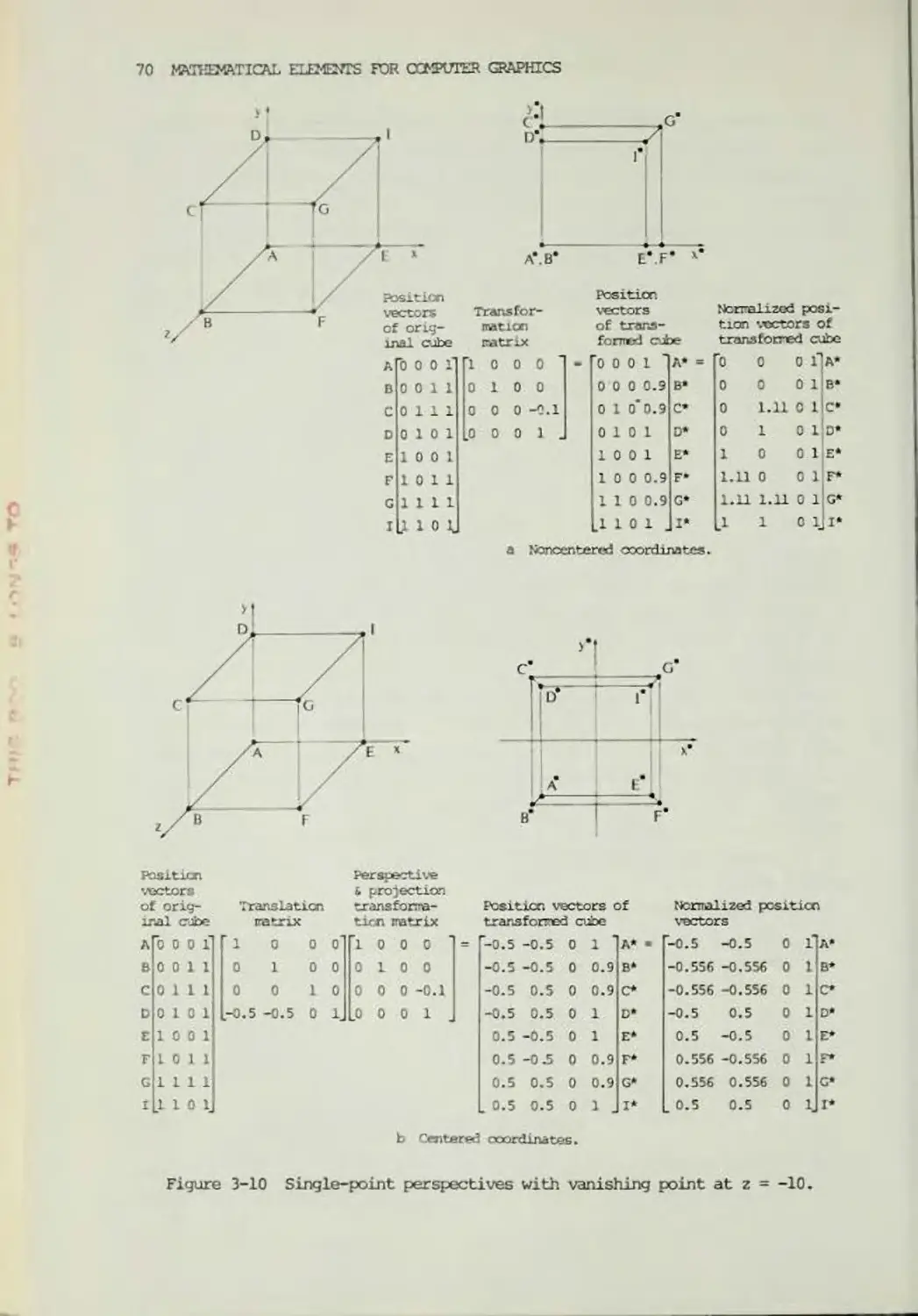
3-11 Perspective Trans formations 66
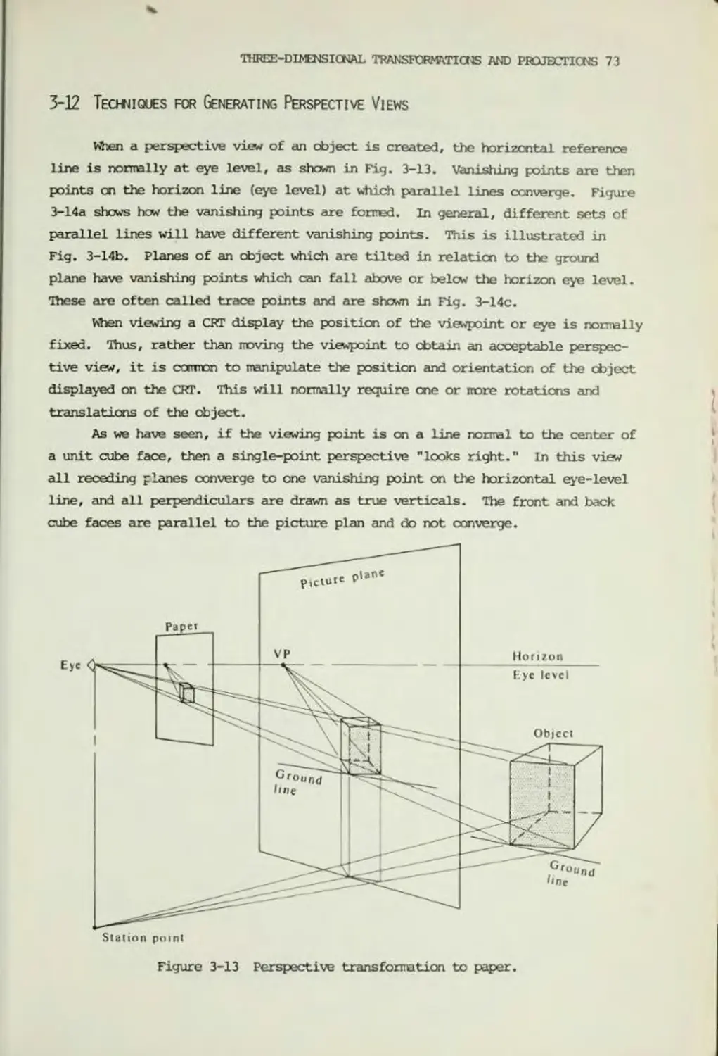
3-12 Techniques for Generating Perspective Views 73
3-13 Points at Infinity 77
3-14 Reconstruction of Three-Dimensional Information 78
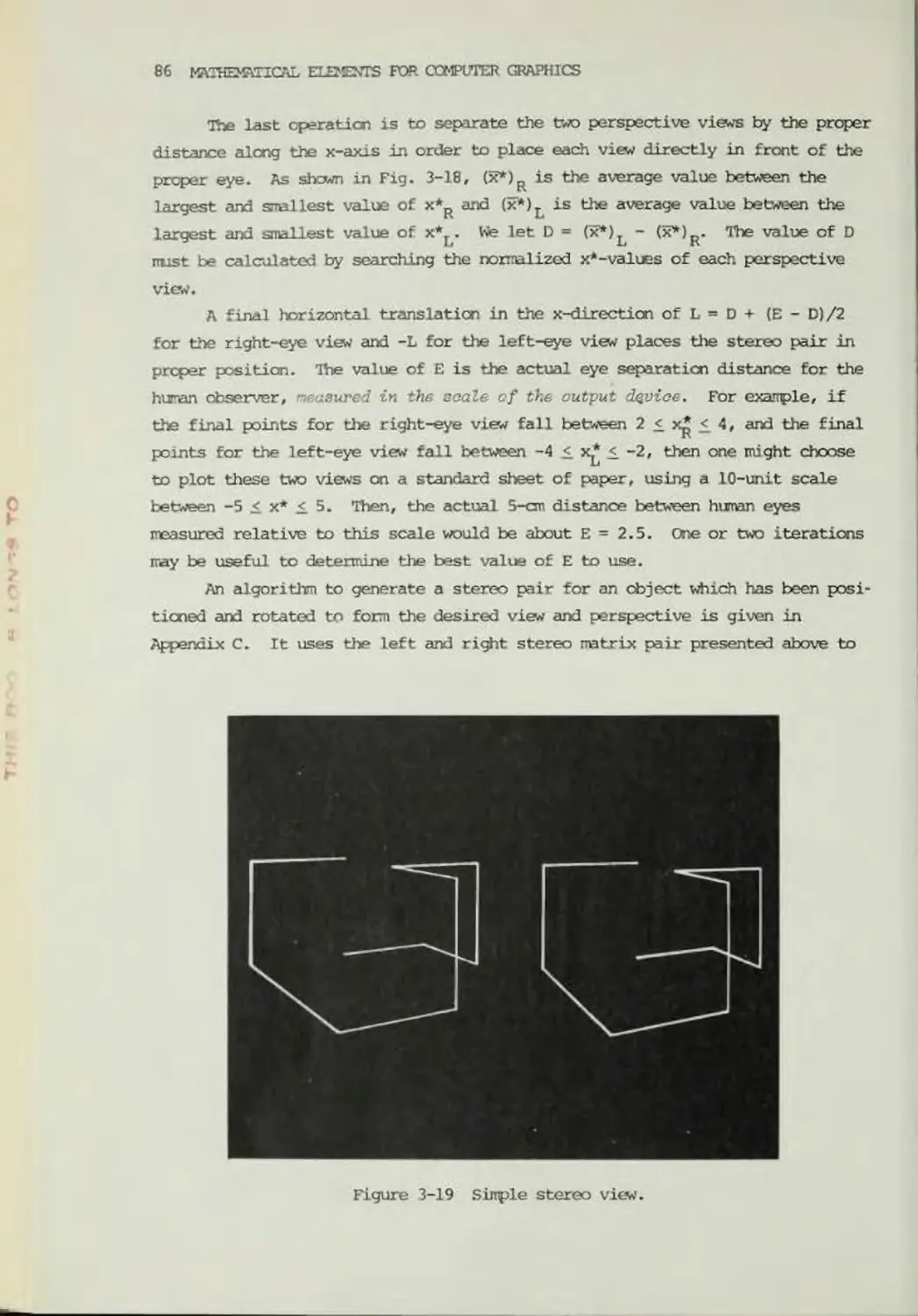
3-15 Stereographic Projection 84
References 87
CHAPTER 4 plane curves 89
4-1 Introduction 89
4-2 Nonparametric Curves 90
4-3 Parametric Curves 92
4-4 Nonparametric Representation of Conic Sections 94
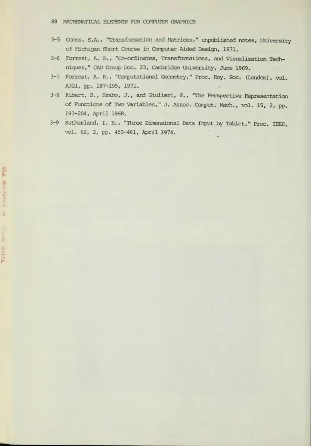
4-5 Nonparametric Circular Arcs 98
4-6 Pararretric Representation of Conic Sections 102
4-7 Parametric Representation of a Circle 103
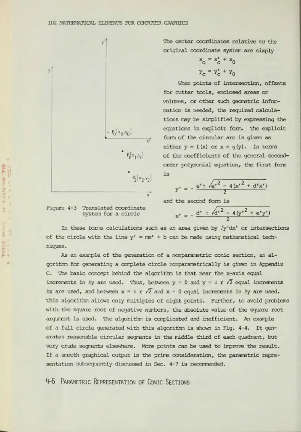
4-8 Parametric Representation of an Ellipse 104
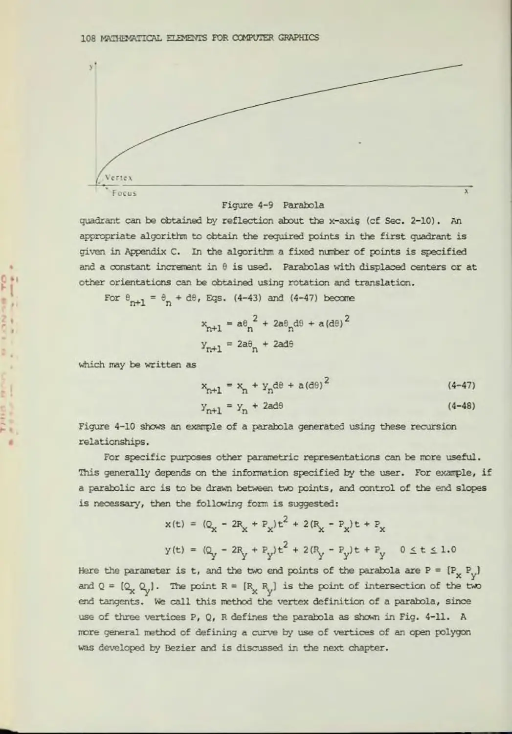
4-9 Parametric Representation of a Parabola 106
4-10 Parametric Representation of a Hyperbola 108

4-11
A Procedure for the Use of Conic Sections
COTTOTTS VII
111
4-12
Circular Arc Interpolation
113
References
115
CHAPTER 5 space curves
116
5-1
Introduction
116
5-2
Representation of Space Curves
116
5-3
Cubic Splines
119
5-4
Normalized Parameters
123
5-5
Boundary Conditions
124
5-6
Parabolic Blending
133
5-7
Bezier Curves
139
5-8
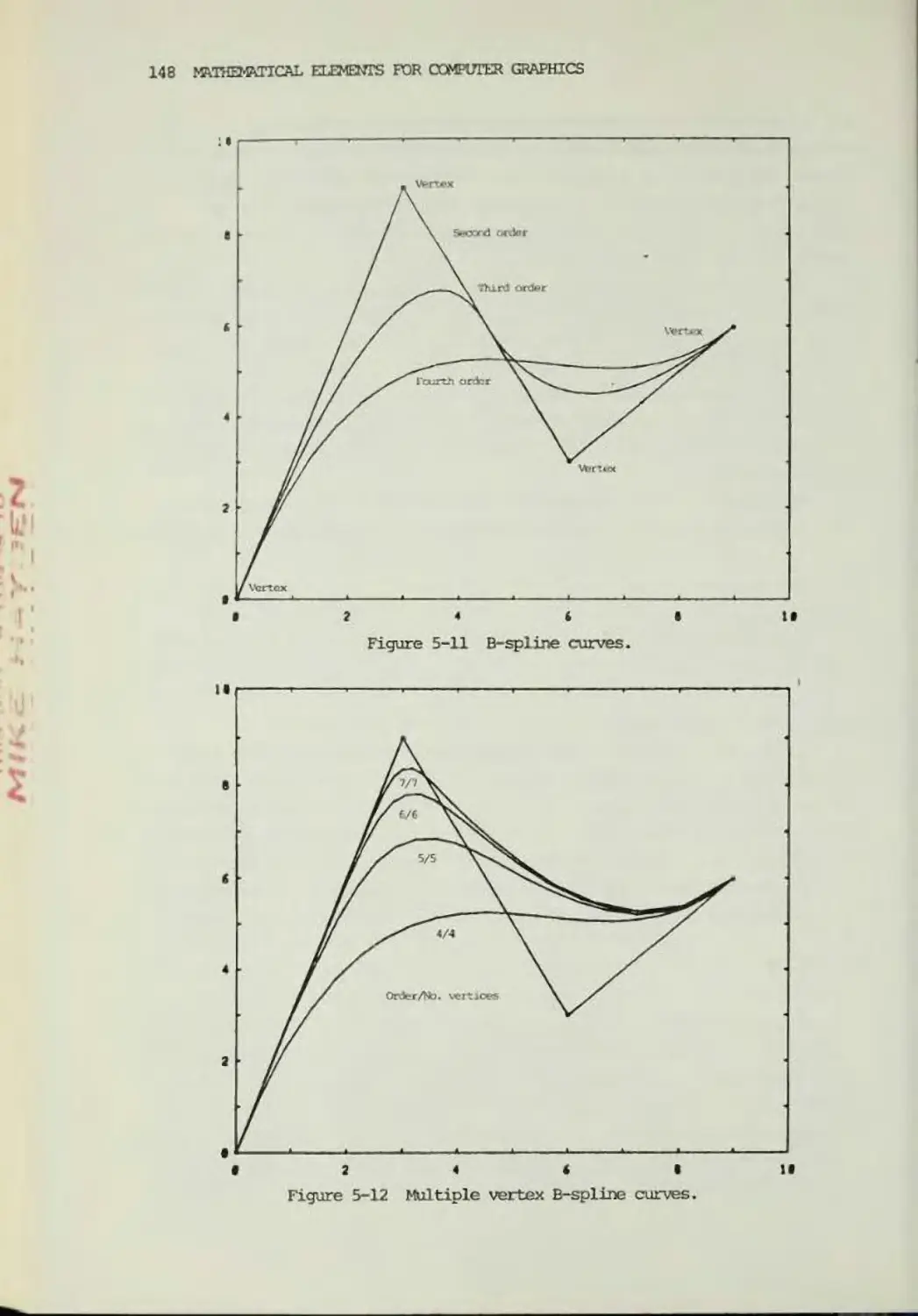
B-spline Curves
144
References
155
CHAPTER 6 SUREACE DESCRIPTION AND GENERATION
157
6-1
Introduction
157
6-2
Spherical Surfaces
158
6-3
Plane Surfaces
162
6-4
Curved Surface Representation
164
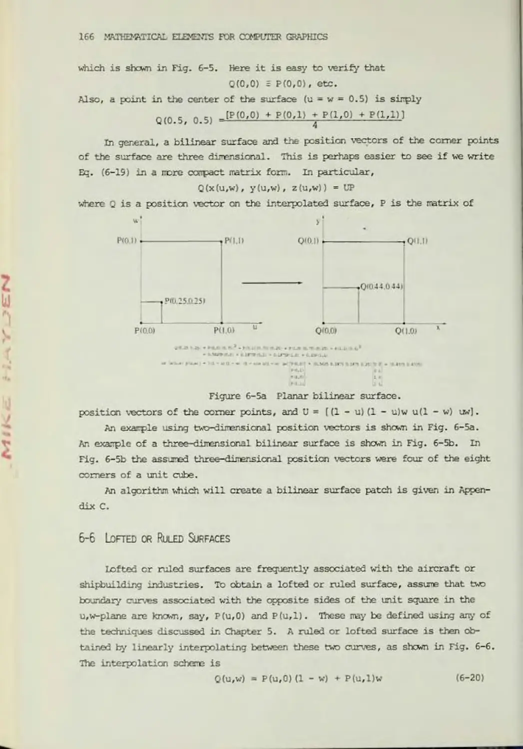
6-5
Bilinear Surface
165
6-6
Lofted or Ruled Surfaces
166
6-7
Linear Coons Surfaces
168
6-8
Bicubic Surface Patch
170
6-9
The F-Patch
175
6-10
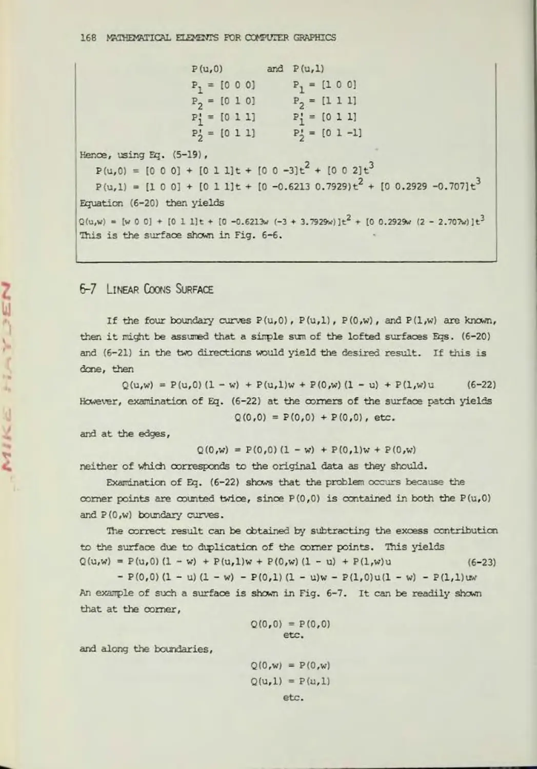
Bezier Surfaces
176
6-11
B-spline Surfaces
180
6-12
Generalized Coons Surfaces
181
6-13
Conclusions
185
References
186
APPENDIX A computer graphics sofiwvre
188
A-l
Corputer Graphics Primitives
189
A-2
Ccnputer Graphics Elements
191
A-3
Canonical Space
194
APPENDIX B MATRIX OPERATIONS
196
B-l
Terminology
196
B-2
Addition and Subtraction
197
B-3
Multiplication
197
B-4
Determinant of a Square Matrix
198

VIII MATHEMATICAL ELEMENTS FOR COMPUTER GRAPHICS
B-5 Inverse of a Square Matrix 199
APPENDIX C COMPUTER ALGORITHMS 200
C-l An Algorithm for Two-Dimensional Translations 200
C-2 A TVo-Dimensional Scaling Algorithm 201
C-3 A TVo-Dimensional Reflection Algorithm 202
C-4 A General TVo-Diircnsional Rotation Algorithm 202
C-5 A Three-Dimensional Scaling Algorithm 203
C-6 An Algorit±ffn for Three-Dimensional Rotation About the x-Axis 204
C-7 An Algorithm for Three-Dinensianal RDtation About the y-Axis 204
C-8 An Algorithm for Three-Dinensional Rotation About the z-Axis 205
C-9 An Algorithm for Three-Dimensional Reflections 206
C-10 An Algorithm for Three-Dirrensional Translation 207
C—11 An Algorithm for Three-Dinsnsional RDtation
about Any Arbitrary Axis in Space 207
C-12 An Axonometric Projective Algorithm 208
C-13 A Dimetric Projective Algorithm 209
C-l4 An Iscretric Projective Algorithm 210
C-15 An Algorithm for Perspective Transformations 210
C-16 Three-Dimensional Reconstruction Algorithms 211
C-17 A Stereo Algorithm 213
C-18 An Algorithm for a Nonparametric Circle 214
C-19 An Algorithm for a Parametric Circle 215
C-20 Parametric Ellipse Algorithm 216
C-21 An Algorithm for a Parametric Parabola 217
C-22 Algorithms for Parametric Hyperbolas 217
C-23 An Algorithm for a Circle through Three Points 218
C-24 An Algorithm for Generating Cubic Splines 220
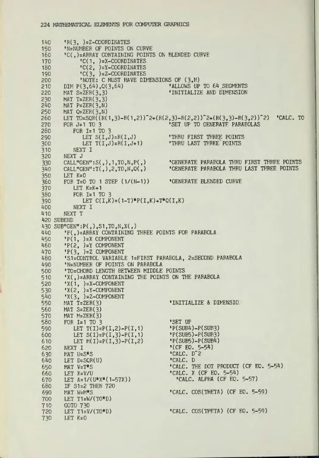
C-25 An Algorithm for Parabolic Blending 223
C-26 A Bezier Curve Algorithm 225
C-27 A B-spline Curve Algorithm 226
C-28 An Algorithm for a Bilinear Surface Patch 228
C-29 An Algorithm for a Linear Coons Surface 228
C-30 An Algorithm for a Bicubic Surface Patch 229
C-31 Bezier Surface Generation Algorithm 230
INDEX 232

%

FOREWORD
Since its inception more than a decade ago, the field of ccrputer graphics has
captured the imagination and technical interest of rapidly increasing nimbers of
individuals fran many disciplines. A high percentage of the gracing ranks of
ccrputer grallies professionals has given primary attention to ccrputer-oriented
problems in programming, system design, hardware, etc. This was pointed out by
Dr. Ivan Sutherland in his introduction to Mr. Prince's book, "Interactive
Graphics for Ccrputer-Aided Design," in 1971 and it is still true today. I
believe that an inadequate balance of attention has been given to application-
oriented problems. There has been a dearth of production of useful information
that bears directly cn the developrent and implejnantation of truly productive
applications. Understanding the practical aspects of carputer graphics with
regard to both the nature and use of applications represents an essential and
ultimate requiresnent in the development of practiced. caTputer graphic systems.
Mathematical techniques, especially principles of geometry and transformations,
are indigenous to most canputer graphic applications. Yet, large nurbers of
graphic programmers and analysts struggle over or gloss over the basic as well
as the caiplex problerrs of the iratheratical elements. Furthermore, the full
operational potential of carputer graphics is often unrealized whenever the
rrathematical relationships, constraints, and options are inadequately exploited.
By their authorship of this text, Drs. Rogers and Adams have recognized the
valuable relevance of their background to these practical considerations.

%
FOREWARD XI
Their text is concise, is carprehensive, and is written in a style unusually
conducive to ease of reading, understanding, and use. It exejTplifies the rare
type of wrk that most practitioners should wish to place in a prominent location
within their library since it should prove to be an invaluable ready reference
for nost disciplines. It is also well suited as the basis for a course in a
carputer science education curriculum.
I congratulate the authors in producing an excellent and needed text,
"Mathematical Elejrents for CaTputer Graphics."
S. H. "Chas" Chasen
Lockheed Georgia Conpany, Inc.

PREFACE
A new and rapidly expanding field called "ccciputer graphics" is emerging.
This field carbines both the old and the new: the age-old art of graphical
comnunication and the new technology of computers. Almost everyone can expect
to be affected by this rapidly expanding technology. A new era in the use of
conputer graphics, not just by the large ccnpanies and agencies utio made many
of the initial advances in software and hardware, but by the general user, is
beginning. Low-cost graphics terminals, time sharing, plus advances in mini-
and microccnputers have made this possible, 'today, ccnputer graphics is
practical, reliable, cost effective, and readily available.
The purpose of this book is to present an introduction to the mathematical
theory underlying conputer graphics techniques in a unified manner. Although
new ways of presenting material are given, no actual "new" mathematical material
is presented. All the material in this book exists scattered throughout the
technical literature. This book attempts to bring it all together in one place
in one notation.
In selecting material, vje chose techniques which were fundamentally math-
mathematical in nature rather than those which v^re more procedural in nature. For
this reason the reader will find wore extensive discussions of rotation, trans-
translation, perspective, and curve and surface description than of dipping or
hidden line and surface removal. First-year college mathematics is a sufficient
prerequisite for the major part of the text.

XIV MATHEMATICAL ELEMENTS FOR COMPUTER GRAPHICS
After a discussion of current ocnputer graphics technology in Chapter 1,
the manipulation of graphical elements represented in matrix form using hero-
geneous coordinates is described. A discussion of existing techniques for
representing points, lines, curves, and surfaces within a digital carputer, as
well as carputer software procedures for manipulating and displaying carputer
output in graphical form, is then presented in the following Chapters.
Mathematical techniques for producing axcnanetric and perspective views
are given, along with generalized techniques for rotation, translation, and
scaling of georetric figures. Curve definition procedures for both explicit
ai*3 par are trie representations are presented for both tvso-dimensional and three-
dimensional curves. Curve definition techniques include.the use of ccmc
sections, circular arc interpolation, cubic splines, parabolic blending, Bezier
curves and curves based on B-splines. An introduction to the mathematics of
surface description is included.
Carputer algorithms for most of the fundamental elanents in an interactive
graphics package are given in an appendix as BASIC* language subprograms. How-
However, these algorithms deliberately stop short of the coding necessary to
actually display the results. Unfortunately there are no standard language
crmrands or subroutines available for graphic display. Although seme preliminary
discussion of graphic primitives and graphic elanents is given in Appendix A,
each user will in general find it necessary to work within the confines of the
carputer system and graphics devices available to him or her.
The fundamental ideas in this bock have been used as the foundation for an
introductory course in carputer graphics given to students majoring in technical
or scientific fields at the undergraduate level. It is suitable for use in this
manner at both universities and schools of technology. It is also suitable as
a supplementary text in rore advanced carputer progranming courses or as a
supplementary text in seme advanced mathematics courses. Further, it can be
profitably used by individuals engaged in professional progranming. Finally,
the documented carputer programs should be of use to carputer users interested
in developing carputer graphics capability.
Acknowledgments
The authors gratefully acknowledge the encouragement arri support of the
Uuted States Naval Academy. The academic environment provided by the adminis-
administration, the faculty, and especially the midshipmen was conducive to the
developrent of the material in this bock.
♦BASIC is a registered trade mark of Dartmouth College

PREFACE XV
No book is ever written without the assistance of a great rany people.
Here we v*xild like to acknowledge a few of them. First, Steve Coons who reviewed
the entire manuscript and made many valuable suggestions, Rich Reisenfeld who
reviewed the material on R-spline curves and surfaces. Professor Pierre Bezier
who reviewed the material on Bezier curves and surfaces and Ivan Sutherland who
provided the impetus for the three-dimensional recontruction techniques discussed
in Chapter 3. Special acknowledgment is due past and present marbers of the
CAD Group at Carrbridge University. Specifically, work done with tabin Forrest,
Charles Lang, and 'Tony Nutboume provided greater insight into the subject of
ccnputer graphics. Finally, to Iouie Knapp who provided an original FORTRAN
program for B-spline curves.
The authors vrould also like to acknowledge the assistance of many individuals
at the Evans and Sutherland Ccnputer Corporation. Specifically, Jim Callan who
authored the document from which many of the ideas on representing, preparing,
presenting and interacting with pictures is based. Special thanks are also due
Lee Billow who prepared all of the line drawings.
Much of the art work for Chapter 1 has been provided through the good
offices of -arious ccnputer graphics equipment iranufacturers. Specific ackncw
ledcpent is irade as follows:
Fig.
1-3
Evans and Sutherland Carpjter Corporation
Fig.
1-5
Adage Inc.
Fig.
1-7
Adage Inc.
Fig.
1-8
Vector General, Inc.
Fig.
1-11
Xynetics, Inc.
Fig.
1-12
CALCOMP, California Carputer Products, Inc.
Fig.
1-15
Gould, Inc.
Fig.
1-16
Tektronix, Inc.
Fig.
1-17
Evans and Sutherland Ccnputer Corporation
Fig.
1-18
CAICCMP, California Ccnputer Products, Inc.
David F. Rogers
J. Alan Adams

CHAPTER 1
INTRODUCTION TO
COMPUTER GRAPHIC
TECHNOLOGY
Since carputer graphics is a relatively new technology, it is necessary
to clarify the current terminology. A nunber of tenns and definitions sire used
rather loosely in this field. In particular, carputer aided design (CAD),
interactive graphics (IG), conputer graphics (CG), and conputer aided manufac-
manufacturing (CAM) are frequently used interchangeably or in such a manner that
considerable confusion exists as to the precise meaning. Of these terms G\D
is the most general. CAD may be defined as any use of the conputer to aid in
the design of an individual part, a subsystem, or a total system. The use
does not have to involve graphics. The design process may be at the system
concept level or at the detail part design level. It nay also involve an in-
interface with CAM.
Qxrputer aided manufacturing is the use of a conputer to aid in the
manufacture or production of a part exclusive of the design process. A direct
interface between the results of a CAD application and tlve necessary part
programming using such languages as APT (Automatic Programmed Tcols) and UNIAPT
(United*s APT), the direction of a machine tool using a hardwired or softwired
(miniconputer) controller to read data frxr a punched paper tape and generate
the necessary a*rmands to control a machine tool, or the direct control of a
michine tool using a minicomputer may be involved.
Conputer graphics is the use of a carputer to define, store, manipulate,

2 MYIHSMTCAL ELEMENTS FOR COMPUTER GRAPHICS
interrogate/ and present pictorial output. This is essentially a passive oper-
operation. The conputer prepares and presents stored information to an observer
in the form of pictures. The observer has no direct control over the picture
being presented. The application nay be as sinple as the presentation of the
graph of a sinple function using a high-speed line printer or a time-sharing
teletype terminal to as ctnplex as the sinrulation of the automatic reentry and
landing of a space capsule.
Interactive graphics also uses the ccrrputer to prepare and present pictor-
pictorial material. However, in interactive graphics the observer can influence the
picture as it is being presented; i.e., the observer interacts with the picture
in real tire. To see the importance of the real time restriction, consider the
problem of rotating a ccnplex three-dimensional picture conposed of 1000 lines
at a reasonable rotation rate, say, 15°/second. As we shall see subsequently,
the 1000 lines of the picture are most conveniently represented by a 1000 x 4
matrix of homogenous coordinates of the end points of the lines, and the rota-
rotation is most conveniently acccnplished by multiplying this 1000 x 4 matrix by
a 4 x 4 transformation natrix. Accomplishing the required matrix multiplication
requires 16,000 nultiplicaticns, 12,000 additions, and 1000 divisions. If this
matrix multiplication is acccrplished in software, the time is significant. To
see this, consider that a typical mini conputer using a hardware floating-point
processor requires 6 microseconds to multiply two nirrbers, 4 microseconds to
add two nunbers, and 8 microseconds to divide two nirrbers. Thus the matrix
multiplication requires 0.15 seconds.
Since ccnputer displays that allow dynamic motion require that the picture
be redrawn (refreshed) at least 30 times each second in order to avoid flicker,
it is obvious that the picture cannot change smoothly. Even if it is assured
that the picture is recalculated (updated) only 15 times each second, i.e.,
every degree, it is still not possible to accorplish a smooth rotation in soft-
software. Thus this is now no longer interactive graphics. To regain the ability
to interactively present the picture several things can be done. Clever pro-
programming can reduce the time to accorplish the required matrix multiplication.
However, a point will be reached where this is no longer possible. The ccm-
plcxity of the picture can be reduced. In this case, the resulting picture
nay not be acceptable. Finally, the matrix multiplication can be acccrplished
by using a special-purpose digital hardware matrix multiplier. This is the
ixjst promising approach. It can easily handle the problem outlined above.
With this terminology in mind the remainder of this chapter will give an
ovorvii3w of conputer graphics and discuss and classify the types of graphic
displays available. The necessary considerations for development of a soft-
software system for the fundamental drawing, device-ccntrol, and data-handling

imrotXCTiCN to ccmpoter graphics TOC3B*)U)GY 3
aspects of carputer graphics is given in Appendix B.
1-1 Overview Of Computer Graphics
Carputer graphics as defined above can be a very corrplex and diverse si±>-
ject. It encorpasses fields of study as diverse as electronic and mechanical
design of the oorrponents used in conputer graphics systems and the concepts of
display lists and tree structures for preparing and presenting pictures to an
cbserver using a conputer graphics system. A discussion of these aspects of
interactive carputer graphics is given in the book by Newman and Sproul (Ri*f.
1-1). Here we will attenpt to present only those aspects of the subject of
interest from a user's point of view. From this point of view, conputer
graphics can be divided into the following areas:
Representing pictures to be presented
Preparing pictures for presentation
Presenting previously prepared pictures
Interacting with the picture
Here the word "picture” is used in its broadest sense to mean any collection
of lines, points, text, etc., to be displayed on a graphics device. A picture
ray be as siirple as a single line or curve, or it may be a fully scaled and
annotated graph or a corrplex representation of an aircraft, ship, or automobile.
1-2 Representing Pictures To Be Presented
Fundamentally the pictures represented in conputer graphics can be con-
considered as a collection of lines, points, and textual material. A line can be
represented by the coordinates of its end points (x^y^z^) and (x2,y2,z2), a
point by a single-coordinate triplet (x^,y^,Zj) , and textual material by col-
collections of lines or points.
The representation of textual material is by far the most corplex, involv-
involving in many cases curved lines or dot matrices. Hcwever, unless the user is
concerned with pattern recognition, the design of graphic hardware, or unusual
character sets, he or she need not be concerned with these details, since al-
almost all graphic devices have built-in "iiarclware" of software character gen-
generators. The representation of curved lines is usually accomplished by approxi-
approximating them by short straight-line segments. Hcwever, this is sometimes accom-
accomplished using hardware curve generators.
1-3 Preparing Pictures For Presentation

4 NMM2MTCAL ElfMNTS FDR (Xt&UIER GRAPHICS
Pictures ultimately consist of points. The coordinates of these points
are gere rally stored in a file (array) prior to being used to present the pic-
picture. This file (array) is called a data base. Very ccnplex pictures require
very complex data bases which require a ccnplex program to access them. These
ccnplex data bases nay involve ring structures, tree structures, etc., and the
data base itself ray contain points, substructures, and other nongraphic data.
The design of these data bases and the programs which access them is an ongoing
topic of research, a topic which is clearly beyond the scroe of this text.
However, many ccnputer graphics applications involve much sinpler pictures for
which the user can readily invent sinple data base structures which can be
easily accessed.
Points are the basic building blocks of a graphic data base. There are
three basic methods or instructions for treating a point as a graphic geometric
entity: nuve the beam, pen, cursor, plotting head (hereafter called the cursor)
to the point, dratf a line to that point, or draw a cbt at that point. Funda-
Fundamentally there are tw ways to specify the position of a point: absolute or
relative (incremental) coordinates. In relative or incremental coordinates the
position of a point is defired by giving the displacement of the point with
respect to the previous point.
The specification of the position of a point in either absolute or relative
coordinates requires a nurrber. This can lead to difficulties if a ccnputer
with a limited word length is used. Generally a full ccnputer word is used
to specify a coordinate position. The largest integer nurrber that can be spec-
specified by a full ccnputer word is 2^1 - 1, where n is the nurber of bits in the
vrord. For the 16-bit miniccnputer frequently used to support ccnputer graphic
displays, this is 32767. For marry applications this is acceptable. However,
difficulties are encountered when larger integer rxrbers than can be specified
are required. At first we might expect to over core this difficulty by using
relative coordinates to specify a nurber such as 60,000, i.e., using an absolute
coordinate specification to position the cursor to (30000, 30000) and then a
relative coordinate specification of (30000, 30000) to position the beam to the
final desired point of (60000, 60000). However, this will not work, since an
att*3Tpt to aociimilate relative position specifications beyorri the maximum rep-
representable value will result in the generation of a nuiber of opposite sign
and erroneous magnitude. For cathode ray tube (CRT) displays this will gererally
yield the phenomena called wraparound.
The way out of this dilerrma is to use homogeneous coordinates. The use of
horogeneous coordinates introduces sore additional canplexity, sont? loss in
speed, and sore loss in resolution. Hcxvever, these disadvantages are far out-
wighed by the advantage of being able to represent large integer nurbers with

IOTRODUCTION TO CCffVFER GRAPHICS TECMOLD& 5
a carputer of limited word size. For this reason as well as others presented
later, homogeneous coordinate representations are generally used in this book.
In homogeneous coordinates an n dimensional space is represented by n + 1
dimensions, i.e., three-dimensional data where the position of a point is given
by the triplet (x,y,z) is represented by four coordinates (hx,hy,hz,h) , where
h is an arbitrary nurrfoer.
If each of the coordinate positions represented in a 16-bit conputer were
less than 32767, then h would be irade equal to 1 and the coordinate positions
represented directly. If, ho/ever, one of the Eucledean or ordinary coordinates
is larger than 32767, say, x = 60000, then the pcwer of haicgeneous coordinates
beocrtis apparent. In this case we can let h = 1/2, and the coordinates of the
point are then defined as (30000, l/2y, l/2z, 1/2), all acceptable nurbers for
a 16-bit ccnputer. However, some resolution is lost since x - 60000 and x =
59999 are both represented by the sane homogeneous coordinate. In fact resolu-
resolution is lost in all the coordinates even if only one of them exceeds the maxi-
maximum expressable nunber of a particular conputer.
W Presenting Previously Prepared Pictures
With these comrrents about data bases in mind it is necessary to note that
the data base used to prepare the picture for presentation is almost never the
same as the display file used to present the picture. The data base represents
the total picture while the display file represents only some portion, view, or
scene of the picture. The display file is created by transforming the data
base. The picture contained in the data base may be resized, rotated, trans-
translated, or part of it removed or viewed frcm a particular point to obtain nec-
necessary perspective before being displayed. Many of these operations can be
accaiplislted by using sinple linear trans formations which involve matrix milti-
plications. Among these are rotation, translation, scaling, and perspective
views. As we shall see later, homogeneous coordinates are very convenient for
accomplishing these transformations.
As will be shewn in detail in Chapters 2 and 3, a 4 x 4 matrix can be used
to perform any of these individual transformations on points represented as a
matrix in iKmogeneous coordinates. When a sequence of transformations is
desired, each individual transformation can be sequentially applied to the
points to achieve the desired result. If, however, the nuroer of points is
substantial, this is inefficient and time consuming. An alternate and more
desirable method is to multiply the individual matrices representing each
required transformation together and then to finally multiply the matrix of
points by the resulting 4x4 transformation matrix. This matrix operation is

6 MftniEMYTICAL ELEMENTS TOP. COMPUTER GRAPHICS
called concatenation. It results in significant time savings when performing
ccrpound matrix operations cn sets of data points.
Although in many graphics applications the corplete data base is displayed,
frequently only portions of the data base are to be displayed. This process of
displaying only part of the oonplete-picture data base is called windowing.
Windowing is not easy, particularly if the picture data base has been transform-
transformed as discussed above. Performance of the windowing operation in software gen-
generally is sufficiently time cons lining that dynamic real-time interactive graphics
is not possible. Again, sophisticated graphics devices perform this function
in hardware. In general there are two types of windowing - clipping and scis-
scissoring. Clipping involves determining which lines or portions of lines in the
picture lie outside the window. Those lines or portions of lines are then dis-
discarded and not displayed? i.e., they are not passed on to the display device.
In the scissoring technique, the display device has a larger physical drawing
space than is required. Only those lines or line segments within the specified
window are node visible even though lines or line segments outside the winckw
are drawn. Clipping accomplished in hardware is generally more advantageous
than scissoring; e.g., clipping makes available a much larger drawing area than
scissoring. In scissoring, those lines or segments of lines which are not vis-
visible in the window are also drawn. This, of course, requires tine, since the
line generator rust spend time drawing the entire data base whether visible or
invisible rather than only part of the data base as in the case for clipping.
In two dimensions a window is specified by values for the left, right, top,
and bottom edges of a rectangle. Clipping is easiest if the edges of the
rectangle are parallel to the coordinate axes. If, however, this is not the
case, the rotation of the window can be conpensated for by rotating the data
base in the opposite direction. Tridimensional clipping is represented in
Fig. 1-1. Lines are retained, deleted, or partially deleted, depending on
whether they are ccrpletely within or without the window or partially within
or without the window. In three dimensions a window consists of a frustum of
vision, as shown in Fig. 1-2. In Fig. 1-2 the near (hither) boundary is at N,
the far (yon) boundary at F, and the sides at SL, SR, ST, and SB.
As a final step in the picture presentation process it is necessary to
convert frcn the coordinates used in the picture data base called user coordin-
coordinates, to those used by the display device, called display coordinates. In par-
particular, It is necessary to convert coordinate data which pass the windowing
process into display coordinates such that ti*e picture appears in some specified
area on the display, called a viewport. The viewport can be specified by giv-
giving its left, right, top, and bottom edges if two-dimensional or if three-
dimensional by also specifying a near (hither) and far (yon) boundary. In the

rorPODUCTICN to compittcr GRAPHICS TTEHNOIAGy 7
Line entirely
within
window *.
cnl ire I ine
displayed
line par (1a 11 > within window:
pari from a-b displaycd;
part from b-c not displayed
c,
Line partially within
window part from b-c
displayed, parts a-b. c-d
not displayed
Line entirely
outside of
window: not
displayed
Figure 1-1 TVro diirensional
windaving (clipping).
Figure 1-2 Three-dimensional
frustum of vision windc*/.
nt>st general case conversion to display coordinates within a specified three-
dimensional viewport requires a linear mapping frcm a six-sided frustim of
vision (window) to a six-sided viewport.
An additional requirarent for most pictures is the presentation of alpha-
alphanumeric or character data. There are in general two methods of generating
characters - software and har&vare. If characters are generated in software
using lines, they are treated in the same manner as any other picture element.
In fact this is necessary if they are to be clipped and then transfomed along
with other picture elanents. However, many graphic devices have seme kind of
hardware character generator. Khen harckvare character generators cure used, the
actual characters are generated just prior to being drawn. Up until this point
they are treated as only character codes. Hardware character generation is less
flexible since it does not allow for clipping or infinite transformation, e.g.,
only limited rotations and sizes are generally possible, but it yields signifi-
significant efficiencies.
When a hardware character generator is used, the program which drives the
graphic device must first specify size, orientation, and the position where
the character or text string is to begin. The character codes specifying tliese

8 MAMEranCAL ELE2-1EOTS TOR COMPUTER GRAPHICS
characteristics are then added to the display file. Upon being processed the
character generator interprets the text string, looks up in hardware the neces-
necessary lines to draw the character, and draws the characters on the display de-
device.
1-5 Interacting With The Picture
Interacting with the picture requires some type of interactive device to
oominicate with the program while it is running. In effect this interrupts
the program so that new or different information can be provided. Numerous
devices have been used to accorplish this task. The sinpj.est is, of course,
the alphanumeric keyboard such as is fourd on the teletype. More sophisticated
devices include light pens, joy sticks, track balls, a rouse, function switches,
control dials, and analog tablets. We shall examine each of these devices
briefly.
A simple alphanumeric keyboard as shewn in Fig. 1-3 can be a useful inter-
interactive device. Precise alphabetic, numerical, or control information can be
easily supplied to the program. Hcwever, it is not capable of high rates of
interaction, expccially if the user is not a cpod typist.
Perhaps the best known interactive device is the light pen. The light pen
contains a light-sensitive photoelectric cell ard associated circuitry. When
positioned over a Line sequent or other lighted area of a CRT and activated,
the position of the pen is sensed and an in tempt is sent to the corrputer. A
schematic of a typical light pen is shewn in Fig. 1-4. Figure 1-5 shews a light
pen in use for rrenu picking.
The joy stick, mouse, and track ball all operate on the same principle.
By roving a control, t>/o-dimensional positional information is comunicated to
the conputer. All these devices are analog in nature. In particular, movement
of the control changes the setting of a sensitive potentiometer. The resulting
signals are converted from analog (voltages) to digital signals using an analog
to digital (A/D) converter. These digital signals are then interpreted by the
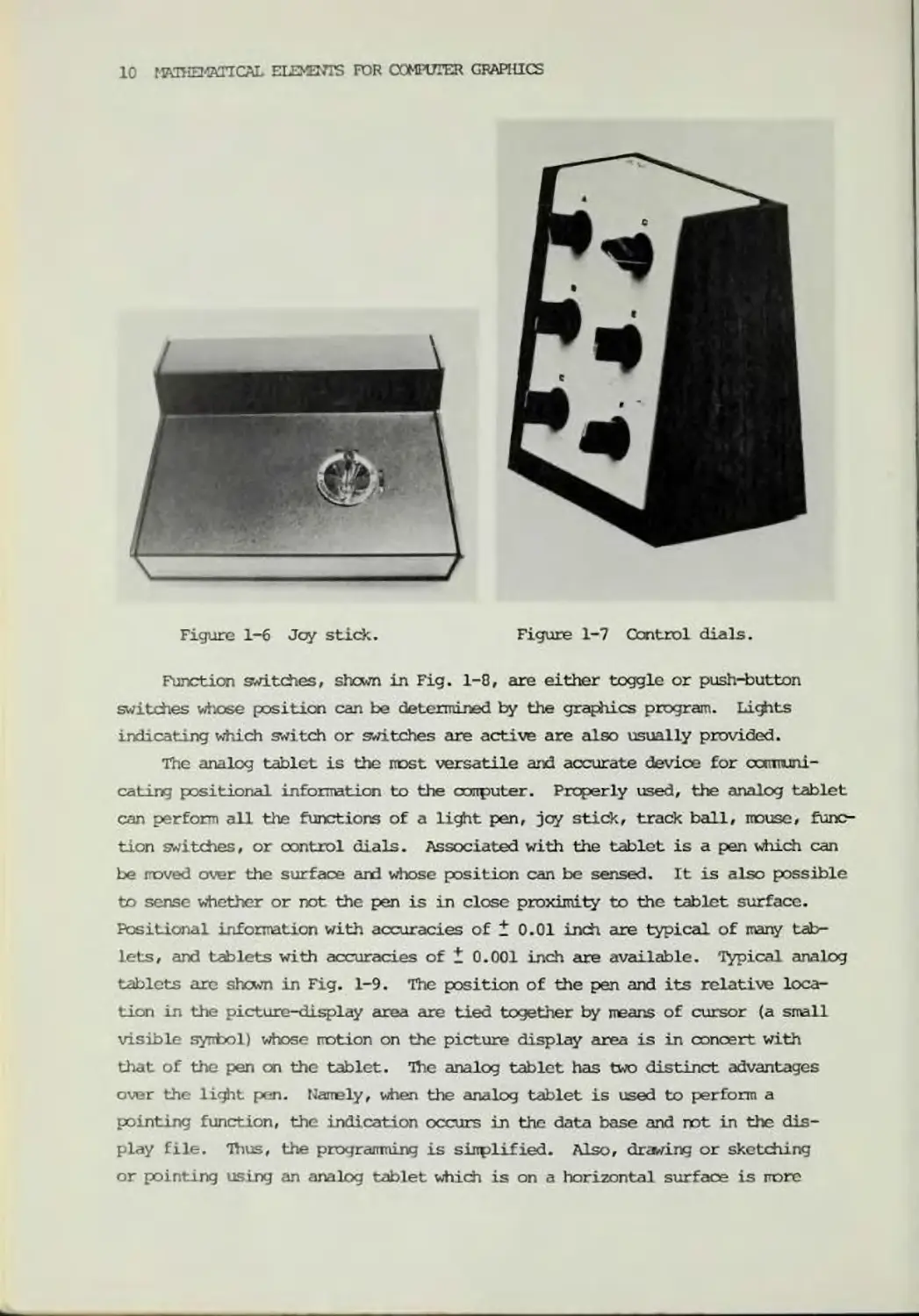
ccrputer as positional information. A joy stick is shewn in Fig. 1-6. Joy
sticks, rouses, track balls, and similar devices are useful for particular
applications. Ho/ever, they should not be used to provide very precise position-
positional information.
Control dials as shewn in Fig. 1-7 are essentially sensitive rotating poten-
potentiometers and associated circuitry such that the position of the dial can be
sensed using analog to digital conversion techniques. They are particularly
useful for activating rotation, translation, or zoom features of hardware and
software system.

V
INTRODUCTION TO QDMWTER GRAPHICS TECHMOI13GV 9
I icId <>f view
\
 Holder
Pulse shaping circuilr>
Io dispi.i)
com roller
Figure 1-3 Alphanumeric
keyboard.
Figure 1-4 Schcmatic
of a light pen.
Figure 1-5 Light pen in use for menu picking.

10 MMHEPRTICAL ELEMEOTS TOR COMPUTER GRAPHICS
WIi
Figure 1-6 Joy stick. Figure 1-7 Control dials.
Function switches, shown in Fig. 1-0, are either toggle or push-button
switches wtiose position can be determined by the graphics program. Lights
indicating which switch or switches are active are also usually provided.
The analog tablet is the nost versatile and accurate device for camuni-
cating positional information to the conputer. Properly used, the analog tablet
can perform all the functions of a light pen, joy stick, track ball, mouse, func-
function switches, or control dials. Associated with the tablet is a pen which can
be noved over the surface and whose position can be sensed. It is also possible
to sense whether or not the pen is in close proximity to the tablet surface.
Positional information with accuracies of t 0.01 inch are typical of many tab-
tablets, and tablets with accuracies of t 0.001 inch are available. Typical analog
tablets arc sham in Fig. 1-9. The position of the pen and its relative loca-
location in tiie picture-display area are tied together by means of cursor (a small
visible syrrbol) whose notion on the picture display area is in concert with
that of tl>e pen on the tablet. The analog tablet has two distinct advantages
over the light pen. Namely, when the analog tablet is used to perform a
pointing function, the indication occurs in the data base and not in the dis-
display file. Thus, the programming is sirrplified. Also, drawing or sketching
or pointing using an analog tablet which is on a horizontal surface is more

nmCDUCTION TO CaWTER GRAPHICS TEGINQLOGY 11
natural than performing the sane oper-
operation with a light pen in a vertical
orientation.
An analog tablet can be implemented
in hardware by using a variety of elec-
electromagnetic principles. Scne of these
are discussed in Ref. 1-1 in more detail.
Except in unusual environments the user
need not be concerned with the precise
operating principle.
1-6 Description Of Sort Typical
Graphics Devices
There are a large nmber of differ-
different types of graphics devices available,
far too many to describe then all here.
Therefore only a limited nizrber of de-
devices representative of those available
Figure 1-8 Function switches. will be considered. In particular,
three different types of CRT graphics
devices - storage tike, refresh, and raster scan; a pen and ink plotter? and
a dot matrix plotter - will be described. Additional devices and rore detail-
detailed descriptions are provided in R^f. 1—1.
The three types of CFT (cathode ray tube) devices are direct view storage
tibe displays, refresh displays, and raster scan displays. The direct view
storage tube display, also called a bistable storage tube display, can be
considered as similar to an oscilloscope with a very long persistence phosphor.
A storage tube display is shewn in Fig. 1-9. A line or character will remain
visible (up to an hour) until erased by the generation of a specific electrical
signal. Tfte erasing process requires about 1/2 second. Storage tii>e displays
have several advantages and disadvantages. Sane of the advantages are: the
display is flicker free, resolution of the display is good (typically 1024 x
1024 addressable raster points in an approximate 8x8 inch square), and cost
is lav. Further, it is relatively easy and fast to cbtain an acceptable hard
copy of the picture, and conceptually they are somewhat easier to program and
more suited to t irr?-sharing applications than refresh or raster scan displays.
The principal disadvantage is that the screen cannot be selectively erased;
i.e., in order to change any element of a picture the entire picture must be
redrawn. Because of this the display of dynamic motions is not possible. In

12 fMK2«nCAL ELEMENTS FOR COMPUTER GRAPHICS
Figi2re 1-9 Analog tablet.
addition, this characteristic results in the interaction between the user and
the display being sarewhat slower than with a refresh display.
A refresh CRT yraphics display is based on a television-like cathode ray
ttbe. Hcwever, the method of generating the image is quite different. Tele-
Television uses a raster scan technique (see belcw) to generate the required pic-
picture, whereas the traditional refresh CRT graphics display is of the calligraphic
cr line-drawing type. A refresh CRT graphics display requires t*o elements in
addition to the cathode ray ti±>e itself: a display buffer and a display con-
controller. In order to understand the advantages arad limitations of a refresh
display it is necessary to conceptually understand the purpose of these devices.
Since the phosphor used on the cathode ray tube of a refresh display fades
very rapidly, i.e., has a short persistence, it is necessary to repaint or re-
reconstruct the entire picture many tines cacti second. This is callcd the refresh
rate. A refresh rate that is too lew will result in a phenomenon called flicker.
This is similar to the effect which results from running a movie projector too
slxw. A minimim refresh rate of 30 times per second is required to achieve a
flicker-free display. A refresh rate of 40 times per second is recarrended.
Hie function of the display buffer is to store in sequence all of the ins true-

INTRODUCTION TO COMPUTER GRAPHICS TDCIINOLOGV 13
tions necessary to draw the picture on the cathode ray tube. The function of
the display controller is to access (cycle through) these instructions at the
refresh rate. Inrodiately, a limitation of the refresh display is cbvious:
The complexity of the picture is limited by the size of the display buffer and
the speed of the display controller. Hcwever, the short persistence of the
image can be used to advantage to shew dynamic notion. In particular, the pic-
picture can be updated every refresh or, say, every other refresh cycle if double
buffering is used. Further, since each element or instruction necessary to
draw the complete picture exists in the display buffer, any individual elemant
can be changed, deleted, or an additional element added? i.e., a selective
erase feature can be inplemented. One additional disadvantage of a refresh CRT
graphic device is the relative difficulty of obtaining a hard cxxjy of the pic-
picture. Although refresh CRT graphic displays are generally more expensive than
storage tube displays, the above characteristics make them the display of choice
when dynamic motion in real time or very rapid interaction with the display is
required.
A raster scan CRT graphics display uses a standard television monitor for
the display console. In the raster scan display the picture is composed of a
series of dots. These dots are traced out using a dual raster scan technique,
i.e., as a series of horizontal lines. IWo rasters as shewn in Fig. 1-10 are
used to reduce flicker. The basic electrical signal used to drive the display
console is an analog signal whose modulation represents the intensity of the
individual dots which compose the picture. In using a raster scan display con-
console it is first necessary to convert the line and character information to a
form compatible with the raster presentation. This process is ceil led scan con-
conversion. Once it is converted the information must be stored such that it can
be accessed in a reasonable manner. With the advances in data storage techni-
techniques this is becoming more feasible. In considering a raster scan CRT graphic
display, the advantages and disadvantages are similar to those for line-drawing
displays, with scene additional considerations. Namely, they are generally some-
somewhat slower, the selective erase feature is more difficult to implement, and
they may be directly interfaced to closed-circuit television systems.
Digital incremental pen and ink plotters are of two general types - flat-
flatbed and drum. Figure 1-11 shoes a flat-bed plotter and Fig. 1-12 shews a drum
plotter. Itost dnxn and flat-bed plotters operate in an incremental mode; i.e.,
the plotting tool, which need not be a pen, moves across the plotting surface
in a series of small steps, typically 0.001 to 0.01 inch. Frequently the num-
number of directions in which the tool can move is limited, say, to the eight
directions shewn in Fig. 1-13. Ihis results in a curved line appearing to be
a series of small steps. In a flat-bed plotter the table in generally station-

14 KMHEMftXIGtfi EJJ&BHS FOR COMFLTER GRAPHICS
ary and the writing head moves in two
dimensions over the surface of the table.
A druT\ plotter uses a scnewhat different
technique to achieve two-dimensional no-
notion. Here the marking tool roves back
and forth across the paper while the
lengthwise notion is obtained by rolling
the paper back and forth under the nark-
narking tool.
Digital incremental plotters can provide
high-quality hard copy of graphical out-
output. Cbrpared to CRT graphics devices
they are quite slow. Consequently they
are not generally used for real-time
interactive graphics. However, where
large drawings are norrrally required for
a particular application, a flat-bed
plotter can be utilized as a cxxrbination
digitizer and plotter and an interactive
conputer graphic system successfully
developed (see Ref. 1-2).
The electrostatic dot matrix printer/plotter operates by depositing part-
particles of a toner onto srcall electrostatically charged areas of a special paper.
Figure 1-14 shows the general scheme which is enplqyed. In detail, a specially
coated paper which will hold an electrostatic charge is passed over a writing
head which contains a row of small writing nibs or styli. Frcm 70 to 200 styli
per inch are typical. The styli deposit an electrostatic charge onto the spec-
special paper. Since the electrostatic charges are themselves not visible, the
charged paper is passed over a toner which is a liquid containing dark toner
particles. The particles are attracted to the electrostatically charged areas,
making than visible. The paper is then dried and presented to the user. Very
high speeds can be obtained, typically from 500 to 1000 lines per minute.
The electrostatic dot matrix printer/plotter is a raster scan device; i.e.,
it presents information one line at a time. Because it is a raster scan device
it requires a substantial amount of ccuputer storage to construct a corplete
picture. This plus the fact tiiat the device is useable for only passive graph-
graphics are the principle disadvantages. A further disadvantage is relatively lew
accuracy and resolution, typically t 0.01 inch. The principal advantages are
the very' high speed with which drawings can be produced and an excellent reli-
reliability record. Figure 1-15 shows an electrostatic dot ratrix printer/plotter
__ First raster
ScconJ raster
Figure 1-10 Raster
scan technique.

INTRODUCTION TO COtVUSER GRAPHICS TtaNOIiXY 15
Figure 1-11 Flat-bed plotter.
Figure 1-12 Drum plotter

16 KA3HC&TIC\L EXET'CTTS PGR COOTIER GRAPHICS
4
Writing
head
Figure 1-13 Directions Figure 1-14 Conceptual
for incremental plotters. description of electrostatic
dot ratrix printer/plotter.
and typical output.
1-7 Classification Of Graphics Devices
Ihere are a number of methods of classifying conputer graphics devices.
Each method yields sate insight into the sere times confusing array of possible
devious. V/e will discuss several different methods.
First let's consider the difference between a passive and an active graphics
device. A passive graphics device siirply draws pictures under ccnputer control;
i.e., it allews the ccrrputer to communicate graphically with the user. Exarples
are a teletype, a high-speed line printer, and an electrostatic dot matrix
printer, pen and ink plotters, and storage tube cathode ray tube (CRT) and re-
refresh CRT devices. Exarples of seme of these devices and the typical pictures
that they might generate are shown in Fig. 1-10, 1-12, and 1-15 through 1-20.
The reader might wonder about considering the teletype and the high-speed line
printer as grajjhics devices. Ilcwever, they have been used to draw sinple
graphs or plots for a niTTber of years.

mjOXCTICN TO OMPU1ER GRAPHICS TEQCiOLOGY 17

18 MOTIEMAXIG\L EUNQ7TS TOR COMPUTER GRAPHICS
Ficjure 1-16 Storage tube CRT graphics device
and typical output.

r>rraaxCTicN to computer graphics teqinou)gy 19
Figure 1-17 Refresh CRT graphics device
and typical output.

F.rjre 1-1? TVpical xtPL*:
the -ser tc 3Tn^icste •“- * r« xrx rjrr
iRfctraricr ir sere iniirect ~c.vcr, i.e.. rr. ams :v-tr tfcar r.-pir>r t--*e ^rr:-
n-rx^rs. =iro= a p^rr^rs. cur-.^. cr 5-rf=^e car. ce ccrsiiertc i -\jcrax
cf rcrdir^te d=t^, the is ssxplyiTK: tr>:- pirtcnsl ir^fcrratinn. L^-iaHy
ar. znzx-zs advice *ia= the abilitr cc reccsic-icr. the r_r:-:r sx read
1*15 r& xsiux, 5cu*.“ rrsr-ics .-clxe sirrle r^s:r c-t-
trr^ cr zr. rr -reels ".3. >16 iirii^zcr ir rdb: trcl^s Fit. >*• ^x:
~.c. 1-4 , Joy sticfcs Fir. 1-f *rr3:^=ll or -cjbz. aithou?: iigi—cars
rery sxturt< be js~*c alcr^e, --fcSe 5evaces js-all.- re^—r= sere -7^ cf passive
rr=g--2 ^e—ice frr rxprrt. ^.is rrar. rriccizs 5ence i« frer^tly bssei
or. a CHT.
Another recroi cf classifying ttctucs zievicss is by -■»• are
?c:-*-rlcttin3 cr lire- vector- Uve fwiansrtal i.::>roxf here -s
-Tt-Jtr a h^r-i-are vector ^£rr^r i= available. A hardware verier aeneraicr
ally's the irii.'c cf l_me£ vith a rardJM arcjrt cf datj*. ^is, cf course,
ixs xt tar that a x_-r-plcr_n: device carrct: i>2 -see tc ±ra- .’eccrrs by
jsi-n MftvaxH. A *.^ncr car., cf course, h= zcr^trjnei as a series cf pc-r.ts.

iotpocucticn to computer graphics teqinoi/)gy 21
v- l/lllllllWWU
- •• ■ 1
•• •*
• •
• •
•• •
••
••
••
• • •
• • ••
•« «
i« ••
a
• ••
It 10
•I’
Figure 1-19 High-speed printer
and typical graphic output.

f'MHEM'wTICAL EUMTJTS FOR ODJ'tPUTER GRAPHICS
s. I—
• •••
«•••
• ••
• ••
ti
• t
•
•
•
■
•
•
■
•
•
•
•
•
•
•
•
t
•
•
•
■
• •
• ••
• ••
••••
Figure 1-20 Teletype
and typical grapiiic output.

IOTRODUCTICN TO COMPUTER GRAPHICS TD3iNOIX)C^ 23
If points are plotted close enough together, they will appear to the eye to be
a solid line. All the storage tube CRT and most refresh CRT graphics devices
are line-drawing devices. All the pen plotters are lijie-drawing devices. Sane
refresh CRT graphics devices, particularly raster scan (television-like) devices,
can be considered as point-plotting graphics devices. Teletypes, high-speed
line printers, and electrostatic dot matrix printers are classed as point-
plotting devices. The utility of a device can frequently be considered in terms
of its resolution; e.g., a teletype has a resolution of t 1/20 inch horizontally
and t 1/12 inch vertically, whereas an electrostatic dot matrix device may have
a resolution of 1 0.01 inch.
Still another method of classifying graphics devices requires determining
whether a device can accept true three-dimensional data or whether three-
dimensional data must first be converted to two-dimensional data by the appli-
application of sane projective transformation and presented as two-dimensional data.
In essence this method requires determining whether a graphics device has two
or three registers to hold coordinate data. In the case of a three-dimensional
device the third or z coordinate is usually used to control the intensity of
a CRT beam. fTVtis feature is called intensity modulation or gray scaling. It
is used to give the illusion of depth to a picture.
Each of the classification methods will frequently place a particular
graphics device in a different category. Hcwever, each method does yield some
insight into the characteristics of the various graphics devices.
Appendices A and C contain the architecture of a software scheme based on
the concepts presented in this and in subsequent chapters. Of course, the
description of position vectors, lines, curves, and surfaces and the transfor-
transformation of these geometric entities can be acccrplished matheiratically indepen-
independent of any display technique or display software. The remainder of this book
is concerned with these mathematical, device-independent techniques.
References
1-1 NiMnan, W. M., and Sproull, R., Principles of Interactive Ccrputer
Graphics, McGraw-Hill Book Carpany, New York, 1973.
1-2 Bezier, P. E., "Exairple of an Existing Systems in the f-totor Industry:
The Unisurf System" Proc. Rsy. Soc. (London), Vol A321, pp. 207-218,
1971.

CHAPTER 2
POINTS AND LINES
2-1 Introduction
We begin our study of the fundarentals of the mathematics underlying corr-
putcr graphics by considering the representation and transformation of points
and lines. Points and the lines which join them are used to represent objects
or to display information graphically on devices, such as discussed in Chapter
1. The ability to transform these points and lines is basic to ccrputer gra-
graphics. When visualizing an cbject it may be desirable to scale, rotate, trans-
translate, distort, or develop a perspective view of the object. All of these trans-
transformations can be accarplisl^ed using the mathematical techniques discussed in
this and the next chapter.
2-2 Representation Of Points
A point can be represented in two dimensions by its coordinates. These
two values can be specified as the elements of a one-row, tv>T>-colunn matrix
[x y]. In three dimensions a one by three matrix [x y z] is used. Alternate-
Alternately, a point can be represented by a two-row, one-column matrix in two
dimensions or I in three dimensions, tow matrices like |x or colunn
matrices like e frequently called vectors. A series of points, each of

POINTS AMD LINES 25
which is a position vector relative to a local coordinate system, may be
stored in a conputer as a matrix of nunbers. The position of these points can
be controlled by manipulating the matrix which defines the points. Lines can
be drawn between the points using appropriate conputer hardware or software to
generate lines, curves, or pictures as output.
2-3 TRANSFORf-wncNS And Matrices
The elemants that make up a matrix can represent various quantities, such
as a nuirber store, a network, or the coefficients of a set of equations. The
rules of matrix algebra define allowable operations on these ratrices (cf Appen-
Appendix B). Many physical problems lead to a matrix formulation. Here the prcblem
may be formulated as: Given the matrices A and B find the solution matrix, i.e.,
AX = B. In this case the solution is T = A”^B, where A"1 is the inverse of the
square matrix A (see Ref. 2-1).
An alternate use of a matrix is to treat the T-iratrix itself as an operator.
Here matrix multiplication is used to perform a geometrical transformation on
a set of points represented by the position vectors contained in matrix A. The
matrices A and T are assumed known and it is required to determine the elemants
of the matrix B. This interpretation of a matrix multiplication as a geometrical
operator is the foundation of the mathematical transformations useful in oon>-
puter graphics.
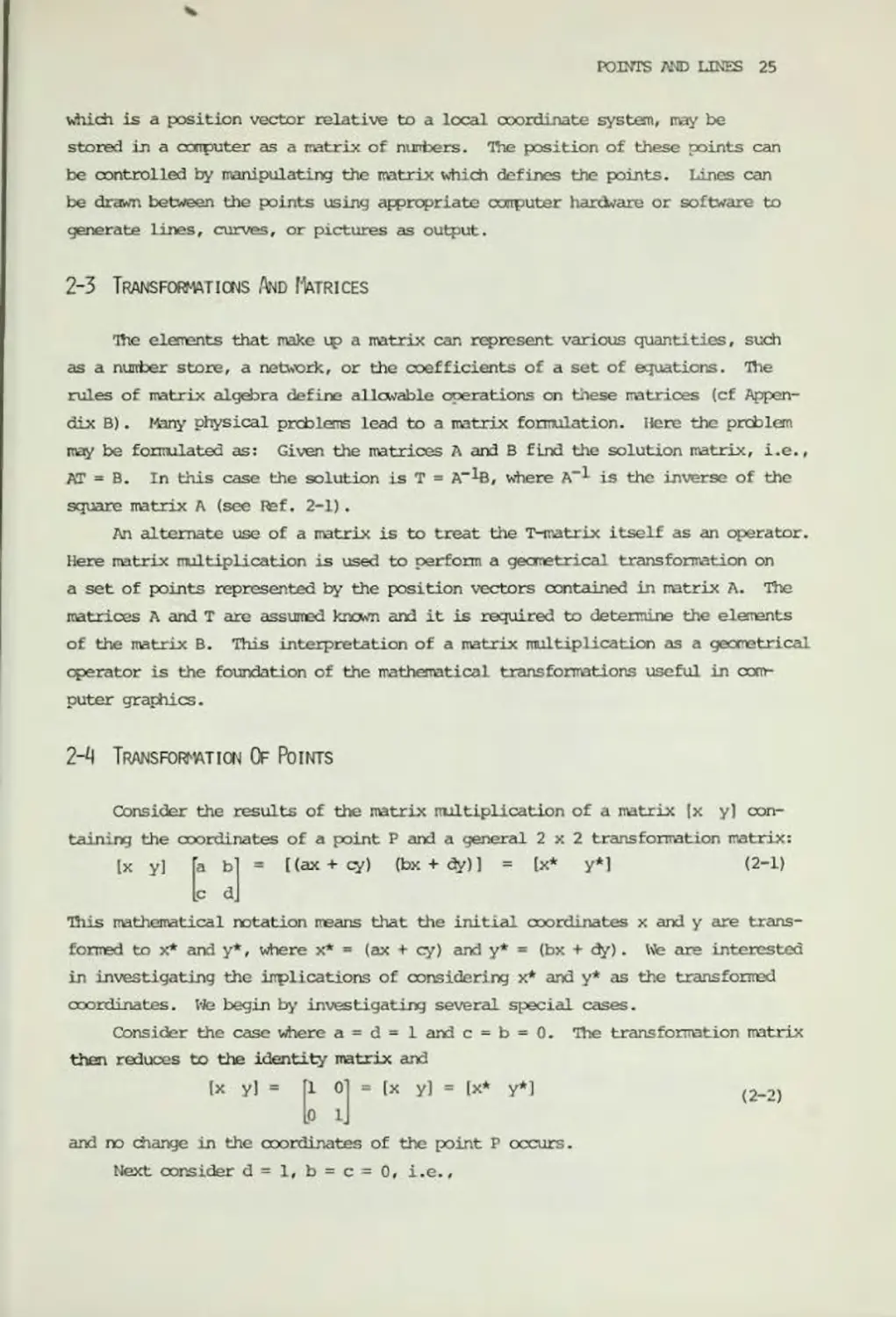
Consider the results of the matrix multiplication of a matrix (x yl con-
This mathematical notation neans that the initial coordinates x and y are trans-
transformed to x* and y*, where x* = (ax + cy) and y* = (bx + dy). We are interested
in investigating the iirplications of considering x* and y* as the transformed
coordinates. We begin by investigating several special cases.
Consider the case where a = d = 1 and c = b = 0. The transforrration matrix
then reduces to the identity matrix and
2-4 Transformticn Of Points
taining the coordinates of a point P and a general 2x2 transformation matrix:
[x y] [a bl = [ (ax + cy) (bx + dy) ] = |x* y*] (2-1)
c d
(2-1)
[x y] =
[x y] = |x* y*]
(2-2)
and no change in the coordinates of the point P occurs.
Next consider d = 1, b = c = 0, i.e..

26 MATHEMATICAL EIZTfNTS TOR (XMPUTER GRAPHICS
!x y]
n
-lax yj = [x* y*)
(2-3)
This produocs a scale change since x* = ax. This transformation is shown in
Fig. 2-la. Hence* this matrix multiplication has the effect of stretching the
original coordinate in the x-direction.
Mow consider b = c = 0, i.e.,
[x y]
1
[ax dy] = [x* y*]
(2-4)
This yields a stretching in both the x- and y-ooordinates, as shown in Fig.
2-lb. If a / d» then the stretchings are not equal. If a = d > 1, then a pure
enlargement or scaling of the coordinates of P occurs.. If 0 < a = d < 1, then
a compression of the cxx>rdinates of P will occur.
If a and/or d are negative, then reflections occur. To see this, consider
b = c = 0, d=l and a = -1. Then
[x y]
= l-x y) = [x* y*]
(2-5)
-1 0
0 1
and a reflection about the y-axis has occurred. The effect of this transforma-
tion is shown in Fig. 2-lc. If b = c = 0, a = 1, and d = -1, then a reflection
about the x-axis occurs. If b = c = 0, a = d < 0, then a reflection about the
origin will occur. This is shorn in Fig. 2-Id, with a = -1, d = -1. Note that
reflection, stretching, and scaling of the coordinates involve only the diagonal
terms of the transformation matrix.
Now consider the case where a = d = 1, and c = 0. Thus
[x y]
1 b
0 1
[x (bx + y) J = [x* y*]
(2-6)
and the x-cxx>rdinate of the point P is unchanged, while y* depends linearly on
the original coordinates. This effect is called shear and is shown in Fig. 2-le.
Similarly when a = d = 1, b = 0, the transformation produces shear proportional
to the y-aoordinate, as shown in Fig. 2-lf. Thus, we see that the off-diagonal
terns produce a shearing effect on the coordinates of the point P.
Before ccrpleting our discussion of the transformation of points, consider
the effect of the general 2x2 transformation given by Eq. (2-1) when applied
to the origin, i.e.,
(x y) a b] = [(ax + cy) (bx + dy) J = (x* y*] (2-1)
or for the origin,
[0 0]
b
d
b
d
[0 0] = [x* y*]
Here we see that the origin is invariant under a general 2x2 trans forma tion.
Ihis Is a limitation which will be overcone by the use of homogeneous coordinates.

POINTS AND LINES 27
»'i
T = -
[1 -3
■* - \.v*
>* »>*•>
h\
 Figure 2-1 Transformation of points.
2-5 Transformation Of Straight Lines
A straight line can be defined by two position vectors which specify the
coordinates of its end points. Hie position and orientation of the line join-
joining these two points can be changed by operating on these tv*> position vectors
The actual operation of drawing a line between two points will depend on the
output device used. Here we consider only the mathematical operations on the
end position vectors.
A straight line between two points A and B in a two-dimensional plane is
drawn in Fig. 2-2. Hie position vectors of points A and B are (0 1) and
[2 3] respectively. Now consider the transformation matrix
T =
1 2
3 1
(2-7)
which we recognize frcm our previous discussion as producing a shearing effect
Using nutrix multiplication on the position vectors for A and B produces the
new transformed vectors A* and B* given by
AT * 10 I|
1 2
3 1
- 13 1J
A*
(2-8)

28 MATHEMATICAL EI£M03TS FOR CCfPlTTER GRAPHICS
and
BT = [2 3]
1 2
3 1
= [11 7] = B*
(2-9)
Thus, the resulting elements in A* are x* = 3 and y* = 1. Similarly, B* is a
new point specified by x* = 11 and y* « 7. tore ccrpactly the line AB ray be
represented by the 2x2 matrix L = [0 I. Matrix multiplication then yields
LT
n
113
L*
(2-10)
1 2
.3 1.
where the ccrrponents of L* represent the trans fomed position vectors A* and
B*. The transformation of A to A* and B to B* is shown in Fig. 2-2. The ini-
initial axes are x,y and the trans fomed axes are x*, y*. This shearing effect
has increased the length of the line and changed its orientation.
2-6 Midpoint Transformation
Figure 2-2 shows that the 2x2 transformation matrix transforms the
straight line y = x + 1, between points A and B, into another straight line
y ■ (3/4) x - 5/4, between A* and B*. In fact a 2 x 2 matrix transforms any
straight line into a second straight line. Points on the second line have a
one to ore correspondence with points on the first line. We have already shewn
this to be true for the erc1 points of the line. To further confirm this we
consider the trans formation of the midpoint of the straight line between A and
B. Letting A = [x^ y^], B = [x2 y2) / and T = fa b] and transforming both
ca
points simultaneously gives
*1
n
’a b1
=5
lX2
y2
c d
4
axi
ax2 + C¥2 bx2 + ^2j
A*
B*
Hence, the transformed end points are
A* = (ax^ + cyi
B* = (ax2 + cy2 bx2 + dy2)
The midpoint of the initial line AB is
bx1 + dy^)
(*1* yx*)
(x2* y2*>
Xi + X-
yi + i’2
2 2
The trans formation of this midpoint is
*1 + *2
2
[: a ■
axj + ax2 + cy^ + cv2
(2-11)
(2-12)
(2-13)

POINTS AND LINES 29
This transformation places the midpoint of AB on the midpoint of A*B* since
the midpoint of A*B* is given by
axi + cyx + ax2 + cy2 axx + ax2 + cyx + cy2 (2-14)
^ =
y*
bx^ + dy^ + bx2 ♦ d/2 ^X1 + ^x2 + 3/1 + ^2
[1
It' 2
For the special case shorn in Fig. 2-2/ the midpoint of line AB is =
2]. This transforms to
[1 2]
2
1
[7 4]
(2-15)
which gives the midpoint on line A*B*. This process can be repeated for any
subset of the initial line, and it is clear that all points on the initial line
transform to points on the second line. Thus the transformation provides a one
to one correspondence between points on the original line and points on the
transformed line. Fbr conputer graphics applications, this means that any
straight line can be transferred to any new position by simply transforming its
end points and then redrawing the line between the transformed end points.
2-7 Parallel Lines
When a 2 x 2 matrix is used to transform a pair of parallel lines, the
result is a second pair of parallel lines. TO see this, consider a line between
A = [xx Yj] and B = [x2 y2) and a line parallel to AB between E and F. To
she*/ that these lines and any transformation of them are parallel, we examine
the slopes of A3, EF, A*B*, and E*F*. The slope of both AB and EF is
Y2 “ YI
ml
x2 - xi
(2-16)
Transforming AB using a general 2x2 transformation yields the end points
of A*B*:
axi + cy] bx^ + dy^
ax2 + cy2 bx2 + by2
X1
*1
a b'
=
*2
^2
c d
=
yl"
=
A*
(2-17)
x2
*2.
B*
The slope of A*B* is then
(bx2 + dy2) - (bx^ + dy^
(ax2 + cy2) - (a*i + cy^
“2
b(x2 - xx) + d(y2 - yi)
a(x2 - x:) + c(y2 - yx)
or
m2
y2 - yi
b + d x2 - x^
a + "c y2 - yi
x2 - X1
a +
“T
(2-18)

30 MATHEr-WTICAL ELEMENTS FOR CDflPCTER GRAPHICS
10
8
>•>
B"
V
0
6
vx‘
8
10
12
12
10
U
8-
B
M/2.3/2>A^
-4
-2
M.-1U •
-4
/
\ >' 2x-Jy-I
^TV - 4 x x'
(3.5/3)
•F
N
\ K-y-I
•BC3.-2)
•A
Figure 2-2 Transformation
of straight lines.
Figure 2-3 Transformation
of intersecting lines.
Since the slope is independent of x^, xv y1# and y2, and since m^r a, b, c,
and d are the sane for EF and AB, it follows that for both E*F* and A*B* are
equal. Thus, parallel lines remain parallel after trains formation. This neans
that parallelogram transform into other parallelograms as a result of operation
by a 2 x 2 transformation matrix. These siirple results begin to shw the power
of using matrix mil tipi ication to produce graphical effects.
2-8 Intersecting Lines
TV.o dashed intersecting lirvss AB and EF are sho/n in Fig. 2-3. The point
of intersection is at x = 4/5 and y = 1/5. We now multiply the matrices con-
containing the end points of the two lines AB and EF by the transformation matrix
Thus,
1
2
3 -2
1 2
=
1
1 -3
1 12

POINTS AND LINES 31
-1 -1'
1 2
-
-2 1'
3 !.
1 -3
T 1
This gives the solid lines A*B* and E*F* shewn in Fig. 2-3. The transformed
point of intersection is
= 11 1]
1 2
1 “3.
That is, the point of intersection of the initial pair of lines transforms to
the point of intersection of the transformed pair of lines. Close examination
of the above trans formation of intersecting straight lines will she*/ that it
has involved a rotation, a reflection, and a scaling of the original pair.
However, the total effect of a 2 x 2 matrix transformation is easier to see,
considering the effects of rotation, reflection, and scaling separately. In
order to illustrate these individual effects, we shall consider a sinple plane
figure - namely, a triangle.
2-9 Rotation
Consider the plane triangle ABC shewn in Fig. 2~4a. This triangle is ro-
rotated through 90° about the origin in a counterclockwise sense by operating on
eacti vertex with the transformation
0 1
-1 0
ing the x- and y-coordinates of the vertices, then
If we use a 3 x 2 matrix contain-
0 11
-1 Oj
1
-1
-1
(2-19)
This produces the triangle A*B*C*. A 180° rotation about the origin is obtain-
obtained by using
-1 0
0 -1
and a 270° rotation about the origin by using
0 -1
1 0
Note that neither scaling nor reflection has occurred in these exarples.
2-10 Reflection
Whereas a pure two-dimensional rotation in the xy-plane occurs about an
axis normal to the xy-plane, a reflection is a 180° rotation about an axis in
the xy-plane. TWo reflections of the triangle VEF are shown in Fig. 2-4b. A
reflection about the line y = x occurs by using ft)
The transformed, new vertices are given by

32 y^zy^nc^L zuyEzns ftp cawn?. graphics
>.>
4
y
/
► *.r
D
: 4 6
D'
\
 V
’6 1
7 3
.
.6 2.
A reflection about y =
are giver* by
j
8 1
a b
Figure 2-4 Relation arc reflection.
r.
r° ^ = '1 61
.1 OJ 3 7
U 6j
(2-20)
.0 -1
In this case the new vertices
7 3
.€ 2.
1 0
l0 -1J
8 -1
7 3
6 2
2-U Scaling
Fecailir/g our discussion of the transformation of points, we can see that
scaling is controlled by the magnitude cf the two terrs on the prirary diagonal
of the ratrix. If the matrix 2 0~ is used as an operator cn the vertices
lO 2.
of a triangle, a "2-tiiTes" enlargement occurs about the origin. If the magni-
magnitudes are unequal, a distortion occurs. These effects are shcun in Fig. 2-5.
Triangle ABC is transferred by *2 0l ; thus a scaling occurs, and triangle
iO 2J

P0H7TS AND UXES 33
CEF is transformed by
3 0
0 2
which yields
a distortion due to the unequal scale
factors.
It is new clear hew plane surfaces,
defined by vertices joined by straight
lines, can be manipulated in a variety
of ways. By performing a matrix opera-
operation on the position vectors which define
the vertices, the shape and position of
the surface can be controlled. Hcwever,
a desired orientation may require nore
than one transformation. Since matrix
multiplication is noncanrutative, the
order of the transformations is import-
important when performing cccrbined operations.
2-12 Combined Oerations
Figure 2-5 Uniform and
in order to illustrate the effect nonuiuform scaling
or distortion.
of noncanmutative matrix multiplication,
consider the operations of rotation and reflection on the vertices of a triangle
[x y]. If a 90° rotation is follas'ed by reflection about x = 0, these two
consecutive transformations give
• [-Y x)
[x y]
0 1
-1 0
and then
[-y x]
l-x y]
-1 0
. o 1
On the other hand, if reflection is followed by rotation, a different result
given by
= l-x y]
[x y]
-1
0
and
I-x y]
o
-l
- [-y -x]
is obtained.
So far we have concentrated on the behavior of points and lines to deter-
determine the effect of sinple matrix transformations. However, the matrix is
correctly considered to operate on every point in the plane. As has been shewn,

34 MATHEMATICAL ELO-E7TS FDR COMPUTER GRAPHICS
the only point that remains invariant in a 2 x 2 matrix transformation is the
origin. All other points within the plane of the coordinate system are trans-
transformed. This trans formation may be interpreted as a stretching of the initial
plane and coordinate system into a new shape, ffore formally, we say that the
transformation causes a mapping from one plane into a second plane. Exarples
of this mapping are shown in the re*xt section.
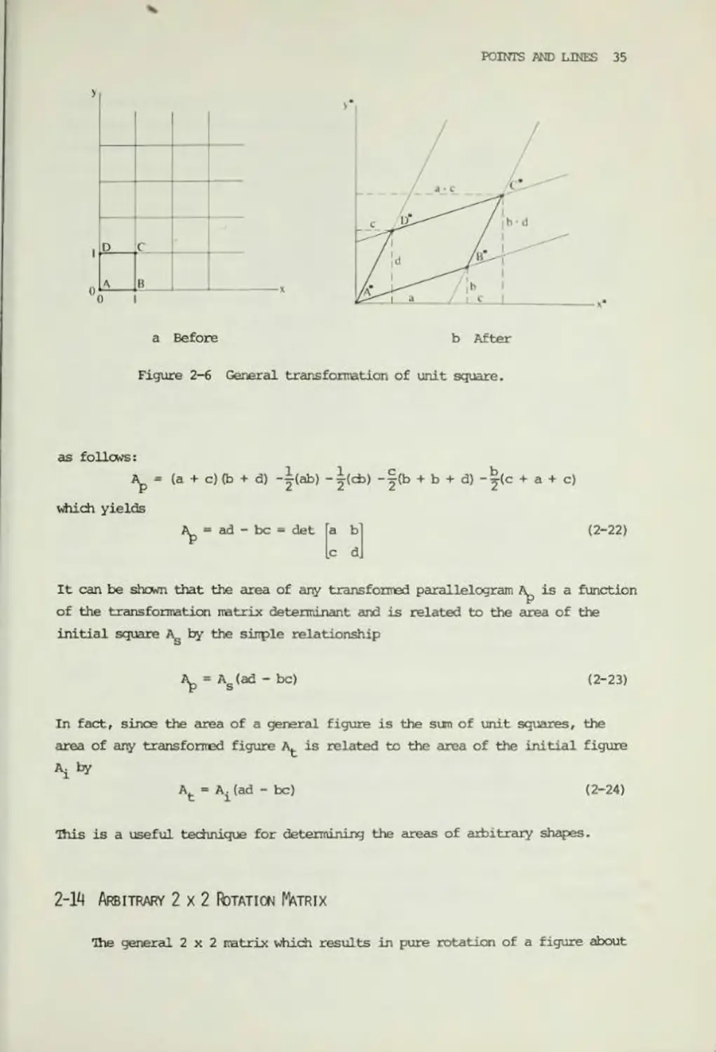
2-13 Transformation Of A Unit Square
consider a square-grid network consisting of unit squares in the xy-plane.
The four position vectors of a unit square with one copier at the origin of the
coordinate system are
0 O' origin of the coordinates - A
1 0 unit point on the x-axis - B
1 1 outer comer - C
0 1J unit point on the y-axis - D
This unit square is shown in Fig. 2-6a. Application of a general 2x2 matrix
trans formation
a b
to the unit square yields
c d^
A-*
►
0
0
1
0
C*
1
1
D-
0
1
0
-A*
(2-21)
b
-B*
b +
d
«-c*
d
-D*
a b = 0
c d a
a + c
c
The results of this transformation are shown in Fig. 2-6fc>. First notice from
Eq. (2-21) that the origin is not affected by the transformation, i.e., A ■ A*
= [0 0). Further, notice that the coordinates of B* are equal to the first
rcM in the general transformation matrix, and the coordinates of D* are equal
to the second rcw in the general trans formation matrix. Thus, once the coor-
coordinates of B* and D* (the transformed unit points [1 0] and [0 1] respectively)
are kncwn, the general trans forma tion matrix is determined. Since the sides
of the unit square are originally parallel and since we have previously shown
that parallel lines transform into parallel lines, the transformed figure is
a parallelogram.
The effect of the terms, a, b, c, and d in the 2x2 matrix can be identi-
identified separately. The terms b and c cause a shearing (cf Sec. 2-4) of the initial
square in the y- and x-directions respectively, as can be seen in Fig. 2-6.
The terms a an3 d act as scale factors as noted earlier. Thus, the general
2x2 matrix produces a conbination of shearing and scaling.
It is also possible to easily determine the area of the parallelogram
A*B*C*D# shewn in Fig. 2-6. The area within the parallelogram can be calculated

POINTS PND LINES 35
0
c
A
B
0
a Before
b After
Figure 2-6 General transformation of unit square.
as follows:
which yields
(a + c) (b + d) -|(ab) -|(cto) -j(b + b + d) -|(c + a + c)
ad - be = det
a b
c d
(2-22)
It can be shewn that the area of any transformed parallelogram A^ is a function
of the transformation matrix determinant and is related to the area of the
initial square Ag by the sirrple relationship
Ap = As(ad - be)
(2-23)
In fact, since the area of a general figure is the sum of unit squares, the
area of any transformed figure At is related to the area of the initial figure
\ by
At = Ai(ad-bc) (2-24)
This is a useful technique for determining the areas of arbitrary shapes.
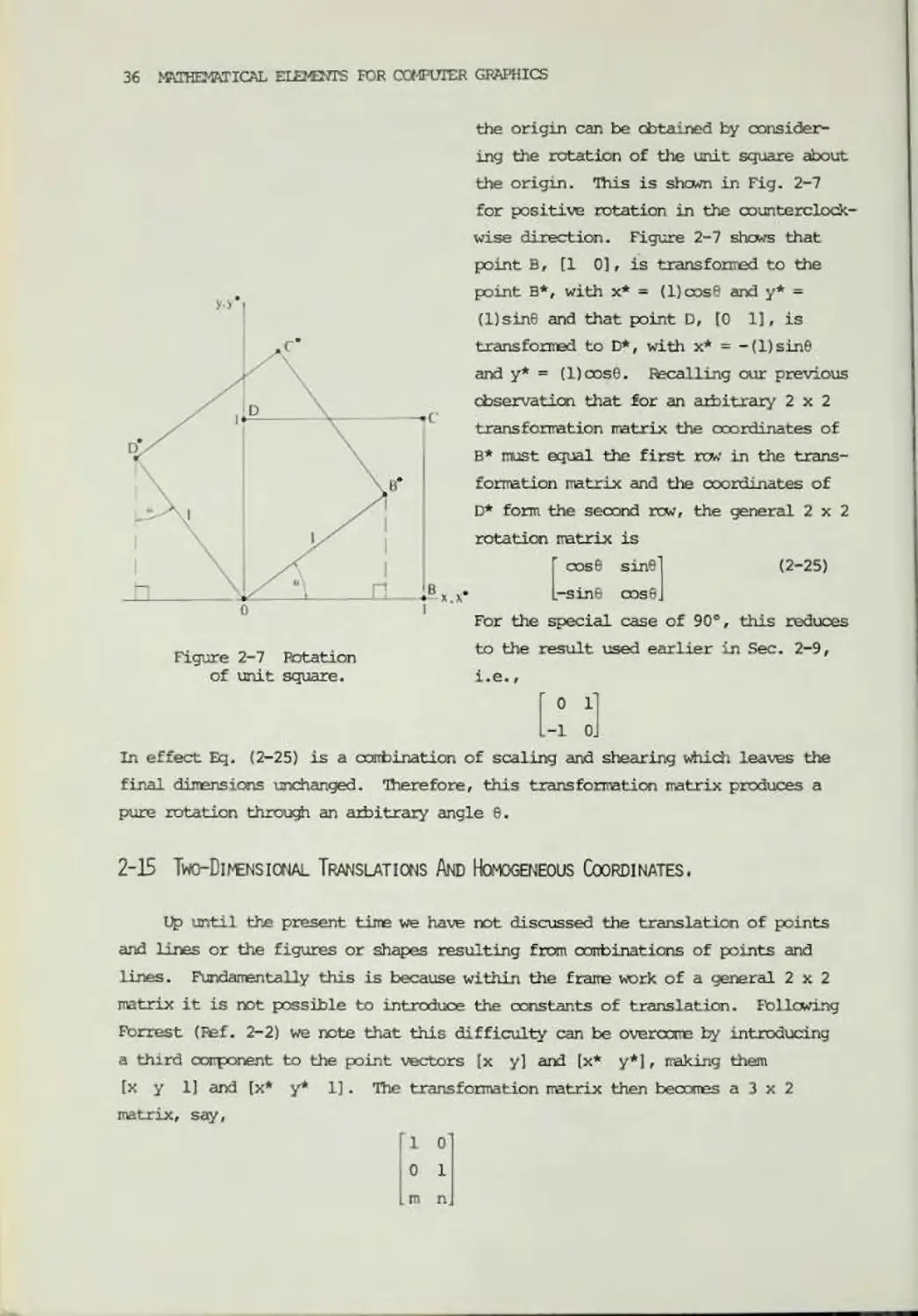
2-14 Arbitrary 2x2 Rdtaticn Matrix
The general 2x2 matrix which results in pure rotation of a figure about

36 >MHEM7VTICAL EIBCTS FOR COMPUTER GRAPHICS
Figure 2-7 Potation
of unit square.
the origin can be obtained by consider-
considering the rotation of the unit square about
the origin. This is shewn in Fig. 2-7
for positive rotation in the counterclock-
counterclockwise direction. Figure 2-7 shews that
point B, [1 0], is transformed to the
point B*, with x* = (l)cosQ and y* =
(l)sin6 and that point D, [0 1], is
trains formed to D*, with x* = - (1) sin6
and y* = (l)oos6. Recalling our previous
observation that for an arbitrary 2x2
transformation rratrix the coordinates of
B* rust equal the first rw in the trans-
transform tion matrix and the coordinates of
D* form the second rcw, the general 2x2
rotation ratrix is
cose sine] (2-25)
.-sin6 cos6.
For the special case of 90°, this reduces
to the result used earlier in Sec. 2-9,
i.e.,
" 0 1
-1 oj
In effect Eq. (2-25) is a combination of scaling and shearing which leaves the
final dimansions unchanged. Therefore, this transformation rratrix produces a
pure rotation through an arbitrary angle 6.
2-15 Two-Dimensicnal Translations And Homogeneous Coordinates.
Up until the present time we have not discussed the translation of points
and lines or the figures or shapes resulting from combinations of points and
lines. Fundamentally this is because within the frame work of a general 2x2
matrix it is not possible to introduce the constants of translation. Following
Forrest (Pef. 2-2) we note that this difficulty can be overccre by introducing
a third component to the point vectors [x y] and [x* y*], raking them
[x y 1] and (x* y* 1]. The transformation matrix then becomes a 3 x 2
matrix, say,
1 0
0 1
. m n.

POINTS AND LINES 37
This is necessary since the nurber of colums in the point nutrix mist equal
the nurber of rcws in the trans forma tion matrix for the operation of matrix
multiplication to be defined. Thus,
(x y 1]
1 0
0 1
m n
[x + m y + n] « [x* y*]
(2-26)
where we note that the constants m, n cause a translation of x* and y* relative
to x and y. Ho/ever, a 3 x 2 matrix is not square and thus does not have an
inverse (cf Appendix B). This difficulty can be overcome by utilizing a full
3x3 matrix, say,
1 0 0‘
0 10
Lm n 1
as the trans forration matrix. Notice that the third oonponent of the position
vectors is not affected by the addition of the third colunn to the transforma-
transformation matrix. Using this matrix in Eq. (2-26) gives Ix* y* 1] for the trans-
transformed vector.
The addition of the third element to the position vector and the third
colum to the trans formation matrix allows us to perform a translation of the
position vector. Alternately we ray consider the third element as an additional
coordinate of the position vector. For rotational purposes we assure that when
the position vector [x y 1] is operated on by a general 3x3 matrix it becomes
the position vector [X Y Hi. Previously the transformation was perfonred such
that [X Y H] * [x* y* 1]. If we consider the transformation to be taking
place in three-dimensional space, this confines our transformations to the plane
H = 1. If, however, we assume that the third column of the general 3x3 trans-
transfonration matrix T is
p
rather than
0
q
0
s
.1
matrix multiplication yields [x y 1]T = (X Y H], where H / 1.
The general plane in which the transformed position vector new lies is in
three-dimensional space. Hcwever, at the present time we are not interested in
what happens in three-dimensional space. Hence we ctotain x* and y* by project-
projecting frcm the general plane back onto the plane H = 1, using a pencil of rays
through the origin. This effect is shown in Fig. 2-8. Using similar triangles
we see that HA = 1/x* and HA ° 1/y*. With three conponents it follows that:
(2-27)
The three-dimensional vector representation of a two-dimensional position
Ix* y*] = | 1]

38 [-TOTiEMftXICAL ELE24E27IS FOR CCMPITCER GRAPHICS
Figure 2-8 Geometric representation of
homogeneous coordinates -
vector, or in general the representation of an n-crrponent vector by an n + 1
ocvrponent vector, is called homogeneous coordinate representation. In hcrrogen-
eous coordinate representation the transformation of n-dimensiona 1 vectors is
performed in (n + 1) dimensional space, and the transformed n-dimensional results
are obtained by projection bade into the particular n-dimensional space of in-
interest. Thus, in two dimensions the position vector [x y] is represented by
the three-oorrpcnent vector [hx hy h]. The extra conponent in the vector acts
like an additional coordinate. The ordinary or "physical" coordinates are re-
related to the homogeneous coordinates by
(2-28)
hx
TT
and
hjr
h
There is no unique homogeneous coordinate representation of a point in
two-dimensional space. For exajrple, the horogeneous coordinates [12 8 4],
[6 4 2], and [3 2 1] all represent the ordinary point [3 2]. For ease
of calculation we choose [x y 1) to represent a non transformed point in two
dimensional horogeneous coordinates. Then the transformation*
[x* y*] = [x y]
b
d
*Note that here we have put the result of the transformation on the left-hand
side of the equation rather than on the right-hand side as was done previously;
i.e., we write matrix equations as B = AT rather than as AT = B. Fran hereon
we will adept this convention for ease in translating results into carputer
algorithms.

POINTS AND LINES 39
in regular coordinates is given by
(X Y H] = [x y
1]
a b
c d
0 0
in homogeneous coordinates. Carrying out the above two trans formations slxws
that X = x*, Y = y*, and H = 1. That is, since the additional coordinate H is
unity, the trans fomed hcrrogeneous coordinates are the sane as the transformed
ordinary coordinates. In general, H / I, and the transformed ordinary coordi-
coordinates are obtained by normalizing the transformed homogeneous coordinates, e.g..
and
y* = —
y H
(2-29)
In a geometrical sense, all transformations of x and y fall within the plane
H=1 after normalization of the transformed homogeneous coordinates.
The advantage of introducing horogenecxis coordinates occurs in the general
3x3 trans fonration matrix
a b p
c d q
m n s.
where space is new available to include other transforrrations such as translation.
The scaling and shearing effects of the matrix terms a, b, c, and d have been
shewn previously.
To show the effect of the third column in the 3x3 transformation matrix,
consider the following operation:
(X Y H] = [x y 1]
Ix y (px + qy + 1) ]
(2-34)
1 0 p
0 1 q
0 0 1
Here X ■ x, Y - y, and H ■ px + qy + 1. The coordinate H which defines the
plane containing the transformed points expressed in homogeneous coordinates
new has the equation of a plane in three-dimensional space. This transforma-
transformation is shorn in Fig. 2-9, where the line AB in the two-dimensional xy-plane
is projected to the line CD in the three-dimensional plane pX + qY-H+ 1 = 0.
In Fig. 2-9 the values p = q = 1 are used.
Normalizing to cbtain the two transformed ordinary coordinates, we write
x*. 2U
X H
y* =1 =
Y H
pX + qY + 1
Y
Letting p
gives
pX + qY + 1
1.0 	and using points A, [1 3) and B, [4 1J shewn in Fig. 2-9
x* =
TTTTT
1
5
and
=

40 r-MKETM'ICAL ELEMENTS FOR COMPUTER GRAP!HCS
Figure 2-9 Transformation in hcrrogeneous coordinates.
for the transformation and projection of A to C*, and
x* ■
2
T
and
y.l
ttttt
for the transformation and projection of B to D*. The honogeneais coordinates
for C* and D* shewn in Fig. 2-9 are [1/5 3/5 1] and (2/3 1/6 1] respectively.
The effect of normalizing is to project the three-dimensional line CD back onto
a two-dimensional line C*D* in the plane H = 1.0. As shewn in Fig. 2-9, the
center of projection is the origin.
The general 3x3 transformation matrix for two-dimensional horogeneous
coordinates can be subdivided into four parts:
a b i p
i
C d , q
[m n I s
As we have seen a, b, c, and d produce scaling, shearing, and rotation; m and
n produce translation; and p and q produce a projection. The fourth part,
element s, produces overall scaling. Tb shew this, consider the transformation
(X Y H] = [x y 1]
[i
lS
0
1
0
[x y s]
(2-30)

POINTS AND LINES 41
Here, X = x, Y = y, and H = s. This gives
x* = I* and y* » X-
s 2 s
The effective transformation is [x y 1] - (x/s y/s 1], a uniform scaling of
the position vector. If s < 1, then an enlargement occurs, and if s > 1, a re-
reduction in scale occurs.
2-16 Points At Infinity
The use of homogeneous coordinates gives a convenient and efficient way
of napping a set of points fran one coordinate system into a corresponding set
in an alternate coordinate system. Usually the infinite range of one coordinate
system will map into a finite range within the second coordinate system. Also,
lines which are parallel in one system will usually not be parallel in the other.
However# geometrical properties such as points of intersection can be evaluated
in either coordinate system as shewn belc*/.
The tvro lines given by
have a point of intersection at x = 3/5, y = 2/5. This solution can be obtain-
obtained in terms of the homogeneous coordinates. By rewriting the equations as
x + y -1 = 0? 2x - 3y = 0 it is possible to represent the tw equations by the
matrix equation
However, for a matrix to have an inverse it must be square. The following rep-
representation of the same set of equations can be used to meet this requirement;
x + y - 1
2x + 3y = 0
[x y 1] 1 21 = [0 0]
1 -3
Ix y 1] ' 1 2 0 =[0 0 1]
1-3 0
l-l 0 1.
The inverse of this square matrix M is
(2-31)
3 2 l
J 5 1
>fciltiplying both sides of Eq. (2-31) by m"1 arri noting that MM 1 = I, the
identity matrix yields

42 MKnffMRTICM. ELQ-ETTS FDR CCWWER GRAPHICS
[x y 11
0 1]
[l
L3
2
-1
2
rl 1
5 5
11
Thus, x = 3/5 and y = 2/5 as required.
Consider two parallel lines defined by
x + y « 1
x + y * 0
Proceeding as above leads to the matrix equation
[x y 1]
1
1
-1
1
1
0
= [0 0 1]
Hcwever, ever, though a square matrix exists in this equation, it does not have
an inverse, since two rows are identical. Another alternate equation is pos-
possible which does have an invertible matrix. This is given by (cf Pef. 2-3)
[x y
ii n
i
[0 0 x]
1 1
1 0
1-1 0 0J
The inverse of the 3x3 rratrix in Eq. (2-32) is
M-1 = fO 0 -1'
Oil
Li -i o.
Multiplying both sides of Eq. (2-32) by this inverse gives
(2-32)
[x y 1] = [0 0 x]
[x -x 0] « x[l -1 0]
(2-33)
0 1 -1
Oil
1 -1 0.
The resulting hcrogenecus coordinates [1 -1 0J nust represent the "point of
intersection" for the two parallel lines, i.e., a point at infinity. In general,
the two-dimensional horogeneous vector [a b 0) represents the point at infinity
on the line ay - bx = 0.
T5\e fact that a vector with the homogeneous corrponent H equal to zero does
indeed represent a point at infinity can be illustrated by the limiting process
given be lav. Consider the line y* = (3/4)x* and the point [X Y] ■ [4 3]. Re-
Recalling that a unique representation of a position vector does not exist in
hcrrogeneous coordinates, the point [4 31 can be represented in horogeneous
coordinates in all the ways shown in Table 2-1. See tef. 2-3. Note that in
Table 2-1 as HH3, the ratio of y*/x* rerains at 3/4 as is required by the govern-
governing equation. Further note that successive pairs of fx* y*], all of which
fall on the line y* - (3/4)x*, become closer to infinity. Thus, in the limit
as H*K), the point at infinity fx* y* 1] = [® ® 1) is given by [X Y HJ =

POINTS AND LINES 43
Table 2-1
Homogeneous Coordinates for the Point [4 3]
H
X*
y*
X
y
1
4
3
4
3
1/2
8
6
4
3
1/3
12
9
4
3
V4
•
16
12
4
3
•
•
1/10
•
40
30
4
3
•
•
1/100
400
300
4
3
[4 3 OJ in homogeneous coordinates. It follows that the position vector
(1 0 0] represents a point at infinity on the x*-axis and [0 1 01 represents
a point at infinity on the y*-axis. In this manner homogeneous coordinates
give a convenient representation of points at infinity in addition to the cap-
capability for generalized transformations.
2-17 Two-Dimensional Rotation About An Arbitrary Axis
Previously we have considered rotations as occuring about the origin.
Homogeneous coordinates provide a mechanism for acconplishing rotations about
points other than the origin. In general a rotation about an arbitrary point
can be acccrplished by first translating the center of rotation to the origin#
performing the required rotation# and then translating the result back to the
original center of rotation. Thus# rotation of the position vector [x y 11
about the point m# n through an arbitrary angle can be acccrplished by
Ix
y i]
i
0
0
cosQ
sinG
0
1
0
0
0
1
0
-sinG
COS0
0
0
1
0
-m
-n
1.
0
0
1
jn
n
1
IX Y H] (2-34)

44 fOTHE'RTICAL ELM27TS FOR CX*5PUTER GRAPHICS
SLil
By carrying out the two interior matrix products we can write
[X Y K] * [x y u r cose sinO O’ (2-35)
-sin6 cose 0,
-m(ccsO -1) + n(sinO) -m(sine) - n(cos6 - 1) 1^
For exanple, suppose the center of an cfcject is at [4 3] and it is desired to
rotate the cbject 90° counterclockwise about its own central axis. Operation
by the matrix
0 1 (T
-10 0
.0 0 lj
causes a rotation about the origin, not the cbject axis. As shewn above, the
necessary procedure is to first translate the cbject so that the desired center
of rotation is at the origin by using the translation matrix
1 0 O'
0 10
-4 -3 1
then apply the rotation rratrix, and finally translate the results of the rota-
rotation back to the original center by means of the reverse translation matrix.
The entire operation
(X Y H] • (x y 1]
' 1 0 o'
'010'
1 0 o'
0 1 0
-10 0
0 10
l-4 -3 ij
0 0 1.
l4 3 1.
(2-36)
can be ccrbined into one matrix operation by concatenating the transformation
matrices, i.e.,
[X Y H] = [x y 1]
0 1
-1 0
7 -1
(2-37)
Then, x* = X/H and y* = Y/H.
TWo-dimensional rotations about each axis of an orthogonal axis system are
represented in Fig. 2-10. A ccrputer algorithm for performing a two-diirensional
rotation about an arbitrary point is given in Appendix Cf along with other
algorithms for two-dimensicnal translation, scaling, and reflection.
References
2-1 Fox, L. An Introduction to Numerical Linear Algebra, Oxford University
Press, LiDndon, 1964.
2-2 Forrest, A. P.., "Co-ordinates, Transformations, and Visualization Techni-
Techniques," CAD Group Document No. 23, Cambridge University, June 1969.

POINTS AND LINES 45
2-3 Ahuja, D. C., and Coons, s. A., "Geometry for Construction and Display,
IBM Syst. J., vol. 7, nos. 3 and 4, pp. 188-205, 1968.
10 0'
0 cos> siny
.0 -siny cosy
Koiat ion about *
a
0
1 0
0 cos 0
Kola I ioii a bon t >
b
sina
cosa
0
0
0
1
cosa
Notation about z
c
Figure 2-10 Rotation

CHAPTER 3
THREE DIMENSIONAL
TRANSFORMATIONS
AND PROJECTIONS
3-1 Introduction
Tne ability to represent or display a three-dimensional object is fundamen-
fundamental to the understanding of the shape of that object. Furthermore, the ability
to rotate, translate, and project views of that object is also, in rany cases,
fundamental to the understanding of its shape. This is easily demonstrated by
picking up a relatively ccnplex unfamiliar object. Irrmediately one rotates it,
holds it at arm's length, stands back frcn it, etc., in order to obtain an under-
understanding of its shape. To do this with a ccrputer we must extend our previous
tw>-dimc!Tisional analyses to three dimensions. Based on our previous experience
we immediately introduce homogeneous coordinates. Hence a point in three-
dimensional space [x y z] is represented by a four-dimensional position vector
[x y z 1] or [X Y Z Hi. Again the transformation frcn homogeneous coordinates
to ordinary coordinates is given by
[X Y Z HJ - [x y z 1]T
and
Ix* y Z* l] =* |] (3-1)
where T is sane transformation matrix.
The generalized 4x4 transformation matrix for three-dimensional bcroge-
neous coordinates is

THREE-DIMENSIONAL TRANSFORMATIONS AND PROJECTIONS 47
T * b c pj (3-2)
d e f q
h i j r
i m n s
The 4x4 transformation matrix in Eq. (3-2) can bo partitioned into four
separate sections:
1
3
3 x 3 |
X
1
1
.1x3 |
lxl
The 3x3 matrix produces a linear transformation* in the form of scaling, shear-
shearing, and rotation. The 1x3 rcw rratrix produces translation, and the 3x1
column matrix produces perspective transformation. The final single element pro-
produces overall scaling. The total transformation obtained by operating an a posi-
position vector with the 4x4 matrix and normalizing the transformed vector is
called a bilinear transformation. This gives a combination of shearing, local
scaling, rotation, reflection, translation, perspective, arxl over'aU scaling.
3-2 TmEE-Dif'ENsioNAL Scaling
The diagonal terms of the general 4x4 transformation produce local and
overall scaling. Consider
[x y z 1] fa 0 0 0] = [ax ey jz 1) = [x* y* z* 1] (3-3)
0 e 0 0
0 0 j 0
.0 0 0 1
which shews the local scaling effect. Figure 3-la shows a parallelepiped re-
rescaled as a unit cube. Overall scaling is obtained by using the fourth diagonal
element, i.e.,
[x y z s]
[X y z 1]
10 0
0
0
1
0
0
0
0
1
0
0
0
0
s.
= (x* y* Z* 1] = l|J | 1]
A linear transformation is one which transforms an initial linear carbination
of vectors into the same linear combination of transformed vectors.

48 MMHEMATIOVL ELEMENTS FOR OOMPUXER GRAPHICS
C- G#
A
0 0 0 1
10 0 0
•
0 0 0 1
B
0 0 11
0 10 0
0 0 7 1
»•
C
0 10 1
0 0 10
0 2 0 1
C*
c
0 1)1
0 o 0 i
0 2 2 1
r*
r
1 0 n 1
2 0 0 1
E*
i
10 11
7 0 2 1
M
c
110 1
2 2 0 1
C*
i
MM
2 2 2 1.
1*
*
0 0 0 1
l
-0.85
0.25
0
*
0
0
0
1
B
0 0 11
-C.75
I
0.7
0
0.5
1
I
I
C
0 10 1
0.5
1
1
0
-0.75
1
0.7
1
0
0 111
, 0
0
0
I.
-0.2*.
2
1.7
1
E
10 0 1
1
-
0.25
1
r
10 11
1.5
0.15
1.25
1
G
110 1
0.25
0.15
0.95
1
1
nil
0.75
1.15
1.95
:
A*
C001
: o o o
l»*
0 0 11
l
r*
0 10 1
0 j o 0
D*
0 J 1 1
0 0 10
E*
2 0 0 1
Lo o o i
F»
2 0 11
o*
2 J 0 1
I*
; »i iJ
Figure 3-1 Three-dimensional scale transformations

TOREE-DIMENSICNAL TRANSFORMATIONS AND PROJECTIONS 49
This effect is shewn in Fig. 3-lb. Incidentally, the same effect can be obtained
by means of equal local scalings. In this case the transforma tion ratrix would
be
•4 o
0 0
0
0
0 0 0 1
3-3 Twee-Dimensional Shearing
The off-diagonal terms in the upper left 3x3 conpcnent matrix of the gen-
generalized 4x4 transformation matrix produce shear in three dimensions, e.g..
Ix y z 1]
[x + yd + hz bx + y + iz cx + fy + z 1)
1 b c 0
d 1 f 0
h i 1 0
0 0 0 1
A simple three-dimensional shear on a unit cube is shewn in Fig. 3-lc.
3-4 Three-Dimensional Rotations
In the previous sections we saw that a 3 x 3 carponent matrix produced a
carbinaticn of scaling and shear. However, if the determinant (cf Appendix B)
of the 3x3 carponent matrix is +1, then it produces a pure rotation about
the origin. Before considering the general case of three-dimensional rotation
about an arbitrary axis, we examine several special cases.
In a rotation about the x-axis, the x-dimensions do not change. Thus, the
transformation matrix will have zeros in the first rev; and first colurm, except
for unity on the main diagonal. The other terms are determined by considering
the rotation of a unit cube in the same rranner as discussed in Sec. 2-13. This
leads to the transformation matrix for a rotation of angle 6 about the x-axis
given by
T=fl 0 0 0l (3-6)
0 cosG sinO 0
0 -sinG cos© 0
0 0 0 1
Rotaticn is assumed to be positive in a right-hand sense as one looks fron the
origin outward along the axis of rotation. Figure 3-2a shews a -90° rotation
about the x-axis.

50 MATHEMATICAL ELEMENTS FOP COPUTCR GRAPHICS
L
/
A
/
1/
*
0 -1
1 0
0 0
0 0
0
0
0
1
Figure 3-2 Three-durensi^al rotations.
For a rotation of angle $ about the y-axis, zeros appear in the second
rcw and second colunn of the transformation rratrix, except for unity on the
main diagonal. Tne ccrplete rratrix is
T = lcos£ 0 -sinO 0] (3-7)
0 10 0
sint 0 ccs<t 0
0 0 0 1
Figure 3-2b shows a 90c rotation about the y-axis.
In a similar manner, the transformation matrix for a rotation of angle v
about the z-axis is
T =
j” cosy* sin^
-cim'i rr^C'.
0 o'
■sinO cost 0 0
0 0 10
0 0 0 1
(3-8)
Examining the determinant of Eqs. (3-6) to (3-8) demonstrates that any rigid-
boay rotation natrix has a determinant value of +1.0.
Since rotations are caused by rratrix multiplication, three-dimensional
rotations are noncomitative; i.e., the order of multiplication will affect the

THREE-DIMENSICHAL TRANSFORMATIONS AND PROJB7TICKS 51
final result. In order to shew this, consider a rotaticn about the x-axis fol-
followed by an equal rotaticn about the y-axis. Using Eqs. (3-6) and (3-7) with
6 = $, we have
10 0 0
0 cos0 sin© 0
0 -sinG cosG 0
0 0 0 1
■
cosC
0
-sin$
O'
0
1
0
0
sin«i
0
cosO
0
1
. o
0
0
1.
(3-9)
cos6 0 -sin6 0
sin2G cosG cosGsinG 0
cos0sin© -sinG cos2© 0
. 0 0 0 1.
On the other hand, the reverse operation, i.e., a rotaticn about the y-axis
followed by an equal rotation about the x-axis with 0 = 0, yields
=
cos£
0 -sin$
0
1 0
0
0
0
1 0
0
0 cosG
sinG
0
sin<
0 cos$
0
0 -sinG
cosG
0
. 0
0 0
1
.0 0
0
1
E
COS0
sin20
-cost*sinG 0
0
cos0
sinG 0
sin6 -cos0sin0
cos2G 0
0
0
0 1
(3-10)
Carparison of the right-hand sides of Eqs. (3-9) and (3-10) shews that they are
not the same. The fact that three-dimensional rotations are nonccrmutative must
be kept in mind when more than one rotation is to be made.
The result of transformation of the upper left object in Figure 3-3 con-
consisting of two 90° rotations using the matrix product given in Eqs. (3-9) is
shewn as the dashed figures. When the opposite order of rotaticn as specified
by Eq. (3-10) is performed, the solid figures shewn in Fig. 3-3 graphically
demonstrate that different results are obtained by changing the order of rota-
rotation.
Frequently it is desirable to rotate an object about one of the cartesian
coordinate axes. Algorithms given in Appendix C allcw rotation about the x-,
y-, and z-axes.
3-5 Reflection in Three Dimensions
Sane orientations of a three dimensional object require reflections. In
three dimensions the simplest reflections occur through a plane. For a rigid-

52 M&THZWVTICAL ELQ-E7TS FOR CCMPOTER GRAPHICS
Figure 3-3 'Itiree-dijnensional rotations are noncommtative.

THREE-DD33KI0NAL TRANSFORMATIONS AND PROJECTIONS 53
A
B
C
D
E
F
G
I
0 -1
1 -1
0 -2
1 -2
0 -1
1 -1
0 -2
1 -2
1
1
1
1
1
1
1
1
1
0
0
0
0 0 0
10 0
0-10
0 0 1
10 11
1111
10 2 1
112 1
2 0 11
2 111
2 0 2 1
2 12 1
A*
B*
C*
D*
E*
F*
G*
I*
Figure 3-4 Three-dimensional reflection through the xy-plane.
body reflection the determinant of the reflection transformation will be -1.0.
In a reflection through the xy-plane, only the z-coordinate values of the
object's position vectors will be changed. In fact they will be reversed in
sign. Thus, the transformation netrix for a reflection through the xy-plane is
1 0 0 ol (3-11)
0 10 0
0 0-10
.0 0 0 0.

54 MATHEMATICAL ELEMENTS FOR COMPUTER GRAPHICS
The reflectier, of a unit cube through the xy-plane is shown in Figure 3-4. For
a reflection through the yz-plane,
(3-12)
-1
0
0
0
0
1
0
0
0 0
1
0
0
0
0
1
and for a reflection through the xz-plane.
10 0 0
0-100
0 0 10
0 0 0 1.
An algorithm which will perform three-dimensional reflections is given in
Appendix C. Reflections about other planes can be obtained by a combination of
rotation and reflection.
(3-13)
3-6 Translation in Twee Dimensions
Three-dimensional translation is obtained by writing
[XYZH] = [xyzl] [1 0 0 ol (3-14)
0 10 0
0 0 10
I m n 1
Ivhen expanded this yields
[X Y Z H] = [ (x + £) (y + m) (z + n) 1] (3-15)
It follows that
x* = £ - x +■ H (3-16)
y* = I = y + m
z*-|=z + n
An algorithm for translations in three dimensions appears in Appendix C.
3-7 Twee-Dimensional Rotations about an Arbitrary Axis
Tfte method of tuo-dimensional plane rotation about an arbitrary axis was
discussed in Sec. 2-7. The generalization of that problem is rotation about any
axis in three-diirensional space. Again, the procedure is to translate the ob-
object and the desired axis of rotation so that the rotation is node about an axis
passing through the origin of the coordinate system. The method involves a
three-dimensional translation, a rotation about the origin, and a translation
back to the initial position. If the axis about which rotation is desired

TOREE-DIMENSICI vJAL TRANSFOfWOTCNS AND PROJECTIONS 55
passes through the point A =* |fc m n 1|, then the form of the transform ticn
matrix is
[X Y Z H] = |x y z 1] 1 0 0 0l[ [100 0] (3-17)
0 10 0
0 0 10
-m -n 1
where the elements in the 4x4 rotation matrix R are in general given by
1 0 0 0'
R
0 10 0
0 0 10
m
I m n 1
IR)
n^2 + (1 - n^JcosO nin2(1 “ cos0) ♦ i^sine lyi^d - cos) - r^sin- 0
lyi^l - cos9) - n^sinfc n^2 + (1 - n^cos© - cosO) ♦ njSinO 0
n^n^U - cose) + r^sine n^d - cosG) - n^sinG n32 ♦ (1 - n32)cos8 0
0 0 0 1
(3-18)
Since generalized three-dimensional rotation is a very important capability,
a derivation for determing the elements of the rotation matrix R is given in the
next section.
Equations* (3-17) and (3-18) can be used as a basis for conputer software
algorithms. Such an algorithm is particularly useful for cccrputer animations.
This transformation, as well as others discussed in this chapter, can also be
produced by use of hardware ccrrpcnents in a display device.
An algorithm which will produce a three-dimensional rotation about an arbi-
arbitrary axis in space based on Eq. (3-17) is given in Appendix C. The algorithms
for rotation about the individual x~, y-, and z-axes previously discussed are
special cases of the present algorithm.
3-8 Elements for the General Rotation Matrix*
We begin by considering Fig. 3-5, which shews an arbitrary axis of rotation
(ON) translated so that it passes through the origin. We then rotate a point cn
the translated object (such as point P) about the axis by an angle 8. This will
move the point frccn P to P*. In Fig. 3-5, PQ = P*Q, and both of these lines are
perpendicular to OQ. P*S is constructed to be perpendicular to PQ. To deter-
determine the elements in the matrix R, we mast relate the transformed coordinates of
P* to three variables: the coordinates of P, the rotation angle 0, and the
direction of the axis of rotation as specified by the unit vector n. This deri-
derivation is given below.
The direction of the axis of rotation is most easily expressed in terms of
three direction cosines, n^ = cosa, = cos6 and n^ = cosy. Ihe angles a, 6,
*This section my be omitted without loss of continuity.

56 MNniQMTCSL EIS-EJTS FDR COMPUTER GRAPHICS
and y are identified in Fig. 3-5. She direction cosines are the three ccrpcnents
of the unit vector n. For any general vector 5 = q^ + q2~ + q^k, this unit
vector is calculated by n ■ 0/ O', where |Q is the absolute value of the vector
given by |Q| ■ /q^2 + q22 + <532» a™5 5» * are unit vectors in the x-, y-,
and z-directians respectively. It follows that
cosa * = n.
W * q22 * %2
cos 3
,/ql * *2 "■ q3‘
aoarf - n,
/ 2 2 2 J
^ qL q2 * q3
Ihe unit vector is then given by
n = riji ♦ n^3 + nyc
In ratrix form this is written as n * [n^ n^ n^J.
Two other results frcr. vector calculus, the dot product ar*i the cross
il
cjZx
/ *
Figure 3-5 Three-dirrensional rotaticn about an arbitrary axis.

THFEE-DLMENSICNAL TRANSPOIW\TICNS AND PROJECTIONS 57
product, are needed to relate P* to P. The vector dot product is given by
P • n = |P! Jn|cos<J> » |?|cos$
where $ is the angle between the tw vectors, as shown in Fig. 3-5. since
P = [x y z) and n * n2 n3), the dot product can also be expressed in matrix
form as
P • n = xn1 + yn2 + zn3 = [x y z] fr^
n
The vector cross product is given by
n x P = det
-t *
i 3 k
nl n2 n3
x y z
n2 n3
nl n3
+
n2
y z
X 2
X
y
= i(n2z - n3y) + }(n3x - n^z) + k^y - n2x)
In matrix fom the cross product is
n x p = lx y zj
0
n3
_n2
-n3
0
nl
n2
“nl
0
It is also true that
|n x P| = |n||P|sin$ = |p|sin$
where $ is again the angle betvreen the tvro vectors.
The following three vector equalities are obtained fran Fig. 3-5:
(5 + Qf5* - £* (3-19)
QP* = QS + SP* (3-20)
5 + Q? =* ? (3-21)
From Eq. (3-21), QP = (P - Q). Since the magnitudes of QP and CP* are equal,
the magnitude of vector QS, which is in the direction of QP, is given by
OS = | QP | cosB. Thus QS ■ (P - Q)cos0. Using this result and corbining
Eqs. (3-19) and (3-20) gives
P* = $ + (P - Q)cos6 + S?*
The magnitude of SP* is equal to
SP* = |QP|sin0 * |P - Q|sinO
The direction of SP* is perpendicular to the plane PQN and is therefore
parallel to the vector n x P. The unit vector in this direction is
u =
n x P
n x P
n x P| |p|sin$

58 MATHEJtfVTICAL ELEMENTS FOR COMPUTER GRAPHICS
P
It follows that
SP*
n x
P - Q sin9
P sin*
but P;sir4> = QP = |? - 5| and thus
SP* * (n x ?)sin0
Equation (3-21) can new be written
P* = C + (P - Q)ccs6 + (n x P)sin6 (3-22)
Figure 3-5 shows that the vector Q is the projection of the vector P on the axis
of rotation. The magnitude of Q is P-n = P|cos$, and the direction of Q is n.
Using the equality Q = (P-n)n, Eq. (3-22) becanes
P* = (?.n)n(l - cos9) + Pcos6 + (n x P)sin8
As required, this equation gives the transformed point in terms of the initial
point, the angle of rotaticn, and the direction of the axis of rotaticn. we new
write this res\ilt in matrix form.
Using the matrix expression given earlier for the dot product (P-n) and for
the cross product (n x £), the equaticn for P* beccnes
£• - fx y z)
ni
tr.L n2 n3) (1 - cos-) ♦ (x y ilccs^- ♦ [x y z)
0 n3 ~n2
sin" (3-23)
"2
-n3 0 nl
/•a.
n2 ’"I
This can be written in an equivalent form using harogeneous coordinates:
P* = (x y z 1J
" r.1n2 old - cos-) ♦
rl 0 0 oleosr ♦ 1
'0
°3
-n2
«
ol
rln2 n2 n2n3 0
0 10 0'
-"3
0
nl
0
nIf13 n3 0
0 0 10
-n,
0
0
lo 0 0 lj
.0 0 0 1,
.0
0
0
e
sin- (3-24)
The three terms within the braces give the required rotation matrix [R].
Finally, if desired they can be ccrbined and written as
IRI
n♦ d - n^Jcos
n^n^d - cos' ) ♦ n33iaf n^d - cos) - r^suifc O' (3-18)
vyigd - cos^) - n^smr n22 ♦ (1 - n^icos© n^d - cos ) ♦ n^sinr 0
ryijd - ccs?) * r^sint* n2n3<l - cos') - n^sinO n3* ♦ (1 - n32)cos- 0
It is seen that to produce a general rotation by use of Eq. (3-17), the [x y z]
coordinates of the point P, the direction cosines of the axis of rotation
Inl n2 n^l, and the angle of rotaticn about the axis 6 are needed to define [R]
As a specific exanple consider rotation about the z-axis. Then n^ = 0, n2
and n^ ■ 1.0. For this special case the rotation ratrix R beccnes
0,

THREE-DIMMSICNAL TRANSFORMS IONS AND PROJECTIONS 59
R = cose sine 0 0"
-sinG cosO 0 0
0 0 10
0 0 0 1
This rratrix agrees with that given in Sec. 3-4 for rotation about the z-axis in
the xy-plane.
3-9 Affine and Perspective Geometry
The idea of a vector to describe a point was initially conceived from geo-
geometrical concepts. Geometric theorems have been developed for both perspective
and affine geometry. The theorems of affine geometry are identical to those for
Euclidean geometry. In affine geometry parallelism is an important concept, and
the ratios between parallel lines is an integral part of the geometry. Since
Euclidean geometry has been taught in schools for many years, drawing and sketch-
sketching techniques based upon this geometry have become standard methods for graphi-
graphical ccrnnuni cation.
An affine transformation is a combination of linear transformations followed
by translation. For an affine transformation, the last oolum in the general
Otherwise, as shewn in Sec. 3-11 below,
4x4 transformation matrix must be
the transformed homogeneous coordinate H is not unity and there is not a one to
one correspondence between the affine transformation and the 4x4 matrix opera-
operator. Affine transformations form a useful subset of bilinear transformations,
since the product of tw) affine transformations is also affine. This allows one
to perform a general orientation of a set of points relative to an arbitrary
coordinate system while still maintaining a value of unity for the homogeneous
coordinate H.
Although perspective views are often used by artists and architects because
they yield more relaistic pictures, they cure seldom used in technical vrork be-
because of the difficulty of construction. However, when homogeneous coordinates
are used to define an object within a ccrrputer, either affine or perspective
transformations can be obtained with equal ease. In perspective geometry no two
lines <ire parallel. In fact the perspective plane can be considered as a hemi-
hemispherical surface and the perspective transformation considered as a transforma-
transformation from one three space into another three space.
When the elements in the last coliinn of the general 4x4 transformation
rratrix are not zero, a perspective transformation is formed. A perspective

60 MMHEMATICAL ELEMENTS FOR COMPUTER GRAPHICS
transform tion is frequently associated with a projection onto a plane, such as
z = C1# from a local center of projection. The ccrrbination of a perspective
transformation with a projective transformation is called a perspective projec-
projection. A perspective projection represents a transformation from three space to
two space. If the center of projection is located at infinity, then the perspec-
perspective projection is called an axoncmetric projection. Otherwise, the form depends
upon the location of the projection point.
3-10 Axonct-etric Projections
An axoronetric projection is produced by an affine transformation which has
a zero value for its determinant. There are several different types of axoncmet-
ric projections which find application in descriptive geometry and engineering
drafting. To mathematically form an axoncmetric projection, the 4x4 transform-
transformation matrix is used to produce an affine transformation on a set of points.
The points are then projected onto a plane from a center of projection at infin-
infinity. The camon axoncmetric projections are classified in Table 3-1.
'fable 3-1
Axoncmetric Projections
Projection
Description
Trimetric
The transformation matrix causes pure
rotaticn. Thus, the coordinate axes
rerain orthogonal when projected
Dimetric
T\*d of the three axes are equally
foreshortened when projected
Isometric
All throe axes are equally foreshort-
foreshortened when projected
Axoncmetric projections were shown in Fig. 3-2 and 3-3. An axoncmetric
projection from three-dimensional space onto a plane z = n can be obtained by
the following operation:
[X Y Z H] ■ [x y z 1) [l 0 0 0] = [xyn 1] (3-25)
0 10 0
0 0 0 0
_0 0 n 1
Then,
[x* y* z* 11 - [x y n 11
Notice that this transformation represents a translation in the z-direction
by the amount n given by the transformation

THREE-DL^ENSICNAL TRANSFORMATIONS AND PROJECTIONS 61
10 0 0
0 10 0
0 0 10
L0 0 n 1.
followed by a projection fran Infinity onto the now z = 0 plane given by the
transformation
T" = 10 0 0
0 10 0
0 0 0 0
.0 0 0 1.
Tfce concatenation of T' and T", i.e., T" T*, will yield the transformation iratrix
given in Eq. (3-25). The effect of the translation is to move the z = 0 plane
to some other position in the object. Projection onto the z = 0 plane then cor-
corresponds to projection onto the z * n plane.
Axoncmetric projection transformations onto the appropriate zero plane
always contain a colum of zeros, which corresponds to the plane of projection.
Such projections are frequently called orthographic projections. They are ccm-
monly used in mechanical drawing. Exanples of an axoncmetric projection onto
the x = S. and y = m planes are given by
T* «
rl 0 0 O'
and T" =
1 0 0 0'
0 0 0 0
0 10 0
0 0 10
0 0 0 0
J. 0 0 1
*
L0 m 0 1.
As noted in Table 3-1 the transformation matrix for a trimetrix axoncmetric
projection causes pure rotation. 'Hiis type of transformation was studied in
Sec. 3-5. Auxiliary views used in engineering drawings are trimetric projec-
projections. An example of a trimetric projection of the unit cube onto the z = 0
plane after a 90° rotation about the x-axis is shewn in Fig. 3-6.
In order to develop the conditions for dune trie and isanetric projections,
recall that combined rotations followed by projection fran infinity form the
basis for generating all axoncmetric projections. In particular, we consider
a rotation about the y-axis, followed by a rotation about the x-axis. Fran
Eqs. (3-7) and (3-6) the nvatrix project which gives this is
[X Y Z HJ - |x y z 1]
"cos{i
0 -sin<t
0^
1
0
0
0
0
1
0
0
0
cose
sinG
0
sin<J>
0
COStp
0
0
-sinO
cosG
0
0
0
0
0^
.0
0
0
0.
Concatenation yields

62 KATHE^TICAL ELEMENTS FOR CCMPOTER GPAPHCIS
A*C'
B*D‘
•
■
E*G*
1
X-
. FT
A
0
0
0
1'
0
0
0
=
'0 0 0 I1
A*
B
0
0
1
1
0
0
0
0
0 0 0 1
B*
C
0
1
0
1
0
-1
0
0
0 10 1
c*
D
0
11
1
0
0
0
1
0 10 1
D*
E
1
0
0
1
10 0 1
E*
F
1
0 1
1
110 1
F*
G
1
1 0
1
10 0 1
G»
I
1
1
1
1.
.110 1.
I*
Figure 3-6 Axoncmetric Projections.
[X Y Z H] = (x y z 1] [cose sin$sin& -sirajcose o] (3-26)
0 cos 9 sine 0
sir.c -cosisinS cosocos? 0
0 0 0 1
•
By use of this trans formation matrix, the unit vector on the x-axis, [10 0 1],
transforms to
[X Y Z H] ■ (cose sin$sin6 -sin$cos6 1]
and
x* = cost i V* = sinteinQ, z* * -sin<cos6
In projecting onto the z* - 0 plane, z* is effectively neglected as previously
shown by Eq. (3-25) with n = 0 and Eq. (3-28). As a result of this transforma-
transformation, the initial z-axis unit vector new has a magnitude of
7cos2$ + (sin$sin0)2
/x*2 +- y*2 = fa
Similarly, the unit vector on the y-axis, [0101], transforms to
IX Y Z HJ = [0 cosB sine 1]
and
x* =0, y* = cosG, z* = sin6
Vc& magnitude of the transformed y-axis unit vector is new
/c
cos e = COS0

V
THREE-DIMENSIONAL TRANSFORMS*ICNS AND PROJECTIONS 63
To create a dime trie projection, the magnitude of the two transformed unit
vectors is shortened by an equal arount. Equating the magnitude of the x- and
y-axis vectors yields
cos2<J» + sin2<>sin20 = cos^G
2 2 2 ?
Using the identities cos $ = 1 - sin <J> and cos 6 = 1- sin 6, it follows that
sin2* = —/ (3-27)
1 - sin 0
When the value of sin0 is chosen, and <J> is calculated by the use of Eq. (3-27),
the matrix in Eq. (3-26) produces a dime trie projection.
We new consider a specific exanple for a dime trie projection. One method
of choosing sin0 is to shorten the z-axis by a fixed anount. Consider the unit
vector on the z-axis, [0 0 1 11. This transforms to
[X Y Z H] = (sin<}> -cos^sinG cos<>cos0 1]
and
x* = sin<*>, y* = -cosCsinG
Hcm we shorten the magnitude of this transformed unit vector to a value of 1/2
by setting
sin2* + cos2$sin2e = (|)2
or
sin^tp + (1 - sin2$)sin20 = ~
Introducing Eq. (3-27) leads to
8sin40 - 9sin20 +1=0
This equation has roots of sin "G = ± 1/8 and sin 6 «= ± 1.0. When sinG * /l/8
or 0 = 20.705°, then sin<> = /(1/8)/(1-1/8) or 0 = 22.208°. The terms in the
transforiration matrix in Eq. (3-26) are thus determined.
Using the values for a dimetric projection, the transformation matrix
(Eq. 3-26) is given by
[Z Y Z H] = (x y z 1] r0.925820 0.133631 -0.353553 0
0 0.935414 0.353553 0
0.377964 -0.327321 0.866025 0
0 0 0 1
A dimetric projection is shewn in Fig. 3-7.
Perhaps nore ccrmon is the isometric projection. 'To form an isometric pro-
projection, all three transformed axes are equally shortened. This requires that
both
and
2 2 2 2
cos <J> + sin 4>sin G = cos G
2 2 2 2
sin p + cos <J>sin 0 = cos 0

€4 WTK2-RTICAL ELEMENTS FOR CCKPVTCP GRAPHICS
Figure 3-7 Axoncretric projections

THREE-DIMENSIONAL TRANSFORMATIONS AND PROJECTIONS 65
The first condition again gives
sin2$
sin29
The second condition gives
sin2$
1 - sin 6
1 - 2s in 9
It follows that sin 6
1 - sin 9
1/3, or sin© ■ /T/3 and 6
35.26439°. Then
sin2$
1/3 _ 1
r - 173 “ I
and
by
cos2<t = 1 - sin2$ = J or $ = 45°
The angle which the projected x-axis makes with the horizontal is given
tana = s^sine
cos£
For sinQ == /l/3, sin <p m 1/2, and cos $ m 1/2, this angle is
ct
tan
30'
[X Y z H] = (x y z 1)
0
0
0
1
This result is well kncwn to those who have produced an isometric projection on
a drawing board. A plastic right triangle with included angles of 30° and 60°
is a caiTOonly used tool for this purpose.
Using the angular values for an iscmetric projection the transformation
matrix in Eq. (3-26) becomes
“0.707107 0.408248 -0.577353
0 0.816597 0.577345
0.707107 -0.408248 0.577353
.0 0 0
An exanple of an iscmetric projection is also shewn in Fig. 3-7.
Oblique projections such as Cavalier and Cabinet do not preserve orthogon-
orthogonality of the coordinate system. The characteristics of these two are shewn in
Table 3-2. Since they are not frequently used in technical work they are not
discussed further.
A sinple orthographic projection onto a zero plane perpendicular to any
of the three orthogonal axes results when the corresponding colam in the 4x4
transformation matrix contains all zeros. For exanple, a projection onto the
Z = 0 plane will result when the following matrix is used.
10 0 0
0 10 0
0 0 0 0
0 0 0 1.
(3-28)

66 MATHEMATICAL ELME27TS FOR CCt&UTER GRAPHICS
Table 3-2
Oblique Projections
Projection
Description
Cavalier
TV*d axes appear perpendicular and are not
foreshortened? the third axis is inclined
with respect to the horizontal and is not
foreshortened
Cabinet
A special case of the Cavalier projection
in which the third axis is foreshortened
by a factor of 1/2
At. algorithm for siirple projections is given in Appendix C.
A trimetric projection can be obtained by using the three-dimensional
rotation algorithm's presented previously follcwd by the sirple projection
algorithm given above.
An algorithm which implements the specific diiretric and isometric transfor-
transformation matrices discussed above (i.e., Eq. (3-26) with 8 = 20.704811°,
< = 22.20765° and 6 - 35.26439, $ = 45° respectively! and asstming projection
on the 2 = 0 plane is given in Appendix C.
3-11 Perspective Transformations
As previously mentioned, nonzero elements in the first three rows of the
last colirm of the 4x4 transformation matrix yield a perspective transforma-
transformation. A perspective projection is obtained by concatenation of a perspective
transformation followed by a projection onto sane two-dimensional "viewing”
plane. A perspective projection onto the z = 0 plane is given by the transfor-
transformation
10 0 0
0 10 0
0 0 0 r
0 0 0 1
The ordinary transformed coordinates are then
X x
[X Y Z H] = [x y z 1]
[x y 0 (rz + 1)]
(3-29)
y*
H
rz +
1
Y .
y
H
rz +
1
Z
0
(3-30)
H
The geometrical effect of this transformation can be indicated with the aid

TOREE-DIMENSICNAL TRANSFORMATIONS AND PROJECTIONS 67
of Fig. 3-8. The non transformed point
P is transformed to P* by the above
operation, with r = 1/k- In Fig. 3-8
the center of projection is located
at [0 0 -k) and the plane of projec-
projection is z = 0. Since the above oper-
operation produces no translation, the
origin is unchanged and the xy- and
x*y*-coordinates share the same
origin. By using the similar tri-
triangles shewn in Fig. 3-8 it follows
that
x* _ x
Jc (z + k)
or
+ 1
Considering the yz-plane in a similar
manner gives
y*
+ 1
(3-31)
of a point.
These are the transformed coordinates produced by the matrix operation with
r - 1A- Tftis operation produces a perspective projection on the z = 0 plane
from a center of projection located at z = -k. In a perspective transform ticn
the transformed space is not Euclidean, since orthogonality of the axes is not
preserved. When k approaches infinity, the axonometric transformation discussed
above is obtained.
Equations (3-30) and (3-31) shew that when z = 0, then x* = x, and y* = y.
CXje to this identity transformation, points in the viewing plane z = 0 are not
changed by a perspective projection. This is only true, however, when the homo-
homogeneous coordinate H is unity after the transformation has been applied to a
point [x y z 1). Since affine transformations retain a value of unity for H,
a perspective transformation may be preceded by an arbitrary sequence of affine
transformations. Thus, to obtain perspective views from an arbitrary view point,
affine transformations are first used to establish a coordinate system with the
z-axis alcng the desired line of sight; then the perspective transformticn is
applied and a projective transformation is used to project the total set of
points onto the viewing plane z = 0 of the current coordinate system. In prac-
practice, it is often necessary to apply further affine transformations to scale
and position the projected view (Ref. 3-3).

68 ftfmnMVTICAL ELEMENTS for computer graphics
Above we have considered projection onto the z = 0 plane. Hcwever, this
may not always be desirable. One reason is that projection onto the z - 0 plane
loses the z-coordinated information which can be useful in controlling the
brightness of displayed points on a plane (Ref. 3-4). To include the z-coordinate
information the perspective transformation
[X Y Z H] = [x y z 1]
and
10 0 0
0 10 0
0 0 1 r
0 0 0 1
II - ^ 11 „ * 111
ray be used and the full three-dunensional results obtained.
Here we rote that the origin of the coordinate system [0 0 0 1] is again
unchanged. Notice that the point at infinity on the z-axis, [0010], new
transforms to the noninfinite point [X Y Z H] = [0 0 1 r] with the ordinary
coordinates [x* y* z* 1] = [0 0 1/r 1], i.e., a finite point on the z*-axis.
This means that the entire positive half of the darain (0 < z < ®) is projected
within a finite darain (0 £ z* < 1/r). Further, lines which were originally
parallel to the z-axis will new appear to pass throught the point [0 0 1/r 1].
This point is frequently called the
vanishing point of the perspective
trans formation. When the results of
the transformation are projected onto
a plane, a perspective projection as
mentioned above is obtained. Assiming
that the z = 0 plane is the projection
plane, the center of projection is
located on the same axis as the vanish-
vanishing point at an equal distance on the
opposite side of the zero plane; i.e.,
if the vanishing point is located at
z * 1/r on the z-axis, the center of
projection is located at z = -1/r on
the z-axis. This is shown in Fig.
3-9.
Similarly the perspective trans-
transformation
[x y z (rz + 1)]
(3-33)
Figure 3-9 Projection of a line
parallel to the z-axis.

THREE-DIMENSIONAL TFANSFQR’-SVTIONS AND PROJECTIONS 69
[X Y Z H] = [X y z 1]
‘1 0 0 0'
0 1 0 q
0 0 10
.0 0.0 1
[x y z (qy + 1))
(3-34)
with ordinary coordinates
fx* y* z* IJ
[qy + 1 qy + 1 qyTT ^ (3-35)
will result in a vanishing point located on the y-axis at [0 1/q 0 1], and tte
perspective trans format ion
fX Y Z H] = fx y z 1)
with ordinatey coordinates
fx* y1
1]
lOOp
0 10 0
0 0 10
0 0 0 1.
= fx y z (px + 1))
r_x y z ,,
lpx + 1 px + 1 px + 1 1
(3-36)
(3-37)
will result in a vanishing point located on the x-axis at [1/p 0 0 1). The
transformations given in Eqs. (3-32), (3-34), and (3-36) are called single-point
or parallel perspective transformations. 'They result in views such as shewn in
Fig. 3-10a. Figure 3-10a shews a single-point perspective of a unit cube
projected onto the z ■ 0 plane. The vanishing point is on the z-axis at z = -10,
A more natural single-point perspective can be obtained by first centering the
face BCFG with respect to the z-axis. That is, translate the eight comers of
the unit cube by x = -0.5 and y = -0.5 before applying the perspective opera-
operation. The resulting view is shewn in Fig. 3-10b. This centered, single-point
perspective is the type that artists often use. It can, hewever, give a dis-
distorted view of the depth of the object if the vanishing point is moved too far
away from tte center of the picture. This is what causes the "unnatural" view
in Fig. 3-10a.
If two terms in the 4x1 colum matrix are nonzero, then a two-point or
angular perspective is obtained. The two-point perspective transformation
fX Y z 1] = fx y z 1]
lOOp
0 1 0 q
0 0 10
.0 0 0 1.
- fx y z (px -f qy + 1) ]
(3-38)
with ordinaty coordinates
fx* y* z* 1]
r x y. z 1
px + qy + 1 px + qy + 1 px + qy + 1
(3-39)
results in two vanishing points: one on the x-axis at fl/p 0 0 1) and one on
the y-axis at (0 1/q 0 1). This is shewn in Fig. 3-11a, where the results are

70 MATHEMATICAL ELE4E27TS TOR CCf-SWHR GRAPHICS
Transfor-
Transformation
rratrxx
Position
vectors
of trans-
transformed cjbe
Ncrmli2od posi-
position vectors of
transformed cube
0
0
0
0
1
1.11 o
0
0
1
A*
0
0
1
B*
•
►-
o
1
c*
1
0
X
D*
0
0
1
E*
0
0
1
r*
1.11
0
1
G*
1
0
1]
!•
a Noncentererf oDordinates.
Position Perspective
vectors & projection
of orig- Translaticn transforrra-
inal cjbe
ratrix
tir-n matrix
A
0 0 0 1
1 0 0 0
10 0 0
B
0 0 11
0 10 0
o
o
r-t
a
c
0 111
0 0 10
0 0 0-0.1
D
0 10 1
-0.5 -0.5 0 1
0 0 0 1
z
10 0 1
F
10 11
G
1111
I
110 1,
b Centered
A t*
Position vectors of Normalized position
transformed cube vectors
-0.5
-0.5
0
1
A* ■
-0.5
-0.5
0
1
A*
-0.5 -0.5
0
0.9
B*
-0.556
-0.556
0
1
B*
-0.5
0.5
0
0.9
C*
-0.556
-0.556
0
1
C*
-0.5
0.5
0
1
D*
-0.5
0.5
0
1
D*
0.5
-0.5
0
1
E*
0.5
-0.5
0
1
E*
0.5 -0.5
0
0.9
F*
0.556
-0.556
0
1
F*
0.5
0.5
0
0.9
G*
0.556
0.556
0
1
0*
0.5
0.5
0
1 .
I*
0.5
0.5
0
\
 i*
coordinates.
Figure 3-10 Single-point perspectives with vanishing point at z = -10

THREE-DIMENSIONAL TRANSPOPItfiTIONS AND PROJECTIONS 71
Perspec-
Position tive and
Vectors Projection
of Origi- Trans forrraticfi Transforma-
ticr. Matrix
A
B
C
D
E
F
G
I
nal Cube
0 0 0 1
0 0 11
0 111
0 10 1
10 0 1
10 11
1111
Li i o i.
Matrix
‘ 1 0
0 1
0 0
-0.5 -0.5
0
0
1
0
1 0 0 0.1
0 ] 0 0.1
0 0 0 0
0 0 0 1
tosition Vectors
of Transformed
Cube
Norrwlized Position
Vectors of Trans-
Transformed Cube
'-0.5 -0.5
0
1 ‘
A* =
-0.5
-0.5
0
f
A*
-0.5 -0.5
0
1
B*
-0.5
-0.5
0
I
B*
-0.5
0.5
0
1.1
C*
-0.455
0.455
0
1
C*
-0.5
0.5
0
1.1
D*
-0.455
0.455
0
1
D*
0.5
-0.5
0
1.1
E*
0.455 -0.455
0
1
E*
0.5
-0.5
0
1.1
F*
0.455
-0.455
0
1
F*
0.5
0.5
0
1.2
G*
0.417
0.417
0
1
G*
0.5
0.5
0
1-2
I*
0.417
0.417
0
1
r*
Centered coordinates.
Figure 3-11 T\*>-point perspectives.

TO
72 1-WTHEMA.TICAL ELEMENTS FOP. CO'POTER GRAPHICS
projected onto the z - 0 plane. In Fig. 3-11a, the vanishing points are on the
x-axis at x = 10 and on the y-axis at y - 10. If we first center the z-axis
with respect to the front face as shewn in Fig. 3-lib, a suitable two-point
{perspective is still not obtained. This is due to the fact that the object
stould first be rotated about the y-axis in order to attain an esthetically
pleasing two-point persepctive. This is discussed later.
If three terns in tte 4x1 colirm matrix are nonzero, then a three-point
or oblique perspective is obtained. The three-point perspective transformation
[XY Z 1] = (xy z llrl 0 Op
0 1 0 q
[x y z (px + qy + rz + 1| (3-40)
0 0 1 r
.0 0 0 1
with ordinary coordinates
.x* y* z* 1. = lpx + qy + rz + 1 px + qy + rz + 1 px + qy + rz + 1 ^
results in three vanishing points: one on the x-axis at [1/p 0 0 1], one on
the y-axis at [0 1/q 0 1], and one on the z-axis at [0 0 1/r 1). A three-point
perspective view of a unit cube is shewn in Fig. 3-12. The results are projected
onto the z = 0 plane. In Fig. 3-12 the three vanishing points are located on
the x-axis at x = 10, on the y-axis at y * 10, and on the z-axis at z = -10.
Position
Vectors
of Grig- Transford-
Transfordinal Cube tion Vatrix
Position
Vectors of
Trans fonred
Cube
Nonralized Posi-
Position Vectors of
Transformed
Cube
A
0 0 0 1
1
0
0
0.1
=
"0
0
0
1
A* *
0
0
0
■
1
A*
B
0 0 11
0
1
0
0.1
0
0
0
0.9
B*
0
0
0 1
B*
C
0 111
0
0
0
-0.1
0
1
0
1
c*
0
1
0
1
C*
D
0 10 1
0
0
0
1 .
0
1
0
1.1
D*
0
0.91 0 1
D*
E
10 0 1
1
c
0
1.1
£•
0.91
0
0 1
E*
F
10 11
1
0
0
1
F*
1
0
0
1
F*
G
1111
1
1
0
1.1
G*
0.91
0.91
0
1
G*
I
110 1
1
1
0
1.2-
I*
0.83 0.83 0
1
I*
To V PI on >-axis
i o* ai^lO
To VP2 on
at x 10
E* F* *#
Figure 3-12 Three-point perspectives.

TORKE-DIWE24SICMAL TRAKSTOR^Tia^S AND PROJECTIONS 73
3-12 Techniques for Generating Perspective Views
When a perspective view of an object is created, the horizontal reference
line is normally at eye level, as shewn in Fig. 3-13. Vanishing points are then
points on the horizon line (eye level) at which parallel lines converge. Figure
3-14a shows hew the vanishing points are formed. In general, different sets of
parallel lines will have different vanishing points. This is illustrated in
Fig. 3-14b. Planes of an object which are tilted in relation to the grourri
plane have vanishing points which can fall above or below the horizon eye level.
These are often called trace points and are shown in Fig. 3-14c.
When viewing a CRT display the position of the viewpoint or eye is normally
fixed. Thus, rather than moving the viewpoint to obtain an acceptable perspec-
perspective view, it is ccmon to manipulate the position and orientation of the cbject
displayed on the CRT. This will normally require coe or more rotations and
translations of the object.
As we have seen, if the viewing point is on a line normal to the center of
a unit cube face, then a single-point perspective "looks right." In this view
all receding planes converge to one vanishing point on the horizontal eye-level
line, and all perpendiculars are drawn as true verticals. The front and back
cube faces are parallel to the picture plan and do not converge.
Figure 3-13 Perspective transformation to paper.

▼o
“4 ELM2JTS PIP CCMVTLP GRAPHICS
Ficpre 3-lih Vanishing points fcr various parallel lines.
Hoiif on
ng'jre 3-I4a Vanishing points for parallel lines.
TP
Hortfon ^ P
T P •
Figure 3-14c Trace points and vanishing points.

THREE-DLMENSICNAL TRANSFORMATIONS AND PROJECTION’S 75
We will now rotate the unit cube about the y-axis and translate it to the
point [0 m n]. The resulting figure will then be viewed from a position k on
the z-axis arri finally projected onto the z = 0 plane. Using Eqs. (3-7), (3-11),
and (3-29) with r = 1A yields
" "l 0 0 0
0 10 0
cos 6
0
sin6
0
0 -sinG
1 0
0 COS0
m n
0
0
0
1
0 0 0
Lo o o i.
cos6 0 0
0 10
sinG 0 0
-sin6 -
E
0
cos 6
~TT~
0 BO ?+l
Since projection onto the plane z = 0 was desired, the third cclum of this
matrix is all zeros. Notice that two of the three terns in the fourth colixm
which control perspective in the matrix are nonzero. Thus a two-point perspec-
perspective view will result.
Tfte eight vertices of the unit cube, expressed in horogeneous coordinates,
can be represented as an 8 x 4 matrix. Multiplication of this iratrix with the
above transformation rratrix produces the required transformation on each point.
This is given by
0 0 0 1
0 0 11
0 111
0 10 1
10 0 1
10 11
1111
110 1
cos5 0 0
0 10
sinO 0 0
0 m 0
-sinG -
-
0
0
sine
cose
c
k
sine
+
H*
i
0
cose
m
m
n
1 + m 0
1 + nO
cosO n .
Tr~ + k + 1
cost) + sin9
n -sinO n .
m 0 tt- + £+1
m o -sine + oose + n + x
cose + sin6 1 + m 0 + “Si + " + i
cosQ
1 + m 0 + jU 1
Ft>r 0 - 60°, m * 12, n = 1, and k = 1, this matrix of transformed, homogeneous
coordinates is
'0 -2 0 2
0.86 -2 0 2.5
0.86 -1 0 2.5
0 -10 2
0.5 -2 0 1.14
1.36 -2 0 1.64
1.36 -1 0 1.64
0.5 -1 0 1.14

76 MATHEMATICAL EXE>ENTS FOR COSVTER GRAPHICS
Then, since
[x* y* 1J - if | 1]
the projected points x*, y* are given by
-1.0
-0.8
-0.4
-0.5
-1.75
-1.22
-0.61
-0.88.
The transformed cube is shewn in Fig. 3-15. Observe what has happened to
the parallel sides of the cube. Lines which were initially parallel to the x-
and z-axes respectively new intersect at one of the twD vanishing points. The
intersections of the initial parallel lines occured at infinity. They raw occur
at finite values along the x*-axis. Only lines initially parallel to the y-axis
rera in parallel after the transformation.
Following similar logic, a three-point perspective can be created and
Figure 3-15 Perspective trans foriration

THREE-DIMENSIONAL TRANSFORMATIONS AND PROJECTIONS 77
different axes. For exanple, one might rotate 6 degrees about the y-axis and
then 0 degrees about the x-axis before applying the perspective transformation.
A caiplete set of transformations on a unit cube to obtain a three-point per-
perspective is then
i o o o']
[atP
0 -®uit
0
1
o
0
0
i o o o
•
CDS?
0
-2
0 10 0
0
X
0
0
0
(DM
tin?
0
0 1 0
0
*
C 0 1 0
■irf
0
cor
0
.
-«in<
a*
0
0 0 0
I
L'
0
cnmi
0
K ,u“
lUBl
.0
0
0
I.
:
0
0
1
pool,
aloft
0
• rmitf tow • (leir*
- rtxxCUin; 0
(1 . ■>“» -_•«{'£ * «“ |
3-13 Points at Infinity
To shew rore clearly what has happened to points at infinity, consider
the following exairple.
Exanple 3-1: PERSPECTIVE TRANSFORMATION
Three points are given by [1 0 0 0], [0100], and [0010]. These
vectors represent points at infinity cn the x-, y-, and z-axes respectively.
New, performing the tv*o-point perspective transformation, given by,
10 0 0
0 10 0
0 0 10
• 4
Thus, the point atx = ® transforms to x* = 0.5/-0.86 = -0.58 and y* ■ 0.
This is the vanishing point VP1 in Fig. 3-15. The point at y = « transforms
to y* » ®, and the point z * 00 transforms to x* ■ 0.86/0.5 » 1.7 and y* = 0.
This is the vanishing point VP2 in Fig. 3-15. The result is that points at
infinity in cne coordinate system have been transformed to finite points in a
second system by use of homogeneous coordinates.
0.5
0
0
-0.86
=
0.5
0
0 -0.86
0
1
0
0
0
1
0 0
0.86
0
0
0.5
0.86
0
0 0.5
0
-2
0
2
To further clarify this important characteristic of hcrogeneous coordin-
coordinates, we again consider the transformation of a line parallel to the z-axis onto
the x*z*-plane. The line AB is shown in Fig. 3-9. Applying a perspective trans-
transformation matrix to a general point on the line gives

78 MOTHEMVTICAL ELEMENTS FOR COMPUTER GRAPHICS
(X Y Z H] = |x y z 1)
0
»-
V.
ft
1 0 0 0‘
0 10 0
OOli
0 0 0 1.
[X y z <! + 1)1
[x* y* z* 1] =
(| -f 1) £+l) (£ + 1)
This operation (with k = 1/4) transforms the initial line AB to the line A*B*
shewn in Fig. 3-9. A*B* lies on a line which passes through a vanishing point
at [0 0 k]. When the z-coordinate is neglected, the line A*B* is projected onto
tte plane z* = 0, as shewn by line A'B'. The net result is a projection from
the line AB onto the plane z* = 0, from a center of projection at [0 0 -k].
Notice the symmetry of the vanishing point and the center of projection.
An algorithm which will generate a general perspective view is given in
Appendix C.
3-14 Reconstruction of Three-Dimensional Information
I,'
The reconstruction of a three-din^nsional object or position in space is
a ccciTTcn problem. It occurs continuously in utilizing mechanical drawings which
are orthographic projections. The method of reconstructing a three-dimensional
object or position from two or rrore views (orthographic projections) given on a
mechanical drawing is well knewn. However, the technique of reconstructing a
three-dimensional position vector from two perspective projections, for exanple,
tvro photographs is not as well knewn. Of course if the method is valid for
perspective projections, then it is also valid for the siirpler orthographic
projections, and in fact for all the projections mentioned above. Farther, as
we will shew belew, if certain other information is available, then no direct
knowledge is required about the transformstion.
Recall that the general perspective transformation can be represented as
a general 4x4 matrix. Thus
[x y z ljT'B- [X Y Z Hi (3-42)
whore
T'
U
rp»
1 12
T»
13
T«
1 14
T*
1 21
T»
22
T*
1 23
1 24
T*
31
T'
1 32
T«
1 33
T»
1 34
T*
1 41
T»
42
T'
1 43
T'
44
Tlie results can be projected onto a two-dimensional plane, say, z = 0 by using

V
THREE-DIMENSICMAL TRANSPORWOTONS AND PROJECTIONS 79
Eq. (3-28), i.e.,
T" =
'1
0
0
0"
0
1
0
0
0 0
0
0
.0
0
0
1-
(3-28)
Concatenation of the two matrices yields
*P — *pw,pt —
T11
hT3
ro
0
T14
T21
T22
0
T24
T31
T32
0
T34
T41
T42
0
T44
(3-43)
It is useful to write the transformation, say,
(x y z 1]
T11
T12
0
V
T21
T22
0
T24
T31
T32
0
T34
T41
T42
0
T44
[X Y 0 1]
044)
= [x* y* 0 1J (3-45)
Note that x* and y* are the coordinates in the perspective projection onto the
z - 0 plane. The same procedure could be accorplished using projections cnto
the x = 0 or y = 0 planes.
Writing out Eq. (3-45) yields
ilX
+ T2iy
+
T31z
+
T41 =
Hx*
(3-4 6a)
12*
+ T22y
♦
T32Z
+
T42 =
Hy*
(3-4 6b)
14* + T24y
T34Z
+
T44“
H
(3-4 6c)
Using H fran Eq. (3-46c) and substituting yields
<T11 “ T14x*)x + (T21 ~ T24X*)y + (T31 “ T34X*)z + (T41 " T44X*) = 0 (3“47a)
(T12 " Tn**>x + (Too “ T0>,y*)y + (T„ - T^y*)z + (T,, - T^y*) - 0 (3-47b)
14
22
24
32
34
42
44'
As suggested by Sutherland (Ref. 3-9) this pair of equations can be considered
in three different ways. First assume T and x, y, z are known. Then there are
two equations in the two unknowns x* and y*. Thus, they may be used to solve
directly for the coordinates of the perspective projection. This is the approach
taken in all the previous discussions in this chapter.
Alternately T, x*, y* can be assured kncwn. In this case we have two
equations in the three unknown space coordinates x, y, z. The system of equa-
equations cannot be solved. However, if t\>ro perspective projections say two photo-
photographies are available, then Eq. (3-47) may be written for both projections.

80 MATHEMATICAL ELEtfEOTS FOR COMPUTER GRAPHICS
This yields
“ ^4X‘1,X + (T21 " ^24^ + **31 " ^4X‘1)Z + (TJl - ^4X*1) " 0
(T^ - tJ^Jx + (t\2 - T^y-^y ♦ (T^ - T^4y*1)z + (tJ2 - T^y*1) = 0
(T^ - T^x*2)x + (T^ - T^4x*2)y + (T^ - T^x‘2)z + <T^ - T^x*2) = 0
(Ti2 - T?4y*2)x + (TL ■ ^4y‘2)y+ (TL ■ + (^2 - ^4y*2) “0
where the superscripts 1 and 2 indicate the first and second perspective pro-
projection views. Note that the transformations T1 and T2 need not be the sane.
These equations nay be rewritten in rratrix form as
[A] [X] = [B]
(3-48)
where
[A] =
'ii
- T* X** T*
14 *21
-T1 x*1
24
T1
*31
- T1 x*1!
34
*12
- x*1 T^
14 22
- y*^
24
32
- T1 y*1
34
*11
- T2 x*2 T2
14 21
- T2 x*2
24
T2
X31
- T2 x*2
34
fn
- T2 y*2 T2
14 22
- T2 y*2
24
T2
32
- T2 y*2
34y
[X]
IB)'
= [X y z )
= (T^x*1 - Tj1 T^y*1 - Ti, T^x*2 - T^, T^y*2 - T?,]
44
42 44
41 44-
42-
Equation (3-48) represents four equations in the three unknown space coordinates
x,y, z. The problem is over specified and thus can be solved only in sane mean
or best fit sense.* This is an extremely pcwerful technique for obtaining
three-dimensional positional data.
Example 3-2: THREE-DIMENSIONAL RECONSTRUCTION
Assume that the measured position of a point in one perspective projec-
projection is [0.3763 -0.8258 0 1] and in a second perspective projection is
[0.6548 0 0.2886 1). The first perspective projection transformation is knewn
to be the result of a 30° rotation about the y-axis followed by a 60° rotation
*A mean squares fit can be ccrputed by solving the equation
[A]T[A] [X] = IA]T[BJ
where [A] [A] is square and of the correct dimension for [B]. In particular
[X] = [ [A]T[A] J"1 [A]t[B] . Note that if no solution results, then the imposed
conditions are redundant and no unique solution which gives a "least" error
condition exists.

V
THREE-DIMENSIONAL TRANSFOttVVTIQNS AND PRr OFCTIONS 81
about the x-axis plus a translation of 2 units in the negative y-direction.
The point of projection is at z = 1, and the result is projected onto the z - 0
plane.
The second perspective projection is the result of a 30° rotation about
the x- and y-axes. The point of projection is at y » 1, and the result is
projected onto the y = 0 plane. T1 and T2 are thus
T* s
0.5
0
0
-0.867
and T2 *
*0.867
0
-0.5
0
0
1
0
0
0.25
0
0.433
0.867
0.867
0
0
0.5
0.433
0
0.75
-0.5
0
-2
0
2
0
0
0
1
The A-matrix is then
[A] -
0.826252 0 0.67885
-0.715969 1 0.4129
0.867 -0.317712 0.7604
-0.5
0.182784 -0.8943
and
IB)
[0.7526 0.3484 0.6548 0.28861
solution yield* X = [0.5 0.5 0.5], i.e., the center of a unit cube.
An algorithm which utilizes this technique is given in Appendix C.
As a third way of considering Eq. (3-47) we note that if the location of
several points which appear in the perspective projection are known in object
space and in the perspective projection, then it is possible to determine the
transfonration elements, i.e., the T^'s. These transformation elorents can
subsequently be used to determine the location of unknown points using the
technique described above. To see this we again examine Eq. (3-46), which nay
be rewritten as
T11X * T2ly + T31Z * T41 ~ Ti4xx* * T24yX* ~ T342X* ~ T44X* = ° <>49a)
T12X * T22y * T32Z + T42 ~ T14^ ~ T24yy* “ T34Zy^ + T44y* = 0 (3’49b)
Assuming that x* and y* as well as x, y, z are known, the Eqs. (3-49a,b)
represent tvro equations in the 12 unknown transformation elements Ty Apply-
Applying these equations to six noncoplanar known locations in object space and in
the perspective projection yields a system of 12 equations in 12 unkncwns.
These equations can be solved for the T^’s. Thus we have determined the
transformation. Notice that in this case no prior knowledge of the transfor-
transformation is required. If, for exanple, the perspectice projections are photo-
photographs, neither the location nor the orientation of the camera is required.
In matrix form the system of 12 equations can be written as

82 MATHEMATICAL ELEMENTS FOR OCPLTER GRAPHICS
X1
0 "XjXj*
yl
0
“ylXl*
Z1
0
~zlxl*
1
0
xl*
TI1
0
X1 "xlyl*
0
yl
“ylyi*
0
Z1
"Zlyl*
0
1
yl*
T12
*2
0 -*2*2*
y2
0
-y2X2*
Z2
0
-Z2X2*
1
0
x2*
T14
0
X2 "X2V
0
y2
-y2y2*
0
Z2
~Z2y2*
0
1
y2*
T21
X3
0 -X3X3*
y3
0
-y3X3*
Z3
0
"Z3X3*
1
0
X3*
T22
0
X3 'X3y3*
0
y3
"y3y3*
0
z3
“Z3y3*
0
1
y3*
T24
X4
0 -X4X4*
y4
0
-y4x4*
z4
0
-Z4X4*
1
0
X4*
T31
0
X4 -X4y4*
0
y4
-y4v
0
Z4
-Z4y4*
0
1
y4*
T32
X5
0 -x5x5*
y5
0
"Vs*
Z5
0
-Z5X5*
1
0
" X5*
T34
0
^ -X5y5*
0
y5
-y5y5*
0
Z5
_Z5y5*
0
1
y5*
T41
X6
0 -xeV
y6
0
Z6
0
"W
1
0
X6
T42
0
X6 -X6y6*
0
y6
_y6y6*
0
z6
_Z6y6*
0
1
y6
T44
(3-50)
where the subscripts correspond to points with knewn locations. Equations
(3-50) can be written in more canpact form as
1A‘] [T] = 0
Since Eqs. (3-50) are homogeneous, they will contain an arbitrary scale factor.
Hence rray, for exanple, be defined as unity and the resulting transforma-
transformation normalized. This reduces the requirement to 11 equations or 5 1/2 points.
If the transformation is normalized, then the last colum in [A11 is moved to
the right-hand side and the nonhanogeneous ratrix equation is solved.
Exanple 3-3: ELEMENTS FOR RECONSTRUCTION
As a specific exanple, ccnsider the unit cube with the six knewn corner
points in the physical plane given by
IP) = [000
0 0 1
0 11
0 10
10 0
.1 0 U
the corresponding points in the transformed view are given by

X
THFEE-DLMENSICNAL TRANSTORMATIONS AND PROJECTIONS 83
An algorithm which utilizes this technique is given in Appendix C

84 MATHEMATICAL UmENVS FOR COMPUTER GRAPHICS
3-15 Stereographic Projection
Once an object has been transformed to a desired position, many techniques
can be used to actually display the object. Techniques such as shading, color-
coloring, etc., are frequently device-dependent and are beyond the scope of this
book. Others, such as hidden-line removal and clipping can be acccrplished in
either software or hardware. Another useful display technique is the use of
stereo pairs to create the illusion of depth. Often stereographic projection
can be used for this purpose rather them hidden-line removal. Graphical output
of engineering structures such as bridges and tcwers lend themselves nicely to
stereographic projection. Also, the representation of three-dimensional
arrangements such as piping systems, architectural designs, medical x-ray
studies, the chemical structure of organic molecules, and solid crystal config-
configurations can be inproved by the use of stereographic projection.
In a stereographic projection, a separate perspective vie^ mist be created
for each eye. Then a stereo viewer such as shewn in Fig. 3-16 can be used to
view the apparent single three-dimensional object. If desired, a stereo viewer
can be designed and attached directly to the ccrrputer controlled output device.
For a human with average eyesight, the strongest stereo effect occurs at
a distance of about 50 cm in front of the eyes. Thus, for an eye separation of
Figure 3-16 Stereo viewer. Figure 3-17 Stereographic perspectives.
P(x.y.z)
of
Projcciion

THREE-DIMENSIONAL TRANSFORmTICNS AND PROJECTIONS 85
5.0 	an, the stereo angle is e » tan"1 (5/50) = 5.71°. For a stereo viewer we
let d be the scaled separation distance between the eyes (cf Fig. 3-17). If
the viewer has a focal length of k units, then the value of d is fixed by the
requirement tan 1{d/k) = 5.71°. Thus, d = k/10 is required to maintain the
correct stereo angle c. To obtain this scaled eye-separation distance fran a
single view of the object, a +d/2 = +k/20 horizontal translation is perforred
before creating the left-eye perpsective view and a -<3/2 = -k/20 horizontal
translation is performed before creating the right-eye perspective view.
Before generating a stereographic projection it is convenient to center
the object with respect to the z-axis and then rotate it about the y-axis in
preparation for a two-point perspective, or about y and x in preparation for a
three-point perspective. One final precaution is advisable. Rotation may cause
sere of the points to be behind the point of observation, z = k. These over
the shoulder points cause a distortion of perspective views. To prevent this a
final translation in the negative z-directicn can be made to ensure that all
points on the object lie on or behind the x*y*-plane, e.g., -z* <_ 0. These
preliminary operations result in new position vectors which describe the trans-
transformed initial object.
To create a stereo pair, the rratrix containing the new position vectors
is transformed by use of the two matrices
Left eye Right eye
1 0 0 0"
" 1 0 0 0‘
0 10 0
0 10 0
ooo-l
0 0 0-i
50 0 0 1
1
sr
o
o
o
•
This creates two separate perspective views, one for the left eye and one for
the right eye. At this intermediate step the left-eye view is to the right of
the origin, and the right-eye view is to the left, as shewn in Fig. 3-18.
Right cyc view Left c>c view
— E -
Left eye v Righi eye
Figure 3-18 Intermediate Stereo Position.

86 MATHEMATICAL ELUENTS FOR COMPUTER GRAPHICS
The last operation is to separate the two perspective views by the proper
distance along the x-axis in order to place each view directly in front of the
proper eye. As shewn in Fig. 3-18, (x*)R is the average value between the
largest arri smallest value of x*R and (x*)r is the average value between the
largest and smallest value of x*L- We let D = (x*)L “ (x*)R- The value of D
roist be calculated by searching the normalized x*-values of each perspective
view.
A final horizontal translation in the x-direction of L = D + (E - D)/2
for the right-eye view and -L for the left-eye view places the stereo pair in
proper position. The value of E is the actual eye separation distance for the
human observer, insured in the scale of the output device. For exanple, if
the final points for the right-eye view fall between 2 <_ x£ £ 4, and the final
points for the left-eye view fall between -4 £ x* <. -2, then one might choose
to plot these two views on a standard sheet of paper, using a 10-unit scale
between -5 £ x* £ 5. Then, the actual 5-cm distance between human eyes
measured relative to this scale would be about E = 2.5. One or tvro iterations
may be useful to determine the best value of E to use.
An algorithm to generate a stereo pair for an object which has been posi-
positioned and rotated to form the desired view and perspective is given in
Appendix C. It uses the left and right stereo matrix pair presented above to
Figure 3-19 Sinple stereo view

TOPEE-DIMENSICNAL TRANSFORMATIONS AND PROJECTIONS 87
create the two perspectives and a final translation matrix to generate the
required eye separation distance.
An exanple of a stereo view of a sinple three-dimensional wire frarre
generated using the STEREO subprogram of Appendix C is shewn in Fig. 3-19. The
position vectors describing the wire frame are
'0 0 0*
10 0
10 1
111
1 1
0 12
0 0 2
-10 2
-10 0
-110
.010.
Prior to calling the STEREO subprogram, this data was first translated by using
subprogram 3OTRANS (Appendix C, Sec. C-10), with I = -0.5, m = -1.5, and
n = -0.5. Then a 20° rotation about the y-axis was performed in preparation
for a tvso-point perspective. The subprogram 3DYROT (Appendix C, Sec. C-7) was
used for this operation. At this point a carputer search showed that the
raxinum z-value was 1.9226. Then 3DTRANS was used again with I = 0, m = 0 and
n = -1.9226 to place the object behind the x*y*-plane. At this point STEREX)
(Appendix C, Sec. C-17) was called, using k - 4 and E = 2. This resulted in
the stereo pair shewn in Fig. 3-19. However, a final overall scaling was
applied to produce Fig. 3-19 in order to fit the output to a particular storage
tube CRT.
References
3-1 Roberts, L.G., "Homogeneous ftatrix Representation and Manipulation of
N-Dimensicnal Constructs,” Docin^nt MS 1405, Lincoln Laboratory, M.I.T.,
Cambridge, Massachusetts, May 1965.
3-2 Ahuja, D. V., and Coons, S. A., "Geometry for Construction and Display,"
IBM Syst. J., vol. 7, nos. 3 and 4, pp. 188-205, 1968.
3-3 Wjodsford, P. A., "The Design and Implementation of the GIMO 3D Graphics
Software Package," Software-Pract. Exper., vol. 1, 1971.
3-4 Wjodsford, P. A., "GINO-Design and Inplementation," CAD Group Doc. 27,
LML, Cambridge University, 1969.

Thur. - m . OM-34I TO
88 MATHEMATICAL ELEMENTS FOR COMPUTER GRAPHICS
3-5 Coons, S.A., "Transformation and Matrices," unpublished notes, University
of Michigan Short Course in Conputer Aided Design, 1971.
3-6 Forrest, A. R., "Co-ordinates, Trans formations, and Visualization Tech-
Techniques," CAD Group Doc. 23, Cambridge University, June 1969.
3-7 Forrest, A. R., "Corputationa 1 Geometry’," Proc. Roy. Soc. (linden), vol.
A321, pp. 187-195, 1971.
3-8 Hubert, B., Szabo, J., and Giulieri, S., "The Perspective Representation
of Functions of TWo Variables," J. Assoc. Ccnput. Mach., vol. 15, 2, pp.
193-204, April 1968.
3-9 Sutherland, I. E., "Three Dimensional Data Input by Tablet," Proc. IEEE,
vol. 62, 2, pp. 453-461, April 1974.

CHAPTER 4
PLANE CURVES
4-1 Introduction
Today a multitude of techniques are available for manually drawing and
designing curves. The instrument used can be chosen frcm a wide variety of
pencils, pens, brushes, knives, etc. A ccnpass, straight edge, French curve,
ships curves, splines, terplates, and many other mechanical devices, as well
as models, color charts, and perspective grids, may be used to assist in the
construction of a curve. A great many different techniques and tools for curve
generation and display will also be needed when using conputer graphics. Seme
of the ideas that have proven useful for generating plane, tw-dimensional
curves are discussed in this chapter.
The previous ti*> chapters have treated the transformation of points. A
curve may be presented by a collection of points, provided they cure closely
spaced as the radius of curvature decreases. Hcwver, there are several
reasons why a mathematical representation of a curve has an advantage over its
representation by a grid of points. Some of these are
1. A matharatical representation is precise, and the properties of the
curve such as slope and radius of curvature can be easily calculated.
2. A rrathenatical representation can be conpactly stored in a computer.
3. Drawings of an object represented matheoretically in a conputer can

90 MATHEMATICAL ELMOTS TOR C0MP17IER GRAPHICS
be easily produced.
4. When curves are analytically defined ever the region of interest, no
interpolation schone is needed to oenpute intermediate points.
5. The use of points to represent curves has proven difficult when it is
desirable to continually alter the shape of the curves to meet certain design
criteria. A rath ora tical representation of the curves has proven nuch more
useful for this purpose.
We tcm consider various techniques for rrathoratically representing tv*o-dimen-
sional curves.
4-2 Nonparametric Curves
Either a parametric or a nonparametric form can be used to represent a
curve mathematically. A nonpar are trie expression can be explicit or implicit
in form. For a plane curve, the explicit, nonpararetric expression takes the
forr.
y * f(x) (4-1)
In this form there is only one y-value for each x-value. For this reason the
explicit form cannot represent closed or multiple-valued corves. This limi-
limitation can be over core by using an implicit expression of the form
f(x,y) = 0 (4-2)
Hcv*2ver, a point on an implicit curve segment must be calculated by finding the
correct root of an algebraic equation. The determination of roots of iirplicit
curves sane tires requires lengthy calculations.
Both explicit and inplicit nonpar are trie curves are axis-dependent. Thus,
the choice cf the coordinate system can affect the ease of using the curves and
calculating their properties. In spite of these limitations, nonparametric
curves have been used with success (cf Pefs. 4-1 and 4-2). Sinple second-and
third-degree equations provide a wide variety of curve forms.
Frcm a mathematical point of view, the problem cf defining a curve from a
knewn set of data points is one of interpolation. The curve can be made to pass
through all knewn points by use of polynomial interpolation. This requires
determining the coefficients in the mathematical equation for a polynomial of
seme degree. The actual shape betwen the data points depends upon the order
of the polynomial and the mathematical boundary conditions which are applied.
On the other hand, if the data points are only approximations to seme
unknown "true" values, then a curve is required which indicates the correct
trend of the data. In general this curve may pass through only a few data
points and, in fact, nay not pass through any of the data points. This

PLANF. CURVES 91
requirement exists when a curve is needed to fit (interpolate) data obtained
frcxn experiirfcintal measurements or other observed data. This curve fit gives
estimated values over the range of observation.
When the data points inherently contain uncertainties, the method of least
squares approximation is a ccrntmly used curve fitting (or curve fairing)
technique. This technique produces a curve fit of prescribed form y = f (x)
which minimizes the sun of squared y-deviations between the observed and
estimated values. The prescribed form is usually based on a knowledge of the
physical phenomenon which produced the data.
CCrmonly prescribed explicit, nonparametric forms used in the least squares
technique are power functions, exponential functions, and polynomials. A power
function might be prescribed as y = axb and an exponential form as y = aebx,
where a and b are constants. A general polynomial has the form y = Cj + C>x ♦
C^x2 + ... + cm.jXn. Regardless of the prescribed curve form, the least squares
technique requires solving a set of simultaneous, linear algebraic equations in
order to determine the unknown constants in the prescribed equation.
Most conputer facilities have library programs for least square curve
fitting. Reference 4-3 contains a wll documented BASIC algorithm which imple-
implements this technique. For the remainder of this chapter we consider plane
curves which pass through the specified data points.
A general second-degree, implicit equation is written as
ax2 + 2bxy + cy2 + 2cy + f = 0 (4-3)
If the curve is defined relative to a local coordinate system through which the
curve passes, then f = 0. By defining the constant coefficients a, b, c, d, e,
and f, several types of plane curves can be produced. Boundary conditions are
used to establish a particular curve through specific points, as shewn belcw.
If we ncm choose c = 1.0 in the general equation, then to define a curve
secpnent between two points, five independent conditions mist be specified to
determine the values of the remaining five coefficients. One choice is to
specify the position of the two end points, the slope of the curve segment at
each end point, and an intermediate point through which the curve must pass.
If, instead, wc specify b = 0 and c = 1.0, then the analytical description
of the resulting curve is fixed by specifying only four additional conditions,
such as the tv*> end points and the two end slopes. An even simpler curve can
be defined by first setting a - 1.0, b = 0, and c = 1.0. Then the form of the
curve is given by
x2 + y2 + 2dx + 2ey + f = 0 (4-4)
The three conditions required to fix d, e, and f can be the twd end points and
either the slope at the beginning or the slope at the end of the curve segment.

92 MATHEMATICAL ELEMENTS FOR COMPUTER GRAPHICS
Arother choice is to specify the two end points and a third internal point
through which the curve must pass.
A straight line is obtained by setting a * b = c = 0. Then the equation
is
dx + ey + f = 0 (4-5)
or
y - -<J)x - | = mx + b (4-6)
6 c
where m is the slope of the straight line. The values of m and b are fixed by
specifying the two end points of the line.
TO create an inflection point in the curve sequent, it is necessary to use
a higher order curve such as a cubic. This curve form-can be expressed by
a + bx + oc2 + dx3 - y = 0 (4-7)
Specifying the two end points and the slopes at these two points fixes the
values of the four coefficients.
A difficulty arises when using axis-dependent nonparametric curves if the
end point of a curve has a vertical slope relative to the chosen coordinate
system. This infinite slope cannot be used as a nurerical boundary condition.
It is necessary to change the coordinate system or approximate an infinite slope
with a large positive or negative value. Further, when points on an axis-
dependent nonparametric curve are calculated with equal increments in x, the
position of the points will not be distributed evenly along the length of the
curve. This can affect the quality and accuracy of the graphical output. These
difficulties lead to an interest in parametric curves for ccnputer graphics.
4-3 Parw-etric Curves
In parametric form each coordinate of a point on a curve is represented
as a function of one or more parameters. For a curve of one parameter, the
position vector for a point on a curve is fixed by one value of the parameter.
If the parameter is t ar*I the curve is two-dimensicnal, one writes
“ ■ £<t> <4-8,
y - g(t)
The position vector for a point on the curve is then a single rcw matrix given
by
P(t) = [f(t) g(t)J (4-9)
If required, the nonparametric form can be obtained fron the parametric form by
eliminating the parameter fron Eq. (4-8) to obtain one equation in terms of x
and y.
In addition to simple curves, the parametric form is suitable for

PLANE CURVES 93
P'(t) = fx* y’] = [f(t) g'(t)] (4-10)
where the * denotes differentiation with
respect to the parameter. The slope of
the curve, dy/dx, is written as
with multiple values at a given value of
an independent variable. The tangent
vector at a point on a par are trie curve
is given by
representing closed curves and curves
10
y ■
ir
x = cos9
y = sinG
(4-11)
When the term f'(t) = 0 in Eq. (4-11),
the slope dy/dx is infinite. Since an
0 * 1.0
10
infinite slope occurs when one conponent
of the tangent vector is equal to zero,
it does not introduce computational
v
difficulties.
Since a point on a parametric curve o ——-—*—*—*
o x ,(0
is specified by a single value of the
parameter, the parametric form is axis- Figure 4-1 Circle representations
independent. The curve length is fixed by the range of the parameter. It is
often convenient to normalize the parameter so that the parametric curve falls
between 0 < t < 1.0. Due to its axis-independent nature, a parametric curve is
easily transformed into a curve of the same shape but with various orientations.
This is acccnplished by using the matrix multiplication techniques discussed in
the previous chapters to perform rotation, translation, scaling, and perspective
projection.
A comparison of the parametric and nonparametric form of a circular arc is
shewn in Fig. 4-1. This figure was used by Woodsford (Ref. 4-4) to shew that
a choice of parametric functions can be used to inprove the distribution of
computed points on a curve and thus give a better graphical representation. The
guadrant of the circle sho»n in Fig. 4-la is represented by the nonparametric
form y = /l - x2. Equal increments of x were used to obtain the points on the
arc. This form is inconvenient to conpute because a square root algorithm is
necessary. It also produces poor results since the arc lengths are unequal.
Figure 4-lb is obtained fran the basic parametric form given by
is inefficient because trigncmetric functions require several operations to
ccrrpute. Figure 4-lc is an alternate parametric representation given by
P(t) a [cosQ sin0]
(4-12)
This produces good output since the arc lengths are equal, but the calculation

94 MATHEMATICAL ELEMENTS FOR CCMPLTER GRAPHICS
(1 - t2) 2t
(1 + t“) (1 + t2
Where t = tan9/2. Vnis choice requires very little ccrrputation time, but it is
a eery remise since the arc lengths are not exactly equal.
Now, consider the problem of determining the value of y when the value of
x is known. As an example assime that x » 0.5 and that it is required to deter-
determine y on a unit circle. For the explicit representation this is straightfor-
straightforward:
y = A - x2 = /0775 = 0.866
For tl*e parametric representation it is first necessary to solve for the para-
parameter t in terms of x and then use this value to obtain y. Specifically for
the parametric representation of Eq. (4-12) we have
x ■ cos 9
y = sinQ
Thus,
0 = cos“^x = cos~*(0.5) = 60°
y = sin (60°) = 0.866
Alternately, for Eq. (4-13)
i +1*
y - 2t
1 + t2
Solving the first of these equations for t yields
1 - x 1/2 1
t = (r+_x) = = 0.57735
and thus
y = ^=4= °-866
For more complicated parametric representations an iterative search technique
rray be more convenient to find the unknwn values of an explicit variable.
4-4 Nonparametric Representation of Conic Sections
Conic sections form useful planar curves for many applications. We now
surrarize some useful relationships fran analytic geometry. Figure 4-2 ill-
illustrates how the intersection of a plane and right circular cone defines the
various conic sections, i.e., the circle, parabola, ellipse and hyperbola.
The general definition of a conic section can be given as:

li
Circic
a
Hyperbola
b c
Parabola Lllipsc
Figure 4-2 Conic Sections
A conic section is a curve described by a point which moves
such that its distance frccn a fixed point (called the focus)
divided by its distance fran a fixed line (called the directrix)
is a constant e (called the eccentricity).
All the conic sections can be described by the general inplicit second-
degree curve
ax2 + bxy + cy2 + dx + ey + f = 0
The cross product term bxy in this equation controls the orientation of the
resulting conic with respect to some reference axis system. If the reference
axis system is selected such that one of the axes is an axis of syrrmetry of the
curve, then b = 0. Since we can always rotate the curve such that the axis of
syrrmetry is one of the axes of the reference system, we need only consider the
equation
a'x'2 + c’y'2 + d'x' + e'y' + f’ = 0 (4-15)
where
2 2
a* = acos a + bcosasina + csin a
c' = asin2a - bsimcosa + ccos2a
d' = dcosa + esina
e* - -dsina + ecosa
f' = f
and
cot (2c0 = (416)
Alternately if the curve exists such that one of the reference axes is an
axis of syrrmetry, then it can be rotated through any angle a to a new orien-
orientation. If the coefficients a*, c', d', e*, and f' are knewn for the original
axis of syrrmetry orientation, then the ocefficients a, b, c, d, e, and f of

96 MATHEMATICAL EI2MENTS FOR COMPUTER GRAPHICS
Eq. (4-14) in the new orientation are
2 2
a = a'cos a + c'sin a
b = 2(c* - a')cos:isina (4-17)
2 2
c = a'sin a + c'cos a
d = d'cosa + e'sijvi
e = e'coso - d'sirn
f = f *
Equation (4-14) can then be used to generate the required curve.
The character of the conic described by Eq. (4-14) is an ellipse, a para-
parabola, or a hyperbola, depending on the value of the discriminate b2 - 4ac
(cf Ref. 4-5). Namely, the curve is
a parabola if b2 - 4ac = 0
2
an ellipse or a circle if b - 4ac < 0
a hyperbola if b2 - 4ac > 0
Considering Eq. (4-15), a circle occurs if a* = c*. The equation of the
circle with center at n, k and radius r is given by
(x1 - h)2 + (y* - k)2 = r2 (4-18)
where
h - ip-
k ~ sr
and
d|2 + e'2 - 4a1 f' ^2
r = (5—+e 4a f } r ,> 0
4a'
If r = 0, the circle degenerates to a point.
A parabola occurs if a' ^ 0 and c* = 0. Written in the ccrmon form the
equation of the parabola is
where
(x' - h)2 - 4p(y' - k) (4-19)
h-|i
e'
P=4~
- ^.2
k = e VO
2i
Equation (4-19) represents a parabola whose axis of syrmetry is y*. If

PLANE CURVES 97
the roles of x' and y1 are interchanged, the x'-axis will be the axis of
symnotry. If p > 0, the parabola will open up or to the right; if p < 0, it
will open dcwn or to the left.
An ellipse occurs when neither a* nor c' in Eq. (4-15) is zero and both a'
and c' have the same sign, i.e., when a'c' > 0. The equation of the ellipse with
center at (h,k) is then
JSU22.31 . IxLzM-, j, „ > 6 (4.„,
a e2
where
and
h “ ^
IC*Er
*2-tr
d'2 . e'2
5 ' ~V' * + SP" 910
When g = 0, a point results. The eccentricity of the ellipse e is
< 1
a
A hyperbola is generated by Eq. (4-15) when neither a' nor c* is zero and
both have opposite signs, i.e., when a'c' < 0. The equation of the hyperbola
with center at (h,k) is then
(X- - h)2 <y’ - k)2 _ ,
5 ^ 1 <4-21a>
or
a B
(y‘ - k)2 - (x1 - h)2 = 1
where
5 5— = 1 (4-21b)
a tr
h « d<
h ^

98 MATHEMATICAL ELEMEOTS FOR COMPUTER GRAPHICS
d*2 e*
q = -£' + y- + %- q>0
y 4a* 4c
If g = 0, the hyperbola degenerates into a pair of intersecting straight lines.
Note that in tte case of a hyperbola the direction of opening is determined by
the signs of a' and c* in censtrast to an ellipse, where the orientation is
controlled by the relative signs of a' and c*. The eccentricity of the hyper-
hyperbola is given by
4-5 Nonparametric Circular Arcs
Many of the early techniques for curve definition wrc based on the use of
nonparametric ccnic sections. As long as relatively short curve segments were
defined, coordinates could be chosen which produced reasonably smooth curves,
even through the point distribution was not uniform. The shape of ships and
airplanes were adequately defined in this manner. One advantage of this approach
was the relative ease in calculating the intersection of tw curves, each defined
by nonparametric, algebraic equations.
Exanple 4-1: CIRCUIAR ARC THROUGH THREE POINTS
Consider the determination of a circle through three points given by
[1 1J, [2 2], and (3 2] respectively (see also Sec. 4-11). To generate a
circle through these points, let a' = c' = 1 and write Eq. (4-15) as
x2 + y2 + dx + ey + f = 0
where we have dropped the primes for convenience. Evaluating this equation
at the three points yields
2 + d + e + f = 0
8 + 2d + 2e + f = 0
13 + 3d+2e + f = 0
Solving these three equations for the three unknowns gives d = -5, e - -1,
artf f = 4. Thus, the equation for the circular arc through the three given
points is
x2 + y2 - 5x - y + 4 = 0; 1 <, x < 3
The center of the circular arc is located at x = h = -d/2a = 5/2 and y = k =
e/2a = 1/2. Using Eq. (4-18) the radius is r = /10/2 = 1.5811. Differen-
Differentiation of Eq. (4-18) yields
2xdy + 2ydy-5dy*0

PLANE CURVES 99
or
S?Z = 5 - 2x
dx (2y - 1)
It follows that dy/dx = 0 when x = 5/2 and dy/dx = ® when y = 1/2. However,
note that this infinite slope does not occur within the arc segnent between
[1 1] and (3 2).
When cne creates curves for use in carputer graphics, consideration must
be given to hew the user will define the curve. For exanple, it irtiy be necessary
to create a circular arc with a specified radius between two erd points, rather
than passing through three specified points as in the previous exanple.
Exanple 4-2: CIRCULAR ARC WITH FIXED RADIUS
Let the twd end points be [1 1] and [3 2] as before. In addition we re-
require a radius of r = 5. Fran Eq. (4-15) we obtain the three equations which
result fron these three conditions:
2+d+e+f=0
13+3d + 2e + f = 0
and
,r _ d2 + e2 - 4af
25 —2
4a
The solution to the above equations is more difficult due to the nonlinear
terms in the third equation. An iterative technique must be used. By trial
and error, it can be shown that an approximate solution to the above set of
equations is
d - -8.4
e = 5.7
and I
f = 0.7
for a = c = 1.0
Thus, the center of the circular arc which meets the irrposed conditions occurs
at x = 4.2 and y ■ -2.85. The arc no longer passes through the intermediate
point [2 21.
Cn the other hand, it may be necessary to control the slope of the cir-
circular arc at the initial and/or final points. This can be done by choosing an

100 MATHEMATICAL ELEMEOTS FOR CCKPOTER GRAPHICS
alternate set of cxnditicns.
Exanple 4-3: CIRCUIAR ARC WITH A FIXED TCRJ ANGIE
If an initial slope of +1 is required at [1 1] and a final slope of zero
is necessary, then the final point on the circular arc cannot be independently
specified. For this case, vre require
at x ■ 1, y » 1
at x ® 1, = 1
Wy " 1
at x a 3^ = 0;
These three conditions lead to
2+d+e+f=0
4 + d + e = 0
6 + d « 0
which has the solution d = -6, e = 2, f = 2. The equation for the circular
arc is thus
x2 + y2 - 6x + 2y + 2 = 0? 1 < x <. 3
Notice that x = 3, y = (-2 t /3?)/2 = 1.828; i.e., the final point is 13 1.828].
If the final point on a circular arc irust be specified, then only one end
slope can be specified in addition to tw end points. For example, to produce
a fillet between two straight lines, one might specify the initial point, the
fineil point, and the final slope.
Exanple 4-4: CIRCULAR ARC WITH GIVEN END SliDPE
Given the end points [1 1] and [3 2) with dy/dx = 0 at x = 3 yields
2 + d + e + f = 0
13+3d + 2e + f= 0
6 + d =* 0
Then d ■ -6, e ■ 1, and f ■ 3, with h » 3, k = 1/2, and r = 5/2. This so-
solution produces a slope of 4/3 at the initial point. This may be unacceptable
and an iterative solution may be required to find a final point which allows
an acceptable initial slope. An alternate approach is to require the user to
specify the radius which will produce acceptable slopes at the two end points
and to proceed as in Exanple 4-2.

%
PLANE CURVES 101
These exanples illustrate the problems encountered when trying to provide
a ccnputer software (or hardware) interface between the user and the graphical
output. The creation of the desired curve may be straightforward, or it may
require iterative techniques, depending on the known or desired characteristics
of the curve. Even when the required equation for the curve is known, calcula-
calculations which produce well-distributed points along the curve ray be expensive in
terms of ccnputer time. Further, when nonparamstric curves are created, care
must be taken to find the real roots rather than imaginary ones, and independent
variable step sizes between consecutive data points ray require changes based
upon the local curvature and coordinate system.
Consider again the problem of passing a circular arc through three points.
If the points are far removed from the origin of the coordinate system, large
values of the coefficients can occur. Tb avoid this, translate the origin of
the original coordinate system to the first point and define a new coordinate
system x'y1 as shewn in Fig. 4-3. The coordinates of the three points, relative
to this transformed system, are then
PQ = [0 0]
P1 = [ (Xx - x0) ^ - y0) ] = [xj y£]
p2 = I(*2 - V (y2 - Y0> J = lx2
Since x^ = y^ = 0 due to the location of the transformed coordinate system,
f1 = 0. The other two equations, obtained by evaluating the general equation
at and P^, are
xj2 + yj2 + d'xj + e'y' - 0
x£2 + y£2 + d’x£ + e'y^ = 0
Solving for d' and e' yields
ai _ *2(*i2 + Vi2) - *i(x22 + V22>
r^r - x|y‘)
_ _ x£ (xj2 + y'2) - x^ (x^2 + y£2)
e' (xiy2 - W
It follows that the center of the circular arc, relative to the x'y'-coordi-
x'y'-coordinate system, is

102 MATHEMATICAL ELEMENTS FOR CCHF17IER GRAPHICS
>
The center coordinates relative to the
original coordinate system are siirply
>
When points of intersection, offsets
for cutter tools, enclosed areas or
volumes# or other such geometric infor-
information is needed, the required calcula-
calculations may be simplified by expressing the
equations in explicit form. The explicit
form of the circular arc is given as
either y - f(x) or x * g(y). In terms
of the coefficients of the general second-
order polynomial equation, the first form
*2 *2’*2'
is
/e'2 - 4 (x|2 + d'x1)
2
and the second form is
Figure 4-3 Translated coordinate f 5 o
system for a circle x. a _ d* ± /d' - 4(y'" + e'y')
2
In these forms calculations such as an area given by /y'dx* or intersections
of the circle with the line y' = mx' + b can be rade using irathematical tech-
techniques.
As an exanple of the generation of a nonparanetric conic section, an al-
algorithm for generating a conplete circle nonpararetrically is given in Appendix
C. 	The basic concept behind the algorithm is that near the x-axis equal
increments in Ay are used. Thus, between y = 0 and y - ± r J2 equal increments
Ax are used, and between x * ± r /F and x = 0 equal increments in Ay are used.
This algorithm allows only multiples of eight points. Further, to avoid problems
with the square root of negative nurrbers, the absolute value of the square root
argument is used. The algorithm is complicated and inefficient. An exanple
of a full circle generated with this algorithm is shown in Fig. 4-4. It gen-
generates reasonable circular segments in the middle third of each quadrant, but
very crude segments elsewhere. More points can be used to improve the result.
If a smooth graphical output is the prine consideration, the parametric repre-
representation subsequently discussed in Sec. 4-7 is reccmended.
4-6 Par/wetric Representation of Conic Sections

PLANE CURVES 103
A parametric representation of conic sections is of interest because it
produces axis-independent curves. These can have advantages over nonpararetric
curves for some applications. Ifcwever, neither type of curve representation is
a panacea, since both have advantages and disadvantages and both find useful
applications in conputer graphics.
The conic sections can be simply represented in parametric form. The
origin-centered circle can be parametrically represented as
x = rcosO (4-22)
y = rsinQ (4-23)
where r is the radius of the circle and G is the parameter. In Sec. 4-3 we
remarked that although equal increments of G vrould produce good output cn a
display device, the calculation was inefficient because the trigonometric func-
functions must be repeatedly calculated. Following Ref. 4-6 we shall show below
that a nore efficient algorithm is possible.
4-7 Parametric Representation of a Circle
The circle can be efficiently represented parametrically by eliminating
the necessity for calculating the trigonometric functions at each step. This
can be accomplished by using the double-angle formulas:
cos (0 + dB) = cosOcosdB - sinBsindG
sin (0 + dG) = cosGsindG + cosdGsinB
Noting that the circle will be conpletely swept out for a range of G from 0 to
2tt and assuming that a fixed ninber of points will be used, then dO will be a
constant. The Cartesian coordinates of any point on an origin-centered circle
are then given by
= rcos(0 + dG) (4-24)
y x = rsin(6 + dB) (4-25)
Using the double-angle formulas allows Eqs. (4-24) and (4-25) to be rewritten as
x * x cosdG - y sindG (4-26)
rvt-1 n Jn
^n4»l; = xns*JX*G + yncosdG (4-27)
If the circle is located at h, k relative to the origin of the coordinate system,
then we have
x^i = h + (xn - h) cosdG - (yn - k) sindG (4-28)
yn+1 = k + (xn - h)sindG + (yn - k)cosdG (4-29)
A BASIC subroutine incorporating this algorithm is given in Appendix C.
Since dO is constant, the values sindG and cosdG need to be calculated only
once. This produces an efficient algorithm. The results of using this algorithm

104 MMHB«nCAL ELEMENTS FOR COMPUreR GRAPHICS
are stown in Fig. 4-5. Notice the equal spacing of the points.
4-8 Parametric Representation of an Ellipse
Fran the results for the circle we note that a fixed nutter of points pro-
provided a good representation of the circle when connected by short straight vector
With a circle/ the distribution of that fixed nurber of points is obvious -
equal-angle increinents. However, for an ellipse, if equal angle increments
are used to calculate the display points, an unacceptable result will be obtained
This is particularly true for ellipses with high eccentricities (c = 1), as shcwr
in Fig. 4-6. Here we see that the ends are not adequately represented. Hus is
because near the ends of the ellipse the curvature is too large to be represented
by a few points.
An alternate method might be to use equal perimeter lengths. For a suffi-
sufficient nunber of lengths this vrould give a better representation. However, die
ellipse would be overspecified along the sides, where the curvature is srall,
with a resultant waste of ccnputer time. Further, as pointed out in Ref. 4-5,
determination of the equal perimeter lengths involves calculation of an elliptic
integral, a time-consuming task. One vrculd like to take small increinents in
Figure 4-4 Crude nonporametric Figure 4-5 Equal-angle representation
representation of a circle of a high-occentricity ellipse

*
PLANE CURVES 105
Figure 4-6 Equal-angle representation of a high-eccen tricity ellipse
perimeter length near the ends, where the curvature is large, and larger peri-
perimeter increments along the side, where the curvature is small.
To overcane the problems of point distribution, consider the parametric
representation of an origin-centered ellipse of semimajor axis a and seminujior
axis b. Then
x = acose (4-30)
y = bsinG (4-31)
where 0 is again the parameter. Varying 6 between 0 arxl 2tt sweeps out the entire
ellipse. A specified fixed number of points can be used to represent the ellipse
by taking fixed increments in the parameter 0, say, increments of 2-n/(n - 1),
where n is the nurber of points.
Examining the derivatives
dx = -asin8d0 (4-32)
dy = bcosGdO (4-33)
shews that the desired perimeter increments are automatically obtained. When
0 is near 0 or tt, i.e., near the ends, we have |dx| = 0 and |dy| = bd0{ and when
0 is near tt/2 or 3tt/2, i.e. along the sides, |dx| = ad0 and |dy| = 0. Thus,
near the ends v*2 have more points and along the sides fewr points. In fact
the ratio of the peruneter increment size at the ends to that along the sides
is approxirrately b/a. Further, note that in the case of a circle where b = a

106 MATHEMATICAL ELEMENTS FOR COMPUTER GRAPHICS
KHi
the optimun representation also results,
i.e., equal perimeter or equal angle in-
increments.
Since equal increments in the para-
parameter 0, i.e., a fixed nurber of points,
is to be used, an efficient algorithm can
be developed by again using the double-
doubleangle formulas (Ref. 4-6). Here the ellipse
is assumed to be inclined at an angle i
to the horizontal, as shewn in Fig. 4-7.
Hence
x1 = xcosi - ysini (4-34)
y' = xsini + ycosi (4-35)
or
x' = acosGcosi - bsinOsini (4-36)
y1 = acosGsini + bsinGcosi (4-37)
Introducing the coordinates of the
center of the ellipse yields
xA+i “ xc+ xAoosi" *Asini (4~38)
Figure 4-7 Ellipse y^+1 = yc + x^sini + y^cosi (4-39)
For the recursion formulas, note that the ellipse algorithm in Appendix C uses
a somewhat different technique than used previously in the circle algorithm.
In this case a torporary variable T1 is used in the inner loop.
Smith (Ref. 4-6) has shewn that this algorithm can be irade still nore effi-
efficient such that only four additions and four multiplications are required within
the inner loop. SSnith has also shewn that this technique yields the inscribed
polygon with maximum area. Thus, the additions and multiplications give an
efficient representation of the ellipse, such as the exanple shewn in Fig. 4-8.
4-9 Parametric Representation of a Parabola
Consider an origin-centered parabola opening to the right, i.e., with the
axis of symmetry the positive x-axis, as shown in Fig. 4-9. In rectangular
coordinates such a parabola is represented in nonparametric form by
y2 = 4ax (4-40)
A parametric representation of Eq. (4-40) is
x = tan20 (4-41)
y = ±2*'Stan6 (4-42)

PLANE CURVES 107
Figure 4-8 Parametric representation of an ellipse
where 0 £ G <. tt/2. Although this provides an adequate representation of a parab-
parabola, Smith (Ref. 4-6) points out that it does not yield a figure with maximum
inscribed area and thus is not the rrost efficient representation. An alternate
parametric representation which does yield maximum inscribed area is
x = a02 (4-43)
y “ 2a6 (4-44)
where 0 <. 6 <. ® sweeps out the entire parabola. The parabola, hoover, unlike
the ellipse, is not a closed curve. Thus, the amount of the parabola to be
displayed must be limited by choosing a maximum value for 6 « 6^ . This can be
max
done in a variety of ways; e.g., the range of the x-ooordinate could be limited.
If this is done then
p
max a (4-45)
If the range of the y-coordinate is limited, then
6
mix
max 2a (4-46)
Once 6^^ is established, an algorithm to calculate N representative points for
the parabola in the first quadrant can be developed. Once the parabola is obtair
ed in the first quadrant, the rest of the parabola which appears in the fourth

108 WOim&nOiL ELEMENTS FOR COMPUTER GRAPHICS
quadrant can be obtained by reflection about the x-axis (cf Sec. 2-10). An
appropriate algorithm to obtain the required points in the first quadrant is
given in Appendix C. In the algorithm a fixed number of points is specified
and a constant increment in 0 is used. Parabolas with displaced centers or at
other orientations can be obtained using rotation and translation.
F°r e . = 6 + d8, Eqs. (4-43) and (4-47) becare
lirx n
Vi " aen2 + 2a9nd9 + a(dS)2
Vl * 2a0n + 23135
which rray be written as
Vl = *n + ynd9 + a(dS)2 (4_47)
■ yn + 2ad9 (4-48)
Figure 4-10 shews an exanple of a parabola generated using these recursion
relationships.
For specific purposes other parametric representations can be nore useful.
This generally depends on the inforrration specified by the user. For example, if
a parabolic arc is to be drawn between two points, ard control of the end slopes
is necessary, then the following form is suggested:
x(t) = (Qjj - 2RX + Px)t2 + 2(RX - Px)t + Px
y(t) - (Qy - 2Ry + Py)t2 + 2(Ry - Py)t + Py 0 < t < 1.0
Here the parameter is t, and the tend points of the parabola are P = [P PI
x y
end tangents. We call this method the vertex definition of a parabola, since
use of three vertices P, Q, R defines the parabola as shewn in Fig. 4-11. A
more general method of defining a curve by use of vertices of an open polygon
was developed by Bezier and is discussed in the next chapter.

PIANE CURVES 109
4-10 Parametric Representation of a Hyperbola
As was the case for the parabola, we assume that we want to generate a
hyperbola which is origin-centered, with the axis of symmetry being the positive
x-axis. The rectangular nonparametric coordinate representation of this hyperbola
13 2 _
x2 2
7 b-
which inplies that the vertex is at a
and the asynptotic slopes are tb/a. A
parametric represen tat ion is given by
x = ±asec6 (4-49)
y = tbtanO (4-50)
where 0101 tt/2 yields the desired
hyperbola. Snith (Ref. 4-6) points out
that with this parametric representation
the inscribed polygon is not of rnaxiirum
area. However, it is of nearly maximum
area, and the double-angle formulas can
be used to yield an efficient algorithm.
To see this recall that
860 (<* d0) = cosfe"* d6)
and
cos6cosd8 - sin0sind0
, /Q A _ tan0 + tandQ
48,1(6 + de) - 1 - tahe'tende
Thus we my write
*NR-(R*Ry]
I \
 \
 N
\
 \
 \
 \
 \
 \
 \
 110 WYTKEMCICAI, ELEMENTS FOR (XMPUTER GRAPHICS

and
bx^
c ^ n
Xr>+1 " ' fccosdc - ynsindO
. btanG + btandG
Vl = 1 btan(6 + dG) = 1 1 - tanetaiife
b(yn + btandG)
(4-52)
yn+l ' b - yntand6
The algorithm HYPERB1 in Appendix C uses these relationships.
An alternate parametric representation of a hyperbola which yields the
polygon with maxijnLm inscribed area is
x = acoshS • (4-53)
y = bsinh6 (4-54)
6 —0
The hyperbolic functions are defined as cosh6 = (e' + e )/2 and sinh6 =
6 —0
(e - e ')/2. As 9 varies fron 0 to ® the hyperbola is traced out. The double-
doubleangle formulas for cosh and sinh are
cosh (9 + d0) = coshGcoshdG + sinhGsinhd©
sinh(G + d6) = sinhGcosbd© + cosh0sinhd0
These allw writing Eqs. (4-53) and (4-54) as
x^^ = a (coshGcoshdG + sinhGsinhdG)
and
y^^ = b(sinhrcoshd9 + cosh^sinhdG)
or
^ = xncoshdf + ^ ynsinhd6 (4-55)
y - = ^ x sinhdG + y coshdG (4-56)
ir+1 an n
As was the case for the parabola, the maximum value of 9 = must be set in
max
order to limit the extent of the hyperbola. If we consider the branch of the
hyperbola in the first and fourth quadrants and wish to plot the portion of the
hyperbola for a <. x <. a + c, then
6max = COsh 1 <^F£> (4-57)
Similarly other limits can be determined. The algorithm HYPEFB2 given in Appendix
C uses Eqs. (4-55) and (4-56). Since most carputer systems do not have hyper-
hyperbolic functions, the exponential relations have been used, i.e.,
ed6 + e^9
coshdG =
d9 _ -dG
sinhdB = - ” e
2
and the inverse hyperbolic cosine has been written as

PLANE CURVES 111
COBh^X = X) - lg9<* -■ 1).
An exanple of a hyperbola using this technique is shown in Fig. 4-12.
4-11 A Procedure for the Use of Conic Sections
In Sec. 4-5 the nonparametric representation of a circle through three
points was considered. An essentially brute force approach was adopted. I Sere
w consider the sane problem; i.e., determine the location of the center and the
radius of a circle which will pass through three specific points. However, here
we divorce the problm of drawing the appropriate circle from determining what
it is.
Consider three arbitrary points P^, ?2, P^ in the x,y,-coordinate system,
as shown in Fig. 4-13. The general, ncnparametric equation for the circle
through these points is
(x - h)2 + (y - k)2 « r2 (4-58)
Since P^, P2, P^ may be anywhere in the xy-plane, direct substitution into
Eq. (4-58) rray yield extremely large nurctoers. This would make solution of the
resulting equations difficult. We therefore translate the origin of the coordi-
coordinate system to the first point P^. As we shall see, this will also make the
Figure 4-12 Parametric representation of a hyperbola

112 MOTHJEYTICAL HLEM37TS FOR CCMPUTER GRAPHICS
\ \
 Figure 4-13 Circular arc Figure 4-14 Circular arc
through three points (gecnetry) through three points (parametric)
solution more convenient, Letting
x* = x - m and y' = y - n
where m and n are the translation factors (cf Sec. 2-27), we have m = x^, n = y^.
Equation (4-58) nay then be written in the x'y'-coordinate system as
(x* - h')2 + (y’ - k')2 - r2 (4-59)
where
h' * h - ra and k' = k - n
Direct substitution of the coordinates of P^, P2, P^ in the x'y'-coordinate
system yields
h' + k'2 - r2 = 0 for PA
xj2 - 2x|h' + h*2 + y|2 - 2y^k' + k'2 - r2 = 0; i = 2, 3 for P2,P3
These equations represent three equations in the three unknowns h*, k*, and r
and thus nay be solved. However, the system of equations is nonlinear and re-
requires an iterative solution, which is undesirable. Notice, however, that becaus
the origin is at the first point, the first equation can always be subtracted
fron the second and third equations such that the nonlinear terms are eliminated.
The resulting equations are

PLANE CURVES 113
2x!h- + 2y!k' = xJ2 + y!2 i - 2,3 (4-60)
These are two linear equations in the tvro unknowns h' and k' which can be solved
directly. The radius r can then be determined from the first equation r2 ^
2 2
h' + k' . The location of tho center of the circle and its radius are now known.
To draw the arc of the circle, we first translate directly to tte center
of the circle, i.e., to h*, k* or h, k, as shown in Fig. 4-13. With
y * y *
ei = tan"15^ ^ e2 = tan_1S7 (4-61)
known, a standard origin-centered algorithm, either parametric or netlparanetric,
can be used to generate the points which describe the circular arc fran Pj to P3
through
Exanples 4-5: CIRCULAR ARC PROCEDURE
Consider the three points given by V^(3,2), P2(4,4), and P^(0#6). Trans-
Translating to P^ yields P£(0,0), P!>(1,2), and P^(-3,4). Equations (4-60) are then
2h' + 4k* = 5
-6h' + 8k* « 25
Solution yields k' =2, h* = -3/2, and r - 5/2. Translation to the center
yields Px*(3/2, -2), P9*(5/2,0), and P3*(-3/2,2). Thus, Eqs. (4-61) give
- tan-1(-2/(3/2)) - tan-1(-4/3) - -53.13°
e2 = tan-1(2/(-3/2)) = tan"1(-4/3) = 126.87°
This provides the angular input for the arc drawing subroutine.
A parametric form is chosen to inprove the point distribution along the
arc. Figure 4-14 shows the resulting parametric representation. The algorithm
used to generate this curve is called 3PCIRARC and is given in Appendix C. The
parametric circular arc subroutine was discussed in Sec. 4-7.
4-12 Circular Arc Interpolation
The smoothness or fairness of a curve is generally a qualitative judgment
based on what is pleasing to the huran eye. Nevertheless, it is possible to
select a quantitative measure of sroothness and generate curves according to
this criterion. One such criterion used successfully by Me hi urn (Ref. 4-8) is

114 MATHEMATICAL EXS^EOTS FGR COMPUTER GRAPHICS
to minimize the integral along the arc length of the square of the curvature.
Curvature can be expressed as
K =
(1 + y,2)3/2 (4-62)
where the primes indicate differentiation with respect to x. Thus, the problem
is to minimize I, where I is given by
I = /K2ds (4-63)
The problem of minimizing the value of I by use of variational calculus was
solved by Mehlun (Ref. 4-8). An important result of this solution, expressed
as a theorem, is stated as follows:
When a piecewise curve is drawn which minimizes the integral
along the arc length of the square of the curvature, then the
curve segments lie in a direction along which the curvature varies
linearly betwen the end points of each sequent.
Assure that such a curve is to be drawn between two specified end points and
several intermediate data points. The curvature profile between these points
might look like that shewn in Fig. 4-15a. Hcwver, as pointed out by Mehlum,
kL
a Liner variation
*i.i fj-i
b Mcp\M>e approximation
Figure 4-15 Curvature profiles
*i-2

V
PLANE CURVES 115
the actual direction of the linear curvature variation is difficult to determine.
It requires the solution to elliptic integrals whose integration constants are
dependent in a couplicated way on the specified boundary conditions. Mehlun
suggested that an approximation to the piecewise linear curvature be made by
replacing the linear variation with a series of discontinuous steps, each with
constant curvature, as indicated in Fig. 4-15b. The curvature profile is then
piecewise constant over the curve length. Since a constant curvature describes
a circular arc, the piecewise curve is represented by a series of circular arcs
with various centers and radii of curvature. A large nurrber of steps, i.e.,
circular arcs, will produce a closer fit to the ideal curvature. The required
nurrber of circular arcs depends upon the separation distance between the data
points, the change in curvature over the curve segment, and the required accuracy
of the graphical output. Details of this technique for generating smooth curves
by circular arc interpolation are given in the cited reference. The output of
the iteration process gives the value of radius and center point for each cir-
circular arc, as well as the specified x-values where the curvature changes. Then
subroutines for generating parametric circular arcs can be used to produce the
actual piecewise curve.
References
4-1 DATASAAB, "Formela General Description," Reg. No. 917-E, SAAB AKTIEBOIAG,
58188, Linkoping, Sweden, 1965.
4-2 "Ccnputer Graphics Arrangement Program, COGAP Systems Manual," NAVSHIPS
0900-037-9030, CASDAC 233083/MFTS, Naval Ship Engineering Center, Washingtoi
D.C., Nov. 1972.
4-3 Gottfried, B. S., Prograiming with Basic, Schaun's Outline Series, McGraw-
Hill Book Company, New York, 1975.
4-4 Wocdsford, P. A., "Mathematical Methods in Carputer Graphics - A Survey,"
Gesellschaft fiir Informatike, vol. 5, Synposiun on Ccrputer Graphics,
Berlin, Oct. 1971.
4-5 Thanas, G. B., Sr., Calculus and Analytical Gecmetry, Addison-Wesley
Publishing Ccrpany, Cartridge, Mass., 1954.
4-6 anith, L. B., "Drawing ellipses, hyperbolas or parabolas with a fixed
nurrber of points and naximLin inscribed area," Canput. J., vol. 14, p. 81* 1‘
4-7 Cohen, D., "Linear Difference Curves," in Advanced Ccnputer Graphics,
Plenum Press, New York, 1971.
4-8 Mehlun, E., "Curve and Surface Fitting based on Variational Criteriae for
Smoothness," Central Institute for Industrial Research (CIIR), Oslo, Norway
Dec. 1969.

THIS BOOK BELONGS TO
MIKE HAYDEN
CHAPTER 5
SPACE CURVES
5-1 Introduction
Mast objects encountered in the real world are three-dimensional in nature.
Hoover, most drawing techniques are two-dimensicnal, the results being produced
on a plane surface such as a drawing board. This frequently results in the
representation of three-dimensicnal objects by means of tvKxlinensional views
or sectional drawings. The use of a digital conputer to generate curves ados
a new dimension to drawing techniques. Three-dimensional space curves can be
defined, generated, stored, rani pula ted, and produced as output. Spsce curves
can be displayed cn a tv*>-dimensicnal plane by use of axnnometric and perspec-
perspective projections, as discussed in Chapter 3, or three-dimensional models can
be produoed directly by using a numerically controlled cutting tool. The
present chapter extends the previous discussions for curve description to tliree-
dimensional space curves.
5-2 Representation of Space Curves
As was the case for plane curves, space curves nuy be represented either
nonparanetrically or parametrically. Three-dimensional space curves expressed

j- ■ "* -y, ’ . SPACE CURVES 117
in nonparametric form are given explicitly by a set of equations of the form
x = x (5-1)
y - f (x)
z = g(x)
Alternately a space curve may be expressed in a nonparametric, implicit form.
In this case the space curve is represented mathematically by the intersection
of the t>© surfaces given by
f(x,y,z) - 0 (5-2)
g(x,y,z) = 0
As an exanple, consider the two second-degree surfaces given by
f (x,y,z) *= y - z2 = 0 (5-3)
g(x,y,z) = zx - y2 = 0
For z 7* 0, x and y can be expressed in terms of z to obtain the explicit form
of the curve defined by the intersecting surfaces
.3
V2
x = ¥
.2
(5-4)
y = z
Notice that the intersection of two second-degree surfaces leads to a
third-degree rpace curve. This technique of solving for z from the iirplicit
surface functions is valid provided that
3f 3f
<*x ?y
*2 23.
I 3x 8y
det
at a point (x,y,z) which satisfies the two surface equations. A similar argu-
argument applies when solving for x = f (y), z = g(y) or y = f (x), z - g(x).
In general, a parametric space curve is expressed as
x = x(t) (5-5)
y = y(t)
z = z(t)
where the parameter t varies over a given range t^ £ t <. t2* Reconsidering
Eq. (5-1) we see that x itself can be considered a parameter, x *» t, and the
same curve is then expressed in parametric form by
x = t (5-6)
y = f(t)
z = g(t)
Further, if we reconsider the nonparametric iirplicit representation given in
Eq. (5-4) we see that we can let z - t, and the parametric equations for that
curve are

118 MATHEMATICAL F-LEMEOTS FOR COMPUTER GRAPHICS
m&L
x = t3 (5-7)
y-t?
Z = t
Some useful parametric space curves have kncwn analytic solutions. For
exanple, a parametric space curve that is shaped like the seam cn a tennis or
baseball is expressed by the following equations:
x = X(acos(6 + “ bcos3 (0 + £) ] (5-8)
y a u(asin(6 + ^-) + bsin3(6 + j) 1
z = csin(26)
where
X - 1 + dsin(2Q) - 1 + d(-)
c
U = 1 - dsin(2G) = 1 - d(|)
and the parameter 6 = 2rt, where 0 <. t <. 1.0. If d • 0 and c2 * 4ab, then the
space curve lies on a sphere of radius a + b. If a = 1.0, b = 0.5, c = /2,
and d = 0, then the curve lies on a sphere of radius 1.5.
Another exanple of a parametric space curve is the circular helix. The
parametric equations are given by
x = acost (5-9)
y = asint
z = bt
for a and b ^ 0 and -» < t < This curve lies cn the surface of a right cir-
circular cylinder of radius |a . The effect of the equation z = bt is to move the
points of the curve uniformly in the z-directicn. After each 2tt interval in
the parameter t, the variables x and y return to their initial values, but z
increases or decreases by 2tt b1, depending upon the sign of b. This change in
z is called the pitch of the helix.
When an analytical description for a curve is not kncwn, an interpolation
scheme may be used to fit a curve through a given set of data points. This
involves specifying boundary conditions for the space curve in order to deter-
determine the coefficients for a given polynomial curve form and establishing a
smoothness criterion.
Many considerations enter into the decision of how to represent a space
curve. The form of ccnputer input desired, the type of manipulations required,
the available interface between user and ccnputer, and the display device used
for graphical output can all introduce considerations and limitations. Vtoen
the input is a series of points which lie cn the desired curve, spline segments
are often used to form a smooth curve through the points. These are discussed
in the next section.

SPACE CURVES 119
5-3 Cubic Splines
The nathenatical spline derives fran its physical counterpart - the lofts-
nan's spline. A physical spline is a long narrcw strip of wood or plastic used
by a loftsman to fair in curves between specified data points. Tlx? splines are
shaped by lead weights called "ducks.” By varying the nurber and position of
the lead weights the spline can be made to pass through the specified data
points such that the resulting curve appears smooth or "fair."
If the physical spline is considered to be a thin elastic bean, then
Eulers equation (cf Ref. 5-1) yields
*"*> - iHr
where M(x) is the bending mcment, E is Young's modulus, I is the nrxnent of
inertia, and R(x) is the radius of curvature. For small deflections the radius
of curvature R(x) may be replaced by 1/y", where the prime denotes differentia-
differentiation with respect to x. Thus, we have
y" (x> =ilr
Assuning that me ducks act as sinple supports, them M(x) is a linear function
between the supports. Letting M(x) = A + Bx and integrating the above equation
twice shews that the physical spline is described by cubic polynomials between
supports.
In general the mathematical spline is a piecewise polynomial of degree K
with continuity of derivatives of order K - 1 at the camon joints between
segments. Thus, the cubic spline has second-order continuity at the joints.
Piecewise splines of lew degree polynomials are usually wore useful for forming
a curve through a series of points. The use of lew-degree polynomials reduces
the conputational requirements and reduces numerical instabilities that arise
with higher order curves. These instabilities can cause an undesirable wiggle
when several points must be joined in a conixon curve. Hcwever, since lew-degree
polynomials cannot span an arbitrary series of points, adjacent polynomial seg-
segments are needed. Based on these considerations and the analogy with the physi-
physical spline, a cannon technique is to use a series of cubic splines with each
segment spanning only two points. Further, the cubic spline is advantageous
since it is the lowest degree space curve which allows a point of inflection and
has the ability to twist through space.
The equation for a single parametric cubic spline segment, in terms of a
parameter t, is given by
4
P(t> » E B.tx_1; (5-10)
i=l 1 1 *

120 KATHE>3YnCAL ELEMENTS FOR COMPUTER GRAPHICS
where P(t) = [x(t) y(t) z(t)]. P(t) can be considered the position vector of
any point on the spline. It has three conponents x(t), y(t), and z(t) which
ray be considered the cartesian coordinates of the position vector. The coeffi-
coefficients B. are determined by specifying four boundary conditions for the spline
segment.
In expanded form Eq. (5-10) may be written as
P(t) = B1 + £2t + B3t2 + B4t3
(5-11)
Let a given pair of points through which a curve segment passes be the vectors
P,, P„ (see Fig. 5-la). Corresponding tangent vectors at these given points
are indicated by P^, P^, the derivatives with respect to the parameter t. With-
Within the cubic segrrent the parameter t varies between tvto end-point values t^ and
t^. To simplify the calculations, we can assign t^ = 0.
The required boundary conditions for each cubic segment consist of the tuo
end points and the tangent vector at each end point. For the single segment
between P^ and P^, these conditions are given by
P(0) =
P1
P(t2) =
P2
dP
P'
dt
t=0
1
d?
n f
at
t=t.
2
(5-12)
Four relationships follw from Eqs. (5-11) and (5-12):
P(0) = B
dP
dt
t=0 i=2 1
B.
t=0
pi
(5-13)
(5-14)
P(t2>
I Bit
i=l 1
i-1
t=t.
B1 + *2*2 + B3fc2 + B4fc2
(5-15)
dt,
t=t.
L (i - l)t1_2B.
i=l
^2
■ B2 * 2B3t2 + 3B4t2
Solving for B^ and B^ yields
B3 =
3(P2 - P,)
A
2P'
P2
7
(5-16)
(5-17)
and

SPACE CORVES 121
2(P - P~) PJ P*
B4— 73 + 4+4 <5-18)
2 *2 2
along with Bj = P^ and B2 = P'^. Tliese values of B^, B2, B^r and fix the*
curve for the cubic segment. The shape of the cubic spline segment depends cn
the end-point position and tangent vectors. Further, notice that the value of
the parameter t = t2 at the end of the segment occurs in the results. Since
each of the end-point vectors and end tangent vectors has three conponents, the
parametric equation for a cubic space curve depends upon 12 vector components
athe parameter value t2 at the end of the segment.
Substituting Eqs. (5-13), (5-14), (5-17), and (5-18) into Eq. (5-11)
yields the equation for a cubic spline segment:
3(P,-P,) 2P' P' 2(P -P) P' P’
P(t) = Pj + Pjt + I \ - -A - + ^ 73 + i + (5“19)
2 2 2 2
Equation (5-19) is for one cubic spline segment. It can be generalized
for any two adjacent cubic segments PK(t) and PK v ^ (t), 1 <_ K <_ n - 2, where
n is the number of data points through which the curve must pass (see Fig. 5-lb)
The generalized equations are of the form
pR<t> = pk ♦ Pit ♦ | 11 - - -r - -=W3 (5"20)
and
- pj 2p* p'i2 r2<pK" W pk pk+i1
= rK.l • W *
(5-21)
[3(IW " ‘'KM* 2PK,1 Pm1 t2 . [2(PKU * *W PK*1 ?K^2] 3
[—3 vJ L—3 T TJ
Here we assume that the parameter variation is 0 < t < for the first segment
and 0 £ t £ t3 for the second seynent, etc.
For exanple, if only three position vectors (data points) are specified,
the known conditions for the entire curve between P^ and P3 are the position
vectors P^, P2, and P^ and the tangent vectors at the ends of the curve, i.e.,
Pj and P^. To ensure second-order continuity for a cubic spline, we inpose the
condition for constant curvature at the internal joint between the twd spans.
This inplies that the second derivative, i.e., P"(t), be continuous across the
joint.
Fran Eq. (5-10) we have
4 . .
P"(t) = £ (i - 1) (i - 2) B. t t. < t < t_ (5-22)
i=l 1 1
At the end of the first cubic spline segment, where t = t^,
P” = 6B4t2 ♦ 2B3
and at the beginning of the second spline se<^nent, whore t=0.

122 MA31JEMATICAL ELEMENTS FOP. COMPUTER GRAPHICS
2B.
Equating these tvo results and using Eqs, (5-17) and (5-18) yields
2p:
p(p - ? ) p* p*]
3(P2 - Px)
'l P2l _ J3(P3 ' P2l *2 P3l
r vr2L ^
(5-23)
Multiplying by t2^ and collecting terms gives
Vi * 2(t3 + *2,P2 * V3 = tfe [*2<»* -
'2 3
P2) + t2
<p2 - px>]
(5-24)
which can be solved for P^, the unknown tangent vector at the internal joint.
Again notice that the end values of the parameter t, i.e., t2 and t^, occur in
the resulting equation.
For n data points the results given above can be generalized to yield n - 1
cubic spline segrents with position, slope, and curvature continuity at all the
internal joints. The nomenclature for multiple spline seynents is shewn in
Fig. 5-lb. In the general case Eqs. (5-20) and (5-21) apply for any tv*> adja-
adjacent data points. The second-derivative continuity condition Eq. (5-24) gener-
generalizes to
Wi -2 S>2 • Wirt * Wi.2 * v7wt^,P>^ " w * ^2(Vi - v] 1 - * - » - 2 (5-25)
Equation (5-25) applies recursively over all segments. The corresponding matrix
equation for all segments of the piecewise cubic is therefore
~(5-26)
tj 2<t2 * t3) c2 0
Pi
-
tnrfaffi ' V + t23(P2 - pi>]
0 t4 2(t3 ♦ t4) t3 0
P2
3 T 2 2 il
t5 2(t< » t,) t4
• • •
Pj
•
- «V * Wp) * P2 J
•
• •
«
•
P'
♦
•
» •
n
r^r[li(rn - Vl» * ^,pn-i • Pn-2>]
The expansion of Eq. (5-26) gives r. - 2 equations in n unknown tangent
vectors. When the tv*o end tangent vectors PJ and P^ are specified, then the
system of equations is determinant. Thus, to generate a curve the position
vectors P^, 1 < i <. n, along with P^ and P^, are specified. Then Eq. (5-26)
is used to calculate the intermediate tangent vectors P2, Py . . ., P^-l*
This calculation is most conveniently acccrplished by matrix inversion
(cf Sec. 5-5). The tangent vectors are then used to calculate the coeffi-
coefficients given by the generalized form of Eqs. (5-13), (5-14), (5-17), and (5-18)
for each curve segment, e.g.,
Bl " PK (5-27)
B2 = (5-28)

V
SPPCE CURVES 123
B3 =
3<tW - PK>
2P*
P*
*K+1
S<4l **+1
PK
K+l
o - 2<Pk " ***' .
4 3 z -J
Vtl *T<+1 Vfl
(5-29)
(5-30)
Finally, each cubic segment is gen-
era ted by use of Eq. (5-10), with
0 < t < t
max
Before the curve can be
generated, the iraxiimm parameter value
tmax for each se9inent' i-e-' l2' t3t
. . . , t^, must be chosen. This choice
will affect the curve smoothness.
Continuity of second derivatives at
the internal joints does not in itself
produce a smooth spline in the sense of
minirxm curvature alcog the curve. To
obtain a minimm, and hence mxirmim
smoothness, the coefficients B. and BJ
3 4
must be minimized for each segment by
Figure 5-1 Cubic spline. choosing the correct values of the par-
parameter range within each segment. This
additional computational effort is normally not required. Simpler methods
for choosing t^^ can be used to generate curves smooth enough for most practi-
practical purposes.
One approach is to set the maximum parameter values equal to the chord
lengths between successive data points. This has proven to give acceptably
smooth curves for graphical display. A second approach is to normalize the
variation by choosing t
max
1.0 for each cubic segment. As can be seen fran
the previous equations, each choice of t^^ will produce different coefficient
values and, hence, different curves through the given data points. As the
magnitude of the tangent vectors is changed, the slcpe of the cubic segments
between data points is changed. On the other hand, the direction of the tangent
vectors controls the shape of the cubic segments at their points.
5-4 NoRmuzED Parameters
In spite of the approximate smoothness of the resulting curve, normalized
parameter ranges for all cubic segments of a spline curve can be used when
defining a curve. When this approach is used, 0 <. t <. 1 for all spans and
Eq. (5-26) can be rearranged in the form

124 MftTHEMKTICAL ELEMENTS FOR CCMPCTER GRAPHICS
r4 1 0 0 . -
'14 10 0.
0 14 10.
.01410
0 14
P2
P3
n-1
3<P3 - Px) - PJ
(5-31)
3(P4 - P2>
3<P5 - P3)
•
3 (P - Pn 9) " P* 9
n n-2 n-2
Try* four coefficients for each parametric cubic equation, given by Eqs.
(5-27) and (5-30) f can be expressed in matrix form as
(5-32)
V
1 -
B3
B2
Bl.
2-211
-3 3 -2 -1
0 0 10
10 0 0
K+l
K
K+l
1 < K < -n - 1
With the normalized formulation the tridiagonal matrix in Eq. (5-31) need only
be inverted once to determine the tangent vectors at the internal joints. For
a set of n position vectors, this represents a considerable savings of ccnputer
time. However, if the position vectors are not uniformly distributed, experience
indicates that the resulting curves are not as srrooth as when each segment par-
parameter length is rade equal to its local chord. Tfte normalized formation does
find use in creating cubic boundary curves for three-dimensional surface patches
(see Chapter 6).
Although parametric cubics have irany advantages for representing and
Irani pulating curves, there are also disadvantages which limit their usefulness.
Parametric cubics never reduce exactly to a circular arc, and so true circles
can only be approximated. Also, they do not closely approximate nathematical
curves which are asyirptotic. Nevertheless, they are widely used for many
applications, expecially in the shipbuilding and aircraft industries.
5-5 Boundary Conditions
When Eq. (5-26) is used to determine the tangent vectors at the internal
joints of a curve defined by n points, a nonsquare matrix with n-2 rows and
n colurms results. The tangent vector colum matrix contains n rows and the
coefficient colum matrix contains n-2 rews. Thus Eq. (5-26) may be written
in the form
[Ml [P*) = [B] (5-33)
where

SPACE CURVES 125
M is an n - 2 x n rratrix
P* is an n x 1 matrix
B is an n - 2 x 1 rratrix
The only nonzero terms on each row of the nonsquare [Ml -fnatrix are
M(Jr J-l), M(J, J), and M(J, J+l) for 2 £ J £ n - 1. Hence the expanded form
of Eq. (5-33) is
”r ^ (5-34)
M(2,l) M(2,2)
M(3,2) 1*1(3# 3)
P'(K,1)
P'(K,2)
P* (K,N).
B(K,2)
B(K,3)
-B(K,N - 1)J
M(N - 1, N - 1) M(N - 1, N)J
A square [M)-matrix is necessary to obtain a unique solution for the un-
unknown tangent vectors. Tfte required square matrix M can be created by specify-
specifying boundary conditions at each end of the total piecewise cubic curve as
shewn be lew. In this case Eq. (5-33) may be written as
(M] [Pf] = [B] (5-35)
where M is the required square rratrix. Then the internal tangent vectors
. ., P^..}) are given by
[P’l = IM]_1[B] (5-36)
(P-.
-1
where [M] is the inverse of [M]. Once the P'-values are knewn, B^-values for
each segment are calculated using Eqs. (5-27) and (5-30).
Kany choices exist for specifying the end boundary conditions for a piece-
wise cubic curve. Several different choices may be desirable if cnly a few
data points are known or if physical constraints require accurate control of
the curve shape at the ends. The mast direct solution is obtained by specify-
specifying the two end tangent vectors PJ and P^ of the total piecewise spline. This
boundary condition is called the clamped end condition in Ref. 5-2, and the
encastered spline in Pef. 5-3. The conplete matrix equation for the cubic
spline curve is then given by
M(2,l) M(2,2)
M(3,2) M(3,3)
M(N - 1, N - 1) M(N - 1, N)
I JLP* (K,N)
P'(K,l)
P*(K,2)
P'(K/3)
=
B(K,1)
B(K, 2)
B(K, 3)
•
•
•
B(K,N - 1)
B(K,N)
(5-37)

126 MATHEMATICAL EXULTS FOR COMPITTER GRAPHICS
This equation irrplies that P'(K,1) = B(K,1) as is required. Notice that the
resulting square (Ml-natrix is also tridiagonal. This system of equations can
readily be solved for the unknown tangent vectors P* (K,2).. .P' (K,N - 1). Since
this (M)-matrix is tridiagonal, the solution can be obtained very concisely by
means of recursion formulas. Tlus procedure is used in the algorithm which
appears in Appendix C.
Other end conditions will increase the number of nonzero terms in the first
ar*l last rows of the M-matrix. Fbr exa;nple, consider the nathemtical end con-
2 2
dition that d P/dt = 0. This condition is called either relaxed or natural.
Setting Eq. (5-22) equal to zero for the first sp*in.(K = 1), with t = 0, and
using Eq. (5-17) leads to
1 1 (P9 ~ Pi>
p« + £ p- = 1 _£ L_ 5-30)
*12*2 2 t? * ‘ '
If the same end condition is used for the last span (K = N - 1), with t ■ t^,
then with the help of Eqs. (5-29) and (5-30) one obtains
2P* , + 4P' = ~<P - Pn . > (5-39)
n-1 n t n n-1
n
It follows that the nonzero terms in the first rcw of the square (MJ-matrix are
M(l,l) = 1.0 and M(l,2) = 0.5. The nonzero terms in the last rcw are
M(N,N - 1) = 2.0 and M(N,N) = 4.0. In the [Bl-matrix, B(K,1) equals the right
side of Eq. (5-38) and B(K,N) equals the right side of Eq. (5-39). Notice that
this relaxed (natural) end condition also produces a tridiagonal [Ml-matrix.
TVo other end conditions of practical use are the cyclic end condition and
the anticyclic end condition. A cyclic spline can be used to produce a closed
curve or a portion of a curve which repeats at intervals. It is based on the
follcwing end condition specifications
and
PJ(0) « P‘(t ) (5-40)
1 n n
P"(0) « p-(t ) (5-41)
1 n n
i.e., the slope and curvature at the beginning and end of the curve are equal.
Recalling Eqs. (5-16) and (5-28) to (5-30) the condition expressed by
Eq. (5-40) yields
[3(P - P J 2P' . P*1
—P- , ft-1 ^ - r5 t +3
?n n nj n
2(P , - P ) P* P!'
n-1 n n-1 n
5 ~T ~2
t t tz
n n n-
tn(5-42)
Similarly the condition expressed by Eq. (5-41) yields

V
SPACE CURVES 127
These two equations can be contained to yield a single equation which when com-
bined with the M-matrix yields a (n - 1) x (n - 1) square matrix. Note that
the order of the square rratrix has been reduced by one. This is because the
slope and curvature conditions inposed at two of the n points are no longer in-
independent. Thus, there are only n - 1 independent slopes to be determined.
We carbine Eqs. (5-42) and (5-43) by multiplying Eq. (5-43) by t^ and sub-
subtracting it fran Eq. (5-42). This results in
F(P - p ) 2Pj p*l (;
^nT 2 .P'Vl-V *n-l -;l
s[— * t>]'
rr n n nJ
(5-44)
Recalling that P-j = P^ and rearranging the terms yields
t t
2(1 ♦ ~i)P' + P'-^-f P»
^2 1 2 n-1
3(P- - P,)-4 - 3 (P.
r 2
2
n-1
(5-45)
Using this result allots writing Eq. (5-35) as
P'(K,1)
2 2
M(2f1)
t t
2(1 + p) tP-
M(2,2) M(2/3)
M(3,2) M(3,3)
P'(K,2)
P*(K,3)
=
"B(K,1)
B(K,2)
B(K,3)
•
•
•
B(K,N - 1)_
(5-46)
M(N - 1,N - 1)J [P1 (K,N - 1)
Nornal Gaussian elimination or other rratrix inversion methods can be used to
invert the nontridiagonal matrix in Eq. (5-46).
Notice that the P' and B matrices are new (n-1) x 1 matrices as required
for matrix multiplication in Eq. (5-46).
The anticylic spline is similar to the cyclic spline, except that
and
P • (0) = -P' (t )
1 n n
Pi' (0) = -P"(t )
1 n n
Fallowing that same procedure used to derive Eq. (5-45) yields
n,
n
2(1 + t^p; + p; f
2 Z L2
- P
n-1
(5-47)
Equation (5-47) shows that the only effect of inposing the anticyclic end
conditions is to change the one in the M(1,N - 1) position of the M-matrix for
the cyclic spline boundary conditions (cf Eq. 5-46) to a minus one, as well
as the sign on the second term of B(K,N-1). This type of spline is useful for
producing parallel end spans with end tangent vectors which are equal in magni-

128 M&THE>1ATICAL ELEMENTS FDR COMPUTER GRAPHICS
»M<!
tude but opposite in direction (cf Fig. 5-2b).
The cubic spline end conditions considered above are sirnrarized in
Table 5-1.
Table 5-1
D>d Conditions for Cubic Splines
Condition Requirement
M-fnatrix
Nonzero Elonants in
First and Last Rc**s
B(K#1)
B(K,N)
1. CUnpod (oncAstu^rcd)
specify P'(0), P*(tn)
M(l,l) • 1 M(N,N) = 1
B(K,l) - U(K,1)
B(K,N) = U<K,N)
2. Relaxed (natural)
require d2P/dt2 a 0
N(l,l) - 1 M(N,N - 1) - 2
M(1,2) - 0.5 M(N,N) » 4
B(K, 1).3 (3/2){Pn-Pn-1)(l/tn)
B(K,N) - 6(Pr - Pn-1)(l/tn)
3. Cyclic rcsjuire
dii/dt ^ - dp/dt
Ik*i |k-h-i
arc]
d2?/dc2 t-o = d2p/dt2 t-t
n
Ik-1 |k*n-1
M(l,l) - 2(1 ♦ \/t2)
H(l,2) - tn/t2
M(1,N-1) = I
B(K»1) - 3(P2 - P,J (tn/t^J
-3<P . - P ) (1/t )
n-1 n n
B(K,N): undefined
4. Anti-cyclic require
dP/dt t_Q - -dP/dt .
Ik-i 1
ar-d
d^/dt2 «= -
dt
|k-1
^n
K-K-l
**n
K-K-l
M(l,l) « 2(1 ♦ tn/t2)
M(l,2) - tn/t2
M(l,N-1) =* -1
B(K,1) » 3(P2 - P:(tn/t2)
+3(Pn_i -PpXl/V
B(K,N): undefined
Cubic splines will have continuous first and seccnd derivatives with any of
these end conditions. Hcwever, if the nurber of data points is large, the ccrv-
putaticn tine required to invert the (Ml -matrix can be excessive when cyclic
spline or anticyclic splines are generated. Additional spline end conditions
are discussed in Refs. 5-3 and 5-4.
CCrrparisons of the effects of the various end conditions is shown in
Fig. 5-2. These results wre obtained with the SPLINE subroutine given in
Appendix C. In Fig. 5-2a, the "clanped" curve has a specified slope of dy/dx 3
(dy/dt)/(dx/dt) equal to -1 at the beginning and a slope of +1 at the end. The
other curve has relaxed boundary conditions so that d2P/dt2 = 0 at each end
point. There is a significant variation in curve shape, especially near the
beginning. Both curves consist of three cubic spans through the four indicated
data points. The conputer program generates 10 intermediate points per span
for this particular output.

SPACE CURVES 129
Figure 5-2a Conparison of clanped and relaxed end conditions.
Figure 5-2b Comparison of cyclic and anticyclic end conditions.

130 ^THO-ATICAL ELEME2JTS OF COMPUTER GRAPHICS
Figure 5-2b stows two closed curves, a curve with cyclic end conditions
through the 12 data points, the first and last point being identical at x = 0,
y = 0, and a curus, also closed, with an anticyclic end condition at x - y = 0.
Notice that tte direction of the initial end tangent vector is vertically upward,
while the direction of the final end tangent vector is vertically downward.
Figure 5-2c corpares a relaxed end boundary condition to a cyclic end condi-
condition. This illustrates how a cyclic end condition can be used with an open
curve, ftowever, the direction of the initial end tangent vector on the curve
with cyclic end conditions is the same as the direction of the final end tangent
vector.
r
Exanple 5-1 s CUBIC SPLINES
Assume that the three position vectors Pj (0 0], P^H 2], and P^ [3 2] are
known. We wish to determine a cubic spline fit through these points using re-
relaxed end conditions. We base t on the chord lengths of each span.
max
To begin we first calculate the chord distances t2 and t^:
t2 = /(j^ - xx)2 + (y2 - Yl)2 = /(l)2 + (2)
t3 = /(x3 - x^2 + (y3 - y2)2 = /(Z~-
JS
l)2 + (0)2 - 2
Using Eq. (5-26) and the relaxed end condition Eqs. (5-38) and (5-39), the
matrix equation required to find the internal derivative P^ is
P'
m
3
1
2fL
•
3
2
2/5
•
3 (P.
<p2 - pj
[5(P3 - P2) + 4(P2 - Pj)]
1 0.5 0
2 8.472 2.236
0 2 4
m «
Solving for the derivatives by inverting the 3x3 square matrix and multiply-
multiplying yields
P-
=
■ 1.1574 -0.0787 0.0440
'0.671 (P2 - Px)
P2
-0.3148 0.1574 -0.08798
0.671(5(P3 - P2) + 4<P2
- Pl>)
0.1574 -0.0787 0.2940
_3(P3 - P2)
Thus,
P* = 0.5654(P2 - PL) - 0.132(P3 - P2)
= 0.5654[1 2] - 0.132(2 0]
= [0.3013 1.1308)

V
SPACE CURVES 131
P£ - 0.2112(P2 - Pj) + 0.2641(P3 - P2)
= 0.2112[1 2] + 0.264112 0]
- [0.7394 0.4224]
P^ = -0.1056(P2 - Pj) + 0.618(P3 - P2)
= -0.1056(1 2] + 0.618[2 0)
= [1.1305 -0.2111]
Recalling Eqs. (5-11) and (5-27) to (5-30) allcws calculation of the cubic
spline segments. Fbr the first segment
P(t) = + B2t + B3t + B4t'
and
B1
B2
B
Pj - [0 0]
[0.3013 1.1308]
P2
3 5-2 -1' ,/§
= 0.6[1 2] - 0.8944(0.3013 1.1308] - 0.4472(0.7394 0.4224] = [0 0]
B4 - i^5IPl - p2> + T * T
= 0.178891-1 -2] + 0.2(0.3013 1.1308] + 0.2(0.7394 0.4224]
- (0.0293 -0.0472]
Choosing t/t2 = 1/3, 2/3 yields t = 0.745, 1.4907, and
P(0.745) = (0 0] + 0.745(0.3013 1.1305] + (0.745)2(0 0] + (0.745) 3[0.0293 -0.0472]
= (0.2366 0.8227]
and similarly
PU.4907) = (0.5462 1.5289]
For the second span, Eqs. (5-27) and (5-30) yield
Bj = P2 ■ (1 2]
B2 = P* = (0.7394 0.4224]
J)
B.
3(P2 - P2>
2P1 P*
" 10.19535 -0.31685]
2(P_ - p ) p; Pi
B4 - =g — + = (-0.03253 0.05283]
Again choosing t/t^ = 1/3, 2/3 yields t = 2/3, 4/3, and Eq. (5-11) gives
P(2/3) = (1.573 2.1579]
P(4/3) - (2.256 2.125]
The results are plotted in Fig. 5-3. It should be noted that it is not
necessary to invert the matrix to obtain the internal derivatives. Equations
(5-24), (5-38), and (5-39) can be easily solved by substitution to yield the

132 MATHEMATICAL ELE>ENTS FOR COMPUTER GRAPHICS
required results.
An algorithm for generating cubic spline fits for n known data points is
given in Appendix C.
It is possible to nake various modifications to the’ above technique which
may offer irproverent for certain applications. For exanple, in Pef. 5-5,
Manning describes an algorithm in which the shape of the curve is controlled
by varying the tangent vector ragnitudes at the data points (knots) through
which the curve passes. This technique has found application in carpjter-aided
footwear design.
Another method for improving curve srcothness for explicit crabic splines
was reported by Denran (Ref. 5-6). His technique requires an interactive
numeral search and the use of Gaussian quadrature integration. Details are
described in the cited reference. The unique feature of this rethod is that the
end conditions are automatically selected based upon a minimization criterion.
It has been used in the autcrobile industry.
A technique used to smooth out undesirable oscillations which sarretines
occur with cubic spline curves is the use of splines urder tension. Oscilla-
Oscillations occur since the cubic spline is influenced locally by each data point
Figure 5-2c Ccrpariscn of relaxed and cyclic end conditions for
open curves.

SPACE CURVES 133
along the curve, and the third deriva-
derivative is only piecewise constant. Dis-
Discontinuities in third derivatives can
thus induce urwanted inflection points
at certain locations along the curve.
Consider a physical spline supported
by ducks at certain points. If the
thin, flexible beam has smll oscilla-
oscillations, one way to rerove then v*xild be y
to apply tension to the ends of the beam
to smooth out the spline. A mathemati-
mathematical spline under tension is an approxi-
approximation to this procedure. Theory and
applications for this technique are dis- 1
cussed in Refs. 5-7 and 5-8.
5-6 Parabolic Blending
0
0 I 2 h 3
The technique for parabolic blend- Figure 5.3 nesuits of c^bic spline
ing presented here was first suggested fit for Exanple 5-1.
by A. W. Overha user (Ref. 5-9). The interpolation scheme considers four consec-
consecutive points simultaneously. A smooth curve between the two interior points is
generated by blending t\k> overlapping parabolic segments. The first parabolic
segment is defined by the first three points, and the last three points of the
set of four define the second parabolic segment.
Consider four consecutive points in space specified by the position vectors
P3, and P^. Two overlapping parabolas P(r) and Q(s) between these
points are shewn in Fig. 5-4. Each parabola goes through three points and each
is defined relative to its own local coordinate system. The parabola P(r)
through P^, P^, and P^ is governed by the following equation, relative to the
ur-coordinate system
u = P(r) = or(d - r) (5-48)
where as shown in Fig. 5-4 r is measured along the chord length P^P^ and u is
measured perpendicular to r in the plane defined by P^, P^, and P^. The chord
length between P^ and P^ is d. A parabola can be ccxrpletely specified by two
a is chosen such that the parabola P(r) passes through P^.
In a similar manner, the parabola Q(s) is defined so as to pass through
the points P^, P^, and P^.. The equation is

134 MATHEMATICAL ELEMENTS FOR CCMP17TER GRAPHICS
v = Q(s) = Bs(e - s) (5-49)
Here s is measured along the chord length P^P^, v is perpendicular to s in the
plane defined by P^, P^, and P^, and 8 is chosen such that the parabola passes
through P5- The chord length between P4 and P^ is e.
The parameter t is now chosen as the distance measured along the chord
length between P^ and P^. A curve C (t), which is a blend of the two overlapping
parabolas, is constructed between P^ and P^ by use of an interpolation scheme.
The blending curve C(t) is defined as
(5-50)
The coefficients of P(r) and Q(s)
where tQ is the distance between P^ and P^.
act as blending functions, varying linearly between 1.0 and 0, and 0 and 1.0
respectively.
The position vectors P^, P^, P^, and P^ above are specified in terms of
the Cartesian xyz-coordinate system, whereas the blending parabolas P(r) and
Q(s) are specified in terms of a local coordinate system. To derive the para-
parametric, parabolic equations in terms of the xyz-coordinate system, the geanetry
shewn in Fig. 5-5 is helpful. In Fig. 5-5a, P^J is perpendicular to the chord
between P^ and P<-. Thus, the ur-plane can be defined by the vector dot product
(P4 - J)•(P5 - P3) = 0 (5-51)
If J is located in the ur-plane at r = xd,
then in the xyz=coordinate system
J = P3 + x(P5 - P3) (5-52)
and Eq. (5-51) rc&y be written
{P4- [P3+ x(P5- P3)]} • (P5-P3) =0(5-53)
Solving for x in the xyz-coordinate sys-
system yields
<p4 - p3>
<p5 - p3)
(5-54
(P5 " P3>
(p4 - *3>
(P5 - P3>
d2
With this information the vector equation
for a point P on the parabola P (r), rela-
relative to the xyz-coordinate system, is
given by
i/
Figure 5-4 Parabolic blending.

SPACE CURVES 135
P(r) = P3 + S(P5 ’ P3} + ar(d ~ r) (P4 ~ J) <5’55>
or after using Eq. (5-52) for J,
P(r) = P3 + |(P5 - P3) + or(d - r) [(P4 - P3> - x(P5 - P3)) (5-56)
It remains to determine a and the parametric equation for r(t). Since in the
ur-ccordinate system P(xd) ■ P4/ it follcws that the vector equation for P4 - J
is
P4 - J * axd(d - xd) (P4 - J)
or
a = -5—^ (5-57)
d x(l - x)
The required relationship for r = r(t) can be obtained from the gecmetry
shewn in Fig. 5-5. It follows that
r = xd + tcosB (5-58)
where
P - P
cose = (P5 - P4) • (-ig-g- 3) (5-59)
o
For the parabola Q(s), similar equations can be derived using Fig. 5-5b. For
the parabola Q(s), the relationship s = s(t) is
P - P
s = tcose = t[(P5 - P4)•( 6t e 4)] (5-60)
and
Q(s) = P4 - |(P6 - P4) + 6s(e - s) [ (P5 - P4) - x(P6 - P4)J (5-61)
Once the points are specified, the procedure is to calculate x using
Eq. (5-54) and then a using Eq. (5-57). For a given value of t, r is given
by Eqs. (5-58) and (5-59). Finally, points on the curve, P(r), are calculated
using Eq. (5-56). This procedure is then repeated for the Q(s) parabola.
To continue generating a curve through additional points, a blending curve
C. (t.) is formed between each adjacent pair of points. This creates a contin-
continuous curve which is also continuous in first derivative at the internal data
points. These first derivatives can be easily determined if Eq. (5-50) is
rewritten as
C(t) = P(t) + (^r-)lQ(t) - P(t)) (5-62)
o
Then
§ - &+ <f>1 <ir - i* + (Q -p) (5"63)
o o
At point P^ on the blending curve, t = 0 and P = Q. Thus
dC

136 ItfffiEtoTICAL EL2-S7TS FOR COMPUTER GRAPHICS
P6
That is, the slope of the blending curve
equals the slope of the parabola P{r) at
P^. Likewise, at on the blending
curve, t = tQ and P = Q. Thus,
<i>P -
*5 5
The equation for the blerding curve
C(t) is cubic when expressed in terrrs of
the basic Cartesian coordinate system.
For this reason it can produce a point
of inflection within an interval. How-
However, the blending cubic which defines
the curve between points P^ and P<- does
not pass through P^ and Pg. This behavior
rakes parabolic blending a different in-
terpolaticr. schene than one which passes
a cubic through four points on a curve.
Figure 5-5 GecnBtric relationships Acc°rding to °verhauser (Ref. 5-9), this
r(t) and s(t). characteristic guarantees that spuricus
wiggles are not introduced during the curve definition.
Parabolic blending car. be used only for internal segrrents of a curve.
The twD end segments must each be a single parabola, defined through the first
arri last three data points respectively (cf Sec. 4-9). The distance between
these points can be smaller than that for other segments in order to carefully
specify the shape of the curve at its end points. Also, closely spaced points
can be used in regions of high curvature.
The technique of parabolic blending offers a different approach to curve
definition and generation. In the cubic spline technique discussed previously,
it was necessary to define the conplete set of points and tvro end tangent
vectors before the curve was generated. In parabolic interpolation, only three
points are needed to start a curve. These define the initial parabolic segment
between points P1 and P^ passing through P2- A fourth point can then be added
and the cubic blending segment between points P^ and P^ determined as shown
above. Successive points may be added, one by one, and these determine the
continuous cubic blending cur/e segments that make up the interior part of
the curve. If the shape is not correct, the last point or points can be
deleted and a new shape defined by using alternate points.
When an artist, stylist, or designer sketches, he or she uses short, over-
overlapping strokes to produce the contour desired. This is not unlike the tech-

*
SPACE CURVES 137
nique that can be used with parabolic blending. Cnee the sketch is defined in
a conputer, then the vectors defining the points can be quickly displayed in a
variety of ways. In sere applications it may be desirable to sketch a shape
by using parabolic blending and then use the resulting junction points as data
for other techniques.
Exanple 5-2: PARABOLIC BLENDING
Assure that the position vectors P^OjO], P^ [1 r 1] # P^[3,2], and Pf [4,3]
are knewn. Vte wish to determine a curve between the two points P^ and using
parabolic blending. The procedure is
1. Ftar each span corposed of three points
a. calculate x
b. calculate a or 6
c. calculate r or s for given t
2. Calculate the blended curve
For the first span Eq- (5-54) yields
- P ) • (Pr> - P;i) (i + j) • (31 + 2j) 3 + 2
x = -j ■ ■ 3 0.3846
(P5 - P3P (9 ♦ 4) 13
Equation (5-57) yields
° = d2x(l^- x) " (13) (0.3846?(1 - 0.3846) = 0-325
Recalling Eq. (5-58) we first calculate
t = /(2)2 + (l)2 = /5
o
(P5-P4)-(P5-P3)
cose
and
o
= (2i + j) * (3i + 2j) = 6 4-2 = 8 = Q ^3
/5 /13 .''S /D /5 /I3
r = xd + tcos9 = 0.3846/13 + — ■ = 1.3867 + 0.9923t
& m
For t/tQ = 1/3, t = 0.745, which yields r = 2.126. Equation (5-56) then
yields
P(r) = P3 + |(P5 - p3) + cu:(d - r) [ (P4 - P3) - x(P5 - P3)]
P(2.126) = P3 + 0.5896(P,- - P3) + 1.0223[(P4 - P3) - 0.3846(P5 - P3>
= [0 0J + 0.5896[3 2] + 1.0223[[1 1] - 0.3846[3 2]]
= 10 0] + [1.7688 1.1792) + 1.0223[-0.1538 0.23081

138 MATHEMATICAL ELENE27TS FOR COMPUTER GRAPHICS
£*55
P(2.126) = [1.612 1.154]^ = 1/3
For t/tQ = 2/3, t = 1.4907, and r = 2.8659, Bq. (5-56) then yields
P(2.8659) = [2.279 1.7487]|fc/t n2/3
For the second span
(P5-p4).(p6-P4) 8
x = ~ = TT = °-6154
(p, - p,)2
8 » 0.325
t = /5
o
e - /13
(P5 " P4)-(P6 ’ P4}
cosG = —2 — - 0.9923
*oe
s = tcose = 0.9923t
For t/tQ = 1/3, t - 0.745, and s - 0.7392, Bq. (5-61) yields
Q(s) = P4 + J(P6 - P4) + 0s(e - s) [(P5 - P4) - x(P6 - P4) ]
= P4 + 0.205(Pg - P4) + 0.6887[(P5 - P4> - 0.6154(Pg - P4)]
= [1.721 1.251J|t/t =1/3
and for t/tQ « 2/3, t = 1.4907 and s = 1.479, Eq. (5-61) yields
Q(1.479) = [2.3882 1.584] 1^ ,2/3
o
Equation (5-62) nay now be used to blend the two parabolas to yield the
desired curve between P. and Pc:
4 5
C(t) = (1- |-)P(r) + (£-)Q(s)
o o
for t/tQ * 1/3,
C(0.745) = ~P(2.126) + ~Q(0.7392)
= [1.648 1.361]
and for t/tQ = 2/3,
CU.4907) = i-P (2.8659) + |q(1.479)
= [2.352 1.6398]
The results are shown plotted in Fig. 5-6.
An algorithm which will implement the parabolic blending technique
described above is given in Appendix C.

K
5-7 Bezier Curves
SPACE CURVES 139
The previously discussed rrethods
for three-dimonsiona 1 -curve generation
have been constrained to pass through
all the specified data points; i.e., 3
they are curve fitting techniques. In
many cases excellent results are achieved >
with these methods. There are, however,
certain drawbacks which render these
methods ineffective for interactive "ab
initio" curve design. This is due to
the fact that control of the curve shape
by nunerical specification of both direc-
direction and magnitude of tangent derivatives
does not provide the intuitive "feel"
required for curve design; i.e., there
is not always an obvious relation be-
between the numbers and the curve shape.
In addition, the cubic curve fitting
I 1 2x3
Figure 5-6 Results of parabolic
blending for Exanple
5-2.
technique specifies a curve of unique order, which does not vary fron spline
to spline. In order to increase flexibility, more points must be input, creat-
creating more splines which are all still of cubic order.
An alternate method of curve description has been described by Bezier
(Refs. 5-10, 5-11, and 5-12) which allows the user a mxh greater feel for
the relation between input and output. This enables him to use the program
as an artist, stylist or designer, varying curve shape and order by the use of
easily controlled input parameters until the output matches the desired shape.
A Bezier curve is associated with the "vertices" of a polygon which unique-
uniquely define the curve shape. Only the first and last vertices of the polygon
actually lie on the curve; however, the other vertices define the derivatives,
order, and shape of the curve. Thus, the curve is defined by an open polygon,
as shown in Fig. 5-7. Since the curve shape will tend to follow the polygon
shape, changing the vertices of this polygon gives the user a nuch greater
intuitive feeling for input/output relationships. All that is necessary to
increase die order of any curve segment is to specify another interior vertex.
This greatly increases flexibility and overcanes many of the difficulties of
the cubic spline fitting and parabolic blending techniques. Furthermore, local
control is easy with Bezier curves. Any change in the vertices of a span will
only effect the curve within that span. The rest of the curve will remain

140 M\THE>ATICAL ELEMENTS FOR COMPUTER GRAPHICS
*V.
i-l
Figure 5-7 Nomenclature for Bezier curves.
unaffected.
The mathematical basis of the Bezier curve is a polynomial blending func-
function which interpolates between the first and last vertices. The Bezier poly-
polynomial is related to the Bernstein polynomial. Thus, the Bezier curve is said
to have a Bernstein basis. The basis function is given by
J (t) - (”) tX(l - t)n-i (5-64)
ll/I 1
where
- n! (5-65)
i i! (n-1)!
with n being the degree of the polynomial and i the particular vertex in the
ordered set (from 0 to n). In general an nth order polyncrial is specified by
n + 1 vertices. The curve points are then given by
n
P(t) = £ P.J . (t) 0 < t < 1 (5-66)
i=0 1 n,±
where P^ contains the vector ccrponents of the various vertices. At the start-
starting point of a curve segment,
Jn n(0)
n,o
At the end point of a curve segment,
, _ n!(l)n(0)n_n
n,n HT7Ij
n! (1) <1 - 0)
n-Q
ni
(5-67)
(5-68)
Equations (5-67) and (5-68) along with £c. (5-66) shew that P(0) = Pq and
P(l) = P^; i.e., the vertices PQ and P^ lie on the actual curve segment at the
starting point and the end point respectively.
Another characteristic of the interpolation function is that maxinxxn
values occur at t = i/n. This maximum is given by Ref. 5-12 as
(5-69)
Fbr exanple, for a cubic.
and

SPACE CURVES 141
As an example, consider cubic
Bezier curves, as shewn in Fig. 5-8.
For this case n = 3. Assume equal in-
increments in the parameter t for the
segnent, say, t = 0, 1/3, 2/3, 1. Then
using Eqs. (5-64) and (5-65) yields
" iren-*11 -12> ■3E(1 -12>
and
J3,2(t) E 2T7TTTt2(1 " t] = 3fc2(1 " fc)
The results are tabulated in Table 5-2.
Using Table 5-2 and Eq. (5-66)
P<3> - 7TP0 + f P1 + lP2 *
Thus, to create a cubic curve seg-
segment, it is only necessary to specify the
the four polygon vertices and then cal-
calculate points along the curve for
0 £ t £ 1.0 using Eqs. (5-64) and (5-80)
Table 5-2
Results for Bezier Curve
n = 3
0 1/3 2/3 1
0
1
8/27
1/27
0
n
o
1
1
0
4/9
2/9
0
J3,! =
3t(1 - t)2
2
0
2/9
4/9
0
J3,2 =
3t2 (1 - t)
3
0
1/27
8/27
1
J3,3 =
1
as shewn above. It is not necessary to explicitly consider parametric deriva-
derivatives. A user can quickly learn to predict the shape of a curve which will be
generated by a certain polygonal shape. Various Bezier cubic curve segments
are shewn in Fig. 5-8.
Although it is not necessary to consider curve derivatives in generating

142 MATHEMATICAL ELEMENTS FOR CCMPOTER GRAPHICS
individual Bezier curves, maintaining continuity of slope and curvature when
joining two Bezier curves requires consideration of these derivatives. The
rth derivative at the starting point is given by
<5-70>
and at the end point by
p"'11 - -nr?rn- i ‘s-71’
Thus, the first derivatives at the end points are
and
P* (0) = n(P1 - PQ) . (5-72)
P'(l) = n(Pn - Pn-1) (5-73)
This illustrates that the first derivative of the Bezier curve at the initial
and final points is tangent to the initial and final polygon segments, i.e.,
the end slopes are fixed by the direction of the line joining the two end
vertices.
Similarly the second derivatives are
P” (0) = n(n - 1)(PQ - 2PX + P2)
and (5-74)
P"(l) =n(n-l)(Pn-2Pn_1 + Pn_2)
These results illustrate that the second derivative of the Bezier curve at the
initial and final points depends cn the nearest two polygon segments or on the
nearest three polygon vertices. In general the rth derivatives at an end point
or starting point are determined by the end or starting point and its r neigh-
neighboring polygon vertices.
Continuity conditions betwen adjacent Bezier curves can thus be siirply
specified. If one Bezier curve of order n is defined by vertices P^ and an
adjacent Bezier curve of order m by vertices Q^, then first derivative contin-
continuity at the joint is obtained when
Pf(1) = go1(0)
or where g is a scaler. Using Eqs. (5-72) and (5-73)
Q1 - Q0 - § (pn - Pn-lJ (5-75)
Since the curve must be continuous at the joint, = P^. Thus, the end of
one sequent is equal to the starting slope of the next secpent when the three
points Q,, P , P , are colinear. For the particular case of twD adjacent
a n n-i
cubic Bezier curves (cf Fig. 5-9), n = m = 3. If both direction and magnitude
of the joint tangents are to be equal, Eq. (5-75) yields
Q1 - Q0 - P3 - p2 = - P3

SPACE CURVES 143
Thus
Figure 5-9 First-order continuity in Bezier cubic segments.
Ql + P2 - 2P3
That is, P3 is the midpoint of P2Q1- Note that continuity of slope cnly requires
derivative continuity is given
that P3 lie on P2Q1 somev*t>ere between P2 and Q1
For the same P and Q curves above, se
by
m(m - 1) (Qq - 2Q1 -f Q2) - n(n - 1) (Pn_2 - 2Pn-1 + Pn)
(5-76)
As a practical natter it may be necessary to increase the order of the
curve, i.e., ii.crease the nurber of polygon vertices to maintain higher order
derivative continuity. This is frequently easier than splitting the overall
curve into smaller segments and maintaining lower orders, say cubic, within the
segment. This flexibility of increasing the order of curve se^nents to get bet-
better control of the curve shape is one of the major advantages of the Bezier
method.
Exanple 5-3s BEZIER CURVE
Assure that PQ(1 11, P1(2 3], P2[4 3], and P3(3 1) are the position vec-
vectors of a Bezier polygon.
Recall Eqs. (5-64) to (5-66)
P(t> - !„ PiJn.i(°
n!
where Jn>i(t) = {J)tA(l - t)n_1 and (?)
have 4 vertices. Hence
i!(n - i)!
Here n - 3, since we
and
,n, _ 6
(i> “ i! (3 -T)T
j. _(t) = d)t°(i - t)3
* ?
J3 ^(t) = 3t(l - t)z
J3>2(t) » 3t2(1 - t)
(1 - t)

144 MAT!D2*MTCAL ELEMENTS FOR COKRTTER GRAPHICS
Thus
j3f3(t) = t3
P(t) ” P0J3,0 + P1J3,1 + P2J3,2 + P3J3,3
A table of J , for various values of t
n,l
is given below.
Table 5-3
Coefficients for a Bezier Curve
t
J3,0
V
V
J3,3
0
1
0
0
0
0.15
0.614
0.325
0.0574
0.0034
0.35
0.275
0.444
0.239
0.043
0.5
0.125
0.375
0.375
0.125
0.65
0.043
0.239
0.444
0.275
0.85
0.0034
0.0574
0.325
0.614
1
0
0
0
1
Figure 5-10 Results for Bezier curve
segment for Exanple 5-3. Finally
P (0) = PQ = (1 11
P(0.15) * 0.614Pq + 0.325Pj + 0.0574P2 + 0.0034P3 - (1.5 1.765]
P(0.35)
0.275Pq + 0.444Pj + 0.239P2
0.043P-
P(0.5) » 0.125Pq + 0.375P1 + 0.375P2 + 0.125P3
(2.248 2.367]
(2.75 2.5J
P(0.65) = 0.043Pq + 0.239P1 + 0.444P2 + 0.275P3 = (3.122 2.36]
P(0.85) = 0.0034PQ + 0.514P] + 0.325P2 + 0.614P3 = (3.248 1.75]
P(l) = P.
(3 11
These points are plotted along with the defining polygon in Fig. 5-10.
An algorithm which nay be used to calculate Bezier curve segments given
the position vectors of the polygon vertices is given in Appendix C.
5-8 B-spline Curves
From a mathematical point of view, a curve which is generated by using the
vertices of a defining polygon is dependent on seme interpolation or approxima-
approximation scheme to establish the relationship between the curve and the polygon.
This scheut- is provided by the choice of a basis or weighting function. As

SPACE CURVES 145
noted in the previous section, the Bernstein basis produces Bezier curves gen-
generated by Eq. (5-66). These have several useful properties.
Tuo characteristics of the Bernstein basis, however, limit the flexibility
of the resulting curves. First the nurrber of specified polygon vertices fixes
the order of the resulting polynomial which defines the curve. For exanple, a
cubic curve rrust be defined by a polygon with four vertices and three spans.
A polygon with six vertices will always produce a fifth-degree curve. The only
way to reduce the order of the curve is to reduce the nunber of vertices, and
conversely the only way to increase the order of the curve is to increase the
nurrber of vertices.
The second limiting characteristic is due to the global nature of the
Bernstein basis. This means that the value of the weighting function J . (t)
n, l
given by Eq. (5-64) is nonzero for all parameter values over an entire span of
the curve. Since any point on a Bezier curve is a result of weighting the val-
values of all defining vertices, a change in one vertex is felt throughout the
entire span. Practically, this eliminates the ability to produce a local change
within a span.
Fcr exanple, since the end slopes of a Bezier curve are established by the
directions of the first and last polygon sides, it is possible to change the
midile vertex of a five-point polygon without changing the direction of the
end slopes. However, the shape of the total curve is affected due to the glcbal
nature of the Bernstein basis. This lack of local span control can be detri-
detrimental in seme applications.
There is another basis, called the B-spline basis, which contains the
Bernstein basis as a special case. This basis is generally nonglobal. The
ronglobal behavior of B-spline curves is due to the fact that each vertex P^ is
associated with a unique basis function. Thus, each vertex affects the shape
of a curve only over a range of parameter values where its associated basis
function is nonzero. The B-spline basis also allows the order of the resulting
curve to be changed without changing the nunber of defining polygon vertices.
The theory for B-splines was first suggested by Schoenberg (Ref. 5-13). A
recursive definition useful for numerical computation was published by Cox
(Ref. 5-14), and by de Boor (Ref. 5-15). Reisenfeld (Ref. 5-16) applied the
B-spline basis to curve definition.
If we again let P(t) be the position vectors along the curve, as a function
of the parameter t, a curve generated by the use of the B-spline basis is given
by
P(t) = Z v(t> (5_77)
i=0 1 1,k

146 MVTHQ-WTICAL ELEMEOTS TOR COMPUTER GRAPHICS
where the P^ are the n + 1 defining polygon vertices.
For the ith normalized B-spline basis curve of order k, the weighting func-
functions N. , (t) are defined by the recursion formilas
1,K
1 if x. < t < x.+1
0 otherwise
and
(t - x )N (t) (x - t)N (t)
N. . (t) - x" - IT— + L— «5-78>
lrK i+k-1 i i+k i-fl
The values of x^ are elements of a knot vector which is discussed below. The
parameter t varies frcm 0 to t^^ along the curve P (t).
An additional variable must be used for B-spline curves to account for
the inherent added flexibility. This is achieved by use of a knot vector. A
knot vector is sijTply a series of real integers x^, such that xi £ x±+i for a11
x^. Exanples of knot vectors are [0 1 2 3 4] and [0 0011233 3]. The
values of x. are considered to be parametric knots. They can be used to indi-
indicate the range of the parameter t used to generate a B-spline curve with
0 < t < t
max
Recall that the parameter range for a Bezier curve was arbitrarily chosen
to be 0 < t < 1 for a Bezier curve of any order. We new deviate from this con-
convention and use a knot vector to specify the parameter variation for the curve.
For exanple, the vector [0 1 2 3 4] indicates that the parameter t varies frcm
0 to 4. Hie nuirber of intermediate knot vectors depends on the nurrber of spans
in the defining polygon. A duplicate intermediate knot value indicates that
a multiple vertex (span of zero length) occurs at a point, and an intermediate
knot value in triplicate indicates three concurrent vertices (tw zero-length
spans). The actual point on a B-spline curve which corresponds to the value
of a parametric knot (t = x^) is called a geometric knot. It is convenient to
use evenly spaced knots with unit separation between noncoincident knots. This
gives integer values for the conponents of the knot vector. In addition to the
knot vector values, the order of the curve must be specified. If the order k
equals the number of polygon vertices, and there are no multiple vertices, then
a Bezier curve will be generated. As the order decreases, the curve produced
lies closer to the defining polygon. Vfoen k = 2 the generated curve is a series
of straight lines which are identical to the defining polygon.
The order of a curve is reflected in the knot vector that is used to gen-
generate the curve. It is necessary to specify knots of multiplicity k at both
the beginning and the end of the knot set. For exanple, consider a five-point
polygon (n + 1 = 5) with no duplicate vertices. Vihen there are no duplicate
vertices, the parameter t varies fron 0 to n - k + 2 over the entire curve.

*
SPPCE CURVES 147
For a third-order curve defined by five vertices, the value of t
max
4 - 3 + 2 ■ 3. The conplete knot vector, using multiplicity of 3 at each end,
is then given by (0 001233 3). A second-order curve for the same defining
polygon has a knot vector [0 0 1 2 3 4 4), and a fourth-order curve has
(0 0 0 0 1 2 2 2 2], If seven polygon vertices are used a third-order curve is
desired, then the knot vector is (00012345551.
As a final exairple, consider a polygon of four distinct vertices. The knot
vector for a second-order curve is (0 0 1 2 3 3]. Now, if the two center ver-
vertices are made to coincide so that a multiple knot occurs between the two end
knots, the knot vector for the second-order curve is (0 0 1 1 2 2].
If smoothness is based on continuity of higher order derivatives, the
order of the curve determines how "srooth" the curve is. For exairple, a fourth
order curve is continuous in first and second derivative, as well as position,
along t/se entire curve.
The B-spline curve is mathematically defined as a polynomial spline func-
function of order k (degree k - 1) since it satisfies the following t\<o conditions:
The function P(t) is a polynomial of degree k - 1 on each interval
(Xi £ t < x.+1).
P(t) and its derivatives of order 1, 2, . . . , k - 2 are all continuous
over the entire curve.
Thus, a fourth order B-spline curve is a piecewise cubic spline.
Due to the flexibility of B-spline curves, different types of control
"handles" can be used to change the shape of a curve. Control can be achieved
by changing the integer order k for 2 < k< n + 1, by use of repeating vertices,
or by changing the nurber and/or position of nonrepeating vertices in the defin-
defining polygon. These effects are illustrated in the following six figures.
Figure 5-11 shows three B-spline curves of different order, each defined
by the same four polygon vertices given by
The second-order curve
0 0
3 9
6 3
.9 6.
creates three straight lines between the four vertices, the fourth-order curve
corresponds to the Bezier curve for the polygon set, and the third-order curve
produces a looser curve between tl>e two end points. Notice that all three
curves have the same end slopes, determined by the slope of the first and last
spans of the defining polygon. As the order of a curve increases, the resulting
shape looks less like the defining polygon shape. Thus, increasing the order
tightens the curve.

MATHEMATICAL ELEMENTS FOR COMPUTER GRAPHICS
Figure 5-11 B-splirve curves.
Figure 5-12 Multiple vertex B-spline curves.

*
SPACE CURVES 149
Figure 5-12 shews the effect of nxiltiple vertices in the defining polygon.
For each of the four curves shewn, the order of the curve is equal to the nurber
of vertices in the defining polygon. The lower curve in Fig. 5-12 is identical
to the lewer curve in Fig. 5-11, a fourth-order curve defined by four polygon
vertices. The second curve in Fig. 5-12 is a fifth-order curve with a double
vertex at [3,9]. The third curve is a sixth-order curve with a triple vertex
at [3,9]. The final seventh-order curve has a defining polygon given by
0 O'
3 9
3 9
3 9
3 9
6 3
.9 6.
e.g., four multiple vertices at [3 9]. This figure clearly shews hew a curve
can be pulled closer to a specific vertex position by use of multiple vertices
while maintaining the same end slopes for each curve. On the other hand,
decreasing the order pulls the curve closer to all polygon vertices.
In Fig. 5-13 the defining vertex is
• 2 4 i I !•
Figure 5-13 Multiple knot B-spline curves.

150 MATHEJ'SVTICAL ELEMENTS FOR CCMPLTER GRAPHICS
0 0
2 5
4 8
6 3
6 3
8 6
10 7
for each curve. That is, we keep a double vertex at the fourth element in the
polygon. Here the curve is altered by changing the order of each curve, keep-
keeping the defining polygon constant. The first curve is of order seven, equal
to the nurber of vertices in the polygon. The second curve is of order five.
This curve shape is closer to the polygon shape, expecially near the double
vertex. The third curve is of order 3. Notice that a "knuckle" occurs at the
double vertex since the slope and curvature are discontinuous. A duplicate
vertex is required to create a knuckle in a third-order curve. A triple vertex
creates a knuckle in a fourth order curve. This ability is a cannon requirement
in ship design.
Figure 5-14 demonstrates hew local changes can be nade without affecting
the entire shape of a curve. Each curve is a fifth-order curve, defined by a
seven-point polygon with no multiple vertices. The only difference between
Figure 5-14 Ixx:al control of B-spline curves.

%
SPPCE CURVES 151
each curve is that the fifth vertex is moved to a new position, as shown in
the figure. It can be seen that the first part of each curve is unchanged.
This behavior is a result of the nonglobal (local) nature of the B-spline
basis.
Figure 5-15 shows curves of order 2 through 5, generated by a six-point
polygon with no multiple vertices. The fourth order curve is a cubic spline.
The B-spline curve technique allows a cubic spline to be generated with three
or more polygon vertices. Since there are five spans in this polygon, the
fifth-order curve is the Bezier curve. The third-order curve may be of special
interest since it is tangent to the midpoints of the internal polygon spans.
This characteristic is also shown in Fig. 5-16, where a third-order curve is
generated with an eight-point polygon.
Exanple 5-4: B-SPLINE CURVE
Consider the same four polygon position vectors used in the previous
exanple for a Bezier curve. These are PQ[1 1], P^[2 31, P2(4 31, and P3[3 11.
The knot vector set for a second-order curve defined by four polygon vertices
is [0 0 1 2 3 3], where we denote x^ * 0, x^ « 0, ® 1, •••# x^ - 3.
When using Eq. (5-78) the convention 0/0 = 0 is applied. The k values
needed are
N0,2(t)
Nl,2(t)
N2,2(t)
(t - 0)N„ , (t) (x- - t)N, , (t)
II
I c
oX;
+
(t - 0)^ (t)
(X3 - t)N2fl(t)
*2 - X1
T
X3_X2
(t " 1,N2,l(t)
(x4 - t)N3 1(t)
X3 - X1
X4 ' X3
(t - 2)N3<1(t)
i
(x5 - t)N41(t)
X4 “ X3
*
^ - X4
N3f2(t)
Specifically, for t = 0, NQ 2<0) = 0(l)/0 + (1 - 0)(1)/1 - 1.0 and
N1 2(t) = 0(1)/1 + <2 ~ (0)/l = 0. For t = 0.5 we find ^ 2(t) = 0.5(1)/1 +
(2 - 0.5)(0)/l = 0.5, and for t = 1 we calculate N3 2<1) = 1(0)/1 + 2<0)/0 = 0.
Other values of N. , are found in a similar manner. Table 5-4 gives the com-
11K
plete results. By using the values of N. . given in Table 5-4, points on the
second-order curve can be determined. From Eq. (5-77), in general,
P(t) - P0N0,2 + P1N1,2 + p*.2 + *3*3,3

152 MATKE'ATICAL ELEMENTS FOR COMPUTER GRAPHICS
Figure 5-15 Varying order of B-spline curves.
Figure 5-16 Third order B-spline curve.

SPACE CURVES 153
Table 5-4
Weighting Functions for a Second-Order B-Spline
VN
0
0.5
1.0
1.5
2
2.5
3
N0,2
1
0.5
0
0
0
0
0
Nl,2
0
0.5
1
0.5
0
0
0
N2,2
0
0
0
0.5
1
0.5
0
N3,2
0
0
0
0
0
0.5
1
P(0) =
P0(1)
+ P1(0) + P2
(0) + p3
(0) -
po
For t = 0,
Similarly
P(0.5) - P0(0-5) + P^ (0.5) + P2(0) + P3(0) = 0.5(PQ + P^
P(l) = PQ(0) ♦ Px(l) + P2 (0) + P3(0) = p1
P(1.5) = PQ(0) + Px(0.5) + P2(0.5) + P3(0) - 0.5(PX + P2)
In a like manner the last three points are P(2) = P2, P(2.5) = 0.5(P^ + P^),
and P(3) = P^. These points obviously fall on the straight lines joining the
polygon vertices.
New, if the order of the curve is increased from two to four for the sane
four defining polygon vertices, a Bezier curve will be obtained since the order
new equals the number of vertices. The knot vector set (with t =
max
3-4 + 2 = 1) is [0 000111 1]. Values of the weighting functions given
by Eq. (5-78) are
(t - 0)Nn (t) (1 - t)N. ~(t)
M (t) = ^- .-'i
0-0 r^O
(t - 0)N, ,(t) (1 - t)N, ,(t)
"l.4<« ■ 1 - o' +
(t - 0)N, ,<t) (1 - t)N- 7(t)
- i - V ■ * r=¥—
(t - 0)N, _(t) (1 - t)N (t)
= 1 -A—+ r=i
Proceeding with the required N. ^ evaluations,
(t - 0)N. ,(t) (1 - t)N (t)
M (t) =
0,3 0-0 + 0-0

154 rWTHEMATICAL ELEMENTS FOR COMPUTER GRAPHICS
(t - 0)N, „(t) (1 - t)N- ^(t)
N2,3(t
N3|3(t
N4,3(t
N0,2(t
Nl,2(t
N2,2(t
N3>2(t
N4,2(t
0-0
+
1 - 0"
(t
- 0)N2 2(t)
4.
(1
- t)N32(t)
1-0
•
1-0
(t
- 0)N3>2(t)
4-
(1
- t)»4.2(t)
1-0
T
1 - 1
(t
- W4.2M
X
(1
- t)N5 2(t)
1 -1
1
1-1
i turn require N.
2 values given
(t
- °>Yi(t)
4-
(0
- t)N1<l(t)
0-0
T
0-0-
(t
- °>Nl,l(t)
4.
(0
- t)N21(t)
0-0
■
0-0
(t
-0)N2 l(t)
4.
(1
- t>H3fl(t>
0-0
•
1-0
(t
- 0)M3fl(t)
4.
(1
- t)N41(t)
1-0
»
1-1
(t
- l)M4fl(t)
4
(1
- t)N51(t)
1-1
•
1-1
(t
- l)N5#1(t)
+
(1
-t)N6/i(t)
N5,2(t
Let us evaluate the point on the curve at t ° 0.5. Since the paraireter
variation as specified by the knot vector falls between 0 <. t < 1 for this case,
the value P(0.5) should correspond to the value P(0.5) found in the Bezier
exanple i» Sec. 5-7. For t = 0.5, = 0,
and H = 1.0. Thus. NQj2 = N = = » = 0, and
N2 2 (0.5) = 0 + (0‘5[(-) = 0.5
N3 2(0.5) = (°'5[(- + 0 = 0.5
Working backward it follows that NQ ^ ^ = 0, and
Likewise
Ni3=0+ (MH0^I=0.25
M2>3, <P.-5yOJ5).+ (0,5). (0,5). . 0j50
N33 = (0.5)^(0.5) + Q . Q-25
N , Q » (0-5) (0,25) . 0jl25
0,4 1
_ (0.5X0.25) . (0.5) (0.5) _ ...
1,4 1 I

SPACE CURVES 155
N = {0'5) (0«5) * °-5^Q-25) - n V7c
2,4 1 + 1 °-J75
N3,4 = -~5-4Q:'25) + 0 = °-125
Finally, the point an the curve at t = 0.5 is given by Eq. (5-77) os
P“-5) - Wo.t * Pl"l,l + P2"2,4 + P3N3,4
or
P(0.5) - 11 1]0.125 + [2 3]0.375 + [4 3)0.375 + [3 1)0.125
= [2.75 2.5)
The x-ccrrponer.t is then Px = 2.75 and the y-conponent Py = 2.5, which
agrees with the Bezier curve results.
Algorithms which will generate the required B-spline basis knot vectors
and the corresponding B-spline curves are given in Appendix C.
References
5-1 Higdon, A., Ohlsen, E., Stiles, W. and Weese, J., Mechanics of Materials,
2d edition, John Wiley & Sons, Inc., New York, 1967.
5-2 South, N.E., and Kelly, J. P., "Analytic Surface Methods," Ford Motor
Corrpany N/C Development LYiit, Product Engineering Office, Decentoer 1965.
5-3 Nutboume, A. W., "A Cubic Spline Package Part 2 - The Mathematics,"
Corrput. Aided Des., vol. 5, no. 1, January 1973.
5-4 /dams, J. Alan, "A Comparison of Methods for Cubic Spline Curve Fitting,"
Ccrput. Aided Des., vol. 6, pp. 1-9, 1974.
5-5 Manning, J. R., "Ccnputer-Aided Footwear Design: A method of constructing
smooth curves," SATRA (Shoe & Allied Trades Research Association - SATRA
House, Rockingham Road, Kettering Northants, England) Research Report
R.R. 251, Deceirber 1972.
5-6 Denman, H. H., "Smooth Cubic Spline Interpolation Functions," Industrial
Mathematics, J. Ind. Math. Soc., vol. 21, Part 2, pp. 55-75, 1971.
5-7 Cline, A. K., "Curve Fitting Using Splines Under Tension," Atmos. Tech.,
no. 3, pp. 60-65, 1973.
5-8 Schweikert, D. C., "An interpolaticn curve using a spline in tension,"
J. Math. Phys., vol. 45, pp. 312-317, 1966.
5-9 Overhauser, A. W., "Analytic Definition of Curves and Surfaces by Parabolic
Blending," Technical Report No. SL68-40, Ford Motor Ccxrpany Scientific
Laboratory, May 8, 1968.

156 M\THE>C\TICAL ELEMENTS FOR COMPUTER GRAPHICS
5-10 Bezier, P.E., hnploi des Machines a Connande Nimerique, Masson et Cie,
Paris, 1970. Translated by Forrest, D. R. and Pankhurst, A. F. as Bezier,
P.F., Nunerical Control Mathematics and Applications, John Wiley & Sons,
Inc., Inndon, 1972.
5-11 Bezier, P.E., "Exanple of an Existing System in the Motor Industry: The
Unisurf System," Proc. Roy. Soc. (London), vol. A321, pp. 207-218, 1971.
5-12 Forrest, A. R., "Interpolation and Approximation by Bezier Polynomials, "
CAD Group Doc. No. 45, IWL, Canferidge University, October 1970.
5-13 Schoenberg, I. J., "Contributions to the Problem of Approximation of
Equidistant Data by Analytic Ponctions," Q. Appl. f*teth., vol. 4, 1946,
pp. 45-99; 112-141.
5-14 Cox, M. G., "The Nunerical Evaluation of B-Splines," Nathional Physical
Laboratory ti&C 4, August 1971.
5-15 de Boor, Carl, "On Calculating with B-Splines," J. Approx. Theory, vol. 6,
pp. 50-62, 1972.
5-16 Riesenfeld, R. F. "Berstein-Bezier r*tethods for the Ccrputer-Aided Design
of Free-Form Curves and Surfaces. Ph.D. Thesis, Syracuse University,
Mirch 1973.

CHAPTER 6
SURFACE DESCRIPTION
AND GENERATION
5-1 Introduction
Surfaces and surface representation play a critical role in most design
and manufacturing processes. The design aixi manufacture of automobiles, air-
aircraft, ships, machine parts, glassware, and clothing are obvious exanples. The
traditional way of representing a surface is to use multiple orthogonal projec-
projections. However, many ccrplex surfaces cannot be efficiently represented in this
manner. Tne development of interactive corputer-aided design techniques along
with that of nunerically controlled machine tools has lead to the development
of more effective methods of surface representation. Here we are not concerned
with carputer representation of just the pictorial aspects of a surface, but
rather the mathenatical description of shape fran which either drawings or numer-
numerical controlled machine tool tapes can be obtained. The feasibility of produc-
producing a surface directly from a carputer stored representation of that surface
has been demonstrated by Bezier (Ref. 6-1), Sabin (Ref. 6-2), Peters (Ref. 6-3),
and others.
Various techniques of analytically and numerically representing a three-
dimensional surface are discussed below. To begin the discussion we consider
a siirple spherical surface.

158 MftTHETtfVTICAL ELEMENTS TOR COMPUTER GRAPHICS
6-2 Spherical Surfaces
Seme properties of curves which are useful in surface definition can be
demonstrated by considering a surface of known analytical description. To this
end consider a spherical surface. Specific curves on the surface are defined by
planes which intersect the sphere. As an example consider the intersection of
a unit sphere and the plane defined by the surface z « cosC'j ■ a^. This is
shown in Fig. 6-la. The resulting curve is a parallel of latitude. The equa-
equation for the parallel of latitude is obtained by solving the tw surface equa-
equations simultaneously. The ncnporairetric equation for a unit sphere is
2 2?
xz + y+ = 1.0
(6-1)
Thus,
x2 + y2 = 1 - a2
defines the intersection.
In Fig. 6-lb, the plane at G = 6^ which intersects the sphere is defined
xsinOg - ycosOQ = 0
or
cix " biY = 0
(6-2)
»sin»|, ycos^-O
d
b
Parallel of latitude
Meridian of longitude
Figure 6-1 Intersections of a plane and sphere.

*
SURFACE DESCRIPTION AND C3NERATION 159
The resulting intersection of the plane and the sphere yields a parallel of
longitude. Solving Eqs. (6-1) and (6-2) simultaneously yields the equation for
the resulting curve, i.e.,
y2I&2 + i] + z2 = i.o
ci
A spherical surface patch can be formed by four planes intersecting the
sphere, as shewn in Fig. 6-2. This creates tw parallels of latitude and two
parallels of longitude for the patch boundaries. The vector equation for the
resulting surface patch S(0,$) is
S = (cos6sin$)e2 + (cos«t>)e3 (6-3)
where e^, e^, and e^ are unit vectors in the rectangular coordinate system, and
S is a position vector on the surface of the sphere as shewn in Fig. 6-2. 'mis
surface patch can be thought of as the locus of a point in three-dimensional
space which moves with twd degrees of freedcfn controlled by the two parameter
variables 0 and <p.
A parametric representation of the unit spherical surface is
x = cosGsin^ (6-4)
y = sin0sinO
2 = cos$>
Notice that two parameters 6 and 0 are required for the parametric representa-
representation of a surface. The patch shewn in
Fig. 6-2 is defined between 0 <. 6 <. v/2
aixl ti/4 <. £ tt/2. Fran Fig. 6-2 we
see that the surface patch is defined
by the four boundary curves A3, BC, CD,
and DA. For the spherical patch these
are circular arcs. Further analysis of
Fig. 6-2 shews that the shape of a boun-
boundary curve can be described by specify-
specifying the tangent vectors at the end of
each curve, i.e., the eight tangent
vectors at the end of each of the comer
points A, B, C, and D. Fbr a knewn
analytical surface these end tangent
vectors can be obtained by differenti- x
ating the equation describing the
surface. Fbr the spherical surface
shown in Fig. 6-2 these are
, _ ^ ^ Figure 6-2 Spherical surface
^ = - (sinOsin^e^ + (cos0sin<$)e2 (6-5) patch.

160 MATHEMATICAL ELEMENTS EOR COMP17TER GRAPHICS
= (cosScos^e^ + (sinScos$)e2 - (sin$)e3 (6-6)
The magnitude of each of these tangent vectors is unity. At comer A, 6 = 0,
$ = 7i/2, and
as _ -r
ae e2
-
3* 3
At comer C, <J» ■ tt/4, 6 = tt/2, and
3S jL
30 /T el
Here the magnitude of 3S/30 is 1//2, and the magnitude of 3S/3<J> is
/(l/^)2 + U//3)2 = 1.0
The tangent vectors at all four comers are shown in Fig. 6-2 and are given in
Table 6-1.
Table 6-1
Tangent Vectors for the Spherical
Surface of Fig. 6-2
Point
3S/30
|3S/96|
3S/30
1 as/34> I
A
-*■
e2
1
“*3
l
R
1_
±-e - -±-e
1
D
Si
SI
1 ^ 3
X
n
__Le
_1_
-i-e - -i- e
1
^ 1
✓5
^ 2 3
X
D
-*1
l
-►
^3
1
The cross derivatives, or twist vectors, at the comers are also useful
in describing the boundaries of a surface patch. For the unit spherical patch
these are
^(H) = W(H) = -(sin6cos*)®1 + (c°secos*)i2
(6-7)
The magnitude of the twist vector is
32S
= v'sin^Bcos^ + cos^fccos^ » cosp
(6-8)
Note at comer A, 32S/363<{> ■ 0 and at comer C, 32S/303<{> = -(l/v®©^. The twist
vectors and their magnitudes for the comers of the spherical and surface patch
are shewn in Table 6-2.

w
SURFACE DESCRIPTION AND GENERATION 161
Table 6-2
TWist Vectors for the Spherical
Surface of Fig. 6-2
Point
a/a<M3s/ae)
13/36 OS/39) |
A
0
0
B
l/fi e2
1//2
C
-1//2 et
1/J5
D
0
0
Surface normals can also be used to indicate the shape and orientation
of a surface patch. The surface normals are given by the vector cross product
of two tangent vectors. For the spherical patch,
N =
e^ e2 e3 (6-9)
-sinGsintJ cos0sin<}‘ 0
cos6cos$ sinOcostf) -sin<J>
It follows that at comers A and D, N = -e^, at comer B, N = -1/2 (e^ + e^) and
at comer C, N * -1/2 (e2 -f e3). The normals at comers B and C are shown in
Fig. 6-2. The outixxrd drawn normals for the surface patch are the negatives of
these values.
A unit surface norml is defined by n ■ K/|n|. Expanding Eq. (6-9) gives
N = -(cosGsin2^)^ - (sin6sin2$)e2 - (sin<JcosO)e3 (6-10)
and
|N| - teos20sin4$ + sin20sin4<? + sin20cos2$ = si(6-11)
Thus,
n = -(cosGsirwjOe^ - (sin0sin$)e2 - (cos<f)e3 (6-12)
where
|n| = 1.0 (6-13)
A final vector operation which is useful for surface description is the
dot product. For the surface patch under consideration,
~ ~ ~ ((-8inesiJ>0)©1 ♦ (oostsiiv»e2] • (<oo«eoo*t)eL ♦ (amOcoe*)^ - (sin$)e3J ■ 0 (6-14)
Since the dot product of these tangents vectors equals zero, the tvo tangent
vectors are perpendicular to one another. Thus, lines of 0 = constant (par-
allels of latitude) are perpendicular to lines of 0 = constant (meridians of

162 MfcTHET-M'ICAL EXTENTS FOR COMPUTER GRAPHICS
longitude) on the surface.
Having used a spherical surface to illustrate a nunber of useful concepts
for surfaces, e.g., tangent vectors, twist vectors and surface norrols, we now
consider methods for describing more arbitrary surfaces.
6-3 Plane Surfaces
Sane of the techniques for surface representation are most conveniently
described by considering a plane surface. In this section we restrict ourselves
to a four-sided plane surface. The four sides defining the surface are four
parametric curves or lines which connect the four corners and form the shape of
the boundaries.
As shewn by Eq. (6-4) in the previous section, it is possible to express
points which fall on a surface in terms of tv*D parameters. Let these tv*D
parameters be u and w. The expression for the plane surface is then
x = f (u,w) (6-15)
y - g(u,w)
The functions in Eqs. (6-15) are chosen such that the four boundary curves are
described by the following four conditions:
u
-
C1
C1
<_
w
~ C2
u
=
C2
C1
<_
w
~ C2
w
-
C1
C1
£
u
— c2
w
-
c2
C1
£
u
ic2
This defines a square in the uw-plane, as shewn in Fig. 6-3. The functions
which represent the actual surface are those which map this square in the ia*-
plane into the desired surface in the xy-plane.
The derivatives of the point functions x and y as defined by Eqs. (6-15)
are
These equations can be written in matrix form as
Equation (6-17) relates a differential change in the w-plane to the correspond-
corresponding differential change in the xy-plane.

SURFACE DESCRIPTION AND GENERATION 163
Exanple 6-1: PLANE SURFACE
Consider the surface in the xy-plane defined by two parametric equations
given by
x = 3u + w
y = 2u + 3w + uw
with boundaries specified by
u = 0 0 < w <. 1.0
u = 1 0 < w <_ 1.0
w = 0 0 £ u <_ 1.0
w = 1 0 < u < 1.0
'Hiis surface is shewn in Fig. 6-4a. The equations for the boundaries can be
obtained by substuting the appropriate u and w values. They are
u = 0
y = 3x
u = 1
y = 4x-10
o
D
3
y - <|>x
w = 1
y - x + 2
the Eq.
(6-17) are Bx/du = 3, 3x/9w = 1
8y/3u = 2 + w, and 8y/dw = 3 + u. From these partial derivatives the slopes
of the boundaries can be found. It follows that
3u _ 2 + w
~I
along w = constant, and
dy _ }y/9w _ 3 + u
?x/9w ” “T
along u = constant. These slopes can be verified in Fig. 6-4a.
If desired, additional parametric lines ray be added to help represent
the surface patch. For exanple, when u * 1/2 the equation for this parametric
line is y - (14x - 17)/4. When w ■ 1/2, the parametric line is y =
(lOx + 13)/12. These two surface parametric lines are shewn as dashed lines
in Fig. 6-4a.
Similar calculations can be made for an expression for a planar surface
written as
u = f(x,y) (6-18)
w = g(x,y)
Figure 6-4b shews the surface defined by
2 ‘

164 MATHEMATICAL ELEMENTS FOR COMPUTER GRAPHICS
y
The boundaries are given by
u = 1 1 £ w £ 4
u * 4 1 <. w £ 4
w = 1 1 £ u <_ 4
w = 4 1 £ u <. 4
The equations for each boundary curve are
indicated in Fig. 6-4b. Many other types
of curves, such as conic sections, cubic
splines, Bezier polynomials, or B-spline
curves can be used to define the boundar-
boundaries of surfaces.
6-4 Curved Surface Representation
Before proceeding with the details
of the representation of curved three-
dimensional surfaces, it is necessary to
make several decisions. First, we assume
a surface representation based on a vector-valued parametric concept. There
are several reasons for this. This type of representation is axis-independent:
it avoids infinite slope values with respect to some arbitrary axis system, it
allows the unarrbiguous representation of multivalued surfaces or space func-
functions, it facilitates the representation of space curves in homogeneous coordin-
coordinates, and it is conpatible with the use of the three-dimensional homogeneous
coordinate transformations discussed in Chapter 3.
We will assure that a surface nay be represented in a piecewise fashion;
i.e., a surface is composed of a nurrber of patches which are joined together
in sane fashion at the boundaries. No attenpt will be made to represent a
ccnplete surface analytically.
In order to efficiently represent a surface, sane notaticnal details are
necessary. For consistency we represent a curve as a vector valued function
of a single variable; i.e., the curve P(t) is
P(t) = fx(t) y(t) ]
for a planar curve arvi
P(t) = [x(t) y(t) z(t)l
for a space curve. Here t is a parameter. As have seen in the previous
tWD sections, representation of a surface requires two parameter values. Thus,
we assume that a surface may be represented by a bivariate vector-valued
f
Figure 6-3 Parametric surface
rectangle.

SURFACE DESCRIPTION AND GENERATION 165
A
Figure 6-4 Plane surfaces.
function
P(u,w) = [x(u,w) y(u,w) z(u,w)]
A curve on this surface may be represented by fixing either u or w, e.g.,
Ptu^w) represents a curve along u « u^ - constant, and P(u,w.) represents a
curve along w = = constant. A curve on the surface P(u,w) ray also be
represented by specifying sere relationship between the two parameters, e.g.,
f(u,w) ■ 0. This relationship might define the intersection of a plane with
a surface patch, for exanple.
A point on the surface ray be represented by specifying values of both
parameters, i.e., P(u^, w^), or by specifying two independent relationships
between the parameters, say, f(u,w) = 0 and g(u,w) * 0. Note that the latter
representation does not necessarily define a single fixed point.
We will consider that a surface patch can be built up from known data;
i.e., we consider a surface to be constructive. With this in mind we adopt
the following convention:
P is the vector obtained from known or input design data.
Q is the vector defining the surface constructed frcm the input data P.
Thus, P and Q coincide only at the specified data points.
6-5 Bilinear Surfaces
One of the sinplest surfaces is the bilinear surface. Consider that the
four comer points of the surface are given in the u,w-plane by P(0,0), P(0,1),
P(1,0), and P(l,l), the comers of the unit square. We wish to construct a
bivariate function or bilinear surface Q(u,w) where (u,we[0,1]) allows us to
linearly-interpolate any point on the surface. This yields
Q(u,w) = P(0,0)(l-u)(l-w) + P(0,1) (l-u)w + P(l,0)u(l-w) + P(l,l)utf (6-19)
or
Q(u,w) = [(1 - u) u] IP(0,0) P(0,1)1 [1 -wl
|p(i,o) P(i,i)J L w J

166 MATHEMATICAL E1IXE2TIS FOR CQMPUTER GRAPHICS
which is shc*/n in Fig. 6-5. Here it is easy to verify that
0(0,0) = P(0,0), etc.
Also, a point in the center of the surface (u = w = 0.5) is siirply
Q(0.5, 0.5) -tP(0'0) + P{0tl) + P(1'0) + P(1'X))
In general, a bilinear surface and the position vectors of the comer points
of the surface are three dimensional. This is perhaps easier to see if we write
Eq. (6-19) in a ncre corpact iratrix forr.. In particular,
Q(x(u,w), y (u,w), z(u,w)) = UP
where Q is a position vector on the interpolated surface, P is the matrix of
•
u 1
•
>
•
m.i>
Aim
run
W'
P^0.25.0.25)
* 1 ■ — ■ -
i
. - ■ • »—
■ ■ i
>— ..
P(0.0) P(l.0> u Qt0.0> OdjOJ *
„*,n • uti « n * -i * itm • wui - »«uin n*
* im • ci» u
u-.i.w. • >«.!•. siKAi.ini.u'ii n:ir . iiiciitn.
; ,»i
jl«:
Figure 6-5a Planar bilinear surface,
position vectors of the comer points, and U * [ (1 - u) (1 - u)w u(l - w) uw].
An exanple usirvg twdirensi.cna 1 position vectors is shewn in Fig. 6-5a.
An exanple of a three-dimensional bilinear surface is shewn in Fig. 6-5b. In
Fig. 6-5b the assigned three-dimensional position vectors were four of the eight
comers of a unit cube.
An algorithm which will create a bilinear surface patch is given in Appen-
Appendix C.
6-6 Lofted or Ruled Surfaces
Lofted or ruled surfaces are frequently associated with the aircraft or
shipbuilding industries. To obtain a lofted or ruled surface, assume that two
boundary carves associated with the opposite sides of the unit square in the
u,w-plane are knewn, say, P(u,0) and P(u,l). Tnese rray be defined using any of
the techniques discussed in Chapter 5. A ruled or lofted surface is then ob-
obtained by linearly interpolating between these two curves, as shewn in Fig. 6-6.
The interpolation schcrts is
Q(u,w) » P(u,0) (1 - w) + P(u,l)w (6-20)

SURFACE DESCRIPTION AND
?s<co
RATION 167
|(l-u) <l-w) (l-u)wu(l-w) uw]
(x(u,w), y(u,w), z(u,w)J Figure 6-6 lofted Surface.
[(1-u) (1-w) (l-u)wu(l-w) uwj fp(0,0) again note that
Q<0,0) = P(0,0), etc.
Further note that the edges of the inter-
interpolated surface and the given data curves
are coincident, i.e.,
Q(u,0) = P(u,0)
Q(u,l) = P(u,l)
Alternately we can assure that P(0,w)
and P(l,w) are knewn. The lofted surface is then given by
Q(u,w) = P(0,w) (1 - u) 4- P(1 ,w)u (6-21)
Again it is easy to shew that
0(0,0) = P(0,0), etc.
P(0,0)
P(0,1)
P(1,0)
P(1#U
0 0 0
0 10
10 1
oil
Figure 6-5b Three-dimensional
bilinear surface.
Exanple 6-2: LOFTED SURFACE
TVo curves P(u,0) and P(u,l) are given by ci±>ic spline secpnents (cf
Sec. 5-3).
We wish to find the equation for the lofted surface between these two
boundaries. The cubic spline segments are assured to have clanped ends.
Assure for

166 J-MHEJftTICAL ELOEJTS FOR CCWUTER GRAPHICS
P(u,0) and P(u,l)
Px = 10 0 0] Px - [10 0]
P2 - 10 1 0] P2 - [1 1 11
P{ = 10 1 1] p{ = [0 1 1]
P£ = [0 1 1) P£ = [0 1 -1]
Hence, using Eq. (5-19),
P{u,0) = [0 0 01 + [0 1 l]t +[0 0 -31t2 +[0 0 2] t3
P(u,l) - [1 0 0] + [0 1 lit + [0 -0.6213 0.7929)t2 + [0 0.2929 -0.7071t3
Equation (6-20) then yields
Q(u,v) ■ [w 0 0] M0 1 lit ♦ 10 -0.621>* (-3 ♦ 3.1929*)]t2 + [0 0.2929w (2 - 2.707w))t3
This is the surface shewn in Fig. 6-6.
6-7 Linear Coons Surface
If the four boundary curves P(u,0), P(u,l), P(0,w), and P(l,w) are knewn,
then it night be assuired that a siirple sun of the lofted surfaces Eqs. (6-20)
and (6-21) in the two directions wsuld yield the desired result. If this is
dene, then
Q(u,w) = P(u,0) (1 - w) + P(u,l)w P(0,w) (1 - u) + P(l,w)u (6-22)
However, examination of Eq. (6-22) at the comers of the surface patch yields
Q(0,0) = P(0,0) + P(0,0), etc.
and at the edges,
Q (0,w) - P(0,0) (1-w) ♦ P (0,l)w + P (0,w)
neither of which corresponds to the original data as they should.
Examination of Eq. (6-22) shews that the problem occurs because the
corner points are counted twice, since P(0,0) is cer.tained in both the P(u,0)
and ?(0,w) boundary curves.
The correct result can be obtained by subtracting the excess contribution
to the surface due to duplication of the comer points. This yields
Q(u,w) = P(u,0) (1 - w) 4- P(u, 1)w + P(0,w) (1 - u) + P(l,w)u (6-23)
- P(0,0) (1 - u) (1 - w) - P(0,1) (1 - u)w - P(l,0)u(l - w) - P(l,l)uu*
An exanple of such a surface is shewn in Fig. 6-7. It can be readily shewn
that at the comer,
0(0,0) = P(0,0)
and along the boundaries.
etc.
Q(0,w) = P(0,w)
Q(u,l) - P(u,l)
etc.

SURFACE DESCRIPTION WTO GENERATION 169
which inplies that the interpolation is correct at the corners and boundaries.
This linear blend of the four boundary curves is the sinplest Coons surface.
A more general Coons surface is discussed in Sec. 6-17 and Ref. 6-4. In vector
notation, Eq. (6-22) may be written as
Q(u,w) - [(1 - u) ulfi?(0,w)l ■*- (P(u,0) P(u,l))p-w| - (1 -uu)fP(0,0) PIO.Dlfl - wl
UP(l,w)J [ w J [p(l.O) P(1.1)JL w J
or irore corpactly as
Q(u,w) = [1 - u u 1]
-P(0,0) -P(0,1)
P (0,w)
1 - W
-P (1,0) -P(l,l)
P(l,w)
w
. P(u,0) P(u,l)
0
1
The functions (1 - u), u, (1 - w), and w are called blending functions because
they blend the boundary curves to produce the internal shape of the surface.
Exanple 6-3: LINEAR CCCNS SURFACE
Let the four boundary "curves" be the diagonals of four of the sides of
a unit cuve as shown in Fig. 6-7. We wish to find the center point on a linear
Coens surface between these boundaries.
For the center point on the surface, Eq. (6-24) yields
(^(0.5,0.5) «* [0.5 0.5 1]
[0.5 0.5 1]
Qy(0.5,0.5) = [0.5 0.5 1]
[0.5 0.5 1]
Qz(0.5,0.5) = [0.5 0.5 1]
0.5'
0.5
X .
0.5
0.5
JL
= [0.5 0.5 1]
0
0
0.5
0.5
Other points on the surface are calculated in a similar manner.

170 MATHEMATICAL ELEMENTS FOR COMPUTER GRAPHICS
An alcprithm which will generate a
linear COons surface as described by
EG. (6-24) is given in Appendix C.
6-8 Bicubic Surface Patch
z
kl
N
r
The previous sections haw discussed
the representation and description of
sirple surface patches fron a ccnoeptual
point of view. We new turn our attention
to sere practical aspects. One of the
more useful patch descriptions uses para-
parametric ci±>ics for the edge curves P(u,0),
P(u,l) and P(0,w), P(l,w) and the blend-
blending functions. The blending functions
for this scheme are derived below.
Frcfn our previous work (cf Sec. 5-3)
recall that the form of a parametric
cubic is (cf Eq. (5-11))
P(t) = B.
+ B2t + B3t2 + B4t3
Figure 6-7 Linear Coon's surface.
(6-25)
where P(t) is a vector-valued function
having x-, y-, z-carponents. For convenience we limit the range of the para-
parameter to 0 < t < 1; i.e., we use a normalized parametric cubic. For the
boundary curves of a surface, t = u for one pair of curves and t ■ w for the
other pair.
We now derive the blending functions which will allcw interpolation of
the points on the unit square between the two parametric cubics describing the
edge curves, i.e., between P(0) and P(l). There are four unknown coefficients
in Eq. (6-25), and thus we require four iixlependent equations. Recalling that
the derivative of the parametric cubic is
P’(t)
B2 + 2B3t + 3B4t
and letting t * 0 or 1 in Eqs. (6-25) and (6-26) yields
P(0) = B:
P(l)
Bl+ B2 + B3 + B4
P' (0) = B.
B2 + 2B3 + 3B4
P* (1)
Writing Eqs. (6-27) in matrix form yields
(6-26)
(6-27a)
(6-27b)
(6-27c)
(6-27d)

SURFACE DESCRIPTION AND GENERATION 171
p(0)
=
0 0 0 1
\Ba]
PU)
1111
B3
P’ (0)
0 0 10
B2
P'(l).
3 2 10
B1
(6-28)
or
P - MB
Solving Eq. (6-29) for the coefficients, i.e., for B, yields
B - If1?
where
-1
(6-29)
(6-30)
(6-31)
M ~ = 2-211
-3 3 -2 -1
0 0 10
.1 0 0 0^
Substituting Eq. (6-30) into Eq. (6-25) and re-
This agrees with Eq. (5-22).
arranging yields
P(u) = F^ujPfO) + F2(u)P(l) + F3(u)P'(0) + F4(u)P'(1)
where in general, with t as the parameter,
3 J2
(F^t) F2(t) F3(t) F4(t)) = [t- tfc t 1]
(6-32)
(6-33)
2-211
-3 3 -2 -1
0 0 10
.1 0 0 0.
The F^(t) 's can be considered as scalar blending functions for the parametric
cubic. They blend the quantities P(0), P(l), P*(0), and P'(1) together to form
a continuous curve. Figure 6-8 shews these blending functions.
We now utilize these results to generate a bicubic patch. The secre pro-
procedure that was used to develop the form for the bilinear patch is enployed.
We first construct surfaces which will satisfy one family of boundary condi-
conditions along the edges where u = 0 and u = 1 and then construct another surface
which will satisfy boundary conditions along the edges where w = 0 and w = 1.
We then ccrbine these results to obtain the bicubic patch.
Before proceeding, sane notaticnal details are iirportant. For convenience
in later work we introduce a superscript notation for the derivatives of posi-
position vectors. In particular
pa(u)
3aP(u)
3u‘
and
pa(u.) =
3ua
u=u

172 MATHEWTICAL ELH'HTTS FOR COMPUTER GRAPHICS
This irrplies that substitution occurs
after differentiation. Higher order
derivatives are given by
3a+bP(u,w)
Pa,LW)
3ua-wF
and
pa'b<u.,w.)
l+bP (U/W)
9u
\J=U.
1
Fbr exanple,
10
0
10
I4(U)
0
p^l(u w)=^w)
1 3 3u3w
u=u.
1
w=w
j
Figure 6-8 Parairetric cubic
blending functions.
A ruled or lofted surface which
will satisfy the boundary conditions
along the constant u edges is then
represented by
U(u,w> * P(0,w) (1 - *u2 ♦ 2u3| • Pd.winu2 - 2u3) - p1,0(0,w)(u - 2o2 ♦ u3) ♦ p1'°<1 .wM-ti2 ♦ u}) (6-34)
Notice that the cubic blending functions previously given in terns of the
general parameter t [cf Bq. (6-33)) are used. Here again it is easy to show
that along the boundaries Bq. (6-34) reduces to the required result, e.g.,
when u = 0, Q(u,w) = P(0,w), i.e., the given curve along the u = 0 edge.
Similarly a ruled or lofted cubic surface which will satisfy the boundary
conditions along the constant w edges is
0(u,w| - Plu.OHl - ♦ 2w3) ♦ P(w,l)(3u2 - 2w3) ♦ P°'1(ur0)(w - 2w2 * w3) ♦ P°»1(u,l) (“W2 ♦ w3) (6-35)
Again it is easy to shew that the boundary conditions along the edges are
satisfied.
As in the development of the bilinear patch, a sinple addition of Kgs.
(6-34) and (6-35) will not yield the correct result. Again the comers of
the surface would be included twice and in this case the tangent vectors at
each comer for the boundary curves and the cross-derivative terms; i.e., the
twist vectors at the comers v*xild also be included twice. Thus, we mist
subtract, weighted in an appropriate ranner, these factors to obtain the
correct synthesis of the surface. The final result for tlx? bicubic surface
patch is

SURFACE DESCRIPTION AND
ESI
ERATION 173
q(u,w) = IFj(u) F2(u) F3(u) F4(u)J
P0,1<0,0) P0,1(0,1)
P(0,0) P(0,1>
P<1,0> P(1,1) P0'1(1,0) P0'1(1,1)
P1,0(0,0) P1,0(0,1) P1,1(0,0) Pl,l(0,l)
P1,0(1,0) P1'°(l,l) P1'1(1,0) P1'1(l,l)
Alternately Eq. (6-36) may be written more ocrpactly as
Q(u,w) = [u3 u2 u 1)N P NT[w3 w2 w 1]T
F,(w)
F2(w)
F3(w)
f4(w)
(6-36)
(6-37)
where N is the square matrix given previously in Bq. (6-31) r and P is the square
matrix given in Eq. (6-36). N7 is the transpose of N.
Examination of Eqs. (6-36) and (6-37) shews that a bicubic surface patch
is defined by the cubic blending functions F^, F^, Fy F^, four cifcic boundary
curves, four comer points, eight tangent vectors at the comers, and four twist
vectors at the comers.
The 4x4 P-matrix may be considered as a boundary condition matrix. It
contains only information about comer points, comer tangent vectors, and
comer twist vectors. For a given surface patch all the elements in the P-
matrix are knewn constants. Examination of the P-matrix shews that the terms
can be classiried as
COmer
coordinates
i w-tangent
I
I
4
vectors
u-tangent
vectors
TVist
I vectors
Since for the surface patch to be physically reasonable, adjacent boundary
curves nnst intersect at a corner, ccnstraints are placed on the specific func-
function used to represent the boundary curves. For exanple, at comer A in
Fig. 6-9, P(0,w) *= P(u,0); at comer B, P(0,w) = P(u,l)? at comer C, P(u,l) =
P(l,w); and at comer D, P(l,v/) = P(u,0).
A cnrplete derivation of the constraints iirposed on the blending functions
in order that they satisfy certain boundary conditions was derived in Ref. 6-4
and is given in Table 6-1.
The shape of a bicubic patch is controlled by the contents of the 4x4
P-matrix, i.e., by the location of the corner position vectors and the magni-
magnitude and direction of the comer tangent and twist vectors. Figure 6-10a
shows the effect of changing tho magnitude but not the direction, of the cor-
corner tangent vectors along the (0,w) and (l,w) boundaries. Figure 6-lCb shews
the effect of changing the direction, but not the magnitude, of these same
comer tangent vectors. Figures 6-10c and 6-10d show the effect of adding a
twist vector to an initial surface patch with zero twist vectors.

174 MATHEMATICAL ELEMENTS TOR CXXMPUTER GRAPHICS
The bicjbic surface patch has been suc-
successfully used to design surfaces (cf
Refs. 6-5 and 6-6). Hcwever, several
disadvantages exist when using bicubic
surface patches in a cccrputer-aided
design system. The major disadvantage
exists because three different quantities,
position, tangent and tvist vectors all
generally of different orders of magnitude
nust be specified to describe the surface.
For example, for a patch 10 units long,
the tangent vectors might have an order
of magnitude of 10 units, the twist vec-
vectors 100 units, and the position vector
1000 units. Further, the user typically
lacks intuition when creating surfaces by
changing elements in the defining matrix.
For exanple, the comer tangent vector
P^'*(0,0) points toward the interior of
the boundary curve, while the comer
Table 6-1
Boundary Condition Inposed Constraints cn
Surface Blending Functions
u = 0 or w = 0
u = 1 or w = 1
F1
1
0
F2
0
1
F3
0
0
F4
0
0
Fi*
0
0
F2
0
0
F3
1
0
F4
0
1
♦Primes indicate differentiation with respect to the
independent variable either u or w.
PU(!.I)
Figure 6-9 Three-dimensional sur-
surface patch notation.

SURFACE DESCRIPTION WTO GENERATION 175
a
Variation of tangent
vector magnitude
b
Variation of tangent
vcctoi direction
c
Zero twist at C Finite twist at C
Figure 6-10 Control of bicubic surface patches.
tangent vector P^'^(0,1) points away frcm the interior of the boundary curve
as shewn in Fig. 6-11. Also note that incrementing the y-conpcnent of the
comer tangent vector P^'1 (0,0) causes the (0,w) boundary curve to bend up,
vtiereas incrementing the y-ccrponent of the comer tangent vector P^'1 (0,1)
an equal anount has the opposite effect at the (0,1) comer. The same unex-
unexpected behavior occurs when incrementing twist vectors. Equal changes in all
twist vectors cause opposite surface bends at the (0,1) and (1,0) comers
ccrpared with the effect at the (0,0) and (1,1) comers. Thus, manipulating
the conponents of the P boundary condition matrix can be confusing.
An algorithm which will generate the bicubic surface patch described by
Eq. (6-37) is given in Appendix C.
6-9 The F-Patch
In order to eliminate some of the problems which occur when manipulating
bicikic surface patches, a simplified version originally due to Ferguson (cf
Ref. 6-7), called an F-patch, is sometimes used. An F-patch is siirply a bicubic
surface patch with zero twist vectors. Only first-order continuity is possi-
possible across the boundaries of an F-patch, because the surface is constrained to
leave zero cross derivatives at the comers. This on occasion may lead to

176 MATHEMATICAL ELEMENTS FOR COMPUTER GRAPHICS
B
surfaces which are not sufficiently smooth
for sane a^lications. Nevertheless, it
is easier to construct and modify an
F-patch, and they are suitable for many
types of surface definition. In partic-
particular, F-patches have proven to be useful
for axisynretric surfaces, e.g., vases,
cups, bottles, aircraft bodies, etc.
Z
U
r
6-10 Bezier Surfaces
'Hie previous sections have dis-
discussed a nurrber of aspects of surface
description. In all cases the tacit
assunption has been rrade that the neces-
necessary mathematical information such as
position, tangent, or twist vectors or
blending functions is available. Kcw-
ever, providing this information may be
extremely difficult for the user, espe-
especially a normathematical or non-ccnputer-
oriented user. A nurber of schemes have been devised to over cane this diffi-
difficulty. Prcbably the most successful of these is the extension of the Bezier
curve (cf Sec. 5-7) to surfaces (Ref. 6-8).
The surface equation for a Bezier surface patch can be written in the
form of Eq. (6-36). Using the binomial representation of a Bezier curve given
in Sec. 5-7, the equation for a surface patch with boundary curves described
by four point Bezier polygons, i.e., a 4 x 4-point Bezier surface patch is
given by
b. Final curve
Figure 6-11 Effect of change in
end tangent vectors on
the boundary curve
shape.
P(u,w)
[(1 - u3) 3(1 - u)2u 3(1 - u)u2 u3] IB]
(1 - w)J
3(1 - wl^w
3(1 - w)w2
v3
where
B =
B<1,1)
B(1,2)
B (1,3)
B(l,4)
B(2,l)
B(2,2)
CD
ro
UJ
B(2,4)
B(3,l)
B (3,2)
B(3,3)
B(3,4)
*(4,1)
B(4,2)
B(4,3)
B(4,4)
The B-tcnsor is cxxrposcd of the position vectors of the defining polygon
points, as shown in Fig. 6-12. In the Bezier formulation, only the comer

SURFACE
RIPTICN AND GENERATION 177
points A, B, C, and D actually lie on
the surface. The point 2 defines the
slope vector frcm the first to the sec-
second point on the first Bezier polygon in
the u-direction. The point B„ defines
the slope vector from the first to the
second point on the first Bezier polygon
in the w-directicn. The points B
1,3'
B2,4' B3,4' B4,3' B4,2' ^ B3,l de-
fined in a similar manner. Tne points
B2,2' B2,3' B3,3' *** B3,2 to
the defining polygonal surface are used
to define the twist vectors at the cor-
corners A, B, C, and D respectively.
As shown in Fig. 6-12 the Bezier
surface is completely defined by a net
of design points cn the polygonal sur-
surface. These points serve to define a
tfeo-parameter family of Bezier curves on
the design surface. To generate a para-
parametric curve on the Bezier surface shown in Fig. 6-12, let the parametric curve
be defined by 0 < u < 1.0 and w = c^, where 0 <_ C^ <_ 1.0. Before this curve
can be generated, the elements in the S-tensor giv^n by Eq. (5-53) must be
knewn. For w = C^, the rratrix product
(6-40)
Boundary of Bc/icr vurfacc
Surfaic design net
Figure 6-12 4x4 Bezier surface
nomenclature.
[b]
■(1 - W)3
.
[pil
3(1 - w)*w
A
p2
3(1 - wjw2
A
p3
1
ro
P4.
produces four position vectors P^, P2, P^, and P^, for the Bezier polygon which
defines a Bezier curve with a parametric value of w = C^. The point P^ lies
on the surface boundary Ow, and the point P^ lies on the surface boundary lw.
Tlie points P2 and P^ are slope design points which lie off the curve.
Then, the rratrix product
Pju,^) = [(1 - u)3 3(1 - u)2u 3(1 - u)u2 u3]fp,l (6-41)

178 MATHEMATICAL ELEMENTS FOR COMPUTER GRAPHICS
gives the expression for a point on the surface along the curve w = C^. For
each value u, Eq. (6-41) gives the corresponding position vector for the point
on the surface.
The boundary curves for a Bezier surface can be defined in an analogous
manner to the Coons surface boundaries. In fact, a Bezier surface can be placed
within the family of generalized Coons surfaces described in Sec. 6-12. For
exarple, along the boundary u « 0, 0 <.w <. 1.0, the Bezier curve is
lBl,l' *2.1' B3,1' b4,i]
(1 - w)J •
3(1 - w)2w
3(1 - wjw2
.3
w
(6-42)
or alternately,
C - [(1 - w) 3 3(1 - w)2w 3(1 - w)w2 w3]
1,1
2,1
3,1
.B4,l
(6-43)
The Bezier boundary curve for 0 <. u 1.0, w = 1.0 is
C “ [(1 - u)3 3(1 - u)2u 3(1 - u)2 u3]
(6-46)
4.1
4.2
4.3
-B4,4.
The equations for the other two boundary curves can be written directly, with
the aid of Fig. 6-12.
It is sometimes desirable to create a surface patch that is not described
by a square tensor. This can be used to allcw sirrple curves to be bounded by
a coup lex surface. As an exanple, the surface shewn in Fig. 6-13 has three-
point Bezier curve boundaries along u ■ 0 and u - 1.0 and five-point Bezier
curve boundaries along w = 0 and w = 1.0. The equation for the boundary along
w ■ 0 is given by
C = ((1 - w)2 2(1 - w)w w2]
1,1
1,2
Bl,3
(6-47)
The equation for the boundary along u = 0 is
C = [(1 - u) 4u(l - u)J 6u (1 - u) 4u (1 - u) u J
*1,1
B2,l
B3,l
B4,l
B5,l
(6-48)

SURFACE DESCRIPTIPN AND GENERATION 179
»l.l
Figure 6-13 3x5 Bezier surface.
The surface equation is then given by
P(U/W) = [(1 - u)4 4u(l - u)3 6u2(1 - u)2 4u3(1 - u) u4) JB]
(1 - W)2 -
2(1 - w)w
w2
(6-47)
A five-point Bezier boundary curve has an advantage over a four-point
curve, since a change in the central design point does not effect the slope at
either end of the boundary curve. Thus, the surface shape can be changed with-
without disturbing the slope design points, which ray then be independently speci-
specified to satisfy continuity requirements with adjacent surfaces.
The Bezier surface discos sod above can be represented in the form of a
Cartesian product surface. In particular the surface is given by
m m
0(u,wl" §> jS
where by analogy with Eq. (5-63),
(6-48)
J . = (Wd - U)n_i
n,i 1
Kn,j
(^)wi(l - w)^j
(6-49)
(6-50)
and m and n are one less than the nurber of polygon vertices in the w- and
u-directions respectively.
Bezier has been successful in using his technique in a production environ-
irent as described in Ref. 6-8. In the Unisurf system at Regie Renault a free-
freehand curve is first drawn with a pencil in the xy-plane to give y = f (x). A
carputer controlled drafting machine used as a digitizer receives the input
coordinates of the polygon vertices which roughly define the curve. The result-
resulting Bezier curve is then drawn by the carputer controlled drafting machine. If
modifications are needed, the polygon vertices are adjusted and the curve is
redrawn until the designer is satisfied. A three-dimensional curve is obtained
by repeating the process to produce z = f (x).
This method is used to define the four boundary curves for a surface frame-

180 MATHEMATICAL ELEM2TTS FOR COMPUTER GRAPHICS
work. The surface definition is then caipleted by specifying the coordinates
of the remaining surface design network points, mis data is then input into
a ccnputer prograrmsd to produce rotated, scaled, or perspective views of the
described surface curves or into a ccnputer controlled cutting machine to pro-
produce a three-dimensional model fron a block of polystyrene foam.
A. P. Armit (Ref. 6-9) has also developed a design system called MULTIOBJECT
which rakes use of Bezier surface patches. His system allcws easy use of various
types of Bezier boundary curves, ranging fron a three-point to a seven-point
curve definition. This capability is dependent upon the binctnial nature of the
blending functions. A surface framework of six-point and four-point curves was
found useful for many applications. The system allows for curve splitting at
any point to produce a pair of continuous curves of the same order as the pre-
previous single curve. This system is described in Ref. 6-5 and discussed in detail
in Ref. 6-9.
Seme of the difficulties associated with Eq. (6-48) as with the Bezier
curve are concerned with local control. This is because the movement of one
point cn the polygonal generating surface will affect the entire Bezier sur-
surface. This can be a distinct disadvantage to the designer, especially for detail
work. In order to obtain local control a patch must effectively be subdivided.
The use of a B-spline basis, i.e., by using B-spline curves as blending func-
functions, eliminates this problem. This is discussed in the next section.
An algorithm which will generate a Cartesian product surface based on
Eq. (6-48), using Bezier curves as the blending functions, is given in Appen-
Appendix C.
6-11 B-spline Surfaces
Iirplementaticn of B-spline surfaces can take many forms. Perhaps the
sinplest is the Cartesian product surface analogous to the Bezier surface of
the previous section. FDr a B-spline surface the corresponding Cartesian pro-
product surface is
m m
Q(u,w) = Y, H n+1Ni V(U,Mn T (w) (6-51)
i=0 j=0 *
where by analogy with Eq. (5-78)
!1 if x. < u < x. +1
1
0 otherwise
(u ~ xi)Ni,k-l(u) (xi+k ~ u)wi+l.k-l(u) (6-52)
i,k U xi+k-l ‘ xi xi+k " xi+l
and the x^ are the elements of the k knot vector discussed in Sec. 5-8.

SURFACE DESCRIPTION AND GENERATION 181
Further,
0 otherwise
(w, = (W ~ yj>»W(W) + (*i+L - w)M1+l,L-l(w) (6-53,
>Wi - ^ yj+L - yj+i
and the are the elements of the L knot vector discussed in Sec. 5-8, and m
and n are one less than the nurrber of vertices in the defining polygons in the
u- and w-directions respectively. The Bi+1^+1 are the position vectors of the
defining poly^Dnal surface, as shewn for exanple in Fig. 6-12.
As with B-spline curves, knot vectors with various degrees of multiplicity
can be defined in either the u- or w-directions. However, the above forration
requires that each defining polygon in a given direction must have the saire
degree of multiplicity in a given direction. Alternate formulations could
allow various degrees of knot multiplicity in a given direction in order to
increase the flexibility of local control. Further discussion of how B-spline
curves can be used to form surface patches is given by S. A. Coons, W. J.
Gordon, R. F. Riesenfeld, and others in Ref. 6-10.
6-12 Generalized Cocns Surfaces
Examination of the results discussed above suggests a more general repre-
representation for a surface. Following Forrest (Ref. 6-11) we introduce a general
scalar function 6 . (u). The 8 • 's serve to blend the boundary conditions
r,i r,i
and/or boundary curves to form a surface.
The r subscript indicates that the general blending function is weighted
by a single-valued function representing a boundary derivative of order r.
For curves, r = 0; for tangent vectors, r = 1; and for curvature or twist vec-
vectors, r = 2. The i subscript indicates the position on the unit w-square of
the function being weighted by the .. Here we assume that u = u. is inplied:
r, l A
e.g.,
(w) is the blending function weighting the curve P(u,l).
u, 1
6n n(u) is the blending function weighting the curve P(0,w).
o, o
Ftarrest (Ref. 6-10) has pointed out several properties of these blending func-
functions. If a patch is specified by boundary curves alone, then
P0,i^ = *ij
where 6^ is the Kronecker delta, i.e., 6^ = 1, i = j and 6^ = 0, i ? j.
As an exanple, recall the equation describing the bilinear surface, i.e.,

182 MATHEMATICAL ELEMENTS FOR COMPUTER GRAPHICS
Q(u,w) = (1 - u) (1 - w)P(0,0) + (1 - u)wP(0,l) + u(l - w)P(l,0) + uwP(l,l> (6-19)
New suppose that we replace the linear blending function (1 - u) by Bq q (u) but
still require that 6Q Q(0) =1 and 6Q Q(l) = 0. Further, we replace the linear
blending function u by BA , (u) and require Bn , (0) - 0 and Bn .(1) ■ 1, (1 - w)
U , * U»1 U,1
by Bq q (w) and require that Bq q(0) =1 and BQ Q (1) =0 and wby 8Q 2 (w) with
Bq ^(0) and Bq ^(1) a 1. Equation (6-19) way then be written as
0(u'w) “ eo,o<u)Bc,o(w)p(0'0) * 6o,o(u,6o,l<w>p^o'I, * 6o,i<u)eo.o(w)p(1'0) * po,i(u>Bo,i<w)P(1'1)
which may be written as
1 1 11
Q(u,w) « £ B .(u)P(i,w) + £ H(w)P(u,j> - E <(u)Bn <(w)p<i'i> (6-54)
i-0 U#1 j=0 i*0 j-0 0/i
Noting that in Eq. (6-54) r ■ 0, we see that thesfc sinple bilinear Coons
surfaces admit only positional continuity.
The bicubic surfaces discussed in Sec. 6-8 can also be written in a more
general form. First let's consider the bicubic lofted surfaces represented by
Eqs. (6-34) and (6-35).
In the more general notation Eq. (6-34) may be written as
°lu.vr) - P(0,w)60 0<u) * P<l,w)60 ^<u) ♦ P1'°(0,w)6l Q(u) ♦ P1'0*!,*)*^ j (u) - ^ ^ 6l#)(u)
and Eq. (6-35) as
O(u.w) - p(u,0)Bn n(w) ♦ r<u,uen .«w) ♦ p°'l(u,0)fc, -M * p0,1(u.i)t. ,(w) - £ b 4«v>p°'l(u#j> (6-56)
w»i w» im j_Q *tj
where the blending functions, i.e., the obey the relations
« UL ,(u)]
du
B . (u.) = 6 • 6.
r,i j' pr 13
u=u
j
Thus
eo,o(0) = x' 6o,o(1) - Bi,o(0) - *o,oa) - 0
ei,i(0> = 6li(0) =0' Bi,i(1) " 1
Corrparison of Eqs. (6-55) and (6-56) with Eqs. (6-34), (6-35) and recalling
Eq. (6-33) shows that
3 2
“Wu) *0.1 <u> *i.o(u) ei,i(u)l * Iu u ulJ
2-211
-3 3 -2 -1
0 0 10
10 0 0
- (Fj (u) f2(u) f3(u) f4(u)) (6-57a)
and
l*o,o<w) *o,i(*> ei,o(w)
Iw3 w2 w 1]
2-211
-3 3 -2 -1
0 0 10
1 0 0 0.
- iFj(w) P2<w) f3(w) f4(w)) (6-57b)

SURFACE DESCRIPTION AND GENERATION 183
Taming now to the bicubic surface patch itself, we see that Eq. (6-36)
nay be written in the general notation as
«-» - i £ pr'0a,w)at llu) . £ £ - i £ £ £ r'-V,.),<«8>
By substitution and/or differentiation it can be shc**n that at the comers
Q(i,j) » P(i,j)
Q1'°(i,j) = P1'°(i,j)
Q°'1 (i»j) - P0,1(i,j)
Q1'1 (i, j) = P1'1^)
and along the boundary curves
Q(i,w) = P(i,w)
Q(u*j) = P(u,j)
Q0,1(u,j) - P0,1(u,j)
Q1,0(i,w) = P1,0(i,w)
Notice that since r = 1 here, norrral derivatives can be satisfied across patch
boundaries to first order i.e., bicubic patches may be joined with first order
continuity across the boundaries.
Forrest (Ref. 6-11) has shorn that it is possible to generalize tlie Coons
surface description such that higher order boundary conditions can be satisfied.
Assiming that we wish to satisfy nornal derivatives to order m. on u = u, and to
order n^ cn w = w^, then the surface boundary curves are given by the functions
pr'°(i,w), with 0 < r < nu, and P0,s(u,j), with 0 < s <_n^, and the blending
functions by B •(u) and . (w). The surface equation is then
r,i s,j
l “i i ni A i i "i ni
‘ & 5 • £ £, - S £ S £
where the blending functions have the properties
Br!i (uk} = 6pr ‘ 5ik for 0 £ P " mi (6"60)
e»!j‘“k1 ■ v • v taoipixj
Equation (6-59) represents the nost general form of a Coons surface. It should
be noted that rost implementations do not utilize this form, but rather one of
the special cases discussed previously.
Fbrrest (Ref. 6-11) points out that if in Eq. (6-59)
1 mi
p0,s(u,j) ** £ £ Pr,s(M>er i<u)
i«0 r=0
then the last two terms of Eq. (6-59) cancel and the surface equation is

184 MATHEMATICAL ELEMENTS TOR COMPUTER GRAPHICS
3S&&L
1 mi
Q(u,w) = £ £ pr,0(i,w)B .(u) (6-61)
i=0 r=0 r#1
which is a type of ruled or lofted surface. Similarly if
1
pr'°(i,w) = i £ pr,s(i,j)e ,(w)
j=0 s=0
then the surface equation is
1 ni
Q(u,w) = EL P°,S(u, j)6 .(w) (6-62)
j=0 s=0 S'J
which is a ruled or lofted surface using the alternate boundary conditions.
If both the conditions represented by Eqs. (6-61) and (6-62) are imposed,
then the surface equation is
1 1 mi n *
Q(uw)= £ £ £ f pr'S(i-j)B (u)B (w) (6-63)
0(u,wj i=Q ^ ^ g.Q r,i s,j
which is the so-called tensor product or Cartesian product surface. Equation
(6-63) is important because it represents the natural extension to surfaces of
the ccniTDn methods of curve approximation. The Cartesian surface represented
by Eq. (6-63) or the lofted surfaces represented by Eqs. (6-61) and (6-62) are
the most frequently implemented forms of Coons surfaces.
Vfoen m. = n. = 1 and the 8. .'s are given by Eq. (6-57), Eq. (6-63) repre-
1 !) 1 iJ
sents a bicubic patch, i.e.,
1 1 1 1 r- .
Q(u,w) “ E E E E P ' (u,j)B i(u)P .(w)
i=0 j=0 r=0 s=0 r,x s'3
Conparison of Eq. (6-63) with Eq. (6-58) shews that it is of a more limited
form. In particular, the bicubic surface patch described by Eq. (6-63) depends
only cn comer information - position, tangent, and twist vectors, along with
the cubic blending functions to determine the interior shape of the patch. The
bicubic surface patch described by Eq. (6-58) also takes into account the
boundary curves which outline the patch when determining the interior shape of
the surface patch. The bicubic surface patch described by Eq. (6-58) is thus
irore general.
tot ice that in Eq. (6-56) and its special cases, sumration occurs for
i - 0 and 1, j = 0 and 1, i.e., frcm one boundary curve to the other. This
implies that the interior of the surface patch is governed entirely by the boun-
boundary curves, comer points, comer tangent and twist vectors, and the blending
function. That is, the interior of the surface patch is controlled by the ex-
exterior boundary conditions. If, hoover, we sum fron 0 <_ i £ M, 0 < j <. N,
then all curves P(u^,w) and P(u,w_.) between the boundary curves, and in fact any

SURFACE DESCRIPTION AND GENERATION 185
normal derivatives on these curves, are accounted for. This allows specifying
interior curves and boundary conditions to assist in controlling the interior
shape of the surface patch. In this case the surface is then represented by
0'“,“, ' & t >’t-0<v->*r.i«.> £ Z ,m - vn? ,r-»(u <6"64>
»-0 «>-0 1 j*-o 6-n j *0 i-o )-o r-O rh » ) r,i «*|
Here the blending curves satisfy the relations
6r,i(V " 6pr ‘ 6ik 0 ^ P £ ^ 0 < k < m
pr
6.. 0 < P < n. 0 <. k < N
JK J
Notice that the degree of the interpolated nornvjl derivatives is given by itv and
n^. Further notice that for M = N = 1, Eq. (6-64) reduces to the Coons surface
described by Eq. (6-56). Figure 6-14 illustrates the difference between the
surfaces described by Eqs. (6-56) and (6-64). Figure 6-14a shews an exterior
blended surface. Only the boundary curves P(u,0), P(u,l), P(0,w), and P(l,w)
and the comer points, comer tangent, and twist vectors at A, B, C, and D are
considered in blending the center of the surface patch. Figure 6-14b shews an
interior blended surface where the interior crurves P(u,0.5) and P(0.5,w) are
also considered.
Tfte generalized lofted surface and the Cartesian product surface can be
obtained in a nanner analogous to those in tl>e previous section. They are
given by
M ™i n
Q(u,w) = £ £ pr (u. ,w)B .(u) (6-65)
i=0 r=0 1 r'1
n.
| ^ mm*
0(U,W) = £ £ P°'s(u,
j=0 s=0
and
w)B _«(w)
s, j
(6-66)
0<u.w. * S § ^ ^ (6“6?)
6-13 Conclusion
The final tuo chapters have been an
introduction to some of the current meth-
methods for curve and surface descriptions.
Many other techniques have been suggested
and used with varying degrees of success.
This is a young and dynamic field with
new ideas and techniques constantly
Figure 6-14 Exterior and interior
"blended" surfaces.

186 MATHEMATICAL ELEMENTS FOR CCMPOTER GRAPHICS
appearing in the literature.
Tt> actually implement these techniques in a production or design environ-
environment requires nvany more considerations than can be discussed here. Specific
requirements will depend upon the needs of specific applications. Problems
such as joining surface patches, calculating cutter path offsets, determining
intersections of lines and surfaces, designing data and file structures in
which to store and manipulate the inforration, writing analysis programs to
calculate needed parameters, removing hidden lines and surfaces for proper
graphical display, etc., are the types of requirements that will arise. Scne
solutions to these problems can be found in the current ccmputer-aided design
literature. The reader of this book should be able to build upon the founda-
foundation presented herein to create a capability to meet his needs.
References
6-1 Bezier, P. E., Brploi des Machines a Cemrande Numerique, Masson et Cie,
Paris, Prance, 1970; Bezier, P. E., "Exanple of an Existing System in the
Motor Industry: The Unisurf System," Proc. Roy. Soc. (London), Vol. A321,
pp. 207-218, 1971.
6-2 Sab in, M. A., "An Existing System in the Aircraft Industry. The British
Aircraft Corporation Numerical Master Geometry System," Proc. Roy. Soc.
(London), Vol. A321, pp. 197-205, 1971.
6-3 Peters, G. J., "Interactive Computer Graphics Application of the Bi-Cubic
Parametric Surface to Engineering Design Problems," McDonnell Douglas
Automation Ccnpany. St. Louis, Missouri, presented at Society of Indus-
Industrial and Applied Mathematics 1973 National Meeting, Harp ton, Va., 18-21
June 1973.
6-4 Coens, S. A., "Surfaces for Conputer-Aided Design of Space Forms," M.I.T.
Project M&C, MAC-TR-41, June 1967. (Also as AD 663 504).
6-5 Armit, A. P., "CCrputer Systems for Interactive Design of Three-Dimensional
Shapes," Ph.D. Thesis, Cartridge University, November 1970.
6-6 Lee, T. M. P., "Analysis of an Efficient Homogeneous Tensor Representation
of Surfaces for Ccnputer Display," in Advanced Ccnputer Graphics. Edited
by Pars lev, R. D., and Green, R. E., Plenun Press, New York, pp. 1119-1141,
1971.
6-7 Ferguson, J. C., "Multivariable Curve Interpolation," J. Assoc. Ccnput.
Mach., Vol. no. 2, pp. 221-228, April 1964.
6-8 Bezier, P., Numerical Control-Mathesratics and Applications, (translated
by A. R. Forrest), John Wiley & Sons, Inc., London, 1972.

*
SURFACE DESCRIPTION AND GENERATION 187
6-9 Armit, A. P., "Multipatch and MxLtiobject Design Systems/' Proc. Roy.
Soc. (London), Vol. A321, pp. 235-242, 1971.
6-10 Barnhill, R. E., and Riesenfeld, R. F., "Conputer Aided Geometric Design,"
Academic Press, New York, 1974.
6-11 Forrest, A., "On Coons and other Methods for the Representation of Curved
Surfaces," Ccrputer Graphics and Image Processing, Vol. 1, pp. 341-359,
1972.

APPENDIX A
COMPUTER GRAPHICS
SOFTWARE
system it is
of the obvious
parts are the support carputer and the graphics device itself. These are both
hardware. In considering these descriptions a not too narrcw view should be
taken. In general, the support conputer is the systesn on which the data base
exists and on which software manipulation of the data base occurs. Hcwever, in
seme systems this function may be physically split between tuo or more carputer
systems. The graphics device is the hardware which actually produces the picture.
A conceptual view of a carputer graphics software system is shewn in Fig. A-l.
TVo software systems produce an interface between the support conputer and
the graphics device. The first is the data base manipulation software. The
mathematical basis for this system is the topic of the main part of the book.
It consists of routines to translate, rotate, clip etc. the data base. Specific
algorithms to perform rrany of these functions occur later in Appendix C. This
software system is carpletely device-independent since it is only ccncemed with
rrathefratical manipulations.
The second is a software system which provides an interface between the
normal "drawing functions" and the hardware associated with a particular graphics
device. It is this system which causes the necessary codes (information in
terms of binary bits) to be sent to the graphics device to cause that device to
In developing the concepts for a carputer graphics software
convenient to divide the overall system into several parts. TVo

COMPUTER GRAPHICS SOFTWARE 189
draw lines, plot points, etc. Although as outlined in Secs. A-l ard A-2 below,
this software system can be made minimally device-dependent; it cannot be made
ccurpletely device-independent. Because cf this Secs. A-l and A-2 only concept-
conceptually discuss this software system.
A-l Computer Graphics Primitives
As pointed out above, when designing or building a computer graphics system
it is convenient to define those areas where the support conputer must interact
with the graphics device. All graphics devices, of course, receive inforration
frcm the support ccmputer as a data stream ocnposed of binary bits. In partic-
particular cases cne or more bits may be significant. However, except for very
sophisticated users, the ccrpositicm of this data stream is seldan of interest.
It is more convenient to think of the fundamental effects that the data stream
has on the graphics device. These fundamental effects are called graphic
primitives. They generally fall into three areas: cursor control, device state
or mode control, and graphic input. Here cursor is used in a general sense to
mean the electron beam on a CRT graphics device, the print head on a teletype,
high-speed printer, electrostatic dot matrix printer, or the pen on a pen and
ink plotter, etc. We will briefly
discuss the graphic primitives associ-
associated with each of these areas. Fran
these graphic primitives several com-
compound graphic comrands can be developed
which are of more general interest.
These will be discussed in the next
section.
The two graphic primitives associ-
associated with cursor control are
Move the cursor
Turn the cursor on/off
The function of each of these primitives
is self-explanatory.
The graphic primitives associated
with device state or mode control are,
for exanple:
Figure A-l Conceptual view of a
conputer graphics software system
Alphanumeric mode (1)
Graphics mode (2)

190 MATHEMATICAL ELEMENTS TOR COMPUTER GRAPHICS
Standby rode (3)
Absolute coordinate node (4)
Relative (incremental) coordinate mode (5)
Erase the screen (6)
Dash line mode (7)
Carved line mode (8)
Local tracking on (9)
Local tracking off (10)
etc.
For some graphics devices, particular modes ray not be appropriate and for
others additional nodes are required. For the latter case a particular exanple
might be a color CRT graphics device where blue, red, and yellw modes wuld
also be required. Hcwever, the above list represents those required for a
reasonably sophisticated graphics device. Before continuing, a wrd about the
function of each of these various modes or states is in order.
Alphanumeric and graphics modes are generally associated with devices which
can interpret a data stream as either alphanuneric characters or graphic elements.
Standby mode generally is used to disable the terminal such that it ignores data
sent to it and also data generated by interactive devices such as key boards,
light pens, etc. Absolute and relative coordinate modes determine whether the
coordinates specified in the graphic primitive position ccnmand are to be inter-
interpreted as absolute or relative coordinate data. The erase mode is important
for storage tube CRT graphics devices. Dashed line mode allows the generation
of dashed lines using the hardware characteristics of the graphics device.
Curved line node is used to activate hardware curve generation. Local tracking
mode can be used to activate hardware, which allcws a visible cursor on a CRT
graphics device to follow the movement of an interactive input device such as
a light pen or the pen on an analog table.
The graphic primitive associated with graphic incut is
read the cursor position.
This primitive assumes that the information supplied is a tv*x>r three-ccrponent
position vector, i.e., either x,y-pairs or x,y,z-triplets. All interactive
ccrputer systems and higher level languages have adequate facilities for accept-
accepting alphanumeric character input, and hence character input is not considered
as a graphic primitive.
Fran the above we see that there are essentially four graphic primitives
which conceptually can be represented either as carmands within or subroutines
of a higher level language sue* as BASIC or FORTRAN. These four primitives are

OOMPUIER GRAPHICS SOFTWARE 191
ONOFF (control variable)
M3VE (coordinate, coordinate, <coordinate>)
MODE (control variable)
RC (coordinate, coordinate, <coordinate>)
where < > is used to represent optional variables. The control variable in CNOFF
could be tin integer with a 0 or 1, indicating that the cursor is either off or
on respectively. The control variable in MODE could be an integer assigned a
specific neaning, as indicated above in parenthesis to the right of each indi-
individual function. These four graphics primitives can be carbined into several
compound graphic elements which are of more interest to the general user.
A-2 Computer Graphic Eluents
The ccnputer graphic primitives discussed in the previous section can be
carbined into ccnputer graphic elements. These are generally caipound operations
i.e., they generally involve more than one of the graphic primitives. The
graphic eleirents are of more fundamental interest to the user than the graphic
primitives. In fact, the user may not be aware of the graphic primitives.
Again, as with the graphic primitives, the graphic elements can be placed in
three categories: drawing functions, terminal or picture control functions, and
interactive device control functions.
The classification method discussed in Sec. 1-6, as well as traditional
drawing methods, assist in determining the fundamental drawing elements. A user
will want to be able to move the cursor about without drawing, to draw a line,
and to plot a point. It is convenient to be able to do this in either absolute
or relative coordinates. These ideas lead to six graphic elements:
Move Absolute
Move Relative
Point Absolute
Point Relative
Draw Absolute
Draw Relative
In addition the user will want to be able to print textual material at a speci-
specified location in the picture, say,
Text Absolute
Text Relative

192 MATHEMATICAL ELEMENTS FOR COMPUTER GRAPHICS
In each case it is convenient to consider that the action initiates fran
the current position of the cursor. Functionally each of these graphic elorcnts
can be described in terms of graphic primitives. For exanple, the f*tove Absolute
algorithm might be
1. Set graphic mode - MODE 2
2. Turn cursor off - ONQFF 0
3. Set absolute coordinate rode - MODE 4
4. Move to the coordinates specified - MCVE (coor., coor., <coor.>)
5. Set alpha rode - MODE 1
The Point Absolute algorithm might be
1. Set graphic mode - MODE 2
2. Turn cursor off - ONQFF 0
3. Set absolute coordinate rode - MCOE 4
4. Move to the coordinates specified - M3/E (coor., coor., <coor.>)
5. Turn cursor on - OMDFF 1
6. Turn cursor off - ONOFF 0
7. Set alpha rode - MQOE 1
The Draw Absolute algorithm might be
1. Set graphic mode - MCOE 2
2. Turn cursor on - QNOFF 1
3. Set absolute coordinate mode - MODE 4
4. Move to the coordinates specified - t'tTJE (coor., coor., <coor.>)
5. Turn cursor off - ONOET 0
6. Set alpha mode - MODE 1
and the Text Absolute algorithm might be
1. Set graphic mode - MCOE 2
2. Turn cursor off - QNOFF 0
3. Set absolute coordinate mode - MODE 4
4. Move to location - MCA/E (coor., coor., <coor.>)
5. Set alpha node - MDDE 1
6. Turn cursor on - CNDFF 1
7. Print characters
8. Turn cursor off - 0N3FF 0
The four relative coordinate elements have the same algorithms, except that the
third ccnmand sets relative mode (MCOE 5). 1he above algorithms set each recjuired

%
COMPUTER GRAPHICS SOPIWARE 193
graphic primitive every time it is used and leave the graphic device with the
cursor off and in alpha mode. This is good insurance. Hwever, an increase in
the efficiency of data transmission can be achieved at the expense of scrre
additional complexity. For exanple, the algorithm for the Point Absolute connand
might be
1. Is the device in graphic mode? If yes - continue, if no - set graphic
mode - MODE 2.
2. Is the cursor off? If yes - continue, if no - turn cursor off - CNCFF 0.
3. Is the device in absolute coordinate mode? If yes - continue, if no -
set absolute coordinate mode - MODE 4.
4. Move to the coordinate specified - MOVE (coor., coor., <coor.>).
5. Turn cursor on - CNOFF 1
This schene requires that a small storage buffer which contains information
representing the "state of the device" at the end of the previous graphic corrmand
exist. However, the potential exists for reducing the nurfcer of data stream
elen^nts which must be connunicated to the graphic device. Further, analysis
of the original algorithm shews that if a method can be devised to anticipate
whether the next ccmnand will be a graphic cormand or a nongraphic (alpha) com-
command, then additional efficiencies result. Before continuing it should be noted
that although functionally identical, these algorithms might be structured
differently for different graphics devices.
Terminal or picture control graphic elemsnts are associated with initializ-
initializing the graphic device, erasing the screen for storage tube CRT graphics devices,
starting and ending frames for refresh CRT graphic devices, and buffering the
data stream and on conmar*3 sending it to the graphics device. For exanple, the
graphic elements
Initialize the Device
Begin Frame
EXmp Buffer
could serve these purposes. Functionally, the Initialize the Device ocmrand
serves to set the default conditions and zero the output buffer; the Begin Frame
ccrrand serves to erase the screen for storage tube CRT graphic devices, to
indicate a new plot for pen and ink devices, and to ratify a refresh graphic
device that the picture is ccnplete and a new frame must be started. The Dump
Buffer connand serves to send the stored data stream to the graphics device and
leave the device in alpha mode.
From the user's point of view the control of interactive devices mist be

194 MATHEMATICAL ELEMENTS FOR COMPUTER GRAPHICS
more explicit than a sirrple cormand to read the cursor position. As discussed
in Sec. 1-5 there are several interactive graphic devices available. As a
minimnn the input graphic elements should include
Reading the Cursor Position
Activating an Analog Tablet
Activating a Joy Stick
Activating a Light Pen
Activating Control Dials
Activating Function Switches
Others can be added as is required or a general graphic input element can be
developed. As an exanple, the algorithm for activating an analog table with
local tracking might be
1. Set graphics rrode - MODE 2
2. Set absolute coordinate mode - MODE 4
3. Set local tracking - MXE 9
4. Read the cursor position
5. Read any table switch positions
6. Turn off local tracking - MCOE 10
7. Set alpha mode - MODE 1
The other graphic elements vrould have similar algorithms. Again economies in
the data stream can be obtained by using sophisticated checking procedures for
the various modes, etc.
A-3 Canonical Space
It is necessary to ccnplete our discussion of graphic systems by considering
the various spaces or coordinate systems which are of interest to both the user
and the system architect.
There are three spaces that are of interest-user space, canonical space,
and device space. User space represents the coordinates or units in uhich the
application is performed, canonical space is a pseudo space used to obtain
device independence, and device space represents the coordinate system in wtvich
the graphics device must be addressed, e.g., raster points or units for CRT
devices, inches or centimeters for plotters, etc. These are illustrated in
Fig. A-2.
The concept of a canonical or pseudo space is of interest. By using a
standard canonical or pseuds space for all graphic devices, device-independent

Figure A-2 Graphic spaces
CCMPUIER GRAPHICS SOPIYJAKE 195
graphic software can rrore easily be
obtained. In particular, the picture is
first transformed frcm user space or co-
coordinates to the standard canonical space
and then transformed from the canonical
space to the appropriate device space.
A simple concept for the canonical
space assumes that the addressable area
is the unit square in the first quadrant;
i.e., the addressable area of the pseudo
graphic device represented by the canon-
canonical space is 0 < x < 1.0, 0 < y < 1.0.
a a
Although this appears to limit the picture
to a square forrat, this is not necessar-
necessarily true. The 1.0 x 1.0 square format is
assured for independence among graphics
devices and is predicated on the basis
that many plotters and most storage tube
CRT graphics devices have a square ad-
addressable area, Hcwever, addressable and
viewable areas are not necessarily iden-
identical. Frequently the viewable area is a
rectangle; e.g., most storage tube CRT
graphics devices have a viewable area that
is approxirately 0.8 of the addressable
area in one dimension, nost often the
vertical dimension. In this case, the
viewable area is assimed to be 0 < £ 1.0
and 0 < yv < 0.8. Further, many plotters
have the ability to extend one axis in-
indefinitely. In this case the viewable
area is assimed tobe 0 < ^< a, where
a is some nurber which is greater than
one. One could, of course, argue that the
addressable area should then be rectangular.
However, unless extreme care was taken
with scale factors, distortion of geometric
figures would occur; i.e., a circle vould
be seen as an ellipse. This is, of course,
unacceptable for geanetric carputer graphics.
A

APPENDIX B
MATRIX OPERATIONS
A few simple rules frcm matrix algebra are given here for convenience. A
matrix is simply a rectangular array of numbers which are governed by these
rules.
B-l Terminology
The array of nurbers which make up a matrix are called its elements. These
elements form rws and colurms within a matrix. If the nurrber of rows and
colums are equal, the matrix is called square.
Consider the 4x4 square matrix given by
all a12 a13 a14
^1 *22 *23 *24
a31 a32 a33 a34
a41 a42 a43 a44
• «
The first subscript refers to the matrix rcw and the second refers to the matrix
col am. Thus, a34 is the element in the third row and fourth colum. A matrix
of m rcws and n colurms is one of order m x n. In the square rratrix above,
m = n and the elements a^, a22, a33, and a^4 are called its diagonal elements.
The sun of the diagonal elements in a square matrix is called the trace.

V
'1ATR2X OPERATIONS 197
A zero matrix is one in which every element is zero. An identity mati-ix
is one in which every element is zero, with the exception of the diagonal
elements, which are all unity. An exanple of a 3 x 3 identity matrix is:
1 0 01
0 10
0 0 1
TVro matrices are equal only when each elesrent in one is equal to the correspond-
corresponding element in the other; that is, they mast be identical.
B-2 Addition and Subtraction
If two matrices are of the sane order, then addition and subtraction are
defined. To add or subs tract tvo matrices, the operation of addition or sub-
subtraction is applied to each of the corresponding elements. As an exanple:
and
1 2 3*
'1 4 7'
2 6 10'
4 5 6
+
2 5 8
=
6 10 14
.7 8 9.
.3 6 9j
10 14 18.
1 2 3'
1 4 7'
0 -2 -4'
4 5 6
—
2 5 8
—
2 0-2
7 8 9_
.3 6 9.
l 4 2 0,
B-3 fU.TI PLICATION
Matrix multiplication is the most useful matrix operation for carputer
graphics. Consider cne matrix of order n^ x and a second matrix of order
n2 x For multiplication of two matrices to be defined, the value of must
equal the value of n2- That is, the nurtoer of columns in the first matrix must
equal the nurrber of rows in the second matrix.
The rules for matrix multiplication are best described by the following
example. If [A] is a matrix of order 4x3 and [B] is a square matrix of order
3x3, then the matrix product [A] [B] is defined by the following operation.
aU a12 *u
bll b12 his"
a21 a22 a23
b21 b22 b23
a31 a32 “33
b31 b32 b33.
-,41 *42 *43
■“lAl * “1^11 * a13b31 *Ub12 • “1^22 * “1^32 allbl3 * alt>23 * alf>33
d21bll * aZ?U * a23b31 a21b12 * a22b22 + a23b32 a21bU * a22b23 4 a2^J
*11*11 * *32*21 * *33*31 a3lb12 4 *32*22 * a33b32 *31bL3 * a32b23 * “33*33
a41bll * *42*21 * aA?il °41b12 * a«2b22 * “43*32 a41b13 * *42*43 * a43*33

198 M&mC&TXGAL ELEMENTS FOR CCNPUTER GRAPHICS
Notice that a 4 x 3 matrix multiplied by a 3 x 3 matrix produces a 4 x 3 natrix.
In general, a xir^ matrix tiroes a n2 xn^ matrix, where rr^ = n^, produces a
x ir^ matrix. As a nirerical exarple, consider
1 3'
4 2
1 1
6 4
L3 2.
Bl]
1 +
4 +
1 +
9
6
3
2+12
6+8
2+4
"10 14
10 16
4 6
18 28
. 9 14_
6 + 12 12 + 16
L3 + 6 6 + 8J
The operation of matrix nultiplication is not carr^jtative. That is, in
general, [A] [B] is not equal to [B] (A). Thus, the order (sequence) of multi-
multiplication is inpDrtant. Matrix operations foliar the first and second distri-
distributive laws; e.g., A(B + C) = AB + AC and (A + B)C = AC + BC. Also, the asso-
associative law A(BC) = (AB)C applies.
B-4 DrrERMiriANT of a Square Matrix
The deteminant of a square matrix [A] is denoted by j A,. The determinant
has many useful properties in rratrix theory. For our purpose, it is sufficient
to illustrate the method for finding the determinant of a 3 x 3 square matrix.
If
M= [alla12a13
a21 °22 a23
a31 a32 a33
then
all a12 a13
| _ _ 4
22 23
a21 a23
a21 a22 a23
“ all „ i - a12
a13
32 33 i
m
cn
s
a31 a32 a33
a21 a22
a31 a32
“ all(a22a33 a23a32) " a12(a21a33 _ a23a31)
+ a13(a21a32 - a22a31)
This gives a single nirerical value for the determinant. Consider the evaluation
of
;3 9 4
6 18
12 5 3.
The result is
3(3 - 40) - 9(18 - 16) + 4(30 - 2)
= 3 (-37) - 9(2) + 4(28) = -17

MATRIX OPERATIONS 199
B-5 Inverse of a Square fWreix
There are many techniques for calculating the inverse of a square matrix.
Most carputer languages have functions or subroutines which will perform the
repetitive calculations necessary to evaluate the elements of the inverse of a
given rratrix.
In algebra, where single variables are considered, if ax = y, then x = a”1'/,
where a-1 is siinply the reciprocal of a, e.g., a-1 - 1/a. In irutrix algebra,
division is not defined and the reciprocal of a rratrix does not exist. However,
if [A] [X) = [YJ, the [X] = [A] 1 [V], where {A] ‘, is called the inverse of the
square matrix [A].
A matrix inverse will exist if the matrix is square and if the rratrix is
ncnsingular. Thus, not every square matrix has an inverse. However, if the
determinant of the square matrix is nonzero and an inverse exists, then that
inverse is unique.
The inportant property of a rratrix inverse that is used in this book is
that, for any square matrix [Al, the equality [A] [Al*~1 = [I] is valid, where
[IJ is the identity rratrix.
Consider the matrix product of the tw following 3x3 matrices:
'1 2 3
6 -2 -3
1 o o'
13 3
-110
=
0 10
X 2 4.
-1 0 L
.0 0 1.
If this product is represented by [A] [B] = [I], then [B] is equal to (A]

APPENDIX C
DATA BASE
MANIPULATION
ALGORITHMS
The algorithms presented in this section are based on the mathematical
discussion presented in the body of the text. They are given as subprogram,
written in Dartmouth Sixth Edition BASIC. They can easily be converted to other
languages. The algorittas are not intended to be tte most efficient possible.
They are intended to be instructive. Each of the trans formation algorithms
assumes that the data base is presented in ordinary coordinates. Ths algorithm
then develops the necessary homogeneous coordinate representation, performs the
transforraticn, and returns to ordinary coordinates. The apparent inefficiency
associated with reconversion to ordinary coordinates has been deliberately
accepted since experience indicates that users norrally will perform one or two
transformations, display the result, which requires ordinary coordinates, and
then continue. If additional efficiency is required the reader can either modify
the algorithms or develop his or her own based on the theory presented in the
body of the text.
C-l An Algor itvm for Tw>Dimensional Translations
An algorithm for an arbitrary translation utilizing harogeneous coordinates
is given belcw as a BASIC language subprogram. It is based on Sec. 2-15.

DATA BASE MANIPULATION ALGORITHMS 201
2DTRANS
100 SUB"2DTRANS":P,X(),Y(),M,N '2-D TRANSLATION
110 'PsNUMBER CF X.Y-PAIRS
120 'X()=ARRAY CONTAINING X-COORDINATES
130 ' Y()=ARRAY CONTAINING Y-COORDINATES
mo
'M=X TRANSLATION FACTOR
150
•N=Y TRANSLATION FACTOR
160
DIM U(100,3),V(100,3)
170
MAT U=ZER(P,3)
180
MAT V=ZER(F,3)
190
FOR 1=1 TO P
200
LET U( 1.1)=X( I)
210
LET U(I,2)=Y(I)
220
LET U(I,3)=1
230
NEXT I
2*40
MAT T=ZER(3,3)
250
LET T(1,1)=T(2,2)=T(3,3)=1
260
LET T(3.1)=M
270
LET T(3,2)=N
280
MAT V=U»T
290
FOR 1=1 TO P
300
LET X(I)=V(I.1)
310
LET Y(I)=V(I,2)
320
NEXT I
330
SUBEND
'100 POSITION VECTORS
1 REDIMENSION U&V FILL WITH ZEROS
'SET UF HCMCGENEOUS
•POSITION VECTORS
'REDIMENSION T FILL KITH ZEROS
'PLACE TS ON DIA CF T MATRIX
'SET X TRANSLATION FACTOR
'SET Y TRANSLATION FACTOR
'CALC. TRANSLATED POSITION VECTORS
'RETURN TO PHYSICAL CCOR.
C-2 A Two-Dimensional Scaling Algorithm
A scaling algorithm is given belcw as a BASIC language subprogram. The
algorithm based on Sees. 2-11 and 2-15 provides both local and overall scaling.
Thus, distortion of a shape can be accomplished. It utilizes homogeneous coordi-
coordinates.
2DSCALE
100 SUB"2DSCALE":P,X(),Y(),A,D,S '2-D SCALE
110
•F=NUMBER OF X.Y-PAIRS
120
'X()=ARRAY CONTAINING :
X-COORDINATES
130
'Y()=ARRAY CONTAINING
^-COORDINATES
1U0
*A=X STRETCHING FACTOR
A> 1
STRETCHES A<1 CONTRACTS
150
*D=Y STRETCHING FACTOR D>1
STRETCHES D<1 CONTRACTS
160
•SrOVERALL SCALING S<1
ENLARGES S>1 REDUCES
170
DIM S(100,3).0(100,3)
'100 POSITION VECTORS
180
MAT S=ZER(P,3)
'REDIMENSION SAC FILL WITH ZEROS
190
MAT C=ZER(P,3)
2C0
FOR 1=1 TO F
•SET UP HOMOGENEOUS
210
LET S(I,1)=X(I)
'POSITION VECTORS
220
LET S(1,2)=Y(I)
230
LET S(I,3)=1
2iJ0
NEXT I
250
MAT T=ZER(3,3)
'REDIMENSICN T FILL WITH ZEROS
260
LET T(1,1)=A
'SET X STRETCHING FACTOR
270
LET T(2,2)=D
■SET Y STRETCHING FACTOR
280
LET T(3,3)=S
'SET OVERALL SCALING

202 NA3HEMA3TCAL ELEMENTS FOR COMPUTER GRAPHICS
290 HAT Q=S»T 'CALC. TRANSFORMED POINTS
300 FOR 1=1 TO P 'CALC. PHYSICAL COOR.
310 LET X(I)=Q(I,1)/Q(1,3)
320 LET Y(I)=Q(I,2)/Q(I,3)
330 NEXT I
3^0 SUBEND
C-3 A Two-Dimensional Reflection Algorithm
A siirple algorithm to reflect about either the x- or y-axis is given belcw
as a BASIC language subprogram. This routine depends on the analysis of See. 2-5
and uses homogeneous coordinates. This operation is also frequently referred
to as mirror image.
2DREFLT
100 SUB"2DREFLT":P,X(),Y(),N
2-D REFLECTION
110 *P=NUMBER CF X.Y-PAIRS
120 *X()=ARRAY CONTAINING X-CCORDINATES
130 'Y()=ARRAY CONTAINING Y-C00RDINATES
11)0 'N=REFLECTION CODE 1=X-AXIS, 2= Y-AXIS
150 DIM S( 100,3) .Q( 100,3)
160 MAT S=ZER(P,3)
170 MAT 0=ZER(P,3)
180 FOR 1=1 TO P
190 LET S(I,1)=X(I)
200 LET S(I,2)=Y(I)
210 LET S(I,3)=1
220 NEXT I
230 MAT T=ZER(3.3)
240 IF N=2 THEN 280
250 LET T(1,1)=T(3.3)=1
260 LET T(2,2)=-1
270 GO TO 300
280 LET T(2,2)=T(3,3)=1
290 LET T(1,1)=-1
300 MAT Q=S«T
310 FOR 1=1 TO P
320 LET X(I)=Q(I.1)
330 LET Y(I)=Q(1,2)
3^0 NEXT I
350 SUBEND
•100 POSITION VECTORS
•REDIMENSION S&Q FILL KITH ZEROS
•SET UP HOMOGENEOUS
•POSITION VECTORS
'REDIMENSION T FILL WITH ZEROS
'SET UP TRANSFORMATION MATRIX
'CALC. TRANSFORMED POINTS
•CALC. PHYSICAL COOR.
C-4 A General Two-Dimensional Rotation Algoritvm
An alcprit±m for two-dimensional rotation about an arbitrary point is given
belcw as a BASIC language subroutine. It utilizes the analysis of Sec. 2-16.

DATA BASE MANIPULATION AIXJORnHC 203
2DR0T
100 SUB"2DR0T":P,X(),Y(),T1,M,N *2-D ROTATION
110 'PsNUMBER OF X.Y-PAIRS
120 'X()=ARRAY CONTAINING X-COORDINATES
130 'Y()=ARRAY CONTAINING Y-COORDINATES
HO *T1=R0TATI0N ANGLE IN DEGREES
150 'M=X TRANSLATION FACTOR
160 'N=Y TRANSLATION FACTOR
170 DIM S(100,3),C(100,3) '100 POSITION VECTORS
180 MAT S=ZER(P,3) 'REDIMENSION SftQ FILL
190 MAT Q=ZER(P,3) 'WITH ZEROS
200 FOR 1=1 TO P 'SET UP HOMOGENEOUS
210 LET S(I,1)=X(I) 'POSITION VECTORS
220 LET S(I,2)=Y(I)
230 LET S(I,3)=1
2U0 NEXT I
250 LET T2=T1/57.2957795 'CONVERT TO RADIANS
260 MAT T=ZER(3,3) 'REDIMENSION T FILL WITH ZEROS
270 LET T(1,1)=T(2,2)=C0S(T2) 'SET TRANSFORMATION MATRIX
280 LET T(1,2)=SIN(T2)
290 LET T(2,1)=-SIN(T2)
300 LET T(3,1)=-M*(COS(T2)-1M«SIN(T2)
310 LET T(3,2)=-M*SIN(T2)-N*(COS(T2)-1)
320 LET T(3,3)=1
330 MAT Q=S*T 'CALC. TRANSFORMED POINTS
3^0 FOR 1=1 TO P 'CALC. PHYSICAL COOR.
350 LET X(I)=C(1,1)
360 LET I(I)sQ(I,2)
370 NEXT I
380 SUBEND
C-5 A Three-D^ensiotjal Scaling Algoritw
An algorithm for three-dimensional scaling is given as a BASIC language
subprogram. It is based on Eq. (3-4).
3DSCALE
1C0 SUB"3DSCALE":P,X(),Y(),Z(),A,E,J,S '3-D SCALE
110 'P=NIKBER OF X,Y,Z-TRIPLETS
120 * X()=ARRAY CONTAINING X-COORDINATE
130 *Y()=ARRAY CONTAINING Y-COORDINATE
140 *Z()=ARRAY CONTAINING Z-COORDINATE
150 'A=X STRETCHING FACTOR A>1 STRETCHES, A<1 CONTRACTS
160 'E=Y STRETCHING FACTOR E>1 STRETCHES, E<1 CONTRACTS
170 'J=Z STRETCHING FACTOR J>1 STRETCHES, J<1 CONTRACTS
180 'S=0VERALL SCALING S>1 ENURGES S<1 REDUCES
190 DIM U(100,J*),V(100,4) '100 POSITION VECTORS
200 MAT U=ZER(P 4) 'REDIMENSION U&V FILL WITH ZEROS
210 MAT V=ZER(P,lJ)
220 FOR 1=1 TO P 'SET UP HOMOGENEOUS
230 LET U(I,1)=X(I) 'POSITION VECTORS
2»*0 LET U(I,2)=Y(I)
250 LET U(I,3)=Z(I)
260 LET U(I,*4) = 1
270 NEXT I
280 MAT T=ZER(M) 'REDIMENSION T FILL WITH ZEROS
290 LET T(1,1)=A 'SET X STRETCHING FACTOR
300 LET T(2,2)=E 'SET Y STRETCHING FACTOR

204 MATHEMATICAL El^MQTTS FOR COMPUTER GRAPHICS
'SET Z STRETCHING FACTOR
'SET OVERALL STRETCHING FACTOR
'CALC. TRANSFORMED POINTS
'CALC. PHYSICAL COOR.
310 LET T(3.3)=J
32C LETT (M)=1/S
330 MAT V=U*T
340 FOR 1=1 TO P
350 LET X(I)=V(I,1)/V(I,4)
360 LET Y(I)«V(If2)/V(I,l0
370 LET Z(I)=V(I,3)/V(I,4)
380 NEXT I
390 SUBEND
C-6 An Algor ith-i for Three-Dimensional Rotation About tve x-Axis
The algorithm given below as a BASIC language subprogram allows rotation
of the position vectors of an object about the x-axis. It utilizes hcrogeneous
coordinates.
3DXF0T
icc suBw3DXRar*:p,xo,y(),z()tTi
110 'P=NUMBER OF X,Y,Z-TRIPLETS
120 *X()=ARRAY CONTAINING X-C00RDINATES
130 * Y()=ARRAY CONTAINING Y-C00RDINATES
HO 'Z()=ARFAY CONTAINING Z-C00RDINATES
150 'T1=R0TATI0N ANGLE IN DEGREES
160 DIM U(100,4).V(100,4)
170 MAT U=ZER(P,4)
180 MAT V=ZER(P,4)
190 FOR 1=1 TO P
200 LET U(I,1)=X(I)
210 LET U(I.2)=Y(I)
220 LET U(I,3)=Z(I)
230 LET U(I,4)=1
240 NEXT I
250 LET T2=T1/57.2957795
260 MAT T=ZER(4,4)
270 LET T(1,1)=T(4,4)=1
280 LET T(2.2)=T(3,3)=C0S(T2)
290 LET T(2,3)=SIN(T2)
300 LET T(3,2)=-T(2,3)
310 MAT V=U»T
320 FOR 1=1 TO P
330 LET X(I)=V(I,1)
340 LET Y(I)=V(1,2)
350 LET Z(I)=V(I,3)
360 NEXT I
370 SU5END
3-D ROTATION AEOUT X-AXIS
'100 POSITION VECTORS
'REDIMENSION U&V FILL KITH ZEROS
'SET UP HOMOGENEOUS
'POSITION VECTORS
'CONVERT TO RADIANS
'REDIMENSION T FILL WITH ZEROS
•SET UP TRANSFORMATION MATRIX
•CALC. TRANSFORMED POINTS
•CALC. PHYSICAL COOR.
C-7 An Algorith-i for Twee Dimensional Rotation About t>c y-Axis
He algorithm given below as a BASIC language subprogram allows rotaticn
of the position vectors of an object about the y-axis. It utilizes hcnogenecus
coordinates.

DATA BASE TONIPULATION ALGORITHMS 205
3DYRCT
100
SUB"3DYROT":P,X(),Y(),Z(),T1
'3-D ROTATION ABOUT Y-AXIS
110
'P=NUKBER CF X.Y.Z-TRIFLETS
120
1X()=ARRAY CONTAINING X-COORDINATES
130
'Y()=ARRAY CONTAINING Y-COORDINATES
140
'Z()=ARRAY CONTAINING Z-COORDINATES
150
•T1=R0TATI0N ANGLE IN DEGREES
160
DIM U(100,4),V(100,4)
•100 POSITION VECTORS
170
MAT U=ZER(P,4)
'REDIMENSION U&V FILL WITH ZEROS
180
MAT V=ZER(P,4)
190
FOR 1=1 TO P
’SET UP HOMOGENEOUS
200
LET U(I,1)=X(I)
'POSITION VECTORS
210
LET U(I,2)=Y(I)
220
LET U(I,3)=Z(I)
230
LET U(I,4)=1
240
NEXT I
250
LET T2=T1/57.2957795
'CONVERT TO RADIANS
260
MAT T=ZER(4,4)
'REDIMENSION T FILL WITH ZEROS
270
LET T(1,1)=T(3,3)=COS(T2)
280
LET T(3, D=SIN(T2)
290
LET T(1,3)=-T(3,1)
300
LET T(2,2)=T(4,4)=1
310
MAT V=U«T
'CALC. TRANSFORMED POINTS
320
FOR 1=1 TO P
'CALC. PHYSICAL COOR.
330
LET X(I)=V(I,1)
340
LET Y(I)=V(I,2)
350
LET Z(I)=V(I,3)
360
NEXT I
370 SUBEND
C-8 An Algorithm for Three Dimensional Rotation About the z-Axis
The algorithm given belcw as a BASIC language subprogram provides for three-
dimensional rotation about the z-axis.
3DZP0T
100 SUB"3DZRCT":PfX(),Y(),Z(),T1 '3-D ROTATION ABOUT Z-AXIS
110
'P=NUMBER OF X,Y,Z-TRIPLETS
120
'X()=ARRAY CONTAINING X-COORDINATES
130
•Y()=ARRAY CONTAINING Y-COORDINATES
140
•Z()=ARRAY CONTAINING Z-COORDINATES
150
'T1=R0TATICN ANGLE IN DEGREES
160
DIM U(100,4),V(100,4)
• 100 POSITION VECTORS
170
MAT U=ZER(P.il)
•REDIMENSION U&V FILL WITH ZEROS
180
MAT V=ZER(P,4)
190
FOR 1=1 TO P
'SET UP HOMOGENEOUS
200
LET U(I,1)=X(I)
•POSITION VECTORS
210
LET U(I,2)=Y(I)
220
LET U(I,3)=Z(I)
230
LET U(I,4)=1
240
NEXT 1
250
LET T2=T1/57.2957795
'CONVERT TO RADIANS
260
HAT T=ZER{4,4)
' REDIMEtiSION T FILL WITH ZEROS
270
LET T(1,1)=T(2,2)=COS(T2)
280
LET T(1,2)=-SIN(T2)

206 MTOTHmTICAL ELEMENTS FOR COMPUTER GRAPHICS
290 LET T(2,1)=-T(1,2)
300 LET T(3,3)=T(4,4)=1
310 MAT V=U*T
320 FOR 1=1 TO P
330 LET X(1)=V(I.1)
340 LET Y(I)=V(I,2)
350 LET Z(I)=V(1,3)
360 NEXT 1
370 SUBEND
'CALC. TRANSFORMED POINTS
•CALC. PHYSICAL COOR.
C-9 An Algorithm for Three-Dimensional Reflections
An al^Drithm which will perform three-dimensional reflections through the
coordinate planes xy, xz, or yz is given belcw as a BASIC language subprogram.
Reflections about other planes can be obtained by a carbiriaticn of rotation and
reflection.
3DREFLT
100 SUB"3DfiEFLT":PfX()fY(),Z()fN *3-0 REFLECTIONS
110 'P=NUMBER OF X,Y,Z-TRIPLETS
120
•X()=ARRAY CONTAINING X-CCORDINATES
130
'Y()=ARRAY CONTAINING Y-COORDINATES
140
'Z()=ARRAY CONTAINING Z-CCORDINATES
150
'N=REFLECTI0N CODE: 1=XY-PLANE,
2=YZ-PLANE, 3=XZ-PLANE
160
DIM U(100,4),V(100,4)
• 100 POSITION VECTORS
170
MAT U=ZER(P,4)
'REDIMENSION U&V FILL WITH ZEROS
180
MAT V=ZER(P,4)
190
FOR 1=1 TO P
'SET UP HOMOGENEOUS
200
LET U(I,1)=X(I)
'POSITION VECTORS
210
LET U(I,2)=Y(I)
220
LET U(I,3)=Z(I)
230
LET U(I,4)=1
240
NEXT I
250
MAT T=ZER(4,4)
' REDIMENSION T FILL WITH ZEROS
260
IF N=2 THEN 310
'SET UP TRANSFORMATION MATRIX
270
IF N=3 THEN 340
280
LET T(1,1)=T(2,2)=T(4,4)=1
290
LET T(3,3)=-1
300
GO TO 360
310
LET T(4,4)=T(3,3)=T(2,2)=1
320
LET T(1,1)=-1
330
GO TO 360
340
LET T(1,1)=T(3.3)=T(4,4)=1
350
LET T(2,2)=-1
360
MAT V=U»T
'CALC. TRANSFORMED POINTS
370
FOR 1=1 TO P
'CALC. PHYSICAL COOR.
380
LET X(I)=V(I,1)
390
LET Y(I)=V(I,2)
400
LET Z(I)=V(I,3)
410
NEXT 1
420
SUBEND

DATA BASE MANIPULATION AU30RITOMS 207
C-10 An Algorithm for Three-Dimensional Translation
An algorithm for translation in three dimensions is given below as a BASIC
language subprogram. It makes use of horogeneous coordinates.
3DTRANS
100 SUB"3DTRANS":P,X().Y(),Z()IL.M.N '3-D TRANSLATION
110
120
130
140
150
160
170
180
190
200
210
220
230
240
250
260
270
280
290
300
310
320
330
340
350
360
370
380
'P=NUMBER OF X,Y.Z-TRIPLETS
'X()=ARRAY CONTAINING X-COORDINATES
•Y()=ARRAY CONTAINING Y-COORDINATES
'Z()=ARRAY CONTAINING Z-COORDINATES
'L=X TRANSLATION FACTOR
•M=Y TRANSLATION FACTOR
'N=Z TRANSLATION FACTOR
DIM U(100,4),V(100,4)
MAT U=ZER(P,4)
MAT V=ZER(P,4)
FOR 1=1 TO P
LET U(1,1)=X(I)
LET U(I,2)=Y(I)
LET U(I,3)=Z(I)
LET U(I,4)=1
NEXT I
MAT T=ZER(4,4)
LET-T(1.1)=T(2,2)=1
LET T(3,3)=T(4,4)=1
LET T(4,1)=L
LET T(4,2)=M
LET T(4,3)=N
MAT U=U*T
FOR 1=1 TO P
LET X(I)sV(I.1)
LET Y(1)=V(I<2)
LET Z(I)=V(I,3)
NEXT I
'100 POSITION VECTORS
'REDIMENSION U&V FILL WITH ZEROS
'SET UP HOMOGENEOUS
'POSITION VECTORS
•REDIMENSION T FILL WITH ZEROS
•PLACE 1'S ON DIAG. OF T-MATRIX
'SET
'SET
X
Y
'SET Z
•CALC.
'CALC.
TRANSLATION FACTOR
TRAMSLATION FACTOR
TRANSLATION FACTOR
TRANS POSITION VECTORS
PHYSICAL COOR.
390 SUBEND
C-1I An Algorithm for Twee-Dimensional Rotaticn About Any Arbitrary Axis in
Space
An algorithm which will produce a three-dimensional rotaticn about an
arbitrary axis in space is given belcw as a BASIC language subprogram. It is
based on Eqs. (3-17) and (3-18).
3DGENR0T
100 SUE"3DGENR0T":P,X(),Y(),Z(),N1,N2,N3,T1 '3-D GENEPAL ROTATION
110 'P=NUKEER OF X,Y,Z-TRIPLETS
120 *X()=ARRAY CONTAINING X-COORDINATES
130 ’Y()=ARRAY CONTAINING Y-COORDINATES
140 'Z()=ARRAY CONTAINING Z-COORDINATES
150 'MIsDIRECTION COSINE OF ROTATION AXIS W.R.T. X-DIRECTION

208 KRTHMOTCAL ELC-EfTS FOR CCHPOTER GRAPHICS
160
170
180
190
200
210
220
230
240
250
260
270
260
290
300
310
320
330
340
350
360
370
360
390
400
410
420
430
440
450
460
•N2=EIPECTICN COSINE OF ROTATION
'N3=CIFECTI0N COSINE CF POTATION
'T1=POTATION ANGLE IN DEGREES
DIP
MAT
MAT
FOP
LET
LET
LET
LET
AXIS
AXIS
W.R.T.
W.P.T.
Y-DIPECTION
Z-DIPECTION
U(100,4),V(10C,t)
U*ZEP(P,4)
V=ZEF(P,4)
1=1 TO P
u(i,i)=xm
u(it2)=y(i)
U(I,3)=Z(I)
U(I,4)s1
NEXT I
MAT T=ZEP(4,4)
T2=T1/57.2957795
T(4,4)=1
•ICC POSITION VECTOPS
’PEDIMEJ1SIGN USV FILL WITH ZEROS
•SET UP HOMOGENEOUS
'POSITION VECTORS
LET
LET
LET
LET
LET
LET
LET
LET
LET
LET
LET
MAT
FOP
LET
LET
LET
NEXT I
Sl'EEND
•FEDIMENSIGN T
•CONVERT T1 TO
FILL WITH ZEPOS
RADIANS
SET UP TRANSFORMATION MATRIX
TCl,1)=?n*NU(1-K1«W1)»C0S(T2)
T(1,2)=N1*N2»(1-CGS(T2)HN3*SIN(T2)
T(1,3)=N1*N3*(1-C0S(T2))-N2»SIN(T2)
T(2,1)=N1*.’J2*(1-C0S(T2))-N2,SIN(T2)
T(2,2)=N2»N2*(1-N2*N2)iC0S(T2)
T(2,3)=N2»N3*(1-COS(T2;KN1»SIN(T2)
T( 3,1) =M*N3* (1-CGSCI2))*N2*SIN(T2)
T(3,2)=N2*N3#(1-CCS(T2))-N1#SIN(T2)
T(3.3)=N3#N3+(1-N3*N3)#COS(T2)
V=U#T 'CALC.
1=1 TO P 'CALC.
X(I)aV(I,1)
Y(I)*V(I,2)
Z(I)=V(1,3)
TRANSFORMED POINTS
PHYSICAL COOP.
C-12 An Axoncmetric Projective Algorithm
An algcritfrn for a simple orthographic projection onto a zero plane per-
perpendicular to any of the three orthogonal axes is given belew as a SASIC language
subprogram.
PFOJ
100 SUE"PFGJ":P,X(),Y(),Z(),N •PROJECTION
110 'PsMUMBEP OF X,Y,Z-TRIPLETS
12C *X()=APPAY CONTAINING X-C00RDINATES
130 'Y()=APPAY CONTAINING Y-COOPLINATES
14G 'Z()=APPAY CONTAINING Z-COOFDINATES
150 ’NsCODE NUMBER INDICATING PERPENDICULAR AXIS:
160 '1=X-AXIS, 2=Y-AXIS, ’=Z-AXIS
170 DIM U( 100,4),V( 100,4) • 100 POSITION VECTOPS
160 MAT U=ZEP(P,4) 'PEDIMENSION U»V FILL WITH ZEPOS
190 MAT V=ZEP(P,4)
200 FOF 1=1 TO P 'SET UP HOMOGENEOUS
210 LET U(I,1)=X(I) 'POSITION VECTOPS
220 LET U(I,2)=Y(I)
230 LET U(I,3)=Z(I)
2^0 LET U(I,4)=1
250 NEXT I
260 MAT T=ZEP(4,4) 'PEDIMENSION T FILL WITH ZEPOS

DATA BASE MANIPULATION ALGORITHMS 209
270
LET T(1,1)=T(2,2)=1
•PUT l'S ON ALL DTA ELEVENTS
280
LET T(3,3)=T(4,4)=1
290
IF N=3 THEN 350
•SET APPROPRIATE DIAGONAL TCRM=0
300
IF N=2 THEN 330
310
LET T(1,1)=0
320
GO TO 360
330
LET T(2,2)=0
3^0
GO TO 360
350
LET T(3,3)=0
360
MAT V=U*T
•CALC. TRANSFORMED POINTS
370
FOR 1=1 TO P
•CALC. PHYSICAL COOR.
380
LET X(I)=V(I,1)
390
LET Y(I)=V(I,2)
LET Z(I)=V(I,3)
400
410
NEXT I
420 SUBEND
C-13 A Dimetric Projective Algorithm
An algorithm which iirplejnents the specific dimetric transformation given
in Eq. (3-26) and assigning projection onto the z = 0 plane is given belw as a
BASIC language subprogram.
DIPETRIC
100 SUB"DIMETRIC":P,X()fY(),Z() •DIMETRIC PROJECTION
110
■P=NUMBER OF X,Y.Z-TRIPLETS
120
•X()=ARRAY CONTAINING X-COORDINATES
130
•Y()=ARRAY CONTAINING Y-COORDINATES
140
•Z()=ARRAY CONTAINING Z-COORDINATES
150
DIM U(100,4),V(100,4)
•100 POSITION VtL'JURS
160
MAT U=ZER(P,4)
•REDIMENSION l&V FILL WITH ZEROS
170
MAT V=ZER(P,4)
180
FOR 1=1 TO P
•SET UP HOMOGENEOUS
190
LET U(I,1)=X(I)
•POSITION VECTORS
200
LET U(I,2)=Y(I)
210
LET U(I,3)=Z(I)
220
LET U( 1,4) = 1
230
NEXT I
240
MAT T=ZER(4,4)
• REDIMENSION T FILL WITH ZEROS
250
LET T(1,1)=0.925820
•SET UP TRANSFORMATION MATRIX
260
LET T(1,2)=0.133631
LET T(2,3)=0.353553
270
280
LET T(1,3)=-0.353553
290
LET T(2,2)=0.935414
300
LET T(3,1)=0.377964
310
LET T(3,2)=-0.327327
320
LET T(3,3)=0.866025
330
LET T(4,4)=l
340
MAT V=U*T
•CALC. TRANSFORMATION
350
FOP 1=1 TO P
•CALC. PHYSICAL COOR.
360
LET X(I)=V(I,1)
370
LET Y(I)=V(1,2)
380
LET Z(I)=V(I,3)
390
NEXT I
400
CALL "PROJ" :P,X() ,Y() ,Z() ,3
•PROJECT ON TO Z=0 PLANF
410
SUEEND

210 JKH3MTCRL ELS-SJTS FOR CXMPtflER GRAPHICS
C-14 An Isometric Projective Algoritw
An algorithm \rfiich iirplener.ts the iscnetric transformation discussed in
Sec. 3-10 [i.e., Sq. (3-26) with 6 = 35.264° and $ = 45°] and assuaing projection
on the z = 0 plane is given belcw as a BASIC language subprogram.
ISOMET
ICC SUEnIS0KET":P,X()fY(),Z() # ISOMETRIC PROJECTION
110
•P=NUMBER CF X,Y,Z-TPIPLETS
120
•X()=APRAY CONTAINING X-COORDINATES
130
•Y()=APPAY CONTAINING Y-COCPDINATES
140
'Z( )=ARRAY CONTAINING Z-COORDINATES
150
DIM U(100,4),V(100,4)
•100 POSITION VECTORS
160
MAT U=ZEP(P,4)
•FEDIVENSI0N U*V FILL WIT? ZEPCS
170
MAT V=ZEP(P,4)
160
FCF 1=1 TO P
'SET UP HOMOGENEOUS
19C
LET U(I,1)=X(I)
•POSITION VECTORS
200
LET U(I,2)=Y(I)
210
LET U(I,3)*Z(I)
220
LET U(I,4)s1
230
NEXT I
240
MAT T=ZEP(4,4)
LET T(1,1)=T(3,1)=0.707107
'PEDIMENSION T FILL WITH ZEFCS
250
•SET UP TRANSFORMATION MATPIX
260
LET T<1,2)80.406248
270
LET T(3,2)=-C.4C6248
26 0
LET T< 1,3)=-0.577353
290
LET T(3,3)=0.577353
300
LET T(2,2)=0.816497
310
LET T(2,3)=0.577345
320
LET T(4,U)=1
330
MAT V«U»T
•CALC. TRANSFORMATION
340
FCF 1=1 TO P
•CALC. PHYSICAL COOP.
350
LET X(I)=V(I,1)
360
LET Y(I)=V(I,2)
LET Z(I)=V(I,3)
370
360
NEXT I
390
CALL "PP0J":P,X(),Y(),Z(),3
•PROJECT ONTO Z=0 PLANE
4 CO
SUEEND
C-I5 An Algor itw for Perspective Transformations
An algorithm which will generate a general perspective view is given belcw
as a BASIC language subprogram.
FLf-i.FLC
ICC SUc"FchSFEC":F1 ,X(),Y(),Z(),P,C,F ’PERSPECTIVE TRANSFORMATION
11C 'PIsHUhBER OF X.Y.Z-TRIPLETS
12C 'X()=ArRAY CONTAINING X-CGGRLINATES

w
DATA BASE MANIPUIATICN AliSORITWS 211
130
'Y()=ARRAY-CONTAINING Y-COORDINATES
140
'Z()=ARRAY CONTAINING Z-COORD1NATES
150
'P=X-AXIS POINT OF PROJECTION
160
'C=Y-AXIS POINT CF PROJECTION
170
'R=Z-AXIS POINT CF PROJECTION
180
DIM U( 100,4),V(100,4)
'100 POSITION VECTORS
190
MAT U=ZER(P1,4)
'RED1MENSI0N U&V FILL WITH ZEROS
200
MAT V=ZER(P1,4)
210
FOR 1=1 TO PI
'SET UP HLMGGENF.GUS210
220
LET U(1,1)=X(1)
•POSITION VECTORS
230
LET U(I,2)=Y(I)
240
LET U(I,3)=Z(1)
250
LET b( 1,4) = 1
260
NtXT I
270
MAT-T=ZER(4,4)
* REDIMENSION T-FILL WITH ZEROS
280
LET T(1,1)=T(2,2)=1
•PUCE 1*S ON DIAG. OF T MATRIX
290
LET T(3,3)=T(4,4)=1
300
LET T(1.4)=P
'SET X PROJECTION POINT
310
LET T(2,4)=0
'SET Y PROJECTION POINT
320
LET T(3,4)=h
'SET Z PROJECTION POINT
330
MAT V=U*T
'CALC. TRANSFORMATION
340
FOR 1=1 TO PI
'CALC. PHYSICAL COOR.
350
LET X(I)=V(I,1)/V(I,4)
360
LET Y(I)=V(I,2)/V(I,4)
370
LET Z(I)=V(I,3)/V(I,4)
38C
NEXT I
390 SUbLND
016 TrtREE-DlMENSIONAL RECONSTRUCTION ALGORITHMS
An algorithm to reconstruct three-dimensional coordinates fron tvro perspec-
perspective projections, say, two photographs, when the matrix transformation elements
are known is given belcw as a BASIC language subprogram. It is based cn Bq.
(3-48).
3DREC0N1
100 SUB"3DREC0N1":T(,),S(,),X1,Y1,X2,Y2,X(,) '3-D RECONSTRUCTION-1
110 'T(,)=4«4 TRANSFORMATION MATRIX FOR THE FIRST VIEW
120 'S(,)=4«4 TRANSFORMATION MATRIX FOR THE SECOND VIEW
130 ' X1, Y1=C00RDINATES OF POINT IN FIRST VIEW
140 'X2,Y2=COORDINATES OF POINT IN SECOND VIEW
150 DIM A(4,3),B(4,l),C(3,4),D(3,3),E(3,3),Y(3,1)
160 MAT X=ZER(3,1) 'FILL X-KATRIX-WITH ZEROS
170 FOR J=1 TO 3 'FIND PROJECTION PLANE
180 FOR 1=1 TO 4 'IN T-MATRIX
190 IF T(I,J)00 THEN 220
200 NEXT I
210 GO TO 250
220 NEXT J
230 PRINT "TRANS T IS NOT A PROJECTION"
240 OO TO 660
250 ON J 00 TO 260,290,320 'ELIMINATE 0-C0LIWN
260 LET 11=2 ’FROM EQUATIONS
270 LET 12=3
280 GO TO 3^0
290 LET 11=1

212 MATHEMATICAL ELEMENTS FOR ODMPUTER GRAPHICS
•HI
300 LET 12=3
310 GC TO 3^0
320 LET 11=1
330 LET 12=2
340 FOR J=1 TO 3 'FIND PROJECTION PLANE
350 FOR 1=1 TO 4 'IN S-MATRIX
360 IF S(I,J)<>0 THEN 390
370 NEXT I
380 CO TO 420
390 NEXT J
400 PRINT "TPANS S IS NOT A PROJECTION"
410 GC TO 660
420 OH J GO TO 430,460,490- 'ELIMINATE O-COLUMN
430 LET J1=2 'FROM EQUATIONS
440 LET J2=3
450 GO TC 510
46C LET J1=1
470 LET J2=3
480 GC TO 510
490 LET J1=1
500 LET J2=2
510 FOR 1=1 TO 3 'SET UP A-MATRIX
520 LET A(1,I)=TCI,I1)-T(I,4)»xi
530 LET A(2,I)=T(I,I2)-T(I,4)»Y1
540 LET A(3,I)=S(I,J1)-S(I,4)*X2
550 LET A(4,I)=S(I,J2)-S(I,4)*Y2
560 NEXT I
570 LET E(1,1)=T(4,4)*X1-T(4,I1) 'SET UP P-MATPIX
580 LET E(2,1)=T(4,U)«Y1-T(4,I2)
590 LET B(3,1 )=S(4,ii)*X2-S(4,J1)
600 LET E(4,1)=S(4,4)*Y2-S(4,J2)
610 MAT C=TRN(A) 'TRANSPOSE A
620 MATRIX D=C*A 'FORM SC MATRIX FROM A A IT'S TRANSFCSE
630 VAT E=INV(D) 'INVFFT SCUARE MATRIX
640 MAT Y=C*E 'FORM A TRANSPOSE • 5
650 MAT X=F*Y 'OBTAIN SOLUTION
660 SUEEND
An algorithm to reconstruct the transformation used to obtain a perspective
projection fron the kncv.n location of six points in the physical and projection
spaces is given below as a BASIC language subprogram. It is based on Eq. (3-50)
in the normalized form.
3DFECON2
ICO SUB"3CFECON2":X(,),U(,),T(,) '3-D RECONSTRUCTION-2
110 'X(,)=6*3 MATRIX CONTAINING TOE LOCATIONS OF THE SIX PCINTS
120 ' IN FHYSICAL COORDINATES IN ORDER
130 'U(,)=6*2 MATRIX CONTAINING THE LOCATIONS OF THE SAME SIX
140 ' POINTS IN TOE PERSPECTIVE VIFW IN TOE SAME CPDEF
15C 'T(,)=THE 4«4 TRANSFORMATION MATRIX
160 DIM A( 12,12),E( 11,11),C(11,1) ,D( 11,1),E(11,11)
170 MAT T=ZER(4,4) 'FILL T&A MATPICES WITH ZEROS
180 MAT A=ZER(12,12)
190 FOR 1=1 TO 12 STEP 2 'SET UP A-MATPIX
200 LET J=J+1

DATA BASE MANIPULATION AD30RITOMS 213
210 LET A(I,1)=A(I+1,2)=X(J,1)
220 LET A(I,4)=A(I*1,5)=X(J,2)
230 LET A(I,7)=A(I+1,8)=X(J,3)
240 LET A(I,10)=A(1+1,11)=1
250 LET A(I,12)=U(J,1)
260 LET A(I+1,12)=U(J,2)
270 LET A(1,3)=-X(J,1)*U(J,1)
280 LET A(I+1,3)=-X(J,1)*U(J,2)
290 LET A(I,6)=-X(J,2)*U(J,1)
300 LET A(1+1,6)=-X(J,2)*U(J,2)
310 LET A(I,9)=-X(J,3)*U(J,1)
320 LET A(I*1,9)=-X(J,3)*U(J,2)
330 NEXT I
340 FOR 1=1 TO 11
350 FOR J=1 TO 11
360 LET B(I,J)=A(I,«J)
370 NEXT J
380 LET C(I,1)=A(I,12)
390 NEXT I
400 MAT E=1NV(E)
410 MAT D=E*C
420 LET T(1,1)=D(1,1)
430 LET T(1,2)=D(2,1)
440 LET T(1,4)=D(3,1)
450 LET T(2,1)=D(4,1)
460 LET T(2,2)=D(5,1)
470 LET T(2,4)=D(6,1)
480 LET T(3,1)=D(7,1)
490 LET T(3,2)=D(8,1)
500 LET T(3,*0=D(9,1)
510 LET T(4,1)=D(10,1)
520 LET T(4,2)=D(11,1)
530 LET T(4,4)=1
540 SUBEND
C-17 A Stereo Algorithm
An algorithm to generate a stereo pair for an object which has been posi-
positioned and rotated to form the desired view and perspective is given below as
a BASIC language subprogram.
STEREO
100 SUB"STEREO":P1,X(),Y(),Z(),K,E,A(,),B(,)
110 'P1=NUMBER OF POINTS USED TO DEFINE 0FJFCT
120 'X()=ARRAY CONTAINING X-C00RDINATES
130 'Y()=ARRAY CONTAINING Y-COOFDINATES
140 'Z()=ARPAY CONTAINING Z-COORDINATES
150 'DIM X(PI),Y(P1),Z(P1) IN PAIN PRCGRAM
160 'K=F0CAL LENGTH OF STEREO VIEWER
170 'E=DISTANCE EETWEEN EYFS OF OBSERVER (RELATIVF TO OUTPUT SCALE)
180 'A(,)=RESULTIM3 X«-,Y«-C00RDINATES FOP LEFT EYE
190 'DIM A(PI,2) IN MAIN PPOCRAM
200 'B(,)=RESULTING X»-,Y«-C00PDINATES FOR RIGHT EYE
210 ’DIM B(PI,2) IN MAIN PROGRAM
220 DIM U(100,4)
230 DIM L(100,4)
•SET UP BSC MATRICES
•FORM E-MATPIX
•FORM C-MATRIX
•CALC. TRANS. MATRIX

214 MMHEMATICAL ELEMENTS FOR OCMPLTER GRAPHICS
240 DIM F(100,4)
250 DIM P(100,4)
260 DIM 0(100,4)
270 FOF 1=1 TO P1 'SET UP HOMOGENEOUS
280 LET U(I,1)=X(I) 'POSITION VECTOPS
290 LET U(I,2)=Y(I)
300 LET U(I,3)=Z(I)
310 LET U(I,4)=1
320 NEXT I
330 MAT T=ZER(4,4) 'CREATE LFFT-EYE PERSPECTIVE
340 LET T(1,1)=T(2,2)=T(3,3)=T(4,4)=1
350 LET T(3,4)=-1/K
360 LET T(4,1)=K/20
370 MAT L=U*T
380 LET T(4,1)=-K/20 'CREATE FICHT-EYE PERSPECTIVE
390 MAT R=U*T
400 LET X2=X6=0
410 LET X3=X7=99999
420 FOP 1=1 TO PI
430 LET P(I,4)=C(I,4)=1 'NORMALIZE RESULTS
440 LET P(I,1)=R(I,1)/R(I,4)
450 LET P(I,2)=R(I,2)/R(I,4)
460 LET 0(1,1)=L(I,1)/L(I,4)
470 LET Q(I,2)=L(I,2)/L(I,4)
480 LET X1=P(I,1) 'FIND X" MAX/MIN FOP L/P EYES
490 LET X5=0(I,1)
500 IF X1>X3 THEN 520
510 LET X3=X1
520 IF X1<X2 THEN 540
530 LET X2=X1
540 IF X5>X7 THEN 560
550 LET X7=X5
560 IF X5<X6 THEN 580
570 LET X6=X5
580 NEXT I
590 LET D=(X6+X7)/2-(X3+X2)/2 'FIND EYE SEPARATION DISTANCE
600 LET L=D+(E-D)/2
610 MAT T=ZER(4,4) 'TRANSLATE PIGHT-EYE VIEW
620 LET T(1,1)=T(2,2)=T(3.?)=T(4,4)=1
630 LET T(4,1)=L
640 MAT R=P*T
650 LET T(4,1)=-L 'TRANSLATE LEFT-EYE VIEW
660 MAT L=C*T
670 MAT A=ZER(P1,2)
680 MAT B=ZER(P1,2)
690 FOF 1=1 TO P1 'SET UP RETURN MATRIX
700 LET A(I,1)=L(I,1)
710 LET A(I,2)=L(I,2)
720 LET E(I,1)=R(I,1)
730 LET E(I,2)=R(I,2)
740 NEXT I
750 SUEEND
C-18 An Algorithm For a Nonpafwettuc Circle
The algorithm given below as a BASIC language subprogram generates a circle
based on a nonparametric representation. It is based on the discussion of Sec.
4-5. The algorithm in tte next section is recamended for circle generation.

DATA BASE MANIPULATION ALGORITHMS 215
NFCIRCLE
100 SUB”NPCIRCLE":H,K,R,N,X(),Y() 'NONPARAMETRIC CIRCLE
110 * H,K=X&Y COOR. OF CENTER
120 ' R=RADIUS CF CIRCLE
130 ' NsNUMBER CF POINTS DESIRED
140 ' X()=ARRAY CONTAINING THE X-COORDINATES OF CIRCLE
145 ' Y()=ARRAY CONTAINING THE Y-COORDINATES OF CIRCLE
150 ' NCTE:N MUST BE DIVISIBLE BY EIGHT. IF NOT PROGRAM WILL
160 ' USE NEXT HIGHER NUMBER DIVISIBLE BY EIGHT
170 LET A=II«T(N/8) 'DETERMINE IF DIVISIBLE BY EIGHT
180 IF ArN/8 THEN 210
19C LET N1=(A+1)*6 'SET Nl DIVISIBLE BY EIGHT
200 GO TO 230
210 LET N1=N
230 MAT X=ZER(M+1)
240 MAT Y=ZER(N1+1)
250 LET D=R*(1-1/SCR(2))/(N1/8) 'CALC. INCREMENT
260 LET X(1)=R 'CALC. INITIAL POINT
270 LET Y(1)=0
280 FOR 1=1 TO Nl 'CALC. POINTS AROUND ORIGIN
290 IF 1=1 THEN 370 'DETERMINE SECT. FOR CALC.
300 IF AbS(X(I))<0.0CC5 THEN 320
310 GO TO 3*^0
320 IF Y(I)>0 THEM 440
330 GO TO 59C
340 IF Y( 1X0.0005 THEN 500
350 IF X( 1X0.0005 THEN 430
360 IF Y(I)>=R/SCR(2)-0.0005 THEN 400
370 LET X(1+1)=X(I)-D 'CALC. POINTS 0-45 DEC.
360 LET Y(I+1)=SQR(ABS(R«R-X(I+1)*X(I+1)))
390 GO TO 640
400 LET Y(1+1)=Y(I)+D 'CALC. POINTS 45-90 DEG.
410 LET X(1+1)=SCR(ABS(R*R-Y(1+1)*Y(1+1)))
420 GO TO 640
430 IF Y(1)<=R/SCR(2)+0.0005 THEN 470
440 LET Y( 1+1) = Y(I)-D 'CALC. POINTS 90-135 DEG.
450 LET X(1+1)=-SCR(AcS(R*R-Y(1+1)*Y(1+1)))
460 CO TO 640
470 LET X(I+1)=X(I)-D 'CALC. POINTS 135-180 DEG.
480 LET Y(I+1)=SCR(AbS(R#R-X(I+1)*X(1+1)))
490 GO TO 640
500 IF X(I)>-0.0005 THEN 580
510 IF -Y(I)>=R/SCR(2)-C.C005 THEN 550
520 LET X(I+1)=X(I)+D 'CALC. POINTS 160-225 DEG.
530 LET Y(1+1)=-SOR(AbS(R*R-X(1+1)*X(1+1)))
540 GO TO 640
550 LET Y(1+1)=Y(I)—D 'CALC. POINTS 225-270 DEG.
560 LET X(1+1)=-SCR(ABS(R"R-Y(1+1)*Y(1+1)))
570 GO TO 640
580 IF -Y(1X=R/SOR(2)+0.0005 THEN 620
590 LET Y(1+1)=Y(I)+D 'CALC. POINTS 270-315 DEG.
600 LET X(1+1)=SCR(ABS(R*R-Y(1+1)*Y(1+1)))
610 GO TO 640
620 LET X( 1+1)=X(I)+D 'CALC. POINTS 315-360 DEG.
630 LET Y(1+1)=-SGR(ABS(R*R-X(1+1)*X(1+1)))
640 NEXT I
650 FOR 1=1 TO N1+1 'TRANSLATE CIRCLE
660 LET X(I)=X(I)+H
670 LET Y(1)=Y(I)+K
680 NEXT I
730 SUBEND

216 MATHEMATICAL ELEMENTS FOR COMPUTER GRAPHICS
C-19 An Algorithm for a Parametric Circle
An algorithm for a parametric representation of a circle is given as a
BASIC language subprogram. It is based on Eqs. (4-28) and (4-29) of Sec. 4-6.
CIRCLE
100 SUE"CIRCLE":h,k.R.N.X().Y() 'PARAMETRIC CIRCLE
110 'h=X-C00RDI!.ATE OF CENTER OF THE CIRCLE
120 'K=Y-CCORDINATE OF CENTER OF THE CIRCLE
130 'hrRADIUS
140 'N=NUM£EF OF POINTS ON CIRCLE
150 'XO ARRAY CONTAINING THE X-CCjCRDINATES OF POINTS ON CIRCLE
160 ’Y() ARRAY CONTAINING THE Y-CGCRDINATES OF POINTS ON CIRCLE
170 LET P:2*3.14156/(N-1) 'CALC. INCREMENT IN THETA
160 LET C1=COS(P) 'CALC. CONSTANTS
190 LET S1=SIN(P)
200 LET X(C)=H+R 'CALC. INITIAL POINT
210 LET Y(0)=K
220 FOR M=1 TO N 'INNER LOOP
230 LET X(M)=H+(X(M-1)-H)*C1-(Y(M—1)-K)*Sl
240 LET Y(M)=MX(M-1)-H)»SU(Y(M-1)-K)»C1
250 NEXT M
Pf,n SIIRRNn
C-20 Parametric Ellipse Algorithm
The algorithm given belcw as a BASIC language subprogram generates an
ellipse. It is based on Eqs. (4-38) and (4-39) of Sec. 4-8.
ELLIPSE1
ICO Sl:6"ELLIPSE1" :H,K,A,B,I,N,X(), Y()
110
'HsX-COORDINATE OF CENTER CF ThE ELLIPSE
120
•k=Y-COOFDINATE OF CENTER CF THE ELLIPSE
130
•ArLENGTH CF SEMI-MAJOR AXIS
140
'b=LENGTH OF SEMI-MINOR AXIS
150
'1=INCLINATION ANGLE OF MAJOR AXIS IN DEGREES
160
'N=NUMBER CF POINTS OH ELLIPSE
170
•X()=ARPAY CONTAINING THE X-COORDINATES CF POINTS ON ELLIPSE
180
•Y()=ARRAY CONTAINING THE Y-COORDINATES CF POINTS ON ELLIPSE
190
LET P=2»3.14156/(N-1)
•CALC. THE INCREMENT IN THE PARAMETER
2CC
LET 11=1/57.2957795
'CONVERT I TO RADIANS
210
LET C1=CGS(I1)
'CALC. THE COSINE AND
220
LET S1=S1N(11)
•SINE CF THE INCLINATION ANGEL
230
LET C2=C0S( P)
'CALC. THE INCREMENTS IN COSINE
240
LET S2=SIN(P)
•AND SINE OF THE PARAMETER INCREMENT
250
LET C3=1
•INITIALIZE THE ACCUMULATION
260
LET S3=0
•VARIABLES
270
FOP Ms 1 TO N
■BEGIN INNER LOOP
280
LET X1=A*C3
•CALC. INCREMENTS IN X AND Y
29C
LET Y1=B«S3
300
LET X(M)=H+X1"C1-Y1*S1
•CALC. NEW X AND Y
310
LET Y(K)=K+X1«SUY1»C1
320
LET T1=C3*C2-S3*S2
•CALC. NEW ANGLE FORMULAS
330
LET S3=S3*C2fC3«S2
•DOUBLE ANGLE FOR SINE
340
LET C3=T1
•COUELE ANGLE FOR COSINE
350
NEXT M
360
SUBEND

*
DATA BASE MANIPULATION ADjCSUTOMS 217
C-21 An Algorithm for a Parametric Parabola
The algorithm for a parametric parabola given below as a BASIC language
subprogram is based cn Eqs. (4-54) and (4-55) of Sec. 4-9.
PARABOLA
100 SUE"PARAEOLA":A,P1,N,X(),Y() 'PAFAMETR1C PARABOLA
11C 'ArDISTANCE FROM FOCUS TO VERTEX OF PARABOLA
120 'PIsMAXIMUM ANGLE (DEGREES) (CF. E0. 4-45 OR 4-46)
130 'N=NUKBER OF POINTS CN PARABOLA
140 'X()=ARRAY CONTAINING THE X-COORDINATES OF PG1NTS OK PARAFCLA
150 'Y()=ARRAY CONTAINING THE Y-COORDINATES OF POINTS 0*.' PARAFCLA
160 LET P=P1/((N-1)»57.295)7795) 'CALC. INCREMENT IN THFTA
170 LET X(1)=0 'INITIALIZE
180 LET Y(1)=0
190 LET A1=A*P*P
200 LET B1=2»A*tP
210 FOR M=2 TO N ’INNER LOOP
220 LET X(M)=AWX(M-1)+F*Y(M-1)
230 LET Y(M)=BUY(M-1)
240 NEXT M
250 SUBEND
C-22 Algorithms For Parametric Hyperbolas
An algorithm which generates a parametric hyperbola is given be lew as a
BASIC subprogram. The algorithm is based on Eqs. (4-57) and (4-58) of Sec. 4-10.
hYPERfcl
100 SUB"HYPERE1":A,b,N,X(),Y() 'PARAMETRIC HYPERBOLA
110 'A=DISTANCE FROM CENTER OF HYPERBOLA TO VERTEX
120 'B=DETERMINES SLOPE FO ASYMPTOTESr+-B/A
130 'NsNUHEER OF POINTS ON HYPERBOLA
140 'XOrARRAY CONTAINING X-COORDINATES OF POINTS ON HYPERBOLA
150 'Y()=ARRAY CONTAINING Y-COORDINATES OF POINTS ON HYPERBOLA
200 LET P=3.141592654/(2*(N-1)) 'CALC. PARAMETER INCREMENT
210 LET C2=CGS(P) 'CALC. COSINE.SINE,TANGENT
220 LET S2=SIK(P) 'OF PARAMETER INCREMENT
230 LET T2=TAN(P)
240 LET 09=E*T2
250 LET S9=fc*C2
260 LET X(1)=A 'INITIALIZE
270 LET Y(1)=0
280 FOR M=2 TO N 'INNER LCOP
290 LET X(M)r(B*X(M-1))/(S9-Y(M-1)"S2)
300 LET Y(M)r(E*(Y(M-1)+09))/(B-Y(M-1)*T2)
310 NEXT M
320 SUcEND
Another algorithm which generates a parametric hyperbola is given below as
a BASIC subprogram. This algorithm is based on Eqs. (4-61) and (4-62) of

218 MAIHEJ5AXICAL. ELEMENTS FOR CCMPWER GRAPHICS
'T .
lMw!
Sec. 4-10. This algorithm yields the portion of the hyperbola in the first
quadrant. The portions in the other quadrants or nonorigin-centered hyperbolas
can be obtained by appropriate rotation, reflection, and translation operations.
HYPERE2
100 SUB"HYPERB2":A,E.C,N,X(),Y() 'PARAMETRIC HYPERBOLA
110 'ArDISTANCE FRCM CENTER OF HYPERECLA TO VERTEX
120 'B=DETLRMINES SLOPE FO ASYMPTOTES=+-B/A
130 'C=LIMIT OF X-C00RDINATE
140 'NsNUMEER OF POINTS C« HYFEREOLA
150 'X()=ARRAY CONTAINING X-COORDINATES OF POINTS ON HYPEFEGLA
160 'Y()=ARRAY CGNTA1MNG Y-CC/GRDINATES CF PGINTS CN HYPERECLA
170 LET P2=(A+C)/A *CALC. PARAMETER INCREMENT
180 LET P1 = ((LCG(UP2)/LOG(10))-(LOG(P2-1)/LOG(10)))/(2*(N-1))
190 LET C2=(EXP(P1)+EXP(-P1))/2 'CALC. COSH P1 '
200 LET S2=(EXP(F1)-EXF(-Pl))/2 'CALC. SINH P1
210 LET X(1)=A 'INITIALIZE
220 LET Y(1)=0
230 FOR M=2 TG K 'INNER LCOP
240 LET X(M)=C2*X(M-1 )-*•( A/E)*S2*Y(M-1)
250 LET Y(M)=(B/A)*S2*X(M-1)+C2*Y(M-1)
260 NEXT M
27C SUBENL
C-23 An Algorithm For A Circle Through Three Points
The algorithm given belcw as a BASIC subprogram determines the circular arc
passing through three points. It is based an the discussion of Sec. 4-11.
3PC1RARC
100 SUE,l3PCIRARCn:X(),Y(),NtHtKfRtS()fT() 'ARC THRU THREE POINTS
110
' X(),Y()=CCORDINATES CF THREE POINTS
120
' N=NUKBER OF STRAIGHT LINES TO REPRESENT AFC
130
' H,K=X,Y-CGORDINATES CF CENTER (RETURNED)
140
' RrfiADIUS (RETURNED)
150
•S()=ARRAY CONTAINING X-COORDINATES CF CIRCLE
160
•T()=ARRAY CONTAINING Y-COORDINATES CF CIRCLE
170
MAT A=ZER(3)
•DIM & SET EQUAL TO ZERO
180
MAT E=ZER(3)
190
FOR 1=1 TO 3
•CGPY X() 4 Y() INTO A() 4 B()
200
LET A(I)=X(I)
210
LET B(I)=Y(I)
220
NEXT I
230
CALL"2DTRANS.":3,A(),B().
-A(1),-B(1) 'TRANS. 1ST POINT TG ORIGIN
240
CALL"SOLVE":A(),B(),H1,K1
•SOLVE FOR CENTER OF TRANS. ARC
250
LET H=X(1)+H1
•CALC. CENTER-CGORDINATES
260
LET K=Y(1)+K1
270
LET R=S0R(H1»HUK1»K1)
'CALC. RADIUS
280
CALL"2DTRANS.":3,A(),B()t
-H1.-K1 'TRANS. CIRCLE TO ORIGIN
290
CALL"ATANn:A(1),B(1),T1
•CALC. BEGINNING 4 ENDING ANGLES
300
CALL"ATAN":A(2),E(2).T2
310
CALL"ATAN":A(3),B(3).T3
320
LET T1=T1*57.29577951
•CHANGE RADIANS TO DEGREES
330
LET T2=T2«57.29577951

DMA BASE MANIPULATION ALGORITHMS 219
340 LET T3=T3*57.29577951
350 IF T1<T2 THEN 420
360 IF T2>T3 THEN 470
370 LET T3=T3-360
380 IF ABS(T3-T1)<360 THEN 470
390 LET T3=T3+360
400 LET T1=T1-360
410 CO TO 470
420 IF T2<T3 THEN 470
430 LET T1=T1-360
440 IF AbS(T3-T 1X360 THEN 470
450 LET T1=T1+360
'TEST FUR DIFFERENT CASES
•T1>T2>T3
•T1>T2<T’ CASE 1
•TEST IF CASE 1 CORRECT
•T1>T2<T3 CASE 2
•T1<T2<T3
'T1<T2>T3 CASE 1
'TEST IF CASE. 1 CORRECT
•T1<T2>T3 CASE 2
460 LET T3=T3-360
470 CALL"ARCA":H.K.R.T1.T3.N,S().T() 'DRAW ARC THRU THE THREE POINTS
460 SUbEKD
500 ' A(),B()=COOR OF 3 POINTS WHERE A(1)=B(1)=0
510 ' HI,K1=X,Y-COOR OF CENTER (RETURNED)
520 MAT C=ZEfi(2,2)
530 MAT D=ZER(2,1)
540 MAT E=ZER(2,2)
550 MAT FsZER(2,1)
560 FOR 1=2 TO 3 'SET UP MATRIX
570 LET C(1-1,1)=2*A(I)
580 LET C(l-1,2)=2*c(I)
590 LET D(I—1.1)=A(I)*A(I)+B(I)*B(I)
600 NEXT I
610 HAT E=.irtV(C) 'CALC. CENTER
620 HAT F=E»D
630 LET H1=F( 1,1) 'SET CENTER ECUAL TO H1.K1
640 LET K1=F(2,1)
650 SUBEND
660 SUB"ATAN":X,Y,A 'TAN OF (YX)
670 ' X,Y=PROGRAM FINDS TANGENT OF (Y/X)
660 * A=TANGENT OF (Y/X) IN RADIANS (RETURNED)
690 IF Y<0 THEN 760
700 IF X=0 THEN 740
710 IF X<0 THEN 760
720 LET A=ATN(Y/X) '0-9C DEG.
730 GO TO 850
740 LET A=1.570796327 '90 DEG.
750 GO TO 650
760 LET A= 3.141592654-ATN(AES(Y/X)) '90-160 DEG.
770 CO TO 850
760 IF X=G THEN 840
790 IF X<0 THEN 620
800 LET A=6.2631&53C6-ATN(ABS(Y/X)) '270-360 DEG.
610 GO TO 850
820 LET Ar ATN(ABS(Y/X))+3.1'H592654 '160-270 DEG.
630 GO TO 650
640 LET A=4.712366981 '270 DEG.
650 SUBEND
660 SUB"ARCA":X.Y,R,T1.T2.t;.XO.Y() 'PARAMETRIC CIRCULAR ARC
870 ' X=X-C00RD1NATE CF CENTER CF ARC
660 ' YrY-COORDlhATE Of' CENTER OF' ARC
690 'RrRADIUS OF ARC
900 'T1,T2=fcEGlNNING AND ENDING ANGLES IN DECREES
910 'NrNUHbER OF' FOlNTS TO REPRESENT ARC
920 'X()=ARRAY CONTAINING THE X-COORDINATES CF THE ARC
930 'YOrARRAY CONTAINING THE Y-COORDINATES Ut THE ARC
490 SUB"SOLVE":A(),B(),H1,K1
•SOLVE FOR CENTER CF CIRCLE

220 MA1HEMAIICAL ELEMENTS FOR OCMPUTEH GRAPHICS
940 LET T3=T1/57.355b
950 LET P=(12-T1)/(57.2956"(W-1))
960 LET C1=C0S(P)
970 LET S1=S1N(P)
980 LEI X(1)=X+R*C0S(T3)
990 LET Y(1)=Y*H«SIK(T3)
1000 FOF M=2 TO N
1010
1020
1030
1040
•CHANCE DEGREES TO RADIANS
•CALC. INCREME(N-1)T IN RADIA(t.-1)S
•CALC. COS & SIN CF INCREMENT
'INITIALIZE THE ACCUMULATION
•VARABLE
•CALC. X.Y COOR.
LET X(M)=X+(X(M-1)-X)*C1-(Y(M-1)-Y)*S1
LET Y(M)=Y+(X(M-1)-X)»SH(Y(M-1)-Y)»C1
NEXT M
SUBEND
C-24 An Algorithm For Generating Cubic Splines
An algorithm for generating cubic spline fits to n knewn data points with
various end boundary conditions is given below as a BASIC language subprogram.
The algorithm calculates the parameter range based upon chord distance between
data points rather than using normalized splines.
SPLINE
100 SUB-SPLINE":S,N,P(,),C1,C2,N(,),B(,),L(),Z,U(,),C(,)
110 'S=C0NTR0L VARIAELE S=2 FOP 2-D CURVE, S=3 FOP 3-D CUPVF
120 'NsNUMBER OF DATA POINTS
130 'P(,)=ARRAY CONTAINING DATA POINTS
140 'ClrlNITIAL END CONDITION
150 '1=hELAXED
160 •2=CLANPED
170 '3=CYCLIC
180 '4=ANTICYCLIC
190 'C2=FINAL END CONDITION
200 '1=RELAXED
210 '2=CLAMPED
220 'NOTE: IF A CYCLIC OP ANTICYCLIC INITIAL END CONDITION
230 'IS SPECIFIED THF FINAL END CONDITION IS ALSO SPECIFIED
240 'N(,)=N0NZER0 ELEMENTS OF M-MATRIX, SEE EC. (5-33)
250 'N MUST HAVE DIMENSIONS OF (N,2) OR (H,3)
260 'B(,)=ELEMENTS OF E-MATRIX, SEE EO. (5-^3)
270 'B MUST HAVE DIMENSIONS OF (2,N) OR (3,N)
260 'LOsSPAN CHORD LENGTHS
290 'L MUST HAVE DIMENSIONS OF (N-1)
300 'Z= NUMBER CF INTERMEDIATE POINTS PER SPAN
310 'U(,)=ELEMENTS IN TANGENT VECTOP MATRIX, SEE EO. (5-33)
320 'U MUST HAVE DIMENSIONS OF (2,N) FOR 2-D AND (3,N) FOR 3-D
330 'ud, )=x-component
340 'U(2, )=Y-COMPONENT
350 'U(3, )=Z-COMPONENT IF APPROPRIATE
360 'NOTE: IF CLAMPED END CONDITIONS ARE SPECIFIED
370 'THEN THE VALUES FOR THE TANGENT VECTORS FOR
360 'THE FIRST END CONDITION MUST EE IN U(l,1), U(2,1), U(3,1)
390 'AND FOR THE LAST END CONDITION IN U(1,N), U(2,N), U(3,N)
400 'C(,)=ARRAY CONTAINING GENERATED POINTS ALONG CURVE
410 'C MUST HAVE DIMENSIONS OF (2,N+(N-1)*7.) OR (3,N+(N-1)«Z)
420 'C(1, )=X-COMPONENT
430 'C(2, )=Y-C0MP0NEWT
440 'C(3, )=Z-COMPONENT IF APPROPRIATE

DATA BASE KANIPUIATICN ALGdRITHMS 221
450 LET Z=Z+1 'ADD ONE TO NO. INTERMEDIATE POINTS
460 IF Cl>2 THEN 560
470 'GENERATE CHORD LENGTHS AND ELEMENTS IN B-,U-, AND M-MATPICES
480 'WHICH DEPEND UPON THE SPECIFIED END CONDITIONS.
490 CALL"ENDPNT":S,N,P(,),N(,),E(,),L(),Z,U(,),C1,C2
500 'IMPLEMENT GAUSSIAN ELIMINATION TO SOLVE FOR TWF
510 'UNKNOWN TANGENT VECTORS.
520 CALL"GAUSS":S,N,P(,),N(,),B(,),L(),U(,)
530 GO TO 580
540 'INVERT MATRIX M AND SOLVE FOR UNKNOWN TANGENT VECTOR MATRIX U.
550 '(CYCLIC AND ANTICYCLIC SPLINES ONLY)
560 CALL"MATINV":S,N,P(,),N(,),B(,),L(),U(,),C1,Z
570 'GENERATE THE POINTS Of. THE SPLINE CURVE
580 CALL"CURGEN":S,N,P(,),L(),Z,U(,),C(,)
590 SUBEND
600 SUB"ENDPNT":S,N,P(,),K(,),B(,),L(),Z,U(,),C1,C2
610 IF C1=1 THEN 680
620 LET N(1,2) = 1 'FIRST ROW OF M-MATRIX
630 LET N(1,3)=0 'FOR CUMPED INITIAL END CONDITION
640 FOR K=1 TO S
650 LET B(K, 1 )=U(K, 1) 'SET E(K, 1)=U(K,1) FOP CLAMPED END
660 NEXT K
670 GO TO 700
680 LET NO,2)= 1 'FIRST ROW Cf M-MATRIX
690 LET N(1,3)=-5 'FOP FELAXEL END CONDITION
700 FOR J=1 TO N-1
710 IF S=3 THEN 760
720 'CALCUUTE THE 2-D SPAN CHORD LENGTHS
730 LET L(J)=SCR((P(1,J+1)-P(1,J))“2+(F(2,J+1)-P(2,J))~2)
740 GO TO 770
750 'CALCUUTE THE 3-D SPAN CHORD LENGTHS
760 LET L(J)=SCR((P(1 ,J+1)-P(1, J) )"2+(P(2, J-f 1)-P(2, J) )~2+(P(3,J+1)-P(3,J))~2)
770 NEXT J
780 IF Cl=2 THEN 820
790 FOP K=1 TO S 'SET B(K,1) FOR RELAXED END
800 LET B(K,1)=(3/(2«L(1)))«(P(K,2)-P(K,1))
810 NEXT K
820 IF C2=1 THEN 890
830 LET N(N,1)=0 'LAST ROW OF M-MATRIX
840 LET N(N,2)=1 'FOR CLAMPED FINAL END CONDITION
850 FOR K=1 TO S
860 LET E(K,K)=U(K,N) 'SET E(K,N)=U(K,N) FOR CLAMPED END
870 NEXT K
880 GO TO 940
890 LET N(N,1)=2 'UST ROW OF M-MATRIX
900 LET N(N,2)=4 'FOR RELAXED END CONDITION
910 FOR K=1 TO S 'SET B(K,N) FOR RELAXED END
920 LET B(K,N)=(6/L(N-1))«(P(K,N)-P(K,N-1))
930 NEXT K
940 SUBEND
950 SUB-GAUSS" :S,N,P(,) ,N(,) ,P-(,) ,L() ,U(,)
960 FOR J=2 TO N-1
970 LET N(J,1)=L(J) 'CREATE NONZERO VALUES FOR
980 LET N(J,2)=2*(L(J)+L(J-1)) 'INTERNAL ROWS OF M-MATRIX
990 LET N(J,3)=L(J-1)
IOCO FOR K=1 TO S 'CREATE ROWS 2 THROUGH N-1 OF F-MATRIX
1010 LET B(K,J)=3*(L(J-1)~2*(P(K,J+1)-P(K,J))+L(J)"2*(P(K,J)-P(K,J-1)))
1020 LET B(K,J)=B(K,J)/(L(J)*L(J-1))
1030 NEXT K
1040 NFXT J

222 MATHEMATICAL ELET-EOTS FOR COMPUTER GRAPHICS
1050 ' THE FOLLOWING IS THE GAUSSIAN ELIMINATION,
1060 FOF 1=2 TO N
1070 IF N(I,1)=0 THEN 1180 'NORMALIZE
1080 LET D=N(1-1,2)/N(1,1)
1090 FOR K=1 TO 3
1100 LET N(I,K)=N(I,K)*D-N(I-1,K+1) 'PFDUCE
1110 LET B(K,I)=B(K,I)*D-B(K,I-1)
1120 NEXT K
1130 LET C-N(I,2)
1140 FOR K=1 TO 3
1150 LET N(I,K)=N(I,K)/C 'NORMALIZE
1160 LET B(K,I)=B(K,I)/C
1170 NEXT K
1180 NEXT I
1190 FOR K=1 TO S 'SOLVE FOF UNKNOWN TANGENT VECTORS
1200 FOR J=0 TO N-1
1210 LET U(K,N-J)=(B(K,N-J)-N(N-J,3)*U(K,N+1-J)‘)/N(N-J,2)
1220 NEXT J
1230 NEXT K
1240 SUBEND
1250 SUB"CURGEN":S,N,P(,),L(),Z,U(,),C(,)
1260 LET 1=1
1270 FOP J=1 TO N-1
1280 FOP K=1 TO S 'SOLVE FOR THE FOUR CUEIC SPLINE COEFF.
1290 LET F(1,K)=P(K,J)
1300 LET F(2,K)=U(K,J)
1310 LET F(3,K)=(3/L(J)"2)*(P(K,J+1)-P(K,J))-(1/L(J))*(U(K,J+1)*2*U(K,J))
1320 LET F(4,K) = (-2/L(J)”"3)*(P(K,J+1 )-P(K,J))+( 1/L(J)“2)I‘(U(K,J+1 )+U(K,J))
1330 NEXT K
1340 FOR T=0 TO L(J) STEP L(J)/Z
1350 IF J=1 THEN 1380
1360 IF TOO THEN 1380
1370 GO TO 1490
1380 FOP. K=1 TO S ’CALC. POINTS ALONG CUEIC SPLINE
1390 LET R(K)=F(1,K)-*F(2,K)*T+F(3,K)#(T~2)+F(4,K)*(T“3)
1400 NEXT K
1410 IF S=3 THEN 1450
1420 LET C(1,I)=R(1) 'CREATE C(,) MATRIX OF RESULTS
1430 LET C(2,I)=R(2)
1440 GO TO 1480
1450 LET C(1,I)=R(1)
1460 LET C(2,I)=R(2)
1470 LET C(3,I)=P(3)
1480 LET 1=1+1
1490 NEXT T
1500 NEXT J
1510 SUBEND
1520 SUE"MATINV":S,N,P(,),N(,),&(,),L()tU(,),C1,Z
1530 DIM M(70,70),C(70)fV(70,70),W(70) 'DIMENSION INTERNAL MATRICES
1540 MAT K=ZER(N-1,N-1) 'INITIALIZE AND PEDIMFNSIOH
1550 MAT C=ZER(N-1) 'EACH INTERNAL MATRIX
1560 MAT W=ZER(N-1)
1570 MAT V=ZER(N-1,N-1)
1580 FOR J=1 TO N-1 'CALC. SPAN CHORE LENGTHS
1590 IF S=3 THEN 1620
1600 LET L(J)=S0R((P(1,J+1)-P(1,J))‘2+(P(2,J*1)-P(2,J))"2)
1610 GO TO 1630
1620 LET L(J)=SOR((F(1,J+1)-P(1,J))“2+(P(2fJ+1)-P(2,J))'2+(P(3.J+1)-P(,.J))"2)
1630 NEXT J
1640 LET S3=L(N-1)/L(1)

%
DATA BASE MANIPULATION ALGORITOMS 223
1650 IF C1=4 THEN 1730
1660 LET M(1,1)=2+?*S3 'FIRST ROW OF M-MATRiy
1670 LET H(1,2)=S3 'FOR CYCLIC SPLINE
1680 LET H(1,H-1)=1
1690 FOR K=1 TO S 'SET B(K,1) FOR CYCLIC SPLINE
1700 LET E(K,1)=(3/L(1))#(S3t(P(K,2)-P(K,1))+(1/S^)*(P(K.N)-P(K.N-1)))
1710 NEXT K , , m
1720 CO TO 1800
1730 LET M( 1,1)=2*2*S3 'FIRST ROW OF M-MATRIX
1740 L£T M(1,2)=S3 'FOR ANTICYCLIC SPLINE
1750 LET K(1,N-1)=-1
1760 FOR K=1 TO S 'SET E(K,1) FOR ANTICYCLIC SPLINE
1770 LET B(KI1)=(3/L(1))*(S3»(P(Kf2)-P(K,1))-(l/S3)MP<K,N)-P<K,N-1)))
1780 NEXT K
1790
18CO 'SET UP INTERIOR KATFIX AND INVERT
1810 FOR J=2 TO Nl 'CREATE NONZERO VALUES FOR
1820 LET M(J,J-1)=L(J) 'INTERNAL ROWS OF M-MATRIX
1830 LET M(J,J)=2*(L(J)+L(J-1))
1840 FOR K=1 TO S 'CREATE ROWS OF B-MATRIX
1850 LET E(K,J)=3*(L(J-1)~2*(P(K,J+1)-P(K,J))+L(J)~2*(P(K,J)-P(K,J-1)))
1860 LET B(K,J)=E(K,J)/(L(J)*L(J-1))
1870 NEXT K
1880 NEXT J
1890 HAT VsINV(M)
1900 FOR K=1 TO S
1910 FOR J=1 TO N-1
1920 LET C(J)rB(K,J)
1930 NEXT J
1940 MAT WrV»C
1950 FOR J=1 TO N-1
1960 LET U(K,J)=V»(J)
1970 NEXT J
1980 NEXT K
1990 IF Cl=4 THEN 2040
2000 FOR K=1 TO S
2010 LET U(K,N)=U(K,1)
2020 NEXT K
2030 GO TO 2070
2040 FOR K=1 TO S
2050 LET U(K,N)=-U(K,1)
2060 NEXT K
2070 SUBEND
C-25 An Algorit>m For Parabolic Blending
An algorithm which implements the parabolic blending technique described
in Sec. 5-6 is given below as a BASIC language subprogram.
PARBLEND
100 SUE"PARBLEND":R(,),N,C(,) 'PARABOLIC BLENDING
110 'R(,)=ARRAY CONTAINING THE COORDINATES OF FOUR POINTS
120 'R(1, )=X-COORDINATES
130 'R(2, )=Y-COORDINATES
'INVERT M-MATRIX
•CALC. SINGLE ROW C-MATRIX
•CALC. TANGENT VECTOR VALUES
•CREATE TANGENT VECTOR MATRIX
'SET FINAL TANGENTrlNITIAL TANGENT
•SET FINAL TANGENTr-INITIAL TANGENT

224 MATHEMATICAL ELUENTS FOR CCMPOTER GRAPHICS
SEE
140 *B(3, )=Z-CCORDINATES
150 'N=NUMBER CF POINTS ON CURVE
160 'C(,)=ARRAY CONTAINING POINTS ON BLENDED CURVE
170 *C(1, )=X-CCORDINATES
180 'C(2, )=Y-CGORDINATES
190 'C(3, )=Z-CCORDINATES
2C0 'TOTE: C MUST HAVE DIMENSIONS OF (3,N)
210 DIM P(3,64),0(3,64) 'ALLOWS UP TO 64 SEGMENTS
220 PAT S=ZFR(3,3) 'INITIALIZE AND DIMENSION
230 MAT T=ZER(3i3)
240 NAT P=ZER(3,N)
250 MAT Q=ZER(3,N)
260 LET TO=SOR((R(1,3)-R(1,2))“2+(R(2,3)-R(2,2))‘2-t-(R(3,3)-R(3,2))“2) 'CALC. TO
270 FOP J=1 TO 3 'SET UP TO GENERATF PARAEOLAS
280 FOR 1=1 TO 3
290 LET S(I,J)=R(I,J) 'THRU FIRST THREE POINTS
300 LET T(I,J)=R(I,J+1) 'THRU LAST THREE POINTS
310 NEXT I
320 NEXT J
330 CALL"GEN":S(,), 1 ,T0,N,P( ,) 'GENERATE PARAPOLA THRU FIRST THRFE POINTS
340 CALL"GEN":T(,),2,T0,N,0(,) 'GENERATE PARABOLA THRU LAST THREE POINTS
350 LET K=0
360 FOR T=0 TO 1 STEP (1/(N-1)) 'GENERATE BLENDED CURVE
370 LET K=K+1
380 FOR 1=1 TO 3
390 LET C(I,K)=(1-T)*P(I,K)+T*0(I,K)
400 NEXT I
410 NEXT T
420 SUEEND
430 SUB"GEN" :P(,) ,S1 ,T0,N',X(,)
440 'P(,)=ARRAY CONTAINING THREE POINTS FOR PARABOLA
450 'P(1, )=X CCMPONENT
460 'P(2, )=Y CCMPONENT
470 'P(3, )=Z CCMPONENT
480 'S1=CONTROL VARIABLE 1=FIRST PARAEOLA, 2=SECOHD PARABOLA
490 'N=NUMEER OF POINTS ON PARABOLA
500 'TO=CHORD LENGTH BETWEEN MIDDLE POINTS
510 'X(,)=ARRAY CONTAINING THE POINTS CN THE PARABaA
520 'X(1, )=X-COMPONENT
530 'X(2, )=Y-CCMFONENT
540 'X(3, )=Z-COMPONENT
550 MAT T=ZER(3) 'INITIALIZE & DIMEWSIO.
560 MAT S=ZER(3)
570 MAT V=ZER(3)
580 FOR 1=1 TO 3 'SET UF
590 LET T(I)=P(I,2)-P(I,1) *P(SUB4)-P(SUB3)
600 LET S(I)=P(I,3)-P(I.1) *P(SUB5)-P(SUB3)
610 LET M(I)=P(I,3)-P(I,2) *P(SUB5)-P(SUB4)
620 NEXT I '(CF EO. 5-5*1)
630 MAT U=S*S 'CALC. D"2
640 LET D=SCR(U) 'CALC. D
650 MAT V=T*S 'CALC. THE DOT PRODUCT (CF EC. 5-54)
660 LET X=V/U 'CALC. X (CF EO. 5-54)
670 LET A=1/(UfcX«(1-57X)) 'CALC. ALPHA (CF EQ. 5-57)
680 IF S1=2 THEN 720
690 MAT W=M*S 'CALC. COS(THETA) (CF EO. 5-59)
700 LET T1=W/(T0*D)
710 GOTO 730
720 LET T1=V/(T0*D) 'CALC. COS(THFTA) (CF EO. 5-59)
730 LET K=0

DATA BASE MANIPULATION ALGORITHMS 225
740
750
760
770
780
790
800
810
820
830
840 SUBEND
C-26 A Bezier Curve Algorithm
An algorithm which will generate Bezier curve se^nents is given belcw as
a BASIC language subprogram. It is based c*i the discussion of Sec. 5-7.
BEZIER
100 SUB"BEZIER":N1,,S,X(,),Y(,),Z(,),P,R(,) 'EEZIEF CURVE
110 »N1=NUHBER OF VERTICES IN BEZIER POLYGON
120 'SsCONTROL VARIAELE 2=PLANE CURVE, 3=SPACE CUPVE
130 'X( ,1)=ARRAY CONTAINING THE X-CCMPONENT OF POLYGON VERTICES
140 1Y( ,1ARRAY CONTAINING WE Y-CCMPOKENT CF POLYGON VERTICES
150 'Z( ,1)=ARRAY CONTAINING T?E Z-CCMPONENT CF POLYGON VERTICES
160 'P=NUMBER OF POINTS ALONG EEZIER CURVE
170 'R( , )=ARRAY CONTAINING THE POINTS ALONG THE BEZIEF CURVE
180 'R( 1, )=X-C0MP0NENT
190 'R(2, )=Y-COMPCNENT
200 'R(3, )=Z-C0MP0NENT
210 'INITIALIZE AND DIMENSION ALL MATRICES
220 'ASSUMES A MAXIMUM OF 10 POLYGON VERTICES
230 MAT J=ZER(1,N1)
240 MAT C=ZEF(1,1)
250 MAT D=ZER(1,1)
260 MAT E=ZER( 1,1)
270 LET N=N1-1
280 'DEFINE FUNCTION TO EVALUATE BINOMIAL EXPANSION (CF EC. 5-65)
290 DEF FNF(X)
300 IF X=0 THEN 360
310 LET Y=1
320 LET Y=Y*X
330 LET X=X-1
340 IF X=0 THEN 380
350 GOTO 320
360 LET FHF=1
370 GOTO 390
380 LET FNF=Y
390 fnend
400 LET K=1
410 FOR T=0 TO 1 STEP 1/(P-641) 'CENERATE BASIS FUNCTION (CF EO. 5-64)
420 FOR 1=1 TO N
430 LET J( 1,1+1 ) = (FNF(N)/(FNF(I)*FMF(N-I)))*,T~I*( 1-T)~(N-I)
440 NEXT I
450 MAT C=J»X ’GENERATE POINTS ALONG A
460 MAT D=J»Y ’2-D OR 3-D BEZIER CURVE (CF EO. 5-66)
FOR T2=0 TO 1 STEP( 1 /(N— 1)) ’CALC. POINTS OTJ PARABOLA
LET K=K«-1
LET T=T0"T2 ’CALC. T
LET RsT"T1
IF S1=2 THEN 800 'TEST FOR FIRST OR SECOND PAFAPOLA
LET R=R+X»D
FOP J=1 TO 3
LET X(J,K)=P(J, 1 )♦(R/D)*S(J)+A*P*(D-R)I,(T(J)-y*S(J))
NEXT J
NEXT T2

226 MATtCMATIGAL EUMQJTS FOR CaWIF.R GRAPHICS
470 let h(i,k)=co,i) 'create point results
480 LET F(2,K)=D(1,1)
490 IF S=2 THEN 520
500 MAT E=J«Z
510 LET R(3,K)=E(1,1)
520 LET K=K*1
530 NEXT T
540 SUBEND
C-27 B—sPLifJE Algorithm
Algorithms which will generate the required B-spline basis knot vectors
and B-spline curves are given below as BASIC language si±»rograms. They are
based on the discussion of Sec. 5-8. Note that the subprogram B-spline calls
KNOT. The subprogram B-spline uses the Cox and de Boor algorithm to generate
the B-spline curves of various order.
FSPLINE
100 SUE"BSPLINE":A,C,V(,),S,P,R(,)
110 'ArNLHBER CF POLYGON VFhTICES MINUS ONE
120 'C=0RCER Cf B-SPLINE PASIS
130 ' V(, )=ARRAY CONTAINING DEFINING POLYGON VEPTICFS
140 'V(1, ) CONTAINS X-COORDINATES
150 'V(2, ) CONTAINS Y-COORDINATES
160 'V(3, ) CONTAINS Z-COORDINATES
170 'S=CCNTR0L VARIABLE S=2 FOR 2-D CURVE, S=3 FOR 3-D CURVE
180 'P-THE NUMBER Cf POINTS GENEFATED ALONG THE CURVE
190 'R(,)=ARRAY CONTAINING THE PESULTING B-SPLINE CURVE
200 'R(1, ) CONTAINS X-CCORDINATFS
210 'R(2, ) CONTAINS Y-CCORDINATES
220 'R(?, ) CONTAINS Z-COORDINATES
230 'N(,)=WE1GHTING FUNCTION (CF EO. 5-78)
240 DIM N(25,25),X(100)
250 MAT N=ZEF((A*C), (A+C)) 'RED1MENSICN N fi Fill. WITH ZEROS
260 LET E=A-C+2
270 CALL"KNOT":V(,),B,C,X(),S
280 FOR H=C-1 TO C+B
290 FOR 1=0 TO MC-1)»2-1 'INCREMENT KNOT VECTOR SUBSCRIPT
300 IF IOW THEN 350 'CHECK FOR A GEOMETRIC KNOT
310 IF X(I)=X(U1) THEN 340
320 LPT N(I,1)=1 'CALC. VALUES
330 GO TO 350 'FOR N(I,1); LINES 260-320
340 LET N(I,1)=0
350 NEXT I
360 FOR T=X(VO TO X(K+1)-.05 STEP .05 'INCREMENT PARAMETER T
370 LET L=L*1
360 FOR K=2 TO C 'CALC. VALUES OF N(I,K) IN
390 FOR 1=0 TO A 'LINES ^40-440
400 IF N(I,K-1)<>0 THEN 430
410 LET D=0
420 GO TO 440
430 LET D=((T-X(I))*N(I,K-1))/(X(I-*-K-1 )-X( I)) 'FIRST TERM,
440 IF «(!♦!,K-1) <>0 THEN 470 'EO. (5-78)

DATA BASE MANIPULATION AIX30RITOS 227
450 LFT E=0
460 CXI TO 480
^70 LET E=((X(I+K)-T)*W(I+1,K-1))/(X(I*K)-X(1*1)) •SECOND TER!'
480 LETT N(I,K)=D+E ijtq ($_76)
490 LET CsV( 1,1)*M(I,K)-tC 'X-COMPGNEl.'T OF P(T)
500 LET H=V(2,I) *N(I,K)+H
510 IF S=2 THEN 530
520 LET Z=V(3,I)*N(I,K)+7.
530 NEXT I
540 IF K=C THEN 590
550 LET 0=0
560 LET H=0
570 LET Z=0
580 NEXT K
590 LET R(L,1)=G
600 LET R(L,2)=H
610 IF S=2 THEN 630
620 LET R(L,3)=Z
630 LET G=0 'RESET INITIAL X,Y,Z VALUFS
640 LET H=0
650 LET Z=0
660 NEXT T
670 NEXT W
680 LET L=U1
690 LET R(L,1)=V(1,A)
700 LET R(L,2)=V(2,A)
710 IF S=2 THEN 730
720 LET R1l,3)=V(3J)
730 SUEEND
740 SUB"KNOT": V( , ),B,C,X(),S
750 ' V(,)=ARRAY CONTAINING DEFINING POLYGON VERTICES
760 ' E=t<AXIKUK T VALUE=A-C+2
770 ' C=ORDER OF E-SPLINE BASIS
780 • X()=ARRAY CONTAINING KNOT VECTOPS GENERATED IN THIS SUPPOUTINF
790 ' S=CONTROL VARIABLE S=2 PLANE S=3 SPACE CURVF
800 FOR 1=0 TO B*(C-1)*2
810 IF I>C-1 THEN 840 'ASSURE MULTIPLICITY OF DEGRFF C
820 LET X(I)=0 'ASSIGN MULTIPLE END KNOT VECTORS
830 GO TO 960
840 IF I<B+C THEN 880 'CHECK IF END KNOT VECTORS REACHED
850 LET X(I)=X(I-1) 'ASSIGf. MULTIPLE OP DUPLICATE KNOTS
860 GO TO 960
870 IF S=3 THEN 910
880 IF V(1,I-C)OV(1,I-Gfl) THEN 950 'CHECK FOR REPEATING VERTICES
890 IF' V(2,I-C)OV(2,I-C+1) THEN 950 'CHECK FOP REPEATING VFRTICFS
900 GO TO 850
910 IF V(1,I-C)OV(1,I-C+1) THEN 950
920 IF V(2,I-C)OV(2,I-C+1) THEN 950
930 IF V(3,l-C)OV(3,I-C+1) THEN 950
940 GO TO 850
950 LET X(I)=X(I-1)+1 'ASSIGN SUCCESSIVE INTERNAL VECTOPS
960 NEXT I
970 SUBEND

228 MATHEMATICAL ELEMENTS FOR CCMPUIER GRAPHICS
Mil
C-28 An Algorithm For a Bilinear Surface Patch
An algorithm which vail create the bilinear surface patch described in
Eq. (6-19) is given below as a BASIC language subprogram.
BILINEAR
ICO SUB"BILINEAR":N,M,P(,),0(,) 'BILINEAR SURFACF
110 'NsNUMBER OF INCREMENTS OF U
120 'MsNUMBEB CF INCREMENTS OF W
130 'P(,)=C0NTAINS THE COORDINATES CF THE CORNER POINTS
140 'P HAS DIMENSIONS CF 4*3. FIRST COLUMN CONTAINS X-
150 'COMPONENTS, SECOND Y-COMPONENTS, THIRD Z-COMPONENTS
160 'OF THE CORNER POSITION VECTORS.
170 '0(,)=C0NTAINS THE COORDINATES OF THE INTERPOLATED SURFACE
180 'C WILL HAVE DIMENSIONS OF (M+1)(N*l)«3
190 'THE FIRST M*1 COORDINATE PAIRS CORRESPOND TO U=0=C0NSTANT
200 'THE SECOND M+1 COORDINATE PAIRS CORRESPOND TO U=1/N=CONSTANT
210 'THIRD M*1 COORDINATE PAIRS CORRESPOND TO U=2/N=CONSTANT
220 'NOTE: 0 MUST BE DIMENSIONED IN DRIVER PROGRAM
230 MAT Q=ZER((N*1)*(M+1),3) 'REDIMENSION C A FILL WITH ZEROS
240 FOR 1=1 TO N+1 'SET UP U=CONSTANT LOOP
250 LET U=(I-1)/(N) 'CALC. INCREMENT FOP U
260 FOR J=1 TO M+l 'SET UP W LOOP
270 LET K=K4-1 'INCREMENT POINT COUNTER
280 LET W=(J-1)/M 'SET W
290 LET C(K,1)=P(1,1)*(1-U)»(l-W)-fP(2,1)*(1-U)*W*P(3t1)*U»(1-W)
300 LET 0(K,1)=G(K,1)+P(4,1)*U*W 'CALC. X-COKPONENT
310 LET 0(K,2)=P(1,2)*(1-U)*(1-W)-fP(2,2)*(1-U)#W+P(?,2)*U*(1-W)
320 LET Q(K,2)=C(K,2)*P(4,2)*U*W 'CALC. Y-COMPONENT
330 LET Q(K,3)=P(1,3)*(1-U)*(1-W)+P(2,3)*(1-U)*WfP(3,3)*U‘(1-W)
340 LET C(K,3)=0(K,3)+P(4,3)‘U*W 'CALC. Z-COMPONENT
350 NEXT J
360 NEXT I
370 SUBEND
C-29 An Algorithm For Linear Coons Surface
An algorithm which will generate the linear Coons surface described by
Eq. (6-24) is given below as a BASIC language subprogram. The algorithm
assumes that the boundary curve can be described by equally spaced (in parameter
values) points on the boundary curves. The P(u,0) and P(u,l) curves are assured
to be described by the same niirber of points as are the P( 0,w) and P(l«w) curves.
COONSLIN
100 SUE"LINEAP C00NSLIN":N,M,A(,),6(,),C(,),D(,),0(,) 'LINEAR COONS SURFACE
110 'N=NUMEER OF POINTS OK THE P(U,0) AND P(U,1) BOUNDARY CURVES
120 *M=NUMBER OF POINTS ON THE P(0,W) AND P(1,W) BOUNDARY CURVES
130 'A(,)=ARRAY CONTAINING THE POINTS ON THE P(U,C) CURVE
140 'HAS DIMENSIONS OF N*3
150 'B(,)=APRAY CONTAINING THF. POINTS ON THE P(U,1) CURVE
160 'HAS DIMENSIONS OF N*3

V
DATA BASE MANIPULATION ALGORITHMS 229
170 'C(,)=ARRAY CONTAINING THE POINTS ON THE P(0,W) CURVE
180 ’HAS DIMENSIONS OF M*3
190 'D(,)=ARRAY CONTAINING THE POINTS ON THE P(1,W) CURVE
200 'HAS DIMENSIONS OF M*3
210 '0(,)=ARRAY CONTAINING THE CURVES WHICH DESCRIBE THE SURFACE
220 'HAS DIMENSIONS OF (N*M)»3. THE FORMAT IS FOR A FIXED
230 'VALUE OF U. THE NFXT M ROWS OF THE 0 MATRIX CONTAIN
240 'THE VALUES FOF VARIABLE W.
250 'NOTE: Q MUST BE DIMENSIONED IN DRIVER PROGRAM
260 MAT Q=ZER(N*M,3) 'RED1MENI0N 0 & FILL WITH ZEPOS
270 FOR K=1 TO M 'CALC. SURFACF
280 LET U=(K-1)/(M-1)
290 FOR J=1 TO N
300 LET W=(J-1)/(N-1)
310 LET S=S*1
320 FOR L=1 TO 3
330 LET C(S,L)=A(K,L)*( 1-W)+E(K,L)*W+C(J,L)*( 1-U)-*-D( J ,L)*U
340 LET Q(S,L)=Q(S,L)-A(1,L)«(1-U)«(1-W)-E(1,L)»(1-U)*W
350 LET Q(S,L)=C(S,L)-A(N,L)*U*(1-W)-E(N,L)*U*W
360 NEXT L
370 NEXT J
380 NEXT K
390 SUEEND
C-30 An Algorithm For A Bicubic Surface Patch
An algorithm which will generate the bicubic surface patch described by
Eq. (6-37) is given below as a BASIC language subprogram. The routine assures
that the boundary condition and the blending function matrices are known.
EICUBIC
100 SUB"BICUEIC":U1,W1,X(,),Y(,),Z(,),C(,) 'BI-CUBIC SURFACE
110 *U1=NO OF INCREMENTS ALONG U-DIRECTION
120 'W1=N0 OF INCREMENTS ALONG W-DIRECTION
130 'X(,)=4 X 4 ARRAY CONTAINING THE X-COMPONENTS OF THE
140 'P BOUNDARY CONDITION MATRIX EO. (6-36)
150 'Y(,)=4 X 4 ARRAY CONTAINING THE Y-COMPONENTS OF THE
160 'P BOUNDARY CONDITION MATRIX EC. (6-36)
170 'Z(,)=4 X 4 ARRAY CONTAINING THE Z-CCMPONENTS OF THE
180 'P BOUNDARY CONDITION MATRIX EO. (6-36)
190 *P(,)=4 X 4 BOUNDARY CONDITION MATRIX EO. (6-36)
200 ’N(,)=4 X 4 BLENDING FUNCTION MATRIX EO. (6-3D
210 'U(,)=1 X 4 CUBIC ELENDING VFCTOR EC. (6-37)
220 'W(,)=4 X 1 CUBIC LENDING VECTOR EO. (6-37)
230 'Q(,)=MATRIX CONTAINING THE POSITION VECTOFS FOR THE
240 'BICUBIC SURFACE, HAS DIMENSIONS OF (U1+1)*(W1+1) X ?
250 'FIRST COLUNM IS X-COMPONF.NT
260 'SECOND COLUMN IS Y-CCMPONENT
270 'THIRD COLUMN IS Z-COMPONENT
280 'FIRST WH1 ELEMENTS FOR U=0
290 'SECOND WH1 ELEMENTS FOR U=1/U1, ETC.
300 MAT P=ZER(4,4) 'PEDIMEMSION MATRICES A
310 MAT N=ZER(4,4) 'FILL WITH ZEROS
320 MAT U=ZER(1,4)
330 MAT W=ZER(1,4)

230 MATHEMATICAL EI^ETTS FOR COMPUTER GRAPHICS
340 MAT C=ZER((UU1)“(WU1)t3)
350 MAT A=ZER(4,1)
3C0 KAT E=ZER(4,1)
370 MAT C=ZEF(4,1)
360 MAT D=ZEF(1,1)
390 LET N(1,1)=2 'SET UP N-MATRIX
400 LET N(1,2)=N(2,3)=-2
410 LET N(2,1)=-3
420 LET N(2,2)=3
430 LET H(1,3)*N(1,4)=N(3,3)=N(4,1)=1
440 LET N(2,4)=-l
450 MAT M=TFN(K)
460 MAT P=X
470 LET K=K*1
460 FCF 1=0 TO U1
490 LET U2=I/L'1
500 LET U(1,1)=U2“3
510 LET U(1,2)=U2»U2
520 LET U(1,3)=U2
530 LET U(1,4)=1
540 FOF J=0 TO W1
550 LET L=L*1
560 LET W2=J/W1
570 LET W(1,1)=U2"3
560 LET W(2,1)=W2*V.2
590 LET W(3,1)=W2
600 LET W(4,1)=1
610 MAT A=M*W
620 MAT E=F*A
630 MAT C=H«E
640 MAT D=U*C
650 LET C(L,K)=D(1,1)
660 NEXT J
670 NEXT I
660 IF K=2 THEN 720
690 IF K>2 THEN 740
700 MAT P=Y
710 GO TO 470
720 MAT P=Z
730 GO TO 470
740 SUEEND
'CALC. TRANSPGSF OF N-MATPIX
'CALC. X-COMPONENTS CF
•SUFFACE ELEMENTS
'SET UP U-MATFIX
'SET UP W-MATFIX
•CALC. SURFACE ELD-’EtlT
'calc. y-components of
'SUFFACE FLEMENTS
'CALC. Z-COMPONENTS CF
'SURFACE ELEMENTS
C-31 Bezier Surface Generation Algorithm
An algorithm which will generate a cartesian product Bezier surface based
on Eq. (6-48) is given belc*/ as a BASIC language subprogram. Bezier curves are
used as the blending functions.
EEZSURF
100 SUB,,BEZSURFW:X(,),Y(v)»Z(,),N,M,P,S(,) 'PEZIER SURFACE
110 *X( t )=AFFAY CONTAINING THE X-CCKFCNENTS CF THE POLYGON VERTICES
120 *Y( ,)=ARRAY CONTAINING THE Y-COKFCNENTS OF THE POLYGON VEPTICFS
130 ,Z(f)=AHRAY CONTAINING THE Z-CCPFCNENTS CF WE POLYGON VERTICES

V
DATA BASE MANIPULATION ALCORITCMS 231
140 'NOTE: X,Y,Z HAVE DIMENSIONS OF N X M
150 'FORMAT IS THAT SHOWN IN FIGS. 6-12 f, 6-13
160 *N*0RDER CF THE DEFINING BEZIER POLYGONS FOR U=0 AMD U=1
170 'M=ORDER CF THE DEFINING EEZIER POLYGONS FOR VfeO AND W=1
180 'PsNUMBER CF GRID LINES FOR THE DEFINING SURFACE
190 'S(,)=POSITION VECTORS FOR SURFACE DEFINING GRID
200 'S(1, )=X-COMPONENTS
210 'S(2, )=Y-COPPONFNTS
220 'S(3, )=Z-COMPONENTS
230 'FORMAT IS THAT FOR A FIXED VALUE CF U TOE NEXT
240 'M ELEMENTS CONTAIN THE VALUES FOP TOF CURVE C(U(SUP I),W)
250 'S HAS DIMENSIONS OF 3 X P'2
260 MAT B=ZER(N,M) •REDIMENSION & ZERO INTERNAL MATRIX
270 EEF FNF(X) 'DEFINE FUNCTION TO CALC. FACTORIAL CF EC.(5-65)
280 IF X=0 THEN 340
290 LET Y=1
300 LET Y=Y»X
310 LET X=X-1
320 IF X=0 THEN 360
330 GOTO 300
340 LET FNF=1
350 GOTO 370
360 LET FKF=Y
370 FNEND
360 FOR C=1 TO 3 'FOR EACH COMPONENT CALC. SURFACE
390 LET W1=0 'GRID POSITION VECTORS
400 ON C GOTO 410,430,450
410 MAI E=X 'X-CCMPONENT
420 GOTO 460
430 MAT E=Y 'Y-COMPONENT
440 GOTO 460
450 MAT E=Z 'Z-CGKPONENT
460 FOP U= 0 TO 1 STEP 1/(P-1) 'FOR FIXED U CALC. VARIOUS W'S
470 FOR W= 0 TO 1 STEP 1/(P-1)
460 LET WIsKHI
490 FOR 1=0 TO N
500 LET J1=(FNF(N)/(FNF(I)*FNF(N-I)))*U"l*(1-U)~(N-I)
510 FOR J= 0 TO M
520 LET K1=(FNF(M)/(FNF(J)*FNF(M-J)))*W“J*(1-W)“(M-J)
530 LET S(C,W1)=S(C,W1)*B(1+1,J+1)*J1*K1
540 NEXT J
550 NEXT I
560 NEXT W
570 NEXT U
560 NEXT C
590 SUBEND

INDEX
A/D converter, 8
APT, 1
Absolute coordinates, 4, 191
Active coordinates, 4, 191
Affine transformation, 59
Algorithms, 200
Alphanumeric keyboard, 8
Alphanumeric mode, 190
Analog tablet, 8, 10, 12, 30, 194
Analytic geometry, 94
Analytic space curve, 118
Analytic surface, 158
Angular perspective, 69
Animations, 55
Anticyclic spline, 126, 129
Arbitrary axis, 43, 54, 56
Arc, parabolic, 108
Area, 34
Array, 4
Associative, 198
Axis:
arbitrary, 43, 54, 56, 207
independence, 93
Axoncmetric projection, 60, 62, 64, 208
BASIC, 200
Basis, Bernstein, 140, 145
Basis function, 140, 145
Beam, 4
Begin frame, 193
Bernstein basis, 140, 145
Bernstein polyncrual, 140
BEZIER, 225
Bezier:
curve, 139, 225
polygon, 176
surface, 176, 179, 230
BEZSURF, 230
BICUBIC, 229
Bicubic lofted surface, 182

Bicubic surface patch, 170, 173,
183, 229
BILINEAR, 228
Bilinear Coons surface, 182
Bilinear surface, 165, 167, 228
Bilinear transformation, 47
Bistable storage tube, 11
Bits, 4
Bivariate vector, 164
Blended exterior surface, 185
Blended interior surface, 185
Blending curve, 134, 143
Blending function, 140, 169,
171, 174
Blending, parabolic, 133, 137, 223
Boundary condition nBtrix, 173
Boundary conditions, 91, 120, 124
174
Boundary curve, 176
BSPLINE, 226
B-spline, 226
curves, 144, 148, 151
surface, 180
Cabinet projection, 65
Calligraphic, 12
Canonical space, 194, 195
Cartesian product surface, 179, 180,
184
Cathode ray tube, 4, 11, 16, 18, 23
Cavalier projection, 65
Center of projection, 40, 60, 67
Characters, 7
CIRCLE, 216
Circle, 95, 96
nonparametric, 214
parametric, 103, 215
Circular arc, 93, 98, 112, 115,
218
Circular arc interpolation, 113
Circular helix, 118
Clanped end, 125, 129
Clipping, 6
Closed curve, 93
Codes, 188
Color CRT, 190
Camrutative, 198
Ccnputer aided design, 1, 157
Ccrputer aided manufacturing, 1
Ccnputer graphics, 1, 3
Concatenation, 6, 44
Conic:
sections, 94, 111
nonpar are trie, 102
parametric, 103
Constructive surface, 165
Continuity, 123, 142
second-order, 119, 121
Control dials, 8, 10
COCNSLIN, 228
Coons surface, 168, 170, 181, 228
bilinear, 182
generalized, 181
linear, 168, 170
Coordinate mode, 190
Coordinates:
absolute, 4, 191
display, 6
homogeneous, 4, 38, 42, 46, 200
incremental, 4
relative, 4, 191
transformed, 25
user, 6
Cross derivatives, 160
Cross product, 57, 161
CRT display, 73
Cubic, 92
Bezier curve, 141
blending, 172
parametric, 170

234 INDEX
spline, 119, 130, 220
spline, parametric, 119
spline segment, 121, 123
Cursor, 4, 10, 20, 189
buttons, 20
control, 189
Curve:
B-spline, 144, 148, 151
Bezier, 139, 225
blending, 134, 143
boundary', 176
closed, 93
cubic, Bezier, 141
fitting, 91, 139
generator, 3
mathematical, 89
nonparametric, 90
parametric, 92
plane, 89
second degree, 91
space, 116
Curved line mode, 190
Curved surfaces, 164
Cyclic spline, 126, 129, 132
Dashed line mode, 190
Data base, 4, 188
Data stream, 189
Derivative, partial, 163
Derivatives, 162
Determinant, 198
Device independent, 189
Device space, 194, 195
Device state, 189
Diagonal elements, 196
Dials, control, 8, 10
Digitizer, 20
DIMETRIC, 209
Diretric, 60, 63
projection, 209
Direction cosine, 55
Directrix, 95
Discriminate, 96
Display buffer, 12
Display controller, 12
Display coordinates, 6
Display file, 5
Distortion, 32
Distributative, 198
Dot rratrix plotter, 11, 16, 23
Dot product, 57, 161
Double buffering, 13
Draw absolute, 192
Drawing functions, 188, 191
Drun plotter, 13
IXial raster scan, 13
Dump buffer, 193
Dynamic motion, 2, 11, 13
Eccentricity, 95, 97
Elements, 196
ELLIPSE1, 216
Ellipse, 95, 97
pararretric, 104, 216
Elliptic integral, 104, 115
Encastered spline, 125
Erri conditions, 128
End tangent, 159, 176
Enlargement, 32, 41
Erase, 11
Erase mode, 190
Euclidean geometry, 59
Eulers equation, 119
Explicit representation, 90
Explicit space curve, 117
Exterior blended surface, 185
File, 4
Fitting, curve, 91, 139
Flat bed plotter, 13

Flicker, 2, 11, 13
Focux, 95
F-piitch, 175
Function:
blending, 140# 169, 171, 174
drawing, 188, 191
generalized scal.ir, 181
liyperbolic, 110
interact ive ci<-vi#*• control, 191
joint, 162
Bvd.tdx*s, 8, 10, 11
terminal control, 191
vector valm*!, If >4
wright: irxj, 145
Generalized Coons surface, 1BJ
Generalized scalar function, 181
Geiterator# curve, 1
G«*nr?try# perspective, 59
Graphic elcnr-nta, 191
Graphic input, 189
Gr«ij>h)C primit iv»*3, 189
Graphics:
<K*vic*‘, 188
interactive*, I, 2
nrxli*, 190
ptuiBiw, 14, 16
ILirdoojjy, 1 i , 13
Hirdware character gr?norator, 7
High speed |>rinter, 21, 23
IJrjrrxp'iK'*>US coord irtfito**, 4, <8, 42,
46, 200
lIYPEHBl, 217
!!Yir.l«li2, 21R
Hyperbola, 95, 97
paranv trie, 108, 217
Hyperbolic function*, 110
Identity rreitrix, 25, 41, 197
INDIOC 235
lirp licit MJpreiiont/ition, 90
Implicit • ;j >•>■*' eurve, 117
Increin*nt.il coord inatce, 4
lncr«nr-ntvil iiixlt?, 13
Inf ini le flloj*», 92, 99
Ini loci ion |*>int , 92
In it Lil i»*, 193
Input, graphic el<iwu»ta, 194
Integral ,**11 ipt ic, 104, 115
Intensity nrvlul.it ion, 2 J
Interactive d<-vi<x cxxit rol fnictioim,
191
Interactive graphics, I, 2
In tor face, 1 MB
Interior bM»rk?d mirf.ioe, 1)1%
Interpolate surface, !<>f»
Interpolation, 90, 118, 140
circular .ire, 113
1 inear, 105
Interfiling liix*-s, KJ, 42
Inverse hyj- r»x;l ic cosine, 110
IflOMBT, 210
l:**tr tr ic, fiO, Ci J
project ion, 210
Joy stick, 8, JO, 20
Knot vector, 146
Latitude# 158
Is'ast Pjuares, 9J
Light jxn, 8, 70
Lino printer, 16
Line plot.t ing, ->0, 2 i
Linrvir Qxmn surface, 168, 1/0
Li n< vu:
blend, 169
interpolat ion, 165
transformations, 5
Lines:

236 INDEX
parallel, 29
surface, parametric, 163
transformation of, 27
Local tracking, 194
Local tracking node, 190
lofted bicubic surface, 182
Lofted surface, 166, 184
Loftsnans spline, 119
Longitude, 158
Machine tool, 1
Manipulation software, 188
Mapping, 34, 41, 162
Mathematical curves, 89
Mathematical spline, 119
Matrix, 24, 196
addition, 197
algebra, 196
identity, 25, 41, 197
inverse, 41, 199
inversion, 122
multiplication, 5, 25, 33, 197
multiplier, 2
non tridiagonal, 127
product, 177
square, 42, 125, 196
subtraction, 197
transformation, 28, 47
tridiagonal, 124, 126
zero, 197
Midpoint transformation, 28
Miniconputer, 1
Mode control, 189
Mode:
curved line, 190
erase, 190
graphics, 190
incremental, 13
local tracking, 190
standby, 190
Mouse, 8, 20
Move absolute, 192
MULTIOBJECT, 180
Multiple vertices, 146, 149
Natural end, 126 -
Ncnccmnutative, 50
Nonparametric circle, 214
Nonparanetrie conics, 102
Nonparametric curve, 90
Nonsingular, 199
Nontridiagonal matrix, 127
Normal, 160
unit surface, 161
Normalization, 39, 93
Normalized parameters, 123
NPCIRCLE, 214
Nunerical control, 157
Cfolique perspective, 72
Oblique projection, 65
Order, 196
Orthographic projection, 208
Oscilloscope, 11
Outward normal, 161
Overall scaling, 40
PARABOLA, 217
Parabola, 95
parairctric, 106, 217
arc, 108
blending, 133, 137, 223
Parallel lines, 29
Parallelograms, 30
Parameter, vector valued, 164
Parametric circle, 103, 215
Parametric conics, 103
Pararetric cubic, 170
Parametric cubic spline, 119
Parametric curve, 92

Parametric ellipse, 104, 216
Parairetric hyperbola, 108, 217
Parametric parabola, 106, 217
Parametric space curve, 117
Parametric surface, 159, 162, 164
PARBLEND, 223
Partial derivatives, 163
Passive graphics, 14, 16
Patch surface, 159, 176
Pen, 4
Pen and ink plotter, 11, 16, 23
Perspective, 47
angular, 69
geometry, 59
oblique, 72
projection, 60, 66, 67
single point, 69
three point, 72
transformation, 76, 77, 210
tvo-point, 71, 75
Phosphor, 12
Picture, 3, 4
Picture control functions, 191. 193
Piecewise cubic, 120, 122, 147
Piecewise surface, 164
Planar bilinear surface, 166
Plane curves, 89
Plane surface, 162, 165
Plotter, dot matrix, 11, 16, 23
Plotter, flat bed, 13
Plotter, pen and ink, 11, 16, 23
Plotting head, 4
Point absolute, 192, 193
Point at infinity, 68, 77
Point function, 162
Point, inflection, 92
Point-plotting, 20, 23
Point, vanishing, 68, 73, 76
Points, 4, 24
Points at infinity, 41
INTEX 237
Points, trace, 73
Points, transformation of, 25, 28
Polygon, 139, 146
Bezier, 176
Polygonal surface, 177
Polynomial, 91
Bernstein, 140
spline, 147
Position vector, 92, 120, 159, 166, 190
Potentiometers, 8
PFOJ, 208
Projection, 40
axoncmetric, 60, 62, 64, 208
cabinet, 65
cavalier, 65
center of, 40, 60, 67
dimetric, 209
isometric, 210
oblique, 65
orthographic, 208
perspective, 60, 66, 67
stereographic, 84
Raster scan, 11, 13, 23
Real tiro, 2
Reconstruction, 78, 211
Reduction, 41
Reflection, 26, 31, 47, 51, 53, 202, 206
Refresh rate, 12
Refresh tube, 11, 19, 23
Relative coordinates, 4, 191
Relaxed end, 126, 129, 132
Resolution, 23
Rotation, 31, 33, 36, 40, 43, 47, 50,
52, 56, 202
about arbitrary axis, 207
about x, 204
about y, 204
about z, 205
Ruled surface, 166, 184

238 INDEX
Scale transformation, 48
Scaling, 26, 32, 34, 40, 47,
201, 203
Scan conversion, 13
Scissoring, 6
Second degree curve, 91
Second degree surfaces, 117
Second order continuity, 119, 121
Shear, 26, 34, 40
Shearing, 47, 49
Single point perspective, 69
Sketching, 136
Slope, 29, 163
Slope, infinite, 92, 99
Smoothness, 123, 147
Software system, 188
Space# canonical, 194
Space curve, 116
analytic, 118
explicit, 117
iirplicit, 117
parametric, 117
Space device, 194, 195
Space, three-dimensional, 37
Space, user, 194, 195
Sphere, 158
Spherical surface, 159
SPLINE, 220
Spline:
anticyclic, 126, 129
cubic, 119, 130, 220
cubic segment, 121, 123
cyclic, 126, 129, 132
loftsnans, 119
mathematical, 119
polynomial, 147
Square rratrix, 42, 125, 196
Standby mode, 190
STEREO, 213
Stereo pair, 213
Stereo viewer, 84
Stereographic projection, 84
Storage tube, 11, 16, 18
Storage buffer, 193
Straight line, 27, 28, 92
Stretching, 26
Superscript notation, 171
Support ccrputer, 188
Surface:
Bezier, 176, 179, 230
CDons, 168, 170, 181, 228
analytical, 158
bicubic lofted, 182
bilinear, 165, 167
bilinear, Coons, 182
b-spline, 180
cartesian product, 179, 180, 184
constructive, 165
curved, 164
exterior blended, 185
generalized Coons, 181
interior blended, 185
interpolated, 166
linear Coons, 168, 170
lofted, 166, 184
normals, 160
parametric, 159, 162, 164
parametric lines, 163
patch, 159, 176
patch, bicubic, 170, 173, 183, 229
patch, bilinear, 228
planar, bilinear, 166
plane, 162, 165
polygonal, 177
representation, 157, 162
ruled, 166, 184
second degree, 117
spherical, 159
tensor product, 184
vector valued, 164

Tangent, end, 159, 176
Tangent vector, 93, 120, 122,
159, 173
Teletype, 16, 22, 23
Television, 12
Tensor product surface, 184
Terminal control functions, 191,
193
Text absolute, 192
Textual material, 3, 191
3DGENROT, 207
3DRECCN1, 211
3DREFLT, 206
3DSCALE, 203
3OTRANS, 207
3DXP0T, 204
3DYROT, 205
3DZROT, 205
Three diirensional data, 23
Ihree dirrensicnal space, 37
3PCIRAHC, 218
Three point perspective, 72
Thmb wheels, 20
Trace, 196
Trace points, 73, 74
Track ball, 8, 20
Transf ormaticn:
affine, 59
bilinear, 47
linear, 5
lilies, 27
matrix, 28, 47
midpoint, 28
perspective, 76, 77, 210
points, 25, 28
scale, 48
Transformed coordinates, 25
Translation, 39, 44, 47, 54, 200, 207
Tridiagonal matrix, 124, 126
Trimetric, 60
INDEX 239
TWist vector, 160, 173
2DREFLECT, 202
2DPOT, 203
2DSCALE, 201
2DTRANS, 201
T^o-point perspective, 71, 75
UNIAPT, 1
Unisurf system, 179
Unit sphere, 159
Unit square, 34
Unit surface normal, 161
Unit vector, 62
Unit vectors, 159
User coordinates, 6
User space, 194, 195
Vanishing point, 68, 73, 76
Vanishing points, 74
Vector, 24
cross product, 161
generator, 20
magnitude, 160
position, 92, 120, 159, 166, 190
tangent, 93, 120, 122, 159, 173
twist, 160, 173
unit, 62
valued function, 164
valued parameter, 164
unit, 159
Vertex definition, 108
Viewport, 6
Vision winder, 7
Weighting function, 145
Windcw, visicn, 7
Windowing, 6
Work length, 4
Zero matrix, 197

Cover photos: DAVID F. ROGERS
The cover photographs show parametric
solutions of the compressible boundary
layer equations. Photos 3, 4, 5 show
various views of the shear stress as a
function of the pressure gradient,
parameterized with surface temperature.
Photos 1 and 2 show the surface heat
transfer rates as a function of the pres-
pressure gradient, parameterized with
surface temperature (Ref. Phys. of
Fluids, Vol. 12, No. 3, 1969)